THE PAUSE IN GLOBAL WARMING: A NUMERICAL APPROACH

THE PAUSE IN GLOBAL WARMING: A NUMERICAL APPROACH

JAMAL MUNSHI

ABSTRACT: A Monte Carlo simulation of monthly mean surface temperatures is used to construct a time series of 156 moving

decadal temperature trends in a 165-year sample period from 1850 to 2014. We define the current pause in global warming as

five consecutive moving decades without a statistically significant decadal temperature trend and find that although such

pauses are prevalent in the dataset, the prevalence is mostly a feature of the non-warming first half of the period 1850-1932.

The current pause of 2001-2014 is the sole such occurrence in the warming latter half of the sample period 1933-2014. We

conclude that the 2001-2014 pause in warming is unlikely to be a manifestation of random natural variability in the context of

an overall warming trend.1

1. INTRODUCTION

The theory of anthropogenic global warming (AGW) is that mankind's use of fossil fuels since 1750 in the

post industrial era has caused a dangerous perturbation in the planet's climate system by injecting an

external and unnatural flow of carbon dioxide (CO2) into nature's delicately balanced CO2 cycle (IPCC,

2014). Empirical evidence of the perturbation is two-fold. First, the observed unrelenting and

accelerating rise in atmospheric CO2 from less than 200 parts per million by volume (ppmv) before 1750

to over 400 ppmv in 2015 is explained in terms of human emissions. Secondly, the observed concurrent

rise in surface temperature is ascribed solely to the enhanced greenhouse effect of the atmosphere due

to changes in composition imposed on it by human activity (NASA Earth Observatory, 2010) (IPCC,

2014). Although both of these relationships are controversial (Munshi, Responsiveness of Atmospheric

CH4 to Human Emissions, 2015) (Munshi, Uncertain flow accounting and the IPCC carbon budget, 2015),

the greater controversy in recent years has been the so called "pause" in global warming, a period of no

decadal trend in recent years (Karl, 2015) (Nieves, 2015) (Munshi, A Robust Test for OLS Trends in Daily

Temperature Data, 2015) (Scientific American, 2015) (IPCC, 2014).

Climate science has responded to the recent pause by arguing that the pause is illusory or that the pause

can be explained with innovative heat balances. In this short note we take a new approach. First we

define the pause as five consecutive moving decades from 2001 to 2014 in which no decadal trend can

be detected. We then use the Hadcrut4 dataset of global surface temperatures from 1850 to 2014 to

estimate the probability of such a pause by way of the stochastic variability of nature during a period of

long term warming. We set up a Monte Carlo simulation of moving decadal temperature trends and find

that of the 13 observed pauses in the sample only one occurred in the latter half of the period from

1933 to 2014. The pause period of five consecutive moving decades without a decadal temperature

trend in 2001-2014 is found to be anomalous in the context of the global warming hypothesis.

1 Date: September 2015 Key words and phrases: global warming, climate change, global warming pause, warming hiatus, Monte Carlo simulation, stochastic process, moving decadal analysis, uncertainty, anthropogenic emissions, carbon dioxide, temperature trends, detrended analysis, agw, cagw, human emissions, fossil fuels, pause in global warming, warming hiatus, time series, Hadcrut4, bootstrap, numerical methods, decadal temperature trends, natural variability, climate variables Author affiliation: Sonoma State University, Rohnert Park, CA, 94928, [email protected]

THE PAUSE IN GLOBAL WARMING: A NUMERICAL APPROACH, JAMAL MUNSHI, 2015 2

2. DATA AND METHODS

The UK Met Office Hadley Centre for Climate Change (Hadley Centre, 2015) maintains a temperature

dataset of global monthly mean anomalies that includes both land and sea surface temperatures

(Hadley Centre, 2015). The current version of the data is Hadcrut 4.4.0.0. A feature of this dataset is that

the uncertainty due to measurement error, sampling error, and coverage error are codified into a single

standard deviation value for each monthly mean anomaly reported (Hadley Centre, 2013)(Morice,

2013).

The data are processed and analyzed using a Monte Carlo simulation numerical procedure

(Thomopoulos, 2012) (Shumway, 2011)(Munshi, Simulation in Finance, 2014) (Munshi, Uncertainty in

radiocarbon dating, 2015) (Munshi, Uncertain flow accounting, 2015). The Microsoft spreadsheet used

to set up the numerical analysis may be downloaded from the data archive for this note(Munshi, Temp

trend paper data archive, 2015). Screenshots from this spreadsheet are used below to describe the

methodology applied.

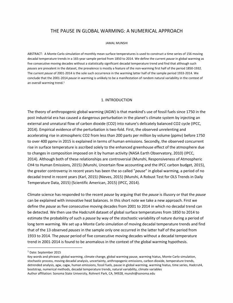
Figure 1: Random temperature samples for each month

The first three rows in Figure 1 are the data as received from Hadcrut4. Row 1 contains the year and

month. The mean monthly temperature anomaly and its standard deviation appear in Rows 2 and 3.

Row 5 to Row 1004 represent a random sample of 1000 monthly temperature anomalies drawn from

the Normal distribution represented by the mean and standard deviations in Rows 2 and 3. The RAND()

and NORMSINV() Excel functions are used to generate these samples as shown in Figure 1. These

samples are draw for each of 1,980 months in the 165-year sample period spanning 1850-2014.

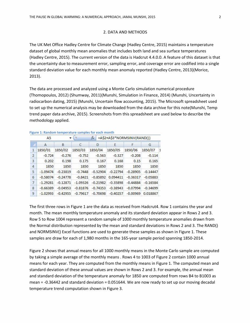
Figure 2 shows that annual means for all 1000 monthly means in the Monte Carlo sample are computed

by taking a simple average of the monthly means . Rows 4 to 1003 of Figure 2 contain 1000 annual

means for each year. They are computed from the monthly means in Figure 1. The computed mean and

standard deviation of these annual values are shown in Rows 2 and 3. For example, the annual mean

and standard deviation of the temperature anomaly for 1850 are computed from rows B4 to B1003 as

mean = -0.36442 and standard deviation = 0.051644. We are now ready to set up our moving decadal

temperature trend computation shown in Figure 3.


Figure 2: Computation of annual means

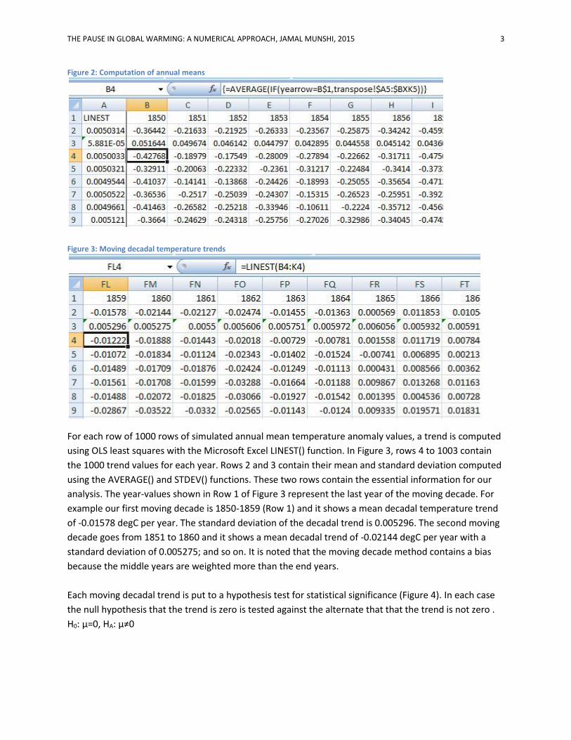
Figure 3: Moving decadal temperature trends

For each row of 1000 rows of simulated annual mean temperature anomaly values, a trend is computed

using OLS least squares with the Microsoft Excel LINEST() function. In Figure 3, rows 4 to 1003 contain

the 1000 trend values for each year. Rows 2 and 3 contain their mean and standard deviation computed

using the AVERAGE() and STDEV() functions. These two rows contain the essential information for our

analysis. The year-values shown in Row 1 of Figure 3 represent the last year of the moving decade. For

example our first moving decade is 1850-1859 (Row 1) and it shows a mean decadal temperature trend

of -0.01578 degC per year. The standard deviation of the decadal trend is 0.005296. The second moving

decade goes from 1851 to 1860 and it shows a mean decadal trend of -0.02144 degC per year with a

standard deviation of 0.005275; and so on. It is noted that the moving decade method contains a bias

because the middle years are weighted more than the end years.

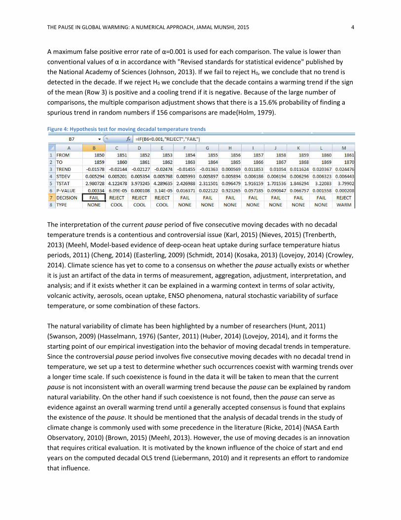
Each moving decadal trend is put to a hypothesis test for statistical significance (Figure 4). In each case

the null hypothesis that the trend is zero is tested against the alternate that that the trend is not zero .

H0: µ=0, HA: µ≠0


A maximum false positive error rate of α=0.001 is used for each comparison. The value is lower than

conventional values of α in accordance with "Revised standards for statistical evidence" published by

the National Academy of Sciences (Johnson, 2013). If we fail to reject H0, we conclude that no trend is

detected in the decade. If we reject H0 we conclude that the decade contains a warming trend if the sign

of the mean (Row 3) is positive and a cooling trend if it is negative. Because of the large number of

comparisons, the multiple comparison adjustment shows that there is a 15.6% probability of finding a

spurious trend in random numbers if 156 comparisons are made(Holm, 1979). Figure 4: Hypothesis test for moving decadal temperature trends

The interpretation of the current pause period of five consecutive moving decades with no decadal

temperature trends is a contentious and controversial issue (Karl, 2015) (Nieves, 2015) (Trenberth,

2013) (Meehl, Model-based evidence of deep-ocean heat uptake during surface temperature hiatus

periods, 2011) (Cheng, 2014) (Easterling, 2009) (Schmidt, 2014) (Kosaka, 2013) (Lovejoy, 2014) (Crowley,

2014). Climate science has yet to come to a consensus on whether the pause actually exists or whether

it is just an artifact of the data in terms of measurement, aggregation, adjustment, interpretation, and

analysis; and if it exists whether it can be explained in a warming context in terms of solar activity,

volcanic activity, aerosols, ocean uptake, ENSO phenomena, natural stochastic variability of surface

temperature, or some combination of these factors.

The natural variability of climate has been highlighted by a number of researchers (Hunt, 2011)

(Swanson, 2009) (Hasselmann, 1976) (Santer, 2011) (Huber, 2014) (Lovejoy, 2014), and it forms the

starting point of our empirical investigation into the behavior of moving decadal trends in temperature.

Since the controversial pause period involves five consecutive moving decades with no decadal trend in

temperature, we set up a test to determine whether such occurrences coexist with warming trends over

a longer time scale. If such coexistence is found in the data it will be taken to mean that the current

pause is not inconsistent with an overall warming trend because the pause can be explained by random

natural variability. On the other hand if such coexistence is not found, then the pause can serve as

evidence against an overall warming trend until a generally accepted consensus is found that explains

the existence of the pause. It should be mentioned that the analysis of decadal trends in the study of

climate change is commonly used with some precedence in the literature (Ricke, 2014) (NASA Earth

Observatory, 2010) (Brown, 2015) (Meehl, 2013). However, the use of moving decades is an innovation

that requires critical evaluation. It is motivated by the known influence of the choice of start and end

years on the computed decadal OLS trend (Liebermann, 2010) and it represents an effort to randomize

that influence.


3. DATA ANALYSIS AND RESULTS

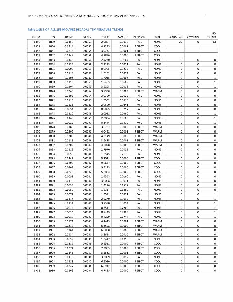
A Monte Carlo simulation procedure yielded 156 values of moving decadal trends and their standard

deviations. These results, along with hypothesis tests for the statistical significance of the decadal trends

are listed in Table 1. The values of the decadal trends range from -0.04 degC/year to +0.04 degC/yr with

a mean of 0.00503 degC/yr. The information in Table 1 is summarized in Figure 5 where the mean values

of all 156 moving decadal trends are depicted graphically.

Figure 5: Summary of the 156 moving decadal trends in the sample period

Of the 156 moving decadal trends in the overall study period 1850-2014, 40% showed a warming trend

and 14% showed a cooling trend. The largest segment is the "No Trend" category with 45% of the

decades without a statistically significant trend in either direction. These statistics are somewhat

different in the two halves of the sample period with the latter half showing a stronger warming trend

with half the moving decades containing a decadal warming trend. Another relevant difference between

the two halves is that more than half of the moving decades in the early half show no statistically

significant trend while this proportion is reduced to 36% in the latter half.

The last three columns in Table 4 contain a search for five consecutive moving decadal trends in the

same direction. When this pattern is found the last decade in the series is tagged with a value of "1" and

when it is not found the value is set to "0". A simple sum of each column of flags is displayed in the first

row of each of these columns. The summation shows that there were 25 occurrences of five consecutive


moving decades of decadal warming and 13 occurrences of five consecutive moving decades with no

decadal trend. There were no occurrences of five consecutive moving decades with a cooling decadal

trend. The known so called "global cooling" period from 1940 to 1970 contains 10 moving decades with

a cooling decadal trend but they are interspersed with periods of no detectable decadal trend.

The 165-year sample period 1850-2014 shows an overall warming trend of 0.0053 degC/year and yet it

contains 13 pauses defined as occurrences of five consecutive moving decades that do not contain

decadal temperature trends. These data appear to indicate that pauses can co-exist with global warming

because they can be explained by random natural variability or the stochastic nature of climate

variables. If that were the case our findings would be consistent with that of researchers who have

sought an explanation of the current pause in terms of natural variability.

However, a very different picture emerges when we divide the period into two halves of 78 moving

decades each. The differences between the two halves depicted in Figure 5 become even more stark

when we look for five consecutive moving decades with each containing the same decadal trend. The

results are summarized in Table 6.

Figure 6: Comparison of the two halves of the sample period

Figures 5 and 6 together show that the latter half of the sample period contains more moving decades

that show a warming trend and fewer moving decades that show no trend or a cooling trend. In

particular, Figure 6 shows that the great prevalence of pause-like conditions2 in the sample period 1850-

2014 is mostly a feature of the first half of the period 1850-1932 with 12 such occurrences. In the

second half of the sample period 1933-2014, the current pause is the sole such phenomenon. Likewise,

we see in Figure 6 that the warming trend in the period 1850-2014 is mostly a feature of the second half

1933-2014 because no temperature trend is detected in the first half 1850-1932. We conclude that

pause-like conditions are common in periods with no long term3 temperature trend but uncommon and

perhaps even singular and anomalous in periods with a long term warming trend.

All data and computational details used in this work are available for download in the online data

archive for this paper (Munshi, Temp trend paper data archive, 2015).

2 no decadal trend detected in five consecutive moving decades 3 80 years or more


Table 1:LIST OF ALL 156 MOVING DECADAL TEMPERATURE TRENDS

FROM TO TREND STDEV TSTAT P-VALUE DECISION TYPE WARMING COOLING NO

TREND

1850 1859 -0.0158 0.0053 2.9807 0.0033 FAIL NONE 25 0 13

1851 1860 -0.0214 0.0052 4.1225 0.0001 REJECT COOL

1852 1861 -0.0213 0.0054 3.9732 0.0001 REJECT COOL

1853 1862 -0.0247 0.0058 4.2896 0.0000 REJECT COOL

1854 1863 -0.0145 0.0060 2.4270 0.0164 FAIL NONE 0 0 0

1855 1864 -0.0136 0.0059 2.3115 0.0221 FAIL NONE 0 0 0

1856 1865 0.0006 0.0059 0.0965 0.9233 FAIL NONE 0 0 0

1857 1866 0.0119 0.0062 1.9162 0.0572 FAIL NONE 0 0 0

1858 1867 0.0105 0.0062 1.7015 0.0908 FAIL NONE 0 0 1

1859 1868 0.0116 0.0063 1.8463 0.0668 FAIL NONE 0 0 1

1860 1869 0.0204 0.0063 3.2208 0.0016 FAIL NONE 0 0 1

1861 1870 0.0245 0.0064 3.7990 0.0002 REJECT WARM 0 0 0

1862 1871 0.0196 0.0064 3.0700 0.0025 FAIL NONE 0 0 0

1863 1872 0.0119 0.0061 1.9592 0.0519 FAIL NONE 0 0 0

1864 1873 0.0121 0.0060 2.0300 0.0441 FAIL NONE 0 0 0

1865 1874 -0.0054 0.0061 0.8885 0.3757 FAIL NONE 0 0 0

1866 1875 -0.0122 0.0058 2.0932 0.0380 FAIL NONE 0 0 1

1867 1876 -0.0140 0.0059 2.3804 0.0185 FAIL NONE 0 0 1

1868 1877 -0.0020 0.0057 0.3444 0.7310 FAIL NONE 0 0 1

1869 1878 0.0186 0.0052 3.5782 0.0005 REJECT WARM 0 0 0

1870 1879 0.0202 0.0050 4.0492 0.0001 REJECT WARM 0 0 0

1871 1880 0.0209 0.0048 4.3149 0.0000 REJECT WARM 0 0 0

1872 1881 0.0183 0.0046 3.9435 0.0001 REJECT WARM 0 0 0

1873 1882 0.0202 0.0047 4.3098 0.0000 REJECT WARM 1 0 0

1874 1883 0.0128 0.0046 2.7970 0.0058 FAIL NONE 0 0 0

1875 1884 -0.0055 0.0044 1.2545 0.2116 FAIL NONE 0 0 0

1876 1885 -0.0243 0.0043 5.7021 0.0000 REJECT COOL 0 0 0

1877 1886 -0.0409 0.0042 9.8637 0.0000 REJECT COOL 0 0 0

1878 1887 -0.0401 0.0040 9.9173 0.0000 REJECT COOL 0 0 0

1879 1888 -0.0220 0.0042 5.2883 0.0000 REJECT COOL 0 0 0

1880 1889 -0.0099 0.0041 2.4353 0.0160 FAIL NONE 0 0 0

1881 1890 -0.0119 0.0040 3.0008 0.0031 FAIL NONE 0 0 0

1882 1891 -0.0056 0.0040 1.4196 0.1577 FAIL NONE 0 0 0

1883 1892 -0.0052 0.0039 1.3314 0.1850 FAIL NONE 0 0 0

1884 1893 -0.0077 0.0040 1.9571 0.0521 FAIL NONE 0 0 1

1885 1894 -0.0115 0.0039 2.9270 0.0039 FAIL NONE 0 0 1

1886 1895 -0.0131 0.0040 3.2590 0.0014 FAIL NONE 0 0 1

1887 1896 -0.0014 0.0039 0.3511 0.7260 FAIL NONE 0 0 1

1888 1897 0.0034 0.0040 0.8449 0.3995 FAIL NONE 0 0 1

1889 1898 0.0017 0.0041 0.4209 0.6744 FAIL NONE 0 0 1

1890 1899 0.0171 0.0041 4.1449 0.0001 REJECT WARM 0 0 0

1891 1900 0.0219 0.0041 5.3508 0.0000 REJECT WARM 0 0 0

1892 1901 0.0261 0.0039 6.6850 0.0000 REJECT WARM 0 0 0

1893 1902 0.0134 0.0040 3.3614 0.0010 REJECT WARM 0 0 0

1894 1903 -0.0052 0.0039 1.3417 0.1816 FAIL NONE 0 0 0

1895 1904 -0.0212 0.0038 5.5512 0.0000 REJECT COOL 0 0 0

1896 1905 -0.0274 0.0038 7.2865 0.0000 REJECT COOL 0 0 0

1897 1906 -0.0145 0.0037 3.9382 0.0001 REJECT COOL 0 0 0

1898 1907 -0.0120 0.0036 3.3099 0.0012 FAIL NONE 0 0 0

1899 1908 -0.0228 0.0037 6.2080 0.0000 REJECT COOL 0 0 0

1900 1909 -0.0247 0.0036 6.8912 0.0000 REJECT COOL 0 0 0

1901 1910 -0.0163 0.0034 4.7435 0.0000 REJECT COOL 0 0 0


1902 1911 -0.0112 0.0034 3.2485 0.0014 FAIL NONE 0 0 0

1903 1912 -0.0060 0.0035 1.7259 0.0864 FAIL NONE 0 0 0

1904 1913 -0.0048 0.0035 1.3729 0.1718 FAIL NONE 0 0 0

1905 1914 0.0027 0.0035 0.7724 0.4411 FAIL NONE 0 0 0

1906 1915 0.0211 0.0035 6.0057 0.0000 REJECT WARM 0 0 0

1907 1916 0.0304 0.0036 8.3949 0.0000 REJECT WARM 0 0 0

1908 1917 0.0244 0.0036 6.8048 0.0000 REJECT WARM 0 0 0

1909 1918 0.0222 0.0036 6.2026 0.0000 REJECT WARM 0 0 0

1910 1919 0.0207 0.0036 5.7598 0.0000 REJECT WARM 1 0 0

1911 1920 0.0198 0.0035 5.5817 0.0000 REJECT WARM 1 0 0

1912 1921 0.0157 0.0036 4.3498 0.0000 REJECT WARM 1 0 0

1913 1922 0.0087 0.0034 2.5345 0.0123 FAIL NONE 0 0 0

1914 1923 0.0024 0.0034 0.7159 0.4751 FAIL NONE 0 0 0

1915 1924 0.0054 0.0034 1.5978 0.1121 FAIL NONE 0 0 0

1916 1925 0.0187 0.0034 5.4799 0.0000 REJECT WARM 0 0 0

1917 1926 0.0232 0.0034 6.8240 0.0000 REJECT WARM 0 0 0

1918 1927 0.0133 0.0034 3.9547 0.0001 REJECT WARM 0 0 0

1919 1928 0.0093 0.0033 2.8683 0.0047 FAIL NONE 0 0 0

1920 1929 0.0002 0.0033 0.0721 0.9426 FAIL NONE 0 0 0

1921 1930 0.0054 0.0032 1.6695 0.0970 FAIL NONE 0 0 0

1922 1931 0.0158 0.0032 4.9724 0.0000 REJECT WARM 0 0 0

1923 1932 0.0147 0.0032 4.6203 0.0000 REJECT WARM 0 0 0

1924 1933 0.0060 0.0031 1.9523 0.0527 FAIL NONE 0 0 0

1925 1934 0.0043 0.0031 1.3781 0.1702 FAIL NONE 0 0 0

1926 1935 0.0030 0.0029 1.0151 0.3116 FAIL NONE 0 0 0

1927 1936 0.0100 0.0030 3.3462 0.0010 FAIL NONE 0 0 0

1928 1937 0.0173 0.0030 5.8147 0.0000 REJECT WARM 0 0 0

1929 1938 0.0234 0.0030 7.7025 0.0000 REJECT WARM 0 0 0

1930 1939 0.0151 0.0032 4.7358 0.0000 REJECT WARM 0 0 0

1931 1940 0.0211 0.0033 6.3707 0.0000 REJECT WARM 0 0 0

1932 1941 0.0290 0.0032 9.0167 0.0000 REJECT WARM 1 0 0

1933 1942 0.0294 0.0032 9.2854 0.0000 REJECT WARM 1 0 0

1934 1943 0.0207 0.0032 6.5055 0.0000 REJECT WARM 1 0 0

1935 1944 0.0264 0.0031 8.4559 0.0000 REJECT WARM 1 0 0

1936 1945 0.0194 0.0032 6.0155 0.0000 REJECT WARM 1 0 0

1937 1946 0.0070 0.0032 2.1655 0.0319 FAIL NONE 0 0 0

1938 1947 0.0030 0.0032 0.9266 0.3556 FAIL NONE 0 0 0

1939 1948 0.0003 0.0032 0.0862 0.9314 FAIL NONE 0 0 0

1940 1949 -0.0077 0.0032 2.4389 0.0159 FAIL NONE 0 0 0

1941 1950 -0.0163 0.0031 5.1776 0.0000 REJECT COOL 0 0 0

1942 1951 -0.0156 0.0031 5.0901 0.0000 REJECT COOL 0 0 0

1943 1952 -0.0127 0.0032 4.0236 0.0001 REJECT COOL 0 0 0

1944 1953 -0.0054 0.0030 1.7716 0.0784 FAIL NONE 0 0 0

1945 1954 -0.0022 0.0031 0.6994 0.4854 FAIL NONE 0 0 0

1946 1955 -0.0060 0.0030 2.0243 0.0447 FAIL NONE 0 0 0

1947 1956 -0.0177 0.0028 6.4020 0.0000 REJECT COOL 0 0 0

1948 1957 -0.0105 0.0027 3.8195 0.0002 REJECT COOL 0 0 0

1949 1958 -0.0004 0.0027 0.1408 0.8882 FAIL NONE 0 0 0

1950 1959 0.0044 0.0026 1.6797 0.0950 FAIL NONE 0 0 0

1951 1960 -0.0019 0.0026 0.7257 0.4691 FAIL NONE 0 0 0

1952 1961 0.0033 0.0026 1.2729 0.2050 FAIL NONE 0 0 0

1953 1962 0.0119 0.0026 4.5803 0.0000 REJECT WARM 0 0 0

1954 1963 0.0268 0.0026 10.3736 0.0000 REJECT WARM 0 0 0

1955 1964 0.0120 0.0026 4.6709 0.0000 REJECT WARM 0 0 0

1956 1965 -0.0007 0.0026 0.2872 0.7743 FAIL NONE 0 0 0


1957 1966 -0.0154 0.0025 6.1902 0.0000 REJECT COOL 0 0 0

1958 1967 -0.0160 0.0025 6.3569 0.0000 REJECT COOL 0 0 0

1959 1968 -0.0150 0.0024 6.2570 0.0000 REJECT COOL 0 0 0

1960 1969 -0.0063 0.0025 2.4810 0.0142 FAIL NONE 0 0 0

1961 1970 -0.0050 0.0025 2.0348 0.0436 FAIL NONE 0 0 0

1962 1971 -0.0065 0.0025 2.6580 0.0087 FAIL NONE 0 0 0

1963 1972 -0.0006 0.0025 0.2250 0.8223 FAIL NONE 0 0 0

1964 1973 0.0158 0.0025 6.4094 0.0000 REJECT WARM 0 0 0

1965 1974 -0.0009 0.0024 0.3961 0.6926 FAIL NONE 0 0 0

1966 1975 -0.0086 0.0025 3.4340 0.0008 REJECT COOL 0 0 0

1967 1976 -0.0159 0.0025 6.4714 0.0000 REJECT COOL 0 0 0

1968 1977 -0.0063 0.0024 2.5631 0.0113 FAIL NONE 0 0 0

1969 1978 -0.0072 0.0025 2.8876 0.0044 FAIL NONE 0 0 0

1970 1979 0.0074 0.0024 3.0376 0.0028 FAIL NONE 0 0 0

1971 1980 0.0201 0.0024 8.3162 0.0000 REJECT WARM 0 0 0

1972 1981 0.0232 0.0023 9.8904 0.0000 REJECT WARM 0 0 0

1973 1982 0.0234 0.0023 10.0434 0.0000 REJECT WARM 0 0 0

1974 1983 0.0410 0.0023 17.5038 0.0000 REJECT WARM 0 0 0

1975 1984 0.0275 0.0024 11.6876 0.0000 REJECT WARM 1 0 0

1976 1985 0.0156 0.0024 6.3767 0.0000 REJECT WARM 1 0 0

1977 1986 0.0006 0.0024 0.2320 0.8168 FAIL NONE 0 0 0

1978 1987 0.0092 0.0024 3.8245 0.0002 REJECT WARM 0 0 0

1979 1988 0.0092 0.0023 3.9578 0.0001 REJECT WARM 0 0 0

1980 1989 0.0095 0.0023 4.1195 0.0001 REJECT WARM 0 0 0

1981 1990 0.0207 0.0024 8.8043 0.0000 REJECT WARM 0 0 0

1982 1991 0.0298 0.0024 12.6498 0.0000 REJECT WARM 1 0 0

1983 1992 0.0206 0.0023 8.8219 0.0000 REJECT WARM 1 0 0

1984 1993 0.0241 0.0024 10.0945 0.0000 REJECT WARM 1 0 0

1985 1994 0.0175 0.0024 7.2144 0.0000 REJECT WARM 1 0 0

1986 1995 0.0137 0.0023 5.9019 0.0000 REJECT WARM 1 0 0

1987 1996 0.0033 0.0023 1.4558 0.1475 FAIL NONE 0 0 0

1988 1997 0.0128 0.0024 5.3965 0.0000 REJECT WARM 0 0 0

1989 1998 0.0288 0.0025 11.7325 0.0000 REJECT WARM 0 0 0

1990 1999 0.0225 0.0023 9.5909 0.0000 REJECT WARM 0 0 0

1991 2000 0.0252 0.0024 10.4011 0.0000 REJECT WARM 0 0 0

1992 2001 0.0331 0.0024 13.6310 0.0000 REJECT WARM 1 0 0

1993 2002 0.0318 0.0024 13.1418 0.0000 REJECT WARM 1 0 0

1994 2003 0.0289 0.0024 11.9493 0.0000 REJECT WARM 1 0 0

1995 2004 0.0223 0.0025 9.0315 0.0000 REJECT WARM 1 0 0

1996 2005 0.0256 0.0025 10.2302 0.0000 REJECT WARM 1 0 0

1997 2006 0.0148 0.0024 6.0396 0.0000 REJECT WARM 1 0 0

1998 2007 0.0137 0.0024 5.6283 0.0000 REJECT WARM 1 0 0

1999 2008 0.0159 0.0024 6.6983 0.0000 REJECT WARM 1 0 0

2000 2009 0.0100 0.0024 4.1560 0.0001 REJECT WARM 1 0 0

2001 2010 0.0039 0.0025 1.5904 0.1138 FAIL NONE 0 0 0

2002 2011 -0.0030 0.0025 1.1705 0.2436 FAIL NONE 0 0 0

2003 2012 -0.0032 0.0025 1.2822 0.2017 FAIL NONE 0 0 0

2004 2013 -0.0009 0.0025 0.3710 0.7111 FAIL NONE 0 0 0

2005 2014 0.0012 0.0025 0.4881 0.6262 FAIL NONE 0 0 1


4. SUMMARY AND CONCLUSIONS

A Monte Carlo simulation of monthly mean surface temperature anomalies is used to construct

a time series of 156 moving decadal temperature trends in a 165-year sample period from 1850

to 2014. We define a pause in warming as five consecutive moving decades without a

statistically significant decadal temperature trend.

The full temperature dataset 1850-2014 shows an overall warming trend and contains 13 such

pauses including the controversial current pause period which occurs in our dataset in 2001-

2014. However, when the dataset is split into two halves, it is found that the warming trend

derives from the second half and that the occurrence of pauses derives from the first half.

The first half 1850-1932 contains no warming trend and 12 pauses while the second half shows

a strong warming trend and contains only one pause at the end of the period. The data appear

to indicate that pauses and warming trends are mutually exclusive and that therefore, the

current contentious pause of 2001-2014 is not likely to be the result of random natural

variability in the context of a longer period of global warming.

5. REFERENCES

Brown, P. (2015). Comparing the Model-Simulated Global Warming Signal to Observations Using

Empirical Estimates of Unforced Noise. Retrieved 2015, from Duke Environment:

https://nicholas.duke.edu/news/global-warming-more-moderate-worst-case-models

Cheng, X. (2014). Varying planetary heat sink led to global warming slowdown. Science , 345: 897-903.

Crowley, T. J. (2014). Recent global temperature plateau in the context of a new proxy reconstruction.

Earth's Future , 2: 281-294.

Easterling, D. R. (2009). Is the climate warming or cooling? Geophysical Research Letters , 36: L08706.

EPA. (2015). Climate Change Indicators in the United States. Retrieved 2015, from Climate Change:

http://www.epa.gov/climatechange/science/indicators/weather-climate/temperature.html

Hadley Centre. (2015). Hadcrut4. Retrieved 2015, from Met Office Hadley Centre for Climate Change:

http://www.metoffice.gov.uk/hadobs/hadcrut4/data/current/download.html

Hadley Centre. (2013). Hadcrut4 ensemble. Retrieved 2915, from Met Office Hadley Center:

http://www.metoffice.gov.uk/hadobs/hadcrut4/data/current/ensemble_series_format.html


Hadley Centre. (2015). Met Office Hadley Centre for Climate Change. Retrieved 2015, from Met Office

Hadley Centre for Climate Change: http://www.metoffice.gov.uk/climate-

change/resources/hadleycentre

Hasselmann, K. (1976). Stochastic climate models Part I. Theory. Tellus , 28, 473–485.

Holm, S. (1979). A simple sequentially rejective multiple test procedure. Scandinavian Journal of

Statistics , 6:2:65-70.

Huber, M. (2014). Natural variability, radiative forcing, and climate response in the recent hiatus

reconciled. Nature Geoscience , 10.1038/ngeo2228.

Hunt, B. G. (2011). The role of natural climatic variation in perturbing the observed global mean

temperature trend. Climate Dynamics , 36: 509-521.

IPCC. (2007). Climate change 2007 the physical science basis. Retrieved 2015, from IPCC:

https://www.ipcc.ch/publications_and_data/ar4/wg1/en/spmsspm-projections-of.html

IPCC. (2014). Climate Change 2013 The Physical Science Basis. Retrieved 2015, from IPCC:

https://www.ipcc.ch/report/ar5/wg1/

Johnson, V. (2013). Revised standards for statistical evidence. Retrieved 2015, from Proceedings of the

National Academy of Sciences: http://www.pnas.org/content/110/48/19313.full

Karl, T. (2015). Possible artifacts of data biases in the recent global surface warming hiatus. Science ,

348:6242 pp 1469-1472.

Kosaka, Y. (2013). Recent global warming hiatus tied to equatorial Pacific surface cooling. Nature , 501:

403-407.

Liebermann, B. (2010). Influence of choice of time period on on global surface temperature trend

estimation. American Meteorological Society , November: 1485-1491.

Lovejoy, S. (2014). Return periods of global climate fluctuations and the pause. Geophysical Research

Letters , 41: 2014GL060478.

Meehl, G. A. (2013). Decadal Climate Prediction: An Update from the Trenches. Meehl, G. A. et al.

Decadal Climate Prediction: An UpdBulletin of the American Meteorological Society , Meehl, G. A. et al.

Decadal Climate Prediction: An Update from the Tren95, 243–267, 10.1175/BAMS-D-12-00241.

Meehl, G. A. (2011). Model-based evidence of deep-ocean heat uptake during surface temperature

hiatus periods. Nature Climate Change , 1: 360-364.

Morice, C. (2013). Quantifying uncertainties in global and regional temperature change. Retrieved 2015,

from metoffice.gov.uk: http://www.metoffice.gov.uk/hadobs/hadcrut4/HadCRUT4_accepted.pdf


Munshi, J. (2015). A Robust Test for OLS Trends in Daily Temperature Data. Retrieved 2015, from ssrn:

http://papers.ssrn.com/sol3/papers.cfm?abstract_id=2631298

Munshi, J. (2015). Responsiveness of Atmospheric CH4 to Human Emissions. Retrieved 2015, from

ssrn.com: http://papers.ssrn.com/sol3/papers.cfm?abstract_id=2652524

Munshi, J. (2015). Responsiveness of atmospheric CO2 to anthropogenic emissions. Retrieved 2015, from


Munshi, J. (2014). Simulation in Finance. Retrieved 2015, from ssrn:


Munshi, J. (2015). Temp trend paper data archive. Retrieved 2015, from Dropbox:

https://www.dropbox.com/sh/40dzhyv0y2ofdiw/AAD5T-o5jO2ht9bJYfxvsdBea?dl=0

Munshi, J. (2015). TempTrend Data Archive. Retrieved 2015, from Dropbox:

https://www.dropbox.com/sh/40dzhyv0y2ofdiw/AAD5T-o5jO2ht9bJYfxvsdBea?dl=0

Munshi, J. (2015). Uncertain flow accounting. Retrieved 2015, from ssrn:


Munshi, J. (2015). Uncertain flow accounting and the IPCC carbon budget. Retrieved 2015, from


Munshi, J. (2015). Uncertainty in radiocarbon dating. Retrieved from ssrn:


NASA Earth Observatory. (2010). Is Current Warming Natural? Retrieved 2015, from NASA Earth

Observatory: http://earthobservatory.nasa.gov/Features/GlobalWarming/page4.php

Nieves, V. (2015). Revent hiatus caused by decadal shift in Indo-Pacific heating. Science , Vol. 349 no.

6247 pp. 532-535.

Ricke, K. (2014). Maximum warming occurs about one decade after a carbon dioxide emission.

Environmental Research Letters , Volume 9, Number 12.

Santer, B. D. (2011). Separating signal and noisein atmospheric temperature changes: the importance of

timescale. Journal of Geophysical Research , 116: D22105.

Schmidt, G. (2014). Reconciling warming trends. Nature Geoscience , 7: 158-160.

Scientific American. (2015). No pause in global warming. Retrieved 2015, from Scientific American:

http://www.scientificamerican.com/article/no-pause-in-global-warming/

Shumway, R. (2011). Time series analysis. Springer.


Swanson, K. L. (2009). Long term natural variability and 20th century climate change. Proceedings of the

National Academy of Sciences , 106: 16120-16123.

Thomopoulos, N. (2012). Essentials of Monte Carlo Simulation. Spenger.

Trenberth, K. (2013). An apparent hiatus in global warming. Earth's Future , 10.1002/2013EF000165.

THE PAUSE IN GLOBAL WARMING: A NUMERICAL APPROACH

Documents

Transcript of THE PAUSE IN GLOBAL WARMING: A NUMERICAL APPROACH