753

European Journal of Remote Sensing - 2014, 47: 753-771 doi: 10.5721/EuJRS20144743 Received 24/07/2014, accepted 06/11/2014European Journal of Remote Sensing - 2014, 47: 753-771 doi: 10.5721/EuJRS20144743 Received 24/07/2014, accepted 06/11/2014

European Journal of Remote SensingAn official journal of the Italian Society of Remote Sensing

www.aitjournal.com

Examining the relationship between the Enhanced Vegetation Index and grapevine phenology

Helder Fraga1*, Malik Amraoui2,3, Aureliano C. Malheiro1, José Moutinho-Pereira1, José Eiras-Dias4, José Silvestre4 and João A. Santos1

1Centre for the Research and Technology of Agro-Environmental and Biological Sciences, Universidade de Trás-os-Montes e Alto Douro, UTAD, 5000-801 Vila Real, Portugal

2Universidade de Trás-os-Montes e Alto Douro, UTAD, 5000-801 Vila Real, Portugal3Instituto Dom Luiz, University of Lisbon, Campo Grande, Edifício C8, Piso 3, 1749-016 Lisbon, Portugal

4Instituto Nacional de Investigação Agrária e Veterinária, I.P., 2565-191 Dois Portos, Portugal*Corresponding author, e-mail address: hfraga@utad.pt

AbstractMonitoring the main grapevine phenological stages is a key procedure for optimizing vineyard activities and improving yield and quality attributes. Remote sensing may be an effective and practical monitoring tool, as data from on-board satellite sensors can measure vegetative growth. In the current study, a 12-year time series of four main phenophases (budburst, flowering, veraison and harvest) were obtained from an experimental vineyard located in Lisbon (Portugal). LANDSAT surface reflectances were used to calculate the Enhanced Vegetation Index (EVI) and derived metrics. Both time series were then analysed. Results show statistically significant relationships between vegetation metrics and phenological timings and intervals, such as the linkage between the peak greenness and flowering/veraison. The current study highlights the applicability of remote sensing to monitor grapevine phenology in both retrospective and real-time, bringing an added-value to the winemaking sector.Keywords: Remote sensing, EVI, Vine phenological development, Lisbon winemaking region, LANDSAT.

IntroductionMonitoring the main phenological stages is critical for viticultural decision-making and has impacts on both yield and quality attributes [Jones and Davis, 2000; Hall et al., 2002; Taylor, 2004; Vaudour et al., 2010]. Vitis vinifera L. varieties (deciduous species) undergo several morphological/physiological changes throughout the growing season. After wintertime dormancy, the grapevine vegetative cycle starts with the budburst (BUD) stage, leading to the first signs of greenness in the vineyard. The next main event is flowering (FLO; small flower clusters), which usually occurs in May/November or early June/December (Northern/Southern Hemisphere). Almost immediately berries initiate growth, corresponding to the

Fraga et al. Remote sensing of grapevine phenology

754

beginning of the “fruit/berry set”. When 50% of the red grape clusters show changes in colour, or when signs of softening in white grapes appear, the veraison (VER) stage occurs. Vegetative growth (shoots and leaves) generally stops or decreases after this stage. Veraison also sets the beginning of the maturity period, which extends until harvest (HAR). Finally, the growing season ends and leaves begin to fall [Lopes et al., 2008; Magalhães, 2008; Fraga et al., 2014c].Monitoring the timings of these development stages is commonly performed by periodical observations, requiring specialized and trained human skills. Furthermore, this ground-based (in situ) monitoring is difficult to implement in large vineyards, mainly due to the time and resources needed. In such a context, remote sensing measurements (satellite data) are a very appealing tool to monitor vegetation activity [Sakamoto et al., 2005; Zhang et al., 2009; Kim et al., 2012], particularly when provided by moderate spatial resolution sensors on-board polar orbiting platforms. In effect, remote sensing is becoming an increasingly reliable source of information for vegetation monitoring [Duchemin et al., 1999].The LANDSAT Thematic Mapper (TM) and Enhanced Thematic Mapper Plus (ETM+) sensors on-board the LANDSAT 5 and 7 satellites continuously acquire images of the Earth, with a 16-day repeat cycle. LANDSAT TM and ETM+ images consist of spectral bands with a spatial resolution of 30 m [Masek et al., 2006]. Given the relatively high resolution provided by these images, also in comparison to other remote sensing datasets, suitable vineyard-scale assessments are possible. Nonetheless, for a proper inter-row/inter-vine comparison much higher resolutions (<1 m) are required [Taylor, 2004; Puletti, 2014].In order to enhance the sensitivity of satellite inferred data to vegetation characteristics, vegetation indices, i.e. mathematical functions of spectral bands, are used [Huete et al., 2002; Rodrigues et al., 2013]. The standard remote sensing data products, used for local- to global-scale vegetation monitoring, are the Normalized Difference Vegetation Index (NDVI) and the Enhanced Vegetation Index (EVI) [Jensen, 2009]. Although both indices provide a seasonal measure of greenness, the NDVI is being gradually replaced by the EVI [Huete et al., 2002; Pennec et al., 2011], because it contains empirically derived correction factors accounting for canopy background (e.g. covered/bare soil) and atmospheric effects (e.g. aerosol resistance), while also being more sensitive to high biomass conditions, such as vineyard vigour/foliar area.Vegetation indices provide a measure of the seasonal variations in greenness [Zarco-Tejada et al., 2005; Ratana et al., 2006], which is related to vigour and leaf area [Johnson et al., 2003]. Applied to viticulture, these indices have shown significant relationships with yield [Cunha et al., 2010b; Gouveia et al., 2011], phenology [Cunha et al., 2010a; Rodrigues et al., 2013], total phenolic content and pH of wine [Lamb et al., 2004], while assisting in irrigation planning [Johnson et al., 2003] and ultimately improving wine quality [Johnson et al., 2001]. These assessments are extremely valuable for viticulturists, particularly for regions under Mediterranean-like climates, such as the Lisbon winemaking region (central-western Portugal). In these regions grapevines are exposed to water stress, especially during the dry summer period [Koundouras et al., 1999]. Nevertheless, under these stress conditions, relationships between grapevine phenology and vegetation indices are still largely unknown, constituting a research gap. One of the main constraints when establishing these relationships is that crop growth (greenness/vigour) and development (phenology), though intertwined, are two different aspects of the vegetative cycle. For

755

European Journal of Remote Sensing - 2014, 47: 753-771

instance, grapevines can privilege the phenological development in detriment of growth under certain stress conditions [Magalhães, 2008].The aim of the present study is: 1) to provide a suitable vineyard-scale assessment of four main grapevine phenological stages (BUD, FLO, VER and HAR) in the Lisbon winemaking region; 2) to characterize the grapevine seasonal growth cycle using the EVI and derived metrics; and 3) to establish significant relationships between ground-based grapevine phenology and these remote sensing vegetation metrics.

Material and MethodsSite descriptionA 12-year time series (2000-2011) of phenological data was obtained from the Portuguese ‘Instituto Nacional de Investigação Agrária e Veterinária’. Data was collected at an experimental vineyard (39º 02’ 35’’N, 9º 11’ 0’’W, elevation 110 m; Fig. 1), located at Dois Portos, within the Lisbon winemaking region (central-western Portugal). This region is characterized by a typical Mediterranean climate, namely warm dry summers and mild wet winters [Peel et al. 2007]. Monthly minimum (Tmin), maximum (Tmax) and mean (Tmean) air temperatures, and precipitation (Prec) recorded in Lisbon (~30 km from the experimental vineyard) are obtained from the Portuguese Meteorological Office (‘Instituto Português do Mar e da Atmosfera’ – www.ipma.pt) and shown in Figure 2. Annual precipitation total and annual mean temperature are of about 750 mm and 15ºC, respectively. Precipitation tends to be lowest in July (2 mm) and highest in October (114 mm), while mean air temperature reaches maximum values in August (24ºC) and minimum values in January (12ºC) (Fig. 2).

Figure 1 - On the left: Experimental vineyard site (Dois Portos, Portugal) and the geographical representation of the selected 20 LANDSAT pixels (red frame). Image source: Google Earth®. On the right: Location of the experimental site in the Lisbon winemaking region, along with the borders of other winemaking regions in Portugal (southwestern Europe).

Fraga et al. Remote sensing of grapevine phenology

756

Figure 2 - Monthly averages of minimum (Tmin), maximum (Tmax) and mean (Tmean) air temperatures (ºC), along with monthly average accumulated precipitation (Prec; mm) for the study period (2000-2011).

The rainfed vineyard, with north-south orientation, has approximately 3 ha and a plant density of about 3500 vines ha-1, comprises different varieties (Aragonez, Castelão, Chasselas and Fernão-Pires) trained on vertical trellis with 1.2 m between vines. The plants grafted onto SO4 rootstocks are about 25 years old. The soil is homogeneous calcic fluvisol (eutric). The inter-rows (of about 2.5 m) are managed about three times during the vegetative cycle (e.g. herbicide, mowing), minimizing the influence of inter-row vegetation. The different varieties are arranged in groups with a minimum of 7 individuals throughout the vineyard rows. The timings (calendar day of year – DOY) of BUD, FLO, VER and HAR were recorded by field observations of the different varieties according to the OIV (‘Organisation Internationale de la Vigne et du Vin’) grapevine descriptors [OIV, 2009]. Harvest dates where determined when probable alcohol content of the fruits was about 11.5% (vol.), which is a common procedure in this region. Lastly, the DOY of each phenophase is the average taken over those varieties (multi-variety means of DOY), allowing the comparison with remote sensing data at the vineyard-scale, as will be described below. In order to take into account statistically significant differences between the mean timings for each variety, a one-way ANOVA multiple comparison test was performed.

LANDSAT dataA 12-year time series (2000–2011) of LANDSAT TM/ETM+ reflectance data [Masek et al., 2006] were retrieved from the United States Geological Survey (USGS) EarthExplorer

757

European Journal of Remote Sensing - 2014, 47: 753-771

(http://earthexplorer.usgs.gov). These images are previously subjected to atmospheric and geographic correction routines (e.g. correction of turbidity, cloud detection, cloud shadow effects and geometric correction) by the LANDSAT Ecosystem Disturbance Adaptive Processing System processor (LEDAPS) [Masek et al., 2013]. LANDSAT TM and ETM + (World reference system type 2, path 204, row 033) contains spectral bands at a 30 m spatial resolution covering the study area, with a 16-day repeat cycle (for each pixel there are 2 images in each month, around 288 for the entire study period). 20 pixels with vineyard-only (monoculture) data were selected for the upcoming analyses (Fig. 1). Although some within-pixel heterogeneity may still be present (spectral response of the inter-row spacing), the signal-to-noise ratio should be minimized through i) the analysis of the full grapevine season cycle, ii) background correction embedded in the calculated vegetation metrics (EVI - explained below) and iii) averaging of a representative and homogeneous amount of pixels. Furthermore, LANDSAT radiometric and geometric correction routines have previously demonstrated a high accuracy (0.1-0.4 pixel) [Gill et al., 2010; Saroglu et al., 2006]. The 20 pixels used in the present study thus provide a sufficiently large number of samples to neglect the influence of surrounding vegetation [Knudby et al., 2014]. Reflectance data were then subject to a quality control assessment using the quality layer embedded in the dataset. Data inconsistencies were isolated (e.g. missing values, scan gaps) and values are removed to minimize errors and obtain a high quality sequence of data.

Vegetation indicesThe EVI is calculated using the reflectance of blue, red, and near-infrared [equation 1].

EVI = G × NIR - REDNIR + C1×RED - C2×BLUE + L

1[ ]

where NIR corresponds to the near-infrared band (LANDSAT band 4), RED corresponds to the red band (LANDSAT band 3), BLUE corresponds to the blue band (LANDSAT band 1), L is the canopy background adjustment (L = 1), C1 and C2 are coefficients of the aerosol resistance and influence in the blue and red bands, respectively (C1 = 6 and C2 = 7.5), and G is a gain factor (G = 2.5) [Huete et al., 1994; Huete et al., 1997]. All previous parameters are defined according to LEDAPS surface reflectance product description (http://landsat.usgs.gov/CDR_ECV.php). The EVI values range from 0 (bare ground) to 1 (complete vegetation cover). As previously stated, this index provides minimized canopy background influence and reduced atmospheric variations [Miura et al., 2001]. As the LANDSAT data is available at a 16-day time-step, cubic splines are applied on an annual basis to interpolate the EVI at any given DOY. This temporal interpolation method allows obtaining a homogeneous and gap-free time-series of EVI data, which is a commonly employed procedure for establishing relationships between remote sensing datasets and land surface phenology [Beurs and Henebry, 2010]. A spatial average of the EVI is then performed for the 20 pixels covering only vineyard vegetation in the experimental site. The correlation coefficients and differences to the mean EVI of the 20 pixels were assessed in order to provide a spatial agreement at the vineyard-scale.Based on the EVI, other metrics are applied in this study. As grapevine growth differs not

Fraga et al. Remote sensing of grapevine phenology

758

only in the leaf area magnitude, but also on the onset and length of its cycle, the EVI is transformed into the EVIratio as follows [equation 2]:

EVI = EVI - EVIEVI - EVIratio

min

max min2[ ]

where EVI is the daily EVI value, EVImax and EVImin are the maximum and minimum EVI for a given grapevine growing season (1-March to 31-October, Northern Hemisphere), similar to the NDVIratio applied by White et al. [1997]. This metric, ranging from 0 to 1, also retains high frequency changes that may be lost in the original EVI, due to the smoothing procedure applied – cubic splines [Beurs and Henebry, 2010]. The days to peak (DTP) measure is determined for each year, accounting for the number of days required for the EVIratio to reach its maximum (EVIratio = 1). The rate of change in the EVIratio is also determined by the EVIslope [equation 3]:

EVI = EVI t - EVI t-1slope ratio ratio( ) ( ) [ ]3

where t corresponds to the day for which EVIratio is assessed. The EVIslope also allows capturing the greatest increase/decrease in the EVI, which is also a useful metric to compare against grapevine phenology [Beurs and Henebry, 2010]. Spearman rank correlations (rs) are then used to assess relations between EVI and DOY of each phenophase measured in the field.

ResultsPhenological stagesThe ground-based phenological dataset for the Lisbon winemaking region is first described. Table 1 shows the DOY of the four phenological stages over the study period. The mean DOY of BUD, FLO, VER and HAR are 76, 142, 213 and 260, respectively (Tab. 1). Standard deviations indicate a moderate inter-annual variability, ranging from 5 to 9 days (Tab. 1). Delays/advances are largest for BUD (± 8 days) and VER (± 9 days) timings and lowest for FLO (± 5 days) and HAR (± 6 days). The intervals between these events also show some variability, with FLO-VER being the longest interphase (71 ± 7 days) and VER-HAR the shortest (47 ± 9 days). These differences in the timings and intervals of the phenological stages can be largely attributed to inter-annual variability in the atmospheric conditions [Jones et al., 2005; Malheiro et al., 2013; Sadras and Moran, 2012]. A one-way ANOVA multiple comparison test shows that there are no statistically significant differences between the mean timings of each variety (at a 5% confidence level). The varieties presented similar mean phenological timings, allowing the use of multi-variety means of DOY for each event when relations with EVI are established. Nonetheless, there is an inherent natural variability in the inter-annual timings of each variety (Tab. 2), which can be mostly attributed to genetic factors and environmental effects, such as climate, soil and viticultural practices [Petrie and Sadras, 2008; Magalhães, 2008; Malheiro et al., 2013].

759

European Journal of Remote Sensing - 2014, 47: 753-771

Table 1 - Day of year (DOY) and intervals of the phenological stages (BUB – budburst, FLO – flowering, VER – veraison and HAR – harvest) in the experimental vineyard for the period of 2000-2011. The mean dates of occurrence and the corresponding standard deviations (SD in days) for the full period are also presented.

YearsDOY Interphase (days)

BUD FLO VER HAR BUD-FLO FLO-VER VER-HAR

2000 71 148 222 267 78 74 45

2001 60 139 209 257 79 70 48

2002 68 138 217 272 70 79 55

2003 71 140 216 253 69 76 38

2004 70 143 218 260 73 75 42

2005 91 146 218 252 55 72 34

2006 85 142 219 260 57 77 41

2007 79 146 223 259 68 77 36

2008 80 146 211 262 66 65 51

2009 74 142 203 261 68 61 58

2010 82 143 203 259 60 61 56

2011 78 131 192 253 54 60 60

Mean 76 142 213 260 66 71 47

SD 8 5 9 6 8 7 9

Table 2 - Mean day of year (Mean) and corresponding standard deviation (SD) of each phenophase (BUB – budburst, FLO – flowering, VER – veraison and HAR – harvest) for each variety grown in the experimental site.

Variety BUDMean (SD)

FLOMean (SD)

VERMean (SD)

HARMean (SD)

Aragonez 82 (8) 146 (5) 212 (9) 258 (5)

Castelão 72 (9) 139 (4) 215 (7) 260 (5)

Chasselas 75 (8) 141 (4) 210 (11) 266 (8)

Fernão-Pires 75 (8) 142 (4) 214 (10) 254 (7)

Fraga et al. Remote sensing of grapevine phenology

760

EVI spatial coherenceThe EVI calculated for each pixel indicates a very high spatial coherence (Fig. 3). The correlations between the EVI of each of the 20 pixels during the study period range from 0.82 to 0.97 (Spearman rank correlation – rs), significant at 1% level. While there is some variability in the pixel minimum/maximum, the EVI values for the 20 pixels depict very low 25–75th percentile ranges (approximately 0.02, Fig. 3). Hence, the pixel-mean EVI values are spatially coherent, thus justifying the representativeness of the spatially averaged EVI for the whole experimental vineyard. Although each pixel contains bare ground zones (inter-rows and lanes), they seem to affect only the EVI pixel-mean magnitude and not its seasonality.

Figure 3 - Spatial coherence of the EVI for the 20 pixels in the study area. The mean, minimum, maximum, 25th and 75th percentiles of the 20 pixels for the period of 2000-2011 are shown.

EVI seasonal cycleThe EVI mean seasonal cycle (Fig. 4) depicts increasing values from the beginning of the growing season, reaching its maximum at DOY 180, and then followed by a decrease until the end of the growing season. From the EVI curve (Fig. 4), BUD corresponds to the lowest EVI values (circa 0.30), then increasing to approximately 0.40 at FLO, and reaching a maximum in mid FLO-VER period (0.47). EVI then decreases from this maximum until HAR (0.35). The minimum, maximum and percentiles show similar seasonal behaviour as the mean EVI. These results are in agreement with the literature, since vineyards generally reach maximum total leaf area around veraison, July-August [Magalhães, 2008]. However, at this stage, low water availability in the Mediterranean climates may trigger physiological stress (heat and water combined stresses), inhibiting longer growth periods, as is indeed observed in other regions [Sousa et al., 2006].

761

European Journal of Remote Sensing - 2014, 47: 753-771

Figure 4 - Monthly means of the 20-pixel averaged EVI of the experimental vineyard for the period of 2000-2011 (12 years) as a function of DOY. The monthly minimum, maximum, 25th and 75th percentiles are also represented. Mean DOY of BUD - budburst, FLO - flowering, VER - veraison and HAR - harvest events are also represented by vertical lines.

Temporal evolutionWhile the EVI mean curve shows a good agreement with the mean phenology, there are remarkable inter-annual differences. The extent of time in which greenness values remain high is one of the main outcomes of the EVIratio (Fig. 5). While the profile suggests that maximum values are reached in the FLO–VER period, with some stabilization around the maximum, there are marked differences in the length of this stabilization period, also suggesting a high variation in the rate of growth between phenophases in different years.EVIslope confirms the existence of a high inter-annual variability in the rate of growth (Fig. 6). As an example, 2001 and 2002 depict a very slow growth around the BUD, followed by a very fast growth around the FLO. While these years show a thin peak around FLO–VER, others show much wider peaks (e.g. 2006). This behaviour is expected to be tied to the amount of precipitation during this period. According to the climatic records, summer precipitation in 2006 exceeded by about 180% its climatic normals, which may underlie the longer high greenness period (not shown). In fact, several studies demonstrate a connection between fluctuations in the EVI values and the inter-annual variability of precipitation [Ratana et al., 2006; Bradley et al., 2011; Gaughan et al., 2012; Walker et al., 2014], which can partially explain this variability.

Fraga et al. Remote sensing of grapevine phenology

762

Figure 5 - DOY vs. year diagram of the EVIratio of the experimental vineyard for the period of 2000-2011. BUD – budburst, FLO – flowering, VER – veraison and HAR – harvest events are also represented by white curves.

Figure 6 - DOY vs. year diagram of the EVIslope of the experimental vineyard for the period of 2000-2011. BUD – budburst, FLO – flowering, VER – veraison and HAR – harvest events are also represented by white curves.

763

European Journal of Remote Sensing - 2014, 47: 753-771

The influence of climate in the vineyard EVIAn analysis of the influence of air temperature (minimum, maximum and mean) and precipitation on the vineyard EVI is now performed. EVI inter-annual variability appears to be largely influenced by precipitation (Fig. 7a). The relatively high correlation coefficient between these two variables (0.63) is indeed expected and widely reported in literature [Bradley et al., 2011; Gaughan et al., 2012]. No significant relationship can be established between the inter-annual variability of the air temperature or growing-degree days and the EVI (not shown). Conversely, the EVI intra-annual variability, throughout the grapevine growing season, appears to be much more influenced by air temperature (rs > 0.90; Fig. 7b) than by precipitation. In this Mediterranean-like climatic region, summer precipitation is scarce but grapevines continue to grow, highlighting the role of soil water reserves and grapevine root structure for grapevine vigour [Fraga et al., 2014a].

Figure 7 – a) EVI and precipitation (Prec; mm) inter-annual variability through the study period (2000-2011). b) EVI and air temperature (minimum – Tmin, maximum – Tmax and mean – Tmean; ºC) intra-annual variability. Spearman rank correlations coefficients (rs) are also shown.

Fraga et al. Remote sensing of grapevine phenology

764

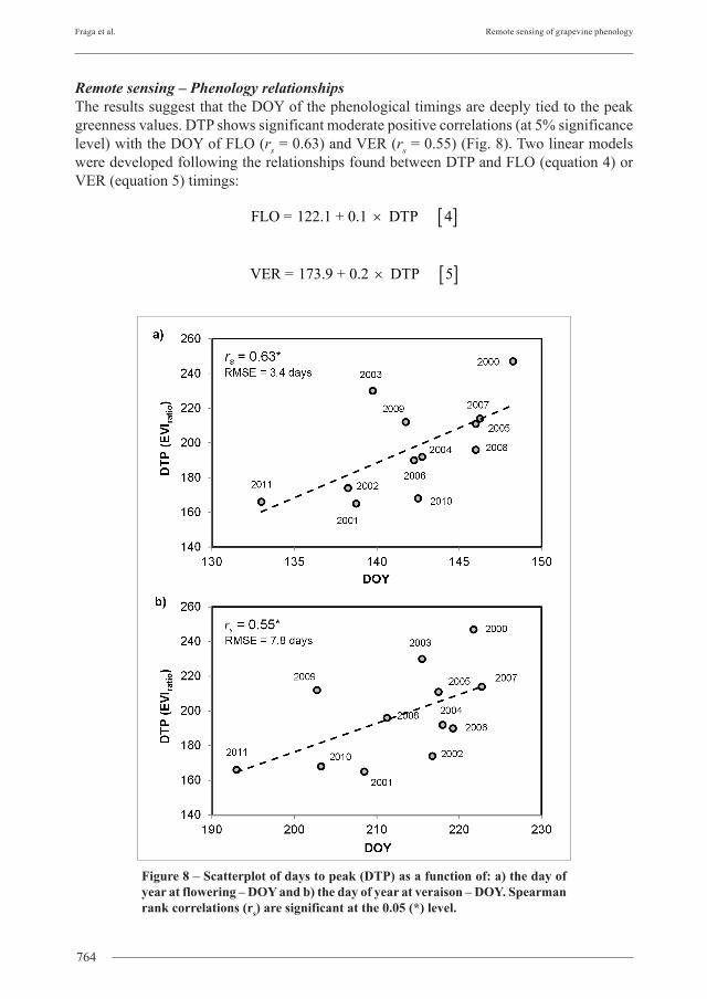
Remote sensing – Phenology relationshipsThe results suggest that the DOY of the phenological timings are deeply tied to the peak greenness values. DTP shows significant moderate positive correlations (at 5% significance level) with the DOY of FLO (rs = 0.63) and VER (rs = 0.55) (Fig. 8). Two linear models were developed following the relationships found between DTP and FLO (equation 4) or VER (equation 5) timings:

FLO = 122.1 + 0.1 DTP× [ ]4

VER = 173.9 + 0.2 DTP× [ ]5

Figure 8 – Scatterplot of days to peak (DTP) as a function of: a) the day of year at flowering – DOY and b) the day of year at veraison – DOY. Spearman rank correlations (rs) are significant at the 0.05 (*) level.

765

European Journal of Remote Sensing - 2014, 47: 753-771

The FLO model presents a root-mean-squared error (RMSE) of 3.4 days, while the VER model presents a RMSE of 7.8 days. As such, the models provide a moderate-to-high skill in predicting FLO and VER DOY. For both models, DTP has a positive regression coefficient, indicating that a higher number of days to reach peak greenness is indeed linked to later phenological events. Nonetheless, these delays in phenology are more pronounced in years that show a slow and steady growth rate during the entire cycle (Figs. 5-6).While some years exhibit a slow steady EVI growth, others show rapid increases/decreases in-between each phenophase (Fig. 6). In years with an isolated EVIratio decrease in the early season (e.g. 2001, 2002 and 2010) grapevines seem to display a compensation response, with a rapid EVIratio increase. This rapid growth has implications in the interval of the respective interphase, leading to a shortening of that phase. These relationships are confirmed by the significant correlations found between mean EVI, EVIratio or EVIslope and the intervals between phenophases (Tab. 3). Higher growth rates (EVIslope) during BUD–FLO and FLO–VER lead to a shortening of these intervals (rs = −0.63 and rs = −0.52 at 5% significance level). Additionally, anomalously high EVI and EVIratio values in-between phases also seem to promote the shortening of FLO–VER and VER–HAR (rs = −0.73 and rs = −0.51 at a 1% and 5% significance levels). Rapid vegetative growth is expected to contribute to the shortening of their corresponding interphases. However, the overall timings on which these events occur seem to be unaffected by these vegetative boost periods, i.e. while there are some shortening/lengthening of some intervals due to fast momentary growth, the length of the entire growing season remain invariant (BUD–HAR).

Table 3 - Spearman rank correlations between mean values of EVI, EVIratio or EVIslope and each phenological interval (BUB – budburst, FLO – flowering, VER - veraison and HAR – harvest). All correlations are significant at 0.05 (*) and 0.01 (**) p-levels.

Intervals BUD–FLO FLO–VER VER–HAR

EVI -0.73**

EVIratio -0.51*

EVIslope -0.63* -0.52*

DiscussionThe results suggest that the EVI and derived vegetation metrics are able to capture grapevine phenological development. In effect, it is possible to identify the main grapevine vegetative growth cycle throughout the EVI profile. These outcomes are in agreement with other studies showing remote sensing vegetation indices allow estimating grapevine vigour [Johnson et al., 2003; Fraga et al., 2014a], seasonal cycle [Cunha et al., 2010a; Golnaz and Gerrit, 2013] and phenological timings [Lamb et al., 2004; Rodrigues et al., 2013]. However, for vineyards grown in Mediterranean-like climatic conditions, the relationships between the EVI and phenological timings were still unclear. In many cases, the lack of sufficiently long and heterogeneous records of phenological data impedes establishing significant relationships. Additionally, the relationships found herein can be strengthened in regions with higher spring-summertime rainfall, where vines are less constrained by water stress.

Fraga et al. Remote sensing of grapevine phenology

766

Satellite derived vegetation metrics suggests a high sensitivity to detect FLO and VER, through the detection of the DTP. This metric has shown to be significantly correlated with the time required to reach these stages of development. In fact, peak greenness has proven to be a useful metric for many crops [Walker et al., 2014], and this relationship with grapevine development is a major advancement. Although the correlations found are still moderate, they have proven to be significant. Nonetheless, these relationships provide a valuable tool for decision support at vineyard-scale, as FLO and VER are crucial for determining the appropriate vineyard operations and are tied to grapevine maturity properties [Magalhães, 2008; Cunha et al., 2010a]. For FLO, which occurs before DTP, this metric can be used as a retrospective tool by growers, enabling a comparison with previous years. On the other hand, for VER, this metric can be used as a real-time tool in estimating VER timings, allowing growers to improve their planning of management activities. Additionally, as several studies point to air/soil temperature as the main leading factor for the advances/delays of the phenological stages [Webb et al., 2012; Malheiro et al., 2013], DTP could also prove to be a very useful indicator for monitoring the impacts of future climates in Portuguese viticulture [Andrade et al., 2014; Fraga et al., 2014b].In our study, the grapevine growth profile differs in each year, with different peak greenness and growth rates. Maximum growth rate was consistent with the FLO stage, with growth reductions starting around VER, which is supported by previous research [Borghezan et al., 2012; Scarpare et al., 2012]. Altogether, the outcomes suggest that a slow-steady growth rate throughout the growing season can lead to longer phenological intervals, while rapid growth peaks tend to shorten the interphase. In some years, grapevines present very low or negative growth rates (EVI/greenness decreases) at the early stages of development (BUD–FLO), which are likely related to vineyard management activities (leaf/shoot removal) and to unfavourable climatic conditions, such as low precipitation (Fig. 2), highlighting the role played by water availability on vine vigour during this stage [Moriondo and Bindi, 2007; Camps and Ramos, 2012]. Of particular interest is the fact that this low or negative growth rate is usually followed by rapid growth rates, which can be explained by either physiological mechanisms that tend to offset the climate signal in the vine phenology or to newly favourable environmental conditions (optimal thermal conditions) necessary for enhanced vegetative growth [Hendrickson et al., 2004; Magalhães, 2008]. This demonstrates the usefulness of the rate of growth as an essential vegetation metrics that allows capturing the vegetative development [Rapaport et al., 2014]. As such, the obtained correlations reveal that the variability in the greenness measured by satellite derived vegetation metrics is able to capture the fluctuation in both phenological timings and intervals.Although the relationships found are clear, these procedures still present some limitations. The relatively coarse temporal resolution provided by the LANDSAT sensor may increase the error in the modelling approach, since the DTP metric requires knowledge of the EVI maximum (or downturn date). However, as far as new remote sensing data with higher temporal/spatial resolution will become available, the obtained relationships might be significantly improved. Nonetheless, some of the limitations of the current study could in fact be explained by the non-linear relationship between grapevine phenology and growth, being two different aspects of the vegetative cycle that, although related, are not strictly inter-dependent. Viticultural practices, such as pruning, thinning, topping and crop load, can influence both growth and development separately [Magalhães, 2008; Parker et al., 2011].

767

European Journal of Remote Sensing - 2014, 47: 753-771

Furthermore, several climatic factors can also influence phenology and growth differently. Inter-annual variability in grapevine phenology is mostly driven by air temperature [Keller, 2010; Malheiro et al., 2013], whereas precipitation (and water availability) is reported as a major climatic factor for greenness (leafs) [Bradley et al., 2011; Gaughan et al., 2012].

ConclusionsThe current study provides a novel assessment of the relationship between grapevine growth (and growth rate) and phenology in a Mediterranean-like climate region. Regarding the conditions in which most vineyards are grown in Portugal, in large farms with monocropping and multi-varietal environments, the use of moderate spatial resolution remote sensing data is an effective tool for grapevine monitoring. Results clearly highlight the usefulness of the EVI in monitoring the grapevine phenophases, in retrospective (FLO) and in real-time (VER), decreasing the need for intensive ground-based observations. As the LANDSAT EVI 16-day data are a real-time product, growers will be able to use these data to optimise vineyard management and field intervention needs by combining remote sensing with experienced agricultural practices. Additionally, the referred remote sensing vegetation metrics could also provide a useful indicator of stress conditions, which is crucial for the adaptation to a changing climate.

AcknowledgementsThis study was supported by the FCT – Portuguese Foundation for Science and Technology under project ClimVineSafe [PTDC/AGR-ALI/110877/2009], project PEst-OE/AGR/UI4033/2014 and by the PRODER project GreenVitis PA 43879 – IF 0018. LANDSAT reflectance data products are a courtesy of the U.S. Geological Survey Earth Resources Observation and Science Center.

ReferencesAndrade C., Fraga H., Santos J.A. (2014) - Climate change multi-model projections for

temperature extremes in Portugal. Atmospheric Science Letters, 15 (2): 149-156. doi: http://dx.doi.org/10.1002/asl2.485.

Beurs K., Henebry G. (2010) - Spatio-Temporal Statistical Methods for Modelling Land Surface Phenology. In: Phenological Research, Hudson IL, Keatley MR (Eds.), Springer Netherlands, pp. 177-208. doi: http://dx.doi.org/10.1007/978-90-481-3335-2_9.

Borghezan M., Gavioli O., Vieira H.J., da Silva A.L. (2012) - Shoot growth of Merlot and Cabernet Sauvignon grapevine varieties. Pesquisa Agropecuaria Brasileira, 47 (2): 200-207. doi: http://dx.doi.org/10.1590/S0100-204X2012000200008.

Bradley A.V., Gerard F.F., Barbier N., Weedon G.P., Anderson L.O., Huntingford C., Aragão L.E.O.C., Zelazowski P., Arai E. (2011) - Relationships between phenology, radiation and precipitation in the Amazon region. Global Change Biol 17 (6): 2245-2260. doi: http://dx.doi.org/10.1111/j.1365-2486.2011.02405.x.

Camps J.O., Ramos M.C. (2012) - Grape harvest and yield responses to inter-annual changes in temperature and precipitation in an area of north-east Spain with a Mediterranean climate. International Journal of Biometeorology, 56 (5): 853-864. doi: http://dx.doi.org/10.1007/s00484-011-0489-3.

Fraga et al. Remote sensing of grapevine phenology

768

Cunha M., Marcal A.R.S., Rodrigues A. (2010a) - A comparative study of satellite and ground-based vineyard. Phenology Symposium of the European Association of Remote Sensing Laboratories. Imaging Europe, pp. 68-77. doi: http://dx.doi.org/10.3233/978-1-60750-494-8-68.

Cunha M., Marcal A.R.S, Silva L. (2010b) - Very early prediction of wine yield based on satellite data from VEGETATION. International Journal of Remote Sensing, 31 (12): 3125-3142. doi: http://dx.doi.org/10.1080/01431160903154382.

Duchemin B., Goubier J., Courrier G. (1999) - Monitoring phenological key stages and cycle duration of temperate deciduous forest ecosystems with NOAA/AVHRR data. Remote Sensing of Environment, 67 (1): 68-82. doi: http://dx.doi.org/10.1016/S0034-4257(98)00067-4.

Fraga H., Malheiro A.C., Moutinho-Pereira J., Cardoso R.M., Soares P.M.M., Cancela J.J., Pinto J.G., Santos J.A. (2014a) - Integrated analysis of climate, soil, topography and vegetative growth in Iberian viticultural regions. Plos One, 9 (9): e108078. doi: http://dx.doi.org/10.1371/journal.pone.0108078.

Fraga H., Malheiro A.C., Moutinho-Pereira J., Jones G.V., Alves F., Pinto J.G., Santos J.A. (2014b) - Very high resolution bioclimatic zoning of Portuguese wine regions: present and future scenarios. Regional Environmental Change, 14 (1): 295-306. doi: http://dx.doi.org/10.1007/s10113-013-0490-y.

Fraga H., Malheiro A.C., Moutinho-Pereira J., Santos J.A. (2014c) - Climate factors driving wine production in the Portuguese Minho region. Agricultural and Forest Meteorology, 185: 26-36. doi: http://dx.doi.org/10.1016/j.agrformet.2013.11.003.

Gaughan A.E., Stevens F.R., Gibbes C., Southworth J., Binford M.W. (2012) - Linking vegetation response to seasonal precipitation in the Okavango-Kwando-Zambezi catchment of southern Africa. International Journal of Remote Sensing, 33 (21): 6783-6804. doi: http://dx.doi.org/10.1080/01431161.2012.692831.

Gill T., Collett L., Armston J., Eustace A., Danaher T., Scarth P., Flood N., Phinn S. (2010) - Geometric correction and accuracy assessment of Landsat-7 ETM+ and Landsat-5 TM imagery used for vegetation cover monitoring in Queensland, Australia from 1988 to 2007. Journal of Spatial Science, 55 (2): 273-287. doi: http://dx.doi.org/10.1080/14498596.2010.521977.

Golnaz B., Gerrit H. (2013) - Estimating the growing season length using remotely sensed based vegetation indices: a case study for Washington State vineyards. American Society of Agricultural and Biological Engineers, 131616169. doi: http://dx.doi.org/10.13031/aim.20131616169.

Gouveia C., Liberato M.L.R., DaCamara C.C., Trigo R.M., Ramos A.M. (2011) - Modelling past and future wine production in the Portuguese Douro Valley. Climate Research, 48 (2): 349-362. doi: http://dx.doi.org/10.3354/cr01006.

Hall A., Lamb D.W., Holzapfel B., Louis J. (2002) - Optical remote sensing applications in viticulture - a review. Australian Journal of Grape and Wine Research, 8 (1): 36-47. doi: http://dx.doi.org/10.1111/j.1755-0238.2002.tb00209.x.

Hendrickson L., Ball M.C., Wood J.T., Chow W.S., Furbank R.T. (2004) - Low temperature effects on photosynthesis and growth of grapevine. Plant, Cell &Environmental, 27 (7): 795-809. doi: http://dx.doi.org/10.1111/j.1365-3040.2004.01184.x.

Huete A., Didan K., Miura T., Rodriguez E.P., Gao X., Ferreira L.G. (2002) - Overview of

769

European Journal of Remote Sensing - 2014, 47: 753-771

the radiometric and biophysical performance of the MODIS vegetation indices. Remote Sensing of Environment, 83 (1-2): 195-213. doi: http://dx.doi.org/10.1016/S0034-4257(02)00096-2.

Huete A., Justice C., Liu H. (1994) - Development of Vegetation and Soil Indexes for Modis-Eos. Remote Sensing of Environment, 49 (3): 224-234. doi: http://dx.doi.org/10.1016/0034-4257(94)90018-3.

Huete A.R., Liu H.Q., Batchily K., vanLeeuwen W. (1997) - A comparison of vegetation indices global set of TM images for EOS-MODIS. Remote Sensing of Environment, 59 (3): 440-451. doi: http://dx.doi.org/10.1016/S0034-4257(96)00112-5.

Jensen J.R. (2009) - Remote Sensing of the Environment: An Earth Resource Perspective. 2nd Eds. Pearson Education.

Johnson L.F., Bosch D.F., Williams D.C., Lobitz B.M. (2001) - Remote sensing of vineyard management zones: Implications for wine quality. Applied Engineering in Agriculture, (4): 557-560.

Johnson L.F., Roczen D.E., Youkhana S.K., Nemani R.R., Bosch D.F. (2003) - Mapping vineyard leaf area with multispectral satellite imagery. Computers and Electronics in Agriculture, 38 (1): 33-44. doi: http://dx.doi.org/10.1016/S0168-1699(02)00106-0.

Jones G.V., Davis R.E. (2000) - Climate influences on grapevine phenology, grape composition, and wine production and quality for Bordeaux, France. American Journal of Enology and Viticulture, 51 (3): 249-261.

Jones G.V., Duchêne E., Tomasi D., Yuste J., Braslavska O., Schultz H.R. C. Martinez, Boso S., Langellier F., Perruchot C., Guimberteau G. (2005) - Changes in European winegrape phenology and relationships with climate. In: Proceedings XIV GESCO Symposium, Geisenheim, Germany, August 23-26.

Keller M. (2010) - Managing grapevines to optimise fruit development in a challenging environment: a climate change primer for viticulturists. Australian Journal of Grape and Wine Research, 16: 56-69. doi: http://dx.doi.org/10.1111/j.1755-0238.2009.00077.x.

Kim S., Kang S., Lim J-H., Chun J-H., Sung J-H. (2012) - Regional parameterization of canopy onset models using MODIS and flowering onset data. Ecological Modelling, 247: 190-198. doi: http://dx.doi.org/10.1016/j.ecolmodel.2012.08.026.

Knudby A., Nordlund L.M., Palmqvist G., Wikstrom K., Koliji A., Lindborg R., Gullström M. (2014) - Using multiple Landsat scenes in an ensemble classifier reduces classification error in a stable nearshore environment. International Journal of Applied Earth Observation and Geoinformation, 28: 90-101. doi: http://dx.doi.org/10.1016/j.jag.2013.11.015.

Koundouras S., Van Leeuwen C., Seguin G., Glories Y. (1999) - Influence of water status on vine vegetative growth, berry ripening and wine characteristics in mediterranean zone (example of Nemea, Greece, variety Saint-George, 1997). Journal International des Sciences de la Vigne et du Vin, 33:149-160.

Lamb D.W., Weedon M.M., Bramley R.G.V. (2004) - Using remote sensing to predict grape phenolics and colour at harvest in a Cabernet Sauvignon vineyard: Timing observations against vine phenology and optimising image resolution. Australian Journal of Grape and Wine Research, 10 (1): 46-54.

Lopes J., Eiras-Dias J.E., Abreu F., Climaco P., Cunha J.P., Silvestre J. (2008) - Thermal requirements, duration and precocity of phenological stages of grapevine cultivars of the Portuguese collection. Ciência Técnica Vitivinicola, 23 (1): 61-71.

Fraga et al. Remote sensing of grapevine phenology

770

Magalhães N. (2008) - Tratado de viticultura: a videira, a vinha e o terroir. Chaves Ferreira, Lisboa, Portugal.

Malheiro A.C., Campos R., Fraga H., Eiras-Dias J., Silvestre J., Santos J.A. (2013) - Winegrape phenology and temperature relationships in the Lisbon Wine Region, Portugal. Journal International des Sciences de la Vigne et du Vin, 47 (4): 287-299.

Masek J.G., Vermote E.F., Saleous N., Wolfe R., Hall F.G., Huemmrich F. Gao F., Kutler J., Lim T.K. (2013) - LEDAPS Calibration, Reflectance, Atmospheric Correction Preprocessing Code, Version 2. Oak Ridge National Laboratory Distributed Active Archive Center, Oak Ridge, Tennessee, U.S.A. doi: http://dx.doi.org/10.3334/ORNLDAAC/1146.

Masek J.G., Vermote E.F., Saleous N.E., Wolfe R., Hall F.G., Huemmrich K.F.,Gao F., Lim T.K. (2006) - A Landsat surface reflectance dataset for North America, 1990-2000. Geoscience and Remote Sensing Letters, 3 (1): 68-72. doi: http://dx.doi.org/10.1109/LGRS.2005.857030.

Miura T., Huete A.R., Yoshioka H., Holben B.N. (2001) - An error and sensitivity analysis of atmospheric resistant vegetation indices derived from dark target-based atmospheric correction. Remote Sensing of Environment, 78 (3): 284-298. doi: http://dx.doi.org/10.1016/S0034-4257(01)00223-1.

Moriondo M., Bindi M. (2007) - Impact of climate change on the phenology of typical mediterranean crops. Italian Journal of Agrometeorology, 3:5-12.

OIV (2009) - Code des caractères descriptifs des variétés et espèces de Vitis 2éme édition. Organisation Internationale de la Vigne et du Vin.

Parker A.K., de Cortazar-Atauri I.G., van Leeuwen C., Chuine I. (2011) - General phenological model to characterise the timing of flowering and veraison of Vitis vinifera L. Australian Journal of Grape and Wine Research, 17 (2): 206-216. doi: http://dx.doi.org/10.1111/j.1755-0238.2011.00140.x.

Peel M.C., Finlayson B.L., McMahon T.A. (2007) - Updated world map of the Koppen-Geiger climate classification. Hydrology and Earth System Sciences, 11 (5): 1633-1644.

Pennec A., Gond V., Sabatier D. (2011) - Tropical forest phenology in French Guiana from MODIS time series. Remote Sensing Letter, 2 (4): 337-345. doi: http://dx.doi.org/10.1080/01431161.2010.507610.

Petrie P.R., Sadras V.O. (2008) - Advancement of grapevine maturity in Australia between 1993 and 2006: putative causes, magnitude of trends and viticultural consequences. Australian Journal of Grape and Wine Research, 14 (1): 33-45. doi: http://dx.doi.org/10.1111/j.1755-0238.2008.00005.x.

Puletti N. (2014) Unsupervised classification of very high remotely sensed images for grapevine rows detection. European Journal of Remote Sensing, 47: 45-54. doi: http://dx.doi.org/10.5721/EuJRS20144704.

Rapaport T., Hochberg U., Rachmilevitch S., Karnieli A. (2014) - The Effect of Differential Growth Rates across Plants on Spectral Predictions of Physiological Parameters. Plos One, 9 (2): 11. doi: http://dx.doi.org/10.1371/journal.pone.0088930.

Ratana P., Huete A.R., Didan K. (2006) - MODIS EVI-based Variability in Amazon Phenology across the Rainforest-Cerrado Ecotone. 2006 Geoscience and Remote Sensing Symposium, 1-8: 1942-1944. doi: http://dx.doi.org/10.1109/Igarss.2006.502.

Rodrigues A., Marcal A.S., Cunha M. (2013) - Monitoring Vegetation Dynamics Inferred

771

European Journal of Remote Sensing - 2014, 47: 753-771

by Satellite Data Using the PhenoSat Tool. Geoscience and Remote Sensing, 51 (4): 2096-2104. doi: http://dx.doi.org/10.1109/TGRS.2012.2223475.

Sadras V.O., Moran M.A. (2012) - Nonlinear effects of elevated temperature on grapevine phenology. Agricultural and Forest Meteorology, 173: 107-115. doi: http://dx.doi.org/10.1016/j.agrformet.2012.10.003.

Sakamoto T., Yokozawa M., Toritani H., Shibayama M., Ishitsuka N., Ohno H. (2005) - A crop phenology detection method using time-series MODIS data. Remote Sensing of Environment, 96 (3-4): 366-374. doi: http://dx.doi.org/10.1016/j.rse.2005.03.008.

Saroglu E., Kaya S., Ormeci C. (2006) - Analysis of geometric accuracy of Landsat 5 TM and IRS 1D data by means of DGPS and Map data. Global Developments in Environmental Earth Observation from Space. Millpress Science Publishers, Rotterdam.

Scarpare F., Scarpare Filho J., Rodrigues A., Reichardt K., Angelocci L. (2012) - Growing degree-days for the ‘Niagara Rosada’ grapevine pruned in different seasons. International Journal of Biometeorology, 56 (5): 823-830. doi: http://dx.doi.org/10.1007/s00484-011-0484-8.

Sousa T.A., Oliveira M.T., Pereira J.M. (2006) - Physiological indicators of plant water status of irrigated and non-irrigated grapevines grown in a low rainfall area of portugal. Plant and Soil, 282 (1-2): 127-134. doi: http://dx.doi.org/10.1007/s11104-005-5374-6.

Taylor J.A. (2004) - Digital Terroirs and Precision Viticulture: Investigations Into the Application of Information Technology in Australian Vineyards. PhD Thesis. The University of Sydney. Sydney, Australia.

Vaudour E., Carey V.A., Gilliot J.M. (2010) - Digital zoning of South African viticultural terroirs using bootstrapped decision trees on morphometric data and multitemporal SPOT images. Remote Sensing of Environment, 114 (12): 2940-2950. doi: http://dx.doi.org/10.1016/j.rse.2010.08.001.

Walker J.J., de Beurs K.M., Wynne R.H. (2014) - Dryland vegetation phenology across an elevation gradient in Arizona, USA, investigated with fused MODIS and Landsat data. Remote Sensing of Environment, 144: 85-97. doi: http://dx.doi.org/10.1016/j.rse.2014.01.007.

Webb L.B., Whetton P.H., Bhend J., Darbyshire R., Briggs P.R., Barlow E.W.R. (2012) - Earlier wine-grape ripening driven by climatic warming and drying and management practices. Nature Climate Change 2 (4): 259-264. doi: http://dx.doi.org/10.1038/Nclimate1417.

White M.A., Thornton P.E., Running S.W. (1997) - A continental phenology model for monitoring vegetation responses to interannual climatic variability. Global Biogeochemical Cycles 11 (2): 217-234. doi: http://dx.doi.org/10.1029/97gb00330.

Zarco-Tejada P.J., Berjón A., López-Lozano R., Miller J.R., Martín P., Cachorro V., Gonzales M.R., de Frutos A. (2005) - Assessing vineyard condition with hyperspectral indices: Leaf and canopy reflectance simulation in a row-structured discontinuous canopy. Remote Sensing of Environment, 99 (3): 271-287. doi: http://dx.doi.org/10.1016/j.rse.2005.09.002.

Zhang M.W., Fan J.L., Zhu X.X., Li G.C., Zhang Y.P. (2009) - Monitoring winter-wheat phenology in North China using time-series MODIS EVI. Remote Sensing for Agriculture, Ecosystems, and Hydrology, XI (747227). doi: http://dx.doi.org/10.1117/12.829972.