Evolutionary Selection of Individual Expectations and Aggregate Outcomes

Evolutionary Selection of Individual Expectations

and Aggregate Outcomes∗

Mikhail Anufriev† Cars Hommes‡

CeNDEF, School of Economics, University of Amsterdam,

Roetersstraat 11, NL-1018 WB Amsterdam, Netherlands

September 2009

Abstract

In recent ‘learning to forecast’ experiments with human subjects (Hommes, et al. 2005),

three different patterns in aggregate asset price behavior have been observed: slow mono-

tonic convergence, permanent oscillations and dampened fluctuations. We construct a

simple model of individual learning, based on performance based evolutionary selection

or reinforcement learning among heterogeneous expectations rules, explaining these dif-

ferent aggregate outcomes. Out-of-sample predictive power of our switching model is

higher compared to the rational or other homogeneous expectations benchmarks. Our

results show that heterogeneity in expectations is crucial to describe individual forecast-

ing behavior as well as aggregate price behavior.

JEL codes: C91, C92, D83, D84, E3.

Keywords: Learning, Heterogeneous Expectations, Expectations Feedback, Experimental Economics

∗We thank the participants of the “Complexity in Economics and Finance” workshop, Leiden, October

2007, the “Computation in Economics and Finance” conference, Paris, June 2008, the “Learning and Macroe-

conomic Policy” workshop, Cambridge, September 2008, and seminar participants at the University of Ams-

terdam, Sant’Anna School of Advanced Studies (Pisa), University of New South Wales, Catholic University of

Milan, University of Warwick, Paris School of Economics, and the European University Institute (Florence)

for stimulating discussions. We benefitted from helpful comments by Buz Brock, Cees Diks, John Duffy,

Doyne Farmer, Frank Heinemann and Valentyn Panchenko on earlier versions of this paper. This work is

supported by the Complex Markets E.U. STREP project 516446 under FP6-2003-NEST-PATH-1 and by the

EU 7th framework collaborative project “Monetary, Fiscal and Structural Policies with Heterogeneous Agents

(POLHIA)”, grant no.225408.†Tel.: +31-20-5254248; fax: +31-20-5254349; e-mail: [email protected].‡Tel.: +31-20-5254246; fax: +31-20-5254349; e-mail: [email protected].

1

1 Introduction

In an economy today’s individual decisions crucially depend upon expectations or beliefs about

future developments. For example, in speculative asset markets such as the stock market, an

investor buys (sells) today when she expects prices to rise (fall) in the future. Expectations

affect individual decisions and the realized market outcome (e.g., prices and traded quantities)

is an aggregation of individual behavior. A market is therefore an expectations feedback system:

market history shapes individual expectations which, in turn, determine current aggregate

market behavior and so on. How do individuals actually form market expectations, and what

is the aggregate outcome of the interaction of individual market forecasts?

Neoclassical economic theory assumes that all individuals have rational expectations (Muth,

1961; Lucas and Prescott, 1971). In an economic model, forecasts then coincide with mathe-

matical expectations, conditioned upon available information. In a rational world individual

expectations coincide, on average, with market realizations, and markets are efficient with

prices fully reflecting economic fundamentals (Fama, 1970). In the traditional view, there is

no room for market psychology and “irrational” herding behavior. An important underpinning

of the rational approach comes from an early evolutionary argument made by Alchian (1950)

and Friedman (1953), that “irrational” traders will not survive competition and will be driven

out of the market by rational traders, who will trade against them and earn higher profits.

Following Simon (1957), many economists have argued that rationality imposes unrealis-

tically strong informational and computational requirements upon individual behavior and it

is more reasonable to model individuals as boundedly rational, using simple rules of thumb

in decision making. Laboratory experiments indeed have shown that individual decisions

under uncertainty are at odds with perfectly rational behavior, and can be much better de-

scribed by simple heuristics, which sometimes may lead to persistent biases (Tversky and

Kahneman, 1974; Kahneman, 2003; Camerer and Fehr, 2006). Models of bounded rationality

have also been applied to forecasting behavior, and several adaptive learning algorithms have

been proposed to describe market expectations. For example, Sargent (1993) and Evans and

Honkapohja (2001) advocate the use of adaptive learning in modeling expectations and deci-

sion making in macroeconomics, while Arthur (1991), Erev and Roth (1998) and Camerer and

Ho (1999) propose reinforcement learning as an explanation of average behavior in a number

of experiments in a game-theoretical setting. In some models (Bray and Savin, 1986) adaptive

learning enforces convergence to rational expectations, while in others (Bullard, 1994) learning

may not converge at all but instead lead to excess volatility and persistent deviations from

1

rational equilibrium similar to real markets (Shiller, 1981; De Bondt and Thaler, 1989). Re-

cently, models with heterogeneous expectations and evolutionary selection among forecasting

rules have been proposed, e.g., Brock and Hommes (1997) and Branch and Evans (2006), see

Hommes (2006) for an extensive overview.

Laboratory experiments with human subjects, with full control over economic fundamen-

tals, are well suited to study individual expectations and how their interaction shapes aggregate

market behavior (Marimon, Spear, and Sunder, 1993; Peterson, 1993). But the results from

laboratory experiments are mixed. Early experiments, with various market designs such as

double auction trading, show convergence to equilibrium (Smith, 1962), while more recent

asset pricing experiments exhibit deviations from equilibrium with persistent bubbles and

crashes (Smith, Suchanek, and Williams, 1988; Hommes, Sonnemans, Tuinstra, and Velden,

2005). A clear explanation of these different market phenomena is still lacking (Duffy, 2008).

It is particularly challenging to provide a general theory of learning which is able to explain

both the possibilities of convergence and persistent deviations from equilibrium.

In recent learning to forecast experiments, described at length in Hommes, Sonnemans, Tu-

instra, and Velden (2005), three qualitatively different aggregate outcomes have been observed

in the same experimental setting. In a stationary environment participants, for 50 periods,

had to predict the price of a risky asset (say a stock) having knowledge of the fundamental

parameters (mean dividend and interest rate) and previous price realizations, but without

knowing the forecasts of others. If all agents would behave rationally or learn to behave ra-

tionally, the market price would quickly converge to a constant fundamental value pf = 60.

While in some groups in the laboratory price convergence did occur, in other groups prices

persistently fluctuate (see Fig. 2). Another striking finding in the experiments is that in all

groups individuals were able to coordinate on a common predictor (see Fig. 2, lower parts

of different panels). The main purpose of this paper is to present a simple model based on

evolutionary selection of simple heuristics explaining how coordination of individual forecasts

can emerge and, ultimately, enforce different aggregate market outcomes. Although our model

is very simple it fits the experimental data surprisingly well (see, e.g., Fig. 7).

The paper is organized as follows. Section 2 reviews the findings of the laboratory exper-

iment and looks at individual forecasting rules which will form the basis of our evolutionary

model. Section 3 focusses on the price dynamics under homogeneous forecasting rules which

were identified in the experiment. A learning model based on evolutionary selection between

simple forecasting heuristics is presented, analyzed and simulated in Section 4. In Section 5

we discuss how our model fits the experimental data, and Section 6 concludes.

2

2 Learning to Forecast Experiments

In this section we discuss the laboratory experiments. Subsection 2.1 recalls the experimental

design, Subsection 2.2 focuses on aggregate price behavior, while Subsection 2.3 discusses

individual prediction rules.

2.1 Experimental Design

A number of sessions of a computerized learning to forecast experiment in the CREED labora-

tory at the University of Amsterdam have been presented in Hommes, Sonnemans, Tuinstra,

and Velden (2005), henceforth HSTV. In each session human subjects had to predict the price

of an asset for 51 periods and have been rewarded for the accuracy of their predictions. Fig. 2

shows the result of the experiment for six different groups. The reader can immediately rec-

ognize two striking results of the experiment: different qualitative patterns in aggregate price

behavior and high coordination of individual forecasts, even though individuals do not know

the forecasts of others. Before starting to develop an explanation for these findings, we briefly

describe the experimental design.

Each market consists of six participants, who were told that they are advisors to a pension

fund which can invest money either in a risk-free or in a risky asset. In each period the

risk-free asset pays a fixed interest rate r, while the risky asset pays stochastic dividends,

independently identically distributed (IID), with mean y. Trading in the risky asset had been

computerized, using an optimal demand schedule derived from maximization of myopic CARA

mean-variance utility, given the subject’s individual forecast. Hence, subject’s only task in

every period was to give a two period ahead point prediction for the price of the risky asset,

and their earnings were inversely related to their prediction errors. An advantage of this

approach is that it provides clean data on expectations, assuming all other underlying model

assumptions to be satisfied. Learning to forecast experimental data can be used as a test

bed for various expectations hypotheses, such as rational expectations or adaptive learning

models, in any benchmark dynamic economic model with all other assumptions controlled by

the experimenter; see the discussion in Duffy (2008).

Participants in the experiments knew that the actual price realization of the risky asset is

determined by market clearing on the basis of the investment strategies of the pension fund.

The exact functional form of the strategies and the market equilibrium equation were unknown

to the participants. However, they were informed that the higher their own forecast is, the

larger will be the demand for the risky asset. Stated differently, they knew that there was

3

positive feedback from individual price forecasts to the realized market price. They were also

aware that, ultimately, the demand also depends on the forecasts of other participants, but

they did not know the number nor their identity.

More formally the session of the experiment can be presented as follows. At the beginning

of every period t = 0, . . . , 50 every participant i = 1, . . . , 6 provides a forecast for the price

of the risky asset in the next period, pt+1, given the available information. An individual

forecast, pei,t+1, can be any number (with two decimals) between 0 and 100. The information

set Ii,t, at date t, consists of past prices, past own predictions1, past own earnings ei,t and the

fundamental parameters (the risk-free interest rate r = 0.05 and the dividend mean y = 3):

Ii,t = {p0, . . . , pt−1; pei,0, . . . , p

ei,t; ei,0, . . . , ei,t−1; r, y} . (2.1)

Note that, since the price pt is unknown at the beginning of period t, it is not included in

the information set. The same holds for the earnings ei,t in period t, which will depend on

the price pt. Notice also that participants can, in principle, compute the rational fundamental

price of the risky asset, pf = y/r = 60, given by the discounted sum of the expected future

dividend stream.

The market clearing price was computed according to a standard mean-variance asset

pricing model (Campbell, Lo, and MacKinlay, 1997; Brock and Hommes, 1998):

pt =1

1 + r

((1− nt) pe

t+1 + nt pf + y + εt

). (2.2)

The market price at date t depends on the average of individual predictions, pet+1 =

∑i p

ei,t+1

/6,

and the fundamental forecast pf given by a small fraction nt of “robot” traders. It is also

affected by a small stochastic term εt, representing, e.g., demand or supply shocks. The robot

traders were introduced in the experiment as a far from equilibrium stabilizing force to prevent

the occurrence of long lasting bubbles. The fraction of robot traders increased in response to

the deviations of the asset price from its fundamental level:

nt = 1− exp(− 1

200

∣∣pt−1 − pf∣∣)

. (2.3)

This mechanism reflects the feature that in real markets there is more agreement about over- or

undervaluation of an asset when the price deviation from the fundamental level is large2.

1Past prices and predictions were visualized on the computer screen both in a graph and a table.2In the experiments the fraction of robot trader never became larger than 0.2. Recently, Hommes, Sonne-

mans, Tuinstra, and van de Velden (2008) ran experiments without robot traders in which long lasting bubbles

occurred.

4

40

45

50

55

60

65

70

0 10 20 30 40 50

Pric

e

Time

fundamental priceprice under rational expectations

-1

-0.5

0

0.5

1

0 10 20 30 40 50

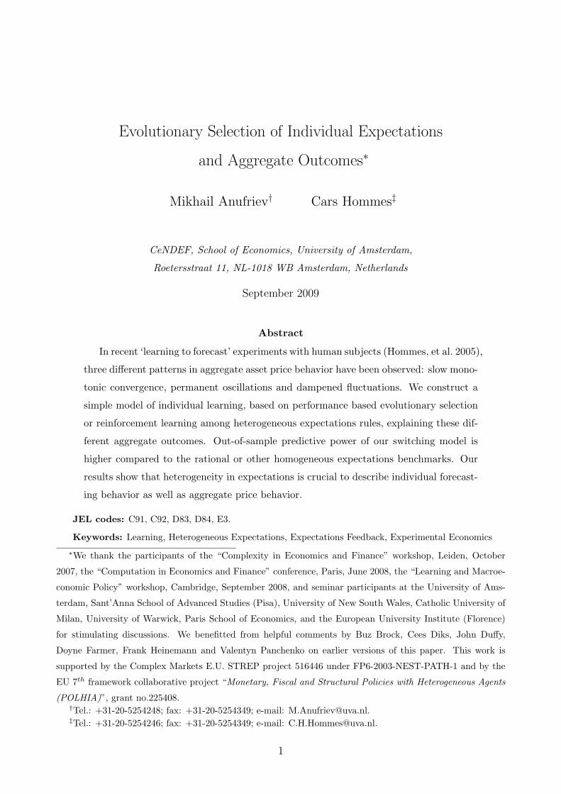
Figure 1: Price evolution and prediction errors (inner frame) under Rational Fun-

damental Expectations. When every participant predicts pf the realized price (red) fluctuates

around fundamental level. Small, non-systematic prediction errors (blue) are due to stochastic shocks.

At the end of the period every participant was informed about the realized price pt. The

earnings per period were determined by a quadratic scoring rule

ei,t =

1−(

pt−pei,t

7

)2

if |pt − pei,t| < 7 ,

0 otherwise ,(2.4)

so that forecasting errors exceeding 7 would result in no reward at a given period. At the end

of the session the accumulated earnings of every participant were converted to euros (1 point

computed as in (2.4) corresponded to 50 cents) and paid out.

There were seven sessions of the experiment, each with the same realizations of the stochas-

tic shocks εt drawn independently from a normal distribution with mean 0 and standard

deviation 0.5. The same stochastic process {εt}50t=0 will be used in our simulations.

Fig. 1 shows the simulation of realized prices, which would occur when all individuals

use the rational, fundamental forecasting rule, pei,t+1 = pf , for all i and t. Under rational

expectations the realized price pt = εt/(1 + r) randomly fluctuates around the fundamental

level pf = y/r = 60 with small amplitude. In the experiment, one can not expect rational

behavior at the outset, but aggregate prices might converge to their fundamental value through

individual learning.

5

35

45

55

65

0 10 20 30 40 50

Pred

ictio

ns

45

55

65

Pric

e

Group 2

-2 0 2

35

45

55

65

0 10 20 30 40 50

Pred

ictio

ns

45

55

65

Pric

e

Group 5

-2 0 2

35

45

55

65

0 10 20 30 40 50

Pred

ictio

ns

45

55

65

Pric

e

Group 1

-5 0 5

35

45

55

65

0 10 20 30 40 50

Pred

ictio

ns

45

55

65Pr

ice

Group 6

-5 0 5

10 30 50 70 90

0 10 20 30 40 50

Pred

ictio

ns

10

30

50

70

90

Pric

e

Group 4

-30 0

30

45

55

65

75

0 10 20 30 40 50

Pred

ictio

ns

45

55

65

75

Pric

e

Group 7

-10 0

10

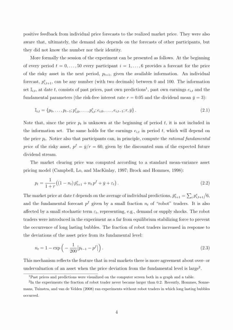
Figure 2: Three different qualitative outcomes in 6 sessions of the forecasting ex-

periment. For every panel an upper part shows observed prices (red) in comparison with the

fundamental level (black); a lower part shows individual predictions of 6 participants with forecast-

ing errors in an inner frame. In two sessions (upper panels) the price converges monotonically to

the fundamental value, in two sessions (middle panels) price exhibited persistent oscillations, in

two sessions (lower panels) the price converged through large (observe the change of scale for group

4) but damping oscillations. 6

2.2 Aggregate price behavior

Fig. 2 shows time series of prices, individual predictions and forecasting errors in six different

sessions of the experiment. A striking feature of aggregate price behavior is that three dif-

ferent qualitative patterns emerge. The prices in groups 2 and 5 converge slowly and almost

monotonically to the fundamental price level. In groups 1 and 6 persistent oscillations are

observed during the entire experiment. In groups 4 and 7 prices are also fluctuating but their

amplitude is decreasing.3

A second striking result concerns individual predictions. In all groups participants were

able to coordinate their forecasting activity. The forecasts, as shown in the lower parts of the

panels in Fig. 2, are dispersed in the first periods but then become very close to each other

in all groups.4 The coordination of individual forecasts has been achieved in the absence of

any communication between subjects and knowledge of past and present predictions of other

participants.

To summarize, in the HSTV learning to forecast experiment we have the following:

- participants were unable to learn the rational, fundamental forecasting rule; only in

some cases individual predictions moved (slowly) in the direction of the fundamental

price towards the end of the experiment;

- three different price patterns were observed: (i) slow, (almost) monotonic convergence,

(ii) persistent price oscillations with almost constant amplitude, and (iii) large initial

oscillations dampening slowly towards the end of the experiment;

- already after a short transient, participants were able to coordinate their forecasting

activity, submitting similar forecasts in every period.

The purpose of this paper is to explain these “stylized facts” simultaneously by a simple

model of individual learning behavior.

3Price dynamics in group 3 (not shown, but see the concluding remarks) is more difficult to classify. Similar

to group 1 it started with moderate oscillations, then stabilized at a level below the fundamental, suddenly

falling in period t = 40, probably due to a typing error of one of the participants.4To quantify the degree of coordination, HSTV analyze the average prediction error over time and across

the six participants for each group. It turns out that this error is explained more by the “common” prediction

error (measured as the deviation of the average prediction from the realized price), than by the dispersion

between individual predictions. Even in groups 4 and 7 with the lowest coordination, the dispersion between

individual predictions accounts only for 29% and 34%, respectively, of the average total prediction error.

7

2.3 Individual Forecasting Rules

Which forecasting rules did individuals use in the learning to forecast experiment? Comparison

of the RE benchmark in Fig. 1 with the lab experiments in Fig. 2 suggests that rational

expectations is not a good explanation of individual forecasting and aggregate behavior. For

the oscillating groups 1 and 6 this is immediately clear. One could perhaps argue that the

other groups show a tendency to converge to RE after 50 periods, but in contrast to the RE-

benchmark, e.g., in the monotonically converging groups 2 and 5 market prices are consistently

below the RE-benchmark 60. Moreover, RE does not explain the slowly dampened oscillating

patterns.

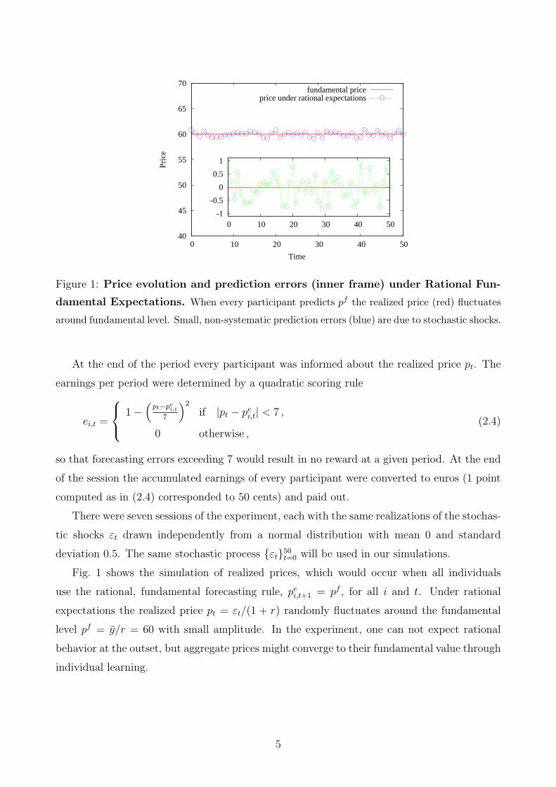
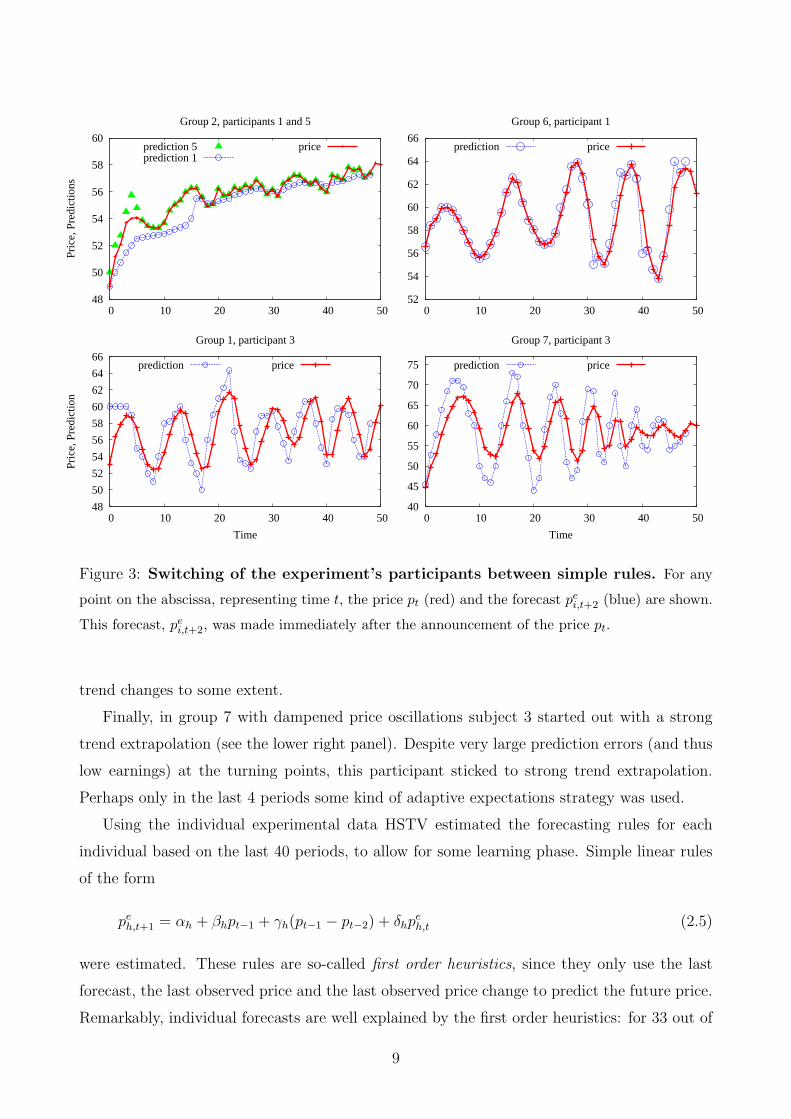
To get some intuition for individual behavior it is useful to look at some of the time evo-

lution of individual predictions. Fig. 3 shows time series of some (lagged) individual forecasts

together with the realized price. The timing in the figure is important. For every time t

on the horizontal axes we show the price pt together with the individual two-period ahead

forecast pei,t+2 of that price by some participant i. In this way we can infer graphically how the

two-period ahead forecast pei,t+2 uses the last observed price pt. For example, if they coincide,

i.e., pei,t+2 = pt, it implies naive expectations in period t.

In group 2, subject 5 extrapolates price changes in the early stage of the experiment (see

the upper left panel), but, starting from period t = 6, uses a simple naive rule pet+2 = pt.

In other words, in period 6, subject 5 switched from an extrapolative to a naive forecasting

rule. Subject 1 from the same group used a “smoother”, adaptive forecasting strategy, always

predicting a price between the previous forecast and the previous price realization. These

graphs already suggest individual heterogeneity in forecasting strategies.

In the oscillating group 6, subject 1 used naive expectations in the first half of the ex-

periment (until period 24, see the upper right panel). Naive expectations however, lead to

prediction errors in an oscillating market, especially when the trend reverses. In period 25

subject 1 switches to a different, trend extrapolating prediction strategy. Thereafter, this sub-

ject uses a trend extrapolating strategy switching back to the naive rule at periods of expected

trend reversal (e.g., in periods 27 and 28, 32 and 33, 37 and 38, 42, 43 and 44, and 47).

Interestingly, participant 3 from another oscillating group 1 starts out predicting the fun-

damental price, i.e., pet+1 = pf = 60 in the first four periods of the experiments (see the lower

left panel). But since the majority in group 1 predicts a lower price, the realized price is much

lower than the fundamental, causing participant 3 to switch to a different, trend extrapolating

strategy. Trend extrapolating predictions overshoot the realized market price at the moments

of trend reversal. Towards the end of the experiment participant 3 learned to anticipate the

8

48

50

52

54

56

58

60

0 10 20 30 40 50

Pric

e, P

redi

ctio

ns

Group 2, participants 1 and 5

prediction 5prediction 1

price

52

54

56

58

60

62

64

66

0 10 20 30 40 50

Group 6, participant 1

prediction price

48

50

52

54

56

58

60

62

64

66

0 10 20 30 40 50

Pric

e, P

redi

ctio

n

Time


prediction price

40

45

50

55

60

65

70

75

0 10 20 30 40 50

Time


prediction price

Figure 3: Switching of the experiment’s participants between simple rules. For any

point on the abscissa, representing time t, the price pt (red) and the forecast pei,t+2 (blue) are shown.

This forecast, pei,t+2, was made immediately after the announcement of the price pt.

trend changes to some extent.

Finally, in group 7 with dampened price oscillations subject 3 started out with a strong

trend extrapolation (see the lower right panel). Despite very large prediction errors (and thus

low earnings) at the turning points, this participant sticked to strong trend extrapolation.

Perhaps only in the last 4 periods some kind of adaptive expectations strategy was used.

Using the individual experimental data HSTV estimated the forecasting rules for each

individual based on the last 40 periods, to allow for some learning phase. Simple linear rules

of the form

peh,t+1 = αh + βhpt−1 + γh(pt−1 − pt−2) + δhp

eh,t (2.5)

were estimated. These rules are so-called first order heuristics, since they only use the last

forecast, the last observed price and the last observed price change to predict the future price.

Remarkably, individual forecasts are well explained by the first order heuristics: for 33 out of

9

42 participants (i.e., for 78%) an estimated linear rule falls into this simple class with an R2

typically higher than 0.80. In fact, within the class of first order heuristics three extremely

simple rules came up from the estimation results, characterizing the three different observed

aggregate outcome: convergence, permanent oscillations and dampened oscillations.

Participants from the converging groups 2 and 5 often used an adaptive expectations rule

of the form:

pet+1 = w pt−1 + (1− w) pe

t = pet + w (pt−1 − pe

t) , (2.6)

with weight 0 ≤ w ≤ 1. Note that at the moment when the forecast for the price pt+1 is

submitted, the price pt is still unknown (see Eq. 2.2), so that the last observed price is pt−1.

At the same time, the last forecast pet is of course known when forecasting pt+1. Notice also

that for w = 1, we obtain the special case of naive expectations.5 The individual forecast series

shown in the upper left panel of Fig. 3 are examples of estimated rules of the form (2.6), with

w = 1 for subject 5 and w ' 0.25 for subject 1.

Especially for the subjects in the permanent and the dampened oscillating groups estima-

tion revealed a simple trend-following forecasting rule of the form:

pet+1 = pt−1 + γ (pt−1 − pt−2) , (2.7)

where γ > 0. This rule has a simple behavioral interpretation: the forecast uses the last price

observation and adjusts in the direction of the last price change. The extrapolation coefficient

γ measures the strength of the adjustment. The estimates of this coefficient ranged from

relatively small extrapolation values, γ = 0.4, to quite strong extrapolation values, γ = 1.3.

Finally, especially in the permanently oscillating groups 1 and 6, a number of participants

used slightly more sophisticated AR(2) rules of the form

pet+1 = 0.5 (pf + pt−1) + (pt−1 − pt−2) . (2.8)

This is an example of an anchoring and adjustment rule (Tversky and Kahneman, 1974), since

it extrapolates the last price change from the reference point or anchor (pf +pt−1)/2 describing

the “long-run” price level. One could argue that the anchor for this rule, defined as an equally

weighted average between the last observed price and the fundamental price, was unknown

5The adaptive rule (2.6) was estimated for 5 out of 12 participants in groups 2 and 5, and three among

them had w insignificantly different from 1 (i.e., they used naive rule). Four other participants used an AR(1)

rule, pet+1 = a + bpt−1, conditioning only on the past price with a coefficient b < 1.

10

in the experiment, since subjects were not provided explicitly with the fundamental price.6

Therefore, in our evolutionary selection model in Section 4 one of the rules will be we (2.8)

with the fundamental price pf replaced by a proxy given by the (observable) sample average

of past prices pavt−1 =

∑t−1j=0 pj, to obtain

pet+1 = 0.5 (pav

t−1 + pt−1) + (pt−1 − pt−2) . (2.9)

To distinguish these rules, we will refer to the forecasting rule (2.8), with an anchor partly

determined by the fixed fundamental price pf , simply as an anchoring and adjustment (AA)

heuristic, and to the more flexible forecasting rule (2.9), with an anchor learned through a

sample average of past prices, as the learning anchoring and adjustment (LAA) heuristic.

Two important observations follow by the above discussion. First, the subjects in the

experiment tended to base their predictions on past observations, using relatively simple and

intuitive rules of thumb, such as adaptive expectations or trend extrapolation. Second, it

seems that participants tried to learn from past errors, and their learning behavior was in

the form of switching between different heuristics. These two observations, simplicity of the

forecasting strategy and (imperfect) evolutionary switching on seemingly more successful rules

will form the basis of our learning model in Section 4.

3 Price Behavior under Homogeneous Expectations

Having a set of estimated individual forecasting rules, one can ask whether these homogeneous

expectation rules can generate the qualitatively different patterns observed in the experiments.

The experimental evidence about forecasting behavior suggests strong coordination on a com-

mon prediction rule. One can therefore suspect that this common rule (which, for whatever

reason, turned out to be different in different groups) generates the resulting pattern. In

this Section we investigate this conjecture by studying price fluctuations under homogeneous

expectations in the forecasting experiment.

6It is remarkable that exactly this anchor and adjustment rule (2.8) was estimated for participant 3 in

group 1, who did submit the fundamental price forecast in the first four periods of the experiment, see the

lower left panel of Fig. 3. For 4 out of 12 participants of groups 1 and 6 the estimated AR(2) rule was very

close to (2.8), as it can be be seen in the middle panels of Fig. 6.

11

The model with homogeneous expectations is given by

pet+1 = f(pt−1, pt−2, p

et) ,

nt = 1− exp(− 1

200

∣∣pt−1 − pf∣∣)

,

pt =1

1 + r

((1− nt)p

et+1 + nt p

f + y + εt

).

(3.1)

The first equation describes forecasting behavior with a simple first order heuristic f as in

(2.5), which can be either adaptive expectations (in which case f does not depend on pt−2) or

trend following expectations (in which case f does not depend on pet ). The second equation

gives the evolution of the share of “robot” traders, identical to the rule used in the experiment.

The third equation is the equilibrium pricing equation used in the experiment, cf. (2.2). We

present an analysis of the so-called deterministic skeleton model, setting term εt in (3.1) to

zero, as well as stochastic simulations with the same realizations of the shocks, εt, as in

the experiment, in order to investigate how the noise affects price fluctuations. In terms of

deviations from the fundamental price the model can be rewritten as

pt − pf =1

1 + r

((1− nt)p

et+1 + nt p

f − pf)

=1− nt

1 + r

(pe

t+1 − pf), (3.2)

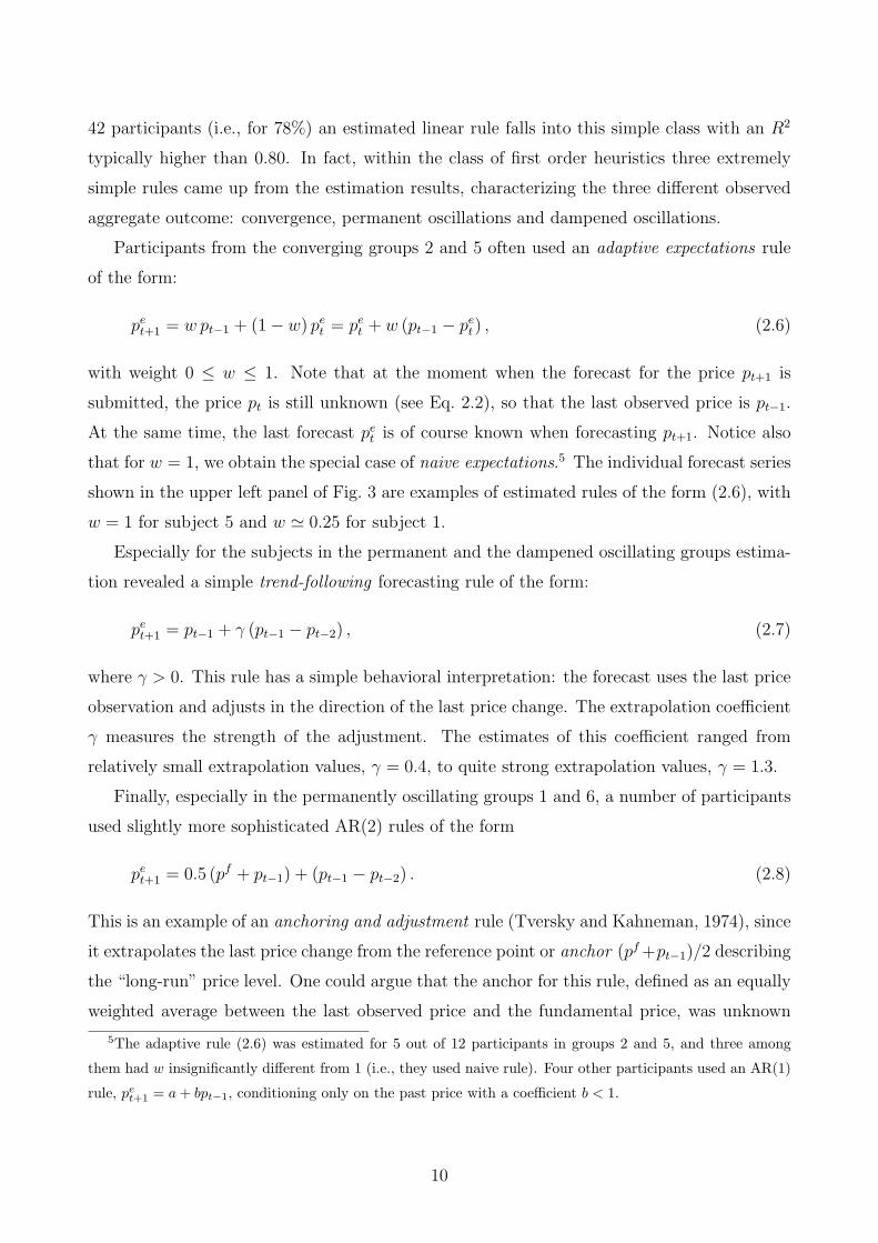
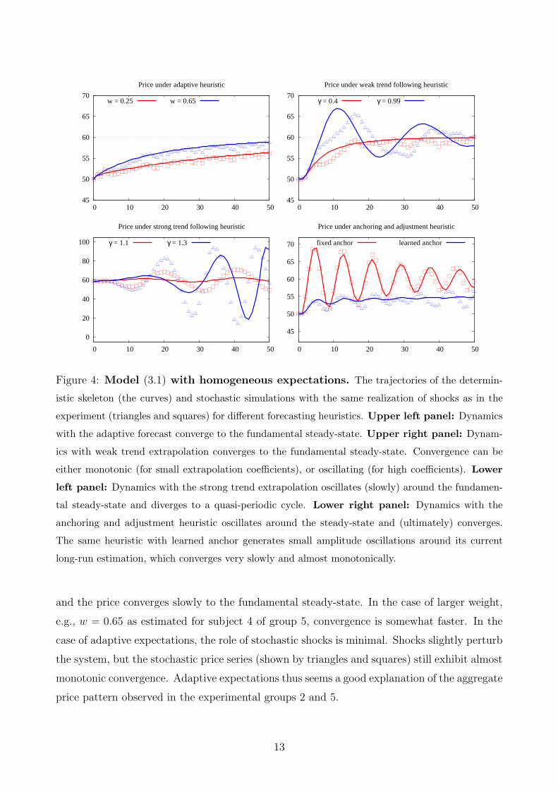
Fig. 4 shows example of simulated dynamics for different adaptive, trend-following and anchor-

ing and adjustment rules which have been estimated from individual forecasting experimental

data.

3.1 Adaptive Heuristic

Assume that all participants use the same adaptive heuristic pet+1 = w pt−1 +(1−w) pe

t in their

forecasting activity. Notice that naive expectations is obtained as a special case, for w = 1.

The following result describes the behavior of system (3.1) in this case.

Proposition 3.1. Consider the deterministic skeleton of (3.1) with the adaptive prediction

rule (2.6). This system has a unique steady-state with price equal to fundamental price, i.e.

p∗ = pf . The steady-state is globally stable for 0 < w ≤ 1, with a real eigenvalue λ, 0 < λ < 1,

so that the convergence is monotonic.

Proof. See Appendix A.

The dynamics with the adaptive forecasting heuristic is illustrated in the upper left panel

of Fig. 4 for two different values of the weight w assigned to the past price. When the weight

is relatively low, e.g., w = 0.25 as for participant 1 in group 2, the error correction is small,

12

45

50

55

60

65

70

0 10 20 30 40 50

Price under adaptive heuristic

w = 0.25 w = 0.65

45

50

55

60

65

70

0 10 20 30 40 50

Price under weak trend following heuristic

γ = 0.4 γ = 0.99

0

20

40

60

80

100

0 10 20 30 40 50

Price under strong trend following heuristic

γ = 1.1 γ = 1.3

45

50

55

60

65

70

0 10 20 30 40 50

Price under anchoring and adjustment heuristic

fixed anchor learned anchor

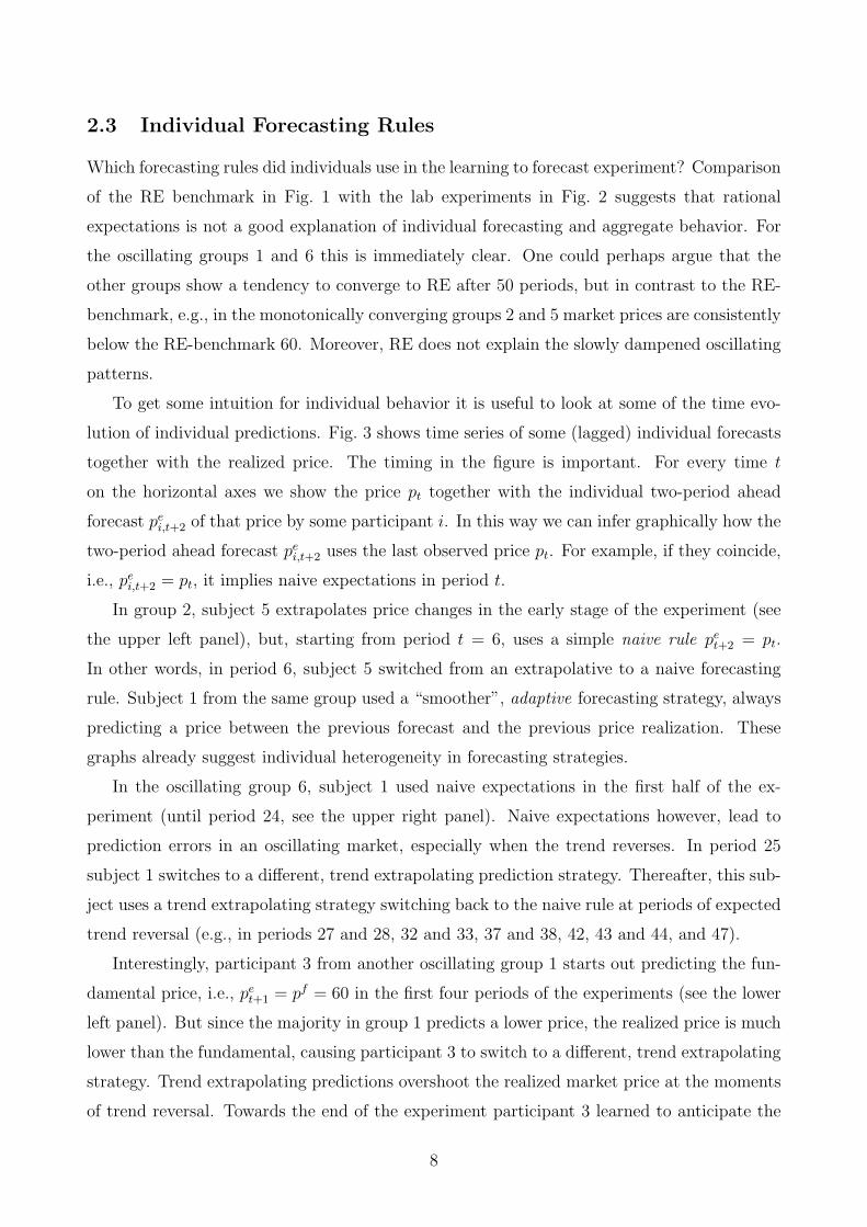
Figure 4: Model (3.1) with homogeneous expectations. The trajectories of the determin-

istic skeleton (the curves) and stochastic simulations with the same realization of shocks as in the

experiment (triangles and squares) for different forecasting heuristics. Upper left panel: Dynamics

with the adaptive forecast converge to the fundamental steady-state. Upper right panel: Dynam-

ics with weak trend extrapolation converges to the fundamental steady-state. Convergence can be

either monotonic (for small extrapolation coefficients), or oscillating (for high coefficients). Lower

left panel: Dynamics with the strong trend extrapolation oscillates (slowly) around the fundamen-

tal steady-state and diverges to a quasi-periodic cycle. Lower right panel: Dynamics with the

anchoring and adjustment heuristic oscillates around the steady-state and (ultimately) converges.

The same heuristic with learned anchor generates small amplitude oscillations around its current

long-run estimation, which converges very slowly and almost monotonically.

and the price converges slowly to the fundamental steady-state. In the case of larger weight,

e.g., w = 0.65 as estimated for subject 4 of group 5, convergence is somewhat faster. In the

case of adaptive expectations, the role of stochastic shocks is minimal. Shocks slightly perturb

the system, but the stochastic price series (shown by triangles and squares) still exhibit almost

monotonic convergence. Adaptive expectations thus seems a good explanation of the aggregate

price pattern observed in the experimental groups 2 and 5.

13

3.2 Extrapolative Rules

Consider now the dynamics with homogeneous extrapolative expectations. For the sake of

generality we write the extrapolative forecasting rule as:

pet+1 = α + β1 pt−1 + β2 pt−2 . (3.3)

This extrapolative rule contains both the trend following and the anchor and adjustment

heuristic as special cases. Indeed, setting α = 0, β1 = 1 + γ and β2 = −γ, the trend-

following heuristics (2.7) is obtained, while α = pf/2, β1 = 1.5 and β2 = −1 correspond to the

anchoring and adjustment heuristic (2.8). The rules for which the forecasts are not consistent

with realizations will be disregarded by the participants, sooner or later. Therefore, both in

the formal analysis and in simulations we confine our attention to the rules satisfying the

following simple steady-state consistency requirement:

Definition 3.1. The extrapolative rule (3.3) is called consistent in the steady-state p∗, if it

predicts p∗ in this steady-state.

In other words, consistent rules give unbiased predictions at the steady-state. Obviously,

the extrapolative rule is consistent in p∗ if and only if α = (1 − β1 − β2)p∗. Notice that,

the trend-following heuristic (2.7) is consistent at any steady-state, while the anchoring and

adjustment heuristic (2.8) is consistent only at the steady state with p∗ = pf .7

The following result describes all possible steady-states of the asset-pricing dynamics with

consistent extrapolative heuristic, as well as their local stability.

Proposition 3.2. Consider the dynamics of the deterministic skeleton of (3.1) with extrap-

olative prediction rule (3.3).

There exists a unique steady-state in which the rule is consistent. In this steady-state,

p∗ = pf and the fraction of robot traders n∗ = 0. The “fundamental” steady-state is locally

stable if the following three conditions are met

β2 < (1 + r)− β1 , β2 < (1 + r) + β1 , β2 > −(1 + r) . (3.4)

The steady-state generically exhibits a pitch-fork, period-doubling or Neimark-Sacker bifurca-

tion, if the first, second or third inequality in (3.4) turns into an equality, respectively. More-

over, the dynamics is oscillating (i.e., the eigenvalues of the linearized system are complex)

when β21 + 4β2(1 + r) < 0.

7In related learning-to-forecasting experiments Heemeijer, Hommes, Sonnemans, and Tuinstra (2009) find

that the estimated linear forecasting rules for many subjects are consistent in the steady state p∗ = pf , both

in market environments with positive and negative expectations feedback.

14

-1.5

-1

-0.5

0

0.5

1

1.5

-2 -1 0 1 2

β 2

β1

Neimark-Sacker

pitch-fork

perio

d-do

ublin

g

γ = 0.4

γ = 1.3

A&A

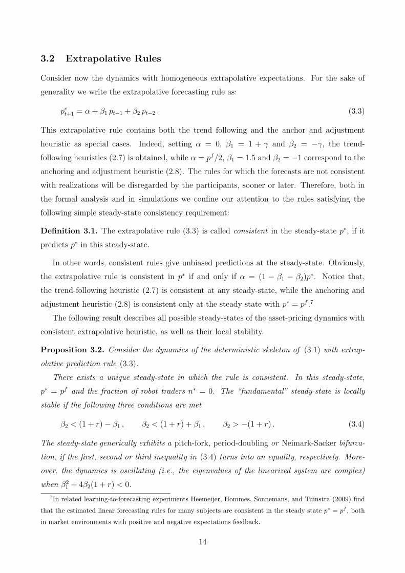
Figure 5: Stability of the fundamental steady-state in an asset-pricing model with

homogeneous extrapolative expectations. The dynamics (3.1) with expectations (3.3) con-

verges to the fundamental steady-state if the pair of coefficients (β1, β2) belongs to the union of light

and dark grey regions. The edges of the triangle at the border of the stability region correspond

to pitchfork, period-doubling and Neimark-Sacker bifurcations respectively. The price dynamics is

oscillating if the pair (β1, β2) lies below the parabolic curve. The three dots correspond to two trend-

following heuristics (labeled γ = 0.4 and γ = 1.3) and an anchoring and adjustment heuristic (labeled

AA), which will be used in the learning model in Section 4.

Proof. See Appendix B.

In general, the dynamical system (3.1) with homogeneous extrapolative expectations (3.3)

may have multiple steady-states. Proposition 3.2 asserts, however, that the extrapolative

rule is consistent only in the fundamental steady state pf . The stability conditions (3.4) are

illustrated in Fig. 5 in the parameter space (β1, β2). The dark regions contain all rules for

which the extrapolative heuristic (3.3) generates stable dynamics. For the pairs lying below

the parabolic curve, the dynamics are oscillating. A loss of (local) stability occurs when the

pair (β1, β2) leaves the stability area and crosses the boundary formed by the triangle. The

dynamics immediately after the bifurcation are determined by the type of bifurcation through

which stability is lost. For instance, after the pitchfork bifurcation the price diverges from its

fundamental level and converges to one of two new stable steady-states. The Neimark-Sacker

bifurcation implies existence of (quasi-)periodic price fluctuations right after the bifurcation.

The three dots shown in Fig. 5 correspond to three extrapolative forecasting rules estimated

from individual experimental data. Two trend-following heuristic (2.7) with different values

15

of the extrapolation coefficient γ are labeled as γ = 0.4 and γ = 1.3. The anchoring and

adjustment heuristic (2.8) is labeled as AA.

Trend-following heuristic. These results imply that the price may either converge or

diverge under the trend-following rule (2.7), depending upon the parameter γ. To distinguish

between these two cases we will use the terms weak and strong trend extrapolation.

The dynamics with the weak trend extrapolation is illustrated in the upper right panel of

Fig. 4. When the extrapolative coefficient is small (e.g., γ = 0.4), convergence is monotonic;

for larger γ-values (e.g., γ = 0.99) convergence becomes oscillatory. Notice however that these

stable oscillations are different (e.g., of lower frequency) compared to the dampened oscillations

observed in groups 4 and 7 in the experiments. Indeed, the estimation of individual strategies

in groups 4 and 7 did not reveal a trend-following rule which would generate such converging

oscillations. The case of the strong trend extrapolation is illustrated in the bottom left panel

of Fig. 4. The price dynamics diverges from the fundamental steady state throughoscillations

of increasing amplitude. The speed of divergence and amplitude of the long run fluctuations

increase with γ, as shown by comparison of the cases γ = 1.1 and γ = 1.3.

Anchoring and adjustment heuristic. Applying Proposition 3.2 to the anchoring and

adjustment rule (2.8) we conclude that the implied price dynamics is converging. Since the

parameters of the anchoring and adjustment rule are very close to the Neimark-Sacker bifur-

cation, the convergence to the fundamental steady-state is oscillatory and slow (cf. the bottom

right panel of Fig. 4). For the stochastic simulation the convergence is even slower and the

amplitude of the price fluctuations remains more or less constant in the last 20 periods, with

an amplitude ranging from 55 to 65 comparable to that of the permanently oscillatory group

6 in the experiments. The small shocks εt added in the experimental design, to mimic (small)

shocks in a real market, thus seem to be important to keep the price oscillations alive.

The bottom right panel of Fig. 4 also shows the price dynamics of the learning anchoring

and adjustment (LAA) rule (2.9). Notice that the dynamics with a LAA heuristic is described

by a non-autonomous system, whose formal analysis is complicated. Simulations under ho-

mogeneous expectations given by the LAA heuristic (2.9) converge to the same fundamental

steady-state as with the anchoring and adjustment heuristic (2.8), but much slower and with

less pronounced oscillations. In the presence of noise, the price oscillations under the LAA

heuristic are qualitatively similar to the price fluctuations in the permanently oscillatory group

1 of the experiment (with prices fluctuating below the fundamental most of the time, between

52 and 62).

16

-1.5

-1

-0.5

0

0.5

1

1.5

-2 -1 0 1 2

Stability region and group 2

-1.5

-1

-0.5

0

0.5

1

1.5

-2 -1 0 1 2


-1.5

-1

-0.5

0

0.5

1

1.5

-2 -1 0 1 2


-1.5

-1

-0.5

0

0.5

1

1.5

-2 -1 0 1 2


-1.5

-1

-0.5

0

0.5

1

1.5

-2 -1 0 1 2


-1.5

-1

-0.5

0

0.5

1

1.5

-2 -1 0 1 2


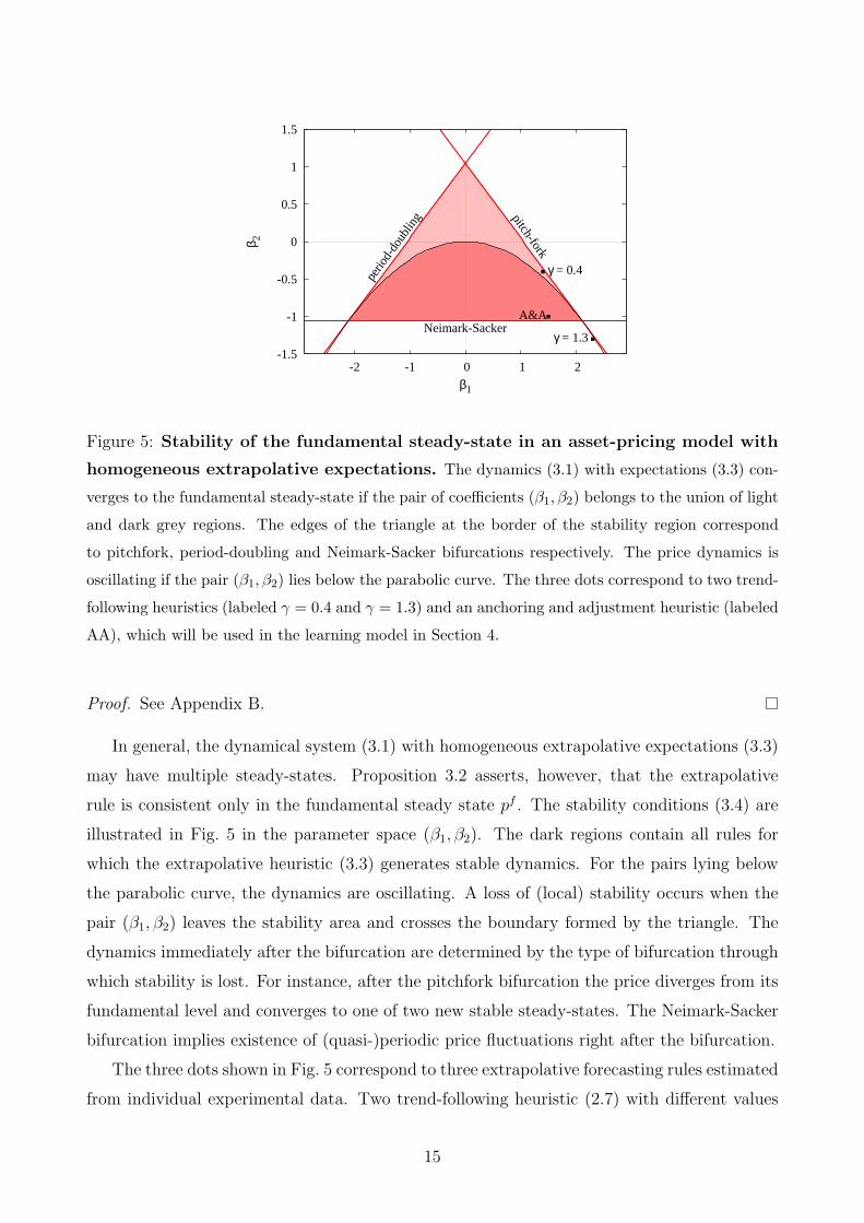
Figure 6: Stability of a model with homogeneous extrapolative rules estimated in

the experiment. Upper panel: In both groups with converging price, all rules generate stable

monotonic dynamics. Middle panel: In both groups with oscillating price, there were two rules on

the stability border of the Neimark-Sacker bifurcation. Lower panel: In both groups with damping

oscillations, both stable and unstable rules were present.

17

Homogeneity versus heterogeneity

In this Section we analyzed the price dynamics underlying the experiment, under the assump-

tion that expectations are homogeneous and all individuals use the same forecasting heuristic.

Qualitatively, all three observed patterns in the experiments, monotonic convergence, constant

oscillations and dampened oscillations can be reproduced. However, the dampened oscillations

have a different amplitude and frequency compared to the experimental groups 4 and 7. More-

over, a model with homogeneous expectations leaves open the question why different patterns

in aggregate behavior emerged in different experimental groups.

The dots in Fig. 6 represent the coefficients of the estimated individual extrapolative rules

(3.3).8 While the dispersion of individual forecasting rules is clear, the figure suggests some

regularities. In the converging groups 2 and 5, the majority of rules belong to the region of

monotonic convergence. In contrast, in the oscillating groups almost all individual rules lie in

the oscillatory region (i.e., the linear forecasting rule has complex eigenvalues). Furthermore,

in groups 1 and 6 with constant price oscillations, at least two individual rules in every group

are very close to the locus of the Neimark-Sacker bifurcation (i.e., are close to complex unit

roots), while in groups 4 and 7 with dampened oscillations there is at least one (strongly)

unstable individual forecasting rule. These results suggest that heterogeneous expectations

may be a key element in order to explain the learning to forecast experiments.

4 Heuristics Switching Model

In this Section we present a simple model with evolutionary selection between different simple

forecasting heuristics. Before describing the model, we recall the most important “stylized

facts” which we found in the individual and aggregate experimental data:

- participants tend to base their predictions on past observations following simple fore-

casting heuristics;

- individual learning has a form of switching from one heuristic to another;

- in every group some form of coordination of individual forecasts occurs; the rule on

which individuals coordinate may be different in different groups;

8In every group there were rules which cannot be represented by the extrapolative prediction (3.3), e.g., an

adaptive heuristic or linear rules with three lags.

18

- coordination of individual forecasting rules is not perfect and some heterogeneity of the

applied rules remains at every time period.

The main idea of the model is simple. Assume that there exists a pool of simple prediction

rules (e.g., adaptive or trend-following heuristics) commonly available to the participants of

the experiment. At every time period these heuristics deliver forecasts for next period’s price,

and the realized market price depends upon these individual forecasts. However, the impacts

of different forecasting heuristics upon the realized prices are changing over time because the

participants are learning based on evolutionary selection: the better a heuristic performed in

the past, the higher its impact in determining next period’s price. As a result, the realized

market price and impact of the forecasting heuristics co-evolve in a dynamic process with

mutual feedback. It turns out that this evolutionary model exhibits path dependence explaining

coordination on different forecasting heuristics leading to different aggregate price behavior.

The Model

Let H denote a set of H heuristics which participants can use for price prediction. In the

beginning of period t every rule h ∈ H gives a two-period ahead point prediction for the price

pt+1. The prediction is described by a deterministic function fh of available information:

peh,t+1 = fh(pt−1, pt−2, . . . ; p

eh,t, p

eh,t−1, . . . ) . (4.1)

The price in period t is computed on the base of these predictions as in (2.2):

pt =1

1 + r

((1− nt) pe

t+1 + nt pf + y + εt

), (4.2)

where pet+1 is the average predicted price, r is the risk free interest rate, y is the mean dividend,

and εt is the noise term. Finally, nt is the share of robot traders evolving as in the experiment

(cf. (2.3)) according to

nt = 1− exp(− 1

200

∣∣pt−1 − pf∣∣)

. (4.3)

In all simulations we use the same parameter values and the same realization of stochastic

shocks εt as in the experiment. In particular, the fundamental price as predicted by robots is

set to pf = y/r = 0.05/3 = 60.

In our evolutionary model, the average pet+1 in (4.2) is a population weighted average of

the different forecasting heuristics

pet+1 =

H∑

h=1

nh,t peh,t+1 , (4.4)

19

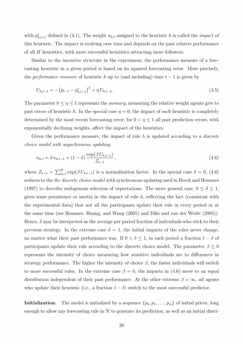
with peh,t+1 defined in (4.1). The weight nh,t assigned to the heuristic h is called the impact of

this heuristic. The impact is evolving over time and depends on the past relative performance

of all H heuristics, with more successful heuristics attracting more followers.

Similar to the incentive structure in the experiment, the performance measure of a fore-

casting heuristic in a given period is based on its squared forecasting error. More precisely,

the performance measure of heuristic h up to (and including) time t− 1 is given by

Uh,t−1 = −(pt−1 − pe

h,t−1

)2+ η Uh,t−2 . (4.5)

The parameter 0 ≤ η ≤ 1 represents the memory, measuring the relative weight agents give to

past errors of heuristic h. In the special case η = 0, the impact of each heuristic is completely

determined by the most recent forecasting error; for 0 < η ≤ 1 all past prediction errors, with

exponentially declining weights, affect the impact of the heuristics.

Given the performance measure, the impact of rule h is updated according to a discrete

choice model with asynchronous updating

nh,t = δ nh,t−1 + (1− δ)exp(β Uh,t−1)

Zt−1

, (4.6)

where Zt−1 =∑H

h=1 exp(β Uh,t−1) is a normalization factor. In the special case δ = 0, (4.6)

reduces to the the discrete choice model with synchronous updating used in Brock and Hommes

(1997) to describe endogenous selection of expectations. The more general case, 0 ≤ δ ≤ 1,

gives some persistence or inertia in the impact of rule h, reflecting the fact (consistent with

the experimental data) that not all the participants update their rule in every period or at

the same time (see Hommes, Huang, and Wang (2005) and Diks and van der Weide (2005)).

Hence, δ may be interpreted as the average per period fraction of individuals who stick to their

previous strategy. In the extreme case δ = 1, the initial impacts of the rules never change,

no matter what their past performance was. If 0 < δ ≤ 1, in each period a fraction 1 − δ of

participants update their rule according to the discrete choice model. The parameter β ≥ 0

represents the intensity of choice measuring how sensitive individuals are to differences in

strategy performance. The higher the intensity of choice β, the faster individuals will switch

to more successful rules. In the extreme case β = 0, the impacts in (4.6) move to an equal

distribution independent of their past performance. At the other extreme β = ∞, all agents

who update their heuristic (i.e., a fraction 1− δ) switch to the most successful predictor.

Initialization. The model is initialized by a sequence {p0, p1, . . . , pin} of initial prices, long

enough to allow any forecasting rule in H to generate its prediction, as well as an initial distri-

20

bution {nh,in}, 1 ≤ h ≤ H of the impacts of different heuristic (summing to 1). Additionally,

the initial share of robot traders and initial performances of all H heuristics are set to 0.

Given initial prices, the heuristic’s forecasts can be computed and, using the initial im-

pacts of the heuristics, the price pin+1 can be computed. In the next period, the forecasts of

the heuristics are updated, the fraction of robot traders is computed, while the same initial

impacts nh,in for the individual rules are used, since past performance is not well defined yet.

Thereafter, the price pin+2 is computed and the initialization stage is finished. After this ini-

tialization state the evolution according to (4.2) is well defined: first the performance measure

in (4.5) is updated, then, the new impacts of the heuristics are computed according to (4.6),

and the new prediction of the heuristics are obtained according to (4.1). Finally, the new

average forecast (4.4) and the new fraction of robot traders (4.3) are computed, and a new

price is determined by (4.2).

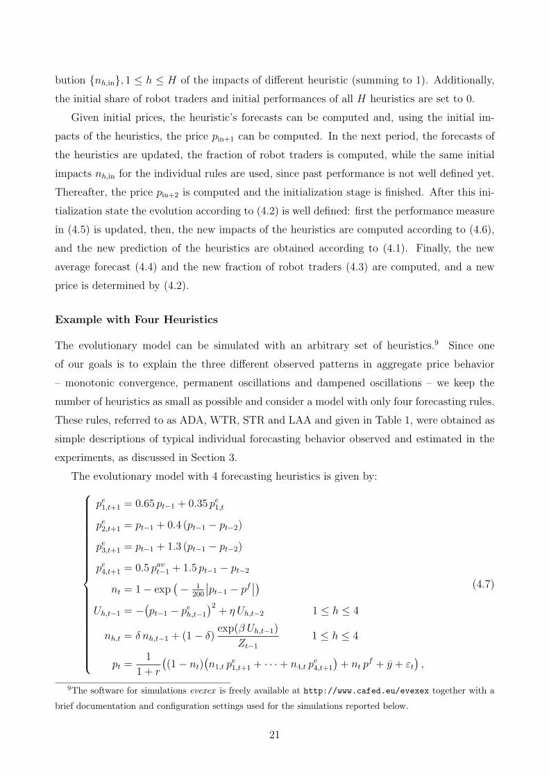
Example with Four Heuristics

The evolutionary model can be simulated with an arbitrary set of heuristics.9 Since one

of our goals is to explain the three different observed patterns in aggregate price behavior

– monotonic convergence, permanent oscillations and dampened oscillations – we keep the

number of heuristics as small as possible and consider a model with only four forecasting rules.

These rules, referred to as ADA, WTR, STR and LAA and given in Table 1, were obtained as

simple descriptions of typical individual forecasting behavior observed and estimated in the

experiments, as discussed in Section 3.

The evolutionary model with 4 forecasting heuristics is given by:

pe1,t+1 = 0.65 pt−1 + 0.35 pe

1,t

pe2,t+1 = pt−1 + 0.4 (pt−1 − pt−2)

pe3,t+1 = pt−1 + 1.3 (pt−1 − pt−2)

pe4,t+1 = 0.5 pav

t−1 + 1.5 pt−1 − pt−2

nt = 1− exp(− 1

200

∣∣pt−1 − pf∣∣)

Uh,t−1 = −(pt−1 − pe

h,t−1

)2+ η Uh,t−2 1 ≤ h ≤ 4

nh,t = δ nh,t−1 + (1− δ)exp(β Uh,t−1)

Zt−1

1 ≤ h ≤ 4

pt =1

1 + r

((1− nt)

(n1,t p

e1,t+1 + · · ·+ n4,t p

e4,t+1

)+ nt p

f + y + εt

),

(4.7)

9The software for simulations evexex is freely available at http://www.cafed.eu/evexex together with a

brief documentation and configuration settings used for the simulations reported below.

21

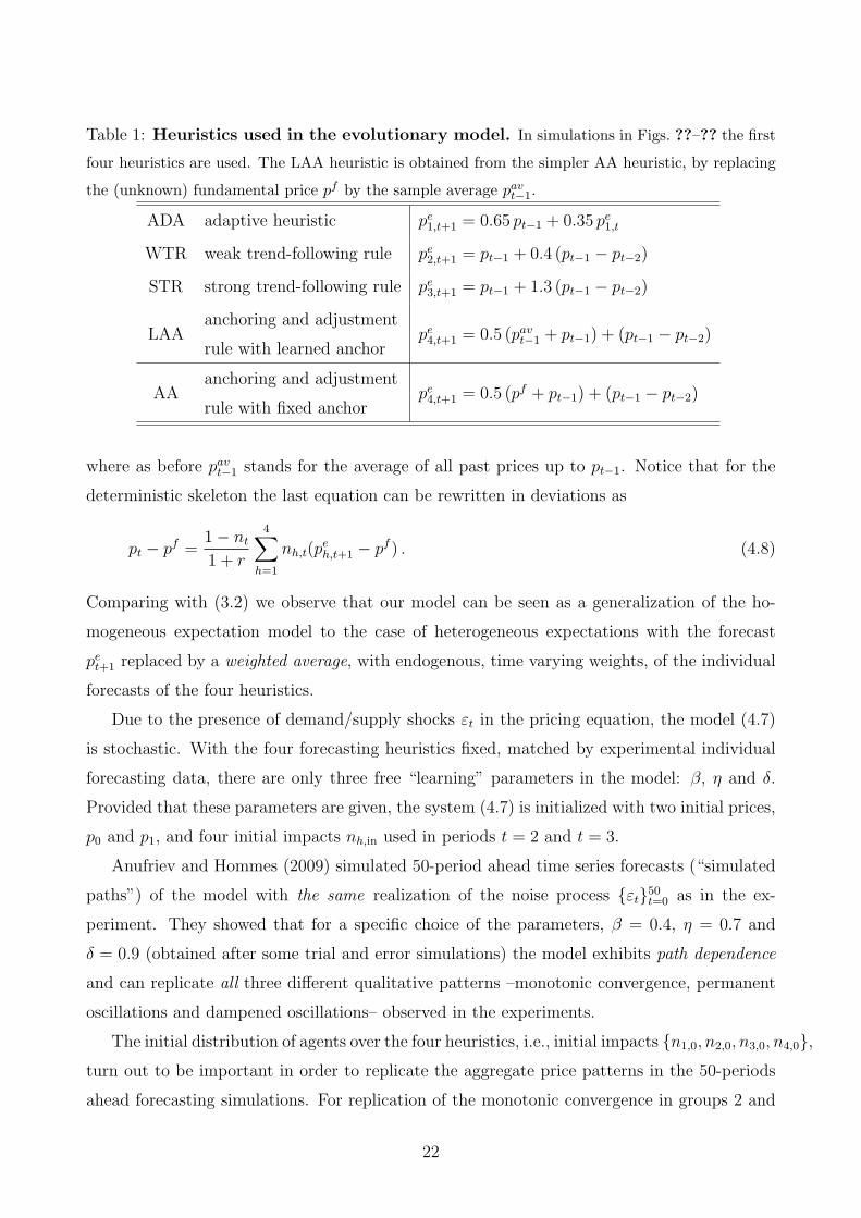
Table 1: Heuristics used in the evolutionary model. In simulations in Figs. ??–?? the first

four heuristics are used. The LAA heuristic is obtained from the simpler AA heuristic, by replacing

the (unknown) fundamental price pf by the sample average pavt−1.

ADA adaptive heuristic pe1,t+1 = 0.65 pt−1 + 0.35 pe

1,t

WTR weak trend-following rule pe2,t+1 = pt−1 + 0.4 (pt−1 − pt−2)

STR strong trend-following rule pe3,t+1 = pt−1 + 1.3 (pt−1 − pt−2)

LAAanchoring and adjustment

pe4,t+1 = 0.5 (pav

t−1 + pt−1) + (pt−1 − pt−2)rule with learned anchor

AAanchoring and adjustment

pe4,t+1 = 0.5 (pf + pt−1) + (pt−1 − pt−2)

rule with fixed anchor

where as before pavt−1 stands for the average of all past prices up to pt−1. Notice that for the

deterministic skeleton the last equation can be rewritten in deviations as

pt − pf =1− nt

1 + r

4∑

h=1

nh,t(peh,t+1 − pf ) . (4.8)

Comparing with (3.2) we observe that our model can be seen as a generalization of the ho-

mogeneous expectation model to the case of heterogeneous expectations with the forecast

pet+1 replaced by a weighted average, with endogenous, time varying weights, of the individual

forecasts of the four heuristics.

Due to the presence of demand/supply shocks εt in the pricing equation, the model (4.7)

is stochastic. With the four forecasting heuristics fixed, matched by experimental individual

forecasting data, there are only three free “learning” parameters in the model: β, η and δ.

Provided that these parameters are given, the system (4.7) is initialized with two initial prices,

p0 and p1, and four initial impacts nh,in used in periods t = 2 and t = 3.

Anufriev and Hommes (2009) simulated 50-period ahead time series forecasts (“simulated

paths”) of the model with the same realization of the noise process {εt}50t=0 as in the ex-

periment. They showed that for a specific choice of the parameters, β = 0.4, η = 0.7 and

δ = 0.9 (obtained after some trial and error simulations) the model exhibits path dependence

and can replicate all three different qualitative patterns –monotonic convergence, permanent

oscillations and dampened oscillations– observed in the experiments.

The initial distribution of agents over the four heuristics, i.e., initial impacts {n1,0, n2,0, n3,0, n4,0},turn out to be important in order to replicate the aggregate price patterns in the 50-periods

ahead forecasting simulations. For replication of the monotonic convergence in groups 2 and

22

5, the initial impacts of heuristics are distributed almost uniformly, with a slight dominance of

the WTR heuristics to produce a small initial trend in prices. For the oscillating groups 1 and

6, where the initial trend was stronger, both trend heuristics WTR and STR were initialized

with somewhat higher weights. Finally, in the dampened oscillating groups 4 and 7, with the

strongest trend in price in initial periods, the STR rule has a large initial impact.

5 Empirical Validation

In this section we address the issue of how well the nonlinear stochastic switching model with

four forecasting heuristics fits with the experimental data. This section is divided in three

parts. We, first, illustrate the one-period ahead forecasts of the model visually, then turn

to the rigorous evaluation of the in-sample performance of the model, and, finally, look at

out-of-sample forecasts made by the model.

5.1 One-period ahead simulations

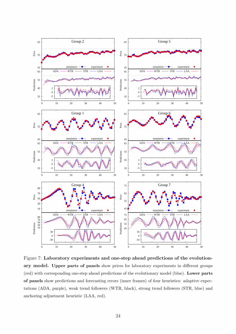
Fig. 7 compares the experimental data with the one-step ahead predictions made by our

model, using the same benchmark parameters β = 0.4, η = 0.7 and δ = 0.9 as before. In

these simulations the initial prices coincide with the initial prices in the first two periods in

the corresponding experimental group, while the initial impacts of all heuristics are equal to

0.25. Fig. 7 suggests that the switching model with four heuristics fits the experimental data

quite nicely.

It is useful to briefly discuss the differences of the stochastic simulations in Fig. 7 with the

“simulated paths” in Anufriev and Hommes (2009). At each time step, the simulated path only

uses simulated price data as inputs to compute the heuristics’ forecasts and to update their

impacts. Therefore, the simulated paths are essentially 50 period ahead forecasts generated

by the nonlinear switching model. These simulated paths already showed that the nonlinear

switching model (augmented by the same small noise as in the experiment) is capable of

generating all three different patterns observed in the experimental data. In contrast, the one-

step ahead predictions of the nonlinear switching model in Fig. 7 use past experimental price

data, i.e., exactly the same information that was available to participants in the experiments,

as inputs for the forecasting rules and the updating of fractions. An immediate observations

by comparing these simulations is that the one-period ahead forecasts can follow more easily

the sustained oscillations as well as the dampened oscillatory patterns. While the simulated

paths could only reproduce the (dampened) oscillatory patterns for 50 periods if the initial

23

35

45

55

65

0 10 20 30 40 50

Pred

ictio

ns

ADA WTR STR LAA 45

55

65

Pric

e

Group 2

simulation experiment

-2

0

2

35

45

55

65

0 10 20 30 40 50

Pred

ictio

ns

ADA WTR STR LAA 45

55

65

Pric

e

Group 5


-2

0

2

35

45

55

65

0 10 20 30 40 50

Pred

ictio

ns

ADA WTR STR LAA 45

55

65

Pric

e

Group 1


-5

0

5

35

45

55

65

0 10 20 30 40 50

Pred

ictio

ns

ADA WTR STR LAA 45

55

65

Pric

e

Group 6


-5

0

5

10 30 50 70 90

0 10 20 30 40 50

Pred

ictio

ns

ADA WTR STR LAA

10

30

50

70

90

Pric

e

Group 4


-30

0

30 45

55

65

75

0 10 20 30 40 50

Pred

ictio

ns

ADA WTR STR LAA

45

55

65

75

Pric

e

Group 7


-10

0

10

Figure 7: Laboratory experiments and one-step ahead predictions of the evolution-

ary model. Upper parts of panels show prices for laboratory experiments in different groups

(red) with corresponding one-step ahead predictions of the evolutionary model (blue). Lower parts

of panels show predictions and forecasting errors (inner frames) of four heuristics: adaptive expec-

tations (ADA, purple), weak trend followers (WTR, black), strong trend followers (STR, blue) and

anchoring adjustment heuristic (LAA, red).

24

0

0.2

0.4

0.6

0.8

1

0 10 20 30 40 50

Fractions of 4 rules in the simulation for Group 2

ADA WTR STR LAA

0

0.2

0.4

0.6

0.8

1

0 10 20 30 40 50


ADA WTR STR LAA

0

0.2

0.4

0.6

0.8

1

0 10 20 30 40 50


ADA WTR STR LAA

0

0.2

0.4

0.6

0.8

1

0 10 20 30 40 50


ADA WTR STR LAA

0

0.2

0.4

0.6

0.8

1

0 10 20 30 40 50


ADA WTR STR LAA

0

0.2

0.4

0.6

0.8

1

0 10 20 30 40 50


ADA WTR STR LAA

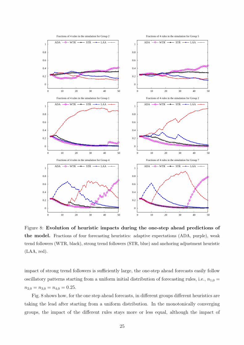
Figure 8: Evolution of heuristic impacts during the one-step ahead predictions of

the model. Fractions of four forecasting heuristics: adaptive expectations (ADA, purple), weak

trend followers (WTR, black), strong trend followers (STR, blue) and anchoring adjustment heuristic

(LAA, red).

impact of strong trend followers is sufficiently large, the one-step ahead forecasts easily follow

oscillatory patterns starting from a uniform initial distribution of forecasting rules, i.e., n1,0 =

n2,0 = n3,0 = n4,0 = 0.25.

Fig. 8 shows how, for the one step ahead forecasts, in different groups different heuristics are

taking the lead after starting from a uniform distribution. In the monotonically converging

groups, the impact of the different rules stays more or less equal, although the impact of

25

adaptive expectations gradually increases and slightly dominates the other rules in the last

20-25 periods. The oscillatory groups yield similar results as before, with the LAA rule

dominating the market early and its impact increasing to about 90% towards the end of the

experiment. Notice, that the domination of the LAA rule happens much faster in simulations

for group 1, than for group 6. (For instance, 80% impact is reached by the LAA rule after

20 periods for group 1 and after 40 periods for group 6.) This difference reflects the fact that

the frequency of oscillations in the two experimental groups were not the same. During the

experiment we observe about 6 “cycles” in group 1, but only about 4 and a half “cycles” in

group 6. The stochastic one-step ahead simulations match the oscillations closely and produce

clear difference in the evolution of impacts. Our model thus explains oscillatory behavior by

coordination on the LAA rule by most subjects, and gives higher relative weight to the LAA

when the oscillations are more frequent.

Finally, for the groups with the dampened oscillations, one step ahead forecast produces a

rich evolutionary selection dynamics, see the bottom panel of 8. The groups with dampened

oscillations go through three different phases where the STR, the LAA and the ADA heuristics

subsequently dominate. The STR dominates during the initial phase of a strong trend in prices,

but starts declining after it misses the first turning point of the trend. The LAA does a better

job in predicting the trend reversal and its impact starts increasing. The LAA takes the lead

in the second phase of the experiment, with oscillating prices. But the oscillations slowly

dampen and therefore, between periods 30-35, the impact of adaptive expectations, which has

been the worst performing rule until that point, starts increasing and adaptive expectations

dominates the groups in the last 7-9 periods.

5.2 Forecasting performance

Table 2 compares the mean squared error (MSE) of the one-step ahead prediction for 10

different models: the RE fundamental prediction, six homogeneous expectations models (naive

expectations, the fixed anchor and adjustment (AA) rule, and each of the four heuristics of

the switching model), and three heterogeneous expectations models with 4 heuristics, namely,

the model with fixed fractions (corresponding to δ = 1), the switching model with benchmark

parameters β = 0.4, η = 0.7 and δ = 0.9, and, finally, the “best” switching model fitted

by means of a grid search in the parameter space (the last three lines in Table 2 show the

corresponding optimal parameter values). The MSEs for the benchmark switching model are

shown in bold and, for comparison, for each group the MSEs for the best among the four

heuristics are also shown in bold. The best among 10 models for each group is shown in

26

italic.10

An immediate observation from Table 2 is that, for all groups, the fundamental prediction

rule is by far the worst. This is due to the fact that in the experiment realized prices deviate

persistently from the fundamental benchmark. Another observation is that, all models ex-

plain the monotonically converging groups very well, with very low MSE.11 The homogeneous

expectations models with naive, adaptive or WTR expectations fit the monotonic converging

groups particularly well, some of them slightly better than the benchmark switching model.

For the permanent as well as the dampened oscillatory groups, the flexible LAA rule is the

best homogeneous expectations benchmark, but the benchmark switching model has an even

smaller MSE especially in the permanently oscillating group 6 and the dampened oscillatory

groups 4 and 7.

To summarize, the evolutionary learning model is able to make the best out of different

heuristics. Indeed, none of the homogeneous expectations models fits all different observed

patterns, but for each group in the experiment, the lowest MSE is achieved by the best fit

10We evaluate the MSE over 47 periods, for t = 4, . . . , 50. This minimizes the impact of the initial conditions

(i.e., the initial impacts of the heuristics) for the switching model, since t = 4 is the first period when the

prediction is computed with both the heuristics forecasts and the heuristics impacts being updated based on

the experimental data. For comparison, in all other models we compute errors also from t = 4.11The only exception is the AA rule, which performs relatively well in the oscillatory groups, but not so well

in the monotonically converging groups.

Table 2: MSE over 47 periods of the one-step ahead forecast for different groups and 10

different model specifications.

Specification Group 2 Group 5 Group 1 Group 6 Group 4 Group 7

RE Fundamental Prediction 16.6231 10.8238 15.7581 9.3245 300.9936 21.9123

naive 0.0388 0.0514 3.5415 2.4494 141.0558 13.2453

AA 5.1259 3.4323 2.9309 0.888 65.2296 5.0594

ADA 0.0712 0.0378 5.6734 4.6095 210.3313 19.5158

WTR 0.0862 0.1419 2.0905 1.1339 92.2163 9.2932

STR 0.5001 0.6605 2.9071 0.8131 124.3494 14.7224

LAA 0.4588 0.4756 0.456 0.6591 66.2637 5.8635

4 heuristics (δ = 1) 0.0814 0.1698 1.2417 0.6618 70.8516 7.0956

4 heuristics (Figs. 7-8) 0.0646 0.1108 0.4672 0.2917 47.2492 4.3154

4 heuristics (best fit) 0.0493 0.0353 0.4423 0.1655 34.4932 2.9358

β ∈ [0, 10] 10 10 0.1 10 3 0.2

η ∈ [0, 1] 0.4 0.9 1 0.1 0.8 0.5

δ ∈ [0, 1] 0.9 0.6 0.5 0.7 0.6 0.4

27

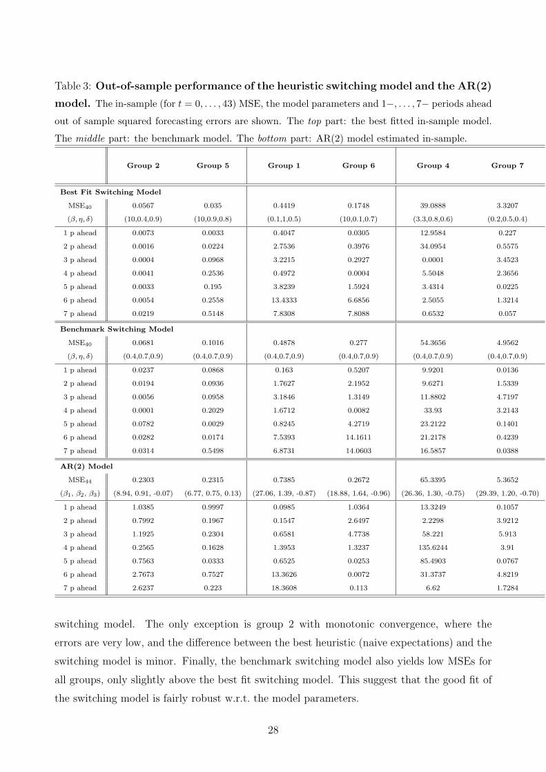
Table 3: Out-of-sample performance of the heuristic switching model and the AR(2)

model. The in-sample (for t = 0, . . . , 43) MSE, the model parameters and 1−, . . . , 7− periods ahead

out of sample squared forecasting errors are shown. The top part: the best fitted in-sample model.

The middle part: the benchmark model. The bottom part: AR(2) model estimated in-sample.

Group 2 Group 5 Group 1 Group 6 Group 4 Group 7

Best Fit Switching Model

MSE40 0.0567 0.035 0.4419 0.1748 39.0888 3.3207

(β, η, δ) (10,0.4,0.9) (10,0.9,0.8) (0.1,1,0.5) (10,0.1,0.7) (3.3,0.8,0.6) (0.2,0.5,0.4)

1 p ahead 0.0073 0.0033 0.4047 0.0305 12.9584 0.227

2 p ahead 0.0016 0.0224 2.7536 0.3976 34.0954 0.5575

3 p ahead 0.0004 0.0968 3.2215 0.2927 0.0001 3.4523

4 p ahead 0.0041 0.2536 0.4972 0.0004 5.5048 2.3656

5 p ahead 0.0033 0.195 3.8239 1.5924 3.4314 0.0225

6 p ahead 0.0054 0.2558 13.4333 6.6856 2.5055 1.3214

7 p ahead 0.0219 0.5148 7.8308 7.8088 0.6532 0.057

Benchmark Switching Model

MSE40 0.0681 0.1016 0.4878 0.277 54.3656 4.9562

(β, η, δ) (0.4,0.7,0.9) (0.4,0.7,0.9) (0.4,0.7,0.9) (0.4,0.7,0.9) (0.4,0.7,0.9) (0.4,0.7,0.9)

1 p ahead 0.0237 0.0868 0.163 0.5207 9.9201 0.0136

2 p ahead 0.0194 0.0936 1.7627 2.1952 9.6271 1.5339

3 p ahead 0.0056 0.0958 3.1846 1.3149 11.8802 4.7197

4 p ahead 0.0001 0.2029 1.6712 0.0082 33.93 3.2143

5 p ahead 0.0782 0.0029 0.8245 4.2719 23.2122 0.1401

6 p ahead 0.0282 0.0174 7.5393 14.1611 21.2178 0.4239

7 p ahead 0.0314 0.5498 6.8731 14.0603 16.5857 0.0388

AR(2) Model

MSE44 0.2303 0.2315 0.7385 0.2672 65.3395 5.3652

(β1, β2, β3) (8.94, 0.91, -0.07) (6.77, 0.75, 0.13) (27.06, 1.39, -0.87) (18.88, 1.64, -0.96) (26.36, 1.30, -0.75) (29.39, 1.20, -0.70)

1 p ahead 1.0385 0.9997 0.0985 1.0364 13.3249 0.1057

2 p ahead 0.7992 0.1967 0.1547 2.6497 2.2298 3.9212

3 p ahead 1.1925 0.2304 0.6581 4.7738 58.221 5.913

4 p ahead 0.2565 0.1628 1.3953 1.3237 135.6244 3.91

5 p ahead 0.7563 0.0333 0.6525 0.0253 85.4903 0.0767

6 p ahead 2.7673 0.7527 13.3626 0.0072 31.3737 4.8219

7 p ahead 2.6237 0.223 18.3608 0.113 6.62 1.7284

switching model. The only exception is group 2 with monotonic convergence, where the

errors are very low, and the difference between the best heuristic (naive expectations) and the

switching model is minor. Finally, the benchmark switching model also yields low MSEs for

all groups, only slightly above the best fit switching model. This suggest that the good fit of

the switching model is fairly robust w.r.t. the model parameters.

28

5.3 Out-of-sample forecasting

Let us now turn to the out of sample validation of the model. In order to evaluate the out-

of-sample forecasting performance of the model, we first perform a grid search to find the

parameters of the model minimizing the MSE for periods t = 4, . . . , 43. Then, the squared

forecasting errors of the “best” model are computed for the next 7 periods. The results are

reported in the upper part of Table 3 for each group. In the middle part of the table, we also

report the corresponding squared prediction errors for the switching model with benchmark

parameters. Finally, we compare our structural learning model with a simple non-structural

model with three parameters. To this purpose we estimate an AR(2) model to the data up

to period t = 43 and show in the bottom part of Table 3 the in- and out-of-sample squared

prediction errors.

For the converging groups 2 and 5 the squared prediction errors typically increase with

horizon but remain very low and comparable with the MSEs computed in-sample. This is

not surprising given that the qualitative property of the data (i.e., monotonic convergence)

does not change in the last periods, and that the adaptive heuristic, which generates such

convergence, takes a lead already around period 40 (cf. Fig. 8). In the oscillating groups 1

and 6 the out-of-sample errors generated by the switching model are varying with the time

horizon. The errors are especially large for the 6− and 7−periods ahead forecasts. The

ultimate reason for the relatively large prediction errors is the oscillating behavior observed

in the experiment. Even if the switching model with leading LAA heuristic captures this

phenomenon qualitatively and also produces oscillations, the error can become large when

the two types of oscillations have different frequencies and the prediction goes out of phase.

Notice that the same forecasting problem arises also for the AR(2) model in group 1. The

prediction errors for the groups 4 and 7 with damping oscillations are not very high, when

compared with the in-sample MSE. This is because, towards the end of the experiment, in

both treatments convergence was observed. At the end of the in-sample period, i.e., at t = 43,

the switching model does not yet clearly select the ADA heuristic for group 4, but does select

it for group 7. That explains why the forecasting errors in group 4 are larger than in group 7.

Comparing the forecasting errors of the switching and AR(2) models we conclude that the

former model is better than the latter, on average. More specifically, in the converging group

5 and oscillating group 6 the out-of-sample performances are very similar, but in the groups

1, 2, 4 and 7 the different variations of the switching model outperform the AR(2) model

out-of-sample. Furthermore, in group 4, for 3−, 4− and 5− periods ahead predictions, the

AR(2) model produces errors larger than 7 in absolute value, which would lead to 0 earnings

29

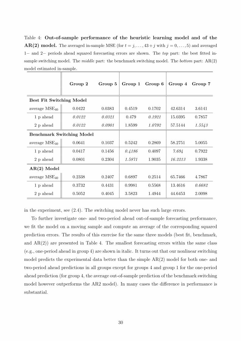
Table 4: Out-of-sample performance of the heuristic learning model and of the

AR(2) model. The averaged in-sample MSE (for t = j, . . . , 43+ j with j = 0, . . . , 5) and averaged

1− and 2− periods ahead squared forecasting errors are shown. The top part: the best fitted in-

sample switching model. The middle part: the benchmark switching model. The bottom part: AR(2)

model estimated in-sample.

Group 2 Group 5 Group 1 Group 6 Group 4 Group 7

Best Fit Switching Model

average MSE40 0.0422 0.0383 0.4519 0.1702 42.6314 3.6141

1 p ahead 0.0122 0.0321 0.479 0.1921 15.0395 0.7857

2 p ahead 0.0122 0.0901 1.8599 1.0792 57.5144 1.5543

Benchmark Switching Model

average MSE40 0.0641 0.1037 0.5242 0.2869 58.2751 5.0055

1 p ahead 0.0417 0.1456 0.4186 0.4097 7.694 0.7922

2 p ahead 0.0801 0.2304 1.5871 1.9035 16.2213 1.9338

AR(2) Model

average MSE40 0.2338 0.2407 0.6897 0.2514 65.7466 4.7867

1 p ahead 0.3732 0.4431 0.9981 0.5568 13.4616 0.6682

2 p ahead 0.5052 0.4045 3.5823 1.4944 44.6453 2.0098

in the experiment, see (2.4). The switching model never has such large errors.

To further investigate one- and two-period ahead out-of-sample forecasting performance,

we fit the model on a moving sample and compute an average of the corresponding squared

prediction errors. The results of this exercise for the same three models (best fit, benchmark,

and AR(2)) are presented in Table 4. The smallest forecasting errors within the same class

(e.g., one-period ahead in group 4) are shown in italic. It turns out that our nonlinear switching

model predicts the experimental data better than the simple AR(2) model for both one- and

two-period ahead predictions in all groups except for groups 4 and group 1 for the one-period

ahead prediction (for group 4, the average out-of-sample prediction of the benchmark switching

model however outperforms the AR2 model). In many cases the difference in performance is

substantial.

30

6 Conclusion and Discussion

The time evolution of aggregate economic variables, such as stock prices, is affected by market

expectations of individual agents. Neo-classical economic theory assumes that individuals form

expectations rationally, thus enforcing prices to track economic fundamentals and leading to

an efficient allocation of resources. Laboratory experiments with human subjects have shown

however that individuals do not behave fully rational, but instead follow simple heuristics. In

laboratory markets prices may show persistent deviations from fundamentals similar to the

large swings observed in real stock prices.

Our results show that performance based evolutionary selection among simple forecasting

heuristics can explain coordination of individual behavior leading to three different aggregate

outcomes observed in recent laboratory market forecasting experiments: slow monotonic price

convergence, oscillatory dampened price fluctuations and persistent price oscillations. In our

model forecasting strategies are selected every period from a small population of plausible

heuristics, such as adaptive expectations and trend following rules. Individuals adapt their

strategies over time, based on the relative forecasting performance of the heuristics. As a

result, the evolutionary switching mechanism exhibits path dependence and matches individual

forecasting behavior as well as aggregate market outcomes in the experiments. Our results are

in line with recent work on agent-based models of interaction and contribute to a behavioral

explanation of universal features of financial markets.

Our approach is similar to other models of reinforcement learning, e.g. Arthur (1991),

Arthur (1993), Erev and Roth (1998) and Camerer and Ho (1999). However, our model is built

in a market environment different from the strategic environments usually studied in standard

game theory. For example, agents in our framework do not have a well defined strategy, other

than predicting a number between 0 and 100 (in two decimals) and the strategies used in our

switching model are state dependent. Moreover, individuals do not know the “payoff matrix”,

which is moreover changing over time in a path-depended manner. To our best knowledge,

the model presented in this paper is the first learning model explaining different time series

patterns in the same laboratory experiments.

How robust are these results? While it is beyond the scope of the current paper to study in

detail the performance of our nonlinear switching model in other market environments, Fig. 9

illustrates how well our switching model fits some other learning to forecast asset pricing

experimental groups in Hommes, Sonnemans, Tuinstra, and Velden (2005). Price behaviour

in group 3 (top panel) starts with moderate oscillations, then stabilizes at a level below the

31

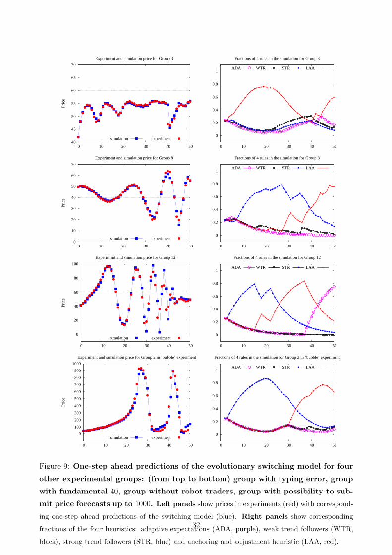
40

45

50

55

60

65

70

0 10 20 30 40 50

Pric

eExperiment and simulation price for Group 3

simulation experiment 0

0.2

0.4

0.6

0.8

1

0 10 20 30 40 50


ADA WTR STR LAA

0

10

20

30

40

50

60

70

0 10 20 30 40 50

Pric

e

Experiment and simulation price for Group 8


0.2

0.4

0.6

0.8

1

0 10 20 30 40 50


ADA WTR STR LAA

0

20

40

60

80

100

0 10 20 30 40 50

Pric

e

Experiment and simulation price for Group 12


0.2

0.4

0.6

0.8

1

0 10 20 30 40 50


ADA WTR STR LAA

0

100

200

300

400

500

600

700

800

900

1000

0 10 20 30 40 50

Pric

e

Experiment and simulation price for Group 2 in ’bubble’ experiment


0.2

0.4

0.6

0.8

1

0 10 20 30 40 50

Fractions of 4 rules in the simulation for Group 2 in ’bubble’ experiment

ADA WTR STR LAA

Figure 9: One-step ahead predictions of the evolutionary switching model for four

other experimental groups: (from top to bottom) group with typing error, group

with fundamental 40, group without robot traders, group with possibility to sub-

mit price forecasts up to 1000. Left panels show prices in experiments (red) with correspond-

ing one-step ahead predictions of the switching model (blue). Right panels show corresponding

fractions of the four heuristics: adaptive expectations (ADA, purple), weak trend followers (WTR,

black), strong trend followers (STR, blue) and anchoring and adjustment heuristic (LAA, red).

32

fundamental price 60, but suddenly falls in period t = 41, probably due to a typing error of

one of the participants12. Our nonlinear switching model of course misses the typing error,

but nevertheless matches the overall pattern before and after the unexpected price drop quite

nicely. Group 8 (second panel) is an example with a fundamental price of 40 (instead of 60),

whose strong oscillations are captured by an initially dominating STR rule, until the LAA

rule becomes dominating after period 40. Group 12 (third panel) is an example without robot

traders (i.e. its fraction nt in the price generating law of motion (2.2) is fixed to 0). Large

amplitude price oscillations, with prices almost reaching their maximum 100 and minimum 0,

arise, but prices stabilize towards the end of the experiment. The evolution of the impacts of

the four forecasting heuristics is similar to the case of dampening price oscillations considered

before (see the lower panels of Figure 8), with the strong trend rule (STR) initially dominating

the market, followed by the anchor and adjustment rule (LAA) taking over around period 25,

and the adaptive expectations (AA) rule finally dominating towards the end. Finally, group

2 in the “bubble experiments” of Hommes, Sonnemans, Tuinstra, and van de Velden (2008)

(see bottom panel) is another example without robot traders, this time with a much larger

upper-bound of 1000 (instead of 100). The asset price oscillates with very large amplitude,

with a long lasting rend of 25 periods with prices rising close to their maximum 1000, after

which a crash follows to values close to their minimum 0, and the market starts ocillating.

The evolution of the impacts of the four forecasting heuristics is similar as before, with the

STR rule taking the lead, increasing its share to more than 80% after 25 periods, then slowly

declining and finally dominated by the LAA rule with more than 60% of the share after 50

periods. The fact that our nonlinear switching model nicely captures all patterns in these

different groups shows that the model is robust concerning changes of the asset pricing market

environment.

In a related paper, Hommes and Lux (2009) explain learning to forecast experiments

in the classical cobweb (hog-cycle) market environment, using a heterogeneous expectations

model, where individual agents use a genetic algorithm. The GA-learning model captures

all stylized facts of the cobweb markets, both at the individual and at the aggregate level,

quite nicely across different experimental treatments. In the cobweb markets, aggregate price

behavior is quite different and much more irregular, characterized by random looking (i.e.

12The sudden fall of the asset price in group 3 from 55.10 in period 40 to 46.93 in period 41 is due to the

fact that one of the participants predicts 5.25 for period 42. It is likely that this corresponds to a typing error

(perhaps his/her intention was to type 55.25), since this participants five previous predictions all were between

55.00 and 55.40.

33

zero-autocorrelations) price fluctuations around the RE benchmark price. The amplitude

of these price fluctuations depends critically upon underlying parameters, especially upon

the slopes of demand and supply curves. In the case when the cobweb market is stable

under naive expectations, the laboratory experiments as well as the GA-simulations, nicely

converge to the RE benchmark price. On the other hand, when the cobweb is unstable

under naive expectations, experimental as well as GA-simulated prices are characterized by

large price fluctuations (much higher than under RE, i.e. there is excess price volatility)

with zero autocorrelations. Our performance based switching heuristics model can easily

explain the stable treatment in the cobweb experiments, with convergence to RE due to

a dominating adaptive expectations rule, but has difficulty in capturing simultaneously the

high price volatility with randomly (no autocorrelations) looking prices. Apparently, the

random looking behavior of strongly fluctuating prices is better captured by the mutation-noise

driven GA-simulations than by our simple heuristics switching model. We conjecture that our

simple heuristics switching model works well in market environments with some structure and

persistence in price fluctuations, either in the form of converging prices or in the presence of

price oscillations and (temporary) price trends and bubbles. A more systematic investigation

in which market environments other than the asset pricing framework our nonlinear heuristics

switching model can explain individual forecasting behavior as well as aggregate price behavior

is beyond the scope of this paper and left as an important topic for future research.

34

References

Alchian, A. A. (1950): “Uncertainty, Evolution, and Economic Theory,” The Journal of

Political Economy, 58(3), 211–221.

Arthur, W. (1991): “Designing Economic Agents that Act like Human Agents: A Behavioral

Approach to Bounded Rationality,” American Economic Review, 81, 353–359.

(1993): “Economic Agents that Behave like Human Agents,” Journal of Evolutionary

Economics, 3, 1–22.

Branch, W., and G. Evans (2006): “Intrinsic heterogeneity in expectation formation,”

Journal of Economic Theory, 127(1), 264–295.

Bray, M., and N. Savin (1986): “Rational Expectations Equilibria, Learning, and Model

Specification,” Econometrica, 54(5), 1129–1160.

Brock, W. A., and C. H. Hommes (1997): “A Rational Route to Randomness,” Econo-

metrica, 65(5), 1059–1095.

(1998): “Heterogeneous Beliefs and Routes to Chaos in a Simple Asset Pricing

Model,” Journal of Economic Dynamics and Control, 22, 1235–1274.

Bullard, J. B. (1994): “Learning equilibria,” Journal of Economic Theory, 64, 468–485.

Camerer, C. F., and E. Fehr (2006): “When Does ’Economic Man’ Dominate Social

Behavior?,” Science, 311(5757), 47–52.

Camerer, C. F., and T.-H. Ho (1999): “Experienced-Weighted Attraction Learning in

Normal Form Games,” Econometrica, 67(4), 827–874.

Campbell, J., A. Lo, and A. MacKinlay (1997): The Econometrics of Finanical Markets.

Princeton University Press, Princeton.

De Bondt, W. F., and R. Thaler (1989): “Does the Stock Market Overreact?,” Journal

of Finance, 40(3), 793–805.

Diks, C., and R. van der Weide (2005): “Herding, a-synchronous updating and hetero-

geneity in memory in a CBS,” Journal of Economic Dynamics and Control, 29, 741–763.

Duffy, J. (2008): “Experimental Macroeconomics,” in New Palgrave Dictionary of Eco-

nomics, ed. by S. Durlauf, and L. Blume. New York: Palgrave Macmillan, forthcoming.

35

Erev, I., and A. E. Roth (1998): “Prediction how people play games: Reinforcement

learning in games with unique strategy equilibrium,” American Economic Review, 88, 848–

881.

Evans, G. W., and S. Honkapohja (2001): Learning and Expectations in Macroeconomics.

Princeton University Press.

Fama, E. F. (1970): “Efficient Capital Markets: a Review of Theory and Empirical Work,”

Journal of Finance, 25, 383–417.

Friedman, M. (1953): Essays in Positive Economics. University Of Chicago Press.

Heemeijer, P., C. Hommes, J. Sonnemans, and J. Tuinstra (2009): “Price stability

and volatility in markets with positive and negative expectations feedback: An experimental

investigation,” Journal of Economic Dynamics and Control, 33, 1052–1072.

Hommes, C. (2006): “Heterogeneous Agent Models in Economics and Finance,” in Hand-

book of Computational Economics Vol. 2: Agent-Based Computational Economics, ed. by

K. Judd, and L. Tesfatsion. Elsevier/North-Holland (Handbooks in Economics Series).

Hommes, C., H. Huang, and D. Wang (2005): “A robust rational route to randomness in

a simple asset pricing model,” Journal of Economic Dynamics and Control, 29, 1043–1072.

Hommes, C., and T. Lux (2009): “Individual Expectations and Aggregate Behavior in

Learning to Forcast Experiments,” Discussion paper, CeNDEF Working Paper.

Hommes, C., J. Sonnemans, J. Tuinstra, and H. van de Velden (2008): “Expecta-

tions and bubbles in asset pricing experiments,” Journal of Economic Behavior and Orga-

nization, 67(1), 116–133.

Hommes, C., J. Sonnemans, J. Tuinstra, and H. v. d. Velden (2005): “Coordination

of Expectations in Asset Pricing Experiments,” Review of Financial Studies, 18(3), 955–980.

Kahneman, D. (2003): “Maps of Bounded Rationality: Psychology for Behavioral Eco-

nomics,” American Economic Review, 93, 1449–1475.

Lucas, R. E., and E. C. Prescott (1971): “Investment Under Uncertainty,” Economet-

rica, 39(5), 659–681.

Marimon, R., S. E. Spear, and S. Sunder (1993): “Expectationally Driven Market

Volatility: An Experimental Study,” Journal of Economic Theory, 61(1), 74–103.

36

Muth, J. F. (1961): “Rational Expectations and the Theory of Price Movements,” Econo-

metrica, 29(3), 315–335.

Peterson, S. P. (1993): “Forecasting dynamics and convergence to market fundamentals:

Evidence from experimental asset markets,” Journal of Economic Behavior and Organiza-

tion, 22(3), 269–284.

Sargent, T. J. (1993): Bounded Rationality in Macroeconomics. Oxford University Press.

Shiller, R. (1981): “Do Stock Prices Move Too Much to be Justified by Subsequent Changes

in Dividends?,” American Economic Review, 71(3), 421–436.

Simon, H. A. (1957): Models of Man: Social and Rational. John Wiley, New York.

Smith, V. L. (1962): “An Experimental Study of Competitive Market Behavior,” The Jour-

nal of Political Economy, 70(2), 111–137.

Smith, V. L., G. L. Suchanek, and A. W. Williams (1988): “Bubbles, Crashes, and

Endogenous Expectations in Experimental Spot Asset Markets,” Econometrica, 56(5), 1119–

1151.

Tversky, A., and D. Kahneman (1974): “Judgement under uncertainty: Heuristics and

biases,” Science, 185, 1124–1130.

37

APPENDIX

A Proof of Proposition 3.1

From the general relation (3.2) it follows that

pet+1 − pf = w (pt−1 − pf ) + (1− w) (pe

t − pf ) = (pet − pf )

(w

1− nt−1

1 + r+ 1− w

).

The expression in the last parenthesis is a convex combination of 1 and (1− nt−1)/(1 + r) < 1. For

positive weight w such combination is always less than 1. Therefore, the dynamical system defines

a contraction of expectations, which then must globally converge to pf . The price realization in this

point is uniquely defined from (2.6) as p∗ = pf . Finally, the evolution of robot traders implies that

n∗ = 0 in this fixed-point.

B Proof of Proposition 3.2

Consider the steady-state (p∗, n∗) with consistent forecasting rule, and notice that (3.2) implies that

either p∗ = pf or 1− n∗ = 1 + r. The second case is impossible, so p∗ = pf and, therefore, n∗ = 0.

Using (3.2), the dynamics in deviations is given by

pt − pf = exp(− |pt−1 − pf |/200

) (β1

1 + r(pt−1 − pf ) +

β2

1 + r(pt−2 − pf )

). (B.1)

The first term in the right hand-side is never greater than 1. Thus, dynamics of (B.1) is a superpo-

sition of contraction with linear process of second order

(1 + r)xt = β1 xt−1 + β2 xt−2 (B.2)

with xt = pt − pf . If the latter dynamics is locally stable, the steady-state pf of original dynamics

(B.1) will be also locally stable. Furthermore, since the exponential term in (B.1) is equal to 1 in the

steady-state, the linear parts of the dynamics of the last two processes are the same. Thus, processes

(B.1) and (B.2) lose stability simultaneously and through the same bifurcation type.

The Jacobian matrix of (B.2) in the steady-state is given by

J =

∥∥∥∥∥∥

β1

1+rβ2

1+r

1 0

∥∥∥∥∥∥.

The standard conditions for the stability can be expressed through the trace Tr(J) and the determi-

nant Det(J) of this matrix, and are given by

Tr(J) < Det(J) + 1 , Tr(J) > −1−Det(J) , Det(J) < 1 . (B.3)

38

Furthermore, the dynamics is oscillatory if Tr(J)2 − 4Det(J) = 0. The substitution of the values of

trace and determinant gives inequalities (3.4) and condition β21 +4β2(1+ rf ) < 0 for the oscillations.

The bifurcation types can be determined from (B.3), since when one of these inequalities turns to

equality, the unit circle is crossed by a corresponding eigenvalue of the system. the second inequality

is violated when an eigenvalue becomes equal to −1, which implies the period-doubling bifurcation.

The violation of the last inequality in (B.3) implies that two complex eigenvalues cross the unit

circle. This happens under the Neimark-Sacker bifurcation. Finally, consider the first inequality,

which is violated when one eigenvalue becomes equal to 1. It turns out that at this occasion two new

steady-states are emerging, which implies that the system exhibits pitchfork bifurcation. Indeed, any

steady-state (p∗, n∗) should satisfy to

(1 + r)p∗ = (1− n∗)((1− β1 − β2)pf + (β1 + β2)p∗

)+ n∗pf + y

m(1 + r)p∗ = pf + (β1 + β2)(p∗ − pf )(1− n∗) + y

m(1 + r)(p∗ − pf ) = (β1 + β2)(p∗ − pf )(1− n∗)

Thus, in any non-fundamental steady-state, the fractions of robots n∗ = 1− (1 + r)/(β1 + β2). Only

if this fraction belongs to the interval (0, 1) two other steady-states exist with

p∗± = pf ± 200 log(1− n∗) .

(The prediction rule is, of course, inconsistent in both steady-states.) When the first inequality in

(B.3) is satisfied, these two steady-state do not exist, but they appear at the moment when the

inequality changes it sign.

39

Evolutionary Selection of Individual Expectations and Aggregate Outcomes

Documents

Transcript of Evolutionary Selection of Individual Expectations and Aggregate Outcomes