Evolutionary decision rules for predicting protein contact maps

Noname manuscript No.(will be inserted by the editor)

Evolutionary Decision Rules for Predicting Protein ContactMaps

Alfonso E. Marquez-Chamorro · Gualberto Asencio-Cortes · Federico

Divina · Jesus S. Aguilar-Ruiz

Received: date / Accepted: date

Abstract Protein structure prediction is currently oneof the main open challenges in Bioinformatics. An use-ful, and commonly used, representation for protein 3D

structure is the protein contact map, which representsbinary proximities (contact or non-contact) betweeneach pair of amino acids of a protein. In this work,

we propose a multi-objective evolutionary approach forcontact map prediction based on physico-chemical prop-erties of amino acids. The evolutionary algorithm pro-

duces a set of decision rules that identifies contacts be-tween amino acids. The rules obtained by the algorithmimpose a set of conditions based on amino acid prop-

erties in order to predict contacts. We present resultsobtained by our approach on four different protein datasets. A statistical study was also performed in order to

extract valid conclusions from the set of prediction rulesgenerated by our algorithm. Results obtained confirmthe validity of our proposal.

Keywords Protein Structure Prediction, ContactMap, Multi-objective Evolutionary Computation,

Residue-residue Contact.

1 Introduction

The Protein Structure Prediction (PSP) problem con-sists in determining the three-dimensional model of a

Alfonso E. Marquez-Chamorro (B) · Gualberto Asencio-Cortes · Federico Divina · Jesus S. Aguilar-RuizSchool of EngineeringPablo de Olavide UniversitySeville, SpainTel.: +34-954-978094E-mail: [email protected]

protein, using only information contained in its aminoacid sequence. The PSP problem is one of the most im-portant open problems in computational biology [68].

This is because the 3D structures determine the pro-tein function. It follows that knowing the 3D structureof a protein would be of enormous help for designing

new drugs for diseases such as cancer or Alzheimer. Al-though there exist experimental methods for determin-ing protein structures, e.g., X-ray crystallography and

nuclear magnetic resonance, such techniques are veryexpensive and present limitations with the structures ofcertain proteins [26,38,53]. In addition to this, the great

number of protein sequences whose three-dimensionalstructures must be determined, make computationalmethods for protein structure prediction an essential

tool. However, the accuracy achieved by the most re-cent and relevant proposals in the literature is up to35% approximately [44], and clearly must be improved.

The first thing one has to decide when using a com-putational method, is how to represent the data. In the

PSP literature, there are three main data structures torepresent a protein 3D structure: torsion angles, dis-tance maps and contact maps. Torsion angles represent

the values of the flexible angles of a protein molecule.Torsion angles are based on the assumption of constantbond lengths and some constant bond angles between

atoms. This representation is based on three torsion an-gles in the protein backbone plus the angles in proteinsidechains. This is a simplification of the real situation

where the supposed constant bond lengths and anglesdepend on the environment of atoms. Examples of re-cent proposals that predict protein torsion angles are

Faraggi et al. [16] and Furuta et al. [20].

On the other hand, distance maps represent the dis-

tances between reference atoms of each pair of protein

2 Alfonso E. Marquez-Chamorro et al.

residues. Examples of methods that predict protein dis-

tance maps are [4,36].

Contact maps are the most commonly used struc-

ture in the PSP literature. In a nutshell, a contact maprepresents binary proximities between each pair of pro-tein residues, which are predicted by residue-residue

contact predictors. The prediction of contact maps is avery important problem. For instance, there is a com-petition dedicated to contact map predictors in CASP

[44], but there is no competitions in CASP for distancemap or torsion angles predictors. More details aboutcontact maps will be given in section 2.

In addition to this, some proposals discretize the dis-tances between atoms, providing an intermediate rep-

resentation between contact and distance maps. For in-stance, Walsh et al. [60] which uses 4-class distancemaps.

As already mentioned, in PSP, the prediction of the

3D structure of a protein must be based on characteris-tics of the amino acids forming its sequence. Some com-monly used features are the physico-chemical properties

of residues. Usually the properties that are used are hy-drophobicity, polarity, charge and residue size, as wellas the properties of the AAindex repository [32], which

contains currently 544 amino acid properties. On theother hand, predictors often use secondary structures(commonly from DSSP [31] or PSIPRED [28]), solvent

accessibility [41], evolutionary information (commonlythe Position Specific Scoring Matrix (PSSM) from PSI-BLAST [2]) and contact orders (usually CO [48], RCO[33], CN [34] or the most recent RWCO [54]). Some

authors also used topological measures of the proteinmolecule like the recursive convex hull [55].

Several types of approaches have been proposed inthe literature with the aim of computationally solving

the PSP problem and they will be detailed in section 2.Within such proposals, evolutionary algorithms (EAs)have proven to achieve excellent results, see, for in-

stance [8]. EAs have become popular as robust andeffective methods for solving optimization problems.In particular, EAs have shown the capacity of finding

suboptimal solutions in search spaces when the searchspace is characterized by high dimensionality. This isthe case of the protein folding problem, where the set of

possible folding rules of a protein determine the searchspace.

In this paper, we propose a method based on anEA in order to predict contact maps. In particular, theEA adopted is a multi-objective EA (MOEA), which

bases its prediction on three physico-chemical proper-ties (hydrophobicity, polarity and charge), on solventaccessibility and on secondary structure. We used an

evolutionary approach based on the Strength Pareto

Evolutionary Algorithm (SPEA) [69]. Our algorithm

generates a set of decision rules that predicts contactsbetween amino acids. In particular, each rule imposesa set of conditions on some specific amino acids prop-

erties that, if satisfied, predict a contact.The rest of the paper is organized as follows: in sec-

tion 2 we provide a general description of the main con-

cepts regarding contact maps and their prediction, andwe review the state of the art of contact map prediction.In section 3, we define the elements, procedures and

evaluation measures used by our prediction method. Insection 4, we detail the predictions performed and theprotein datasets that we used, we discuss the achieved

results and we analyze the predicted rules. Finally, insection 5, we describe the main conclusions of the workand we outline approaches for future studies.

2 Contact map prediction

The contact map of a protein sequence is a square ma-trix of order L, where L is the number of amino acidsin the sequence. The contact map is divided into two

parts: the observed part (upper triangular) and the pre-dicted part (lower triangular). An element (i, j) of thecontact map is 1 if amino acids i and j are in contact,

or 0 otherwise. In this context, we consider two aminoacids to be in contact if the distance between them isless than or equal to a given threshold. To this aim,

a commonly used threshold is 8 angstroms (A) [44],threshold that is also adopted in this paper. In order tomeasure the distance between two amino acids, it is nec-

essary to use a reference atom of each amino acid, beingthe alpha carbon and the beta carbon of amino acidsthe most commonly used [14]. In our method, we use

the beta carbon (with the exception of glycine, whichhas no beta carbon, and for which its alpha carbon isused).

Usually contacts between amino acids are dividedand predicted by groups according to their sequenceseparation. Sequence separation between amino acids

ai and aj , where i and j represent the positions of theresidues in the sequence, is |i − j|. Based on the sepa-rations, contacts are classified into three classes: short,

medium and long range. In short range, a minimumseparation of six residues is used in order to consider acontact, whereas in medium and long range, the mini-

mum separations are 12 and 24, respectively.Contact maps present several advantages with re-

spect to other representations. For instance, unlike 3D

models of proteins, contact maps, as well as distancemaps, have the desirable property of being insensitiveto rotation or translation of the protein molecule. On

the other hand, given a contact map of a protein, it is

Evolutionary Decision Rules for Predicting Protein Contact Maps 3

possible to reconstruct a 3D model of the protein back-

bone, solving the Molecular Distance Geometry Prob-lem (MDGP) [39]. This can be done in different ways,e.g., using quadratic potential GO model [3] or using

tools like FT-COMAR [58,59]. It is also possible to ob-tain the coordinates of all protein atoms from the pro-tein backbone using tools like SCWRL, IRECS, SCAP,

SCATD or SCCOMP [18], or using the recent tool SIDE-pro [47]. Contact maps, as protein structure represen-tation, are also useful to compare protein structures,

using the maximum contact map overlap [12].

Many different approaches for contact map predic-

tion have been proposed in the literature, being thethree mostly used approaches based on artificial neuralnetworks (ANNs) [41,56,65], evolutionary algorithms

(EAs) [8,9,30] and support vector machines (SVMs)[42,63].

Regarding the ANNs approaches, Xue et al. pro-posed SPINE-2D [65] that consists of two neural net-works using one and two layers, respectively. These net-

works use 34 features as input, including PSSM fromPSIBLAST [2], seven physico-chemical properties of a-mino acids, including hydrophobicity, volume and po-

larizability, and secondary structure from the DSSPsecondary-structure assignment program [31]. Tegge etal. [56] proposed NNcon which uses 2D-Recursive Neu-

ral Network (2D-RNN) models to predict both generalresidue-residue contacts and specific beta contacts (i.e.,pairs of residues in beta sheets). They combine general

and specific contact maps to produce predictions. Lippiet al. [41] proposed a novel hybrid architecture basedon neural and Markov logic networks with grounding-

specific weights, in order to predict contacts between β-strand residues. Multiple alignment profiles, secondarystructure and solvent accessibility in two states were

used as input.

As far as EAs are concerned, Chen and Li [9] pro-

posed an ensemble of genetic algorithm (GA) classi-fiers to predict long-range contacts. The individualsof the GA include three amino acid windows and 20

properties obtained from HSSP database [13] for eachresidue in such windows. The method uses the sequenceprofile centers, that is the average sequence profiles of

residue pairs belonging to the same contact class ornon-contact class. Judy et al. [30] propose a MOEA,representing protein structures by torsion angles. They

modified the classical algorithm Pareto Archived Evo-lutionary Strategy (PAES) [11,51], introducing two im-mune inspired operators: vaccination and immune selec-

tion. Their algorithm, named MI-PAES uses adaptiveprobabilities of crossover, mutation and immune opera-tion, and a geometric annealing schedule in the immune

operator. Calvo et al. [8] also proposed a MOEA, called

Pitagoras-PSP. This algorithm uses an evolutionary ab

initio approach based on PAES. The algorithm predictsprotein backbone and side-chain torsion angles and ituses an energy function as fitness function. Mutation

operators maintain values of torsion angles in feasibleranges according to secondary structure of residues androtamer libraries.

With respect to SVM approaches, Wu, Szilagyi andZhang [63] developed a composite set of nine SVM-based contact predictors that are used in I-TASSER [52]

simulation in combination with sparse template con-tact restraints. They used the original energy functionof I-TASSER and contact predictions generated by ex-

tended versions of SVMSEQ [64]. Lo et al. [42] proposeda hierarchical scheme for contact prediction, with anapplication in membrane proteins. This approach con-sists of two levels: in the first level, contact residues are

predicted from sequences; while in the second one, theirpairing relationships are further predicted. The statisti-cal analyses on contact propensities are combined with

evolutionary profile, relative solvent accessibility andhelical features.

Apart from these three main approaches, there are

other important approaches that try to address theresidue-residue contact prediction problem. Li et al.[40] developed ProC S3, based on a set of Random

Forest algorithm based models using 1287 sequence-based features. Marks et al. [43] use a global modelof maximum entropy constrained by correlated muta-

tions from multiple sequence alignments. Finally theyreconstruct protein 3D models using distance geometryand simulated annealing. On the other hand, ensemble

approaches, which combine several predictors, are alsorecently applied for contact map prediction [15,21,66],as well as nearest neighbor-based algorithms [1], Hidden

Markov Models [7], integer linear optimization [49,50,62], sparse inverse covariance [29] and template-basedapproaches [5,61].

3 Methods

Before describing our algorithm, this section presents abrief introduction to multi-objective optimization prob-

lems and related concepts.A Multi-objective optimization problem require the

optimization of a set of objectives, usually in conflict

with each other. The existence of multiple objectivesposes a fundamental difference with the single objectiveproblems: typically there will not be a single solution,

but a set of solutions that can present different clashesbetween the values of the objectives to optimize. Wecan define a multi-objective optimization problem in

this way: let (f1(x), f2(x)...fn(x)) be a set of functions


to be optimized, where x = (x1, ..., xp) is a vector of

decision variables belonging to a universe X and fi(x)is an arbitrary linear or non-linear function, 1 ≤ i ≤ n.Therefore, the problem consists of finding the x that

provides the best compromise value for all fi(x).

Table 1: Values of different properties according to thecited scales for each amino acid. H represents the hy-

drophobicity, P the polarity and C the charge.

Prop. A C D E F G H I K LH 0.40 0.56 -0.78 -0.78 0.62 -0.09 -0.71 1.00 -0.87 0.84P -0.21 -0.85 1.00 0.83 -0.93 0.01 0.36 -0.93 0.58 -1.00C 0 0 -1 -1 0 0 0 0 1 0

Prop. M N P Q R S T V W YH 0.42 -0.78 -0.36 -0.78 -1.00 -0.18 -0.16 0.93 -0.20 -0.30P -0.80 0.65 -0.23 0.38 0.38 0.06 -0.09 -0.75 -0.88 -0.68C 0 0 0 0 1 0 0 0 0 0

To solve the above problem, we should defined somecriteria to determine which solutions are considered of

good quality and which are not. To this aim, the con-cept of dominance is generally used. A solution x issaid to be not dominated iff there is not another so-

lution y such that: fi(y) <= fi(x) for all i = 1..n andfi(y) < fi(x) for some i. From this, it follows that thebest solutions are those that are not dominated. This

set is called Pareto front.

We have applied these concepts to the PSP prob-

lem. In this article, we consider two objectives to beoptimized separately, which are defined in section 3.2.In order to do so, we have implemented a MOEA, called

MECoMaP (Multi-objective Evolutionary Contact MapPredictor), based on a SPEA. This algorithm uses anexternal population with non-dominated solutions, which

is obtained at the end of every generation. The algo-rithm is based on the strength concept. The strengthof an individual x is given by the number of individ-

uals that x dominates. The fitness of an individual isproportional to its strength, as will be detailed in thefollowing of this section.

Each individual of the population represents a deci-

sion rule. In particular, rules are based on some specificamino acid properties. Basically they specify a set ofconditions on each property, that, if satisfied, predict

a contact between two amino acids. It is known thatamino acid properties play an important role in the PSPproblem [23]. Several PSP methods were proposed that

relied on amino acids properties, e.g., hydrophobicityand polarity were employed in HP models [57]. In ourapproach, the decision rules evolved by our algorithm,

base the prediction on three physico-chemical proper-

ties: hydrophobicity, polarity and charge of the residues.

It has been shown that such properties have certain rel-evance in PSP. In addition to these properties, we alsomake use of two structural features of proteins: sec-

ondary structure prediction (SS) and solvent accessi-bility (SA). We selected the Kyte-Doolittle hydropathyprofile [37] for hydrophobicity, the Grantham’s profile

[22] for polarity and Klein’s scale for net charge [35]. Intable 1, we can appreciate the property values for eachamino acid according to the cited scales, normalized

between −1 and 1 for hydrophobicity and polarity.Secondary structure prediction consists of predict-

ing the location of alpha-helices, beta-sheets and turns

from a sequence of amino acids. The location of thesemotifs could be used by approximation algorithms toobtain the tertiary structure of the protein. A 3-state

representation of SS (helix, sheet or coil) is employed inour approach. The prediction is performed using PSI-PRED [27].

SA refers to the degree to which a residue inter-

acts with the solvent molecules. The SA of amino acidresidues provide us with useful information for the pre-diction of the structure and function of a protein. Rela-

tive solvent accessibility (RSA) is required for the pre-diction. To calculate the RSA of a residue, we use theDSSP program to obtain the actual SA of each residue

as described in [6]. In order to predict the RSA, SA isdivided by the maximum accessible surface in the ex-tended conformation of its AA type. We finally obtain

a 5-state representation (ranging from 0 to 4) for RSA,where lower values mean a buried state and higher val-ues represent exposed states.

In the following we address the various solutionsadopted for what regards the representation, the ge-netic operators and the fitness function used by the

EA.

3.1 Encoding

We represent a protein sequence by s1 . . . sL, where L is

the sequence length and si (1 ≤ i ≤ L) is an amino acid.Each individual in our algorithm represents a decisionrule which determines whether amino acids si and sjare in contact, with 1 ≤ i < j ≤ L. For this purpose,we include in each individual properties of two windowsof ±3 residues centered around the two target amino

acids si and sj . Therefore, one window is relative toamino acids si−3, si−2, si−1, si, si+1, si+2, si+3 and theother one is relative to amino acids sj−3, sj−2, sj−1,

sj , sj+1, sj+2, sj+3. For each amino acid k belonging tothe two windows, we define the descriptor Qk (wherek ∈ {i − 3, i − 2, i − 1, i, i + 1, i + 2, i + 3, j − 3, j −2, j − 1, j, j + 1, j + 2, j + 3}) which represents a set of


conditions for the amino acid k, as shown in Equation

1.

Qk = {Hmin,Hmax, Pmin, Pmax, C, SS, SA} (1)

where

−1 ≤ Hmin < Hmax ≤ 1

−1 ≤ Pmin < Pmax ≤ 1

C ∈ {−1, 0, 1}SS ∈ {−1, 0, 1, 2}SA ∈ {−1, 0, 1, 2, 3, 4}

We define the decision rule Ri,j for amino acids iand j, encoded in each individual of our algorithm, as

shown in Equation 2, for each k ∈ {i−3, i−2, i−1, i, i+1, i+ 2, i+ 3, j − 3, j − 2, j − 1, j, j + 1, j + 2, j + 3}.

Ri,j = {Qk} (2)

Given a test sequence t1 . . . tL′ , where L′ is the test

sequence length, and a pair of amino acids ta and tb(1 ≤ a < b ≤ L′), the algorithm predict a contactbetween these amino acids if there exist any rule Ri,j

(1 ≤ i < j ≤ L) that covers the pair (ta, tb).

A rule Ri,j covers the pair (ta, tb) if that pair satis-

fies Qk for all k ∈ {a− 3, a− 2, a− 1, a, a+1, a+2, a+3, b − 3, b − 2, b − 1, b, b + 1, b + 2, b + 3}. The pair (ta,tb) satisfies Qk if it fulfills the following equations for

all k ∈ {a− 3, a− 2, a− 1, a, a+1, a+2, a+3, b− 3, b−2, b− 1, b, b+ 1, b+ 2, b+ 3}.

Hmin ≤ H(tk) ≤ Hmax (3)

Pmin ≤ P (tk) ≤ Pmax (4)

C(tk) = C (5)

SS(tk) = SS (6)

SA(tk) = SA (7)

where H(tk) is the hydrophobicity of the amino acid

tk, P (tk) its polarity, C(tk) its charge, SS(tk) its sec-ondary structure and SA(tk) its solvent accessibility.

3.2 Genetic Operators and Fitness Function

The algorithm starts with a randomly initialized popu-

lation and is run for a maximum number of generations.If the fitness of the best individual does not increaseover twenty generations, the algorithm is stopped and

a solution is provided. In order to obtain the next gen-eration, individuals are selected with a tournament se-lection mechanism of size two. Crossover and mutation

are then applied in order to generate offsprings.

Various crossover operators have been tested. In par-

ticular, we have tested the performances of one-point,two-points, uniform and BLX-α crossovers. These cross-over operators act at the level of the amino acid proper-

ties. For instance, one-point crossover randomly selectsa point inside two parents and then builds the offspringusing one part of each parent. It follows that the re-

sulting rule has to be tested for validity, since it couldcontain incorrect ranges. BLX-α crossover creates a newoffspring Ri,j , where the values of the elements of Qk

(for each k ∈ {i−3, i−2, i−1, i, i+1, i+2, i+3, j−3, j−2, j− 1, j, j+1, j+2, j+3}) are mutated within an in-terval delimited by the maximum and minimum values

of the two parent individuals for the same element ofQk. An α value is also selected to calculate this interval.In our case, we set the α value for the crossover to 0.1.

This parameter must be higher or equal than 0. Thiscrossover operator can be seen as a linear combinationof the two parents. After having performed several runs

of the algorithm, the best results were obtained whenthe two-points crossover was used, which was then usedas standard crossover in the algorithm.

We have applied two different mutation operators.The first operator, called Gaussian operator, mutates

an element of Qk of an individual Ri,j , where k ∈{i−3, i−2, i−1, i, i+1, i+2, i+3, j−3, j−2, j−1, j, j+1, j + 2, j + 3}, following a Gaussian distribution. The

value of this element is increased or decreased with aprobability of 0.5. If the values of a mutated individualare not within the allowed ranges for each properties,

the mutation is discarded. A second mutation operator,called Enlarge operator, randomly selects an element ofQk of an individual, that is related to a given property,

and varies its range, to all the allowed values. For in-stance, if the property is the hydrophobicity, this opera-tor varies the range to [-1, 1]. This means that the rule

does not take into account this property in this case.This type of mutation is applied with a 0.1 probabil-ity. The parameter setting of the algorithm are shown

in table 2. This setting was determined after severalpreliminary runs.

The aim of the algorithm is to find both generaland precise rules for identifying residue-residue con-

tacts. The fitness of an individual is equal to the num-ber of individuals that it dominates. We consider twoobjectives to be optimized, rule coverage and rule ac-

curacy. Thus, an individual dominates another accord-ing to its values of rule coverage and rule accuracy.Rule coverage represents the proportion of contacts cov-

ered by each rule and rule accuracy evaluates the cor-rectly predicted contacts rate by each rule. Therefore,Rule coverage = C/Ct and Rule accuracy = C/Cp,

where C is the number of correctly predicted contacts


Table 2: Parameter setting used in the experiments.

Population size 100Crossover probability 0.5

Gaussian mutation probability 0.5Enlarge mutation probability 0.1Max number of generations 100

Tournament size 2

of a protein, Ct is the total number of contacts of theprotein and Cp is the number of predicted contacts. We

aim at finding the best compromise between these twomeasures. The set of non-dominated individuals are in-cluded in a external archive and they will be selected

for the next generation.

An execution of the algorithm provides as a resulta set of rules. If the algorithm is run several times,

the final prediction model will consist of all the rulesobtained at each execution. In other words, each timethe algorithm is run, a number of rules are added to

the final solution.

This is done in an incremental way: first, the bestindividual, according to its F-measure, is selected and

added to the solution S. Then the next best individualis added to S, and the F-measure of S is calculated.This process is repeated until the addition of a rule

causes the F-measure of S to decrease. The F-measureis defined as in equation 8:

Fmeasure = 2 · Rule coverage ·Rule accuracy

Rule coverage+Rule accuracy(8)

Repeated or redundant rules are not included in thefinal solution. Each pair of rules (Ra,b, R

′c,d) is checked.

If we find that Ra,b is contained in R′c,d, then Ra,b is

removed from our final rule set. In this context, a ruleRa,b is contained in another rule R′

c,d if the values of the

elements of Qk (for each k ∈ [a−3, a+3]∪ [b−3, b+3])and the values of the elements of Q′

k′ (for each k′ ∈[c−3, c+3]∪ [d−3, d+3]) satisfy the conditions shown

in Equation 9.

Hmin ≥ H ′min ∧Hmax ≤ H ′

max (9)

Pmin ≥ P ′min ∧ Pmax ≤ P ′

max

C = C ′

SS = SS′

SA = SA′

The pseudocode of MECoMaP is shown in Algo-

rithm 1. The evolutionary process is repeated numIttimes where numIt is the number of iterations. Thealgorithm starts by randomly initialize the population.

Then, it evaluates the current population P and the

Pareto front is determined. Non-dominated solutions,

which constitute the external population A, will be in-cluded in the population P ′ of the next generation. Asalready mentioned, four genetic operators are used: a

binary tournament selection operator, a 2-point crossoveroperator and two mutation operators. The first 50% ofthe individuals in P ′ is formed by the non-dominated

individuals (external population A) and by the selectedindividuals with the binary tournament selection oper-ator. The last 50% of the individuals in P ′ is created us-

ing the 2-point crossover operator. Mutation is appliedto the whole population, except to the Pareto front in-dividuals, at the end of the evolutionary process. This

process is repeated a maximum number of generationsmaxGen. At the end of each iteration a set of best in-dividuals is stored in Results set. Hence, the Results

set is formed in an incrementally way, as we have saidbefore, and constitutes the output of our algorithm.

Algorithm 1 MECoMaP Algorithm for Con-tact Map PredictionINPUT set of protein subsequences M , maximum num-

ber of iterations numIt, maximum number of generationsmaxGen, size of the population S.

OUTPUT set of generated rules Results.

beginnum← 0, Results← ∅while (num < numIt) do

Initialize Pi← 0, A← ∅while (i < maxGen) do

Evaluate population PFind Non-dominated solutions PUpdate Non-dominated solutions set AP ′ ← AP ′ ← Selection Method with binary tournament(P )P ′ ← 2-point Crossover Method with binarytournament(P )P ′ ← Mutation Method(P )P ← P ′

i← i+ 1end whileResults← the best combination of rules from Pnum← num+ 1

end whileend

4 Experimentation

In this section we will present the results obtained by

MECoMaP on four different datasets. MECoMaP wasimplemented in Java using a multithreading architec-ture. Furthermore, due to the enormous volume of data,

all the experiments were run on a 64-bit workstation,


with 32 GB DDR SDRAM and four dual-core proces-

sors.

The first protein data set (DS1) consists of 173 non-redundant proteins with sequence identity less than 25%,

and was obtained from [17]. As in [17], four subsetshave been obtained according to the sequence length(Ls): Ls < 100, 100 <= Ls < 170, 170 <= Ls < 300,

Ls >= 300. The minimum and maximum lengths ofproteins are 31 and 753 amino acids, respectively. DS1contains 240, 501 positive examples and 5, 034, 050 neg-

ative examples (non-contacts).

The second data set (DS2), with 53 non-redundant

and non-homologous globulin proteins, is detailed in[10]. In this case, proteins are classified according totheir SCOP class [46] as described in [10]. Alpha pro-

teins contain only alpha helical secondary structure.Beta proteins contain only beta-sheet secondary struc-ture. Alpha/beta proteins contain alternating α-helical

and β-sheet secondary structure elements. This struc-ture is known as a TIM barrel. In alpha/beta pro-teins, the alpha helical and beta sheet regions occur

in independent regions of the molecule. Small proteinsare referred to the size of the protein and are usuallydominated by metal ligand or disulfide bridges. Finally,

Coiled-coil proteins refers to a structural motif in whichalpha helices are coiled together. The sequence identityof DS2 dataset is also lower than 25%. DS2 is formed

by a total of 30, 546 contacts and 356, 528 non-contacts.

The third data set is presented in [67]. This dataset (DS3) includes 48 non-homologous proteins. DS3 is

divided into five subsets according to Ls: Ls < 100,100 <= Ls < 200, 200 <= Ls < 300, 300 <= Ls <400, Ls >= 400. DS3 contains 10, 498 positive examples

and 367, 299 negative examples.

The forth data set (DS4), is detailed in [29]. A total

of 150 non-homologous proteins are contained in thisdata set. The sequence length of the proteins variesbetween 50 and 275 amino acids. DS4 is formed by

225, 352 positive examples and 3, 194, 288 negative ex-amples.

All the experimentations were performed under the

same conditions that appeared in the cited articles. Athreshold of 8 angstroms (A) was established to deter-mine a contact as in [17]. In order to avoid the effect

of learning local contacts, we set the same minimumsequence separation between each pair of amino acidsto establish a contact as in the reference works.

Before presenting the results obtained by our algo-rithm on the datasets, we present results of two prelim-

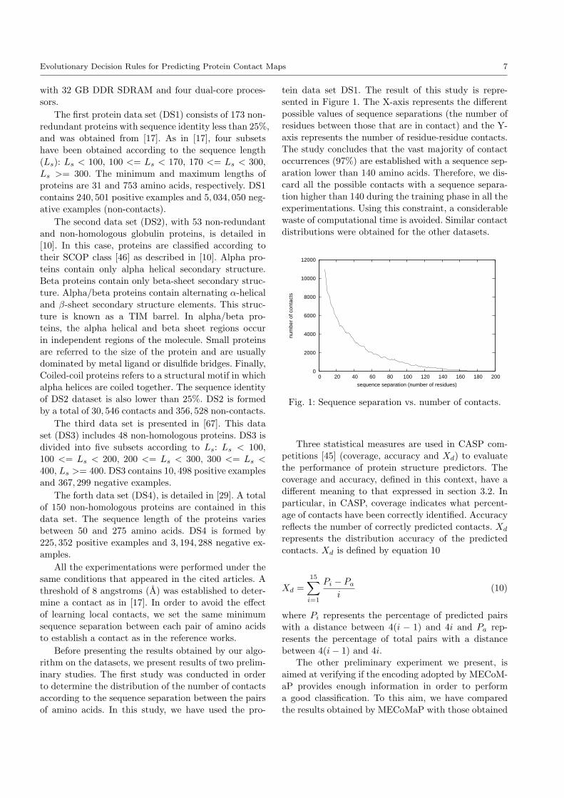
inary studies. The first study was conducted in orderto determine the distribution of the number of contactsaccording to the sequence separation between the pairs

of amino acids. In this study, we have used the pro-

tein data set DS1. The result of this study is repre-

sented in Figure 1. The X-axis represents the differentpossible values of sequence separations (the number ofresidues between those that are in contact) and the Y-

axis represents the number of residue-residue contacts.The study concludes that the vast majority of contactoccurrences (97%) are established with a sequence sep-

aration lower than 140 amino acids. Therefore, we dis-card all the possible contacts with a sequence separa-tion higher than 140 during the training phase in all the

experimentations. Using this constraint, a considerablewaste of computational time is avoided. Similar contactdistributions were obtained for the other datasets.

0

2000

4000

6000

8000

10000

12000

0 20 40 60 80 100 120 140 160 180 200

num

ber

of c

onta

cts

sequence separation (number of residues)

Fig. 1: Sequence separation vs. number of contacts.

Three statistical measures are used in CASP com-

petitions [45] (coverage, accuracy and Xd) to evaluatethe performance of protein structure predictors. Thecoverage and accuracy, defined in this context, have a

different meaning to that expressed in section 3.2. Inparticular, in CASP, coverage indicates what percent-age of contacts have been correctly identified. Accuracy

reflects the number of correctly predicted contacts. Xd

represents the distribution accuracy of the predictedcontacts. Xd is defined by equation 10

Xd =15∑i=1

Pi − Pa

i(10)

where Pi represents the percentage of predicted pairswith a distance between 4(i − 1) and 4i and Pa rep-

resents the percentage of total pairs with a distancebetween 4(i− 1) and 4i.

The other preliminary experiment we present, is

aimed at verifying if the encoding adopted by MECoM-aP provides enough information in order to performa good classification. To this aim, we have compared

the results obtained by MECoMaP with those obtained


by five well known classifiers: Naive Bayes (NB), C4.5

classifier tree, Nearest Neighbor approach with k = 1(IB1), Neural Network (NN) and Support Vector Ma-chine (SVM). For this experimentation we have used

DS1 (Ls < 100), DS2, DS3 and DS4. We have setthe same experimental conditions in all the cases: a se-quence separation of 6 amino acids and a 3-fold cross-

validation was performed, as cited in [17]. From all theextracted data, we have built four files in ARFF for-mat, with all the training data information. The posi-

tive class (contact) is represented with 1 and the neg-ative class (no contact) is represented with 0. The to-tal data sets consists of 123, 949 instances with 6, 922

positive and 117, 027 negative cases (contacts and nocontacts respectively) for DS1, 171, 916 instances with5, 530 positive cases and 166, 386 negative cases for DS2

and 55, 988 instances, 18, 486 contacts and 1, 119, 751no contacts for DS3 and 44, 444 positive cases and 1, 51-2, 823 negative cases for DS4. We have used the WEKA[25] implementation of C4.5 (J48), Naive Bayes (NB),

IB1, Multilayer Perceptron (Neural Network) and Se-quential minimal optimization algorithm (SMO) whichrepresents a Support vector machine approach. We set

the parameters of the algorithms by default, except theparameter buidingLogisticModel which is set to trueand -E flag of kernel which is set to 2.0. These settings

belong to SMO approach.

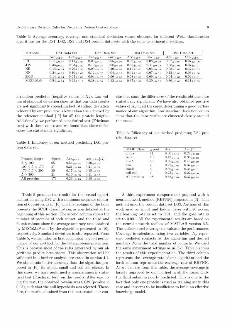
Table 3 shows the results of this experiment. Theobtained results are within normal values of accuracyand coverage rates for the contact map prediction [10].

These results confirm that our encoding provides enoughinformation for a good performance of a learning clas-sifier. Furthermore, we can also notice that MECoMaP

achieved the best results for this experiment in the ma-jority of the cases. High values of coverage are achievedby NB for DS2 and DS4, however, the accuracy rate is

significantly low in these cases, so these results are over-come on average by our algorithm. On the other hand,NN achieves higher values of accuracy than MECoMaP

for DS3, but its coverage is much lower than the cover-age obtained by our method. In addition, we performeda statistical test (Friedman test) on the results shown

in table 3 and we found that the differences of accuracyvalues for DS2 and DS4 are statistically significant.

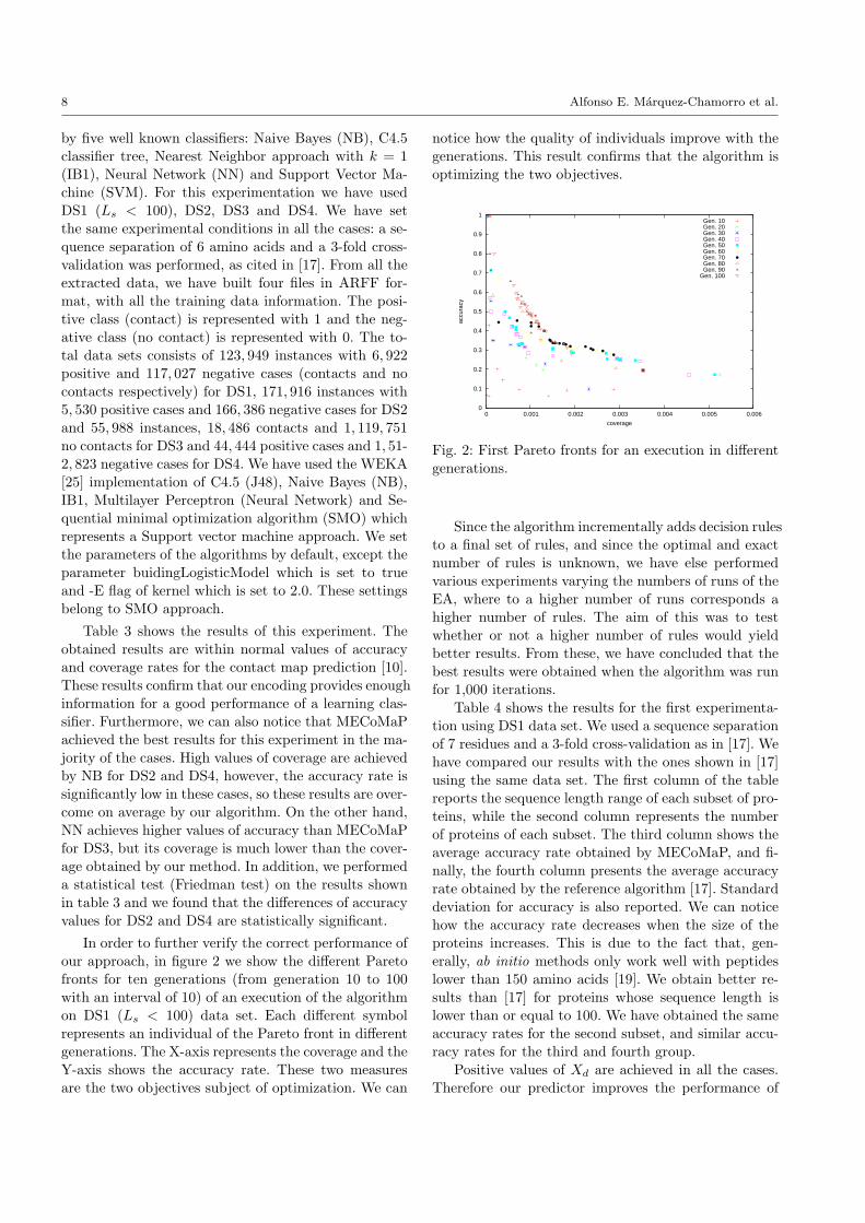
In order to further verify the correct performance ofour approach, in figure 2 we show the different Pareto

fronts for ten generations (from generation 10 to 100with an interval of 10) of an execution of the algorithmon DS1 (Ls < 100) data set. Each different symbol

represents an individual of the Pareto front in differentgenerations. The X-axis represents the coverage and theY-axis shows the accuracy rate. These two measures

are the two objectives subject of optimization. We can

notice how the quality of individuals improve with the

generations. This result confirms that the algorithm isoptimizing the two objectives.

0

0.1

0.2

0.3

0.4

0.5

0.6

0.7

0.8

0.9

1

0 0.001 0.002 0.003 0.004 0.005 0.006

accu

racy

coverage

Gen. 10Gen. 20Gen. 30Gen. 40Gen. 50Gen. 60Gen. 70Gen. 80Gen. 90

Gen. 100

Fig. 2: First Pareto fronts for an execution in different

generations.

Since the algorithm incrementally adds decision rules

to a final set of rules, and since the optimal and exactnumber of rules is unknown, we have else performedvarious experiments varying the numbers of runs of the

EA, where to a higher number of runs corresponds ahigher number of rules. The aim of this was to testwhether or not a higher number of rules would yield

better results. From these, we have concluded that thebest results were obtained when the algorithm was runfor 1,000 iterations.

Table 4 shows the results for the first experimenta-tion using DS1 data set. We used a sequence separationof 7 residues and a 3-fold cross-validation as in [17]. We

have compared our results with the ones shown in [17]using the same data set. The first column of the tablereports the sequence length range of each subset of pro-

teins, while the second column represents the numberof proteins of each subset. The third column shows theaverage accuracy rate obtained by MECoMaP, and fi-

nally, the fourth column presents the average accuracyrate obtained by the reference algorithm [17]. Standarddeviation for accuracy is also reported. We can notice

how the accuracy rate decreases when the size of theproteins increases. This is due to the fact that, gen-erally, ab initio methods only work well with peptides

lower than 150 amino acids [19]. We obtain better re-sults than [17] for proteins whose sequence length islower than or equal to 100. We have obtained the same

accuracy rates for the second subset, and similar accu-racy rates for the third and fourth group.

Positive values of Xd are achieved in all the cases.

Therefore our predictor improves the performance of


Table 3: Average accuracy, coverage and standard deviation values obtained for different Weka classificationalgorithms for the DS1, DS2, DS3 and DS4 protein data sets with the same experimental settings.

Methods DS1 Data Set DS2 Data Set DS3 Data Set DS4 Data SetAcc.µ±σ Cov.µ±σ Acc.µ±σ Cov.µ±σ Acc.µ±σ Cov.µ±σ Acc.µ±σ Cov.µ±σ

IB1 0.11±0.37 0.11±0.27 0.05±0.01 0.05±0.01 0.08±0.00 0.08±0.00 0.07±0.00 0.07±0.00

J48 0.33±0.31 0.03±0.22 0.10±0.05 0.08±0.04 0.35±0.03 0.41±0.02 0.08±0.01 0.07±0.01

NB 0.14±0.34 0.20±0.39 0.09±0.02 0.20±0.02 0.19±0.02 0.05±0.08 0.08±0.02 0.32±0.03

NN 0.24±0.05 0.10±0.02 0.12±0.07 0.04±0.27 0.42±0.01 0.07±0.01 0.12±0.00 0.03±0.00

SMO 0.14±0.14 0.03±0.09 0.04±0.02 0.06±0.03 0.08±0.01 0.09±0.01 0.04±0.01 0.09±0.01

MECoMaP 0.54±0.24 0.21±0.18 0.38±0.09 0.12±0.01 0.37±0.08 0.39±0.02 0.36±0.09 0.11±0.03

a random predictor (negative values of Xd). Low val-ues of standard deviation show us that our data results

are not significantly spread. In fact, standard deviationachieved by our predictor is lower than the achieved bythe reference method [17] for all the protein lengths.

Additionally, we performed a statistical test (Friedmantest) with these values and we found that these differ-ences are statistically significant.

Table 4: Efficiency of our method predicting DS1 pro-tein data set.

Protein length #prot. Acc.µ±σ Acc.µ±σ[17]L ≤ 100 65 0.54±0.24 0.26±0.39

100 ≤ L < 170 57 0.21±0.16 0.21±0.32

170 ≤ L < 300 30 0.17±0.08 0.15±0.22

L ≥ 300 21 0.10±0.05 0.11±0.15

All proteins 173 0.26±0.13 0.18±0.32

Table 5 presents the results for the second experi-mentation using DS2 with a minimum sequence separa-

tion of 6 residues as in [10].The first column of the tablepresents the SCOP classification, as was detailed at thebeginning of this section. The second column shows the

number of proteins of each subset, and the third andfourth column show the average accuracy rate obtainedby MECoMaP and by the algorithm presented in [10],

respectively. Standard deviation is also reported. FromTable 5, we can infer, as first conclusion, a good perfor-mance of our method for the beta proteins prediction.

This is because most of the rules generated by our al-gorithms predict beta sheets. This observation will bevalidated in a further analysis presented in section 4.1.

We also obtain better accuracy than the algorithm pro-posed in [10], for alpha, small and coil-coil classes. Inthis cases, we have performed a non-parametric statis-

tical test (Friedman test) on the results. After execut-ing the test, the obtained p-value was 0.039 (p-value <0.05), such that the null hypothesis was rejected. There-

fore, the results obtained from this test sustain our con-

clusions, since the differences of the results obtained arestatistically significant. We have also obtained positive

values of Xd in all the cases, determining a good perfor-mance of our algorithm. Low standard deviation valuesshow that the data results are clustered closely around

the mean.


SCOP Class #prot. Acc. Acc.[10]alpha 11 0.30±0.13 0.24±0.13

beta 10 0.42±0.12 0.38±0.16

a+ b 15 0.38±0.09 0.45±0.10

a/b 7 0.22±0.05 0.37±0.07

small 4 0.50±0.01 0.36±0.07

coil-coil 1 0.25±0.00 0.22±0.00

All proteins 48 0.38±0.08 0.37±0.14

A third experiment compares our proposal with aneural network method (RBFNN) proposed in [67]. This

method used the protein data set DS3. Authors of thiswork used an input and hidden layer with 20 nodes,the learning rate is set to 0.01, and the goal rate is

set to 0.001. All the experimental results are based onthe neural network toolbox of MATLAB version 6.5.The authors used coverage to evaluate the performance.

Coverage is calculated using two variables, Np repre-sent predicted contacts by the algorithm and desirednumbers Nd is the total number of contacts. We used

the same experiment settings as in [67]. Table 6 showsthe results of this experimentation. The third columnrepresents the coverage rate of our algorithm and the

forth column represents the coverage rate of RBFNN.As we can see from this table, the average coverage islargely improved by our method in all the cases. Only

the third subset is poorly predicted. This is due to thefact that only one protein is used as training set in thiscase and it seems to be insufficient to build an effective

knowledge model.



Protein length #prot. Cov. Cov.[67]L ≤ 100 10 0.41 0.26100 ≤ L < 200 13 0.62 0.30200 ≤ L < 300 2 0.15 0.31300 ≤ L < 400 13 0.29 0.26L ≥ 400 9 0.75 0.26All proteins 48 0.44 0.27

At the end of the execution, the program generatesa resulting contact map for each protein test. In Figure

3, we show an example for the protein 5PTI from DS1data set. We can appreciate that the lower triangular(predicted contacts) is largely similar to the upper one

(real contacts).

Fig. 3: Contact map of protein 5PTI with a thresholdof 8A.

4.1 Analysis of predicting rules

In order to further evaluate the results obtained by

MECoMaP, we have statistically analyzed the set ofrules obtained on DS1 with Ls < 100. Similar resultswere found for other Ls. A set of 10,244 rules were ex-

tracted by the algorithm after an execution of 1,000 it-erations. With this study, we want to analyze the prop-erties of the amino acids that are predicted to be in

contact. This would allow us to draw conclusions about

the influence that these properties have on the folding

problem.

First, we have analyzed the properties of the aminoacid i in the rules set. The histograms in Figures 4 and5 show the relative frequency of hydrophobicity and

polarity values for the amino acid i. The properties val-ues have been discretized into five groups in intervals of0.5 from −1 to 1 for the hydrophobicity and polarity. In

Figures 4 and 5 we added in each group of hydrophobic-ity and polarity, respectively, the rules whose interval[Hmin,Hmax] is totally or partially included. There-

fore, note that the same rule could be included in oneor more groups. Although all the study is referred toresidue i, the amino acid j presents similar behavior.

These rules indicate that a vast majority of aminoacids in contact have high values of hydrophobicity. Fur-

thermore, a high percentage of contacts have non-polarresidues. These conclusions were expected, because hy-drophobic and non-polar amino acids tend to be located

in the core of the protein. The core of proteins containsmuch less space than other protein regions, and con-tacts among amino acids are more frequent. Therefore,

these type of residues have more probabilities to be incontact [24]. We have not observed any clear conclusionregarding the net charge of amino acids i and j individ-

ually. Although amino acids with opposite charges aresupposed to be in contact [24], this condition seems tobe irrelevant in our rule set.

Figure 6 and 7 represent the relative frequencies of

values of solvent accessibility and secondary structurerespectively. As we can see in Figure 6, lower valuesof solvent accessibility are the most represented val-

ues in the rules. This is due to the fact that aminoacids with low values of solvent accessibility are in thecore of the protein and are often in contact. We can

appreciate from figure 7, that a high number of rules(77%) presents secondary structure values of type E(β-sheets). This is explained by the separation in the

sequence constraint which was set to 7. In fact, in thisway, intra turn and intra α-helix contacts are avoided.However, this fact does not affect the long-range β-sheet

contacts and, therefore, they predominate in our set ofrules.

We have also analysed the relation between the prop-erties of amino acids i and j that are predicted to be in

contact. In Figures 8 and 9 we show the hydrophobicityand polarity regions, respectively, for amino acids i andj covered by our predicted rules. The representation of

that regions is based on overlapping translucent rect-angles whose area covers the range of hydrophobicitiesor polarities of amino acids i and j that are included in

the rules.


0

10

20

30

40

50

60

-1 -0.5 0 0.5 1

prop

ortio

n of

rul

es (

%)

hydrophobicity

Fig. 4: Relative frequency of hydrophobicity values foramino acid i in our predicted rules.

0

10

20

30

40

50

60

-1 -0.5 0 0.5 1

prop

ortio

n of

rul

es (

%)

polarity

Fig. 5: Relative frequency of polarity values for aminoacid i in our predicted rules.

0

10

20

30

40

50

60

0 1 2 3 4

prop

ortio

n of

rul

es (

%)

solvent accesibility

Fig. 6: Relative frequency of solvent accessibility valuesfor amino acid i in our predicted rules.

Fig. 7: Relative frequency of secondary structures foramino acid i in our predicted rules.

From Figure 8, we appreciate that the obtained rules

predict contact between amino acids whose hydropho-bicity is high, especially when both amino acids arehydrophobic (values close to 1.0). As we can observe

in the Figure 9, non-polar amino acids (values close to

-1.0) are more likely to be in contact, according to our

rules. These results are consistent with those obtainedin Figures 4 and 5. In figure 10 we show the relativefrequency of charge values for amino acids i and j in

the rules. We found that amino acids with charge 0 areoften in contact (in 79.3% of cases) according to therules.

Fig. 8: Hydrophobicity regions for amino acids i and jcovered by our predicted rules.

Fig. 9: Polarity regions for amino acids i and j covered

by our predicted rules.

Figure 11 shows an example of two resulting rules.

If we inspect the first rule, we can infer that, for exam-


+1 0.8 6.8 0.3

Amino acid j 0 2.5 79.3 5.4

-1 0.3 3.5 0.8

-1 0 +1

Amino acid i

Fig. 10: Relative frequency (%) of charge values foramino acids i and j in our predicted rules.

ple, the hydrophobicity value for the amino acid i lies

between 0.52 and 0.92, the polarity value between −1.0and −0.93, neutral charge 0, solvent accessibility 0 andsecondary structure 2 (β-sheet). Therefore, the amino

acid i could be L (Lysine) or F (Phenylalanine), whichfulfills all these features according to the cited scales.As it can be noticed the produced rules are easily in-

terpretable by experts in the field.

if Hi ∈ [0.52, 0.92] and Pi ∈ [−1.00,−0.93] andCi = 0 and SSi = 2 and SAi = 0 and

Hj ∈ [0.32, 0.82] and Pj+1 ∈ [−0.41,−0.01] andCj+1 = 0 and SSj+1 = 2 and SAj+2 = 1 then contact

if Hi−1 ∈ [0.20, 0.82] and Pi ∈ [−0.41,−0.01] andCi = 0 and SSi+1 = 2 and SAi+2 = 1 and

Hj ∈ [0.45, 0.62] and Pj+1 ∈ [−0.73,−0.01] andand SSj = 2 and SSj+1 = 2 then contact

...

else no contact;

Fig. 11: Description of two predicted rules obtainedfrom the dataset DS1.

5 Conclusions and future work

In this article, we proposed a multi-objective evolution-ary algorithm approach for protein contact map predic-tion. Our algorithm generates a set of rules for residue-

residue contact prediction using a representation basedon amino acid properties. The rules forming the finalsolution express a set of conditions on specific physico-

chemical properties of amino acids. As a consequence,such rules can easily be interpreted and analyzed byexperts in the field in order to obtain more insight on

the protein folding process.

Our approach have been tested with four different

protein data bases which appear in the literature ob-taining acceptable results. A statistical study of our setof rules have been performed. Some conclusions about

the folding protein can be inferred from the rules. Theseconclusions are related to the physico-chemical proper-ties of amino acids (hydrophobicity and polarity) and

two predicted structural features (SA and SS) used byour approach.

As for future work, we intend to expand this study

to other significant amino acid properties, e.g., isoelec-tric point and steric parameter. Furthermore, we areplanning to include evolutionary information like Pos-

ition-Specific Score Matrix (PSSM). This informationmust be encoded in the representation of the algorithm.We also intend to study the possibility of using self-

adaptable parameters for controlling the genetic opera-tors used in the algorithm. Another future developmentis the application of the algorithm to larger proteinsdata set, in order to test the validity of our proposal

in these cases, where the resulting rules set could covermore of the search space.

Acknowledgements This research was supported by theJunta de Andalucia, Project of Excellence P07-TIC-02611and by Spanish Ministry of Science and Technology undergrants TIN2007-68084-C02-00 “Sistemas Inteligentes para de-scubrir patrones de comportamiento. Aplicacion a base dedatos biologicas”.

References

1. Abu-Doleh, A.A., Al-Jarrah, O.M., Alkhateeb, A.: Pro-tein contact map prediction using multi-stage hybrid in-telligence inference systems. J Biomed Inform (2011)

2. Altschul, S.F., Madden, T.L., Schffer, A.A., Zhang, J.,Zhang, Z., Miller, W., Lipman, D.J.: Gapped blast andpsi-blast: a new generation of protein database searchprograms. Nucleic Acids Res 25(17), 3389–3402 (1997)

3. Andrew Toona, G.W.: A dynamical approach to contactdistance based protein structure determination. Journalof Molecular Graphics and Modelling 32, 75–81 (2012)

4. Asencio Cortes, G., Aguilar-Ruiz, J.S.: Predicting proteindistance maps according to physicochemical properties.J Integr Bioinform 8(3), 181 (2011)

5. Ashkenazy, H., Unger, R., Kliger, Y.: Hidden conforma-tions in protein structures. Bioinformatics 27(14), 1941–1947 (2011)

6. Bacardit, J., Stout, M., Hirst, J., Valencia, A., Smith, R.,Krasnogor, N.: Automated alphabet reduction for proteindatasets. BMC Bioinformatics 10, 6 (2009)

7. Bjrkholm, P., Daniluk, P., Kryshtafovych, A., Fidelis, K.,Andersson, R., Hvidsten, T.R.: Using multi-data hiddenmarkov models trained on local neighborhoods of proteinstructure to predict residue-residue contacts. Bioinfor-matics 25(10), 1264–1270 (2009)

8. Calvo, J.C., Ortega, J., Anguita, M.: Pitagoras-psp: In-cluding domain knowledge in a multi-objective approachfor protein structure prediction. Neurocomputing 74(16),2675–2682 (2011)


9. Chen, P., Li, J.: Prediction of protein long-range contactsusing an ensemble of genetic algorithm classifiers withsequence profile centers. BMC Struct Biol 10 Suppl 1,S2 (2010)

10. Cheng, J., Baldi, P.: Improved residue contact predictionusing support vector machines and a large feature set.Bioinformatics 8, 113 (2007)

11. Cutello, V., Narzisi, G., Nicosia, G.: A multi-objectiveevolutionary approach to the protein structure predictionproblem. J R Soc Interface 3(6), 139–151 (2006)

12. Di Lena, P., Fariselli, P., Margara, L., Vassura, M., Casa-dio, R.: Fast overlapping of protein contact maps byalignment of eigenvectors. Bioinformatics 26(18), 2250–2258 (2010)

13. Dodge, C., Schneider, R., Sander, C.: The hssp databaseof protein structure-sequence alignments and family pro-files. Nucleic Acids Res 26(1), 313–315 (1998)

14. Duarte, J.M., Sathyapriya, R., Stehr, H., Filippis, I.,Lappe, M.: Optimal contact definition for reconstructionof contact maps. BMC Bioinformatics 11, 283 (2010)

15. Eickholt, J., Wang, Z., Cheng, J.: A conformation ensem-ble approach to protein residue-residue contact. BMCStruct Biol 11, 38 (2011)

16. Faraggi, E., Yang, Y., Zhang, S., Zhou, Y.: Predictingcontinuous local structure and the effect of its substi-tution for secondary structure in fragment-free proteinstructure prediction. Structure 17(11), 1515–1527 (2009)

17. Fariselli, P., Olmea, O., Valencia, A., Casadio, R.: Predic-tion of contact map with neural networks and correlatedmutations. Protein Engineering 14, 133–154 (2001)

18. Faure, G., Bornot, A., de Brevern, A.G.: Protein con-tacts, inter-residue interactions and side-chain modelling.Biochimie 90(4), 626–639 (2008)

19. Fernandez, M., Paredes, A., Ortiz, L., Rosas, J.: Sistemapredictor de estructuras de protenas utilizando dinmicamolecular (modypp). Revista Internacional de SistemasComputacionales y Electrnicos pp. 6–16 (2009)

20. Furuta, T., Shimizu, K., Terada, T.: Accurate predictionof native tertiary structure of protein using moleculardynamics simulation with the aid of the knowledge ofsecondary structures. Chemical Physics Letters 472(13),134–139 (2009)

21. Gao, X., Bu, D., Xu, J., Li, M.: Improving consensuscontact prediction via server correlation reduction. BMCStruct Biol 9, 28 (2009)

22. Grantham, R.: Amino acid difference formula to help ex-plain protein evolution. J. J. Mol. Bio. 185, 862–864(1974)

23. Gu, J., Bourne, P.: Structural Bioinformatics (Methodsof Biochemical Analysis). Wiley-Blackwell (2003)

24. Gupta, N., Mangal, N., Biswas, S.: Evolution and sim-ilarity evaluation of protein structures in contact mapspace. Proteins: Structure, Function, and Bioinformatics59, 196–204 (2005)

25. Hall, M., Frank, E., Holmes, G., B., P., Reutemann, P.,Witten, I.: The weka data mining software: An update.SIGKDD Explorations 11 (2009)

26. Jaravine, V., Ibraghimov, I., Yu Orekhov, V.: Removal ofa time barrier for high-resolution multidimensional nmrspectroscopy. Nat Meth 3(8), 605–607 (2006)

27. Jones, D.: Protein secondary structure prediction basedon position-specific scoring matrices. Journal of Molecu-lar Biology 292, 195–202 (1999)

28. Jones, D.T.: Protein secondary structure predictionbased on position-specific scoring matrices. J Mol Biol292(2), 195–202 (1999)

29. Jones, D.T., Buchan, D.W.A., Cozzetto, D., Pontil, M.:Psicov: precise structural contact prediction using sparseinverse covariance estimation on large multiple sequencealignments. Bioinformatics 28(2), 184–190 (2012)

30. Judy, M.V., Ravichandran, K.S., Murugesan, K.: Amulti-objective evolutionary algorithm for protein struc-ture prediction with immune operators. Comput Meth-ods Biomech Biomed Engin 12(4), 407–413 (2009)

31. Kabsch, W., Sander, C.: Dictionary of protein secondarystructure: pattern recognition of hydrogen-bonded andgeometrical features. Biopolymers 22(12), 2577–2637(1983)

32. Kawashima, S., Pokarowski, P., Pokarowska, M., Kolin-ski, A., Katayama, T., Kanehisa, M.: Aaindex: aminoacid index database, progress report 2008. Nucleic AcidsRes 36(Database issue), D202–D205 (2008)

33. Kihara, D.: The effect of long-range interactions on thesecondary structure formation of proteins. Protein Sci14(8), 1955–1963 (2005)

34. Kinjo, A.R., Horimoto, K., Nishikawa, K.: Predicting ab-solute contact numbers of native protein structure fromamino acid sequence. Proteins 58(1), 158–165 (2005)

35. Klein, P., Kanehisa, M., DeLisi, C.: Prediction of proteinfunction from sequence properties: Discriminant analysisof a data base. Biochim. Biophys. 787, 221–226 (1984)

36. Kloczkowski, A., Jernigan, R., Wu, Z., Song, G., Yang, L.,Kolinski, A., Pokarowski, P.: Distance matrix-based ap-proach to protein structure prediction. Journal of Struc-tural and Functional Genomics 10, 67–81 (2009)

37. Kyte, J., Doolittle, R.: A simple method for displayingthe hydropathic character of a protein. J. J. Mol. Bio.157, 105–132 (1982)

38. Lattman, E.: The state of the protein structure initiative.Proteins 54(4), 611–615 (2004)

39. Lavor, C., Liberti, L., Maculan, N., Mucherino, A.: Re-cent advances on the discretizable molecular distance ge-ometry problem. European Journal of Operational Re-search pp. – (2011)

40. Li, Y., Fang, Y., Fang, J.: Predicting residue-residue con-tacts using random forest models. Bioinformatics 27(24),3379–3384 (2011)

41. Lippi, M., Frasconi, P.: Prediction of protein beta-residuecontacts by markov logic networks with grounding-specific weights. Bioinformatics 25(18), 2326–2333(2009)

42. Lo, A., Chiu, Y.Y., Rdland, E.A., Lyu, P.C., Sung,T.Y., Hsu, W.L.: Predicting helix-helix interactions fromresidue contacts in membrane proteins. Bioinformatics25(8), 996–1003 (2009)

43. Marks, D.S., Colwell, L.J., Sheridan, R., Hopf, T.A.,Pagnani, A., Zecchina, R., Sander, C.: Protein 3dstructure computed from evolutionary sequence vari-ation. PLoS ONE 6(12), e28,766– (2011). DOI10.1371/journal.pone.0028766

44. Monastyrskyy, B., Fidelis, K., Tramontano, A.,Kryshtafovych, A.: Evaluation of residue-residuecontact predictions in casp9. Proteins 79 Suppl 10,119–125 (2011)

45. Monastyrskyy, B., Fidelis, K., Tramontano, A.,Kryshtafovych, A.: Evaluation of residue-residue contactpredictions in casp9. Proteins: Structure, Function, andBioinformatics 79(S10), 119–125 (2011)

46. Murzin, A., Brenner, S., Hubbard, T., Chothia, C.: Scop:a structural classification of proteins database for the in-vestigation of sequences and structures. Journal of Molec-ular Biology 247, 536–540 (1995)


47. Nagata, K., Randall, A., Baldi, P.: Sidepro: A novel ma-chine learning approach for the fast and accurate predic-tion of side-chain conformations. Proteins 80(1), 142–153(2012)

48. Plaxco, K.W., Simons, K.T., Baker, D.: Contact order,transition state placement and the refolding rates of sin-gle domain proteins. J Mol Biol 277(4), 985–994 (1998)

49. Rajgaria, R., McAllister, S.R., Floudas, C.A.: Towardsaccurate residue-residue hydrophobic contact predictionfor alpha helical proteins via integer linear optimization.Proteins 74(4), 929–947 (2009)

50. Rajgaria, R., Wei, Y., Floudas, C.A.: Contact predictionfor beta and alpha-beta proteins using integer linear op-timization and its impact on the first principles 3d struc-ture prediction method astro-fold. Proteins 78(8), 1825–1846 (2010)

51. R.O. Day J.B. Zydallis, G.L., Pachter, R.: Solving theprotein structure prediction problem through a multi-objective genetic algorithm. Nanotechnology 2, 32–35(2002)

52. Roy, A., Kucukural, A., Zhang, Y.: I-tasser: a unifiedplatform for automated protein structure and functionprediction. Nat Protoc 5(4), 725–738 (2010)

53. Service, R.: Structural biology: structural genomics,round 2. Science 307, 15541558 (2005)

54. Song, J., Burrage, K.: Predicting residue-wise contact or-ders in proteins by support vector regression. BMC Bioin-formatics 7, 425 (2006)

55. Stout, M., Bacardit, J., Hirst, J.D., Krasnogor, N.: Pre-diction of recursive convex hull class assignments for pro-tein residues. Bioinformatics 24(7), 916–923 (2008)

56. Tegge, A.N., Wang, Z., Eickholt, J., Cheng, J.: Nncon:improved protein contact map prediction using 2d-recursive neural networks. Nucleic Acids Res 37(WebServer issue), W515–W518 (2009)

57. Unger, R., Moult, J.: Genetic algorithms for protein fold-ing simulations. Biochim. Biophys. 231, 75–81 (1993)

58. Vassura, M., Di Lena, P., Margara, L., Mirto, M., Aloisio,G., Fariselli, P., Casadio, R.: Blurring contact maps ofthousands of proteins: what we can learn by reconstruct-ing 3d structure. BioData Min 4(1), 1 (2011)

59. Vassura, M., Margara, L., Di Lena, P., Medri, F.,Fariselli, P., Casadio, R.: Ft-comar: fault tolerant three-dimensional structure reconstruction from protein con-tact maps. Bioinformatics 24(10), 1313–1315 (2008)

60. Walsh, I., Bau, D., Martin, A., Mooney, C., Vullo, A.,Pollastri, G.: Ab initio and template-based prediction ofmulti-class distance maps by two-dimensional recursiveneural networks. BMC Structural Biology 9(1), 5 (2009)

61. Wang, Z., Eickholt, J., Cheng, J.: Multicom: a multi-levelcombination approach to protein structure prediction andits assessments in casp8. Bioinformatics 26(7), 882–888(2010)

62. Wei, Y., Floudas, C.A.: Enhanced inter-helical residuecontact prediction in transmembrane proteins. Chem EngSci 66(19), 4356–4369 (2011)

63. Wu, S., Szilagyi, A., Zhang, Y.: Improving protein struc-ture prediction using multiple sequence-based contactpredictions. Structure 19(8), 1182–1191 (2011)

64. Wu, S., Zhang, Y.: A comprehensive assessment ofsequence-based and template-based methods for proteincontact prediction. Bioinformatics 24(7), 924–931 (2008)

65. Xue, B., Faraggi, E., Zhou, Y.: Predicting residue-residuecontact maps by a two-layer, integrated neural-networkmethod. Proteins 76(1), 176–183 (2009)

66. Yang, J.Y., Chen, X.: A consensus approach to predictingprotein contact map via logistic regression. In: J. Chen,

J. Wang, A. Zelikovsky (eds.) Bioinformatics Researchand Applications - 7th International Symposium, ISBRA2011, Changsha, China, May 27-29, 2011. Proceedings,Lecture Notes in Computer Science, vol. 6674, pp. 136–147. Springer (2011)

67. Zhang, G., Huang, D., Quan, Z.: Combining a binaryinput encoding scheme with rbfnn for globulin proteininter-residue contact map prediction. Pattern Recogni-tion Letters 16(10), 1543–1553 (2005)

68. Zhou, Y., Duan, Y., Yang, Y., Faraggi, E., Lei, H.:Trends in template/fragment-free protein structure pre-diction. Theoretical Chemistry Accounts: Theory, Com-putation, and Modeling (Theoretica Chimica Acta) 128,3–16 (2011)

69. Zitzler, E., Thiele, L.: Multiobjective evolutionary algo-rithms: a comparative case study and the strength paretoapproach. Evolutionary Computation, IEEE Transac-tions on 3(4), 257 –271 (1999)

Evolutionary decision rules for predicting protein contact maps

Documents

Transcript of Evolutionary decision rules for predicting protein contact maps