i

Evidence of Low-dimensional Determinism

in Short Time Series of Solute Transport

Sina Khatami

Water Resources Engineering Department

Lund Institute of Technology (LTH)

Lund University

Fall 2013

Advance Research Course

Evidence of Low-dimensional Determinism in

Short Time Series of Solute Transport

By: Sina Khatami

Supervisor: Prof. Magnus Persson

Department of Water Resources Engineering Lund University Fall 2013

Visiting Address: John Ericssons väg 1, V-huset, SE-223 63, Lund, Sweden

Postal Address: Box 118, S-221 00 Lund, Sweden

Telephone: +46 (0)46-222 4009; +46 (0)46-222 7398; +46 (0)46-222 8987

Web page: http://www.tvrl.lth.se

E-mail: tvrl@tvrl.lth.se

Avd för Teknisk Vattenresurslära

ii

iii

Abstract

Investigating the vadose zone, the physics behind the temporal and spatial instabilities of flow

(in unsaturated media) is still of question. Although chaotic approaches have been widely em-

ployed for identifying different surface hydrology processes, such as rainfall, runoff, lake vol-

ume, etc., they were not applied for subsurface systems as much. On this ground, the present

study attempts to investigate nonlinear determinism in solute transport processes in vadose

zone. Previously, a few studies have investigated/examined solute transport processes from

the view point of nonlinear chaos. However, this is the first study that is directly analyzing so-

lute transport time series from field experiments. Also, it is analyzing short time series (68 data

points) from a soil profile (62 measurement probes). For this purpose, Correlation Dimension

Method is used as the most celebrated nonlinear chaotic technique in the hydrological studies.

In general, the results of correlation dimension analysis provide the minimum number of or-

dinary differential equations needed to map a given dynamics. This study placed its main focus

on the evolution of Correlation Exponent (CE) vs. Embedding Dimension (EM). The oscilla-

tion of correlation exponents between different values (2-4) which is referred to as Instable

Saturation (IS) has been observed. Plausible explanations for this instability is discussed. The

values of correlation dimensions for stable saturation are 2 and 3 among which CD=3 is the

most frequent CD for SS is 3; for the rest of SS, CD is 2. In case of instable saturation, how-

ever, CD values are varying between 2 and 4 where IS-2, 3 is the most frequent one. Although

the results are not as ‘accurate’ as other hydro-chaotic studies which dealt with longer time

series, the consistent pattern and the order of magnitude in the results are in good agreement

with previous findings. On a large scheme, the results encouragingly indicate a promising ave-

nue from the presuppositional perspective of stochasticism towards nonlinear determinism for

hydrological studies especially subsurface processes.

Keywords: Nonlinear time series analysis, Chaos Theory, Correlation Dimension Method,

Solute transport, short time series, unsaturated zone, vadose zone.

Recommended Citation

Khatami, S. (2013). Evidence of Low-dimensional Determinism in Short Time Series of So-

lute Transport. Advanced Research Course, Department of Water Resources Engineering,

Lund University, Lund, Sweden.

iv

v

Acknowledgment

I would like to express my greatest appreciation to my supervisor, Professor Magnus Persson,

for his patient guidance, enthusiastic encouragement and constructive critiques during the

planning and development of this research work. Magnus has been always there to help me.

His kind and generous support cannot be simply appreciated by a few lines of acknowledg-

ment.

I would like to extend my gratitude to Professor Michael Small at the University of Western

Australia. I have greatly benefited from his valuable suggestions on Chaos Theory and its ap-

plications. His willingness to give his time so generously means a lot to me.

Sina

30 October 2013, Lund

vi

vii

Acronyms and Abbreviations

CC Correlation Coefficient

CE Correlation Exponent

CDM Correlation Dimension Method

DOF Degree of Freedom

EM Embedding Dimension

FNA False Neighbors Algorithm

FNN False Nearest Neighbors

GKA Gaussian Kernel Algorithm

GPA Grassberger-Procaccia Algorithm

KEM Kolmogorov Entropy Method

LEM Lyapunov Exponent Method

ODE Ordinary Differential Equation

NPM Nonlinear Prediction Method

RC Relative Concentration

ST Solute Transport

viii

ix

Table of Contents

Abstract ..................................................................................................................................... iii

Acknowledgment ........................................................................................................................ v

Acronyms and Abbreviations .................................................................................................. vii

Table of Contents ..................................................................................................................... ix

List of Figures .......................................................................................................................... xi

List of Tables .......................................................................................................................... xiii

List of Equations ...................................................................................................................... xv

1 INTRODUCTION .............................................................................................................. 17 1.1. Problem Definition ............................................................................................................................ 18

2 LITERATURE REVIEW .................................................................................................... 21 2.1. Chaos Theory in Solute Transport .................................................................................................. 21

3 MATERIAL & METHODS ................................................................................................. 25 3.1. Data Sets & Study Area ..................................................................................................................... 25 3.2. Correlation Dimension Method....................................................................................................... 26

4 RESULTS & DISCUSSIONS............................................................................................... 33 4.1. Analysis ................................................................................................................................................ 33

4.1.1. Solute Transport Signals .......................................................................................................... 34 4.1.2. Pseudo-Phase Space Attractors of Solute Transport Signals ............................................. 35 4.1.3. Autocorrelation ......................................................................................................................... 36 4.1.4. Correlation Dimension: log C(r) vs. log r .............................................................................. 37 4.1.5. Correlation Dimension vs. Embedding Dimension ............................................................ 38

4.2. Discussion of the Results .................................................................................................................. 39 4.2.1. Time Series Length ................................................................................................................... 39 4.2.2. Classification of the Dynamics ............................................................................................... 39

4.2.2.1. Stability vs. Instability ........................................................................................................ 40 4.2.3. Consistent Pattern of Correlation Dimensions .................................................................... 41

5 CONCLUSION .................................................................................................................... 45

References ................................................................................................................................ 47

Appendix .................................................................................................................................. 50

x

xi

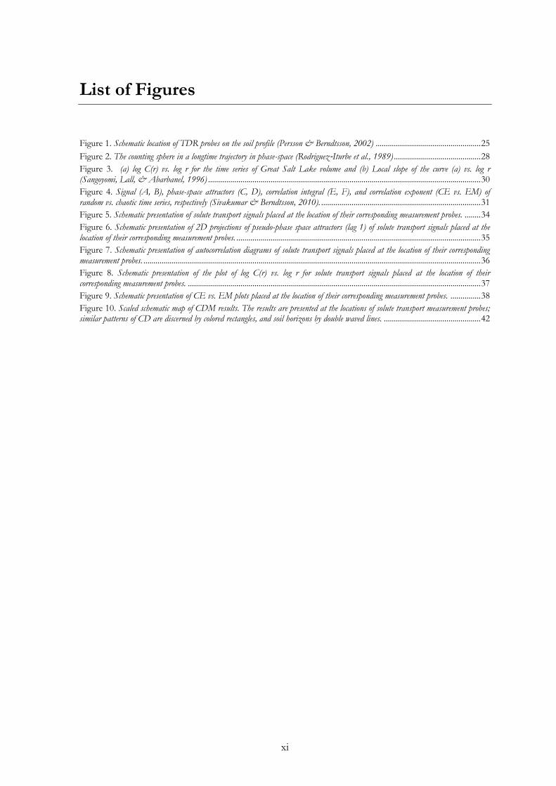
List of Figures

Figure 1. Schematic location of TDR probes on the soil profile (Persson & Berndtsson, 2002) .................................................... 25

Figure 2. The counting sphere in a longtime trajectory in phase-space (Rodriguez‐Iturbe et al., 1989) ........................................... 28 Figure 3. (a) log C(r) vs. log r for the time series of Great Salt Lake volume and (b) Local slope of the curve (a) vs. log r (Sangoyomi, Lall, & Abarbanel, 1996) ....................................................................................................................................... 30 Figure 4. Signal (A, B), phase-space attractors (C, D), correlation integral (E, F), and correlation exponent (CE vs. EM) of random vs. chaotic time series, respectively (Sivakumar & Berndtsson, 2010). ............................................................................... 31 Figure 5. Schematic presentation of solute transport signals placed at the location of their corresponding measurement probes. ........ 34 Figure 6. Schematic presentation of 2D projections of pseudo-phase space attractors (lag 1) of solute transport signals placed at the location of their corresponding measurement probes. ......................................................................................................................... 35 Figure 7. Schematic presentation of autocorrelation diagrams of solute transport signals placed at the location of their corresponding measurement probes. ....................................................................................................................................................................... 36 Figure 8. Schematic presentation of the plot of log C(r) vs. log r for solute transport signals placed at the location of their corresponding measurement probes. ................................................................................................................................................. 37 Figure 9. Schematic presentation of CE vs. EM plots placed at the location of their corresponding measurement probes. ............... 38 Figure 10. Scaled schematic map of CDM results. The results are presented at the locations of solute transport measurement probes; similar patterns of CD are discerned by colored rectangles, and soil horizons by double waved lines. ................................................ 42

xii

xiii

List of Tables

Table 1. Classified summary of nonlinear chaotic analyses of solute transport processes .................................................................. 23 Table 2. Soil properties (Persson & Berndtsson, 2002) ................................................................................................................ 25 Table 3. Classified results of 62 solute transport signals. ................................................................................................... 50

xiv

xv

List of Equations

(Equation 1)................................................................................................................................................................................ 26 (Equation 2)................................................................................................................................................................................ 27 (Equation 3)................................................................................................................................................................................ 27 (Equation 4)................................................................................................................................................................................ 27 (Equation 5)................................................................................................................................................................................ 27 (Equation 6)................................................................................................................................................................................ 29 (Equation 7)................................................................................................................................................................................ 29 (Equation 8)................................................................................................................................................................................ 29 (Equation 9)................................................................................................................................................................................ 29 (Equation 10) ............................................................................................................................................................................. 29

xvi

17

1 INTRODUCTION

Investigating hydrologic processes from the view point of Chaos Theory has been of great

interest during recent times. For one thing, possible presence of nonlinear determinism in

such systems could be utilized to model and predict the dynamics of these hydrologic systems.

The favorable outcomes of such studies together with the great performance and predictability

of nonlinear techniques in comparison to other methods (Sivakumar, Persson, Berndtsson, &

Uvo, 2002), such as stochastic, neural networks, indicate a promising avenue towards the ex-

tension of the applications of nonlinear deterministic approaches for solving hydrological

problems.

So far, one of the main challenges of chaos application in hydrology has been its limited

scope; it was mainly concentrated on surface hydrologic processes such as rainfall, rainfall-

runoff, river flow, lake volume and sediment transport. Despite the fact that the results of

these studies are promising, nonlinear determinism framework has not received much atten-

tion in order to be employed for subsurface problems (Sivakumar, Harter, & Zhang, 2005).

This is due to the fact that it is generally presupposed that the heterogeneous – essentially

nonuniform in composition/character – nature of soil and aquifers would result in random

behavior (dynamics) of flow and transport. This presupposition has been justified by the tem-

poral and spatial variability exhibited by these processes. Therefore, flow and transport models

most commonly employ the concept of stochastic process. Especially the fact that these mod-

els fairly represent the basic statistical properties (e.g. mean, variance) of flow and transport

processes may have further strengthened the view on the usefulness of stochastic

field/process concept for subsurface problems (Sivakumar et al., 2005).

One of the most challenging problems in the modern subsurface hydrology/hydrogeology is

the characterization of unstable flow and transport in unsaturated zones and rocks. The un-

saturated zone, also known as vadose zone, is situated between the soil surface and the

groundwater table (saturated zone). Based upon this layer the food chain is built; plants take

up water and nutrient from this zone. Therefore, it plays an essential role in the ecosystem

(Persson, 1999). Understanding the nature of unsaturated flow in fractures is imperative to

incorporate a foundation for resolving practical problems related to hydrogeological systems

including the vadose zone (Faybishenko, 2002). Unstable flow has various fundamental appli-

cations, both theoretically and practically:

Theoretically speaking, wetting-front instability can invalidate our best-laid theories of

vertical infiltration and groundwater recharge (Hillel, 1987).

18

Moreover, it can have important practical consequences. For example, unstable flow

can allow small ‘outlaw’ streams of water to flow directly, and carry raw pollutants, in-

to the groundwater while avoiding the profile’s filtration and purification mechanisms

(Hillel, 1987). It could also be utilized for developing technical and economic pro-

grams for environmental remediation; the exploitation of oil, gas, and geothermal res-

ervoirs; and nuclear waste disposal in fractured rock (Faybishenko, 2002).

Transport and flow processes in fractured rocks occur, generally, in a “nonvolume-averaged”

fashion; relatively slow flow through the rock matrices and fast flow in localized preferential

pathways within fractures. Currently, nevertheless, modeling of these processes in unsaturated

fractured rocks utilizes macro-scale continuum concepts based upon large-scale volume aver-

aging. Such models would be well fitted to represent large-scale features of fractured-rock, yet

would be insufficient for resolving time varying and spatially localized flow phenomena. This

causes serious challenges for mathematical modeling and demands alternative methods of

modeling for a given site. As it is explained earlier, the common approach has been based up-

on stochastic techniques in order to describe the seemingly random data sets, overlooking the

fact that deterministic nonperiodic (chaotic) processes could yield ostensible randomness

(Faybishenko, 2002). In light of the above, it is crucially important to identify chaotic process-

es in subsurface systems in order to develop appropriate models for short- and long-term pre-

dictions. The very first step in this direction would be to investigate the possible presence of

low-dimensional determinism in the underlying dynamics of subsurface systems such as solute

transport process(es).

1.1. Problem Definition

Within the field of hydrogeology and specifically investigating the vadose zone, the physics

behind the temporal and spatial instabilities of flow (in unsaturated media) is still of question.

In addition, it is yet unclear how laboratory and field experiments should be optimized and

also how some paradoxes in unsaturated flow theory (Gray & Hassanizadeh, 1991) could be

explained (Faybishenko, 2002). On this ground, the main objective of the present study is to

investigate the potential utilization of a nonlinear deterministic framework for understanding

the underlying dynamics of Solute Transport (ST) processes. In other words, this study at-

tempts to explore the possible presence of low-dimensional determinism in short time series

of solute transport. Pursuing this goal, Correlation Dimension Method (CDM) as a celebrated

technique of nonlinear time series analysis is employed to distinguish determinism and sto-

chasticity.

The possibility of the existence of chaotic behavior in transport processes in the soil stems

from the fact that such transport processes and also most of the models used to exhibit them

19

are nonlinear (Addiscott & Mirza, 1998). Faybishenko (2002) and Sivakumar et al. (2005) have

examined the possible existence of chaotic behavior in flow and transport processes using dif-

ferent data sets. Nonetheless, no study has so far placed its main focus on the evolution of

Correlation Exponent (CE) vs. Embedding Dimension (EM). Almost all studies in this realm

with the objective of ‘system identification’ have attempted to simply calculate the Correlation

Dimension (CD) as the diagnostic parameter of deterministic chaos. However, it is very im-

portant to look at the unfolding behavior of CE vs. EM considering the time series length and

also the nature of the studied system(s).

It is vitally crucial to keep this possibility open that there might be chaotic systems where the

number of generating mechanisms – the number of governing autonomous Ordinary Differ-

ential Equations (ODE) – are not constant during the evolution of the system; that is, instabil-

ity in the mechanisms generating the dynamic of the process. Not just the results of a few in-

teracting mechanisms are hugely different based upon their initial conditions (the essence of

Chaos Theory), but also as the system evolves its generating mechanisms/variables and their

number could be highly dependent on the conditions of the process in which initial conditions

could be one of them. Therefore, in light of the above, CDM analysis has been conducted on

a data set of solute transport signals measured at different levels of a soil profile; that is, to see

if any pattern could be discerned in the evolution of CE vs. EM, horizontally or vertically.

20

21

2 LITERATURE REVIEW

After presenting a brief history of Chaos Theory, Khatami (2013) has thoroughly explained its

fundamental elements and concepts, namely, phase-space, trajectory and attractor. Further, he

has discussed various aspects and criticisms on the application of Chaos Theory in hydrologi-

cal studies. Therefore, this study would not explore the theory and its related issues but put its

main focus on its application in solute transport process.

Chaos Theory attempts to study dynamical systems and how they behave with their highly de-

pendence on initial conditions – dynamical instability. A chaotic process or system evolves in a

deterministic way that its current state depends unequivocally on its previous state (Addiscott

& Mirza, 1998). Chaos theory could be seen and employed on a larger scheme as “complexity

theory”, “complex systems theory,” “synergetics”, and “nonlinear dynamics”. Nevertheless, to

the present time, application of chaos theory in practical problems remains as much an art as a

science (Faybishenko, 2002). So far, different methods have been employed in order to inves-

tigate deterministic chaos in hydrological processes. The simplest tool is the phase diagram

plot of a dynamical system which is in fact a visual evaluation of the process investigating pre-

liminary evidence on deterministic chaotic behavior. Sophisticated diagnostic techniques,

namely, Correlation Dimension Method (CDM), Lyapunov Exponent Method (LEM), Kol-

mogorov Entropy Method (KEM), Nonlinear Prediction Method (NPM), Gaussian Kernel

Algorithm (GKA), and False Neighbors Algorithm (FNA) or False Nearest Neighbors

(FNN), could also be employed for different purposes. In principle, these methods are tests

examining whether a given system/process is deterministic chaotic or stochastic. Among

which CDM is the fundamental approach and it has been widely used in hydrological studies.

2.1. Chaos Theory in Solute Transport

Addiscott and Mirza (1998) was the first study – to the knowledge of the author – that has

proposed a paradigm shift from stochastic to deterministic chaos in order to investigate

and/or model transport processes in soil. Their proposition was based upon studies by

Flühler, Durner, and Flury (1996) and Steenhuis et al. (1998). Experimental observations by

Flühler et al. (1996) has shown that the variable extent and rates of lateral mixing cause sub-

stantially different transport regimes which could neither be explained nor predicted mecha-

nistically in terms of known state variables. They have speculated that solute flow may not on-

ly be chaotic but may also have further complication as the chaotic processes depend upon

randomly distributed state variables. This might explain the transport regimes found by

Flühler et al. (1996), i.e., “neither be predicted nor explained mechanistically in terms of

22

known state variables”. Therefore, they have proposed an even more complex approach of

modeling in which deterministic chaos is interacting with stochastic distribution of state varia-

bles. To their opinion, suppose one can show chaotic behavior in a transport model, then two

fundamental questions should be met; ‘So what?’ and ‘What then?’. The former, calls attention

to careful and critical thinking about the way in which the models are used. The latter, none-

theless, could be answered in various ways. One possibility is to reformulate the theoretical

approach to transport processes endorsing their chaotic natures. Study by Rodriguez-Iturbe,

Entekhabi, Lee, and Bras (1991) could be an example for this case. Addiscott and Mirza

(1998) have looked through this question and discussed several different options as well.

Faybishenko (2002) has compared the results of Persoff–Pruess experiments (Persoff & Pruess,

1995) with nonlinear chaotic analyses of both laboratory dripping-water experiments in frac-

ture models and field-infiltration experiments in fractured basalt. Based upon this comparison

he has hypothesized that processes of intrinsic fracture flow and dripping as well as extrinsic

water dripping from a fracture subjected to a capillary-barrier effect are deterministic chaotic

systems with a certain random component. In brief, it has been concluded that the unsaturat-

ed fractured rock is a chaotic dynamic system as the flow processes are dissipative, nonlinear,

and sensitive to initial conditions. These flow processes are exhibiting chaotic oscillations gen-

erated by intrinsic properties of the system, not external random factors. Identifying such sys-

tems as deterministic is a crucial turning point in terms of developing well-defined models for

short- and long-term predictions of these dynamic systems, evaluating the uncertainty inherent

to the system and its predictions, assessing the spatial distribution of flow characteristics from

solute transport time series, and ultimately improving chemical-transport simulations.

Sivakumar et al. (2005) have employed CDM in order to investigate deterministic behavior in

solute particle transport time series in a heterogeneous aquifer medium. They have studied

simulated time series for different scenarios using an integrated probability/Markov chain

(TP/MC) model. The phase-space is reconstructed in two dimensions (i.e. m=2), with 1 year

delay time which is a typical sampling interval for groundwater monitoring. CDM nonlinear

analyses of solute transport processes have interestingly yielded correlation dimension of 2 for

a two facies medium (sand 20%, clay 80%), and correlation dimension of 3 for a three facies

medium (sand 21.26%, clay 53.28%, loam 25.46%). It should be noted that anisotropy condi-

tions have been considered for different simulation scenarios and different number of facies.

As Khatami (2013) has summarized major studies of Chaos Theory in hydrology, summary of

its main applications in ST processes are presented in TABLE 1.

23

Table 1. Classified summary of nonlinear chaotic analyses of solute transport processes

Study Results Summary

Addiscott and Mirza (1998)

- Proposes a paradigm shift from stochastic to deterministic chaos for investigating transport

processes in soil

Faybishenko (2002) CD=2-4

“The unsaturated fractured-rock system is chaotic as the flow processes are sensitive to

initial conditions, nonlinear and dissipative. The presence of chaotic behavior is confirmed by

calculating diagnostic chaotic parameters for gas, liquid, and capillary pressures, measured during the water–gas injection in fractures, as well as

laboratory and field dripping-water experiments.”

Sivakumar et al. (2005) CE=1.33 & 2.12,

CD=2-3

Simulated solute transport through the two and three facies media in a heterogeneous aquifer

medium

24

25

3 MATERIAL & METHODS

3.1. Data Sets & Study Area

Solute transport time series are collected from the field experiments that has been carried out

in a site situated in Löddeköpinge in southern Sweden by Persson (1999). The soil in this field

consists of 4 horizons, namely, Ap (topsoil or surface mineral horizons with anthropogenic

disturbances e.g. ploughing, deep ripping), E (eluviated), B (subsoil), and C (parent material).

Details of each horizon are presented in table below.

Table 2. Soil properties (Persson & Berndtsson, 2002)

Horizon Depth (cm)

Sand (%)

Silt (%)

Clay (%)

Organic C (%)

Bulk Density (g/cm3)

Porosity (m3/m3)

Ap 0-20 80 16.5 3.5 4.3 1.53 0.40

E 20-45 78.8 18.3 2.9 3.4 1.55 0.39

B 45-70 84.3 11.8 3.9 2.6 1.55 0.39

C >70 93.4 4.8 1.8 0.5 1.56 0.39

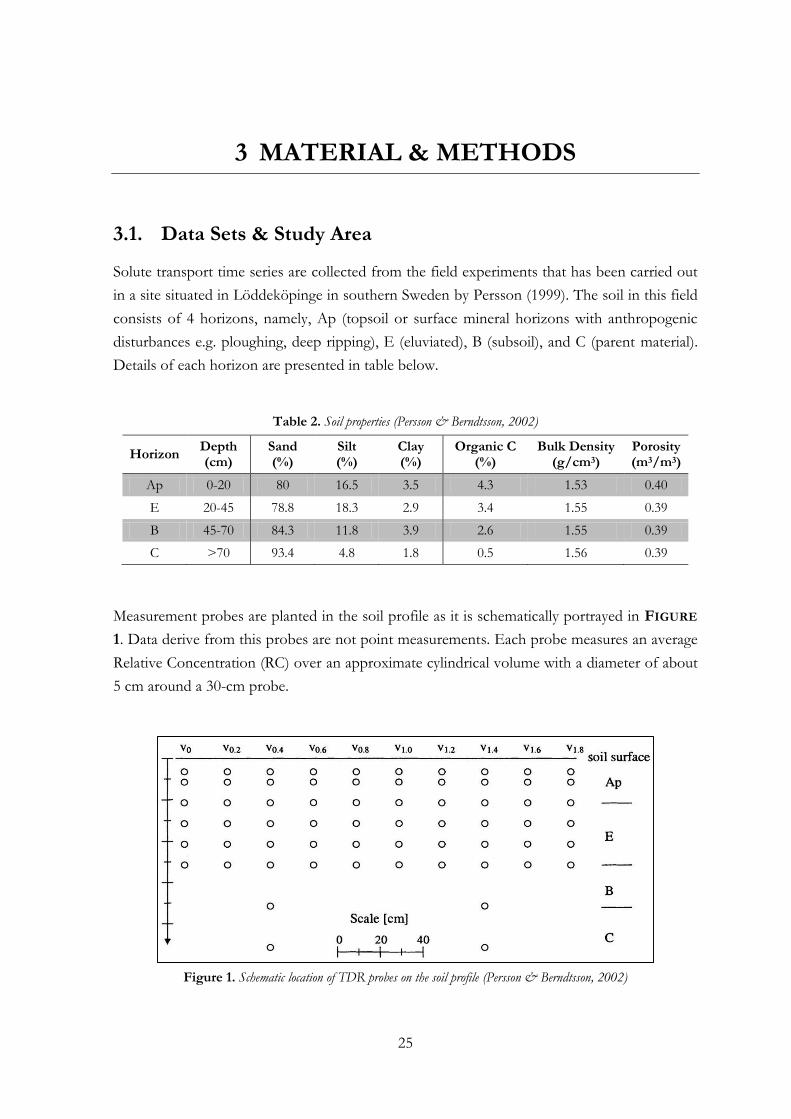
Measurement probes are planted in the soil profile as it is schematically portrayed in FIGURE

1. Data derive from this probes are not point measurements. Each probe measures an average

Relative Concentration (RC) over an approximate cylindrical volume with a diameter of about

5 cm around a 30-cm probe.

Figure 1. Schematic location of TDR probes on the soil profile (Persson & Berndtsson, 2002)

26

The temporal resolution of time series is 12 h and the measurement is began 132 h (i.e. 11

time steps) prior to applying the tracer into the soil. Each time series contains 68 data points

from which 57 values are after the tracer is applied. Overall, 64 probes are placed at 8 different

depths of 5, 10, 20, 30, 40, 50, 70, and 90 cm. The first 6 depths contain 10 probes each, and

the two deepest ones include 2 each. It should be noted that two sensors were broken and so

only 62 signals are at hand. These two sensors are number 48 at depth 40 cm and number 59

at depth 50 cm. Further information about the field experiments and data collection are ex-

plained by Persson (1999) and Persson and Berndtsson (2002).

3.2. Correlation Dimension Method

Due to the fact that sophisticated mathematics behind Chaos Theory has been explained

thoroughly in several authentic sources (e.g.(Broer & Takens, 2011; Gidea & Niculescu, 2002;

Ivancevic & Ivancevic, 2008), the present study only focuses on the application aspect of the

theory and CDM technique in particular.

There are different methods discerning low-order deterministic chaotic processes from sto-

chastic ones. Among those, CDM is almost certainly the most fundamental one that has been

used in a wide range of subjects. In simple words, CDM attempts to estimate the dimension

of a dynamic system’s attractor. CDM is established upon the concept of the correlation integral

(or correlation function). The concept is that an ostensibly irregular phenomenon could arise from

deterministic dynamic. Therefore, such systems will have a limited number of DOF equal to

the smallest number of first order differential equations that capture the most important fea-

tures of their dynamic. From different approaches in estimating the correlation dimension, the

present study utilizes the Grassberger-Procaccia Algorithm (GPA)(Grassberger & Procaccia,

1983).

The reconstruction of the phase-space of a scalar time series and, hence, its attractor is the

first important step in any chaos identification approach. Such a reconstruction method uses

the concept of embedding a single-variable series in a multi-dimensional phase-space to repre-

sent its underlying dynamic (Sivakumar & Jayawardena, 2002). As the present study aims to

analyze discrete time series of ST observations, hence, the phase-space reconstruction method

is explained for discrete scalar time series.

For an autonomous system characterized by d interacting state variables (a d-dimensional state

space z) the associated dynamics could be represented as:

𝑑𝒛(𝑡)

𝑑𝑡= 𝐹(𝒛(𝑡)) (Equation 1)

27

Assume a scalar univariate time series x(t), t=1, 2,…, N for one of the d state variables (i.e. RC

in this study), generated by this system. This system can be rewritten as a high-ordered differ-

ential equation in terms of the single state variable x as follow:

𝑥(𝑑) = 𝑓(𝑥, 𝑥′, … , 𝑥(𝑑−1)) (Equation 2)

Based upon the notion of phase-space reconstruction (Packard, Crutchfield, Farmer, & Shaw,

1980; Takens, 1981) a pseudophase-space could be defined using delay coordinates by

defining a delay vector Yt:

𝑌𝑡 = { 𝑥(𝑡), 𝑥(𝑡 − 𝜏), … , 𝑥(𝑡 − (𝑚 − 1)𝜏)} (Equation 3)

where 𝜏 is delay time, appropriately chosen as an integere multiple of simpling time Δt, and m

is an integer embedding dimension. If the solution of the equations lies on an attractor of

dimension dA (dA < d), choosing the integer m (m > 2dA) is a sufficient condition for

unfolding the attractor from time series x(t). Subjecting to generic assumptions on F and Δt,

for any delay time τ and forecast period T, the underlying dynamics could be represented by a

smooth (i.e. differentiable) map:

𝑌𝑡+𝑇 = 𝑓𝑇(𝑥(𝑡), 𝑥(𝑡 − 𝜏), 𝑥(𝑡 − 2𝜏), … , 𝑥(𝑡 − (𝑚 − 1)𝜏)) = 𝑓𝑇(𝑌𝑡)

𝑓𝑇: ℝ𝑚 → ℝ

(Equation 4)

Where Yt and Yt+T are vectors of dimension 𝑚, describing the system state at current state 𝑡

and future state t+T, respectively. Equation 4 is a basis for reconstructing the phase-space of

the underlying dynamic of a given scalar time series by providing the map fT if appropriate

values of τ and m are chosen.

Simply put, the reconstruction of the phase-space from a discrete time series (pseudophase-

space) can be achieved with the help of an m-dimensional “embedding space”, EM, which is

spanned by delay vectors for any given (integer) time delay τ. For a scalar univariate time series

Xi, where i=1, 2,…, N the phase-space could be reconstructed as (Sivakumar, Berndtsson,

Olsson, & Jinno, 2001):

𝑌𝑗 = ( 𝑋𝑗, 𝑋𝑗+𝜏, 𝑋𝑗+2𝜏, … , 𝑋𝑗+(𝑚−1)𝜏 ) (Equation 5)

28

where j=1, 2,…, N-(m-1)τ/Δt, m is the embedding dimension (dimension of vector Yj) and τ

is delay time. τ is almost an ‘arbitrary’, but fixed time delay for an infinite amount of noise-free

data (Takens, 1981). τ should be a suitable integer multiple of the sampling time Δt (Packard et

al., 1980; Takens, 1981). m is the number of coordinate of the embedding space.

Despite the basic assumption of phase-space reconstruction method that for an infinite noise-

free time series, τ is an almost ‘arbitrary’, there is no such time series in real life problems and

hydrological time series are no exceptions to this. Therefore, there has been a quest finding

the optimal delay time for practical problems. In practical problems and in particular hydro-

logical studies investigating the existence of chaos in hydrological time series (e.g.(Jayawardena

& Lai, 1994; Khatami, 2013; Puente & Obregón, 1996; Rodriguez‐Iturbe, Febres De Power,

Sharifi, & Georgakakos, 1989; Sharifi, Georgakakos, & Rodriguez-Iturbe, 1990; Sivakumar et

al., 2001; Sivakumar et al., 2005; Sivakumar, Liong, Liaw, & Phoon, 1999; Sivakumar,

Woldemeskel, & Puente, 2013), the first zero-crossing of the autocorrelation function has

been commonly used as the proper delay time.

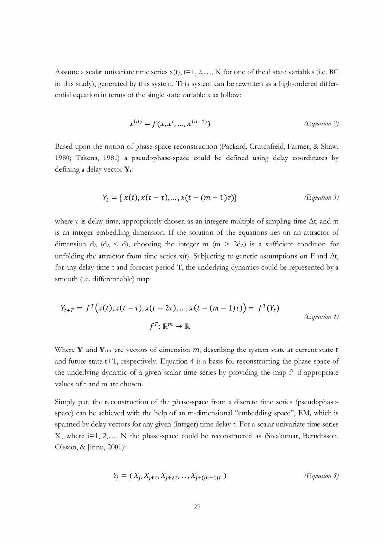
Based upon EQUATION 5, a trajectory in an m-dimensional space can be constructed. There-

fore, moving along with time t, a series of m-dimensional vectors will be obtained which rep-

resent the m-dimensional phase-space of the system. Suppose a circle (a sphere for m=3 or a

hypersphere for m≥4) of radius r centered about an arbitrary point of the m-dimensional set

of vectors (see Figure 2) and count the number of points N(r) located inside the circle. Nor-

malizing such a count, the so called correlation integral C(r) of the process will be obtained

(Rodriguez‐Iturbe et al., 1989).

Figure 2. The counting sphere in a longtime trajectory in phase-space (Rodriguez‐Iturbe et al., 1989)

The GPA uses the described concept of phase-space reconstruction to represent the system’s

dynamic. According to GPA, for an m-dimensional phase-space (m is an integer), the correla-

tion function C(r) of an infinite time series is (Grassberger & Procaccia, 1983):

29

𝐶(𝑟) = 𝑙𝑖𝑚𝑁 → ∞

2

𝑁(𝑁 − 1)∑ 𝐻(𝑟 − ǁ𝑌𝑖 − 𝑌𝑗 ǁ)𝑖,𝑗

1≤𝑖<𝑗≤𝑁

𝑖 ≠ 𝑗 (Equation 6)

where N is the number of data point, 𝑟 is the vector norm (radius of a sphere) centered on Yi

or Yj and H is the Heaviside step function or the unit step function defined as below:

𝐻(𝑢) = {0, 𝑢 < 01, 𝑢 ≥ 0

(Equation 7)

C(r) is also called the correlation function or correlation integral. The correlation integral C(r)

is used to describe the dimension of the attractor (Berndtsson et al., 2001). It defines the den-

sity of points around a specific coordinate xi. In other words, it measures how densely the tra-

jectories populate phase-space. If the time series is characterized by an attractor, according to

EQUATION 8, the correlation function C(r) and radius r for positive values, are related:

𝐶(𝑟)𝑟→∞𝑁→∞

≈ 𝛼 𝑟𝜈 (Equation 8)

where α is constant and υ is the correlation exponent. In case the values of υ are not integers, it is

implied that the attractor is fractal and thus chaotic (Berndtsson et al., 2001). Correlation ex-

ponent υ, as the slope of log C(r) vs. log r, could be simply obtained as follow:

𝜐 = 𝑙𝑖𝑚𝑟→∞𝑁→∞

log 𝐶(𝑟)

log 𝑟 (Equation 9)

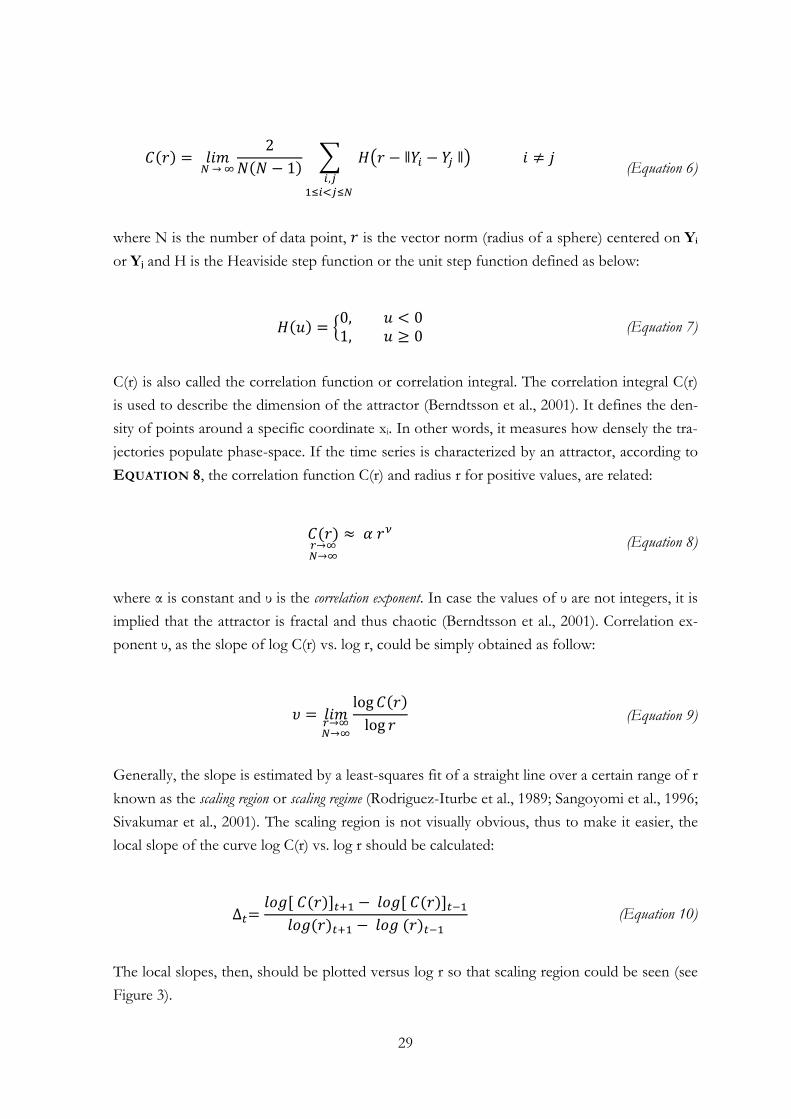
Generally, the slope is estimated by a least-squares fit of a straight line over a certain range of r

known as the scaling region or scaling regime (Rodriguez-Iturbe et al., 1989; Sangoyomi et al., 1996;

Sivakumar et al., 2001). The scaling region is not visually obvious, thus to make it easier, the

local slope of the curve log C(r) vs. log r should be calculated:

∆𝑡=𝑙𝑜𝑔 [ 𝐶(𝑟)]𝑡+1 − 𝑙𝑜𝑔 [ 𝐶(𝑟)]𝑡−1

𝑙𝑜𝑔 (𝑟)𝑡+1 − 𝑙𝑜𝑔 (𝑟)𝑡−1 (Equation 10)

The local slopes, then, should be plotted versus log r so that scaling region could be seen (see

Figure 3).

30

Figure 3. (a) log C(r) vs. log r for the time series of Great Salt Lake volume and (b) Local slope of the curve (a) vs. log r (Sangoyomi, Lall, & Abarbanel, 1996)

It has to be noted that Lai and Lerner (1998) have probed the dependency of the scaling re-

gion on fundamental parameters τ, m, and mτ. The results suggested that the effective linear

scaling region used for reliably estimating correlation dimension, is highly sensitive to the

choice of delay time employed in the phase-space reconstruction. It is always desirable to have

a larger scaling region to determine the slope, since the determination of the slope for a small-

er scaling region may be difficult and could possibly give rise to errors.

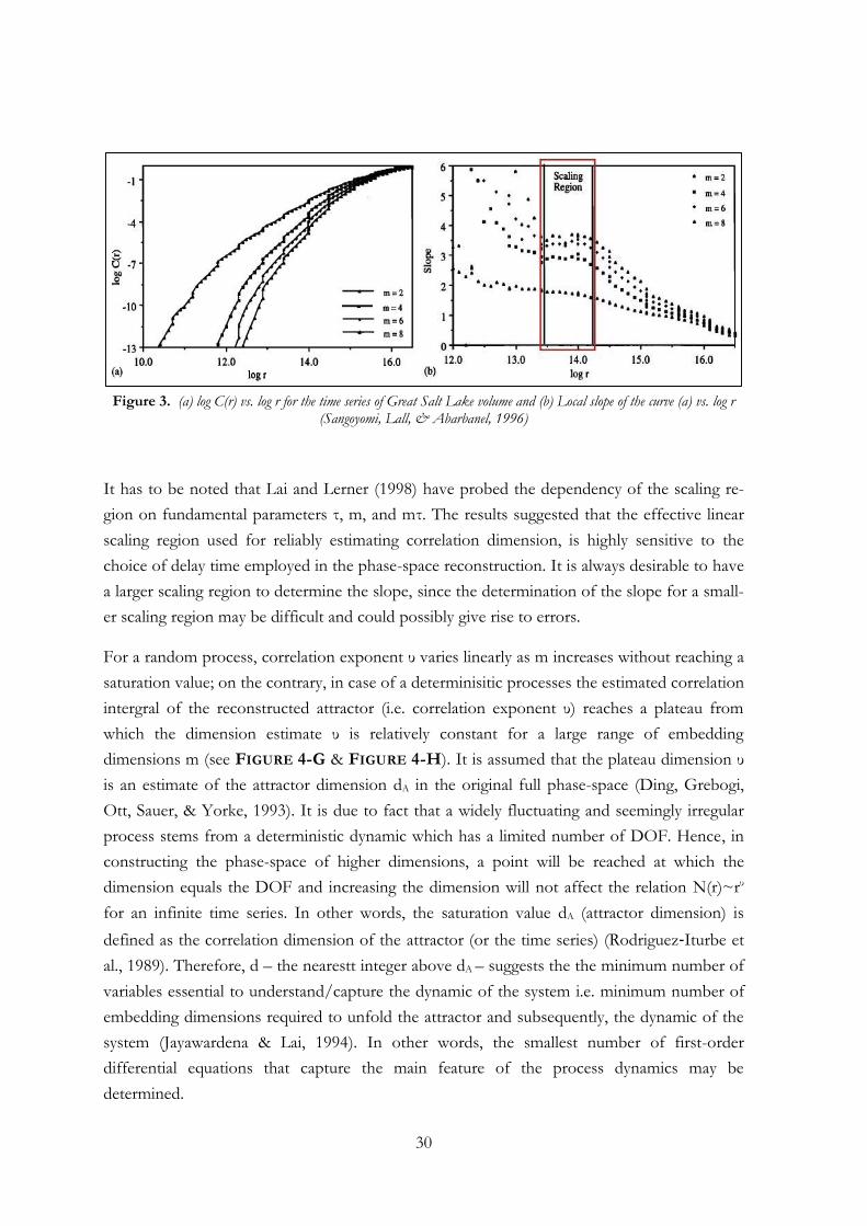
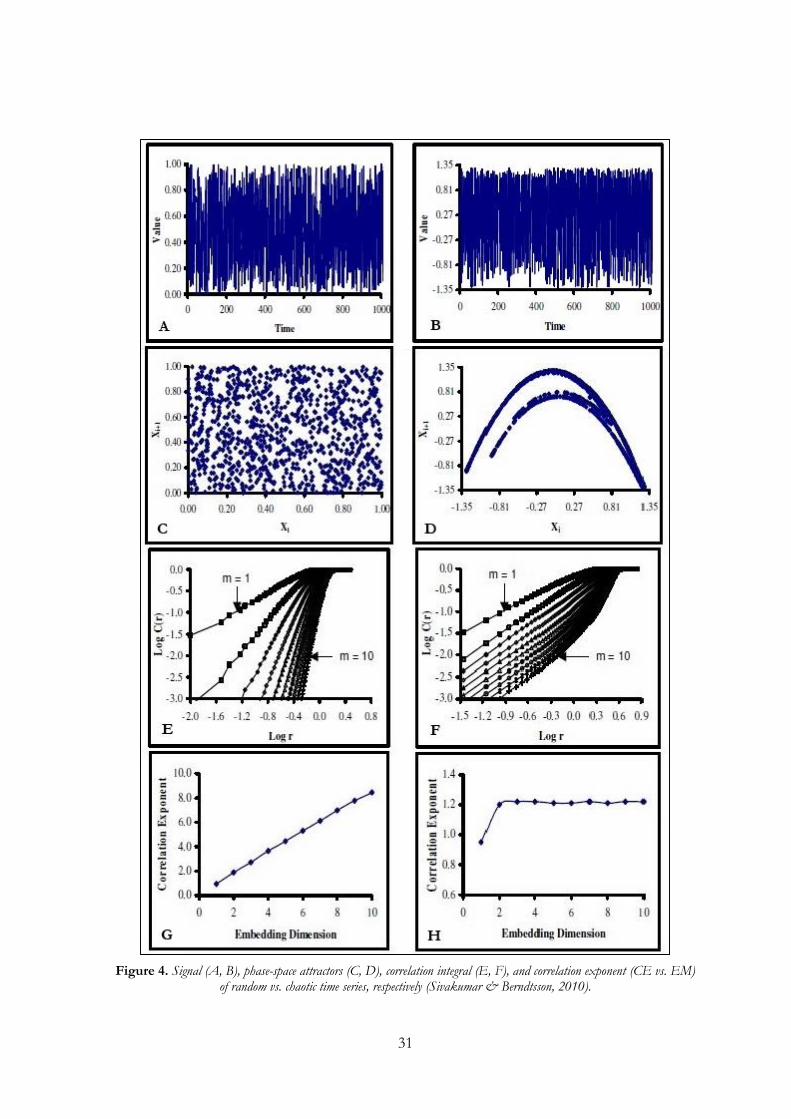
For a random process, correlation exponent υ varies linearly as m increases without reaching a

saturation value; on the contrary, in case of a determinisitic processes the estimated correlation

intergral of the reconstructed attractor (i.e. correlation exponent υ) reaches a plateau from

which the dimension estimate υ is relatively constant for a large range of embedding

dimensions m (see FIGURE 4-G & FIGURE 4-H). It is assumed that the plateau dimension υ

is an estimate of the attractor dimension dA in the original full phase-space (Ding, Grebogi,

Ott, Sauer, & Yorke, 1993). It is due to fact that a widely fluctuating and seemingly irregular

process stems from a deterministic dynamic which has a limited number of DOF. Hence, in

constructing the phase-space of higher dimensions, a point will be reached at which the

dimension equals the DOF and increasing the dimension will not affect the relation N(r)~rυ

for an infinite time series. In other words, the saturation value dA (attractor dimension) is

defined as the correlation dimension of the attractor (or the time series) (Rodriguez‐Iturbe et

al., 1989). Therefore, d – the nearestt integer above dA – suggests the the minimum number of

variables essential to understand/capture the dynamic of the system i.e. minimum number of

embedding dimensions required to unfold the attractor and subsequently, the dynamic of the

system (Jayawardena & Lai, 1994). In other words, the smallest number of first-order

differential equations that capture the main feature of the process dynamics may be

determined.

31

Figure 4. Signal (A, B), phase-space attractors (C, D), correlation integral (E, F), and correlation exponent (CE vs. EM) of random vs. chaotic time series, respectively (Sivakumar & Berndtsson, 2010).

32

There could be a suspicion of stochastic chaos when one deals with a low-length finite data

(Schertzer et al., 2002). Phase-space – or better say pseudophase-space – could be a helpful

tool for providing reliable evidence that the system is not stochastic indeed. In case of a sto-

chastic time series, one would expect a space-filling phase-space diagram in all embedding di-

mensions m. (see FIGURE 4-C) Nonetheless, Figure 4 vividly represents that despite the

phase-space of a purely stochastic time series (FIGURE 4-C), when phase-space of a chaotic

time series is embedded in a 2-dimensional space (FIGURE 4-D), it fills up the space only par-

tially. As it was mentioned earlier, for measuring the dimension of the strange attractor i.e.

correlation exponent, log C(r) vs. log r plot should be plotted. As it could be seen from FIG-

URE 4, in case of a stochastic process (FIGURE 4-G), the correlation exponent is increasing as

the embedding dimension increases. However, for a chaotic process (FIGURE 4-H), correla-

tion exponent saturates beyond a certain embedding dimension.

33

4 RESULTS & DISCUSSIONS

A series of 62 solute transport signals are examined using the nonlinear analysis of Correlation

Dimension Method. The results of CE vs. EM for all signals have been analyzed both individ-

ually and comparatively; measurements are assessed horizontally and vertically in order to ob-

tain a larger scheme of the ST dynamics considering the variation of depth and soil horizon.

The results generally imply the nonlinear low-dimensional nature of solute transport process.

That is, the dynamics are dominantly governed by a few variables, majorly on the order of 2-4

– with a few exceptions. Although the nature of the studied time series in this project are dif-

ferent from previous ones, the results are in a good agreement with the correlation dimensions

that have been reported by previous studies on subsurface hydrology. Faybishenko (2002) has

reported CD of 2-4 for the flow processes in the unsaturated fractured-rock system for both

laboratory and field dripping-water experiments. Sivakumar et al. (2005) have also computed

correlation dimensions of 2-3 for simulated solute transport through the two and three facies

media in a heterogeneous aquifer medium. Even so, there is still an essential difference be-

tween the results and implications of this study and prior ones – chaotic analysis of hydrologic

time series using CDM. This difference together with its probable causes are discussed.

4.1. Analysis

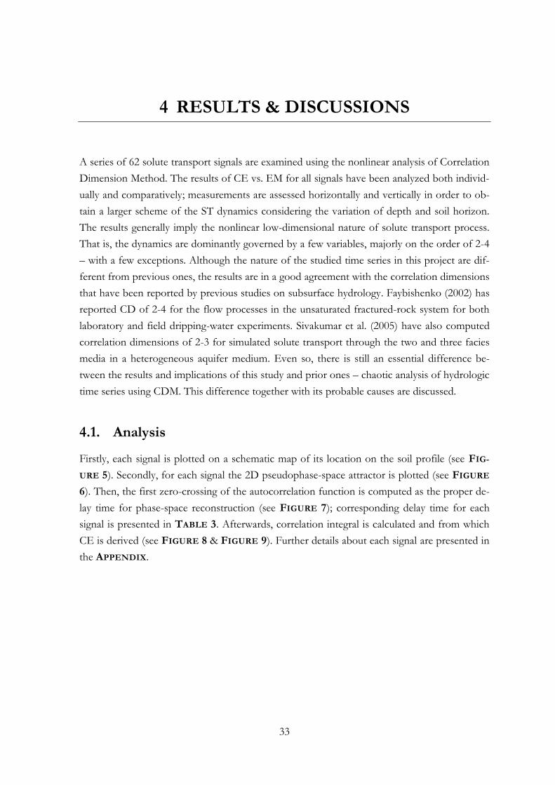
Firstly, each signal is plotted on a schematic map of its location on the soil profile (see FIG-

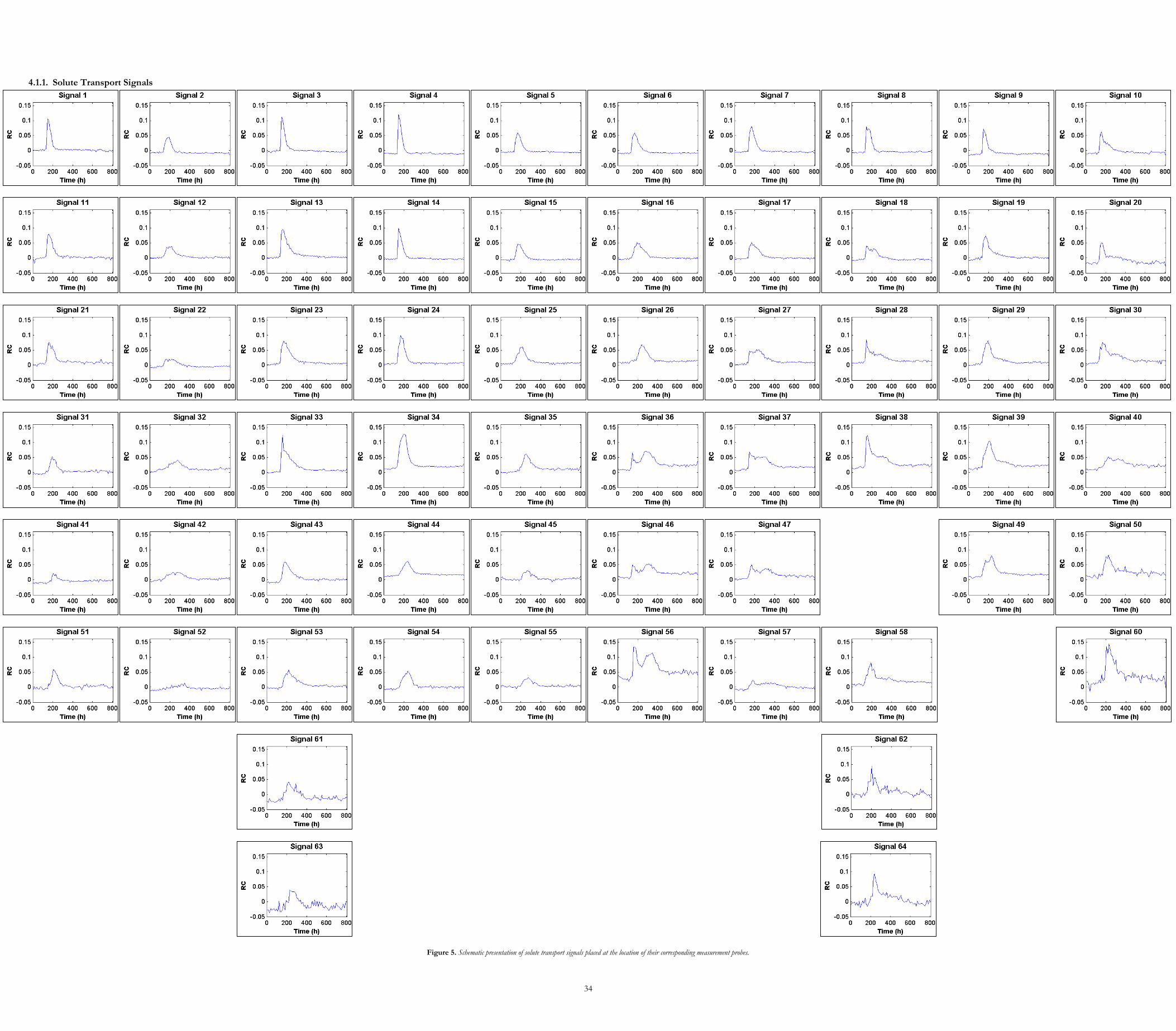
URE 5). Secondly, for each signal the 2D pseudophase-space attractor is plotted (see FIGURE

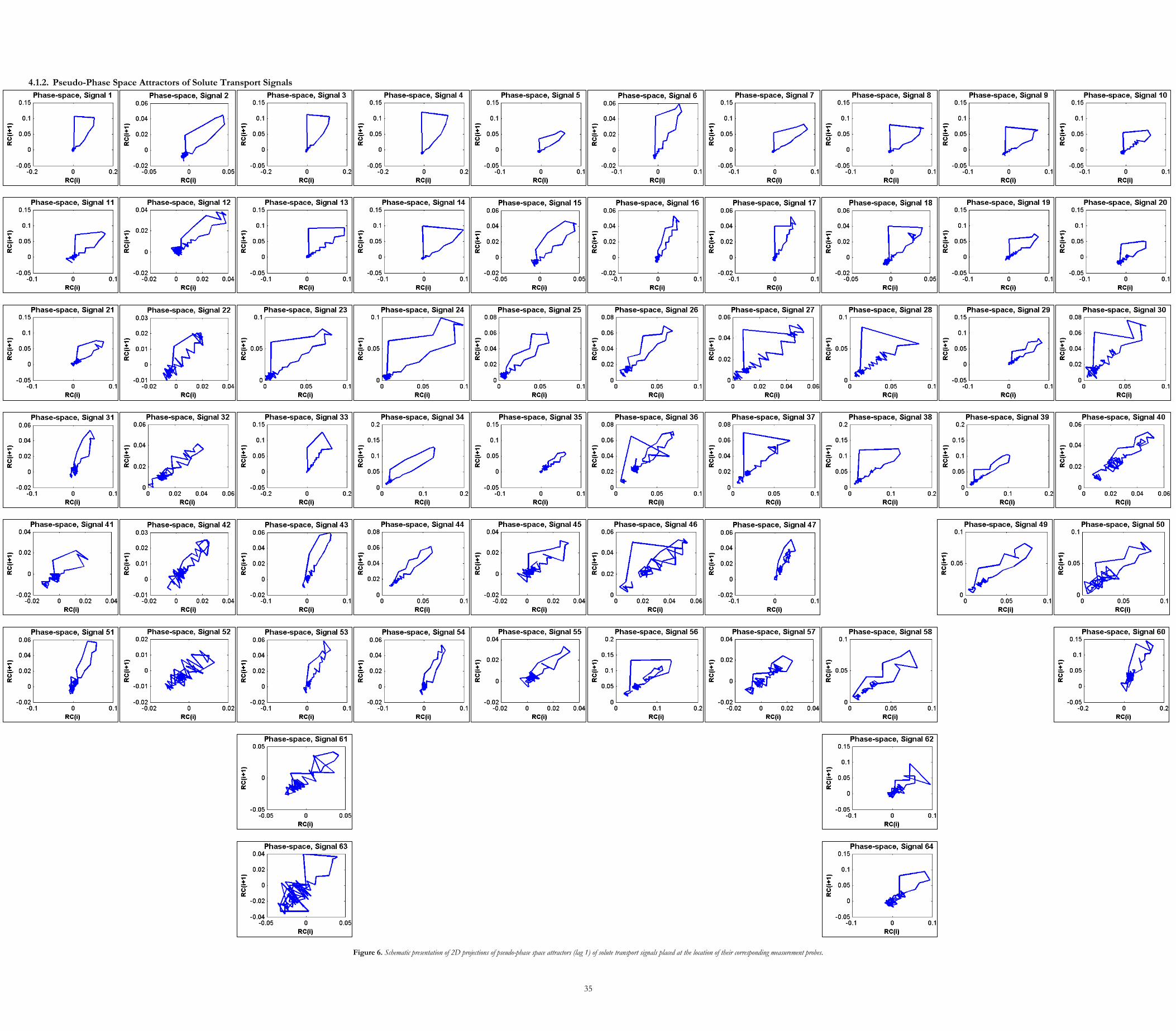
6). Then, the first zero-crossing of the autocorrelation function is computed as the proper de-

lay time for phase-space reconstruction (see FIGURE 7); corresponding delay time for each

signal is presented in TABLE 3. Afterwards, correlation integral is calculated and from which

CE is derived (see FIGURE 8 & FIGURE 9). Further details about each signal are presented in

the APPENDIX.

34

4.1.1. Solute Transport Signals

Figure 5. Schematic presentation of solute transport signals placed at the location of their corresponding measurement probes.

35

4.1.2. Pseudo-Phase Space Attractors of Solute Transport Signals

Figure 6. Schematic presentation of 2D projections of pseudo-phase space attractors (lag 1) of solute transport signals placed at the location of their corresponding measurement probes.

36

4.1.3. Autocorrelation

Figure 7. Schematic presentation of autocorrelation diagrams of solute transport signals placed at the location of their corresponding measurement probes.

37

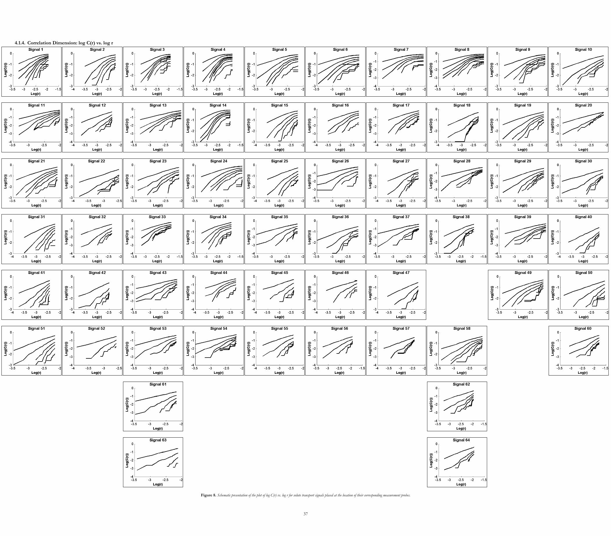
4.1.4. Correlation Dimension: log C(r) vs. log r

Figure 8. Schematic presentation of the plot of log C(r) vs. log r for solute transport signals placed at the location of their corresponding measurement probes.

38

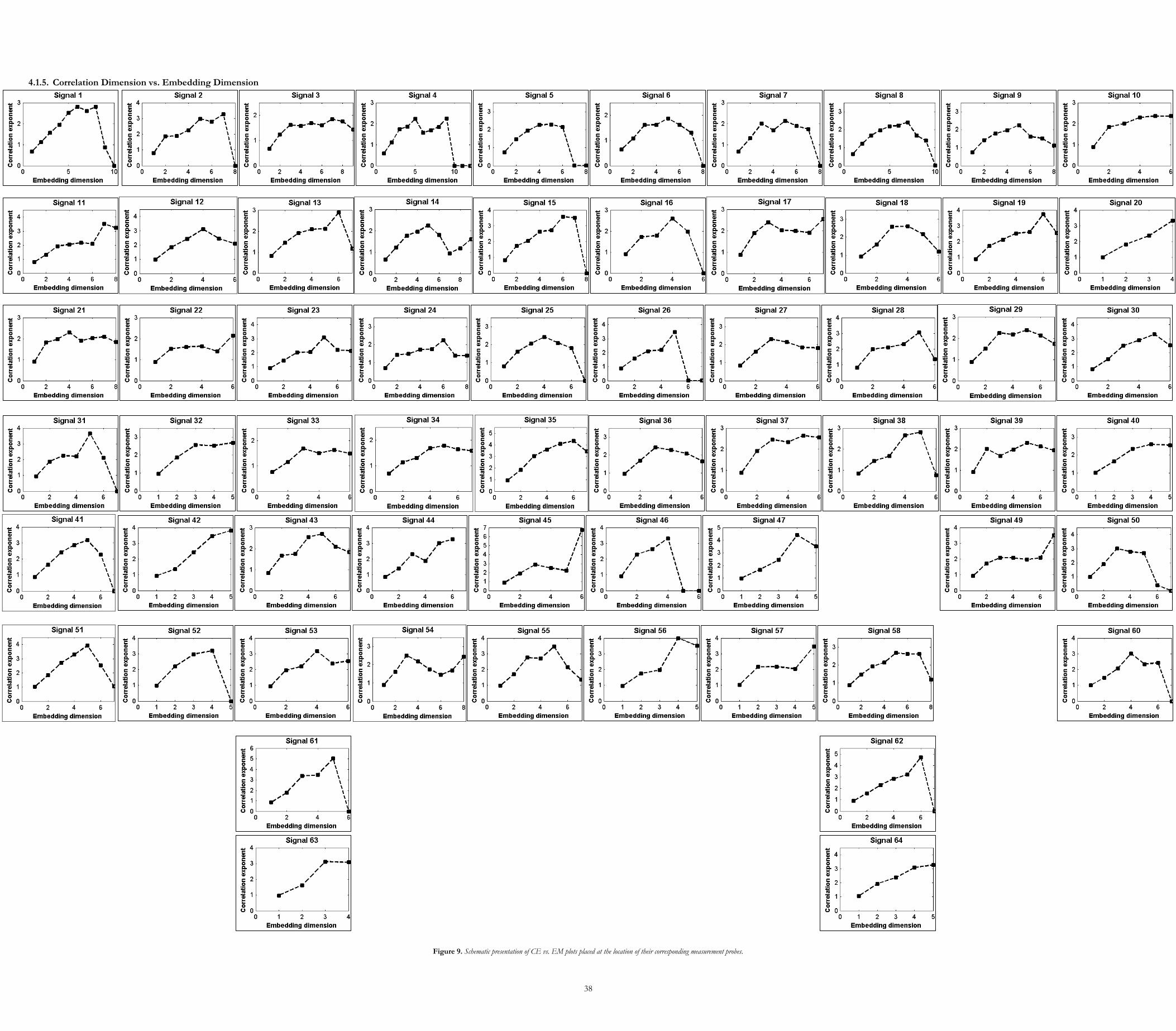
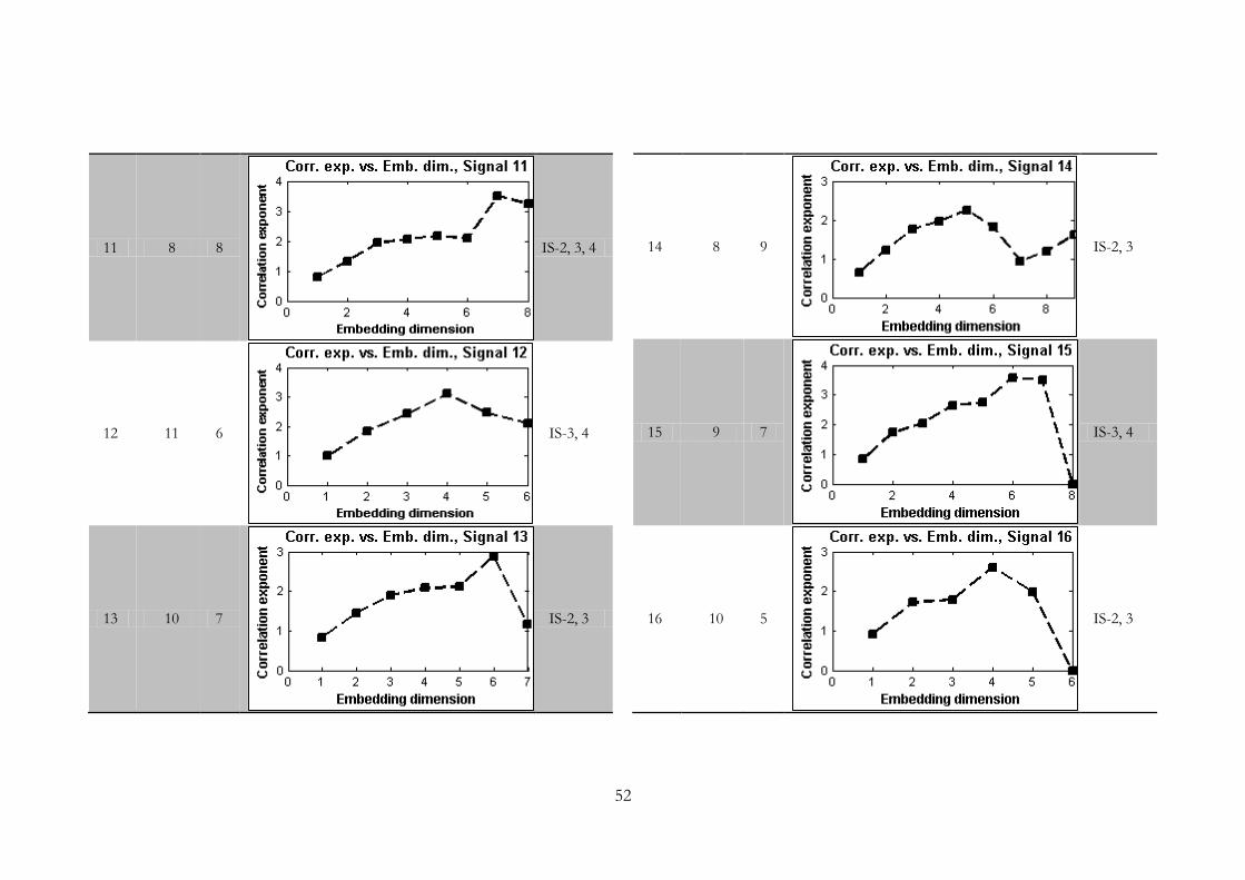
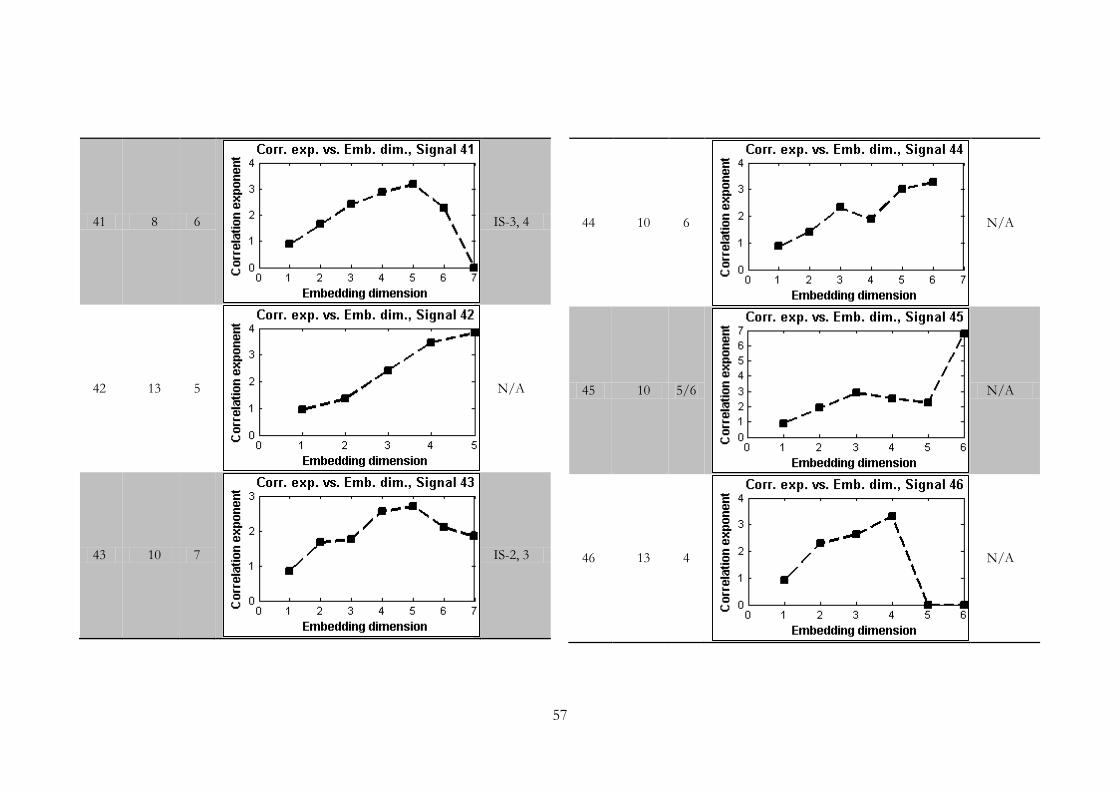
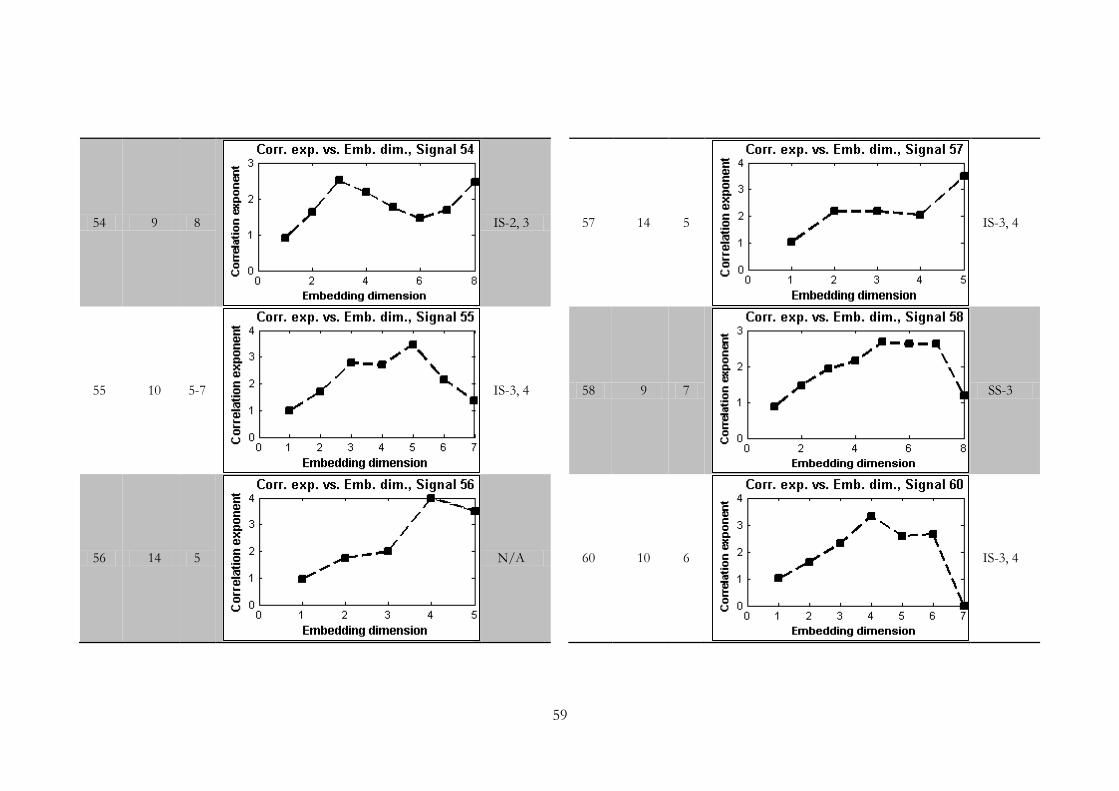
4.1.5. Correlation Dimension vs. Embedding Dimension

Figure 9. Schematic presentation of CE vs. EM plots placed at the location of their corresponding measurement probes.

39

4.2. Discussion of the Results

4.2.1. Time Series Length

No study has so far investigated such short time series (68 data points) using nonlinear chaotic

techniques. For one reason, it is normally presumed that short time series do not contain

enough information about the evolution of the given dynamic system to be captured, there-

fore, time series length is a limiting factor for CDM analysis. As it is discussed by Khatami

(2013), due to inherent qualitative characteristics that would be different in dynamical systems,

it is not practically nor theoretically possible to formulate a criterion of minimum data length.

So far, the shortest time series – to the knowledge of author – analyzed by CDM are

(Sivakumar, 2005):

100-point time series for an artificially generated chaotic time series (using the Henon

map equation)

and 360-point time series for a hydrological data set (real monthly flow series from

Göta River basin, Sweden (Sivakumar et al., 2001) where generating mechanisms are

not known a priori.

Nonetheless, the results of the present study suggest that short time series might contain es-

sential information about the characteristics of their generating dynamics as it is well reflected

in CE vs. EM dimensions. This is implying that no time series should be ruled out of chaotic

investigation solely due to its size; even short hydrologic time series are potential to reveal

fundamental information about the underlying dynamics of their processes.

4.2.2. Classification of the Dynamics

As it is thoroughly explained by Khatami (2013) the diagram of CE vs. EM could be used in

order to differentiate stochastic and chaotic systems considering that their characteristics are

known a priori. In case of a stochastic process, there is a linear relationship of υ=m for any m

(see FIGURE 4-G). On the other hand, for a chaotic time series the υ is increasing as m in-

creases on the basis of υ=m (in practice it is υ≈m) until a certain m at which υ saturates (see

FIGURE 4-H). Be that as it may, for hydrologic time series, which their characteristics are not

known a priori, it would not always be a clear steady saturation. Therefore, the nature of hydro-

logical processes is an ongoing question, deterministic chaotic versus stochastic.

Due to possible causes, which will be discussed in SECTION 4.2.2.1, in some cases there are

instable or fluctuating saturations that in this study are called Instable Saturation (IS) as op-

posed to Stable Saturation (SS) where a clear steady saturation is evident. Therefore, the re-

40

sults of this investigation are classified into two groups of SS and IS. In each case, the value(s)

of the (potential) correlation dimension(s), i.e. number of autonomous ODE needed to de-

termine the dynamic of the system, is (are) presented in TABLE 3. For instance, in case of

SIGNAL 3 there is a steady saturation of CE with CD=2 (coded as SS-2); while for SIGNAL 4

the saturation is instable and CE values are fluctuating between 2 and 3 (coded as IS-2, 3). In

some cases such as SIGNAL 49 correlation exponents are varying between more than two val-

ues. Nonetheless, in cases like SIGNAL 18, SIGNAL 47, SIGNAL 51 and etc. it is difficult to

easily classify the signals as either SS or IS. Such signals are coded as N/A.

In order to clearly demonstrate the saturation of CE values after a certain m, generally in cha-

os studies, CEs are computed and presented for embedding dimensions up to 10 or 20. How-

ever, in this study as time series are very short for CDM analysis, CEs could not usually be

calculated for embedding dimensions greater than 7 (see FIGURE 9). In many cases, regardless

of stable or instable saturation, there is a breakdown in CE values after a certain m. For exam-

ple, in case of SIGNAL 1 and after EM=8, CE values start breaking down to zero. Therefore,

in TABLE 3 the maximum number of EMs until which the computed CEs are considered to

be valid are presented. It should be noted that one should make a distinction between a

breakdown, which is due to data size, and fluctuations of correlation exponents (SS vs. IS)

which in not necessarily due to data length (see SECTION 4.2.2.1).

The values of correlation dimensions for signals with stable saturation are either 2 or 3, among

which CD=3 is the most frequent. In the study by Sivakumar et al. (2005) the CD values for

simulated solute transport were also 2 and 3. In case of instable saturation, however, CD val-

ues are varying between 2 and 4 from which IS-2, 3 is the most frequent one.

4.2.2.1. Stability vs. Instability

Instability in the CE saturation of solute transport signals could be explained from three

standpoints: (1) the data properties, (2) numerical computation, and (3) the physical process of

solute transport – and certainly a combination of the above.

(1) Using a short time series of a given dynamic for the CDM could result in a significant un-

derestimation of the CD value. Further, the presence of noise in the observed data may lead to

an overestimation of the CD (Ma, 2013). However, in this study the CD values are in good

agreement with previous studies by (Faybishenko, 2002; Sivakumar et al., 2005); in both cases

of SS and SI signals, the CD values are in the range of 2-4. Therefore, it could be argued that

the data properties (size and noise) may not significantly influence the CD values (at least its

order of magnitude), but the instability in the CE values in SI cases could be due to the noise

and the limited length of the signals.

41

(2) In addition to the data properties, numerical computation could be a source for the insta-

bilities. In essence, correlation integral is the normalized count of the points inside a cir-

cle/sphere/hyper-sphere centered about an arbitrary point of the m-dimensional set of vec-

tors (see FIGURE 2, SECTION 3.2). Further, determining the scaling region is the main prob-

lem with many of the earlier methods to estimate correlation dimension (Judd, 1992). There-

fore, it is difficult to solely rely on CDM results in order to obtain intrinsic information about

the underlying mechanism of solute transport process.

(3) Another explanation for the fluctuation of CE values is from a different perspective than

the previous two. The previous two explanations are discussing the SI from a mathemati-

cal/numerical view point. Nonetheless, it is worthwhile to bring a physical interpretation into

the discussion. On a more sophisticated level, the CE variations could be due to instability on

a far more complex level; a highly complex nonlinear system of preferential flows formation

and solute transport. Although there is a link between preferential flows and solute transport

to some extent (e.g. solutes can travel from macropores out to the soil matrix during low flow

periods), they are two isolated processes. Strictly speaking, formation of preferential flows is a

4D system. It is a spatially dependent time variant process. In other words, it is dependent on

specifics such as soil properties, texture, structure, seasonal variabilities, etc. It is also a delicate

function of time. Assuming the preferential flows to be constant – the path is not changing

throughout time and space – the solute transport process itself could be chaotic, i.e., deter-

ministic but highly instable due to crucial dependence on initial conditions. ST process, how-

ever, is interconnected to the process of preferential flow formation. In fact, they are highly

interactive. In fact, preferential flows could be chaotic as well. Consequently, the combination

of these two supposedly chaotic systems could lead to a highly instable nonlinear dynamical

system where the generating mechanisms, both the mechanisms and their numbers, could vary

throughout time and space. As much tentative is this speculation, studies on solute transport

process using large data matrices (long solute transport signals on a soil profile) could test this

hypothesis.

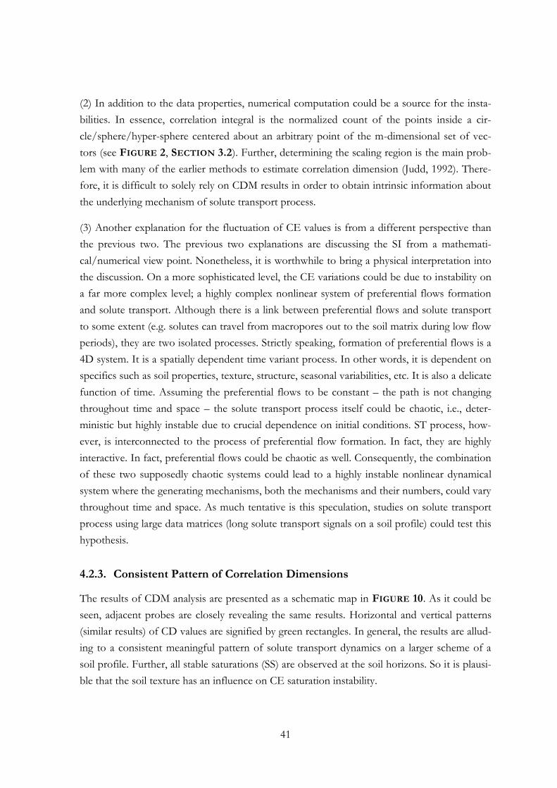
4.2.3. Consistent Pattern of Correlation Dimensions

The results of CDM analysis are presented as a schematic map in FIGURE 10. As it could be

seen, adjacent probes are closely revealing the same results. Horizontal and vertical patterns

(similar results) of CD values are signified by green rectangles. In general, the results are allud-

ing to a consistent meaningful pattern of solute transport dynamics on a larger scheme of a

soil profile. Further, all stable saturations (SS) are observed at the soil horizons. So it is plausi-

ble that the soil texture has an influence on CE saturation instability.

42

Figure 10. Scaled schematic map of CDM results. The results are presented at the locations of solute transport measurement probes; similar patterns of CD are discerned by colored rectangles, and soil horizons by double waved lines.

43

It is important to note that the results of CDM analysis, i.e. CD values, and pseudo-phase

space attractors are complementary. Although at lower levels it is not possible to get meaning-

ful results from the CDM analysis (it is shown as N/A), the solute transport attractors are be-

coming more evident (see FIGURE 9). Therefore, in case CDM do not yield a meaningful CD

values one cannot reject the possibility of low-dimensional chaos in the given system. It simp-

ly means that CDM cannot be applied for that specific data set and resolution. . In some cases,

CDM could be applied to the time series by changing the temporal resolution of data.

Application of chaos, in general, and CDM, in particular, for hydrological studies has been

criticized previously (Koutsoyiannis, 2006; Schertzer et al., 2002). Although the criticisms have

been answered widely (Khatami, 2013; Ma, 2013; Sivakumar, 2000; Sivakumar, 2005;

Sivakumar, Berndtsson, Olsson, & Jinno, 2002; Sivakumar, Persson, et al., 2002), it is vitally

important to employ other chaotic methods such as Gaussian Kernel Algorithm (GKA) as

well (Yu, Small, Harrison, & Diks, 2000). Scaling regions are problematic in chaos studies and

GKA avoids some of these problems. Nonetheless, one is still fitting a function to a distribu-

tion and some problems remain. Further, other phase-space constructions should be engaged

in ‘hydro-chaotic’1 analyses. Revisiting previous studies with other chaotic methodologies

would strengthen the argument for chaos determinism in hydrology and could promote break-

throughs in the field.

It is crucially important to note that the discussion on the present results could not be too de-

tailed. Fist, although the observations are comprehensive in terms of collection from soil pro-

file, there are limited to the soil type, data size, and existence of noise. Therefore, observation

in other soil types are needed to confirm the results. As huge observed data sets could not be

prepared easily, lab experiments are inevitable. Therefore, the next phase of this research will

engage experimental data to see to what extent their outcome could be related to the field

studies results.

1 Hydrological studies that are using chaotic approaches for system identification, prediction, noise reduction or other purposes.

44

45

5 CONCLUSION

The physics behind the temporal and spatial instabilities of flow (in unsaturated media) is still

of question. Therefore, the main objective of the present study was to investigate the potential

utilization of a nonlinear deterministic framework for understanding the underlying dynamics

of solute transport processes. Pursuing this objective, the nonlinear chaotic technique of cor-

relation dimension method is employed to study short signals of solute transport (68 data

points). Correlation dimension method can provide an assessment of the minimum number of

processes that are governing a given dynamical system. Several issues have been raised against

the application of chaos, in general, and CDM, in particular, for hydrological studies. Almost

all these issues have been addressed by previous studies. Further, the consistent results of ‘hy-

dro-chaotic’ are strengthening the interest in using CDM and other chaotic approaches in this

area.

What make the present hydro-chaotic study special are:

(1) the field of interest is subsurface process of solute transport than surface hydrology,

(2) extremely short time series (68 points) are used,

(3) and the spatial distribution of data set is taken into account, i.e., solute transport on a

soil profile.

The results of CE vs. EM for all signals have been analyzed both individually and compara-

tively; measurement are assessed horizontally and vertically in order to obtain a larger scheme

of the ST dynamics considering the variation of depth and soil horizon. Despite previous

studies, the CE vs. EM is not always a stable saturated figure; therefore, there are two types of

stable and instable saturations. The instability in the saturation of CE values could be ex-

plained by (1) data properties (data size and noise), (2) numerical computation (scaling region

and phase-space reconstruction), and (3) physical interpretation.

The main results of this study could be summarized as follow:

a) The outcome of CDM analyses suggest that the number of governing equations for

solute transport are as low as 2-4 – i.e. low dimensional determinism. A consistent pat-

tern has been observed in CD on the soil profile.

b) Despite the claim of previous studies, time series length is not a limiting factor for hy-

dro-chaos studies. Even short hydrologic time series are potential to reveal fundamen-

tal information about the underlying dynamics of a given process. The results of a

short time series of only 68 data points, are in fairly good agreement with previous

studies.

46

c) Instability in the CE saturation of IS signals could be interpreted – only a speculation

– as instability in the underlying dynamics of this process. Number of variables gener-

ating the mechanism are transitionally changing as the system evolves. In other words,

depending on the status of the system throughout its evolution, number of determin-

ing variables – and most probably variables themselves – are changing; therefore, the

dimension of the attractor is varying between different values. Consequently, no stable

saturation could be observed.

The concluding remark from this study is therefore formed as a hypothesis. The implication

of this hypothesis would be that although it is presumed that there are universal equations

governing the solute transport process, the local conditions (soil texture and structure, soil

horizon, elevation, preferential flows and macro pores, soil moisture distribution, time of day,

evaporation, temperature and etc.) could intrinsically influence/change the dynamic of the

process. In other words, the governing equations could change both spatially and temporally.

47

References

Addiscott, T. M., & Mirza, N. A. (1998). New paradigms for modelling mass transfers in soils. Soil and Tillage Research, 47(1–2), 105-109. doi: http://dx.doi.org/10.1016/S0167-1987(98)00081-6

Berndtsson, R., Uvo, C., Matsumoto, M., Jinno, K., Kawamura, A., Xu, S., & Olsson, J. (2001). Solar-climatic relationship and implications for hydrology. Nordic hydrology, 32(2), 65-84.

Broer, H., & Takens, F. (2011). Dynamical systems and chaos (Vol. 172): Springer. Ding, M., Grebogi, C., Ott, E., Sauer, T., & Yorke, J. A. (1993). Estimating correlation

dimension from a chaotic time series: when does plateau onset occur? Physica D: Nonlinear Phenomena, 69(3), 404-424.

Faybishenko, B. (2002). Chaotic dynamics in flow through unsaturated fractured media. Advances in water resources, 25(7), 793-816. doi: http://dx.doi.org/10.1016/S0309-1708(02)00028-3

Flühler, H., Durner, W., & Flury, M. (1996). Lateral solute mixing processes — A key for understanding field-scale transport of water and solutes. Geoderma, 70(2–4), 165-183. doi: http://dx.doi.org/10.1016/0016-7061(95)00079-8

Gidea, M., & Niculescu, C. P. (2002). Chaotic dynamical systems: An introduction: Universitaria Press Craiova.

Grassberger, P., & Procaccia, I. (1983). Measuring the strangeness of strange attractors. Physica D: Nonlinear Phenomena, 9(1), 189-208.

Gray, W. G., & Hassanizadeh, S. M. (1991). Paradoxes and realities in unsaturated flow theory. Water resources research, 27(8), 1847-1854.

Hillel, D. (1987). Unstable flow in layered soils: A review. Hydrological Processes, 1(2), 143-147. Ivancevic, V. G., & Ivancevic, T. T. (2008). Complex Nonlinearity: Chaos, Phase Transitions,

Topology Change, and Path Integrals. Verlag Berlin Heidelberg: Springer. Jayawardena, A., & Lai, F. (1994). Analysis and prediction of chaos in rainfall and stream flow

time series. Journal of Hydrology, 153(1), 23-52. Judd, K. (1992). An improved estimator of dimension and some comments on providing

confidence intervals. Physica D: Nonlinear Phenomena, 56(2–3), 216-228. doi: http://dx.doi.org/10.1016/0167-2789(92)90025-I

Khatami, S. (2013). Nonlinear Chaotic and Trend Analyses of Water Level at Urmia Lake, Iran. M.Sc. Thesis report: TVVR 13/5012, ISSN:1101-9824, Lund: Lund University.

Koutsoyiannis, D. (2006). On the quest for chaotic attractors in hydrological processes. Hydrological Sciences Journal, 51(6), 1065-1091.

Lai, Y.-C., & Lerner, D. (1998). Effective scaling regime for computing the correlation dimension from chaotic time series. Physica D: Nonlinear Phenomena, 115(1), 1-18.

Ma, M. (2013). Correlation Dimension analysis of complex hydrological systems: what information can the method provide? (Doctoral Dissertation), Freie Universität Berlin, Berlin. Retrieved from http://www.diss.fu-berlin.de/diss/receive/FUDISS_thesis_000000094635 (103687284X)

Packard, N., Crutchfield, J., Farmer, J., & Shaw, R. (1980). Geometry from a time series.

Persoff, P., & Pruess, K. (1995). Two‐Phase Flow Visualization and Relative Permeability

Measurement in Natural Rough‐Walled Rock Fractures. Water resources research, 31(5), 1175-1186.

48

Persson, M. (1999). Conceptualization of solute transport using time domain reflectometry. A combined laboratory and field study. Lund University, Lund, Sweden. Retrieved from http://www.lunduniversity.lu.se/o.o.i.s?id=24965&postid=39605 (LUTVDG/TVVR-1025(1999))

Persson, M., & Berndtsson, R. (2002). Transect scale solute transport measured by time domain reflectometry. Nordic hydrology, 33(2-3), 145-164.

Puente, C. E., & Obregón, N. (1996). A deterministic geometric representation of temporal rainfall: Results for a storm in Boston. Water resources research, 32(9), 2825-2839.

Rodriguez-Iturbe, I., Entekhabi, D., Lee, J.-S., & Bras, R. L. (1991). Nonlinear Dynamics of Soil Moisture at Climate Scales: 2. Chaotic Analysis. Water resources research, 27(8), 1907-1915. doi: 10.1029/91WR01036

Rodriguez‐Iturbe, I., Febres De Power, B., Sharifi, M. B., & Georgakakos, K. P. (1989). Chaos in rainfall. Water resources research, 25(7), 1667-1675.

Sangoyomi, T. B., Lall, U., & Abarbanel, H. D. (1996). Nonlinear dynamics of the Great Salt Lake: dimension estimation. Water resources research, 32(1), 149-159.

Schertzer, D., Tchiguirinskaia, I., Lovejoy, S., Hubert, P., Bendjoudi, H., & LarchevÊQue, M. (2002). DISCUSSION of “Evidence of chaos in the rainfall-runoff process” Which chaos in the rainfall-runoff process? Hydrological Sciences Journal, 47(1), 139-148. doi: 10.1080/02626660209492913

Sharifi, M., Georgakakos, K., & Rodriguez-Iturbe, I. (1990). Evidence of deterministic chaos in the pulse of storm rainfall. Journal of Atmospheric Sciences, 47, 888-893.

Sivakumar, B. (2000). Chaos theory in hydrology: important issues and interpretations. Journal of Hydrology, 227(1), 1-20.

Sivakumar, B. (2005). Correlation dimension estimation of hydrological series and data size requirement: myth and reality/Estimation de la dimension de corrélation de séries hydrologiques et taille nécessaire du jeu de données: mythe et réalité. Hydrological Sciences Journal, 50(4).

Sivakumar, B., & Berndtsson, R. (2010). Nonlinear dynamics and chaos in hydrology Advances in Data-Based Approaches for Hydrologic Modeling and Forecasting (pp. 411-461).

Sivakumar, B., Berndtsson, R., Olsson, J., & Jinno, K. (2001). Evidence of chaos in the rainfall-runoff process. Hydrological Sciences Journal, 46(1), 131-145.

Sivakumar, B., Berndtsson, R., Olsson, J., & Jinno, K. (2002). Reply to “Which chaos in the rainfall-runoff process?”. Hydrological Sciences Journal, 47(1), 149-158.

Sivakumar, B., Harter, T., & Zhang, H. (2005). Solute transport in a heterogeneous aquifer: a search for nonlinear deterministic dynamics. Nonlinear Processes in Geophysics, 12(2), 211-218.

Sivakumar, B., & Jayawardena, A. (2002). An investigation of the presence of low-dimensional chaotic behaviour in the sediment transport phenomenon. Hydrological Sciences Journal, 47(3), 405-416.

Sivakumar, B., Liong, S.-Y., Liaw, C.-Y., & Phoon, K.-K. (1999). Singapore rainfall behavior: chaotic? Journal of Hydrologic Engineering, 4(1), 38-48.

Sivakumar, B., Persson, M., Berndtsson, R., & Uvo, C. B. (2002). Is correlation dimension a reliable indicator of low-dimensional chaos in short hydrological time series? Water resources research, 38(2), 1011.

Sivakumar, B., Woldemeskel, F. M., & Puente, C. E. (2013). Nonlinear analysis of rainfall variability in Australia. Stochastic Environmental Research and Risk Assessment, 1-11.

Steenhuis, T., Vandenheuvel, K., Weiler, K., Boll, J., Daliparthy, J., Herbert, S., & Kung, K. J. S. (1998). Mapping and interpreting soil textural layers to assess agri-chemical movement at several scales along the eastern seaboard (USA). In P. Finke, J. Bouma &

49

M. Hoosbeek (Eds.), Soil and Water Quality at Different Scales (Vol. 80, pp. 91-97): Springer Netherlands.

Takens, F. (1981). Detecting strange attractors in turbulence Dynamical systems and turbulence, Warwick 1980 (pp. 366-381): Springer.

Yu, D., Small, M., Harrison, R. G., & Diks, C. (2000). Efficient implementation of the Gaussian kernel algorithm in estimating invariants and noise level from noisy time series data. Physical Review E, 61(4), 3750-3756.

50

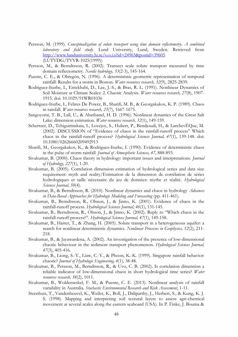
Appendix

The results for the 62 ST signals are encapsulated in the table below. Em refers to the value of EM until which computed correlation exponent could

be considered as valid. Class refers to stable/instable saturation followed by the value(s) of correlation dimension.

Table 3. Classified results of 62 solute transport signals.

Signal Delay, τ Em Results Class

1 7 8

SS-3

2 9 7

IS-3, 4

3 8 9

SS-2

4 6 9

IS-2, 3

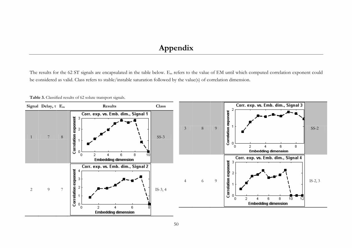
51

5 8 6

SS-3

6 9 6/7

IS-2, 3

7 9 7

IS-2, 3

8 7 9

IS-2, 3

9 9 8

IS-2, 3

10 11 6

SS-3

52

11 8 8

IS-2, 3, 4

12 11 6

IS-3, 4

13 10 7

IS-2, 3

14 8 9

IS-2, 3

15 9 7

IS-3, 4

16 10 5

IS-2, 3

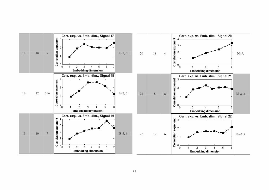
53

17 10 7

IS-2, 3

18 12 5/6

IS-2, 3

19 10 7

IS-3, 4

20 18 4

N/A

21 8 8

IS-2, 3

22 12 6

IS-2, 3

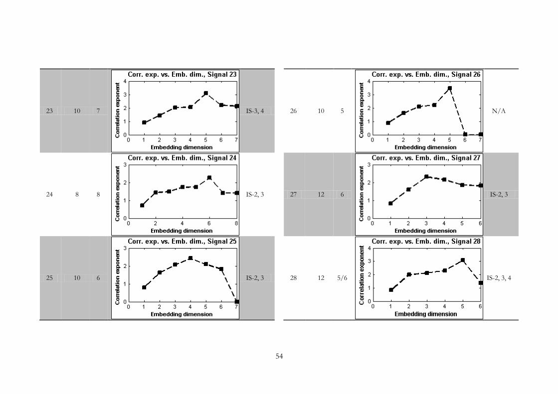
54

23 10 7

IS-3, 4

24 8 8

IS-2, 3

25 10 6

IS-2, 3

26 10 5

N/A

27 12 6

IS-2, 3

28 12 5/6

IS-2, 3, 4

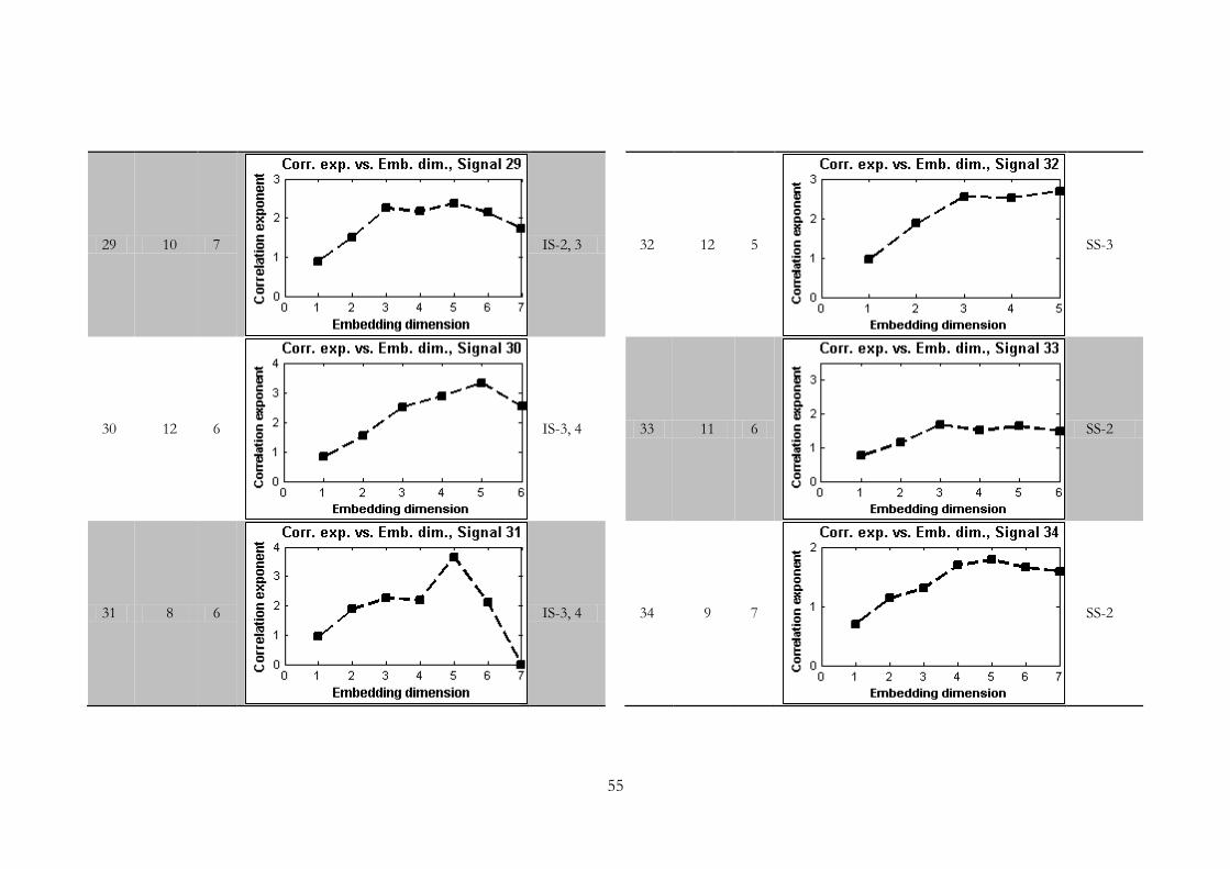
55

29 10 7

IS-2, 3

30 12 6

IS-3, 4

31 8 6

IS-3, 4

32 12 5

SS-3

33 11 6

SS-2

34 9 7

SS-2

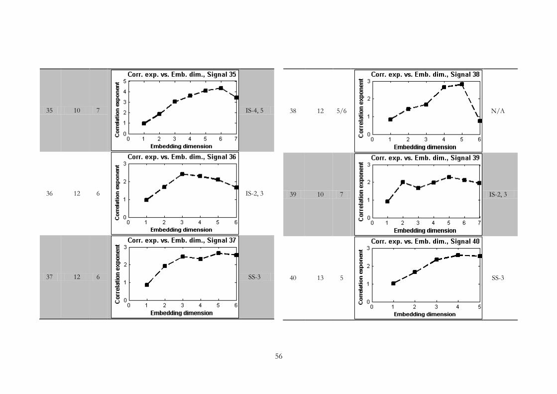
56

35 10 7

IS-4, 5

36 12 6

IS-2, 3

37 12 6

SS-3

38 12 5/6

N/A

39 10 7

IS-2, 3

40 13 5

SS-3

57

41 8 6

IS-3, 4

42 13 5

N/A

43 10 7

IS-2, 3

44 10 6

N/A

45 10 5/6

N/A

46 13 4

N/A

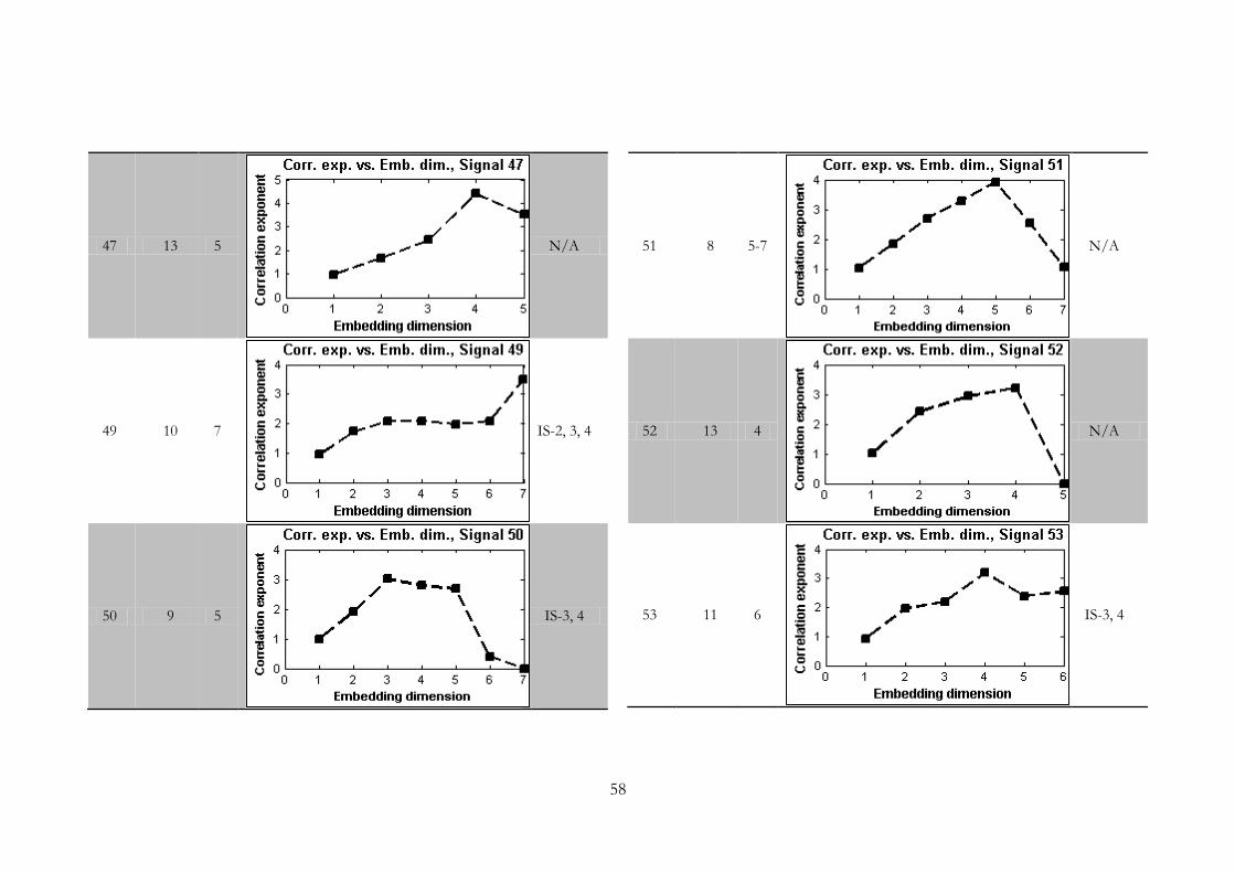
58

47 13 5

N/A

49 10 7

IS-2, 3, 4

50 9 5

IS-3, 4

51 8 5-7

N/A

52 13 4

N/A

53 11 6

IS-3, 4

59

54 9 8

IS-2, 3

55 10 5-7

IS-3, 4

56 14 5

N/A

57 14 5

IS-3, 4

58 9 7

SS-3

60 10 6

IS-3, 4

60

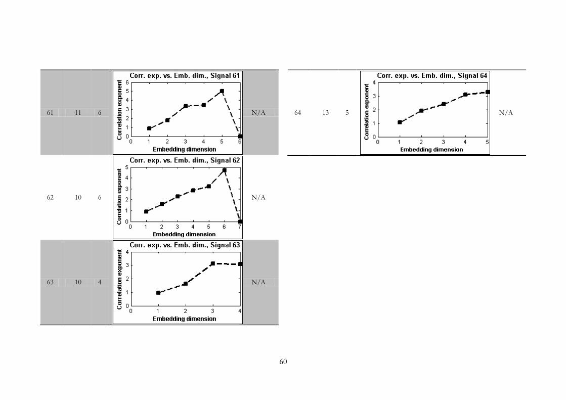
61 11 6

N/A

62 10 6

N/A

63 10 4

N/A

64 13 5

N/A

61