Evaluation of time varying stresses in a Howden fan - DiVA

Master's Thesis in Mechanical Engineering

Evaluation of time varying stresses in a Howden fan

Authors: Tim van Mierlo & Rafał Żywalewski Supervisor LNU: Andreas Linderholt Supervisor LNU: Yousheng Chen Examinar, LNU: Andreas Linderholt Course Code: 4MT01E Semester: Spring 2015, 15 credits Linnaeus University, Faculty of Technology

Abstract In this work, the time varying stresses in a Howden axial flow fan are obtained by finite element analyses. Dynamic substructuring is used to obtain accurate values of the stresses in the threads of the blade shaft, the component which connects the blade with the hub.

Three different global models are used to compare the influence of neglecting the fan shaft and the stiffness influence of the centrifugal force.

The relative displacements, which are obtained from the global models, have been used as boundary condition in the detailed models. The detailed models are used to obtain the Von Mises stresses in the root of the threads of the blade shaft. Finally the results of the three global models are compared with experimental measured data provided by Howden.

The experimental data results in the highest Von Mises stresses. The model with the fan shaft and the stiffness influence of the centrifugal force gives values for the Von Mises stresses which are approximately twenty percent lower. The model without the fan shaft results in the lowest stresses which are approximately forty percent lower than the stresses obtained using the measured data.

Key words: Finite element analyses, Dynamic substructuring, Axial flow fan, Blade, Rotor dynamics, Centrifugal force

III

Acknowledgement During this degree project, we gathered a lot of knowledge. We learned how to implement the theoretical knowledge of structural dynamics in a practical situation. We also learned about rotor dynamical systems and how to use SimXpert and Nastran.

This would not be possible without Howden Axial Fans, which gave us the opportunity to do this project. We especially want to thank Göran Kronmar and Henrik Tryggeson, who are both working at Howden Axial Fans in Växjö, for answering our questions during meetings and delivering information during this project. We appreciate their critical view and informal communication.

We also want to thank our supervisors from Linnaeus University, Andreas Linderholt and Yousheng Chen (Linnaeus University, Department of Mechanical Engineering, Växjö). Andreas especially for his help when we had difficulties with the use of SimXpert and Nastran. Yousheng especially for her feedback on all report parts. We really appreciate the fast responses on questions from both Andreas and Yousheng.

Rafał Żywalewski & Tim van Mierlo

Växjö 26th of May

IV

Table of contents 1. INTRODUCTION.......................................................................................................... 1

1.1 BACKGROUND ....................................................................................................................................... 1 1.2 DRAWINGS AND PICTURES OF THE HOWDEN FAN .................................................................................. 2

1.2.1 An exploded view of a Howden fan ............................................................................................... 2 1.2.3 Finite element model ..................................................................................................................... 2 1.2.4 Analysed part ................................................................................................................................ 3

1.3 AIM AND PURPOSE ................................................................................................................................ 4 1.4 LIMITATIONS ......................................................................................................................................... 4 1.5 RELIABILITY, VALIDITY AND OBJECTIVITY ............................................................................................ 4

2. THEORY ........................................................................................................................ 5

2.1 FINITE ELEMENT ANALYSES (FEA) ........................................................................................................ 5 2.2 DYNAMIC MOTION, EIGENVALUES/EIGENFREQUENCIES ......................................................................... 6 2.3 FREQUENCY RESPONSE FUNCTION (FRF) ............................................................................................... 8 2.4 DYNAMIC SUBSTRUCTURING ................................................................................................................. 9 2.5 FORCE DISTRIBUTION ON THE BLADES ................................................................................................. 11 2.6 ROTATING STRUCTURES ...................................................................................................................... 11

2.6.1 Vibrations ................................................................................................................................... 11 2.6.2 Centrifugal force ......................................................................................................................... 12

2.7 ROTATING STRUCTURES MODELLING ................................................................................................... 14 2.7.1 Nastran solution sequences ........................................................................................................ 15 2.7.2 Element types .............................................................................................................................. 15 2.7.3 Connecting 1D with 3D elements ............................................................................................... 16

3. METHOD ..................................................................................................................... 17

3.2 GLOBAL MODEL................................................................................................................................... 18 3.2.1 Component overview .................................................................................................................. 18 3.2.2 Simplified global models ............................................................................................................. 19 3.2.3 3D hub model design and simplification .................................................................................... 21 3.2.4 Shaft model ................................................................................................................................. 23 3.2.5 Mass and moment of inertia calculations ................................................................................... 23 3.2.6 Final models ............................................................................................................................... 24

3.3 DETAILED MODEL ................................................................................................................................ 29 3.3.1 Detailed blade shaft simulations ................................................................................................. 31

4. RESULTS AND ANALYSIS ...................................................................................... 34

4.1 GLOBAL MODEL................................................................................................................................... 34 4.1.1 Results- simplified models .......................................................................................................... 34 4.1.2 Global model eigenfrequencies .................................................................................................. 35 4.1.3 FRF ............................................................................................................................................. 36 4.1.4 Displacements ............................................................................................................................. 40

4.2 DETAILED MODEL ................................................................................................................................ 44

6. DISCUSSION ............................................................................................................... 47

7. CONCLUSIONS .......................................................................................................... 48

REFERENCES ................................................................................................................. 49

APPENDICES .................................................................................................................. 50

V

1. Introduction The axial flow fan is a machine used in many industries such as mining, power generation and industrial processes. The main task of a fan is to deliver flow of air or gas with a specified flow and pressure. A typical axial fan consists of a number of blades connected to a hub and a shaft which is driven by an electric motor. These components are fitted in a housing forcing the air to move parallel to the shaft axis. Fans produce high flows with a low air pressure.

Howden is a manufacturer of axial flow fans. It is an international company with offices all over the world. Howden has over 50 years of experience in the design of variable pitch axial fans [1]. For these rotating machines having large dimensions and weights, the strength calculations are very important. Nowadays it is possible to predict the behaviour of the structure during its motion by use of finite element analyses (FEA). The analysed fan is one of the larger axial fans manufactured by Howden. The diameter of the impeller reaches approximately three meters. The rotational speed is constant; approximately 900 rotations per minute. Due to its size, mass (approximately 16 tonnes) and speed, big forces appear in the structure. The company is interested in calculations of time varying stresses in the fan. The reason is a need to predict and optimize the lifetime of their product. It assures better maintenance, safety and reduces costs.

1.1 Background

The main focus is put on the threaded blade shaft, which connects the blades to the hub. This area is considered as a place where the most critical stresses occur. To ensure a long lifetime of the machine in safe conditions, reliable predictions of the stresses in the described area are necessary. The company has done measurements of the stresses on the surface of the blade shaft by use of strain gauges during fan motion as well as some static analyses. The problem is complex and it is difficult to perform analyses which will give reliable solution. One of the issues is stability of the blade. In many previous works a blade is treated as a rigid body. Aerodynamic loads, unbalance, vibrations and resulting deformations are not taken into consideration. In rotating structures like the Howden fan due to the non-stable flow of fluid, a fluctuating force will appear. It causes vibrations between solid-fluid couplings [2]. Another problem is machine modelling in the software. It is not easy to design and perform dynamic simulations of large, complex structures. There are many aspects like supports, the shaft and hubs which design have great influence on the accuracy of the final result. The knowledge of dynamic the behaviour of rotating structures is very important [3]. To analyse the dynamic behaviour of the fan may render in a large FE-model, which is computational expensive. Nowadays substructuring also becomes more popular. This is a theory which helps evaluating the dynamic

1 Tim van Mierlo & Rafał Żywalewski

behaviour of complicated structures. It divides a problem in smaller subcomponents. Therefore an analysis is faster and less computational expensive [4]. In this work, substructuring is used to use displacements obtained from the global model as boundary conditions to the more detailed model of the blade shaft.

1.2 Drawings and pictures of the Howden fan

1.2.1 An exploded view of a Howden fan

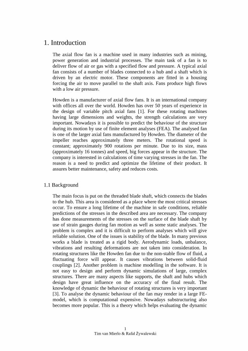
Figure 1 presents an exploded view of a Howden fan; in grey the hubs and in yellow the fan shaft which drives the impellers.

Figure 1. An exploded view of a Howden fan. The figure is provided by Howden.

1.2.3 Finite element model

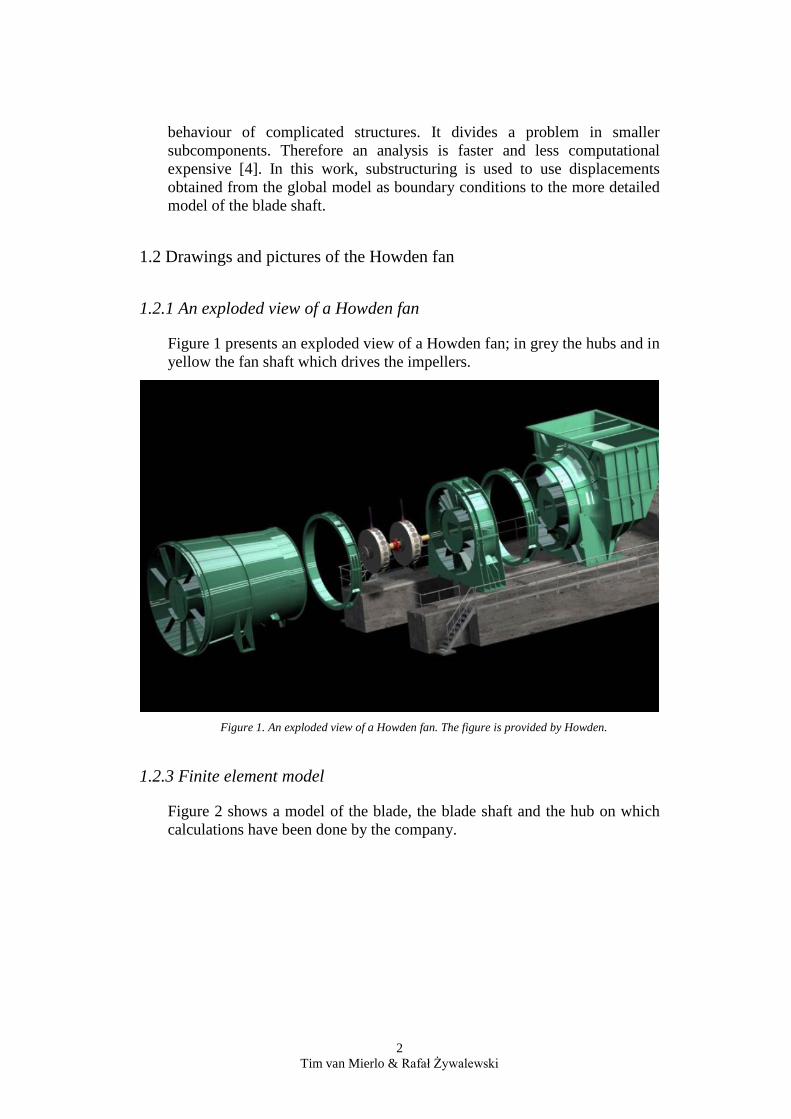
Figure 2 shows a model of the blade, the blade shaft and the hub on which calculations have been done by the company.


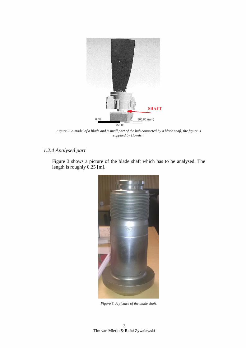
Figure 2. A model of a blade and a small part of the hub connected by a blade shaft, the figure is

supplied by Howden.

1.2.4 Analysed part

Figure 3 shows a picture of the blade shaft which has to be analysed. The length is roughly 0.25 [m].

Figure 3. A picture of the blade shaft.


1.3 Aim and Purpose

The aim of this master thesis is to obtain the time varying stresses acting in a Howden variable pitch axial fan with special focus on the stresses in the threads of the blade shaft.

The purpose is to predict the lifetime of the blade shaft.

1.4 Limitations

The used global models only consist of simplified parts. The detailed parts are only used for the blade shaft analyses. The stresses are only calculated for this part.

During the project there is no experimental testing as validation for these calculations, it is only based on the experimental results given by the company.

1.5 Reliability, validity and objectivity

The reliability of this project depends on many factors. First of all it depends on the used models. Different models will be used for performing different calculations. These models are normally simplified models and the reliability of the calculations depend on these simplifications. The use of the finite element method results in approximated values. The accuracy of these calculated values depend on many variables, such as, the number of elements which have been used, the selected element type and the used boundary conditions.


2. Theory

2.1 Finite element analyses (FEA)

This master thesis is mostly based on finite element analyses. It can be used to test the structural strength and to simulate deformations, but also heat and fluid flows in a computer environment. It introduces a lot of benefits for the industry. The most important is the ability to virtually test machines before their manufacturing. It is crucial to predict the behaviour of the structure before the manufacturing process since it reduces the number of failures and saves time and material.

Finite element analyses (FEA) relies on the numerical calculations of approximate solutions to boundary value problems by usage of partial differential equations. It is a subdivision of the whole problem domain into simpler parts which are called finite elements [5].

To obtain time varying stresses in the blade shaft the dynamic analysis of the Howden fan has to be done. A dynamic analysis differs from static analysis by its time dependent properties

The structural dynamic theory has to be introduced.

The general equation of motion can be written as:

𝑀𝑀𝑢(𝑡𝑡) + 𝐶𝐶𝑢(𝑡𝑡) + 𝐾𝐾𝑢𝑢(𝑡𝑡) = 𝑃𝑃(𝑡𝑡) (1)

Where:

- M is the mass matrix

- C is the damping matrix

- K is the stiffness matrix

- P is the force vector

Fortunately modern FEA software can help to do this kind of simulations. It contains all the necessary tools to model and obtain reliable results for rotating structure analyses.


2.2 Dynamic motion, eigenvalues/eigenfrequencies

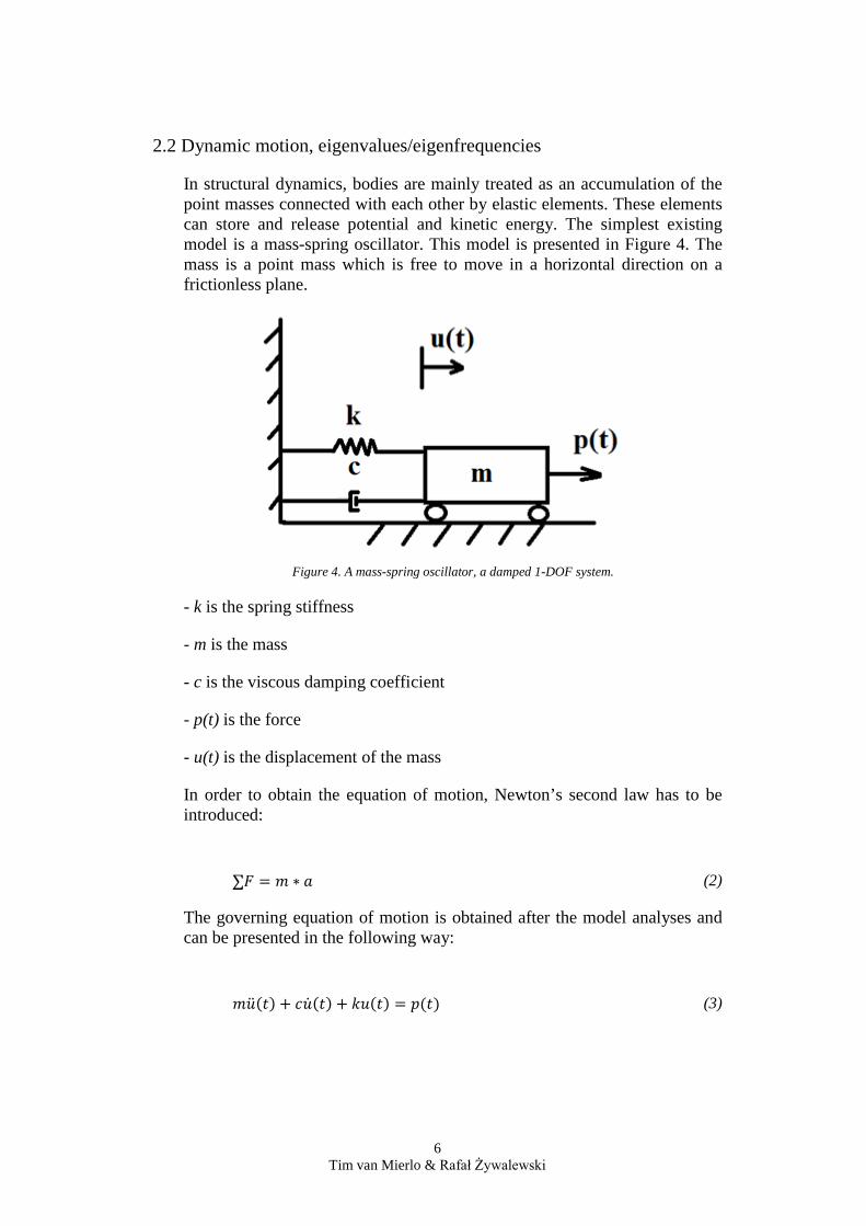
In structural dynamics, bodies are mainly treated as an accumulation of the point masses connected with each other by elastic elements. These elements can store and release potential and kinetic energy. The simplest existing model is a mass-spring oscillator. This model is presented in Figure 4. The mass is a point mass which is free to move in a horizontal direction on a frictionless plane.

Figure 4. A mass-spring oscillator, a damped 1-DOF system.

- k is the spring stiffness

- m is the mass

- c is the viscous damping coefficient

- p(t) is the force

- u(t) is the displacement of the mass

In order to obtain the equation of motion, Newton’s second law has to be introduced:

∑𝐹𝐹 = 𝑚𝑚 ∗ 𝑎𝑎 (2)

The governing equation of motion is obtained after the model analyses and can be presented in the following way:

𝑚𝑚𝑢(𝑡𝑡) + 𝑐𝑐𝑢(𝑡𝑡) + 𝑘𝑘𝑢𝑢(𝑡𝑡) = 𝑝𝑝(𝑡𝑡) (3)


Now an undamped 2-DOF system is considered, which is shown in Figure 5.

Figure 5. An undamped 2-DOF system.

The equation of motion can be written in following way for the undamped 2-DOF system shown in Figure 5.

𝑚𝑚1 0

0 𝑚𝑚2 𝑢1𝑢2

+𝑘𝑘1 + 𝑘𝑘2 −𝑘𝑘2−𝑘𝑘2 𝑘𝑘2

𝑢𝑢1𝑢𝑢2=

𝑃𝑃1𝑃𝑃2

(4)

For the free vibration case, equation (5) can be written as:

𝑀𝑀𝑢(𝑡𝑡) + 𝐾𝐾𝑢𝑢(𝑡𝑡) = 0

(5)

Where: 𝑀𝑀 = 𝑚𝑚1 0

0 𝑚𝑚2

(6)

𝑢𝑢 = 𝑢𝑢1𝑢𝑢2

(7)

𝐾𝐾 = 𝑘𝑘1 + 𝑘𝑘2 −𝑘𝑘2−𝑘𝑘2 𝑘𝑘2

(8)


An assumption for u(t) is:

u(t)=U*cos(ωt-α) (9)

Which gives:

𝑢1𝑢2

= −𝜔𝜔2 𝑈𝑈1𝑈𝑈2 𝑐𝑐𝑐𝑐𝑐𝑐(𝜔𝜔𝑡𝑡 − 𝛼𝛼) = −𝜔𝜔2

𝑢𝑢1𝑢𝑢2

(10)

According to above assumptions the new motion equation is obtained:

𝑘𝑘1 + 𝑘𝑘2 −𝑘𝑘2

−𝑘𝑘2 𝑘𝑘2−𝜔𝜔2 𝑚𝑚1 0

0 𝑚𝑚2

𝑢𝑢1𝑢𝑢2 = 00

(11)

One of the solutions is:

𝑢𝑢1𝑢𝑢2 = 00

(12)

This solution is trivial and not interesting to obtain the eigenfrequencies. The second solution is:

𝑘𝑘1 + 𝑘𝑘2 −𝑘𝑘2

−𝑘𝑘2 𝑘𝑘2−𝜔𝜔𝑟𝑟2

𝑚𝑚1 00 𝑚𝑚2

= 0 (13)

The determinant is calculated for the second solution and after this the value of ωr

2 can be obtained, where ω is called the eigenvalue. The frequency can be obtained from ω by the following formula:

𝑓𝑓 =

𝜔𝜔2𝜋𝜋

[𝐻𝐻𝐻𝐻] (14)

These frequencies are called the eigenfrequencies or natural frequencies of the system and are the frequencies where the displacements and accelerations obtain their maximum value, which results in high stresses.

2.3 Frequency response function (FRF)

A frequency response function (FRF) can be interpreted as a mathematical representation of the relationship between the input force and the output as a


function of frequency. The basic formula can be written in the following form [6]:

𝐻𝐻(𝑟𝑟) ≡𝑈𝑈𝑈𝑈0

(15)

- H(r) is the non-dimensionalised frequency response function

- U is the amplitude of the steady-state response

- U0 is the static displacement, the displacement that the mass would undergo if a force were to be applied “statically”

Modal analyses based on FRF are done in order to obtain the dynamic characteristics of a given structure. The mode shapes, modal frequencies and modal damping are obtained.

There are two ways to obtain the FRF. One of them is to excite an experimental structure (using a special hammer or shaker) at a particular point and receive measured data from strain gauges or accelerometers which are attached at the structure. These measurements deliver data that show the relation between the output and the input. The second possibility is to perform FEA.

Howden delivered the results of measurements using strain gauges on the blade shaft. These data validate the FE-model.

2.4 Dynamic substructuring

In order to analyse complex structures like the Howden fan, a high number of calculations have to be done. Sometimes the model is too complicated. A high quantity of variables and elements needs a powerful computer system to solve the calculations otherwise it takes a long time to solve the problem. In this case the substructuring theory is very helpful. It is a method based on the idea of decomposing an object into much smaller subcomponents which are solved faster than the complete structure. The obtained data can be transferred between models, for example as boundary conditions. By parallel computation, the solution for the complex problem is gradually obtained [6].

In other words substructuring is the way to focus on specific components from the whole structure. Figure 6 presents the main idea of substructuring.


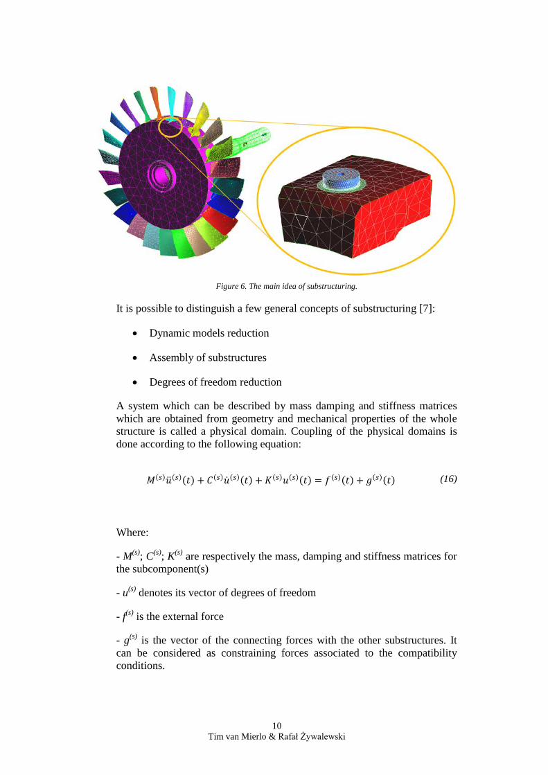
Figure 6. The main idea of substructuring.

It is possible to distinguish a few general concepts of substructuring [7]:

• Dynamic models reduction

• Assembly of substructures

• Degrees of freedom reduction

A system which can be described by mass damping and stiffness matrices which are obtained from geometry and mechanical properties of the whole structure is called a physical domain. Coupling of the physical domains is done according to the following equation:

𝑀𝑀(𝑠𝑠)𝑢(𝑠𝑠)(𝑡𝑡) + 𝐶𝐶(𝑠𝑠)𝑢(𝑠𝑠)(𝑡𝑡) + 𝐾𝐾(𝑠𝑠)𝑢𝑢(𝑠𝑠)(𝑡𝑡) = 𝑓𝑓(𝑠𝑠)(𝑡𝑡) + 𝑔𝑔(𝑠𝑠)(𝑡𝑡) (16)

Where:

- M(s); C(s); K(s) are respectively the mass, damping and stiffness matrices for the subcomponent(s)

- u(s) denotes its vector of degrees of freedom

- f(s) is the external force

- g(s) is the vector of the connecting forces with the other substructures. It can be considered as constraining forces associated to the compatibility conditions.


Above equation only applies with the assumption that the system is linear [8].

2.5 Force distribution on the blades

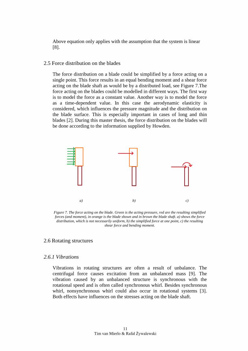
The force distribution on a blade could be simplified by a force acting on a single point. This force results in an equal bending moment and a shear force acting on the blade shaft as would be by a distributed load, see Figure 7.The force acting on the blades could be modelled in different ways. The first way is to model the force as a constant value. Another way is to model the force as a time-dependent value. In this case the aerodynamic elasticity is considered, which influences the pressure magnitude and the distribution on the blade surface. This is especially important in cases of long and thin blades [2]. During this master thesis, the force distribution on the blades will be done according to the information supplied by Howden.

a) b) c)

Figure 7. The force acting on the blade. Green is the acting pressure, red are the resulting simplified forces (and moment), in orange is the blade shown and in brown the blade shaft. a) shows the force distribution, which is not necessarily uniform, b) the simplified force at one point, c) the resulting

shear force and bending moment.

2.6 Rotating structures

2.6.1 Vibrations

Vibrations in rotating structures are often a result of unbalance. The centrifugal force causes excitation from an unbalanced mass [9]. The vibration caused by an unbalanced structure is synchronous with the rotational speed and is often called synchronous whirl. Besides synchronous whirl, nonsynchronous whirl could also occur in rotational systems [3]. Both effects have influences on the stresses acting on the blade shaft.


Another type of vibration in rotating structures is torsional vibration. This is the vibrational twisting of the shafts in a system containing rotors and a shaft [3]. These vibrations influence the rotational behaviour of the rotors. This behaviour also influences the stresses in the blade shaft.

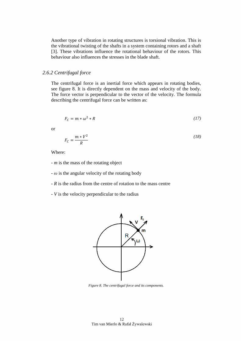
2.6.2 Centrifugal force

The centrifugal force is an inertial force which appears in rotating bodies, see figure 8. It is directly dependent on the mass and velocity of the body. The force vector is perpendicular to the vector of the velocity. The formula describing the centrifugal force can be written as:

𝐹𝐹𝐶𝐶 = 𝑚𝑚 ∗ 𝜔𝜔2 ∗ 𝑅𝑅 (17)

or

𝐹𝐹𝐶𝐶 =𝑚𝑚 ∗ 𝑉𝑉2

𝑅𝑅

(18)

Where:

- m is the mass of the rotating object

- ω is the angular velocity of the rotating body

- R is the radius from the centre of rotation to the mass centre

- V is the velocity perpendicular to the radius

Figure 8. The centrifugal force and its components.


The centrifugal force has high influences on structures with high rotational speeds. In the Howden fan the centrifugal force represents a significant part of the forces acting on the blade shaft.

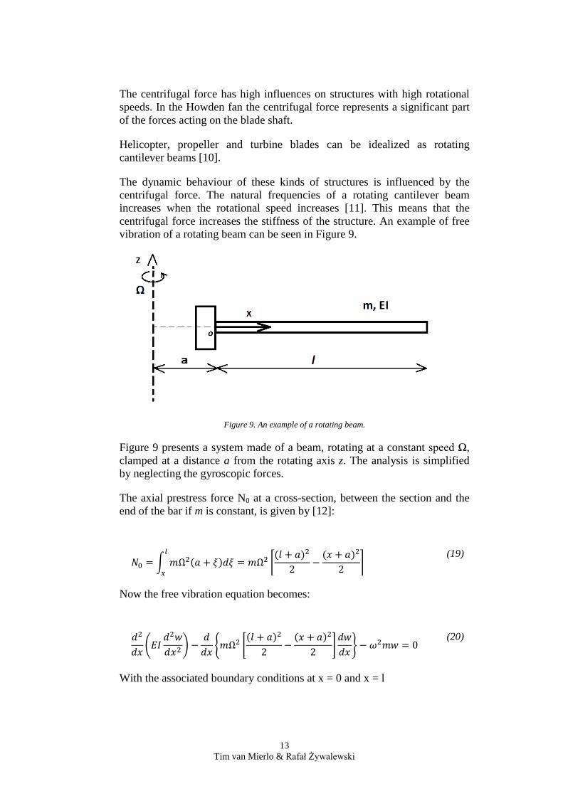
Helicopter, propeller and turbine blades can be idealized as rotating cantilever beams [10].

The dynamic behaviour of these kinds of structures is influenced by the centrifugal force. The natural frequencies of a rotating cantilever beam increases when the rotational speed increases [11]. This means that the centrifugal force increases the stiffness of the structure. An example of free vibration of a rotating beam can be seen in Figure 9.

Figure 9. An example of a rotating beam.

Figure 9 presents a system made of a beam, rotating at a constant speed Ω, clamped at a distance a from the rotating axis z. The analysis is simplified by neglecting the gyroscopic forces.

The axial prestress force N0 at a cross-section, between the section and the end of the bar if m is constant, is given by [12]:

𝑁𝑁0 = 𝑚𝑚Ω2(𝑎𝑎 + 𝜉𝜉)𝑑𝑑𝜉𝜉 = 𝑚𝑚Ω2

(𝑙𝑙 + 𝑎𝑎)2

2−

(𝑥𝑥 + 𝑎𝑎)2

2

𝑙𝑙

𝑥𝑥

(19)

Now the free vibration equation becomes:

𝑑𝑑2

𝑑𝑑𝑥𝑥 𝐸𝐸𝐸𝐸𝑑𝑑2𝑤𝑤𝑑𝑑𝑥𝑥2

−𝑑𝑑𝑑𝑑𝑥𝑥

𝑚𝑚Ω2 (𝑙𝑙 + 𝑎𝑎)2

2−


2𝑑𝑑𝑤𝑤𝑑𝑑𝑥𝑥

− 𝜔𝜔2𝑚𝑚𝑤𝑤 = 0 (20)

With the associated boundary conditions at x = 0 and x = l


- on the rotation

𝑑𝑑𝑤𝑤𝑑𝑑𝑥𝑥

= 0 𝑐𝑐𝑟𝑟 𝐸𝐸𝐸𝐸𝑑𝑑2𝑤𝑤𝑑𝑑𝑥𝑥2

= 0 (21)

- on the displacement

𝑤𝑤 = 0 𝑐𝑐𝑟𝑟 𝑑𝑑𝑑𝑑𝑥𝑥

𝐸𝐸𝐸𝐸𝑑𝑑2𝑤𝑤𝑑𝑑𝑥𝑥2

−𝑚𝑚Ω2 (𝑙𝑙 + 𝑎𝑎)2

2−


2𝑑𝑑𝑤𝑤𝑑𝑑𝑥𝑥

= 0 (22)

2.7 Rotating structures modelling

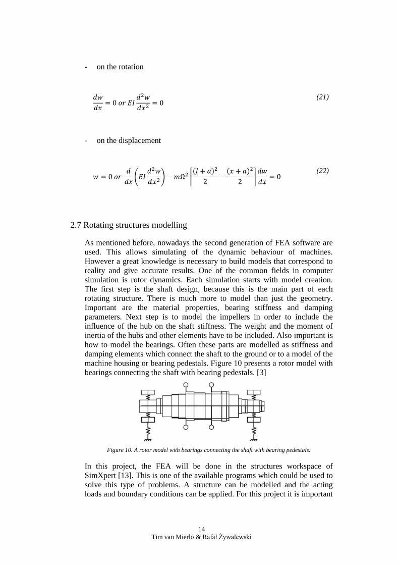
As mentioned before, nowadays the second generation of FEA software are used. This allows simulating of the dynamic behaviour of machines. However a great knowledge is necessary to build models that correspond to reality and give accurate results. One of the common fields in computer simulation is rotor dynamics. Each simulation starts with model creation. The first step is the shaft design, because this is the main part of each rotating structure. There is much more to model than just the geometry. Important are the material properties, bearing stiffness and damping parameters. Next step is to model the impellers in order to include the influence of the hub on the shaft stiffness. The weight and the moment of inertia of the hubs and other elements have to be included. Also important is how to model the bearings. Often these parts are modelled as stiffness and damping elements which connect the shaft to the ground or to a model of the machine housing or bearing pedestals. Figure 10 presents a rotor model with bearings connecting the shaft with bearing pedestals. [3]

Figure 10. A rotor model with bearings connecting the shaft with bearing pedestals.

In this project, the FEA will be done in the structures workspace of SimXpert [13]. This is one of the available programs which could be used to solve this type of problems. A structure can be modelled and the acting loads and boundary conditions can be applied. For this project it is important


that the software supports the use of dynamic loads. SimXpert is a pre-processor and post-processor environment which supports this. SimXpert is connected to the NASTRAN solver to solve the pre-processed models. After solving the models, the results can be attached in SimXpert and the results can be used for post-processing.

2.7.1 Nastran solution sequences

Five different Nastran solution sequences have been used during this project.

SOL103 (modal analysis) is used to obtain the eigenmodes and the corresponding eigenfrequencies of the first (very simplified) models. SOL110 (modal complex eigenvalues) has been used for the more recent models because SOL103 does not include the influence of the rotational speed.

For obtaining the frequency response the solution sequence SOL111 (modal frequency response) has been used.

SOL112 (modal transient analysis) has been used for the transient response analysis. Unfortunately this solution sequence does not include the influence of the rotational speed.

To include the effect of the centrifugal force, SOL400 (general nonlinear) has been used. In this solution sequence the centrifugal force has been used as the first step load and the transient response analysis as the second step load. In this way the influence of the rotational speed has been included [14].

2.7.2 Element types

Bar elements are used to model the fan shaft. The great benefit of the use of 1D bar elements is the short calculation time. Nastran uses a connection card (CBAR) and a property card (PBAR). The bar element includes torsion, extension, shears and bending in two perpendicular planes [15].

During this project, the two different cross-section types which have been used were the “ROD” and the “TUBE” types. The use of these elements is integrated in SimXpert. The user picks the correct cross-section type of a list and inserts the dimensions.

The simplest 3D element is the linear tetrahedral element with four nodes. The tetrahedral element also exists in a quadratic 10-node variant. Another commonly used solid element type is the prism element. The linear prism element has eight nodes and the quadratic prism element twenty nodes [5].


2.7.3 Connecting 1D with 3D elements

The RBE2 rigid element is a commonly used element to connect different parts node-by-node. It can connect parts with different element types, for example 1D with 3D elements. In this project the RBE2 connector is used to connect the solid meshed impeller with the fan shaft which is modelled using 1D elements [16].

1D beam elements typically have six DOFs per node and 3D solid elements, for example the tetrahedral element, often only three DOF per node. This results in problems when coupling the node of a beam element with a node of the 3D solid element. The connection will act as a ball-joint instead of a stiff connection. A simple way to solve this problem is to use tetrahedral elements with rotational DOFs.

Another solution is to penetrate the beam element inside the solid geometry, but unfortunately this only partially solves the problem because this connection does not transfer torsion moments [17].

An alternative is to use some short beams connecting the 1D beam with multiple closely located nodes on the 3D element surface [18]. This can easily be done by use of the RBE2 connector.


3. Method 3.1 Introduction

To obtain the stresses in the blade shaft, two different models are used; a global model and a detailed model. The global model is used to obtain the displacements at the blade shaft. To obtain these displacements, the model should contain at least:

• A hub

• A blade shaft

• A blade

One of the questions is if the use of the fan shaft is really necessary to obtain reliable values. If the fan shaft is included, the model could also include the second (simplified) impeller, two bearings as boundary conditions and a point-mass which represents the coupling.

The displacements which are obtained in the global model are used as boundary conditions in the detailed model. The stresses are obtained using the detailed model.


3.2 Global model

3.2.1 Component overview

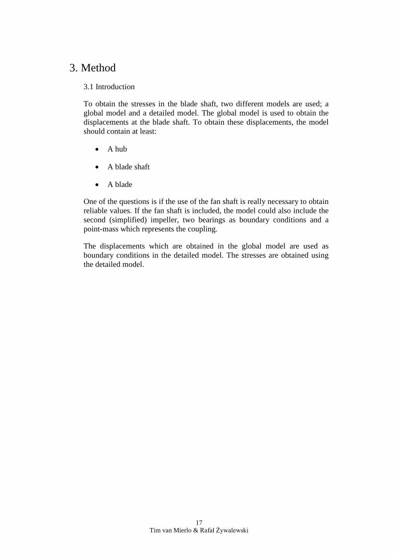
The global model consists of different components which are shown in figure 11. Impeller 1 consists of hub 1, the connected blade shafts and blades. The shaft, hub and the blade shaft are made of steel. The blades are made of aluminium.

Figure 11. A numbered overview of the components in the global model.

1: rotational speed

2: concentrated mass representing the coupling 3: bearing 2

4: concentrated mass representing impeller 2 5: bearing 1

6: concentrated mass for compensating hub 1 7: RBE2 connectors connecting the fan shaft and the hub

8: hub 1 (3D elements) 9: blade shaft (3D elements)

10: blade (3D elements) 11: fan shaft (1D elements)


3.2.2 Simplified global models

Three different very simplified models are used to obtain the eigenfrequencies with their corresponding eigenmode shapes. The results are compared to obtain the influences of 1D and 3D elements.

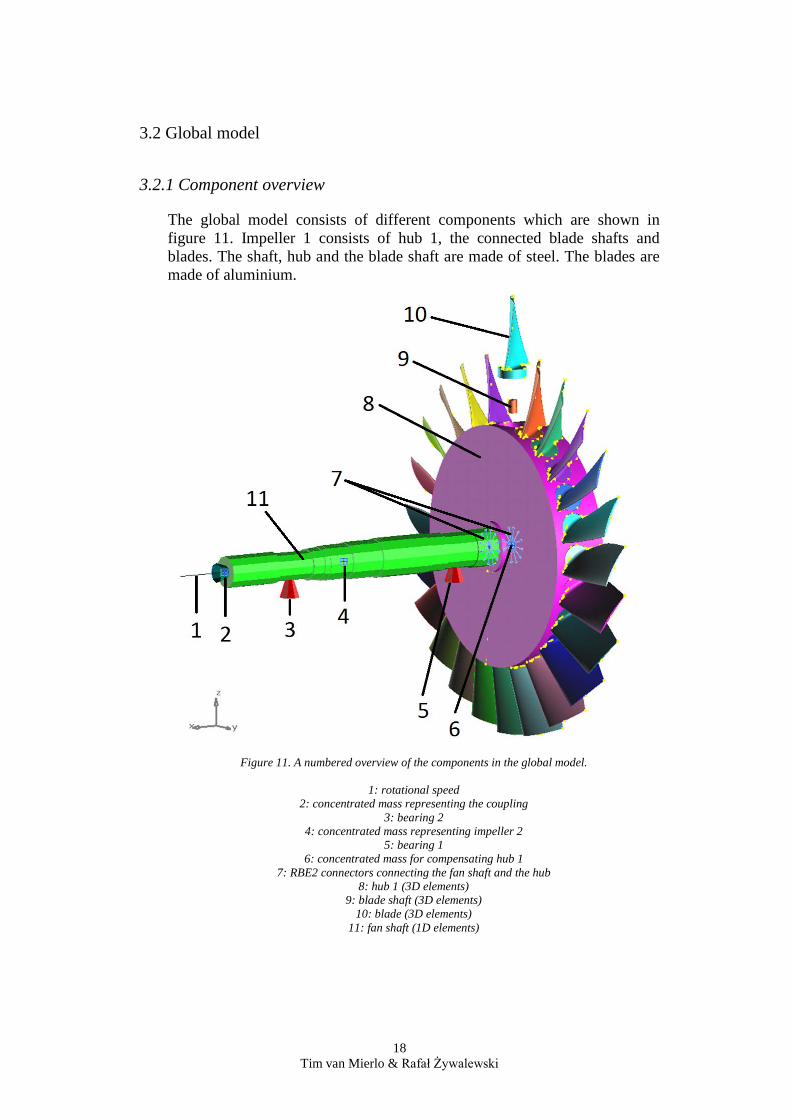
3.2.2.1 Simplified model 1

If it is only necessary to obtain the eigenvalues of the fan, the structure could be strongly simplified. One of the approaches is a model which only consists of 1D elements. An example of this kind of model is shown in Figure 12.

Figure 12. Simplified model 1.

Unfortunately the model consisting of only 1D elements is not sufficient to attach blades.

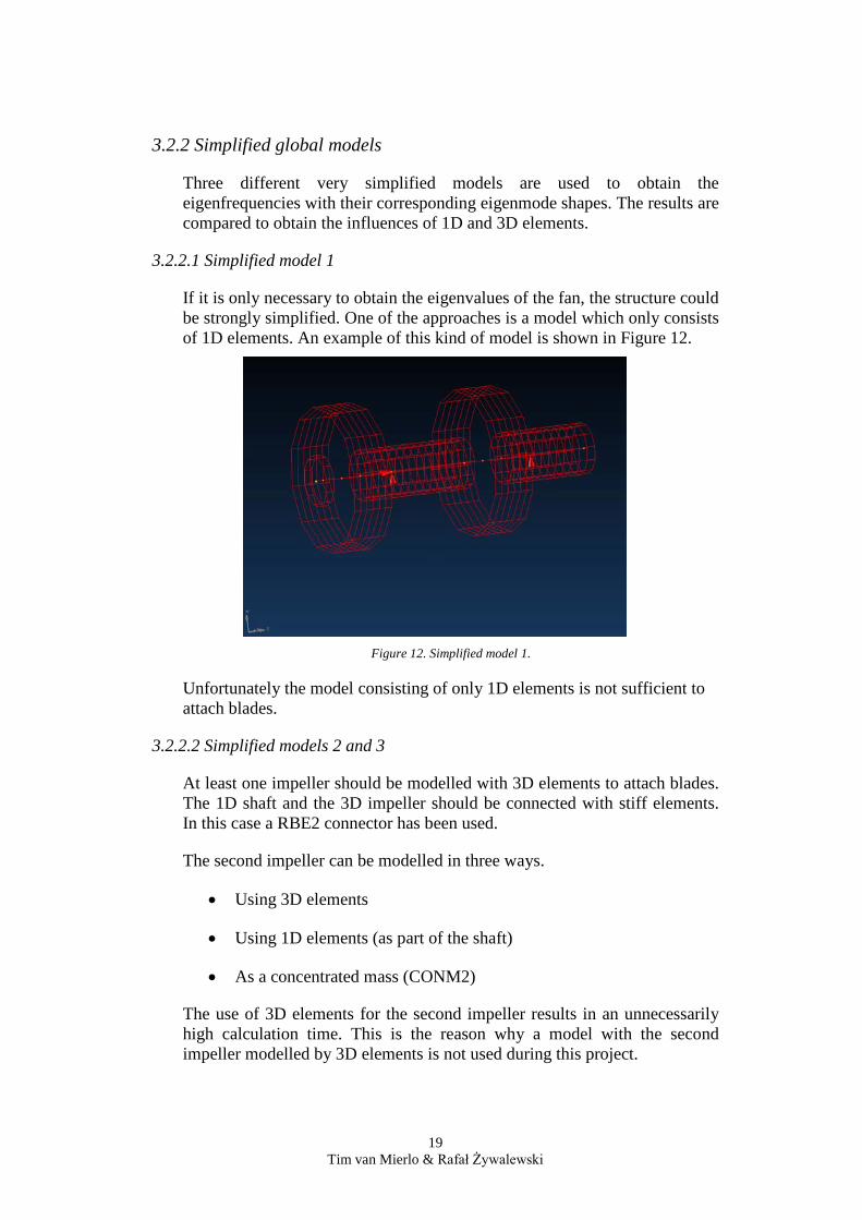
3.2.2.2 Simplified models 2 and 3

At least one impeller should be modelled with 3D elements to attach blades. The 1D shaft and the 3D impeller should be connected with stiff elements. In this case a RBE2 connector has been used.

The second impeller can be modelled in three ways.

• Using 3D elements

• Using 1D elements (as part of the shaft)

• As a concentrated mass (CONM2)

The use of 3D elements for the second impeller results in an unnecessarily high calculation time. This is the reason why a model with the second impeller modelled by 3D elements is not used during this project.


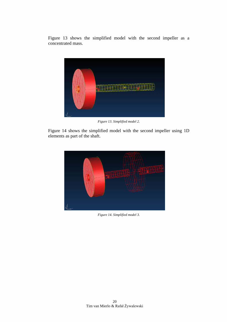
Figure 13 shows the simplified model with the second impeller as a concentrated mass.


Figure 14 shows the simplified model with the second impeller using 1D elements as part of the shaft.



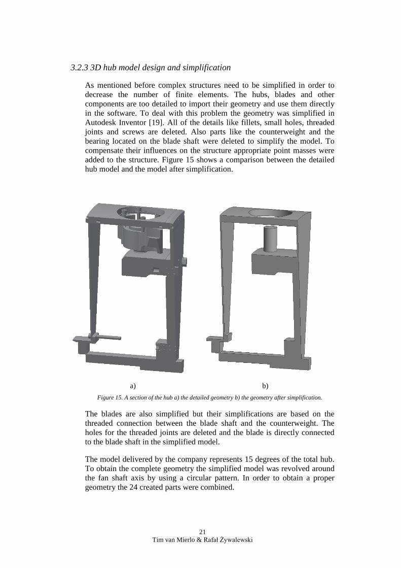
3.2.3 3D hub model design and simplification

As mentioned before complex structures need to be simplified in order to decrease the number of finite elements. The hubs, blades and other components are too detailed to import their geometry and use them directly in the software. To deal with this problem the geometry was simplified in Autodesk Inventor [19]. All of the details like fillets, small holes, threaded joints and screws are deleted. Also parts like the counterweight and the bearing located on the blade shaft were deleted to simplify the model. To compensate their influences on the structure appropriate point masses were added to the structure. Figure 15 shows a comparison between the detailed hub model and the model after simplification.

a) b)

Figure 15. A section of the hub a) the detailed geometry b) the geometry after simplification.

The blades are also simplified but their simplifications are based on the threaded connection between the blade shaft and the counterweight. The holes for the threaded joints are deleted and the blade is directly connected to the blade shaft in the simplified model.

The model delivered by the company represents 15 degrees of the total hub. To obtain the complete geometry the simplified model was revolved around the fan shaft axis by using a circular pattern. In order to obtain a proper geometry the 24 created parts were combined.


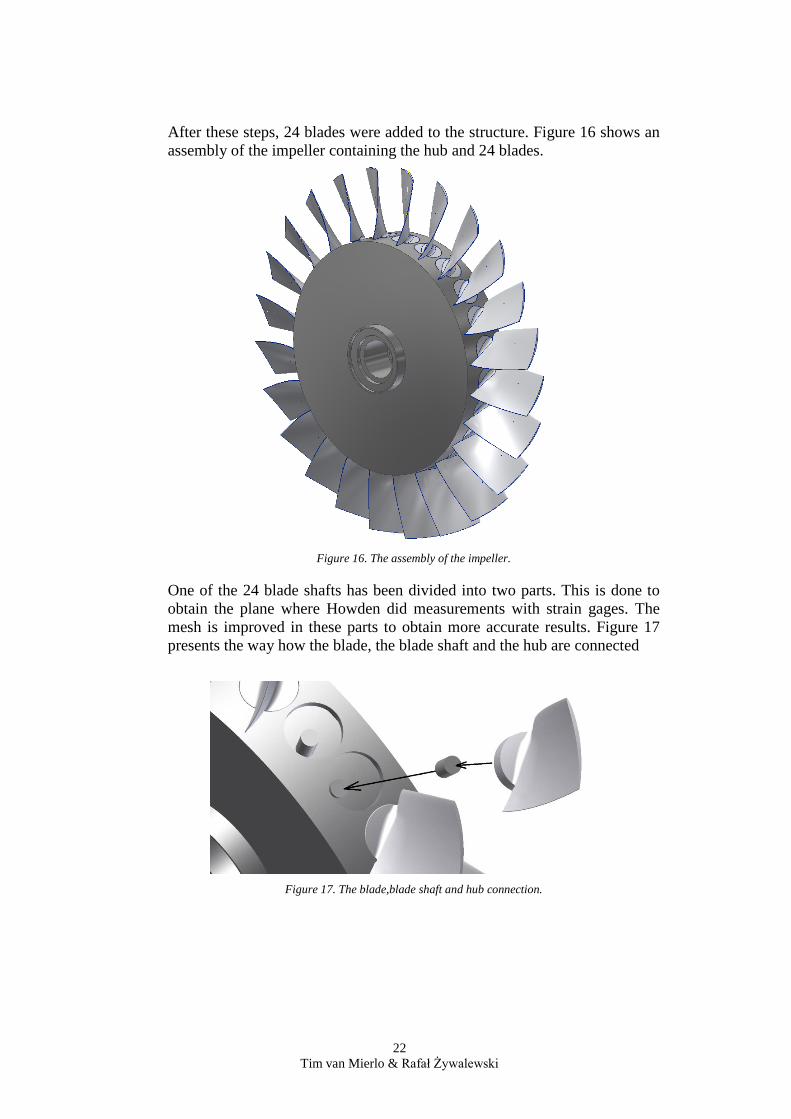
After these steps, 24 blades were added to the structure. Figure 16 shows an assembly of the impeller containing the hub and 24 blades.

Figure 16. The assembly of the impeller.

One of the 24 blade shafts has been divided into two parts. This is done to obtain the plane where Howden did measurements with strain gages. The mesh is improved in these parts to obtain more accurate results. Figure 17 presents the way how the blade, the blade shaft and the hub are connected

Figure 17. The blade,blade shaft and hub connection.


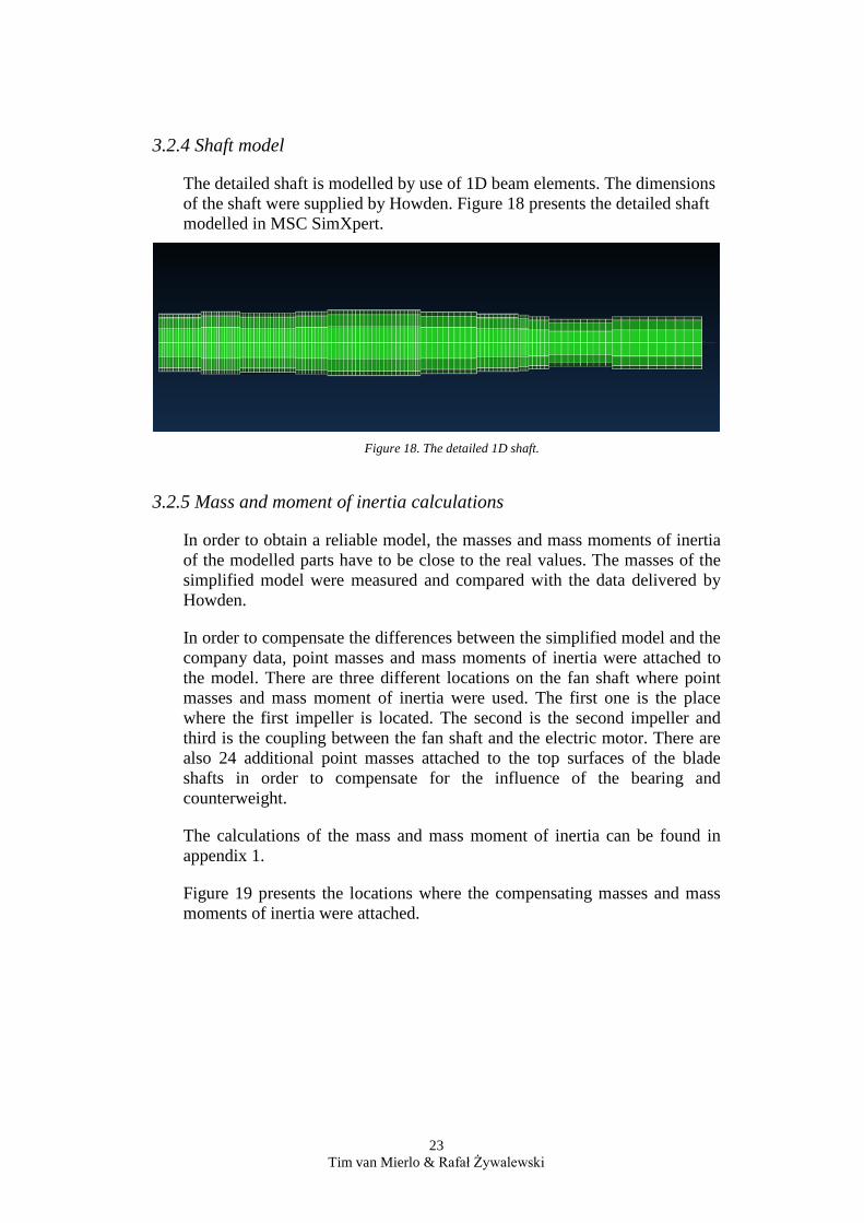
3.2.4 Shaft model

The detailed shaft is modelled by use of 1D beam elements. The dimensions of the shaft were supplied by Howden. Figure 18 presents the detailed shaft modelled in MSC SimXpert.

Figure 18. The detailed 1D shaft.

3.2.5 Mass and moment of inertia calculations

In order to obtain a reliable model, the masses and mass moments of inertia of the modelled parts have to be close to the real values. The masses of the simplified model were measured and compared with the data delivered by Howden.

In order to compensate the differences between the simplified model and the company data, point masses and mass moments of inertia were attached to the model. There are three different locations on the fan shaft where point masses and mass moment of inertia were used. The first one is the place where the first impeller is located. The second is the second impeller and third is the coupling between the fan shaft and the electric motor. There are also 24 additional point masses attached to the top surfaces of the blade shafts in order to compensate for the influence of the bearing and counterweight.

The calculations of the mass and mass moment of inertia can be found in appendix 1.

Figure 19 presents the locations where the compensating masses and mass moments of inertia were attached.


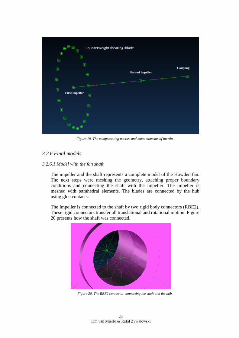
Figure 19. The compensating masses and mass moments of inertia.

3.2.6 Final models

3.2.6.1 Model with the fan shaft

The impeller and the shaft represents a complete model of the Howden fan. The next steps were meshing the geometry, attaching proper boundary conditions and connecting the shaft with the impeller. The impeller is meshed with tetrahedral elements. The blades are connected by the hub using glue contacts.

The Impeller is connected to the shaft by two rigid body connectors (RBE2). These rigid connectors transfer all translational and rotational motion. Figure 20 presents how the shaft was connected.

Figure 20. The RBE2 connector connecting the shaft and the hub.


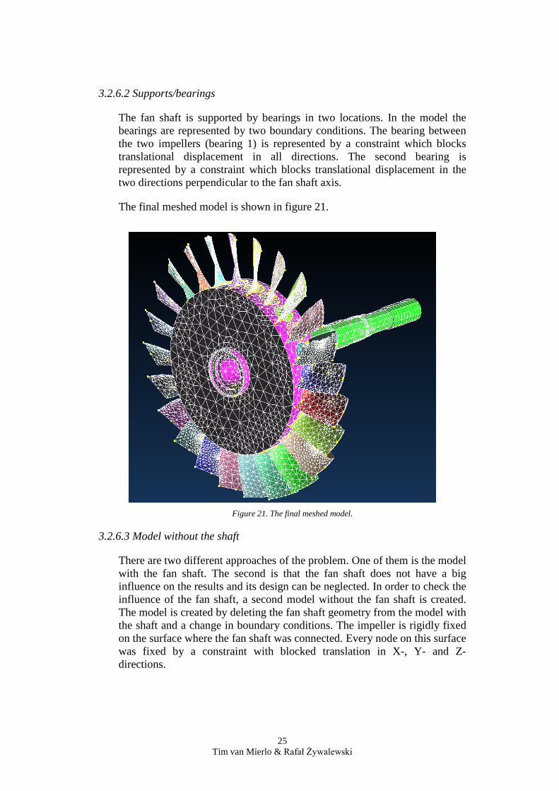
3.2.6.2 Supports/bearings

The fan shaft is supported by bearings in two locations. In the model the bearings are represented by two boundary conditions. The bearing between the two impellers (bearing 1) is represented by a constraint which blocks translational displacement in all directions. The second bearing is represented by a constraint which blocks translational displacement in the two directions perpendicular to the fan shaft axis.

The final meshed model is shown in figure 21.

Figure 21. The final meshed model.

3.2.6.3 Model without the shaft

There are two different approaches of the problem. One of them is the model with the fan shaft. The second is that the fan shaft does not have a big influence on the results and its design can be neglected. In order to check the influence of the fan shaft, a second model without the fan shaft is created. The model is created by deleting the fan shaft geometry from the model with the shaft and a change in boundary conditions. The impeller is rigidly fixed on the surface where the fan shaft was connected. Every node on this surface was fixed by a constraint with blocked translation in X-, Y- and Z-directions.


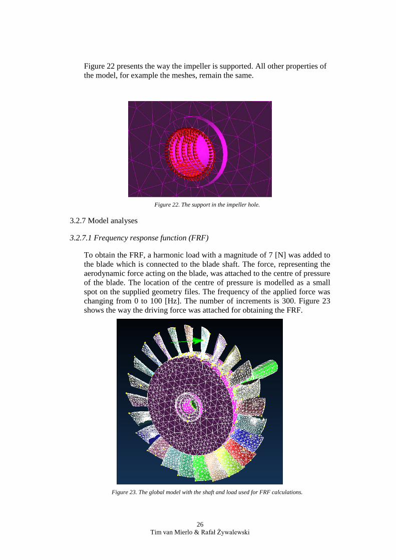
Figure 22 presents the way the impeller is supported. All other properties of the model, for example the meshes, remain the same.

Figure 22. The support in the impeller hole.

3.2.7 Model analyses

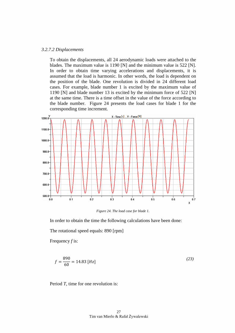
3.2.7.1 Frequency response function (FRF)

To obtain the FRF, a harmonic load with a magnitude of 7 [N] was added to the blade which is connected to the blade shaft. The force, representing the aerodynamic force acting on the blade, was attached to the centre of pressure of the blade. The location of the centre of pressure is modelled as a small spot on the supplied geometry files. The frequency of the applied force was changing from 0 to 100 [Hz]. The number of increments is 300. Figure 23 shows the way the driving force was attached for obtaining the FRF.

Figure 23. The global model with the shaft and load used for FRF calculations.


3.2.7.2 Displacements

To obtain the displacements, all 24 aerodynamic loads were attached to the blades. The maximum value is 1190 [N] and the minimum value is 522 [N]. In order to obtain time varying accelerations and displacements, it is assumed that the load is harmonic. In other words, the load is dependent on the position of the blade. One revolution is divided in 24 different load cases. For example, blade number 1 is excited by the maximum value of 1190 [N] and blade number 13 is excited by the minimum force of 522 [N] at the same time. There is a time offset in the value of the force according to the blade number. Figure 24 presents the load cases for blade 1 for the corresponding time increment.

Figure 24. The load case for blade 1.

In order to obtain the time the following calculations have been done:

The rotational speed equals: 890 [rpm]

Frequency f is:

𝑓𝑓 =

89060

= 14.83 [𝐻𝐻𝐻𝐻] (23)

Period T, time for one revolution is:


𝑇𝑇 =

1𝑓𝑓

=1

14.83= 0.0674 [𝑐𝑐] (24)

Time increment t is:

𝑡𝑡 =

𝑇𝑇24

=0.0674

24= 0.0028096 [𝑐𝑐] (25)

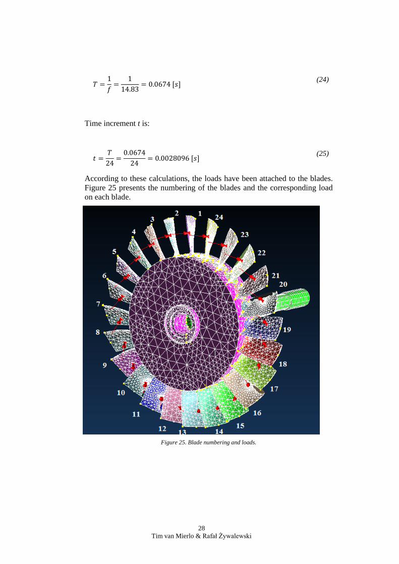
According to these calculations, the loads have been attached to the blades. Figure 25 presents the numbering of the blades and the corresponding load on each blade.

Figure 25. Blade numbering and loads.


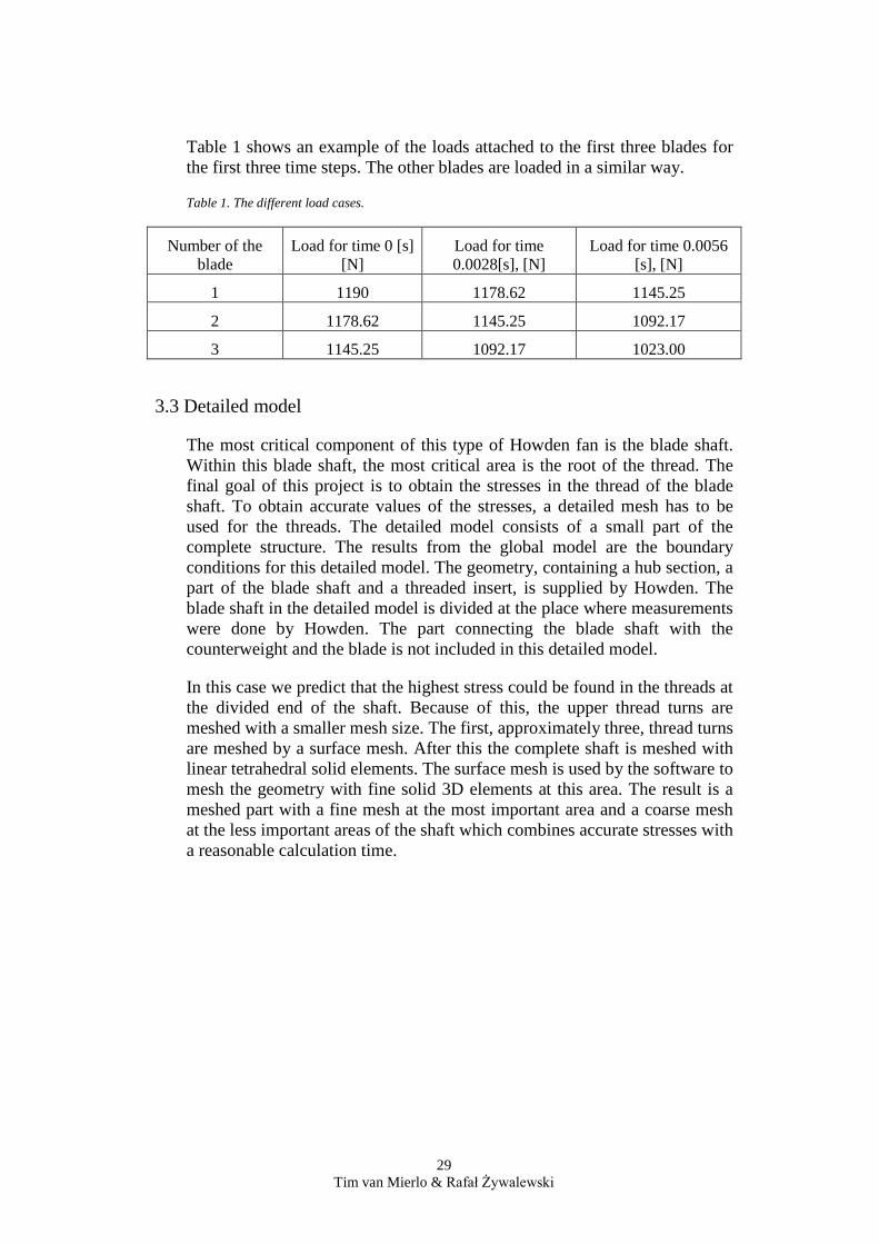
Table 1 shows an example of the loads attached to the first three blades for the first three time steps. The other blades are loaded in a similar way.

Table 1. The different load cases.

3.3 Detailed model

The most critical component of this type of Howden fan is the blade shaft. Within this blade shaft, the most critical area is the root of the thread. The final goal of this project is to obtain the stresses in the thread of the blade shaft. To obtain accurate values of the stresses, a detailed mesh has to be used for the threads. The detailed model consists of a small part of the complete structure. The results from the global model are the boundary conditions for this detailed model. The geometry, containing a hub section, a part of the blade shaft and a threaded insert, is supplied by Howden. The blade shaft in the detailed model is divided at the place where measurements were done by Howden. The part connecting the blade shaft with the counterweight and the blade is not included in this detailed model.

In this case we predict that the highest stress could be found in the threads at the divided end of the shaft. Because of this, the upper thread turns are meshed with a smaller mesh size. The first, approximately three, thread turns are meshed by a surface mesh. After this the complete shaft is meshed with linear tetrahedral solid elements. The surface mesh is used by the software to mesh the geometry with fine solid 3D elements at this area. The result is a meshed part with a fine mesh at the most important area and a coarse mesh at the less important areas of the shaft which combines accurate stresses with a reasonable calculation time.

Number of the blade

Load for time 0 [s] [N]

Load for time 0.0028[s], [N]

Load for time 0.0056 [s], [N]

1 1190 1178.62 1145.25

2 1178.62 1145.25 1092.17

3 1145.25 1092.17 1023.00


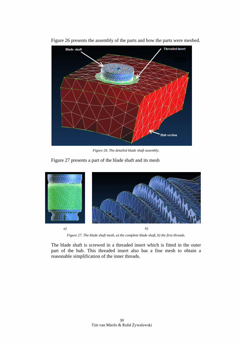
Figure 26 presents the assembly of the parts and how the parts were meshed.

Figure 26. The detailed blade shaft assembly.

Figure 27 presents a part of the blade shaft and its mesh

a) b)

Figure 27. The blade shaft mesh, a) the complete blade shaft, b) the first threads.

The blade shaft is screwed in a threaded insert which is fitted in the outer part of the hub. This threaded insert also has a fine mesh to obtain a reasonable simplification of the inner threads.


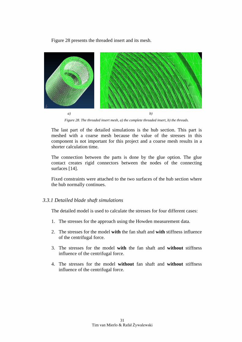
Figure 28 presents the threaded insert and its mesh.

a) b)

Figure 28. The threaded insert mesh, a) the complete threaded insert, b) the threads.

The last part of the detailed simulations is the hub section. This part is meshed with a coarse mesh because the value of the stresses in this component is not important for this project and a coarse mesh results in a shorter calculation time.

The connection between the parts is done by the glue option. The glue contact creates rigid connectors between the nodes of the connecting surfaces [14].

Fixed constraints were attached to the two surfaces of the hub section where the hub normally continues.

3.3.1 Detailed blade shaft simulations

The detailed model is used to calculate the stresses for four different cases:

1. The stresses for the approach using the Howden measurement data.

2. The stresses for the model with the fan shaft and with stiffness influence of the centrifugal force.

3. The stresses for the model with the fan shaft and without stiffness influence of the centrifugal force.

4. The stresses for the model without fan shaft and without stiffness influence of the centrifugal force.


The centrifugal and bending moment which are supplied by Howden are obtained from the results from experimental analyses. The loads used for the simulation acting on the top surface of the divided blade shaft are:

• Resultant from the centrifugal force :144 [MPa]

• Resultant from bending: 14 [MPa]

For cases 2 and 3 the obtained displacements from the global dynamic finite element analysis have been attached as boundary conditions to the surface of the divided blade shaft.

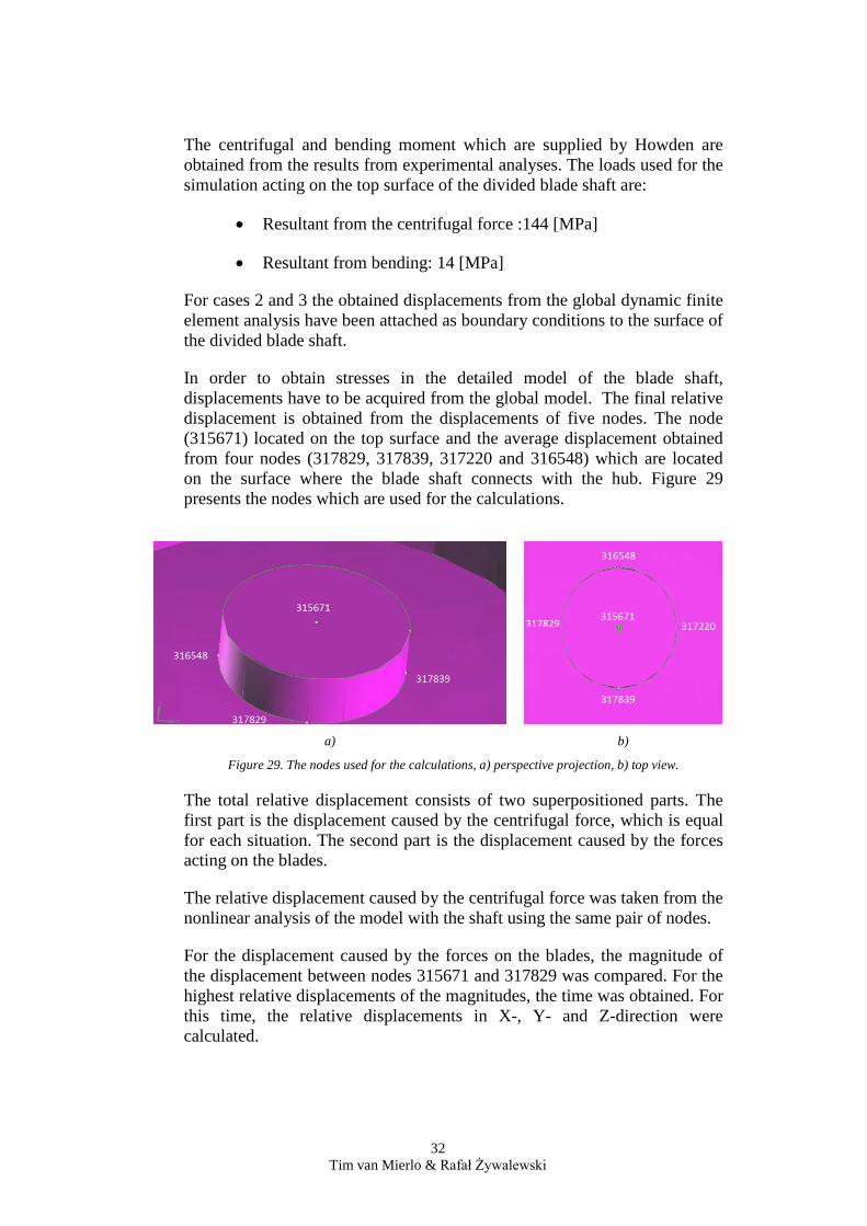
In order to obtain stresses in the detailed model of the blade shaft, displacements have to be acquired from the global model. The final relative displacement is obtained from the displacements of five nodes. The node (315671) located on the top surface and the average displacement obtained from four nodes (317829, 317839, 317220 and 316548) which are located on the surface where the blade shaft connects with the hub. Figure 29 presents the nodes which are used for the calculations.

a) b)

Figure 29. The nodes used for the calculations, a) perspective projection, b) top view.

The total relative displacement consists of two superpositioned parts. The first part is the displacement caused by the centrifugal force, which is equal for each situation. The second part is the displacement caused by the forces acting on the blades.

The relative displacement caused by the centrifugal force was taken from the nonlinear analysis of the model with the shaft using the same pair of nodes.

For the displacement caused by the forces on the blades, the magnitude of the displacement between nodes 315671 and 317829 was compared. For the highest relative displacements of the magnitudes, the time was obtained. For this time, the relative displacements in X-, Y- and Z-direction were calculated.


Now the total relative displacements for the X-, Y- and Z-direction were calculated by summing up the values of the two different parts. The total relative displacements were applied to the top surface of the detailed model.


4. Results and analysis

4.1 Global model

4.1.1 Results- simplified models

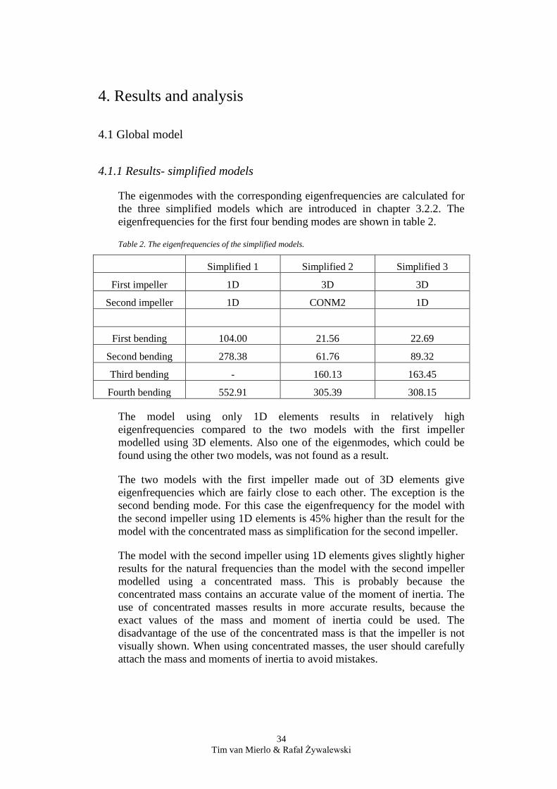
The eigenmodes with the corresponding eigenfrequencies are calculated for the three simplified models which are introduced in chapter 3.2.2. The eigenfrequencies for the first four bending modes are shown in table 2.

Table 2. The eigenfrequencies of the simplified models.

Simplified 1 Simplified 2 Simplified 3

First impeller 1D 3D 3D

Second impeller 1D CONM2 1D

First bending 104.00 21.56 22.69

Second bending 278.38 61.76 89.32

Third bending - 160.13 163.45

Fourth bending 552.91 305.39 308.15

The model using only 1D elements results in relatively high eigenfrequencies compared to the two models with the first impeller modelled using 3D elements. Also one of the eigenmodes, which could be found using the other two models, was not found as a result.

The two models with the first impeller made out of 3D elements give eigenfrequencies which are fairly close to each other. The exception is the second bending mode. For this case the eigenfrequency for the model with the second impeller using 1D elements is 45% higher than the result for the model with the concentrated mass as simplification for the second impeller.

The model with the second impeller using 1D elements gives slightly higher results for the natural frequencies than the model with the second impeller modelled using a concentrated mass. This is probably because the concentrated mass contains an accurate value of the moment of inertia. The use of concentrated masses results in more accurate results, because the exact values of the mass and moment of inertia could be used. The disadvantage of the use of the concentrated mass is that the impeller is not visually shown. When using concentrated masses, the user should carefully attach the mass and moments of inertia to avoid mistakes.


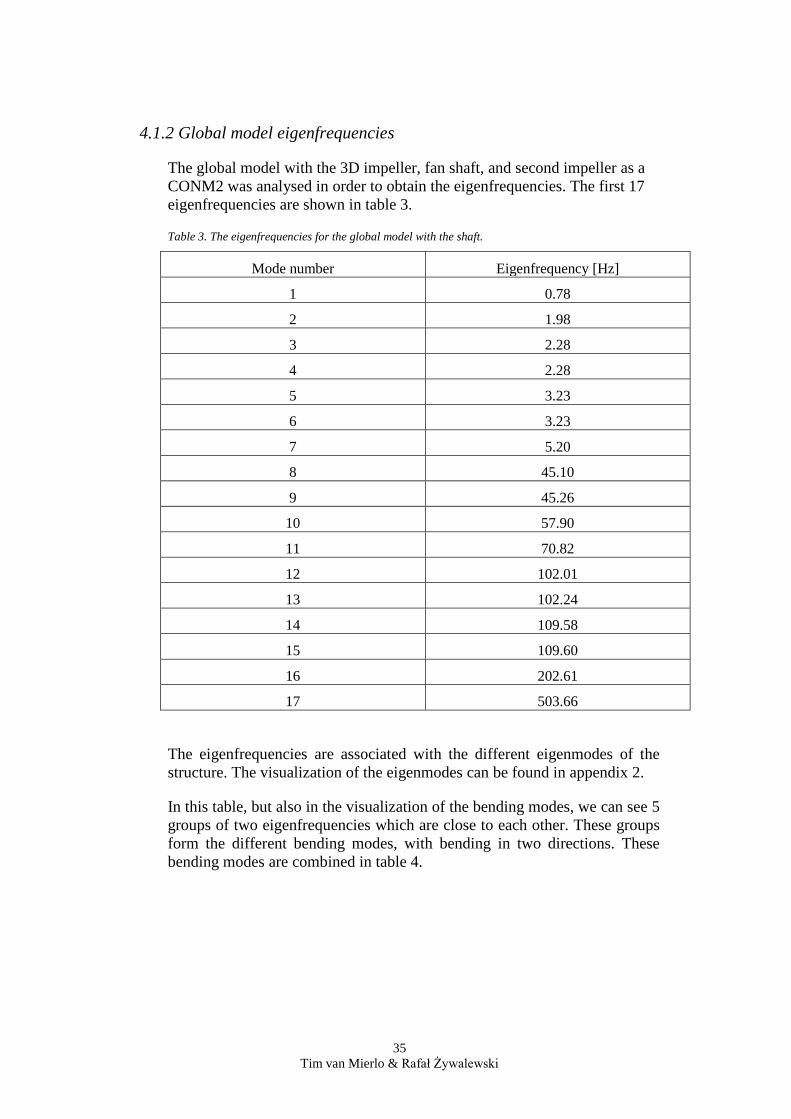
4.1.2 Global model eigenfrequencies

The global model with the 3D impeller, fan shaft, and second impeller as a CONM2 was analysed in order to obtain the eigenfrequencies. The first 17 eigenfrequencies are shown in table 3.

Table 3. The eigenfrequencies for the global model with the shaft.

Mode number Eigenfrequency [Hz]

1 0.78

2 1.98

3 2.28

4 2.28

5 3.23

6 3.23

7 5.20

8 45.10

9 45.26

10 57.90

11 70.82

12 102.01

13 102.24

14 109.58

15 109.60

16 202.61

17 503.66

The eigenfrequencies are associated with the different eigenmodes of the structure. The visualization of the eigenmodes can be found in appendix 2.

In this table, but also in the visualization of the bending modes, we can see 5 groups of two eigenfrequencies which are close to each other. These groups form the different bending modes, with bending in two directions. These bending modes are combined in table 4.


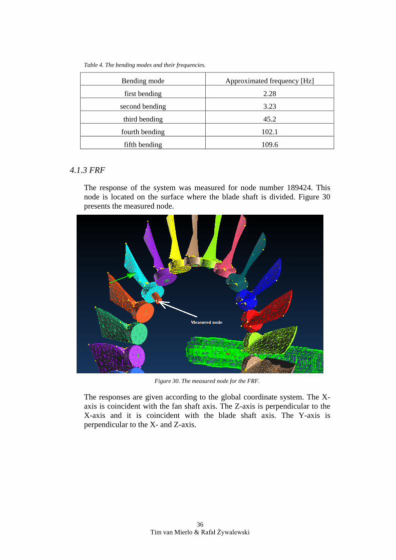
Table 4. The bending modes and their frequencies.

Bending mode Approximated frequency [Hz]

first bending 2.28

second bending 3.23

third bending 45.2

fourth bending 102.1

fifth bending 109.6

4.1.3 FRF

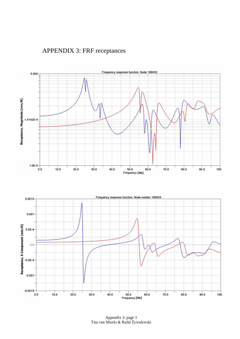
The response of the system was measured for node number 189424. This node is located on the surface where the blade shaft is divided. Figure 30 presents the measured node.

Figure 30. The measured node for the FRF.

The responses are given according to the global coordinate system. The X-axis is coincident with the fan shaft axis. The Z-axis is perpendicular to the X-axis and it is coincident with the blade shaft axis. The Y-axis is perpendicular to the X- and Z-axis.


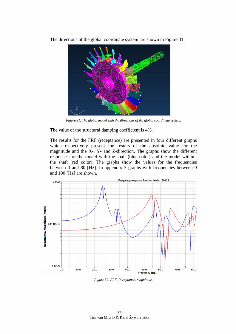
The directions of the global coordinate system are shown in Figure 31.

Figure 31. The global model with the directions of the global coordinate system.

The value of the structural damping coefficient is 4%.

The results for the FRF (receptance) are presented in four different graphs which respectively present the results of the absolute value for the magnitude and the X-, Y- and Z-direction. The graphs show the different responses for the model with the shaft (blue color) and the model without the shaft (red color). The graphs show the values for the frequencies between 0 and 80 [Hz]. In appendix 3 graphs with frequencies between 0 and 100 [Hz] are shown.

Figure 32. FRF, Receptance, magnitude.


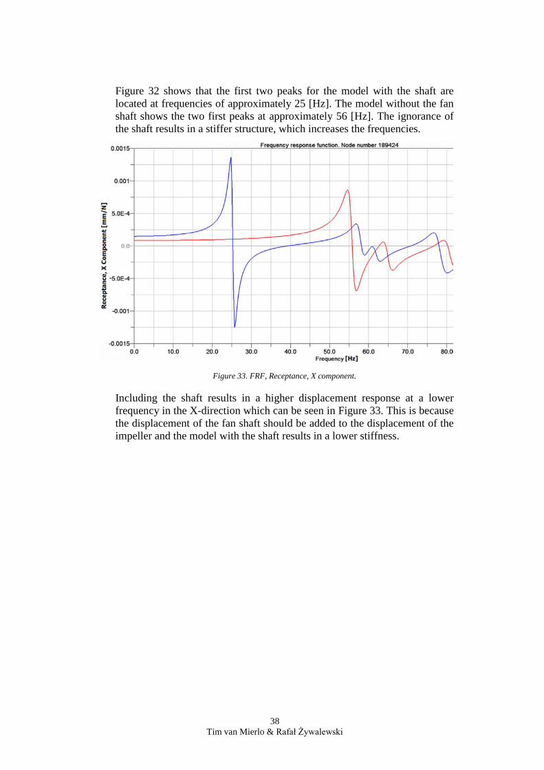
Figure 32 shows that the first two peaks for the model with the shaft are located at frequencies of approximately 25 [Hz]. The model without the fan shaft shows the two first peaks at approximately 56 [Hz]. The ignorance of the shaft results in a stiffer structure, which increases the frequencies.

Figure 33. FRF, Receptance, X component.

Including the shaft results in a higher displacement response at a lower frequency in the X-direction which can be seen in Figure 33. This is because the displacement of the fan shaft should be added to the displacement of the impeller and the model with the shaft results in a lower stiffness.


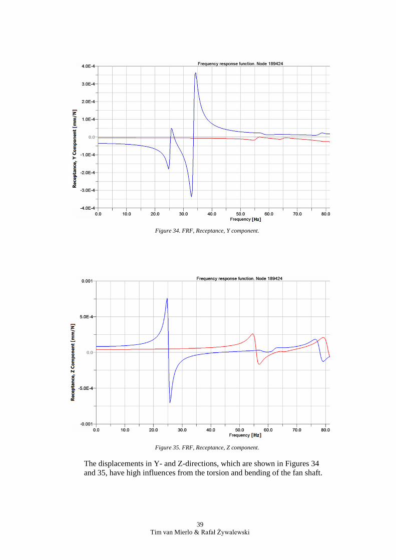
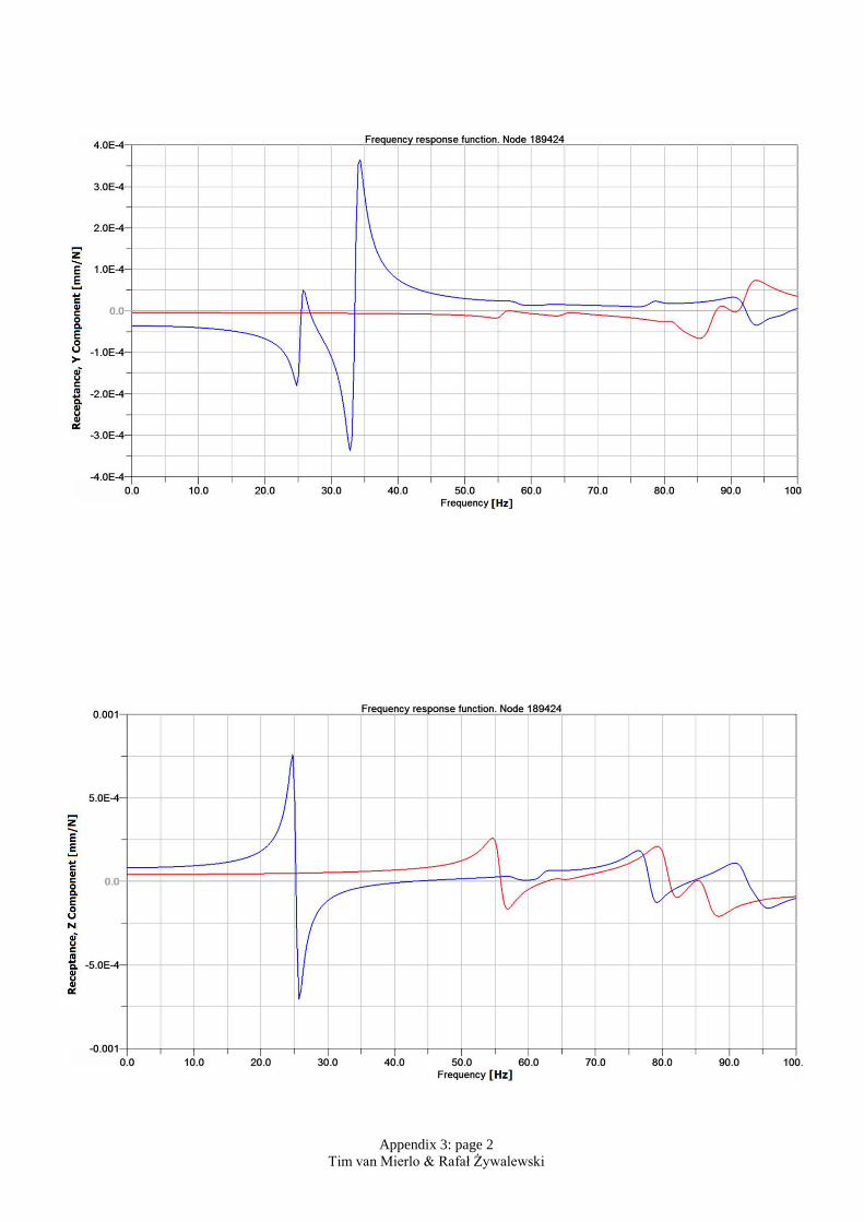
Figure 34. FRF, Receptance, Y component.

Figure 35. FRF, Receptance, Z component.

The displacements in Y- and Z-directions, which are shown in Figures 34 and 35, have high influences from the torsion and bending of the fan shaft.


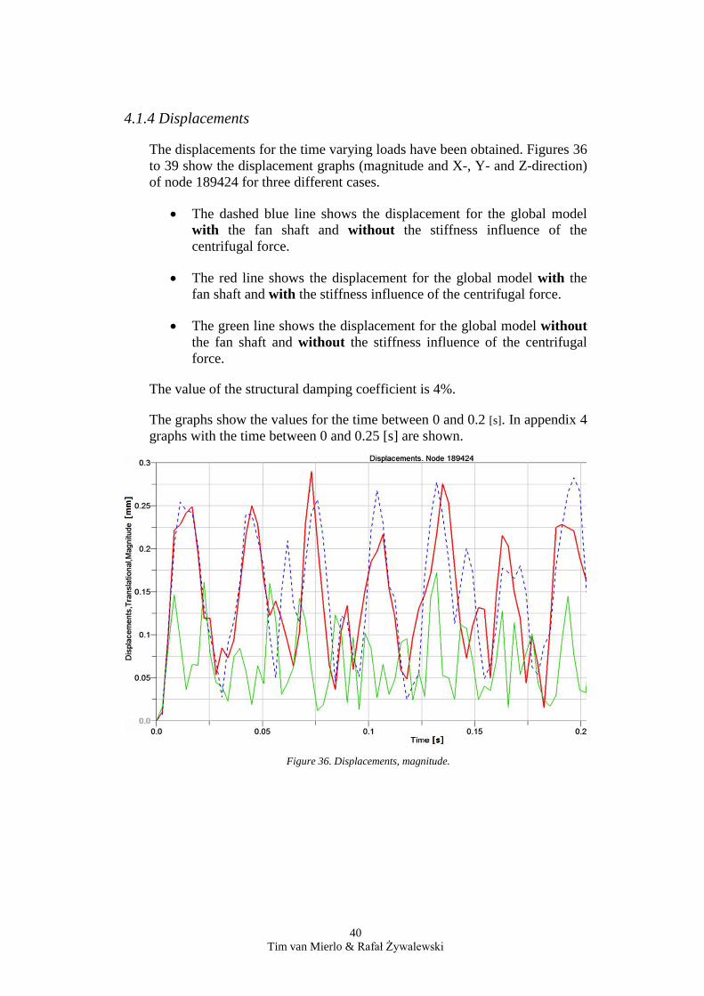
4.1.4 Displacements

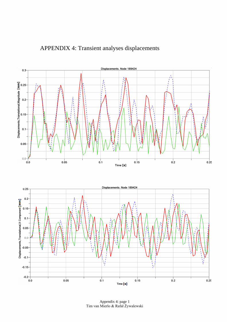
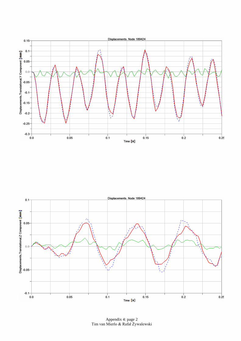
The displacements for the time varying loads have been obtained. Figures 36 to 39 show the displacement graphs (magnitude and X-, Y- and Z-direction) of node 189424 for three different cases.

• The dashed blue line shows the displacement for the global model with the fan shaft and without the stiffness influence of the centrifugal force.

• The red line shows the displacement for the global model with the fan shaft and with the stiffness influence of the centrifugal force.

• The green line shows the displacement for the global model without the fan shaft and without the stiffness influence of the centrifugal force.

The value of the structural damping coefficient is 4%.

The graphs show the values for the time between 0 and 0.2 [s]. In appendix 4 graphs with the time between 0 and 0.25 [s] are shown.

Figure 36. Displacements, magnitude.


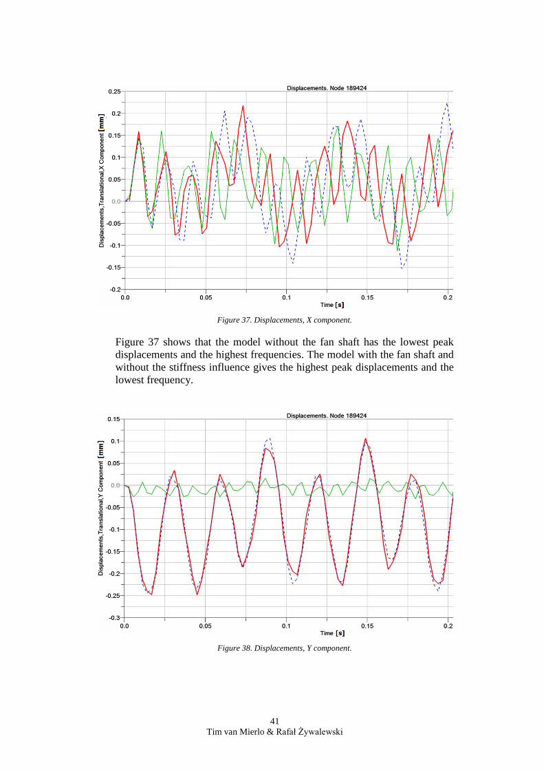
Figure 37. Displacements, X component.

Figure 37 shows that the model without the fan shaft has the lowest peak displacements and the highest frequencies. The model with the fan shaft and without the stiffness influence gives the highest peak displacements and the lowest frequency.

Figure 38. Displacements, Y component.


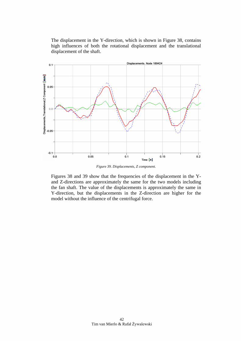
The displacement in the Y-direction, which is shown in Figure 38, contains high influences of both the rotational displacement and the translational displacement of the shaft.

Figure 39. Displacements, Z component.

Figures 38 and 39 show that the frequencies of the displacement in the Y- and Z-directions are approximately the same for the two models including the fan shaft. The value of the displacements is approximately the same in Y-direction, but the displacements in the Z-direction are higher for the model without the influence of the centrifugal force.


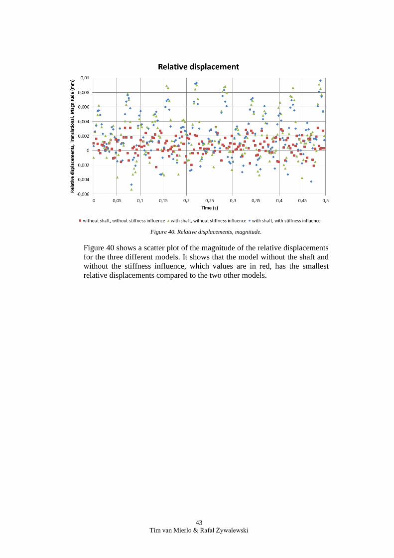
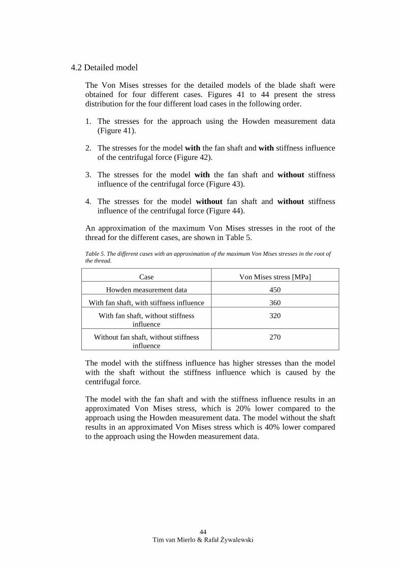
Figure 40. Relative displacements, magnitude.

Figure 40 shows a scatter plot of the magnitude of the relative displacements for the three different models. It shows that the model without the shaft and without the stiffness influence, which values are in red, has the smallest relative displacements compared to the two other models.


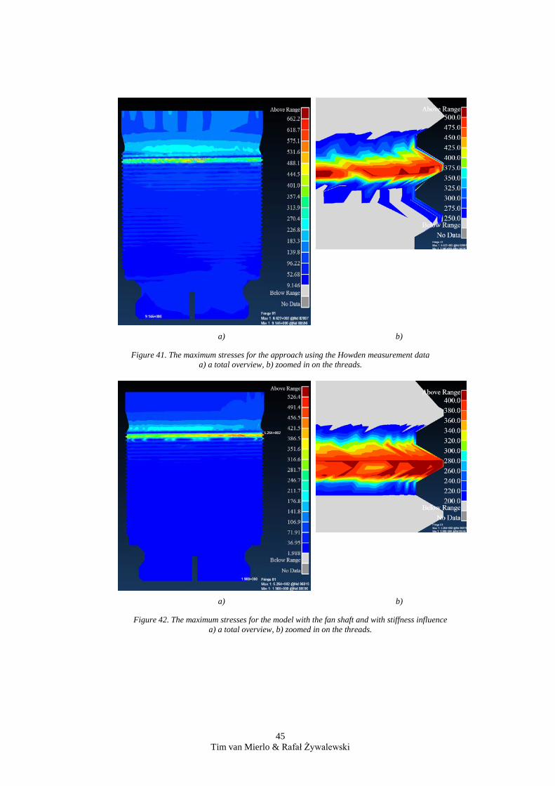
4.2 Detailed model

The Von Mises stresses for the detailed models of the blade shaft were obtained for four different cases. Figures 41 to 44 present the stress distribution for the four different load cases in the following order.

1. The stresses for the approach using the Howden measurement data (Figure 41).

2. The stresses for the model with the fan shaft and with stiffness influence of the centrifugal force (Figure 42).

3. The stresses for the model with the fan shaft and without stiffness influence of the centrifugal force (Figure 43).

4. The stresses for the model without fan shaft and without stiffness influence of the centrifugal force (Figure 44).

An approximation of the maximum Von Mises stresses in the root of the thread for the different cases, are shown in Table 5.

Table 5. The different cases with an approximation of the maximum Von Mises stresses in the root of the thread.

Case Von Mises stress [MPa]

Howden measurement data 450

With fan shaft, with stiffness influence 360

With fan shaft, without stiffness influence

320

Without fan shaft, without stiffness influence

270

The model with the stiffness influence has higher stresses than the model with the shaft without the stiffness influence which is caused by the centrifugal force.

The model with the fan shaft and with the stiffness influence results in an approximated Von Mises stress, which is 20% lower compared to the approach using the Howden measurement data. The model without the shaft results in an approximated Von Mises stress which is 40% lower compared to the approach using the Howden measurement data.


a) b)

Figure 41. The maximum stresses for the approach using the Howden measurement data a) a total overview, b) zoomed in on the threads.

a) b)

Figure 42. The maximum stresses for the model with the fan shaft and with stiffness influence a) a total overview, b) zoomed in on the threads.


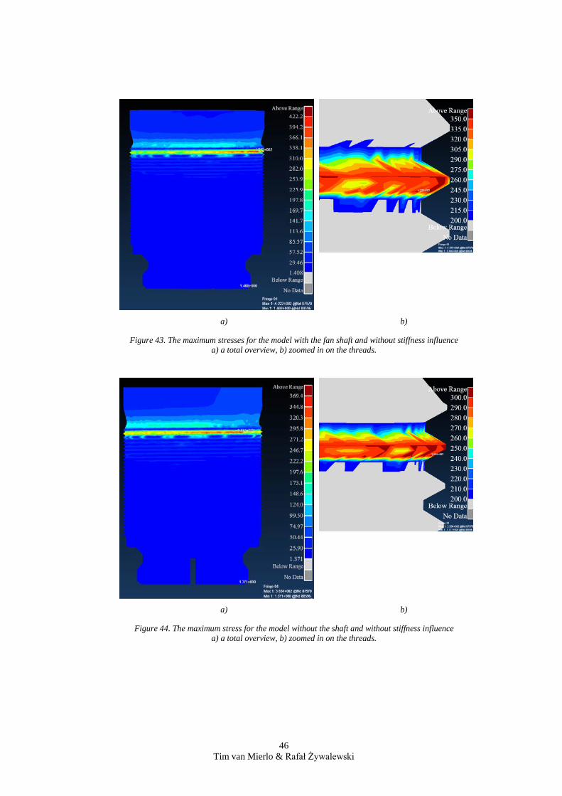
a) b)

Figure 43. The maximum stresses for the model with the fan shaft and without stiffness influence a) a total overview, b) zoomed in on the threads.

a) b)

Figure 44. The maximum stress for the model without the shaft and without stiffness influence a) a total overview, b) zoomed in on the threads.


6. Discussion The results proof that the centrifugal force increases the stiffness of the structure, which results in lower displacements and higher eigenfrequencies.

The global model could be improved in many ways.

First of all, all models which were used during this project neglected the bearing stiffness and the stiffness of the ground. The bearings were just modelled as stiff supports. Flexible bearings make the shaft system more flexible which is likely to increase the stresses even closer to the measurement data. Secondly the meshes could be improved and the model could be more detailed. In the used global models the hub and blade shaft have been strongly simplified which affects the results.

During this project the forces acting on the blades were assumed as harmonic loads. In the real fan, there are many effects which could influence the load. For example, the parts connecting the bearings to the fan housing.

Because the computational time was reasonable, the time steps could be smaller to improve the graphs.

The obtained stresses are based on the translational displacements of just one point on the top surface of the blade shaft and the average value of four nodes on its lower part. In order to obtain better results, the rotational displacements should also be taken into consideration. In this project the rotations were neglected which results in less accurate simulations for the detailed models. The influence of the rotational displacement will be higher for the models including the fan shaft than for the model which does not include the fan shaft.

It is very useful to use 3D elements which contain rotational displacements for the divided blade shaft in the global model to make the substructuring easier.

In this project the displacement was applied on all the nodes of the top surface. This is not according to the real situation, because the real situation will include the Poisson effect.


7. Conclusions From the results of the models with and without the fan shaft it can be concluded that the fan shaft has a significant influence on the displacements and Von Mises stresses in the root of the threads of the blade shaft. The centrifugal force influences the stiffness of the structure which effects the displacements and the stresses although the influence is not that high compared to the influence of the presence of the fan shaft. The results with the fan shaft are probably less accurate due to simplifications and assumptions.

On the other hand the models are comparable with the measured data from experiments done by Howden. The measured data results in the highest stresses and the model with the fan shaft and stiffness influence results in stresses which are 20% lower.

The safest approach is to use the results obtained using the experimental data, because they constitute is the worst case scenario.


References [1] “Howden axial fans,” Howden, [Online]. Available:

http://www.howden.com/AboutUs/bu/HAXS/pages/home.aspx. [Accessed 01 march 2015].

[2] M. Jun, X. Yanhong and Y. Liguo, “Numerical simulation of the pneumatic elasticity for the blade of a big axial-flow fan,” Engineering Failure Analysis, vol. 18, no. 3, pp. 1037-1048, 2011.

[3] J. Vance, B. Murphy and F. Zeidan, Machinery Vibration and Rotordynamics, Hoboken: John Wiley, 2010.

[4] M. Gibanica, “Experimental-Analytical Dynamic Substructuring,” Department of Applied Mechanics , Division of Dynamics, Chalmers University of Technology, Göteborg, 2013.

[5] H. Petersson and N. Ottosen, Introduction to the Finite Element Method, New York: Prentice Hall, 1992.

[6] R. Craig and A. Kurdila, Fundamentals of structural dynamics, Hoboken: John Wiley, 2006.

[7] D. Rixen, “Dynamic Substructuring Concepts-Tutorial,” Delft University of Technology, Delft, 2010.

[8] D. de Klerk, D. Rixen and S., “General Framework for Dynamic Substructuring: History, Review and Classification of Techniques,” AIAA Journal, vol. 46, no. 5, pp. 1169-1181, 2008.

[9] S. Rao and F. Yap, Mechanical vibrations, Singapore: Prentice Hall, 2011. [10] J. Banerjee, “Free vibration of centrifugally stiffened uniform and tapered

beams using the dynamic stiffness method,” Journal of Sound and Vibration, vol. 233, no. 5, pp. 857-875, 2000.

[11] H. Yoo and S. Shin, “Vibration analysis of rotating cantilever beams,” Journal of Sound and Vibration, vol. 212, no. 5, pp. 807-828, 1998.

[12] D. Rixen and M. Géradin, Mechanical vibrations, Chichester: John Wiley, 1997.

[13] MSC software, SimXpert version 2012.0.1, 2012. [14] “SimXpert structure workspace guide,” MSC Software, 2012. [15] C. McCormick, The NASTRAN User's Manual, Washington, DC: National

Aeronautic and Space Administration, 1972. [16] “SimXpert modeling guide,” MSC Software, 2012. [17] S. Bournival, J. Cuillière and V. François, “A mesh-geometry based method

for coupling 1D and 3D elements,” Advances in Engineering Software, vol. 41, no. 6, pp. 838-858, 2010.

[18] J. Craveur and D. Marceau, De la CAO au calcul, Paris: Dunod, 2001. [19] Autodesk, Inventor Professional, Build: 159, Release 2015 RTM - Date: Thu

02/27/2014, Usage Type: Student Version, 2015.


Appendices

Appendix 1: Calculations missing masses and moment of inertia

Appendix 2: Eigenmodes for the global model with the shaft

Appendix 3: FRF receptances

Appendix 4: Transient analyses displacements


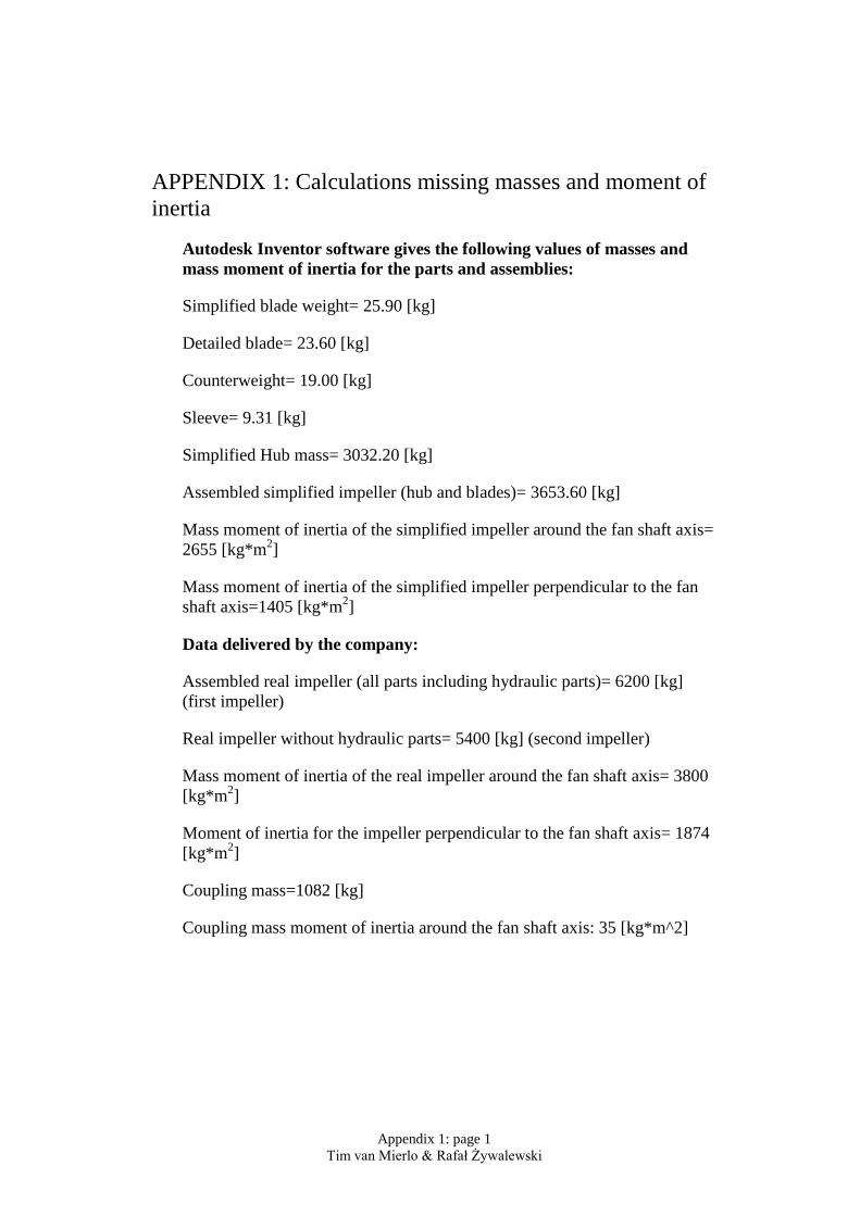
APPENDIX 1: Calculations missing masses and moment of inertia

Autodesk Inventor software gives the following values of masses and mass moment of inertia for the parts and assemblies:

Simplified blade weight= 25.90 [kg]

Detailed blade= 23.60 [kg]

Counterweight= 19.00 [kg]

Sleeve= 9.31 [kg]

Simplified Hub mass= 3032.20 [kg]

Assembled simplified impeller (hub and blades)= 3653.60 [kg]

Mass moment of inertia of the simplified impeller around the fan shaft axis= 2655 [kg*m2]

Mass moment of inertia of the simplified impeller perpendicular to the fan shaft axis=1405 [kg*m2]

Data delivered by the company:

Assembled real impeller (all parts including hydraulic parts)= 6200 [kg] (first impeller)

Real impeller without hydraulic parts= 5400 [kg] (second impeller)

Mass moment of inertia of the real impeller around the fan shaft axis= 3800 [kg*m2]

Moment of inertia for the impeller perpendicular to the fan shaft axis= 1874 [kg*m2]

Coupling mass=1082 [kg]

Coupling mass moment of inertia around the fan shaft axis: 35 [kg*m^2]

Appendix 1: page 1 Tim van Mierlo & Rafał Żywalewski

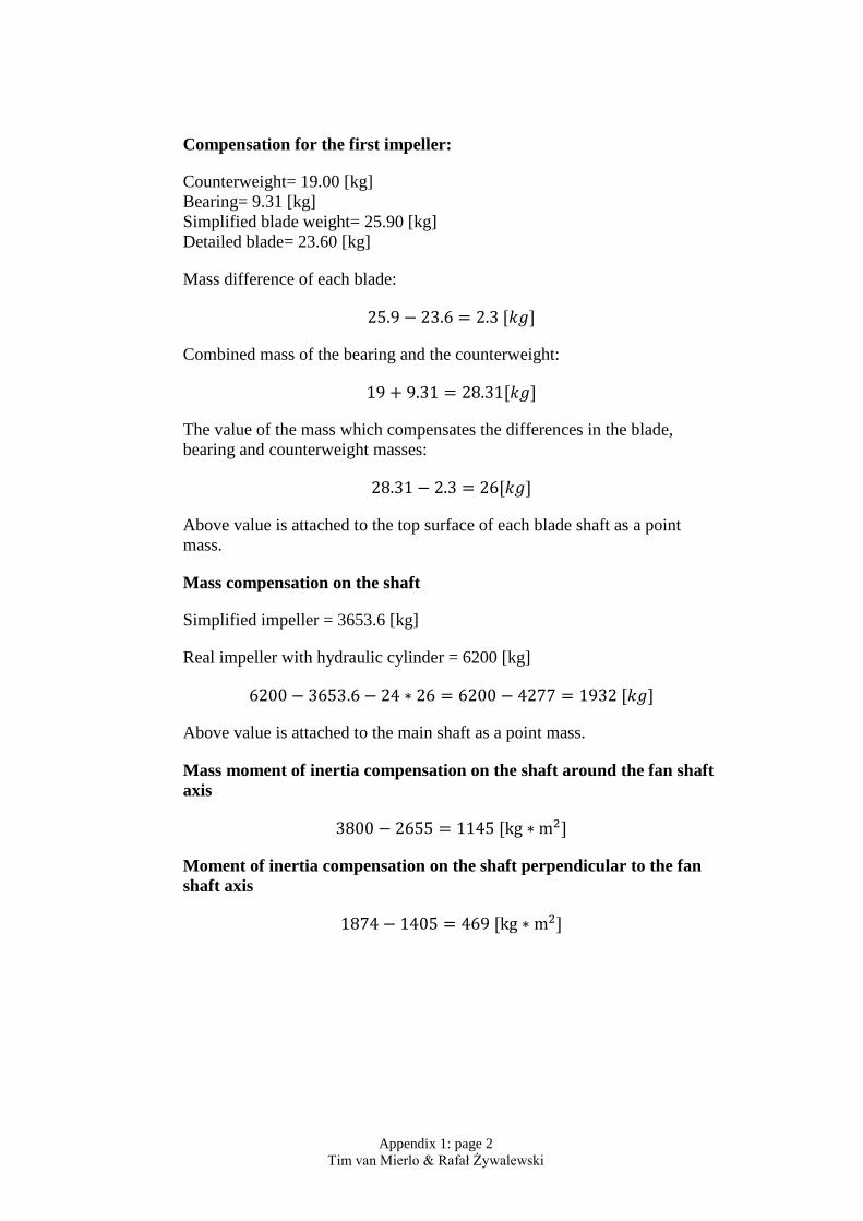
Compensation for the first impeller:

Counterweight= 19.00 [kg] Bearing= 9.31 [kg] Simplified blade weight= 25.90 [kg] Detailed blade= 23.60 [kg]

Mass difference of each blade:

25.9 − 23.6 = 2.3 [𝑘𝑘𝑔𝑔]

Combined mass of the bearing and the counterweight:

19 + 9.31 = 28.31[𝑘𝑘𝑔𝑔]

The value of the mass which compensates the differences in the blade, bearing and counterweight masses:

28.31 − 2.3 = 26[𝑘𝑘𝑔𝑔]

Above value is attached to the top surface of each blade shaft as a point mass.

Mass compensation on the shaft

Simplified impeller = 3653.6 [kg]

Real impeller with hydraulic cylinder = 6200 [kg]

6200 − 3653.6 − 24 ∗ 26 = 6200 − 4277 = 1932 [𝑘𝑘𝑔𝑔]

Above value is attached to the main shaft as a point mass.

Mass moment of inertia compensation on the shaft around the fan shaft axis

3800 − 2655 = 1145 [kg ∗ m2]

Moment of inertia compensation on the shaft perpendicular to the fan shaft axis

1874 − 1405 = 469 [kg ∗ m2]


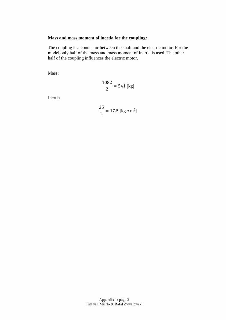
Mass and mass moment of inertia for the coupling:

The coupling is a connector between the shaft and the electric motor. For the model only half of the mass and mass moment of inertia is used. The other half of the coupling influences the electric motor.

Mass:

10822

= 541 [kg]

Inertia

352

= 17.5 [kg ∗ m2]


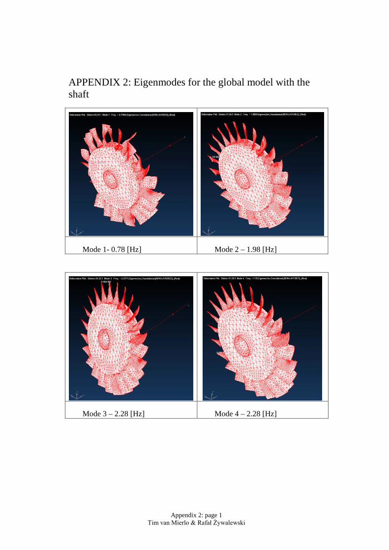
APPENDIX 2: Eigenmodes for the global model with the shaft

Mode 1- 0.78 [Hz] Mode 2 – 1.98 [Hz]

Mode 3 – 2.28 [Hz] Mode 4 – 2.28 [Hz]


Mode 5 – 3.23 [Hz] Mode 6 – 3.23 [Hz]

Mode 7 – 5.20 [Hz] Mode 8 – 45.10 [Hz]


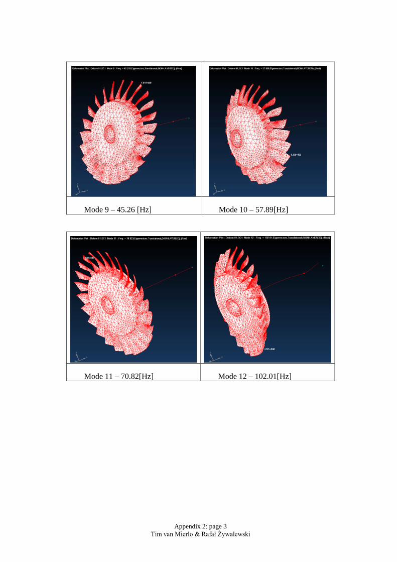
Mode 9 – 45.26 [Hz] Mode 10 – 57.89[Hz]

Mode 11 – 70.82[Hz] Mode 12 – 102.01[Hz]


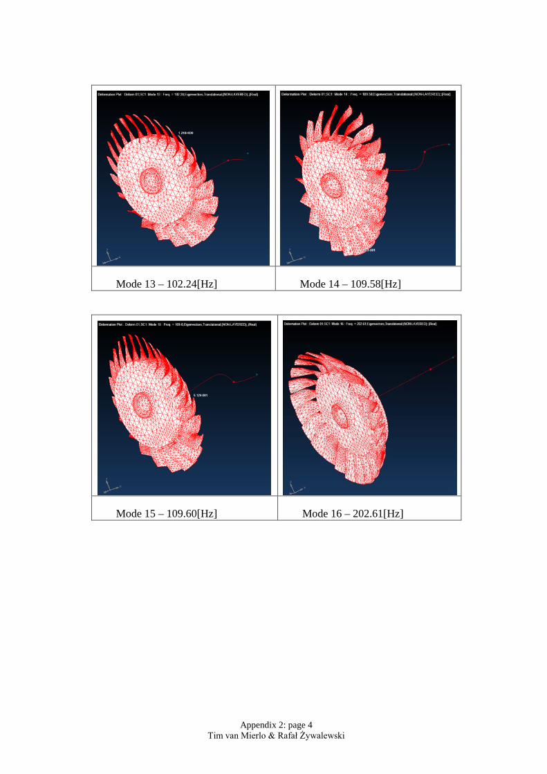
Mode 13 – 102.24[Hz] Mode 14 – 109.58[Hz]

Mode 15 – 109.60[Hz] Mode 16 – 202.61[Hz]


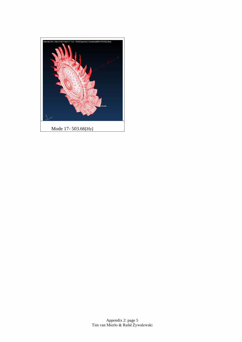
Mode 17- 503.66[Hz]


APPENDIX 3: FRF receptances


APPENDIX 4: Transient analyses displacements


Faculty of Technology 351 95 Växjö, Sweden Telephone: +46 772-28 80 00, fax +46 470-832 17

Evaluation of time varying stresses in a Howden fan - DiVA

Documents

Transcript of Evaluation of time varying stresses in a Howden fan - DiVA