1

EVALUATION OF THE CAPITAL VALUE, INVESTMENTS AND CAPITAL COSTS IN THE FISHERIES SECTOR

No FISH/2005/03

FINAL REPORT

by

IREPA Onlus

In co-operation with

IFREMER, France FOI, Denmark

SEAFISH, United Kingdom LEI BV, Netherlands

FRAMIAN BV, Netherlands

October 2006

2

CONTENTS SUMMARY.................................................................................................................................................................12 1.INTRODUCTION................................................................................................................................................13 2.PROPOSED METHOD ......................................................................................................................................18 2.1 PIM proposed by OECD...................................................................................................................................18 2.2 Application of PIM to fishing fleets .................................................................................................................19 2.3 Calculation of capital costs.................................................................................................................................26 2.4 Valuation model...................................................................................................................................................28 2.5 Valuation of intangible assets ............................................................................................................................34 2.6 Valuation of ‘other assets ...................................................................................................................................36 3.THEORETICAL CONSIDERATIONS...........................................................................................................38 3.1 The conceptual framework ................................................................................................................................38 3.2 Overview of measurement methods.................................................................................................................52 REFERENCES..........................................................................................................................................................56 APPENDIX A: Denmark ........................................................................................................................................58 Introduction: Data sources .......................................................................................................................................58 1. General national situation.....................................................................................................................................58 1.1 Investments in new vessels ................................................................................................................................58 1.2 Investments in fishing rights..............................................................................................................................59 1.3 Investments in 2nd hand vessels.......................................................................................................................60 1.4 Investments in shore facilities............................................................................................................................60 1.5 Approach to calculation of capital value in agriculture .................................................................................61 2. National fleet ..........................................................................................................................................................62 2.1 Description of the case study fleet....................................................................................................................62 2.2 Data and estimation of price per capacity unit ...............................................................................................62 2.3 Capital value and capital costs ...........................................................................................................................66 2.4 Evaluation .............................................................................................................................................................68 3. Fleet under 12 meters............................................................................................................................................69 3.1 Description of the case study fleet < 12m.......................................................................................................69 3.2 Data and estimation of price per capacity unit ...............................................................................................70 3.3 Capital value and capital costs ...........................................................................................................................71 4. Fleet 12 meters and over.......................................................................................................................................72 4.1 Description of the case study fleet >12m........................................................................................................72 4.2 Data and estimation of price per capacity unit ...............................................................................................73 4.3 Capital value and capital costs ...........................................................................................................................73 Appendix A.1 Account Statistics for Fisheries - Denmark .................................................................................75 APPENDIX B: France .............................................................................................................................................78 Introduction: Data sources .......................................................................................................................................78 1. General national situation – national markets for fishery assets ....................................................................79 1.1 Investments in new vessels ................................................................................................................................79 1.2 Investments in fishing rights..............................................................................................................................80 1.3 Investments in 2nd hand vessels.......................................................................................................................81 1.4 Investments in shore facilities............................................................................................................................82 1.5 Approach for the calculation of capital value in agriculture and/or by statistical office .........................83 2. Estimation of value per capacity unit .................................................................................................................83 2.1 Data and estimation of price per capacity unit ...............................................................................................83 2.2 Capital value and capital costs ...........................................................................................................................87 3 Total fleet (under 30meters, NSCA coast).........................................................................................................92 3.1 Description of the case study total fleet...........................................................................................................92

3

3.2 Data and estimation of price per capacity unit ...............................................................................................93 3.3 Capital value and capital costs ...........................................................................................................................93 4. Fleet under 12 meters (NSCA coast) ..................................................................................................................95 4.1 Description of the case study fleet <12m........................................................................................................95 4.2 Data and estimation of price per capacity unit ...............................................................................................96 4.3 Capital value and capital costs ...........................................................................................................................96 5. Fleet 12 - 30 meters (NSCA coast) .....................................................................................................................98 5.1 Description of the case study fleet 12 - 30 m..................................................................................................98 5.2 Data and estimation of price per capacity unit ............................................................................................ 100 5.3 Capital value and capital costs ........................................................................................................................ 100 6. Trawlers 16-24 meters........................................................................................................................................ 102 6.1 Description of the case study Trawlers 16-24 m. ........................................................................................ 102 6.2 Data and estimation of price per capacity unit ............................................................................................ 103 6.3 Capital value and capital costs ........................................................................................................................ 103 7. Passive gears less than 12 meters...................................................................................................................... 105 7.1 Description of the case study Passive gears <12m. .................................................................................... 105 7.2 Data and estimation of price per capacity unit ............................................................................................ 106 7.3 Capital value and capital costs ........................................................................................................................ 106 8. Evaluation ............................................................................................................................................................ 108 References ................................................................................................................................................................ 114 Appendix B.1 : Historical vessel price model ..................................................................................................... 115 APPENDIX C: Italy............................................................................................................................................... 116 Introduction: Data sources .................................................................................................................................... 116 1. General national situation – national markets for fishery assets ................................................................. 116 1.1 Investments in new vessels ............................................................................................................................. 116 1.2 Investments in fishing rights........................................................................................................................... 117 1.3 Investments in 2nd hand vessels.................................................................................................................... 119 1.4 Investments in shore facilities......................................................................................................................... 121 1.5 Approach to calculation of capital value by statistical office..................................................................... 121 2. National fleet ....................................................................................................................................................... 123 2.1 Description of the case study fleet................................................................................................................. 123 2.2 Data and estimation of price per capacity unit ............................................................................................ 123 2.3 Capital value and capital costs ........................................................................................................................ 129 2.4 Evaluation .......................................................................................................................................................... 131 3. Fleet under 12meters .......................................................................................................................................... 132 3.1. Description of the case study fleet <12m.................................................................................................... 132 3.2 Data and estimation of price per capacity unit ............................................................................................ 134 3.3 Capital value and capital costs ........................................................................................................................ 135 3.4 Evaluation .......................................................................................................................................................... 137 4. Fleet 12 meters and over.................................................................................................................................... 137 4.1 Description of the case study fleet >12m..................................................................................................... 137 4.2 Data and estimation of price per capacity unit ............................................................................................ 138 4.3 Capital value and capital costs ........................................................................................................................ 139 4.4 Evaluation .......................................................................................................................................................... 141 5. Passive gears ........................................................................................................................................................ 141 5.1. Description of the case study Passive gears ................................................................................................ 141 5.2 Data and estimation of price per capacity unit ............................................................................................ 143 5.3 Capital value and capital costs ........................................................................................................................ 143 5.4 Evaluation .......................................................................................................................................................... 145 6. Demersal Trawl Fleet ......................................................................................................................................... 146 6.1 Description of the case study Demersal Trawl Fleet .................................................................................. 146 6.2 Data and estimation of price per capacity unit ............................................................................................ 146 6.3 Capital value and capital costs ........................................................................................................................ 147

4

6.4. Evaluation ......................................................................................................................................................... 149 References ................................................................................................................................................................ 150 APPENDIX D: Netherlands ................................................................................................................................ 151 Introduction: Data sources .................................................................................................................................... 151 1.1 Investments in new vessels ............................................................................................................................. 151 1.2 Investments in fishing rights........................................................................................................................... 151 1.3 Investments in 2nd hand vessels.................................................................................................................... 154 1.4 Investments in shore facilities......................................................................................................................... 154 1.5 Approach to calculation of capital value in agriculture .............................................................................. 155 2. Estimation of value per capacity unit .............................................................................................................. 155 2.1 Data and estimation of price per capacity unit ............................................................................................ 155 2.1.1 Replacement value LEI method.................................................................................................................. 156 2.1.2 Insurance value .............................................................................................................................................. 159 2.2 Data, prices and estimation value of intangible capital............................................................................... 166 2.2.1 Licenses ........................................................................................................................................................... 166 2.2.2 Shrimp licenses, list I and list II licenses.................................................................................................... 166 2.2.3 Fish quota ....................................................................................................................................................... 167 3. Total cutter fleet the Netherlands .................................................................................................................... 168 3.1 Description of the case study total cutter fleet (all vessels >12 m.) ......................................................... 168 3.2 Data and estimation of price per capacity unit ............................................................................................ 169 3.3.1 Tangible capital .............................................................................................................................................. 170 3.3.2 Intangible capital............................................................................................................................................ 172 4. Vessels 261-300 hp (beam trawlers over 24 meters) ..................................................................................... 172 4.1 Description of the case study vessels 261-300 hp (beam trawlers <24 m.) ............................................ 172 4.2 Data and estimation of price per capacity unit ............................................................................................ 172 4.3 Capital value and capital costs ........................................................................................................................ 173 4.3.1 Tangible capital .............................................................................................................................................. 173 4.3.2 Intangible capital............................................................................................................................................ 174 5. Vessels >1.501 hp (beam trawlers >24 m.) .................................................................................................... 175 5.1 Description of the case study vessels >1.501 hp (beam trawlers >24m.) ............................................... 175 5.2 Data and estimation of price per capacity unit ............................................................................................ 175 5.3 Capital value and capital costs vessels ........................................................................................................... 176 5.3.1Tangible capital ............................................................................................................................................... 176 6. Evaluation ............................................................................................................................................................ 178 APPENDIX E: United Kingdom........................................................................................................................ 179 Introduction: Data sources .................................................................................................................................... 179 1. General national situation – national markets for fishery assets ................................................................. 179 1.1 Investments in new vessels ............................................................................................................................. 179 1.2 Investments in fishing rights........................................................................................................................... 180 1.3 Investments in 2nd hand vessels.................................................................................................................... 182 1.4 Investments in shore facilities......................................................................................................................... 182 1.5 Approach to calculation of capital value in agriculture and/or by statistical office............................... 182 2. Total fleet ............................................................................................................................................................. 183 2.1 Description of the case study fleet................................................................................................................. 183 2.2 Data and estimation of price per capacity unit ............................................................................................ 184 2.3 Capital value and capital costs ........................................................................................................................ 188 2.4 Evaluation .......................................................................................................................................................... 190 3. Fleet under 12 meters......................................................................................................................................... 191 3.1 Description of the case study fleet................................................................................................................. 191 3.2 Data and estimation of price per capacity unit ............................................................................................ 192 3.3 Capital value and capital costs ........................................................................................................................ 193 4. Fleet 12 meters and over.................................................................................................................................... 195

5

4.1 Description of the case study.......................................................................................................................... 195 4.2 Data and estimation of price per capacity unit ............................................................................................ 195 4.3 Capital value and capital costs ........................................................................................................................ 196 5. Over 40m Pelagic Fleet...................................................................................................................................... 198 5.2 Data and estimation of price per capacity unit ............................................................................................ 198 5.3 Capital value and capital costs ........................................................................................................................ 199 5.4 Evaluation .......................................................................................................................................................... 200 6. Over 24 meters Demersal Trawl Fleet ............................................................................................................ 201 6.1 Description of the case study.......................................................................................................................... 201 6.2 Data and estimation of price per capacity unit ............................................................................................ 201 6.3 Capital value and capital costs ........................................................................................................................ 202

6

TABLES Table 1. Depreciation period of hull, engine and electronics applied in AER by country, 2002..................41 Table 2. Average service lives in Fishing (OECD, 1992) ....................................................................................42 Table 3 Classification of fixed assets.......................................................................................................................47 Table A.1.1 Value of land-based assets owned by commercial Danish fishing vessels ..................................60 Table A.2.1 Distribution of recently build vessels with total fleet structure (%).............................................62 Table A.2 2 Average replacement values for total fleet in 2004 (Euro) ............................................................63 Table A.2.3 Distribution of asset value for the Danish commercial fishing vessels (%)................................63 Table A.2.4 Correlation coefficients between selected physical characteristics ...............................................65 Table A.2.5 Weights used to calculate price indices .............................................................................................65 Table A.2.6 Overview of assumptions made in the Danish case studies (%) ..................................................66 Table A.2.7 Capital value and capital costs and their consequences on profit (mln Euro)............................67 Table A.2 8 Summary of the capital values – comparison of approaches (mln Euro) ...................................67 Table A.2 9 Relative composition of capital (%) .................................................................................................67 Table A.3.1 Average replacement values for vessels below 12 meters in 2004 (Euro)...................................70 Table A.3.2 Capital value and capital costs and their consequences on profit for vessels below 12 meters (mln Euro)...................................................................................................................................................................71 Table A.3.3 Summary of the capital values – comparison of approaches for vessels below 12 meters (mln Euro) ............................................................................................................................................................................71 Table A.3.4 Relative composition of capital (%) for vessels below 12 meters.................................................72 Table A.4.1 Average replacement values for vessels above 12 meters in 2004 (Euro)...................................73 Table A.4.2 Capital value and capital costs and their consequences on profit for vessels above 12 meters (mln Euro)...................................................................................................................................................................74 Table A.4.3 Summary of the capital values - comparison of approaches for vessels above 12 meters (mln Euro) ............................................................................................................................................................................74 Table A.4.4 Relative composition of capital for vessels above 12 meters (%).................................................74 Table B.2.1 Reducing balance rate in the French fiscal regulatory basis...........................................................89 Table B.2. 2 Overview of assumptions made in the French case studies .........................................................90 Table B.3.1Composition of the total fleet < 30m. by main DCR sub-segment ..............................................92 Table B.3.2 Price per capacity unit – Model estimates – Total fleet (NSCA, less than 30.) ..........................93 Table B.3.3 Summary of the capital values – NSCA Fleet <30m. .....................................................................93 Table B.4.1Composition of the fleet < 12m. by main DCR sub-segment .......................................................95 Table B.4.2 Price per capacity unit – Model estimates – Total fleet (NSCA, less than 12 meters) ..............96 Table B.4.3 Summary of the capital values – Fleet < 12m..................................................................................97 Table B.5.1 Composition of the total fleet 12-30 m. by main DCR sub-segment ..........................................99 Table B.5.2 Price per capacity unit – Model estimates – Total fleet (NSCA, 12-30m. ) ............................. 100 Table B.5.3 Summary of the capital values - 12– 30 m. NSCA fleet ............................................................. 100 Table B.6.1 Composition of Trawlers 16-24 m. by main DCR sub-segment ............................................... 102 Table B.6.2 Price per capacity unit – Model estimates –Trawlers, 16-24 m.................................................. 103 Table B.6.3 Summary of the capital values – Trawlers 16-24 m. NSCA coast ............................................. 103 Table B.7.1 Composition of Passive gears <12 m. by main DCR sub-segment .......................................... 105 Table B.7.2 Price per capacity unit – Model estimates –Passive gears <12m. .............................................. 106 Table B.7.3 Summary of the capital values – Passive gears < 12m. ............................................................... 106 Table B.8.1 Results from a sub sample of Trawlers 16 -24 m. (45 vessels)................................................... 108 Table B.8.2 Results from a sub sample of Passive gears <12m. (109 vessels) .............................................. 110 Table C.1.2 II hand market prices per capacity units, 2004 ............................................................................. 119 Table C.1.3 Scales of assistance relating to fishing fleets (Euro)..................................................................... 120 Table C.1.4 Hedonic values ................................................................................................................................... 120 Table C.1.5 Classification of Sectors and Standard Average Service Lives (years)....................................... 122

7

Table C.2.1 Composition of the total fleet by main DCR sub-segment ........................................................ 123 Table C.2.2 RINA indexes: Price per GRT unit, 1992 (Euro)......................................................................... 124 Table C.2.3 Percentage composition of investments by main sub-segment and group of assets.............. 125 Table C.2.4 Depreciation rates by groups of assets........................................................................................... 125 Table C.2.5 Fiscal rates by groups of assets........................................................................................................ 126 Table C.2.6 Prices (€) per capacity units in 1992 and 2004 .............................................................................. 128 Table C.2.7 Qualitative description of the relevant fishing rights................................................................... 128 Table C.2.8 Valuation of the relevant fishing rights .......................................................................................... 129 Table C.2.9 Background for calculation of depreciation and interest for the total fleet ............................. 129 Table C.2.10 Capital value and capital costs and their consequences on profit for the total fleet............. 129 Table C.2.11 Summary of the capital values - comparison of approaches for the total fleet ..................... 130 Table C.2.12 Background for calculation of depreciation and interest .......................................................... 131 Table C.3.1 Composition of the fleet <12m. by main DCR sub-segment .................................................... 133 Table C.3.2 Prices (€) per capacity units of the fleet <12m. in 1992 and 2004 ............................................ 134 Table C.3.3 Valuation of the relevant fishing rights .......................................................................................... 135 Table C.3.4 Background for calculation of depreciation and interest of fleet < 12m. ................................ 135 Table C.3.5 Capital value and capital costs and their consequences on profit of fleet < 12m................... 135 Table C.3.6 Summary of the capital values - comparison of approaches of fleet < 12m. .......................... 136 Table C.4.1 Composition of the 12m. and over fleet by main DCR sub-segment ...................................... 138 Table C.4.2 Prices (€) per capacity units in 1992 and 2004 of the 12m. and over fleet............................... 138 Table C.4.3 Valuation of the relevant fishing rights of the 12m. and over fleet........................................... 139 Table C.4.4 Background for calculation of depreciation and interest of the 12m and over fleet .............. 139 Table C.4.5 Capital value and capital costs and their consequences on profit of the 12m. and over fleet139 Table C.4.6 Summary of the capital values - comparison of approaches of the 12m. and over fleet ....... 140 Table C.5.1 Prices (€) per capacity units in 1992 and 2004 of Passive gears................................................. 143 Table C.5.2 Valuation of the relevant fishing rights of Passive gears............................................................. 143 Table C.5.3 Background for calculation of depreciation and interest of Passive gears ............................... 143 Table C.5.4 Capital value and capital costs and their consequences on profit of Passive gears................. 144 Table C.5.5 Summary of the capital values - comparison of approaches of Passive gears ......................... 144 Table C.6.1 Prices (€) per capacity units in 1992 and 2004 of Demersal Trawl Fleet.................................. 146 Table C.6.2 Valuation of the relevant fishing rights of Demersal Trawl Fleet ............................................. 147 Table C.6.3 Background for calculation of depreciation and interest of Demersal Trawl Fleet................ 147 Table C.6.4 Capital value and capital costs and their consequences on profit of Demersal Trawl Fleet . 147 Table C.6.5 Summary of the capital values - comparison of approaches of Demersal Trawl Fleet.......... 148 Table D.1.1 Average scrapping premiums for capacity Dutch fleet 2005 ..................................................... 154 Table D.2.1 Estimated replacement value vessel and engine grouped by hp-class ...................................... 157 Table D.2.2 Estimated replacement value vessel and engine grouped by fleet segment............................. 157 Table D.2.3 Estimated book value vessel and engine grouped by hp-class................................................... 158 Table D.2.4 Estimated book value vessel and engine grouped by fleet segment ......................................... 158 Table D.2.5 Mean values technical variables ...................................................................................................... 159 Table D.2.6 Results regression.............................................................................................................................. 161 Table D.2.7 Mean values technical variables by hp-class.................................................................................. 162 Table D.2.8 Mean values technical variables per capacity unit by fleet segment.......................................... 162 Table D.2.9 Estimated insurance value grouped by hp-class........................................................................... 163 Table D.2.10 Estimated insurance value grouped per capacity unit by fleet segment................................. 163 Table D.2.11 Estimated average insurance value per capacity unit by hp-class............................................ 164 Table D.2.12 Estimated average insurance value per capacity unit by fleet segment .................................. 164 Table D.2.13 Number of vessels with a license to fish for shrimp by hp-class (2004)................................ 166 Table D.2.14 Number of vessels with a license to fish for shrimp by fleet segment (2004) ...................... 166 Table D.2.15 Total quota for sole, plaice, cod and whiting sorted by hp-class (2004)................................ 167 Table D.2.16 Total quota for sole, plaice, cod and whiting by fleet segment (2004)................................... 167 Table D.2.17 Average quota for sole, plaice, cod and whiting by hp-class (2004) ....................................... 167 Table D.2.18 Average quota per vessel for sole, plaice, cod and whiting by fleet segment (2004) ........... 167

8

Table D.2.19 Estimated values of quota sole and plaice active vessels in the Netherlands........................ 168 Table D.2.20 Estimated value intangible capital active cutter fleet................................................................. 168 Table D.3.1 Technical variables by hp-class ....................................................................................................... 169 Table D.3.2 Estimated average insurance value per capacity unit................................................................... 169 Table D.3.3 Background for calculation of depreciation and interest entire Cutter fleet ........................... 170 Table D.3.4 Capital value and capital costs and their consequences on profit for entire cutter fleet ....... 170 Table D.3.5 Summary of the capital values - comparison of approaches entire cutter fleet ..................... 171 Table D.3.6 Relative composition ........................................................................................................................ 171 Table D.3.7 Level of depreciation ........................................................................................................................ 171 Table D.4.1 Average values for vessels 261-300 hp (12-24m. ) in 2004 (Euro) ........................................... 172 Table D.4.2 Background for calculation of depreciation and interest............................................................ 173 Table D.4.3 Capital value and capital costs and their consequences on profit (sensitivity analysis) ......... 173 Table D.4.4 Summary of the capital values - comparison of approaches...................................................... 174 Table D.4.5 Relative composition ........................................................................................................................ 174 Table D.4.6 Level of depreciation ........................................................................................................................ 174 Table D.4.7 Estimated value intangible capital vessels 261-300 hp................................................................ 175 Table D.5.1 Average values for vessels >1.501 hp in 2004 (Euro)................................................................. 176 Table D.5.2 Background for calculation of depreciation and interest >1.501 hp ........................................ 176 Table D.5.3 Capital value and capital costs and their consequences on profit >1.501 hp.......................... 176 Table D.5.4 Summary of the capital values - comparison of approaches >1.501 hp .................................. 177 Table D.5.5 Relative composition ........................................................................................................................ 177 Table D.5.6 Level of depreciation ........................................................................................................................ 177 Table E.1.2 Depreciation rates for different time periods for agricultural plant and machinery............... 183 Table E.2.1 Registered and active vessels in the UK fleet as at 1 January 2005, split by DCR segment.. 184 Table E.2.2 Characteristics of population and sample vessels for the whole UK fleet case study............ 185 Table E.2.3 Estimated average historic price (insured value indexed to 2004) per capacity unit and estimated replacement value (insured value in money of the day) per capacity unit for the whole UK fleet.................................................................................................................................................................................... 186 Table E.2.4 Correlation coefficients between insured value (adjusted to 2004 equivalent) and selected physical characteristics, based on sample of whole UK fleet........................................................................... 186 Table E.2.5 Assumed depreciation rates applied in the UK calculations....................................................... 188 Table E.2.6 Capital value and capital costs and their consequences on profit (sensitivity analysis)......... 188 Table E.2.7 Summary of the capital values (€ mln) - comparison of approaches ........................................ 189 Table E.2.8 Relative composition of capital ....................................................................................................... 189 Table E.3.1 Characteristics of population and sample vessels for the under 12m. ...................................... 192 Table E.3.2 Estimated average historic price (insured value indexed to 2004) per capacity unit and estimated replacement value (insured value in money of the day) per capacity unit for the under 12m. UK fleet. ........................................................................................................................................................................... 192 Table E.3.3 Correlation coefficients between insured value (adjusted to 2004 equivalent) and selected physical characteristics, based on sample of under 12m. vessels in the UK fleet......................................... 192 Table E.3.4 Capital value and capital costs and their consequences on profit (sensitivity analysis).......... 193 Table E.3.5 Summary of the capital values (€ mln) - comparison of approaches ........................................ 193 Table E.3.6 Relative composition of capital (%)................................................................................................ 194 Table E.4.1 Characteristics of population and sample vessels for the 12m. and over vessel case study .. 195 Table E.4.2 Estimated average historic price (insured value indexed to 2004) per capacity unit and estimated replacement value (insured value in money of the day) per capacity unit for the 12m. and over UK fleet .................................................................................................................................................................... 196 Table E.4.3 Correlation coefficients between insured value (adjusted to 2004 equivalent) and selected physical characteristics, based on sample of over 12m. vessels in the UK fleet ........................................... 196 Table E.4.4 Capital value and capital costs and their consequences on profit (sensitivity analysis).......... 196 Table E.4.5 Summary of the capital values (€ mln) - comparison of approaches ........................................ 197 Table E.4.6 Relative composition of capital (%)................................................................................................ 197

9

Table E.5.1 Characteristics of population and sample vessels for the >40m. pelagic UK fleet case study.................................................................................................................................................................................... 198 Table E.5.2 Estimated average historic price (insured value indexed to 2004) per capacity unit and estimated replacement value (insured value in money of the day) per capacity unit for the >40m. pelagic UK fleet .................................................................................................................................................................... 199 Table E.5.3 Correlation coefficients between purchase price (adjusted to 2004 equivalent) and selected physical characteristics, based on sample of pelagic vessels in the UK fleet................................................. 199 Table E.5.4 Capital value and capital costs and their consequences on profit (sensitivity analysis).......... 199 Table E.5.5 Summary of the capital values (€ mln) - comparison of approaches ........................................ 200 Table E.5.6 Relative composition of capital (%)................................................................................................ 200 Table E.6.1 Characteristics of population and sample vessels for the over 24m. demersal segment case study .......................................................................................................................................................................... 201 Table E.6.2 Estimated average historic price (insured value indexed to 2004) per capacity unit and estimated replacement value (insured value in money of the day) per capacity unit the UK over 24m. demersal trawl fleet ................................................................................................................................................. 202 Table E.6.3 Correlation coefficients between purchase price (adjusted to 2004 equivalent) and selected physical characteristics, based on sample of over 24m. demersal trawl vessels in the UK fleet ................ 202 Table E.6.4 Capital value and capital costs and their consequences on profit (sensitivity analysis).......... 202 Table E.6.5 Summary of the capital values (€ mln) - comparison of approaches ........................................ 203 Table E.6.6 Relative composition of capital (%)................................................................................................ 203

10

FIGURES Figure 1 Application of the PIM in practice by OECD ......................................................................................19 Figure 2 PIM application to fishing fleets.............................................................................................................20 Figure 3 Presentation of the composition of a fleet.............................................................................................23 Figure 4 Procedure for interpretation and estimation of prices per capacity unit...........................................24 Figure 5 Micro / macro calculation of depreciation and interest costs in the year t, tangible assets only (vessel and equipment) ..............................................................................................................................................27 Figure 6 Valuation model..........................................................................................................................................30 Figure 7 Spreadsheet for macro calculation of replacement value, depreciation and interest costs.............31 Figure 8 Spreadsheet for micro calculation of historic value, depreciation and interest costs ......................32 Figure 9 Comparison of macro and micro approach and sensitivity analysis ..................................................33 Figure 10 Accounting for intangible assets ............................................................................................................36 Figure 11. Typical mortality and survival functions .............................................................................................44 Figure A.1.1 Age composition of the Danish commercial fleet per 1/1-2005 (% of total)...........................59 Figure A.2.1 Accounting for tangible assets – decision tree –Denmark...........................................................64 Figure A.3.1 Age distribution of vessels <12 m....................................................................................................70 Figure A.4.1 Age distribution of vessels >= 12m.................................................................................................73 Figure B.1.1 Age composition of the French total fleet at 1rst January 2005..................................................79 Figure B.1.2 Evolution of the transaction rate on the second-hand Market (Atlantic Area) ........................81 Figure B.1.3 Evolution of average price per meter in constant kEuros on the second-hand Market (Atlantic Area).............................................................................................................................................................81 Figure B.1.4 Evolution of theoretical premium to scrap vessel (Atlantic Area) ..............................................82 Figure B.2.1 Accounting for tangible assets – decision tree – France...............................................................86 Figure B.3.1 Age composition of French NSCA fleet .........................................................................................92 Figure B.4.1 Age composition of Fleet < 12m......................................................................................................95 Figure B.5.1 Age composition of fleet 12-30 m....................................................................................................99 Figure B.6.1 Age composition of Trawlers 16-24m. ......................................................................................... 102 Figure B.7.1 Age composition of Passive gears < 12m. ................................................................................... 105 Figure C.1.1 Age composition of the total Italian fleet..................................................................................... 116 Figure C.1.2 Trend in second hand vessels’ prices ............................................................................................ 119 Figure C.2.1 Age composition of the total Italian fleet, 1935 - 2004.............................................................. 123 Figure C.2.2 Production Price Heavy Machinery index (base = 1992) .......................................................... 124 Figure C.2. 3Accounting for tangible assets – decision tree – for each vintage – Italy ............................... 127 Figure C.2.4 Capital values 2004 -Comparison between the general and the Italian assumptions............ 132 Figure C.3.1 Percentage incidence by length classes of the Italian fleet......................................................... 133 Figure C.3.2 Age composition of the fleet <12m.............................................................................................. 134 Figure C.3.3 Capital values 2004 - Comparison between the general and the Italian assumptions for fleet < 12m........................................................................................................................................................................ 137 Figure C.4.1 Age composition of the 12m. and over fleet ............................................................................... 138 Figure C.4.2 Capital values 2004 -Comparison between the general and the Italian assumptions for the 12m. and over fleet ................................................................................................................................................. 141 Figure C.5.1 Percentage incidence by main sub-segment................................................................................. 142 Figure C.5.2 Age composition of Passive gears ................................................................................................. 142 Figure C.5.3 Capital values 2004 - Comparison between the general and the Italian assumptions for Passive gears............................................................................................................................................................. 145 Figure C.6.1 Age composition of Demersal Trawl Fleet .................................................................................. 146 Figure C.6.2 Capital values 2004 - Comparison between the general and the Italian assumptions for the Demersal Trawl Fleet ............................................................................................................................................. 149 Figure D.1.1 Age composition of the active fishing fleet of the Netherlands .............................................. 151

11

Figure D.2.1 Correlation between hp, length of a vessel and the insurance value ....................................... 160 Figure D.2.2 Accounting for tangible assets- decision tree- Netherlands...................................................... 165 Figure D.3.1 Age distribution of vessels entire cutter fleet .............................................................................. 169 Figure D.4.1 Age distribution of vessels 261-300 hp (12-24m.) in 2004 ....................................................... 172 Figure D.5.1 Age distribution of vessels >1.501 hp (beam trawlers >24m.) ................................................ 175 Figure E.1.1 Age composition as percent of total for vessels in the UK 2005 fleet register........................179 Figure E.2.1 Age composition of the total UK fleet..........................................................................................184 Figure E.2.2 Accounting for tangible assets – decision tree – for each vintage – United Kingdom...........187 Figure E.3.1 Age composition of the under 12m. UK fleet...............................................................................191 Figure E.4.1 Age composition of the 12m. and over UK fleet .........................................................................195 Figure E.5.1 Age composition of the UK pelagic fleet.......................................................................................198 Figure E.6.1 Age composition of the UK over 24m. demersal trawl fleet ......................................................201 ABBREVIATIONS AER Annual Economic Report EAA/EAF 97 Economic Accounts for Agriculture and Forestry ESA 95 European Systems of Accounts FADN Farm Accounting Data Network in agriculture GCS Gross Capital Stock GFCF Gross Fixed Capital Formation IASCF International Accounting Standard Committee Foundation IFRS International Financial Reporting Standard MSY Maximum Sustainable Yield PIM Perpetual Inventory Method

12

SUMMARY This study has been carried to improve the quality of assessment of economic performance of the European fishing fleets. The objectives of the study can be summarized as follows: 1. To provide exhaustive definitions of concepts related to capital value and costs 2. To outline an overview of methods to estimate capital value and capital costs 3. To propose a method to be used 4. To demonstrate the applicability of the proposed method in a representative number of case

studies. The project team has reviewed approaches to capital valuation proposed by OECD and used by the national statistical offices and the Farm Accounting Data Network in agriculture. The review shows unambiguously that Perpetual Inventory Method (PIM) has become the most important international standard for valuation of tangible capital goods. This method has been exhaustively described by OECD and therefore the present report reflects only the main issues of relevance. PIM proposes to determine the aggregate value of the tangible capital goods used in the current year by aggregation of the value of all vintages (year classes). Such aggregation can be based either on historical, current or constant prices. Once the value of the capital goods in a given benchmark year has been determined, the capital value of each subsequent year is calculated by adding investments of that year (gross capital formation), revaluing the existing stock and subtracting value of capital goods taken out of operation. The capital costs (depreciation and interest) are than calculated, using agreed depreciation schedule and interest rate. It is important to stress that there is no one unique single definition of capital value and capital costs. The definition to be used depends on the analytical purpose. Two fundamentally different types of analysis are distinguished: - Macro (economic) approach, which values capital at replacement (current) prices and accounts for opportunity costs. - Micro (fiscal) approach, which is close to fiscal accounting, values capital at historical prices and accounts only for interest costs paid. Different schedules of depreciation can be applied in both approaches, although the linear depreciation seems most popular. The proposed method distinguishes among for components of tangible capital: vessel, engine, electronics and other equipment. These four components are valued and depreciated separately. Valuation of intangible assets has been also evaluated. It is proposed to apply the approach established by FADN, i.e. tradable intangibles should be valued at current market price (or a multi year average), independently of the question whether they have or have not been acquired or whether they are or are not linked to specific tangible (e.g. vessel). However, price information on intangibles is scarce and estimations of their value when linked to tangibles are far from simple. Further research n valuation of intangible will be essential, as their value probably exceeds the value of tangible assets in many fisheries.

13

The report points out that other types of capital have traditionally not received any attention, in particular land based assets (cars, buildings, etc.) and liquidity (working capital and reserves).

1. INTRODUCTION

Background The EU legislation regarding collection of data on economic performance of fishing fleets1 obliges the Member States to compile and process data on capital values, investments and capital costs. However, the definitions of the data to be collected have not been sufficiently precise to assure one common approach and analytical interpretation across the EU. Reliable and unified approach to valuation of capital and determination of capital costs is required for the following reasons: - calculation of net profit; - estimation of profitability of invested capital; - assessment of the dynamics of the sector in terms of level of investments (renovation of capital stock) and an evaluation of the ability of the sector maintain its capital value and continue operating in the future.

Objectives

The main goals of the study, as specified in the ToR of this study, are the following: a) To provide an exhaustive definition of the following economic terms in the fishery sector: - Capital value - Investments - Depreciation cost - Opportunity cost

The study has to define all the tangible and intangible assets that compose the capital and the investments by element. It also needs to define criteria in order to classify assets, in terms of age life and share of total capital. A thorough research has to be made as to which components of the fixed capital should be included in the calculation of depreciation.

b) To outline an overview of the existing methods for the estimates of: - capital evaluation (historical value, replacement value, insurance value, book value and the question of fishing rights)

1 - Council Regulation N°1543/2000 of 29 June 2000 establishing a Community framework for the collection and

management of the data, the general principles and the procedures for the content of National Programmes needed to conduct the Common Fisheries Policy (CFP).

- Commission Regulation N° 1639/2001 of 17 August 2001 establishing the minimum and extended Community programmes for the collection of data in the fisheries sector and laying down detailed rules for the application of Council reg. N° 1543/2000.

- Commission Regulation N°1581/2004 of 27 August 2004 amending Regulation (EC) N°1639/2001 establishing the minimum and extended Community programmes for the collection of data in the fisheries sector.

14

- depreciation calculation (perpetual inventory method, “straight line” method) - opportunity cost calculation.

c) To propose the best methods for the evaluation of capital value, investments, calculation of depreciation and opportunity costs, from a theoretical point of view, and to list the problems connected with their implementation. The method must produce results that are comparable between and across European fishing fleets.

Terms of Reference The ToR of the study formulates further the following requirements: The results of the study must be applicable to all the European fishing fleet segments as defined in appendix III of the EU regulation 1581/04. Definitions and methods must be in line with the European System of Accounts and have regard to existing regulations concerning the definition of characteristics for structural business statistics, as well as the OECD report on measuring capital.

Structure of the report The structure of the report is tailored to the needs of the main users i.e. STECF/SGECA and EC in their work on the review of the data collection regulation, which should be introduced in 2008. In the following sections of the introduction several main issues of importance are discussed: - OECD approach and definitions (also accepted by statistical offices) of capital,

investments and capital costs; - applications of Micro and Macro approach with brief definitions; - choice of the basic statistical unit: vessel and/or company. Chapter two presents the proposed method for capital valuation, which is largely based on the Perpetual Inventory Method (PIM) as proposed by OECD. This method has been accepted by many national statistical offices. On certain aspects, e.g. valuation of intangibles, reference is made to FADN and IFRS. This section can be read by those readers who are primarily interested in what needs to be done and how and not so in theoretical considerations, conceptual background or alternative options. Chapter three presents the conceptual background to the proposed method. It elaborates the advantages and disadvantage of alternative approaches and it explains why certain choices have been made. It also makes some further theoretical propositions which could be of relevance in the future (e.g. relation of rent to capital value or inclusion of considerations of risk interest rate). Chapter four compares the main results of the various case studies from five countries (Denmark, France, Italy, Netherlands and United Kingdom), which are presented in detail in appendices. Its primary relevance is to show that the proposed method can be applied in different countries, where data is collected in quite different ways.

15

Finally, appendices contain the case studies of the five countries participating in this study. Capital values have been estimated for the total national fleet, fleet less than 12 meters, fleet 12 meters and over and in some cases also for specific segments, mostly based on DCR definitions.

Structure of the capital Capital value is in principle the sum of all assets (or liabilities) presented on the annual balance sheet. The capital value of the fishing firms is in principle composed of the following components: - Fixed tangible assets – sea-based = vessel, engine, electronics, other equipment on board. - Fixed tangible assets – shore based = buildings, cars and other facilities on shore. - Intangible assets = licences, quota, permits, etc. - Working capital = liquidity (money) required to pay regularly on-going operational

expenses. - Reserves, participations, shares, etc. = resources (money) ‘invested’ in assets not directly

related to the fishing operations, but for example maintained to assure pension payments to the owner.

Until present, capital valuation in fisheries focused primarily on the vessel and its equipment. This report demonstrates that this partial approach falls short of the realities of the fishing sector and the analytical needs of fisheries managers. In particular value of intangible assets plays an important role in operational decision of fishing companies. Other components of capital should be born in mind, but are quantitatively much less important. Capital goods can be valued on the basis of different principles. The two most important principles are: - Historical value, which is the value (or price) paid at the time of the acquisition of that

good. Prices of used vessels (2nd hand market) are also historical values. - Replacement value is the value which would have to be paid for identical capital good now.

Replacement value is also called value at current prices, i.e. prices of the most recent year. Historical values can be in principle observed and recorded. Replacement value has to be estimated. The main problem with estimating replacement values is that technology progresses and in 2006 it is not possible to build a vessel with the same characteristics as a vessel built 20-30 years earlier. In the end it must be assumed that this problem does not really exist. Valuing capital goods, it is necessary to distinguish between gross and net values. - Gross value is the total historical value paid (or replacement value calculated). - Net value is the cross value minus depreciation. Various approaches to depreciation can be

followed. The details are elaborated in chapters 2 and 3. Although not practiced in fisheries, in other sectors capital goods are commonly leased or rented. The value of leased fixed assets should be included in the total value of capital of the firm. The costs are either the lease costs or calculated depreciation plus opportunity costs.

16

OECD approach and definitions

The accepted standard in relation to capital valuation is the OECD Manual ‘Measuring capital – measurement of capital stocks, consumption of fixed capital and capital services’. The main definitions used in the manual are presented below (quotation from Annex 1 of the Manual): - Gross capital stock is the value of all fixed assets still in use when a balance sheet is drawn up, at the actual

or estimated current purchasers’ prices for new assets of the same type, irrespective of the age of the assets. - Gross fixed capital formation (net investment) is measured by the total value of a producer’s acquisitions, less

disposals, of fixed assets during the accounting period plus certain additions to the value of non-produced assets (such as land or subsoil assets) realised by the productive activity of institutional units.

- Gross capital formation is measured by the total value of the gross fixed capital formation, changes in inventories and acquisitions less disposals of valuables for a unit or sector.

- Consumption of fixed capital (depreciation) represents the reduction in the value of the fixed assets used in production during the accounting period resulting from physical deterioration, normal obsolescence or normal accidental damage.

- Net capital stock is the sum of the written-down values of all the fixed assets still in use when a balance sheet is drawn up.

- Net fixed capital formation consists of gross fixed capital formation less consumption of fixed capital. - The net (or written-down) value of a fixed asset is equal to the actual or estimated current purchaser’s price of

a new asset of the same type less the cumulative value of the consumption of fixed capital accrued up to that point in time.

- Tangible fixed assets are non-financial produced assets that consist of dwellings; other buildings and structures; machinery and equipment and cultivated assets.

- Intangible fixed assets are non-financial produced fixed assets that consist of mineral exploration, computer software, entertainment, literary or artistic originals and other intangible fixed assets intended to be used for more than one year.

OECD Manual uses three definitions of prices: - Constant prices - A stock of assets is expressed at constant prices when all members of the stock are valued at

the prices of a single base period. - Current prices - A stock of assets is expressed at current prices when all members of the stock are valued at

the prices of the year in question. - Historic prices - The historic price is the price that was actually paid for an asset when it was first acquired by

a resident user. It is a synonym for “acquisition price”. In the present document the concept of ‘constant prices’ is not considered relevant for the required application and consequently not used. The term current prices refers to the most recent year and is used interchangeably with ‘replacement price’. The term historic prices is used in the above meaning of ‘acquisition value’.

Micro / Macro approach with brief definitions Various approaches to capital valuation and use of different indicators are relevant depending on specific analytical needs. From the perspective of assessment of performance of fishing vessels,

17

two main approaches should be distinguished – micro and macro. Their relevance is characterized in the table below. Micro approach Macro approach Scope Individual firm level Sector and macro / society

level Type of analysis / application Fiscal accounting Economic valuation Time horizon Economic life time of the

capital good or firm Indefinite

Value used Historical value

Replacement value (current prices)

Micro / macro approach are further elaborated in chapters 2 and 3.

Vessel or company as a basic statistical unit The above overview of the structure of capital shows that in some cases data can be collected using vessel as the basic statistical unit, but in other cases it must be the total firm. The latter case refers to shore based capital, reserves, etc. Until present fisheries statistics used fundamentally the vessel as a basic unit. This applied not only to economics, but also to biologic research or to logbook data. There are various arguments for using vessel as the basic unit also in the future: - vessel and its equipment compose the most significant part of the capital, - intangibles are often related to vessel and not to firm, - in most cases, one firm owns only one vessel, so that the link between vessel and firm related

capital components is straightforward2. Consequently, capital costs of a firm which are not directly related to a specific vessel, need to be divided among the vessels belonging to that firm using some division key or assumptions. It must be stressed that this is a very common ‘problem’ in cost accounting and economics3. The only solution is to make the required assumption as realistic or acceptable as possible. In the coming years this may remain a largely artificial problem in fisheries for reasons specified above (one-man-one boat firms, vessel plus intangibles represent most of the capital value). However, should a significant concentration trend occur in the future, than the established vessel-firm accounting may have to be reconsidered.

A unique value of a vessel does not exist It is important to stress that valuation of capital (and consequently calculation of depreciation, interest or opportunity costs) is fundamentally different from keeping accounting records of operational expenses like fuel or maintenance. Capital goods can be valued in different ways, which are appropriate (or not) according to the question asked. A vessel represents a so called

2 However, in some countries (e.g. UK and NL) a significant minority of vessels is owned by fleet operators. 3 See e.g. Robert Kaplan and W. Bruns, Accounting and Management: A Field Study Perspective (Harvard Business School Press 1987 ISBN 0-87584-186-4).

18

sunk investment (i.e. money involved cannot be used for anything else). Its value can be viewed in different ways (overview is not exhaustive): - Net present value of a successfully continued operation – will depend on expectations about

future performance (revenues and costs) and assumed interest rate. - 2nd hand market price – depends on local and international supply of and demand for

comparable vessels. It may be affected by expected decommissioning schemes, which would set a bottom price.

- Book value – historical price less depreciation - Economic value 1, which would also take into account potential benefits and costs of

shifting to a new and more productive technology. - Economic value 2 – from the perspective of the society it could be even desirable to include

the environmental impact.

2. PROPOSED METHOD

2.1 PIM proposed by OECD On the basis of the theoretical considerations and current practices in many countries, it was decided to focus the common method to be developed on the Perpetual Inventory Method (PIM). This method is recommended by OECD as well as by various national statistical offices. Application of PIM is presented in the following figure 1 from OECD (2001a). OECD describes the Perpetual Inventory Method (PIM) as follows: The Perpetual Inventory Method (PIM) generates an estimate of the capital stock by accumulating past purchases of assets over their estimated service lives. The standard, or traditional, procedure is to use the PIM to estimate the gross capital stock, to apply a depreciation function to calculate consumption of fixed capital and to obtain the net capital stock by subtracting accumulated capital consumption from the gross capital stock. The traditional application of the PIM requires the direct estimation of depreciation from which the net capital stock is obtained indirectly. The basic requirements to apply the PIM to estimate the Gross Capital Stock are: - An initial benchmark estimate of the capital stock. - Statistics on gross fixed capital formation extending back to the bench-mark, or, if no bench-mark is

available, back over the life of the longest-lived asset. - Asset price indices. - Information on the average service lives of different assets. - Information on how assets are retired around the average service life (mortality functions). Provided the capital stock series go back as many years as the longest-lived asset, it is possible to estimate the capital stock without having an initial benchmark estimate. However, as the longest lived assets, usually structures, may have service lives in excess of 100 years, most countries need to start their PIM estimates with a bench-mark estimate, at least for assets with long lives. Possible sources for benchmark estimates include: - Population censuses. - Fire insurance records.

19

- Company accounts. - Administrative property records. - Share valuations. None of these sources will give an accurate estimate of precisely what is required – namely the “as new” values of assets in place at a point in time. Once the initial bench-mark of the stock has been estimated, the capital value of each following year can be updated by adding new investments (gross fixed capital formation) and subtracting depreciation and retirements. This is illustrated in figure 1.

Figure 1 Application of the PIM in practice by OECD

Source: OECD Manual, p.59

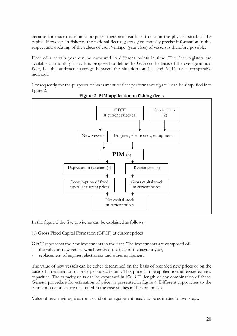
2.2 Application of PIM to fishing fleets For the application to fisheries figure 1 can be slightly reformulated and simplified. Figure 1 assumes that the value of the GCS is expressed in price level of another than the current year. Therefore it is necessary to recalculate the GFCF of the current year to the base year to obtain constant prices. In the proposed application to fisheries the entire GCS is revaluated each year to the current value, because that is analytically relevant. When data on earnings and costs refer to 2005 it does not make sense to insert capital costs referring to another year. OECD proposes specific values for service lives (average life time of an asset) and mortality functions (retirement of the asset around the service life). These functions are introduced

20

because for macro economic purposes there are insufficient data on the physical stock of the capital. However, in fisheries the national fleet registers give annually precise information in this respect and updating of the values of each ‘vintage’ (year class) of vessels is therefore possible. Fleet of a certain year can be measured in different points in time. The fleet registers are available on monthly basis. It is proposed to define the GCS on the basis of the average annual fleet, i.e. the arithmetic average between the situation on 1.1. and 31.12. or a comparable indicator. Consequently for the purposes of assessment of fleet performance figure 1 can be simplified into figure 2.

Figure 2 PIM application to fishing fleets

In the figure 2 the five top items can be explained as follows. (1) Gross Fixed Capital Formation (GFCF) at current prices GFCF represents the new investments in the fleet. The investments are composed of: - the value of new vessels which entered the fleet in the current year, - replacement of engines, electronics and other equipment. The value of new vessels can be either determined on the basis of recorded new prices or on the basis of an estimation of price per capacity unit. This price can be applied to the registered new capacities. The capacity units can be expressed in kW, GT, length or any combination of these. General procedure for estimation of prices is presented in figure 4. Different approaches to the estimation of prices are illustrated in the case studies in the appendices. Value of new engines, electronics and other equipment needs to be estimated in two steps:

GFCF at current prices (1)

Service lives (2)

PIM (3)

Depreciation function (4)

Consumption of fixed capital at current prices

Net capital stock at current prices

Gross capital stock at current prices

Retirements (5)

New vessels Engines, electronics, equipment

21

- numbers of replaced asset items (engines, etc.) is estimated with the assumed service lives: o engine 10 years o electronics 5 years o other equipment 7 years

For example, the average fleet of 2005 indicates that X vessels built in 1995 are still in operation. This means that X engines will be replaced by new ones.

- Average price per asset item. Usually it is not possible to obtain a sufficiently large number

of observations of these prices. Therefore it is proposed to estimate the share of each asset item in the total vessel price and determine the average price on the basis of this share and the vessel price.

(2) Service lives An average service life has to be determined for each type of assets. The following service lives are generally accepted for macro (economic) analysis: - Hull – 25 years - Engine – 10 years - Electronics – 5 years - Other equipments – 7 years It is possible that different service lives should be used for micro (fiscal) analysis in different countries, depending on rules set by the national fiscal offices. (3) PIM PIM contains the details of the Gross Capital Stock (GCS) by vintage (year of construction) valued at current prices. This is the bench-mark value of GCS from each preceding year. The very first estimation of the bench-mark value is discussed in the following section. For the fishing fleet, PIM contains age structure of the active fleet (based on construction year of the hull, as recorded in the fleet register) and an age schedule of the other assets (engine, electronics and other). (See also section 2.4 Valuation model). (4) Depreciation function Various depreciation functions can be applied. It is proposed to use two different depreciation functions, according to the approach. For the macro (economic) approach a ‘degressive’ depreciation function should be used. This function leads to relatively high depreciation when the assets are still relatively new, but the value of even very old assets never becomes zero. Using ‘degressive’ function implies the following annual depreciation rate, which is applied to the net capital stock: - Hull – 7% - Engine – 25% - Electronics – 50% - Other equipments – 35%

22

For micro (fiscal) approach it is recommended to use depreciation schedules permitted by the national tax laws. This will be usually a linear function, with approximate life times stated above. Using ‘degressive’ function implies the following annual depreciation rate, which is applied to the historical value of the asset: - Hull – 2.5% - Engine – 10% - Electronics – 20% - Other equipments – 16% In case of the hull a scrap value of 2.5-5% of the historical price can be assumed after 25 years. For the EEO (Engine, Electronics and Other) the scrap value is assumed zero. (5) Retirements Retirements are the vessels (or capacity units) which have stopped operating in the course of the year. This is the difference per vintage of two subsequent fleet registers. This data is in detail available in all EU MS. Establishment of the bench-mark of gross capital stock (GCS) Estimation of the bench-mark value of GCS would be ideally achieved if historical prices of all active vessels would be available. This is evidently not the case. On the contrary, information on historical, new and second prices is relatively scarce. Therefore it is proposed to estimate the value of GCS in three steps: 1. Specification of the composition of the active fleet by age. 2. Estimation of price per unit of capacity (e.g. per GT) 3. Calculation of the value of each vintage (year of construction) of the fleet and either

converting values of all vintages to current prices or to historic prices using price indices. Specification of age composition Composition of the national fleets and all distinguished DCR segments by age can be drawn from the fleet registers. Format of the table to be generated for each DCR segment is presented in figure 3.

23

Figure 3 Presentation of the composition of a fleet

Year of construction Number GRT GT kW

Total200420032002……………

1935

Estimation of the prices per capacity unit depends on the availability of the data and the correctness of its interpretation. The scheme to be followed is presented in figure 3. The figure 3 is based on experiences and diversity of the countries involved in the project. It shows that different approaches can be followed to arrive at a conceptually same result. Estimation of price per capacity unit Determination of the price per capacity unit is the central theme of entire valuation of GCS in fisheries. It required careful interpretation of the collected information on values of vessels and if necessary its adaptation. The procedure is presented schematically in figure 4. First, it must be determined what value indicators can be reliably observed and collected. In principle three or four types of observable value indicators exist: - Historic prices, i.e. prices actually paid in for newly constructed vessels. - 2nd hand prices, i.e. prices actually paid for used vessels. - Insurance premiums, which are based on insurance values, and so insurance values can be

derived from them. - Insurance values, collected for example from company administrations or insurance

companies. - Book value as presented on the balance sheets.

24

Figure 4 Procedure for interpretation and estimation of prices per capacity unit

Notes:

cu = capacity unit vessel refers to complete unit incl. hull, engine, electronics and all other equipment (1) Price index heavy machinery or another index related to boat building (2) Depreciated / book value will be usually based on historical price. (3) RV = Value at current price of the most recent year (4) HV= Value at historical prices, in case only one or several years available, remaining years can be extra/interpolated with the price index

What value indicators can be collected / observed?

Insurance premiums Historic value

Insurance values

Do the data refer to the tangible assets only or do theyalso contain value of intangibles?

Value of tangible (vessel) only

2nd hand values

Replacement value (RV) (3)

What does the available value per vessel represent?

Contain intangibles

Estimate / separate tangible and intangible value,

describe approach

Other Book value(2)

Historic value (HV) (4)

Determine series of historical prices/cu

Recent historic price =

replacement price./cu

Follow columns (RV) or (HV)

Estimate replacement price / cu

Estimate total depreciation to

determine historical value

Estimate series of historic

prices / cu

Estimate RV and /or HV,

describe approach

Price index series (1)

Book value

25

Secondly, it must be determined whether the observed value refers only to the physical vessel (plus equipment, etc.) or whether it also contains implicitly values of intangibles like licenses, quotas or permits. This consideration must be given explicitly to all types of observable values. In many countries specific intangibles are tied to a vessel. Not only that 2nd hand vessels may contain the value of that intangible, but also newly built vessels may contain it as shipyards in some case hold the necessary intangibles to facilitate new constructions. Consequently, even insurance value may refer to the sum of tangible and intangible assets. Thirdly, subsidies and taxes need to be accounted for if necessary. Historic prices paid for new vessels may be affected by subsidies provided under the EU structural funds or otherwise. This was particularly common in the 1980ies. Also non-reimbursable taxes should be taken into account, but in practice such taxes have not occurred4. Historic cost of a new vessel to the owner amounted to price paid to shipyard minus subsidy. The following definitions should be used: - Micro approach: Historic price = price paid to shipyard + taxes – subsidies - Macro approach: Replacement price = (historic price – taxes + subsidies)*price index In case that intangibles are part of the asset value, it is necessary to separate them from the tangibles so that the determined value per capacity unit refers exclusively to physical assets. There is probably no one single way to achieve this separation. One possible approach is presented in appendix B (French case study). After it has been ascertained that the raw data contain only values referring to the tangible assets, it must be concluded which kind of value (price) it represents. There are in principle the following possibilities: - Replacement value, i.e. value in the current year. This is for example the case in countries

where insurance values are determined on the basis of replacement in case of total loss. - Historic value, i.e. the originally paid price for a new vessel. - Book value, i.e. historic price less total depreciation. This value is presented on the balance

sheet. 2nd hand prices could in ideal situations reflect the book values. Book value can be transposed to historic value by adding the (estimated) total depreciation costs.

- Other value. In this case a further interpretation will be required to create a link either to replacement or to historic value.

The observed data will refer to vessels of different sizes and ages. On the basis of this data it is necessary to estimate a price per capacity unit, using e.g. least squares or other estimation method. It is proposed that the price per capacity unit be estimated as far as possible for all major fleet segments. The segments should be homogenous in the sense that the standard variation of the estimated price per capacity unit should not be ‘excessive’. This means that for this purpose the segments do not necessarily have to be defined in terms of DCR, although it must be possible to relate the results directly to the DCR segments. Due to lack of data, not all presented case studies meet this requirement of homogeneity of the segments. Further data may have to be collected to improve the quality of the estimations in the future. The result will be either an estimation of the current (replacement) price per capacity unit or an estimation of series of historic prices. The current price can be transposed to a series of historic

4 All vessel prices must be considered excluding VAT.

26

prices by applying an appropriate index. It is proposed to use the ‘heavy machinery index’, which is available at national as well as EU level, or another suitable index which may be available or which may have been developed for this purpose5. In case that a series of historic prices has been estimated, it is likely that the number of observations for each vintage will be quite limited. Especially since 1990, when the level of investments has been rather low in most fleet segments. Consequently, there may be significant variations of the estimated price between the various years. Unless these variations can be explained, it is proposed to recalculate the series into multi-annual averages. Appendices present different approaches of estimations as developed by the members of the team in different countries. It is essential that all countries carrying out the estimation of the GCS value describe their approach in detail in terms of available data (its representativity), its meaning, concepts behind estimation, estimated relations (incl. R2, etc.), applied series of indices and specification of assumptions.

2.3 Calculation of capital costs Capital costs can be calculated in different ways, according to the analytical perspective. Two such perspectives can be distinguished: micro and macro. Micro perspective Micro perspective reflects the context of the firm. This implies that the calculations should be as close as possible to the actual monetary flows using historic prices paid (i.e. after addition of eventual taxes6 and subtraction of subsidies). The capital costs (depreciation and interest) should closely follow the national fiscal rules. This means that depreciation costs should be based on fiscally accepted life times and depreciation schemes. Usually linear depreciation based on the historic price will be used. Performance is positive when the historic investment can be recuperated. Only interest paid on loans is included in costs. In case that the data on paid interest is not available this would have to be calculated, using market interest rate for medium term loans (5-10 years). The interest rate must be applied to loans only, so that also information on debts or the solvability ratio (debt/total capital) is required. Macro perspective Macro perspective reflects the context of the society at large, with an indefinite time horizon. This means that the fishing sector should continue operating ‘for ever’ and its performance is

5 Specific index has been developed in Denmark and in the Netherlands. 6 Except VAT.

27

evaluated accordingly. The results should allow regular replacement of capital goods beyond the current generation. Calculation of capital costs is based on replacement value. It is proposed to use degressive depreciation scheme so that the residual value never reaches zero. Interest costs should be the opportunity costs of capital. This means that the interest on government bonds (as an alternative to investment in fishing) should be applied to the net capital stock (replacement value less aggregate depreciation). It could be argued that the proposed method of calculation of the replacement value leads to an overestimation. If the physical productivity of one unit of fishing capacity is increasing (i.e. catch in tonnes per capacity unit per year) while the resource is exploited at a relatively constant MSY level, the number of required capacity units is falling at the speed of the productivity rise. Consequently the replacement value should be adjusted accordingly. The problem is that with fluctuating stocks, it is difficult to obtain a good estimate of the increase in physical productivity. The relation between micro and macro approach is presented in figure 5.

Figure 5 Micro / macro calculation of depreciation and interest costs in the year t, tangible assets only (vessel and equipment)

As micro and macro approach lead to different figures, resulting indicators, like net profit, are also different.

Micro approach (Fiscal)

Depreciation costs

Macro approach (Economic)

Fiscal depreciation

scheme

Paid interest or

market interest rate * debts

Paid interest costs

Historical value

Depreciation costs

Economic depreciation

scheme

Interest costs / opportunity

Replacement value

Government bonds rate

Total depreciation

28

2.4 Valuation model In order to make all calculations among the authors consistent a valuation model was developed and applied. The structure of the model is presented in figure 6. The spreadsheets are in figure 7 and 8. Input data The following data are inserted in the spreadsheet, either based on national evidence or on proposed assumptions: - Estimated replacement price per capacity unit of the current year or the series of historical

prices per capacity unit. - Price indices, to calculate historical values from replacement values or vice versa (boat

building or heavy machinery index). - Selected capacity units, belonging to the estimated price per capacity. - If available, price indices for engines, electronics and other equipment. This will allow a

more precise estimation of the values of these asset items. If not available the above mentioned price index must be used.

- Relative composition of the value of the assets in the four main distinguished components of the assets: hull, engine, electronics and other.

- Depreciation schemes for macro and micro approach. With this data it is possible to estimate gross historic and replacement values of the four asset components and their sum, which represents the gross capital stock. The total values for each year represent the gross fixed capital formation, after accounting for the mortality which occurred in that vintage. This is the yellow area in the spreadsheet. Two depreciation schemes are used in the model as means of sensitivity analysis: degressive and linear. Applying these schemes generates the net fixed capital formation of each vintage. The sum of the vintage generates the total net capital stock and value of net capital stock by asset type. Applying the depreciation rates to the gross capital stock by asset type generates the depreciation costs of the current year. In the case of degressive depreciation, the value of the hull is continuously depreciated, without reaching zero. In the case of linear depreciation it is assumed that after 40 years the value of the hull remains at 2.5% of the replacement value (macro approach). Renovation of engines, electronics and other equipment takes place on a continuous and regular basis. Therefore engines get never older than 10 years and electronics are replaced after 5 years. To allow the calculation of the net value of the EEO assets (Engine, Electronics and Other), an appropriate age schedule must be used. The models for macro and micro approach are almost identical, with the exception of two items: - Macro approach applies same price to all vintages, while micro approach uses the original

historical prices (column G in figure 7 and 8).

29

- In the micro approach prices of the EEO assets (Engine, Electronics and Other) must be adjusted to their actual age of acquisition, e.g. engine on an 11 years old vessel is only one year and therefore its price cannot be related to historic vessel price of 11 years ago. A separate price schedule has been introduced.

The spreadsheet for micro valuation also allows for two different types of depreciation. This, however, may not be relevant in many countries, where only one system of fiscal depreciation is common. Finally, the valuation model generates an overview to compare the result of the four different calculations (figure 9). It shows the details of the depreciation schemes (table A), effect on the net profit (table B) and a comparison of the gross and net capital stock values. The given example (based on data for Italy) shows that: - The difference between historical (micro) and replacement (macro) gross and net capital

stock is primarily caused by the different values of the hull. Values of EEO assets are not significantly different, due to their regular replacement.

- Using degressive depreciation leads substantially lower capital values than using linear depreciation.

- Linear depreciation leads to lower deprecation costs than the degressive depreciation scheme.

30

Figure 6 Valuation model

(1) Gross fixed capital value at current prices (prices actually paid) (2) Gross fixed capital value at constant prices (prices to be paid in most recent year = year of analysis) (3) Net fixed capital value at current prices (4) Net fixed capital value at constant prices (5) For the calculation of historical value of engine, electronics and other, it is necessary to increase the historical value per capacity unit with a price index to account for the fact that e.g. on a 12 meters year old vessel engine and electronics are 2 years old and other equipment 5 years.

Selected capacity units

Relative composition: hull, engine, electronics, other

Total historical value (HV) (1)

Replacement price / capacity unit

Historical value - hull - engine - electronics - other

Historical price / capacity unit

Price index

Total depreciated

HV (3)

Depreciation scheme - hull - engine - electronics - other

Depreciated HV value - hull - engine - electronics - other

Total replacement value (RV) (2)

Replacement value - hull - engine - electronics - other

Total depreciated

RV (4)

Depreciated RV value - hull - engine - electronics - other

Micro / fiscal approach

Macro / economic approach

Price index E-E-O (5)

31

Figure 7 Spreadsheet for macro calculation of replacem

ent value, depreciation and interest costs

12345678910111213141516171819202122232425262728293031323334

AF

GH

IJ

KL

MN

OP

QR

ST

UV

WX

YZ

AAA

B

Fleet composition per

Deprecia-tion rate

Renova-tion every X

yearsShare in total

investm.

Deprecia-tion rate

Renova-tion every X

yearsShare in total

investm.

Hull

7%40

60%H

ull2.5%

4060%

Fill in only the white area:

Engine

25%10

20%E

ngine10.0%

1020%

- selected capacity unitsE

lectronics50%

510%

Electronics

20.0%5

10% - price per capacity unit

Other equipm

ent35%

710%

Other equipm

ent16.0%

710%

Governm

ent bonds5%

Residual val. hull

2.5%Adjust possibly assum

ptions in redaccording to national data

Depreciation costs

177D

epreciation costs107

Interest costs43

Interest costs68

Total capital c

220Total capital c

175

Replacem

ent value (mln E

uro)D

epreciated value (mln E

uro)D

epreciated value (mln E

uro)Age schedule

Digressive depreciation

Linear depreciationG

ross capital stockN

et capital stockN

et capital stock

Year

Selected capacity units

(1000 GRT)

Price / capacit y unit 2004 (1000

Euro)T

otalH

ullEngine

Electronics

Other

TotalH

ullEngine

Electro-nicsO

therT

otalH

ullEngine

Electro-nics

Other

Hull

Engi-ne

Elect-

ronicsO

ther

Total183

2,8191,691

564282

282858

427209

111111

1,352719

312172

149

20041.9

15.429.3

17.65.9

2.92.9

29.317.6

5.92.9

2.929.3

17.65.9

2.92.9

00

00

20032.3

15.435.8

21.57.2

3.63.6

28.118.6

5.41.8

2.333.3

21.06.4

2.93.0

11

11

20024.6

15.470.5

42.314.1

7.17.1

46.734.0

7.91.8

3.060.5

40.211.3

4.24.8

22

22

20013.6

15.456.1

33.711.2

5.65.6

32.225.2

4.70.7

1.544.2

31.17.9

2.22.9

33

33

20002.8

15.443.4

26.08.7

4.34.3

21.918.1

2.70.3

0.831.1

23.45.2

0.91.6

44

44

19993.2

15.448.8

29.39.8

4.94.9

26.719.0

2.34.9

0.636.4

25.64.9

4.91.0

55

05

19983.4

15.452.6

31.510.5

5.35.3

23.919.0

1.92.6

0.435.4

26.84.2

4.20.2

66

16

19975.0

15.476.9

46.215.4

7.77.7

37.525.8

2.11.9

7.755.0

38.14.6

4.67.7

77

20

19963.2

15.448.8

29.39.8

4.94.9

20.015.2

1.00.6

3.231.4

23.42.0

2.04.1

88

31

19953.0

15.446.6

27.99.3

4.74.7

16.513.5

0.70.3

2.026.7

21.60.9

0.93.2

99

42

19942.5

15.438.9

23.47.8

3.93.9

23.310.5

7.83.9

1.131.2

17.57.8

3.92.0

100

03

19933.4

15.452.1

31.210.4

5.25.2

24.413.1

7.82.6

0.938.1

22.69.4

4.21.9

111

14

19922.2

15.433.4

20.06.7

3.33.3

12.87.8

3.80.8

0.422.0

14.05.3

2.00.7

122

25

19913.3

15.450.1

30.110.0

5.05.0

16.110.9

4.20.6

0.429.5

20.37.0

2.00.2

133

36

19903.9

15.460.5

36.312.1

6.06.0

22.512.2

3.80.4

6.038.1

23.67.3

1.26.0

144

40

Based on data for Italy

32

Figure 8 Spreadsheet for micro calculation of historic value, depreciation and interest costs

12345678910111213141516171819202122232425262728293031323334

AF

GH

IJ

KL

MN

OP

QR

ST

UV

WX

YZ

AAAB

AC

Fleet composition per 1/1/2005

Fiscal rate 1Renovation

every X years

Share in total investm

entFiscal rate 2

Renovation every X

yearsShare in total

investment

Hull

7%40

60%H

ull2.5%

4060%

Fill in only the white area:

Engine

25%10

20%E

ngine10%

1020%

- selected capacity unitsE

lectronics50%

510%

Electronics

20%5

10% - price per capacity unit

Other equipm

ent35%

710%

Other equipm

ent16%

710%

Market rate for loans

5%R

est value hull2.5%

Adjust possibly assumptions in red

Loans as % of G

CS50%

according to national dataD

epreciation costs167

Depreciation costs

100Interest costs

19Interest costs

28Total capital costs

186Total capital costs

128

Historical value (m

ln Euro)

Depreciated value (m

ln Euro)

Depreciated value (m

ln Euro)

Age schedulePrice index

Fiscal rate 1 (digressive depreciation)Fiscal rate 2 (linear depreciation)

Gross capital stock

Net capital stock

Net capital stock

Year

Selected capacity units

(1000 GRT)

Price / capacity unit

2004 (1000 E

uro)T

otalH

ullE

ngineE

lectronicsO

therT

otalH

ullE

ngineE

lectronicsO

therTotal

Hull

Engine

Electronics

Other

Hull

Engine

Electro-

nicsO

therE

ngineE

lectro-nics

Other

Total183

1,976888

537277

274742

318204

111110

1,122502

302170

147

20041.9

15.429

186

33

2818

63

229

186

32

00

00

1.001.00

1.002003

2.315.2

3521

74

427

185

21

3221

63

21

11

11.00

1.001.00

20024.6

15.169

4214

77

4533

82

258

4011

44

22

22

1.001.00

1.002001

3.615.0

5533

115

531

255

11

4230

82

23

33

31.00

1.001.00

20002.8

14.742

258

44

2117

30

029

225

11

44

44

1.001.00

1.001999

3.214.6

4728

95

525

182

50

3424

55

05

50

51.00

0.951.00

19983.4

14.550

3010

55

2718

23

538

254

45

66

16

1.000.95

1.001997

5.014.2

7243

148

835

242

28

5235

45

87

72

01.00

0.940.92

19963.2

13.945

279

55

1814

11

329

212

24

88

31

1.000.93

0.911995

3.013.3

4224

94

515

121

02

2419

11

39

94

20.86

0.900.88

19942.5

12.635

198

44

219

84

128

148

42

100

03

0.820.82

0.841993

3.412.2

4525

105

522

108

31

3318

94

211

11

40.80

0.800.83

19922.2

11.828

157

33

116

41

019

115

21

122

25

0.780.78

0.811991

3.311.4

4222

105

513

84

10

2415

72

013

33

60.76

0.760.79

19903.9

11.049

2612

66

199

40

631

177

16

144

40

0.750.75

0.71 Based on data for Italy

33

Figure 9 Comparison of macro and micro approach and sensitivity analysis Table A. Background for calculation of depreciation and interest

Depreciation rate / year -

digressive

Depreciation rate / year -

linearFiscal rate 1 -

digressiveFiscal rate 2 -

linearHull 7% 2.5% 7.0% 2.5%Engine 25% 10.0% 25.0% 10.0%Electronics 50% 20.0% 50.0% 20.0%Other equipment 35% 16.0% 35.0% 16.0%Rest value hull after 40 years 2.5% 5.0% 2.5%Interest rate government bonds 5%Market rate for loans 5%Loans as % of total capital 50%

Table B. Capital value and capital costs and their consequences on profit (sensitivity analysis)2004

mln EuroDigressive

depreciationLinear

depreciation Fiscal rate 1 Fiscal rate 2

Value of landings 1,379.6Fuel costs 224.6Other running costs 155.9Vessel costs 128.1Crew share 400.4Gross cash flow 470.6Depreciation 92.4 176.6 107.5 167.0 100.3Interest 10.4 42.9 67.6 18.6 28.0Net profit 367.8 180.8 225.3 214.8 272.0Gross value added 871.0

Capital value 2,202.6 858.2 427.0 208.8 111.5Profit / capital 16.7% 21.1% 52.8% 102.9% 244.1%

Table C. Summary of the capital values - comparison of approachesTotal Hull Engine Electronics Other

Replacement value (mln Euro)Total 2,819.0 1,691.4 563.8 281.9 281.9Digressive depreciated 858.2 427.0 208.8 111.5 110.9Linear depreciated 1,352.3 719.0 311.9 172.0 149.5

Historical value (mln Euro)Total 1,975.8 888.0 537.2 276.8 273.8Digressive depreciated 742.3 318.1 203.6 110.6 110.1Linear depreciated 1,121.6 502.3 302.1 169.9 147.3Total = Gross fixed capital stockDigressive or Linear depreciated = Net fixed capital stock

Replacement value Historical value(Macro approach) (Micro approach)

Replacement value(Macro approach)

Historical value(Micro approach)

Based on data for Italy

34

2.5 Valuation of intangible assets General considerations Implementation of the CFP in the various MS has lead to an introduction of various types of rights (licenses, ITQs, etc.). Some of these rights are freely tradable; others can be only transferred together with the vessel to which they are attached. Still other rights ore officially not transferable, but in reality they too can be transferred. In many countries the value of these intangible assets approaches or even exceeds the value of the tangible assets. Attaching value to the intangible assets faces several conceptual as well as practical problems: - In theory value of total assets could be determined as net present value of the future

stream of benefits. This value than should be split into tangible and intangible assets. One unique approach to this division does not exist.

- When intangibles are freely tradable, observation of their prices in the market is often difficult because the number of transactions is small and they are not recorded.

- When the intangibles are attached to vessel, direct observation of the price is impossible. The value has to be estimated.

- In many cases, the fishing companies have not yet acquired any intangibles, but simply hold the rights which they have received free of charge from the government, when they were introduced. In that case it is not clear if these rights should be valued as an asset, increasing substantially the total asset value of the company, or not.

- It is also not clear if the rights should be depreciated. Are they permanent or temporary? On what value should the depreciation be imputed and at which rate?

- The value of the fishing rights may fluctuate strongly with the economic performance of the fisheries concerned. This would lead to strong fluctuation of the asset value, depreciation costs and possibly profitability of capital.

These questions are not unique to fisheries. Intangibles are also common in other sectors – milk quota, CO2 emission rights, patents and intellectual property rights, etc. The valuation of intangibles has been therefore on the agenda of the IASCF (International Accounting Standard Committee Foundation) and it is reflected in its IRFS (International Financial Reporting Standard). The principles have been adopted for collection and interpretation of agricultural statistics in FADN. It is proposed to adopt these principles also for the valuation of intangible assets in fisheries. Proposed approach Two types of intangibles should be distinguished:

1. Tradable intangibles

Intangibles are considered tradable when the size of the market is sufficient to allow (regular) trade. This may also be the case if they are attached to tangible assets (vessel). These intangibles should be valued at market price, independently of the question whether they have been acquired or administratively received. It is assumed that these intangibles have infinite life time and consequently they are not depreciated.

35

In case that the intangible is attached to a tangible asset, its value should be estimated. A possible approach to such estimation has been developed by Ifremer7 (Appendix B). However, other methods may have to be developed, depending on the availability of the data and characteristics of the intangibles in question. Valuation of tradable intangibles is an area where substantial research effort will be required in the future.

2. Non-tradable intangibles

These intangibles are either non-tradable at all, or the market is too small or fragmented to allow for regular trade8. These intangibles are valued at estimated market price, but because the life time is not certain they are depreciated. Summary Type of tangible Value based on Depreciation Freely tradable, not attached Market price No Tradable, attached to other asset Estimated value No Not tradable Estimated value Yes

Consequences for total capital value Accounting for the value of intangibles increases the value of the equity capital. In case that the firm has received the intangible administratively it represents a ‘hidden reserve’. This implies that when the intangible would be sold, the firm will monetize these assets, which will increase its profits in the given year. The profits will be taxed against usual tax rate on profit. This implies that the firm does not only have a ‘hidden reserve’ in assets, but also a ‘hidden liability’ to the tax office. Consequently this latent tax claim must be included among the liabilities of the firm. The overview of the capital value must distinguish intangible assets separately from other type of assets. Also depreciation and opportunity costs should be presented separately. Required data and / or estimations - Market price of intangible, or - Estimated value of intangible - Profit tax rate (differs per country) - Estimation of the share of the total assets which has / has not been traded. Such

estimation is required to determine the aggregate tax claim for the sector or fleet segment.

7 Ifremer is not able to estimate directly the value of intangible asset but proposes a method based on a comparison of the price of a vessel on the 2nd hand market and the "book value" of the vessel at a certain moment of time. This indicates what could be the "maximum" value of the fishing rights. However, this difference is not exclusively explained by the implicit value of fishing rights. Furthermore, evidence shows that this "implicit" value is very variable from one year to other. 8 Example are ammonia quota which can be traded only within a small region.

36

Figure 10 Accounting for intangible assets

2.6 Valuation of ‘other assets Two other types of assets may have to be taken into account: - Land based assets: cars, buildings, etc. - Liquid assets (money) and reserves (incl. shares, bonds, etc.) These assets are not directly related to a vessel as a statistical unit, but rather to the firm, or the legal person who also owns the vessel(s). This creates a number of practical as well as conceptual problems: - In case of a firm owning more than one vessel, the capital costs related to the ‘other assets’

will have to be allocated to the individual vessels. This implies that a division key has to be derived or assumed9.

- A company running in principle a land based operation, e.g. fish processing, may also own a vessel.

- One vessel may be owned by several owners, each also running other type of business.

9 This is a common problem when all costs have to be allocated to production units.

Define intangible asset

Determine tradability

Freely tradable Non-tradableTradable linked to other assets

Collect data on price / unit

Calculate total value, increase assets

Estimate price / unit

Estimate price / unit

Determine share traded

Calculate latent tax liability, decrease capital value

Depreciation = 0, Calculate opportunity costs

of interest

Calculate total value, increase assets

Calculate depreciation, Calculate opportunity costs

of interest

Determine depreciation scheme

37

- Collection of historical information on the size of these assets seems rather tricky. It will require special surveys to determine vintages of buildings and cars. Prices indices for such assets exist.

In the current situation a large majority of EU fishing fleet is owned on a one-man-one-boat basis. A preliminary expert assessment indicates that these companies only own very limited land based assets. However, for some groups of vessels and companies ‘other assets’ do play an important role. This regards particularly companies operating the large freezer trawlers, (tuna) purse seiners and those with fleets of smaller fishing vessels. Proper evaluation of their performance requires to account for these ‘other assets’. Land based assets Land based assets can be in principle treated in the same manner as the vessel – at historical prices for the purpose of micro approach and at replacement value for the macro assessment. Depreciation rates must be selected according to the type and service life of the asset. Gross and net capital value, depreciation costs and interest costs can be added to the appropriate values of the vessel. Liquid assets Some firms may hold substantial liquid assets (incl. shares and bonds) not only as working capital, but also as reserves to pay pension to the owner or as investments of earlier profits. Working capital is part of the on-going operation and should be therefore accounted for within the overall capital valuation. Collecting data on working capital may be difficult. Therefore it is proposed to estimate the working capital as a percentage of annual operational expenses. Until concrete evidence is available, this percentage could be put at 7%. Other kinds of liquid assets are not directly related to the operation of the firm and may be disregarded as far as capital costs (depreciation and interest) are concerned. However, reserves are evidently relevant for the assessment of the survival capability of a firm, i.e. how long the firm can survive in economically difficult times. The main problem of collecting the required information is that many vessel owners are not obliged to prepare an annual balance sheet, which is the only document where the required information could be obtained in an organized manner.

38

3. THEORETICAL CONSIDERATIONS

3.1 The conceptual framework This section introduces some basic concepts and definitions related to capital stock measurement, mainly sourced from the European Systems of Accounts (ESA 95), from the Economic Accounts for Agriculture and Forestry (EAA/EAF 97) and from the OECD Manual on the Measurement of Capital Stocks, Consumption of Fixed Capital and Capital Services (OECD, 2001a). In the first part we illustrate the standard equation for the value of an asset, which provides the conceptual framework for the measurement of the capital stocks. It is meant to clarify some fundamental concepts related to the capital stock measurement in order to evaluate their applicability to the fishery context. In the second part we discuss the most common methods applied to measure capital stock. The standard equation for the value of an asset The value of an asset depends primarily on the value of the rentals that is expected to earn during its lifetime. Rentals, which are the incomes earned by an asset during each accounting period, are equal to the quantity of capital services produced by the asset multiplied by the unit price of those service. Because the rentals generated by an asset are received over several years, they have to be discounted in calculating the value of an asset at any point in time. The rentals expected in future periods are discounting using a discount rate, which is often taken as the interest rate on long terms bond. The scrap value is the value of an asset at the end of its service life, when the asset is discarded or scrapped. This will be a positive amount corresponding to the value of any parts or waste materials that can be recuperated from the asset minus the cost of dismantling or removing the asset. If these costs are too high, the scrap value becomes negative. Combining these three variables, the rentals, the discount rate and the scrap value, we can obtain the economic value of an asset both when it is new and when it is at the later stages of its service life. The standard formula for the value of an asset can be written as follows:

(1) Where Vt is the value of an asset at time t, ft is the rental in period t, T is the service life of the asset,

39

r is the discount rate10, S is the scrap value. The above equation indicates the present value of the expected potential cash flows of an asset. The present value is computed by discounting the expected future value to users at the cost of capital. This equation is also defined the Fundamental Equations Relating Stocks and Flows of Capital (Diewert, 2004), which provides the link between stock measures and consumption of fixed capital on the one hand, and the measurement of capital services on the other hand. It is important to realize that value is to be understood as the market price, or as the purchase price of the durable commodity. It corresponds to the investment price and, consequently, it is assumed to be equal to the discounted value of the future service flow (Hall, 1968). In considering whether to purchase an asset, rational producers will first calculate the rentals they expect to receive from an asset and will then solve equation (1) for r. They will buy the asset only if the price at which it is offered implies a rate of return – as measured by r – which is at least as high as they can earn from alternative use of their funds. If an asset is offered for sale at a price that does not seem likely to generate a satisfactory rate of return, there will be no market for that asset. If an asset is offered at a price that seems likely to generate a very high rate of return, demand for the asset will rise and bid up the price until the rate of return falls to a “normal” level. In practice, manufacturers of capital goods will themselves calculate the rates of return that assets are likely to earn and will not produce assets that are unlikely to generate rates of return that are sufficiently high to ensure that there will be a market for them. Equation (1) can, therefore, be seen as a very plausible explanation of how asset prices are determined in a market economy. Opportunity costs The capital value is related to the opportunity cost of capital or the required rate of return that is, the rate of return that a company would otherwise be able to earn at the same risk level as the investment that has been selected. The opportunity cost of production is the value of the firm's best alternative use of its resources. A firm’s opportunity costs can be explicit or implicit: - Explicit costs are paid in money. The amount paid for a resource could have been spent on

something else, so it is the opportunity cost of using the resource. - A firm incurs implicit costs when it forgoes an alternative action but does not make a

payment. A firm incurs implicit costs when it uses its own capital or it uses its owner's time or financial resources.

Since the opportunity cost is related to the risk level of the investment, for the fishery context it should be differentiated according to different fleet’s segments and metiers. Service lives (or lifetime) of assets

10 The discount rate is a real interest rate, than can be calculated as the difference between the nominal rate of interest and the rate of general inflation.

40

In the standard formula for the value of a capital asset, the economic service life is defined as the total period that an asset is in productive use from the moment that it is first installed or constructed. This definition of expected service life is based on the length of time that assets are retained in the capital stock, whether in the stock of the original purchaser or in the stocks of producers who purchase them as second hand assets. This concept corresponds to the economic service life of the assets, which is not determined exclusively by the technical or physical characteristics of the assets as it depends also on expectations about the price as well the quantities of the service, either of which may fall sufficiently to cause the asset to be retired. It is worth noting that even if the lifetime of an asset can be collected from many different sources, these sources actually furnish different estimates of the service life. For example in most countries, the tax authorities specify the number of years over which the depreciation of various types of assets may be deducted from profits before calculating tax liabilities. This source provides information on the so-called fiscal lifetime, which often is shorter than its useful service life if governments adopt accelerated depreciation to encourage investment. Also company accounts can provide useful information of acquisition as well as the date of disposal of the assets. Direct sources are surveys, which ask producers about discards of assets or those which ask respondents to give the purchase dates and expected remaining lives of assets currently in use. Another approach consists in asking experts or firms that produce capital assets for the normal service lives of different sorts of equipment. In this way it is possible to take a view on the physical and technical services of the assets they produce. For some assets, government agencies maintain administrative records that can be used to determine service lives. This is the case of the shipping registers of construction and demolition. It is worth noting that since these sources provide different measures of service lives, it would be better to collect and compare this different information. It is also important that such information be adapted to the specific circumstances. Hence a recommended practice on estimating the useful lives of capital assets should take into account some important factors as the quality and the application (Gruenwald, 2002): - Quality. Similar assets may differ substantially in quality, and hence in their useful lives,

because of differences in materials, design and workmanship. - Application. The useful life of a given type of capital asset may vary significantly depending

upon its intended use. Finally, information on service lives should be collected for restrict asset groups and regularly updated in order to reflect cyclical or longer-term changes in the lengths of time that assets remain in the stock. Table 1 presents the depreciation period of hull, engine and electronics currently applied in AER.

41

Table 1. Depreciation period of hull, engine and electronics applied in AER by country, 2002 Country Depreciation period

(no. of years) Hull Engine ElectronicsBelgium 10 10 5Denmark Finland 25 10 France 25 10 Germany Greece 25 10 Ireland 25 10 Italy 25 10/15 Netherlands 20 10/15 10Norway 30 15 10Portugal 25 10 Spain 25 10/15 Sweden 25 25 25UK 10 10 10 Table 2 summarizes the average service lives for some assets of Agriculture, Forestry and Fishing for 15 OECD countries. The categories of assets considered are machinery and equipment, building and engineering construction and some types of vehicles. In some cases, as for fishing boats, the average lifetime strongly differs from a country to another. These differences are probably due to the difference approaches used to estimate the service lives.

42

Table 2. Average service lives in Fishing (O

EC

D, 1992)

M

achinery and equipm

ent Buildings

Engineering

construction Building and engineering construction

Fishing boats O

ther ship

Canada 3

2525

2535

United States

3127

27A

ustralia 13

43A

ustria 18

Belgium

1530

715

Finland 60

1010

France 16

2222

Germ

any 14

6920

26Iceland

1445

3737

Italy 18

N

orway

645

8H

ulls 40, E

ngines 15, O

ther maritim

e equipm

ent 10

Ocean 15,

Inland water 20

United K

ingdom

1250

2520

43

Mortality patterns Mortality patterns consider the assumptions made about the distribution of retirements around the average service life. In the literature, “scrappings” and “discards” are employed as synonyms of retirements to mean the removal of an asset from the capital stock because it is withdrawn from service, exported, sold for scrap, dismantled, pulled down or abandoned. Retirements are hence distinguished from “disposals”, which also includes sales of assets as second-hand goods for continued use in production (OECD, 2001a). Mortality patterns assume different functions (simultaneous exit, linear, delayed linear, bell-shaped) that represent the rates of retirement over the lifetimes of the longest-lived member of a group of assets of a particular type that were installed in a given year. They are probability density functions with the area under each curve equal to unity. To each mortality function corresponds a survival function that shows what proportion of the original members of the group of assets are still in service at each point during the lifetime of the longest-lived member of the group (OECD, 2001a). Figure 2 shows typical mortality and survival functions underlying the various retirement patterns. The mortality patterns involve assumption about the distribution around the expected or average service life (L). With a linear retirement pattern, assets are assumed to be discarded at the same rate each year from the time of installation until twice the average service life L. The mortality function is a rectangle whose height – the rate of retirement – equals 1/2L. The corresponding survival function shows that the surviving assets are reduced by a constant amount each year, equal to 50/L per cent of the original group of assets. A linear retirement pattern is generally regarded as an unrealistic assumption because it assumes that a constant proportion of assets of a given vintage are discarded each year beginning in the first year that they are installed. On the contrary, assets are by definition expected to remain in use for several years and discards in the years immediately after installation are likely to be rare for most assets. A delayed linear retirement pattern makes the more realistic assumption that discards occur over some period shorter than 2L. Retirements start later and finish sooner than in the simple linear case. Suppose for example that it is assumed that the assets are retired over the period from 80% to 120% of their average service life. The rate of retirement in the mortality function is then equal to 1/L (1.2-0.8) or 250/L per cent per year during the period when the retirements are assumed to occur. With a bell-shaped mortality pattern, retirements start gradually some time after the year of installation, reach a peak around the average service life and then decrease some years after. Various mathematical functions are available to produce bellshaped retirement patterns and most provide considerable flexibility as regards skewness and peakedness (or kurtosis). They include gamma, quadratic, Weibull, Winfrey and lognormal functions. The last three are probably most widely used in PIM models. Finally, the simultaneous exit mortality function assumes that all assets are retired from the capital stock at the moment when they reach the average service life for that asset type. The survival

44

function therefore shows that all assets of a given type and vintage (i.e. year of installation) remain in the stock until time L, at which point they are all retired together. The simultaneous exit model is inappropriate for the most part of the assets. In fact, assets usually are discarded before they reach the average age of death because they are overworked, poorly maintained or fall victim to accidents, while others continue to provide good service several years beyond their average life expectancy (OECD, 2001a).

Figure 11. Typical mortality and survival functions

45

Capital services and productive capital stock As defined before, the values of fixed assets depend on the values of the rentals that they are capable of contributing to production over their service lives. The rentals are the quantity of capital services generated by an asset multiplied by the price of those services. The price of capital services, or the rental price, are the amounts that users of the assets are prepared to pay, either implicitly or explicitly, for a unit of quantity. For example, in the case of operational leasing, the costs of leasing or of the transaction furnish an estimate of capital services. In absence of a market, the implicit rent is also defined user cost of capital. Because flows of the quantity of capital services are not usually directly observable, they have to be approximated by assuming that service flows are in proportion to the stock of assets after each vintage has been converted into standard ‘efficiency’ units (OECD, 2001b). The so computed stock is referred to as the ‘productive stock’ of a given type of asset (Triplett, 1997). This concept of capital stock is appropriate for production function and productivity analysis in which fixed capital is treated as a factor of production. The productive capital stock is obtained by multiplying the gross value (i.e. its value as if new) by its relative efficiency, a number equal to, or less than unity. Therefore, the productive capital stock will be less than the gross capital stock (Hill, 1998). The productive capital stock is meant to provide a better measure of short run productive capacity than the gross stock. The gross stock, in fact, assigns the same value to two assets of the same type but with different ages even though an asset does not usually provide a constant flow of services over its life. On the contrary, since most assets are subject to some physical deterioration due to wear and tear, it is generally assumed that the flow of services tends to decline over the life of an asset. This loss in productive efficiency as an asset ages is described as its efficiency profile or age-efficiency profile. The productive capital stock is equal to the difference between the gross capital stock and the effect of wear and tear. Efficiency and price profiles Efficiency profile and price profile of an asset refer to the two main components of the depreciation: the depreciation due to the wear and tear and the foreseen obsolescence. The efficiency (or age-efficiency) profile of an asset describes the pattern of the quantity of capital services produced by an asset. It is related to the loss in productive capacity of a capital good and so it is associated with the physical deterioration (loss of productivity), due to “wear and tear” or the ageing of the asset.

46

The price (or age-price) profile of an asset describes the pattern of asset prices over its service life. It is related to the loss in value of a capital good and so it is associated with the foreseen obsolescence or economic depreciation. In general, the quantity of services will decline during the service life of the asset because the physical deterioration reduces the efficiency of assets as they age. The price of the capital services, on the other hand, may move in either direction. For example, the price may rise in line with inflation or it may fall, either absolutely or relatively to the prices of competing capital services. Obsolescence reduces the prices of capital services as newer assets become available which produce better capital services or as tastes and fashions change so that the demand for particular types of capital services falls. Efficiency and price profiles can decline linearly, at constant rate (geometric) or at hyperbolic rates, meaning that capital services fall by small amounts initially and by larger amounts at the asset ages. The two profiles are always different except for assets whose age-efficiency profiles decline “geometrically” and which have an infinite life. Even if they are not necessarily identical, they are related. Thus, they cannot be defined independently of each other. As explained previously, the efficiency profile is relevant for the calculation of productive capital stock. The price profile is relevant to the net capital stock and consumption of fixed capital (or depreciation). Following the so called Vintage accounting approach (Jorgenson et al., 1967), an estimate of consumption of fixed capital is obtained as the difference between successive values of the net stock derived from age-price profiles. Classification of assets in the ESA In the context of this ESA 95, capital refers to stocks of economic fixed assets that are included in gross fixed capital formation (GFCF). Fixed assets are goods that are used repeatedly, or continuously, over long periods of time (at least a year) in the process of producing other goods or services. The ESA makes a distinction between produced (AN1) and non-produced non financial assets (AN2) by whether the assets have come into existence from production process or not (ESA 95, 7.09-7.24). Produced assets consider tangible and intangible assets. Tangible fixed assets consist of dwellings, other buildings and structures, machinery and equipment and cultivated assets. Intangible fixed assets consist of mineral exploration, computer software, entertainment, literary or artistic originals, and other intangible fixed assets intended to be used for more than one year. A third category of economic assets are the financial assets (AF), which comprise means of payment, financial claims and other economic assets close to financial claims in nature.

47

According to these definitions, the fixed capital stocks can be defined as the produced assets used as inputs into the production process. Therefore, a primary issue is to distinguish homogenous groups of physical and non physical assets in order to consider the multitude of capital goods employed in the harvesting process. Eurostat, in its Handbook on Price and Volume Measures in National Accounts (Eurostat, 2001) recommends as aggregation criterion the selection of goods with homogenous price movements. This because the accuracy of capital stock estimates depends in large part on the accuracy of the price indices used to revalue assets. With these considerations in mind and following the same distinction made in the EAA/EAF 97, we suggest five types of fixed produces assets which should be separately recorded (tab. 3). Tangible assets are distinguished in hull, engine, storage equipment, gear and electronic equipment. Intangible assets refer to the fishing rights and comprise licenses, quotas, permits, etc. Table 3 Classification of fixed assets

Hull Engine Electronics Other (gear, deck and storage equipment)

Tangible assets

Intangible assets Fishing rights

(licenses, individual quotas, ITQ, effort rights). Change in the value of a stock As defined in the balance sheets (ESA 95, 7.08), the value of assets in the closing balance sheet (or at the end of the period) is identical to the value of assets in the opening balance sheet (or at the beginning of the period) plus transaction which take place within the accounting period minus Consumption of fixed capital plus Other volume changes plus Revaluations: Value of assets in the closing balance =Value of assets in the opening balance + GFCF+ - Consumption of fixed capital + Other Volume changes – Revaluations Hence, the change in the value of assets (given by the difference between the value of assets in the closing balance and the Value of assets in the opening balance) is affected by four elements: - Transactions of financial and non-financial assets, which are equal to the total value of the

assets acquired less the total value of those disposed; - Consumption of fixed capital (depreciation); - Other volume changes, which include the value of other positive or negative changes in the

volume of the assets held. For example in the case of agricultural and forestry activities, changes in volume may be due to disasters losses, higher depreciation than anticipated (caused by unforeseen obsolescence, damage deterioration or accidental events), changes in classification or structure of fixed assets.

48

- Revaluations, which are the value of the positive or negative nominal holding gains accruing during the period resulting from a change in the price of the asset.

Gross Fixed Capital Formation Gross fixed capital formation (GFCF) consists of resident producers’ acquisitions, less disposals, of fixed assets during a given period plus certain additions to the value of non-produced assets (ESA 95, 3.102). Acquisitions of fixed assets comprise new or existing fixed assets, which have been purchased, acquired through barter; received as capital transfers in kind or acquired as a financial lease; retained by their producers for their own use. Hence, they comprise new used assets that are traded on second-hand markets. They cover also any renovations, reconstruction or enlargements that significantly increase the productive capacity or extend the service life of an existing asset. On the contrary, changes which take place routinely as part of ordinary maintenance and repair programmes, are excluded. These acquisitions, undertaken to keep fixed assets in good working order, count as intermediate consumption. Disposals of fixed assets comprise the sale, demolition, scrapping or destruction of fixed assets by the owner. These disposals should normally lead to a change in ownership and have a direct economic purpose. Therefore, fixed assets that are demolished, scrapped or destroyed in order to be put to no further economic use are not include in these disposals (EAA 97). Major improvements to non-produced assets include: reclamation of land from the sea by the construction of dykes or sea walls; clearance of forests to enable land to be used; draining of marshes; prevention of flooding or erosion by the sea or rivers. There is substantial diversity in the different type of GFCF that may take place. The following main types may be distinguished (ESA 95, 3.105): - Acquisitions less disposals, of new or existing tangible fixed assets (dwellings; other buildings

and structures, machinery and equipment; cultivated assets) - Acquisitions, less disposals, of new and existing intangible fixed assets (Mineral exploration;

Computer software, Entertainment; literary or artistic assets) - Major improvements to tangible non-produced assets including land - Cost associated with the transfers of ownership on non-produced assets such as land and

production rights For the EAA/EAF 97, a distinction is made between agricultural assets (plantations and animals) and fixed assets other than agricultural assets (machine and other capital goods, transport equipment, farm building and other).

49

Valuation of fixed assets Three kinds of valuation are generally used: 1. Historical prices, when assets are valued at the prices at which they were originally acquired.

The term acquisition price is used as synonym for historic price and is usually used in business accounts.

2. Current prices, when assets are revaluated at the prices of the current year. Valuation at current prices has been referred as valuation at ‘current replacement costs’ in the ESA 95.

3. Constant prices, when assets are revaluated at the prices of a selected base year. In the ESA 95 valuations at constant price is referred as valuation at ‘constant replacement costs’

The valuation at historical prices is the most widely used form of setting accounting book values since it can be objectively verified by examining the invoices relating to asset purchases. Commercial accountants also prefer historic prices because they give a conservative valuation of assets. These advantages are offset by the fact that assets that have been acquired at different dates are being valued at different prices so that when prices are rising/falling assets acquired more recently are implicitly given a higher/lower weight than those acquired in earlier periods (OECD, 2001a). In other words, this method understates the economic value of assets during times of high inflation and overstates the economic value of assets during times of rapid technological change. Valuation at current prices values assets on the basis on what it would cost to replace them if they were acquired today11. This method overcomes the most serious deficiency of the valuation at historic price, namely the understatement of depreciation during periods of inflation and it also takes account of the technological change. In the EEC Regulation on The Form of Farm Return to Be Used for the Purpose of Determining Incomes of Agricultural Holdings, the replacement value is required both for the opening and closing valuation of goods subject to depreciation (Commission Regulation No 2237/77). Both valuation at current prices and valuation at constant prices require inflating or deflating asset values. Adopting the valuation at current prices implies that assets acquired in earlier periods have to be revaluated each year to bring them to the prices of the current year. In the second case, assets are valued at the prices of a single base period. Since this latter procedure is clearly less laborious than the former, a method for calculating the assets at current price consists in estimating the assets at constant prices and then inflating with price indices (OECD, 2001a) Aggregating assets to obtain stocks The capital stock may be calculated on a “gross” or “net” basis. Gross valuation is generally thought to be more appropriate for measuring the contribution of capital assets to production, while net valuation is appropriate for measuring the wealth of assets holders.

11 A method similar to the replacement value is the “recoverable” value, that measures what the company could obtain by selling the asset on the market.

50

- Gross Capital Stock is the value of all fixed assets still in use when a balance sheet is drawn up, at the actual or estimated current purchasers’ prices for new assets of the same type, irrespective of the age of the assets. - Net Capital Stock is defined as the value, at a point in time, of assets at the prices for new assets of the same type less the cumulative value of consumption of fixed capital accrued up to that point. It is derived from the gross capital stock by deducting accumulated consumption of fixed capital on the assets purchased in the previous years. The Gross Capital Stock expresses the value of assets on the assumption that there has been no decline in their productive efficiency due to age. Each asset in the stock is therefore valued at the price at which it would be purchased if it were still new. Wear and tear are assumed to be made good through repair and maintenance until the assets reach the end of their service life, i.e. the point at which they are discarded either because of obsolescence or because repair and maintenance costs become too high. In contrast, for the Net Capital Stock the same assets are valued at the prices at which they would be purchased if they were put on the market in their present state. These will be lower than ‘‘as new’’ prices even if the assets are just as productive now as when they were originally purchased. The reduction in price over an asset’s lifetime reflects the fact that each year there is an inexorable decline in the future income stream that the asset can be expected to generate. Since ‘‘present state’’ prices are not generally observable, they are estimated by assuming that asset values decline in some regular fashion over their lifetimes. In practice, countries usually assume either that prices decline by an equal amount each year (straight-line depreciation) or that they decline by an equal percentage (declining balance depreciation). It should be noted that even if the gross capital stock is not a part of the System of National Accounts, it is an important element and starting point for the calculation of consumption of fixed capital and net capital stock. The usual procedure in practice is to obtain current price estimates of consumption of fixed capital and the net capital stock by first calculating them at constant prices and inflating to current year prices using the relevant price indices. The year-average prices are the correct ones to use for valuing consumption of fixed capital, both at current and constant prices. The Perpetual Inventory Method (PIM) requires an estimate to be made of the stock of fixed assets in existence and in the hands of producers. Gross capital stock is also used as a broad indicator of the productive capacity of a country. The gross capital stock for a sector or the economy as a whole is often compared with value added to calculate capital-output ratios. The operating surplus, usually on a gross basis, is divided by the gross capital stock to give measures of profitability for a sector or the economy as a whole. Consumption of fixed capital In the ESA (ESA 95, 6.02), consumption of fixed capital is defined as the decline, during the course of the accounting period, in the current value of the stock of fixed assets owned and used by a producer as a result of physical deterioration, normal obsolescence or normal accidental damage.

51

The “physical deterioration” refers to wear and tear that is not made good by repairs or by replacing worn components. For the assets that don’t suffer any physical deterioration through careful maintenance, the fall in asset value over time will be due only to foreseen obsolescence or to normal accidental damage. This definition excludes the value of fixed assets destroyed by acts of war or exceptional events such as major natural disasters, which occur very infrequently. Such losses are recorded in the System in the account for ‘Other changes in the volume of assets’. It also excludes the “abnormal” or unforeseen obsolescence that may occur either because of unexpected technological breakthroughs or because of sudden changes in the relative prices of inputs (ESA 95, 6.25). It should be noted that this definition is identical with depreciation as economists usually understand this term. In the capital stock literature, the two terms are often used interchangeably. The consumption of fixed capital should hence be distinguished from the depreciation calculated for fiscal purposes or that appearing in company accounts (ESA 95, 6.04). Consumption of fixed capital should be evaluated on the basis of the stock of fixed assets and the probable average economic life of the different categories of those goods. If no information on the stock of fixed assets is available, it is recommended that it be calculated using the perpetual inventory method (PIM) and it should be valued at the purchasers' prices of the current period (i.e. the replacement value of the assets during the reference period and not the historic values). In the EAA/EAF 97 it is underlined that consumption of fixed capital cost must be calculated using a straight-line depreciation method, i.e. by attributing a constant amount per period over the lifetime of an asset. The rate of depreciation is equal to 1/Lth of the initial value of the asset, where L is the average service life for that type of asset. It implies a linear decline in efficiency that falls by the same absolute amount in each period. The rate of the depreciation can, in certain cases, be geometric (EAA/EAF 97, 3.36.6). With geometric (declining balance) depreciation, the market value in constant prices is assumed to decline at a constant rate in each period. The depreciation factor can be written as R/L where R is known as the declining balance rate. A particular geometric rate is the “double declining balance” formula, where R= 2/L. For example an asset with an average lifetime of ten years declines in the value at rate of 20% per year. While the straight-line method assumes that the asset depreciates by an equal percentage of its original value for each year that it's used, the declining balance method assumes that the asset depreciates more in the earlier years. Geometric depreciation is therefore appropriate for assets whose efficiency declines by the largest absolute amount in the first year of their service lives. On the contrary, it is not appropriate for assets that require an increasing amount of maintenance as they get older or that consume more energy and other inputs with age. Another depreciation function commonly used is the sum-of-the-digits method, which assumes that the market value in constant prices fall by an amount which declines linearly over the lifetime of the asset. Sum-of-the-years-digits depreciation implies that the largest efficiency losses occur at the

52

beginning of the asset's service life. The main difference with the geometric depreciation is that the sum-of-the-years-digits exhausts the initial outlay on the asset by the end of its service life. All these methods are based on the assumption that asset prices decline in a systematic way over the course of the asset’s service lives. They estimate consumption of fixed capital by the application of a depreciation function to the gross value of assets In addition to these conventional approaches, an alternative way consists in deriving consumption of fixed capital indirectly as the difference between successive values of the net capital stock. This procedure uses the relationship between the efficiency profile and the price profile of an asset, but it is for now applied only by the Australian Bureau of Statistics (OECD, 2001a). Obsolescence Obsolescence can be defined as the loss in value of an old asset because a newly introduced asset of the same class contains improvements in productiveness or efficiency or suitability for production. It occurs when an asset is retired before its physical capability is exhausted and it can occur due to technical innovation or to changes in demand. Obsolescence affects only the prices at which capital services can be sold. It does not affect the quantities of services that a capital asset is capable of producing. The quantities are affected only be wear and tear as the asset ages or, in the case of a group of assets, by losses of individual assets through accidental damage. There are two types of obsolescence: foreseen and unforeseen. Foreseen obsolescence refers to obsolescence that the purchaser was expecting to occur when the asset was acquired and it is included in consumption of fixed capital. The terms ‘expected obsolescence’ and ‘normal obsolescence’ are also used as synonyms for foreseen obsolescence. As pointed out in the 1993 SNA paragraph 6.187 normal, or foreseen, obsolescence is included in consumption of fixed capital in the national accounts because it is an expected cost of production. Unforeseen or abnormal obsolescence is the loss in value of an asset due to a fall in demand for that type of asset that could not have been foreseen when the asset was acquired. It is not included in consumption of fixed capital but in the ‘Other volume changes in non-financial assets (ESA 95, 6.25).

3.2 Overview of measurement methods Measurement methods can be classified in those which estimate gross capital stock and those which estimate net capital stock. The difference depends on the fact that some sources, as the insurance value and the market value, estimate directly the net value of the assets. On the contrary, the most

53

part of the sources give the gross valuation of the assets. Net capital stock is successively obtained by subtracting Consumption of fixed assets to the Gross capital stock. Gross capital stock measures The gross capital stock can be estimated in a direct or indirect way. Direct estimates of gross capital stock can be obtained using the administrative records on the numbers of assets together with price information obtained by the statistical agency. Administrative registers are often available for maritime shipping, even if in some countries, vessel register does not report detailed information about equipment, gears, and etc. These registers usually give the numbers rather than values of the assets concerned, but if the records give additional information on their technical specifications they can be valued either at current values to obtain the net capital stock or at historic values updated to the current year to obtain the gross stock. Also survey methods are often used, which ask enterprises to report historic values of all assets still in use and the dates of installation. In this case, the historical values cannot be aggregated to obtain estimates of the capital stock, but they have to be revaluated to current or constant prices using revaluation coefficients. Another problem is that unincorporated enterprises are not generally required to keep accounts for their capital assets. The commonest method to estimate (indirectly) gross capital stock is the Perpetual Inventory Method (PIM), which involves adding gross fixed capital formation to an initial estimate of the capital stock and subtracting capital assets that are withdrawn. It is a cheap and convenient method and it is the most used in several countries and for several economic sectors. In order to apply the PIM, four types of information are required: the value of the capital stock in an initial period (benchmark estimate); data on gross fixed capital formation for each year after the starting year; the length of time that the assets remain in the capital stock before being retired and the changes in the prices of capital assets. The standard, or traditional, procedure is: - to estimate the gross capital stock, - to apply a depreciation function to calculate consumption of fixed capital, - to obtain the net capital stock by subtracting accumulated capital consumption from the gross

capital stock. As already illustrated, the alternative approach of applying the PIM starts by estimating age-efficiency profiles for each type of asset which are then used to generate age-price profiles for the assets. The age-price profiles are used to directly estimate the net capital stock from which depreciation is obtained indirectly.

54

The theory of hedonic prices provides another approach to directly measuring the capital stock. This method basically hypothesises that the price of a commodity or product is influenced by its characteristics. The assumption is that the economic agents value the product for their attributes and that the implicit or hedonic prices exist as a function of the attributes. In this framework, the individual capital goods are viewed as bundles of characteristics rather than as discrete physical entities. The “inputs” to the production or fishing power function are the amount of each characteristic rather than the amount of each physical good. The hedonic approach is especially useful when there are many varieties of capital embodying a few characteristics. For unique capital goods, such as ships, it is promising method of calculating capital stock (FAO, 1999). It offers one solution to the problem of accounting for a wide variety and number of capital goods, such as the vessel hull, engine, gear, equipment, and even varying characteristics such as hold capacity (Hulten, 1990). A few studies have considered the application of hedonic models to fisheries. Kirkley and Squires (1988) presented an approach for estimating capital stock and investment in the New England fishery. In recent years, Guyader et al. (2003) applied the hedonic theory for the estimation of the access rights of the French fleet operating in Atlantic coast. Using a hedonic pricing model, they tested the hypothesis that the price of the exchanged vessels can be broken up into two components: a tangible value explained by the technical characteristics and the age of the fishing units, and an intangible value representing the access rights to the fisheries. These harvesting rights may to some extent capitalise the value of the rent or quasi-rent flows exhausted from the fishing activity. Their results confirmed the assumption that vessel prices do not only value tangible capital but also intangible capital. In fact, while the size of the vessels and their age significantly influence vessel prices, operation permits and licenses account for a weighty part of vessel prices on the second hand market. This share increases with vessel ageing because tangible capital depreciated with wear and tear. Another interesting result of the French study is related to the economic depreciation. In fact, through the record of transactions on the second hand fishing vessel market, it was possible to gather some empirical results about the real model of depreciation of the French fleet. For example, in the case of 12 meters vessels, the market value exhibited a non-linear trend, especially at the beginning and at the end of the vessel’s life. In particular, in the first years (4-10 years) there is an increase in vessel capital value mainly due to the renewal of engines, electronic equipments and hull. Around 30 years old, vessel values are fairly constant. The minimum value of these oldest vessels might be bounded by the residual value of their equipments.

55

Net capital stock measures In the company balance sheets, assets are commonly recorded on a net basis that is at the prices at which they would be purchased if they were put on the market in their present state. Unfortunately, company accounts use a variety of depreciation methods in calculating net asset values which render them unsuitable for national accounts purposes. Another problem is the use of historic valuation, which means that the stock of assets is valued at a mixture of prices. Two other sources based on a direct observation of net capital stock are: 1. Insurance companies, which record the current values of commercial properties insured against

damage by fire or other catastrophes. However, properties are sometimes under-insured so that insurance values will understate the net stock. This because insurance value is not changed every year, but rather mostly once new equipment has been installed or a major repair has occurred. Under-insurance is less likely to happen with assets exposed to a high risk of loss, such as ships. Insurance values for assets of this kind may provide a realistic estimate of net stocks and could be used as a cross-check on net asset stocks estimated by other methods, even if it is not compulsory in all countries.

2. The market values of a company can provide the net value too. In the fishery context, this kind of information can be gathered form the second hand vessel market.

56

REFERENCES Ball V.E. et al. (1992) - The Stock of Capital in European Community Agriculture, European Review

of Agricultural Economics, 20, pp. 437-50. Boncoeur, J. et al. (1998). Enquête économique sur la pêche professionnelle française en Manche.

CEDEM (UBO), 81 p. Brest (France). Commission Regulation (EEC) No 2237/77 of 23 September 1977 amending Regulation No

118/66/EEC on the form of farm return to be used for the purpose of determining incomes of agricultural holdings.

Concerted Action (FAIR PL97-3541) Promotion Of Common Methods For Economic

Assessment Of Eu Fisheries (1999) - Economic Performance of selected European fishing fleet. Second annual economic report.

Diewert W.E. (1980) - Aggregation Problems in the Measurement of Capital, in Usher D. (ed.),

The Measurement of Capital, Chicago, The University Press, pp. 433-528. Diewert, W. E. (2004) - Measuring Capital. Department of Economics, Discussion Paper 04-10,

University of British Columbia, Vancouver, B.C., Canada. Eurostat (2000) - Manual of the Economic Accounts for Agriculture and Forestry (EAA/EAF

97). Rev.1.1. Luxemburg. Eurostat (2001) - Handbook on Price and Volume Measures in National Accounts. Luxemburg. FAO. (1996) - A system of economic accounts for food and agriculture. Rome FAO. (1999) - Managing Fishing Capacity: Selected Papers on Underlying Concepts and Issues.

FAO Fisheries Technical Paper, 386. Rome. Gruenwald, P. E. (2002) - Estimating useful lives for capital assets. GAAFR Review. Guyader, O. et al. (2003). A hedonic analysis of capital stock in fisheries: the case of second hand

market of the French fishing vessels. XVth EAFE Conference Proceedings. Ifremer, Brest. Hall, R.E. (1968) - Technical Change and Capital from the Point of View of the Dual. Review of

Economic Studies. Harper M.J. (1982) - The Measurement of Productive Capital Stock. Washington, DC, US

Department of Labour, June.

57

Hill, P. (1998) - Gross, Productive and Net Capital Stock. Second meeting of the Canberra group on capital stock statistics. OECD, Paris.

Hulten, C.R. (1990) - The Measurement of Capital. Income and Wealth, Vol. 54, University of

Chicago Press. Jorgenson D.W. et al. (1967) - The explanation of productivity change. Review of Economic Studies.

Vol. 34. Jorgenson D.W. (1989) - Capital as a factor of Production, in Jorgenson D.W., Landau R. (eds.),

Technology and Capital Formation, Cambridge, Massachusetts, The Mit Press, pp 1-35 Kirkley, J.E. and D. Squires. (1988) - A Limited Information Approach for Determining Capital

Stock and Investment in a Fishery. Fishery Bulletin, Vol. 86, No. 2, pp. 339-349. LEI-DLO, SEAFISH, SUC, IFREMER (1993) Costs and earnings of fishing fleets in four EC

countries. Onderzoekverslag 110. OECD. (1993) - Methods Used By OECD Countries To Measure Stocks Of Fixed Capital. Paris. OECD. (2001a) - Measuring Capital. OECD Manual. Measuring of capital stock, consumption, of

fixed capital and capital services. Paris. OECD. (2001b) - Measuring Productivity Manual: A Guide to the Measurement Of Industry-

Level And Aggregate Productivity Growth. Oulton, N. (2001). Measuring Capital Services in the United Kingdom, Bank of England Quarterly

Bulletin. Raknerud, A., D. Ronningen and Terje Skjerpen. (2003). A method for improved capital

measurement by combining accounts and firm investment data. Statistics Norway, Research Department.

Triplett, J.E. (1997) - Concepts of Capital for Production Accounts and for Wealth Accounts: the

Implications for statistical Programs. International Conference on Capital Stock Statistics. Australia, Canberra.

U.S. BUREAU OF LABOUR STATISTICS. (1983) - Trends in Multifactor Productivity, 1984-81. Bulletin 2178, Washington.

58

APPENDIX A: Denmark

Introduction: Data sources Two primary data sources are utilised in the Danish analysis of capital valuation being the Directorate of Fisheries (DF) database and the Institute of Food and Resource Economics (FOI) fisheries account statistics. The Directorate of Fisheries hosts the official Danish fleet-database, which contains a range of physical information about the vessels in the Danish fishing fleet. The FOI database has only information about a representative selected part of the Danish commercial fleet.12 Extensive economic information is collected for these vessels, and by calculation of weights to each account, it is possible to obtain estimations covering the economics for the whole commercial Danish fishing fleet. The DF data is as mentioned official data, and thus for the variables used here considered to be reasonable reliable in general. The FOI data is based on voluntary participation of fishermen and their accountants. It is not available for the authorities to investigate any illegal behaviour, and is therefore considered very reliable, given the assumptions made in order to obtain comparable information. Also several interviews with insurance firms and ship brokers have been made in order to obtain insights into the practical approaches for capital valuation of Danish fishing vessels. In Appendix A.1, a short description of the current FOI approach to capital valuation is given for reference.

1. General national situation

1.1 Investments in new vessels The Danish fleet totally consists of 3,407 vessels at the end of 200413 of which 1,181 were considered as commercial. With exclusion of the vessels conducting specialized fisheries after mussels, horse shrimps and fishing in Greenland waters, the age composition of the remaining commercial fleet (called the total fleet in the following) of 1,035 vessels is displayed in Figure A.1.1 with respect to number of vessels and tonnage.

12 A commercial vessel is one with a catch value above the FOI limit, which in 2004 was approximately 30,000 €. 13 Based on information from the Directorate of Fisheries database 1 March 2006.

59

Figure A.1.1 Age composition of the Danish commercial fleet per 1/1-2005 (% of total)

Besides interviewing ship brokers no information is available about the cost of building a new vessel. The price can of course vary a lot depending on the equipment onboard the new vessel and so forth.

1.2 Investments in fishing rights At the moment, several types of fishing rights, i.e. intangible assets, exist in Danish fisheries. These are all linked to the individual vessel:

Fishery Type of right Definition Tradability Year of introduction

Approximate price per unit in

2005 All Fishing permit Every vessel

must be registered in the Directorate of Fishery, if they wish to conduct commercial fishing

No Running process in the 80’ies

Unknown

All Capacity license Tonnage (GT) and engine power (kW)

Possible within certain limits

Running process in the 80’ies

Tonnage 400€/GTEngine power 70- 100€/kW

Herring and mackerel

Individual Transferable Quotas

Share of quota Free 2003/2004 Herring 1.3-1.6€/kg. Mackerel 7-8€/kg.

Sprat Individual Quotas Share of quota Not possible, except if it is sold with the vessel

2005 Unknown

60

North Sea, Skagerrak, Kattegat, eastern part of English Channel and Irish Sea

Number of days at sea

Maximum number of days at sea allocated based on used mesh size

Free within gear/mesh size-groups

2003 Unknown

The intangible assets have been allocated to the vessels without any cost for them, and they are not included in the book value of the intangible assets before they are bought and sold the first time, if tradability is possible. In context of the regulation, it is not required that fishermen inform the authorities about the selling or buying prices of rights except for herring and mackerel quotas (the latter was obligatory from 2006). Only traded quantities have to be informed for control purposes. A revision of the Danish regulation within the demersal fishery will from 2007 give the majority of fishermen individual vessel shares on the most important species. Restricted tradability with these shares will afterwards become possible.

1.3 Investments in 2nd hand vessels It is possible to obtain some information about the prices of second hand vessels from ship brokers.14 However, it is not possible to validate whether the initial requested price is equal to the actual price, because no official collection of these prices are made. In conclusion it is therefore not considered possible to obtain general information in relation to the price of second hand vessels useable for research purposes.

1.4 Investments in shore facilities The Directorate of Fisheries does not collect information about the value of land-based facilities, i.e. gear sheds, offices, vans, trucks etc. However, in the Account Statistics for fisheries (FOI, 2005), the asset value of land-based facilities is estimated, cf. Table A.1.1. Table A.1.1 Value of land-based assets owned by commercial Danish fishing vessels 1996 1997 1998 1999 2000 2001 2002 2003 2004 Total value (1,000€) 9,366 7,691 7,733 10,049 10,962 10,112 11,345 12,870 10,690Average value per fishing firm (€) 5,349 4,780 5,348 6,659 7,174 6,675 8,052 10,346 8,607

The total value of land-based assets is seen to be around 10 mln. €. However, the average value of land-based assets per fishing firm is seen to increase. The number of fishing firms has been reduced from 1996 to 2004, thus leading to increased concentration of on-shore facilities. The new Danish regulation starting in 2007 is expected to further concentrate the on-shore facilities in the Danish fleet. 14 See for instance www.westship.dk.

61

1.5 Approach to calculation of capital value in agriculture The Danish Agricultural Account Statistics is based on data collected from a stratified sample of approximately 2,000 annual accounts for Danish farms with more than 10 ha of land or a Standard Gross Margin (SGM) that exceeds 8 European Size Units (ESU). Land and buildings are assessed according to the latest public valuation. The valuation is supposed to reflect market prices and is based on price statistics for real estate. Newly acquired estate without a public valuation is set to the expected value at the first coming valuation. Machinery and equipment are set to the technical reacquisition price, which is determined as the acquirement price corrected for price changes, net investments and depreciation, cf. the approach within fisheries. The same yearly depreciation rate is used, and the standard depreciation rate is set to 15%. Livestock is valuated by using market based prices. Each year a set of recommended prices is determined. These can be used by the accountants, but this is not required. Goods such as for instance corn, fertiliser and fuel on stock are valuated at the current price. This also applies for those that have been brought out on the fields. Lifetime of assets is determined individually on farm level in dialogue between the farmer and the account consultant. Within the RICA/FADN system, the recommended lifetime for different types of buildings and so forth has been set. According to the RICA/FADN approach, a distinction is made between the following assets: 1) Land and buildings; 2) Machinery and equipment; 3) Delivery rights; 4) Livestock; 5) Stocks in ground; 6) Stocks in store; 7) Dwelling; 8) Other physical assets; and 9) Financial assets. Several intangible assets exist within Danish agriculture. These include: 1) Milk quotas; 2) Delivery rights to starch potatoes; and 3) Delivery rights to sugar beets. The Danish Ministry of Food, Agriculture, and Fisheries has authorized the so-called Milk Board15 to administer the quota scheme in order to ensure full utilization of the Danish national milk quota and secure that all Danish milk producers have equal terms within the quota system in relation to payment of additional levy and allocation of additional quota. As a consequence the Milk Board has two main functions - to purchase/sell milk and to administer the quota system. Through the collected accounts, information is obtained about the stock of milk quota for each farm. Valuation of the milk quotas is done by setting a price equal to 80% of the actual price milk quota price. Furthermore the value is corrected by taking the fat percentage into consideration, where this is on average assumed to be 4.36%. Thus the same standard price is used by every farm Quotas on milk, sugar beets and starch potatoes etc. are tradable. Prices of milk quotas are available on the Danish Milk Board, while prices on quotas on potatoes and sugar beets are not publicly available and not known by FOI. 15 See www.maelkeudvalget.dk/dmb/ for further information.

62

The value of tradable quotas is not included in other tangible assets. In general quotas are not depreciated.

2. National fleet

2.1 Description of the case study fleet The Danish commercial fleet is considered to by a very flexible fleet, which can relatively easy adjust to different fishing conditions with respect to species and fishing areas. In 2004, there were 1,035 vessels in total, when the vessels in specialised fisheries are excluded. The vessels are regulated using various instruments. These range from Individual Transferable Quotas to monthly and yearly rations. Furthermore there are technical restrictions, in form of mesh sizes and closed periods and areas. Also vessels in the North Sea are subject to effort limitations in form of allowed days at sea. The age composition of the Danish fleet can be seen in Figure A.1.1, and the average age is around 30 years with the oldest being from 1910.

2.2 Data and estimation of price per capacity unit In the Directorate of Fisheries database there is information about the insurance value of each vessel for approximately all vessels. The vessel owners are obliged to inform about changes in insurance value, if changes occur for instance because of modernisation. Generally, the current insurance value of a vessel can therefore only be expected to depict the historical building price to some extent, unless the vessel is build within recent years. This is also supported by personal communication with insurance companies and ship brokers. Combined with the fact that there is no registration of historical building prices in Denmark, it can therefore be concluded that it is impossible to obtain specific knowledge of the historical building price of the vessels in the Danish fleet register. Based on the insurance value of the recently build vessels, an approximation to the current building price can be obtained instead, i.e. replacement price. Considering the Danish fleet register, Table A.2.1 shows the number of vessels built within the last four years, and their distribution on length groups compared to the total fleet. Table A.2.1 Distribution of recently build vessels with total fleet structure (%) <12m. 12-15m. 15-18m. 18-24m. 24-40m. >40m. Vessels build from 2001-2004 19.44 22.22 16.67 25.00 11.11 5.56Total fleet 33.72 22.22 14.11 14.30 11.50 4.15"Difference" -14.28 0.00 2.56 10.70 -0.39 1.40

Note: Total fleet includes the 1,035 vessels considered as commercial and not conducting specialized fisheries.

63

An acceptable difference between the distribution of the vessels in the total fleet and the vessels build from 2001-2004 is observed. However, vessels below 12 meters are underrepresented, while the opposite is the case for vessels between 18 and 24. The building price of a new vessel does of course not solely depend on the vessel size. Other factors also influence this value including type of vessel, amount of electronic equipment and so forth. However, it has not been possible to obtain useable information about the price of building a new vessel from ship yards, and furthermore, the number of vessels build within recent years in Denmark is rather limited, thus excluding the possibility of taking for instance vessel type into consideration. In order to estimate the replacement value of the Danish fleet, it will thus be based on the insurance value of the 36 vessels build in one of the years from 2001 to 2004. The insurance value of a vessel build in 2001 is furthermore converted to 2004 value using an index based on the price development in iron, electronic equipment and wages. With these figures, it can therefore be approximated, what the price/cost of building a vessel in 2004 would be, and with this figure in hand, the replacement value of the total Danish fleet can be calculated. Table A.2.2 shows the estimated replacement values for different types of vessel characteristics. Table A.2 2 Average replacement values for total fleet in 2004 (Euro) Tonnage (GT) Engine power (kW) Length (meters) Estimated replacement value 11,901 4,595 94,815

These replacement values does not as mentioned consider the composition of capital value on different groups. Such information cannot be obtained from the insurance values in the DF database. It is however possible to obtain some information about the distribution from the FOI database. The distribution of insurance value for a limited number of vessels (28) is found in the FOI database. In 2004, the insurance value for these vessels was distributed with 55% to Vessel, hull etc., 33% to Engines and winches and 12% to Electronic equipment. Based on the collected account statistics for fisheries, FOI calculates the asset value for the complete Danish commercial fishing fleet. A distinction is made between assets onboard the vessels, land-based assets, stocks and financial assets. The land-based assets were discussed previously, while stocks and financial assets excluded. Thus only the distribution of tangible assets directly related the vessels fishing activities on the sea is presented in Table A.2.3. Table A.2.3 Distribution of asset value for the Danish commercial fishing vessels (%)

1996 1997 1998 1999 2000 2001 2002 2003 2004 Average

96-04 Vessel, hull etc. 62 62 63 63 62 62 64 65 67 63Engines and winches 26 26 25 25 26 26 25 24 22 25Electronic equipment 9 9 8 8 8 8 7 8 7 8Other equipment (fishing gear) 4 4 4 4 4 4 4 3 4 4

Comparing the distribution of asset and insurance value shows that the former has a higher proportion of vessel and hull, but a lower share of engines and winches, when comparing to the latter. In order to get an overview of the approach to estimate the value per capacity unit and thus the total capital value of tangible assets (done in section 3, 4 and 5) is in the Danish case approached as shown in Figure A.2.1.

64

Figure A.2.1 Accounting for tangible assets – decision tree –Denmark

The replacement price for tonnage (GT) is used in the calculations, because this is considered to be the most suitable measure. Previous regression analysis has found that tonnage is the best physical characteristic to explain the insurance value compared to engine power and length. This is also supported by the correlation

What value indicators can be collected / observed?

Insurance premiums Historical value

Insurance values / vessel

Do the data refer to the tangible assets only or do theyalso contain value of intangibles?

Value of tangible (vessel)

Paid 2nd hand values / vessel

Replacement value (RV) (3)

What does the available value per vessel represent?

Contain intangibles

Estimate / separate tangible and intangible value,

describe approach

Other Depreciated / book value (2)

Historical value (HV) (4)

Determine series of historical prices/cu

Most recent historical price =

replacement price./cu

Follow columns (RV) or (HV)

Estimate replacement price / cu

Estimate total depreciation to

determine historical value

Estimate series of historical

prices / cu

Estimate RV and /or HV,

describe approach

Price index series (1)

65

coefficients shown in Table A.2.4. Vessel type is also important, but due to the lack of information, this has not been considered further here. Table A.2.4 Correlation coefficients between selected physical characteristics

Insurance value Tonnage Engine power Length Tonnage (GT) 1.00 1.00 Engine power (kW) 0.91 0.90 1.00 Length (meters) 0.97 0.97 0.93 1.00

Having estimated the replacement price per capacity unit, the next step is to estimate the historical building price of the individual vessels. This is done by taking the current 2004-replacement value and by adjusting this for price changes over the period from 1910, where the first vessel was build, to 2004. The price adjustment is done for hull, engine, electronics and other assets separately using different price indices. In the FOI account statistics, the price indices for hull, engine and electronics is dependent on up to four individual whole sale price indices. These are:

1) iron and steel 2) goods of iron and steel 3) machines, instruments and mechanical tools 4) electronic machines and instruments 5) hourly wages

In order to obtain an index for each of the three asset types, these five indices are weighted together using the share distribution shown in Table A.2.5. Table A.2.5 Weights used to calculate price indices Hull Engine Electronics Iron and steel 15 0 0Goods of iron and steel 20 0 0Machines, instruments and mechanical tools 25 65 0Electronic machines and instruments 0 0 100Hourly wages 40 35 0

It is possible from Statistics Denmark to obtain information on the five indices back until 1981. In order to have indices dating back to the building year of the first included vessel, i.e. 1910, the development in each price index is expected to follow the development in the consumer price index, which is available from 1900. The consumer price index is also used to adjust the value of other assets. Using the consumer price index is of course an approximation, which may to some extend be wrong. With further investigations it may be possible to obtain better price indices from 1981 and back, but Statistics Denmark could not supply these with out significant costs. However, the expected error in the long run is considered to be acceptable. Having adjusted the replacement value using these price indices, the historical building price per capacity unit can be approximated for each of the three case studies 1) whole fleet, 2) vessels below 12 meters and 3) vessels above 12 meters, consider in the forthcoming sections.

66

The general assumptions made regarding depreciation rates, interest and loans made in the Danish case studies are shown in Table A.2.6. The interests are taken from the Danish National Bank statistics and the share of loans is based on the FOI Fisheries Statistics 2004. Table A.2.6 Overview of assumptions made in the Danish case studies (%)

Depreciation rate/year - degressive

Depreciation rate/year -

linear

Assumed fiscal rate - rate/year

- degressive Hull 7.0 2.5 5.5Engine 25.0 10.0 13.5Electronics 50.0 20.0 20.0Other equipment 35.0 16.0 37.5Rest value hull after 40 years 2.5 Interest rate government bonds 4.3 4.3 4.3Market rate for loans 6.0 6.0 6.0Loans as % of total capital, total fleet 25.0 25.0 25.0Loans as % of total capital, vessels below 12 meters 51.0 51.0 51.0Loans as % of total capital, vessels above 12 meters 23.0 23.0 23.0 Regarding the assumed fiscal rates, it has not been possible to identify this for Denmark. However using the average figures from the FOI recommendations to the accountants participating in the statistics, some ad hoc rates have been set.

2.3 Capital value and capital costs Based on the values and approach presented in section 2.2, the capital value including depreciation and interests is calculated using the replacement and historical value. The figures are in Table A.2.7 compared to the figures from FOI’s Fisheries Account Statistics 2004. It is observed that the replacement value under degressive depreciation result in a very similar level of depreciation costs, but that the interests are underestimated compared to the FOI figures. This is also the case for the capital value, which is only half of the FOI figures, and because the net profit in this case is higher than FOI’s, a much higher profit/capital level is observed. With linear depreciation imposed when calculating the replacement value, depreciation costs are reduced to approximately half of the FOI figures, while the calculated figures are also lower. This results in a higher net profit, and also a higher profit/capital ratio, despite that the capital value is increased compared to the one calculated with degressive depreciation.

67

Table A.2.7 Capital value and capital costs and their consequences on profit (mln Euro) Replacement value Historical value (Macro / economic approach) (Micro / fiscal approach)

2004 Degressive

depreciation Linear

depreciation Fiscal rate 1 Value of landings 349.0 Fuel costs 3.5 Other running costs 40.8 Vessel costs 74.2 Crew share 88.0 Gross cash flow 142.4 Depreciation 58.8 53.1 30.4 38.4Interest 29.2 12.0 18.2 4.3Net profit 54.4 77.3 93.8 99.7Gross value added 230.5 Capital value 585.8 279.7 423.4 287.2Profit / capital 9.3% 27.6% 22.1% 34.7%

Looking finally at the micro approach and thus calculation of historical value, it is observed that depreciation costs are again lower that the FOI figures, and interests are significantly lower. Therefore a high net profit is observed. Combined with an estimated historical capital value at the similar level as the replacement value with degressive depreciation, the highest profit/capital ratio is observed. The absolute and relative distribution of capital values is displayed in Table A.2.8 and Table A.2.9. The total replacement value is estimated to be 1001 mln Euro of which the primary part is placed in the hull. The degressive replacement value amounts to 28% the total replacement value, while the linear replacement value sums to 42%. However, comparing the relative composition of the capital values, the degressive and linear values are very similar. However, compared to the composition observed in the FOI statistics, the share for hull is lower, but higher for engine. Table A.2 8 Summary of the capital values – comparison of approaches (mln Euro)

Total Hull Engine Electronics Other Replacement value (constant prices) Total 1001.1 645.7 242.8 75.1 37.5Degressive depreciated 279.7 145.1 89.0 31.4 14.1Linear depreciated 423.4 234.4 124.3 44.6 20.1Historical value (current prices) Total 640.9 299.6 232.5 52.2 56.6Degressive depreciated 287.2 118.2 114.8 22.5 31.7 Table A.2 9 Relative composition of capital (%)

Total Hull Engine Electronics Other Replacement value (constant prices) Total 100.0 64.5 24.3 7.5 3.8Degressive depreciated 100.0 51.9 31.8 11.2 5.1Linear depreciated 100.0 55.4 29.4 10.5 4.7Historical value (current prices)

68

Total 100.0 46.8 36.3 8.1 8.8Degressive depreciated 100.0 41.1 40.0 7.8 11.0

The total historical value is estimated to be 641 mln Euro, while the degressive depreciated historical value is calculated to be 287 mln Euro. The composition of the capital value is to some extend to similar, but compared to the replacement values, the relative share of hull with historical value is lower than for the replacement value, while engine is higher. 2.4 Evaluation Assumptions In the Danish analysis only commercial vessels not conducting specialised fisheries are included. In order to estimate the capital price and capital value several assumptions have been made. These include: - replacement value/cost is based on the insurance values for vessels build in the period from 2001-2004

corrected for price changes; - vessels built in 2001-2004 is assumed to follow the general distribution of the Danish fishing fleet with

respect to size (has been verified with reasonable success) and also vessel type in form of onboard equipment. The latter has not been verified due to the limited amount of new vessels, and is therefore assumed;

- the distribution of capital on asset types is assumed to generally follow the one observed in the FOI account statistics for fisheries;

- historical prices are corrected using price indices for iron, steel, electronic equipment, wages, etc; - at the macro-level, lifetimes and depreciation rates are assumed to follow the general values agreed to

within this project; - at the micro-level, lifetimes and depreciation rates has been set on the basis of the values

recommended by FOI to be used by accountants delivering economic information for the fisheries statistics.

All these assumptions are of course questionable, but because the complexities involved, necessary in order to obtain some credible estimations, which can consider the different aspects of capital valuation, and which are comparable between countries. Strength and weaknesses of the approach The primary strength of the approach is that it is simple to use. The data requirement is moderate and can generally be assumed credible. However, at least compared to the FOI account statistics, there are discrepancies (as expected), amongst other things because of the different ways the values are produced. Where the FOI statistics is based on the individual judgement of the accountants, the present approach is based on simple calculations based on the replacement value. The Danish approach have part been weakened by the possibility to obtain information regarding the vessel prices. Information about historical building prices is not available, while the number of vessels build in Denmark is low, thus leading to a troublesome process of estimating these. Interviews with ship brokers and ship builders revealed this to be, as expected, a complex issue, and despite the dependency on size and equipment, several other factors influenced the building price.

69

The difficulties related to obtaining useful information about building prices therefore weakens the estimations of replacement prices and thus also the historical prices, because these are based on the replacement prices. Within the estimated replacement prices, the ones related to vessels below 12 meters should be considered with caution, because the number of vessels build within recent years is limited to a few vessels. For the vessels above 12 meters, the number of new vessels is higher, however this fleet is also more diversified with respect to size and type of vessel. Generally, the limited number of new vessels is related to the strict enforcement of the capacity restrictions for the Danish fleet. However, a new regulatory framework will be installed from 2007 covering the major part of Danish fisheries. This framework is expected to first of all reduce the number of vessels in the fleet, but also in a longer term result in an increase of new vessels due to the expected improvement of the economic situation for the remaining vessels. Collection of information related to the historical building price of a vessel is of course possible, but primarily for vessels build in the future. Collecting the information for vessels already build in Denmark is problematic for several reasons including that the vessel may have had new owners, been bought abroad, be so old that nobody knows this etc. However, it may also be troublesome to collect for vessels build in the future, especially if these are bought second hand from foreigners. The lifetimes and depreciation rates are also problematic to use. At an overall level, these have at the macro-level in this analysis been fixed at some reasonable level. However, in future analysis is necessary to investigate these further in order to either verify these or come up with “more correct” values. At the micro-level, the values used are based on the recommendations giving by FOI to the accountants participating in the collection of Danish economic data. Because there is a certain amount of flexibility within these recommendations, the values are given in form of intervals, within which the individual accountant must be. This therefore makes it problematical to fixed specific values, also because the tax regulation also facilitates flexibility. Setting the lifetimes and depreciation rates to be used could be addressed by investigating this topic even further together with the accountants. Using their expertise, it may be possible to come up with some more precise figures, which can be used in future calculations. Also for the calculations, several price indices have been utilised. These are of course debatable, but previous analysis performed by FOI has recommended these as being the best ones to use, including the shares used to weigh these together in order to have a measure for each asset type. The assumptions made about the indices for the years before 1981 is simply that they follow the development in the consumer price index. This may lead to some miscalculations, but the importance hereof is reduced as the individual vessel gets older. The consumer price index was used, because this was the only available price indices for such long time periods.

3. Fleet under 12 meters

3.1 Description of the case study fleet < 12m. The Danish vessels below 12 meters are primarily fishing in the coastal waters around Denmark due to their limited size and thus ability to go far ashore. Their catches primarily consist of consumption species, cod, plaice etc. As mentioned in section 2.2, the fleet consisted in 2004 of 349 commercially active vessels, of

70

which the primary part is netters (67%), while dinghies, multi-purpose vessels, Danish seiners and trawlers make up the rest. Most of the vessels have only one crew member, i.e. the skipper, and the capital intensity is generally low for these vessels. Figure A.3.1 shows the age distribution of the vessels below 12 meters. The oldest vessel is from 1910, but the major part of the fleet was built in 70’ies and 80’ies. Some new vessels have come into the fleet since then, but as mentioned previously, this is a very moderate number.

Figure A.3.1 Age distribution of vessels <12 m.

0,0%

2,0%

4,0%

6,0%

8,0%

10,0%

12,0%

2004

1998

1992

1986

1980

1974

1968

1962

1956

1950

1944

1938

1932

1926

1920

1914

Construction year

NumberGT

3.2 Data and estimation of price per capacity unit Based on the insurance values and the approach presented in section 2.2, the average replacement value of a vessel below 12 meters is calculated giving the figures shown in Table A.3.1. However, these values are only based on information from 7 vessels, and must therefore be analysed with caution. Table A.3.1 Average replacement values for vessels below 12 meters in 2004 (Euro) Tonnage (GT) Engine power (kW) Length (meters) Estimated replacement value 25,041 2,355 21,328 Compared to the estimations for the total fleet, a higher price on tonnage is observed, a lower value on engine power, and a much lower value on length. This of course reflects the fact that these vessels with low capital intensity are primarily netters fishing in coastal waters with a low engine power and length, but with a relatively larger size in tonnage. The distribution of asset value for this group of vessels can either be based on FOI’s limited information given about distribution of insurance values or the FOI calculated asset values. The former is divided on no more than three types of capital, and information is only available for six vessels below 12 meters. However, for these vessels, 54% of the insurance value is related to Vessel, hull etc., 31% to Engines and winches and 15% to Electronic equipment.

71

Contrary is the FOI asset value distributed on four capital groups, and estimated for the whole fleet. The distribution of FOI asset value is 57% to Vessel, hull etc., 27% to Engines and winches, 8% to Electronic equipment and 8% Fishing gears. 3.3 Capital value and capital costs For the vessels below 12 meters, Table A.3.2 shows the estimated replacement and historical values and the 2004 figures from FOI. Because the relative importance of these vessels is marginal with respect to catch value and physical characteristics in Danish fisheries, the capital value of these vessels only makes up a minor part of the total Danish commercial fishing fleet. As it was the case for the total fleet, the estimations result in lower values of depreciation, interest and capital value is lower than the FOI figures, and that the replacement value with degressive depreciation and historical value gives approximately similar values. Table A.3.2 Capital value and capital costs and their consequences on profit for vessels below 12 meters (mln Euro)

Replacement value Historical value (Macro / economic approach) (Micro / fiscal approach)

2004 Degressive

depreciation Linear

depreciation Fiscal rate 1 Value of landings 26.5 Fuel costs 1.8 Other running costs 3.3 Vessel costs 6.5 Crew share 2.2 Gross cash flow 12.7 Depreciation 4.2 3.6 2.2 3.4Interest 1.2 0.7 1.2 0.6Net profit 7.2 8.4 9.3 8.7Gross value added 14.9 Capital value 34.3 16.8 27.5 19.3Profit / capital 21.0% 49.8% 33.6% 45.0% Composition of capital values on hull, engine, electronics and other is displayed in Table A.3.3 and Table A.3.4 for the absolute and relative figures respectively. The same trends are observed for these small vessels as was also observed for the whole fleet. Table A.3.3 Summary of the capital values – comparison of approaches for vessels below 12 meters (mln Euro)

Total Hull Engine Electronics Other Replacement value (constant prices) Total 64.1 36.5 17.3 5.1 5.1Degressive depreciated 16.8 7.3 5.7 2.1 1.7Linear depreciated 27.5 13.4 8.7 3.1 2.4Historical value (current prices)

72

Total 44.0 16.4 16.6 3.5 7.5Degressive depreciated 19.3 5.7 7.5 1.4 4.7 Table A.3.4 Relative composition of capital (%) for vessels below 12 meters

Total Hull Engine Electronics Other Replacement value (constant prices) Total 100.0 57.0 27.0 8.0 8.0Degressive depreciated 100.0 43.6 34.1 12.3 10.0Linear depreciated 100.0 48.5 31.5 11.3 8.7Historical value (current prices) Total 100.0 37.2 37.7 8.0 17.1Degressive depreciated 100.0 29.7 38.9 7.3 24.2 4. Fleet 12 meters and over 4.1 Description of the case study fleet >12m. The Danish commercial fishing fleet above 12 meters is a diversified fleet with high capital intensity. First of all, their physical characteristics ranging from vessel size to gear type used. Furthermore, the vessels also conduct different types of fisheries. The smaller vessels primarily catches consumption species, cod, plaice, lobster, the middle size vessels also catches consumption species, but has furthermore catches of industrial species. The large vessels catch industrial species and pelagic species, herring and mackerel. The fleet is thus characterized by generally being flexible, but the recent regulatory changes have facilitated a trend towards specialization on a limited number of fisheries. Several gear types is utilized including net, Danish seine, purse seine, beam trawl and common trawl. Furthermore, a range of vessels is rigged to use several gear types. A total of 686 commercial vessels make up the group above 12 meters in 2004. The oldest vessel is from 1913, but as it was also the case with the vessels below 12 meters, the major part of the fleet was built in 70’ies and 80’ies. However, compared to the number of new vessels coming in to the small vessel group, the number is larger for the vessels above 12 meters. The distribution of number and tonnage on building year is shown in Figure A.4.1.

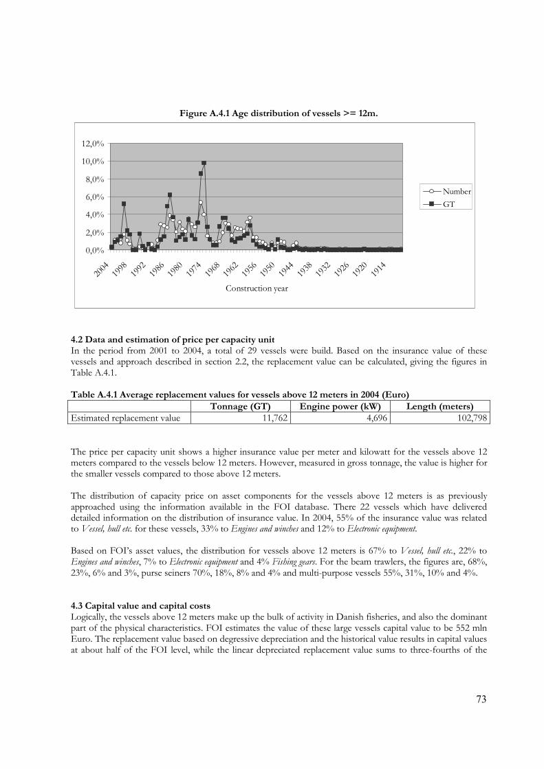
73

Figure A.4.1 Age distribution of vessels >= 12m.

0,0%

2,0%

4,0%

6,0%

8,0%

10,0%

12,0%

2004

1998

1992

1986

1980

1974

1968

1962

1956

1950

1944

1938

1932

1926

1920

1914

Construction year

NumberGT

4.2 Data and estimation of price per capacity unit In the period from 2001 to 2004, a total of 29 vessels were build. Based on the insurance value of these vessels and approach described in section 2.2, the replacement value can be calculated, giving the figures in Table A.4.1. Table A.4.1 Average replacement values for vessels above 12 meters in 2004 (Euro) Tonnage (GT) Engine power (kW) Length (meters) Estimated replacement value 11,762 4,696 102,798 The price per capacity unit shows a higher insurance value per meter and kilowatt for the vessels above 12 meters compared to the vessels below 12 meters. However, measured in gross tonnage, the value is higher for the smaller vessels compared to those above 12 meters. The distribution of capacity price on asset components for the vessels above 12 meters is as previously approached using the information available in the FOI database. There 22 vessels which have delivered detailed information on the distribution of insurance value. In 2004, 55% of the insurance value was related to Vessel, hull etc. for these vessels, 33% to Engines and winches and 12% to Electronic equipment. Based on FOI’s asset values, the distribution for vessels above 12 meters is 67% to Vessel, hull etc., 22% to Engines and winches, 7% to Electronic equipment and 4% Fishing gears. For the beam trawlers, the figures are, 68%, 23%, 6% and 3%, purse seiners 70%, 18%, 8% and 4% and multi-purpose vessels 55%, 31%, 10% and 4%. 4.3 Capital value and capital costs Logically, the vessels above 12 meters make up the bulk of activity in Danish fisheries, and also the dominant part of the physical characteristics. FOI estimates the value of these large vessels capital value to be 552 mln Euro. The replacement value based on degressive depreciation and the historical value results in capital values at about half of the FOI level, while the linear depreciated replacement value sums to three-fourths of the

74

FOI value. Given that the depreciation and interest is also calculated to be lower, the profit/capital ratios are much higher than FOI. Table A.4.2 Capital value and capital costs and their consequences on profit for vessels above 12 meters (mln Euro)

Replacement value Historical value (Macro / economic approach) (Micro / fiscal approach)

2004 Degressive

depreciation Linear

depreciation Fiscal rate 1 Value of landings 322.5 Fuel costs 1.8 Other running costs 37.5 Vessel costs 67.7 Crew share 85.8 Gross cash flow 129.8 Depreciation 54.5 48.6 27.9 37.7Interest 28.0 11.4 17.3 3.9Net profit 47.3 69.7 84.6 88.1Gross value added 215.6 Capital value 551.5 264.9 401.5 281.8Profit / capital 8.6% 26.3% 21.1% 31.3% The composition of the capital values is shown in Table A.4.3 and Table A.4.4. Comments to this are in line with the previous ones made for the total fleet and vessels below 12 meters. Table A.4.3 Summary of the capital values - comparison of approaches for vessels above 12 meters (mln Euro)

Total Hull Engine Electronics Other Replacement value (constant prices) Total 958.4 642.1 210.8 67.1 38.3Degressive depreciated 264.9 144.8 77.5 28.1 14.5Linear depreciated 401.5 233.1 108.1 39.8 20.6Historical value (current prices) Total 631.3 311.2 210.9 48.7 60.4Degressive depreciated 281.8 122.8 104.2 21.0 33.8 Table A.4.4 Relative composition of capital for vessels above 12 meters (%)

Total Hull Engine Electronics Other Replacement value (constant prices) Total 100.0 67.0 22.0 7.0 4.0Degressive depreciated 100.0 54.7 29.3 10.6 5.5Linear depreciated 100.0 58.0 26.9 9.9 5.1Historical value (current prices) Total 100.0 49.3 33.4 7.7 9.6Degressive depreciated 100.0 43.6 37.0 7.5 12.0

75

Appendix A.1 Account Statistics for Fisheries - Denmark The current practice to estimation of capital value in the Danish Account Statistics for Fisheries produced by the Danish Institute of Food and Resource Economics is described in this appendix. Source of data The Danish Account Statistic for Fishery is compiled on the basis of collected accounts from 311 fishing firms, owning approximately one vessel each. These 311 firms corresponds to about 25 per cent of the Danish fishing firms, with a total output from the fishery in 2004 of at least 224,342 DKK16 measured in Standard Catch Value (SCV). The sample represents 98 per cent of total output of the sector and gives full coverage of the Danish fishery. Information is collected about activity, earnings, costs, assets and vessel characteristics. Each firm/vessel has attached a weight, which reflects its importance in the representation of the statistics. This factor is found by using a restricted least squares regression model. In the model, a restriction is included to secure that the number of vessels within each length category is equal to the number of vessels in the total population. Furthermore, the deviation from other restrictions such as distribution on homeports, fishermen’s age and catch revenues is sought to be minimised. The statistic therefore reflects the commercial fleet with respect to key characteristics in the best possible way, given the included vessels. Description of method and assumptions - Tangible assets In the Danish accounting form for fishery, a deduction is made between several tangible assets utilised in the fishery production. The information given in the accounts for a fishing firm/vessel is shown in the table below.

Primo Price regulation Investments

(cash value) Depreciation Ultimo

A B C D E Vessel, hull etc. Engines and winches Electronic equipment Fishing gears Vehicles (cars, trucks etc.) Buildings etc. Other assets (stocks etc.) Total value 0 0 0 0 0 Having determined the primo value of the tangible assets, these are regulated with changes in prices, new investments and depreciation, thus giving the ultimo value of the tangible asset. The calculation of each figure in the statistics is calculated as follows, cf. the letter attached to each column in the table above:

16 1 Euro is approximately equal to 7.53 DDK.

76

A. The first time a firm/vessel is included in the statistics, the primo value of the assets are determined together with the vessel accountant. For a new firm/vessel, the values of the tangible assets are relatively easy to determine, because the depreciation costs are of minor importance. It is generally the case that the value is closely related to the insurance value. For an older firm/vessel, it is often more difficult to determine the tangible asset value, because the depreciation related to taxation is much larger than the physical depreciation. For these firms/vessels, the insurance value is often used as starting point, and adaptations are afterwards made.

B. The price regulation for vessel, engine and electronic equipment are determined using fixed indexes calculated by FOI. Wholesale price indexes and wage indexes from Statistics Denmark is used. These are used to calculate an index for 1) vessel, hull etc., 2) engines and winches and 3) electronic equipment.

C. The allocation of vessel expenses between maintenance and investment (including improvements

and renovation to prolong operational lifetime) has been given special attention from the start of the Account Statistic for Fishery. Especially the cost on fishing gear, which were usually set as an operational cost before FOI started collecting data for the account statistic. Now the purchase of new fishing gear is activated on the balance and depreciated according to expected lifetime.

D. Depreciation is individually calculated for each vessel (firm) in the accounts. Individually set

depreciation percentages based on the expected (operational) lifetime of the physical assets (scrap value set to 20%) are used in the calculations for each type of fishery asset:

Lifetime (years) Depreciation percentage Vessel, hull etc > 20 3% - 8% Engines and winches 7-23 7% - 20% Electronic equipment 5-15 10% - 30% Fishing gear 2-5 25% - 50% Other operative assets* Depends on the asset type 4% - 30%

* Land based like buildings, trucks or other vehicles In the individual accounts, depreciation is calculated using the method of diminishing balance, where a fixed percentage is multiplied on the sum of tree items:

• The book value at the beginning of the year • An adjustment for price trends is made for vessel, engine and electronic equipment • The net investment (purchase minus sale) for that type of asset for the year

E. Adjusting the primo asset value with price changes, net investments and depreciation, the ultimo

book value of the assets is finally obtained. Description of method and assumptions - Intangible assets In the account statistics, it is possible to register the value of these intangible assets. However, it is in reality only the sale and purchase of quotas on herring and mackerel that is registered. It is problematic to estimate the value of these assets, because it is primarily only the vessels buying quota that stays within the fishery, while vessels selling quota leaves. Furthermore the bought quota shares are valuated, while the rest of the vessels catch “rights” are not valuated.

77

The value of the bought quota share is obtained through the obtained account schemes. It is difficult to investigate whether the intangible assets are included in the value of the tangible assets. An approach could be to compare the development in the value of the tangible and intangible assets in order to see whether a lower value of the tangible assets is outweighed by an increase for the intangible assets. Considering that only the value of bought herring and mackerel is currently included in the statistics, it is not possible to investigate in more detail. Within the account statistics, no depreciation is made of the intangible assets. Some accountants consider this to be possible within the tax laws, but this is more related to taxation issues.

78

APPENDIX B: France

Introduction: Data sources The primary data used for this study are belonging to four databases: - The national fleet register of the Ministry of Agriculture and Fisheries, - The data base of the IFREMER Fisheries Observatory Network for individual data on fishing vessel's

activity and economic situation - The second hand market transactions database - The accounting and balance sheets database of the Brittany Regional Observatory of Fisheries The national fleets register of the Ministry of Agriculture and Fisheries Some agreements exist between the ministry and Ifremer to make the French annual fleet register available for all the research projects where this public body is involved. In addition with the fishing fleet register downloadable from the EU databases, the ministry transmits annually to Ifremer a picture of the fleet at the 31/12/YearN (or 01/01/YearN+1). This picture is very useful to build time series of the French fleet without the bias linked with the entry and exit of vessels in the fleet register all over one given year. This table contains for each vessel of the French fleet its technical characteristics (size in length, kW, GRT, age...), the geographical location of the owner and other information like gears used by the vessel each year. The data base of the IFREMER Fisheries Observatory Network This database contains two kinds of information: - the detailed fishing activity of each vessel registered in the Fleet Register in terms of gear, target species and so on (census); - the individual economic situation of some fishing vessels registered in the Fleet Register (sample). It has been proved that in many cases, the reliability of the fleet register to characterize the fishing activity of each vessel through the gears declared is doubtful. Additionally, the exhaustivity of logbooks data files, even for vessel over 10 m., is not proved. Then, Ifremer has developed a collection of data on individual fishing activity through its Fisheries Observatory Network. Each year since 2000, information regarding the monthly fishing activity (métiers, fishing areas...) for each vessel present in the Fleet register has been collected through exhaustive surveys. This information, complementary to logbooks, allows affecting each vessel present in the Fleet Register to a specific "fleet" taking account of the "metier" it practised during a given year. Parallel to this census, the Ifremer Fisheries Observatory Network makes yearly surveys on a sample of 800 vessels (around 600 vessels from the Atlantic coast) to collect individual data on costs, earnings but also capital and employment devoted to the commercial fishing activity. The "economic sample" made available for this study is composed by 3500 individual data collected from 2000 to 2004. The vessel owners are questioned on their costs and earnings in detailed but also on the features of their fishing vessel (s) and its components (hull, engine, gear and winches, electronics, storage) and their related prices (historical, replacement, insurance or market value). The second hand market transaction database A complementary database exists at Ifremer and consists in the record of around 70% of the second hand market transactions occurred from 1985 to 2003 along the French NSCA coast. These data come from the so-called Affaires Maritimes districts and were collected with the support of the French Ministry of Fisheries. The date and the price of each transaction are available. This data set contains around 4600 observations from 1985 to 2004 which were used for an assessment of the second hand market vessel prices through hedonic method. Results on depreciation method and value of intangible assets in the French sector are deduced for this model.

79

The Brittany Regional Observatory of Fisheries Finally, the Brittany Regional Observatory of Fisheries database has also been made available for this study. This database contains yearly accounting and balance sheets data for a large part of Brittany fishing vessels, the major fishing region of the Atlantic coast (representing almost 50% of the fleet).The commercial fishing fleet of the French region of Brittany is well informed by the Regional Economic Observatory of Fisheries which is a NGO created in 1992 by a professional fishermen organization. This Observatory collects bookkeeping from a network of 12 local accounting agencies and landings data from three producer organizations by individual units.

1. General national situation – national markets for fishery assets

1.1 Investments in new vessels The French total fleet (excluding Corsica and Overseas territories) is composed at the 1rst January 2005 of 5216 vessels for a total of 830,099 kW and 148,337 GRT. The total fleet that we will consider here is composed with 3640 vessels below 30 meters and belonging to fishing harbors of the North Sea, Channel and Atlantic coast. This fleet accounts for 550,445 kW and 74,695 GRT and is called now "French NSCA fleet".

Figure B.1.1 Age composition of the French total fleet at 1rst January 2005

Age composition total fleet

0.0%

1.0%2.0%

3.0%4.0%

5.0%

6.0%7.0%

8.0%9.0%

10.0%

2004

2000

1996

1992

1988

1984

1980

1976

1972

1968

1964

1960

1956

1952

1948

1944

1940

1936

Construction year Number (%)GRT (%)

Source: IFREMER At the 1rst January 2005, the French NSCA fleet is composed with vessels building since the 30's but the large majority of the vessels (95%) have been built after 1970. The percentage of vessels which have entering the fleet each year increases regularly from the 1970's to 1985. This is consistent with the public policies during this period which aiming at the development of the fishing fleet in the country. The GRT curve shows that sometimes, the entry in number is not consistent with the real fishing capacity entering the fleet. The graph shows that the middle of 80's has corresponded with investments in relative large vessels. This strategy increased the fishing capacity directed to EU fishing stocks already overexploited for some of them.

80

In total, the two curves show an increasing trend of entries and fishing capacities from the 70's to the second part of the 80's, following by a large decrease. In five years, the rate of new entry went from 9% to 1%. For more than 10 years now, the entry of new vessels in the fleet is stable at a constant rate by 1% - 2% per year.

1.2 Investments in fishing rights Different types of fishing rights have been implemented to limit entry into the French fishing industry or to specific fisheries. The first is an operation permit attached to each vessel, namely “permis de mise en exploitation” enforced in 1988. This system aimed at limiting entry flows to the French commercial fleet and became the main regulatory tool on the basis of which Multi-Annual Guidance Programs were implemented. Each new capacity project has been subject to an operation permit issuing. Capacity projects consist of: new buildings, importations of vessels, entries of vessels previously used for non-commercial fishing activity, change of the fishing capacity by an increase in vessel tonnage or increase in engine power, readmitted vessels which were not active for a transitory period. Based on this regulation, the ministry of fisheries defines the annual allowance of engine power and more recently, of tonnage that could be issued for each year. This allowance is shared between two vessel categories, more or less 25, with a split by region for the last category. The fleet segment criterion has been added to the sharing rules since 2000. The second types of fishing rights are licences aimed at limiting entry and controlling effort into specific fisheries. Each licence is attached to a vessel and its owner. The number of licence systems is growing and the system is mainly managed by the so called “interprofessional organisation” at national or regional levels. The most common examples are the scallop inshore fisheries which are mainly regulated by individual licences with a "numerus clausus" and constraints on days or hours at sea (Guyader, Daurès and Fifas 2004). Fishery Type of right Definition Tradability Year of

introduction Approximate price / unit in 2005

Fishing industry (and segment since 2000)

Operation permit

kW, GRT Forbidden by the Law, implicit market in practice through the sale of vessel

1988

Dependent on fisheries (ex: Scallop fisheries in coastal areas, nephrops fisheries in the bay of Biscay, gillnet in the Brittany region etc...)

Fishery licence Access to a stock or/and area with a specific gear, effort limitation in some cases

Forbidden by the Law, implicit market in practice through the sale of vessel

Varies from fisheries to fisheries (First in 1974)

These fishing rights are, however, not transferable by themselves on the market, because of the national law on fisheries, which explicitly forbids the exchange of rights between owners (JORF 1997). In most of the

81

cases, these fishing rights attached to the vessel are in practice tradable through the sale of the boat on the second-hand market.

1.3 Investments in 2nd hand vessels Since the beginning of the 90s, the second-hand market for vessels has been the main way to enter the fishing industry, mainly because of the strong limitation of new entries, especially buildings. Because of these constraints and the change in the economic environment of the fleet (improvement in the performance of the fleets, decrease in the cost of capital because of the decline in real interest rate) the activity on the second hand market increased. As illustrated on the figure B.1.2, the rate of transaction rose from 5.0% in 1992 to 10.2% in 1999. The consequence was a gain in the average value of the vessels on the market despite the global ageing of the vessels exchanged, from a minimum of 9,000 Euros per meter in 1994 to around 20,000 per meter in 2002 (figure B.1.3).

Figure B.1.2 Evolution of the transaction rate on the second-hand Market (Atlantic Area)

5.0%

5.5%

6.0%

6.5%

7.0%

7.5%

8.0%

8.5%

9.0%

9.5%

10.0%

10.5%

11.0%

1992 1993 1994 1995 1996 1997 1998 1999 2000 2001 2002 2003

Tran

sact

ion

Rat

e (A

tlant

ic A

rea)

Figure B.1.3 Evolution of average price per meter in constant kEuros on the second-hand Market (Atlantic Area)

5

7

9

11

13

15

17

19

21

1992 1993 1994 1995 1996 1997 1998 1999 2000 2001 2002 2003

KEur

os p

er m

eter

Note: Transaction rate: Number of transaction (t) / Number of vessels in the Fleet (t-1)

Source: IFREMER Vessel prices on the second hand market seem to value not only the material capital (i.e. the value of the vessel) but also the intangible capital (i.e. operation permits and licence). While the size of the vessel and their

82

age significantly influence vessels prices, these access rights account for a weighty part of vessels prices on the second hand market (Guyader and Daurès, 2003). A series of decommissioning schemes have been implemented nearly every year since 1991. These schemes were regularly implemented to fulfill the MAGPs intermediate and final MAGPs targets or when delays appeared (Guyader, Berthou and Daurès 2004). In the application of decommissioning schemes, the government adjusted the premium levels to scrap vessels according to E.U. rules and to the second hand market prices evolution. This is rational because vessels owners decide or not to scrap their fishing unit by comparing the price of their fishing units on the second hand market and the premium offered by decommissioning schemes.

Figure B.1.4 Evolution of theoretical premium to scrap vessel (Atlantic Area)17

0

2

4

6

8

10

12

14

16

1992 1993 1994 1995 1996 1997 1998 1999 2000 2001 2002 2003

Prem

ium

in K

Euro

s pe

r met

er

Source: based on DPMA regulations

1.4 Investments in shore facilities Little information exists on this topic and the only available source for this study is the annual economic surveys conducted by Ifremer. Based on a standardized questionnaire, the vessel owner is questioned on the number of in shore assets he owns and their type. Moreover, if the investment in this type of assets occurred recently, the price of the asset is asked in order to constitute time series of prices. Four categories of in shore assets are considered: - vehicles (cars, vans), - buildings (only storage buildings or "fish wells"...), - computers and other electronic assets (not installed on the vessel), - equipment for commercialization at land. In some cases where the interviewer is able to give more details, these categories can be divided into more precise subcategories. Based on the economic sample from 2001 to 2004 of the Ifremer Fisheries Observatory Network, around 42% of vessel owners are in possession of at least one "in shore" facility. This percentage is slightly higher for

17 Premium is considered as theoretical because it does consider the effective premium received for decommissioned vessels but what vessel owners could receive according

decommissioning regulations. In 2003, for a 100% level of the premium allocated to vessels targeting species under recovering plans or stocks in bad state.

83

large vessels (over 12 meters). Based on a sub sample where the information is more detailed, the van is the "in shore" facility mostly declared (37%), then the car (17%), the storage building (12%) and the computers (10%). Very preliminary treatments of the data lead to an assessment of the replacement value of in shore facilities in the fishing sector at 34 000 € on the average. However, this amount is generally excluded from the calculation of the traditional indicator of capital value in the fishing sector which considers exclusively vessel. The concentration of the fishing sector has not been proved with statistical measures. The owning property system of the French fishing sector is still deeply characterized with the individual ownership. Then, the owner of a fishing vessel is still an individual ownership and precisely the captain of the vessel. A recent study on the Brittany fleet made by Ifremer showed that the ownership remains in a large majority individual even if the number of societies has increased for the last 15 years (Talidec at al. 2006). This is confirmed by the FIDAL and PWHC report (2005) which underlines the difficulty in this case to operate a clear distinction between family and firm assets.

1.5 Approach for the calculation of capital value in agriculture and/or by statistical office

1.5.1 Agriculture Source: CE – DG Agriculture RI/CC 1256, rev.3, "FADN Data definition..." based on EC Regulation N° 2253/2004. This document specifies all the items which have to be included in the calculation of the capital value and the way to proceed. The depreciation calculation is based on the replacement value and is linear for the French case.

1.5.2 Statistical office The French method implemented by INSEE (Institut National de la Statistique et des Etudes Economiques) is described in the OECD 2001 reference book on the measurement of capital. It recalls that "the PIM method is used with the hypothesis that fixed assets are discarded according to a lognormal mortality function and that depreciation is assumed to be straight line". The difference between closing and opening capital stocks in gross terms based on company accounts is used to estimate GFCF in current prices. Then an index procedure (Chain Laspeyres price indexes) is used to obtain series of GFCF in constant price by type of asset. Coefficients of mortality and depreciation are also depending on the type of asset and industry.

2. Estimation of value per capacity unit

2.1 Data and estimation of price per capacity unit Using its Fisheries Observatory Network data base, IFREMER runs in 2006 some models for the estimation of gross capital stock indicators per vessel per year (Daurès et al. , 2006). A sample of 420 observations is used for the "Historical price" model which is corresponding to the number of vessels for which the building year and the related building price are available. Note that the difficulty to have information on large vessels makes this model only applicable to less than 30 vessels. According to the age and the DCR segment composition of the total fleet the sample appears well representative. Moreover,

84

the sample composition according to hull material allows taking account of this feature in the historical price of a vessel. Historical prices used for this model are building prices collected through the annual economic surveys conducted by the Ifremer Fisheries Observatory Network. These data refer exclusively to tangible assets. The methodology refers to the hedonic approach and to the hypothesis that the historical price of a new vessel will be a function of its characteristics. The following specification is then considered: NVP = f (LGTH, Dev_GRT, Dev_kW, Fleet, Hull, Year) where NVP is the historical price of the vessel, LGTH is the length, Dev_GRT is the deviation of the vessel GRT from the mean GRT of the group of vessel belonging to the same length classes (8 length classes are considered), Dev_kW is the deviation of the vessel kW from the mean kW of the group of vessel belonging to the same length classes, Fleet are 5 dummy variables characterizing the fishing activity (Trawler, Seiner, Dredger, Passive gears, Other), Hull are 4 dummy variables characterizing the type of hull (Wood, Plastic, Metal, Other) and Year are 19 dummy variables equal the building year from 1985 to 2003. The equation is estimated using a semi logarithmic functional form where the dependant variable is the logarithm of the price of the vessel measured in the real term (taking account of the inflation rate).

∑=

+++=2003

1985,)log(

TTtTTi IKY εδβα

Where T = Building year K = Technical characteristics (length, deviation from GRT and from kW, Type of hull) YT=Acquisition price IT=1 if the building year equals T, 0 else The expected parameter signs are obtained and the increase in the size of the vessel (length) leads to increase in prices. Moreover, the vessel price in the same length category is positively linked with the fact that the vessel is bigger or smaller compared to the average of its category. This using of relative variable allows not

Sample distribution per Fleet segment: Fleet1: Trawler

Fleet2: Seiner

Fleet3: Dredger

Fleet4: Passive

Fleet5: Other

152 7 41 176 44 Sample distribution per hull material Metal Wood Plastic Other

155 61 201 3

Source: IFREMER

Sample distribution per building year Age structure of the sample

0

5

10

15

20

25

30

35

40

45

50

1985

ante

1987

1989

1991

1993

1995

1997

1999

2001

2003

85

facing the problems of multi co linearity of variables where length, kW and GRT must all be considered in a regression. The parameter estimates are given in annex. Regarding the fishing activity of a vessel, it seems that the item prices for new trawlers are significantly superior to other fleets. Considering the type of hull, the price of a vessel made with metal are generally lower that for other type of hull. Nevertheless, the parameters are not significant for the "other type of hull" category. Regarding the influence of the year, there are very few significant years (1990, 1991, 1998 and 2003). One main conclusion is that there are no big changes in building price of fishing vessels from year to year over the concerned period, if we take account of the inflation rate and every thing equal elsewhere. The model allows the calculation of an historical value for each vessel registered in the fleet at the 01/01/2005 given its specific characteristics. This deflated value was converted in current value for the purpose of this study based on consumption price index. Based on the knowledge of the capacity of each vessel, a price per capacity is then deduced from the estimates. Three capacity units are generally considered (kW, GRT, meter) and the trends of the different values per capacity unit (based on current values) are generally increasing with the time. The recent years are also characterized with high variability of the value per capacity which is less accentuated if we consider the value per GRT. The reliance of the kW as a capacity unit is very low. As far as the kW is the control variable in the fishing sector, large incentives exist for the fishermen to increase their real engine power. In this context, the analysis of reference prices has focused on the values per GRT and value per meter. The value per GRT per vessel deduced from the model is a little bit bigger for over 12 meters vessel, it depends on the size category of the vessel but in a less extent than the value per meter. For the value per meter, the distinction between the less than 12 meters vessels and the over 12 meters fleet is necessary. In the context where the GRT is replaced now by the GT and the obsolescence of the GRT as a capacity measure in the fishing sector will generate an inevitable cut in the time series values per capacity unit, the value per meter was considered as the best price per capacity measure for this study. This price per capacity measure will be retained for all the calculations at the finest level (less and over than 12 meters fleets, segments...). However, the price per GRT was retained for the calculation at the level of the total fleet even if it is obvious that the measure will be underestimated due to the largest weight of the small vessels for the calculation of a unique price per GRT per vessel. The small vessels (less than 12 meters) represented 71% of the total fleet in 2005. For each vessel i (1,.., N) present in the fleet register at 01/01/2005, built the year y (1,...,2004), belonging to the segment s, with X capacity unit and with an estimated cost P through the model, a historical price per X per building year is deduced. For the replacement price, we take account of the historical price of the recent years (2000-2004). The French method for estimation of prices per capacity unit is summarized in figure B.2.1.

86

Figure B.2.1 Accounting for tangible assets – decision tree – France

What value indicators can be collected / observed?

Insurance premiums Historical value

Insurance values / vessel

Do the data refer to the tangible assets only or do theyalso contain value of intangibles?

Value of tangible (vessel)

Paid 2nd hand values / vessel

Replacement value (RV) (3)

What does the available value per vessel represent?

Contain intangibles

Estimate / separate tangible and intangible value,

Other Depreciated / book value (2)

Historical value (HV) (4)

Determine series of historical prices/cu

Most recent historical price =

replacement price/cu

Follow columns (RV) or (HV)

Estimate replacement price / cu

Estimate total depreciation to

determine historical value

Estimate series of Historical Prices/ cu

Estimate RV and /or HV,

Describe approach

Price index series (1)

"Historical price" model (Daurès et al., 2006)

87

2.2 Capital value and capital costs 2.2.1 Tangible capital The assessment of tangible capital is primary based on the estimates resulting from the "Historical price model" applied to each vessel present in the Fleet register at the 01/01/2005. Only the results of vessels less than 30 registered in fishing harbors of North Sea, Channel and Atlantic coast are considered. As said before, historical price series of new vessels are used for the calculation of historical value of capital (micro or business approach) and the average price per capacity for the vessels build over the five recent years (2000-2004). In order to apply an evaluation per components, the results of the Ifremer economic surveys have been used for the evaluation of the share of each component in this tangible capital. Globally, the surveys confirm the assumptions of the common methodology proposed: - Hull (60%) - Engine (20%) - Electronics (10%) - Equipment and Other (10%) Some minor differences are observed if we split the vessels between length categories but they are considered as marginal. Depreciation methods: The most ancient work existed in France aiming at the definition of a depreciation method for the tangible capital was conducted by Boncoeur et al. (2000). In this method, three components of fixed capital were separated: Hull, engine and electronic materials. The depreciation of the vessel is supposed to be the sum of the depreciation of each component: - Depreciation for hull: Based on a linear regression made between vessels’ life span and the ratio insurance value / purchase price (sample of 62 vessels, with historical prices), the following relationship was concluded. Insurance value ≈ Purchase price x (-0.02 x vessel life span + 1.034) Consequently, a straight Line Depreciation by 2% a year was applied in this report (a rate very close to as estimated result computed for the UK English Channel fleet – Pascoe, Robinson and Coglan. 1996). Depreciation hull = 0.02 x Capital Value for vessel t0 - Depreciation for engine: Based on the economic life span estimated to 8 years from the survey Depreciation engine = 0.125 x Capital Value for enginet1. Capital value for engine was estimated from a sample of 100 individual data through an economic survey of fishermen (exploiting fisheries in the Channel). A log-linear regression was tested between engine power (kW) and available capital value for engine. Finally, the following estimation was used: Capital Value for enginet1= 0.5 x kW 1.16. Hence, Depreciation engine = 0.0625 x kW 1.16. -Depreciation for electronics: Life span considered for electronics was 5 years. Depreciation electronics = 0.2 x Capital Value for electronicst1 Capital Value for electronics t1 can be given from a face to face questionnaire or from a historical procedure based on market prices for standard materials. Depreciation vessel = 0.02 x Capital Value for vesselt0 + 0.0625 x kW1.16 + 0.2 x Capital Value for

electronicst1

88

In the recent context where the fleet is ageing, the degressive method for depreciation seems more appropriate than linear ones. The degressive method is more convenient because there are no strong assumptions on the life duration of the vessel. More recently, some works have been conducted on the basis of data on the second hand market vessels price (Guyader and Daurès, 2003). Based on a price model aiming to measure the influence of vessel features as length, age, fleet... as well as the date of the transaction (t) on the vessel price on the second hand market, a depreciation curve of the vessel price in relation with its age is deduced, every thing equals elsewhere.

Source: IFREMER

Some preliminary results are summarized based on the example of a vessel of 12 meters from Guilvinec (Brittany famous fishing harbor): - The trend is not linear, especially at the beginning and at the end of the vessel’s life. - For age ranging from 4 to 10 years, a stabilization or slight increase in vessel capital value occurs. It is consistent with the fact that most of the vessels have to renew their engines, electronic equipments, or to renovate the hull over the period. - For the period from 10 to 22 years old, a 21k€ average loss is observed every two years. Then, the decrease drops to 13 k€ per age class when the vessel age is between 22 and 28 years old. - After 28 years old, vessel values are fairly constant. The minimum value of these oldest vessels might be bounded by the residual value of their equipments. The recent works on depreciation tried to investigate the depreciation at the beginning of the vessel life through the integration of new vessel price data in the model (Daurès et al., 2006). The results are still preliminary but seem in a favor of a degressive method with different depreciation rates according to the age class of the vessel. In other terms, at the very beginning of the vessel life, the depreciation rate of the tangible capital (all components included) should be very higher than over the rest of its life. These questions about the consistency of a constant rate over the period were already investigated by Levy (1978). Finally, the fiscal regime was examined through Le Floch et al. (2006). The French fiscal regulation is based on two depreciation methods, the linear and the geometric system. If the former is considered as the usual case, the latter is admitted only to a few capital assets. Fishing companies can use the reducing balance rate for new vessels and second hand vessels too. From a fiscal perspective, fishing vessel’s life time is 6 years minimum. In these conditions, a company can fully depreciate its vessel in 6 years, whereas estimated economic lifetime overtakes usually 20 years. As indicated in the following table, showing fiscal computation for capital depreciation according to the French regulatory basis, a coefficient is applied to straight line depreciation rate for obtaining the

0255075

100125150175200225250275300

≤ 2 years

2-4 years

4-6 years

6-8 years

8-10 years

10-12 years

12-14 years

14-16 years

16-18 years

18-20 years

20-22 years

22-24 years

24-26 years

26-28 years

28-30 years

30-36 years

>36 years

Age Categories

Vess

el P

rice

in k€

89

appropriated reducing balance. New and second hand vessels bought before 01/01/2001 could be depreciated in applying a 33.33 or a 37.5 coefficient (respectively 29.17 and 33.75 since 01/01/2001). Table B.2.1 Reducing balance rate in the French fiscal regulatory basis Life time Straight line Before

01/01/2001 Since 01/01/2001

Coefficient Reducing balance rate

Coefficient Reducing balance rate

3 33.33 1.5 50 1.25 41.674 25 1.5 37.5 1.25 31.255 20 2 40 1.75 356 16.67 2 33.33 1.75 29.17

6 2/3 15 2.5 37.5 2.25 33.758 12.5 2.5 31.25 2.25 28.13

10 10 2.5 25 2.25 22.512 8.33 2.5 20.83 2.25 18.7515 6.67 2.5 16.67 2.25 1520 5 2.5 12.5 2.25 11.25

Source : Mémento pratique Francis Lefebvre (p165) – Fiscal - 2003 The adoption of the geometric method in the French case can be explained in term of investment incentives in the sector. Main aftermath due to fiscal life time for depreciating fishing vessels (6 years) is to generate a high gain capital for sellers. Every time a fishing vessel is sold, capital gain results from the difference between the amount of second hand value and worth value (or depreciated historic price). Consequently, capital gain is equal to second hand value if fishing capital is fully depreciated from a fiscal point of view (worth value being equal to zero). In this case, the French fiscal regulation considers capital gain as a short run gain and is liable for income tax, close to 60% (FIDAL, 2005). According to the cited study, the amount of tax burden on capital gain is the reason why prices on the fishing vessels second hand market have reached very high levels. However, a tax avoidance regime was implemented through the Fishing Guidance Act adopted in 1997, following the “fishing crisis” in 1993-1994. Under a few conditions, fishing vessel’s owners can benefit from partial tax exemption on capital gain. They have to reinvest fully the amount of sold asset in fisheries in a period of 18 months following transaction. In this case, capital gain is spread on the following seven fiscal years, whereas capital gain is taxed to 60% during the last fiscal year if there is not reinvestment in fisheries sector. For instance, consider a capital gain by 150 000 €, linked to a fishing vessel sold on the French second hand market. If the skipper-owner reinvest 100 000 € in a new fishing vessel (new or a second-hand one), a fraction of capital gain (50 000 €) will be taxed to 60 % on the current fiscal year, and the other part (100 000 €) will be spread on the next 7 fiscal years. This measure was decided in 1997 in the Fishing Guidance Act and should be ended in 2003, but finally has been extended. A distinction must be made between short term and long term capital gain. The former represents cumulated fiscal depreciation and the latter is the gap between second hand price and cumulated fiscal depreciation (equal to historical price if fully depreciated).

90

Historical price (A)

Cumulated fiscal

depreciation (B)

Residual value

(C) = (A)–(B)

Second hand price

(D)

Capital gain (E) = (D)–

(C)

Short term capital gain(1)

(F) = (B)

Long term capital gain(2)

(G) = (E)–(F)

100 50 50 120 70 50 20 100 80 20 120 100 80 20 100 100 0 120 120 100 20

(1) The French fiscal law taxes short term capital gain at 59.09% (a maximum income tax at 48.09% and social deductions at 11%) (2) The law taxes long term capital gain at 27% (a flat rate of tax at 16% and social deductions at 11 %) Two fiscal regimes are applied every time a fishing vessel is sold on the second-hand market. If a capital gain is expected, meaning a second-hand price higher than residual value, cumulated depreciation (B) defines short term capital gain (F) and long term capital gain is derived from the difference between capital gain and the short term side (G). Usually, fishing vessels are sold once capital is fully depreciated, as the third example in the table. Hence, taxes concern essentially short term capital gain, for which the level of taxes is the highest (59.09%). For this reason, the French authority decided a tax regime by installments if a reinvestment in the fishery sector is made. It appears that fishing companies in France can use the degressive system for new and second hand vessels too. In these conditions, a company can fully depreciate its vessel in 6 years, whereas estimated economic lifetime usually is above 20 years. Some comparisons of the results from the proposed methodology and real accountings data were made at the level of case studies on a common sample of vessel (Trawlers 16-24m., Passive gears less than 12m) where detailed accounting data exists. Data sources for loans as a % of total capital are also Ifremer annual economic surveys. Notice that these estimates are based on a sample of 453 vessels over the period 2002-2003. The loans as a % of total capital refer exclusively to the financing plan of the vessel at the date of the acquisition (new building or acquisition on the second hand market). The estimation is not taking account of the financing of investment occurring over the vessel's life. Moreover, this rate is given by the vessel owner without any possibility to check if the reference portfolio is the family one or the firm. Data sources for the interest rate of government bonds and market rate for loans (long term loans): Insee (http://www.insee.fr/fr/home/home_page.asp:Institut National de la Statistique et des Etudes Economiques -) Finally, for the assessment of capital value and capital costs for all the French case studies, the degressive and linear methods with the above depreciation rate per components presented in the following tables have been applied both for the macro approach and the business approach. Table B.2. 2 Overview of assumptions made in the French case studies

Economic depreciation rate / year - degressive

Economic depreciation rate / year - linear

Fiscal depreciation Degressive

Fiscal depreciation Linear

Hull 7% 4% 7% 4%Engine 25% 10% 25% 10%

91

Electronics 50% 20% 50% 20%Other equipment 35% 16% 35% 16%Rest value hull after 25 years 2.5% 2.5%Interest rate government bonds 4.1% Market rate for loans 4.1% Loans as % of total capital (Total Fleet) 68% Loans as % of total capital (<12 meters Fleet) 67% Loans as % of total capital (>12 meters Fleet) 72%

2.2.2 Intangible capital The French context is characterized by access rights to fisheries which have increasingly been implemented to control the fishing capacity of fleets facing the problem of common-pool resources. An important point is that these rights to harvest are not tradable except through the sale of the vessels. Using a hedonic pricing model, the hypothesis that the price of the exchanged vessels can be broken up into two components was tested: a tangible value explained by the technical characteristics and the age of the fishing units, and an intangible value representing the access rights to the fisheries. These harvesting rights may to some extent capitalize the value of the rent or quasi-rent flows exhausted from the fishing activity. This valuation of non-tangible assets is done based on record of transactions on the second hand fishing vessel market data (3500 prices from 1985 to 2003 with 1988 the year of implementation of PME). The equation was estimated using semi logarithmic functional forms where the dependant variable is the logarithm of the price of each item measured in the real term (taking account of the inflation rate)

∑=

++++=2003

1985)log(

TiTTi ItKY εδλβα

t = Age of the vessel i the transaction year T = Transaction year K = Technical characteristics (length, deviation from GRT and from kW, Type of hull)

iY = Market price of the vessel i

TI =1 if the transaction occurs the year T, 0 else On the contrary to the historical price model, the "year" variable has a great influence for the vessel price in the second hand market and seems to capture implicit fishing right value within the vessel value. In 2000, this value accounts for 50% of the vessel value on the second hand market. This value drops to a minimum in 1993, when the economic situation of the fleets was considered to be very bad.

92

3 Total fleet (under 30 meters, NSCA coast)

3.1 Description of the case study total fleet The French NSCA fleet (excluding all Overseas and Mediterranean vessels and over 30 meters Atlantic vessels) is a significant fleet at European level. A large part of the vessels is built in the middle of the eighties and the average age of the fleet at the 01/01/2005 is 21 years old.

Figure B.3.1 Age composition of French NSCA fleet

Age com position total fleet

0.0%1.0%2.0%3.0%4.0%5.0%6.0%7.0%8.0%9.0%

2004

2000

1996

1992

1988

1984

1980

1976

1972

1968

1964

1960

1956

1952

1948

1944

1940

1936

Construction year Num ber (%)m eter (%)

Source: IFREMER The NSCA fleet of less than 30 meters is diversified in term of fishing activity but the most important segment is the "bottom trawl and seine" segment which is composed by 879 vessels but develop an important fishing capacity measured on the basis of kW and GRT. Beside, the vessels using passive gears represent a non negligible part of the French fleet (156,000 kW and 16,000 GRT). Table B.3.1Composition of the total fleet < 30m. by main DCR sub-segment DCR Fleet Number GRT kW Average AgeBeam Trawler 18 752 4 362 21Bottom Trawl and Seine 879 37 591 223 591 21Pelagic Trawl and Seine 124 6 949 36 684 19Dredgers 267 5 751 46 508 24Other mobile gears 265 958 15 124 22Polyvalent mobile gears 97 2 016 14 712 23Hook 372 3 133 37 054 21Netters 686 10 860 94 887 19Pots and Traps 372 2 997 34 306 18Other passive gears 92 256 4 834 16Polyvalent passive gears 145 763 10 240 17Polyvalent mobile and passive 207 1 850 20 891 23Inactive 116 819 7 252 25TOTAL NSCA < 30m. 3 640 74 695 550 445 21

93

The average age of vessel is variable from fleet segment and goes from 16 years old for "Other Passive gears" to 24 years old for the dredgers.

3.2 Data and estimation of price per capacity unit Based on the historical price model, the price per GRT was around 8,500 € (in average for all the vessels present in the fleet at the 01/01/2005) and is around 13,500 € in the recent years. Table B.3.2 Price per capacity unit – Model estimates – Total fleet (NSCA, less than 30.) €/GRT

< 12m. €/GRT 12– 30m.

€/m. < 12m.

€/m. 12– 30m.

Replacement value (2000-2004) 12,810 14,666 8,965 55,906

Historical value (average over the period) 7,729 9,996 5,754 30,263Source: IFREMER The historical value per capacity increases continuously until 1991, corresponding to the period of high level of new entries. Since 1991, the historical prices per capacity fluctuate around the replacement prices.

3.3 Capital value and capital costs 3.3.1 Tangible capital

Table B.3.3 Summary of the capital values – NSCA Fleet <30m. Total Hull Engine Electronics OtherReplacement value (constant prices) Total 1 239.4 743.7 247.9 123.9 123.9Degressive depreciated 410.0 221.3 88.7 48.9 51.1Linear depreciated 496.2 217.2 135.6 74.6 68.7 Historical value (current prices) Total 709.1 425.5 141.8 70.9 70.9Degressive depreciated 266.5 158.1 51.2 27.4 29.9Linear depreciated 327.9 167.9 78.8 42.0 39.3Total = Gross fixed capital stock Degressive or Linear depreciated = Net fixed capital stock

The total value of the French NSCA fleet is evaluated at €709 mln (historical value) and €1240 mln (replacement value). The table shows a strong difference between replacement value and historical value of the total fleet. The analysis of profitability shows that the poorest profit rate is registered with the macro approach with a degressive method. A sensitivity analysis shows that this profit rate is can registered a difference of 15.3% with the highest profit rate belonging from the fiscal approach based on a linear method.

94

The profit rate is diversely influenced by the depreciation method retained for the capital components. A degressive depreciation is always generated higher depreciation costs than a linear depreciation and as a consequence a lowest profit rate due to low net profits. On the contrary and obviously, the linear method generally induces a highest net value of the capital compared to the degressive method. Relative composition Total Hull Engine Electronics OtherReplacement value Total 100.0% 60.0% 20.0% 10.0% 10.0%Degr. Depreciated 100.0% 54.0% 21.6% 11.9% 12.5%Linear depreciated 100.0% 43.8% 27.3% 15.0% 13.9% Historical Total 100.0% 60.0% 20.0% 10.0% 10.0%Degr. Depreciated 100.0% 59.3% 19.2% 10.3% 11.2%Linear depreciated 100.0% 51.2% 24.0% 12.8% 12.0%

Starting with a share per components of 60% for the engine, 20% for the engine, 10% for the Electronics and 10% for the other, the relative shares are not varying a lot despite the ageing of the fleet. The hull remains the predominant capital component, whatever the depreciation method used, but faces an increasing contribution of the engine (around 27%) instead of 20%. Level of depreciation Total Hull Engine Electronics OtherReplacement value Total 100% 100% 100% 100% 100%Degr. Depreciated 33% 30% 36% 39% 41%Linear depreciated 40% 29% 55% 60% 55% Historical Total 100% 100% 100% 100% 100%Degr. Depreciated 38% 37% 36% 39% 42%Linear depreciated 46% 39% 56% 59% 55%

Finally, despite an average age of 21 years old, the net value of the fleet is still around 35% of its initial value (historical or replacement) with the degressive method and around 40-45% with the linear method. 3.3.2 Intangible capital The 2003 value of the less than 30 meters NSCA fleet present at the 01/01/2005 was estimated at €835 mln by the hedonic second hand market price model. On the other hand, the book value of the capital (business approach) is around €300 mln based on the previous tables. The difference between these to value is €535 mln and could not be assimilated entirely to the value of intangible assets as it may include all sorts of investments made over the vessel life which are not considered in our analysis.

95

4. Fleet under 12 meters (NSCA coast)

4.1 Description of the case study fleet <12m. The less than 12 meters fleet is composed at the 01/01/2005 with 2,601 vessels developing 228,427 kW and 16,992 GRT. The large majority of vessels were built between 1978 and 1992. The average age of the fleet is 21 years old.

Figure B.4.1 Age composition of Fleet < 12m.

Age composition fleet < 12m

0.0%

1.0%2.0%

3.0%

4.0%

5.0%

6.0%

7.0%

8.0%

9.0%

2004

2000

1996

1992

1988

1984

1980

1976

1972

1968

1964

1960

1956

1952

1948

1944

1940

1936

Construction year Number (%)

meter (%) Source: IFREMER This fleet is represented in all fleet segments in terms of dominant gear. The most important segments are netters, bottom trawls and seine, hook and pots/traps. Table B.4.1Composition of the fleet < 12m. by main DCR sub-segment DCR Fleet Number GRT kW Average Age Beam Trawler 7 86 841 22 Bottom Trawl and Seine 338 3 292 36 830 25 Pelagic Trawl and Seine 12 174 1 894 18 Dredgers 146 1 437 15 917 25 Other mobile gears 264 948 15 037 22 Polyvalent mobile gears 65 649 6 173 25 Hook 352 1 958 31 066 21 Netters 531 3 750 54 338 19 Pots and Traps 350 1 860 28 868 18 Other passive gears 92 256 4 834 16 Polyvalent passive gears 140 625 9 233 17

96

Polyvalent mobile and passive 195 1 547 18 337 23 Inactive 109 410 5 059 25 TOTAL 2 601 16 992 228 427 21

Source: IFREMER The segments fleets are also different in terms of average age of vessels. The most ageing fleet are generally fleets using active gears with the exception of pelagic trawl and seine.

4.2 Data and estimation of price per capacity unit Table B.4.2 Price per capacity unit – Model estimates – Total fleet (NSCA, less than 12 meters) €/GRT €/meter Replacement value 12 810 8 965

Historical value (average over the period) 7 729 5 754Source: IFREMER The current prices per capacity estimated by the model are increasing over the period with large fluctuations in the recent years. The recent price is around 13,000 €/GRT (or 9,000 €/m.) in the recent period while it is around 7,800 €/GRT (or 5,800 €/m.) in average for all the vessels present in the fleet at the 01/01/2005.

€/ m.

0

2000

4000

6000

8000

10000

12000

14000

16000

18000

2004

2001

1998

1995

1992

1989

1986

1983

1980

1977

1974

1971

1968

1965

1962

1959

1956

1952

1942

€/GRT

0

5000

10000

15000

20000

25000

2004

2001

1998

1995

1992

1989

1986

1983

1980

1977

1974

1971

1968

1965

1962

1959

1956

1952

1942

Source: IFREMER

4.3 Capital value and capital costs 4.3.1 Tangible capital The value of the fleet is evaluated at €166.6 mln (historical value) and €201.3 mln (replacement value). This fleet contributes to 20% of the total capital of the NSCA less than 30m. fleet. Regarding the technical characteristics, the less 12m fleet contributes to 22% of the total GRT and 41% of the total kW.

97

Table B.4.3 Summary of the capital values – Fleet < 12m. Total Hull Engine Electronics Other Replacement value (constant prices) Total 201.3 120.8 40.3 20.1 20.1Degressive depreciated

63.7 33.1 14.7 7.8 8.0

Linear depreciated 75.7 30.7 21.9 12.1 10.9

Historical value (current prices) Total 166.6 78.0 44.9 21.7 22.1Degressive depreciated

66.4 28.3 17.6 10.7 9.8

Linear depreciated 81.5 29.3 24.9 14.6 12.6Total = Gross fixed capital stock Degressive or Linear depreciated = Net fixed capital stock There is no strong difference between replacement value and the historical value of the total fleet due to the hypothesis for the calculation of the replacement value. If the 2004 replacement value was taken instead of an average over the 2000-2004 period, the total replacement value would have been €351 mln (+74% ) and the resulting net profit would be in diminution due to a strong increase in the depreciation costs, especially with the degressive method. A sensitivity analysis based on a hypothetical gross cash flow shows that the profit rate is the lowest for the macro approach with a degressive method and can registered a difference of 13.6% with the highest profit rate belonging from the fiscal approach based on a linear method. Relative composition Total Hull Engine Electronics Other Replacement value Total 100.0% 60.0% 20.0% 10.0% 10.0%Degr. Depreciated 100.0% 51.9% 23.1% 12.3% 12.6%Linear depreciated 100.0% 40.6% 29.0% 16.0% 14.5% Historical Total 100.0% 60.0% 20.0% 10.0% 10.0%Degr. Depreciated 100.0% 58.5% 19.5% 10.6% 11.4%Linear depreciated 100.0% 49.9% 24.1% 13.4% 12.6%

The hull remains the major component of the tangible assets and still weight between 40 to 50% of the total capital.

98

Level of depreciation Total Hull Engine Electronics Other Replacement value Total 100% 100% 100% 100% 100%Degr. Depreciated 32% 27% 37% 39% 40%Linear depreciated 38% 25% 54% 60% 54% Historical Total 100% 100% 100% 100% 100%Degr. Depreciated 37% 36% 36% 40% 42%Linear depreciated 45% 38% 54% 61% 57%

With an average age of 21 years old, the net value of the less than 12 meters fleet is still around 35% of its replacement value and 40% of its historical value.

4.3.2 Intangible capital The 2003 value of the less than 12 meters NSCA fleet present at the 31/12/2004 was estimated at €238 mln by the hedonic second hand market price model while the net value of capital is around €70-80 mln (business approach).

5. Fleet 12 - 30 meters (NSCA coast)

5.1 Description of the case study fleet 12 - 30 m. The over 12 meters fleet is composed at the 01/01/2005 with 1,039 vessels developing 322,018 kW and 57,703 GRT. The large majority of vessels were built in the eighties and the average age of the fleet is 19 years old.

99

Figure B.5.1 Age composition of fleet 12-30 m.

Age composition fleet > 12m

0.0%

1.0%

2.0%

3.0%

4.0%

5.0%

6.0%

7.0%

8.0%

9.0%

2004

2000

1996

1992

1988

1984

1980

1976

1972

1968

1964

1960

1956

1952

1948

1944

1940

1936

Construction year Number (%)

meter (%) Source: IFREMER The vessels are mainly concentrated in the "bottom trawl and seine" segment (541 vessels, 35,000 GRT and 187,000 kW) and more generally, there are more present in segment fleet using active gears than passive ones. Table B.5.1 Composition of the total fleet 12-30 m. by main DCR sub-segment DCR Fleet Number GRT kW Average Age Beam Trawler 11 666 3 521 19 Bottom Trawl and Seine 541 34 299 186 761 18 Pelagic Trawl and Seine 112 6 775 34 790 19 Dredgers 121 4 314 30 591 23 Other mobile gears 1 10 87 35 Polyvalent mobile gears 32 1 367 8 539 20 Hook 20 1 175 5 988 19 Netters 155 7 111 40 549 17 Pots and Traps 22 1 138 5 438 23 Polyvalent passive gears 5 137 1 007 18 Polyvalent mobile and passive 12 303 2 554 18 Inactive 7 409 2 193 26 TOTAL 1 039 57 703 322 018 19

Source: IFREMER Compared to other "active gears" segments, the segment of dredgers is more ageing and the "bottom trawl" segment is less ageing, this can reveal different investments policies over time regarding one or other segment.

100

5.2 Data and estimation of price per capacity unit Table B.5.2 Price per capacity unit – Model estimates – Total fleet (NSCA, 12-30m. ) €/GRT €/meter Replacement value 14 666 55 906

Historical value (average over the period) 9 996 30 263 Source: IFREMER The prices per capacity estimated by the model are increasing over the period with again fluctuations in the recent years. The recent price is around 15,000 €/GRT (or 56,000 €/m.) in the recent period while it is around 10,000 €/GRT (or 30,000 €/m.) in average for all the vessels present in the fleet at the 01/01/2005.

€/ m

0

10000

20000

30000

40000

50000

60000

70000

80000

90000

2004

2001

1998

1994

1991

1988

1985

1982

1979

1976

1973

1970

1967

1964

1960

1957

€/ GRT

0

5000

10000

15000

20000

25000

2004

2001

1998

1994

1991

1988

1985

1982

1979

1976

1973

1970

1967

1964

1960

1957

Source: IFREMER

5.3 Capital value and capital costs 5.3.1 Tangible capital The value of the fleet is evaluated at €580 mln (historical value) and €1038 mln (replacement value). Based on the model estimates, this fleet contributes to 80 % of the total capital of the NSCA less than 30m. fleet. Table B.5.3 Summary of the capital values - 12– 30 m. NSCA fleet Total Hull Engine Electronics Other Replacement value (constant prices) Total 1038.1 622.9 207.6 103.8 103.8Degressive depreciated 346.3 188.2 73.9 41.1 43.0Linear depreciated 420.4 186.5 113.6 62.5 57.8

Historical value (current prices) Total 579.2 347.5 115.8 57.9 57.9Degressive depreciated 218.1 129.8 41.7 22.3 24.3Linear depreciated 269.2 138.6 64.6 34.1 31.9Total = Gross fixed capital stock Degressive or Linear depreciated = Net fixed capital stock

101

There is a strong difference between replacement value and the historical value of the fleet due to the high difference between the average historic price per capacity unit and the replacement value (based on estimated prices of the five last years). A sensitivity analysis based on a hypothetical gross cash flow shows the profit rate is the lowest for the macro approach with a degressive method and can registered a difference of 15.5% with the highest profit rate belonging from the fiscal approach based on a linear method. Relative composition Total Hull Engine Electronics Other Replacement value Total 100.0% 60.0% 20.0% 10.0% 10.0%Degr. Depreciated 100.0% 54.4% 21.3% 11.9% 12.4%Linear depreciated 100.0% 44.4% 27.0% 14.9% 13.7% Historical Total 100.0% 60.0% 20.0% 10.0% 10.0%Degr. Depreciated 100.0% 59.5% 19.1% 10.2% 11.2%Linear depreciated 100.0% 51.5% 24.0% 12.7% 11.8%

The hull remains the most important capital component but the engine takes a large part of the capital if we consider the method based on replacement value and linear depreciation. Level of depreciation Total Hull Engine Electronics Other Replacement value Total 100% 100% 100% 100% 100%Degr. Depreciated 33% 30% 36% 40% 41%Linear depreciated 40% 30% 55% 60% 56% Historical Total 100% 100% 100% 100% 100%Degr. Depreciated 38% 37% 36% 38% 42%Linear depreciated 46% 40% 56% 59% 55%

With an average age of 19 years old, the net value of the 12- 30 meters fleet is still around 35% of its replacement value and 40% of its historical value. 5.3.2 Intangible capital The 2003 value of the 12-30 m. NSCA fleet present at the 31/12/2004 was estimated at €597 mln by the hedonic second hand market price model while the net value deduced from the previous methodology is around €250 mln.

102

6. Trawlers 16-24 meters

6.1 Description of the case study Trawlers 16-24 m. The trawlers 16-24 m. fleet account 380 vessels at the beginning of 2005 and represent a important part of the over 12 meters NSCA Fleet. The capacity developed is around 145,000 kW and 27,000 GRT. Compared to other segments, the vessels belonging to this fleet and presents at the 01/01/2005 are relatively young with an average age of 17 years old. The large part of the vessels was built in the end of the eighties.

Figure B.6.1 Age composition of Trawlers 16-24m.

Age composition Trawlers 16-24 m

0.0%

2.0%

4.0%

6.0%

8.0%

10.0%

12.0%

2004

2002

2000

1998

1996

1994

1992

1990

1988

1986

1984

1982

1980

1978

1976

1974

1972

Construction year Number (%)meter (%)

Source: IFREMER Regarding the DCR segmentation based on dominant gear, the vessels are concentrated in priority in the bottom trawl and seine segment (more than 80% of the vessels) but also in a less extent in the pelagic trawl segment. Table B.6.1 Composition of Trawlers 16-24 m. by main DCR sub-segment DCR Fleet Number GRT kW Average Age Beam Trawler 1 67 220 20 Bottom Trawl and Seine 308 22 328 119 359 17 Pelagic Trawl and Seine 67 4 214 23 387 19 Polyvalent mobile gears 4 235 1 302 20 TOTAL 380 26 844 144 268 17

Source: IFREMER

103

6.2 Data and estimation of price per capacity unit Table B.6.2 Price per capacity unit – Model estimates –Trawlers, 16-24 m. €/GRT €/meter Replacement value 15 319 69 815

Historical value (average over the period) 11 282 39 495Source: IFREMER The prices per capacity unit estimated by the model for the trawlers 16-24 m. segment are generally higher than those estimated at the level of the entire over 12 meters This is consistent with the negative signs of the "fleet" parameters of the model which mean that the historical price of all type of fleets are significantly different (and inferior) compared to trawlers (reference segment) everything equals elsewhere. The prices per capacity are increasing over time and reaching very high values in the recent period.

€/m

0

20000

40000

60000

80000

100000

120000

140000

2004

2002

2000

1998

1995

1993

1991

1989

1987

1985

1983

1981

1979

1977

1975

1973

€/GRT

0

5000

10000

15000

20000

25000

30000

2004

2002

2000

1998

1995

1993

1991

1989

1987

1985

1983

1981

1979

1977

1975

1973

Source: IFREMER

6.3 Capital value and capital costs 6.3.1 Tangible capital The capital value of the trawlers 16-24m. fleet is evaluated at €540 mln (replacement value) and €310 mln (historical value) at the 01/01/2005. It is confirmed that this segment contributes to a significant part of the total capital of the French NSCA fleet. Table B.6.3 Summary of the capital values – Trawlers 16-24 m. NSCA coast Total Hull Engine Electronics Other Replacement value (constant prices) Total 538.8 323.3 107.8 53.9 53.9Degressive depreciated 183.3 103.0 38.7 20.2 21.5Linear depreciated 223.8 104.2 59.4 31.4 28.8

Historical value (current prices)

104

Total 310.3 186.2 62.1 31.0 31.0Degressive depreciated 116.1 70.1 22.3 11.5 12.1Linear depreciated 143.8 75.5 34.5 17.9 15.8Total = Gross fixed capital stock Degressive or Linear depreciated = Net fixed capital stock

There is a strong difference between replacement value and the historical value of the fleet due to the high difference between the average historic price per capacity unit and the replacement value (based on the five last years). A sensitivity analysis based on a hypothetical gross cash flow shows that the profit rate is still the lowest for the macro approach with a degressive method and can registered a difference of 14.8% with the highest profit rate belonging from the fiscal approach based on a linear method. Relative composition Total Hull Engine Electronics Other Replacement value Total 100.0% 60.0% 20.0% 10.0% 10.0%Degr. Depreciated 100.0% 56.2% 21.1% 11.0% 11.7%Linear depreciated 100.0% 46.6% 26.5% 14.0% 12.9% Historical Total 100.0% 60.0% 20.0% 10.0% 10.0%Degr. Depreciated 100.0% 60.4% 19.3% 9.9% 10.4%Linear depreciated 100.0% 52.5% 24.0% 12.5% 11.0%

The hull accounts for the major part of the gross and depreciated capital even if the engine takes an increasing part as the fleet is ageing. Level of depreciation Total Hull Engine Electronics Other Replacement value Total 100% 100% 100% 100% 100%Degr. Depreciated 34% 32% 36% 37% 40%Linear depreciated 42% 32% 55% 58% 53% Historical Total 100% 100% 100% 100% 100%Degr. Depreciated 37% 38% 36% 37% 39%Linear depreciated 46% 41% 56% 58% 51%

105

With an average age of 17 years old, the net value of the trawlers 16-24m. fleet goes from 34 to 42% of its replacement value and from 37 to 46% of its historical value. 6.3.2 Intangible capital The 2003 value of the trawlers 16-24m. NSCA fleet present at the 31/12/2004 was estimated at €292 mln by the hedonic second hand market price model while its book value was estimated at € 130 mln by the previous calculations.

7. Passive gears less than 12 meters The passive gears less than 12 meters fleet is composed with 1171 vessels at the beginning of 2005 and accounts for a significant part of the less than 12 meters fleet.

7.1 Description of the case study Passive gears <12m. The average age of the fleet is 19 years old with the presence of very old vessels. The recent rate of new buildings is around 2% which is higher than for the rest of the French fleet.

Figure B.7. 1 Age composition of Passive gears < 12m.

Age com position - Passive gears less than 12 m .

0.0%

2.0%

4.0%

6.0%

8.0%

10.0%

12.0%

2004

2001

1998

1995

1992

1989

1986

1983

1980

1977

1974

1971

1968

1965

1962

1959

1956

Construction year Num ber (%)m eter (%)

Source: IFREMER The fishing activity of vessels is very diverse and there is apparently no concentration in one passive gear. Table B.7.1 Composition of Passive gears <12 m. by main DCR sub-segment DCR Fleet Number GRT kW Average Age Hook 282 1 527 24 910 21 Netters 426 3 141 45 242 19 Pots and Traps 314 1 659 26 038 17 Other passive gears 9 27 476 20 Polyvalent passive gears 140 625 9 233 17 TOTAL 1 171 6 979 105 899 19

106

7.2 Data and estimation of price per capacity unit Table B.7.2 Price per capacity unit – Model estimates –Passive gears <12m. €/GRT €/meterReplacement value 12 906 8 142

Historical value (average over the period) 8 307 5 749Source: IFREMER The average price per capacity unit is around 8300 €/GRT and 5800 €/m. which is very closed to what was observed at the level of the entire less than 12 meters fleet. The same observation is made with the replacement price.

€/m

0

2000

4000

6000

8000

10000

12000

14000

16000

18000

2004

2001

1998

1995

1992

1989

1986

1983

1980

1977

1974

1971

1968

1965

1962

1957

€/GRT

0

2000

4000

6000

8000

1000012000

14000

16000

18000

20000

2004

2001

1998

1995

1992

1989

1986

1983

1980

1977

1974

1971

1968

1965

1962

1957

Source: IFREMER

7.3 Capital value and capital costs 7.3.1 Tangible capital The value of the capital is estimated around €70 mln (historical value) to €80 mln (replacement value). Table B.7.3 Summary of the capital values – Passive gears < 12m. Total Hull Engine Electronics Other Replacement value (constant prices) Total 80.0 48.0 16.0 8.0 8.0Degressive depreciated 27.6 15.5 5.8 3.1 3.2Linear depreciated 33.1 15.3 8.7 4.8 4.4 Historical value (current prices) Total 71.6 35.0 19.4 8.4 8.9Degressive depreciated 30.2 14.4 7.4 4.4 4.0Linear depreciated 36.7 15.4 10.3 5.9 5.1

107

Total = Gross fixed capital stock Degressive or Linear depreciated = Net fixed capital stock

There is no strong difference between replacement value and the historical value of the total fleet. This is mainly due to the hypothesis for the calculation of the replacement value. If the 2004 replacement value was taken instead of an average over the 2000-2004 period, the total replacement value would have been €162 mln and the resulting net profit would be in diminution due to a strong increase in the depreciation costs, especially with the degressive method. A sensitivity analysis based on a hypothetical gross cash flow shows that, the profit rate is the lowest for the macro approach with a degressive method and can registered a difference of 10.8% with the highest profit rate belonging from the fiscal approach based on a linear method. Relative composition Total Hull Engine Electronics OtherReplacement value Total 100.0% 60.0% 20.0% 10.0% 10.0%Degr. Depreciated 100.0% 56.2% 21.2% 11.1% 11.5%Linear depreciated 100.0% 46.2% 26.1% 14.5% 13.2% Historical Total 100.0% 60.0% 20.0% 10.0% 10.0%Degr. Depreciated 100.0% 61.2% 18.2% 9.9% 10.7%Linear depreciated 100.0% 53.7% 22.0% 12.5% 11.8% Level of depreciation Total Hull Engine Electronics OtherReplacement value Total 100% 100% 100% 100% 100%Degr. Depreciated 34% 32% 36% 38% 40%Linear depreciated 41% 32% 54% 60% 54% Historical Total 100% 100% 100% 100% 100%Degr. Depreciated 40% 41% 37% 40% 43%Linear depreciated 49% 44% 54% 61% 58%

With an average age of 19 years old, the hull remains the major capital component and the net value of the passive gears fleet less than 12m. goes from 34 to 42% of its replacement value and from 40 to 49 % of its historical value.

108

7.3.2 Intangible capital The 2003 value of the passive gears fleet less than 12m. NSCA fleet present at the 31/12/2004 was estimated at €104 mln by the hedonic second hand market price model while the book value of the fleet is estimated around €35 mln at the same time.

8. Evaluation The valuation of the price per capacity is derived from the "Historical vessel price" model elaborated on the basis of the Ifremer Observatory dataset. To evaluate the strength and the weaknesses of the approach to assess tangible assets, some complementary analysis has been made on specific sub samples of trawlers 16-24 meters (45 vessels) and passive gears less than 12 meters (109 vessels) where individual accounting and balance sheets data are available. On the basis of the balance sheets data and specifically gross and net tangible capital (Fixed assets), time series of value per capacity have been recalculated and the resulting historical and replacement values (gross value and after depreciation) for these fleets have been compared to what have been obtained through the model time series. NB: For the calculation of the replacement value of the capital, we face the problem of the low level of the new constructions in the recent years when we work at the level of sub samples. In the sub sample of trawlers 16-24 meters. (45 vessels), only one vessel was constructed between 2000 and 2004 so the replacement price derived from the model applied to the entire fleet of trawlers 16-24 meters was also used (at the entire level of this segment, 25 vessels have been constructed between 2000 and 2004 and the price per capacity is estimated at 69,815 €/meter). Identically, in the sub sample of passive gears less 12 meters (109 vessels), only one vessel was constructed between 2000 and 2004 so the replacement price derived from the model applied to the entire fleet of passive gears less than 12 meters was also used (at the entire level of this segment, 113 vessels have been constructed between 2000 and 2004 and the price per capacity is estimated at 8,142 €/meter). For the business approach, the aggregated accounting data of the sample have been compared to the proposed methodology and particularly, the assumptions on depreciation and interest calculation have been assessed. The profit sensitivity analysis was applied on the basis of the real aggregated Gross Cash Flow of the sub sample. Table B.8.1 Results from a sub sample of Trawlers 16 -24 m. (45 vessels)

Sources Price per capacity time series

Historical vessel price model (34,068 €/m.)

Historical vessel price model (69,815 €/m.)

Time series from Accounting system (51,092 €/m.)

Depreciation and interest calculation Not specific (see assumptions p.91)

Replacement value (Sectoral Approach) Capital value Total 29.3 60.0 43.9Degressive 8.8 18.0 13.2Linear 10.6 21.7 15.9Gross cash flow 2.8 2.8 2.8

109

Depreciation Degressive 1.7 3.4 2.5Linear 1.0 2.1 1.6Interest Degressive 0.4 0.7 0.5Linear 0.4 0.9 0.7Net profit Degressive 0.8 -1.4 -0.3Linear 1.3 -0.2 0.6Profit / capital Degressive 8.6% -7.7% -2.0%Linear 12.4% -1.1% 3.6%

Sources Price per capacity time series

Historical vessel price model

Time series from Accounting system (Book value)

Aggregated accounting data of the sample

Depreciation and interest calculation Not specific (see assumptions p.91) Direct accounting data

Historical value (Business approach) Capital value Total 27.2 30.4 30.1Degressive 8.6 9.4 6.9Linear 10.7 11.6 Gross cash flow 2.8 2.8 2.8Depreciation Degressive 1.6 1.8 2.0Linear 1.0 1.1 Interest Degressive 0.3 0.3 0.5Linear 0.3 0.3 Net profit Degressive 1.0 0.8 0.3Linear 1.5 1.3 Profit / capital Degressive 11.0% 8.0% 4.4%Linear 13.8% 11.5%

Source: IFREMER, CEDEM, Brittany Regional Observatory of Fisheries

110

Table B.8.2 Results from a sub sample of Passive gears <12m. (109 vessels)

Sources Price per capacity time series

Historical vessel price model (6,250 €/m)

Historical vessel price model (8,142 €/m)

Time series from Accounting system (Book value)

Depreciation and interest calculation Not specific (see assumptions p12)

Replacement value (Sectoral Approach) Capital value Total 6.1 8.0 14.2Degressive 1.8 2.3 4.2Linear 2.1 2.8 4.9Gross cash flow * 4.1 4.1 4.1Depreciation Degressive 0.4 0.5 0.8Linear 0.2 0.3 0.5Interest Degressive 0.1 0.1 0.2Linear 0.1 0.1 0.2Net profit Degressive 3.7 3.5 3.1Linear 3.8 3.7 3.4Profit / capital Degressive 204% 151.4% 74%Linear 178% 133.2% 68%

Sources Price per capacity time series

Historical vessel price model

Time series from

Accounting system (Book

value)

Aggregated accounting data of the sample

Depreciation and interest calculation Not specific (see assumptions p12)

Direct accounting data

Historical value (Business approach)Capital value Total 6.6 15.2 16.0Degressive 2.2 4.7 5.8Linear 2.8 5.7 Gross cash flow * 4.1 4.1 4.1Depreciation Degressive 0.4 0.9 1.8Linear 0.3 0.5 Interest Degressive 0.1 0.1 0.4Linear 0.1 0.2 Net profit Degressive 3.6 3.1 1.9Linear 3.8 3.4

111

Profit / capital Degressive 161% 66% 33% Linear 134% 60%

* The Gross Cash Flow available for the analysis must be considered with cautious: for boats less than 12 meters long, bookkeeping database generally lead to high gross cash flow due to low labour costs. Main explanation is due to the share system which is used in the artisanal sector of the fishing industry. In fact, the share system is not always used on small boats. In the French version of the share system, the skipper-owner of an artisanal fishing boat is normally rewarded through two channels, which are the owner-share, and part of the crew-share (as a member of the crew). However, when the crew is composed of only one person (the skipper-owner himself), as is often the case on small boats, the share system is not always used, and the skipper-owner may be rewarded entirely on the basis of gross surplus (or gross cash flow). This institutional feature creates some heterogeneity in the accounting data of smaller boats, which sometimes include part of the skipper-owner’s income in the labour costs, and sometimes don’t. Source: IFREMER, CEDEM, Brittany Regional Observatory of Fisheries Historical value: Regarding the trawlers fleet, the historical value estimated by the model is much closed to the estimated historical values based on times series from accountings and the real gross capital value registered in the accountings. This is not the case for the passive gears fleet.

Source: IFREMER, CEDEM, Brittany Regional Observatory of Fisheries The major explanation is coming from the age structure of the fleet which is very linked with: - The potentiality or not that some vessels have been already exchanged on the second hand market or not - The amount of investment potentially done over the vessel life which is not captured by the model (except, in a certain extent, engine, electronic etc.). In the first case, the gross value registered in the balance sheet can be the second hand market value which is comprised the value of the tangible asset (book value or value after depreciation) but also the value of intangible assets (see the first result of the hedonic second hand market vessel price). It has been proved that this value on second hand market is much influenced by the vessels characteristics (size, fishing technique but also age) and the level of profitability in the fishing sector at the moment of the transaction captured in the model by the year of acquisition of the vessel. The previous graphs show that as far as we go far in the past, the deviation between the prices per capacity estimated by the model and those deduced from the accountings is bigger which seems to confirm that for these vessels, the accountings data are in fact acquisition prices in the second hand market instead of new building prices.

Price per capacity (€/m.) - Trawlers 16-24m. (45 vessels)

0

10000

20000

30000

40000

50000

60000

70000

2001

1993

199119

9019

89198

81987

1986

1985

1984

198319

82198

1198

01979

1978

1977

Historical price model Accounting data

Price per capacity (€/m .) - Passive gears less than 12 m . (109 vesse ls )

0

5000

10000

15000

20000

25000

30000

35000

40000

45000

2002

1998

1995

1991

1988

1986

1984

1982

1980

1978

1976

1974

1972

1970

1962

Historical price model

Accounting data

112

Replacement value The replacement value is very dependent on the data available in the context where very few new buildings occur. However, the profit rate in the macro approach is very sensible to the price per capacity finally retain for the analysis. Business approach: assumptions on depreciation and interest calculation. The comparison between the capital costs (depreciation and interest) deduced from the proposed generic methodology and the real data observed through the accountings raises a lot of questions. Concerning fixed capital depreciation, bookkeeping rules are influenced by fiscal considerations that are not necessarily in harmony with the actual economic life span of fixed capital. According to fiscal rules, complete depreciation of the purchase value of a boat (new vessel or second hand vessel) may be accounted for in 6 years. The problem is increased by the fact that the market value of a second hand boat incorporates, in France, the implicit value of the fishing rights that are attached to it and are de facto sold with it and subject to depreciation. Consequently, annual depreciation cost is higher from a fiscal perspective and leads to a lower profitability of depreciated capital. Interest cost appears higher with accounting system compared to business and sectoral approach. As the fiscal duration of fishing capital is a minimum of 6 years in the French fiscal law, skip-owners can be motivated to reimburse short term and long term loans on the same period. Finally, the level of profitability is very sensible to the assumptions made for the calculation: the replacement price per capacity is determinant for the macro approach, the assumptions on depreciation and interest calculation as well as the time series available for the calculation of the historical value for the micro approach. Conclusion: The method proposed here for the estimation of price per capacity unit and the valuation of tangible asset based on a model seems to require a large set of data but these data are rather simple to obtain. Through economic surveys, it is possible to collect information on insurance values of vessel. In the French case, personal interviews with insurance companies lead to the above conclusions: 1. The insurance value is based on an agreement and is not corresponding to the book value of the vessel: in case of accident, the insurance company refinances the totality of the insurance value without taking account of the depreciation and the obsolescence of the vessel. 2. The "entry permit" is not considered in the negotiation. 3. The insurance value of new vessels is based on the building price in addition sometimes with the value of the old vessel that had to be bought in order to have the right capacity to engage the new building (e.g. the regulation of the capacity imposes to withdraw a capacity equivalent or superior to the capacity of the building vessel). 4. The insurance value of second hand vessels are based on the acquisition price plus some additional works if it is the case. 5. The insurance values are renegotiated every 5 years depending on the financial constraint of the owner, different fiscal advantages and the observed trends on the fishing vessel's second hand market. The assumption that the insurance value is a good proxy of the building price (or historical price) for "new vessels" has been tested based on a sample of 560 vessels present in the database and which have been built by the owner interviewed, whatever the year of building. The insurance values reported in the surveys are confronted with the historical prices of the vessel in average per building year. There is a strong relationship between these two values and especially for the vessels building after the 80's i.e. vessels less than 25 years now. For the oldest, the insurance values per GRT are generally higher but there is so little data that it is difficult to conclude anything. From 2000 to 2004, around 3500 data on insurance value per vessel have been collected on a sample defined each year on the basis of a random stratified sampling and 560 data are

113

corresponding to the situation where the interviewed vessel owner has built the vessel. For the other part of the sample corresponding to vessels bought on the second hand market, insurance value is a proxy of the acquisition price and could lead to specific treatment on intangible assets if there is strong evidence that the "implicit" value of fishing rights is included in this acquisition price. Through accountings and balance sheet data, it is easy to obtain time series on fixed assets. However, as shows by the comparison, some complementary elements at individual level are necessary before processing these data (the nature of the acquisition (New/ Second Hand), year of the acquisition) specifically in the French context where acquisition price on the second hand market contains the value of intangible assets. These time series on accountings data could be of great interest for the analysis of investment in the fishing sector which are not exclusively limited to entry or exit of vessel from the sector and could be new technologies and items during the life time of the vessel.

114

References Bailly, D., J. Boncoeur, et al. (1996). Economie et Droit des Ressources Naturelles Renouvelables de la Mer : Aspects théoriques et application à la zone côtière de la Manche Occidentale française - Etude Economique : Tome 1. Brest (France), CEDEM (UBO) - IFREMER: 167 p. Boncoeur, J., P. Le Floc'h, et al. (2000). Les aides publiques à la flotte de pêche de la région Bretagne et leur effets économiques, CEDEM (UBO): 111 p. Daurès F., Bihel J., Guyader O., Roudaut N., Brigaudeau C., Le Floc’h P., Thebaud O., (2006), "Estimating Capital Value and Depreciation: Application to the French North Sea – Channel – Atlantic (NSCA) fleet", IIFET Portsmouth 2006 Conference Proceedings. FIDAL, PWHC (2005). "Transmission et financement des entreprises de pêche", 49p. Guyader, O. and F. Daurès. (2003). Implicit Value of Access Rights in the Price of Fishing Vessels: a Hedonic Analysis, paper presented at the Brest EAFE Conference and submitted to Environmental and Resource Economics. Guyader, O., Daurès, F. and S. Fifas 2004. ‘A Bioeconomic Analysis of the Impact of Decommissioning Programs: Application to a Limited-entry French Scallop Fishery’, Marine Resource Economics, 19(2), pp. 225-242 Guyader, O., Berthou, P., and F. Daurès (2004). ‘Decommissioning Schemes and Capacity Adjustment: A Preliminary Analysis of the French Experience’, Forthcoming in Blackwell (Ed) Fisheries Buyback, proceedings of the International workshop on Fishing Vessel and Licence Buy-Back Programs, March 22-24, 2004 La Jolla, California Kirkley, J. E. and D. Squires (1988). "A limited information approach for determining capital stock and investment in a fishery." Fishery Bulletin Vol. 86(N° 2): pp 339-349. Lee, Bun S., (1978), Measurement of Capital Depreciation within the Japanese fleet, The Review of Economics and Statistics, Vol. 60, N° 2, pp. 225-237. Le Floc'h, P., Daures F., Bihel J., Guyader O., Thebaud O., J. Boncoeur, (2006), " Assessing economic performance and capital productivity in the fisheries sector: the case of fishing vessel in Brittany (France)" Communication to IIFET Porstmouth Conference, July.Guyader and Daurès 2003, Rosen, S. (1974). "Hedonic prices and implicit markets: product differenciation in pure competition." Journal of Political Economy Vol. 82: pp 34-55. Talidec C., et al. (2006), "Scénarios d’aménagement de la bande côtière bretonne. Etude économique et juridique". Rapport 2005. Etude cofinancée par la Région Bretagne dans le cadre du 12ème CPER. UBO CEDEM / Ifremer DEM. Triplett, J. (1986). "The economic interpretation of hedonic methods." Surv. Curr. Bus. Vol 66: pp 36-40.

115

Appendix B.1 : Historical vessel price model Analysis of Variance Source DF Sum of

Squares Mean Square F Value Pr > F

Model 28 1113.20449 39.75730 159.08 <.0001Error 391 97.71749 0.24992 Corrected Total

419 1210.92198

Root MSE 0.49992 R-Square 0.9193 Dependent Mean 12.12687 Adj R-Sq 0.9135 Coeff Var 4.12239

Parameter Estimates Variable DF Parameter Estimate Standard Error t Value Pr > |t| Intercept 1 3.78714 0.25798 14.68 <.0001 LGTH_log 1 3.30600 0.08296 39.85 <.0001 Dev_GRT 1 0.16434 0.07045 2.33 0.0202 Dev_kW 1 0.21681 0.06445 3.36 0.0008 Fleet_SEI 1 -0.56232 0.20124 -2.79 0.0055 Fleet_DRG 1 -0.18562 0.10100 -1.84 0.0668 Fleet_PassG 1 -0.34149 0.07925 -4.31 <.0001 Fleet_Oth 1 -0.79915 0.12002 -6.66 <.0001 Hull_Wood 1 0.47709 0.08333 5.73 <.0001 Hull_Plast 1 0.59226 0.05846 10.13 <.0001 Hull_Oth 1 0.14727 0.31600 0.47 0.6414 class_year1985 1 0.12055 0.14163 0.85 0.3952 class_year1986 1 0.02177 0.11810 0.18 0.8538 class_year1988 1 0.08672 0.11332 0.77 0.4446 class_year1989 1 0.04781 0.11985 0.40 0.6901 class_year1990 1 0.23991 0.11700 2.05 0.0410 class_year1991 1 0.21776 0.12337 1.77 0.0783 class_year1992 1 0.10949 0.17022 0.64 0.5205 class_year1993 1 0.02555 0.19450 0.13 0.8956 class_year1994 1 0.04534 0.16035 0.28 0.7775 class_year1995 1 0.11329 0.13812 0.82 0.4126 class_year1996 1 0.21591 0.14923 1.45 0.1487 class_year1997 1 0.22412 0.18622 1.20 0.2295 class_year1998 1 0.28186 0.16003 1.76 0.0790 class_year1999 1 0.23717 0.16012 1.48 0.1394 class_year2000 1 0.07677 0.14915 0.51 0.6070 class_year2001 1 0.18459 0.15619 1.18 0.2380 class_year2002 1 0.19160 0.15190 1.26 0.2079 class_year2003 1 0.43693 0.19048 2.29 0.0223

116

APPENDIX C: Italy

Introduction: Data sources The primary data sources used for this study are: - the national fleet register of the Ministry of Agriculture and Fisheries for data collection and estimates of economic parameters concerning the Italian fishing fleet; - the data base of the IREPA Fisheries Observatory for individual data on fishing vessel's activity and economic situation (IREPA, 2005).

1. General national situation – national markets for fishery assets

1.1 Investments in new vessels At 1st January 2005, the Italian fleet consisted of 14,989 vessels, with an average age of 27 years. The total fishing capacity expressed in terms of gross registered tonnage and engine power amounted respectively to 183,742 GRT and 1,242,279 kW. Vessels that have been built after 2000 represent only the 5% of the whole fleet. On the contrary, the 1% of the registered fleet is composed by vessels with year of construction hull prior to 1935. The most part of active vessels have entered in the fleet between 1976 and 1989. After this year, a huge reduction has been registered both in terms of number and capacity (Figure C.1.1). The fishing capacity of the Italian fleet has fallen very sharply since 1999, particularly following the decommissioning scheme under the EU Multi-Annual Guidance Programme (MAGP IV), which aimed to reduce fishing fleets to adjust fishing effort to the volume of available fishery resources. In the last five years, 4795 vessels have been removed from the fleet, leading to a reduction of 18% in terms of engine power (kW). A large part of the decommissioned vessels were coastal bottom trawlers, which decreased by 1 916 units in the period 2002–04.

Figure C.1.1 Age composition of the total Italian fleet

Age composition total fleet

0,0%

0,5%

1,0%

1,5%

2,0%

2,5%

3,0%

3,5%

4,0%

2004

2000

1996

1992

1988

1984

1980

1976

1972

1968

1964

1960

1956

1952

1948

1944

1940

1936

1932

Construction year Number (%)GRT (%)

117

1.2 Investments in fishing rights All Italian vessels, fishing by means of all possible gears are required to possess a licence, which is centrally managed by the Direction of Fishery of the Ministry of Agriculture Policy18.. Licenses are issued by the Ministry to each vessel. The license specifies detailed terms and conditions for the operations, including limitations of fishing areas, gear use and fishing categories (overseas and ocean-going fishing, Mediterranean fishing, in-shore coastal fishing, local coastal fishing, service boats). On the license all the characteristics of the vessel used for the fishing activity are reported in order to identify the vessel (among these, the name of the vessel, the UE number, GT, kW, LOA). Consequently, one fishing license corresponds to one fishing vessel.

Licenses are valid for eight years and are renewed on the request of the ship-owner. They can’t be traded without the vessel. Therefore, a separate market of licenses doesn’t exist.

The license ceases to be valid for the following reasons (Article 6, Italian Ministerial Decree of 26 July 1995: - breaking-up or ceasing of the holder’s activity, if this is a legal entity; - voluntary abandonment of the activity of fishing; - ceasing of fishing activity (confirmed by the missed application for renewal of the license, within six months of the expiry of its period of validity; when the vessel has been dismantled for at least 3 years or following sinking); - not communicating the following events to the Ministry within the time limit of 120 days: transfer of the registration in the commercial fishing register of other maritime district and variation of the elements considered as essential by EC Regulation; - not communicating the licence holder's death to the Minister, in the case that the holder is an individual, within the time limit of 180 days;

Presidential decree 1639/68 also fixed the suspension or revocation of the fishing license as an additional sanction against the illegal fishing activity as listed by Law 963/65 and modified by Legislative decree n. 153/04.

The system gives the possibility to reissue old licenses in some specific situation, such as: - Licenses can be reissued when old licenses attached to vessels of identical or larger tonnage and power have been withdrawn. The permanent decommissioning of a higher percentage of tonnage and power is required in case of trawlers, i.e. in case of licenses falling within those segments where overcapacity has been assessed. The percentage is set within the measures foreseen in each plan. - Licenses can be reissued in case smaller vessels are decommissioned, aiming at the building of a new one whose dimension is not larger than the sum of those withdrawn. - In specific case; for example, as a consequence of the ban of drifnets, the national plan for the withdrawal and the re-conversion of spadare has provided for a re-conversion option; in the case the ship-owners had no other fishery authorisation they were entitled to apply for a purse-seiner or a new authorisation for small-scale fishing gears.

In addition to this generalized licensing scheme, since 1998 a system of individual quotas has been implemented for vessels performing long line and seine blue fin tuna fishery.

Vessels performing longline and seine tuna fishery shall be registered in the list of the Directorate-General of Fisheries and Aquaculture. This list records all the vessels allowed to perform longline or seine tuna fishery by the pertinent licence or temporary authorizations which ship owners are entitled to request by submitting the relevant application.

18 Italian laws No. 963/1965 and No. 41/1982 and now, according to the EU Regulation, it has been confirmed by the Italian Legislative Decrees adopted during the year 2004: n. 153/2004 (Article 4) and n. 154/2004 (Article 12, p. 5.

118

To date, the overall quota allocated to the longline segment is shared among the registered vessels according to the average value of catches recorded in the statistic statements of each vessel. The quotas are then determined on the basis of the best two years out of the four recorded by each boat.

The allocation of quota among the registered seine vessels follows the modalities given below: - vessel tonnage multiplied by coefficient 1 if the vessel is only licensed for seine fishing; - vessel tonnage multiplied by coefficient 0.5 if the vessel is also licensed for another fishing system; - vessel tonnage multiplied by coefficient 0.33 if the vessel is also licensed for two or more fishing systems.

The total annual quota for the seine system is broken down among vessels according to the tonnage resulting from the application of the above coefficients.

Following the bluefin tuna fishing campaign of 2003, the producers’ associations whose boats had been licensed to perform bluefin tuna longline and seine fishing were entitled to allocate the total allowed quota among vessels. A single producers’ association is assigned a quota that is equal to the sum of the quotas owned by each unit belonging to the association. Within a single association, it is possible to compensate the unexploited shares of the quota by the surpluses harvested by members until reaching the fixed threshold.

Finally, it’s important to underline that while quotas are related to specific stocks, the license refers to the activity. This means that if the license is sold, the related activity will be ceased. On the contrary in case of the selling of the quota, the vessel can address its fishing effort to other stocks than Bluefin tuna.

Table below depicts for the main fisheries the characteristics of the corresponding rights and the approximate values. Considering that in Italian context the intangibles are attached to the tangible assets, an objective value of intangibles does not exist. The values of the rights linked to dredgers are based on interviews to producers. The values of the rights linked to the tuna fishery are derived from an analysis of production prices. In particular a difference of about 1.5 €/kg exists between the price of the tuna sold with the ICCAT certificate and the tuna sold without certificate.

Types of fishing rights in the Italian fishery Fishery Type of right Definition Tradability Year of

introduction Approximate price / unit in 2005

Bluefin tuna IQ Share in quota Within the producer associations

1998 1.5 €/kg*

All fishing vessels registered in the fishing fleet register.

Fishing licence All Italian fishing vessels allowed to operate within or outside Italian waters

Only with vessel

1965

All Fishing permit Permit to fish particular species in some seasons and areas and to use specific gears

No Unknown

Dredgers TURF Individual right within Consortium

Only with vessel

1996 180,000 - 200,000 € per vessel

119

1.3 Investments in 2nd hand vessels From the ship sale records 2005-2006 of an Italian ships brokerage company (leader in this sector) it was possible to gather information about the second hand prices of 589 vessels. In addition to the market prices, the data set also contained information about: - six dimensional characteristics: GRT, LOA (length overall), horse power, breadth, construction year of the hull and construction year of the engine; - six qualitative information: geographical area (office of enrolment), engine’s mark, hull’s material, shipyard, license.

The trend of prices clearly highlights a reduction with the age of vessels (Figure C.1.2). Since it is not possible to buy a license separately by the vessels, the value of the license is included in the value of the vessel. This clearly emerges by observing the second hand market prices of the old vessels that are bought (for instance by shipyards) with the only intent to use their licenses for new built vessels.

Figure C.1.2 Trend in second hand vessels’ prices

Trend 2nd hand prices

05000

100001500020000250003000035000

2004

1999

1994

1989

1984

1979

1974

1969

1964

1959

1954

1949

1944

construction year

€

€ /GRT

The following table C.1.2 shows the prices per capacity units by different fleet’s segments. When expressed in GRT units, the highest prices refer to passive gears and to vessels lower than 12 meters in length. The results change if prices are expressed per kW and length units. In these cases, trawlers and vessels longer than 12 meters exhibit higher second market prices.

Table C.1.1 II hand market prices per capacity units, 2004 Fleet segments II hand/GRT II hand/kW II hand/length Total sample 22,207 1,710 34,753 <12 meters 35,422 505 12,621 >=12 meters 22,207 1,710 34,753 trawlers 18,653 2,065 43,249 passive gears 32,787 408 15,789

120

Many factors seem to affect the second hand market prices of vessels. In addition to some quantitative variable, as those related to the age of the vessels and to its dimension, there are some other qualitative variables, as the engine’s mark, the hull’s material and the shipyard.

Interviews with ship owners have highlighted that the scrapping premiums are considered as a minimum reference value in particular for the evaluation of old vessels (> 10 years of age). At present, the Ministerial decree 29 September 2005 is in force which has introduced a buy back measure for a period of two months and has modified a previous decree dated 5 February 2003 that had reduced the amounts of premiums and hence also the requests. The amount of subsidy allowed in case of permanent withdrawal are established on the basis of the CE Regulation 2792/99 (art. 7, annex IV). This criterion considers the Gross Tonnage (Table C.1.3) and the age of the vessel. According to article 7.5, the scrapping premiums listed in table C.1.3 are decreased by 1.5 % per year over 15 years for vessels from 16 to 29 years old. For vessels of 30 years old or more, the rates are equal to the scales in table C.1.3 less 22.5%.

Table C.1.2 Scales of assistance relating to fishing fleets (Euro) GT classes Scales 0<10 11,000 GT + 200010<25 51,000 GT + 6200025<100 42,000 GT + 82000100<300 27,000 GT + 232000300<500 22,000 GT + 382000<500 12,000 GT + 882000

Following the hedonic approach, a sample of 62 vessel’s owners was asked to evaluate their vessels both with and without license (table C.1.4). From these interviews, it’s evident that the large share of the license in the total value of vessels. The license is predominant in the case of dredgers and less important for passive gears.

Table C.1.3 Hedonic values

Average values

Fleet’s segments No Year

of hull GRT GT kW Length

Hedonic Value with

license

Hedonic Value

without license

Value with

license - Value

without license

Diff. %

Trawlers 34 1982 30 37 184 18 9680002 2124002 7556000 78%Purse seines 3 1957 22 20 148 16 450000 99500 350500 78%Dredges 6 1985 10 12 106 13 1365000 232501 1132499 83%Passive gears 13 1981 3 2 68 8 686001 330701 355300 52%Long lines 6 1995 8 9 111 12 675001 190001 485000 72%Total fleet 62 1982 20 24 149 15 12856004 2976705 9879299 77%

121

1.4 Investments in shore facilities This kind of assets generally belongs to cooperatives of fishermen and not to individual firms. In this latter case fishermen usually use their own cars, building and etc. Only in the case of larger vessels (e.g. units above 18 meters), fishermen own means of transport and production.

1.5 Approach to calculation of capital value by statistical office The methodology used for producing the official estimates of fixed capital stock are based on the “Perpetual inventory method (PIM)” (Goldsmith, 1951), even if criteria used are now under revision. Series of investment have been valued both at constant prices (base year =1995) and at current prices and refer only to tangible assets (National Statistical Institute - ISTAT, 1994).

For the application of the PIM, the following hypotheses have been assumed: I Constant average expected service lives of capital goods II Normal distribution of retirements III Linear depreciation law of capital

I. Service lives are estimated for the four Nace sections (Machinery and Equipment, Means of Transport, Building and Other) split into 31 different subsections. ISTAT has published a very detailed list of the minimum, average and maximum service lives estimated for economic activities and some asset’s categories, which are based on empirical evidences, international experiences and the opinions of experts in the field. Table C.1.5 indicates the average expected lives applied by ISTAT.

II) A truncated normal distributions has been chosen as survival function of investments:

Where: µ is the mean of the distribution and is equal to the average service life of the asset x.

The variance 2σ is assumed to be proportional to mean and such that the 90% of retirements is within the

± 25% of the average service life.

The truncated limits A and B are ± 40% of the average service life.

These values have been allowed on the basis of the different preliminary studies aimed to compare alternative hypotheses. Actually it would be expected that the average service life of an asset tends to vary with the economic cycle’s phase, the technical progress rate and existing fiscal and monetary regulations. Hence, it’s probably that fixed average service lives may engender not random measurement errors for the estimation of the capital stock. However, the lack of necessary information and the uncertainty concerning the empirical estimates of the average life times have suggested the application of fixed service lives.

122

Table C.1.4 Classification of Sectors and Standard Average Service Lives (years)

Machinery and

Equipment Means of Transport

Building

1 Agriculture, forestry and fishery products 18 10 50

2 Electricity, gas and water supply 18 10 35

3 Metallic products 15 10 35

4 Non-metallic mineral products 16 10 35

5 Chemicals and pharmaceutical products 16 10 35

6 Fabricated metal products 20 10 35

7 Industrial and agriculture machinery and equipment 18 10 35

8 Manufacture of office, accounting and computing 16 10 35

9 Manufacture of electrical machinery and apparatus 16 10 35

10 Transport equipment 16 10 35

11 Food products and beverages 18 10 35

12 Tanning and dressing of leather 16 10 35

13 Paper and paper products 15 10 35

14 Rubber and plastics products 18 10 35

15 Wood and products of wood 18 10 35

16 Construction 18 10 50

17 Transport 16 10 35

18 Communications 18 10 50

19 Wholesale trade 18 10 65

20 Hotels and restaurants 18 10 65

21 Financial intermediation 18 10 65

22 Real estate, renting and business activity 18 10 80

23 Public administration 18 10 80

Source: ISTAT

III) As regards the estimate of the net capital, ISTAT used a linear depreciation, according to which capital depreciation is a linear function of the time. This procedure consists in allocating the value of an asset in constant quotas such as the total value of the investment is completely depreciated at the time of the retirement that happens on the basis of the probability function above described.

123

2. National fleet

2.1 Description of the case study fleet The data set refers to the Italian fleet composition at 1/1/2005 as resulting from the Italian Fleet Register. The Italian total registered fleet accounts 14,989 vessels at the end of 2004, for a total capacity of 183,742 GRT and 1,242,279 kW (Figure C.2.1).

Figure C.2.1 Age composition of the total Italian fleet, 1935 - 2004

Age composition total fleet

0,0%0,5%

1,0%1,5%

2,0%2,5%

3,0%3,5%

4,0%

2004

2000

1996

1992

1988

1984

1980

1976

1972

1968

1964

1960

1956

1952

1948

1944

1940

1936

Construction year Number (%)GRT (%)

The Italian fleet is diversified in term of size of vessels and fishing activity. It is largely composed with small vessels with length less than 12 meters belonging to passive gears (Table C.2.1). The average age is 27 years old. Table C.2.1 Composition of the total fleet by main DCR sub-segment DCR Segment No GRT kW Average age Mediterranean Trawler 2983 107093 609358 26 Mid water pair trawlers 124 6507 42272 23 Purse seines 321 17391 83986 47 Dredgers 713 7388 76666 19 Passive gears 9099 26889 275692 28 Polyvalent 816 4849 49386 27 Beam trawl 83 3480 22658 30 Hook 567 9689 78861 22 Total 14706 183287 1238879 27

2.2 Data and estimation of price per capacity unit 2.2.1 Tangible capital For the estimation of the value per capacity unit, the following inputs have been used:

124

- Current price (Historical value) per unit of capital: the RINA construction index 1992

In order to apply the PIM and in absence of other possibilities, as initial benchmark of the gross capital stock has been chosen the RINA (Italian Naval Register) construction index. The RINA indexes are based on a survey undertaken by the Italian Naval Register in 1992. These indexes express the value of a GRT unit for different GRT classes and types of hull (Table C.2.2). However, they don’t distinguish by fleet’s segments and vessel’s age. Table C.2.2 RINA indexes: Price per GRT unit, 1992 (Euro) GRT classes wood steel fibreglass less than 5 GRT 13,428 - 11,362from 6 to 10 GRT 12,395 13,428 9,296from 11 to 20 GRT 10,846 8,263 7,747from 21 to 50 GRT 8,263 9,296 -from 51 to 100 GRT 7,230 8,263 -over 100 GRT 6,714 9,296 - Hence, the year 1992 has been chosen as base year for the application of PIM. Then, on the basis of the RINA indexes the total price per GRT unit for the vessel’s vintage 1992 has been estimated.

- Price index per unit of capital: the production index for heavy machines Following the approach of Kirkley and Squires (1988), the other year classes (vintage) included in the data set have been estimated on the basis of the annual price change of Italian producer index for heavy machines, which also includes boat constructions. This index lies between 0.1 and 1.3 per annum, with an average of 0.5% (Figure C.2.2).

Figure C.2.2 Production Price Heavy Machinery index (base = 1992)

Production Price Heavy Machinery index (base=1992)

0,00

0,20

0,40

0,60

0,80

1,00

1,20

1,40

2004

2001

1998

1995

1992

1989

1986

1983

1980

1977

1974

1971

1968

1965

1962

1959

1956

1953

1950

1947

1944

1941

1938

1935

Source: :ISTAT

125

- Relative composition of the capital value The share in total investments of hull, engine, electronics and other equipment has been estimated on the basis of a survey conducted by IREPA on a sample of 62 fishermen. As it can observed in table C.2.3, there is a difference between the results of the Irepa sample and the assumptions made in the general scheme19. As expected the share of equipments (electronics, engine and other equipments) tends to decrease with the increasing of the hull’s dimension. Table C.2.3 Percentage composition of investments by main sub-segment and group of assets % No Vessels hull engine other equipment electronics LFT>=12 44 36% 38% 24% 2%LFT<12 18 35% 38% 17% 10%Trawlers 7 46% 25% 27% 2%Passive gears 5 33% 39% 16% 12%Total sample 62 36% 38% 23% 3%General scheme 60% 20% 10% 10%

- Age schedule of the assets and depreciation rates for the macro (replacement) approach In absence of relevant data, the age schedule of the assets is the same of the general scheme. Hence it has been assumed that engine is renovated every 10 years, electronics every 5 years, other equipment every 7 years while the hull is never renovated. Also the depreciation rates are the same adopted in the general scheme (Table C.2.4). Table C.2.4 Depreciation rates by groups of assets General scheme Hull 7%Engine 25%Electronics 50%Other equipment 35%

- Interest rates: government bonds Ten year government bond yields have been used as a measure for long-term interest rates. In 2004, this rate was equal to 4.26% for Italy (EUROSTAT).

- Interest paid: commercial rate. It has been obtained from the commercial interest rate (medium term loans 3-5 years) to Agricolture, Fishery and Aquaculture customers. In December 2004 it was equal to 3.87% (Banca d’Italia).

- Fiscal depreciation scheme and age schedule for the micro approach 19 The composition of the investments estimated by Irepa has been verified through interviews to other experts too, as the ship brokers. They found the Irepa composition more realistic than that one resulting from the general scheme.

126

The Italian tax scheme20 provides the following rates (Table C.2.5) for the fishing industry: Table C.2.5 Fiscal rates by groups of assets Italian tax scheme Age schedule

(renovation years) Hull 12.5% 8Engine 31.5% 3Electronics 20% 5Other equipment 31.5% 3 The approach followed for the estimation of price per capacity unit can be summarized in the following figure C.2.3. The lack of any other information related to insurance prices and acquisition prices led us to consider only two kinds of information: the historical construction index of the Italian Naval Register (RINA) and the second hand market prices. No other sources of information were available. In fact according to the Italian Law, the hull insurance is mandatory only if the vessel’s owner asks for a loan. In this case, lenders require mortgaged vessels to be insured at least to the amount owed by the lender. The hull policy is based on the market value as determined by a technical estimate usually made by the same experts who make the second hand market evaluation. In practice, very few vessel-owners stipulate an insurance policy and no more than two or three insurance companies accept to insure fishing vessels. Also historic acquisition values are not available because in most cases vessels are received by inheritance. In addition in the Italian legislation, the most part of fishing firms are not required to draw up book records. Hence book data are not available too.

20 Ministerial Decree No. 31, January 1998.

127

Figure C.2. 3Accounting for tangible assets – decision tree – for each vintage – Italy

What value indicators can be collected / observed?

Insurance premiums Historical value

Insurance values / vessel

Do the data refer to the tangible assets only or do they also contain value of intangibles?

Value of tangible (vessel)

Paid 2nd hand values / vessel

Replacement value (RV) (3)

What does the available value per vessel represent?

Contain intangibles

Estimate / separate tangible and intangible value,

describe approach

Other Depreciated / book value (2)

Historical value (HV) (4)

Determine series of historical prices/cu

Most recent historical price =

replacement price./cu

Follow columns (RV) or (HV)

Estimate replacement price / cu

Estimate total depreciation to

determine historical value

Estimate series of historical

prices / cu

Estimate RV and /or HV,

describe approach

Price index series (1)

128

Since the RINA construction indexes don’t distinguish among fleet’s segment, it can be assumed that they refer only to tangible assets. For this reason the second hand market prices have been used for the estimation of the intangible assets. In a first stage the price/GRT units for 1992 were calculated for each case study on the basis of the RINA indexes 1992 presented in the previous table C.2.2. The price/GT, the price/kW and the price/length (meters) have been estimated according to the following formulas:

P/GT1992 = (P/GRT1992 * GRT1992) / GT1992 P/kW1992 = (P/GRT1992 * GRT1992) / kW1992

P/length 1992 = (P/GRT1992 * GRT1992) / length 1992

For the other years included in the data sets (prior and following to 1992), the prices per capacity unit have been extrapolated from 1992 on the basis of the annual price change of Italian producer index for heavy machines. Table C.2.6 reports the prices per capacity units 1992 and the prices per capacity units 2004 estimated for the whole fleet. Table C.2.6 Prices (€) per capacity units in 1992 and 2004

1992 2004 Segment P/GRT P/GT P/kW P/ length P/GRT P/GT P /kW P/ length

Total fleet 11808 8768 1167 10933 15380 11421 1520 14241 The price per GRT is the value per capacity applied for the estimation of the replacement value and the historical value since it was the only information originally available. Nevertheless, these prices are quite similar with those calculated by other countries for homogenous fleet’s segments. 2.2.2 Intangible capital Fishing licenses represent the main component of the intangibles assets (Table C.2.7). Table C.2.7 Qualitative description of the relevant fishing rights Fishery Type of right Definition Tradability Year of introduction Total fleet LFT<12 LFT>=12 Passive gears Trawlers

Fishing license

All Italian fishing vessels allowed to operate within or outside Italian waters

Only with vessel

1965

Since licenses are attached to the vessels, the only data available were those related to the second hand market prices and to the hedonic prices. Considering that the market data refer only to 589 observations and hedonic prices refer to 62 observations, we limited the analysis to a comparison among these prices and the values per capacity units estimated according to PIM method. For a vessel built in 2004 the second hand prices is 44% higher than its historical value (Table C.2.8). As expected, if we consider vessels with construction year equals to 1943, the difference between the second hand market price and the estimated historical price raises to 203%. This suggests that the second hand

129

market value of old vessel mostly depends on its license. Finally, according to the Hedonic approach the difference between the vessels with license and the vessels without license is equal to 77%. Table C.2.8 Valuation of the relevant fishing rights

Construction year II hand/GRT Historical

Price/GRT

% difference II hand - Historical

price

% difference value without license- with license

2004 22207 15380 44% 77%

1943 5935 1957 203%

2.3 Capital value and capital costs Table C.2.9 Background for calculation of depreciation and interest for the total fleet

Depreciation rate / year -

degressive

Depreciation rate / year -

linear Fiscal rate 1 Fiscal rate 2Hull 7% 4,0% 12,5% 4,0%Engine 25% 10,0% 31,5% 10,0%Electronics 50% 20,0% 20,0% 20,0%Other equipment 35% 16,0% 31,5% 16,0%Rest value hull after 40 years 2,5% 3,9% 2,5%Interest rate government bonds 4% Market rate for loans 4% Loans as % of total capital 11%

Table C.2.10 Capital value and capital costs and their consequences on profit for the total fleet 2004 Replacement value Historical value mln Euro (Macro / economic approach) (Micro / fiscal approach)

Degressive

depreciationLinear

depreciation Fiscal rate 1 Fiscal rate 2 Value of landings 1.379,6 Fuel costs 224,6 Other running costs 155,9 Vessel costs 128,1 Crew share 400,4 Gross cash flow 470,6 Depreciation 92,4 248,6 150,1 424,4 207,0Interest 10,4 41,4 55,2 6,8 7,7Net profit 367,8 110,5 195,1 -30,8 185,7

130

Gross value added 871,0 Capital value 2.207,6 971,0 1.295,1 1.624,3 1.824,6Profit / capital 16,7% 11,4% 15,1% -1,9% 10,2%

Table C.2.11 Summary of the capital values - comparison of approaches for the total fleet Total Hull Engine Electronics OtherReplacement value (constant prices) Total 2.819,0 924,7 1.099,6 329,9 464,8Degressive depreciated 971,0 250,3 407,3 130,4 182,9Linear depreciated 1.295,1 239,0 608,3 201,2 246,5 Historical value (current prices) Total 2.308,5 485,5 1.047,6 323,9 451,5Degressive depreciated 1.624,3 325,7 752,8 220,8 325,0Linear depreciated 1.824,6 302,6 943,1 198,9 380,0Total = Gross fixed capital stock Degressive or Linear depreciated = Net fixed capital stock Relative composition Total Hull Engine Electronics OtherReplacement value Total 100,0% 32,8% 39,0% 11,7% 16,5%Degr. Depreciated 100,0% 25,8% 42,0% 13,4% 18,8%Linear depreciated 100,0% 18,5% 47,0% 15,5% 19,0% Historical Total 100,0% 21,0% 45,4% 14,0% 19,6%Degr. Depreciated 100,0% 20,1% 46,3% 13,6% 20,0%Linear depreciated 100,0% 16,6% 51,7% 10,9% 20,8% Level of depreciation Total Hull Engine Electronics OtherReplacement value Total 100% 100% 100% 100% 100%Degr. Depreciated 34% 27% 37% 40% 39%Linear depreciated 46% 26% 55% 61% 53%

131

Historical Total 100% 100% 100% 100% 100%Degr. Depreciated 70% 67% 72% 68% 72%Linear depreciated 79% 62% 90% 61% 84%

2.4 Evaluation 2.4.1 Assumptions In order to evaluate the effects of assumptions on the estimated capital values, we repeated the same elaborations considering the general assumptions as shown in Table C.2.12. Table C.2.12 Background for calculation of depreciation and interest

Depreciation rate

/ year - degressiveDepreciation rate

/ year - linear Fiscal rate 1 Fiscal rate 2Hull 7% 4,0% 7,0% 4,0%Engine 25% 10,0% 25,0% 10,0%Electronics 50% 20,0% 50,0% 20,0%Other equipment 35% 16,0% 35,0% 16,0%Rest value hull after 40 years 2,5% 5,0% 2,5%Interest rate government bonds 5% Market rate for loans 5% Loans as % of total capital 50%

In all case studies considered, except for passive gears, the capital values estimated according the general hypotheses are lower than those estimated using the Italian assumptions. For the total fleet, as shown in Figure C.2.4, the replacement values 2004 highlight the lowest differences between the two approaches (9% for the degressive depreciation and 21% for the linear depreciation). The historic capital value 2004 estimated on the basis of the general assumptions is lower of 112% respect to the historic value estimated according to the Italian fiscal rates.

132

Figure C.2.4 Capital values 2004 -Comparison between the general and the Italian assumptions

Total fleet

0200400600800

1.0001.2001.4001.6001.800

Replacement value2004_Digressive depreciation

Replacement value 2004_Linear depreciation

Historical value 2004_Fiscalrate 1

General assumptions ITA assumptions

These comparisons suggest that some information as those related to the composition of investments, to the depreciations rates or to the percentage incidence of loans over total capital can heavily affect the results of the estimates. For this reason for further elaborations it could be useful to collect this kind of relevant information from a larger sample of units. 2.4.2 Strength of the approach The main strength of the Italian approach is its simplicity: all the assumptions made are consistent with the features of the Italian fishery context and the RINA construction indexes are relatively easy to collect and to apply. 2.4.3 Weaknesses of the approach The valuation of the capital value has been exclusively based on the construction indexes originally estimated in 1992. Therefore, a first step to improve the estimates of the capital value is to update the construction indexes to the current year. In addition these indexes do not distinguish by fleet’s segments and vessel’s age. A second step is to account for these differences and for the real investments and depreciations made by each vessel in the period considered. Finally, when possible, it should be collected other sources of information as those related to insurance premiums or to initial acquisition prices.

3. Fleet under 12 meters

3.1. Description of the case study fleet <12m. The data set refers to the whole population as resulting from the Italian fleet Register at 1/1/2005. The 68% of the Italian fishing fleet is composed by small vessels with length overall (LOA) less than 12 meters (Figure C.3.1). At 1st January 2005 in the national fleet register there were around 10000 small vessels, which accounts only for 16% in the total registered tonnage (GRT) and for 23% in the total engine power (kW). The primary part of this segment is passive gears and polyvalent vessels (Table C.3.1).

133

Figure C.3.1 Percentage incidence by length classes of the Italian fleet

0%

20%

40%

60%

80%

100%

Number GRT GT kW Meters

Percentage Incidence by length classes

<12 m >=12m

Table C.3.1 Composition of the fleet <12m. by main DCR sub-segment DCR Segment No GRT kW Average ageMediterranean Trawler 226 1571 16809 30Midwater pair trawlers 3 20 220 21Purse seines 36 250 2373 31Dredgers 117 1028 11733 22Passive gears 8650 21860 212111 29Polyvalent 676 3265 32255 28Beam trawl 13 65 879 33Hook 226 961 9926 26Total fleet <12m 9947 29019 286306 29

The average age of fleet under 12 meters is equal to 29 years. Of the 2934 vessels built between 1990 and 2004, the 54% (1573 units) are vessels with LOA less than 12 meters (Figure C.3.2). From this first overview, it’s clear that the Italian fishing fleet is composed for the most part by small and old vessels while there is only a limited number of modern vessels with larger average sizes.

134

Figure C.3.2 Age composition of the fleet <12m.

Age composition fleet < 12m

0,0%0,5%1,0%1,5%2,0%2,5%3,0%3,5%4,0%

2004

2000

1996

1992

1988

1984

1980

1976

1972

1968

1964

1960

1956

1952

1948

1944

1940

1936

Construction year Number (%)GRT (%)

3.2 Data and estimation of price per capacity unit 3.2.1 Tangible capital For the estimation of the price per capacity units, we considered the same assumption made for the total fleet. Table C.3.2 reports the prices per capacity units calculated for 1992 and the prices per capacity units estimated for 2004 on the basis of the RINA construction indexes. The prices per GRT units 1992 represent the starting point for the application of PIM to the Italian case studies. As expected, fleet under 12 meters and passive gears show the lowest prices per kW and per length and the highest prices per GRT and GT. Table C.3.2 Prices (€) per capacity units of the fleet <12m. in 1992 and 2004

1992 2004 Segment P/GRT P/GT P/kW P/ length P/GRT P/GT P /kW P/ length

LFT<12 12461 15587 863 5075 16231 20303 1124 6610 3.2.2 Intangible capital Table C.3.3 shows the second hand prices and the historical value in 2003 and 1964. In the case of small vessels, the differences are very high for the new built vessels. On the contrary, the low percentage difference between the second hand vessel and the estimated historical price for vessels with year of construction hull equals to 1964 seems to indicate the limited importance of license for old and small vessels.

135

Table C.3.3 Valuation of the relevant fishing rights

Construction year II hand/GRT Historical Price/GRT

% difference II hand - Historical price

% difference value without license- with license

2003 35422 16231 118% 68%

1964 4668 4215 11% According to the Hedonic approach the difference between the vessels with license and the vessels without license is equal to 68%.

3.3 Capital value and capital costs Methods were the same as those used for the whole Italian fleet, except that share in total investment (Table C.2.3) and loans as % of total capital were selected on the basis of an Irepa survey on 18 vessels under 12 meters Table C.3.4 Background for calculation of depreciation and interest of fleet < 12m.

Depreciation rate / year -

degressive

Depreciation rate / year -

linear Fiscal rate 1 Fiscal rate 2Hull 7% 4,0% 12,5% 4,0%Engine 25% 10,0% 31,5% 10,0%Electronics 50% 20,0% 20,0% 20,0%Other equipment 35% 16,0% 31,5% 16,0%Rest value hull after 40 years 2,5% 3,9% 2,5%Interest rate government bonds 4% Market rate for loans 4% Loans as % of total capital 16%

Table C.3.5 Capital value and capital costs and their consequences on profit of fleet < 12m. 2004 Replacement value Historical value mln Euro (Macro / economic approach) (Micro / fiscal approach)

Degressive

depreciationLinear

depreciation Fiscal rate 1 Fiscal rate 2 Value of landings 407,1 Fuel costs 44,3 Other running costs 45,1 Vessel costs 37,8 Crew share 112,4 Gross cash flow 167,6 Depreciation 21,8 40,1 23,8 68,8 33,3

136

Interest 2,1 6,6 8,7 1,6 1,8Net profit 143,6 65,7 79,9 42,0 77,3Gross value added 279,9 Capital value 537,08 155,1 203,2 262,6 293,2Profit / capital 26,7% 42,4% 39,3% 16,0% 26,4%

Table C.3.6 Summary of the capital values - comparison of approaches of fleet < 12m. Total Hull Engine Electronics OtherReplacement value (constant prices) Total 471,0 165,2 178,0 48,8 79,0Degressive depreciated 155,1 37,5 66,1 19,2 32,3Linear depreciated 203,2 33,6 97,1 29,6 42,9 Historical value (current prices) Total 373,6 79,7 169,2 47,9 76,8Degressive depreciated 262,6 53,5 121,4 32,6 55,1Linear depreciated 293,2 47,3 152,2 29,3 64,5Total = Gross fixed capital stock Degressive or Linear depreciated = Net fixed capital stock Relative composition Total Hull Engine Electronics OtherReplacement value Total 100,0% 35,1% 37,8% 10,4% 16,8%Degr. Depreciated 100,0% 24,2% 42,6% 12,4% 20,8%Linear depreciated 100,0% 16,5% 47,8% 14,6% 21,1% Historical Total 100,0% 21,3% 45,3% 12,8% 20,6%Degr. Depreciated 100,0% 20,4% 46,2% 12,4% 21,0%Linear depreciated 100,0% 16,1% 51,9% 10,0% 22,0% Level of depreciation Total Hull Engine Electronics OtherReplacement value Total 100% 100% 100% 100% 100%Degr. Depreciated 33% 23% 37% 39% 41%

137

Linear depreciated 43% 20% 55% 61% 54% Historical Total 100% 100% 100% 100% 100%Degr. Depreciated 70% 67% 72% 68% 72%Linear depreciated 78% 59% 90% 61% 84%

3.4 Evaluation As shown in Figure C.3.3, the replacement values 2004 estimated on the basis of the general assumptions is lower of 13% for the degressive depreciation and of 25% for the linear depreciation. The discrepancy between the historic capital values 2004 is equal to 128%. Figure C.3.3 Capital values 2004 - Comparison between the general and the Italian assumptions for

fleet < 12m.

Fleet below 12 meters

0

50

100

150

200

250

300

Replacement value2004_Digressive depreciation

Replacement value 2004_Linear depreciation

Historical value 2004_Fiscalrate 1

General assumptions ITA assumptions

4. Fleet 12 meters and over

4.1 Description of the case study fleet >12m. The data set refers to the whole population as resulting from the Italian fleet Register at 1/1/2005. The 32% of the national fleet consists of vessels above 12 meters (around 4750 units) mostly performing trawler (Table C.4.1). This segment represents the 84% of the total GRT and the 77% of the total kW. The average age of vessels longer than 12 meters is equal to 36 years. They represent the 54% of vessels built between 1990 and 2004.

138

Figure C.4.1 Age composition of the 12m. and over fleet

Age composition fleet >= 12m

0,0%0,5%1,0%1,5%2,0%2,5%3,0%3,5%4,0%4,5%

2004

2000

1996

1992

1988

1984

1980

1976

1972

1968

1964

1960

1956

1952

1948

1944

1940

1936

Construction year Number (%)GRT (%)

Table C.4.1 Composition of the 12m. and over fleet by main DCR sub-segment DCR Segment No GRT kW Average age Mediterranean Trawler 2757 105523 592549 38 Midwater pair trawlers 121 6488 42052 35 Purse seines 285 17142 81613 49 Dredgers 596 6360 64932 20 Passive gears 449 5029 63581 39 Polyvalent 140 1584 17130 34 Beam trawl 70 3415 21779 43 Hook 341 8728 68935 31 Total fleet >=12m 4759 154268 952573 36

4.2 Data and estimation of price per capacity unit 4.2.1 Tangible capital Table below shows the average estimated historic price per unit of engine power, tonnage and length for the over 12 meters Italian fleet. As could be expected, the values per kW and length are lower for the larger vessels than for the smaller fleet.

Table C.4.2 Prices (€) per capacity units in 1992 and 2004 of the 12m. and over fleet.

1992 2004 Segment P/GRT P/GT P/kW P/ length P/GRT P/GT P /kW P/ length

LFT>=12 10852 7422 1178 13738 14135 9668 1535 17894 Again the prices per GRT units have been used as starting point for the application of PIM.

139

4.2.2 Intangible capital Table C.4.3 gives an over view of intangible fishing rights for the Italian fleet over 12m. Unlike the fleet under 12 meters, license represents the main component of the second hand prices of old vessels.

Table C.4.3 Valuation of the relevant fishing rights of the 12m. and over fleet

Construction year II hand/GRT

Historical Price/GRT

% difference II hand - Historical

price

% difference value without license- with

license

2004 22207 14135 57% 78%

1943 5935 1798 230%

4.3 Capital value and capital costs Methods were the same as those used for the whole Italian fleet, except that share in total investment (Table C.2.3) and loans as % of total capital were selected on the basis of IREPA survey conducted on around 40 vessels 12 meters and over. Table C.4.4 Background for calculation of depreciation and interest of the 12m and over fleet

Depreciation rate / year -

degressive

Depreciation rate / year -

linear Fiscal rate 1 Fiscal rate 2Hull 7% 4,0% 12,5% 4,0%Engine 25% 10,0% 31,5% 10,0%Electronics 50% 20,0% 20,0% 20,0%Other equipment 35% 16,0% 31,5% 16,0%Rest value hull after 40 years 2,5% 3,9% 2,5%Interest rate government bonds 4% Market rate for loans 4% Loans as % of total capital 9%

Table C.4.5 Capital value and capital costs and their consequences on profit of the 12m. and over fleet 2004 Replacement value Historical value mln Euro (Macro / economic approach) (Micro / fiscal approach)

Degressive

depreciationLinear

depreciation Fiscal rate 1 Fiscal rate 2 Value of landings 972,4 Fuel costs 180,3 Other running costs 110,8 Vessel costs 90,3

140

Crew share 288,0 Gross cash flow 303,1 Depreciation 70,5 185,9 112,4 322,9 156,1Interest 8,3 32,0 42,3 4,2 4,7Net profit 224,2 70,1 133,2 -39,0 127,2Gross value added 591,0 Capital value 1.670,51 750,7 993,8 1.245,1 1.398,9Profit / capital 13,4% 9,3% 13,4% -3,1% 9,1%

Table C.4.6 Summary of the capital values - comparison of approaches of the 12m. and over fleet Total Hull Engine Electronics OtherReplacement value (constant prices) Total 2.180,6 764,8 824,1 226,0 365,7Degressive depreciated 750,7 213,3 305,1 89,4 142,8Linear depreciated 993,8 205,6 457,1 138,0 193,0 Historical value (current prices) Total 1.770,2 407,6 785,5 221,9 355,1Degressive depreciated 1.245,1 273,4 564,6 151,4 255,7Linear depreciated 1.398,9 256,2 707,2 136,4 299,1Total = Gross fixed capital stock Degressive or Linear depreciated = Net fixed capital stock Relative composition Total Hull Engine Electronics OtherReplacement value Total 100,0% 35,1% 37,8% 10,4% 16,8%Degr. Depreciated 100,0% 28,4% 40,6% 11,9% 19,0%Linear depreciated 100,0% 20,7% 46,0% 13,9% 19,4% Historical Total 100,0% 23,0% 44,4% 12,5% 20,1%Degr. Depreciated 100,0% 22,0% 45,3% 12,2% 20,5%Linear depreciated 100,0% 18,3% 50,6% 9,8% 21,4% Level of depreciation Total Hull Engine Electronics Other

141

Replacement value Total 100% 100% 100% 100% 100%Degr. Depreciated 34% 28% 37% 40% 39%Linear depreciated 46% 27% 55% 61% 53% Historical Total 100% 100% 100% 100% 100%Degr. Depreciated 70% 67% 72% 68% 72%Linear depreciated 79% 63% 90% 61% 84%

4.4 Evaluation Also for this case study, the main difference between the two assumptions relates to the historical values (107%).

Figure C.4.2 Capital values 2004 -Comparison between the general and the Italian assumptions for

the 12m. and over fleet

Fleet above 12 meters

0200400600800

100012001400

Replacement value2004_Digressive depreciation

Replacement value 2004_Linear depreciation

Historical value 2004_Fiscalrate 1

General assumptions ITA assumptions

5. Passive gears

5.1. Description of the case study Passive gears The data set refers to the whole segment that at 1/1/2005 amounted to 9 099 vessels for a total capacity of 26 889 GRT and 275 692 kW and an average length of 7 meters. Passive gears represent the Italian fleet segment with the greatest number of vessels, representing 62% of the total (Figure C.5.1). The segment covers vessels using passive gears, mainly fixed nets, which are less than 12 meters in length. The small scale fishery accounts for more than a quarter of the national value of landings. However it accounts for only 15% of the total gross registered tonnage and for 22% of the total engine power. Fishermen represent 50% of

142

national total with an average crew of 2 men. Average incomes are low, but these vessels represent an important economic resource in some geographical areas with a high level of dependence on fishery.

Figure C.5.1 Percentage incidence by main sub-segment

0%

10%20%

30%40%50%

60%70%80%

90%100%

Number GRT GT kW Meters

Percentage Incidence by main sub-segment

Passive gears Trawlers Other segments

The average age of passive gears is equal to 28 years, against a national average of 27 years. Over 80% of passive gears have been built prior of 1990. The most part of the active vessels have entered in the fleet between 1977 and 1989. After this year a huge reduction has been registered in the number of newly constructed passive gears vessels (Figure C.5.2).

Figure C.5.2 Age composition of Passive gears

Age composition Passive Gears

0,0%0,5%1,0%1,5%2,0%2,5%3,0%3,5%4,0%4,5%

2004

2000

1996

1992

1988

1984

1980

1976

1972

1968

1964

1960

1956

1952

1948

1944

1940

1936

Construction year Number (%)GRT (%)

143

5.2 Data and estimation of price per capacity unit 5.2.1 Tangible capital Table C.5.1 show the prices per capacity units calculated for 1992 and the prices per capacity units estimated for 2004 on the basis of the RINA construction indexes. As for fleet under 12 meters, passive gears confirm the lowest prices per kW and per length and the highest prices per GRT and GT. Table C.5.1 Prices (€) per capacity units in 1992 and 2004 of Passive gears.

1992 2004 Segment P/GRT P/GT P/kW P/ length P/GRT P/GT P /kW P/ length

Passive gears 12387 14130 831 5806 16135 18405 1083 7563

5.2.2 Intangible capital Passive gears exhibit the lowest differences in terms of hedonic values, but the highest differences in terms of differences between the second hand prices and the historical estimated prices (Table C.5.2). Table C.5.2 Valuation of the relevant fishing rights of Passive gears

Construction year II hand/GRT

Historical Price/GRT

% difference II hand - Historical

price

% difference value without license-

with license

2002 32787 16135 103% 52%

1961 10067 3784 166%

5.3 Capital value and capital costs The only differences with the assumptions made for the whole IT fleet concern to the share in total investments (Table C.2.3) and loans as % of total capital. Table C.5.3 Background for calculation of depreciation and interest of Passive gears

Depreciation rate / year -

degressive

Depreciation rate / year -

linear Fiscal rate 1 Fiscal rate 2Hull 7% 4,0% 12,5% 4,0%Engine 25% 10,0% 31,5% 10,0%Electronics 50% 20,0% 20,0% 20,0%Other equipment 35% 16,0% 31,5% 16,0%Rest value hull after 40 years 2,5% 3,8% 2,5%Interest rate government bonds 4% Market rate for loans 4% Loans as % of total capital 22%

144

Table C.5.4 Capital value and capital costs and their consequences on profit of Passive gears 2004 Replacement value Historical value mln Euro (Macro / economic approach) (Micro / fiscal approach)

Degressive

depreciationLinear

depreciation Fiscal rate 1 Fiscal rate 2 Value of landings 350,2 Fuel costs 35,3 Other running costs 38,9 Vessel costs 33,0 Crew share 94,9 Gross cash flow 148,1 Depreciation 17,5 38,5 23,0 65,4 31,9Interest 1,7 6,3 8,4 2,1 2,3Net profit 128,9 50,1 63,5 27,4 60,7Gross value added 243,0 Capital value 426,3 147,7 196,1 249,6 280,2Profit / capital 30,2% 33,9% 32,4% 11,0% 21,7%

Table C.5.5 Summary of the capital values - comparison of approaches of Passive gears Total Hull Engine Electronics OtherReplacement value (constant prices) Total 433,8 142,3 169,2 50,8 71,5Degressive depreciated 147,7 35,7 62,5 20,3 29,2Linear depreciated 196,1 33,7 92,4 31,1 39,0 Historical value (current prices) Total 352,9 72,5 161,0 49,9 69,5Degressive depreciated 249,6 48,9 116,5 34,1 50,1Linear depreciated 280,2 45,7 145,2 30,7 58,6Total = Gross fixed capital stock Degressive or Linear depreciated = Net fixed capital stock Relative composition Total Hull Engine Electronics OtherReplacement value Total 100,0% 32,8% 39,0% 11,7% 16,5%

145

Degr. Depreciated 100,0% 24,2% 42,3% 13,8% 19,8%Linear depreciated 100,0% 17,2% 47,1% 15,8% 19,9% Historical Total 100,0% 20,5% 45,6% 14,1% 19,7%Degr. Depreciated 100,0% 19,6% 46,7% 13,7% 20,1%Linear depreciated 100,0% 16,3% 51,8% 11,0% 20,9% Level of depreciation Total Hull Engine Electronics OtherReplacement value Total 100% 100% 100% 100% 100%Degr. Depreciated 34% 25% 37% 40% 41%Linear depreciated 45% 24% 55% 61% 54% Historical Total 100% 100% 100% 100% 100%Degr. Depreciated 71% 67% 72% 68% 72%Linear depreciated 79% 63% 90% 62% 84%

5.4 Evaluation Only for passive gears, the replacement capital values estimated according the general hypotheses are higher than those estimated using the Italian assumptions (for both degressive and linear values the percentage difference is around 80%).

Figure C.5.3 Capital values 2004 - Comparison between the general and the Italian assumptions for

Passive gears

Passive gears

0

200

400

600

800

1000

1200

Replacement value2004_Digressive depreciation

Replacement value 2004_Linear depreciation

Historical value 2004_Fiscalrate 1

General assumptions ITA assumptions

146

6. Demersal Trawl Fleet

6.1 Description of the case study Demersal Trawl Fleet The data set refers to the whole segment that at 1/1/2005 amounted to 2 983 vessels for a total capacity of 107 093 GRT and 609 358 kW and an average length of 18 meters. The demersal trawler fleet represents the main segment in terms of capacity, amounting respectively the 58% and 49% of the total GRT and kW. These vessels vary substantially in size and target a variety of species. In 2005, this segment accounted for 37% of total national catches and 49% of total value of landings, employing around 10 200 fishermen (32% of full time fishers). Despite the reduction of 2% in the volume of landings over the years 2004 and 2005, this segment has registered an increase of 10% of the total revenues and a general improvement in terms of average productivity. The average age of trawlers is equal to 27 years. Also in this case, over 70% of new vessels have entered the fleet before 1990, while only 26% of trawlers have registered after 1990. Between 2002 and 2003 the new registered vessels passed from 52 to 38 units (Figure C.6.1)

Figure C.6.1 Age composition of Demersal Trawl Fleet

Age composition Trawlers

0,0%0,5%1,0%1,5%2,0%2,5%3,0%3,5%4,0%4,5%5,0%

2004

2000

1996

1992

1988

1984

1980

1976

1972

1968

1964

1960

1956

1952

1948

1944

1940

1936

Construction year Number (%)GRT (%)

6.2 Data and estimation of price per capacity unit 6.2.1 Tangible capital Table C.6.1 below shows the average estimated historic price per unit of tonnage, engine power and length for the over 12m IT fleet. As for fleet over 12m., this segment exhibits the lowest values in terms of prices per GRT and GT and the highest values in terms of prices per kW and length. Table C.6.1 Prices (€) per capacity units in 1992 and 2004 of Demersal Trawl Fleet

1992 2004 Segment P/GRT P/GT P/kW P/ length P/GRT P/GT P /kW P/ length

Trawlers 10733 7217 1393 14208 13981 9400 1815 18507

147

6.2.2 Intangible capital Table C.6.2 gives an overview of intangible fishing rights for the trawler fleet. As for the fleet over 12 meters, license represents the main component of the second hand prices of old vessels. Table C.6.2 Valuation of the relevant fishing rights of Demersal Trawl Fleet

Construction year II hand/GRT

Historical Price/GRT

% difference II hand - Historical price

% difference value without license- with license

2004 18653 13981 33% 78%

1943 5935 1779 234%

6.3 Capital value and capital costs The only differences with the assumptions made for the whole Italian fleet concern to the share in total investments (Table C.2.3) and loans as % of total capital. Table C.6.3 Background for calculation of depreciation and interest of Demersal Trawl Fleet

Depreciation rate / year -

degressive

Depreciation rate / year -

linear Fiscal rate 1 Fiscal rate 2Hull 7% 4,0% 12,5% 4,0%Engine 25% 10,0% 31,5% 10,0%Electronics 50% 20,0% 20,0% 20,0%Other equipment 35% 16,0% 31,5% 16,0%Rest value hull after 40 years 2,5% 3,9% 2,5%Interest rate government bonds 4% Market rate for loans 4% Loans as % of total capital 6%

Table C.6.4 Capital value and capital costs and their consequences on profit of Demersal Trawl Fleet 2004 Replacement value Historical value mln Euro (Macro / economic approach) (Micro / fiscal approach)

Degressive

depreciationLinear

depreciation Fiscal rate 1 Fiscal rate 2 Value of landings 621,1 Fuel costs 142,2 Other running costs 70,0 Vessel costs 60,9

148

Crew share 176,6 Gross cash flow 171,4 Depreciation 46,1 107,9 65,3 205,0 97,3Interest 5,4 21,0 26,3 1,8 2,0Net profit 119,9 47,6 85,1 -30,2 77,4Gross value added 348,0 Capital value 1.156,6 493,1 616,4 804,3 888,1Profit / capital 10,4% 9,7% 13,8% -3,8% 8,7%

Table C.6.5 Summary of the capital values - comparison of approaches of Demersal Trawl Fleet Total Hull Engine Electronics OtherReplacement value (constant prices) Total 1.497,2 687,0 381,0 31,6 397,6Degressive depreciated 493,1 186,6 142,9 12,7 150,9Linear depreciated 616,4 177,6 213,9 19,4 205,6 Historical value (current prices) Total 1.136,4 355,9 363,6 31,0 385,9Degressive depreciated 804,3 241,5 262,6 21,2 279,0Linear depreciated 888,1 215,9 327,7 19,1 325,4Total = Gross fixed capital stock Degressive or Linear depreciated = Net fixed capital stock Relative composition Total Hull Engine Electronics OtherReplacement value Total 100,0% 45,9% 25,4% 2,1% 26,6%Degr. Depreciated 100,0% 37,8% 29,0% 2,6% 30,6%Linear depreciated 100,0% 28,8% 34,7% 3,1% 33,4% Historical Total 100,0% 31,3% 32,0% 2,7% 34,0%Degr. Depreciated 100,0% 30,0% 32,6% 2,6% 34,7%Linear depreciated 100,0% 24,3% 36,9% 2,2% 36,6% Level of depreciation Total Hull Engine Electronics Other

149

Replacement value Total 100% 100% 100% 100% 100%Degr. Depreciated 33% 27% 38% 40% 38%Linear depreciated 41% 26% 56% 61% 52% Historical Total 100% 100% 100% 100% 100%Degr. Depreciated 71% 68% 72% 68% 72%Linear depreciated 78% 61% 90% 62% 84%

6.4. Evaluation This case study shows the lowest discrepancies in terms of replacement values between the general and the Italian assumptions (4% and 8% respectively for degressive and linear depreciation). The highest percentage difference relates to the historical values (95%). Figure C.6.2 Capital values 2004 - Comparison between the general and the Italian assumptions for

the Demersal Trawl Fleet

Trawlers

0100200300400500600700800900

Replacement value2004_Digressive depreciation

Replacement value 2004_Linear depreciation

Historical value 2004_Fiscalrate 1

General assumptions ITA assumptions

150

References Goldsmith, R.W., (1951). A Perpetual Inventory Method of National Wealth. Studies in Income and Wealth, NBER, New York.

IREPA. 2005. Osservatorio economico sulle strutture produttive della pesca marittima in Italia. Franco Angeli Eds. Milano, 2004.

ISTAT (1994). Ricostruzione delle serie degli investimenti per branca utilizzatrice e calcolo dello stock di capitale. Quaderni di ricerca Economica, 14/1994. Rome.

Kirkley J.E., D.E. Squires (1988). A limited information approach fro determining capital stock and investment in fishery. Fishery Bulletin: Vol. 86, No. 2.

151

APPENDIX D: Netherlands

Introduction: Data sources Two databases are used to analyze the capital valuation of the fishing fleet of the Netherlands being the National Register of Fishery vessels (NRV, Nederlands Register van Vissers vaartuigen) and the database of LEI (BIN, Bedrijven Informatie Net). NRV contains physical information about vessels of the fishing fleet of the Netherlands whereas the LEI database contains economic information about a representative selected part of the active fishing fleet of the Netherlands. Owners of fishing vessels participate voluntary in collecting the data by LEI. The collected data are considered very reliable and aggregation of economic information gives figures, covering the economics of the whole active fleet. Fishing vessels are supposed to be active if they operate more than a certain minimum days at sea and having a catch value above approximately € 50.000. 1. General national situation - national markets for fishery assets

1.1 Investments in new vessels The active fishing fleet of the Netherlands consists of 384 vessels at the end of 2004. In this study, the average age of the vessels is 26 years and total fishing capacity in GT and engine power amounted 166155 GT and 365105 kW. The last few years’ investments in new vessels were at a low level. In number of vessels, approximately 9% of the fleet is build between the years 2001 and 2004. More than 64% of the fleet is build between 1980 and 2000. The age composition of the fleet with respect to number of vessels, tonnage and engine power is displayed in figure D.1.1 All active commercial fishing vessels in the Netherlands have a length over 12 meters.

Figure D.1.1 Age composition of the active fishing fleet of the Netherlands

1.2 Investments in fishing rights All individual fishing vessels of the Netherlands require an EU licence. The Ministry of Agriculture, Nature and food safety, (Direction Fisheries) issues licences and also manages the entry and exit system of the fleet through the licences. Total GT (tonnage) and kW/hp (power) allocated to the fishing fleet are limited. All characteristics of vessels (among these, the name of the vessel, the EU number, GT, kW/hp, LOA and so on

152

are prescribed on the license paper. Licences (GT and kW/hp) represent value and since introduction they are tradable. The Ministry of Agriculture is allowed to suspend or to revoke a fishing license as an additional sanction against illegal fishing activity. Beside the fishing license, vessel owners need also specific permissions and sometimes quota (for some species) to take part of fisheries. Year by year, vessel owners also receive a document in which maximum days at sea for the vessel are given. Within the Producers Organisation (PO) to a certain extend these rights are transferable. Till now, further trade in days at sea like buying and selling, did not occur in the Netherlands. Furthermore, detailed terms and conditions for operations are applicable for the different types of fishing vessels, including limitations of fishing areas, gear use and fishing categories (coastal fisheries and sea fisheries). The “Vessel Inspection” (Scheepvaart Inspectie) is responsible for documenting the fishing vessels in a different way. This institute does permit or refuse permit for vessels with respect to sail to areas. On the basis of technical reports the vessels are restricted in sailing the North Sea and other areas. To target: -Shrimp; Vessel owners need a special shrimp document. Two documents are distinguished, GK document (allowance to fish shrimp in the coastal zone and inshore Waddensea) and the other one is GV document (general allowance to fish shrimp in the just in the coastal zone). A shrimp document gives a right to fish shrimp, without volume restrictions by law. Quota for shrimp does not exist by EU or by national regulation. -Sole, plaice (flatfish), herring and mackerel (pelagic fish species); Vessel owners need (individual) quota to catch and land these species. These quotas vary year by year through quota reset by the EU. -Some other flatfish (flounder, brill, turbot and dab) and other pelagic fish (horse mackerel and blue whiting); Vessel owner are permitted to take up a part of common, national quota which varies year by year. -Whitefish (cod and whiting); Vessel owner need quota (special document) to land these species. Two documents are distinguished, a so called season-document and a year-round-document. For both documents a maximum quantity of fish is stated every year again. The quantities are depending on the EU quota and the national share in it. Almost all documents, permits and quota mentioned above represent a value and are tradable since introduction. Since 1974 a system of individual quotas (sole and plaice) has been implemented for vessels performing flatfish. Generally all fishing rights are linked to vessels but they can be sold apart from the vessel. Every year licenses are issued again. General, fishing rights represent a value now and are tradable, but in the past the rights have been given for free to fishermen by the Ministry of Agriculture of the Netherlands. Costs for fishing rights with respect to investments are not calculated by LEI. Just costs (and revenues) concerning leasing of quotas. In the Netherlands there are opportunities to reserve fishing rights or permits for a limited time. Decommissioning of license-tonnage and -power can make fishing capacity smaller because of the capacity is not reissued again.

153

Overview of types of fishing rights in the Dutch fishery sector Fishery Type of right Definition Tradability Year of

introduction Approximate price per unit in 2005

All fishing vessels registered in the fishing fleet register.

Fishing licence Allowance for all Dutch fishing vessels to operate at the North Sea and coastal waters. Tonnage and power.

Yes, tonnage and power. Reservation period 6 years.

1985 1 GT € 1.250 1 kW € 100

Flatfish Fishing licence List I ‘Speciaal visdocument’

Allowance for Dutch shrimp fishing vessels to operate in coastal waters (<12 metersiles) to target sole and place using gear max. 2x 4,5

Yes 1987 No trade in 2005. Estimation value € 30.000

Channel fishery -Demersal and -Scallop fisheries

Fishing permit Allowance for Dutch fishing vessels to operate in the Channel area and Norway Zone

Yes

1996 No trade in 2005. No prices available. Estimation Channel permit: € 100.000

Shrimp Fishing permit 1.GK permit Waddensea 2.GV permit North Sea and coastal zone Max. gear 2x9 .

Yes Yes

1975 with a structural update in

1988

No trade in 2005.

Flatfish Fishing Permit List II

Allowance for Dutch shrimp trawlers < 300 hp to use gear max. 2x6 meter in coastal zone to fish flatfish

Yes 1987 No trade in 2005.

Flatfish Quota Individual share in TAC NL for sole and place

Yes 1976 Only a few transactions with small quantities of sole € 22-25/kg and plaice € 5-6/kg

Whitefish Quota Individual Cod and Whiting documents.

Yes

1981 with updates in 1988 and

1996

No trade in 2005

Pelagic fish Quota Individual share in TAC NL for Herring, Mackerel, Horse

Yes 1996 - 1999 No trade in 2005

154

Mackerel, Blue Whiting and some other pelagic species

1.3 Investments in 2nd hand vessels In the Netherlands trade in second hand vessels is very slow. Only a few vessels were sold in 2005 and generally they did not enter the Dutch fishing fleet again. The vessels were sold to other countries. Most of the vessels are sold them outside the EU and only some inside the EU. LEI gathered only few data with respect to trade in second hand vessels which did not enter the fishing fleet again. Many factors seem to affect the second hand market prices of vessels but generally the value of the fishing licence is normative for the market price also. The value of a fishing vessel without licenses is very low. In addition to some quantitative variables, as those related to the age of the vessels and to its dimension, there are some other qualitative variables, as the engine’s mark, the hull’s material and the shipyard. In fact prices for dismantling of vessels are normative at the moment. Interviews with ship owners have highlighted that the last few years scrapping premiums are considered as a minimum reference value in particular for the evaluation of old vessels (> 15 years of age). In 2005 a decommissioning scheme was applicable for the Dutch fresh fish fishing fleet and 29 vessels (>12 meters) were decommissioned. Total scraping premium amounted € 26 mln and the capacity decreased by 36.092 kW and 8.688 GT. The average scrapping premium is indicative for the value of a vessel including the fishing licence. In table D.1.1 average prices for capacity are given with respect to scraped vessels. Table D.1.1 Average scrapping premiums for capacity Dutch fleet 2005 Type fishing vessel

Average kW Average GT Average age hull (years)

Average scrapping premium

Average price per unit

kW

Average price per unit

GT Vessels >24 m 1627 403 21 € 1155000 € 735 € 2879Vessels <24 m 148 33 65 € 185000 € 1422 € 5731

1.4 Investments in shore facilities LEI registers all these land based assets but only little information is available now. Almost all individual firms do have facilities on shore. In this respect the fishermen own or lease: 1. Buildings - to store gear and spare parts - to repair nets etc. by their own - to store frozen fish (Pelagic sector) - to keep office (administration, bookkeeping, sales (pelagic sector) etc.) 2. Vehicles - Cars - Vans - Trucks to transport fish to customers (pelagic sector) - Fork-lift trucks and cranes to off load and load vessels 3. Computers and other land based electronic assets For buildings the depreciation rate is set to 2.5 %, total period of depreciation is 40 years. All other assets are set to a depreciation rate of 33.3%, total period of depreciation is 3 years.

155

The replacement value of shore based facilities varies per segment and depends on the size of the vessel and/or company. Small shrimp vessel owners do have smaller buildings compared to large beam trawl companies. Freezer trawler companies even do have much more shore facilities than companies in the cutter sector, possessing several buildings in many places and so on. It is estimated that the replacement value of all shore facilities of companies with small vessels amount on average € 50.000. The estimated replacement value of shore facilities of beam trawl vessel owners amount on average to € 250.000. The costs of these facilities are included in the traditional LEI calculations of economic result of the fishing fleet. The assets are also included in the calculated indicator of capital value in the cutter fleet sector. Total replacement value of land based assets of the cutter sector is estimated to around € 35 mln and the book value is estimated around € 15 mln. Average replacement value for land based assets per firm is estimated to € 97.000 and the book value is estimated to € 41.500. Investments in shore facilities by the pelagic freezer trawler companies are not known. Costs of shore facilities in this sector are partly calculated in the results but assets are not included in the indicator of capital value of the pelagic fleet.

1.5 Approach to calculation of capital value in agriculture The standards used to evaluate the assets in the agricultural sector are in accordance with the guidelines of the International Financial Reporting Standards (previously the International Accounting Standards). The biological assets should be valuated according to the actual value at time of harvest. However, since these values are often difficult to retrieve, the actual value at time of audit is usually taken. The actual value is calculated in several different ways. If an active market is present, the actual values should be calculated as the market price minus the transport costs. If no active market is present, the market price of similar goods that are traded in an active market is taken as a measure of the actual value. If it is not possible to retrieve a market price in anyway then the historical value of the input plus the production costs should be taken as a measure of the actual value. The intangibles or quota can be traded freely on the market. They are valued according to an observable market price. In accordance with the recommendation of the International Accounting Standard Committee in IAS41, the quotas are valued at market price at time of audit. These quotas are not depreciated. For some quota no observable market exists. These quotas are valued at historical purchase price, and are depreciated over a limited time period. The material assets, like buildings and machinery are valued at historical purchase values and these values are indexed to retrieve the replacement value. Land is valued at prices published by the national land registry office.

2. Estimation of value per capacity unit

2.1 Data and estimation of price per capacity unit To estimation prices per capacity unit, LEI considered two methods.

1. Replacement value 2. Insurance value

156

2.1.1 Replacement value LEI method For the estimation of the value per capacity unit, in the 1970’s LEI developed an index method. LEI estimates replacement value and book value of the entire fleet every year by using this construction index method and depreciation method. Survey of building costs of different types of hulls of fishing vessels and also survey of building costs of different types of engines and machineries serves as a basis for the replacement value calculation. Prices of building materials are collected every year and price development in steel and wages are followed. Beside materials, the size of vessels (in meters or GT) and some other factors influence the building price such as type of vessel and design. Calculating costs for GT and kW gives prices for vessels and engines. The last few years it has not been possible to obtain price information from ship yards with respect to new vessels because of the number of new build vessels was very limited. Every year the index method is applied to calculate the new replacement value of hull and engine. Not included in this method are: - all electronic equipment - gear - catch processing equipment - cold storage on board and several extra machinery These investments are separately rated, estimated and valued. A different depreciation method is applied to these items. The yearly depreciation costs of these investments are stated separate from depreciation costs of hull and engine. It is estimated that the above mentioned equipment count for approximately 20% of total investments in the cutter fleet. For the Dutch fleet, two separate replacement value calculations are developed because of two types of vessels are distinguished. One method is developed for vessels <70 GT and one for >70 GT. For both methods constant costs are calculated for the hull and beside that also variable costs depending on GT. To calculate the replacement value of an engine a variable cost component is assigned. Replacement value of the engine is achieved by multiplying the variable and kW. The replacement value of a vessel (in 2004) is calculated as: Vessels with GT<70:

Replacement value vessel= 32.694+12.425(GT) Vessels with GT≥70: Replacement value vessel=551.713+3.082(GT) The replacement value of the engine (in 2004) is calculated as:

Replacement value engine=1.161(kW) The LEI replacement value calculation tries to approach the replacement value for vessel and engine excluding nautical equipment, electronics, gear, catch handling installations etc. Based on the LEI value method for assets the estimated value for hull and engine accounts for around 80% of total value of the assets, of which approximately 60.4% for the hull and 19.6% for the engines, winches and other machinery. Electronic equipment, fishing gears etc. are valued separate and are both estimated at 10% of total investment. The data on replacement value (and also on insurance value) do not include values for intangible assets.

157

Table D.2.1 and table D.2.2 show the estimated replacement value of vessel and engine grouped by hp-class and by fleet segment. Total replacement value (hull and engine) of the cutter fleet in 2004 using the LEI method was € 730,518,294. Considering this value is around 80 % of total value of the vessels, total replacement value of the vessels (including the value of electronics and other equipment a 20%) is 100/80* € 730,518,294= € 913,147,868. Table D.2.1 Estimated replacement value vessel and engine grouped by hp-class

Hp-class Number of vessels

Mean Replacement

value

Total Replacement

value Minimum Maximum Standard Deviation

Replacement value vessel 0-260 hp 53 472,259 25,029,718 268,765 927,729 142,428261-300 hp 167 785,453 131,170,614 219,066 1,078,752 159,629301-800 hp 9 1,018,822 9,169,399 875,333 1,198,954 129,367801-1500 hp 11 1,298,141 14,279,556 1,118,819 1,571,888 140,8341501-2000 hp 92 1,886,865 173,591,617 1,417,783 2,314,674 219,0982001 hp and more 34 2,014,895 68,506,423 1,624,284 2,317,757 222,180Total 366 1,152,315 421,747,326 219,066 2,317,757 605,757 Replacement value engine 0-260 hp 53 176,103 9,333,480 89,679 218,647 31,289261-300 hp 167 255,408 42,653,185 232,312 256,227 3,295301-800 hp 9 472,501 4,252,507 341,635 682,417 96,735801-1500 hp 11 1,049,753 11,547,278 768,680 1,281,133 214,6401501-2000 hp 92 1,693,351 155,788,324 1,446,826 1,708,177 50,3292001 hp and more 34 2,505,770 85,196,193 1,823,479 3,415,500 497,940Total 366 843,637 308,770,968 89,679 3,415,500 831,677 Table D.2.2 Estimated replacement value vessel and engine grouped by fleet segment

Length Number of vessels

Mean Replacement

value

Total Replacemen

t value Minimum Maximu

m Standard Deviation

Replacement value vessel 12-24 meter 195 692,233 134,985,438 219,066 1,047,931 209,444>24 meter 171 1,676,970 286,761,887 566,960 2,317,757 467,010Total 366 1,152,315 421,747,326 219,066 2,317,757 605,757 Replacement value engine 12-24 meter 195 234,257 45,680,075 89,679 256,227 38,649>24 meter 171 1,538,543 263,090,892 160,569 3,415,500 756,108Total 366 843,637 308,770,968 89,679 3,415,500 831,677

158

Based on data concerning the depreciation rate and age of the vessel, the book value in 2004 is calculated. The estimated book value of the whole cutter fleet (hull and engines) in 2004, using the LEI method, was total € 204,711,870, being approximately 28% of the LEI replacement value. Talking into account the book value of electronics and other equipment, estimated at (913,147,868–730,518,249)*50%= € 91,314,809, total book value in 2004 was € 296,026,679 being 32% of total replacement value. Total book value according this method was around 51% compared to the previous calculated insurance value (which was € 584,516,821). The calculated LEI book values for hull and engine are shown in tables D.2.3 and D.2.4. Table D.2.3 Estimated book value vessel and engine grouped by hp-class

Hp-class Number of vessels

Mean Replacement

value

Total Replacement

value MinimumMaximu

m

StandardDeviatio

n Book value vessel 0-260 hp 53 80,352 4,258,638 10,751 865, 150,312261-300 hp 167 234,012 39,080,062 14,230 1, 281,653301-800 hp 9 244,830 2,203,471 35,013 940, 394,613801-1500 hp 11 141,595 1,557,542 44,753 1, 301,0611501-2000 hp 92 722,915 66,508,215 58,067 2, 624,4762001 hp and more 34 321,962 10,946,710 78,039 649, 119,546Total 366 340,313 124,554,637 10,751 2, 443,889 Book value engine 0-260 hp 53 56,221 2,979,701 2,870 218, 56,789261-300 hp 167 118,513 19,791,708 7,150 256,2 76,018301-800 hp 9 153,314 1,379,822 11,957 417, 156,123801-1500 hp 11 194,944 2,144,386 21,523 639, 245,6441501-2000 hp 92 475,371 43,734,150 40,511 1, 584,6922001 hp and more 34 297,867 10,127,465 51,057 1, 412,621Total 366 219,009 80,157,233 2,870 1, 362,819 Table D.2.4 Estimated book value vessel and engine grouped by fleet segment

Length Number of vessels

Mean Replacement

value

Total Replacement

value Minimum Maximum Standard

Deviation Replacement value vessel 12-24 meter 195 213,234 41,580,656 10,751 1,047,931 276,022>24 meter 171 485,228 82,973,982 22,678 2,102,009 544,480Total 366 340,313 124,554,637 10,751 2,102,009 443,889 Replacement value engine 12-24 meter 195 100,437 19,585,203 2,870 256,227 75,358>24 meter 171 354,222 60,572,030 5,138 1,730,483 491,564Total 366 219,009 80,157,233 2,870 1,730,483 362,819

159

2.1.2 Insurance value To estimate value per capacity unit, the insurance value of vessels can be considered as a way to measure values. For a limited number of fishing vessels, LEI collected data about the insurance value of vessels. Data regarding the pelagic sector were not available. The data set consists of 46 vessels of the cutter fleet and has been constructed for the year 2004. The data set consists of numerous technical variables in addition to the insurance value: -Length -kW -GT -Construction year hull -Construction year engine Interviews with owners of vessels and brokers learned that this value can be considered roughly as a mix of replacement value and historical value. Table D.2.5 shows mean values of the variables ordered by hp-class (excl. pelagic vessels). The insurance value of a vessel can roughly be specified as for 80% hull and engine, 10% for nautical instruments and 10% for gear and catch. The mean insurance value is higher for the larger vessels with more engine power. Most of the vessels in the data set have either a small engine (261-300 hp) or a large engine (1501-2000 hp). Table D.2.5 Mean values technical variables Hp-class N Length GT kW Hull

year Engine year

Insurance value

0-260 hp 3 19.3 36.7 170.0 1951 1995 260,252261-300 hp 17 23.3 101.7 220.8 1983 1997 1,032,915301-800 hp 2 23.3 77 329.5 1968 2002 408,404801-1500 hp 0 - - - - - -1501-2000 hp 17 41.5 455.4 1469.1 1993 1997 3,369,1452001 and more hp 7 41.0 430.6 1776.7 1986 1995 2,740,947Total 46 32.4 277.1 920.3 1985 1996 2,078,679 The data shows a structural break between vessels with a length smaller than 30 meters with an engine less than 600 hp and vessels larger than 30 with an engine bigger than 600 hp. Figure D.2.1 shows the correlation between hp, length and insurance value. The data shows also a strong correlation between length of a vessel and hp of the engine.

160

Figure D.2.1 Correlation between hp, length of a vessel and the insurance value

0 500 1000 1500 2000 2500kw

0

1000000

2000000

3000000

4000000

5000000

6000000

insu

ranc

e va

lue

15,00 20,00 25,00 30,00 35,00 40,00 45,00length

0

1000000

2000000

3000000

4000000

5000000

6000000

insu

ranc

e va

lue

Linear relation between insurance value and physical characteristics GT Hp/kW Length R2 linear=0.782

R2 linear=0.586

R2 linear=0.701

0

1000000

2000000

3000000

4000000

5000000

6000000

0 100 200 300 400 500 600

Gross Tonnage

ObservedLinear

Insurance value

0

1000000

2000000

3000000

4000000

5000000

6000000

0 500 1000 1500 2000 2500

kw

ObservedLinear

insurance value

161

0

1000000

2000000

3000000

4000000

5000000

6000000

15.00 20.00 25.00 30.00 35.00 40.00 45.00

length

ObservedLinear

insurance value

To estimate the insurance value of the entire fleet, LEI tried to investigate a significant relation between the insurance value and the technical variables. Therefore an estimation model for the insurance value is made. The relation is best described by a log-log function on age of the hull and GRT:

Log (insurance value)=α + β1log(age)+ β2log(GRT)+ β3Dummy To take into account the above mentioned structural break in the data a dummy variable is included for all vessels with an engine larger than 600 hp. Table D.2.6 shows the results of this regression. Table D.2.6 Results regression

Sum of Squares

Decrees of

freedom Mean Square F-value Pr>F Regression 41.146 3 13.715 257.838 0.000Residual 2.234 42 0.053 Total 43.381 45

Variable Parameter estimate Standard. Error t-value Pr>|t|

Intercept 9.555 0.625 15.299 0.000Log(age) -0.304 0.059 -5.180 0.000Log(GT) 1.089 0.114 9.566 0.000Dummy hp/kW -0.492 0.191 -2.577 0.014 R2 0.948 R2-adj 0.945

162

All variables in the model have a significant effect. As can be expected, the older a vessel, the lower the insurance value. GT of a vessel has a positive effect on the insurance value. General counts: the bigger the size of the vessel in GT, the higher the insurance value. The regression has a high explanatory power. Almost 95% of the variance in the insurance value can be explained by this regression. Based on the previous regression we can now estimate the insurance value of the entire cutter fleet. In table D.2.7 and D.2.8, is shown mean values of the variables ordered by hp-class and by fleet segment. Table D.2.7 Mean values technical variables by hp-class Hp-class N Length GT kW Hull year Engine

year 0-260 hp 53 19 36 152 1,956 1,991261-300 hp 167 22 82 220 1,977 1,997301-800 hp 9 28 152 407 1,979 1,991801-1500 hp 11 33 242 904 1,979 1,9891501-2000 hp 92 41 433 1,458 1,990 1,9952001 and more hp 34 43 475 2,158 1,987 1,991Total 366 29 207 727 1,978 1,995 Table D.2.8 Mean values technical variables per capacity unit by fleet segment Length N Length GT kW Hull year Engine

year 12-24 meter 195 21 68 202 1,972 1,995>24 meter 171 38 365 1,325 1,986 1,994Total 366 29 207 727 1,978 1,995

163

Table D.2.9 and table D

.2.10 show the estim

ated insurance value grouped by hp-class and by fleet segment for the w

hole Dutch cutter fleet, am

ounting € 584,516,821. T

able D.2.9 E

stimated insurance value grouped by hp-class

Hp-class

Num

ber of vessels

Mean

insurance value T

otal insurance value

Minim

um

Maxim

um

Standard D

eviation 0-260 hp

53263,405

13,960,46689,904

1,372,252205,769

261-300 hp 167

816,013136,274,138

129,3003,563,570

610,568 301-800 hp

91,495,994

13,463,944759,588

2,961,163884,534

801-1500 hp 11

1,335,86914,694,560

875,1802,641,971

474,260 1501-2000 hp

923,312,620

304,761,0641,481,129

7,526,2361,426,122

2001 hp and more

342,981,254

101,362,6492,059,763

3,793,304527,296

Total

3661,597,040

584,516,82189,904

7,526,2361,480,232

Table D

.2.10 Estim

ated insurance value grouped per capacity unit by fleet segment

Length N

umber

of vessels M

ean insurance value

Total

insurance value M

inimum

M

aximum

Standard D

eviation 12-24 m

eter 195

673,173131,268,789

89,9043,563,570

619,962 >

24 meter

1712,650,573

453,248,032 211,529

7,526,2361,473,182

Total

3661,597,040

584,516,821 89,904

7,526,2361,480,232

164

Using the estimated insurance value per hp-class and per fleet segment, average prices per unit capacity per hp-class can be given. The insurance value can be considered roughly as a mix of replacement value and historical value, including the value for nautical equipment and electronics etc. In 2004, for all vessels, 80% of the insurance value was related to the hull and engine, 10% to electronic equipment en 10% to gear, catch and some other assets. The data on insurance value (and also on replacement value) do not include values for intangible assets. In table D.2.11 and D.2.12, the estimated average price per unit capacity is shown for the whole fleet amounting 7,729 per GT, 2,198 per kW and 55,034 per meter. Table D.2.11 Estimated average insurance value per capacity unit by hp-class Hp-class GT kW Length (m) 0-260 hp 7,252 1,738 13,565261-300 hp 9,963 3,705 36,272301-800 hp 9,871 3,676 54,332801-1500 hp 5,516 1,478 39,9451501-2000 hp 7,647 2,272 80,8572001 hp and more 6,280 1,382 69,900Total 7,729 2,198 55,034 Table D.2.12 Estimated average insurance value per capacity unit by fleet segment Length GT kW Length (m) 12-24 meter 9,941 3,334 31,694>24 meter 7,261 2,001 69,953Total 7,729 2,198 55,034

165

Figure D.2.2 Accounting for tangible assets- decision tree- Netherlands

cu = capacity unit vessel refers to complete unit incl. hull, engine, electronics and all other equipment (1) price index heavy machinery or another index related to boat building (2) Depreciated / book value will be usually based on historical price. (3) RV = Value at constant price of the most recent year (4) HV= Value of current prices, in case only one or several years available, remaining years can be extra/interpolated with the price index

What value indicators can be collected / observed?

Insurance premiums Historical value

Insurance values / vessel

Do the data refer to the tangible assets only or do theyalso contain value of intangibles?

Value of tangible (vessel)

Paid 2nd hand values / vessel

Replacement value (RV) (3)

What does the available value per vessel represent?

Contain intangibles

Estimate / separate tangible and intangible value,

describe approach

Other Depreciated / book value (2)

Historical value (HV) (4)

Determine series of historical prices/cu

Most recent historical price =

replacement price./cu

Follow columns (RV) or (HV)

Estimate replacement

price/cu

Estimate total depreciation to

determine historical value

Estimate series of historical

prices / cu

Estimate RV and /or HV,

describe approach

Price index series (1)

166

2.2 Data, prices and estimation value of intangible capital

2.2.1 Licenses The Dutch Ministry of Agriculture keeps register of owners and keepers of licenses in the Dutch fishing fleet. The number of licences/total GT and kW in the Netherlands is limited since mid 1980. Fishing licenses are considered as the most important intangible assets for fishery companies. A vessel without license is not allowed to take part of fisheries and in that case the vessel does not represent much value in the market for fishing vessels. Licenses in the Netherlands are tradable and related to tonnage and power of the vessels. Only some transactions (GT and/or hp/kW) have been observed in the last few years. It is considered that these observed prices are not representative for the whole fleet because of quantities of the (partly) traded licenses were very small. Paid prices in 2005 amounted approximately € 1.250 per GT and € 100 per kW. Taking these figures into account, the estimated value of licenses for the Dutch cutter fleet, being 75,762 GT and 266,082 kW, would be € 94,702,400 (for GT) and € 26,608,200 (for kW). Total value would be in this case € 121,310,600. Some licenses are not in use by fishermen at this moment. Owners reserve the license, awaiting developments in fisheries. Taking the above mentioned figures into account, an average value of €331,450 per vessel for the license can be estimated.

2.2.2 Shrimp licenses, list I and list II licenses In table D.2.13 and D.2.14 an overview is given of shrimp, list I and list II licenses in the Dutch cutter fleet. In the Netherlands owners of shrimp fishing vessels need these licenses to fish shrimp. Just vessels <300 hp (221 kW) are allowed to fish shrimp. An unknown number of licenses are owned by fishermen not using the shrimp license at the moment. A reason could be that they do not own a fishing boat now. Another reason could be that in the past they just invested in shrimp fishing rights. This with the idea to be flexible in case flatfish fishery or other fisheries will not be profitable anymore or some other reasons.

Table D.2.13 Number of vessels with a license to fish for shrimp by hp-class (2004)

Hp-class License shrimp coastal waters

License shrimp coastal waters

‘bordennet’

License shrimp

‘visserijzone’

List I List II

0-260 hp 36 0 12 49 16261-300 hp 43 1 101 155 33301-800 hp 0 0 0 0 0801-1500 hp 0 0 0 0 01501-2000 hp 0 0 0 0 02001 hp and more 0 0 0 0 0Total 79 1 113 204 49

Table D.2.14 Number of vessels with a license to fish for shrimp by fleet segment (2004) Length

License shrimp coastal

waters

License shrimp coastal

waters ‘bordennet’

License shrimp

‘visserijzone’ List I List II 12-24 meter 78 0 92 181 47>24 meter 1 1 21 23 2Total 79 1 113 204 49

167

Lack of information about prices paid for shrimp licenses, list I and list II licenses (because of no trade in 2004 and 2005) makes valuation of capital for these assets very difficult. It is estimated that shrimp licenses at the moment do have a value of approximately € 30,000 each. In that case total value for the fleet (193 licenses) could amount to € 5,790,000. Estimations for list I and list II licenses can not be given.

2.2.3 Fish quota The Dutch Ministry of Agriculture keeps register of owners of fishing quota in the Dutch fishing fleet. Analysis of the list of quota owners active in the Dutch fleet (exclusive the pelagic sector) resulted in the following tables D.2.15 and D.2.16. Table D.2.15 Total quota for sole, plaice, cod and whiting sorted by hp-class (2004) Hp-class Sole Plaice Cod Whiting 0-260 hp 24,981 17,957 6,359 1,976261-300 hp 1,429,338 2,511,122 446,257 137,939301-800 hp 32,190 124,588 253,945 87,755801-1500 hp 209,803 538,437 44,519 14,4561501-2000 hp 5,979,048 10,439,489 87,637 27,3702001 hp and more 2,713,414 4,413,039 92,981 31,536Total 10,388,774 18,044,632 931,698 301,032 Table D.2.16 Total quota for sole, plaice, cod and whiting by fleet segment (2004) Length Sole Plaice Cod Whiting 12-24 meter 1,243,449 2,133,996 360,016 106,238>24 meter 9,145,325 15,910,636 571,682 194,794Total 10,388,774 18,044,632 931,698 301,032 Share in total EU quota of the Netherlands for all species is higher than the sum of assigned quota to the active fishermen by the government. This gap between total quota rights for the Netherlands and the distribution of quota to the fisherman is caused by quota owners (some of them temporary) without having a vessel. These quota owners are called ‘sofa fishermen’. As a result of the above tables, the average quota per vessel can be shown in tables D.2.17 and D.2.18. Table D.2.17 Average quota for sole, plaice, cod and whiting by hp-class (2004) Hp-class Sole Plaice Cod Whiting 0-260 hp 2,082 1,496 530 165261-300 hp 13,235 23,251 4,132 1,277301-800 hp 3,577 13,843 28,216 9,751801-1500 hp 23,311 59,826 4,947 1,6061501-2000 hp 68,725 119,994 1,007 3152001 hp and more 79,806 129,795 2,735 928Total 40,111 69,670 3,597 1,162 Table D.2.18 Average quota per vessel for sole, plaice, cod and whiting by fleet segment (2004) Length Sole Plaice Cod Whiting 12-24 meter 12,191 20,922 3,530 1,042>24 meter 58,250 101,342 3,641 1,241Total 40,111 69,670 3,597 1,162

168

In 2004 and 2005 trade in quota was very slow. LEI observed just a few transactions. The observed prices for quota were not representative for the whole fleet as the concerned transactions covered small quantities. Most of the flatfish vessel owners did lease quota from each other. Prices for cod and whiting are not known. If using the observed prices for sole and plaice and multiplying these by total quota for these species, the following figures in table D.2.19 would count for fleet and per vessel: Table D.2.19 Estimated values of quota sole and plaice active vessels in the Netherlands Quota (€) Total cutter fleet Average per vessel Sole 23,50 € 244,136,189 € 667,039

Plaice 5,50 € 99,245,476 € 271,163

Total flatfish € 343,381,665 € 938,202

Valuation of other licenses like List I, List II, Channel licenses and other fishing rights is not possible because of lack of price information. Valuation of all intangible capital together in fact can not be calculated for the Dutch cutter fleet due to lack of (price) information. Just some information about quota and licences is available. However, on the basis of the scarce information careful estimations can be made, in order to approach at least total value. In table D.2.20 a summary is given of estimated values of intangibles for the active fleet, totalling at least Euro 470,5 mln. Table D.2.20 Estimated value intangible capital active cutter fleet Intangible capital Estimated value in € m Licenses 121,3Shrimp licenses 5,8Other licenses pmOther intangibles pmFish quota 343,4Total 470,5

3. Total cutter fleet the Netherlands

3.1 Description of the case study total cutter fleet (all vessels >12 m.) The active commercial fishing fleet of the Netherlands consists of 6 segments and can be divided into the

cutter fleet (landing fresh fish) and the pelagic freezer trawler fleet. The cutter fleet consists of 5 segment with an hp range between 150 - 2.800 hp. This fleet depends highly on flatfish fishery in the first place and shrimp fishery is the second important fishery for the fleet. The pelagic freezer trawler fleet is the 6th segment and hp ranges from 2.890- 13.382 hp. In this report, the segment pelagic freezer trawlers is not taken into account and excluded from analysis. At 1-1-2005 the Dutch cutter fleet consisted of 366 commercial vessels. The oldest vessel is built in the year 1899 but the major part of the fleet was built in the 1980’ies. All vessels are larger than 12 meters and average length of the vessels is around 29 meters. Average power is 727 kW and average size of the vessels is 207 GT. The age composition of the fleet is shown in figure D.3.1. The smallest, and often also the oldest vessels, primarily catch just shrimp. The biggest vessels depend on flatfish fishery.

169

Figure D.3.1 Age distribution of vessels entire cutter fleet

Age composition of the cutter fleet Netherlands

0,0

2,0

4,0

6,0

8,0

10,0

12,0

14,0

20041999

19941989

19841979

19731967

19621957

19491938

19271921

1909

year

%

numberGTkW

Table D.3.1 shows the main segments of the Dutch cutter fleet. All vessels are larger than 12 meters. Both hp classes 0-260 and 261-300 contain mainly vessels smaller than 24 meters with an average length of 22 meters per vessel. Both hp classes 1.501-2.000 and 2.001 and more contain mainly vessels larger than 40 meters with an average length of 42 meters per vessel. Table D.3.1 Technical variables by hp-class Hp-class N Length GT kW 0-260 hp 53 1,007 1,908 8,056 261-300 hp 167 3,674 13,694 36,740 301-800 hp 9 252 1,368 3,663 801-1500 hp 11 363 2,662 9,944 1501-2000 hp 92 3,772 39,836 134,136 2001 and more hp 34 1,462 16,150 73,372 Total 366 10,530 75,618 265,911

3.2 Data and estimation of price per capacity unit Table D.3.2 shows the average price per unit capacity for the whole fleet based on insurance value. Table D.3.2 Estimated average insurance value per capacity unit GT kW Length (m) 0-260 hp 7,252 1,738 13,565 261-300 hp 9,963 3,705 36,272 301-800 hp 9,871 3,676 54,332 801-1500 hp 5,516 1,478 39,945 1501-2000 hp 7,647 2,272 80,857 2001 hp and more 6,280 1,382 69,900 Average 7,729 2,198 55,034

170

3.3 Capital value and capital costs

3.3.1 Tangible capital Based on the insurance value of vessels (as prescribed in chapter 2) the value can be calculated for the entire cutter fleet. Assumptions regarding depreciation of the different elements of physical capital are shown in table D.3.3. For the national case studies these standard rates are used because of, the more or the less, they match with the balance sheets of Dutch firms. In the tables below figures are given of capital value of the cutter fleet amounting € 425.8 mln. This is an estimated value used in Annual Economic Reports (AER) assuming that capital value of the fleet is around 50 times the insurance premiums paid by the vessel owners. The replacement value based on degressive depreciation results in approximately 53% of this calculated value while linear depreciation results in approximately 66% of the value. Profit/capital ratios are all higher than LEI calculations. The composition of the capital values is shown in tables D.3.6 and D.3.7. Table D.3.3 Background for calculation of depreciation and interest entire Cutter fleet

Depreciation rate / year -

degressiveDepreciation

rate / year - linearFiscal rate

1 Fiscal rate 2Hull 7% 4,0% 7,0% 4,0%Engine 25% 10,0% 25,0% 10,0%Electronics 50% 20,0% 50,0% 20,0%Other equipment 35% 16,0% 35,0% 16,0%Rest value hull after 40 years 2,5% 4,3% 2,5%Interest rate government bonds 2,04% Market rate for loans 4,26% Loans as % of total capital 50%

Table D.3.4 Capital value and capital costs and their consequences on profit for entire cutter fleet 2004 Replacement value Historical value

mln Euro (Macro / economic approach) (Micro / fiscal approach)

Degressive

depreciation

Linear deprecia

tion Fiscal rate 1 Fiscal rate 2 Value of landings 248,8 Fuel costs 61,7 Other running costs 41,0 Vessel costs 33,4 Crew share 66,5 Gross cash flow 46,2 Depreciation 40,8 40,6 24,9 39,9 24,8Interest 5,1 4,6 5,7 4,6 5,9Net profit 0,3 0,9 15,6 1,7 15,5Gross value added 112,7

171

Capital value 425,8 226,2 279,6 216,7 279,0Profit / capital 0,1% 0,4% 5,6% 0,8% 5,5%

Table D.3.5 Summary of the capital values - comparison of approaches entire cutter fleet Total Hull Engine Electronics OtherReplacement value (constant prices) Total 584,5 350,7 116,9 58,5 58,5Degressive depreciated 226,2 132,3 48,8 22,8 22,2Linear depreciated 279,6 142,2 70,3 36,1 31,0 Historical value (current prices) Total 584,5 350,7 116,9 58,5 58,5Degressive depreciated 216,7 123,4 48,8 22,8 21,8Linear depreciated 279,0 142,2 70,3 36,1 30,3Total = Gross fixed capital stock Degressive or Linear depreciated = Net fixed capital stock

Table D.3.6 Relative composition Total Hull Engine Electronics OtherReplacement value Total 100,0% 60,0% 20,0% 10,0% 10,0%Degr. Depreciated 100,0% 58,5% 21,6% 10,1% 9,8%Linear depreciated 100,0% 50,9% 25,2% 12,9% 11,1% Historical Total 100,0% 60,0% 20,0% 10,0% 10,0%Degr. Depreciated 100,0% 56,9% 22,5% 10,5% 10,0%Linear depreciated 100,0% 51,0% 25,2% 12,9% 10,9%

Table D.3. 7 Level of depreciation Total Hull Engine Electronics OtherReplacement value Total 100% 100% 100% 100% 100%Degr. Depreciated 39% 38% 42% 39% 38%Linear depreciated 48% 41% 60% 62% 53% Historical Total 100% 100% 100% 100% 100%Degr. Depreciated 37% 35% 42% 39% 37%Linear depreciated 48% 41% 60% 62% 52%

172

3.3.2 Intangible capital Total value of intangible capital of the fleet can not be calculated due to lack of (price) information. Just some information about quota and (some) licences is available and just on the basis of this information careful estimations (but incomplete) are made. According to information prescribed in chapter 2, value of intangible capital can be estimated to at least approximately Euro 470,5 mln.

4. Vessels 261-300 hp (beam trawlers over 24 meters)

4.1 Description of the case study vessels 261-300 hp (beam trawlers <24 m.) A total of 167 commercial vessels make up the group of vessels 261-300 hp (12-24m.) in 2004. In number, these vessels account for 46% of the fleet. The oldest vessel is built in the year 1899. The major part of the fleet was built in mid 80’ies and the year 2000. In 2004 no new vessels were built. Average age of the vessels is 27 years and average length of the vessels is around 22 meters. Average power of the vessels is 300 hp (220 kW) and average size of the vessels is 82 GT. The distribution of number of vessels and tonnage of the vessels on building year is shown in figure D.4.1. The fleet is generally flexible, but this depends on the individual fishing rights per owner. It is a diversified fleet with respect to type of gear used conducting different types of fisheries. Most of the older vessels primarily catch just shrimp and most of the newer vessels catch flatfish, shrimp and some other species. Several gear types are used including beam trawl, shrimp trawl, common trawl and twin rig.

Figure D.4.1 Age distribution of vessels 261-300 hp (12-24m.) in 2004

Age composition of the 261-300 hp fleet Netherlands

0,02,04,06,08,0

10,012,014,0

20031997

19921987

19821976

19681963

19571945

19241908year

%

numberGTkW

4.2 Data and estimation of price per capacity unit Based on the insurance value of vessels the price per capacity unit can be calculated, giving the figures in table D.4.1. Compared to the average prices of all vessels in the fleet, the price per unit capacity for this segment shows a much higher insurance value per GT (129%) and kilowatt (169%). The price for length is just 66% of the price for the entire fleet. Table D.4.1 Average values for vessels 261-300 hp (12-24m. ) in 2004 (Euro) Tonnage (GT) Engine power (kW) Length (meters) Estimated price 9,963 3,705 36,272

173

4.3 Capital value and capital costs

4.3.1 Tangible capital The capital value of these vessels was estimated Euro 95 mln in 2004 by LEI. The replacement value based on degressive depreciation results is approximately 52% of this value, while linear depreciation results in approximately 64% of the LEI value. Depreciations are all lower and profit/capital ratios are all higher than LEI calculations. The composition of the capital values is shown in tables D.4.5 and D.4.6. Table D.4.2 Background for calculation of depreciation and interest

Depreciation rate / year -

degressive

Depreciation rate / year -

linear Fiscal rate 1 Fiscal rate 2Hull 7% 4,0% 7,0% 4,0%Engine 25% 10,0% 25,0% 10,0%Electronics 50% 20,0% 50,0% 20,0%Other equipment 35% 16,0% 35,0% 16,0%Rest value hull after 40 years 2,5% 4,3% 2,5%Interest rate government bonds 2,04% Market rate for loans 4,26% Loans as % of total capital 50%

Table D.4.3 Capital value and capital costs and their consequences on profit (sensitivity analysis) 2004 Replacement value Historical value

mln Euro (Macro / economic approach) (Micro / fiscal approach)

Degressive

depreciationLinear

depreciation Fiscal rate 1 Fiscal rate 2 Value of landings 64,0 Fuel costs 9,5 Other running costs 11,0 Vessel costs 10,2 Crew share 20,9 Gross cash flow 12,4 Depreciation 9,6 8,7 5,3 8,6 5,3Interest 1,3 1,0 1,2 1,0 1,3Net profit 1,5 2,7 5,8 2,7 5,9Gross value added 33,3 Capital value 95,1 49,2 60,5 49,0 60,0Profit / capital 1,6% 5,5% 9,7% 5,6% 9,8%

174

Table D.4.4 Summary of the capital values - comparison of approaches Total Hull Engine Electronics OtherReplacement value (constant prices) Total 136,3 81,8 27,3 13,6 13,6Degressive depreciated 49,2 28,9 11,0 4,5 4,8Linear depreciated 60,5 30,8 15,9 7,3 6,5 Historical value (current prices) Total 136,3 81,8 27,3 13,6 13,6Degressive depreciated 49,0 28,9 11,0 4,6 4,5Linear depreciated 60,0 30,8 15,9 7,3 6,0Total = Gross fixed capital stock Degressive or Linear depreciated = Net fixed capital stock

Table D.4.5 Relative composition Total Hull Engine Electronics OtherReplacement value Total 100,0% 60,0% 20,0% 10,0% 10,0%Degr. Depreciated 100,0% 58,8% 22,4% 9,1% 9,7%Linear depreciated 100,0% 50,8% 26,4% 12,0% 10,8% Historical Total 100,0% 60,0% 20,0% 10,0% 10,0%Degr. Depreciated 100,0% 59,1% 22,5% 9,3% 9,1%Linear depreciated 100,0% 51,2% 26,6% 12,2% 10,0%

Table D.4.6 Level of depreciation Total Hull Engine Electronics OtherReplacement value Total 100% 100% 100% 100% 100%Degr. Depreciated 36% 35% 40% 33% 35%Linear depreciated 44% 38% 59% 53% 48% Historical Total 100% 100% 100% 100% 100%Degr. Depreciated 36% 35% 40% 33% 33%Linear depreciated 44% 38% 59% 54% 44%

4.3.2 Intangible capital Total value for intangible capital can not be calculated for this segment, due to lack of (price) information. Just some information about quota and licences is available. On the basis of available

175

information, careful estimations are made to approach total value for this fleet segment. Valuation of intangible capital is given in table D.4.7 and estimated to at least € 74 mln, being 16% of total value cutter fleet. Table D.4.7 Estimated value intangible capital vessels 261-300 hp Intangible capital Estimated value in € m Licenses 20,8Shrimp licenses 5,8Other licenses pmOther intangibles pmFish quota 47,4Total 74

5. Vessels >1.501 hp (beam trawlers >24 m.)

5.1 Description of the case study vessels >1.501 hp (beam trawlers >24m.) The Dutch commercial fishing fleet >1.501 hp consists of 126 vessels being in number 34% of the cutter fleet. The oldest vessel is built in 1973. Many vessels (43%) are built in the period 1986-1990. In 2004 only 2 new vessels were built. The average age of the vessels is 15 years and average length of the vessels around 41 meters. Average power is 1.647 kW and average size of the vessels is 444 GT. The distribution of number of vessels and tonnage on building year is shown in figure D.5.1. This part of the fleet is 100% depending on flatfish fishery (beam trawl) and is not flexible. Economically, this is the most important part of the fleet and accounting for 67% of the revenues. In this segment capital investment is rather high (capital intensive).

Figure D.5.1 Age distribution of vessels >1.501 hp (beam trawlers >24m.)

Age composition of the >1,501 hp fleet Netherlands

0

2

4

6

8

10

12

14

16

18

2.0042.002

1.9991.997

1.9941.992

1.9901.988

1.9861.984

1.9821.980

1.9751.973

%

numberGTkW

5.2 Data and estimation of price per capacity unit Based on the insurance value, the price per unit capacity of vessels can be calculated, giving the figures in table D.5.1. The price per unit capacity for these vessels shows rather the same value per GT (94%) and kilowatt (89%) compared to the average of all vessels in the Dutch fleet. However, measured in meters, the value is much higher (141%) compared to the average of the whole fleet.

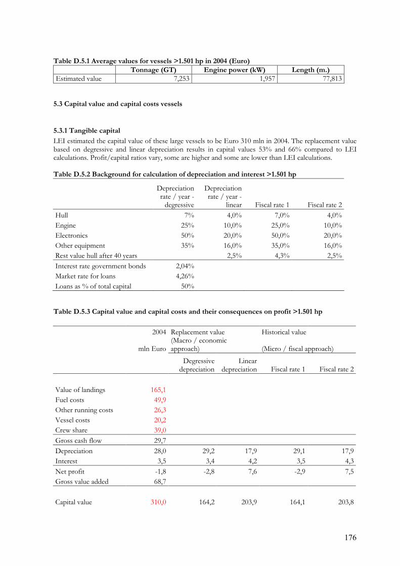
176

Table D.5.1 Average values for vessels >1.501 hp in 2004 (Euro) Tonnage (GT) Engine power (kW) Length (m.) Estimated value 7,253 1,957 77,813

5.3 Capital value and capital costs vessels

5.3.1 Tangible capital LEI estimated the capital value of these large vessels to be Euro 310 mln in 2004. The replacement value based on degressive and linear depreciation results in capital values 53% and 66% compared to LEI calculations. Profit/capital ratios vary, some are higher and some are lower than LEI calculations. Table D.5.2 Background for calculation of depreciation and interest >1.501 hp

Depreciation rate / year -

degressive

Depreciation rate / year -

linear Fiscal rate 1 Fiscal rate 2Hull 7% 4,0% 7,0% 4,0%Engine 25% 10,0% 25,0% 10,0%Electronics 50% 20,0% 50,0% 20,0%Other equipment 35% 16,0% 35,0% 16,0%Rest value hull after 40 years 2,5% 4,3% 2,5%Interest rate government bonds 2,04% Market rate for loans 4,26% Loans as % of total capital 50%

Table D.5.3 Capital value and capital costs and their consequences on profit >1.501 hp 2004 Replacement value Historical value

mln Euro(Macro / economic approach) (Micro / fiscal approach)

Degressive

depreciationLinear

depreciation Fiscal rate 1 Fiscal rate 2 Value of landings 165,1 Fuel costs 49,9 Other running costs 26,3 Vessel costs 20,2 Crew share 39,0 Gross cash flow 29,7 Depreciation 28,0 29,2 17,9 29,1 17,9Interest 3,5 3,4 4,2 3,5 4,3Net profit -1,8 -2,8 7,6 -2,9 7,5Gross value added 68,7 Capital value 310,0 164,2 203,9 164,1 203,8

177

Profit / capital -0,6% -1,7% 3,7% -1,8% 3,7%

Table D.5.4 Summary of the capital values - comparison of approaches >1.501 hp Total Hull Engine Electronics OtherReplacement value (constant prices) Total 406,1 243,7 81,2 40,6 40,6Degressive depreciated 164,2 97,6 34,7 16,6 15,3Linear depreciated 203,9 106,5 49,7 26,2 21,6 Historical value (current prices) Total 406,1 243,7 81,2 40,6 40,6Degressive depreciated 164,1 97,6 34,7 16,6 15,2Linear depreciated 203,8 106,5 49,7 26,2 21,4Total = Gross fixed capital stock Degressive or Linear depreciated = Net fixed capital stock

Table D.5.5 Relative composition Total Hull Engine Electronics OtherReplacement value Total 100,0% 60,0% 20,0% 10,0% 10,0%Degr. Depreciated 100,0% 59,4% 21,2% 10,1% 9,3%Linear depreciated 100,0% 52,2% 24,3% 12,9% 10,6% Historical Total 100,0% 60,0% 20,0% 10,0% 10,0%Degr. Depreciated 100,0% 59,5% 21,2% 10,1% 9,3%Linear depreciated 100,0% 52,3% 24,4% 12,9% 10,5%

Table D.5.6 Level of depreciation Total Hull Engine Electronics OtherReplacement value Total 100% 100% 100% 100% 100%Degr. Depreciated 40% 40% 43% 41% 38%Linear depreciated 50% 44% 61% 65% 53% Historical Total 100% 100% 100% 100% 100%Degr. Depreciated 40% 40% 43% 41% 37%Linear depreciated 50% 44% 61% 65% 53%

178

6. Evaluation 6.1 Assumptions In this study just commercial (active) vessels of the Dutch cutter fleet are included. The pelagic sector (only 17 vessels) was excluded because of lack of information. In order to estimate prices and value of capital, several assumptions have been made. These include: 1. calculations with respect to depreciation in fisheries, usually the LEI construction index method is used, which is based on prices and price-indices for the hull and engine (steel and labour costs) 2. replacement value is based on the insurance values for vessels in this study and results with respect to capital costs are analyzed and compared to results calculated using the LEI- construction index method 3. the estimated insurance value is considered a mix of replacement value and historical value 4. historical prices and second hand prices of vessels are not known 5. the distribution of capital on asset types is assumed to follow the one observed in the LEI panel account statistics for fisheries 6. at micro-level, lifetimes and depreciation rates has been set on the basis of values which are generally used by accountants 7. intangible capital is estimated as far as possible but need to be more investigated Valuation of the price per capacity is derived from the insurance value elaborated on the basis of the LEI panel observations. The capital value of the whole fleet by using the insurance value and depreciating degressive gives 53% of the value using the LEI construction index method. However, depreciation costs are almost the same (99.5%) and results do not differ very much from each other. Replacement

Value (€ mln) Book value(€

mln) % Depreciation(€

mln) Insurance value method 584,5 226,2 39 40,8LEI construction method 913,1 296,0 32 40,6

6.2 Strength of the approach The primary strength of the approach is that data can be collected rather easy by LEI every year and information is always up to date. Assumptions made are consistent with the features of the Dutch fishery context and furthermore the insurance value method is simple to use and to apply. The LEI construction index method is also simple to use but indexes need to be revised every year in order to keep calculations up to date. 6.3 Weaknesses of the approach Insurance value can be used to estimate the replacement value but it is considered that the value is in fact a mix of replacement value and historical value. Owners of vessels can vary in premiums to be paid for insurance and as a result of this also in insurance value.

179

APPENDIX E: United Kingdom

Introduction: Data sources Data sources for this paper were the UK National Fleet Register, sets of audited vessel accounts collected by Seafish Economics from vessel owners and other data collected by Seafish Economics direct from vessel owners. The UK National Fleet Register is held by the Marine Fisheries Agency, part of the Department for Environment, Food and Rural Affairs. This contains information on the physical characteristics of the vessel and the power of the main engine. This is officially held data and can be considered accurate. Vessel financial accounts, collected by Seafish to give information on balance sheets and depreciation practices, come from the major fleet segments. These are supplied to Seafish on a voluntary basis and there is therefore an element of self selection in the sample. Sample sizes for the recent UK-wide data collection exercise were on the whole good however so these balance sheets can be considered to be reasonably representative of the UK fleet. Seafish staff conducted short interviews in person and by telephone to collect a data set of around 125 vessels from a range of fleet segments to provide information on insured value and insurance premiums. This data, along with the results of interviews with insurance companies, led to the conclusion that for UK vessels, insured value is not a very good proxy for historic price.

1. General national situation – national markets for fishery assets The UK fleet consisted of 6,966 registered vessels on 1st January 2005, according to official government records. Of the vessels registered in 2004 only around 40% were deemed active, which means they had declared landings of any value to the government. A very large majority of the inactive vessels are under 10m. length.

1.1 Investments in new vessels The age composition of the fleet is shown in figure E.1.1, showing the number of vessels and total gross tonnage built in each calendar year of vessels which are still in the UK fleet.

Figure E.1.1 Age composition as percent of total for vessels in the UK 2005 fleet register A g e co m p o sit io n to tal fleet

0 .0%

1.0%

2.0%

3.0%

4.0%

5.0%

6.0%

7.0%

8.0%

20052000

19951990

19851980

19751970

19651960

19551950

19451940

19351930

C o n s tru ct io n year N u m b er (% )

G T (% )

180

The only way to obtain data on build price of new vessels is to survey the vessel owners. The price of new vessels depends on construction material and method and the level of equipment included in the vessel. Successful vessel owners are increasingly likely to order a vessel which is set up to handle the catch in such as a way as to maximize its market value, for example, to enable storage of live nephrops on board for smaller west coast vessels or to enable freezing at sea for larger, north sea vessels.

1.2 Investments in fishing rights Several different kinds and types of fishing right exist in the UK, some relating to the right to operate a fishing boat (of a given capacity), some to the area of sea which can be fished and some to the volume of fish (of a given species) which can be caught. Fixed Quota Allocation units and associated quota These quota units were distributed at no cost to vessel owners based on the fishing history of the vessel over a three year period in the mid 1990s. A Fixed Quota Allocation unit is for a certain species in a certain area and relates to a proportion of the total UK quota for the species / area. They are no longer linked to vessels permanently. The units are still only allocated to vessel owners and are not legally owned by them. The government reserves the right to distribute the UK quota in another way if it chooses and indeed in 2006, this happened with nephrops, as the government allocated a slightly higher proportion of quota to the 10m. & under vessels – which means that the proportion of the UK quota allocated to each FQA unit will be lower than in previous years. This caused great upset because vessel owners show FQA units as assets and borrow money against them, buy and sell them – in other words they behave as though they hold legal title to the units even though the government has repeatedly stated that they do not. In cases of vessel businesses going into liquidation, the lender (bank) has ended up “holding” FQA units. FQA units have been sold to POs, community quota schemes, vessel agents, other fishermen and recently, processing firms. FQAs are traded, either permanently (equivalent to selling a right in perpetuity) or within the quota year (leasing out the tonnage of fish which the units give right to in the current year). Prices vary greatly between species, area and from year to year, depending on the total UK TAC, fish sales prices, availability of FQAs for sale or to lease, level of uncertainty among the fleet and success of the quota enforcement regime. A recent dramatic improvement in the effectiveness of quota enforcement has lead to a sharp increase in the prices being paid for purchase of FQAs. Example lease costs in 2005: £80,000 for 1,136 tonnes of mixed white fish (mostly haddock). In 2006: £68,000 to lease 550 tonnes mixed whitefish (most haddock). An example noted was of mixed whitefish quota leased in 2005 at a price of £40,000 for 104 tonnes. Licences Licences are set for a certain number of kilowatts and GRT (just changing over from VCUs). i.e. a fisherman has a licence to apply x number of kW and tonnes to that fishery. Licences match the vessel which they related to at the time these regulations came into force. Licences do not have to remain with the original vessel however. If the licence is transferred to another vessel it must be to a vessel of equal or smaller size. Licences give entitlement to catch and land certain species groups (eg. pelagic licence, whitefish) (with various subsets eg. A category = all species, B and C have limitations on species and sometimes on areas). A scallop entitlement is an add-on to a licence, and it permits catching of certain types of scallop by certain methods. Also, a shellfish entitlement, entitles the licence holder to land crabs and lobsters

181

beyond a certain level. If the vessel has no entitlement, then they are restricted to catch levels per week that are largely for personal use only. These entitlements sit on top of any white fish licence. Also, whitefish licences are split by size of vessel –10m. and under and over 10m for whitefish. Only over 10m. vessel licences can split into A, B and C. 10m. and under is always category A. The scallop entitlement fits with the 10m.+ fleet only. The shellfish entitlement is available to both size groups. The UK imposed an entitlement to use beam trawl gear in Area 4 and Area 7 (for over 10m licences). Not all licences allow vessels to use beam trawl to land certain species (eg. Sole) in Areas 4 and 7. (A vessel may not use the gear commercially in these areas if it does not have this entitlement). The cod recovery programme has cut across UK licensing and added an extra dimension to over 10m whitefish licences and affected their value. Only licences with a track record of fishing in CRZ between 2001 and 2005, using a regulated gear, can now fish in the CRZ. The gears were actually used at any point during those years, determine entitlement to use certain gear types in the CRZ now. The value of a over 10m. licence is hugely affected by its ability to fish in the CRZ – because if the licence cannot fish in the CRZ then there is a smaller market for the licence. Licences are tradable and entitlements (scallop and shellfish) enhance the value of the licence but cannot be traded separately. Recent pelagic licence sales have been of the order of £1,400 per Vessel Capacity Unit21. Typically, prices of around £300 - £400 per VCU for whitefish have been noted recently. Fishing rights in the UK Fishery Type of right Definition Tradability Year of

introduction Approx price per unit 2005

Quota Stocks Fixed quota allocation (FQA) units

Share of UK TAC Yes, in practice but there is no legal title to FQAs

1998 Not known. Varies hugely per species, per area of sea, per year.

All Capacity license

Based on GRT and kW. Also associated with species group, e.g. pelagic, whitefish.

Yes, but if combining licenses for a new build, must lose % of capacity

Not known Not known

Scallops Scallop entitlement

Permits catching of certain types of scallop by certain methods

Not known Not known Not known

Shellfish Shellfish entitlement

Entitles the licence holder to land crabs and lobsters beyond a certain level.

Not known Not known Not known

21 Vessel capacity unit = (length x breadth) + (0.45 x Kw). This unit is being phased out for licences and replaced with Kw and GT

182

1.3 Investments in 2nd hand vessels There is no central UK data set of 2nd hand vessel sales prices, so the only way to obtain data is by survey. There is no time trend data therefore to compare the number and value of sales of 2nd hand vessels in the UK. Vessels without licences can only be sold to a limited market within the UK, eg. if someone already holds a licence but has no vessel, either to replace a vessel they have sold or their vessel sank. Larger vessels for sale are usually sold out of the UK, because the owner retains the licence and quota units for his next new vessel.

1.4 Investments in shore facilities Analysis of balance sheets of UK fishing companies, collected by survey, shows that there are some features in onshore facilities for one-vessel businesses. Most own a motor vehicle suitable for carrying and spreading nets or towing smaller boats. The majority of the need for onshore facilities is purchased by one-vessel companies from a range of suppliers. For example, office space is not directly required as administrative functions are conducted by the vessel agent, which may be a minority shareholder in the vessel. General onshore storage space may be rented or shared or in some cases owned. Multi-vessel owning companies may own or rent office space, own other vehicles, own fuel storage and dispensing facilities, and other onshore assets, as these companies carry out for their own vessels the full range of administrative and marketing services. There is no UK data set which can be analysed to estimate the total value of onshore assets owned by fishing vessel companies.

1.5 Approach to calculation of capital value in agriculture and/or by statistical office The Scottish Executive Environment & Rural Affairs, Aggregate Policy & Incomes has designed methodologies for the estimation of Gross Fixed Capital Formation (GFCF) with regards to the estimation of GFCF for buildings and works, plant and machinery, and vehicles and farm cars. Plant and Machinery A measure of the numbers of types of agricultural machinery used on Scottish holdings is collected in the annual agricultural census carried out each December. From this information SEERAD derives a gross stock at 1995(Mid year) prices. The agricultural census carried out in December measures the numbers of different types of machinery and tractors used on Scottish holdings. Then to convert the GFCF at 1995 (mid year) constant prices to current prices we use a weighted average of the price series for ‘Other Agricultural and Forestry Machinery’ and ‘Agricultural Tractors’ published by the Office of National Statistics. Depreciation of Plant and Machinery Depreciation is estimated within a Perpetual Inventory Model (PIM) over a 25 year period using a depreciation method using variable factors for specific years. The factors are derived from calculations of capital retirements based on Gross Fixed Capital Formation at 1995 prices. The factors used to calculate capital retirements used the following percentages applied to GFCF. These represent the different retirement rates for separate assets within the total (no information is available on how the original factors were calculated).

183

Table E.1.1 Depreciation rates for different time periods for agricultural plant and machinery.

8 year 10 year 12 year 15 year 18 year 20 year 3% 25% 33% 27% 3% 9%

Source: SEERAD For the 2000 calculation, the first calculation of depreciation is for 1976 and is calculated from the 20 year capital retirement proportion of GFCF only. The calculations for each year in the 2000 cycle for Scotland are shown in table E.1.2. The calculation is rebased to a value at the current price using a weighted average of the price series ‘Other Agricultural and Forestry Machinery’ and ‘Agricultural Tractors’ published by the Office of National Statistics. Buildings and Works Investment in Buildings and Works is split into two types – Grant Aided and Non-Grant Aided. The value of Grant Aided Investment is obtained from the Land Use and Rural Policy division in SEERAD. The Grant Aided Investment is estimated from Gross Value Added (Output-Input). The yearly percentage change in GVA is applied to a historic value for Non-Grant Aided Investment. Depreciation of Buildings and Works Depreciation is estimated within a Perpetual Inventory Model (PIM) over a 38 year period using a depreciation method using variable factors for specific years. The factors are applied to the Gross Capital Formation for specific years and the sum of the values equals the amount of depreciation recorded at a 1995 constant price. The value for the earliest year represents the 2000 depreciation for the depreciation cycle beginning in 1964. The calculation is rebased to a value at the current price using the price series ‘Buildings and Works: Private Sector Industrial’ published by the Department of Trade and Industry Lessons to be learned? An example of non-tangible assets in agriculture is the milk quota. This is valued through market demand and can either be permanently transferred or leased. The value of milk quota is not included in the calculation of any other tangible asset.

2. Total fleet For the whole fleet estimates, the initial data set was collected by survey asking for insurance value, rather than historic price, in accordance with expectations among the research group, although for some vessels both figures were available. Once data was collected and insurance companies were interviewed, it became clear that insured value of vessels is not a particularly good proxy for historic price. However, this was the only data available for use in this estimate, so the estimates are based on the relationships between insured value and various physical attributes of the vessels in the UK fleet.

2.1 Description of the case study fleet Figure E.2.1 below shows the distribution of age and gross tonnage by year of build within the UK registered fishing fleet.

184

Figure E.2.1 Age composition of the total UK fleet

Age composition total fleet

0.0%1.0%2.0%3.0%4.0%5.0%6.0%7.0%8.0%

2005

2000

1995

1990

1985

1980

1975

1970

1965

1960

1955

1950

1945

1940

1935

1930

Construction year Number (%)GT (%)

Table E.2.1 shows the main segments of the UK fleet in line with the EU Data Collection Regulation, split to show the total number of registered vessels and the total number of active, or commercial, vessels. Table E.2.1 Registered and active vessels in the UK fleet as at 1 January 2005, split by DCR segment *

<12m 12-24 m 24-40 m >40 m <12m 12-24 m 24-40 m >40 mActive gearsBeam trawl 157 39 64 16 276 34 32 56 16 138Demersal trawl and seine 1306 532 113 33 1984 395 491 113 14 1013Pealgic trawl and seine 32 14 2 33 81 14 12 0 33 59Dredgers 178 122 27 2 329 70 99 20 1 190Polyvalent active 4 4 0 0 8 4 4 0 0 8All Active Gears 1677 711 206 84 2678 517 638 189 64 1408

Passive gearsGears using hooks 417 8 11 2 438 165 1 8 1 175Drift and fixed nets 1299 28 25 1 1353 260 23 23 0 306Pots and traps 2408 90 5 0 2503 931 74 3 0 1008Polyvalent passive 6 1 0 0 7 6 1 0 0 7All Passive Gears 4130 127 41 3 4301 1362 99 34 1 1496

Polyvalent (active/passive)

All Vessels 5807 838 247 87 6979 1879 737 223 65 2904

Total number of registered vessels Number of commercial vessels

* A small error exists in the registered vessels table, amounting to 55 <10m vessels not accounted for by segment.

2.2 Data and estimation of price per capacity unit A data set of just over 100 UK vessels, from a range of fleet segments, was collected by survey. This was used with official data relating to the physical characteristics of the vessels and the main engine. 2.2.1 What value indicators can be collected Physical characteristics of vessels and the main engine are collected via the national fleet register. Insured value of vessels is collected by survey of vessel owners, conducted by Seafish staff. Some balance sheet data is also collected by survey, giving value of fixed assets and rates of depreciation.

185

A comparison of the average physical characteristics of the UK whole fleet and the sample vessels used for this study is given in table E.2.2 below. The averages for the whole UK fleet population are considerably lower than the averages for our sample of the UK fleet. This implies that our sample contains a higher proportion of larger vessels compared to the proportion in the entire UK fleet. The proportion of under 12m vessels in the UK fleet is 1,879 out of 2,904, or 65% of active vessels, whereas the proportion of under 12m vessels in the sample used for this study is relatively smaller, only 42%. Table E.2.2 Characteristics of population and sample vessels for the whole UK fleet case study Whole UK fleet Average GT Average kW Average length (m) Population 31.91 128.59 9.89 Sample 84.67 270.70 15.22

This sample bias means that estimates of total UK fleet capital value based on this combined sample of over and under 12m. vessels are likely to significantly overstate the total capital value of the UK fleet. Less inaccurate estimates could be achieved by segmenting the sample and summing the two estimates. 2.2.2 Does the data refer to tangibles or does it also contain intangibles The data on insurance value and insurance premium exclude the value of the intangible assets. The vessel price (both build and second hand price) as used here do not include the value of the intangible asset. Some intangible assets, such as FQAs were allocated to fishing business by the government free of charge based on their historic landings over a three year period in the mid 1990s and as a result, fishermen only consider the financial value of quota if it is purchased in addition to what they were originally given for free. Therefore, only in some cases is the value of quota units included on balance sheets, and when it is included, it is sometimes not the entire quota held by the vessel, but only that proportion purchased after the start of the current quota scheme. It should be noted however that vessels do not in fact hold legal title to these fishing rights as title is retained by the government. Other intangibles, such as scallop or shellfish entitlements, are not typically shown on balance sheets. 2.2.3 What do the available values per vessel represent The insured value of vessels in the sample collected are taken to represent historic value, despite the fact that insured value has been shown to be a less than ideal proxy for historic value in the UK. 2.2.4 Derivation of the price per capacity unit (historical or replacement) In the UK the only data available for a large number of vessels was collected by survey and is the insured value of the vessels. This was taken to be a proxy for the historic price of the vessel in money of the day. Therefore, before average price per capacity unit could be found, insured values, as proxies for historic price in money of the day, were converted to a 2004 price equivalent using a steel price index,22 which ran back to the mid 1980s, and then extrapolating that index back to 1935 using a retail price index from the Office of National Statistics. The estimated historic price (insured value) per capacity unit was calculated for each of these three measures for the whole data set simply by dividing the adjusted insured value by the number of kW, GT and meters (length) for each vessel. The averages of each price per capacity unit were found and are shown below, converted to Euro at rate of €1.0 = £0.67, in Table E.2.3.

22 Source: ISSB (Iron and Steel Statistics Bureau) Website

186

Table E.2.3 Estimated average historic price (insured value indexed to 2004) per capacity unit and estimated replacement value (insured value in money of the day) per capacity unit for the whole UK fleet

Length (m) Tonnage (GT) Engine Power (kW)

Estimated historic price €33,214 €12,887 €2,298

Estimated replacement value €21,774 €7,295 €1,272

Simple correlations between insured value and physical characteristics showed the following strong relationships, after removal of a few under 12m. vessel outliers. Gross Tonnage gives the strongest linear relationship and so this measure is used for the estimation of capital for the UK fleet. Table E.2.4 Correlation coefficients between insured value (adjusted to 2004 equivalent) and selected physical characteristics, based on sample of whole UK fleet Adjusted

Insured Value Tonnage (GT) Engine Power

(kW) Length (m)

Tonnage (GT) 0.978** 1.00 Engine Power (kW) 0.975** 0.971** 1.00 Length (m) 0.939** 0.963** 0.919** 1.00

**correlation is significant at the 0.01 level (2-tailed). For the calculation based on historic value, the average 2004 price per GT from the sample was adjusted using the same steel price index used to transform insured values in estimated 2004 prices. This gave a 2004 price equivalent value per GT for vessels in each year of build in the UK fleet. This figure was then multiplied by the total GT of vessels from each year of build and the figures for each year were summed to give an estimate of total gross capital in the UK fleet, at 2004 prices.

187

Figure E.2.2 Accounting for tangible assets – decision tree – for each vintage – United Kingdom

cu = capacity unit vessel refers to complete unit incl. hull, engine, electronics and all other equipment (1) price index heavy machinery or another index related to boat building (2) Depreciated / book value will be usually based on historical price. (3) RV = Value at constant price of the most recent year (4) HV= Value of current prices, in case only one or several years available, remaining years can be extra/interpolated with the price index

What value indicators can be collected / observed?

Insurance premiums Historical value

Insurance values / vessel

Do the data refer to the tangible assets only or do they also contain value of intangibles?

Value of tangible (vessel)

Paid 2nd hand values / vessel

Replacement value (RV) (3)

What does the available value per vessel represent?

Contain intangibles

Estimate / separate tangible and intangible value,

describe approach

OtherDepreciated / book value (2)

Historical value (HV) (4)

Determine series of historical prices/cu

Most recent historical price =

replacement price./cu

Follow columns (RV) or (HV)

Estimate replacement price / cu

Estimate total depreciation to

determine historical value

Estimate series of historical

prices / cu

Estimate RV and /or HV,

describe approach

Price index series (1)

188

Assumptions regarding depreciation of the different elements of physical capital are shown in table E.2.5. These are the standard rates used across the national case studies as they match reasonably to the range of rates identified in balance sheets for UK vessels. Table E.2.5 Assumed depreciation rates applied in the UK calculations Background for calculation of depreciation and interest

Economic depreciation rate / year - degressive

Economic depreciation rate / year -

linear

Fiscal depreciation

rate 1

Fiscal depreciation

rate 2 Hull 7% 4.0% 7.0% 4.0%Engine 25% 10.0% 25.0% 10.0%Electronics 50% 20.0% 50.0% 20.0%Other equipment 35% 16.0% 35.0% 16.0%Rest value hull after 40 years 2.5% 5.0%Interest rate government bonds 5% Market rate for loans 5% Loans as % of total capital 50%

2.3 Capital value and capital costs 2.3.1 Tangible capital The approach described in section 2.2 was applied to the data relating to vessels in the UK fleet register to estimate total capital value by estimating historic value and replacement value. In the replacement value method, the most recent historic build price was taken as the replacement value per unit of capacity. Table E.2.6 Capital value and capital costs and their consequences on profit (sensitivity analysis) 2004 Replacement value Historical value

mln Euro (Macro / economic

approach) (Micro / fiscal approach)

Degressive

depreciationLinear

depreciation Fiscal rate 1 Fiscal rate 2Value of landings 739.5 Fuel costs 93.5 Other running costs 155.5 Vessel costs 174.6 Crew share 216.4 Gross cash flow 99.5 Depreciation 66.7 215.1 125.8 194.3 113.4Interest 31.9 58.7 69.6 26.1 31.7Net profit 0.9 -174.3 -95.9 -120.9 -45.6Gross value added 315.9 Capital value 1,487.7 1,174.0 1,392.4 1,045.9 1,266.8Profit / capital 0.1% -14.8% -6.9% -11.6% -3.6%

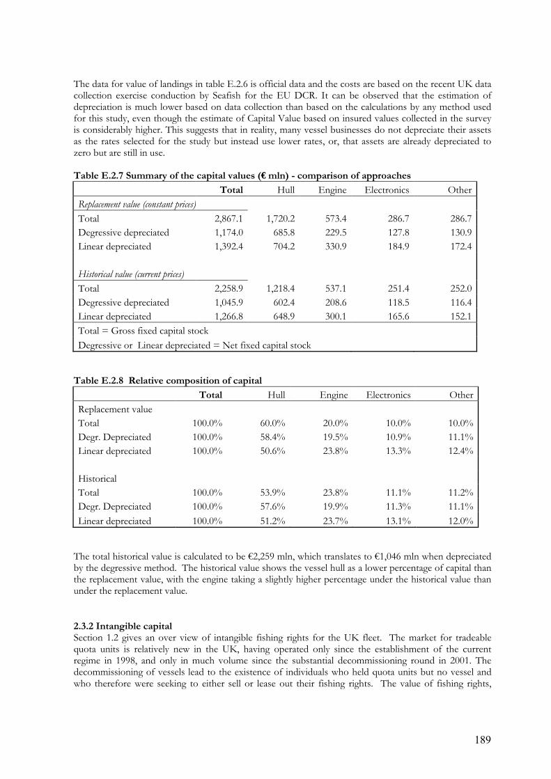
189

The data for value of landings in table E.2.6 is official data and the costs are based on the recent UK data collection exercise conduction by Seafish for the EU DCR. It can be observed that the estimation of depreciation is much lower based on data collection than based on the calculations by any method used for this study, even though the estimate of Capital Value based on insured values collected in the survey is considerably higher. This suggests that in reality, many vessel businesses do not depreciate their assets as the rates selected for the study but instead use lower rates, or, that assets are already depreciated to zero but are still in use. Table E.2.7 Summary of the capital values (€ mln) - comparison of approaches Total Hull Engine Electronics OtherReplacement value (constant prices) Total 2,867.1 1,720.2 573.4 286.7 286.7Degressive depreciated 1,174.0 685.8 229.5 127.8 130.9Linear depreciated 1,392.4 704.2 330.9 184.9 172.4 Historical value (current prices) Total 2,258.9 1,218.4 537.1 251.4 252.0Degressive depreciated 1,045.9 602.4 208.6 118.5 116.4Linear depreciated 1,266.8 648.9 300.1 165.6 152.1Total = Gross fixed capital stock Degressive or Linear depreciated = Net fixed capital stock

Table E.2.8 Relative composition of capital Total Hull Engine Electronics OtherReplacement value Total 100.0% 60.0% 20.0% 10.0% 10.0%Degr. Depreciated 100.0% 58.4% 19.5% 10.9% 11.1%Linear depreciated 100.0% 50.6% 23.8% 13.3% 12.4% Historical Total 100.0% 53.9% 23.8% 11.1% 11.2%Degr. Depreciated 100.0% 57.6% 19.9% 11.3% 11.1%Linear depreciated 100.0% 51.2% 23.7% 13.1% 12.0%

The total historical value is calculated to be €2,259 mln, which translates to €1,046 mln when depreciated by the degressive method. The historical value shows the vessel hull as a lower percentage of capital than the replacement value, with the engine taking a slightly higher percentage under the historical value than under the replacement value. 2.3.2 Intangible capital Section 1.2 gives an over view of intangible fishing rights for the UK fleet. The market for tradeable quota units is relatively new in the UK, having operated only since the establishment of the current regime in 1998, and only in much volume since the substantial decommissioning round in 2001. The decommissioning of vessels lead to the existence of individuals who held quota units but no vessel and who therefore were seeking to either sell or lease out their fishing rights. The value of fishing rights,

190

principally quotas, varies hugely within a calendar year, and from year to year, depending on several factors: - the UK quota of the species itself and other species caught in the same fisheries - the sales price of the fish species - the expected and actual demand for purchase or lease of quota units - the supply of quota units for sale or rent - uncertainty relating to legal title of quota units exacerbated by current government review of quota management system.

There is not enough data available from UK vessels to make any estimates of what proportion of net fixed capital value is made up by intangible assets. In vessel business balance sheets, the value assigned to quota units is often the historic price paid for any purchased units. The units cannot be depreciated in any usual way because their value depends on the factors listed above. Because of uncertainties relating to stock levels and legal title however, a prudent approach might be to depreciate the value of purchased quota rights to zero over five years.

2.4 Evaluation 2.4.1 Assumptions - Insured value has been used as a proxy for historic price in the whole UK fleet, and the under and over 12m segments, due to lack of other available data. - Actual historic price was used for the pelagic and demersal trawl segment case studies - Historic price estimates for vessels were adjusted using a steel price index which only went back to 1987 and then had to be extrapolated using a retail price index. - The distribution of capital among asset types is assumed to be the same as the standard used for the whole study - The depreciation rates for various assets are assumed to be the same as the standard used for the whole study Some of these assumptions are clearly unlikely to be accurate but for the purpose of this study, testing and illustrating the method, it can be said that they were sufficient for the purpose. In order to obtain more robust estimates of the capital value of the UK fleet, using this overall methodology, the main improvement that could be made would be to collect a much larger and broader sample of historic price data from vessel owners. This however would require primary data collection by survey which is time consuming and costly. 2.4.2 Strengths of the approach For the UK, this approach is relatively simple and straightforward once the sample data is collected. It can be explained easily and the results can be compared with other methods. 2.4.3 Weaknesses of the approach There are several weaknesses of the approaches used in the UK case studies. - Small sample size of insured value obtained, with some substantial sample bias in terms of average characteristics of sample versus population vessels. - Insurance values used as proxy for historic value in the calculation of price per capacity unit for the total fleet, >12m. fleet and <12m. fleet segments - No price index for heavy machinery was found and a steel price index was used instead, which had to be extrapolated for years before 1987 based on a retail price index. - No information is available on land based assets which for large fishing companies will represent a large outlay and is essential to the fishing business.

191

- Lack of information about the value of intangible assets, and impossibility of valuing intangible assets. - No UK-specific fiscally allowed lifetime for each component e.g. hull engine etc has been specified, and in fact many UK vessels are still economically active for years beyond the date when they would have been depreciated to zero value. - Depreciation rules used by the UK tax office for equipment such as hull, engine and electronics. How can the weaknesses be addressed in future? - If the historic (build) prices of the vessels were obtained as part of the data collection requirement or licensing requirement then it could be used in the calculation of price per capacity unit. - Further research into obtaining a heavy plant machinery price index is required. There is a possibility of obtaining one but at some expense. Further consultation with the Office of National Statistics in the UK required. - There could be exploration into how land-based assets are included into the calculations for large companies. We have to be aware that the basic unit we are looking at is the vessel and that any land based capital has to be recalculated from the company spreadsheets to be included in the vessel value. Further work on how FADN have tackled this issue could be useful to find out whether their methodology would be applicable in the UK fishing industry. - More information about intangible assets and how they are traded in the UK is required. The ability to assess the ‘stock’ of quota that each vessel has would also be essential – could this be collected from the UK fisheries administrations? The current problem is that it is difficult to attach a price to the asset due to the volatility of the market for say quota, only having a few observations of market price and the uncertainty surrounding the volume of fish that the FQA unit will actually be worth in the following year due to the changes in quota levels as decided at December council each year which can fluctuate down (increasing the price of the quota) and up (causing a fall in the price of quota). - Further investigation into the lifetime allowed by UK fiscal rules and depreciation rules is also required. It also needs to be determined if these depreciation rules have changed over the last 15 to 20 years and what these past rates were.

3. Fleet under 12 meters

3.1 Description of the case study fleet Figure E.3.1 below shows the distribution of age and gross tonnage by year of build within the under 12m. segment of the UK registered fishing fleet.

Figure E.3.1 Age composition of the under 12m. UK fleet.

Age composition fleet < 12m

0.0%1.0%2.0%3.0%4.0%5.0%6.0%7.0%8.0%9.0%

2005

2000

1995

1990

1985

1980

1975

1970

1965

1960

1955

1950

1945

1940

1935

1930

Construction year Number (%)GT (%)

192

A comparison of the average physical characteristics of the UK whole fleet and the sample vessels used for this study is given in table E.3.1 below. Our survey sample averages are significantly higher than the averages for the fleet population. This sample bias is a result of the untargeted approach that had to be adopted due to time constraints in the survey. The calculations based on this sample are therefore likely to significantly over state the capital value of this segment. With more time it would be possible to extend the survey to ensure that the sample characteristics were more similar to the population of UK under 12m vessels. The chosen characteristic for predicting the capital value for this segment is length, which is the characteristic least dissimilar between the sample and the population. Table E.3.1 Characteristics of population and sample vessels for the under 12m. <12m. segment Average GT Average kW Average length (m) population 4.33 57.9 7.44 sample 8.74 102.05 9.12

3.2 Data and estimation of price per capacity unit Table E.3.2 below shows the average estimated historic price per unit of length, tonnage and engine power for the sample of the under 12m. UK fleet. As could be expected, the values are higher for the smaller vessels than for the overall UK fleet (see table E.2.3). This is because for larger vessels there is the equivalent of a “bulk discount” per capacity unit for larger vessels. The fixed costs of construction (those that do not vary with the size of the vessel) form a much larger proportion of total cost for smaller vessels, so the overall cost per capacity unit is higher. Table E.3.2 Estimated average historic price (insured value indexed to 2004) per capacity unit and estimated replacement value (insured value in money of the day) per capacity unit for the under 12m. UK fleet.

Length (m.) Tonnage (GT) Engine Power (kW)

Estimated historic price €37,683 €18,861 €3,363

Estimated replacement value €8,400 €9,863 €1,610

The data collected for under 12m vessels was more variable than the larger vessel data and consequently a few extreme outliers had to be removed from the data set in order to observe correlations between insured value and physical characteristics. This variation could be because with smaller vessels, any added equipment for handling or storage of fish will form a larger proportion of the overall value of the vessel. Simple correlations between insured value and physical characteristics showed the following rather weaker relationships, after removal of some outliers (table E.3.3). For the under 12m. vessels, length (m.) has the strongest relationship with insured value (as proxy for historic price), and so was used to estimate capital for the whole segment. Table E.3.3 Correlation coefficients between insured value (adjusted to 2004 equivalent) and selected physical characteristics, based on sample of under 12m. vessels in the UK fleet Adjusted

Insured Value Tonnage (GT) Engine Power

(kW) Length (m)

Tonnage (GT) 0.617** 1.00 Engine Power (kW) 0.402* 0.622** 1.00 Length (m) 0.680** 0.790** 0.565** 1.00

** Correlation is significant at the 0.01 level (2-tailed). * Correlation is significant at the 0.05 level (2-tailed).

193

3.3 Capital value and capital costs Methods were the same as those used for the whole UK fleet, except that length was selected as the capacity unit to multiply by average price per capacity unit. 3.3.1 Tangible capital Table E.3.4 Capital value and capital costs and their consequences on profit (sensitivity analysis) 2004 Replacement value Historical value

mln Euro (Macro / economic

approach) (Micro / fiscal approach)

Degressive

depreciationLinear

depreciation Fiscal rate 1 Fiscal rate 2 Value of landings 181 Fuel costs 16.1 Other running costs 47.4 Vessel costs 44.9 Crew share 74.4 Gross cash flow -1.7 Depreciation 18.1 109.8 65.6 98.8 58.9Interest 6.6 28.9 34.9 12.8 15.8Net profit -26.4 -140.4 -102.2 -113.3 -76.4Gross value added 72.7 Capital value 404.1 578.5 697.3 511.7 633.1Profit / capital -6.5% -24.3% -14.7% -22.1% -12.1% The value of landings figure in table E.3.4 is from official data for 10m and under vessels, rather than under 12m. vessels, as this is how the vessels are currently segmented in UK official data. Costs figures and estimated capital value of vessels are based on Seafish survey of the UK fleet and are also for under 10m. vessels. The addition of vessels of length between 10m. and 12m. which are excluded from this estimate would bring the Seafish estimate in reasonably close proximity to the estimates made in this study. If the gross cash flow included all vessels up to 12m. length, and were therefore higher, then there would be less discrepancy between the Seafish profit as a proportion of capital figure and the figures generated by this study. It is expected that the UK official data will be able to fit the under and over 12m split from next year.

Table E.3.5 Summary of the capital values (€ mln) - comparison of approaches Total Hull Engine Electronics OtherReplacement value (constant prices) Total 1,624.4 974.6 324.9 162.4 162.4Degressive depreciated 578.5 323.5 121.0 66.7 67.3Linear depreciated 697.3 324.7 183.4 99.7 89.6 Historical value (current prices) Total 1,273.0 686.0 301.7 141.7 143.6Degressive depreciated 511.7 280.9 108.5 61.5 60.7

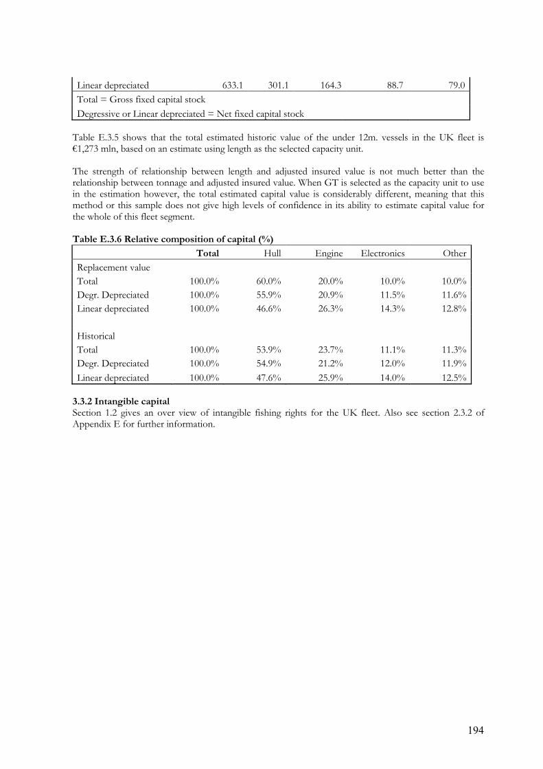
194

Linear depreciated 633.1 301.1 164.3 88.7 79.0Total = Gross fixed capital stock Degressive or Linear depreciated = Net fixed capital stock

Table E.3.5 shows that the total estimated historic value of the under 12m. vessels in the UK fleet is €1,273 mln, based on an estimate using length as the selected capacity unit. The strength of relationship between length and adjusted insured value is not much better than the relationship between tonnage and adjusted insured value. When GT is selected as the capacity unit to use in the estimation however, the total estimated capital value is considerably different, meaning that this method or this sample does not give high levels of confidence in its ability to estimate capital value for the whole of this fleet segment. Table E.3.6 Relative composition of capital (%) Total Hull Engine Electronics OtherReplacement value Total 100.0% 60.0% 20.0% 10.0% 10.0%Degr. Depreciated 100.0% 55.9% 20.9% 11.5% 11.6%Linear depreciated 100.0% 46.6% 26.3% 14.3% 12.8% Historical Total 100.0% 53.9% 23.7% 11.1% 11.3%Degr. Depreciated 100.0% 54.9% 21.2% 12.0% 11.9%Linear depreciated 100.0% 47.6% 25.9% 14.0% 12.5%

3.3.2 Intangible capital Section 1.2 gives an over view of intangible fishing rights for the UK fleet. Also see section 2.3.2 of Appendix E for further information.

195

4. Fleet 12 meters and over

4.1 Description of the case study Figure E.4.1 below shows the distribution of age and gross tonnage by year of build within the over 12m. segment of the UK registered fishing fleet.

Figure E.4.1 Age composition of the 12m. and over UK fleet

Age composition fleet > 12m

0.0%1.0%2.0%3.0%4.0%5.0%6.0%7.0%8.0%9.0%

2005

2000

1995

1990

1985

1980

1975

1970

1965

1960

1955

1950

1945

1940

1935

1930

Construction year Number (%)GT (%)

Table E.4.1 below shows a comparison of the physical characteristics of the over 12m. fleet population and sample used for this study. Unlike the under 12m. fleet, in this case, our sample vessels are typically smaller than average for the population, which could lead to an understatement of the estimated capital value for this segment. Table E.4. 1 Characteristics of population and sample vessels for the 12m. and over vessel case study >=12m segment Average GT Average kW Average length (m) population 167.85 476.97 22.00 sample 140.34 394.37 19.70

4.2 Data and estimation of price per capacity unit Table E.4.2 below shows the average estimated historic price per unit of length, tonnage and engine power for the sample of the over 12m. UK fleet. As could be expected, the values are lower for the larger vessels than for the overall UK fleet. This is because for larger vessels there is the equivalent of a “bulk discount” per capacity unit for larger vessels. The fixed costs of construction (those that do not vary with the size of the vessel) form a much lower proportion of total cost for larger vessels, so the overall cost per capacity unit is lower.

196

Table E.4.2 Estimated average historic price (insured value indexed to 2004) per capacity unit and estimated replacement value (insured value in money of the day) per capacity unit for the 12m. and over UK fleet

Length (m.) Tonnage (GT) Engine Power (kW)

Estimated historic price €30,184 €8,837 €1,576

Estimated replacement value €31,227 €5,479 €1,610

Simple correlations between insured value and physical characteristics showed the following correlation coefficients, with no outliers removed (table E.4.3). For the over 12m.vessels, tonnage (GT) also has the strongest relationship with insured value (as proxy for historic price) and was selected capacity unit for estimating historic value for the whole segment. Table E.4.3 Correlation coefficients between insured value (adjusted to 2004 equivalent) and selected physical characteristics, based on sample of over 12m. vessels in the UK fleet Adjusted

Insured Value Tonnage (GT) Engine Power

(kW) Length (m)

Tonnage (GT) 0.975** 1.00 Engine Power (kW) 0.973* 0.967** 1.00 Length (m) 0.954** 0.981** 0.932** 1.00

** Correlation is significant at the 0.01 level (2-tailed).

4.3 Capital value and capital costs Methods were the same as those used for the whole UK fleet, and again tonnage was selected as the capacity unit to multiply by average price per capacity unit. 4.3.1 Tangible capital The figures in table E.4.4 for value of landings, costs and capital estimate in 2004 are based on Seafish survey data for vessels 10m. and over. This is also due to segmentation of the UK official data. If the vessels between 10m. and 12m. in length were excluded from the Seafish survey estimates, then the figures for capital value and profit in relation to capital would be in closer proximity to the figures estimated by this study. Table E.4.4 Capital value and capital costs and their consequences on profit (sensitivity analysis) 2004 Replacement value Historical value

mln Euro (Macro / economic

approach) (Micro / fiscal approach)

Degressive

depreciationLinear

depreciation Fiscal rate 1 Fiscal rate 2 Value of landings 558.6 Fuel costs 79.2 Other running costs 111.2 Vessel costs 133.1 Crew share 146.3 Gross cash flow 88.7

197

Depreciation 49.9 132.4 77.3 119.6 69.7Interest 25.9 36.3 43.0 16.2 19.5Net profit 13.0 -79.9 -31.5 -47.0 -0.5Gross value added 235.1 Capital value 1,082.6 725.9 859.2 647.0 781.7Profit / capital 1.2% -11.0% -3.7% -7.3% -0.1%

Table E.4.5 shows that the estimated historic value of the 12m. and over segment of the UK fleet is €1,374 mln based on using tonnage to estimate historic value. Table E.4.5 Summary of the capital values (€ mln) - comparison of approaches Total Hull Engine Electronics OtherReplacement value (constant prices) Total 1,744.3 1,046.6 348.9 174.4 174.4Degressive depreciated 725.9 426.2 141.0 78.3 80.4Linear depreciated 859.2 438.5 201.9 113.0 105.8 Historical value (current prices) Total 1,374.0 740.7 327.2 153.0 153.2Degressive depreciated 647.0 374.7 128.4 72.6 71.3Linear depreciated 781.7 403.7 183.4 101.2 93.3Total = Gross fixed capital stock Degressive or Linear depreciated = Net fixed capital stock

Table E.4.6 Relative composition of capital (%) Total Hull Engine Electronics OtherReplacement value Total 100.0% 60.0% 20.0% 10.0% 10.0%Degr. Depreciated 100.0% 58.7% 19.4% 10.8% 11.1%Linear depreciated 100.0% 51.0% 23.5% 13.2% 12.3% Historical Total 100.0% 53.9% 23.8% 11.1% 11.2%Degr. Depreciated 100.0% 57.9% 19.8% 11.2% 11.0%Linear depreciated 100.0% 51.7% 23.5% 13.0% 11.9%

4.3.2 Intangible capital Section 1.2 gives an over view of intangible fishing rights for the UK fleet. Also see section 2.3.2 of Appendix E for further information.

198

5. Over 40m Pelagic Fleet 5.1 Description of the case study Figure E.5.1 below shows the distribution of age and engine power (kW) by year of build within the pelagic segment of the UK registered fishing fleet.

Figure E.5.1 Age composition of the UK pelagic fleet

Age composition Pelagic fleet

0.0%

5.0%

10.0%

15.0%

20.0%

25.0%

30.0%

2005

2000

1995

1990

1985

1980

1975

1970

1965

1960

1955

1950

1945

1940

1935

1930

Construction year Number (%)kW (%)

5.2 Data and estimation of price per capacity unit Because the data for vessels from a range of segments in the UK fleet had indicated that insured value was not necessarily a very good proxy for historic price, we collected actual historic price of pelagic and demersal trawl case study vessels, since further survey was required anyway, and with relatively newer boats in these two segments, it was likely that current owners of vessels would know the original build cost in money of the day (historic price). A data set of physical characteristics and vessel historic price was collected by survey and from the fleet register for 17 >40m. pelagic vessels. Two cases were rejected because they were vessels being built in 2006. The total size of the segment is currently 33 vessels (excluding the two on order) in the UK fleet, so this sample was almost half of the segment. A comparison of the average physical characteristics of the UK whole fleet and the sample vessels used for this study is given in table E.5.1 below. Our sample averages are slightly higher than the averages for the fleet population. This sample bias is a result of the untargeted approach that had to be adopted due to time constraints in the survey. The calculations based on this sample are therefore likely to slightly over state the capital value of this segment. Table E.5.1 Characteristics of population and sample vessels for the >40m. pelagic UK fleet case study Pelagic segment Average GT Average kW Average length (m) Population 1,631.7 3,951.6 62.5Sample 1,864.5 4,582.2 64.7

199

Table E.5.2 below shows the average estimated historic price per unit of length, tonnage and engine power for the sample of the UK pelagic fleet. Table E.5.2 Estimated average historic price (insured value indexed to 2004) per capacity unit and estimated replacement value (insured value in money of the day) per capacity unit for the >40m. pelagic UK fleet

Length (m) Tonnage (GT) Engine Power (kW)

Estimated historic price €235,001 €8,256 €3,519

Estimated replacement value €219,650 €7,743 €3,343

Historic prices were converted to 2004 values using the steel price index to give an adjusted purchase price for each vessel built before 2004. Correlations between adjusted purchase price and physical characteristics showed relationships of strengths shown in table E.5.3, not especially strong. For the pelagic vessels, engine power (kW) has the strongest relationship with purchase price, and was therefore selected for estimating historic value for the whole segment. Table E.5.3 Correlation coefficients between purchase price (adjusted to 2004 equivalent) and selected physical characteristics, based on sample of pelagic vessels in the UK fleet Purchase Price Tonnage (GT) Engine Power

(kW) Length (m)

Tonnage (GT) 0.737** 1.00 Engine Power (kW) 0.746** 0.705** 1.00 Length (m) 0.649* 0.957** 0.617* 1.00

** Correlation is significant at the 0.01 level (2-tailed). * Correlation is significant at the 0.05 level (2-tailed).

5.3 Capital value and capital costs 5.3.1 Tangible capital Table E.5.4 Capital value and capital costs and their consequences on profit (sensitivity analysis) 2004 Replacement value Historical value

mln Euro (Macro / economic approach) (Micro / fiscal approach)

Degressive

depreciationLinear

depreciationFiscal rate 1

Fiscal rate 2

Value of landings Fuel costs Other running costs Vessel costs Crew share Gross cash flow Depreciation 44.9 25.8 40.5 23.4Interest 14.5 16.7 6.6 7.6

200

Net profit Gross value added Capital value 290.0 334.1 263.8 305.7Profit / capital

There are no cost and earnings tables available yet for the UK pelagic fleet in 2004 so the 2004 capital costs column in the above table has been left blank. Therefore it is not possible to compare the effect on profit in relation to capital value of the different methods of estimating total capital value for the segment. Table E.5.5 Summary of the capital values (€ mln) - comparison of approaches Total Hull Engine Electronics OtherReplacement value (constant prices) Total 458.9 275.3 91.8 45.9 45.9Degressive depreciated 290.0 196.8 45.7 21.0 26.5Linear depreciated 334.1 210.7 60.1 31.1 32.1 Historical value (current prices) Total 417.3 250.8 85.5 39.8 41.2Degressive depreciated 263.8 180.6 41.5 19.0 22.7Linear depreciated 305.7 194.8 54.6 27.4 28.8Total = Gross fixed capital stock Degressive or Linear depreciated = Net fixed capital stock

Table E.5.6 Relative composition of capital (%) Total Hull Engine Electronics OtherReplacement value Total 100.0% 60.0% 20.0% 10.0% 10.0%Degr. Depreciated 100.0% 67.9% 15.8% 7.2% 9.1%Linear depreciated 100.0% 63.1% 18.0% 9.3% 9.6% Historical Total 100.0% 60.1% 20.5% 9.5% 9.9%Degr. Depreciated 100.0% 68.5% 15.7% 7.2% 8.6%Linear depreciated 100.0% 63.7% 17.9% 9.0% 9.4%

5.4 Evaluation This case study benefited from better quality data on which to base estimates for the whole segment: - good sample size; - actual historical price paid by the current owner; - all vessels relatively new so less distortion by indexing prices.

201

6. Over 24 meters Demersal Trawl Fleet

6.1 Description of the case study Figure E.6.1 below shows the distribution of age and engine power (kW) by year of build within the over 24m. demersal trawl segment of the UK registered fishing fleet.

Figure E.6.1 Age composition of the UK over 24m. demersal trawl fleet

Age composition >24m Whitefish fleet

0.0%

2.0%

4.0%

6.0%

8.0%

10.0%

12.0%

14.0%

2005

2000

1995

1990

1985

1980

1975

1970

1965

1960

1955

1950

1945

1940

1935

1930

Construction year Number (%)kW (%)

A comparison of the average physical characteristics of the UK whole fleet and the sample vessels used for this study is given in table E.6.1 below. Our sample averages are only slightly lower than the averages for the fleet population. This sample bias is a result of the untargeted approach that had to be adopted due to time constraints in the survey. The calculations based on this sample are therefore likely to slightly under state the capital value of this segment. Table E.6.1 Characteristics of population and sample vessels for the over 24m. demersal segment case study

>24m. Demersal trawl segment

Average GT Average kW Average length (m)

population 338.4 833.3 32.1sample 326.9 768.9 28.2

6.2 Data and estimation of price per capacity unit Data collected by Seafish survey as described in section 5.2. The total size of the over 24m demersal trawl segment is currently 97 vessels in the UK fleet, so this sample was around 14% of the segment. Table E.6.2 below shows the average estimated historic price per unit of length, tonnage and engine power for the sample of the UK over 24m demersal trawl fleet.

202

Table E.6.2 Estimated average historic price (insured value indexed to 2004) per capacity unit and estimated replacement value (insured value in money of the day) per capacity unit the UK over 24m. demersal trawl fleet

Length (m.) Tonnage (GT) Engine Power (kW)

Estimated historic price €81,946 €7,203 €3,070

Estimated replacement value €75,732 €6,562 €2,807

Correlations between insured value and physical characteristics showed the following relationships. For the over 24m. demersal trawl vessels, engine power (kW) has the strongest relationship with purchase price. Table E.6.3 Correlation coefficients between purchase price (adjusted to 2004 equivalent) and selected physical characteristics, based on sample of over 24m. demersal trawl vessels in the UK fleet Purchase Price Tonnage (GT) Engine Power

(kW) Length (m.)

Tonnage (GT) 0.778** 1.00 Engine Power (kW) 0.894** 0.822** 1.00 Length (m) 0.728** 0851** 0.780** 1.00

** Correlation is significant at the 0.01 level (2-tailed). * Correlation is significant at the 0.05 level (2-tailed).

6.3 Capital value and capital costs 6.3.1 Tangible capital The landings, gross cash flow and capital value estimates for the segment in 2004 are based on recent Seafish survey of the UK fleet for the EU data collection programme. The Seafish estimate of capital value is somewhat lower than the historic value estimated by this study. Table E.6.4 Capital value and capital costs and their consequences on profit (sensitivity analysis) 2004 Replacement value Historical value

mln Euro (Macro / economic approach) (Micro / fiscal approach)

Degressive

depreciationLinear

depreciationFiscal rate

1 Fiscal rate 2

Value of landings 74.3 Fuel costs Other running costs Vessel costs Crew share Gross cash flow 5.0 Depreciation 18.6 10.9 17.5 10.1Interest 4.9 6.0 2.3 2.8

203

Net profit -2.1 -18.5 -11.9 -14.8 -8.0Gross value added 27.5 Capital value 71.0 98.9 120.7 91.7 113.3Profit / capital -3.0% -18.7% -9.9% -16.2% -7.0%

Table E.6.5 Summary of the capital values (€ mln) - comparison of approaches Total Hull Engine Electronics OtherReplacement value (constant prices) Total 248.1 148.9 49.6 24.8 24.8Degressive depreciated 98.9 57.7 17.7 12.5 11.0Linear depreciated 120.7 62.5 26.8 16.8 14.5 Historical value (current prices) Total 202.5 112.0 46.6 22.1 21.8Degressive depreciated 91.7 52.5 16.3 11.8 11.1Linear depreciated 113.3 59.5 24.6 15.4 13.8Total = Gross fixed capital stock Degressive or Linear depreciated = Net fixed capital stock

Table E.6.6 Relative composition of capital (%) Total Hull Engine Electronics OtherReplacement value Total 100.0% 60.0% 20.0% 10.0% 10.0%Degressive depreciated 100.0% 58.3% 17.9% 12.7% 11.1%Linear depreciated 100.0% 51.8% 22.2% 13.9% 12.0% Historical Total 100.0% 55.3% 23.0% 10.9% 10.8%Degressive depreciated 100.0% 57.2% 17.8% 12.9% 12.1%Linear depreciated 100.0% 52.5% 21.7% 13.6% 12.2%