evaluation of foam concrete physical properties and mechanical

EVALUATION OF FOAM CONCRETE PHYSICAL PROPERTIES AND MECHANICAL

RESPONSE UNDER INDENTATION

BY

YU SONG

DISSERTATION

Submitted in partial fulfillment of the requirements

for the degree of Doctor of Philosophy in Civil Engineering

in the Graduate College of the

University of Illinois at Urbana-Champaign, 2019

Urbana, Illinois

Doctoral Committee:

Professor David A. Lange, Chair

Professor John S. Popovics

Professor Imad L. Al-Qadi

Professor Jeffery R. Roesler

Professor John R. Abelson

ii

ABSTRACT

Lightweight foam concrete is a widely accepted construction material with a controllable low strength.

Conventional use of this material is often seen in applications such as excavatable landfilling or thermal

isolation. Different from solid material, this cellularized cementitious foam tends to exhibit extensive

plastic deformation when loaded to failure, accompanied by considerable energy dissipation. Taking

advantage of this crushable nature, a novel usage of foam concrete is found in impact-absorbing

applications. Unlike structural concrete, the functional application of foam concrete also shows good

feasibility for accommodating high-volume recycled fine particles. This potential brings a promising

prospect to pursue the green engineering concept with foam concrete. However, the implementation of

this material as an energy absorber is awaiting a more in-depth investigation of its key material attributes

to the mechanical especially crushing performance.

In this dissertation, several critical aspects of the mechanical performance of lightweight foam concrete

are investigated using a series of advanced characterization techniques, as well as computational

approaches. The elastic modulus of foam concrete is measured via a nondestructive vibrational frequency

test. The crushing behavior is characterized based on the load-displacement response in a penetration

test. Build on these, further attention is paid to the foam densification phenomenon using correlation

analysis, digital image correlation (DIC), and X-ray computed tomography (CT). The material failure

process of foam concrete is explained based on the experimental observations. A constitutive relationship

is further established for elaborating the relationship between foam densification and mechanical

performance. Using the measured material properties, the crushing behavior of foam concrete is

investigated using a smoothed particle hydrodynamic (SPH) simulation, where good agreements with

the experimental observations are obtained. Subsequently, a more complex crushing scenario is

investigated, in which an aircraft wheel crushing on a lightweight foam concrete pavement is modeled.

This simulation yields a realistic prediction of the arresting performance of the engineered material

arresting system (EMAS) made of foam concrete during an overrun. With respect to the fine particle

inclusion in foam concrete, its effect on different properties of foam concrete is investigated, which

iii

primarily includes foam geometry, fundamental frequency, elastic modulus, crushing response,

compressive strength, as well as drying shrinkage.

As a side project of this Ph.D. study, two featured studies on concrete petrographic analysis are also

included in this dissertation. The first one is using deep learning-based concrete image segmentation.

The second is predicting the 3D concrete freeze-thaw protection based on 2D imaging.

iv

ACKNOWLEDGEMENTS

In retrospect, I feel very lucky to get supports from many people during my graduate study at the

University of Illinois at Urbana-Champaign.

I would like to first thank my advisor, Dr. David A. Lange. In addition to the dedicated guidance to

my Ph.D. study, his open and inclusive attitude toward scientific research, kindness to students and other

people, and sophisticated academic and administrative leadership are the utmost precious assets and

wisdom to my life. I would also like to thank Dr. John S. Popovics and Dr. Leslie J. Struble for their

support to my graduate study, and Dr. Hui Wu for his guidance since my undergraduate.

My deepest thanks to my parents, as well as the other family members, for their understanding,

patience, and unconditional support.

Many thanks to my research fellows for their generous help to my Ph.D. grind: Robbie Damiani,

Daniel Castaneda, Ruofei Zou, Xu Chen, Ang Li, Jihwan Kim, James Bittner, Homin Song, Chuanyue

Shen, and Sangmin Lee; also to my friends being with me for the happy and difficult moments: Honghui

Shi, Jaeyel Lee, Xin Li, Meng Han, Wei Liu, Di Wu, Ziduan Han, and Miaojie Sang. Forgive my bad

memory for missing those who I would also like to thank. You are all in my heart with sincere gratitude.

My graduate study is funded by the research grant from the University Transportation Center for

REsearch on Concrete Applications for Sustainable Transportation (RE-CAST), the O’Hare

Modernization Program, and the Chicago Department of Aviation (CDA).

v

Dedication

I dedicated this dissertation to my father who always supporting me with his best effort.

vi

TABLE OF CONTENTS

CHAPTER 1: Introduction ........................................................................................................... 1

CHAPTER 2: Measuring Young’s modulus of low-density foam concrete using resonant

frequency .................................................................................................................................... 20

CHAPTER 3: Crushing behavior and crushing strengths of low-density foam concrete .......... 34

CHAPTER 4: Characterizations of the foam densification phenomenon .................................. 54

CHAPTER 5: SPH simulation of foam concrete crushing behavior .......................................... 73

CHAPTER 6: Effect of sand inclusion on foam morphology and mechanical performance of

lightweight foam concrete .......................................................................................................... 89

CHAPTER 7: Drying effect and shrinkage mitigation in foam concrete ................................. 115

CHAPTER 8: Automated visual understanding for concrete petrographic analysis using deep

learning ..................................................................................................................................... 136

CHAPTER 9: A 3D petrographic analysis for concrete freeze-thaw protection ..................... 163

CHAPTER 10: Conclusion ...................................................................................................... 193

1

CHAPTER 1: Introduction

1.1. Introduction and background

“Cellular solids are nature's equivalent of the I-beam,” an ingenious metaphor by Ashby [1]. Cellular

materials can be found throughout the natural world, and they are receiving increasing attention from

researchers, engineers, and the general public. In the construction industry, lightweight and insulation

properties are often achieved by the use of cellular material structure.

Foam concrete, a cellular solid, is generally classified as a lightweight ceramic construction product

possessing a high void content. The content of air voids is not strictly specified, but the minimum is

approximately 20% by volume and the high end reaches more than 80% [2,3]. Conventional concrete, in

contrast, has less than 10% air content in almost all civil construction applications. Due to its high

porosity, foam concrete has a low density ranging between 0.4 to 1.6 g/cm3 [4]. Accordingly, its strength

ranges from 0.2 to 10 MPa—significantly weaker than conventional concrete, whose value ranges from

20 to 40 MPa [3].

Production of foam concrete is generally understood as a process of blending a non-gaseous phase

(paste or mortar) with precursor foam. The mortar consists of portland cement, water, fine aggregates,

and mineral and chemical admixtures. The precursor foam is generated by rapidly stirring a foaming

agent with proper amounts of water. After set, the high-volume fraction of closely spaced pores

embedded in the solid phase renders foam concrete a number of unique material properties, such as

ultra-high ductility under compressive load. Unlike autoclaved cellular concrete, foam concrete does not

have to be produced and cured in a qualified facility [5]. Therefore, the cast-in-place feature is of practical

importance as it can reduce construction costs involved with material transportation. This feature also

leaves leeway for field engineers to adjust the material properties according to the need for a specified

project. Advantages possessed by foam concrete make it a competitive candidate for many civil

engineering applications, including energy-absorbing pavements, such as Engineered Material Arresting

Systems (EMAS); filtration media, such as water treatment; construction materials, such as temporary

landfilling; and isolation layers, such as acoustic barrier [2,3].

It is known that foam concrete can be used to absorb energy during an impact or crushing event.

However, foam concrete is so far used more functionally than structurally for construction proposes,

mostly because the current understanding of this unique mechanical behavior is insufficient. The basic

properties of cellular materials, in general, are relatively well studied by Ashby [1,6], and mechanical

properties of cellular solids are extensively discussed by Olivier [7]. A study addressing the use of metal

2

foams is finished by Banhart, where a good knowledge of cellular materials from a mechanistic

perspective can be found [8]. Some discussions on the mechanical behavior of cellular ceramic material

are given by Scheffler and Colombo [9]. As for research on foam concrete, various aspects of it have been

studied in recent decades, such as density, strength, thermal conductivity, and fire resistance [10–15].

However, topics related to the mechanical behavior of foam concrete are generally less understood; in

particular, there has been limited research on mechanical behavior and energy-absorbing capacity of

foam concrete. It is therefore necessary to gain better insight regarding those issues in order to advance

the use of foam concrete.

To fill this knowledge gap, this study aims at understanding foam concrete behavior from a

mechanical perspective. This study considers the production, microstructure, properties, modeling and

applications of foam concrete. The primary goals of the research include but are not limited to: 1)

developing a feasible mixing protocol to produce foam concrete with robustness in terms of both fresh

and hardened properties; 2) identifying appropriate testing approaches and methods that can be used to

systematically characterize fundamental properties of foam concrete and evaluate its mechanical

performance; 3) investigating effects of chemical and mineral admixtures on material properties of foam

concrete, and utilizing the findings to provide a guidance for tuning the material performance; 4)

establishing a mechanical model that bridges the fundamental material properties of foam concrete and

its energy-absorbing behavior based on the understanding of the material failure mode; 5) using finite

element method (FEM) to imitate mechanical response of foam concrete in a crushing event.

1.2. Literature review

Cellular materials are common in the world around us. One of the most effective strategies proven

by natural selection is improving the efficiency of material utilization. For a given mass of material, a

cellular structure often has higher strength and stiffness—an optimized load-bearing capacity—as

compared with a solid. Conversely, the cellular material can significantly reduce the structure’s self-

weight when the mechanical requirement is determined.

1.2.1. Basic properties of cellular material

Researchers have been studied the properties of cellular materials for decades. The basic materials

science principles of cellular materials have been elaborated by Ashby and his colleagues [1,6,16]. Based

on the solid components consisting of the cell wall, cellular materials can be classified as—metal, ceramic,

and polymers and elastomer foams. Based on the cell structures, they can be either closed-cell or open-

cell foams. In general, foam materials have lower densities, which make it an excellent candidate to

https://en.wikipedia.org/wiki/Finite_element_method

https://en.wikipedia.org/wiki/Finite_element_method

3

reduce the weight of a product or structure. Foam materials also occupy a lower thermal conductivity

that offers a better choice to replace vacuum-based isolations. In addition, the low strength and large

deformation under compression characteristics in these materials are frequently utilized to make energy-

absorbing materials that can reduce or prevent damage caused by various impacts, such as cushion wraps

or the internal liner in packing.

One key material property of cellular materials is its density, which is a function of void fraction.

The relative density—the ratio between foam density and that of its solid cell wall material ρ/ρs—is

adopted for the foam material characterization [6,16]. The relative density of a foam material drops as

more voids are included in the bulk material. The void content of a cellular solid is directly related to the

relative density, and it can be calculated using the equation below [6]:

α = 1 −ρ

ρs (1.1)

where α is void content or porosity, ρ is bulk density, and ρs is the density of the pure solid phase in the

cellular solid, which is the cell wall material.

The material properties of cellular solids are also profoundly influenced by void geometry, mainly

cell size and cell shape. The cell size, the dimension of the voids, is easy to understand; the cell shape,

such as the degree of elongation, involves more complexity. In comparison, it is concluded that the cell

shape exhibits greater importance on the foam property [6]. Another critical parameter related to the void

geometry is the degree of connection among voids; this parameter is related to whether voids are isolated

(closed-cell) or interconnected (open-cell).

The Young’s modulus of cellular solids is determined by two major factors: porosity and Young’s

modulus of the cell wall material. It is found that the relative Young’s modulus E/Es is proportional to

the power of relative density [1]:

𝐸

𝐸𝑠= c × (

𝜌

𝜌𝑠)2 (1.2)

where E is Young’s modulus of the cellular solid, Es is Young’s modulus of the solid cell wall material,

and c is a constant related to the solid material.

For ceramic materials, experimental data indicate that the constant c equals 1 (see Fig. 1.1). Hence,

Eq. 1.2 is rewritten as:

𝐸

𝐸𝑠= (

𝜌

𝜌𝑠)2 (1.3)

The relationship described by Eq. 1.3 sets the cornerstone for studying the mechanical behavior of

cellular solids in this research. This point will be further addressed in Chapter 2.

4

Figure 1.1. A general relationship between relative density and relative Young’s modulus for cellular

solids [1].

1.2.2. Mechanical behavior of cellular material

In addition to Ashby’s publications[1,6], the mechanical behavior of porous solids was specifically

discussed by Olivier [7]. In general, the behavior is reflected by the load-displacement curve or the

corresponding stress-strain relationship. A typical load-placement of cellular solid material is given in

Fig. 1.2. Based on deformation mechanisms presented at different stages of crushing, this curve is divided

into three sections in general: a linear-elastic behavior at low strains, followed by a steady plastic crushing

plateau with almost constant stress and ended with densification region as the foam is highly compressed

together. In this case, the linear elastic stage ends at the point where the strain value is about 0.05. The

crushing plateau continues until the strain reaches approximately 0.4. When it comes to the densification

phase, it is seen that the compressive stress increases exponentially throughout the entire section.

Ultimately, there should be no void in the crushed material when it comes to the very end of this curve.

Alternatively, the mechanical behavior can be better presented using a deformation mechanism

diagram, which is obtained by normalizing the stress value of the stress-strain curve by Young’s modulus

of the cell wall solid of cellular material (see Fig. 1.3). A detailed discussion of the deformation

mechanism diagram was given by Ashby [17]. In the example given in Fig. 1.3, the deformation

mechanism curves of a group of plastic foams with different relative densities are plotted on the same

diagram to render a deformation mechanism map, in which the bold solid lines are the watersheds

5

splitting fields representing the three different mechanisms of deformation (linear-elastic, plateau, and

densification). It has been discussed that the load-displacement curve of a solid foam is affected by two

factors: the property of the cell wall material and the void system. Since the cell wall property is mostly

reflected on Young’s modulus, Es, the normalization process essentially makes the deformation

mechanism diagram as a strong indication of the void system in cellular materials. Thus, the

characterization of the mechanical behavior is greatly simplified by plotting out the deformation

mechanism map. Different curves on the map imply that different void systems are anticipated in the

tested specimens. Although the greatest factor affecting the void system is the relative density, other

factors may, more or less, make a difference as well (e.g., void size, connectivity).

.

Figure 1.2. A typical stress-strain response of a foam [1].

Figure 1.3. An example of the deformation mechanism map for a plastic foam [1].

6

1.2.3. Current studies on foam concrete

The density of foam concrete ranges from 0.4 to 1.6 g/cm3, depending on the amount of foam that is

mixed with the paste or mortar. Like other cellular solids, the advantages of foam concrete include light

self-weight, high relative stiffness, outstanding thermal insulation, and good energy-absorbing

performance. This material was first patented in the early 1920s, and the preparation, physical property,

and application of foam concrete were systematically discussed by Valore [18,19], Rudnai [20], and Short

and Kinniburgh [21]. In recent decades, the latest foam concrete-related studies were reviewed by Jones

and McCarthy [2], Narayanan and Ramamurthy [5], and Ramamurthy, Nambiar, and Ranjani [11].

A nice summary of the literature addressing various properties was given in [11]. In these studies,

the discussions can be broadly classified into two aspects: material and property. The first aspect covers

material composition, mixture design, and mixing protocol of foam concrete. The second aspect can be

further divided into two major categories: fresh and hardened properties. The fresh property of foam

concrete involves the rheological performance of the fresh mixture and the volume stability of the void

system of the foam. As for the hardened property, the discussions are similar to investigations of normal

concrete—the physical property, mechanical property, and concrete durability are of the most

consideration. The special functionalities, including thermal insulation, acoustical properties, and fire

resistance of foam concrete are relatively less addressed. However, none of these specialties are related

to foam concrete mechanical behavior. The investigations of using foam concrete as an energy absorber

in civil construction are rather limited.

For the fresh properties, the stability of the fresh mixture is critical to the quality of foam concrete.

In practice, the void system in foam concrete losses stability gradually in the first few hours after casting

[22]. Inappropriate design of the mixing proportion or poor casting protocol can cause drastic

construction failure due to the loss of volumetric stability, as exemplified in Fig. 1.4. This early-age

collapse is a major concern in the field that has been cursed by practitioners for decades. A schematic of

the force equilibrium state of a single bubble within a fresh foamed concrete mix is given in Fig. 1.5. An

air bubble is stabilized so long as this equilibrium is not interrupted. On a macro scale, foam concrete can

hold its shape without any volumetric collapse at least most of the bubbles, if not all, are kept in such an

equilibrium. The confining force Fc is determined by the rheological property of the fresh foam concrete,

mainly related to its wet density; internal pressure Pi is affected by surfactant used for foaming, and it is

developing with the change of air bubble size before final set so that the equilibrium can be maintained

[22]. Due to low density, the confining force in foam concrete is much smaller than conventional concrete,

which leads to a pressure difference at two sides of the bubble wall. In order to keep the equilibrium, air

bubbles in fresh foam concrete tend to expand under the low confinement. The buoyancy force, however,

7

escalates with the expansion of the bubbles. Eventually, there is a point that the buoyancy is so large that

it dominates the equilibrium. When bubble size goes beyond the threshold, the fresh matrix is no longer

able to stabilize the bubble and it raise upward and eventually gets separated from the mortar. To

improve the stability, the key point comes to setting time of the fresh mix. As the foam concrete begins

to set, the matrix media becomes more elastic-porous rather than liquid-porous in original, where self-

weight of foam concrete is less hold by the void system and more by the build-up of the skeleton

framework. This results in an equilibrium increasingly more difficult to be broken. The setting time of

foam concrete could be evaluated using an ultrasonic method [4], and the related basics were discussed

in detail in several studies [23–29].

Figure 1.4. Examples of the instability of foam concrete due to collapse at early ages: (left) in the lab and

(right) in the field [22].

Figure 1.5. Idealized forces acting on a single bubble in a fresh foam concrete, where an equilibrium

state needs to be achieved among bubble confinement force Fc, the drainage force Fd, internal bubble

pressure Pi, surface tension due to the effect of foaming surfactant Fst, and the buoyancy force Fb [22].

8

For the harden properties, the material strength of foam concrete is the most concerned, which was

already studied by some researchers. It is found that the strength value is directed influenced by the

density of the mixture [5]. This relationship was experimentally investigated in several publications

[15,30]. The most widely accepted strength prediction is proposed by Hoff [15], and the relationship is

expressed as:

𝜎𝑦

𝜎0= (

𝑑𝑐

1+𝑘)𝑏 (

1+0.2pc

pcγw)

b

(1.4)

where σy is the compressive strength of foam concrete; σ0 is the theoretical compressive strength of the

paste without any porosity; k is w/c ratio; pc is the specific gravity of the cement; dc is foam concrete

density; γw is the unit weight of water; b is an empirical constant determined by cement fineness.

Thus, the relative strength is actually only affected by w/c ratio and density of a foam concrete

mixture. It was confirmed that this equation worked effectively for strength prediction [15]. However, a

major limitation of this equation is that the void system characteristics are not considered, which indeed

makes a significant difference [10]. Additionally, the prediction is valid for foamed paste, which does not

work for foam concrete mixtures with sand inclusion.

In addition to the conventional testing approaches described in [5,11], several novel approaches were

used to clarify strength related questions: a response surface methodology was proposed to facilitate the

study of influences from various factors on the strength [30]; in another study, artificial neural networks

was suggested to determine the correlation between the density and the mechanical properties [31]; an

asymptotic expansion homogenization technique was adopted to predict strength and elastic modulus

of lightweight aggregate concrete [32], which also had an ultra-low density like foam concrete. Despite

all the research work mentioned above, a general agreement on the density-strength relationship has not

been reached by researches. Evidently, the density is not the single material parameter controlling the

mechanical properties. There is a need to revisit the foam concrete from a material perspective, and

further explore the relationship on the microstructural level.

The microstructure of the foam structure was given attention from a few publications. The void

system in foam concrete was characterized by conducting image analysis on digital photos of the

specimens [10]. The metrics of this evaluation involved air content, void size distribution, shape factor,

and spacing factor. A primary conclusion was that the material strength was more controlled by larger

voids than the smaller ones. Mercury intrusion porosity and scanning electron microscopy (SEM) were

used in addition to image analysis by Just and Middendorf in another study on gas generated foam

concrete [33]. Except for the similar view on the effect of void size, it was also concluded that the void

roundness had a positive influence on the strength.

9

A group of research work studies the other foam concrete related topics. The feasibility of using

foam concrete as traditional structural elements was examined by Jones and McCarthy [2,3]. It was found

that foam concrete could meet with some critical requirements, such as strength, but the durability issue

of this material left the problem unsolved. The foam concrete freeze-thaw durability was investigated

based on the loss of dynamic modulus obtained from the resonance frequency [13], which followed the

ASTM C666 test [34]. It was stated that the degree of water absorption played a key role in resisting the

freeze-thaw attack for foam concrete, while other factors, like density and permeability, only made an

insignificant difference. The effects of different types of fillers were investigated as well, such as low-lime

fly ash [35], polypropylene [3,14,36], expanded polystyrene particles [37]. and sand [12].

1.2.4. Mechanical and energy-absorbing properties of foam concrete and other cellular materials

One of the most important features of cellular materials is that they exhibit much higher energy

absorption capacities during an impact event, as compared with their solid counterparts. Although this

beneficial property has not been well understood in the field of concrete, some preliminary investigations

related to this topic are seen for foam concrete [36,38]. More studies regarding the mechanical and energy-

absorbing properties were conducted for other cellular materials, including polymer foams [39–44], metal

foams [8,45–50], ceramic foams [38,51], and foams in general [52–55]. The studies on man-made

honeycombs or sandwich panels offer a starting point for understanding the complex 3D structure

network in foams from a 2D perspective that is relatively easy to analyze [6,8,46,50,52].

For the aforementioned studies, the analyzing approaches can be divided into three groups:

theoretical deductions, experimental tests, and modeling works, although multiple approaches are used

simultaneously in most of the investigations. The theoretical studies are more fundamental and

generalized, such as the works seen in [1,6,7]. The experimental approaches mainly include physical

punching or indentation tests [40,45–47,52,55] and the morphology analysis of the foam microstructure

with imaging techniques (e.g., SEM and CT) [29,40,41,48]. For the modeling works, finite element analysis

is a powerful tool for understanding the mechanical behavior of foam materials with complicated

geometries [32,45,53]. Especially, a FEM software, LS-DYNA, was reported to be more feasible than other

conventional FEM programs [46,54,55]. Due to such a reason, modeling foam materials using LS-DYNA

is given special attention in the following section.

1.2.5. EMAS and modeling the mechanical behavior of foam concrete

The Federal Aviation Administration (FAA) has advocated the use of EMAS for cases where airport

land is restricted or costly [56]. Constructed at airport runway ends, EMAS acts as a buffer zone that can

10

take aircraft to a safe halt if overrun happens (see Fig. 1.6) [57]. As the landing gears of an aircraft roll

into this soft-ground arrestor during overruns, the crushing of EMAS increases ground resistance to the

aircraft. Ideally, EMAS should possess the following features: 1) yield a right amount of drag force such

that the total distance required to stop the aircraft can be significantly reduced than that specified in FAA

regulations for non-EMAS runways; 2) cause no casualty and damage to the aircraft; 3) strong enough to

support the weight of emergency vehicles running on the EMAS bed [57]. Using foam concrete as the

base material of EMAS is appealing and also of special interest for this study. A related discussion was

first seen in a paper written by Cook [58], where the possibility of using different types of materials (e.g.

clay and sand) as passive soft-ground arrestors was investigated. It was found only foam materials could

be the best candidate. Cook further explained the advantages of using cementitious foam material as the

aircraft arrestor in subsequent work [59]. A similar opinion was held by White and Agrawal in another

report [60]. Some recent studies investigated the use of foam concrete as EMAS are found in the literature

[57,61–65]. However, a good knowledge of the mechanical behavior of foam concrete has not been

achieved yet.

Figure 1.6. The EMAS pads (left) constructed at one end in Yeager Airport, West Virginia and (right)

crushed by an aircraft in a real-world test [56].

To achieve the goals stated above, it is critical to study the mechanical resistance brought by the

EMAS during crushing and understand the interaction between it and an aircraft. To avoid high costs of

real-scale tests in the field, an alternative is using computer modeling and simulation to investigate the

arrestor’s response. A computer code for civil aircraft, ARRESTOR, was adopted from a military code,

FITER1, to estimate the arresting efficiency of an arrestor based on aircraft type, arrestor geometry, and

material composition [66]. The basis of this mathematical model is the force equilibrium of aircraft in

both vertical and horizontal directions [67]. Using ARRESTOR code to predict stopping distance in

various arrestors and with various parameters (including the foam concrete mixture design) was done

by Heymsfield and his colleagues [64,67–70]. In addition to the ARRESTOR, other mathematical

11

modeling ideas were also attempted, such as drag force model [65,71], crushing flow stress equation [72],

and multiple rigid-body analytical models [61]. However, this approach has certain limitations: it can be

only applied on a few types of aircraft; some factors may be oversimplified in these codes; the result is

more of an engineering prediction, rather than a robust evaluation of the arrestor mechanical

performance that takes the fundamental mechanical behavior into consideration.

Alternatively, FEM analysis provides a better choice for simulation work. Among all the FEM

programs that are commercially available, LS-DYNA gains the greatest popularity from researchers who

are working on modeling the behavior of EMAS under crushing [57,71,73,74]. The primary reason is that

conventional FEM software is good at solving static problems, but not tackling a situation heavily

involves dynamic movements. LS-DYNA is developed to handle such a problem, where large

deformation and heavy compaction take place. It was stated that using the smoothed particle

hydrodynamics (SPH) method in LS-DYNA showed the best simulation results [57,75], due to its

inherently meshless dissociative nature. A detailed comparison between FEM and SPH method on the

simulation was conducted in[75]. Croop and Lobo discussed material model selection in this software

for foam concrete simulation as well [74]. The use of SPH model in LS-DYNA for EMAS design

optimization is intensively investigated in [57,76]. In addition, LS-DYNA was adopted to simulate the

mechanical behavior of other cellular materials, such as honeycomb board [77] and EPS foam [78].

1.3. Fabrication of foam concrete

Based on the literature [2,11,22], a standard mixing protocol developed in this study for fabricating

foam concrete is detailed in this section. Note that actually mixing protocols may be subjected to minor

modifications according to the specific research interest. The materials used to prepare the foam concrete

mixtures mainly include cement (Essroc Italcementi Group, Type I/II), fly ash (Boral, Class C), water,

superplasticizer (Sika, ViscoCrete 2100), an accelerator (Grace, Calcium Chloride 37), a foaming agent

(BASF MasterCell 30), and river sand when applicable. The hardening accelerator is typically dosed at 8%

by weight of cement powder for improving the void stability of the fresh mixture. The superplasticizer

dosage depends on the actual mixing proportions, but the overall goal is to maintain a consistently high

flowability among all paste mixtures. For the foam generation, a foaming solution is prepared by

dissolving the foaming agent into water at a weight ratio of 1:15. All the liquids dosed are considered as

the water source for cement hydration.

The foam concrete mixture design generally follows ASTM C796 [79], and the procedures are

divided into four steps: paste mixing, preparation of aqueous foam, foamed paste blending, and sand

12

inclusion (if applicable). For preparing the paste, the mixing protocol follows ASTM C305 [80] and a table

planetary mixer is used. The dry cementitious powders are added into the mixer bowl and first low-

speed mixed. At 30 seconds, the water with superplasticizer dissolved is gradually poured into the

mixture for paste mixing. The mixture is further low-speed mixed for 90 seconds and then high-speed

mixed for 180 seconds. To obtain a highly flowable yet fast-set paste to ease the sample fabrication, the

accelerator is added within the last 30 seconds of the high-speed mixing. Meanwhile, the aqueous foam is

separately prepared in a bucket. The foaming solution is fast stirred using a hand mixer until the total foam

volume does not increase further and all the larger air bubbles are sufficiently blended, as illustrated in Fig.

1.7.

The third step involved with further blending the paste and foam prepared previously together, as

illustrated in Fig. 1.8. First, 1/3 of the total foam is scooped into a bucket with markers for volume indication.

Afterward, the paste is gradually poured into the bucket while high-speed blending. Once the foam is fully

dispersed into the paste, the remaining foam is progressively added into the mixture with continued

blending. The fourth step is gradually pouring the sand particles into the foam mixture with further

blending. Lastly, the entire mixture is blending for another 15 seconds to ensure good evenness.

Figure 1.7. Preparation of the aqueous foam in a bucket with a hand mixer: (left) before and (right) after

the mixing.

13

Figure 1.8. Blending the paste and foam together: (left) the paste is gently poured into a bucket pre-

filled with foam, (middle) mixing the two phases with a larger hand mixer, (right) the foam concrete

mixture is obtained after the foam is evenly dispersed into the paste.

1.4. Objectives and Goals

Based on the literature review, it is realized that the current understanding of foam concrete

mechanical behavior is rather limited. However, some valuable insights for studying the foam concrete

mechanical performance can be possibly borrowed from the related studies on cellular solids to inspire

the experimental design. This study provided new experimental work to deepen and broaden the

knowledge of foam concrete.

In the pursuit of this Ph.D. work, the following questions are addressed:

1. How to experimentally determine the fundamental material properties of foam concrete?

2. How to establish the constitutive relationship in foam concrete based on the obtained material

properties?

3. What is the failure mechanism associated with the foam concrete crushing?

4. How is the failure mechanism correlated to the mechanical behavior and energy-absorbing

capacity of foam concrete?

5. Is it feasible to use FEM analysis to facilitate the study of foam concrete mechanical behavior?

6. What is the effect of particle inclusion on the material property and crushing performance?

1.5. Structure of this dissertation

Each chapter of this dissertation examines an individual research topic. These chapters reflect

completed journal papers or in-progress manuscripts that will be published in the near future.

14

Chapters 2 and 3 first introduce two core material mechanical characterizations adopted in this

research. They respectively address measuring the elastic modulus using a resonant frequency test and

evaluating the crushing behavior of lightweight foam concrete using a penetration test.

Chapter 4 is developed from the foam densification phenomenon observed in the penetration test,

where several techniques (primarily, a self-proposed correlation analysis, DIC, and CT) are implemented

to investigate the material failure mechanism involved in the foam densification process. Chapter 5 is

about using the SPH simulation to study the crushing behavior as observed in the experiments done in

the previous chapters; this chapter further provides a case study demonstrating the impact-absorbing

performance of an EMAS pad made of various foam concrete mixtures.

Chapters 6 and 7 are related to the effect of adding fine particles to lightweight foam concrete, while

the former focuses on several key mechanical properties and the latter puts great weight on the shrinkage

durability issue in this material.

Different from the main topic on foam concrete, Chapters 8 and 9 display two featured studies on

concrete petrographic analysis that are also accomplished in this Ph.D. study. Chapter 8 addresses using

deep learning techniques for automated concrete image segmentation, and Chapter 9 introduces a

stereological analysis that allows predicting the 3D concrete freeze-thaw protection based on 2D imaging.

Chapter 10 briefly summaries this Ph.D. work, as well as predicts the research trajectory in the future.

References

[1] M.F. Ashby, R.F.M. Medalist, The mechanical properties of cellular solids, Metall. Trans. A. 14

(1983) 1755–1769. doi:10.1007/BF02645546.

[2] M.R. Jones, A. McCarthy, Behaviour and assessment of foamed concrete for construction

applications, in: Use Foam. Concr. Constr., 2005: pp. 62–88.

[3] M.R. Jones, A. McCarthy, Preliminary views on the potential of foamed concrete as a structural

material, Mag. Concr. Res. 57 (2005) 21–31. doi:10.1680/macr.2005.57.1.21.

[4] S. Wei, Z. Yunsheng, M.R. Jones, Using the ultrasonic wave transmission method to study the

setting behavior of foamed concrete, Constr. Build. Mater. 51 (2014) 62–74.

doi:10.1016/j.conbuildmat.2013.10.066.

[5] N. Narayanan, K. Ramamurthy, Structure and properties of aerated concrete: A review, Cem.

Concr. Compos. 22 (2000) 321–329. doi:10.1016/S0958-9465(00)00016-0.

[6] L.J. Gibson, M.F. Ashby, Cellular Solids, Cambridge University Press, Cambridge, 1999.

doi:10.1017/CBO9781139878326.

15

[7] O. Coussy, Mechanics and Physics of Porous Solids, John Wiley & Sons, Ltd, Chichester, UK, 2010.

doi:10.1002/9780470710388.

[8] J. Binner, Cellular Ceramics, Wiley-VCH Verlag GmbH & Co. KGaA, Weinheim, FRG, 2005.

doi:10.1002/3527606696.

[9] C. Advantage, Cellular Ceramics Structure, Manufacturing, Properties and Applications, 2010.

[10] E.K.K. Nambiar, K. Ramamurthy, Air-void characterisation of foam concrete, Cem. Concr. Res. 37

(2007) 221–230. doi:10.1016/j.cemconres.2006.10.009.

[11] K. Ramamurthy, E.K. Kunhanandan Nambiar, G. Indu Siva Ranjani, A classification of studies on

properties of foam concrete, Cem. Concr. Compos. 31 (2009) 388–396.

doi:10.1016/j.cemconcomp.2009.04.006.

[12] E.K.K. Nambiar, K. Ramamurthy, Influence of filler type on the properties of foam concrete, Cem.

Concr. Compos. 28 (2006) 475–480. doi:10.1016/j.cemconcomp.2005.12.001.

[13] P.J. Tikalsky, J. Pospisil, W. MacDonald, A method for assessment of the freeze-thaw resistance

of preformed foam cellular concrete, Cem. Concr. Res. 34 (2004) 889–893.

doi:10.1016/j.cemconres.2003.11.005.

[14] A. Laukaitis, R. Žurauskas, J. Keriene, The effect of foam polystyrene granules on cement

composite properties, Cem. Concr. Compos. 27 (2005) 41–47.

doi:10.1016/j.cemconcomp.2003.09.004.

[15] G.C. Hoff, Porosity-strength considerations for cellular concrete, Cem. Concr. Res. 2 (1972) 91–

100. doi:10.1016/0008-8846(72)90026-9.

[16] M.F. Ashby, Materials Selection in Mechanical Design, 2010. doi:10.1016/B978-1-85617-663-

7.00011-4.

[17] M.F. Ashby, A first report on deformation-mechanism maps, Acta Metall. 20 (1972) 887–897.

doi:10.1016/0001-6160(72)90082-X.

[18] Cellular Concretes Part 1 Composition and Methods of Preparation, ACI J. Proc. 50 (1954).

doi:10.14359/11794.

[19] J. Rudolph C. Valore, Cellular Concretes Part 2 Physical Properties, ACI J. Proc. 50 (1954) 817–836.

doi:10.14359/11795.

[20] G. Rudnai, Light weight concretes, Budapest: Akademiai Kiamoz., 1963.

[21] A. Short, W. Kinniburgh, Lightweight concrete, Elsevier Science Ltd, London, 1968.

[22] M.R. Jones, K. Ozlutas, L. Zheng, Stability and instability of foamed concrete, Mag. Concr. Res. 68

(2016) 542–549. doi:10.1680/macr.15.00097.

[23] A.L. Anderson, Acoustics of gas-bearing sediments I. Background, J. Acoust. Soc. Am. 67 (1980)

1865. doi:10.1121/1.384453.

[24] M.A. Biot, Theory of Propagation of Elastic Waves in a Fluid-Saturated Porous Solid. I. Low-

16

Frequency Range, J. Acoust. Soc. Am. 28 (1956) 168. doi:10.1121/1.1908239.

[25] J. Keating, D.J. Hannant, A.P. Hibbert, Comparison of shear modulus and pulse velocity

techniques to measure the build-up of structure in fresh cement pastes used in oil well cementing,

Cem. Concr. Res. 19 (1989) 554–566. doi:10.1016/0008-8846(89)90007-0.

[26] Z. Sun, T. Voigt, S.P. Shah, Rheometric and ultrasonic investigations of viscoelastic properties of

fresh Portland cement pastes, Cem. Concr. Res. 36 (2006) 278–287.

doi:10.1016/j.cemconres.2005.08.007.

[27] Y. Zhang, W. Zhang, W. She, L. Ma, W. Zhu, Ultrasound monitoring of setting and hardening

process of ultra-high performance cementitious materials, NDT E Int. 47 (2012) 177–184.

doi:10.1016/j.ndteint.2009.10.006.

[28] J. Zhu, S.-H. Kee, D. Han, Y.-T. Tsai, Effects of air voids on ultrasonic wave propagation in early

age cement pastes, Cem. Concr. Res. 41 (2011) 872–881. doi:10.1016/j.cemconres.2011.04.005.

[29] J. Boos, W. Drenckhan, C. Stubenrauch, Protocol for Studying Aqueous Foams Stabilized by

Surfactant Mixtures, J. Surfactants Deterg. 16 (2013) 1–12. doi:10.1007/s11743-012-1416-2.

[30] E.K.K. Nambiar, K. Ramamurthy, Models relating mixture composition to the density and

strength of foam concrete using response surface methodology, Cem. Concr. Compos. 28 (2006)

752–760. doi:10.1016/j.cemconcomp.2006.06.001.

[31] M.C.R. Farage, A.-L. Beaucour, L.P. da S. Barra, Y. Ke, D.F. dos S. Sanábio, A.P.G. Ferreira,

Multiscale modeling of the elastic moduli of lightweight aggregate concretes: numerical

estimation and experimental validation, Rem Rev. Esc. Minas. 62 (2009) 455–462.

doi:10.1590/S0370-44672009000400007.

[32] L. Paulo, A. Paula, G. Ferreira, Engenharia Civil Multiscale modeling of the elastic moduli of

lightweight aggregate concretes : numerical estimation and experimental validation, 62 (2009)

455–462.

[33] A. Just, B. Middendorf, Microstructure of high-strength foam concrete, Mater. Charact. 60 (2009)

741–748. doi:10.1016/j.matchar.2008.12.011.

[34] Astm C666/C666M, Standard Test Method for Resistance of Concrete to Rapid Freezing and

Thawing, ASTM Int. West Conshohocken, PA. 03 (2003) 1–6. doi:10.1520/C0666_C0666M-15.

[35] M. Jones, A. McCarthy, Utilising unprocessed low-lime coal fly ash in foamed concrete, Fuel. 84

(2005) 1398–1409. doi:10.1016/j.fuel.2004.09.030.

[36] R.F. Zollo, C.D. Hays, Engineering material properties of a fiber reinforced cellular concrete, ACI

Mater. J. 95 (1998) 631–635.

[37] K. Miled, K. Sab, R. Le Roy, Particle size effect on EPS lightweight concrete compressive strength:

Experimental investigation and modelling, Mech. Mater. 39 (2007) 222–240.

doi:10.1016/j.mechmat.2006.05.008.

[38] S. Meille, M. Lombardi, J. Chevalier, L. Montanaro, Mechanical properties of porous ceramics in

17

compression: On the transition between elastic, brittle, and cellular behavior, J. Eur. Ceram. Soc.

32 (2012) 3959–3967. doi:10.1016/j.jeurceramsoc.2012.05.006.

[39] M.C. Shaw, T. Sata, The plastic behavior of cellular materials, Int. J. Mech. Sci. 8 (1966) 469–478.

doi:10.1016/0020-7403(66)90019-1.

[40] N. Gupta, E. Woldesenbet, S. Sankaran, No Title, J. Mater. Sci. 36 (2001) 4485–4491.

doi:10.1023/A:1017986820603.

[41] N. Gupta, E. Woldesenbet, Kishore, Compressive fracture features of syntactic foams-microscopic

examination, J. Mater. Sci. 37 (2002) 3199–3209. doi:10.1023/A:1016166529841.

[42] H.S. Kim, P. Plubrai, Manufacturing and failure mechanisms of syntactic foam under

compression, Compos. Part A Appl. Sci. Manuf. 35 (2004) 1009–1015.

doi:10.1016/j.compositesa.2004.03.013.

[43] M.D. Montminy, A.R. Tannenbaum, C.W. MacOsko, The 3D structure of real polymer foams, J.

Colloid Interface Sci. 280 (2004) 202–211. doi:10.1016/j.jcis.2004.07.032.

[44] D. De Vries, Characterization of polymeric foams, 2009.

http://www.mate.tue.nl/mate/pdfs/10702_sec.pdf.

[45] N.A. Fleck, H. Otoyo, A. Needleman, Indentation of porous solids, Int. J. Solids Struct. 29 (1992)

1613–1636. doi:10.1016/0020-7683(92)90012-I.

[46] Q. Zhou, R.R. Mayer, Characterization of Aluminum Honeycomb Material Failure in Large

Deformation Compression, Shear, and Tearing, J. Eng. Mater. Technol. 124 (2002) 412.

doi:10.1115/1.1491575.

[47] U. Ramamurty, M.C. Kumaran, Mechanical property extraction through conical indentation of a

closed-cell aluminum foam, Acta Mater. 52 (2004) 181–189. doi:10.1016/j.actamat.2003.09.004.

[48] J.J. Bock, A geometric study of liquid retention in open-cell metal foams, University of Illinois at

Urbana-Champaign, M.S. thesis , 2011.

[49] W. Deqing, Relation of cell uniformity and mechanical property of a close cell aluminum foam,

Adv. Eng. Mater. 15 (2013) 175–179. doi:10.1002/adem.201200135.

[50] B.G. Vijayasimha Reddy, K. V. Sharma, T. Yella Reddy, Deformation and impact energy

absorption of cellular sandwich panels, Mater. Des. 61 (2014) 217–227.

doi:10.1016/j.matdes.2014.04.047.

[51] A. Wiest, C.A. Macdougall, R.D. Conner, Optimization of cellular solids for energy absorption,

Scr. Mater. 84–85 (2014) 7–10. doi:10.1016/j.scriptamat.2014.02.013.

[52] J.W. Klintworth, W.J. Stronge, Plane punch indentation of a ductile honeycomb, Int. J. Mech. Sci.

31 (1989) 359–378. doi:10.1016/0020-7403(89)90060-X.

[53] W.S. Sanders, L.J. Gibson, Mechanics of hollow sphere foams, Mater. Sci. Eng. A. 347 (2003) 70–

85. doi:10.1016/S0921-5093(02)00583-X.

[54] D.A. Shockey, J.W. Simons, D.R. Curran, The damage mechanism route to better armor materials,

18

Int. J. Appl. Ceram. Technol. 7 (2010) 566–573. doi:10.1111/j.1744-7402.2010.02509.x.

[55] Committee on Opportunities in Protection Materials Science and Technology for Future Army

Applications, Advances in Ceramic Armor VIII, John Wiley & Sons, Inc., Hoboken, NJ, USA, 2012.

doi:10.1002/9781118217498.

[56] The Runway Tech That Stops Runaway Planes.

http://www.popularmechanics.com/flight/a10938/the-runway-tech-that-stops-runaway-planes-

17024987/.

[57] M.A. Barsotti, J.M.H. Puryear, D.J. Stevens, Developing Improved Civil Aircraft Arresting

Systems, National Academies Press, Washington, D.C., 2009. doi:10.17226/14340.

[58] R.F. Cook, Soft-Ground Aircraft Arresting Systems, Universal Energy Systems Inc., Dayton OH,

1987.

[59] R.F. Cook, Evaluation of a Foam Arrestor Bed for Aircraft Safety Overrun Areas, University of

Dayton Research Institute, Dayton OH, 1988.

[60] J.C. White, S.K. Agrawal, Soft Ground Arresting System for Airports, Federal Aviation

Administration Technical Center, Atlantic City NJ, 1993.

[61] Z.Q. Zhang, J.L. Yang, Q.M. Li, An analytical model of foamed concrete aircraft arresting system,

Int. J. Impact Eng. 61 (2013) 1–12. doi:10.1016/j.ijimpeng.2013.05.006.

[62] C. Jiang, H. Yao, X. Xiao, X. Kong, Y. Shi, Phenomena of Foamed Concrete under Rolling of

Aircraft Wheels, J. Phys. Conf. Ser. 495 (2014) 012035. doi:10.1088/1742-6596/495/1/012035.

[63] E. Santagata, M. Bassani, E. Sacchi, Performance of new materials for aircraft arrestor beds,

Transp. Res. Rec. (2010) 124–131. doi:10.3141/2177-15.

[64] E. Heymsfield, W.M. Hale, T.L. Halsey, Optimizing Low Density Concrete Behavior for Soft

Ground Arrestor Systems, in: Airf. Highw. Pavements, American Society of Civil Engineers,

Reston, VA, 2008: pp. 122–133. doi:10.1061/41005(329)11.

[65] H. Yao, X. Kong, Y. Shi, X. Xiao, Experimental study on drag model of aircraft arresting system,

Eng. Mech. 32 (2015) 243–249. doi:10.6052/j.issn.1000-4750.2014.01.0076.

[66] G.H. RF Cook, CA Teubert, G. Hayhoe, Soft Ground Arrestor Design Program, Federal Aviation

Administration Technical Center, Atlantic City NJ, 1995.

[67] E. Heymsfield, W.M. Hale, T.L. Halsey, A Parametric Sensitivity Analysis of Soft Ground Arrestor

Systems, in: Aviation, American Society of Civil Engineers, Reston, VA, 2007: pp. 227–236.

doi:10.1061/40938(262)20.

[68] E.P. Heymsfield, Performance Prediction of the Strong Company’s Soft Ground Arrestor System

using a Numertical Analysis, Department of Civil Engineering Mack-Blackwell Rural

Transportation Center, University of Arkansas, 2009.

[69] E. Heymsfield, Predicting Aircraft Stopping Distances within an EMAS, J. Transp. Eng. 139 (2013)

1184–1193. doi:10.1061/(ASCE)TE.1943-5436.0000600.

19

[70] E. Heymsfield, W.M. Hale, T.L. Halsey, Aircraft Response in an Airfield Arrestor System during

an Overrun, J. Transp. Eng. 138 (2012) 284–292. doi:10.1061/(ASCE)TE.1943-5436.0000331.

[71] F. Xu, Z. Tan, Y.J. Shi, Numerical Simulation of Aircraft over Run Arresting System, Adv. Mater.

Res. 787 (2013) 485–489. doi:10.4028/www.scientific.net/AMR.787.485.

[72] J. Wang, W. Guo, R. Zhao, Y. Shi, L. Zeng, Energy-absorbing properties and crushing flow stress

equation of lightweight foamed concrete, J. Civil, Archit. Environ. Eng. 35 (2013) 97–102.

doi:10.11835/j.issn.1674-4764.2013.06.015.

[73] Y. Shi, EMAS Core Material Modeling with LS-DYNA ®, in: 11th Int. LS-DYNAUsers Conf., 2010:

pp. 21–36.

[74] B. Croop, H. Lobo, Selecting material models for the simulation of foams in LS-DYNA, in: 7th Eur.

LS-DYNA Conf., 2009. http://www.dynamore.de/de/download/papers/konferenz09/papers-

depr/D-II-04.pdf.

[75] M. Barsotti, Comparison of FEM and SPH for Modeling a Crushable Foam Aircraft Arrestor Bed,

in: 11th Int. LS-DYNA® Users Conf., 2010: pp. 37–54.

[76] H. Millwater, Y. Feng, B. Nowak, X. Wang, Optimization of a Passive Aircraft Arrestor With a

Depth-Varying Crushable Material Using a Smoothed Particle Hydrodynamics ( Sph ) Model, The

University of Texas at San Antonio, 2008.

[77] S. Heimbs, P. Middendorf, M. Maier, Honeycomb sandwich material modeling for dynamic

simulations of aircraft interior components, in: 9th Int. LS-DYNA Users Conf., Dearborn, MI, 2006:

pp. 1–13.

[78] Q.H. Shah, A. Topa, Modeling Large Deformation and Failure of Expanded Polystyrene

Crushable Foam Using LS-DYNA, Model. Simul. Eng. 2014 (2014) 1–7. doi:10.1155/2014/292647.

[79] American Society for Testing and Materials, ASTM C796 - Standard Test Method for Foaming

Agents for Use in Producing Cellular Concrete Using Preformed Foam, ASTM Int. (2012).

doi:10.1520/C0796.

[80] ASTM, ASTM 305. Standard Practice for Mechanical Mixing of Hydraulic Cement Pastes and

Mortars of Plastic Consistency, Annu. B. ASTM Stand. (2011). doi:10.1520/C0305-13.2.


setting behavior of foamed concrete, Constr. Build. Mater. (2014).


[82] ASTM, C796 Foaming Agents for Use in Producing Cellular Concrete Using Preformed Foam 1,

ASTM Int. West Conshohocken, PA. (2012) 1–12. doi:10.1520/C0796.

[83] ASTM C305 - 14 Standard Practice for Mechanical Mixing of Hydraulic Cement Pastes and

Mortars of Plastic Consistency, (n.d.). doi:10.1520/C0305-14.

20

CHAPTER 2: Measuring Young’s modulus of low-density foam concrete using

resonant frequency

Foam concrete is a construction material with controllable low strength and untraditional physical

properties. Its highly crushable nature leaves it a niche as an engineered energy-absorbing material in

many value-added applications; however, a fundamental understanding of the material properties is

crucial. As foam concrete is highly cellularized and ductile, conventional concrete testing methods such

as the uniaxial compression test are insufficient to characterize the key material attributes of foam

concrete, especially when the foam density is low. The resonant frequency test (ASTM C215) is specified

for evaluating dynamic Young’s modulus of normal concrete. Inspired by the non-destructive feature of

this test, we investigate the possibility of using the resonant frequency test to continuously monitor the

modulus build-up of foam concrete with age. For the representativeness of the samples, three variables

are considered in material design—bulk density ranging from 0.4 to 1.2 g/cm3, water to cementitious

materials ratio of 0.42 and 0.47, and fly ash replacement of 10 and 30% by weight of cement. After

examining the different vibration modes, the fundamental transverse frequency is determined most

suitable for interpreting the foam modulus. The experimental results demonstrate good accuracy of

using this approach for the measurement of different samples. It is also confirmed that, for a given foam

concrete, the foam modulus can be predicted by knowing the foam density and solid modulus of its base

cement paste, which provides an important insight for future studies and real applications of foam

concrete.

2.1. Introduction

Foam concrete is a lightweight construction material with a highly cellularized microstructure. As

compared with solids, it is a composite of air voids and hardened cement paste or mortar. In extremity,

the air content may be higher than 85% [1]. Due to its high porosity, the foam concrete density ranges

from 0.3 to 1.6 g/cm3 [2], leading to a low strength ranging between 30 and 1500 psi [3,4]. It is classified

as low-density controlled low-strength material (LD-CLSM) according to ACI 229 [5]. Compared to

conventional low-strength concrete, foam concrete consumes less solid material including cement and

aggregates. Furthermore, owing to its low-strength nature, foam concrete is an attractive use of high-

volume recycled materials, such as fly ash and recycled fine aggregate. Potential applications of foam

concrete exploit its unique lightweight and cellular features, such as temporary landfilling material,

thermal isolation, and acoustic barrier [3,4].

Past studies on foam concrete have focused on general properties such as density, strength, thermal

conductivity, and fire resistance. Comprehensive reviews of related research efforts are given by

21

Ramamurthy et al. [6,7]. Advantages of using foam concrete for low-strength construction applications

include ease of construction, improved affordability, such as material and labor costs, and enhanced

engineering sustainability, such as with the inclusion of recycled materials [4,8,9]. However, the current

understanding the mechanical properties of foam concrete remains limited, which impedes broader field

application. This issue is strongly tied to our ability to measure Young’s modulus of foam concrete, as

this material correlates to other critical mechanical properties. Most testing methods for mechanical

properties are destructive to the void structure in a low-density foam.

To address the above-stated problem, this research effort aims at estimating Young’s modulus of

foam concrete using a non-destructive resonant frequency test (ASTM C215). This test is specified for

evaluating dynamic Young’s modulus of normal concrete based on the material’s fundamental vibration

frequency [10,11]. This method was also used for indicating the freeze-thaw durability of foam concrete

[12]. However, the feasibility of using resonant frequency test for measuring Young’s modulus of foam

concrete has not been confirmed by any publication. In this study, we examined different foam concrete

samples with bulk density ranging from 0.4 to 1.2 g/cm3, water to cementitious materials ratio of 0.42 and

0.47, and fly ash replacement of 10 and 30% by weight of cement. The experimental results of this study

demonstrate good consistency in the frequency measurement and desirable accuracy for measuring

Young’s modulus of foam concrete samples with different densities and material constituents.

Furthermore, a prediction of Young’s modulus of the foam concrete based on that of hardened cement

paste is proved to be successful.

2.2. Hypothesis

For typical cellular solids, Young’s modulus of solid cellular material is mainly controlled by two

factors: porosity and property of the cell-wall material, as proposed by Ashby et al. [13,14]. The

relationship between Young’s modulus of the cellular (foam modulus) and the solid (solid modulus) is

provided in Eq. 2.1 [13]:

𝐸

𝐸𝑠= c × (

𝜌

𝜌𝑠)2 (2.1)

where E is foam modulus of a cellular solid; Es is solid modulus, Young’s modulus of the solid the cell

wall material; ρ/ρs is relative density, the density ratio between the bulk material and solid component;

and the parameter c is a material dependent constant.

However, it has not been confirmed that this rule is suitable for characterizing foam concrete. For

the experimental side, E of foam concrete was measured with the resonant frequency test, and ρ and ρs

were determined by lab measurements. Thus, Es of the hardened cement in the foam concrete sample

22

was obtained from calculation. Meanwhile, Es was obtained experimentally by testing the pure cement

paste without foaming. If Ashby’s theory is applicable, the values of Es from the two approaches are

expected to be closely matched, in spite of the density variation of the foam concrete; additionally, the Es

obtained from the direct measurement can also be used to predict E of the foamed sample.

2.3. Material and methods

2.3.1. Mixture design

To study the performance of the resonant frequency test for various mixtures, three groups of foam

concrete samples of different water to cementitious ratios, w/cm (0.42 and 0.47) and different fly ash

replacements (10% and 30%) were compared. Five foamed samples with different densities ranging from

0.4 to 1.2 g/cm3 and a solid cement paste were prepared for each group, and two specimens were cast for

each of the samples. Detailed information on the mixture design is given in Table 2.1. As a control group,

samples of Group C had a w/cm of 0.42 and 10% fly ash replacement by weight of cement. In contrast,

Group HW samples had a higher w/cm ratio of 0.47, and Group HF samples had a higher fly ash

replacement of 30%.

For the convenience of the discussion, the name of the samples designates the mixture group and

the target density, while “solid” is used for the paste samples. In each mixture, the dosage of the

hardening accelerator was 8% by weight of the cement. Because a portion of the water was used for the

foam, the effective w/cm for mixing the cement paste was lower. To maintain the same flowability of

cement paste across all mixtures, different amounts of superplasticizer were dosed, depend on cement

usage, w/cm of the whole mixture, and the effective w/cm of paste mixing.

23

Table 2.1. Mixture design and bulk density of the samples.

Sample #

Target density

[g/cm3]

Fly ash replacement

[%] w/cm

Bulk density

[g/cm3] Relative density

C_0.4 0.40

10 0.42

0.408 0.206

C_0.6 0.60 0.619 0.313

C_0.8 0.80 0.796 0.402

C_1.0 1.00 0.980 0.495

C_1.2 1.20 1.260 0.637

C_solid 1.91 1.978 1.000

HW_0.4 0.40

10 0.47

0.381 0.199

HW_0.6 0.60 0.583 0.304

HW_0.8 0.80 0.786 0.410

HW_1.0 1.00 0.983 0.512

HW_1.2 1.20 1.160 0.604

HW_solid 1.85 1.919 1.000

HF_0.4 0.40

30 0.42

0.416 0.218

HF_0.6 0.60 0.568 0.298

HF_0.8 0.80 0.827 0.433

HF_1.0 1.00 1.023 0.536

HF_1.2 1.20 1.170 0.613

HF_solid 1.88 1.908 1.000

2.3.2. Sample preparation

The sample preparation followed the procedures described in Section 1.3. After casting, the fresh

mixture was then gently cast into 2×2×8 inch (50.8×50.8×203.2 mm) prism molds. A thin plastic film was

used to seal the specimens to prevent moisture loss. The specimens were demolded three days after

casting and then kept in a 100% RH environment throughout the testing period. Following this, the

specimens were then tested for the resonant frequency at the ages of 7, 14, and 21 days. The bulk density

of each mixture was measured upon demolding, and the results are provided in Table 2.1. Any specimen

that deviated more than 5% of the designed density was rejected, and the corresponding sample was

recast. Additional measurements at later ages suggested little change in bulk density. For the “solid”

samples that were pure cement paste, the density is equal to that of the solid phase in foam concrete (i.e.,

ρs), whereby the relative density of each sample was calculated.

24

2.3.3. Resonant frequency test

The resonant frequency test used in this study was carried out according to ASTM C215 [11]. The

essential components of the test setup were an accelerometer (PCB, model 352C03) to sense the vibration,

a signal conditioner (PCB, model 482) to process the signal, and a DAQ (National Instruments, model

9171) for data collection. To ensure desirable data quality, the sampling frequency in this test was set at

200 kHz, resulting in a 4-Hz signal resolution in the frequency domain.

During the measurement, all three fundamental vibration modes (longitudinal, transverse, and

torsional) were excited by impacting the specimen with a small ball bearing impactor at different

locations on the specimen, as specified in ASTM C215 [11]. The testing module transferred the mechanical

vibrations detected by the sensor into time-domain signals, which were further transformed to

frequency-domain spectrum using an FFT algorithm. The frequency of each fundamental vibration mode

was then determined from the frequency-domain spectrum, based on the location and intensity of the

peak [10,11]. For each specimen, the measurement for each vibration mode was repeated three times, and

the vibration frequency result was averaged from the three readings.

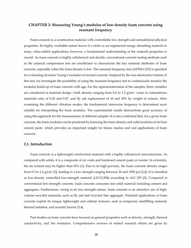
For each group of samples, the foam modulus results of the foamed samples were used to estimate

the solid modulus using Eq. 2.1. A well-matched comparison of the measured and predicted solid

modulus is attainable only if the measurement is accurate and the relationship revealed by Eq. 2.1 is

applicable. This is to say, since the solid phases in the samples are identical, the predicted solid modulus

of the foamed samples should be similar to that experimentally measured from the paste samples.

2.4. Results and discussion

2.4.1. Comparison of results from different fundamental vibration modes

To investigate Young’s modulus of foam concrete, three groups of samples with different densities

were prepared and tested for bulk density and fundamental vibration frequency. According to ASTM

C215, Young’s modulus of the samples can be calculated either using the longitudinal and transverse

fundamental frequency[11]. However, it was found that the transverse mode was preferable, as

illustrated with a simple example of the frequency measurement in Fig. 2.1.

25

Figure 2.1. A typical result of the frequency spectrum of the three fundamental vibration modes

(Sample C_0.6 at 21 d). The y-axis values are normalized by the maximum value seen.

The peak belonging to the transverse fundamental vibration mode was typically sharper, reaching a

greater amplitude; in contrast, the peak of longitudinal mode was relatively gentle, making the peak

position easily affected by noise and leaving a more subjective measurement. Note that the secondary

vibration modes were generated when the measurement was intended for the longitudinal and the

torsional vibrations. With the same amount of impact force, it was easier to excite the transverse vibration

in the specimens. Furthermore, the transverse peak was consistently found as the first major peak in the

spectrum. Therefore, the transverse mode was more recognizable and accurate in practical terms. For

each specimen and at all ages of testing in this experiment, the fundamental frequency of the transverse

variation mode was found to vary in a small range of ±4 Hz. As a result, only the transverse frequency

was used for the subsequent analysis of Young’s modulus.

2.4.2. Young’s modulus of foam concrete

After the measurement, the fundamental transverse vibration frequency was used to calculate foam

modulus of the samples., and the equation for the calculation is provided in Eq. 2.2 [11]:

𝐸 = 𝑑𝑀𝑛2 (2.2)

where, E is Young’s modulus; d is a geometry parameter; M is the mass of the specimen; and n is the

fundamental transverse vibration frequency.

26

After averaging the three readings of the transverse frequency, foam modulus of each specimen was

obtained. The final foam modulus results of each sample took the average from the two specimens.

Subsequently, solid modulus of each foamed sample was calculated using Eq. 2.1. In terms of the

parameter c in this equation, a good fit between the calculated solid modulus and that measured directly

from the paste samples can be obtained when it is equal to 1, as agreed by previous study on cellular

ceramics [13].

To study the feasibility of the proposed testing approach, the focus is placed on Group C results in

this section. The transverse frequency, foam modulus, and solid modulus of each specimen of Group C

samples are summarized in Table 2.2. For the convenience of discussion, the averaged results of foam

and solid modulus are compared in Figs. 2.2a and 2.2b, respectively. As expected, foam modulus of the

samples increased with the bulk density, ranging from 0.6 to 18 GPa. Sample C_0.4 had the smallest E

value at all three ages, and that of Sample C_solid was the largest. Comparing the result for each sample,

little difference was noticed from the two specimens. Meanwhile, the Es results were considerably close

at the same age. On average, the Es results were gradually increased from 7 to 21 days, as cement paste

in the samples continued to hydrate during this period.

Table 2.2. Transverse frequency, foam modulus, and solid modulus of Group C samples.

Specimen Transverse frequency [Hz] Foam modulus [GPa] Solid modulus [GPa]

7 d 14 d 21 d 7 d 14 d 21 d 7 d 14 d 21 d

C_0.4 1 1370 1392 1476 0.60 0.62 0.69 14.05 14.50 16.30

2 1364 1402 1472 0.59 0.62 0.69 13.84 14.63 16.12

C_0.6 1 1796 1836 1940 1.55 1.62 1.80 15.78 16.49 18.41

2 1788 1844 1932 1.54 1.64 1.80 15.76 16.76 18.40

C_0.8 1 1964 2108 2196 2.37 2.73 2.96 14.64 16.87 18.31

2 1986 2088 2196 2.45 2.71 3.00 15.15 16.74 18.52

C_1.0 1 2184 2220 2204 3.63 3.75 3.70 14.78 15.27 15.05

2 2184 2236 2236 3.64 3.81 3.81 14.81 15.52 15.52

C_1.2 1 6362 6726 6604 6.36 6.73 6.60 15.68 16.58 16.27

2 6292 6634 6593 6.29 6.63 6.59 15.51 16.35 16.25

C_solid 1 3188 3352 3440 15.61 17.25 18.17 15.61 17.25 18.17

2 3180 3331 3392 15.54 17.05 17.68 15.54 17.05 17.68

27

(a)

(b)

Figure 2.2. Results of Group C: (a) foam modulus; and (b) solid modulus.

Based on Fig. 2.2a, there is a clear trend that the sample foam modulus increases exponentially with

density at all three ages. This finding is encouraging, as the measured results follow the relationship

revealed by Eq. 2.1. Despite the small fluctuations in Fig. 2.2b, the similar Es values indicate that the

different samples had a highly similar solid phase. After all, the same cement paste was designed for

these samples. Hence, an accurate measurement of E of the samples must have been achieved so that the

resonant frequency test is validated, which further supports applying Ashby’s theory for understanding

foam concrete in this study [13].

0

2

4

6

8

10

12

14

16

18

20

7 d 14 d 21 d

Foam

mo

du

lus,

E [

GP

a] C_0.4

C_0.6

C_0.8

C_1.0

C_1.2

C_solid

0

2

4

6

8

10

12

14

16

18

20

7 d 14 d 21 d

Solid

mo

du

lus,

Es

[GP

a] C_0.4

C_0.6

C_0.8

C_1.0

C_1.2

C_solid

28

In terms of hydration age, marginal increments were found after 7 days, indicating cement hydration

in the samples was almost stopped at this stage. This result may be explained by the fact that a high

dosage of hardening accelerator was used during sample preparation, which significantly reduced the

time length for cement hydration. One unanticipated finding was that E and Es of Samples C_1.0 and

C_1.2 declined at 21 days. This result is likely related to the shrinkage issue of the hydrated cement. This

is partially supported by the crevices visually observed on the corresponding specimens. Although this

decline was not identified for the samples of lower densities, the shrinkage issue may still exist due to

the nature of cement hydration. Possibly, the shrinkage stress in the low-density samples is more evenly

distributed due to the highly discontinuous solid phase so that the modulus results are less affected.

2.4.3. Influence of varying w/cm ratio and fly ash replacement on the measurement

The influence of different material constitution of foam concrete on the testing is studied using

samples in Groups HW and HF, which had a higher w/cm ratio of 0.47 and a higher fly ash replacement

of 30%, respectively. The results of foam and solid modulus, averaged from two specimens of each

sample, are summarized in Table 2.3. In general, the measured E values in both groups also followed a

pattern of exponential growth as a function of density. Gradual increments of Es were seen from 7 to 21

days, but the results of Group HF were slightly higher than Group HW at the same ages. However, both

the two groups of samples had smaller Es values as compared with Group C. This is expected, as the two

changes in Groups HW and HF are intended to reduce Young’s modulus of the paste.

Table 2.3. Foam modulus and solid modulus of samples in Groups HW and HF.

Sample # Foam modulus [GPa] Solid modulus [GPa]

7 d 14 d 21 d 7 d 14 d 21 d

HW_0.4 0.54 0.61 0.63 13.67 15.51 15.94

HW_0.6 1.52 1.54 1.47 16.63 16.85 16.13

HW_0.8 2.71 2.88 2.89 16.15 17.19 17.22

HW_1.0 3.81 4.14 4.21 14.59 15.84 16.12

HW_1.2 5.08 5.42 5.38 15.66 16.68 16.57

HW_solid 14.44 15.09 15.55 14.37 15.03 15.49

HF_0.4 0.66 0.71 0.70 13.693 14.709 14.533

HF_0.6 1.13 1.22 1.30 12.709 13.680 14.618

HF_0.8 2.85 2.88 3.05 15.152 15.267 16.203

HF_1.0 4.37 4.55 4.69 15.160 15.788 16.240

HF_1.2 5.50 5.60 5.90 14.824 15.114 15.901

HF_solid 15.79 15.76 15.46 15.790 15.756 15.468

29

To further evaluate the effectiveness of the test, solid modulus of the two groups of samples is

compared in Figs. 3a and 3b. Similar to the results of Group C shown in Fig. 2.2b, the Es values in each of

the two groups are reasonably close at the same ages, suggesting identical solid phases of the same group

samples. On average, the Es values of Group HW and HF are noticeably lower than Group C. These

results support that the resonant frequency measurement is not affected by the changes of material

constitution and the measurement is still acceptably accurate.

(a)

(b)

Figure 2.3. Comparisons of the solid modulus of samples in (a) Group HW and (b) Group HF.

0

2

4

6

8

10

12

14

16

18

20

7 d 14 d 21 d

Solid

mo

du

lus,

Es

[GP

a] HW_0.4

HW_0.6

HW_0.8

HW_1.0

HW_1.2

HW_solid

0

2

4

6

8

10

12

14

16

18

20

7 d 14 d 21 d

Solid

mo

du

lus,

Es

[GP

a] HF_0.4

HF_0.6

HF_0.8

HF_1.0

HF_1.2

HF_solid

30

However, the consistency of the Es results drops as the density reaches to the lower end, which is

seen in all three groups. This phenomenon is most likely caused by the foam stability issue. As the sample

density becomes smaller, the fresh foam is less stable and the foam structure in fresh foam concrete

becomes more difficult to control. This observation is in accord with several studies indicating that

aqueous foam structures vanish at a higher rate when density decreases [1,15,16].

For a given foam concrete, the foam modulus predicted by Eq. 2.1 is in fact the maximum value in

theory, whereas the actual result can be largely influenced by the quality of its foam structure. During

the sample preparation, a trade-off exists in the mixing of foam and paste. If the mixing is insufficient,

the two phases cannot be mixed effectively. If the mixing is excessive, it is difficult to preserve the air

bubbles in the mixture. Both scenarios will result in degradation of the void structure. This problem of

void instability is especially true when the foam density approaches the lower limit.

2.4.4. Predict Young’s modulus of foam concrete with that of hardened cement paste

As solid modulus of the paste samples was also obtained from the measurement, Young’s modulus

of the foamed samples could be predicted using Eq. 2.1, with the constant c is equal to 1. Following this

idea, the measured and predicted results of E of the foamed samples are compared on a group basis in

Fig. 2.4. Across the three comparisons, the data points are distributed closely to the line of equality at all

three ages. Considering unavoidable measurement error related to the experimental condition, the limit

of the testing instrument, as well as human judgment for peak identification, the prediction agrees

considerably well with the measurement. This agreement is insensitive to density, hydration age, and

change of cement paste constitution investigated in this study.

This strong correlation further supports the idea of using the solid modulus of the hardened cement

paste to calculate the foam modulus of foam concrete, whereby the unknown of foam concrete is directly

bridged with our well-established knowledge of solid cement paste. From a practical perspective, this

encouraging finding is of special significance. As the hardened property of solid cement paste (i.e. solid

modulus) has been studied extensively and can be measured using many different approaches, the foam

modulus can be directly predicted with acceptable accuracy.

31

(a) (b)

(c)

Figure. 2.4. Comparisons of the measured and the predicted foam modulus of samples in (a) Group C,

(b) Group HW, and (c) Group HF.

2.5. Conclusion

A non-destructive approach of measuring Young’s modulus of low-density foam concrete was

shown to be feasible. Three groups of samples of different material constituents were cast for

measurement of fundamental resonant frequency. For each group, the density of the foamed samples

32

ranged from 0.4 to 1.2 g/cm3, and a paste sample was prepared for comparison. In terms of the vibration

mode, it was found that the peak frequency of transverse mode was not only easier to identify but also

more consistent. Therefore, the transverse fundamental frequency was used for calculating the foam

modulus of the samples in this study.

For all three groups of samples, the foam modulus increased exponentially as a function of density.

The test method worked well for all mixtures and the mixing protocol used in this study. By comparing

samples with different density, the results were consistent with Ashby’s formulation for Young’s

modulus of the cellular material and its solid component. For samples that were composed of the same

paste mixtures (i.e., solid constituents), the normalized solid modulus results were proved to be very

similar in magnitude. In general, this method worked well for a wide range of bulk density, hydration

age, material constitution of the foam concrete samples.

The results also showed that the foam modulus can be predicted with reasonable accuracy based on

the solid modulus of hardened cement paste, unless the foam density becomes extremely low such that

the void instability issue becomes prominent. This finding is insightful from a practical perspective for

designing foam concrete products. Once the property of a solid unfoamed cement paste is known, the

property of any foam concrete made with that paste can be predicted.

References


(2016) 542–549. https://doi.org/10.1680/macr.15.00097.



https://doi.org/10.1016/j.conbuildmat.2013.10.066.




material, Mag. Concr. Res. 57 (2005) 21–31. https://doi.org/10.1680/macr.57.1.21.57866.

[5] ACI Committee 229, Report on Controlled Low-Strength Materials, Farmington Hills, MI, 2013.


Concr. Compos. 22 (2000) 321–329. https://doi.org/10.1016/S0958-9465(00)00016-0.



https://doi.org/10.1016/j.cemconcomp.2009.04.006.

33

[8] M. Jones, A. McCarthy, Utilising unprocessed low-lime coal fly ash in foamed concrete, Fuel. 84

(2005) 1398–1409. https://doi.org/10.1016/j.fuel.2004.09.030.


Concr. Compos. 28 (2006) 475–480. https://doi.org/10.1016/j.cemconcomp.2005.12.001.

[10] R. Hooton, S. Kolluru, J. Popovics, S. Shah, Determining Elastic Properties of Concrete Using

Vibrational Resonance Frequencies of Standard Test Cylinders, Cem. Concr. Aggregates. 22 (2000)

81. https://doi.org/10.1520/CCA10467J.

[11] T.D. Cores, Standard Test Method for Fundamental Transverse , Longitudinal , and Torsional

Resonant Frequencies of Concrete Specimens 1, 04 (2003) 1–9. https://doi.org/10.1520/C0215-14.


of preformed foam cellular concrete, Cem. Concr. Res. 34 (2004) 889–893.

https://doi.org/10.1016/j.cemconres.2003.11.005.


(1983) 1755–1769. https://doi.org/10.1007/BF02645546.


https://doi.org/10.1017/CBO9781139878326.

[15] J. Boos, W. Drenckhan, C. Stubenrauch, Protocol for Studying Aqueous Foams Stabilized by

Surfactant Mixtures, J. Surfactants Deterg. 16 (2013) 1–12. https://doi.org/10.1007/s11743-012-1416-

2.

[16] K. Feitosa, O.L. Halt, R.D. Kamien, D.J. Durian, Bubble kinetics in a steady-state column of

aqueous foam, Europhys. Lett. 76 (2006) 683–689. https://doi.org/10.1209/epl/i2006-10304-5.

34

CHAPTER 3: Crushing behavior and crushing strengths of low-density foam

concrete

Foam concrete is a highly cellularized cementitious material that undergoes extensive plastic

deformation when loaded to failure. Understanding foam concrete crushing behavior is of special

importance for its engineering applications. This chapter focuses on characterizing the crushing behavior

of lightweight foam concrete ranging from 0.4 to 0.8 g/cm3, using the resonant frequent test and a

penetration test. Four distinct crushing phases: linear elastic, transitional, plateau, and final densification

are observed for the samples. Furthermore, the yield strength and plateau strength are defined for

characterizing the foam crushing behavior. Using the experimental data, the modulus-strength

constitutive relationship is established for predicting the crushing behavior with fundamental material

properties.

3.1. Introduction

Foam concrete is commonly used as a low strength flowable fill material, but it also exhibits good

potential for many other applications including impact absorption. The unique cellular structure in foam

concrete has a profound impact on its crushing behavior and mechanical property. Foam concrete is

described as a low-density controlled low-strength material (LD-CLSM) in ACI specifications [1,2]. In

contrast to normal concrete which has a density around 2.3 g/cm3 and a compressive strength between

20 to 40 MPa, the foam concrete strength can be 0.2 MPa at a low density of 0.3 g/cm3 [3–5]. When the

foam density is above 0.8 g/cm3, this material is mostly a closed-cell foam that behaves closer to solid

material. As the density decreases, foam concrete gradually becomes an open cell material, which leads

to distinct changes in material properties. Lower than 0.4 g/cm3, the fresh mixture tends to lose its volume

stability before hardening [6]. Currently, low-density foam concrete between 0.4 to 0.8 g/cm3 is mostly

used for flowable fill applications due to its lightweight and ease-of-excavation characteristics, as well as

for acoustic and thermal isolation [3]. Meanwhile, interests have also been growing in using low-density

foam concrete for advanced applications, with engineered material arresting system (EMAS) as an

example [7–10].

Foam concrete strength is strongly correlated to its foam density [11–13] and is also restrained by

the foam geometry [6]. As reviewed by Ramamurthy et al., foam concrete at 0.8 to 1.8 g/cm3 is frequently

investigated for its structural properties such as compressive, flexural, and tensile strength [11,14–17].

Studies over the past two decades have also provided findings on the influence of cement paste

properties to foam concrete strength, such as water-to-cementitious ratio (w/cm) [18–21], pozzolanic

materials [11,19,20,22,23], curing methods [19,24,25], as well as fine aggregate inclusion [1,26–28].

35

Specifically, several studies reported the benefits of using fly ash in foam concrete. Kearsley and

Wainwright, for example, found that the 28-day and 1-year compressive strength of foam concrete with

foam density between 1.0 to 1.5 g/cm3 was not diminished by using a 70% replacement of cement with

fly ash [22,29]. When low-grade coarse fly ash, instead of natural sand, was used as fine aggregate in

foam concrete, the mixtures ranging from 1.0 to 1.4 g/cm3 exhibited significant improvements on

compressive strength and other performance such as flowability and freeze-thaw durability [30,31].

Although several investigations attempted to correlate the compressive strength with Young’s

modulus and foam density for high-density foam concrete [4,17,32], their applicability may be limited to

certain mixtures, as a thorough consideration should also incorporate the variation on paste density.

Moreover, studies to date provide little insight into the relationship between mechanical properties and

material constitution for low-density foam concrete. This lack of knowledge is potentially attributed to

the technical difficulties for characterizing the low-strength foam.

This study proposes a new methodology for investigating the modulus-strength constitutive

relationship of low-density foam concrete, while the use of fine aggregate is not considered. To

accommodate typical variations in low-density foam concrete, the samples were prepared with different

w/cm and fly ash content, and with foam density ranging from 0.4 to 0.8 g/cm3. As crushing represents a

more general material failure scenario of foam materials, a penetration test was carried out to characterize

the crushing behavior and crushing strength of foam concrete. In addition, a resonant frequency test was

used to measure the dynamic Young’s modulus of the samples, due to its non-destructive nature and

good accuracy [33]. The proposed modulus-strength constitutive relationship was validated with the

experimental data. It is found that the strength can be well predicted using Young’s modulus of the paste

as a solid property and relative density of the foam as a geometric property. The findings provide

valuable information for studying foam concrete and designing the applications.

3.2. Background

3.2.1. Strengths of solid foam and normal concrete

This study aims at investigating foam concrete crushing strength based on its relative density and

the hardened paste property. The studies on cellular solid material reveal that the crushing strength of

solid foam is governed by two aspects: solid base material and foam geometry [34,35]. The empirical

equations proposed by Ashby to estimate the elastic yield strength and plastic yield strength of solid

foams are given in Eqs. 3.1 and 3.2, respectively [35]:

𝜎𝑒𝑙

∗

𝐸𝑠= 𝑐1 (

𝜌

𝜌𝑠)

2

(3.1)

36

𝜎𝑝𝑙

∗

𝜎𝑦= 𝑐2 (

𝜌

𝜌𝑠)

1.5

(3.2)

where 𝜎𝑒𝑙∗ and 𝜎𝑝𝑙

∗ are the elastic and the plastic yield strength, 𝐸𝑠 and 𝜎𝑦 are the elastic modulus and

the yield strength of the solid base material, 𝑐1 and 𝑐2 are empirical constants obtained experimentally,

and 𝜌 and 𝜌𝑠 are the densities of the foam and the solid. In these equations, the contribution from solid

base material to foam strength is counted through 𝐸𝑠 and 𝜎𝑦, and the influence from the foam property

is determined by the relative density, ρ/ρs. 𝐸𝑠 is referred as solid modulus.

Ashby also studied the crushing strength of brittle foams and developed the following relationship

[35]:

𝜎𝑓

∗

𝜎𝑓= 𝑐3 (

𝜌

𝜌𝑠)

1.5

(3.3)

where 𝜎𝑓∗ is the crushing strength of brittle foam, 𝜎𝑓 is the flexural strength of base material, and 𝑐3

is a constant. Although this equation showed a weaker correlation with the experimental data, the

crushing strength of brittle foams is controlled by both the base material via 𝜎𝑓 and the foam property

via ρ/ρs. This equation uses the flexural strength of the base material to represent the solid property.

However, the true value of flexural strength of hardened cement is not easy to obtain and a previous

study showed poor correlation between this parameter and pore volume in cement paste [36].

Furthermore, it is questionable whether this approach works for foam concrete, as concrete materials do

not behave like pure brittle materials.

Since limited information on the flexural strength of the hardened cement paste is available, some

insights are borrowed from studies on normal concrete. As recommended by ACI 318, the empirical

relationships linking Young’s modulus to the compressive yield strength and flexural strength of plain

concrete are given in Eqs. 3.35 and. 6, respectively [37,38]:

𝐸𝑐 = 4734(𝑓𝑐′)0.5 (3.5)

𝑓𝑟 = 0.62(𝑓𝑐′)0.5 (3.6)

where Ec is 28-day static modulus of elasticity, fc’ is 28-day cylinder compressive strength, and fr is 28-

day flexural strength, all with units in N/mm2.

3.2.2. Young’s modulus of foam concrete

In a recent study, it is proven that Young’s modulus of foam concrete is predictable if the relative

density and solid modulus are known [33]:

𝐸

𝐸𝑠= (

𝜌

𝜌𝑠)2 (3.7)

37

where E is Young’s modulus of foam concrete, and Es is Young’s modulus of the hardened paste. For

conciseness, the E is referred as foam modulus in the rest of this paper. This equation provides an

important function to bridge foam modulus to solid modulus of foam concrete.

3.2.3. From Young’s modulus to crushing strength of foam concrete

In comparison to using flexural strength to indicate the hardened property, the solid or foam

modulus of foam concrete has several outstanding advantages to serve the same function. First, the solid

modulus is a fundamental property that governs a number of mechanical properties, including the

flexural strength [37]. Second, solid modulus has been proven feasible to predict foam strength in Eq. 3.1.

Third, both the foam and the solid moduli of foam concrete can be experimentally determined, and

further interchangeable using Eq. 3.7.

Therefore, it is reasonable to hypothesize that the foam concrete crushing strength can be estimated

using the solid or foam modulus. As foam modulus is directly measured from foam concrete, it should

perform better than solid modulus. As such, an equation generalized in the form of Eqs. 3.1 to 3.3 was

proposed for predicting the crushing yield strength of foam concrete:

𝜎𝑓𝑐

(𝐸)𝑎 = 𝑘 (𝜌

𝜌𝑠)

𝑏

(3.8)

where σfc is foam concrete yield strength under indentation, and a, b, and k are constants to be determined.

Thus, characterizing the correlation between the crushing strength and the foam modulus, which is

interchangeable with solid modulus, is of special importance to this study.

3.3. Experimental procedures

3.3.1. Mixture design

Three groups of foam concrete mixtures were prepared, where different w/cm ratio and fly ash

replacement of cement were used. The mixing design is provided in Table 3.1. Design of the foam

concrete mixtures followed the ASTM C796 [39]. For each group of mixtures, a pure paste sample and

five foamed paste samples with density from 0.4 to 0.8 g/cm3 were prepared. Further reducing the density

raised the foam instability issue significantly. The sample name designation indicates the paste mixture

group and the target density. The Group C (i.e., controlled) had a w/cm ratio of 0.42 and a 10% class C

fly ash replacement. In comparison, a greater fly ash replacement of 30% was used for Group HF (i.e.,

high-fly ash) samples, and a higher w/cm ratio of 0.47 was used for Group HW (i.e., high-water). The use

of 10% fly ash in Group C mixtures was useful to improve flowability of the paste mixtures that would

otherwise have been overly viscous, as part of the water was used for generating the aqueous foam.

38

Table 3.1. Mixture design of the samples.

Mix #

Target

density

[g/cm3]

Fly ash

replacement

[%]

w/c

Bulk

density

[g/cm3]

Relative density

Void content

[%]

C_0.4 0.4

10 0.42

0.391 0.198 80.2

C_0.5 0.5 0.495 0.250 75.0

C_0.6 0.6 0.587 0.297 70.3

C_0.7 0.7 0.712 0.359 64.1

C_0.8 0.8 0.825 0.417 58.3

C_solid 1.91 1.977 1 0

HF_0.4 0.4

30 0.42

0.400 0.210 79.0

HF_0.5 0.5 0.529 0.278 72.2

HF_0.6 0.6 0.609 0.319 68.1

HF_0.7 0.7 0.748 0.393 60.7

HF_0.8 0.8 0.837 0.439 56.1

HF_solid 1.88 1.907 1 0

HW_0.4 0.4

10 0.47

0.414 0.216 78.4

HW_0.5 0.5 0.503 0.262 73.8

HW_0.6 0.6 0.576 0.300 70.0

HW_0.7 0.7 0.664 0.346 65.4

HW_0.8 0.8 0.755 0.393 60.7

HW_solid 1.85 1.923 1 0

3.3.2. Sample preparation

The sample preparation followed the procedures described in Section 1.3. After mixing, the fresh

foam concrete was gently poured into 101.6×203.2 mm standard concrete cylinder and 50.8×50.8×203.2

mm prism molds. For each sample, nine cylinders for the penetration test and two prism specimens for

the resonant frequency test were cast. Then, the molds were sealed to allow mixture hardening for three

days, after which the specimens were further cured in a 100% RH environmental chamber at 21ºC. The

bulk density of each sample was measured right after demolding, and additional measurements at later

ages confirmed little change in the bulk density. During the sample preparation, any sample found its

density off the target by more than 0.05 g/cm3 was recast. The density information of the final mixtures

is provided in Table 3.1, along with the relative density and air content calculated using Ashby’s

equations [35].

39

3.3.3. Characterization of the crushing behavior

The crushing behavior and mechanical property of a solid foam are commonly assessed by analyzing

its load-displacement curve from indentation [40–43]. This test simulates a basic crushing scenario that

is representative of a wide range of crushing, impacting, and indentation events. In this study, the test

was carried out for the cylinder specimens at 7, 14, and 21 days after casting, as previous experiments

suggested an imperceptible strength buildup after this period [33]. This shortened strength gaining

period is attributed to the use of hardening accelerator during sample casting. At each testing date, three

cylinders were tested for each foam concrete sample.

The penetration test was done with an Instron 4502 testing frame, as shown in Fig. 3.1. During the

experiment, a steel rod of a 19.05 mm diameter was indented into the foam concrete cylinder vertically

from the top center. The loading capacity of the Instron frame was 10 kN, which yielded a maximum

indentation stress of 35 MPa. The foam concrete cylinder was tested without demolding, and the loading

was displacement controlled at a 75 mm/min rate, according to a previous study on glass foam [44].

Previous lab tests suggested that the obtained load-displacement curve was not evidently affected by

varying the loading rate from 10 to 500 mm/min and the plastic cylinder mold did not impose a difference

on the test results.

Figure 3.1. Testing setup for the penetration test. The Instron 4052 loading frame is coupled with a 10

kN load cell.

40

3.3.4. Characterization of foam concrete Young’s modulus

Young’s modulus of foam concrete was characterized to seek the protentional correlation to the

crushing property. According to ASTM C215 [45], Young’s modulus of the two prism specimens of each

sample was monitored by measuring the resonant frequency. The measurement was conducted at 7, 14,

and 21 days after casting, in correspondence to the penetration test. For each specimen, three individual

measurements were conducted at each time, and the foam modulus was calculated based on their

average. More details about this test have been reported in Section 2.3.3.


3.4.1. Foam concrete load-displacement response

Analyzing the load-displacement behavior under indentation provides important insights for

studying the mechanical property of cellular solids. Three load-displacement results representing the

general crushing behavior of the foam concrete samples are given in Fig. 3.2. These curves compare the

7-day load-displacement behavior of three Group C specimens at 0.4, 0.6, and 0.8 g/cm3. The ordinate

value of indentation stress is obtained by dividing the load force over the nominal contact area of the

indenter. The indentation was stopped at around 180 mm, at which clear sign of final densification was

seen.

Figure 3.2. A comparison of the load-displacement curves of three Group C specimens at 0.4, 0.6, and

0.8 g/cm3. All the specimens are tested at 7 days after casting.

41

A total of four crushing phases were identified for foam concrete. For a cellular material, it typically

has three crushing phases, which are linear elastic, crushing plateau, and final densification [35]. In

addition to these typical phases, a transitional phase that bridges the elastic and the plateau phases are

observed distinctively here. During this phase, the stress is built up to the plateau level at a relatively

constant rate. This transitional phase has not been previously reported. Taking the C_0.8-7d as an

example, the linear elastic phase corresponds to the instantaneous rise at the very beginning of the

indentation, which ends at the yield strength of 10 MPa. In the transitional phase, the stress further raises

to 27 MPa at the penetration depth of 50 mm at a relatively constant rate, followed by a smooth transition

to the plateau phase. The plateau phase that gives a consistent plateau strength of 30 MPa is found from

80 to 160 mm. Lastly, the final densification occurs when the indenter reaches the rigid bottom where the

densified foam was further compressed. The four crushing phases are also recognizable in C-0.6-7d and

C-0.4-7d. Note that the fourth phase could be omitted because it does not reflect material characteristics

alone, but we include it in Fig. 3.2 to be consistent with the established literature [34,35].

For all the curves shown in Fig. 3.2, two crushing strengths, yield strength and plateau strength, can

be identified at the beginning of the transitional phase and the crushing plateau. The crushing strengths

become progressively lower by the descent on foam density. Compared to C-0.8-7d, it is clear for C-0.6-

7d that the ending point of the transitional phase is postponed to 100 mm; for C-0.8-7d, this point is

further delayed to 140 mm. For all the tested specimens, it is observed that the transitional phase becomes

increasingly longer when foam density goes down. At a low foam density such as 0.4 g/cm3, the slope of

the transitional phase is infinitesimal so that it seems the plateau phase is obtained right after the elastic

phase. Therefore, observation of the transitional phase should be attributed to foam density. As the

density gets higher, the indentation stress builds up at a much higher rate, making the transitional phase

more distinguishable.

3.4.2 Local accumulation of the crushed foam under indenter at the four phases

The four crushing phases relate to the local accumulation of the densified material underneath the

indenter. To illustrate this phenomenon, the cross-section of a 21-day C_0.6 specimen at the four phases

is demonstrated in Fig. 3.3. In a close agreement to observations commonly seen in other cellular

materials studies, the crushed material formed a cone-shaped region under the indenter, where this cone-

shaped local densification is often referred to dead zone [44, 45] or passive cone [46].

42

Figure 3.3. Development of the local densification on the same cross-section of a C_0.6 cylinder

specimen. The crushing depths were 1, 30, 120, and 180 mm, corresponding to the elastic, transitional,

plateau phase, and densification crushing phases, respectively. The densified region is distinctive from

the uncrushed foam.

During the indentation process, the foam concrete only experienced internal volume collapse under

the indenter. The top surface of a 21-day C_0.6 cylinder specimen is shown in Fig. 3.4. The crushed region

of the cross-section at the transitional phase shown in Fig. 3.3 is magnified for a demonstration in Fig. 3.5.

After removing the indenter, a clean interface was observed, and the crushed foam exhibited minimal

lateral expansion. Both observations suggested that the foam was crushed downward without cracking

issues. This behavior was caused by the extremely low Poisson's ratio of low-density cellular

solids.31,38,41,47

Figure 3.4. Top surface of a C_0.6 cylinder specimen after the test, in which no crack was seen.

43

Figure 3.5. Magnified view of the local densification of the C_0.6 specimen cross-section, before and

after removing the indenter.

Further inspection of Figs. 3.3 and 3.5 reveals that the transitional phase correlates strongly to the

build-up of the densification cone during indentation, which also explains the different length of the

transitional phase for different samples. As only the solid material contributes to the densification cone

volume, this phase completes within a shorter indentation depth for the higher density foams.

Additionally, the foam density should also affect the size of the densification cone, imposing an indirect

influence on the onset depth of the fourth crushing phase.

3.4.3. Characterization of yield strength and plateau strength of the samples

As the yield strength and plateau strength are of special importance to characterize foam concrete

crushing behavior, these parameters were measured from the load-displacement curve of each cylinder

specimen. The yield strength was determined as the starting point of the transitional phase. The plateau

strength was averaged from the plateau section of the load-displacement curve. For each mixture, the

strength values of the three replicate specimens were found to be consistent, and the average is reported

in Table 3.2. Because of the limited capacity of the testing frame, the plateau strength of sample HF_0.8

at 14 and 21 days was not obtained. Note that a direct strength comparison of the same density mixtures

across different groups may be inappropriate, as the strength value of each individual mixture is affected

by the actual foam density, which varies within the ±0.05 g/cm3 range. However, this influence is

mitigated by considering relative density in the subsequent analysis.

44

Table 3.2. Testing results of yield strength and plateau strength of the samples.

Mix # Yield strength σy [MPa] Plateau stress σpl [MPa]

7d 14d 21d 7d 14d 21d

C_0.4 0.295 0.353 0.410 1.70 1.95 2.14

C_0.5 1.70 1.88 2.19 6.33 7.16 8.64

C_0.6 3.74 4.53 4.96 12.6 14.1 15.3

C_0.7 7.22 7.73 8.02 20.5 22.2 25.2

C_0.8 10.4 11.3 12.3 29.7 32.1 35.0

C_solid - - - - - -

HF_0.4 0.262 0.268 0.274 1.17 1.24 1.41

HF_0.5 0.847 1.01 1.13 2.47 3.02 3.29

HF_0.6 2.32 2.62 2.82 6.58 7.40 8.46

HF_0.7 6.56 7.66 8.57 19.8 22.6 25.4

HF_0.8 11.6 14.2 15.1 32.8 N/A N/A

HF_solid - - - - - -

HW_0.4 0.323 0.337 0.375 1.38 1.63 1.71

HW_0.5 1.59 2.02 2.31 7.09 8.42 9.51

HW_0.6 2.46 2.51 2.76 8.85 9.49 10.0

HW_0.7 3.63 3.76 3.86 12.9 14.4 15.6

HW_0.8 6.57 8.59 9.06 24.9 30.9 34.5

HW_solid - - - - - -

In Table 3.2, there was a steep rise in both yield strength and plateau strength for all the foam samples

when the density went up from 0.4 to 0.8 g/cm3. Continuous growth of the crushing strengths was

observed over time. Due to the lower w/cm ratio and fly ash content, the paste mixture for Group C

samples gained the highest strength among all, which resulted in higher crushing strengths seen in

Group C samples. When foam density is the same, the paste strength plays a determinative role in foam

concrete strength. This finding also corroborates the conclusion drawn in many other studies [12,14,15].

3.4.4. Characterization of the foam and solid modulus

As a fundamental material parameter, Young’s modulus is critical for studying foam concrete. In the

experimental work, the dynamic Young’s modulus of the samples was interpreted based on the

fundamental transverse frequency using resonant frequency test as specified by ASTM C215. For each

foamed sample, the transverse frequency and Young’s modulus results averaged from the two prism

45

specimens are given in Table 3.3. Young’s modulus of the samples was then calculated using Eq. 3.9 [45]

𝐸 = 𝐶𝑀𝑛2 (3.9)

where E is dynamic Young’s modulus; C is a geometry parameter; M is specimen mass; and n is

transverse fundamental frequency.

Table 3.3. Testing results of fundamental transverse frequency and dynamic Young’s modulus of the

samples.

Mix # Transverse fundamental frequency [Hz] Dynamic young's modulus E [MPa]

7d 14d 21d 7d 14d 21d

C_0.4 1235 1268 1316 463 488 526

C_0.5 1720 1828 1836 1138 1285 1297

C_0.6 1884 1956 2024 1619 1745 1868

C_0.7 2091 2116 2140 2415 2473 2530

C_0.8 2200 2256 2265 3104 3283 3290

C_solid 3448 3512 3539 18255 18943 19236

HF_0.4 1084 1116 1144 365 387 407

HF_0.5 1200 1296 1346 591 690 744

HF_0.6 1591 1672 1696 1200 1325 1364

HF_0.7 1999 2076 2057 2333 2517 2660

HF_0.8 2208 2284 2340 3169 3391 3559

HF_solid 3264 3383 3471 15783 16955 17853

HW_0.4 1152 1216 1264 427 476 514

HW_0.5 1700 1760 1804 1129 1210 1286

HW_0.6 1644 1728 1663 1212 1339 1457

HW_0.7 1872 1904 1896 1817 1880 1935

HW_0.8 2040 2120 2191 2450 2646 2826

HW_solid 3192 3305 3400 15227 16322 17276

Similar to the observations on the crushing strengths in Table 3.2, the foam modulus results were

found to positively correlate with foam density, age, and the property of the hardened paste. For the

same group of samples, a higher foam modulus always corresponded to larger crushing strengths for

each sample. By influencing both foam modulus (see Eq. 3.7) and hardened paste strength, the solid

modulus is a major factor governing the foam concrete crushing behavior.

3.4.5. Yield strength and plateau strength

The plateau strength seems to be correlated with the yield strength, based on the data given in Table

3.2. The yield strength and plateau strength results for each sample group are compared individually in

46

Fig. 3.6. The dashed line in these plots is the linear curve fitting, along with the fitting equation and the

coefficient of determination, R2, to indicate the fitting quality. The results of R2 in the three plots of Fig.

3.6 are all close to 1, suggesting a remarkable correlation between these two parameters. For Group C

samples in Fig. 3.6a, the curve fitting finds a plateau-to-yield strength ratio of 2.93. Regardless of the foam

density, the plateau strength is about three times the yield strength in this case. In comparison, a slightly

smaller ratio of 2.91 is found for Group HF samples in Fig. 3.6b; however, the ratio becomes 3.76 for

Group HW samples in Fig. 3.6c. These results suggest that the plateau-to-yield strength is only relevant

to the hardened paste property, meaning that the plateau strength can be potentially predicted from the

yield strength that is easier to measure. This finding gives a useful insight for simplifying the relationship

of foam concrete crushing strengths.

(a) (b)

(c)

Figure 3.6. Comparisons on the measured yield strength and plateau strength of the three groups of

foam concrete samples: (a) Group C, (b) Group HF, and (c) Group HW.

47

3.4.6. Using foam modulus to estimate the crushing strengths

The proposed foam concrete modulus-to-strength relationship Eq. 3.8 was examined using the

experimental data of relative density (Table 3.1), yield strength (Table 3.2), and foam modulus (Table 3.3)

to seek the best correlation through data fitting. Considering Eqs. 3.2 and 3.5, constant a should equal to

1; however, it is more likely to be 2 as indicated by Eqs. 3.3 and 3.6. Coincidentally, the fitting

optimization in MATLAB found the best fit when a is equal to 1.905, which supports the use of 2 for a.

Subsequently, the constant b was determined to be -0.5. Then, k was determined to be 7.5×10-7. After

plugging these values into Eq. 3.8, we have Eq. 3.10 for the yield strength estimation:

𝜎𝑓𝑐 = 7.5 × 10−7𝐸2 (𝜌

𝜌𝑠)

−0.5

(3.10)

An excellent agreement is found between the measured yield strength and the prediction obtained

using Eq. 3.10, as shown in Fig. 3.7. Eq. 3.10 provides an accurate yield strength estimation for each

individual sample group, and this relationship is applicable for all different age and foam density

investigated in this study.

Figure 3.7. A comparison on foam concrete yield strength between the measured results and the values

predicted by the purposed equation.

Adding a term rs of the yield-to-plateau strength ratio to Eq. 3.10, the plateau strength can be

calculated as Eq. 3.11:

𝜎𝑝𝑙 = 7.5 × 10−7𝑟𝑠𝐸2 (𝜌

𝜌𝑠)

−0.5

(3.11)

where rs is the plateau-to-yield strength ratio. Determination of the plateau-to-yield strength ratios for

Groups C, HF, and HW samples has been addressed in the last section. The predicted plateau strength

48

results are compared with the experimental measurements in Fig. 3.8, where decent agreement is

achieved for the individual groups. For the 0.4 g/cm3 samples, the data points are more off the fitted

curve. This is likely to be a foam instability issue [6]. At such a low density, the fresh paste cannot provide

enough confining force to stabilize the air bubbles, leading to a degradation of the foam structure.

Figure 3.8. A comparison on foam concrete plateau strength between the measured results and the

values predicted by the purposed equation. The yield-to-plateau strength ratios for different sample

groups are considered individually in this case.

Overall, the results presented in Figs. 3.7 and 3.8 support using foam modulus to estimate the

crushing strengths of foam concrete. The good agreement of the predictions encourages the use of the

proposed modulus-strength relationships for subsequent studies.

3.4.7. Using solid modulus to estimate the crushing strengths

If foam modulus can be used to predict the crushing strengths, it should be plausible to use solid

modulus. Substituting the foam modulus in Eq. 3.11 with solid modulus, the foam concrete yield strength

can be estimated based on solid modulus:

𝜎𝑓𝑐 = 7.5 × 10−7𝐸𝑠2 (

𝜌

𝜌𝑠)

3.5

(3.12)

This approach provides practical convenience for estimating foam concrete crushing property

without testing on foam concrete with the special experimental apparatus. Based on the solid modulus

values of the paste mixtures measured from C_solid, HF_solid, and HW_solid (Table 3.3), the yield

strength of the foamed samples is estimated using Eq. 3.12 and further compared with the experimental

result (Table 3.2) in Fig. 9. As suggested by the wider scatter as well as the smaller R2 value, the prediction

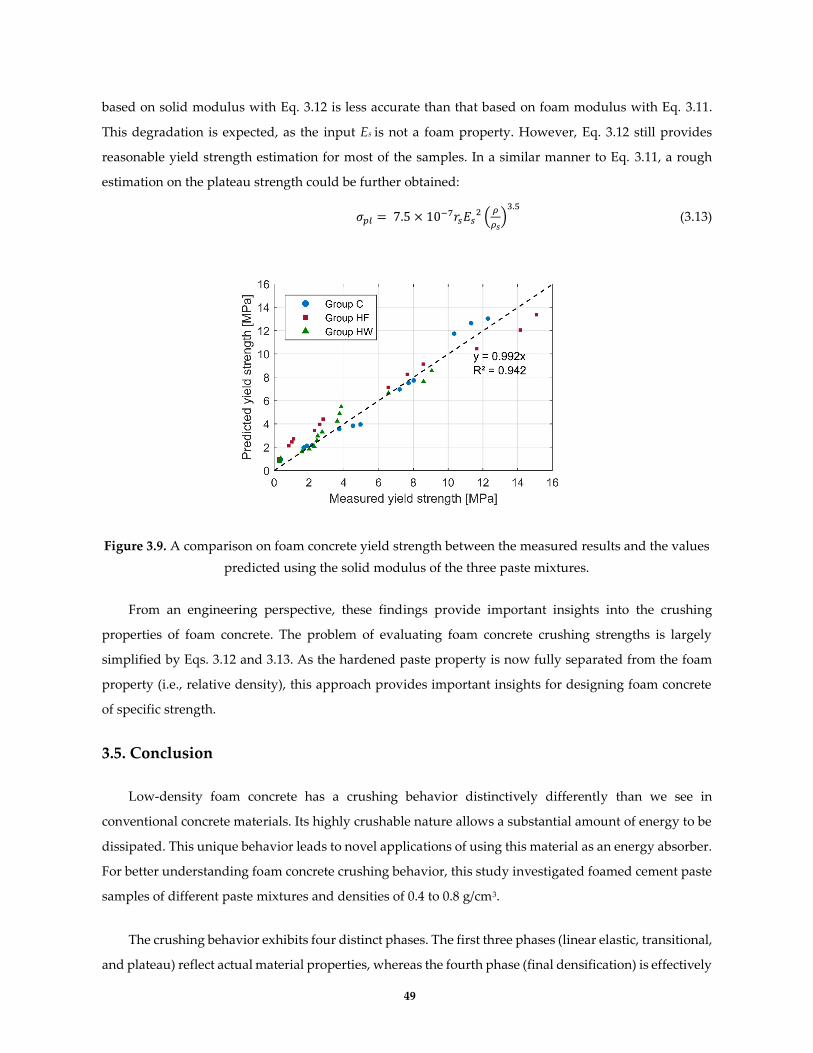
49

based on solid modulus with Eq. 3.12 is less accurate than that based on foam modulus with Eq. 3.11.

This degradation is expected, as the input Es is not a foam property. However, Eq. 3.12 still provides

reasonable yield strength estimation for most of the samples. In a similar manner to Eq. 3.11, a rough

estimation on the plateau strength could be further obtained:

𝜎𝑝𝑙 = 7.5 × 10−7𝑟𝑠𝐸𝑠2 (

𝜌

𝜌𝑠)

3.5

(3.13)

Figure 3.9. A comparison on foam concrete yield strength between the measured results and the values

predicted using the solid modulus of the three paste mixtures.

From an engineering perspective, these findings provide important insights into the crushing

properties of foam concrete. The problem of evaluating foam concrete crushing strengths is largely

simplified by Eqs. 3.12 and 3.13. As the hardened paste property is now fully separated from the foam

property (i.e., relative density), this approach provides important insights for designing foam concrete

of specific strength.

3.5. Conclusion

Low-density foam concrete has a crushing behavior distinctively differently than we see in

conventional concrete materials. Its highly crushable nature allows a substantial amount of energy to be

dissipated. This unique behavior leads to novel applications of using this material as an energy absorber.

For better understanding foam concrete crushing behavior, this study investigated foamed cement paste

samples of different paste mixtures and densities of 0.4 to 0.8 g/cm3.

The crushing behavior exhibits four distinct phases. The first three phases (linear elastic, transitional,

and plateau) reflect actual material properties, whereas the fourth phase (final densification) is effectively

50

a testing artifact. The yield strength and plateau strength can be clearly identified from the loading curve.

It is found that these strength parameters are mainly influenced by solid paste properties and foam

geometry, while the ratio between them remains constant for sets of materials made with the same paste

mixture. Further investigation reveals that the foam strength is closely related to Young’s modulus of the

paste, which is largely determined by factors such as mix proportion and hydration age.

The most significant finding to emerge from this study is that the strength and crushing behavior of

low-density foam concrete can be well predicted by knowing the foam modulus and the relative density.

Excellent agreement is found between the experimental data and the values given by the proposed

equations for strength prediction. By substituting the foam modulus, the prediction can be further

simplified using the solid modulus of the hardened paste.

References

[1] ACI Committee 523., Guide for cellular concretes above 50 lb/ft3 (800 kg/m3), Guid. Cell. Concr.

above 50 Lb/Ft3 (800 Kg/M3). (n.d.).





material, Mag. Concr. Res. 57 (2005) 21–31. https://doi.org/10.1680/macr.2005.57.1.21.





(2016) 542–549. https://doi.org/10.1680/macr.15.00097.

[7] Z.Q. Zhang, J.L. Yang, Q.M. Li, An analytical model of foamed concrete aircraft arresting system,

Int. J. Impact Eng. 61 (2013) 1–12. https://doi.org/10.1016/j.ijimpeng.2013.05.006.


Transp. Res. Rec. (2010) 124–131. https://doi.org/10.3141/2177-15.

[9] J. Wang, W. Guo, R. Zhao, Y. Shi, L. Zeng, Energy-absorbing properties and crushing flow stress

equation of lightweight foamed concrete, J. Civil, Archit. Environ. Eng. 35 (2013) 97–102.

https://doi.org/10.11835/j.issn.1674-4764.2013.06.015.

[10] C. Jiang, H. Yao, X. Xiao, X. Kong, Y. Shi, Phenomena of Foamed Concrete under Rolling of

Aircraft Wheels, J. Phys. Conf. Ser. 495 (2014) 012035. https://doi.org/10.1088/1742-

6596/495/1/012035.

51

[11] C. Bing, W. Zhen, L. Ning, Experimental Research on Properties of High-Strength Foamed

Concrete, J. Mater. Civ. Eng. 24 (2012) 113–118. https://doi.org/10.1061/(ASCE)MT.1943-

5533.0000353.

[12] Y.H.M. Amran, N. Farzadnia, A.A.A. Ali, Properties and applications of foamed concrete; A

review, Constr. Build. Mater. 101 (2015) 990–1005.


[13] E.K.K. Nambiar, K. Ramamurthy, Shrinkage Behavior of Foam Concrete, J. Mater. Civ. Eng. 21

(2009) 631–636. https://doi.org/10.1061/(ASCE)0899-1561(2009)21:11(631).


Concr. Compos. 22 (2000) 321–329. https://doi.org/10.1016/S0958-9465(00)00016-0.




[16] J. Rudolph C. Valore, Cellular Concretes Part 2 Physical Properties, ACI J. Proc. 50 (1954) 817–836.

https://doi.org/10.14359/11795.

[17] K. Byun, H. Song, S. Park, Y. Song, Development of structural lightweight foamed concrete using

polymer foam agent, Icpic-98. (1998). http://parkss87.com.ne.kr/foam.pdf.

[18] M.R. Jones, A. McCarthy, Heat of hydration in foamed concrete: Effect of mix constituents and

plastic density, Cem. Concr. Res. 36 (2006) 1032–1041.


[19] E.S. H. Fujiwara and Y. Ishikawa, Manufacture of High-Strength Aerated Concrete Containing

Silica Fume, ACI Spec. Publ. 153 (1995) 779–794. https://doi.org/10.14359/1141.

[20] L. De Rose, J. Morris, The influence of mix design on the properties of microcellular concrete,

Thomas Telford, London, UK, 1999.

[21] Z. Huang, T. Zhang, Z. Wen, Proportioning and characterization of Portland cement-based ultra-

lightweight foam concretes, Constr. Build. Mater. (2015).


[22] E.P. Kearsley, P.J. Wainwright, The effect of high fly ash content on the compressive strength of

foamed concrete, Cem. Concr. Res. 31 (2001) 105–112. https://doi.org/10.1016/S0008-

8846(00)00430-0.

[23] A.S. Tarasov, E.P. Kearsley, A.S. Kolomatskiy, H.F. Mostert, Heat evolution due to cement

hydration in foamed concrete, Mag. Concr. Res. 62 (2010) 895–906.

https://doi.org/10.1680/macr.2010.62.12.895.

[24] D.K. Panesar, Cellular concrete properties and the effect of synthetic and protein foaming agents,

Constr. Build. Mater. 44 (2013) 575–584. https://doi.org/10.1016/j.conbuildmat.2013.03.024.

[25] E.P. Kearsley, P. Booysens, Reinforced foamed concrete- can it be durable, Concrete/Beton. (1998)

52

5–9.


Concr. Compos. (2006). https://doi.org/10.1016/j.cemconcomp.2005.12.001.

[27] E.K.K. Nambiar, K. Ramamurthy, Models relating mixture composition to the density and

strength of foam concrete using response surface methodology, Cem. Concr. Compos. (2006).


[28] S.K. Lim, C.S. Tan, B. Li, T.C. Ling, M.U. Hossain, C.S. Poon, Utilizing high volumes quarry wastes

in the production of lightweight foamed concrete, Constr. Build. Mater. (2017).


[29] E.P. Kearsley, P.J. Wainwright, Ash content for optimum strength of foamed concrete, Cem.

Concr. Res. (2002). https://doi.org/10.1016/S0008-8846(01)00666-4.

[30] M.R. Jones, A. McCarthy, Utilising unprocessed low-lime coal fly ash in foamed concrete, in: Fuel,

2005. https://doi.org/10.1016/j.fuel.2004.09.030.

[31] W. She, Y. Du, G. Zhao, P. Feng, Y. Zhang, X. Cao, Influence of coarse fly ash on the performance

of foam concrete and its application in high-speed railway roadbeds, Constr. Build. Mater. (2018).


[32] F.. McCormick, Rational proportioning of preformed foam cellular concrete, ACI J. Proc. 64 (1967)

104–110.

[33] Y. Song, D. Lange, Measuring Young’s Modulus of Low-Density Foam Concrete Using Resonant

Frequency, Preprints. (2019). https://doi.org/10.20944/preprints201902.0207.v1.


https://doi.org/10.1017/CBO9781139878326.


(1983) 1755–1769. https://doi.org/10.1007/BF02645546.

[36] J.D. Birchall, A.J. Howard, K. Kendall, Flexural strength and porosity of cements, Nature. (1981).

https://doi.org/10.1038/289388a0.

[37] I.T. Yusuf, Y.A. Jimoh, W.A. Salami, An appropriate relationship between flexural strength and

compressive strength of palm kernel shell conc rete, Alexandria Eng. J. (2016).

https://doi.org/10.1016/j.aej.2016.04.008.

[38] ACI Committee 318, Building Code Requirements for Structural Concrete (ACI 318-14) and

Commentary (ACI 318R-14), 2014. https://doi.org/10.1016/0262-5075(85)90032-6.

[39] ASTM, C796 Foaming Agents for Use in Producing Cellular Concrete Using Preformed Foam 1,

ASTM Int. West Conshohocken, PA. (2012) 1–12. https://doi.org/10.1520/C0796.

[40] Q. Zhou, R.R. Mayer, Characterization of Aluminum Honeycomb Material Failure in Large

Deformation Compression, Shear, and Tearing, J. Eng. Mater. Technol. (2002).

https://doi.org/10.1115/1.1491575.

53


closed-cell aluminum foam, Acta Mater. (2004). https://doi.org/10.1016/j.actamat.2003.09.004.

[42] T.Y. Reddy, H.M. Wen, S.R. Reid, P.D. Soden, Dynamic perforation of composite sandwich panels

by projectiles with hemispherical and conical tips, in: Am. Soc. Mech. Eng. Press. Vessel. Pip. Div.

PVP, 1997.

[43] H.M. Wen, T.Y. Reddy, S.R. Reid, P.D. Soden, Indentation, Penetration and Perforation of

Composite Laminate and Sandwich Panels under Quasi-Static and Projectile Loading, Key Eng.

Mater. (1998). https://doi.org/10.4028/www.scientific.net/KEM.141-143.501.


Systems, National Academies Press, Washington, D.C., 2009. https://doi.org/10.17226/14340.

[45] C215 − 14, Standard Test Method for Fundamental Transverse, Longitudinal, and Torsional

Resonant Frequencies of Concrete Specimens 1, ASTM Int. (2014). https://doi.org/10.1520/C0215-

14.

[46] R. Hooton, S. Kolluru, J. Popovics, S. Shah, Determining Elastic Properties of Concrete Using

Vibrational Resonance Frequencies of Standard Test Cylinders, Cem. Concr. Aggregates. 22 (2000)

81. https://doi.org/10.1520/CCA10467J.

[47] T.D. Cores, Standard Test Method for Fundamental Transverse , Longitudinal , and Torsional

Resonant Frequencies of Concrete Specimens 1, 04 (2003) 1–9. https://doi.org/10.1520/C0215-14.

[48] A.-F. Bastawros, H. Bart-Smith, A.G. Evans, Experimental analysis of deformation mechanisms in

a closed-cell aluminum alloy foam, J. Mech. Phys. Solids. (2000). https://doi.org/10.1016/S0022-

5096(99)00035-6.

54

CHAPTER 4: Characterizations of the foam densification phenomenon

This chapter pays special attention to investigate the foam densification as previously observed in

the penetration test. This phenomenon is determined to be closely related to the crushing behavior of

lightweight foam concrete. With the experimental observations obtained, the material failure mechanism

associated with the foam crushing is clarified and its correlation to the development of the crushing

strength is further elaborated.

4.1. Introduction

In the last chapter, the penetration of foam concrete results in localized densification under the

indenter. This densely packed zone is of high interest for understanding the mechanical behavior of foam

concrete under impact or crushing. The experiments in this chapter include a correlation analysis, digital

image correlation (DIC), and X-ray computed tomography (CT), which will be covered in the subsequent

sections individually. The general idea of conducting these tests is to characterize the geometrical and

density change of the densified foam the penetration process, and further correlate these characteristics

with the material strength development at the different crushing stages. Unless specified, the foam

concrete samples used in these studies are all made by foaming a cement paste mixture of a 0.42 w/c, and

all the tests are conducted 7 days after casting, during which the mixture was cured under a sealed

condition.

4.2. Understanding the material densification and failure mechanisms using a

correlation analysis

The correlation analysis is a self-proposed investigation built on the penetration test. The idea of this

analysis is to create regular patterns to the inner surface of the foam concrete cylinder before the

penetration test, such that any dislocation of the crushed foam material can be traced by studying the

deformed patterns after testing.

Prior to the penetration test, the cylinder specimen is pre-cut vertically by half from its top center;

the pattern is then assigned to the exposed inner surface with a color spray, where a geometric template

can be used to ease this task. The two parts of the cylinder are then tied back together using a number of

large hose clamps along the cylinder height. The clamps are slightly fastened to allow the combined

cylinder to behave like an intact one during the test. Special attention is used in this step to avoid inducing

additional hoop stress from overly tightening the cylinder. During testing, the steel rod is loaded into the

desired depth using the standard protocols proposed for the penetration test. Once the test is finished,

the cylinder is unloaded from the loading frame, and the hose clamps are gently released. Afterward, the

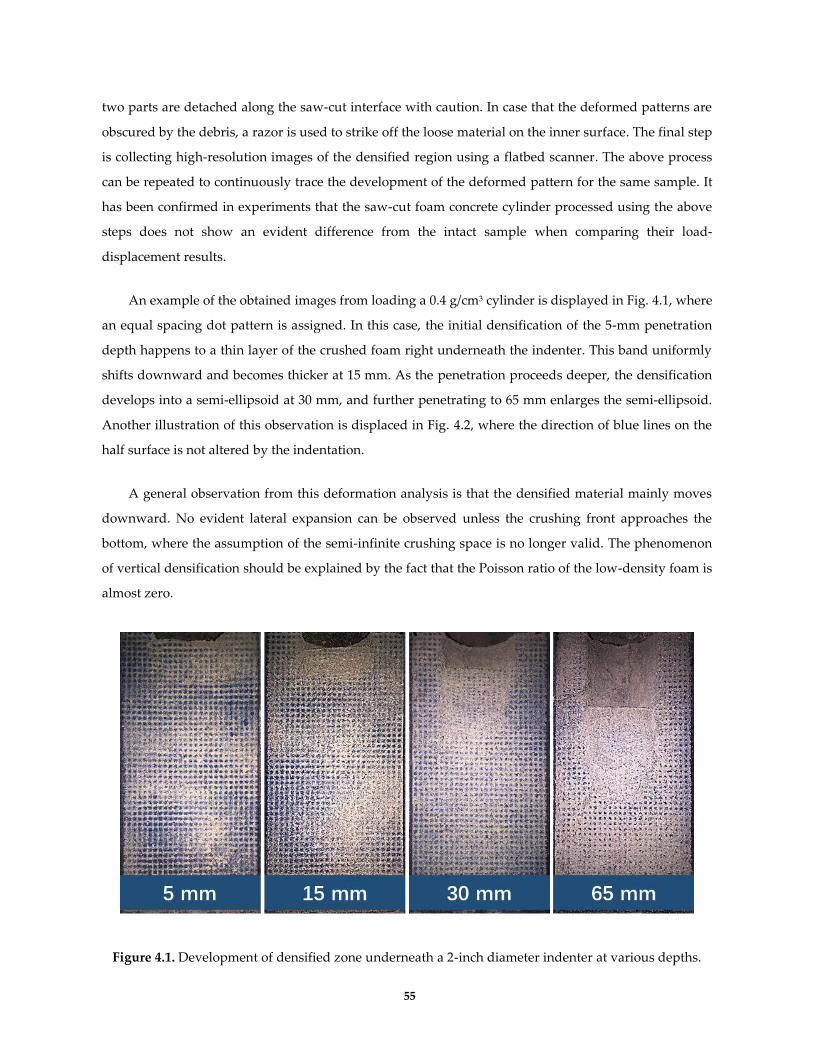
55

two parts are detached along the saw-cut interface with caution. In case that the deformed patterns are

obscured by the debris, a razor is used to strike off the loose material on the inner surface. The final step

is collecting high-resolution images of the densified region using a flatbed scanner. The above process

can be repeated to continuously trace the development of the deformed pattern for the same sample. It

has been confirmed in experiments that the saw-cut foam concrete cylinder processed using the above

steps does not show an evident difference from the intact sample when comparing their load-

displacement results.

An example of the obtained images from loading a 0.4 g/cm3 cylinder is displayed in Fig. 4.1, where

an equal spacing dot pattern is assigned. In this case, the initial densification of the 5-mm penetration

depth happens to a thin layer of the crushed foam right underneath the indenter. This band uniformly

shifts downward and becomes thicker at 15 mm. As the penetration proceeds deeper, the densification

develops into a semi-ellipsoid at 30 mm, and further penetrating to 65 mm enlarges the semi-ellipsoid.

Another illustration of this observation is displaced in Fig. 4.2, where the direction of blue lines on the

half surface is not altered by the indentation.

A general observation from this deformation analysis is that the densified material mainly moves

downward. No evident lateral expansion can be observed unless the crushing front approaches the

bottom, where the assumption of the semi-infinite crushing space is no longer valid. The phenomenon

of vertical densification should be explained by the fact that the Poisson ratio of the low-density foam is

almost zero.

Figure 4.1. Development of densified zone underneath a 2-inch diameter indenter at various depths.

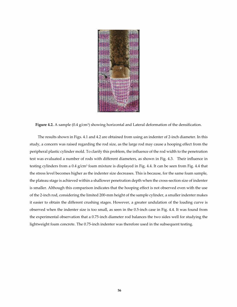
56

Figure 4.2. A sample (0.4 g/cm3) showing horizontal and Lateral deformation of the densification.

The results shown in Figs. 4.1 and 4.2 are obtained from using an indenter of 2-inch diameter. In this

study, a concern was raised regarding the rod size, as the large rod may cause a hooping effect from the

peripheral plastic cylinder mold. To clarify this problem, the influence of the rod width to the penetration

test was evaluated a number of rods with different diameters, as shown in Fig. 4.3. Their influence in

testing cylinders from a 0.4 g/cm3 foam mixture is displayed in Fig. 4.4. It can be seen from Fig. 4.4 that

the stress level becomes higher as the indenter size decreases. This is because, for the same foam sample,

the plateau stage is achieved within a shallower penetration depth when the cross-section size of indenter

is smaller. Although this comparison indicates that the hooping effect is not observed even with the use

of the 2-inch rod, considering the limited 200-mm height of the sample cylinder, a smaller indenter makes

it easier to obtain the different crushing stages. However, a greater undulation of the loading curve is

observed when the indenter size is too small, as seen in the 0.5-inch case in Fig. 4.4. It was found from

the experimental observation that a 0.75-inch diameter rod balances the two sides well for studying the

lightweight foam concrete. The 0.75-inch indenter was therefore used in the subsequent testing.

57

Figure 4.3. Indenters with different diameters used in the penetration test.

Figure 4.4. The penetration test results of indenting samples of a 0.4 g/cm3 mixture using indenters of

four diameters.

Another factor related to the indenter investigated in this study is the tip angle. Since the plateau

crushing stage is related to the formation of the densification zone, it is hypothesized that a sharper tip

can lead to an earlier onset of the plateau stage, as the tip should act as an equivalent part of the densified

material. To test the effect of the angled tip, four different tips with bottom angles of 30°, 45°, 60°, and

75°, as shown in Fig. 4.5, were investigated. Before testing, these tips were glued to the flat end of the

58

indenter. The test results of penetrating samples cast from a 0.4 g/cm3 mixture are shown in Fig. 4.6.

Obviously, the onset depth of the plateau stage is reduced with the increase of the tip angle. In the

extreme case of 75°, the plateau is achieved instantaneously as the indentation initiated.

Figure 4.5. Additional pointed indenter tips (0.75-inch diameter) used in the penetration test.

Figure 4.6. The penetration test results of indenting samples of a 0.4 g/cm3 mixture using indenters of

five tip angles.

Based on the preliminary investigation, it is noticed that special attention should be paid to the

vertical displacement of the densified material. After trial and error, the optimal correlation analysis

59

pattern to ease this observation was determined as 10-mm thick horizontal bands with alternating colors.

This arrangement ensures the color band not too thin after densification, nor too thick to capture the

details in the densified zone. A set of scans showing the deformed pattern from a progressive indentation

using the optimized pattern is displayed in Fig. 4.7. Notice that the pattern thickness of the densified

material becomes thinner as the indentation proceeds deeper, suggesting further densification of the

crushed material can happen when the penetration proceeds deeper, as the stress level becomes larger

(before the plateau stage).

Figure 4.7. Penetration of samples of a 0.4 g/cm3 mixture to 60, 90, and 120 mm, using a 0.75-inch

diameter indenter and the optimized pattern.

Several important crushing phenomena can be observed in Fig. 4.7. In all three cases, a zone

occupied with the densified material can be seen right underneath the indenter, where the deformed

color patterns are still mostly parallel to each other in this a cone-shaped region. This kind of densification

cone has been also reported in the literature studying the crushing of cellular materials, also named as

passive cone or dead zone [1,2]. To facilitate the discussion, a local magnification of the 90-mm deformed

pattern is highlighted in Fig. 4.8. The parallel pattern inside of the passive cone indicates the material

within its volume is failed through vertically volume collapse, which is essentially compressive

densification. Despite the minor progressive densification, the patterns in this passive cone are almost

unchanged as the penetration goes deeper. This implies that the densified material does not participate

in the crushing actively any longer. In contrast, it can be seen from Fig. 4.8 that the material densified at

both sides of the passive cone shows very a different deformed pattern—the color bands are highly

stretched along the edge of the passive cone. Seemingly, the densified material there experienced a

60

different type of deformation, very likely to be caused by shear. Note that the material underneath the

passive cone should still be crushed by compressive densification. In this study, the region experiencing

the active densification in between the passive cone and the intact foam (i.e., undeformed pattern) is

named as failure process zone. At this point, it is unclear whether the shear crushes the intact foam

directly, or it only affects the material densified by the crushing front.

Figure 4.8. A local magnification of the densified zone of the 90-mm penetration in Fig. 4.7, and

interpretation of its material densification mechanism.

To get an in-depth understanding of the densification phenomenon, the evolvement of the densified

pattern in a single 0.6 g/cm3 cylinder was further investigated with meticulous experimental control. This

cylinder had a greater height of 250 mm to allow inspecting the deformed pattern at larger depth. The

test was carried out with a 20-mm penetration interval before 140mm and a maximum penetration of

210mm at last. The loading response from the penetration test between 0 to 120 mm is shown in Fig. 4.9,

in which the result of a non-stop test for another sample from the same mixture (highlighted using the

dotted line) is provided for reference. Compared with the reference data, it is shown that the influence

of the 20-mm stepped penetration on the mechanical behavior of the sample is not significant.

Furthermore, the continuity of the loading curve is not affected by the interruption. The deformed pattern

collected at each interval from this test is displayed in Fig. 4.10. The information conveyed from these

patterns is largely in accordance with what has been observed in Fig. 4.8—the passive cone, process zone,

and deformation associated with the two types of densification. In this figure, a clear triangle shaped

passive cone is observed at 140 mm, through the outline of this cone has been gradually formed at a

shallower depth from 80 mm. Based on Fig. 4.9, the plateau stage of this test starts in between 80 and

100mm. Therefore, it is reasonable to correlate the formation of passive cone to the mechanical behavior

of foam concrete. Once formed, the deformed pattern in the passive cone does not experience obvious

change as the penetration proceeds further, as suggested by the almost identical pattern from 140 to 210

mm in Fig. 4.10.

61

However, part of the densified material must be deposited elsewhere so that the newly crushed

foam will not lead to infinite accumulation underneath the indenter. A relevant observation that helps to

explain the volume balance of the crushed material is the fractures found in the failure process zone in

Fig. 4.10. The discontinuity of the color bands in each photo of Fig. 4.10 are highlighted in Fig. 4.11, where

the green line indicates the primary shear planes at the two sides of the passive cone and the yellow line

indicates the fractures. It is found that the densified material in this region is fractured by shear, as

suggested by the clear offset of the color bands. It seems very possible that, compared with the stabilized

crushed material in the passive cone, the densified material in the process zone is temporarily presented

under the indenter. As the densified material accumulates in the process zone, the shear stress induced

by the local geometry and pressure buildup overcomes the cohesion of the crushed material and leads to

the shear fractures. These secondary shear fractures split the accumulated material into smaller

fragments. Afterward, the outmost fragment in the process zone is further pushed aside from the

penetration path and eventually deposited at the crushing wake. With respect to the mechanical

behavior, this dynamic material balance makes it possible to attain a steady stress state, which is the

plateau stage seen in the penetration test.

Figure 4.9. Test result of penetrating a 0.6 g/cm3 sample with a 20-mm step interval. The dotted curve is

a reference obtained by testing another sample from the same mixture without interruptions.

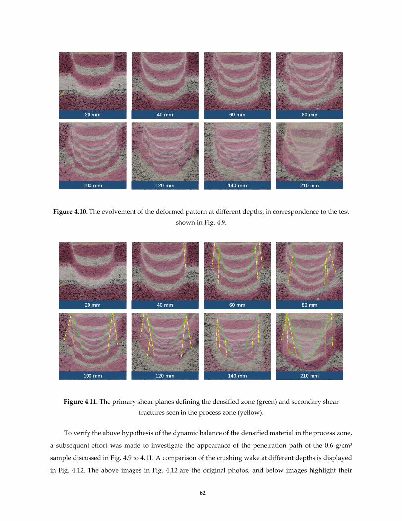
62

Figure 4.10. The evolvement of the deformed pattern at different depths, in correspondence to the test

shown in Fig. 4.9.

Figure 4.11. The primary shear planes defining the densified zone (green) and secondary shear

fractures seen in the process zone (yellow).

To verify the above hypothesis of the dynamic balance of the densified material in the process zone,

a subsequent effort was made to investigate the appearance of the penetration path of the 0.6 g/cm3

sample discussed in Fig. 4.9 to 4.11. A comparison of the crushing wake at different depths is displayed

in Fig. 4.12. The above images in Fig. 4.12 are the original photos, and below images highlight their

63

primary shear planes and secondary fractures in correspondence. At a closer inspection, it can be found

that the newly formed fragments are eventually deposited along the penetration path. The blue fractures

in Fig. 4.12, for example, are initially observed within the process zone at 80 mm, then pushed outward

by the new fragments at 100 mm, and deposited at 120 mm when the penetration proceeds to 120 mm. It

can be also observed from the crushing wake becomes thicker between about 0 to 60 mm, and then it

does not increase further at a greater depth. This observation can be reasonably correlated to the change

of the crushing stress as shown in Fig. 4.9, indicating that the evolvement of the crushing wake, densified

zone, and the mechanical behavior of the foam concrete are inner-connected. Overall, the above

observations regarding the crushing wake further validate the material deformation and densification

mechanism proposed in this study.

Figure 4.12. Crushing wakes along the path of penetration. In the bottom images, the primary shear

planes are highlighted with green and the secondary fractures are indicated with different colors.

4.3. Observation of the stress distribution in densification zone using DIC analysis

Despite the important observations regarding the densification phenomenon of foam concrete, some

limits of the correlation analysis can be noticed. One is that it does not allow continuous observation of

the development of the densified zone. Furthermore, each observation requires to interrupt the

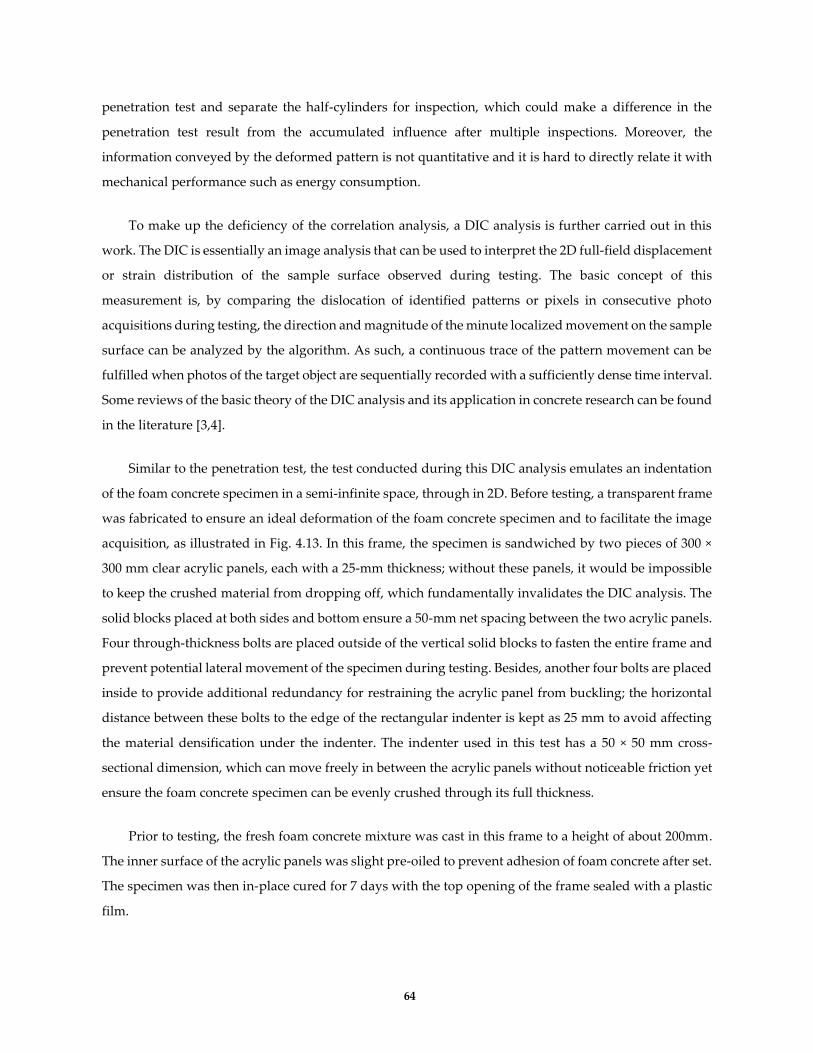
64

penetration test and separate the half-cylinders for inspection, which could make a difference in the

penetration test result from the accumulated influence after multiple inspections. Moreover, the

information conveyed by the deformed pattern is not quantitative and it is hard to directly relate it with

mechanical performance such as energy consumption.

To make up the deficiency of the correlation analysis, a DIC analysis is further carried out in this

work. The DIC is essentially an image analysis that can be used to interpret the 2D full-field displacement

or strain distribution of the sample surface observed during testing. The basic concept of this

measurement is, by comparing the dislocation of identified patterns or pixels in consecutive photo

acquisitions during testing, the direction and magnitude of the minute localized movement on the sample

surface can be analyzed by the algorithm. As such, a continuous trace of the pattern movement can be

fulfilled when photos of the target object are sequentially recorded with a sufficiently dense time interval.

Some reviews of the basic theory of the DIC analysis and its application in concrete research can be found

in the literature [3,4].

Similar to the penetration test, the test conducted during this DIC analysis emulates an indentation

of the foam concrete specimen in a semi-infinite space, through in 2D. Before testing, a transparent frame

was fabricated to ensure an ideal deformation of the foam concrete specimen and to facilitate the image

acquisition, as illustrated in Fig. 4.13. In this frame, the specimen is sandwiched by two pieces of 300 ×

300 mm clear acrylic panels, each with a 25-mm thickness; without these panels, it would be impossible

to keep the crushed material from dropping off, which fundamentally invalidates the DIC analysis. The

solid blocks placed at both sides and bottom ensure a 50-mm net spacing between the two acrylic panels.

Four through-thickness bolts are placed outside of the vertical solid blocks to fasten the entire frame and

prevent potential lateral movement of the specimen during testing. Besides, another four bolts are placed

inside to provide additional redundancy for restraining the acrylic panel from buckling; the horizontal

distance between these bolts to the edge of the rectangular indenter is kept as 25 mm to avoid affecting

the material densification under the indenter. The indenter used in this test has a 50 × 50 mm cross-

sectional dimension, which can move freely in between the acrylic panels without noticeable friction yet

ensure the foam concrete specimen can be evenly crushed through its full thickness.

Prior to testing, the fresh foam concrete mixture was cast in this frame to a height of about 200mm.

The inner surface of the acrylic panels was slight pre-oiled to prevent adhesion of foam concrete after set.

The specimen was then in-place cured for 7 days with the top opening of the frame sealed with a plastic

film.

65

Figure 4.13. An illustration of the transparent frame prepared for the DIC analysis.

The entire DIC testing setup used in this study is shown in Fig. 4.14. In this case, the specimen is a

0.4 g/cm3 mixture. Note that the color pattern assigned to the surface is only used for visual inspection

during testing and has no obvious contribution to the DIC analysis, as the air voids naturally appeared

on the surface of the foam concrete specimen provide sufficient characteristic patterns for this analysis.

During testing, the indentation was controlled with a small displacement rate of 10 mm/min. The image

acquisition was done with a VIC-2D measurement system. The camera fixed on a tripod was set in front

of the sample frame for consecutive image acquisition from a stationary viewpoint. The camera used had

a 12-megapixel resolution (4000 × 3000 pixels). The framing rate was set as 4 frames per second to capture

the details of the densification process.

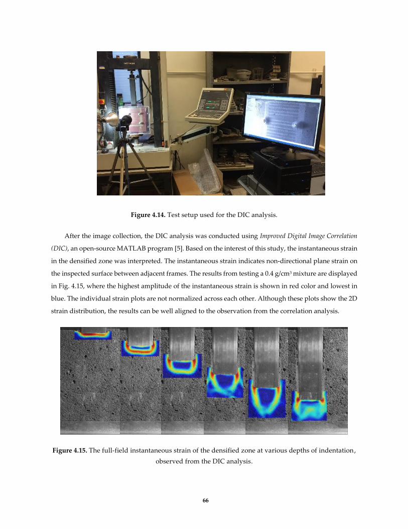
66

Figure 4.14. Test setup used for the DIC analysis.

After the image collection, the DIC analysis was conducted using Improved Digital Image Correlation

(DIC), an open-source MATLAB program [5]. Based on the interest of this study, the instantaneous strain

in the densified zone was interpreted. The instantaneous strain indicates non-directional plane strain on

the inspected surface between adjacent frames. The results from testing a 0.4 g/cm3 mixture are displayed

in Fig. 4.15, where the highest amplitude of the instantaneous strain is shown in red color and lowest in

blue. The individual strain plots are not normalized across each other. Although these plots show the 2D

strain distribution, the results can be well aligned to the observation from the correlation analysis.

Figure 4.15. The full-field instantaneous strain of the densified zone at various depths of indentation,

observed from the DIC analysis.

67

As the penetration started, a thin horizontal strain band first developed underneath the indenter.

The uniform strain distribution should be a result of the vertical crushing. The band then uniformly

extends downward which leaves a rectangular contour of the densified zone. Note that the dark-blue

material inside of this rectangular region had no strain value and it moved together with the indenter

like a rigid body. Once crushed, the densified material within this region did not experience further

deformation. Obviously, this corresponds to an early formation of the passive cone as what has been seen

in the correlation analysis. The process zone is seen of brighter colors at the outline of the passive cone.

As the indentation proceeds deeper, the rectangular densified zone was gradually transited to triangular.

The triangular shape of the passive cone remained unchanged until it touched the solid bottom.

Another marked finding is the different intensity of the strain in the process zone. It can be seen from

the third to fifth cases from Fig. 4.15 that the strain at the sides of the process zone (i.e., shear zone) is

much stronger than at near its bottom (i.e., crushing front). This observation is in line with the finding

from correlation analysis that the color pattern is more stretched in the shear zone. As larger strain

corresponds to larger stress, it is therefore deduced that the shear zone involves further densification of

the crushed material and therefore a larger resistance to the penetration during testing. Therefore, it is

very likely that the raise of the stress level before the plateau stage is essentially a transitional process

where the shear densification becomes increasingly more dominating in the foam concrete crushing.

4.4. A comparison of density variation of crushed foam concrete in the densified

zone using CT

A hypothesis proposed based on the DIC analysis is that, in the crushing process zone, the material

densified due to the shear failure experiences greater stress than compressive failure. If this is true, the

shear failure should lead to a more intensified densification at the sides of the process zone. To confirm

this hypothesis, the density variation in the densified zone is also examined using CT.

The CT specimen was excised from a cylinder cast with a 0.4 g/cm3 mixture after a penetration test

conducted at 7 days of age (penetration depth = 120 mm). The extracted specimen was a 40-mm diameter

by 100-mm height cylindrical core and its top surface was slightly above the contact surface between the

densified zone and the indenter, as shown in Fig. 4.16. The core extraction was done by 1) removing the

tested cylinder from the plastic mold and 2) progressively shaving it into the target dimension using a

utility knife. After cutting, no sign of densification was observed from the outside and bottom of this

cone. The CT test was implemented with 42-KeV X-ray tube voltage and 9.8-mA X-ray current. A total of

1440 frames were captured during the full rotation along the centerline of the specimen, with a 4-second

exposure for each frame.

68

Figure 4.16. Side (left) and top (right) views of the core extraction for CT analysis.

Several images obtained from the CT scan are shown in Fig. 4.17. In the CT scans, an object of a

higher density appears to be brighter. The small bright particles in the CT images are some cement

agglomerations left from the mixing process. From these images, it is seen that the diameter of the

densified zone becomes progressively smaller at larger depth and no densification can be observed at the

depth of 50 mm.

Figure 4.17. CT images of the specimen at different depths from its top surface. The side length of

each image is 40 mm.

The reconstructed 3D volume of the densified region is shown in Fig. 4.18. To investigate the density

variation inside of the densified zone, a split view of the CT model was taken and further processed to

optimize the visual contrast, as displayed shown in Fig. 4.19. In the original rendering, the densified zone

appears as the brighter region in the center of the CT model, and its contour is consistent with the

densification phenomena observed from the correlation analysis and DIC. Markedly, the inside of the

densified zone (i.e., passive cone) is seemingly darker than the outside (process zone). After the visual

enhancement, this difference becomes more obvious where the interface between the passive cone and

process zone can be well recognized. Clearly, the process zone has a higher brightness than the passive

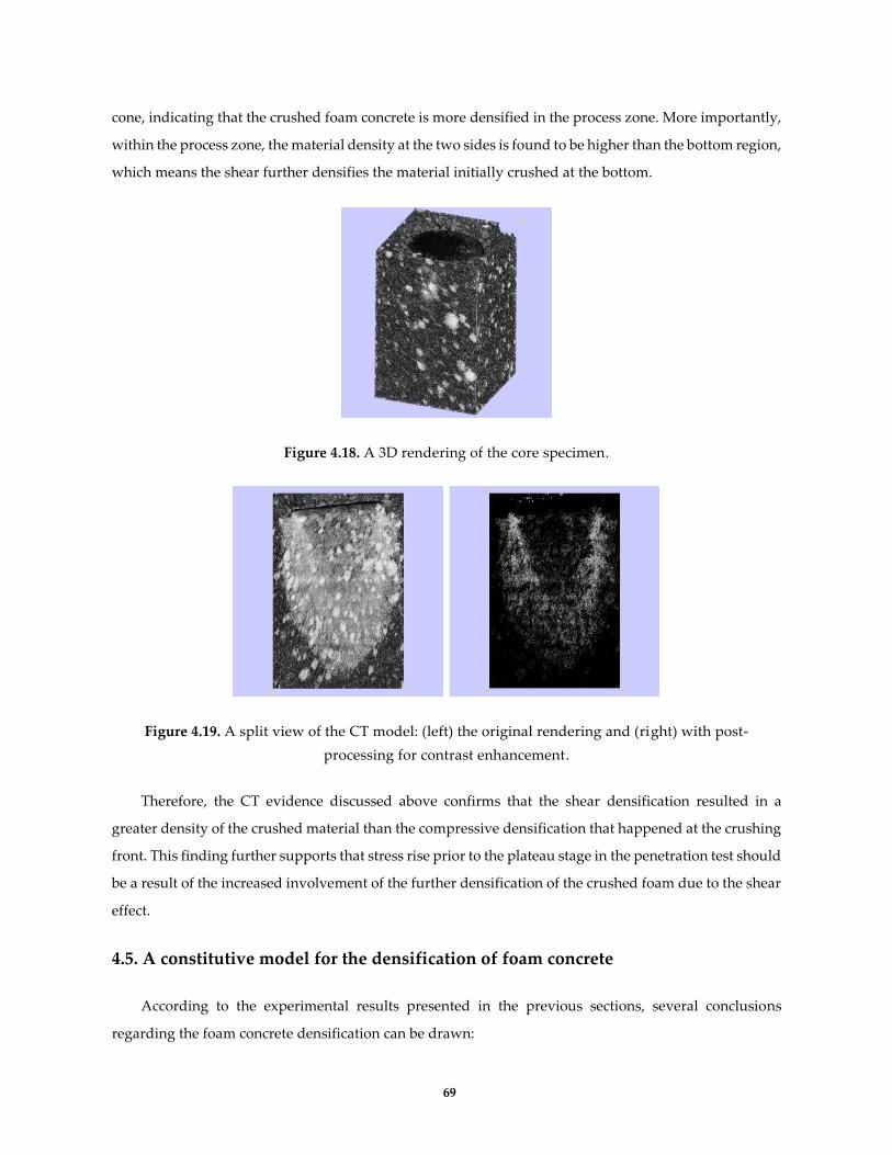
69

cone, indicating that the crushed foam concrete is more densified in the process zone. More importantly,

within the process zone, the material density at the two sides is found to be higher than the bottom region,

which means the shear further densifies the material initially crushed at the bottom.

Figure 4.18. A 3D rendering of the core specimen.

Figure 4.19. A split view of the CT model: (left) the original rendering and (right) with post-

processing for contrast enhancement.

Therefore, the CT evidence discussed above confirms that the shear densification resulted in a

greater density of the crushed material than the compressive densification that happened at the crushing

front. This finding further supports that stress rise prior to the plateau stage in the penetration test should

be a result of the increased involvement of the further densification of the crushed foam due to the shear

effect.

4.5. A constitutive model for the densification of foam concrete

According to the experimental results presented in the previous sections, several conclusions

regarding the foam concrete densification can be drawn:

70

1) The densified zone can be divided into two parts: passive cone and process zone.

2) Two material densification mechanisms (compressive and shear) are involved in the crushing

process.

3) The passive cone is formed by the densified foam due to the compressive densification, while

the crushed material in the process zone additionally experiences the shear densification.

4) During crushing, foam concrete is initially crushed due to the compressive densification at the

beginning of the penetration, but the shear densification becomes more dominant with the

increase of the penetration depth.

5) The shear induces a more intensified densification than the compression, as supported by the

highly stretched patterns and higher density of the densified material in the shear zone (at side

of the process zone). This shear densification leads to the raise of the resistance stress in between

the elastic and the plateau stages, as seen from the penetration test.

6) The secondary shear fracture observed in the process zone is of special importance to the

fulfillment of the material balance in the plateau stage.

7) The material balance involves the input of the newly crushed material formed at the bottom of

the process zone (crushing front) and output of the highly densified material deposited along the

penetration path (crushing wake).

Based on the above findings, an idealized constitutive model is proposed for explaining the

densification process of foam concrete during crushing, as illustrated in Fig. 4.20. This figure reflects the

dislocation of the densified foam concrete at one point of the plateau crushing stage in the penetration

test, where the material at different depth before penetration is highlighted using various colors and the

densified foam is shown with a darker color tone. Note that some densification details are simplified in

this model and the dimension of the crushed material does not necessarily represent the real size. For

instance, the width of the crushing wake should be much thinner, and the deformed pattern and shear

fractures in the process zone are not symmetric in reality.

71

Figure 4.20. An idealized densification model for the foam concrete crushing during penetration.

The crushing process in the penetration test can be described as follows. In the beginning, the foam

concrete under the indenter is all densified due to compression; and all the densified material contributes

to the formation of the top layer of the passive cone. As the penetration proceeds deeper, the crushed

foam outside the primary shear plane further experiences shear densification, which leads to the raise of

the stress curve. During the entire transitional crushing stage, the width of the passive cone gradually

becomes smaller, and increasingly more crushed foam is further densified by the shear effect. At the

starting point of the plateau stage, the formation of passive cone is accomplished so that all newly

crushed foam at the crushing front is further shear densified. Meanwhile, a balance between the newly

crushed and highly densified foam is achieved, which ensures that total resistant stress reacted to the

indenter is not increase any longer. This balance is maintained by concurrently 1) fracturing the densified

material in the process zone, 2) pushing the fractured fragments aside, due to the thrust of the passive

cone, and 3) depositing the outmost fragments along the crushing wake.

Based on the above findings, the energy consumption correlates to foam densification as shown in

Fig. 4.21. As explained above, the compressive densification is the dominating factor at the beginning of

the penetration. However, the shear densification makes an increasingly larger contribution to the total

energy at a greater depth before the plateau stage, as increasingly more crushed foam is further shear

densified. After that, the energy ratio between the two densification modes becomes constant, although

the contribution from shear can be higher by several times.

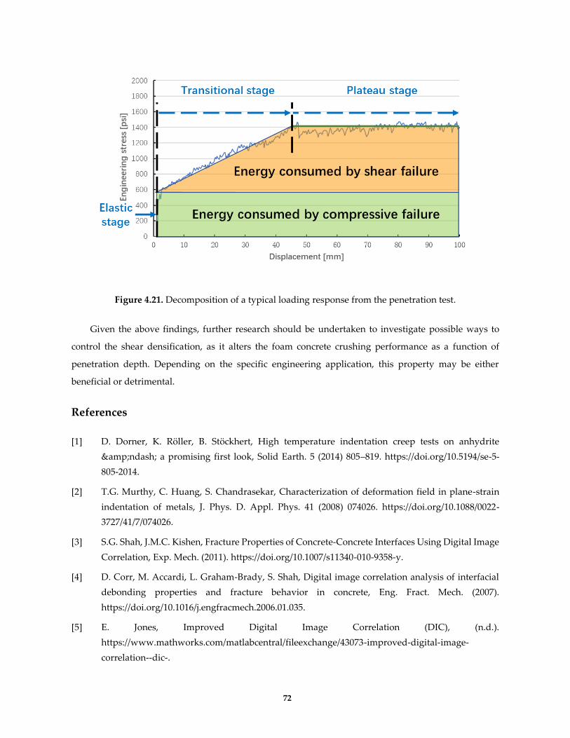
72

Figure 4.21. Decomposition of a typical loading response from the penetration test.

Given the above findings, further research should be undertaken to investigate possible ways to

control the shear densification, as it alters the foam concrete crushing performance as a function of

penetration depth. Depending on the specific engineering application, this property may be either

beneficial or detrimental.

References

[1] D. Dorner, K. Röller, B. Stöckhert, High temperature indentation creep tests on anhydrite

– a promising first look, Solid Earth. 5 (2014) 805–819. https://doi.org/10.5194/se-5-

805-2014.

[2] T.G. Murthy, C. Huang, S. Chandrasekar, Characterization of deformation field in plane-strain

indentation of metals, J. Phys. D. Appl. Phys. 41 (2008) 074026. https://doi.org/10.1088/0022-

3727/41/7/074026.

[3] S.G. Shah, J.M.C. Kishen, Fracture Properties of Concrete-Concrete Interfaces Using Digital Image

Correlation, Exp. Mech. (2011). https://doi.org/10.1007/s11340-010-9358-y.

[4] D. Corr, M. Accardi, L. Graham-Brady, S. Shah, Digital image correlation analysis of interfacial

debonding properties and fracture behavior in concrete, Eng. Fract. Mech. (2007).

https://doi.org/10.1016/j.engfracmech.2006.01.035.

[5] E. Jones, Improved Digital Image Correlation (DIC), (n.d.).

https://www.mathworks.com/matlabcentral/fileexchange/43073-improved-digital-image-

correlation--dic-.

73

CHAPTER 5: SPH simulation of foam concrete crushing behavior

This chapter covers an effort of using computer simulation to continue the investigation of the

crushing behavior of foam concrete. After determining the modeling strategies (e.g., simulation

algorithm, material model, and critical parameters, etc.), a simulation of the penetration test is first

implemented to cross-validate the results between the experiment and simulation. The simulation data

are then examined to highlight useful information that can be additionally obtained from this approach,

such as energy consumption. Subsequently, the crushing of an engineered material arresting system

(EMAS) made of foam concrete is simulated and further compared with the experimental observations

reported in the literature.

5.1. Introduction

Material modeling is essential for translating the findings of laboratory studies into practical full-

scale applications. The advancement of the finite element method (FEM) in recent years has unveiled

many new possibilities for the accurate evaluation of material mechanical behavior via computer

simulation. However, the work on simulating the crushing performance of foam concrete is rather limited

in the literature. A major challenge lies in the non-solid property of the foam material, which allows this

material to deform extensively under loading. The large deformation, along with the complex fracturing

process, makes it prohibitive to implement the conventional FEM built on Lagrange mesh for studying

foam concrete [1]. As illustrated in Fig. 5.1, either the compressive or shear densification leads to

extremely large deformation of the Lagrange mesh, which profoundly jeopardizes the computational

accuracy in the simulation.

Figure 5.1. Using Lagrange mesh for simulating the foam concrete crushing can result in severe mesh

distortion problems.

74

To overcome the inherent mesh distortion problem involved with the conventional Lagrange mesh,

attention is paid to the smoothed particle hydrodynamic (SPH) method, which is a novel meshless FEM

algorithm [2,3]. An illustration of the meshing of this approach is given in Fig. 5.2 [4]. In short, each

element in SPH simulation is a dissociative particle representing a local volume in the material. The

interaction between the particle of interest with its adjacent particles is computed using a concept of

influence zone (e.g., a circle in 2D and a sphere in 3D). In the analysis, all the other elements within the

influence zone are mathematically bonded with the element in concern, while a kernel function is further

applied to ensure the degree of interaction becomes smaller with the increase of the element distance.

This approach can be thereby used for simulating either solid continuum or more discrete materials such

as fluid. As a result, the meshing issue of the conventional FEM analysis is fundamentally bypassed.

Other merits of this approach include solving non-linear dynamic mechanical problems, ease for the

mesh generation, and good accuracy and time efficiency for computing high-strain deformation

problems, which is also applicable to the problem studied here.

Figure 5.2. An illustration of the SPH meshing algorithm, in the case of 2D [4].

After the literature review, it was determined that LS-DYNA is a good option for conducting the

SPH simulation. Although the SPH algorithm can be also implemented in other FEM software, LS-DYNA

is good at handling dynamic simulations where the large strain and extensive cracking need to be tackled.

The use of SPH simulation with LS-DYNA has been accepted in studying the crushing performance of

the glass-based engineered material arresting system (EMAS) and successful cases have been seen of

using this approach to evaluate the engineering behavior of this foam [5–7]. LS-DYNA has been also

adopted to simulate other cellular materials, such as honeycomb board [8] and EPS foam [9].

75

5.2. Critical settings of the simulation analysis

In LS-DYNA, hundreds of material cards (preset material model prototype) are provided for

simulating different material response under specific conditions. Based on the suggestion given from the

user manual, several material cards were considered, including LOW_DENSITY_FOAM,

CRUSHABLE_FOAM, MODIFIED_ CRUSHABLE_FOAM, and LOW_DENSITY_VISCOUS_FOAM.

According to the suggestions from previous studies, preliminary simulation results, and the material

parameters available from the experiments, it was finally determined that the CRUSHABLE_FOAM card

should provide the most reliable simulation result overall.

The material input parameters as required by the CRUSHABLE_FOAM card mainly includes foam

density, Young’s modulus of the foam (i.e., foam modulus), Poisson ratio, a load curve defining the

relationship of yield stress versus volumetric strain, a tensile stress cutoff, and a damping parameter. In

this study, the foam density, foam modulus, and load curve can be measured from the experiments such

as the resonant frequency test and penetration test. The Poisson ratio for low-density foam concrete is

typically assumed as a small value between 0 to 0.05. The tensile stress cutoff controls the tensile behavior

of the material, which reasonably ranges from 0.01 to 3% of the foam strength, depending on the foam

density. The damping factor is related to the strain rate sensitivity of the material; based on the

experimental observation, the lightweight foam concrete is not sensitive to the different strain rate

applied (e.g., 1-1000 mm/min) and this parameter value is therefore typically set to a small value close to

zero, such as 0.0001.

Another critical factor involves the contact parameters between the foam material (SPH elements)

with the solid boundary like the rigid ground or the indenter (Lagrange elements). It has been found that

inappropriate setting of the contact condition often results in unrealistic results in the simulation.

Problems such as unphysical object penetration, instable material response, and erroneous termination

of the analysis were seen during the model tuning phase. Base on the recommendations provided by the

LS-DYNA technician, it was found that the AUTOMATIC_NODES_TO_SURFACE contact card can

handle the contact between SPH and Lagrange elements soundly. Furthermore, it was found that the

SOFT constraint contact type under this contact card is superior to the other options for simulating the

foam crushing.

5.3. Simulation of the penetration test

The penetration test is the most frequently used mechanical test for characterizing the crushing

behavior of foam concrete in this research. Special attention has been paid to further investigate the foam

76

densification phenomenon involved in this test. Given the simplicity of this test yet relatively well-

studied testing phenomenon, the penetration test was first used as a benchmark for validating the SPH

simulation.

Multiple views of a 3D model built for simulating the penetration test is displayed in Fig. 5.3. This

model is generated with the actual dimension of the 100 mm × 200 mm foam concrete cylinder, as well

as for the cross-section size of the indenter. To ease the comparison with results obtained from the

correlation analysis, the color of SPH elements is altered after each 10-mm thickness. The rod indenter

and bottom plate are modeled as a rigid body. To emulate the penetration test, the indenter is vertically

loaded into the cylinder from its top center and the bottom plate and the SPH elements in the peripheral

layer of the cylinder are constrained for all six degrees of freedom. In order to reduce the computational

time, the loading rate of the indenter is set at a constant speed around ten times higher than the actual

value. It has been confirmed in a preliminary analysis that the influence of doing so is rather minor

compared to other model parameters in concern.

Figure 5.3. The meshed model of a 100 mm × 200 mm foam concrete cylinder in the penetration test.

For meshing the foam concrete cylinder, a critical factor that can constitute a hindrance to the

simulation accuracy is the mesh size. The inherent algorithm of SPH requires all elements distributed in

a cubic lattice fashion with equal particle spacing on the three directions [10]. However, a too dense mesh

requires significantly more computational time without noticeable gain on accuracy. As recommended

by the LS-DYNA technician, a general rule for choosing the mesh size is ensuring that each Lagrange

77

element in contact with at least nine SPH particles. The meshing of the foam concrete sample in this study

is slightly higher than this requirement at the critical regions such as the indenter edge.

A comparison between the experimental and the simulation results of the deformed pattern under

the indenter on the half surface of a 0.4 g/cm3 cylinder is given in Fig. 5.4. Evidently, the simulation

reasonably captures the details of foam densification, where the curved pattern caused by the shear effect

at both sides of the passive cone aligns well with the experimental observation.

Figure 5.4. Deformed patterns observed on the half surface of a 0.4 g/cm3 foam concrete cylinder from

the correlation analysis (left cases) and the corresponding simulation results (right cases).

The simulation shown in Fig. 5.4 can be further interpreted from different perspectives depending

on the property of interest. Some examples of these interpretations are displayed in Figs. 5.5 and 5.6. Note

that the color fringe of each case in these figures is adjusted for better visualization, not necessarily the

max/min value. In Fig. 5.5, the density of the crushed material is not even in the densified zone. Almost

all the intact foam is initially densified at the crushing front. Within the densified zone, the density at the

sides (i.e., the region dominated by shear effect in the process zone) is slightly higher, which agrees with

the conclusion on the shear densification from the CT analysis previously done. The second case shown

in Fig. 5.5 is a direct output of the crushing energy. Obviously, the shear densification at the sides

consumes more energy than the compressive densification at the crushing front. The strain distributions

at the same stage are provided in Fig. 5.6. The strain associated with the compressive densification is

exclusively concentrated at the crushing front. However, it is much smaller as compared to the strain

related to the shear densification, which is evident from the overall strain distribution as shown in the

other image. It is also encouraging that the overall strain distribution is very similar to what has been

obtained from the DIC analysis. Overall, the results of the experimental studies and SPH simulation

regarding the foam densification are in line with each other as cross-validation.

78

Figure 5.5. Different results of the simulated penetration test for the 0.4 g/cm3 sample: (left)

densification degree and (right) energy consumption.

Figure 5.6. Different results of the simulated penetration test for the 0.4 g/cm3 sample: (left)

compressive strain at the crushing front and (right) overall strain distribution.

The results of another simulation of penetrating a 0.6 g/cm3 foam concrete cylinder are shown in Figs.

5.7 to 5.10. The deformed patterns, densification, and strain rate are still in line with the observations

from the experimental studies. A clear sign of the densified material deposited along the crushing wake

is seen in Fig. 5.8. Note that the density difference between the passive cone and process zone too small

to differentiate in this case. In terms of the strain rate results in Fig. 5.9, it is encouraging to notice that

the fracturing process of the densified material in the process zone is also captured in the simulation. In

Fig. 5.9, the fracturing phenomenon is most obvious at 120 mm, but this phenomenon can be also

observed at the depths of 80 and 140 mm. Based on Fig. 5.10, the good agreement on the stress-

displacement curve further builds the confidence in using this proposed simulation approach to study

the mechanical behavior of foam concrete.

79

Figure 5.7. The deformed patterns observed on the half surface of a 0.6 g/cm3 foam concrete cylinder

from the simulation.

Figure 5.8. The densification in the 0.6 g/cm3 foam concrete cylinder from the simulation.

80

Figure 5.9. The strain rate in the 0.6 g/cm3 foam concrete cylinder from the simulation.

Figure 5.10. A comparison of the loading response between the experimental and simulation results.

5.4. Simulation of the crushing of an EMAS made of foam concrete by a B-737

wheel

After the cross-validation, a more complex crushing scenario was simulated. The aim of the new

simulation is to further investigate the feasibility of using the SPH method to predict the performance of

foam concrete in impact-absorbing applications. The background of the simulation is a halt of a B37-800

aircraft brought by an EMAS pad, similar to what is shown in Fig. 5.11.

81

Figure 5.11. An aircraft stopped by EMAS [11].

For simplification, this simulation focused on the arresting process of a wheel of the main landing

gear of the B737 aircraft. Based on the literature, some real design parameters of the aircraft wheel and

the EMAS pad used in practice is summarized in Table 5.1 [7,12], where the aircraft load that applied to

the wheel is derived by distributing the maximum take-off weight (MTOW) of the B373-800 to each wheel

of its main landing gears. This table also provides each corresponding parameter adopted in this

simulation. For the model setup, the aircraft wheel was assumed to be a piece of disc-shaped solid made

of stiff rubber. In the simulation, the aircraft load was applied as a vertical load to the center of the wheel

model. The gravity effect was also considered. At the beginning of the simulation, it was assumed that

the bottom of the wheel is just touching the top surface of an EMAS pad made of lightweight foam

concrete. The wheel has a horizontal speed of 9 m/s, along with a rotational speed such that there is no

relative speed at the touching point. The detailed properties of the foam concrete are the experimental

values measured in this study.

The simulated crushing of an EMAS made of a 0.4 g/cm3 foam concrete mixture is displayed in Fig.

5.12. In this case, the aircraft wheel is fully stopped after 3 seconds. The particle color indicates material

density, where the blue and red are respectively associated debris smaller than 0.2 g/cm3 from the

crushing action and the densified material greater than 1.0 g/cm3 along the rut. The simulated crushing

shows that the aircraft wheel mainly crushes the foam concrete downward, while the material at the side

surface of the rut remains almost undamaged. It is also worth mentioning that multiple rebounds of the

wheel due to the ground resistance are observed. The output results regarding the wheel deceleration

and energy absorbed from this simulation are respectively shown in Figs. 5.13 and 5.14, where these

82

results are reasonably correlated with each other. Note that the negative velocity observed between 2.5

and 3 seconds in Fig. 5.13 is caused by a roll-back action of the wheel at the end, which is a realistic

behavior that can be expected.

Table 5.1. Design parameters of the aircraft wheel and EMAS pad, and the assumed parameters.

Parameters Practical Simulation

Main gear tire

(B737-800)

Width [m] 0.41 Same

Diameter [m] 1.14 Same

Speed [m/s] 5-36 9

Load (per tire) [N] 167000 Same

EMAS

Length [m] 48-122 50

Depth [m] 0.56-0.71 0.6

Density [g/cm3] ~0.3 0.4/0.6

Figure 5.12. Different stages of the simulated crushing of a 0.4 g/cm3 foam concrete EMAS pad, from a

3D view.

83

Figure 5.13. Deceleration of the aircraft wheel in the simulation.

Figure 5.14. Energy absorption of the foam concrete pad in the simulation.

More details of the above simulation are compared with an experimental study conducted by Jiang

et al. [13]. In that experimental effort, the crushing phenomenon of a 0.2 g/cm3 lightweight foam concrete

is evaluated using a pendulum setup emulating the crushing from an aircraft wheel. For the simulation

results, the particle color still reflects the material density. As shown in Fig. 5.15, the first set comparisons

focus on the appearance of the rut. Despite that the EMAS pad cast in the experiment starts with a ramp,

the results are well comparable in terms of the subsequent regions with the in-depth crushing. As seen

from the first case, the foam under the wheel is compressed downward and little densification is found

on the side surface of the rut. In both experimental and simulation results, some debris left from the

84

crushing process is seen on the top surface. The second and third cases in Fig. 5.15 shows the cross-

sections of the rut, where a clear sign of densification can be seen under the wheel and the local

densification can be easily differentiated from the intact foam around. The major difference between the

second and third cases is that the crushing does not occur through the full depth of the foam concrete in

the former. The variation on crushing depth in the simulation is related to the rebound of the wheel

during the arresting process. These observations can be further aligned with the previous investigations

on the densification phenomenon in the penetration test.

The second set of comparisons shown in Fig. 5.16 focuses on the foam crushing around the wheel.

The simulation is consistent with the experimental observation that the rolling of the wheel does not lead

to foam densification forward. From the section view of the half surface along the center path, a curved

crushing front is seen underneath the wheel. Both the results further confirm that the foam concrete is

mostly compacted by the roll-over action from the wheel. This finding indicates that, if the crushing

energy of a unit volume of foam concrete and the average crushing depth is known, the total energy

dissipation involved in an arresting event of EMAS should be reasonably estimated.

Figure 5.15. A comparison of the crushing details at different locations along the rut between the

experimental observations reported by Jiang et al. [13] (above) and the simulated results obtained in

this study (below).

85

Figure 5.16. A comparison of the crushing details at the wheel front between the experimental

observations [13] (above) and the simulated results (below).

In this simulation effort, the arresting performance of an EMAS pad made of three typical foam

concrete mixtures was further evaluated. A comparison of the key material parameters of these materials

is given in Table 5.2. The other settings regarding the model geometry and boundary condition were kept

as the same as the standard model (see Table 5.1). The simulated crushing at the 3 seconds of these three

foam concrete mixtures is compared in Fig. 5.17, and their arresting performance is shown based on the

deceleration of the aircraft wheel in Fig. 5.18. To highlight the wheel movement during the entire

crushing, a black curve tracing the wheel center is added for each case in Fig. 5.17.

Table 5.2. Different design of the foam concrete compared in the EMAS crushing simulation.

Material Density

[g/cm3]

Elastic modulus

[MPa]

Plateau strength

[MPa]

Foam concrete 1 0.4 600 0.4



86

Figure 5.17. A comparison of the crushed EMAS pad made of three different foam concrete mixtures at

the end of the 3-second simulation, where the particle color indicates the material density. For each

case, half of the EMAS volume is are set transparent to show the density variation on the rut cross-

section, and the black curve is a trace of the wheel movement.

Figure 5.18. A comparison of the crushed EMAS pad made of different foam concrete mixtures after at

the end of a 3-second simulation.

Comparing the performance of the three EMAS pads, it is somewhat surprising to find that the

strongest 0.6 g/cm3 foam concrete exhibits the worst arresting capability. It is seen from Figs. 5.17 and

5.18 that it even does not bring the aircraft wheel to a full halt within the 50-m length of the EMAS pad

and within the 3-second simulation. This should be caused by the fact that the crushing strength of the

87

0.6 g/cm3 foam concrete is too high to allow enough penetration depth of the wheel. Therefore, most of

the foam under the wheel remains inactive regarding absorbing the kinetic energy from the running

wheel.

In contrast, both the 0.4 g/cm3 mixtures stop the wheel almost at the same time of 2.5 seconds.

However, further comparison between these two cases finds a more intensive vertical bumping of the

wheel (i.e. rebound observed previously) exists when the weakest foam is used. In comparison, a

smoother deceleration and a more consistent crushing depth are seen from its counterpart. Furthermore,

it can be observed in Fig. 5.17 that the crushing distance associated with the stronger 0.4 g/cm3 foam is

the shortest among all. Therefore, this comparison indicates that the material selection of foam concrete

for EMAS needs an overall consideration of the wheel-foam interaction—a foam that is too strong or

overly soft cannot bring the optimal attesting performance to an EMAS application.

In summary, the above results demonstrate that the SPH simulation can provide a realistic

estimation of the crushing behavior of foam concrete, either for the lab test or field application. The

simulation can give important information about the impact-absorbing performance of foam concrete.

This simulation approach also serves as an efficient way to facilitate the material optimization of foam

concrete design with respects to specific engineering applications.

References

[1] J. Fish, T. Belytschko, A First Course in Finite Elements, 2007.

https://doi.org/10.1002/9780470510858.

[2] J.J. Monaghan, Smoothed particle hydrodynamics, Reports Prog. Phys. (2005).

https://doi.org/10.1088/0034-4885/68/8/R01.

[3] R.A. Gingold, J.J. Monaghan, Smoothed particle hydrodynamics: theory and application to non-

spherical stars, Mon. Not. R. Astron. Soc. (1977). https://doi.org/10.1093/mnras/181.3.375.

[4] Z. Dai, F. Wang, Y. Huang, K. Song, A. Iio, SPH-based numerical modeling for the post-failure

behavior of the landslides triggered by the 2016 Kumamoto earthquake, Geoenvironmental

Disasters. (2016). https://doi.org/10.1186/s40677-016-0058-5.

[5] Y. Shi, EMAS Core Material Modeling with LS-DYNA ®, in: 11th Int. LS-DYNAUsers Conf., 2010:

pp. 21–36.

[6] B. Croop, H. Lobo, Selecting material models for the simulation of foams in LS-DYNA, in: 7th Eur.

LS-DYNA Conf., 2009. http://www.dynamore.de/de/download/papers/konferenz09/papers-

depr/D-II-04.pdf.

[7] M. Barsotti, ACRP Report 29: Developing Improved Civil Aircraft Arresting Systems, 2009.

https://doi.org/10.17226/14340.

88

[8] S. Heimbs, P. Middendorf, M. Maier, Honeycomb sandwich material modeling for dynamic

simulations of aircraft interior components, in: 9th Int. LS-DYNA Users Conf., Dearborn, MI, 2006:

pp. 1–13.

[9] Q.H. Shah, A. Topa, Modeling Large Deformation and Failure of Expanded Polystyrene

Crushable Foam Using LS-DYNA, Model. Simul. Eng. 2014 (2014) 1–7.

https://doi.org/10.1155/2014/292647.

[10] J. Hallquist, LS-DYNA theory manual, 2006.

[11] Fact Sheet of EMAS, (n.d.). https://www.flysfo.com/about-sfo/airport-development/runway/fact-

sheet.

[12] M. Barsotti, Optimization of a Passive Aircraft Arrestor with a Depth-Varying Crushable Material

Using a Smoothed Particle Hydrodynamics (SPH) Model, The University of Texas at San Antonio,

2008.

[13] C.S. Jiang, H.Y. Yao, X.B. Xiao, X.J. Kong, Y.J. Shi, Phenomena of foamed concrete under rolling

of aircraft wheels, in: J. Phys. Conf. Ser., 2014. https://doi.org/10.1088/1742-6596/495/1/012035.

89

CHAPTER 6: Effect of sand inclusion on foam morphology and mechanical

performance of lightweight foam concrete

Lightweight foam concrete may be produced with fine aggregates. Such material provides an

opportunity to utilize waste materials that are commonly discarded. Especially when recycled fine

particles are used at high volumes, there may be an adverse effect on the foam structure, which

diminishes mechanical performance. This chapter examines the effect of particle dosage and size on the

microstructure and mechanical performance of foam concrete are investigated. Lightweight mixtures

with different densities were produced with river sand of various dosages and sizes. The foam

morphology was inspected using optical and scanning electron microscope (SEM) imaging, and the

tested mechanical properties included fundamental frequency, elastic modulus, crushing strength, and

compressive strength. A constitutive relationship was further proposed for predicting the crushing

strength. This study suggests that the high-volume particle inclusion can be facilitated by improving the

foam density and reducing the particle size.

6.1. Introduction

Among all the man-made engineering materials, concrete is at the forefront in terms of total

production. Over the past decades, the way that concrete was fabricated, used, and demolished all

contributed to the current environmental issues, such as the CO2 emission [1], potable water pollution

[2], and damage to the natural riverbed [3,4]. To promote green engineering, recycling of various waste

materials as aggregates for new concrete structures has broad prospects [5–10]. Due to inconsistent

properties, recent research generally finds the use of recycled waste fine particles more challenging for

producing normal concrete, especially when the material strength is of a high priority [9–11]. As such,

the utilization of recycled fines is often seen in the fabrication of a type of concrete engineered with an

inferior strength, known as controlled low-strength concrete (CLSM) [12]. The conventional CLSM

mixture often has a high water-to-cementitious ratio (w/cm) and consists of low-grade binder and fillers.

While it has been increasingly accepted in engineering practice, its application is mainly limited to

excavatable backfill [13,14].

In contrast, foam concrete as a novel CLSM has more diversified application scenarios [14,15],

potentially enriching the use of various recycled fines in construction projects. Foam concrete is typically

a low-density cement paste or mortar cellularized with a large amount of air entrainment, where the

maximum air content can be more than 80% in extremity [16]. While the density range of foam concrete

varies from 0.3 to 1.6 g/cm3, the lightweight foam concrete (< 0.8 g/cm3) usually possesses a series of

unique functionalities not seen in conventional cementitious materials, such as low thermal and acoustic

90

isolation [17,18]. Taking advantage of its crushable nature, some recent studies have also found that

lightweight foam concrete provides an ideal engineering solution for impact absorption. Engineered

materials arresting system (EMAS), for instance, can be made with lightweight foam concrete to absorb

the kinetic energy of aircraft when overrun happens and bring the aircraft to a safe halt [19,20]. Other

examples include vibration damping for high-speed rail [21] and seismic isolation of structures [22,23].

These applications provide many chances for using recycled fines in foam concrete, which can also

reduce the cement usage in turn. Existing literature has investigated the feasibility of using different

types of particles, such as coarse fly ash [21,24], quarry wastes [25], and crumb rubber [24].

When adding particles to foam concrete, one of the biggest challenges is preserving the foam structure

in the cement paste during the mixing and placement process. Before set, the fragile air bubbles in fresh

concrete are sensitive to the physical condition applied so that insufficient control of the particle inclusion

can result in a drastic performance loss [18,26–28] or even a catastrophic volume collapse of the foam

[17,29,30]. However, existing literature addressing the particle inclusion in foam concrete mostly focused

on the mixtures greater than 0.8 g/cm3 [17,18,27], and only a few studies extended emphasis on the

microstructure morphology in foam concrete [16,26,31,32]. As the bulk density of foam concrete is the

design target in most of the studies, the density of the foamed cement paste of the investigated mixtures,

however, varies with sand dosage such that it is hard to quantify the effect of particle inclusions on the

foam specifically. This lack of understanding still constitutes a hindrance to the broad use of particle

inclusion in functional applications of lightweight foam concrete.

This study aims to clarify the influence of particle inclusion on the morphology and mechanical

performance of lightweight foam concrete. Two sets of mixtures are designed with identical densities of

the foamed cement paste, as 0.6 and 0.4 g/cm3. Fine river sand was invoked as the standard reference

particle inclusion. Four consecutive sand sizes between 150 to 1180 μm are investigated under the sand-

cementitious weight ratio, namely sand ratio, of 0, 0.25, 0.5, and 1.0. After an initial inspection of the foam

microstructure for all the mixtures using optical imaging, the void size distribution and circularity of the

mixtures of 0.5 sand ratio were characterized using scanning electron microscope (SEM). The mechanical

performance of the mixture was evaluated using vibrational frequency test for fundamental frequency

and dynamic modulus, a penetration test for crushing behavior, and the conventional compression test.

Based on the experimental findings, a relationship previously proposed for predicting the crushing

strength of foamed paste was amended to accommodate the scenario with particle inclusion. The

predicted results showed a good agreement with the testing data.

91

6.2. Materials and Sample Preparation

Two sets of foam mixtures were investigated, with their basic information summarized in Table 6.1.

They are different in the density of the foamed cement paste (hereinafter, foam density), which

respectively are 0.4 and 0.6 g/cm3. The foam concrete design generally followed ASTM C796 [33]. The

sample nomenclature in this paper specifies foam density, sand ratio, and sand size. At each foam

density, a controlled mixture of pure foamed paste and three sets of composite mixtures with sand ratios

of 0.25, 0.5, and 1.0 were prepared. The resultant volume percentage of sand in the mixture is given as

Vsand in Table 6.1. Note that this value does not increase by proportion perfectly, as the cement usage is

slightly decreased by the sand addition. Regarding the sand size, the raw sand was sieved into four

consecutive categories from 150 to 1180 μm for casting mixtures at each sand ratio. This range was chosen

to cover the air void size span in some similar samples previously studied [32]. For a fixed foam density,

the bulk density of the mixtures increases with the sand ratio, which also leads to reduced usage of the

cementitious materials in a unit volume. In this table, αpaste indicates the void content in the foamed paste.

The ρdesign and ρmix indicate the designed and measured bulk density of the whole mixture, respectively.

For the mixture fabrication, the mixing work followed the procedures described in Section 1.3. The

foam concrete mixture was then weighed in a standard container with a known volume to determine ρmix.

In case that ρmix deviated more than 3% from ρdesign, the mixture would be recast. Table 6.1 only shows the

accepted mixtures. The density change at later ages was found to be negligible. During mixing, severe

volume collapse was observed in all mixtures of 0.4 g/cm3 foam density and 1.0 sand ratio (0.4_1.0_150 to

0.4_1.0_850), as their foam structure could not support the self-weight of sands. Hence, those mixtures were

excluded from all subsequent testing.

The foam concrete mixture was cast into thee cylindrical molds (101.6 mm diameter × 203.2 mm tall)

and two prismatic molds (50.8 × 50.8 × 203.2 mm). The samples were cured in sealed condition until 7

days to avoid the potential damage from demolding at earlier ages. Only the prism samples were

demolded at 7 days, as the cylinder samples were tested without demolding. The samples were

subsequently cured in a 100% RH environmental chamber.

92

Table 6.1. Layout the mixtures and their densities.

Mixture ρfoam

[g/cm3]

αpaste

[%]

Sand

ratio

Vsand

[%]

Sand size

[um]

ρdesign

[g/cm3]

ρmix

[g/cm3]

0.6_Control

0.6 68.1

0 0 - 0.6 0.609

0.6_0.25_150

0.25 3.76

150-300 0.682 0.685

0.6_0.25_300 300-600 0.682 0.688

0.6_0.25_600 600-850 0.682 0.694

0.6_0.25_850 850-1180 0.682 0.672

0.6_0.5_150

0.5 7.24

150-300 0.752 0.753

0.6_0.5_300 300-600 0.752 0.758

0.6_0.5_600 600-850 0.752 0.740

0.6_0.5_850 850-1180 0.752 0.755

0.6_1.0_150

1.0 13.50

150-300 0.879 0.882

0.6_1.0_300 300-600 0.879 0.904

0.6_1.0_600 600-850 0.879 0.897

0.6_1.0_850 850-1180 0.879 0.901

0.4_Control

0.4 78.7

0 0 - 0.4 0.400

0.4_0.25_150

0.25 2.52

150-300 0.458 0.457

0.4_0.25_300 300-600 0.458 0.447

0.4_0.25_600 600-850 0.458 0.445

0.4_0.25_850 850-1180 0.458 0.469

0.4_0.5_150

0.5 4.93

150-300 0.512 0.517

0.4_0.5_300 300-600 0.512 0.510

0.4_0.5_600 600-850 0.512 0.500

0.4_0.5_850 850-1180 0.512 0.506

0.4_1.0_150

1.0 9.38

150-300 0.611 NA

0.4_1.0_300 300-600 0.611 NA

0.4_1.0_600 600-850 0.611 NA

0.4_1.0_850 850-1180 0.611 NA

93

6.3. Testing methods

6.3.1. Mechanical tests

The vibrational frequency test specified by ASTM C215 was used to measure the dynamic elastic

modulus of the foam prism samples (hereinafter, foam modulus) at 7, 14, 21 days [35]. During testing,

the transverse fundamental vibration frequency n was measured, and five measurements were collected

from each sample to give the average value for calculating the dynamic elastic modulus of the foam

concrete mixtures (hereinafter, foam modulus) E:

𝐸 = 𝐶𝑀𝑛2 (6.1)

where C is a geometry parameter and M is specimen mass. The M was measured at each testing date.

More details about this test are reported in Section 2.3.3.

The foam concrete crushing behavior was studied using a penetration test at 7, 14, 21 days. This

testing measured the load-displacement curve while loading a steel rod into the foam concrete cylinder

from the top center, as detailed in Section 3.3.3.

After the last vibrational test at 21 days, the prism samples were saw-cut into 50.8-mm cubes for

measuring unconfined uniaxial compressive strength. For each mixture, six cubes were tested; the two

remaining short prisms were reserved for studying void morphology. This test was implemented using

the Instron-4502 loading frame. Prior to loading, the top and bottom ends of each cube was capped using

unbonded rubber pads. The loading rate was controlled at 6 mm/min. The maximum stress recorded was

reported as the compressive strength.

6.3.2. Morphology characterizations

The foam morphology of the mixtures was investigated using two methods. Optical imaging of the

polished sample section was first done using a high-resolution flatbed scanner. This an initial inspection

covered for all the mixtures, and the goal is to check if any mixture has a segregation issue of the air void

or sand. The samples were excised from the unloaded short prisms left by the saw-cutting from the

compression test at 21 days. For the surface preparation, the cross-section of the short prism was

progressively polished using 80 (200 μm), 180 (80 μm), 240 (35 μm), and 600 grit (35 μm) sandpapers.

Further polishing was found unhelpful to improve the surface quality, which was limited by the

damaging to the foam structure induced by the abrasion action. After blowing off the debris with low-

pressure air, a 50×50 mm region was scanned for each mixture, at a 4800 dpi (5.3-μm) pixel resolution.

94

However, it was found that the contrast of the optical images was not satisfactory for a quantitative

comparison of the foam microstructure, and therefore a set of mixtures was further characterized using

SEM. This analysis was implemented on the two controlled mixtures and all those of 0.5 sand ratio. The

test was done with a JEOL JSM-6060LV SEM. The SEM sample was extracted as a 10×10×3 mm chip from

the center of the short prism at 28 days, using a low-speed ceramic saw. To preserve the void structure

from polishing damages, each sample was firstly epoxy impregnated with LR White resin under high

vacuum for 24 hours, followed by a 60°C curing for 12 hours. The hardened sample was then sawed and

polished down to 1200 grit (5 μm). The SEM scans were collected under the back-scatter mode, using

10kV voltage at a magnification of 25 ×. Each scan covered an area of about 5.1 ×3.8 mm, with a 3.97-μm

pixel resolution. The SEM scan was processed using ImageJ for obtaining the size distribution of the void

intersections appeared on the cross-section.


6.4.1. Optical imaging

A 50×50 mm region of the polished cross-section of each mixture was scanned using a flatbed

scanner. For visualizing the sand particles, a 10×10 mm center portion of each scan is displayed in Fig.

6.1. In Fig. 6.1a, the void size in the 0.6 g/cm3 mixtures becomes larger at a higher sand ratio or a larger

particle size. In Fig. 6.1b, more large voids can be observed from the 0.4 g/cm3 mixtures, but the contrast

across different mixtures is less noticeable, which is partly because some large voids already exist in

Control_0.4. Some cement agglomerations are found in the 0.4 g/cm3 mixtures, as suggested by the solid

regions in gray. Under a closer inspection of the full-size scans, no evident segregation of either air void

or sand was observed in any foam-sand composite mixtures.

95

(a)

(b)

Figure 6.1. A comparison of the optical scan of the polished cross-section (10×10 mm) of the prism

samples for the (a) 0.6 and (b) 0.4 g/cm3 mixtures.

96

6.4.2. SEM

SEM was implemented as an extension of the optical inspection. The scanning covered the eight

composite mixtures of 0.5 sand ratio, along with the two controlled mixtures. The SEM images are

displayed in Fig. 6.2. Under the back-scatter scanning mode, the low-density epoxy impregnated into the

air voids appears to be darker, giving a contrast to the brighter solid phases (i.e., hydrated cement paste

and sand). The sand particles are seen braced by the thin cement struts, while the struts in the 0.4 g/cm3

mixtures are slimmer than the 0.6 g/cm3 mixtures. The air voids become larger from 0.6 to 0.4 g/cm3

mixtures. With respect to the influence of sand size, the larger particles induce greater disturbance to the

foam system during mixing, as agreed by previous studies [25,26,32].

Figure 6.2. A comparison of the SEM images for the controlled and 0.5 sand ratio mixtures. The

samples are scanned under back-scatter mode, at a 25× magnification.

97

Figure 6.2. continued.

6.4.3. Fundamental frequency and foam modulus

Foam modulus is an intrinsic parameter that can be correlated to many mechanical properties. Over

the testing period, the result of foam modulus for each mixture is primarily controlled by the

fundamental frequency, as the change on sample mass and geometry was found to be negligible. The test

98

results of fundamental frequency and foam modulus are shown in Tables 6.2 and 6.3 for the 0.6 and 0.4

g/cm3 mixtures, respectively. Note that the larger standard deviation of foam modulus is primarily

attributed to the fact that the modulus is proportional to the square of frequency (see Eq. 6.1).

In Table 6.2, the frequency of the 0.6 g/cm3 mixtures with 150-, 300-, and 600-µm sand are close to

that of 0.6_Control. However, the use of 850-µm sand decreases the frequency as the sand ratio becomes

larger. In contrast, the foam modulus is evidently improved as sand ratio goes higher. The modulus gain

of the mixtures with 850-µm is smaller than those with finer sand inclusions, due to the frequency

reduction. In Table 6.3, the inclusions of 300-, 600-, and 850-µm sand all result in decreased fundamental

frequency for the 0.4 g/cm3 mixtures, as compare with Control_0.4. The frequency reduction of the 0.4

g/cm3 mixtures is also more intensive than their 0.6 g/cm3 counterparts. At both 0.25 and 0.5 sand ratios,

the foam modulus of the 0.4 g/cm3 mixtures declines as larger sand particles are used.

Table 6.2. Fundamental frequency and foam modulus of the 0.6 g/cm3 mixtures. The standard

deviation for each case is shown in parentheses.

Mixture Fundamental frequency [Hz] Foam modulus [MPa]

7 days 14 days 21 days 7 days 14 days 21 days

0.6_Control 1856 (6) 1904 (11) 1964 (12) 1588 (19) 1669 (34) 1779 (61)

0.6_0.25_150 1837 (12) 1911 (9) 1965 (24) 1805 (38) 1947 (31) 2072 (69)

0.6_0.25_300 1869 (2) 1953 (15) 2028 (6) 1880 (12) 2053 (41) 2210 (24)

0.6_0.25_600 1764 (13) 1880 (6) 1937 (2) 1682 (22) 1894 (3) 2013 (8)

0.6_0.25_850 1768 (3) 1861 (8) 1905 (9) 1627 (0) 1795 (4) 1871 (38)

0.6_0.5_150 1857 (3) 1945 (6) 1929 (0) 2023 (14) 2221 (11) 2191 (11)

0.6_0.5_300 1895 (3) 1984 (3) 1930 0 2121 (12) 2327 (14) 2206 (6)

0.6_0.5_600 1820 (7) 1933 (11) 1932 (13) 1937 (10) 2176 (26) 2178 (29)

0.6_0.5_850 1731 (1) 1795 (6) 1828 (22) 1757 (33) 1891 (55) 1960 (27)

0.6_1.0_150 1824 (4) 1925 (6) 1945 (11) 2284 (5) 2541 (1) 2603 (17)

0.6_1.0_300 1818 (11) 1904 (8) 1944 (17) 2322 (55) 2547 (46) 2662 (77)

0.6_1.0_600 1770 (8) 1883 (2) 1928 (4) 2179 (22) 2465 (1) 2585 (6)

0.6_1.0_850 1568 (13) 1665 (15) 1711 (31) 1720 (36) 1940 (45) 2047 (101)

99

Table 6.3. Fundamental frequency and foam modulus of the 0.4 g/cm3 mixtures. The standard

deviation for each case is shown in parentheses.

Mixture Fundamental frequency [Hz] Foam modulus [MPa]

7 days 14 days 21 days 7 days 14 days 21 days

0.4_Control 1430 (18) 1488 (22) 1500 (14) 638 (19) 691 (22) 700 (16)

0.4_0.25_150 1415 (8) 1472 (12) 1488 (20) 726 (4) 788 (26) 807 (22)

0.4_0.25_300 1237 (28) 1272 (34) 1268 (33) 554 (34) 582 (43) 576 (42)

0.4_0.25_600 1098 (3) 1193 (18) 1231 (10) 421 (1) 495 (13) 532 (9)

0.4_0.25_850 1093 (27) 1121 (14) 1187 (33) 436 (21) 459 (11) 511 (29)

0.4_0.5_150 1568 (2) 1588 0 1591 (23) 1039 (19) 1062 (18) 1066 (19)

0.4_0.5_300 1323 (6) 1347 (1) 1416 (5) 719 (11) 742 (1) 824 (11)

0.4_0.5_600 1312 (3) 1308 (7) 1331 (4) 688 (5) 700 (19) 709 (2)

0.4_0.5_850 941 (11) 977 (7) 1021 (6) 350 (13) 377 (10) 412 (9)

6.4.4. Crushing behavior

The crushing behavior of the mixtures is evaluated at the age of 7, 14, and 21 days using a penetration

test. Despite the difference in resistant force, the trend of the load curves for the same mixture is found

to be almost identical at the three ages. To ease the discussion, only the 21-day load-displacement curves

are given in Figs. 6.3 and 6.4 to display the crushing behavior of the 0.6 and 0.4 g/cm3 mixtures,

respectively. The load curves show the crushing behavior of the samples at a maximum indentation

depth of 140 mm, beyond which the material response is affected by the rigid bottom. The indentation

stress in these figures equals to the resistant force divided by the area of the circular indenter cross-

section. The crushing behavior follows the typical response of foamed cement paste--the load curve start

with a linear elastic phase once the indenter contacted the sample, followed by a transitional phase with

the indentation stress increasing at a constant rate, and finally reaching to a plateau phase where the

stress level becomes constant [32,36].

As seen from Figs. 6.3 and 6.4, the sand inclusion diminishes the foam concrete crushing

performance at high dosage or/and with larger particles. For the 0.6 g/cm3 mixtures of 0.25 sand ratio, the

crushing performance seems to be slightly enhanced with 150- and 300-µm sand, but the 850-µm leads

to an evident performance loss. With the sand ratio improved to 0.5 and 1.0, the plateau of the mixtures

containing 150-, 300-, and 600-µm sand is only mildly reduced, while the performance loss for 0.6_0.5_850

and 0.6_1.0_850 are much aggravated. In comparison, the 0.4 g/cm3 mixtures are more influenced by sand

100

inclusion. Only the 150-µm sand does not cause a performance loss but using 300-, 600-, and 850-µm sand

particles all lead to diminished crushing performance, for both 0.25 and 0.5 sand ratios.

From Figs. 6.3 and 6.4, it seems that the sand inclusion can shorten the onset depth of the crushing

plateau, as suggested by the leftward shift of the plateau phase at a higher sand ratio. For example, this

depth is about 120 mm for 0.6_0.25_600, 100 mm for 0.6_0.5_600, and 80 mm for 0.6_1.0_850. In another

case, the depth is about 100 mm for 0.4_0.25_300 and 80 mm for 0.4_0.5_300. Although further studies

are needed, the use of sand might have a certain significance for controlling the onset of the crushing

plateau in foam concrete. In EMAS applications, for instance, this depth varying energy-absorbing rate

is an important design factor [39].

(a) (b)

(c)

Figure 6.3. Indentation stress-displacement response at 21 days for the 0.6 g/cm3 mixtures with a

sand ratio of (a) 0.25, (b) 0.5, and (c) 1.0.

101

(a) (b)

Figure 6.4. Indentation stress-displacement response at 21 days for the 0.4 g/cm3 mixtures with a

sand ratio of (a) 0.25 and (b) 0.5.

6.4.5. Strength of foam concrete

The strength results collected from the penetration and compressive tests are summarized in Table

6.4 for the 0.6 g/cm3 mixtures and Table 6.5 for the 0.4 g/cm3 mixtures. The crushing behavior is quantified

by plateau strength, which is calculated by averaging the plateau stress between 130 to 140 mm of the

load curve at 7, 14, and 21 days, during which a moderate increase can be seen for all mixtures. The

compressive strength is the maximum stress while loading the cubic specimens at 21 days; the mean and

standard deviation of the six specimens for each mixture are given. The 21-day plateau and compressive

strength are found to be proportional in mixtures of the same foam density.

102

Table 6.4. Strength results of the 0.6 g/cm3 mixtures from both the penetration and compressive tests.

The standard deviation for compressive strength is shown in parentheses.

Mixture Plateau strength [MPa] Compressive strength [MPa]

7 days 14 days 21 days 21 days

0.6_Control 12.1 14.7 15.2 2.21 (0.24)

0.6_0.25_150 12.1 14.3 15.6 2.36 (0.18)

0.6_0.25_300 11.4 12.7 15.7 2.26 (0.29)

0.6_0.25_600 10.1 12.9 15.6 2.20 (0.35)

0.6_0.25_850 10.2 11.9 13.2 1.91 (0.16)

0.6_0.5_150 11.7 13.6 14.0 2.41 (0.16)

0.6_0.5_300 13.0 14.7 15.3 2.50 (0.14)

0.6_0.5_600 11.2 12.2 13.3 2.18 (0.16)

0.6_0.5_850 9.3 10.9 11.1 1.82 (0.05)

0.6_1.0_150 11.3 13.0 13.5 2.15 (0.28)

0.6_1.0_300 12.2 14.5 15.5 2.31 (0.25)

0.6_1.0_600 9.4 12.0 13.2 2.11 (0.07)

0.6_1.0_850 7.0 8.2 8.5 1.64 (0.05)

Table 6.5. Strength results of the 0.4 g/cm3 mixtures from both the penetration and compressive tests.

The standard deviation for compressive strength is shown in parentheses.

Mixture Plateau strength [MPa] Compressive strength [MPa]

7 days 14 days 21 days 21 days

0.4_Control 2.48 2.67 2.99 0.887 (0.07)

0.4_0.25_150 2.37 2.69 2.97 0.830 (0.04)

0.4_0.25_300 1.46 2.09 2.38 0.630 (0.02)

0.4_0.25_600 1.65 1.90 1.99 0.478 (0.05)

0.4_0.25_850 1.11 1.33 1.41 0.434 (0.02)

0.4_0.5_150 2.73 3.24 3.29 0.994 (0.08)

0.4_0.5_300 1.91 2.12 2.23 0.584 (0.04)

0.4_0.5_600 2.10 2.15 2.47 0.595 (0.05)

0.4_0.5_850 0.97 1.18 1.26 0.289 (0.03)

103

6.5. Discussion

6.5.1. Foam morphology

To allow a quantitative comparison of the foam morphology, the size distribution of the void

intersections appeared in each SEM image was extracted for further analysis. The image analysis was

conducted in ImageJ where the void intersections were first segmented based on the color contrast and

then separated using “watershed”. A comparison between the measured void content and the

corresponding designed value is given in Table 6.6, where a good agreement is seen. The void size

distribution from each SEM image was then determined. During the analysis, the air voids intercepted

by the image boundary and those smaller than 25 μm were excluded. To ensure a valid comparison

across the mixtures, the obtained void size distribution was further normalized based on the αpaste in Table

6.1. The normalized distribution reflects the equivalent void system of the foamed paste in each mixture.

The goal of this normalization is eliminating the influence of sand inclusion to ease the comparison.

Table 6.6. Void content determined from each SEM image.

Mixture Void content [%]

Mix design SEM

0.6_Control 67.2 68.7

0.6_0.5_150 62.3 63.0

0.6_0.5_300 62.3 63.4

0.6_0.5_600 62.3 63.0

0.6_0.5_850 62.3 62.0

0.4_Control 78.2 79.0

0.4_0.5_150 74.3 73.0

0.4_0.5_300 74.3 72.3

0.4_0.5_600 74.3 75.1

0.4_0.5_850 74.3 76.1

The normalized void size distributions are shown in Fig. 6.5. For the controlled mixtures, 0.6_Control

has a narrower peak with a maximum void size of 400 μm, as compared to 500 μm for 0.4 _Control. As

agreed by the optical imaging, the 0.6 g/cm3 mixtures have more small voids than their 0.4 g/cm3

counterparts. This difference should be attributed to the smaller void stability in the 0.4 g/cm3 mixtures

where the air bubbles are less confined by the cement paste during the fresh stage [29]. A similar effect

is also seen in air-entrained concrete, as the viscous paste constitutes an energy barrier to the expansion

104

of entrained air bubbles [40]. For the composite mixtures, the change on void distribution suggests that

the sand inclusion destabilized the voids in the mixture, causing the merging of voids. For the 0.6 g/cm3

mixtures in Fig. 6.5a, the inclusion of 150-, 300-, and 600-μm sand only mildly alters the foam system

when compared to the controlled mixture; but the use of 850-μm sand destabilizes a considerable amount

of voids larger than 300 μm, leading to an increased portion of the large voids overall. In comparison,

the void distributions for the 0.4 g/cm3 mixtures are readily affected under the same sand inclusion. Each

increased particle size evidently alters the foam system, and a substantial amount of voids larger than

100 μm are replaced by the larger ones in the extreme case of 0.4_0.5_850.

(a) (b)

Figure 6.5. Void size distribution obtained from the SEM scans of the (a) 0.6 g/cm3 and (b) 0.4 g/cm3

mixtures with 0.5 sand ratio, as normalized based on the total void content in the foamed paste.

Except for the size, the shape of air voids is another factor affecting the mechanical performance of

foam concrete, such as compressive strength [26,41]. Circularity (or its inverse, shape factor) is an index

typically used to quantify the void shape in concrete, as given by:

𝐶𝑖𝑟𝑐𝑢𝑙𝑎𝑟𝑖𝑡𝑦 = 4𝜋 ∙𝐴𝑟𝑒𝑎

𝑃𝑒𝑟𝑖𝑚𝑒𝑡𝑒𝑟2 (6.2)

A decrease in circularity (from 1 to 0) indicates an increasingly irregular void deviating from a perfect

circle, which lead to a diminished strength. For each SEM image, the circularity of all the voids that were

not intersected by the image boundary was computed. Based on the void size distribution, the air voids

were divided into three size categories, 25-200, 200-500, and 500-750 μm. The result is shown in Table 6.7.

The void circularity is affected by two factors—confinement from the cement paste, which is mainly

determined by foam density, and presence of sand particles. As the paste confinement decreases with

foam density, a reduction of the void circularity is seen in the 0.4 g/cm3 mixtures, which agrees with the

observation in literature [26,31]. Increasing the particle size shows a different influence on the two sets

of mixtures. The void shape is not much affected by the sand inclusion for the 0.6 g/cm3 mixtures. This

105

because the fraction of deformed voids (mostly the largest ones) is rather limited. The voids in the 0.4

g/cm3 mixtures are readily affected by the particle sizes; for the same mixture, and the influence is

stronger at a higher particle dosage and/or with larger particle size.

Table 6.7. Averaged circularity of the different sized voids in the 0.5 sand ratio mixtures.

Circularity

Mixture

Range of void diameter

25-200 [um] 200-500 [um] 500-750 [um]

0.6_Control 0.84 0.81 -

0.6_0.5_150 0.85 0.78 -

0.6_0.5_300 0.84 0.80 0.80

0.6_0.5_600 0.84 0.81 -

0.6_0.5_850 0.84 0.80 0.82

0.4_Control 0.83 0.76 0.79

0.4_0.5_150 0.84 0.77 0.78

0.4_0.5_300 0.81 0.74 0.70

0.4_0.5_600 0.78 0.74 0.61

0.4_0.5_850 0.78 0.69 0.67

Clearly, the sand inclusion can diminish the void stability of the fresh mixture and affect the

morphology of foam concrete, especially for the 0.4 g/cm3 mixtures. The foam degradation is reflected in

both the size and shape of air voids. For a given mixture, the larger voids are more easily affected. At a

fixed foam density, the degradation is aggravated by using higher sand dosage and/or larger particle

size. However, it is possible to implement a high-volume sand dosage to the foam concrete mixture with

little change to the foam morphology if the void stability is sufficiently high. The compatibility of foam

concrete to particle inclusion can be substantially improved through either reducing the particle size or

using a higher foam density.

6.5.2. Mechanical performance

Four material parameters are considered for evaluating the influence of sand inclusion, which are

fundamental frequency, foam modulus, plateau strength, and compressive strength. To compare the

effect of sand inclusion on these properties, the normalized 21-day testing results of all mixtures are

shown in Fig. 6.6, where the original results are normalized by the values of the control mixtures.

106

(a)

(b)

Figure 6.6. A comparison of the normalized 21-day mechanical properties of the (a) 0.6 and (b) 0.4

g/cm3 mixtures.

107

Based on the normalized data, the sand inclusion does not increase the fundamental frequency,

plateau strength, and compressive strength of foam concrete. Conversely, these mechanical properties

can be diminished at a high sand dosage or with large sand particles, especially for the 0.4 g/cm3 mixtures.

At 0.6 g/cm3, these properties are not obviously affected by the sand inclusion except for mixtures with

850-μm sand. The 0.4 g/cm3 mixtures are more sensitive to the sand inclusion--only the mixtures with

150-μm sand do not show performance loss, while the properties of the remaining mixtures are

progressively diminished by increasing sand ratio and using larger sand particles. Note that a few

mixtures (e.g., 0.6_0.5_30 and 0.4_0.5_150) have some normalized properties higher than 1 only because

their bulk densities are slightly higher than the designed value (see Table 6.1). In theory, the sand

inclusion should raise the fundamental frequency of the composite mixture, as the river sand is much

stiffer than the cement foam (i.e., a higher frequency) [42]. Nonetheless, the deficient bonding between

sand particles and the cement skeleton determines that the sand cannot contribute to the fundamental

frequency of the composite overall. In terms of the plateau and compressive strength, the observations

on the normalized results make sense from the perspective of structural analysis. During crushing, failure

of the foam-particle composite is basically due to the fracture of the cement skeleton, whereas the sand

primarily plays a role of space filler in the foam structure.

As for the normalized foam modulus, it shares similar trends with the other three properties when

increasing the particle size within each sand ratio; however, the influence of increasing sand ratio to foam

modulus is different. Though foam modulus is partially contingent on fundamental frequency (see Eq.

6.1), the mass gain brought by the sand further affects the calculation of foam modulus. However, this

increment on foam modulus does not point to a matched gain on the strength results, as seen in Fig. 6.6.

Thus, it would be misleading to directly align the foam modulus of the composite mixtures to their

strength performance unless the mass effect from sand inclusion can be removed.

It is found that the performance loss can be well correlated with the altered foam morphology as

observed in Section 6.5.1. For example, among all the mixtures investigated with SEM, Mixtures

0.6_0.5_850 and 0.4_0.5_850 showing the greatest foam degradation also have the smallest normalized

values on the three properties at their respective foam densities at 0.5 sand ratio. It seems that the strength

of the composite mixture is bottlenecked by the robustness of the cement foam, with negligible

contribution from sand inclusion. It should be noted that the acceptance of foam concrete to the particle

size is improved at a higher foam density. For this study, the 0.6 g/cm3 mixtures exhibit good

compatibility for 150-, 300-, and 600-μm sand, but only 150-μm sand for the 0.4 g/cm3 mixtures. This

difference can be primarily related to the greater cement paste confinement at higher foam density, which

serves an energy barrier to stabilize the air bubbles in the fresh mixture. At a given foam density, the use

of larger particles is more likely to trigger foam degradation.

108

Therefore, sand inclusion can potentially compromise the mechanical performance of foam concrete,

but this negative effect can be mitigated as long as the foam morphology can be preserved. In order to

achieve high-volume particle inclusion in foam concrete, two factors can be primarily considered in

material design. At the foam side, improving the foam stability is of special importance. Possible

solutions may include increasing the density of foamed paste, using viscosity modifying admixture, or

enhancing the stability of the aqueous foam with various techniques [43,44]. On the particle side, using

small particles is effective for restraining the disturbance to the fresh foam, as supported by previous

studies with rive sand [32] and coarse fly ash [45].

Whereas the test results suggest particle inclusion does not improve the strength of foam concrete,

it is encouraging that a high-volume particle inclusion can be achieved without compromising the

mechanical performance. A notable advantage here lies in that cement usage can be proportionally

reduced with the particle dosage, along with the incidental environmental benefits when recycled fines

are used. Form a practical viewpoint, the sand inclusion may also provide a way to make more durable

foam concrete energy absorber. The foam concrete at a higher density (e.g., >0.8 g/cm3) typically has a

closed-cell foam structure (i.e., air voids not interconnected) with superior durability [18,46], but its

higher strength also constitutes hindrance for making a good energy absorber, as the foam can be too

stiff to be crushable in an impact event [39]. Based on the observation from this study, the closed-cell

foam concrete should have even better void stability to withstand a higher dosage of particle inclusion.

Therefore, the particle inclusion may be useful for making the closed-cell foam concrete into a durable

energy absorber with reduced cement usage. This would be an interesting topic for future studies.

6.5.3. Prediction of the mechanical properties

Designing the plateau strength is of special importance for advancing the engineering application

of lightweight foam, such as impact absorption. In a previous study, we studied the crushing

performance of a series of foamed paste between 0.4 and 0.8 g/cm3 [36]. Based on Ashby’s work on

cellular solid material [28,37] and the experimental data, it was found that the plateau strength, σpl, of

foamed paste can be predicted with a series of fundamental material parameters:

𝜎𝑝𝑙 = 7.5 × 10−7𝑟𝑠𝐸2 (𝜌𝑓𝑜𝑎𝑚

𝜌𝑝𝑎𝑠𝑡𝑒)

−0.5

(6.3)

where rs is a strength ratio related to foam density, E is foam modulus, and ρfoam/ρpaste is relative density

as the ratio between foam density versus that of the solid in foam. When using the measured parameters

in this study to calculate the plateau strength directly, however, the prediction was found to be much

higher than the measurement. Obviously, the discrepancy is related to the particle inclusions in foam

concrete.

109

As discussed in Section 6.5.2, sand particles act as fillers in lightweight cement foam and do not

generally contribute to the plateau strength. Note that the sand did lead to strength reduction in some

cases, but this is essentially caused by the degradation of cement foam. Therefore, we speculate the

deviated prediction is associated with the influence of sand particles on the material parameters used in

Eq. 6.3, which should be removed to amend the prediction. In other words, the mechanical property of

this composite mixture should be considered as that of the cement foam itself. Several amendments are

therefore conducted to let Eq. 6.3 accommodate the use of particle inclusions.

Influence of the mass of sand needs to be excluded from foam modulus, which can be expressed as:

𝐸′ = 𝐸 ∙𝜌𝑓𝑜𝑎𝑚

𝜌𝑚𝑖𝑥 (6.4)

where E’ is the corrected modulus.

The determination of rs can be simplified. For the 0.6 and 0.4 g/cm3 mixtures investigated, the results

are approximately 5 and 3, respectively. This trend is found to be well described by the inverse of relative

density, as:

𝑟𝑠 =𝜌𝑝𝑎𝑠𝑡𝑒

𝜌𝑓𝑜𝑎𝑚 (6.5)

Using this equation, the calculated values are 4.7 and 3.13. When the foam density equals the solid

density, it also makes sense that this ratio is getting to 1 ultimately. The rationale of this relationship may

be explained by the fact that the crushed foam is highly densified in the plateau stage, which should

have a density close to ρpaste, while that of the uncrushed foam is ρfoam.

With the amendments described by Eqs. 6.4 and 6.5, Eq. 6.3 is further developed for predicting the

plateau strength for both pure foamed paste or composite mixture:

𝜎𝑝𝑙 = 7.5 × 10−7 ∙ 𝐸2 ∙𝜌𝑓𝑜𝑎𝑚

0.5 ∙𝜌𝑝𝑎𝑠𝑡𝑒1.5

𝜌𝑚𝑖𝑥2 (6.6)

Based on Eq. 6.6, the plateau strength of all the mixtures at the three testing ages was estimated using

the measured data, where ρfoam and ρmix are listed in Table 6.1, ρpaste is a known value as 1.95 g/cm3, and

the E value is shown in Tables 6.2 and 6.3. A comparison of the calculation and the lab measurement

(Table 6.4 and 6.5) for all three testing ages is displayed in Fig. 6.6. A good agreement is found for

mixtures of both the two foam densities. Eq. 6.6 should also provide insights for predicting the crushing

strength of lightweight foam concrete mixtures with other types of particle inclusions

110

Figure 6.7. Predictions of the plateau strength versus the experimental measurements.

6.6. Conclusions

This chapter investigated the influence of particle inclusion on the microstructure morphology of

lightweight foam concrete and its correlation to mechanical performance. As a common filler available

for construction, sand particles are used for the sample fabrication. With the impact-absorbing

applications in mind, two groups of foam-particle composite mixtures with 0.6 and 0.4 g/cm3 foam

densities are investigated, with the four sand ratios from 0 to 1.0 and four sand sizes ranging between

150 to 1180 µm. For either the density group, the void content in the foamed cement paste is designed to

be identical across the individual mixtures, so that any change on the foam morphology is primarily

caused by the interaction between foamed paste and sand. During mixing, the 0.4 g/cm3 mixtures with

1.0 sand ratio experienced volume collapse, while the other mixtures were successfully prepared.

From the foam morphology analysis, the sand particles are seen evenly dispersed in the cement

foam; however, the foam structure can be negatively affected if the particle inclusion overcomes the void

stability of the foam, as indicated by the migration of void size distribution and reduction in void

circularity. It was observed from the optical imaging that the degree of foam degradation can be

exacerbated at a higher sand ratio. For the 0.5 sand ratio mixtures studied using SEM, this issue is only

obvious on the mixture with the largest 850-µm sand at 0.6 g/cm3; however, all the mixtures with sand

larger than 150-µm are evidently affected at 0.4 g/cm3. This difference is related to that the void stability

decreases as the foam density becomes smaller.

The mechanical test results indicate that the strength of the composite mixture is bottlenecked by the

robustness of the cement foam, while the sand particles make negligible strength contribution. After

111

correlating the observations from the morphology analysis with the mechanical test results, a good

agreement was found between foam degradation and loss of mechanical performance. The performance

loss is not linear to the sand dosage or size, as the foam degradation is only triggered when the void

stability is compromised. Based on the understandings from this study, a relationship previously

proposed for predicting the crushing performance of foamed paste was amended to further

accommodate the scenario of particle inclusion. A good agreement between the prediction and the

experimental data is obtained.

Overall, the results suggest that a high-volume inclusion of recycled particles in foam concrete is

feasible. For a given particle dosage, the key in the foam production is preventing the cement foam from

degradation, which can be accomplished by increasing foam density and/or decreasing particle size from

the perspective of material design. Whereas the particle inclusion does not improve the strength of foam

concrete, a notable advantage lies in the cement reduction in proportional to the particle dosage, along

with the incidental environmental benefits the material recycling.

References

[1] K.H. Yang, Y.B. Jung, M.S. Cho, S.H. Tae, Effect of Supplementary Cementitious Materials on

Reduction of CO2 Emissions From Concrete, in: Handb. Low Carbon Concr., 2016.

doi:10.1016/B978-0-12-804524-4.00005-1.

[2] P.K. Dey, E.K. Ramcharan, Analytic hierarchy process helps select site for limestone quarry

expansion in Barbados, J. Environ. Manage. (2008). doi:10.1016/j.jenvman.2007.07.011.

[3] B. Bhardwaj, P. Kumar, Waste foundry sand in concrete: A review, Constr. Build. Mater. (2017).


[4] M. Dan Gavriletea, Environmental impacts of sand exploitation. Analysis of sand market, Sustain.

(2017). doi:10.3390/su9071118.

[5] C.J. Zega, Á.A. Di Maio, Use of recycled fine aggregate in concretes with durable requirements,

Waste Manag. (2011). doi:10.1016/j.wasman.2011.06.011.

[6] P. Onprom, K. Chaimoon, R. Cheerarot, Influence of Bottom Ash Replacements as Fine Aggregate

on the Property of Cellular Concrete with Various Foam Contents, Adv. Mater. Sci. Eng. (2015).

doi:10.1155/2015/381704.

[7] Z.Z. Ismail, E.A. AL-Hashmi, Recycling of waste glass as a partial replacement for fine aggregate

in concrete, Waste Manag. (2009). doi:10.1016/j.wasman.2008.08.012.

[8] M. Frigione, Recycling of PET bottles as fine aggregate in concrete, Waste Manag. (2010).

doi:10.1016/j.wasman.2010.01.030.

[9] S. Manzi, C. Mazzotti, M.C. Bignozzi, Short and long-term behavior of structural concrete with

112

recycled concrete aggregate, Cem. Concr. Compos. (2013). doi:10.1016/j.cemconcomp.2013.01.003.

[10] J.M. Khatib, Properties of concrete incorporating fine recycled aggregate, Cem. Concr. Res. (2005).

doi:10.1016/j.cemconres.2004.06.017.

[11] L. Evangelista, J. de Brito, Mechanical behaviour of concrete made with fine recycled concrete

aggregates, Cem. Concr. Compos. (2007). doi:10.1016/j.cemconcomp.2006.12.004.


[13] D.-F. Lin, H.-L. Luo, H.-Y. Wang, M.-J. Hung, Successful Application of CLSM on a Weak

Pavement Base/Subgrade for Heavy Truck Traffic, J. Perform. Constr. Facil. 21 (2007) 70–77.

doi:10.1061/(ASCE)0887-3828(2007)21:1(70).

[14] T.C. Ling, S.K. Kaliyavaradhan, C.S. Poon, Global perspective on application of controlled low-

strength material (CLSM) for trench backfilling – An overview, Constr. Build. Mater. (2018).


[15] ACI Committee 523., Guide for cellular concretes above 50 lb/ft3 (800 kg/m3), Guid. Cell. Concr.

above 50 Lb/Ft3 (800 Kg/M3). (n.d.).

[16] T.H. Wee, D.S. Babu, T. Tamilselvan, H.S. Lim, Air-void system of foamed concrete and its effect

on mechanical properties, ACI Mater. J. (2006).


Concr. Compos. (2000). doi:10.1016/S0958-9465(00)00016-0.


properties of foam concrete, Cem. Concr. Compos. (2009). doi:10.1016/j.cemconcomp.2009.04.006.

[19] W.K. San Filippo, H. DeLong, Engineered Materials Arresting System (EMAS): An Alternative

Solution to Runway Overruns, in: Des. Constr. Maint. Financ. Today’s Airpt. Proj., American

Society of Civil Engineers, Reston, VA, 2002: pp. 1–12. doi:10.1061/40646(2003)23.


Transp. Res. Rec. (2010) 124–131. doi:10.3141/2177-15.

[21] W. She, Y. Du, G. Zhao, P. Feng, Y. Zhang, X. Cao, Influence of coarse fly ash on the performance

of foam concrete and its application in high-speed railway roadbeds, Constr. Build. Mater. (2018).


[22] Z. Xu, Z. Chen, B.H. Osman, S. Yang, Seismic performance of high-strength lightweight foamed

concrete-filled cold-formed steel shear walls, J. Constr. Steel Res. (2018).

doi:10.1016/j.jcsr.2017.12.027.

[23] Y.M. Hunaiti, Strength of composite sections with foamed and lightweight aggregate concrete, J.

Mater. Civ. Eng. (1997). doi:10.1061/(ASCE)0899-1561(1997)9:2(58).

[24] R. Jones, L. Zheng, A. Yerramala, K. Srinivasa Rao, Use of recycled and secondary aggregates in

foamed concretes, Mag. Concr. Res. (2012). doi:10.1680/macr.11.00026.

[25] S.K. Lim, C.S. Tan, B. Li, T.C. Ling, M.U. Hossain, C.S. Poon, Utilizing high volumes quarry wastes

113

in the production of lightweight foamed concrete, Constr. Build. Mater. (2017).


[26] E.K.K. Nambiar, K. Ramamurthy, Air-void characterisation of foam concrete, Cem. Concr. Res.

(2007). doi:10.1016/j.cemconres.2006.10.009.

[27] Y.H.M. Amran, N. Farzadnia, A.A.A. Ali, Properties and applications of foamed concrete; A

review, Constr. Build. Mater. (2015). doi:10.1016/j.conbuildmat.2015.10.112.


doi:10.1017/CBO9781139878326.

[29] M.R. Jones, K. Ozlutas, L. Zheng, Stability and instability of foamed concrete, Mag. Concr. Res.

(2016). doi:10.1680/macr.15.00097.

[30] S. Ghorbani, S. Ghorbani, Z. Tao, J. Brito, M. Tavakkolizadeh, Effect of magnetized water on foam

stability and compressive strength of foam concrete, Constr. Build. Mater. 197 (2019) 280–290.


[31] A.A. Hilal, N.H. Thom, A.R. Dawson, On entrained pore size distribution of foamed concrete,

Constr. Build. Mater. (2015). doi:10.1016/j.conbuildmat.2014.09.117.

[32] Y. Song, D. Lange, Crushing performance of ultra-lightweight foam concrete with fine particle

inclusions, Appl. Sci. (2019). doi:10.3390/app9050876.



doi:10.1520/C0796.


Mortars of Plastic Consistency, Annu. B. ASTM Stand. (2011). doi:10.1520/C0305-13.2.


Resonant Frequencies of Concrete Specimens 1, ASTM Int. (2014). doi:10.1520/C0215-14.

[36] Y. Song, D. Lange, Crushing behavior and crushing strengths of low-density foam concrete, ACI

Mater. J. (n.d.).


(1983) 1755–1769. doi:10.1007/BF02645546.


closed-cell aluminum foam, Acta Mater. (2004). doi:10.1016/j.actamat.2003.09.004.


Systems, National Academies Press, Washington, D.C., 2009. doi:10.17226/14340.

[40] L. Du, K.J. Folliard, Mechanisms of air entrainment in concrete, Cem. Concr. Res. (2005).

doi:10.1016/j.cemconres.2004.07.026.

[41] A. Just, B. Middendorf, Microstructure of high-strength foam concrete, Mater. Charact. (2009).

doi:10.1016/j.matchar.2008.12.011.

114

[42] Y. Wang, D.D.L. Chung, Effects of sand and silica fume on the vibration damping behavior of

cement, Cem. Concr. Res. (1998). doi:10.1016/S0008-8846(98)00104-5.

[43] A. Hajimohammadi, T. Ngo, P. Mendis, Enhancing the strength of pre-made foams for foam

concrete applications, Cem. Concr. Compos. (2018). doi:10.1016/j.cemconcomp.2017.12.014.

[44] U.T. Gonzenbach, A.R. Studart, E. Tervoort, L.J. Gauckler, Ultrastable particle-stabilized foams,

Angew. Chemie - Int. Ed. (2006). doi:10.1002/anie.200503676.

[45] M.R. Jones, A. McCarthy, Utilising unprocessed low-lime coal fly ash in foamed concrete, in: Fuel,

2005. doi:10.1016/j.fuel.2004.09.030.


of preformed foam cellular concrete, Cem. Concr. Res. (2004).

doi:10.1016/j.cemconres.2003.11.005.

115

CHAPTER 7: Drying effect and shrinkage mitigation in foam concrete

This chapter continues on addressing the effect of using fine particles in foam concrete, while the

focus here is placed on the shrinkage behavior of this material. As foam concrete is typically produced

through foaming cementitious paste, a major problem that can influence its long-term performance is

associated with the material shrinkage, especially after exposure to a drying condition. Given that the

use of particle inclusion can effectively mitigate the shrinkage of pure cement paste, it may also work for

the foamed cement paste. The results of this investigation generally confirm this hypothesis, further

supporting the promising prospect of high-volume inclusion of recycled fines in the production of foam

concrete.

7.1. Introduction

Hydrated cement often exhibits drying shrinkage after hardening. Shrinkage cracking can lead to

low strength and poor durability. Foam concrete is often produced with a paste of cementitious material.

Because foam concrete has high void content (up to 85%), there is less actual solid material to provide

strength, stiffness, and resistance to cracking. Therefore, shrinkage behavior can be a major concern for

practical applications of foam concrete.

Similar to the shrinkage mitigation effect of adding sand into cement paste, the particle inclusion

may be useful to reduce the shrinkage in foam concrete. At the same time, another approach to address

this issue can be dosing the shrinkage-reducing admixture (SRA) in the paste mixture. As the foam

concrete density varies, its foam morphology can be changed. When the density of foamed cement paste

is below about 0.8 g/cm3, the air voids in the foam are largely inner-connected, given an open-cell foam

that is frequently used in functional applications such as impact absorption; above this density, the void

content decreases and the air voids are separated by the cement paste, resulting in a closed-cell foam

more used in structural applications for bearing loads. As a result, the response to dying conditions is

expected to vary for foam concrete of different density, due to the void connection to the ambient

environment. Therefore, it is pertinent to first clarify the influence of drying shrinkage on the material

properties of foam concrete at different density, and then explore the shrinkage mitigation effect of the

different shrinkage mitigation methods.

This study focuses on investigating the influence of drying on the mechanical and shrinkage

behavior of foam concrete at different densities and evaluating shrinkage mitigation effect of using sand

inclusion and SRA. To cover the large density variation of foam concrete, three groups of mixtures are

fabricated. The first group of 0.6 g/cm3 emulates a low-density foam concrete with an open-cell foam

structure. The second group of 1.0 g/cm3 represents a high-density foam concrete with a closed-cell

116

structure. The third group of 2.0 g/cm3 (without foaming) is used as a reference. Each group of the

mixtures contains four cases—pure cement paste as the controlled sample, added with sand particles,

dosed with SRA, and with both. After dividing the specimens of each subgroup evenly by half, the

specimens are separately cured at 50% and 100% ambient relative humidity (RH) to contrast the drying

effect, up to 168 days. During the entire testing period, the change in sample mass, length, and

fundamental frequency of each mixture are monitored. The compressive strength of each mixture is also

measured to study the potential influence on the mechanical performance of foam concrete. Furthermore,

a phenolphthalein test and a thermogravimetric analysis (TGA) are implemented to determine the

carbonation degree in different mixtures, which is found to be of special importance in this investigation.

7.2. Sample fabrication

The mixtures prepared for this study can be divided into three groups by the bulk density of the

cement paste (hereinafter, paste density, ρpaste), as shown in Table 7.1. The paste density of the three

groups is respectively designed as 0.6, 1.0, and 2.0 g/cm3 (i.e., pure paste). Each group consists of the four

combinations of two variables for shrinkage control—with or without sand/SRA. Note that the bulk

density ρbulk of the mixtures with sand inclusion is higher than their counterparts, which is different from

the paste density. The mixture nomenclature in Table 7.1 specifies paste density, sand inclusion, and the

SRA dosage.

The foam concrete material design and preparation were conducted according to ASTM C796 [1].

The mixing work was basically divided into three parts. The first part was cement paste preparation

following ASTM C305 [2]. Concurrently, an aqueous foam was prepared as the second part by fast

stirring a foamer-water solution. The third part involved in further blending the foam and sand (if used)

evenly into the cement paste to obtain the final mixture. Detailed procedures for mixture fabrication have

been previously reported [3].

Once mixing was done, the fresh mixture was first weighted using a container with known volume

to check the density. In case that the measured value ρmix deviated more than five percent from the target

bulk density ρbulk, the mixture was recast until this criterion was met. The ρmix and its deviation from ρbulk,

Δ, are reported in Table 7.1. After that, four 25×25×285 mm prisms with shrinkage studs pre-embedded

at each end and eleven 50×100 mm cylinders (diameter by height) were cast and sealed to allow setting.

117

Table 7.1. Mixtures involved in this study.

Mixture Mix design (normalized by weight to cement) ρpaste

[g/cm3]

ρbulk

[g/cm3]

ρmix

[g/cm3]

Δ

[%] Cement Sand Water SRA SP ACC

0.6_C_0SRA

1.0

- 0.332 -

0.008

0.080

0.60

0.60 0.606 1.0

0.6_C_3SRA 0.319 0.013 0.628 4.7

0.6_S_0SRA 1.0

0.336 - 0.004 0.89

0.886 0.2

0.6_S_3SRA 0.323 0.013 0.915 3.0

1.0_C_0SRA -

0.338 - 0.002

1.00

1.00 1.021 2.1

1.0_C_3SRA 0.325 0.013 1.019 1.9

1.0_S_0SRA 1.0

0.332 - 0.008 1.37

1.390 1.6

1.0_S_3SRA 0.319 0.013 1.367 0.1

2.0_C_0SRA -

0.336 - 0.004

1.95

1.95 2.047 5.0

2.0_C_3SRA 0.323 0.013 2.044 4.8

2.0_S_0SRA 1.0

0.338 - 0.002 2.13

2.206 3.6

2.0_S_3SRA 0.325 0.013 2.200 3.3

7.3. Experimental procedures

7.3.1. Mass, shrinkage, and vibrational frequency measurements

The variation of mass, shrinkage, and vibrational of each mixture was monitored using the prism

specimens up to 168 days after casting. The shrinkage measurement was done using a standard length-

comparing setup by following ASTM C157 [5]. The frequency measurement was carried out with a

vibrational test as specified by ASTM C215 [6], as detailed in Section 2.3.3. The vibration was excited at

the mid-span of the specimen to avoid any physical touch to the shrinkage studs at the ends. Doing so

minimizes the potential influence on the length measurement. From the frequency spectrum obtained,

the longitudinal fundamental frequency was collected in this study for its ease of recognition. Five

readings were recorded from each test each time.

The testing scheme and curing condition implemented for the specimens are shown chronologically

in Table 7.2. At the age of 1 day, all the specimens were carefully unmolded to avoid potential damage

to the low-strength specimens. All the specimens were transported into a sealed container with 100% RH

for moisture-curing. This curing container was placed in an environmental room with an ambient

condition of 50% RH and 23 °C. Between the age of 1 and 7 days, the prism specimens were monitored

at a two-day interval. After 7 days, half of the specimens of each mixture were relocated into the 50% RH

118

ambient environment, emulating the effect of drying. The subsequent testing time interval progressively

increased up to 168 days. For the prism previously cured under 100% RH, an additional 3-day drying

under 50% RH was further implemented. For data presentation of the mass, length, and frequency

measurements in the subsequent sections, the results between 1 and 7 days are averaged from the four

prisms of each mixture. Between 7 and 84 days, the results for each case are averaged from the two prisms

cured under the same condition. Due to one prism was used for determining the sample carbonation at

84 days, the subsequent results only involve with the measurement from one prism.

Table 7.2. Curing condition and testing scheme of this study.

Age [day] 1 3 5 7 8 9 11 14 28 42 56 70 84 168 171

Curing 100% RH* 4 P, 11 C 2 P, 4 C 2 P 1 P -

50% RH* - 2 P, 4 C 2 P 1 P 1 P**

Mass • • • • • • • • • • • • • • •

Length • • • • • • • • • • • • • • •

Vibrational frequency • • • • • • • • • • • • • •

Compressive strength • •

Phenolphthalein test • •

TGA •

* Specimen: P for prism, C for cylinder; ** Applied to the prism previously cured under 100% RH

7.3.2. Supplementary tests

The compressive strength test was conducted at 7 and 28 days where three cylinders were tested for

each case. This test was implemented using a Forney compression machine with a loading rate of 0.2

MPa/s. Prior to loading, each cylinder was sulfur capped.

During the experiment, an evident mass increment was identified on the foam concrete prism

specimens exposed to 50% RH between 7 and 28 days. It was speculated that this phenomenon is caused

by faster carbonation of the cement foam, due to the high air void connectivity. To clarify this issue, a

carbonation check using phenolphthalein was conducted at 28 and 84 days. The 28- and 84-day checks

were respectively implemented on the cylinder and prism specimens. The specimens were cut

perpendicular to their length using a low-speed ceramic saw. Isopropanol was used as the lubricating

agent during the cutting process. Immediately after cutting, the cross-section was sprayed with a

phenolphthalein solution (5% by weight in 200 proof alcohol) to minimize additional carbonation from

the air exposure.

119

A thermogravimetric analysis (TGA) was further implemented to quantitatively determine the

carbonation degree of the mixtures. This test only included the mixtures without sand inclusion and SRA

(three cured at 50% RH and three cured at 100% RH). At 84 days, three 25×25×1 mm slice was exercised

from a prism from each tested mixture using a low-speed saw. Immediately after cutting, the slices were

placed in isopropanol to stop hydration, using the solvent exchange method. Afterward, the slices were

dried for 24 hours in a desiccator under vacuum and then ground into fine powders all passing through

a 325-mesh (45-μm) sieve. The powders of each mixture were collected in a small sealed glass container

and tested on the same day. The TGA analysis was implemented using a Q50 analyzer (TA Instruments).

For each test, 18±1 mg sample powder was loaded. The test was performed under nitrogen flow at a

10°C/min heating ramp from 25 to 1000°C. The weight loss within this temperature range was monitored

to determine the compositional difference among the mixtures.


7.4.1. Mass change

The relative mass change of the mixtures as normalized by the 1-day result is displayed in Fig. 7.1.

Note that the influence of shrinkage studs is excluded in the mass calculation. The shrinkage behavior of

the 2.0 g/cm3 mixture is shown in Fig. 7.1a. Due to the different curing conditions applied starting from

7 days, a sudden mass drop of Mixtures 2.0_X_XSRA_50RH was seen due to the moisture loss. On the

contrary, a gradual mass rise was observed for Mixtures 2.0_X_XSRA_100RH. The 3-day additional dry

after the 168 days resulted in the relative mass of Mixtures 2.0_X_XSRA_100RH dropped to nearly zero,

suggesting their mass gain is mainly due to moisture absorption. As compared with Mixtures

2.0_C_XSRA_50RH, the reduced cement usage (50%) in 2.0_S_XSRA_50RH led to an evidently smaller

mass change.

In comparison to the 2.0 g/cm3 mixtures, the foam concrete mixtures in Figs. 7.1b and 7.1c show

different trends of the mass change. At 100% RH, both of the two groups of mixtures absorbed a

substantial amount of moisture, where the paste Mixtures 1.0/0.6_C_XSRA_100RH all gained 8 to 10%

mass at 168 days, while the additional 3-day drying still brought their mass change back to about zero.

At 50% RH, the 7-day mass drop was more intensive as the paste density decreases. Unexpectedly,

Mixtures 1.0/0.6_X_XSRA_50RH started to become heavier a few days and thereafter experienced a

considerable mass gain. It is impressive that the 168-day normalized mass values of Mixtures

0.6_C_XSRA_50RH (about 2.5%) are even higher than the 171-day results of Mixtures 0.6_C_ XSRA

_100RH. It is therefore deduced that foam Mixtures 1.0/0.6_X_XSRA_50RH gained a substantial amount

of weight from the air. Compared to Mixtures 1.0/0.6_C_XSRA_X, the smaller mass changes of Mixtures

120

1.0/0.6_S_XSRA_X should be also related to the reduced cement used. In terms of the influence of SRA,

the 3SRA mixtures all showed a greater mass change than their 0SRA counterparts. The reason is likely

to be that the foaming agent acts in a way to enhance the surface tension of water, whereas SRA works

in the reversed way to reduce the surface tension. In other words, SRA should offer an anti-foaming effect

indirectly. As a result, it led to a slightly degraded foam structure so that the air voids in the 3SRA

mixtures were more inner-connected.

The different rates of the mass change of the 50RH mixtures should be associated with their different

morphology. In this regard, the 2.0, 1.0, and 0.6 g/cm3 mixtures are solid, closed-cell foam, and open-cell

foam, respectively, where the specific surface area connected to the ambient becomes increasingly larger.

This difference explains why the mass loss at 7 days becomes progressively intensive as the paste density

decreases. Due to the wide presence of CO2 in air, the long-term mass gain in the 50RH mixtures is likely

caused by the carbonation of the hydrated cement.

(a)

Figure 7.1. Relative mass change of the (a) 2.0, (b) 1.0, and (c) 0.6 g/cm3 mixtures over the testing

period.

121


(b)

(c)

122

7.4.2. Characterization of the foam concrete carbonation

To confirm whether the 50RH foam samples experience more carbonation, a phenolphthalein test

was conducted at 28 and 84 days. The 28-day inspection was conducted on the cylinder cross-sections

and covered the foam mixtures, as shown in Fig. 7.2a. The 184-day inspection used the prism cross-

sections and cover all mixtures, as shown in Fig. 7.2b. Note that some samples appear to be darker in Fig.

7.2b because of the high moisture content inside, such as C_2.0_0SRA_100RH. Qualitatively, a clear sign

of carbonation is seen at both ages for the 50RH foam mixtures, while no evident carbonation can be

observed for their 100RH counterparts. At the same age, the 0.6 g/cm3 mixtures (open-cell foam) had a

greater carbonation depth than the 1.0 g/cm3 mixtures (closed-cell foam). Despite the different sample

geometry, the carbonation front was much deeper at 84 days, where the entire cross-sections of Mixtures

X_0.6_XSRA_50RH appeared to be carbonated. Obviously, the foam concrete mixtures have a much

stronger tendency of carbonation than the solid mixtures.

(a)

Figure 7.2. Results of the phenolphthalein inspection on the cross-section of (a) the cylinders of the

foam mixtures at 28 days and (b) the prisms of all mixtures at 168 days.

123


(b)

The TGA analysis is further used for quantitative analysis of the carbonation degree in the 168-day

paste mixtures (X_C_ 0SRA_XRH). By heating the sample to a high temperature at a constant rate, this

test determines the weight loss of different phases in the material due to their respective thermal

decomposition at different temperature ranges. For cement paste, two major factors can cause weight

loss. The First factor is the loss of water, which can be further divided into physically and chemically

bound water. At the boiling temperature of about 100 °C, the physically bonded water leaves the material

first. As the temperature rises further, the chemically bonded water is gradually lost between 105 to 400

°C from a series of hydrate phases [7]. During this process, the weight loss first happens to several

hydrates such as gypsum, ettringite and then to C-S-H and carboaluminate hydrates [7,8]. Between 400

and 550 °C, the dehydroxylation of Ca(OH)2 occurs [7,9,10]. The second factor for the weight loss stems

from decarbonation of CaCO3 at a higher temperature between 500 and 950 °C [7,10,11]. The reason for

this wide temperature span is associated with the non-crystallized and different polymorphs of CaCO3,

typically including vaterite, aragonite, calcite (in an increasingly thermal stable order) [8,12,13]. Note

that the above-stated temperature ranges are subjected to minor shifts because of a series of factors, such

as the fineness of the grounded sample powders and heating rate. Among all the weight loss, two

reactions as the dehydroxylation of Ca(OH)2 (weight loss = 24.34%) and decarbonation of CaCO3 (weight

loss = 44.00%) are typically used for estimating the carbonation degree [10].

124

The TGA curves of the tested samples and their first derivative (DTG) are displayed in Fig. 7.3.

Using 2.0_C_0SRA_100RH as a reference, it can be seen from Fig. 7.3 that this mixture experienced four

rapid weight loss. The first weight loss locates between 25 and 200 °C indicates the dehydration reactions.

Given the sample age is 168 days, this loss should be more expected from the water in C-S-H. The second

major weight loss at around 400 °C is attributed to the dehydroxylation of Ca(OH)2. The third and fourth

loss respectively observed at around 650 and 800 °C should be associated with the decarbonation of

CaCO3. In comparison, the DTG peak in Fig. 7.3b at 800 °C is likely caused by the decomposition of well-

crystallized calcite, and one at 650 °C is related to a less crystallized polymorph of CaCO3.

Under the same 100% RH, the results of Mixtures 1.0/0.6_C_0SRA_100RH are close to the reference

until 500 °C, beyond which an increasingly greater decarbonation is seen as the density decreases. This

is expected as the sample surface area becomes larger which facilitates the CO2 absorption, even in the

sealed curing box without air circulation. Meanwhile, the DTG peak at 800 °C of these two mixtures

becomes progressively weaker, suggesting that the presence of the well-crystallized calcite reduces as

the paste is more cellularized. This is possibly a result of leaching, as significant penetration of CO2 under

a high moisture environment can cause CaCO3 converting to soluble Ca(HCO3)2 [14].

Under the 50% RH, the carbonation in Mixtures 1.0/0.6_C_0SRA_50RH is substantially promoted.

It is seen in Fig. 7.3b that peak of Ca(OH)2 dehydroxylation at around 400 °C is weaker and the peaks

associated with CaCO3 decomposition at higher temperatures are stronger. In the extremity case of

0.6_C_0SRA_50RH, the peak of Ca(OH)2 is completely disappeared, as all the Ca(OH)2 is carbonated.

Both the RH and sample morphology accelerate the carbonation in these cases, though the latter is

obviously more dominate. The 50% RH was reported as the optimal level for cement carbonation, as the

CO2 diffusion in hydrated cement can be slowed down as the moisture content further improves [15].

Another study also reported that the carbonation rate is much faster for thin cement specimens at the

optimum RH [16].

A marked rise of the DTA curves in Fig. 7.3b for Mixtures 1.0/0.6_C_0SRA_50RH is observed after

400 °C, and three independent peaks are seen between 600 and 700 °C. The multiple-peak decomposition

of CaCO3 in TGA has been reported in the literature [8,10,11,13,17]. As explained by Dweck et al., the

gentler weight loss before 600 C is associated with the decarbonation of the non-crystalline CaCO3; the

peaks 600~750 at the lower temperature within this range results from decarbonation of poorly

crystallized vaterite, aragonite and calcite; and peak at a higher temperature of 800 C is attributed to the

decomposition of well-crystallized calcite [10]. It was also understood that the bulk of the CO2 cannot be

all present as well-crystallized calcite and the other forms of CaCO3 decompose at the lower

temperatures as the CO2 bond is less thermally stable [11,13]. The decarbonation induced weight loss at

https://en.wikipedia.org/wiki/Derivative

125

the lower temperature is specifically studied by Villain et al. using a combination of TGA, chemical

analysis, and mass spectrometry [11]. The coexistence of different polymorphs of CaCO3 is likely to be

promoted by the carbonation of C-S-H, which forms the less thermally stable vaterite and aragonite [11].

This reaction has a greater proclivity when Ca(OH)2 is highly carbonated [8], which is exactly what

happened to 1.0/0.6_C_0SRA_50RH in this study.

(a)

(b)

Figure 7.3. TGA test results of the 168-day paste mixtures on the (a) weight loss and (b) its derivative

(i.e., DTG).

126

Obviously, the foam concrete mixtures can absorb a considerable amount of CO2 actively from the

air, especially for the open-cell foam at a low density. The carbonation process can improve the strength

and durability of hydrated cement as the reaction densifies the microstructure [11][15]. However, a

counter effect of reducing the material strength may also exist due to the carbonation of C-S-H [15]. This

point will be further discussed with the other testing results. It is also worth mentioning that, given this

high surface reactivity, there is a good potential to use the low-density foam concrete as the medium of

air or liquid filters, through coupling it with various surface treatments.

7.4.3. Shrinkage behavior

The relative length change of each mixture as normalized by the 1-day result is displayed in Fig 7.4.

The length changes of all the mixtures were small before 7 days with 100% RH curing, where autogenous

shrinkage should be the dominating factor for the length variation. Starting from 7 days, a clear

divergence of the length curves was seen because of the 50% RH drying. The larger drying shrinkage of

the foam mixtures should be attributed to their high void content and low stiffness.

Under the 100% RH, a gradual increase of the sample length was seen for all the mixtures. This gain

was evidently larger for Mixtures 0.6_C_XSRA_100RH, which should be attributed to the greater

moisture absorption, as agreed by the mass change results). The rapid decrease of the relative length of

the 100% RH mixtures after 168 days was related to the 3-day drying period implemented.

Under the 50% RH, the magnitude of drying shrinkage is largely exacerbated as the paste density

decreases. For instance, the 168-day shrinkage of Mixture 0.6_C_0SRA_50RH (-7910 µε) almost doubled

that of 2.0_C_0SRA_50RH (-4340 µε). In terms of the long-term shrinkage behavior between 28 and 168

days, the length reductions were progressively larger as the paste density reduces. The low-density

mixtures also showed a longer period of drying shrinkage—it took more time for the length curves to

flatten out for the 0.6 g/cm3 mixtures (about 56 days) than the 2.0 g/cm3 mixtures (about 42 days).

The use of both sand inclusion and SRA effectively mitigated the shrinkage in the foam mixtures. In

case of Mixture 0.6_S_3SRA_50RH, its 168-day shrinkage (-3240 µε) is only about 40% of Mixture

0.6_C_0SRA_50RH. Comparing the two shrinkage mitigation approaches, the 50% sand replacement

works better than the 3% SRA. However, it should be noted that the lower shrinkage in the sand included

mixtures is partially caused by the reduced cement usage.

127

(a)

(b)

Figure 7.4. Relative length change of the (a) 2.0, (b) 1.0, and (c) 0.6 g/cm3 mixtures over the testing

period.

128


(c)

7.4.4. Fundamental frequency

The fundamental frequency indicates the material stiffness, which is used to infer the robustness of

the microstructure of each mixture over the testing period. The fundamental frequency results are

displayed in Fig. 7.5, with several remarkable findings observed.

The first one is the influence of sand inclusion. For the 2.0 g/cm3 mixtures in Fig. 7.5a, the mortar

mixtures gained higher frequency values than their paste counterparts. However, this difference becomes

smaller for the 1.0 g/cm3 mixtures in Fig. 7.5b. In the case of the 0.6 g/cm3 mixtures in Fig. 7.5c, this

relationship is reversed, where the frequencies of the sand-included mixtures are smaller. The reason

should be related to the bonding quality between the cement paste and sand particles. As the paste

density decreases, the higher void content in the foamed mixtures makes the bonding to be increasingly

weaker such that it is more difficult for the two phases to vibrate harmonically. As a result, the vibrational

characteristics of the samples are therefore mostly determined by the cement skeleton. As compared with

Mixtures 0.6_C_X_X, the lower frequency of 0.6_S_X_X should be related to reduced cement usage.

The second one is the different responses to the drying from the mixtures. After 7 days, a short

increase in the fundamental frequency was observed for all the 50RH mixtures. This frequency gain

129

became increasingly phenomenal at a lower paste density. A similar frequency gain was also seen when

the 100RH mixtures were dried after 168 days. It is suspected that this phenomenon can be correlated

with the intensive moisture loss in the microstructure. A possible explanation is that the water as a liquid

phase provides a damping source during the sample vibration. As such, the vibrational frequency will

raise up in case of moisture loss; the low-density samples whose foam structure traps more moisture

therefore showed a large frequency leap after the drying.

After the initial frequency gain between about 7 to 11 days, the foamed mixtures experienced a

frequency reduction. The frequency reduction should be a result of the drying shrinkage. In comparison,

the relative reduction of the 0.6 g/cm3 mixtures is greater than the 1.0 g/cm3. This difference may indicate

that a greater micro-damage takes place in the low-density open-cell foam mixtures, while the high-

density closed-cell foams have greater resistance to drying shrinkage, as agreed by the results of the

length change (see Fig. 7.4). However, the greatest frequency reduction was seen in Mixture

1.0_C_0SRA_50RH where an abrupt drop was observed at around 21 days. Given that no shrinkage

mitigation was used for this mixture, as well as its rate and magnitude of reduction, it is very likely that

the problem is due to the initiation of concentrated shrinkage cracks. The reason that this kind of issue

was not observed for the 0.6 g/cm3 mixtures may relate to their open-cell morphology whereby the

shrinkage cracks are forced to be more evenly distributed.

The third finding is that a gradual frequency increase is observed at later ages for the 50RH foam

mixtures, where it is more evident for the 0.6 g/cm3 mixtures. This long-term frequency regain indicates

that the microstructure in the foam mixtures became stronger during the exposure to the 50% RH

environment. Based on the observations from the mass change (see Fig. 7.1) and TGA results (see Fig.

7.3), this phenomenon can be related to the carbonation, as the formation of CaCO3 leads to a denser

microstructure in hydrated cement. A similar observation was reported by Villain et al. who confirmed

this microstructure refinement using gammadensimetry [11].

130

(a)

(b)

Figure 7.5. Development of the vibration frequency of the (a) 2.0, (b) 1.0, and (c) 0.6 g/cm3 mixtures.

131


(c)

7.4.5. Compressive strength

The 7- and 28- day compressive strength results are summarized in Table 7.3. This test was done to

evaluate the effect of drying and shrinkage mitigation (i.e., sand inclusion and SRA) to different density

mixtures. In terms of the sand inclusion, a clear reduction is seen when comparing Mixtures

X_C_0SRA_100RH to their counterparts X_S_0SRA_100RH. The differences are significantly enlarged as

the paste density decreases. Similar to the observation from the fundamental frequency results in Section

6.4.4, this strength reduction should be primarily related to the reduced cement usage. Meanwhile, it is

known that the sand inclusion can reduce the foam stability of the low-density foam mixture, since the

stiff sand particles shear the fresh foam during mixing [3]. Given the relatively large sand particles used

in this study, there is a good chance that the foam degradation also attributes to the strength reduction,

especially for the 0.6 g/cm3 mixtures. In terms of the effect of SRA, a small strength reduction is

consistently observed when comparing the 3SRA foam mixtures with the counterparts, which is

generally in line with the fundamental frequency results showed in Section 6.4.4. As explained in Section

6.4.1, the antifoaming effect SRA can also degrade the foam structure, leading to a smaller strength of the

foam mixtures.

132

With respect to the drying effect, all the 50RH foam mixtures show inferior 28-day strength than

their 100RH counterparts due to drying shrinkage. The worst case is seen in 0.6_C_0SRA with an almost

50% relative reduction; this is expected as no shrinkage mitigation was used for this mixture. Comparing

the impact of the shrinkage-reducing effect of sand inclusion and SRA, the reduction is greater for the

former while nearly no reduction is observed for the later. Therefore, using SRA should be a better option

in terms of reducing the drying shrinkage in foam concrete.

Table 7.3. Results of the compressive strength test.

Mixture 7 Days 28 Days

RH [%] Avg. Str. [Mpa] St. Dev. RH [%] Avg. Str. [Mpa] St. Dev.

0.6_C_0SRA 100 3.2 0.2 100 3.8 0.4

50 2.3 0.3

0.6_C_3SRA 100 2.7 0.6 100 3.0 0.2

50 2.9 0.1

1.0_C_0SRA 100 8.1 0.1 100 10.3 1.1

50 7.2 0.4

1.0_C_3SRA 100 7.5 0.3 100 9.6 0.8

50 9.1 1.1

2.0_C_0SRA 100 53.8 7.0 100 64.2 0.9

50 47.7 3.8

2.0_C_3SRA 100 52.3 2.6 100 56.9 4.7

50 63.6 2.1

0.6_S_0SRA 100 1.1 0.1 100 1.3 0.1

50 1.0 0.1

0.6_S_3SRA 100 1.2 0.2 100 1.5 0.2

50 1.5 0.1

1.0_S_0SRA 100 6.4 0.4 100 7.6 0.1

50 6.8 0.6

1.0_S_3SRA 100 5.9 0.3 100 7.3 0.6

50 7.1 0.7

2.0_S_0SRA 100 46.8 2.8 100 57.9 2.1

50 50.3 7.1

2.0_S_3SRA 100 41.6 2.1 100 56.0 2.9

50 51.3 5.5

133

Overall, both sand inclusion and SRA show a positive effect of mitigating the drying shrinkage issue.

Note that sand inclusion and SRA may reduce the strength of foam concrete through physically and

chemically interacting with the foam, respectively. In contrast, the SRA should provide a smaller impact

on foam concrete strength and better shrinkage mitigation. Special attention should be used when

dealing with the low-density foam concrete, as its foam system is more readily affected.

7.5. Conclusions

This study investigates the influence of drying shrinkage on the foam concrete material properties,

as well as the shrinkage mitigation effect of sand inclusion and SRA. The foam concrete mixtures can be

divided into three groups respectively with paste density of 0.6, 1.0, and 2.0 g/cm3. The 0.6 g/cm3 low-

density foam mixtures mostly have an open-cell foam structure, while the 1.0 g/cm3 high-density foam

mixtures have a closed-cell foam structure. The different drying conditions are contrasted with 100% and

50% RH ambient curing, where the samples of each mixture are evenly allocated into the two curing

conditions. Sand inclusion and SRA are investigated to clarify how the foam concrete shrinkage behavior

can be altered, and their effect on material strength. The change of mass, length, and fundamental

frequency for the prism samples of each mixture were monitored up to 168 days after casting.

After a 7-day initial 100% RH curing for all samples, the mass of those continued to be cured at 100%

RH was found to be increased with time, where the low-density foam mixtures showed the greatest mass

gain due to moisture absorption. The foam mixtures cured at 50% RH first showed a drastic mass loss at

7 days because of exposure to drying; however, a consistent mass gain was observed thereafter. This

mass gain was also found to be more significant for the low-density foams. After checking the sample

cross-sections at 28 and 84 days using phenolphthalein inspection, it was determined that the mass gain

of the 50RH foam mixtures is mainly caused by cement carbonation.

The carbonation phenomenon was further investigated with TGA in this study. The test results

confirmed that the degree of carbonation is greatly advanced as the paste density decreases. In the

extremity, the DTG result suggests that all Ca(OH)2 in Mixture 0.6_C_0SRA_50RH was carbonated at 84

days; furthermore, the result also implies a considerable amount of C-S-H being carbonated. Compared

to the solid cement paste or mortar, the high specific surface area and greater void connectivity in the

foam concrete mixtures (especially the open-cell foam) largely improve the surface reactivity between

the hydration products with CO2 from the air. The measurements of mass and fundamental frequency

indicate that the carbonation improves the stiffness of the foam concrete mixtures, through densifying

the microstructure.

134

It was noted that the shrinkage is largely enlarged as the paste density decreases. This is expected as

the mixture of a higher void content is less restrained from deformation. Both sand and SRA are found

to be effective to mitigate the drying shrinkage based on the length measurement; however, they may

also cause a reduction of foam concrete compressive strength via different mechanisms. In contrast, SRA

works more efficiently to eliminate the drying shrinkage in foam concrete. It is also recommended that

special attention should be paid to the strength reduction issue when applying shrinkage mitigations to

low-density foam concrete, as its foam structure can be more readily affected.

References



https://doi.org/10.1520/C0796.


Mortars of Plastic Consistency, Annu. B. ASTM Stand. (2011). https://doi.org/10.1520/C0305-13.2.


inclusions, Appl. Sci. (2019). https://doi.org/10.3390/app9050876.

[4] M.R. Jones, K. Ozlutas, L. Zheng, Stability and instability of foamed concrete, Mag. Concr. Res.

(2016). https://doi.org/10.1680/macr.15.00097.

[5] ASTM C157, StandardTest Method for Length Change of Hardened Hydraulic-Cement Mortar

and, Annu. B. ASTM Stand. (2016). https://doi.org/10.1520/C0157.


Resonant Frequencies of Concrete Specimens 1, ASTM Int. (2014). https://doi.org/10.1520/C0215-

14.

[7] L. Alarcon-Ruiz, G. Platret, E. Massieu, A. Ehrlacher, The use of thermal analysis in assessing the

effect of temperature on a cement paste, Cem. Concr. Res. (2005).


[8] V. Rostami, Y. Shao, A.J. Boyd, Z. He, Microstructure of cement paste subject to early carbonation

curing, Cem. Concr. Res. (2012). https://doi.org/10.1016/j.cemconres.2011.09.010.

[9] I. Pane, W. Hansen, Investigation of blended cement hydration by isothermal calorimetry and

thermal analysis, Cem. Concr. Res. (2005). https://doi.org/10.1016/j.cemconres.2004.10.027.

[10] J. Dweck, P.M. Buchler, A.C.V. Coelho, F.K. Cartledge, Hydration of a Portland cement blended

with calcium carbonate, Thermochim. Acta. (2000).

[11] G. Villain, M. Thiery, G. Platret, Measurement methods of carbonation profiles in concrete:

Thermogravimetry, chemical analysis and gammadensimetry, Cem. Concr. Res. (2007).


135

[12] T. Siva, S. Muralidharan, S. Sathiyanarayanan, E. Manikandan, M. Jayachandran, Enhanced

Polymer Induced Precipitation of Polymorphous in Calcium Carbonate: Calcite Aragonite

Vaterite Phases, J. Inorg. Organomet. Polym. Mater. (2017). https://doi.org/10.1007/s10904-017-

0520-1.

[13] W.F. Cole, B. Kroone, Carbon Dioxide in Hydrated Portland Cement, ACI J. Proc. (1960).

https://doi.org/10.14359/8141.

[14] S. Boualleg, M. Bencheikh, L. Belagraa, A. Daoudi, M.A. Chikouche, The Combined Effect of the

Initial Cure and the Type of Cement on the Natural Carbonation, the Portlandite Content, and

Nonevaporable Water in Blended Cement, Adv. Mater. Sci. Eng. (2017).

https://doi.org/10.1155/2017/5634713.

[15] J.M. Marangu, J.K. Thiong’O, J.M. Wachira, Review of Carbonation Resistance in Hydrated

Cement Based Materials, J. Chem. (2019). https://doi.org/10.1155/2019/8489671.

[16] A. Morandeau, M. Thiéry, P. Dangla, Investigation of the carbonation mechanism of CH and C-

S-H in terms of kinetics, microstructure changes and moisture properties, Cem. Concr. Res. (2014).


[17] J.M. Bukowski, R.L. Berger, Reactivity and strength development of CO 2 activated non-hydraulic

calcium silicates, Cem. Concr. Res. (1979). https://doi.org/10.1016/0008-8846(79)90095-4.

136

CHAPTER 8: Automated visual understanding for concrete petrographic analysis

using deep learning

The standard petrography test method (ASTM C457) for measuring air voids in concrete typically

requires an extensive and long examination by a trained operator. This test method requires the operator

to make monotonous and repetitive judgments about material phase composition using a microscope. It

is a tedious and expensive process using specialized equipment and labor. Though the task can be

alleviated with the aid of image analysis, additional surface treatment is often required to color contrast

the different phases in the sample, which is readily affected by the complex material nature in concrete.

Recently, deep learning algorithms using convolutional neural networks (CNN) have achieved

unprecedented segmentation performance on image testing benchmarks. Taking advantage of this

revolutionary advance, we investigated the feasibility of using CNN to conduct semantic segmentation

on concrete images without color enhancement. The experimental results showed that the accurate visual

understanding brought by CNN outperforms the color-based segmentation by a large margin and even

achieves comparable accuracy to human judgment. Taking ASTM C457 test as an example, the processing

time to obtain the air void parameters from a polished concrete is greatly reduced from several hours for

manual inspection to mere seconds. More importantly, the CNN model demonstrated a strong potential

to process new concrete samples that are never involved in model training.

8.1. Introduction

Concrete is a complex composite that plays an essential role in modern construction. During

production, the material proportioning and mixing protocol affect its structural, serviceability and

durability performance. As such, concrete quality is largely contingent on the property and distribution

of the different phase compositions, mainly aggregate, cement paste, and air void. Petrographic analysis

is a major test for evaluating concrete quality and predicting its long-term performance. While

petrographic analysis is a collective term for a series of tests, it generally examines the phases on a

polished concrete section via various imaging methods like optical microscopy [1], flatbed scanning [2,3],

scanning electron microscope (SEM) [4], and energy dispersive X-ray analysis (SEM- EDX) [5]. This kind

of analyses has been broadly applied for crack characterization under various damaging mechanisms

such as fire exposure [6,7] and alkali-silica reaction (ASR) [8–10], air void analysis for evaluating freeze-

thaw performance [2,11], and phase quantification for aggregate [12–14], paste [15,16] and other

components [5,17–19].

137

In practice, manually conducted petrographic inspections often require massive time involvement,

as well as the high cost of manpower. A well-known example is the hardened concrete air void analysis,

as specified by the ASTM C457 in US [11] or EN 480-11 in Europe [20]. Although this standard has been

widely adopted, the tedious testing procedures have long been lamented by practitioners. Furthermore,

the repeated visual judgment required for the operator over hours during the inspection arises certain

concerns about operator subjectivity [21–23].

Pertinent studies in recent decades have attempted to reduce the manual involvement by fulfilling

a color-based image segmentation with various image analysis techniques. As a common approach, the

RapidAir 457 testing instrument [24] and several other studies [25–27] applied black ink and white

powder to create a binary surface to highlight air voids. Subsequent advancements achieved a trinary

sample surface by using phenolphthalein dye to separate the paste and aggregate [2,3,28]. Either case,

the scan of the sample surface can be segmented based on the created color contrast, making an automatic

C457 measurement possible [3] or other advanced analysis [29] possible using simple program script.

Although the analysis can be facilitated by the color-based segmentation, the petrographic analysis

is still a notorious problem due to the following reasons. First, the surface treatment costs extra time and

requires high workmanship. Second, due to the subtle variation of color treatment on different samples,

the color threshold typically needs to be adjusted for each scan. Third, improper color dyeing may easily

constitute hindrances to the segmentation accuracy. These limits have long been recognized in concrete

studies. In a study by Werner and Lange [30], for example, a convolution kernel algorithm extracting the

texture contrast was used to differentiate the aggregate and cement paste in SEM images.

Recently, scientific research is rapidly reshaped by artificial intelligent. The recent development in

the fields of computer vision and machine learning has made significant breakthroughs regarding image

segmentation. The relevant topics on semantic segmentation (i.e., pixel-leveled classification for an

image) are in special accordance with the goal of petrographic analysis. As a machine learning subset,

the recent rise of deep learning has substantially improved the precision and processing speed of machine

visual understanding, attracting strong attention from various fields, like autonomous driving [31],

satellite sensing [32], and medical imaging [33]. Garcia-Garcia et al. reviewed the major deep learning

techniques for semantic segmentation [34], among which convolutional neural networks (CNN) is well-

recognized for visual imagery with its dominant superiority in accuracy and efficiency. As compared

with the color-based methods, this approach implements more sophisticated computational strategies

for determining different objects in an image autonomously.

138

Given the good potential of deep learning, we investigate the efficacy of using CNN to segment

uncolored concrete scans. As for the implementation, a CNN model was first trained with a group of

concrete image-label pairs. The segmentation performance was evaluated based on both the training

images and a set of new testing images. The CNN segmentations were statistically compared against

human recognition, as well as the color-based segmentation. Furthermore, the sensitivity of the ASTM

C457 air void parameters to the different segmentation methods was investigated.

In this paper, the Background section first details technical issues about the dyeing treatment for

color-based segmentation as observed in our previous research. Then, the basics of CNN for semantic

segmentation are introduced. Furthermore, the state-of-art CNNs for semantic segmentation are briefly

reviewed. The Methodology section covers the experimental procedure of sample preparation, details of

the CNN model selection, training, testing, and also the accuracy assessment. The test results and

important findings regarding the segmentation performance of CNN are then addressed.

8.2. Background

8.2.1. Technical limitations of the color treatment

Taking advantage of the color reaction of phenolphthalein with the high alkalinity in cement paste

(pH > 9), the aggregate and paste phases can be differentiated to facilitate the petrographic analysis.

Nonetheless, it cannot be used for carbonated concrete that has a lower pH, which is common for samples

cored from old constructions. Even without carbonation, high workmanship of surface treatment is still

required to achieve a good color contrast, as carbonation initiates once the fresh sample section is exposed

to ambient [2,3]. Based on our lab experience, improper color dying typically results in unacceptable

samples for the analysis. Lamentably, the problem can be more intrinsic in some cases thus even harder

to tackle, as displayed in Fig. 8.1. In Fig. 8.1a, the periphery of coarse aggregate is contaminated by the

pink color; this issue is more observed on whitish limestone. Fig. 8.1b shows the uneven coloration of

cement paste. Under a higher magnification as shown in Fig. 8.1c, some fine aggregates are colored as

well, which is related to the semi-transparent nature of sand grains (primarily quartz) [30,31]. Based on

our observation, the color dye may penetration into the substrate through the interfacial transitional zone

(ITZ) around sands, leaving a pinkish visual effect. Despite the obvious challenges, the above problems

can be fundamentally avoided if the segmentation can be done directly on the uncolored samples.

139

(a) (b) (c)

Figure 8.1. Typical issues of improper phenolphthalein treatment: (a) color contamination of the coarse

aggregate; (b) inhomogeneous color dye of cement paste; (c) color contamination of fine aggregate.

8.2.2. Accurate visual understanding using CNN

With the rapid evolution of high-performance computation, semantic segmentation using deep

learning has been the core topic in the field of computer vision since 2014. Different from the color-based

segmentation, this new approach relies on a substantial number of high-level features to fulfill proper

identification of different graphical constituents. The high-level features are often abstract, obscure, or

even non-visible, as obtained from complex non-linear combinations of low-level features (color, shape,

pattern, texture, etc.). The state-of-art deep learning technique to fulfill this functionality is CNN, as it

can find more discriminative features with less computation [34,35].

CNN is essentially an artificial neural network integrated with the concept of convolution kernel—

a type of image filtering algorithm commonly used in image processing. An illustration of using CNN

for semantic segmentation is given in Fig. 8.2. In terms of the general structure of CNN, its first layer

contains a large number of sublayers with convolutional kernels, which extract hundreds of low-level

140

feature maps from the input image. As the network gets deepened, the subsequent layers in CNN

gradually synthesize the low-level features to perceive complex high-level features for a more

discriminative decision function. The implementation of CNN for image segmentation can be generally

divided into model training and testing. The CNN training typically requires feeding the model with a

group of images with their labels. With the iterations, the algorithm updates the model parameters for

proposing an optimized segmentation strategy. The above step can be understood as a “learning“

process. Afterward, the CNN model can be tested with new images, where a better model is expected to

yield more accurate segmentation in this “predicting” process.

Figure 8.2. A simplified CNN structure for semantic segmentation, with an example of dog identification.

8.2.3. Review of the major advancements in deep learning

Back in 2014, Simonyan and Zisserman published a fundamental work investigating the effect of the

depth of CNN on its accuracy in the large-scale image recognition [36]. After comparing different

strategies of building CNN, they found that the most effective approach is increasing the CNN layer

depth (by that time, up to 19) while using very small convolutional kernels (3×3) in the convolutional

layer. This structure configuration, named as VGG by the authors, simultaneously reduces the model

parameters involved in the computation and increases the non-linearity of the high-level features.

One of the earliest breakthroughs of using CNN for semantic segmentation is achieved by R.

Girshick et al. [35]. The authors proposed a simple and scalable detection algorithm R-CNN, where R

stands for region proposals. Specifically, R-CNN first generates category-independent region proposals

141

to highlight locations of interest in the image; then, the feature of each region is computed using a bottom-

up CNN structure; and lastly, the features are examined by a classification algorithm such that the

regions belonging to different objects can be segmented. In 2014, R-CNN achieved a mean average

performance of 53.3% on the canonical VOC evaluation dataset for classification evaluation--a 30%

improvement than the previous best. To overcome the need for a large amount of labeled training data

in CNN, Pinheiro and Collobert proposed a CNN model that accepts weakly labeled training data

(image-level annotation) in 2015 [37]. To correlate with the image-level annotation, the output of this

algorithm is an image-level score evaluated based on the pixel-level scores, by using aggregation

algorithm in the last step of the model computation. Although the proposed CNN model is not as

accurate as those using fully labeled data, this paper provides innovative insights for reducing the

computation cost and bridging semantic segmentation with image classification problems.

Built over the successes of classification neural networks, a fully convolution network (FCN) is

proposed by Long et al. in 2015 [38]. This structure first realized an end-to-end and pixel-to-pixel

semantic segmentation, where the end-to-end means that the intermediate procedures are not involved

with human interference such as parameter tuning, and pixel-to-pixel means the segmented image can

be directly output from the model. To realize these functions, the authors used fully convolutional layers

to replace the fully connected layers in several state-of-art CNNs including VGG originally designed for

classification problems. The core thoughts of this algorithm are 1) it takes advantage of the powerful

feature extractor from the existing CNNs, and then 2) the fully connected layers can, as a reversed

manner, deconvolute the high-level features back to an image segmented at pixel-level. It turns out that

this idea is extremely successful. The FCN achieved a mIoU (mean of intersection over union, an accuracy

measure) of 62.7%, which is a 20% relative improvement than other CNNs with reduced computational

demand.

As CNNs are previously designed for object classification, its emphasis on the invariance of spatial

transformations inherently limits the spatial precision for semantic segmentation. To overcome this issue,

Chen et al. introduced the idea of conditional random field (CRF), a probabilistic graphical model, into

FCN and named this new approach as DeepLab [39]. With the additional implementation of the hole

algorithm for sparse feature extraction [40], the author achieved highly refined object boundaries in the

segmented image and reduced computational cost. In the continued development of DeepLab, Chen et

al. further proposed average-pooling and max-pooling mechanisms to stimulate CNN focusing on more

discriminative features [41]. With those improvements, the mIoU scored by DeepLab reached above 70%.

Whereas the greater CNN depth is expected to bring great benefits to segmentation work, the

implementation is bottlenecked by a problem known as vanishing gradients. As the CNN layer number

142

increases, the model training becomes a daunting task because the algorithm will eventually stop from

convergence, i.e. “learning nothing”. With the hypothesis that introducing skip connections to the

successive CNN layers can alleviate this problem, He et al. reformulated the classic CNN layers with a

residual learning framework and named it ResNet [42]. In short, this solution ensures that a CNN layer

not only learning from its previous layer but also even earlier layers, such that it should always “learn

something”. Using this philosophy, the authors successfully modified a VGG structure to reach a

maximum layer depth of 152 (ResNet-152), 8 times deeper than the original. With respect to the

performance, ResNet beat all previous CNNs and won 1st place in ILSVRC-2015 classification test with

96.4% accuracy, as well as the 1st place on a series of other major competitions for object detection,

localization, and segmentation in recent years.

8.3. Methodology

The work done in this study can be divided into four parts, as illustrated in Fig. 8.3. Section 8.3.1

details the first part, which involves obtaining a group of high-resolution concrete images from different

concrete samples, as well as the corresponding segmented images. Section 8.3.2 provides the technical

information involved with CNN model selection, and CNN training (i.e., the second part) and testing

(i.e., the third part). Section 8.3.3 details the fourth part, which is the strategy used for determining

segmentation accuracy.

Figure 8.3. The framework of the major works conducted in this study. ResNet-101 is adopted as the

backbone algorithm for the CNN model.

143

8.3.1. Material and sample preparation

Eight types of concrete mixtures with various proportioning and material constituents were involved

in this study, as summarized in Table 8.1. The first four mixtures each had two images for training and one

for testing, and the other four each had only one for testing. All the samples investigated in this study were

obtained in the form of hardened concrete. The labels of the training images were prepared using the color-

based segmentation (see Fig. 8.3). The testing images can be divided into two groups as familiar and

unfamiliar. In comparison, the unfamiliar images had different material constituents from the images

involved in training, and they are used to test CNN’s ability to segment new concrete scans in practice.

Sample nomenclature indicates the sample name, type, and number (if applied), such as “Lime_train_1”.

Table 8.1. Concrete samples investigated in this study.

Mix Name Type Total scan Remarks on material constituent

1 Lime Train 2

Whitish limestone aggregate with a high sand ratio Test (familiar) 1

2 Pebble Train 2

High color variation in pebble aggregate Test (familiar) 1

3 Slag Train 2

Grayish limestone aggregate with slag in paste Test (familiar) 1

4 Trap Train 2

Reddish trap rock aggregate with silica fume in paste Test (familiar) 1

5 Flyash Test (unfamiliar) 1 Larger limestone aggregate with fly ash in paste

6 Brown Test (unfamiliar) 1 Brownish aggregate and paste

7 Cobble Test (unfamiliar) 1 Cobble aggregate of various colors

8 Light Test (unfamiliar) 1 Lightweight aggregate with a high void content

The sample surface preparation generally followed a protocol previously reported by Song et al. unless

otherwise specified [3]. After saw cutting each sample into a 60×60 mm flat specimen, the cross-section was

progressively polished down to 1800 mesh (9 μm). The specimen was then air-dried in a desiccator until

the visual effect brought by the surface moisture was fully disappeared. The air voids on the polishing

section were then filled using an orange chalk powder, with the excess powder stricken off with a razor.

Once these treatments were done, a digital image of the polished surface was collected using a flatbed

scanner. Each of the scans was 50×50 mm, with a 5.3-μm pixel resolution.

144

Labels for the training images were obtained using an established colored-based method [3,28]. This

required additional steps to process the training samples. First, the existing powder in the air voids was

removed using compressive air. Then, a phenolphthalein solution (5 wt.% in 200 proof ethanol) was

sprayed on the surface to dye the paste to pink. To minimize the potential negative influence from the color-

based method, any sample showing major flaws were rejected and reprocessed from the polishing step.

After drying, the air voids were filled again with the chalk powder. Lastly, a second image for each training

sample with the color treatment was scanned, where the scanning region was cautiously aligned to the first

scan. In subsequent image processing, each pair of scans were further aligned in ImageJ to ensure a pixel-

level agreement. The label images were segregated using MultiSpec. For aggregates and air voids, objects

respectively smaller than 10000 and 100 μm2 likely to be noise were ignored.

8.3.2. CNN selection, training, and testing

In this work, we adopted a CNN framework compiled by Huang et al. [43] that incorporates the

latest advancements. The prototype of this framework is publicly available on GitHub [44]. Built on a

state-of-art CNN DeepLabv3 [45] and with Resnet101 [42] as the backbone, this framework has been

implemented in several segmentation studies, with exceptional performance on prevailing testing

benchmarks [46,47]. In this study, the algorithm implementation is conducted with PyTorch, an open-

source machine learning library in Python.

The CNN model was trained for 20000 iterations to ensure sufficient optimization, and the training

was accomplished with four graphics processing units (GPU). In each iteration, a batch of eight 800×800

pixel sections and their labels were randomly cropped from the training dataset (see Table 8.1). A jitter

(i.e., a random combination of flipping, rotation, and scaling modification) was performed on the

cropped sections to enrich the data variety. Thus, a total of 160000 individual sections were used for

training. After each iteration, the CNN model parameters were updated using a stochastic gradient

descent (SGD) optimizer. Also, a loss factor was updated to trace the model performance. The loss factor

considers both the cross-entropy and Lovász-Softmax to better indicate the discrepancy between the

model prediction and the label. The entire training work took about 72 hours; however, segmenting any

new concrete scan only took a few seconds using the trained CNN.

8.3.3. Accuracy assessment with statistical analysis

The accuracy of the segmented image was statistically evaluated based on manual recognition. For

each assessment, an orthogonal grid system was assigned to pinpoint 100×100 points across the entire

concrete scan, and the same grid was replicated on its segmentation. To get the most reliable ground

145

truth data of the sample, the 10000 points were manually annotated with the three phases—like the point-

counting method specified in the ASTM C457, but with a denser point spacing. Then, the ground truth

annotations were compared with phase recognition at corresponding points in the segmented image to

obtain a confusion matrix. Thus, the IoU of each the three phases and mIoU of the whole segmentation

were calculated to indicate the segmentation accuracy.

Furthermore, the ASTM C457 parameters of each sample were measured with the point-counting

method, based on both the ground truth data and the segmented result. This analysis was implemented

to clarify the implication of the IoU accuracy to the air void parameters used in practical testing. This

study focuses on the results of air content, paste content, and spacing factor.


8.4.1. Basic outputs of the CNN model

The segmentation performance was traced with iterations using both the segmentation result and

loss factor. Taking Lime_train_1 as an example, Fig. 8.4 displays its segmentations at three 50, 100, and

20000 iterations, with the aggregate shown in dark purple, paste in green, and air void in bright yellow.

In Figs. 8.4b and 8.4c, the CNN at the early iterations respectively learned identifying the air voids and

further separating out a small portion of the paste. Ultimately, the quality of the final segmentation is

quite self-explanatory in Fig. 8.4d, where CNN is not seemingly misled by the color variation on the

coarse aggregates.

The magnitude of loss correlates with the discrepancy between the training target (label) and

training result (prediction), with 0 for a perfect match. It is often used as an indirect inference to the

segmentation accuracy [39,41,47]. The loss recorded during training is displayed in Fig. 8.5, where a

continuous decrease is seen. The rate of loss reduction becomes quite small after 1500 iterations, as the

subsequent improvement mainly happened on refining the phase boundary. As a comparison, the

segmentation accuracy of the CNN segmentations on the training dataset is additionally plotted in Fig.

8.5. A good reverse-correlation is observed between loss and accuracy. Note that the loss is calculated

based on the discrepancy from the label images obtained from the color method, while the accuracy uses

the ground truth data from human judgment as of the reference.

146

(a) (b)

(c) (d)

Figure 8.4. CNN segmentation for Lime_train_1: (a) the 50×50 mm uncolored scan, and segmented

images at (b) 50, (c) 100, and (d) 20000 iterations.

147

Figure 8.5. The loss and accuracy of the CNN model training. This loss factor considered both the cross-

entropy and Lovász-Softmax with equal weight. The accuracy here indicates the mIoU averaged from

all training images.

8.4.2. CNN vs. color-based segmentation for training scans

As the label images are obtained from the color-based segmentation, a concern raised is that the

CNN model can be affected by the flaws in the label images, so it is important to clarify its actual influence

on CNN segmentation. Due to the composition nature of “Lime” concrete, its label quality is lower than

the other training samples, making a greater chance to mislead the CNN segmentation. Still taking

“Lime_train_1” as an example, the 5×5 mm upper left corner of its color-based and CNN segmentation

at 20000 iterations are compared in Fig. 8.6. Fig. 8.6a shows the original scan, overlaid with cross markers

highlighting the grid system used for the accuracy assessment. Fig. 8.6c displays the label image

interpreted from Fig. 8.6b. In this color segmentation, some aggregates are mistakenly recognized as

paste or bridged together. In comparison, these issues are not observed from the CNN segmentation in

Fig. 8.6d, as obtained from the uncolored scan. Although the color of some fine aggregates is close to the

paste and the object boundary looks fuzzy, the CNN yields a more creditable segmentation with a precise

description of the phase boundary. The observation from Fig. 8.6 still holds true for the other scans in the

training dataset.

148

(a) (b)

(c) (d)

Figure 8.6. A comparison on the 5×5 mm upper left corner of Lime_train_1: (a) the original sample

surface, (b) same surface with the color treatment, (c) segmentation obtained with color-based analysis,

and (d) CNN segmentation. The cross markers on (a) indicate the grid points used for the accuracy

assessment.

The accuracy statistics of the two types of segmentation for Lime_train_1 are given in Table 8.2. The

IoU accuracy results were calculated based on the confusion matrix obtained by comparing the 10000

149

grid points, as detailed in Section 8.3.3. A significant improvement can be seen in the CNN segmentation,

where the mIoU raises from 0.872 to 0.929. As for the improvement in the individual phases, the greatest

improvement happens to the differentiation between aggregate and paste. Interestingly, it seems that the

CNN segmentation was able to capture the valid features of different phases. This may be explained by

the fact that some flaws in the labels can be canceled out by the recurrence of similar yet correctly

segmented features during training.

Table 8.2. Confusion matrix and IoU accuracy of Lime_train_1.

Confusion

matrix

Color-based CNN

Segmentation Accuracy Segmentation Accuracy

Agg. Paste Void IoU mIoU Agg. Paste Void IoU mIoU

Gro

un

d t

ruth

Ag

g.

5697 227 5 0.900

0.872

5673 251 23 0.948

0.929

Pas

te

369 2611 46 0.800 36 2964 15 0.901

Vo

id

34 8 1003 0.915 3 254 1010 0.939

The accuracy statistics of each training image is summarized in Table 8.3, along with a comparison

of the ASTM C457 parameters. The IoU results averaged from all the samples are shown at the bottom of

the table. For all the training samples, the mIoU of the CNN segmentation is consistently higher than the

color segmentation, with the averaged mIoU improved from 0.898 to 0.934. As for the IoU for the

individual phases, the accuracy of paste is lowest for most cases. With respect to the concrete type, the

“Slag” and “Trap” samples show greater accuracy on both types of segmentations.

The higher accuracy of the CNN segmentation is also reflected in the following ASTM C457

parameters—air content A, paste content P, and spacing factor L. Among the three parameters, the air

and paste contents are close to the ground truth reference. In terms of the spacing factor that takes a

greater statistical significance [28,48,49], the results from both the segmentations essentially give the same

prediction for the freeze-thaw performance. As compared with the IoU results, a smaller difference in

the C457 parameters is observed. This can be attributed to that the IoU takes a more rigorous algorithm

for contrasting the accuracy difference, while the C457 test is relatively less affected by the precise phase

detection on a pixel level.

150

Table 8.3. Segmentation accuracy for all training images.

Sample Type IoU

mIoU ASTM C457

Agg. Paste Void A [%] P [%] L [um]

Lime_train_1

Ground truth 1.000 1.000 1.000 1.000 10.4 30.1 0.136

color-based 0.900 0.800 0.915 0.872 10.5 28.5 0.127

CNN 0.948 0.901 0.939 0.929 10.5 32.4 0.146

Lime_train_2

Ground truth 1.000 1.000 1.000 1.000 11.4 32.1 0.119

color-based 0.869 0.740 0.887 0.832 10.6 27.9 0.124

CNN 0.924 0.884 0.916 0.908 11.8 35.4 0.131

Pebble_train_1

Ground truth 1.000 1.000 1.000 1.000 10.5 29.8 0.089

color-based 0.940 0.865 0.812 0.872 10.2 31.1 0.092

CNN 0.942 0.882 0.904 0.909 10.2 30.9 0.093

Pebble_train_2

Ground truth 1.000 1.000 1.000 1.000 6.7 33.1 0.266

color-based 0.937 0.910 0.936 0.927 5.1 38.2 0.203

CNN 0.946 0.911 0.933 0.930 6.6 35.0 0.269

Slag_train_1

Ground truth 1.000 1.000 1.000 1.000 11.1 29.1 0.095

color-based 0.934 0.852 0.936 0.907 11.1 26.3 0.085

CNN 0.954 0.901 0.958 0.938 11.1 27.3 0.089

Slag_train_2

Ground truth 1.000 1.000 1.000 1.000 8.0 29.5 0.150

color-based 0.932 0.860 0.937 0.910 8.1 32.2 0.164

CNN 0.971 0.938 0.970 0.960 7.9 30.3 0.154

Trap_train_1

Ground truth 1.000 1.000 1.000 1.000 9.5 33.7 0.220

color-based 0.947 0.903 0.932 0.928 8.9 34.2 0.246

CNN 0.962 0.929 0.947 0.946 9.7 34.1 0.222

Trap_train_2

Ground truth 1.000 1.000 1.000 1.000 8.2 37.0 0.092

color-based 0.933 0.907 0.973 0.938 8.2 39.0 0.094

CNN 0.965 0.952 0.935 0.951 8.0 38.3 0.092

Average color-based 0.924 0.855 0.916 0.898 - - -

CNN 0.952 0.912 0.938 0.934 - - -

8.4.3. Retraining for further accuracy improvement

From the training results shown above, it is noticed that a few labels have lower accuracy, which

may affect the training quality. Given the higher accuracy of the segmented images by CNN, a possible

151

way to fix this issue is replacing the low-quality labels with the segmented images by CNN and run

another round of model training. This idea was implemented on Lime_train_1, Lime_train_2,

Pebble_train_1, and Slag_train_1. The rationale for keeping the other labels is allowing CNN to learn

critical features from the color-based segmentation, which are may not be fully reflected from the CNN

segmentation that has been obtained. The new accuracy results obtained from the retraining are given in

Table 8.4. As compared with the original results in Table 3, a moderate improvement is achieved by the

new model, with the averaged mIoU increased by 0.01.

Table 8.4. Segmentation accuracy for all training images after retraining.

Sample Type IoU

mIoU ASTM C457


Lime_train_1 CNN (retrain) 0.958 0.916 0.943 0.939 10.3 31.9 0.143

Lime_train_2 CNN (retrain) 0.941 0.903 0.933 0.926 11.5 34.6 0.128

Pebble_train_1 CNN (retrain) 0.947 0.891 0.911 0.916 10.2 30.9 0.093

Pebble_train_2 CNN (retrain) 0.951 0.920 0.924 0.932 6.4 34.6 0.265

Slag_train_1 CNN (retrain) 0.976 0.947 0.962 0.962 11.0 29.7 0.097

Slag_train_2 CNN (retrain) 0.977 0.949 0.971 0.966 7.9 29.9 0.152

Trap_train_1 CNN (retrain) 0.966 0.934 0.951 0.950 9.6 34.0 0.222

Trap_train_2 CNN (retrain) 0.971 0.960 0.945 0.959 7.9 37.7 0.091

Average CNN (retrain) 0.961 0.928 0.942 0.944 - - -

8.4.4. CNN segmentation for testing scans

Different from the training images discussed above, the results on the testing images reflect the real

segmentation performance of the CNN model. For the two subgroups of testing images investigated (see

Table 8.1), the familiar group contains the same concrete types as used for training, while the unfamiliar

group does not and is therefore more challenging to analyze. Fig. 8.7 displays the testing scans segmented

by the retrained CNN model at 20000 training iterations, along with a magnification of the 5×5 mm upper

left corner. On a macro scale, the CNN segmentation gives a proper phase description for the original

testing scans, including the unfamiliar samples. The appearance of aggregates and cement paste varies

widely across the samples and within the same scan, whereas the CNN segmentation is seemingly not

much affected.

With respect to the local magnification in Fig. 8.7, the segmentation results are impressive. On such

a micro scale, the semi-transparent quartz sand and the blurry transition between phases make some

152

small objects less distinguishable, but well defined in the CNN segmentations. Even when the aggregates

and paste have almost the same color, CNN can reasonably separate the two phases, as seen from

Slag_test in Fig. 8.7c, Brown_test in Fig. 8.7f, and Cobble_test in Fig. 8.7g. Note Light_test in Fig. 8.7g

contains lightweight aggregates. Based on our previous experience, conducting the surface treatment for

color-based segmentation is infeasible for this kind of sample, due to the high absorption of color dye by

the porous aggregates [3]. This issue is avoided by handling the uncolored samples directly using CNN.

(a)

Figure 8.7. CNN segmentation of the testing images: (a) Lime_test, (b) Pebble_test, (c) Slag_test, (d)

Trap_test, (e) Flyash_test, (f) Brown_test, (g) Cobble_test, (h) Light_test. Each of the small inset sections

magnifies the 5×5 mm upper left corner of the original 50×50 mm scan.

153

Figure 8.7. Continued.

(b)

(c)

154


(d)

(e)

155


(f)

(g)

156


(h)

The accuracy statistics for the testing images are summarized in Table 8.5. Compared with the

training images (Table 8.4), the averaged mIoU of the testing images is slightly diminished from 0.944 to

0.934. Due to the higher confidence level for CNN to segment familiar testing images, the averaged mIoU

of the familiar samples is higher than that of the unfamiliar samples by 0.011. Interestingly, Flyash_test

that is found with the lowest mIoU, 0.894, does not exhibit the worst visual contrast. From its

segmentation in Fig. 8.7e, it can be found that some coarse aggregates are merged together with the

nearby fine aggregates. This should be a representativeness issue of the CNN model, which can be fixed

by further enriching concrete types involved in training. As for the C457 parameters, the results given by

the CNN segmentation are close to the ground truth values, which is consistent with the observation

from the training images. Even for Flyash_test, its C457 results measured based on the CNN

segmentation are rather reasonable.

Overall, the CNN shows a remarkable ability to distinguish the different phases in uncolored

concrete scan precisely. In many cases, the performance of CNN is almost equivalent to human judgment,

not to mention its time-wise superiority. Furthermore, its capability to deal with various concrete samples

also supports applying this technique in routine concrete petrographic testing.

157

Table 8.5. Segmentation accuracy for the testing images.

Sample Type IoU

mIoU ASTM C457 results


Lime_test

(familiar)

Ground truth 1.000 1.000 1.000 1.000 13.3 29.0 0.053

CNN 0.932 0.883 0.926 0.913 13.0 30.7 0.056

Pebble_test

(familiar)

Ground truth 1.000 1.000 1.000 1.000 3.8 34.8 0.250

CNN 0.967 0.941 0.922 0.943 4.0 34.8 0.255

Slag_test

(familiar)

Ground truth 1.000 1.000 1.000 1.000 9.2 32.3 0.149

CNN 0.967 0.930 0.932 0.943 9.0 33.1 0.153

Trap_test

(familiar)

Ground truth 1.000 1.000 1.000 1.000 7.9 35.9 0.126

CNN 0.970 0.953 0.950 0.958 7.7 36.4 0.125

Flyash_test

(unfamiliar)

Ground truth 1.000 1.000 1.000 1.000 8.6 32.6 0.146

CNN 0.911 0.867 0.902 0.894 7.9 35.2 0.155

Brown_test

(unfamiliar)

Ground truth 1.000 1.000 1.000 1.000 13.8 28.1 0.100

CNN 0.966 0.929 0.952 0.949 14.0 28.3 0.100

Cobble_test

(unfamiliar)

Ground truth 1.000 1.000 1.000 1.000 16.8 28.7 0.045

CNN 0.958 0.921 0.940 0.939 16.3 29.9 0.047

Light_test

(unfamiliar)

Ground truth 1.000 1.000 1.000 1.000 17.7 26.2 0.045

CNN 0.945 0.921 0.921 0.929 17.4 27.4 0.047

Average

Familiar 0.959 0.927 0.932 0.939 - - -

Unfamiliar 0.945 0.909 0.929 0.928 - - -

Overall 0.952 0.918 0.931 0.934 - - -

8.4.5. Potential of deep learning in broader petrographic applications

This study demonstrates that machine visual understanding can be a powerful tool for concrete

petrographic analysis. The use of CNN makes it possible to segment concrete scans without color

enhancement. Since CNN can extract substantially more discriminative features, it exhibits a strong

advantage over the commonly used color-based segmentation on accuracy. Timewise, with simple

158

program code for post-processing, it costs mere seconds to accomplish the image segmentation and

calculate the C457 parameters. The accurate visual understanding of the material composition opens new

possibilities to predict various concrete performance conveniently and expeditiously. For example, given

the cross-section image of a sample cored from infrastructure, it would be intriguing to output an all-in-

one assessment regarding strength, permeability, and durability risks (e.g. freeze-thaw, ASR, and

chemical attacks).

By infusing deep learning to petrography, the benefits may not only simply be higher accuracy and

less time, but also understanding the material property and behavior from a novel perspective. In future

investigations, it would be also interesting to explore the potential use of deep learning for processing

other types of signals involved in concrete studies, such as structural health monitoring or non-

destructive testing.

8.5. Conclusion

This study looks into the potential of using novel deep learning techniques in concrete petrographic

analysis, where CNN is adopted for segmenting uncolored concrete images. Two groups of concrete

scans were prepared, with one for CNN model training and the other for performance testing. For each

scan, a rigorous manual recognition was conducted to obtain a reliable reference for evaluating the

segmentation accuracy based on the IoU index and C457 parameters. Compared to the color-based

segmentation, the CNN segmentation achieved considerably higher accuracy on the training images. The

CNN model also exhibited impressive performance on the testing images, which include several new

concrete types never involved in the model training. For some samples, CNN was even competitive

against human judgment. As compared with the IoU results, the C457 parameters calculated from the

CNN segmentation were closer to the ground truth results.

The results demonstrate that CNN has strong accuracy and time advantages over the conventional

color-based approach. Take the ASTM C457 analysis as an example, the total processing time to output

the final air void parameters from a concrete scan is successfully reduced from hours of manual

inspection to mere seconds. In short, CNN can be a powerful tool for concrete petrographic analysis, and

the accurate machine visual understanding further opens up many new possibilities for concrete

research.

159

References

[1] J. Elsen, Microscopy of historic mortars-a review, Cem. Concr. Res. (2006).


[2] K.W. Peterson, R.A. Swartz, L.L. Sutter, T.J. Van Dam, Hardened Concrete Air Void Analysis with

a Flatbed Scanner, Transp. Res. Rec. J. Transp. Res. Board. (2007). https://doi.org/10.3141/1775-06.

[3] Y. Song, R. Zou, D.I. Castaneda, K.A. Riding, D.A. Lange, Advances in Measuring Air-Void

Parameters in Hardened Concrete Using a Flatbed Scanner, J. Test. Eval. (2017).

https://doi.org/10.1520/jte20150424.

[4] P. Stutzman, Applications of Scanning Electron Microscopy in Cement and Concrete Petrography,

in: Petrogr. Cem. Mater., ASTM International, 100 Barr Harbor Drive, PO Box C700, West

Conshohocken, PA 19428-2959, n.d.: pp. 74-74–17. https://doi.org/10.1520/STP12646S.

[5] J. Pacheco, O. Çopuroğlu, Quantitative Energy-Dispersive X-Ray Microanalysis of Chlorine in

Cement Paste, J. Mater. Civ. Eng. (2015). https://doi.org/10.1061/(asce)mt.1943-5533.0001336.

[6] J.P. Ingham, Application of petrographic examination techniques to the assessment of fire-

damaged concrete and masonry structures, Mater. Charact. (2009).

https://doi.org/10.1016/j.matchar.2008.11.003.

[7] B. Georgali, P.E. Tsakiridis, Microstructure of fire-damaged concrete. A case study, Cem. Concr.

Compos. (2005). https://doi.org/10.1016/j.cemconcomp.2004.02.022.

[8] S.A. Marfil, P.J. Maiza, Deteriorated pavements due to the alkali-silica reaction: A petrographic

study of three cases in Argentina, Cem. Concr. Res. (2001). https://doi.org/10.1016/S0008-

8846(01)00508-7.

[9] Š. Lukschová, R. Přikryl, Z. Pertold, Petrographic identification of alkali-silica reactive aggregates

in concrete from 20th century bridges, Constr. Build. Mater. (2009).


[10] K. Peterson, D. Gress, T. Van Dam, L. Sutter, Crystallized alkali-silica gel in concrete from the late

1890s, Cem. Concr. Res. (2006). https://doi.org/10.1016/j.cemconres.2006.05.017.

[11] Astm C 457, Standard Test Method for Microscopical Determination of Parameters of the Air-

Void System in Hardened Concrete 1, ASTM Int. 05 (2013) 1–15. https://doi.org/10.1520/C0457.

[12] R. Mielenz, Petrographic Evaluation of Concrete Aggregates, in: Significance Tests Prop. Concr.

Concr. Mate Rials, ASTM International, 100 Barr Harbor Drive, PO Box C700, West


[13] ASTM C295/C295M, Standard Guide for Petrographic Examination of Aggregates for Concrete,

Astm. (2012). https://doi.org/10.1520/C0295_C0295M-12.

[14] T. Katayama, How to identify carbonate rock reactions in concrete, in: Mater. Charact., 2004.


160

[15] S. Zhang, M. Zhang, Hydration of cement and pore structure of concrete cured in tropical

environment, Cem. Concr. Res. (2006). https://doi.org/10.1016/j.cemconres.2004.11.006.

[16] L. Sutter, K. Peterson, S. Touton, T. Van Dam, D. Johnston, Petrographic evidence of calcium

oxychloride formation in mortars exposed to magnesium chloride solution, Cem. Concr. Res.

(2006). https://doi.org/10.1016/j.cemconres.2006.05.022.

[17] A. Hussin, C. Poole, Petrography evidence of the interfacial transition zone (ITZ) in the normal

strength concrete containing granitic and limestone aggregates, Constr. Build. Mater. (2011).


[18] U. Müller, K. Rübner, The microstructure of concrete made with municipal waste incinerator

bottom ash as an aggregate component, Cem. Concr. Res. (2006).


[19] P. Purnell, A.J. Buchanan, N.R. Short, C.L. Page, A.J. Majumdar, Determination of bond strength

in glass fibre reinforced cement using petrography and image analysis, J. Mater. Sci. (2000).

https://doi.org/10.1023/A:1004882419034.

[20] SFS-EN 480-11, Admixtures for concrete, mortar and grout. Test methods. Part 11: Determination

of air void characteristics in hardened concrete, Suom. Stadardisoimisl. SFS. (2006).

[21] J. Cahill, J. Dolan, P. Inward, The Identification and Measurement of Entrained Air in Concrete

using Image Analysis, in: Petrogr. Cem. Mater., ASTM International, 100 Barr Harbor Drive, PO

Box C700, West Conshohocken, PA 19428-2959, n.d.: pp. 111-111–14.

https://doi.org/10.1520/STP12648S.

[22] Xianghong Zhao, R. Gosine, S. Davis, P. LeFeuvre, I. Sinclair, E. Burden, Automated image

analysis for applications in reservoir characterization, in: KES’2000. Fourth Int. Conf. Knowledge-

Based Intell. Eng. Syst. Allied Technol. Proc. (Cat. No.00TH8516), IEEE, n.d.: pp. 620–623.

https://doi.org/10.1109/KES.2000.884124.

[23] F. Fueten, J. Mason, An artificial neural net assisted approach to editing edges in petrographic

images collected with the rotating polarizer stage, Comput. Geosci. (2007).

https://doi.org/10.1016/j.cageo.2006.12.007.

[24] U.H. Jakobsen, C. Pade, N. Thaulow, D. Brown, S. Sahu, O. Magnusson, S. De Buck, G. De

Schutter, Automated air void analysis of hardened concrete - a Round Robin study, Cem. Concr.

Res. (2006). https://doi.org/10.1016/j.cemconres.2006.03.005.

[25] R. Pleau, M. Pigeon, J.L. Laurencot, Some findings on the usefulness of image analysis for

determining the characteristics of the air-void system on hardened concrete, Cem. Concr.

Compos. (2001). https://doi.org/10.1016/S0958-9465(00)00079-2.

[26] Z. Zhang, F. Ansari, N. Vitillo, Automated determination of entrained air-void parameters in

hardened concrete, ACI Mater. J. (2005).

[27] A.A. Ramezanianpour, M. Jafari Nadooshan, M. Peydayesh, Effect of New Composite Cement

Containing Volcanic Ash and Limestone on Mechanical Properties and Salt Scaling Resistance of

161

Concrete, J. Mater. Civ. Eng. (2012). https://doi.org/10.1061/(asce)mt.1943-5533.0000679.

[28] Y. Song, A. Das, D.A. Lange, H. Mosavi, K. Riding, A Performance-Based Approach to Concrete

Freeze-Thaw Durability, in: 2018 Jt. Rail Conf., ASME, 2018: p. V001T01A010.

https://doi.org/10.1115/JRC2018-6167.

[29] J. Wawrzeńczyk, W. Kozak, Protected Paste Volume (PPV) as a parameter linking the air-pore

structure in concrete with the frost resistance results, Constr. Build. Mater. 112 (2016) 360–365.


[30] A.M. Werner, D.A. Lange, Quantitative Image Analysis of Masonry Mortar Microstructure, J.

Comput. Civ. Eng. (2002). https://doi.org/10.1061/(asce)0887-3801(1999)13:2(110).

[31] C. Chen, A. Seff, A. Kornhauser, J. Xiao, DeepDriving: Learning affordance for direct perception

in autonomous driving, in: Proc. IEEE Int. Conf. Comput. Vis., 2015.

https://doi.org/10.1109/ICCV.2015.312.

[32] M. Kubat, R.C. Holte, S. Matwin, Machine Learning for the Detection of Oil Spills in Satellite

Radar Images, Mach. Learn. (1998).

[33] G. Litjens, T. Kooi, B.E. Bejnordi, A.A.A. Setio, F. Ciompi, M. Ghafoorian, J.A.W.M. van der Laak,

B. van Ginneken, C.I. Sánchez, A survey on deep learning in medical image analysis., Med. Image

Anal. (2017). https://doi.org/10.1016/j.media.2017.07.005.

[34] A. Garcia-Garcia, S. Orts-Escolano, S. Oprea, V. Villena-Martinez, J. Garcia-Rodriguez, A Review

on Deep Learning Techniques Applied to Semantic Segmentation, (2017).

http://arxiv.org/abs/1704.06857.

[35] B. Hariharan, P. Arbeláez, R. Girshick, J. Malik, Simultaneous Detection and Segmentation, in:

2014: pp. 297–312. https://doi.org/10.1007/978-3-319-10584-0_20.

[36] K. Simonyan, A. Zisserman, Very Deep Convolutional Networks for Large-Scale Image

Recognition, (2014). http://arxiv.org/abs/1412.7062.

[37] P.O. Pinheiro, R. Collobert, From image-level to pixel-level labeling with Convolutional

Networks, in: Proc. IEEE Comput. Soc. Conf. Comput. Vis. Pattern Recognit., 2015.

https://doi.org/10.1109/CVPR.2015.7298780.

[38] J. Long, E. Shelhamer, T. Darrell, Fully Convolutional Networks for Semantic Segmentation, IEEE

Trans. Pattern Anal. Mach. Intell. (2015). https://doi.org/10.1109/TPAMI.2016.2572683.

[39] L.-C. Chen, G. Papandreou, I. Kokkinos, K. Murphy, A.L. Yuille, Semantic Image Segmentation

with Deep Convolutional Nets and Fully Connected CRFs, (2014). http://arxiv.org/abs/1412.7062.

[40] S. Mallat, A Wavelet Tour of Signal Processing - The Sparse Way, 1999.

https://doi.org/10.1016/B978-012466606-1/50004-0.

[41] L.C. Chen, Y. Yang, J. Wang, W. Xu, A.L. Yuille, Attention to Scale: Scale-Aware Semantic Image

Segmentation, in: Proc. IEEE Comput. Soc. Conf. Comput. Vis. Pattern Recognit., 2016.

https://doi.org/10.1109/CVPR.2016.396.

162

[42] K. He, X. Zhang, S. Ren, J. Sun, Deep residual learning for image recognition, in: Proc. IEEE

Comput. Soc. Conf. Comput. Vis. Pattern Recognit., 2016. https://doi.org/10.1109/CVPR.2016.90.

[43] Z. Huang, Y. Wei, X. Wang, W. Liu, A PyTorch Semantic Segmentation Toolbox, (2018).

[44] Z. Huang, Pytorch-segmentation-toolbox, (n.d.). https://github.com/speedinghzl/pytorch-

segmentation-toolbox.

[45] L.-C. Chen, G. Papandreou, F. Schroff, H. Adam, Rethinking Atrous Convolution for Semantic

Image Segmentation, (2017). http://arxiv.org/abs/1706.05587.

[46] Z. Huang, X. Wang, L. Huang, C. Huang, Y. Wei, W. Liu, CCNet: Criss-Cross Attention for

Semantic Segmentation, (2018). http://arxiv.org/abs/1811.11721.

[47] T. Ruan, T. Liu, Z. Huang, Y. Wei, S. Wei, Y. Zhao, T. Huang, Devil in the Details: Towards

Accurate Single and Multiple Human Parsing, (2018). http://arxiv.org/abs/1809.05996.

[48] S.H. Smith, K.E. Kurtis, I. Tien, Probabilistic evaluation of concrete freeze-thaw design guidance,

Mater. Struct. 51 (2018) 124. https://doi.org/10.1617/s11527-018-1259-z.



163

CHAPTER 9: A 3D petrographic analysis for concrete freeze-thaw protection

Petrographic analysis is routinely implemented to measure air void parameters for predicting freeze-

thaw durability of concrete. The 1D or 2D measurements obtained from polished concrete sections are

used to infer 3D protection of the paste. Since an arbitrary point in a section view may be partially

protected by air voids that are not intersected, a stereological model is proposed to consider both

intersected and un-intersected voids. The model is tested with a group of concrete mixtures with varying

air entrainment, mix proportion, and aggregate type. As compared with the 2D analysis, this 3D analysis

indicates a higher percent of cement paste being protected. When equating the protection range to

Powers’ spacing factor, it is found that roughly 98% of paste is protected in 3D. Findings in this study

also align with results obtained by other authors using numerical simulation and computed tomography.

This model offers a realistic concrete freeze-thaw assessment.

9.1. Introduction

Freeze-thaw cyclic damage is a significant damage-inducing distress mechanism in concrete.

Resistance to freezing of pore solution is contingent on the void structure of concrete. If voids are closely

spaced, damage will be mitigated as freezing pore solution will expand within the voids [1–3]. Entrapped

air generated during mixing offers little capability to prevent damage as those voids are too large and

sparsely spaced [4,5]. Entrained air is therefore typically incorporated within the concrete microstructure

by using a surfactant. Entrained air has void size diameters from near-zero to lower hundreds of microns

in size [2,6,7], with ideal spatial distribution for freeze-thaw mitigation. However, overdosing with air

entrainment results in unfavorable outcomes such as greater shrinkage [8], strength reduction [9,10], and

segregation [11,12]. Therefore, adequate characterization of the concrete air void system is needed to

predict freeze-thaw protection and as part of quality assurance.

The concrete air void system can be inspected via different techniques. Due to convenience,

measurement of the air content in the fresh mixture is frequently adopted in concrete production. When

the air content is higher than a certain level, a mixture is generally secured with a sufficiently dense and

uniform air void distribution. American Concrete Institute (ACI), for example, specifies a minimal air

content of 3.0% [13]. The void system in hardened concrete is typically determined using petrographic

analysis as specified by ASTM C457 [14]. This method requires collecting statistical data of three different

phases on a well-polished concrete section: aggregate, paste, and void. The spacing factor is accepted as

a reliable indication of concrete freeze-thaw performance [15–17]. ACI specifies this parameter should

not be higher than 200 µm [13,18], while the Canadian standard allows 250 µm for high-strength concrete

[19]. However, spacing factor is restrained by Powers’ hypothesis that the voids are mono-sized spheres

164

uniformly distributed in cement paste with a cubic lattice network [2], which has been pointedly debated

by several researchers [20–25]. For a more realistic evaluation, several studies used X-ray computed

tomography (CT) to reveal the 3D void structure in cement paste or mortar [26–28]. Nonetheless, it is not

technically feasible to apply the CT method for real concrete samples due to the limit on the specimen

size and/or resolution; nor is it yet feasible to adopt CT for routine quality control in the production.

Recent research has studied protected paste volume (PPV) using 2D polished sections of concrete

[29–31]. Originally proposed by Larson et al. [32], the analysis assumes that any paste within a certain

range from the air void is protected within freeze-thaw cycles. By assigning a protection range around

the observed void intersections, the protection degree can be quantified by the fraction of paste falling

into this range. Compared with Powers’ approach, this analysis provides a more credible representation

of the concrete void spatial distribution. As recognized by the previous authors who conducted the 2D

PPV analysis, however, this method is restrained as a surface measurement [31] and the prediction

accuracy can be affected [29].

From a 3D perspective, some issues cannot be fully considered in a 2D PPV analysis. Firstly, the

protection range varies when an intersected air void (hereinafter, in-section void) is cut at different

height. Secondly, the inspected concrete section can also be protected by an un-intersected air void

(hereinafter, out-section void). The three left-most cases in Fig. 9.1 display the influence of the off-center

intersection for in-section voids on PPV analysis. By defining protected paste originating from the void

surface, the current format of analysis of 2D imaging underestimates the protected range. The three right-

most cases in Fig. 9.1 display the influence of the out-section protection for out-section voids. Since the

out-section voids are undetectable from a concrete section, the corresponding protection cannot be

accounted from typical 2D analysis. Thus, paste protection will be further underestimated. To determine

the degree of protection accurately, the 3D distribution of both in- and out-section voids must be known.

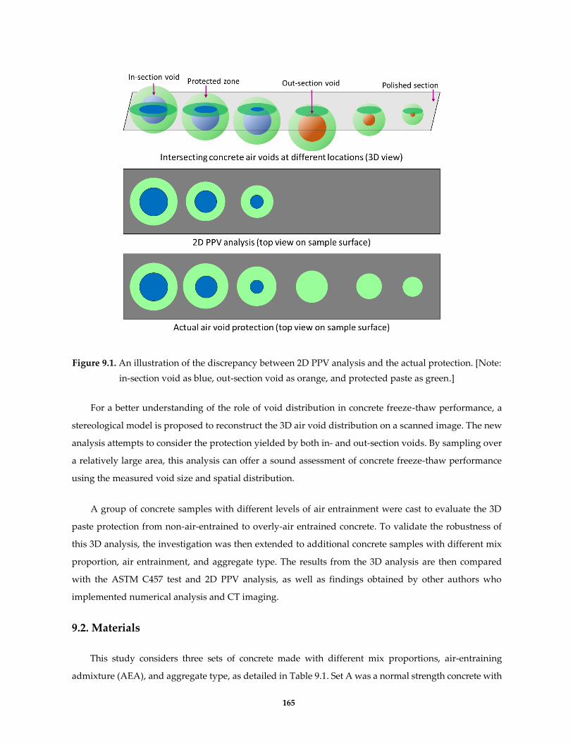
165

Figure 9.1. An illustration of the discrepancy between 2D PPV analysis and the actual protection. [Note:

in-section void as blue, out-section void as orange, and protected paste as green.]

For a better understanding of the role of void distribution in concrete freeze-thaw performance, a

stereological model is proposed to reconstruct the 3D air void distribution on a scanned image. The new

analysis attempts to consider the protection yielded by both in- and out-section voids. By sampling over

a relatively large area, this analysis can offer a sound assessment of concrete freeze-thaw performance

using the measured void size and spatial distribution.

A group of concrete samples with different levels of air entrainment were cast to evaluate the 3D

paste protection from non-air-entrained to overly-air entrained concrete. To validate the robustness of

this 3D analysis, the investigation was then extended to additional concrete samples with different mix

proportion, air entrainment, and aggregate type. The results from the 3D analysis are then compared

with the ASTM C457 test and 2D PPV analysis, as well as findings obtained by other authors who

implemented numerical analysis and CT imaging.

9.2. Materials

This study considers three sets of concrete made with different mix proportions, air-entraining

admixture (AEA), and aggregate type, as detailed in Table 9.1. Set A was a normal strength concrete with

166

limestone aggregate. Other sets of concrete samples were used for validation of the analysis method. Set

B used a high-strength concrete made with traprock aggregate (basalt). Set C used a lab prepared concrete

made with pea gravel aggregate (mainly granite and quartz, with a smoother surface and less angular

shape than the other two aggregates). Samples in Set B and C were obtained in form of hardened concrete.

A processed sample scan of each the three sets is shown in Fig. 9.2.

Table 9.1. Sample label scheme for different sets of concrete mixtures.

Set Mixture Basic information

A:

limestone

aggregate

AV0 Base mixture with no AEA, mix 3.5 min, sampling

AV1 Add 1-ml AEA (DARAVAIR® 1400) to AV0, mix 1 min, sampling

AV2 Add 1-ml AEA to AV1, mix 1 min, sampling




B:

trap rock

aggregate

TN Non-air-entrained

TA Normally air-entrained, AEA (Sika® Air-260)

TO Overly air-entrained

C:

pea gravel

aggregate

PN Non-air-entrained

PA Normally air-entrained, AEA (DARAVAIR® 1400)

PO Overly air-entrained

Figure 9.2. A sample scan (50×50 mm) for the three concrete sets with (a) limestone, (b) traprock, and (c)

pea gravel aggregate, where the cement paste is colored purple using phenolphthalein.

For Set A, six samples of various quantities of AEA were prepared out of a single batch of fresh

concrete. The base mixture consisted of 398.3 kg/m3 Type I cement (specific gravity, SG=3.15 g/cm3), 943.1

kg/m3 coarse limestone chips ranging from 4.75 to 12.70 mm (SG=2.67 g/cm3), 763.5 kg/m3 river sand passing

167

4.75-mm sieve (SG=2.72 g/cm3), and 179.5 kg/m3 water (SG=1.00 g/cm3). A total volume of 0.015 m3 mixture

was prepared. The mixing protocol followed the ASTM C192 [33]. After initial mixing, the first non-air-

entrained sample “AV0” was cast into a 4×8-inch standard cylinder mold. The remaining mixture was then

air-entrained using DARAVAIR® 1400. Based on the suggested dosage, 1-ml agent was dosed and 60

seconds of mixing was done before the second sample “AV1” was cast. The previous step was then iterated

to obtain the other four samples, “AV2” to “AV5”. The fresh concrete samples were consolidated on a

vibration table for 60 seconds and then sealed. Once demolded after 24 hours, the concrete samples were

moist cured until 28 days.

The base mixture of Set B consisted of 526.6 kg/m3 Type I cement, 1055.0 kg/m3 coarse trap rock, 532.0

kg/m3 river sand passing 4.75-mm sieve, and 160.2 kg/m3 water, and a different AEA, Sika® Air-260, was

used. This set consisted of three samples with various (AEA), “TN” (non-air-entrained), “TA” (air-

entrained), and “TO” (overly air-entrained). Set C mixtures generally shared the same mixing

methodology and mixing proportion as Set A, except for a higher water-to-cement ratio (w/c) of 0.50.

This set also had three samples, “PN” (non-air-entrained), “PA” (air-entrained), and “PO” (overly air-

entrained). In this paper, the Methods and Results sections focus on Set A exclusively, and the other two

set results processed using the same steps are presented in the Discussion section.

9.3. Methods

For the sample surface preparation, in short, the cylindrical samples were cut longitudinally in half,

polished with a 3-µm grind disc, processed with surface treatments, and then scanned, which have been

done previously and justified to be successful [34]. The polishing work generally followed the ASTM C457

procedures, while the polished surface was then treated differently with two steps. To contrast the paste

from aggregates, a phenolphthalein solution (5% by weight in 200 proof alcohol) was first evenly sprayed

on the surface to dye the hardened cement paste dark purple. After 10 seconds, the solution was removed

using a paper towel to avoid color contamination to the aggregate phase. Then an orange fluorescent chalk

powder was used to highlight the air voids. For this step, the powder was evenly spread across the polished

section and pressed into the voids; the excessive powder was removed by scraping the surface with a razor.

The above procedure was repeated three times to ensure all the air voids were infilled appropriately.

For each mixture from AV0 to AV5, six 50×50 mm regions were scanned from the polished sections.

The analysis of the scanned images can be divided into five steps: 1) phase segmentation, 2) 3D void size

distribution of in-section voids, 3) 3D void size distribution of out-section voids, 4) void spatial distribution,

and 5) paste protection evaluation. The following subsections detail each step, using a scan from a Set A

sample as the reference.

168

9.3.1. Step one: phase segmentation

Phase segmentation identifies the aggregate, paste, and void phases appearing in the scanned images.

For each mixture in Set A, six 50×50 mm regions were scanned using a flatbed scanner with a 5.3-μm pixel

resolution. Each individual scan was further identified with its number, such as “AV0-6” for the sixth scan

of Mixture AV0. The scans were segmented using two open-source programs, Multispec and ImageJ. Based

on the color contrast given by the surface treatment, a semi-automatic image segmentation was

implemented using Multispec. For each image, segmentation required to pre-select a minimum of 25

training fields for each of the three phases to exemplify their different color nature. Then, the classification

algorithm employed in Multispec segmented the entire image according to the training data, and the output

was a trinary image. More details of this program and the procedures can be found in the literature [34].

Subsequently, ImageJ was used to post-process the segmented image to remove noise (e.g., “void” smaller

than 10 µm in diameter) and to fill the voids present in aggregates. This final processing output was a

grayscale image containing three phases—aggregate in black, paste in gray, and voids in white. Fig. 9.3

displays the original scan of AV1-1 along with its phase segmented image. From the phase segmented

image, the apparent void distribution can be determined. An automated C457 analysis was also conducted

as a baseline for later discussion [37,38].

(a) (b)

Figure 9.3. Scan image of Section AV1-1: (a) original scan, and (b) three-phase image. The scanning area is

50×50 mm, with a 5.3-µm pixel resolution.

169

9.3.2. Step two: 3D void size distribution of in-section voids

The second step determines the actual void size distribution of the intersected voids from the apparent

void size distribution on the concrete scan. To achieve this goal, a statistical approach known as 2D-to-3D

unfolding was used [35]. This technique has been previously adopted in concrete research by Fonseca and

Scherer, where the interpretation of the actual void size distribution from the binary scan of a polished air-

entrained mortar was demonstrated [36]. The theoretical background of the unfolding technique is

explained as follows. Mathematically, the unfolding technique is built on a simple concept, in which the

likelihood P of yielding a circular intersection within a certain size interval by randomly intersecting a

sphere is given by Eq. 9.1 [35]:

P(𝑟1 < 𝑟 < 𝑟2) =(√𝑅2− 𝑟1

2−√𝑅2− 𝑟22)

𝑅 (9.1)

where R is the actual void radius, r is the apparent radius, and r1 and r2 prescribe the size range of the

intersection. Fig. 9.4. displays a schematic for an in-section void.

Figure 9.4. An in-section void. R is the actual radius of the air void, and r is the apparent radius of the

intersection.

For an ideal mono-sized void system that is isotropic, uniform, and random (IUR), the apparent size

distribution of the void intersections yielded by a random cut intersection through its volume can be

described by Eq. 9.1. Assuming such a void system with the apparent distribution known, the actual size

distribution can be back-calculated. As a multi-sized void system can be conceptualized as a superposition

of multiple mono-sized distributions, the actual size distribution of the multi-sized void system is

recoverable through the 2D-to-3D unfolding technique.

170

The air voids in concrete can be deemed as a multi-sized void system, and its unfolding process is as

follow. All the void intersections are classified using a histogram with consecutively size bins. Note that the

largest bin is only associated with the largest sized voids--all the apparent intersections counted in this bin

are yielded by cutting the largest sized voids near their centroids. With this information, Eq. 9.1 can be used

to determine the other bin counts from the smaller void intersections belonging to the largest sized voids.

As such, the sum of all these void intersections gives the actual count for the largest voids. After deducting

these counts from each bin, the second-largest bin now becomes the largest in the resultant histogram and

its actual count can be analyzed using the above-stated steps. The process is iterated down to the smallest

bin, until a final determination of actual void size distribution is achieved. The concrete void unfolding

process was programmed to ease the analysis [37].

For Section AV1-1, a histogram displaying the apparent size distribution of its void intersections, r, is

analyzed from the three-phase image in Fig. 9.3b. The obtained distribution is shown in Fig. 9.5a. For

optimal unfolding quality and efficiency, a total of 20 bins between 10 and 500 µm were used to represent

the apparent distribution [37]. The intersections larger than 500 µm were ignored, as the larger entrapped

air is typically irregular in shape and also insignificant to concrete freeze-thaw protection [4,38].

Furthermore, as the population of these large air voids is typically minuscule, doing so has a negligible

influence on the overall paste protection.

Fig. 9.5b displays the actual void size distribution of the void intersections, R, as determined through

the unfolding algorithm. The legend notes the contribution of voids of each apparent size to this actual

void distribution--the different colored sections at each bin corresponds to all the intersections yielded by

the air voids of that actual size.

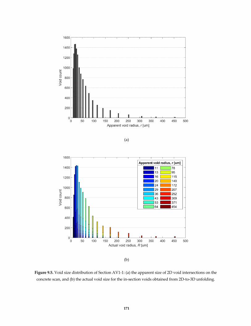
171

(a)

(b)

Figure 9.5. Void size distribution of Section AV1-1: (a) the apparent size of 2D void intersections on the

concrete scan, and (b) the actual void size for the in-section voids obtained from 2D-to-3D unfolding.

172

9.3.3. Step three: 3D void size distribution of out-section voids

The actual void size distribution of out-section voids is then determined. The out-section void refers to

an un-intersected void whose protection range falls onto the inspected concrete section. Fig. 9.6. illustrates

an out-section void along with pertinent parameters defined. For a given protection range, p, the larger

radius associated with the out-section void, R+p, should be considered in the calculation. When a section

cuts right on the void boundary, the radius of the out-section protection, t, is maximized:

t𝑚𝑎𝑥 = (√(𝑅 + 𝑝)2 − 𝑅2) (9.2)

By substituting Eq. 9.2 into Eq. 9.1, the probability of getting an out-section void is:

P𝑜𝑢𝑡 =√(𝑅+𝑝)2− 02−√(𝑅+𝑝)2− t𝑚𝑎𝑥

2

𝑅+𝑝=

𝑝

𝑅+𝑝 (9.3)

while the probability for an in-section void is:

P𝑖𝑛 =√(𝑅+𝑝)2− t𝑚𝑎𝑥

2−√(𝑅+𝑝)2− (𝑅+𝑝)2

𝑅+𝑝=

𝑅

𝑅+𝑝 (9.4)

In PPV analysis [29–31], the protection range is consistent for different void radius. Therefore, for varying

void radius, the ratio between the in- and out-section voids can be expressed as:

𝛼𝑖𝑛/𝑜𝑢𝑡 = 𝑅

𝑝 (9. 5)

Figure 9.6. An out-section void and the associated paste protection around it. R is the actual radius of the

air void, p is a protection range, and t is the radius of the protection yield to the inspected section.

The actual in-section void size distribution, along with a prescribed protection range, is then used to

determine the out-section voids for a concrete section. For each sized in-section void, the corresponding

173

out-section voids can be determined using Eq. 9.5. Presuming a protection range of 200 µm (as typically

investigated), a summary of the distribution of all the voids yielding protection to the Section AV1-1 is

shown in Fig. 9.7. In this case, a total of 12766 in-section voids were identified from the scan and 92087 out-

section voids were obtained from the calculation. Air voids smaller than the protection range have more

out-section voids than the in-section voids, and the ratio increases continuously as the void size reduces

further. For example, about 100 in-section voids and 80 out-section voids of a 250-µm radius are identified

in this sample; however, about 1400 in-section voids and 14000 out-section voids are seen for the 20-µm

radius voids.

Figure 9.7. The overall void size distribution of AV1-1, for both in- and out-section voids.

9.3.4. Step four: void spatial distribution

This step involves reconstructing the spatial distribution of in- and out-section voids on the original

concrete scan. Fig. 9.8 displays a simplified model for a group of mono-sized voids with a side view, where

the concrete scan is placed at the mid-section (z=0). For the in-section voids, the centroid-section distance

ranges from -R to R. For the out-section voids, the centroid exists further away, either from -R to –(R+p) or

R to R+p. As for the actual 3D void reconstruction, the process is divided into two components, respectively

addressing in- and out-section voids.

174

Figure 9.8. Modeling a mono-sized void system. R is the actual radius of the air void, r is the apparent

radius of the intersection, and p is the protection range. [Note: in-section void as blue, and out-section

void as orange.]

To reconstruct in-section voids, the air void intersections are first categorized into the size bins by their

apparent radii (see Fig. 9.5a). For each of the in-section voids, its actual radius R and apparent radius r are

known from the size distribution in Fig. 9.5b. Accordingly, a 3D sphere with the actual radius R can be

generated for each void and further appended with a centroid-section distance to yield the apparent radius

r. This 3D sphere is then mapped back to an air void intersection on the concrete scan, which coincides the

apparent radius r. In instances where multiple air voids can be matched, the mapping is randomly decided.

For modeling all the in-section voids, the above void assignment process is iterated from the largest to

smallest actual void size. The stereological model for the in-section voids is displayed in Fig. 9.9a. To

prevent conflicts in this process, any newly assigned void that interferes with the boundary of an existing

void or an aggregate wall is reattempted at other locations. In this stereological model, aggregates are

assumed to have boundaries that are orthogonal to the cross-section. We consider this to be a valid

assumption as the radius of most aggregates are larger than the entrained air voids. As such, the overall

reconstruction offers a statistically reliable representation of the intersected voids in the original concrete

scan.

To reconstruct out-section voids, a similar approach is used, while allowing a higher level of

stochasticity. For each count of out-section voids in Fig. 9.7, the actual radius R is known. The spatial

position of out-section void is randomly generated but prescribed by the following rules: 1) the planar

position does not fall into the aggregate phase on the concrete scan; 2) the centroid-section distance is larger

than R and smaller than R+p (see Fig. 9.8); and 3) any newly generated void should not overlap with existing

in- and out-section voids. The stereological model for the out-section voids is displayed in Fig. 9.9b.

175

The in-section void model representing a 10000×10000 µm area at the lower-left corner of Section AV1-

1 is shown in Fig. 9.9a, in which the voids are shown as blue spheres while the larger voids excluded from

the analysis (R>500 µm) are shown as 2D gray objects in their original shape. Within Fig. 9.9a, the protection

range is visualized as a semi-transparent blue shell, 200 µm in radius larger than the void. The projection

of this protected paste volume appears as a transition from green to yellow on the 2D image scan. The 2D

regions shown in red are unprotected paste beyond the 200-µm range from air voids. The out-section void

model for Section AV1-1 is shown in Fig. 9.9b, in which all the voids are distributed either above or below

the scan without contact. After superimposing the in- and out-section void models, the final stereological

model is shown as Fig. 9.9c.

(a)

(b)

Figure 9.9. The 3D stereological void models for the lower-left subsection of AV1-1 (10000×10000 µm): (a)

for in-section voids, (b) for out-section voids, and (c) for the overall protection. The in- and out-section

voids are shown as blue and yellow spheres, respectively, and their protection is visualized as the semi-

transparent shells.

176


(c)

9.3.5. Step five: paste protection evaluation

The final step quantifies the 3D paste protection, in the same vein as the PPV concept. The mid-section

in each stereological model provided a map reflecting the paste protection from in- and/or out-section

voids. Fig. 9.10 displays the protection maps of the stereological models shown in Fig. 9.9, along with the

original concrete scan. The paste protection at any arbitrary point was only determined by its distance to

the nearest void providing the largest protection. The paste within the protection range was differentiated

with a green-yellow color gradient to reflect the protection as a function of the range distance; the remaining

unprotected paste was colored in red. Any protection intruded into the void or aggregate phase was

ignored.

Fig. 9.10b represents the protection originating from the in-section voids, where the modeled void

intersections (marked blue) can be well correlated with the actual void intersections in Fig. 9.10a. Fig. 9.10c

displays the out-section protection originating from out-section voids. The final protection map

synthesizing both in- and out-section protection is shown in Fig. 9.10d. Notably, a considerable portion of

the paste is protected from out-section voids. Based on the final protection map of AV1-1, it was determined

that this sample had 99.4% paste protected by presuming a protection range of 200 µm.

177

(a) (b)

(c) (d)

Figure 9.10. Comparison of (a) the lower-left subsection of AV1-1 (10000×10000 µm) with its protection

maps: (b) in-section protection, (c) out-section protection, and (d) the overall protection. [Note: The void

intersections in (c) are muted, as they do not contribute to the out-section protection.]

178

9.4. Results

9.4.1. ASTM C457 results

Based on the ASTM C457 analysis, the phase contents of the six scans for the Set A base mixture

(Mixture AV0) are compared to the reference values from the mixture design, as shown in Table 9.2. This

is used as an assurance of the quality of the phase segmentation. The reference phase contents are based on

the mixture design, where the details have been provided in the Methods section. Note that the mixture

design is considered for an air-content concrete, but the AEA was not used yet in the base mixture. The

segmentation results reasonably agree with the designated volume fractions. The phase content differences

across the individual scan image mainly reflect the compositional variation, which is contingent on the

scanning area.

Table 9.2. A comparison of the measured phase volume contents of Mixture AV0 to the reference values

from the base mixture design of Set A.

Section AV0-1 AV0-2 AV0-3 AV0-4 AV0-5 AV0-6 Averaged Reference

Aggregate [%] 59.9 63.9 64.0 63.3 65.5 58.8 62.6 63.4

Paste [%] 35.9 31.2 31.7 31.7 28.8 35.9 32.5 30.6

Air void [%] 4.3 4.9 4.5 5.0 5.5 5.2 4.9 6.0

The air void parameters for Mixture AV0 to AV5 are summarized in Fig. 9.11 where error bars are used

to indicate standard deviation. In general, the air content trends higher and spacing factor lower with

greater air entrainment. But exceptions for air content can be seen with Mixtures AV4 and AV5 that have

highest air-entraining admixture and longer vibration period. This could be caused by the micelle formation

phenomenon, whereby the air-entraining effect is limited after certain surfactant concentration [15]. The

undulation of air content may also reflect the secondary effect of air entrainment in improving mixture

workability. During the vibration, more air bubbles were observed escaping from the highly air-entrained

mixtures. Since the tendency of air loss increases with the bubble diameter during vibration [39], the

spacing factor, which is more determined by the presence of small voids, is less affected than air content.

Since only the voids from 10 to 500 µm radius were simulated in the 3D stereological model, the results

without considering the voids larger than 500 µm are also given in Fig. 9.11. This action results in a

considerable decrease in air content for all mixtures, while a smaller change on spacing factor for the air

entrained mixtures. These observations are in line with the understanding that the large entrapped air plays

a minimal role in protection concrete from freeze-thaw damage [4,5,40]. For consistency, the spacing factor

without considering the larger voids is used for the subsequent 3D paste protection analysis.

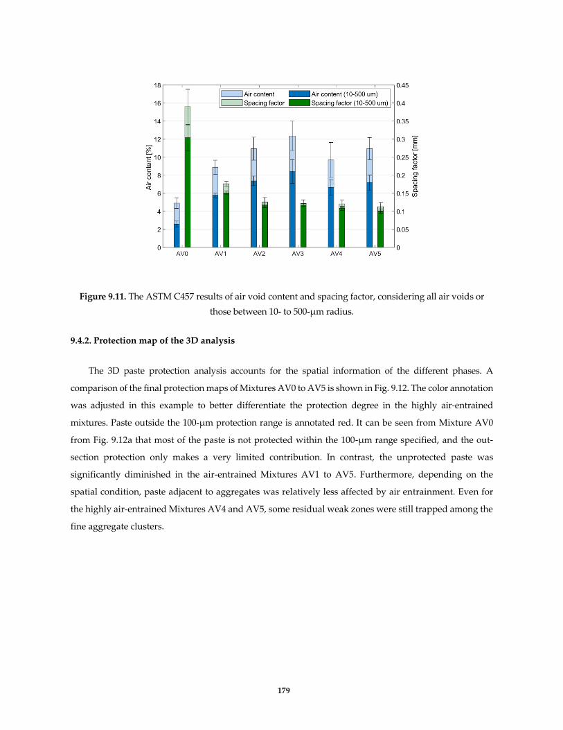
https://www.sciencedirect.com/topics/engineering/bubble-diameter

179

Figure 9.11. The ASTM C457 results of air void content and spacing factor, considering all air voids or

those between 10- to 500-µm radius.

9.4.2. Protection map of the 3D analysis

The 3D paste protection analysis accounts for the spatial information of the different phases. A

comparison of the final protection maps of Mixtures AV0 to AV5 is shown in Fig. 9.12. The color annotation

was adjusted in this example to better differentiate the protection degree in the highly air-entrained

mixtures. Paste outside the 100-µm protection range is annotated red. It can be seen from Mixture AV0

from Fig. 9.12a that most of the paste is not protected within the 100-µm range specified, and the out-

section protection only makes a very limited contribution. In contrast, the unprotected paste was

significantly diminished in the air-entrained Mixtures AV1 to AV5. Furthermore, depending on the

spatial condition, paste adjacent to aggregates was relatively less affected by air entrainment. Even for

the highly air-entrained Mixtures AV4 and AV5, some residual weak zones were still trapped among the

fine aggregate clusters.

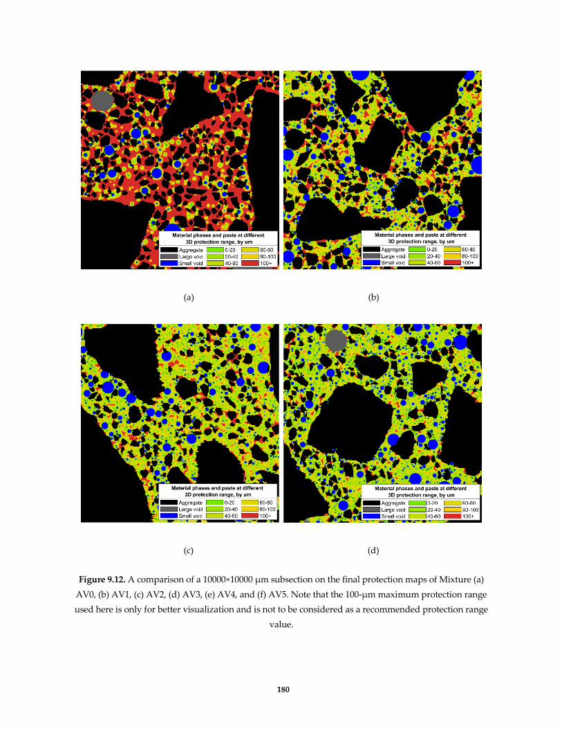
180

(a) (b)

(c) (d)

Figure 9.12. A comparison of a 10000×10000 µm subsection on the final protection maps of Mixture (a)

AV0, (b) AV1, (c) AV2, (d) AV3, (e) AV4, and (f) AV5. Note that the 100-µm maximum protection range

used here is only for better visualization and is not to be considered as a recommended protection range

value.

181


(e) (f)

9.4.3. 3D paste protection analysis

The protection range value has been the subject of past research. As originated from Powers’ spacing

factor [2], different metrics have been proposed to improve the mathematical description of the paste-void

protection range, such as Philleo factor [22], mean spacing by Attiogbe [24], flow length by Pleau and Pigeon

[25], and lineal path by Mayercsik et al. [41]. It is generally agreed that the protection extends out by 200-

250 µm from the void periphery [13,23,27], but could be higher than 350 µm for high strength concrete [42].

The implication of using different values for protection range is shown in Fig. 9.13 where the data for each

mixture comes from six scanned images. When the assumed protection range increases, the protection

degree increases in a non-linear manner, while the more air-entrained mixtures always have larger paste

protection. If the protection range around each void is 200 µm, there would be more than 10% paste

unprotected in Mixture AV0, while all the air-entrained mixtures would be fully protected.

182

Figure 9.13. Protection spectra obtained from the 3D paste protection analysis.

9.5. Discussion

9.5.1. A comparison with the conventional 2D PPV analysis

A conventional 2D PPV analysis does not fully consider paste protection offered by in-section voids

and further omits that of out-section voids. To quantify the underestimation of paste protection, the 3D

paste protection was compared with the 2D result. A comparison of the 2D and 3D protection using the

same concrete scans is shown in Fig. 9.14. The 2D protection spectrum for each mixture is markedly shifted

when compared to its 3D counterpart. For example, presuming a 200-µm protection range, the 3D analysis

indicates 99.4% paste protection for Mixture AV1; the corresponding result with 2D analysis is only 61.6%.

In terms of the individual contribution to the 3D protection analysis from in- and out-section voids,

additional analysis was conducted using the same 3D stereological models. As compared with the 2D

analysis, a marginal improvement was seen when only further considering the off-center intersection issue

for in-section voids. As an illustration, the result of Mixture AV1 is shown in Fig. 9.15. This observation is

explained by the fact that most of the in-section voids are intersected near their centroids; for example,

according to Eq. 9.1, the chance of intersecting a void outside of the R/2 is only 13.3%. Evidently, the paste

protection is not markedly altered by solely considering the in-section protection from the 3D perspective.

Therefore, out-section protection plays a major role in the difference between 2D and 3D paste protection

analysis.

183

Figure 9.14. A comparison of the protection spectra obtained from 2D and 3D PPV analysis.

Figure 9.15. The influence of the off-center intersection issue to PPV analysis.

9.5.2. A comparison with Powers’ spacing factor

Although Powers’ model simplifies the concrete air void system [2], the ASTM C457 test method built

on this hypothesis is widely accepted and Powers’ spacing factor serves as a critical index for predicting

concrete freeze-thaw performance. Powers’ spacing factor approximates the maximum distance from a

point in paste to its adjacent air void [2,20]. Conceptually, when the protection range equals the spacing

184

factor, a 100% paste protection should be observed. The use of this parameter has been extensively verified

in experiments [4,29,43–48], but its underlying rationality continues to be of interest to researchers, to

quantify the influence of the simplification placed on the concrete air void system and to further advance

the assessment of concrete freeze-thaw durability [20,23].

To contrast the 2D and 3D analyses, the protection range value was equated to the corresponding

spacing factor for the investigated mixtures. The results are shown in Table 9.3. The 2D analysis resulted in

a protection degree ranges from 50 to 70%, which agrees with the 2D PPV results reported in previous

literature [31]. From the 3D analysis, however, the spacing factor consistently points to almost full

protection for all the mixtures. For the air-entrained samples, the suggested protections are found

consistently at around 98%. For consistency, the results given in Table 9.3 including spacing factor do not

consider the voids larger than 500 µm radius; however, the impact is minuscule, as the spacing factor values

are just slightly reduced (see Fig. 9.11) and the protection spectrum almost flattens out at the range as

designated by spacing factor (see Fig. 9.13). Therefore, it seems that Powers’ empirically derived spacing

factor has always implied a high paste protection degree at around 98th percentile.

Table 9.3. Percentage of protected paste at the protection range as suggested by the spacing factor.

Mixture

(spacing factor)

AV0

(303.9 µm)

AV1

(150.9 µm)

AV2

(123.7 µm)

AV3

(117.6 µm)

AV4

(108.5 µm)

AV5

(100.5 µm)

2D analysis [%] 51.9 61.2 64.2 65.5 67.1 68.3

3D analysis [%] 99.4 98.4 98.2 97.7 98.3 97.8

The finding from Table 9.3 is consistent with Snyder [20,49] who found that Powers’ spacing factor

predicts a protection higher than the 95th percentile of the paste-void spacing distribution. Furthermore, a

study by Yun et al. [26] using CT imaging found that the spacing factor correlated to protection higher than

the 95th percentile. Moreover, it is reported in that CT study that the ratio between the protection range

giving 95th percentile paste protection to Powers' spacing factor ranges from 0.7 to 0.8. This conclusion is

aligned with the protection spectrum obtained in this study (see Fig. 9.13).

9.5.3. Applying the 3D paste protection analysis for other concrete sets

To test the applicability of the proposed 3D paste protection analysis for concrete with different

materials and mixing proportions, two additional sets of concrete samples were investigated, which were

respectively made with trap rock and pea gravel (see Table 9.1). The samples were analyzed using the

procedures described in the Methods section, and the key results are summarized in Table 9.4. A

185

10000×10000 µm subsection of each protection map is shown in Fig. 9.16, with the same 100-µm maximum

protection range used for visualization. The 3D paste protection spectra of these samples are shown in

Fig. 9.17. The results show that the proposed 3D paste protection analysis works well for concrete

samples with different types of aggregate. As seen from Tables 9.3 and 9.4, the 2D paste protections for

new mixture sets fall into a similarly low range (about 50 to 70%) as that of Set A mixtures, while the 3D

paste protections as designated by the spacing factor consistently indicate a nearly full coverage for all

the mixtures with varying phase composition.

An enhanced paste protection from increasing air entrainment can be found from the protection

maps in Fig. 9.16, similar to the previous observation from Fig. 9.12. However, both the protection spectra

in Figs. 9.13 and 9.17 indicate that, even for the non-air-entrained mixtures, the fraction of unprotected

paste may already be considerably low. Given a 200-µm protection range, the Mixture AV0 has about

10% unprotected paste, and this value is around 5% for Mixtures TN and PN. This observation suggests

that the overall freeze-thaw performance of concrete may be contingent on a relatively small, yet critical,

portion of paste being unprotected.

It is interesting to notice that Mixture TO and AV4, PA and AV1, and PO and AV5 have roughly

matched spacing factors but Mixture TO, PA, and PO show more red zones (i.e., vulnerable localities) in

Figs. 9.16. This observation remains even true when the protection range was increased to 200 µm.

Another notable observation is that the coarse aggregate shape seemingly shows an influence on the

concrete air void size distribution, as well as the 3D paste protection. For example, in comparison to AV5

(see Fig. 9.12f), Mixture PO (see Fig. 9.16f) has a greater amount of larger voids and a lower 3D paste

protection. Considering that the same AEA was used in both the mixtures, this void size difference might

be related to that the rounded pea gravel used in Mixture PO generates less impact to the larger air

bubbles during mixing [15].

Two likely explanations can be offered for the small variation of the spacing factor-designated 3D

paste protection in the different mixtures. The first one is related to the real void distribution in concrete.

In the calculation of spacing factor, the void size distribution is only represented by a few void

parameters (i.e., air content, paste content, and average chord length) [14]; however, the credibility of this

approach can be undermined if the real void distribution shows low compliance to Powers’ idealized

void model. The second is the presence of aggregates, as completely omitted by spacing factor. As seen

from the protection maps in Figs. 9.12 and 9.16, the protection to the paste trapped among fine aggregate

clusters can be still poor in highly air-entrained mixtures, as 1) the closely spaced fine aggregates obstruct

the space for creating an air void in between and 2) the connection between the paste to the outside

protection is confined.

186

Depending on the size and spatial distributions of void and aggregate in concrete, the local paste

protection can be affected; however, this subtle variation may not be captured by Powers’ void model

and the ASTM C457 test. This suggests that different concretes with the same spacing factor may not be

protected to the same degree, as agreed by previous studies [20,23,26].

Table 9.4. ASTM C457 air void parameters and the 3D paste protection suggested by spacing factor.

Mixture TN TA TO PN PA PO

Air content [%] 3.9 7.4 5.1 3.8 4.6 12.2

Spacing factor [µm] 247.8 139.9 109.6 222.5 153.0 89.9

2D analysis [%] 64.8 65.2 70.3 55.4 63.9 71.4

3D analysis [%] 98.9 97.9 96.8 98.7 98.6 96.6

(a) (b) (c)

(d) (e) (f)

Figure 9.16. A comparison of a 10000×10000 µm subsection on the protection maps of Mixture (a) TN, (b)

TA, (c) TO, (d) PN, (e) PA, and (f) PO. Note that the 100-µm maximum protection range used here is only

for better visualization.

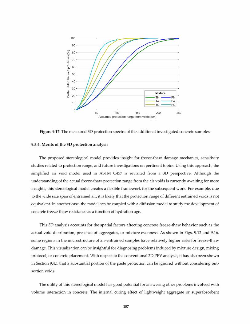
187

Figure 9.17. The measured 3D protection spectra of the additional investigated concrete samples.

9.5.4. Merits of the 3D protection analysis

The proposed stereological model provides insight for freeze-thaw damage mechanics, sensitivity

studies related to protection range, and future investigations on pertinent topics. Using this approach, the

simplified air void model used in ASTM C457 is revisited from a 3D perspective. Although the

understanding of the actual freeze-thaw protection range from the air voids is currently awaiting for more

insights, this stereological model creates a flexible framework for the subsequent work. For example, due

to the wide size span of entrained air, it is likely that the protection range of different entrained voids is not

equivalent. In another case, the model can be coupled with a diffusion model to study the development of

concrete freeze-thaw resistance as a function of hydration age.

This 3D analysis accounts for the spatial factors affecting concrete freeze-thaw behavior such as the

actual void distribution, presence of aggregates, or mixture evenness. As shown in Figs. 9.12 and 9.16,

some regions in the microstructure of air-entrained samples have relatively higher risks for freeze-thaw

damage. This visualization can be insightful for diagnosing problems induced by mixture design, mixing

protocol, or concrete placement. With respect to the conventional 2D PPV analysis, it has also been shown

in Section 9.4.1 that a substantial portion of the paste protection can be ignored without considering out-

section voids.

The utility of this stereological model has good potential for answering other problems involved with

volume interaction in concrete. The internal curing effect of lightweight aggregate or superabsorbent

188

polymer, for example, has already been studied with the PPV concept for determining the optimal usage

to compensate autogenous shrinkage [50,51]. Following this concept, the effect of different types of

inclusions to the surrounding cement paste volume, such as microcapsules in self-healing concrete [52], can

also be investigated from a 3D perspective. In addition, the model can be further coupled with concrete

diffusion theories to investigate other durability mechanisms like alkali-silica reaction [53].

9.6. Conclusion

The conventional PPV analysis provides insights for evaluating concrete air void system and freeze-

thaw performance, but this 2D implementation ignores factors such as off-center intersection and out-

section protection. This study advances a 3D paste protection analysis that overcomes these issues. This

analysis is built on a stereological model that integrates the probabilistic-based 2D-to-3D unfolding

technique into the image-based concrete void analysis, which allows a 3D reconstruction for both in- and

out-section voids near the analyzed concrete section. By assuming a protection range around each air

void, a protection map reflecting the 3D paste protection can be extracted from the proposed model for

subsequent analysis. With this protection map, a more thorough concrete freeze-thaw evaluation can be

achieved by resolving the actual void distribution, presence of aggregates, and local paste protection as

influenced by different phases in actual concrete. Meanwhile, the protection spectrum as a statistical

summary of the protection map provides a thorough consideration of the 3D void spatial distribution to

concrete freeze-thaw performance.

The proposed 3D analysis was tested with three sets of concrete mixtures with different AEA, mix

proportion, and aggregate type. The results were further compared with the ASTM C457 test and 2D PPV

analysis. The obtained protection spectra for all samples were found to follow a similar trend, where the

protection degree increases non-linearly with the protection range. By equating the obtained spacing factor

with the protection range, 3D analysis indicates about 98% protection, which aligns well with CT results

obtained by others. However, conventional 2D PPV analysis with the same samples results in 50-70%

protection. This difference is attributed to the out-section protection that is considered by the 3D analysis.

The authors foresee a good potential to achieve a more realistic freeze-thaw analysis by further

developing the 3D stereological void model, by further taking into consideration the influence of air void

size to protection range or combining it with a diffusion model to account for time effect. The proposed

technique can be also applied to assist other concrete studies that are involved with phase volume

interaction problems.

https://www.sciencedirect.com/topics/engineering/autogenous-shrinkage

189

References

[1] C. Powers, T, A. Helmuth, R, THEORY OF VOLUME CHANGES IN HARDENED PORTLAND-

CEMENT PASTE DURING FREEZING, in: Proc. Thirty-Second Annu. Meet. Highw. Res. Board,

1953: pp. 285–297.

[2] T.C. Powers, T.F. Willis, The Air Requirement of Frost-Resistant Concrete, Proc. Twenty-Ninth

Annu. Meet. Highw. Res. Board. (1949).

[3] G.W. Scherer, J. Valenza, Mechanisms of Frost Damage, Mater. Sci. Concr. VII. i (2005) 209–246.

[4] Z. Liu, W. Hansen, B. Meng, Characterisation of air-void systems in concrete, Mag. Concr. Res.

(2015). https://doi.org/10.1680/macr.15.00074.

[5] K. Hover, Air Content and Unit Weight of Hardened Concrete, in: Significance Tests Prop. Concr.

Concr. Mate Rials, ASTM International, 100 Barr Harbor Drive, PO Box C700, West


[6] H.S. Wong, A.M. Pappas, R.W. Zimmerman, N.R. Buenfeld, Effect of entrained air voids on the

microstructure and mass transport properties of concrete, Cem. Concr. Res. (2011).


[7] S. Rath, N. Puthipad, A. Attachaiyawuth, M. Ouchi, Critical Size of Entrained Air to Stability of

Air Volume in Mortar of Self-Compacting Concrete at Fresh Stage, J. Adv. Concr. Technol. (2017).

https://doi.org/10.3151/jact.15.29.

[8] W. Piasta, H. Sikora, Effect of air entrainment on shrinkage of blended cements concretes, Constr.

Build. Mater. (2015). https://doi.org/10.1016/j.conbuildmat.2015.09.018.

[9] P. Mehta, K. Hover, Some Recent Problems with Air-Entrained Concrete, Cem. Concr.

Aggregates. 11 (1989) 67. https://doi.org/10.1520/CCA10104J.

[10] S. Popovics, A Hypothesis Concerning the Effects of Macro-Porosity on Mechanical Properties of

Concrete, in: Fract. Concr. Rock, Springer New York, New York, NY, 1989: pp. 170–174.

https://doi.org/10.1007/978-1-4612-3578-1_17.

[11] K.H. Khayat, Optimization and performance of air-entrained, self-consolidating concrete, ACI

Struct. J. (2000).

[12] K.H. Khayat, J. Assaad, Air-void stability in self-consolidating concrete, ACI Mater. J. (2002).

[13] ACI, ACI 201.2R-01 Guide to Durable Concrete reported by ACI Committee 201, 2008.

[14] Astm C 457, Standard Test Method for Microscopical Determination of Parameters of the Air-

Void System in Hardened Concrete 1, ASTM Int. 05 (2013) 1–15. https://doi.org/10.1520/C0457.



[16] M. Pigeon, R. Pleau, Durability of Concrete in Cold Climates, E & FN Spon, London, 1995.

[17] S.H. Smith, K.E. Kurtis, I. Tien, Probabilistic evaluation of concrete freeze-thaw design guidance,

190

Mater. Struct. 51 (2018) 124. https://doi.org/10.1617/s11527-018-1259-z.

[18] ACI Committee 212, Report on Chemical Admixtures, 2010.

[19] CSA A23.1-14/A23.2-14, CSA A23.1 (Concrete materials and methods of concrete construction) &

A23.2 (Test methods and standard practices for concrete), 2014.

[20] K.A. Snyder, A Numerical Test of Air Void Spacing Equations, Adv. Cem. Based Mater. 8 (1998)

28–44. https://doi.org/10.1016/S1065-7355(98)00007-8.

[21] K.A. Snyder, K.C. Hover, K. Natesaiyer, The stereological and statistical properties of entrained

air voids in concrete: a mathematical basis for air void system characterization, in: Mater. Sci.

Concr. VI, 1st ed., Wiley-American Ceramic Society, Westerville, OH, 2001: pp. 129–214.

[22] P. Wedding, R. Philleo, A Method for Analyzing Void Distribution in Air-Entrained Concrete,

Cem. Concr. Aggregates. 5 (1983) 128. https://doi.org/10.1520/CCA10263J.

[23] M.T. Hasholt, Air void structure and frost resistance: a challenge to Powers’ spacing factor, Mater.

Struct. 47 (2014) 911–923. https://doi.org/10.1617/s11527-013-0102-9.

[24] E.K. Attiogbe, Mean spacing of air voids in hardened concrete, ACI Mater. J. (1993).

[25] R. Hooton, R. Pleau, M. Pigeon, The Use of the Flow Length Concept to Assess the Efficiency of

Air Entrainment with Regards to Frost Durability: Part I—Description of the Test Method, Cem.

Concr. Aggregates. 18 (1996) 19. https://doi.org/10.1520/CCA10308J.

[26] T.S. Yun, K.Y. Kim, J. Choo, D.H. Kang, Quantifying the distribution of paste-void spacing of

hardened cement paste using X-ray computed tomography, Mater. Charact. (2012).


[27] E.N. Landis, D.J. Corr, THREE DIMENSIONAL ANALYSIS OF AIR VOID SYSTEMS IN

CONCRETE, in: Meas. Monit. Model. Concr. Prop., Springer Netherlands, Dordrecht, n.d.: pp.

517–524. https://doi.org/10.1007/978-1-4020-5104-3_63.

[28] J. Schock, S. Liebl, K. Achterhold, F. Pfeiffer, Obtaining the spacing factor of microporous concrete

using high-resolution Dual Energy X-ray Micro CT, Cem. Concr. Res. 89 (2016) 200–205.


[29] S.L. Peterson K., VanDam T., Determination of the Paste to Void Proximity Distribution in Two

Dimensions from a Cross-Section through a Concrete Specimen, in: Eighth Euroseminar Microsc.

Appl. to Build. Mater., 2001: pp. 4–7.


a Flatbed Scanner, Transp. Res. Rec. J. Transp. Res. Board. (2007). https://doi.org/10.3141/1775-06.

[31] J. Wawrzeńczyk, W. Kozak, Protected Paste Volume (PPV) as a parameter linking the air-pore

structure in concrete with the frost resistance results, Constr. Build. Mater. 112 (2016) 360–365.


[32] T.D. Larson, P.D. Cady, J.J. Malloy, The protected paste volume concept using new air-void

measurement and distribution techniques, J. Mater. 2 (1967) 202–226.

191

[33] ASTM International, Standard Practice for Making and Curing Concrete Test Specimens in the

Laboratory, ASTM C192/C192M-13. (2013). https://doi.org/10.1520/C0192.

[34] Y. Song, R. Zou, D.I. Castaneda, K.A. Riding, D.A. Lange, Advances in Measuring Air-Void

Parameters in Hardened Concrete Using a Flatbed Scanner, J. Test. Eval. 45 (2017).

https://doi.org/10.1520/JTE20150424.

[35] J.C. Russ, R.T. Dehoff, Practical Stereology, Springer US, Boston, MA, 2000.

https://doi.org/10.1007/978-1-4615-1233-2.

[36] P.C. Fonseca, G.W. Scherer, An image analysis procedure to quantify the air void system of mortar

and concrete, Mater. Struct. Constr. 48 (2015) 3087–3098. https://doi.org/10.1617/s11527-014-0381-

9.

[37] Y. Song, C. Shen, R. Damiani, D. Lange, A 3D stereological model for investigating air voids in a

concrete scan (under review), Constr. Build. Mater. (n.d.).

[38] P. Choi, J.H. Yeon, K.K. Yun, Air-void structure, strength, and permeability of wet-mix shotcrete

before and after shotcreting operation: The influences of silica fume and air-entraining agent,

Cem. Concr. Compos. (2016). https://doi.org/10.1016/j.cemconcomp.2016.03.012.

[39] J.A. Koch, D.I. Castaneda, R.H. Ewoldt, D.A. Lange, Vibration of fresh concrete understood

through the paradigm of granular physics, Cem. Concr. Res. (2019).


[40] W. Micah Hale, S.F. Freyne, B.W. Russell, Examining the frost resistance of high performance

concrete, Constr. Build. Mater. (2009). https://doi.org/10.1016/j.conbuildmat.2008.04.006.

[41] N.P. Mayercsik, R. Felice, M.T. Ley, K.E. Kurtis, A probabilistic technique for entrained air void

analysis in hardened concrete, Cem. Concr. Res. 59 (2014) 16–23.


[42] P.C. Aïtcin, The durability characteristics of high performance concrete: A review, Cem. Concr.

Compos. (2003). https://doi.org/10.1016/S0958-9465(02)00081-1.

[43] M. Pigeon, R. Pleau, R. Gagné, P. Mehta, P. Plante, Practical Considerations Pertaining to the

Microscopical Determination of Air Void Characteristics of Hardened Concrete (ASTM C 457

Standard), Cem. Concr. Aggregates. (2010). https://doi.org/10.1520/cca10383j.

[44] U.H. Jakobsen, C. Pade, N. Thaulow, D. Brown, S. Sahu, O. Magnusson, S. De Buck, G. De

Schutter, Automated air void analysis of hardened concrete - a Round Robin study, Cem. Concr.

Res. 36 (2006) 1444–1452. https://doi.org/10.1016/j.cemconres.2006.03.005.


a Flatbed Scanner, Transp. Res. Rec. J. Transp. Res. Board. 1775 (2001) 36–43.

https://doi.org/10.3141/1775-06.

[46] P. Mehta, G. Giaccio, V. Malhotra, Concrete Incorporating High Volumes of ASTM Class F Fly

Ash, Cem. Concr. Aggregates. 10 (1988) 88. https://doi.org/10.1520/CCA10088J.

192

[47] W. Punurai, J. Jarzynski, J. Qu, J.Y. Kim, L.J. Jacobs, K.E. Kurtis, Characterization of multi-scale

porosity in cement paste by advanced ultrasonic techniques, Cem. Concr. Res. (2007).


[48] F. Saucier, R. Pleau, D. Vézina, Precision of the air void characteristics measurement by ASTM C

457: results of an interlaboratory test program, Can. J. Civ. Eng. 23 (1996) 1118–1128.

https://doi.org/10.1139/l96-919.

[49] K.A. Snyder, Estimating the 95th percentile of the paste-void spacing distribution in hardened

cement paste containing air entrainment, in: International RILEM Workshop on Frost Damage in

Concrete, 1999.

[50] D.P. Bentz, K.A. Snyder, Protected paste volume in concrete: Extension to internal curing using

saturated lightweight fine aggregate, Cem. Concr. Res. (1999). https://doi.org/10.1016/S0008-

8846(99)00178-7.

[51] S. Zhutovsky, K. Kovler, A. Bentur, Revisiting the protected paste volume concept for internal

curing of high-strength concretes, Cem. Concr. Res. 41 (2011) 981–986.


[52] J.Y. Wang, H. Soens, W. Verstraete, N. De Belie, Self-healing concrete by use of microencapsulated

bacterial spores, Cem. Concr. Res. (2014). https://doi.org/10.1016/j.cemconres.2013.11.009.

[53] A. Suwito, W. Jin, Y. Xi, C. Meyer, A Mathematical Model for the Pessimum Size Effect of ASR in

Concrete, Concr. Sci. Eng. (2002).

193

CHAPTER 10: Conclusion

Lightweight foam concrete has a distinctive crushing behavior from what we see in conventional

concrete materials. Its highly crushable nature allows a substantial amount of energy dissipation during

crushing. This special property leads to a novel application of this material as an impact absorber. Given

the pertinent needs of advancing this value-added application of foam concrete and its good potential of

accommodating recycled fine particles, several aspects revolving around this core motivation are

investigated under the framework of this Ph.D. work. The major findings from the research projects

accomplished are summarized below.

10.1. Major findings of this work

Experimental characterizations of foam concrete mechanical property

The resonant frequency test is confirmed to be a feasible approach for measuring the elastic modulus

of lightweight foam concrete, and this property is found to be mainly determined by the foam density

and the elastic modulus of the solid base material. The penetration test can provide critical information

about foam concrete crushing behavior. Different crushing phases are observed from the loading

response of this test, where the transitional and plateau phases are of special importance for evaluating

the crushing performance. The crushing strength at the different stages can be reasonably predicted with

the foam modulus and the relative density.

Foam densification and material failure mechanism involved in crushing

Several major conclusions can be drawn based on the experimental observations from the tests

implemented, including correlation analysis, DIC, and CT. The densified zone formed during crushing

can be divided into passive cone and process zone, where two material failure mechanisms, compressive

densification and shear densification are involved in the crushing process. The passive cone is only

formed due to compressive densification, while the process zone with both the densification mechanisms.

During crushing, the foam is initially crushed due to the compressive densification, but the shear

densification becomes more dominant as the penetration proceeds deeper. The shear induces a more

intensified densification than the compression, leading to the stress rise in the transitional crushing stage.

In the plateau stage, a material balance is achieved between the input of the newly crushed material and

the output of the highly densified material, whereby the plateau crushing stage can be achieved. In

comparison, it is more important to further investigate the shear densification for practical impact

applications of foam concrete.

194

Crushing simulation of foam concrete

The SPH simulation can provide a realistic estimation of the crushing behavior and important

information about the impact-absorbing performance, either for lab tests or field application. It is

demonstrated that this simulation serves as an efficient way to facilitate the material optimization of foam

concrete design with respects to specific engineering applications.

Use of fine particle inclusion in foam concrete

A high-volume inclusion of recycled particles in foam concrete is feasible. For a given particle dosage,

the key in foam concrete production is preventing foam degradation. This can be accomplished by

increasing foam density and/or decreasing particle size from the perspective of material design. Although

the particle inclusion does not improve the strength of foam concrete, a notable advantage lies in the

cement reduction in proportional to the particle dosage, along with the incidental environmental benefits

the material recycling. Furthermore, the use of particle inclusion sand is found to be effective to mitigate

the drying shrinkage of foam concrete, which indirectly improves the durability performance of this

material.

10.2. Contribution of this work

This research focuses on characterizing the mechanical performance of open-cell lightweight foam

concrete, which is insufficiently studied due to the challenge of material characterization. The use of

resonant frequency test and penetration test is validated with various foam concrete mixtures [1,2]. The

subsequent investigation provides important insights on the foam densification phenomenon and further

correlates it with the material mechanical performance. The proposed constitutive relationships bridge

the fundamental material parameters with different mechanical properties of foam concrete, which

facilitates the subsequent research on this foam as well as the performance design in engineering practice.

The crushing simulation makes it possible to predict the real impact absorbing performance of

lightweight foam concrete in complex engineering scenarios, as exemplified with the case of EMAS. The

simulation approach proposed in this study can be also used as a powerful tool for optimizing the impact

application of foam concrete. The green engineering concept is pursued through exploring the possibility

of fine particle inclusion in foam concrete, where a good potential of using recycled fines is confirmed

with the experimental results [3].

The work done regarding the concrete petrographic analysis for predicting freeze-thaw performance

are also contributory to both practical and intelligential levels. The use of deep learning reduces the

processing time of the ASTM C457 test from several hours of manual counting to mere seconds. A

195

stereological model of the air voids in concrete is further proposed [4]. It allows a more credible

estimation of the void freeze-thaw protection on the concrete surface from a 3D perspective [5]. These

techniques are readily available to be implemented as the next-generation routine tests for concrete

quality control.

10.3. Future research

Based on the findings listed above, an important issue for future research lies in further exploring

the mechanics behind the densification phenomenon. The knowledge from geotechnical engineering

regarding the penetration response of loose soil should be insightful for studying this problem, as some

of the experimental observations can be correlated with the testing phenomenon reported in that field.

This study should be greatly facilitated by the SPH simulation, which has been shown dependable for

interpreting the complex crushing behavior of foam concrete. Further research should also be undertaken

to investigate possible ways to control the shear densification, as it alters the foam concrete crushing

performance as a function of penetration depth. Depending on the specific engineering application, this

property may be either beneficial or detrimental.

A good potential has been confirmed through this Ph.D. work to pursue green building concepts

and develop smart functional materials with foam concrete, which are economic, versatile, and fully

recyclable. A critical question is to what extent can particles be incorporated in this cementitious material

without diminishing the material performance. Along with this thought, improving the void stability of

lightweight foam concrete is the key to the success of subsequent studies. There is abundant room for

further progress in determining the best strategy in this regard. It may be approached from multiple

angles such as foaming agent, mixing protocol, or curing conditions.

To further enhance the functional application of this material, it may be also rewarding to infuse

open-cell foam concrete with various surface treatments. In this case, the research focus should be placed

on the open-cell foam concrete. As compared with solid material, the ultra-high specific area in

lightweight foam concrete make it an excellent media for various chemical reactions. For example, it may

serve as a filtration substrate for capturing ambient pollutants in the air.

196

References

[1] Y. Song, D.A. Lange, Measuring Young’s modulus of low-density foam concrete using resonant

frequency, ASTM J. Test. Eval. (accepted).

[2] Y. Song, D.A. Lange, Crushing behavior and crushing strengths of low-density foam concrete,

ACI Mater. J. (accepted).


inclusions, Appl. Sci. (2019). doi:10.3390/app9050876.

[4] Y. Song, C. Shen, R. Damiani, D.A. Lange, A 3D stereological model for investigating air voids in

a concrete scan, Constr. Build. Mater. (under review).

[5] Y. Song, R. Damiani, C. Shen, D.I. Castaneda, D.A. Lange, A 3D Petrographic Analysis for

Concrete Freeze-Thaw Protection, Cem. Concr. Res. (accepted).

evaluation of foam concrete physical properties and mechanical

Documents

Transcript of evaluation of foam concrete physical properties and mechanical