Evaluation of Dynamic Behavior a Machine Tool Spindle ...

Abstract—The spindle system is one of the most important

components of machine tool. The dynamic properties of the spindle

affect the machining productivity and quality of the work pieces.

Thus, it is important and necessary to determine its dynamic

characteristics of spindles in the design and development in order to

avoid forced resonance. The finite element method (FEM) has been

adopted in order to obtain the dynamic behavior of spindle system.

For this reason, obtaining the Campbell diagrams and determining the

critical speeds are very useful to evaluate the spindle system

dynamics. The unbalance response of the system to the center of

mass unbalance at the cutting tool is also calculated to investigate the

dynamic behavior. In this paper, we used an ANSYS Parametric

Design Language (APDL) program which based on finite element

method has been implemented to make the full dynamic analysis and

evaluation of the results. Results show that the calculated critical

speeds are far from the operating speed range of the spindle, thus, the

spindle would not experience resonance, and the maximum

unbalance response at operating speed is still with acceptable limit.

ANSYS Parametric Design Language (APDL) can be used by spindle

designer as tools in order to increase the product quality, reducing

cost, and time consuming in the design and development stages.

Keywords—ANSYS parametric design language (APDL),

Campbell diagram, Critical speeds, Unbalance response, The Spindle

system.

I. INTRODUCTION

HE most important components in machine tool system is

the system of spindle. The dynamic properties of the

spindle directly affect the machining productivity and quality

of the product. Thus it is important and necessary to determine

the dynamic behaviors of spindles in the design and

development stages of spindle system in order to avoid

resonance due to machining operations. To obtain dynamic

analysis of spindle system analytically in the early design

stage, the finite element method (FEM) has been frequently

adopted in modeling rotor dynamics. Basically, the FEM

model for the spindle systems of machine tools is similar to

those developed in rotor dynamic. However, the spindle shafts

used in machine tools usually have smaller shaft diameters and

bearings, and possess disk-like in turbomachine components.

Khairul Jauhari is with the University of Diponegoro, Semarang, Indonesia

(phone: +62 815 65 45792; e-mail: [email protected]).

Khairul Jauhari is with the Agency for The Assessment and Application of

Technology, Center for Machine Tools, Production & Automation, Tangerang Selatan, Indonesia (phone: +62 21 702 86019; e-mail:

[email protected]).

Ahcmad Widodo and Ismoyo Haryanto are with with the University of Diponegoro, Semarang, Indonesia (e-mail: [email protected]).

Thus, in this paper we attempt to review some researches

relating to the field of rotordynamics.

Lin et al. [1] stated that the most popular approach for

modeling the dynamic behavior of a spindle shaft is the finite

element method (FEM), because of its capability to manage

complex geometry and boundary condition and the calculation

approaches save time and money while solving the finite

element system equation. Lin [2] developed a genetic

algorithm (GA) optimization approach to search the optimal

location of bearings on the motorized spindle shaft. The goal

is to maximize its first-mode natural frequency (FMNF). In

order to achieve the results, dynamic model of the spindle-

bearing system is formulated by finite element method (FEM)

that was developed in the rotordynamics. Nelson and

McVaugh [3], and Nelson [4] employed the Timoshenko beam

theory to establish the matrix of systems for analyzing the

dynamics of rotor systems including the effects of rotational

inertia, gyroscopic moments, shear deformation, and axial

load. Zorzi and Nelson [5] presented the influences of

damping on the rotating systems dynamics. Cao and Altintas

[6] proposed a general method that can be used for the

modeling of the spindle-bearing systems. The spindle shaft

and housing are modeled as Timoshenko’s beam element by

including the centrifugal force and gyroscopic effect. The

stiffness matrix of the bearing, the contact angle, preload and

deflection of spindle shaft and housing are all coupled in the

finite element model of the spindle assembly. Erturk et al. [7]

proposed an analytical method that uses the inverse of

dynamics stiffness matrix coupling and structural modification

for modeling spindle-holder-tool assemblies. All components

of the spindle-holder-tool assembly are modeled as multi-

segment Timoshenko beams and Euler-Bernoulli beam model,

and the results are compared with those formulation. They

found that Euler-Bernoulli model may yield inaccurate results

at high frequencies. Chateled et al. [8] studied the modeling

approaches are used in a modal analysis method for

calculating the dynamic characteristics (frequencies and mode

shapes) of the rotating assemblies of turbo-machines. They

compared the results of modeling approaches are obtained

from the 3D finite element and 1D finite element. The results

show that the behavior of such systems may be inaccurate

modeled using one-dimensional beam. Whalley and Abdul-

Ameer [9], by using simple harmonic response methods,

calculated the critical speed and rotational frequency of shaft-

rotor systems where the shaft profiles are contoured. Taplak

and Parlak [10] studied the evaluation of gas turbine rotor

Evaluation of Dynamic Behavior a Machine Tool

Spindle System through Modal and Unbalance

Response Analysis Khairul Jauhari, Achmad Widodo, Ismoyo Haryanto

T

World Academy of Science, Engineering and TechnologyInternational Journal of Industrial and Manufacturing Engineering

Vol:9, No:2, 2015

400International Scholarly and Scientific Research & Innovation 9(2) 2015 scholar.waset.org/1307-6892/10002193

Inte

rnat

iona

l Sci

ence

Ind

ex, I

ndus

tria

l and

Man

ufac

turi

ng E

ngin

eeri

ng V

ol:9

, No:

2, 2

015

was

et.o

rg/P

ublic

atio

n/10

0021

93

http://waset.org/publication/Evaluation-of-Dynamic-Behavior-a-Machine-Tool-Spindle-System-through-Modal-and-Unbalance-Response-Analysis/10002193

http://scholar.waset.org/1307-6892/10002193

dynamic analysis using finite element method. They obtained

the critical speeds, Campbell value and the response of the

rotor to the center of mass unbalance in the compressor. A

program named Dynrot was used to make full dynamic

analysis and the evaluation of the results. For this purpose, a

gas turbine rotor with certain geometrical and mechanical

properties was modeled and its dynamic analysis was made by

Dynrot program. Jalali et al. [11] performed the full rotor

dynamic analysis of a high speed rotor-bearing system using

3D finite element model generated by ANSYS, one-

dimensional model beam type model and experimental modal

test. They obtained the Campbell diagram, critical speeds, and

unbalance response with the use of both beam model and 3D

FE model. The results were compared and good agreement

between the theoretical and experimental result indicates the

accuracy of the finite element model. Villa et al. [12] have

been investigated the behavior of nonlinear flexible

unbalanced rotor which supported by roller bearings. In this

case, the method of harmonic balance was used to find a

periodic response of this non-linear system. In frequency

form, stability of the system was identified based on a

perturbation applied method. They stated that the method of

harmonic balance with the AFT application can be used to

obtain harmonic solutions. Bai and colleagues [13] examined

the dynamic behaviors of hydroturbine main shaft by using a

program named ANSYS. They developed ANSYS Parametric

Design Language to generate the geometry model of 3D,

analysis of modal, and obtaining critical speed at the spin

speed. By using ANSYS Parametric Design Language, critical

speed determination and analysis of unbalance response for a

multi segment rotor have been presented by [14] and [15].

They showed the advantage of using this method is that by

typing one of the input script as example shaft diameter, rotor

segment length, loads experienced by the rotor, the command

of ”ANTYPE,MODAL”, and ”HARMIC” command, all of

these commands can be read as variable input and execution

command of the program. These scripts are executed by

ANSYS Programming Design Language. Results of these

programming languages are validated with results of

theoretical and measurement, which are a good agreement of

the acceptable limits.

This paper presents an alternative procedure called a full

rotor-dynamics analysis for investigating the modal and

harmonic analysis of the spindle systems. For this reason,

obtaining the Campbell diagrams and determining the critical

speeds are very useful to evaluate the spindle system

dynamics. The unbalance response of the system to the center

of mass unbalance at the cutting tool is also calculated to

investigate the dynamic behavior practically and to verify the

critical speeds obtained from the modal analysis. In this study,

a program named ANSYS Parametric Design Language

(APDL) has been implemented to make the dynamic analysis

and evaluation of the results. For this purpose, a grinding

spindle system with certain geometrical and mechanical

properties is modeled and its dynamic analysis was made by

ANSYS (APDL). The results show that the calculated critical

speeds are far enough from the operating speed range of the

spindle, thus, the spindle would not experience resonance, and

the maximum unbalance response is still with acceptable limit.

II. THEORETICAL AND PRACTICAL FORMULATION

In this paper, a Leadwell STD V-30 spindle system of

grinding machine tool is shown in Fig. 1. The spindle is

designed to operate at up 8,000 rev/min with a 5.6 kW motor

connected to the shaft with a pulley-belt system. In this model,

cutting tool, tool-holder, spindle shaft, and bearings were

included. All components of cutting tool-holder-spindle-

bearings assembly are modeled as an assemblage of discrete

disk and bearings and the multi-segment beams with

distributed mass and elasticity. Since the finite element

discretization procedure is well documented in many

literatures [16]-[18], the detail of equations will not be derived

here and only the general equation of motion is presented

below.

A. Equation of the Element Motion

The shaft element is modeled as a Timoshenko beam with a

constant circular cross-section. The finite element used has

two nodal points and having eight degree of freedom elements

which are two translations and two rotations at each nodal

point of the element. Each shaft element has a translational

mass matrix (MeT), a rotational mass matrix (Me

R), a

gyroscopic matrix (Ge), a stiffness matrix (Ke), and a force

vector (Fe). The equation of motion in a fixed frame, for one

shaft element rotating with a constant speed Ω can be

expressed as

( )T R

e e e e e e eeM M q G q K q F•• •

+ − Ω + = (1)

where qe is the nodal displacement vector, containing the eight

degrees-of-freedom of the shaft element (two translations and

two rotations in each node). By combining the individual

matrices of each shaft element, one can obtain the global

matrices that represent the whole shaft, thus resulting to the

following equation of motion:

( )T R

G G G G GM M q G q K q F•• •

+ − Ω + = (2)

where (MT) is the global translational mass matrix, (M

R) is the

global rotational mass matrix, (G) is the global gyroscopic

matrix, (K) is the global stiffness matrix, (F) is the global

force vector acting on the shaft element, and (q) is the

displacement vector containing all 4(ne + 1) degrees-of-

freedom of the shaft elements that represent the physical shaft

(ne is the number of shaft elements).

Mass elements are modeled as rigid disk. The rigid disk is

required to be located at a finite element nodal point. For the

rotating speed Ω is assumed to be constant then here qd is the

nodal displacement vector of the disk center. The equation can

be expressed as

( )T R

d d d d ddM M q G q F

•• •

+ − Ω = (3)


Vol:9, No:2, 2015


Inte

rnat

iona

l Sci

ence

Ind

ex, I

ndus

tria

l and

Man

ufac

turi

ng E

ngin

eeri

ng V

ol:9

, No:

2, 2

015

was

et.o

rg/P

ublic

atio

n/10

0021

93



where (MdT) is the disk element translational mass matrix,

(MdR) is the disk element rotational mass matrix, (G) is the

disk element gyroscopic matrix.

The dynamic characteristics of the bearings can be

represented by stiffness and damping coefficients. The forces

acting on the shaft can be expressed as

br br br br brC q K q F•

+ = (4)

where (Cb) and (Kb) are the bearing damping and stiffness

matrices, and (Fb) is the bearing force acting on the shaft.

B. Equation of Global System and Analysis of Eigenvalue

Based on the motion equations of elements in (2), (3), and

(4) then a certain global element equation can be established

and other global equations also can be generated for the other

elements. These elements are constructed to form the general

equation, which represents the behavior of the whole system.

Then here, the motion equation of the damped system for

global coordinates which can expressed as

G G G GM q C q K q F•• •

+ + = (5)

Here,

CG = Cbr- ΩGe- ΩGd, KG = Ke+ Kbr, FG = Fg+ Fu + Fa+ Fh

In order to obtain the natural frequency of system, then

eigenvalue must be solved and expressed by (5); the system

equation can be set as a state variable vector.

0s sA x B x•

+ = (6)

where the matrices of As, Bs, and displacement x consist of

element matrices given as

0

G G

s

M CA

I

=

,

0

0

G

s

KB

I

= −

, qxq

• =

For assuming harmonic solution 0

tx x eλ= of (6), the

solution of an eigenvalue problem is

0( ) 0s sA B xλ + = (7)

To obtain the matrix solution of (7) then the determinant of

this matrix equation must be equal to zero

0aI Cλ + = (8)

where, Ca = As-1

Bs and λ is an eigenvalue. The eigenvalues are

usually as the complex number and conjugate roots.

k k kiλ α ω= ± (9)

Here, αk and ωk are the stability factor of growth and the kth

mode of damped frequencies, respectively.

C. Response of Unbalance

The forces of mass unbalance (Fu) which is shown in (5)

can be expressed as

2

max

i t

u uF F e Ω= Ω (10)

The response of unbalance mass is considered to be as the

form

i t

uP P e Ω= (11)

Substituting (10) and (11) into (5), the equation can be

expressed as

2 2( ) u uK M i C p F− Ω + Ω = Ω (12)

By solving (12), the response of steady state can be

obtained.

D. ANSYS Parametric Design Language (APDL)

In this paper, a practical APDL macro scripting language

has been developed to generate all the required results,

containing amplitude plots and frequency plots at all the nodes

of the model, with minimal effort of the user. The algorithm

incorporated in the macro is as

1) Setup the model. Impose the boundary conditions and

apply excitation force.

2) Performing the analysis of modal for obtaining the

natural frequencies and the critical speeds. Set solution

using “ANTYPE, MODAL” command. Retrieve mode

frequency and critical speed frequency using ‘*GET’

command and store in using ‘*VFILL’ command.

3) Perform harmonic analysis for obtaining unbalance

response and provides validation for the frequency found

by modal analysis through harmonic analysis. Set

solution using ”HARMIC” command and set the range of

excitation frequencies to increment from 0 to maximum

operating speed in a number of steps (using ”NSUBST”

command).

4) Solve for unbalance response. Plot results to get an

unbalance response at nodal point ‘n’.

5) Increment parameter ‘n’ by 1. If n > 18 (since the

spindle-bearing system model here contains 18 nodal

points), if ok then go to the next step. Otherwise, go back

to step 3.

6) End of program.

III. THE MODEL OF FINITE ELEMENT

Table I describes the mechanical and geometrical properties

of shaft element. In this study, the spindle shaft is modeled

into 17 elements of beam and points of node at the end of each

element. Two-masses of the cutting tool and the pulley-belt

components can be considered as 1 and 3 elements of rigid

disk, respectively. These elements of rigid disk are located at

the nodal point of number 1, 14, 15 and 16. The parameters of

the mass element are tabulated in Table II. In addition the two


Vol:9, No:2, 2015


Inte

rnat

iona

l Sci

ence

Ind

ex, I

ndus

tria

l and

Man

ufac

turi

ng E

ngin

eeri

ng V

ol:9

, No:

2, 2

015

was

et.o

rg/P

ublic

atio

n/10

0021

93



sets of bearings, located at the nodal points 5 and 12. These

bearings are modeled as symmetric isotropic bearings and stiff

elastic constraints. Table III shows a model of bearing

elements. A schematic of the spindle's finite element model is

shown in Fig. 2.

Fig. 1 Cross section geometry of spindle system

TABLE I

MECHANICAL PROPERTIES AND GEOMETRICAL OF THE SHAFT ELEMENT

Element numbers 1 2 3 4 5 6 7 8 9

Diameter Do (mm) 88 88 70 70 70 70 64.5 64.5 64.5

Length L (mm) 20.5 20.5 43.75 43.75 43.75 43.75 34 34 34

ρ (kg/m3) 7800 7800 7800 7800 7800 7800 7800 7800 7800

E (GPa) 210 210 210 210 210 210 210 210 210

Element numbers 10 11 12 13 14 15 16 17 18

Diameter Do (mm) 60 60 60 60 54.5 54.5 50.4 50.4 -

Length L (mm) 18.25 18.25 18.25 18.25 63.5 63.5 21 21 -

ρ (kg/m3) 7800 7800 7800 7800 7800 7800 7800 7800 -

E (GPa) 210 210 210 210 210 210 210 210 -

TABLE II

MODEL PROPERTIES OF DISK ELEMENT

Mass numbers 1 2 3 4

Nodal numbers 1 14 15 16

m (kg) 15.866 2.415 2.415 2.415

Jp (kg.m2) 0.486 0.005 0.005 0.005

Jt (kg.m2) 0.247 0.003 0.003 0.003

TABLE III MODEL PROPERTIES OF THE BEARING ELEMENT

Bearing number 1 2

Nodal number 5 12

Kyy (N/m) 1.911×108 2.476×108

Cyy (N.m/s) 191.10×102 247.60×102

Kzz (kg.m2) 1.911×108 2.476×108

Czz (N.m/s) 191.10×102 247.60×102

Fig. 2 Discretization model of the STD V-30 grinding spindle

As can be described in Fig. 3, a three-dimensional geometry

model of the spindle-bearing system is established with the

APDL (ANSYS Parametric Design Language) program. The

spindle shaft is considered as the elements of BEAM188 with

an internal node and the function of quadratic shape to

increase the element accuracy. The characteristic of

BEAM188 has two nodal points and having twelve degrees of

freedom at each element; the motions are translated in the x, y

and z axis direction and rotation about x, y and z axis. The

element of MASS21 is used for modeling of disk element

(mass of rigid disk) and element of COMBIN14 is used for

modeling the symmetry bearings. The nodal points, elements,

material properties, real constants, boundary conditions and

other physical system-defining features that constitute the

model have been created by using APDL commands such as

RO, PEX, PGXY, MP, ET, MAT, K, N, LSTR, R, RMORE,

LATT, LESIZE and E.

Shear effect cannot be ignored in the spindle shaft. The

constraints are applied to the element motions of displacement

in the x axis direction and rotation about the x axis, thus the

spindle shaft would not experience any displacements of

translation and twist motion about the x axis direction.

Parameters for the material and element properties of this

spindle shaft model are the same as in the beam finite element

model.

A modal analysis is performed on a spindle-bearing system

with QRDAMP method to determine the whirl speeds and

Campbell value, the CORIOLIS command is activated in a


Vol:9, No:2, 2015


Inte

rnat

iona

l Sci

ence

Ind

ex, I

ndus

tria

l and

Man

ufac

turi

ng E

ngin

eeri

ng V

ol:9

, No:

2, 2

015

was

et.o

rg/P

ublic

atio

n/10

0021

93



stationary reference frame to apply “Coriolis Effect” to the

rotating structure. The whirl speeds for slope (excitation per

revolution) 1x is determined. Harmonic analysis also

performed with SYNCHRO command to determine amplitude

response values.

Fig. 3 3D view finite element of spindle shaft generated by APDL

program

IV. RESULTS

In this paper, in order to investigate the dynamic behavior

of the spindle at operating speeds, the Campbell diagrams,

critical speeds, and unbalance response are obtained. The

numerical analyzes are performed considering speeds ranging

from 0 to 27000 rpm. Table IV shows the damped natural

frequencies of the spindle assembly (at operating speed 8000

rpm) obtained by the APDL FE model. Fig. 6 shows the

Campbell diagrams obtained by the finite element (FE) model

constructed in APDL program. Also, the operating deflection

shapes at two speeds are obtained in Figs. 4 and 5.

TABLE IV

NATURAL FREQUENCIES AT OPERATING SPEED (AT 8000RPM)

No Nat. Frequencies APDL Model (Hz)

1 Mode 1 (1stbackward whirling) 137.518

2 Mode 2 (1stforward whirling) 186.467

3 Mode 3 (2ndbackward whirling) 321.266

4 Mode 4 (2ndforward whirling) 338.133

5 Mode 5 (3rdbackward whirling) 514.517

6 Mode 6 (3rdforward whirling) 683.315

Fig. 4 Deflection shape corresponding to 1stFW mode

Fig. 5 Deflection shape corresponding to 2nd FW mode

Fig. 6 Campbell diagram from APDL model

As can be seen from Table V, the speeds which are the

coincidence of the spindle rotating speed and the rotating

natural frequencies of the spindle are obtained from the APDL

finite element models. There are three backward whirls (BW)

and two forward whirls (FW) modes were considered. They

are 1st backward whirl, 1st forward whirl, 2nd backward whirl,

2nd

forward whirl, and 3rd

backward whirl, respectively critical

speeds. We also obtained the deflection of mode shapes

relating to these five critical speeds. The shape of deflection at

critical speed relating to 1st backward whirl, 1

st forward whirl,

2nd

backward whirl, 2nd

forward whirl, and 3rd

backward whirl

are shown in Figs. 7-11.

TABLE V CRITICAL SPEEDS AT SPEED RANGE

No Critical Speed APDL Model (Rpm)

1 1st backward whirl 8215.225

2 1st forward whirl 11751.541

3 2nd backward whirl 18610.909

4 2nd forward whirl 21017.776

5 3rd backward whirl 26033.467

186.467 Hz

FW (Forward Whirl)

338.133 Hz

FW (Forward Whirl)


Vol:9, No:2, 2015


Inte

rnat

iona

l Sci

ence

Ind

ex, I

ndus

tria

l and

Man

ufac

turi

ng E

ngin

eeri

ng V

ol:9

, No:

2, 2

015

was

et.o

rg/P

ublic

atio

n/10

0021

93



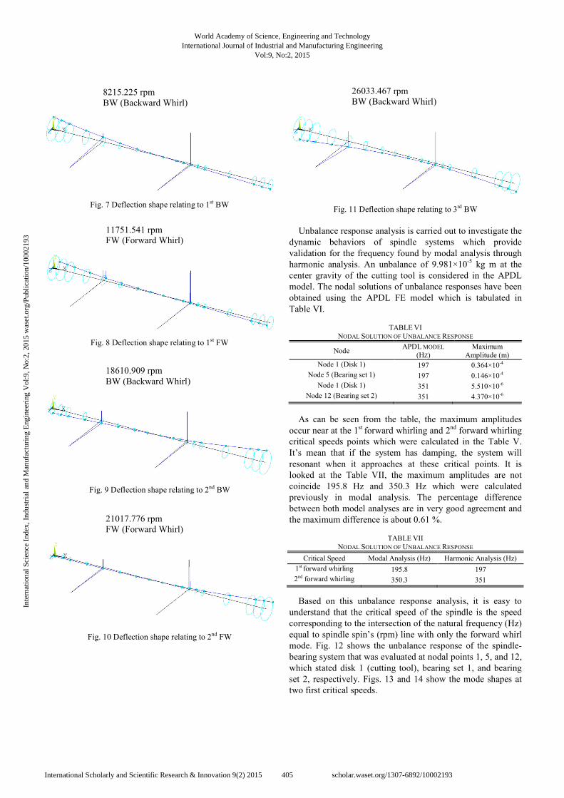
Fig. 7 Deflection shape relating to 1st BW

Fig. 8 Deflection shape relating to 1st FW

Fig. 9 Deflection shape relating to 2nd BW

Fig. 10 Deflection shape relating to 2nd FW

Fig. 11 Deflection shape relating to 3rd BW

Unbalance response analysis is carried out to investigate the

dynamic behaviors of spindle systems which provide

validation for the frequency found by modal analysis through

harmonic analysis. An unbalance of 9.981×10-5

kg m at the

center gravity of the cutting tool is considered in the APDL

model. The nodal solutions of unbalance responses have been

obtained using the APDL FE model which is tabulated in

Table VI.

TABLE VI

NODAL SOLUTION OF UNBALANCE RESPONSE

Node APDL MODEL

(HZ)

Maximum

Amplitude (m)

Node 1 (Disk 1) 197 0.364×10-4

Node 5 (Bearing set 1) 197 0.146×10-4

Node 1 (Disk 1) 351 5.510×10-6

Node 12 (Bearing set 2) 351 4.370×10-6

As can be seen from the table, the maximum amplitudes

occur near at the 1st

forward whirling and 2nd

forward whirling

critical speeds points which were calculated in the Table V.

It’s mean that if the system has damping, the system will

resonant when it approaches at these critical points. It is

looked at the Table VII, the maximum amplitudes are not

coincide 195.8 Hz and 350.3 Hz which were calculated

previously in modal analysis. The percentage difference

between both model analyses are in very good agreement and

the maximum difference is about 0.61 %.

TABLE VII

NODAL SOLUTION OF UNBALANCE RESPONSE

Critical Speed Modal Analysis (Hz) Harmonic Analysis (Hz)

1st forward whirling 195.8 197

2nd forward whirling 350.3 351

Based on this unbalance response analysis, it is easy to

understand that the critical speed of the spindle is the speed

corresponding to the intersection of the natural frequency (Hz)

equal to spindle spin’s (rpm) line with only the forward whirl

mode. Fig. 12 shows the unbalance response of the spindle-

bearing system that was evaluated at nodal points 1, 5, and 12,

which stated disk 1 (cutting tool), bearing set 1, and bearing

set 2, respectively. Figs. 13 and 14 show the mode shapes at

two first critical speeds.

8215.225 rpm

BW (Backward Whirl)

11751.541 rpm

FW (Forward Whirl)

18610.909 rpm

BW (Backward Whirl)

21017.776 rpm

FW (Forward Whirl)

26033.467 rpm

BW (Backward Whirl)


Vol:9, No:2, 2015


Inte

rnat

iona

l Sci

ence

Ind

ex, I

ndus

tria

l and

Man

ufac

turi

ng E

ngin

eeri

ng V

ol:9

, No:

2, 2

015

was

et.o

rg/P

ublic

atio

n/10

0021

93



Fig. 12 Unbalance response of spindle system (APDL model)

Fig. 13 The behavior of the system at the 1st forward critical speed

Fig. 14 The behavior of the system at the 2nd forward critical speed

V. CONCLUSION

A program named ANSYS Parametric Design Language

(APDL) based on finite element method has been

implemented to make the full dynamic analysis and evaluation

of the results. A grinding spindle system with certain

geometrical and mechanical properties is modeled as beam

APDL model technique. The deflection shapes of the spindle

at operating speeds, the Campbell diagrams, critical speeds,

and unbalance response are obtained. Based on this unbalance

response analysis that the critical speeds of the spindle are the

1st

forward whirling and 2nd

forward whirling, which the speed

corresponding to the intersection of the natural frequency (Hz)

equal to spindle spin’s (rpm) line with only the forward whirl

mode. These critical speeds are still far from the operating

speed range of the spindle, thus, the spindle would not

experience resonance, and the maximum unbalance response

at operating speed is still with acceptable limit. Thus, APDL

program can be used by spindle designer as tools in order to

increase the product quality, reducing cost, and time

consuming in the design and development stages.

REFERENCES

[1] C.W. Lin, Y.K. Lin, C.H. Chu, Dynamic models and design of spindle-

bearing system of machine tools: a review, International Journal of Precision Engineering and Manufacturing 14 (2013) 513-521.

[2] C.W. Lin, Optimization of bearing locations for maximizing first mode

natural frequency of motorized spindle-bearing systems using a genetic algorithm, Applied Mathematics 5 (2014) 2137-2152.

[3] H.D. Nelson, J.M. McVaugh, The Dynamics models of rotor-bearing

systems using finite elements, Journal of Engineering for Industry, Transactions of the ASME 93 (1976) 593-600.

[4] H.D. Nelson, A finite rotating shaft element using Timoshenko beam

theory, Journal of Mechanical Design, Transactions of the ASME 102 (1980) 793-803.

[5] E. Zorzi, H.D. Nelson, Finite element simulation of rotor-bearing

systems with internal damping, Journal of Engineering for Power, Transactions of the ASME 7 (1977) 71-76.

[6] Y. Cao, Y. Altintas, A general method for the modeling of spindle-

bearing system, Journal of Mechanical Design 120 (2004) 1089-1104. [7] A. Erturk, H.N. Ozguven, E. Budak, Analytical modeling of spindle-tool

dynamics on machine tools using Timoshenko beam model and

receptance coupling for the prediction of tool point FRF, International Journal of Precision Machine Tools & Manufacture 46 (2006) 1901-

1912.

[8] E. Chatelet, F. D’Ambrosio, G. Jacquet-Richardet, Toward global modeling approaches for dynamic analyses of rotating assemblies of

turbomachines, Journal of Sound and Vibration 282 (2005) 163–178.

[9] R. Whalley, A. Abdul-Ameer, Contoured shaft and rotor dynamics, Mechanism and Machine Theory 44 (2009) 772–783.

[10] H. Taplak, M. Parlak, Evaluation of gas turbine rotor dynamic analysis

using the finite element method, Measurement 45 (2012) 1089-1097. [11] M.H. Jalali, M. Ghayour, S. Ziaei-Rad, B. Shahriari, Dynamic analysis

of high speed rotor-bearing system, Measurement 53 (2014) 1-9. [12] C. Villa, J.J. Sinou, F. Thouverez, Stability and vibration analysis of a

complex flexible rotor bearing system, Communications in Nonlinear

Science and Numerical Simulation 13 (2008) 804–821.

[13] B. Bai, L. Zhang, T. Guo, C. Liu, Analysis of dynamic characteristics of the main shaft system in a Hydro-turbine based on ANSYS, Procedia

Engineering 31 (2012) 654 – 658.

[14] B. Gurudatt, S. Seetharamu, P. S. Sampathkumaran, V. Krishna, Implementation of ANSYS Parametric Design Language for the

determination of critical speeds of a fluid film bearing supported multi-

sectioned rotor with residual unbalance through modal and out-of-balance response analysis, Proceedings of world congress of

Engineering 2 (2010) 1592-1596.

[15] K. Jagannath, Evaluation of critical speed of Generator Rotor with external load, International Journal of Engineering Research and

Development 1 (11) (2012) 11-16.

[16] M. Lalanne, B.G. Ferraris, Rotordynamics prediction in engineering, Wiley, New York 1998.

[17] M.I Friswell, J.E.T. Penny, S.D Garvey, A.W. Lees, Dynamics of

rotating machines, Cambridge University Press, 2010. [18] T. Yamamoto, Y. Ishida, Linear non linear rotordynamics a modern

treatment with applications, John wiley and sons, USA 2001.

0 0.5 1 1.5 2 2.5

x 104

10-8

10-7

10-6

10-5

10-4

Spindle spin speed (rpm)

Am

plit

ude

(m

)

Disk 1

Bearing Set 1

Bearing Set 2

11820 rpm

FW

Deflection max = 36.4µm

21060 rpm

FW

Deflection max = 5.51µm


Vol:9, No:2, 2015


Inte

rnat

iona

l Sci

ence

Ind

ex, I

ndus

tria

l and

Man

ufac

turi

ng E

ngin

eeri

ng V

ol:9

, No:

2, 2

015

was

et.o

rg/P

ublic

atio

n/10

0021

93



Evaluation of Dynamic Behavior a Machine Tool Spindle ...

Documents

Transcript of Evaluation of Dynamic Behavior a Machine Tool Spindle ...