
Evaluation of Description Logic Programs using an RDBMS
103
Evaluation of Description Logic Programs using an RDBMS DIPLOMARBEIT zur Erlangung des akademischen Grades Diplom-Ingenieur im Rahmen des Studiums Computational Intelligence eingereicht von Patrik Schneider, BSc. Matrikelnummer 0627383 an der Fakultät für Informatik der Technischen Universität Wien Betreuung Betreuer: O.Univ.Prof. Dipl.-Ing. Dr. techn. Thomas Eiter Mitwirkung: Dipl.-Ing. Thomas Krennwallner Wien, 30.12.2010 (Unterschrift Verfasser) (Unterschrift Betreuer) Technische Universität Wien A-1040 Wien Karlsplatz 13 Tel. +43-1-58801-0 www.tuwien.ac.at
-
Upload
khangminh22 -
Category
Documents
-
view
3 -
download
0
Transcript of Evaluation of Description Logic Programs using an RDBMS
Evaluation of Description LogicPrograms using an RDBMS
DIPLOMARBEIT
zur Erlangung des akademischen Grades
Diplom-Ingenieur
im Rahmen des Studiums
Computational Intelligence
eingereicht von
Patrik Schneider, BSc.Matrikelnummer 0627383
an der
Fakultät für Informatik der Technischen Universität Wien
Betreuung
Betreuer: O.Univ.Prof. Dipl.-Ing. Dr. techn. Thomas Eiter
Mitwirkung: Dipl.-Ing. Thomas Krennwallner
Wien, 30.12.2010
(Unterschrift Verfasser) (Unterschrift Betreuer)
Technische Universität Wien
A-1040 Wien � Karlsplatz 13 � Tel. +43-1-58801-0 � www.tuwien.ac.at

Erklärung zur Verfassung der Arbeit
Patrik SchneiderPostfach 6689490 VaduzLiechtenstein
Hiermit erkläre ich, dass ich diese Arbeit selbstständig verfasst habe, dass ich die verwen-deten Quellen und Hilfsmittel vollständig angegeben habe und dass ich die Stellen derArbeit – einschließlich Tabellen, Karten und Abbildungen –, die anderen Werken oderdem Internet im Wortlaut oder dem Sinn nach entnommen sind, auf jeden Fall unterAngabe der Quelle als Entlehnung kenntlich gemacht habe.
Wien, 30.12.2010
(Unterschrift Verfasser)

v
Abstract
We propose a novel approach to evaluate description logic programs (dl-programs) usinga Relational Database Management System (RDBMS). Such dl-programs are a state-of-the-art Semantic Web formalism of combining rules and ontologies, whereby rules areexpressed as logic programs and ontologies are expressed in Description Logics (DL).In dl-programs a modular concept of plug-ins was introduced, which allows to combinedl-programs with different DL reasoner. Grounding in dl-programs is still considereda performance bottleneck, caused by having exponentially many rules to process. Butfor the success of the Semantic Web technologies, it is crucial to efficiently process vastamounts of data. The goal of this work is to show, that dl-programs can be efficientlyevaluated by using RDBMSs. For this purpose we report on a prototype implementation,where SQL is generated by an existing DL-Lite reasoner, which is incorporated into aDatalog rewriter. For testing the prototype, we develop a benchmark suite with pureDatalog and Datalog/DL tests. Based on the benchmark suite, we produce experimentalresults. These results are used to compare the prototype with the reasoners of the DLVfamily.
Zusammenfassung
Wir entwickeln einen neuen Ansatz, bei dem Description Logic Programs (dl-programs)auf einem relationalen Datenbank System (RDBMS) evaluiert werden. Die dl-programssind ein vielversprechender Semantik Web Formalismus um Regeln und Ontologien zukombinieren. Dabei werden die Regeln als Logische Programme und die Ontologienin Beschreibungslogiken (DL) ausgedrückt. Bei der bottom-up Auswertung eines dl-programs gibt es aber immer noch Geschwindigkeitseinbussen, da exponentiell vieleRegeln im Verhältnis zur Grösse des Programms entstehen können. Ein wichtiger Faktorfür die Akzeptanz von Semantik Web Technologien besteht aber darin, dass grosse Daten-mengen effizient verarbeitet werden können. Das Ziel dieser Arbeit ist nun zu zeigen, dassdl-programs mit Hilfe von RDBMS effizient verarbeitet werden können. Um dieses Zielzu erreichen, wurde ein Prototyp entwickelt, bei dem mit Hilfe eines DL-Lite und einesDatalog Systems, SQL generiert wird. Um die Effizienz des Prototyps zu zeigen, werdenBenchmarks entwickelt, welche aus Datalog und Datalog/DL Tests bestehen. Aufgrunddieser Benchmarks wird dann der Prototyp an den Systemen der DLV-Familie gemessen.
Acknowledgements
First of all, I owe my sincerest gratitude to my supervisor, Thomas Eiter, who gaveme the opportunity to write my thesis, supported me throughout with his patience andknowledge, while giving me enough space to work in my own pace. He gave me greatinsight into the field of Knowledge Representation and Reasoning as well as into scien-tific research as a whole. Moreover, I have learned good practise for scientific writing.Particularly, I enjoyed the session about princesses, dragons, and heroes.
I would also like to thank Thomas Krennwallner, who provided me with many importanthints, remarkably, when I exactly needed them. Moreover, I am indebted to the staff ofKBS, for supporting me whenever needed.
Lastly, I am truly grateful to my family providing me with support and a loving environ-ment. Writing a thesis is often a long journey with many obstacles, but it is definitely avaluable experience, especially with great backing.
Contents
1. Introduction 11.1. Logic Programming . . . . . . . . . . . . . . . . . . . . . . . . . . . . . . . 3
1.1.1. Datalog . . . . . . . . . . . . . . . . . . . . . . . . . . . . . . . . . 31.1.2. Answer-Set Programming . . . . . . . . . . . . . . . . . . . . . . . 41.1.3. Tools . . . . . . . . . . . . . . . . . . . . . . . . . . . . . . . . . . . 5
1.2. Semantic Web Technologies . . . . . . . . . . . . . . . . . . . . . . . . . . 61.2.1. OWL . . . . . . . . . . . . . . . . . . . . . . . . . . . . . . . . . . 71.2.2. OWL 2 EL . . . . . . . . . . . . . . . . . . . . . . . . . . . . . . . 81.2.3. OWL 2 QL . . . . . . . . . . . . . . . . . . . . . . . . . . . . . . . 91.2.4. OWL 2 RL . . . . . . . . . . . . . . . . . . . . . . . . . . . . . . . 91.2.5. Tools . . . . . . . . . . . . . . . . . . . . . . . . . . . . . . . . . . . 10
1.3. Combining Rules and Ontologies . . . . . . . . . . . . . . . . . . . . . . . 111.3.1. Loose Coupling . . . . . . . . . . . . . . . . . . . . . . . . . . . . . 111.3.2. Tight Semantic Integration . . . . . . . . . . . . . . . . . . . . . . 121.3.3. Full Integration . . . . . . . . . . . . . . . . . . . . . . . . . . . . . 12
1.4. Structure of the Thesis . . . . . . . . . . . . . . . . . . . . . . . . . . . . . 12
2. Preliminaries 132.1. Relational Algebra . . . . . . . . . . . . . . . . . . . . . . . . . . . . . . . 132.2. Stratified Programs . . . . . . . . . . . . . . . . . . . . . . . . . . . . . . 14
2.2.1. Syntax and Semantics of Positive Programs . . . . . . . . . . . . . 152.2.2. Dependency Graphs of Logic Programs . . . . . . . . . . . . . . . . 162.2.3. Fixpoint Theory . . . . . . . . . . . . . . . . . . . . . . . . . . . . 162.2.4. Syntax of Stratified Programs . . . . . . . . . . . . . . . . . . . . . 172.2.5. Semantics of Stratified Programs . . . . . . . . . . . . . . . . . . . 182.2.6. Complexity of Stratified Programs . . . . . . . . . . . . . . . . . . 21
2.3. DL-Lite and the Notion of FOL-Reducibility . . . . . . . . . . . . . . . . . 222.3.1. The DL-Lite Family . . . . . . . . . . . . . . . . . . . . . . . . . . 222.3.2. Reasoning in DL-LiteR . . . . . . . . . . . . . . . . . . . . . . . . 242.3.3. FOL-Reducibility . . . . . . . . . . . . . . . . . . . . . . . . . . . . 242.3.4. KB Satisfiability is FOL-Reducible in DL-LiteR . . . . . . . . . . 252.3.5. Query Answering over DL-LiteR Ontologies . . . . . . . . . . . . . 282.3.6. Complexity Results for DL-LiteR . . . . . . . . . . . . . . . . . . . 30
2.4. Description Logic Programs . . . . . . . . . . . . . . . . . . . . . . . . . . 302.4.1. Syntax of Description Logic Programs . . . . . . . . . . . . . . . . 302.4.2. Well-Founded Semantics for Description Logic Programs . . . . . 31
vii
Contents viii
3. Combining Datalog with DL-Lite 333.1. Rewriting Datalog to Relational Algebra extended with Fixpoint Evaluation 33
3.1.1. Nonrecursive Datalog . . . . . . . . . . . . . . . . . . . . . . . . . 333.1.2. Positive Recursive Datalog . . . . . . . . . . . . . . . . . . . . . . . 363.1.3. Datalog with Negation . . . . . . . . . . . . . . . . . . . . . . . . . 393.1.4. Stratified Datalog . . . . . . . . . . . . . . . . . . . . . . . . . . . . 40
3.2. An Algorithm for Improving Query Answering over DL-LiteR Ontologies 403.3. First-Order Rewritable Case of Description Logic Programs . . . . . . . . 433.4. Stratified Evaluation of Description Logic Programs . . . . . . . . . . . . 46
4. Implementation 514.1. Overview . . . . . . . . . . . . . . . . . . . . . . . . . . . . . . . . . . . . 514.2. Design . . . . . . . . . . . . . . . . . . . . . . . . . . . . . . . . . . . . . . 52
4.2.1. Architecture . . . . . . . . . . . . . . . . . . . . . . . . . . . . . . . 524.2.2. Data- and Control-Flow . . . . . . . . . . . . . . . . . . . . . . . . 53
4.3. Details of Rewriting Datalog to SQL . . . . . . . . . . . . . . . . . . . . . 544.3.1. Datatypes . . . . . . . . . . . . . . . . . . . . . . . . . . . . . . . . 544.3.2. Rewriting the EDB . . . . . . . . . . . . . . . . . . . . . . . . . . . 554.3.3. Rewriting Nonrecursive Rules . . . . . . . . . . . . . . . . . . . . . 564.3.4. Rewriting Recursive Rules . . . . . . . . . . . . . . . . . . . . . . . 58
4.4. Interfacing Owlgres with the DL Plug-in . . . . . . . . . . . . . . . . . . . 594.4.1. DL-Atoms . . . . . . . . . . . . . . . . . . . . . . . . . . . . . . . . 604.4.2. Owlgres Overview . . . . . . . . . . . . . . . . . . . . . . . . . . . 614.4.3. Owlgres KB Management . . . . . . . . . . . . . . . . . . . . . . . 624.4.4. Rewriting the Standard DL-Atom . . . . . . . . . . . . . . . . . . . 634.4.5. Rewriting the Update DL-Atom . . . . . . . . . . . . . . . . . . . . 634.4.6. Adaptions in Owlgres 0.1 . . . . . . . . . . . . . . . . . . . . . . . 64
4.5. Limitations . . . . . . . . . . . . . . . . . . . . . . . . . . . . . . . . . . . 65
5. Experiments 675.1. Methodology . . . . . . . . . . . . . . . . . . . . . . . . . . . . . . . . . . 675.2. Scenario 1 - Datalog . . . . . . . . . . . . . . . . . . . . . . . . . . . . . . 67
5.2.1. Large Join Benchmark . . . . . . . . . . . . . . . . . . . . . . . . . 685.2.2. Default Negation Benchmark . . . . . . . . . . . . . . . . . . . . . 685.2.3. Stratified Negation Benchmark . . . . . . . . . . . . . . . . . . . . 68
5.3. Scenario 2 - Derived DBpedia . . . . . . . . . . . . . . . . . . . . . . . . . 695.3.1. Simple Benchmark . . . . . . . . . . . . . . . . . . . . . . . . . . . 695.3.2. Advanced Benchmark . . . . . . . . . . . . . . . . . . . . . . . . . 705.3.3. Update Benchmark . . . . . . . . . . . . . . . . . . . . . . . . . . . 705.3.4. DBpedia queries . . . . . . . . . . . . . . . . . . . . . . . . . . . . 71
5.4. Scenario 3 - Derived LUBM . . . . . . . . . . . . . . . . . . . . . . . . . . 715.4.1. Simple Benchmark . . . . . . . . . . . . . . . . . . . . . . . . . . . 715.4.2. Advanced Benchmark . . . . . . . . . . . . . . . . . . . . . . . . . 715.4.3. Update Benchmark . . . . . . . . . . . . . . . . . . . . . . . . . . . 72
ix Contents
5.4.4. LUBM queries . . . . . . . . . . . . . . . . . . . . . . . . . . . . . 725.5. Scenario 4 - Limitations and Extensions . . . . . . . . . . . . . . . . . . . 73
5.5.1. Well-Founded Semantics . . . . . . . . . . . . . . . . . . . . . . . . 735.5.2. Combining DLVDB with generated Owlgres queries . . . . . . . . . 73
6. Experimental Results 756.1. Scenario 1 - Datalog . . . . . . . . . . . . . . . . . . . . . . . . . . . . . . 76
6.1.1. Large Join Benchmark . . . . . . . . . . . . . . . . . . . . . . . . . 766.1.2. Default Negation Benchmark . . . . . . . . . . . . . . . . . . . . . 776.1.3. Stratified Negation Benchmark . . . . . . . . . . . . . . . . . . . . 77
6.2. Scenario 2 - Derived DBpedia . . . . . . . . . . . . . . . . . . . . . . . . . 786.2.1. Simple Benchmark . . . . . . . . . . . . . . . . . . . . . . . . . . . 786.2.2. Advanced Benchmark . . . . . . . . . . . . . . . . . . . . . . . . . 796.2.3. Update Benchmark . . . . . . . . . . . . . . . . . . . . . . . . . . . 79
6.3. Scenario 3 - Derived LUBM . . . . . . . . . . . . . . . . . . . . . . . . . . 806.3.1. Simple Benchmark . . . . . . . . . . . . . . . . . . . . . . . . . . . 806.3.2. Advanced Benchmark . . . . . . . . . . . . . . . . . . . . . . . . . 816.3.3. Update Benchmark . . . . . . . . . . . . . . . . . . . . . . . . . . . 82
6.4. Scenario 4 - Limitations and Extensions . . . . . . . . . . . . . . . . . . . 826.4.1. Well-Founded / Stable-Model Semantics . . . . . . . . . . . . . . . 826.4.2. Combining DLVDB with Owlgres . . . . . . . . . . . . . . . . . . . 836.4.3. Summary of Results . . . . . . . . . . . . . . . . . . . . . . . . . . 83
7. Conclusion 857.1. Evaluation Results . . . . . . . . . . . . . . . . . . . . . . . . . . . . . . . 857.2. Future Work and Further Studies . . . . . . . . . . . . . . . . . . . . . . . 86
A. Installation and Use: 87A.1. Prerequisites . . . . . . . . . . . . . . . . . . . . . . . . . . . . . . . . . . 87A.2. Installation . . . . . . . . . . . . . . . . . . . . . . . . . . . . . . . . . . . 87A.3. Calling MOR from the Command Line . . . . . . . . . . . . . . . . . . . . 88
Bibliography 89

1. Introduction
The Semantic Web, anticipated by Tim Berners-Lee in 2001, is by 2010 becoming an im-portant topic in the World Wide Web (WWW) and the information system community.This is observable through mature standards like the Resource Description Framework1
(RDF) and the Web Ontology Language1 (OWL), but also through evolving projectslike Ontorule, DBpedia, or SIOC.2 In their Scientific American article Berners-Lee et al.capture the Semantic Web as follows [Berners-Lee et al., 2001]: Knowledge representa-tion (KR), ontologies and agents are central to the Semantic Web and should lead toan “evolution of knowledge”. KR is crucial, so the WWW can be better understood bycomputer systems and humans. Ontologies, expressed in Description Logics (DL), are acentral part of the “understanding”, adding taxonomies and inference rules to the infor-mation of a web page or a document. Software agent will collect and process informationusing these ontologies. Taking the idea further, an agent could “bootstrap” new reason-ing capabilities when discovering new ontologies. Several agents can be linked togethercreating a “value chain” of information processing, whereby every agent is “adding value”to parts of the information product.
This thesis is inspired by the idea of “adding value” to the information process by ex-tending ontology based inference with Logic Programming (LP) based inference rules. Inrecent years, combining rules and ontologies become an important focus of Semantic Webresearch. The W3C founded the Rule Interchange Format (RIF) working group, whichaim is to create a standard for exchanging rules among rule based systems.3 Extendingthe idea of exchanging rules, a W3C working draft was written concerning “RIF RDF andOWL Compatibility”, which considers the import of RDF and OWL in RIF.4 The RIFworking group also specified different rule languages, which led to a Core, a Basic LogicDialect (BLD), and a Production Rules Dialect (PRD) dialect [Kifer, 2008]. Relatedto the RIF and OWL compatibility, we focus on the strain of research, where rules areexpressed as logic programs and a loose coupling of rules and ontologies is considered.As the starting point of this thesis, we take the state-of-the-art approach of descriptionlogic programs (dl-programs) for loose coupling. Dl-programs were introduced by severalpapers of Eiter et al., describing dl-programs under the answer set semantics [Eiter et al.,2004] and under the well-founded semantics [Eiter et al., 2009b]. The papers mentionedshow that dl-programs regarding to their “advanced” expressive power are still decidable.Furthermore, a modular concept of plug-ins was introduced, which allows to combine
1http://www.w3.org/RDF/ and http://www.w3.org/2007/OWL/wiki/OWL_Working_Group
2http://ontorule-project.eu/, http://dbpedia.org/, and http://sioc-project.org/
3http://www.w3.org/2005/rules/
4http://www.w3.org/TR/rif-rdf-owl/
1
2
dl-programs with different DL reasoners. The concept of plug-ins was generalized toHEX-programs and lead to the successful development of the reasoner dlvhex 5 [Eiteret al., 2006].
Another inspiring idea is related to the size of projects like DBpedia. We observe that avast amount of data is collected and linked to ontologies. For the acceptance of SemanticWeb applications it is crucial, that these data is processed efficiently. Efficient dataprocessing was a main reason for the advent of relational database (DB) technology, sowe will use this technology as the foundation of our inference system. DL-Lite, whichwas introduced by Calvanese et al., builds the link needed between DL-based inferenceand a Relational Database Management System (RDBMS) [Calvanese et al., 2007].
DLV6 or dlvhex, belonging to the group of Answer Set (AS) solvers, which first grounda logic program before the solutions are computed. Even with highly efficient groundingalgorithms, we might encounter a grounding bottleneck, caused by having exponentiallymany rules to process [Eiter et al., 2007, 2009a]. If we reason with a large Knowledgebase (KB), we definitely need a more efficient technique for inference, however withoutsacrificing the expressibility.
The main aim of this thesis is to show the feasibility of an efficient implementation ofdl-programs using an RDBMS. In particular, we answer the emerging questions of howexpressible the proof of concept is, what technical limitations are encountered, and howscalable the implementation is.
The following list gives a brief overview of the contributions of this thesis:
1. We show that dl-programs under stratified semantics are rewritable into SQL, withthe restriction that the DL-Lite plug-in provides positive Datalog. To achieve thisrewriting, we leverage from stratified Datalog and DL-Lite, since both formalismsare rewritable in SQL.
2. We report on a prototype implementation, called MOR, where an existing DL-Litereasoner is incorporated into our Datalog rewriter. The Datalog rewriter takesadvantage of linear recursive queries in SQL:1999 [ISO, 1999].
3. For showing the scalability of MOR, we develop a benchmark suite consideringexpressibility and performance. The suite is separated into a scenario for plainDatalog and two scenarios for Datalog combined with DL-Lite.
4. Based on the benchmark suite, we produce and compare experimental results withMOR and the reasoners of the DLV family. We can remark in advance that theresults are encouraging.
An example should illustrate the need for our efforts. Take a “smart” route planner, whichshould provide the user not just with short routes, but with customized routes. Thesecustom routes, tailored to the needs of an user, could consider environmental, monetary,or even shopping objectives. Ontologies would be needed to define different means of
5http://www.kr.tuwien.ac.at/research/systems/dlvhex/
6http://www.dbai.tuwien.ac.at/proj/dlv/
3 Introduction
transport, geographical locations, and different types of shops. Furthermore ontologieswould be needed to link different types of information to each other. The data for thisinformation would be extracted from several external sources (e.g. public rail system,maps, routes, yellow pages, etc.). Then we would need rule based reasoning to calculatethe shortest, cheapest, most environmental friendly or most “interesting” way. Thiscould be even extended with the capabilities for user to formulate their own constraintsregarding transport, money or their personal interests. This example illustrates that newkinds of applications could be captured by integration ontologies with rules in a scalablefashion.
1.1. Logic Programming
In the 1970s and 1980s, LP evolved out of a debate about two different paradigmsof KR. One paradigm, procedural knowledge representation, advocated mainly at MITaround Marvin Minsky, features recursive procedures that operate on lists. Lisp, basedon Lambda Calculus, become the main programming language for this paradigm [Mc-Carthy, 1960]. It is still in considerable use by AI-researchers.7 The other paradigm,declarative knowledge representation, features logic as a declarative language, which isevaluated by a theorem-prover or model-generator. This paradigm was advocated aroundJohn McCarthy of Standford, Pat Hayes, and Bob Kowalski of Edinburgh. The main ideaevolved from the deduction method Resolution Principle, developed by John Alan Robin-son in 1965 [Robinson, 1965]. This deduction method was then implemented by AlainColmerauer in Prolog. The principle of Prolog can be subsumed as: ALGORITHM =LOGIC + CONTROL [Colmerauer, 1985]. As Lisp, Prolog attracted and held a stronglydevoted user community. Carl Hewitt in [Hewitt, 2009] gives an in-depth view of thedevelopments and controversies in LP research around the 1970s.
1.1.1. Datalog
Strongly influenced by the research in the relational DB field, Datalog restricts LP andparticularly Prolog, to a function-free first-order vocabulary. Due to its use in the DBfield, facts are not stored in the logic program itself, but kept in an extensional database(EDB) usually maintained by an RDBMS. Datalog can be traced back to several re-searchers, particularly to H. Gallaire and J. Minker, which were researching the intersec-tion between LP and DBs [Gallaire et al., 1977]. The name “Datalog” was coined laterby David Maier. An interesting property of Datalog is related to its semantics. Datalogcomes with three different equivalent semantics, namely model-theoretic, fixpoint, andproof-theoretic semantics [Abiteboul et al., 1995]. We will have a closer look at Datalogin Chapter 2.
According to Abiteboul et al. Datalog can be distinguished from LP as follows [Abiteboulet al., 1995]:
7See the conference for the 50th anniversary of Lisp: http://www.lisp50.org/
Logic Programming 4
• Syntax: In Datalog only relation symbols are allowed, hence functions symbols areexcluded. Furthermore variables in Datalog rules have to fulfill certain safenessconditions.
• Model-theoretic semantics: Datalog programs always have finite models, in oppo-site to infinite models in LP.
• Fixpoint semantics: Fixpoint semantics does not certainly provide a constructivesemantics for LP.
• Proof-theoretic semantics: In LP, SLD resolution is crucial, due to the infinitenessof answers, whereby bottom-up approaches are not feasible. In Datalog, resolutionis rather used for optimization (e.g. magic sets).
• Expressive power: LP can express all recursive enumerable languages predicates,whereby Datalog’s expressive power is in PTIME.
Example 1. The ancestor problem is a well-known example for Datalog:
parent(a, b). parent(b, c).parent(b, d). parent(d, e).ancestor(X,Y ) ← parent(X,Y ).ancestor(X,Y ) ← parent(X,Z), ancestor(Z, Y ).
1.1.2. Answer-Set Programming
Answer-Set Programming (ASP) is a nonmonotonic LP paradigm based on the StableModel Semantics [Gelfond and Lifschitz, 1988] and extended with classical negation in[Gelfond and Lifschitz, 1991]. The development of ASP was surely influenced by certainlimitations of Prolog. One limitation is the absence of a purely declarative representationof Prolog programs, because the order of the rules in Prolog are important for theirevaluation. If negation-as-failure (NAF) is interpreted in the Stabe Model Semantics,the NAF of a literal means that the literal is “not known”, which differs to the classicalinterpretation of the literal’s negation. In Prolog classical negation is simply omitted.Moreover the solution of a Prolog program is not encoded in a model. With ASP somelimitations of Prolog were overcome and a more general problem solving strategy evolved.This strategy can be outline according to [Eiter et al., 2009a] as follows:
1. A problem instance is encoded in a (nonmonotonic) logic program, such that thesolutions are represented by the models of the program;
2. some models of the program are computed using an ASP solver; and
3. a solution for the problem is extracted from the model.
This strategy is well suited to solve NP-complete problems like three-colorability of agraph [Eiter et al., 2009a].
5 Introduction
Example 2. To illustrate the method of ASP, we take the strategic companies problemas an example. Central to this problem is the concept of a strategic set, which is aminimal set of companies, being controlled by three other strategic companies. Basedon this, it should be determined which companies can be sold, whereby all products stillhave to be produced and no company should be controlled by its holding company afterselling:
prod_by(p1, c1, c2). prod_by(p2, c2, c3).prod_by(p3, c3, c4). prod_by(p4, c4, c5).contr_by(c1, c2, c3, c4). contr_by(c2, c1, c3, c4).contr_by(c4, c2, c3, c1). contr_by(c3, c1, c2, c4).strateg(C1) ∨ strategic(C2) ← prod_by(P,C1, C2).strateg(C) ← contr_by(C,C1, C2, C3), strateg(C1), strateg(C2), strateg(C3).
An ASP solver would return several answer sets for this example.
1.1.3. Tools
For Prolog, SWI-Prolog8 is a widely used open source implementation. Datalog is morea conceptional language and has effected RDBMS standards. For example the SQL:1999standard is partly influenced by Datalog [ISO, 1999]. Furthermore Datalog had an impacton deductive DB systems like XSB9.
ASP has been implemented by the following systems:
• DLV10, a joint development of University of Calabria and Vienna University ofTechnology, extends ASP with weak constraints, aggregates, and a SQL front-end[Leone et al., 2006]. DLVDB 11 is an extended development of DLV for evaluat-ing ASP on RDBMS [Terracina et al., 2008]. Finally, in dlvhex12 the concept ofmodularization was introduced [Eiter et al., 2006]. We will use DLV, DLVDB, anddlvhex in our experiments.
• Smodels13 , developed at Helsinki University of Technology, extending ASP withsimilar functions as DLV [Niemelä and Simons, 1997].
• Clasp14, developed at University of Potsdam and using a conflict-driven solvingtechnique [Gebser et al., 2007a].
8http://www.swi-prolog.org/
9http://xsb.sourceforge.net/
10http://www.dbai.tuwien.ac.at/proj/dlv/
11http://www.mat.unical.it/terracina/dlvdb/
12http://www.kr.tuwien.ac.at/research/systems/dlvhex/
13http://www.tcs.hut.fi/Software/smodels/
14http://www.cs.uni-potsdam.de/clasp/
Semantic Web Technologies 6
1.2. Semantic Web Technologies
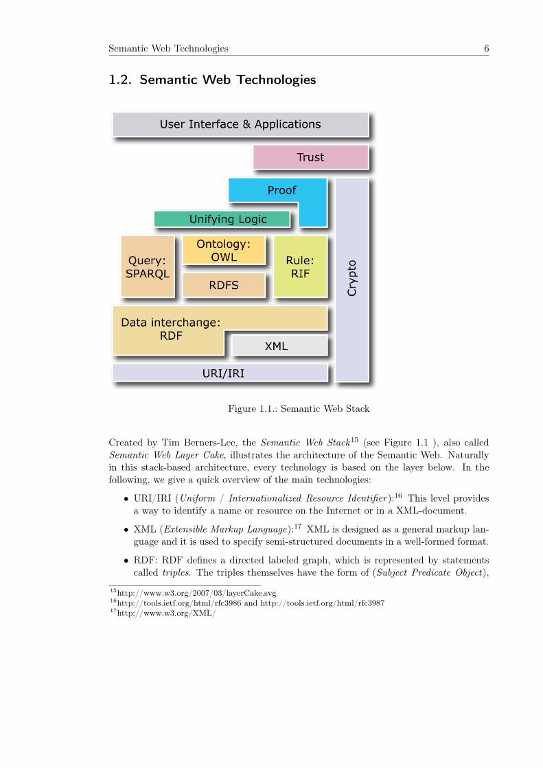
Figure 1.1.: Semantic Web Stack
Created by Tim Berners-Lee, the Semantic Web Stack15 (see Figure 1.1 ), also calledSemantic Web Layer Cake, illustrates the architecture of the Semantic Web. Naturallyin this stack-based architecture, every technology is based on the layer below. In thefollowing, we give a quick overview of the main technologies:
• URI/IRI (Uniform / Internationalized Resource Identifier):16 This level providesa way to identify a name or resource on the Internet or in a XML-document.
• XML (Extensible Markup Language):17 XML is designed as a general markup lan-guage and it is used to specify semi-structured documents in a well-formed format.
• RDF: RDF defines a directed labeled graph, which is represented by statementscalled triples. The triples themselves have the form of (Subject Predicate Object),
15http://www.w3.org/2007/03/layerCake.svg
16http://tools.ietf.org/html/rfc3986 and http://tools.ietf.org/html/rfc3987
17http://www.w3.org/XML/
7 Introduction
whereby- the Subject is a vertice and the tail of the edge representing the triple;- the Object is a vertice and head of the triple’s edge;- the Predicate is defined as the label of the edge.
A Subject is represented by either a resource (URI) or a blank node; an Objectis represented by either a resource, a blank node, or a data type literal.
• RDFS (RDF Schema):18 RDFS extends RDF with a basic vocabulary for ontolo-gies, e.g. Class, Property, and Label.
• SPARQL:19 SPARQL is a RDF query language loosely based on SQL. SPARQLcan be seen as the main technology to retrieve information from RDF graphs.
• OWL: In the following section we will have a closer look at it.
• RIF and Unifying Logic: RIF serves as an interchange format between existing rulesystems. RIF is, as well as Unifying Logic an important focus of current SemanticWeb research, whereby Unifying Logic is aiming for a combined formalisms of rulesand ontologies. These topics are a key issues of this thesis and will be discussed inthe following chapters.
• Proof: This layer is concerned with proof techniques for the underlying ontologies,rules, and unifying logic.
• Trust and Crypto: The provided information are validated and supported regardingsound and complete reasoning and trusted sources.
• User Interface & Applications: This level relates to applications which make use ofthe Semantic Web or give access to one of the different layers.
1.2.1. OWL
Already ongoing for several years, a main focus of Semantic Web research was shaping anadequate language for ontology modeling. As one of the achievements of this research,in 2004, OWL was for the first time recommended [Schreiber and Dean, 2004]. Now, themost recent recommendation by the W3C is OWL 2 [Krötzsch et al., 2009]. There arestill speculations about the confusion of “W” by “O” in OWL. According to Tim Finin,OWL is primary an acronym for the bird, which is easy to illustrate and associatedwith wisdom. Additionally OWL relates to an early KR language called One WorldLanguage.20
In the OWL 2 Primer the main two alternative semantics for OWL 2 are outlined. ARDF-based semantics, called OWL 2 Full, which allows the full expressivity of RDFS,with the unfavorable drawback of being undecidable. On the other hand, a DL based18
http://www.w3.org/TR/rdf-schema/19
http://www.w3.org/TR/rdf-sparql-query/20
http://lists.w3.org/Archives/Public/www-webont-wg/2001Dec/0169.html
Semantic Web Technologies 8
semantics, called OWL DL, which puts syntactic restrictions on RDFS [Krötzsch et al.,2009].
DL is a family of KR formalisms based on a fragment of first-order logic (FOL). A DLknowledge base (KB) is separated into an intentional knowledge base (TBox) and anextensional knowledge base (TBox). The base vocabulary of a DL consists of Individuals,Classes, and Roles. Furthermore, Classes and Roles are put in relations to eachother andIndividuals are asserted to them [Baader et al., 2004]. We assume that DL was chosendue its well-defined computational properties and modular concept. A modular conceptin that sense, that most families of DL are based on the simple DL called ALC, whereasALC expressivity is extended with new language constructs. For example SHOIN (D)extends ALC with transitivity, cardinality, equivalence between Individuals, functionalRoles, and more. For further details, we refer the interested reader to [Baader et al.,2004].
The DL SHOIN (D) provides the formal base of OWL DL and enables, due to itscomputational properties, the development of efficient reasoning systems. Notice thatundecidability in OWL Full results mainly from not distinguishing between the sets ofIndividuals, Classes, and Roles. In contrast to this, these types are pairwise disjunctivesets in SHOIN (D).
With OWL 2 a further extension called OWL 2 Profiles was introduced by the W3C[Motik et al., 2009]. The aim of these profiles is, formally called fragments, tradingexpressive power for lower complexity. As we will see with OWL 2 QL, this trade-offestablishes capabilities of using technologies like RDBMS. Note that in DL, most of thereasoning systems are based on tableaux based algorithms.
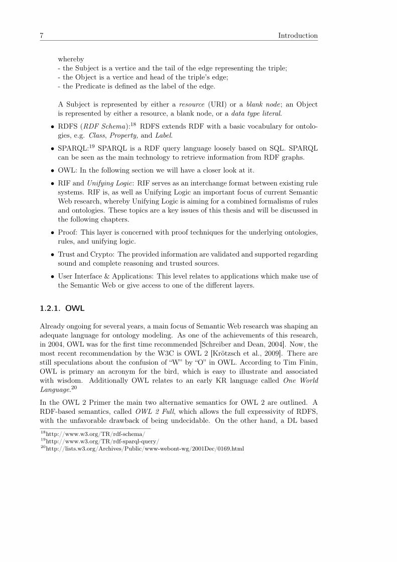
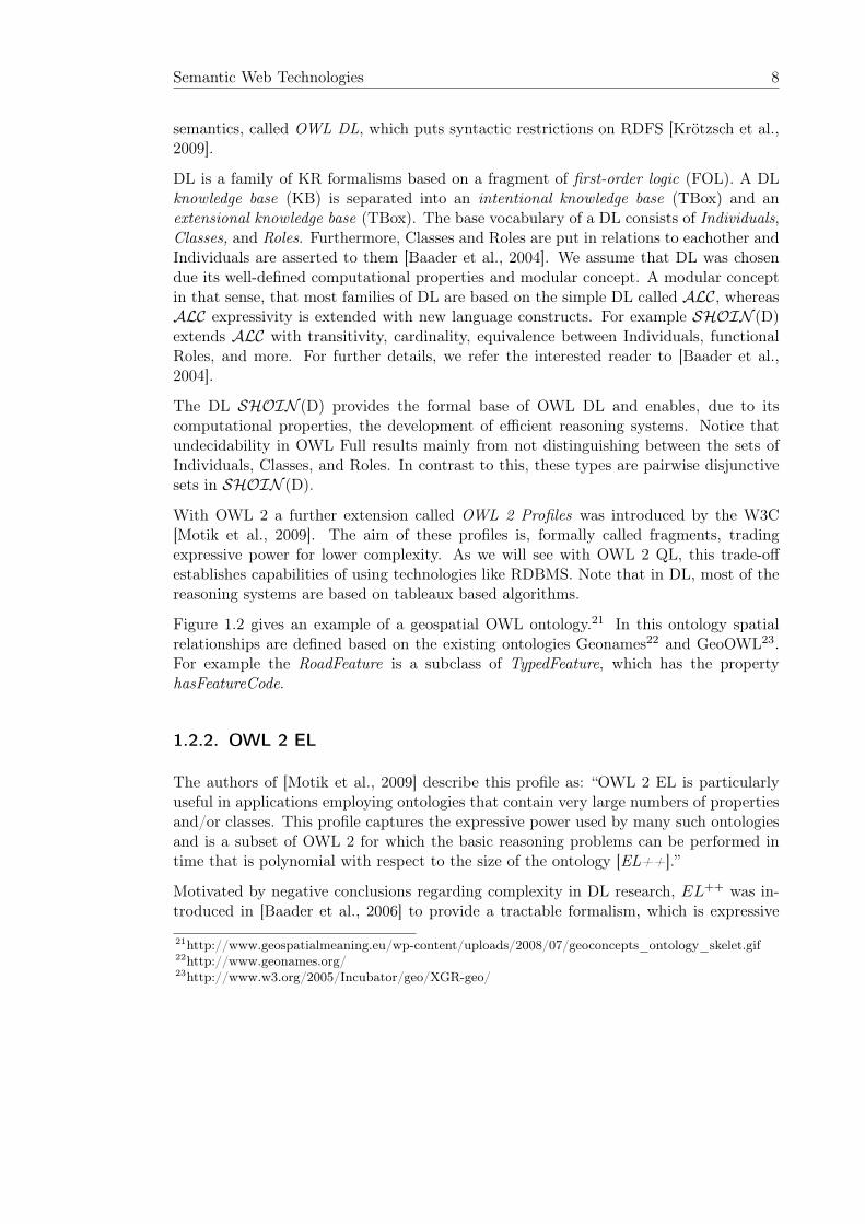
Figure 1.2 gives an example of a geospatial OWL ontology.21 In this ontology spatialrelationships are defined based on the existing ontologies Geonames22 and GeoOWL23.For example the RoadFeature is a subclass of TypedFeature, which has the propertyhasFeatureCode.
1.2.2. OWL 2 EL
The authors of [Motik et al., 2009] describe this profile as: “OWL 2 EL is particularlyuseful in applications employing ontologies that contain very large numbers of propertiesand/or classes. This profile captures the expressive power used by many such ontologiesand is a subset of OWL 2 for which the basic reasoning problems can be performed intime that is polynomial with respect to the size of the ontology [EL++].”
Motivated by negative conclusions regarding complexity in DL research, EL++ was in-troduced in [Baader et al., 2006] to provide a tractable formalism, which is expressive
21http://www.geospatialmeaning.eu/wp-content/uploads/2008/07/geoconcepts_ontology_skelet.gif
22http://www.geonames.org/
23http://www.w3.org/2005/Incubator/geo/XGR-geo/
9 Introduction
Figure 1.2.: A Geospatial Ontology
enough to capture ontologies used in practice. For example, the biomedical ontologySNOMED CT24 is expressible in EL++.
1.2.3. OWL 2 QL
In [Motik et al., 2009] this profile was summarized as: “OWL 2 QL is aimed at ap-plications that use very large volumes of instance data, and where query answering isthe most important reasoning task. In OWL 2 QL, conjunctive query answering canbe implemented using conventional relational database systems. Using a suitable rea-soning technique, sound and complete conjunctive query answering can be performed inLOGSPACE with respect to the size of the data (assertions).”
OWL 2 QL will be one of the main focus points of this thesis, due its capabilities ofanswering conjunctive query over a DL KB using an RDBMS. In Chapter 2 we will havea in-depth look at the DL-Lite family and particularly at DL-LiteR [Calvanese et al.,2007].
1.2.4. OWL 2 RL
Again in [Motik et al., 2009] this profile is characterized as: “OWL 2 RL is aimed at ap-plications that require scalable reasoning without sacrificing too much expressive power.24
http://www.ihtsdo.org/snomed-ct/

Semantic Web Technologies 10
It is designed to accommodate OWL 2 applications that can trade the full expressivityof the language for efficiency, as well as RDF(S) applications that need some added ex-pressivity. OWL 2 RL reasoning systems can be implemented using rule-based reasoningengines. The ontology consistency, class expression satisfiability, class expression sub-sumption, instance checking, and conjunctive query answering problems can be solved intime that is polynomial with respect to the size of the ontology.”According to Motik et al. the design of OWL 2 RL was influenced by Description LogicPrograms and pD*, which enables the implementation of reasoning capabilities by rule-based reasoner [Motik et al., 2009].
1.2.5. Tools
Depending on the level of the Semantic Web Stack, different tools come into use. Forediting RDF any XML-Editor can be used, for editing OWL the open-source editorProtégé25 is convenient. For developing Semantic Web applications the Jena26 frameworkprovides a favorable starting poing.However, our interest is more related to the DL reasoning systems. For OWL DL well-known systems are:27
• FaCT++28,• Hermit29,• KAON230,• Pellet31, and• RacerPro32, which will be used in combination with dlvhex for parts of our exper-
iments.The following OWL 2 Profiles are supported by:
• CEL supports OWL EL33,• QuOnto34 and Owlgres35 supports DL-LiteRand OWL QL, whereas we will have a
in-depth look at Owlgres in Chapter 4, and• ORACLE 11g36 supports OWL RL.
25http://protege.stanford.edu/
26http://jena.sourceforge.net/
27A comprehensive list of DL reasoners can be found on
http://www.cs.manchester.ac.uk/~sattler/reasoners.html28
http://owl.man.ac.uk/factplusplus/29
http://hermit-reasoner.com/30
http://kaon2.semanticweb.org/31
http://clarkparsia.com/pellet/32
http://www.racer-systems.com/products/racerpro/33
http://lat.inf.tu-dresden.de/systems/cel/34
http://www.dis.uniroma1.it/~quonto/35
http://pellet.owldl.com/owlgres/36
http://www.oracle.com/database/
11 Introduction
1.3. Combining Rules and Ontologies
In the past couple of years, another focus of Semantic Web research was towards findinga combined KR formalism for rules and ontologies. The discussion was encouraged bycertain shortcomings of DL. The authors of [Motik et al., 2006] point out some reasonsfor extending DL with rules:
• Higher Relational Expressivity: DL is designed to model relations in a tree-likemanner, whereby in LP general relational structures can be defined.
• Polyadic Predicates: In DL only unary (Classes) and binary (Roles) predicates areintended. Particularly in the DB field, larger predicates are common.
• Closed-World Reasoning: Again in the relational and deductive DB field, it isdesired, that if no proof of a positive ground literal is found, then the negation ofthat literal is assumed true [Reiter, 1977].
• Integrity Constraints: In FOL expressing constraints as used in ASP, is not possible.In ASP, constraints are special rules with an empty head and effect the filtering ofunwanted models.
• Modeling Exceptions: In DL being a strict subset of FOL, NAF is not express-ible, which is considered an important capability of non-monotonic formalisms.The famous “usually birds fly, but penguins cannot fly” is used to illustrate thisshortcoming.
The Semantic Web Rule Language (SWRL) was one of the first proposals to overcomethese limitations. The rule layer in SWRL was set on top of OWL, achieved by allowingmaterial implication of OWL expressions [Horrocks et al., 2004]. This leads to undecid-ability in general, however, fragments of SWRL are implemented in several DL reasoner(e.g. KAON2 and Pellet).
In Eiter et al. [Eiter et al., 2008b] an interesting taxonomy of combination approachesis given. The approach is mainly based on the level of integration. Another taxonomy isgiven by the authors of [Mei et al., 2006], which differs between homogeneous and hybridapproaches, taking into account safeness condition and information flow. We will have adetailed look at the taxonomy of [Eiter et al., 2008b].
1.3.1. Loose Coupling
The rule and DL KB are kept as separate, independent components. An interface mech-anism connects both components allowing the exchange of knowledge between them.The interface is designed in a way, that decidability is guaranteed for the combined KB.Furthermore the knowledge flow can be uni- or bi-directional.
Resulting from dl-programs [Eiter et al., 2004], HEX-programs [Eiter et al., 2006] belongto the loose coupling approach. In Chapter 3 we will view dl-programs more detailed.
1.3.2. Tight Semantic Integration
In this approach the rule and DL KB are kept distinct. The integration will not occurthrough an interface mechanism, but through the integration of the rule and DL models,whereby each model should satisfy its domain and “agree” with the other model.
CARIN [Levy and Rousset, 1998] and DL+ log [Rosati, 2006] represent this approach.
1.3.3. Full Integration
The authors of [Eiter et al., 2006] describe full integration the following way: “Fullintegration approaches are mostly distinct by the absence of separation between twovocabularies at hand: the two universes are treated to a large extent in a homogeneousway”.
Description Logic programs (DLP) [Grosof et al., 2003], Hybrid MKNF knowledge bases[Motik et al., 2006], first-order Autoepistemci Logic [de Bruijn et al., 2006], and OpenAnswer Set Programs [Heymans et al., 2007] can be counted to this approach.
1.4. Structure of the Thesis
The structure of the thesis is the following. Chapter 2 provides the formal foundationof combining rules and ontologies. In Chapter 3 the evaluation of dl-programs understratified Datalog is presented. Furthermore, the reformulation of dl-programs to SQL isdescribed. Chapter 4 highlights the technical aspects of the prototype MOR. In Chapter5 we introduce a benchmark suite regarding the evaluation of rule based and combinedprograms. In Chapter 6 we report on the empirical results relating the performance ofMOR in comparison with similar reasoning systems. In Chapter 7 the main results aresummarized and we outline future work and further studies.
2. Preliminaries
In Chapter 1 we gave a brief introduction to Datalog, which will be further elaborated inthis chapter. In Datalog it is feasible to express program classes with unstratified negation(e.g. normal programs under well-founded semantics [Gelder et al., 1991] or under stablemodel semantics [Gelfond and Lifschitz, 1991]). However, we consider the less expressiveclass of stratified programs, which impose some syntactic restrictions on normal programs[Apt et al., 1988]. For current SQL standards, namely SQL:1999, stratified programssuffice to capture the expressivity of SQL [ISO, 1999]. Afterwards, we capture the DL-Lite family and the notion of First-Order Reducibility (FOL-reducibility) for differentreasoning tasks. This introduction is kept close to the paper of [Calvanese et al., 2007].Then, we introduce the formalism of dl-programs. The main idea of dl-programs iscombining normal programs under well-founded semantics with different fragments ofDL [Eiter et al., 2009b]. Again we remain close to the mentioned paper.
2.1. Relational Algebra
General relational algebra is a well studied field and already Tarski was concerned with it.However his algebra is solely based on binary relations [Tarski, 1941]. Codd’s RelationalAlgebra (RA) as an algebraic notation is associated with the Relational Data Model andstill is an important formalism in the DB field [Codd, 1970]. Despite RA was introducedin 1970, it is used as a basic concept of RDBMS. We follow the definitions for RAfrom [Ceri et al., 1990] and [Ullman, 1988]. Particularly Ullmann elaborated the relationbetween RA and Datalog and showed that except recursion RA is as expressive as Datalog[Ullman, 1988].
Definition 3. [Ullman, 1988] The relational data model consists of relations and do-mains. Let D1, ..., Dn be sets, called domains, where D = D1 × ... × Dn. A relationdefined on D1, ..., Dn is any subset R of D. Elements of relations are called tuples, de-fined as �d1, ..., dn� with d1 ∈ D1, ..., dn ∈ Dn. The columns of a relation are calledattributes. The set of attributes for a relation R is denoted the schema of R. Theattributes of R can either be referred by their name or by their position in the schema.
We assume that domains are finite sets, because in the context of RDBMS infinite do-mains can be neglected. Since a relation is a set, the tuples are distinct but not ordered.
Definition 4. [Ullman, 1988] Relational Algebra has the following basic operators:
13
Stratified Programs 14
• Union (∪): Given relations R and S, R ∪ S is the set-theoretic union of the tuplesbelonging to R and S. To ensure the result is again a relation, R and S must haveidentical schemas. This condition is also called union-compatibility.
• Difference (–): Given relations R and S, R – S is the set-theoretic difference of thetuples belonging to R and S. Union-compatibility must be fulfilled.
• Cartesian product (×): Given relations R and S, R × S is the set of all tuples tsuch that t is the concatenation of a tuple r ∈ R and a tuple s ∈ S.
• Projection (πL): Given a list of attributes L, the tuples of the result are derivedfrom the tuples of the operand relation by elimination of the attributes which arenot in L.
• Selection (σF ): Let F be a formula involving operands that are constants, at-tributes, arithmetic comparison operators (e.g. <,>,≤, ...), and logical operators(e.g. ¬,∨,∧). Then, the result of a selection σF on a relation R is the set of tuplesof R which fulfill formula F .
Definition 5. [Ullman, 1988] The Relational Algebra operators Intersection (∩), Com-plement (\), Natural join (��), θ-join (θ), Semijoin (�), Antijoin (�), and Outer joincan be derived from by the basic operators.
Definition 6. [Ceri et al., 1990] If we exclude the difference operator, we obtain thesublanguage Positive Relational Algebra (RA+).
Due to the success of SQL, RA never become a query language for RDBMS, neverthelessit is often used for the internal representation of queries. Following the definitions from[Ceri et al., 1990], we show that SQL can be interpreted in RA.
Definition 7. [Ceri et al., 1990] Let Q be a set of relations and let S be a SQL block ofthe form:
SELECT �A� FROM �Q� WHERE �F �,
where S is interpreted by applying selection σF to Q and projection πA to Q. Q is definedas the Cartesian product of all relations in Q. If F contains a join condition, insteadof the Cartesian product a θ-join can be directly evaluated. Furthermore, several SQLblocks can be combined with the set-based operators union, natural join, and differenceto build new SQL blocks.
Out of Definition 7, we can also apply the reversal to rewrite RA expressions into SQL.
2.2. Stratified Programs
First we give a brief introduction to positive programs and extend them to stratifiedprograms.
15 Preliminaries
2.2.1. Syntax and Semantics of Positive Programs
The following definitions are taken from [Eiter et al., 2009a].
Definition 8. A program P is defined on an alphabet Φ = (S,V, C), consisting of thenonempty sets of predicates S, variables V , and constants C. A term is either a constantor a variable. An atom is defined as p(t1, ..., tk), where p ∈ S, each t1, ..., tk is a term,and k is called the arity of p. A classical literal is a positive (resp. negative) atom a(resp. ¬a). A negation-as-failure (NAF) literal has the form of the default-negated atoma, denoted as not a. Propositional atoms are atoms with arity k = 0.
Definition 9. A positive program is a finite set of rules (clauses) of the form:
a ← b1, ..., bm. ,
where a, b1, ..., bm are atoms based on alphabet Φ. We refer to H(C) as the head of Cand the conjunction b1, ..., bm is denoted as the body B(C). We denote rule C as a factiff m = 0.
Definition 10. Given a program P , the Herbrand universe HUP is the set of all groundterms which can be formed from the alphabet Φ. The Herbrand base HBP is the set ofall ground atoms which can be formed from predicates in S and the terms in HUP . Forany rule C ∈ P , we call ground(C) the set of all possible ground instances of C.
Definition 11. A (Herbrand) interpretation is an interpretation I over HUP , such thatI is a subset of HBP .
Definition 12. A ground rule C is satisfied in an interpretation I, if the head literal istrue in I or at least one body literal is false in I. It is falsified if the head literal is falsein I and all body literals are true in I.
Definition 13. Let I be an interpretation. Then I is a model of
• a ground rule C = a ← b1, ..., bm, denoted I � C, if the rule C is satisfied;
• a rule C, denoted I � C, if I � C � for every C � ∈ ground(C);
• a program P , denoted I � P , if I � C for every rule C ∈ P .
In LP there is usually no distinction between predicates appearing in the head or body.By contrast in Datalog predicates are separated into distinct sets, according to Abiteboulet al. defined as:
Definition 14. [Abiteboul et al., 1995] Let P be a Datalog program, the extensionaldatabase denoted EDB(P ) (resp. intensional database IDB(P ) ) is the set of all predi-cates p ∈ P , iff there exists a rule C ∈ P such that p ∈ B(C) (resp. p ∈ H(C)).
Stratified Programs 16
Definition 15. [Ceri et al., 1990] Let P be a Datalog program, rule C ∈ IDB(P ) hasto satisfy the following conditions:
(i) The predicate occurring in the head of C belongs to IDB(P ).
(ii) All variables which occur in the head of C also occur in the body of C. (ii)is called safety condition.
2.2.2. Dependency Graphs of Logic Programs
Adopted from [Ullman, 1988] we give the definition for a dependency graph of a logicprogram.
Definition 16. [Ullman, 1988] Let P be a program. The dependency graph of P isdefined as a directed labeled graph G = (V,E, L), where V consist of all predicates ofP , L = {+,−} such that, (i) for all p, q ∈ V , �p, q,+� ∈ E, iff there is a rule C ∈ P suchthat p ∈ head of C and q ∈ postive body of C, (ii) for all p, q ∈ V , �p, q,−� ∈ E, iff thereis a rule C ∈ P such that p ∈ head of C and q ∈ negative body of C.
In the context of a dependency graph the notion of topological sorting is interesting.
Definition 17. [Tarjan, 1976] Let G(V,E) be a directed acyclic graph. A topologicalsort of G is the sequence S =
�v1, v2, ..., v|V |
�in which each vertex of V appears exactly
once. For every pair vi and vj of distinct vertices in S, if there is an edge in G from vito vj , then i < j.
2.2.3. Fixpoint Theory
Knaster-Tarski Theorem and Kleene’s fixed-point Theorem are used in several proofs.
Definition 18. Let X be a set and the operator T : P(X) → P(X) be a function . Wesay that T is monotone, if for all X,Y ,X ⊆ Y it follows T (X) ⊆ T (Y ). We say that Tis finitary if for every infinite sequence S0 ⊆ S1 ⊆ ...,
T
� ∞�n=0
Sn
�⊆
∞�n=0
T (Sn)
holds. If T is both monotonic and finitary then it is called continuous. Another oftenused equal definition of continutiy is for every infinite sequence S0 ⊆ S1 ⊆ ..., it is
T
� ∞�n=0
Sn
�=
∞�n=0
T (Sn).
Observe that each continuous operator is also monotone, but the other direction doesnot hold.
17 Preliminaries
Theorem 19. [Knaster-Tarski’s Fixpoint Theorem] Let T be a monotonic operator ona nonempty set X. Then T has a least fixpoint, denoted lfp(T ):
lfp(T ) =�
{X : T (X) ⊆ X} =�{X : T (X) = X}
Definition 20. Let T be a monotonic operator on a nonempty set X. For each finite andtransfinite ordinal the ordinal power of T is defined as follows, where n is an arbitraryordinal and ω is an arbitrary limit ordinal:T ↑0 (X) = X
T ↑n+1 (X) = T (T ↑n (X))T ↑ω (X) =
�n<ω
T ↑n (X)
Theorem 21. [Kleene’s Fixpoint Theorem] Let T be a continuous operator. Thenlfp(T ) = T ↑ω holds (ω is the first limit ordinal, the one corresponding to N).
2.2.4. Syntax of Stratified Programs
In stratified programs positive programs are extended with NAF literal, keeping certainsyntactic restrictions regarding the NAF literal.
Definition 22. [Eiter et al., 2009a] A normal program is a finite set of rules based onthe alphabet Φ, where a rule is in the form:
a ← b1, ..., bk, not bk+1, ..., not bm. ,
where a, b1, ..., bm are atoms and m � k � 0.
By convention, which is also used in the DLV family, variable names start with uppercaseletters, whereas predicate and constant names start with lowercase letters. Furthermoreunderscore “_” denotes an anonymous variable, which stands for a variable which is notused anywhere else in the program.
Definition 23. [Eiter et al., 2009a] For a rule C of a normal program, we refer to H(C)as the head of C, the conjunction of b1, ..., bk, not bk+1, ..., not bm is denoted as the bodyB(C). B(C) can be separated into B+(C) and B−(C), where the former represents allpositive atoms b1, ..., bk and the later all default-negated atoms not bk+1, ..., not bm.
Definition 24. [Apt et al., 1988] Let P be a normal program. A stratification is apartition P = P1, ..., Pn such that for i = 1, ..., n holds:
(i) if a positive literal occurs in a clause in Pi then its relation symbol is definedwithin
�j≤i
Pj .
(ii) if a negative literal occurs in a clause in Pi then its relation symbol is definedwithin
�j<i
Pj .
Stratified Programs 18
Note that P1 can be empty. We denote each Pi as a stratum.
Lemma 25. [Apt et al., 1988] A normal program P is stratified iff its dependency graphGP has no cycle containing a negative labeled edge.
Lemma 26. [Apt et al., 1988] A normal program P is stratified iff there exists a strati-fication of P .
2.2.5. Semantics of Stratified Programs
Stratification is a syntactic property, however it also has “nice” semantical properties.Apt et al. introduced an iterated fixpoint semantic for stratified programs [Apt et al.,1988]. They provide the notions and results, which are recalled in shortened form for thisthesis. For this section, we denote by I a Herbrand interpretation following Definition11.
Definition 27. An interpretation I of program P is supported iff for each atom a ∈ Ithere exists a ground clause C with a ∈ H(C) and B(C) is true in I .
Lemma 28. Let P be a program. Then I is a model iff TP (I) ⊆ I.
Proof. See [Lloyd, 1984] for the proof for programs without negation.
Lemma 29. Let P be a program. Then I is supported iff TP (I) ⊇ I.
Proof. Direct from definition.
Operators are studied over an arbitrary, fixed, complete lattice. The least element isdenoted as φ and the elements of the lattice as I, J,M . The order relation on the latticeis denoted as ⊆.
Lemma 30. If T is finitary then for all I
T (T ↑ω (I)) ⊆ T ↑ω (I).
Proof. See Lemma 4 in [Apt et al., 1988].
Lemma 31. If T is growing then for all I.
T (T ↑ω (I)) ⊆ I ∪ T ↑ω (I).
Proof. See Lemma 5 in [Apt et al., 1988].
19 Preliminaries
Now we take the fixed, complete lattice I, J,M and introduce the notion of iterations.Let T1, ..., Tn be operators . We put
N0 = IN1 = T1 ↑ω (N0)...Nn = Tn ↑ω (Nn−1)
Notice that Nn is computed using Ti in an iterative fashion, which is expressed by theoperator iter(T1, ..., Tn, I). We need to define the properties local and growing for thisoperator.
Definition 32. A sequence of operators T1, ..., Tn is local, if for all I, J and i = 1, ..., n
I ⊆ J ⊆ Nn implies Ti(J) = Ti(J ∩Ni).
Local means that each Ti is determined by its values on the subsets of Ni.
Lemma 33. Suppose that the sequence T1, ..., Tn is local and that all Ti are finitary.Then
(n�
i=1Ti)(iter(T1, ..., Tn, I)) ⊆ iter(T1, ..., Tn, I).
Proof. See Lemma 6 in [Apt et al., 1988].
Lemma 34. Suppose that the sequence T1, ..., Tn is local and each Ti is growing. Then
iter(T1, ..., Tn, I) ⊆ I ∪ (n�
i=1Ti)iter(T1, ..., Tn, I)).
Proof. See Lemma 7 in [Apt et al., 1988].
Corollary 35. Suppose that sequence T, ..., Tn is local and that all Ti are finitary andgrowing. Then
iter(T1, ..., Tn, I) ⊆ I ∪ (n�
i=1Ti)iter(T1, ..., Tn, I)).
Thus for a local sequence T, ..., Tn of finitary and growing operators iter(T1, ..., Tn,φ) is
a fixed point ofn�
i=1Ti.
Theorem 36. Suppose that the sequence T1, ..., Tn is local and that all Ti are growing.If
I ⊆ J ⊆ iter(T1, ..., Tn, I) and
(n�
i=1Ti)(J) ⊆ J then
J = iter(T1, ..., Tn, I) .
Stratified Programs 20
Proof. See Theorem 1 in [Apt et al., 1988].
To relate iter(T1, ..., Tn, I) with (n�
i=1Ti) ↑ω (I), we need the following notion.
Definition 37. A sequence of operators T1, ..., Tn is raising if for all I, J,M and i =1, ..., n
I ⊆ J ⊆ M ⊆ Nn implies Ti(J) = Ti(M).
Apt et al. introduce two equivalent definitions for the minimal model of a stratifiedprogram. We focus on the main definition which is more operational, since it is basedon the iterations of the operator TP [Apt et al., 1988]. This definition shows that for aprogram P stratified by P = P1, ..., Pn the interpretation of P is:
M1 = TP1 ↑ω (φ)M2 = TP2 ↑ω (M1)...Mn = TPn ↑ω (Mn−1).
Let MP = Mn.
Theorem 38. For all programs P , TP is finitary.
Proof. See Theorem 4 in [Apt et al., 1988].
Definition 39. A program P is called semi-positive, if none of its negated relationsymbols occurs in a head of a clause. Furthermore we define:
NegP ={A: ¬A is a variable-free instance of a negative literal in a clause in P} and
DefP ={A: A is a variable-free instance of a head of a clause in P}.
Lemma 40. Let P be a subprogram of P �. Then
I ⊆ J ⊆ UP � and I ∩NegP = J ∩NegP implies TP (I) ⊆ TP (J).
Proof. See Lemma 10 in [Apt et al., 1988].
Informally, P � and UP � are used to regard TP on a larger space.
Theorem 41. If P is semi-positive, then TP is growing.
Proof. See Theorem 5 in [Apt et al., 1988].
Theorem 42. If the sequence P1, ..., Pn defines new relations, then the sequence of theoperators TP1 , ..., TPn considered on the space UP1∪...∪Pn is local.
Proof. See Theorem 6 in [Apt et al., 1988].
21 Preliminaries
Theorem 43. 1. MP is a model of P .
2. MP is supported.
Proof. See Theorem 7 in [Apt et al., 1988].
Theorem 44. MP is a minimal model of P .
Proof. See Theorem 8 in [Apt et al., 1988].
We have not shown yet that the model MP does not depend on the explicit way how Pis stratified.
Theorem 45. Let P be a stratified program. Then the model MP is independent of thestratification of P .
Proof. We refer to Theorem 11 in [Apt et al., 1988].
2.2.6. Complexity of Stratified Programs
We assume the reader is familiar with the concept of Computational Complexity andcomplexity classes (cf. [Papadimitriou, 1993]). We follow mostly [Dantsin et al., 1997].Due to our focus on Datalog and RDBMS, we mainly consider the data complexity.
Definition 46. The data complexity is the complexity of checking whether Din ∪P � Afor a fixed Datalog program P and variable EDB Din and ground atoms A.
The program complexity is the complexity of checking whether Din ∪ P � A for variableDatalog programs P and ground atoms A over a fixed EDB Din. We recall that if Din
is fixed, then the set of constants that may appear in P and A is fixed too.
The combined complexity is the complexity of checking whether Din ∪P � A for variableDatalog programs P , ground atoms A, and EDB Din.
Theorem 47. Datalog is data complete in P.
Proof. See Theorem 3.4 in [Dantsin et al., 1997].
Theorem 48. Datalog is program complete in DEXPTIME.
Proof. See Theorem 3.5 in [Dantsin et al., 1997].
Theorem 49. Stratified propositional LP is P-complete. Stratified Datalog is data com-plete in P and program complete in DEXPTIME.
Proof. Implicit in [Apt et al., 1988].
DL-Lite and the Notion of FOL-Reducibility 22
2.3. DL-Lite and the Notion of FOL-Reducibility
Calvanese et al. introduced in 2005 a new family of Description Logics (DL), calledDL-Lite [Calvanese et al., 2005]. DL-Lite is designed for tractable reasoning and efficientquery answering. An interesting feature of DL-Lite is, while keeping a low complexity forreasoning a variety of ontology languages are still representable. Namely conceptual datamodels (e.g. Entity-Relationship-Models [Abiteboul et al., 1995]) and object-orientedmodels (e.g. basic UML class diagrams [Larman, 2001]) are still covered by DL-Lite. Inthe development of DL-Lite the focus was put on answering conjunctive queries over DLKB. This is again an interesting issue for this thesis, due the capabilities of DL-Lite tomaintain an ABox in an RDBMS and rewriting conjunctive queries into SQL.
2.3.1. The DL-Lite Family
In [Calvanese et al., 2007] the DL-Lite family was further refined. A base DL calledDL-Litecore was extended to DL-LiteF and DL-LiteR. Our focus will be mainly onDL-LiteR, because it is the logical foundation of OWL 2 QL. The following definitionsare taken from [Calvanese et al., 2007].
2.3.1.1. Syntax of DL-Litecore and DL-LiteR
We first describe the syntax of DL-Litecore.
Definition 50. Let Ψ = (A,P ) be the base vocabulary, where A denotes an atomicconcept, P denotes an atomic role and P− the inverse of the atomic role P .
Definition 51. Based on the vocabulary Ψ, the following syntax can be formed:
B −→ A | ∃RC −→ B | ¬BR −→ P |P−
E −→ R | ¬R
where B denotes a basic concept, R denotes a basic role, C denotes a general concept, Edenotes a general role, and ∃R is an unqualified existential quantification on a basic role.
Furthermore the authors use the notation R−, which means that R− = P− if R = P ,and R− = P , if R = P− . A similar notation is used for ¬C and ¬E.
Definition 52. A DL KB K = �T ,A� consists of a DL-Litecore or DL-LiteR TBox T ,the intentional knowledge, and an ABox A, the extensional knowledge, where:
(i) The DL-Litecore TBox is defined as a finite set of inclusion assertions of theform: B � C .
23 Preliminaries
(ii) The DL-LiteR TBox is defined as a finite set of inclusion assertions of theform: (i) or R � E .
(iii) The ABox is defined as a finite set of membership assertions of the form:A(a) and P (a, b), where a and b are constants.
The set of inclusion assertions can be extended with B1 �B2 � C which is equivalent toB1 � C and B2 � C , and with B � C1�C2 which is equivalent to B � C1 and B � C2.We can use the constructs � to shorten A � ¬A and ⊥ to shorten A � ¬A.
Definition 53. A conjunctive query (CQ) q is a query of the form:�→x | ∃→y .conj(→x,→y )
�
where conj(→x,
→y ) is a conjunction of atoms and equalities with free variables →
x and →y .
A union of conjunctive queries (UCQ) q is defined as:�
→x |
�i=1,...,n
∃→yi.conji(→x,
→yi)
�
where each conji(→x,
→yi) is defined as before.
2.3.1.2. Semantics of DL-Litecore and DL-LiteR
We now define the semantics of DL-Litecore, which is straightforward extendable toDL-LiteR.
Definition 54. An interpretation I = (∆I , ·I) consists of a non-empty interpretationdomain ∆I and an interpretation function ·I that assigns to each concept C a subset CI
of ∆I , and to each role R a binary relation RI over ∆I . For the constructs of DL-Litecorewe have:
AI ⊆ ∆I ;P I ⊆ ∆I ×∆I ;
(P−)I =�(a, b)|(b, a) ∈ P I
�;
(∃R)I =�x|∃y : (x, y) ∈ RI
�;
(¬B)I = ∆I \BI ;(¬R)I = ∆I ×∆I \RI .
An interpretation I is a model of an inclusion assertion B � C , if BI ⊆ CI . This canbe extended to a more general form. An interpretation I is a model of C1 � C2 (resp.E1 � E2), where C1 and C2 (resp. E1 and E2) are general concepts (resp. general roles),if CI
1 ⊆ CI2 (resp. EI
1 ⊆ EI2).
For membership assertions the interpretation function is extended to constants by as-signing to each constant a a distinct object aI ∈ ∆I . This implies that the unique name
DL-Lite and the Notion of FOL-Reducibility 24
assumption [Baader et al., 2004] on constants is enforced. An interpretation I is a modelof a membership assertion A(a), (resp. P (a, b)) if aI ∈ AI (resp. (aI , bI) ∈ P I).
Given any assertion α, and an interpretation I, we denote by I |= α that I is a modelof α. Given a finite set of assertions κ, we denote by I |= κ that I is a model of everyassertion in κ. A model of a KB K = �T ,A� is an interpretation I such that I |= T andI |= A, furthermore we write I |= K if I |= T and I |= A. A KB K is satisfiable, if it hasat least one model. A KB K (resp. a TBox T ) logically implies an assertion α, writtenK |= α (resp. T |= α), if all models of K (resp. T ) are also models of α.
It is important to note that by the extended inclusion assertions in DL-LiteR the seman-tics does not need to be reformulated. Furthermore DL-Litecore and DL-LiteR enjoythe finite model property [Baader et al., 2004], due to the absence of assertions of theform (funct R).
Definition 55. Given a conjunctive FOL query q and a KB K, the answer to q over K isthe set ans(q,K) of tuples →
a of constants appearing in K such that →a M ∈ qM, for every
model M of K.
Definition 56. Given a conjunctive FOL query q and a KB K, the set of all possibletuples of constants in K whose arity is the one of q is denoted AllTup(q,K).
2.3.2. Reasoning in DL-LiteR
The following reasoning task are covered by the DL-Lite family:
• Knowledge base satisfiability, i.e. decide if a given KB K is satisfiable.
• Logical implication of KB assertions, which covers as well:- instance checking; and- subsumption of concepts or roles.
• Query answering, i.e. given a KB K and a query q over K , compute the setans(q,K).
In this thesis the main focus will be on query answering, especially with the capabilitiesof DL-LiteR to deal with large volumes of membership assertions stored in an RDBMS.
2.3.3. FOL-Reducibility
Before we can cover the reasoning task the notion of FOL-reducibility has to be defined.
Definition 57. Given an ABox A, an interpretation db(A) =�∆db(A), ·db(A)
�is defined
as follows:
(i) ∆db(A) is the non-empty set consisting of all constants in A,
(ii) adb(A) = a , for each constant a,
25 Preliminaries
(iii) Adb(A) = {a |A(a) ∈ A}, for each atomic concept A, and
(iv) P db(A) = {(a1, a2) |P (a1, a2) ∈ A}, for each atomic role P .
Notice that the interpretation db(A) is a minimal model of A.
Definition 58. Satisfiability in a DL L is FOL-reducible, if for every TBox T expressedin L, there exists a Boolean FOL query q over the alphabet of T , such that for everynon-empty ABox A, �T ,A� is satisfiable iff q evaluates to false in db(A).
Definition 59. Query answering in a DL L for unions of conjunctive queries is FOL-reducible, if for every union of conjunctive queries q and every TBox T expressed in L,there exists a FOL query q1, over the alphabet of T , such that for every non-empty ABoxA and every tuple of constants →
a occuring in A, →a ∈ ans(q, �T ,A�), iff →
a db(A) ∈ qdb(A)1 .
The idea behind FOL-reducibility is the following: instead of using common DL tech-niques (e.g. tableau calculus) for satisfiability or query answering, a FOL query is eval-uated over the ABox, which is viewed as a relational DB.
2.3.4. KB Satisfiability is FOL-Reducible in DL-LiteR
As a starting point it can be shown that KB Satisfiability is FOL-reducible. The conceptsof positive inclusion (PI) and negative inclusion (NI) are crucial for this, where a positiveinclusion (resp. negative inclusion) is an assertion of the form B1 � B2 (resp. B1 � ¬B2)or R1 � R2 (resp. R1 � ¬R2). Calvanese et al. recognized that the NIs have to be closedwith respect to the PIs. They introduced NI-closure as a function of the original TBox.
Definition 60. The NI-closure of a DL-LiteR TBox T , denoted by cln(T ), is definedinductively as following:
1. all NI assertions in T are also in cln(T );
2. if B1 � B2 is in T and B2 � ¬B3 or B3 � ¬B2 is in cln(T ), then alsoB1 � ¬B3 is in cln(T );
3. if R1 � R2 is in T and ∃R2 � ¬B or B � ¬∃R2 is in cln(T ), then also∃R1 � ¬B is in cln(T );
4. if R1 � R2 is in T and ∃R−2 � ¬B or B � ¬∃R−
2 is in cln(T ), then also∃R−
1 � ¬B is in cln(T );
5. if R1 � R2 is in T and R2 � ¬R3 or R3 � ¬R2 is in cln(T ), then alsoR1 � ¬R3 is in cln(T );
6. if one of the assertions ∃R � ¬∃R, ∃R− � ¬∃R− or R � ¬R is in cln(T ),then all three such assertions are in cln(T ).
DL-Lite and the Notion of FOL-Reducibility 26
To fully understand the NI-closure we have to consider can(K), the canonical interpre-tation of K. We can see can(K) as an application of PIs on the ABox. This this is donestepwise, creating new membership assertions out of PIs (see Definition 62).
Definition 61. The function ga is defined as follows:
ga(R, a, b) =
�P (a, b), if R = P
P (b, a), if R = P−
where R is a basic role, a and b are constants, and the result P is a membership assertion.
Definition 62. Let K = �T ,A� be a DL-LiteR KB, let Tp be the set of PI assertions inT . Let n be the number of membership assertions in A, where the membership assertionsare numbered from 1 to n according to their lexicographic order. Let ΓN be the set ofconstants defined above. Consider next the following definition:
• S0 = A,
• Sj+1 = Sj ∪{fnew}, where fnew is a membership assertion numbered with n+ j+1in Sj+1 and obtained as follows:Let f be the first membership assertion in Sj such that there exists a PI α ∈ Tpapplicable in Sj to f ; let α be the lexicographically first PI applicable in Sj tof ; and let αnew be the constant of ΓN that follows lexicographically all constantsoccurring in Sj .Case α, f of(cr1) α = A1 � A2, f = A1(a) then fnew = A2(a);(cr2) α = A � ∃R and f = A(a) then fnew = ga(R, a, anew);(cr3) α = ∃R � A and f = ga(R, a, b) then fnew = A(a);(cr4) α = ∃R1 � ∃R2 and f = ga(R1, a, b) then fnew = ga(R2, a, anew);(cr5) α = R1 � R2 and f = ga(R1, a, b) then fnew = ga(R2, a, b).
Then, we define chase of K, denoted chase(K), as follows: chase(K) =�j∈N
Sj .
Definition 63. Let K = �T ,A� be a DL-LiteR KB. We define the canonical interpreta-tion can(K) as the interpretation
�∆can(K), ·can(K)
�, where:
(i) ∆can(K) is the set consisting of all constant symbols in A,
(ii) acan(K) = a, for each constant a occurring in chase(K),
(iii) Acan(K) = {a |A(a) ∈ chase(K)}, for each atomic concept A, and
(iv) P can(K) = {(a1, a2) |P (a1, a2) ∈ chase(K)}, for each atomic role P .
Lemma 64. Let K = �T ,A� be a DL-LiteR KB and let Tp be the set of positive inclusionassertions in T . Then, can(K) is a model of �Tp,A�.
Proof. See Lemma 7 in [Calvanese et al., 2007].
27 Preliminaries
Lemma 65. Let K = �T ,A� be a DL-LiteR KB. Then, can(K) is a model of K iffdb(A) is a model of �cln(T ),A�.
Proof. See Lemma 12 in [Calvanese et al., 2007].
Now the algorithm Consistent(K) can be introduced. It computes db(A) and cln(T ),then evaluates over db(A) the union of all FOL formulas as a Boolean FOL query. TheFOL formulas are created by the following function δ.
Definition 66. Translation function δ rewrites assertions of cln(T ) to FOL formulas asfollows:
(i) δ(B1 � ¬B2) = ∃x.γ1(x) ∧ γ2(x),
(ii) δ(R1 � ¬R2) = ∃x, y.ρ1(x, y) ∧ ρ2(x, y),
whereγi(x) = Ai(x) if Bi = Ai,γi(x) = ∃yi.Pi(x, yi) if Bi = ∃Pi,γi(x) = ∃yi.Pi(yi, x) if Bi = ∃P−
i ,
andρi(x, y) = Pi(x, y) if Ri = Pi,ρi(x, y) = Pi(y, x) if Ri = P−
i .
Algorithm 2.1 ConsistentInput: DL-LiteR KB K = �T ,A�Result: true, if K is satisfiable, false otherwisequnsat ← ⊥;foreach α ∈ cln(T ) do
qunsat ← qunsat ∨ δ(α);endif qdb(A)
unsat = ∅ thenreturn true;
elsereturn false;
end
Lemma 67. Let K = �T ,A� be DL-LiteR KB. Then, algorithm Consistent(K) termi-nates, and K is satisfiable, iff Consistent(K) = true.
Proof. See Lemma 16 in [Calvanese et al., 2007].
Lemma 68. Knowledge base satisfiability in DL-LiteR is FOL-reducible.
Proof. A direct consequence of Lemma 67.
DL-Lite and the Notion of FOL-Reducibility 28
2.3.5. Query Answering over DL-LiteR Ontologies
Query answering in DL-LiteR is realized in two steps. First, the TBox axioms arerewritten into the main query, which results in a union of queries. Second, the result ofthe first step is evaluated over the ABox. For reformulating query q the function gr(g, I)is central and used in Algorithm 2.2.
Definition 69. Let I be an inclusion assertion that is applicable to atom g. Then,gr(g, I) rewrites g as follows:
1. if g = A(x) and I = A1 � A, then gr(g, I) = A1(x);
2. if g = A(x) and I = ∃P � A, then gr(g, I) = P (x,_);
3. if g = A(x) and I = ∃P− � A, then gr(g, I) = P (_, x);
4. if g = P (x,_) and I = A � ∃P , then gr(g, I) = A(x);
5. if g = P (x,_) and I = ∃P1 � ∃P , then gr(g, I) = P1(x,_);
6. if g = P (x,_) and I = ∃P−1 � ∃P , then gr(g, I) = P1(_, x);
7. if g = P (_, x) and I = A � ∃P−, then gr(g, I) = A(x);
8. if g = P (_, x) and I = ∃P1 � ∃P−, then gr(g, I) = P1(x,_);
9. if g = P (_, x) and I = ∃P−1 � ∃P−, then gr(g, I) = P1(_, x);
10. if g = P (x1, x2) and either I = P1 � P or I = P−1 � P− , then gr(g, I) =
P1(x1, x2);
11. if g = P (x1, x2) and either I = P1 � P− or I = P−1 � P , then gr(g, I) =
P1(x2, x1).
Similar to some dialects in Datalog, the symbol underscore denotes an non-distinguished,non-shared variable and shows that an argument is unbound. Particularly function τand reduce in Algorithm 2.2 make use of unbound variables. Function τ replaces allunbound variables in a conjunctive query with underscores. Function reduce calculatesthe most general unifier (mgu) of the atoms g1 and g2 in a conjunctive query. Note thatby unifying g1 and g2, each underscore symbol in g1 is replaced with the correspondingargument of g2 and vice-versa.
29 Preliminaries
Algorithm 2.2 PerfectRefInput: Conjunctive query q, DL-LiteR TBox TResult: Union of conjunctive queries PR
PR ← {q};repeat
PR� ← PR;foreach query q ∈ PR� do
/* Step (a) */foreach atom g in q do
foreach PI I in T doif I is applicable to g then PR ← PR ∪ {q[g/gr(g, I)]};
endend/* Step (b) */foreach atom g1, g2 in q do
if g1 and g2 unify then PR ← PR ∪ {τ(reduce(q, g1, g2))};end
enduntil PR� = PR
return PR;
Lemma 70. Let T be DL-LiteR TBox, and let q be a conjunctive query over T . Then,the algorithm PerfectRef(q, T ) terminates.
Proof. See Lemma 34 in [Calvanese et al., 2007].
The second step of query answering is simple. Algorithm 2.3 computes the answer for aunion of conjunctive queries over a DL-LiteR KB. Furthermore algorithm Consistent(K)
is used to determine whether a KB is satisfiable; if not, all tuples of constants are returned.
Algorithm 2.3 AnswerInput: Union of conjunctive queries Q, DL-LiteR KB K = �T ,A�Result: set of tuples ans(Q,K)
if not Consistent(K) thenreturn AllTup(Q,K);
elsereturn (
�qi∈Q
PerfectRef(qi, T ))db(A);
end
Lemma 71. Let K = �T ,A� be a DL-LiteR KB, and let Q be a union of conjunctivequeries. Then, the algorithm Answer(Q,K) terminates.
Proof. See Lemma 37 in [Calvanese et al., 2007].

Description Logic Programs 30
The correctness of Answer(Q,K)is illustrated by the following theorem:
Theorem 72. Let K = �T ,A� be a DL-LiteR KB, Q be a union of conjunctive queries,and
→t a tuple of constants in K. Then,
→t ∈ ans(Q,K) iff
→t ∈ Answer(Q,K). Therefore
answering unions of conjunctive queries in DL-LiteR is FOL-reducible.
Proof. See Theorem 40 and 41 in [Calvanese et al., 2007].
2.3.6. Complexity Results for DL-LiteR
The complexity results are one of the main reasons for our interest in DL-LiteR. Theauthors of [Calvanese et al., 2007] point out that the worst-case complexity of queryanswering is exponential in the size of the queries. This is unavoidable, because it isgiven by the complexity of relational DB query evaluation.
Theorem 73. Answering unions of conjunctive queries in DL-LiteR is PTIME in thesize of the TBox, and LOGSPACE in the size of the ABox (data complexity).
Proof. See Theorem 43 in [Calvanese et al., 2007].
Theorem 74. Answering unions of conjunctive queries in DL-LiteR is NP-complete incombined complexity.
Proof. See Theorem 44 in [Calvanese et al., 2007].
2.4. Description Logic Programs
Introduced by [Eiter et al., 2004], dl-programs combine DL and normal programs understable model semantics. Later they were extended in [Eiter et al., 2009b] to well-foundedsemantics. Due to the strict semantic seperation of the DL KB and logic program,dl-programs belong to the loose coupling approaches.
2.4.1. Syntax of Description Logic Programs
Definition 75. A dl-program consists of a KB = (L, P ), where P denotes a generaliza-tion of a normal program as in Definition 22 and L a DL KB. The specification of L canbe found in Definition 52.
Notice that the DL KB L could also be replaced with more expressive DLs, like SHIF(D)or SHOIN (D). In our case this is not desired, because the focus of this thesis is primarilyon DL-Lite.
31 Preliminaries
Definition 76. [Eiter et al., 2009b] To couple P and L we introduce the notion of adl-query Q(t), which is either:
(i) a concept inclusion assertions F or its negation ¬F , where t is empty; or
(ii) of the forms C(x) or ¬C(x), where C is a concept, and x is a term and equalto t; or
(iii) of the forms R(x1, x2) or ¬R(x1, x2), where R is a role, and x1 and x2 areterms and elements of argument list t; or
(iv) of the forms = (x1, x2) or �= R(x1, x2), where x1 and x2 are terms andelements of argument list t.
Definition 77. [Eiter et al., 2009b] Extending Definition 22, we introduce a new typeof atoms, called dl-atom. A dl-atom solely occurs in the rule body and has the form:
DL[S1op1p1, ..., Smopmpm;Q](t), m ≥ 0,
where each Si is either a concept or a role, opi ∈ {�, −∪}, pi is a unary resp. binarypredicate symbol, and Q(t) is a dl-query.
Roughly speaking, p1, ..., pm are the input predicate symbols modifying the ABox of Lby adding positive (�) resp. negative (−∪) assertion to the concepts or roles of S1, ..., Sm.In [Eiter et al., 2004] a nomonotonic operator −∩ is defined, however it is not consideredin this thesis.
2.4.2. Well-Founded Semantics for Description Logic Programs
Eiter et al. generalized the well-founded semantics for ordinary programs to dl-programs[Eiter et al., 2009b]. They introduced the notion of unfounded set for dl-programs; firstwe need some preliminary definitions.
Definition 78. [Eiter et al., 2009b] Let KB = (L, P ) be a dl-program and P be anormal program. We denote HBP the Herbrand base of P , ground(P ) the set of allground instances in P and, LitP the set of all ground literals in P . A set of groundliterals S ⊆ LitP is consistent iff S ∩ ¬.S = ∅, where ¬.S = {¬.l | l ∈ S}. We call I a(three-valued) interpretation relative to P , where I ⊆ LitP .
Definition 79. [Eiter et al., 2009b] Let I ⊆ LitP be consistent. A set U ⊆ HBP is anunfounded set of KB = (L, P ) relative to I iff the following holds:
for every atom a ∈ U and every rule r ∈ ground(P ) with H(r) = a, either
(i) ¬b ∈ I ∪ ¬.U for some ordinary atom b ∈ B+(r), or
(ii) b ∈ I for some ordinary atom b ∈ B−(r), or
(iii) for some dl-atom b ∈ B+(r), it holds that S+ �L b for every consistentS ⊆ LitP with I ∪ ¬.U ⊆ S, or
(iv) for some dl-atom b ∈ B−(r), I+ �L b.
From Definition 79 the first lemma can be derived.
Lemma 80. [Eiter et al., 2009b] Let KB = (L, P ) be a dl-program and let I ⊆ LitP beconsistent. Then, the set of unfounded sets of KB relative to I is closed under union.
Proof. We refer to Lemma 4.5 in [Eiter et al., 2009b].
Definition 81. [Eiter et al., 2009b] The operators TKB, UKB and WKB on all consistentI ⊆ LitP are defined as follows:
(i) atom a ∈ TKB(I) iff a ∈ HBP and some rule r ∈ ground(P ) exists s.t.(a) H(r) = a,(b) I+ �L b. for all b ∈ B+(r),(c) ¬b ∈ I for all ordinary atoms b ∈ B−(r), and(d) S+ �L b for each consistent S ⊆ LitP with I ⊆ S, for all dl-atomsb ∈ B−(r);
(ii) UKB(I) is the greatest unfounded set of KB relative to I; and
(iii) WKB(I) = TKB(I) ∪ ¬.UKB(I).
Lemma 82. [Eiter et al., 2009b] Let KB = (L, P ) be a dl-program. Then TKB, UKB
and WKB are monotonic.
Proof. We refer to Lemma 4.7 in [Eiter et al., 2009b].
Due to the monotonicity of operator WKB, it has a least fixpoint. Based on the leastfixpoint the well-founded semantics for dl-programs is defined as follows:
Definition 83. Let KB = (L, P ) be a dl-program. The well-founded semantics of KB,denoted WFS(KB), is defined as lfp(WKB). An atom a ∈ HBP is well-founded (resp.unfounded) relative to KB iff a (resp. ¬a) belongs to WFS(KB).
3. Combining Datalog with DL-Lite
In this chapter we present our approach of combining Datalog with DL-LiteR. We firstexhibit the rewriting of stratified Datalog to RA extended with fixpoint evaluation [Ull-man, 1988]. Then, we introduce an improvement for query answering over DL-LiteR on-tologies. This rewriting refinement produces nonrecursive Datalog queries for a DL-LiteRKB and conjunctive queries [Rosati and Almatelli, 2010]. Afterwards we highlight the re-sults of [Eiter et al., 2009b], which show that acyclic dl-programs coupled with DL-LiteRare FO-rewritable. The combination of these results will lead to the evaluation of dl-programs under stratified Datalog. Finally we outline the straightforward conversion ofRA to SQL, which is needed for the evaluation of dl-program using an RDBMS.
3.1. Rewriting Datalog to Relational Algebra extended with
Fixpoint Evaluation
In Chapter 3 of [Ullman, 1988] the connection between Datalog and RA is illustrated.Ullman provides the necessary results and algorithms for rewriting nonrecursive Dataloginto RA. Furthermore Ullman introduces a fixpoint evaluation on RA expressions todeal with recursion in Datalog. Based on his work, we give a step-wise introduction ofthe algorithms and results. First we show how to rewrite a single rule and a positivenonrecursive program into RA (Algorithm 3.1, 3.2, and 3.3). Second, we extend positiveprograms with recursion (Algorithm 3.4 and 3.5). Third, we integrate the handling ofnegation in the algorithms (Algorithm 3.6). Finally the algorithm for rewriting stratifiedDatalog programs is introduced (Algorithm 3.7).
3.1.1. Nonrecursive Datalog
Algorithm 3.1 is used in 3.3 for computing the RA expression for a single rule body.
33
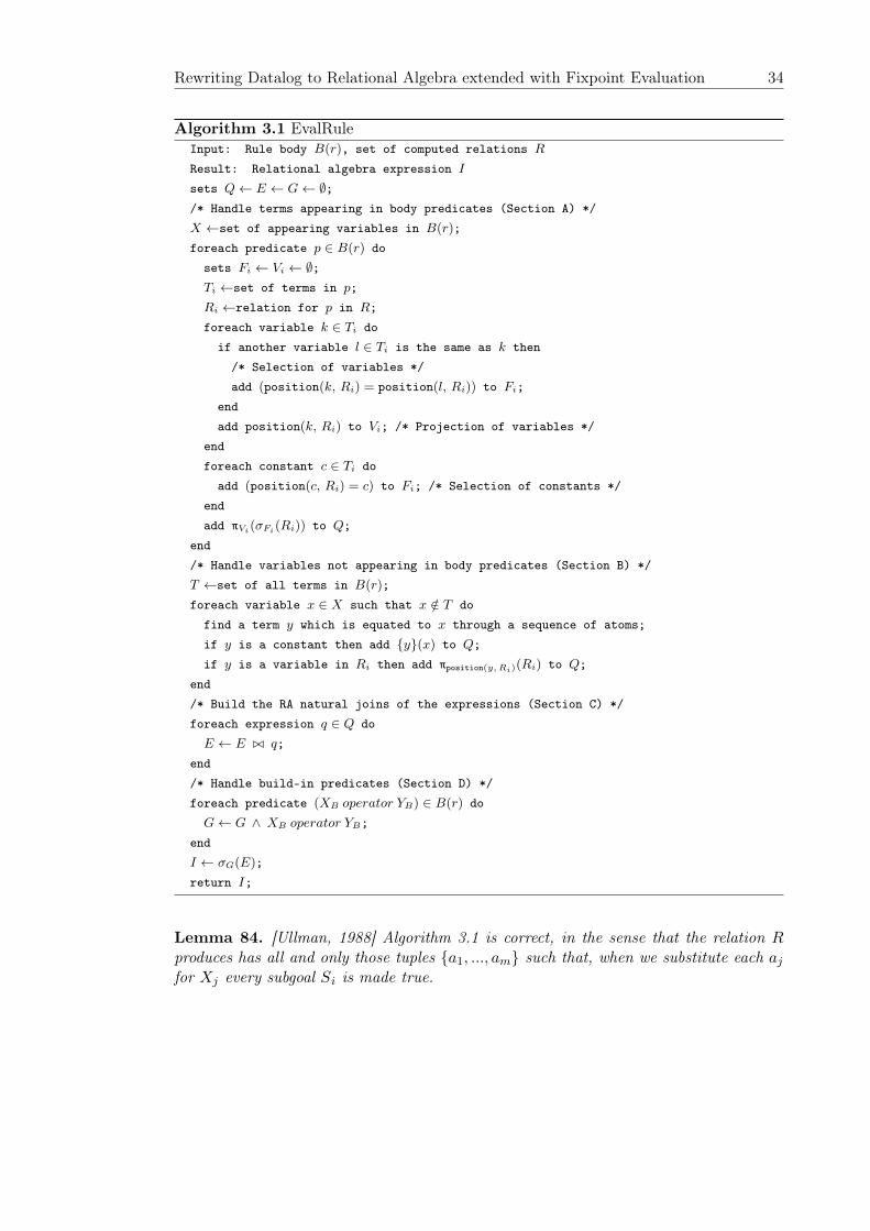
Rewriting Datalog to Relational Algebra extended with Fixpoint Evaluation 34
Algorithm 3.1 EvalRuleInput: Rule body B(r), set of computed relations R
Result: Relational algebra expression I
sets Q ← E ← G ← ∅;/* Handle terms appearing in body predicates (Section A) */X ←set of appearing variables in B(r);foreach predicate p ∈ B(r) do
sets Fi ← Vi ← ∅;Ti ←set of terms in p;Ri ←relation for p in R;foreach variable k ∈ Ti do
if another variable l ∈ Ti is the same as k then/* Selection of variables */add (position(k, Ri) = position(l, Ri)) to Fi;
endadd position(k, Ri) to Vi; /* Projection of variables */
endforeach constant c ∈ Ti do
add (position(c, Ri) = c) to Fi; /* Selection of constants */endadd πVi(σFi(Ri)) to Q;
end/* Handle variables not appearing in body predicates (Section B) */T ←set of all terms in B(r);foreach variable x ∈ X such that x /∈ T do
find a term y which is equated to x through a sequence of atoms;if y is a constant then add {y}(x) to Q;if y is a variable in Ri then add πposition(y,Ri)(Ri) to Q;
end/* Build the RA natural joins of the expressions (Section C) */foreach expression q ∈ Q do
E ← E �� q;end/* Handle build-in predicates (Section D) */foreach predicate (XB operator YB) ∈ B(r) do
G ← G ∧ XB operator YB;endI ← σG(E);return I;
Lemma 84. [Ullman, 1988] Algorithm 3.1 is correct, in the sense that the relation Rproduces has all and only those tuples {a1, ..., am} such that, when we substitute each ajfor Xj every subgoal Si is made true.
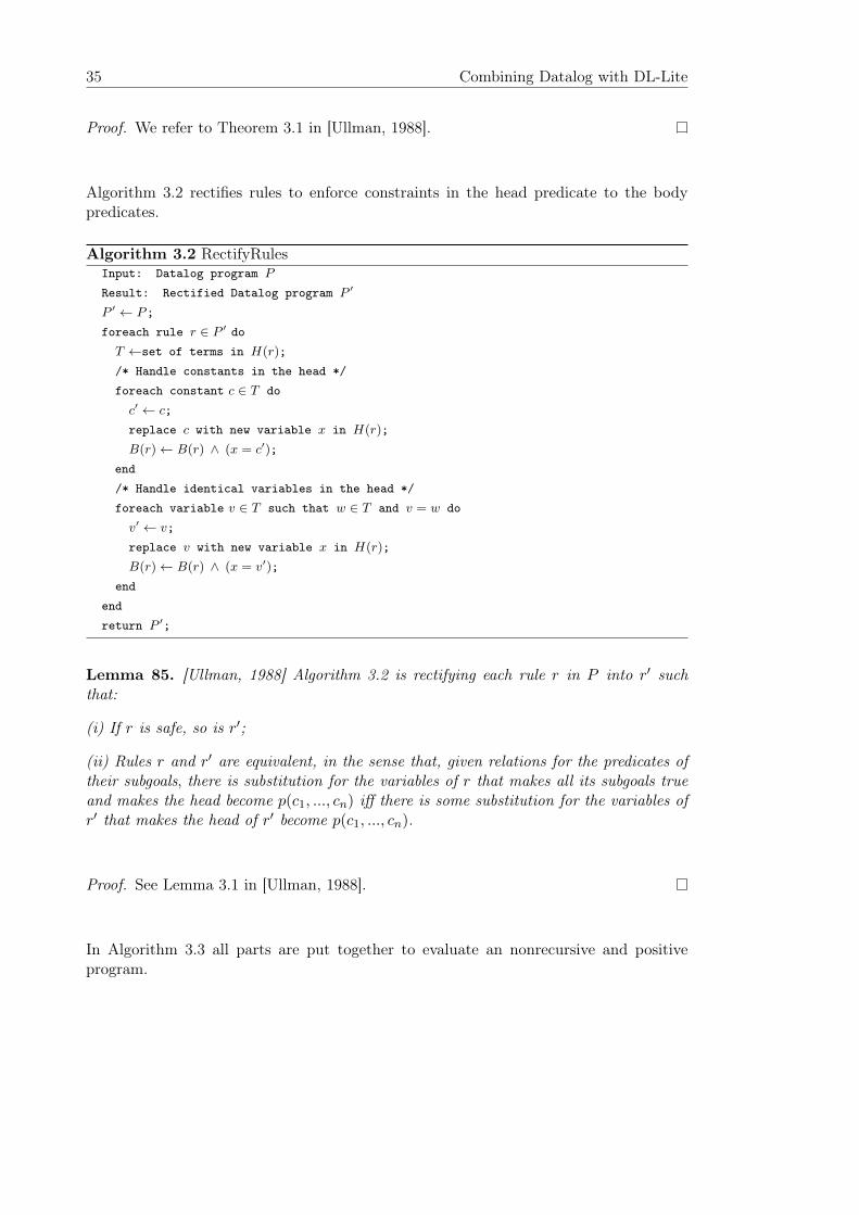
35 Combining Datalog with DL-Lite
Proof. We refer to Theorem 3.1 in [Ullman, 1988].
Algorithm 3.2 rectifies rules to enforce constraints in the head predicate to the bodypredicates.
Algorithm 3.2 RectifyRulesInput: Datalog program P
Result: Rectified Datalog program P �
P � ← P;foreach rule r ∈ P � do
T ←set of terms in H(r);/* Handle constants in the head */foreach constant c ∈ T do
c� ← c;replace c with new variable x in H(r);B(r) ← B(r) ∧ (x = c�);
end/* Handle identical variables in the head */foreach variable v ∈ T such that w ∈ T and v = w do
v� ← v;replace v with new variable x in H(r);B(r) ← B(r) ∧ (x = v�);
endendreturn P �;
Lemma 85. [Ullman, 1988] Algorithm 3.2 is rectifying each rule r in P into r� suchthat:
(i) If r is safe, so is r�;
(ii) Rules r and r� are equivalent, in the sense that, given relations for the predicates oftheir subgoals, there is substitution for the variables of r that makes all its subgoals trueand makes the head become p(c1, ..., cn) iff there is some substitution for the variables ofr� that makes the head of r� become p(c1, ..., cn).
Proof. See Lemma 3.1 in [Ullman, 1988].
In Algorithm 3.3 all parts are put together to evaluate an nonrecursive and positiveprogram.
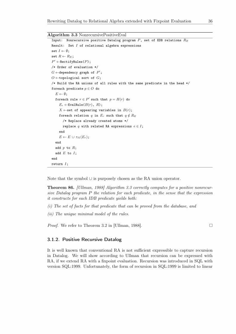
Rewriting Datalog to Relational Algebra extended with Fixpoint Evaluation 36
Algorithm 3.3 NonrecursivePositiveEvalInput: Nonrecursive positive Datalog program P, set of EDB relations RE
Result: Set I of relational algebra expressionsset I ← ∅;set R ← RE;P � ←RectifyRules(P);/* Order of evaluation */G ←dependency graph of P �;O ←topological sort of G;/* Build the RA unions of all rules with the same predicate in the head */foreach predicate p ∈ O do
E ← ∅;foreach rule r ∈ P � such that p = H(r) do
Er ←EvalRule(B(r), R);X ←set of appearing variables in B(r);foreach relation q in Er such that q /∈ RE
/* Replace already created atoms */replace q with related RA expressions e ∈ I;
endE ← E ∪ πX(Er);
endadd p to R;add E to I;
endreturn I;
Note that the symbol ∪ is purposely chosen as the RA union operator.
Theorem 86. [Ullman, 1988] Algorithm 3.3 correctly computes for a positive nonrecur-sive Datalog program P the relation for each predicate, in the sense that the expressionit constructs for each IDB predicate yields both:
(i) The set of facts for that predicate that can be proved from the database, and
(ii) The unique minimal model of the rules.
Proof. We refer to Theorem 3.2 in [Ullman, 1988].
3.1.2. Positive Recursive Datalog
It is well known that conventional RA is not sufficient expressible to capture recursionin Datalog. We will show according to Ullman that recursion can be expressed withRA, if we extend RA with a fixpoint evaluation. Recursion was introduced in SQL withversion SQL:1999. Unfortunately, the form of recursion in SQL:1999 is limited to linear
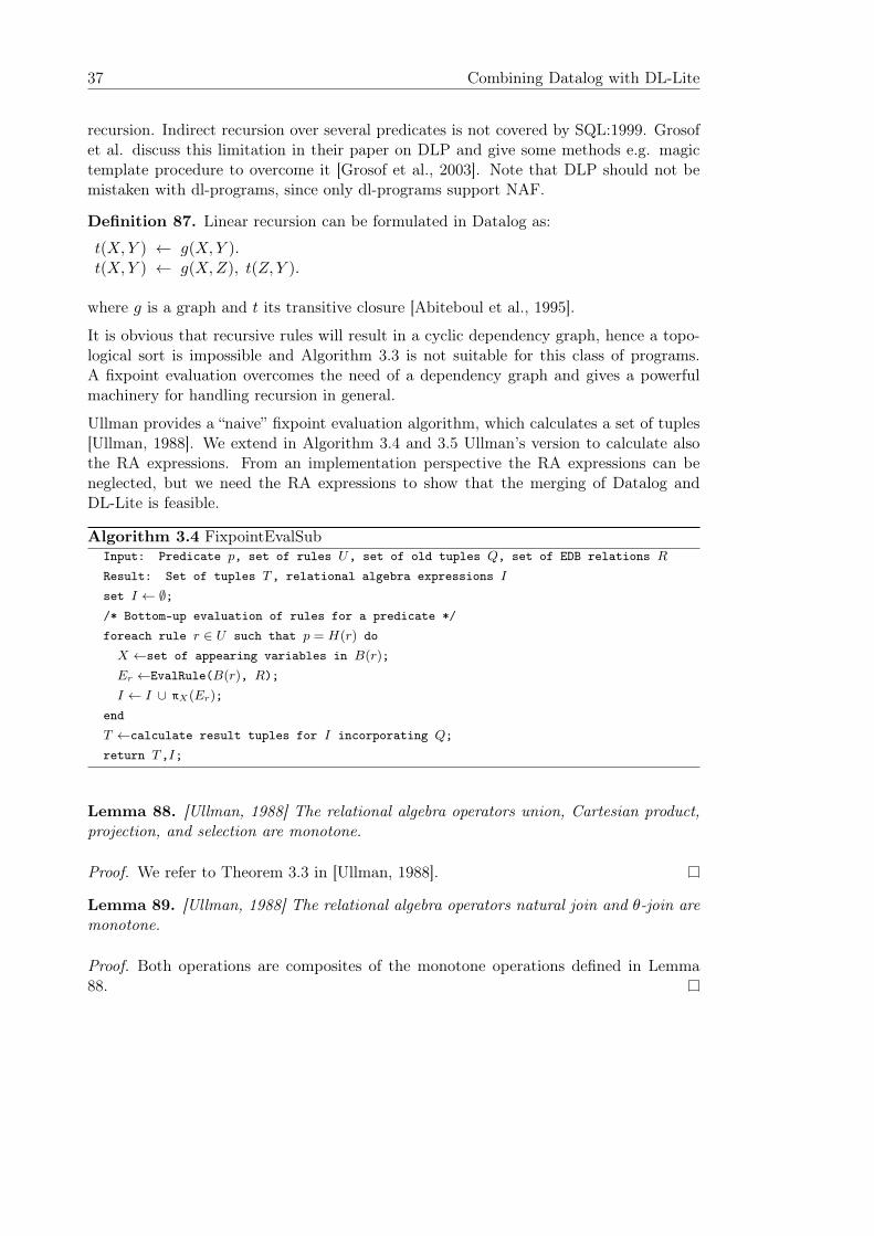
37 Combining Datalog with DL-Lite
recursion. Indirect recursion over several predicates is not covered by SQL:1999. Grosofet al. discuss this limitation in their paper on DLP and give some methods e.g. magictemplate procedure to overcome it [Grosof et al., 2003]. Note that DLP should not bemistaken with dl-programs, since only dl-programs support NAF.
Definition 87. Linear recursion can be formulated in Datalog as:
t(X,Y ) ← g(X,Y ).t(X,Y ) ← g(X,Z), t(Z, Y ).
where g is a graph and t its transitive closure [Abiteboul et al., 1995].
It is obvious that recursive rules will result in a cyclic dependency graph, hence a topo-logical sort is impossible and Algorithm 3.3 is not suitable for this class of programs.A fixpoint evaluation overcomes the need of a dependency graph and gives a powerfulmachinery for handling recursion in general.
Ullman provides a “naive” fixpoint evaluation algorithm, which calculates a set of tuples[Ullman, 1988]. We extend in Algorithm 3.4 and 3.5 Ullman’s version to calculate alsothe RA expressions. From an implementation perspective the RA expressions can beneglected, but we need the RA expressions to show that the merging of Datalog andDL-Lite is feasible.
Algorithm 3.4 FixpointEvalSubInput: Predicate p, set of rules U, set of old tuples Q, set of EDB relations R
Result: Set of tuples T, relational algebra expressions I
set I ← ∅;/* Bottom-up evaluation of rules for a predicate */foreach rule r ∈ U such that p = H(r) do
X ←set of appearing variables in B(r);Er ←EvalRule(B(r), R);I ← I ∪ πX(Er);
endT ←calculate result tuples for I incorporating Q;return T,I;
Lemma 88. [Ullman, 1988] The relational algebra operators union, Cartesian product,projection, and selection are monotone.
Proof. We refer to Theorem 3.3 in [Ullman, 1988].
Lemma 89. [Ullman, 1988] The relational algebra operators natural join and θ-join aremonotone.
Proof. Both operations are composites of the monotone operations defined in Lemma88.
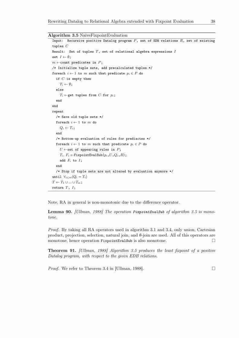
Rewriting Datalog to Relational Algebra extended with Fixpoint Evaluation 38
Algorithm 3.5 NaiveFixpointEvaluationInput: Recursive positive Datalog program P, set of EDB relations R, set of existingtuples C
Result: Set of tuples T, set of relational algebra expressions I
set I ← ∅;m ←count predicates in P;/* Initialize tuple sets, add precalculated tuples */foreach i ← 1 to m such that predicate pi ∈ P do
if C is empty thenTi ← ∅;
elseTi ←get tuples from C for pi;
endendrepeat
/* Save old tuple sets */foreach i ← 1 to m do
Qi ← Ti;end/* Bottom-up evaluation of rules for prediactes */foreach i ← 1 to m such that predicate pi ∈ P do
U ←set of appearing rules in P;Ti, Fi ←FixpointEvalSub(pi,U,Qi,R);add Fi to I;
end/* Stop if tuple sets are not altered by evaluation anymore */
until ∀i≤m(Qi = Ti)
T ← T1 ∪ ... ∪ Tm;return T, I;
Note, RA in general is non-monotonic due to the difference operator.
Lemma 90. [Ullman, 1988] The operation FixpointEvalSub of algorithm 3.5 is mono-tone.
Proof. By taking all RA operators used in algorithm 3.1 and 3.4, only union, Cartesianproduct, projection, selection, natural join, and θ-join are used. All of this operators aremonotone, hence operation FixpointEvalSub is also monotone.
Theorem 91. [Ullman, 1988] Algorithm 3.5 produces the least fixpoint of a positiveDatalog program, with respect to the given EDB relations.
Proof. We refer to Theorem 3.4 in [Ullman, 1988].
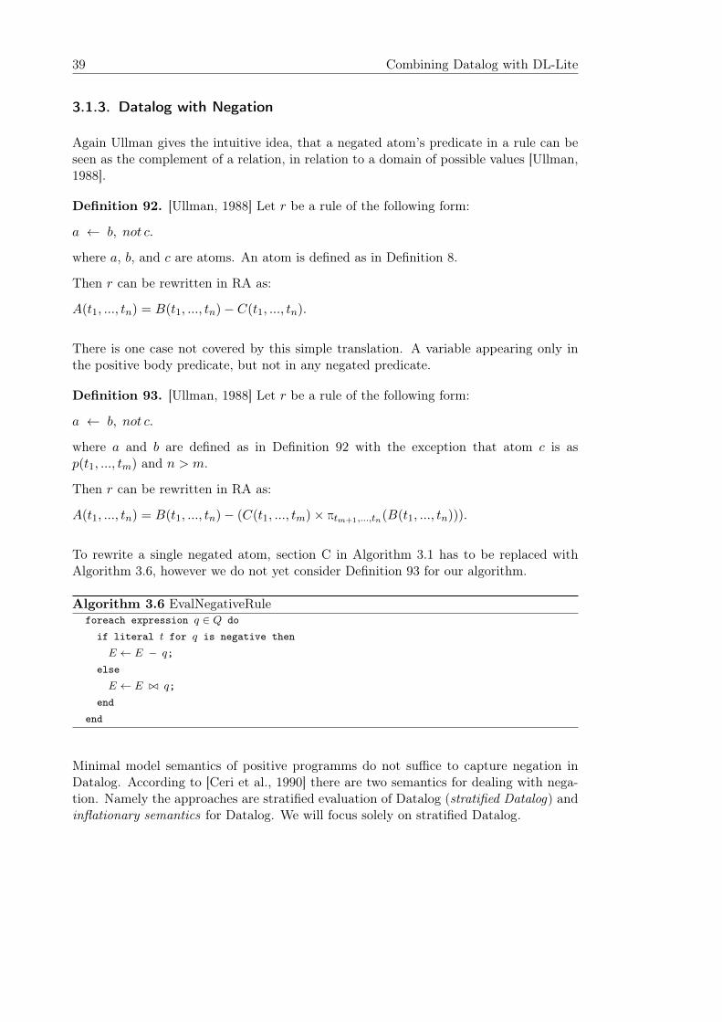
39 Combining Datalog with DL-Lite
3.1.3. Datalog with Negation
Again Ullman gives the intuitive idea, that a negated atom’s predicate in a rule can beseen as the complement of a relation, in relation to a domain of possible values [Ullman,1988].
Definition 92. [Ullman, 1988] Let r be a rule of the following form:
a ← b, not c.
where a, b, and c are atoms. An atom is defined as in Definition 8.
Then r can be rewritten in RA as:
A(t1, ..., tn) = B(t1, ..., tn)− C(t1, ..., tn).
There is one case not covered by this simple translation. A variable appearing only inthe positive body predicate, but not in any negated predicate.
Definition 93. [Ullman, 1988] Let r be a rule of the following form:
a ← b, not c.
where a and b are defined as in Definition 92 with the exception that atom c is asp(t1, ..., tm) and n > m.
Then r can be rewritten in RA as:
A(t1, ..., tn) = B(t1, ..., tn)− (C(t1, ..., tm)× πtm+1,...,tn(B(t1, ..., tn))).
To rewrite a single negated atom, section C in Algorithm 3.1 has to be replaced withAlgorithm 3.6, however we do not yet consider Definition 93 for our algorithm.
Algorithm 3.6 EvalNegativeRuleforeach expression q ∈ Q do
if literal t for q is negative thenE ← E − q;
elseE ← E �� q;
endend
Minimal model semantics of positive programms do not suffice to capture negation inDatalog. According to [Ceri et al., 1990] there are two semantics for dealing with nega-tion. Namely the approaches are stratified evaluation of Datalog (stratified Datalog) andinflationary semantics for Datalog. We will focus solely on stratified Datalog.
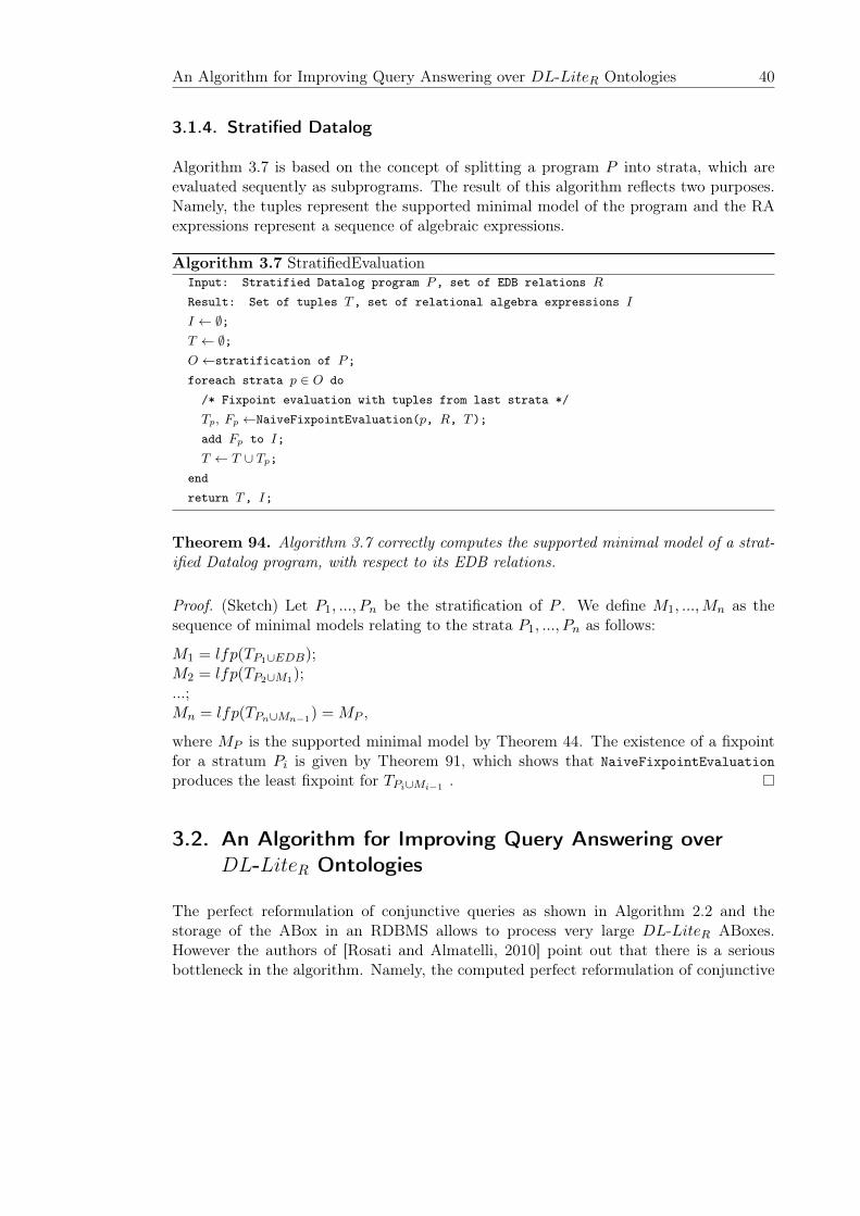
An Algorithm for Improving Query Answering over DL-LiteR Ontologies 40
3.1.4. Stratified Datalog
Algorithm 3.7 is based on the concept of splitting a program P into strata, which areevaluated sequently as subprograms. The result of this algorithm reflects two purposes.Namely, the tuples represent the supported minimal model of the program and the RAexpressions represent a sequence of algebraic expressions.
Algorithm 3.7 StratifiedEvaluationInput: Stratified Datalog program P, set of EDB relations R
Result: Set of tuples T, set of relational algebra expressions I
I ← ∅;T ← ∅;O ←stratification of P;foreach strata p ∈ O do
/* Fixpoint evaluation with tuples from last strata */Tp, Fp ←NaiveFixpointEvaluation(p, R, T);add Fp to I;T ← T ∪ Tp;
endreturn T, I;
Theorem 94. Algorithm 3.7 correctly computes the supported minimal model of a strat-ified Datalog program, with respect to its EDB relations.
Proof. (Sketch) Let P1, ..., Pn be the stratification of P . We define M1, ...,Mn as thesequence of minimal models relating to the strata P1, ..., Pn as follows:
M1 = lfp(TP1∪EDB);M2 = lfp(TP2∪M1);...;Mn = lfp(TPn∪Mn−1) = MP ,
where MP is the supported minimal model by Theorem 44. The existence of a fixpointfor a stratum Pi is given by Theorem 91, which shows that NaiveFixpointEvaluation
produces the least fixpoint for TPi∪Mi−1 .
3.2. An Algorithm for Improving Query Answering over
DL-LiteR Ontologies
The perfect reformulation of conjunctive queries as shown in Algorithm 2.2 and thestorage of the ABox in an RDBMS allows to process very large DL-LiteR ABoxes.However the authors of [Rosati and Almatelli, 2010] point out that there is a seriousbottleneck in the algorithm. Namely, the computed perfect reformulation of conjunctive
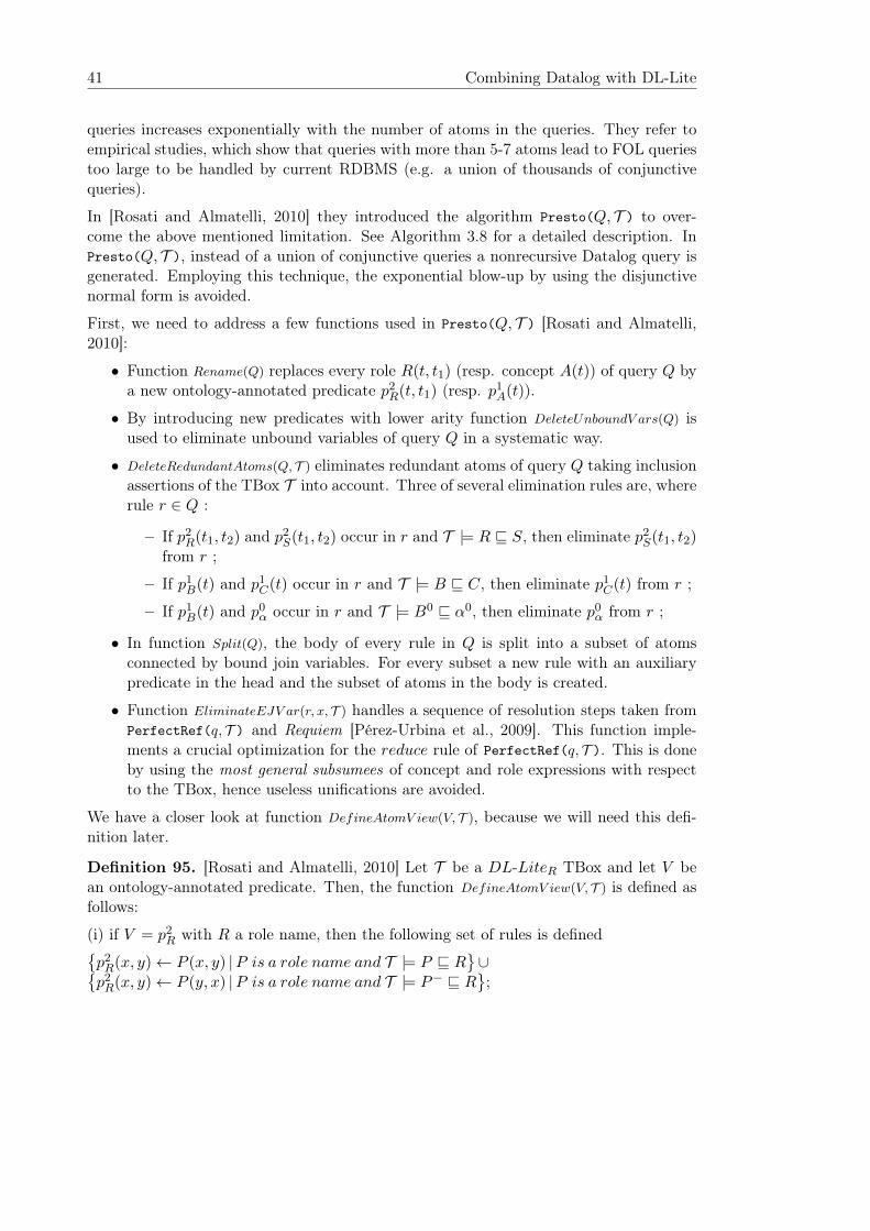
41 Combining Datalog with DL-Lite
queries increases exponentially with the number of atoms in the queries. They refer toempirical studies, which show that queries with more than 5-7 atoms lead to FOL queriestoo large to be handled by current RDBMS (e.g. a union of thousands of conjunctivequeries).
In [Rosati and Almatelli, 2010] they introduced the algorithm Presto(Q, T ) to over-come the above mentioned limitation. See Algorithm 3.8 for a detailed description. InPresto(Q, T ), instead of a union of conjunctive queries a nonrecursive Datalog query isgenerated. Employing this technique, the exponential blow-up by using the disjunctivenormal form is avoided.
First, we need to address a few functions used in Presto(Q, T ) [Rosati and Almatelli,2010]:
• Function Rename(Q) replaces every role R(t, t1) (resp. concept A(t)) of query Q bya new ontology-annotated predicate p2R(t, t1) (resp. p1A(t)).
• By introducing new predicates with lower arity function DeleteUnboundV ars(Q) isused to eliminate unbound variables of query Q in a systematic way.
• DeleteRedundantAtoms(Q, T ) eliminates redundant atoms of query Q taking inclusionassertions of the TBox T into account. Three of several elimination rules are, whererule r ∈ Q :
– If p2R(t1, t2) and p2S(t1, t2) occur in r and T |= R � S, then eliminate p2S(t1, t2)from r ;
– If p1B(t) and p1C(t) occur in r and T |= B � C, then eliminate p1C(t) from r ;
– If p1B(t) and p0α occur in r and T |= B0 � α0, then eliminate p0α from r ;
• In function Split(Q), the body of every rule in Q is split into a subset of atomsconnected by bound join variables. For every subset a new rule with an auxiliarypredicate in the head and the subset of atoms in the body is created.
• Function EliminateEJV ar(r, x, T ) handles a sequence of resolution steps taken fromPerfectRef(q, T ) and Requiem [Pérez-Urbina et al., 2009]. This function imple-ments a crucial optimization for the reduce rule of PerfectRef(q, T ). This is doneby using the most general subsumees of concept and role expressions with respectto the TBox, hence useless unifications are avoided.
We have a closer look at function DefineAtomV iew(V, T ), because we will need this defi-nition later.
Definition 95. [Rosati and Almatelli, 2010] Let T be a DL-LiteR TBox and let V bean ontology-annotated predicate. Then, the function DefineAtomV iew(V, T ) is defined asfollows:
(i) if V = p2R with R a role name, then the following set of rules is defined�p2R(x, y) ← P (x, y) |P is a role name and T |= P � R
�∪�
p2R(x, y) ← P (y, x) |P is a role name and T |= P− � R�;
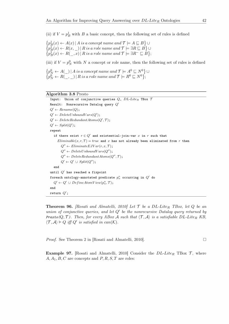
An Algorithm for Improving Query Answering over DL-LiteR Ontologies 42
(ii) if V = p1B with B a basic concept, then the following set of rules is defined�p1B(x) ← A(x) |A is a concept name and T |= A � B
�∪�
p1B(x) ← R(x,_) |R is a role name and T |= ∃R � B�∪�
p1B(x) ← R(_, x) |R is a role name and T |= ∃R− � B�;
(iii) if V = p0N with N a concept or role name, then the following set of rules is defined�p0N ← A(_) |A is a concept name and T |= A0 � N0
�∪�
p0N ← R(_,_) |R is a role name and T |= R0 � N0�;
Algorithm 3.8 PrestoInput: Union of conjunctive queries Q, DL-LiteR TBox TResult: Nonrecursive Datalog query Q�
Q� ← Rename(Q);Q� ← DeleteUnboundV ars(Q�);Q� ← DeleteRedundantAtoms(Q�, T );Q� ← Split(Q�);repeat
if there exist r ∈ Q� and existential-join-var x in r such thatEliminable(x, r, T ) = true and x has not already been eliminated from r then
Q�� ← EliminateEJV ar(r, x, T );Q�� ← DeleteUnboundV ars(Q��);Q�� ← DeleteRedundantAtoms(Q��, T );Q� ← Q� ∪ Split(Q��);
enduntil Q� has reached a fixpointforeach ontology-annotated predicate pnα occurring in Q� do
Q� ← Q� ∪ DefineAtomV iew(pnα, T );endreturn Q�;
Theorem 96. [Rosati and Almatelli, 2010] Let T be a DL-LiteR TBox, let Q be anunion of conjunctive queries, and let Q� be the nonrecursive Datalog query returned byPresto(Q, T ). Then, for every ABox A such that �T ,A� is a satisfiable DL-LiteR KB,�T ,A� � Q iff Q� is satisfied in can(K).
Proof. See Theorem 2 in [Rosati and Almatelli, 2010].
Example 97. [Rosati and Almatelli, 2010] Consider the DL-LiteR TBox T , whereA,A1, B, C are concepts and P,R, S, T are roles:
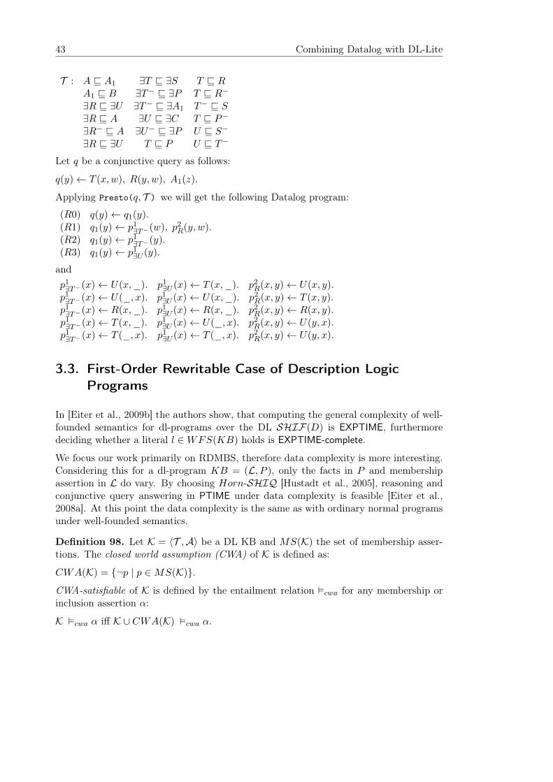
43 Combining Datalog with DL-Lite
T : A � A1 ∃T � ∃S T � RA1 � B ∃T− � ∃P T � R−
∃R � ∃U ∃T− � ∃A1 T− � S∃R � A ∃U � ∃C T � P−
∃R− � A ∃U− � ∃P U � S−
∃R � ∃U T � P U � T−
Let q be a conjunctive query as follows:
q(y) ← T (x,w), R(y, w), A1(z).
Applying Presto(q, T ) we will get the following Datalog program:
(R0) q(y) ← q1(y).(R1) q1(y) ← p1∃T−(w), p2R(y, w).(R2) q1(y) ← p1∃T−(y).(R3) q1(y) ← p1∃U (y).
andp1∃T−(x) ← U(x,_). p1∃U (x) ← T (x,_). p2R(x, y) ← U(x, y).p1∃T−(x) ← U(_, x). p1∃U (x) ← U(x,_). p2R(x, y) ← T (x, y).p1∃T−(x) ← R(x,_). p1∃U (x) ← R(x,_). p2R(x, y) ← R(x, y).p1∃T−(x) ← T (x,_). p1∃U (x) ← U(_, x). p2R(x, y) ← U(y, x).p1∃T−(x) ← T (_, x). p1∃U (x) ← T (_, x). p2R(x, y) ← U(y, x).
3.3. First-Order Rewritable Case of Description Logic
Programs
In [Eiter et al., 2009b] the authors show, that computing the general complexity of well-founded semantics for dl-programs over the DL SHIF(D) is EXPTIME, furthermoredeciding whether a literal l ∈ WFS(KB) holds is EXPTIME-complete.
We focus our work primarily on RDMBS, therefore data complexity is more interesting.Considering this for a dl-program KB = (L, P ), only the facts in P and membershipassertion in L do vary. By choosing Horn-SHIQ [Hustadt et al., 2005], reasoning andconjunctive query answering in PTIME under data complexity is feasible [Eiter et al.,2008a]. At this point the data complexity is the same as with ordinary normal programsunder well-founded semantics.
Definition 98. Let K = �T ,A� be a DL KB and MS(K) the set of membership asser-tions. The closed world assumption (CWA) of K is defined as:
CWA(K) = {¬p | p ∈ MS(K)}.CWA-satisfiable of K is defined by the entailment relation �cwa for any membership orinclusion assertion α:
K �cwa α iff K ∪ CWA(K) �cwa α.

First-Order Rewritable Case of Description Logic Programs 44
Theorem 99. [Eiter et al., 2009b] Given KB = (L, P ) and a literal l ⊆ LitP , whereevery dl-atom in P can be evaluated in PTIME , deciding whether l ∈ WFS(KB) iscomplete for PTIME under data complexity.
Proof. See Theorem 7.2 in [Eiter et al., 2009b].
As mentioned in Theorem 73, answering unions of conjunctive queries in DL-LiteR isLOGSPACE in the size of the ABox. DL-LiteR data complexity and query answeringcapabilities makes it a plausible choice to couple with dl-programs. Hence the authorsof [Eiter et al., 2009b] introduce the concept of first-order rewritability, where a dl-querycan be rewritten into a FOL formula over the ABox. To achieve first-order rewritabilityfor a normal program P , they restrict P to be acyclic and rewrite ordinary predicates ofP to FOL formulas.
Notice, that (i), (ii) and, (iii) of Definition 76 can be expressed as a conjunctive query.We recall the Theorems 7.3 and 7.4 of [Eiter et al., 2009b] and introduce some minoradaptions.
Theorem 100. [Eiter et al., 2009b] Let KB = (L, P ) be an acyclic dl-program and aliteral l ∈ LitP , where
(i) every dl-query in P is first-order rewritable, and
(ii) if the operator −∪ occurs in P , then L is defined over a DL, that
(ii.a) is CWA-satisfiable, and
(ii.b) allows for first-order rewritable concept and role membership, deciding whetherl ∈ WFS(KB) is first-order rewritable.
Proof. Since KB is acyclic, there is an acyclic dependency graph GP . We derive from GP
the strict partial order of GP the mapping of predicate symbols K : PP → {0, 1, ..., n}.We call K(p) the rank of p. By Theorem 72, every dl-query in P can be expressed interms of a FOL formula over the set A of all membership and inclusion assertions in L.We now show by induction on K(p) ∈ {0, 1, ..., n} that each predicate symbol p ∈ PP canbe expressed in terms of a FOL formula over the set F of all membership and inclusionassertions in L and the EDB(P ).
Basis: Each predicate p ∈ PP of rank 0 can trivially be expressed in terms of a FOLformula over F .
Induction: We have to consider the evaluation of a dl-atom DL[λ;QLite](c) and thedefinition of a predicate p ∈ PP via the set of all rules in P with p ∈ H(r):
(i) Consider the dl-atom DL[λ;QL](c) with λ = λ+,λ−, where λ+ = S1 � p1, ..., Sl � pl,λ− = Sl+1−∪pl+1, ..., Sm−∪pm, and m ≥ l ≥ 0. The dl-query QL(c) can be expressedin terms of a FOL formula α(x) over A, that is, L � QL(c) iff IA � α(c). Since theunderlying DL allows first-order rewritable membership and inclusion assertions, every
45 Combining Datalog with DL-Lite
Si in λ−, l < i ≤ m, can be expressed in terms of a FOL formula ψSi(y) over A, thatis, L � Si(c) iff IA � ψSi(c) for every c. By the induction hypothesis, every inputpredicate pj in λ can be expressed in terms of a FOL formula ψj(x) over F , that is,pj(c) ∈ WFS(KB) iff IF � ψj(c). We define the FOL formula δ(x) for DL[λ;QL](x)over F as follows:
δ(x) = αλ+(x) ∨
m�
j=l+1
∃y(ψλ+
Sj(y) ∧ ψj(y)),
where βλ+ is obtained from β by replacing every Si(s) such that Si occurs in λ+ bySi(s) ∨ ψi1(s) ∨ ... ∨ ψiki
(s), where Si1 , ..., Sikiare all occurrences of Sj in λ+.
Note that IF � Si(c) iff IF � Si(c) ∈ L, for all 1 ≤ i ≤ l. Hence,
IF � Si(c) ∨ ψi1(c) ∨ ... ∨ ψiki(c)
iff Si(c) ∈ L or pij (c) ∈ WFS(KB), for some 1 ≤ j ≤ ki
iff Si(c) ∈ L ∪l�
i=1Ai(WFS(KB))
iff IA� � Si(c), where A� = A ∪l�
i=1Ai(WFS(KB)).
It follows from this that
IF � αλ+(c) iff IA� � α(c) and IF � ψλ+
Sj(c) iff IA� � ψSj (c), for all l < j ≤ m.
This in turn implies that
IF � δ(c) iff (i) L ∪A� � QL(c), or (ii) L ∪A� � Sj(d) and pj(d) ∈ WFS(KB), for somel < j ≤ m and d.
Let A�� = A� ∪m�
j=l+1Aj(WFS(KB)). If L ∪ A�� � QL(c), then clearly both (i) and (ii)
are false; conversely, if L∪A� � QL(c)) and L∪A� � Sj(d) for every pj(d) ∈ WFS(KB)where l < j ≤ m, then L∪A�� � QL(c) holds since the underlying DL is CWA-satisfiable.
In summary, this shows that IF � δ(c) iff L ∪ A�� � QL(c) iff WFS(KB) satisfiesDL[λ;QL](c). That is, δ(x) is a FOL formula for DL[λ;Q](x) over F .
(ii) Consider next the set of all rules in P with p ∈ H(r). W.l.o.g., the heads p(x) ofall these rules coincide. Let α(x) denote the disjunction of the existentially quantifiedbodies of these rules, where the default negations in the rule bodies are interpreted asclassical negations. By the induction hypothesis, every body predicate in α(x) can beexpressed in terms of a FOL formula over F , and the same holds for every dl-atom inα(x). Let α�(x) be obtained from α(x) by replacing all but the predicates of rank 0 bythese FOL formulas. Then α�(x) is a FOL formula over F for p.
Example 101. Consider the DL-LiteR TBox T , where A,A1, B, C are concepts andP,R, S, T are roles:
Stratified Evaluation of Description Logic Programs 46
Theorem 102. [Eiter et al., 2009b] Let KB = (L, P ) be an acyclic dl-program and aliteral l ∈ LitP , where
(i) L is defined in the description logic DL-LiteR, and
(ii) all dl-queries in P are membership or inclusion assertions in L, where concepts androles are atomic.
Then deciding whether l ∈ WFS(KB) is first-order rewritable.
Proof. We apply Theorem 67, 72, and 100. Observe that in DL-LiteR KB satisfiabilityand query answering are FOL-reducible, where FOL-reducible corresponds to first-orderrewritable. Observe also that DL-LiteR is a CWA-satisfiable DL [Calvanese et al., 2007],and thus Theorem 100 also allows operator −∪ to occur in P . All dl-atoms with dl-queries of the form C(t) and R(t1, t2) are immediately first-order rewritable. Dl-queriesof the form C � D resp. ¬(C � D) can be reduced to conjunctive queries as follows:L� � C � D iff L� ∪ {C(e), D�(e), D� � ¬D,A�(d), A� � ¬A} � A(d) resp. L� � ¬(C � D)iff L� ∪ {C � � D,A�(d), A� � ¬A} � A(d), where d and e are fresh individuals, and A, A�,and D� are fresh atomic concepts. By Theorem 100, it thus follows that deciding whetherl ∈ WFS(KB) is first-order rewritable.
Example 103. [Eiter et al., 2009b] Consider the DL KB L = �T ,A� , where C is aconcept in T and C(a) is an membership assertion in A. Let (L, P ) be a dl-program asfollows:p(c). q(b).r ← p(x).r ← DL [C � p;C] (x).s ← not DL [C � p, C−∪q;C] (x).
The dl-program (L, P ) can be expressed by the following formulas:
• The query Q(x) is expressed by α(x) = C(x) over A = {C(a)};• the predicates p and q as ψp(x) = p(x) and ψq(x) = q(x) over F = {C(a), p(c), q(b)};
• the dl-atom DL [C � p;C] (x) is translated into δ1(x) = αλ+(x) = C(x) ∨ p(x) over
F (note that m = l);
• the dl-atom DL [C � p, C−∪q;C] (x) is expressed by δ2(x) = (C(x)∨p(x))∨∃y((C(y)∨p(y)) ∧ q(y)) over F .
3.4. Stratified Evaluation of Description Logic Programs
By Theorem 100 and 102, we have shown that acyclic dl-programs can be coupled withDL-LiteR. Next, we extend dl-programs to be evaluated under stratified Datalog. Theevaluation is split into a preprocessing part and a standard stratified evaluation part. Thefirst part is concerned with the rewriting of the dl-atoms by compiling the DL-LiteR KB
47 Combining Datalog with DL-Lite
and the conjunctive query into Datalog. Then, the adapted dl-program can be rewritteninto RA expressions extended with fixpoint evaluation. In Algorithm 3.9 we give adetailed description.
Algorithm 3.9 dl-program EvaluationInput: Stratified dl-program (L, P ) with a DL-LiteR KB L = �T ,A�,
set of EDB relations R
Result: Set of tuples T, set I of relational algebra expressions
/* Step (a): Preprocessing ABox */write ABox A to EDB R;
/* Step (b): Preprocessing dl-atoms */for each dl-atom d ∈ P do
qf ← rewrite TBox T and conjunctive query Q of d
to a nonrecursive Datalog query with Presto(Q, T );qd ← rewrite query qf to include DL update predicates;extend P with query qd;replace dl-atom d in P with a new ordinary atom referring to qd;
end
/* Step (c): Datalog to RA */set of RA expressions I=∅;S = stratification of P;foreach strata st ∈ S do
/* Fixpoint evaluation with tuples from last strata */Tp, Fp ←NaiveFixpointEvaluation(st, R, T);add RA expressions Fp to I;T ← T ∪ Tp;
end
return T, I;
Theorem 104. Algorithm 3.9 correctly computes the supported minimal model of a strat-ified dl-program KB = (L, P ), with respect to its EDB relations R, where
(i) L is defined in the description logic DL-LiteR,
(ii) dl-queries in P are positive membership or inclusion assertions in L, where conceptsand roles are atomic, and
(iii) in dl-atoms, only update operators of the form � are allowed.
Proof. (Sketch) . We need to show that rewriting the ABox(L) and dl-atoms in P tononrecursive Datalog queries is (a) feasible and (b) the queries stay positive, resulting inprogram P �.
Stratified Evaluation of Description Logic Programs 48
(a) The membership assertions of an ABox(L) can be immediately rewritten to EDB factsof P . Next, consider the dl-atom DL[λ;QLite](c), the dl-query QLite can be reduced tothe conjunctive query QCQ according to Theorem 102. By Theorem 96 of AlgorithmPresto(Q, T ), the conjunctive query QCQ can be rewritten to a positive nonrecursiveDatalog query R. A dl-update λ of the form Si � pi rewrites the query R by (Si ∨ pi) forevery occurrence of Si in the rule bodies of R.
(b) Observe that by condition (ii) and Definition 95 of Algorithm Presto(Q, T ) thenonrecursive Datalog query R is positive. Furthermore by (iii) only positive inclusionassertions by the dl-update λ are allowed.
Thus by (a) and (b) rewriting P to P � preserves the stratification of P , because onlypositive atoms are introduced. Then by Theorem 94, the supported minimal model forthe stratified dl-program P � is computed correctly.
Finally, we need to rewrite the generated RA expressions with fixpoint evaluation intoSQL. This is primarily achieved by applying the reversal of Definition 7 to create SQLstatements from the RA expressions.
The RA expressions can be rewritten into a single large SQL statement or to an inter-mediate DB, containing views for every IDB relation. We favor the second approach. Byany approach, the created SQL statements can be evaluated on an RDBMS, exploitingthe efficient query optimizers in modern RDBMSs.
Example 105. Consider the DL KB L = �T ,A�, where R and Q are roles and T isdefined as R � Q. Furthermore Q(c1, c2) and Q(c2, c3) are membership assertion in A.Let DLP = (L, P ) be a dl-program as follows:
b(c1). b(c2).a(x, y) ← b(x), not s(x, y).s(x, y) ← DL [R � t;R] (x, y).b(x, y) ← DL [;Q] (x, y).t(x, y) ← b(x, y).t(x, z) ← t(x, y), t(y, z).
The dl-program DLP can be rewritten to the following Datalog rules, where the firstpart is directly taken and the second part is adapoted according to Algorithm 3.9:
b(c1). b(c2).q(x, y) ← a(x), not s(x, y).t(x, y) ← b(x, y).t(x, z) ← t(x, y), t(y, z).
and
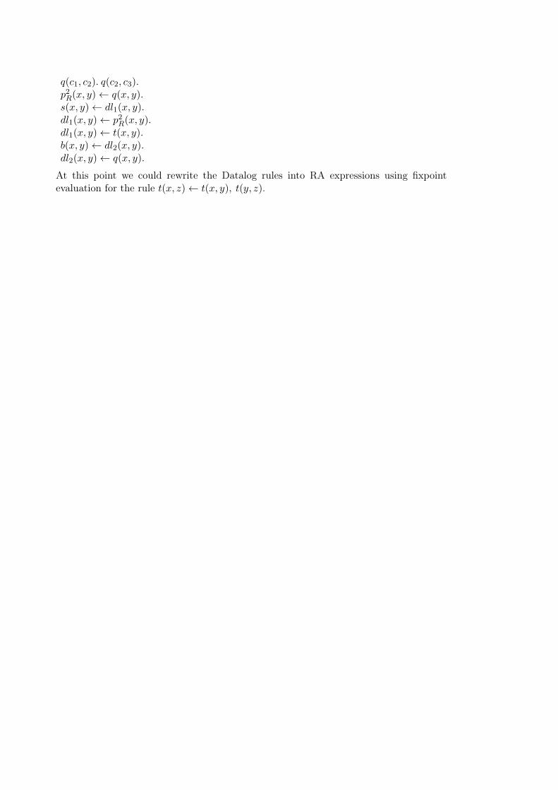
q(c1, c2). q(c2, c3).p2R(x, y) ← q(x, y).s(x, y) ← dl1(x, y).dl1(x, y) ← p2R(x, y).dl1(x, y) ← t(x, y).b(x, y) ← dl2(x, y).dl2(x, y) ← q(x, y).
At this point we could rewrite the Datalog rules into RA expressions using fixpointevaluation for the rule t(x, z) ← t(x, y), t(y, z).

4. Implementation
4.1. Overview
In this chapter we introduce the experimental implementation of a RDBMS-based solver,called MOR. MOR is the abbreviation for MergeOntologyRule. The implementationstands as a proof of concept for the theories developed in Chapter 3.
We setup the following design goals for MOR:
1. Taking fully advantage of RDBMS technology;
2. reusing existing Open Source software components;
3. interfacing a DL reasoner through plug-ins; and
4. using an object-oriented programming language for the implementation.
With respect to Goal 4, Java 1.6 was chosen, because its accepted use in academiaand the availability of a wide range of components (particularly the JGraphT library1).Crucial to Goal 3 is the existence of DL reasoners supporting DL-LiteR, namely Owl-gres2 and QuOnto3. As for Goal 1, PostgreSQL 8.44 was chosen due its support forthe SQL:1999 standard and its efficient query optimizer. Particularly the capability ofevaluating recursive queries opened up interesting extensions for this thesis.
Resulting from the design goals, the implementation of MOR was carried out in threesteps:
1. Developing a basic rewriter for Datalog to SQL.
2. Designing and developing a DL plug-in for using Owlgres 0.1 and possible otherOWL2 QL reasoners.
3. Adapting Owlgres 0.1 for extracting rewritten SQL statements,
For the first step, already existing Datalog-based inference engine were considered. Par-ticularly KAON [Bozsak et al., 2002] was promising, but the following limitations speakagainst it:5
1http://www.jgrapht.org/
2http://pellet.owldl.com/owlgres/
3http://www.dis.uniroma1.it/quonto/
4http://www.postgresql.org/
5http://sourceforge.net/projects/kaon/
51
Design 52
• The main developing efforts appear to be in KAON2, while the last changes inKAON happened in 2005,
• KAON is not plug-able, so major changes in the source code would have beennecessary, and
• some steps of the query evaluation are not based on recursion based on SQL.
4.2. Design
4.2.1. Architecture
The UML class diagram of Figure 4.1 gives a brief overview of the architecture. We omitthe architecture on class level but refer to the source code of MOR (see Appendix A).Briefly, MOR consists of the following libraries:
• The base library,
• the main library, and
• SQL-based plug-in libraries.
The base library is made of the basic classes representing a logic program (e.g. Rule,Predicate, and Literal) and auxiliary classes used by the builder and the plug-ins.
The main library covers the control flow, the access to the RDBMS, the parsing, andthe rewriting strategy. Depending on the configuration, plug-ins are loaded and calledon demand by this library.
As for the plug-in libraries, the bridge pattern [Gamma et al., 1995] was chosen, so MORcan be extended with different SQL based plug-ins. The idea of using plug-ins with logicprograms was adopted from HEX-programs [Eiter et al., 2006].
The first developed plug-in library is the DL plug-in, which encapsulates the DL-LiteRreasoner Owlgres. Beside interfacing Owlgres, parsing of DL predicates, creating auxil-iary views and reprocessing SQL statements of Owlgres are implemented in this library.
The Owlgres reasoner, a Java library itself, performs the rewriting of conjunctive queriesaccording to DL-LiteR. A more detailed picture of Owlgres and the plug-in will be givenin Section 4.4.
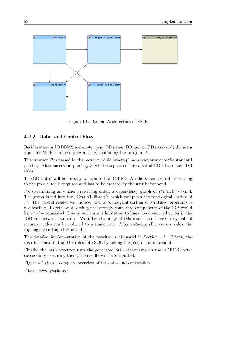
53 Implementation
Figure 4.1.: System Architecture of MOR
4.2.2. Data- and Control-Flow
Besides standard RDBMS parameter (e.g. DB name, DB user or DB password) the maininput for MOR is a logic program file, containing the program P .
The program P is parsed by the parser module, where plug-ins can overwrite the standardparsing. After successful parsing, P will be separated into a set of EDB facts and IDBrules.
The EDB of P will be directly written to the RDBMS. A valid schema of tables relatingto the predicates is required and has to be created by the user beforehand.
For determining an efficient rewriting order, a dependency graph of P ’s IDB is build.The graph is fed into the JGraphT library6, which computes the topological sorting ofP . The careful reader will notice, that a topological sorting of stratified programs isnot feasible. To retrieve a sorting, the strongly connected components of the IDB wouldhave to be computed. Due to our current limitation to linear recursion, all cycles in theIDB are between two rules. We take advantage of this restriction, hence every pair ofrecursive rules can be reduced to a single rule. After reducing all recursive rules, thetopological sorting of P is viable.
The detailed implementation of the rewriter is discussed in Section 4.3. Briefly, therewriter converts the IDB rules into SQL by taking the plug-ins into account.
Finally, the SQL executor runs the generated SQL statements on the RDBMS. Aftersuccessfully executing them, the results will be outputted.
Figure 4.2 gives a complete overview of the data- and control-flow.6http://www.jgrapht.org/
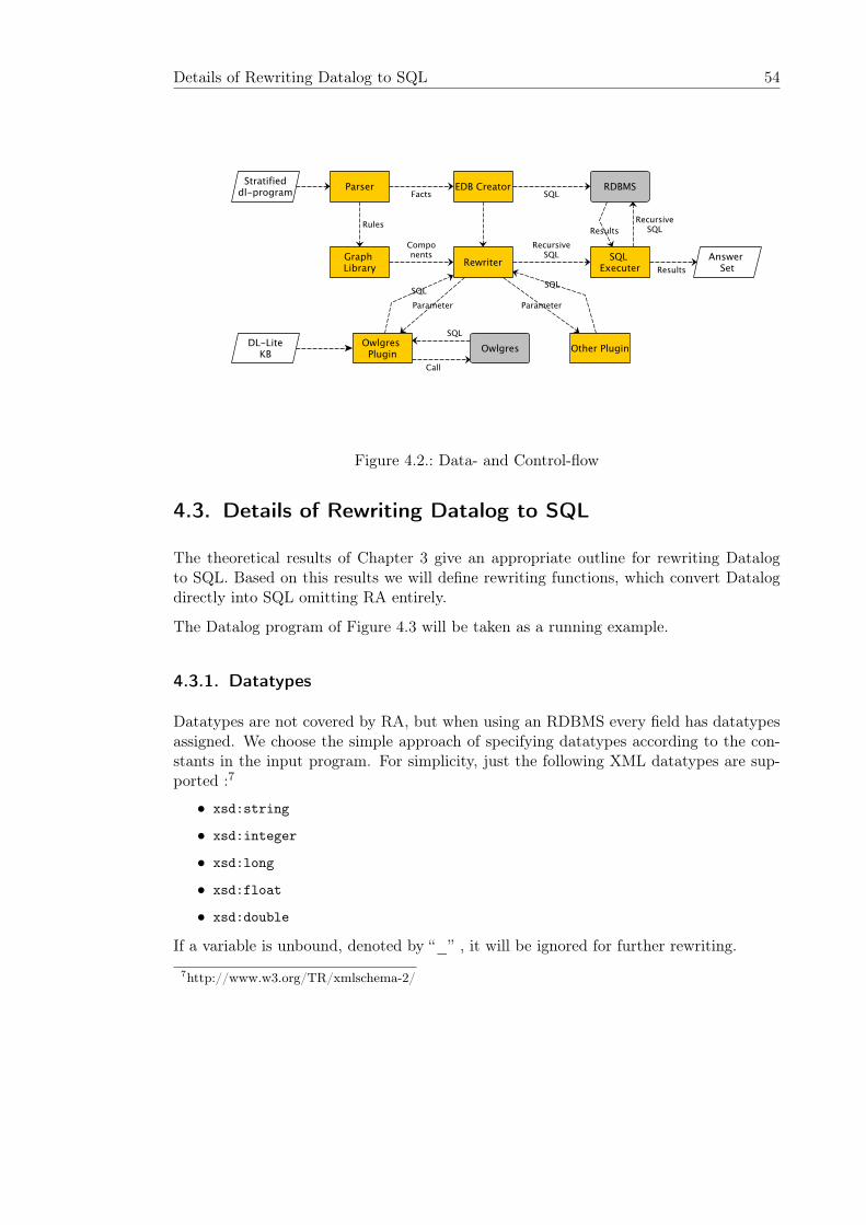
Details of Rewriting Datalog to SQL 54
Figure 4.2.: Data- and Control-flow
4.3. Details of Rewriting Datalog to SQL
The theoretical results of Chapter 3 give an appropriate outline for rewriting Datalogto SQL. Based on this results we will define rewriting functions, which convert Datalogdirectly into SQL omitting RA entirely.
The Datalog program of Figure 4.3 will be taken as a running example.
4.3.1. Datatypes
Datatypes are not covered by RA, but when using an RDBMS every field has datatypesassigned. We choose the simple approach of specifying datatypes according to the con-stants in the input program. For simplicity, just the following XML datatypes are sup-ported :7
• xsd:string
• xsd:integer
• xsd:long
• xsd:float
• xsd:double
If a variable is unbound, denoted by “_” , it will be ignored for further rewriting.7http://www.w3.org/TR/xmlschema-2/
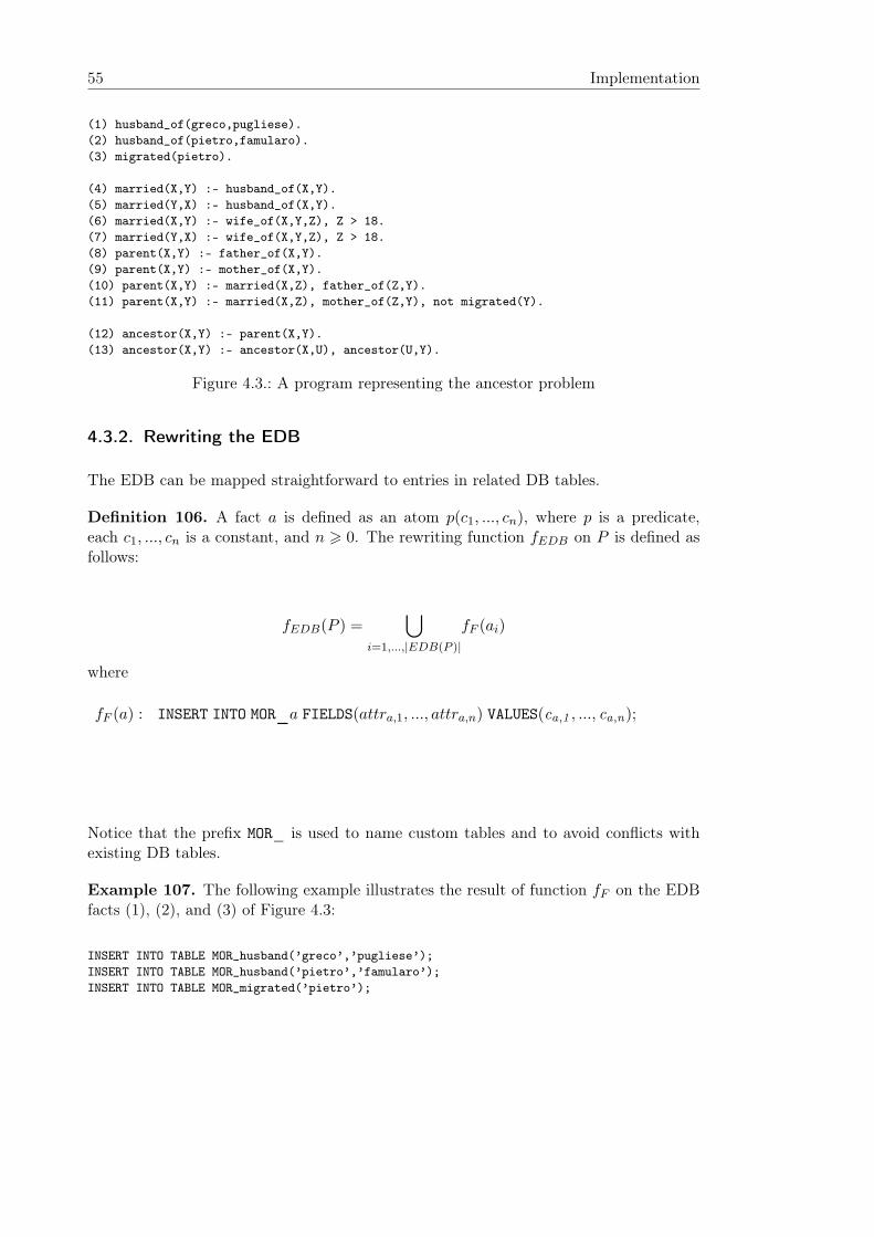
55 Implementation
(1) husband_of(greco,pugliese).(2) husband_of(pietro,famularo).(3) migrated(pietro).
(4) married(X,Y) :- husband_of(X,Y).(5) married(Y,X) :- husband_of(X,Y).(6) married(X,Y) :- wife_of(X,Y,Z), Z > 18.(7) married(Y,X) :- wife_of(X,Y,Z), Z > 18.(8) parent(X,Y) :- father_of(X,Y).(9) parent(X,Y) :- mother_of(X,Y).(10) parent(X,Y) :- married(X,Z), father_of(Z,Y).(11) parent(X,Y) :- married(X,Z), mother_of(Z,Y), not migrated(Y).
(12) ancestor(X,Y) :- parent(X,Y).(13) ancestor(X,Y) :- ancestor(X,U), ancestor(U,Y).
Figure 4.3.: A program representing the ancestor problem
4.3.2. Rewriting the EDB
The EDB can be mapped straightforward to entries in related DB tables.
Definition 106. A fact a is defined as an atom p(c1, ..., cn), where p is a predicate,each c1, ..., cn is a constant, and n � 0. The rewriting function fEDB on P is defined asfollows:
fEDB(P ) =�
i=1,...,|EDB(P )|
fF (ai)
where
fF (a) : INSERT INTO MOR_a FIELDS(attra,1, ..., attra,n) VALUES(ca,1 , ..., ca,n);
Notice that the prefix MOR_ is used to name custom tables and to avoid conflicts withexisting DB tables.
Example 107. The following example illustrates the result of function fF on the EDBfacts (1), (2), and (3) of Figure 4.3:
INSERT INTO TABLE MOR_husband(’greco’,’pugliese’);INSERT INTO TABLE MOR_husband(’pietro’,’famularo’);INSERT INTO TABLE MOR_migrated(’pietro’);
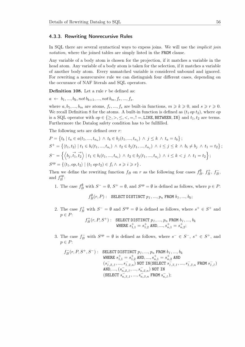
Details of Rewriting Datalog to SQL 56
4.3.3. Rewriting Nonrecursive Rules
In SQL there are several syntactical ways to expess joins. We will use the implicit joinnotation, where the joined tables are simply listed in the FROM clause.
Any variable of a body atom is chosen for the projection, if it matches a variable in thehead atom. Any variable of a body atom is taken for the selection, if it matches a variableof another body atom. Every unmatched variable is considered unbound and ignored.For rewriting a nonrecursive rule we can distinguish four different cases, depending onthe occurance of NAF literals and SQL operators.
Definition 108. Let a rule r be defined as:
a ← b1, ..., bk, not bk+1, ..., not bm, fr, ..., fs.
where a, b1, ..., bm are atoms, fr, ..., fs are built-in functions, m � k � 0, and s � r � 0.We recall Definition 8 for the atoms. A built-in function is defined as (t1 op t2), where opis a SQL operator with op ∈ {≥, >,≤, <,=, ! =, LIKE, BETWEEN, IN} and t1, t2 are terms.Furthermore the Datalog safety condition has to be fullfilled.
The following sets are defined over r:
P =�tb | ta ∈ a(t1, ..., tna) ∧ tb ∈ bj(t1, ..., tnj ) ∧ j ≤ k ∧ ta = tb
�;
S+ =��t1, t2� | t1 ∈ bi(t1, ..., tni) ∧ t2 ∈ bj(t1, ..., tnj ) ∧ i ≤ j ≤ k ∧ bi �= bj ∧ t1 = t2
�;
S− =��
bj ,→t1,
→t2�| t1 ∈ bi(t1, ..., tni) ∧ t2 ∈ bj(t1, ..., tnj ) ∧ i ≤ k < j ∧ t1 = t2
�;
Sop = {�t1, op, t2� | (t1 op t2) ∈ fi ∧ s � i � r} .Then we define the rewriting function fB on r as the following four cases f∅
B, f+B , f−
B ,and fop
B :
1. The case f∅B with S− = ∅, S+ = ∅, and Sop = ∅ is defined as follows, where p ∈ P :
f∅B(r, P ) : SELECT DISTINCT p1 , ..., pn FROM b1 , ..., bk ;
2. The case f+B with S− = ∅ and Sop = ∅ is defined as follows, where s+ ∈ S+ and
p ∈ P :f+B (r, P, S+) : SELECT DISTINCT p1 , ..., pn FROM b1 , ..., bk
WHERE s+1,1 = s+1,2 AND, ..., s+n,1 = s+n,2;
3. The case f−B with Sop = ∅ is defined as follows, where s− ∈ S−, s+ ∈ S+, and
p ∈ P :
f−B (r, P, S+, S−) : SELECT DISTINCT p1 , ..., pn FROM b1 , ..., bk
WHERE s+1,1 = s+1,2 AND, ..., s+n,1 = s+n,2 AND
(s−1 ,2 ,1 , ..., s−1 ,2 ,n) NOT IN(SELECT s−1 ,3 ,1 , ..., s
−1 ,3 ,n FROM s−1 ,1 )
AND, ..., (s−n,2 ,1 , ..., s−n,2 ,n) NOT IN
(SELECT s−n,3 ,1 , ..., s−n,3 ,n FROM s−n,1 );
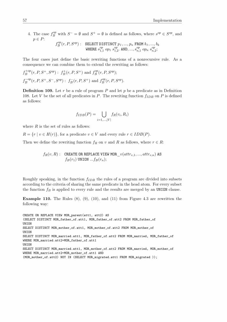
57 Implementation
4. The case fopB with S− = ∅ and S+ = ∅ is defined as follows, where sop ∈ Sop, and
p ∈ P :fopB (r, P, Sop) : SELECT DISTINCT p1 , ..., pn FROM b1 , ..., bk
WHERE sop1,1 op1 sop1,2. AND, ..., s
opn,1 opn sopn,2;
The four cases just define the basic rewriting functions of a nonrecursive rule. As aconsequence we can combine them to extend the rewriting as follows:
f+opB (r, P, S+, Sop) : f+
B (r, P, S+) and fopB (r, P, Sop);
f−opB (r, P, S+, S−, Sop) : f−
B (r, P, S+) and fopB (r, P, Sop).
Definition 109. Let r be a rule of program P and let p be a predicate as in Definition108. Let V be the set of all predicates in P . The rewriting function fIDB on P is definedas follows:
fIDB(P ) =�
i=1,...,|V |
fR(vi, Ri)
where R is the set of rules as follows:
R = {r | v ∈ H(r)}, for a predicate v ∈ V and every rule r ∈ IDB(P ).
Then we define the rewriting function fR on v and R as follows, where r ∈ R:
fR(v,R) : CREATE OR REPLACE VIEW MOR_v(attrv,1, ..., attrv,n) ASfB(r1) UNION ...fB(rn);
Roughly speaking, in the function fIDB the rules of a program are divided into subsetsaccording to the criteria of sharing the same predicate in the head atom. For every subsetthe function fB is applied to every rule and the results are merged by an UNION clause.
Example 110. The Rules (8), (9), (10), and (11) from Figure 4.3 are rewritten thefollowing way:
CREATE OR REPLACE VIEW MOR_parent(att1, att2) AS(SELECT DISTINCT MOR_father_of.att1, MOR_father_of.att2 FROM MOR_father_ofUNIONSELECT DISTINCT MOR_mother_of.att1, MOR_mother_of.att2 FROM MOR_mother_ofUNIONSELECT DISTINCT MOR_married.att1, MOR_father_of.att2 FROM MOR_married, MOR_father_ofWHERE MOR_married.att2=MOR_father_of.att1UNIONSELECT DISTINCT MOR_married.att1, MOR_mother_of.att2 FROM MOR_married, MOR_mother_ofWHERE MOR_married.att2=MOR_mother_of.att1 AND(MOR_mother_of.att2) NOT IN (SELECT MOR_migrated.att1 FROM MOR_migrated ));
Details of Rewriting Datalog to SQL 58
4.3.4. Rewriting Recursive Rules
For this thesis, the rewriting of Datalog to SQL would have been less appealing withoutthe introduction of recursion to the DB field. This occurred with the SQL:1999 standard[ISO, 1999] and fortunately, some RDBMS vendor have implemented SQL:1999 almostentirely. The listed RDBMS support recursive queries:
• PostgreSQL with version 8.4,8
• Microsoft SQL Server with version 2008,9
• IBM DB2 with version 7.2,10 and
• Oracle with version 9i release 2.11
As already pointed out in Chapter 3, the main drawback of SQL:1999 is its limitation tolinear recursion.
Definition 111. In PostgreSQL 8.4, the syntax of linear recursive queries is taken fromthe upcoming SQL:2008 standard:
WITH RECURSIVE < query name > AS ( < table subquery > )
{...} [ SEARCH clause | CYCLE clause ] < SELECT body >
Definition 112. The rewriting function f recB for linear recursive rules is an additional
case of function fB. Let the rules r1 and r2 of program P be defined as:
r1 : a ← b, c1, ..., ck.
r2 : a1 ← a2, a3, c1, ..., ck.
where the rules, atoms, predicates, and terms are defined as in Definition 108. Further-more the atoms a, a1, a2, and a3 share the same predicate.
The following sets are defined over r1 and r2:
P 1 = {tb | r1 ∧ ta ∈ a(t1, ..., tna) ∧ tb ∈ b(t1, ..., tnb) ∧ ta = tb} ;
P 2 = {tc | r2 ∧ ta ∈ a1(t1, ..., tna1) ∧ ((tc ∈ a2(t1, ..., tna2
) ∧ ta = tc) ∨
(tc ∈ a3(t1, ..., tna3) ∧ ta = tc))};
S =��t1, t2� | r2 ∧ t1 ∈ a2(t1, ..., tna2
) ∧ t2 ∈ a3(t1, ..., tna3) ∧ t1 = t2
�;
8http://www.postgresql.org/
9http://www.microsoft.com/sqlserver/
10http://www.ibm.com/db2/
11http://www.oracle.com/database/
59 Implementation
The function f recB is defined as follows, where s ∈ S, p1 ∈ P 1, p2 ∈ P 2, and lm ∈ N :
f recB (r1, r2, P 1, P 2, S, lm) : CREATE OR REPLACE VIEW MOR_a_base(attra,1 , ..., attra,n) AS
(SELECT DISTINCT p11 , ..., p1n FROM b);
CREATE OR REPLACE VIEW MOR_a(p21 , ..., p2n ) AS(
WITH RECURSIVE MOR_a_rc(p21 , ..., p2n ) AS
((SELECT DISTINCT p11 , ..., p1n FROM MOR_a_base)
UNION
(SELECT DISTINCT p21 , ..., p2n ,
FROM MOR_a_rc, MOR_a_baseWHERE s1 ,1 = s1 ,2 AND, ..., sn,1 = sn,2 ))SELECT p21 , ..., p
2n FROM MOR_a_rc LIMIT lm);
If there are cycles in the EDB, the recursive query evaluation of PostgreSQL will notterminate. In the PostgreSQL documentation this issue is stated as: “When workingwith recursive queries it is important to be sure that the recursive part of the query willeventually return no tuples, or else the query will loop indefinitely.”12 As commented bythe PostgreSQL developers, the recursive query evaluation is implemented as follows:13
1. Evaluate the non-recursive term of the SEARCH clause.
2. Evaluate the CYCLE clause by applying a breadth-first search, where a working tableand a result table is kept.
We decided to introduce the LIMIT parameter, to restrict the rows which are fetched bythe parent query. This has the effect, that a circular evaluation will stop after a certainamount of iteration in the breadth-first search. It is crucial to set the LIMIT parameternot less than the size of the expected result set. An incorrect parameter will cause aincomplete result set. A better approach and valuable extension of MOR would be theintroduction of a native DB function, which tracks all visited vertices to break cycles.See the PostgreSQL documentation for an in-depth discussion of this issue.14
4.4. Interfacing Owlgres with the DL Plug-in
As a second step, an intermediate layer between MOR and Owlgres had to be developed.We follow the design of dlvhex and HEX-programs (see [Eiter et al., 2006]) and introducea DL plug-in to interface with Owlgres and possible other DL reasoner.
The authors of [Stocker and Smith, 2008] put the focus of Owlgres as: “Owlgres aimsat both efficient querying over a scalable persistent store and automatic reasoning forRDF and OWL data.” Owlgres in its beta-release 0.1 is optimized for PostgreSQL, but12
http://www.postgresql.org/docs/8.4/static/queries-with.html13
http://archives.postgresql.org/pgsql-hackers/2008-02/msg00642.php14
http://www.postgresql.org/docs/8.4/static/queries-with.html
Interfacing Owlgres with the DL Plug-in 60
could be adapted to other RDBMS. Owlgres can act as server, awaiting queries throughTCP/IP. We decided to used Owlgres directly by referencing it as a component.
The DL plug-in covers two major cases:
• The first case is querying the DL KB. This is realized by calling Owlgres with agiven SPARQL query.
• The second case extends the simple query with updates to Owlgres’ DL KB.
4.4.1. DL-Atoms
In HEX-programs a strict approach for querying the DL KB with DL atoms was chosen.This has the advantage of uniformly interfacing different DL reasoner with different querylanguages. Thereby users of the system are strictly guided with the formulation of theirDL query. According to Eiter et al. DL atoms of HEX-programs support the followingqueries [Eiter et al., 2006]:
• Concept queries with the &dlC atom,
• object role queries with the &dlR atom,
• data role queries with the &dlDR atom, and
• conjunctive queries (resp. union of conjunctive queries) with &dlCQ (resp. &dlUCQ)atom.
In MOR on the contrary, accessing the DL KB is accomplished by SPARQL queries.The main reason for using SPARQL is influenced by the fact, that Owlgres uses it asthe language for query answering. Since Owlgres is not full SPARQL-complete, there aresome limitation regarding expressivity. For example the expression OPTIONAL is not sup-ported by Owlgres [Stocker and Smith, 2008]. Opposed to DL atoms of HEX-programs,the SPARQL queries are stored in external files and referenced in the DL atom. UsingSPARQL directly has the nice advantage, that it opens up the full expressibility of thelanguage. Thus any extensions in SPARQL and Owlgres are immediately available inMOR.
We follow the notion of dl-atom and dl-query introduced in Chapter 3. We use thedl-atom for practical purposes in two forms, namely as a standard atom and an updateatom.
Definition 113. The standard dl-atom is defined the following way:
&dlQS[query_uri](X1, ..., Xn) ,
where query_uri is the URI of a SPARQL query and X1, ..., Xn is the list of output terms.
Example 114. The following example is a plain dl-program. It references a query doDbpedia, which retrieves all books of a certain type:
61 Implementation
book(X,Y) :- &dlQS["books.rq"](X,Y). ,
where the SPARQL query books.rq is defined as:SELECT ?s ?n WHERE { ?s rdf#type yago:Book106410904 . ?s dbpedia:name ?n . }
Definition 115. The update dl-atom extends the DL KB access with concept, object-roleand data-role updates:
&dlQU[query_uri, op1, pred1, op2, pred2, op3, pred3](X1, ..., Xn) ,
with the following parameter:
query_uri ... is the URI of a SPARQL query.op1 ... denoting a positive (+) or negative (-) concept assertions.
pred1 ... designating the binary predicate for concept extensions, where the firstterm is a DL class and the second term is a DL individual.
op2 ... similar to op1 but for object-role assertions.pred2 ... designating the ternary predicate for concept extensions, where the first
term is a DL individual, the second a DL role and the third again an DLindividual.
op3 ... is similar to op1 but it is intended for data-role assertion.pred3 ... is similar to pred2 but the third term is plain text instead of an DL
individual.X1, ..., Xn denotes the list of output terms. Note that the output terms have to match
the variables of the SPARQL query defined in query_uri.
Example 116. The following dl-program extends Example 114 with membership asser-tions of a Spanish book.
book(X,Y) :- &dlQU["data/dbpedia_query.rq",+,updateC,+,updateOR,+,updateDR](X,Y).updateC(http://dbpedia.org/class/yago/Book106410904,study_Spanish_1).updateDR(study_Spanish_1,http://dbpedia.org/property/name,einführungSpanish1).updateOR(study_Spanish_1,http://dbpedia.org/property/successor,study_Spanish_2).
4.4.2. Owlgres Overview
The Owlgres DL KB has to be initialized by creating the TBox and filling the ABox.This is accomplished in the command line interface by the following commands [Stockerand Smith, 2008]:
• Creating the TBox is achieved by using the sh/create command. The name ofthe RDBMS and the URI of the OWL file with the TBox definitions have to beprovided.
• Loading the ABox assertions is done with sh/load command. Furthermore theRDBMS’s name and the URI of the OWL file with the ABox definition have to begiven.
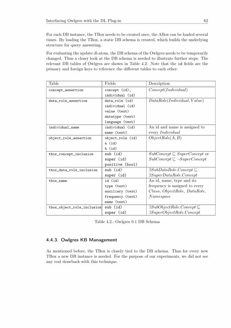
Interfacing Owlgres with the DL Plug-in 62
For each DB instance, the TBox needs to be created once, the ABox can be loaded severaltimes. By loading the TBox, a static DB schema is created, which builds the underlyingstructure for query answering.
For evaluating the update dl-atom, the DB schema of the Owlgres needs to be temporarilychanged. Thus a closer look at the DB schema is needed to illustrate further steps. Therelevant DB tables of Owlgres are shown in Table 4.2. Note that the id fields are theprimary and foreign keys to reference the different tables to each other:
Table Fields Descriptionconcept_assertion concept (id),
individual (id)
Concept(Individual)
data_role_assertion data_role (id)
individual (id)
value (text)
datatype (text)
language (text)
DataRole(Individual, V alue)
individual_name individual (id)
name (text)
An id and name is assigned toevery Individual
object_role_assertion object_role (id)
a (id)
b (id)
ObjectRole(A,B)
tbox_concept_inclusion sub (id)super (id)positive (bool)
SubConcept � SuperConcept orSubConcept � ¬SuperConcept
tbox_data_role_inclusion sub (id)super (id)
∃SubDataRole.Concept �∃SuperDataRole.Concept
tbox_name id (id)
type (text)
auxiliary (text)
frequency (text)
name (text)
An id, name, type and itsfrequency is assigned to everyClass, ObjectRole, DataRole,Namespace
tbox_object_role_inclusion sub (id)super (id)
∃SubObjectRole.Concept �∃SuperObjectRole.Concept
Table 4.2.: Owlgres 0.1 DB Schema
4.4.3. Owlgres KB Management
As mentioned before, the TBox is closely tied to the DB schema. Thus for every newTBox a new DB instance is needed. For the purpose of our experiments, we did not seeany real drawback with this technique.
63 Implementation
4.4.4. Rewriting the Standard DL-Atom
The rewriting of the standard dl-atom is straightforward. The query_uri and theRDBMS parameter are forwarded to the rewrite function of Owlgres. After Owlgresis called, the resulting SQL statements are embedded into a newly created DB view.The rewrite function of Owlgres is an implementation of the Algorithm Answer(Q,K) inDL-LiteR (we refer to Chapter 2). As described in [Stocker and Smith, 2008], the stan-dard rewriting of [Calvanese et al., 2007] was extended with three types of optimizations:
• Query simplification,
• selectivity optimization, and
• rewriting a set of conjunctive queries as a single query of UNION clauses.
4.4.5. Rewriting the Update DL-Atom
The following requirements have to be considered by rewriting the update dl-atom:
• After updating and accessing the DL KB, we need to transform it in its prior state,and
• as discussed in Section 4.3.3, a cascade of DB views and SQL statements is createdand evaluated synchronous.
Note that otherwise the DL KB could be directly manipulated on the RDBMS.
The update process, which is shown in Algorithm 4.1 has the following steps:
• First, the original DB tables are renamed;
• Second, the auxiliary tables are created;
• And third, the auxiliary tables are “unionized” with the renamed tables using theiroriginal name.
In Algorithm 4.1 the update of the DL KB occurs in stages. A stage is represented by thevariable lvl. The introduction of stages is needed, otherwise different update dl-atomswould interfere with each other. Through stages, every update dl-atom constructs itsown temporary state of the DL KB.
The statements UNION (resp. EXCEPT) are used to implement positive (resp. nega-tive) membership assertion. As apparent from the DB schema in Table 4.2, thereare no negative assertion defined in concept_assertion, object_role_assertion, anddata_role_assertion. Thus we decided to use EXCEPT for excluding the negative asser-tions from the result.
Furthermore, for every created individual, a temporary id is created, otherwise the newindividual would collide with already existing individuals. For creating new ids withoutmaterializing the individuals, we used PostgreSQL’s sequence function, which createsunique identifiers on demand.15
15http://www.postgresql.org/docs/8.4/static/sql-createsequence.html
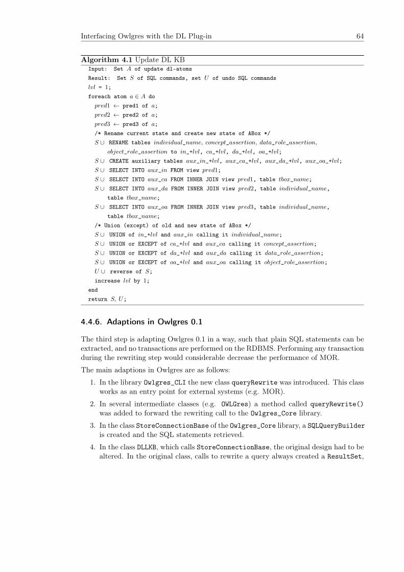
Interfacing Owlgres with the DL Plug-in 64
Algorithm 4.1 Update DL KBInput: Set A of update dl-atomsResult: Set S of SQL commands, set U of undo SQL commandslvl = 1;foreach atom a ∈ A do
pred1 ← pred1 of a;pred2 ← pred2 of a;pred3 ← pred3 of a;/* Rename current state and create new state of ABox */S ∪ RENAME tables individual_name, concept_assertion, data_role_assertion,
object_role_assertion to in_+lvl, ca_+lvl, da_+lvl, oa_+lvl;S ∪ CREATE auxiliary tables aux_in_+lvl, aux_ca_+lvl, aux_da_+lvl, aux_oa_+lvl;S ∪ SELECT INTO aux_in FROM view pred1;S ∪ SELECT INTO aux_ca FROM INNER JOIN view pred1, table tbox_name;S ∪ SELECT INTO aux_da FROM INNER JOIN view pred2, table individual_name,
table tbox_name;S ∪ SELECT INTO aux_oa FROM INNER JOIN view pred3, table individual_name,
table tbox_name;/* Union (except) of old and new state of ABox */S ∪ UNION of in_+lvl and aux_in calling it individual_name;S ∪ UNION or EXCEPT of ca_+lvl and aux_ca calling it concept_assertion;S ∪ UNION or EXCEPT of da_+lvl and aux_da calling it data_role_assertion;S ∪ UNION or EXCEPT of oa_+lvl and aux_oa calling it object_role_assertion;U ∪ reverse of S;increase lvl by 1;
endreturn S, U;
4.4.6. Adaptions in Owlgres 0.1
The third step is adapting Owlgres 0.1 in a way, such that plain SQL statements can beextracted, and no transactions are performed on the RDBMS. Performing any transactionduring the rewriting step would considerable decrease the performance of MOR.
The main adaptions in Owlgres are as follows:
1. In the library Owlgres_CLI the new class queryRewrite was introduced. This classworks as an entry point for external systems (e.g. MOR).
2. In several intermediate classes (e.g. OWLGres) a method called queryRewrite()was added to forward the rewriting call to the Owlgres_Core library.
3. In the class StoreConnectionBase of the Owlgres_Core library, a SQLQueryBuilderis created and the SQL statements retrieved.
4. In the class DLLKB, which calls StoreConnectionBase, the original design had to bealtered. In the original class, calls to rewrite a query always created a ResultSet,
which decrease the performance of the overall system. This was adapted, that incase of queryRewrite() only a string and not the whole result set is returned.
4.5. Limitations
As already mentioned, MOR is an experimental system, and due to “usual” limitation ofresources (e.g. time), we did not implement the following functions yet:
• As discussed in Chapter 3, only linear recursion and not general recursion is sup-ported;
• Algorithm RectifyRules of Chapter 3 is not considered;
• Other OWL2 QL reasoners (e.g. QuOnto) could be integrated;
• A generic SQL plug-in is missing;
• The public interface of the MOR libraries have to be reconsidered, so MOR couldbe used as a software component in other systems;
• Replacing the LIMIT parameter with a native DB function, which handles cycles inrecursive queries.

5. Experiments
5.1. Methodology
The Asparagus competition was a major step in the field of ASP for benchmarking ASPreasoners [Gebser et al., 2007b, Denecker et al., 2009]. Also for OWL several benchmarksuites as Lehigh University Benchmark (LUBM) and Ontology Benchmark (UOBM) haveevolved. We refer the interested reader to [Guo et al., 2005, Ma et al., 2006]. For moregeneral rule-based systems, OpenRuleBench was developed to benchmark different typesof reasoners, namely Prolog-based, Deductive Database, Productive Rule, and ReactiveRule systems [Liang et al., 2009].
None of the mentioned benchmarks is designed to cover dl-programs. Fortunately, Open-RuleBench includes some useful benchmarks, which could be adopted for these exper-iments. When reasoning systems are benchmarked, there is an ongoing discussion onthe separation of loading and inference time [Liang et al., 2009]. In contrast to Open-RuleBench, this benchmark does not separate loading and inference time. This is donebecause we focus on RDBMS technology, where important optimizations are done in theloading step.
The experiment is split into four different scenarios, whereby the last does not containbenchmarks:
1. This scenario is composed of ordinary Datalog programs.
2. In this scenario Datalog programs query a DBpedia DL KB.
3. More complex than the second scenario, a LUBM DL KB is queried instead.
4. This scenario shows extensions and limitations of our prototype.
To cover a wide area of testing, both random and “real world” data is used. The generateddata for each scenario contains approximately 10,000, 100,000, 500,000, and 1,000,000facts or assertions.
5.2. Scenario 1 - Datalog
This scenario focuses just on Datalog programs. Based on three benchmarks, somefeatures like recursion and default negation are tested.
MOR is compared to the following systems:
67
Scenario 1 - Datalog 68
• DLV using its ODBC interface [Leone et al., 2006], and
• DLVDB using the auxiliary directives USE for importing the EDB and CREATE fordefining the IDB [Terracina et al., 2008].
5.2.1. Large Join Benchmark
This benchmark is taken from OpenRuleBench, whereby the EDB consists of the relationsc2, c3, c4, d1, d2, and ex. These relations are first randomly generated and then importedto PostgreSQL. Note that the #import directive in MOR is used as in DLV, mapping DBrelations to the EDB. For implications the symbol :- is used instead of ←.
Definition 117. The first benchmark is a non-recursive program evaluating a tree ofbinary joins:
#import(c2). #import(c3). #import(c4). #import(d1). #import(d2).% Queryresult(X,Y) :- b1(X,Z), b2(Z,Y).% Mainb1(X,Y) :- c1(X,Z), c2(Z,Y).b2(X,Y) :- c3(X,Z), c4(Z,Y).c1(X,Y) :- d1(X,Z), d2(Z,Y).
5.2.2. Default Negation Benchmark
Definition 118. This benchmark is extending the previous program simply with defaultnegation:
#import(c2). #import(c3). #import(c4). #import(d1). #import(d2). #import(ex).% Queryresult(X,Y) :- b1(X,Z), b2(Z,Y).% Mainb1(X,Y) :- c1(X,Z), c2(Z,Y), not ex(Y).b2(X,Y) :- c3(X,Z), c4(Z,Y), not ex(Y).c1(X,Y) :- d1(X,Z), d2(Z,Y), not ex(X).
5.2.3. Stratified Negation Benchmark
The well know ancestor problem is taken to show recursion and default negation. Againthe relations of the EDB are generated randomly, hence certain instances of the EDBmight be cyclic.
Definition 119. This program captures the transitive closure of the relation parent. Itconsists of the following rules:
69 Experiments
#import(migrated). #import(husband_of). #import(wife_of). #import(father_of).#import(mother_of).% Queryresult(X,Y) :- married(X,Y), not ancestor(X,Y).% Mainmarried(X,Y) :- husband_of(X,Y).married(Y,X) :- husband_of(X,Y).married(X,Y) :- wife_of(X,Y,Z), Z > 18.married(Y,X) :- wife_of(X,Y,Z), Z > 18.parent(X,Y) :- father_of(X,Y).parent(X,Y) :- mother_of(X,Y).parent(X,Y) :- married(X,Z), father_of(Z,Y).parent(X,Y) :- married(X,Z), mother_of(Z,Y), not migrated(Y).% Recursionancestor(X,Y) :- parent(X,Y).ancestor(X,Y) :- ancestor(X,U), ancestor(U,Y).
5.3. Scenario 2 - Derived DBpedia
Being the goal of this work, the capabilities of combining Datalog and DL-Lite based onan RDBMS are shown. This scenario is split into three benchmarks, whereby the first isa simple access to the DL layer, the second has access to the DL layer and negation isincluded, and the third combines access and update to the DL layer.
MOR is benchmarked agains dlvhex, using the Description Logic Plug-in with RacerPro1.9.2 [Eiter et al., 2006].
We extracted three types of literature (e.g. books, periodicals, and publications) fromthe DBpedia DB1. The extracted data was then imported to Owlgres filling the ABox.
Definition 120. We defined the TBox as follows, because the whole TBox of DBpediais not capturable with Owlgres:
Book � PublicationPeriodical � Publication∃Name.nameString�publication, nameString� : Name
.
5.3.1. Simple Benchmark
Definition 121. This program is simple merging two DL queries for books and journals:1http://wiki.dbpedia.org/OnlineAccess
Scenario 2 - Derived DBpedia 70
% Queryresult(X,Y) :- book(X,Y).result(X,Y) :- journ(X,Y).% DL Accessbook(X,Y) :- &dlQS["dbpedia_query1"](X,Y).journ(X,Y) :- &dlQS["dbpedia_query2"](X,Y).
5.3.2. Advanced Benchmark
Definition 122. This program selects all available books and excludes the periodicalsfrom the total set. Then a given range of books are chosen from the total set:
% Queryresult(X,Y) :- journ_sel_a(X,Y).result(X,Y) :- journ_sel_d(X,Y).% Mainjourn_sel_a(X,Y) :- journ(X,Y), Y > ’Book 1000’, Y < ’Book 1500’.journ_sel_d(X,Y) :- journ(X,Y), Y > ’Book 8000’, Y < ’Book 8500’.journ(X,Y) :- publ(X,Y), not book(X,Y).% DL Accessbook(X,Y) :- &dlQS["dbpedia_query1"](X,Y).publ(X,Y) :- &dlQS["dbpedia_query3"](X,Y).
5.3.3. Update Benchmark
Definition 123. In this program the ABox is extended with three Spanish books:
% Queryresult(X,Y) :- book(X,Y).result(X,Y) :- journ(X,Y).% DL Access and Updatebook(X,Y) :- &dlQU["dbpedia_query1",+,updateConcept,+„+,updateData](X,Y).journ(X,Y) :- &dlQS["dbpedia_query2"](X,Y).% Update PredicatesupdateConcept(X,Y) :- uc(X,Y).updateData(X,Y,Z) :- ud(X,Y,Z).uc(yago:Book106410904,study_Spanish_1).uc(yago:Book106410904,study_Spanish_2).uc(yago:Book106410904,study_Spanish_3).ud(study_Spanish_1,dbpedia:name,einführungSpanish1).ud(study_Spanish_2,dbpedia:name,einführungSpanish2).ud(study_Spanish_3,dbpedia:name,enführungSpanish3).
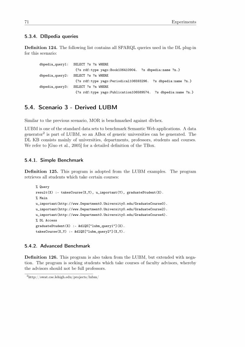
71 Experiments
5.3.4. DBpedia queries
Definition 124. The following list contains all SPARQL queries used in the DL plug-infor this scenario:
dbpedia_query1: SELECT ?s ?n WHERE{?s rdf:type yago:Book106410904. ?s dbpedia:name ?n.}
dbpedia_query2: SELECT ?s ?n WHERE{?s rdf:type yago:Periodical106593296. ?s dbpedia:name ?n.}
dbpedia_query3: SELECT ?s ?n WHERE{?s rdf:type yago:Publication106589574. ?s dbpedia:name ?n.}
5.4. Scenario 3 - Derived LUBM
Similar to the previous scenario, MOR is benchmarked against dlvhex.
LUBM is one of the standard data sets to benchmark Semantic Web applications. A datagenerator2 is part of LUBM, so an ABox of generic universities can be generated. TheDL KB consists mainly of universities, departments, professors, students and courses.We refer to [Guo et al., 2005] for a detailed definition of the TBox.
5.4.1. Simple Benchmark
Definition 125. This program is adopted from the LUBM examples. The programretrieves all students which take certain courses:
% Queryresult(X) :- takesCourse(X,Y), u_important(Y), graduateStudent(X).% Mainu_important(http://www.Department0.University0.edu/GraduateCourse0).u_important(http://www.Department0.University0.edu/GraduateCourse2).u_important(http://www.Department0.University0.edu/GraduateCourse4).% DL AccessgraduateStudent(X) :- &dlQS["lubm_query1"](X).takesCourse(X,Y) :- &dlQS["lubm_query2"](X,Y).
5.4.2. Advanced Benchmark
Definition 126. This program is also taken from the LUBM, but extended with nega-tion. The program is seeking students which take courses of faculty advisors, wherebythe advisors should not be full professors.
2http://swat.cse.lehigh.edu/projects/lubm/
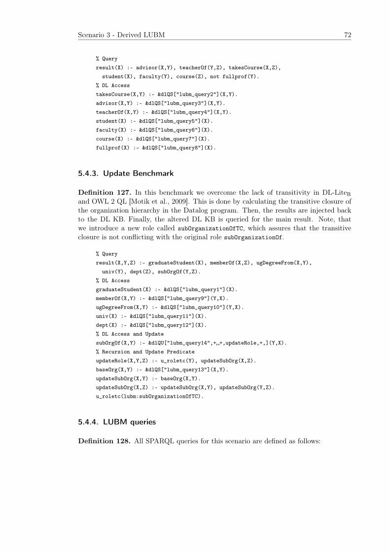
Scenario 3 - Derived LUBM 72
% Queryresult(X) :- advisor(X,Y), teacherOf(Y,Z), takesCourse(X,Z),
student(X), faculty(Y), course(Z), not fullprof(Y).% DL AccesstakesCourse(X,Y) :- &dlQS["lubm_query2"](X,Y).advisor(X,Y) :- &dlQS["lubm_query3"](X,Y).teacherOf(X,Y) :- &dlQS["lubm_query4"](X,Y).student(X) :- &dlQS["lubm_query5"](X).faculty(X) :- &dlQS["lubm_query6"](X).course(X) :- &dlQS["lubm_query7"](X).fullprof(X) :- &dlQS["lubm_query8"](X).
5.4.3. Update Benchmark
Definition 127. In this benchmark we overcome the lack of transitivity in DL-LiteRand OWL 2 QL [Motik et al., 2009]. This is done by calculating the transitive closure ofthe organization hierarchy in the Datalog program. Then, the results are injected backto the DL KB. Finally, the altered DL KB is queried for the main result. Note, thatwe introduce a new role called subOrganizationOfTC, which assures that the transitiveclosure is not conflicting with the original role subOrganizationOf.
% Queryresult(X,Y,Z) :- graduateStudent(X), memberOf(X,Z), ugDegreeFrom(X,Y),
univ(Y), dept(Z), subOrgOf(Y,Z).% DL AccessgraduateStudent(X) :- &dlQS["lubm_query1"](X).memberOf(X,Y) :- &dlQS["lubm_query9"](Y,X).ugDegreeFrom(X,Y) :- &dlQS["lubm_query10"](Y,X).univ(X) :- &dlQS["lubm_query11"](X).dept(X) :- &dlQS["lubm_query12"](X).% DL Access and UpdatesubOrgOf(X,Y) :- &dlQU["lubm_query14",+„+,updateRole,+,](Y,X).% Recursion and Update PredicateupdateRole(X,Y,Z) :- u_roletc(Y), updateSubOrg(X,Z).baseOrg(X,Y) :- &dlQS["lubm_query13"](X,Y).updateSubOrg(X,Y) :- baseOrg(X,Y).updateSubOrg(X,Z) :- updateSubOrg(X,Y), updateSubOrg(Y,Z).u_roletc(lubm:subOrganizationOfTC).
5.4.4. LUBM queries
Definition 128. All SPARQL queries for this scenario are defined as follows:
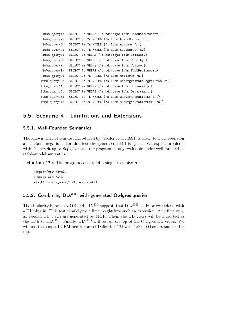
lubm_query1: SELECT ?s WHERE {?s rdf:type lubm:GraduateStudent.}lubm_query2: SELECT ?s ?n WHERE {?s lubm:takesCourse ?n.}lubm_query3: SELECT ?s ?n WHERE {?s lubm:advisor ?n.}lubm_query4: SELECT ?s ?n WHERE {?s lubm:teacherOf ?n.}lubm_query5: SELECT ?s WHERE {?s rdf:type lubm:Student.}lubm_query6: SELECT ?s WHERE {?s rdf:type lubm:Faculty.}lubm_query7: SELECT ?s WHERE {?s rdf:type lubm:Course.}lubm_query8: SELECT ?s WHERE {?s rdf:type lubm:FullProfessor.}lubm_query9: SELECT ?s ?n WHERE {?s lubm:memberOf ?n.}
lubm_query10: SELECT ?s ?n WHERE {?s lubm:undergraduateDegreeFrom ?n.}lubm_query11: SELECT ?s WHERE {?s rdf:type lubm:University.}lubm_query12: SELECT ?s WHERE {?s rdf:type lubm:Department.}lubm_query13: SELECT ?s ?n WHERE {?s lubm:subOrganizationOf ?n.}lubm_query14: SELECT ?s ?n WHERE {?s lubm:subOrganizationOfTC ?n.}
5.5. Scenario 4 - Limitations and Extensions
5.5.1. Well-Founded Semantics
The known win-not-win test introduced by [Gelder et al., 1991] is taken to show recursionand default negation. For this test the generated EDB is cyclic. We expect problemswith the rewriting to SQL, because the program is only evaluable under well-founded orstable-model semantics.
Definition 129. The program consists of a single recursive rule:
#import(wnw_move).% Query and Mainwin(X) :- wnw_move(X,Y), not win(Y).
5.5.2. Combining DLVDB with generated Owlgres queries
The similarity between MOR and DLVDB suggest, that DLVDB could be extendend witha DL plug-in. This test should give a first insight into such an extension. As a first step,all needed DB views are generated by MOR. Then, the DB views will be imported asthe EDB to DLVDB. Finally, DLVDB will be run on top of the Owlgres DB views. Wewill use the simple LUBM benchmark of Definition 125 with 1,000,000 assertions for thistest.

6. Experimental Results
In this chapter, we present and discuss the results for our experiments. The test wereperformed on a server running on openSUSE 11.1 (x86_64) with the following specifica-tion:
• Processor (CPU): Intel® Xeon® CPU E5450 @ 3.00GHz;
• Total memory (RAM): 15.7 GB.
The standard installation of PostgreSQL 8.4 in openSUSE 11.1 was taken. To utilize theavailable RAM, the parameters shared_buffers was set to 4096 MB (from 32 MB) andwork_mem was set to 512 MB (from 1 MB) . These recommendations for performanceoptimization were taken from PostgreSQL wiki.1 Further optimization of PostgreSQL,such as creating DB indices, was not considered for the Datalog scenario, but for thecombined scenarios the DL reasoner Owlgres creates useful indices on its initialization.
For every system/benchmark combination, the experiment followed the following proce-dure:
1. Initializing PostgreSQL to clear its cache.
2. Five rounds of calls with the respective tool and the respective benchmark’s pro-gram file are executed, whereby start- and finishing times are logged. To avoid anybias in measuring, the result output is turned off for every system.
3. After a timeout of 12 hours the particular experiment is canceled.
4. The average of the five execution times is taken to calculate the final result, whichis kept in seconds.
Notice, that we consciously decided to initialize PostgreSQL only at the beginning, sothe query optimizer of PostgreSQL could take advantage of cached data. In Section 6.1.1we will discuss the results related to caching.
To validate the correctness of every benchmark, the resulting sets were counted andcompared with the other systems. We did not encounter any differences in the resultingsets.
1http://wiki.postgresql.org/wiki/Performance_Optimization
75
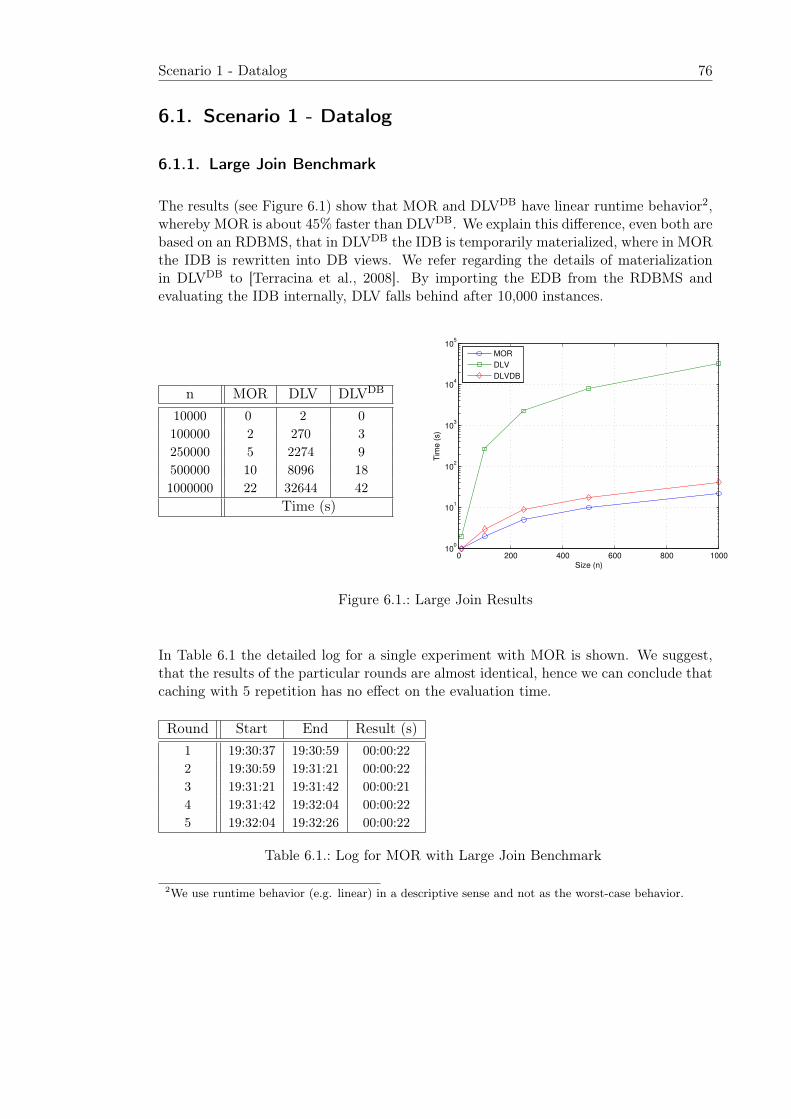
Scenario 1 - Datalog 76
6.1. Scenario 1 - Datalog
6.1.1. Large Join Benchmark
The results (see Figure 6.1) show that MOR and DLVDB have linear runtime behavior2,whereby MOR is about 45% faster than DLVDB. We explain this difference, even both arebased on an RDBMS, that in DLVDB the IDB is temporarily materialized, where in MORthe IDB is rewritten into DB views. We refer regarding the details of materializationin DLVDB to [Terracina et al., 2008]. By importing the EDB from the RDBMS andevaluating the IDB internally, DLV falls behind after 10,000 instances.
n MOR DLV DLVDB
10000 0 2 0100000 2 270 3250000 5 2274 9500000 10 8096 181000000 22 32644 42
Time (s)
0 200 400 600 800 100010
0
101
102
103
104
105
Size (n)
Tim
e (
s)
MOR
DLV
DLVDB
Figure 6.1.: Large Join Results
In Table 6.1 the detailed log for a single experiment with MOR is shown. We suggest,that the results of the particular rounds are almost identical, hence we can conclude thatcaching with 5 repetition has no effect on the evaluation time.
Round Start End Result (s)1 19:30:37 19:30:59 00:00:222 19:30:59 19:31:21 00:00:223 19:31:21 19:31:42 00:00:214 19:31:42 19:32:04 00:00:225 19:32:04 19:32:26 00:00:22
Table 6.1.: Log for MOR with Large Join Benchmark
2We use runtime behavior (e.g. linear) in a descriptive sense and not as the worst-case behavior.
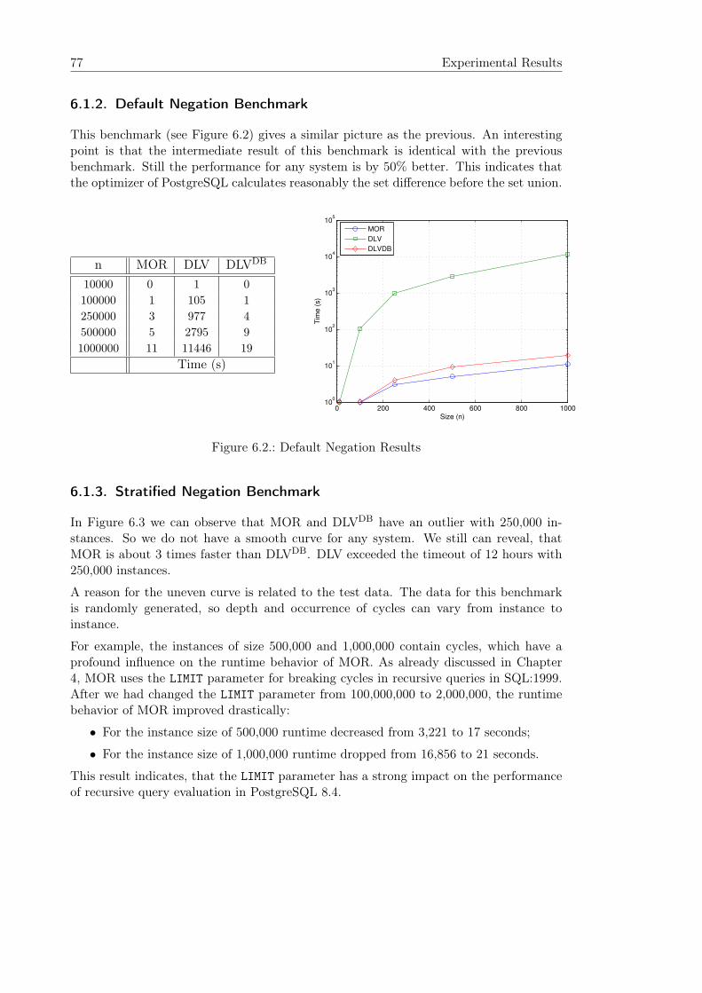
77 Experimental Results
6.1.2. Default Negation Benchmark
This benchmark (see Figure 6.2) gives a similar picture as the previous. An interestingpoint is that the intermediate result of this benchmark is identical with the previousbenchmark. Still the performance for any system is by 50% better. This indicates thatthe optimizer of PostgreSQL calculates reasonably the set difference before the set union.
n MOR DLV DLVDB
10000 0 1 0100000 1 105 1250000 3 977 4500000 5 2795 91000000 11 11446 19
Time (s)
0 200 400 600 800 100010
0
101
102
103
104
105
Size (n)
Tim
e (
s)
MOR
DLV
DLVDB
Figure 6.2.: Default Negation Results
6.1.3. Stratified Negation Benchmark
In Figure 6.3 we can observe that MOR and DLVDB have an outlier with 250,000 in-stances. So we do not have a smooth curve for any system. We still can reveal, thatMOR is about 3 times faster than DLVDB. DLV exceeded the timeout of 12 hours with250,000 instances.
A reason for the uneven curve is related to the test data. The data for this benchmarkis randomly generated, so depth and occurrence of cycles can vary from instance toinstance.
For example, the instances of size 500,000 and 1,000,000 contain cycles, which have aprofound influence on the runtime behavior of MOR. As already discussed in Chapter4, MOR uses the LIMIT parameter for breaking cycles in recursive queries in SQL:1999.After we had changed the LIMIT parameter from 100,000,000 to 2,000,000, the runtimebehavior of MOR improved drastically:
• For the instance size of 500,000 runtime decreased from 3,221 to 17 seconds;
• For the instance size of 1,000,000 runtime dropped from 16,856 to 21 seconds.
This result indicates, that the LIMIT parameter has a strong impact on the performanceof recursive query evaluation in PostgreSQL 8.4.
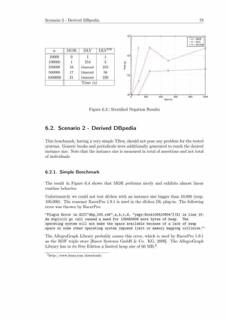
Scenario 2 - Derived DBpedia 78
n MOR DLV DLVDB
10000 0 1 1100000 1 254 5250000 16 timeout 255500000 17 timeout 561000000 21 timeout 239
Time (s)
0 200 400 600 800 100010
0
101
102
103
Size (n)
Tim
e (
s)
MORDLVDLVDB
Figure 6.3.: Stratified Negation Results
6.2. Scenario 2 - Derived DBpedia
This benchmark, having a very simple TBox, should not pose any problem for the testedsystems. Generic books and periodicals were additionally generated to reach the desiredinstance size. Note that the instance size is measured in total of assertions and not totalof individuals.
6.2.1. Simple Benchmark
The result in Figure 6.4 shows that MOR performs nicely and exhibits almost linearruntime behavior.
Unfortunately we could not test dlvhex with an instance size bigger than 10,000 (resp.100,000). The reasoner RacerPro 1.9.1 is used in the dlvhex DL plug-in. The followingerror was thrown by RacerPro:
“Plugin Error in dlC["dbp_100.rdf",a,b,c,d, "yago:Book106410904"](X) in line 10:
An explicit gc call caused a need for 139460608 more bytes of heap. The
operating system will not make the space available because of a lack of swap
space or some other operating system imposed limit or memory mapping collision.”
The AllegroGraph Library probably causes this error, which is used by RacerPro 1.9.1as the RDF triple store [Racer Systems GmbH & Co. KG, 2009]. The AllegroGraphLibrary has in its Free Edition a limited heap size of 60 MB.3
3http://www.franz.com/downloads/
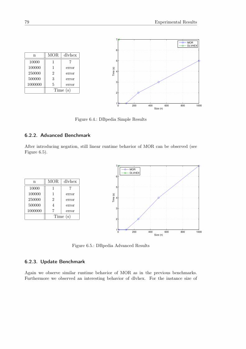
79 Experimental Results
n MOR dlvhex10000 1 7100000 1 error250000 2 error500000 3 error1000000 5 error
Time (s)
0 200 400 600 800 10001
2
3
4
5
6
7
Size (n)
Tim
e (
s)
MORDLVHEX
Figure 6.4.: DBpedia Simple Results
6.2.2. Advanced Benchmark
After introducing negation, still linear runtime behavior of MOR can be observed (seeFigure 6.5).
n MOR dlvhex10000 1 7100000 1 error250000 2 error500000 4 error1000000 7 error
Time (s)
0 200 400 600 800 10001
2
3
4
5
6
7
Size (n)
Tim
e (
s)
MOR
DLVHEX
Figure 6.5.: DBpedia Advanced Results
6.2.3. Update Benchmark
Again we observe similar runtime behavior of MOR as in the previous benchmarks.Furthermore we observed an interesting behavior of dlvhex. For the instance size of
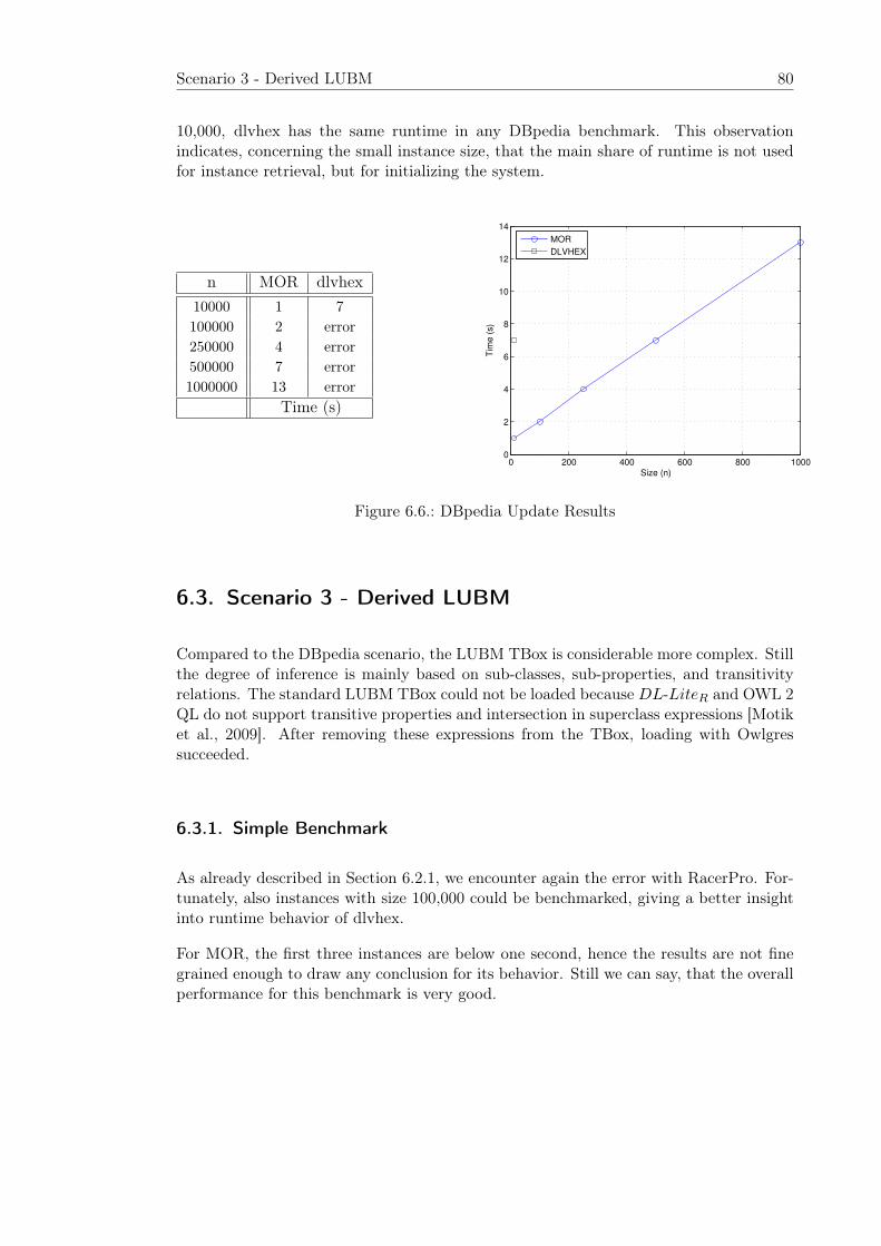
Scenario 3 - Derived LUBM 80
10,000, dlvhex has the same runtime in any DBpedia benchmark. This observationindicates, concerning the small instance size, that the main share of runtime is not usedfor instance retrieval, but for initializing the system.
n MOR dlvhex10000 1 7100000 2 error250000 4 error500000 7 error1000000 13 error
Time (s)
0 200 400 600 800 10000
2
4
6
8
10
12
14
Size (n)
Tim
e (
s)
MOR
DLVHEX
Figure 6.6.: DBpedia Update Results
6.3. Scenario 3 - Derived LUBM
Compared to the DBpedia scenario, the LUBM TBox is considerable more complex. Stillthe degree of inference is mainly based on sub-classes, sub-properties, and transitivityrelations. The standard LUBM TBox could not be loaded because DL-LiteR and OWL 2QL do not support transitive properties and intersection in superclass expressions [Motiket al., 2009]. After removing these expressions from the TBox, loading with Owlgressucceeded.
6.3.1. Simple Benchmark
As already described in Section 6.2.1, we encounter again the error with RacerPro. For-tunately, also instances with size 100,000 could be benchmarked, giving a better insightinto runtime behavior of dlvhex.
For MOR, the first three instances are below one second, hence the results are not finegrained enough to draw any conclusion for its behavior. Still we can say, that the overallperformance for this benchmark is very good.
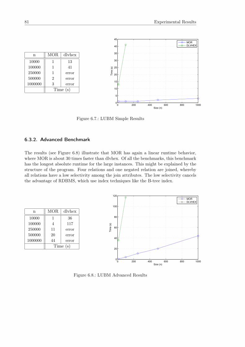
81 Experimental Results
n MOR dlvhex10000 1 13100000 1 41250000 1 error500000 2 error1000000 3 error
Time (s)
0 200 400 600 800 10000
5
10
15
20
25
30
35
40
45
Size (n)
Tim
e (
s)
MORDLVHEX
Figure 6.7.: LUBM Simple Results
6.3.2. Advanced Benchmark
The results (see Figure 6.8) illustrate that MOR has again a linear runtime behavior,where MOR is about 30 times faster than dlvhex. Of all the benchmarks, this benchmarkhas the longest absolute runtime for the large instances. This might be explained by thestructure of the program. Four relations and one negated relation are joined, wherebyall relations have a low selectivity among the join attributes. The low selectivity cancelsthe advantage of RDBMS, which use index techniques like the B-tree index.
n MOR dlvhex10000 1 36100000 4 117250000 11 error500000 20 error1000000 44 error
Time (s)
0 200 400 600 800 10000
20
40
60
80
100
120
Size (n)
Tim
e (
s)
MORDLVHEX
Figure 6.8.: LUBM Advanced Results
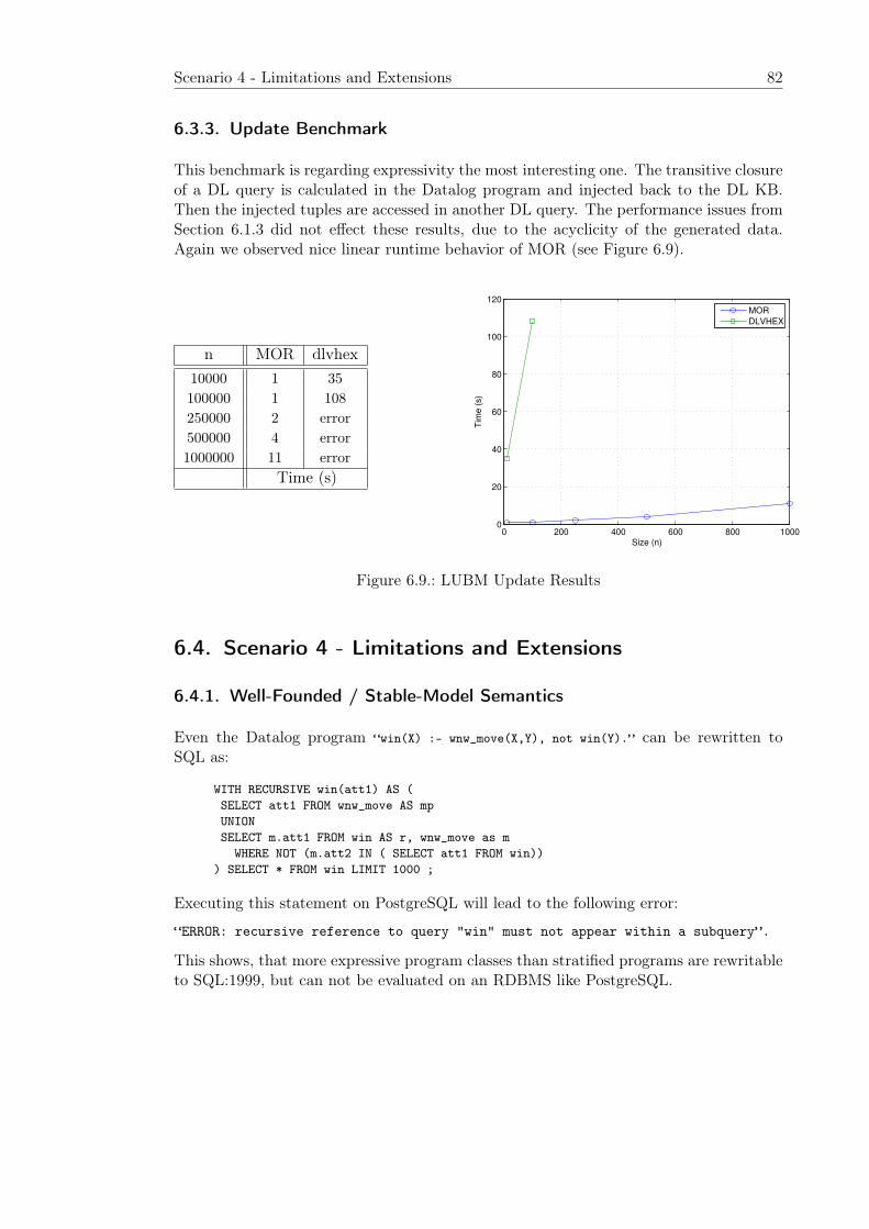
Scenario 4 - Limitations and Extensions 82
6.3.3. Update Benchmark
This benchmark is regarding expressivity the most interesting one. The transitive closureof a DL query is calculated in the Datalog program and injected back to the DL KB.Then the injected tuples are accessed in another DL query. The performance issues fromSection 6.1.3 did not effect these results, due to the acyclicity of the generated data.Again we observed nice linear runtime behavior of MOR (see Figure 6.9).
n MOR dlvhex10000 1 35100000 1 108250000 2 error500000 4 error1000000 11 error
Time (s)
0 200 400 600 800 10000
20
40
60
80
100
120
Size (n)
Tim
e (
s)
MORDLVHEX
Figure 6.9.: LUBM Update Results
6.4. Scenario 4 - Limitations and Extensions
6.4.1. Well-Founded / Stable-Model Semantics
Even the Datalog program “win(X) :- wnw_move(X,Y), not win(Y).” can be rewritten toSQL as:
WITH RECURSIVE win(att1) AS (SELECT att1 FROM wnw_move AS mpUNIONSELECT m.att1 FROM win AS r, wnw_move as m
WHERE NOT (m.att2 IN ( SELECT att1 FROM win))) SELECT * FROM win LIMIT 1000 ;
Executing this statement on PostgreSQL will lead to the following error:
“ERROR: recursive reference to query "win" must not appear within a subquery”.
This shows, that more expressive program classes than stratified programs are rewritableto SQL:1999, but can not be evaluated on an RDBMS like PostgreSQL.
83 Experimental Results
6.4.2. Combining DLVDB with Owlgres
We compare DLVDB results with the already existing results of MOR in Benchmark 6.3.1.We choose 1,000,000 instances for the experiment and proceeded the following way:
1. DB views for accessing the DL KB were created. This was achieved within 3 secondsby MOR.
2. At this point it was possible to run DLVDB, where the previous created DB viewswere imported to DLVDB. Evaluating the program resulted in an average runtimeof about 12 seconds (see Table 6.2).
Round Start End Result (s)1 17:43:10 17:43:22 00:00:122 17:43:22 17:43:33 00:00:113 17:43:33 17:43:45 00:00:124 17:43:45 17:43:56 00:00:115 17:43:56 17:44:08 00:00:12
Table 6.2.: Log for DLVDB with the LUBM Simple Benchmark
The same evaluation in MOR was in average about 4 times faster (3 seconds in MOR to12 seconds in DLVDB). Yet this result let us conclude, that is feasible and encouragingto combine DL-Lite reasoning with DLVDB.
6.4.3. Summary of Results
The results for MOR indicate, that in most benchmarks almost linear runtime behaviorwas observed. One exception was Benchmark 6.1.3, where runtime behavior seems tobe unpredictable. We suggest, that this is related to the depth and occurrence of cyclesin the randomly generated test data. We also observed that the LIMIT parameter hasa strong impact on the performance of recursive query evaluation in PostgreSQL 8.4.Besides influencing the performance, using the LIMIT parameter can lead to incompleteresults, if its size is chosen lower than the expected result set. We conclude that thenative implementation of linear recursive queries in PostgreSQL 8.4 as a breadth-firstsearch is not favourable (see Section 4.3.4).
The results for the benchmarks in Scenario 1 show, that MOR and DLVDB have similarruntime behavior. DLVDB is materializing the IDB temporarily, which leads to the fact,that MOR is constantly about 45% faster than DLVDB. Furthermore we showed inBenchmark 6.4.2, that is encouraging to combine DL-LiteR reasoning with DLVDB.
As seen in Section 6.2.1, we encountered an error with the DL plug-in and RacerPro1.9.1 for large instances, because of the limitation of the heap size in RacerPro. But weobserved with the working benchmarks, that MOR is usually about 30 times faster thandlvhex.
In Benchmark 6.3.3 we showed, that with MOR it is possible to update the DL-LiteRKB with results, which were calculated in the Datalog program as the transitive closureof a DL query. The calculation of the transitive closure is interesting, because the unsup-ported transitive properties in DL-LiteR KB can be simulated. With Benchmark 6.4.1we observed that stratified programs are not rewritable with MOR.
7. Conclusion
In this thesis, we presented a novel approach to efficiently evaluate dl-programs on anRDBMS. Due to the expressive power of SQL, we restricted the dl-programs to stratifiedsemantics and linear recursion. To show the feasibility of such an approach, we developedthe prototype implementation MOR, which interfaces the DL-Lite reasoner Owlgres anduses the RDBMS PostgreSQL 8.4. We followed with MOR the approach of rewriting thedl-programs fully into a cascade of DB views, not materializing any intermediate results.Still the query evaluation engine of PostgreSQL could process these complex, recursiveSQL statements. The prototype was then benchmarked in four different scenarios to theDLV family of reasoners. For the combined scenarios, we designed our own benchmarksbased on a DBpedia and LUBM KB.
7.1. Evaluation Results
With the experimental setup, MOR outperformed all the involved systems, namely DLV,DLVDB and dlvhex. The reason for this encouraging results can mainly be accountedto the power of SQL optimizers of modern RDBMSs like PostgreSQL. These RDBMSsare designed to process vast amount of data, hence MOR and the incorporated DL-Litereasoner Owlgres are focused to rewrite dl-programs to complex SQL statements andreceive the evaluated results from the RDBMS.
In the purely Datalog scenario, MOR and DLVDB showed similar runtime behavior, whereMOR is constantly about 45% faster. DLV using ODBC, which never was designed forlarge scale data processing, is considerably slower than the other two systems. Evaluatingrecursive queries with PostgreSQL needed particularly attention, because cycles in theEDB lead to non-termination. We introduced the LIMIT parameter of SQL:1999 to avoidnon-termination, however the runtime behavior of MOR is sensitive to this parameter.
In the combined scenarios, MOR performed remarkably better than dlvhex. In all ofthe benchmarks, MOR showed almost linear runtime behavior. This behavior was evenapparent in the most interesting benchmark, where the transitive closure of a role queryis calculated in the Datalog program, injected back to the DL KB. Then the DL KB isqueried again to obtain the final result.
Finally, we showed the feasibility of using DLVDB with DL-Lite reasoning. This wasachieved by prepossessing the DL-Lite queries and saving the created SQL statements inDB views. After that, the DB view were imported by DLVDB. The overall performanceof this approach was by a factor four slower than MOR.
85
7.2. Future Work and Further Studies
We recognize the overlapping fields of theory, implementation, benchmarks, and practice,where research for the evaluation of dl-programs on an RDBMS could be pushed further.
On the theoretical side, it would be appealing to extend the introduced stratified se-mantics to well-founded or even answer-set semantics. Clearly, the evaluation of thesesemantics should be natively on the RDBMS, so we could follow our approach of utilizingthe power of query optimizers in RDBMSs.
Regarding the implementation of MOR, we need to overcome the limitation mentionedin Chapter 4. For example, a more advanced handling of cycles regarding recursivequeries could be developed, a generic SQL plug-in is missing, and the restriction to linearrecursion could be overcome. Furthermore, MOR could be adapted, so that it would beusable as a Java component by other systems. For example, MOR could be coupled withthe Jena framework, figuring as another rule-based inference engine. Concerning the earlyrelease state of Owlgres, further plug-ins to other DL-Lite reasoners (e.g. Quonto) couldbe written. Moreover, a similar implementation to MOR could be applied to DLVDB.
The benchmarks could be extended with different tests regarding size and scenarios. Avery interesting extension could contain large data sets with 200 million assertions asit is used in the Berlin SPARQL Benchmark1. Besides, MOR could be compared withother systems (e.g. Prolog based reasoners) besides the DLV family.
Getting back to the introductory example of a “smart” route planner, the use of MORin a “real-world” project would give further insight into practical issues regarding thecombination of rules and ontologies. As Johann Wolfgang von Goethe captures it inFaust [Goethe and Prudhoe, 1974]:
“Dear friend, all theory is gray, And green the golden tree of life.”
1http://www4.wiwiss.fu-berlin.de/bizer/BerlinSPARQLBenchmark/
A. Installation and Use:
Briefly, we outline how MOR can be installed on a Linux system. Since MOR wasdeveloped in Java 1.6, it should be easy deployable on other operating systems. Thesource code and the compiled binary files are available on:
http://code.google.com/p/dbmor/
A.1. Prerequisites
Basically, every RDBMS supporting SQL:1999 could be used, but we recommend to usePostgreSQL 8.4. There are several OWL2 QL reasoners available, but only Owlgres 0.1is supported. It is mandatory to use our branch of Owlgres, due to some adaptions donein the main branch of Owlgres. Furthermore the JGraphT library is needed. We deliverthe binary files for Owlgres and JGraphT with the source code.
A.2. Installation
After the binary files are deployed, the following steps have to be processed to setup theinstallation:
1. Create a PostgreSQL database with createdb, for example: createdb -U myusermydb.
2. Check compatibility of the Owlgres TBox by sh/expchk --tbox data/tbox_sample.rdf.Note, that Owlgres only supports data serialized in RDF/XML.
3. Create the Owlgres database by loading the TBox: sh/create --db mydb --usermyuser --passwd mypw --tbox data/tbox_sample.rdf.
4. Load the Owlgres ABox into the database: sh/load --db mydb --user myuser--passwd mypw --abox data/abox_sample.rdf.
5. Create custom tables and import the data from other databases. This step isneeded, if the dl-program imports the EDB from external data sources.
87
A.3. Calling MOR from the Command Line
We provide the shell script mor.sh to call MOR. The following parameters are validinputs:
--pgm URI of the dl-program.--host Database host, where the default is localhost.
--db Database name.--user Database user.
--passwd Database password.--silent Status messages are suppressed.
--keepviews Keeps the created database views, otherwise all intermediate views aredropped after execution.
Bibliography
ISO/IEC 9075–1:1999, Information Technology – Database languages – SQL – part 1:Framework. Technical report, 1999.
Serge Abiteboul, Richard Hull, and Victor Vianu. Foundations of Databases. Addison-Wesley, 1995. ISBN 0-201-53771-0.
Krzysztof R. Apt, Howard A. Blair, and Adrian Walker. Towards a theory of declarativeknowledge. In Foundations of Deductive Databases and Logic Programming., pages89–148. Morgan Kaufmann, 1988. ISBN 0-934613-40-0.
Franz Baader, Ian Horrocks, and Ulrike Sattler. Description logics. In Handbook onOntologies, pages 3–28. 2004.
Franz Baader, Carsten Lutz, and Boontawee Suntisrivaraporn. Efficient reasoning in l+.In Proceedings of the 2006 International Workshop on Description Logics (DL2006),Windermere, Lake District, UK, May 30 - June 1, 2006, 2006.
Tim Berners-Lee, James Hendler, and Ora Lassila. The semantic web. Scientific Amer-ican, 284(5):34–43, 2001. ISSN 0036-8733. URL http://www.scientificamerican.com/article.cfm?id=the-semantic-web.
Erol Bozsak, Marc Ehrig, Siegfried Handschuh, Andreas Hotho, Alexander Maedche,Boris Motik, Daniel Oberle, Christoph Schmitz, Steffen Staab, Ljiljana Stojanovic,Nenad Stojanovic, Rudi Studer, Gerd Stumme, York Sure, Julien Tane, Raphael Volz,and Valentin Zacharias. Kaon - towards a large scale semantic web. In E-Commerce andWeb Technologies, Third International Conference, EC-Web 2002, Aix-en-Provence,France, September 2-6, 2002, Proceedings, pages 304–313, 2002.
Diego Calvanese, Giuseppe De Giacomo, Domenico Lembo, Maurizio Lenzerini, and Ric-cardo Rosati. Dl-lite: Tractable description logics for ontologies. In Proceedings, TheTwentieth National Conference on Artificial Intelligence and the Seventeenth Inno-vative Applications of Artificial Intelligence Conference, July 9-13, 2005, Pittsburgh,Pennsylvania, USA, pages 602–607, 2005.
Diego Calvanese, Giuseppe De Giacomo, Domenico Lembo, Maurizio Lenzerini, andRiccardo Rosati. Tractable reasoning and efficient query answering in descriptionlogics: The dl-lite family. J. Autom. Reasoning, 39(3):385–429, 2007.
Stefano Ceri, Georg Gottlob, and Letizia Tanca. Logic Programming and Databases.Springer, 1990. ISBN 3-540-51728-6.
E. F. Codd. A relational model of data for large shared data banks. Commun. ACM, 13(6):377–387, 1970.
89
Bibliography 90
Alain Colmerauer. Prolog in 10 figures. Commun. ACM, 28(12):1296–1310, 1985.
Evgeny Dantsin, Thomas Eiter, Georg Gottlob, and Andrei Voronkov. Complexity andexpressive power of logic programming. In IEEE Conference on Computational Com-plexity, pages 82–101, 1997.
Jos de Bruijn, Thomas Eiter, Axel Polleres, and Hans Tompits. On representationalissues about combinations of classical theories with nonmonotonic rules. In KnowledgeScience, Engineering and Management, First International Conference, KSEM 2006,Guilin, China, August 5-8, 2006, Proceedings, pages 1–22, 2006.
Marc Denecker, Joost Vennekens, Stephen Bond, Martin Gebser, and MiroslawTruszczynski. The second answer set programming competition. In Logic Program-ming and Nonmonotonic Reasoning, 10th International Conference, LPNMR 2009,Potsdam, Germany, September 14-18, 2009. Proceedings, pages 637–654, 2009.
Thomas Eiter, Thomas Lukasiewicz, Roman Schindlauer, and Hans Tompits. Combininganswer set programming with description logics for the semantic web. In Principlesof Knowledge Representation and Reasoning: Proceedings of the Ninth InternationalConference (KR2004), Whistler, Canada, June 2-5, 2004, pages 141–151, 2004.
Thomas Eiter, Giovambattista Ianni, Roman Schindlauer, and Hans Tompits. dlvhex:A prover for semantic-web reasoning under the answer-set semantics. In 2006 IEEE /WIC / ACM International Conference on Web Intelligence (WI 2006), 18-22 December2006, Hong Kong, China, pages 1073–1074, 2006.
Thomas Eiter, Wolfgang Faber, Michael Fink, and Stefan Woltran. Complexity resultsfor answer set programming with bounded predicate arities and implications. Ann.Math. Artif. Intell., 51(2-4):123–165, 2007.
Thomas Eiter, Georg Gottlob, Magdalena Ortiz, and Mantas Simkus. Query answering inthe description logic horn-. In Logics in Artificial Intelligence, 11th European Confer-ence, JELIA 2008, Dresden, Germany, September 28 - October 1, 2008. Proceedings,pages 166–179, 2008a.
Thomas Eiter, Giovambattista Ianni, Thomas Lukasiewicz, Roman Schindlauer, andHans Tompits. Combining answer set programming with description logics for thesemantic web. Artif. Intell., 172(12-13):1495–1539, 2008b.
Thomas Eiter, Giovambattista Ianni, and Thomas Krennwallner. Answer set program-ming: A primer. In Reasoning Web. Semantic Technologies for Information Systems,5th International Summer School 2009, Brixen-Bressanone, Italy, August 30 - Septem-ber 4, 2009, Tutorial Lectures, pages 40–110, 2009a.
Thomas Eiter, Giovambattista Ianni, Thomas Lukasiewicz, and Roman Schindlauer.Well-founded semantics for description logic programs in the semantic web. Tech-nical Report INFSYS RR-1843-09-01, March 2009b. To appear in ACM Transactionson Computational Logic (revised).
Hervé Gallaire, Jack Minker, and Jean-Marie Nicolas. An overview and introduction tologic and data bases. In Logic and Data Bases, pages 3–30, 1977.
91 Bibliography
Erich Gamma, Richard Helm, Ralph E. Johnson, and John Vlissides. Design Patterns:Elements of Reusable Object-Oriented Software. Addison-Wesley, Reading, MA, 1995.ISBN 978-0-201-63361-0.
Martin Gebser, Benjamin Kaufmann, André Neumann, and Torsten Schaub. lasp : Aconflict-driven answer set solver. In Logic Programming and Nonmonotonic Reasoning,9th International Conference, LPNMR 2007, Tempe, AZ, USA, May 15-17, 2007,Proceedings, pages 260–265, 2007a.
Martin Gebser, Lengning Liu, Gayathri Namasivayam, André Neumann, Torsten Schaub,and Miroslaw Truszczynski. The first answer set programming system competition.In Logic Programming and Nonmonotonic Reasoning, 9th International Conference,LPNMR 2007, Tempe, AZ, USA, May 15-17, 2007, Proceedings, pages 3–17, 2007b.
Allen Van Gelder, Kenneth A. Ross, and John S. Schlipf. The well-founded semanticsfor general logic programs. J. ACM, 38(3):620–650, 1991.
Michael Gelfond and Vladimir Lifschitz. The stable model semantics for logic program-ming. In Logic Programming: Proceedings of the 5th International Conference andSymposium, pages 1070–1080, 1988.
Michael Gelfond and Vladimir Lifschitz. Classical negation in logic programs and dis-junctive databases. New Generation Comput., 9(3/4):365–386, 1991.
Johann Wolfgang von Goethe and John Edgar Prudhoe. Faust, the tragedy. Part 1;translated for the English speaking stage by John Prudhoe. Manchester UniversityPress; Barnes & Noble, Manchester, New York, 1974. ISBN 0719005701.
Benjamin N. Grosof, Ian Horrocks, Raphael Volz, and Stefan Decker. Description logicprograms: combining logic programs with description logic. In Proceedings of the WorldWide Web Conference (WWW2003), pages 48–57, 2003.
Yuanbo Guo, Zhengxiang Pan, and Jeff Heflin. Lubm: A benchmark for owl knowledgebase systems. J. Web Sem., 3(2-3):158–182, 2005.
Carl Hewitt. Middle history of logic programming. CoRR, abs/0904.3036, 2009.
Stijn Heymans, Davy Van Nieuwenborgh, and Dirk Vermeir. Open answer set program-ming for the semantic web. J. Applied Logic, 5(1):144–169, 2007.
Ian Horrocks, Peter F. Patel-Schneider, Harold Boley, Said Tabet, Benjamin Grosof, andMike Dean. SWRL: A semantic web rule language combining owl and ruleml. W3Csubmission, W3C, October 2004. URL URLhttp://www.w3.org/Submission/SWRL/.
Ullrich Hustadt, Boris Motik, and Ulrike Sattler. Data complexity of reasoning in veryexpressive description logics. In IJCAI-05, Proceedings of the Nineteenth InternationalJoint Conference on Artificial Intelligence, Edinburgh, Scotland, UK, July 30-August5, 2005, pages 466–471, 2005.
Michael Kifer. Rule interchange format: The framework. In Web Reasoning and RuleSystems, Second International Conference, RR 2008, Karlsruhe, Germany, October31-November 1, 2008. Proceedings, pages 1–11, 2008.
Bibliography 92
Markus Krötzsch, Peter F. Patel-Schneider, Sebastian Rudolph, Pascal Hitzler, and BijanParsia. OWL 2 web ontology language primer. Technical report, W3C, October 2009.URL http://www.w3.org/TR/2009/REC-owl2-primer-20091027/.
Craig Larman. Applying UML and Patterns: An Introduction to Object-Oriented Analysisand Design and the Unified Process. Prentice Hall PTR, Upper Saddle River, NJ, USA,2001. ISBN 0130925691.
Nicola Leone, Gerald Pfeifer, Wolfgang Faber, Thomas Eiter, Georg Gottlob, SimonaPerri, and Francesco Scarcello. The dlv system for knowledge representation andreasoning. ACM Trans. Comput. Log., 7(3):499–562, 2006.
Alon Y. Levy and Marie-Christine Rousset. Combining horn rules and description logicsin carin. Artif. Intell., 104(1-2):165–209, 1998.
Senlin Liang, Paul Fodor, Hui Wan, and Michael Kifer. Openrulebench: an analysis ofthe performance of rule engines. In Proceedings of the 18th International Conferenceon World Wide Web, WWW 2009, Madrid, Spain, April 20-24, 2009, pages 601–610,2009.
John W. Lloyd. Foundations of Logic Programming, 1st Edition. Springer, 1984. ISBN3-540-13299-6.
Li Ma, Yang Yang, Zhaoming Qiu, Guo Tong Xie, Yue Pan, and Shengping Liu. Towardsa complete owl ontology benchmark. In The Semantic Web: Research and Applications,3rd European Semantic Web Conference, ESWC 2006, Budva, Montenegro, June 11-14, 2006, Proceedings, pages 125–139, 2006.
John McCarthy. Recursive functions of symbolic expressions and their computation bymachine, part i. Commun. ACM, 3(4):184–195, 1960.
Jing Mei, Harold Boley, Jie Li, Virendrakumar C. Bhavsar, and Zuoquan Lin. Datalogdl:Datalog rules parameterized by description logics. In Canadian Semantic Web,CSWWS 2006, first Canadian Semantic Web Working Symposium, June 2006, Quebec,Canada, pages 171–187, 2006.
Boris Motik, Ian Horrocks, Riccardo Rosati, and Ulrike Sattler. Can owl and logicprogramming live together happily ever after? In The Semantic Web - ISWC 2006,5th International Semantic Web Conference, ISWC 2006, Athens, GA, USA, November5-9, 2006, Proceedings, pages 501–514, 2006.
Boris Motik, Achille Fokoue, Ian Horrocks, Zhe Wu, Carsten Lutz, and Bernardo CuencaGrau. OWL 2 web ontology language profiles. W3C recommendation, W3C, October2009. URL http://www.w3.org/TR/2009/REC-owl2-profiles-20091027/.
Ilkka Niemelä and Patrik Simons. Smodels - an implementation of the stable modeland well-founded semantics for normal lp. In Logic Programming and NonmonotonicReasoning, 4th International Conference, LPNMR’97, Dagstuhl Castle, Germany, July28-31, 1997, Proceedings, pages 421–430, 1997.
93 Bibliography
Christos H. Papadimitriou. Computational Complexity. Addison Wesley, December 1993.ISBN 0201530821.
Héctor Pérez-Urbina, Boris Motik, and Ian Horrocks. A comparison of query rewritingtechniques for dl-lite. In Proceedings of the DL Home 22nd International Workshop onDescription Logics (DL 2009), Oxford, UK, July 27-30, 2009, 2009.
Racer Systems GmbH & Co. KG. Release Notes for RacerPro 1.9.2 beta.,March 2009. URL http://www.racer-systems.com/products/racerpro/release-notes-1-9-2-beta.pdf.
Raymond Reiter. On closed world data bases. In Logic and Data Bases, pages 55–76,1977.
John Alan Robinson. A machine-oriented logic based on the resolution principle. J.ACM, 12(1):23–41, 1965.
Riccardo Rosati. Dl+log: Tight integration of description logics and disjunctive datalog.In Proceedings, Tenth International Conference on Principles of Knowledge Represen-tation and Reasoning, Lake District of the United Kingdom, June 2-5, 2006, pages68–78, 2006.
Riccardo Rosati and Alessandro Almatelli. Improving query answering over dl-lite on-tologies. In Principles of Knowledge Representation and Reasoning: Proceedings of theTwelfth International Conference, KR 2010, Toronto, Ontario, Canada, May 9-13,2010, 2010.
Guus Schreiber and Mike Dean. OWL web ontology language reference. W3Crecommendation, W3C, February 2004. URL http://www.w3.org/TR/2004/REC-owl-ref-20040210/.
Markus Stocker and Michael Smith. Owlgres: A scalable owl reasoner. In Proceedingsof the Fifth OWLED Workshop on OWL: Experiences and Directions, collocated withthe 7th International Semantic Web Conference (ISWC-2008), Karlsruhe, Germany,October 26-27, 2008, 2008.
Robert Endre Tarjan. Edge-disjoint spanning trees and depth-first search. Acta Inf., 6:171–185, 1976.
Alfred Tarski. On the calculus of relations. J. Symb. Log., 6(3):73–89, 1941.
Giorgio Terracina, Nicola Leone, Vincenzino Lio, and Claudio Panetta. Experimentingwith recursive queries in database and logic programming systems. TPLP, 8(2):129–165, 2008.
Jeffrey D. Ullman. Principles of Database and Knowledge-Base Systems, Volume I. Com-puter Science Press, 1988. ISBN 0-7167-8158-1.