The Dependency Triple Framework for

Termination of Logic Programs⋆

Peter Schneider-Kamp1, Jurgen Giesl2, and Manh Thang Nguyen3

1 IMADA, University of Southern Denmark, Denmark2 LuFG Informatik 2, RWTH Aachen University, Germany3 Department of Computer Science, K. U. Leuven, Belgium

Abstract. We show how to combine the two most powerful approachesfor automated termination analysis of logic programs (LPs): the directapproach which operates directly on LPs and the transformational ap-proach which transforms LPs to term rewrite systems (TRSs) and triesto prove termination of the resulting TRSs. To this end, we adapt thewell-known dependency pair framework from TRSs to LPs. With theresulting method, one can combine arbitrary termination techniques forLPs in a completely modular way and one can use both direct and trans-formational techniques for different parts of the same LP.

1 Introduction

When comparing the direct and the transformational approach for termination ofLPs, there are the following advantages and disadvantages. The direct approachis more efficient (since it avoids the transformation to TRSs) and in additionto the TRS techniques that have been adapted to LPs [13, 15], it can also usenumerous other techniques that are specific to LPs. The transformational ap-proach has the advantage that it can use all existing termination techniques forTRSs, not just the ones that have already been adapted to LPs.

Two of the leading tools for termination of LPs are Polytool [14] (implement-ing the direct approach and including the adapted TRS techniques from [13,15]) and AProVE [7] (implementing the transformational approach of [17]). Inthe annual International Termination Competition,4 AProVE was the most pow-erful tool for termination analysis of LPs (it solved 246 out of 349 examples),but Polytool obtained a close second place (solving 238 examples). Nevertheless,there are several examples where one tool succeeds, whereas the other does not.

This shows that both the direct and the transformational approach have theirbenefits. Thus, one should combine these approaches in a modular way. In otherwords, for one and the same LP, it should be possible to prove termination ofsome parts with the direct approach and of other parts with the transformational

⋆ Supported by FWO/2006/09: Termination analysis: Crossing paradigm borders andby the Deutsche Forschungsgemeinschaft (DFG), grant GI 274/5-2.

4 http://www.termination-portal.org/wiki/Termination Competition

approach. The resulting method would improve over both approaches and canalso prove termination of LPs that cannot be handled by one approach alone.

In this paper, we solve that problem. We build upon [15], where the well-known dependency pair (DP) method from term rewriting [2] was adapted inorder to apply it to LPs directly. However, [15] only adapted the most basicparts of the method and moreover, it only adapted the classical variant of theDP method instead of the more powerful recent DP framework [6, 8, 9] whichcan combine different TRS termination techniques in a completely flexible way.

After providing the necessary preliminaries on LPs in Sect. 2, in Sect. 3 weadapt the DP framework to the LP setting which results in the new dependencytriple (DT) framework. Compared to [15], the advantage is that now arbitrarytermination techniques based on DTs can be applied in any combination andany order. In Sect. 4, we present three termination techniques within the DTframework. In particular, we also develop a new technique which can transformparts of the original LP termination problem into TRS termination problems.Then one can apply TRS techniques and tools to solve these subproblems.

We implemented our contributions in the tool Polytool and coupled it withAProVE which is called on those subproblems which were converted to TRSs. Ourexperimental evaluation in Sect. 5 shows that this combination clearly improvesover both Polytool or AProVE alone, both concerning efficiency and power.

2 Preliminaries on Logic Programming

We briefly recapitulate needed notations. More details on logic programming canbe found in [1], for example. A signature is a pair (Σ, ∆) where Σ and ∆ are finitesets of function and predicate symbols and T (Σ,V) resp. A(Σ, ∆,V) denote thesets of all terms resp. atoms over the signature (Σ, ∆) and the variables V . Wealways assume that Σ contains at least one constant of arity 0. A clause c isa formula H ← B1, . . . , Bk with k ≥ 0 and H, Bi ∈ A(Σ, ∆,V). A finite set ofclauses P is a (definite) logic program. A clause with empty body is a fact anda clause with empty head is a query. We usually omit “←” in queries and justwrite “B1, . . . , Bk”. The empty query is denoted �.

For a substitution δ : V → T (Σ,V), we often write tδ instead of δ(t), where tcan be any expression (e.g., a term, atom, clause, etc.). If δ is a variable renaming(i.e., a one-to-one correspondence on V), then tδ is a variant of t. We write δσ todenote that the application of δ is followed by the application of σ. A substitutionδ is a unifier of two expressions s and t iff sδ = tδ. To simplify the presentation,in this paper we restrict ourselves to ordinary unification with occur check. Wecall δ the most general unifier (mgu) of s and t iff δ is a unifier of s and t andfor all unifiers σ of s and t, there is a substitution µ such that σ = δµ.

Let Q be a query A1, . . . , Am, let c be a clause H ← B1, . . . , Bk. Then Q′

is a resolvent of Q and c using δ (denoted Q ⊢c,δ Q′) if δ = mgu(A1, H), andQ′ = (B1, . . . , Bk, A2, . . . , Am)δ. A derivation of a program P and a query Q isa possibly infinite sequence Q0, Q1, . . . of queries with Q0 = Q where for all i, wehave Qi ⊢ci,δi

Qi+1 for some substitution δi and some renamed-apart variant ci of

2

a clause of P . For a derivation Q0, . . . , Qn as above, we also write Q0 ⊢nP,δ0...δn−1

Qn or Q0 ⊢nP

Qn, and we also write Qi ⊢P Qi+1 for Qi ⊢ci,δiQi+1. A LP P is

terminating for the query Q if all derivations of P and Q are finite. The answerset Answer(P , Q) for a LP P and a query Q is the set of all substitutions δ suchthat Q ⊢n

P,δ � for some n ∈ N. For a set of atomic queries S ⊆ A(Σ, ∆,V), wedefine the call set Call(P ,S) = {A1 | Q ⊢

nP

A1, . . . , Am, Q ∈ S, n ∈ N}.

Example 1. The following LP P uses “s2m” to create a matrix M of variablesfor fixed numbers X and Y of rows and columns. Afterwards, it uses “subs mat”to replace each variable in the matrix by the constant “a”.

goal(X, Y,Msu)← s2m(X, Y, M), subs mat(M,Msu).s2m(0, Y, [ ]). s2m(s(X), Y, [R|Rs ])← s2ℓ(Y, R), s2m(X, Y,Rs).s2ℓ(0, [ ]). s2ℓ(s(Y ), [C|Cs ])← s2ℓ(Y,Cs).subs mat([ ], [ ]). subs mat([R|Rs], [SR|SRs ])← subs row(R,SR), subs mat(Rs,SRs).subs row([ ], [ ]). subs row([E|R], [a|SR])← subs row(R,SR).

For example, for suitable substitutions δ0 and δ1 we have goal(s(0), s(0),Msu)⊢δ0,P s2m(s(0), s(0), M), subs mat(M,Msu) ⊢8

δ1,P �. So Answer(P , goal(s(0),s(0),Msu)) contains δ = δ0δ1, where δ(Msu) = [[a]].

We want to prove termination of this program for the set of queries S ={goal(t1, t2, t3) | t1 and t2 are ground terms }. Here, we obtain

Call(P ,S) ⊆ S ∪ {{s2m(t1, t2, t3) | t1 and t2 ground} ∪ {s2ℓ(t1, t2) | t1 ground}∪ {subs row(t1, t2) | t1 ∈ List} ∪ {subs mat(t1, t2) | t1 ∈ List}

where List is the smallest set with [ ] ∈ List and [t1 | t2] ∈ List if t2 ∈ List .

3 Dependency Triple Framework

As mentioned before, we already adapted the basic DP method to the LP settingin [15]. The advantage of [15] over previous direct approaches for LP terminationis that (a) it can use different well-founded orders for different “loops” of theLP and (b) it uses a constraint-based approach to search for arbitrary suitablewell-founded orders (instead of only choosing from a fixed set of orders basedon a given small set of norms). Most other direct approaches have only one ofthe features (a) or (b). Nevertheless, [15] has the disadvantage that it does notpermit the combination of arbitrary termination techniques in a flexible andmodular way. Therefore, we now adapt the recent DP framework [6, 8, 9] to theLP setting. Def. 2 adapts the notion of dependency pairs [2] from TRSs to LPs.5

Definition 2 (Dependency Triple). A dependency triple (DT) is a clauseH ← I, B where H and B are atoms and I is a list of atoms. For a LP P, theset of its dependency triples is DT (P) = {H ← I, B | H ← I, B, . . . ∈ P}.

5 While Def. 2 is essentially from [15], the rest of this section contains new conceptsthat are needed for a flexible and general framework.

3

Example 3. The dependency triples DT (P) of the program in Ex. 1 are:

goal(X, Y,Msu)← s2m(X, Y, M). (1)

goal(X, Y,Msu)← s2m(X, Y, M), subs mat(M,Msu). (2)

s2m(s(X), Y, [R|Rs ])← s2ℓ(Y, R). (3)

s2m(s(X), Y, [R|Rs ])← s2ℓ(Y, R), s2m(X, Y,Rs). (4)

s2ℓ(s(Y ), [C|Cs ])← s2ℓ(Y,Cs). (5)

subs mat([R|Rs ], [SR|SRs])← subs row(R,SR). (6)

subs mat([R|Rs ], [SR|SRs])← subs row(R,SR), subs mat(Rs,SRs). (7)

subs row([E|R], [a|SR])← subs row(R, SR). (8)

Intuitively, a dependency triple H ← I, B states that a call that is an in-stance of H can be followed by a call that is an instance of B if the correspondinginstance of I can be proven. To use DTs for termination analysis, one has to showthat there are no infinite “chains” of such calls. The following definition corre-sponds to the standard definition of chains from the TRS setting [2]. Usually, Dstands for the set of DTs, P is the program under consideration, and C standsfor Call(P ,S) where S is the set of queries to be analyzed for termination.

Definition 4 (Chain). Let D and P be sets of clauses and let C be a set ofatoms. A (possibly infinite) list (H0 ← I0, B0), (H1 ← I1, B1), . . . of variantsfrom D is a (D, C,P)-chain iff there are substitutions θi, σi and an A ∈ C suchthat θ0 = mgu(A, H0) and for all i, we have σi ∈ Answer(P , Iiθi), θi+1 =mgu(Biθiσi, Hi+1), and Biθiσi ∈ C.

6

Example 5. For P and S from Ex. 1, the list (2), (7) is a (DT (P),Call(P ,S),P)-chain. To see this, consider θ0 = {X/s(0), Y/s(0)}, σ0 = {M/[[C]]}, and θ1 ={R/[C],Rs/[ ],Msu/[SR,SRs]}. Then, for A = goal(s(0), s(0),Msu) ∈ S, wehave H0θ0 = goal(X, Y,Msu)θ0 = Aθ0. Furthermore, we have σ0 ∈ Answer(P ,s2m(X, Y, M)θ0) = Answer(P , s2m(s(0), s(0), M)) and θ1 = mgu(B0θ0σ0, H1) =mgu(subs mat([[C]],Msu), subs mat([R|Rs], [SR|SRs])).

Thm. 6 shows that termination is equivalent to absence of infinite chains.

Theorem 6 (Termination Criterion). A LP P is terminating for a set ofatomic queries S iff there is no infinite (DT (P),Call(P ,S),P)-chain.

Proof. For the “if”-direction, let there be an infinite derivation Q0, Q1, . . . withQ0 ∈ S and Qi ⊢ci,δi

Qi+1. The clause ci ∈ P has the form Hi ← A1i , . . . , A

ki

i .Let j1 > 0 be the minimal index such that the first atom A′

j1in Qj1 starts

an infinite derivation. Such a j1 always exists as shown in [17, Lemma 3.5]. Aswe started from an atomic query, there must be some m0 such that A′

j1=

6 If C = Call(P ,S), then the condition “Biθiσi ∈ C” is always satisfied due to thedefinition of “Call”. But our goal is to formulate the concept of “chains” as generalas possible (i.e., also for cases where C is an arbitrary set). Then this condition canbe helpful in order to obtain as few chains as possible.

4

Am00 δ0δ1 . . . δj1−1. Then “H0 ← A1

0, . . . , Am0−10 , Am0

0 ” is the first DT in our

(DT (P),Call(P ,S),P)-chain where θ0 = δ0 and σ0 = δ1 . . . δj1−1. As Q0 ⊢j1P

Qj1

and Am00 θ0σ0 = A′

j1is the first atom in Qj1 , we have Am0

0 θ0σ0 ∈ Call(P ,S).

We repeat this construction and let j2 be the minimal index with j2 > j1such that the first atom A′

j2in Qj2 starts an infinite derivation. As the first atom

of Qj1 already started an infinite derivation, there must be some mj1 such that

A′j2

= Amj1

j1δj1 . . . δj2−1. Then “Hj1 ← A1

j1, . . . , A

mj1−1j1

, Amj1

j1” is the second DT

in our (DT (P),Call(P ,S),P)-chain where θ1 = mgu(Am00 θ0σ0, Hj1) = δj1 and

σ1 = δj1+1 . . . δj2−1. As Q0 ⊢j2P

Qj2 and Amj1

j1θ1σ1 = A′

j2is the first atom in Qj2 ,

we have Amj1

j1θ1σ1 ∈ Call(P ,S). By repeating this construction infinitely many

times, we obtain an infinite (DT (P),Call(P ,S),P)-chain.

For the “only if”-direction, assume that (H0 ← I0, B0), (H1 ← I1, B1), . . .is an infinite (DT (P),Call(P ,S),P)-chain. Thus, there are substitutions θi,σi and an A ∈ Call(P ,S) such that θ0 = mgu(A, H0) and for all i, we haveσi ∈ Answer(P , Iiθi) and θi+1 = mgu(Biθiσi, Hi+1). Due to the constructionof DT (P), there is a clause c0 ∈ P with c0 = H0 ← I0, B0, R0 for a list ofatoms R0 and the first step in our derivation is A ⊢c0,θ0 I0θ0, B0θ0, R0θ0. Fromσ0 ∈ Answer(P , I0θ0) we obtain the derivation I0θ0 ⊢

n0

P,σ0� and consequently,

I0θ0, B0θ0, R0θ0 ⊢n0

P,σ0B0θ0σ0, R0θ0σ0 for some n0 ∈ N. Hence, A ⊢n0+1

P,θ0σ0

B0θ0σ0, R0θ0σ0. As θ1 = mgu(B0θ0σ0, H1) and as there is a clause c1 = H1 ←I1, B1, R1 ∈ P , we continue the derivation with B0θ0σ0, R0θ0σ0 ⊢c1,θ1 I1θ1, B1θ1,R1θ1, R0θ0σ0θ1. Due to σ1 ∈ Answer(P , I1θ1) we continue with I1θ1, B1θ1, R1θ1,R0θ0σ0θ1 ⊢

n1

P,σ1B1θ1σ1, R1θ1σ1, R0θ0σ0θ1σ1 for some n1 ∈ N.

By repeating this, we obtain an infinite derivation A ⊢n0+1P,θ0σ0

B0θ0σ0, R0θ0σ0

⊢n1+1P,θ1,σ1

B1θ1σ1, R1θ1σ1, R0θ0σ0θ1σ1 ⊢n2+1P,θ2σ2

B2θ2σ2, . . . ⊢n2+1P,θ3σ3

. . . Thus, theLP P is not terminating for A. From A ∈ Call(P ,S) we know there is a Q ∈ Ssuch that Q ⊢n

PA, . . . Hence, P is also not terminating for Q ∈ S. ⊓⊔

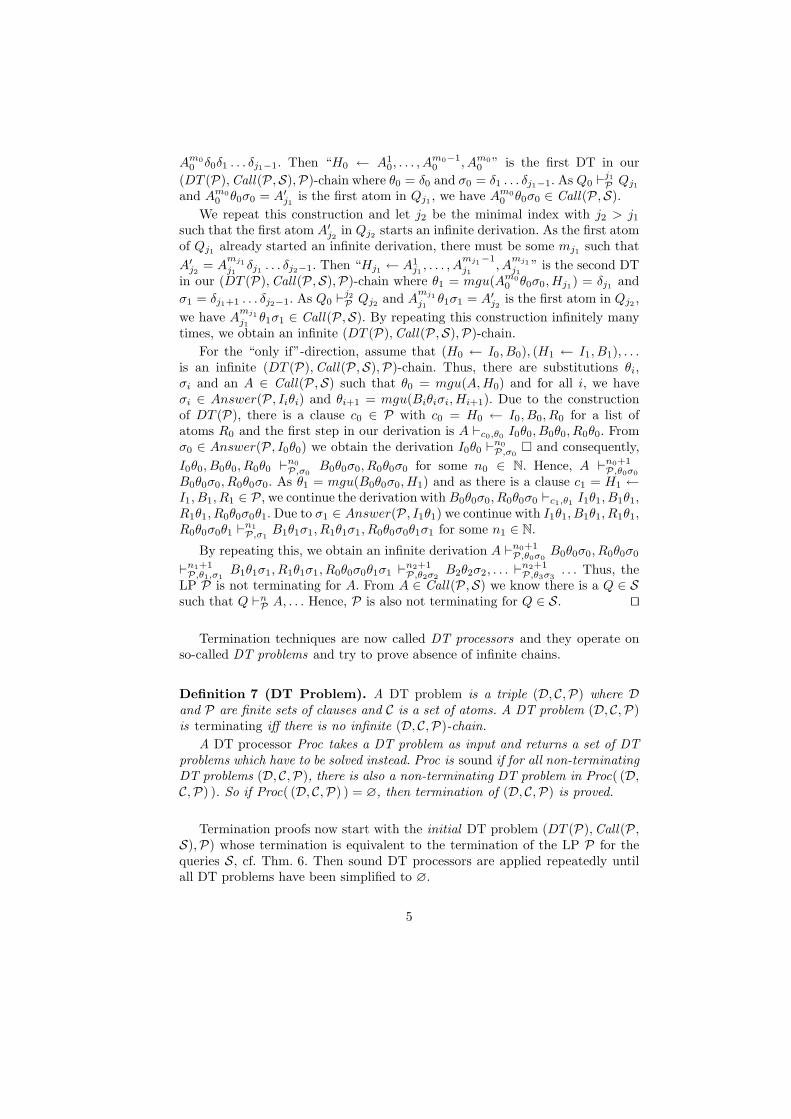
Termination techniques are now called DT processors and they operate onso-called DT problems and try to prove absence of infinite chains.

Definition 7 (DT Problem). A DT problem is a triple (D, C,P) where Dand P are finite sets of clauses and C is a set of atoms. A DT problem (D, C,P)is terminating iff there is no infinite (D, C,P)-chain.

A DT processor Proc takes a DT problem as input and returns a set of DTproblems which have to be solved instead. Proc is sound if for all non-terminatingDT problems (D, C,P), there is also a non-terminating DT problem in Proc( (D,C,P) ). So if Proc( (D, C,P) ) = ∅, then termination of (D, C,P) is proved.

Termination proofs now start with the initial DT problem (DT (P),Call(P ,S),P) whose termination is equivalent to the termination of the LP P for thequeries S, cf. Thm. 6. Then sound DT processors are applied repeatedly untilall DT problems have been simplified to ∅.

5

4 Dependency Triple Processors

In Sect. 4.1 and 4.2, we adapt two of the most important DP processors fromterm rewriting [2, 6, 8, 9] to the LP setting. In Sect. 4.3 we present a new DTprocessor to convert DT problems to DP problems.

4.1 Dependency Graph Processor

The first processor decomposes a DT problem into subproblems. Here, one con-structs a dependency graph to determine which DTs follow each other in chains.

Definition 8 (Dependency Graph). For a DT problem (D, C,P), the nodesof the (D, C,P)-dependency graph are the clauses of D and there is an arc froma clause c to a clause d iff “c, d” is a (D, C,P)-chain.

Example 9. For the initial DT problem (DT (P),Call(P ,S),P) of the programin Ex. 1, we obtain the following dependency graph.

(1) //

))T

T

T

T

T

T

T

T

T

T

T

(3) // (5)SS

(2) //

))T

T

T

T

T

T

T

T

T

T

T

(6) // (8)SS

(4)

aaBB

B ��(7)

aaBB

B ��

As in the TRS setting, the dependency graph is not computable in general.For TRSs, several techniques were developed to over-approximate dependencygraphs automatically, cf. e.g. [2, 9]. Def. 10 adapts the estimation of [2].7 Thisestimation ignores the intermediate atoms I in a DT H ← I, B.

Definition 10 (Estimated Dependency Graph). For a DT problem (D, C,P), the nodes of the estimated (D, C,P)-dependency graph are the clauses ofD and there is an arc from Hi ← Ii, Bi to Hj ← Ij , Bj, iff Bi unifies with avariant of Hj and there are atoms Ai, Aj ∈ C such that Ai unifies with a variantof Hi and Aj unifies with a variant of Hj.

For the program of Ex. 1, the estimated dependency graph is identical to thereal dependency graph in Ex. 9.

Example 11. To illustrate their difference, consider the LP P ′ with the clausesp ← q(a), p and q(b). We consider the set of queries S′ = {p} and obtainCall(P ′,S′) = {p, q(a)}. There are two DTs p← q(a) and p← q(a), p. In the es-timated dependency graph for the initial DT problem (DT (P ′),Call (P ′,S′),P ′),there is an arc from the second DT to itself. But this arc is missing in the realdependency graph because of the unsatisfiable body atom q(a).

The following lemma proves the “soundness” of estimated dependency graphs.

7 The advantage of a general concept of dependency graphs like Def. 8 is that thispermits the introduction of better estimations in the future without having to changethe rest of the framework. However, a general concept like Def. 8 was missing in [15],which only featured a variant of the estimated dependency graph from Def. 10.

6

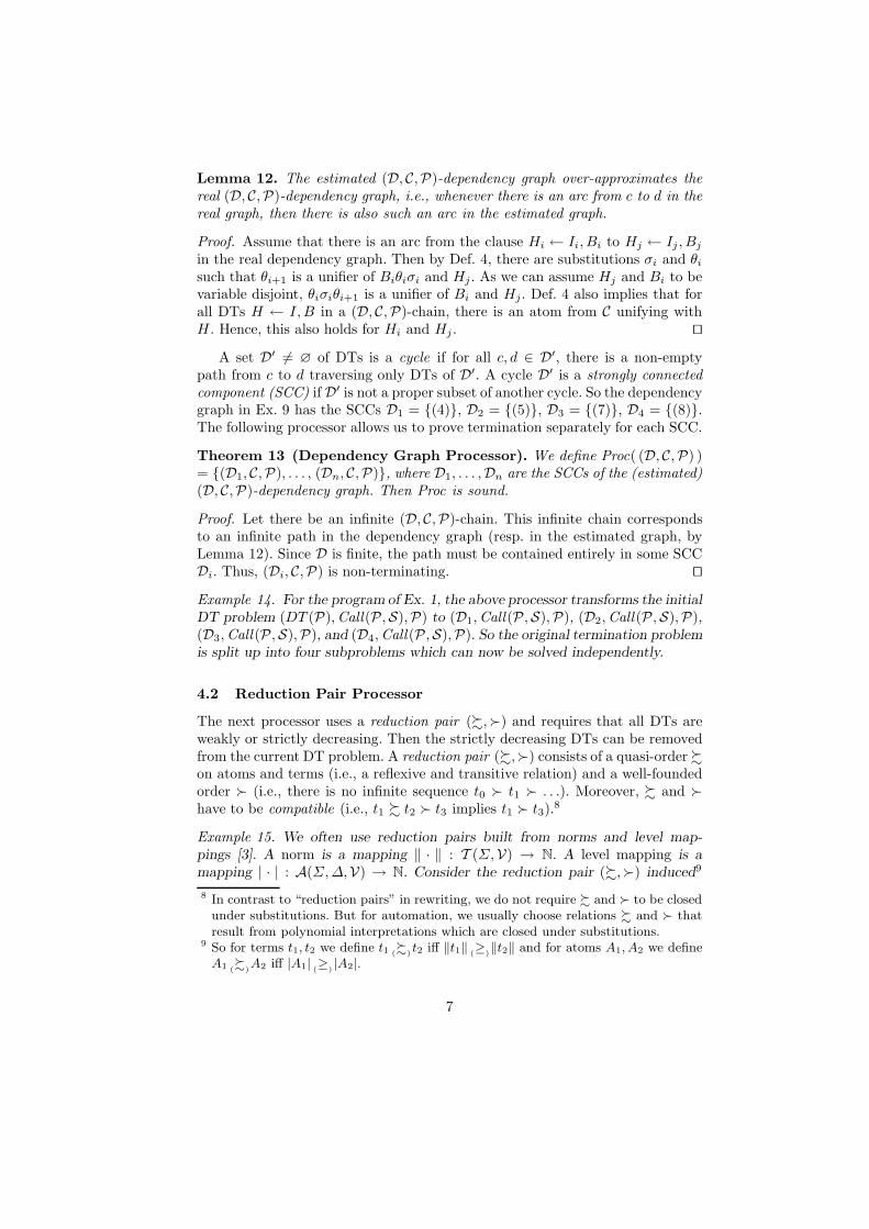
Lemma 12. The estimated (D, C,P)-dependency graph over-approximates thereal (D, C,P)-dependency graph, i.e., whenever there is an arc from c to d in thereal graph, then there is also such an arc in the estimated graph.

Proof. Assume that there is an arc from the clause Hi ← Ii, Bi to Hj ← Ij , Bj

in the real dependency graph. Then by Def. 4, there are substitutions σi and θi

such that θi+1 is a unifier of Biθiσi and Hj . As we can assume Hj and Bi to bevariable disjoint, θiσiθi+1 is a unifier of Bi and Hj. Def. 4 also implies that forall DTs H ← I, B in a (D, C,P)-chain, there is an atom from C unifying withH . Hence, this also holds for Hi and Hj . ⊓⊔

A set D′ 6= ∅ of DTs is a cycle if for all c, d ∈ D′, there is a non-emptypath from c to d traversing only DTs of D′. A cycle D′ is a strongly connectedcomponent (SCC) if D′ is not a proper subset of another cycle. So the dependencygraph in Ex. 9 has the SCCs D1 = {(4)}, D2 = {(5)}, D3 = {(7)}, D4 = {(8)}.The following processor allows us to prove termination separately for each SCC.

Theorem 13 (Dependency Graph Processor). We define Proc( (D, C,P) )= {(D1, C,P), . . . , (Dn, C,P)}, where D1, . . . ,Dn are the SCCs of the (estimated)(D, C,P)-dependency graph. Then Proc is sound.

Proof. Let there be an infinite (D, C,P)-chain. This infinite chain correspondsto an infinite path in the dependency graph (resp. in the estimated graph, byLemma 12). Since D is finite, the path must be contained entirely in some SCCDi. Thus, (Di, C,P) is non-terminating. ⊓⊔

Example 14. For the program of Ex. 1, the above processor transforms the initialDT problem (DT (P),Call(P ,S),P) to (D1,Call(P ,S),P), (D2,Call(P ,S),P),(D3,Call(P ,S),P), and (D4,Call(P ,S),P). So the original termination problemis split up into four subproblems which can now be solved independently.

4.2 Reduction Pair Processor

The next processor uses a reduction pair (%,≻) and requires that all DTs areweakly or strictly decreasing. Then the strictly decreasing DTs can be removedfrom the current DT problem. A reduction pair (%,≻) consists of a quasi-order %on atoms and terms (i.e., a reflexive and transitive relation) and a well-foundedorder ≻ (i.e., there is no infinite sequence t0 ≻ t1 ≻ . . .). Moreover, % and ≻have to be compatible (i.e., t1 % t2 ≻ t3 implies t1 ≻ t3).

8

Example 15. We often use reduction pairs built from norms and level map-pings [3]. A norm is a mapping ‖ · ‖ : T (Σ,V) → N. A level mapping is amapping | · | : A(Σ, ∆,V) → N. Consider the reduction pair (%,≻) induced9

8 In contrast to “reduction pairs” in rewriting, we do not require % and ≻ to be closedunder substitutions. But for automation, we usually choose relations % and ≻ thatresult from polynomial interpretations which are closed under substitutions.

9 So for terms t1, t2 we define t1 (%

)t2 iff ‖t1‖ (

≥)‖t2‖ and for atoms A1, A2 we define

A1 (%

)A2 iff |A1| (≥)

|A2|.

7

by the norm ‖X‖ = 0 for all variables X , ‖ [ ] ‖ = 0, ‖s(t)‖ = ‖ [s | t] ‖ =1+‖t‖ and the level mapping |s2m(t1, t2, t3)| = |s2ℓ(t1, t2)| = |subs mat(t1, t2)| =|subs row(t1, t2)| = ‖t1‖. Then subs mat([[C]], [SR | SRs]) ≻ subs mat([ ],SRs),as |subs mat([[C]], [SR | SRs])| = ‖[[C]]‖ =1 and |subs mat([ ],SRs)| = ‖ [ ] ‖ =0.

Now we can define when a DT H ← I, B is decreasing. Roughly, we requirethat Hσ ≻ Bσ must hold for every substitution σ. However, we do not haveto regard all substitutions, but we may restrict ourselves to such substitutionswhere all variables of H and B on positions that are “taken into account” by %

and ≻ are instantiated by ground terms.10 Formally, a reduction pair (%,≻) isrigid on a term or atom t if we have t ≈ tδ for all substitutions δ. Here, we defines ≈ t iff s % t and t % s. A reduction pair (%,≻) is rigid on a set of terms oratoms if it is rigid on all its elements. Now for a DT H ← I, B to be decreasing,we only require that Hσ ≻ Bσ holds for all σ where (%,≻) is rigid on Hσ.

Example 16. The reduction pair from Ex. 15 is rigid on the atom A = s2m([[C]],[SR |SRs]), since |Aδ| = 1 holds for every substitution δ. Moreover, if σ(Rs) ∈List , then the reduction pair is also rigid on subs mat([R | Rs], [SR | SRs])σ.For every such σ, we have subs mat([R | Rs], [SR |SRs])σ ≻ subs mat(Rs,SRs)σ.

We refine the notion of “decreasing” DTs H ← I, B further. Instead of onlyconsidering H and B, one should also take the intermediate body atoms I intoaccount. To approximate their semantics, we use interargument relations. Aninterargument relation for a predicate p is a relation IRp = {p(t1, . . . , tn) | ti ∈T (Σ,V) ∧ ϕp(t1, . . . , tn)}, where (1) ϕp(t1, . . . , tn) is a formula of an arbitraryBoolean combination of inequalities, and (2) each inequality in ϕp is either si %sj or si ≻ sj , where si, sj are constructed from t1, . . . , tn by applying functionsymbols of P . IRp is valid iff p(t1, . . . , tn) ⊢m

P� implies p(t1, . . . , tn) ∈ IRp for

every p(t1, . . . , tn) ∈ A(Σ, ∆,V).

Definition 17 (Decreasing DTs). Let (%,≻) be a reduction pair, and R ={IRp1 , . . . , IRpk

} be a set of valid interargument relations based on (%,≻). Letc = H ← p1(t1), . . . , pk(tk), B be a DT. Here, the ti are tuples of terms.

The DT c is weakly decreasing (denoted (%, R) |= c) if Hσ % Bσ holds forany substitution σ where (%,≻) is rigid on Hσ and where p1(t1)σ ∈ IRp1 , . . . ,pk(tk)σ ∈ IRpk

. Analogously, c is strictly decreasing (denoted (≻, R) |= c) ifHσ ≻ Bσ holds for any such σ.

Example 18. Recall the reduction pair from Ex. 15 and the remarks about itsrigidity in Ex. 16. When considering a set R of trivial valid interargument re-lations like IRsubs row = {subs row(t1, t2) | t1, t2 ∈ T (Σ,V)}, then the DT (7) isstrictly decreasing. Similarly, (≻, R) |= (4), (≻, R) |= (5), and (≻, R) |= (8).

We can now formulate our second DT processor. To automate it, we refer to[15] for a description of how to synthesize valid interargument relations and howto find reduction pairs automatically that make DTs decreasing.

10 This suffices, because we require (%,≻) to be rigid on C in Thm. 19. Thus, % and≻ do not take positions into account where atoms from Call(P ,S) have variables.

8

Theorem 19 (Reduction Pair Processor). Let (%,≻) be a reduction pairand let R be a set of valid interargument relations. Then Proc is sound.

Proc( (D, C,P) ) =

{(D \ D≻, C,P)}, if• (%,≻) is rigid on C and• there is D≻ ⊆ D with D≻ 6= ∅ such that (≻, R) |= c

for all c ∈ D≻ and (%, R) |= c for all c ∈ D \ D≻

{(D, C,P)}, otherwise

Proof. If Proc( (D, C,P) ) = {(D, C,P)}, then Proc is trivially sound. Now weconsider the case Proc( (D, C,P) ) = {(D\D≻, C,P)}. Assume that (D\D≻, C,P)is terminating while (D, C,P) is non-terminating. Then there is an infinite (D, C,P)-chain (H0 ← I0, B0), (H1 ← I1, B1), . . . where at least one clause fromD≻ appears infinitely often. There are A ∈ C and substitutions θi, σi suchthat θ0 = mgu(A, H0) and for all i, we have σi ∈ Answer(P , Iiθi), θi+1 =mgu(Biθiσi, Hi+1), and Biθiσi ∈ C. We obtain

Hiθi

≈ Hiθiσiθi+1 (by rigidity, as Hiθi = Bi−1θi−1σi−1θi

and Bi−1θi−1σi−1 ∈ C)% Biθiσiθi+1 (since (%, R) |= ci where ci is Hi ← Ii, Bi,

as (%,≻) is also rigid on any instance of Hiθi,and since σi ∈ Answer(P , Iiθi) implies Iiθiσiθi+1 ⊢

nP

�

and R are valid interargument relations)= Hi+1θi+1 (since θi+1 = mgu(Biθiσi, Hi+1))≈ Hi+1θi+1σi+1θi+2 (by rigidity, as Hi+1θi+1 = Biθiσiθi+1 and Biθiσi ∈ C)% Bi+1θi+1σi+1θi+2 (since (%, R) |= ci+1 where ci+1 is Hi+1 ← Ii+1, Bi+1)= . . .

Here, infinitely many %-steps are “strict” (i.e., we can replace infinitely many%-steps by ≻-steps). This contradicts the well-foundedness of ≻. ⊓⊔

So in our example, we apply the reduction pair processor to all 4 DT problemsin Ex. 14. While we could use different reduction pairs for the different DTproblems,11 Ex. 18 showed that all their DTs are strictly decreasing for thereduction pair from Ex. 15. This reduction pair is indeed rigid on Call(P ,S).Hence, the reduction pair processor transforms all 4 remaining DT problems to(∅,Call(P ,S),P), which in turn is transformed to ∅ by the dependency graphprocessor. Thus, termination of the LP in Ex. 1 is proved.

4.3 Modular Transformation Processor to Term Rewriting

The previous two DT processors considerably improve over [15] due to theirincreased modularity.12 In addition, one could easily adapt more techniques from

11 Using different reduction pairs for different DT problems resulting from one and thesame LP is for instance necessary for programs like the Ackermann function, cf. [15].

12 In [15] these two processors were part of a fixed procedure, whereas now they canbe applied to any DT problem at any time during the termination proof.

9

the DP framework (i.e., from the TRS setting) to the DT framework (i.e., to theLP setting). However, we now introduce a new DT processor which allows us toapply any TRS termination technique immediately to LPs (i.e., without havingto adapt the TRS technique). It transforms a DT problem for LPs into a DPproblem for TRSs.

Example 20. The following programP from [11] is part of the Termination Prob-lem Data Base (TPDB) used in the International Termination Competition.Typically, cnf’s first argument is a Boolean formula (where the function symbolsn, a, o stand for the Boolean connectives) and the second is a variable whichwill be instantiated to an equivalent formula in conjunctive normal form. To thisend, cnf uses the predicate tr which holds if its second argument results from itsfirst one by a standard transformation step towards conjunctive normal form.

cnf(X, Y )← tr(X, Z), cnf(Z, Y ). cnf(X, X).tr(n(n(X)), X). tr(o(X1, Y ), o(X2, Y ))← tr(X1, X2).tr(n(a(X, Y )), o(n(X), n(Y ))). tr(o(X, Y 1), o(X, Y 2))← tr(Y 1, Y 2).tr(n(o(X, Y )), a(n(X), n(Y ))). tr(a(X1, Y ), a(X2, Y ))← tr(X1, X2).tr(o(X, a(Y, Z)), a(o(X, Y ), o(X, Z))). tr(a(X, Y 1), a(X, Y 2))← tr(Y 1, Y 2).tr(o(a(X, Y ), Z), a(o(X, Z), o(Y, Z))). tr(n(X1), n(X2))← tr(X1, X2).

Consider the queries S = {cnf(t1, t2) | t1 is ground} ∪ {tr(t1, t2) | t1 is ground}.By applying the dependency graph processor to the initial DT problem, weobtain two new DT problems. The first is (D1,Call(P ,S),P) where D1 containsall recursive tr-clauses. This DT problem can easily be solved by the reductionpair processor. The other resulting DT problem is

({cnf(X, Y )← tr(X, Z), cnf(Z, Y )},Call(P ,S),P). (9)

To make this DT strictly decreasing, one needs a reduction pair (%,≻) wheret1 ≻ t2 holds whenever tr(t1, t2) is satisfied. This is impossible with the orders ≻in current direct LP termination tools. In contrast, it would easily be possible ifone uses other orders like the recursive path order [5] which is well establishedin term rewriting. This motivates the new processor presented in this section.

To transform DT to DP problems, we adapt the existing transformation fromlogic programs P to TRSs RP from [17]. Here, two new n-ary function symbolspin and pout are introduced for each n-ary predicate p:

• Each fact p(s) of the LP is transformed to the rewrite rule pin(s)→ pout(s).• Each clause c of the form p(s)← p1(s1), . . . , pk(sk) is transformed into the

following rewrite rules:pin(s)→ uc,1(p1in

(s1),V(s))uc,1(p1out

(s1),V(s))→ uc,2(p2in(s2),V(s) ∪ V(s1))

. . .uc,k(pkout

(sk),V(s) ∪ V(s1) ∪ . . . ∪ V(sk−1))→ pout(s)

Here, the uc,i are new function symbols and V(s) are the variables in s.Moreover, if V(s) = {x1, . . . , xn}, then “uc,1(p1in

(s1),V(s))” abbreviatesthe term uc,1(p1in

(s1), x1, . . . , xn), etc.

10

So the fact tr(n(n(X)), X) is transformed to trin(n(n(X)), X) → trout(n(n(X)),X) and the clause cnf(X, Y )← tr(X, Z), cnf(Z, Y ) is transformed to

cnfin(X, Y )→ u1(trin(X, Z), X, Y ) (10)

u1(trout(X, Z), X, Y )→ u2(cnfin(Z, Y ), X, Y, Z) (11)

u2(cnfout(Z, Y ), X, Y, Z)→ cnfout(X, Y ) (12)

To formulate the connection between a LP and its corresponding TRS, thesets of queries that should be analyzed for termination have to be representedby an argument filter π where π(f) ⊆ {1, . . . , n} for every n-ary f ∈ Σ ∪ ∆.We extend π to terms and atoms by defining π(x) = x if x is a variable andπ(f(t1, . . . , tn)) = f(π(ti1), . . . , π(tik

)) if π(f) = {i1, . . . , ik} with i1 < . . . < ik.Argument filters specify those positions which have to be instantiated with

ground terms. In Ex. 20, we wanted to prove termination for the set S of allqueries cnf(t1, t2) or tr(t1, t2) where t1 is ground. These queries are describedby the filter with π(cnf) = π(tr) = {1}. Hence, we can also represent S as S ={A | A ∈ A(Σ, ∆,V), π(A) is ground}. Thm. 21 shows that instead of provingtermination of a LP P for a set of queries S, it suffices to prove terminationof the corresponding TRS RP for a corresponding set of terms S′. As shownin [17], here we have to regard a variant of term rewriting called infinitaryconstructor rewriting, where variables in rewrite rules may only be instantiatedby constructor terms,13 which however may be infinite. This is needed since LPsuse unification, whereas TRSs use matching for their evaluation.

Theorem 21 (Soundness of the Transformation [17]). Let RP be the TRSresulting from transforming a LP P over a signature (Σ, ∆). Let π be an argu-ment filter with π(pin) = π(p) for all p ∈ ∆. Let S = {A | A ∈ A(Σ, ∆,V),π(A) is finite and ground } and S′ = {pin(t) | p(t) ∈ S}. If the TRS RP termi-nates for all terms in S′, then the LP P terminates for all queries in S.

The DP framework for termination of term rewriting can also be used forinfinitary constructor rewriting, cf. [17]. To this end, for each defined symbol f ,one introduces a fresh tuple symbol f ♯ of the same arity. For a term t = g(t)with defined root symbol g, let t♯ denote g♯(t). Then the set of dependency pairsfor a TRS R is DP (R) = {ℓ♯ → t♯ | ℓ→ r ∈ R, t is a subterm of r with definedroot symbol}. For instance, the rules (10) - (12) give rise to the following DPs.

cnf♯in(X, Y )→ tr

♯in(X, Z) (13)

cnf♯in(X, Y )→ u

♯1(trin(X, Z), X, Y ) (14)

u♯1(trout(X, Z), X, Y )→ cnf

♯in(Z, Y ) (15)

u♯1(trout(X, Z), X, Y )→ u

♯2(cnfin(Z, Y ), X, Y, Z) (16)

Termination problems are now represented as DP problems (D,R, π) whereD andR are TRSs (here, D is usually a set of DPs) and π is an argument filter. A

13 As usual, the symbols on root positions of left-hand sides of rewrite rules are calleddefined symbols and all remaining function symbols are constructors. A constructorterm is a term built only from constructors and variables.

11

list s1 → t1, s2 → t2, . . . of variants from D is a (D,R, π)-chain iff for all i, thereare substitutions σi such that tiσi rewrites to si+1σi+1 and such that π(siσi),π(tiσi), and π(q) are finite and ground, for all terms q in the reduction from tiσi

and si+1σi+1. (D,R, π) is terminating iff there is no infinite (D,R, π)-chain.

Example 22. For instance, “(14), (15)” is a chain for the argument filter π with

π(cnf♯in) = π(trin) = {1} and π(u♯

1) = π(trout) = {1, 2}. To see this, consider the

substitution σ = {X/n(n(a)), Z/a}. Now u♯1(trin(X, Z), X, Y )σ reduces in one

step to u♯1(trout(X, Z), X, Y )σ and all instantiated left- and right-hand sides of

(14) and (15) are ground after filtering them with π.

To prove termination of a TRS R for all terms S′ in Thm. 21, now it sufficesto show termination of the initial DP problem (DP (R),R, π). Here, one has tomake sure that π(DP (RP )) and π(RP ) satisfy the variable condition, i.e., thatV(π(r)) ⊆ V(π(ℓ)) holds for all ℓ→ r ∈ DP (R)∪R. If this does not hold, then πhas to be refined (by filtering away more argument positions) until the variablecondition is fulfilled. This leads to the following corollary from [17].

Corollary 23 (Transformation Technique [17]). Let RP ,P , π be as in

Thm. 21, where π(pin) = π(p♯in) = π(p) for all p ∈ ∆. Let π(DP (RP )) and

π(RP ) satisfy the variable condition and let S = {A | A ∈ A(Σ, ∆,V), π(A) isfinite and ground}. If the DP problem (DP (RP ),RP , π) is terminating, then theLP P terminates for all queries in S.

Note that Thm. 21 and Cor. 23 are applied right at the beginning of thetermination proof. So here one immediately transforms the full LP into a TRS (ora DP problem) and performs the whole termination proof on the TRS level. Thedisadvantage is that LP-specific techniques cannot be used anymore. It wouldbe better to only apply this transformation for those parts of the terminationproof where it is necessary and to perform most of the proof on the LP level.

This is achieved by the following new transformation processor within ourDT framework. Now one can first apply other DT processors like the ones fromSect. 4.1 and 4.2 (or other LP termination techniques). Only for those subprob-lems where a solution cannot be found, one uses the following DT processor.

Theorem 24 (DT Transformation Processor). Let (D, C,P) be a DT prob-

lem and let π be an argument filter with π(pin) = π(p♯in) = π(p) for all predicates

p such that C ⊆ {A | A ∈ A(Σ, ∆,V), π(A) is finite and ground} and such thatπ(DP (RD)) and π(RP ) satisfy the variable condition. Then Proc is sound.

Proc( (D, C,P) ) =

{

∅, if (DP (RD),RP , π) is a terminating DP problem{(D, C,P)}, otherwise

Proof. If Proc( (D, C,P) ) = {(D, C,P)}, then soundness is trivial. Now letProc( (D, C,P) ) = ∅. Assume there is an infinite (D, C,P)-chain (H0 ← I0, B0),(H1 ← I1, B1), . . . Similar to the proof of Thm. 6, we have

A ⊢H0←I0,B0, θ0 I0θ0, B0θ0 ⊢n0P,σ0

B0θ0σ0 ⊢H1←I1,B1, θ1 I1θ1, B1θ1 ⊢n1P,σ1

B0θ1σ1 . . .

12

For every atom p(t1, . . . , tn), let p(t1, . . . , tn) be the term pin(t1, . . . , tn). Then bythe results on the correspondence between LPs and TRSs from [17] (in particular[17, Lemma 3.4]), we can conclude

Aθ0σ0 (ε→RD

◦> ε→∗

RP)+

B0θ0σ0, B0θ0σ0θ1σ1 (ε→RD

◦> ε→ ∗

RP)+

B1θ0σ0θ1σ1, . . .

Here,→R denotes the rewrite relation of a TRS R,ε→ resp.

>ε→ denote reductions

on resp. below the root position and→∗ resp.→+ denote zero or more resp. oneor more reduction steps. This implies

A♯θ0σ0 (

ε→DP (RD)◦

> ε→ ∗RP

)+

B0♯θ0σ0, B0

♯θ0σ0θ1σ1 (

ε→DP (RD)◦

> ε→ ∗RP

)+

B1♯θ0σ0θ1σ1,

etc. Let σ be the infinite substitution θ0σ0θ1σ1θ2σ2 . . . where all remaining vari-ables in σ’s range can w.l.o.g. be replaced by ground terms. Then we have

A♯σ (

ε→DP (RD)◦

> ε→∗

RP)+

B0♯σ (

ε→DP (RD)◦

> ε→ ∗

RP)+

B1♯σ . . . , (17)

which gives rise to an infinite (DP (RD),RP , π)-chain. To see this, note thatπ(A) and all π(Biθiσi) are finite and ground by the definition of chains of DTs.

Hence, this also holds for π(A♯σ) and all π(Bi

♯σ). Moreover, since π(DP (RD))

and π(RP ) satisfy the variable condition, all terms occurring in the reduction(17) are finite and ground when filtering them with π. ⊓⊔

Example 25. We continue the termination proof of Ex. 20. Since the remainingDT problem (9) could not be solved by direct termination tools, we apply theDT processor of Thm. 24. Here, RD = {(10), (11), (12)} and hence, we obtainthe DP problem ({(13), . . . , (16)},RP , π) where π(cnf) = π(tr) = {1}. On theother function symbols, π is defined as in Ex. 22 in order to fulfill the variablecondition. This DP problem can easily be proved terminating by existing TRStechniques and tools, e.g., by using a recursive path order.

5 Experiments and Conclusion

We have introduced a new DT framework for termination analysis of LPs. Itpermits to split termination problems into subproblems, to use different ordersfor the termination proof of different subproblems, and to transform subproblemsinto termination problems for TRSs in order to apply existing TRS tools. Inparticular, it subsumes and improves upon recent direct and transformationalapproaches for LP termination analysis like [15, 17].

To evaluate our contributions, we performed extensive experiments compar-ing our new approach with the most powerful current direct and transformationaltools for LP termination: Polytool [14] and AProVE [7].14 The International Ter-mination Competition showed that direct termination tools like Polytool and

14 In [17], Polytool and AProVE were compared with three other representative tools forLP termination analysis: TerminWeb [4], cTI [12], and TALP [16]. Here, TerminWeb

and cTI use a direct approach whereas TALP uses a transformational approach. Inthe experiments of [17], it turned out that Polytool and AProVE were considerablymore powerful than the other three tools.

13

transformational tools like AProVE have comparable power, cf. Sect. 1. Never-theless, there exist examples where one tool is successful, whereas the other fails.

For example, AProVE fails on the LP from Ex. 1. The reason is that byCor. 23, it has to represent Call(P ,S) by an argument filtering π which satisfiesthe variable condition. However, in this example there is no such argument fil-tering π where (DP (RP ),P , π) is terminating. In contrast, Polytool representsCall(P ,S) by type graphs [10] and easily shows termination of this example.

On the other hand, Polytool fails on the LP from Ex. 20. Here, one needsorders like the recursive path order that are not available in direct terminationtools. Indeed, other powerful direct termination tools such as TerminWeb [4]and cTI [12] fail on this example, too. The transformational tool TALP [16] failson this program as well, as it does not use recursive path orders. In contrast,AProVE easily proves termination using a suitable recursive path order.

The results of this paper combine the advantages of direct and transforma-tional approaches. We implemented our new approach in a new version of Poly-

tool. Whenever the transformation processor of Thm. 24 is used, it calls AProVE

on the resulting DP problem. Thus, we call our implementation “PolyAProVE”.In our experiments, we applied the two existing tools Polytool and AProVE as

well as our new tool PolyAProVE to a set of 298 LPs. This set includes all LP ex-amples of the TPDB that is used in the International Termination Competition.However, to eliminate the influence of the translation from Prolog to pure logicprograms, we removed all examples that use non-trivial built-in predicates orthat are not definite logic programs after ignoring the cut operator. This yieldsthe same set of examples that was used in the experimental evaluation of [17].In addition to this set we considered two more examples: the LP of Ex. 1 andthe combination of Examples 1 and 20. For all examples, we used a time limitof 60 seconds corresponding to the standard setting of the competition.

Below, we give the results and the overall time (in seconds) required to runthe tools on all 298 examples.

PolyAProVE AProVE Polytool

Successes 237 232 218Failures 58 58 73Timeouts 3 8 7Total Runtime 762.3 2227.2 588.8Avg. Time 2.6 7.5 2.0

Our experiments show that PolyAProVE solves all examples that can be solvedby Polytool or AProVE (including both LPs from Ex. 1 and 20). PolyAProVE

also solves all examples from this collection that can be handled by any of thethree other tools TerminWeb, cTI, and TALP. Moreover, it also succeeds on LPswhose termination could not be proved by any tool up to now. For example,it proves termination of the LP consisting of the clauses of both Ex. 1 and 20together, whereas all other five tools fail. Another main advantage of PolyAProVE

compared to powerful purely transformational tools like AProVE is a substantialincrease in efficiency. PolyAProVE needs only about one third (34%) of the total

14

runtime of AProVE. The reason is that many examples can already be handledby the direct techniques introduced in this paper. The transformation to termrewriting, which incurs a significant runtime penalty, is only used if the otherDT processors fail. Thus, the performance of PolyAProVE is much closer to thatof direct tools like Polytool than to that of transformational tools like AProVE.

For details on our experiments and to access our collection of examples, werefer to http://aprove.informatik.rwth-aachen.de/eval/PolyAProVE/.

References

1. K. R. Apt. From Logic Programming to Prolog. Prentice Hall, London, 1997.2. T. Arts and J. Giesl. Termination of Term Rewriting using Dependency Pairs.

Theoretical Computer Science, 236(1,2):133–178, 2000.3. A. Bossi, N. Cocco, and M. Fabris. Norms on Terms and their use in Proving

Universal Termination of a Logic Program. Th. Comp. Sc., 124(2):297–328, 1994.4. M. Codish and C. Taboch. A Semantic Basis for Termination Analysis of Logic

Programs. Journal of Logic Programming, 41(1):103–123, 1999.5. N. Dershowitz. Termination of Rewriting. J. Symb. Comp., 3(1,2):69–116, 1987.6. J. Giesl, R. Thiemann, and P. Schneider-Kamp. The Dependency Pair Framework:

Combining Techniques for Automated Termination Proofs. In Proc. LPAR ’04,LNAI 3452, pp. 301–331, 2005.

7. J. Giesl, P. Schneider-Kamp, R. Thiemann. AProVE 1.2: Automatic TerminationProofs in the DP Framework. In Proc. IJCAR ’06, LNAI 4130, pp. 281–286, 2006.

8. J. Giesl, R. Thiemann, P. Schneider-Kamp, and S. Falke. Mechanizing and Im-proving Dependency Pairs. Journal of Automated Reasoning, 37(3):155–203, 2006.

9. N. Hirokawa and A. Middeldorp. Automating the Dependency Pair Method. In-formation and Computation, 199(1,2):172–199, 2005.

10. G. Janssens and M. Bruynooghe. Deriving Descriptions of Possible Values of Pro-gram Variables by Means of Abstract Interpretation. Journal of Logic Program-ming, 13(2,3):205–258, 1992.

11. M. Jurdzinski. LP Course Notes. http://www.dcs.warwick.ac.uk/~mju/CS205/.12. F. Mesnard and R. Bagnara. cTI: A Constraint-Based Termination Inference Tool

for ISO-Prolog. Theory and Practice of Logic Programming, 5(1, 2):243–257, 2005.13. M. T. Nguyen and D. De Schreye. Polynomial Interpretations as a Basis for Ter-

mination Analysis of Logic Programs. Proc. ICLP ’05, LNCS 3668, 311–325, 2005.14. M. T. Nguyen and D. De Schreye. Polytool: Proving Termination Automatically

Based on Polynomial Interpretations. In Proc. LOPSTR ’06, LNCS 4407, pp.210–218, 2007.

15. M. T. Nguyen, J. Giesl, P. Schneider-Kamp, and D. De Schreye. TerminationAnalysis of Logic Programs based on Dependency Graphs. In Proc. LOPSTR ’07,LNCS 4915, pp. 8–22, 2008.

16. E. Ohlebusch, C. Claves, and C. Marche. TALP: A Tool for the TerminationAnalysis of Logic Programs. In Proc. RTA ’00, LNCS 1833, pp. 270–273, 2000.

17. P. Schneider-Kamp, J. Giesl, A. Serebrenik, and R. Thiemann. Automated Ter-mination Proofs for Logic Programs by Term Rewriting. ACM Transactions onComputational Logic, 11(1), 2009.

15