Mathematical Biosciences 225 (2010) 141–155

Contents lists available at ScienceDirect

Mathematical Biosciences

journal homepage: www.elsevier .com/locate /mbs

Evaluating treatment of hepatitis C for hemolytic anemia management

Swati DebRoy a,*, Christopher Kribs-Zaleta b, Anuj Mubayi b,c,d,h, Gloriell M. Cardona-Meléndez e,Liana Medina-Rios f, MinJun Kang g, Edgar Diaz h

a Department of Mathematics, University of Florida, Gainesville, FL, USAb Department of Mathematics, University of Texas at Arlington, Arlington, TX, USAc School of Human Evolution and Social Change, Arizona State University, Tempe, AZ, USAd Prevention Research Center, Berkeley, CA, USAe University of Puerto Rico, Cayey, Puerto Ricof Mount Holyoke College, South Hadley, MA, USAg Kyungpook National University, Daegu, Republic of Koreah Mathematical, Computational and Modeling Sciences Center, Arizona State University, Tempe, AZ, USA

a r t i c l e i n f o

Article history:Received 10 June 2009Received in revised form 30 January 2010Accepted 5 February 2010Available online 19 March 2010

Keywords:Hepatitis CRibavirinInterferonEpoietinAnemiaMathematical modeling

0025-5564/$ - see front matter � 2010 Elsevier Inc. Adoi:10.1016/j.mbs.2010.02.005

Abbreviations: HCV, Hepatitis C; RBV, Ribavirin; pRBC, red blood cells; EPO, Epoietin, Epoetin.

* Corresponding author at: 358 Little Hall, P.O.32611-8105, USA. Tel.: +1 352 392 0281x294; fax: +1

E-mail addresses: swati@math.ufl.edu (S. DebRoy)DebRoy).

a b s t r a c t

The combination therapy of antiviral peg-interferon and ribavirin has evolved as one of the better treat-ments for hepatitis C. In spite of its success in controlling hepatitis C infection, it has also been associatedwith treatment-related adverse side effects. The most common and life threatening among them is hemo-lytic anemia, necessitating dose reduction or therapy cessation. The presence of this side effect leads to atrade-off between continuing the treatment and exacerbating the side effects versus decreasing dosage torelieve severe side effects while allowing the disease to progress. The drug epoietin (epoetin) is oftenadministered to stimulate the production of red blood cells (RBC) in the bone marrow, in order to allowtreatment without anemia. This paper uses mathematical models to study the effect of combination ther-apy in light of anemia. In order to achieve this we introduce RBC concentration and amount of drug in thebody as state variables in the usual immunological virus infection model. Analysis of this model providesa quantification of the amount of drug a body can tolerate without succumbing to hemolytic anemia.Indirect estimation of parameters allow us to calculate the necessary increment in RBC production tobe P2.3 times the patient’s original RBC production rate to sustain the entire course of treatment withoutencountering anemia in a sensitive patient.

� 2010 Elsevier Inc. All rights reserved.

1. Introduction the body’s immune system does not naturally clear the virus.

About 170 million people live with hepatitis C virus (HCV) infec-tion world-wide [1]. Currently, there is no vaccine for HCV infection.The major mode of transmission of HCV is by exposure to infectedblood. Sexual and vertical transmission of HCV has been reported;however, it is rare [2]. Hepatitis C (Hep-C) causes chronic diseasesof the liver like cirrhosis and hepatocellular carcinoma [3]. TheHCV infects hepatocytes which form a major portion of the cytoplas-mic mass of the liver. Although HCV predominantly replicates inhepatocytes, traces of it have been detected in other cell types [4,5].

Some patients with Hep-C infection will naturally clear thevirus without medical intervention. However, a major proportionof HCV infected individuals develop chronic HCV infection in which

ll rights reserved.

eg-IFN, pegylated interferon;

Box 118105, Gainesville, FL352 392 8357.

, debroy.swati@gmail.com (S.

About 55–85% of HCV patients do not clear the virus themselvesand develop chronic Hep-C infection [2]. The progression tochronic-stage HCV infection is a result of weak immune responseagainst HCV (reviewed in [6]). Currently, the standard protocolfor the treatment of Hep-C involves two antiviral drugs, Inter-feron-a (IFN) and ribavirin (RBV), given in combination [7,8]. Ithas been clinically observed that the combination of RBV and IFNdemonstrates a synergistic pharmacological effect. That is to say,the treatment efficacy of this combination therapy goes well be-yond the efficacies of the individual treatments added together[1]. Although the exact mechanism of the action of either of thesedrugs in treatment of Hep-C infection is not clear, direct antiviral,antiproliferative, and immunomodulatory activities of IFN are wellknown [1]. In the case of RBV, many scientists seem to favor itsimmunomodulatory action as an explanation of its efficacy inHCV treatment; however, its role as a viral RNA mutagen cannotbe ignored, as discussed in Lau et al. [1, and references cited there-in]. Hep-C patients receive weekly injections of IFN and take RBVpills daily for the period of treatment [8]. If a patient does not show

142 S. DebRoy et al. / Mathematical Biosciences 225 (2010) 141–155

traces of Hep-C viral load in the body after six months of therapycessation, the patient is said to have achieved Sustained VirologicalResponse (SVR), implying clinically cured. The goal of this treat-ment is to lower the viral load and eventually achieve SVR. IfSVR is not achieved, a patient is considered a chronic Hep-C pa-tient. The rate of achievement of SVR in Hep-C patients variesaccording to the genotype of the particular infecting virus. Thetreatment for genotypes 1 and 4 are usually carried out for 48weeks and that for genotypes 2 and 3 typically lasts for 24 weekswith lesser dosing of RBV [9]. Under this treatment, SVR rates of46% are observed in patients with HCV genotype 1, whereas 76%and 82% of patients with HCV genotypes 2 or 3 achieve SVR [10].

In spite of being a sufficiently successful treatment for Hep-Cinfection, there are several negative side effects of the treatmentranging from flu-like symptoms and anemia to temporary disabil-ity and depression, which is a major cause for concern among med-ical practitioners. The most common and alarming side effect ofIFN and RBV combination therapy is reversible hemolytic anemianecessitating dose reduction or complete cessation of RBV in manypatients [11]. The RBV induces excessive hemolysis, that is, thebreakdown of red blood cells (RBC) and release of hemoglobin intothe surrounding blood plasma. The body’s ability to produce RBC ata faster rate to compensate for this excessive loss is stunted by thesimultaneous bone-marrow suppressing effect of IFN [10]. Theadjective ‘reversible’ signifies the fact that in most cases, the RBCcount gets back to normal levels once the treatment is stopped.To combat the situation, doctors often prescribe a third drug,epoietin-a (EPO), which acts like the hormone erythropoietin andfacilitates RBC production in the bone marrow [10]. Epoietin (alsospelled epoetin) is observed to be quite efficient at reversing RBV-induced anemia in most patients. According to Sulkowski [10], suc-cess of the combination therapy with IFN and RBV is contingent onmaintaining adequate doses of both drugs throughout the treat-ment period. The occurrence of side effects leads to a trade-off be-tween continuing the treatment with optimal dosage to clear thevirus and exacerbating the side effects versus decreasing dosageto relieve severe anemia, while reducing the chances of achievingSVR. With this in mind, we use mathematical modeling to estimatethe EPO-induced increase in RBC production necessary for a patientto be able to undergo the complete course of the combination ther-apy without suffering from acute anemia.

The anti-anemic drug EPO is known to be well tolerated amongHCV patients. However, increase in RBC production by more than afactor of 4 within 2 weeks should be avoided, and EPO does not in-crease RBC production without bounds for all patients [12]. CertainEPO-initiated side effects like pure red-cell aplasia due to presenceof anti-erythropoietin antibodies has been observed in some pa-tients with chronic renal failure [13,10]. Thus dosing only sufficientEPO is desirable.

In the context of Hep-C, mathematical modeling has beenextensively used to determine the efficacy of IFN as monotherapyand in combination with RBV [7,14]. Differences in responsedepending on genotype [15], and the concept of early virologicalresponse (EVR) to estimate possibility of achieving SVR [16] havebeen reinforced with mathematical models. Viral and drug kineticsstudies using mathematical models have shed light on the under-standing of this virus and its treatment in several directions [17].All these studies have contributed enormously to the improvementof the treatment procedure that doctors presently apply to pa-tients. We further this effort to develop mathematical methodolo-gies that can be used to estimate the necessary usage of EPO tohelp an HCV patient to sustain the antiviral treatment.

We construct a set of coupled five ordinary differential equa-tions where the first three represent uninfected target hepatocytes,infected hepatocytes and free virions based on the first model ofNeumann et al. [18]. To that we incorporate the side effect of

hemolytic anemia by considering the RBC concentration as a sepa-rate state variable and also the amount of drug in the body as a dy-namic quantity rather than a constant parameter.

We focus on the interaction of the RBC level and amount of drugwith the goal of finding an optimal drug treatment regimen to min-imize the severity of anemia while still obtaining SVR. Using thefirst three equations we determine the minimum amount of drugnecessary for the patient to achieve SVR. Then, we mathematicallyreplicate a hypothetical situation with a sensitive Hep-C patient un-der combination therapy who starts taking the regular dosage pre-scribed by the doctors depending on body weight. Here, ‘sensitive’means that the patient has a history of encountering hemolyticanemia when on this treatment. During treatment the patient’sRBC concentration is monitored, and his dosage adjusted accord-ingly. From this process we calculate the amount of drug the pa-tient can handle without hitting anemia. Then we introduce theeffect of EPO in the equations, i.e., increase the RBC productionby a factor of the patient’s original RBC production level, to letthe patient intake greater amounts of drug in the body while main-taining a healthy RBC concentration. This allows us to calculate theEPO-induced increment in RBC production necessary to let the pa-tient sustain at least the minimum amount of drug to achieve SVRfor the necessary period of time. A schematic representation of theusual scenario can be seen in Fig. 1. Analytic and numerical meth-ods facilitate evaluation of several dosing regimens.

In Section 2, we introduce our model and its parameters; in Sec-tion 3, we analyze the model and calculate different reproductivenumbers for HCV with and without treatment under varyingassumptions. In Section 4, we discuss the estimation of parametersand establish the results of our analytic work numerically. In addi-tion, critical drug amounts are numerically calculated for the sys-tem and the results of simulations are shown.

2. Model

Our model is an extension and modification of that used byNeumann et al. [18] which includes the state variables T(t), targethealthy hepatocytes; I(t), infected hepatocytes; and V(t), the viralload of free HCV. In order to focus on the interplay between thedrugs and the RBC concentration in an HCV patient, we introducetwo further state variables, R(t) for the RBC concentration in thebody and C(t) for the amount of drug (IFN and RBV) in the body.(Note that C(t) represents the total amount of drug in the body attime t and not the concentration or dosage at time t.) We definet ¼ 0 to correspond to the beginning of treatment. Fig. 2 illustratesthe key elements of the model and their interactions (labeled byparameters) (see Table 1).

The model equations are:

dTdt¼ sT � dT T � a

aþ CbTV ; ð1Þ

dIdt¼ a

aþ CbTV � dII; ð2Þ

dVdt¼ p

kkþ C

I � hCV � dV V ; ð3Þ

dRdt¼ sR � dRR� sCR; ð4Þ

dCdt¼ DðRÞ � hC; ð5Þ

where

DðRÞ ¼ kR2

a2 þ R2 :

We begin by considering the drug-RBC interplay which is indepen-dent of the HCV within-host dynamics. We assume that the RBC

Fig. 1. Schematic representation of sensitivity of RBC concentration in the body and viral load to the amount of drug in the body. The bold grey curve represents the RBCconcentration in the patient which decreases as the amount of drug in the body increases. RI is the initial RBC concentration of the patient when no drug is present and RA isthe RBC concentration at anemia. The black curve represents the viral load which also decreases as the amount of drug in the body increases. C* is the amount of drug in thebody when the RBC concentration reaches equilibrium. CA is the amount of drug that causes anemia and CSVR is the minimum amount of drug required by the body to achieveSVR. C�; CA; CSVR are calculated from the model. A clinical problem occurs when the drug amount CSVR is much higher than CA . Our goal is to use EPO to boost the RBCproduction to make CA greater than CSVR. The grey dotted line represents the expected effect of EPO which keeps the RBC concentration at a healthy level even at higher dosesof combination drugs. Further discussion of the drug related quantities can be found in Section 3.3.

Fig. 2. Compartmental model.

S. DebRoy et al. / Mathematical Biosciences 225 (2010) 141–155 143

concentration in the body (R, measured in cells mL�1) is affected bythree factors: the natural rate of RBC production in the bone mar-row, which we denote by the constant sR; natural cell mortality,which occurs at a rate dR; and additional mortality induced by thepresence of antiviral drugs in the body. Since this last rate is propor-tional to the amount of drug in the body, we model it with a massaction term sRC, where s is the rate constant.

The amount of drug C in the body, measured in mg, changescontinuously over time in response to two factors: the drug dosage(in mg day�1), denoted by DðRÞ, and the body’s ability to clear thedrugs from the body at a rate h per day. A typical HCV patient isinitially prescribed a dosage of IFN and RBV, based on his/her body

weight. The daily RBV dosage is around 1000–1200 mg, and the IFNdosage is 0.1 lg kg�1 week�1, which is orders of magnitude lowerin quantity. Although the pharmacokinetics and possibly modesof action of IFN and RBV are different, the mechanism of actionof each of the drugs individually has not been firmly established,leaving the exact nature of their synergy even less confirmed [1].Thus, for simplicity, rather than modeling the amount of each drugseparately we consider the amount of drug C to be the quantity ofRBV since that is the drug which has the major effect on RBC levelsand is reduced to half upon encountering anemia. However, weconsider the efficacy of the drug to be that of the combinationIFN-RBV therapy, since that is what affects the viral load.

Table 1Brief interpretation of the parameters used in the model.

Parameter Interpretation

sT Natural production rate of hepatocytessR Natural production rate of RBCdV Natural clearance rate of virusdT Natural death rate of hepatocytesdI Clearance rate of infected hepatocytesdR Natural death rate of RBCa Drug amount to reduce infection rate to halfp Production rate of virusb Rate of new infections per virionk Drug amount to reduce virus production rate to halfh Rate of virion death per unit drugs Rate of RBC death per unit drugk Maximum drug dosagea RBC concentration at which drug dosage is reduced to k

2

h Rate of drug clearance

144 S. DebRoy et al. / Mathematical Biosciences 225 (2010) 141–155

We consider the dosage as a function of the RBC concentration,since in this scenario the goal is to avoid anemia caused by HCV ther-apy. If a patient encounters anemia at any point during the course ofthe therapy, doctors reduce the dosage of RBV to half, which in-creases the chances of unsuccessful achievement of SVR [10]. Weare interested in finding out the maximum amount of drug a patientcan take without encountering anemia. Thus, instead of waiting forthe patient to hit anemia and then reducing the dosage to half wewill consider the following hypothetical situation to construct ourdosing term, DðRÞ, in the dC

dt equation. Suppose a Hep-C patient oncombination drug therapy undergoes RBC concentration monitoringfollowed by a continuous reduction in the relative dose. Studyingthis correlation we can calculate the amount of drug in the bodywhich keeps the RBC concentration at a healthy equilibrium. Wefirst construct DðRÞ, the dosage term as a function of RBC concentra-tion, R. In reality, the dosage given by a doctor is best approximatedby a RBC concentration dependent step function

DðRÞ ¼DI; R > RA;DI2 ; R 6 RA;

(

where DI is the initially prescribed dose and RA is the RBC concen-tration at anemia. However, in order to facilitate model analysis,here we construct a continuous function for our virtual dosing reg-imen to approximate the actual step function, according to the fol-lowing properties:

1. It should be a strictly increasing function of R,2. At time t = 0, DðRÞ should equal the value of initial dosage DI

prescribed by the doctor,3. When the RBC concentration reaches anemic levelsðR ¼ RAÞDðRÞ should be reduced to half the original dosage, DI

2 .

It can be noted that the function k R2

a2þR2 with its unique inflectionpoint fits into criterion (1) very well. Using conditions (2) and (3),we calculate the constants k and a in the numerical section. It iseasy to note that k is the maximum possible dosage that can be the-oretically administered. However, we never actually attain that,since as soon as we start treatment, the RBC concentration de-creases, causing the entire dosage term to decrease. Also, the initialdosage will most likely be less than k. Again, a is the RBC concentra-tion at which the dosage term DðRÞ is equal to half of k.

We also suppose here that the patient’s RBC concentration isconstantly monitored and his dosage adjusted continuously. Thisassumption of optimal (continuous rather than discrete) responsetime permits the dosage adjustments to be incorporated into thequalitative analysis of the model, in addition to the numerical anal-ysis. In practice the patient’s condition is likely to be monitoredonce every several days, although in one clinical trial viral load

was monitored several times per day [18]. This assumption also al-lows us to address the question of whether it is technically possibleto achieve SVR while avoiding anemia.

This description of treatment as continuous in time and dosageis inaccurate in two regards. First, therapy is typically administeredin discrete doses rather than continuously like some IV drugs. Sec-ond, in practice the dosage would not be adjusted on a continuousbasis, but rather switched between a limited number (possiblyonly two) of levels, say the initial level and a reduced level. How-ever, the first inaccuracy has minimal effect on the long-term pre-dictions of the model, since doses are typically given daily anyway(see the end of Section 4.2 for an illustration of the difference). Thesecond inaccuracy tends to idealize the effects of making drug dos-age responsive to RBC concentration: that is, the model describesan optimal (immediate and continuous) responsiveness whereasreal responsiveness is likely to be more coarse (in both time andRBC level). Thus the results evaluate ‘proof of concept’ – whetherthe various drugs at their current efficiencies can be used in con-junction in such a way as to avoid anemia while achieving SVR.In order for a less adaptive, more uniform dosing policy to strikethis critical balance, drug efficiencies (including EPO, which willbe discussed later) will need to be higher than the threshold valuescalculated in this paper.

The (T, I,V) system explains the HCV interaction in the hepato-cyte cells of the liver. The parameter sT is the rate of production,and dT is the natural death rate of healthy hepatocytes from thebone marrow. a is related to the efficacy of combination therapy.It is essentially the amount of the drug at which production ofnew infected cells is reduced to half; that is, when C ¼ a, we getb2. If there is no drug in the body (or the drug has no efficacy inreducing infection), a

aþC ¼ 1 and the virus infects the healthy hepa-tocytes at a constant rate b. If instead the drug works with 100%efficacy, a

aþC ¼ 0. b is the number of infections caused by one in-fected cell per unit time. As the amount of drug increases, a

aþC be-comes a smaller fraction and the production of infected cellsdecrease. bTV is the [unreduced] concentration (in cells/mL) ofhealthy hepatocytes infected by virus, V, per unit of time. This totalrate of infected hepatocytes, bTV , goes into the second class ofhepatocytes which is the infected hepatocytes, I. Here, dII is therate at which infected hepatocytes are cleared per unit of time.

The per capita production rate of HCV is p and hence pI accountsfor the virions produced by the total population of infected hepato-cytes per unit time. k, like a, is related to the efficacy of the drugs. Itis essentially the amount of the drug in the body which reduces theproduction of new virions to half of the amount produced inabsence of treatment. h is a rate with unit amount�1 time�1. hCVaccounts for increased clearance of free virions due to the immuno-modulatory effect of both drugs. Neumann et al. observed only apossibly minor effect of drugs on viral clearance in the first 2 daysof therapy, based on a model which assumes constant drug efficacyover the whole period of treatment. Since, in our case, the efficacyof the drugs is constantly changing as RBC concentration varies, itis worth considering this possible effect of the drugs, in the ab-sence of more extensive clinical data on this aspect of treatment.Since dV is the clearance rate of virion in absence of treatment,dV V is the total concentration of virions cleared per unit time.

3. Analytical work

The model is essentially split into two separate systems becausethe RBC equation and drug amount equation are decoupled fromthe rest of the model. This allows us to analyze this model astwo separate systems and as a cohesive system of equations. Oneof these subsystems is two-dimensional and considers only theeffect that drug amount and RBC count have on each other. The

S. DebRoy et al. / Mathematical Biosciences 225 (2010) 141–155 145

other is three-dimensional and models the dynamics of targethepatocytes, infected hepatocytes, and free virions.

3.1. Analysis of (R,C) system

We determine the equilibrium of the decoupled dRdt and dC

dt with-out regard to the complete system. Equating dC

dt ¼ 0 we identifyC� ¼ k

hR2

a2þR2. Then we use C* to find the abscissa of the equilibriumpoint, by equating dR

dt to zero, resulting in the cubic equation

FðRÞ ¼ dR þskh

� �R3 � sRR2 þ dRa2R� sRa2 ¼ 0: ð6Þ

In light of this, we rescale the equation using r ¼ Ra ; d ¼ dR

SR=a ;

and ~a ¼ skh

SR=a to make our cubic equation depend on two parameters~a and d which simplifies to

f ðrÞ ¼ ð~aþ dÞr3 � r2 þ dr � 1 ¼ 0: ð7Þ

Further details on these calculations can be found in Appendix A.1.

Observation 1. Eq. (7) has exactly one positive real root.

Proof. Since f ðrÞ is cubic in r, there is a possibility of a maximum ofthree roots. Note that, if r = 0, f ðrÞ < 0, and if r is large, f ðrÞ > 0, sothere is one or three real positive roots. Thus there cannot be tworoots. Now let us consider the case of three possible roots. Usingthe rescaled equation, we analyze the possible roots in the param-eter space. We consider f ðrÞ as a function of ~a and d, that is,r3~aþ ðr3 þ rÞd ¼ r2 þ 1. Then, we use the original equation andthe first derivative of this equation 3r2~aþ ð3r2 þ 1Þd ¼ 2r. Since iff ðrÞ has two roots, f ðrÞ ¼ 0 and at that point f ðrÞ should be tangentto the x-axis, thus f 0ðrÞ ¼ 0. We apply linear algebra to this systemof equations. Solving the system using the Gauss method, we find~a ¼ � ðr2þ1Þ2

2r3 < 0 and d ¼ r2þ32r > 0. These solutions are biologically

extraneous since all parameter values are positive and the bifurca-tion lies only in the second quadrant as shown in Fig. 3. Therefore,we have determined that the system does not have a biologicallyrelevant bifurcation point.

Hence, we conclude that the system cannot have three positivereal roots. We determine that there is only one positive real root byanalyzing the bifurcation diagram in the first quadrant. For furtherdetails on exact method, refer to Appendix A.2. h

Fig. 3. This curve is plotted using parametric curve ~a ¼ � ðr2þ1Þ22r3 < 0 and

d ¼ r2þ32r > 0.

Observation 2. The equilibrium R�;C�ð Þ is locally asymptoticallystable.

Proof. To analyze the local stability of this non-trivial equilibriumpoint we use a Jacobian matrix,

J R� ;C�ð Þ ¼�dR � sC� �sR2 a2kR

a2þR�2ð Þ2�h

24 35:Since dR > 0; C� > 0; h > 0; s > 0, we know trðJÞ ¼ �ðdR þ sC�þhÞ < 0, and detðJÞ ¼ h dR þ sC�ð Þ þ 2sR�2a2k

a2þR�2> 0, thus we show R�;C�ð Þ

is locally asymptotically stable. For further details refer to AppendixA.3. h

Observation 3. The equilibrium R�;C�ð Þ is globally stable.

Proof. We have proven local stability; now our interest is in the glo-bal stability of the (R,C) system. To this end, we apply the Poincaré–Bendixson Theorem. The Poincaré–Bendixson Theorem states thatthere are three possibilities for the asymptotic behavior of solutionsto a two-dimensional system: a limit cycle, an unbounded solutionor a stable equilibrium point. Now, using Dulac’s criterion usingthe coefficient function, g ¼ 1

R, we prove that there is no limit cycle.We also note by simple comparison that lim suptCðtÞ < k

h andlim suptRðtÞ < sR

dR; hence the solution cannot be unbounded. Thus

local stability is extended to global stability for the unique equilib-rium point. Further technical details are relegated to AppendixA.4. h

Consequently by a theorem of Thieme [19] the behavior of thesystem (1)–(5) is asymptotic to the behavior of the three-dimen-sional subsystem (1)–(3) with the equilibrium values C� and R�

substituted for the state variables C and R. In the next subsection,we will use this reduced system to determine the necessary equi-librium drug amount to eliminate HCV from the (T, I,V) system.

3.2. Analysis of (T, I,V)

We analyze the (T, I,V) subsystem and determine the desiredcritical drug amount, CSVR, for which the disease free equilibriumof (T, I,V) is stable. In the absence of hepatitis C treatment, Callawayand Perelson [20] calculate the basic reproduction number ðR0Þ.

R0 ¼1dI

pbdV

sT

dT; ð8Þ

R0 can be interpreted as the average number of newly infectedT-cells produced by an infected T-cell during its (infected) lifetime.That is, an infected T-cell lives for 1

dIunits of time; each of p virions

produced by a bursting infected T-cell will produce bdV

new infected

T-cells, from the population of uninfected T-cells of sTdT

.

We first analyze Eqs. (1)–(3), taking C as an asymptotic con-stant; in a sense we take it to be a parameter. Then the disease freeequilibrium (DFE) is

ðT0; I0;V0Þ ¼sT

dT;0; 0

� �:

Linearizing the system about the DFE, and imposing conditions forstability we calculate bR which we call the controlled reproductionnumber (CRN).

bR ¼ aaþ C

kkþ C

dV

hC þ dV

sT pbdI dT dV

; ð9Þ

bR ¼ aaþ C

kkþ C

dV

hC þ dVR0: ð10Þ

146 S. DebRoy et al. / Mathematical Biosciences 225 (2010) 141–155

Observation 4. When bR < 1, the DFE is stable, and when bR > 1, theDFE exists but is unstable.

This observation is established in Appendix A.5. Thus, the infec-tion is eliminated from the hepatocyte population when the DFE isstable. Now our attention shifts to the endemic equilibrium sinceour biological interest is treatment of chronically HCV infectedindividuals. Here the endemic equilibrium is defined as the equi-librium when I� > 0 and V� > 0.

We solve the endemic equilibrium conditions to get:

T� ¼ sT

dTbR ; ð11Þ

I� ¼ sT

dI1� 1bR� �

; ð12Þ

V� ¼ dTðaþ CÞ

abbR � 1� �

: ð13Þ

Observation 5. The endemic equilibrium of the (T, I,V) system isglobally stable if bR > 1.

See Appendix A.5 for further details on the equilibrium point of the(T, I,V) subsystem. The global stability of the T�; I�;V�ð Þ equilibriumin the (T, I,V) subsystem can be proved using a Liapunov’s functionas in DeLeenher and Pilyugin [21]. Defining the Liapunov’s functionas

W ¼ nZ T

T�1� T�

s

� �dsþ g

Z I

I�1� I�

s

� �dsþ f

Z V

V�1� V�

s

� �ds

and using properties of the equilibrium we have proved its globalstability (see Appendix A.5.4).

3.3. Critical dosages

Now that we have found the condition bR 6 1� �

for which theDFE is stable, we solve for CSVR, the drug value for which bR ¼ 1.This provides the minimum amount of drug needed to achieveSVR in a Hep-C patient. When we use Eq. (10) to solve for C, weobtain a cubic equation in C of the form GðCÞ ¼ C3 þ A2C2þA1C þ A0 ¼ 0, where

GðCÞ¼C3þ dV

hþkþa

� �C2þ kaþðkþaÞdV

h

� �Cþ ka

dV

hð1�R0Þ

� �:

ð14Þ

We observe that Gð0Þ < 0 if and only if R0 > 1. In addition G0ðCÞ > 0for each C and limC!1GðCÞ ¼ þ1; therefore there exists one uniqueroot, namely

CSVR ¼ �A2 �1

3ffiffiffi23p B1 þ

ffiffiffiffiffiffiffiffiffiffiffiffiffiffiffiffiffiffiffiB2

1 � 4B2

q� �13

þ B1 �ffiffiffiffiffiffiffiffiffiffiffiffiffiffiffiffiffiffiffiB2

1 � 4B2

q� �13

" #;

ð15Þ

where

B1 ¼ 2A32 � 9A1A0 þ 27A0;

B2 ¼ A22 � 3A1:

It has been noted in [18] that for higher efficacy of the therapy, theeffect of treatment on the infection rate bTV is negligible. In thislimiting case, we have a

aþC ¼ 1. Then Eq. (14) becomes quadratic:

C2 þ kþ dV

h

� �C þ k

dV

hð1�R0Þ ¼ 0;

with solution

CSVR ¼�ðdV þ hkÞ þ

ffiffiffiffiffiffiffiffiffiffiffiffiffiffiffiffiffiffiffiffiffiffiffiffiffiffiffiffiffiffiffiffiffiffiffiffiffiffiffiffiffiffiffiffiffiffiffiffiffiffiffiffiffiffiffiffiffiðdV þ hkÞ2 þ 4kdV ðR0 � 1Þ

q2h

: ð16Þ

Note that we introduce treatment into an infected population onlyif R0 > 1, implying that the body is incapable of clearing out thevirus by itself. Therefore, ðR0 � 1Þ > 0 making CSVR > 0 always.

As mentioned before we define CA as the maximum amount ofdrug a body can tolerate without encountering anemia. To com-pute CA we first determine RA, i.e., the RBC concentration at anemiafor the patient, which is a clinically fixed quantity independent ofthe amount of drug in the body. Eq. (5) represents the change inRBC concentration with respect to the amount of drug, and at equi-librium it gives a relationship between the amount of drug in thebody and the RBC concentration. Thus, using the RBC concentrationRA we solve dR=dt ¼ 0 for CA, the amount of drug (IFN + RBV) in thebody that causes anemia in the absence of additional treatmentwith EPO:

CA ¼sR � dRRA

sRA: ð17Þ

Thus, if the amount of drug in the body is more than CA, a personwill get anemia. In terms of the biology of hepatitis C treatmentand the side effect of anemia, the analysis of the (R,C) and (T, I,V)subsystems allows us to compare the following critical drugamounts: the equilibrium drug amount C*, which keeps the RBCconcentration at an equilibrium; the minimum amount of drug inthe body so that the viral load goes below detection, CSVR, leadingto successful achievement of SVR; and the drug amount CA, thatis, the maximum amount of drug a patient can tolerate without get-ting anemia. Numerical estimation of these values, and their rela-tive values can provide an objective view about the patient’scondition and necessary steps to be taken. This is explained in detailin Section 5.

The ideal scenario for a doctor is to observe CSVR 6 CA. Thendepending upon other factors concerning the patient he can pre-scribe a dosing regime so that the amount of drug in the body staysin the interval ðCSVR;CAÞ. That will ensure that SVR is achievedwithout encountering anemia. The patients for whom the inequal-ity is reversed, we treat with EPO to boost CA higher than CSVR sothat doctors have an opportunity to treat them without anemiccomplications.

To introduce the effect of epoietin we increase (multiply) theRBC production by a factor b and recalculate CA. Epoietin is knownto increase RBC production by a factor of the patient’s original RBCproduction level from clinical trials [10]. The aim for our treatmentis to achieve CSVR 6 CA by increasing the production of RBC in Eq.(17) by a factor of b (b > 1). Solving for b in

CSVR ¼bsR � dRRA

sRAð18Þ

calculates the critical factor bc which is the minimum-fold increasein RBC production using epoietin for a particular patient, to safelyachieve SVR. In the following section, we estimate the value of bc

from numerical simulations.

4. Numerical simulation

4.1. Model parameter estimation

In this section, we address the estimation of some of the param-eters using various sources and ‘indirect’ estimation procedures inthe absence of real patient data. Please note that this numericalcalculation is more of a ‘proof of idea’ and not an effort to estimatethe dosing for every patient. All the assumptions and special casesconsidered in this section are mentioned in the discussion of esti-mation of individual parameters. During estimation, we fix the val-ues of certain parameters ðsT ; dT ; dI; dR; p; b and hÞ taken fromthe literature (given in Table 3) [7,22,23]. Recall that our goal is

Table 3Parameter value table.

Parameter Value Reference

sT 26000 cells mL�1 day�1 [7]sR 1.4 � 102 cells mL�1 day�1 Estimateda

dV 5.5 day�1 Estimateda

dT 0.0026 day�1 [7]dI 0.26 day�1 [7]dR 0.0231 day�1 [22]p 2.9 virions cells�1 day�1 [7]b 2.25 � 10�7 mL virion�1 day�1 [7]k 657 mg Estimateda

h .009 mg�1 day�1 Estimateda

s 9 � 10�5 mg�1 day�1 Estimateda

k 3.3 � 103 mg day�1 Estimateda

a 8.1 � 103 cells mL�1 Estimateda

h 1.9 day�1 [23]

S. DebRoy et al. / Mathematical Biosciences 225 (2010) 141–155 147

to provide optimal treatment for a HCV patient who otherwisewould develop anemia under standard treatment. In this theoreti-cal study, we capture this hypothetical HCV patient by appropri-ately estimating the rest of the parameters (except b). We applythe effect of EPO (anti-anemic drug) to this patient, through changeof the parameter b in the model. The complete list of parametersincluding the estimated ones is tabulated in Table 3.

4.1.1. Estimating k and aWe first develop estimates for parameters k and a used in the

dosing function DðRÞ. As stated in Section 2, this function shouldhave the property that when the RBC concentration is normal,say R ¼ RI (as at the onset of treatment), DðRIÞ gives the initial dos-age DI prescribed by a doctor, and when anemia occurs, R ¼ RA, thedosage is cut in half, DðRAÞ ¼ RI=2. If RI; RA; and DI are known, thenwe can solve these equations,

DI ¼ kR2

I

a2 þ R2I

and DI=2 ¼ kR2

A

a2 þ R2A

;

to obtain k and a:

a ¼ RIRAffiffiffiffiffiffiffiffiffiffiffiffiffiffiffiffiffiffiffiR2

I � 2R2A

q ¼ 1ffiffiffiffiffiffiffiffiffiffiffiffiffi1

R2A� 2

R2I

q and k ¼ DI 1þ a2

R2I

!

¼ DIR2

I � R2A

R2I � 2R2

A

: ð19Þ

Doses of RBV are typically prescribed based on hemoglobin concen-tration at a given point in time. It is known from [24] that theRBC-to-hemoglobin ratio in a person is roughly constant, as makesbiological sense. Therefore, taking values for RI , the usual (initial)hemoglobin concentration HI , and the hemoglobin concentrationHA at anemia from [25], we can determine the RBC concentrationRA at anemia by a simple proportion:

RI

RA¼ HI

HA: ð20Þ

We take the value of DI = 1200 mg day�1 for the initial dosage from[10]. The clinical definition of anemia appears to vary in the litera-ture: papers like Afdhal et al. reduce dosing of RBV at hemoglobinlevel <12 g dL�1 [11] whereas Sulkowski et al. take this value tobe 10 g dL�1 [10]. In this paper, we use 10 g dL�1 as the hemoglobinlevel at which the RBV dose is reduced to half. From these quantitieswe can then use Eq. (19) to calculate k and a (see Table 2 for allvalues).

It should be noted that Eq. (19) (and hence the criteria from whichthey were derived) require that RI=RA >

ffiffiffi2p� 1:414, that is, that the

normal RBC concentration be at least 41.4% greater than the RBCconcentration at anemia. From (20), this is equivalent to sayingHI=HA >

ffiffiffi2p

. If this inequality does not hold, then it is not possiblefor a dosing function of the given form (a rational quadratic) to obey

Table 2Base values used to determine dosing parameters.

Symbol Meaning Value Source

HI Normal (initial) hemoglobin level 160 mg mL�1 [25]HA Hemoglobin level at anemia 100 mg mL�1 [25]RI Normal (initial) RBC concentration 6.1 � 103 cells mL�1 [25]RA RBC concentration at anemia 3.8 � 103 cells mL�1 Eq. (20)DI Initial dosage 1.2 � 103 mg day�1 [10]a Half-saturation constant for

dosing8.1 � 103 cells mL�1 Eq. (19)

k Maximum dosage 3.3 � 103 mg day�1 Eq. (19)

the constraint DðRAÞ ¼ DðRIÞ=2, and one must adjust either the func-tion (to, say, a rational polynomial of higher order) or the constraint.In clinical practice, an anemic patient is often given medication toboost up the hemoglobin count to healthy levels before antiviraltherapy is initiated. Since HA is always 100 mg mL�1, the initialhemoglobin level of 140 mg mL�1 is desired to apply this model. Thishemoglobin level could be too much to ask from a patient with his-tory of anemia since hemoglobin levels of approximately 120–150 mg mL�1 for women, 130–170 mg mL�1 for men, are considerednormal (see Table 4).

4.1.2. Estimation of sR

In a healthy or uninfected individual, the dynamics of the RBCconcentration will be

dRdt¼ sR � dRR:

Then at equilibrium, sR ¼ dRR. From [22], we get that dR =0.0231 day�1. Now using the initial RBC concentration R ¼ RI (givenin Table 2), we calculate sR = 1.4 � 102 cells mL�1 day�1.

4.1.3. Estimation of sWe estimate the value of s using the dynamical equation dR

dt bysubstituting appropriate estimates of R, C, dR

dt along with the param-eter values, as follows.

s ¼ 1RC

sR � dRR� dRdt

� �:

Note that

dRdt� RI � RA

dt;

where dt is the time taken for the initial RBC concentration to de-crease to anemic levels.

From the results of the clinical trial in [26], we know that morethan 50% of patients receiving IFN-a and RBV encountered anemia

a As explained in the text.

Table 4Initial conditions of state variables.

Variable Initial value

T(0) 2.19 � 106 cells mL�1

I(0) 1.8 � 106 cells mL�1

V(0) 1 � 106 virion mL�1

R(0) 6.1 � 103 cells mL�1

C(0) 0 mg

Initial values of variables used for the simulation.

148 S. DebRoy et al. / Mathematical Biosciences 225 (2010) 141–155

within the 14–28 days leading to dose reduction. From Table 2, wesee that our hypothetical patient will develop anemia if thereduction in RBC concentration is RI � RA ¼ 2:3� 103 cells mL�1.Since our patient is ‘sensitive’, we assume this reduction to takeplace within 14 days of initiation of therapy. Hence, dR

dt �� 2:3�103

14 cells mL�1 day�1.To calculate the amount of drug in the expression for s, we con-

sider the effect of drug on the RBC concentration if a constant dos-ing regime was used instead of the ‘self-adjusting’ dosing. Thisdynamics is represented by the equation dC

dt ¼ DI � hC. Then atequilibrium, the amount of drug in the body would be

Cavg ¼DI

h¼ 631:5 mg: ð21Þ

Since the patient encounters anemia at t ¼ 14 days,we take the RBCconcentration R ¼ RA. Substituting these values we calculates ¼ 9� 10�5 mg�1 day�1.

From the last two equations, i.e., from the dRdt ¼ 0 and dC

dt ¼ 0equations we calculate the C� ¼ 233:67 mg and R� ¼ 3:19�103 cells mL�1.

4.1.4. Estimation of a and kNeumann et al. [18] found that the initial drop in the viral load

under therapy depends mostly on the efficacy of the drug on theproduction rate of virus. In fact, if the efficacy of the drug on p is100%, then the effect on b can be ignored. However, no drug is per-fect, and if k

kþC < 1, the effect of drug on b becomes more prominentas treatment continues. Other literature has modeled treatment ofHCV with these antivirals without considering any effect of drugson b at all [14,27].

Here we perform our primary computations considering thescenario that there is no effect of drugs on b. The changes in finalresult due to considering the effect of drugs with 50% efficacy inreducing infection a

aþC

� �will be discussed in Section 5. Now, k

kþC

is the efficacy of the combination therapy in reducing new virionproduction in infected cells. From Herrmann et al. [28] we havethat the mean efficacy of the therapy with standard IFN and RBVis 36% and of peg-IFN is 63%. Taking the average we use � = 49%,for the calculation of k. For the amount of drug in the expressionfor k we use the value of Cavg as calculated in Eq. (21).

Therefore,

kkþ C

¼ ð1� �Þ; ð22Þ

k ¼ 1� ��

C; ð23Þ

k ¼ 657 mg: ð24Þ

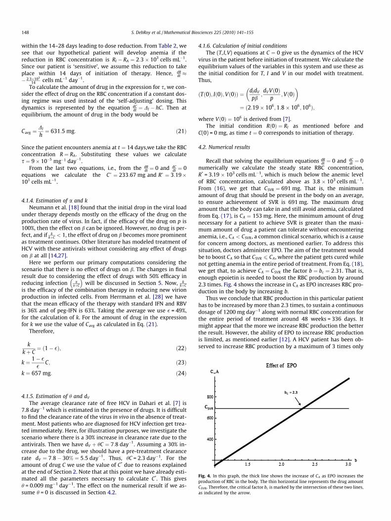
Fig. 4. In this graph, the thick line shows the increase of CA as EPO increases theproduction of RBC in the body. The thin horizontal line represents the drug amountCSVR. Therefore, the critical factor bc is marked by the intersection of these two lines,as indicated by the arrow.

4.1.5. Estimation of h and dV

The average clearance rate of free HCV in Dahari et al. [7] is7.8 day�1 which is estimated in the presence of drugs. It is difficultto find the clearance rate of the virus in vivo in the absence of treat-ment. Most patients who are diagnosed for HCV infection get trea-ted immediately. Here, for illustration purposes, we investigate thescenario where there is a 30% increase in clearance rate due to theantivirals. Then we have dV þ hC ¼ 7:8 day�1. Assuming a 30% in-crease due to the drug, we should have a pre-treatment clearancerate dV ¼ 7:8� 30% ¼ 5:5 day�1. Thus, hC = 2.3 day�1. For theamount of drug C we use the value of C* due to reasons explainedat the end of Section 2. Note that at this point we have already esti-mated all the parameters necessary to calculate C*. This givesh = 0.009 mg�1 day�1. The effect on the numerical result if we as-sume h = 0 is discussed in Section 4.2.

4.1.6. Calculation of initial conditionsThe (T, I,V) equations at C ¼ 0 give us the dynamics of the HCV

virus in the patient before initiation of treatment. We calculate theequilibrium values of the variables in this system and use these asthe initial condition for T, I and V in our model with treatment.Thus,

ðTð0Þ; Ið0Þ;Vð0ÞÞ ¼ dIdV

pb;dV Vð0Þ

p;Vð0Þ

� �¼ ð2:19� 106;1:8� 106;106Þ;

where Vð0Þ ¼ 106 is derived from [7].The initial condition Rð0Þ ¼ RI as mentioned before and

C(0) = 0 mg, as time t ¼ 0 corresponds to initiation of therapy.

4.2. Numerical results

Recall that solving the equilibrium equations dRdt ¼ 0 and dC

dt ¼ 0numerically we calculate the steady state RBC concentration,R* = 3.19 � 103 cells mL�1, which is much below the anemic levelof RBC concentration, calculated above as 3.8 � 103 cells mL�1.From (16), we get that CSVR ¼ 691 mg. That is, the minimumamount of drug that should be present in the body on an average,to ensure achievement of SVR is 691 mg. The maximum drugamount that the body can take in and still avoid anemia, calculatedfrom Eq. (17), is CA ¼ 153 mg. Here, the minimum amount of drugnecessary for a patient to achieve SVR is greater than the maxi-mum amount of drug a patient can tolerate without encounteringanemia, i.e., CA < CSVR, a common clinical scenario, which is a causefor concern among doctors, as mentioned earlier. To address thissituation, doctors administer EPO. The aim of the treatment wouldbe to boost CA so that CSVR 6 CA, where the patient gets cured whilenot getting anemia in the entire period of treatment. From Eq. (18),we get that, to achieve CA ¼ CSVR the factor b ¼ bc ¼ 2:31. That is,enough epoietin is needed to boost the RBC production by around2.3 times. Fig. 4 shows the increase in CA as EPO increases RBC pro-duction in the body by increasing b.

Thus we conclude that RBC production in this particular patienthas to be increased by more than 2.3 times, to sustain a continuousdosage of 1200 mg day�1 along with normal RBC concentration forthe entire period of treatment around 48 weeks = 336 days. Itmight appear that the more we increase RBC production the betterthe result. However, the ability of EPO to increase RBC productionis limited, as mentioned earlier [12]. A HCV patient has been ob-served to increase RBC production by a maximum of 3 times only

Fig. 6. In the above graph, we show by the bold line the dynamics of the viral load.The small dashed lines shows the behavior when only EPO enough to makeCA ¼ CSVR is given to a patient. When enough EPO to increase RBC production about1.5 times is given, we note from the dotted line that the viral load tends to re-emerge before therapy cessation although the RBC concentration is maintainedabove anemic levels (see Fig. 5). The large dashed line shows the behavior of theviral load when sufficient EPO is given to achieve b ¼ 3. We observe that the viralload has a steep decline but does not shoot back during the period of treatment of48 weeks = 336 days, and the RBC concentration is maintained at pre-treatmentlevels (see Fig. 5). However, this might be clinically undesirable.

S. DebRoy et al. / Mathematical Biosciences 225 (2010) 141–155 149

[10]. Many patients with weak immune system do not respondwell to EPO dosing, as explained in the introduction. Thus the min-imum increment necessary to endure antiviral treatment should betargeted.

We numerically solve the entire model equations (1)–(5) with-out and with epoietin at different levels, for the period of 48 weekstreatment (=336 days). For the purpose of this paper we are inter-ested in the period of treatment only, since therapy-induced hemo-lytic anemia is reversible. That is, RBC concentration shoots back tohealthy levels as soon as these antivirals are discontinued. We notein the graphs in Figs. 5 and 6, when EPO is not administered (de-noted by bold line), the RBC concentration drops below anemic lev-els. Due to that, our hypothetical dosing regimen starts decreasingthe antiviral dosing, leading to a relapse in viral load even beforethe end of the treatment period. When instead we give enoughEPO to increase the RBC production by 2.3 times (denoted by largedashed line), the viral load is significantly reduced throughout theperiod of therapy whereas the RBC concentration is maintained atnon-anemic levels throughout treatment. Note that the RBC canalso be maintained at non-anemic levels (dotted line) when a light-er dose of EPO (causing approximately 1.5 times increase in RBCproduction) is given. However, the viral load starts to relapsearound therapy cessation (336 days), resulting in unsuccessfulachievement of SVR. (In practice, relapse is more common aftertreatment stops than before.) Finally, a higher dose of EPO to in-crease RBC production by 3 times (small dashed line) can maintainthe RBC concentration at healthy pre-treatment levels, which helpsthe body sustain a higher constant concentration of the antivirals.Although this appears to be the perfect scenario, it is practically al-most impossible to increase a person’s RBC production by 3 timeswithout significant complications, as described before.

Because estimates for several model parameters are based onscant data and/or heuristic arguments, we have carried out uncer-tainty analysis on CSVR and R0 as a function of some of the inputparameters (see Fig. 7(a)). The mean estimates and ranges of theinput parameters are obtained from the literatures ([18,28]). Theparameter � (used in estimation of k and a) is assumed normallydistributed with mean 0.36 and variance 0.09 whereas parametersdV ; dI and RI are assumed uniformly distributed with mean6.20 day�1, 0.24 day�1 and 5450 cells mL�1, respectively. Distribu-

Fig. 5. In this graph, we observe the trajectories of the RBC concentration at differentlevels of EPO administration. The bold line shows the trajectory when no EPO is give,i.e., b ¼ 1. The small dashed lines show the behavior when only EPO enough to makeCA ¼ CSVR is given to a patient. When enough EPO to increase RBC production about1.5 times is given, we note from the dotted line that the RBC concentration ismaintained above anemic levels. The large dashed line shows the behavior of the statevariable when sufficient EPO is given to achieve b ¼ 3. We observe that the viral loadhas a steep decline but does not shoot back during the period of treatment of 48weeks = 336 days (see Fig. 6), and the RBC concentration is maintained at pre-treatment levels. However, this might be clinically undesirable.

tions for the rest of the input parameters ðRA; a; k; sR; s; kÞ are de-rived using model equations. The distributions for unknownparameters are obtained via a Monte-Carlo sampling procedure.Variation in k (mean = 3342 mg day�1) and CA (mean = 154 mg)are found to be negligible. On the other hand, relatively high vari-ance is found in our output variables CSVR (mean = 786 mg,SD = 153 mg) and R0 (mean = 5.03, SD = 2.01).

In order to determine which model parameter(s) may have themost effect on these critical quantities, we carried out a sensitivityanalysis on CSVR, a function of parameters k; h; sT ; b; p; dT ;

dV and dI . The local sensitivity indices (SI) are computed by normal-izing the partial derivatives of CSVR with respect to each of its param-eters. The SI suggest that the most sensitive parameter to CSVR is hfollowed by b whereas the least sensitive among its parameters isk (see Fig. 7(b)). CSVR is positively related to parameters k, sT, b andp, whereas h; dT ; dV and dI are negatively related. This implies thatincreases in the former set of parameters will result in increases inthe value of CSVR, and the reverse for the latter set of parameters.In particular, the SI are highest for h and b, which implies that it iscritical to identify the potential effects of treatment on the rates offree virus clearance and new infections of hepatocytes, neither ofwhich has been clearly documented to date. We therefore considerin the remainder of this section a few alternative scenarios involvingthese parameters.

Now, if we assume the efficacy of effect of drug on b is 50% andcompute a exactly like k, we get a equal to 631 mg. Keeping all theother parameters same we get the new CSVR = 405 mg, from Eq.(15). Then an increase in RBC production by around 1.6 times is en-ough to clear the virus and not cause anemia at the same time, i.e.,to have CA ¼ CSVR. We observe that changes in these parameter val-ues can change the results significantly and thus the necessity toconduct clinical studies to estimate the mean and range of valuesof these parameters cannot be over-emphasized.

If we assume no effect of drug on the clearance of free HCV fromthe liver, that is, h = 0, with efficacy of drug effect on b as 50% weget CSVR = 726 mg. In that case, the RBC production rate will requirean increase of 2.4 times to achieve CA ¼ CSVR.

Finally, we present in Fig. 8 an illustration of the difference be-tween administration of HCV drugs continuously or on a (discrete)daily basis. It can be seen that the amount of drug in the body

Fig. 7. Results of uncertainty and sensitivity analyses.

Fig. 8. An illustration of the drug amount in the body, RBC level, and virion count resulting from continuous (smooth curve) vs. discrete (sawtooth) daily administration ofHCV drugs during treatment. The continuous (red) curve is generated from our model. The other curve (blue) is generated from a model where the last equation is changed todCdt ¼ �hC, and an impulsive dosing regimen which is adjusted and administered daily is conducted. Note total drug administered per day remains the same for the two sets ofcurves, as do all other model parameters.

150 S. DebRoy et al. / Mathematical Biosciences 225 (2010) 141–155

under continuous dosing falls well within the sawtooth intervalresulting from discrete daily dosing.

It is useful to have an estimate of the minimum increase in RBCproduction necessary to maintain healthy RBC concentration aboveanemic levels and sufficiently reduce viral load at the same time.Choosing a responsive dosing strategy DðRÞ turns out to be pivotal,since otherwise the system would maintain the high dose irrespec-tive of the patient’s RBC level.

5. Discussion

Mathematical models have been used in the past to understanddetails of the mechanism of infection of HCV with or without treat-

ment [18]. Models by Dixit et al. [14], Neumann et al. [18] andDahari et al. [7] have estimated efficacies of antiviral peg-inter-feron by itself and in combination with ribavirin. Although thiscombination therapy is highly successful, it has been associatedwith many adverse treatment-related side effects, the most com-mon being reversible hemolytic anemia. To combat hemolytic ane-mia, many patients are prescribed the drug epoietin (EPO). EPO isthe artificially synthesized version of the hormone erythropoietinthat stimulates RBC production in the bone marrow. Our modelis extended from the immunological model in Neumann et al.[18] by adding two separate state variables to represent the RBCconcentration and drug amount in the body as dynamical systems.Analysis of the decoupled equations separately gives two critical

S. DebRoy et al. / Mathematical Biosciences 225 (2010) 141–155 151

values of drug amount: C*, the drug concentration required tomaintain the RBC population at equilibrium, and CSVR, the drugconcentration required for patient recovery. Also, the RBC concen-tration and amount of drug equation helps us to calculate anothercritical drug amount CA which is the maximum amount of drug inthe body that can avoid anemia.

If in a patient CA < CSVR, the doctors can prescribe a dosage tomaintain the equilibrium amount of drug in the interval ðCSVR;CAÞwhich will achieve SVR in the patient without encountering anemia.The clinical problem arises when in a patient this inequality is re-versed. In that case, the doctor applies EPO to boost CA by increasingthe RBC production to make CA P CSVR. The factor by which RBCneeds to be increased can be calculated from our models. Our esti-mated set of parameters presents a ‘proof of idea’ situation in whichthis factor is found to be 2.3 to achieve CA ¼ CSVR.

We also show through graphical simulations that a lower in-crease in RBC production might compromise chances of achievingSVR. Theoretically, very high doses of EPO can avoid any significantdecrease in RBC concentration throughout therapy and increasetolerability of drug thus strengthening chances of achieving SVR.However, that is not practically feasible in a majority of patients.EPO has limited capabilities to increase RBC production and comeswith its share of possible side effects. Thus the need to estimate thenecessary increase in RBC production cannot be over-emphasized.Our model provides a way to use mathematical modeling to pre-dict if a patient will encounter anemia under the prescribed dosingof IFN + RBV, or not. Further, it can estimate the increase in EPO-in-duced RBC production necessary to achieve SVR without encoun-tering anemia.

Our model has some limitations. Firstly, we are considering amean field model where the stochastic variability in the numericalvalues of parameters is not taken into account. As analyses in theprevious section illustrate, the uncertainty in the estimates ofseveral key treatment-related parameters may cause significantvariations in the threshold quantities that determine patient out-comes. The parameter values for different patients with their spe-cific strength of immune system and medical history could bevaried, and it is essential to have a comprehensive notion of howdosing should be adjusted if a parameter changes within a certainrange. Such a detailed understanding of the system, however, willrequire targeted clinical trials which can provide relevant data forfitting this model.

Second, a more detailed model could treat the two drugs, IFNand RBV, as separate state variables. Since they have differentpharmacokinetic profiles and probably different antiviral effects,it would be a more realistic representation of the scenario. How-ever, for that to be useful it is necessary to have well-establishedtheories regarding the modes of action of these drugs indepen-dently and in synergy, which is not yet available [1]. Also, the ini-tial dose of IFN and RBV for a specific patient is determined basedupon his/her body mass, liver condition, etc. In this model, this dif-ferentiation is implicit in taking the DI as 1000 mg for patients withbody mass less than 75 kg and 1200 mg for body mass greater than75 kg. The model can be made more realistic by putting in param-eters or modifying initial conditions of the differential equations totake into account the intrinsic properties of a patient. However,including this change will necessitate estimation of more drug-specific parameters, and relevant patient data will be essential.

Acknowledgments

We thank Dr. Carlos Castillo-Chavez and MTBI/SUMS for givingus this opportunity and, the National Science Foundation (DMS-0502349), National Security Agency (DOD-H982300710096), theSloan Foundation, Research Initiative for Scientific Enhancement(RISE) program (GM59429) and Arizona State University for mak-

ing this research possible. We thank Dr. Abdessamad Tridane forintroducing us to this topic. Our heartiest appreciation goes toDr. Maia Martcheva and Dr. Ben Bolker for their insightful sugges-tions. We also thank Dr. Sergei Pilyugin, Dr. Patrick DeLeenher andthe reviewers for helping us improve the paper. CMKZ and AMacknowledge the support of a Norman Hackerman Advanced Re-search Program grant. Publication of this article has been sup-ported by the NSF grant, DMS-00817789.

Appendix A

A.1. Finding equilibrium points for (R,C) system

Equating dCdt ¼ 0, we get C� ¼ kR2

hða2þR2Þ.Substituting C* into dR

dt ¼ 0, we get

0 ¼ sR � dRR� sC�R ¼ sR � dRR� skR3

hða2 þ R2Þ:

Multiplying by hða2 þ R2Þ and then dividing by h results in

FðRÞ ¼ dR þsh

k� �

R3 � sRR2 þ dRa2R� sRa2:

Next, dividing by a3 throughout, we get

dR þ s kh

� �Ra

� �3

� sR

aRa

� �2

þ dRRa

� �� sR

a¼ 0:

Again dividing throughout by sRa , we get

ðdR þ s khÞ R

a

� �3

sRa

� � � Ra

� �2

þ dRsRa

� � Ra

� �� 1 ¼ 0:

Now we rescale using r ¼ Ra ; d ¼ dR

sRað Þ ;

~a ¼ skh

sRhð Þ

. Then we get

f ðrÞ ¼ ð~aþ dÞr3 � r2 þ dr � 1 ¼ 0:

Here note f ð0Þ ¼ �1; limr!1f ðrÞ ¼ þ1 > 0 as ~aþ d > 0, and mostimportantly f ðrÞ < 0 if r 6 0 (because if r 6 0, all terms of the equa-tion will be <0).

A.2. Bifurcation analysis for (R,C) system

From the previous section, we have

f ðrÞ ¼ ð~aþ dÞr3 � r2 þ dr � 1 ¼ 0:

Now the possible cases are as follows: We know that at a bifurca-tion point, f ðrÞ ¼ 0 and f 0ðrÞ ¼ 0, since at this point the subsystemwill have two positive real roots; thus for our system

f ðrÞ ¼ 0) ~ar3 þ drðr2 þ rÞ ¼ r2 þ 1; ðA:1Þf 0ðrÞ ¼ 0) 3~ar2 þ dð3r2 þ 1Þ ¼ 2r: ðA:2Þ

This is a linear system with respect to ~a and d. Hence, we can write:

r3 r3 þ r

3r2 3r2 þ 1

" #~a

d

¼ r2 þ 1

2 r

" #:

Now, since the determinant of the coefficient matrix is non-zeroðr–0Þ, we can calculate its inverse to get

~a

d

¼ �1

2r3

� �3r2 þ 1 �r3 � r

�3 r2 r3

" #r2 þ 1

2r

" #:

Therefore,

~a ¼ �ðr2 þ 1Þ2

2r3 < 0; ðA:3Þ

d ¼ r4 þ 3r2

2r3 ¼ r2 þ 32r

> 0: ðA:4Þ

152 S. DebRoy et al. / Mathematical Biosciences 225 (2010) 141–155

Thus our bifurcation line lies in the second quadrant of the param-eter plane. However, motivated by biological reasons, our region ofinterest lies in the first quadrant where ~a > 0 and d > 0. Plugging inð~a;dÞ ¼ ð1;1Þ in f ðrÞ we get f ðrÞ ¼ 2r3 � r2 þ r � 1. In this case,f ðrÞ ¼ 0 has only one positive real root. Hence, we conclude thatwe have only one equilibrium point throughout the first quadrant.

A.3. Local stability of (R,C) system

Recall that

dRdt¼ sR � dRR� sCR;

dCdt¼ k

R2

ða2 þ R2Þ� hC:

From the previous results, we derive that

J R� ;C�ð Þ ¼�dR � sC� �sR�

2 a2kR�

a2þR�2ð Þ2�h

24 35:Since dR > 0; C� > 0; h > 0; s > 0, we have) trðJÞ ¼ �ðdR þ sC� þ hÞ< 0, and detðJÞ ¼ hðdR þ sC�Þ þ sR� 2a2R�k

a2þR�2> 0.

Therefore R�;C�ð Þ is locally asymptotically stable.

A.4. Global stability of (R,C)

According to the Poincaré–Bendixson Theorem there are threepossibilities for end behavior solutions to our system: a limit cycle,an unbounded solution or a globally stable equilibrium point. Weuse Dulac’s criterion and the Poincaré–Bendixson Theorem toprove global stability of R�;C�ð Þ which allows us to say that C(t)is asymptotically constant.

To apply Dulac’s criterion, let g ¼ 1R. Then we have

r � ðg _xÞ ¼ o

oRsR

R� dRsC

� �þ o

oCk

R

a2 þ R2 �hCR

� �¼ � sR

R2 �hR< 0:

Therefore there is no limit cycle.We observe that

dCdt

< k� hC;

so lim supt!1CðtÞ 6 kh. Likewise

dRdt

< sR � dRR;

so lim supt!1RðtÞ < sRdR

; hence the solution cannot be unboundedand by the Poincaré–Bendixson Theorem we have a globally stableequilibrium. We see that local stability has extended to globalstability.

A.5. Analysis of (T, I,V) system

Since R�;C�ð Þ is globally stable in the (R,C) system, we can applya theorem of Thieme [19] to conclude that the dynamics of the fullsystems (1)–(5) are asymptotic to those of the reduced (T, I,V) sys-tems (1)–(3) with C ¼ C�. To find the equilibria of the reduced sys-tem, we write

dTdt¼ sT � dT T � a

aþ CbTV ¼ 0; ðA:5Þ

dIdt¼ a

aþ CbTV � dII ¼ 0; ðA:6Þ

dVdt¼ p

kkþ C�

I � hCV � dV V ¼ 0: ðA:7Þ

To determine the disease free equilibrium (DFE), we let I ¼ 0and V ¼ 0 and solve dT

dt ¼ 0 for T. It is clear by inspection that theDFE is sT

dT;0; 0

� �.

A.5.1. Stability analysis of DFEFrom the previous section, we know that the DFE is ST

dT;0;0

� �;

now we will analyze the stability of the DFE. Using the Jacobianmatrix,

JðT� ;I� ;V�Þ ¼�dT � ab V

aþC 0 � abTaþC

abVaþC �dI

abTaþC

0 pkkþC �hC � dV

26643775:

Substituting sTdT; 0;0

� �for ðT�; I�;V�Þ yields

JsTdT;0;0

� � ¼ �dT 0 �ab

sTdT

ðaþCÞ

0 �dIab

stdT

ðaþCÞ

0 pkkþC �hC � dV

266664377775:

The characteristic equation is:

ð�dT � kÞ �dI � kab

sTdT

aþCpk

kþC �hC � dV � k

������������ ¼ 0:

We have that k1 ¼ �d�T ; now we consider the other sub-matrix andfind its eigenvalues.

ðdI þ kÞðhC þ dV þ kÞ �ab sT

dT

aþ C

!pk

kþ C

� �¼ 0;

k2 þ ðdI þ hC þ dV Þkþ dIðhC þ dV Þ �ab sT

dT

aþ C

!pk

kþ C

� �:

Let d ¼ dIðhC þ dV Þ �ab

sTdT

aþC

� �pk

kþC

� �. Now we apply the quadratic

formula,

k2;3 ¼�ðdI þ hC þ dV Þ �

ffiffiffiffiffiffiffiffiffiffiffiffiffiffiffiffiffiffiffiffiffiffiffiffiffiffiffiffiffiffiffiffiffiffiffiffiffiffiffiffiffiffiffiðdI þ hC þ dV Þ2 � 4d

q2

< 0:

For stability of the DFE, we want all the eigenvalues to have nega-

tive real parts. IfffiffiffiffiffiffiffiffiffiffiffiffiffiffiffiffiffiffiffiffiffiffiffiffiffiffiffiffiffiffiffiffiffiffiffiffiffiffiffiffiffiffiffiffiðdI þ hC þ dV Þ2 � 4d

qis imaginary, then we are

done as �ðdI þ hC þ dV Þ is always negative. If �ðdI þ hC þ dV Þ�ffiffiffiffiffiffiffiffiffiffiffiffiffiffiffiffiffiffiffiffiffiffiffiffiffiffiffiffiffiffiffiffiffiffiffiffiffiffiffiffiffiffiffiffiðdI þ hC þ dV Þ2 � 4d

qis real then it is negative. Thus we only con-

sider k2, and the criterion for stability of DFE is

� ðdI þ hC þ dV Þ þffiffiffiffiffiffiffiffiffiffiffiffiffiffiffiffiffiffiffiffiffiffiffiffiffiffiffiffiffiffiffiffiffiffiffiffiffiffiffiffiffiffiffiðdI þ hC þ dV Þ2 � 4d

q< 0

() ðdI þ hC þ dV Þ >ffiffiffiffiffiffiffiffiffiffiffiffiffiffiffiffiffiffiffiffiffiffiffiffiffiffiffiffiffiffiffiffiffiffiffiffiffiffiffiffiffiffiffiðdI þ hC þ dV Þ2 � 4d

q() ðdI þ hC þ dV Þ2 > ðdI þ hC þ dV Þ2 � 4d:

We can cancel out like terms from both sides, since they are bothpositive.

() � 4d < 0() d > 0

() dIðhC þ dV Þ �absT

dTðaþ CÞpk

kþ C> 0

() bR ¼ absT pkdIdTðaþ CÞðkþ CÞðhC þ dV Þ

< 1:

Thus the DFE is locally asymptotically stable if and only if bR < 1.

S. DebRoy et al. / Mathematical Biosciences 225 (2010) 141–155 153

A.5.2. Endemic equilibriumNow, we solve for the endemic equilibrium points, using

V�–0 and I�–0.

dIdt¼ a

aþ CbTV � dII ¼ 0

) I� ¼ aaþ C

bT�V�

dI;

dVdt¼ p

kkþ C

I � hCV � dV V ¼ 0;

0 ¼ pakbðkþ CÞðaþ CÞ T

�V� � hCV� � dV V�;

V�–0) T� ¼ dIðdV þ hCÞðkþ CÞðaþ CÞkapb

:

From dTdt ¼ 0, we see that

sT � dT T ¼ aaþ C

bTV ;

) V� ¼ sT

T�b aaþC

� dTðaþ CÞab

;

) V� ¼ sT kpdIðdV þ hCÞðkþ CÞ �

dTðaþ CÞba

:

Thus, the endemic equilibrium is

T�; I�;V�ð Þ ¼ dIðdV þ hCÞðkþ CÞðaþ CÞkapb

;a

aþ CbT�V�

dI;

�� sT kp

dIðdV þ hCÞðkþ CÞ �dTðaþ CÞ

ba

�: ðA:8Þ

Then simplifying using bR, the endemic equilibrium is

T� ¼ sT

dTbR ; ðA:9Þ

I� ¼ sT

dI1� 1bR� �

; ðA:10Þ

V� ¼ ðaþ CÞdT

abbR � 1

� �3: ðA:11Þ

A.5.3. Local stability of endemic equilibriumInto the Jacobian matrix,

J T� ;I� ;V�ð Þ ¼�dT � abV

aþC� 0 � baT�

aþC�

abV�

aþC� �dIabT�

aþC�

0 pkkþC� �hC� � dV

26643775;

we substitute ðT�; I�;V�Þ for definitions (A.9)–(A.11); the followingJacobian matrix results:

bJ ¼�dT � dT

bR � 1� �

� k 0 � ab sT

dTbR aþCð Þ

dTbR � 1

� ��dI � k ab sT

dT RðaþCÞ

0 pkkþC �hC � dV � k

266664377775:

From this matrix, we determine the characteristic equation:

PðkÞ ¼ � dTbR þ k

� �ðdI þ kÞ hC�dV þ kð Þ

þ dTbR þ k

� � absT pk

dTðaþ C�Þðkþ C�Þ bR � dIdT hC� þ dVð Þ bR � 1� �

:

Let q ¼ ðhC� þ dV Þ, then

PðkÞ ¼�k3þ k2 dI þdTbRþq

� �þ kdT

bRðqþdIÞ�dIdT q 1� bR� �¼ 0:

Now we apply the Routh–Hurwitz Criterion to determine stability.Let

D ¼ aaþ C

kkþ C

pbsT : ðA:12Þ

Then we can writebR ¼ DdIdT q

: ðA:13Þ

We have analyzed the disease free equilibrium to understand underwhich conditions the DFE is stable. Now our attention shifts to theendemic equilibrium since our biological interest is treatment ofchronically HCV infected individuals. Turning to the endemic equi-librium, we solve to get:

The Routh–Hurwitz criteria are now the following conditions:

1. dI þ dTbR þ q

� �> 0;

2. dIdT q bR � 1� �

> 0;

3. dI þ dTbR þ q

� �dTbRðqþ dIÞ > �dIdT q 1� bR� �

.

Given the assumed positivity of the parameters, the first conditionalways holds, and the second condition is true if and only if bR > 1. IfbR > 1 is true and condition 3 is satisfied then the endemic equilib-rium is stable. From condition 3, we have

D2 ðqþ dIÞd2

I dT q2þ D

ðqþ dIÞ2

dIdT q� 1

dT

!þ dIq > 0: ðA:14Þ

Equating the left-hand side of Eq. (A.14) to zero, we obtain tworoots, D1;2 as

D1;2 ¼� ðqþdIÞ2

dIdT q � 1dT

� ��

ffiffiffiffiffiffiffiffiffiffiffiffiffiffiffiffiffiffiffiffiffiffiffiffiffiffiffiffiffiffiffiffiffiffiffiffiffiffiffiffiffiffiffiffiffiffiffiðqþdIÞ2dIdT q � 1

dT

� �2� 4 ðqþdIÞ

dI dT q

r2 qþdI

d2I dT q2

� � : ðA:15Þ

Let

Q ¼ ðqþ dIÞ2

dIdT q� 1

dT

!2

� 4ðqþ dIÞdIdT q

: ðA:16Þ

If Q is negative, then inequality (A.14) is always satisfied. Further-

more, since 4 ðqþdIÞdIdT q is positive, if Q is positive, then � ðqþdIÞ2

dI dT q � 1dT

� �dominates the sign of the roots, making D1;2 < 0 since

ðqþ dIÞ2

dIdT q� 1

dT

!> 0;

which can be seen from the fact that

ðqþ dIÞ2

dIdT q� 1

dT

!> 0() ðq� dIÞ2 > dIq:

A.5.4. Global stability of endemic equilibrium

� � �

Observation 6. The endemic equilibrium T ; I ;Vð Þ, of the (T, I,V)system is globally asymptotically stable, when it exists (i.e., R > 1).

Proof. Let us define

f ðTÞ ¼ sT � dT T: ðA:17Þ

Then,

ðf ðTÞ � f ðT�ÞÞ 1� T�

T

� �¼�dTðT � T�Þ 1� T�

T

� �¼�dT

TðT � T�Þ2 6 0:

ðA:18Þ

154 S. DebRoy et al. / Mathematical Biosciences 225 (2010) 141–155

The above inequality holds true since T, the concentration ofhealthy hepatocytes is always positive. Recall that the endemicequilibrium is

T�; I�;V�ð Þ ¼ dIðdV þ hCÞðkþ CÞðaþ CÞkapb

;a

aþ CbT�V�

dI;

�� sT kp

dIðdV þ hCÞðkþ CÞ �dTðaþ CÞ

ba

�: ðA:19Þ

Also, at this equilibrium we get the following equalities from theequilibrium conditions:

aaþ C

bT� ¼ dIðdV þ hCÞðkþ CÞkp

; ðA:20Þ

f ðT�Þ ¼ aaþ C

bT�V� ¼ dII�; ðA:21Þ

pkkþ C

I� ¼ ðhC þ dV ÞV�: ðA:22Þ

Now, let n, g, f be chosen constants and W be the Liapunov function.

W ¼ nZ T

T�1� T�

s

� �dsþ g

Z I

I�1� I�

s

� �dsþ f

Z V

V�1� V�

s

� �ds:

Then

W 0 ¼ n 1� T�

T

� �sT � dT T � a

aþ CbTV

� �þ g 1� I�

I

� �a

aþ CbTV � dII

� �þ f 1� V�

V

� �p

kkþ C

I � hCV � dV V� �

: ðA:23Þ

Choosing f ¼ ndIkþCpk ; n ¼ g ¼ 1 and using (A.20)–(A.22) and (A.17)

simplified W0 becomes

W 0 ¼ f ðTÞ 1�T�

T

� �� a

aþCbI�

TVIþdII

� �dIIV�

VþdI

kþCpkðhCþdV ÞV�:

ðA:24Þ

Then adding and subtracting f ðT�Þ 1� T�

T

� �yields

W 0 ¼ ðf ðTÞ � f ðT�ÞÞ 1� T�

T

� �� a

aþ CbI�

TVIþ dII

�

þ f ðT�Þ 1� T�

T

� �þ dII

� � dIIV�

V: ðA:25Þ

Now using (A.21) and (A.22) we get,

W 0 ¼ ðf ðTÞ � f ðT�ÞÞ 1� T�

T

� �� dII

� T�

Tþ TVI�

T�V�Iþ V�I

VI�� 3

:

We know from construction that the first term is negative. The sec-ond term is also negative since the geometric mean of the three

non-negative terms T�

T � TVI�

T�V�I � V�IVI�

� �13 ¼ 1

� �is always less than the

arithmetic mean of those terms. Therefore, W 06 0.

We note that W 0 ¼ 0 iff both the first and the second term iszero. The second term is zero if T�

T ¼ 1 and V�IVI� ¼ 1, in which case

the first term also becomes zero. Thus the largest invariant set is

M ¼ ðT; I;VÞ� int R3þ

� �: T ¼ T� and

II�¼ V

V�

� :

Then LaSalle’s Principle [29] implies that all bounded solutions inintðR3

þÞ converge to the largest invariant set in M. Now to showthe boundedness of the system. Consider,

dðT þ IÞdt

¼ sT � dT T � dII 6 sT � d0ðT þ IÞ;

where d0 ¼minfdI; dTg.

Z TþI

T0þI0

dðT þ IÞsT � d0ðT þ IÞ 6

Z t

0dt:

Here, T0 ¼ Tð0Þ; I0 ¼ Ið0Þ; V0 ¼ Vð0Þ. Then

lnsT � d0ðT þ IÞ

sT � d0ðT0 þ I0Þ

���� ���� 6 �d0t;

I þ T 6sT

d01� e�d0T� �

þ ðI0 þ T0Þe�d0t;

lim supt!1

ðI þ TÞ 6 sT

d0:

Again,

dVdT¼ p

kkþ C

I � ðhC þ dV ÞV 6 pk

kþ CsT

d0� ðhC þ dV ÞV ;

V 6 � e�t

hCþdV

hC þ dV

pksT

ðkþ CÞd0� ðhC þ dV ÞV0

þ pksT

ðK þ CÞðhC þ dV Þd0;

lim supt!1

V 6pksT

ðK þ CÞðhC þ dV Þd0:

Hence, the (T, I,V) system has bounded solutions and it is clear thatthe largest invariant set in M is the singleton set T�; I�;V�ð Þf g. This isbecause M is a simply connected one-dimensional domain, wheresolutions are always monotone. Alternatively, using TðtÞ ¼ T� inEq. (1) (i.e., dT

dt ¼ 0) we conclude that V is constant with respect totime inside M, which in turn implies (with Eq. (2)) I is also constant.Also, the solutions starting on the boundary move into the interiorof the set except on the T-axis. Hence, the result holds for all solu-tions. Therefore, T�; I�;V�ð Þ is globally asymptotically stable. h

References

[1] J.Y.N. Lau, R.C. Tam, T.J. Liang, Z. Hong, Mechanism of action of ribavirin in thecombination treatment of chronic HCV infection, Hepatology 35 (5) (2005)1002.

[2] J.H. Hoofnagle, Course and outcome of hepatitis C, Hepatology 36 (5 Suppl. 1)(2002) S21.

[3] T. Kato, T. Date, M. Miyamoto, M. Sugiyama, Y. Tanaka, E. Orito, T. Ohno, K.Sugihara, I. Hasegawa, K. Fujiwara, K. Ito, A. Ozasa, M. Mizokami, T. Wakita,Detection of anti-hepatitis C virus effects of interferon and ribavirin by asensitive replicon system, JCM 43 (11) (2005) 5679.

[4] C. Bain, A. Fatmi, F. Zoulim, J.P. Zarski, C. Trpo, G. Inchausp, Impairedallostimulstory function of dentric cells in chronic hepatitis C infection,Gasteroenterology 120 (2) (2001) 512.

[5] V.M. Sung, S. Shimodaira, A.L. Doughty, G.R. Picchio, H. Can, T.S. Yen, K.L.Lindsay, A.M. Levine, M.M. Lai, Establishment of B-cell lymphoma cell linespersistently infected with hepatitis C virus in vivo and in vitro: the apoptoticeffects of virus infection, J. Virol. 77 (3) (2003) 2134.

[6] C. Gremion, A. Cerny, Hepatitis C virus and the immune system: a concisereview, Rev. Med. Virol. 15 (4) (2005) 235.

[7] H. Dahari, A. Loa, R.M. Ribeiro, A.S. Perelson, Modeling hepatitis C virusdynamics: liver regeneration and critical drug efficacy, J. Theor. Biol. 247(2007) 371.

[8] J.L. Dienstag, J.G. Mchutchison, American gastroenterological associationmedical position statement on the management of hepatitis C,Gastroenterology 130 (1) (2006) 225.

[9] D.B. Strader, T. Wright, D.L. Thomas, L.B. Seeff, Diagnosis, management andtreatment of hepatitis C, Hepatology 39 (4) (2004) 2004.

[10] M. Sulkowski, Anemia in the treatment of hepatitis C virus infection, CID 37(Suppl 4) (2003) S315.

[11] N. Afdhal, D.T. Dieterich, P.J. Pockros, E.R. Schiffshort, M.L. Shiffman, M.S.Sulkowski, T. Wright, Z. Younossi, B.L. Goon, K. Tang, P. Bowers, T.P.S. Group,Epoetin alpha maintains ribavirin dose in HCV-infected patients: aprospective, double-blind, randomized controlled study, Gastroenterology126 (5) (2004) 1302.

[12] University of Sciences in Philadelphia (Ed.), The Science and Practice ofPharmacy, 21st ed., Lippincott/Williams and Wilkins, Philadelphia, PA, 2006.

[13] D.T. Dieterich, R. Wasserman, N. Brau, T.I. Hassanein, E.J. Bini, P.J. Bowers, M.Mark, S. Sulkowski, Once-weekly epoetin alfa improves anemia and facilitatesmaintenance of ribavirin dosing in hepatitis C virus infected patients receivingribavirin plus interferon alfa, Am. J. Gastroenterol. 98 (11) (2003) 2491.

[14] N.M. Dixit, J.E. Layden-Almer, T.J. Layden, A.S. Perelson, Modelling howribavirin improves interferon response rates in hepatitis C virus infection,Nature 432 (2004) 922.

S. DebRoy et al. / Mathematical Biosciences 225 (2010) 141–155 155

[15] A.U. Neumann, N.P. Lam, H. Dahari, M. Davidian, T.E. Wiley, B.P. Mika, A.S.Perelson, T.J. Layden, Differences in viral dynamics between genotypes 1 and 2of hepatitis C virus, J. Infect. Dis. 182 (2000) 28.

[16] G.L. Davis, J.B. Wong, J.G. McHutchison, M.P. Manns, J. Harvey, J. Albrecht, Earlyvirologic response to treatment with peginterferon alfa-2b plus ribavirin inpatients with chronic hepatitis C, Hepatology 38 (3) (2003) 645.

[17] K.A. Powers, N.M. Dixit, R.M. Ribeiro, P. Golia, A.H. Talal, A.S. Perelson,Modeling viral and drug kinetics: hepatitis C virus treatment with pegylatedinterferon alfa-2b, Semin. Liver Dis. 23 (Suppl 1) (2003) 13.

[18] U.A. Neumann, N.P. Lam, H. Dahari, D.R. Gretch, T.E. Wiley, T.J. Layden, A.S.Perelson, Hepatitis C viral dynamics in vivo and the antiviral efficacy ofinterferon-alpha therapy, Science 282 (2) (1998) 103.

[19] H.R. Thieme, Convergence results and a Poincaré–Bendixson trichotomyfor asymptotically autonomous differential equations, J. Math. Biol. 30(1992) 763.

[20] D.S. Callaway, A.S. Perelson, HIV-1 infection and low steady state viral loads,Bull. Math. Biol. 64 (1) (2002) 29.

[21] P. DeLeenheer, S.S. Pilyugin, Multi-strain virus dynamics with mutations: aglobal analysis, Math. Med. Biol. 25 (4) (2008) 285.

[22] M. Mackey, Periodic auto-immune hemolytic anemia: an induced dynamicaldisease, Bull. Math. Biol. 41 (1979) 829.

[23] L.T. Baxter, F. Yuan, R.K. Jain, Pharmacokinetics analysis of the perivasculardistribution of bifuntional antibodies and haptens: comparison withexperimental data, Cancer Res. 52 (1992) 5838.

[24] R.C. Davis, M.K. Davies, G.Y.H. Lip, ABC of Heart Failure, second ed., Wiley–Blackwell, New York, 2007.

[25] S.L. Bricker, R.P. Langlais, C.S. Miller, Oral Diagnosis, Oral Medicine andTreatment Planning, second ed., BC Decker Inc., Ontario, Canada, 2002.

[26] S. Takaki, A. Tsubota, T. Hosaka, et al., Factors contributing to ribavirin dosereduction due to anemia during interferon alfa2b and ribavirin combinationtherapy for chronic hepatitis C, J. Gastroenterol. 39 (2004) 668.

[27] H. Dahari, R.M. Ribeiro, A.S. Perelson, Triphasic decline of hepatitis C virus RNAduring antiviral therapy, Hepatology 46 (2007) 16.

[28] E. Herrmann, J. Lee, G. Marinos, M. Modi, S. Zeuzem, Effect of ribavirin onhepatitis C viral kinetics in patients treated with pegylated interferon,Hepatology 37 (6) (2003) 1351.

[29] J.P. LaSalle, Stability theory for ordinary differential equations, J. Diff. Eqns. 4(1968) 57.