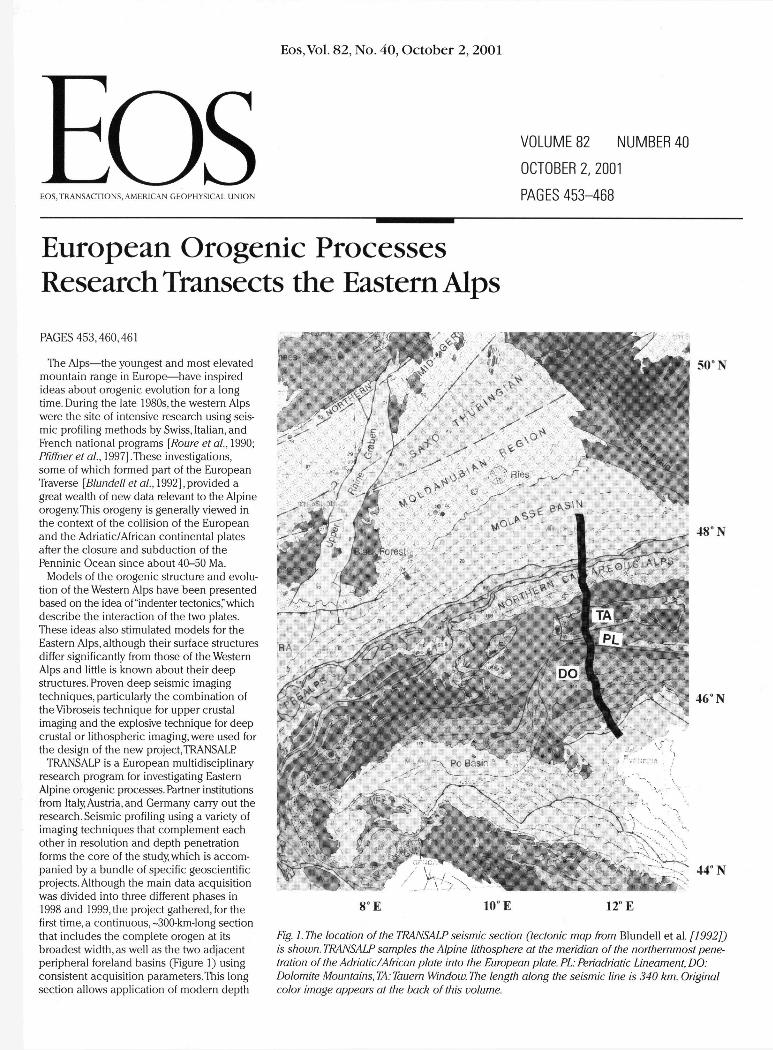
Eos, Vol. 82, No. 40, October 2, 2001

EOS, TRANSACTIONS, AMERICAN GEOPHYSICAL UNION

European Orogenic Processes Research Transects the Eastern Alps

VOLUME 82 NUMBER 40

OCTOBER 2, 2001

PAGES 453 -468

PAGES 4 5 3 , 4 6 0 , 4 6 1

The Alps—the youngest and most elevated mountain range in Europe—have inspired ideas about orogenic evolution for a long time. During the late 1980s, the western Alps were the site of intensive research using seis­mic profiling methods by Swiss, Italian, and French national programs [Rome et ai, 1990; Pfiffner et ai, 1997] .These investigations, some of which formed part of the European Traverse [Blundell et ai, 1992], provided a great wealth of new data relevant to the Alpine orogeny.This orogeny is generally viewed in the context of the collision of the European and the Adriatic/African continental plates after the closure and subduction of the Penninic Ocean since about 4 0 - 5 0 Ma.

Models of the orogenic structure and evolu­tion of the Western Alps have been presented based on the idea of "indenter tectonics," which describe the interaction of the two plates. These ideas also stimulated models for the Eastern Alps, although their surface structures differ significantly from those of the Western Alps and little is known about their deep structures. Proven deep seismic imaging techniques, particularly the combination of the Vibroseis technique for upper crustal imaging and the explosive technique for deep crustal or lithospheric imaging, were used for the design of the new project,TRANSALP

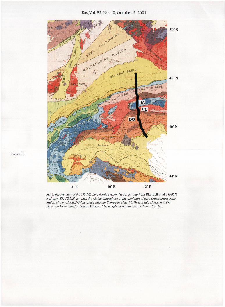
TRANSALP is a European multidisciplinary research program for investigating Eastern Alpine orogenic processes. Partner institutions from Italy, Austria, and Germany carry out the research. Seismic profiling using a variety of imaging techniques that complement each other in resolution and depth penetration forms the core of the study, which is accom­panied by a bundle of specific geoscientific projects. Although the main data acquisition was divided into three different phases in 1998 and 1999, the project gathered, for the first time, a continuous, ~300-km-long section that includes the complete orogen at its broadest width, as well as the two adjacent peripheral foreland basins (Figure 1) using consistent acquisition parameters.This long section allows application of modern depth

50° N

48° N

46° N

44° N

Fig. 1. The location of the TRANSALP seismic section (tectonic map from Blundell et al. [1992]) is shown. TRANSALP samples the Alpine lithosphere at the meridian of the northernmost pene­tration of the Adriatic/African plate into the European plate. PL: Periadriatic Lineament, DO: Dolomite Mountains, TA: Tauern Window. The length along the seismic line is 340 km. Original color image appears at the back of this volume.

N

20 i

Eos,Vol. 82, No. 40, October 2, 2001

Bavarian Molasse Northern Calcareous Alps Dolomite Mountains PL

*>pean c m t

40

60^ Km

Adriatic/African Crust

1 2 3 4 5 6 7 8 9 10 Length of Section: 320 km

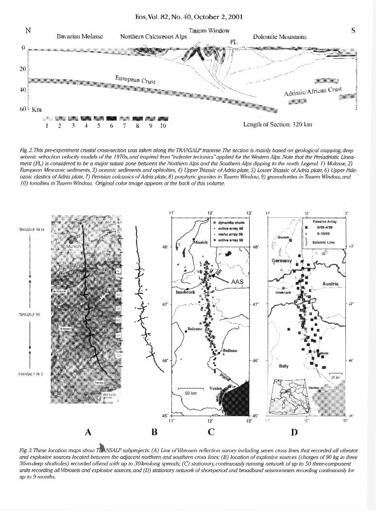
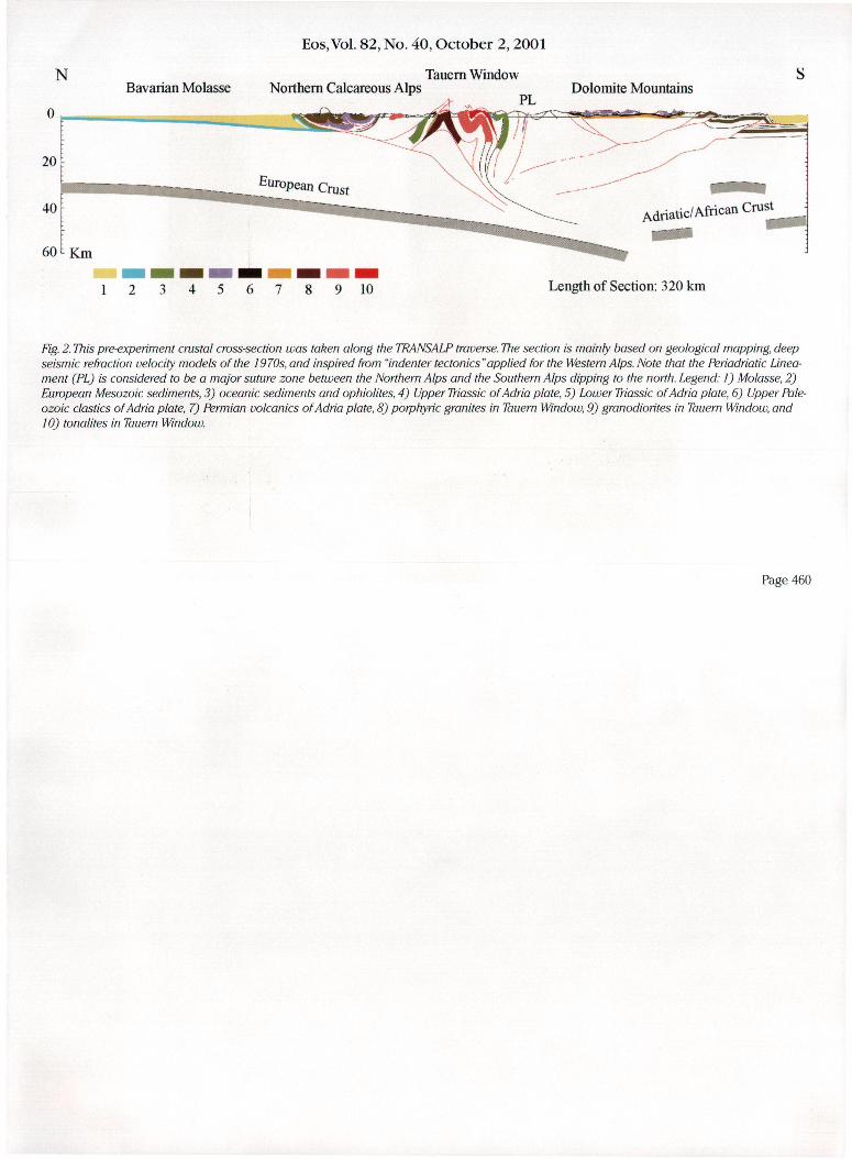
Fig. 2. This pre-experiment crustal cross-section was taken along the TRANSALP traverse. The section is mainly based on geological mapping, deep seismic refraction velocity models of the 1970s, and inspired from "indenter tectonics" applied for the Western Alps. Note that the Periadriatic Linea­ment (PL) is considered to be a major suture zone between the Northern Alps and the Southern Alps dipping to the north. Legend: 1) Molasse, 2) European Mesozoic sediments, 3) oceanic sediments and ophiolites, 4) Upper Triassic ofAdria plate, 5) Lower Triassic ofAdria plate, 6) Upper Pale­ozoic elastics ofAdria plate, 7) Permian volcanics ofAdria plate, 8) porphyric granites in Tauern Window, 9) granodiorites in Tauem Window, and 10) tonalites in Tauern Window. Original color image appears at the back of this volume.

TRANSALP 98 N

TRANSALP 98 S

B D

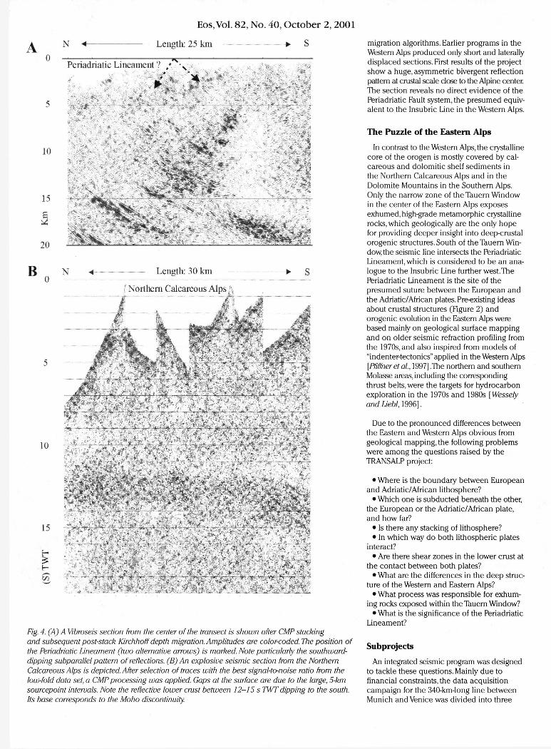
Fig. 3. These location maps show 1&NSALP subprojects: (A) Line ofVibroseis reflection survey including seven cross lines that recorded all vibrator and explosive sources located between the adjacent northern and southern cross lines; (B) location of explosive sources (charges of 90 kg in three 30-m-deep shotholes) recorded off-end with up to 30-km-long spreads; (C) stationary, continuously running network of up to 50 three-component units recording all Vibroseis and explosive sources; and (D) stationary network of short-period and broadband seismometers recording continuously for up to 9 months.

Tauem Window

Eos, Vol. 82, No. 40, October 2,2001

A N « 0

Length: 25 km

*s—

• S

Periadriatic Lineament ? / v

5

10

15

S

20

B N Length: 30 km

I Northern Calcareous Alps, \

10

mm-

-

s l y ? ^ M w m ^ f f ^ f e ^ w r ^ i

15

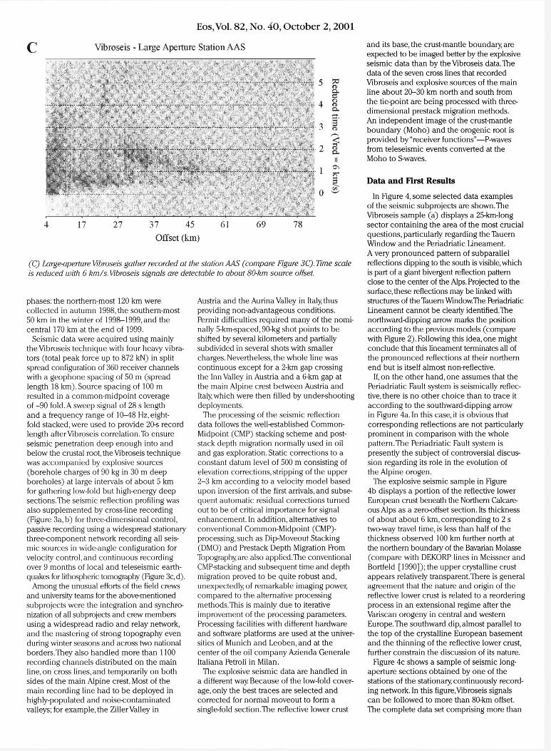
Hg. 4. £4J) ,4 Vibroseis section from the center of the transect is shown after CMP stacking and subsequent post-stack Kirchhoff depth migration. Amplitudes are color-coded. The position of the Periadriatic Lineament (two alternative arrows) is marked. Note particularly the southward-dipping subparallel pattern of reflections. (B) An explosive seismic section from the Northern Calcareous Alps is depicted. After selection of traces with the best signal-to-noise ratio from the low-fold data set, a CMP processing was applied. Gaps at the surface are due to the large, 5-km sourcepoint intervals. Note the reflective lower crust between 12-15 s TWT dipping to the south. Its base corresponds to the Moho discontinuity.

migration algorithms. Earlier programs in the Western Alps produced only short and laterally displaced sections. First results of the project show a huge, asymmetric bivergent reflection pattern at crustal scale close to the Alpine center. The section reveals no direct evidence of the Periadriatic Fault system, the presumed equiv­alent to the Insubric Line in the Western Alps.

The Puzzle of the Eastern Alps

In contrast to the Western Alps, the crystalline core of the orogen is mostly covered by cal­careous and dolomitic shelf sediments in the Northern Calcareous Alps and in the Dolomite Mountains in the Southern Alps. Only the narrow zone of the Tauern Window in the center of the Eastern Alps exposes exhumed, high-grade metamorphic crystalline rocks, which geologically are the only hope for providing deeper insight into deep-crustal orogenic structures. South of the Tauern Win­dow, the seismic line intersects the Periadriatic Lineament, which is considered to be an ana­logue to the Insubric Line further west.The Periadriatic Lineament is the site of the presumed suture between the European and the Adriatic/African plates. Pre-existing ideas about crustal structures (Figure 2 ) and orogenic evolution in the Eastern Alps were based mainly on geological surface mapping and on older seismic refraction profiling from the 1970s, and also inspired from models of "indenter-tectonics" applied in the Western Alps [Pfiffner et al., 1997] .The northern and southern Molasse areas, including the corresponding thrust belts, were the targets for hydrocarbon exploration in the 1970s and 1980s [Wessely and Liebl, 1996] .

Due to the pronounced differences between the Eastern and Western Alps obvious from geological mapping, the following problems were among the questions raised by the TRANSALP project:

• Where is the boundary between European and Adriatic/African lithosphere?

• Which one is subducted beneath the other, the European or the Adriatic/African plate, and how far?

• Is there any stacking of lithosphere? • In which way do both lithospheric plates

interact? • Are there shear zones in the lower crust at

the contact between both plates? • What are the differences in the deep struc­

ture of the Western and Eastern Alps? • What process was responsible for exhum­

ing rocks exposed within the Tauern Window? • What is the significance of the Periadriatic

Lineament?

Subprojects

An integrated seismic program was designed to tackle these questions. Mainly due to financial constraints, the data acquisition campaign for the 340-km-long line between Munich and Venice was divided into three

Eos,Vol. 82, No. 40, October 2,2001

4 17 27 37 45 61 69 78

Offset (km)

CQ Large-aperture Vibroseis gather recorded at the station AAS (compare Figure 3Q. Time scale is reduced with 6 km/s. Vibroseis signals are detectable to about 80-km source offset.

phases: the northern-most 120 km were collected in autumn 1998, the southern-most 50 km in the winter of 1998-1999, and the central 170 km at the end of 1999.

Seismic data were acquired using mainly the Vibroseis technique with four heavy vibra­tors (total peak force up to 872 kN) in split spread configuration of 360 receiver channels with a geophone spacing of 50 m (spread length 18 km).Source spacing of 100 m resulted in a common-midpoint coverage of - 9 0 fold. A sweep signal of 28 s length and a frequency range of 10-48 Hz, eight­fold stacked, were used to provide 20-s record length after Vibroseis correlation.To ensure seismic penetration deep enough into and below the crustal root, the Vibroseis technique was accompanied by explosive sources (borehole charges of 90 kg in 30 m deep boreholes) at large intervals of about 5 km for gathering low-fold but high-energy deep sections.The seismic reflection profiling was also supplemented by cross-line recording (Figure 3a, b ) for three-dimensional control, passive recording using a widespread stationary three-component network recording all seis­mic sources in wide-angle configuration for velocity control, and continuous recording over 9 months of local and teleseismic earth­quakes for lithospheric tomography (Figure 3c, d).

Among the unusual efforts of the field crews and university teams for the above-mentioned subprojects were the integration and synchro­nization of all subprojects and crew members using a widespread radio and relay network, and the mastering of strong topography even during winter seasons and across two national borders. They also handled more than 1100 recording channels distributed on the main line, on cross lines, and temporarily on both sides of the main Alpine crest. Most of the main recording line had to be deployed in highly-populated and noise-contaminated valleys; for example, the Ziller Valley in

Austria and the Aurina Valley in Italy, thus providing non-advantageous conditions. Permit difficulties required many of the nomi­nally 5-km-spaced, 90-kg shot points to be shifted by several kilometers and partially subdivided in several shots with smaller charges. Nevertheless, the whole line was continuous except for a 2-km gap crossing the Inn Valley in Austria and a 6-km gap at the main Alpine crest between Austria and Italy, which were then filled by under-shooting deployments.

The processing of the seismic reflection data follows the well-established Common-Midpoint (CMP) stacking scheme and post-stack depth migration normally used in oil and gas exploration. Static corrections to a constant datum level of 500 m consisting of elevation corrections, stripping of the upper 2 -3 km according to a velocity model based upon inversion of the first arrivals, and subse­quent automatic residual corrections turned out to be of critical importance for signal enhancement. In addition, alternatives to conventional Common-Midpoint (CMP)-processing,such as Dip-Moveout Stacking (DMO) and Prestack Depth Migration From Topography are also applied.The conventional CMP-stacking and subsequent time and depth migration proved to be quite robust and, unexpectedly, of remarkable imaging power, compared to the alternative processing methods.This is mainly due to iterative improvement of the processing parameters. Processing facilities with different hardware and software platforms are used at the univer­sities of Munich and Leoben,and at the center of the oil company Azienda Generale Italiana Petroli in Milan.

The explosive seismic data are handled in a different way Because of the low-fold cover­age, only the best traces are selected and corrected for normal moveout to form a single-fold section.The reflective lower crust

and its base, the crust-mantle boundary, are expected to be imaged better by the explosive seismic data than by the Vibroseis data. The data of the seven cross lines that recorded Vibroseis and explosive sources of the main line about 2 0 - 3 0 km north and south from the tie-point are being processed with three-dimensional prestack migration methods. An independent image of the crust-mantle boundary (Moho) and the orogenic root is provided by "receiver functions"—P-waves from teleseismic events converted at the Moho to S-waves.

Data and First Results

In Figure 4, some selected data examples of the seismic subprojects are shown.The Vibroseis sample (a ) displays a 25-km-long sector containing the area of the most crucial questions, particularly regarding the Tauern Window and the Periadriatic Lineament. A very pronounced pattern of subparallel reflections dipping to the south is visible, which is part of a giant bivergent reflection pattern close to the center of the Alps. Projected to the surface, these reflections may be linked with structures of the Tauern Window.The Periadriatic Lineament cannot be clearly identified.The northward-dipping arrow marks the position according to the previous models (compare with Figure 2 ) . Following this idea, one might conclude that this lineament terminates all of the pronounced reflections at their northern end but is itself almost non-reflective.

If, on the other hand, one assumes that the Periadriatic Fault system is seismically reflec­tive, there is no other choice than to trace it according to the southward-dipping arrow in Figure 4a. In this case, it is obvious that corresponding reflections are not particularly prominent in comparison with the whole pattern.The Periadriatic Fault system is presently the subject of controversial discus­sion regarding its role in the evolution of the Alpine orogen.

The explosive seismic sample in Figure 4b displays a portion of the reflective lower European crust beneath the Northern Calcare­ous Alps as a zero-offset section. Its thickness of about about 6 km, corresponding to 2 s two-way travel time, is less than half of the thickness observed 100 km further north at the northern boundary of the Bavarian Molasse (compare with DEKORP lines in Meissner and Bortfeld [1990]) ; the upper crystalline crust appears relatively transparent. There is general agreement that the nature and origin of the reflective lower crust is related to a reordering process in an extensional regime after the Variscan orogeny in central and western Europe. The southward dip, almost parallel to the top of the crystalline European basement and the thinning of the reflective lower crust, further constrain the discussion of its nature.

Figure 4c shows a sample of seismic long-aperture sections obtained by one of the stations of the stationary, continuously record­ing network. In this figure,Vibroseis signals can be followed to more than 80-km offset. The complete data set comprising more than

(2 Vibroseis - Large Aperture Station AAS

Eos,Vol. 82, No. 40, October 2, 2001

o O

^ °>

17 O CD < 5 0 O l L + -» CO > 1— -I—» CD _C0 Q- CD

E a: 0

0.8

0.6

0.4

0.2

0.0

-0.2

-0.4

-0.6

-0.8

. 0.4 1 1 1 1

. 0.4 CRU LSAT minus UKMO SST " 0.2

_ 0.0 \/\ tW^\, /J _ 0.0

-0.2

-0.4 1860 1880 1900 1920 1940 1960 1980 2000 f. &

-

UKMO SST (adapted from Jones et al., 2001) UKMO NMAT (adapted from Parker et al., 1995) " CRU LSAT (Jones et al., 2001)

1 . . . . 1 . . . . 1 1 . . . 1 . . . . L, _!. J ... J.

1860 1880 1900 1920 1940 Year

1960 1980 2 0 0 0

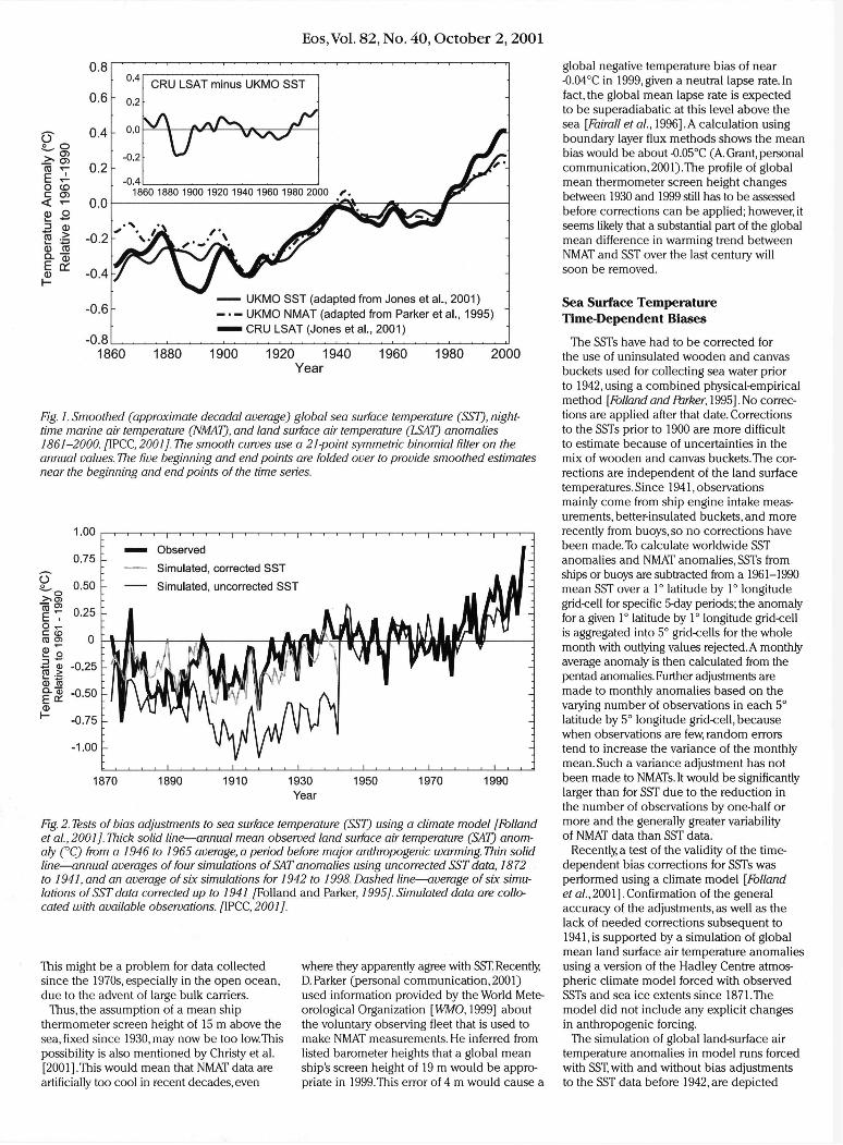
Fig. 1. Smoothed (approximate decadal average) global sea surface temperature (SST), night­time marine air temperature (NMAT), and land surface air temperature (LSAT) anomalies 1861-2000. [\?CC, 2001]. The smooth curves use a 21-point symmetric binomial filter on the annual values. The five beginning and end points are folded over to provide smoothed estimates near the beginning and end points of the time series.

1.00

0.75

£ 0.50 ~ o CO °> E . o C CD CO O)

CD

-T—>

E ^ 0 TO Q _ Q E * 0 h-

- 0.25

^ o -g <D -0.25

-0.50

-0.75

-1.00

Observed

Simulated, corrected SST

Simulated, uncorrected SST

1870 1890 1910 1930 Year

1950 1970 1990

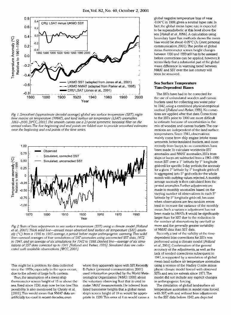
Fig. 2. Tests of bias adjustments to sea surface temperature (SST) using a climate model [Folland et ai, 2001]. Thick solid line—annual mean observed land surface air temperature (SAT) anom­aly (°C) from a 1946 to 1965 average, a period before major anthropogenic warming. Thin solid line—annual averages of four simulations of SAT anomalies using uncorrected SST data, 1872 to 1941, and an average of six simulations for 1942 to 1998. Dashed line—average of six simu­lations of SST data corrected up to 1941 /Folland and Parker, 1995]. Simulated data are collo­cated with available observations. /1PCC, 2001j.

This might be a problem for data collected since the 1970s, especially in the open ocean, due to the advent of large bulk carriers.

Thus, the assumption of a mean ship thermometer screen height of 15 m above the sea, fixed since 1930, may now be too low.This possibility is also mentioned by Christy et al. [2001].This would mean that NMAT data are artificially too cool in recent decades, even

where they apparently agree with SST. Recently D.Parker (personal communicat ion,2001) used information provided by the World Mete­orological Organization [WMO, 1999] about the voluntary observing fleet that is used to make NMAT measurements. He inferred from listed barometer heights that a global mean ship's screen height of 19 m would be appro­priate in 1999.This error of 4 m would cause a

global negative temperature bias of near -0.04°C in 1999, given a neutral lapse rate. In fact, the global mean lapse rate is expected to be superadiabatic at this level above the sea [Fairall et al., 1996].A calculation using boundary layer flux methods shows the mean bias would be about -0.05°C (A. Grant, personal communication, 2001) .The profile of global mean thermometer screen height changes between 1930 and 1999 still has to be assessed before corrections can be applied; however, it seems likely that a substantial part of the global mean difference in warming trend between NMAT and SST over the last century will soon be removed.

Sea Surface Temperature Time-Dependent Biases

The SSTs have had to be corrected for the use of uninsulated wooden and canvas buckets used for collecting sea water prior to 1942, using a combined physical-empirical method [Folland and Parker, 1995]. No correc­tions are applied after that date. Corrections to the SSTs prior to 1900 are more difficult to estimate because of uncertainties in the mix of wooden and canvas buckets. The cor­rections are independent of the land surface temperatures. Since 1941, observations mainly c o m e from ship engine intake meas­urements, better-insulated buckets, and more recently from buoys, so no corrections have been made.To calculate worldwide SST anomalies and NMAT anomalies, SSTs from ships or buoys are subtracted from a 1961-1990 mean SST over a 1° latitude by 1° longitude grid-cell for specific 5-day periods; the anomaly for a given 1° latitude by 1° longitude grid-cell is aggregated into 5° grid-cells for the whole month with outlying values rejected. A monthly average anomaly is then calculated from the pentad anomalies. Further adjustments are made to monthly anomalies based on the varying number of observations in each 5° latitude by 5° longitude grid-cell, because when observations are few, random errors tend to increase the variance of the monthly mean. Such a variance adjustment has not been made to NMATs. It would be significantly larger than for SST due to the reduction in the number of observations by one-half or more and the generally greater variability of NMAT data than SST data.

Recently, a test of the validity of the time-dependent bias corrections for SSTs was performed using a climate model [Folland et ai, 2001 ] . Confirmation of the general accuracy of the adjustments, as well as the lack of needed corrections subsequent to 1941, is supported by a simulation of global mean land surface air temperature anomalies using a version of the Hadley Centre atmos­pheric climate model forced with observed SSTs and sea ice extents s ince 1871.The model did not include any explicit changes in anthropogenic forcing.

The simulation of global land-surface air temperature anomalies in model runs forced with SST, with and without bias adjustments to the SST data before 1942, are depicted

Eos, Vol. 82, No. 40, October 2, 2001

o ° o . CD >> CD CO

E o >~ 0 O

S _ 0 _co Q - 0 E 0

CD

0

a:

UKMO SST (adapted from Jones et al., 2001) UKMO NMAT (adapted from Parker et al., 1995)

— CRU LSAT (Jones et al., 2001)

1860 1880 1900 1920 1940 Year

1960 1980 2 0 0 0

Fig. 1. Smoothed (approximate decadal average) global sea surface temperature (SST), night­time marine air temperature (NMAT), and land surface air temperature (LSAT) anomalies 1861-2000. /1PCC, 2001]. The smooth curves use a 21-point symmetric binomial filter on the annual values. The five beginning and end points are folded over to provide smoothed estimates near the beginning and end points of the time series.

1.00

0.75

E 0.50

. o 2 0.25

CO

E \ O T " C CO CO CD £ O 13 2 ^ 0 ro Q . CD

E * 0

- i o -0.25

-0.50

-0.75 -

-1.00 -

Observed

Simulated, corrected SST Simulated, uncorrected SST

1870 1890 1910 1930 Year

1950 1970 1990

Fig. 2. Tests of bias adjustments to sea surface temperature (SST) using a climate model [Folland et al, 2001]. Thick solid line—annual mean observed land surface air temperature (SAT) anom­aly (°C) from a 1946 to 1965 average, a period before major anthropogenic warming. Thin solid line—annual averages of four simulations of SAT anomalies using uncorrected SST data, 1872 to 1941, and an average of six simulations for 1942 to 1998. Dashed line—average of six simu­lations of SST data corrected up to 1941 /Folland and Parker, 1995]. Simulated data are collo­cated with available observations. /IPCC, 2001].

This might be a problem for data collected since the 1970s, especially in the open ocean, due to the advent of large bulk carriers.

Thus, the assumption of a mean ship thermometer screen height of 15 m above the sea, fixed since 1930, may now be too low.This possibility is also mentioned by Christy et al. [2001].This would mean that NMAT data are artificially too cool in recent decades, even

where they apparently agree with SST. Recently D.Parker (personal communicat ion,2001) used information provided by the World Mete­orological Organization [WMO, 1999] about the voluntary observing fleet that is used to make NMAT measurements. He inferred from listed barometer heights that a global mean ship's screen height of 19 m would be appro­priate in 1999.This error of 4 m would cause a

global negative temperature bias of near -0.04°C in 1999, given a neutral lapse rate. In fact, the global mean lapse rate is expected to be superadiabatic at this level above the sea [Fairall et ai, 1996] .A calculation using boundary layer flux methods shows the mean bias would be about -0.05°C (A. Grant, personal communication, 2001) .The profile of global mean thermometer screen height changes between 1930 and 1999 still has to be assessed before corrections can be applied; however, it seems likely that a substantial part of the global mean difference in warming trend between NMAT and SST over the last century will soon be removed.

Sea Surface Temperature Time-Dependent Biases

The SSTs have had to be corrected for the use of uninsulated wooden and canvas buckets used for collecting sea water prior to 1942, using a combined physical-empirical method [Folland and Parker, 1995]. No correc­tions are applied after that date. Corrections to the SSTs prior to 1900 are more difficult to estimate because of uncertainties in the mix of wooden and canvas buckets. The cor­rections are independent of the land surface temperatures. Since 1941, observations mainly come from ship engine intake meas­urements, better-insulated buckets, and more recently from buoys, so no corrections have been made.To calculate worldwide SST anomalies and NMAT anomalies, SSTs from ships or buoys are subtracted from a 1961-1990 mean SST over a 1° latitude by 1° longitude grid-cell for specific 5-day periods; the anomaly for a given 1° latitude by 1° longitude grid-cell is aggregated into 5° grid-cells for the whole month with outlying values rejected. A monthly average anomaly is then calculated from the pentad anomalies. Further adjustments are made to monthly anomalies based on the varying number of observations in each 5° latitude by 5° longitude grid-cell, because when observations are few, random errors tend to increase the variance of the monthly mean. Such a variance adjustment has not been made to NMATs. It would be significantly larger than for SST due to the reduction in the number of observations by one-half or more and the generally greater variability of NMAT data than SST data.

Recently, a test of the validity of the time-dependent bias corrections for SSTs was performed using a climate model [Folland et al., 2001] . Confirmation of the general accuracy of the adjustments, as well as the lack of needed corrections subsequent to 1941, is supported by a simulation of global mean land surface air temperature anomalies using a version of the Hadley Centre atmos­pheric climate model forced with observed SSTs and sea ice extents since 1871.The model did not include any explicit changes in anthropogenic forcing.

The simulation of global land-surface air temperature anomalies in model runs forced with SST, with and without bias adjustments to the SST data before 1942, are depicted

Eos, Vol. 82, No. 40, October 2, 2001

-0.6

1860 1880 1900 1920 1940 1960 1980 2000 Year

Southern Hemisphere

1860 1880 1900 1920 1940 1960 1980 2000 Year

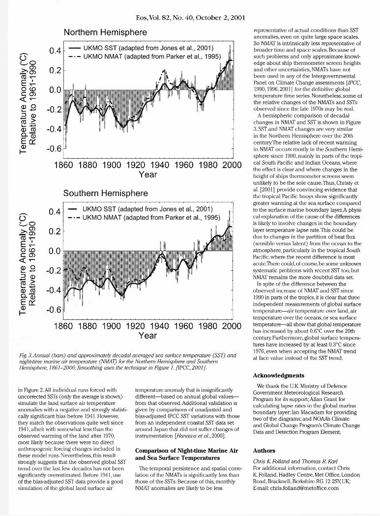
Fig. 3. Annual (bars) and approximately decadal averaged sea surface temperature (SST) and night-time marine air temperature (NMAT) for the Northern Hemisphere and Southern Hemisphere, 1861-2000. Smoothing uses the technique in Figure 1. /IPCC, 2001].

in Figure 2. All individual runs forced with uncorrected SSTs (only the average is shown) simulate the land surface air temperature anomalies with a negative and strongly statisti­cally significant bias before 1941. However, they match the observations quite well since 1941, albeit with somewhat less than the observed warming of the land after 1970, most likely because there were no direct anthropogenic forcing changes included in these model runs. Nevertheless, this result strongly suggests that the observed global SST trend over the last few decades has not been significantly overestimated. Before 1941, use of the bias-adjusted SST data provide a good simulation of the global land surface air

temperature anomaly that is insignificantly different—based on annual global values— from that observed. Additional validation is given by comparisons of unadjusted and bias-adjusted IPCC SST variations with those from an independent coastal SST data set around Japan that did not suffer changes of instrumentation [Hanawa et al., 2000] .

Comparison of Night-time Marine Air and Sea Surface Temperatures

The temporal persistence and spatial corre­lation of the NMATs is significantly less than those of the SSTs. Because of this, monthly NMAT anomalies are likely to be less

representative of actual conditions than SST anomalies, even on quite large space scales. So NMAT is intrinsically less representative of broader time and space scales. Because of such problems and only approximate knowl­edge about ship thermometer screen heights and other uncertainties, NMATs have not been used in any of the Intergovernmental Panel on Climate Change assessments [IPCC, 1990,1996,2001] for the definitive global temperature time series. Nonetheless, some of the relative changes of the NMATs and SSTs observed since the late 1970s may be real.

A hemispheric comparison of decadal changes in NMAT and SST is shown in Figure 3. SST and NMAT changes are very similar in the Northern Hemisphere over the 20th century The relative lack of recent warming in NMAT occurs mostly in the Southern Hemi­sphere since 1990, mainly in parts of the tropi­cal South Pacific and Indian Oceans, where the effect is clear and where changes in the height of ships thermometer screens seem unlikely to be the sole cause.Thus, Christy et al. [2001] provide convincing evidence that the tropical Pacific buoys show significantly greater warming at the sea surface compared to the surface marine boundary layer. A physi­cal explanation of the cause of the differences is likely to involve changes in the boundary layer temperature lapse rate.This could be due to changes in the partition of heat flux (sensible versus latent) from the ocean to the atmosphere, particularly in the tropical South Pacific, where the recent difference is most acute.There could, of course, be some unknown systematic problems with recent SST too, but NMAT remains the more doubtful data set.

In spite of the difference between the observed increase of NMAT and SST since 1990 in parts of the tropics, it is clear that three independent measurements of global surface temperature—air temperature over land, air temperature over the oceans, or sea surface temperature—all show that global temperature has increased by about 0.6°C over the 20th century Furthermore, global surface tempera­tures have increased by at least 0.3°C since 1976, even when accepting the NMAT trend at face value instead of the SST trend.

Acknowledgments

We thank the U.K. Ministry of Defence Government Meteorological Research Program for its support; Allan Grant for calculating lapse rates in the global marine boundary layer; Ian Macadam for providing two of the diagrams; and NOAAs Climate and Global Change Program's Climate Change Data and Detection Program Element.

Authors

Chris K. Folland and Thomas R. Karl For additional information, contact Chris K. Folland, Hadley Centre, Met Office, London Road, Bracknell, Berkshire RG 12 2SY UK; E-mail: chris.foIland@metoffice.com

Northern Hemisphere

Eos,Vol. 82, No. 40, October 2, 2001

References

Christy, J. R., D. E. Parker, S. J. Brown, I. Macadam, M. Stendel, and W B. Norris, Differential trends in tropical sea surface and atmospheric tempera­tures since 1979, Geophys. Res. Lett., 28,183-186, 2001.

Fairall, C. W, E. E Bradley, D. P Rogers, J. B. Edson, and G. D.Young, Bulk parameterization of air-sea fluxes for TOGA-COARE,./ Geophys. Res., 101, 3744-3764,1996.

Folland, C. K., and D. E. Parker, Correction of instru­mental biases in historical sea surface temperature data, Quart. J. R. Metorol. Soc, 121,319-367,1995.

Folland, C. K., N. Rayner, S. J. Brown,T. M. Smith, S. S. Shen, D. E. Parker, I. Macadam, RD. Jones,

R. N. Jones, N. Nicholls and D. M. H. Sexton, Global temperature change and its uncertainties since 1861, Geophys. Res. Lett., 706,2621-2624, 2001.

Hanawa, K., S.Yasunaka,T. Manabe, and N. Iwasaka, Examination of correction to historical SST data using long-term coastal SST data taken around Japan,./ Meteorol. Soc. Japan, 78,187-195,2000.

IPCC, Climate Change,The IPCC Scientific Assessment, edited by J.T. Houghton, G. J. Jenkins, and J. J. Ephraums,365 pp., Cambridge University Press, Cambridge, UK, 1990.

IPCC, Climate Change 1995: The Science of Climate Change. Contribution of Working Group I to the Second Assessment Report of the Intergovernmental Panel on Climate Change, edited by J.T. Houghton, L.

G. Meira Filho, B. A. Callander, N. Harris, A. Katten-berg,and K. Maskell, 572 pp., Cambridge University Press, Cambridge, UK, 1996.

IPCC, Climate Change 2001: The Third Assessment Report of Working Group I of the Intergovernmen­tal Panel on Climate Change, edited by J.T. Houghton,Y Ding, D. J. Griggs, M. Noguer, P van der Linden, X. Dai, K. Maskell, and C. I. Johnson, 881 pp., Cambridge University Press, Cambridge, UK, 2001.

KarlJ. R., R.W Knight, and B. Baker,The record breaking global temperatures of 1997 and 1998: Evidence for an increase in the rate of global warming?, Geophys. Res. Lett, 27,719-722,2000.

WMO, International list of selected, supplementary and auxiliary ships. Annual publication, WMO No. 47, World Meteorological Organisation, Geneva, 1999.

GIS Plays Key Role in NYC Rescue and Relief Operation

PAGE 454

New York City, Sept. 17—The posters of miss­ing loved ones are pasted onto New York City walls and street signs six days after 2 hijacked commercial airlines destroyed the World Trade Center in lower Manhattan on September 11. Several miles uptown from "ground zero," heightened security hovers around the city's Office of Emergency Management rescue and relief command center, an around-the-clock operation. Police, firefighters, military, officials with the Federal Emergency Management Agency, communications technicians, and a beehive of others work in controlled chaos in this cavernous, convention center-sized hall, lined with computers and adorned with several American flags.

After the original command center at 7 World Trade Center collapsed to rubble as an after-effect of the plane strikes, city officials scrambled to recreate it. Alan Leidner, director of New York's citywide geographic information systems (GIS), and who is with the Department of Information Technology and Telecommuni­cations, knew that maps would be an integral component of the rescue and relief efforts. Maps provide emergency workers and others with accurate and detailed scientific data in the form of visual aids upon which they can make informed decisions.

Leidner called on a number of GIS experts, including the Center for Analysis and Research of Spatial Information (CARSI) at Hunter Col­lege—part of the City University of New York (CUNY)—to assist him with mapping needs.

The center has worked with the city since 1993 to create and maintain a highly precise baseline map of the metropolitan area—called NYCMap—including the city's above-and below-ground infrastructure. Prior to the World Trade Center disaster, NYCMap already had proved its worth in mapping wetlands, and fighting the West Nile virus by developing a model space-time clustering map to help determine whether the location of crows that succumbed to the virus are or are not random.

NYCMap proved to be a key starting point and the geographic "glue" for churning out

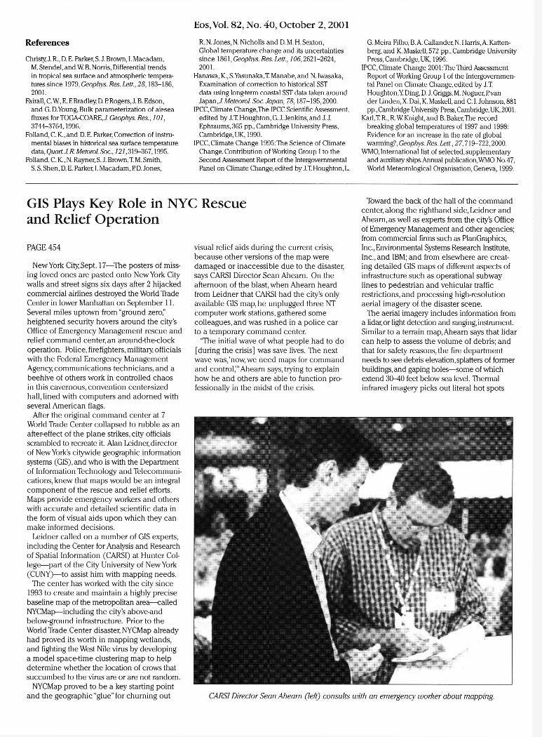
visual relief aids during the current crisis, because other versions of the map were damaged or inaccessible due to the disaster, says CARSI Director Sean Ahearn. On the afternoon of the blast, when Ahearn heard from Leidner that CARSI had the city's only available GIS map, he unplugged three NT computer work stations, gathered some colleagues, and was rushed in a police car to a temporary command center.

"The initial wave of what people had to do [during the crisis] was save lives. The next wave was,'now, we need maps for command and control,'" Ahearn says, trying to explain how he and others are able to function pro­fessionally in the midst of the crisis.

Toward the back of the hall of the command center, along the righthand side, Leidner and Ahearn, as well as experts from the city's Office of Emergency Management and other agencies; from commercial firms such as PlanGraphics, Inc., Environmental Systems Research Institute, Inc., and IBM; and from elsewhere are creat­ing detailed GIS maps of different aspects of infrastructure such as operational subway lines to pedestrian and vehicular traffic restrictions, and processing high-resolution aerial imagery of the disaster scene.

The aerial imagery includes information from a lidar,or light detection and ranging, instrument. Similar to a terrain map, Ahearn says that lidar can help to assess the volume of debris; and that for safety reasons, the fire department needs to see debris elevation, splatters of former buildings, and gaping holes—some of which extend 30-40 feet below sea level. Thermal infrared imagery picks out literal hot spots

CARSI Director Sean Ahearn (left) consults with an emergency worker about mapping.

Eos, Vol. 82, No. 40, October 2, 2001

Page 453

8°E 10° E 12° E

Fig. 1. The location of the TRANSALP seismic section (tectonic map from Blundell et al. [1992]) is shown. TRANSALP samples the Alpine lithosphere at the meridian of the northernmost pene­tration of the Adriatic/African plate into the European plate. PL: Periadriatic Lineament, DO: Dolomite Mountains, TA: Tauern Window. The length along the seismic line is 340 km.

Eos, Vol. 82, No. 40, October 2, 2001

N Tauern Window S Bavarian Molasse Northern Calcareous Alps Dolomite Mountains

1 2 3 4 5 6 7 8 9 10 Length of Section: 320 km

Fig. 2. This pre-experiment crustal cross-section was taken along the TRANSALP traverse. The section is mainly based on geological mapping, deep seismic refraction velocity models of the 1970s, and inspired from "indenter tectonics" applied for the Western Alps. Note that the Periadriatic Linea­ment (PL) is considered to be a major suture zone between the Northern Alps and the Southern Alps dipping to the north. Legend: 1) Molasse, 2) European Mesozoic sediments, 3) oceanic sediments and ophiolites, 4) Upper Triassic ofAdria plate, 5) Lower Triassic ofAdria plate, 6) Upper Pale­ozoic elastics ofAdria plate, 7) Permian volcanics ofAdria plate, 8) porphyric granites in Tauern Window, 9) granodiorites in Tauern Window, and 10) tonalites in Tauern Window.

Page 4 6 0