6th EHF Scientific Conference - European Handball Federation
Upload
khangminh22Category
view
1download
0
European Journal of Scientific Research
ISSN: 1450-216X Volume 18, No 2 September, 2007 Editor-In-chief or e Adrian M. Steinberg, Wissenschaftlicher Forscher Editorial Advisory Board e Parag Garhyan, Auburn University Morteza Shahbazi, Edinburgh University Raj Rajagopalan, National University of Singapore Sang-Eon Park, Inha University Said Elnashaie, Auburn University Subrata Chowdhury, University of Rhode Island Ghasem-Ali Omrani, Tehran University of Medical Sciences Ajay K. Ray, National University of Singapore Mutwakil Nafi, China University of Geosciences Felix Ayadi, Texas Southern University Bansi Sawhney, University of Baltimore David Wang, Hsuan Chuang University Cornelis A. Los, Kazakh-British Technical University Jatin Pancholi, Middlesex University
Teresa Smith, University of South Carolina Ranjit Biswas, Philadelphia University Chiaku Chukwuogor-Ndu, Eastern Connecticut State University John Mylonakis, Hellenic Open University (Tutor) M. Femi Ayadi, University of Houston-Clear Lake Emmanuel Anoruo, Coppin State University H. Young Baek, Nova Southeastern University Dimitrios Mavridis, Technological Educational Institure of West Macedonia Mohand-Said Oukil, Kind Fhad University of Petroleum & Minerals Jean-Luc Grosso, University of South Carolina Richard Omotoye, Virginia State University Mahdi Hadi, Kuwait University Jerry Kolo, Florida Atlantic University Leo V. Ryan, DePaul University
As of 2005, European Journal of Scientific Research is indexed in ULRICH, DOAJ and CABELL academic listings.

European Journal of Scientific Research http://www.eurojournals.com/ejsr.htm Editorial Policies: 1) European Journal of Scientific Research is an international official journal publishing high quality research papers, reviews, and short communications in the fields of biology, chemistry, physics, environmental sciences, mathematics, geology, engineering, computer science, social sciences, medicine, industrial, and all other applied and theoretical sciences. The journal welcomes submission of articles through [email protected]. 2) The journal realizes the meaning of fast publication to researchers, particularly to those working in competitive & dynamic fields. Hence, it offers an exceptionally fast publication schedule including prompt peer-review by the experts in the field and immediate publication upon acceptance. It is the major editorial policy to review the submitted articles as fast as possible and promptly include them in the forthcoming issues should they pass the evaluation process.
3) All research and reviews published in the journal have been fully peer-reviewed by two, and in some cases, three internal or external reviewers. Unless they are out of scope for the journal, or are of an unacceptably low standard of presentation, submitted articles will be sent to peer reviewers. They will generally be reviewed by two experts with the aim of reaching a first decision within a three day period. Reviewers have to sign their reports and are asked to declare any competing interests. Any suggested external peer reviewers should not have published with any of the authors of the manuscript within the past five years and should not be members of the same research institution. Suggested reviewers will be considered alongside potential reviewers identified by their publication record or recommended by Editorial Board members. Reviewers are asked whether the manuscript is scientifically sound and coherent, how interesting it is and whether the quality of the writing is acceptable. Where possible, the final decision is made on the basis that the peer reviewers are in accordance with one another, or that at least there is no strong dissenting view.
4) In cases where there is strong disagreement either among peer reviewers or between the authors and peer reviewers, advice is sought from a member of the journal's Editorial Board. The journal allows a maximum of two revisions of any manuscripts. The ultimate responsibility for any decision lies with the Editor-in-Chief. Reviewers are also asked to indicate which articles they consider to be especially interesting or significant. These articles may be given greater prominence and greater external publicity.
5) Any manuscript submitted to the journals must not already have been published in another journal or be under consideration by any other journal, although it may have been deposited on a preprint server. Manuscripts that are derived from papers presented at conferences can be submitted even if they have been published as part of the conference proceedings in a peer reviewed journal. Authors are required to ensure that no material submitted as part of a manuscript infringes existing copyrights, or the rights of a third party. Contributing authors retain copyright to their work.
6) Submission of a manuscript to EuroJournals, Inc. implies that all authors have read and agreed to its content, and that any experimental research that is reported in the manuscript has been performed with the approval of an appropriate ethics committee. Research carried out on humans must be in compliance with the Helsinki Declaration, and any experimental research on animals should follow internationally recognized guidelines. A statement to this effect must appear in the Methods section of the manuscript, including the name of the body which gave approval, with a reference number where

appropriate. Manuscripts may be rejected if the editorial office considers that the research has not been carried out within an ethical framework, e.g. if the severity of the experimental procedure is not justified by the value of the knowledge gained. Generic drug names should generally be used where appropriate. When proprietary brands are used in research, include the brand names in parentheses in the Methods section.
7) Manuscripts must be submitted by one of the authors of the manuscript, and should not be submitted by anyone on their behalf. The submitting author takes responsibility for the article during submission and peer review. To facilitate rapid publication and to minimize administrative costs, the journal accepts only online submissions through [email protected]. E-mails should clearly state the name of the article as well as full names and e-mail addresses of all the contributing authors.
8) The journal makes all published original research immediately accessible through www.EuroJournals.com without subscription charges or registration barriers. European Journal of Scientific Research indexed in ULRICH, DOAJ and CABELL academic listings. Through its open access policy, the Journal is committed permanently to maintaining this policy. All research published in the. Journal is fully peer reviewed. This process is streamlined thanks to a user-friendly, web-based system for submission and for referees to view manuscripts and return their reviews. The journal does not have page charges, color figure charges or submission fees. However, there is an article-processing and publication charge. Further information is available at: http://www.eurojournals.com/ejsr.htm © EuroJournals Publishing, Inc. 2005

European Journal of Scientific Research Volume 18, No 2 September, 2007
Contents Financial Ratios and the Probabilistic Prediction of Bank Failure in North Cyprus 191-200 Nil Gunsel Microbial and Chemical Portability of Packaged Drinking Water Sold in Kaduna, Nigeria 201-209 V. O. Ante, A.U. Shehu and K.Y. Musa An Analysis of the Locational Pattern of Some Life-Enhancing Facilities in Kaduna State, Nigeria 210-216 Isa, Umar Faruq and Ibrahim, Jaro Musa Sources of Sport Confidence of Elite Male and Female Soccer Players in Nigeria 217-222 Olufemi Adegbola Adegbesan Problématique de L’Accès à L’Eau Potable Dans la Ville de Ngaoundéré (Centre Nord-Cameroun) 223-230 Ngounou Ngatcha Benjamin, Lewa Sara and Ekodeck Georges Emmanuel Evaluation of Reservoirs as Flood Mitigation Measure in Nyando Basin, Western Kenya Using Swat 231-239 Joseph Sang, Mwangi Gatheny and George Ndegwa Anisotropy and Pressure Dependence of the Compressional Wave Velocity of Suevites from the Bosumtwi Impact Crater, Ghana 240-249 Danuor, S. K, Menyeh, A and Berckhemer, H Effects of Petroleum Hydrocarbon Pollution on the Levels of Ascorbic Acid and Dehydroascorbic Acid in Germinating Bean (Vigna Unguiculata (L) Walp) Seeds 250-254 Igbinosa O. Osamuyimen Parallel Execution of Block Runge-Kutta Methods for Solving Ordinary Differential Equations 255-266 Zailan Siri, Fudziah Ismail, Mohamad Othman and Mohamed Suleiman Experimental Investigation on Buckling Behavior of Prestressed Concrete Piles in Sand 267-276 P. Senthil Kumar, AT. Nagappan and P. Parameswaran Analgesic and Anti-Inflammatory Activities of Ethanol Seed Extract of Nigella Sativa (Black Cumin) in Mice and Rats 277-281 Tanko.Y, Mohammed A, Okasha. M.A, Shuaibu. A, Magaji. M.G and Yaro A.H The Study of Solvent Effect on the Diastereoselectivity of Diels-Alder Reaction in the Presence of Nanoporous Silica-Supported Cerium Sulfonate Catalyst 282-286 Ghodsi Mohammadi Ziarani, Alireza Badiei and Azam Miralami

Measurement of Inequality in Pakistan (Expenditure Approach) 287-297 Masood Sawar Awan, Sohail Jehangir Malik, Zakir Hussain and Haroon Sarwar Design and Operation of Multi-Media Filter 298-305 S. Bou-Hamad Training Pre-service Teacher Education on Reflective Practice in Jordanian Universities 306-331 Hani A. Weshah Development of Computer Simulation of Wavelet Selection Technique for Time-Frequency Analysis 332-337 Preety D. Swami, Mohammed Al-Fayoumi and P. Mahanti Heterosis, Inbreeding Depression and Mean Performance of Segregating Population in Upland Cotton 338-353 Naqib Ullah Khan, Gul Hassan, Moula Bux Kumbhar, Sungtaeg Kang, Ikramullah Khan, Aisha Parveen, Umm-e-Aiman and Muhammad Saeed


European Journal of Scientific Research ISSN 1450-216X Vol.18 No.2 (2007), pp.191-200 © EuroJournals Publishing, Inc. 2007 http://www.eurojournals.com/ejsr.htm
Financial Ratios and the Probabilistic Prediction of Bank
Failure in North Cyprus
Nil Gunsel Near East University, Faculty of Economics and Administrative Sciences
Banking and Finance, K.K.TC, Mersin 10/TURKEY E-mail: [email protected]
Tel: + 90 392 223 6464
Abstract
This paper provides a measure of the probability of financial institutions failure in the North Cyprus banking sector for the period of 1984-2002 using a multivariate logit model. The empirical methodology employed in this analysis allows us to identify the determinants of the likelihood of bank failure in North Cyprus. In this model, bank failure is a function of CAMELS rating system. The CAMELS approach appears to be appropriate for identifying weaknesses specific to individual banks. The empirical findings suggest that inadequate capital, poor asset quality, high interest expenses, low profitability, low liquidity and small asset size are significant variables that determine the likelihood of bank failure in North Cyprus. Keywords: North Cyprus, bank failure, CAMELS, logit model
1. Introduction The North Cyprus economy has experienced two banking sector distress periods. The first took place in 1994 and the second took place in 2000s. In 1994 two banks, namely Everest Bank Ltd. and Mediterranean Guarantee Bank Ltd., were placed under the control of the TRNC Ministry of Finance. Later, these banks had to be bailed out by the Government. The second banking distress period took place between the years 2000-2002. During these periods ten financial banks were forced by the Government of North Cyprus to suspend their operation. In 2000, five banks, namely the Cyprus Credit Bank Ltd., Cyprus Liberal Bank Ltd., Everest Bank Ltd., Kibris Yurtbank Ltd. and Cyprus Finance Bank Ltd., were put under the Saving Deposit Insurance Fund (SDIF), and then these banks were closed in the year 2001. The bankruptcy of these five banks started a serious banking crisis in North Cyprus. Another four banks, namely Cyprus Commercial Bank Ltd., Yasa Bank Ltd., Tilmo Bank Ltd. and Asia Bank Ltd., were put under the SDIF in 2001, and Cyprus Industrial Bank Ltd. was put under SDIF in 2002. Safakli (2003) states that during the failure of 10 banks economic loss in North Cyprus was around 200 trillion TL, which was almost 50 percent of the total Gross National Product (GNP). Furthermore, Finba Ltd. was taken over by Artam Bank Ltd. in 2000 and Med Bank Ltd. and Hamza Bank Ltd. were taken over by Seker Bank Ltd. in the years 2001 and 2002 respectively. The increase in the failure of commercial banks in North Cyprus increased attention on efforts to investigate the determinants of bank failure. Understanding what caused the banking sector failure in North Cyprus is the key to preventing recurrence.

Financial Ratios and the Probabilistic Prediction of Bank Failure in North Cyprus 192
The attempt in this article is to develop a model of bank failure using financial information obtained from bank balance sheets and income statements. In particular, financial ratios are used to determine the important factors that can significantly explain the changes in the internal conditions of banks. The linkage between bank-specific factors (financial ratios) and bank failure is estimated using a multivariate logit analysis, which is utilized to estimate the probability of bank failure in North Cyprus. 2. Review of the Literature Most widely used bank-specific indicators are financial ratios that are designed to measure CAMELS’s six categories of information, which basically emphasize the potential risk inherent within financial institutions. The weaknesses of banks can be apparent over time from a number of financial ratios that reflect capital inadequacy (C), excessive credit, poor loan quality or poor fund diversification (A), management inefficiency (M), lower income (E), liquidity risk (L) and small asset size (S) as reported by banks. It is theoretically and empirically proved by other studies that each of the above categories has an affect on the probability of bank failure. Sinkey (1975), Meyer and Pifer (1970), Martin (1977), Avery and Hanweck (1984), Espahbodi (1991), Thomson (1991), Persons (1999) and Rahman et al. (2004) are some of the studies employing the financial and accounting information as a ratio analysis that is mainly included in the context of CAMELS criteria. Their results show that the financial and accounting information is an efficient way of showing the characteristics of failed financial institutions and non-failed financial.
Moreover, the logit model is the most commonly employed methodology applied in the banking sector, especially in detecting potential failure risks. Martin (1977) is the first author to use the logit model to evaluate commercial bank failures in US. Following the first logit application to bank failure by Martin (1977), several relevant studies have appeared. For instance, Avery and Hanweck (1984) investigated US bank failure during the period 1979-1983. Espahbodi (1991) adopted logit analyses in the US in 1983. Thomson (1991) employed a logit model for US banks over the period of 1983-1988. In Thailand, Persons (1999) employed a multivariate logit model and predicted potential failure between 1993 and 1996. In Asia, Rahman et al. (2004) utilised the logit model and investigated the banking sector distress between 1995 and 1997. More specifically, countries such as Indonesia, South Korea and Thailand are used as a function of financial ratios. Their results reveal that the logit model is an appropriate methodology that has been utilized for bank failure predictions. 3. Sample and Data 3.1. Sample
During 1999 there were 37 surviving banks in North Cyprus. However, only 2 of these banks were of public origin and the remaining 35 were financed by the private sector. Towards the end of 2002 ten of these banks were revoked from operation, two banks were taken over by other bank, and only 25 banks remained. The original sample for this research consists of 7 failed banks, 3 taken-over banks and 13 non-failed banks. From the 14 discarded banks 6 were foreign, 2 were cooperative and the rest were small banks without complete data. To analyse the North Cyprus banking sector distress, 23 banks out of 37 in the total system were used. The failure rate between 1999 and 2002 was 32.4%. The failure rate in the selected sample was 39%, i.e. virtually the same as the rate in the universal population.
An important point to be stressed about the model is the fact that the North Cyprus banking sector is a small industry. Therefore, the number of observations included in the model is considerably small. For this reason, it is useful to use the pooled cross-section time-series data set, which allows using panel data regression procedures to consider both individual bank’s effects and time effects. Moreover, the results of the works of Gonzalez-Hermosillo et al. (1996), Heffernan (1996), Persons (1999), Brovikova (2000), Langrin (2001), Molina (2002), Yilmaz (2003), Canbas et al. (2004) and

193 Nil Gunsel
Rahman et al. (2004) provide evidence that the existence of a small number of observations can work well in bank failure estimations. 3.2. Variables
This paper defines bank failure as a situation in which banks were closed because of financial difficulties and the bank-specific variables are drawn from various financial ratios that are in the context of CAMELS criteria. Based on previous empirical analysis, a number of financial ratios appearing to provide a suitable basis for predicting bank failure in North Cyprus is tabulated in Table 1. The same table also displays a description of the selected data and expected effects on the probability of bank failure. Table 1: Definitions and Expected Signs of the Micro (Bank-Specific) Variables
Variables Definitions Expected Sign Failure Capital Adequacy Capital/Asset Total capital as a percentage of total assets - Loan/Capital Total loans as a percentage of total capital + Asset Quality Loan/Asset Total loan as a percentage of total assets + Management Quality Operating Expense/Asset Operating expense as a percentage of total assets + Interest Expense/Deposit Deposit interest expense as a percentage of total deposits + Earning Net Income/Asset Net income as a percentage of total assets - Interest Income/Asset Net-interest income as a percentage of total assets - Liquidity Liquid/Asset Liquid assets as a percentage of total assets - / + Liquid/Deposit Liquid assets as a percentage of total deposits - / + Deposit/Loan Total deposits as a percentage of total loans - / + Asset Size Asset Size (1) Total assets as a percentage of total banking sector assets - Asset Size (2) Logarithm of total assets -
Capital Adequacy (C) The first variable is the indicator of capital adequacy, defined as the ratio of total capital equity to total assets (Capital/Asset) and the ratio of total loans to total equity (Loan/Capital). The ratio of total capital equity to total assets is expected to be negatively related to the probability of failure. The higher this ratio indicates that there is sufficient capital to absorb unexpected losses (such as unexpected customers’ defaults on loans), hence the lower the probability that bank will fails. The second variable of the capital adequacy is the ratio of total loans to total equity capital. The capital equity of a bank can decline as a result of continuous losses. As loans are the riskiest assets, any increase of the value of non-performing loans may lead to a decline in bank capital. Asset Quality (A) Asset quality is one of the main risks that banks face. As loans have the highest default risk, an increasing number of non-performing loans shows a deterioration of asset quality. With worsening loan quality, non-performing loans (bad debts) are written off from the books, which reduce the value of banks. Severe deterioration in asset quality may affect the profitability and the capital of the bank and may also trigger bank failure. To measure the quality of assets the ratio of the total loans to total assets (Loan/Asset) is utilized. Again, growth in bank’s riskiest assets may concern banks underestimates of non-performing loans. Hence, a higher leverage may reflect poorer asset quality, and an increase in this ratio is expected to increase the probability of failure.

Financial Ratios and the Probabilistic Prediction of Bank Failure in North Cyprus 194
Management Quality (M) As management is a qualitative issue, such as the ability for risk taking, it is usually difficult to measure the quality of management. The management quality of a bank can be measured by operating efficiency, which constitutes cost of management and productivity of employees. The ratio of operating expense to total assets (Operating Expense/Asset) and the ratio of interest expense to total deposits (Interest Expense/Deposit) are used as a measure of the quality of management 1. Higher costs expected to be positively related with the probability of bank failure. Earning Ability (E) Earning is the most important performance measurement of banks. The ratio of net income to total assets (Net Income/Assets), which is also known as the ‘return on assets’, and the ratio of net interest income to total assets (Interest Income/Asset) is utilized to measure the profitability, of banks. It is expected that higher profitability ratios will be negatively related to the probability of failure. This implies that the higher these ratios are the lower the probability that the bank will fail. Liquidity (L) Liquidity risk measures an institution’s ability to meet unanticipated funds that are claimed by depositors. Liquidity ratios are expected to be both positively and negatively related to the likelihood of failure. On the one hand, a high ratio of liquidity may send a positive signal to the depositors that the bank is liquid and higher is the depositors’ confidence, and is therefore associated with a lower probability of failure. On the other hand, higher liquidity may also imply a weak financial investment activities (i.e. non-marketability of loans), and therefore may also be related to a higher probability of failure.
To measure the overall liquidity risk three ratios are used: the ratio of liquid assets to total assets (Liquid/Assets), the ratio of liquid assets to total deposits (Liquid/Deposits) and the ratio of total deposits to total loans (Deposit/Loan). A higher ratio of liquid assets (cash and government securities) to total assets implies a greater capacity to discharge liabilities. The second variable that represents liquidity is the ratio of liquid assets to total deposits. A bank with more liquidity can be in a better position to face unexpected deposit runs. Liquidity risk here is the risk that depositors will withdraw a large amount of their deposits and a bank will be unable to have enough liquid assets to cover these withdrawals. When the volume of liquid assets is large enough it allows banks to meet unexpected demand from creditors. The last variable that stands for liquidity risk is the ratio of total deposits to total loans that measure the deposit runs. When information becomes available to the public on the condition of banks, a transfer of funds from fragile banks to more healthy banks may indicate this ratio. Asset Size (S) The last variable is meant to serve as a proxy for the size of the bank and is measured as the ratio of bank assets to total banking sector asset value (Asset (1)) and natural logarithm of total assets (Asset (2)). Size variable is expected to have a negative influence on the probability of failure. That is, as the size of the banks increase it is less likely that they will fail and longer the survival time. Larger banks have the advantage of better access to additional financing, dealing with liquidity problems and diversifying risk. This is probably due to the fact that larger banks benefit from a ‘too large to fail’ policy and are believed to be more likely to survive than smaller banks. 4. The Econometric Methodology 4.1. The Logit Model
The bank failure is a binary event that takes the value of one when an event occurs and zero when an event does not occur. In the context of the logit model, the binary dependent variable Yit takes the
1 Molina (2002) states that: “the proxy for aggressive competition through interest rates measures the relative deposits
financial expenses, to account for the competition in attracting new customers deposit during the crisis” (Molina (2002, 39)).

195 Nil Gunsel
value of 1 if a bank fails (transferred to SDIF, closed or taken over by another bank) during the year, and 0 otherwise.
In practice, Yit* is the latent variable, which is not observable by the researcher and assumed to depend on k explanatory variables, ranging from - ∞ to ∞. The latent variable is linked to the observable Yi variable by a measurement equation.
The latent variable Yit* is linked to the observable categorical variable as follows: 1 If individual banks fail If 0* >itY
Yit = (1.1) 0 otherwise If 0* ≤itY
(see Madalla (2001, 322)) The latent variable link to the explanatory variables as follows:
ititj
k
jjit uXY ++= ∑
=10
* ββ (1.2)
Where, Yit*: Represents latent variable, and its scale can not be determined. uit: is a composite error term. βj: coefficient of j th independent variable, and measures the effects on the odds of
failure of a unit change in the corresponding independent variables. Xitj: is a vector of k number of explanatory variables in period t for bank i. (micro
variables that are in the context of CAMEL criteria). The above equation implies that the larger values of Yit* are observed as Yit=1 (i.e. failed
banks), while those with smaller values of Yit* are observed as Yit =0 (i.e. non-failed banks). In the logit model, the log-odds ratio 2 is a linear function of the explanatory variables . The
estimated multivariate logit model links the likelihood of banking problems to a set of variables.
Log ( )i
i
PP−1
= itjk
j jO X∑ =+
1ββ (1.3)
Where, Pi: represents the probability that bank i will fail. 1-Pi: represents the probability that bank i will not fail.
5. The Empirical Results The Logit Analysis
This section provides the results of the multivariate logit regression for the model of bank failure in North Cyprus. The variable selection depends on the fact that there is no high-correlation variable in the models, which ensures the accuracy of the estimated parameters and the significance levels of each variable. Overall, results suggest that bank-specific variables are important determinants of the likelihood of failure. Table 2 presents the empirical findings for the estimated multivariate logit models for five alternative specifications, which contains the results of one-year-ahead probability for the direct intervention with banks. The results are obtained from STATA 8 Software. The negative sign coefficient suggests a lower probability of bank failure and vise-versa for the positive sign coefficient. Further, the signs of the estimated coefficients are consistent with the expectations in all cases.
In this paper, assessment of the quality of model specification is based on three criteria: Pseudo R2, Model Chi-Square and Akaike’s Information Criterion (AIC). Due to sampling limitations and the 2 There are two steps for the logit transformation. Firstly, the probability is transformed into the odds (odds denotes the
likelihood of the occurrence of an event to the likelihood of the non-occurrence of an event) and the then the log of odds gives the logit. The logistic transformation ensures that there is no possibility of getting predictions of the probabilities less than 0 or greater than 1

Financial Ratios and the Probabilistic Prediction of Bank Failure in North Cyprus 196
need to preserve a degree of freedom, variables are added to or dropped from each model based on their contribution to the overall fit of the model, which is measured by pseudo R2. A close inspection of table 2 indicates that the last specification (fifth specification) has the highest Pseudo R2 (42.95), lowest chi-square (12.51), and lowest Akaike’s Information Criterion (AIC) (31.663). These findings suggest that the final specification is more robust when predicting future bank failure in North Cyprus.
The results reveal that the coefficient of the total capital equity to total assets is correctly signed and it is significant at 10% significance level for specifications (2), (3), (4) and (5). This result is consistent with Martin (1977), Avary et al. (1984), Heffernan (1996) and Yilmaz (2003), which suggests that if this variable increases, the capacity to absorb losses will also increase; hence, the probability of bank failure declines. Table 2: Logit Analysis and Determinants of Bank Intervention
Variables (1) (2) (3) (4) (5) Capital Adequacy Capital/Asset _ -0.043* -0.085* -0.055* -0.048* (0.025) (0.044) (0.030) (0.025) Loan/Capital 0.001 _ _ _ _ (0.001) Asset Quality Loan/Asset 0.012 *** 0.015*** 0.014** 0.023** 0.018*** (0.004) (0.005) (0.006) (0.010) (0.006) Management Efficiency Operating Expense/Asset _ 0.97 _ _ _ (0.625) Interest Expense/Deposit _ _ _ 0.027** _ (0.013) Earning Net Income/Asset _ _ -0.136* -0.181** -0.202*** (0.070) (0.081) (0.070) Interest Income/Asset -0.065* _ _ _ _ (0.036) Liquidity Liquid/Asset _ _ 0.030 _ _ (0.031) Liquid/Deposit -0.010 _ _ _ _ (0.015) Deposit/Loan _ -0.033** _ -0.049** -0.038*** (0.015) (0.023) (0.015) Size Asset Size (1) _ -0.74** -0.684** -1.027** -0.836** (0.305) (0.295) (0.5201) (0.347) Asset Size (2) -0.611* _ _ _ (0.358) Constant 0.882 0.43 -2.767** 0.062 0.133 (2.311) (1.07) (1.370) (0.954) (0.999) Model Statistics: Wald Chi2 38.23*** 38.11*** 13.44** 18.83*** 12.51** Pseudo R2 0.1905 0.3903 0.3756 0.3889 0.4295 Log pseudo-lik -31.40 -28.43 -29.18 -26.601 -26.663 AIC 36.40 33.43 34.18 32.601 31.663
Notes: (1) ***, **, * indicates significance at the 1, 5 and 10 percent level, respectively. (2) Standard errors are given in parentheses for the logit model. (3) Specification from 1-5 is the bank probability of intervention model.
In the specification (1), instead of the ratio of the total equity capital to total assets, the ratio of
the loans to total capital is employed as the proxy of capital adequacy. However, it seems to have no significant power. This implies that the level of capital does not seem to have been affected by the

197 Nil Gunsel
deterioration in quality of bank loan portfolios. This result is consistent with Espahbodi (1991), Persons (1999) and Langrin (2001).
The second variable measures the asset quality and it is generally associated with the leverage volume. The credit risk (portfolio risk) seems to be positively related to the probability of failure. A higher ratio may reflect poor loan quality and higher probability of failure. The reason for taking this variable is that loans are believed to be more risky than securities and cash assets that banks hold. As is illustrated in the table, for specifications (1), (2) and (5) the results indicate significance at 1%, and for specification (3) and (4) the results indicate significance at 5%. These results agree with those obtained by Avary et al. (1984), Thompson (1991) and Borovikova (2000).
The ratio of operating expense to total assets is used as a measure for quality of management. Higher costs show lower management quality; therefore, this ratio is expected to be positively related to the probability of bank failure. For specification (2) this ratio appears to be correctly signed but statistically insignificant. This result is consistent with Gonzalez-Hermosillo et al. (1996) and Borovikova (2000).
Furthermore, the ratio of interest expense to total deposits represents an aggressive competition through interest rates and it accounts for the competition in attracting new customer deposits during bank distress periods. As expected, the findings show that this ratio is positive and statistically significant at 5%. This suggests that an increase in interest expense increases the probability of failure in North Cyprus.
The fourth ratio of net income to total assets measures the earnings. This ratio is negatively related to bank failure, which means that by holding all other variables constant, an increase in the ratio of net income to total assets can be expected to decrease the probability of failure. This variable is correctly signed and statistically significant for specifications (3), (4), (5) at 10%, 5% and 1% significance levels respectively. Martin (1977), Avary et al. (1984), Thompson (1991), Heffernan (1996) and Persons (1999) also concluded that the ratio of net income to total assets is negatively related to the probability of failure. Some studies also undertake the ratio of net interest income to total assets as a measure of profitability. Specification (1) illustrates that this ratio is correctly signed and statistically significant at 10 % significance level.
A fifth type of risk is the liquidity risk, which arises because a bank issues short-term liquid liabilities to fund longer-term loans that are less liquid. The ratio of total deposits to total loans appears to be significant for specifications (2), (4) and (5) at 5% significance level. This variable is negatively related to the probability of failure. This suggests that higher liquidity indicates a high capacity to fulfill liabilities, and it is therefore associated with a lower probability of failure.
Finally, two measures of bank size were tested. These were the logarithm of total asset and the ratio of total assets of banks to total banking sector assets. These ratios have a negative sign of the coefficients, which means that larger banks experienced a lower probability of intervention when compared to smaller banks. This result is consistent with the expectation in the literature. In general, the influence of a “too big to fail” policy is cited as the reason to expect larger banks with a lower probability of intervention. With respect to the significance level of the estimated coefficients, the ratio of total assets to total banking sector assets is appears to be statistically significant at a 5% significance level for specification (2), (3), (4) and (5). Another measure of size variable (natural logarithm of total assets), illustrated in specification (1), appears to be correctly signed and statistically significant at a 10% significance level. This result is also confirmed by Thompson (1991), Heffernan (1996), Persons (1999), Borovikova (2000) and Langrin (2001). 6. Conclusions This paper basically uses a micro approach to explain the determinants of bank failure in North Cyprus. In particular, a model structure is explored by questioning the direct connections between financial ratios and the particular outcome of bank failure/closure.

Financial Ratios and the Probabilistic Prediction of Bank Failure in North Cyprus 198
According to the microeconomic results, the bank-specific determinants of bank failure suggest that low capital adequacy is one of the factors that increase the risk of bank failure in North Cyprus. As a consequence of the low level of minimum capital requirement of the Government, the banks in North Cyprus were seriously undercapitalized. Hence, the ability of banks to absorb internal and external losses was difficult. Another variable that is associated with banking sector distress is high leverage. In general, loans are perceived to be the most risky assets that banks hold. As banks were operating under a poor credit and risk management system, increase in leverage reflects poor asset quality. In particular, between the years 2001-2002 most of the debt accounts in North Cyprus are turned into non-performing loans. Results reveal that high leverage increased the probability of failure in North Cyprus. Furthermore, high interest expense, which in particularly represents aggressive competition through interest rates, increased the probability of failure. The newly-established bank was giving a very high level of deposit interest rate, which increased the unjustified competition between the banks. The findings from the profitability measure confirm that low profitability significantly increased the likelihood of failure. Liquidity ratio (total deposits as a percentage of total loans) indicates that banks in North Cyprus face unexpected deposit runs, which increases the probability of failure in North Cyprus. The last micro variable is the asset size, which suggests that larger banks experience a lower probability of failure compared to small banks. Probably, the “too big to fail” policy is cited as the reason to expect larger banks to have a lower probability of failure.
In general, the empirical findings in this paper also suggest that bank-specific variables play a significant role in explaining the probability of bank failire. Unlike Canbas et al. (2004), who claim that CAMEL criteria do not represent the specific financial characteristics of the Turkish commercial banks, the results emphasize that CAMELS components are significant in forecasting bank distress in North Cyprus. For further research in addition to the microeconomic factors, macroeconomic fundamentals can also include in the model.

199 Nil Gunsel
References [1] Altman, E. (1977), “Predicting Performance in the Saving and Loan Association Industry”,
Journal of Monetary Economics, 3, 443-466. [2] Avery, R. B. and Hanweck, G. A. (1984), “A Dynamic Analysis of Bank Failures”,
Proceedings of the 20th Annual Conference on Bank Structure and Competition, Federal Reserve Bank of Chicago, 380-395.
[3] Borovikova, V. (2000), “The Determinants of Bank Failures: the Case of Belarus”. M.A Thesis, National University, Kiev - Mohyla Academy.
[4] Canbas, S., Cabuk, A. and Kilic, S. B. (2004), “Prediction of Commercial Bank Failure via Multivariate Statistical Analysis of Financial Structures: The Turkish Case”, European Journal of Operational Research, 1-19.
[5] Espahbodi, P. (1991) “Identification of Problem Banks and Binary Choice Models”, Journal of Banking and Finance, 15, 53-71.
[6] Gonzalez-Hermosillo, B. (1999), “Determinants of Ex-Ante Banking system Distress: A Macro-Micro Empirical Exploration of Some Recent Episodes”, IMF Working Paper, 33.
[7] Heffernan, S. (1996), Modern Banking in Theory and Practice, John Wiley and Sons. [8] Kolari, J., Glennon, D., Shin, H., Caputo, M. (2002), “Predicting Large US Commercial Bank
Failure”, Journal of Economics and Business, 54, 361-387. [9] Langrin, R. B. (2001), “The Determinants of Banking System Distress: A Microeconomic and
Macroeconomic Empirical Examination of the Recent Jamaican Banking Crisis”, PhD. Thesis, The Pennsylvania State University.
[10] Maddala, G. S. (2001), Introduction to Economics, 3rd Edition, John Wiley and Sons, Ltd. [11] Martin, D. (1977), “Early Warning of Bank Failure: A Logit Regression Approach”, Journal of
Banking and Finance, 1, 249-276. [12] Molina, C. A. (2002), “Predicting Bank Failures Using a Hazard Model: The Venezuelan
Banking Crises”, Emerging Markets Review, 3, 31-50. [13] Persons, O. S. (1999), “Using Financial Information to Differentiated Failed vs. Surviving
Finance Companies in Thailand; An implication for Emerging Economies”, Multinational Finance Journal, 3, 2, 127-145.
[14] Rahman, S. Tan, L., Hew, O. and Tan, Y. (2004), “Identifying Financial Distress Indicators of Selected Banks in Asia”, Asian Economic Journal, 18, 1.
[15] Safakli, O. (2003), “Basic Problems of the Banking Sector in the T.R.N.C with Partial Emphasis on the Proactive and Reactive Strategies Applied”, Journal of Dogus University, 4, 2, 217-232.
[16] Thomson, J. B. (1991), “Predicting bank failures in the 1980”s”, Federal Reserve Bank of Cleveland, Economic Review, 27, 9–20.
[17] Whalen, G. (1991), “A Proportional Hazards Model of Bank Failure: An Examination of its Usefulness as an Early Warning Tool”, Federal Reserve Bank of Cleveland, Economic Review, 1, 21-31.
[18] Wheelock, D. C. and Wilson, P. W. (1995), “Explaining Bank Failures: Deposit Insurance, Regulation and Efficiency”, Review of Economics and Statistics, 77, 689-700.
[19] Yilmaz, R. (2003), “Bank Runs and Deposit Insurance in Developing Countries: The Case of Turkey”, PhD. Thesis, American University, Washington D. C. 20016.

Financial Ratios and the Probabilistic Prediction of Bank Failure in North Cyprus 200
List of Sample of Failed Banks and Non-Failed Banks
Surviving Banks (Non-Failed Banks) Public Banks 1.Cyprus Vakiflar Bank Ltd 2.Mediterranean Guarantee Bank Ltd. Private Banks 1. Turkish Bank Ltd. 2. Asbank Ltd. 3. Cyprus Economy Bank Ltd. 4. Rumeli Bank Ltd. 5. Kibris Altinbas Bank Ltd. 6. Denizbank Ltd. 7. Near East Bank Ltd. 8. Yesilada Bank Ltd. 9. Universal Bank Ltd. 10.Kibris Continental Bank Ltd. 11.Viyabank Ltd. Failed Banks Closure Year Problem / Failed 1. Cyprus Credit Bank Ltd 2000 Closed 2. Liberal Bank Ltd 2000 Closed 3. Everest Bank Ltd 2000 Closed 4. Cyprus Yurtbank Ltd* 2000 Closed 5. Cyprus Finance Bank Ltd 2000 Closed 6. Cyprus Commercial Bank Ltd 2001 Transfer to the SDIF 7. Industrial Bank Ltd 2002 Transfer to the SDIF 8. Finba Financial Bank Ltd 2001 Renamed as Artam Bank Ltd. 9. Med Bank 2001 Renamed as Seker Bank Ltd. 10. Hamza Bank Ltd 2002 Taken-over by Seker
Source: Central Bank of the Turkish Republic of Northern Cyprus (2002) Note: * Formerly Tunca Bank Ltd, established in 1994, and taken-over by Kibris Yurtbank Ltd. in 1999.

European Journal of Scientific Research ISSN 1450-216X Vol.18 No.2 (2007), pp.201-209 © EuroJournals Publishing, Inc. 2007 http://www.eurojournals.com/ejsr.htm
Microbial and Chemical Portability of Packaged Drinking
Water Sold in Kaduna, Nigeria
V. O. Ante General Outpatient Department Ahmadu Bello University
Teaching Hospital Zari, Nigeria E-mail: [email protected]
A.U. Shehu
Department of Community Medicine Ahmadu Bello University Zaria, Nigeria
K.Y. Musa Department of Pharmacognosy and
Drug Development Ahmadu Bello University Zaria, Nigeria
Abstract
The inadequacy both in quality and quantity of public water supply is almost endemic. Many resort to packaged water which has been reported to be of poor quality. The objective of this study is to find out the quality of this packaged water. Sixty samples were randomly picked from vendors and hawkers and subjected to chemical and bacteriological analysis as laid down in the method for examination of water and waste water by the American Public Health Association. The result showed that none of the samples met the W.H.O guideline value for drinking water. Fifty five percent (55%) of the samples however, met the National Agency for Food and Drug Administration and Control guideline value of 10 coliforms and below per 100ml of water. The chemical parameter were within the WHO and NAFDAC guidelines. NAFDAC should enforce the regulation guiding the quality of drinking water and should also aim at improving from their present guideline values to meet that of WHO. There is a need to maintain and improve the quality of drinking water from this informal sector.
Introduction John Snow, in his study 1848 – 1854, established the role of polluted drinking water in the spread of cholera. In 1956 William Budd also concluded that typhoid fever was spread by drinking water. This gave urgency to the campaigns of Edwin Chadwick to provide water, adequate in quantity and quality to the people. Next to air, water constitutes the most essential need of man. Man can survive longer without food than water. The basic physiological requirement for drinking water is estimated to be 2 litres per day (Gorcheu. and Ozolin, 1989) However; the requirement varies depending on climatic condition, standard of living and habit of the people. In short, water may be described as the vehicle for sustaining life, for drinking, cooking, flushing, washing, and personal hygiene.
Over the years, there has been relative decline in government effort to provide water supplies as shown by the decline from 7.7% of the total capital expenditure in 1955 – 1960 plan period 2.5% in 1980 – 1985 plan period. The later periods were those when greater demands were generated for water by expanded population and rising living standards, increasing urbanization as well as the demand of

Microbial and Chemical Portability of Packaged Drinking Water Sold in Kaduna, Nigeria 202
the international drinking water supply and sanitation decade 1981 –1990 (Oyebande,1977;. Babalola,1990; Oyebande,1990) Nevertheless, the hope of reaching the target of health for all, by the year 2000 and beyond is still elusive, considering the fact that safe water supply and basic sanitation, a component of Primary Health Care is still far from being achieved. As the World Health Organisation puts it in preparation for the 42nd World Health Day, “That on the eve of the 21st century, 1 billion people (including Nigerians) still lack access to safe water and 1.2 billion do not have adequate sanitation facilities. A great deal of suffering and most deaths in developing countries are traceable to lack of safe wholesome water supply (Kirkwood, 1998).
In Kaduna metropolis as a whole, pipe borne potable water is inadequate, both in quantity and quality. Consequently, water borne diseases such as diarrhoeal disease and typhoid fever often have their epidemic during the rainy season (Park, 2000).
The commonest reason of Pediatric referral from a first level health facility in Zaria was found to be due to diarrhoea disease (34%) (Adekunle, 2004). Over 80% of patients seen at the University College Hospital, Ibadan Nigeria with typhoid were between 10 –30 years with case fatality 20% to 28% (Agada, 1998). Typhoid remains a great socio-economic and health problem in Nigeria. Perforation of intestines is associated with high mortality with wound infection occurring in about 50%s – 75% of survivor. Unsafe drinking water had been the major source of this infection.
Since this health problem are traceable to unhygienic water supply, an alternative to the seemingly inadequate water supply was found in bottled water introduced into the market, it price not being within the reach of the middle and lower socio-economic class. However to meet this demand for adequate water supply at an affordable price some small scale entrepreneurs introduced small nylon sachets which contain about 500mls water and popularly called “Pure Water.” The production of packaged water has increased tremendously such that there are Eighty-six brand registered with NAFDAC as at December 2003 in Kaduna, exclusive of unregistered ones. This packaged water finds patronage from middle class and members of low socio-economic class. It is easy to serve and the price affordable, however controversies have traced the packaged water over the years of being substandard and not meeting the guidelines for drinking water (Ademoroti,1996).
It has been observed that majority of the packaged water are produced in areas of questionable hygienic environment and conditions (Aliyu, 2000). The implication of this is that, there is no guarantee that this product will meet the set standard for drinking water quality. It is therefore desirable to assess the quality of packaged water sold in Kaduna in terms of their microbial as well as some physico-chemical properties.
Water for human consumption should be free from microbial contamination, should not have chemical concentrations greater than prescribed limits, be available in sufficient quantity to enable adequate domestic hygiene and also meet standard for taste, odour and colour which should be tasteless odourless and colourless. Unfortunately, most Nigerians do not have access to such water. W.H.O. “Standard” for drinking water was changed to guideline to reflect more accurately the advisory nature of its recommendations so that they are not confused with legal standard, which are the responsibilities of appropriate authorities in member states. This authority is the Ministry of Health, through its Agency – the National Agency for Food and Drug Administration and Control (NAFDAC). World Health Organisation guidelines for pipe urban water system are strict, and usually state that water should be completely free of faecal coliforms. Standard for unprotected source are less clear. The guideline stipulates that unpiped water supply should not contain more than 10 faecal coliforms. However, the people in rural areas of Africa drink water with over 1000 faecal coliform/100mls of water (Population report,1992). Thus application of the guideline requires judgment and common sense. The usual practice of closing down factory due to some defect in water quality from these sources should be done with caution, knowing that the only alternative may be worse in terms of coliform count.
Microbiological contamination by human or animal excreta is the most common reason for water to be deemed unsafe for drinking, contamination of package water can occur at any stage of production from source through treatment to actual packaging and consumption resulting in a variety

203 V. O. Ante, A.U. Shehu and K.Y. Musa
of water borne diseases. Natural and treated waters vary in microbiological quality. The primary bacterial indicator recommended is the coliform bacteria as a whole. The coliform groups are gram negative, aerobic and facultative anaerobic, non sporing motile and non motile rods, capable of growing in the presence of bile and other surface active agents and are able to ferment lactose at 35-37ºC with production of acid and gas within 24 – 48hrs. Those that are thermo-tolerant coliform are those that ferment lactose at 44-45ºC. The typical example of faecal coliform is E. coli while the non faecal group is Klebsiella Aerogens. For practical purpose it is assumed that all coliforms are of faecal origin unless, a non-faecal origin can be proved.
Chemical contamination of water create problem of turbidity, odour and taste as well as causing hardness of water with its economic waste. However due to cost, chemical analysis shall be limited to residual chlorine only (Richard, 1989).
The aging public water works and distribution system has also contributed in no small measure to worsen the scarcity of drinking water. The need for drinking water by the teaming population has also been on the increase. Many resort to the affordable and easy to serve packaged water (Pure Water) sold in Kaduna metropolis. Controversy has traced the package water as being substandard and of a questionable quality. Particles have been reported in the packaged water sold. These products are produced at an alarming rate and mostly in unhygienic environment. Also the quest for profit has resulted in manufacturers sidelining laid down procedures for production leading to poor quality products. Results of other studies have also shown that the quality of packaged water sold is of poor quality. With this background, it is desirable to carry out a study to determine the quality of water sold to the people in Kaduna metropolis. Methodology Sampling:
The samples for this study were taken out of 86 brands of packaged water registered with NAFDAC as at December 2003. Sample Techniques: Samples were identified by numbers not brand name in order to maintain product confidentiality. Approval has been given by the appropriate authorities in the University as well as seeking NAFDAC cooperation for this work.
Sixty samples were randomly selected from vendors and hawkers of the product in the market. No particular sampling ratio was used since all the product were not found with one particular vendor/hawker Bacteriological Analysis:
Determination of Coliform Count Each pack of water was filtered through a membrane consisting of a cellulose compound with a uniform pore diameter of 0.45nm; the bacterial are retained on the surface of the membrane filter. The membrane filter was then placed in a Petri-dish containing
Mac-Conkey Agar with the grid side up and incubated at 30-35ºC for 18-24hours. The bacterial colonies were then counted and expressed as numbers of coliform per 100mls of water.
Total coliforms per 100mls = No of coliform colonies counted x 100 ml of sample filtered 1
The result is expressed as coliform per 100mls of water.
Microbial and Chemical Portability of Packaged Drinking Water Sold in Kaduna, Nigeria 204
Chemical Analysis:
Determination of pH The PH meter was standardized using a buffer solution. After standardization, the sample was poured into the tube and placed in the pH meter where the reading was taken and recorded for each sample. Determination of Turbidity
The turbidity of drinking water is a function of particulate matter. This interferes with disinfections. It also affects colour, taste and odour of water was done by using the Nephlometry .The medium was first standardized using a buffer solution, then the samples were now analysed and the result recorded in Nephlometric unit (NTU) and recorded for each sample. Determination of Total Solid: 100mls of water sample was measured into a Petri-dish. This was placed on a water bath and allowed to evaporate to dryness. The dish is then placed in an oven to further dry. This is then cooled to room temperature in desiccators and weighed.
It .is put back in an oven, dried and cooled and weighed until successive weight does not differ more than 0.1gm.
Total solid = B – A x 100 Sample use
Where B = Petri Dish with dried water sample A = Empty Petri Dish
The result expressed in mg/l Determination of Residual Chloride: The water sample was analysed for residual chlorine. Chlorine also impact salty taste depending on the chemical component of the water. Up to 250mg/litre of chlorine per litre may produce a salty taste if the predominant cation is sodium. As opposed to 1000mg/litre of chlorine without a salty taste in the presence of cations such as calcium or magnesium.
Mohr’s Method was used. This is a qualitative analysis procedure using potassium chlorate indicator and titrating with standard silver nitrate solution of 0.014 N to brownish or dirty brown precipitate. The result is expressed in mg/litres. Data Analysis
The data from the laboratory result on the samples were analysed using the computer-based software, the statistical program for social sciences (SPSS) version 11. The mean and standard deviation were used to summarize the characteristics of the packaged water in this study. Results A total of sixty samples of packaged water were analysed for coliform counts, residual chlorine, pH, total solid and Turbidity. The method adopted for sample analysis is as laid down in the standard method for the examination of water and wastewater by the American public Health Association (Adeyemo, 2002). The results are presented as Tables 1and 2. The parameters in this study are summerised by their mean and standard deviation.

205 V. O. Ante, A.U. Shehu and K.Y. Musa
Table 1: Microbial / Chemical Characteristic of Packaged Water Sold in Kaduna
Parameters Range Mode Mean / Sd Coliform Count (Per 100mls) 3 – 28 10.00 11.33 ± 5.873 PH 4.8 – 8.4 6.5 6.361 ± .832 Turbidity (Nut) 0.172 - 0.271 0.180 0.189 ± 0.25 Residual Chlorine (Mg/L) 0.10 - .60 0.05 0.41 ± .172 Total Solid (Mg/L) 0.0 – 170 10.00 73.83 ± 55.938
Table 2: Relationship between Coliform; pH, Turbidity, Residual Chlorine and Total solid
Parameters pH Turbidity Residual Chlorine Total Solids
Pearson’s correlation -0.040 0.220 0.019 0.176 Coefficient of determination (R2) 0.020 0.041 0.0004 0.031 t-value 1.077 1.570 1.102 1.613 Critical value of t at 0.05 -2.000 2.000 2.000 2.000
Discussion The result of this study support an earlier observation that packaged water produced are of poor quality (Ademoroti,, 2000; Richard, 1989). However, public water supply is inadequate both in quality and quantity, “Pure water” as it seems is an alternative to public water supply for drinking. The products are made at an alarming rate, such that they flood the markets and motor parks in this part and many part of the country. They are the product of middle class entrepreneur who know little or care very little about the quality of water they produce.
They are commonly served in most of the parties and social gathering. As useful as they are; the result of the analysis raise a lot of doubt as to it quality and thus its safety for human consumption.
Coliform bacteria are Lactose fermenting bacteria belonging to the family Enterobacteriaceae including E.coli and Klebsiella and Enteribacter species (Carter, and Wise 2004). Coliforms are easily enumerated in water and feed samples and as such serve as valuable indicator organism for contamination of water and other food - borne organism transmitted in feaces. High coliform count indicates recent or heavy contamination while low count could indicate slight pollution (Lynn, 1998). In this study all the samples had coliform count range of 3-28 cfu/100mls of water as shown in table 1 of the result with a 95% confident interval of 0.397 to 23.063 coliform per 100ml of water.
It is clear from the study that none of the packaged water therefore meets the standard (guideline) value set by the World Health Organisation for drinking water which states that “drinking water must be free from microbial contamination and the coliform count must be zero per 100mls for treated water (Pierre,1999). All the water samples analysed are therefore not safe for human consumption by W.H.O standard, these are sources of diarrhoea diseases and other health hazards.
World Health Organisation however, has not set rigid legal standards, but a guideline which every member state can modify according to their stage and level of their development in the spirit of self determination and self reliance. The regulatory body responsible for this in Nigeria is the National Agency for Food and Drugs Administration and Control (NAFDAC). The NAFDAC guideline recommends a plate count of 10 coliform per 100mls of water. The samples analysed Table 1 showed that 26 samples (44.3%) of the water samples analysed fail to meet NAFDAC guideline values of a plate count of 10 coliform and below per 100ml of water. This indicates gross contamination; hence the public is exposed to high risk of pathogenic bacterial, which are important causes of water-borne diseases such as Cholera, typhoid fever, bacillary and amoebic dysentery.
The residual chlorine content of the samples of packaged water in table 2 showed that 42 samples (70%) met both W.H.O and NAFDAC guideline value for residual Chlorine level of 0.5mg/l and above. Free residual chlorine serves to inactivate residual micro organism in treated water. From the result it will be expected that since 70% of the water met the residual chlorine level, that atleast

Microbial and Chemical Portability of Packaged Drinking Water Sold in Kaduna, Nigeria 206
70% of the water should meet the coliform count guideline, if the inactivating action of the residual chlorine is optimal. The explanation for this is that there are other factors, such as the contact time, the pH of the water, the total solid and turbidity of the water. This is supported by a study to evaluate the inactivating power of residual chlorine in two-treatment plants and distribution system. Except for E.coli microorganisms remain relatively unaffected from the distribution system tested. Thermo-tolerance coliforms were inactivated only when water obtained from site very closed to the treatment plant and contained a higher residual chlorine concentration. Clostridium perfringes were barely inactivated. The result of the study suggested that the maintenance of a free residual chlorine concentration in a distribution system does not provide a significant inactivation of pathogens and could even mask event of contamination of the distribution system and thus provide a false sense of safety with little active protection of public health (Pierre, 1999)In another study, system that maintain free chlorine level of less than 5gramms per Litre add substantially more coliforms than systems that maintain higher disinfectant residua chlorine (Norton and Lecchevallier 1996.)
The recommended PH range for drinking water is 6.5 –8.5. Thirty three samples (55. %) had pH below 6.5 as shown in table 1. A low pH encourages corrosion of pipe while a PH above 7 requires more chlorine and more contact time for proper disinfections. Even though pH has no direct effect on health its indirect action on physiological process cannot be over emphasised. As pH increase water coliform count decreases in a study. The range of water pH observed in the study was from 6.6 to 9.7 decrease coliform level in alkaline water samples suggest that maintaining a higher pH may help control coliform level, but no relationship has been identified between water pH and the presence of E.coli in water(Sargeant,2004).
The turbidity of packaged drinking water ranges from .172 NTU to .271 NTU table 1. This is in keeping with W.H.O recommendation and NAFDAC guideline of less than 5 NTU. This was fulfilled by all the water samples analysed, it should be noted that high turbidity affect disinfections by chlorine requiring a longer contact time and increase the quantity of chlorine require for disinfections.
Total solid are a measure of dissolved and suspended solid in the water. Dissolved solids include calcium, chlorides, nitrates, phosphorus iron, sulphur and other ions. Suspended solids includes silt and clay as well as plankton algae, bacteria small inorganic debris and other small particulate matter(Michael et al ,2005). The total solid ranged from 0 –170mg/l as against a value of 500mg/l (table 1) thus 60 samples (100%) had total solid that is lower than the recommended value. High total solid interferes with disinfections of water. Filtration which slows down production process but reduces the total solid is one step in water purification, which some “get rich quick”, manufacturers of this product will want avoid thus increasing the total solid as well as increasing the demand for chlorine during disinfection.
The coefficient of correlation was calculated for this purpose. In previous study there are some relationship between the pH, total solid and coliform count (Lecheralleir et al 1996) there are some measure of relationship between the coliform count and the other variables as shown in table 1. The measure of strength of relationship between the variable and the coliform count is provided by the coefficient of correlation denoted by (R). This is sometime referred to as coefficient of linear correlation or pearson’s product movement correlation. In this study the numerical value will vary small being .140 for pH .202 for turbidity .019 for residual chlorine and .176 for total solid. The greater the numerical value of (R) the stronger the relationship between the variables. The coefficient of determinants (R2) has a readily understandable interpretation in terms of strength of a relationship. In this study the values of R2 were 0.020 for PH and 0.041 for turbidity, 0.0004 for residual chlorine and 0.031 for total solid. These translate to 2% for pH, 4.1% for turbidity, 0.04% for residual chlorine and 3.1% for total solid. This means that 2% of the variation in coliform count is explained by the variation in pH. Four percent (4%) of the variation in coliform count is explained by the variation in turbidity, chlorine and total solid are 0.04% and 3.1% respectively. The t test showed that the critical value of t was higher than the calculated t value for each of the variables and therefore were not significant. This is in keeping with full -scale studies of factors related to coliform re-growth in drinking water. The study concluded that the occurrence of coliform bacteria within a distribution system is dependent

207 V. O. Ante, A.U. Shehu and K.Y. Musa
upon a complex interaction of chemical, physical, operational and engineering parameters. No one factor could account for all the coliform occurrences and one must consider all the parameters in devising a solution to the re-growth problem (Lecheralleir, 1996).
From the results so far, the packaged water sold in Kaduna does not meet the W.H.O guideline values however some of the water met NAFDAC guideline value. There could be a sustained reduction in diarrhoea morbidity with improvement in quality of water and if facilities for sanitation and waste disposal are improved (WH O, 1992)
The result of this study is in conformity with earlier findings i.e. gross contamination of packaged water with coliform ranging from 4 to 58 coliform per 100mls of water, in the Zaria study.
In a similar study in Ilorin (Nigeria) there was also gross contamination, Pseudomonas being the most frequently recovered organism. Bacteriological quality of food and water given to some children was shown to have a count of 1.67 to 6.53 ± 1.15 0.81 logs 10. Water from vending machine are not spared from contamination as shown in a study the result of which showed that 23% of the water collected has P. aeroginosa as contaminant. Gross contamination of domestic water supply with faecal coliform ranges from 0 – 216/100mls as also been reported of water. In a well water study 69% of the samples had more than 2400 coliform per 100mls of water (NAFDAC: 2002. In the same studies the average distance of well to latrine varied from 1.8 metres to 16.5 metres, which is less than 30 metres recommended by W.H.O. Since the underground water is so heavily contaminated it is not surprising that most of our packaged water though much improved does not meet the W.H.O recommended standard. Proper labelling of the product was completely missing; there were no batch numbers, manufacturing or expiration date. Batch numbering enable eay withdrawal of a product from the market and also makes it easy to alert the public and prevent the common practice of closing down a factory where other batches of the same product must have met the guideline. Conclusion From the above study it can be concluded that packaged water sold in Kaduna metropolis does not meet the W.H.O and NAFDAC guidelines for safe wholesome water.

Microbial and Chemical Portability of Packaged Drinking Water Sold in Kaduna, Nigeria 208
References [1] Ademoroti, CMA(1996), Mini Water Development in Ibadan. Environmental Chemistry and
Toxicology. 1st edition; Foludor Press Ibadan Nigeria 90. [2] Adekunle L.V, Schridar M.K.C, Ajayi A.A, Oluwade P.A, Olawuyi, J.F(2004). An assessment
of the Health and socio/Economic implications of sachet water in Ibadan, Nigeria; A Public Health Challenges. African Journal of Biomedical Research; 7, 5-8.
[3] Adeyemo O.K, Ayodeji 10, and Aiki-Raji C.O(2002). The water quality and sanitary conditions in a major abattoir (Bodija) in Ibadan Nigeria, African Journal of Biomedical Research; 5 51-55
[4] Agada. O.A (1998), Result of baseline studies on water supply and sanitation conducted by Federal Ministry of Water Resources and rural development. Nigeria, UNICEF assisted National water supply and sanitation monitoring programme- an overview FGN, UNICEF, WEB Review meeting February; 1 - 14
[5] Aliyu A.A (2000) How pure is Pure Water. A microbial /chemical analysis. MPH thesis. September
[6] Babalola J.O(1990), Coping with water supply demands and growth in the 1990’s Journal of Nigerian Association of Hydrogeologist October; 2(1) 26 – 31.
[7] Carter G.R, and D.J Wise (2004) Essentials of Veterinary bacteriology and mycology, Iowa State University Press, Ames,
[8] Gorcheu. HG and Ozolins G(1989). Guidelines for drinking water quality, W.H.O Chronicle.; 38 (3) 104 – 109
[9] Kirkwood Andrew(1998), safe water for Africa, African Health, September;9–10 [10] Lecheralleir MW , NJ Welch and DB Smith (1996). Full-Scale study of factors related to
coliform re-growth in drinking water, Applied and Environmental Microbiology. 1 (62) 7 2201 - 2211
[11] Lynn T.V. D.D. Hancock., T.E. Besser., J.H. Harrison, D.H. Rice., N.T., Stewarts., and L.L Rowan., The occurance and replication of Escherichia Coli in cattle feeds. Journal of Diary Science 81: 1998. 1102 - 1108
[12] Michael W. Sanderson; Jan M. Sergeant, David G. Renter., D. Dee Griffin and Robert A. Smith(2005). Factors of coliform in the feed and water of feedlot cattle. Applied and Environmental Microbiology Oct., (71) 10 6026- 6032
[13] MW Lecheralleir, NJ Welch and DB Smith(1996. Full-Scale study of factors related to coliform re-growth in drinking water, Applied and Environmental Microbiology. Aug (62) 7 2201 - 2211
[14] NAFDAC: 2002 Guideline for Registration of packaged water in Nigeria. National Agency for Food and Drug Administration Control. 21-5
[15] Norton C.D., Lecchevallier M.W. A Pilot study of Bacteriology population change through potable water treatment and distribution. Applied Environmental Microbiology 66; 268-278.
[16] Oyebande L(1977). An inventory of Urban Water Supply Resource Development in Nigeria. Hydrological Report Federal Ministry of Water Resources, Lagos 1; 107
[17] Oyebande Lekan(1990) Water Supply need in the and strategies for satisfying them. Journal of the Nigerian Association of Hydrologist Oct. 1990; 2 (1) 14 – 25.
[18] Park, K(2000). Man and Medicine: Towards Health For All, In Park’s textbook of Preventive and Social Medicine 17th edition B. Bhanot Jabalpur; 1-11.
[19] Pierre Payment (1999): Poor efficiency of residual chlorine disinfectant in drinking water to inactivate water-borne pathogen in distribution systems. Canadian J. Microbiology/ Review of Canada microbiology 45(8) :, 709 – 715.
[20] Population report(1992). The Environmental and population Growth Decade for action. May; series Number 10 special topic 5-7.
[21] Richard Helmer(1989);. Drinking-water Quality control W.H.O cares for About Rural Areas; Water Line Jan. 7, (3),2-4.

209 V. O. Ante, A.U. Shehu and K.Y. Musa
[22] Sargeant, J.M., Sanderson, R.A. Smith, and D.D. Griffin(: 2004),. Factors associated with the presence of Escherichia coli 0157 in feedlot-cattle water and feed in the Midwestern USA. Preview. Veterinary medicine 66, 207- 237.
[23] World Health Organisation (1972):Health Hazard of Human environments W.H.O Geneva.2-3

European Journal of Scientific Research ISSN 1450-216X Vol.18 No.2 (2007), pp.210-216 © EuroJournals Publishing, Inc. 2007 http://www.eurojournals.com/ejsr.htm
An Analysis of the Locational Pattern of Some Life-Enhancing
Facilities in Kaduna State, Nigeria
Isa, Umar Faruq Department of Geography, Ahmadu Bello University
School of Basic and Remedial Studies, (ABU/SBRS), Funtua
Ibrahim, Jaro Musa Department of Geography, Ahmadu Bello University
School of Basic and Remedial Studies, (ABU/SBRS) Funtua
Abstract
This study explains the pattern of the distribution of some life-enhancing facilities (health, education, industries and water supply) in Kaduna State. The population size of local government areas (LGAs) as well as their political power were taken as the factor that could explain the pattern of distribution of these facilities in the state. For this reason the chi-square and the point biserial correlation coefficient methods were used to test the strength of the relationship between each of population size and size of political power with each of the facility. The chi-square test results show a weak relationship between distribution of schools and boreholes and variables such as the population size and political power. The results of the point biserial correlation coefficient show a positive and statistically significant relationship between the distribution of population and industries and the distribution of general hospitals, but the same technique showed political power as not a significant determinant of the distribution of industries and hospitals in the study area. The general conclusion that can be drawn from this is the tendency towards the even spread of facilities in the study area.
Introduction The distribution, accessibility and utilization of social facilities have attracted the interest of geographers (Yeates, 1963; Morrill and Erickson, 1969; Okafor 1987, Adamu, 2000, Atubi 200, Jumbo, 2002). The reasons for this interest lies in the importance of social facilities to the quality of people lives. As a result governments have been playing a direct role in the provision of such facilities. This trend is a reflection of the growing emphasis on human well being and the rise of the “welfare state” in the last four decades (Okafor 1987).
The provision and spatial distribution of facilities have been of vital importance in both developed and developing countries. The need to provide facilities is for the purpose of promoting and sustaining growth and development. Access to basic facilities is an integral and essential part of human welfare, and an increase in facilities satisfies basic needs and also sustains improvement in the quality of life Mabogunje (1980).
Given the possible role that social facilities can play in national and regional development it became of interest to examine the development of social facilities in Kaduna State. Our interest is however; principally focused on the incidence of spatial disparity in facility location in Kaduna State- thrust of the paper is therefore geographic. We wish to determine the spatial variables, which explain

An Analysis of the Locational Pattern of some Life-Enhancing Facilities in Kaduna State, Nigeria 211
the incidence of geographic variation in the distribution of facilities in Kaduna State. The incidence of spatial disparity in facility location if allowed to continue lead to uneven development and slow down improvements in living standard in the study area. This study, is therefore a geographic study in which the spatial aspects of facilities location are examined. The specific objective of the study is therefore as follows:
i) A quantitative analysis of the geographic determinants of facility location in Kaduna State. The facilities are education, health care, water supply and industries. This is done with a view to outlining policy issues, which may be targeted to ensure a balanced social facilities development in the study area. The analyses which follows in for the year 2006 and concerns the twenty three local government areas of the state which are Birnin Gwari, Chikun, Giwa, Kajuru, Igabi, Ikara, Jaba, Jema’a, Kachia, Kaduna North, Kaduna South, Kagarko, Kaura, Kauru, Kubau, Kudan, Lere, Markarfi, Sabon Gari, sanga, Soba, Zango Kataf and Zaria. Literature Review According to Psacharopoulous (1994) education plays an important role in the development of the individual as well as in regional and national development. Also that at the regional level, a high relationship exist between the education and increase in Gross Domestic Product.
Furthermore, Simmons and Taiwo (1980) gives much attention to the positive role that education can play in development of traditional societies as well as tool against ignorance, diseases and poverty. Also Swindell (1989) point out that education is a legal right of every individual and should be provided, for a society that is not educated cannot develop.
The need to provide health facilities are for the purpose of promoting and substantiating growth and development. According to World Health Organisation (WHO 1988) health care facilities are very important for human welfare and economic progress. Therefore, access to health facilities does not only forms the backbone of development but recognised as human right.
According to (Walton 1970) today with the exception of air, water is the most important natural resources used by man. Also Suleiman (2002) observed that the supply of good drinking water in adequate quantity and quality are vital factors in the determination of health, welfare and productivity of man.
According to Akinlola (1967); Sueliran et al (1980) and French (1990) states that the general expectation is that through industrialization specifically, more employment, increase income and standard of living, improvement in the balance of payment as a result of both import substitution and export promotion, diffusion of technological and managerial skills will be generated. Mehodology The use of quantitative techniques in facility location are well documented (See Okafor 1987, Haruna 1990, Iweka 1996, Isa 2006).
Two methods were employed to analyse the data. The first method is the chi-square test which was used to measure the strength of the association between distribution of schools and population; between schools and political power; between population and boreholes and between political power and boreholes. In this regards the variables were categorized into contingency tables, or cross-tabulated. The chi-square was calculated for each table and results were compared with the critical chi-square value with the appropriate degrees of freedom and level of significance. The chi-square test is given by the formula:
X2 = Σ(0-E)2 E
Where

212 Isa, Umar Faruq and Ibrahim, Jaro Musa
0 = observed frequency E = expected frequency
The calculated X2 is compared with critical X2 value in the critical values for X2 with the number of degrees of freedom that are determined by the number of categories into which the data have been classified. The second method of data analyses employed is the point biserial correlation coefficient. This method is recommended for testing the strength of the relationship between two variables when one variable is measured at interval scale and the other a dichotomous scale (Norcliffe, 1977). This method has been used for testing the relationship between the distribution of hospitals and industries with population and political power.
The point biserial correlation coefficient is given by the formula: rp
h = Mp – Mq √Pq δ
Where: rp
h= point biserial coefficient Mp= mean of the first group Mq= mean of the second group δ= standard deviation of the two groups considered as one p= the first group expressed as a proportion of the two groups considered as one q= the second group expressed as a proportion of the two groups considered as one.
The calculated rpb is tested for statistical significance by converting it into a ‘t’ value thus: t = rpb √ n-2
1(rpb)2 Where:
t= is the ‘t’ value to be calculated rpb= point biserial coefficient n= the number of observations, i.e. the two groups considered as one group.
The calculated “t” is compared with the critical ‘t’ value in the table of statistics with n-2 degrees of freedom. The level of significance chosen for this study is 0.05 both for the chi-square test and the point biserial correlation coefficient. Data The data used in this study are for the year 2006 and concerns the twenty three (23) local government areas in the state (See table 3). The data on secondary schools were obtained from Kaduna State Ministry of Education. Data on general hospital were obtained from the Ministry of Health. Information regarding industries was obtained from Ministry of Commerce and Industries, and data on boreholes from the Ministry of Water Resources. Also, data were obtained from the National Population Commission for population of Local Government Areas. The office of the Secretary to the State Government (SSG) provides information on “political power”. Also political power were weighted as follows: Governor - 5 Deputy Governor - 1 Permanent Secretary - 4 Commissioner - 3 Secretary to the State Government - 2 Minister - 2

An Analysis of the Locational Pattern of some Life-Enhancing Facilities in Kaduna State, Nigeria 213
Results The chi-square test result are summarized in Table 1 below shows that there is no significant relationship between the distribution of political power and distribution of secondary schools and boreholes. As well there is also no statistically significance association between population size and distribution of schools and boreholes in the study area. Table 1: Summary of the chi-square results
Association Calculated X2
Degrees of Freedom
Level of Significance
Critical X2 Remarks
Political power With schools 2.50 2 0.05 5.99 Not significant Political power with boreholes 0.91 2 0.05 5.99 Not Significant Population with Schools 4.13 4 0.05 9.49 Not Significant Population with boreholes 2.70 1 0.05 3.84 Not Significant
The calculated X2 of 2.50 while the critical X2 with 2 degrees of freedom at 0.05 level of
significance is 5.99. The calculated X2 is less than the critical X2, so the association between political power and distribution of schools is not statistically significant. Also the association between political power and distribution of boreholes are not statistically significant. This is because the calculated X2 of 0.91 is less than the critical X2 of 5.99.
Similarly, the calculated X2 of 4.13, is less than the critical X2 of 9.49, also the calculated X2 of 2.79 is less than critical X2 of 3.84, this means that the association between population size and distribution of schools and boreholes are not statistically significance respectively. The overall results of the X2 test reveals that there is no significant relationship between the dependent and independent variables. The results indicate a general tendency towards even distribution of secondary school and boreholes in Kaduna State respectively. Also, the point biserial correlation coefficient results are summarized in Table 2 below. Table 2: Summary of the point Biserial Correlation Coefficient Result
Correlation distribution of rpb t Degrees of Freedom Level of Significance Remarks Population with hospitals 0.47 2.44 21 0.05 Not significant Political power with hospitals 0.10 0.46 21 0.05 Not Significant Population with Industries 0.65 3.91 21 0.05 Not Significant Political power with industries -0.125 0.58 21 0.05 Not Significant
The correlation coefficient between the distribution of population and general hospitals is
statistically significant. It means that there is significant correlation between population distribution and distribution of general hospitals in the study area. But the correlation coefficient between the distribution of political power and distribution of hospitals is not statistically significant. This mean that population size rather than political power is a significant determinant of hospitals distribution in Kaduna State. A test correlation between the distribution of population and the distribution of industries reveals a statistically significant relationship between the distribution of population and distribution of manufacturing industries. The correlation coefficient distribution between political power and distribution of industries on the other hand is not statistically significant This result is expected, because private firms own majority of the industries in Kaduna State. Political power therefore is not a significant determinant of the distribution of industries in the state. Also the result of the point biserial correlation coefficient indicates a tendency towards even distribution of facilities in the state.

214 Isa, Umar Faruq and Ibrahim, Jaro Musa
Discussion of Results The results so far obtained are further examined in this section and the possible implications of the study outlined. In the first instance population size of Local Government Areas (LGAs) do not positively influence secondary school and borehole distribution in the study area. Also political power of LGAs is not a significant determinant of secondary schools ad boreholes. In the second instance population size of LGAs do positively influence general hospital and industries in the study area. Also political power of LGAs is not significant determinant of hospital and industries distribution in the study area. But this could mean that population size rather than political power is a significant determinant of hospitals and distribution of industries in Kaduna State. Summary and Conclusion The objective of this study had seen to quantitatively analyse the spatial distribution of social facilities in Kaduna State. The facilities considered in this study are secondary schools, general hospitals, boreholes and manufacturing industries. The factors considered as explanatory variables of the distribution of these facilities are population and political power. The findings of the research work shows that there is even distribution for some and there is bias for some of the facilities. This is further confirmed by the result of the analyses conducted using the chi-square and the point biserial correlation coefficient. The chi-square test show a weak relationship between population, political power, and school and boreholes. This could mean that other factors also play a significant role in the distribution of these facilities. But such factors are yet to be identified. It could also mean that there is a tendency towards even distribution of these facilities in the state, an argument that sounds plausible given many years of cumulative development in the study area. The point biseral correlation analysis result also show that the relationship between political power and distribution of industries is not significant. This result is not surprising by the fact that most of the manufacturing industries are privately owned rather than political consideration play a significant role in the location of industries in Kaduna State. But the same statistical method shows a strong relationship between population and distribution of industries and health facilities. This has also proved that the general distribution of these facilities are influenced by population both in the urban and rural areas of the state. Thus the study call for policies designed to sustain this development in the state.

An Analysis of the Locational Pattern of some Life-Enhancing Facilities in Kaduna State, Nigeria 215
References [1] Adamu, Y.M. (2000). Spatial patterns of health facilities provision in Jigawa State. In 43rd
annual Conference of Nigeria Geographical Association pp. 7-8. [2] Akinlola, R.A. (1967). Industrial Location in Nigeria Geographical Association paper, pp. 19-
22. [3] Atubi, A.O. (2000). The accessibility of centres of the concentration of public facilities. A case
study of Lagos Island Local Government Area. In 43rd Annual Conference of the Nigeria Geographical Association pp. 24-25.
[4] French, H.F. (1990). Clearing the Air: A Global Agenda Cambridge University Press, Cambridge, pp 14-44.
[5] Isa, U.F. (2006). An analysis of the Locational pattern of some Socio-economic facilities in Kaduna State, an unpublished M.Sc Thesis Department of Geography, Ahmadu Bello University, Zaria.
[6] Iweka D.E. (1996). The impact of road network on the distribution of social amenities: A case study of Ika Local Government Area, Delta State. Dan-Masani A multi-disciplinary journal, pp 50-58.
[7] Jumbo, S.E. (2000). Spatial Distribution, Development and patronage of Tourist Resources in Plateau State. In 43rd Annual Conference of the Nigeria Geographical Association, pp 67-68.
[8] Mabogunge A.L. (1980). The development process: Spatial perspective. London Hutchmson pp. 11-13.
[9] Morrill, R.L. and Erickson, R. (1969). Locational Efficiency of Chicago Hospitals: An experimental Model Health Services Research, 4, pp 128-141.
[10] Okafor, S.I. (1987). Inequalities in the distribution of health care facilities in Nigeria. In Health and Diseases in Tropical Africa. Geographical and Medical view point (R.A. Akhatar ed). London, Harwood.
[11] Psacharopoulous, G. (1994). Returns to investment in Education: A further international update and implications Journal of Human Resources, 20, pp 583-597.
[12] Simmons, J. (1980). The education dilemma; policy issues for developing countries in the 1980.
[13] Sueliran, B.C. and Ikpeze, w. (1980) Problems of industrial growth in Nigeria. [14] Suleiman, S. (2002). Evaluation of water consumption for Malumfashi Metropolis.
Unpublished project National Water resources Institute Mando Kaduna, pp 1-43. [15] Swindell, K. (1989). Inequalities and Development: A case studies from the third world London
Macmillan. [16] Taiwo, C.O. (1980). The Nigerian education system. Thomas Nelson (Nig) Limited Lagos. [17] Walton, W.K. (1970). The world of water Weiderfred and Nicholson, London. [18] WHO: The World Health Reports 1988. [19] Yeates, M.H. (1963). Hinterland Delimitation: A Distance Minimizing Approach. The
professional Geographer, 15, pp 7-10.
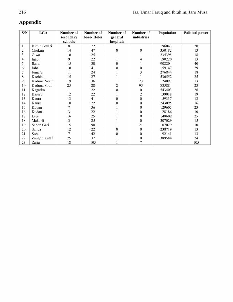
216 Isa, Umar Faruq and Ibrahim, Jaro Musa
Appendix
S/N LGA Number of secondary
schools
Number of bore- Holes
Number of general
hospitals
Number of industries
Population Political power
1 Birnin Gwari 8 22 1 1 196043 20 2 Chukun 14 47 0 0 350182 13 3 Giwa 10 25 1 1 234395 18 4 Igabi 9 22 1 4 190220 13 5 Ikara 15 30 0 1 90220 40 6 Jaba 10 41 0 0 159147 29 7 Jema’a 11 24 1 3 276844 18 8 Kachia 15 27 1 1 536552 25 9 Kaduna North 19 36 1 23 124097 13 10 Kaduna South 25 28 2 95 83588 23 11 Kagarko 11 22 0 0 543403 26 12 Kajuru 12 22 1 2 139018 19 13 Kaura 13 41 0 0 159337 12 14 Kauru 10 22 0 0 243095 16 15 Kubau 7 36 1 0 129605 23 16 Kudan 3 22 1 0 128186 10 17 Lere 16 25 1 0 148609 25 18 Makarfi 3 25 1 0 307029 15 19 Sabon Gari 15 90 1 21 107029 10 20 Sanga 12 22 0 0 238719 13 21 Soba 7 42 0 0 192141 13 22 Zangon Kataf 25 37 1 0 389584 24 23 Zaria 18 105 1 7 105

European Journal of Scientific Research ISSN 1450-216X Vol.18 No.2 (2007), pp.217-222 © EuroJournals Publishing, Inc. 2007 http://www.eurojournals.com/ejsr.htm
Sources of Sport Confidence of Elite Male and Female Soccer
Players in Nigeria
Olufemi Adegbola Adegbesan University of Botswan, Department of Physical Education Health and Recreation, P.Bag 0022,Gaborone, Botswana
E-mail: [email protected]
Abstract
Sport confidence is a unique and relatively untested approach to conceptualising achievement motivation and self-confidence in sport. The real strength of Vealey’s model is that it is situation-specific and represents a legitimate attempt at theory development within the discipline. This study compared the sources of sport confidence of male and female elite soccer players in Nigeria.
The descriptive survey research design was used in the study. The participants (n = 172) used in the study were selected using the random sampling procedure. Data was collected using Vealeys SSCQ with an overall coefficient determination of .90. Correlation matrix and student t-test were used for data analyses.
The result shows that significant difference (p <.05) was found between the male and female elite soccer player’s sources of sport confidence of mastery, demonstration of ability, physical and mental preparation, physical self preparation, social support, coaches leadership, vicarious experience and environmental comforts, while significant difference (p>.05) was not found on the situational favourableness as a source of sport confidence of the two groups.
The female elite soccer players derived their confidence in sport from all the sport confidence sub-scales more than their male counterpart when the mean values of the sources were compared. Also the positive relationship of the sources of sport confidence will further enhance successful outcome of behavioural responses of the players when sport confidence skill training programmes are well integrated into the overall training schedules of the players. Keywords: Sport Confidence, Performance and Elite Soccer players
Introduction Confidence is seen as one of the important parameters of psychological well-being in sport participation. Indeed, an enhanced confidence resulting from physical activities is an index for the promotion of exercise and sport participation. Sport confidence is a unique and relatively interested approach to conceptualising achievement motivation and self-confidence (Cox, 1994). The real strength of Vealey’s (1986, 1988b) model is that it is situation-specific and represents a legitimate attempt at theory development within the discipline. The relationship between performance and sport confidence is a unique area that warrants in-depth investigation. Studies such as Mahoney, Gabriel & Perkin (1987) and Chi (1996) had demonstrated that athletes with superior sport confidence would
Sources of Sport Confidence of Elite Male and Female Soccer Players in Nigeria 218
possess better concentration, the ability to strategies, control their performance tempo and exhibit balanced emotions.
Indeed, sport confidence can be an inconsistent and temporary variable of study. The inconsistence of sport confidence according to Chie-der, Chen, Hung-yu & Li-Kang (2003) within a period of time is basically affected by the sources of the confidence. The studies of Sonstroem (1997a; 1997b) also identified motivational approach or personal development hypothesis whereby self-confidence and esteem acts as a motivational determinant of sports and exercise participation.
The concepts of self-confidence and sport confidence have been attributed to have influence on elite athlete performance. However, researches on sources of sport confidence of elite athletes from developing countries of the world especially in Africa are seldom found. Soccer is the most popular sport in Nigeria and the game has gone through tremendous development in the country. Where do the male and female elite soccer players derive their confidence prior to competitions? Are there relationships amongst the sources of sports confidence variables? It is in the light of this that this study examined the sources of sport confidence of elite male and female soccer players in Nigeria. Method Participants
Participants used for this study were 172 male and female elite soccer players who had participated in the League and the Challenge Cup competitions. They were selected using the random sampling procedure. The male players were 103 and the female players were 99. The mean age of the male player was 22.63¬ ± 2.91(SD), while the mean age of the female players was 21.61 ± 2.21 (SD). Measures
The sources of sport confidence (SSCQ) developed by Vealey et al. (1998) was used for this study. The instrument is a (7) – point Likert scale that ranges from 1 (not at all important) to 7 (of highest importance). It consists of (9) sub-scales of mastery, demonstration of ability, physical/mental preparation, physical self-preparation, social support, coaches’ leadership, vicarious experience, environmental comfort and situational favourableness.
The instrument comprises of 43 – items, however, 41-items were used for this study based on Vealey’s et al (1998) submissions that item “win” under the sub-scale of demonstration of ability and item “follow certain rituals” under the subscale of environmental comfort were deleted from the inventory due to the significantly lower loadings and squared multiple correlations than other items. The overall coefficient of determination (COD) was .90, which is a representation of acceptable generalised measure of reliability for the entire model. The validity of (SSCQ) is reflected in Vealey et. al. (1998) in which several predictions including the sub-scales influence on SC – trait, in an attempt to examine the link between sources and levels of sport-confidence were made. There are no norms available for (SSCQ) since the instrument is a subjective psychological test. Procedure
The consent of the team officials as well as the players was sought before the administration of the instrument. The researchers with the assistance of 4 other researchers explained the content of the instrument to the participants for clarity and understanding. They were assured of the confidentiality of all the information given. The administrations of the instrument were done at the training venues and at the camps of the teams. Design and Analysis
The descriptive survey research design was used for this study. This design is probably the best that can be adapted to obtaining personal and social facts, beliefs and attitude as it is reflected in this study.

219 Olufemi Adegbola Adegbesan
This design according to Kerlinger (1992) has the advantage of wide scope as well as a great deal of information that can be obtained from a moderately large sample from a particular population. This design is also adequate since no intervention was used in this study.
The descriptive statistics of mean and standard deviation were computed, where appropriate, the parametric statistics of t-test and correlation matrix were also used for analysis. Results Table 1: Descriptive statistics and Internal consistency coefficient for the sources of sport confidence
factors#
Alpha (α) Alpha (α) Subscales Mean SD (Present study) Vealey (1998)
Mastery 27.33 5.91 .85 .88 Demonstration of Ability 26.62 5.37 .81 .86 Physical/Mental Preparation 33.89 5.94 .85 .79 Physical self-presentation 15.55 3.61 .72 .78 Social support 31.53 6.02 .79 .88 Coaches’ leadership 25.58 6.79 .88 .92 Vicarious experience 26.33 4.89 .73 .90 Environmental comfort 15.49 3.79 .84 .93 Situational favourableness 15.04 3.82 .75 .71
Table 2: T-test Analysis of the sources of sport confidence factors between the male and female elite soccer
players
Sources of sport confidence factors Group N Mean SD t-value df Sig. Male 103 26.22 6.525 3.09 170 .002** Mastery Female 69 29.00 4.399 Male 103 25.32 5.361 4.07 170 .000** Demonstration of Ability Female 69 28.57 4.797 Male 103 32.58 6.801 3.66 170 .000** Physical/Mental Preparation Female 69 35.85 3.594 Male 103 14.77 3.767 3.57 170 .000** Physical self-presentation Female 69 16.72 3.057 Male 103 30.62 6.139 2.46 170 .015** Social support Female 69 32.89 5.631 Male 103 24.61 7.265 2.33 170 .021** Coaches’ leadership Female 69 27.04 5.761 Male 103 25.16 5.226 4.00 170 .000** Vicarious experience Female 69 28.08 3.748 Male 103 14.33 4.173 5.29 170 .000** Environmental comfort Female 69 17.23 2.217 Male 103 14.60 3.529 1.85 170 .066* Situational favourableness Female 69 15.69 4.173
Note: ** Significant at .05 * Not significant at .05

Sour
ces o
f Spo
rt C
onfid
ence
of E
lite
Mal
e an
d Fe
mal
e So
ccer
Pla
yers
in N
iger
ia
220
Tab
le 3
: C
orre
latio
n M
atrix
of a
ll th
e so
urce
s of s
port
conf
iden
ce fa
ctor
s M
aste
ry
Dem
onst
ratio
n of
A
bilit
y Ph
ysic
al/M
enta
l Pr
epar
atio
n Ph
ysic
al se
lf-pr
esen
tatio
n So
cial
Su
ppor
t C
oach
es
lead
ersh
ip
Vic
ario
us
expe
rien
ce
Env
iron
men
tal c
omfo
rt
Situ
atio
nal
favo
urab
lene
ss
Mas
tery
.6
19**
Dem
onst
ratio
n of
Abi
lity
.000
.685
**
.540
**
Phys
ical
/Men
tal P
repa
ratio
n .0
00
.000
.4
60**
.4
98**
.3
85**
Phys
ical
self-
pres
enta
tion
.000
.0
00
.000
.501
**
.540
**
.460
**
.644
**
Soci
al su
ppor
t .0
00
.000
.0
00
.000
.4
49**
.4
08**
.5
61**
.4
90**
.6
46**
Coa
ches
’ lea
ders
hip
.000
.0
00
.000
.0
00
.000
.604
**
.529
**
.558
**
.620
**
.656
**
.591
**
Vic
ario
us e
xper
ienc
e .0
00
.000
.0
00
.000
.0
00
.000
.5
29**
.4
30**
.3
66**
.5
67**
.5
09**
.3
84**
.6
21**
Envi
ronm
enta
l com
fort
.000
.0
00
.000
.0
00
.000
.0
00
.000
.406
**
.419
**
.270
**
.372
**
.320
**
.331
**
.499
**
.542
**
Situ
atio
nal f
avou
rabl
enes
s .0
00
.000
.0
00
.000
.0
00
.000
.0
00
.000
N
ote:
**
in
dica
te si
gnifi
cant
P<.
05 p
ositi
ve re
latio
nshi
p am
ong
the
spor
t con
fiden
ce fa
ctor
s

221 Olufemi Adegbola Adegbesan
The results in Table 1, shows the descriptive statistics of mean and standard deviation for the sources of sport confidence factors. It further revealed the internal consistency coefficient (α) for this present study and that of Vealey et. al. (1998). The internal consistency of all the 9 sub-scales revealed for this present study in Table 1, surpassed the required criterion of 0.70, as allocated by Nunnally (1978, as cited in Vealey et. al., 1998). These findings further established the consistency of (SSCQ) in this study area. The t-test analyses in Table 2, indicated significant difference (P<.05) in all the subscales except situational favourableness. Table 3, presented the correlation analysis of all the sources of sport confidence subscales on the two groups. The results indicates significant (P <.05) relationship of all the subscales as reflected in the responses to the items. Discussion Confidence is seen as one of the important psychological contribution to successful sport performance. This assertion is corroborated by the study of Jones and Hardy (1990a) in which they highlighted the importance of high-level confidence as expressed by elite athletes used in their study. This present study found significant differences in sources of sport confidence between the male and female elite soccer players on the subscales of mastery, demonstration of ability, physical/mental preparation, physical self presentation, social support, coaches’ leadership, vicarious experience and environmental comfort. This findings is in congruence with Vealey (1998) in which perceived sources of sport confidence were different between athletes of both genders. Although significant difference was not found on the sub-scale of situational favourableness, but an appreciable level of difference was established between both genders. The findings in this study also indicate that the female elite soccer players derived their confidence in sport from all the sport confidence subscales more than their male counterparts when the mean values of all the sources were compared as indicated in Table 2.
The result of this study also indicates significant positive relationship among the sources of sport confidence of the two elite soccer groups. The implication of these findings may be that those sources of sport confidence may serve as significant predictors for successful performance with the elite athletes when they are correlated with other performance variables as revealed in studies such as Swain and Jones (1992) and Duda (1992). The findings of this study also indicate that the relationship of the subscales of mastery and physical/mental preparation possess the highest correlation value in the matrix as shown in Table 3. This signifies the vital role of mastery skill and physical/mental preparation by the elite soccer players in high level sport performance. While the relationship with the least correlation value in the matrix was the relationship of the subscales of situational favourableness and physical/mental preparation. Conclusion A basic psychological factor need for the achievement of excellence in sport performance is confidence. The sources of the confidence and how they influence the performance of the elite athletes are of utmost importance to the coaches, the sport psychologists and the elite athletes. This present study established that the female elite soccer players derived their confidence in sport from all the sport confidence subscales more than the male elite soccer players. The positive relationship of the sources of sport confidence indicated in this study will further enhance successful outcome of behavioural responses of the players when sport confidence skill training programmes are well integrated into the overall training schedules of the players.

Sources of Sport Confidence of Elite Male and Female Soccer Players in Nigeria 222
References [1] Chi, L.K. (1996) Stress management of athletes. National Physical Education Quarterly, 25 (4)
51 – 57. [2] Chi-der, D., Chen, S., & Hung-y, C. and Li-Kang (2003) Male and female basketball players’
goals orientation, perceived motivational climate, perceived ability and sources of sport confidence. Sport Journal, Vol. 3 (6).
[3] Cox, R.H. (1994) Sport psychology. Concepts and Applications. Dubuque, 1A; WBC Brown & Benchmark.
[4] Duba, L.J. (1992) Motivation in sport settings: A goals perspective approach. In G.C. Roberts (ed.) motivation and sport and exercise, 57 – 91. Champaign, Illinois. Human Kinetics.
[5] Jones, G.O & Hardy, L. (1990a) Stress in Sport: Experiences of some elite performers. In G. Jones and l. Hardy (eds) Stress and performance in sport; 247 – 277, Wiley; Chichester.
[6] Kerlinger, F.N. (1992) Foundations of Behavioural Research. New York. Harcourt Brace College Publishers.
[7] Mahoney, M.J., Gabriel, T.J., & Perkins, T.S. (1987) Psychological skills and exceptional athletic performance. The Sport Psychologist. 1, 181 – 199.
[8] Sonstroem, R.L. (1997a) Physical activity and self-esteem. In W.P. Morgan(ed.), Physical activity and mental health, 127 – 43, Washington D.C.: Taylor and Francis.
[9] Sonstroem, R.L. (1997b) The physical self-esteem: A mediator of exercise and self-esteem. In K.R. Fox (ed.) The Physical self: From motivation to well being 3 – 26, Champaign, IlL: Human Kinetics.
[10] Swain, A., & Jone, G. (1992) Relationship between sport achievement orientation and competitive state anxiety. The Sport Psychologist, 6, 42 – 54.
[11] Vealey, R.S. (1986) Conceptualisation of Sport-confidence and competitive orientation: Preliminary investigation and instrument development. Journal of Sport Psychology 8 (3) 221 – 246.
[12] Vealey, R.S. (1988b) Sport confidence and competitive orientation: An addendum on scoring procedures and gender differences. Journal of Sport & Exercise Psychology 10(4), 471 – 478.
[13] Vealey, R.S. Hayashi, S.W. Garner-Holman, M., & Giacobbi, P. (1998) Sources of sport-confidence: conceptualisation and instrument development. Journal of Sport and Exercise Psychology 20(1) 54 – 80.
European Journal of Scientific Research ISSN 1450-216X Vol.18 No.2 (2007), pp.223-230 © EuroJournals Publishing, Inc. 2007 http://www.eurojournals.com/ejsr.htm
Problématique de L’Accès à L’Eau Potable Dans la Ville de
Ngaoundéré (Centre Nord-Cameroun)
Ngounou Ngatcha Benjamin Département des Sciences de la Terre, Faculté des Sciences Université de Ngaoundéré, B.P. 454 Ngaoundéré, Cameroun
E-mail: [email protected]
Lewa Sara Département des Sciences de la Terre, Faculté des Sciences
Université de Yaoundé 1, B.P. 812 Yaoundé, Cameroun
Ekodeck Georges Emmanuel Département des Sciences de la Terre, Faculté des Sciences
Université de Yaoundé 1, B.P. 812 Yaoundé, Cameroun
Abstract
Des enquêtes de terrain menées dans la ville de Ngaoundéré ont permis de constater que plus de 70% de personnes sur une population estimée à environ 200 000 habitants, n’ont pas accès à l’eau potable à travers le réseau de distribution de la Société Nationale des Eaux du Cameroun (SNEC). La situation est particulièrement préoccupante dans les quartiers périurbains à habitat spontané de plus de 5000 habitants qui devraient bénéficier de réseaux d’adduction d’eau de la SNEC en lieu et place des solutions de type hydraulique rurale, avec multiplication des sources, puits peu profonds, traditionnellement mis en œuvre malgré leur inadaptation et la très mauvaise qualité de l’eau qui y est associée. Sur 397 personnes enquêtées dans les quartiers périurbains, 243 (soit plus de 60%) affirment souffrir régulièrement de maladies d’origine hydrique telles que la typhoïde, la dysenterie amibienne, la diarrhée.... Quinze échantillons d’eau analysées présentent des pH acides (en moyenne 4), des concentrations en matières en suspension variant de 0,65 à 3,42 mg/l et des turbidités comprises entre 1,7 et 43,15 N.T.U. Keywords: Ngaoundéré, quartiers périurbains, eau potable, maladie hydrique, qualité de
l’eau. 1. Introduction Par sa situation géographique, la ville de Ngaoundéré (Fig. 1) se trouve entre le 7° et le 8° de latitude Nord et entre le 13° et le 14° de longitude Est. Elle occupe une partie du plateau de l’Adamaoua qui présente un relief peu élevé compris entre 900 et 1500 m. L’ensemble du plateau et des zones limitrophes reçoit une précipitation annuelle supérieure à 1300 mm. La répartition des pluies au cours de l’année est caractérisée par l’alternance de la saison sèche (novembre-mars) et de la saison des pluies (avril-octobre). La température moyenne annuelle est de 22 °C. La population de la ville de Ngaoundéré connaît un taux d’accroissement élevé (> 3,5 %), qui s’explique par le développement de
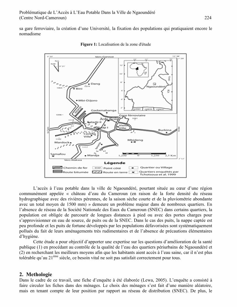
Problématique de L’Accès à L’Eau Potable Dans la Ville de Ngaoundéré (Centre Nord-Cameroun) 224 sa gare ferroviaire, la création d’une Université, la fixation des populations qui pratiquaient encore le nomadisme
Figure 1: Localisation de la zone d'étude
L’accès à l’eau potable dans la ville de Ngaoundéré, pourtant située au cœur d’une région
communément appelée « château d’eau du Cameroun (en raison de la forte densité du réseau hydrographique avec des rivières pérennes, de la saison sèche courte et de la pluviométrie abondante avec un total moyen de 1500 mm) » demeure un problème majeur dans de nombreux quartiers. En l’absence de réseau de la Société Nationale des Eaux du Cameroun (SNEC) dans certains quartiers, la population est obligée de parcourir de longues distances à pied ou avec des portes charges pour s’approvisionner en eau de source, de puits ou de la SNEC. Dans le cas des puits, la nappe captée est peu profonde et les puits de fortune développés par les populations défavorisées sont systématiquement pollués du fait de leurs aménagements très rudimentaires et de l’absence de précautions élémentaires d’hygiène.
Cette étude a pour objectif d’apporter une expertise sur les questions d’amélioration de la santé publique (1) en procédant au contrôle de la qualité de l’eau des quartiers périurbains de Ngaoundéré et (2) en recherchant les meilleurs moyens afin que les habitants aient accès à l’eau saine, car il n’est plus tolérable qu’au 21ème siècle, ce besoin vital ne soit pas satisfait correctement pour tous. 2. Methologie Dans le cadre de ce travail, une fiche d’enquête à été élaborée (Lewa, 2005). L’enquête a consisté à faire circuler les fiches dans des ménages. Le choix des ménages s’est fait d’une manière aléatoire, mais en tenant compte de leur position par rapport au réseau de distribution (SNEC). De plus, le

225 Ngounou Ngatcha Benjamin, Lewa Sara and Ekodeck Georges Emmanuel
nombre de ménages choisis par quartiers n’a pas été limité. Les entretiens se sont déroulés selon le principe de question-réponse.
A la suite des enquêtes de terrain, 15 ouvrages ont été sélectionnés en vue des prélèvements pour analyses de laboratoire. Le choix des ouvrages a pris en compte leurs fortes sollicitations pour l’approvisionnement en eau des ménages, ainsi que leur proximité par rapport à une source potentielle de contamination. Les analyses de laboratoire ont été exécutées au Département de Chimie Appliquée de l’Ecole Nationale Supérieure Agro-Industrielle (ENSAI) de l’Université de Ngaoundéré. Elles ont porté sur le pH, la conductivité, les matières en suspension et la turbidité. Les pH des eaux ont été mesurés à l’aide d’un pH-mètre type TACUSSEL MINI-80, les conductivités à l’aide du conductivimètre TACUSSEL type CD-60, la turbidité par un turbidimètre de marque HACH type RATIO/XR et les matières en suspensions par filtration et pesage des papiers filtres (type Whatman) après séchage à l’étuve. 3. Resultats et Discussions 3.1. Modes d’approvisionnement en eau des ménages.
L’approvisionnement en eau se fait à 80 % à travers les puits (Fig. 2). La SNEC assure 10,9% et les forages et ruisseaux 1,8 et 7,27% respectivement. Une enquête faite par Tchotsoua et al. (1999) dans les quartiers Vielle-Ville, Joli Soir, Mbideng, Samafou à Ngaoundéré, indique également que les puits et les sources représentent les moyens de ravitaillement les plus importants de la ville (environ 70%). Figure 2: Répartition des modes d’approvisionnement en eau des ménages à Dang, Bini, Burkina,
Mbideng, Bamyanga, Gadamabanga, Baladji I et Baladji II.
Le coût d’accès au réseau SNEC et le prix de vente au m3 seraient les raisons primordiales qui
amènent les populations des quartiers périphériques à converger vers les puits. Ces puits seraient facile à mettre en œuvre avec à un coût d’environ 20000 Fcfa (environ 30 €).

Problématique de L’Accès à L’Eau Potable Dans la Ville de Ngaoundéré (Centre Nord-Cameroun) 226 3.2. Relations puits-sources potentielles de pollution.
Figure 3: Représentation des sources potentielles de contamination des puits.
Figure 4: Représentation des types de WC dans la ville de Ngaoundéré.
La Fig. 3 souligne que plus de 80% des W.C. visités sont proches des puits (distance moyenne
5 m). Quelques ouvrages sont également implantés au voisinage des décharges publiques et des porcheries. Dans ces quartiers, il n’existe ni marché, ni abattoir. Les W .C., essentiellement de type
0
10
20
30
40
50
60
70
80
90
W.C. Voirie Porcherie Marché Artisanat Abattoir
Source potentielle de contamination de l'eau
Pour
cent
age
(%)
0
20
40
60
80
100
120
W.C Moderne W.C Traditionnel
Type de W.C.
Pour
cent
age
(%)

227 Ngounou Ngatcha Benjamin, Lewa Sara and Ekodeck Georges Emmanuel
traditionnel (Fig. 4), c’est-à-dire des fosses perdues dans le sous sol, pouvant être en contact avec la nappe, sont communément utilisés dans le Centre Nord - Cameroun. 3.3. Quelques cas de maladies
Les démangeaisons et la dysenterie amibienne sont les maladies les plus récurrentes qui touchent près de 40 % de la population (Tableau 1 ; Fig. 5). Elles sont suivies respectivement par la diarrhée 12,5 % et la typhoïde 8,8 %. Chaque année, près de 3,5 millions de décès dans le monde sont encore directement imputables à l’insuffisance d’eau et d’assainissement. D’après Bontoux (1987), les enquêtes épidémiologiques sont les seuls instruments de mesure en principe objectifs de l’impact de la qualité des eaux sur la population. Au regard du nombre de personne affectées par les maladies hydriques (plus de 60 % des personnes enquêtées), le niveau des incertitudes sur la qualité de l’eau est suffisamment élevé pour situer aujourd’hui l’accès à l’eau potable dans la ville de Ngaoundéré comme une préoccupation majeure de santé publique. La sécurité d’alimentation en eau potable, qui est assurée par les populations des quartiers périphériques par la mise en oeuvre d’ouvrages de captage de substitution (sources, puits, …) indépendants du réseau SNEC ne se traduit pas par un plan de secours, mais une source de problème entravant déjà la qualité de la vie. La protection de tels ouvrages est complexe. Elle ne peut être efficace que si les populations concernées de concert avec la municipalité et les acteurs économiques prennent conscience des enjeux et de la nécessité que l’eau est un bien indispensable à la vie et à la santé. Table 1: Quelques maladies fréquentes dans les quartiers périphériques de Ngaoundéré
Diarrhée Démangeaisons Typhoïde Dysenterie amibienne
Gale Non affecté Total
Nombre de malades 50 73 35 70 15 154 397 Pourcentages (%) 12,59 18,39 08,82 17,63 03,78 38,79 100
Figure 5: Répartition des maladies hydriques recensées.
0
5
10
15
20
25
30
35
40
45
Diarrhée Démangeaison Typhoïde Dysenterie a. Gale Non affecté
Type de maladie
Pour
cent
age (%
)

Problématique de L’Accès à L’Eau Potable Dans la Ville de Ngaoundéré (Centre Nord-Cameroun) 228 3.4. Analyse de quelques paramètres physico-chimiques
Le pH, la conductivité et la température
Figure 6: Répartition des pH des eaux
Figure 7: Répartition de la conductivité des eaux
Les analyses chimiques ont permis de mettre en évidence le caractère acide (Fig. 6) des eaux
ainsi que leur faible minéralisation soulignée par des valeurs de conductivité variant entre 9 µS/cm à Baladji II et 445 µS/cm à Baladji I (Fig. 7). Cette acidité est liée à l’intense activité biologique dont la conséquence est la libération du CO2 d’origine biogénique qui contribue à la mise en solution d’ions H+ et HCO3
- (Joseph et al., 1990 ; Savane et Soro, 2001). Dans le cadre de cette étude, les prélèvements ont été fait dans des ouvrages peu profonds ; les aquifères évolueraient en systèmes ouverts à l’atmosphère. Dans ce cas, la zone non saturée correspondrait évidemment à une zone d’aération des sols et des réservoirs. La présence de la phase gazeuse assurerait la réalimentation de la nappe en CO2. L’hydratation de CO2 engendre de l’acide carbonique suivant les réactions :
CO2 + H2O ⇔ H2CO3- lequel contribue à la mise en solution d’ions H+ et HCO3
-; H2CO3- ⇔ H+
+ HCO3-
La température mesurée est presque partout la même et comprise entre 24 et 25 °C (Tableau 2).
0123456
A B C D E F G H I J K L M N O
Code des localités
pH
0
100
200
300
400
500
A B C D E F G H I J K L M N O
Code des localités
Con
duct
ivité
s (µ
S/cm
)

229 Ngounou Ngatcha Benjamin, Lewa Sara and Ekodeck Georges Emmanuel
Table 2: Données d’analyses chimiques de quelques paramètres de structure naturelle des eaux (température, pH, Conductivité) et de fonctionnement des installations (Turbidité, MES)
Localités Code P.N.S T (°C) pH Cond.(µs/cm) Turb. (NTU) MES (mg/l) Dang - Soulgouta A 11,50 24 3,38 10,42 14,40 0,68 Dang - Sobadjo B 5,05 24 3,77 20,96 3,35 0,67 Bini - Quarantaine C 6,91 24 4,26 33,11 1,70 1,32 Bini - Extrême D 5,30 24 3,46 17,36 2,05 0,68 Bini - Morelle E 10,39 24 3,49 12,12 1,70 1,35 Burkina 1 F 9,88 24 4,60 30,86 20,30 1,33 Burkina 2 G 7,65 24 5,06 74,63 11,00 2,00 Mbideng 1 H 3,78 25 4,52 58,48 43,15 2,00 Mbideng 2 I 2,26 25 4,37 28,25 5,00 0,66 Bamyanga 1 J 4,73 24 5,06 53,76 17,95 2,00 Bamyanga 2 K 4,20 24 4,34 19,61 12,35 1,32 Gadamabanga 1 L 15,33 24 3,97 24,09 11,75 3,42 Baladji I M 4,75 24 3,89 444,44 10,80 0,65 Gadamabanga 2 N 5,58 24 3,99 12,70 24,40 1,59 Baladji II O 6,77 24 3,80 9,25 9,60 0,66
P.N.S = profondeur niveau statique ; T= température, Cond. = Conductivité ; Turb. = Turbidité ; MES = Matière en suspension Les matières en suspensions (MES) et la turbidité
Figure 8: Répartition des MES
Figure 9: Répartition de la turbidité
Les matières en suspension dans l’eau sont essentiellement les argiles, les limons, les débris de
litières, etc. La turbidité est la mesure du degré d’opacité ou de transparence de l’eau. Elle met en évidence la charge de l’eau en éléments en suspension finement divisés (limon, argile, résidus organiques …). Les MES varient entre 0,65 et 3,42 mg/l (Fig. 8) et la turbidité est comprise entre 1,7 et 43,15 NTU (Fig. 9).
Les bactéries apparaissent rarement isolées, elles sont généralement fixées aux MES (Nebbache, 1998). En effet, les mesures des MES et de la turbidité dans eaux étudiées visent à mieux
01
23
4
A B C D E F G H I J K L M N O
Code des localités
M E
S (m
g/l)
010
203040
50
A B C D E F G H I J K L M N O
Code des localités
Turb
idité
en
NTU

Problématique de L’Accès à L’Eau Potable Dans la Ville de Ngaoundéré (Centre Nord-Cameroun) 230 appréhender dans le futur, les hétérogénéités locales de réaction des bactéries vis à vis des MES (turbidité) dans les aquifères. La turbidité élevée indique qu’il n’y a pas une filtration très efficace entre le réservoir et les puits. A faible concentration, la turbidité ne présente pas de risque direct pour la santé, mais en cas de valeurs élevées, elle peut diminuer l’efficacité des traitements de désinfection et générer les risques microbiologiques (Nebbache, 1998). La consommation des eaux des quartiers périphériques nécessite au préalable une filtration. 4. Conclusion Cette contribution qui rend compte d’une série d’enquêtes et d’analyses physico-chimique entreprises au cours de l’année 2003, représente un travail partiel de l’inventaire des problèmes liés à la maîtrise de l’eau potable dans la ville de Ngaoundéré. Il en ressort que l’accès à une eau de boisson sûre et saine est un droit fondamental dont sont encore privés plus de 70 % de la population potentiellement exposée à de l’eau ne respectant pas les limites de qualité requises. Les maladies hydriques observées montrent que les ressources en eaux sont de plus en plus menacées par la pollution. Le recensement des causes de contamination permet de constater que les WC traditionnels ont une morphologie susceptible de faciliter les transferts de polluants dans le système aquifère. Les maladies hydriques touchent les populations pauvres soumises à de mauvaises conditions de vie et d’hygiène et ayant un accès limité à l’eau potable. Des améliorations en faveur des quartiers périphériques doivent être faite par la SNEC. La réussite de cette action d’amélioration de l’accès à l’eau pour une forte proportion de la population demande un effort des pouvoirs publics pour le développement des adductions collectives. References [1] BONTOUX, J., 1987, Impact de la qualité des eaux sur l’état sanitaire des populations. In :
Actes du Colloque Pollution et environnement des eaux souterraines. Protection et problèmes d’assainissement, pp 11- 20.
[2] JOSEPH, A., ARANYOSSY, J. F. et KANTA, I., 1990, Recharges et paléorecharges des aquifères discontinues du socle de l’Aïr (Niger). Geodinamica Acta (Paris) 4, 3, 185 – 197.
[3] LEWA, Sara 2005, Etude de la qualité des eaux de boisson et de ménage dans le Département de la Vina. Mémoire DEA, Université de Yaoundé 1, Cameroun,
[4] NEBBACHE, S., 1998, Turbidité et micro-organismes. Transferts des matières en suspension et risques sanitaires dans un aquifère karstifié (Haute-Normandie, France). Thèse Université de Rouen, 109 P.
[5] SAVANE, I., et SORO, N., 2001, Caractérisation chimique et isotopique des eaux souterraines du Nord-Ouest de la Côte d’Ivoire : recharge des aquifères discontinus de la région d’Odienné. Africa Geosciences Review, 8, 379 – 390.
[6] TCHOTSOUA, M., NDAME, J. P., WAKPONOU A., et BONVALLOT, J., 1999, Maîtrise et gestion des eaux à Ngaoundéré (Cameroun). Problèmes et esquisses de solutions. Geo-Eco-Trop, 23, 91-105.

European Journal of Scientific Research ISSN 1450-216X Vol.18 No.2 (2007), pp.231-239 © EuroJournals Publishing, Inc. 2007 http://www.eurojournals.com/ejsr.htm
Evaluation of Reservoirs as Flood Mitigation Measure in
Nyando Basin, Western Kenya Using Swat
Joseph Sang Graduate student, Jomo Kenyatta University of Agriculture and Technology
Biomechanical and Environmental Engineering Department (BEED). P. O. Box 62000-00200 Nairobi, Kenya
E-mail: [email protected]
Mwangi Gatheny Senior Lecturers, Jomo Kenyatta University of Agriculture and Technology
Biomechanical and Environmental Engineering Department (BEED). P. O. Box 62000-00200 Nairobi, Kenya
George Ndegwa
Senior Lecturers, Jomo Kenyatta University of Agriculture and Technology Biomechanical and Environmental Engineering Department
(BEED). P. O. Box 62000-00200 Nairobi, Kenya
Abstract
Reservoirs have been proposed as flood mitigation measure in Nyando basin. The 3,587 km2 basin in Western Kenya is prone to recurrent annual floods, which are preceded by droughts. These annual floods disrupt socio-economic activities in the basin, where flood risks seem to intensify with time due to population increase and encroachment into flood plains. In this study, whose objective was to establish the effectiveness of proposed reservoirs in controlling floods in the Nyando basin, a hydrological model was applied in scenario simulation. The hydrological model, Soil and Water Assessment Tool (SWAT), was used to simulate streamflow in the Nyando basin under two assumed scenarios (with or without reservoirs). The scenario simulation showed that the proposed reservoirs could effectively reduce flood peaks in the main Nyando River. In this river, simulated peak flow was reduced from 60.6 m3/s (without reservoirs) to 34.2 m3/s (with reservoirs) at River Gauging Station (RGS) 1GD07. However, in Ainabng’etuny tributary, whose streamflow at RGS 1GB03 is almost equal to that of the main Nyando river at RGS 1GD07 could still contribute enough streamflow to cause flooding and may need additional control measure apart from the proposed reservoir. In addition to reducing the intensity and frequency of floods, the reservoirs could also increase the water and irrigation potential in the Nyando basin. Keywords: Floods, Reservoirs, Nyando River, SWAT

Evaluation of Reservoirs as Flood Mitigation Measure in Nyando Basin, Western Kenya Using Swat 232 1. Introduction Floods have remained a challenge to agricultural development in floods prone basins. To aggravate their disastrous effects, the floods are usually preceded by droughts. These alternating floods and droughts result in loss of life, bio-diversity alteration and land degradation. In essence they undermine the socio-economic activities in the basin.
Nyando basin in Western Kenya is prone to the recurrent annual flooding and droughts in the lower part of the basin. As a mitigation measure against the floods, the Ministry of Water Resource Management and Development (MoWRMD) proposed to construct four reservoirs in the basin, which were found to be feasible after a field survey (MoWRMD, 2003). This study therefore evaluated how effective the proposed reservoirs would be in controlling the recurrent annual floods in the Nyando basin using a hydrological model called Soil and Water Assessment Tool (SWAT; Arnold et al, 1998; Neitsch et al, 2002). The study involved scenario simulation using SWAT. The model was selected for this study because it is computational efficient, allows considerable spatial details, requires readily available inputs, continuous time, capable of simulating land management scenarios and gives reasonable results (Arnold et al, 1998). The ability of the model to simulate the impact of reservoirs and ponds was an added advantage.
Reservoirs have been used in various parts of the parts of the world to control floods. In addition they have been used as a source of water for domestic, industrial and agricultural use. For example, in Tennessee valley in the United States,
Hydrological models are mathematical representation of one or more of the hydrologic processes resulting from precipitation and culminating in basin’s runoff (Refsgaard, 1996). Modelling either aid to explore the implication of making certain assumptions about the real world system, or to predict the behaviour of the real system under a set of naturally occurring circumstances (Beven, 1989).
Soil and Water Assessment Tool (SWAT; Neitsch et al, 2002) is an example of a hydrological model. SWAT is a physically based, continuous time and distributed parameter model (Ref.). It has been widely used to simulate runoff and sediment yield in small basin (Triphati et al, 2003 and Spruill et al, 2000). It is meant to simulate the impact of management practises on water, sediment and agricultural chemical yield in large complex watersheds (Di Luzio et al, 2002; Jha et al, 2002).
There are three major components of SWAT where various process simulations are based. These are sub-basins, channel and reservoirs. For modelling purposes, the basin is divided into hydrologic response units (HRU) and sub-basins (Neitsch et al, 2002). These are the basic units of water balance calculation and enable the model to accurately simulate the spatial variation in water balance components. The water balance equation used in SWAT is given by Arnold et al (1998) as.
( )∑=
−−−−+=t
it QRWEQRSWSW
1
(1)
Where SW is the soil water content minus 15-bar water content, t is time in days, and R, Q, E, W and QR are the daily amount of precipitation, surface runoff, evapotranspiration percolation and return flow all in mm.
Surface runoff is simulated using either the modified Soil Conservation Service (SCS) curve number method (USDA-SCS, 1972) or the Green and Ampt infiltration method (Green and Ampt, 1911). In this study the SCS curve number was used. The SCS curve numbers are function of the soil permeability, land use and the antecedent moisture condition. The curve number varies non¬-linearly based on antecedent moisture condition. The basic equation used in the SCS curve number method is given by equation below.
( )SIR
IRQ+−
−=
2
(2) Where: Q is the accumulated surface runoff or rainfall excesses (mm)
R is the rain depth for the day

233 Joseph Sang, Mwangi Gatheny and George Ndegwa
I is the initial abstraction, which includes surface storage, interception and infiltration prior to runoff (mm) and S the retention parameter (mm).
The initial abstraction (Ia) is commonly approximated as 0.2S and thus ( )
)8.0(2.0 2
SRSRQ
+−
=, SR 2.0> (3)
0.0=Q , SR 2.0≤ (4) The retention parameter S varies due to changes in soils, land use, management and slope. The
parameter also varies temporally due to changes in soil water content. The retention parameter S is defined as:
⎟⎠⎞
⎜⎝⎛ −= 1100254
CNS
(5) Where CN is curve number. The Soil Conservation Service (SCS) defines three moisture conditions. I (dry) wilting point, II
average moisture conditions and III (wet) field capacity. The curve number is adjusted for the other moisture condition using the following formulae.
[ ]( ))100(03636.0533.2exp(100)100(20
22
221 CNCN
CNCNCN
−−+−−×
−= (6)
( )[ ]223 10000673.0exp CNCNCN −××= (7) Where CN1, CN2 and CN3 are the Curve number for moisture condition I, II and III
respectively. SWAT has the ability to simulate the impact of water impoundment, which alters the
streamflow characteristics, (Neitsch et al, 2002). The simulated impoundment structures include reservoirs. Reservoirs are located in the main channel and receive water from all the sub-basins upstream. The main features of a reservoir as modelled by SWAT are given in Figure 1 below. Figure 1: Components of a reservoir with flood water detention features as modeled by SWAT (Source:
Neitsch et al 2002)
2. Methodology 2.1. Description of the study area
Nyando basin in Western Kenya (Figure 2) covers about 3,587 km2 and is bounded by latitudes 00 7’ 48”N and 00 24’ 36”S and longitude 340 24’36”E and 350 43’ 12”E. The land slopes generally in the

Evaluation of Reservoirs as Flood Mitigation Measure in Nyando Basin, Western Kenya Using Swat 234 Northeast-Southwest direction. Altitude varies from about 1,100 m above sea level at Lake Victoria shores to about 3, 000 m in the highlands.
Figure 2: Location of the Nyando basin (Source: Sang, 2005)
River Nyando and its tributaries drain the basin. The main river, Nyando, rises from the
Western Mau hills (Njogu, 2000). The river has a steep gradient in the upper reaches, but the gradient gentles as it approaches and meanders through the Kano plains. A major tributary of River Nyando, Ainabng’etuny, rises from the Nandi hills and joins the main river near Awasi market (Waruru et al, 2003). The other tributaries are Nyaidho, Awach, Namuting, Mbogo and Kapchorua. It finally dissipates into swamps in Kusa area before discharging into Lake Victoria at Winam gulf
The climate of the Nyando basin varies spatially due to the variation in altitude within the basin. Mean annual rainfall varies from 1,000 mm near Lake Victoria to over 1,600 mm in the highlands (Njogu, 2000). The characteristic diurnal peaks occur during the long rains (March-May) and short rains (October-December). These peaks are associated with flooding in the lower parts of the basin (MoWRMD, 2003).
The land use/land cover types in the basin are diverse. The main land use types could be categorised into forestry and agriculture (Wagate and Macharia, 2003). The diverse patterns depend on lithology, geology, topography, rainfall characteristics and most important human activities (Van Der Kwast, 2002). 2.2. Effectiveness of the Proposed Reservoirs
Simulation of the effectiveness of the proposed reservoirs was preceded by calibration and validation of the model to predict streamflow in the Nyando basin. Calibration of the model against observed streamflow in the basin by Sang (2005) established that the model could simulate streamflow in the basin, though its performance needs to be improved further.

235 Joseph Sang, Mwangi Gatheny and George Ndegwa
To simulate the effectiveness of the proposed reservoirs, the locations of the four reservoirs was established from the Ministry of Water Resources Management and Development (MoWRMD). The location of the reservoirs is given in Figure 3, whereas Table 1 gives possible volume of the proposed reservoirs and their intended use.
Figure 3: Location of the proposed reservoirs (Source: Sang, 2005)
Table 1: The proposed reservoirs, their volume and intended use
Site Capacity (*106M3) Intended use 03 33 Flood control and irrigation in the Kano plains 08 42 Floods control, Irrigation and domestic water supply for Muhoroni and Koru town 11 50 Flood control and irrigation in the Kano plains 13 21 Flood control and gravity water supply to Koru and Fort Ternan urban centres.
Source: MoWRMD (2003)
These proposed reservoirs were used to develop two simulation scenarios (with and without reservoirs). The additional characteristics of the reservoirs, which were required for simulation in SWAT and used in this study, are given in Table 2. This were obtained from the MoWRMD report (MoWRMD, 2003) or approximated with plausible values.

Evaluation of Reservoirs as Flood Mitigation Measure in Nyando Basin, Western Kenya Using Swat 236 Table 2: Characteristics of the reservoirs used in the scenario simulation
Reservoir characteristic Dam site 03 Dam site 08 Dam site 11 Dam site 13 Surface area to emergence spillway (ha) 20 140 420 80 Surface area to principal spillway (ha) 15 120 300 60 Volume when filled to emergence spillway (106 m3) 33 42 50 21 Volume when filled to principal spillway (106 m3) 10 10 30 9 Initial reservoir volume (106 m3) 10 10 30 9
The average annual release rate (Neitsch et al, 2002) used in SWAT to simulate the outflow of
reservoir was used in this study. The initial release rate was estimated from the mean streamflow of the sub-basin without the reservoir. This was systematically adjusted until a plausible outflow rate was attained. The mean, peak and flow duration characteristics of simulated streamflow for the two reservoir scenarios were compared to determine how effective the reservoirs could be. 3. Results and Discussion Calibration and validation of SWAT to simulate streamflow in the Nyando basin demonstrated that model could simulate streamflow in the Nyando basin. The performance of the model in the basin attained coefficient of determination (R2) values between 0.45 and 0.72 (Sang, 2005). Therefore, the model could be used in this scenario simulation, while maintaining the same calibration parameter values, to evaluate the impact of the proposed reservoirs.
The results of simulations to evaluate the expected impact of reservoirs on streamflow are given in Figure 4 to Figure 6 and Table 3.
Figure 4: Flow duration curves for the reservoir storage scenarios at 1GD07.
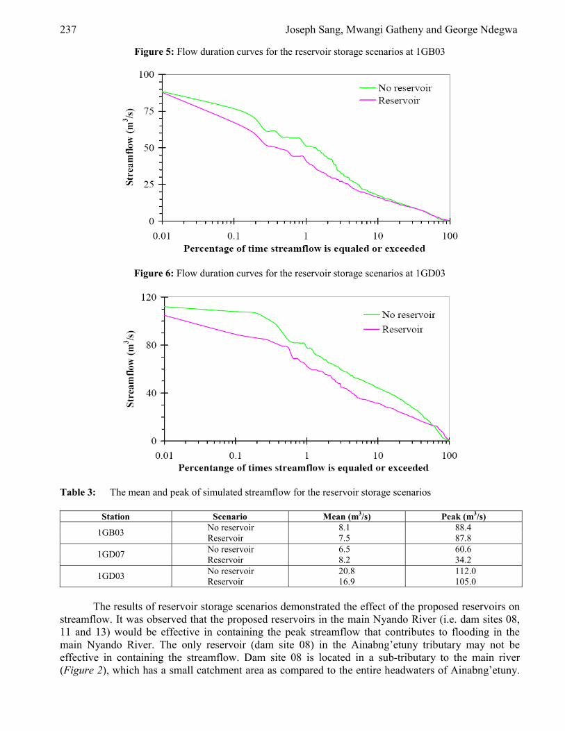
237 Joseph Sang, Mwangi Gatheny and George Ndegwa
Figure 5: Flow duration curves for the reservoir storage scenarios at 1GB03
Figure 6: Flow duration curves for the reservoir storage scenarios at 1GD03
Table 3: The mean and peak of simulated streamflow for the reservoir storage scenarios
Station Scenario Mean (m3/s) Peak (m3/s) No reservoir 8.1 88.4 1GB03 Reservoir 7.5 87.8 No reservoir 6.5 60.6 1GD07 Reservoir 8.2 34.2 No reservoir 20.8 112.0 1GD03 Reservoir 16.9 105.0
The results of reservoir storage scenarios demonstrated the effect of the proposed reservoirs on
streamflow. It was observed that the proposed reservoirs in the main Nyando River (i.e. dam sites 08, 11 and 13) would be effective in containing the peak streamflow that contributes to flooding in the main Nyando River. The only reservoir (dam site 08) in the Ainabng’etuny tributary may not be effective in containing the streamflow. Dam site 08 is located in a sub-tributary to the main river (Figure 2), which has a small catchment area as compared to the entire headwaters of Ainabng’etuny.

Evaluation of Reservoirs as Flood Mitigation Measure in Nyando Basin, Western Kenya Using Swat 238 The effect of this reservoir is seen in the mid-flows (Figure 5) where there is a change in flow duration characteristics.
At River Gauging Station (RGS) 1GD03, the peak flow is reduced from 112.0 m3/s to 105.0 m3/s. The flow duration curves were altered by the reservoirs as shown by Figure 6. RGS 1GD03, located just before the flood plain, is a good indicator of the effectiveness of the reservoirs in controlling the floods. It was observed that the proposed reservoirs would be effective in the main Nyando River. However, the Ainabng’etuny tributary would still contribute sufficient streamflow to cause flooding, though the frequency and intensity of the floods will be reduced. 4. Conclusion From the scenario simulation applied in this study it was concluded that the proposed reservoirs could be an immediate mitigation measure against the recurring floods in the Nyando basin. They could reduce incidences and intensities of flooding in the basin. The reservoirs in the main Nyando River may be effective in containing the peak streamflow; however, the Ainabng’etuny tributary would still contribute sufficient streamflow to cause the floods in the basin. At RGS 1GD03 peak streamflow would be reduced from 112.0 m3/s to 105.0 m3/s. The reservoirs could also regulate streamflow; provide water for irrigation, domestic and industrial use. To increase the chances of taming the floods, alternative control measures would have to be applied in the Ainabng’etuny tributary.

239 Joseph Sang, Mwangi Gatheny and George Ndegwa
References [1] Arnold J. G., Srinivisan R. Muttiah R. S. and Williams J. R. (1998) Large area hydrologic
modeling and assessment part 1: model development. Journal of the American Water Resources Association 34 (1) 73-89.
[2] Beven, K. (1989). Changing Ideas in Hydrology – The Case of Physically Based Models. Journal of Hydrology, 105: 157 - 172.
[3] Di Luzio, M., R. Srinivasan, J.G. Arnold, S.L. Neitsch (2002). ArcView interface for SWAT2000, user’s guide. Blackland Research & Extension Centre, Texas Agricultural Experiment Station Texas
[4] Green, W.H. and G.A. Ampt. (1911). Studies on soil physics, 1. The flow of air and water through soils. Journal of Agricultural Sciences 4:11-24.
[5] Jha, M., P. W. Gassman, S. Secchi, R. Gu, and J Arnold (2002). Impact of Watershed Subdivision Level on Flows, Sediment Loads, and Nutrient Losses Predicted by SWAT. Working Paper 02-WP 315. Center for Agricultural and Rural Development Iowa State University (www.card.iastate.edu)
[6] MoWRMD (2003). Flood control on the lower reaches of Nyando River. Pre-investment study, final report.
[7] Neitsch, S. L, J. G. Arnold, J. R. Kiniry, J. R. Williams and K. W King (2002). Soil and water assessment tool theoretical documentation, version 2000. Blackland Research & Extension Centre, Texas Agricultural Experiment Station Texas
[8] Njogu, A. K. (2000). An Integrated River Basin Planning Approach – Nyando Case Study in Kenya - 1st WARFSA/Water Net Symposium: sustainable use of water resources; Maputo,1-2 November 2000
[9] Refsgaard, C. J. (1996). Parameterization, Calibration and Validation of Distributed Hydrological Models. Journal of Hydrology, 198: 69 – 97.
[10] Refsgaard, J.C. and B. Storm (1996). Construction, calibration and validation of hydrological models: In M. B. Abott and C. J. Refsgaard (Editors) Distributed hydrological modelling. Kluwer Academic Publishers.
[11] Sang J. K. (2005). Modelling the impact of changes in Land use, climate and reservoirs storage on flooding in the Nyando basin MSc thesis Jomo Kenyatta University of Agriculture and Technology (JKUAT). Nairobi, Kenya.
[12] Spruill, C. A, S. R. Workman and J. L. Taraba (2000). Simulation of daily and monthly discharge from small watershed using the SWAT model. Transaction of the ASAE. 43(6): 1431-1439.
[13] Tripathi, M. P, R. P. Panda, and N. S Raghuwanshi (2003). Calibration and validation of SWAT model for predicting runoff and sediment yield of a small watershed in India. Agricultural engineering journal, 12 (1 and 2) 95-118.
[14] USDA-Soil Conservation Service (1972). Section 4: Hydrology In National Engineering Handbook. SCS.
[15] Van der Kwast, J. (2002). Land use classification and DEM generation using SPOT and LandSat imagery in Lake Victoria basin, Western Kenya. Utrecht University, Netherlands.
[16] Waruru, B.K, C.R.K. Njoroge and S.N. Wanjogu (2003). Biophysical baseline information for the Nyando catchment area: The soils of the Nyando catchment area. Reconnaissance Soil Survey Report No. R21, October 2003.

European Journal of Scientific Research ISSN 1450-216X Vol.18 No.2 (2007), pp.240-249 © EuroJournals Publishing, Inc. 2007 http://www.eurojournals.com/ejsr.htm
Anisotropy and Pressure Dependence of the
Compressional Wave Velocity of Suevites from the Bosumtwi Impact Crater, Ghana
Danuor, S. K Department of Physics
Kwame Nkrumah University of Science and Technolog, Kumasi, Ghana E-mail: [email protected]
Menyeh, A
Department of Physics Kwame Nkrumah University of Science and Technology, Kumasi, Ghana
Berckhemer, H
Institute for Meteorology and Geophysics University of Frankfurt/M, Germany
Abstract
Suevites, which are impact-derived rocks, are found at the Bosumtwi impact crater in Ghana. They are located in the Northern and Southern parts outside the crater rim. Suevites found in the North and South locations have some characteristic differences. In this paper, we report on the behaviour of the compressional wave velocity Vp with pressure and azimuth for suevite samples collected from the North and South locations. The effect of pressure on Vp for the sample from the South is more pronounced than that from the North because of the high porosity of the sample at the South location. Also seismic velocity anisotropy is more pronounced in the samples from the South probably due to the distribution of rock inclusions in the matrix. Vp-minimum directions determined for some samples indicate that the Vp-minimum axes seemed to point toward the center of the crater. This supports the reasoning that after the impact, the ejected material on the ground might have assumed a preferred orientation with respect to the center of the crater. It was also found that suevite samples require higher saturation pressures (650 MPa and above) than solid rocks such as amphibolite which reaches velocity saturation at 100 MPa. Keywords: Suevites, impact crater, compressional wave velocity, anisotropy, velocity
saturation. Introduction Location of the Bosumtwi Crater
The Bosumtwi meteorite impact crater in Ghana is located about 32 km southeast of Kumasi, the capital town of the Ashanti Region (Fig. 1a). The crater, which is about 1.07 Ma old (Koeberl et al., 1997) has a rim-to-rim diameter of 10.5 km and was excavated in 2 Ga-old metamorphosed and
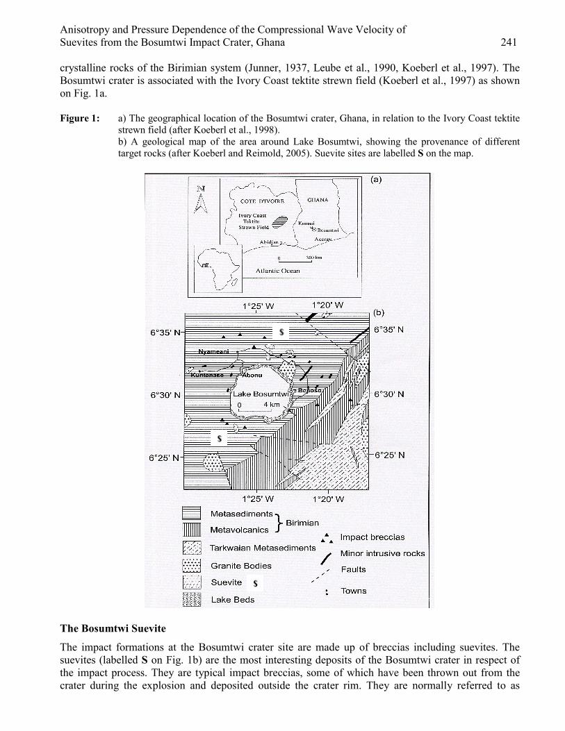
Anisotropy and Pressure Dependence of the Compressional Wave Velocity of Suevites from the Bosumtwi Impact Crater, Ghana 241
crystalline rocks of the Birimian system (Junner, 1937, Leube et al., 1990, Koeberl et al., 1997). The Bosumtwi crater is associated with the Ivory Coast tektite strewn field (Koeberl et al., 1997) as shown on Fig. 1a. Figure 1: a) The geographical location of the Bosumtwi crater, Ghana, in relation to the Ivory Coast tektite
strewn field (after Koeberl et al., 1998). b) A geological map of the area around Lake Bosumtwi, showing the provenance of different target rocks (after Koeberl and Reimold, 2005). Suevite sites are labelled S on the map.
The Bosumtwi Suevite
The impact formations at the Bosumtwi crater site are made up of breccias including suevites. The suevites (labelled S on Fig. 1b) are the most interesting deposits of the Bosumtwi crater in respect of the impact process. They are typical impact breccias, some of which have been thrown out from the crater during the explosion and deposited outside the crater rim. They are normally referred to as

242 Danuor, S. K, Menyeh, A and Berckhemer, H
“fallout” suevites and are found mainly in the northern and southwesten parts of the crater (Fig. 1b). The suevites were first described as volcanic breccia because of their resemblance with pumiceous tuff (Junner, 1937, Jones et al., 1981). Consequently, some earlier researchers misinterpreted the origin of the crater to be due to volcanic action. Stoeffler and Grieve (1994) defined the suevite as polymict impact breccia including cogenetic impact melt particles, which are in a glassy or recrystallized state and occur in clastic matrix containing lithic and mineral clasts of various stages of shock metamorphism.
The Bosumtwi suevite (Fig. 2) is a glass-bearing breccia similar to the suevite found at the Ries crater in Germany (Jones et al., 1981). It contains melt inclusions and rock fragments (grewacke, phyllite, shale, granite) up to about 40 cm in size, with greywacke dominating. Most of the rock fragments are subangular in shape and less than 20 cm long and are arranged in a disordered fashion. The locations of these “fallout” suevites have come to be popularly known as the North and South locations. The suevites in the North are white grey whilst those in the South are dark grey.
Figure 2: Cross section of a typical suevite from the North of the Bosumtwi impact crater.
This paper reports on seismic velocity measurements, which have been carried out for samples
of suevite collected from both the Northern and Southern parts of the crater. A knowledge of the seismic velocity of suevites is important for the interpretation of the insitu seismic measurements. Compressional or P-wave velocities, Vp, have therefore been measured by ultrasonic methods as a funtion of azimuth and confining pressure in a special apparatus developed in the Institute for Meteorology and Geophysics of the University of Frankfurt am Main, Germany. This paper reports on experimental investigations carried out on the behaviour of the compressional wave velocity Vp of the Bosumtwi suevite samples under confining pressures and with azimuth to determine the velocity anisotropy. The orientation of the Vp-maximum and Vp-minimum directions in the suevite samples were determined to see if there is any reason to suspect that the suevites would have assumed some preferred orientation with respect to the center of the crater after the impact. Also, the behaviour of the compressional wave velocities of the suevites with pressure was studied to find out if these rocks reach

Anisotropy and Pressure Dependence of the Compressional Wave Velocity of Suevites from the Bosumtwi Impact Crater, Ghana 243
a velocity saturation as found in other crystalline rocks which reach velocity saturation at about 100 MPa (Zang et al., 1996). The Geology of the Bosumtwi Crater Area
The Bosumtwi impact event occurred about 1 million years ago in a target that consisted of Precambrian crystalline rocks, the 2.1-2.2 Ga metasedimentary rocks in greenschist facies of the Lower Birimian System of phyllites, graywackes, quarzites, sandstones, shale, micaschist, as well as granites as indicated in the geological map of Fig. 1b (Jones et al., 1981; Wright et al., 1985; Leube et al., 1990; Hirdes et al., 1996; Reimold et. al., 1998). Upper Birimian metamorphosed basalts and pyroclastic rocks (metavolcanics) occur in the Obuom Range, south-east of the crater. Precambrian Tarkwaian metasedimentary rocks occur to the east and south-east of the crater as well (Moon and Mason, 1967; Woodfield, 1966; Jones et al., 1981).
The regional geology is characterized by northeast-southwest trends with steep dips either to the northwest or southeast. However, variations in this trend, due to folding, have been observed (Reimold et al., 1998). Lithology at and around the Bosumtwi crater is dominated by metagraywackes and metasandstones, but some shale and mica schist are found, especially in the north-eastern and southern rim sectors (Reimold et al., 1997; Reimold et al., 1998). A variety of granitoid intrusions (mainly biotite or amphibole granites) have been mapped by Junner (1937) and Moon and Mason (1967). Small granite intrusions, probably connected with the Kumasi granite, crop out around the north-east, west, and south sides of the lake, the largest at Pepiakese on the north-east side of the crater (Jones et al., 1981). In addition, numerous, but generally less than 1-m-wide, dikes of biotite granitoid at many basement exposures in the crater rim have been observed. The overall granitoid component in the region is estimated at about 2 percent (Reimold et al., 1998).
Recent rock formations include the Bosumtwi lake beds, as well as soils and breccias associated with the formation of the crater (Junner, 1937; Kolbe et al., 1967; Woodfield, 1966; Moon and Mason, 1967; Jones et al., 1981; Koeberl et al., 1997, and Reimold et al., 1998). Materials and Methods Preparation of the Rock Samples
Several oriented rock samples were taken from the suevite outcrops from the North and South locations at the Bosumtwi crater (Fig. 1b). For the seismic velocity measurements, cylindrical cores of 30 mm diameter and 30 mm length were drilled out of the rock samples. The axes of the cylindrical samples were vertical and the north direction was marked on the cores. The cores were coated with three layers of oil resistant varnish to protect them from intrusion of pressure-oil. In some cases, the sealing failed due to irregularities of the rock and the softness of the cementation agent, and as a result, oil penetrated the sample. Those samples were however excluded from the measurements. Experimental Procedure
The core was mounted in the measuring head. Two pairs of piezoelectric transducers were used as transmitter and receiver, respectively, for axial (vertical) and radial (horizontal) ultrasound transmission. The core can be rotated in the pressure vessel in steps of 10° (pressure steps) to measure the anisotropy. Pressures up to 400 MPa can be applied to measure the pressure dependence of the compressional wave velocity Vp. The travel times were measured automatically and plotted in different ways.

244 Danuor, S. K, Menyeh, A and Berckhemer, H
Results and Discussion Results of Compressional Wave Velocity Vp of the Bosumtwi Suevite – Anisotropy and Pressure
Dependence
The seismic velocity in radial direction of the core (horizontal-Vp) has been determined for the suevite samples from the two different locations. The results of the anisotropy and pressure dependence of the compressional wave velocity of the Bosumtwi suevite for sample 3a1 (from North location) and sample 12 (from South location) are shown in Fig. 3 and Fig. 4 respectively. Figure 3a: Variation of horizontal Vp with azimuth at constant confining pressures of 5, 20, 80, 160 and 320
MPa for sample 3a1 from North location; the different confining pressures are indicated on the left side of the figure.
In Fig. 3a, Vp-horizontal (seismic velocity in radial direction in the core) has been plotted as a
function of azimuth at different confining pressures of 5, 20, 80, 160 and 320 MPa. The increase of Vp with pressure is remarkable and is certainly due to the gradual closure of grain contacts and pores, and not to the intrinsic pressure sensitivity of the minerals of the rock. The suevite sample 3a1 from the North location can be described as exhibiting low anisotropy. Figure 3b: Variation of minimum and maximum horizontal Vp (Vp-hor min and Vp-hor max), and vertical
Vp (Vp-vert) as a function of pressure for suevite sample 3a1 from North location.
Azimuth (°)
320 MPa
160 MPa
80 MPa
20 MPa
5 MPa

Anisotropy and Pressure Dependence of the Compressional Wave Velocity of Suevites from the Bosumtwi Impact Crater, Ghana 245
In general, Vp increases gradually with pressure for the samples from the North (Fig. 3b). This trend differs from that observed for samples from the South (Fig. 4b), where an initial fast increase of seismic velocity with pressure is observed for pressures below 40 MPa.
The behaviour of the compressional wave velocity Vp with confining pressure and azimuth for suevite sample 12 from the South location is shown in Fig. 4a. Figure 4a: Variation of horizontal Vp with azimuth at constant confining pressures of 5, 20, 80, 240 and 320
MPa for suevite sample 12 from South location; the different confining pressures are indicated on the left side of the figure.
From Fig. 4a, it can be seen that the compressional wave velocity Vp increases with increase in
pressure. However, the suevite sample 12 is found to display significant anisotropic behaviour probably due to the distribution of rock inclusions in the matrix. Figure 4b: Variation of minimum and maximum horizontal Vp (Vp-hor min and Vp-hor max), and vertical
Vp (Vp-vert) as a function of pressure for suevite sample 12 from South location.
In general, the initial fast increase of Vp with pressure below 40 MPa (Fig. 4b) is due to the
gradual closure of pores and grain contacts. This situation is more significant for the samples from the South location, which are more porous than those from the North, which do not display a similar

246 Danuor, S. K, Menyeh, A and Berckhemer, H
phenomenon below 40 MPa (Fig. 3b). However, the gradual increase of the velocity with pressure above 40 MPa is explained as due to the dependence of the bulk modulus on pressure. Significance of Vp-Minimum
The anisotropy measurements were made to find out whether there are any consistencies in the orientation of the maximum Vp or minimum Vp in such samples, which have considerable anisotropy. One could have suspected perhaps that after the impact, the ejected material on the ground might have assumed a preferred orientation with respect to the center of the crater. A compilation of results with the geographical position of the outcrops and the direction of Vp-min is ahown in Fig. 5. Figure 5: Compilation of Vp-minimum directions for suevite samples from the North and South locations
which show significant anisotropy. S is the location of the suevite deposit.
Out of a total of 6 samples for which Vp-min directions were determined, it was found that 5
samples seemed to have some indications that the Vp–min axes pointed about toward the center of the crater. This is an interesting result. However, it is not considered as a conclusive proof yet because the number of samples which was used in the study was quite small. A confirmation of this result would need further investigation. Dependence of Vp with Pressure for Suevite Samples from North and South
The compressional wave velocities Vp as a function of pressure for three suevite samples from the North (samples 3a1, 3a and 3b2) and South (samples 12, 6b2 and 10) have been measured and plotted as shown in Fig. 6. The effect of pressure on Vp for suevite is quite pronounced as can be seen on Fig. 6. It is possible to differenciate between suevite samples from the North (lower curve) and South (upper curve) on Fig. 6. Those from the North are usually more compact and lighter in colour than the sometimes very dark, porous and more weathered rocks from the South. The pressure dependence of Vp is stronger, the higher the porosity and the elastic compressibility of the structure of the matrix of the suevite. This is clearly exhibited by the three samples from the South location as indicated in Fig. 6.
S
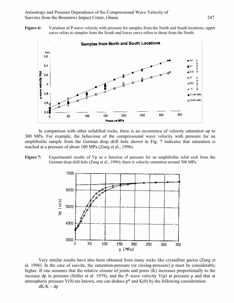
Anisotropy and Pressure Dependence of the Compressional Wave Velocity of Suevites from the Bosumtwi Impact Crater, Ghana 247
Figure 6: Variation of P-wave velocity with pressure for samples from the North and South locations; upper curve refers to samples from the South and lower curve refers to those from the North.
In comparison with other solidified rocks, there is no occurrence of velocity saturation up to
300 MPa. For example, the behaviour of the compressional wave velocity with pressure for an amphibolite sample from the German deep drill hole shown in Fig. 7 indicates that saturation is reached at a pressure of about 100 MPa (Zang et al., 1996). Figure 7: Experimental results of Vp as a function of pressure for an amphibolite solid rock from the
German deep drill hole (Zang et al., 1996); there is velocity saturation around 300 MPa.
Very similar results have also been obtained from many rocks like crystalline gneiss (Zang et
al. 1996). In the case of suevite, the saturation-pressure (or closing-pressure) p must be considerably higher. If one assumes that the relative closure of joints and pores (K) increases proportionally to the increase dp in pressure (Stiller et al. 1979), and the P–wave velocity V(p) at pressure p and that at atmospheric pressure V(0) are known, one can deduce p* and K(0) by the following consideration:
dK/K ~ dp

248 Danuor, S. K, Menyeh, A and Berckhemer, H
K(p) = K(0) exp (-p/p*) if Vm = velocity of the compact solid matrix, then V(p) = Vm (1- K(p)) = Vm (1- K(0) exp (-p/p*)) V(0) = Vm (1- K(0)) Elimination of the unknown Vm leads to:
V(p) / V(0) =[1 – K(0) exp (-p/p*)] / [(1- K(0)] The two unknown parameters K(0) and p have to be determined simultaneously from the shape
of the curves of the observations K(p) = f(p). A good fit to the observed curves was obtained with the following results: V(0) = 2500 m/s, K(0) = 0.5, p* = 650 MPa
for the samples from the South location and V(0) = 2450 m/s, K(0) = 0.48, p* = 850 MPa
for the samples from the North location. p = p* means that 63% of the pores and joints are closed. The high values of K(0) and of p* are
quite unusual for solid rocks and apparently typical features of the Bosumtwi suevites. Conclusion Suevite outcrops from the North and South locations around the Bosumtwi impact crater have characteristic differences. Suevites in the North are more compact and light grey in colour whilst those in the South are more porous and darker in colour. Compressional wave velocities show more significant anisotropies in the suevites from the South than those from the North. Seismic velocities tend to increase faster with pressure initially for pressures below 40 MPa for the samples from the South whilst such a phenomenon is not observed for samples from the North. Vp-minimum directions determined for 6 samples indicate that the Vp-minimum axes seemed to point toward the center of the crater. This supports the reasoning that after the impact, the ejected material on the ground might have assumed a preferred orientation with respect to the center of the crater. The variation of P-wave velocity with pressure for the suevite samples does not show velocity saturation up to 300 MPa as observed for solid rocks such as amphibolite where velocity saturation is reached at a pressure of 100 MPa. It was found out that the suevites require much higher saturation pressures of 650 MPa for samples from the South and 850 MPa for samples from the North. This phenomenon is a typical feature of the Bosumtwi suevites. Acknowledgement The authors wish to thank the technicians of the geophysics laboratory of the Institute of Meteorology and Geophysics of the University of Frankfurt am Main, Germany for their support in the work. We also wish to express our sincere gratitude to the German Research Foundation (DFG) for the financial support they provided for the research work.

Anisotropy and Pressure Dependence of the Compressional Wave Velocity of Suevites from the Bosumtwi Impact Crater, Ghana 249
References [1] Hirdes, W., Davis., D. W., Lüdtke, G., Konan, G., 1996. Two generations of Birimian
(Paleoproterozoic) volcanic belts in northeastern Cote d’Ivoire (West Africa): Consequences for the “Birimian Controversy”. Precambrian Research, 80, 173-191.
[2] Jones, W. B., Bacon, M., Hastings, D. A., 1981. The Lake Bosumtwi impact crater, Ghana. Geological Society of America Bulletin, 92, 342-349
[3] Junner, N. R., 1937. The Geology of the Bosumtwi caldera and surrounding country. Gold Coast Geological Survey Bulletin, 8, 1-38
[4] Koeberl, C., 1997. Impact cratering: The mineralogical and geochemical evidence. In: Ames structure in northwest Oklahoma and similar features: Origin and petroleum production (1995 symposium), edited by Johnson K. S., and Campbell, J. A. Oklahoma. Geological Survey Circular, 100, 30-54.
[5] Koeberl, C., and Reimold, W. U., 2005. Bosumtwi impact crater. An updated and revised geological map, with explanations. Jahrbuch der Geologischen Bundesanstalt, Wien (Yearbook of the Austrian Geological Survey) 145:31-70 (+1 map, 1:50,000).
[6] Kolbe, P., Pinson, W. H., Saul, J. M., and Miller, E. W., 1967. Rb-Sr study on country rocks of the Bosumtwi crater, Ghana. Geochimica et Cosmochimica Acta, 31, 869-875.
[7] Leube, A., Hirdes, W., Mauer, R., Kesse, G. O., 1990. The Early Proterozoic Birimian Supergroup of Ghana and some aspects of ist associated gold mineralization. Precambrian Research, 46, 136-165.
[8] Moon, P. A., Mason, D., 1967. The geology of ¼º field sheets nos. 129 and 131, Bompata S.W. and N.W. Ghana Geological Survey Bulletin, 31, 1-51.
[9] Reimold, W. U., Brandt, D., Koeberl, C., 1997. Geological Studies at Lake Bosumtwi impact crater, Ghana. Meteoritics and Planetary Science, 32, Supplement, A107.
[10] Reimold, W. U., Brandt, D., Koeberl, C., 1998. Detailed structural analysis of the rim of a large, complex impact crater: Bosumtwi crater, Ghana. Geology, 26, 543-546.
[11] Stiller, H., Wagner, F. C., Vollstädt, H., 1979. Influence of pressure and joints on the velocity of elastic waves. Akademie der Wissenschaften der DDR. Forschungsbericht Geo- und Kosmos-Wissenschaften, Heft 9, 177-194.
[12] Stöffler, D., Grieve, R. A. F., 1994. Classification and nomenclature of impact metamorphic rocks: A proposal to the IUGS Subcommission on Systematics of Metamorphic Rocks (abstract). In: European Science Foundation Second International Workshop on “Impact Cratering and the Evolution of Planet Earth”: The Identification and Characterization of Impacts, Ostersund, Sweden.
[13] Wright, J. B., Hastings, D. A., Jones, W. B., Williams, H. R., eds., 1985. Geology and Mineral Resources of West Africa. George Allen and Unwin, London, 38-45.
[14] Woodfield, P. D., 1966. The geology of the ¼° field sheet 91, Fumso N.W., Ghana Geological Survey Bulletein, 30, 66 pp.
[15] Zang, A., Berckhemer, H., Lienert, M., 1996. Crack closure pressures inferred from ultrasonic drill-core measurements to 8 km in the KTB wells. Geophysical Journal International, 124, 657-674.

European Journal of Scientific Research ISSN 1450-216X Vol.18 No.2 (2007), pp.250-254 © EuroJournals Publishing, Inc. 2007 http://www.eurojournals.com/ejsr.htm
Effects of Petroleum Hydrocarbon Pollution on the Levels of
Ascorbic Acid and Dehydroascorbic Acid in Germinating Bean (Vigna Unguiculata (L) Walp) Seeds
Igbinosa O. Osamuyimen Department of biochemistry, Delta state university, P M B 1, Abraka, Nigeria
E-mail: [email protected]
Abstract
The effect of various sub-lethal concentrations (1.0%, 2.0%, 3.0% and 4.0%) of petroleum hydrocarbon polluted soil on the levels of ascorbic acid and dehydroascorbic acid was studied in germinating bean seeds. The levels of ascorbic acid, the reduced form of vitamin C was significantly lower (P < 0.001) in the plantlets grown in the polluted soil compared to the plantlets from the unpolluted control soil. However an opposite response was obtained with dehydroascorbic acid, the oxidized form of vitamin C. The results in this study may suggest that one of the probable effects of oil pollution on plants is the imposition of oxidative stress. Keywords: Ascorbic acid, Dehydroascorbic acid, Oxidative Stress Petroleum
hydrocarbon pollution, Crude oil. Introduction Nigeria is a major producer of crude oil in the world and contamination of the environment due to oil spillage has steadily increased over the years. In the Niger- Delta alone there have been over 550 reported cases of crude oil spillage since 1976 releasing about 2.8 million barrels of crude oil to the environment (Kori- Siakpere, 1998; Odiete, 1999). Oil spills on agricultural lands generally reduce plant growth, due to direct toxic effects on the plants, (Baker, 1970); reduced germination (Udo and Fayemin, 1975) and unsatisfactory conditions resulting from insufficient aeration of the soil because of displacement of air from the space between the soil particles (Gill et al., 2003)
Ascorbic acid (vitamin C) is an abundant component in plants. It reaches a concentration of over 20mM in chloroplast and occurs in the cell compartment, including cell wall. It functions as an antioxidant, an enzyme cofactor and as a precursor for oxalate and tartrate synthesis. It participates in a variety of processes, including photosynthesis, photoprotection, cell wall growth and cell expansion, resistance to environmental stresses and synthesis of ethylene gibberellinis, anthocyanins and hydroxproline (Loewus and Loewus, 1987). The antioxidative effect of ascorbic acid is exerted by its reduced form; dehydroascorbic acid (DHAA); a known marker of oxidative stress (Ayaori et al., 1991)
The aim of this study was to evaluate the effects of hydrocarbon pollution on the levels of ascorbic acid and dehydroascorbic acid on germinating bean (Vigna unguiculata (L) Walp) seeds; an important legume commonly grown to supplement the total protein intake in many Nigerians (Elegbede, 1999).

Effects of Petroleum Hydrocarbon Pollution on the Levels of Ascorbic Acid and Dehydroascorbic Acid in Germinating Bean (Vigna Unguiculata (L) Walp) Seeds 251
Materials Plant Materials
The seeds of cowpea were bought from the same source in a local market in Benin City, Edo State, Nigeria. Six groups of perforated polythene bags (15cm x 10cm) in 10 replicates were filled with eight hundred grams of garden soil that were each supplemented with 1.0%, 2.0%, 3.0%, 4.0%, 5.0%, and 0% (control) respectively with crude oil obtained from Texaco, Nigeria Plc (specific gravity 0.8708). The soil supplemented soil samples were mixed thoroughly to ensure a homogenous mixture. Seed Treatment
A set of five viable seeds determined by flotation, were drilled to an approximate depth of 2cm into each of the hydrocarbon-supplemented soil in the polythene bags. The control soil in the polythene bags received the same number of seeds. A polythene bag constituted an experimental unit that was replicated ten times. The polythene bags were left in the nursery beds and protected from pest and rodents by means of wire mesh. Water was added daily for up to six days and seeds that failed to sprout after that time (6d) were regarded as having not germinated. Germination was indicated by the appearance of epicotyls above the soil level. The plantlets grown in 1.0%, 2.0%, 3.0% and 4.0 polluted soils and the control (zero supplementation) were then used for this study. A similar procedure was adopted by Malallah et. al., (1996) Seeds in 5.0% petroleum hydrocarbon polluted soil did not germinate. Method Dehydroascorbic Acid Content
After six days, the plantlets were harvested, washed with water and blotted dry. Dehydroascorbic acid (DHAA) was determined by the method of Roe and Oesterling (1944). The plantlets were ground in homogenization solution (1:20w/v) containing 5% metaphosphoric acid and 1% thiourea. After centrifugation, 4ml of extract was placed in each of three matched test-tubes. One tube was kept for a blank. To each of the other test tube, 1ml of 2%. 2,4, dinitrophenylhydrazine in 9N sulphuric acid was added.
These were held at 37ºC for 3 hours, and then cooled, together with the blank in ice water. To each of the three tubes, while in the ice water bath, 5ml of 85% sulphuric acid was added from a burrette, a drop at a time, during not less than 1 minute. Finally 1 ml of 2% 2,4 dinitrophenylhydraxine solution was placed in the blank tube. These tubes were immensed in ice at 0ºC and placed on a rack, wiped dry after 30 minutes and read in a spectrophotometer at 540nm. The results obtained are the means of five determinations. Standard Curve for Dehydroascorbic Acid
In preparing dehydroascorbic acid standard, a solution of 25mg of ascorbic acid in 25ml of 5% metaphosphoric acid was treated with 0.05ml of bromine solution. The mixture was stirred until a yellow colour was observed. Thereafter, excess bromine was decanted. The residue was then aerated until a colorless solution was observed. Standards of appropriate concentration were made by diluting with 5% metaphosphoric acid containing 1% thiourea
The concentration of dehydroascorbic acid in each case was extrapolated from a standard calibration curve

252 Igbinosa O. Osamuyimen
Ascorbic Acid Determination Ascorbic acid content was determined by the indophenol method of Oliver et al., 1945. Principle
This method depends on the reducing power of vitamin C. Reducing substances other than ascorbic acid may interfere with the determination unless the titration is performed rapidly in acid solution. The oxidized form of the dye is blue at pH 7 and above, but red at acid pH. The reduced form of the dye is colorless Procedure 1. Standardization of the dye
A standard solution of ascorbic acid about 100mg/250cm3 was also prepared with 0.5% oxalic acid solution.
A standard solution of blue dye about 50mg/100cm3 was also prepared with water. The dye solution was then titrated against 10cm3 of the standard solution of ascorbic acid to a faint pink color and the dye equivalent was calculated. 2. Preparation of plantlets
1g of plantlets was ground in 50cm3 and 0.5% oxalic acid and made up to 250cm3 and filtered. 10cm3 of the filtrate was used for titration. Results Table 1: Dehydroascobic acid and ascorbic acid levels in 6-day old V. unguiculata plantlets as affected by
varying concentrations of petroleum hydrocarbon polluted soil.
Percentage of crude oil in soil (%)
Ascorbic acid (µmole cm-3)n=5
Dehydroscobic acid (µmole cm-3)n = 5
Polluted/ Control (Ascorbic acid)
Polluted/ Control (DHAA)
1.0% **1.58± 0.63 **0.63 ± 0.02 0.52 1.80 2.0% **1.48 ± 0.3 **0.76 ± 0.06 0.49 2.17 3.0% **1.48± 0.5 **0.79 ± 0.08 0.48 2.26 4.0% **1.26 ± 0.8 **0.84 ± 0.05 0.42 2.40 Control 3.02 ± 0.5 0.84 ± 0.01
Result are expressed as mean±S.D ** Statistically significant (P< 0.001) n= number of samples.
The effect of petroleum-contaminated soil on the levels of dehydroascobic acid and ascorbic acid content is shown on table 1. A dose dependent significant increase (P< 0.001) in the levels of dehydroascorbic acid content in the plantlets grown in polluted soil relative to control was observed. Conversely an opposite response was obtained with ascorbic acid content. Also the ratio of dehydroascorbic acid in plantlets grown in crude oil polluted soil to control is greater the one (> 1), a possible reflection of oxidative stress. Discussion In this study plantlets grown in 1% hydrocarbon polluted soil were better with good growth compared to the plantlets from other higher concentrations of crude oil. Seeds planted in 5% concentration of crude oil did not grow hence termed “lethal dose” and received no futher analysis. The plantlets grown

Effects of Petroleum Hydrocarbon Pollution on the Levels of Ascorbic Acid and Dehydroascorbic Acid in Germinating Bean (Vigna Unguiculata (L) Walp) Seeds 253
in other concentrations of hydrocarbon showed highly unimpressive growth, indicating that these concentrations were toxic to the growth of V. unguiculata. Although growth-stimulating compounds have been reported to occur in crude oil; trace element (Baker, 1971) and phenlacetatic acid (Gudin and Syratt, 1975); it is possible that plant suffer permanent injuries as a result of hydrocarbon pollution without marked symptoms.
Ascorbic acid is reversibly oxidized to dehydroascorbic acid (Levine, 1986) and the radical scavenging capacity of ascorbic acid disappears when transformed to dehydroascorbic acid (Gill et. al., 1999). Increase levels of dehydroascorbic acid suggest an enhanced turnover of ascorbic acid possibly in response to sustained oxidant load (Duthie et.al., 1991, Kacmaz et al., 1997). The decrease in the content of ascorbic acid in the plantlets grown in the polluted soil may shift the redox of ascorbic acid status in favor of dehydroascorbic acid and this altered redox status could be suggestive of oxidative stress from oil pollution. Indeed, dehydroascorbic acid is considered a marker of stress. (Ayaori et. al., 2000).
Thus it is reasonable to suggest that the culminated effect of oil pollution on plant is the generation of oxidative stress possibly due to compromised levels of ascorbic acid and elevated levels of dehydroascorbic acid. Acknowlegement A debt of gratitude is own to my supervisor Dr. G. K. Isamah (late) of Biochemistry Department Delta State University, Abraka Nigeria, for his immeasurable contribution in the preparation of this paper.

254 Igbinosa O. Osamuyimen
References [1] AYAORI, M., Tetsuya, H., Micho, S. Hiroshi, Y., and Masato, N (2000) Plasma Levels and
Redox status of ascorbic acid and levels of lipid peroxidation in active and passive smokers. Environ. Health Persp. 108(2): 105-108
[2] Baker, J.M. (1970). The effect of oil in plants. Environ. Pollut. 1:27-44 [3] Baker, J.M. (1971). Growth stimulation following oil pollution. In: Cowell e. b. (eds.)
Ecological effect of oil pollution on littoral communities, Institute of petroleum, London, pp.72-77
[4] Duthie, G.G., Arthur, J.R., James, W.P. (1991) Effect of smoking and vitamin E on blood antioxidant status. Am. J. Clin. Nutr.53: 1061S-1063S
[5] Elegbede, J.A. (1999) Legumes In: Osagie A.U., Eka O.U. (eds.) Nutritional quality plant foods. Ambik Press, Benin City, pp. 53-83
[6] Gill, L.S.,Hyawuame, H.G. and Ehikhametolar,A.O. (2003) Effect of crude oil on the growth and anatomical features of Chromolaena odorata (L). Cent. Biol.Info. Tech. 15:35-40
[7] Gill, M.I., Ferreres F., Tomas- Barberan F.A. (1999) Effects of posthavest storage and processing on the antioxidant constituents (flavonoid and vitamin C) on fresh-cut spinach. J.Agric. Food Chem. 47:2213-17
[8] Gudin, C. and Syratt, W.J. (1975).Biological aspect of land rehabilitation following hydrocarbon contamination. Environ. Pollut.8.107-112
[9] Kacmaz, M., Ozturk, S.H., Cete, S. (1997). The effect of smoking on antioxidant defense system and membrane free fatty acid content of erythrocytes and plasma lipid parameters: Protective role of antioxidant vitamins. Nutri. Res. 17:931-940.
[10] Kori-Siakpere, O. (1998) Petroleum induced alteration in the African Catfish, Clarias gariepinus. Nig. J. Sci. Environ. 49-55
[11] Levine, M. (1986. New concepts in the biology and biochemistry of ascorbic acid. N. Engl.J. Med. 314:892-902
[12] Loewus, F.A. and Loewus, M.W. (1987). Biosynthesis and metabolism of ascorbate in plants. Crit. Rev. Plant Sci. 5:101-119
[13] Malallah, G., Afzal, M., Gulshom, S., Abraham, D., Kurian, M. and Ghumi, M.S. (1996). Vicia faba as a bioindicator of oil pollution. Environ. Pollut. 92:213-217
[14] Odiete, W.O. (1999). Environmental physiology of animals and pollution. Diversified Resources Ltd. Lagos
[15] Oliver H.L., Jeanne A.L. and Otto A.B. (1945). The Determination of ascorbic acid in small amounts of blood serum. Public Health Research Institute of the City of New York, Inc., New York, pp 609-515.
[16] Roe, J.H. and Oesterling, M.J. (1944). The determination of dehydroascorbic acid and ascorbic acid in plant tissues by the 2, 4- dinitrophenylhydraxine method. J. Biol. Chem.148:511-517
[17] Udo, E.J. and Fayemi, A.A. (1975). The effect of oil pollution of soil on germination, growth and nutrient uptake of corn. J. Environ. Quali. 4:537-540

European Journal of Scientific Research ISSN 1450-216X Vol.18 No.2 (2007), pp.255-266 © EuroJournals Publishing, Inc. 2007 http://www.eurojournals.com/ejsr.htm
Parallel Execution of Block Runge-Kutta Methods for Solving
Ordinary Differential Equations
Zailan Siri Institute of Mathematical Sciences, University of Malaya
50603 Lembah Pantai, Kuala Lumpur, Malaysia
Fudziah Ismail Department of Mathematics, University Putra Malaysia
43400 UPM Serdang, Selangor, Malaysia
Mohamad Othman Department of Communication Technology and Network
University Putra Malaysia, 43400 UPM Serdang, Selangor, Malaysia
Mohamed Suleiman Department of Mathematics, University Putra Malaysia
43400 UPM Serdang, Selangor, Malaysia
Abstract
The objective of this paper is to exploit the favourable characteristics of block explicit Runge-Kutta and block diagonally implicit Runge-Kutta methods for sequential machines to parallel ones. Both methods are used to solve ordinary differential equations, codes based on the methods are execute in sequential and parallel. Numerical results based on the two modes of executions are tabulated and compared. Keywords: Block Explicit Runge-Kutta , Block Diagonally Implicit Runge-Kutta,
sequential, parallel. 1. Introduction Parallelism in ODE (ordinary differential equation) software can be divided into three categories: in coding the method so that it can be executed simultaneously on several processors, in splitting variables in a multivariable ODE system between processors and lastly in exploiting parallelism in solving the algebraic system involved. This paper focuses on the parallel execution of the method.
Work on parallel Runge-Kutta methods for solving first order ODEs have been proposed by a number of researchers as can be seen in [1 - 4]. Iserles and Norsett [5] proposed diagonally implicit Runge-Kutta method which is designed specifically for parallel execution. Cash [6,7] derived explicit and diagonally implicit block Runge-Kutta method which can be exploited for the purpose of parallel implementation. We hope by parallelizing the algorithms a more effective codes can be developed.

Parallel Execution of Block Runge-Kutta Methods for Solving Ordinary Differential Equations 256 2. Block Explicit Runge-Kutta Methods Cash [6] derived a family of block explicit Runge-Kutta (BERK) methods of order two. At the first point ( )1+nx the formula is given by
0 0 1 1 0 (2.1a)
21
21
And at the second point ( )2+nx after normalizing the method in (2.1a) and adding one more step, the formula is given by
0 0 1 1 0 (2.1b)
0 2 where
( )k f x yn n1 = , ( )112 , hkyxfk nn += + ( )
11
1 hkyy nn +=+ ( ) )( 2122
1 kkyy hnn ++=+
( ) )( 211
2 kkhyy nn ++=+ ( )2
22 2hkyy nn +=+
)(mk denotes the mth iteration of k. Formula (2.1) produces second order approximations at both xn+1 and xn+2 and estimate of the local truncation error (LTE) in )1(
jny + is )1()2(jnjn yy ++ − for j = 1, 2.
To investigate parallelism in (2.1), we produce a digraph as follows:
Figure 2.1: Illustration of Second Order BERK Methods on Parallel Machine

257 Zailan Siri, Fudziah Ismail, Mohamad Othman and Mohamed Suleiman
From Figure 2.1 above, on S2; it can be seen that all )(mjny + for j,m = 1, 2 are independent of each
other but not for k1 and k2 on S1. Meaning, it is possible to calculate )(mjny + for m, j = 1, 2 in parallel with
four processors after we compute k1 and k2. On S4, calculate both LTE in parallel using two processors and then find the maximum error of the LTE.
Another second order BERK given in Cash [6] is as follows: At the point ( )1+nx , the formula is given by 0 0 1 1 0 (2.2a)
21
21
And at ( )2+nx the formulae is given by
(2.2b) where ( )k f x yn n1 = , ( )k f x y hkn n2 1 1= ++ ,
( ))(, 2123 kkhyxfk nn ++= + ( )
11
1 hkyy nn +=+ ( ) )( 2122
1 kkyy hnn ++=+
( ) )( 211
2 kkhyy nn ++=+ ( ) )2( 32122
2 kkkyy hnn +++=+
The following diagraph is shown to make it easier to visualize the parallelism in this method.
Figure 2.2: Illustration of Second Order BERK Methods on Parallel Machine
211
21
0112011
00

Parallel Execution of Block Runge-Kutta Methods for Solving Ordinary Differential Equations 258
This method is similar to the previous method; parallelism arises only on 2,1.;)( =+ jmy mjn
because they are independent of each other. In this method, calculate 1k first followed by 2k and then
3k , after 3,2,1; =iki have been computed, calculate 2,1.;)( =+ jiy mjn simultaneously using four
processors. The following is the parallel algorithms for second order BERK methods. Step 1:
Sequentially compute n
xxh n 0−= is the step-size of the method, k1 and k2 on P1.
Step 2: Calculate )1(
1+ny , )2(1+ny , )1(
2+ny and )2(1+ny on P1, P2, P3 and P4 respectively.
Step 3: By using two processors; calculate LTE1 and LTE2 in parallel on P1 and P2. Then, find the
maximum error of these two LTEs. Step 4:
Repeat Step 1- Step 3 until the end of the integration interval. 3. Parallelism in BDIRK Methods In this section, the execution of block diagonally implicit Runge-Kutta (BDIRK) methods in Cash [7] on parallel computer will be presented. The method is given by the following tableau
111
1113
1111211
11211
23
23
23
23
21
21
−
−
−−
(3.1)
Sequentially the method can be implemented as follows: 1+nx we have : 1)1(1 hkyy nn +=+
At 1+nx we have : 1)1(1 hkyy nn +=+
At 2+nx we have : )( 21)1(2 kkhyyn ++=+
At 1+nx we have : ( )3212(
1 2kkkhyy nn +−+=+
At 2+nx we have : )( 4321)2(2 kkkkhyyn ++−+=+
And at : )23
23( 543213 kkkkkhyy nn +++−+=+
BDIRK method with Butcher array as in (4.1) provides second order solution at 3+nx and 2+nx and first order solution at 1+nx .
The digraph of this method is given below

259 Zailan Siri, Fudziah Ismail, Mohamad Othman and Mohamed Suleiman
Figure 5.1: Illustration of BDIRK Methods on Parallel Machine
The digraph of second-order BDIRK method above, clearly showed that every )1(
iny + and )2(jny + for
i = 1, 2; j = 1, 2, 3 are independent of each other. So, we can calculate them simultaneously using five processors. 4. Numerical Results Before presenting the numerical results, let us introduce the metric for measuring the performance of parallel programs:
1. The number of processors, p used. 2. Parallel time, pt that is the time period elapsed between the beginning of the first processor and
the end of the last processor during the execution of the algorithm. 3. Speed-up, pS compares the parallel running time, pt of an algorithm that uses p processors to
solve a particular problem, to the sequential running time, st of an algorithm for the same problem, it is given by:
p
sp t
tS =
Or it can be defined as the ratio of the execution time of the parallel algorithm on a single processor and the execution time of the parallel algorithm on p processors, that is:
p
pp t
tS 1==
4. p
p
p
sp pt
tptt
pSE 1====
pE is the efficiency of the parallel algorithm and it must be less or equal to one ( 1≤pE ). If Ep = 1, the speed-up is said to be perfect. Perfect speed-up is rarely ever achievable and it can be multiplied by 100 to get the percentage.
)1(1
+mk )1(2
+mk )1(
3+mk )1(
4+mk )1(
5+mk
)0(ik
)1(1+ny )1(
2+ny )2(1+ny )2(
2+ny )2(3+ny

Parallel Execution of Block Runge-Kutta Methods for Solving Ordinary Differential Equations 260
5. pt
T 1= . Temporal Performance of the method
Given below are the test problems used, they are solved using BERK and BDIRK methods and the programs are run on Sequent 30 which is available at University Putra Malaysia for various values of step-size. Problem 1:
501)0(
)2011(
41
≤≤=
−=′
ty
yyy
Exact solution:
te
ty41
191
20)(−
+=
Problem 2:
101)0(
2
≤≤=+=′
ty
teyy t
Exact solution:
tetty )1()( 2 += Problem 3:
100)0(
22
≤≤=
+=′
ty
ytey t
Exact solution:
tetty 22
21)( =
Problem 4:
101)0(
)cos(
≤≤=
=′
ty
tty
Exact solution:
)sin()cos()( tttty += Problem 5:
4.001)0(
2
≤≤=−=′
ty
yty
Exact solution:
222)( ttety t +−−= − Numerical results obtained are given in Tables 3 - 12 and the notations used are as follows:

261 Zailan Siri, Fudziah Ismail, Mohamad Othman and Mohamed Suleiman
Table 2: Notations are used in the Numerical Results Tables
Notation Description BERK1 BERK method for Butcher array (2.1) BERK2 BERK method for Butcher array (2.2) BDIRK BDIRK method for Butcher array (4.1) h Step-size used METHOD Method employed
seqt The execution sequential time (in microseconds)
part The execution parallel time (in microseconds)
MAXE Magnitude of the maximum error of the computed solution S Speed-up of the method E Efficiency of the method C Cost of the method T Temporal Performance of the method
Table 3: Numerical Results for Problem 1
h METHOD seqt part MAXE BERK1 3212 3048 7.44555 × 10⁻⁴ BERK2 3304 3078 7.50849 × 10⁻⁴ 1.0 x 110− BDIRK 4888 3892 6.54178 × 10⁻² BERK1 33359 31222 7.68991 × 10⁻⁶ BERK2 34081 31960 7.69632 × 10⁻⁶ 1.0 x 210− BDIRK 51292 36932 6.74254 × 10⁻³ BERK1 332486 310530 7.71452 × 10⁻⁸ BERK2 357018 318595 7.71516 × 10⁻⁸ 1.0 × 10⁻³ BDIRK 377545 366810 6.76280 × 10⁻⁴ BERK1 4151072 2975945 7.71698 × 10⁻¹⁰ BERK2 4304168 3038146 7.71705 × 10⁻¹⁰ 1.0 × 10⁻⁴ BDIRK 3785277 3655726 6.76483 × 10⁻⁵ BERK1 4651527 2922069 7.71700 × 10⁻¹² BERK2 49952251 30380257 7.71700 × 10⁻¹² 1.0 × 10⁻⁵ BDIRK 44187934 38357113 6.76503 × 10⁻⁶
Table 4: Numerical Results for Problem 2
h METHOD seqt part MAXE BERK1 3215 3122 2.68265 × 10⁻¹ BERK2 3431 3163 2.91612 × 10⁻¹ 1.0 × 10⁻¹ BDIRK 4396 3956 6.45222 × 100 BERK1 33843 30886 3.10373 × 10⁻³ BERK2 34733 30943 3.12764 × 10⁻³ 1.0 × 10⁻² BDIRK 39476 37973 6.51413 × 10⁻¹ BERK1 336528 310980 3.14617 × 10⁻⁵ BERK2 354034 311464 3.14856 × 10⁻⁵ 1.0 × 10⁻³ BDIRK 396133 379053 6.51290 × 10⁻² BERK1 3338592 2548952 3.15040 × 10⁻⁷ BERK2 3454525 2644023 3.15064 × 10⁻⁷ 1.0 × 10⁻⁴ BDIRK 3901977 3795640 6.51274 × 10⁻³ BERK1 34736209 25689459 3.15083 × 10⁻⁹ BERK2 36534227 26949736 3.15085 × 10⁻⁹ 1.0 × 10⁻⁵ BDIRK 40482528 39443653 6.51274 × 10⁻⁴

Parallel Execution of Block Runge-Kutta Methods for Solving Ordinary Differential Equations 262 Table 5: Numerical Results for Problem 3
h METHOD seqt part MAXE BERK1 3358 2964 7.51716 × 10⁻¹ BERK2 3480 2995 8.89355 × 10⁻¹ 1.0 × 10⁻¹ BDIRK 4446 4161 2.39502 × 101 BERK1 37934 31214 9.93971 × 10⁻³ BERK2 39340 32423 1.00743 × 10⁻² 1.0 × 10⁻² BDIRK 39560 38434 2.22956 × 100 BERK1 415294 310561 1.01573 × 10⁻⁴ BERK2 429194 310738 1.01705 × 10⁻⁴ 1.0 × 10⁻³ BDIRK 387679 381531 2.17819 × 10⁻¹ BERK1 4060980 3006762 1.01784 × 10⁻⁶ BERK2 4096098 3178707 1.01797 × 10⁻⁶ 1.0 × 10⁻⁴ BDIRK 3887938 3824693 2.17290 × 10⁻² BERK1 39278591 28757755 1.01805 × 10⁻⁸ BERK2 41553138 29857012 1.01806 × 10⁻⁸ 1.0 × 10⁻⁵ BDIRK 38907232 37979786 2.17236 × 10⁻³
Table 6: Numerical Results for Problem 4
h METHOD seqt part MAXE BERK1 3231 3015 1.91467 × 10⁻³ BERK2 3379 3094 3.02466 × 10⁻³ 1.0 × 10⁻¹ BDIRK 4338 3862 8.37090 × 10⁻² BERK1 33549 30699 2.90066 × 10⁻⁵ BERK2 35358 31099 3.01182 × 10⁻⁵ 1.0 × 10⁻² BDIRK 45123 35472 8.41596 × 10⁻³ BERK1 333609 317679 3.00057 × 10⁻⁷ BERK2 376714 329301 3.01169 × 10⁻⁷ 1.0 × 10⁻³ BDIRK 449193 348015 8.41644 × 10⁻⁴ BERK1 3592339 2607253 3.01058 × 10⁻⁹ BERK2 3617280 2618477 3.01169 × 10⁻⁹ 1.0 × 10⁻⁴ BDIRK 4375188 3469182 8.41645 × 10⁻⁵ BERK1 3375981 2122692 3.01160 × 10⁻¹¹ BERK2 36370391 23107885 3.01170 × 10⁻¹¹ 1.0 × 10⁻⁵ BDIRK 48596000 36909709 8.41645 × 10⁻⁶
Table 7: Numerical Results for Problem 5
h METHOD seqt part MAXE BERK1 3274 3024 1.83728 × 10⁻³ BERK2 3368 3060 1.86484 × 10⁻³ 1.0 × 10⁻¹ BDIRK 4034 3617 5.66906 × 10⁻² BERK1 33431 31143 1.80315 × 10⁻⁵ BERK2 33707 31223 1.80594 × 10⁻⁵ 1.0 × 10⁻² BDIRK 35205 34617 5.96789 × 10⁻³ BERK1 480013 308860 1.79983 × 10⁻⁷ BERK2 487536 309071 1.80011 × 10⁻⁷ 1.0 × 10⁻³ BDIRK 355176 345497 5.99680 × 10⁻⁴ BERK1 5845446 3455051 1.79950 × 10⁻⁹ BERK2 5953279 3564413 1.79953 × 10⁻⁹ 1.0 × 10⁻⁴ BDIRK 3559931 3461494 5.99968 × 10⁻⁵ BERK1 65757617 36441696 7.71698 × 10⁻¹⁰ BERK2 66702946 37187850 1.79950 × 10⁻¹¹ 1.0 × 10⁻⁵ BDIRK 44137409 35645602 5.99997 × 10⁻⁶

263 Zailan Siri, Fudziah Ismail, Mohamad Othman and Mohamed Suleiman
Table 8: Results on the efficiency of the methods for Problem 1
h METHOD par
seq
tt
S = pSE =
parptC = part
T 1=
BERK1 1.05381 0.52690 6096 3.28084 × 10⁻⁴ BERK2 1.07342 0.53671 6156 3.24886 × 10⁻⁴ 1.0 × 10⁻¹ BDIRK 1.25591 0.25118 19460 2.56937 × 10⁻⁴ BERK1 1.06845 0.53422 62444 3.20287 × 10⁻⁵ BERK2 1.06636 0.53318 63920 3.12891 × 10⁻⁵ 1.0 × 10⁻² BDIRK 1.38882 0.27776 184660 2.70768 × 10⁻⁵ BERK1 1.07070 0.53535 621060 3.22030 × 10⁻⁶ BERK2 1.12060 0.56030 637190 3.13878 × 10⁻⁶ 1.0 × 10⁻³ BDIRK 1.02927 0.20585 1834050 2.72621 × 10⁻⁶ BERK1 1.39488 0.69744 5951890 3.36028 × 10⁻⁷ BERK2 1.41671 0.70835 6076292 3.29148 × 10⁻⁷ 1.0 × 10⁻⁴ BDIRK 1.03544 0.20709 18278630 2.73543 × 10⁻⁷ BERK1 1.59186 0.79593 5844138 3.42223 × 10⁻⁷ BERK2 1.64423 0.82212 60760514 3.29161 × 10⁻⁸ 1.0 × 10⁻⁵ BDIRK 1.23823 0.24765 178228010 2.80540 × 10⁻⁸
Table 9: Results on the efficiency of the methods for Problem 2
h METHOD par
seq
tt
S = pSE = parptC =
partT 1=
BERK1 1.02979 0.51489 6244 3.20307 × 10⁻⁴ BERK2 1.08473 0.54236 6326 3.16156 × 10⁻⁴ 1.0 × 10⁻¹ BDIRK 1.11122 0.22224 19780 2.52781 × 10⁻⁴ BERK1 1.09574 0.54787 61772 3.23771 × 10⁻⁵ BERK2 1.12248 0.56124 61886 3.23175 × 10⁻⁵ 1.0 × 10⁻² BDIRK 1.03958 0.20792 189865 2.63345 × 10⁻⁵ BERK1 1.08215 0.54108 621960 3.21564 × 10⁻⁶ BERK2 1.13668 0.56834 622928 3.21064 × 10⁻⁶ 1.0 × 10⁻³ BDIRK 1.04506 0.20901 1895265 2.63815 × 10⁻⁶ BERK1 1.30979 0.65490 5097904 3.92318 × 10⁻⁷ BERK2 1.30654 0.65327 5288046 3.78212 × 10⁻⁷ 1.0 × 10⁻⁴ BDIRK 1.02802 0.20560 18978200 2.63460 × 10⁻⁷ BERK1 1.35216 0.67608 51378918 3.89265 × 10⁻⁸ BERK2 1.35564 0.67782 53899472 3.71061 × 10⁻⁸ 1.0 × 10⁻⁵ BDIRK 1.02634 0.20527 197218265 2.53526 × 10⁻⁸

Parallel Execution of Block Runge-Kutta Methods for Solving Ordinary Differential Equations 264 Table 10: Result on the efficiency of the methods for Problem 3
h METHOD par
seq
tt
S = pSE = parptC =
partT 1=
BERK1 1.13293 0.56646 5928 3.37382 × 10⁻⁴ BERK2 1.16194 0.58097 5990 3.33890 × 10⁻⁴ 1.0 × 10⁻¹ BDIRK 1.06849 0.21370 20805 2.40327 × 10⁻⁴ BERK1 1.21529 0.60764 62428 3.20369 × 10⁻⁵ BERK2 1.21334 0.60667 64846 3.08423 × 10⁻⁵ 1.0 × 10⁻² BDIRK 1.02930 0.20586 192170 2.60186 × 10⁻⁵ BERK1 1.33724 0.66862 621122 3.21998 × 10⁻⁶ BERK2 1.38121 0.69060 621476 3.21815 × 10⁻⁶ 1.0 × 10⁻³ BDIRK 1.01611 0.20322 1907655 2.62102 × 10⁻⁶ BERK1 1.35062 0.67531 6013524 3.32584 × 10⁻⁷ BERK2 1.28860 0.64430 6357414 3.14593 × 10⁻⁷ 1.0 × 10⁻⁴ BDIRK 1.01654 0.20331 19123465 2.61459 × 10⁻⁷ BERK1 1.36584 0.68292 57515510 3.47732 × 10⁻⁸ BERK2 1.39174 0.69587 59714024 3.34930 × 10⁻⁸ 1.0 × 10⁻⁵ BDIRK 1.02442 0.20488 189898930 2.63298 × 10⁻⁸
Table 11: Result on the efficiency of the methods for Problem 4
h METHOD par
seq
tt
S = pSE = parptC =
partT 1=
BERK1 1.07164 0.53582 6030 3.31675 × 10⁻⁴ BERK2 1.09211 0.54606 6188 3.23206 × 10⁻⁴ 1.0 × 10⁻¹ BDIRK 1.12325 0.22465 19310 2.58933 × 10⁻⁴ BERK1 1.09284 0.54642 61398 3.25744 × 10⁻⁵ BERK2 1.13695 0.56847 62198 3.21554 × 10⁻⁵ 1.0 × 10⁻² BDIRK 1.27207 0.25441 177360 2.81912 × 10⁻⁵ BERK1 1.05014 0.52507 635358 3.14783 × 10⁻⁶ BERK2 1.14398 0.57199 658602 3.03674 × 10⁻⁶ 1.0 × 10⁻³ BDIRK 1.29073 0.25815 1740075 2.87344 × 10⁻⁶ BERK1 1.37783 0.68891 5214506 3.83545 × 10⁻⁷ BERK2 1.38144 0.69072 5236954 3.81901 × 10⁻⁷ 1.0 × 10⁻⁴ BDIRK 1.26116 0.25223 17345910 2.88252 × 10⁻⁷ BERK1 1.59042 0.79521 4245384 4.71100 × 10⁻⁷ BERK2 1.57394 0.78697 46215770 4.32753 × 10⁻⁸ 1.0 × 10⁻⁵ BDIRK 1.31662 0.26332 184548545 2.70931 × 10⁻⁸

265 Zailan Siri, Fudziah Ismail, Mohamad Othman and Mohamed Suleiman
Table 12: Result on the efficiency of the methods for Problem 5
h METHOD par
seq
tt
S = pSE = parptC =
partT 1=
BERK1 1.08267 0.54134 6048 3.30688 × 10⁻⁴ BERK2 1.10065 0.55033 6120 3.26797 × 10⁻⁴ 1.0 × 10⁻¹ BDIRK 1.11529 0.22306 18085 2.76472 × 10⁻⁴ BERK1 1.07347 0.53673 62286 3.21099 × 10⁻⁵ BERK2 1.07956 0.53978 62446 3.20277 × 10⁻⁵ 1.0 × 10⁻² BDIRK 1.01699 0.20340 173085 2.88875 × 10⁻⁵ BERK1 1.55414 0.77707 617720 3.23771 × 10⁻⁶ BERK2 1.57742 0.78871 618142 3.23550 × 10⁻⁶ 1.0 × 10⁻³ BDIRK 1.02801 0.20560 1727485 2.89438 × 10⁻⁶ BERK1 1.69186 0.84593 6910102 2.89431 × 10⁻⁷ BERK2 1.67020 0.83510 7128826 2.80551 × 10⁻⁷ 1.0 × 10⁻⁴ BDIRK 1.02844 0.20569 17307470 2.88893 × 10⁻⁷ BERK1 1.80446 0.90223 72883392 2.74411 × 10⁻⁸ BERK2 1.79368 0.89684 74375700 2.68905 × 10⁻⁸ 1.0 × 10⁻⁵ BDIRK 1.23823 0.24765 178228010 2.80540 × 10⁻⁸
5. Discussions From the results we observed that
(i) Parallel executions of all the methods performed better in terms of execution time compared to their sequential counterparts. This is more obvious when the stepsize is smaller.
(ii) Comparing BERK and BDIRK method on parallel machines; we observed that BERK method performed better in terms of speed up, efficiency, cost and temporal performance compared to BDIRK. BDIRK method gives less than 30% efficiency compared to 60% efficiency in BERK method. For all the methods the efficiency increases as the stepsizes decreases. It is noted too that as the efficiency increases the speed up also increases, the cost decreases and the temporal performance increases. The reason why BERK method perform better is that in BDIRK method there are iterations on the ik which have to be performed sequentially and this consumed a lot of time.
(iii) It is also observed that in BERK method BERK2 method performed slightly better compared to BERK1 method, this is expected because in BERK2 method the values of y ‘s at 21, ++ nn xx and at 3+nx can be computed in parallel compared to only values of y ‘s at 21, ++ nn xx in BERK1 method. As a conclusion, before any assumption is made, more experiment should be carried out, such
as test problems which include bigger systems of equations, so that the superiority of the parallel execution as well as the method is more obvious.

Parallel Execution of Block Runge-Kutta Methods for Solving Ordinary Differential Equations 266 References [1] [9] Gear, C. W. and Xu, X. (1993). Parallelism Across Time in ODEs. Applied Numerical
Mathematics 11: 45-68. [2] Amodio, P. and Trigianete, D. (1993). A Parallel Direct Method for Solving IVP for ODEs.
Applied Numerical Mathematics 11: 85 - 93. [3] Jackson, K. R. and Nørsett, S. P. (1990). The Potential for Parallelism in Runge-Kutta
Methods, Part I: RK Formulas in Standard Form. Natural Science and Engineering Research Council of Canada, The Information Technology Research Centre of Ontario and The Norwegian Research Council for Science and Humanities.
[4] Burrage, K. (1993). Parallel Methods for Initial Value Problems. Applied Numerical Mathematics 11: 5 - 25.
[5] Iserles, A. and Nørsett, S. P. (1990). On the Theory of Parallel Runge-Kutta Methods. A Journal of Numerical Analysis 10: 463-488.
[6] Cash, J. R. (1983). Block Runge-Kutta Methods for the Numerical Integration of Initial Value Problems in Ordinary Differential Equations, Part I: The Nonstiff Case. Mathematics of Computation, Vol. 40, No. 161: 175-191.
[7] Cash, J. R. (1985). Block embedded explicit Runge-Kutta methods. Comput. Math. Appl , 11:395-409.

European Journal of Scientific Research ISSN 1450-216X Vol.18 No.2 (2007), pp.267-276 © EuroJournals Publishing, Inc. 2007 http://www.eurojournals.com/ejsr.htm
Experimental Investigation on Buckling Behavior of Prestressed
Concrete Piles in Sand
P. Senthil Kumar Senior Lecturer, Department of Civil Engineering
PSG College of Technology, Coimbatore, Tamilnadu, India E-mail: [email protected]
AT. Nagappan
Graduate Student, Department of Civil Engineering PSG College of Technology, Coimbatore, Tamilnadu, India
P. Parameswaran
Professor, Department of Civil Engineering PSG College of Technology, Coimbatore, Tamilnadu, India
Abstract
This paper aims to unify the structural and geotechnical aspects of the partially embedded slender concrete pile-soil system together, with specific attention to partially prestressed concrete pile subjected to eccentricity, where eccentricity is inevitable in actual practice. Six prestressed concrete specimens partially embedded in sand as foundation medium were tested with the various critical combinations of unsupported length, loading eccentricity and coefficient of subgrade modulus of the sand medium. In this study, a single and simple procedure to predict the buckling capacity of an eccentrically loaded partially embedded prestressed concrete pile in sand is formulated using conventional Davisson and Robinson method combined with the ACI’s flexural stiffness equation of the slender column and also, introducing a reduction factor to account eccentricity. Comparison between the theoretical predictions and the test results indicate the closeness among these two. Keywords: Partially embedded pile, Prestressed concrete pile, Flexural stiffness,
Coefficient of subgrade modulus, Buckling capacity Introduction Piles are structural elements that are used to transfer the loads to the foundation medium. Normally, the lateral confinement given to a pile, even by the softest foundation medium, is sufficient to prevent it from buckling under the applied super structure loads [Cummings, 1938; Glick, 1948; Howard, 1953]. However, due to the increasing use of very slender piles and long piles extending above the ground surface for offshore structures or bridges, where the unsupported section of pile behaves as a structural column and is more vulnerable to buckling [Klohn and Hughes, 1964; Lee, 1968; Ramsamooj, 1975; Senthil Kumar et al., 2006].

Experimental Investigation on Buckling Behavior of Prestressed Concrete Piles in Sand 268
Until recently, the theoretical studies available on partially embedded piles concerns mainly on assessing the buckling capacity of the pile mathematically [Hetenyi, 1946; Francis, 1964; Davisson and Robinson, 1965; Gabr et al., 1994; Chen, 1997; Hellis et al., 1997; San-Shyan Lin, 2002; Baghery, 2004]. On the other hand, extensive experimental investigations conducted earlier were to understand about the column strength of actual long reinforced concrete pile [Hromadik, 1961], ignoring the effect of supporting foundation medium. At the same time, detailed studies made on partially embedded timber piles was covering well with the theory and the field experiments [Klohn and Hughes, 1964], but its application is limited to such members only. Similarly, numerous laboratory investigations on piles in partially embedded condition with consistent foundation medium was carried out on steel as well as aluminum piles [Lee, 1968] and also on, brass piles [Ramsamooj, 1975]. Senthil Kumar et al., (2006) indicated the importance of carrying out experimental investigations on partially embedded pile, in which the study is limited reinforced concrete pile only. However, limited experimentation were made since then considering the effect of supporting foundation medium together with the structural properties of partially embedded concrete pile and that too for prestressed concrete pile.
Normally, eccentricity may occur in the form of material non-homogeneity of the concrete and initial crookedness of the member. Moreover, the majority of long piles invariably are installed slightly out of plumb, even under the best of the conditions [Klohn and Hughes, 1964; Prakash and Sharma, 1990]. Therefore, partially embedded piles are always subjected to an eccentricity which is inevitable in actual practice.
Hence, the present study aims to formulate an approach for predicting the buckling capacity of eccentrically loaded partially embedded prestressed concrete pile considering both geotechnical as well as structural aspects of the soil-pile system together. In order to understand the behavior of partially embedded pile, experimental investigation was carried out on consistently reproducible foundation medium at various required states of sand medium. The experimental results are compared to the theoretically predicted buckling load. Analytical Approach It is well known that the importance of the present study lies on the exact determination of equivalent length of the pile (Le), which is equal to the sum of unsupported length (Lu) and depth of fixity (Lf). Davisson and Robinson (1965) have proposed simplified formulas, to determine the depth of fixity (Lf), which is adopted by AASHTO LFRD (1994) as well as ACI committee 543 (2000). For the partially embedded piles in sand, Lf, measured from ground, is computed from,
Lf = 1.8 [EI/nh]0.20 (1) Where
E = modulus of elasticity of the pile material I = moment of inertia of the pile nh = coefficient of horizontal subgrade modulus.
Equation (1) was based on the conventional beam-on-elastic-foundation theory, and intended for partially embedded piles. The coefficient of 1.8 in equation (1) was suggested for simplification and compromise such that the equation is applicable to both bending and buckling. This equation is also included in the FHWA report (1987).
Therefore, Euler load (Pcr) for an eccentrically loaded partially embedded prestressed concrete pile is:
Pcr = П2EI/(0.7 Le)2 (2) Equation (2) is applicable for the end conditions of the present study that is fixed at the base
and pinned at the top. However, it can be solved for other top end conditions also. However, in case of an eccentrically loaded slender member, it is well known that the buckling
load will be always smaller than the Euler load irrespective to the magnitude of the eccentricity. Therefore in order to account eccentricity, a reduction factor (α) is introduced in the equation (2), as
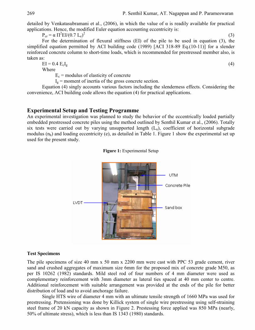
269 P. Senthil Kumar, AT. Nagappan and P. Parameswaran
detailed by Venkatasubramani et al., (2006), in which the value of α is readily available for practical applications. Hence, the modified Euler equation accounting eccentricity is:
Pcr = α П2EI/(0.7 Le)2 (3) For the determination of flexural stiffness (EI) of the pile to be used in equation (3), the
simplified equation permitted by ACI building code (1989) [ACI 318-89 Eq.(10-11)] for a slender reinforced concrete column to short-time loads, which is recommended for prestressed member also, is taken as:
EI = 0.4 EcIg (4) Where
Ec = modulus of elasticity of concrete Ig = moment of inertia of the gross concrete section.
Equation (4) singly accounts various factors including the slenderness effects. Considering the convenience, ACI building code allows the equation (4) for practical applications. Experimental Setup and Testing Programme An experimental investigation was planned to study the behavior of the eccentrically loaded partially embedded prestressed concrete piles using the method outlined by Senthil Kumar et al., (2006). Totally six tests were carried out by varying unsupported length (Lu), coefficient of horizontal subgrade modulus (nh) and loading eccentricity (e), as detailed in Table 1. Figure 1 show the experimental set up used for the present study.
Figure 1: Experimental Setup
Test Specimens
The pile specimens of size 40 mm x 50 mm x 2200 mm were cast with PPC 53 grade cement, river sand and crushed aggregates of maximum size 6mm for the proposed mix of concrete grade M50, as per IS 10262 (1982) standards. Mild steel rod of four numbers of 4 mm diameter were used as complementary reinforcement with 3mm diameter as lateral ties spaced at 40 mm center to centre. Additional reinforcement with suitable arrangement was provided at the ends of the pile for better distribution of load and to avoid anchorage failure.
Single HTS wire of diameter 4 mm with an ultimate tensile strength of 1660 MPa was used for prestressing. Pretensioning was done by Killick system of single wire prestressing using self-straining steel frame of 20 kN capacity as shown in Figure 2. Prestessing force applied was 850 MPa (nearly, 50% of ultimate stress), which is less than IS 1343 (1980) standards.

Experimental Investigation on Buckling Behavior of Prestressed Concrete Piles in Sand 270
Figure 2: Killick System of Prestressing and Prestressing Steel Frame
Deflection rods were fixed during casting, to measure the lateral deflection in the embedded
region. Control specimens were cast along with each pile specimen and cured under similar conditions of parent specimen. The values of concrete compressive strength (fcc) are given in Table 1. Table 1: Details of Partially Embedded Piles
Specimen Reference fcc (N/mm2) Lu (m) e (mm) R.D (%) nh (kN/m3) EPP 1 31.87 1.0 20 30 9801 EPP 2 33.72 1.0 60 30 9801 EPP 3 32.21 1.2 40 30 9801 EPP 4 25.11 1.1 40 30 9801 EPP 5 25.17 1.1 40 50 12197 EPP 6 19.88 1.1 40 70 19543
Foundation Medium
Dry river sand was used as a foundation medium. The specific gravity and uniformity coefficient of the sand were 2.62 and 1.4 respectively. The limiting void ratios were emax = 0.63, emin = 0.47 corresponding minimum dry densities were 1.599 g/cc and 1.782 g/cc respectively. The placement density for various relative densities was obtained by calculation.
Experimental determination of the coefficient of subgrade modulus for the foundation sand at a particular relative density was carried out separately, by the procedure outlined by Lee (1968), using a very rigid concrete pile with square cross-section as recommended by Terzaghi (1955). The values of nh for various relative densities are presented in Table 1, which is based on the average of three test values. Test Setup and Procedure
Amsler universal testing machine (UTM) of 1000 kN capacity, suitably modified to allow a maximum specimen length of 2200 mm, was used to test the pile specimen. UTM keeps the assembly set up intact up to specimen failure, even under large deformations.
A specifically designed wooden box (Fig 1) of size 0.6 m x 0.6 m x 1.5 m to meet the testing requirement, was placed in position to fill the sand after securing the position of the specimen between the ball-socket arrangements at both ends. Weighed mass of sand obtained for 150 mm thickness, based on the placement density, was poured and uniformly compacted till achieving 150 mm graduated level mark for each and every layer.
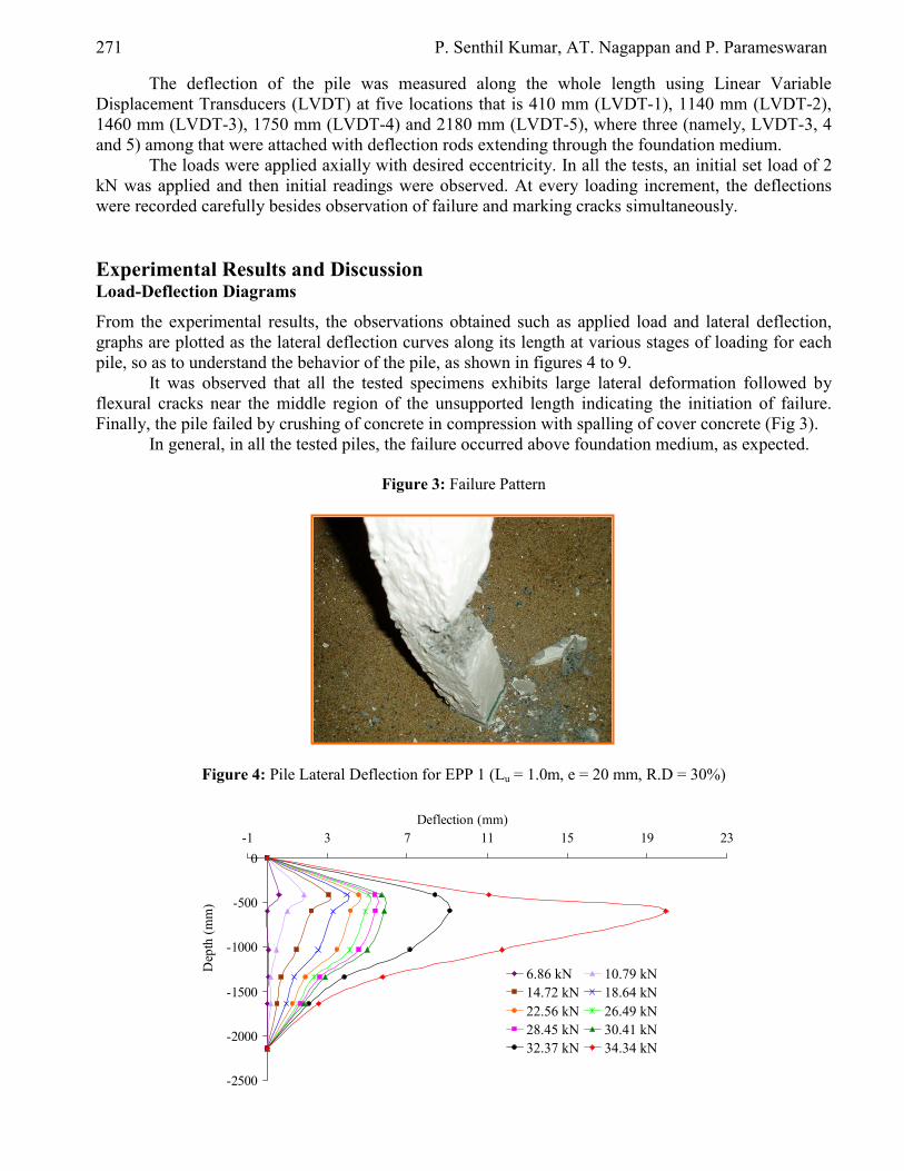
271 P. Senthil Kumar, AT. Nagappan and P. Parameswaran
The deflection of the pile was measured along the whole length using Linear Variable Displacement Transducers (LVDT) at five locations that is 410 mm (LVDT-1), 1140 mm (LVDT-2), 1460 mm (LVDT-3), 1750 mm (LVDT-4) and 2180 mm (LVDT-5), where three (namely, LVDT-3, 4 and 5) among that were attached with deflection rods extending through the foundation medium.
The loads were applied axially with desired eccentricity. In all the tests, an initial set load of 2 kN was applied and then initial readings were observed. At every loading increment, the deflections were recorded carefully besides observation of failure and marking cracks simultaneously. Experimental Results and Discussion Load-Deflection Diagrams
From the experimental results, the observations obtained such as applied load and lateral deflection, graphs are plotted as the lateral deflection curves along its length at various stages of loading for each pile, so as to understand the behavior of the pile, as shown in figures 4 to 9.
It was observed that all the tested specimens exhibits large lateral deformation followed by flexural cracks near the middle region of the unsupported length indicating the initiation of failure. Finally, the pile failed by crushing of concrete in compression with spalling of cover concrete (Fig 3).
In general, in all the tested piles, the failure occurred above foundation medium, as expected.
Figure 3: Failure Pattern
Figure 4: Pile Lateral Deflection for EPP 1 (Lu = 1.0m, e = 20 mm, R.D = 30%)
-2500
-2000
-1500
-1000
-500
0-1 3 7 11 15 19 23
Deflection (mm)
Dep
th (m
m)
6.86 kN 10.79 kN14.72 kN 18.64 kN22.56 kN 26.49 kN28.45 kN 30.41 kN32.37 kN 34.34 kN

Experimental Investigation on Buckling Behavior of Prestressed Concrete Piles in Sand 272
Figure 5: Pile Lateral Deflection for EPP 2 (Lu = 1.0m, e = 60 mm, R.D = 30%)
Figure 6: Pile Lateral Deflection for EPP 3 (Lu = 1.2m, e = 40 mm, R.D = 30%)
Figure 7: Pile Lateral Deflection for EPP 4 (Lu = 1.1m, e = 40 mm, R.D = 30%)
-2500
-2000
-1500
-1000
-500
0-3 2 7 12 17 22 27
Deflection (mm)
Dep
th (m
m)
5.40 kN 7.85 kN9.81 kN 11.77 kN13.73 kN 15.70 kN17.66 kN 19.62 kN20.60 kN
-2500
-2000
-1500
-1000
-500
00 5 10 15 20 25 30 35
Deflection (mm)
Dep
th (m
m)
3.53 kN 5.39 kN7.36 kN 9.32 kN11.28 kN 13.24 kN15.21 kN 17.17 kN 18.64 kN 19.13 kN
-2500
-2000
-1500
-1000
-500
00 5 10 15 20 25 30 35
Deflection (mm)
Dep
th (m
m)
0.98 kN 2.94 kN4.91 kN 6.87 kN
8.83 kN 10.79 kN12.75 kN 14.72 kN
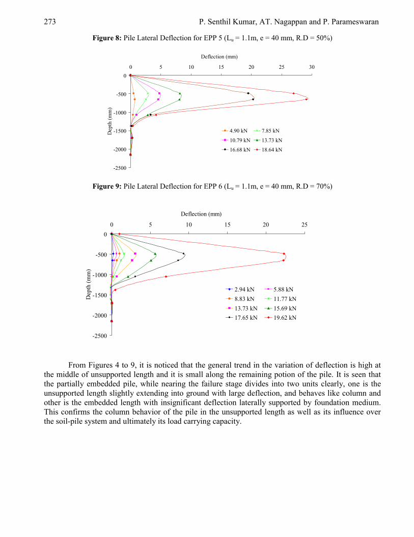
273 P. Senthil Kumar, AT. Nagappan and P. Parameswaran
Figure 8: Pile Lateral Deflection for EPP 5 (Lu = 1.1m, e = 40 mm, R.D = 50%)
Figure 9: Pile Lateral Deflection for EPP 6 (Lu = 1.1m, e = 40 mm, R.D = 70%)
From Figures 4 to 9, it is noticed that the general trend in the variation of deflection is high at
the middle of unsupported length and it is small along the remaining potion of the pile. It is seen that the partially embedded pile, while nearing the failure stage divides into two units clearly, one is the unsupported length slightly extending into ground with large deflection, and behaves like column and other is the embedded length with insignificant deflection laterally supported by foundation medium. This confirms the column behavior of the pile in the unsupported length as well as its influence over the soil-pile system and ultimately its load carrying capacity.
-2500
-2000
-1500
-1000
-500
00 5 10 15 20 25 30
Deflection (mm)
Dep
th (m
m)
4.90 kN 7.85 kN
10.79 kN 13.73 kN
16.68 kN 18.64 kN
-2500
-2000
-1500
-1000
-500
00 5 10 15 20 25
Deflection (mm)
Dep
th (m
m)
2.94 kN 5.88 kN8.83 kN 11.77 kN13.73 kN 15.69 kN17.65 kN 19.62 kN

Experimental Investigation on Buckling Behavior of Prestressed Concrete Piles in Sand 274
Figure 10: Load-Deflection Curves for Different Piles
From Figures 4 to 9, it is clear to observe that the deflection measured using LVDT-2 shows
maximum value and reveals the actual load-deflection relation of the partially embedded pile. Hence, based on this value experimental critical loads were obtained, and also a separate load-deflection curves were drawn for all the tested piles, as shown in Figure 10. The curves in Figure 9 show the ductile behavior of the partially embedded pile. Based on the experimental results, the following general features were also observed.
• The deflection of the pile is high at the middle of the unsupported length and reduces significantly in the foundation medium.
• The behavior of piles is similar in loose (R.D = 30%), medium (50%) as well as dense (70%) states of sand. A summary of test results is given in Table 2, which gives the ultimate load (Pu) for the test
specimen, the theoretically predicted critical load (Pt) and the experimental critical load (Pe). Table 2: Summary and Comparison of Results
Specimen Reference Pu (kN) Pt (kN) Pe (kN) Pe/Pt EPP 1 34.34 17.71 34.34 1.939 EPP 2 20.60 6.34 20.60 3.249 EPP 3 19.13 8.26 19.13 2.315 EPP 4 18.64 8.39 18.64 2.221 EPP 5 18.64 8.60 18.64 2.167 EPP 6 19.62 8.12 19.62 2.416
Finally, the theoretical critical loads were estimated based on the present approach and
compared with the experimental critical loads, in which the experimental loads were determined based on the procedure suggested by Kwon and Hancock (1992). As expected, the present approach is highly conservative especially for large eccentricity since the prestressing is more effective under flexure, which is not accounted anywhere in the ACI code. Apart from that the ACI equations for EI singly accounts many factors including slenderness effects and the use of most conservative (i.e., greatest) value [Lee, 1968] for the coefficient of the depth of fixity. Conclusion Buckling capacity of the partially embedded slender prestressed concrete pile may be predicted conservatively using the flexural stiffness equation of the ACI code. Comparison between the predicted
0
5
10
15
20
25
30
35
40
0 5 10 15 20 25 30 35Maximum Deflection (mm)
Loa
d (k
N)
EPP 1 EPP 2EPP 3 EPP 4EPP 5 EPP 6

275 P. Senthil Kumar, AT. Nagappan and P. Parameswaran
load and test results indicates the correctness in determining the effective length of the pile. Further, this study can be extended by incorporating the sectional properties of the member. However, owing to its simplicity, the proposed approach is readily adjustable to cater for various states of sandy soil, and hence it is likely to be of significant benefit to structural and geotechnical engineers. References [1] AASHTO, LFRD (1994) “Bridge Design Specifications,” American Association of State
Highways and Transport Office, Washington, D.C. [2] ACI Committee 318 (1989) “Building Code Requirements for Reinforced Concrete and
Commentary,” ACI 318R-89, American Concrete Institute, Detroit. [3] ACI Committee 543 (2000) “Design, Manufacture, and Installation of Concrete Piles,” ACI
543R-00, American Concrete Institute Detroit. [4] Baghery, S. (2004) “Buckling of Linear Structures above the Surface and/or Underground,”
Journal of Structural Engineering, ASCE, Vol. 130, No. 11, 1748- 1755. [5] Buckle, I.G., R. Mayes, and M.R. Button (1987) “Seismic Design and Retrofit Manual for
Highway Bridges,” Final Report, FHWA-IP-87-6, Federal Highway Administration, Washington, D.C.
[6] Chen, Y. (1997) “Assessment on Pile Effective Lengths and Their Effects on Design-I. Assessment,” Journal of Computers & Structures, Vol. 62, No. 2, 265- 286.
[7] Cummings, A.E. (1938) “The Stability of Foundation Piles Against Buckling Under Axial Load,” Proceedings, Part II, Vol. 38, Highway Research Board, National Research Council, Washington, D.C.
[8] Davisson, M.T. and K.E. Robinson (1965) “Bending and Buckling of Partially Embedded Piles,” Proceedings of 6th International Conference on Soil Mechanics and Foundation Engineering, Canada, Vol. III, Div. 3-6, 243-246.
[9] Francis, A.J. (1964) “Analysis of Pile Groups with Flexible Resistance,” Journal of Soil Mechanics and Foundation Engineering Division, ASCE, Vol. 90, No. SM3, 1-31.
[10] Gabr, M.A., J. Wang, and S.A. Kiger (1994) “Effect of Boundary Conditions on Buckling of Friction Piles,” Journal of Engineering Mechanics, ASCE, Vol. 120, No. 6, 1392-1400.
[11] Glick, G.W. (1948) “Influence of Soft Ground on the Design of Long Piles,” Proc. 2nd International Conference on Soil Mechanics and Foundation Engineering, Vol. 4, pp84-88.
[12] Heelis, M.E., M.N. Pavlovic, and R.P. West (2004) “The Analytical Prediction of the Buckling Loads of Fully and Partially Embedded Piles,” Journal of Geotechnique, 54, No. 6, 363-373.
[13] Hetenyi, M. (1946) “Beams on Elastic Foundation,” University of Michigan Press, Ann Arbor, Michigan, pp.148-150.
[14] Hromadik, J.J. (1961) “Column Strength of Long Piles.” Journal of the American Concrete Institute, Title No. 59-28, 757-778.
[15] IS: 10262 (1982), “Code of Practice for Recommended Guidelines for Concrete Mix Design,” Indian Standard Institution, New Delhi.
[16] IS: 1343 (1980), “Code of Practice for Prestressed Concrete,” Indian Standard Institution, New Delhi.
[17] Klohn, E.J. and G.T. Hughes (1964) “Buckling of Long Unsupported Timber Piles,” Journal of Soil Mechanics and Foundation Engineering Division, ASCE, Vol. 90, No. SM6, 107-123.
[18] Kwon, Y.B. and G.J. Hancock (1992) “Tests of Cold-formed Channels with Local and Distortional Buckling,” Journal of Structural Engineering, Vol. 118, No. 7, 1786-1803.
[19] Lee, K.L. (1968) “Buckling of Partially Embedded Piles in Sand,” Journal of Soil Mechanics and Foundation Engineering, ASCE, Vol. 94, No. SM1, 255-270.
[20] Lin, S.S. and W.K. Chang (2002) “Buckling of Piles in a Layered Elastic Medium,” Journal of Chinese Institute of Engineers, Vol. 25, No. 2, 157-169.

Experimental Investigation on Buckling Behavior of Prestressed Concrete Piles in Sand 276
[21] Prakash, S. and H.D. Sharma (1990) “Pile Foundation in Engineering Practice,” John Wiley and Sons, Inc. New York, pp.27-28.
[22] Ramsamooj, D.V. (1975) “Buckling Capacity of Piles in Soft Clay,” Journal of Geotechnical Engineering, ASCE, Vol. 101, No. GT11, 1187-1191.
[23] Senthil Kumar, P., T. Sivasamy, and P. Parameswaran (2006) “Buckling Capacity of Concrete Piles in Sand,” EJGE, Volume 11D. http://www/ejge.com/2006/Ppr0687/Ppr0687.htm
[24] Terzaghi, K. (1955) “Evaluation of Coefficients of Subgrade Reaction,” Journal of Geotechnique, Vol. 5, 297-326.
[25] Venkatasubramani, G.S., Ruben Selvaraj. and Parameswaran, P. (2006) “Stability of Axially Loaded Slender Reinforced Columns,” The Indian Concrete Journal, 41-46.

European Journal of Scientific Research ISSN 1450-216X Vol.18 No.2 (2007), pp.277-281 © EuroJournals Publishing, Inc. 2007 http://www.eurojournals.com/ejsr.htm
Analgesic and Anti-Inflammatory Activities of Ethanol Seed
Extract of Nigella Sativa (Black Cumin) in Mice and Rats
Tanko.Y Department of Human physiology Faculty of Medicine
Ahmadu Bello University Zaria, Nigeria E-mail: [email protected]
Mohammed A
Department of Human physiology Faculty of Medicine Ahmadu Bello University Zaria, Nigeria
Okasha. M.A
Department of Human physiology Faculty of Medicine Ahmadu Bello University Zaria, Nigeria
Shuaibu. A
Department of Human physiology Faculty of Medicine Ahmadu Bello University Zaria, Nigeria
Magaji. M.G
Department of Pharmacology and Clinical Pharmacy Ahmadu Bello University Zaria, Nigeria
Yaro A.H
Department of Pharmacology and Clinical Pharmacy Ahmadu Bello University Zaria, Nigeria
Abstract
The ethanol extract of Nigella sativa was investigated for possible anti-nociceptive and anti-inflammatory effects in mice and rats which were carried out using acetic acid-induced abdominal contractions in mice and formalin-induced hind paw edema in rats. . Three doses of the ethanolic extract (50, 100, 200mg/kg body weight) were used intraperitoneally for both anti-nociceptive and anti-inflammatory studies.
Significant effects (P≤0.05) was found at a dose of 50mg/kg of the ethanol extract in both anti-nociceptive and anti-inflammatory studies.
Preliminary phytochemical screening of the extract showed the presence of flavonoids, ,glycosides, steroids ,tannins, alkaloids and saponins. The extract had an intraperitoneal (i.p)LD50 of 471.2 mg/kg body weight in mice. The result supports the local use of the plant in painful and inflammatory conditions. Keywords: Nigella sativa anti-nociceptive, anti-inflammatory; phytochemical
constituents, acute toxicity studies.

Analgesic and Anti-Inflammatory Activities of Ethanol Seed Extract of Nigella sativa (Black Cumin) in Mice and Rats 278 Introduction Nigella sativa originates from the common fennel flower plant of the butter cup (Ranunculaceae) family. It is an annual herbaceous plant with common name as black cumin seed. The plant has finely divided foliage and pale bluish purple or white flowers. The flowers grow terminally on its branches while the leaves grow opposite each other in pairs. On either side of the stem, its lower leaves are small and petioles, and the upper leaves are long (6-10cm). The stalk of the plant reaches a height of twelve to eighteen inches as its fruit,and the black seed, matures. Nigella sativa is bisexual and forms a fruit capsule which consists of many white triagonal seeds. Once the fruit capsule has matured, it opens up and the seeds contained within are exposed to the air, becoming black in colour (black seeds). In English, Nigella sativa the plant is commonly referred to as black cumin (Ahmadiani, et al., 2000).
It has been traditionally used to treat ailments including bronchial asthma and bronchitis, rheumatism, to increase milk production in nursing mothers, to treat digestive disturbances, to support the body’s immune system, to promote digestion and elimination and to fight parasitic infestation. Its oil has been used to treat skin conditions such as eczema and boils and is used topically to treat cold symptoms
This research was aimed at investigating the possible anti-nociceptive and anti-inflammatory activities of ethanol extract of the plant in order to support or refute the claims by traditional herbalists.
Tanko. Y,Mohammed.A,Okasha. M.A,Shuaibu. A, Magaji. G.A and Yaro. A.H Materials and Methods (black cumin seed) was obtained from Department of Plant Science, Faculty of Agricultural Science, Ahmadu Bello University, Zaria It was identified at the herbarium unit of Biological Science Department, of the same University, where a voucher specimen No.2770 has been deposited. Preparation of Seeds Extract The seeds were collected, dried and later ground into paste using laboratory mortar and pestle. The fine powder , was extracted with ethanol for 72 h using a soxhlet extractor. The percentage yield of the extract was calculated to be 10.2 %(w/w). The extract was reconstituted in water at appropriate concentrations for the various experiments conducted. Phytochemical Screening The ethanol extract obtained was subjected to preliminary phytochemical screening, to identify the chemical constituents. The methods of analysis employed were those described by (Trease and Evans, 1989 ; Harbone and Baxter, 1993) Experimental Animals Adult wistar rats of both sexes weighing between 200-250g and adult swiss albino mice of both sexes weighing between 20-25g were used for the experiments. The animals were obtained from animal house of Department of Veterinary Medicine, Ahmadu Bello University, Zaria .They were kept in well ventilated room and fed with standard grower mash. Excel feeds Plc, Kaduna and allowed water ad libitum

279 Tanko.Y, Mohammed A, Okasha. M.A, Shuaibu. A, Magaji. M.G and Yaro A.H
Acute Toxicity Study This was conducted by using the method described by Lorke, 1983. In the initial phase, mice were divided into 3 groups of three and treated with the ethanol extract of the plant at doses of 10, 100 and 1000mg extract/ kg body weight intraperitoneally (i.p.) and were then observed for 24 hours for signs of toxicity including death .In the final phase, mice were divided into 4 groups of one mouse each and treated with the ethanol extract at doses of 140, 225, 370 and 600 mg / kg body weight i.p. The final LD50 was calculated as the square root of the product of the lowest lethal dose and the highest non- lethal dose, i.e the geometric mean of the consecutive doses which 0 and 100% survival rates were recorded. Test For Anti-Nociceptive Study The Acetic acid induced writhing test in mice as described by Koster et al., 1959 was employed. Swiss albino mice were divided into 4 groups of 5 mice each. The first group was given 10 ml/kg of Normal saline i.p. and served as control, groups 2, 3 and 4 received 50, 100 and 200 mg of extract per kg of body weight i.p. respectively. Thirty minutes later, mice in all the groups were treated with Acetic acid (0.6%v/v, 1ml per 100g body weight i.p.). Five minutes after Acetic acid injection mice were placed in individual cage and the number of abdominal contractions was counted for each mouse for a period of 10 mins. Percentage inhibition of writhing was calculated using the formula
Inhibition (%) = Mean No of writhings(control)- Mean No. of writhings(test) x 100 Mean number of writhing (control)
Test for Anti-Inflammatory Study Increases in the rat hind paw diameter induced by subplanter injection of a phlogistic agent was used as the measure of acute inflammation The phlogistic agent employed in this study was formalin (50µl of 2.5% v/v). The rats were divided into five groups 30 mins before the injection of formalin, the groups were treated i.p as follows group 1: normal saline (1ml/kg as a negative control) group 2,3 and 4 extract of Nigella sativa (50, 100 and 200mg/kg) respectively lastly group 5: Diclofenac 25mg/kg as positive control). Inflammation of the hind paw was induced by injecting formalin into the subplanter surface of the left hind paw. Paw diameter (cm) was measured at 1, 2, 3 4 and 5 hours after formalin injection. Paw diameter after administration of the phlogistic agent was measured of effect. using vernier caliper (Winter et al., 1962).
Inhibition (%)=Mean paw diameter (control) – Mean paw diameter (treated) x 100 Mean paw diameter (control)
Statistical Analysis Results were expressed as mean ± Standard Error of Mean (SEM). The data was statistically analyzed using the one-way ANOVA to determine whether results in a particular group were significantly different from those in the corresponding control groups. Results were statistically significant when p values is less than 0.05 (P≤0.05) as described by Duncan et al., (1977). Results and Discussion Phytochemical Analysis
The freshly prepared extracts were subjected to preliminary phytochemical screening test for various constituents. This revealed the presence of alkaloids, tannins, saponins, glycosides, flavonoids, glycerin and steroids.

Analgesic and Anti-Inflammatory Activities of Ethanol Seed Extract of Nigella sativa (Black Cumin) in Mice and Rats 280 Acute Toxicity Study (LD50)
The sign of toxicity were first noticed after 4-6 hours of extract administration. There was decreased locomotor activity and decreased in sensitivity to touch and jerking. Also there was decreased feed intake, tachypnoea and prostration after 10 hours of extract administration.
The median lethal dose (LD50) in mice was calculated to be 471.2 mg/kg body weight The ethanol extract of Nigella sativa was found to have shown a significant (P<0.05)
antinociceptive effect at all the doses tested. Although, the inhibitory effect on the acetic-induced writhings in mice was not dose- dependent, the percentage inhibition at a dose of 50mg/kg body weight of extract was found to be highest (67.1%) while that of the Diclofenac is 74.1%. The abdominal constriction method is a very sensitive one and can detect anti-nociceptive effect of substances at a dose that cannot be detected by other methods, such as the tail- flick test (Collier et al., 1968). Abdominal constriction responses were found to partly involve local peritoneal receptors (Bentley et al., 1981). The method has been associated with prostanoids in general, e.g increased levels of PGE2 and PGEF2α in peritoneal fluids (Derardt et al.,1980) as well as lipoxygenase products by some rearchers (Levini et al., 1984; Dhara et al., 2000) . Therefore, the results of the acetic acid-induced writhing strongly suggest that the mechanism of action of this extract may be linked partly to lipoxygenases and or cyclo-oxygenases. The activity demonstrated by the extract might be due to the presence of flavonoids and tannins that were present in the extract. This was supported by other workers who found that flavonoids and tannins were found to have antinociceptive and /or anti-inflammatory activities (Ahmadiani, et al., 1998).
The significant (P< 0.05) anti-inflammatory activity exhibited by the extract at all the doses used (50, 100, and 200mg/kg body weight extract i.p.) against oedema induced by formalin in rats compared to the control group was an indication that, the plant might serve as a useful source of anti-inflammatory agent. This anti-inflammatory effect of the extract observed might be due to the presence of flavonoid, in the plant. This was supported by other workers, who found that flavonoids inhibit phosphodiesterases which are involved in cell activation, and their effect depend upon the biosynthesis of protein cytokines that mediate adhesion of circulating leucocytes to the sites of injuries (Duke, 1992).
Finally the ethanolic Nigella sativa extract does possess significant antinociceptive and anti-inflammatory effects in laboratory animals at the doses investigated. The results support the traditional use of this plant in some painful and inflammatory conditions and suggest the presence of biologically active components which may be worth further investigation and elucidation. Further studies are infact currently under way to isolate and characterized the active components of the crude extract. Analgesic and anti-inflammatory activities of ethanol seed extract of Table 1: Mean number of writhings and percentage inhibition of ethanol seed extract of Nigella sativa on
acetic acid –induced writhings in mice.
Treatment Dose mg/kg b.w Mean number of writhing % inhibition P-value N/saline. 1ml/kg 24.300 ± 0.600 - - Extract 50mg/kg 8.000 ± 2.510 67.1 P<0.05 Extract 100mg/kg 8.200 ± 2.478 66.3 P<0.05 Extract 200mg/kg 9.400 ± 3.776 61.3 P<0.05 Piroxicam 20mg/kg 6.300± 1.800 74.1 P<0.05

281 Tanko.Y, Mohammed A, Okasha. M.A, Shuaibu. A, Magaji. M.G and Yaro A.H
Table 2: Mean effect of ethanol extract of Nigella sativa of formalin-induced edema in rats paw diameter(cm) at various interval.
Treatment Given 1hour 2 hours 3 hours 4 hours 5hours N/saline 0.734±0.0732(a) 0.802 ±0.0559(a) 0.784 ±0.0564(a) 0.784 ± 0.0564(a) 0.722± 0.0508(a) 50mg/kg extract 0.528±0.0334(a) 0.552± 0.0318(a) 0.512± 0.0248(a) 0.452 ± 0.0185(a) 0.444± 0.0312(a) 100mg/kg extract 0.568±0.0275(a) 0.560± 0.0318(a) 0.546± 0.0393(a) 0.484 ± 0.0790(a) 0.440±0.0200(a) 200mg/kg extract 0.630±0.0333(ns) 0.520± 0.0316(a) 0.528± 0.0449(a) 0.486 ± 0.0306(a) 0.442± 0.0196(a) 25mg/kg Diclofenac 0.59 ±0.02 0.61±0.02(a) 0.61± 0.01(a) 0.63±0.02(a) 0.64±0.02(a)
a=P≤ 0.05 significant ns=not significant References [1] Ahmadiani, A; Hosseiny, J; Semnanian, S; Javan, M; Saeedi, F; Kamalinejad, M and Sareni, S.
Anti-nociceptive and anti-inflammatory effects of Eleagnus angustifolia fruits extract, J. Ethnopharmacol; 72: 287 – 292.(2000).
[2] Ahmadiani, A., Fereidoni, M., Semnanian, S., Kamalinejad, M., Saremi, S. Anti-nociceptive and anti-inflammatory effects of Sambucus ebulus rhizome extract in rats. J. Ethanopharmacology 61:229-235 (1998).
[3] Bentley, G. A. Newton, S. H. and Starr, J.. Evidence for an action of morphine and the enkephallins can Sensory nerve endings in the mouse peritoneum, Brit. J. Pharmacol, 79: 125 – 134 (1981).
[4] Brain, K. R and Turner, T. D. The Practical Evaluation of Phytopharmaceuticals, Wright Scientechnica, Bristol, pp. 57 – 58.(1975).
[5] Collier, H. O. J; Dinneen, L. G; Johnson, C. A. and Schneider, C . The Abdominal constriction response and its suppressesion by analgesic drugs in the mouse, Brit. J. Pharmacol; 32: 295 – 310 (1968).
[6] Derardt, R., Jougney , S., Delevalcee, F., Falhourt, M. Release of prostaglandins E and F in an algogenic reaction and its inhibition. European Journal of Pharmacology 51, 17 -24 (1980).
[7] Dhara, A.K., Suba, V., Sen, T., Pal, S., Nag Chaudhuri, A.K Preliminary studies on the anti-inflammatory and analgesic activity of the methanolic fraction of the root extract of Tragia involucrate. J. Ethanopharmacology 72, 265-268.(2000).
[8] Duke, J.A . Handbook of Biologically Active Phytochemcials and their activities. CRC Press, Boca Raton, FL, pp. 22 – 25(1992).
[9] Duncan, R. C; Knapp, R. G and Miller, M. C.Test of Hypotheses in population Means, In: Introductory Biostatistics for Health Sciences, John Wiley and Son, Inc. N. Y. pp. 71 – 76.(1977).
[10] Harbone, J.B. and Baxter, H,H Phytochemical Dictionary. A hand Book of Bioactive Compound from plants. Taylor and Francis, Washington , D.C., U.S.A Pg 237 (1993).
[11] Hess,S..M., and Milong R.C. Inflammation Mechanism and Control.Lepow. i.h. and Ward,P.A.ed, academic Press New York .Pg 1-2.(1972).
[12] Levini, J.D., Lau, W., Kwait, G., Goetzl E.J.. Leukotriene B4 produces hyperalgesia that is dependent on the polymorphonuclear leucocytes. Science 255, 743-745.(1984).
[13] Lorke, D. A New Approach to Practical Acute Toxicity Testing, Arch. Toxicol, 53: 275 – 287.(1983).
[14] Trease, G.E., Evans, M.C., Text book of Pharmacognosy 13th Edition Bailiere Tindall, London, Toronto, Tokyo. Pgs. 200-201, 340-348, 419-423, 626-630, 765-775 (1989).
[15] Winter, E. A. Risley, E.A., Nuss, G. V. Anti-Inflammatory and antipyretic activities of indomethacin. Journal of pharmacology and Experimental Therapeutics. 141, 369 – 376.(1963).

European Journal of Scientific Research ISSN 1450-216X Vol.18 No.2 (2007), pp.282-286 © EuroJournals Publishing, Inc. 2007 http://www.eurojournals.com/ejsr.htm
The Study of Solvent Effect on the Diastereoselectivity of
Diels-Alder Reaction in the Presence of Nanoporous Silica-Supported Cerium Sulfonate Catalyst
Ghodsi Mohammadi Ziarani Department of Chemistry, Alzahra University, Tehran, Iran
E-mail: [email protected]
Alireza Badiei School of Chemistry, University College of Science
University of Tehran, Tehran, Iran
Azam Miralami Department of Chemistry, Alzahra University, Tehran, Iran
Abstract
The diastereoselectivity of the Diels-Alder reaction in the presence of cerium sulfonate immobilized on nanoporous silica type SBA-15 was studied in different solvents. The polarity of solvent had effective role on the Lewis acid activity of the catalyst. The increase of the solvent polarity significantly enhanced the diastereoselectivity of the Diels-Alder reaction. Keyword: Diels-Alder reaction (DA), modified SBA-15, cerium, Diastereoselectivity,
Cyclopentadiene, methylacrylate and dienophiles. Introduction The Diels-Alder reaction is a very useful tool for synthetic organic chemistry [1] because it can be used to prepare optically active molecules in one simple reaction step which traditionally performed using homogeneous Lewis acid catalyst [2]. Following the replacing homogeneous acidic catalysts by their heterogeneous counterparts, Diels-Alder reaction catalyzed by solid organic frameworks [3], clays [4], zeolites [5], immobilized heteropoly acids [6], mesoporous molecular sieves (Al-HMS and La-SBA-15), alumina and metal functionalized silica (ZnCl2, AlCl3, FeCl3). The SBA-15 is new mesoporous templated silica with hexagonal structure, large pore, high surface area, high thermal stability and especially 3D channel connectivity. These types of materials are suitable for using as catalyst. The surface of mesoporous structure can be modified to obtain suitable catalytic activity. Considering to this viewpoint that rare earths salts of strong acids are sometimes able to work as effective Lewis acid catalysts in the presence of water, alcohols, or even amines [7] and regarding to immobilization of a rare earth metal on mesoporous silica that has been reported [8].
The effect of the solvent on the endo-exo selectivity of the Diels-Alder reaction was systematically studied by Berson [9]. They interpreted the solvent dependence of the endo-exo ratio by considering the different polarities of the individual activated complexes involved. The importance of solvent polarity has also been discerned by other authors on the basis of experimental and theoretical

The Study of Solvent Effect on the Diastereoselectivity of Diels-Alder Reaction 283
work [10, 11]. Interestingly, Nakagawa and coworkers have observed a correlation between the endo-exo ratio and solvent polarisability [12]. Extensive multiparameter analyses by the group directed by Mayoral demonstrated that a proper description of the solvent effect on the endo-exo ratio requires a number of different interactions [13-16]. Hydrogen bonding by the solvent contributes most significantly, but also solvent polarity and solvent solvophobicity are important [17].
In this paper, we presence the solvent effect on the diastereoselectivity of Diels-Alder reaction in the Presence of nanoporous silica-supported cerium sulfonate catalyst. Experimental Section Materials
All materials were purchased from Merck. All reactants were distilled before used. Preparation the modified SBA-Ce catalyst Preparation of the modified SBA-15-cerium catalyst was performed according to scheme 1. The calcinated SBA-15 (2 g) was reacted with 3-(trimethoxysilyl)-1-propanethiol (10 ml) in dry toluene (20ml) for 24h at reflux temperature. The product was filtered and extracted for 6h in CH2Cl2 using a soxhlet apparatus, then dried under vacuum. The solid product was oxidized with H2O2 (excess) in methanol (20 ml) for 24 h at rt. After filtering, the mixture was reacted with cerium (III) nitrate (3 mmol, 1.7g) in acetonitrile (20 ml) at reflux temperature for 24h. After cooling to rt, CH3CN was added and the mixture was filtered and washed with CH3CN and dried under vacuum. Then this produce was treated with trifluoromethanesulfonic acid (about 0.3 ml, 10 drops) in dichloromethane (20 ml) at rt for 12h. After addition of H2O, the mixture was filtered and washed with H2O, H2O-THF, THF, Et2O and dried under vacuum to obtain the modified SBA-Ce catalyst. Scheme 1: Diels-Alder reaction on the presence of the different amount of SBA-Ce catalyst under solvent free
conditions
At first, the diels-Alder reaction between cyclopentadiene and methyl acrylate was carried out
on the presence of prepared catalyst (20 mg) without solvent. Methyl acrylate (0.9 ml) was added to catalyst. Freshly distilled cyclopentadiene (2.5 ml) was added to mixture of reaction with stirring. The reaction was left to stir for 2h at about -10 ºC. Then it was filtered to separate the catalyst and the
SH(MeO)3Si(CH2)3SH
Reflux in dry toluene
H2O2 in methanol SO3H
SO3Ce(NO3)2
SBA-15 SBA-15 SBA-15
SBA-15
Ce(NO3)3
in acetonitrileTfOH in CH2Cl2 SO3Ce(TfO)2
SBA-15
6 nm
SBA-Ce

284 Ghodsi Mohammadi Ziarani, Alireza Badiei and Azam Miralami
product mixtures were analyzed by Gas Chromatography. This reaction was repeated with 40 mg and 200 mg catalyst respectively. The results of these reactions were reported in table 1. Diels-Alder reaction on the presence of the SBA-Ce in different solvents This Diels-Alder reaction was carried out with 20 mg of the SBA-Ce in different solvent. Methyl acrylate (0.9 ml) was added to catalyst (20 mg) in 3ml solvent in a small round bottom flask. Freshly distilled cyclopentadiene (2.5 ml) was added to mixture reaction with stirring. The reaction was left to stir for 2h at about -10 ºC. Then it was filtered to separate the catalyst and the product mixtures were analyzed by Gas Chromatography. The results were reported in table 2. Results and discussion Table 1 shows the yield and diastereoselectivity of Diels-Alder reaction between cyclopentadiene and methylacrylate on the presence of the different amount of SBA-Ce catalyst under solvent free condition. The obtained results reveal that the quantity of the catalyst has a little effect on the diastereoselectivity of the Diels-Alder reaction under solvent free condition. Table 1: Diels-Alder reaction between cyclopentadiene and methyl acrylate on the presence of the different
amount of modified catalyst under solvent free conditions
The catalyst amount Yield(%) De(%) 20 mg 98 52 40 mg 98 54 200 mg 98 60
Table 2 shows the diels-Alder reaction between cyclopentadiene and methylacrylate on the
presence of the SBA-Ce in different solvents. The best diastereoselectivity of the Diels-Alder reaction obtain in water (with high dielectric constant). The diastereoselectivity of the Diels-Alder reaction enhances with the increase of dielectric constant. The diastereoselectivity of reaction between cyclopentadiene and methylacrylate improved about 70% from low to high polarity of solvent in table 2. The mechanism of activation by Lewis acids can be understood with the aid of the FMO theory [18, 19] (fig.1). The electron withdrawing character of the catalyst lowers the energy of the LUMO of the reactant to which it is coordinated, resulting in a decrease of the HOMO-LUMO energy difference and, in turn, an increase in the rate of the Diels-Alder reaction. The solvent effects on the diastereoselectivity of Diels-Alder reactions have revealed the importance of hydrogen bonding interactions besides the already mentioned solvophobic interactions and polarity effects. Hydrogen bonds strengthen the electron-withdrawing capacity of this functionality and thereby decrease the HOMO-LUMO gap between diene and dienophile. Thess results strongly suggest that in water, a hydrogen bond donating solvent par excellence, and the Diels-Alder benefits not only from hydrophobic interactions but also from hydrogen-bonding interactions. The small size of water molecules allows efficient interaction with hydrogen-bond acceptors by forming more hydrogen bonds than protic organic solvents.However, Large pore SBA-Ce (about 6 nm) containing a cavity can bind both Diels-Alder reagents simultaneously and promote their reaction. The increase in diastereoselectivity is a result of an increased secondary orbital interaction that can be attributed to the increased orbital coefficient on the carbonyl carbon.

The Study of Solvent Effect on the Diastereoselectivity of Diels-Alder Reaction 285
Figure 1: Frontier orbital energies (eV) and coefficients for acrolein and protonated acrolein. In the latter case the upper numbers refer to the situation where bond lengths and angles correspond to those of acrolein. The lower numbers are more suitable for a hydroxyallyl cation. The actual situation is assumed to be intermediate. The data are taken from ref. [19].
Table 2: the diels-Alder reaction between cyclopentadiene and methyl acrylate on the presence of the SBA-
Ce in different solvents.
Solvent Dielectric constant (at 25°C) (vacuum)-1 Yield De% Water 78.5 98 75 Methanol 32.6 98 71 Ethanol 24.3 98 69 1-hexanol 13.3 98 68 2-propanol 18.3 98 64 Dichloromethane 9.1* 98 62 Trichloromethane 4.8* - 61 1,2-dichloroethane 10.6 * 42 59 Tetrachloride carbon 2.2 * 86 52
*at 20ºC. Conclusions The cerium sulfonate immobilized on nanoporous silica type SBA-15 can be effective heterogeneous catalyst in diastereoselectivity of the Diels-Alder reaction of between cyclopentadiene and methyl acrylate in different solvents. The polarity of solvent had effective role on the Lewis acid activity of the catalyst. The diastereoselectivity of the Diels-Alder reaction enhances with the increase of dielectric constant. The highest diastereoselectivity obtains for water. Acknowledgement This work was financially supported by the Research Affair of Alzahra University and University of Tehran.

286 Ghodsi Mohammadi Ziarani, Alireza Badiei and Azam Miralami
References [1] J. March, Advanced Organic Chemistry, 4th ed., Willey/Interscience, New York, 1992. [2] H. B. Kagam, O. Riant, Chem. Rev. 1992, 92, 1007. [3] K. Endo, T. Koiko, T. Sawaki, O. Hayashida, H. Masuda, Y. Aoyama, J. Am. Chem. Soc. 1997,
119, 4117. [4] J. M. Fraile, J. I. Garcia, D. Gracia, J. A. Mayoral, T. Tamai, F. Figueras, J. Mol. Catal. A.
1997, 121, 97. [5] L. Eklund, A-k. Axelsson, A. Nordahl, R. Carlson, Acta Chim. Scand. 1993, 47, 581. [6] G. J. Meuzelaar, L. Maat, R. A. Sheldon, Catal. Lett. 1998, 59, 49. [7] S. Kobayashi, S. Nagayama, T. Busujima, J. Am. Chem. Soc., 1998, 120, 8287. [8] P. Sreekanth, S. Kim, T. Hyeon, B. MoonKim, Adv. Synth. Catal., 2003, 345, 936. [9] J. A. Berson, Z. Hamlet, W. A. Mueller, J. Am. Chem. Soc., 1962, 84, 297. [10] G. Desimoni, G. Faita, P. P. Righetti, L. Toma, Tetrahedron, 1990, 46, 7951. [11] T. Oshima, S. Arikata, T. Nagai, J. Chem. Research, 1981, 204. [12] K. Nakagawa, Y. Ishii, M. Ogawa, Tetrahedron, 1976, 32, 1427. [13] C. Cativiela, J. I. García, J. A. Mayoral, A. J. Royo, X. Assfeld, M. F. Ruiz-Lopez, J. Phys.
Org. Chem,. 1992, 5, 230. [14] C. Cativiela, J. I. Garcia, J. A. Mayoral, A. Avenoza, M. A. Roy, J. Phys. Org. Chem,. 1991, 4,
48 [15] C. Cativiela, J. I. Garcia, J. Gil, R. M. Martinez, J. A. Mayoral, L. Salvatella, J. S. Urieta, A. M.
Mainar, M. H. Abraham, J. Chem. Soc., Perkin Trans. 2, 1997, 653. [16] C. Cativiela, J. I. Garcia, J. A. Mayoral, L. Salvatella, J. Chem. Soc., Perkin Trans. 2, 1994,
847. [17] C. Cativiela, J. I. Garcia, J. A. Mayoral, L. Salvatella, Chem. Soc. Rev, 1996, 209. [18] J. M. Mellor, C. F. Webb, J. Chem. Soc., Perkin Trans. 2, 1974, 26. [19] K. N. Houk, R. W. Strozier, J. Am. Chem. Soc., 1973, 95, 4094.
European Journal of Scientific Research ISSN 1450-216X Vol.18 No.2 (2007), pp.287-297 © EuroJournals Publishing, Inc. 2007 http://www.eurojournals.com/ejsr.htm
Measurement of Inequality in Pakistan (Expenditure Approach)
Masood Sawar Awan Assistant, Professor, Department of Economics, University of Sargodha
Sohail Jehangir Malik
Chairman and Professor, Department of Economics, University of Sargodha
Zakir Hussain Graduate Student, Department of Economics, University of Sargodha
Haroon Sarwar
Graduate Student, Department of Economics, University of Sargodha
Abstract
The income inequality is perhaps globally established phenomena and continued to inflict mankind since time immemorial. The problem of income inequality is alarming and Pakistan is no exception. In Pakistan, the income inequality is much elevated, the dawdling trickle down of growth in recent years has affected the poor adversely and the poverty incidence registered an increase. There was hardly any study which used expenditure approach to measure the income e inequality. The data on income were often under estimated. The objective of this paper was to estimate income inequality using different methods through expenditure approach. The data were utilized from Household Income and Expenditure Survey, 2001. The results revealed that in Pakistan there was lesser inequality in terms of food expenditure. The non-durable expenditure showed relatively higher inequality and durable inequality was even much higher. The axiomatic approach showed that the methods of generalized entropy class were better estimates which satisfied all the axioms. Keywords: Inequality, Gini Coefficient, Generalized Entropy, Atkinson Index
Introduction Global income inequality is probably greater than it has ever been in human history. There is some debate about whether it is getting worse or getting better. Currently, the richest one percent of people in the world received as much as the bottom 57 percent. The ratio between the average incomes of the top 5 percent in the world to the bottom 5 percent increased from 78:1 in 1988 to 114:1 in 1993 (Milanovic 1999). Milanovic found that the richest 25 percent of the world's population received 75 percent of the world's income, even when adjusting for Purchasing Power Parity. The poorest 75 percent of the population shared just 25 percent. This occurred because a large proportion of the world's population lived in the poorest countries, and within the poorest regions of those countries, particularly in the rural areas of China, rural and urban India and Africa.
In Pakistan, where the degree of exclusion of the underclass was greater and the income inequality was much higher, the slowdown in growth in recent years affected the poor much more and

Measurement of Inequality in Pakistan (Expenditure Approach) 288
the poverty incidence has increased, despite momentum growth rate in the last two years (7 percent to 8.4 percent, GOP, 2006). The increased growth rate even contributed towards yawning inequality and increased inflation. The liquidity through easy credit and highly speculative economic activities further widened the rich-poor gap. In order to arrest ever-increasing inequality, it seems imperative in providing sound estimates to policy makers for corrective actions.
In the literature, many studies which used expenditure data for measuring income inequality. The expenditure data were generally more precisely measured and are considered reliable estimators of welfare. The personal income was an obvious choice for analyzing distribution of income; the gross understatement of the income in surveys often distorted the estimates. In Pakistan, household data collected by the Federal Bureau of Statistics (FBS) has suffered from underestimation at both ends of the income distribution. The richest and the poorest households were often reluctant to part with personal information. Therefore, household data collected by FBS source may understate income inequalities. The income data also suffered from the seasonality, the periods for which income was reported by respondents, the imputed incomes etc. Therefore, expenditure data were preferred over income for computing income inequalities because expenditures truly reflect the permanent incomes of the individuals. However, the fact remains that expenditures were generally overstated and in particular poor tend to overstate expenditures. Moreover, the income inequalities based on expenditure often understate true income inequalities because the rich typically save a larger proportion of their incomes while the poor forced to dis-save or borrow to meet their consumption needs. In Pakistan, estimates of income inequalities were derived on the basis of both the incomes as well as the expenditures. (A.R Kemal (2003). The expenditure approach was used in this study. The Data and the Methodology The data used in this study was taken from Pakistan Household Income and Expenditure Survey 2001-02. The study used five different inequality measures to find out inequality among food expenditure, durables and non-durable expenditures. The five inequality measures were: Gini coefficient:
The Gini coefficient is one of the most commonly used indicators of income inequality. The Gini is derived from the Lorenz curve, which plots the cumulative share of total income earned by households ranked from bottom to top. In Figure 1, the curve showed the shares of income earned by successive deciles of households, arrayed in order from the bottom 10 percent to upwards. If incomes were equally distributed, the Lorenz curve would follow the 45° diagonal. As the degree of inequality increases, so does the curvature of the Lorenz curve, and thus the area between the curve and the 45° line becomes larger. The Gini was calculated as the ratio of the area between the Lorenz curve and the 45° line, to the whole area below the 45° line.

289 Masood Sawar Awan, Sohail Jehangir Malik, Zakir Hussain and Haroon Sarwar
Figure 1: Graphical Presentation of a Lorenz Curve
Atkinson Index:
The Atkinson Index is one of the few inequality measures that explicitly incorporate normative judgments about social welfare (Atkinson 1970). The index is derived by calculating the equity-sensitive average income (ye), defined as the level of per capita income which if enjoyed by everybody would make total welfare exactly equal to the total welfare generated by the actual income distribution (MacArthur,2000). The equity-sensitive average income is given by:
111
.[ ( ) ]ie iy f y y −−= ∑
εε
Where Ye=Equity-Sensitive average income Yi=Proportion of income earned by ith group ε=Inequality aversion parameter.
The parameter ε reflects the strength of society's preference for equality, and can take values ranging from zero to infinity. When ε > 0, there is a social preference for equality (or an aversion to inequality). As ε rises, society attaches more weight to income transfers at the lower end of the distribution and less weight for transfers to the top. Typically used values of ε are 0.5 and 2.
The Atkinson Index (A) is then given by: 1
1
11n i
i
yAn Y=
⎡ ⎤⎧ ⎫⎪ ⎪⎢ ⎥= − ⎨ ⎬⎢ ⎥⎪ ⎪⎩ ⎭⎣ ⎦∑
ε ε
–
Where Y_
: was the actual mean income. The more equal the income distribution; the ye is close
to Y_
, and the lower the value of the Atkinson Index. For any income distribution, the value of “A” lies between 0 and 1. In this study we have taken the value at 0.5. Generalised Entropy Measures:
Members of the Generalized Entropy class of measures have the general formula as follows:

Measurement of Inequality in Pakistan (Expenditure Approach) 290
Where n is the number of individuals in the sample, yi is the income of individual i, i є (1,
2,…,n), and = (1/n) Σ yi, the arithmetic mean income. The value of GE ranges from 0 to ∞, with zero representing an equal distribution (all incomes identical) and higher values represent higher levels of inequality. The parameter α in the GE class represents the weight given to distances between incomes at different parts of the income distribution, and can take any real value. For lower values of α GE is more sensitive to changes in the lower tail of the distribution, and for higher values GE is more sensitive to changes that affect the upper tail. The commonest values of α used are 0, 1 and 2: hence a value of α =0 gives more weight to distances between incomes in the lower tail, α=1 applies equal weights across the distribution, while a value of α =2 gives proportionately more weight to gaps in the upper tail. The GE measures with parameters 0 and 1 become, with l'Hopital's rule, two of Theil’s measures of inequality (Theil, 1967), the mean log deviation and the Theil index respectively, as follows:
With α =2 the GE measure becomes 1/2 the squared coefficient of variation, CV:
Coefficient of Variation:
The Coefficient of Variation is a distribution’s standard deviation divided by its mean.
C. V = vµ
The Coefficient of variation is sensitive to income transfers for all income levels and is
independent of the mean income level. The Coefficient of variation attaches equal weights to transfers of income at different income levels. It is, however, possible that the impact of a transfer would be greater at a lower income level than at the high-income level. Share – Ratio:
Share-ratio is another measure of inequality, which denotes the Share Ratio for population domain ‘k’ by P4, P3, P2, P1, SR (where P1 and P2 are lower and upper percentiles that delimitate a first group and P3 and P4 are lower and upper percentiles that delimitate a second group). The Share Ratio is the ratio of the income share of the first group over the income share of the second group:
L (P3) - L (P4)( , P1, P2, P3, P4)L (P2) - L (P1)
SR k =
In order to find out the effect of different forces on distribution of income this study used earning functions and occupational choice equations.
A review of the existing work on income distribution shows that efforts were largely concentrated on measurement of income distribution using Gini coefficient based on either household income or consumption expenditure. Existing work also indicates that different authors/institutions

291 Masood Sawar Awan, Sohail Jehangir Malik, Zakir Hussain and Haroon Sarwar
employed different methods, chose different measurement of living standard e.g., income or consumption and different unit of measurement e.g. household or population and thereby have reported different inequality trends. Thus, there exists ambiguity about the inequality trends over time since these studies are not only inconsistent in terms of measurement of living standard and unit of measurement but also limited in terms of coverage of period and therefore, cannot be the basis for a longer-term trend analysis.
The overall objective of the paper was to estimate different measures of inequality for Pakistan. This provides reliable inequality statistics to policy makers as well as enable us to compare different inequality measures. The Results and Discussion Gini Coefficient:
The Gini coefficient was one of the most commonly used indicators of income inequality. Table 1: Gini Coefficients of Rural and Urban population in Pakistan
Description of Inequality Rural Inequality Urban Inequality Pakistan’s Inequality Food Expenditure 0.330 0.340 0.338 Non-Durable Expenditure 0.280 0.346 0.327 Durable Expenditure 0.714 0.798 0.760 Overall Expenditure 0.328 0.360 0.339
The Gini coefficients (Table 1) depicted severe inequality in durable expenditures while food
and non-durable expenditure inequality was relatively low. The distribution was more skewed in urban areas as compared to rural areas. Overall expenditure inequality also followed the same pattern; however, it declined to 0.34 percent as apposed to 0.37 revealed by Ahmed & Ludlow (1987). This demonstrates that inequality has declined overtime. The analysis provided component wise inequality statistics but this measure i.e. Gini coefficient, although extensively used by the researchers, was fraught with inherent short-comings. The Gini index attached more weight to transfers affecting middle income classes and not much weight to changes in extreme income classes. Gini ignores intra group inequalities and as such it understates consumption inequality. Atkinson index:
The results in the Table 2 showed that inequality was more in durable expenditure as compared to the other components. Our estimates for Atkinson index (�=0.5) were showing lesser overall expenditure inequality in 2001-02 (0.096) as compared with 1984-85 estimates (0.1236) by Ahmed and Ludlow. Table 2: Atkinson (Inequality) Indices of Rural and Urban
Description of Inequality Rural Inequality Urban Inequality Pakistan’s Inequality Food Expenditure 0.088 0.095 0.093 Non-Durable Expenditure 0.064 0.099 0.089 Durable Expenditure 0.447 0.560 0.509 Overall Expenditure 0.086 0.108 0.096
Generalised Entropy Measures(GE):
Generalized Entropy is the most reliable estimate because it satisfies all axioms. Entropy estimates are also showing serious inequality in durable, while rural urban gulf is also evident from the results.

Measurement of Inequality in Pakistan (Expenditure Approach) 292
Coefficient of Variation:
The Coefficient of Variation is a distribution’s standard deviation divided by its mean. Prospects: • Easy to understand. • If data is weighted, it is immune to outliers. • Incorporates all data. • Not skewed by inflation.
Constraints: • Requires comprehensive individual level data. • No standard for an acceptable level of inequality.
The Coefficient of variation is sensitive to income transfers for all income levels and is independent of the mean income level. The Coefficient of variation attaches equal weights to transfers of income at different income levels. It is, however, possible that the impact of a transfer would be greater at a lower income level than at the high-income level. The estimates of this study indicate that there is more intense rich poor disparity in durable expenditures because generally rich expand more on luxuries; most of which are durables, while poor spend very little on durables. In terms of rural-urban devoid, results for urban area were showing more unequal distribution in all the three components of expenditure. Table 3: Measures of Inequality in Pakistan
Description of Inequality Rural Inequality Urban Inequality Pakistan’s Inequality Atkinson (Inequality) Food Expenditure 0.185 0.208 0.199 Non-Durable Expenditure 0.136 0.224 0.201 Durable Expenditure 1.334 1.800 1.618 Overall Expenditure 0.180 0.245 0.217 Coefficient of Variation Food Expenditure 0.678 0.769 0.733 Non-Durable Expenditure 0.591 0.818 0.779 Durable Expenditure 3.622 4.920 4.729 Overall Expenditure 0.679 0.866 0.821 Shared Ratio Food Expenditure 0.286 0.295 0.285 Non-Durable Expenditure. 0.367 0.314 0.328 Durable Expenditure 0.086 0.058 0.075 Overall Expenditure 0.285 0.297 0.320
Share ratio estimates were also showing serious inequality in durable, while rural urban gulf is
also evident from the results. 4. The Axiomatic approach The Pigou-Dalton Transfer Principle:
(Dalton (1920), Pigou (1912) principle requires that an income transfer from a poorer person to a richer person should register as a rise (or at least not as a fall) in inequality and an income transfer from a richer to a poorer person should register as a fall (or at least not as an increase) in inequality (Atkinson, 1970, 1983, Cowell, 1985, Sen, 1973). Most measures in the literature, including the Generalized Entropy class, the Atkinson class and the Gini coefficient, satisfy this principle, with the main exception of the logarithmic variance and the variance of logarithms (Cowell, 1995).
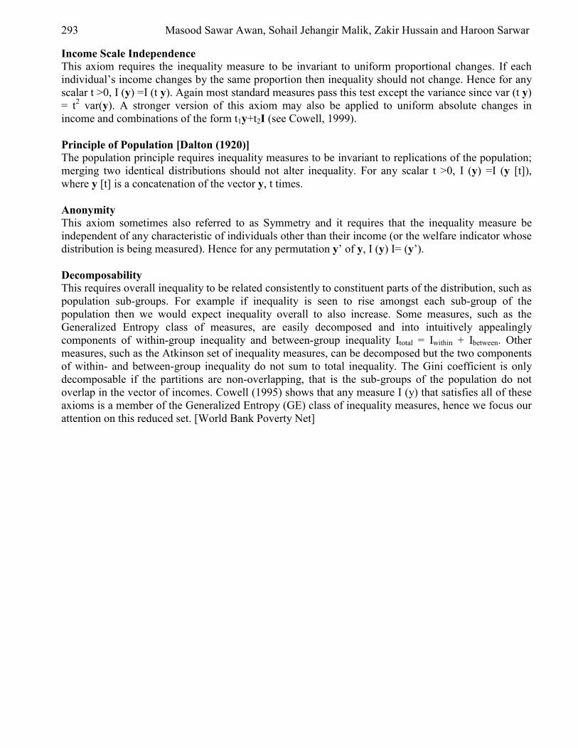
293 Masood Sawar Awan, Sohail Jehangir Malik, Zakir Hussain and Haroon Sarwar
Income Scale Independence This axiom requires the inequality measure to be invariant to uniform proportional changes. If each individual’s income changes by the same proportion then inequality should not change. Hence for any scalar t >0, I (y) =I (t y). Again most standard measures pass this test except the variance since var (t y) = t2 var(y). A stronger version of this axiom may also be applied to uniform absolute changes in income and combinations of the form t1y+t2I (see Cowell, 1999). Principle of Population [Dalton (1920)] The population principle requires inequality measures to be invariant to replications of the population; merging two identical distributions should not alter inequality. For any scalar t >0, I (y) =I (y [t]), where y [t] is a concatenation of the vector y, t times. Anonymity This axiom sometimes also referred to as Symmetry and it requires that the inequality measure be independent of any characteristic of individuals other than their income (or the welfare indicator whose distribution is being measured). Hence for any permutation y’ of y, I (y) I= (y’). Decomposability This requires overall inequality to be related consistently to constituent parts of the distribution, such as population sub-groups. For example if inequality is seen to rise amongst each sub-group of the population then we would expect inequality overall to also increase. Some measures, such as the Generalized Entropy class of measures, are easily decomposed and into intuitively appealingly components of within-group inequality and between-group inequality Itotal = Iwithin + Ibetween. Other measures, such as the Atkinson set of inequality measures, can be decomposed but the two components of within- and between-group inequality do not sum to total inequality. The Gini coefficient is only decomposable if the partitions are non-overlapping, that is the sub-groups of the population do not overlap in the vector of incomes. Cowell (1995) shows that any measure I (y) that satisfies all of these axioms is a member of the Generalized Entropy (GE) class of inequality measures, hence we focus our attention on this reduced set. [World Bank Poverty Net]

Mea
sure
men
t of I
nequ
ality
in P
akis
tan
(Exp
endi
ture
App
roac
h)
294
Tab
le 4
: A
xiom
atic
Ana
lysi
s of d
iffer
ent i
nequ
ality
mea
sure
s In
equa
lity
Mea
sure
Fo
rmul
a M
ean
Inde
pend
ent
Popu
latio
n In
depe
nden
t. Pi
gou-
Dal
ton
Dec
ompo
sabi
lity
Tra
nsfe
r se
nsiti
vity
/oth
ers
Gin
i Coe
ffic
ient
21
2
nn
ij
ji
GY
Yn
=−
∑∑
µ
Yes
Y
es
Yes
N
o Se
nsiti
ve to
cen
ter
of d
ist.
Atk
inso
n (∈
)
1
1
11
n i
yA
nY
=
⎡⎤
⎧⎫
⎪⎪
⎢⎥
=−
⎨⎬
⎢⎥
⎪⎪
⎩⎭
⎣⎦
∑ε
ε
–
Yes
Y
es
Yes
N
o D
epen
ding
on ∈
Gen
eral
ized
Ent
ropy
M
easu
re (α
)
Yes
Y
es
Yes
Y
es
Dep
endi
ng o
n α
.
Thei
l Ind
ex(α
=1)
1lo
gYi
YiT
nY
Y=∑
––
Y
es
Yes
Y
es
Yes
Se
nsiti
ve to
low
er
end.
Coe
ffic
ient
of
V
aria
tion
(α=2
) (
)22
1;
2V
GE
CV
CV
==µ
Y
es
Yes
Y
es
Yes
Eq
ually
sens
itive
to
all
inco
me
trans
fers
[M
aria
Ane
Lug
o: in
equa
lity
and
Hum
an D
evel
opm
ent]

295 Masood Sawar Awan, Sohail Jehangir Malik, Zakir Hussain and Haroon Sarwar
5. Summary and Conclusion In summary the appraisal of the results showed that in Pakistan there was lesser inequality in terms of food expenditure approach, because food was a necessity and rich as well as poor have to incur the expenditure on food items, therefore there was lesser inequality depicted by this analysis. The second component i.e. non-durable expenditure has shown relatively higher inequality as compared with food expenditure, but this was the major area of concern, because non durables include medical care, education, housing etc. which are indispensable needs & inequality in this field can be very harmful and concerning for the society. Inequality in durable expenditure is very high because poor population spends very low proportion of their income on durable goods because they consider durable goods as luxuries whereas it is very difficult for them to fulfill even basic needs. Although inequality in durables was higher, yet it was of secondary importance; because a man can do without air-conditioner, car, or personal computer, but cannot do without food and medical care, education etc.
The analysis on the basis of axiomatic approach showed that although Gini coefficient was very popular inequality measure but the members of Generalized Entropy class were the better estimates they satisfy all the axioms. As inequality was at alarming proportion in Pakistan, there was a need of proper policy measures to eradicate this social injustice.

Measurement of Inequality in Pakistan (Expenditure Approach) 296
References [1] Ahmad, E. and S. Ludlow (1989): Growth, Poverty and inequality in Pakistan, Pakistan
Development Review. [2] Alauddin, T. (1975), Mass Poverty in Pakistan, A further Study, Pakistan Development Review [3] Amjad, R and Kemal, A.R. (1997), Macroeconomic Policies and their Impact on Poverty
Alleviation in Pakistan, Pakistan Development Review, 36:1 (Spring) [4] Anwar, Talat. (1996), Structural Adjustment and Poverty: The Case of Pakistan, Pakistan
Development Review; Proceedings of the Papers at the 12th Annual General Meeting of Pakistan Society for Development Economist.
[5] Anwar, Talat (1997) Inequality and Social Welfare in Pakistan, Journal of Social Sciences and Humanities, Vol.1, No.2, 1997, Allama Iqbal Open University, Islamabad.
[6] Anwar, T. (1998) Incidence of Relative Poverty in Pakistan, The Asian Economic Review, The Journal of the Indian Institute of Economics, Vol. XL, No.1, April 1998,P.95-107, Red Hills, Hyderabad, India.
[7] Anwar, T. (2002a), The Impact of Globalization and Liberalization on Growth, Employment and Poverty: A Case Study of Pakistan. WIDER Discussion Paper No.2002/17, United Nations University/World Institute for Development Economic Research, Helsinki, Finland.
[8] Anwar, T., Qureshi, S.K. and Ali, H. (2005), Landlessness and Rural Poverty in Pakistan, paper presented at the 20th Annual General Meeting and Conference held in January 2005, Islamabad.
[9] Anwar, Talat (2004), Trends in Income Inequality in Pakistan between 1998-99 and 2001, Proceeding of the Papers at the 19th Annual General Meeting and Conference, January 2004, Islamabad.
[10] Anwar, Talat and Qureshi, Sarfraz Khan (2003), Trends in Absolute Poverty in Pakistan: 1990-2001, Proceeding of the Papers at the 18th Annual General Meeting and Conference held in January 2003, Islamabad.
[11] Atkinson, A.B (1970) "On the measurement of Inequality", Journal of Economic Theory. [12] Azfar, J. (1973): "The Distribution of Income in Pakistan: 1966-67" Pakistan Economic and
Social Review, Vol. 11: 40-66. [13] Bergan, A. (1967): "Personal Income Distribution and Personal Savings in Pakistan, 1963-64"
Pakistan Development Review, Vol. 7: 160-212.Vol. 17: 63-80. [14] Bourgignon, et al. (1991), Poverty and income distribution during adjustment issue and
evidence from the OECD project, in World Development, Vol. 19, No.11. [15] Chaudhry, M.G. (1982): "Green Revolution and Redistribution of Rural Income in Pakistan"
Pakistan Development Review, Vol. 21: 173-205 [16] Cowell, Frank (1993), Measuring Inequality, 2nd editions. [17] Cornia, G. A.; Jolly, R; Stewart, F. (1987). Adjustment with a Human Face, Oxford, Oxford
University Press. [18] Drunen, van Laetitia and Kraaij, Fred van der, (1994), Structural Adjustment in Sub-
Saharan Africa, Poverty and Development, Research and Policy Issues, Development Cooperation Information Department, Hague
[19] Government of Pakistan, Economic Survey Various issues, Ministry of Finance, Islamabad. [20] Federal Bureau of Statistics (2001), Poverty in the 1990s, Statistics Division, Islamabad. [21] Government of Pakistan (2005), Medium Term Development Framework, 2005-10, Planning
Commission, Islamabad, P.194-196 [22] Hoeven, van der, R. (1995), Structural Adjustment, poverty and macro-economic policy, ILO. [23] Kakwani, Nanak, (1980), Income Inequality and Poverty: Methods of Estimation and Policy
Applications, New York: Oxford University Press. [24] Kemal, A.R. (2002), Macro-economic Policy and Poverty in Pakistan in Human Condition
Report 2002, Centre for Research on Poverty Reduction and Income Distribution (CRPRID), Islamabad.

297 Masood Sawar Awan, Sohail Jehangir Malik, Zakir Hussain and Haroon Sarwar
[25] Kemal, A.R. (2003), Income Distribution Studies in Pakistan and the Agenda for Future Research in Human Condition Report 2003, Centre for Research on Poverty Reduction and Income Distribution (CRPRID), Islamabad.
[26] Khandkar, R. (1973): "Distribution of Income and Wealth in Pakistan" Pakistan Economic and Social Review,
[27] Kruik and Leeuwen (1985), Changes in Poverty in Pakistan, Pakistan Development Review, Vol.24,
[28] Kuznets S (1955), Economic growth and income inequality, American Economic Review XLV:1- 28
[29] Lambert, P. J (1989), The Distribution and Redistribution of Income: A Mathematical Analysis, Oxford: Basil Blackwell.
[30] Mahmood, Zafar (1984), Income Inequality in Pakistan: An Analysis of Existing Evidence, Pakistan Development Review, Vol.23 ,Nos.2 & 3.
[31] Malik, Shahnawaz (1992), Rural Poverty in Pakistan, unpublished Ph.D. Thesis submitted to the University of Sussex.
[32] Malik, Sohail, J. (1992), Rural Poverty in Pakistan, Pakistan Development Review. [33] Mauro, Paolo (1998), Corruption and the Composition of Government Expenditure” Journal of
Public Economics 69: 263-79. [34] Mujahid, G.B. (1978), Measurement of Poverty and Income Distribution, Pakistan
Development Review 17:3 [35] Morris, N. and Preston, I. (1986), 'Inequality, Poverty and the Redistribution of Income,
Bulletin of Economic Research, Vol.38,no.4,November [36] Naseem, S.M. (1973): "Mass Poverty in Pakistan: Some Preliminary Findings" Pakistan
Development Review, Vol. 12: 4, 312-360. [37] Ravallion, Martin, (1997), Can high-inequality developing countries escape absolute poverty?
Economic Letters, Vol. 56 (1997): 51-57. [38] Sen , A. (1973). On Economic Inequality. Oxford: Oxford University Press, 1973 [39] Shorrocks, A.F. (1983), 'Ranking income distributions', Economica, vol. 50, pp.3-17. [40] Shorrocks, A.F. and Foster, J.E. (1987), 'Transfer sensitive inequality measures', Review of
Economic Studies, vol. 54, pp. 485-497. [41] World Bank (2000), World Development Report, 2000/2001: Attacking Poverty. Washington,
DC. [42] World Bank (2003), Poverty in Pakistan: Vulnerabilities, Social Gaps, and Rural Dynamics,
Washington, D.C.

European Journal of Scientific Research ISSN 1450-216X Vol.18 No.2 (2007), pp.298-305 © EuroJournals Publishing, Inc. 2007 http://www.eurojournals.com/ejsr.htm
Design and Operation of Multi-Media Filter
S. Bou-Hamad Kuwait Institute for Scientific Research, Water Technologies Department
WTD, P.O. Box 24885, Safat 13109, Kuwait E-mail: [email protected]
Abstract
Dual-media filter is one of the oldest water treatment technologies known. If properly designed, constructed, operated and maintained, a dual- media filter produces very high quality water. The filter is utilized to remove matters such as silt, clay, micro-organisms and colloidal particles. At Desalination Research Plant (DRP)-Kuwait, four multi-media filters were installed to study the performance of the system as pretreatment technique for Reverse Osmosis plant. During the design of this system many factors has been taking into consideration such as type, size and number of filters, media depth, material, terminal head loss, filter flow rate, filter washing technique.
This paper presents a design and operation of multi-media filter, which has been used for reverse osmosis (RO) pretreatment system based on data collected over a period of one year. Keywords: Conventional treatment, coagulation, flocculation, silt density index.
Introduction Filtration is a unit process widely used in the water industry as pretreatment technique for the removal of particulate materials commonly found in water.
Pretreatment of the seawater prior desalination process is considered a major step in water desalination weather reverse osmosis or multi-stage flash. Difference pretreatment systems are known in reverse osmosis desalination; generally they are divided into conventional and non-conventional. Example of the former includes flocculation–coagulation filtration process. Conventional pretreatment such as filtration is widely used in the desalination process. Successful long-term performance of a filtration system depends on two main factors: proper design, proper operation, and proper maintenance of the system.
Granular media filtration has been practiced in the water treatment field for a long time (Hamoda et al., 2004). In water treatment, dual-media granular filtration is utilized to remove matters such as silt, clay, microorganisms and colloids. Sand filter can reduce fecal coliform level from approximately 106 colony forming units (cfu)/100ml in septic tank effluent to 103 cfu/100ml in sand filter effluent.(RIDEM, 1999). The objective of pretreatment process is to reduce fouling constituents in the feed water to level that would provide stable, long term performance of membrane elements (Ebrahim et al., 2001).

Design and Operation of Multi-Media Filter 299
Material and Methods In this specific process design, a pressurized dual media filters are used. Filters of this type are intended for use where raw water is supplied under pressure (about 2.0 bar). The flow rate is reasonably low (Q = 4 m3/hr); consequently, one tank is sufficient. The media filer design involves determination of the following items:
• Type, size and number of filters; • Media depth, size and material; • Filtration and terminal head loss; • Filter flow control scheme; and • Filter washing and related systems.
Type
In this small plant, pressurized type dual-media filter is contained in reinforced fiberglass. The media are consisted of carbon, silica sand and gravel. The size of the cylindrical filter tank is 2 m length and 1 m diameter. Two filter in operation and two in stand-by mode. Media Depth, Size and Material
In fact both small and large plants utilize a 30-inch deep multi-media filter bed. It consists of 18 in of 1.0 to 1.2 mm anthracite coal, 9 in of 0.54 to 1.0 mm silica sand and 3 in of 1.5 to 2.5 mm gravel (garnet). It is very important that the sand particles all about the same size. There is uniform gradation from coarse to fine in the direction of filtration. This media arrangement has provided excellent service. Its advantage is the prevention of gravel movement. Filter Flow Control Scheme
The five basic types of filter control schemes are constant-rate filtration, declining rate filtration, constant-level filtration, equal-loading filtration and constant-pressure filtration. For gravity filters, declining rate and constant level and equal loading filtration are the most suitable, while declining-rate and constant pressure are used for pressurized filters as used in this study. Filtration Rate and Terminal Head Loss
The filtration rate depends on the type of chemical floc, such as alum; filter effluent quality tends to degrade at low filtration rates. Higher rate tend to increase solids penetration; therefore, they decrease head loss due to low solids build-up. Terminal head loss is dictated by effluent quality requirements. Filter backwashing
Three basic types of backwashing systems exist: complete fluidization of filter media by a high backwash rate with or without surface washing; a scoring wash with partial fluidization of the media by backwash, or a combination of both (Montgomery, 1985). Backwash static head of more than 10 m is provided by elevated tank (filtered water tank). Although most filters require 1.2 to 2 m of head, 80% of the 10 m head is lost in the piping, throttling valve and flow controller. If an elevated tank is not present in the system, a centrifugal pump is used to supply head usually in the range of 2.0 bar at the discharge point.
In water treatment, certain chemicals are added to raw water to remove impurities. While some particles will spontaneously settle out from water on standing (a process called sedimentation), others will not. To cause particles that are slow to settle or are non-settling to settle out more readily, a soluble chemical or mixture of chemicals is added to the water. Such a chemical is called a coagulant and the process is called coagulation. The mixing process of these chemicals with raw water to form floc is called (flocculation). The coagulant reacts with the particles in the water, forming larger

300 S. Bou-Hamad
particles called flocs, which settle rapidly. Flocs can also be effectively removed by passing the water through a filter. The process is controlled so that the coagulant chemicals are removed along with the contaminants. Coagulation /flocculation processes are very effective at removing fine suspended particles that attract and hold bacteria and viruses to their surface. Research has shown that these processes alone are capable of removing bacteria and some viruses from water supplies. Dual Media Filter Design Type: Sand/Carbon and gravel Pressurized Filter. Given:
• Flow rate : Q = 0.000972 m3/s • Filtering velocity : u = 12 m/h = 3.33 x 10⁻³ m/sec. • Pressure : Po = 2.0 bar • Water Dynamic viscosity : µ = 10-3 N.sec. • Water Density : ρ = 10-3 kg/m3 • Depth to diameter ratio : L/dp = 950 • Average porosity : ε = 0.45 • Standard layer distribution (applicable for <2 mgd) Table 1.
Table 1: Properties of Filter Media Materials. Medium Material Depth (Inches) Density kg/m3 Porosity ε Particle Size mm Carbon 18” 1.5 0.55 1.0 – 1.2 Silica 9” 2.6 0.42 0.54 – 1.0 Gravel 3” 2.6 0.40 15 – 25
Assumptions:
The total filter tank height = 3 x media depth (i.e., 3 * 30” = 90” equivalent to 2.0 m) Design Variables:
• The diameter : Dr • Tank height : H • Feed pressure : P • Area : A
Calculations:
1. Filter Sizing 2
3
2 729.01033.3)45.0(
000972.04
mx
DAuAQ r =≡≡⇒=∈−
π
mDr 96.0≡∴ 2. Pressure Drop
Using Eurgen Equation for the pressure drop across a packed bed (Montgomery, 1985). 2
3 )1( udLFP
p
ρ∈
∈−=∆
µρudp
=Re
66.610
)1033.3)(102)(10(Re 3
333
== −
−− xx

Design and Operation of Multi-Media Filter 301
2)33 )1033.3)(10)(950)(45.0
45.01(15.14 −−=∆ xP
barkPaP 2.019.98 ==∆
75.1)Re
1(150 where +∈−
=f
15.1475.1)66.6
45.01(150 =+−
=f
Therefore; Feed pressure = P0 + ∆P = 2.0 + 0.2 = 2.2 bar Table 2: Filter Specifications.
Tank Diameter 1.0 m Tank Height 2.0 m Po 2.2 bar Material Polyvinyl Chloride (PVC)
Pumps Design
Type: Centrifugal pump. Given:
• Flowrate : Q = 0.000972 m3/s • Pressure : P: 2.0 bar = 2.0 x 10⁵ kPa • Water Density : ρ = 10-3 kg/m3 • Gravity : g = 9.8 m/s2 • Pump power 1.47 kW
Table 3: Pumps Specifications.
Type Capacity Power kW Material of Casing Material of Shaft Material of Impeller Units No. Feed 4 m3/h 1.5 DIN 1.4460 DIN 1.4462 DIN 1.4660 1 Backwash 4 m3/h 1.5 DIN 1.4460 DIN 1.4462 DIN 1.4660 1 Dosing 0.5 1/h 0.05 PVC PVC PVC 3 Type Capacity Power kW Material of Casing Material of Shaft Material of Impeller Units No.
Operation
A schematic diagram of the filtration system is shown in Fig. 1, whereas, fig.2 represent photo setup of the system. The filtration system consists of four glass reinforced plastic (GRP) filter tanks, feed and backwash pumps. Also the system contains flocculation and coagulation system which consists of three chemical tanks equipped with dosing pumps and agitators for Sulfuric acid (H2SO4), Ferric Chloro-Sulphite (FeClSO4) and Sodium bi-Sulphite (NaHSO3). The filtration GRP tanks filled with four media (carbon, silica sand and gravel).
The system was operated 24 hours per day and capable of producing 4 m3/h of filtrate water to meet RO system demand. The buffer tank was fed with surface seawater. H2SO4 and FeCLSO4 were dosed into the seawater stream prior to the entrance of system. The H2SO4 used to adjust the pH of feed water from 7.9 to 6.6 in order to assist the coagulate aide (FeCLSO4) to form a floc. The dosing rate for the FeCLSO4 was 2 ppm. The feed pump delivered seawater to two dual media filters connected in parallel (the other two are standbys) where the water is filtered to the RO unit.
NaHSO3 is added to the line to insure the complete removal of residual chlorine. The silt density index (SDI) is continuously monitored. The filter was periodically cleaned by back washing the media to avoid clogging.

302 S. Bou-Hamad
Figure 1: Schematic diagram of the filtration system
Figure 2: Photo setup of the filtration system
Results and Discussion Multi-media filter was tested at Doha Research plant (DRP), Kuwait. The average monthly temperature of the feed stream was in the range of 22-32 °C during winter and summer and showed no significant changes on day-to-day basis. Therefore, the effect of temperature in the flux is almost negligible in the system performance. The conductivity of the feed was 50,000 µS/cm and was steady most of the time. The value of the silt density index (SDI) for the filtrate was measured and plotted as shown in Fig.3. Its worth mentioning, that the SDI average value of the feed was more than 6%. It can be seen from Fig. 3 that the SDI values of the filtrate vary between (3.5-6 %). The average filtrate flow rate for the system was 4m3/h as shown in Fig 4.
Fig. 3 and 4 represent the performance of the filtration system in reducing the values of biological oxygen demand (BOD) and chemical oxygen demand (COD), respectively. Table 4a, 4b and
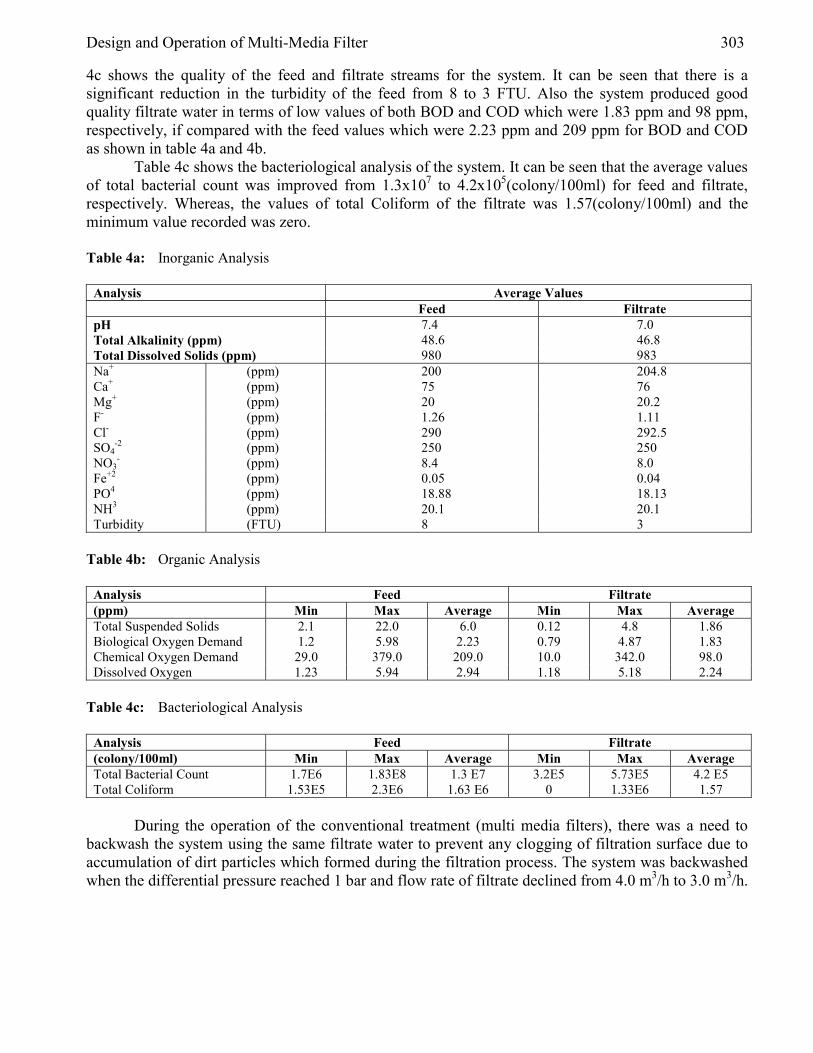
Design and Operation of Multi-Media Filter 303
4c shows the quality of the feed and filtrate streams for the system. It can be seen that there is a significant reduction in the turbidity of the feed from 8 to 3 FTU. Also the system produced good quality filtrate water in terms of low values of both BOD and COD which were 1.83 ppm and 98 ppm, respectively, if compared with the feed values which were 2.23 ppm and 209 ppm for BOD and COD as shown in table 4a and 4b.
Table 4c shows the bacteriological analysis of the system. It can be seen that the average values of total bacterial count was improved from 1.3x10⁷ to 4.2x10⁵(colony/100ml) for feed and filtrate, respectively. Whereas, the values of total Coliform of the filtrate was 1.57(colony/100ml) and the minimum value recorded was zero. Table 4a: Inorganic Analysis
Analysis Average Values Feed Filtrate pH 7.4 7.0 Total Alkalinity (ppm) 48.6 46.8 Total Dissolved Solids (ppm) 980 983 Na+ (ppm) 200 204.8 Ca+ (ppm) 75 76 Mg+ (ppm) 20 20.2 F- (ppm) 1.26 1.11 Cl- (ppm) 290 292.5 SO4
-2 (ppm) 250 250 NO3
- (ppm) 8.4 8.0 Fe+2 (ppm) 0.05 0.04 PO4 (ppm) 18.88 18.13 NH3 (ppm) 20.1 20.1 Turbidity (FTU) 8 3
Table 4b: Organic Analysis
Analysis Feed Filtrate (ppm) Min Max Average Min Max Average Total Suspended Solids 2.1 22.0 6.0 0.12 4.8 1.86 Biological Oxygen Demand 1.2 5.98 2.23 0.79 4.87 1.83 Chemical Oxygen Demand 29.0 379.0 209.0 10.0 342.0 98.0 Dissolved Oxygen 1.23 5.94 2.94 1.18 5.18 2.24
Table 4c: Bacteriological Analysis
Analysis Feed Filtrate (colony/100ml) Min Max Average Min Max Average Total Bacterial Count 1.7E6 1.83E8 1.3 E7 3.2E5 5.73E5 4.2 E5 Total Coliform 1.53E5 2.3E6 1.63 E6 0 1.33E6 1.57
During the operation of the conventional treatment (multi media filters), there was a need to
backwash the system using the same filtrate water to prevent any clogging of filtration surface due to accumulation of dirt particles which formed during the filtration process. The system was backwashed when the differential pressure reached 1 bar and flow rate of filtrate declined from 4.0 m3/h to 3.0 m3/h.
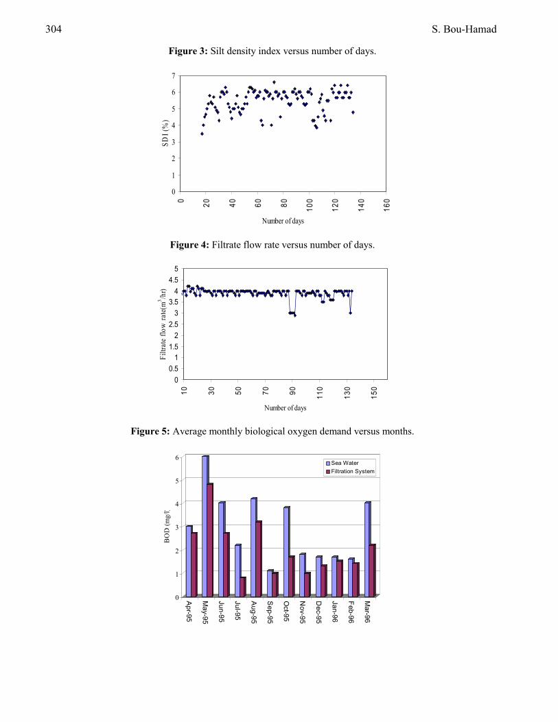
304 S. Bou-Hamad
Figure 3: Silt density index versus number of days.
Figure 4: Filtrate flow rate versus number of days.
Figure 5: Average monthly biological oxygen demand versus months.
0
1
2
3
4
5
6
7
0 20 40 60 80 100
120
140
160
Number of days
SDI (
%)
00.5
11.5
22.5
33.5
44.5
5
10 30 50 70 90 110
130
150
Number of days
Filtr
ate
flow
rate
(m3 /h
r)
0
1
2
3
4
5
6
BO
D (m
g/l)
Apr-95
May-95
Jun-95
Jul-95
Aug-95
Sep-95
Oct-95
Nov-95
Dec-95
Jan-96
Feb-96
Mar-96
Sea WaterFiltration System

Design and Operation of Multi-Media Filter 305
Figure 6: Average monthly chemical oxygen demand versus months.
Conclusions The study shows that the multi-media system was very effective in removing naturally occurring seawater impurities.
Chemical analysis results revealed that the system has improved the quality of the feed with an average SDI (5.6%). There was consistent reduction in BOD, COD and bacteria total count. Hence filtrate can be considered safe as feed water for RO plant.
When designing a filtration system it is important that the sand particles all about the same size. If the grain sizes vary greatly, the smaller ones will fill in the spaces between the larger particles, making it easier for the system to clog. References [1] Ebrahim S., M. Abdel-Jawad, S. Bou-Hamad and M.Safar. 2001. Fifteen Years of R&D IN
Seawater Desalination at KISR Part I. Pretreatment technologies for RO systems. Desalination, 135:141-153.
[2] Hamoda M.F., I. Al-Ghusain, N.Z. Al-Mutairi, 2001. Sand filtration of wastewater for tertiary treatment and water reuse. Desalination, 164:203-211.
[3] Montgomery J.M. Water treatment principal and design. 1985. ISBN: 0-471-04384-2 USA. P:153-165.
[4] Rhode Island Department of Environmental Management. 1999. Guidelines for the design and use of sand filters in critical resource area. USA P.5.
0
50
100
150
200
250
300
350
400
CO
D (m
g/l)
Apr-95
May-95
Jun-95
Jul-95
Aug-95
Sep-95
Oct-95
Nov-95
Dec-95
Jan-96
Feb-96
Mar-96
SeawaterFiltrate Water

European Journal of Scientific Research ISSN 1450-216X Vol.18 No.2 (2007), pp.306-331 © EuroJournals Publishing, Inc. 2007 http://www.eurojournals.com/ejsr.htm
Training Pre-service Teacher Education on
Reflective Practice in Jordanian Universities
Hani A. Weshah Dept. of Curriculum and Instruction, Faculty of Educational Sciences
The University of Jordan, Amman, 11942 –Jordan E-mail: [email protected]
Tel: 00962-65355000; Ext.24464; Mobile: 00962- 777499341
Abstract
The purpose of this study was to investigate the degree to which university supervisors at the public Jordanian universities train preservice teachers on reflective practice.The instrument used in this study featuring 37 indicators for four reflective practice skills; planning, implementation, evaluation and problem solving. Validity and reliability of the instrument were established.
Findings showed that the overall mean ratings of university supervisors was (3.90) which considered high. The mean ratings for the implementation, planning, and evaluation skills were (4.08, 4.02, 3.87) respectively. Meanwhile, the problem solving skill was the lowest (3.54) which considered to be moderate. Independent samples T-test was performed to find out if there are any statistically significant differences in the mean ratings that are attributed to gender, educational qualification and number of field visit. The T -test results indicated that the overall mean ratings is statistically significant at level α <0.05 and these differences were in favor of female. The T test results also showed that there are no statically significant differences in the mean ratings of university supervisors on overall reflective practice skills that are attributed to educational qualification and number of field visits.
Finally, based on these findings, some recommendations were proposed to develop and enhance reflective practice skills in preservice teacher education programs at the Jordanian universities. Keywords: Reflective practice, teacher education, preservice teacher.
Introduction Over the last two decades, there has been a wide tendency in teacher development programmes include pre-service and in-service teacher education towards ‘reflective teaching’ and ‘reflective practitioners’. Its primary meaning to achieve profesional improvement and development in the quality of teaching and learning process. The whole ‘reflection movement’ was mainly lead by Donald A.Schon in 1980s through the publication of his two famous books: The Reflective Practitioner (1983) & Educating the Reflective Practitioner (1987). Shon’s notion of ‘reflective practice’ was actually the resurgence of Dewey’s concept of ‘reflective thinking’ that took palce in the early 1930s (Loughran,1996; Pollard & Tann,1994; Sprinthall et al, 1996; p688).
This wide concern of reflection springs from the fact that “it is an important human activity in which people recapture their experience, think about it, mull it over and evaluate it”(Loughran, 1994;

Training Pre-service Teacher Education on Reflective Practice in Jordanian Universities 307
p3). Reflection, therefore, "is an active and delibarate consideration of what is usually taken for granted" (Field, 1994; p27). Dewey’s definition of ‘reflective thinking’ involves "the state of being in a situation, sensing a problem, clarifying it with information, working out suggested solutions, and testing the ideas by applications"(Ornstein & Hunkins, 1993; p140). Based on these elements of reflective thinking, Dewey has put forward two new terminologies related to actions: the routine action and the reflective action. The routine action, according to Dewey, is the action that takes the definition of social reality for granted which guided by factors such as tradition, habit and authority and by institutional definitions and expectations. Thus, it is static and does not easily respond to the changes in circumstances or priorities. Reflective action, on the other hand, is the active, persistent and careful consideration of any belief or supposed form of knowledge in light of the grounds that support it and the further consequences to which it leads. Reflective action involves a willingness to engage in constant self-appraisal and development. It also implies flexibility, rigorous analysis and social awareness (Pollard & Tann,1994).
As a result of the above mentioned, reflective practice has become an essential feature of the increasing world-wide interest in monitoring the quality of teaching. It is also believed that it could establish a link between research and theory on the one hand and the real classroom practice on the other hand. Reflective practitioners are seen to generate a dialogue between theory and practice and establish modes of collaboration that can benefit both of them. Theoretical Foundation of Reflective Practice Teachers-educators’ interest in reflective practice corresponds with changes that took place in cognitive psychology during the last three decades, where constructivist theory has become dominant in respect of learning (Skilling, 2001). Constructivism is “a view of learning in which learners use their own experiences to construct understandings that make sense to them, rather than having understanding delivered to them in already organized form” (Kauchak & Eggen, 1998; p184). Learners are encouraged to take up responsibility for their own learning by constructing meaning through social interaction. The new meaning they construct depends on their current understanding .
By considering reflective practice, teacher learning and professional development rely mainly on particular perspective. Pre-service teacher education is seen more effective in school-based courses. Student teachers are placed in real-life teaching situations where they can experience what they have learned in theory and have a chance to build better understanding of the teaching and learning process. They also have a chance to deeply and carefully reflect on these situations afterwards either through thinking aloud or sharing them with other teachers, cooperative teachers or supervisors. As a result, reflective practice emphasis exceeding of basic skills and academic content and also include the investigation of the relationship between what the teacher is trying to teach on the one hand and students’ experiences and personal purposes on the other hand. Students construct the meaning of their lessons based on their past experiences and personal purposes.(Henderson, 1992) Types of Reflections There is no one agreement in the growing body of theoretical literature on the types of reflections that teachers should durably rely on. Schon and others describe reflection with models that develop in a cumulative way. They argue that there are initially two types of reflection reactive: reflection on action and reflection in action. The third, reflection for action is a looked-for outcome of the previous two types of reflection and is proactive in nature. (Power, Clark and Hine, 2002).
Reflection-on-action is similar to Dewey’s reflective action and it basis of much of the literature that spotlighted with reflective teaching and reflective teacher education. It usually takes place after the action considered as a more systematic process of deliberation enabling analysis, reconstruction and reframing in order to plan for further teaching and learning. It could be done in

308 Hani A. Weshah
isolation through questioning one’s self, or it could be an issue to talk about with others such as, mentors, colleagues, supervisors, or even teacher educators. (Henderson, 1992).
Reflection-in-action refers to the process of decision-making while actively engaged in teaching. Reflection in this case is "context bound" (Day,1999; p26). It is much more like thinking about doing something while doing it. It involves the exercise of analysis and judgement. Skilling (2001). This kind of reflection needs what Tickle (1993, p114) has called "immediate, on-the-spot judgements". This is actually why many educators and researchers believe that it is more complicated to teach and apply.
Reflection for action refers to the process of mind that enables prac¬titioners to call upon what they have learned through their cognitive and shared reflections in a more deliberative sense of their future plan teaching episodes. Ideally, this planning would include a critical pedagogy and pedagogical theory that stimulate teachers to analyze different instructional perspectives and exploit them to under¬stand and properly act on revealed inconsistencies. This critical ele¬ment specifically influences prospective teachers' Developmentally Appropriate Practice in Education. (Hyun & Marshall, 1996) Characteristics of Reflective Practice In his book, Reflective Teaching: “Becoming an Inquiring Educator”, (1992), Henderson investigates three main characteristics of reflective practice: an ethic of caring, a constructivist approach to teaching, and artistic problem solving. Another investigation to the characteristics of reflective practice has been carried out by Pollard and Tann in 1994. Depending on Dewey’s notion of reflective action, Pollard and Tann (1994) have identified six key characteristics of reflective practice:
1. Reflective practice implies an active concern with aims and consequences, as well as means and technical efficiency. These aims and consequences are the immediate ones that are related to classroom practice. However they cannot be separated from the influence of the educational aims and social values (Elliot, 1993).
2. Reflective practice is applied in a cyclical or spiralling process, in which teachers monitor, evaluate and revise their own practice continuously. This characteristic shows reflection as a dynamic process which is intended to lead to a higher-quality teaching. The teacher is expected to plan, to make provision and to act.
3. Reflective practice requires competence in methods of classroom enquiry. To support the development of teaching competence, there are three types of competence needed to the cyclical process of reflection. The impirical competence, which relates to the teacher’s knowledge of what is going on in the classroom; the analytical competence, which addresses the issue of how to interpret the data collected; the evaluative competence, which involves making judgements about the educational consequences of the results for the practical enquiry.
4. Reflective practice requires attitudes of open-mindedness, responsibility and wholeheartedness. These three attitudes are considered essential prerequisites to reflective practice. Reflective teachers
5. are open-minded, intellectually responsible for charging the students up with knowledge in training and whole-hearted, i.e dedicated, energetic and enthusiastic.
6. Reflective practice teaching is based on teacher judgement, which is clued-up to a certain extent by self reflection and partly by insights from educational disciplines. It is suggested that this could be done by bridging the gap between practice and theory. Making judgement could be a collaborative matter between teachers and supervisors in relevant disciplines since non of them could stand alone in the field. This idea has been widely adopted by many researchers (Elliott, 1993; Holm & Horn, 2003; Beattie, 1997). O’Hanlon (1993) even goes to an extreme point that teachers are encouraged to develop their own personal theory which they could rely on when making judgements.
7. Reflective practice, professional learning and personal fulfilment are enhanced through collaboration and dialogue with collegues and/or supervisors. Collaboration is the means for

Training Pre-service Teacher Education on Reflective Practice in Jordanian Universities 309
self development and professional improvement. Looking deeply into the following quotation, one would recognize the effect of collaboration in reflective practice: “I think you do it internally, you do it with yourself, but to actually verbalize the things, to
actually talk them out with another person is a much more powerful mechanism…. So actually sitting down and talking with somebody is good clarifying stuff. And they have input too, so there is somebody to bounce their ideas off, an opportunity to modify and change.” (Bell & Gilbert, 1996; p.104) Preparing Preservice teachers to become reflective practitioners In her article, “Assisting and Assessing the Development of Preservice Teachers in Academic and Clinical Settings (1995)” Pasch indicates that it is now believed that reflective practice is learned and could be taught. Preservice teachers and inservice teachers should learn how to be reflective in order to help their students to become reflective as well. There has been a growing consensus for the view that teacher education must help student teachers to become reflective in all terms. Teachers need to be thoughtful, decision-makers, reflective professionals whose ability to asses a situation and respond to it appropriately will have beneficial effects on the learning of their students” (p. 164) Therefore, developing, monitoring, and evaluating cognitive, behavioural, metacognitive skills must begin early in the preservice years. She also presumes that “prospective teachers need to become proficient thinkers in subject-matter disciplines as well as to attain the skills, learn the techniques, and perform the behaviors that make them technically able teachers” (p. 164) They also need to attain and progress in the abilities of reflective thinking that will permit growth to occur as they move from novice to expert over the course of their teaching careers. Three ways teacher educators should relate current knowledge on reflective teaching and its development to teacher-education assessment efforts are to:
1. Emphasize the acquisition foundations in content and professional knowledge that will permit students to act reflectively upon this knowledge at a later point in their Professional growth-and monitor the attainment of this Critical thinking.
2. Specify directly which aspects of reflective practice are emphasized and how those aspects are incorporated in the teacher-education program and identify strategies to assess whether these aspects are being learned.
3. Provide opportunities to rehearse and apply reflective practice in academic and clinical settings and provide sufficient and specific feedback to permit students to im¬prove their abilities (Pasch, 1995; p 165). The ability to reflect requires a clearly articulated program of study and an assessment strategy that encourages both self-evaluation and continuous feedback. In preservice teacher programmes, students could be exposed to practicing reflective practice through the following procedures:
Modelling Student teachers need to be exposed to classes that encourage them to be actively involved in their learning so “that their ideas and thinking are challenged in ways to provoke them to reconsider, and better articulate, their understanding of the subject matter”(Loughran,1996; p25)
Student teachers need to see their teacher educators as reflective practitioners and at the same time they need to experience the development of professional practical knowledge by being part of that learning. This might help them to address the paradox in their own learning about practice.
However, reflection is a way of thinking which resides in the mind of the individual, so it is difficult to be observed. Therefore, to help student teachers have reflective practice and to help them experience and understand the process, they need to hear what the supervisor is thinking. This could be achieved through ‘thinking aloud’ protocol. This could take place through supervising process, so that the student teachers can access the thoughts, the ideas and concerns which shape reflective practice. In addition to the emphasis on reflection, another significant outcome of recent reform efforts is the focus on collaborative inter¬action to address issues of learning, teaching, and schooling. For prospective

310 Hani A. Weshah
teachers to learn that collaborative interaction with colleagues is a critical part of the teaching career, they need to see evidence of such collaboration in their preservice programs. They need opportunities to practice the skills they will be expected to demonstrate in the field. Within teacher-education programs, methods must be insti¬tuted to facilitate, teach and monitor collaborative interac¬tions between students to teach them the importance of cooperative, interactive, collaborative work in teaching and enable them to learn how to do it before they enter the pro¬fession. One outcome of these points is a demand on university faculties to practice what we preach. Students should perceive it demonstrated in their own courseworks, have opportunities to practice it in campus classrooms and in school classrooms, and receive feedback on their progress in applying it. Reflective journals Reflective journals (Calderhead, 1989; Ross, 1990; Wildman et al., 1990; Zeichner, 1987, Loughran, 1996; Pasch, 1995, Field, 1994; Skilling, 2001) have received considerable attention in recent years and were created to help teachers develop as professionals who systematically analyze their teaching behaviors, attitudes and planfully change to improve their skills and knowledge base. Many approaches and formats have been suggested and taken. Asking students teachers to weigh consequences, predict outcomes, plan alternatives, examine their beliefs, assumptions, theories, and reflect on their own thoughts are only several of many possibilities that might be addressed through this medium.
In her article, Pasch, 1995 indicates one practice that facilitates the process of reflection is writing personal journals about experiences and feelings related to teach¬ing. When used this way, journals are designed to help prospective teachers see their own growth, look for patterns of behavior or atti-tudes in teaching, relate readings to experiences, and actively ponder the progress and state of the profession. A simple format for a reflective journal is oversimplified that the students should write fre¬quently (weekly), honestly and in a detailed manner. Entries should focus not only on teaching activities, but also on their stu¬dents' responses to those activities and the prospective teachers' feelings about themselves as teachers. If a student is encouraged to write journals feedback, the main goal must be on developing a reflective professionalism. Supervisors should read these journals at periodic inter¬vals, make suggestions about resources or questions to consider, and share their thoughts about the content of the students' entries. (Field, 1994). They should also keep journals to practice reflection from time to time. They would sense a problem in the learning situation, start to ask why and what questions, and think of probable solutions and write them down. Such journals would help them personally and professionally develop; and if time permits they would sharing them with others in order to reach better understanding collaboratively. Case studies
This is another approach that has generated consid¬erable interest in its attempt to make teacher-education practices more ecologically valid. Case studies can be a unifying method of having students address program dispositions. One way to use case studies is to have students eventually move from addressing issues in case studies provided for them to writing their own case studies based on their clinical experiences. Ongoing monitoring can be used to determine students' development as problem solvers and dictate the type of case studies they explore. Problems or dilemmas may also be structured to include diverse categories such as student-teacher interactions, teacher-teacher interactions, and instructional applications. Students may work collaboratively on case studies; practitioners as well as university supervisors should be involved in the development of the cases and in the assessment of their contribution to student development. Although different problem-solving techniques may be required for differing situations, students can be asked to set up the case, analyze and work it through, synthesize and integrate information, and critique the process in which they have engaged.

Training Pre-service Teacher Education on Reflective Practice in Jordanian Universities 311
Simulations
Videotapes, interactive videodisc simulations, computer-based and live simulations are innovative techniques that hold promise for the future student teachers training. They provide the opportunity to simulate classroom interactions to permit monitoring of student progress in professional skill development and reflective think¬ing. They encourage collaborative interaction between university supervisors and student teachers in their design and in building accompanying assessment systems. They allow for individual differences in that they permit students teachers to work on situations at their own pace and on repeated occasions. The development of these materials provides interest¬ing possibilities and experimentation with teaching experience. Field assignments
Another way to train students teachers on reflective practice is to create packets of field assign¬ments for students to use in developing observational and interac¬tional skills at varying levels of involvement. Concurrent with an initial field experience, students might be required to complete several classroom observations, perhaps using an obser¬vational instrument or rating scale; conduct interviews with class¬room teachers and building administrators; observe and interact with members of the neighborhood and community surrounding the school; and observe and interact with students from varying back¬grounds at varying ages.
Later, students may complete assignments related to their own instructional interactions with students in one-to-one, small-group and large-group situations. Obtaining, observing, and analyzing videotaped segments of their own teaching can also be considered part of this process. Selected assignments may become part of a portfolio and be used to monitor continuation decisions or to provide students with feedback on their development as prospective teachers. Such mechanism can be used to integrate conceptual information, to encourage students to work together collegially and to combine academic and clinical experiences together by emphasizing programmatic themes. Building a programmatic set of field-based assignments with teacher in¬volvement can promote and model collaboration in action.
Reflecting by using the above procedures needs to be guided. Student teachers need to have focused dimensions on which they can concentrate. Those dimensions are the actual aspects of their behaviour in the classroom such as planning, implementing, evaluation and problem solving.
Being reflective means that being able to inquire several aspects of teaching and learning process and to answer several related questions in order to create a dynamic classroom environment in which every student is connected and free to think, question, express his or her ideas and take risks (Holm & Horn, 2003). Some of the most important questions reflective educators should bear in mind have been suggested by Pollard and Tann (1994) in their book: “Reflective Teaching in The Primary School” and the following questions: Who are we? What are the aims, structure, and content of the curriculum? How do we plan and implement the curriculum? How can we support children’s learning? How are we organizing the classroom? How are we managing learning and coping with behaviour? How are we communicating in the classroom? What are we achieving? Practicing inquiry and developing critical thinking inside the class room would provide the students with a good model of reflection. Supervisors are expected to question, to raise issues and to make their problem-solving processes explicit. By modelling these behaviours, student teachers can learn the processes of independent and collaborative meaning making, and can see the benefits of inquiry and active involvement in learning.”(Beattie, 1997) Definition of Terms The following definitions, however,maybe useful: Reflection: is a process of dynamic action and learning that will enable students teachers to develop their practice in the light of their analysis and evaluation (Parsons and Stephenson 2005).

312 Hani A. Weshah
Reflective practice: is a meta-cognitive process which consists of planning, monitoring, evaluation and problem-solving (Parsons and Stephenson 2005). In reflective practices, practitioners engage in a continuous cycle of self-observation and self-evaluation in order to understand their own actions and their reactions they prompt in themselves and learners (Brookfield, 1995 & Eugene, 2003). Planning: The trainer presents the student teachers with a task and explains the rationale behind it. Students are then asked to plan their own approaches to the task, choosing strategies that they think will facilitate its completion (Chojnaka, 2000). Monitoring: During the task, the trainer ask the student teachers to 'self-monitor' their performance by paying attention to their strategy use and checking comprehension (Chojnaka, 2000). Evaluation: After the task has been completed, the student teachers are then given time to 'debrief the activity, e.g. evaluate the effectiveness of the strategies they used during the task (Chojnaka, 2000). Problem-solving: As student teachers encounter difficulties, they are expected to find their own solutions (Chojnaka, 2000). The following steps are integral to the reflective process: collect descriptive data, analyze data, consider how the situation or activity could have been different, create a plan that incorporates new insights (Parsons & Stephenson, 2005) University supervisors: Faculty members of the Jordanian Universities who are responsible for visiting public school classrooms for the purpose of observing, training and conducting evaluation of student teachers. Significance of the Study The aim of educational policy of teacher preparation programs at the Jordanian universities is to prepare an effective and skillful educators who are committed to contribute to the quality of education, and who continually reflect on their practice and serve to improve the profession through offered programs. Therefore, it is expected that the colleges of education faculties, supervisors and student teachers may benefit from this study. Faculties maybe benifited from this study by enhancing their awareness to design and implement innovative professional development programs for student teachers that are aligned with current research findings and standards. The college's supervisors also benifited by enhancing their awareness to examine their beliefs, roles and supervisory practices as facilitators and mentors through the use of critical thinking, engaging in refective practice and self-assessment processes. Based on the assumption that the university supervisors understand that they should be highly competent in their areas of experise. Student teachers might benifited from this study by developing their awareness of how to be reflective practioners. Finally, although the literature on reflective practice is replete and world-widely becoming an essential aspect of the educational process, research and studies on this important topic is rarely found in arab countries, therefore, this study considered important to atract educators and researchers' attention to add knowledge and practices that contribute excellence in preservice and inservice teacher education programs. Literature on Reflective Practice Over the last two decades, research on teaching has shown that effective practice is linked to inquiry, reflection and continuous professional growth and development. Many researchers have studied reflective practice in teacher education from varying perspectives including the nature of reflection, strategies and requirements that promote reflective practice. In this regard, Nolan and Hillkirk (1991) investigated the effects of a reflective coaching program on changing teachers’ thinking and behaviors about teaching. Analyzing data concluded that the coaching process was fruitful in changing teachers’ behaviors in terms of questioning, classroom management, using different teaching strategies, and greater use of techniques to increase student understanding and elements of lesson design. Regarding to changes in thinking and skills about teaching also changed in terms of increases in teacher reflection and self analysis, control, and self confidence in decision making before and during instruction.

Training Pre-service Teacher Education on Reflective Practice in Jordanian Universities 313
Hillkirk (1993) investigated changes in pre-service secondary teacher reflective and ability to articulate a written philosophy of education. Evaluations of scores involved comparison of control and treatment groups. The treatment group experienced a series of writing and discussion activities which emphasized reflection upon the students’ commitments and understandings as they related to course content, including issues like the hidden curriculum and exceptional learners, whereas, the control group experienced the normal course curriculum. The analysis of field experience Journal evaluation scores revealed highly significant differences between control and treatment group journals. On both specific criteria which focused upon particular topics for inquiry and reflection, as well as overall evaluation scores, treatment group journals were rated as more insightful and thorough. On the basis of the study's findings, it was concluded that the treatment had significantly assisted the inquiry and reflective skills of students who experienced the special curriculum.
Ojanen (1993), Kettle and Sellars (1996), & Licklider (1997) explored the role of the teacher educator as coach to help student teachers develop the skills necessary for reflective teaching during their field experiences by using students' personal histories, dialogue journals, extensive interviews and action research about their experiences. Results have revealed that these strategies helped students to reflect upon and improve their reflective practices. Student teachers were enabled to identify knowledge, thinking, and problem-solving techniques and decision-making processes. Furthermore, new performance-based assessments for teachers developed specific teaching methods and strategies; they can also focus on teacher attitudes that affect practice.
In examining the role of reflection in teacher education, Bryan; Abell, and Anderson (1997) investigated the impact reflective coaching program which consists of science methods teaching and learning based on reflective practice as an integrated approach in teaching and learning of preservice elementary science teachers at Purdue University. This reflection program is designed to help students teachers uncover their personal theories, develop new understandings, and practice reflective skills. The reflection program enabled students to confront, shift, and/or refine the beliefs, knowledge, values, and assumptions that form their personal theories about science teaching and learning. The reflective experiences help them in identifying issues of classroom practice and illustrate the nature of pedagogical issues relevant to students' personal theories about technical aspects of the science classroom (e.g., student record keeping, group work, behavioral management techniques). Furthermore, the program enable them to experiment with solutions to problems of practice and examine the consequences and implications of various solutions. Finally, students begin to think about their own theories concerning first graders cognitive abilities, the role of the classroom teacher, and the organization and characteristics of a first grade lesson.
Callouet (1998) conducted a study that focused on growth in reflective practice and used the voices of pre-service teachers. The researcher uncovered four assertions through these novice teachers' voices. These assertions were, (a) reflection requires initiation at the pre-service stage to ensure integration into the classroom, (b) effectiveness is defined by approved practices of respected supervisors, (c) reflection in practice is a difficult concept to internalize, and it requires the experience and confidence of purposeful continuous practice, and (d) professionalization is dependent on school placement and influenced by the culture of that school. The researcher concluded that the voices of these teachers could provide insight into tools for success and impact on pre-service training and in-service teaching.
Reflective practice not only describes a goal for teacher development, but also a process of changing instructional practice into reflective practice. In this context, Reinhold (1999) examined the effects of Ping program which is consisted of an integrated science education (physics, chemistry and biology) and reflection on teachers' ability to transform its content into practice.This program initiated in Germany in 1989, all trainees' teachers in this study were science teachers and have between 5-20 years of experience. Results indicated that the material and the program of PING are proved to be an effective for supporting teachers' personal and professional development; all teachers are changed their teaching practice in various ways to become student-centered, more reflective in planning, teaching and learning and problem solving.

314 Hani A. Weshah
Ellsworth (2002) investigated the effects of portfolios on elementary school teachers’ perceptions of their practice. Teachers reported that the process of implementing portfolios in a culture of reflective practice and critical inquiry resulted in professional growth in four areas: their ability to effectively use portfolios, their understanding of their students in several areas such as recognizing the individuality of students, their ability to make informed improvements in their instructional practice, modeling, classroom discussions and teacher-student interactions The portfolio planning process also helped teachers to clearly internalize the interconnections among assessment, planning curricular experiences, planning instruction and using appropriate assessment procedures.
Power, Clarke & Hine (2002) investigated how reflection on practice can contribute to professional learning.Data analysis indicated that successful teaching was the highest ranked by colleague teachers. Assessment, management strategies, using educational media and questioning skills by student teachers to promote higher order thinking and personal growth were observed.
Eugene (2003) explored the effect of number sense program on student teachers’ reflective practice in mathematics through the use of reflective journals. From the analysis of the data, it is suggested that using reflective journals may have assisted student teachers in interrelating their mathematical knowledge, experiences and understanding and assumptions. They had planned and implemented a number of mathematics lessons which were ‘successful’ reflective practice assisted teacher education students in the analysis of their actions to become reflective practitioners.
Abrams and Middleton (2004) explored the potential benefits of using technology as a reflective tool for teaching interns. Results showed that technology improve pedagogical practices such as using multiple assessment methods, engaging students in higher order thinking, and incorporating technology tools into the classroom and promoting more positive beliefs about teaching and improved attitudes toward technology amongst preservices.
Hamlin, K. (2004) explored strategies that would strengthen the reflective prac¬tices of undergraduate students during early field experiences such as courses, formal field reports, action research and critical incident analysis. Results indicated that student teachers are inclined to engage in reflective practices which encompass issues in education about what are acceptable goals, methods, problems and solutions.
Denny, H. (2005) examines the effectiveness of reflective practice exercise carried out by both pre-service and inservice English teachers at AUT through collaborative action research project to improve teaching in their own classrooms. Findings indicated that 80% of teachers who use reflective practice has a significant impact on both: progress and improve their teaching practice and curriculum development.
Parsons and Stephenson (2005) consider the collaboration interactions with peers and experienced colleagues in which student teachers can be helped to develop their ability to engage in reflection. Analysis of the responses showed that a wide range of aspects of practice had been changed, including classroom management, timing, use of language including questioning and alternative ways of managing behavior.The responses of the teachers showed that a wide range of issues were discussed, including planning, behavior management, individual needs and assessment.Teachers also indicated that the students were proactive in their approach to the weekly review .The collaborative nature of the tasks helped the students to analyze, evaluate and reflect on the tasks.
In summary, the unique aspects of this research are: an effort at investigating the degree to which university supervisors train preservices on reflective practice which rarely considered in the arab countries; the review of the litrature illuminated the major theoritical perspectives of reflective practice; variables that can serve as a source of discussion for teacher education programs that might adopt the reflective practice approach. Methodology The primary purpose of this study is to investigate the extent to which university supervisors at the public universities in Jordan (University of Jordan, Yarmouk, Mu’ta, Hussein, Hashemite, and Balqa)

Training Pre-service Teacher Education on Reflective Practice in Jordanian Universities 315
train preservice teachers on reflective practice. This purpose has fulfilled by answering the following main research questions:
To what degree do university supervisors train preservice teachers on reflective practice skills (planing, implementation, evaluation and problem solving)?
Does the degree of university supervisors train on reflective practice skill differ according to university, gender, educational qualification, major, experience and field visits? Research Design Participants and individuals involved in this study consisted of all university supervisors (87) in the colleges of education at the public Universities of Jordan who are responsible for visiting public school classrooms for the purpose of observing, training and conducting evaluations of the student teachers required in this study during the second semester of the academic year 2005-2006.
Table (1) describes the study of participants according to their affiliation, gender, qualification, specialization, experience, and the number of field visits. Table 1: The distribution of study individuals according to the demographic characteristics
Variable University Freq. Percent Jordan 33 37.9 % Yarmouk 10 11.5% Mu’ta 11 12.6% Hussien 7 8% Hashemeih 8 9.2%
University
Balqa. 18 20.7% Male 49 56.3% Gender female 38 43.7% MA 32 36.8% Qualification Ph.D 55 63.2% language 21 24.1% Science& Math 27 31% Specialization Social studies 39 44.8% >5 35 40.2% 5-10 40 46% Experience <10 12 13.8% 1-2 32 36.8% No. visits 3 and more 55 63.2%
The number of university supervisors from different campuses and public schools was not
equal. They were relative to the size of population on each campus. Instrumentation A primary source of information and the starting point for this review was the Computer Based Bibliographic Search Service, which is a service of the University of Jordan Libraries. Computer-based searches of both the Educational Resources Information Center (ERIC) and Dissertation Abstracts International (DAI) were utilized. Additional sources were located through manual searches of education encyclopedias, reviews, and bibliographies. Particular attention was given to the literature published within the last ten years. However, further research on the following resources was needed to build the first draft of the questionnaire:
1. Theoretical writings, relevant to reflective practice skills. 2. Research and studies that investigate university supervisors regarding training preservice
student teachers on reflective practice skills.

316 Hani A. Weshah
3. Ethnographic studies (classroom-based observation, interviews, and video analysis of microteaching practice) that are related to preservice student teachers training.
Skills and indicators identification
Reflective practice skills and its indicators were identified based on “frequency of mention” in the research literature. In this process, the skills were demonstrated by observable indicators. Because the indicators were too many, a procedure was developed to systematically reduce the number of indicators to a more manageable number for use in this study. This procedure involved the set of indicators, which seemed most appropriate for our needs in Jordan, considering cultural-social differences and exceptionality.
The indicators were grouped into skill dimensions and developed into an instrument. The criteria for inclusion as an indicator were: 1) whether the indicator addressed one or more than one skill; 2) whether the indicator was specific and limited in its application; and 3) whether the indicator appeared more than once.This analysis resulted in indicators of reflective practice skills grouped into four major skills.
The skills and indicators which resulted from this procedure contained skill and indicator statements which were slightly different in terms of wording and in their organization. A pool of 57 statements of reflective practice was ultimately derived from this process and the instrument consists of two parts. The first part deals with demographic characteristics (Table 1). The second part contains four skills. Each skill includes a group of statements (indicators) that are related to one aspect or skill of reflective practice; these skills were divided into four components: planning and organizing for instruction, implementing instructional strategies, evaluating student learning and problem solving. Scoring
The scoring procedures required the university supervisors to rate their practice being assessed on each indicator by assigning a number on a five-point Likert-scale.Numerical ratings on each skill were collected of 1 to 5, where 1) never, 2) rarely, 3) sometimes, 4) often, and 5) always. For each item, which represents a specific skill, university supervisors were asked to select one of these numbers to indicate the level of their practice.A total score for overall ratings was calculated by adding the scores of every indicator under each skill. Instrument Validation Such instrument was developed for the purpose of measuring the perceptions of university supervisors. The 57 statements, stemming from the literature review, were framed in the following four skills. The first draft of the instrument was written in Arabic language since it is the capable one to the participants' language. Next the instrument was distributed to a panel of contemporaries and experts in the Colleges of Education for their comments and suggestions. The instrument was revised and submitted to the panel again for a second critique to provide a logical sequence of thought for the respondents, then the questionnaire was translated from Arabic to English in order to suite the language of this research. The two versions (Arabic & English) of the instrument were given to a panel of colleagues specialized in Linguistics at the Department of Curriculum and Instruction for proof reading.
Measurement validity is defined as the ability of an instrument to measure what it is intended to measure (Popham, 1999). Since the instrument items were adopted from different resources ,the instrument was distributed to a group of veteran supervisors from outside the targeted group to provide responses to 57 items. They were asked to review the content in terms of appropriateness, relevance to the reflective practice and teacher education, and the importance of the skill in the teaching process. They were also asked to consider the wording, question form, clarity of the meaning and the general format.

Training Pre-service Teacher Education on Reflective Practice in Jordanian Universities 317
The comments and suggestions of the participants were helpful in revising the instrument. Some indicators were eliminated from the skills due to overlapping, and others were modified for the sake of logical consistency; 80% of the participants agreed that the skills and indicators were appropriate, relevant, and important in the teaching process. This validation process resulted in a final instrument with a total of 37 items, which served as the basis of this study.
Reliability refers to the consistency with which a test measures whatever it is measuring (Gronlund & Linn, 1990). Reliability of the internal consistency of the instrument (37 items) was assessed by using Cronbach’s alpha coefficient. The reliability coefficient for the whole scale was (.87). The correlation coefficient between each single item and the scale ranged from (.50 to .79) The median of correlation coefficients was (.70).
Cronbach’s alpha coefficient for internal consistency was estimated for the ratings on each of the reflective practice skill making up the instrument. Cronbach’s alpha coefficients are: planning for instruction (.91); implementing instructional strategies (.89); evaluating student learning (.89); problem solving (.90). Total (.91) Correspondingly. The reliabilities would likely be similar in magnitude as those found by the similar instruments (Dickson & Wiersma, 1982; Ellitt, Loup, & Chauvin, 1991).
In summary, the main objective for this process was to achieve adequate validity and reliability for the research instrument through modifying some indicators in terms of wording and clarity of meaning; eliminating inappropriate or irrelevant and overlapped indicators; and finally adding other indicators for some skills in order to improve the instrument prior using it; and to give the researcher more confidence that the instrument really measure the targeted concept as identified by the four components of reflective practice skills intended for this study. Data Collection The procedures of collecting and analyzing data were achieved as follows:
Having the process of validity and reliability was established; the researcher submitted a brief summary of the research along with the instrument to the Institutional Review Board (IRB) at the University of Jordan to obtain permission to conduct the study. In order to obtain data specifically related to the public universities in Jordan, the revised instrument was distributed to the 101 university supervisors with written instructions that explain how to respond to it.Only 93 out of 101 instruments distributed to university supervisors, were received. A total of 87 instruments, (94% of the surveys distributed) were selected to be used in the analysis. Six instruments were eliminated from the study because the respondents had not completed most of the items and had not provided demographic information.
Data was collected in May, 2006 by the end of the academic year 2005 -2006. The university supervisors were asked, based on their total knowledge and experience, to rate the degree to which they were practiced the 37 specific teaching indicators that represent the four reflective practice skills. Numerical rating on each skill was mentioned above. Data analysis procedures
Inferential and descriptive statistics were used to detect a difference among university supervisors’ means ratings of reflective practice skills. All responses from the instruments were converted to computer data and SPSS Version 13 was used for data analysis. Based on the research questions and hypotheses, the following statistics were used:
1. For questions 1-5, descriptive statistics in the form of means, frequencies and standard deviations were used to identify the degree of university supervisors train preservice teachers on reflective practice skills.
2. For questions 6-11, analysis of Variance, the findings of (ANOVA) and T-test were used to detect the level of practicing the reflective practice skills.

318 Hani A. Weshah
3. Post hoc comparisons was used to identify the sources of differences in means. In order to facilitate judging the average estimates of the degree of university supervisors train
preservice teachers on reflective practice skills in the public universities in Jordan, an average criteria was set as follows: (1 - 2.33) Low, (2.34 – 3.67) Moderate, and (3.68 - 5) High average. Findings This section describes the results of statistical analysis, findings and the discussion of the results from the data that was reported by university supervisors at six public universities in Jordan. Q. 1: To what degree do university supervisors train preservice teachers on reflective practice
skills? Table (2) provides descriptive statistics of the university supervisors' ratings on each skill of
reflective practice. The means and standard deviations of the ratings were ordered in a descending way. Table 2: Means and Standard Deviations for the University Supervisors' Ratings on Reflective Practice Skills
Skill Mean Sd Deg. Of training Implementation 4.08 0.462 high Planning 4.02 0.606 high Evaluation 3.87 0.414 high Problem Solving 3.54 0.503 moderate Overall Means Ratings 3.90 0.379 high
Table (2) shows that the overall mean ratings was (3.90), which considered high compared to
the standards set in this study. Meanwhile, the mean ratings of university supervisors for implementation, planning, and evaluation skills were ranging between (3.87 - 4.08), whereas the problem solving skill was the lowest (3.54) which considered to be moderate compared to the standards set in this study. Q. 2: To what degree do university supervisors train student teachers on planing skill?
Table (3) provides descriptive statistics of the university supervisors' ratings on planning skill. The means and standard deviations of the ratings were ordered in a descending way. Table 3: Means and Standard Deviations for the University Supervisors' Ratings on Planning Skill
Indicator Mean SD Deg. training Outcomes of expected learning desired to be achieved during and after the end of the period.
4.46 0.68 high
Change theoretical ideas into learning teaching situations. 4.30 0.57 high Strategies that help in achieving planned learning outcomes. 4.29 0.83 high Arrange procedures that help in implementing proposed teaching strategies. 4.29 0.66 high Previous knowledge that helps in achieving expected learning outcomes. 4.21 0.68 high General rules for facing teaching strategies implementation problems. 3.98 1.03 high Time needed for completing each of the expected learning outcomes 3.92 0.89 high Amend some procedures for implementing proposed teaching strategies. 3.91 0.98 high Design activities focusing on practical problems. 3.89 0.86 high Give justifications for procedures proposed for teaching. 3.79 1.01 high Arrange evaluative strategies to measure intended learning outcomes. 3.76 0.90 high Obstacles of implementing strategies proposed for teaching. 3.52 1.23 moderate Overall Means Ratings 4.02 0.61 high
With the exception of the last indicator, Table (3) indicates that the mean ratings of university
supervisors for planning skill indicators were ranging between (3.76 - 4.46). The table also shows that

Training Pre-service Teacher Education on Reflective Practice in Jordanian Universities 319
the overall mean ratings was (4.02). It is worth mentioning that the average means of the university supervisors’ ratings was high compared to the standard set in this study. Q. 3: To what degree do university supervisors train preservice teachers on implementation
skill? Table (4) provides descriptive statistics of the university supervisors' ratings on implementation
skill. The means and standard deviations of the ratings were ordered in a descending way. Table 4: Means and Standard Deviations for the University Supervisors' Ratings on Implementation Skill
Indicator Mean SD Deg. Of training Think of convenience of implementing teaching strategies; procedures designed by student teacher for the subject and students characteristics.
4.51 0.626 high
Maintain sequence of procedures during implementation of teaching strategies. 4.46 0.625 high Think of effectiveness of teaching plan designed by student teacher to achieve the expected learning oucomes.
4.34 0.607 high
Reflect on what and how things done 4.25 0.967 high Identify when to move from teaching a procedure to another 4.14 0.554 high Notice and record students' reactions in teaching practices during the period. 4.09 1.291 high Maintain expected learning outcomes in the center of interest. 4.05 0.680 high Write down systematic remarks in teaching practices during the period. 3.98 1.321 high Recognize when each expected learning outcomes will be achieved. 3.95 0.761 high Comply with inquiry method in teaching where possible. 3.64 0.976 Moderate Think of how to handle obstacles, mistakes or shortage in information or teaching strategies procedures during the period.
3.48 1.098 Moderate
Overall Means Ratings 4.08 0.462 high
Table (4) points out that the mean ratings for the last two indicators were (3.48) and (3.64) respectively which considered moderated to compare with the standard set in this study. Whereas the mean ratings for the remaining indicators was ranging between (3.95- 4.51) which cosidered high.The table also shows that the overall mean ratings of the university supervisors for implementation skill was (4.08) which was high compared to the standard set in this study. Q. 4: To what degree do university supervisors train preservice teachers on evaluation skill?
Table (5) provides descriptive statistics of the university supervisors' ratings on evaluation skill. The means and standard deviations of the ratings were ordered in a descending way. Table 5: Means and Standard Deviations for the University Supervisors' Ratings on Evaluation Skill
Indicator Mean SD Deg. training Provide student teacher with feedback on performance. 4.43 0.71 high Ask student teacher to give an explanation about teaching practices during the period. 4.02 0.69 high Choose certain teaching situations and analyze them with student teacher 3.99 0.68 high Ask student teacher to review his remarks on his teaching practices. 3.91 0.75 high Ask student teacher to analyze events of the period. 3.86 0.74 high Ask student teacher to make a list of comparison between practices during the period and the students' responses to it.
3.67 0.73 Moderate
Overall Means Ratings 3.98 0.82 high
Table (5) indicates that the mean ratings for the last indicator was (3.67) which considered moderated to compare to the standard set in this study. Whereas the mean ratings for the remaining indicators was ranging between (3.86 - 4.43) which cosidered high. Q. 5: To what degree do university supervisors train student teachers on Problem solving skill?

320 Hani A. Weshah
Table (6) illustrates descriptive statistics of the university supervisors' ratings on problem solving skill. The means and standard deviations of the ratings were ordered in a descending way. Table 6: Means and Standard Deviations for the University Supervisors' Ratings on Problem Solving Skill
Indicator Mean SD. Deg. Of training Hold weekly meeting with student teachers to analyze represented teaching patterns.
4.21 0.780 high
Emphasis on student teacher to follow up research and studies in the sources related to the field of his specialization to solve the problem he faces.
3.85 0.883 high
Ask student teacher to collect information about the nature of problems which comes out in teaching and understanding its real causes.
3.76 0.964 high
Train student teacher on decision making process to solve the problems he faces by himself.
3.74 1.028 high
Raise knowledge questions about the nature of problems which occur while teaching.
3.73 0.773 high
Listen to the largest number of ideas and suggestions made by student teacher to help in solving problems in teaching.
3.67 0.885 Moderate
Share with student teacher thinking for proposed solutions with concentration on discovering the advantages and disadvantages of each solution in order to reach the best solutions.
3.48 1.140 Moderate
Ask student teacher to raise questions to understand problems which appear in teaching from different aspects.
3.34 0.587 Moderate
Ask student teacher to conduct action research with the help of colleagues to solve teaching problems.
2.13 0.986 Low
Overall Means Ratings 3. 54 0.503 Moderate
Table (6) points out that the mean ratings for the last indicator, was the lowest (2.13), whereas the mean ratings for the indicators were rated moderately by university supervisors (3.34, 3.48, 3.67) respectively. Table (6) also indicates that the remaining indicators was ranging between (3.73 - 4.21) which was high. Moreover, the table also shows that the overall mean ratings of the university supervisors for problem solving skill was moderate (3. 54) compared to the standard set in this study. Q. 6: Does the degree of university supervisors train on reflective practice skills differ
according to university? One Way ANOVA was performed to find out whether there are any statistically significant
differences in the mean ratings of the degree university supervisors of train preservice teachers on reflective practice skills that are attributed to the university. Table (7) illustrates the results.

Training Pre-service Teacher Education on Reflective Practice in Jordanian Universities 321
Table 7: ANOVA Test Results for the degree university supervisors differ in training preservice teachers on reflective practice skills according to university
Skill University Feq Mean SD F sig.
Jordan 33 4.11 0.610 Yarmouk 10 3.83 0.453 Mutah 11 3.81 0.436 Hussien 7 3.86 0.407 Hashmeih 8 3.60 0.587 Balqa 18 4.35 0.682
Planning
Total 87 4.02 0.606
2.806 0.022*
Jordan 33 3.97 0.395 Yarmouk 10 4.12 0.475 Mutah 11 4.04 0.518 Hussien 7 4.27 0.344 Hashmeih 8 3.89 0.671 Balqa 18 4.01 0.409
Implementation
Total 87 4.08 0.462
1.923 0.099
Jordan 33 3.84 0.090 Yarmouk 10 3.93 0.554 Mutah 11 3.93 0.525 Hussien 7 4.03 0.215 Hashmeih 8 3.60 0.847 Balqa 18 3.92 0.403
Evaluation
Total 87 3.87 0.414
1.041 0.399
Jordan 33 3.19 0.221 Yarmouk 10 3.87 0.505 Mutah 11 3.84 0.488 Hussien 7 3.94 0.458 Hashmeih 8 3.56 0.715 Balqa 18 3.68 0.426
Problem Solving.
Total 87 3.54 0.503
8.663 0.000*
Jordan 33 3.81 0.317 Yarmouk 10 3.94 0.392 Mutah 11 3.90 0.387 Hussien 7 4.02 0.181 Hashmeih 8 3.67 0.625 Balqa 18 4.09 0.334
Overall
Total 87 3.90 0.379
2.168 0.066
* sig. At level α <0.05
As shown Table (7), ANOVA results indicate that there are statistically significant differences in the mean ratings of the degree university supervisors train preservice teachers on reflective practice skills according to the university in planning and problem solving skills. Scheffe test was conducted in order to determine the direction of these differences.Table (8) illustrates the results.

322 Hani A. Weshah
Table 8: Scheffe test results for the degree university supervisors differ in training preservice teachers on reflective practice skills according to university
Skill University Yarmok(4.12) Mutah(4.04) Hussein (4.27) Hashmeih (3.87) Balqa (4.31)
Jordan (3.97) 0.15 0.07 0.30 0.10 0.34 Yarmouk (4.12) - 0.08 0.15 0.25 0.19 Mutah (4.04) - 0.23 0.17 0.27 Hussein (4.27) - 0.40 0.04
Planning
Hashmeih (3.87) - 0.44 University Yarmok(3.87) Mutah (3.84) Hussein (3.94) Hashimite (3.56) Balqa (3.68) Jordan (3.19) 0.68* 0.65* 0.75* 0.37 0.49* Yarmok (3.87) - 0.03 0.07 0.31 0.19 Mutah (3.84) - 0.10 0.28 0.16 Hussein (3.94) - 0.38 0.26
Problem solving
Hashimite (3.56) - 0.12 * sig. At level α <0.05
By using Scheffe test, the overall results revealed that there are statistically significant differences between the mean ratings of the university of Jordan (3.19) and the mean ratings of the remaining universities in training preservices on problem solving skill. These differences were in favour of the Yamouk, Mu'tah, Hussein, and Balqa universities the means differences were (0.68,0.65,0.75,0.49) respectively.This means that the university of jordan supervisors train preservices less on problem solving skill. Q. 7: Does the degree of university supervisors train on reflective practice skill differ according
to gender? Independent samples T-test was performed to find out if there are any statistically significant
differences in the mean of the university supervisors' ratings in training preservice teachers on reflective practice skills that are attributed to gender. Table (9) illustrates the results. Table 9: T-test results for the degree university supervisors differ in training preservice teachers on reflective
practice skills according to gender
SKILL Gender Freq Mean SD t df sig M 49 4.00 0.61 Planning F 38 4.06 0.62 -0.463 85 0.645
M 49 3.93 0.47 Implementation F 38 4.28 0.37 -3.738 85 0.000*
M 49 3.76 0.47 Evaluation F 38 4.01 0.28 -2.900 85 0.005*
M 49 3.35 0.48 Problem solving F 38 3.79 0.43 -4.487 85 0.000*
M 49 3.78 0.42 Overall F 38 4.05 0.25 -3.385 85 0.001*
* sig. At level α <0.05
The T test results indicate that there are statistically significant differences in the mean ratings of the degree university supervisors train preservice teachers on implementation, evaluation and problem solving skills that are attributed to gender. The results also indicated that the overall mean ratings is statistically significant.These differences were in favor of female, the means differences were (4.06,4.28,4.01;3.79;4.05) respectively. Q. 8: Does the degree of university supervisors train on reflective practice skill differ according
to educational qualification?

Training Pre-service Teacher Education on Reflective Practice in Jordanian Universities 323
Independent T-test was performed to find out if there are any statistically significant differences in the mean of the university supervisors' ratings in training preservice teachers on reflective practice skills that are attributed to educational qualification. Table (10) illustrates the results. Table 10: T-test results for the degree of university supervisors differ in training preservice teachers on
reflective practice skills according to qualification
SKILL Qualification Freq Mean SD t df sig MA 32 4.01 0.628 Planning Ph.D 55 4.04 0.599 0.230- 85 0.819
MA 32 4.00 0.496 Implementation Ph.D 55 4.13 0.438 1.304- 85 0.196
MA 32 3.74 0.628 Evaluation Ph.D 55 3.94 0.177 2.198- 85 0.031*
MA 32 3.52 0.559 Problem solving Ph.D 55 3.56 0.472 0.278- 85 0.782
MA 32 3.84 0.490 Overall Ph.D 55 3.94 0.296 1.189- 85 0.238
* sig. At level α <0.05
The T test results show that there are statistically significant differences in the mean ratings of the degree university supervisors train preservice teachers on evaluation skill that are attributed to educational qualification. These differences were in favor of PhD holders. Meanwhile, the results also indicated that there are no statistically significant differences on planning, implementation, problem solving and overall that attributed to qualification. Q. 9: Does the degree of university supervisors train on reflective practice skill differ according
to the major? One Way ANOVA was performed to find out whether there are any statistically significant
differences in the mean of the university supervisors' ratings in training preservice teachers on reflective practice skills that are attributed to the major. Table (11) illustrates the results. Table 11: ANOVA test results for the degree university supervisors differ in training preservice teachers on
reflective practice skills according to major
Skill Specialization. frq Mean SD F Sig. Languages 21 3.84 0.283 Math&Science 27 4.66 0.554 Social studies 39 3.68 0.389 Planning
Total 87 4.02 0.606
44.619 0.000*
Languages 21 3.86 0.410 Math&Science 27 4.30 0.498 Social studies 39 4.05 0.404 Implementation.
Total 87 4.08 0.462
6.113 0.003*
Languages 21 3.82 0.402 Science& Math 27 4.02 0.263 Social studies 39 3.79 0.482 Evaluation
Total 87 3.87 0.414
2.617 0.079
Languages. 21 3.28 0.596 Math&Science 27 3.61 0.356 Social studies 39 3.64 0.497 Problem solving
Total 87 3.54 0.503
4.103 0.020*
Languages 21 3.72 0.309 Math&Science 27 4.18 0.304 Social studies 39 3.80 0.355 Overall
Total 87 3.90 0.379
15.058 0.000*
* sig. At level α <0.05

324 Hani A. Weshah
The ANOVA results indicated that there are statistically significant differences in the mean of the university supervisors' ratings in training preservice teachers on reflective practice skills that are attributed to the major in planning, implementation and problem solving skills. Moreover, table (11) also shows that the overall mean of the university supervisors' ratings in training preservice teachers on reflective practice skills according to major was statistically significant. In order to determine the significance of these differences, Scheffe post hoc comparisons test was performed. Table (12) illustrates the results. Table 12: Scheffe test results for the differences of the university supervisors' ratings in training preservice
teachers on reflective practice skills according to major
Skill Major Languages.(3.84) Math & Science(4.66) Social Studies (3.68) Languages**(3.84) - 0.82* 0.16 Planning Math & Science (4.66) - 0.98* Languages.(3.86) Math & Science (4.30) Social Studies(4.05) Implementation Languages(3.86) - 0.44* 0.19 Math & Science (4.30) - 0.25 Languages (3.28) Math & Science (3.61) Social Studies (3.64) Languages(3.28) - 0.33 0.36* Problem Solving
Math & Science (3.61) - 0.03 Languages (3.72) Science & math(4.18) Social Studies (3.80) Languages(3.72) - 0.46* 0.08 Overall Math & Science (4.18) - 0.38*
** The value between brackets refers to means * sig. at level α <0.05
Regarding planning skill, as can be seen in table (12), Scheffe test results revealed that there are statistically significant differences between the Languages group and the Math & Science group. These differences are in favor of Math & Science major group with (0.82) means difference. Table (12) also shows that there are statistically significant differences between the Social studies major group and the Math & Science major group. These differences are in favor of Math & Science major group with (0.98) means difference.
As for implementation skill, Table (12) Scheffe post hoc comparisons test results shows that there are statistically significant differences between the Languages major group and the Math & Science major group. These differences are in favor of Math & Science major group with (0.44) means difference.
Concerning the problem solving skill, Table (12) revealed that there are statistically significant differences between the Languages major group and the Social Studies group. These differences are in favor of Social Studies major group with (0.36).
Regarding the overall, Scheffe test results shows that there are statistically significant differences between the Languages major group and the Math & Science major group. These differences are in favor of Math & Science major group with (0.46) means difference. Table (12) shows that there are statistically significant differences between the Social Studies major group and the Math & Science major group. These differences are in favor of Math & Science major group with (0.38) means difference. Q. 10: Does the degree of university supervisors train on reflective practice skill differ according
to the experience? One Way ANOVA was performed to find out whether there are any statistically significant
differences in the mean of the university supervisors' ratings in training preservice teachers on reflective practice skills that are attributed to experience. Table (13) illustrates the results.
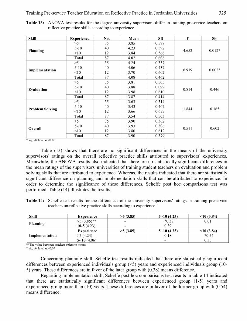
Training Pre-service Teacher Education on Reflective Practice in Jordanian Universities 325
Table 13: ANOVA test results for the degree university supervisors differ in training preservice teachers on reflective practice skills according to experience.
Skill Experience No. Mean SD F Sig
>5 35 3.85 0.577 5-10 40 4.23 0.592 <10 12 3.84 0.566 Planning
Total 87 4.02 0.606
4.652 0.012*
>5 35 4.24 0.357 5-10 40 4.06 0.437 <10 12 3.70 0.602 Implementation
Total 87 4.08 0.462
6.919 0.002*
>5 35 3.81 0.505 5-10 40 3.88 0.099 <10 12 3.98 0.610 Evaluation
Total 87 3.87 0.414
0.814 0.446
>5 35 3.63 0.514 5-10 40 3.43 0.407 <10 12 3.66 0.699 Problem Solving
Total 87 3.54 0.503
1.844 0.165
>5 35 3.90 0.362 5-10 40 3.93 0.306 <10 12 3.80 0.612 Overall
Total 87 3.90 0.379
0.511 0.602
* sig. At level α <0.05
Table (13) shows that there are no significant differences in the means of the university supervisors' ratings on the overall reflective practice skills attributed to supervisors’ experiences. Meanwhile, the ANOVA results also indicated that there are no statistically significant differences in the mean ratings of the supervisors' universities of training student teachers on evaluation and problem solving skills that are attributed to experience. Whereas, the results indicated that there are statistically significant difference on planning and implementation skills that can be attributed to experience. In order to determine the significance of these differences, Scheffe post hoc comparisons test was performed. Table (14) illustrates the results. Table 14: Scheffe test results for the differences of the university supervisors' ratings in training preservice
teachers on reflective practice skills according to experience
Skill Experience >5 (3.85) 5 -10 (4.23) <10 (3.84) >5 (3.85)** - *0.38 0.01 Planning 10-5 (4.23) - 0.39 Experience >5 (3.85) 5 -10 (4.23) <10 (3.84) >5 (4.24) - 0.18 *0.54 Implementation 5- 10 (4.06) - 0.35
**The value between brackets refers to means * sig. At level α <0.05
Concerning planning skill, Scheffe test results indicated that there are statistically significant differences between experienced individuals group (<5) years and experienced individuals group (10- 5) years. These differences are in favor of the later group with (0.38) means difference.
Regarding implementation skill, Scheffe post hoc comparisons test results in table 14 indicated that there are statistically significant differences between experienced group (1-5) years and experienced group more than (10) years. These differences are in favor of the former group with (0.54) means difference.

326 Hani A. Weshah
Q. 11: Does the degree of university supervisors train on reflective practice skill differ according to number of field visits? Independent T-test was performed to find out if there are any statistically significant differences
in the mean of the university supervisors' ratings of training student teachers on reflective practice skills that are attributed to number of visits. Table (15) illustrates the results. Table 15: T-test results for the degree of university supervisors train on reflective practice skills according to
number of field visits.
SKILL No. visits Freq Mean SD t df sig 1-2 32 4.20 0.671 Planning >3 55 3.93 0.548 2.035 85 0.05
1-2 32 4.13 0.460 Implementation >3 55 4.06 0.466 0.668 85 0.51
1-2 32 3.80 0.321 Evaluation >3 55 3.91 0.458 -1.126 85 0.26
1-2 32 3.21 0.286 Problem Solving >3 55 3.74 0.500 -5.501 85 0.00
1-2 32 3.87 0.396 Overall >3 55 3.52 0.372 -0.529 85 0.60
* sig. At level α <0.05
The T test results shows that there are no statically significant differences in the mean of the supervisors' ratings in training preservice teachers on overall reflective practice skills that are attributed to number of field visits. Meanwhile, independent T-test results also indicated that there are statistically significant differences in degree university supervisors train presevices on problem solving skill attributed to number of field visits. These differences were in favor of (3) visits and above. Discussion of the Findings Based on their total knowledge and experience, the university supervisors were asked to rate the degree to which they train preservices on reflective practice skills. The results that have been generated by this investigation indicated that:
1. Overall, descriptive statistics results showed that the mean ratings of the degree to which university supervisors train pre-services on reflective practice skills was (3.90), which considered high. The mean ratings for the implementation, planning and evaluation skills were (4.08, 4.02, 3.87) respectively. Meanwhile, the problem solving skill was the lowest (3.54) which considered to be moderate. It would seem from the results obtained through this investigation that there is a high degree of agreement in applying these skills included in this study and were confirmed by the participants, in general with the literature review. This agreement may be due to university supervisors in perceiving these effective teaching skills, which are a major part of the university teacher education program at the universities in Jordan. Despite this consensus, the conclusions drawn from the statistical analysis generated by universities' supervisors do not provide practical evidence or answer the question: Are supervisors distinguish between effective teaching skills and the reflective practice skills? Abrams & Middlleton (2004), and Denny (2005) suggest that teacher reflection has been promoted as one means of monitoring the quality of performance and enabling student teachers in their teacher-education programs to develop the pedagogical skills necessary for professional growth to reflect on practice in the classroom.
2. Independent samples T -test was performed to find out if there are any statistically significant differences in the mean ratings that are attributed to gender, educational qualification and number of field visits. Concerning the gender, the T-test results indicated that the overall mean ratings is statistically significant at level ά <0.05 and these differences were in favor of female.

Training Pre-service Teacher Education on Reflective Practice in Jordanian Universities 327
The T-test results also showed that there are statistically significant differences in the mean ratings of university supervisors on evaluation skill that are attributed to educational qualification and these differences were in favor of PhD holders. Nolan & Hillkirk (1991) found that promoting relective practice with skilled coaches has produced positive qualities of reflection while providing mentoring in terms of teacher's professional knowledge and practice.
Regarding to number of visits, T-test results indicated that there are statistically significant in the mean differences of the university supervisors on problem solving skill attributed to number of field visits. These differences were in favor of (3) visits and above.
Bryan (1997) and Eugene (2003) contend that learning to observe, analyze, discuss and evaluate practice of one's own teaching; learning to isolate, frame and reframe problems of practice; learning to take action and interpret that action, all of these skills take time and practice to develop. Reflective practice is a developmental process which needs time to explore and try out new ideas. There should be time and opportunities to investigate the value of writing, videotaping, and talking with colleagues as sources of evidence for reflection.
3. One – way ANOVA was performed to find out whether there are any statistical significant differences in the mean ratings that are attributed to the university, major and experience. As for the university, the results indicated that there are statistically significant differences in the mean ratings in planning and problem solving skills at level ά <0.05. Scheffe test results revealed that there are statistically significant differences between the University of Jordan group and the remaining universities regarding problem solving skill. These differences were in favor of the Yarmouk, Mu'tah, Hussein, Hashimeah and Balqa. This means that training preservices on reflective practice on this skill is less than other universities. This result confirmed Tome's (1992), Pedro (2001) and Hamlin's (2004) studies that many teacher education programs might have embedded inquiry into their approach to reflective practice, however, these programs differ due to varying definitions of reflection, methods of implementation, time involved, faculties assumptions and beliefs as well as other factors such as the social and political context. This finding also support Callouet's (1998) research assertion that professionalization is dependent on school placement and influenced by the culture of that school.
Scheffe test revealed that there are statistically significant differences and these differences were in favor of math and science major. The skill of problem solving required specific training. Anderson (1997), Reinhold (1999), Eugene's (2003) suggested that consistent supervision and regular feedback are essential elements to solve problem and make decisions.
Concerning to experience, results indicated that there are statistically significant differences that can be attributed to experience. Scheffe test results indicated that there are statistically significant differences and these differences are in favor of (5 -10) years of experience.
This results support Nolan & Hillkirk (1990), Reinhold's (1999) and Callouet (1998) studies which reported that reflection in practice is a difficult concept to internalize, and it requires the experience and confidence of purposeful continuous practice. Ross (2002) contends that for many teacher educators, reflective practice remains elusive. In order to change this phenomenon, supervisors need to model reflective skills with their student teachers to facilitate the process in our teacher education programs. Both Dewey (1910) and Schon (1983) emphasize the problematic nature of situations in which reflection and growth take place. Therefore, supervisors are encouraged to consider ways in which student teachers learning reflection is promoted in the classroom by considering not just their technical skills but also issues and aspects of practice that go deeper than this. In this context, Zeikner & Liston (1978) believe that through reflective teaching pre-service teachers should be trained to be thoughtful about the teaching and learning process, how to link theory with practice, to solve problems and make decisions and to self-evaluate themselves.

328 Hani A. Weshah
Recommendations Based on the findings of this study, the following recommendations for further research and implications can be presented below.
1. The study results revealed an overall agreement that was found among university supervisors in training preservice student teachers in reflective practice skills. These skills refer to the teacher’s ability to reflect upon experiences which provide students the opportunity to acquire the intended knowledge, skills and attitudes. However, university supervisors indicated a special need to train the preservice student teachers’ ability in problem solving skill.
2. Although this study examined the degree university supervisors train student teachers on reflective practice skills, further studies should facilitate the preparation of a comprehensive plan of teacher growth and professional development in providing time to install reflection in classroom teachers. Subsequently, studies can be conducted to determine the effects implementation has on student performance and achievement. This could be accomplished through a combination of classroom observations, interviews, case studies and portfolios.
3. The results of this study also point to the need for continuing research to find out more about how university supervisors view their own experiences, related to their role as mentors.
4. One of the most important references in this study is the instrument used as a tool for preparing, training, and evaluating reflective practice skills. Study determines two important criteria: pertinent reflective practice skills which represent the most highly developed systems for evaluating all aspects of reflective practice and university supervisors recognized in their comments that the skills are essential for reflective practice.
5. Reflective practice research revealed that development and use of low/high-inferences observation methods to measuring reflective practice skills provided reliable, adequate measurement of reflective practice skills and confidence in the instruments to evaluate reflective practice in the Jordanian schools and universities.
6. Another recommendation for further study is related to teacher evaluation and supervision. In this study, supervisors have provided their perception, evaluation and reported significant implementation of reflective practice skills, findings suggest the following specific instructions could be incorporated into education programs for preservice teachers to be trained.
7. Additional intensifying responsibility and the role of cooperating teacher expand, the need for better communication increases: such as lead teachers; peer coaching; mentoring; collaborative action research; communication with students, parents, personnel and community members; and group dynamics, which all become essential skills for teachers, Such feedback from cooperating teachers should be considered in curriculum development and evaluation.
8. Research also needs to address contemporary reflective practice needed because of advanced technology. Student teachers need to become proficient at being able to access the tremendous amount of information through using different types of technology, the mechanical aspects must be resolved before teachers can begin to use them for the improvement of teaching and learning.
9. Since the study was based on qualitative exploration, it can only be regarded as offering a well grounded hypothesis. Additional research is obviously necessary and innovations in educational systems on a large scale to improve education for all students.
10. Finally Reflective practice has become an integral issue in teacher education nowadays. It is an on going process that play an essential role in teacher development. But still it needs more investigation in our schools. We need to measure the extent to which our teachers are aware of the term and the level they practice reflection in their teaching. Teacher education and professional development programmes need to take the issue of reflective practice more seriously if they are to meet the needs of learning environments of the 21st century.

Training Pre-service Teacher Education on Reflective Practice in Jordanian Universities 329
References [1] Abrams, E and Middleton, M. (2004). Pre-service middle school teachers reflecting on
instructional practice through technology. Paper presented at the National Educational Computing Conference, New Orleans. USA
[2] Antonek, J. (1997). The student teacher portfolio as autobiography: developing a professional identity. Modern Language Journal, 81(1).
[3] Beattie, M. (1997). Fostering reflective practice in teacher education: inquiry as a framework for the construction of a professional knowledge in teaching. Asia-Pacific Journal of Teacher Education; Vol. 25, Issue 2.
[4] Bell, B. & Gilbert, J. (1996) Teacher Development: a model from science education. Falmer Press, London.
[5] Boud, D. & Walker, D. (1998). Promoting reflection in professional courses: The challenge of context. Studies in Higher Education, 23(2).
[6] Brookfield, S. (1995). Becoming a critically reflective teacher. Jossey-Bass Inc. California. [7] Bryan, L; Abell, S; and Anderson, M. (1997). Coaching reflective practice among preservice
elementary science teachers. Purdue University. USA [8] Chojnaka, E. (2000). Raising self-awareness in advanced learners practicing listening
comprehension. TT College Plock, Newsletter 3. [9] Clarke, A. (1995). Teaching and Teacher Education Professional development in practicum
settings: Reflective practice under scrutiny, 11(3). [10] Clift, R; Houston, W; & Pugach, M. (1990). Encouraging reflective practice in education: an
analysis of issues and programs. New York: Teachers College Press. [11] Day, C. (1993). The Development of Teachers’ Thinking and Practice: Does Choice Lead to
Empowerment?”. In: Elliott, J. (Ed). Reconstructing teacher education: teacher Development. Falmer Press, London.
[12] Day, C. (1999). Developing teachers: the challenges of life-long learning. Falmer Press, London.
[13] Denny, H. (2005). Reflective and action research as a source of pre¬-service and in-service professional development and classroom innovation: burden or benefit? Myth or reality? Working Paper No. 14 School of Languages, Auckland University of Technology Auckland, New Zealand.
[14] Elliott, J. (1993). The relationship between understanding and developing teachers’ thinking. In: Elliott, J. (Ed). Reconstructing teacher education: teacher development. Falmer Press, London.
[15] Ellsworth, J. (2002) Using student portfolios to increase reflective practice among elementary teachers. Journal of Teacher Education. Vol. 53, No. 4.
[16] Eugene, K. (2003). Promoting pre-service teacher education students’ reflective practice in mathematics. Asia-Pacific Journal of Teacher Education, Vol. 31, No. 1
[17] Ferraro, J. (2000). Reflective practice and professional development: refining the concept. ERIC Digest. ERIC Document Reproduction Service: ERIC ED449120.
[18] Field, B. (1994). Towards understanding the lived experience of practising student teachers. In: Field, B & Field, T. (Ed). Teachers As Mentors: a practical guide. Falmer Press, London.
[19] Freidus, H. (1997). The telling of story: teachers knowing what they know. Paper presented at the annual meeting of the American Educational Research Association (AERA), Chicago, IL. ERIC Document Reproduction Service: ED 409 274
[20] Furlong, J. (2000). Teacher education in transition. reforming professionalism? Open University Press. England.
[21] Galvez, M. (2003). Reflective Teaching, Reflective Practice, and … what else? University of South Florida. USA
[22] Hamlin, K. (2004). Beginning the journey: supporting reflection in early field experiences. Reflective Practice, Vol. 5, No.2.

330 Hani A. Weshah
[23] Henderson, J.(1992). Reflective teaching: becoming an inquiring educator. Macmillan, New York.
[24] Hillkerk, K. (1993). Pre-service secondary teacher reflective and inquiry skills and ability to articulate a written philosophy of education. Unpublished Dissertation. Penn State University. USA. Hoffman-Kipp, P.;Artiles, A. & Lopez-Torres,L.(2003).Beyond reflection: teacher learning as praxis. Theory into Practice. Vol.42, Issue 3.
[25] Holm, L. & Horn, C. (2003). Brigdging the gap between schools of education and the needs of the 21st century teachers. Phi Delta Kappan. Vol.84, Issue 5.
[26] Hopkins, C, & Antes, R. (1990). Educational research: a structure for inquiry. 3rd ed. Itasca, IL: F.E. Peacock.
[27] Hurst, B; Wilson C; & Cramer, G. (1998). Professional teaching portfolios. Phi Delta Kappan, 79 (8).
[28] Hyun, E. and Marshall, J. (1990). Inquiry-oriented reflective supervision for developmentally and culturally appropriate practice. Journal of Curriculum and Supervision. Vol. 11. No. 2.
[29] Johnson, G. & Stevens, E. (2002). Moving from the personal to the political in teachers' reflective practice. Queensland Journal of Educational Research, 18(1).
[30] Kauchak, D. & Eggen, P. (1998). Learning and Teaching: research-based methods. Allyn and Bacon. USA.
[31] Kettle B. & Sellars, N. (1996). The development of student teachers practical theory of teaching. Teaching and Teacher Education, 12(1).
[32] LaBoskey, V.(1997). Teaching to teach with purpose And passion: pedagogy for reflective practice.’ In: Loughran, J & Russell, T (Ed) Teaching About Teaching: Purpose, Passion and Pedagogy in teacher Education. Falmer Press, London.
[33] Licklider, B. (1997). Breaking ranks: changing the in-service institution. NASSP Bulletin, 81. [34] Loughran, J. (1996). Developing reflective practice: learning about teaching and learning
through modelling. Falmer Press. London. [35] McGreal, T. (1997). Can a supervisor be a coach? Yes’. in: Glanz, J. & Neville, R.(Ed.)
Educational supervision: perspedtives, issues, and controversies. Christopher Publishers,USA. [36] Newman, S. (1996). Reflection and teacher eduation. Journal of Education for Teaching, Vol
22, Issue3. [37] Nolan, j and Hillkerk, K. (1991).The effects of a reflective coaching project for veteran
teachers. Journal of Curriculum and Supervision, vol. 7, No.1. [38] Parsons, M and Stephenson, M. (2005). Developing reflective practice in student teachers.
Teachers and Teaching: theory and practice, Vol. 11, No. 3. [39] Pasch, S. (1995). Assisting and Assessing the Development of Preservice Teachers in
Academic and Clinical Settings. In: Soled,S. W. (Ed) Assessment, Testing, and Evaluation in Teacher Education. Ablex Publishing Corporation, New Jersy.
[40] Pedro, J. (2001). Reflection in teacher education: exploring preservice teachers meanings of reflective practice. Unpublished Dissertation. Virginia Polytechnic Institute and State University. Blacksburg, Virginia.
[41] Pollard, A & Tann, S. (1994) Reflective Teaching in the Primary School a Handbook for the Classroom, 2nd ed. The Open University, England.
[42] O’Hanlon, Christine (1993). The Importance of an Articulated Personal Theory of Professional Development. In: Elliott, J. (Ed). Reconstructing Teacher Education: Teacher Development. Falmer Press, London.
[43] Ojanen, S. (1993). A process in which personal pedagogical knowledge is created through the teacher education experience. Paper presented at the International Conference in Teacher Education, Tel-Aviv, Israel. ERIC Document Reproduction Service: ED 398 200
[44] Ornstein,A. & Hunkins, F. (1993).Curriculum Foundations, principles and issues. Allan and Bacon, USA.

Training Pre-service Teacher Education on Reflective Practice in Jordanian Universities 331
[45] Power, A; Clarke, M & Hine, A. (2002). Internship learning connects the dots: the theory and practice of reflection. Paper presented at AARE Conference, Brisbane. Ausralia.
[46] Rearick, M.L. (1997). Educational researchers, practitioners, and students of teaching reflect on experience, practice, and theories: Action research in a pre-service course. Paper presented at the annual meeting of the American Educational Research Association (AERA), Chicago, IL. ERIC Document Reproduction Service: ED 412 229
[47] Reinhold, P. (1999). Case studies of teachers' reflective practice within the developmental research project PING. Journal of Curriculum Studies. Vol. 31, No.5.
[48] Ross. D. (2002). Coperating teachers facilitating reflective practice for student teachers in a professional development school. Education. Vol. 122. Issue 4.
[49] Schon, D. (1983). The reflective practioner: how professionals think in action. N.Y. Basic Books.
[50] Schon, D. (1996). Educating the reflective practitioner: Toward a new design for teaching and learning in the professions. San Francisco: Jossey-Bass, Inc.
[51] Schon, D.(1987). Educating the reflective practioner. London. Jossey-Bass. [52] Skilling, K. (2001). Its time to reflect on the benefits of reflective practice. Primary Educator,
Vol. 7, Issue 3. [53] Sprinthall, N; Reiman, A; & Theis-Sprinthall, L. (1996). Tacher professional development. In:
Sikula, J. Handbook of Research on Teacher Education. Macmillan. New York. [54] Susan, I (1992), Reflective practice in adult education. ERIC Digest No. 122. [55] Syrjala, L. (1996). The teacher as a researcher. In Childhood Education: International [56] Perspectives. Ed. Eeva Hujala. Finland: Association for Childhood Education International,
Oulu University. ERIC Document Reproduction Service: ED 403 069 [57] Tickle, Les. (1993). Capital T Teaching. In: Elliott, J. (Ed). Reconstructing Teacher Education:
Teacher Development. Falmer Press, London. [58] Tomlinson, Peter. (1995) Understanding Mentoring: Reflective Strategies For School-Based
Teacher Preparation. Open University Press, Backingham. [59] Uzat, S. (1998). Cognitive coaching and self-reflection: looking in the mirror while looking
through the window. Paper presented at the annual meeting of the Mid-South Educational Research Association. New Orleans, LA. ERIC Document Reproduction Service: ED 427 064
[60] Zeikner, K & Liston, D. (1978). Teaching Student Teachers to Reflect. Harvard Educational Review. Vol.37 No.1

European Journal of Scientific Research ISSN 1450-216X Vol.18 No.2 (2007), pp.332-337 © EuroJournals Publishing, Inc. 2007 http://www.eurojournals.com/ejsr.htm
Development of Computer Simulation of Wavelet Selection
Technique for Time-Frequency Analysis
Preety D. Swami Department of Electronics S. A. T. I., Vidisha,India
E-mail:[email protected]
Mohammed Al-Fayoumi Faculty of IT ,University for Graduate Studies, Amman, Jordan
E-mail: [email protected]
P. Mahanti Department of CSAS, University of New Brunswick
Saint John, NB, E2L 4L5, Canada E-mail: [email protected]
Abstract
Wavelets are used for the analysis of non-stationary signals. With its zooming in on singularities it has good ability in processing the non-stationary signals. The trick in using wavelets is to find a set of them that provides a description that is optimal in some sense to the problem at hand. If wavelet analysis in general, or the particular set chosen, is not well-suited to the problem at hand, they can be no help or, worse, lead to deeper confusion. In this work features based on duration and bandwidth of Paul, Morlet, and Gaussian derivative wavelets are described which helps in selection of either of them. Application of these wavelets for the time frequency analysis of ECG during ventricular fibrillation is discussed . Keywords: CWT, Non-stationary signal, time frequency analysis, time and frequency
resolution 1. Introduction The limitations of Fourier transform in analyzing non stationary signals led to the introduction of two dimensional signal processing tools such as time-frequency and time-scale representations. Time-frequency representations (Hlawatsch and Boudeaux- Bartels, 1992),(Cohen,1989), for example, the Short Time Fourier Transform (STFT), the Wigner Distribution (WD), the Ambiguity Function (AF), aim at describing time dependent spectral properties of signals, where as time–scale representations such as the Wavelet Transform (WT) (Rioul and Vetterli,1991), aim at extracting the localized contributions of signals which are labeled by a scale parameter. Applications of WT include classification of underwater mammals (Huynh et. al., 1998), defect detection of wheel flats of railway wheels (Jianhai et.al, 2002) acoustic emission signal processing (Serrano and Fabio,1996), studies in geophysics (Georgiou and Kumar,1995), analysis of brain evoked potential signals (Bertrandet.al.,1994), genomic signal processing (Wang and Johnson, 2002). This work describes the

Development of Computer Simulation of Wavelet Selection Technique for Time-Frequency Analysis 333
time-frequency analysis of signals using Continuous Wavelet Transform (Rao & Bopardikar, 2002).Three wavelets namely, Paul, Morlet and Gaussian derivative are discussed. Also their comparative performance analysis for time-frequency analysis is done. 2. Literature Review 2.1 Continuous Wavelet Transform (CWT)
The function ψ (t) is a mother wavelet or wavelet if it satisfies the following properties (Rao &.Bopardikar,02)
The function integrates to zero:
(1) It is square integrable or has finite energy:
(2) Continuous Wavelet Transform (CWT) maps a one dimensional analog signal x(t) to a set of
wavelet coefficient which vary continuously over time b and scale a, using wavelet as a basis:
The wavelet function is used to band pass filter the signal. This can be seen as a kind of time varying spectral analysis in which scale a plays the role of a local frequency.
As a increases, wavelets are stretched and analyze low frequencies, while for small a, contracted wavelets analyze high frequencies. Therefore the time frequency extents of the wavelets vary according to a “constant Q” scheme (Rioul and Vetterli,1991), with various resolutions in time or frequency (multi resolution analysis), where as techniques based on STFT analyze the signal at constant resolution (Rioul and Vetterli,1991). Scale a is related to the local frequency f by the relation a = f0 / f, where f0 is the center frequency of the mother wavelet. 2.2. Wavelets
2.2.1 Morlet Wavelet The most commonly used CWT wavelet is the Morlet . It is defined in the time domain as where m is the wave number.
(3) 2.2.2. Paul wavelet Paul wavelet can be described as
(4) 2.2.3 Gaussian Derivative Wavelet The third mother wavelet used in this work is Gaussian derivative wavelet. The real component is defined as follows:
( ) 2/tm0
2
edtd
21m
)1(t −
∞
∞∞
∞∞+Γ
−=ψ
(5) The lowest derivative, 2, is known as the Marr or Mexican Hat Wavelet.

334 Preety D. Swami, Mohammed Al-Fayoumi and P. Mahanti
2.3. Ventricular Fibrillation
Ventricular tachyarrhythmias, in particular ventricular fibrillation (VF), are the primary arrhythmic events in the majority of patients who present with sudden cardiac death (Serrano and M.A Fabio, 1996),(Wang and Johnson, 2002). Attention has been focused upon these particular rhythms as it is recognized that prompt therapy can lead to a successful outcome. There has been considerable interest in analysis of the surface electrocardiogram (ECG) in VF centered on attempts to understand the pathophysiological processes occurring in sudden cardiac death, predicting the efficacy of therapy, and guiding the use of alternative or adjunct therapies to improve resuscitation success rates. Until recently, the ECG recorded during ventricular fibrillation (VF) was thought to represent disorganized and unstructured electrical activity of the heart. Using the new signal analysis technique based on wavelet decomposition, we have begun to reveal previously unreported structure within the ECG tracing.
The wavelet transform has become a valuable analysis tool because of its ability to elucidate simultaneously local spectral and temporal information within a signal. It overcomes some of the limitations of the more widely used Fourier Transform, which only contains globally averaged information and has the potential to lose transient or location-specific features within the signal. The ECG of most normal heart rhythms is a broad band signal with major harmonics upto about 25Hz . During VF, the ECG becomes concentrated in the narrow band of frequencies between 5 and 7 Hz . This feature is used for VF detection algorithms. 2.4 Time Resolution vs. Frequency Resolution
It is not always possible for the CWT to resolve events in frequency. The same holds true for resolving events in time (Rao & Bopardikar, 2002) . Quantitative metrics for time and frequency resolution are based on duration and bandwidth respectively of the mother wavelet. The first moment of a mother wavelet ψ(t) is given by
( )
( )∫
∫∞
∞
∞
∞
Ψ
Ψ≡
dtt
dtttt0
2
2
||
||
(6) t0 , provides a measure of where ψ(t) is centered along the time axis. Similarly the centre of ψ(ω), the Fourier Transform of ψ(t),is located, along the frequency axis by taking its first moment, given by
( )
( )∫
∫∞
∞−
∞
∞−
ωωΨ
ωωΨ≡ω
d
dt
02
2
||
|| (7)
A measure of duration of the wavelet or spread in time is given by
( ) ( )( )∫
∫∞
∞−
∞
∞−
ψ
ψ≡∆
dt
dtt-t 0
2
22
t
tt
(8) This measure is known as root mean square (RMS) duration. The RMS bandwidth of the
wavelet is given similarly by ( ) ( )
( )∫∫
∞
∞−
∞
∞−
ωωψ
ωωψωω≡ω∆
d
d- 0
2
22
(9) Fast decays in time and in frequency are required for the wavelets and its Fourier Transform to
have finite values for the numerator integrals in equations 6 through 9.

Development of Computer Simulation of Wavelet Selection Technique for Time-Frequency Analysis 335
The time-frequency resolution is governed by the uncertainity principle given by equation
(10) Where ∆tψ(a) and ∆ωψ(a) are the RMS duration and bandwidth respectively of the wavelet
ψ(t),dilated by the scale a and cψ is a constant. Equation 10 indicates that decreasing ∆tψ(a) results in an increase in ∆ωψ(a) and vice-versa. The smaller the value of, ∆tψ(a) the better the ability of the CWT to resolve events closely spaced in time. Similarly, the smaller the value of ∆ωψ(a), the better the ability of the CWT to resolve events closely spaced in frequency. 3. Experimental Results and Discussions We have developed a computer simulation method to illustrate the time frequency resolution trade off, a non-stationary sinusoid corresponding to ECG during ventricular fibrillation is simulated. The signal comprises of a 5Hz sinusoid from 0-30 min., a 6Hz sinusoid from 27-33.6 min and a 7Hz sinusoid from 31.2-6 min. The wavelet transforms corresponding to Paul, Morlet and Gaussian Derivative wavelets for different wave numbers are shown in Figures(1) through (3) respectively. The wavelet peak has been zoomed in to illustrate this time frequency trade off. The RMS duration and RMS bandwidth, of each of the three wavelets for different wave numbers, m, is computed. The result is recorded in Table 1. Table 1: RMS durations and bandwidths of Paul , Morlet and Gaussian Derivative wavelets of different
orders
Paul Morlet Gaussian Derivative m ∆t ∆ω m ∆t ∆ω m ∆t ∆ω 4 0.377964 4.74342 6 0.707107 6.0415 2 1.08012 1.58114
16 0.179605 16.748 12 0.707107 12.0208 12 1.01081 3.53554 40 0.112509 40.7492 20 0.707107 20.0125 20 1.00000 4.5277
All the three wavelet basis is compactly supported which means that the oscillations are
effectively localized in time by rapid decay. Thus all three of the wavelets offer very good time localization. The Paul wavelet localizes most efficiently in the time domain but frequency resolution is not appreciable. Morlet offers better time resolution than the Gaussian Derivative but greater differences tend to be in the frequency domain. For a given count of evident oscillations in the wavelet, the Gaussian derivative offers the best frequency localization.
Figure 1: CWT using Paul Wavelet with Different Orders

336 Preety D. Swami, Mohammed Al-Fayoumi and P. Mahanti
Figure 2: CWT using Morlet Wavelet with Different Orders
Figure 3: CWT using Gaussian Derivative Wavelet with Different Orders
4. Conclusion In this paper properties of Paul, Morlet, and Gaussian derivative wavelets have been studied in both time and frequency domain. Comparative performance of these wavelets for time-frequency analysis, selecting time and frequency localization as the performance metrics is carried out. Finally, it is observed that if in analysis of any signal, interest lies in fine resolution in time domain then Paul wavelet is the best option, while if higher precision is required in frequency domain then Gaussian Derivative wavelet of higher orders gives nice results.

Development of Computer Simulation of Wavelet Selection Technique for Time-Frequency Analysis 337
References [1] Bertrand, O., Bohorquez, J. and Pernier, J. (1994) Time frequency digital filtering based on an
invertible wavelet transform: An application to evoked potentials, IEEE Transactions on Bio Medical Engineering, vol.41, no.1., pp.77-88.
[2] Cohen, L., (1989) Time frequency distributions- A review, Proceedings of the IEEE, vol.77, no.7, pp. 941-981
[3] Georgiou E.F.and Kumar P., (1995) Wavelets in Geophysics Academic Press [4] Goldstein,S., Landis,J.R., Leighton,R., Ritter,G.,Vasu,C.M.,Lantis,A.and Serokman ,R.,(1981)
Characteristics of the resuscitated out-of-hospital cardiac arrest victim with coronary disease,Circulation, vol. 64, no. 5, pp. 977-986.
[5] Hlawatsch F.& Boudeaux- Bartels, G.F.,(1992) Linear and quadratic time frequency signal representations, IEEE Signal Processing Magazine, pp 21-67
[6] Huynh,Q.Q., Cooper,L.N., Intrator N and Shouval, H.,(1998) Classification of underwater mammals using feature extraction based on time frequency analysis and BCM theory, IEEE Transaction on Signal Processing, vol. 46, no.5, pp.1202-1207.
[7] Jacobs,I.G. and Oxer,H.F.,(1990) A review of prehospital defibrillation by ambulance officersin Perth, Western Australia, Med. J. Aust., vol.153, pp. 662-664.
[8] Jianhai,Y., Zheng ding,Q. and Boshi,C.,(2002) Application of wavelet transform to defect detection of wheel flats of railway wheels, Proceedings of International Conference on Signal Processing, Beijing, China, IEEE Press, pp.92-95.
[9] Rao,R.M. &.Bopardikar, A.S.,(2002)Wavelet Transform, Introduction to Theory and Applications, Pearson Education
[10] Rioul,O. and Vetterli,M.,(1991)Wavelets and signal processing, IEEE Signal Processing Magazine.pp14-38.
[11] Serrano, E.P., and Fabio,M.A.,(1996) Application of wavelet transform to acoustic emission signal processing, IEEE Transaction on Signal Processing, vol. 44, no 5, pp. 1270-1275
[12] Wang,B. and Johnson,D.H.,(2002)Computing linear transforms of symbolic signals,IEEE Transactions on Signal Processing, vol.50, no.3, pp.628-634.

European Journal of Scientific Research ISSN 1450-216X Vol.18 No.2 (2007), pp.338-353 © EuroJournals Publishing, Inc. 2007 http://www.eurojournals.com/ejsr.htm
Heterosis, Inbreeding Depression and Mean Performance of
Segregating Population in Upland Cotton
Naqib Ullah Khan Visiting Scholar, Department of Horticulture and Crop Science
The Ohio State University OARDC, 1680 Madison Ave. Wooster OH 44691, U.S.A NWFP Agricultural University Peshawar 25130, Pakistan
E-mail: [email protected]; [email protected]. Tel: +1-330-202-3595; Fax: +1-330-263-3887
Gul Hassan
NWFP Agricultural University Peshawar 25130, Pakistan
Moula Bux Kumbhar Sindh Agriculture University Tandojam 70060, Pakistan
Sungtaeg Kang
Visiting Scholar, Department of Horticulture and Crop Science The Ohio State University OARDC, 1680 Madison Ave. Wooster OH 44691, U.S.A
National Institute of Crop Science, RDA 151 Seodung-Dong, Suwon, 441-857, Korea
Ikramullah Khan NWFP Agricultural University Peshawar 25130, Pakistan
Aisha Parveen
Graduate Students, Department of Plant Breeding and Genetics NWFP Agricultural University, Peshawar 25130, Pakistan
Umm-e-Aiman
Graduate Students, Department of Plant Breeding and Genetics NWFP Agricultural University, Peshawar 25130, Pakistan
Muhammad Saeed
Graduate Students, Department of Plant Breeding and Genetics NWFP Agricultural University, Peshawar 25130, Pakistan
Abstract
Performance of F1 hybrids, F2 population and some selected population in advanced generations (F3, F4 and F5) were studied for bolls per plant, seed cotton yield per plant, lint % and staple length of Gossypium hirsutum during 1999-2004 at Agricultural Research Institute, Dera Ismail Khan, NWFP Pakistan. In F1 hybrids, maximum heterosis was observed for seed cotton yield per plant followed by bolls per plant while lint % and staple length showed low values of heterosis. Majority of the F2 population displayed inbreeding depression and it was high for seed cotton yield per plant followed by bolls per plant, lint

Heterosis, Inbreeding Depression and Mean Performance of Segregating Population in Upland Cotton 339
% and staple length. Inbreeding depression was higher in high performing hybrids than in low performing hybrids. In F1 generation, heterosis over better parent ranged from +3.13 to +65.63% for bolls per plant, +0.82 +115.22% for seed cotton yield per plant, +0.27 +3.88% for lint % and +0.28 to +6.00% for staple length. In F2 population the average some selections were made in promising cross families (CIM-109 x CIM-1100, CIM-240 x CIM-1100, CIM-1100 x CIM-109 and CIM-1100 x CIM-240). In advanced generations (F3, F4 and F5), the single plant families of the above four selected crosses superseded the standard cultivar (CIM-446) for bolls and seed cotton yield per plant and staple length, but in lint % only few of the cross families exhibited superiority over standard. Keywords: Upland cotton; F1 hybrids; F2 population; Mean Performance; Heterosis and
Inbreeding Depression; Segregating Generations. Introduction Heterosis works as a basic tool for improved production of crops in the form of F1 hybrids. The phenomenon of heterosis of F1 hybrids can reflect their own specific combining ability (SCA) and the general combining ability (GCA) of parental lines. Hence, heterotic studies can provide the basis for exploitation of valuable hybrid combinations and their commercial utilization in future breeding programmes. Cook (1909) was the first to utilize hybrid vigor in interspecific hybrids (G. barbadense x G. hirsutum) and after that a number of workers all over the world are still supporting his contention. Hybrid cotton is a good approach for significant improvement in genetic potential for yield and fibre quality traits and has attracted attention of cotton breeders for commercial growing of hybrid generations. However, the efforts have not delivered the expected results due to its self pollination which has some different implications on hybrid seed production in comparison to cross pollinated crops (Waller et al. 1981; Waller and Moffett, 1981; Salam, 1991 and Arshad, 1991). In countries, however, like India and China, where labour is cheaper, the successful hybrid cotton produced on large scale since 1960s as reported by Krishnaswami and Kothandaramon (1977), Salam (1991), Soomro et al. (1991) and Khan et al. (1999a).
In view of the economic importance of hybrid cotton cultivation, and the importance of selected hybrids in segregating generations, a research project was undertaken to evaluate the manifestation of heterosis in F1 hybrids and inbreeding depression in F2 population for bolls per plant, seed cotton yield per plant, lint % and staple length and also to study the other segregating generations for selected breeding material in upland cotton in a set of 6 parent diallel cross. Materials and Methods The crossing block, F1 and F2 population and experiments comprising of other advanced generations (F3, F4 and F5) of upland cotton (Gossypium hirsutum L.) have been conducted and maintained at Agricultural Research Institute, Dera Ismail Khan, Pakistan during 1999-2004. Six diverse genotypes of upland cotton i.e. CIM-109, CIM-240, CIM-1100, FH-682, BH-36 and CRIS-9 were sown during May 1999, in a non-replicated crossing block by dibbling on a well prepared seed bed. Five rows, each of 27 meters length, at the spacing of 60 and 100 cm between plants and rows, respectively, to ensure easy crossing and to handle the breeding material carefully. All cultivars were crossed in a complete diallel fashion. The F1’s were raised during 2000 from half of the crossed seed to get F2 seeds. The F1 and F2 population of 6 X 6 complete diallel cross, having thirty hybrids (including reciprocals) along with six parents were sown by dibbling with randomized complete block design on a well prepared seed bed during May 2001. In F1 each genotype was planted in a single row measuring 3.30 m, with three replications, while in F2 the plant population was increased and each genotype was planted in

340 Naqib Ullah Khan, Gul Hassan, Moula Bux Kumbhar, Sungtaeg Kang Ikramullah Khan
four rows, each of 6.30 m length, with four replications. The row and plant spacing were 75 and 30 cm, respectively. All cultural practices were carried out as per recommended package for cotton production and all the crops were maintained under uniform conditions to discourage environmental variability to the maximum possible extent. Picking was made in November-December every year on single plant basis and ginning was done with eight saw-gin.
Single plant selections were made in F2 crosses on the basis of cotton leaf Curl virus (CLCV) resistance, yield and yield components, which were sown with a standard cultivar (CIM-446) for other segregating generations i.e. during May 2002 for F3, May 2003 for F4 and May 2004 for F5. Each single plant family consisted of four rows of 5 meter in length with spacing of 75 and 30 cm. All cultural practices were carried out as recommended for cotton production and all crops were maintained under uniform conditions to the maximum possible extent to discourage environmental variability. Picking was made in November-December every year on single plant basis and ginning was done with eight saw-gin. In all the experiments the data were recorded for bolls per plant, seed cotton yield per plant and after ginning for lint % and staple length. The staple length was studied by High Volume Instrument (HVI) USTER-900A.
The data were subjected to ANOVA technique using MSTATC, a computer software package (Bricker, 1991) for all the traits to test the null hypothesis of no differences between various F1’s as well as among F2‘s hybrid populations and their parental lines, while in advanced generations the means of single plant families were compared with standard cultivar (CIM-446) for their percent increase or decrease. In F1 hybrids, heterosis was estimated according to Fehr (1987). The F1 hybrid means having positive heterotic values were further tested for significance with “t” test of Wynne et al. (1970). The observed inbreeding depression in F2 hybrids was calculated as percent decrease of F2 hybrids when compared with F1 hybrids as outlined by Hallaner and Miranda (1986) and Baloch et al. (1993a). Results The null hypotheses for equality of 30 F1 and F2 means and their six parental lines tested through ANOVA (Table 1), proved false at P≤0.01 for all the parameters and manifested highly significant mean differences. The results are presented here in seriatim. Boll weight
The boll weight varied from 2.38 g (CIM-109) to 2.91 g (CIM-1100) among the parents, while CRIS-9 showed maximum boll weight (2.91 g). Among the F1 hybrids boll weight ranges from 2.42 g (CIM-109 x CRIS-9) to 3.62 g (CRIS-9 x CIM-1100) (Fig. 1). Nearly 2/3 of F1 hybrids surpassed the parental cultivars. The highest and statistically equal boll weight was recorded in 9 F1 hybrids and their reciprocals in which eight crosses consisting of parent CIM-1100 and their boll weight was ranged from 3.34 to 3.62 g. The lowest boll weight was manifested by two cultivars CIM-109 (2.38 g) and CRIS-9 (2.52 g) and their F1 hybrid and its reciprocal having 2.42 to 2.46 g boll weight. The cross CIM-240 x CRIS-9 (2.61 g) also possessed the least boll weight. In F2 population, boll weight varied from 2.26 g (CIM-109 x BH-36) to 3.20 g (CIM-1100 x FH-682) among the hybrids (Fig. 1). The highest and statistically equal boll weight ranged from 2.96 to 3.20 g was recorded in 6 genotypes and reciprocals, which have CIM-1100 as one parent as also observed in F1 generation, The lowest boll weight was manifested by the genotype CIM-109 x BH-36 (2.26 g).
The heterobeltiotic values ranged from +0.75 (BH-36 x CIM-240) to +24.40% (CRIS-9 x CIM-1100) over better parents, respectively (Fig. 1). In case of heterobeltiosis 13 F1 hybrids surpassed their better parent with highly significant values and only 2 crosses showed significant heterobeltiosis. All the F2 genotypes displayed inbreeding depression for boll weight (Fig. 1) and the observed inbreeding depression was -0.37 to -23.66%. However, some genotypes displayed positive values of inbreeding due to transgressive recombination in F2 generation. The results showed that in F2 even after
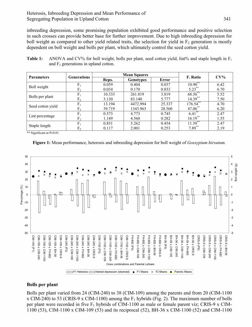
Heterosis, Inbreeding Depression and Mean Performance of Segregating Population in Upland Cotton 341
inbreeding depression, some promising population exhibited good performance and positive selection in such crosses can provide better base for further improvement. Due to high inbreeding depression for boll weight as compared to other yield related traits, the selection for yield in F2 generation is mostly dependent on boll weight and bolls per plant, which ultimately control the seed cotton yield. Table 1: ANOVA and CV% for boll weight, bolls per plant, seed cotton yield, lint% and staple length in F1
and F2 generations in upland cotton.
Mean Squares Parameters Generations Reps. Genotypes Error F. Ratio CV%
F1 0.059 0.404 0.037 10.90** 6.42 Boll weight F2 0.034 0.170 0.033 5.23** 6.70 F1 10.333 261.819 3.819 68.56** 5.52 Bolls per plant F2 3.130 83.140 5.777 14.39** 7.50 F1 13.194 4472.994 25.337 176.54** 4.70 Seed cotton yield F2 39.719 1343.963 28.560 47.06** 6.20 F1 0.573 4.773 0.745 6.41** 2.47 Lint percentage F2 1.149 4.560 0.282 16.19** 1.55 F1 0.851 5.262 0.454 11.59** 2.47 Staple length F2 0.117 2.001 0.253 7.89** 2.19
** Significant at P≤0.01
Figure 1: Mean performance, heterosis and inbreeding depression for boll weight of Gossypium hirsutum.
Bolls per plant
Bolls per plant varied from 24 (CIM-240) to 38 (CIM-109) among the parents and from 20 (CIM-1100 x CIM-240) to 53 (CRIS-9 x CIM-1100) among the F1 hybrids (Fig. 2). The maximum number of bolls per plant were recorded in five F1 hybrids of CIM-1100 as male or female parent viz; CRIS-9 x CIM-1100 (53), CIM-1100 x CIM-109 (53) and its reciprocal (52), BH-36 x CIM-1100 (52) and CIM-1100
-50
-40
-30
-20
-10
0
10
20
30
40
50
CIM
-109 (P1)
CIM
-109 x CIM
-240
CIM
-109 x CIM
-1100
CIM
-109 x FH-682
CIM
-109 x BH
-36
CIM
-109 x CR
IS-9
CIM
-240 (P2)
CIM
-240 x CIM
-109
CIM
-240 x CIM
-1100
CIM
-240 x FH-682
CIM
-240 x BH
-36
CIM
-240 x CR
IS-9
CIM
-1100 (P3)
CIM
-1100 x CIM
-109
CIM
-1100 x CIM
-240
CIM
-1100 x FH-682
CIM
-1100 x BH
-36
CIM
-1100 x CR
IS-9
FH-682 (P
4)
FH-682 x C
IM-109
FH-682 x C
IM-240
FH-682 x C
IM-1100
FH-682 x B
H-36
FH-682 x C
RIS
-9
BH
-36 (P5)
BH
-36 x CIM
-109
BH
-36 x CIM
-240
BH
-36 x CIM
-1100
BH
-36 x FH-682
BH
-36 x CR
IS-9
CR
IS-9 (P
6)
CR
IS-9 x C
IM-109
CR
IS-9 x C
IM-240
CR
IS-9 x C
IM-1100
CR
IS-9 x FH
-682
CR
IS-9 x B
H-36
Cross combinations and Parental cultivars
Per
cent
age
(%)
-5
-4
-3
-2
-1
0
1
2
3
4
5
Bol
l wei
ght (
g)
F1 Heterosis Inbreed depression (observed) F1 Means F2 Means Parents Means

342 Naqib Ullah Khan, Gul Hassan, Moula Bux Kumbhar, Sungtaeg Kang Ikramullah Khan
x CRIS-9 (51). It was closely followed by two other hybrids of CIM-1100 i.e. CIM-1100 x FH-682 (47) and CIM-240 x CIM-1100 (45). The cultivar CIM-240 (24) and its crosses with CIM-1100 (20), BH-36 (22), FH-682 (23) and its reciprocal (26) and CIM-109 (27), produced the least number of bolls per plant. In the F2 generation test, bolls per plant varied from 25 (CIM-240 x FH-682) to 44 (CIM-1100 x FH-682) among the F2 population (Fig. 2). Maximum number of bolls per plant (44) were recorded in the F2 genotype CIM-1100 x FH-682 and it was followed by six other derivatives of CIM-1100 as male parent viz; FH-682 x CIM-1100 (40), CRIS-9 x CIM-1100 (39), CIM-109 x CIM-1100 (37) and as maternal parent CIM-1100 x CRIS-9 (39), CIM-1100 x 109 (38) and CIM-1100 x BH-36 (38). The least number of bolls per plant (25) were produced by the F2 genotypes CIM-240 x FH-682 and BH-36 x FH-682.
In F1 generation, where heterosis for bolls per plant was exhibited it ranged from +3.13 (FH-682 x CRIS-9) to +65.63% (CRIS-9 x CIM-1100) over better parent (Fig. 2). Forty seven percent of the F1 hybrids attained positive heterosis. Nine crosses involving the cultivar CIM-1100 as a paternal or maternal parent manifested maximum and highly significant heterosis for bolls per plant ranged from +17.65 to +65.63% over better parent. In the remaining 21 crosses, two hybrids expressed significant heterosis over better parent. The majority of the F2 genotypes displayed inbreeding depression % for bolls per plant and the observed inbreeding depression ranged -2.78 to -32.69%. Some F2 population pose better mean values and less inbreeding depression % by having increased bolls per plant in F2 generation due to transgressive segregation.
Figure 2: Mean performance, heterosis and inbreeding depression for bolls per plant of Gossypium hirsutum.
Seed cotton yield per plant
Seed cotton yield per plant ranged from 67.85 g (CIM-240) to 86.62 g (CIM-109) among the parents and from 59.12 g (BH-36 x CIM-240) to 188.81 g (CRIS-9 x CIM-1100) among the F1 hybrids (Fig. 3). The highest seed cotton yield was recorded in three F1 hybrids CRIS-9 x CIM-1100 (188.81 g), BH-36 x CIM-1100 (183.58 g) and CIM-1100 x CIM-109 (180.92 g). These were followed by the second
-100
-80
-60
-40
-20
0
20
40
60
80
100
CIM
-109 (P1)
CIM
-109 x CIM
-240
CIM
-109 x CIM
-1100
CIM
-109 x FH-682
CIM
-109 x BH
-36
CIM
-109 x CR
IS-9
CIM
-240 (P2)
CIM
-240 x CIM
-109
CIM
-240 x CIM
-1100
CIM
-240 x FH-682
CIM
-240 x BH
-36
CIM
-240 x CR
IS-9
CIM
-1100 (P3)
CIM
-1100 x CIM
-109
CIM
-1100 x CIM
-240
CIM
-1100 x FH-682
CIM
-1100 x BH
-36
CIM
-1100 x CR
IS-9
FH-682 (P
4)
FH-682 x C
IM-109
FH-682 x C
IM-240
FH-682 x C
IM-1100
FH-682 x B
H-36
FH-682 x C
RIS
-9
BH
-36 (P5)
BH
-36 x CIM
-109
BH
-36 x CIM
-240
BH
-36 x CIM
-1100
BH
-36 x FH-682
BH
-36 x CR
IS-9
CR
IS-9 (P
6)
CR
IS-9 x C
IM-109
CR
IS-9 x C
IM-240
CR
IS-9 x C
IM-1100
CR
IS-9 x FH
-682
CR
IS-9 x B
H-36
Cross combinations and Parental cultivars
Per
cent
age
(%)
-50
-40
-30
-20
-10
0
10
20
30
40
50
Bol
ls p
er p
lant
(No.
)
F1 Heterosis Inbreed depression (observed) F1 Means F2 Means Parents Means

Heterosis, Inbreeding Depression and Mean Performance of Segregating Population in Upland Cotton 343
top scoring hybrids i.e. CIM-1100 x CRIS-9 (169.98 g), CIM-1100 x FH-682 (164.16 g), CIM-109 x CIM-1100 (162.68 g), CIM-240 x CIM-1100 (160.56 g) and FH-682 x CIM-1100 (155.19 g). The parental cultivars of these promising crosses were having nearby half yield in comparison to their hybrids ranging from 67.85 to 86.62 g per plant. In F2 generation the seed cotton yield per plant varied from 63.63 g (CIM-240 x FH-682) to 138.10 g (CIM-1100 x FH-682) among the cross population (Fig. 3). The highest seed cotton yield (138.10 g) was obtained from the F2 genotype CIM-1100 x FH-682. It was followed by three other derivatives of CIM-1100 i.e. FH-682 x CIM-1100 (122.60 g), CIM-1100 x CRIS-9 (121.84 g) and its reciprocal CRIS-9 x CIM-1100 (119.96 g). Two other genotypes of CIM-1100 also gained the third position in seed cotton ranging from 102.53 to 109.42 g. The above derivatives of CIM-1100 surpassed all the hybrids and parents in yield. The lowest seed cotton yield per plant was recorded in the genotype CIM-240 x FH-682 (63.63 g). The CIM-1100 population with the maximum yield could be utilized in the segregating generations to evolve cultivars with better yield potential.
In F1 generation (Fig. 3), 20 F1 hybrids had positive heterosis for seed cotton yield per plant and the increase ranged from +0.82 (CIM-109 x BH-36) to +115.22% (CRIS-9 x CIM-1100). Regarding the superiority over the better parent, 15 hybrids exhibited highly significant (P<0.01) heterosis, while one hybrid surpassed their better parent at the level of P<0.05. The crosses of the cultivar CIM-1100 with all the other cultivars (except as a maternal parent with CIM-240) manifested maximum and highly significant heterosis over better parent (+55.75 to +115.22%). All the F2 genotypes showed inbreeding depression for seed cotton yield per plant and the observed inbreeding depression ranged from -1.87 to -44.15%. In F2 generation, the derivatives of the cultivar CIM-1100 maintained stability for seed cotton yield (Fig. 3) even after segregation and inbreeding depression. The results in F2 generation provide good ground for further study in segregating generations. Figure 3: Mean performance, heterosis and inbreeding depression for seed cotton yield of Gossypium
hirsutum.
Lint percentage
The lint % ranged from 31.83% (FH-682) to 36.44% (CIM-1100) among the parents and from 32.84% (CIM-109 x FH-682) to 36.92% (BH-36 x CIM-1100) among the F1 hybrids (Fig. 4). Maximum and
-120
-100
-80
-60
-40
-20
0
20
40
60
80
100
120
CIM
-109 (P1)
CIM
-109 x CIM
-240
CIM
-109 x CIM
-1100
CIM
-109 x FH-682
CIM
-109 x BH
-36
CIM
-109 x CR
IS-9
CIM
-240 (P2)
CIM
-240 x CIM
-109
CIM
-240 x CIM
-1100
CIM
-240 x FH-682
CIM
-240 x BH
-36
CIM
-240 x CR
IS-9
CIM
-1100 (P3)
CIM
-1100 x CIM
-109
CIM
-1100 x CIM
-240
CIM
-1100 x FH-682
CIM
-1100 x BH
-36
CIM
-1100 x CR
IS-9
FH-682 (P
4)
FH-682 x C
IM-109
FH-682 x C
IM-240
FH-682 x C
IM-1100
FH-682 x B
H-36
FH-682 x C
RIS
-9
BH
-36 (P5)
BH
-36 x CIM
-109
BH
-36 x CIM
-240
BH
-36 x CIM
-1100
BH
-36 x FH-682
BH
-36 x CR
IS-9
CR
IS-9 (P
6)
CR
IS-9 x C
IM-109
CR
IS-9 x C
IM-240
CR
IS-9 x C
IM-1100
CR
IS-9 x FH
-682
CR
IS-9 x B
H-36
Cross combinations and Parental cultivars
Per
cent
age
(%)
-180
-150
-120
-90
-60
-30
0
30
60
90
120
150
180
See
d C
otto
n Y
ield
(g)
F1 Heterosis Inbreed depression (observed) F1 Means F2 Means Parents Means

344 Naqib Ullah Khan, Gul Hassan, Moula Bux Kumbhar, Sungtaeg Kang Ikramullah Khan
statistically equal values of lint percentage were recorded in two derivatives of CIM-1100 in direct (36.92%) and reciprocal cross (36.79%) with BH-36 in F1 hybrids. Statistically equal values of 10 other hybrids (having 4 derivatives of CIM-1100), and 2 parents followed them. These values ranged from 35.58 to 36.61%. The minimum values of lint percentage enunciated by 3 parents (CIM-109, BH-36 & CRIS-9) and 7 hybrids ranged from 32.84 to 34.06%. The lowest lint % was exhibited by cultivar FH-682 (31.83%). In F2 generation, the lint % ranged from 32.36% (FH-682 x CRIS-9) to 36.14% (CRIS-9 x CIM-1100) among the cross population (Fig. 4). CIM-1100 and its three crosses with CRIS-9, CIM-240 and BH-36 ranging from 35.47 to 36.38% exhibited maximum and statistically equal mean lint %.
For lint % in F1 generation (Fig. 4) 12 crosses expressed positive heterosis over their better parental values and the degree of increase ranged from +0.27 (CIM-109 x CIM-1100) to +3.88% (FH-682 x BH-36) and statistically, only one cross manifested highly significant heterosis (3.88%). Almost all the F2 population displayed inbreeding depression % for lint % and the observed inbreeding depression was -0.19 to -5.94%.
Figure 4: Mean performance, heterosis and inbreeding depression for lint percentage of Gossypium hirsutum.
Staple length
In parental cultivars the staple length ranged from 25.66 mm (CRIS-9) to 29.10 mm (CIM-1100) among the parents and from 24.97 mm (CRIS-9 x BH-36) to 30.14 mm (CIM-1100 x FH-682) among the hybrids in F1 generation (Fig. 5). Maximum staple length (30.14 mm) was attained by the F1 cross combination CIM-1100 x FH-682, which was not significantly different from the hybrid CIM-1100 x CIM-240 (29.10 mm). In turn the second top performing cross was not significantly different from the parent cultivar CIM-1100, its 7 derivatives and two other hybrids ranging from 28.11 to 29.04 mm in fibre length. The cultivar CRIS-9 (25.66 mm) and its cross with BH-36 (25.81 mm) had the shortest fibers. In F2 generation the staple length varied from 25.47 mm (BH-36 x CRIS-9) to 29.84 mm (CIM-1100 x FH-682) among the cross population (Fig. 5). In F2 genotypes the maximum staple length (29.84 mm) was also achieved by the same cross combination CIM-1100 x FH-682 as mentioned in F1 generation. It was not significantly different from the parental cultivar CIM-1100 (29.10 mm) and its 3 other derivatives [CIM-109 x CIM-1100 (28.96 mm) and its reciprocal (28.39 mm) and FH-682 x CIM-1100 (28.62 mm)]. The genotype BH-36 x CRIS-9 exhibited the lowest staple length (i.e. 25.47 mm).
-50
-30
-10
10
30
50
CIM
-109 (P1)
CIM
-109 x CIM
-240
CIM
-109 x CIM
-1100
CIM
-109 x FH-682
CIM
-109 x BH
-36
CIM
-109 x CR
IS-9
CIM
-240 (P2)
CIM
-240 x CIM
-109
CIM
-240 x CIM
-1100
CIM
-240 x FH-682
CIM
-240 x BH
-36
CIM
-240 x CR
IS-9
CIM
-1100 (P3)
CIM
-1100 x CIM
-109
CIM
-1100 x CIM
-240
CIM
-1100 x FH-682
CIM
-1100 x BH
-36
CIM
-1100 x CR
IS-9
FH-682 (P
4)
FH-682 x C
IM-109
FH-682 x C
IM-240
FH-682 x C
IM-1100
FH-682 x B
H-36
FH-682 x C
RIS
-9
BH
-36 (P5)
BH
-36 x CIM
-109
BH
-36 x CIM
-240
BH
-36 x CIM
-1100
BH
-36 x FH-682
BH
-36 x CR
IS-9
CR
IS-9 (P
6)
CR
IS-9 x C
IM-109
CR
IS-9 x C
IM-240
CR
IS-9 x C
IM-1100
CR
IS-9 x FH
-682
CR
IS-9 x B
H-36
Cross combinations and Parental cultivars
Per
cent
age
(%)
-50
-40
-30
-20
-10
0
10
20
30
40
50
Lint
per
cent
age
(%)
F1 Heterosis Inbreed depression (observed) F1 Means F2 Means Parents Means

Heterosis, Inbreeding Depression and Mean Performance of Segregating Population in Upland Cotton 345
In F1 generation the 12 hybrids showed positive heterosis (Fig. 5) and the increase for staple length was ranged from +0.28 (CIM-240 x CIM-1100) to +6.00% (CRIS-9 x CIM-240) over the better parent. Two crosses attained maximum and significant heterosis for staple length over better parent (+4.65 to +6.00%). Most of the crosses having CIM-1100 as one of the parent displayed the highest range of heterosis for staple length. All the F2 population depicted inbreeding depression for staple length and the observed inbreeding depression ranged from -0.54 to -5.23%. Figure 5: Mean performance, heterosis and inbreeding depression for staple length of Gossypium hirsutum.
Performance of F3, F4 and F5 cross families F3 Selected cross families
On the basis of CLCV, general performance and observation, the families of four crosses i.e. CIM-109 x CIM-1100, CIM-240 x CIM-1100, CIM-1100 x CIM-109 and CIM-1100 x CIM-240 were maintained and evaluated in the presence of standard cultivar CIM-446 (Table 2). The data were recorded on bolls per plant, seed cotton yield per plant, lint % and staple length. On average, the four crosses having 11 different single plant families superseded the standard cultivar (CIM-4466) for bolls per plant by 14.29 to 60.00 % and by 18.00 to 65.00 % for seed cotton yield per plant. In the case of fibre quality traits, all the cross families, except one, showed an increase for staple length that ranged from 5.06 to 14.01%. In the case of lint % only two families manifested an increase over the standard cultivar (0.27 to 0.82%), two exhibited the same values with the standard and the remaining 7 families showed decrease in lint % (Table 2). Some of the families of these crosses exhibited extra higher mean values as compared to the standard cultivar, which were could not be ignored and fruitful results were expected in the coming generations. So on the basis of their best performance, selection was applied in these four cross families and forwarded to F4 generation. F4 Selected cross families
Out of 25 cross families originating from four crosses, on average, 17 families excelled the standard cultivar for bolls per plant and the increase ranged from 3.23 to 70.97%, 23 families with range of 13.85 to 112.31% increase for seed cotton yield per plant, three families with increase of 1.58 to 2.11%
-50
-30
-10
10
30
50
CIM
-109 (P1)
CIM
-109 x CIM
-240
CIM
-109 x CIM
-1100
CIM
-109 x FH-682
CIM
-109 x BH
-36
CIM
-109 x CR
IS-9
CIM
-240 (P2)
CIM
-240 x CIM
-109
CIM
-240 x CIM
-1100
CIM
-240 x FH-682
CIM
-240 x BH
-36
CIM
-240 x CR
IS-9
CIM
-1100 (P3)
CIM
-1100 x CIM
-109
CIM
-1100 x CIM
-240
CIM
-1100 x FH-682
CIM
-1100 x BH
-36
CIM
-1100 x CR
IS-9
FH-682 (P
4)
FH-682 x C
IM-109
FH-682 x C
IM-240
FH-682 x C
IM-1100
FH-682 x B
H-36
FH-682 x C
RIS
-9
BH
-36 (P5)
BH
-36 x CIM
-109
BH
-36 x CIM
-240
BH
-36 x CIM
-1100
BH
-36 x FH-682
BH
-36 x CR
IS-9
CR
IS-9 (P
6)
CR
IS-9 x C
IM-109
CR
IS-9 x C
IM-240
CR
IS-9 x C
IM-1100
CR
IS-9 x FH
-682
CR
IS-9 x B
H-36
Cross combinations and Parental cultivars
Per
cent
age
(%)
-40
-30
-20
-10
0
10
20
30
40
Sta
ple
Leng
th (m
m)
F1 Heterosis Inbreed depression (observed) F1 Means F2 Means Parents Means

346 Naqib Ullah Khan, Gul Hassan, Moula Bux Kumbhar, Sungtaeg Kang Ikramullah Khan
for lint % and 25 cross families with the range of 4.37 to 17.86% increase for staple length (Table 3). Some of the progenies of these crosses had extra higher mean values in comparison to standard cultivar and therefore fruitful results were expected in the coming generations. On the basis of their best performance, selection was applied in the promising families of these four crosses and forwarded to F5 generation. F5 Selected cross families
Out of nine cross families, on the average, eight cross families excelled the standard cultivar (CIM-4466) for bolls per plant with increase of 26.92 to 107.69%, eight cross families with range of 27.59 to 112.07% increase for seed cotton yield per plant, six with the percent increase of 0.29 to 6.63% for lint % and all the nine cross families with the range of 0.78 to 7.39% increase for staple length (Table 4). Some of the single plant progenies had extremely high values for bolls per plant (58), seed cotton yield per plant (134 g), lint % (39.4%), staple length (28.5 mm) and which should be further studied. On the basis of their best performance, selection was made in the families of these crosses and forwarded to F6 generation.

Het
eros
is, I
nbre
edin
g D
epre
ssio
n an
d M
ean
Perf
orm
ance
of S
egre
gatin
g Po
pula
tion
in U
plan
d C
otto
n 34
7
Tab
le 2
: Pe
rfor
man
ce o
f sel
ecte
d F 3
fam
ilies
com
pare
d w
ith th
e st
anda
rd c
ultiv
ar o
f Gos
sypi
um h
irsu
tum
.
Bol
ls p
er p
lant
Se
ed c
otto
n yi
eld
per
plan
t (g)
L
int %
St
aple
leng
th (m
m)
Cro
sses
Fa
mili
es
Min
M
ax
Mea
n %
+/-
Min
M
ax
Mea
n %
+/-
Min
M
ax
Mea
n %
+/-
Min
M
ax
Mea
n %
+/-
CIM
-109
x C
IM-1
100
1 35
56
49
+4
0.00
10
0 15
2 12
5 +2
5.00
33
.0
36.6
34
.3
-6.5
3 28
.5
30.0
29
.3
+14.
01
” 2
39
61
54
+54.
29
103
155
140
+40.
00
33.2
39
.3
36.8
+0
.27
26.4
29
.0
27.7
+7
.78
CIM
-240
x C
IM-1
100
1 44
54
49
+4
0.00
13
1 16
0 14
6 +4
6.00
34
.1
36.8
35
.5
-3.2
7 26
.9
29.0
27
.9
+8.5
6 ”
2 32
50
40
+1
4.29
90
15
0 11
8 +1
8.00
35
.8
38.8
37
.0
+0.8
2 24
.4
26.9
25
.5
-0.7
8 ”
3 51
57
53
+5
1.43
15
1 17
0 15
8 +5
8.00
34
.4
36.5
35
.5
-3.2
7 26
.4
28.2
27
.3
+6.2
3 ”
4 51
55
52
+4
8.57
15
2 16
8 16
5 +6
5.00
35
.1
38.3
36
.7
0.00
27
.4
28.2
27
.7
+7.7
8 ”
5 40
59
56
+6
0.00
10
5 15
5 14
0 +4
0.00
34
.6
38.5
36
.6
-0.2
7 25
.9
28.2
27
.0
+5.0
6 C
IM-1
100
x C
IM-2
40
1 32
65
46
+3
1.43
90
18
6 13
1 +3
1.00
33
.6
38.2
36
.0
-1.9
0 24
.9
27.9
27
.0
+5.0
6 ”
2 32
46
43
+2
2.83
93
16
0 12
3 +2
3.00
31
.8
38.6
35
.3
-3.8
1 26
.7
28.7
27
.6
+7.3
9 ”
3 31
60
51
+4
5.71
90
16
0 13
8 +3
8.00
32
.9
42.2
36
.7
0.00
27
.4
30.0
28
.3
+10.
12
CIM
-110
0 x
CIM
-109
1
32
56
47
+34.
29
88
155
131
+31.
00
32.9
38
.7
35.8
-2
.45
26.9
28
.5
27.9
+8
.56
Stan
dard
(CIM
-446
) -
30
45
35
- 85
13
5 10
0 -
35.2
38
.5
36.7
-
24.4
26
.2
25.7
-
Min
.(Min
imum
val
ues)
, Max
.(Max
imum
val
ues)
%
+ /
- [Pe
rcen
t inc
reas
e (+
) and
dec
reas
e (-
) of f
amily
mea
ns o
ver s
tand
ard
culti
var (
CIM
-446
)]
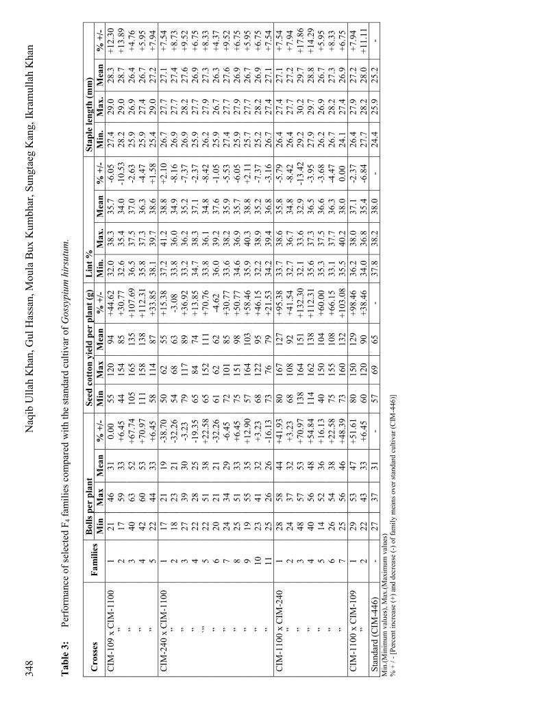
348
Naq
ib U
llah
Kha
n, G
ul H
assa
n, M
oula
Bux
Kum
bhar
, Sun
gtae
g K
ang,
Ikra
mul
lah
Kha
n
Tab
le 3
: Pe
rfor
man
ce o
f sel
ecte
d F 4
fam
ilies
com
pare
d w
ith th
e st
anda
rd c
ultiv
ar o
f Gos
sypi
um h
irsu
tum
.
Bol
ls p
er p
lant
Se
ed c
otto
n yi
eld
per
plan
t (g)
L
int %
St
aple
leng
th (m
m)
Cro
sses
Fa
mili
es
Min
M
ax
Mea
n %
+/-
Min
M
ax
Mea
n %
+/-
Min
. M
ax.
Mea
n %
+/-
Min
. M
ax.
Mea
n %
+/-
CIM
-109
x C
IM-1
100
1 21
46
31
0.
00
55
120
94
+44.
62
32.0
38
.3
35.7
-6
.05
27.4
29
.0
28.3
+1
2.30
”
2 17
59
33
+6
.45
44
154
85
+30.
77
32.6
35
.4
34.0
-1
0.53
28
.2
29.0
28
.7
+13.
89
” 3
40
63
52
+67.
74
105
165
135
+107
.69
36.5
37
.5
37.0
-2
.63
25.9
26
.9
26.4
+4
.76
” 4
42
60
53
+70.
97
111
158
138
+112
.31
35.8
37
.3
36.3
-4
.47
25.9
27
.4
26.7
+5
.95
” 5
22
44
33
+6.4
5 58
11
4 87
+3
3.85
38
.1
39.7
38
.6
+1.5
8 25
.4
29.0
27
.2
+7.9
4 C
IM-2
40 x
CIM
-110
0 1
17
21
19
-38.
70
50
62
55
+15.
38
37.2
41
.2
38.8
+2
.10
26.7
27
.7
27.1
+7
.54
” 2
18
23
21
-32.
26
54
68
63
-3.0
8 33
.8
36.0
34
.9
-8.1
6 26
.9
27.7
27
.4
+8.7
3 ”
3 27
39
30
-3
.23
79
117
89
+36.
92
33.2
36
.2
35.2
-7
.37
26.9
28
.2
27.6
+9
.52
” 4
22
28
25
-19.
35
65
84
74
+13.
85
34.7
38
.3
37.1
-2
.37
25.9
27
.7
26.9
+6
.75
`”
5 22
51
38
+2
2.58
65
15
2 11
1 +7
0.76
33
.8
36.1
34
.8
-8.4
2 26
.2
27.9
27
.3
+8.3
3 ”
6 20
21
21
-3
2.26
61
62
62
-4
.62
36.0
39
.2
37.6
-1
.05
25.9
26
.7
26.3
+4
.37
” 7
24
34
29
-6.4
5 72
10
1 85
+3
0.77
33
.6
38.2
35
.9
-5.5
3 27
.4
27.7
27
.6
+9.5
2 ”
8 25
51
33
+6
.45
75
151
98
+50.
77
34.6
36
.9
35.7
-6
.05
25.9
27
.9
26.9
+6
.75
” 9
19
55
35
+12.
90
57
164
103
+58.
46
35.9
40
.3
38.8
+2
.11
25.7
27
.7
26.7
+5
.95
” 10
23
41
32
+3
.23
68
122
95
+46.
15
32.2
38
.9
35.2
-7
.37
25.2
28
.2
26.9
+6
.75
” 11
25
26
26
-1
6.13
73
76
79
+2
1.53
34
.2
39.4
36
.8
-3.1
6 26
.7
27.4
27
.1
+7.5
4 C
IM-1
100
x C
IM-2
40
1 28
58
44
+4
1.93
80
16
7 12
7 +9
5.38
33
.7
38.6
35
.8
-5.7
9 26
.4
27.4
27
.1
+7.5
4 ”
2 24
37
32
+3
.23
68
108
92
+41.
54
32.7
36
.7
34.8
-8
.42
26.4
27
.7
27.2
+7
.94
” 3
48
57
53
+70.
97
138
164
151
+132
.30
32.1
33
.6
32.9
-1
3.42
29
.2
30.2
29
.7
+17.
86
” 4
40
56
48
+54.
84
114
162
138
+112
.31
35.6
37
.3
36.5
-3
.95
27.9
29
.7
28.8
+1
4.29
”
5 14
52
36
+1
6.13
40
15
0 10
4 +6
0.00
35
.3
37.5
36
.6
-3.6
8 26
.2
26.9
26
.7
+5.9
5 ”
6 26
54
38
+2
2.58
75
15
5 10
8 +6
6.15
33
.1
37.7
36
.3
-4.4
7 26
.7
28.2
27
.3
+8.3
3 ”
7 25
56
46
+4
8.39
73
16
0 13
2 +1
03.0
8 35
.5
40.2
38
.0
0.00
24
.1
27.4
26
.9
+6.7
5 C
IM-1
100
x C
IM-1
09
1 29
53
47
+5
1.61
80
15
0 12
9 +9
8.46
36
.2
38.0
37
.1
-2.3
7 26
.4
27.9
27
.2
+7.9
4 ”
2 22
43
33
+6
.45
60
120
90
+38.
46
34.0
36
.8
35.4
-6
.84
27.7
28
.2
28.0
+1
1.11
St
anda
rd (C
IM-4
46)
- 27
37
31
-
57
69
65
- 37
.8
38.2
38
.0
- 24
.4
25.9
25
.2
- M
in.(M
inim
um v
alue
s), M
ax.(M
axim
um v
alue
s)
% +
/ - [
Perc
ent i
ncre
ase
(+) a
nd d
ecre
ase
(-) o
f fam
ily m
eans
ove
r sta
ndar
d cu
ltiva
r (C
IM-4
46)]

Het
eros
is, I
nbre
edin
g D
epre
ssio
n an
d M
ean
Perf
orm
ance
of
Segr
egat
ing
Popu
latio
n in
Upl
and
Cot
ton
349
Tab
le 4
: Pe
rfor
man
ce o
f sel
ecte
d F 5
fam
ilies
com
pare
d w
ith th
e st
anda
rd c
ultiv
ar o
f Gos
sypi
um h
irsu
tum
.
Bol
ls p
er p
lant
Se
ed c
otto
n yi
eld
per
plan
t (g)
L
int %
St
aple
leng
th (m
m)
Cro
sses
Fa
mili
es
Min
M
ax.
Mea
n %
+/-
Min
M
ax.
Mea
n %
+/-
Min
. M
ax.
Mea
n %
+/-
Min
. M
ax.
Mea
n %
+/-
CIM
-109
x C
IM-1
100
1 22
49
33
+2
6.92
50
11
2 74
+2
7.59
34
.0
36.7
35
.2
+1.4
4 26
.9
28.2
27
.6
+7.3
9 ”
2 30
35
33
+2
6.92
70
81
76
+3
1.03
33
.8
35.7
34
.9
+0.5
8 25
.7
28.5
27
.1
+5.4
5 C
IM-2
40 x
CIM
-110
0 1
30
41
35
+34.
62
70
95
82
+41.
38
32.3
35
.4
33.8
-2
.59
26.9
27
.9
27.5
+7
.00
” 2
44
55
49
+88.
46
100
126
112
+93.
10
34.6
35
.7
35.0
+0
.86
26.7
27
.2
27.0
+5
.06
” 3
49
58
54
+107
.69
112
134
123
+112
.07
33.9
35
.2
34.6
-0
.29
25.9
26
.7
26.3
+2
.33
CIM
-110
0 x
CIM
-240
1
33
57
49
+88.
46
75
130
113
+94.
83
33.7
38
.7
36.4
+4
.90
26.4
27
.4
26.9
+4
.67
” 2
20
26
22
-15.
38
47
59
51
-12.
07
35.0
35
.6
35.4
+2
.02
27.2
27
.7
27.5
+7
.00
CIM
-110
0 x
CIM
-109
1
22
45
33
+26.
92
50
103
76
+31.
03
34.5
39
.4
37.0
+6
.63
25.4
26
.9
25.9
+0
.78
” 2
37
45
41
+57.
69
85
105
95
+63.
79
34.3
35
.3
34.8
+0
.29
26.8
27
.6
27.2
+5
.84
Stan
dard
(CIM
-446
) -
23
28
26
- 52
64
58
-
34.6
34
.8
34.7
-
24.4
26
.2
25.7
-
Min
.(Min
imum
val
ues)
, Max
.(Max
imum
val
ues)
%
+ /
- [Pe
rcen
t inc
reas
e (+
) and
dec
reas
e (-
) of f
amily
mea
ns o
ver s
tand
ard
culti
var (
CIM
-446
)]

350 Naqib Ullah Khan, Gul Hassan, Moula Bux Kumbhar, Sungtaeg Kang Ikramullah Khan
Discussion In F1 generation, the bolls per plant ranged from 20 to 53 among the F1 hybrids, while in F2, the bolls per plant ranged from 25 to 44. The seed cotton yield per plant ranged from 59.12 g to 188.81 g among the F1 hybrids, while in F2 population the range was 63.63 g to 138.10. In F2 generation the abrupt drop in yield and yield components was due to inbreeding depression and segregation. Soomro and Kalhoro (2000) also manifested that hybrids showing higher magnitude of heterosis was generally associated with higher amount of inbreeding depression suggesting dominant genes functioning for these traits. The results are in corroboration with the findings of Baloch et al. (1993a), Galanopoulou and Roupakias (1999) and Khan et al. (2000). The F1 and F2 derivatives of CIM-1100 exhibited highest heterosis and showed leading position due to maximum bolls per plant and increased seed cotton yield. Hassan et al. (1999) and Khan et al. (1999a) also mentioned that heterosis for seed cotton yield was associated with heterosis for boll number. F1 hybrids can be used for hybrid cotton production, which have been greatly supported by Arshad (1991), Salam (1991), Singh et al. (1993), Lakho et al. (2001), Solangi et al. (2001) and Solangi et al. (2002) as they also reported varying degree of heterosis over better parent for bolls and seed cotton yield per plant. The cultivars like CIM-240 and BH-36 and some of their crosses showed poor performance. The results in F2 generation were also encouraging and even after inbreeding depression, majority of the CIM-1100 F2 cross population displayed better mean performance as compared to their parents and the selection in these crosses provided transgressive gene recombination. Tang et al. (1993a) also revealed hat F2 population showed significant heterosis even over high parent. It is noteworthy that selection in the above cross families will be a great achievement for isolation and advancing promising lines for enhanced cotton production. F2 hybrids having extra ordinary performance could also be used as such for seed of F2 crop to increase the seed cotton yield on per unit area as it have been mentioned by Baloch et al. (1991), Baloch et al. (1993a), Baloch et al. (1993b) and Singh et al. (1993).
In case of fibre quality traits, the lint % means values varied from 32.84% to 36.92% in F1 hybrids, while in F2 genotypes the range of lint % was 32.36% to 36.14%, while for staple length the said range was 24.97 mm to 30.14 mm in F1 hybrids and 25.47 mm to 29.84 mm in F2 generation. The decreasing level observed in F2 generation was due to inbreeding and segregation as also noticed by Baloch et al. (1993a) and Dever and Gannaway (1992) that F1 hybrids had longer fibre and F2 generation did not consistently produce longer fibre than parents. In F1 and F2 generations, most of the hybrids predicted negative heterosis over better parent except two hybrids for lint %, hence lint % and staple length manifested the low level of significance. Soomro and Kalhoro (2000) also noted small amount of heterosis. Lower magnitude of inbreeding depression for lint % and staple length indicated that additive genes were responsible for the expression of these traits. These results are also in line with the findings of Tang et al. (1993b) and Khan et al. (1999b) that very few F2 hybrids were superior in fibre properties to their high parent. Davis (1978), Davis (1979), Galanopoulou and Roupakias (1999) and Khan et al. (1999b) also reported that G. hirsutum x G. hirsutum hybrids were quite stable and did not show appreciable heterosis and the crosses appeared to be having a little potential for further improvement. In present studies some promising F2 genotypes showed increase in mean values of lint % and staple length as compared to better parent and it seems to be due to transgressive recombination which exhibited positive and some of them showed significant increase for lint % and selection in these crosses provided better chances for improvement in segregating generations. The fibres with magnificent lint % and staple length are greatly desired by textile industry for more lint production and for having fine and strong yarn with less twist. The fibers with shorter staple length badly affect the efficiency of the textile mill. Our inferences are also supported by Percy and Turcotte (1992), Tang et al. (1993a), Tang et al. (1993b), Galanopoulou and Roupakias (1999), Hassan et al. (1999), Lakho et al. (2001), Solangi et al. (2001), Dayo et al. (2002) and Solangi et al. (2002) and reported varying degree of heterosis for lint % and staple length in F1 and F2 generations.
The results in advanced generations (F3, F4 and F5) revealed that majority of the cross families surpassed the standard cultivar (CIM-446) for bolls per plant, seed cotton yield per plant and staple length, while for lint % some cross families showed increased percentage over standard cultivar as also

Heterosis, Inbreeding Depression and Mean Performance of Segregating Population in Upland Cotton 351
perceived by Dayo et al. (2002) that all the hybrid families excelled the check cultivar while some hybrids ginned more and measured longer staple than better check cultivar. These plant families are greatly desirable from yield and textile point of view and can result in the cultivars having yield potential with desirable fibre quality traits. The results are also in accordance with the findings of Bahadur et al. (1993) and Dever and Gannaway (1992) who reported maximum percent increase of yield, yield components and fibre quality traits through transgressive segregation against check, parental cultivars and F1 hybrids. The results also got support from the research conclusions of Tang et al. (1993a), Tang et al. (1993b), Galanopoulou and Roupakias (1999) and Kalhoro et al. (2002) who reported the same type of improvement in different cross families in segregating generations. Conclusion It is concluded that highest yielding F1 hybrids yielded progressively less in subsequent generations due to inbreeding depression and in advanced generations surpass the best cultivar, whereas some lowest yielding hybrids was stabilized due to low inbreeding depression. It is suggested that yield of the F1 did not predict the yield of the bulks in the advanced generations and the combined performance of the hybrids in the F1 and F2 generation could be a good indicator to identify the most promising populations to be utilized either as F2 hybrids or as a source population for further selection in advanced generations.

352 Naqib Ullah Khan, Gul Hassan, Moula Bux Kumbhar, Sungtaeg Kang, Ikramullah Khan
References [1] Arshad, M. 1991. Use of cytoplasmic male sterility and genetic male sterility in production of
commercial cotton hybrids. The Pak. Cottons, 35(1):29-37. [2] Bahadur, S., Khan, I.A and Mehdi, S.S. 1993. The estimates of heritability and genetic
advances for various plant traits in segregating population of G. hirsutum L. I. Yield and related characters. Pak. J. Agri. Sci., 30(3):280-283.
[3] Baloch, M.J., Lakho, A.R and Soomro, A.H. 1993a. Heterosis in interspecific cotton hybrids. Pak. J. Bot., 25(1):13 20.
[4] Baloch, M.J., Tunio, G.H and Lakho, A.R. 1993b. Performance of F1 hybrids from intra-hirsutum crosses of Upland cotton. Pak. J. Sci. Ind. Res., 36(1):38-40.
[5] Baloch, M.J., Tunio, G.H and Lakho, A.R. 1991. Expression of heterosis in F1 and its deterioration in intra-hirsutum F2 hybrids. Pakphyton, 3:95-106.
[6] Bricker, B. 1991. MSTATC: A microcomputer programme for design management and analysis of agronomic research experiments. Crop and Science department, MSU East Mancing MI 48824, USA.
[7] Cook, C.F. 1909. Suppressed and intensified characters in cotton hybrids. U.S. Dept. Agri. Bull., 1947:127 (Quoted by Memon, 1963).
[8] Davis, D.D. 1978. Hybrid cotton: specific problems and potentials. Adv. Agron. 30:129-157. [9] Davis, D.D. 1979. Yield and fibre properties of selected F1 hybrids. Proc. Beltwide Cotton
Prod. Res. Conf. Phoenix.Ariz,p.71-72. Natl. Cotton Council of America, Memphis,TN. [10] Dayo, G.N., Soomro, A.R., Anjum, R., Bano, S and Kalwar, G.H. 2002. Estimation of heterosis
in Cotton Leaf Curl Virus resistant hybrids. Indus J. Plant Sci.1(1):53-56. [11] Dever, J.K and Gannaway, J.R. 1992. Relative fibre uniformity in between parent and F1 and F2
generations in cotton. Crop Sci., 32: 1402-1408. [12] Fehr, W.R. 1987. Principles of cultivar development. Theory and technique. Macmillan Pub.
Comp. Inc., New York. 115-119. [13] Fonseca, S.M. 1965. Heterosis, heterobeltiosis, diallel analysis and gene action in crosses of
Triticum aestivum L. Ph.D Thesis Purdue Univ. USA. [14] Galanopoulou Sendouca, S and Roupakias, D. 1999. Performance of cotton F1 hybrids and its
relation to the mean yield of advanced bulk generations. European J. Agron., 11(1): 53 62. [15] Hallaner, A.R and Miranda, J.B. 1986. Quantitative genetics in maize breeding. The Lowa State
Univ. Press U.S.A. [16] Hassan, G., Mahmood, G., Khan, N.U and Razzaq, A. 1999. Combining ability and
heterobeltiotic estimates in a diallel cross of cotton (G. hirsutum L.). Sarhad J. Agri., 15(6): 563-568.
[17] Kalhoro, A.D., Soomro, A.R., Anjum, R and Kalwar, G.H. 2002. Seed cotton yield, lint percentage and staple length of F3 glandless cotton as affected by Cotton Leaf Curl Virus. Indus J. Plant Sci., 1(1):73-75.
[18] Khan, N.U. 2003. Genetic analysis, combining ability and heterotic studies for yield, its components, fibre and oil quality traits in upland cotton (G. hirsutum L.). Ph.D Dissertation, Sindh Agriculture University Tando Jam, Pakistan.
[19] Khan, N.U., Abro, H.K., Kumbhar, M.B., Hassan, G and Khan, M. 1999a. Exploitation of heterosis can combat Cotton Leaf Curl Virus (CLCV) incidence in cotton (G. hirsutum L.). The Pak. Cottons, 43(3&4):21-33.
[20] Khan, N.U., Abro, H.K., Hassan, G., Kumbhar, M.B. and Khan, M. 1999b. Study of Heterosis in Upland cotton-I. Quality traits. The Pak. Cottons, 43(3&4):53-64.
[21] Khan, N.U., Abro, H.K., Kumbhar, M.B., Hassan, G and Mahmood, G. 2000. Study of heterosis in Upland cotton-II. Morphology and yield traits. The Pak. Cottons, 44(1&2):13-23.
[22] Krishnaswami, R and Kothandaramon, R. 1977. Heterosis in inter-specific crosses of Gossypium. Ind. J. Genet. Pl. Breed., 36:40-45.

Heterosis, Inbreeding Depression and Mean Performance of Segregating Population in Upland Cotton 353
[23] Lakho, A.R., Bhutto, H., Chang, M.S., Solangi, M.Y., Kalwar, G.H and Baloch, A.H. 2001. Estimation of heterosis for yield and economic traits in cotton. (G. hirsutum L.). Sindh Bal. J. Pl. Sci., 3:26-30.
[24] Percy, R. G and Turcotte, E.L. 1992. Inter-specific hybrid fibre characteristics of cotton altered by unconventional G. barbadense L. fibre genotypes. Crop Sci., 32:1437-1441.
[25] Salam, C.A. 1991. Status of Intra-specific commercial hybrids in the Punjab. The Pak. Cottons, 35(1): 5-17.
[26] Singh, T.H., Randhawa, L.S and Chahal, G.S. 1993. Heterosis and combining ability for harvest index and economic yield in Upland cotton (G. hirsutum L.). Crop Imp. Soc. India, 68-69.
[27] Solangi, M.Y., Baloch, M.J., Bhutto, H., Lakho, A.R and Solangi, M.H. 2001. Hybrid vigour in inter-specific F1 hybrids of G. hirsutum x G. barbadense for some economic characters. Pak. J. Biol. Sci., 4:945-948.
[28] Solangi, M.Y., Baloch, M.J., Solangi, M.H., Chang, M.S and Lakho, A.R. 2002. Performance of intra-hirsutum F1 hybrids (G. hirsutum L.). Asian J. Plant Sci.1(2):126-127.
[29] Soomro, A.R., and A.D. Kalhoro. 2000. Hybrid vigour (F1) and inbreeding depression (F2) for some economic traits in crosses between glandless and glanded cotton. Pak. J. Biol. Sci.3(12):2013-2015.
[30] Soomro, B.A., Chang, M.A and Soomro, A.R. 1991. Status of inter-specific commercial hybrids in Sindh. The Pak. Cottons, 35(1):19-28.
[31] Tang, B., Jenkins, J.N., McCarty, J.C and Watson, C.E. 1993a. F2 hybrids of host plant germplasm and cotton cultivars .1. Heterosis and combining ability for lint yield and yield components. Crop Sci., 33(4):700 705.
[32] Tang, B., Jenkins, J.N., McCarty, J.C and Watson, C.E. 1993b. F2 hybrids of host plant germplasm and cotton cultivars .2. Heterosis and combining ability for fiber properties. Crop Sci., 33(4):706 710.
[33] Waller,G.B., Wilson, F.D and Martin, J.H. 1981. Influence of phenotype, season and time-of-day on nector production in cotton. Crop Sci. 21:507-511.
[34] Waller, G.D and Moffet, J.O. 1981. Pollination of hybrid cotton on the Texas high plains, nector production and honey bees visits. Proceeding of 1981 Beltwide Cotton Conf., Natl. Council of America, Memphis, Tennessee, U.S.A.
[35] Wynne, J.C., Emery, D.A and Rice, P.M. 1970. I. Combining ability estimates in Arachis hypogeae L. II. Field performance of F1 hybrids. Crop Sci., 10(6): 713-715.
Copyright © 2022 FDOKUMEN