Obesity-2014 Obesity & Weight Management Scientific Tracks ...
Upload
khangminh22Category
view
22download
0

Scientific Financial
Management
Advances in Intelligence Capabilities for Corporate
Valuation and Risk Assessment
Morton Glantz with a special contribution by Thomas L. Doorley I11 Senior Partner Deloitte
Consulting/Baxton Associates
American Management Association New York Atlanta Boston Chicago Kansas City San Francisco Washington, D.C.
Brussels Mexico City Tokyo Toronto
Special discounts on bulk quantities of AMACOM books are available to coruorations. urofessional associations, and other , L
organizations. F'or details, contact Special Sales Department, AMACOM, a division of American Management Association 1601 Broadway, New York, NY 10019. Tel.: 212-903-8316. Fax: 212-903-8083. Web site: www.amanet.org
This publication is designed to provide accurate and authoritative information in regard to the subject matter covered. It is sold with the understanding that the publisher is not engaged in rendering legal, accounting, or other professional service. If legal advice or other expert assistance is required, the services of a competent professional person should be sought.
Library of Congress Cataloging-in-Publication Data
Glantz, Morton. Scientific financial management : advances in intelligence capabilities for
corporate valuation and rysk assessment / Morton ~ h t z with a special contribution by Thomas L. Doorely 111.
p. cm. Includes bibliographical references and index. ISBN 0-8144-0500-2
1. Corporations-Finance-Management. 2. Corporations-Valuation. I. Amacom. 111. Title.
O 2000 Morton Glantz. All rights reserved. Printed in the United States of America.
The material in Chapter 12 draws from the research and methodology contained in Thomas L. Doorely ID'S book Value-Creating Growth: How to Lift Your Company to the Next Level of Performance, co- authored with John Donovan O Jossey-Bass 1999, San Francisco, 1-800-956-7739 or www.josseybass.com. (The book is available in bookstores and online at amazon.com) Adapted by permission of Jossey-Bass, a subsidiary of John Wiley & Sons, Inc.
This publication may not be reproduced, stored in a retrieval system, or transmitted in whole or in part, in any form or by any means, electronic, mechanical, photocopying, recording, or otherwise, without the prior written permission of AMACOM, a division of American Management Association 1601 Broadway, New York, NY 10019.
Printing number

To my wqe Mayann and daughter Felise, a continuous source of love, patience,
and inspiration.
To Ida Glantz, in her extraordinary and noble life, a beacon of wisdom
and majesty.


Preface xi
Acknowledgments xiii
CHAPTER 1 Introduction to Scientific Financial Management 1 Nonlinear Financial Models 7 A Quick Look at Data Mining, Neural Networks,
and Fuzzy Logic 9 Scientific Financial Management's Road Map 13
CHAPTER 2 Basic Tools of Financial Risk Management: Portfolios and Options 19 Basics of Modern Portfolio Management 21 Option Pricing Basics 30 The Quintessential Black-Scholes 39 Appendix A: Calculations of Option Values 41 Chapter Two References and Selected
Readings 50
CHAPTER 3 Real Options: Evaluating R&D and Capital Investments 55 The Music Master's Dilemma 56 Flexibility: The Quintessence of Real Options 57 Traditional Methods Versus Real Options 57 The Binomial Model 58 Real Options: Definitions, Examples,
and Case Studies 60 Closing Thoughts 79 Chapter Three References and Selected
Readings 81

viii CONTENTS
CHAPTER 4 Visual Financial Models 85 Background 86 Team Effort 88 Building Effective Models 88 Visual Modeling 92 Analytica: The Nerve Center
for Visual Modeling 93 Comparing Spreadsheet Models
with Visual Models 94 Visual Display of Model Structure
with Influence Diagrams 95 Developing Your Visual Model Step by Step 105 On-Line Demonstration: E-Commerce
Start-Up 113 Conclusion 115 Chapter Four References and Selected
Readings 115
CHAPTER 5 Divisional Cash Flow Analysis and Sustainable Growth Problems 117 Cash Flow 117 Cash Flow and Sustainable Growth Problems 129 Chapter Five References and Selected
Readings 138
CHAPTER 6 Statistical Forecasting Methods and Modified Percentage of Sales 139 A "Statistics" Approach to Financial
Forecasting 140 A "Sensitivities" Approach to Financial
Forecasting 160 Glossary of Forecasting Terms 166 Chapter Six References and Selected Readings 170
CHAPTER 7 How to Apply Monte Carlo Analysis to Financial Forecasting 173 A "Simulations" Approach to Financial
Forecasting 173 Glossary of Distribution Terms 197 Chapter Seven Refewnces and Selected Readings 204

Contents ix
CHAPTER 8 Neural Networks and Scientific Financial Management 207 Neural Networks 209 Building a Simple Neural Network:
The T-C Problem 210 Statistics and Neural Networks 213 Genetic Algorithms 217 Combining Genetic Algorithms with Neural
Networks 218 Designing Neural Networks 221 Developing a Neural Network within Excel 223 Chapter Eight References and Selected
Readings 228
CHAPTER 9 Linear Programming, Optimization, and the CFO 233 The Basics of Linear Programming 234 Basic Deterministic Modeling 236 Stochastic Optimization Modeling 256 Tabu Search 257 Numeric Computation and Visualization
Optimization Modeling 265 Chatper Nine References and Selected
Readings 267
CHAPTER 10 Risk Analysis of the Corporate Entity and Operating Segments 271 Identifying Systematic Risk 272 Corporate Analysis: 274 Corporate Computerized Risk Rating System 303 Chapter Ten References and Selected
Readings 308
CHAPTER 11 A Primer on Shareholder Value 311 Methods 312 Preparation 318 The Drivers 323 Appendix One to Chapter 11 339

Appendix Two to Chapter 11 347 Appendix Three to Chapter 11 387 Chapter Eleven References and Selected
Readings 397
CHAPTER 12 The Value-Growth Link 399 by Thomas L. Doorley 111
Spectacular Growth/Spectacular Performance: A Global Phenomenon 400
Value Creation Everywhere that Matters 403 Growth-Value: Cautionary Tales 404 Metrics for Success: Guiding Implementation 406 A Vision: The Desired State 410
Index 413

MUCH LITERATURE HAS BEEN PUBLISHED about valuation. The authors tell us how to derive shareholder value but not how to model value drivers with the latest technology. They advise us how to analyze valuation alternatives and choose the best one but not how to create choices germinal in corpo- rate data. They refer us to quantitative objective functions. They do not give us the means to run up stochastic solutions and thereby improve the chances of ever being able to explain, qualitatively, optimal objectives on which any assessment of valuation must reside. They provide macrostruc- tures but not how microprocesses work, such as leveraging data technol- ogy to improve decision making.
In the last 10 years, we have seen finance evolve from a casual disci- pline to a rigorous science. Just over a decade ago, technologies such as neural nets, stochastic optimization, simulation, fuzzy logic, and data min- ing were still largely exploratory and at best quite tentative. Algorithms, as a term, rested on the outskirts of financial thought. More than a few finan- cial managers had not even heard of Monte Carlo outside of casinos and travel magazines. Machine learning was in its infancy while shareholder value concepts were encased in the Stone Age logic of earnings multiples and, on more than a few occasions, accounting shenanigans.
Despite dramatic advances in financial techniques and raw comput- ing power, there is still a gap between finance/valuation theory and the utilization of scientific applications. Allow me to quote a wise passage:
We now have a much richer bag of tricks at our disposal, whose effec- tiveness can be realized using mature networking, database, and desktop technologies. Each one models a different aspect of human reasoning and decision-making. Each technique has a different objective and different character. Collectively, these techniques offer the business community a broad set of tools capable of addressing problems that are much harder or virtually impossible to solve using the more traditional techniques from statistics and operations research.]
As this paragraph suggests, risk, complexity, and uncertainty will define financial and business well into the millennium. While few of us need challenge standard financial tools (spreadsheets), new financial intel- ligence capabilities offer a framework to help financial executives cope
1. Vusant Dhar and Roger Stein, Seven Methods for Transforming Corporate Data Into Business Intelligence (Englewood Cliffs, N. J.: Prentice Hall, 1997).

with uncertainty. However, the concern is that some managers are resist- ing computer-actualized solutions. Quantitative methods, such as the use of models or even the use of math, do not alarm sharp professionals. Mod- eling tools are not black boxes that ignore or inhibit wisdom or that mech- anize the decision-making process. However, in many companies, models and, for that matter, change may intimidate financial professionals, inhibiting technological growth and, alas, the requisite skills to participate in strategic decision making at the highest level.
Otherwise capable managers cannot readily quanhfy and respond to developments in the external environment and find it difficult to creatively deploy advanced techniques to crystallize value drivers, explain optimal cap- ital allocation sbategies, and otherwise deliver the goods to CEOs. Knowl- edge gaps, particularly when it comes to valuation appraisals (and knowing how sensitive your job function is to your firm's value), are detrimental to continued growth both within firms and in advancing careers. This book should help you carry out your financial tasks more succinctly and might even empower you to grab the modeling hardball and to pitch winning games in a domain that is hot, dynamic, complex, and often combative.
Each chapter contains a brief introduction of the topic and then is divided into several "hands-on" sections, with each exhibit and table num- bered and titled to facilitate a systematic reading. The book contains a CD that includes (1) a collection of financial models and related software, the author's interactive corporate and divisional risk-rating systems, and (2) software and Intemet links donated by adept vendors in evolving valua- tion disciplines such as financial and real options, optimization, visual modeling, time series/regression, simulation, and neural nets. Most sec- tions are reinforced with problems and examples included on the CD, in the book, or on the Internet. Key concepts are set apart and important equations highlighted. The derivations for equations are provided but are differentiated or appear in appendices. The reader who is not mathemati- cally inclined can skip quantitative passages with no loss of qualitative ideas. A References and Suggested Readings section follows each chapter, and readers can, at their leisure, connect to select Intemet sites, access additional material, or download additional software cognate to chapters.

THE WRITING OF A BOOK on scientific financial management and the interactive " computerized systems that combine to power up a firm's value drivers involves the ideas and work of many individuals. Because the subject is so diverse and comprehensive, specialists were consulted, so that in completing this book, I find myself indebted to many for their thoughtful suggestions, critical review, counsel, and encouragement. Thomas L. Doorely IJI, Senior Partner, Deloitte Consulting/Baxton Associates, for his expertise and contri- bution as author to chapter 12, The Value-Growth Link. Two individuals were especially helpful: Robert Kissell and Bob Muldowney. Mr. Kissell designed the algorithms contained in the interactive corporate and divisional risk-rating systems and was an important source of wise counsel on issues dealing with statistical matters and neural networks. I thank Mr. Muldowney for the time he took reading the manuscript and above all for his patience as chapters were being prepared. I greatly benefited from his ideas.
I wish to offer a special word of thanks to Gary Lynn, a neural network expert at NeuroDimension, Inc. (a top firm in the field), whom I called on for his insight and knowledge. I also want to thank Gary's colleagues, Neil R. Euliano and Dan Wooten, for donating important sections. Larry Gold- man, a product expert at Decisioneering, played an integral role in chapters dealiia with simulation, regression, and o~timization and coordinated readinis of these chapters byvthe experts at ~ecisioneerin~. Keith Woolner, director of marketing, LU& ~ecision Systems, Inc., deserves credit for his suggestions on visual modeling. John Noble and Rick Schmitt, Alcar valuation experts, provided valuation exhibits along with Alcar's new release valuation demo. I want to express gratitude to the previously men- tioned companies for their support along with the models these firms made available to readers via our CD and/or through Web sites.
I wish to thank Bruce Henderson. who ovened uv contacts: David Langer, who provided computer support; and Joseph Blake, a financial expert. I am indebted to a number of persons for their interest and encour- agement in the preparation of this manuscript. In particular, my apprecia- tion goes to Ray O'Connell, senior acquisitions and planning editor, who first suggested the writing of this book; Andy Ambraziejus, managing edi- tor; and Bruce Owens and Peggy Francomb for their valuable assistance in

editing the manuscript. This does not mean, however, that those listed here or others who were helpful are responsible for errors or omissions; the author must assume such responsibility. Finally, I have acknowledged every source I have been able to identify in footnotes and bibliographies, but some writers and sources may have been missed unintentionally.

Introduction to Scientific
Financial Management
Kermit Rich along with thirty recent MBA graduates stood on a Long Island cliffoverlooking the Atlantic. Thefive-acre estate promised the graduates both sun, and the possibility o fan invitation to join Kermit's wealthy, fast paced firm. Near the edge of the cliff, Kermit addressed the group. " My execs have enough smarts to turn quarterly profits, but their ideas lack steam to the point where our (business) segments behabe like random walks. I need organization, not randomness in my business. I need people with guts, the kind of people that translate randomness into direction and new global challenges. Give me someone like a George Patton-blood, timing and guts-an executive, who grabs the day-to-day stuff, makes sense of it and is not afraid to run past goal posts. I f you measure up, take your pick-a divisional presidency, $4 million in company stock, or, yes, I'll even throw in my estate. Do any of you have what it takes?"
Kermit continued while directing the focus to the impeding clifl. "OK, you guys, inch closer to the edge. See that wicked surf crashing ojf the cliff Now, 9 you can time your dive right and land behind one of those big waves, the suufwill carry you right to my schooner. But, heavens forbid, if your timing is off, tke rocks will get you fifty feet below. Blood, timing and guts."
As the group headed toward the house, shouts echoedfrom below. Seconds later ajigure drifted toward the schooner.
"You're my kind of guy," Kermit beamed later that afternoon. "Just name it-+ divisional presidency? Stock? my house?" Tke redyaced MBA glanced across to the twentyjive-room mansion, and then turned to his bedazzled
colleagues hanging about afew feet away. "No, nothing," he replied, "Justfind the jerk who pushed me over. "'
JUST LIKE THE WICKED SURF crashing off the cliff, engineering one's knowl- edge is, indeed, a rather strange concept, but that is the idea behind the fiancial revolution-bridging gaps between traditional, nontechnical (textbook) approaches and modern, asymmetric, real-world solutions that have hit the market.
Recent advances in financial analysis and strategic planning are about dynamic surf patterns, surf timing, rocks, and, yes, surf heights. Dynamic planning is revitalizing financial analysis in areas once thought inaccessi- ble: chaos theory, real options, data mining, artificial intelligence systems such as fuzzy logic and neural networks, plus myriad other powerful models and application builders. These technical advances, virtually unknown a few years back, provide solutions from predicting nonlineari- ties to solving resource allocation problems. The good part is that most of the software is easily mastered by CFOs for the small price of just a little knowledge engineering.
Behind the technology revolution, at the core, are data--simple though elusive and frequently "chaotic" in nature. However, as random as these data appear, the right software can shape these data bits into dis- tinctive patterns of information. Of course, we may ask, Are the data sin- gle or clusted (patterned), short term, and meaningless? The answer may be a little hard to nail down, but one thing is certain: Advances in chaos theory and fiancial and data mining, together with other financial mod- eling tools (fuzzy logic and neural nets), show us ways to synthesize and utilize voluminous amounts of data, from customer payment records to production control. Whether our analysis starts with chaos and ends with the same depends not so much on the nature of data but on how it is mined. It goes something like this:
single event-random (extremely short term, limited value); + genesis--extracting patterns (data mining); + recognizance-
value assessment (simulation, fuzzy logic, neural networks); + finalization-strategic planning; long-term planning.
As the flow diagram shows, strategic plans are blueprints for long-term planning; short-term events are basically random (i.e., quarterly profits) and, in jsolation, do not add up to corporate intrinsic value. If strategic decisions focus on short-term random events (as in chaos theory), they
1. Adapted from From Hard Knocks to Hot Stocks, by J. Morton Davis, Michael T. Ford, Louis Rukeyser (New York: William Morrow, 1998). The author wishes to thank J. Morton Davis for his original anecdote about sharks in a pond.

Introduction to Scientific Financial Management 3
tune out genesis (factors), and the result may be as insignificant to the whole as a single dot in a newspaper photo or a measure's worth of notes in a Bach cantata. We are reminded that investor compensation is more or less proportional to risks taken over reasonably sound projec- tion horizons, but this observation excludes investments over arbitrarily short periods.
Which factor will it be: randomness or genesis? Most of us pick gene- sis, as this offers a greater intrinsic or equity value. Random variables, such as quarterly profits, are trivial, while shareholder value is a definitive strategic concept. Inherently, shareholder value is no less the result of an organic pattern of data that the CFO purifies in a (cash flow) valuation model using modem technology.
While some investors may disagree, quarterly results are random points floating in nonlinear space, influenced by the waywardness of accounting license. We know that financial markets can be stopped cold- short term-while strategic fundamentals tend to hold a steadier course and will not often thwart goals to maximize shareholder value. A wise per- son once said, "Fundamental analysis counts when a rising tide isn't float- ing your firm's earnings." Therefore, suggesting a noncursory look beyond the firm's limited horizons, historically, disorder and chaos will be highlighted.
Let's focus on the analogy in this chapter's opening quotation parable regarding the risk of decision making. If you unwisely risk capital by tak- ing on inferior projects, you will likely plunge against the rocks. On the other hand, by not taking risks and standing by the cliff's edge and watch- ing sunsets ad infinitum, your firm ends up a financial couch potato. Either way, you are dead.
Suppose that you glanced at a solitary wave (random, chaos, like daily profits), and you recorded the time it crashed against the cliff. Hours later you return to repeat the random recording process. The information you "gathered" would be about as useful in predicting the surf as it would be predicting future numbers on a roulette wheel. However, suppose that you activate the latest scientific wave height/pulse measuring equipment. Looking at data configurations, you track recurring timing/depth patterns characteristic to the surf with great accuracy. So go ahead and leap; take Kermit's trophy. The choice-leap or watch sunsets-is chaos (theory) metaphor.
Scientific financial management bridges gaps between chaos theory and financial symmetry. That is, in this new technical age, financial deci- sion making can make or break even the smartest CFOs. That is why smart CFOs feel that it is important to shape data, raw as a clam, in fresh, imag- inative ways and ultimately develop strategetic moves that maximize shareholder value. Data mining, fuzzy logic, real options, pricing capital, model building, and a host of other finely tuned management tools offer financial symrnety to the corporation; and the scientific road map that

leads to the end result-a business tuned like a fine watch-almost, with- out exception, starts with the chaos basics.
Chaos does not necessarily mean "chaotic world economy." Rather, it is associated with tons of information that hit firms daily from all direc- tions; each piece, by itself, is "chaotic." However, if the technology recently developed is applied to all these data, the data cease to be random since patterns emerge (and relationships form) that were hidden beforehand. CFOs who run their shop in a void operate in an environment much like a single sentence operates in a novel. They know how to form words (data) in the sentence and can even read the sentence, but they will not be able to go beyond the single sentence and will not know how the novel turns out. The sentence, with respect to the novel, is itself chaotic.
Think of (the stock market) random walk theory. It is true: while daily price movements are indeed a random walk, longterm trends (bull and bear) are not random, as they are made up of pieces of trend lines. The pieces are chaotic, but not the trend line taken as a whole.
Chaos, rather than being derogatory, actually refers to a really beauti- ful organizing principle. The organizing principle in finance is no less the gravity that binds in orbit the double star system: valuation and portfolio theory. Andrew Ho stated
The most commonly held misconception about chaos theory is that chaos theory is about disorder. Nothing could be further from the truth. Chaos the- ory is not about disorder! It does not disprove determinism or dictate that ordered systems are impossible; it does not invalidate experimental evidence or claim that modeling complex systems is useless. The "chaos" in chaos the- ory is order-not simply order, but the very essence of order.
Chaos theory, order, and fractals describe new technologies applied to corpo- rate fjnance, investment analysis, economics, and capital markets. We define chaos theory as discovering patterns out of distinct forms of irregularities that are, in themselves, nonlinear, dynamic, complex, and enigmatic systems (the
analogy: quarterly results versus intrinsic value). We Exhibit 1-1. can think of "dynamic" as eternally changing complex The Mandelbrot set. systems. It forms the aux of most scientific research,
along with many varied fields-physics, weather fore- casting, and finance, to name a few.
Chaos is in everything: raindrops falling on grass, movements in financial markets measured in minutes, and paperwork atop your desk. A sample of the most famous chaos image of all is the Man- delbrot set, named after its discoverer, Benoit Man- delbrot (see Exhibit 1-1). This image holds a deep fascination, as it can be enlarged over and over with the same patterns emerging.

Introduction to Scientific Financial Management
The point is that tiny changes can produce mammoth fluctuations (of course, we must assume that certain things are held constant). Chaos the- ory and the effect are just about indistinguishable concepts. If a butterfly in West Africa flaps its wings, the theory goes, a hurricane hits the dunes lining the Long Island coast later on. Chaos theory suggests reactive dependence on original conditions. This means simply that the initial departure point in a system (financial or otherwise) greatly influences its course and destination. This is particularly true if the system(s), be they strategies or businesses, are n ~ t ~ ~ ~ r o ~ r i a t e l ~ hedged against risk of loss. For example, businesses made up of a portfolio of homogeneous opera- tions are less insulated against macroeconomic shocks than, say, firms that diversify operations along dissimilar businesses. Perhaps financial managers should avoid putting operating/ financing strategic eggs in one basket.
While forecasting the ultimate closure of a system is as difficult as pre- dicting Clorox's stock price two years hence, it is possible to model the overall behavior of Clorox's stock (see Exhibits 1-2 and 1-3). We know how patterns develop within a financial system, and we often know the end result. The issue is not a system's disorder or unpredictability, which is characteristic of any single component, but rather its natural harmonic structure. If we peered inside a microscope and examined any system, we would see chaos metamorphose to (patterns) and harmony in systems as multifarious as Clorox stock, the cosmos, a Brahms masterpiece, or weather patterns. A butterfly's fit into a bunch of static equations (like the Capital Asset Pricing Model, CAPM) is no better than trifles, but not the dynamic, behavioral nature of our butterfly and its influence within a much larger universe.

Exhibit 1-3. Clorox 1 Cyear stock price: Illustration of long-term market trends.
Stephen Hawking, the great theoretical physicist, agrees with the idea of chaos. He sees nature in terms of particle physics as not fully explicable: Something is missing inside the theories. Hawking believed that chaos theory bridges the gap between particle physics and reality. He stated in his book Black Holes and Baby Universes that "with unstable and chaotic sys- tems, there is generally a time scale on which a small change in an initial state will grow into a change that is twice as big." He goes on to say that "predictability of a system only lasts for a short period of time."
The key point, as Hawking would have it, is time scale and evolving system dynamics. You are asked to prepare your firm's market and pro- duction costs in preparation of a fundamental analysis of your firm's strategic plan. You can get away with a cursory analysis if all the boss asks for is a brief update. Nevertheless, the firm's markets are nonlinear, dynamic systems, and chaos theory suggests mathematics that helps eval- uate such nonlinear, dynamic systems. For example, intraday sales booked by your firm's Rhode Island division are random with a trend component. Nonlinear systems record the accounts receivable portfolio, itself the prod- uct of market, customer, and time frame patterns. Let us connect this to fractals: geometric patterns that are repeated at ever-smaller scales to pro- duce irregular shapes and surfaces. Fractals are self-similar objects, mean- ing that single parts are linked to the whole. Fractals are used especially in computer modeling of irregular patterns and structures in nature.
Privet bushes are good examples. While the stems get narrower and narrower, each stem is structurally similar to larger and thicker stems and finally to the whole bush. Similarly you may record daily or intraday divi- sional sales, sales by product line, national versus regional sales, and sales contribution by customer. Next, you may move on to longer time periods: weekly or monthly sales. The structure (sales) may, at first glance, take on a familiar appearance. However, moving in closer and closer, you see more

Introduction to Scientific Financial Management 7
Exhibit 1 4 . A bifurcation diagram. and more detail, that repetitive patterns form, and perhaps how minute (sales) detail is con- nected to larger structures, very much like Feigenbaum's fractal or solutions provided by a fuzzy logic or neuEal network system. A bifurcation diagram is shown in Exhibit 14.
Chaos theorv infers that insignificant dots create pat-
terns and that patterns translate to pictures. Chaotic data, like dots, can splatter around a page; this is why linear
models cannot really display, at least not clearly, sine qua non arrays of convergence. We need to nurse along the discipline: nonlinear financial models.
Nonlinear Financial Models
Nonlinear financial models emerged from chaos theory. Meteorologist Edward Lorenz is credited largely with discovering chaos theory. Lorenz developed a set of 12 equations to forecast weather patterns by setting computer algorithms to move in a pattern of sequences. To save time, he ran the program at midpoint rather than at the beginning and discovered that the sequence evolved in a wildly different way. It seemed that Lorenz had typed in only three digits, .506, rather than the number in the original sequence, .506127.
The results that came in were unexpected. A weather forecaster is lucky if he or she can measure accurately to three decimal places. The fourth, fifth, or sixth decimal place was nearly impossible to measure at the time and should not have influenced the experiment in the slightest. Lorenz discovered that this notion was wrong. Lorenz's work came to be known as the "butterfly effect." The amount of variance in the start-up points of the two curves (in his experiment) was so small that we can com- pare the variance to a butterfly flapping its wings (Lorenz's weather graph is shown).
The flapping of a single but- terfly's wing produces a micro- scopic shift in the atmosphere. Over a period of time, this shift in the world's weather patterns results in a divergence from what might have beem2 This phenome- non, common to chaos theory, is

also known as sensitive dependence on initial conditions. Just a tiny change in the initial conditions can radically alter the intermediate or even long- term behavior of a system-weather, financial, or otherwise.
Daily share prices are also driven by reactive interdependence on ini- tial and ambient factors as in the fusion of technical, fundamental, and psychological forces that act on the stock between the opening and closing bell-all nonlinear phenomena. Most stock analysts agree (at least until recently) that stock prices move in cycles, with each stock, in motion, spin- ning out ambient factors with its unique set of fingerprints. These are the core fundamentals of fractals that, in a data mining run, reveal the timing and breadth of future cycles existing implicitly in the given stock. In other words, the mining algorithms unearth the "mother" cycle from which underlying cycles gather momentum.
So where is the butterfly? It is in the subject's initial conditions. Slight changes in the starting point of a firm's initial strategic plan can lead to alternative stock (price) outcomes remarkably so if the firm operates in the start-up or rapid growth phase of its life cycle or if operations were not diversified across macroeconomic or industry risk boundries.
Chaotic systems are deterministic and, in the long run, will likely pat- tern out into intrinsic (shareholder) value. While they appear disorderly, even random (investors pained by the recent roller-coaster S&P averages may argue otherwise), chaotic dots and dashes are not. Underneath lies a sense of harmony, order, and above all grand design. T d y random sys- tems are not chaotic.
To see how this all works, let's look at the weather again. There are numerous variables controlling the weather: temperature, air pressure, wind speed, wind direction, and humidity, to name a few. The equations governing weather patterns involve all these variables. You can enter these variables in an equation and determine a reasonable value of all the vari- ables one, two, or five minutes in the future. These results can be reentered into our computer model, as can the values for the next round, six minutes hence, and so on. Let the computer do the iterations for a month, and you will be able to schedule the lawn party on a sunny day.
Or will you? Shown here is an image of the Lorenz attractor. Every moment in time is represented by one point on the attractor. However, differ- ential equations cannot merge, so Lorenz realized that he had discovered a mathematical object that was in fact an infinitely complex set of surfaces, never intersecting. Picnic planners know better than to rely on short-term
2. Ian Stewart, Does God Flay Dice? The Mathematics of Chaos
Introduction to Scientific Financial Management 9
weather forecasts, and meteorologists offer little hope that truly accurate weather predictions for specific places and times will ever be possible.
However, unlike weather equations, financial management formulas are neither infinitely complex nor nonintersecting. Nonetheless, nonlinear solutions, at least in the financial sciences, require analytic power tools. We like to think that some forms of troublesome chaos are things of the past. They will remain so if we dare to start using a few of the scientific finan- cial methods outlined in the rest of this chapter.
A Quick Look at Data Mining, Neural Networks, and Fuzzy Logic
Someone wise recently said, "Chaos can no longer be defined as just a theory--chaos is finance trying to be finance without tomorrow's tech- nology." While technology covers a large playing field, a successful financial game plan cannot ignore data mining, neural networking, simulation and stochastic optimization software, and fuzzy logic (some of these applications are detailed later in this book alongside case stud- ies). However, now we again point to the metamorphose: chaos to syllogism-random to patterns, fixed financial software programs to deductive artificial intelligence. Let's begin with a quick look at data mining, neural networks, and fuzzy logic.
Data mining sifts through large databases, converting meaningless, random information into highly significant if-then patterns. You can then use these patterns to forecast future events and to design "correct" strategies for the firm. Rules or, more correctly, codes fix the limits of data and measure the significance level (reliability) of these rules. These newly discovered codes are then fed back into the mining system to pre- dict more reliable dependent variables and thus new cases. Data models compute the conclusive probability and significance level for each pre- diction along with prediction errors.
Often, data sets are just too complex to represent in two or even three dimensions. Also, finding valuable data is only half the problem; presenting it in a meaningful way, via advanced visualization, is the other half. Newer techniques simultaneously analyze the behavior of data in many dimensions. For example, within a three-dimensional coordinate system, data can be visualized in up to nine dimensions. By animating the visual display across independent variables that you define, you can observe trends in extremely complex data sets. You can observe the motion on the monitor to check for anomalies or dirty data as well. Dirty data are recognized as anomalies through unexplainable behavior.
What are the basic^?^ Suppose that you maintain a data system where each record contains a range of fields about one company, such as name,

number of employees, industry SIC code, sales, profit, and stock value. Assume that you want to define stock value as the dependent variable, while the other variables represent the independent variable, or "condi- tions." With the dependent variable being the stock value, the objectives are to reveal the patterns of those companies having a high (or low) stock value and to search out values of the other fields associated with a high (or low) stock value.
A data mining program first reads the data. You then fine-tune trial runs by defining parameters, such as the minimum probability of rules, minimum number of cases in each rule, and the cost of false alarms. Also, software such as WizWhy derives rules assigned to a particular field to predict other fields. The rules are formulated as if-then sentences or math- ematical formulas. The user makes predictions on the basis of the rules dis- covered and applies results to new cases. For example, given the data of a new company, the computer determines its stock value. The key is to derive the rules that reveal the main patterns and the unexpected phe- nomena in the data.
Data mining can analyze accounts receivable risk (the average collec- tion period, highlighted in many corporate finance books but in practice falling by the wayside). You may want to build accounts receivable mod- els that work with as many as 200 variables. You can deal with accounts receivable data by classifying the information into groups, or cohorts, building models around them.
Self-organizing maps (SOMs) have been used a great deal recently to analyze data. A Belgian company developed a large data set composed of the financial ratios of more than 12,000 Belgian c~mpanies.~ The study's objective was to explore the role of leasing as a financing tool. Results showed that the nonlinear and robust properties of SOMs yielded a deeper understanding of lease financing than using only accounting data.
As data mining technology (software), such as multidimensional visu- alization, becomes more accessible, computing requirements for extracting random data and converting the information into meaningful statistical patterns are shrinking-so much so that soon we will see data mining moving: from NASA to Main Street. "
Alternatively, neural networks processes data by altering the states of networks formed by interconnecting enormous bits of elemental data that interact with one another by exchanging signals, as neurons do in the body's nervous system. Indeed, the best way to visualize neural network- ing is to think of the human nervous system. The basic processing element in the human nervous system is the neuron. Within the human brain dwell
3. From http://www.wizsoft.com (WizSaft Inc., 6800 Jericho Turnpike, Suite 120W, Syos- set, NY 11791). 4. Eric de Bodt, Emmanuel-Frederic Henrion, Marie Cottrell, and Charles Van Wyrneersch, Self-organizing Maps for Data Analysis: An Application to the Belgian Leasing Market.

Introduction to Scientific Financial Management I 1
treelike networks of nerve fiber that connect to the cell body, where the cell nucleus is located. Extending from the cell body is a single, long fiber called the axon, which eventually branches into strands and substrands and connects to other neurons through junctions.
The transmission of signals from one neuron to another is a complex chemical process in which specific transmitter substances are released from the sending end of the junction. The effect is to lower the electrical potential inside the body of the receiving cell. If the potential reaches a threshold, a pulse is sent down the axon, and we then say that the cell has "fired."
In a simplified mathematical model of the neuron, the effects are rep- resented by "weights" that modulate the effect of the associated input sig- nals, and the nonlinear characteristics exhibited by neurons are repre- sented by a transfer function. The neuron impulse is computed as the weighted sum of the input signals transformed by the transfer function. The learning capability of an artificial neuron is achieved by adjusting the weights in accordance to the chosen learning algorithm since it is arduous
- -
to accurately determine multiple values. This involves creating a network that randomly determines parame-
ter values. The network is then used to carry out input-to-output transfor- mations for actual problems. The correct final parameters are obtained by modifymg the parameters in accordance with the errors that the network makes in the process.
Interconnections between corporate risk rating and neural networks are deeply rooted. We explore the methodology in chapter 8 and 10. Cor- porate risk rating, along with bond ratings, requires a "neural" label that evaluates the ability of corporation to repay principal and interest. The stumbling block is the somewhat subjective nature of ratings themselves since there are no hard-and-fast rules for determining credit ratings.
Rating agencies, banks, and corporate analysts consider a spectrum of factors before assigning a rating. A leading financial software devel- oper, Alcar, built its reputation around popular products such as Value Planner and Bond Rater. Nonetheless, while input factors such as sales, operating margins, working capital, cost of capital, net fixed asset requirements, and other critical assumptions might be assignable, others are questionable. How do you input your customer's willingness to repay? That is where neural networks come in. Rather than working out a payment history regression (judging ability to repay), risk-rating func- tions might be appropriately solved by training a network using back- propagation. - -
A-neural network consulting firm (ADS) provides consulting services to large credit financial services companies, developing and testing neural network models for data sets supplied by clients. These firms provide raw data to be processed by computers. For example, a typical data set might have 40,000 records, with each record having between 30 and 100 different
data fields. These fields contain data such as the credit card holder's age, occupation, salary, phone number, and past payment history.
Data may also include information obtained from credit bureaus, such as the number of charge accounts, the number of times the applicant has applied for credit, and the existence of prior bankruptcies. The system pre- dicts the Likelihood of a potential credit card holder being assigned a risk classification of good, criticized, or charged off. Finally, the neural system provides a report detailing factors that correlate highly to the forecast.
Like neural nets, fuzzy logic is another fine-edged tool that generates solutions closer to the way our brains work. That is, in our mind we form a number of partial truths that we aggregate further into higher truths that in turn, when certain thresholds are exceeded, cause certain further results, such as motor reaction. Fuzzy logic does not mean system ambi- guity. Rather, it is a multivalued logic that allows intermediate values to be defined between conventional evaluations such as yes/no, true/false, black/white, and so on. Notions such as "sort of warm" or "fairly chilly" can be transformed mathematically and processed by computers. In this way, a more human-like way of thinking is possible in computer pro- gramming. It is useful to chronicle the German BMW Bank GmbH's fuzzy logic application of its "private customers" leasing operation.
The bank's total fuzzy logic system involved hundreds of fuzzy logic rules in three modules. The designing, testing, and verification of the three modules took years to develop. The system is currently in operation at German BMW dealers, and BMW Bank management considers its perfor- mance equivalent to an experienced leasing contract expert. Although a detailed cost savings analysis was not published by BMW Bank, the assumed savings is quite substantial.
To automate the risk assessment evaluation for car leasing contracts, BMW Bank GmbH of Germany and Inform Software GmbH of Germany developed a fuzzy-enhanced score card system. The objective of BMW Bank was to take the decision process away from the bank and give it to the car dealer. The arrangement allowed dealers to obtain approval in real time rather than waiting-for the BMW Bank to approve a leasing contract.
Exhibit 1-5 shows the structure of the fuzzy logic risk assessment for private customers. The input variable "Scorecard" is the result of the scorecard evaluation. The scorecard result is used with the other input variables to compute a risk profile of the leasing customer. An input vari- able stores the current unemployment rate for the customer's profession. Another input variable comes from a database and rates the relative illiq- uidity risk for the customer's place of residence. The result of this evalua- tion, customer profile is one input that computes the risk rating for the cur- rent leasing contract. The rule block uses input variables to describe how timely the customer paid on previous leasing contracts and is matched with the customer's past banking history.

Introduction to Scientijk Financial Management 13
Exhibit 1-5. Fuzzy-enhanced score card system.
II Leasing Rtsk Evaluation for Private Clistomers
v-.y ( c ) BMW Bank, Inform SofWare Corp
Scientific Financial Management's Road Map
We can see that technique (and software rather than theory) draws the poker hand that snares the chips. Specifically, what is the generic scheme of this book? Clearly, the CFO's goal is value maximization, and this book, to be germane, should focus on-this. A lot has been written about share- holder value (just browse www.amazon.com). But this book is atypical. We do not motif value creation along theoretical lines. What is timely and dif- ferent is the book's direction finder along scientific value driver lines, with chapters organized so that quantitative (scientific) methodology reinforces and strengthens assumptions anchored to each and every value driver.
CFOs want tools that buttress or define his or her firm's strategic direction, employing scientific methods and models found in Fortune 100 work sheds. And the final test? Smart defense of the shareholder value number. Remember that a key progeny associated with financial manage- ment is practical application. The CD-ROM working models offer just that, from simulation to neural networks. In addition Web sites and downloads form the basis of analysis in chapters covering option pricing, valuation, and a host of other engineered applications.
We begin our journey to chapter 12, "The Value-Growth Link" from chapter 2 with an introduction to option analysis, the objective being to introduce generic uses of Black and Scholes. CFOs hedge strategies via the N(d1) component of the option-pricing model. In addition, you learn to measure implied volatility, find debt and equity values, and uncover prob- abilities that options finish "in the money" through the N(d2) component of the option pricing model. Also, you review the model's use in pricing

and valuation decisions; quantify the trade-off between risk and pricing; determine, under option pricing assumptions, yields associated with the volatility of returns; calculate expected default frequencies (EDFs); and use these benchmarks to price and tag portfolio risk and uncover bond ratings.
Preparing techniques necessary to understand chapter 2 (and beyond), we review statistics ordered in financial and investment deci- sidns. You, the financial doctor, will do the ordering, but like any good practitioner, financial or medical, you need to know what you are doing, or else the patient dies. A good ear specialist must be familiar with the functions of the auditory nerve, the stirrup, and the eardrum before he or she operates. You do need a different set of knowledge basics to operate on a financial level field, but remember that your field has happened on a rapidly changing terrain called science finance.
It is interesting that the connection between chaos theory and portfo- lio management is an important one, relating to the hypothesis suggesting that the butterfly effect holds true if few offsetting factors are present. For example, emerging companies producing one product are harticu1arly sensitive to the butterfly effect; firms that produce goods and services spanning numerous, diverse industries a$ less sensitive to macroeco- nomic or industry shocks. This is the notion behind portfolio management. Current thinking suggests that while chaos marks day-to-day market movements, chaos eventually flattens into the genesis of nonrandom mar- ket trends.
Option pricing's role in optimizing investment and financing deci- sions is only part of the story. Chapter 3, "Real Options Evaluating R&D and Capital Investments," covers the rest. Think of the value driver--cap- ital exp&dituves. What specific assets should the business acquire? Assets that promise stronger earnings or assets that deliver lower risk, or perhaps a combination of both? Clearing the correct course to shareholder value is often the dominant investment activity: capital outlays. We key in on pro- ject analysis with one of option pricing's most powerful application: real options.
Real options analysis, like its cousin stock and commodity options, provides a more flexible approach to valuing research investments than traditional financial analysis because it allows CFOs to evaluate those investments at successive stages of a project. The chapter reviews the dif- ferences between financial and real options, discovering flexibility (the quintessence of real options), traditional methods versus real options, the binomial model, implied binomial trees, abandonment options, options to expand or contract, switching and sequencing options, and case studies.
Visual financial models remind us of the old adage "knowledge is in the pudding." Thus, chapter 4, "Visual Financial Models," deals with modeling. Are underlying assumptions leading up to your shareholder value (result) understoodby your audience? ~;ndamentally, a modeling

Introduction to Scientifc Financial Management 15
application is any tool that helps CFOs collect, analyze, and present infor- mation, often in a highly interactive and iterative way. There are many tools in the developer's kit to implement these applications, each owning up to its own strengths and weaknesses. This chapter examines various options for implementing modeling applications, the applicability of these options to various problems, and advantages and disadvantages of each. We begin by creating multidimensional models for strategic planning with the power of intelligent arrays, integrating model documentation, using intuitive influence diagrams, analyzing uncertainties using probability distributions and efficient probabilistic simulation, using graphical inter- faces and hierarchical diagrams and rank-order correlation factors, under- standing the relationship between uncertain variables using scatter plots, and communicating your model to the CEO.
As practitioners, we easily identdy the fundamental force behind shareholder value: cash flow. Chapter 5, "Divisional Cash Flow Analysis and Sustainable Growth Proble&s," advances the notion of cash flow reengineering that includes applying the sustainable growth model to cash flow analysis. That is what microproject analysis is all about. How do you use cash flow analysis to test the feasibility of projects? This session starts by championing cash flow, one of the most powerful analytical tools in corporate analysis. Cash flow raises questions-dealing with ways that pro- jects generate and absorb cash, with unresolved, serious issues forming the basis of do-or-die allocation decisions. The sustainable growth model keeps the cash flows of rapid growth firms in a prudent mode.
Next we develop uncertainty forecast models that sell. In chapter 6, "Statistical Forecasting Methods and Modified Percentage of Sales," pro- jections hit hard when it comes to working out the equity value figure. Thoughtful projections promote departmental interaction, aid in reassess- ing guidelines for standard practices, and define performance levels. More important, projections evaluate constraints with& an organization such as its size, growth rate, debt capacity, and fixed asset allocation. Financial projections are cornerstones determining shareholder value and uncover- ing "value gaps," the unequivocal prerequisite to good decision making. We learn to choose the best forecast method in which to authenticate value drivers. The "E" and "F" equations add an intuitive dimension along with the sustainable growth model, which is used to find the maximum rate at which a company's sales can grow without depleting financial resources and again stopping the butterfly effect dead in its tracks. Futhermore, with all that financial data flowing into office computers, we need to sort the important from the superflous. That is where data mining technique (soft- ware) plays out.
On a still more technical note, usine the CD-ROM included in this " book or downloaded from the internet, along with case studies, we unearth statistically complex methods of time-series forecasting and mul- tiple linear regression. Using time-series forecasting, we work around
chaos factors that I discussed previously, using linear smoothing and sea- sonal smoothing methods. Linear smoothing includes a variety of averag- ing and exponential smoothing techniques. Seasonal smoothing includes regular decomposition methods and percentage growth models. Multiple linear regression lets you input a range of data for a dependent variable and a series of ranges of data for independent variables. Once the com- puter model determines the mathematical relationship, it forecasts each independent variable and then applies the mathematical relationship to forecast the dependent variable.
Applying Monte Carlo to shareholder value has become the hallmark of solid financial thinking. CEOs require more and more justification of crit- ical assumpations now that the technology is available. This notion is the guts and fury behind chapter 7, "How to Apply Monte Carlo Analysis to Financial Forecasting." Monte Carlo, one of the valuable tools testing and validating the value drivers, goes far beyond traditional sensitivity analy- sis, creating spreadsheets that quantify real-world uncertainties. Also it is a true money saver. For example, independent variables having little impact on forecast (dependent) variables need not be arduously researched.
We cover project and research investment analysis. Other key chapter disciplines will help us define assumptions and identify a distribution type, respond to problems with correlated assumptions, work with confi- dence levels, determine certainty levels for specific value ranges, deter- mine the expected default frequency, and understand probability distribu- tions and descriptive statistics tools. Finally, the board of directors will want to know the degree of risk posed by your strategic plans. You may be able to say, "Hey, not to worry! The probability of shareholder value drop- ping below zero (i.e., the chance that real asset values fall below real value liabilities) is 3 basis points. Thus, you can see that my strategic plans move the business into a Triple A rating!"
Also consider this: Monte Carlo simulation will go a long way toward interrupting the butterfly effect dead in its tracks.
Chapter 8, "Neural Networks and Scientific Financial Management," deals with the role that neural nets play in determining shareholder value by applying the scientific method to critical value drivers such as working capital management, cost of capital, and investments. While we do not specifically address these topics you can develop neural network applica- tion from the software included in the CD. Neural networks actualize time- series prediction by automating the process of discovering neural network architectures and grouping and determines input or (X) variables critical to the forecast. As such, neural systems represent a quantum leap in working out financial time-series problems, as they are multivariate nonlinear ana- lytic~, estimating nonlinear relationships with data alone. They are profi- cient at recognizing patterns that come out of noisy, complex data. For example, neural networks learn the underlying mechanics of time series or, in the case of trading applications, market dynamics, in ways that mimic

Introduction to Scientific Financial Management 17
the human brain. Indeed, there are still problems to be worked out with this new technology, but solutions are being worked out at a fast clip. For exam- ple, neural networks are now read in Excel. We actually examine financial applications of neural networks in Excel employing NeuroDimension, Inc.'s, neural networking model, NeuroSolutions.
Linear programming is a mathematical technique that is used by savvy CFOs in working out value drivers, planning efficient operations, and allocating scarce resources. Chapter 9, "Linear Programming, Opti- mization, and the CFO," covers all this. Problems having numeric decision variables and an objective function to be maximized or minimized are called an optimization problem. Linear programs are among the best stud- ied and most easily solved, and they arise frequently in business planning situations. The CFO's model contains three elements: decision variables, objective functions, and constraints. The goal is to find the combination of ingredients that fit your goals, which in many cases means maximizing shareholder value.
Chapter 10, "Risk Analysis of the Corporate Entity and Operating Segments," deals with a very important value driver: debt cost of capital. Our approach will be to employ a corporate interactive credit-scoring model to help you rate your firm and anticipate concerns that suppliers of capital may have. Three essential factors of a risk-rating system are at play. They include the corporate credit grade, the equivalent bond rating, and the expected default factor associated with the grade. In addition, the over- all system is a linked matrix of 19 factors that combine to form a risk grade for a financial offering. The system has a grading line of 1 to 10 in which 1 is the best grade and 10 the worst. In certain cases, a grade of 10 will default the overall grade to an unacceptable 10. Via the model, you work with tools contributing to insightful, well-organized presentations to CEOs, investors, and bankers.
Section 2 of chapter 10, "Corporate Segment Analysis," features a divisional interactive risk-rating model that has been optimized to risk rate operating segments and/or divisions. The overall system is a linked matrix of 11 factors that combine to form a divisional risk grade (and bond rating).
Our road map continues on to shareholder value. Chapter 11, "A Primer on Shareholder Value," highlights cash flow equity value. The essence of strategy formulation is to organize the combined disciplines of risk and valuation and to guide the corporation into a new and better future. The key to effective strategic planning, then, has to deal with two relevant dimensions: (1) responding to changes in the external environ- ment and (2) creatively deploying internal resources to improve the com- petitive position of the firm.5 The key to success is to be able to quantify these factors and integrate them into corporate and shareholder valuation,
5. Arnoldo C. Hax, professor of management, Sloan School of Management, MIT

strategic planning, and formulation. Thus, the exponential growth of ana- lytic~ interfacing with modern-day disciplines-simulation, stochastic optimization, and visual modeling, to name a few-has dramatically changed the way that we view valuation and strategic planning. Proceed- ing chapters fall in place here as readers learn how to reinforce value dri- vers with both logic and scientific technology.
An appendix to chapter 11, "Developing a Formal Valuation Appraisal Report," was especially developed for readers who operate as financial consultants and advisers. Chapters 1 through 10 focus on devel- oping a solid value driver foundation utilizing the scientific method. Chapter 11 applies these techniques to shareholder value and in doing so serves up a great deal of quantitative methodology to CFOs and the sup- port team; as is the case, shareholder value analysis is no longer the sim- ple trick of multiplying number of shares by the share price. However, equity values and value gaps to CFOs are not quite the same as viewed from the financial consultant's perspective. Thus, the appendix to chap- ter 11 offers readers who operate as consultants a framework in which to organize, clarify, and write up a formal and comprehensive valuation appraisal for clients.
The analytics driving valuation decisions arms managment with a powerful tool. Now, for the first time, management has the requisite knowledge to enable it to determine the future value embedded in planned actions. The debate around what to do is honed dramatically by this newfound ability to estimate the value impact. This empowers man- agement to make sound strategic decisions, to chart a positive value- creating course. Thus, focus now shifts from analytics of Chapters 1-11 to practice. Chapter 12, the final chapter, written by Thomas L. Doorley 111, Senior Partner, Deloitte Consulting/Braxton Associates, introduces how all these innovative concepts and-technologies can lead to actions that create the value management seeks. Translating analytic rigor embedded in scientific financial management into application, in practice, repre- sents the synergy of the art and science of strategice management. There- fore, we close the book with a perspective into how leadership teams can take their newfound knowledge into the competitive battle.
Finally, speaking of value, what is this book's final value-added com- ponent? Along with chapter 12's perspective, it may very well be mea- sured by the incremental quality of excellence in your analytics, along with the clear-sighted organization, power, and logic behind your valuation appraisal.
Now it is your turn to stand at cliff's edge. What will you do? You could watch a few lazy sunsets drift by or, as our hero Fox Mulder of the X-Files would have it, go for it: The truth is out there.

Basic Tools of Financial Risk
Management: Portfolios
and Options
The mathematics offinance contain some of the most beautifir1 applications ofproba- bility and optimization t h y . Yet despite its seemingly abstruse mathematics,finance theory o w the last two decades has found its way into the mainstream offinance prac- tice. . . . The scientific breakthroughs in financial modeling both shaped and were shaped by the extraordinaryflow ofjimncial innovation that coincided with revolu- tiona y changes in the structure of world financial markets and institutions during the past two decades.'
Multifractals can be put to work to "stress-test" a portfolio. In this tech- nique the rules underlying multifractals attempt to create the same patterns of variability as do the unknown rules that govern actual markets. Multifractals describe accurately the relation between the shape of the generator and the pat- terns of up-and-down swings of prices to be found on charts of real market data.2
CLIMBERS WHO ASCEND ATOP MOUNT Everest carry along Damocles' sword, and so do CFOs, who are very much alike. Their footing must be as secure on the slopes, their protective gear as up-to-date, fitness as pressing, and
1. Robert C. Merton, "Influence of Mathematical Models in Finance on Practice: Past, Pre- sent, and Future," Journal of Financial Practice and Educafion (Spring/Summer 1995). 2. Benoit Mandelbrot, Scientific American.

concern and knowledge of perils as urgent. Financial graveyards are lit- tered with firms stung by Damocles' sword-businesses that lost their bearings, those that brushed aside or found difficulty measuring early warning signs, and finally strategic couch potatoes who dared not venture up financial trails, let alone mountains.
The issues in this chapter expand on risk-defining, measuring, and pricing it squarely; dealing with it on an optimal scale; and peeking at ways that link to optimal value adding strategies.
Experts generally partition risk into two categories: unsystematic (or default) risk and systematic (or covariance) risk. Unsystematic risk is com- pany specific and likened to the odds of bankruptcy. A sole mountain climber is the mirror analogy (unsystematic risk) versus of the risk of the entire climbing team kunbling down a crevice (systematic). Examples of unsystematic risk include R&D failures, unsuccessful marketing pro- grams, and losing major contracts-vents unique to a firm. Bond ratings mirror unsystematic risk. Inasmuch as these events are essentially ran- dom, their effects in a portfolio can be eliminated through diversification.
Systematic risk is exogenous and is usually tied to macroeconomic conditions, that is, a firm's sensitivities to economic conditions. Systematic risk stems from wars, unanticipated inflation, recessions, high interest rates, energy prices, and other events that affect all firms in some measure. Groups of climbers up Everest face systematic risk: bad weather and avalanches. Systematic risk can be diversified away as long as portfolios having disparate sensitivities to these systematic factors can be con- structed. For example, a portfolio consisting of rental properties would be downside sensitive to unanticipated inflation since rents cannot be raised overnight to compensate for an unanticipated jump in oil prices. Choosing investments with upside sensitivities to unanticipated inflation would conceivably reduce the portfolio's risk. As a result, we can infer that changes in these microeconomic factors affect returns in several ways, depending on how sensitive the firm's return is to each of these factors.
Industry characteristics are important as well. Industries are com- prised of companies with similar risk characteristics shaped by the nature of a shared or closely related economic function. The economic function influences the industry life cycle, the rapidity of change, and the degree of capital intensity. In addition, competition within the industry greatly deter- mines the success or failure of firms. Therefore, changes in the environment or competitive structure can have an impact on a broad range of companies within an industry. An industry's sensitivity to environmental, or "system- atic," factors, such as changes in demand, regulations, taxation, and the cost of key inputs, periodically contributes to surges in business failures. Suc- cessful companies adapt their capital structure to suit the challenges of their industry and manage the uncertainty of future profitability. Let's start our climb to base 1 with a review of portfolio management. We start off on a path that we might christen "from chaos theory to portfolio management."

Basic Tools of Financial Risk Management: Portfolios and Options 21
The connection between risk, chaos theory, and portfolio risk manage- ment is noteworthy, relating to the hypothesis inferring that the butterfly effect holds if few offsetting factors present themselves. For example, emerging companies producing one product are particularly sensitive to the butterfly effect; firms that produce goods and s e ~ c e s spanning numerous, diverse industries may be far less sensitive to macroeconomic/ industry shocks. While chaos marks day-to-day business events (or stock price movements), chaos eventually flattens into the genesis of nonran- dom value, creating financial/operating strategies (market trends).
Moving from chaos to portfolio risk management is somewhat like chaos in astronomy. Astronomers refer to sudden changes in a celestial body's orbit as chaos. A celestial object behaving in a chaotic way may have an orbital eccentricity that deviates cyclically for millions of years, abruptly changing its variation pattern. The resulting sharp break in the body's history no longer helps astronomers predict long-term future behavior. Albert Einstein said that God does not play with dice. Consider antimatter. Antimatter is matter composed of elementary particles that are mirror images of the particles making up ordinary matter. Antimatter is identical to ordinary matter except that the electrical charges are reversed. Their movement as particles is "chaotic" until the two collide. The result: no more chaos, no more dice. The particles simply annihilate into pure energy and disappear, possibly down the mountain trail to dark matter. No one quite knows.
Most risk-reducing portfolio formulas are limited because they sug- gest that price changes are statistically independent of one another. Thus, you have to be careful using them. For example, they assume first that today's Wall Street Journal stock price is noninfluential in terms of tomor- row's price (not very realistic). The second presumption is that price changes are apportioned in a pattern that fits a standard bell-shaped curve. The width of the bell (sigma, or standard deviation) depicts how far price changes diverge from the mean; events at the extremes are consid- ered extremely rare. Typhoons are, in effect, defined out of existence (also not very realistic). The point is that no model is perfect. They exist to serve masters of judgment-commonsense and logic seekers attempting the climb Financial Mountain. That said, welcome to the quantitative approach.
Basics of Modern Portfolio Management
Aside from a few limitations, portfolios reduce systematic risk, as long as someone picks assets so that combined returns are not perfectly correlated. The concepts of correlation are useful in measuring the extent and nature of interrelationships between assets. When investors know the expected return and variance of a portfolio, they can make prudent investment decisions.

However, we note that diversification is occasionally used as justification for novel or risky investment strategies. That strategy is flawed. Diversification is optimal when portfolio risk ebbs without affecting expected returns.
Corporate managers define diversification as the taking of multiple noncorrelated risks. The process is distinct from hedging, which is taking negatively correlated risks. Hedging reduces a portfolio's risk by actually offsetting one risk against another. With diversification, risks do not offset (we develop option hedge strategies in the next section). Rather, risk is reduced because uncorrelated risks do not behave in lockstep. For exam- ple, a single security portfolio will tank if just one security price crashes. Investors holding multiple uncorrelated securities seldom experience calamities, although shelter from all losses is not guaranteed.
We said that portfolios are composed of a diverse array of investments (or assets) that tend to cancel each other's risk component (or as seen earlier, they soften the butterfly effect). How portfolio hedges are constructed will vary according to specific corporate goals. Let's examine a "deal" that illus- trates economic cycle risk/hedge strategies and risk assessment methods.
The Deal
Antimatter Beef Co. Inc. operates a producer of high-end Angus beef. High-end beef consumption is remarkably cyclical. During economy booms, returns are excellent, reflecting peak beef consumption. The com- pany (pardon the pun) is a cash cow. When recessions hit, earnings results are dismal as consumers cut back purchases of high-priced beef in favor of less expensive alternatives. Antimatter's CFO is appraising the takeover of a negatively correlated (countercyclical) business to soften the risk of macriecondmic shocks on existing operations.
A little background. The beef cattle industry stabilized during 1997 after a series of shocks and uncertainty during 1996, including a cyclical peak in cattle numbers, severe weather in various regions of the country, and record-high feed grain prices (not to mention a tiff with Oprah). Generally, U.S. beef production has historically ebbed and flowed in 10- year cycles because of a combination of factors. Beef production expands for approximately five years until prices decline to levels that cause pro- ducers to suffer significant economic losses. This leads to a reduction in the cowherd and smaller beef supplies until prices return to profitable levels and producers decide to- increase production in response to increased net returns.
The most Likely acquisition candidate, Matter Poultry Corp., a poultry producer, has a fair market value of $60 million. The poultry industry is countercyclical. Recessions provide excellent returns, as diminished dis- posable &come triggers higher poultry consumption. Conversely, during good economic times, Matter Poultry suffers dearly as consumers cut back poultry purchases, shifting consumption to high-end beef.

Basic Tools of Financial Risk Management: Portfolios and Options
Exhibit 2-1. Minimum variance set. Mean Efficient frontier: top half of the bullet-all portfolios that return
maximize return for a given level of risk
' 6 Point of bullet:
Interior of bullet: all portfolios possible in given asset class or
2 business segment 0
Backing into portfolio theory for a minute, let us assume that Antimat- ter Beef Co. considered a host of acquisition candidates beforehand and plotted each set (Antimatter Co. together with candidates X, Y, Z, and so on) on Markowitz's efficient frontier. Specifically, we plot the minimum variance set (a set of two investment portfolios that, for each level of return, have the least risk: see Exhibit 2-1). The minimum variance set of portfolios has a quadratic form and graphs as a parabola. We employ the quadratic equation and focus only on those portfolios that lie above the minimum variance portfolio in order to map a typical efficient set. The efficient set appears on the left, plotted in the risk/retum (standard deviation/expected return) space.
A well-behaved utility function gives rise to indifference curves. An indifference curve displays the entire set of risk/return combinations that provides exactly the same utility. Thus, the risk/return combination asso- ciated with Portfolio A and that associated with Portfolio B provide the same satisfaction (utility) because they lie along the same indifference curve. However, we want to know the optimal portfolio. By superimpos- ing the firm's indifference map on the efficient set of available (acquisition) portfolios, we can determine which portfolio maximizes the firm's utility. This point reflects the perfect balance between expected returns and risk. The portfolio that maximizes Antimatter's utility is called the optimal port- folio.-1t occurs at the point of tangency between the CFOs indifference h a p and the efficient set of uortfolios.
Before results are plotted on a portfolio map, Antimatter's financial team determined each firm's return sensitivities to the business cycle. The team assumed economic conditions over five years. Since decision making involves ex ante returns, they quantified uncertainty of these returns. In this regard, we look at the entire probability distribution of returns (see Exhibit 2-2).3
3. Do not be overly concerned that you might not fully grasp distributions and probability graphics just yet. We cover it all in chapter 7.

Exhibit 2-2. Economic assumptions and probability distributions of Antimatter Beef Company Inc. and Matter Poultry Corp.
Assumptions Probability Eeonomy Down
Assumption: Probability Economy Down
Normai distribution with parameters: Mean 17% Standard deviation 1 %
Seiected range is from -infinity to +infinity. Mean value in simulation was 17%. 14% 17% 20%
Pmbabllny Emnomy Average
Assumption: Probabil-Ry Economy Average
Normal dlstnbutton with parameters Mean 50% Standard devtatlon 5%
I
Selected range IS from -1nflnlty to +!nftnlty I
Mean value in slrnulabon was 50% 35% 85%
Assumption: Probability Economy Up 1 Normal distribution with oarameters: 1
Selected range is from -infinity to +infinliy. b
Mean value in simulation was 33%. 23% 38% 43%
Mean and Standard Deviation Calculations for Antimatter
Since decision making involves ex ante returns, the team quantified uncer- tainty associated with these returns under varying (economic) conditions. Here we look at the entire probability distribution of returns.
Central tendency of the distribution is captured in its expected value (the weighted average of all possible outcomes where the probability of each outcome is used as weights). The variability, or risk, of the distribu- tion is summarized by its variance. An equivalent risk measure is the stan- dard deviation of the distribution, which is the square root of the variance. For the special case of a normal distribution, the standard deviation takes on special significance. However, it is possible to provide more precise statements about possible future returns and the probabilities of recession if data entered a Monte Carlo simulation (see Exhibit 2-3).4
Before results are plotted on a portfolio map, Antimatter's financial team determined each firm's eturn sensitivities to the business cycle. The team assumed economic conditions over five years. Since decision making involves ex ante (expected) returns, they quantified the uncertainty of these returns.
4. We take up simulations in chapter 7. It is not necessary to detail them now, except to note that they were run to clear up some points in this deal.

Basic Tools of Financial Risk Management: Portfolios and Options
Exhibit 2-3. Antimatter's expected return under uncertainty conditions. State of Economy Ps Ra PsRa
(0.0323) 0.0900
Up : 3% 0.51 W 0.1683
Exhibit 2 4 . Antimatter's variance and standard deviation. State of Economy PS Ra PsRa (Ra - Ra) Ps(Ra - Ra)Z
Down (0.0323) (0.41 60) 0.0294 Average 0.0900 (0.0460) 0.0011
UP 0.1683 0.2840 0.0266 Ra 0.2260 oa2 =
The first significant number is the expected return of Antimatter, Ra = 22.6%. From theexample we see that Ra is-the sum of each return multiplied by its respective probability associated with expected economic conditions.
To make this clearer, let us look at an example: We visit a casino and flip a coin. The casino offers you $1,000 if the coin comes out heads; tails pay nothing. The expected payoff on the toss is $500 (50% heads multi- plied by $1,000 plus 50% tails multiplied by zero). However, say that the casino offers you $300 if you agree not to chance the coin toss. The $300 payoff represents a certainty return. A bank financing this "transaction" would charge the risk free rate. The difference between $500, the expected risky return, and the $300 certainty return is the risk premium that is required chancing a loss.
We extend Exhibit 2-3 in Exhibit 2 4 . Antimatter Beef operates in a nonequi-
(Ra - Ra) Ps(Ra - Ra)' librium environment. Because Ra, the (0.41 60) 0.0294 expected risky return, ignores variability, (0.0460) 0.001 1 we look to the standard deviation, 0.2389. 0.2840 0.0266 When data are tightly clustered around a oa2 = 0.0571 steep bell-shaped curve, the standard devi-
0.2389 ation is small. When data are sprawled out along a wide bell curve, the standard devi-
ation will be larger. One standard d&iation in either direction of the mean accounts for 68% of the area under the curve. Two and three standard devi- ations on either side represent 95% and over 99%, respectively, of areas under the curve.
While in this example the standard deviation measures the variability, or uncertainty, of returns, uncertainty is not necessarily risk. Risk is a rela- tive measure, and though financial analysts associate a large standard devi- ation with probability bf losses, what constitutes an unacceptable loss or

shortfall is subjective. As modern portfolio theory suggests, only volatility beyond the firm's target return counts as undue risk. Most important, assets (and investments) are held not in isolation but jointly with other assets.
Thus, risk associated with an asset is influenced by interaction of the pattern of its return with the patterns of return of the other assets held in combination. This is correlation, which can be defined as the linear associ- ation between two random variables X and Y. One measure of correlation is the covariance-the standard measure of how returns relate to each other. Before we examine covariance, let's run through Poultry's expected return Rb and standard deviation ob.
Calculations of the Mean and Standard Deviation for Matter Co.
Recall that both the poultry and the beef producers generate identical returns, except that patterns are literally reversed. Matter's returns are grossly negative during peak economic vitality but turn around during recessions (see Exhibit 2-5). The reverse holds for Antimatter Beef. While this example is somewhat far-fetched, it is not totally unrealistic. There are plenty of cyclical businesses out there, including financial companies (such as high-yield credit card issuers) who perform well in economic downturns when consumers need to borrow to replace lost disposable income.
The covariance of Antimatter's return with Matter's is negative, sug- gesting that, given specific economic conditions, the returns of the two firms move in opposite directions (see Exhibit 2-6). A simulation tagging the covariance as the forecast variable indicates, within a confidence level of 95%, that under uncertainty the covariance falls between a certainty range from -0.06583 to -0.04848 with the standard error of the mean, 0.00022. Crystal Ball5 simulations were run on the deal (see Exhibit 2-7).
Exhibit 2-5. Matter's return, variance, and standard deviation. State of Economy PS ~b ~ s ~ b ( ~ b - ~ b ) Ps(Rb - ~ b ) ~
Down 17% 0.0867 0.3960 0.0267 Average 50% 0.0900 0.0660 0.0022
Up 33% (0.0627) 0.3040) 0.0305
R b - 0.1140 cia2 = 0.0593 0.2436
Exhibit 2-6. Covariance of returns: Antimatter Co. with returns of Matter's. State of Economy Po (Ra - Ra)(Rb - Rb) Ps(Ra - Ra)(Rb - Rb)
Down 17% (0.16474) (0.02801)
Average 50% (0.00304) (0.001 52)
Up 33% (0.08634) (0.02849) Cov(Ra, Rb)
5. Trademark of Decisioneering, a leading financial software firm located in Boulder, Colorado.

Basic Tools of Financial Risk Management: Portfolios and Options
Exhibit 2-7. Simulations run on correlation coefticient. Forecast: Correlation Coefficient Cell: 050
-- This means that there is a 96%
4 probabilify that the correlation D sc 3" rnrcc s I rc- 1 C3)C 7: i 97?0. coefficient will be between . , * ~ ~ ~~
Entire range is from -0.9999 to -0.9579. -0.9780 and -1.0
After 400 trials, the standard error of the mean is 0.0003.
Statistics: Trials Mean Median Mode Standard deviation Variance Skewness Kurtosis Coefficient of variability Range minimum Range maximum Range width Mean standard error
Forecast: Correlation Coerfficient
400 Trials Frequency Chart 10 Outliers
,038 15
2. .0Z8 11.25
.- - 7 5 (D m ,019 7.5 f n 8 F a P 0
.om 3.75
.OW 0
-1 .0000 -0.9938 4.9875 -0.9813 4.9750
Certainty is 4.00% from -0.9780 to +infinity
Since the expected return, standard deviation, and covariance are all tied together, let's combine results by assuming that each firm contributes 50% to total assets. The expected return of the combined business (or this two- investment portfolio) is as follows (assume that each firm has equal weight):
where wa is the investment weight of Antimatter Co. (50%) and wb repre- sents the investment weight of Matter Corp. (50%).

Recall, that Antimatter Beef Co. realizes a premerger expected return of 22.6%. However, the postmerger return falls to 17%. The standard devi- ation of returns of the combined entity can be determined. The standard deviation of a two-investment portfolio is as follows:
SD, = [(.5')(.2436') + 2(.5)(.5)(-.058014)]"Z = 0.0100.
With a standard deviation of just I%, the portfolio's risk has been reduced to near zero. The outcome is as follows:
Stand-Alone Merged Stand-Alone Merged Return Return Risk Risk
Antimatter Beef 0.2260 0.1 700 0.2389 0.01 00 Matter Poultry 0.1 140 0.1 700 0.2436 0.01 00
Matter Poultry Corp.'s shareholders are clear winners. Increased returns combine with reduced risk.
Note that the standard deviation of returns of the merged companies approached zero, meaning that variability was infinitesimal. We confirm this with another statistic, the correlation coefficient derived by dividing the covariance by the product of the two standard deviations of each firm's returns. This is measured by Pearson's Y, such that the value of the coeffi- cient ranges from -1 to +l. A positive value of Y means that the association is positive; that is, if X values increases, Y values increase linearly and vice versa. A negative value of Y means that the association is contrary; a value of -1 means that the association is diametric. Correlation factors near zero point to little or no relationship between sets of data.
The correlation coefficient of beef returns with poultry is close to -1, indicating an almost perfect negative relationship between the returns of Antimatter and Matter:
Cov(Ra, Rb) = pub (oaob)
Solving for the correlation coefficient:
In our example of Antimatter and Matter:
pab = -.58014/(.2389)(.2436) = -.997
Following are additional simulations we ran on the deal.

Basic Tools ofFinancia1 Risk Management: PortJklios and Options 29
Sensitivity Chart
The forecast's sensitivity is poultry cash flow positive returns in a down econ- omy and positive beef returns in an up economy.
Target Forecast: Correlation Coefficient
Forecast: Correlation Coefficient
~~t~~ - Maner pounry: E~~~~~~ D~~~
Return -AMlmattsr Barn: Economy Up
Return - Antimatter Bern: ~ m n o m y ~ v g .
Return - Mmer Poultry: Economy A V ~ .
~s lurn - ~ a t t e r ~ o u i ~ : ~oonamy UP
Probabllitf Emnomy Average
Return - ~ntlmaner sern: ~ m n m n
Probability Economy D w n
Probabil* Economy up
Summary:
Entire range i s from -0.9999 to -0.9579. After 400 trials, the standard error of the mean is 0.0003.
- 40
- 40
.18
.17
-.I2
.M
.U4
.03
.01
Note: There is a 96% probability that the correlation coefficient wil l fall between -0.9780 and -1 .O.
I I
Key Assumptions and Distributions
Statistics:
Trials
Mode Standard deviation Variance Skewness Kurtosis Coefficient of variability Range minimum Range maximum Range width Mean standard error

30 SCIENTIFIC FINANCIAL MANAGEMENT
Economic assumptions and distributions appear here:
Return- Anlimmer Beel: Economy Down - --
Assumption: Return-Antimatter Beef: Economy Down A 1 I
Triangular distribution with parameters: I Minimum -0.2090
Selected range is from 4.2090 to 4.1710. Mean value in simulation was -0.1900.
ReturbAntmafRr &el: Economy Average
Assumption: Return-Antimatter Beef: Economy Average
Triangular distribution with parametea: 0.1620 Minimum
Likeliest 0.1800 Maximum 0.1980
b 4
Selected range is fmm 0.1620 to 0.1980. 0l6Xl 0 I710 O1aM 0 1890 0 1W
Mean value in simulation was 0.1802.
Return - AnUmsUer B e e f ~ E a n o y U p
Assumption: Return-Antimatter Beef: Economy Up I Triangular distribution with parameters:
Minimum 0.4590 ! A I
Likeliest 0.5100 A Maximum 0.5610
Selected range is imm 0.4590 to 0.5610. Mean value in simulation was 0.5104.
Note: again, distributions were meant to illustrate powerful new risk mea- suring tools. As for simulation, we jump into the subject deeply in chapter 7.
Option Pricing Basics
Portfolios can provide solid protection against risk, as can options. Finan- cial and real options impact capital selection and allocation decisions, risk reduction, and analysis of corporate restructuring.
A Options form an important basis for decision making. Considerable interest in options and option pricing has come as a result of the development of new option markets and new theoretical develop- ments spanning cost of capital.
A Option pricing is employed to value other complex contingent claim assets, such as shareholder equity, making value gap measur- ments more accurate.

Basic Tools of Financial Risk Management: Porfolios and Options 31
A The pricing of stock and commodity options is completed trough a variety of models (e.g., Black-Scholes). Black-Scholes is based on the creation of a perfect hedge by simultaneously being long (short) in the underlying security and holding an opposite short (long) position on a number of options.
A Option analysis provides a more flexible approach to valuation than traditional financial analysis. In addition, the resultant pricing determines default pr~babilities.~ Default is caused when a firm's asset (market) value falls below debt (market) claims
Options in the Raw
Options are contracts entitling holders to buy or sell designated securities within a certain time period at a particular price. Each contract trades in 100 share units. When used in relation to financial instruments, options are generally defined as a contract between two parties whereby one party has the right but not the obligation to execute a contract, usually to buy or sell some underlying asset. Having rights without obligations has specific and definitive value, so option holders must purchase these rights, creating assets. Option assets derive value from other assets, and so they are called derivative assets or contingent claim contracts.
Pure options are instruments created by investment bankers and spec- ulators. The two least complex and most widely traded options are puts and calls. In addition, most other options can be valued either as combina- tions of puts and calls or by the methodology similar to valuing puts and calls. Consequently, we begin this section with a discussion of puts and calls and then we see how options are used to value debt and equity in the context of mergers and acquisitions M&A activities. Table 2-1 shows the relationship between puts and calls.
Table 2-1. The relationship between calls and puts.
Relationship Calls Puts
S < E In the money Out of the money S = E At the money At the money S > E Out of the money In the money
Note: S = Current price of stock or underlying asset; E = Strike or exercise price of the option.
Calls
Calls are the most common options. A call grants its purchaser, the option holder, the right to purchase a specified number of units of some underly-
6. KMV Corporation developed this concept (www.kmv.com).

ing asset from the option seller. The option seller is called the option writer or sometimes the option grantor. This right is good for some specified period of time, called the time to expiration or the time to expiry. The precise date on which the option right expires is called the expiration date. The agreed-to price is called the strike price or the exercise price. Calls sold in Europe can generally be exercised only at a particular date. Thus, calls con- taining this provision are referred to as European calls. American-style options are usually more valuable than European options since the option can be exercised at any time before expiration. There are quasi-American- style options, notably the Nikkei and Topix index options traded in Japan, which can be exercised on one day a week.
Option values are decomposed into two parts: intrinsic value and time value. Intrinsic value of a European call is given by the maximum of either the difference between the security price and the strike price or zero:
C, = Max[(S - K ) , 0]
Option values are classified into three major types. Options are in the money when intrinsic value is positive, at the money when intrinsic value is zero, and out of the money when intrinsic value is negative. Call values are related to security price, interest rate, time to expiration, and price volatil- ity and are inversely related to strike price.
For example, on January 4, 1999, a call on Sacks' common gave its holder the right to buy one share at an exercise price of $35 good until May 1999. Sacks sold at 31 13/16, the call at $2 and 7/16 per share ($243.75 per contract). The play is out of the money since the exercise price fell below cur- rent price. Again, the option can be European or American, and the option value will be characterized by "in the money," "at the money," or "out of the money." The intrinsic value of a European put option is the maximum of either the difference between the strike price and the security price or zero.
If the stock increased to $40 before expiration and the call is executed, the holder receives a $2.56 profit, excluding broker fees and taxes ($40 stock price less $35 exercise price less the cost of the option, 2 7/16). If the share price rose to only $37, the call owner loses and will not execute the contract since payoff falls below the call's cost.
Puts
Put options are identical to calls except the option purchaser has the right to sell ("put") the underlying asset to the option writer. This sale, if the option purchaser elects to exercise the option, is made at the option's strike price. Again, the option can be European or American, and the option value will be characterized by "in the money," "at the money," or "out of the money." The intrinsic value of a European put option is the

Basic Tools of Financial Risk Management: Portfolios and Options 33
maximum of either the difference between the strike price and the secu- rity price or zero:
PE = Max[(K - S), 0]
Consider, for example, a $28 Sacks put of January 4. The investor who purchased the contract owns the right to sell Sacks to the person who issued the put at $28 a share on or before expiration. Put values are related to strike price, time to expiration, and stock price volatility but inversely related to security price and interest rate.
The Black-Scholes Formula (1973)
Few works have influenced modern civilization as much or have come closer to God's metaphysical universe as Black-Scholes.
The original model of Black-Scholes assumes the following:
1. Stock returns are lognormally distributed and can be quantified with a mean and variance.
2. The risk-free interest rate is known and time invariant. 3. There are no cash dividends paid during the life of the option. 4. The option is European. 5. There are no transaction costs. This allows for riskless hedging
between the option and its underlying security at no sunk cost.
The Black-Scholes formula computes the value of an option on the basis of the strike price, current stock price, risk-free rate, the stock's volatility, and time to expiration. While these parameters can be successfully explained, Black-Scholes merits a brush with statistics and probability theory. In the following example, we'll employ the model to value and price a corporate restructuring of a small-cap firm.
Barns and Mobile Publishing Corp. (B&M), [CD:MODELS/EXCEL/ C2B&MPub] has been in operation since 1969. The firm grew from a small publisher of town weeklies to a respected and widely read New England pub- lisher of health, exercise, and running books. The firm produces a suburban weekly under the wings of its fully owned ~onnecticut subsidiary. The sub- urban operation accounts for one-third of the combined business. Both B&M Publishing and the Connecticut operation have loans with First Corn. Bark
C o m p a n y Loan A m o u n t Years t o Maturity Rate Amortization
B&M Publishing Co. $8,000,000 5 8% None: due at maturity
Connecticut Subsidiary $4,000,000 5 8% None: due at maturity

Connecticut's obligations are guaranteed by its parent. Combined equity market value is $36 million; the standard deviation (o) of percent- age returns is .35.
Percentage returns equate to equity investors' market returns and, in any one year, represent increases in the investor's equity value plus divi- dends divided by the investor's equity value at the beginning of the year. Without the Connecticut operations, the standard deviation of percentage returns equals .45. Over the past few years, different demographics resulted in a correlation coefficient of .5 for the firm.
Significantly, returns of two diverse operations tend to be driven by different supply/demand forces. This scenario pulls the correlation coeffi- cient into play. We saw this earlier in the Antimatter/Matter example. Remember, God does not play with dice. The correlation coefficient is use- ful in untangling complex statistics such as the covariance. The covariance is a measure of the relationship between two random variables and how one element moves in terms of the other. The correlation coefficient "rescales" the covariance to facilitate comparisons with corresponding val- ues for other pairs of random variables.
For example, if the correlation coefficient approaches -1, B&M and Connecticut returns advance (or contract) in an opposite directions (this is akin to diversification). On a scatter diagram, the two returns will have a "perfectly" negative correlation lying precisely on a straight, downward- sloping line. This means that one portion of the operation has a relatively high return and the other a relatively low return. In. this case, risk for both borrower and bank is low.
Contrariwise, a correlation coefficient of +1 suggests that returns of both operations are perfectly correlated ("all the eggs in one basket"). A scatter diagram would show both returns lying directly on a straight, upward-sloping line. When one portion of the operation has a relatively high return, so will the other. Conversely, a relatively low return for one will be the same for the other. A correlation coefficient of +1 involves a high degree of risk and uncertainty for the bank.
B&M opts to sell the Connecticut operation. While the suburban weekly is profitable, the firm recently felt the impact of a decreased cir- culation rate base and downward trends in advertising. Thus, manage- ment wants to redirect its focus to health books. Proceeds will be used to beef up health book operations, the backbone of the company. How- ever, diversification in both health books and newspaper publishing reduces corporate risk, assuming that demand for health books will decline because of social, economic, or demographic changes. Health books are luxury items historically influenced by discretionary income. As the publishing industry has witnessed, the last recession hampered both advertising and circulation revenues, directly affecting the bottom line. The point is that the weekly diversifies total risk by providing a service to different segments of the publishing market. The operation

Basic Tools of Financial Risk Management: PortfoIios and Options 35
supplies considerable local coverage and gives the paper a competitive advantage over medium-size dailies.
B&M's health book publishing market is subject to the business cycle and changing demographics, including a larger ethnic population, the shift of baby boomers into middle age, and an increasing elderly popula- tion. Like many businesses, health book publishing faces limited market share and competition. As technology progresses, the medium for health awareness changes. Time brings about oscillations in the needs, demands, and forms of leisure activities. Thus, this publishing firm has planned operating strategies around a "Darwinian philosophy" in order to survive and will argue that the strategy pointing to divestment will be "good for the firm."
The firm called a meeting with the bank to obtain the bank's approval to divest Connecticut as required by the loan covenants. While B&M's CFO, Jack Smith, feels that First Connecticut Bank will likely go along with the request, he wants to approach the bank prepared, that is, to figure out how best to renegotiate the existing rate on the $12 million loan. The bank may not initially be agreeable to the proposed rate, but Smith's strategy will, it is hoped, "convince" loan officers that only a small rate increase is justified.
The bank may argue that the "value" of the bank's exposure will decline because of the higher default risk given the proposed sale of Con- necticut. In other words, based on the planned Connecticut divestiture, both the firm's CFO and bank officers may derive a loan yield under option pricing conditions that leaves the bank no worse &I terms of risk/reward pricing than before the sale. If Smith approaches the bank with a simplistic pricing scheme in hand, loan officers may say no deal, or, if they make an offer, Smith may not know whether the offer is fair.
Getting back to the correlation coefficient for a moment, the firm's health and-popular psychology operations are negatively correlated. By treating the two operations as a portfolio, management determines the risk of the "portfolio." The mean and standard deviation of percentage returns of two operations are examined separately and combined. Recall the pow- erful equation that we worked out in the earlier example of Matter and ~ntimatter regarding the standard deviation of a two-investment portfolio. If op = zero before the planned divestiture, volatility of the combined returns of B&Mfs two operations (risk) is zero. Thus, the firm is immunized against macroeconomic shocks. If, on the other hand, after divestiture of Connecticut, op increases, percentage returns are more volatile, giving the bank incentive to raise loan rates since the firm is no longer immunized (from the "all the eggs in one basket" syndrome). Default risk increases.
Evaluating returns of B&M's two business units is accomplished by calculating the covariance, the correlation coefficient, and finally the opti- mal allocation that identifies the point where the variance is at a minimum. These data allow management to graph the portfolio's (the combined busi- ness operations) opportunity set and efficiency set. Given a combination of
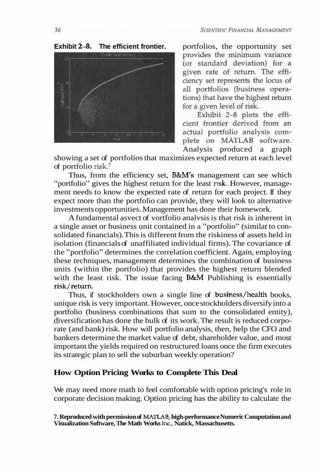
Exhibit 2-8. The efficient frontier. portfolios, the opportunity set
Analysis produced a graph showing a set of portfolios that maximizes expected return at each level of portfolio risk.7
Thus, from the efficiency set, B&M1s management can see which "portfolio" gives the highest return for the least Gsk. However, manage- ment needs to know the expected rate of return for each project. If they expect more than the portfolio can provide, they will look to alternative investments opportunities. Management has done their homework.
A fundamental asvect of vortfolio analvsis is that risk is inherent in a single asset or business unit contained in a "portfolio" (similar to con- solidated financials). This is different from the riskiness of assets held in isolation (financials of unaffiliated individual firms). The covariance of the "portfolio" determines the correlation coefficient. Again, employing these techniques, management determines the combination of business units (within the portfolio) that provides the highest return blended with the least risk. The issue facing B&M Publishing is essentially risk/return.
Thus, if stockholders own a single line of business/health books, unique risk is very important. However, once stockholders diversify into a portfolio (business combinations that sum to the consolidated entity), diversification has done the bulk of its work. The result is reduced corpo- rate (and bank) risk. How will portfolio analysis, then, help the CFO and bankers determine the market value of debt, shareholder value, and most important the yields required on restructured loans once the firm executes its strategic plan to sell the suburban weekly operation?
How Option Pricing Works to Complete This Deal
We may need more math to feel comfortable with option pricing's role in corporate decision making. Option pricing has the ability to calculate the
7. Reproduced with permission of MATLAB, high-performance Numeric Computation and Visualization Software, The Math Works Inc., Natick, Massachusetts.

Basic Tools of Financial Rirk Management: Portfolios and Options 3 7
value of equity on combined operations or on a single-entity basis. Savings from economies of scale, managerial motives, complementary strengths, or technical competence will have an overriding influence on a combined operation. Meanwhile, we have enough of an account to understand how the restructuring was completed.
While the theory looks attractive, the value of combined operations is not easy to quantdy. The general methodology for the analysis of divestitures requires a study of the results of breaking up the two organizations. This undertaking includes an estimate of the applicable cost of capital and expected returns and the application of valuation principles to formulate esti- mates of the value of the firms, separately and combined. If the value of the combined firm is greater than the sum of the two operations taken separately then B&M should not divest itself of its subsidiary. The opportunity cost of capital is a weighted average of the cost of equity and debt capital. Further, it is the return on assets that f i m must earn to increase shareholder wealth. Thus, a study of the capital structure of the subsidiary should be undertaken by means of the Option Pricing Model. With estimates of the cost of equity and cost of debt, the capital structures of both the combined firm and B&M on a stand-alone basis are analyzed to estimate the cost of capital. It is now time for B&M1s CFO and the financial team to step up the analysis to the level of option pricing. See appendix calculation of option values.
Black and Scholes pointed out that common shares are call options, or options to take (or retain) the firm's assets by paying off its debt. By put-call parity, we can also say that the value of debt is marked down by the value of a default put: Stockholders can put the assets of the firm to its creditors and walk away without further liability. The exercise price of the put is the face value of the publishing company's debt. From this, the financial team understood how to price the firm's liabilities.
When creditors place debt, shareholders receive cash by selling assets to creditors plus a call option. At maturity, if the firm's value exceeds the value of debt, stockholders will exercise their call by paying off the firm's $12 million obligation to the bank. However, if spinning off Connecticut causes B&M to belly up, shareholders will not exercise their option. Investors in the firm will walk away as if they purchased stock or com- modity options from their broker and stock or commodity values declined below the exercise price.
The bank ends up with the firm's assets, which will be valued below the face amount of the debt. In other words, regarding equity in a levered firm as a call option implies that investments increase the idiosyncratic or diversifiable risk of a firm without changing its expected return. This will benefit the firm's shareholders at the expense of the bank, even though the value of the firm is unaffected. Because idiosyncratic risk is independent of the market portfolio, an increase in this risk will increase the variance of returns for the firm without changing its beta, or expected, return. Thus, the value of the firm will not change.

Table 2-2. The Barns & Mobile Publishing Corp. (consolidated) assumption: Low-risk diversified business.
Standard deviation 35.00% Risk-free rate 8.0% Combined debt to maturity 5 years Health book operation face amount, debt $8,000,000 Suburban operation face amount, debt $4,000,000 Total face amount of combined debt $1 2,000,000 Market value of the firm's assets (value of firm) $36,000,000 Value of common stock* $28,089,626 Present value of combined Debt* $7,910,373
Note: Asterisks denote Black-Scholes solution
However, a redistribution of wealth to shareholders at the expense of the bank may occur because the higher variance will increase the value of the call option held by B&M shareholders. Thus, increasing the riskiness of the firm's operations increases the value of equity but decreases the value of debt. For example, if the bank lent to a firm whose only purpose is to invest in Treasury bills (as strange as this may seem), the yield the bank expects is Treasury based. However, if the firm wised up, sold its Treasury portfolio, and purchased equipment with the proceeds, volatility of per- centage returns will increase along with shareholder value. The bank rec- ognizes that they no longer could lend at the risk-free rate because increased volatility, associated with more aggressive business strategies, has increased default risk, reducing debt values.
While Barns & Mobile Publishing Corp.'s bankers cannot be absolutely certain of the firm's new level of risk, Jack Smith and the bank may wisely employ option techniques to derive the appropriate compen- sation for the bank to relax loan covanents pertaining to changes in the business.
Now let's assume that projections were completed with support of simulation software. The results indicate within a 95% confidence level that the risk of percentage returns (standard deviation) has increased from 35% to 45%. Incorporating this information in our option pricing spread- sheet, the yield on the loan (from within the universe of option pricing) increases 120 basis points, compensating the bank for the higher level of risk. This translates into the bank receiving a compensation of 120 basis points on the restructured term loan for them to agree to waive the loan covenant restricting divestment activity (if the company's risk level increases from .35 to .45).
You can verify the summaries given in Tables 2-2 and 2-3 by using the Excel template in the CD. The file, B&MPub.XLS, is an option pricing model. You may also want to experiment by changing the assumption variables.

Basic Tools of Financial Risk Management: Portfolios and Options 39
Table 2-3. The Barns & Mobile Publishing Corp. sells its Connecticut subsidiary, thus increasing the standard deviation of percentage returns to 45Oh versus SD of 3 5 O l O before the sell-off.
Standard deviation Risk-free rate Debt to maturity Health book operation face amount, debt Market value of health book's assets (value of firm) Value of common stock* Present value of health operation debt* Proforma change in value common stock* Proforma change in value debt* Yield to compensate for 35% variance* Yield to compensate for 45% variance* Basis-point adjustment: Compensation for
increased risk*
45.00% 8.0%
5 years $8,000,000
$24,000,000 $1 8,950,383
$5,049,616 $223,966
($223,966) 8.0% 9.2%
120.3 basis points
Note: Asterisks denote Black-Scholes solution.
Now, we finish. Though default risk increased, the bank agreed to relax loan covenants, allowing the firm to proceed with the divestiture. A rate increase to 9.2% is reasonable compensation for incremental default risk. The $4 million loan to Connecticut was repaid from the proceeds of the sale.
Option pricing is not the only way to price debt and should never be used alone. However, by estimating the probabilities that shareholders' call options finish "in the money," midsize firms and their capital providers (namely, banks) can arbitrate pricing issues on a level playing field, and that is the important issue: the incremental cost of financing- loan yields in equilibrium with the volatility of a restructured business. For this reason, option pricing provides significant insight into the rela- tionship between degrees of risk versus degrees of returns working its way in a strategic plan demanded by key suppliers of capital.
The Quintessential Black-Scholes
Einstein once said, "Nature shows us only the tail of the lion. But I do not doubt that the lion belongs to it even though he cannot at once reveal him- self because of his enormous size." If Einstein is correct, then volatility/yield (risk/reward) in orbit is the "tail of the lion," and the metaphoric lion is higher-dimensional space-time, the optimal financing plan. Perhaps one day people will concede that "useless statistics-the bane of many financial managersu-is the ultimate source of beauty and simplicity.

Those who have studied portfolio theory no doubt understand how to depict the correlation between assets comprising a portfolio. To readers who are new to these concepts, I hope that the example has shown that the whole is not just the sum of the parts. The correlation between units of a company or stocks in a mutual fund, even if they appear as remote as a butterfly's flight on wind patterns, are very much present and, more important, have a very determinable value.
For example, at any given concert of Beethoven's Eroica, the power and intensity of the music will visibly shake people. If, at the concert's con- clusion, you stroll by the orchestra pit and peek at the sheet music, you will Likely think that the score of this most towering work is a jumble of scribbles and scrawls. However, to a musician the scribbles come alive and resonate in both mind and soul. A musician actually hears Beethoven's rich, organic sounds simply by looking at the score. Bars, clefs, keys, sharps, and flats are more than a short collection of scrawls on paper.
Like the Eroica, the metaphoric poem of Black-Scholes is much more a collection of bars, clefs, and keys. Rather, Like many a great work, this one evokes subtle interactions well beneath the obvious; and, as a poem of sorts, the formula has the potential to transport financial managers to heights of logic and depth. If so, they may see that, like music, the equa- tion evokes a natural progression and a syllogistic reasoning that is any- thing but opaque. Beautiful mathematics is much like an elegant move- ment in a symphony.
We develop options further in the next chapter, which focuses on real options. Real options give CFOs a strategic and valuation tool that con- tributes to R&D and project decisions, ensuring optimum investment opportunities. Real options is a way of thinking and is part of a broad wave of change in financial, product, and corporate investment decisions that requires managers to create value by managing strategic investments squarely, with a minimum of waste, expense, and effort.

Basic Tools of Financial Risk Management: Portfolios and Options 41
Appendix A: Calculations of Options Values
Please open Excel file [CD:MODELS/EXCEL/Opt-bs.XLS], a simple 123 spreadsheet for the Black-Scholes option formula, in the models subdirec- tory on the CD. In the Black-Scholes model, the derivation is based on the creation of a perfect hedge by simultaneously being long (short) in the underlying security and holding an opposite, short (long) position on a number of options. The return on a completely hedged position will then be equal to the risk-free return on the investment in order to eliminate arbi- trage opportunities. Acall option that can be exercised only on some future maturity date can be evaluated by the following expression:
Example Inc.
Assume that the information in Table 2A-1 has been obtained on the Example Inc. stock. Let's begin with the formula:
The value of the option = the stock price multiplied by delta, N(d,), less the risk-adjusted present value of exercised price Xe-RjT N(d,).
This operation is not easy, so let's break the formula down with the B&S formula:
Table 2A-1. Original condition: Example Inc.
C = value of the options to be determined Risk-free rate R, = 6.2% Stock price now S = $46.75 Standard deviation of percentage returns s = .28 European option expires in 199 days T = 199/365 Exercise price X = $45.00 Partial derivative associated with the riskless hedge (delta) N(d,) Riskless hedge rn = 1/ N(d,) Probabilities of the option "in the money" N(d2) Continuous discounting at the risk-free rate for the period
the option is exercisable e-*

Step 1: Find earn
eRfr is the formula for continuous discounting. For example, .9667 would be invested now in a risk-free investment to receive $1.00 in 199 days with interest at 5%; e is the natural log; Rf = 5% and T = 199 days.
Step 2: Understand N(d,)
N(d,) is the probability that the option is in the money; that is, at maturity the stock price is above the strike or exercise price. The probability that the option contract is out of the money is (1 - N(d2)). Assume that N(d,) is .59611.
Step 3: Link Step 2 to Step 1
Receipt of 1.00 is anything but certain unless you invest in a Treasury bill. If there is a .59611 chance that at maturity you hold an in-the-money- option, its expected present value is $1.00(.9667)(.59611) = $.57629, which is the most you would invest to realize $1.00 at maturity. Thus, the exercise price was $45. Its expected present value is $45(0.57629), or $25.95. In other words, the B&S formula risk adjusts the exercise price, and that is what the exercise price is really worth.
Step 4: Determine N(d,)
N(d,) is delta, or the partial derivative, the change in the price of the option with respect to the change in the price of the stock. A delta of .40 means that if the price of the stock changes loo%, the price of the option changes 40% (see the next section).
Finally, the expected stock price SN(d,) less the risk-adjusted exercise price, XeRfr N(d,), equals C, the option price.
Developing the Quantitative Elements
First find dl:

Basic Tools of Financial Risk Management: Portfolios and Options
This converts to .17401.
Examining the curve above, we can see some interesting properties of normal probability distributions. For any normal distribution, the proba- bility of an outcome falling plus or minus one standard deviation from the mean o is 68.26%. If we take the range within two standard deviations of the mean, the probability of an occurrence within this range is 95.46%, and 99.74% of all outcomes will fall within three standard deviations of the mean. Thus, from a z table (table of areas under the normal curve), .451406 con- verts to a value of .17401, the proportion of total area under the normal curve (opt.bs.xls cell B49).
N (dl) ,67401
Cover 100 shares with 148.4 options m = "the riskless hedge"
N(dl), or delta, is simply .5 + .I67 = .67401 (cell B54). Delta is a partial derivative that infers that a 100% change is the stock price results in a 67%

change in price of the option. It is now easy to construct the riskless hedge, r = l/N(dl). In the example, r = 1/.67401 = 1.48366. Thus we write 148.4 options to hedge against 100 shares of stock D.
If the firm hedges foreign currency, or interest rates for their customer, N(d1) provides the currency or interest rate hedge. It is not enough to know what delta is at any given moment. Thus, we also calculate gamma (see definition in Table 2A-2).
N(d,) is the probability that our European option expires in the money:
The computer derives N(d2) = .59611, the probability that the option fin- ishes "in the money" (S > X). Thus, e -* = e--062(199/365) = .966762, represents the present value of $1.00 certain to be received in 199 days, $.9667.
However, the $1.00 is anythmg but certain. There is only a .59611 chance of realizing a $1.00 under these risk conditions; thus, the expected present value is $1.00(.9667)(.59611) = $.57629. Thus, Xe-m N(d,) = $45 (.5763) = $25.95, the expected present value of the exercise price. The stock price adjusts by N(dl), the reciprocal of the riskless hedge:
Finally, the value of the option: C = SN(d,) - XcRfrN(d,) = $31.51 -25.95 = $5.55. Exhibit 2A-1 shows a three-dimensional surface. For each point on the
surface, the height (2-value) represents the sum of the gammas for each option in the portfolio weighted by the amount of each option. The x-axis represents changing price, and the y-axis represents time. The plot adds a fourth dimension by showing delta as surface co10r.~
Recall that gamma is the second derivative of the option price relative to the underlying security price. Exhibit 2A-2 shows a three-dimensional surface whose z-value is the gamma of an option as price (x-axis) and time
8. Reproduced with permission of MATLAB, high-performance Numeric Computation and Visualization Software, The Math Works Inc., Natick, Massachusetts.
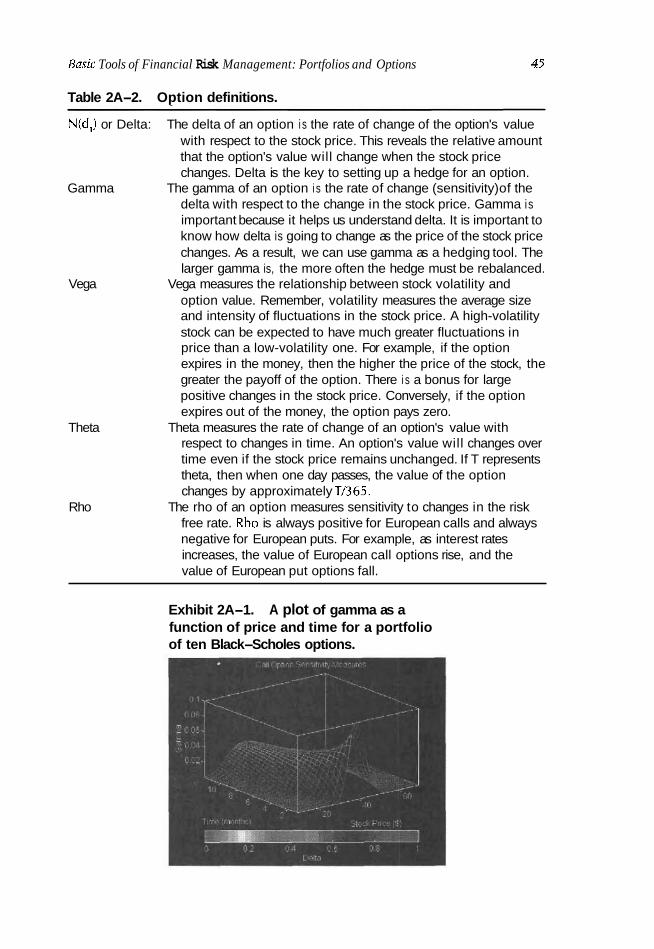
Basic Tools of Financial Risk Management: Portfolios and Options 45
Table 2A-2. Option definitions.
Vega
Theta
Rho
- - - - --
N(d,) or Delta: The delta of an option i s the rate of change of the option's value with respect to the stock price. This reveals the relative amount that the option's value will change when the stock price changes. Delta is the key to setting up a hedge for an option.
Gamma The gamma of an option i s the rate of change (sensitivity) of the delta with respect to the change in the stock price. Gamma is important because it helps us understand delta. It is important to know how delta is going to change as the price of the stock price changes. As a result, we can use gamma as a hedging tool. The larger gamma is, the more often the hedge must be rebalanced.
Vega measures the relationship between stock volatility and option value. Remember, volatility measures the average size and intensity of fluctuations in the stock price. A high-volatility stock can be expected to have much greater fluctuations in price than a low-volatility one. For example, if the option expires in the money, then the higher the price of the stock, the greater the payoff of the option. There i s a bonus for large positive changes in the stock price. Conversely, if the option expires out of the money, the option pays zero.
Theta measures the rate of change of an option's value with respect to changes in time. An option's value will changes over time even if the stock price remains unchanged. If T represents theta, then when one day passes, the value of the option changes by approximately Tl365.
The rho of an option measures sensitivity to changes in the risk free rate. Rho is always positive for European calls and always negative for European puts. For example, as interest rates increases, the value of European call options rise, and the value of European put options fall.
Exhibit 2A-1. A plot of gamma as a function of price and time for a portfolio of ten Black-Scholes options.

Exhibit 2A-2. A three-dimensional plot showing how gamma changes relative to price for a Black-Scholes option.
(y-axis) vary. It adds yet a fourth dimension by showing option delta (the first derivative of option price to security price) as the color of the surface?
The Barns & Mobile Publishing Corp. Practice Session
On page 41, we solved the option problem with mathematical formulas. Now we will use the spreadsheet that is more efficient. Table 2A-3 lists input data. Tables 2 A 4 and 2A-5 represent the spreadsheet solution.
Download "a simple 123 spreadsheet for the Black-Scholes Option Formula-Dividend Adjusted
~rww.numa.corn~~ It might be helpful to review again the Barns & Mobile divestiture,
this time working with the Black-Scholes template B&Mpub.XLS.
A S IMPLE 123 SPREADSHEET FOR THE BLACK-SCHOLES OPTION FORMULA
Table 2A-3. Input data.
INPUT underlying price: 46.75 (e.g. stock price)
strike: 45.00 volatility: 28.00%
interest rate: 6.20% time to exairv: 0.5452 bears)
9. Reproduced with permission of MATLAB, high-performance Numeric Computation and V~sualization Software, The Math Works Inc., Natick, Massachusetts. 10. "You are free to use this spreadsheet as you wish, but we would be grateful if you could include a reference to Numa Financial Systems. Please contact us if you have any com- ments or suggestions."

Basic Tools of Financial Risk Management: Portfolios and Options 47
Table 2 A 4 . Output data.
OUTPUT Ca 11 Put
theoretical value: 5.560 2.314 delta: 0.674 -0.326
gamma: 0.03728 4.03728 theta: -4.803 -2.106 vega: 12.437 12.437 rho: 14.1516 -9.5671
Table 2A-5. Numa calculations.
Calculations
Input underlying price 46.7500 Input strike 45.0000 Input volatility 0.2800 Input interest rate 0.0620 Input time to expiry (years) 0.5452
From B&S formula d 1 0.45 14 From B&S formula d2 0.2447
N' (dl ) 0.3603 k l 0.8694
N (d l ) tmp 0.6741 N (d l ) 0.6741
N' (d2) 0.3872 k2 0.9247
N (d2) tmp 0.5966 N (d2) 0.5966
theorical call value 5.5596 call delta 0.6741
theoretical put value 2.31 39 put delta -0.3259
Same for call & put gamma 0.0373 Same for call & put vega 12.4372
call theta 4.8030 put theta -2.1057 call rho 14.1516 put rho -9.5671

CASE ONE
Original Conditions (Consolidated)
Assumption: Low-Risk Diversified Business
INPUT Standard deviation ENTER 86 35 Risk-free rate ENTER B7 8.0 Days to expiration (5 yrs x 365) ENTER 88 1825 Total face amount of combined debt* ENTER B9 12,000,000 Market value of the firm ENTER B10 36,000,000
*Health book operation face amt. debt *Suburban operation face amt. debt
OUTPUT Value of common stock Present value of combined debt
CASE TWO
Divestiture Strategy (Individual)
The Barns & Mobile Publishing Corp. sells its Connecticut subsidiary, thus increasing the standard deviation of percentage returns to 45%.
Assumption: Higher-Risk Concentrated Business
INPUT Previous: SD 35% Standard deviation ENTER B28 45 Risk-free rate ENTER B29 8.0 Days to expiration (5 yrs x 365) ENTER B30 1825 Total face amount of combined debt* ENTER B31 12,000,000 Market value of the firm ENTER B32 3 6,000,000
*Health book operation face arnt. debt *Suburban operation face amt. debt
OUTPUT Yield to compensate for higher variance: 9.2% (vs. initial condition yield of
8.O0/0) Value of common stock $1 8,950,383 Market value of health book operations $24,000,000 Present value of health operation debt $5,049,616 Change in value common stock $223,966 Change in value debt ($223,966) Basis-point adjustment in yield
to compensate for higher risk and reduction in debt value 120.3
Basic Tools of Financial Risk Management: Porfolios and Options 49
The Numbers Worked Out
**Reconciliation: 120 basis-point adjustment to compensate for increased risk: The increased risk of the divestment of suburban weekly has raised the market value of equity by $223,996:
Value of equity before divestment of weekly: $28,089,626
Adjustment to reduce firm 1/3. (213 x $28,089,626) $1 8,726,417
Less: Postequity (higher variance) ($1 8,950,383) Increase in shareholder value $223,966
The Barns & Mobile Publishing Corp. sells its Connecticut subsidiary, thus increasing the standard deviation of percentage returns to 45%.
The market value of the risky debt on the other hand declined by an equal amount:
Market value of debt as determined by the option pricing model before divestment: $7,910,3 73
Adjustment (2/3 x 7,910,373) Value of debt with increase in
variability to SD .45 from .35 Decrease in the value of debt
Results
The promised yield to maturity associated with post divestiture debt can be determined by solving for the discount rate that equates maturity value five years hence to the present value of debt determined by Black-Scholes. Namely:
where Bo represents the present value of debt F = face value e = the natural log T = years to maturity k, = the required yield
Solving for the yield, we find that creditors require a postdivestiture yield of 0.09269 (in equilibrium with .45 SD) versus an 8% yield before, or 120 basis points increased compensation.

Chapter Ttvo References and Selected Readings
Books and Periodicals
Aliber, R. Z., and B. R. Bruce. (1991). Global portfolios: Quantitative strategies for maximum per- formance. Homewood, Ill.: Business One Irwin.
Bakshi, G., et al. (1997). "Empirical performance of alternative option pricing models." Jour- nal of Finance, 2003-49.
Bates, D. S. (1995). "Testing option pricing models." Working paper. National Bureau of Economic Research, 1-72.
Bates, D. S., and National Bureau of Economic Research. (1995). Testing option pricing mod- els. Cambridge, Mass.: National Bureau of Economic Research.
Bookstaber, R. M. (1987). Option pricing and investment strategies. Chicago: Probus. Breen, R. (1990). "Binomial option pricing and the conditions for early exercise: An exam-
ple using foreign exchange options." Economic and Social Review, 151-61. Brenner, M., and Salomon Brothers Center for the Study of Financial Institutions. (1983).
Option pricing: Theory and applications. Lexington, Mass: Lexington Books. Brockrnan, P., and M. Chowdhury. (1997). "Deterministic versus stochastic volatility: Impli-
cations for option pricing models." Applied Financinl Economics, 499-505. Butler, J. S., and 8. Schachter. (1986). "Unbiased estimation of the Black/Scholes formula"
Journal of Financial Economics, 34-57, The authors present an estimator of the Black and Scholes (1973) option pricing for- mula that is free of the variance-induced bias discussed by Thorp (1976), Boyle and Ananthanarayan (1977), and others.
Chang, C. W., et al. (1998). "Information-time option pricing: Theory and empirical evi- dence." Journal ofFinancia1 Economics, 21142.
Chang, J. S. K., and L. Shanker. (1987). "Option pricing and the arbitrage pricing theory." Journal of Financial Research, 1-16.
Chris, N. (1997). Black-Scholes and beyond: Option-pricing models. Chicago: Irwin. Cox, J. C., et al. (1987). Option pricing theory and its applications. Cambridge: Sloan School of
Management, Massachusetts Institute of Technology. Ferrentino, G. L., and Massachusetts Institute of Technology, Department of Electrical Engi-
neering and Computer Science. (1987). An option-pricing model for R&D projects. Fortune, P. (1996). "Anomalies in option pricing: The Black-Scholes model revisited." New
England Economic ReoiewEederal Reserve Bank of Boston, 17-40. Gilster, J. E., Jr. (1990). "Systematic risk of discretely rebalanced option hedges." Journal of
Financial and Quantitatiue Analysis, 507-16. Demonstrates that Black-Scholes option-pricing model hedge positions that are risk free when rebalanced continuously will frequently exhibit substantial systematic risk when rebalanced at finite intervals. This systematic risk means that the Black-Scholes option-pricing model is inherently inconsistent with the discrete time version of the Capital Asset Pricing Model (CAPM).
Grenadier, S. R., and A. M. Weiss. (1997). "Investment in technological innovations: An option pricing approach." Journal of Financial Economics, 397-416. Develops "a model of the optimal investment strategy for a firm confronted with a sequence of technological innovations."
Haug, E. G. (1998). The complete guide to option pricing formulas. New York: McGraw-Hill. Hodges, S. D. (1990). Options: Recent advances in theory and pracfice. Manchester: Manches-
ter University Press. Jarrow, R. A,, and A. Rudd. (1983). Option pricing. Homewood, Ill.: Dow Jones-Irwin. Johnson, R. S., et al. (1999). "Skewness-adjusted binomial option pricing model: The rele-
vance of the mean." International Rw'ew of Economics and Business, 159-72.
Basic Tnols of Financial Risk Management: Portfolios and Options 51
Kroll, Y. and H. Levy. (1984). "Mean-variance versus direct utility maximization." Jarrnal of Fimnce, 4741. The authors compare the expected utility of the optimum portfolio for given utility functions with the expected utility of well-selected portfolios from the mean-variance efficient frontier.
Lee, S. H., et al. (1997). "The performance of option pricing models: A comparison." Inter- national Journal of Finance (3), 66M2.
Leisen, D. P. J. (1998). "Pricing the American put option: A detailed convergence analysis for binomial models." Journal of Economic Dynamics and Control, 1419-44.
Lo, A. W., and C. Wang. (1993). lmplmenting option-pricing models when asset returns are pre- dictable. Cambridge: Alfred P. Sloan School of Management, Massachusetts Institute of Technology.
Lo, A. W., and 1. Wang. (1994). "Implementing option pricing models when asset returns are predictable." Working Paper. National Bureau of Economic Research, 1-54.
Lyng, A., and Sloan School of Management. (1986). "Option pricing: A life-cycle evaluation of a project."
Majd, S., and R. S. Pindyck. (1985). "Time to build, option value, and investment decisions." Working Paper. National Bureau of Economic Research, 1-24. The authors develop an explicit model of investment projects and use option pricing methods to derive optimal decision rules for investment outlays over the entire con- struction program.
Majd, S., and Sloan School of Management. (1984). "Applications of option pricing to cor- porate finance."
Merrill, C., and S. Thorley. (1996). "Time diversification: Perspectives from option pricing theory." Financial Analysts Journal, 13-19.
Merton, R. C. (1970). An analytic derivation of the eflicient portfoliofrontier. Cambridge: MIT Prfss.
Merton, R. C. (1971). Theory of rational option pricing. Cambridge: MIT Press. Merton, R. C. (1975). Option pricing when underlying stock returns are discontinuous. Cam-
bridge: Alfred P. Sloan School of Management, Massachusetts Institute of Technology. Merton, R. C. (1976). The impact on option pricing of specification error in the underlying stock
price returns. Cambridge: Alfred l? Sloan School of Management, Massachusetts, Insti- tute of Technology.
Merton, R. C. (1998). "Applications of option-pricing theory: Twenty-five years later." American Economic Review, 32349. This article is the lecture that Robert C. Merton delivered in Stockholm, Sweden, December 9, 1997, when he received the Alfred Nobel Memorial Prize in Economic Sciences.
Mitchell, D. W. (1990). "Efficient policy frontier under parameter uncertainty and multiple tools." Journal of Macroeconomics, 13745.
Myers S. C., et al. (1983). Calculating abandonment value using option-pricing theory. Cam- bridge: MIT Press.
Nawalkha, S. K (1995). "Face value convergence for stochastic bond price processes: Anote on Merton's partial equilibrium option pricing model." Journal of Banking and Finance; 15344.
Nelson, D. B., and K. Ramaswamy. (1989). "Simple binomial processes as diffusion approx- imations in financial models." Working Paper. Rodney L. White Center for Financial Research, University of Pennsylvania, 1-45. Presents conditions under which a sequence of binomial processes converges weakly to a diffusion and shows constructively how one can employ a transformation to pro- duce computationally simple binomial processes. In the context of f ianaa l models (especially option pricing models), the binomial method numerically solves a partial differential equation (PDE) for the value of some asset. The methods in this paper per- mit one to solve such PDEs for alternative underlying diffusions.

Prakash, A. J., et al. (1989). "General proof of Merton's analytic derivation of the efficient portfolio frontier." Qmrterly Journal of Business and Economics, 67-77.
Quigg, L. (1993). "Empirical testing of real option-pricing models." Journal of Finance, 621-40. Examines the empirical predictions of a real option-pricing model using a large sam- ple of market prices, with empirical support for a model that incorporates the option to wait to develop land.
Rahman, A,, and L. Kryzanowski. (1986). "Alternative specifications of the errors in the Black-Scholes option-pricing model and various implied-variance formulas." Econom- ics Letters (I), 61-65.
Reiss, A. (1998). "Investment in innovations and competition: An option pricing approach." Quarterly Rrmiew of Economics and Finance (Special Issue), 635-50.
Rogers, L. C. G., and D. Talay. (1997). Numerical methods infinance. Cambridge: Cambridge University Press.
Seiford, L., and R. M. Thrall. (1990). "Recent developments in DEA: The mathematical pro- gramming approach to frontier analysis." Journal of Econometrics, 7-38. Discusses mathematical programming approach to efficient frontier estimation known .. . . as DEA and the advantages &d limitations of a mathematical programming approach to frontier estimation. Annals 1990-4, a supplement to the Journal of Econometrics.
Sundaram, R. K., et al. (1999). An introduction to futures and options. This course provides an intuitive introduction to the nature and pricing of derivative instruments. It covers forwards and futures, swaps, and options. An exposition of derivatives pricing using the Binomial option-pricing model is followed by a dicus- sion of the Black-Scholes model and its extensions.
Turnbull, S. M., and F. M i e . (1991). "Simple approach to interest-rate option pricing." Review of Financial Studies (I), 87-120.
Whaley, R. E. (1986). 'Valuation of American futures options: Theory and empirical tests." Journal of Finance, 127-50. Reviews the theory of futures option pricing and tests the valuation principles on transaction prices from the S&P 500 equity futures option market.
Wilmott, P., J. et al. (1993). Option pricing: Mathematical models and computation. Oxford: Oxford Financial Press.
Other Periodicals
Anders, Ulrich. (1998). "Improving the pricing of options: A neural network approach." Joumal $Forecasting, 17 (5 to 6), 369.
Anonymous. (1998). "How to estimate cumulative volatility." Harvard Business Review, 76(4), 58.
Ballestero, E. (1998). "Approximating the optimum portfolio for an investor with particu- lar preferences." Journal of the Operational Research Society, 49(9), 998.
Buge, John R. (1999). "Risk-neutral option pricing methods for adjusting constrained cash flows." The Enginering Economist, 44(1), 36.
Brown, Mark, and Peter Tedstrom. (1995). "Efficient frontier helps maximize returns." Den- ver Post, March 13, p. C03, Rockies edition.
Carty, C. Michael. (1999). "A new paradigm for structuring portfolios: Planners can reduce the impact of errors in risk and return projections by applying a new method for port- folio selection." Financial Planning, January 1, p. 1.
Chance, Don M. (1999). "Research trends in derivatives and risk management since Black- Scholes." Journal of Portfolio Management (May), 35.

Basic Tools of Financial Risk Management: Portfolios and Options 53
Corrado, Charles. (1998). "An empirical test of the Hull-White option pricing model." Jour- nal of Futures Markets, 18(4), 363.
Dalio, Ray, and Dan Bemstein. (1996). "A nav edge for efficient frontier." Pensions and Investments, 24(19), 12.
Das, Sanjiv Ranjan. (1999). "A direct discrete-time approach to Poisson-Gaussian bond option pricing in the Heath-Jarrow-Morton model." Journal of Economic Dynamics and Control, 23(3), 333.
Diacogiannis, George I? (1997). "Multi-factor risk-return relationships." Journal of Business Finance and Accounting, 24(3/4), 559.
Dong-Hyun Ahn. (1999). "Pricing discrete barrier options with an adaptive mesh model." Journal of Derivatives, 6(4), 33.
Dreman, David. (1998). "Nobel laureates with black boxes." Forbes, December 14,283. Gibbons, Michael R., Stephen A. Ross, and Jay Shanken. (1989). "A test of the efficiency of
a given portfolio." Econometrics, 57(5), 1121. Gollinger, Terri L. (1993). "Calculation of an efficient frontier for a commercial loan portfo-
lio." Journal of PortfDIio Management, 19(2), 39. Grinold, Richard C. (1992). "Are benchmark portfolios efficient?" Journal of Portfolio Man-
apement. 19(1). 34. u , . , . Guo, Chen. (1998). "Option pricing with heterogeneous expectations." The Financial Review,
33f4). 81. \ ,.
Herrick, R. C. (1997). "Exploring the efficient frontier." Risk Management, 44(8), 23. Ma, Chenghu. (1998)." A discrete-time intertemporal asset pricing model: GE approach . -
with recursive utility." Matltematical Finance, 8(3), 249. -
Mahieu, Ronald. (1998). "A Bayesian analysis of stock return volatility and trading vol- ume." Applied Financial Economics, 8(6), 671.
Markowitz, Harry M. (1999). "A more efficient frontier." J o u m l of Portfolio Management (May), 99.
Marmer, Harry S., and F. K. Louis Ng. (1993). "Mean-semivariance analysis of option-based strategies: A tot." Financial Analysts Journal, 49(3), 47.
Mello, Antonio S. (1998). "A portfolio approach to risk reduction in discretely rebalanced option hedges." Management Science, 44(7), 921.
Reitano, Robert R. (1996). "Non-parallel yield curve shifts and stochastic immunization." Journal of Portfolio Management, 22(2), 71.
Rendleman Richard J., Jr. (1999). "Option investing from a risk-return perspectively." Jour- nal of Portfolio Management (May), 109.
Sharma, Maneesh. (1996). "Efficient frontier: The surprising results of shorter relation- ships." Multinational Business Review, 4(1), 1.
Shing, Chue. (1999). "Interactive decision system in stochastic multiobjective portfolio selection." Internatiml Journal of Production Economics, 6061, 187.
Tian, Yisong. (1999). "A flexible binomial option pricing model;" Journal of Futures Markets, 19(7), pg. 817.
Voros, J. (1999). "A note on the kinks at the mean variance frontier." European Journal of Operational Research, 112(1), 236.
Williams, James 0. (1999). "A frontier that's more efficient." Financial Planning, October 1, p. 1.
Winston, Kenneth. (1993). "The ' efficient index' and prediction of portfolio variance." Jour- nal of Portfolio Management, 19(3), 27.
Ziobrowski, Alan J. (1999). "Mixed-asset portfolio composition with long-term holding periods and uncertainty." Journal of Real Estate Portfolio Management, 5(2), 139.

Select Internet Library
Rubash, Kevin. A Study of Option Pricing Models. Extract: Modem option pricing techniques are often considered among the most math- ematically complex of all applied m a s of finance. Financial analysts have reached the point where they are able to calculate, with alarming accuracy, the value of a stock option. Most of the models and techniques employed by today's analysts are rooted in a model developed by Fischer Black and Myron Scholes in 1973. This paper examines the evolution of option pricing models leading up to and beyond Black and Scholes's model. http://bradley.bradley.edu/-arr/bsm/model.html.
The Big AppletTM (November 18,1999). Daniel Sigrist's Black-Scholes Option Calculator implements the Black-Scholes (1973) equation for European calls and puts and produces prices and Greeks. Use it freely, as is, with his compliments. http://www.margrabe.corn/OptionPricing.hhnl.
Monte Carlo Algorithm for Option Pricing. Extract: Monte Carlo simulation is an established numerical tool for pricing of deriva- tive securities. Standard Monte Carlo approach relies on direct stochastic integration of the Langevin equation for the security price process. You will find on this site an improved Monte Carlo option pricing method that generates the probability distribu- tion of security prices using Metropolis algorithm. http://www.npac.syr.edu/ users/miloje/HPFA/Option/home.html.
Name Size T V P ~
BLACK-SCHOLES-OPTION PRICING MODELS Black-Scholes Option Pricing Applet [Margrabe-Derivatives-
Options-Swaps-Risk Management-Model Risk] CZb&MPub C2opt-bs Monte Carlo Option Pricing NumaWeb DERIVATIVES Option Calculator NumaWeb The lnternet Resource Center For Financial
Derivatives The Mathworks-Financial Toolbox
lnternet Shortcut lnternet Shortcut
Microsoft Excel Worksheet Microsoti Excel Worksheet lnternet Shortcut Internet Shortcut lnternet Shortcut
lnternet Shortcut

Real Options: Evaluating R6D
and Capital Investments
CAPITAL EXPENDITURES THAT SHOW UP on any FASB 95 cash flow statement are de facto collections of options on real assets, or real options. Real options are similar to financial options in that firms with discretionary investment opportunities have the right-but are under no obligation-to acquire expected cash flows by making an investment on or before the date that the (investment) opportunity ceases to exist.
Integrating real options into (capital) investment analysis is a must for CFOs aiming to derive shareholder value with any degree of accuracy. The technique really works because of the correspondence between managing real assets and investing in financial assets. For example, deciding to invest in a particular Disney film is identical to exercising a call on Amazon.com stock. Investors in a Disney production provide funds if they believe that the present value of expected cash flows (from the movie) exceed the present value of development costs. In much the same way, it is smart to exercise a call on Arnazon.com if the stock price is greater than the strike price at the time the option is exercised. When to invest in a Dis- ney production is the same question as asking when it is rational to exer- cise a call option-in this case, an American call option. Identical methods value both financial options and real options.
"Options" refer to flexibility, natural hallmarks of investment, or oper- ating decisions. "Real" distinguishes options available on tangible or intan- gible assets from options on financial instruments. Real options explicitly recognize and incorporate the value of being able to defer investment,

expand output, change technologies, or stop investing-be it a new med- ical technology or, for that matter, conducting a master piano class at one of New York's music conservatories
The Music Master's Dilemma
Financial decision making reinforced with real options is very much like selecting protCgCs for music master classes-two highly complicated unpredictable events. Walk into the master's studio on any given day, and you will find the rare protege who plays superbly. Any master teacher would pick this student immediately. At the other extreme, aspirants attend the selection process with knees shaking so badly that the whole piano vibrates. While mild anxiety is normal when a pianist performs, some suffer from terminal levels of fear. They experience palpitations, rapid breathing, and a loss of control over their ability to manage what can be described only as sheer terror. Few master teachers would bother to pick them. Extreme-now or never-are easy decisions. Alas, music and finance inhabit identical space-time boundaries.
Between the two bands (of option space-time) upper and lower, hope- ful protbgks position themselves, each with varying prospects. Some demonstrate adequate skills but no debilitating performance anxiety. These pianists might benefit from more time on the vine. Our master teacher could rush "the decision" and pick them now to prevent compet- ing schools from pirating these young Artur Rubinsteins. Or, if this were simply a case of nonfatal performance anxiety, some prospects might recover enough to return to music's Holy Grail: preparation, planning, and presence. Before the next audition, the talented ones may well keep anxi- ety under control so that the master will not exercise his or her implicit option to abandon. Such is the world of uncertainty.
Protkges needing additional refinement-no point picking them now. These pianists are sufficiently far along and willing to let time give them the upper hand. With more work (and luck), knowing the harmonic struc- ture, grasping the musical form of masterpieces, anticipating where each phrase begins and ends, and performing with the musical understanding to bring out the rich tonalities, they will be reconsidered-perhaps.
Option theory is, in one form or another, everywhere, framing the totality of art, business, medicine, furniture repair, teaching, and just about anything calling for intelligent decision makGg. ~aturall<acco&ts differ, as well thev should. Music svace-time hardlv resembles R&D s~ace-time. However, master piano teachers, like their finance counterparts, are always searching out the right options that might-and that is the impor- tant word-maximize value.
If this parable sounds a bit complicated, it is. Just try solving the mas- ter's dilemma using standard approaches such as net present value or inter-

Real Options: Evaluating R&D and Capital Investments 5 7
nal rate of return! Of course, the key to solving the master's dilemma is an options deployment problem, meaning the explicit valuation of flexibility.
Flexibility: The Quintessence of Real Options
Flexibility is purchased and, like a home insurance policy, adds value and is very much sought after. Special features embedded in capital expansion programs are often elastic, are open to negotiation, and can be purchased, for example, flexible manufacturing systems, options to change the prod- uct mix in oil refineries, or opportunities to temporarily shut down and restart plant facilities. Other examples are choices permitting you to switch production across borders, beneficial labor conditions, demand, and cur- rency fluctuations. Contracts contain other elastic features, such as the right to deliver natural gas or electricity, whichever is cheaper (switching options). In many cases, flexibility is a largely predictable phenomenon with minor uncertainty.
For example, electrical generators might be used during hours of peak demand, on certain times of day, or in certain seasons. This additional capacity is purchased for the probability of exceeding a "known" bench- mark and demonstrates a firm's need for elastic options. However, the exact demand of generated power is unknown, and in fact the actual mar- ket price may be so low that little or no power will be generated.
Flexibility internal to the project allows you to modify capital expen- ditures as external conditions change. These include expansion, alteration or even abandonment. For example, if you are looking to buy a new com- puter, you might be satisfied if the only real requirement is word process- ing and spreadsheets. You simply purchase a low priced model. However, you'll purchase high-end if speed and memory is what you require.
The other type is external-, or "project-," dependent flexibility or elas- ticity. Deciding to embark on a specific project makes possible a second project not feasible without the first. For example, your boss gives you a big bonus, and you go purchase a beach house near your favorite resort. Without the house, you are limited in how often you can get away to relax since local resort hotels are always booked. Purchasing the home gives you flexibility to go sunning and swimming whenever. You are no longer at the mercy of hotels. Elasticity is value. Projects that let managers shift gears midstream-like abandoning a project that will turn out badly-are worth a lot more than investments without this feature.
Traditional Methods Versus Real Options
Traditional methods such as net present value, internal rate of return, pay- back period, and so on will hardly be applauded by the board of directors
if a particular spending program is important to the firm's continuing value. Consider these issues. A firm chooses between static input-output technology and one allowing for dynamic input-output substitution. This means that when conditions change, management modifies the (project's) key value drivers because uncertainties change expectations about the via- bility of a new technology and thus its explicit value.
If alternative strategies are cleanly quantified and reasoned out, man- agement can make spending adjustments when technology is still in R&D stages. For this reason option value rejuvenates in its own space-time and is thus a much better technique than traditional measures we have been using out of habit. Remember that net-present-value analysis disregards opportunities to alter the game plan and consequently undervalues pro- jects that are explicitly elastic. As we can see in the following example, this is precisely what happened to the CFO at New Technologies as he worked up the numbers deaihg with the firm's important, grounibreaking project.
New Technologies has drawn blueprints for a CD-Recordable disk that operates twice as fast as existing models. Production requirements call for significant outlays, drawing cash flow from alternative high-tech pro- jects. The CD project can start now or nine months hence, keeping in mind that deferred investments can find themselves in deep trouble if alterna- tive projects rival for the available cash flows.
The CFO, unfamiliar with real options, called for traditional valuation (net present value, modified internal rate of return, and payback period). He failed to realize that traditional (valuation) methods could easily undervalue the project. Specifically, these methods are not set up to pin- point (discount) rate/risk volatility implicit in the production and market- ing of CD-Recordables, nor can these methods easily identify investment alternatives to alter cash flows. Furthermore, traditional methods ignore abandonment, switching, and sequencing options that are indespensable to planning this pivotal and strategic product.
Without proper decision-making tools, the firm's CFO not only will kill the project out of hand but is destined to open doors to competitors with foresight enough to employ real options analysis. Our CFO, like man- agers who otherwise feel comfortable trading financial options, could not (or did not want to) perceive the tie between financial and real options. Market options are a known entity; their terms are clearly stated. Real options deal with subliminal corporate issues, complicated by real-world peculiarities and involving more than a few layers of uncertainty.
The Binomial Model
A quick review of the Cox-Rubinstein binomial model will help you understand what are termed "implied binomial trees." This important option-pricing model was developed using a similar approach to

Real Options: Evaluating R&D and Capital Investments $9
Black-Scholes, except here the underlying asset follows a binomial distri- bution. The benefit of the binomial model is that it can be used to evaluate options with an American-style exercise, relevant in our study of real options because we use the binomial distribution to value capital expan- sion strategies. Since American options can be exercised at any time prior to maturity, they are more valuable than their European counterparts that allow exercise only on the expiration date.
The binomial model works by dividing the time to expiration into specified time intervals. Over each time period, the price of the underlying contract moves either up or down using a specified probability, thus pro- ducing a binomial distribution for the price of the underlying asset. This distribution generates a recombining lattice or tree of underlying prices. Each of these prices combines with their respective probabilities to calculate a fair option value. Being able to value the option at each point on the tree, you can determine whether you should exercise before the option expires.
Implied Binomial Tree
A progression of prices for the asset underlying the options with different strike prices starts with the asset's current price and evolves period by period through a bifurcation process. The locations of the nodes of the tree conform to the relationship between the options' implied volatility and strike prices. The implied binomial tree is interpreted as the expected or implied proba- bility distribution of the underlying asset (see Exhibit 3-1).
The principal defect of a single-period binomial option pricing model is overcome by extending it through a number periods (as shown in
Exhibit 3-1. A multiple-period binomial model.

Table 3-1. lnforrnation required and not necessary to value options.
Information Required Information Not Required
The (underlying) asset's current value; estimated and observed in the market
Tme to the decision. The investment characteristics reveal this.
Investment cost that represents the exercise or strike price. This information is specific to the investment.
Risk-free rate. Readily known and observable.
The asset's volatility. You will likely need to estimate this.
Cash flows or returns associated with possession of the underlying asset. This is either observable from the market benchmarks or estimated.
Probability estimates of possible future stock prices. This is implicit from the assets current value and estimate of volatility.
The underlying asset's expected rate of return. Tracking portfolios already produce the asset's riskheturn trade- off.
The option's expected rate of return since dynamic tracking values the option directly.
An adjustment to the discount rate.
Exhibit >I) by constructing a recombining binomial tree of asset prices working forward from the present. One path through the tree represents a single sample drawn from the universe of possible future outcomes. The current option value is then calculated by inverting this process and work- ing backward from the end of the tree, being careful at each node to con- sider the possibility of early exercise.
-
When you determine the value of options, you require specific informa- tion. This information differs from that required for, say, a net present or inter- val rate of return analysis (see Table 2-1). Real options differ from financial options (see Table S2) .
Real Options: Definitions, Examples, and Case Studies
Abandonment Options
Firms usually close up projects that destroy value. We recognize the dis- cretionary strategy as abandonment, or termination, options. Abandonment options are similar to American puts giving the holder the right to sell (the project's) cash flows at any time over its remaining life for a determinable

Table 3-2. Differences between financial and real options.
Financial Options
Financial options are completely specified by a contract.
Uncovering the option not required. Private risk not reflected in price if
the instrument i s a financial security. Financial options do not involve
complex packages of multiple and compound risk.
Exercising a financial options usually requires less intensive management decision making.
Current value of stock that is observed in the market.
Exercise price defined by the features of the investment.
Time to expiration.
Stock value uncertainty often the only estimated input.
Riskless interest rate observed in the market.
Real Options
Real options must be identified and specified.
Uncovering the option is required. Affected by multiple sources of uncertainty,
both market and private risk. Real options come in complex packages
of multiple and compound options. For example, a classic real option application i s oil exploration, and this is actually a nested sequence of options to explore, develop, and extract oil.
Exercising a real option requires very specific managerial decision making, which can be slow and expensive.
Gross present value of expected cash flows.a
Investment cost defined by the features of the in~estment.~
Time until opportunity disappears or the time to the decision date, which i s defined by the features of the in~estment.~
Project uncertainty often the only estimated input.d
Riskless interest rate observed in the market."
"Expected cash flows are obvious features of projects. The greater the cash flow, the more valuable the real option, holding other variables constant. For example, if the amount of oil that can be extracted doubles, the well's value increases. blnve~tment cost represents cash committed to purchase the investment. Holding constant other vari- ables, higher investment costs reduce option value. For example, if the cost to extract oil increases, the well's value decreases. =Increasing the time that a project can be deferred increases (real option) value. As deferment time increases, uncertainty associated with future events decreases since you have more time to gather infor- mation. If the future is unfavorable, the project may not be pursued. Conversely, the original project can be expanded to provide maximum returns if conditions warrant. The longer you can defer the project, the greater the likelihood that a favorable outcome may happen. For example, you can keep a silver mine for only one week. The price of silver is unlikely to rise enough during the week to warrant extraction costs. However, if you keep the silver mine for 10 years, commodity prices might increase enough in that time to make drilling worthwhile. dThe degree of uncertainty associated with a project impacts the value of real options. If two projects with identical values can be deferred the same amount of time, the riskier project has more potential value. A risky project provides the opportunity to generate high returns, but there may be failure in the wings. Since management has purchased the flexibility to expand or abandon, the project's cash flow improves for no other reason than lower interest costs tied to lower project risk.
For example, if the price of copper remains relatively stable, the value of copper in the mine remains unchanged as well. If copper prices fluctuate wildly, it is more likely the price of copper will drop dra- matically. In that case, you take no action. If you are fortunate, the price of copper moves up dramati- cally, and you extract copper profitably.
eAn increase in interest rates will increase option value. Normally, higher rates increase capital costs and thus value falls. However, higher rates could trigger exercise. This counterbalancing effect helps reinforce and sustain the option's value as interest rates rise. Thus, real options give growth-oriented projects a decided advantage over traditional measuring tools such as net present value. If you own a 10-year lease on an oil field, you can wait a few years before you need to buy the rigs required to extract the oil. The rig's present value (cost) is lower since the equipment investment's time horizon stretches out in time, lowering cost by "today's" standards.

salvage value The decision to exercise abandonment options or to let them expire is directly influenced by spreads between the asset's liquidation and its ongoing cash flow value; the greater the spread, the greater the temp- tation to pull out.
~bandonment options form an integral part of the analysis of large capital-intensive projects such as mining, pipelines and aircraft, and investments associated with product introductions in an uncertain mar- ketplace. A copper mine may decide at any time to cease operation at a particular location. Before making a decision to mothball the operation, management might consider the following issues:
A Potential environmental liability associated with closing a mine. Environmental protection laws tie directly into expected values of related projects. Thus, management will exercise (abandonment) put options to avoid potentially substantial liability, but they need to quantify the contingency's expected value. Obviously, mining firms are quite familiar with environmental guidelines and risks, and they take advantage of this knowledge by utilizing dynamic option analysis. A recent case in point:
A Federal District Court in West Virginia found late in 1999 that clean water and surface mining laws were being violated in the blocking of hundreds of miles of streams by rock waste dumped into nearby valleys during the strip mining of mountaintops. The technique involves shearing the mountaintops with explosives to get at the underlying low-sulfur coal, with mining wastes bull- dozed into surrounding valleys.
The court ordered the authorities to curb much of the waste dumping to protect vital waterways. Also, the court found that state regulators had loosely interpreted environmental law to allow the waste dumping in vital streams that flow much of the year and are supposed to be protected by buffer zones. Under a valley fill, the water quality of the stream becomes zero. Because there is no stream, there is no water quality. The end result was grinding a local industry to a virtual halt. In carrying out the ruling, only 3 of62 previ- ous mountaintop mining projects could go forward.
A Leases. It is important to accurately appraise landowner leases and any ongoing liabilities.
A Maintenance requirements. The costs of decommissioning can be greatly reduced if a mining firm accepts ongoing maintenance responsibility. This being the case, what role (and weight) will maintenance commitments have on abandonment option value?
A Return to service and associated values linked to reactivation. If there is any chance that the mine might return to service, manage- ment will organize maintenance of mining equipment, elevators,
- - -
and tracks. The goal to minimize recommissioning costs.

Real Options: Evaluating R6'D and Capital Investments 63
Regarding the final issue, let's look at an example. Felise Toys plans to introduce a new line of preteen games. To simphfy matters, assume that the project has a two-year life. An initial investment of $70 million (cash flows in millions) is required to fund a one-year-long development phase. At the end of the year, a further $75 million investment will be needed for production. Cash sdes (net of selling.expenses) are expected at the end of the second year.
There is some uncertaintv about cash inflows since it is unclear whether the market will embrace the new games. Management believes that there is an 80% chance the games will succeed. They also believe that the demand pattern will become clearer over the next year. Moreover, they believe that there is a 70% probability that the demand direction established over the next year will continue in the subsequent year. Required return is 11%.
As can be seen from the binomial distribution tree shown in Table 3-3 and Exhibit 3-2, there are a total of four probable outcomes (shown as the four nodes on the right side of the diagram). If the games catch on, the best- case scenario in year 2 puts cash flow at $240 million, while the worst case (within the successful scenario year 2) results in $140 million cash flow. If the toy fails, the highest cash flow possible in year 2 is only $80 million, but losses (the worst case in the failure scenario) could be as high as $130 million.
If Felise Toys uses the net-present-value method, the project returns E(NPV) = (12.1) million. The project is rejected out of hand since the pres- ent value of inflows minus original investment outlays is negative:
Table 3-3. Real options analysis: expected net-present-value toy project.
Initial investment (70.00) Project life 2 Investment year 1 (75.00) Chance investment is a winner 80.0% Chance investment is a loser 20.0% Chance direction over next year will continue over subsequent year 70.0% Chance direction will not continue over subsequent year 30.0% Required return 1 1 .O% Cash flow year 2 if project is a winner-best case 240.00 Cash flow year 2 if project is a winner-worst case 140.00 Cash flow year 2 if project is a loser-best case 80.00 Cash flow year 2 if project is a loser-worst case (1 30.00) E [N PV] (1 2.09)
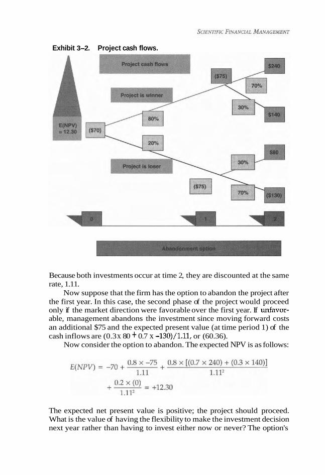
Exhibit 3-2. Project cash flows.
Because both investments occur at time 2, they are discounted at the same rate, 1.11.
Now suppose that the firm has the option to abandon the project after the first year. In this case, the second phase of the project would proceed only if the market direction were favorable over the first year. If &favor- able, management abandons the investment since moving forward costs an additional $75 and the expected present value (at time period 1) of the cash inflows are (0.3 x 80 + 0.7 x -130)/1.11, or (60.36).
Now consider the option to abandon. The expected NPV is as follows:
The expected net present value is positive; the project should proceed. What is the value of having the flexibility to make the investment decision next year rather than having to invest either now or never? The option's

Real Options: Evaluating R@D and Capital Investments 65
value is the difference between the two NPVs, or $12.30 less -$12.09, or $24.39. You can infer that the firm would be willing to pay $24.39 more for the opportunity to invest either now or next year versus now or never. In real option space-time, the project is as shown in Exhibit 3-2.
Shutdown Options
Shutdown options are almost identical to abandonment options, except the firm expects to restart production if conditions become favorable. It may not be feasible to operate a plant if revenues fail to justify costs. For example, if oil prices fall below extraction costs, it might be practical to close down until the price recovers. Shutdown options are valuable assets in agribusiness whereby options are exercised if growing and harvesting costs exceed revenues.
Operating Scale Options
These options give the holder the right (flexibility) to expand or scale down operations, for example, the right to expand production under favorable conditions, such as excess capacity. The "put" side can be exer- cised by forgoing future expenditures. This would indicate contracting operations or the project itself. The (put) option can be quite valuable.
Option to Expand Operations
Plant capacity can accumulate incrementally or in large blocks. One large facility might be constructed or several smaller ones assembled- depending on the timing and magnitude of future demand. For example, a key factor is often economies of scale. One large facility might cost less than four times that of four smaller facilities, each producingone-quarter the output of the big plant. For example, at Happy Doll Industries, rev- enues from a "dancing doll" may increase exponentially or move in the opposite direction, depending on the nature, timing, and demand of, say, the "happy doll fad."
While Happy Doll Enterprises cannot be sure exactly how sales will track, management is confident that plant expansion is the correct strategy. Two options are available: (1) begin with a small expansion program, building up capacity slowly; and (2) invest in large-scale production right then and there. If Happy starts small, the firm implicitly holds valuable options since large-scale- facilities require substantial financing before the first sales dollar appears. High debt levels increase financial risk, which might block addition funding, just when it is needed most. As leverage jumps, funds are redirected away from investment activities to service debt, cannibalizing operating cash flows.

Real options fit the bill nicely. If demand picks up, the option to expand can be exercised. If demand drops off, the option is out of the money, and so management will not exercise the option. If Happy Doll builds a large facility immediately, all options are exercised at once.
The way to go on this: A binomial tree systematizes the array in space- time by quantifying the trade-off between revenues resulting from imme- diate expansion (the tree's upper space) and reduced expected losses asso- ciated with slower expansion rates (referred to as operating leverage risk in the finance literature). Thus, real options has defined the optimal strategy. A conservative expansion strategy maximized the value associated with an immediate large-scale investment.
Contractual Options
These options contain specific contract terms that change the risk profile faced by asset owners. For example, venture capitalists frequently include contract terms that give them priority in liquidation (downside protection) and rights to invest alongside follow-on investors (protection against dilu- tion of the upside potential).
Switching Options
The most general situation-options giving the holder the right to either expand or contract is analogous to a portfolio of puts and calls. Restart- ing production when facilities are currently shutdown is a call option, while shutting down an on-line facility is a put. Projects that can be dynamically turned on and off are more valuable than identical ones without switching elasticity. Perhaps management may elect to build a facility at reduced (initial) construction costs carrying higher mainte- nanc
e
in order to acquire the flexibility to scale down maintenance if sales fall below projections.
Here is an example. AppNetworks Corp. must construct a new facil- ity to produce portable hard drives able to plug into PCMCIA slots of lap- tops. Sales projections show a highly uncertain market that is spread across three geographic areas. A NPV approach indicated that two pro- duction facilities would cost less to build and operate. However, much higher yields result if three plants are constructed, one at each location, thus creating an option to switch production as needed.
Learning Options
The firm invests to learn more about technology or resources. Oil and Gas Development Corp. is engaged in the exploration, development, and production of oil and gas, primarily in the Southwest. To finance
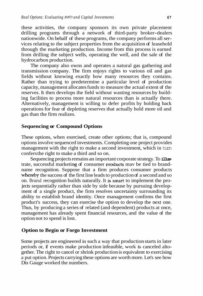
Real Options: Evaluating R 8 D and Capital Investments 67
these activities, the company sponsors its own private placement drilling programs through a network of third-party broker-dealers nationwide. On behalf of these programs, the company performs all ser- vices relating to the subject properties from the acquisition of leasehold through the marketing production. Income from this process is earned from drilling the subject wells, operating the well, and the sale of the hydrocarbon production.
The company also owns and operates a natural gas gathering and transmission company. The firm enjoys rights to various oil and gas fields without knowing exactly how many resources they contains. Rather than trying to predetermine a particular level of production capacity, management allocates funds to measure the actual extent of the reserves. It then develops the field without wasting resources by build- ing facilities to process more natural resources than is actually there. Alternatively, management is willing to defer profits by holding back operations for fear of depleting reserves that actually hold more oil and gas than the firm realizes.
Sequencing or Compound Options
These options, when exercised, create other options; that is, compound options involve sequenced investments. Completing one project provides management with the right to make a second investment, which in turn confers the right to make a third and so on.
Sequencing projects remains an important corporate strategy. To illus- trate, successful marketing of consumer vroducts mav be tied to brand- " name recognition. Suppose that a firm produces consumer products whereby the success of the first line leads to oroduction of a second and so on. ~ra*d recognition builds naturally. It is'smart to implement the pro- jects sequentially rather than side by side because by pursuing develop- ment of a single product, the firm resolves uncertainty surrounding its ability to establish brand identity. Once management confirms the first product's success, they can exercise the option to develop the next one. Thus, by producing a series of related (and dependent) products at once, management has already spent financial resources, and the value of the option not to spend is lost.
Option to Begin or Forgo Investment
Some projects are engineered in such a way that production starts in later periods or, if events make production infeasible, work is canceled alto- gether. The right to cancel or shrink production is equivalent to exercising a put option. Projects carrying these options are worth more. Let's see how Dix Gauge worked the numbers.

CASE STUDY: OPTION TO BEGIN OR FORGO INVESTMENT
Determining the Feasibility and Value of New Technology1
Dix Gauge Corporation produces high-end digital thermometer and ther- mostats, the only digital sensor that can maintain an accuracy of 9 ° C throughout the 3V to 5V power range. By combining economies of scale and cost without sacrificing digital accuracy and flexibility, the firm provides pre- mium thermal management in space- and weight-constrained applications.
Applications for the product include disk drives in PCs, servers, and workstations; environmental and biomedical diagnostic equipment; hand- held instruments, such as cellular telephones; or any thermally sensitive, electronically controlled system.
The firm's growth plans call for greater presence in the biomedical diag- nostics market, a highly competitive environment. Development of a new type of thermal laser sensor is on the drawing boards. To keep the case sim- ple, let's assume that the thermal laser can be evaluated in a single trials phase so that we can lower the range of possible outcomes. Once understood, the approach and calculations are easy to extend to as many phases and out- comes as are appropriate. [CD:MODELS/EXCEL/C3DGCaseSim/ScenOne]
Let's also assume that the company contemplates an R&D project with an initial research phase followed by a development phase. Suppose that the company is contemplating an R&D project with an initial research phase fol- lowed by a development phase. Initial research costs $1.4 million, takes a year, and has three possible outcomes, each with a degree of probability that can be extrapolated from similar research projects in the past. The chance of creating a highly effective laser sensor (or one that will be used widely) is 9%, a moderately effective laser sensor (or one with a narrower range of uses) is also 9%, and no laser sensor production at all is 80%. If researchers come up with a new laser sensor, the project will enter the developmental phase, also lasting a year, at a cost of $4 million. There are two possible out- comes at this juncture: The laser sensor will either pass the safety tests (40% probability) or fail them (60% probability). (In a more complex example, the company might have the option of accelerating the test phase, perhaps in response to competitive pressure, by laying out more money.)
Should the laser sensor pass the safety tests, it can be marketed. The com- pany estimates that a highly effective laser sensor would reap annual rev- enues of $18.5 million. For the sake of simplicity, assume that this would continue in perpetuity and that the company's risk adjusted cost of capital i s 9.5% (real options have not been employed yet, so management cannot argue for an interest rate reduction associated with lower project risk). The
1. This case was thoroughly reworked and expanded, and original spreadsheets were developed. My inspiration came from an excellent short example titled "R&D in pharma- ceuticals," Thomas E. Copeland and Philip T. Keenan, appearing in "Making Real Options Real," The McKinsey Quarterly, no. 3 (1998).

Real Options: Evaluating R@D and Capital Investments 69
Table 3-4. Scenario 1 : Very successful product.
Initial investment, time period 0
Development, time period 1
Cost to build factory, time period 2
Perpetuity income Value of perpetuity Net cash flow, year 2 N PV Probability of
successful research Probability of
successful development Cumulative probability Expected NPV
project has a present value of $194.7 million at the start of the marketing phase: We'll examine four phases of analysis covering ground from naive NPV-decision tree analysis all the way to real options incorporating Monte Carlo simulations (see Table 3-4).
Analysis Phase 1 Expected NPV-Decision Tree Analysis: Most Likely Scenario
Should the company go ahead with the project? Not yet aware of real options, management works out traditional approaches: NPV and deci- sion trees. Realizing that the problem is too complex for a single-scenario NPV calculation, management computes several scenarios. For a great product, the expected NPV is $52.3 million (see Table 3-4) since cash flows (before discounting at the 9.5% cost of capital) are minus $1.4 mil- lion in year 0, minus $4 million in year 1, and $194.7 million less $126 million in year 2.
Using the same analysis, a moderately effective laser sensor would gen- erate income of $13 million and have a present value of $136.8 million. Needless to sav, all these revenues lie at least two vears in the future and are , , thus uncertain. The marketing department suggests that a great product might generate annual revenues ranging from $16 million to $20.3 million and a mediocre one from $1 1.7 million to $14.3 million. Building a factory to pro- duce the laser sensor will cost about $127 million (see Table 3-5).
For a mediocre product, the expected N W is $1 13.6 thousand (seeTable 3-5). Then again, there could be no product at all, which would generate a present

Table 3-5. Scenario 2: Moderately successful pkoduct.
Initial investment, time period 0 Development, time period 1 Cost to build factory, time period 2 Perpetuity income Value of perpetuity Net cash flow, year 2 N PV Probability of successful research Probability of successful develop me^ Cumulative probability Expected NPV
Table 3-6. Scenario 3: Produce value loss of $1.4, or an N W of minus 1 .I no digital sensors. million, depending on whether the com-
pany carried the project into the develop- ($1~400~000) ment phase (see Table 3-6).
Probability 80°/" Next, the company combines these Expected NPV ($1f120'000) scenarios into a single probability-
weighted NPV by drawing a decision tree (see Exhibit 3-3). There is a 3.6% chance (9% in the research phase times 40°/0 in the development phase) of creating a great product with an NPV of $52.3 million and a 4% chance of creating a mediocre product with an NPV of $3.2 million. The chance that the research wil l be an utter failure costine the comwanv $1.4 million is 80%. u 8 ,
Finally, the project has a 13% chance of running aground during the development phase, for a present value loss of $5 million, throwing off a weighted ($656.8) thousand NPV (see Table 3-7).
Thus, the overall value of the R&D project, calculated with decision trees directed at a ~robabilitv-weighted NPV, comes to $21 8.5 thousand. The indi- u
vidual compieting theJanalysis recom'mended that the firm move forward and develop the project (see Table 3-8).
Analysis Phase 2 Expected NPV: Run Monte Carlo Simulations
(We wil l study Monte Carlo simulations in chapter 7. For now, we wil l run the tests and accept the conclusions.)
The CFO was not at all satisfied that the previous analysis went far enough. The probability-weighted NPV was close to breakeven, leaving very little room for error. Senior management wanted simulations run and wil l not proceed until important issues dealing with uncertainty were put to rest.
The standard forecasting model outlined previously relied on a set of assumptions leading to only one-outcome: the base case. The project is

Real Options: Evaluating R&D and Capital Investments 71
Exhibit 3-3. The project's decision tree analysis: Phase 1.
Year 2: Value of Perpetuity - Factory Cost = Net CF Year 2
Table 3-7. Scenario 4: Running around during development.
Initial investment, time period 0 ($1,400,000) Development, time period 1 ($4,000,000) Loss before discount ($5,400,000) Loss after discount @ 9.5% ($5,052,968) Probability 13% Expected NPV ($656,886)
complicated; an analysis cannot proceed to real options until the firm runs Monte Carlo simulations centered around at least two different assumption variables: projected income under very successful product conditions and projected income under moderately successful product conditions. In short, i t is exceedingly difficult to know which strategic options the firm should pursue since we do not yet know the ranges and distributions of outcomes and the most likely scenario associated with each option-golno go (see Tables 3-9 to 3-1 2).
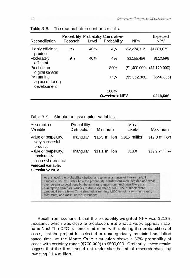
Table 3-8. The reconciliation confirms results.
Probability Probability Cumulative- Expected Reconciliation Research Level Probability NPV NPV
Highly efficient 9% 40% 4% $52,274,312 $1,881,875 product
Moderately 9% 40% 4% $3,155,456 $1 13,596 efficient
Produce no 80% ($1,400,000) ($1,120,000) digital sensors
PV running 13% ($5,052,968) ($656,886) aground during development
1 00% Curnulafive NPV $218,586
Table 3-9. Simulation assumption variables.
Assumption Probability Most Variable Distribution Minimum Likely Maximum
Value of perpetuity, Triangular $1 6.5 million $1 8.5 million $1 9.0 million very successful product
Value of perpetuity, Triangular $1 1.1 million $13.0 $1 3.3 million moderately successful product
Forecast variable: Curnula tive NPV
Recall from scenario 1 that the probability-weighted NPV was $21 8.5 thousand, which was-close to breakeven. But what a week approach sce- nario 1 is! The CFO is concerned more with defining the probabilities of losses, lest the project be selected in a categorically restricted and blind space-time. As the Monte Carlo simulation shows a 63% probability of losses with certainty range ($700,000) to $500,000. Ordinarily, these results suggest that the firm should not undertake the initial research phase by investing $1.4 million.

Real Options: Evaluating R&D and Capital Investments
Table 3-1 0. Scenario 1: Very successful product under uncertainty (key variable: perpetuity income).
Initial investment, time period 0 ($1,400,000) Development, time period 1 ($4,000,000) Cost to build factory, time period 2 ($1 26,000,000) Perpetuity income $18,008,713 Value of perpetuity $1 89,565,404 Net cash flow, year 2 $63,565,404 N PV $47,961,276 Probability of successful research 9% Probability of successful development 40% Cumulative probability 3.6% Expected NPV $1,726,605.95
Table 3-1 1. Scenario 2: Moderately successful product.
Initial investment, time period 0 ($1,400,000) Development time period 1 ($4,000,000) Cost to build factory,
time period 2 ($1 26,000,000) Perpetuity income $12,487,382 Value of perpetuity $131,446,123 Net cash flow, year 2 $4,446,123 N PV -$1,344,853 Probability of successful research 9% Probability of successful development 40% Cumulative probability 3.6% Expected NPV
Given Given
Given Derived = $12,487,3821,095 = $1 31,446,123 - $127,000,000 discounted cash flow @ 9.5%
Analysis Phase 3: Real Opt ions Analysis [CD:MODELS/EXCEL/C3CaseSim/RealOptionl
A real options analysis conducted without the benefit of Monte Carlo sim- ulation places its value at $3.9 million. This suggests that the company should (1) undertake the initial research phase by investing $1.4 mil l ion and (2) take a wait-and-see position until the expiration date of their option a year from today. If conditions are favorable, the firm w i l l exercise their options to invest further in the project. If conditions are unfavorable, the f irm produces no digital sensors. Setting up the option, we note the infor- mation given in Table 3-1 3.

Table 3-1 2. Simulation report.
Forecast: Cumulative NPV Summary: Certainty level i s 63.10%. Certainty range i s from -infinity to $0. Display range is from ($700,000) to $500,000. Entire range is from ($899,232) to $409,579. After 1,0& trials, the std. error of the mean is $7,094.
Statistics Value
Trials Mean Median Mode Standard deviation Variance Skewness Kurtosis Coefficient of variability Range minimum Range maximum Range width Mean standard error
Forecast: Cumulative NPV
1,ODOTrlals Frequency Chart 8 Outliers
($700,000) ($400,000) ($100000) $200,000 $500.000
Certlinty is63.10% from -Infinity to $0
The real option valuation is so much higher than that arrived at through a decision tree or probability-weighted NPV that it changes the recommen- dation from no go to go. There are several reasons for this.
First, real option valuation maps out all available possibilities, including those not readily apparent in the decision tree. Although there are two important sources of uncertainty, technological and product market, tradi-

Real Options: Evaluating R@D and Capital Investments
Table 3-1 3. Real options assumptions forgo commitment now: Wait a year.
1. Cost of capital: Reduces to 9.2% as risk is reduced. 2. Initial investment time: Commitment costs begin in period 0. 3. Development time: Changes from period 1 to period 2. 4. Cost to build factory time period: Changes from period 2 to period 3. 5. E(NPVI: Will be discounted back to time period 0. 6. Development cost: Set at $4,5000,000, a slight increase. 7. Cost to build factory: Increases to $1 35,000,000 because of delay. 8. Perpetuity income: Very successful product increases to $1 9,000,000. 9. Perpetuity income: Moderately successful product decreases to $8,500,000
due to loss of market share associated with project start time delay. 10. Probability of successful development: 60%. 1 1. Probability of successful research: 70%. 12. Probability of producing no sensors: 0% if option exercised and development
starts. 13. Probability of running aground during development: Increases slightly to 14%.
These assurnptions/inpuh are made by the finance area and are not the product of any software.
tional analysis focuses solely on the former, ignoring the latter by focusing too narrowly on the expected value of cash flows. As we saw, the real option valuation takes into account an important element of flexibility: the possibil- ity of not marketing the laser sensor, even if it passes the safety testing phase, should the revised product market outlook seem gloomy. The higher the uncertainty surrounding potential cash flows, the higher the real option val- uation. Traditional approaches ignore this kind of uncertainty and manage- ment's ability to respond to it.
Also, real option valuation differs from the one arrived at through a deci- sion by varying the discount rate appropriately throughout the tree instead of using a single rate, such as the weighted average cost of capital. Thus, it accounts properly for the relative level of risk that different cash flows involve. Where real options represent substantial leverage, this impact on the discount rate may be enormous; not the difference between 9% and 12O/0 but rather between 9% and 40% (or minus 40%, depending on the nature of the o~t ion) .
Moreover by varying the discount rate appropriately throughout the binomial tree instead of using a single rate, such as the WACC (weighted- average cost of capital), a real option valuation differs from a traditional technique valuation (NPV, IRR, MIRR). Thus, a real option valuation accounts ~ r o ~ e r l v for the relative level of risk that different cash flows involve. Where ieai op;ions represent substantial leverage is where the volatility of the dis- count rate may be enormous, reflected not in the difference between 9% and 12% but rather the difference between 9% and 40% (or minus 40% depend- ing on the nature of the option).

Table 3-1 4. Scenario 1 : Very successful product laser sensor.
Erne Discount Period Rate
Initial investment, time period 0 ($1,400,000) 0 9.2% Development, time period 1,
two years from now ($4,500,000) 2 Cost to build factory, time
period 2, three years from now ($1 35,000,000) 3
Perpetuity income $1 9,000,000 Value of perpetuity $206,521,739 Net cash flow year, 3 $71,521,739 N PV $49,751,312 Probability of successful research 70% Probability of successful development 60% Cumulative probability 42.0% Expected NPV $20,895,551
Table 3-15. Scenario 2: Moderately successful product.
Period
Initial investment, time period 0 ($1,400,000) 0 Development, time period 1,
two years from now ($4,500,000) 2 Cost to build factory, time period 2,
three years from now ($1 35,000,000) 3 Perpetuity income $8,500,000 Value of perpetuity $92,391,304 Net cash flow, year 3 ($42,608,696) N PV ($37,894,982) Probability of successful research 70% Probability of successful development 60% Cumulative probability 42.0% Expected NPV ($1 5,915,892)
Table 3-1 6. Scenario 3: Produce no digital sensors.
($1,400,000) Probability 0% Expected NPV $0

Real Options: Evaluating Rt9D and Capital Investments 77
Table 3-1 7. Scenario 4: Running aground during development.
Period
Initial investment, time period 0 ($1,400,000) 0 Development, time period 1,
two years from now ($4,500,000) 2 Loss before discount ($5,900,000) N PV ($5,173,699) Probability estimated one year from now 16% Expected NPV ($827,791.81)
Thus, real option valuation identifies the optimal course for the com- pany at each stage in the process. The initial recommendation is to under- take the research at a cost of $1.4 million. If the research fails, there is no development phase. The company in a sense exercises its put option on further development. Even if the research succeeds, the real option valua- tion demonstrates that it is sometimes unwise to proceed with develop- ment, particularly if the laser sensor in question i s a mediocre one and the revised market forecast for the coming year is less optimistic than origi- nally expected. Should the development phase proceed successfully, i t is still not always wise to market a laser sensor, for when forecasts turn pes- simistic, even a great laser sensor may not cover its costs. By factoring in all alternatives appropriately, the real option approach uncovers addi- tional value that can change recommendations for projects at several stages in their evolution.
Summary, Analysis Phase 3: Real Options Analysis
Tables 3-14 to 3-19 summarize this phase.
Analysis Phase 4: Real Options Analysis Running Monte Carlo Monte Carlo Simulations [CD:MODELS/EXCEL/C3CaseSim/Phase4Sim]
Table 3-20 depicts Phase 4 simulation assumption variables. Assume that the firm exercised i ts one-year option to begin or forgo
investment in this project. A real option and Monte Carlo simulation analysis completed by Crystal Ball would certainty call for a "move for- ward" decision. Why? The certainty level at a 95% confidence reveals that the expected NPV range i s from $2.1 million to $5.3 million. The entire range is from $1.5 million to $6.4 million (see Table 3-21).
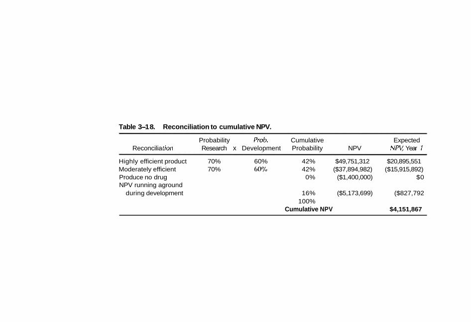
Table 3-1 8. Reconciliation to cumulative NPV.
Probability Prob. Cumulative Expected Reconcilia tion Research x Development Probability NPV NPV Year I
Highly efficient product 70% 60% 42% $49,751,312 $20,895,551 Moderately efficient 70% 60% 42% ($37,894,982) ($1 5,915,892) Produce no drug 0% ($1,400,000) $0 NPV running aground
during development 16% ($5,173,699) ($827,792 100%
Cumulative NPV $4,151,867

Real Options: Evaluating R&D and Capital Investments 79
Table 3-1 9. Option value.
Value of project if option exercised one year from now: Produce laser sensor
Cumulative NPV $4,757,867
Value of project if option exercised one year from now: Do not build
Loss of initial investment ($1,400,000)
Summary Probabilities producing drug 1 00.0% Project value: Wait-and-see 0ption:Weighted alternatives $4,151,876 Project value: Start immediately option $248,610 Option value $3,903,257
Table 3-20. Real option simulation distributions-Input.
Assumption Most Likely or Variables Distribution Minimum Standard Deviation Maximum
Probability of Uniform 68% N/A 71 % successful research
Probability of Uniform 59% N/A 61 % successful development
Probability of running Normal 16% 1 % N/A aground if option exercised
Value of perpetuity Triangular $1 8.8 $19.0 $1 9.2 (very successful million million million product)
Value of perpetuity Normal $8.5 $.2 o N/A (moderately million successful product)
Closing Thoughts
Management's ability to alter future action in response to changing market conditions can profoundly affect the decision to invest since investment opportunities are collections of options on real assets. Remarkably, real option value and equity value fit as needle and thread because capital projects are, in many industries, a firm's most important value driver.
Without real options analysis, management forgoes the chance to evaluate (new) information that might change investment strategies. Lost information is an opportunity cost that has to be considered when investments are valued.

Table 3-21. Simulation results: Real option+Output.
Summary Certainty level is 95.00% Certainty range is from $2,138,239 to $5,256,092 Display range is from $1,500,000 to $6,000,000 Entire range is from $1,472, 881 to $6,384,534 After 1,000 trials, the standard error of the mean is $24,215
Statistics Value Trials 1000 Mean $3,865,754 Median $3,892,888 Mode -
Standard deviation $765,740 Variance 6E+ 11 Skewness 0.03 Kurtosis 3.09 Coefficient of variability 0.20 Range minimum $1,472,881 Range maximum $6,384,534 Range width $4,911,653 Mean standard error $ 24,214.84
-- -~ ~ --
Forecast: Optlon Value
1 1,000Trials Frequency Chart ,037
,028 b .- $ ,019 n 0
,009
,000
$1,500,000 $2,625,000 $3,750,000 $4,875,000 $6,000,000
Certainty is 95.00% from $2,138,239 to $5,256,092 1 --
FinaUy, as technology unfolds at an increasing rate with an increasingly large number of firms focused on returns to the providers of capital, management will take a new hard look at shareholder value and how the number was derived. CFOs, CEOs, and the board want visionary analytics, not old stan- dard bearers delivering this number. Thus, real options have come of age and are no longer looked on as just another business school theory.
So far, we have developed capital investment analysis using two mediums: the vernacular (Word) with help from Excel, a wonderful but

Real Options: Evaluating R&D and Capital Investments 81
flat two-dimensional model. We leave this chapter with our analyses stuck between two insentient, inorganic environments no matter how brilliant the result may appear. Real options are indeed real; they operate in a kinetic, dynamic medium. For that reason, we will transport project analy- sis from flat-plane, two-dimensional space to higher-dimension real time- visual modeling.
Chapter Three References and Selected Readings
Books and Periodicals
Amram, M., and N. Kulatilaka. (1999). "Real options: Managing strategic investment in an uncertain world." Financial Management Association survey and synthesis series. Boston: Harvard Business School Press, x, 246.
Campbell R., C. Harvey, and S. Gray. "International project evaluation, real options and mergers and acquisitions." Global Financial Management.
Chan-Lau, J. A., et al. (1998). "Fixed inoestment and capital flows: A real options approach." Washington, D.C.: International Monetary Fund Research Department.
Childs, P. D., et al. (1998). "Capital budgeting for interrelated projects: A real options approach." Journal of Financial and Quantitative Analysis, 305-34.
Cortazar, G., and J. Casassus. (1998). "Optimal timing of a mine expansion: Implementing a real options model." Quarterly Review of Economics and Finance (Special Issue), 75549.
Davis, G. A. (1998). "Estimating volatility and dividend yields when valuing real options to invest or abandon." Quarterly Review of Economics and Finance (Special Issue), 725-54.
Luehrman, T. A. (1998). "Investment opportunities as real options: Getting started on the numbers." Harvard Business Review, 51-67. Here's a way to apply option pricing to strategic decisions without hiring an army of Ph.D.'s.
Luehrman, T. A. (1998). "Strategy as a portfolio of real options." Harvard Business Reuiew, 89-99.
Neely, J. E. (1998). "Improving the valuation of research and development: A composite of real options, decision analysis and benefit valuation frameworks."
Pinches, G. E., and D. M. Lander (1998). "Challenges to the practical implementation of modeling and valuing real options." Quarterly Reviezu of Economics and Finance (Special Issue), 53747.
Rose, S. (1998). "Valuation of interacting real options in a tollroad infrastructure project." Quarterly Review of Economics and Finance (Special Issue), 711-23.
Sanchez, R. A. (1991). "Strategic flexibility, real options, and product-based skategy." Sick, G., et al. (1990). Capital budgeting with real options. New York: Salomon Brothers Cen-
ter for the Study of Financial Institutions, Leonard N. Stem School of Business, New York University
Trigeorgis, L. (1995). Real options in capital investment: Models, strategies, and applications. Westport, Conn.: Praeger.
Trigeorgis, L. (1996). Real options: Maqerial flexibility and strategy in resource allocation. Cambridge: MIT Press.
Williams, J. ~:(1993). "Equilibrium and options on real assets." Review of Financial Studies, 825-50.

Other Periodicals
Alleman, James. (1999). "Real options: Management flexibility and strategy in resource allocation." Information Economics and Policy, 11(2), 229.
Alvarez, Luis H. R. (1999). "Optimal exit and valuation under demand uncertainty: A real options approach." European Journal of Operational Research, 114(2), 320.
Anonymous. (1998). "Capital investment-A new approach." Management Accounting, 76(5), 28.
Anonymous. (1999). "Survival: The very real option." P~ofessional Engineering, 12(6), 57. Benaroch, Michel. (1999). "A case for using real options pricing analysis to evaluate infor-
mation technology project investments." Information Systems Research, 10(1), 70. Bollen, Nicholas B. P. (1999). "Real options and product life cycles." Management Science,
45(5), 670. Cortazar, Gonzalo. (1998). "Optimal timing of a mine expansion: Implementing a real
options model." Quarterly Review of Economics and Finance, 38, 755. Coy, Peter. (1999). "Exploiting uncertainty; The 'real-options' revolution in decision-
making." Business Week, June 7, p. 118, Industrial/Technology edition. Dangl, Thomas. (1999). "Investment and capacity choice under uncertain demand." Euro-
pean Iournal ofOperationa1 Research, 117(3), 415. Esty, Benjamin C. (1999). "Improving techniques for valuing large-scale projects." Journal of
Project Finance, 5(1), 9. Garud, Raghu. (1998). "Real options or fool's gold? Perspective makes the difference." The
Academy of Management Review, 23(2), 212. Herath, Hemantha S. B. (1999). "Economic analysis of R&D projects: An options approach."
The Engineering Economist, 44(1), 1. Jagle, Axel J. (1999). "Shareholder value, real options, and innovation in technology-
intensive companies." R b D Management, 29(3), 271. Kensinger, John. (1999). "International investment-Value creation and appraisal: A real
options approach." Journal of Finance, 54(6), 2387. Kingley, Jay. (1999). "Six steps to exercising real options at work." 12(17), 52. Leslie, Keith, (1998). "The real power of real options." Corporate Finance (158), 13. Mayo, H. (1999). "Real options: Managing strategic investments, in an uncertain world."
Choice, 36(10), 1833. McGrath, Rita Gunther. (1998). "Only fools rush in? Using real options reasoning to inform
the theory of technology strategy: Response to Garud, Kurnaraswamy, and Nayyar." The Academy of Management Review, 23(2), 214.
Panayi, Sylvia. (1998). "Multi-stage real options: The cases of information technology infra- structure and international bank expansion." Quarterly Review of Economics and Finance, 38, 675.
Perlitz, Manfred. (1999). "Real options valuation: The new frontier in R&D project evalua- tion?" R & D Management, 29(3), 255.
Rose, Simone. (1998). "Valuation of interacting real options in a tollroad infrastructure pro- ject." Quarterly Review of Economics and Finance, 38, 711.
Select Internet Library
Real Options: Others Classical Papers The following selection complements the "Real Options Classical Papers" list and also contributed with important insights into real options approach. There are comments, for each paper, available by clicking their titles (under construction). The papers in this page are in chronological order. http://www.puc-rio.br/marco.ind/non-tabl/ bib-cla2.html.

Real Options: Evaluating Rt9D and Capital Investments 83
Finance Site List These Web lmks are placed here for those interested in understanding and teaching financial ideas. The Journal ofFinnnee maintains the site. http://www.cob.ohio-state.edu/ dept/h/joumal/jofsites.htm.
Real Options Group NIAS/Royal Netherlands Academy of Arts and Sciences Bocconi University, Univer- sity of Calgary, Erasmus University, Northwestern University Last Updated: May 17, 1999 http://www.realoptions.org/.
Real Options Bibliography The following publications provide a good introduction to the theory and application of real options thinking. Admittedly, some is rather esoteric, but most is accessible to nonspecialists. (Notes: Registration is required to access the McKinsey @arterly; PDF files require Acrobat Reader software.) http://www.modus-group.com/realoptionbiblio. htm.
The Real Options Contributions Page! This page is dedicated to contributions from the readers. Working papers, abstracts, dissertations, comments of papers, multimedia materials, and so on, related to real options approach (even if is not petroleum specific). http://www-rpa.puc-rio.br/ marco.ind/contibl.html.
Real Options Softwares Webpage I divided the real options software into three groups: (1) Spreadsheet applications, market currently dominated by Excel; (2) mathematical softwares applications, such as Mathcad, Mathematica Matlab, and Mapple; and (3) computer programming lan- guages, for more professional applications, with highlights for C + + and Java. http:Nwww-rpa.puc-rio.br/marco.ind/software.html.
A Case for Using Real Options Pricing Analysis to Evaluate Information Technology Project Investments http://sominfo.syr.edu/facstaff/mbenaroc/resume/PAPERS/ OPM-ISR/WWW-PAPR.hhn1.
Name Size TYPe
C3DGBaseSim 22YKB Microsoft Excel Worksheet


Visual Financial Models
RECENTLY, TI~E PROFILERATION OF FINANCE technology has been enomous. A few short years from now, our perceptions will not have changed, but "explo- sion" will be the proper word, not "profileration." Corporate valuation analysis and the spreadsheet will have since parted company; visual model- ing will be the lead tool showing CEOs and board members the way through value gap analytics, and office computers will accommodate one or two giga- bytes of memory, at most, having been made obsolete by the live wire. And the Web and Internet will go unmatched as the sustaining force behind a new brand of technologic science that we will come to know as finance.
Today-still, a good assortment of models can dissect and evaluate deals and financial problems--some assorted other corporate assign- ments, some quite complicated. But few models loaded on our worksta- tions or graduate school computers are capable of offering an optimal architecture for, say, the completion of a divisional "make or break" restructuring analysis or an acquisition/divestiture position paper up for review by the CFO or board. In truth, modem visual modeling, not rows and columns, may well be the vehicle of choice to get the deal structured, understood, and above all sold. So the question we might ask is, "Can your software handle the firm's voluminous data and its dynamic environ- ment?" Often not, unless you work with nonlinear models. Linear models have been in use a long time with little empirical testing of their inherent, internal two-dimensional structure. The result is that they force linearity assumptions on nonlinear data.
As an analogy, imagine a two-dimensional world with mythical two- dimentional people called Flatpeople. To keep their children from straying from a playground, Flatpeople simply draw a circle around them. No

matter which way the children move, they hit the impenetrable circle. However, it is a trival task for us to spring the children from the play- ground.' We just reach down, grab the flat children, peel them off their two-dimensional world, and redeposit them elsewhere on their world. To other children, it appears as though one of them has mysteriously van- ished into thin air. This feat, quite ordinary in three dimensions, appears fantastic in two dimensions. Most of our cash flow projections, valuations, and inventory optimization methods have been living in "flat" linear dependence almost since finance was invented.
You may have run across valuation problems that you attemped to puzzle out with "a s.traight line," for example, working the deal under the assumption that variable coefficients are stable over time. Straight lines in our corporate valuations are left in illusional two-dimensional space, like the Flatpeople's playground-parallelism does not exist in real world busi- ness, certainly not in financial analysis. When global influences change, as they must every day, the coefficients of your models must be trained to incorporate that change, or any problem resting on your model's forecast will itself be flawed. Let's investigate, first, a two-dimensional representa- tion: the spreadsheet. From there, we will explore visual modeling.
Background
A modeling application is any tool that helps analysts collect, analyze, and present information, often in an interactive and iterative way. Models help determine the impact of alternative strategies on the operating unit or firm's value-the least common denominator. For example, CFOs often use financial models to:
A Test the relative risk of a corporate buyout A Determine equity values given the dynamic nature of value drivers A Asess debt structures and develop priorities for debt repayment. A Refine working capital policy.
Financial models usually consists of six components: navigation, data entry, data analysis, calculation, reports and presentations, and storage.
Navigation
This capability allows modelers to move around the model's different parts. It may consist of menus, buttons, toolbars, and wizards and on-line help. These engines vary from very tightly controlled, forcing the analyst
1. Thank you Dr. Kaku for your wonderful analogy. MICHIO KAKU, HYPERSPACE, a Sci- entific Odyssey through Parallel Universes, time warps and the Tenth Dimension, Oxford University Press, 1994.

Visual Financial Models 87
through set paths, to very open, offering a good deal of freedom. The sophistication of analysts, together with its proposed use, determines which type of navigation mechanism is best.
Data Bntry
This is the part of the application into which data (assumptions, numbers, and options) can be entered.
Data Analysis
Very often, interactive analysis is supported as well. This is the ability to immediately see how the input affects the results, often referred to as "what-if" analysis. The calculation engine described next makes this possible.
Calculation
This is where the model implements financial rules. These rules are typi- cally represented by formulas, macros, and processes that operate on the inputs to come up with the best results. The important issue is one of integrity and incorruptibility. For example, flexible spreadsheet models such as Excel allow developers almost total freedom in writing formulas. This is fine for basic models.
However, complex models, models for policy analysis or models that determine equity values are much too important to "fiddle" around with the model's nuclear structure. That is why technology delivered by ven- dors such as Decisioneering, MATLAB, ALCAR, Mathematica, and partic- ularly the visual modeling base that Lumina offers (plus a host of other reputable developers) have won the support of financial decision makers- you cannot afford to engage your CFO or board questioning a valuation model's structure and integrity.
Reports and Presentations
This is output either printed or viewed on-screen. This may take the form of tables, charts and multidimensional graphs, visual diagrams, and vari- ous combinations thereof.
Storage
This is where data are stored for further implementation. Templates are made whereby input values are entered later.

Team Effort
Modeling is a team effort and requires good communication. Intricate mod- els that are organized by one or two staff members, no matter how talented, may not escape errors, particularly if the original developer is too close to the problem. Poorly structured models or the infamous black box serve no one.
Although software may produce spectacular results in the hands of a skilled analyst, it can also produce spectacular garbage of extraordinary complexity in the hands of an incompetent or careless analyst. The saving grace of such tools is that, if they make it easier to exercise, scrutinize, audit, and critique models, they can facilitate peer review and open debate about policy models, providing a powerful mechanism for improving stan- dards of practi~e.~
Building Effective Models3
The best financial models are clear, comprehensible, and correct. The key to producing a powerful design is to start with a basic format and pro- gressively refine and extend your model where tests of your initial ver- sions point to improvements. Remember that the whole idea of financial modeling is to help you discover which options will optimize your objec- tives and the financial assignment you have been asked to complete. How can you go about developing an accomplished and skillful model?
First, identlfy key decision variables. A decision variable is a variable that you affect directly: which industry to seek an acquisition, how much to bid on the contract, which accounts receivable policy is best, when to start new product marketing, and so on. Occasionally, financial analysts want to build a model just for the sake of furthering understanding, with- out explicitly considering decisions. Most often, however, the ultimate purpose is to make a better decision. In those cases, the decision variables are where you should start your model.
Next, identify your objectives. Sometimes the objective is simply to maximize expected profit or value, find the optimal financial mix, or min- imize costs. Utility theory and multiattribute decision analysis provide an array of methods to help structure and quantify objectives in the form of utility. Whatever approach you take, it is important to represent the objec- tives in an explicit and quantifiable form if the objectives are to be the basis for recommending one decision option over another. The most common
2. Lumina Decision System White Paper. The white paper on the Web site was written by M. Granger Morgan and Max Henrion. Referenced with permission, Lumina Decisions Systems. 3. The section was coauthored with Lurnina Decision Systems, home to the Analytica prod- uct family and developed with permission. Analytica is the modeling system featured in this chapter.
Visual Financial Models 89
mistake in specifying objectives is to select objectives that are too narrow. You might want to think in terms of the smallest common denominator- start small and build the model to the top. Do not start with the top and try to build down. For example, you will not start at headquarters and work your model down to the divisional level; rather, it is the other way around.
Next you focus on iden+ng the variables that make dear distinctio~~s- variables whose interpretations will not change with time or your boss. Extra effort here will be repaid in model accuracy and cogency. At this point, you begin to think about influence diagrams (more on influence diagrams when we actually learn to build our visual model). An influence diagram is a purely qualitative representation of a qualitative information path related to the model. It shows the variables and their dependencies. It is usually best to draw in most or all of the first version of your model as an influence dia- gram or hierarchy of diagrams before trying to quantify the values and rela- tionships between the variables. In this way, you can concentrate on the essential qualitative issues of what variables to include before having to worry about the details of how to quantify the relationships.
Should you create a simple or an intricate visual model? Financial visual models should be as simple as possible but no simpler. When the model is intended to reflect the views and knowledge of a group of peo- ple, it is especially valuable to start by drawing up an influence diagram as a group. For example, a small group can sit around the computer. It is best if you have the means to project the image onto a large screen so that the entire group can see and comment on the diagram as they create it. The ability to focus on the qualitative structure initially lets you involve early in the process participants who might not have the time or interest to be involved in the detailed quantitative analysis, which will most certainly involve dozens of simulation distribution possibilities.
With this approach, you can often obtain valuable insights and early buy-in to the modeling process from key people who would not otherwise be available. Perhaps the most common mistake in modeling is to try to build a model that is too complicated or that is complicated in the wrong ways. Just because the situation you are modeling is complicated does not necessarily mean that your model should be complicated. Every model is unavoidably a simplification of reality; otherwise, it would not be a model. The question is not whether your model should be a simplification but rather how simple it should be. A large model requires more effort to build, takes longer to execute, is harder to test, and is more difficult to understand than a small model, and it may not even be more accurate.
Testing and Debugging a Model
It is rare to create the first draft of a model without mistakes. For example, on your first try, definitions may not express what you really intended. It

is important to test and evaluate your model to make sure that it expresses what you have in mind. You should design the model specifically to make it as easy as possible to scrutinize model structures and dependencies, to explore model implications and behaviors, and to understand the reasons for them. We will set up our models in Analytica so that we can trust the algorithms. Accordingly, it is relatively easy to debug models once you have identified potential problems.
Test as You Build
You should evaluate variables once you have provided a definition for the variable and all the variables on which it depends, even if many other vari- ables in the model remain to be defined. You should evaluate each variable as soon as you can, immediately after you have provided definitions for the relevant parts of the model. In this way, you will discover problems as soon as possible after specifying the definitions that may have caused them. You can then try to identify the cause and to fix the problem while the definitions are still fresh in your memory. Moreover, you will be less likely to repeat the mistake in other parts of the model. If you wait until you believe that you have completed the model before testing it, it may contain several errors that interact in confusing ways. Then you will have to search through much larger sections of the model to track them down. However, if you have already tested the model components indepen- dently, you will have already removed most of the errors, and it will usu- ally be much easier to track down any that remain.
The best way to check that your model is well specified is to check it against reality. Compare its predictions against past empirical observa- tions. For example, if you are trying to predict future changes in the com- position of acid rain, you should try to compare its "predictions" for past years for which you have empirical observations. Or, if you are trying to forecast the future profitability of an existing enterprise, you should first calibrate your model in past years for which accounting data are available. If the model is hard to test against reality in advance of using it and if the consequences of mistakes could be catastrophic, you can borrow a tech- nique that NASA uses widely for the space program. You can get two inde- pendent modelers (or two modeling teams) to each build their own model, then check the models against each other. It is important that the modelers be independent and not discuss their work ahead of time to reduce the chance that both will make the same mistake. Test model behavior. Many problems become immediately obvious when you look at sensitivities and results, for example, if it has the wrong sign, the wrong order of magni- tude, or the wrong dimensions.
Other problems, of course, are not immediately obvious, for example, if the value is wrong by only a few percentage points. For more thorough testing, it is often helpful to analyze the model behavior by specifying a list

Visual Financial Models 91
of alternative values for one or two key inputs. If the model behaves in an unexpected way, this may be a sign of some mistake in the specification. For example, suppose that you are modeling a project finance's real option solution and the net value increases with reduced cash flow. You might suspect a problem in the model.
If analyzing the behavior or sensitivities of your model creates unex- pected behavior or unexpected results, there are logically two possibilities: Your model contains an error, in that it does not correctly express what you intended, or your expectations about how the model should behave were wrong.
You should first check the model carefully to make sure that it con- tains no errors and does indeed express what you intended. Explore the model to try to find out how it generates the unexpected results. If after thorough exploration you can find no mistake and the model persists in its unexpected behavior, do not despair! It may be that your assumptions were wrong in the first place. This discovery should be a cause for cele- bration rather than disappointment. If models always behaved exactly as expected, there would be little reason to build them. The most valuable insights come from models that behave counterintuitively When you understand how their behavior arises, you can deepen your understand- ing and improve your intuition, which is, after all, a fundamental goal of modeling.
D o m e n t the Model
Give your variables and modules meaningful titles so that, as you build it, others (or you, when you revisit the model a year later) can more easily understand the model from looking at its variables. It is better to refer to your variable as "Capital Expenditures" rather than "see AD144."
It is also a good idea to document your model as you construct it by com- pleting description and attributes for each variable and module. You may find that entering a line or two of description for each variable, explaining clearly what the variable represents, will help keep you clear about the model.
Entering units of measurement for each variable can help you avoid simple mistakes in model specification. Avoid the temptation to put docu- mentation off until the end of the project, when you may run out of time or may have forgotten key aspects. Most models, once built, spend the majority of their lives being used and modified by people other than their original author. Clear and thorough documentation pays continuing divi- dends; a model is incomplete without it. Have other people review your model. It is often very helpful to have outside reviewers scrutinize your model. Experts with different views and experiences may have valuable comments and suggestions for improving it.
For example, one of the advantages of using a modeling environment such as Analytica over conventional systems is that it is usually possible

for an expert in the domain to review the model directly, without addi- tional paper documentation. The reviewer can scrutinize the diagrams, the variables, their definitions, and the behavior of the model electronically. You can share models electronically on diskette or over a network.
Expanding Your Model
The best way to develop a model of appropriate size is to start in stages with a very simple model and then to extend it in stages in those ways that appear to be most important. With this approach, you will have a usable model early on. Moreover, you can analyze the sensitivities of the simple model to find out where the key uncertainties and gaps are and use this to set priorities for expanding the model. If, instead, you try to create a large model from the start, you run the risk of running out of time or computer resources before you have anything usable, and you may end up putting much work into creating an elaborate module for an aspect of the problem that turns out to be of little importance. Remember to:
A Identify ways to expand the model. A Identify ways to expand a model and improve the model. A Add variables that you think will be important. A Add objectives or criteria for evaluating outcomes. A Expand the number of decision options specified for a decision
variable or the number of possible outcomes for a discrete chance variable.
A Expand a single decision into two or more sequential decisions, with the later decision being made after more information is revealed.
A For a dynamic model, expand the time horizon (say, from 10 to 20 years) or reduce the time steps (say, from annual to quarterly time periods).
Visual Modeling
This is a new and comprehensive three-dimensional methodology that integrates visual programming into traditional spreadsheet. Visual model- ing expands the dimensions of spreadsheets by reenineering its basic structure and providing stratums of reality. The methodology captures the enterprise's smallest components (e.g., the uncertainty surrounding inven- tory policy within an insubstantial operating division) and works the effect up through a series of influence diagrams all the way to the consol- idated entity-in a compelling way. Visual models are non-spreadsheet- based. This technology "envisions" real-world finance. Indeed, spread- sheets interface as they must, but in two dimensions, but the structure of visual models is optic, or three dimensional.

Visual Financial Models 93
Visual models are ideal for financial professionals who use spread- sheets for creating quantitative models "but find them hard to organize, maintain, expand, document, and explain to their colleagues, the firm's executives. Visual models are best for analysts who build large, multi- dimensional models and who find spreadsheets or other modeling pack- ages inflexible and cumbersome. For the financial staff who are called on to work collaboratively, visual models offer connective interfaces of the model's elements and relationships that make possible a shared under- standing among the team.
As software becomes more complex, the benefits of developing a com- prehensive "blueprint" that enables financial developers to visualize the complete scope of a project increases substantially. Three elements are needed to successfully diagram and visualize a software system: a process, a notation, and a modeling tool.
Analytica: The Nerve Center for Visual Modeling4
You are about to discover a new and powerful tool for real-world model- ing and analysis. Analytica embodies the idea of using a white board for problem solving. Using a visual point-and-click approach, you draw nodes and arrows to depict the relationships between model components. This approach allows you to describe the essential qualitative nature of the problem without getting lost in the details. As the model develops and your understanding of the problem becomes more clear, you can define the exact quantitative details of the model.
A key feature of Analytica is its ability to create hierarchies of models. By grouping together related components of a problem into separate sub- models, you can impose a top-down organization to your model. This will help you manage complex relationships and allow other users to more eas- ily grasp important concepts.
Another key feature of Analytica is the use of Intelligent ArraysTM. These enable you to add or remove dimensions, such as time periods, geographic regions, alternative decisions, and so on, with minimal changes to the model structure. Unlike spreadsheets, which require you to repeat formulas with each new dimension, Analytica separates the dimensions from the relationships so that models remain simple. As the dimensions change, Analytica automatically updates, reports, and graphs the results.
4. Analytica is a sophisticated modeling tool that uses influence diagrams to communicate the flow of information and harnesses the power of Intelli~ent ArraysTM to model complex problems. Analytica is a registered trademark of Lumina bcision systems. Lumina deci- sion Systems, Analytica Decision Engine, and Intelligent Arrays are trademarks of Lumina Decision Systems. All others are trademarks of their respective companies.

Each node in an Analytica model has a window that displays the node's inputs and outputs and allows you to enter definitions, descrip- tions, units of measure, and other documentary information. This self- documenting capability, combined with hierarchical models and Intelli- gent ArraysTM, makes it easier to understand and communicate how models work. Analytica also features fully integrated risk and sensitivity analysis for analyzing models with uncertain inputs; powerful facilities for time-dependent, dynamic simulations; comprehensive overlay graphs; and over 100 financial, statistical, and scientific functions for calculating just about any type of mathematical expression.
Visual modeling has expanded and will continue to branch into new areas of financial applications, particularly CFOs who are starting to use quantitative decision-support systems for important decisions affecting their firms' competitive positioning and shareholder value. The software hits home for financial professional and/or the firm's advisers who use spreadsheets for creating quantitative models but find them hard to orga- nize, maintain, expand, document, and explain to their colleagues, clients, or managers. In addition, those working collaboratively, as we saw before, need a product that can produce graphical diagrams so as to share the model's elements and relationships among the team.
Financial consultants who build large, multidimensional models may find spreadsheets or other modeling packages inflexible and cumbersome. For example, consider a corporate restructuring. Here, data and analytics are comprehensive and elusive, often requiring a data breakdown into the tiniest operating component. Often these deals mean allocating cash flows down to the business-unit level, benchmarking comparable firms and using internal data. This is very difficult to accomplish using spreadsheets. Now let's put good theory to practice.
Comparing Spreadsheet Models with Visual Models
Despite the drawbacks discussed previously, few of us will question Excel's or Lotus 1-2-3's preeminence in modeling applications. Their spreadsheet formulas and calculation engines are the picture of smooth- ness as they work effortlessly through applications. Formulas are rela- tively easy to amend and understand, especially by nontechs. However, spreadsheets have that one additional weakness: documentation. The models themselves-represented in spreadsheets or in specialist modeling languages-are rarely suitable as a medium for communication. Spread- sheets operate in a restricted, one-medium environment; they cannot endure without help from support software. First, you create your model on a spreadsheet-one medium. Your documentation is written in a sec- ond medium-the word processor-and finally your presentation is

Ksual Financial Modeh
Exhibit 4-1. A typical excel spreadsheet.
B & C Corp. Income Statement December 31,200X
Sales 800,000 Cost of goods sold
Beginning inventory 150,000 Purchases 96,000 Labor 96,000 Overhead 191,000 Less ending inventory (1 00.000)
Cost of goods sold (433,000) Expenses
Administration expenses 200,000 Selling expenses 120,000
Total expenses (320,000) Profits 47,000 Ca~ i ta l expenditures 11 1.000
viewed in a third medium-a video show, again two-dimensional model- ing, which often falls short when your problem calls for high levels of abstraction and intricacy.
For example, one firm was involved in an assessment of a global telecommunications venture. The firm's decision makers went to their consultants5 with a dozen workbooks, each containing 10 to 20 spread- sheets. Just loading all the project's workbooks took more than five min- utes. In comparison, their consultants created a model in Analytica with identical functionality that was not only loaded and executed in seconds but fully extendible. The firm's consultants altered market segmentation, assessment time horizon, and the countries under review-all in minutes rather than the hours, days, or even weeks required to retool the original voluminous spreadsheet models.
While the B&G spreadsheet stands a bit short of Herculean (see Exhibit 4-I), we can still retool it from being simply a portrayal of a pic- ture to being the picture itself.
Visual Display of Model Structure with Influence Diagrams
Financial professionals communicate with each other all the time, and, when they do, they do not run first to open spreadsheets. At the first go- around meeting, say, to turn out a deal structure, team members will
5 . Richard Sonnenblick, Fh.D., is president of Enrich Consulting, Inc., a Silicon Valley-based consulting organization that specializes in customized decision support sys- tems built with Analytica.

sketch out diagrams: lines, bubbles, arrows, assorted shapes, configura- tions, and sometimes even doodles. Just about every business applica- tion works through a visual context: flowcharts, semantic networks, entity-relationship diagrams, fault trees, decision trees, causal networks, belief networks, and systems-dynamics graphs6 The concept of net- works of system-dynamic graphs has maturated recently into a brand new technology: influence diagrams. This visual approach provides an especially intuitive and effective way to foster understanding of complex problems.
Influence diagrams constitute the essential core of visual modeling by providing a simple notation for creating and communicating models. This is accomplished by clarlfylng the qualitative issues of what factors need to be included and how these constituent connect to each other. An analyst can use influence diagrams when working alone, with a single decision maker, or with a group of interested people. Influence diagrams are com- prehensible even to people not interested in the details of quantitative rela- tionships. Later in the process, influence diagrams provide a simple intu- itive representation for communicating the qualitative structure that reflects the underlying quantitative representation^.^
When you open a model detail window or a model without input and output nodes, Analytica displays a Diagram window for the model. The Diagram window depicts the model as an influence diagram. An influence diagram is an intuitive graphical view of the structure of a model consist- ing of nodes and arrows. Each node depicts a variable or a module.
Lumina Decision Systems has provided the opportunity for you to work out the models, exercises and examples themselves. You and your support team are welcome to visit ~umina's web site and sign up for the free 30-day trial of Analytica without any obligation. The site is www.lumina.com. Readers who prefer not to download this model will learn as much by reading through the chapter and linking to pages on the Internet via the CD.
If you open Analytica open the Analytica model IncStatBasicl which is the influence diagram of B&G Corporation Income Statement (Exhibit 4-2).
A variable is any object that has a value or that can be evaluated. As seen in Exhibit 4-2, nodes with thin outlines depict variables. A module, with a thick outline, contains its own influence diagram. The arrows in a Diagram window depict the influences among the variables. An influence arrow from one variable to another means that the value of the first vari- able directly affects the value (or probability distribution).
When working with a group, it is helpful to involve the entire group early on in drawing up initial influence diagrams. The group may draw
6. Analytica White Paper (www.lumina.com). 7. Analytica White Paper.

Vi.sual Financial Models
Exhibit 4-2. Influence Diagram: B & C Corp. income statement.
diagrams on a physical white board or may use software, such as Analyt- ica, and project the image of the diagram onto a large screen. The skilled analyst will facilitate the group first in structuring objectives and identify- ing key decision variables that may affect these objectives. Next, the ana- lyst asks about how the decisions may influence the attainment of the objectives and elicits intermediate variables that mediate between the deci- sions and the objectives. The analyst may elicit this information by asking questions such as, "What other factors might affect these variable^?"^
Nodes
Each node shape in a diagram represents a different class of objects. Here are the classes and their corresponding node shapes:
An oval node depicts a chance variable, that is, a variable that is uncertain and that the decision maker cannot control directly. A chance variable is usually defined by a probability distribution. For example, Sales are uncertain, falling into a specific range of possibilities.
A hexagonal node depicts an objective variable, that is, a quantity that evaluates the relative desirabilitv of vossible outcomes of combinations of
J 1
decision and chance variables, in this example Profits. Most models should contain a single objective node, although the objective can comprise sev- eral subobjectives. A rounded, thick-outline node depicts a module, that is, a collection of nodes organized as a separate diagram. h this example,

there are two modules: Cost of Goods Sold and Expenses. Modules can themselves contain nested modules.
A large model may have hundreds or even thousands of variables, far too many to show on a two-dimensional diagram. Analytica extends the traditional influence diagram notation with the addition of a module node. A module node opens up to another influence diagram, containing its own variables and modules, as shown in Exhibit 4-2. Using modules, you can organize the B&G model into a three-dimensional hierarchy of modules as we see in Exhibit 42. When a diagram gets overcrowded, you can simplify it by creating a new module node and dragging a set of interrelated vari- ables into that module node. A module is depicted as a rounded rectangle with a thick outline. Analytica displays influence arrows to or from a mod- ule node to represent influences to or from variables inside the module.
A rounded, thin-outline node depicts a general variable, that is, a quantity whose class is not determined more precisely or a quantity that the decision maker cannot affect directly and that is not defined as proba- bilistic. Use a general variable initially, if you are not sure what kind of variable you will need, then change the node class later, if appropriate.
A parallelogram-shaped node depicts an index variable. An index is used to define a dimension of an array. For example, Profit Inputs is an index for an array containing input variables that led to profits.
Influence Arcs
Arrows represent influences. Arrows into a deterministic or objective node indicate that the destination node is a function of the origin nodes. An arrow into a chance node expresses that the probability distribution on the chance node is conditioned on the values of the origin node. An m w into a decision node is an infomzation influence: It indicates that the value of the origin node will be known when the decision is made and thus may affect that decision.
The absence of a direct arrow between two nodes expresses the belief that the variables are independent of each other, conditional on the values of those variables from which they do have arrows. The absence of an influence arrow, which specifies conditional independence, is actually a stronger statement than is the presence of an arrow, which indicates only the possibility of dependence?
An influence arrow does not necessarily represent a causal relation- ship from one variable to another. Influences express evidential relation- ships that need not be physical relationships. However, it is often a useful heuristic when eliciting influences to ask about possible causal relation- ships among the variables. For example see Exhibit 4-3.
Sales are defined using a triangular distribution whereby the most likely sales are 800,000, maximum sales, 1,000,000 and minimum sales,
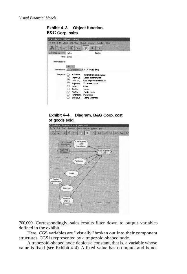
Visual Financial Models
Exhibit 4-3. Object function, B&G Corp. sales.
Rles units:
rn (70DK 800K I M )
~dmmstr . adninhtrst~onexpenses Csiasl-e . C M s l expendlhrras Cosf_of Cod Of goodrseld Inputr Expense. . Expcnaer Input* Labor Labor Plolb Prof1s Profaen Profas h p t s Purcha~es Purchaser Se1ling.c. . Selrng Expenses
Exhibit 4 4 . Diagram, B&G Corp. cost of goods sold.
700,000. Correspondingly, sales results filter down to output variables defined in the exhibit.
Here, CGS variables are "visually" broken out into their component structures. CGS is represented by a trapezoid-shaped node.
A trapezoid-shaped node depicts a constant, that is, a variable whose value is fixed (see Exhibit 4-4). A fixed value has no inputs and is not
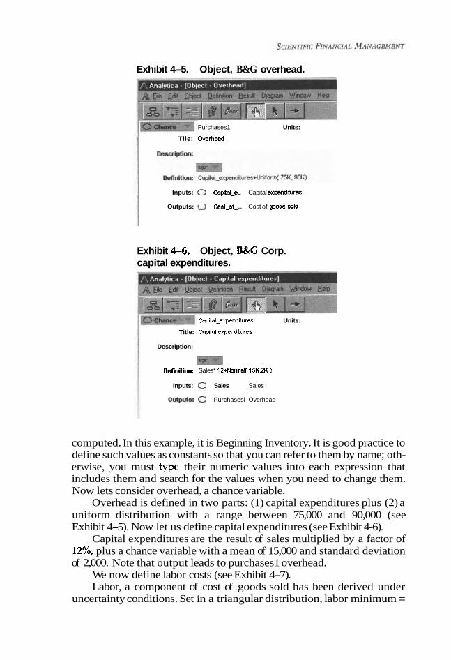
Exhibit 4-5. Object, B&G overhead.
Purchases1 Units:
Tile: Overhesd
Inputs: Capiial-e ... Capital expenditures
Outputs: 0 Cost-07- ... Cost of gmds s ~ l d
Exhibit 4-6. Object, B&G Corp. capital expenditures.
Capiial_expenditures Units:
Title: Capiial expendrtures
Description:
Ilefinilion: Sales* 12+Normal( 15K,2K )
Inputs: Sales Sales
Outpuk 0 Purchasesl Overhead
computed. In this example, it is Beginning Inventory. It is good practice to define such values as constants so that you can refer to them by name; oth- erwise, you must type their numeric values into each expression that includes them and search for the values when you need to change them. Now lets consider overhead, a chance variable.
Overhead is defined in two parts: (1) capital expenditures plus (2) a uniform distribution with a range between 75,000 and 90,000 (see Exhibit 4-5). Now let us define capital expenditures (see Exhibit 4-6).
Capital expenditures are the result of sales multiplied by a factor of 12%, plus a chance variable with a mean of 15,000 and standard deviation of 2,000. Note that output leads to purchases1 overhead.
We now define labor costs (see Exhibit 4-7). Labor, a component of cost of goods sold has been derived under
uncertainty conditions. Set in a triangular distribution, labor minimum =

Visual Financial Models
Exhibit 4-7. Object, B&G Corp. labor. . . . . . . .. . . .
. I t i" t c r ;+furl j: q. .. : c..i.,j,r, 2' :'."" Fc.k
. , f . . - 1 I C..> 7-
-. . - -. - - . % . t , + ! Labor Units:
Title: Labol
Description:
Definnion: Triangular(sales'.l I , sales.12, sales'.l9)
Inputs: 0 Sales Sales
Outputs: 0 Go&-of Cost of goods sold
Exhibit 4-8. Diagram, B&C Corp. expenses.
Exhibit 4-9. Result, sales x 19%, labor most likely = sales x 12% probability bands of profits. labor maximum = sales x 19%. Expenses
include a number of variables that are Probability Profits much easier to define in a visual model
0.05 -32.3K than on the familiar spreadsheet. For exam- 0.25 1 1.45 K ple, consider Exhibit 4-8. Expenses include 0.5 32.46K administration expenses and selling 0.75 58.55K expenses. (We have not broken these 0.95 83.02K expenses out in order to shorten this exam-
ple. However, this diagram includes corre- lations inside the "expenses importance" node.
Probability bands are specified at given percentile values. The model returns an estimate of probability or confidence bands for X if X is proba- bilistic (see Exhibit 4-9).

B&Gfs profit probability density appears in Exhibit 4-10. If the quantity is a continuous probability distribution, Analytica dis-
plays a probability density function. The horizontal (x) axis plots possible values of the uncertain quantity. The height of the curve (probability den- sity) is proportional to the likelihood that the quantity will have the x value. The highest point on the curve is the most likely value (the mode). Where the curve is at zero height or invisible, there is zero probability that the quantity will have that value. (For a discrete probability distribution, Analytica graphs the probability mass.)
The rectangular node, Emissions Reduction, is a decision. The ovals are uncertain variables, and the hexagon is the objective to minimize, Total Cost.
The rounded rectangle nodes are deterministic variables, that is, vari- ables that are defined as deterministic values or as deterministic functions of their input variables. In some notations, deterministic nodes are depicted as ovals that have double outlines.
The hexagonal node on the right-labeled Total Cost depicts the objec- tive, that is, a quantity to be optimized (either maximized or minimized, depending on how it is expressed). In decision analysis, this node expresses the utility-the objectives and values--of the decision maker. Decision theory prescribes that the decision maker seek the decision that maximizes the expected utility.
Uncertainty in Your Model
Recall that the oval nodes depict chance variables, that is, variables that have an uncertain value that is not under your direct control. We express
Exhibit 4-1 0. Result, B&C Corp. profit profitability density graph.

Visual Financial Models 103
the value of each chance variable in terms of a probability distribution, fit- ting it to data or eliciting it from experts. Uncertain variables propagate uncertainty samples during dynamic simulation. If an uncertain variable is used in a dynamic simulation, its uncertainty sample is calculated only once, in the initial time period. If you want to create a new uncertainty sample for each time period (i.e., resample for each time period), place the distribution in the last parameter of the Dynamic() function. You can enter a distribution anywhere in a definition, including in a cell of an edit table. Thus, you can have arrays of distributions. You can choose from an array of distributions, some of which are listed in Table 44.1° If you simply want to ignore the uncertainty, the software will compute and display a rnid- value for any quantity, computed deterministically from the median of each input distribution.
Table 4-1. Uncertaintv distributions.
Distribution Definitions and Parameters
Bernoulli (P) Creates a discrete probability distribution with probability P of result 1 and probability (1 - P) of result 0. P is a probability value or array of probabilities, each between 0 and 1. The Bernoulli distribution is defined as:
If Uniform (0, 1) < P Then 1 Else 0 If P is greater than 1, the distribution is made up of all
1's. If P is less than 0, the distribution is made up of all 0's.
Beta (X, Y, lower, upper) Creates a distribution of numbers between 0 and 1 with X/(X +Y) representing the mean, if the optional parameters lower and upper are omitted. For bounds other than 0 and 1, specify the optional lower and upper bounds to offset and expand the distribution.
X and Y must be positive. Returns the value of U. Uses Certain() when an input node is defined as a
distribution and, in browse mode, when you want to replace the distribution with a nonprobabilistic value.
Creates a discrete probability distribution. A is an array of outcomes, and P is the corresponding array of probabilities. A and P must both be indexed by I.
The values of A must be unique; if A is numeric, the values must be increasing.
Certain (U)
Chancedist (P, A, I )
(continues)
10. Reprinted with permission of Lumina Decisions Systems.

Table 4-1. Continued.
Distribution Definitions and Parameters
Fractiles (L)
Cumdist (P, R, I) Specifies a continuous probability distribution by an array of cumulative probabilities, P, for an array of corresponding outcome values, R, for the quantity. Either R must be an index of P, or P and R must have an index in common. If P or R have more than one index, you must specify the relevant index for linking P and R as a third parameter, I.
CumdistO uses linear interpolation of the cumulative distribution between the specified points, which implies a piecewise uniform distribution.
The values of P must be nondecreasing. P's first value must be equal to or greater than 0, and its last value must be 1.0. The values of R must be increasing.
Specifies a continuous probability distribution by an array of evenly spaced fractiles, L. L must be a one- dimensional array of nondecreasing numbers. FractilesO uses linear interpolation on the cumulative distribution between the specified fractiles, which implies a piecewise uniform distribution.
If any value in L i s probabilistic, its midvalue i s used to obtain the fractile.
Lognormal (median, gsdev) Relates to a lognormal distribution with median of median and geometric standard deviation of gsdev. The geometric standard deviation must be 1 or greater. The range [medianlgsdev, median gsdevl encloses about 68% of the probability. Gsdev is sometimes also known as the uncertainty factor or error factor. Median and gsdev must be positive.
The log of a lognormal quantity has a normal distribution with mean of Log (median) and standard deviation of Log (gsdev).
While the lognormal distribution is unbounded above, Analytica's Lognormal() function truncates sample values at median.
Normal (mean, stddev) Creates a normal or Gaussian probability distribution with mean and standard deviation (stddev). The standard deviation must be 0 or greater. The range [mean - stddev, mean + stddev] encloses about 68% of the probability.
While the normal distribution is unbounded above and below, Analytica's Normal() function truncates sample values at 3 stddev above and below the

Visual Financial Models
Probdist (P, R, I) Specifies a continuous probability distribution as an array of probability density values, P, for an array of corresponding outcome values, and R, for the quantity. Probdist performs a linear interpolation between the points on the density function. The values of P must be nonnegative. They will be normalized so that the total probability enclosed is 1 .O. The values of R must be increasing.
The values of P should start and end at 0. If the first (or last) value of P is not zero, Analytica assumes zero at 2R1 - R2 (or 2Rn - Rn - 1 ).
Either R must be an index of P, or P and R must have an index in common. If P or R have more than one index, you must specify the relevant index for linking P and R as a third parameter, I.
Probtable (11, 12, . . . In) Describes an n-dimensional conditional probability (PI, p2, p3, . . . pm) table, indexed by the indexes 11, 12, . . . In. One
index must be Self. p l , p2, p3, . . . pm are the probabilities in the array.
Triangular (min, Creates a triangular distribution, with minimum min, mode, max) mode mode, and maximum max. Min must be not
be greater than mode, and mode must not be greater than max.
Uniform (min, max) Creates a uniform distribution between values min and max.
Developing Your Visual Model Step by Step
Open Class Donuts.ana
In the models subdirectory of the CD (you need to instal l open Analytica first). The Class Donut model will be your check. However, y o u can either create a fresh mode l for practice o r s imply fo l low h o w Class Donuts.ana was constructed:
Selecting Open M o d e l f rom the Pi le M e n u
When y o u first create a new model, y o u mus t enter a n identifier and other information, also referred to as documentation, describing i ts title, descrip- tion, and author.
Us ing the Edit Tool (A r row Poin t ing Left)
When the Edit too l is selected, a vertical menu o f icons i s displayed in the Node palette. These icons represent the different node types and al low y o u t o add nodes to the influence diagram. Setting up the influence diagram

first will enable you to organize it efficiently. The influence diagram is Exhibit 4-11 and includes all assumption variables that contribute to the forecast variable, profit.
Creating Variables
Each variable has a node type: Select the node type based on what you know about the variable. The first variable we will create is expenses per donut. This is a chance node. We drag the Chance node to a position in the influence diagram. We enter "Expenses per donut" and press the Return key to create a second line.
Saving Your Model
While creating or modifying a model, you should periodically save your changes.
Deleting a Variable
Sometimes you may want to delete a variable that you previously created.
Moving Nodes
When you create a model, you should try to structure the model layout to make the model logic easy to understand. As you refine your model, how- ever, you undoubtedly will want to group nodes in different ways. Click on the Edit Tool icon and try dragging the Donuts Sold per Year Chance node.
Exhibit 4-1 1. Diagram donuts main.

Visual Financial Models 107
Editing Variable Titles
We might select Donuts Sold per Year and click again inside the node's title to select its text for editing (see Exhibit 4-12).
Here we assume a chance variable governed by a normal distribution with a 150,000 mean and 30,000 standard deviation. Sales lead to outputs that follow in Exhibits 4-12A, 4-12B, and 4-12C.
This variable is influenced by two variables: (1) donuts sold per year multiplied by (2) expenses per donut. We also include a description to help "the team" understand the underlying assumptions.
This variable is governed by a normal distribution with a mean of 40 cents and a standard deviation of 10 cents. A good description of the variable is included.
Exhibit 4-12. Obiect, donuts sold per year.
D~nU~_sold_pel_yeai Units:
Tile: DonUs mld per yea,
hltputs: U DonUJr .. Dam% pmms per year hwa 0 D o W j r ... Don!Apmts pa year 0 ~ x p e n ss.. b p m s e s per year D Expen se.. Expmsesper year lnprts
Exhibit 4-12A. Chance, expenses per year.
Descriwion: me tdai tor( 01 pucheslng dews ins yes,. T o w which of m6 vsisbleinplds contrbLdesMe mod lncertalmto mt varabler valuc, rdcd this var ia l l r node il the dmgram window wd Eekd ''MsAelmpntance'lmm the'oblew menu This har slresdy been done ---"lnplld'wd"lmportance" NDdR lollhm velabk are airesdy srpated.
m oemition: D o n u t s . s o l d s e r w a P b p ~ s p r p r ~
Input% 0 D o a - I ... Donuts tdd per YBBI
0 Emsmc ... Expenrer per d m
Output=: 0 Dmirsr . Donld pmma per ysar 0 Expe me.. Expsnres per year Importance

Exhibit 4-12B. Chance, expenses per donut.
True: Expenses per d0r.A
Wffl taH bdwsen S3 carts and 50 ceMs This sbo m e e n s M the wae dirtriMion band n w the con of prmuclng rmcwhM u n o ~ a ~ n
PRhapslhe podudion m a m r M a r get wim It and flnd s betier BOUICe Ot taw meterlab supply!
m De(hln1on: (04.0.1 I
MMr: C7 canuisr cam$ profns per yssrlnputs 0 Expenre Expnnes p r yes.
Expense Expensen per yesr lnm
Exhibit 4-12C. Object, price per donut.
T l i e : Price per donM
Oescripflon: Sale prlce per doMts 6 set under s triangu$r 6strib@mn See "OannltlOne
m DeTnitim: ( 0 6 , o 7 . 0 9 )
(*ltPutx D Donutgr D o m p o t n s pn yes l w s 0 D o n u t p Dorut profbs per yew
Drawing an Arrow between Nodes
One of Analytica's most powerful features is its ability to show relation- ships between variables in the influence diagram. Influence arrows are used to specify the dependencies between variables. Because the Donuts Sold per Year variable influences Expenses per Year, we draw an arrow connecting the two nodes.
Deleting an Arrow
Occasionally, you may need to delete an arrow because of an earlier mis- take or a change in your understanding of the model. Try pressing the Delete key to delete the arrow. The arrow disappears. Do not forget to replace the arrow.
Connecting Multiple Arrows
When one variable is influenced by many other variables, you can draw multiple arrows at once.

Hsual Financial Models 109
Entering Attributes Using the Object Window
A When you create a model, you can add documentation of the model and of its variables. The system supports integrated documentation that can be tied to every variable in the model.
A We double-click again on Donuts Sold per Year to open its Object window (Exhibit 4-12).
A The identifier in the Object window is Donuts Sold per Year. The title is the same. In the description field, we enter. "We expect to sell 150,000, with a standard deviation of 30,000."
A Clicking on the Definition field opens up a field. Click on expr. Select distribution/Normal. Enter "EXACTLY 150,000,30000." Click the Check button. The result is Normal( 150K, 30K)
A Donuts Sold per Year is no longer filled with a diagonal line pattern around its title. The clear node indicates that Donuts Sold per Year now has a definition that is valid and can be computed.
Entering Attributes Using the Attribute Panel
Rather than opening a separate window to alter a variable's attributes, you may prefer to see a variable's attributes in the same window as the model influence diagram (the module icon is surrounded by a bold border). The attribute panel, which appears under the diagram, allows you to edit as well as examine attributes.
Defining a Variable That Is Influenced by Other Variables
A When one variable is influenced by another variable, you must pro- vide a mathematical expression that describes the relationship between the variables. The Expenses per Year node has arrows entering it from two other variables.
A Because Expenses per Year is equal to Expenses per Donut multi- plied by Donuts Sold per Year, we enter the following expression into the Definition field: Donuts Sold per Year x Expenses per Donut (from the Inputs window).
A Notice outputs are Donut Profits per Year and Expenses per Year Importance.
Creating a Module
A To simplify complicated diagrams, most complex models use sub- models, called modules. A module is an influence diagram contain- ing variables and their relationships to one another. While the cur- rent model is simple enough, we could add a module if we had, say, a New York division and wanted to create a submodel.
A Drag the Module icon to a position in the influence diagram. You may want to experiment here. Enter "NY Division." Select the

Exhibit 4-13. Object, donuts profits per year.
rule: DcnU pralbr per yea,
O e r a l p t ~ n : The total proits mmc a m Lmnmmtmt year To find wtich olthis WnsbleIRnds cootrlbUe then& lnnntdntyto the varlakda's vsw, ssmd t ~ s vainbm's nds m ths dsgram wmdmv and seled "MaB Im~nance" t m t h e "obieb mew. ~ h i r har almay h e n cam - -" lnpcwmd ''hportsme.'~odes tor ttis rsrbble are dreaw hirema.
m O d d i o n : P r C e g e r . d o n u l * D o n ~ ~ ~ ~ a ~ ~ r . E x p e n f e ~ g e ~ y ~ ~ ~
W= 0 Dorms-s .. Wnuts sold psr p a r 0 Expense ... Expnses per year 0 P n f e j e r ... Rlce per donll
M v u l r : 0 ommsr .. Dmm pmttrper y e s Wrtance
Decision node (this will be very simplistic). Double-click. Enter "100000" in the definition field. Drag an arrow from profits (within the node to the window Donut Profits per Year). Next, double-click on the Donut Profits per Year node. Notice the new input: Profits.
A Finally, we change the definition by adding profits. Click on the Check button to accept your selection.
Completing the Model
Thus far, we have used several methods for moving between windows, documenting variables, and specifying their definitions. In this last step, we double-click on Donut Profits per Year. The result is shown in Exhibit 4-13.
A While selecting Donut Profits per Year, click on the Show Results button (green question mark and exclamation point icon) to evalu- ate Donut Profits per Year.
The distribution reveals a probability density (Y) of Donut Profits per Year (X). Selecting Result from the main menu gives us a choice, for example, midvalue of Donut Profits per Year (see Exhibits 4-14 and 4-15).
Importance Analysis
Finally, we may want to view correlations. Importance analysis shows the effect that the uncertainty of one or more input variables have on the uncertainty of an output variable. Importance is defined as the rank-order correlation between the sample of output values and the sample for each uncertain input. This is a robust measure of the uncertain contribution
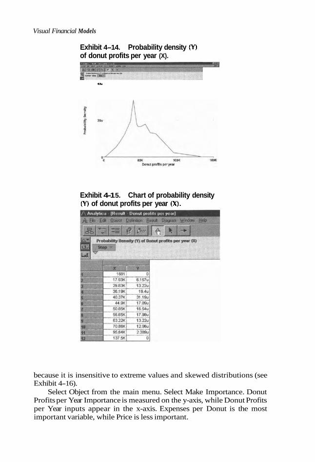
Visual Financial Models
Exhibit 4-14. Probability density (Y) of donut profits per year (X).
I O U
Exhibit 4-1 5. Chart of probability density (Y) of donut profits per year (X).
because it is insensitive to extreme values and skewed distributions (see Exhibit 4-16).
Select Object from the main menu. Select Make Importance. Donut Profits per Year Importance is measured on the y-axis, while Donut Profits per Year inputs appear in the x-axis. Expenses per Donut is the most important variable, while Price is less important.

Exhibit 4-1 6. Midvalue of donut profits per year importance.
Exhibit 4-1 7. Diagram, business opportunity analysis. (See On-Line Demo)
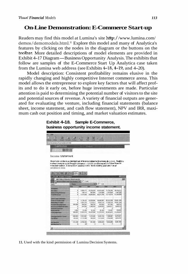
VisuaI Financial Models 113
On-Line Demonstration: E-Commerce Start-up
Readers may find this model at Lumina's site http:/ /www.lumina.com/ demos/demomodels.html.ll Explore this model and many of Analytica's features by clicking on the nodes in the diagram or the buttons on the toolbar. More detailed descriptions of model elements are provided in Exhibit 4-17 Diagram-Business Opportunity Analysis. The exhibits that follow are samples of the E-Commerce Start Up Analytica case taken from the Lumina web address (see Exhibits 4-18,4-19, and 4-20).
Model description: Consistent profitability remains elusive in the rapidly changing and highly competitive Internet commerce arena. This model allows the entrepreneur to explore key factors that will affect prof- its and to do it early on, before huge investments are made. Particular attention is paid to determining the potential number of visitors to the site and potential sources of revenue. A variety of financial outputs are gener- ated for evaluating the venture, including financial statements (balance sheet, income statement, and cash flow statement), NPV and IRR, maxi- mum cash out position and timing, and market valuation estimates.
Exhibit 4-1 8. Sample E-Commerce, business opportunity income statement.
Income Ststemeni
This mode contans a standard set dfinanclal Iaernsms among a o w AnaBca makes ~t easyto cycle hrough scenenos to yulc!+me he impad onfuture hnanclal 5tatement entries Atemplats 15 used to conhol thsfomitmnq and sslerPon of
11. Used with the kind permission of Lumina Decision Systems.

Exhibit 4-1 9. Sample E-Commerce, business opportunity balance sheet.
Th15 modc contirns 6 Standerd set afflnancial statements arnoilg i s outprtj. Analyca makes I! easy ra cycle ttradgh ecenanas to qulcdy see the Impact onfuwre fnsncal SBtemenl entries A tenplate s used to conool thefoirnam?g and selecton of varebIe5 10 show
Exhibit 4-20. Sample E-Commerce, business opportunity IRR.
1 Tile: Internal Rate of Return (IRR)
I Description: -I i horizon, without consideration of a tenninal value for the venbxe stth i end of the time horizon.
Nate that Tlme s In months here, so the squatlon below calculates a I - i monthly IRR, then cmvmts Lto an annusl value 1 n
j Note that IRR may relum nonsensical (NAN) answers if there are no I sign changes hthe cash flows. mis especially may happen where I inputs are probabilistlcgiving the occasional run wth no sign change
i Value: 26% ""I Inputs: 0 Free-cas ... Free Cash flow
i!?+ kf (Values, I, aRss ) @ rine Time

Visual Financial Models
Conclusion
Analytica is a new and powerful visual modeling tool that embodies the notion of problem solving using a white board. Downloading the model or linking to the model via site locations listed on the CD, we learned how to draw nodes and arrows to depict the relationships between model com- ponents, and thus, were able to develop the qualitative nature of financial problems without getting lost in details.
We discovered how to create hierarchies in our models. By grouping together related components of a problem into separate sub models, we imposed a top-down organization and factored this into our models. Far more than spreadsheet models, this permitted us to work out and manage complex relationships and, if other members of the team were involved, could easily allow them to more easily grasp critical issues and concepts.
Another key feature of Analytica is the use of Intelligent ArraysTM. These enabled you to add or remove dimensions such as time periods, geographic regions, alternative decisions, etc., with minimal changes to the model structure. Unlike spreadsheets, which require you to repeat formulas with each new dimension, this tool separates the dimensions from the relationships so that models remain simple. As the dimensions change, Analytica automatically updates, reports, and graphs the results.
Finally, unlike spreadsheet models, this tool features fully integrated risk and sensitivity analysis for analyzing models with uncertain inputs; powerful facilities for time-dependent, dynamic simulations; comprehen- sive overlay graphs; and over 100 financial, statistical, and scientific func- tions for calculating just about any type of mathematical expression.
Chapter Four References and Selected Readings
Books
Benninga, S., and B. Czaczkes. (1997). Financinl modeling. Cambridge: MIT Press. Bertocchi, M., et al. (1996). Modelling techniques for financial markets and bank management.
Heidelberg: Physica-Verlag. Dattatreya, R. E., and K. Hotta. (1994). Advanced interest rafe and currency swaps: State-of-the-
art products, strategies and risk management applications. Chicago: Irwin. D'Ecclesia, R. L., et al. (1994). Operations research models in quantitativefinance. Heidelberg:
Physica-Vertag. Euro Working Group for F i c i a l Modeling, R. L. D'Ecclesia, et al. (1994). Operations
research models in quantitativefinance. Heidelberg: Physica-Verlag. Greenstein, S. M., and J. Wade. (1997). Dynamic modeling of the product life cycle in the c m -
mercial mainframe computer market, 1968-1982. Cambridge, Mass.: National Bureau of Economic Research.
Guerard, J., and H. T. Vaught. (1989). The handbook offinancial modeling: Thefinancial execu- tive's reference guide to accounting,finance, and investment models. Chicago: Probus.
Ijiri, Y. (1993). Creative and innovative approaches to the science of management. Westport, Conn.: Quorum Books.

Meyer, H. I., and M. C. Weaver. (1977). Corporatefifinancial planning wrodels. New York, John Wiley & Sons.
Meyer, M. F. (1983). Financial modeling. Gaithersburg, Md.: Aspen Systems. Morris, J. R. (1987). The Dow Jones-lrwin guide tofinancial modeling. Homewood, Ill.: Dow
Jones-Irwin. Rothman, P. (1999). Nonlinear time series analysis of economic and financial data. Boston:
Kluwer Academic Publishers. Sheldon, T., Consultative Group to Assist the Poorest, et al. (1998). Business planning adfinan-
cia1 modeling for microfirrunce institutions: A handbook. Washington, D.C.: World Bank CGAP Stokes, H. H., and H. M. Neuburger. (1998). New methods infinancial modeling: Explorations
and applications. Westport, Conn.: Quorum Books. Varian, H. R (1993). Economic andfinancial modeling with rnathtica. New York: Springer-Verlag. Wang, R. Y., et al. (1992). Data quality requirements analysis and modeling. Cambridge: Alfred P.
Sloan School of Management, Massachussetts Institute of Technology. Zopounidis, C., and E m Working for Financial Modeling. New operatiml approaches for
financial modeling. Heidelberg: Physica-Verlag.
Select Internet Library
Lurnina Decision Systems, Analytica: Beyond the Spreadsheet Topics Discussed: The Quantita- tive Modeling Tool With Visual Ease; Who's Doing What With Analyhca; Manage Risk and Uncertainty; Decision Making Within the Enterprise; Build Analytica Models in Three Easy Steps; Instant Access to Every Hement of Your Model; Expand Your Models With Intelligent ArraysTM Functions and Operators http://www.lumina.corn/brochure/index.html.
Tweedie, L., R. Spence, H. Dawkes, and S. Hua. Externalizing Abstract Mathematical Models. To appear in the "Proceedings of CHT'96" (Vancouver: ACM Press). Description: Abstract mathematical models play an important part in engineering design, economic decision making, and other activities. Such models can be externalized in the form of interactive Visualization Artifacts (NAs). These IVAs display the data generated by mathematical models in simple graphs that are interactively linked. Visual examina- tion of these graphs enables users to acquire insight into the complex mlations embodied in the model. In the engineering context, this insight can be exploited to aid design. http:/ / w w w . e e . i c . a c . u k / r e s e a c h / ~ o m a t i o n / w w w / l .
Using Mathworks Products; The Financial Toolbox 2.0. Description (1999): The MATLAB Financial Toolbox extends the functionality of MAT- LAB by providing essential tools for quantitative financial modeling and analytic pro- totyping. The Financial Toolbox is used for a wide array of applications, including fixed-income pricing, yield, and sensitivity analysis; advanced term structure analysis; coupon cash flow data and accrued interest analysis; and derivative pricing and sen- sitivity analysis. http:/ /www/mathworks.com/products/finance/.
Name Size Type
ABC Corp About Analytica Analytica Customer List ClassDonuts Demo Models Market Model Nj r Online Demo E-Commerce Model Setupana tutorial.pdf
4KB 1 KB 1 KB 4KB 1 KB
33KB 1 OKB
1 KB 2,515 ...
1 KB
Analytica Model File lnternet Shortcut lnternet Shortcut Analytica Model File lnternet Shortcut Analytica Model File Analytica Model File lnternet Shortcut Application lnternet Shortcut

Divisional Cash Flow
Analysis and Sustainable
Growth Problems
THIS CHAPTER ASSUMES THAT YOU have a working knowledge of basic cash flow. The first section reviews cash flow analysis at the basic (divisional) operating level, and the second section reviews advanced cash flow and sustainable growth problems, again at the divisional level.
Consolidated equity value remains the quest for all operating parts. It begins at the subatomic level-the lowly operating division, its mote cash flow, the genetic capital cost and strategic plan. From these tiny thrrads, the colossus emerges.
Cash Flow
Cash flow has always been one of the most compelling financial and risk analytical tools, raising questions dealing with how businesses generate and absorb cash.
Accounting: Fact or Fiction
Warren Buffet calls net income "white lies." Lee Seidler has been known to say, "If push came to shove, if a chairman wants a nickel more a share, any good controller knows where to find it."

Cash flow is literally the precursor of shareholder value. If an operat- ing unit routinely produces poor cash flow or is inadequately capitalized, it cannot survive long. Indeed, the operating unit may subsist "on a shoe- string" by cannibalizing corporate headquarters. However, siphoning off the parent's cash originally earmarked to improve value-creating busi- nesses is not the way to run a shop.
We can draw on IAS 7 to work out the best way to analyze cash flows at the operating unit level:
A The divisional cash flow statement forms the basis of macro corpo- rate analysis.
A Operating units down to the least common denominator should account for changes in cash and cash equivalents for a specific period, monthly or quarterly.
A Cash equivalents are short-term, highly liquid investments subject to insignificant risk of changes in value. The "basic unit" statement should decompose changes in cash and cash equivalents into oper- ating, investing, and financial activities. Cash changes between periods are unimportant. A reconciliation of net cash flow from operations to net income is required using either the direct or the indirect method. Both techniques provide cash from operations. The direct method shows receipts from customers and payments to suppliers, employees, government (taxes), and so on. The indirect method begins with accrual basis net profit or loss and adjusts for major noncash items. Make sure that you segregate intercompany receipts, disbursements, and inventory profits.
A Investing activities: Disclose (separately) cash receipts and pay- ments arising from acquisition or sale of property, plant, and equip- ment; acquisition or sale of equity or debt instruments of other enterprises (including acquisition or sale of subsidiaries); and advances and loans made to, or repayments from, third parties.
A Financing activities: Disclose cash receipts downstreamed from headquarters and payments upstreamed apart from financing injec- tions obtained from external debt and equity investors.
A Cash flows arising from tax rebates are disclosed apart from oper- ating activities.
A Investing and financing activities that do not give rise to cash flows (a nonmonetary transaction, such as acquisition of property by issu- ing debt) should be excluded from the cash flow statement but dis- closed separately.
The Indirect Method of Cash Reporting: The In-Depth Cash Flow
In order to take advantage of the power of cash flow, you might adjust the cash flow format so that it is more in line with cashflow valuation models. As

Divisional Cash Flow Analysis and Sustainable Growth Problems 119
it stands now, cash flow audits combine working (capital) assets and working (capital) liabilities with gross operating cash flow items. The end result is to arrive at net cash flow from operations. That is too bad, partic- ularly if you are evaluating segment performance. In short, do not com- bine categories. Rather, separate significant account classes.
GYOSS operating cash flow (GOCF), categorically, measures the power of the bottom line. Operating units finance growth in two ways: either from parental downstreams and/or through old-fashioned intemal cash flow. However, keep in mind that intemal cash flow can form simply by selling assets but that the division cannot grow by casting off assets. Strong inter- nal GOCF is the only viable road to value, and there are several signals
You may want to compare GOCF to cash provided by headquarters. This allows you to (1) check operating divisionsfor intemdversus external financing imbalances and (2) make comparisons in financial leverage trends.
Overall, would a business pay stockholder dividends out of GOCF? That is hard to imagine since GOCF must first cover working capital. As far as passing dividends up to the parent, that may be another story. Thus, if working capital sources (increases in accounts payable, accruals, and other working capital accounts) exceed applications (increases in accounts receivable, inventory and other current assets), cash flowing down the income statement will not end up cannibalizing working capital. Rather, it is redirected to finance investment activities, retire debt, and then, per- haps, shoot dividends up to headquarters. Exhibit 5-1 is an example of a comprehensive cash flow.
Cash Flow: The Essence
Investing Activities
Investment activities include advances and repayments to subsidiaries, securities transactions, and investments in long-term revenue-producing assets. Cash inflows from investing include proceeds from disposals of equipment and proceeds from the sale of investment securities. Cash out- flows include capital expenditures and the purchase of stock of other enti- ties, project financing, capital and operating leases, and master limited partnerships.
Property, Plant, and Equipment (PPBE)
Property, plant, and equipment include acquisitions and purchases, capi- tal leases, and proceeds from any disposals of property, plant, or equip- ment. Noncash transactions include translation gains and losses, transfers, depreciation, reverse consolidations, and restatements.
You should ensure that accounts are up to date regarding maintenance of existing capacity and expenditures for expansion into new capacity. This

Exhibit 5-1. Cash flow statement. COMPANY X For the Year Ended December 31,19X8
Increase (Decrease) in Cash and Cash Equivalents Cash flows from operating activities:
Net income Adjustments to reconcile net income to net cash
provided by operating activities: Depreciation and amortization Provision for losses on accounts receivable Gain on sale of facility Undistributed earnings of affiliate
Cross operating cash flow (Inc.) Dec. in accounts receivable (Inc.) Dec. inventory (Inc.) Dec. in prepaid expenses
Operating cash needs Inc. (Dec.) in accounts payable and accrued expenses Inc. (Dec.) in interest and income taxes payable Inc. (Dec.) in deferred taxes Inc. (Dec.) in other current liabilities Inc. (Dec.) Other adjustments
Operating cash sources Net cash provided by operating activities
Cash flows from investing activities: Proceeds from sale of facility Payment received on note for sale of plant Capital expenditures Payment for purchase of Company S, net of cash
acquired Net cash used in investing activities
Cash flows from financing activities: Net borrowings under line of financial agreement Principal payments under capital lease obligation Proceeds from issuance of long-term debt
Net cash provided by debt financing activities Proceeds from issuance of common stock Dividends paid
Net cash provided by other financing activities Net increase in cash and cash equivalents
i s impor tan t segment disclosure since maintenance and capital expenditures are nondiscretionary outlays. How, then, can a CFO determine whether funds are be ing allocated fo r maintenance o f exist ing capacity, replacing - - r u n d o w n equipment, o r providing expansion (and of ten d i s c r e t i o n e ) out- lays? The answer l ies the knowing h o w to take a cash f l o w apart.

Divisional Cash Flow Analysis and Sustainable Growth Problems 121
Unconsolidated Subsidiaries
It is not unusual for operating units to form alliances with outsides to reduce the cost of raw materials and overhead and to improve market- ing. These alliances might take shape in equity investments. When a unit purchases between 20% and 50% of another company's stock, the account "Investment in Unconsolidated subsidiary" shows up on the acquiring business's balance sheet. Cash flows from unconsolidated subsidiaries include dividends from subsidiaries, advances and repay- ments, and acquisition or sale of securities of subsidiaries. Noncash transactions include equity earnings, translation gains and losses, and consolidations.
Investment Project Cash Flows and Joint Ventures
Investments in joint ventures or other separate entities formed to develop projects of various sizes are referred to as projectfinancing and/or joint ven- tures. Typically, the new entity borrows funds to build a plant or a project with a guarantee of debt repayment furnished by companies that formed the new entity. Cash flows from the project (or joint ventures) are generally passed up to headquarters in the form of dividends. Prudence dictates that you obtain a full disclosure of the project's future cash flow since con- struction projects may report noncash earnings: construction accounting or equity earnings.
Asset Divestitures
Asset sales can be a positive move for a company, as in the case of an unprofitable division sold off to allow management to focus on the busi- ness's core businesses.
Working Capital: Operating Cash Uses
Accounts Receivable. Increases represent cash drains and are typically financed. A decrease in receivables is associated with cash inflows.
Accounts receivable policy is closely allied to inventory management since both are the two largest current asset accounts. The volume of finan- cial sales and the average collection period determines accounts receivable levels. You should examine receivables at the divisional level as well as on the corporate level. The divisional average collection period like consoli- dated receivables are influenced partly by economic conditions and partly by a set of controllable factors calledJinancia1 policy variables and they may differ: divisional versus consolidated. Neural networking, data mining, and fuzzy logic are playing important roles setting credit standards and credit policy and working to optimize cash flows. These new methods really dig up hidden data.

Inventory. As we saw, inventory is a vital component in cash flow cycles. Good inventory control starts with ongoing tracking of raw materials, work in process, and finished goods. Raw materials levels are based on anticipated production, the seasonality of the business, and the reliability of suppliers. If raw materials are highly salable and commodity-like, this stage is often closer to cash than work-in-process inventory. A buildup of raw material usually indicates speculative activity in anticipation of price increases or shortages.
Work in process is defined as the length of the production cycle. Fac- tors that directly affect work in process include the grade of the equip- ment, engineering techniques, and the maintenance of highly skilled workers. Exorbitant work-in-process inventory depicts production slow- downs and/or manufacturing inefficiencies, severely hindering cash flow. Finished goods involve coordinating the sales effort. Salability of finished goods depends generally on the type of business operation. If there is a problem in this area, review sales strategy and find out why potential cus- tomers do not want to buy your product. This will advise you what inven- tory stage needs fine-tuning.
Effective inventory management is crucial to good cash flow manage- ment. Carrying excessive inventory is both costly and, in certain cases, leads to failure. Inventory control means careful planning plus maintain- ing open lines of communication within the organization so that inventory adjusts to optimal levels. Just-in-time inventory, economic order quantity, and neural network models do just that.
Operating Cash Sources
The right side of the balance sheet supports assets. Large increases and decreases in current accounts represent substantial inflows and outflows of cash. Operating cash sources generally include non-interest-bearing current liabilities that tend to follow sales increases.
Accounts Payable. Increases in payable are cash sources in the sense that they delay cash outflows into the future. While the division has use of this cash, it can utilize it for daily needs as well as for investment purposes. Generally, decreases from one period to the next represent an amount paid to suppliers in excess of purchases expensed.
Accruals and Taxes Payable. Increases in accruals and taxes payable repre- sent sources of cash since items such as salaries, taxes, and interest are expensed but not paid out. Thus, cash is conserved for a limited period. A decrease in accruals arises from payments in excess of costs expensed. In the current period, therefore, the decrease is subtracted from the cash flow as a use of cash.
Divisional Cash F l m Analysis and Sustainable Growth Problems 123
Net Operating Cash Flow
Net operating cash flow denotes the cash available from gross operating cash flow to internally finance a unit's growth after working capital demands are satisfied. One of the great things about the structure of the cash flow format is how pieces of information surface to formulate powerful insights as to whether the business is optimizing its performance. For example, if gross operating cash flow is consistently larger than net cash flow from operations, the traditional sources of working capital, accounts payable and accrual have provided full support to traditional uses of working capital, accounts receivable, and inven- tory. Thus, precious operating cash income need not be diverted to support working capital and can be rerouted to finance "growth strategies, such as - .
investments in efficient fixed assets and aggressive R&D programs-the lifeblood of maximizing both divisional and consolidated value.
Cash Flow Analysis
Gross Operating Cash Flow
Operating cash flow should contribute toward an optimal financing strat- egy. Thus, imbalances between debt and equity usually begin with weak divisional (internal) cash flow. A less obvious situation is the case of a start- up or rapid growth operation. Although income may increase, expansion costs might rise at an even faster rate. Funding increases in receivables, inventories, and capital expenditures might push debt/equity perilously high unless new equity surfaces. What you do not want is crash-and-burn: crash if cash evaporates, bum if investments are written off.
Depreciation is a noncash charge with adjustments made to net income. You may want to question adequacy of reserves, nonrecurring items, and cash versus accrual-based income. If most of profits consist of equity earnings, beware that inadequate operating cash flow may be available for expansion and repayment of obligations. Most important, the division's capital structure may be distorted since "low quality" earnings have artificially propped up equity. Also, if earnings have relied on deferred tax credits, beware. Deferred tax credits may be part of an accounting game to push profits up. Remember that deferred tax reversals do not offer a sustainable source of cash.
Checklist A The quality, magnitude, and trend of earnings should be analyzed.
Check the division's quality of earnings in such areas as adequacy of reserves, nonrecurring items, cash versus accrual-based income, and cash from operations.
A When you analyze earnings trends, pay particular attention to the contribution of income to overall financing. If income is contributing less and less to overall financing, go back and check strategic plans.

A Net income and dividends should be compared to each other. Are dividends large in proportion to net income? If so, why are they upstreamed?
A Depreciation should be compared with capital expenditures. If depreciation is greater than capital expenditures, assets may be running below optimal levels.
A Although reserves and write-downs such as inventory are add-backs to gross operating cash flow, they should be fully investigated.
Analysis of Operating Cash Uses
Increases in receivables are normal in a growing operating unit as long as the average collection period (aging schedule) remains relatively propor- tionate to sales increases. However, large increases in receivables accompa- nied by weak operating performance and unaccountable increases in the average collection period should be checked against (1) financial standards, (2) terms of discount offered, (3) collection policies, (4) concentration, (5) quality, and (6) the receivables aging report. Changes in net income should be cross-referenced with changes in inventory. If your business seg- ment suffers losses, has inventory levels increased? If so, someone may ask why stockpile goods if they cannot be sold off at a profit?
Checklist A If the average collection period has increased, what is the reason(s)? A Why aren't you writing down inventory if losses are sizable?
Analysis of Operating Cash Sources
Compare accounts payable with gross operating cash flow. You may want to set up a data or tickler system to ensure that divisions take full advantage of trade discounts. No excuses here, particularly when credit lines are appropriated to operating units and accounts payable are large. The spread between loan pricing and an annualized 37% return associated with anticipating 2/10 net-30 terms multiplied by the payable is nothing to sneeze at. Operating cash flow should be com- pared with accounts payable. A "bulge" in payables may indicate late payments, particularly if gross operating cash flow is not making an adequate contribution to investment activities or the operating unit is highly leveraged.
Checklist A Does the payables manager take advantage of trade discounts? A Does the cash conversion cycle contribute to increased payables bal-
ances and late payments?

Divisional Cash Flow Analysis and Sustainable Growth Problems I25
Analysis of Net Cash Provided by Operating Activities
Net cash provided by operating activities is the line providing cash to primary expenditures after working capital coverage. Working capital requirements can p d large amounts of cash from the business. This can cut into capital expansions programs, particularly if operating cash flow falls significantly below expectations. Keep in mind that one of the best ways to check quality of earnings is the comparison of net income to net cash flow from operations. For example, if divisional income consistently reaches high levels but little of it remains to cover investment activities, then, what good is income?
Analysis of Investment Activities
Net Fixed Assets First of all, break investment activities into groups: dis- cretionary and nondiscretionary. Nondiscretionary refers to outlays required to keep a healthy gross margin on the operating unit level. Say, for example, that nondiscretionary investments are covered by the divi- sion's internal cash flow. From this, you may discover that financing activ- ities is discretionary. This is a sign of sure strength-you control the capi- tal structure, unsystematic (company-specific) risk is reduced, and, as far as valuation is concerned, the division can factor in a lower cost of debt when used to discount back free cash flows.
Assets require continuous replacement and upgrading to ensure efficient operations. For example, if XYZ Division fails to maintain property, plant, and equipment, a series of problems could easily ensue. The unit's aging or out- moded machinery would increasingly experience longer periods of down- time, and goods produced could be defective.l The operating unit will begin to fall behind its competitors from both a technological and an opporlmity cost standpoint. Worse, its products may be perceived by customers as infe- rior, lower quality, or "old fashioned compared to those of its competitors.
When depreciation expenses consistently exceed capital expenditures over time, this is an indication of a declining operation. Eventually, it will lead to a decline in earnings and profitability. Capital expenditures repre- sent major nondiscretionary outlays.
Checklist A Check whether deferred taxes are running off. Deferred taxes usu-
ally increase when capital expenditures accelerate. A Download the most recent capital budgeting schedule. Focus on
project cost, net present value, and internal rate of return.
1. See chapter 7 on simulation. The binomial distribution tracks this. Say, for example, that a particular piece of equipment produces three defective parts out of a hundred runs when the target is one defective part out of a hundred trials. The equipment may need to be replaced.

A Is fixed-asset turnover (sales/net fixed assets) increasing sharply? This ratio measures the turnover of plant and equipment in relation to sales. The FA-to-T/O ratio is really a form of cash flow in that it indicates how well fixed assets are being utilized.
A Are backlogs increasing without a large pickup in sales? Ume- solved backlogs happen only once, and then customers go else- where.
A Does work-in-process inventory compare tie-in to a sharply deteri- orating inventory turnover? This question reinforces the previous statement.
A Make sure that the gross margin has not trended down over the past few years because of increased labor costs and decreased oper- ating leverage.
A Real options criteria should always be used when applicable.
Lnvestment Project Cash Flows and Joint Ventures
Once the financial merits of a project have been examined, it must be dis- cerned whether the project's cash flow is reasonably understood.
Checklist A Is the cost of capital appropriate? If it is artificially low, the net pre-
sent value of the project will be inflated. A Is the time frame to complete the project realistic, or is it a "pie in
the sky" scenario? Projects may take longer to complete than pro- jected and will invariably cost more than budgeted. This will lower the project's net present value and may lead to an eventual cash crunch for the company.
A What, if any, contingencies have been made by the company in the event that the project costs and/or completion time exceeds the original estimate? If the business can raise additional capital with- out difficulty, this is a very positive factor from a lender's point of view.
Analysis of Financing Activities: Debt
Checklist A Increases in long-term debt should always be examined on a spe-
cific issue basis in order to ensure optimal financing. Optimal financing means financing that minimizes the cost of capital, maxi- mizes equity value, and prevents the division's credit grade or bond rating from down-tiering. Make sure that you distinguish real debt increases from accounting debt increases on the cash flow state- ment. For example, amortization of bond discount results in debt increases, but no cash is involved.

Divisional Cash Flow Analysis and Sustainable Growth Problems 127
A Decreases in long-term debt should be matched against increases in long-term debt and the magnitude of gross operating cash flow. For example, in an expanding business, increases in long-term debt may exceed reductions. As long as leverage is within acceptable lev- els, cash flow is probably contributing its fair share to the overall financing of the business.
A Amortization of bond premiums distorts debt reductions. Find cash decreases by separating bond premiums.
A Long-term debt conversions to equity should be noted since conversion to equity may represent a substantial noncash exchange.
A Increases in long-term debt are examined on a specific-issues basis to understand how a business might plan its future financing.
Analysis of Equity and Other Financing Activities
Checklist A Dividends should be reviewed to determine whether they are tied
to income or whether they are relatively constant. Financial lever- age should be examined as well to ver~fy that dividends are rea- sonable in light of future prospects. It should be determined whether an established partner exists in the business's capital expenditure program.
Benchmarking divisional performance means that you search out weak cash flow operations (see chapter 11 on valuation) and pinpoint value-destroying operations. If cash flow shareholder value falls below liquidation value, you may decide that the business is better off sold than retained. The bigger the spread the faster you will move. Savvy CFOs perform this analysis frequency, and that is when you see the perfect merger of accounting principles and scientific financial methodology.
How to Assess "Cash Flow" Reports Delivered by Your Divisional Heads
Let's face it, everyone wants to put his or her best foot forward, partic- ularly when it comes to proving one's worth. (I am talking at the divi- sional level.) However, when it comes to headquarters, the consolidated valuation report that you deliver to the board may well serve as the most compelling document published the entire year. More often than not, the numbers in a valuation can easy fall victim to accounting whim. The following section may hold the old adage "garbage in, garbage out" at bay.

The Divisional Accounting Checklist2
A Cash. Portion restricted; currency fluctuations and uncertainty; cur- rency translations. Check frequently.
A Receivables. Large overdue receivables; large increase with divi- sional sales flat; overly dependent on one or two customers; related- party receivables; slow receivables turnover (annualize this fre- quently); right of return exists; change in divisional terms, credit standards, discount, or collections.
A Inventory Salability. Large increase when sales are flat; slow inven- tory turnover; faddish inventory; inventory collateralized without your signature; watch unjustified LIFO-to-FIFO changes; insuffi- cient insurance; change in divisional inventory valuation methods; increase in the number of LIFO pools; unreasonable intercompany profits; inclusion of inflation profits in inventory; large, unex- plained increase in inventory; gross profit trends bad but no mark- downs; inclusion of improper costs in inventory; capitalized instead of flow-through.
A Property Plant and Equipment. Outdated equipment and technology; high maintenance and repair expense; declining output level; inad- equate depreciation charge; change in depreciation method; lengthening depreciation period; decline in depreciation expense; large write-off of assets; watch distortions regarding currency translations.
A Unconsolidated Investments. Watch switching between current and noncurrent classifications; investments recorded in excess of costs; investments-real values along with book.
A Intangibles. Slow amortization period; lengthening amortization period; high ratio of intangibles to total assets and capital; large bal- ance in goodwill even though profits are weak.
A Liabilities and Equity. Liabilities understated; off-balance-sheet liabil- ities; warranties amortized too fast; amortize warranties quickly; unexpected and/or substantial reserves; worrisome negative cumulative translation adjustments.
A Income Statement. Merchandise shipped out at the end of the year to window-dress the financials; unearned income; shifting sales to future periods via reserves; income smoothing gimmicks; cre- ating gains and losses by selling, retiring debt; hiding losses inside discontinued operations; selling assets after pooling; mov- ing current expenses to later periods by improperly capitalizing costs, amortizing costs too slowly, and failing to write off worth- less assets.
2. Some of these accounting examples in this section were drawn from an excellent source: Financial Shenanigans, by Howard Schilit (New York: McGraw-Hill). I have added to this source from my own extensive experience dealing with accounting distortions.

Divisional Cash Flow Analysis and Sustainable Growth Problems 129
Cash Flow and Sustainable Growth Problems
Too often, maximizing growth seems to take center stage as the single most important business priority. Under certain conditions, expansion strategies can easily prove fatal. sales might grow exponentially, causing operating leverage (heavy capital expenditure investment) to hit the cash flow hard. How are these big investments financed? Retained profits and new debt generate some cash, but only in limited amounts. Unless the business exer- cises the equity option via equity carve-outs or draws money from head- quarters, it could find itself in a great deal of trouble.
Growth is indispensable to well-being. However, it is possible that growth may come too fast for one's own good, partialarly if operations are small or if financial planning expertise is deficient. An old rule states that the faster you grow, the greater the requirement for funds to support growth (see Excel's exponential trendline). Leverage increases might sat- isfy cash flows on a short-term basis, but eventually headquarters might dam the river if the financial structure is debt saturated. With no cash available, equity value can easily drop below zero with liquidation in hot pursuit. This corporate headache is worse than a migraine and is called imprudent exponential growth. However, if managers mind the shop, mean- ing that they match growth rates to an optimal (or at least pragmatic) cap- ital structure, growing pains settle down fast.
The sustainable growth rate is the maximum rate sales increase (over the foreseeable future) without depleting financial resources. In simple terms, it means that operating units need money to make money. The primary value of the sustainable growth idea is its emphasis on the need to boost net worth as volume increases-consolidated along with consolidating-the results of which maintain equilibrium between lia- bilities and equity. Since no perfect relationship exists between liabilities and equity (because of the dynamic nature of the capital structure), industry benchmarks are acceptable points of reference. Industry norms reflect the cumulative results of decisions by management, lenders, sup- pliers, customers, and competitors. Whenever the relationship between liabilities and net worth is significantly below industry standards, ques- tions surface about management competence and the firm's unsystem- atic risk control. Just look at the spreads between Treasuries and the rates charged on corporate issues sitting in the lowest quartile of their respective industry.
This cash flow model that we call sustainable growth measures the probability that increases (in sales) of highly leveraged rapid-growth com- panies stress out the financial structure. The model helps identify the por- tion of growth fueled through internal versus external cash flow. The results are set to different degrees of tolerance by manipulating specific variables to determine various levels of risk. Thus, sustainable growth acts as a telescope focused on the cash flow map. For example, if the model

shows 90% of growth financed externally with historical leverage danger- ously out of balance, the situation could get out of hand, and fast.
The sustainable growth rate is derived by setting up variables (X), including projected sales, assets, profit margin, dividend payout, and spon- taneous liabilities and solving for (Y), the sustainable growth rate. Again, sustainable growth runs are singularly important for highly leveraged rapid-growth operations since their cash flows are often volatile and unpre- dictable. These units operate in an environment much riskier than any other period in a typical life cycle since unsystematic (company specific) risks are unique and difficult to analyze. Let's see what this really means.
The Industry Life Cycle
Start-Up Phase
Businesses just starting out face greater risk than any other type of busi- ness unless, of course, they are heavily endowed by the parent. Start-up requires initial asset investments in anticipation of sales. Enter collateral, corporate guarantees, and venture capital. No unsecured debt permitted.
Rapid Growth Phase
Following start-up, an operating unit usually enters phase 2. Achieving initial success, growth accelerates. However, small equity increments established by earnings (source of cash) are often trivial and cannot finance the insatiable appetite for new investments demanded by rapid growth operations. For that matter, creditors may not realize that further advances could easily represent down payments for accelerating credit demands-until the business implodes or, it is hoped, evolves to the mature stage of its life cycle.
Mature or Stable Growth Phase
The mature phase is one in which the growth rates for price, book value, earnings, and dividends are all approximately equal and are in line with the growth of gross national product or a broad range of stocks like the S&P Composite. Operating activities throw off more cash at higher levels of sales. The need for growth diminishes enough so that investing activi- ties are reduced. Financing requirements are much lower now that the business generates more cash than it absorbs.
Decline Phase
Sales decline results in eroding profits, the cause being more competition or changes in consumer demand. Thus, operating cash flow falls short of working capital and capital expenditures, though reduced investment activities provide limited cash flow because plant capacity is lowered.
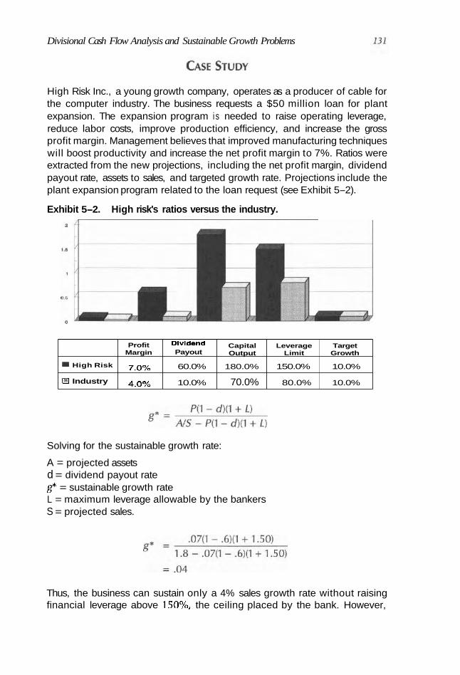
Divisional Cash Flow Analysis and Sustainable Growth Problems
High Risk Inc., a young growth company, operates as a producer of cable for the computer industry. The business requests a $50 million loan for plant expansion. The expansion program i s needed to raise operating leverage, reduce labor costs, improve production efficiency, and increase the gross profit margin. Management believes that improved manufacturing techniques will boost productivity and increase the net profit margin to 7%. Ratios were extracted from the new projections, including the net profit margin, dividend payout rate, assets to sales, and targeted growth rate. Projections include the plant expansion program related to the loan request (see Exhibit 5-2).
Exhibit 5-2. High risk's ratios versus the industry.
Solving for the sustainable growth rate:
I High Risk
I Industry
A = projected assets d = dividend payout rate g* = sustainable growth rate L = maximum leverage allowable by the bankers S = projected sales.
Thus, the business can sustain only a 4% sales growth rate without raising financial leverage above 150%, the ceiling placed by the bank. However,
Profit Margin
7.0%
4.0%
Dlvldend Payout
60.0%
10.0%
Capital Output
180.0%
70.0%
Leverage Limit
150.0%
80.0%
Target Growth
10.0%
10.0%
growth is pegged at 10%. If the company grows at a higher rate than the sustainable growth rate, the business's current leverage will increase beyond the ratio permitted. The next step for High Risk is to deal with three condi- tions that control leverage, discussed next.
Three Different Appoaches for L
The DebtIEquity Ratio
The sustainable growth model (g*) depicts a case in which a company is inundated with additional debt. If the sustainablegrowth rate (g*) falls below the targeted growth rate (n, excessive leverage will halt growth and might even sink the business. This is readily observable as follows:
1. The CFO sets L, the debvequity ratio, at the maximum allowable level. The ratio may be set at the industry unsystematic risk maxi- mum, a "bankruptcy" leverage, or simply at the lender's tolerance level. We saw this approach used on the previous page.
2. The CFO can set g* equal to the targeted growth rate T and solve for L to secure the debvequity ratio in equilibrium with the firm's tar- geted growth rate. Thequestion is, simply, if the firm continues its growth pattern, how high wil l leverage climb, assuming that the busi- ness raises no new equity? Formula: g* = P(1 - D)(1 + L) l [ N S - P(1 - D)(1 + L) ] . LEVERAGE AT GROWTH Equilibrium (L*): Leverage will approach L* when the targeted growth rate (7J and the capital structure are in equilibrium. The model assumes an indefinite growth period.
3. Alternatively, the CFO might develop a forecast taking the debvequity ratio in the last year of the forecast period and substitut- ing it into the formula to determine the sustainable growth rate in the business's residual period.
High Risk's growth rate wil l seriously impact cash flow. Without adequate cash funneling in from sales, operating leverage will increase because of the debt raised to cover cash shortfalls. A high degree of both operating leverage and financial leverage spells trouble because of the high level of sales needed reach its breakeven.
Will the business have to revert to increased borrowings to substitute for differences between internal and external financing? Here, we are con- cerned with the effect that recessions have on a company's cash flow and financial condition. During a period of economic slowdown, sales may decrease enough to cause cash flow streams to run dry. Technological improvements, as with High Risk, also cause financial needs to jump. To keep up with competition in an ever-changing and high-pressure market- place, companies must adapt quickly to the latest changes in machinery and

Divisional Cash Flow Analysis and Sustainable Growth Problems 133
equipment technology-technology that can either improve production effi- ciency or bring the company down in a climate of do-or-die.
The "do" factor: This means that more money must be spent on new asset purchases, and there must be a corresponding increase in sales and internal cash flow to match the purchases of the assets. The "die" factor: Lenders, along with the firm's finance people, are well aware that without adequate cash inflows, default risk compounds dramatically.
Example Approach 2
Set g* equal to the targeted growth rate T and solve for L to obtain the debtlequity ratio in equilibrium with the borrower's targeted growth rate:
Solving for L, we obtain L = 4.84. Thus, leverage must increase to 484% for the sales growth rate and financial structure to fluctuate in equilibrium. Since the maximum allowable debvequity was 150%, the deal, as presented, can- not be approved.
Approach 3 is redundant here and wil l not be explored.
Solving Sustainable Growth Problem
Techniques available to solve sustainable growth problems include issuing equity, improving asset management, reducing dividend payout, and increas- ing the profit margin. Profit pruning, including dissolving unprofitable divi- sions, i s s t i l l another way to ease growing pains. Also, knowing when rapid growth ends and the mature phase starts will quickly end a sustainable growth problem. Once the business has entered the mature phase of its com- pany life cycle, greater amounts of cash wil l be generated, risk decreased, and cash flows more predictable.
Issue Equity
This may be difficult to do in a small operation with limited access to the venture capital market. Most countries do not have active, developed equity markets. Also, new equity is expensive, dilutes ownership, and is likely to reduce earnings per share.
Improve the CapitalIOutput Ratio (AssetsISales)
The asset-to-sales ratio is an important component of the sustainable growth model. It is positioned in the equation to represent the base (before profit

134 S C Z E N ~ F I C FINANCIAL MANAGEMENT
retention) on which an appropriate and sustainable growth rate is calculated. If this rate exceeds a tolerable rate, we know that leverage will increase rapidly.
Capital output is crucial to cash flow because it examines the tier (of assets) needed to produce a given sales level. For example, in today's ultra- competitive environment, the left side of the balance sheet is managed aggressively to allow for sustainable growth. Just-in-time UIT) inventory, as we saw in the section on cash flow, is but one example. Often, JlT inventory requires an expensive investment in technology. For example, JIT can require scanners at the point of sale that transmit information directly to the supplier, who then ships additionally items. This type of arrangement eliminates some cost of carrying inventory. Operations not leveraged to the hilt, with strong debt capacity and cash flow, are in a better position to finance sophisticated asset management systems.
However, High Risk is in no position to bargain and may need to make hard decisions to reduce debt levels. For example, the business may decide to contract out production assignments to other vendors to reduce raw mate- rials and work-in-process inventory-not a sweet pill to digest, as this activity will reduce profit margins as well because goods will cost more to produce.
Increase Profit Margins
Improved profit margins reflect strategic, operating, and financing decisions, certainly on the divisional level. Strategies involve critically important deci- sion areas, such as choice of product market areas in which the business or division conducts operations, whether to emphasize cost reduction or prod- uct differentiation, and whether to focus on selected product areas or seek to cover a broad range of potential buyers.
Reduce Dividend Payout
Increases in both dividends and debt-to-equity ratios are potentially alarm- ing because dividends reduce cash flow. On the other hand, profit retention shows a commitment to reinvest in the business rather than satisfy the short- term satisfaction of equity investors through dividend distributions.
Profit Pruning
When a business spreads its resources across many products, it might not be able to compete effectively in all of them. It is better to sell off marginal operations and plow the proceeds back into the remaining businesses. Prof- itable pruning reduces sustainable growth in two ways: (1) It generates cash directly through the sale of marginal businesses, and (2) reduces actual sales growth by eliminating some sources of the growth. Profit pruning is also available for a single-product company. The business could prune out slow- paying customers or slow-turning inventory. This lessens sustainable growth problems in three ways: (1) It frees up cash that can be used to support new

Divisional Cash Flow Analysis and Sustainable Growth Problems 135
growth, (2) it increases asset turnover, and (3) i t reduces sales. The strategy reduces sales because tightening credit terms and reducing inventory selec- tion wil l drive away some customers.
High Risk's New Strategy
As we saw earlier, g* is equal to 4%; the company can grow at 4% without increasing leverage over 150%. However, High Risk is preparing for a 10°/~ sales increase. Since the company is growing at a higher rate than the sus- tainable growth rate, the business's current debt-to-equity ratio exceeds the 150% maximum level set by the business's lenders. By setting the targeted growth rate at 10% and solving for L the lenders realize that a leverage of 484% equates with the business's 10% growth rate-much too high.
High Risk Inc., like almost all firms, will use sales growth as a major com- ponent of long-run financial planning. However, in the search for more profit dollars, many managers fail to consider the growth rate that the company's finan- cial structure can support. Financial planning establishes guidelines for changes in the business's financial structure. Thus, a sure understanding of this business's financial planning will help reduce credit risk by structuring a tighter deal.
The sustainable growth model depends on the major elements of the business's financial planning. High Risk's financial planning should include the following:
A An identification of the business's financial goals A An analysis of the differences between these goals and the current
financial status of the business A A statement of the actions needed for the business to achieve its finan-
cial goals
The financial policies that the business must decide for its growth and prof- itability include the following:
A The degree of financial leverage the business chooses to employ A The amount of cash the business thinks is necessary and appropriate
to pay shareholders (dividend policy) A The investment opportunities the business elects to take advantage of
in the future
Financial plans are not the same for all firms. Economic assumptions, sales forecast, pro forma statements, asset requirements, and financial require- ments are some common elements of the financial plan.
High Risk's sales wil l be influenced by several "cash flow" factors. The prevailing economic conditions at a given time affect separate industries dif- ferently. For example, automobiles and home construction contracts would be reduced during a recession, whereas food sales would not be affected as

greatly. In analyzing the potential cash flows and credit risks of this business, the prevailing market conditions will need to be considered first. These are factors that wil l affect an industry as a whole. You can analyze an individual company by finding its market share compared with its industry.
The fact that a firm is an innovator and market leader wil l reflect market share. Innovative operations with aggressive R&D programs will often gain advantages over competitors. Confirmed orders are good indications of future sales and needed production capacities, but projecting sales i s often difficult in emerging industries because the predictability horizon is very short.
While growth in leverage ratios also increase the sustainable growth rate, the composition of High Risk's debt is also very important. If this emerging company continuously uses short-term debt as a financing mechanism, the business will become overexposed to volatile and rising yield curves that may drastically increase cost of debt when refinancing/rollover of debt is required; overreliance on short-term debt reduces the company's financing flexibility.
Also, it may suggest that other creditors are skeptical of the company's future cash flows and may not want the credit exposure of extending long-term debt that may not be remunerated. However, what may be inferred here is management's confidence that liquidity can be sustained principally through profit retention, enabling them to search for the lowest cost of capital.
Asset quality should be reviewed with leverage ratios because higher- quality assets allow for increased leverage ratios. Regarding debt capacity, an analysis of High Risk's cash flow coverage ratios should be measured and trended over a period to decide whether the leveraged company is experi- encing any current or near-term problems covering interest expense and sat- isfying debt payments.
Also, leveraged companies that continue to increase debt without rais- ing equity capital may suggest questions about the business's viability if equity capital market investors have rejected any public offerings of stock. It may also suggest that the company is not exploring its various capital-raising alternatives, and overreliance on a single financing method may not provide the business with the least expensive cost of capital.
In High Risk, the business's lenders will likely advise the business to decrease its debt-to-equity ratio by injecting new equity. If the business declines, High Risk could reduce its operating leverage, inventory, and debt levels by hir- ing subcontractors, thus raising the sustainable growth rate to acceptable levels.
The business decided not to issue new equity, preserving ownership control. Instead, as agreed, subcontractors will produce and ship to High Risk's customers. Other considerations are the following (see Exhibit 5-3):
A Because the use of subcontractors wil l squeeze profit margins, sales wil l continue to grow at 10%. High Risk has agreed to absorb higher costs of production.
A Using subcontractors wil l lower inventory levels and reduce capital spending.

Divisional Cash Flow Analysis and Sustainable Growth Problems 137
Exhibit 5-3. Revised srategy. -
A High Risk consents to tight control of receivables. A Dividends must be reduced. A Leverage wil l not transcend the ceiling imposed by the business's
lenders.
Revised Strategy
a Orlglnal Strategy
The previous condition was:
The sustainable growth rate is 11 %. Thus, High Risk Inc. can grow at 11 % a year over the foreseeable future without increasing leverage beyond 150%, the leverage ceiling. Since the business's 10% targeted growth rate is less than its 11 % sustainable growth rate, leverage wil l fall below the maximum level permitted by the business's creditors. With improved asset manage- ment, a less aggressive dividend policy and even considering reduced prof- its, the sustainable growth rate actually increased. In other words, the busi- ness's cash flow problems were substantially eliminated and the strategic problem identified. Poor asset management proved to be the guilty party. With poor asset management, an aggressive dividend policy, and declining profits, the sustainable growth rate actually increased, causing the business to have cash flow problems.
Profit
Margln
4.0%
7.0%
Dividend Payout
10.0%
60.0%
Capital Output
90.0%
180.0%
Leverage Limit
150.0%
150.0%
Target Growth
10.0%
10.0%
Chapter Five References and Selected Readings
Books and Periodicals
Bierlen, R., and A. M. Featherstone. (1998). "Fundamental q, cash flow, and investment: Evidence from farm panel data." Review of Economics and Statistics, 427-35.
Dechow, P. M., et al. (1998). "The relation between earnings and cash flows." Journal of Accounting and Economics, 13M8.
Emmanuel, C. B. (1988). "Cash flow reporting, Part 2: Importance of cash flow data in credit analysis." Journal of Commercial Bank Lending, 16-28.
Gahlon, J. M., and R. L. Vigeland (1988). "Early warning signs of bankruptcy using cash flow analysis." Journal of Commercial Bank Lending, 615. Establishes that seven cash flow variables and suggested ratios capture statistically signif- icant Merences between bankrupt and nonbankrupt firms, on average, as much as five years prior to bankruptcy. These ratios and variables are thus strong candidates for inclu- sion in the early warning systems that banks use for iden-g potential credit problems.
Gentry, J. A., et al. (1990). "Profiles of cash flow components." Financial Analysts Journal, 4148. Helfert, E. A. (1994). Techniques offinancial analysis. Burr Ridge, Ill.: Irwii. Kathuria, R., and D. C. Mueller. (1994). "Investment and cash flow: Asymmetric informa-
tion or managerial discretion." Working paper. Department of Economics, University of Maryland, no. 3,146.
Mills, R. (1998). "Strategic value analysis." Economic and Financial Computing, 15S98. Nordgren, R. K. (1986). "Understanding cash flow: A key step in finanaal analysis." Jour-
nal ofCommercia1 Bank Lending, 2-17. Schulman, E. M. (1988). "Two methods for a quick cash flow analysis." Journal of C o m m -
cia1 Bank Lending, 29-36. Shin, H.-H, and R. M. Stulz. (1996). "An analysis of divisional investment policies."
Other Periodicals
Benveniste, Lawrence M. (1999). "Comment: Gain-on-sale's 'problem': Too much informa- tion." American Banker, September 16, p. 19.
Charitou, Andreas. (1999). "Earnings, cash flows and security returns over long return intervals: Analysis and UK evidence." Journal of Business Fimce and Accounting, 26(3/4), p. 283.
Farragher, Edward J. (1999). "Current capital investment practices." The Engineering Econo- mist, 44(2), p. 137.
Felthan, Gerald A. (1999). "Residual earnings valuation with risk and stochastic interest rates." The Accounting Review, 74(2), p. 165.
Hartmann, Matthias H. (1999). "Theory and practice of technological corporate assess- ment." Intonational Journal of Technology Management, 17(5), p. 504.
Penman, Stephen H. (1998). "A comparison of dividend, cash flow, and earnings approaches to equity valuation." Contemporary Accounting Research, 15(3), p. 343.
Smith, James E. (1998). "Evaluating income streams: A decision analysis approach." Man- agement Science, 44(12), p. 1690.
Strauss, Mel. (1998). "Examining FAS 133." USBanker, 108(9), p. 68.
CD
Name Size Tvoe
2.1 7 International Accounting Standard IAS 7- 1 KB Internet Shortcut Cash Flow Statements

Statistical Forecasting
Methods and Modified
Percentage of Sales
YOGI RERRA, THE FAMOUS BASEBALL catcher, once said, "If you don't know where you're going, any road will take you there." The rules that made baseball the grand game that it is are as rigid as earth's orbit around the sun. However, try applying rules to a great pitch, and it just will not work; and, like the exploding curveball, financial forecasting rises above the steely rulebook of laws and statistics. It has become the hero on the mound; the brave new world. Forecasting is an art, and like great pitching, it is dynamic and somewhat unsettling and moves with the speed of the Discoverer. Yogi would suggest that great pitchers know the road to the mound-"and it ain't a dirt trail either." There are few dirt roads and even fewer mediocre pitchers in the game of financial forecasting. Slow, easy lobs just will not make it in the new century.
Recently scientific forecasting and its family of techniques have won wide acceptance as planning and decision-making tools. To satisfy these diverse situations, computer-generated techniques such as regression, sim- ulation, optimization, neural networks, data mining, and a host of varied time-series techniques and causal methods are now mainstream. This means all areas: sales planning, working capital management, marketing research, R&D, pricing, produdion planning and scheduling, financial planning, pro- gram planning, corporate bond ratings, and strategy formulation.

The good old days when naive methods carried the day have gone the way of the dirt road. Yet, in the final analysis a financial forecast is simply a file. Beyond that, good judgment on your part, plus a bit more than basic knowledge, will metamorphose the document to life. Art, power, and skill deliver the game-winning strikeout. Still, though, the rules, the statistics, and the scientifically generated report define the play and will drive your argument home, and that is what board members like to hear.
This chapter focuses on statistical forecasting and modified percent- age of sales methods. Simulations and neural forecasting are covered in chapters 7 and 8.
A "Statistics" Approach to Financial Forecasting
Statistical methods generally fall into two broad groups: causal models and time-series analysis. Causal models include both regression models and econometric models. Time-series analysis includes moving averages, Box-Jenkins methods, and exponential smoothing.
Forecasting techniques include qualitative and quantitative methods (see Exhibit 6-1). We stress scientific methods in the three chapters on fore- casting, so we will focus on quantitative methods there.
Causal models assume that forecast variables exhibit a cause-effect relationship. For example, sales may be a function of market share, markup, promotion, competition, and economic sensitivities. The whole idea of casual models allows you to discover that relationship so that the future value of sales can be determined. Conversely, a causal model is more involved than time series but can be particularly more relevant to frame policy and decision making.
Causal (simple regression) is a special case of regression when you work with a single independent variable. In simple regression, as in mul- tiple, you assume a linear association within historical data and allow models to estimate the relationship using the method of least squares. Sim- ple regression is not limited to time-series relationship. Rather, it predicts connections between any two variables, determining the value of one vari- able (dependent) as a function of the second variable (independent). Thus, the logo causal model. Mathematically, the causal is written as Y = f(X). The value of Y is a function of the value of X. When this is assumed to be a straight-line relationship, you write it as Y = a + bX.
Time-Series, or Trend, Forecasting
Time series, on the other hand, predicts the future by expressing it as a func- tion of the past, for example, Sales = f (time). We learn forecast modeling by activating Excel's functions that will draw either a line straight (trend func-

Statistical Forecasting Methods and Modified Percentage of Sales
Exhibit 6-1. Flowchart of qualitative and quantitative forecasting techniques.
Moving average methods
Fuzzy loqic Simulntion and ' Data mining modein modp!s aptitnization models
mode15
tion) or a curve (growth function) in such a way that it passes through "the middle" of your historical data. Not long ago, you likely would have shied away from time series because of the large numbers of calculations involved. Since spreadsheet applications began offering built-in trend func- tions, the use of linear and curve fit analysis has become standard.
Excel Example 1 [CD:\MODELS\EXCEL\CGREGBook]
Excel includes several array functions for performing linear (LINEST, TREND, FORECAST, SLOPE, and STEYX) and exponential (LOGEST and GROWTH) regression. These functions are entered as array formulas and produce array results. You can use each of these functions with one or sev- eral independent variables. The following example shows you how to

Exhibit 6-2. RegBook opening page.
develop simple trend and growth regressions. Open RegBook.xls located in the "Models" subdirectory of the CD and follow the instructions (see Exhibit 6-2).
Let us develop a straight-line regression first. Excel labels this func- tion a trend. When you finish, you can generate a curve through your data. Excel labels this function "growth." The following instructions will enable you to complete this operation.
To develop a trend: 1. Select c3:c14 by dragging mouse. 2. Click on formula bar. In formula bar type =trend(. 3. With mouse drag b3:b14. Watch formula bar change. Type in
comma.

Statistical Forecasting Methods and Modified Percentage of Sales 143
Exhibit 6 3 . RegBook solution.
4. With mouse drag a3:a14. Watch formula bar change. Type in ). 5. Create array and regression by pressing simultaneously keys Con-
trol Shift Enter.
Develop regression forecast as follows: 1. Select c15:c24 by dragging mouse. 2. Click on formula bar. In formula bar type. = trend(. 3. With mouse drag b3:b14. Watch fonnula bar change. Type in
comma. 4. With mouse drag a3:a14. Watch formula bar change. Type in
comma. 5. With mouse drag a15:a24. Watch formula bar change. Type in ). 6. Create array and regression by pressing simultaneously keys Con-
trol Shift Enter.
Your solution should look like Exhibit 6-3. [CD:MODELS\EXCEL\ CGREGBkSolutions] If so, congratulations. Now let's move to a much higher order time-series level, reviewing a powerful tool, Decisioneering's CB Predictor.

Regression Using Decisioneering's CB Predictor'
A growing list of top financial executives are convinced that Decisioneer- ing's CB Predictor is one of the best time-series models in the literature. Go to [CD:Applications\Decisioneering\Customer]. The firm's client list includes most of the Fortune 500 along with major accounting, investment, and commercial banking firms.
CB Predictor breaks historical data into three components: trend, sea- sonality, and error. We will develop and optimize time-series forecasting using the model.
CB Predictor uses techniques of time-series and multiple linear regression categories. The Crystal Ball product uses simulation. Each tech- nique and method has advantages and disadvantages for particular types of data, so forecast your data using several methods and then select the method that yields the best results. Time-series forecasting is a category of forecasting that assumes that the historical data is a combination of a pat- tern and some random error.
Its goal is to isolate the pattern from the error by understanding the pat- tern's trend and seasonality. You can then measure the error using a statisti- cal measurement test both to describe how well a pattern reproduces histor- ical data and to estimate how accurately it forecasts the data into the future. When you select different forecasting methods to try from the Methods Gallery, CB Predictor tries all of them. It then ranks them according to which method has the lowest error, depending on the error selected from the Advanced dialog box. The method with the lowest error is the best method.
Before using CB Predictor, you must create an Excel spreadsheet with your historical data not unlike the one we developed (see Exhibits 6-2 and 6-3). [CD:MODELS\EXCEL\C6ShampooSolution] Creating a spread- sheet for use with CB Predictor is easy. The spreadsheet needs to include only a descriptive title and, optionally, a date (or other time period, such as Q4- 1997) column or row, either at the top or along the left side of your data. If you format your dates as Excel dates, CB Predictor's Intelligent Input can find the dates, extend them with the forecasted values, and use them as labels on charts. Historical data, spaced equal time periods apart, are in columns or rows adjacent to the date column or row. You can use CB Predictor to simul- taneously forecast from 1 to 10,000 adjacent historical data series.
After you create your Excel spreadsheet with your historical data, forecasting data using CB Predictor follows a 10-step process:
1. Select a cell range with your historical data to forecast. That is A3:B42 (see Exhibit &I).
2. Specify your data.
1. Reproduced with permission of Decisioneering and Dr. Carl Crosswhite, the man behind CB Predictor. This chapter could not have been developed at the present level without Dr. Crosswhite's innovative and brilliant work in two disciplines: statistical analysis and soft- ware engineering and tools. This author is deeply indebted to this gentleman.

Statistical Forecasting Methods and Modified Percentage of Sales 145
Exhibit 6-4. Shampoo sales opening.
3. View a graph of your historical data to identify any seasonality or trend and to see summary statistics.
4. Identify your time periocls and whether your data has seasonality and, if so, how long your season is.
5. Set whether you want to use multiple linear regression to forecast any variables.
6. Select the time-series forecast methods to try for each variable. 7. Enter the number of periods you want to forecast. 8. Select a confidence interval to calculate or display with your fore-
casted values. 9. Select the results you want.
10. Preview and run the forecast, creating your results.
CB Predictor leads you through these steps using the CB Predictor Wizard, but you can also go directlyto any of these steps to change methods or select different options and reforecast data (see Exhibit 6-5).
Also, many of these steps might be done automatically by CB Predictor. For example, CB Predictor's Intelligent Input can find and select your data, its arrangement, and the data units. You can also skip many other steps if the settings are already what you want. For example, all the &e-series forecast-

Exhibit 6-5. Shampoos data box.
ing methods are selected by default, and that is probably how most users will leave them. Now lets review all the reports (see Exhibits 6-6 through 69).
See glossary of forecasting terms and additional statistical definitions dealing with predictor models at the conclusion of this chapter.
Simple Moving Averages
Simple moving averages are initially calculated by starting with the leftmost period in the data and adding up the specified prices (open, high, low, close, mid-point, or average) for the chosen number of periods. This total is then divided by the number of periods set in the Parameters menu. The formula is:
where n = number of bars P, = selected calculation price P, = selected calculation price 1 period ago P, = selected calculation price n periods ago
The moving average has distilled the trend from the daily price fluctuations (see Exhibit 610).

Statistical Forecasting Methods and Modified Percentage of Sales
Exhibit 6-6. Report for Shampoo Sales. Created: 01 11 212000 at 1 :41 :I 4 PM
Summary: Number of series: 1 Periods to forecast: 4 Seasonality: none Error Measure: RMSE
Series: Unit Sales Method: Double Moving Average Parameters:
Periods: 7 Error: 71 74.1
Range: B4:B42
Series Statistics: Mean: 33,956 Std. Dev.: 1 7,183 Minimum: 11,850 Maximum: 68,190 Ljung-Box: 374.61 52
Forecast:
Date Lower: 5% Forecast Upper: 95%
Exhibit 6-7. Trend line best-fit graph. r r-. *,
Unit Sates 12COOO 7
1WQ9 - #" 4 D31a I
Upper: 95%

Exhibit 6-8. Method errors.
Method RMSE MAD MA PE
Best: 2nd: 3rd: 4th:
Double Moving Average 71 74.1 5527.8 15.53% Single Moving Average 7569.6 5953.6 19.90% Single Exponential Smoothing 8096.3 6435.6 21.74% Double Exponential Smoothing 8 1 99.2 6687.8 25.12%
Method Statistics:
Method Durbin-Watson 7heii's U
Best: Double Moving Average 2.882 0.662 2nd: Single Moving Average 2.676 0.803 3rd: Single Exponential Smoothing 2.543 0.814 4th: Double Exponential Smoothing 2.624 0.878
Method Parameters: - -
Method Parameter Value
Best: Double Moving Average Periods 7 2nd: Single Moving Average Periods 2 3rd: Single Exponential Smoothing Alpha 0.448 4th: Double Exponential Smoothing Alpha 0.302
Beta 0.999
Exponential Smoothing Averages
Since the development of exponential smoothing 50 years ago, the method has become a popular method of forecasting with finance people. Expo- nential smoothing requires only a few data points to produce predictions and is well suited for large numbers or items. Exponential smoothing smoothes past values of a t h e series in a decreasing (exponential) fashion. This is achieved bv a formula embedded on a statistical model that derives exponentially decreasing weights associated with past observations, visu- alized in Exhibit 6-11.
Regression Curve Fitting: The Exponential and Logarithmic Curve Fit
Background
In a nutshell, watch out. If your firm is undercapitalized, exponential growth will likely stress it. Conversely, logarithmic growth is akin to stronger bond ratings, less default risk, and stronger cash flows. Exponential

Exhibit 6-9. Methods table for shampoo sales.
Methods Table for Shampoo Sales Created: 01/12/2000 at 1:41:23 PM
1 series I Unit Sales
Methods Double Exponential Smoothing Double Moving Average Single Exponential Smoothing Single Moving Average
Table Items Rank RMSE MAD MAPE Durbin-Watson Theil's U Periods Alpha Beta
4 8199.2 6687.8 25.115 2.624 0.878 0.302 0.999 1 7174.1 5527.8 15.527 2.882 0.662 7 3 8096.3 6435.6 21.74 2.543 0.814 0.448 2 7569.6 5953.6 19.903 2.676 0.803 2
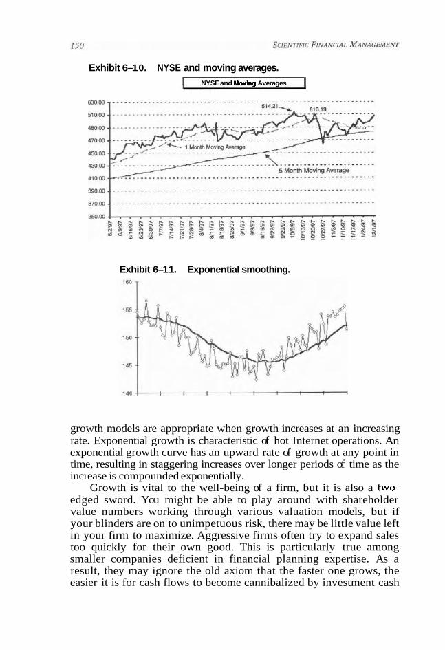
Exhibit 6-1 0. NYSE and moving averages. I NYSE and Moving Averages I
Exhibit 6-1 1. Exponential smoothing.
growth models are appropriate when growth increases at an increasing rate. Exponential growth is characteristic of hot Internet operations. An exponential growth curve has an upward rate of growth at any point in time, resulting in staggering increases over longer periods of time as the increase is compounded exponentially.
Growth is vital to the well-being of a firm, but it is also a two- edged sword. You might be able to play around with shareholder value numbers working through various valuation models, but if your blinders are on to unimpetuous risk, there may be little value left in your firm to maximize. Aggressive firms often try to expand sales too quickly for their own good. This is particularly true among smaller companies deficient in financial planning expertise. As a result, they may ignore the old axiom that the faster one grows, the easier it is for cash flows to become cannibalized by investment cash

Statistical Forecasting Methods and Modified Percentage of Sales 151
drains. Small increments to equity via earnings pale when matched against the insatiable appetite for new assets required by rapid growth firms.
Exponential growth has been the focus of much discussion among researchers investigating food and raw material requirements. Some ana- lysts argue for growth limits because finite space and resources bind expo- nential increases. Others argue that stabilizing social and market mecha- nisms slow or stop exponential growth. As for business, most valuation experts argue that exponential growth retreats in the face of competitive markets when output becomes saturated in the marketplace, forcing down internal rates of return.
Whatever one's position, exponential growth may take place for extended periods of time, and that is the danger. Popular models, notably Excel's trend-line functions, are powerful tools to track data and spin them off into "lower risk"/"higher risk" curve fits.
Trend Lines and Curve Fit Correlations in Excel
Open [CD:MODELS\EXCEL\C6REGRESS\Statistics] and select C6:C15 (see Exhibit 6-12). After you have selected cells C8:C15:
1. Create a Chart using the Wizard. 2. Click on line. You will see square boxes on your line. 3. Select chart and add trend line. See Exhibit 6 1 3 . 4. Click on Exponential. 5. Select Options. Check off display equation on chart and display RZ
value on chart.
To add a trend l i e to a data series, do the following:
1. Click the data series to which you want to add a trend line or moving average.
2. On the Chart menu, click on Add Trend line.
3. On the Type tab, click the type of regression trend line or moving average you want.
4. Under options, select RZ and Formula. See Exhibit 6-14.
Exhibit 6-12. A
5 Year
6 19x0 7 19x1 8 19x2 9 19x3
10 19x4 11 19x5 12 19x6 13 19x7 14 19x8 15 19x9 16 Sum
Sales/inventory matrix. B C
Inventory Sales (Y) (XI
0.403 0.461 0.506 0.507 0.665 1.087 1 .I 65 1.278 1.438 1.216 8.726 131.694

Exhibit 6-1 3. Trend line.
The R2 statistic in Excel tells you what percentage of variation in the dependent variable (Y) is "explained" by changes in the independent vari- able. It ranges from 1 (meaning that the variation in the independent vari- able perfectly explains the variation in the dependent variable or that the relation between the two variables is very strong) to 0 (meaning that there is no relationship between the variables). In general, the larger the R2
value, the better changes in the independent variable explain variations in the dependent variable. Let's examine sales data. We can see whether the trend fits an exponential or logorithmetic curve (see Exhibit 6-15).
Box-Jenkins
The Box-Jenkins methodology, (1976) has emerged as a widespread statisti- cal method for autoregressive or time-series analysis. There are several types of Box-Jenkins models. These include (1) univariate models (modeling a time series as a condition of its past), (2) transfer function models (modeling a time series as a function of its past and the past of one or more independent series), and (3) multiple equation models (modeling more than one time series as a function of all other series in the equation). Transfer function models are a particular case of multiple-equation models, where there is a unidirectional relationship between the output series and each of the input series.

Statistical Forecasting Metl~ods and Modified Percentage of Sales I S 3
Exhibit 6-14. Curve fit statistics.
One model that offers vector Box-Jenkins modeling is MTS. The pack- age includes a menu-driven system to set up and run the program. MTS allows forecasters to retain control over model identification, estimation, and forecasting procedures or to allow the program builds in heuristic to develop the model for the analyst. Vector ARIMA modeling is multiple- equation modeling where each input series may have a causal relationship with every other input series and each series is to be forecast. MTS is AFS's software package designed to allow the modeler/forecasters to develop these multiple endogenous variable models. Contact [email protected].
Box-Jenkins methodology need not assume an initial pattern. It begins with a tentative pattern, and a model is fitted in such a way that the error will be minimized. It then provides explicit information as to whether the tentative pattern employed is the correct one. If this pattern is not correct, the method provides guidelines for finding the right one.

Exhibit 6-15. Exponential and logarithmic curve fit and correlations. -
Thus, the Box-Jenkins methodology provides enough information to ten- tatively identify the pattern that best describes the data, estimate the para- meters involved by minimizing the sum of the squared errors, and provide for a diagnostic check of the residuals to determine whether the tentative pattern (model) is an adequate one.
Multiple Regression
Multiple regression has become one of the most puissant models in the domain of statistical financial analysis. The purpose of multiple regression is to predict a single variable from one or more independent variables. Multi- ple regression with many predictor variables is an extension of linear regres- sion with two predictor variables. A linear transformation of the X variables is done so that the sum of squared deviations of the observed and predicted Y is a minimum. The computations are more complex, however, because the interrelationships among all the variables must be taken into account in the weights assigned to the variables. The interpretation of the results of a mul- tiple regression analysis is also more complex for much the same reason.
Here we find a lead/lag relationship between the dependent variable and a leading (independent) variable that could be used in predicting. From a practical view, the approach of paired indices is useful providing causal information. For example, you employ multiple regression and esti- mate causal relationships in data. This approach complements time-series forecasting. But be careful: You can run into problems. For example, to predict sales you may decide that disposable income and television spots

Statistical Forecasting Methods and Modified Percentage of Sales 155
are two linking factors. However, future levels of that disposable income may prove not to be a viable link, nor can one be certain of the role that television advertising will play in the future (i.e., the "error factor" in the formula).
While a compelling relationship may appear between sales and dis- posable income/advertising, the association might yield limited value. Thus, forecasting issues are not necessarily resolved by identifying cause-effect relationships. Relationships between variables may change as as your firm moves through its economic environment, so causal forecast- ing is never used alone.
Multiple regression designates one variable as dependent (Y) and picks, via a stepwise operation, which variables are independent (X). You may elect to develop the regression apart from stepwise. For example, you may want to change one variable, measure another, and then analyze the data with one or more of the standard statistical tests.
The prediction of Y is accomplished by the following equation:
Y = p, + pl,, + P2=, + P3z, + P4 z,... + random scatter
If there is only a single X variable, then the equation is Y = Po + Dlzl, and the "multiple regression" analysis is the same as simple linear regression (PO is the Y intercept; p, is the slope).
One of the most famous examples of multiple regression is Altman's Z score. Altman developed the Z (zeta) score to predict distress at a certain confidence level. His causal regression, developed from stepwise, found crucial critical variables that were highly correlated to financial distress: working capital, leverage, sales, earnings retention, and operating profits.
Altman's sample included 33 financially distressed manufacturing firms along with a control group of 33 healthy companies. From financial statements one period prior to bankruptcy, Altman extracted 22 financial ratios, of which 5 were found to contribute most to the prediction model. The discriminate function Z was computer derived as:
where x, = working capital/total assets xi = retained earnings/total assets x, = EBIT/total assets x, = market value of equity/book value of debt x5 = sales/total assets
Z > 2.99 is classified as healthy and remained continuing entities. The higher the Z score, the healthier the firm and the lower the probability of failure. Z < 1.81 is classified as financially distressed or bankrupt.

By applying the previous discriminate function to data obtained two to five years before bankruptcy, Altrnan discovered that the model cor- rectly classified 72% of the initial sample two years before failure. A trend analysis shows that all five observed ratios, x, . . . x,, deteriorated as bank- ruptcy approached and that the most seriouschange in most of these ratios occurred among the third and second years before failure. Following is an example of the function Z:
Two researchers, Moses and Liao, have suggested that individual ratios included in the model may be highly correlated with each other. This is serious stuff. As we will see shortly, highly correlated independent vari- ables (multicollinearity) pose a threat to the accuracy of regression and must be statistically resol~ed.~
Individual ratios included in the model may be highly correlated with each other. This causes three problems. First, the relationship between individual ratios and the dependent variable (failure status) may be dis- torted. Second, correlation between predictor ratios may differ in other samples making results developed on one sample applicable only to that specific sample. Third, individual coefficients are not meaningful so conclusions concerning the importance of any individual ratio in explaining failure are not possible, making the model difficult to inter- pret. In fact the standard approach may assign coefficients with signs that are counterintuitive."
Though this may be so, we need to look beyond multicollinearity to con- ceptualize the numerous threads of brilliant financial logic that drives the regression (did the logic drive the regression or the regression, the logic?). Let's give Altman the benefit of the doubt. In any event, I call Altman's linkage the domino-multiplier syndrome. For example, take sales. Firms running high operating leverage are sensitive to revenue declines. Follow how the model tracks sales declines:
1. Abrupt and sharp sales declines drive down x, (EBIT/assets) due to the negative effects of operating leverage. Thus, x, and x, drop.
2. A drop in x, (EBIT/assets) knocks over a domino by driving down 1.4~~ (retained earnings/assets) as losses flow through because fixed costs are not covered.
2. Douglas Moses and Shu S. Liao, "On Developing Models for Failure Prediction," Journal of Commercial Bank Lending (March 1987). 3. IBID

Statistical Forecasting Methods and Modifed Percentage of Sales 157
3. Retained earnings are a component of working capital (along with increases in long-term obligations and reductions in fixed assets). Thus, x, (retained earnings/total assets) links to x, (working capital/total assets).
4. What effect will our dominos have on x, (market value of equity/book value of debt)? Investors start dumping shares in panic selling, fearing that the firm's weak liquidity (caused by operating losses) makes it difficult or nearly impossible to reduce debt.
A second regression factor, low asset productivity, has also been shown to be significant. Firms bankrupt when assets such as inventory, receivables, and equipment go out of control. Distressed companies break the cardinal aphorism of basic planning: Keep assets at minimum levels consistent with maintaining strong sales and profits. We note that four out of five Z score (X) variables carry assets in the denominator. Zeta will fall below crit- ical mass if asset management loses out as a key strategic event. This means that if you want to keep your firm out of the minor leagues, check assets, ensure that they operate at optimal efficiently, develop goods and services that produce healthy profits, and keep watch over the firm's equity base and capital structure.
Is Multiple Regression the Right Tool for Your Forecasts?
1. Is the relationship between the X variable and Y variables linear? If the relationship between X and Y variables is nonlinear, multiple regression may not be the method for the task at hand. In some cases, you may be able to transform one or more X variables to cre- ate a linear relationship. If so, fine. In chapter 8, we explore neural networking, which will resolve nonlinear data problems.
You may also be able to restrict your data to a limited range of X variables where the relationship is close to linear. Some programs can perform nonlinear regression with multiple independent variables.
2. Is the variability the same everywhere? Multiple regression assumes that data scattering from predictions has identical stan- dard deviations for all values of independent variables. The assumption is violated if the scatter goes up (or down) as one of the X variables gets larger. The assumption that the standard deviation is the same everywhere is termed homoscedasticity.
3. Is multicollinearity a problem for your forecasts? Multicollinearity can cause regression results to end up in the old garbage-in, garbage-out bin. This is when two or more independent variables are highly related to one other. High correlation between indepen- dent variables creates computational problems, but you correct this by eliminating all but one of the highly correlated independent

variables from the regression model. Crystal Ball will test degrees of correlation between independent variables, so do not worry.
Here is an example. Imagine you are running a multiple regression to extract the average collection period (the Y variable) from credit policy, credit terms, and collection phone calls. Now imagine that you have entered collection phone calls in hours and collection phone calls in minutes as two separate (X) variables. The two (X) variables measure exactly the same thing, the only difference is that the two variables have different time units. So you solve problems of multicollinearity by taking one of the variables out of the regression.
Simulation software makes it easy by testing how well each independent (X) variable can be predicted from the other (X) variables (ignoring the Y variable). However, in general there are three methods that you can employ to determine the degree of multicollinearity:
1. RZ with other X variables: the fraction of all variance in one X vari- able that can be predicted from the other X variables.
2. Use the variance inflation factor (VIF): If the X variables contain no redundant information, you expect VIF to equal one. If the X vari- ables are collinear (contain redundant information), then VIF will be greater than one. Multicollinearity increases the width of the confidence interval (which is proportional to the square root of variance) by a factor equal to the square root of VZE If a variable has a VIF of 9, the confidence interval of that coefficient is three times wider than it would be were it not for multicollinearity.
3. Determine tolerance, which is the fraction of the total variance in one X variable that is not predicted by the other X variables.
Since all three measure multicollinearity the same way, take your pick between R2 and VIF. Also, for each X variable, the corresponding VIF can be derived from R2 by VIF = 1/(1-R2). And you easily calculate tolerance for each variable as 1.0 - R2. If R2 and VIF are high for some X variables, then multicollinearity is a problem in your data.
What are the benchmarks? The usual threshold is that if any of the R2
values are greater than 0.75 (so VIF is greater than 4.0), suspect that multi- collinearity might be a problem and start thinking of throwing out a dupli- cating independent variable. If any of the RZ values are greater than 0.90 (so VIF is greater than lo), then you should assume that multicollinearity is serious, and at this point do not think but act, discarding the duplicat- ing variable.
Finally, remember that there are individual R2 values for each X vari- able and the R2t correlating all the X's with the Y. The Y R2 is the one that is really the summation but it means little until you tidy up the regression

Statistical Forecasting Methods and Modified Percentage of Sales 159
by adjusting the individual X variables to eliminate multicollinearity. You want the overall R2 value to be high (good fit) and all the individual R2 val- ues to be low (little multicollinearity).
Econometric Forecasting (Econometric Models)
Econometric forecasting is an extension of regression analysis. As we saw, regression analysis assumes that each of the independent variables included in the equation is determined by outside factors. In economic or organizational relationships, however, such an assumption of indepen- dence is unrealistic. Often there is mutual independence among all vari- ables in a forecasting equation, and regression analysis is incapable of dealing with such interdependence.
Econometric forecasting enables one to deal with such a situation. It expresses a more accurate relationship by developing a system of simulta- neous equations. These, by their nature, are capable of dealing with inter- dependent variables.
For example, suppose that Sales = f(GNP, price, advertising). (This is the multiple regression form.) In econometric form, one might have the following:
1. Sales = f(disposa1 income, price, advertising) 2. Cost = f(raw materials, production, and inventory levels) 3. Selling expenses = f(advertising, transportation, and other selling
expenses) 4. Price = cost + selling expenses
Now, instead of one relationship there are four. As with regression analy- sis, you need to do the following:
A Determine the functional form of each of the equations. A Estimate in a simultaneous manner the values of their "parameters." A Test for the statistical significance of the results and the validity of
the assumptions involved.
The main advantage of this method of forecasting is that it provides the values of several of the interdependent variables within the model itself, thus eliminating the need to estimate them externally. It also provides use- ful explanatory information as to the type of relationships involved. The estimating of the equation parameters involves problems far more com- plex than those encountered in regression analysis. It is these problems that make the application of econometric forecasting both difficult and expensive. However, the advantages gained by the method may well com- pensate for the extra costs incurred.
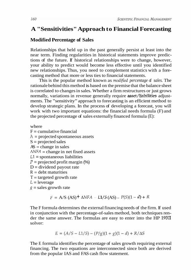
A "Sensitivities" Approach to Financial Forecasting
Modified Percentage of Sales
Relationships that held up in the past generally persist at least into the near term. Finding regularities in historical statements improve predic- tions of the future. If historical relationships were to change, however, your ability to predict would become less effective until you identified new relationships. Thus, you need to complement statistics with a fore- casting method that more or less ties to financial statements.
This is the popular method known as modl$ied percentage of sales. The rationale behind this method is based on the premise that the balance sheet is correlated to changes in sales. Whether a firm restructures or just grows normally, variations in revenue generally require asset/liabilities adjust- ments. The "sensitivity" approach to forecasting is an efficient method to develop strategic plans. In the process of developing a forecast, you will work with two important equations: the financial needs formula (F) and the projected percentage of sales externally financed formula (E):
where F = cumulative financial A = projected spontaneous assets S = projected sales AS = change in sales ANFA = change in net fixed assets L1 = spontaneous liabilities P = projected profit margin (%) D = dividend payout rate R = debt maturities T = targeted growth rate L = leverage g = sales growth rate
F = A/S (AS) + ANFA - Ll/S (AS) - P(S)(l- d ) + R
The F formula determines the external financing needs of the firm. If used in conjunction with the percentage-of-sales method, both techniques ren- der the same answer. The formulas are easy to enter into the HP 19BII solver:
The E formula identifies the percentage of sales growth requiring external financing. The two equations are interconnected since both are derived from the popular IAS and FAS cash flow statement.
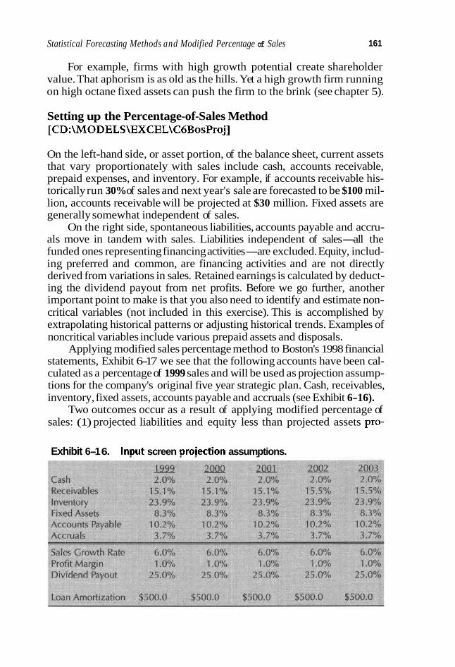
Statistical Forecasting Methods and Modified Percentage of Sales 161
For example, firms with high growth potential create shareholder value. That aphorism is as old as the hills. Yet a high growth firm running on high octane fixed assets can push the firm to the brink (see chapter 5).
Setting up the Percentage-of-Sales Method [CD:\MODELS\EXCEL\C6BosProj]
On the left-hand side, or asset portion, of the balance sheet, current assets that vary proportionately with sales include cash, accounts receivable, prepaid expenses, and inventory. For example, if accounts receivable his- torically run 30% of sales and next year's sale are forecasted to be $100 mil- lion, accounts receivable will be projected at $30 million. Fixed assets are generally somewhat independent of sales.
On the right side, spontaneous liabilities, accounts payable and accru- als move in tandem with sales. Liabilities independent of sales-all the funded ones representing financing activities-are excluded. Equity, includ- ing preferred and common, are financing activities and are not directly derived from variations in sales. Retained earnings is calculated by deduct- ing the dividend payout from net profits. Before we go further, another important point to make is that you also need to identify and estimate non- critical variables (not included in this exercise). This is accomplished by extrapolating historical patterns or adjusting historical trends. Examples of noncritical variables include various prepaid assets and disposals.
Applying modified sales percentage method to Boston's 1998 financial statements, Exhibit 6-17 we see that the following accounts have been cal- culated as a percentage of 1999 sales and will be used as projection assump- tions for the company's original five year strategic plan. Cash, receivables, inventory, fixed assets, accounts payable and accruals (see Exhibit 6-16).
Two outcomes occur as a result of applying modified percentage of sales: (1) projected liabilities and equity less than projected assets pro-
Exhibit 6-1 6. Input screen proiection assumptions.

Exhibit 617 . Boston Widget Co. Inc.
duces financial needs (e.g., amount of additional funding required to obtain predicted sales), and (2) projected liabilities and equity greater than projected assets produce a cash surplus. You can see that Boston requires additional debt or equity funding to meet sales targets in each of the four years projected (see Exhibit 6-18).
Reintroducing the F and E equations, we can draw conclusions that go beyond the yields provided by a simple accounting projection (see Exhibit 6-19). Let's begin by first examining the F equation:
F = A/S (AS) + NFA - LIIS (AS) - P(S)(l - d ) + R
F = .4094 (35,214) + 2,912.3 - .I397 (35,214) - .01(622,109)(1- .25) + 500 = 8,244
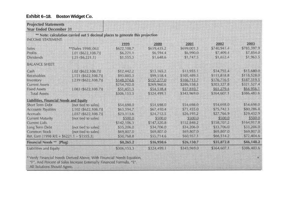
Exhibit 6-18. Boston Widget Co.
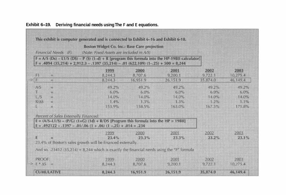
Exhibit 6-19. Deriving financial needs using The F and E equations.

Statistical Forecasting Methods and Modijied Percentage of Sales 165
The results yield exactly the same financial needs as the projected financial statements.
We see the effect independent (X) variables have on Boston's (Y), that is, financial needs after adjustments. The first test involves changes in spontaneous asset levels. Currently, Boston's asset investments are pro- jected at 49.2% of sales. If, for example, spontaneous assets levels decrease, the overall effect on financial needs, or F, will also decrease. Since inven- tory and accounts receivable usually make up 80% of current assets, it may be in your best interest to hold the line to minimum levels to maintain opti- mal levels of working capital. When current assets operate at optimal points, the cash cycles become smooth and clean.
The second sensitivity variable is spontaneous liabilities. If Boston's s~ontaneous liabilities increase from its current level of 14%. financial needs decrease. For example, by increasing accruals (a source of cash), financial needs will decrease as they approach or surpass assets levels. What would be the overall effect if sales decreased? It makes sense that reduced sales projections require less financing and result in reduced external support. The same theory holds true for the dividend rate. By lowering the dividend payout ratio, additional funds will be funneled back into the company (retained earnings). With additional internal funds available to support future needs, cash requirements lower along with unsystematic risk. Stakeholders relax a bit. Now let's look at E:
where E = projected percentage of sales growth externally financed G = growth rate
Thus, 23.4% percent of Boston's sales growth will be generated by external financing with 76.6% generated by internal cash flow (.234 x 35,213 = 8,244, the same answer as previously).
Proof: 1992 1993 1994 1995 1996 E"AS = 8,244.3 8,707.6 9,200.1 9,722.1 10,275.4 Cumulative 8,244.3 16,951.9 26,151.9 35,874.0 46,149.4
As the formula implies, the E equation determines how much sales growth requires external financing. L€ E reaches 95% in the projection period, only
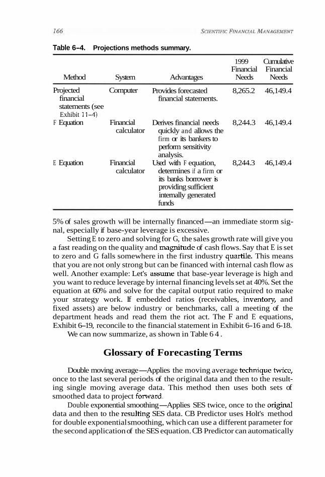
Table 6-4. Projections methods summary.
1999 Cumulative Financial Financial
Method System Advantages Needs Needs
Projected Computer financial statements (see Exhibit 1 1 4 )
F Equation Financial calculator
E Equation Financial calculator
Provides forecasted 8,265.2 46,149.4 financial statements.
Derives financial needs 8,244.3 46,149.4 quickly and allows the firm or its bankers to perform sensitivity analysis.
Used with F equation, 8,244.3 46,149.4 determines if a firm or its banks borrower is providing sufficient internally generated funds
5% of sales growth will be internally financed-an immediate storm sig- nal, especially if base-year leverage is excessive.
Setting E to zero and solving for G, the sales growth rate will give you a fast reading on the quality and magnitude of cash flows. Say that E is set to zero and G falls somewhere in the first industry quartile. This means that you are not only strong but can be financed with internal cash flow as well. Another example: Let's assume that base-year leverage is high and you want to reduce leverage by internal financing levels set at 40%. Set the equation at 60% and solve for the capital output ratio required to make your strategy work. If embedded ratios (receivables, inventory, and fixed assets) are below industry or benchmarks, call a meeting of the department heads and read them the riot act. The F and E equations, Exhibit 6-19, reconcile to the financial statement in Exhibit 6-16 and 6-18.
We can now summarize, as shown in Table 6 4 .
Glossary of Forecasting Terms
Double moving average-Applies the moving average technique twice, once to the last several periods of the original data and then to the result- ing single moving average data. This method then uses both sets of smoothed data to project forward.
Double exponential smoothing-Applies SES twice, once to the original data and then to the resulting SES data. CB Predictor uses Holt's method for double exponential smoothing, which can use a different parameter for the second application of the SES equation. CB Predictor can automatically

Statistical Forecasting Methods and Modified Percentage of Sales 167
calculate the optimal smoothing constants, or you can manually define the smoothing constants.
Single exponential smoothing (SESI-Weights all of the past data with exponentially decreasing weights going into the past. In other words, usu- ally the more recent data have greater weight. This largely overcomes the limitations of moving averages or percentage change models. CB Predic- tor can automatically calculate the optimal smoothing constant, or you can manually define the smoothing constant.
Moving averages-Eliminate randomness and smooth out a time series. This objective is achieved by averaging several data points together in such a way that positive and negative errors eventually cancel themselves out. The term moving average is used because, as each new observation in the series becomes available, the oldest observation is dropped and a new average computed. The result of calculating the moving average over a set of data points is a new series of numbers with little or no randomness. The ability of moving averages to eliminate randomness can be used in time-series analy- sis for two main purposes: to eliminate trend and to eliminate seasonality.
Exponential smoothing methods-Developed in the early 1950s, these have since become a particularly popular method of forecasting among business- people because they are easy to use, require very little computer time, and need only a few data points to produce future predictions. These smoothing methods are well suited for short- or immediate-term predictions of a large number of items. They are suitable for stationary data or when there is a slow growth or decline over time. The method of exponential smoothing is based on averaging (smoothing) past values of a time series in a decreasing (expo- nential) manner. In Excel, for example, exponential smoothing averages the smoothed value for the previous period with the actual data for the previous data point. This feature automatically includes all previous periods in the average. You can spec@ how much to weight the current period.
Definitions: Statistical Forecasting
Mean and variants of each variable-This information can be useful in understanding the sampling distribution of the mean of each variable and can be used in constructing confidence intervals. The mean (average) is a measure of central tendency in a frequency distribution, usually calculated as the arithmetic mean. The arithmetic mean is equal to the sum of observa- tions divided by the number of observations. The geometric mean represents the nth root of the product of a set of n numbers, will always be less than the arithmetic mean unless all numbers are equal and usually is used for aver- aging rates of change. The mode is a measure of central tendency equal to the most commonly occuring value in a distribution. It is generally applicable only to discrete data (e.g., integer values) because with continuous data (e.g., real numbers) it is highly unlikely that duplicate observations will occur. The median represents a measure of central tendency in a frequency
distribution, is very resistant, and often is used in exploratory data analysis (EDA), equal to the value in the distribution that divides the distribution into two halves of equal numbers of observations (50th percentile). If there is an even number of observations in the distribution, then the median is equal to the mean of the two adjacent values
Standard deviation of each variable-A measure of dispersion of a fre- quency distribution standardized to sample size.
R2-A measure of the adequacy of the fit. It indicates the percentage of the total variations of the dependent variable explained by variations in the independent variables. R2 varies from zero to one. If it is zero, it means that the regression equation does not explain the variations in the dependent variable. If it is one, it means that the regression fit is perfect and that any changes in the dependent variable are accounted for by changes in the inde- pendent variables. Such a relationship is deterministic, and forecasting will be perfect. Between these two extremes of zero and one, R2 can serve as one indicator of how "good the regression equation is. However, an R2 value of close to one does not necessarily indicate a good forecashg equation.
Correlation coeficients-The correlation coefficients (or, alternatively, the simple correlation matrix, which is the aggregation of all correlation coefficients) show how all the independent variables are correlated between themselves and with the dependent variable. As a general rule, one does not want to include in a regression equation two or more inde- pendent variables that are highly correlated between themselves (i.e., more than 0.7), nor does one wish to include independent variables with low (i.e., less than .05) correlation with the dependent variable. The first case introduces multicollinearity, which is a computational problem caus- ing the results to become unreliable. (It is like trying to divide 1 by .00000000001: The computer may not have enough significant digits to handle the division.) If there are two independent variables with a high correlation between them, no information is lost by removing one of them. Low correlations imply that there is no relationship between the depen- dent and the corresponding independent variables. Thus, if such an inde- pendent variable is included, it generally will add little in explaining vari- ations in the dependent variable. Looking at the correlation matrix of all variables, one can immediately exclude those independent variables hav- ing a low correlation with the dependent variable and then add indepen- dent variables that do not have a high intercorrelation between them. This can be achieved by starting with the independent variable with the high- est correlation with the dependent variable and then adding the indepen- dent variable with the next highest correlation with the dependent vari- able but with a low correlation with the previously included independent variable(s). (This information can be found by examining the correlation coefficients.) The correlation matrix allows one to exclude many variables (either high or low correlated), which makes the job of deciding on a final equation much easier.

Statistical Forecasting Methods and Modified Percentage of Sales I69
(b) Standard error-A term applied to various statistical measures (such as the mean) that gives the distribution within which that measure will fall when samples are drawn from any population or distribution. The standard error is dependent on the dispersion in the population and the size of the sample. The standard error for the arithmetic means is calcu- lated as standard error = SD of population/SR of number of units in the sample.
Coefficient of determination-This statistic indicates the percentage of the variability of the dependent variable that the regression equation explains. For example, an R2 of 0.36 indicates that the regression equation accounts for 36% of the variability of the dependent variable. It corrects R2
to account for the degrees of freedom in the data. In other words, the more data points you have, the more universal the regression equation is. How- ever, if you only have the same number of data points as variables, the R2
might appear deceivingly high. This statistic corrects for that. For example, the R2 for one equation might be very high, indicating that the equation accounted for almost all the error in the data. However, this value might be inflated if the number of data points was insufficient to calculate a uni- versal regression.
Sum of square deviations-The least-squares technique for estimating regression coefficients minimizes this statistic, which measures the error not eliminated by the regression line. For any line drawn through a scatter plot of data, there are a number of different ways to determine which line fits the data best. One method is to calculate the SSE (sum of the squared errors) for each line. The lower the SSE, the better the fit of the line to the data.
F statistic-Tests the s i w c a n c e of the regression equation as mea- sured by R2. If this value is significant, it means that the regression equa- tion does account for some of the variability of the dependent variable. The F test is similar to the t test except that it tests the simultaneous sig- nificance of the variables in the regression equation. It is a statistical means of checking the hypothesis that the overall relationship between the dependent variable and all the independent ones is statistically sigruficant. As a general rule, if F > 5, it means that there is a statistically significant relationship. The F test is the first statistic to examine in regression analy- sis. If it is greater than 5, then one can continue with the other tests. If it is less than 5, one must examine alternative models. If the F test is significant, one can examine each of the I tests and the R2. If the F test is > 5 and each of the I tests > 2, then one can decide whether the R2 is satisfactory. If it is, the remaining task is to check the regression assumptions. If RZ is not sat- isfactory, it implies that there are other important factors that influence the dependent variable and that have not been included in the regression equation. It may be possible to identify these factors and increase the value of R2 to some acceptable level
t statistic-A very important test, this statistic tests the significance of the relationship between the coefficients of the dependent variable and the

individual independent variable in the presence of the other independent variables. If this value is significant, it means that the independent variable does contribute to the dependent variable.
Percentage variation explained-The percentage variation explained indicates what percentage of the overall variation in the dependent vari- able each one of the independent variables explains. The higher the per- centage, the more influential that variable. The sum of all percentage vari- ations explained is R2.
Durbin-Watson test and homoscedasacity-There are four assumptions made in any application of regression: linearity, normality, independence of residuals, and constant variance. The first two are of little concern because thev are almost alwavs satisfied. For the last two, however, one must check to be sure that they are not violated.
Box-Jenkins-To create forecasts, you need to find a relationship between the variable being predicted, such as equity returns, and lagged values of predictive variables, such as dividend yield or earnings momen- tum. This ensures that forecasts are based solely on data available at the time the forecast is made, thereby avoiding the "look-ahead" bias. The autoregressive and moving average (ARMA) model, proposed by Box and Jenkins, predicts future values of a variable solely on the basis of its own past histbry. One of its sortcomings is that it ignores the role of other fac- tors. ARMA models are often good at providing short-term forecasts but typically produce poor long-term forecasts.
Signficance test-In hypothesis testing, a test that provides a criterion (probability associated with a particular sample or observation) for deter- mining whether a difference between that observation and an expected value can be attributed to chance. The null hypothesis is either accepted or rejected by comparing the calculated probability with a critical value (such as 0.05).
Chi-square test-A nonparametric test for comparing the goodness of fit of a single sample distribution to a theoretical distribution or between any number of sample distributions. It is applicable only to nominal data in the form of frequencies in mutually exclusive categories and not to per- centage data. There should also not be many categories with very low fre- quencies, and none with zero frequency, and if there are only two cate- gories, both frequencies must be a t least 5.
Chapter Six References and Selected Readings
Books
Addin Enbbu, et al. (1991). Multiple regression: Testing and interpreting interactions. Newbury Park, Calif.: Sage Publication$.
Berry, W. D., and S. Feldman. (1985). Multiple regression in practice. Beverly Hills, Calif.: Sage Publications.

Statistical Forecasting Methods and Modified Percentage of Sales 171
Boyce, D. E., et al. (1974). Optimal subset selection: Multiple regression, interdependence, and optimal network algorithms. Berlin: Springer-Verlag.
Grimm; L. G., and P. R. Yamold. (1995). Reading and understanding multivarinte statistics. Washington, D.C.: American Psychological Association.
HZtdle, W., et al. (1988). Investigating smooth multiple regression by the method of awerage dm'v- atives. Cambridge: Sloan School of Management, Massachusetts Institute of Technology.
Heward, J. H., and P. M. Steele. (1973). Business control through multiple regression analysis; a technique for the numerate manager. New York: John Wiley & Sons.
Launer, R. L., et al. (1982). Modern data analysis. New York: Academic Press. Rothman, P. (1999). Nonlinear time series analysis of economic and financial data. Boston:
Kluwer Academic Publishers. Shorter, J. (1982). Correlation analysis of organic reactivity, un'th particular reference to multiple
regression. Chichester: Research Studies Press. Thomas, J. J. (1964). Notes on the theory of multiple regression analysis. Athens. Wesolowsky, G. 0. (1976). Multiple regression and analysis of variance: A n introduction for com-
puter users in management and economics. New York: John Wiley & Sons.
Periodicals
Anonymous. (1992). "Model behavior." Financial World, 161(11), 74. Anonymous. (1997). "Information technology." Chartered Accountants Journal of New
Zealand, 76(3), 75. Anonymous. (1998). "Faster financial forecasting." Credit Management, 18. Anonymous. (1998). "New software speeds up financial forecasting." Accountancy Ireland,
30(2), 28. Baker, Al. (1992). "Financial forecasting at Atlantic Richfield Company." Journal of Business
Forecasting Methods and Systems, 11(3), 9. Balmat, Robert E, III. (1992). "Financial forecasting at Rockwell International's Defense
Electronics." Journal of Business Forecasting Methods and Systems, 11(2), 3. Benson, P. George, and Christopher B. Barry. (1982). "On the implications of specification
uncertainty in forecasting." Decision Sciences, 13(1), 176. Berglas, Anthony. (1999). "Spreadsheet errors: Risks and techniques." Management Account-
ing, 77(7), 46. Brockhoff, Klaus. (1983). "Group processes for forecasting." European Journal of Operational
Research, 13(2), 115. Chopra, Vijay Kumar. (1996). "Improving financial forecasting: Combining data with intu-
ition." Journal of Portfolio Management, 22(3), 97. D'Attilio, David F. (1992). "Net working capital forecasting at Dupont." Journal of Business
Forecasting Methods and Systems, 11(1), 11. Fisher, Steven A. (1991). "Financial forecasting and the CPA." Journal ofBusiness Forecasting
Methods and Systems, 10(1), 7. Fulford, James. (1996). "Financial forecasting software." Accountancy Ireland, 28(6), 30. Funkhouser, G. Ray. (1984). "Using qualitative historical observations in predicting the
future." Futures, 16(2), 173. Hogan, Mike. (1995). "Financial forecasting for the rest of us." PC/Computing, 8(1), 108. Lam, K. Chi. (1999). "Modelling financial decisions in construction firms." Construction
Management and Economics, 17 (5), 589. Martino, James P. (1993). "Financial forecasting at Teleport Communications Group." Jour-
nal of Business Forecasting Methods and Systems, 12(1), 7. Murray, Peter. (1992). "Financial modelling." Australian Accountant, 62(2), 51. Myhre, T. C. (1992). "Financial forecasting at Martin Marietta Energy Systems, Inc." Journal
of Business Forecasting Methods and Systems, 11(1), 28.

Singhvi, Suren S. (1991). "Polishing the controller's crystal ball: Financial forecasting tips." Cornorate Controller. 3(6). 31. . \ ,,
Snyder, Donald. (1982). "Current approaches to time series forecasting." Business Forum, 7(2), 24.
Speight, Alan E. H. (1997). ("Financial forecasting for business and economics." Interna- tional Journal of Forecasting, 13(2), 293.
Walkin, Lawrence. (1991). 'Tro-Forma Plus: The financial forecasting model." CMA, 65(7), 28. Wells, Martin T. (1997). "Financial forecasting for business and economics." Journal of the
American Statistical Association, 92(439), 1227.
Select Internet Library
Statistical Software for Forecasting Provides 20 statistical programs for those who are interested in using the computer to make more profitable forecasting business decisions. It includes such programs as multiple correlation and regression, time-series analysis and decomposition, trend projections, and exponential smoothing for forecasting. A Computer Assisted Investment Handbook, which also functions as the manual, lists and explains all the programs in detail. http://business.sofhvare-directory.com/cdprodl/swhrec/Ol7/214.shtml."
Forecasting Links Author: Brian C. Monsell Last Update: October 23, 1999, Business Forecasting Links to sites of interest to fore- casters, including news, the International Institute of Forecasters, conferences, journals and books for forecasters, FAQs, and other forecasting sites. Maintained by Fred Col- lopy. http://www.cpcug.org/user/bmonsell/forecast.html.
Statistical Software on the Web. http://www.udel.edu/ASA/stats-software.htm1 Forecasting Bibliography and Links; Links to web sites on forecasting
International Association of Business Forecasters (IABF) International Institute of Forecasters (IIF) Forecasting e-mail discussion groups Institute of Business Forecasting (IBF) http:/ /www.autobox.com/links.html.
California State University, Los Angeles, has an extensive collection of l i i to other sites on the Web related to the statistical packages used most often at the university. http:/ /artemis.calstatela.edu/stats/statlinks.htm.
CD
Name Size Tvoe
C6BosProj CbREGBkSolution CGREGBook C6REGRESS C6ShampooSolution Forecasting Bibliography and Links Forecasting Links Statistical Software for Forecasting Statistical Software Links Statistical software on the web 121
Microsoft Excel Worksheet Microsoft Excel Worksheet Microsoft Excel Worksheet Microsoft Excel Worksheet Microsoft Excel Worksheet lnternet Shortcut Internet Shortcut lnternet Shortcut lnternet Shortcut lnternet Shortcut

How to Apply Monte Carlo
Analysis to Financial
Forecasting
THIS CHAFTER AND CHAPTER 8 FOCUS ON S I ~ A T I O N and neural networking, two new and powerful tools in finance, and goes far beyond traditional sensitivity analysis, creating spreadsheets that quantify real-world uncer- tainties. These topics are true money savers, as assumption variables hav- ing little impact on forecast variables need not be highly funded or for that matter, investigated.
This chapter will look at project and research investment analysis, Monte Carlo simulation, defining assumptions and identifying a distribu- tion type, responding to problems with correlated assumptions, working with confidence levels, determining certainty levels for specific value ranges, determining the expected default frequency, understanding prob- ability distributions, and using descriptive statistics tools.
A "Simulations" Approach to Financial Forecasting
Standard forecasting models rely on single sets of assumptions that usu- ally lead to two outcomes: base case and worst case. But how unrealistic these scenarios are! If your sense of being were limited to two scenarios, your existence would compress to an ultramundane static plane. Thus, in finance, as in life, base case/worst case does not exist. Only real case
does--experiential and dynamic, that is, as you define real from experi- ence, wisdom, and a lot of old-fashioned nitty-gritty causalities.
Static forecasting, base and worst cases, limits the variability of out- comes. This is important since variability not only is your moneymaker but also is crucial in strategic decision making. It's very difficult to know which of a series of strategic options the firm should pursue without being able to appreciate differences in both the range and the distribution shape of possible outcomes and the most likely result associated with each option. In the final analysis, simulation forecasting is kinetic; sensitivity models are immobile, models for old-fashioned decision makers.
A simulation is a computer-assisted extension of sensitivity forecast- ing (as an add-on to Excel). It gives the decision maker the ability to answer questions such as "Will we stay under budget if we build this facil- ity?," "What are the chances this project will finish on time and in the money?," "What independent variable do I have to fix up before we get a go on the project?," "IS multicollinearity a problem with my forecast?," and "How do we develop a convincing impact analysis?"
With the technique known as Monte Carlo simulation, an entire range of results and confidence levels are feasible for any given forecast run. The prin- ciple behind Monte Carlo simulation comprises real-world situations involv- ing elements of uncertainty too complex to be solved with naive methods. It is a technique requiring a random number generator set in the program. Crystal Ball and @Risk are two popular programs that generate random numbers for assumption cells that you define. Using these random numbers, simulation programs compute the formulas in the forecast cells. This is a con- tinuous process that recalculates each forecast fonnula over and over again.
France Telecom is a good example of how one firm built a powerful simulation model.' France Telecom, the French national telephone com- pany, provides the network both for its own telephone operations and for the operations of recent competitors, such as Bouygues and Alcatel. Faced with heightened competition, the firm felt that it needed to better grasp market demand. Thus, the firm produced a spreadsheet model that worked with assumptions dealing with French regional market demand. This called for analyzing the number of calls, the distribution of the length of a call, and a host of other key independent variables.
By examining the distribution of these possible demands, France Tele- com wanted to forecast the correlation of these factors on the profit margin, that is the Y, or dependent, variable. The firm invited a consulting company that specialized in operations research to work with them to amend their marketing model through optimization and simulation. Using Crystal Ball, assumptions were defined for all the variable model elements, including the number of calls and the distributions of call duration, and then defined the significant results, such as profit margins, as forecasts.
1. Example courtesy of Decisioneering

How to Apply Monte Carlo Analysis to Financial Forecasting 173
France Telecom was also interested in adding linear programming optimization to the model so that, once the market demand was known, they would be able to project out and reorganize their network so as to minimize costs. For the linear programming element of the model, the con- sultants first wrote a small user macro that called Excel's Solver and requested that this macro be run at the end of each Crystal Ball simulation. Thus, France Telecom was able to simulate possible demand structures and to obtain in each case, through the linear programming optimization, the resulting profit.
France Telecom now has the capacity to optimize, in real time, its net- work structure to satisfy the market demand, an asset that was very use- ful in its budget-planning phase.
Hasbro is the nation's second-largest toy manufacturer. The firm uses simulation in investment analysis to help determine the profitability of new toy brands and lines. In one case, simulations were run to determine the probability of achieving a favorable outcome in a technology acquisition. After running the simulation, management decided that the new technology had only a 20% probability of success, thus allowing Hasbro to walk away before engaging in such a high-risk investment. Before using this powerful financial tool, Hasbro engaged in "eternal what-if scenarios," which required a huge number of manual calculations and still resulted in not much better than best/worst-case scenarios that at best achieved numbers somewhere in the middle. In a competitive environment such as the toy industry, where the product line is continually changing, sensitivity analysis is too simplistic in making the right decisions necessary for survival.
As a third example, Bankers Trust's Risk Management Advisory (RMA) group builds on its recognized strengths in risk measurement and management to help clients reshape their perception of the risks in their businesses and elevate their competitive positions by enhancing their risk management. Their clients span all industries and geographic sectors. RMA uses packages such as Crystal Ball to build customized financial and strate- gic models for their clients. While each of these models is unique, most con- tain stochastic processes and necessitate the incorporation of simulation.
Examples at Bankers include an asset valuation model for electric utili- ties, a cash-flow-at-risk model for a large corporation, and a hedging model for trading portfolios. Without the use of these products, RMA's financial models would require significant amounts of time to run. RMA provides customers with transparent quantitative methodologies and approaches to risk management as opposed to traditional "black box" solutions, as we referred to in our discussion on sensitivity forecasting in chapter 6.
Developing a simulation using Crystal Ball is not difficult. Let's start a tutorial using a simple spreadsheet: SampleSim.xls/Spread (see Tables 7-1 and 7-2). You are invited to open this spreadsheet which is in the "models" subdirectory of your CD. You are also invited to follow Deci- sioneering's demo, Fixdemo, by clicking this application file on the CD.

Table 7-1. The Piece of Cake Company, ori~inal setup.
lncome Statement Percentage
Sales Formula
Sales Cost of goods sold Cross profit Selling expenses Administration expenses Profit before taxes Taxes Net profit
Table 7-2. The Piece of Cake Company, simulation setup.
Percentage Income Statement Sales Formula Distribution
Sales Cost of goods sold Gross profit Selling expenses Administration expenses Profit before taxes Taxes
Net profit
1,255.0 1439.31 35.0% =-$B$4*C5 Triangular 81 5.8
(1 88.3) 15.0% =-$B$4*C7 Uniform (276.1) 22.0% -$B$4*C8 Normal 351.4
(123.0) 35.0% Assumption variables
227.2 [Note: Profits changed because of assumption variables1
Table 7-2A. The Piece Of Cake Company, defining your forecast.
Income Statement Percentage
Sales Formula Distribution
Sales 1,255.0 Cost of goods sold (439.3) 35.0% =-$B$4*C5 Triangular Cross profit 81 5.8 Sell~ng expenses (1 88.3) 15.0% =-$B$4*C7 Uniform Administrat~on expenses 1276.1) 22.0% =-$B$4*C8 Normal Profit before taxes 351.4 Taxes (123.0) 35.0% Net proflt
Nex t p ick (X) variables and define assumptions (Table 7-2). The assumption variables are Cost of goods sold (triangular distribution), Sell- ing expenses, (uni form distribution) and Administration expenses (normal distribution). Next, define forecast by selecting the Y variable, net profit.

How to Apply Monte Carlo Analysis to Financial Forecasting 177
Finally, run the simulation, set profits at 95% confidence and run the report. The report is displayed in Exhibit 7-1.
As you can see there is a world of difference between a simple spread- sheet presentation of Samplesim.xls and the identical spreadsheet devel- oped through a simulation and report provided by Crystal Ball. Without simulation, cost of goods sold as a value driver will reveal only a single outcome, generally 'lhe most likely or average scenario. spreadsheet risk analysis uses both a spreadsheet model and simulation to automatically analyze the effect of ;arying inputs on outputs of the modeled system. One type of spreadsheet simulation is Monte Carlo simulation, which ran- domly generates values for uncertain variables over and over to stimulate a model. How did Monte Carlo simulation get its name?
Monte Car10 simulation was named for Monte Carlo, Monaco, where the primary attractions are casinos containing games of chance. Games of chance, such as roulette wheels, dice, and slot machines, exhibit random behavior. The random behavior in games of chance is similar to how Monte Carlo simulation selects variable values at random to simulate a
Exhibit 7-1. Piece of Cake Crystal Ball report. Crystal Ball Report
Simulation started on 8130199 at 19:47:42 Simulation stopped on 8130199 at 19:47:56
senisnivity Chan
Target Forecast: Net ProW
1. Administration Expenses
Cast of Gwds Sold
Selling Expenses
0% mo m 75% Ion% Measured by Contributions to Variance
64.0%
27.9%
8.1%

Exhibit 7-1. Continued. Forecast: Net Profit
Summary: Certainty Level is 95.00% Certainty Range is from 180.1 to 269.8 Display Range is from 160.0 lo 300.0 Entire Range is from 150.8 to 303.7 After 1,000 Trials, the Std. Error of the Mean Is 0.7
Statistics: Trials Mean Median Mode Standard Deviation Variance Skewness Kurtosis Coefl. of Variability Range Minimum Range Maximum Range Width Mean Std. Ermr
SCIENTIFIC FINANCIAL MANAGEMENT
Cell: 61 1
forecast We( Plmt
i.oOoTna16 Fnqusncy Chart 3 OuUbn
,037 37
,028 27 75
n % - .- - a .- p ,019
n 18.5 C
m s 3 e 008 P
9.25 8
000 0
iBO.0 195 0 23 0 265.0 3W.0
Celralnly Is 9500% from 180 i to 268.8
Forecast: Net Profit (cont'd)
Percentiles:
Percentile 0%
Cell: B1 1

How to Apply Monte Carlo Analysis to Financial Forecasting
Assumption: Cost of Goods Sold
Triangular distribution with parameters: Minimum 31.5% Likeliest 35.0% Maximum 38.5%
Selected range is from 31.5% to 38.5% Mean value in simulation was 35.1%
Assumption: Selling Expenses
Uniform distribution with parameters: Minimum 13.5% Maximum 16.5%
Mean vaiue in simulation was 15.0%
Assumption: Administration Expenses
Normal distribution with parameters: Mean 22.0% Standard Dev. 2.2%
Selected range is from -Infinity to +Infinity Mean vaiue in simulation was 22.0%
End of Assum~tions
Cell: C5
Cell: C7
I_j
Cell: C8
model. When you roll a die, you know that either a 1,2, 3, 4, 5, or 6 will come up, but you do not know which for any particular roll. It is the same with variables that have a known range of values but an uncertain value for any particular time or event (e.g., interest rates, staffing needs, stock prices, inventory, and phone calls per minute).
Following is a sampling of frequently asked questions that may be very helpful to readers not acquainted with simulations.
What do you do with uncertain variables in your sp~eadsheet?~ For each uncertain variable (one that has a range of possible values), you define the possible values with a probability distribution. The type of distribution you select is based on the conditions surrounding that variable.
To add this sort of function to an Excel spreadsheet, you would need to know the equation that represents this distribution. With Crystal Ball 2000, these equations are automatically calculated for you. Crystal Ball 2000 can even fit a distribution to any historical data that you might have.
What happens during a simulation? A simulation calculates multiple scenar- ios of a model by repeatedly sampling values from the probability disiriiutions
2. These questions were extracted from Decisioneering's Crystal Ball Web site. The author wishes to thank Decisioneering for permission to extract these questio
ns
and answers from their site.

for the uncertain variables and using those values for the cell. Crystal Ball 2000 simulations can consist of as many trials (or scenarios) as you wan-hundreds or even thousands-in just a few seconds. During a single trial, Crystal Ball 2000 ran- domly selects a value from the defined possibilities (the range and shape of the distribution) for each uncertain variable and then recalculates the spreadsheet.
How do you analyze the results of a simulation? For every spreadsheet model, you have a set of important outputs, such as totals, net profits, or gross expenses, that you want to simulate and analyze. Crystal Ball 2000 lets you define those cells as forecasts. You can define as many forecasts as you need, and when you run a Monte Carlo simulation with Crystal Ball 2000, Crystal Ball 2000 remembers the values for each forecast for each trial. During the sirnula- tion, you can watch a histogram of the results, referred to as a Frequency Chart (see Exhibit 7-1) developed for each forecast. While the simulation runs, you can see how the forecasts stabilize toward a smooth frequency distribution. After hundreds or thousands of trials, you can view the statistics of the results (such as the mean forecast value) and the certainty of any outcome.
What is certainty? Certainty is the percent chance that a particular forecast value will fall within a specified range. For example, you can see the certainty of breaking even (results better than $0) by entering the $0 amount as the lower limit. In the case of "Piece of Cake" example, 1000 runs were made (Exhibit 7-1). A95% confidence was set with net profit falling between 180.1 and 269.8. There- fore, the forecast results not only show you the different result values for each forecast, but also the probability of any value or, if you want, a particular confi- dence level. Other charts allow you to examine different facets of your model:
The Sensitivity Chart lets you analyze the contribution of the assump- tions (the uncertain variables) to a forecast, showing you which assump- tions have the greatest impact on that forecast. What factor is most responsible for the uncertainty surrounding your net profit? Which geo- logical assumptions are most important when calculating oil reserves? Sensitivity analysis lets you focus on the variables that matter most. The Overlay Chart lets you display multiple forecasts on the same axis, even when the forecasts are from separate spreadsheet models. Which of six potential new projects has the highest expected return with the least variability (smallest range of values) surrounding the mean? With the Overlay Chart, you can compare and select the best alternatives.
The Trend Chart lets you stack forecasts so that you can examine trends and changes in a series.
How do your risks change over time? You need to assign a probability distribution to each uncertain element in the forecast. The distribution describes the possible values at 100% confidence the variable could take on, and, thus, it states the probability of each value occurring. The software ran- domly picks a value for each uncertain variable associated with an assigned probability distribution and will generate a set of financials (if this is what you want) based on values you selected. This creates one trial. Performing the last step many times produces a large number of trials.

How to Apply Monte Car10 Analysis to Financial Forecasting
International Drug Corporation, Project Analysis under Uncertainty3
International Drug Corporation (IDC) is a research-focused pharmaceutical company. Pharmaceutical research has led to numerous advances in medical therapy. However, such research, by its nature, involves a tremendous amount of risk and uncertainty. Often 1,000 or more compounds are screened for each one that ultimately is nominated for development. On average, for every 10 compounds that reach development, only one gains FDA approval.
The "Digoxin Drug Project" spreadsheet models a business situation filled with uncertainty. IDC has completed preliminary development for a new drug, code named Digoxin, designed to correct back problems. While headquartered in Dallas, production facilities are located in Guayaquil, Ecuador. This revolutionary new product could be developed and tested in time for release next year if the FDA approves the product. Although the drug works well for some patients, the overall success rate is marginal, and IDC i s uncertain whether the FDA wil l approve the product. With $30 million in debt and $25 million in equity, the project i s capitalized with a debt to equity ratio of 120%.
An important aspect of pharmaceutical development is selecting the proper portfolio of compounds to develop-a portfolio that wil l provide the expected level of sales at the right level of cost and risk. Crystal Ball simula- tions are used to model the key risks and uncertainties for each individual project. In addition, Crystal Ball simulations are used to estimate total port- folio value and risk-a probability distribution of potential R&D spending and sales by year.
The CFO, Marcia Wilson, wanted the firm to perform simulations. She wants to determine whether to scrap the project or, alternatively, to proceed to the next step, which i s to develop and market this exciting new drug. Few mistakes are allowed. The project i s a multi-million-dollar risk. Marcia knows that simulation models such as Crystal Ball are powerful decision-support programs designed to take the mystery out of decisions like this.
The model gives Wilson the ability to answer questions such as "Will we stay under budget if we build this facility?," "What are the chances this pro- ject wil l finish on time?," "How likely are we to achieve this level of prof- itability?," and most important in this case, "What are the probabilities that the project wil l make money?," "Is the project feasible enough to attract three-year revolver financing?," and "What is the expected default (unsys- tematic risk) factor?"
As i s the case with drug products, being the first or second to the market can have a significant impact on total sales realized. In certain high-potential
3. This case was derived using a Crystal Ball example.

markets, there may be 10 or more competitors with drug products such as Dixogin in development. If the first round of analysis is successful, that is, if the product i s viable from a profit perspective, simulations could be used to estimate the probability of being first or second to market. This information helps focus attention on the need to achieve key project milestones to ensure a reasonable level of certainty that a compound wil l be first to the market.
Departmental estimates were obtained and some of the terminology was reviewed. A project estimate is an "informed" assessment of the likely pro- ject cost or duration. Informed" means that department heads have an iden- tified basis for the estimate. "Likely" does not mean certain the term focuses on the inherent uncertainty of the estimate: Every estimate is but one of many possible outcomes. Cost and duration measures are crucial and refer to the two major categories of estimates. The team, realizing that the project was unique, focused on management similarities rather than on the technical dif- ferences and found that they could generate valuable insights even though the product of the project i s wholly different. They even got biopharmaceu- ticals experts from competing firms to exchange estimating insights.
A few questions came up at initial meetings. Someone on Marcia's team wanted to know whether there are many possible outcomes, and how can he tell the one most likely? The answer is to not pick just one outcome but identify the full range of possible outcomes. If the problem is single point estimates and A and B are equally likely, the information is factored in and the results, for example, might be a uniform distribution. In addition, single point estimates tend to become self-fulfilling prophecies. Indeed, both the Digoxin project manager and the person responsible for a critical X variable needed to know its range dimension. For the most part, the distribution configuration is not nearly as important as recognizing that there is a range of possible results. In the late 1950s, the U.S. Navy developed the Program Evaluation and Review Technique (PERT) using a beta distribution. In the absence of evidence to the contrary, the best approach generally is to assume a triangular distribution because a trian- gular distribution produces more conservative results than a beta.
Marcia brought up the issue dealing with time spent developing range estimates. Her experience has been that it takes less time by eliminating the posturing and gamesmanship that often accompany the estimating process. Competitors have put together teams that spent less than a day estimating a 3,000-hour project-an estimate that later proved highly accurate. The time spent on estimates is not a cost; rather, it is cheap insurance.
Spreadsheet models only approximate a real-world domain. When building the spreadsheet models, careful interpretation must be given to the problem in order to refine the models on a continuous basis until they reflect the real-world condition as closely as possible.
In summary, to perform a simulation, Wilson needed accurate informa- tion from department heads involved in the project. She wanted a probabil- ity distribution assigned to each uncertain element in the forecast. The dis- tribution describes the possible values that the variable conceivably could take on and states the probability of each value occurring.

How to Apply Monte Carlo Analysis to Financial Forecasting 183
The next step is to have the software randomly pick a value for each uncertain variable associated with an assigned probability distribution. The software wil l generate a set of financials based on the values selected. This creates one trial. Performing the last step many times produces a large num- ber of trials. The output from a simulation is a table or a graph summarizing the results of many trials.
The group developed the "Digoxin Drug Project" spreadsheet in the context of a most likely scenario. Wilson required experts from different areas of production to submit reports along with projections and probability distributions. Information i s included as follows (see Exhibit 7-2 and C7DIS- EASE file in the Excel subdirectory).
1 . Defining Testing: The Uniform Distribution. For this variable, "testing costs," IDC felt that any value between $3.6 and $4.4 million has an equal chance of being the actual cost of testing. The budget will not allow costs over $4.4 million. Based on this information, the CFO selected the uniform distribution to describe the testing costs.
The uniform distribution describes a situation where all values between the minimum and maximum values are equally likely to occur, so this distribution best describes the cost of testing Digoxin Drug.
2. Defining Marketing Costs: The Triangular Distribution. IDC plans to spend a sizable amount marketing Digoxin Drug if the FDA approves it. They expect to hire a large sales force and kick off an extensive adver- tising campaign to educate the public about this exciting new product.
(text continues on page 188)
Exhibit 7-2. Digoxin drug project income statement and distributions, Cuayaquil, Ecuador. , . I-. ". , . * -, > , . .. ; ,# ,,' ' " > .",. .,, ' ..,, :s,.* :& , . . . . ., - .. . . -
., : ' :. . . ? > : . ? . 4 : ; . %. . ' 'n . ... ,. . ,,I . R , , , . '. ; i 8, i d . 9'
. . f'J;75 nrr , - D . .
Income Statsment and D#str>bubons
F o i ~ a s i call
(continues)

184
Exhibit 7-2. Continued. Crystal Ball Report
Simulation started on 8/11/99 at 9:32:17 Simulation stopped on 811 1/99 at 9:32:34
Forecast: Gross Profit if Approved (millions)
Sensltlvlty Chart
Target Forecast: Gmss Profit if Approved (millions)
Market penetration
Growth rate of musculoskeietal injulies
Patients cured
Summary: Certainty level is 90.00%. Certainty range is from $25.1 to $42.2 million. Display range is from $17.5 to $45.0 million. Entire range is from $15.0 to $47.9 million. After 900 trials, the Standard of the mean is $0.2.
Statistics: Trials Mean Median Mode Standard deviation Variance Skewness Kurtosis Coefficient of variability Range minimum Range maximum Range width Mean standard error
Testing costs
Cell: C21
Value 900 $31.7 $31.4 - $4.8 $23.1 0.20 2.93 0.15 $15.0 $47.9 $33.0 $0.16
0% 25% 50% 75% l 0 W
Measured by Contribution tovariance
0.0% I I I
I I I I I I I I I I I I

How to Apply Monte Carlo Analysis to Financial Forecasting 185
Forecast: Gross Profit if Approved (millions)
900 Trials Frequency Charl
4 Outliers
Certaiq is 90.00% from $25.1 to $42.2 millions
Forecast: Gross Profit if Approved (mllllons) (cont'd)
Percentiles: Percentile
0% 10% 20% 30% 40% 50% 60% 70% 80% 90% 100%
Cell: C21
Millions $15.0 $25.7 $27.8 $28.9 $30.3
End of Forecast
Forecast: Net Profit (millions) Cell: C23
Summary: Certainty level is 49.22%. Certainty range is from -infinity to $0.0 million. Display range is from (525.0) to $25.0 million. Entire range is from ($41.0) to $21.9 million. After 900 trials. the Standard of the mean is 5C.3
Statistics: Trials Mean Median Mode Standard deviation Variance Skewness Kurtosis Coefficient of variability Range minimum Range maximum Range width Mean standard error
Value 900 ($0.7) $0.1 - $8.9 $78.5 -0.79 4.26 -1 1.82 (541 .O) $21.9 $62.9 $0.30

186 SCIENTIFIC FINANCIAL M A N A G E M E N T
Exhibit 7-2. Continued.
Forecast: Net Protlt (millions) 900Trials Frequency Chart 14 Outliers
,034 31
5 .OZ6 23.25
.- - B .017
3 15.5 f
m n m z g ,009 7.75 2
,000 0
($25.01 ($1 2.5) SO 0 $12.5 $25.0 Certainty is 49.2% from -infinity to $0.0 millions
Forecast: Net Profit (MM) (cont'd)
Percentiles: Percentile
0% 10%
End of Forecast
Assumption:Testing Costs
Uniform distribution with parameters: Minimum $3.6 Maximum $4.4
Mean value in simulation was $4.0
Assumption: Marketing Costs
Triangular distribution with parameters: Minimum $14.4
Likeliest $16.0
Maximum $17.6
Millions ($41 .O) ($12.6) ($7.5) ($4.1 ) ($1.7)
$0.1
Cell: CS
T..l,W EMI
7 I
Cell: C7
Selected range is from $14.4 to $17.6. Mean value in simulation was $16.0.

How to Apply Monte Carlo Analysis to Financial Forecasting 187
Assumption: Patients Cured Cell: C10
Binomial distribution with parameters: .m
Probability 0.25 Trials 100
Selected range is from 0 to +infinity. Mean value in simulation was 25.
Assumptlon: Growth Rate of Musculoskeletal Injuries Cell: C15
Custom distribution with parameters: Relative Probability Continuous range -15.00% to -5.00% 0.250000 Continuous range 0.00% to 5.00% 0.750000
Total relative probability 1 .OOOOOO
Mean value in simulation was 4.76%
Cell: C15
Cell: C19
Assumption: Market Penetration
Normal distribution with parameters: Mean 8.00% Standard deviation 0.80%
Selected range is from -infinity to +infinity. Mean value in simulation was 8.01%.
Cell: C4
Assumption: Development Cost ot Digoxin Drug to Date
Lognormal distribution with parameters: Mean $1 1 .O Standard deviation $6.0
Selected range is from $0.0 to +infinity. Mean value in simulation was $1 1.0.
Cell: C14
Assumption: Persons with Chronic Musculoskeletal Injury R*anrufhChmnLM-uI~s-I (11
Normal distribution with parameters: Mean 40.0 Standard deviation 4.0
Selected range is from -infinity to +infinity. Mean value in simulation was 39.9.

Including sales commissions and advertising costs, IDC expects to spend between $14 and $1 7.6 million, most likely $16.0 million. IDC chooses the triangular distribution to describe marketing costs.
The triangular distribution describes a situation where you can esti- mate the minimum, maximum, and most likely values to occur.
3. Defining Patients Cured: The Binomial Distribution. Before the FDA will approve Digoxin Drug, IDC must conduct a controlled test on a sample of 100 patients for one year. The FDA has stipulated that they will approve Digoxin Drug if it completely corrects the back problems of 20 or more of these patients without any significant side effects. In other words, 20% or more of the patients tested must show corrected vision after taking Digoxin Drug for one year. IDC is very encouraged by their preliminary testing, which shows a success rate of around 20%.
For this variable, "Patients Cured," IDC knows only that their pre- liminary testing shows a cure rate of 50%. Will Digoxin Drug meet FDA standards? Marcia's staff picked the binomial distribution to describe the uncertainties because the binomial distribution describes success number (20) in a fixed number of trials (1 00).
4. Defining Market Penetration: The Normal Distribution. The marketing department estimates that IDC's eventual share of the total market for the product will be normally distributed around a mean value of 80h with a standard deviation of 0.80%. "Normally distributed" means that analysts expect to see the familiar bell-shaped curve with about 68% of all possible values for market penetration falling between one standard deviation below the mean value and one standard deviation above the mean value, or between 7.2% and 8.8%.
The low mean value of 8% i s a conservative estimate that takes into account the side effects of the drug that were noted during prelimi- nary testing. In addition, the marketing department estimates a mini- mum market share of 5%, given the interest shown in the product during preliminary testing.
Wilson wants to know the certainty of achieving a profit. With sim- ulation technology, Wilson can easily answer this question. The final result: Digoxin can be (input your assumptions and see) certain of achieving a minimum profit. IDC is encouraged/discouraged by the forecast results. Wilson wants to know whether key assumptions together with distributions are correct. If assumptions and distribu- tions are reasonable, the project will be accepted/dropped.
Exhibit 7-3 shows a Lognormal Distribution. The assumption name is identified: "Development Cost of Dioxin Drug . . ." The Gallery button provides numerous distribution choices. The Correlate button enables you to test correlations between assumption variables so to reduce the possibilty of redundency in the simulation.
Exhibit 7-3A illustrates a "constructed" custom distribution used if other distribution possibilities do not match your objectives. You are allowed the freedom to develop your own distribution to fit the data.

How to Apply Monte Carlo Analysis to Financial Forecasting 189
Exhibit 7-3. Development cost: An example of a lognormal distribution.
Exhibit 7-3A. Growth Rate of Muscoloskeletal Injuries: An Example of a Custom Distribution

CASE STUDY
Hope Street Apartments
As vacancy rates began to drop in the Providence, Rhode Island, area, Mal- colm Singer, a local contractor, saw an opportunity. Singer realized that the apartments market was growing rapidly. There had been little multifamily construction in Providence's affluent East Side area in over seven years. As a result, vacancy rates in existing apartments near Brown University were dropping rapidly, from 7% in 1995 to 5% in 1997 and down to less than 3% in late 1998.
Singer was determined to move fast. In a short time, he zeroed in on a "builders special" located on Hope Street near Brown. This location was excellent, and so he decided to refurbish and redesign an existing 216-unit "dilapidated" structure and make it "almost like new."
Singer took his plans and projections to ABC Bank, who offered to pro- vide $3 million of permanent financing at 9% interest for a 12-year term with a balloon payment due at the end. The constant payment, including interest and principal, would be 10.23%. The bank stipulated that the building's operating cash flow should be adequate to cover debt service of $306,900 to the tune of at least a 98% probability. While Singer had provided an ade- quate personal net worth statement, the bank did not feel comfortable that external funds were available to supplement the project's expected cash flow coverage ratios. The following Excel income statement projection [C7HopeStOrg] in the Excel subdirectory, was included in the feasibility study developed by the bank4.
Part 1 : Potential Gross Income; Rents Simulation Assumption Cells (Shaded)
Apartment Number of Total $Square Feet Monthly Yearly Gross Annual
$221 $2,646 $95,256 $229 $2,752 $99,066 $217 $2,608 $93,905 $251 $3,011 $108,405
4. Shaded cells represent assumption variables; the forecast variable. Cash flow from oper- ations is labeled on the spreadsheet.

Part 2: Potential Gross Income; Auxiliary Income
I Net income I $22,098
Part 3: Calculation of Reserves
Part 4: Cash Flow from Operations
Projected rent gross income Projected auxiliary income Total gross income VacancyJcollections Effective Gross lncome
Management fees SalariesJtaxes Real estate taxes
Common area utilities Maintenance, redecorating
Cash flow from operations Forecast Cell >>>>
Parl5: Calculatlon of Net Income and Debt Se~ice Coverage Analysis
Loan amount Rate Constant payment, principal and interest
Cash flow from operations Constant payment principal and interest
$3,000,000 9.50% $285,000
10.23% $306,900 Breakeven cash flow From O~erations
$328,998 $306,900 ($306,900)
Probabilities of covering interest and arinc~aal Hlnt: Set upper limit of simulation range to $306,900

Crystal Ball Report Simulation started on 111 7/00 at 11:47:40 Simulation stopped on 1/17/00 at 11:47:45
I Sensitivity Chart I
I I I Target Forecast: Cash Flow From Operatlons I
VacancylCollectons
Maintenance, Redecorating
, General Expenses
Units
PBR,I BA
IBR IBR
2BR 2BA
3BR 2BA
Measured by Rank Correlation p~ ~ - p~ I
The sensitivity chart indicates that vacancy rate is the most sensitive aassumption variable. A small change in vacancy affects cash flow coverage more man any other variable.
Recast: Cash flow from operations. Cell: D70
Sum This means that
there is 17.4% grohrbility that
D~splry range s fVorn S28U.000 lo S350.005. onerating cash Entlre range is from $285,256 to $348,269.
- flow w i l l not be
After 1,000 trials, the Standard error of the mean is $369. sufficient to cover debt service.

How to Apply Monte Carlo Analysis to Financial Forecasting 193
Statistics: Value Trials 1000
1 Mean $318,771 1 Median $320,028 Mode Standard deviation Variance Skewness Kurtosis Coefficient of variability Range minimum Range maximum Range width Mean standard error
-- -~ -
Forecast: Cash Flow From Operations
1,000 Trials Frequency Chart 0 Outliers ~p -
.032 .
... . . , . , ..... , ... . ...... ..
Forecast: Cash Flow from Operations (cont'd) Cell: D70
Percentiles:
Percentile 0% A 20% probability that $285,256
End of Forecast

Assumption: 1 BR 1 BA
Uniform distribution with parameters: Minimum $0.23 Maximum $0.25
Assumption: 1 BR 1 BA
Normal distribution with parameters: Mean $0.30 Standard deviation $0.01
Selected range is from -inifinity to +infinity.
Assumption: 2BR 2BA
Triangular distribution with parameters: Minimum $0.26 Likeliest $0.26 Maximum $0.27
Selected range is from $0.26 to $0.27.
Assumption: 3BR 2BA
Triangular distribution with parameters: Minimum $0.24 Likeliest $0.24 Maximum $0.25
Selected range is fmrn $0.24 to $0.25.
Assumption: 3BR 2BA
Uniform distribution with parameters: Minimum $0.22 Maximum $0.24
Assumption: Maintenance, Redecorating
Cell: E6
IBR,BI,
I --
7
Cell: E7
Cell: E l l
Cell: E l2
Cell: El3
OBRZB1
Cell: B66
nm--,-!gp 7
Uniform distribution with parameters: Minimum 5.00% Maximum 6.72%

How to Apply Monte Carlo Analysis to Financial Forecastinq 195
Assumption: General Expenses Cell: B67
Normal distribution with parameters: - General Expmes
Mean 4.36% 1- Standard deviation 0.40% A
Selected range is from -inifinity to +infinity.
Assumption: Units Cell: C6
Normal distribution with parameters: - units
Mean 24.00 i A Standard deviation 2.40 A
Selected range is from -inifinity to +infinity.
Assumption: 2BR,1 BA Cell: E l 0
Trian~ular distribution with ~arameters: - - 2ER,lEA - Minimum Likeliest Maximum
Selected range is from $0.21 to $0.24. a? sa2r 50?9 SO19 1021
Assumption: VacancylCollections Cell: 856
Tnangular distr~bution with parameters: Min~mum 13.0% Likeliest 15.4% Maximum 25.0%
t
Selected range is from 13.0% to 25.0%. ,lox. ,SO% IIC% ZZOh 2Sm
Since vacancy rate represents the most critical assumption, it is important that we thoroughly examine both underlying assumptions and, for the pur- poses of this case, the distribution.
End of Assumptions

A Comparison of Different Distributions Applied to Vacancy Rate, Sensitivity, and the Effect on the Hope Street Project's Cash Flow Coverage
The income statement was left unchanged from the original. The only changes made were the shape of the distribution. The following table has been set up to compare (1) certainty level (the probability that operating cash flow falls below debt service), (2) sensitivity by rank correlation, and (3) the run's statistics. The important message here is that the distribution selection you arrive at is as important as the underlying assumptions that form the variable itself.
Distribution Summary Sensitivity Statis tics
Triangular Certainty level is 77.40%. -.91 Trials 1,000 Certainty range is from Mean $31 8,771 -infinity to $306,900. Median $320,028
Entire range is from Standard $285,256 to $348,269. deviation $1 1,656
Skewness -0.36 Kurtosis 2.54 Coefficient
of variabilitv 0.04
Normal Certainty level is 20.0%. -.80 Trials Certainty range is from Mean -infinity to $306,900. Median
Entire range is from Standard $301,007 to $353,871. deviation
Skewness Kurtosis Coefficient
of variability
Lognormal Certainty level is 20.0% -.79 Trials Certainty range is from Mean -infinity to $306,900. Median
Entire range is from Standard $305,591 to $353,638. deviation
Skewness Kurtosis Coefficient
of variability
Uniform Certainty level is 39.40%. -.96 Trials 1,000 Certainty range is from Mean $31 3,684 -infinity to $306,900. Median $313,194

How to Apply Monte Carlo Analysis to Financial Forecasting 197
Distribution Summary Sensitivity Statistics
Uniform Entire range is from Standard (cont.) $282,243 to $350,685. deviation $15,641
Skewness 0.09 Kurtosis 1.93 Coefficient
of variability 0.05
Extreme Certainty level is 90%. -.72 Trials 1,000 Value Certainty range is from Mean $326,663
-infinity to $306,900. Median $327,241 Entire range is from Standard
$296,407 to $346,598. deviation $7,265 Skewness -0.42 Kurtosis 3.47 Coefficient
of variability 0.02
Glossary of Distribution Terms
Triangular Distribution-Describes a situation where you know the minimum, maximum, and most likely values to occur. For example, we could describe the vacancy rate associated with the minimum, maximum, and most likely vacancy rate. Three conditions are required:
1. The minimum number of items is fixed. 2. The maximum number of items is fixed. 3. The most likely number of items falls between the minimum and
the maximum values, forming a triangular-shaped distribution that shows that values near the minimum and maximum are less likely to occur than those near the most likely value.
Unlike the uniform distribution, in which all values between the limits are equally likely, the triangular distribution peaks at a central value.
Example
Analysis of Hope Street's property, showing that the vacancy rate will not fall below 13% or increase beyond 25%, with 15.4% the most likely.
The first step in selecting a probability distribution is to match your data with a distribution's conditions. Checking the triangular distribution:
Minimum vacancy rate is 13.0%. Maximum vacancy rate is 25.0%. The most likely vacancy rate is 15.4%, forming a triangle.

Parameters: Lower limit a, central value c > a, upper limit b > c. Domain: a 5 X 5 b.
Likeliest 15.4% 1
Triangular distribution with parameters: vacanc~~co~~ecttons
Minimum 13.0%
Maximum 25.0% :& Selected range is from 13.0% to 25.0%. lam
Triangular Distribution for Type B Uncertainty--Often all that is known about a process that contributes type B uncertainty is the maximum and minimum potential values and that central values are more likely to occur than extreme values. The uncertainty contribution from this process can be calculated from a triangular distribution.
Normal Distribution-This is a continuous probability distribution that is used to characterize a wide variety of types of data. It is a symmetric dis- tribution, shaped like a bell, and is completely determhed by its mean and standard deviation. The normal distribution is particularly important in statistics because of the tendency for sample means to follow the normal distribution (this is a result of the Central Limit Theorem).
Most classical statistics procedures, such as confidence intervals, rely on results from the normal distribution. The normal is also known as the Gaussian distribution, after its originator, Frederich Gauss. The normal dis- tribution is the most important distribution in probability theory because it describes many natural phenomena, such as peoples' IQs or heights. Decision makers can use the normal distribution to describe uncertain variables, such as the inflation rate or the future price of gasoline. The three conditions underlying the normal distribution are as follows:
1. Some value of the uncertain variable is the most likely (the mean of the distribution).
2. The uncertain variable could as likely be above the mean as it could be below the mean (symmetrical about the mean)..
3. The uncertain variable is more likely to be in the vicinity of the mean than far away. Approximately 68% are within 1 standard deviation on either side of the mean. The standard deviation is the average distance of a set of values from their mean.
Example
You feel that the mean vacancy rate on the Hope Street proposed project will be 15.4% with a standard deviation of 1.5%. This means that there is approxi- mately a two-thirds probability that the vacancy rate will fall between 15.4% minus 1.5% and 15.4% plus 1.5%, or between 13.9% and 16.9%.

How to Apply Monte Carlo Analysis to Financial Forecasting 199
The first step in selecting a probability distribution is to match your data with a distribution's conditions. Checking the normal distribution:
Assumption: VacancylCollections Cell: B56
Normal distribution with parameters: Vacm~yICallealms .
Mean 15.4% rA1 Standard deviation 1.5%
Selected range is from -infinity to +infinity. . .- Parameters: Mean mu, standard deviation sigma > 0. Domain: All real X.
Lognormal Distribution-The lognormal distribution is widely used in situations where values are positively skewed (most of the values occur near the minimum value), for example, in financial analysis for security valuation or in real estate for property valuation, such as the Hope project. Stock prices are usually positively skewed rather than normally (symmet- rically) distributed. Stock prices exhibit this trend because they cannot fall below the lower limit of zero but may increase to any price without limit.
Conditions
Real estate prices illustrate positive skewness since property values cannot become negative, unless it poses an environmental hazard. The three conditions underlying the lognormal distribution are as follows:
1. The uncertain variable can increase without limits but cannot fall below zero.
2. The uncertain variable is positively skewed with most of the values near the lower limit.
3. The natural logarithm of the uncertain variable yields a normal distribution.
Example
You assume that the lowest value vacancy rate can drop to zero. On the other hand, the project could end up with a vacancy of 100%.
Assumption: VacancyICollections Cell: 856
Lognormal distribution with parameters: - - vac~cy/GMecl
Mean 1 5.4% Standard deviation 1.5% 1 A
Selected range is from 0.0% to +infinity. i ~ +

Uniform Distribution-A continuous probability distribution that is useful for characterizing data that range over an interval of values, each of which is equally likely. It is sometimes called the rectangular distribution because of its shape when plotted. The distribution is completely deter- mined by the smallest possible value, a, and the largest possible value, b. For discrete data, there is a related discrete uniform distribution. The three conditions underlying uniform distribution are as follows:
1. The minimum value is fixed. 2. The maximum value is fixed. 3. All values between the minimum and maximum are equally likely
to occur.
Examples of Distributions
The vacancy rate of at least 13% is expected but not more than 25%. All val- ues between 13% and 25% are equally likely to occur.
The first step in selecting a probability distribution is to match your data with a distribution's condition. Checkmg the uniform distribution:
Assumption: Vacancy/Collections Cell: B56
Uniform distribution with parameters: V a ~ q / C o ~ l m s _ _ ~
Minimum 13.0% 1 - 1 Maximum
The minimum value is 13%; the value is 25%, and all values in between are equally possible. The conditions in this example match those of the uni- form distribution.
Parameters: Lower limit a, Upper limit b > a. Domain: a 5 X 5 b.
Extreme Value Distribution-A distribution used for random variables that are constrained to be greater than or equal to 0. It is characterized by two parameters: mode and scale.
Parameters: mode a > 0, scale b > 0. Domain. All real X.

How to Apply Monte Carla Analysis to Financial Forecasting 201
Assumption: Vacancy/Collections Cell: 856
Extreme value distribution with parameters: Vscsnw~l l& lms
Mode Scale
Selected range is from -infinity to +infinity.
Other Distributions You May Deal with in Finance
Gamma Distribution-A distribution used for continuous random vari- ables that are constrained to be greater than or equal to 0. It is character- ized by two parameters: shape and scale. The gamma distribution is often used to model data that are positively skewed.
The gamma distribution applies to a wide range of physical quantities and is similar to a host of other distributions: lognormal, exponential, Pas- cal, geometric, Erlang, Poisson, and chi-square. The gamma distribution can be thought of as the distribution of the amount of time until the rth occur- rence of an event in a Poisson process. It is used in meteorological processes to represent pollutant concentrations and precipitation quantities and has other applications in economics, inventory, and insurance risk theories. The parameters for the gamma distribution are location, scale, and shape.
The three conditions underlying the gamma distribution are as follows:
1. The number of possible occurrences in any unit of measurement is not limited to a fixed number.
2. The occurrences are independent. The number of occurrences in one unit of measurement does not affect the number of occurrences in other units.
3. The average number of occurrences must remain the same from unit to unit.
The sum of any two gamma-distributed variables is a gamma variable. The product of any two normally distributed variables is a gamma variable.
Parameters: Shape a > 0, scale B > 0. Domain: X 2 0.
Assumption: Growth Rate of Musculoskeletal injuries Cell: C15
Gamma distribution with parameters: Location Scale Shape 2
Selected range is from 2.00% to +infinity. ,,,.. ,,,, 681% 712s 9624
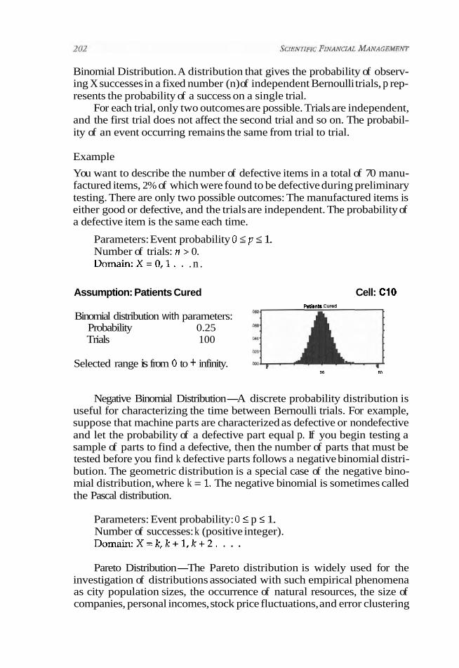
Binomial Distribution. A distribution that gives the probability of observ- ing X successes in a fixed number (n) of independent Bernoulli trials, p rep- resents the probability of a success on a single trial.
For each trial, only two outcomes are possible. Trials are independent, and the first trial does not affect the second trial and so on. The probabil- ity of an event occurring remains the same from trial to trial.
Example
You want to describe the number of defective items in a total of 70 manu- factured items, 2% of which were found to be defective during preliminary testing. There are only two possible outcomes: The manufactured items is either good or defective, and the trials are independent. The probability of a defective item is the same each time.
Parameters: Event probability 0 I p I 1. Number of trials: n > 0. Domain:X=O,l.. . n .
Assumption: Patients Cured Cell: ClO M n l s cum
Binomial distribution with parameters: Probability 0.25 Trials 100
Selected range is from 0 to + infinity. .W
26 59
Negative Binomial Distribution-A discrete probability distribution is useful for characterizing the time between Bernoulli trials. For example, suppose that machine parts are characterized as defective or nondefective and let the probability of a defective part equal p. If you begin testing a sample of parts to find a defective, then the number of parts that must be tested before you find k defective parts follows a negative binomial distri- bution. The geometric distribution is a special case of the negative bino- mial distribution, where k = 1. The negative binomial is sometimes called the Pascal distribution.
Parameters: Event probability: 0 < p < 1. Number of successes: k (positive integer). Domain:X=k,k+l,k+Z. . . .
Pareto Distribution-The Pareto distribution is widely used for the investigation of distributions associated with such empirical phenomena as city population sizes, the occurrence of natural resources, the size of companies, personal incomes, stock price fluctuations, and error clustering

How to Apply Monte Carlo Analysis to Financial Forecasting 2 03
in communication circuits. This is a distribution used for random variables constrained to be greater than or equal to 0.
Parameters: Shape a > 0. Domain: X 5 1. Mean: a/(a-1) for a > 1.
Geometric Distribution-A discrete probability is useful for character- izing the time between Bernoulli trials. For example, suppose that machine parts are characterized as defective or nondefective and let the probability of a defective part equal p. If you begin testing a sample of parts to find a defective, then the number of parts that must be tested before the first defective is found follows a geometric distribution.
The three conditions underlying the geometric distribution are as follows:
1. The number of trials is not fixed. 2. The trials continue until the first success. 3. The probability of success is the same from trial to trial.
If you are drilling for oil and want to describe the number of dry wells that you would drill before the next big "gusher", you would use the geomet- ric distribution. Assume that in the past you have hit oil about 10% of the time. The first step in selecting a probability distribution is to match your data with a distribution's conditions. Checking the geometric distribution:
1. The number of trials (dry wells) is not fixed. 2. You continue to drill wells until you hit the big "gusher." 3. The probability of success (10%) is the same each time you drill a well.
The geometric distribution has only one parameter: probability. In this example, the value for this parameter is .lo, representing the 10% proba- bility of discovering oil. You would enter this value as the parameter of the geometric distribution in Crystal Ball.
Parameters: Event probability 0 5 p 2 1. Domain: X = 0,1,2, . . . .
Poisson Distribution-A distribution often used to express probabilities concerning the number of events per unit. For example, the number of computer malfunctions per year or the number of bubbles per square yard in a sheet of glass might follow a Poisson distribution. The distribution is fully characterized by its mean, usually expressed in terms of a rate.
5. Source: Decisioneering's Crystal Ball Manual and online help.

The three conditions underlying the Poisson distribution are as follows:
1. The number of possible occurrences in any unit of measurement is not limited to a fixed number.
2. The occurrences are independent. The number of occurrences in one unit of measurement does not affect the number of occurrences in other units.
3. The average number of occurrences must remain the same from unit to unit.
Parameters; mean B > 0. Domain: X = 0,1,2, . . .
Chapter Seven References and Selected Readings
Books
Addin Enbu, et al. (1988). The diaidend ratio model and small sample bias: A Monte Carlo study. Cambridge, Mass.: National Bureau of Economic Research.
Gourley, S. K., and Massachusetts Institute of Technology, Department of Aeronautics and Astronautics. (1979). Technological risk analysis/assessment.
Harris, R. F. (1975). Monte Carlo study of fatigue crack growth under random loading. Kleijnen, J. P. C. (1974). Statistzcal techniques in simulation. New York: Marcel Dekker. Lloyd, J. A. (1992). Numerical methods for Monte Car20 datice simulation. Mooney, C. Z. (1997). Monte Carlo simulation. Thousand Oaks, Cali.: Sage Publications. Najafabadi, R. F., and Massachusetts Institute of Technology, Department of Nuclear Engi-
neering. (1983). Monte Car10 simulation of structural and mechanical properties of crystal and bicrystal systems atfinite temperature.
Rubinstein, R. Y. (1981). Simulation and the Monte Carlo method. New York: John Wiley & Sons. Vose, D. (1996). Quantitative risk analysis: A guide to Monte Car10 simulation modelling. Chich-
ester: John Wiley & Sons. Yakowitz, S. J. (1977). Computational probability and simulation. Reading, Mass.: Addison-
Wesley Advanced Book Program.
Periodicals
Anderson, Heather M. (1998). "Testing multiple equation systems for common nonlinear components." Ioumal of Econometrics 84(1).
Campbell, Terry. (1989). "Forecasting financial budgets with Monte Carlo simulation." Financial and Accounting Systems, 5(1), 28.
Clements, Michael P. (1999). "A Monte Carlo study of the forecasting performance of empirical SETAR models." Journal of Applied Econometrics, 14(2), 123.
Fellows, Richard. (1996). "Monte Carlo simulation of construction costs using subjective data: Comment." Construction Management and Economics, 14(5), 457.
Franses, Philip Hans. (1998). "A model selection strategy for t i e series with increasing seasonal variation." International Journal of Fmecasting, 14(3), 405.

How to Apply Monte Carlo Analysis to Financial Forecasting 205
Gupta, Yash I?, and Rajendra K. Gupta. (1984). "Forecasting of working-capital require- ments under capital constraints: A Monte Carlo simulation approach.'' Engineering Costs and Production Economics, 8(3), 223.
Kalff, H. (1982). "How to tackle the future." Marketing and Research Today, 10(1), 37. Kim, lae H. (1999). "Asymptotic and bootstrap prediction regions for vector autoregres-
sion." International Journal of Forecasting, 15(4), 393. McCullough, B. D. (1996). "Consistent forecast intervals when the forecast-period exoge-
nous variables are stochastic."Journal of Forecasting, 15(4), 293. Ozcicek, Orner. (1999). "Lag length selection in vector autoregressive models: Symmetric
and asymmetric lags." Applied Economics, 31(4), 517. Pflaumer, Peter. (1988). "Confidence intervals for population projections based on Monte
Carlo methods." International Journal of Forecasting, 4(1), 135. Ridley, Dennis. (1997). "Antithetic lognormal/normal random variables." Computers and
Industrial Enginewing, 33(1-Z), 149. Ristroph, John H. (1990). "Monte Carlo modeling of the tracking signal for forecast errors
in computer integrated manufacture." Computers and Industrial Engineering, 19(14), 67.
Select Internet Library
Decisioneering, Inc. Decisioneering, Inc., is the leading provider of risk analysis software and desktop deci- sion intelligence software tools. Products include Crystal Ball 2000, CB 2000 Pro, CB Turbo, and CB Predictor. Decisioneering has made a substantial contribution to this book. The firm's risk analysis softwm, the Crystal Ball line of analytic tools, helps individuals and organizations make more informed and lucrative decisions. More than 85% of the Fortune 500 rely on our risk analysis forecasting tools to manage risk, make optimal decisions, and increase shareholder value. http://www.decisioneering. com/index.htrnl.
MATLAB's Simulink Simulink is built on top of MATLAB. This system runs simulations either interactively, using Simulink's graphical interface, or systematically, by running sets of experiments in batch mode from the MATLAB command line. Users can then generate test vectors and analyze the results collectively, if desired. Simulink, StateflowB, provides event- handling simulation and supervisory logic. http://www.mathworks.com/ products/simulii/.
Palisade Palisade is a well-known source for software and books for risk analysis, decision analysis, forecasting, optimization, and data analysis. Products include @Risk to man- age all kinds of risk by adding Monte Carlo simulation to users' spreadsheet models. http://www.palisade.com/Default.hhn.
Name Size Type
Application Stories for Crystal Ball 1 KB Internet Shortcut C7DISEASE 122KB Microsoft Excel Worksheet C7HopeStOrig 312KB Microsoft Excel Worksheet C7SampleSim 39KB Microsoft Excel Worksheet Decisioneering Customer List 34KB Microsoft HTML
of Companies Document 5.0

Name Size T Y P ~
Download Demo Crystal Ball Slideshow 1 KB Internet Shortcut Findemo 2,232 .... Application Risk Analysis, Decision Analysis, 1 KB Internet Shortcut
Monte Carlo Simulation, Optimization Software-Palisade
The Mathworks-Simulink 1 KB Internet Shortcut TIME SERIES FORECASTING SOFTWARE 1 KB Internet Shortcut
CBPredictor forecasting prediction risk analysis
Neural Networks
and Scientific Financial
Management
NEURAL NETWORKS ARE MORE T HA N just a more powerful substitute for sta- tistical models of data. Neural networks are a new set of tools that pro- vide a variety of data analysis capabilities. One main attribute of neural networks is that they are trained from the data, not preprograrnmed like most software and expert systems. The network architecture is chosen based on either a priori knowledge about the problem or through trial and error, but the parameters of the system are learned through training based on the input data. The same network architecture can be used to solve a wide variety of problems (from image recognition to disease clas- sification). Neural networks are typically trained first and then imple- mented using fixed parameters. Neural networks, however, can be used adaptively as well. They can be trained to an "average solution" and then be updated while in use to adapt to unique situations or changing con- ditions.
This new technology is now an international financial tool used in a wide variety of applications. These include financial markets predictions, forecasting demand in banking and manufacturing, corporate bond rating and credit grading, accounts receivable credit standards, inventory con- trol, market classification, modeling manufacturing processes and result- ing product quality, job cost estimating, fraud detection, and many others.

What sets this methodology apart from just a year or two ago is that now it is easy to use. The output is extremely impressive in backing up cash flow valuation reports and serves as a powerful complement to simulation and optimization packages.
A neural network is an adaptable system that can learn relation- ships through the repeated presentation of data and is capable of gener- alizing to new, previously unseen data. Some networks are supervised, in that a human determines what the network should learn from the data. In this case, you give the network a set of inputs and correspond- ing desired outputs, and the network tries to learn the input-output relationship by adapting its free parameters. Other networks are unsu- pervised, in that the way they organize information is hard-coded into their architecture.
When it comes to data, developing reliable forecasting models in the dual arena of neural nets and fuzzy logic requires a winning col- laboration between management and knowledge engineers. Even when fusion of working knowledge and abstract concepts are realized, the outcome is sometimes thwarted by a host of unpredictable dynam- ics congenital to business. Corporate objectives change, operating divi- sions are acquired and divested, and new products are marketed and existing ones phased out. Corporate decision makers and their model builders are also faced with the unprecedented acceleration of new applications in the financial sciences. Thus, it is no wonder that many CFOs push aside elaborate financial business and forecasting models in favor of the ubiquitous spreadsheet and the so-called spreadsheet add-in.
Taking aim at the problem dealing with "what is the right analysis to work this deal," you might train on the model itself. This is a real challenge and can easily mean looking beyond a statistical analysis of your data and/or variations of Bayesian probabilities. You may need to develop financial models that spontaneously and instinctively change their inter- nal behavioral structure to accommodate changes in how X variables react to the outside world.
The adaptive model is, of course, one powerful and obvious solution- a model that changes its rules based on outside world developments. A compelling approach to constructing an adaptive model involves merging three interrelated technologies: fuzzy logic, neural networks, and genetic algorithms. Fuzzy logic preprocesses the data through a collection of fuzzy sets associated with each variable. The preprocessed data is then fed into a neural network for classification. A genetic algorithm creates and tests many candidate models by changing the network parameters until one is optimized. Of course, merging the models is a task far beyond the scope of this book. Let's look at two of these technologies, neural networks and genetic algorithms, one at a time.

Neural Networks and Scientific Financial Management
Neural Networks
Neural networks actualize time-series prediction by automating the process of discovering neural network parameters (i.e., weights). Genetic algorithms can be used to find the best neural network architectures (i.e., input variables, learning rates, and hidden processing elements) and grouping and determines input, or X, variables critical to the forecast.
When a data set channels into the neural net system, genetic algorithms can be used to search through different combinations of forecast variables to find critical ones while weeding out redundant or irrelevant variables. Simultaneously, the optimal neural network parameters are trained and evaluated by the neural training mechanism, called back-propagation.
Thus, neural networks work data automatically, determining appro- priate structures of the systems. Neural models search out and work data by altering the states of networks formed by interconnecting enormous bits of elemental data. As we saw in chapter 1, these data interact with one another by exchanging signals, as neurons do in the body's nervous system.
As such, neural systems represent a quantum leap when working with financial time-series problems, as they use multivariate nonlinear analytics, estimating nonlinea' relationships &th data alone. They are proficient at recognizing patterns that come out of noisy, complex data. For example, neural nehvorks learn the underlying mech-hcs of a time series or, inthe case of trading applications, the market dynamics in ways that mimick the human brain.
Now compare this to statistical time-series models and most regres- sion programs. Statistic models do not "discover." They are predeter- mined bfequations, and if the equations or assumptions are incorrect, the
Exhibit 8-1. Multilayer perceptron results are flawed. A simple
network. classical linear model for a time series uses building blocks much like the equation yIinear = al + a2x, where the dependent variable, y, is a lin- ear function of the regression coefficients, a, and a, (see chapter 6). Neural networks, conversely, attempt to model the same data with nonlinear functions that better capture the intricacies of financial forecasting.
Neural networks are often pictured as layers of functional nodes. Exhibit 8-1 shows a
inputs
Hidden nodes
Output

typical three-layer multilayer perceptron (MLP) network, the most popular neural network architecture.
Layer 1 consists simply of the inputs, all of which are connected to a "hidden" layer 2. In the hidden layer, each node represents a different non- linear function of the inputs. Finally, in layer 3 a single node combines the outputs of the second layer to create the network output. The specific func- tional form in each layer must determined by pragmatic experimentation.
As we just saw, neural network models determine neural network weights. First, random values are assigned to all the weights. Second, a set of training data, consisting of multidimensional input vectors with corre- sponding output values, is submitted to the model. For each input pattern, the model output is compared to the known, correct output. Third, the weights are iteratively adjusted to reduce the mean squared error over all training sets.
However, the MLP is only one neural network topology. Others include time delay, continuous adaptive time, probabilistic, generalized regression, and self-organizing maps.
The iterative algorithm to adjust the weights is an application of the chain rule of calculus. Derivatives of the mean square error are computed, and adjustments are made using a gradient search method that propagates back down the network from layer 3 to layer 2. This learning method is commonly referred to as back-propagation.
While a neural network system can be set up from scratch, the avail- ability of neural network software packages makes the process easier. These packages supply predefined neural network architectures, such as the MLP, and include algorithms to handle the delicate iterative computa- tion of neural network weights. Prepackaging the software has become a vital issue particularly since neural networks have become an important tool for analyzing financial time series. A comprehensive model can craft and produce a first-rate time-series prediction whereby you can compare results to system such as CB Predictor. However, before we get involved with this, let's build a simple network.
Building a Simple Neural Network: The T-C Problem
A Little Background
The T-C problem is a simple example of how a neural network can be used to set up a model to provide optical character recognition (OCR). The problem is one where a handwritten letter ("T" or "C") is scanned into a computer and the computer must determine what the letter is. The prob- lem is slightly more complicated than it seems because the letter, when

Neural Networks and Scientific Financial Management 211
scanned in, may be rotated by 90,180, or 270 degrees. Additionally, the let- ter may not have been scanned completely, or the person writing the letter may have sloppy handwriting.
The model is formulated by having the computer assign a vector to each handwritten letter based on where the markings are (see attached Excel spreadsheet for vector derivation, Exhibit 8-2). The computer then needs a means of mapping the vector to the correct letter. Now, unlike the traditional forecasting techniques that we saw in chapter 6 (causal models or time-series analysis), there is no defined model structure or equation that will map the scanned vector to the correct output. Simple solutions such as a "search-and-compare" algorithm consist of compar- ing the scanned-in data to the data for a "T" and "C" and determine where an exact match is found. This type of solution, however, becomes extremely tedious and time consuming. It is simply not efficient. For example, what if the scanned-in letter does not exactly match an output vector because of sloppy handwriting or there was an error with the scanning process? A procedure could be written so that the output letter is selected on the basis of where the difference between the scanned vec- tor and output vector is smallest. However, as the number of letters used in the OCR algorithm is increased and handwriting becomes sloppy, there is a substantial increase in computational time. How then should this problem be solved?
A more modem modeling technique, such as our neural network, can be easily employed to solve this problem. We need a data-driven model one that lets the data speak by finding a hidden structure in the data set.
The moblem
The T-C problem could be solved by training the neural network using only eight (8) input vectors (see attached excel spreadsheet (in the Excel subdirectory of your CD) C8T-CNeural workbook, Display worksheet entitled Exhibit 8-2 Setting up a Neural Network. The worksheet also appears below. The input vector assigns a value of 0.9 if there is a marking in the grid and a value of 0.1 if there is no marking in the grid. We then assign a value of 0.9 to the letter "T" and a value of 0.1 to the letter "C."
The neural network is then trained (this is an example of a neural net- work that contains three hidden nodes) and finds the hidden structure of the model (e.g., some mapping from the input vector to the output letter value). After training, any input vector can be processed quickly and effi- ciently by the neural network to produce the correct letter. The neural net- work also easily solves for the correct letter for sloppy handwriting. The neural network does not need to compare any vectors and so on. A neural network solution for this problem is much quicker and more efficient than the search-and-compare algorithm. This is illustrated in Exhibit 8-3.

Exhibit 8-2. Letter
Setting up a neural network. Input Vector Output

Neural Networks and Scientific Financial Management
Exhibit 8-3. Neural network layout.
Statistics and Neural Networks1
A survey of relevant literature in this area shows that most researchers use the following methods to interpret their data: linear regression, multiple regression, logistic regression, decision trees, and artificial neural net- works. The majority use logistic regression when the outcome variable is dichotomized.
Simple linear regression finds the best linear model to fit the data, using the mean squared error as the criteria that defines "best." Linear regression is optimal when the error is normally distributed and the vari- ance of the error is a constant for all values of the input-the error associ- ated with different observations are independent. The model used in lin- ear regression is
The goal of linear regression is to adjust the parameters P such that the out- put is most similar to the desired output, Y.
An analytical solution to the parameters can be found using the regres- sion equations. Another approach is to adjust the parameters in an adaptive manner. An adaptive system schematic diagram of a linear regressor is shown in Exhibit M a (typically the offset or bias Po is ignored). The adap- tive system methodology inputs the data to the system and computes a response. The response is compared to the desired response (the dependent variable). The parameters are adjusted to minimize the mean squared error.
1. This important section was written by Neil R. Euliano of NeuroDimension, Inc. and donated with his kind permission along with the kind permission of NeuroDimension.

Exhibit 8-4. Statistical and neural network models.
a) Simple linear regression model
Y = Po* P IX I + B2%'...P*X*
b) Multiple linear regression model
lnnut
w c) Loglstlc regression model
d) ~ultilaye~perceptmn neural network
In linear systems, the adaptive solution will be identical to the analytical solution. In nonlinear systems, however, often times there are not analyti- cal solutions, so an adaptive approach must be taken.
Multiple regression simply extends the simple linear regression model to multiple independent variables. The same assumptions apply to multiple regression with the addition that the errors are assumed inde- pendent for any set of independent variables. The multiple regression equation is:
Exhibit 8 4 b shows an adaptive system diagram of the multiple regression model. In general, linear regression models can use nonlinear functions of their inputs as independent variables, but they are still linear in the unknown parameters and are thus still linear models.

Neural Networks and Scientific Financial Management 215
When the dependent variable is binary or dichotomized, as is typical in outcome-related studies, linear regression suffers from three problems. First, the error terms are heteroskedastic, which means that the error vari- ance is different with different values of the independent variables. Sec- ond, the error is not normally distributed since the dependent variable takes on only two values. Third, regression systems model a continuous output, thus giving results that may be greater than 1 or less than 0. The logistic regression model solves these problems by applying a nonlinear transformation to the linear regression model. The logistic regression model equation can be written as:
where p is the probability that event Y occurs, p(Y=l). This ratio of proba- bilities Limits the output of the model to be between 0 and 1 and applies a logistic nonlinearity (S-shaped distribution) to the output. The main dif- ference between the logistic regression and linear regression is the inter- pretation of the coefficients, 8. In standrad regression analysis, the para- meters p determine the relative importance-of each input. In logistic regression, the coefficients represent the rate of change in the "log odds" as-x changes. Using exp(P) provides a good interpretation of the P val- ues-the "odds ratio" interpretation where a value greater than 1 indicates a correlation between the input and the positive outcome and a value less than 1 indicates a correlation with the negative outcome (Whitehead 1996). In adaptive systems, logistic regression involves simply applying a func- tion to the output of the multiple regression system (see Exhibit Wc) .
Neural networks are systems composed of multiple processing ele- ments (PEs) that are interconnected and arranged in layers. Each PE sums its scaled inputs and applies a nonlinear function to this sumrna- tion before outputting this value to other PEs. Exhibit 8 4 d shows a schematic diagram of the multilayer perceptron (MLP). Notice that all three statistical methods can be easily implemented in a single PE, where the linear regression PE has a linear output function and the logistic regression PE has a sigmoid output function. All three of these methods can be easily implemented in an adaptive system simulator like Neuro- Solutions.
The three statistical methods can only use linear combinations of scaled inputs. Although the logistic regression analysis extends linear regression to classification problems (*here the dependent variable is

216 S C I E N ~ C FINANCUL MANAGEMENT
Exhibit 8-5. Classification and decision surfaces.
binary on/off), it will provide good results only if the data are linearly separable-meaning that the data can be separated by an N-dimensional hyperplane (where N is the number of inputs). Using regression with non- linear functions of the input simply warps the input space, but the new input space must still be linearly separable. Many problems cannot be sep- arated by a single hyperplane. Exhibit 8-5a shows an example of linearly separable problem with two inputs. Exhibit 8-5b shows an example of a problem that cannot be solved using a linear system. There is no single line that can be used to divide the input space and achieve correct classifica- tion. The neural network can solve this problem.
The most common neural network, the MLP, can be thought of as non- linear combinations of many (logistic) regression PEs. It offers greater computational power than the regression models; in fact, an MLP is a uni- versal approximator, meaning that it can approximate any function or rela- tionship to any level of precision, given that it has enough PEs. Thus, it can solve problems that are not linearly separable. In general, since the MLP is a superset of the regression models, the MLP will always provide a solu- tion that is at least as good and usually better-particularly if the data are noisy or nonlinear, as is usually the case with real data. In addition, the MLP does not make any assumptions on the distribution or characteristics of the data.
Decision trees are different than the regression and neural network models. They are structures that determine the result on the basis of creat- ing a series of questions with discrete answers. Based on the answer, the user progresses down different branches of the tree. The end of each branch, the leaf nodes, always indicates the category or classification result. Decision trees are created using a prescribed method of successively improving an arbitrary initial tree. Decision trees typically evaluate a sin- gle input at each branch of the tree, so their decision surface can be made up of only lines perpendicular to the axes of the input space. They can therefore separate classes only using multidimensional rectangular

Neural Networks and Scientific Financial Management 21 7
shapes. Exhibit 8-5c shows an example of a decision tree separation sur- face. Again, the neural network decision surface is potentially much more powerful. Another difficulty with decision trees (and other models that dichotomize their inputs) is that they suffer from the artificial discretiza- tion of their inputs into different classes. For example, the weight of the patient may be discretized into thin, normal, or heavy. Someone near the upper end of normal may be more similar to the heavy class than the nor- mal class. Decision trees are restricted to discretized inputs, and thus the number of classes and the thresholds for each input are critical to their per- formance. In general, however, decision trees can class@ nonlinearly sep- arable patterns and thus are theoretically more powerful than the regres- sion models.
In addition to the theoretical discussions of classification power, there are many relevant papers that compare the performance of neural net- works to regression models and decision trees, including (but not limited to) Rosen (1997), Tucker (1998), Maeda (1997), and Hamilton (1997). Depending on the data, most authors report that the model performance is best with neural networks, then decision trees, and finally regression mod- els. Of course, in some situations, a linear model is a good approximation, and in these cases most techniques will have the same performance.
Genetic AlgorithmsZ
Genetic algorithms are general-purpose search algorithms based on the principles of evolution observed in nature. A genetic algorithm begins by creating a population of chromosomes. Each chromosome is made up of a collection of genes (the parameters to be optimized) and represents a com- plete solution to the problem at hand. The gene values are usually initial- ized to random values within user-specified boundaries.
Once the initial population has been created, each of its chromosomes is evaluated by a user-defined fitness function to determine the quality of the solution. This fitness function is problem specific and defines the genetic algorithms objective for the current problem.
Next, the genetic algorithm uses a selection operator to choose which chromosomes will have their information passed on to the next genera- tion. The most common selection operator is "roulette selection." This selection operator is based on the evolutionary principle know as "sur- vival of the fittest," whereby a chromosome's probability of getting selected is proportional to its fitness.
After two chromosomes have been selected, a crossover operator is applied (according to some user defined probability of crossover) to pro- duce two new chromosomes. The most common crossover operator is
2. The author wishes to thank Dan Wooten of NeuroDimensions for authoring this section,

I , one-point crossover." This crossover operator picks a random point within the chromosomes, then switches the genes of the two chromosomes at this point to produce two new offspring.
Following crossover, the genes of the new offspring undergo mutation according to a user-defied mutation probability. For binary genes, the most common mutation operator simply flips a bit from one type to another (i.e., 0 to 1 or 1 to 0).
The selection, crossover, and mutation operators are continuously applied until the new population is completely filled. The chromosomes in this new population are then evaluated, and the process is repeated again for multiple generations (starting with the selection operation) until some termination condition has been reached, such as population convergence, fitness convergence, or number of generations evolved.
For many problems, genetic algorithms can often find good solutions (near optimal) in around 100 generations. This can be many times faster than an exhaustive search. For example, a chromosome containing 32 binary genes would have 4,294,967,296 possible combinations (solutions) to evaluate when using an exhaustive search. If the same problem were to be solved with a genetic algorithm of population size 50, requiring 100 generations of evolution, the genetic algorithm would need to evaluate only 5,000 possible solutions.
Combining Genetic Algorithms with Neural Networks
There are four main ways that genetic algorithms can be used in conjunc- tion with neural networks to enhance their performance. They can be used to choose the best inputs to the neural network, optimize the neural net- works parameters (such as the learning rates, number of hidden layer pro- cessing elements, and so on), train the actual network weights (rather than using back-propagation), or choose/modify the neural network architec- ture. In each of these cases, the neural network error is the fitness used to rank the potential solutions.
Neural Architectures
While the MLP is the most common neural architecture, other architec- tures exist that may be more appropriate, depending on the task at hand. Radial basis function (RBF) networks and generalized regression neural networks (GRNN) provide excellent performance and fast training when using small data sets with small input dimensionality. Competitive networks implement an on-line version of K-means clustering. Self- organizing maps (SOMs) implement a unique clustering algorithm that maintains the relationships in the data-inputs that are similar are

Neural Networks and Scientijc Financial Management 219
mapped to locations in the output that are similar. In addition, SOMs can be used as a data representation or visualization tool, showing the rela- tionships between various inputs.
Just as a neural network is a nonlinear extension of regression models, temporal neural networks provide a nonlinear extension of standard linear time-series analysis. Temporal neural networks provide much more pow- erful modeling than the linear models and can potentially produce much better results when extracting information or predicting temporal signals such as stock prices or exchange rates. These will be utilized in phase 2.
Real-World Financial Applications
1. Daiwa Securities and NEC Corp. applied neural network technol- ogy to the learning and recognition of stock price chart pattems for use in stock price forecasting. NEC had already developed neural network simulation software. Daiwa Computer Services Co., Ltd., an information-processing subsidiary of the Daiwa Securities Group, transferred the NEC system to its supercomputer and taught it to recognize the stock price chart pattems for 1,134 com- panies listed on the Tokyo Stock Exchange. DCS has since been using neural nets to forecast stock prices.
2. You can use neural nets to rate your firm's corporate bonds by assigning a label that reflects ability to repay coupon plus par and using S&P examples, ratings varying from AAA (very high proba- bility of payment) to BBB (possibility of default in times of eco- nomic adversity) for investment-grade bonds.
The problem is that there is no hard-and-fast rule for determining unsystematic (company risk) since a vast spectrum of factors end up in the rating formula: sales, assets, liabilities, and other factors that are rather nebulous, such as willingness to repay debt. That is where neural training hits the mark, leaving regression far behind.
Some neural experts (e.g., Dutta) maintain the problems with the more aggressive domain (the class of problem domains such as the nonlinear that lack a domain model) such as bond ratings could be better solved by training a network using back-propagation than by trying to perform a statistical regression.
For that reason, regression is inappropriate because no matter how you try, the X, or independent, variables are not clear when applying the standard bond rating formulas to many firms. Con- versely, experiments were conducted with networks having no hid- den layers and networks with one hidden layer (with different num- bers of nodes in the hidden layer). Bond ratings for 30 companies together with 10 financial variables were used as data in training the neural network using back-propagation. The network was then used to predict the ratings of 17 other issuers and consistently out- performed standard statistical regression techniques.

3. Neura l networks can be power fu l forecasting tools in marketing. For years, advertising agencies and other companies have been try- ing to idenhfy and sell to target, or specific, markets. For example, a company selling l i fe insurance might send out an advertisement enclosed in a month ly credit card bill. The company w o u l d l ike t o send out a small percentage o f these advertisements t o consumers and keep information o n what type o f person responds.
Once the company has data o n w h o responded, i t can then build a predictive model to analyze potential ly good customers. Thus, a l i fe insurance company m a y be able t o save money by sending out advertisements t o on ly a select one mi l l i on credit card holders w h o are more l ikely t o buy l i fe insurance rather than t o a l l credit card
Table 8-1. Common neural models, descriptions, and uses.
Model
Multilayer perceptron (MLP)
Generalized feedforward MLP
Modular feedforward
Radial basis function (RBF)
Principal component analysis (PCA) hybrids
Self-organizing feature map (SOFM) hybrid
Time lagged recurrent
General recurrent
Description
The most widely used neural network
MLP plus additional layer-to-layer forward connections
Several parallel MLPs that combine at the output
Linear combination of Gaussian axons
Unsupervised PCA at input followed by a supervised MLP
Unsupervised SOFM at input followed by a supervised MLP
Locally recurrent layer(s) with a single adaptable weight
Fully and partially recurrent networks
Primary Use or Advantage
General classification or regression
Additional computing power over standard MLP
Reduced number of weights between layers compared to standard MLP
Fast training, simple interpretation of Gaussian centers and widths
Project high-dimensional redundant input data onto smaller dimension; resulting outputs are orthogonal
Project high-dimensional data onto smaller dimension while preserving neighborhoods
For temporal problems with short temporal dependencies; guaranteed stability, simple interpretation of recurrent weight in terms of memory depth of data
For more difficult temporal problems, the most powerful neural network but also the most difficult to train; often become unstable

Neural Networks and Scientific Financial Management 22 1
holders. Successful target marketing can save large companies hun- dreds of thousands of dollars each year.
4. A neural network can also be used to solve credit standards prob- lems when applied to your accounts receivable portfolio where cer- tain characteristics are known to exist (e.g., payment history, charge-off, credit bureau rating, industry characteristics, size of order, years in business, and so on), but the actual relationship is "fuzzy." The neural network can aid in determining whether the credit will become delinquent, charged off, or paid off, but the exact relationship or model structure is unknown.
Typically, as a means to get around not knowing the exact struc- ture of the model, some credit models assign scores or number val- ues, depending on what each characteristic is; then, depending on the total score, the person's credit worthiness is determined.
A neural network can be used in this situation by first creating input vectors made up of the characteristics of the historical credit applicant and an output vector of how the applicant performed (e.g., delinquent, charged off, or paid off) using historical data. The model is trained with the historical data and used afterward to determine any new customer's credit worthiness. The neural net- work will provide output as to how the applicant should perform (e.g., delinquent, charged-off, or paid off), thus stating if a credit extension should be accepted. Table 8-1 depicts common neural models, descriptions, and uses.
Designing Neural Networks3
The neural network design and use life cycle is a complex dynamic process with many steps. However, careful consideration of the following steps can yield a vast improvement in neural network perf~rmance.~
The Neural Network design and use life cycle is a complex dynamic process with many steps. However, careful consideration of the following steps can yield a vast improvement in neural network performance.
A Understand the data. Neural networks cannot be used as black boxes, even in the best of circumstances. There is no substitute for a firm understanding of the data. Explore the data in as many ways as possible: 1. Try to understand the physical process that produced the data. 2. Plot the data: Plot the individual channels, as well as one chan-
nel against another.
3. Courtesy of NeuroDimension, Inc., 1800 N. Main Street, Suite D4, Gainesville, FL 32609. 4. Courtesy of NeuroDimension, Inc. Reprinted from online help with permission.

3. Examine the statistics: Calculate the within channel mean and variance, as well as the between channel correlations.
4. Use digital signal processing (DSP) analysis techniques, such as the Fast Fourier Transform (FFT), to understand the data in the frequency domain.
A Transform the data so that it better represents "jeatures" of the known physical process.
~ ~
1. ~ransform the data to a more compact representation using uni- versal techniques such as Principal Component Analysis (PCA) or Kohonen Self-organizing Feature Maps (SOFM). Note that these techniques can also be implemented online at the first layer of a neural network.
2. Eliminate superfluous input channels. It is also possible to iden- tify superfluous input channels after a network has been trained.
A Choose a desired inpu~outpu t mapping. Decide what the neural net- work is to accomplish. In particular, what is to be the desired input-output relationship? Sometimes this can require laborious hand coding of the data.
A Choose a neural architecture. For regression, always start out with a linear network. For classification, always start out with a linear dis- criminant classifier. Even if these networks do not perform well, they provide a baseline comparison for other networks as you grad- uate in complexity. Also, a consideration here is whether an unsu- pervised network can perform the desired input-output mapping.
A Train the network. If possible, monitor the training with a subset of the training exemplars set aside as a cross-validation set. If the data set is too small to use cross-validation, then stop the training when
-
the learning curve first starts to level off. A Repeat the training. There is a high degree of variability in the per-
formance of a network trained multiple times, but starting from dif- ferent initial conditions. Therefore, the training should be repeated several times, varying the size of the network and/or the learning parameters. ~ r n o n ~ those networks that perform the best (on the cross-validation set, if available), choose the one with the smallest number of free weights.
A Perform sensitivity analysis. Sensitivity analysis measures the effect of small changes in the input channels on the output and is computed over the whole training set. It can be used to iden* superfluous input channels. Eliminate those channels and repeat the training process.
A Test the network on new data. This is where you put the network to use. If you have carefully followed the previous steps, the network should generalize well to new data.
A Update the training. Occasionally, when enough new data is accu- mulated, include old test data in with the existing training set and repeat the entire training process.
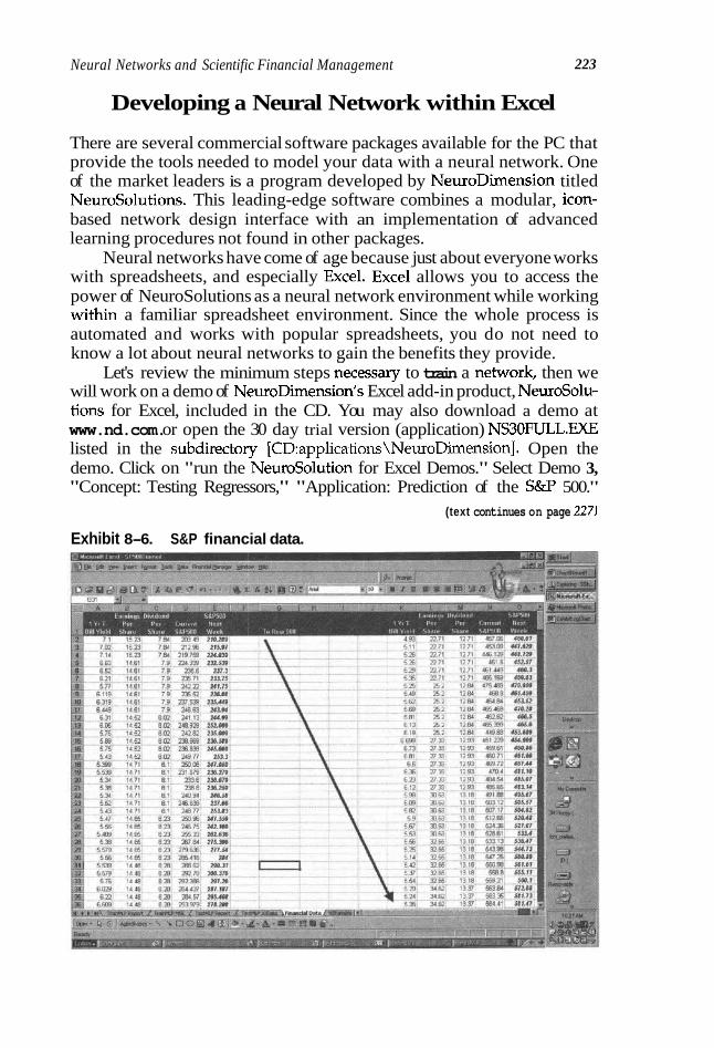
Neural Networks and Scientific Financial Management 223
Developing a Neural Network within Excel
There are several commercial software packages available for the PC that provide the tools needed to model your data with a neural network. One of the market leaders is a program developed by NeuroDimension titled NeuroSolutions. This leading-edge software combines a modular, icon- based network design interface with an implementation of advanced learning procedures not found in other packages.
Neural networks have come of age because just about everyone works with spreadsheets, and especially ~xcel. ~ x c e l allows you to access the power of NeuroSolutions as a neural network environment while working within a familiar spreadsheet environment. Since the whole process is automated and works with popular spreadsheets, you do not need to know a lot about neural networks to gain the benefits they provide.
Let's review the minimum steps necessary to train a network, then we will work on a demo of NeuroDimension's Excel add-in product, NeuroSolu- tions for Excel, included in the CD. You may also download a demo at www.nd.com. or open the 30 day trial version (application) NS30FULL.EXE listed in the subdirectoty [CD:applications\NeuroDimension]. Open the demo. Click on "run the NeuroSolution for Excel Demos." Select Demo 3, "Concept: Testing Regressors," "Application: Prediction of the S&P 500."
(text continues on page 2271
Exhibit 8-6. S&P financial data.

224 SCIENTIFIC FINANCIAL MANAGEMENT
Exhibit 8-7. Train MLP MSE.

Neural Networks and Scientific Financial Management 225
Exhibit 8-8. Test MLP reeort.
I MSE versus Epoch I
Exhibit 8-9. Test MLP input-output data.

Exhibit 8-1 0. NS variables.
Exhibit 8-1 1. Train MLP report.
I Desired Output and Actual Network Output I
I 3 25 49 73 97 121 1" i18 91 132 2:rl
Exemplar I
Neural Networks and Scientific Financial Management 22 7
Exhibits 8-6 through 8-11 are sample pages taken from this application and provided with permission by NeuroDimensions Inc.
First we develop a very simple model for predicting the S&P 500 one week in advance. Later, of course, you can build up more complex finan- cial models once you tackle the basics. The models you develop will be no less compelling than the powerful ones we reviewed early on.
The inputs to the model consist of the one-year Treasury bill yield, the earnings per share and dividend per share for the S&P 500, and the current week's S&P 500. (see Exhibit 8 4 ) The desired output is the next week's S&P 500. (5'h column in Exhibit 8-6) The data have been pretagged and are stored within the worksheet named "Financial Data." There are 507 weeks worth of data that cover approximately a 10-year period. We will use a simvle MLP to model this data.
The data have been presampled such that the first 254 exemplars contain the data for weeks 1,3,5 . . .505,507 and the last 253 exemplars contain the data for weeks 2,4,6 . . .504,506. The first 254 exemplars will be used for train- ing and the last 253 exemplars for evaluating the trained network performance.
An MLP has been pretrained on these data and the training results are shown in the worksheet named "TrainMLP Report." (see Exhibit 8-11) Next, test the networks performance on the 253 weeks of data tagged as "Testing." Let's click on the Test Network button now to run the NeuroSo- lutions for Excel "Test" process. A dialog box will be displayed with the cor- rect options preset such that the testing process will load the best weights (automatically saved during pretraining), run the testing data set through the network, and produce a report summarizing the network's regression performance. Examine the settings, then click on OK. NeuroSolutions for Excel is an Excel Add-in that integrates with any of the six levels of Neu- roSolutions to provide a very powerful environment for manipulating your data, generating reports, and running batches of experiments.
Exhibits 8-7 through &11 are pages selected from NeuroSolutions for Excel Demo, "Prediction of the S&P 500" courtesy of NeuroDimensions Inc.
Because the "Report Type" of the "Test" process was set to "Regres- sion," the resulting report contains a plot of the desired and actual network output in place of the confusion matrix. Furthermore, the "Percent Correct" performance measure has been replaced by the correlation coefficient (see Exhibit 8-8 and Exhibit 8-9. In Exhibit 8-9 the correlation coefficient is its form of - and its value is .9952 for this run.) The other performance mea- sures are the same as those computed for classification since they are use- ful in evaluating the performance of either type of problem. Since this a financial application, the true value of this model can be determined only by applying the model to a trading strategy and computing the profits over several time spans. This type of analysis can easily be done within Excel (see Exhibits 8-6 through 8-11).
5. Reprinted with permission NeuroDimensions, Inc.

This demo5 has shown that NeuroSolutions for Excel can be used to model and test time-series data. To model the S&P500 data, we used a very simple MLP with only four inputs. Perhaps the results could have been improved by using more inputs, including more lags of the inputs that were used, or by using some form of time lagged recurrent network. The Gamma, Leaguer, and Time Delay are three forms of time-lagged recurrent networks included in the Consultants version of NeuroSolutions. You may choose to open the slide show, NDInfo V.
Chapter Eight References and Selected Readings
Books
Arbib, M. A,, and S. I. Amari. (1989). Dynamic interactions in neural networks: Models and data. New York: Springer-Verlag.
Bamdorff-Nielsen, 0. E., et al. (1993). Networks and chaos: Statistical and probabilistic aspects. London: Chapman and Hall.
Beltratti, A,, et al. (1996). Neural networks for economic andfinancial modelling. London: Inter- national Thomson Computer Press.
Cherkassky, V.S., et al. (1994). From statistics to neural networks: Thcoy and pattern recognition applications. Berlin: Springer-Verlag.
Dasarathy, B. V. (1993). Decision fusion. Los Alamitos, Calif.: IEEE Computer Society Press. Deboeck, G. (1994). Trading on the edge: Neural, genetic, andfuzzy systems for chaoticfinancial
markets. New York: John Wiley & Sons. Deboeck, G., and T. Kohonen. (1998). Visual explorations in finance: With self-organizing maps.
London: Springer. Hey, A. J. G., and R. P. Feynman. (1999). Feynman and computation: Exploring the limits of com-
puters. Reading, Mass.: Perseus Books. Husmeier, D. (1999). Neural networks for conditional probability estimation: Forecasting beyond
point predictions. London: Springer. IEEE Computer Society, et al. (1995). Proceedings of the IEEEDAFE 1995 Computational Intel-
ligence for Financial Engineering (CIFEr), April 9-11, New York. Piscataway, N.J.: IEEE Service Center.
Jensen, F. V. (1996). A n introduction to Bayesian networks. New York: Springer. Kingdon, J. (1997). Intelligent systems andfinancial forecasting. London: Springer. Lackes, R., et al. (1998). Neural networks basics and applications. Berlin: Springer-Verlag Elec-
tronic Media. This CD-ROM provides an interactive introduction to neural nets and how to apply them. The learning program is easy to understand and use, and numerous multimedia and interactive components give it an almost gamelike feel. The learner is taken step by step from the basics to the use of neural networks for real projects, and the exam- ples illustrate practical applications of neural networks in business management.
Lindblad, T., and J. M. Kinser. (1998). Image processing using pulse-coupled neural networks. London: Springer.
Neal, R. M. (1996). Bayesian learning@ neural nehuorks. New York: Springer. Refenes, A. P. (1995). Neural networks in the capital markets. Chichester: John Wiey & Sons. Saint-Dizier, P., and E. Viegas. (1995). Computational lexical semantics. Cambridge: Cam-
bridge University Press. Trippi, R. R., and J. K. Lee. (1996). Art@al intelligence in finance and investing: State-of-the-
art technologies for securities selection and portfolio management. Burr Ridge, Ill: Irwin Pro- fessional Publishing.
Neural Networki and Scientific Financial Management 229
Trippi, R. R., and E. Turban. (1990). Investment management: Decision support and expert sys- tems. New York: Van Nostrand Reinhold.
Trippi, R. R., and E. Turban. (1996). Neural networks in finance and investing: Using artificial intelligence to improve real-world performance. Chicago: Irwin Professional Publishing.
Von Altrock, C. (1997). Fuzzy logic and neurofuzzy applications in business andfinance. Upper Saddle River, N.J.: Prentice Hall PTR.
Zirilli, J. S. (1997). Financial prediction using neural networks. London: International Thomson Computer Press.
Technical References
Aiken, M. (1995). "Forecasting T-bill rates with a neural network." Technical Analysis of Stocks and Commodities, 13(5), 85-88.
Aiken, M. (In press). "Artificial neural systems as a research paradigm for the study of group decision support systems." Group Decision and Negotiation.
Aiken, M., Jay Krosp, Chltti Govindarajulu, M. Vanjani, and Randy Sexton. (1995). "A neural network for predicting total industrial production." Journal of End User Com- puting, 7(2), 19-23.
Aiken, M., J. Morrison, J. Paolillo, and L. Motiwalla. (1995). "Forecasting gross domestic product using a neural network." Decision Sciences Conference, November.
Fish, Kelly, James Barnes, and M. Aiken. (1995). "Artificial neural networks: Anew method- ology for industrial market segmentation." Industrial Marketing Management, 24(5).
Singleton, Tommie, Morris Stocks, and M. Aiken. (1995). "Using a group decision support system for financial decision making." SEDSI Conference, March.
Stocks, M., T. Singleton, and M. Aiken. (1995). "Bankruptcy prediction: Logistic analysis vs. an artifical neural network." 1995 Southwest Decision Sciences Institute Conference, March 1 4 , Houston.
Stocks, Morris, T. Singleton, and M. Aiken. (1995). "Forecasting bankruptcies using a neural network." International Business Schools Computing Quarterly, 7(1), 32-35.
Tan, (In prep.). "Automatic selection of neural network architectures via genetic algo- rithm." M.Sc. thesis.
Tan, E, G. Lim, K. Chua, F. Wong, and S. Neo. (1992). "A comparative study among neural networks, radial basis functions and regression models." Second International Confer- ence on Automation, Robotics and Computer Vision, Singapore, September.
Wong, F. "Hybrid systems of neural network, fuzzy logic and genetic algorithms." In Advanced technology for trading, portfolio and risk management, ed. Guido Deboeck. Advanced Analytical Laboratory, Investment Department, World Bank.
Wong, F. (1990). "NeuroForecaster-A neural network for time series predictive analysis." Technical Report, National University of Singapore, May.
Wong, F. (1990). "Time series forecasting using backpropagation neural networks." Neuro- computing. Amsterdam: Elsevier.
Wong, F. (1990/91). "Time series forecasting using back propagation neural networks." Neurocomputing, 2,147, 159.
Wong, F. (1991). "FastProp: A selective training algorithm for fast error propagation." Pro- ceedings of the International Joint Conference on Neural Networks, IJCNN, Singapow.
Wong, F. (1991). "An integrated neural network for financial time series analysis." Pro- ceedings of the 24th Hawaii International Conference on System Sciences, January.
Wong, F. (1994). "NeuroFuzzy computing technology." NeuroVe$t Journal, May-June, pp. 8-10,
Wong, F. (1994). "NeuroGenetic computing." NeuroVe$t Journal, July-August. Wong, F., and C. Tan. (1994). "Hybrid Neural, Genetic and Fuzzy Systems." In Trading on
the Edge, ed. G. Deboeck. New York: John Wiley &Sons.
Wong, F., and D. Lee. (1993). "A hybrid neural network for stock selection." Proceedings of the Second Annual International Conference on Artificial Intelligence Applications on Wall Street, April 19-22, New York.
Wong, F., and E Tan. (In press). "Neural networks and genetic algorithm for economic fore- casting." In A1 in Economics and Business Administration, ed. I. H. Daniels & Feelders.
Wong, F., P. Tan, and X. Zhang. (1992). "Neural networks, genetic algorithms and fuzzy logic for forecasting." Proceedings of the Third International Conference on Advanced Trading Technologies A1 Applications on Wall Street and Worldwide, New York, July.
Wong, F., P. Wang, T. Goh, and B. K. Quek. (1992). "A fuzzy neural system for stock selec- tion." Financial Analysts Journal, January-February.
Wong, F., and P. Tan. "Neural networks and genetic algorithm for economic forecasting." In A1 in economics and business administration, ed. I . H. Daniels & Feelders.
Wong, F., and P. Wang. (1990/91). "A stock selection strategy using fuzzy neural networks." In Neurocomputing, vol. 2. Amsterdam: Elsevier.
Wong, F., and I? Z. Wang. (1991). "A fuzzy neural network approach for forex investment." International Fuzzy Engineering Symposium, November, Japan.
Wong F., l? Wang, and T. Goh. (1991). "Fuzzy neural systems for decision making." Proceed- ings of the International Joint Conference on Neural Networks, November, Singapore.
Zhang, X., and F. Wong. (1992). "A decision support neural network and its financial appli- cations." Technical Report, Institute of Systems Science, National University of Singa- pore, June.
Technical References (General)
Kamijo, K., and T. Tanagawa. (1990). "Stock price pattern recognition: A recurrent neural network approach." Proceedings of the International Joint Conference on Neural Net- works, San Diego, June.
Lapedes, A,, and R. Farber. (1987). "How neural nets work." Advances in Neural Information Systems.
Parker, D. "Learning Logic." Report TR 47. Cambridge: MIT Center for Computational Research in Economics and Management Science.
Peters, E. (1992). Chaos and order in the capital markets. New York: John Wiey & Sons. Peters, E. (1993). "Fractal structure in the capital markets." Financial Analysts Journal
(May/June). Peters, E. (1994). Fractal market analysis. New York: John Wiley & Sons. Holland, J. (1975).
Adaptation in natural and artificial systems. Rumelhart, D., G. Hinton, and R. Williams. (1986). Parallel distributed processing. Cambridge:
MIT Press. Trippi, R., and J. Lee. (1992). State-of-the-art portfolio sdection: Using knowledge-based systems
fo enhance investment performance. Chicago: Frobus. Walter, J., H. Ritter, and K. Schulten. (1990). "Nonlinear prediction with self-organizing
maps." Proceedings of the International Joint Conference on Neural Networks, San Diego, June.
Z i e r m a n n , H. (1990). "Applications of the Boltzman machine in economics." In Meth- ods of operations research, vol. 60/61, ed. Reider. 14th Symposium on Operations Research, Verlag Anton Hain.

Neural Netwarks and Scientific Financial Management
Select Internet Library
NeuroDimension, Inc. This firm's original goal was to develop software tools that would improve their own efficiency and productivity. Since that time, NeuroDimension has assembled research innovators, software design engineers, and technicians encompassing an extended knowledge of the computer sciences. Neurodimension operates with strong ties with the world-renowned Computational Neural Engineering Lab at the University of Florida to enable the firm to bring state-of-the-art neural network technology to the marketplace. The company has customers in more than 40 countries around the world benefiting firsthand from this unique synergism. NeuroDimension has made a gener- ous contribution to this book; its neural network software products are among the most powerful and flexible on the market today, yet their intuitive graphical user inter- faces make them easy to use. The reason may be because their systems can operate in Excel. Readers are invited to download an evaluation copy. http://www.nd.com/ companyhtm.
Artificial Neural Networks and Computational Brain Theory Group This interdisciplinary graduate and faculty discussion group at the University of IUi- nois at Urbana-Champaign addresses issues in neuroscience, cognitive science, and distributed artificial intelligence that concern the functional design of the nervous sys- tem and the construction of large-scale, biologically inspired artificial neural network systems. Visitors are always welcome. http.//anncbt.ai.uiuc.edu/.
The MathWorks The MathWorks develops technical computing software for engineers and scientists in industry and education. The Fuzzy Logic Toolbox features a point-and-click interface that guides users through the steps of fuzzy design, from setup to diagnosis. It pro- vides built-in support for the latest fuzzy logic methods, such as fuzzy clustering and adaptive neuro-fuzzy learning. The Toolbox's interactive graphics allows users to visualize and fine-tune system behavior. http://www.mathworks.com/products/ fuzzylogic/.
Neural Networks and Fuzzy Systems Welcome to the home page of the Research Group on Neural Networks and Fuzzy Sys- tems at the Institute of Knowledge Processing and Language Engineering, Faculty of Computer Science, University of Magdeburg, Germany. http://fuzzy.cs.uni- magdeburg.de/intro.html.
International Neural Network Society The International (INNS), European (ENNS), and Japanese (JNNS) Neural Network Societies are associations of scientists, engineers, students, and others seeking to leam about and advance our understanding of the modeling of behavioral and brain processes and the application of neural modeling concepts to technological problems. http://cns-web.bu.edu/inns/.
University of Bristol, Faculty of Engineering Neural network information, including conferences, societies, archives, journals, pub- lishers, software, hardware, FAQs, mailing lists and newsgroups, and neural nets in industry http://www.fen.bris.ac.uk/engmaths/research/neural/sites.h~l.

Applied Intelligence The International Journal of Artificial Intelligence, Neural Networks, and Complex Problem- Solving Technologies. http://www.wkap.nl/kapis/CGI-BIN/WORLD/jounalome. htm?0924-669X.
IEEE Neural Network Council Member societies, and contact information for NNC officers and various committees, publications of the IEEE NNC, books, videos, and journals of the IEEE NNC, includ- ing the latest journal table of contents, abstracts, and information for authors. Neural networks research, neural computing research programs and professional societies worldwide, information on IEEE NNC Regional Interest Groups, neural networks con- ferences, and up-to-date information on conferences and symposia w i t h a neural net- work component. http://www.ewh.ieee.org/tc/nnc/.
Name Size T V P ~
ANNCBT Group Home Page Application Summaries Applied Intelligence C8ARNNeural C8Backup of SP500Trained C8SP500Trained C8T-CNeural Complex Systems Virtual Library-
Record Details Data Management Review D M Review Business Intelligence &
Data Warehousing Enabling E-Business Download NeuroSolution IEEE Neural Network Council Home Page llliggal Home Page Integration with NeuroSolutions
International Neural Network Society NDlnfoV Neural Network and Kernel Methods Neural Networks and Fuzzy Systmes NS for Excel Generated Report Ns30full Products The Mathworks-Fuzzy Logic Toolbox USNews Putting evolution to work on
the assembly line 17-27-98] What is N N WizSoft Software-WizRule. WizWhv-
lnternet Shortcut lnternet Shortcut lnternet Shortcut Microsoft Excel Worksheet Microsoft Excel Worksheet Microsoft Excel Worksheet Microsoft Excel Worksheet lnternet Shortcut
Internet Shortcut lnternet Shortcut
Microsoft Word Document lnternet Shortcut lnternet Shortcut Microsoft HTML Document 5.0 lnternet Shortcut WinZip File Internet Shortcut lnternet Shortcut lnternet Shortcut Application lnternet Shortcut lnternet Shortcut lnternet Shortcut
lnternet Shortcut lnternet Shortcut
Datamining, Database analizing

Linear Programming,
Optimization, and the CFO
OPTIMIZATION HAS RECENTLY BECOME ONE of the most important tools in shareholder value analysis. This is, in all honesty, "must-have" software for financial managers. Optimization may not be an easy process, but the value-added rewards are impressive: significant cost reductions, cycle time improvements, financial fine-tuning, and revenue opportunities. When strategic plans involve costly assets, financing charges, working capital limits, and marketing investments, there is small margin for error and certainly no room for ad hoc trial-and-error test-outs on those big financial problems. The name of the game is optimized resource allocation, that is, resources meticulously assigned (or combined) in the right amounts, at the right time, and in the right order.
Of course, situations may arise when optimization is inappropriate. Some problems may appear easy candidates for optimization but could just as readily be solved using differential calculus. Alternatively, seem- ingly commonplace problems can be immensely complex (e.g., the travel- ing salesperson problem). How do you plan the shortest route for a sales- person's trip, route airplanes for landings to minimize waiting costs, or find the optimal number of products to produce and sell for maximum profit? a
The optimization (computer method) called for depends on the prob- lem's structure. Many financial applications entail nonlinear functions, logical variables with many (if not tens of thousands) constraints linked to innumerable uncertainty. These problems are difficult to solve with the

great majority of optimization software but are handled quite well by simulation/optimization software such as OptQuest for Crystal Ball, the MATLAB Optimization Toolbox, or Palisade's Risk Optimizer. We will cover all this later in the chapter.
On the other hand, if your decision variables are real (i.e., based on cer- tainty conditions) and the objective variable and constraints are linear func- tions, linear programming will usually do a good job processing your data.
The Basics of Linear Programming
Linear programming is a procedure used to identify optimal maximum or minimum values subject to constraints. A few of today's linear program- ming and optimization models are robust and are able to solve problems containing thousands and even millions of variables without dispropor- tionately tying up your computers. Any problem having decision variables and an objective function to be maximized or minimized is considered a linear programming and/or optimization problem. If the problem is bounded by constraints, it is called constrained optimization; otherwise, the term used is unconstrained optimization. A factory may be limited in size or able to produce only so much of a given product per day. Raw material may be in short supply, working capital sources limited, or work in process bottlenecked because of labor problems. Capital costs might be constrained by systematic and unsystematic risk factors. The question is, How do you combine these perhaps (thousands) of constrained variables in a way that produces maximum value within these set boundaries?
We maximize a linear expression of the form:
where x . . . x, = variables in the linear function a, . . . a, = known coefficients
x variables are subject to constraints (restrictions) expressed by means linear inequalities. For that reason, we refer to these problems as linear pro- gramming problems. Linear programming and optimization models have three essential components: decision variables, objective function, and constraints. The first phase in the process is to define decision variables.
Decision Variables
Each decision variable specifies the level of activity over which someone has control, such as production scheduling, capital investment allocations, and planning and budgeting. There should be enough decision variables

Linear Programming, Optimization, and the CFO 235
to describe all possibilities associated with a financial or operational prob- lem. For example, the management of Ace Cleaning is about to introduce a new detergent, but the company's management is undecided whether to bring out the new product now or next spring. The chief competitor of the firm is the widely known Dume, whose present product is inferior to Ace's. Dume also has a new product to introduce. If they both wait, Ace will come out a winner. If they both introduce their products now, Dume will gain since Ace cannot match Dume's current marketing capability. However, if Dume alone introduces now, Ace will be able to keep afloat this year because of its superior product and will likely outperform Dume next spring.
The decision to market the new product might logically be repre- sented by a real (certainty) variable in the range of coordinates (0,l). Ace's management may want to know what marketing strategy should proceed first among four different strategies (A, B, C, D). The decision is repre- sented by a discrete variable with possible values in (A, B, C, D). Because the decision-proceed or wait-is so crucial to shareholder value, rather than look for easy (generic) solutions, Ace's management will take into account the shape, size, and form surrounding each decision variable. Decision variables take the form of real, integer, logical, choice, and set variables.
Real variables have lower and upper bounds and may take up any value in the range of the coordinates. Integer variables have a lower and upper bound and may take any integer (any member of the set of positive or negative whole numbers and zero) in the range. Logical variables may be either true or false. These variables may be represented by an integer vari- able with a lower bound of 0 (false) and an upper bound of 1 (true). Choice variables have a set of possible values (e.g., the bar codes of different prod- ucts) and must take one of these values. These variables are often repre- sented by an integer variable with a lower bound. Set variables have differ- ent sets as possible values (e.g., the set of products to store in a container) and must be one of these sets. These variables may be represented as choice variables, but their interactions with other variables are often more complex.
Objective Function
The objective function is a numeric benchmark associated with the prob- lem, for example, maximize profits, minimize costs, or maximize share- holder value. The purpose of the decision maker is to select that course of action: A, which will maximize some measure of gain or minimize some measure of loss or cost (i.e., which will optimize some function), E, which measures the effectiveness of the various courses of action; that is, Ei =f(Ai). Objective functions are classified into two types: linear and nonlinear.
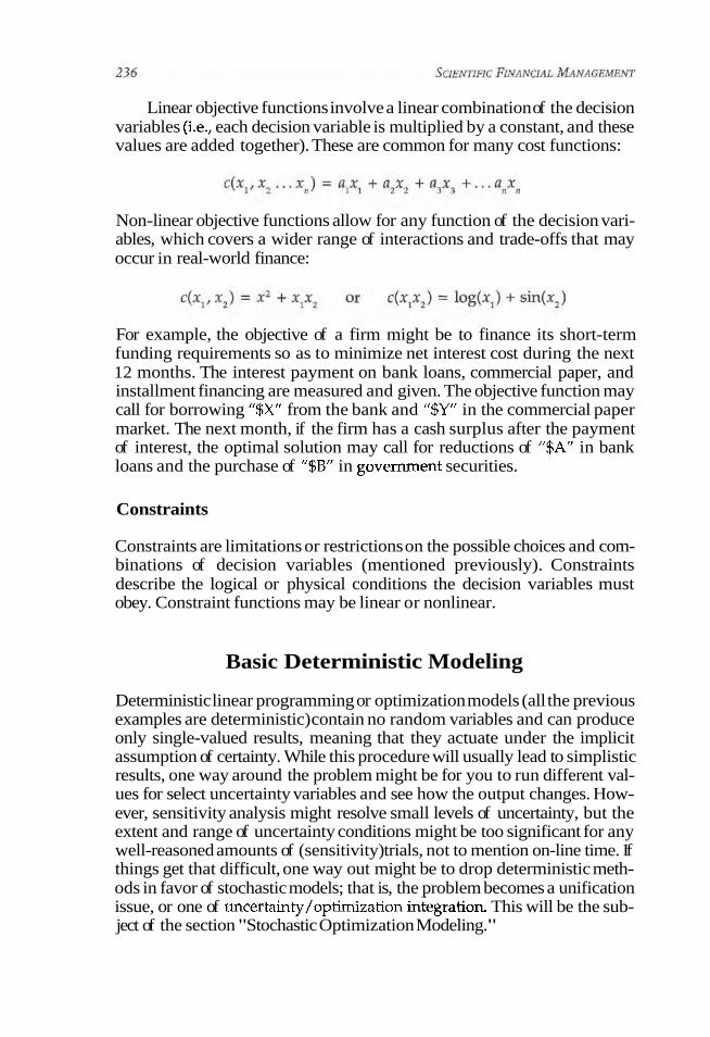
Linear objective functions involve a linear combination of the decision variables (i.e., each decision variable is multiplied by a constant, and these values are added together). These are common for many cost functions:
Non-linear objective functions allow for any function of the decision vari- ables, which covers a wider range of interactions and trade-offs that may occur in real-world finance:
For example, the objective of a firm might be to finance its short-term funding requirements so as to minimize net interest cost during the next 12 months. The interest payment on bank loans, commercial paper, and installment financing are measured and given. The objective function may call for borrowing "$X" from the bank and "$Y" in the commercial paper market. The next month, if the firm has a cash surplus after the payment of interest, the optimal solution may call for reductions of "$An in bank loans and the purchase of "$B" in government securities.
Constraints
Constraints are limitations or restrictions on the possible choices and com- binations of decision variables (mentioned previously). Constraints describe the logical or physical conditions the decision variables must obey. Constraint functions may be linear or nonlinear.
Basic Deterministic Modeling
Deterministic linear programming or optimization models (all the previous examples are deterministic) contain no random variables and can produce only single-valued results, meaning that they actuate under the implicit assumption of certainty. While this procedure will usually lead to simplistic results, one way around the problem might be for you to run different val- ues for select uncertainty variables and see how the output changes. How- ever, sensitivity analysis might resolve small levels of uncertainty, but the extent and range of uncertainty conditions might be too significant for any well-reasoned amounts of (sensitivity) trials, not to mention on-line time. If things get that difficult, one way out might be to drop deterministic meth- ods in favor of stochastic models; that is, the problem becomes a unification issue, or one of uncertainty/optimization integration. This will be the sub- ject of the section "Stochastic Optimization Modeling."

Linear Programming, Optimization, and the CFO
Setting up a Deterministic Linear Programming Exercise
Because constraints represent l imited resources consumed by activities corresponding to decision variables, we write them as Linear inequalities. Employing the "comer point theorem," we can determine an optimal solu- t ion(~) b y locating a feasible region that contains our solutions. The comer point theorem says that if a maximum or minimum value exists, it will occur at a comer point of this feasible region. Let's see how this works as we seek to optimize Generic Bakery's profits.
Assume that we want to maximize profits on a given day (say, Sunday), our linear objective function. The problem becomes to select x,, x, . . . xn in some combination so that the objective function, P, i s maximized. Again, we want maximum profits, which are (graphically) mapped out by specific coor- dinates. Had there been no constraints-hours in a day, the bakery's size, and dozens of other restrictions- our objectives might well be achieved by making x, . . . x, infinitely large. We could choose any point on the chart or even extend the point beyond the page, but clearly this i s unrealistic.
Generic Bakery is subject to four linear inequalities (constraints). Linear inequalities are written as >, 2, <, or $, which occurs in place of the equals sign. Equals signs are associated with linear equations. We write the four constraints given in symbolic form:
The Basic Statement of the Bakery Problem
Next, identify decision variables. Again, each decision variable specifies the level of activity over which someone controls, for example, baking a particular cake for the Sunday crowd. The problem should include enough decision vari- ables to describe all realistic strategies in search of a solution. Let's now select two decision variables: the number of cakes to bake on Sunday, x, and the num- ber of bagels, y. A production plan calls for, essentially, choosing values for xand y. We could have easily defined variables in terms of the number of pounds of cakes and bagels rather than the count. There is usually more than one valid way to choose decision variables. Mathematically, this problem can be stated as:
Maximize P, subject to the constraints x + y < 5; 2x + y > 4; x > 0; y > 0

Setting up the Linear Solution
Step 1 : Rewrite each of these inequalities isolating for y:
Step 2: Graph all Four Constraints.
Inequality Plot
First Slope -1 and y intercept 5 Second Slope -2 and y intercept 4 Third Vertical line (y-axis) Fourth Horizontal line(x-axis)
The area that we want is below the blue line, above the orange line, to the right of the y-axis, and above the x-axis. The feasible region is outlined in black (see Exhibit 9-1).
Finally, we find the maximum value given a function we want to opti- mize. Assume that the function is P = 3 x + 5y. Employing the corner point theorem to maximize the function and using the graph, the corner coordi- nates are (0,4), (0,5), (2,0), and (5,O). Inserting these four values in the objec- tive function, we extract the largest value:
Coordinate Function Value
We find maximum Sunday profits of $25 at coordinate (0, 5). Basic prob- lems, such as that of the Generic Bakery, are easily solved by the Simplex method, an iterative system that locates successive basic-feasible solutions, testing them for optimality. Optimization is accomplished by moving from one corner of the feasible region to another, always improving the objective function until it can be amended no further, in which case the solution is optimal. The simplex method, in the old days, was the easiest and quickest method to optimize a problem. However, as business problems become more complex with a greater number of decision variables and constraints, the use of the simplex method is a thing of the past.

Linear Programming, Optimization, and the CFO
Exhibit 9-1. Graphical representation of feasible re~ion.
Table 9-1. Characteristics of optimization models.
Optimization Model Characteristics
Discrete Operates with only discrete decision variables. A discrete variable can assume only integer values and must have a defined step size that is an integer greater than or equal to 1. Discrete also describes and optimization model that contains only discrete variables.
Continuous Have only continuous decision variables. This is a variable that can be fractional, so no step size is required, and any given range contains an infinite number of possible values. Continuous also describes an optimization model that contains only continuous variables.
Mixed These models have both discrete and continuous decision variables. Linear Terms in the formulas contain only a single variable multiplied by
a constant. For example, - 2 . 3 ~ is a linear relationship since both the first and the second term only involve a constant multiplied by a variable.
Nonlinear Terms in the formula are nonlinear, for example, x2, xy, l lx, or e.lx. Deterministic Input data are constant or assumed to be known with certainty.
These systems have no random variables and can produce only single-valued results.
Stochastic A model or system with one or more random variables. Require simulation to comuute the obiection function.
Computer Optimization Models
Computer optimization models can be classified as (1) discrete, continuous, or mixed; (2) linear or nonlinear; and (3) deterministic or stochastic (see Table 9-1).

There i s no shortage of linear programming and optimization software packages. You can find them easily on the Web, and many are offered free. But be careful: Whi le most of these models are fine for home or small-office use, many are limited to optimizing linear and deterministic problems (see Table 9-2).
Table 9-2. Model packages.
Source
The Optimization Technology Center at Argonne National Laboratory and Northwestern University
Csaba Meszaros ([email protected]) at the Computer and Automation Research Institute of the Hungarian Academy of Sciences
Jacek Gondzio (gondzio@maths. ed.ac.uk)
Details and Model Type
PCx, an interior- point code
Fortran 77 interior- point code, BPMPD
Interior-point LP (and convex QP) solver HOPDM
Commen ts
Available in Fortran or C source or a variety of Windows and Unix executables, with an optional Java-based GUI interface. Input can be specified in MPS form or by use of the AMPL modeling language.
Available as FORTRAN source code, as a Windows951NT executable (which is also extended to solve convex quadratic problems), and in a DLL version for Windows. Separately, a large variety of Unix binaries, including many with a built-in interface to the AMPL modeling language, are available for downloading.
Several papers (also available at the HOPDM Web site) detail the features of this solver, which includes automatic selection of multiple centrality correctors and factorization method and a "warm start" feature for taking advantage of known solutions. A public domain FORTRAN version (2.13, LP only) can be down- loaded, and a newer C version (2.30) is available on request to the developer.

Linear Programming, Optimization, and the CFO 24 1
Source
- - -
Details and Mode! Type
MOSEK optimization software
LPL mathematical modeling language
ABACUS
Robert Vanderbelt at Princeton University
Web-based service by a group at Berkeley
MATLAB optimization toolbox and a parallel version
Use for formulating and maintaining linear and mixed-integer programs
C++ class library
Java-based tools
Interactive linear programming
Comments
Package for Windows PCs that incorporates an interior-point solver for linear and quadratic objectives and constraints. If you want to solve an LP without downloading a code to your own machine, you can execute many of these interior-point codes (as well as commercial LPcodes LOQO, MINOS, and XPRESS) through the NEOS Server.
Particularly notable for its ability to also handle a variety of logical constraints, which are translated symbolically into algebraic constraints using 0-1 variables. You can download the software and documentation free of charge.
Provides a framework for the implementation of branch-and- bound algorithms using linear programming relaxations that can be complemented with the dynamic generation of cutting planes or columns (branch-and- cut and/or branch-and-price). It relies on CPLEX, SoPlex, or XPRESS-MP to solve linear programs. Further information is available from Stefan Thienel, [email protected].
These tools facilitates simplex pivots and facilitating network simplex pivots and well as a variety of Java applets that test students on their knowledge of various simplex-based methods.
Useful for solving small models that can be entered by hand.
(continues)

Table 9-2. Continued.
Source Details and Model Type Comments
Northwestern and Argonne National Laboratory
Operations Research Laboratory at Seoul National University, Korea
Will Naylor
- -
The NEOS Guide Offers a Java-based simplex tool that demonstrates the workings of the simplex method on small user-entered problems.
C source For large-scale linear programming software (both simplex and barrier) and for numerous, more specialized optimization problems.
WNLlB A collection of software with routines that include a dense- matrix simplex method for linear programming (with anticycling and numerical stability "hacks") and a sparse- matrix transportationlassignment problem routine. (WNLIB also contains routines pertaining to nonlinear optimization).
Professor l imo DOS/PC users Friendly linear programming and Salmi ([email protected]) linear goal programming code.
SOLVER, EXAMPLE 1: USING SOLVER TO DETERMINE
THE OPTIMAL STOCK PORTFOLIO
Microsoft Excel Solver uses the generalized reduced gradient nonlinear opti- mization code developed by faculty at the University of Texas and Cleveland State University. Linear and integer problems use the simplex method (dis- cussed earlier) and the branch-and-bound method.
Perfect Portfolio Ltd.
The Problem
You are a financial consultant specializing in retirement financial planning. Your function i s to advise clients to follow conservative investment strategies, though many of your clients' financial objectives are unique. For the fixed- income portion of a typical portfolio, PPL employs yield to maturity. For equities, the firm typically utilizes a weighted average return rate that the S&P 500 compounded over the past 70 years.
Recently, a client brought you a list of securities that she had been following-Microsoft, Intel, UAL, GM, JP Morgan, and so on-and

Linear Programming, Optimization, and the CFO 243
requested that you construct a portfolio positioned in terms of risk equal to the S&P 500. Your client could have easily purchased an S&P index fund, but she was biased to her "basket" alone.
First, you checked the betas of each stock in the client's portfolio. The portfolio's beta averaged 1.21, much too risky given her retirement objec- tives. However, the client's portfolio could be optimized by setting the objec- tive function, equity returns, to maximize while fixing a constraint, portfolio stock beta, to one.
Betas can be obtained from stock research reports (Value Line) or cal- culated with knowledge of the covariance of security returns with the mar- ket and the variance of the market. This is achieved by use of the capital asset pricing model equation:
Rj = Rf + (Rm - Rf)pj,
where
(Rj) = the required equity return investors demand for investing in the stock. (Rm - Rf) = the market risk premium or the difference between the returns on an S&P 500 index (Rm) and the risk-free rate (Rf). (pj) = the security's beta. pj = 1 means the security and the S&P index have identical volatility (returns should be identical); p j > 1 means the security's returns are more volatile than the S&P index (the security is more risky, and returns should be higher than the S&P index). p j < 1 means the security's returns are less volatile than the S&P index (the security i s less risky, and returns should be lower than the S&P index).
Example Assume that 20-year Treasury bonds currently yield 9%. The market returns 12% on a portfolio, while the historical long-term average yields on Treasury bonds are 3.1%. Beta estimate for Detroit Edison is .55. What i s the return demanded by investors in Detroit Edison's stock?
Rj = Rf + (Rm - Rf)pj; Rj = 9% + (12% - 3.1%).55 = 13.9%
However, one stock hardly represents a portfolio, and that is where the Solver comes in. You program Solver to generate a variance equal to a beta of one. Without the Solver optimizing the precise risk-reward space demanded by your client, her portfolio returns fall beneath the efficient frontier1 (see Exhibit 9-2). By superimposing the client's indifference map on the efficient set of available portfolios, you determine the optimal (percentage) mix of securities in a "beta one" portfolio, thus maximizing the investor's utility.
1. See chapter 2 for details on the efficient frontier,

Exhibit 9-2. Minimum variance set. Mean Return
18 16 14 12 10 8 6 4 2 0
Efficient frontier: top half of the bullet-all portfolios that maximize return for a given level of risk
Point of bullet: minimum varience portfolio, the least risky portfolio that
Interior of bullet: all portfolios possible in given asset class or business segment. t
The Solution
Step I : The Spreadsheet [CD:MODELS\EXCEL\C9SoluJoeBk]
Set up the titles for each of the rows and columns (see Exhibit 9-3). Put these in an italic or a bold font to make them easier to find within the entire spreadsheet. It is also a good idea to highlight the cells that will contain the decision variables in a different color. These are the cells that wil l be altered by Solver. The decision cells are F10:F22, the weights of each security with respect to the total portfolio.
Next, insert the given values, the betas of each security, and respective yields. Insert the known formulas. This will include not only the formulas for the
resource utilization, weighted yields, and weighted betas, but also the formula for the target functions, portfolio dividend yield, equity return, and stock beta.
Allocate a cell for the target cell that you want to maximize--Equity Return, cell F25.
Allocate cells for constraints. Constraints are fundamental to Solver. A constraint specifies an upper or a lower limit, or an exact value that a calculated function of the decision variables must satisfy at any solution found by the Solver. The primary constraint, or the main decision cell, wil l be G25 = 1 ; that is, beta must equal 1. This type of constraint is of the form C25 = integer, where equity return is one of the decision variables. This spec- ifies that the solution value for this cell must be an integer or whole number to within a small tolerance (also the precision setting).
The other constraints we set in Solver wil l prevent illogical solutions from occurring. You should plan constraints before calling up Solver:
A The basket of securities held must be greater than or equal to zero. ($F$lO:$F22 >= 0); $ signifies an absolute reference.


Exhibit 9-4. Solver parameters.
A The portfolio weights must total to 100%; that is, $F$23 = 1 A Beta must equal 1; that is, $G25 = 1.
Now call up Excel's add-in, the Solver, by selecting ToolslSolver. The Solver dialog box consists of three main areas. The first area is the target cell and what we are attempting to do with that target (see Exhibit 9-4).
In our scenario, the SetTarget Cell box wil l read $F25, corresponding to equity return. This can be entered directly or selected with the mouse. In this example, the Max radio button is selected because we are attempting to maximize equity return. The next area of the dialog box defines those cells that can change in the determination of the solution. This can be entered as a range of cells using the colon (:) operator or a cornma-separated l ist of the cells. In our situation, the box wil l read $F$lO:$F$22.
The last area of the dialog box deals with the constraints. To begin enter- ing "Subject to the Constraints:", click on Add. This presents a new dialog box. In this dialog box, the left box represents the formula being constrained, and the right box represents the limit. In the middle is an operator where you can define the type of constraint. Because the spreadsheet is organized as it is, it i s very easy to enter these constraints using the mouse. To add each con- straint, click first on the left box, then on the appropriate cell in the spread- sheet that contains the formula being constrained. Then click on the right box, followed by clicking on the cell in the spreadsheet that contains the lim- its of that formula. If necessary, change the operator. The constraints are

Linear Programming, Optimization, and the CFO
Exhibit 9-5. Solver solution.
Finally, click on Solve. This wil l perform the calculations and change the values in the spreadsheet to show the results of the solution (see Exhibit 9-5). You are then presented with another dialog box asking whether you want the values to return to their original state or to leave them as is. Additionally, you can select which reports of the analysis you need to generate. Use the mouse to select any or all of the reports.
Solver optimizes the spreadsheet, and, in a manner of speaking, your client's custom-made securities portfolio is fixed on the efficient frontier- not too aggressive, not to conservative. Thus, the portfolio's risk profile exactly matches the S&P 500. The optimized spreadsheet has not been repro- duced here but if you have worked out the optimization you can view the worksheet on your computer. Open C9SoluJoeSolution.
Solver creates three reports: Answer, Limits, and Sensitivity. We wil l review the reports in the next case. For now, let's use Solver to optimize an oil refinery's profits by allocating scarce resources.
New Jersey Refinery is located in northern New Jersey. The business i s engaged in the following operations. Open C9mjr in the Excel subdirectory.
The Refining Process
Gasoline i s produced from crude oil either by a distillation process alone or by a distillation process followed by a catalytic cracking process. Outputs of these processes are blended to obtain different grades of gasoline.

The distillation process at a typical refinery separates gasoline from other parts of crude and places the crude oil under tremendous pressure until the gasoline vaporizes. The vapors are then collected and cooled in a con- denser to produce distillate. New Jersey Refining buys i ts crude at $1 2 a bar- rel. The distillation tower uses five barrels of crude oil to produce one barrel of distillate and four barrels of other petroleum by-products. New Jersey Refining currently sells these other products for $12 a barrel.
The refinery's distillation tower can produce a daily output of up to 50,000 barrels of distillate at an operating cost of $4 per barrel. Some distil- late wi l l be blended into gasoline products; some wil l become "feedstock" for the Catalytic Cracker.
Catalytic Crackers
The catalytic cracking process utilizes high temperatures to break up "crack" heavy hydrocarbon compounds into lighter compounds. This process pro- duces high-quality gasoline stock from the feedstock. New Jersey Refining catalytic cracker requires two barrels of feedstock to produce one barrel of gasoline stock and one barrel of petroleum by-products. These by-products
currently sell for $20 a bar- rel. The catalytic cracker can produce up to 15,000 barrels of gasoline stock per day. The catalytic cracker has an operating cost of $5 per barrel output (see Exhibits 9-6 and 9-7).
The distillate produced by New Jersey Refining dis- tillation tower has an octane rating of 84, while the gaso-
line stock from the catalytic cracker has an octane rating of 94. The New Jer- sey Refining gasoline refining process ends by blending distillate and cracker stock to form regular and premium gasoline, which have required octane rat- ings of at least 86 and 90, respectively. There i s no volume or octane loss in blending; the variable cost of blending is negligible. New Jersey Refining sells its regular gasoline for $20 per barrel and its premium gasoline for $25 per barrel.
The final gasoline products are pumped from the New Jersey Refining Oi l refinery in Louisiana via two small pipelines to several storage and dis- tribution facilities in the eastern United states. One pipeline carries only reg- ular gasoline, the other carries only premium gasoline. Each pipeline can handle up to 25,000 barrels a day.
Let's look at New Jersey Refining's initial spreadsheet setup (see Exhibit 9-8).

Linear Programming, Optimization, and the CFO 249
Exhibit 9-7. Visual flow diagram using Analytica (The New Jersey model is included in the CD).
-'( Revenue )
Highlight cells that wi l l contain decision variables in a different font size or color. These are the cells that wil l be altered by Solver in order to achieve an optimal solution. The decision cells are B7:B9-Tower Capac- ity (bbllday distillate, Distillate-Regular bblslday, Distillate-Premium bblslday). Allocate a cell for the target cell you want to maximize-Profits, cell D53.

Exhibit 9-8. New Jersey Refining, original condition.
Pmduction cmarraims opmting nuts, a d bypmduef rsmues
Crude Oil Input (bbtlday): Crude>D~~~liate Elfinency Distillate Output (octaned4) W i l d a d : Tower Capacity (bbllday or Bstillafe): Byproductr Output IbMfday):
, , a o ; i a n ; Constraint RHS la) W l c t u a l Octane la) 86 Actual Octane (:
86 Odane Constolnt RHS (a) 90 3) 91
20 Revenue Sfbbl 25 350000 Total Revenue ISRlay) 437500 I
D,rtillation Tower
Allocate cells for constraints. A constraint specifies an upper or a lower limit, or an exact value that a calculated function of the decision variables must satisfy at any solution found by the Solver.
Call up Solver by selecting ToolsISolver. The Solver dialog box consists of three main areas. The first area is the target cell and what we are attempt- ing to do with that target (see Exhibits 9-9 and 9-10).
Set the target sell to Profits, $D$54. Next, select the Max radio button, maximize profits. The next area of the dialog box-By Changing
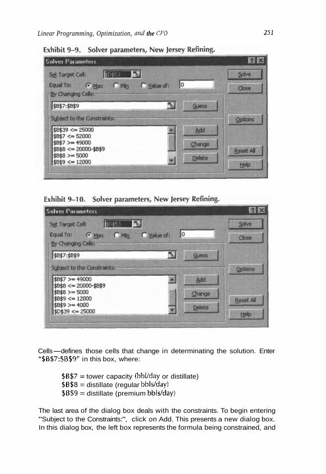
Linear Programming, Optimization, an2 the CFO 23 1
Cells-defines those cells that change in determinating the solution. Enter "$B$7:$B$gU in this box, where:
$B$7 = tower capacity (bbllday or distillate) $B$8 = distillate (regular bbls/day) $B$9 = distillate (premium bblsfday)
The last area of the dialog box deals with the constraints. To begin entering "Subject to the Constraints:", click on Add. This presents a new dialog box. In this dialog box, the left box represents the formula being constrained, and

the right box represents the limit. In the middle is an operator where you can define the type of constraint. Because the spreadsheet is organized as it is, i t is very easy to enter these constraints using the mouse. To add each con- straint, click first on the left box, then on the appropriate cell in the spread- sheet that contains the formula being constrained. Then click on the right box, followed by clicking on the cell in the spreadsheet that contains the lirn- its of that formula. If necessary, change the operator. Important constraints are explained as follows:
Constraint Reference
Regular output (bbllday) i s restricted to less than or equal to 25,000.
Tower capacity (bbllday or distillate) is limited to less than or equal to 52,000.
Tower capacity (bbllday or distillate) is greater than or equal to 49,000.
Due to capacity limits, regular distillate constraint must be less than or equal to 20,000 bblslday (maximum capacity of both distillate--regular and premium) less premium distillate.
Regular distillate production set at greater than or equal to 5,000 bblslday.
Distillate-premium bblslday production less than 12,000.
Premium distillate production set at greater than or equal to 5,000 bblslday.
Premium output (bbllday) production limited to 25,000 or less.
Click on Solve. This wil l perform the calculations and change the values in the spreadsheet to show the results of the solution. You are then presented with another dialog box asking whether you want the values to return to their original state or leave them as is. Additionally, you can select which reports of the analysis you need to generate. Use the mouse to select any or all of the reports.
If you call for reports, Solver creates three reports: Answer, Limits, and Sensitivity. See C9NJRSolution.
Answer Report
The report lists the target cell and adjustable cells with their original and final values, constraints, and information about the constraints (see Exhibit 9-1 1). This report also includes information about the status of, and slack value for, each constraint. The status can be Binding, Not Binding, or Not Satisfied. The slack value i s the difference between the solution value of the
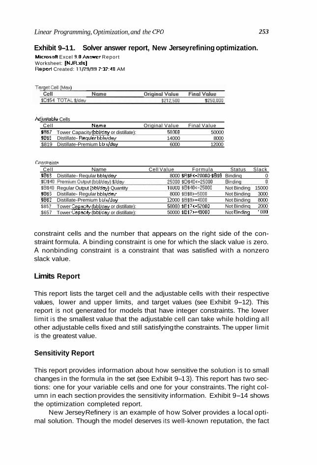
Linear Programming, Optimization, and the CFO 253
Exhibit 9-1 1. Solver answer report, New Jersey refining optimization. Microson Excel 9.0 A n m r Report Worksheet: [NJR.xls] Report Created: 11129/9!3 7:32:48 AM
Adjuaable Cells Cell Nams Original Value Final Value
$857 Tower Capacity @bl/day or distillate): 50000 50000 $816 Distillate- Requiar bblsjday 14000 8000 $819 Distillate-Premium bbis/day 6000 12000
- - . . -. -. . . .- Cell Name Cell Value Formula Status Slack
$858 Distillate- Reqular bblsjday 8000 $B$8<-20000-5859 Bindinq 0
$&$40 Regular Output (bbl/d~y) Quantity 10000 58$40r=25000 Not Binding 15000 $856 Distillate- Regular bblsjday 8000 5658>=5000 Not Binding 3000 $659 Distillate-Premium bblsjday 12000 $8$9>=4000 Not Binding 8000 $857 Tower Capaciiy (bbl/d-ay or distillate): 50000 $8$7<=52000 Not Bindinq 2000 $657 Tower Capaow (bbltday or distillate): 50000 5857>=49000 Not 8ind1nq 1 DO0
constraint cells and the number that appears on the right side of the con- straint formula. A binding constraint is one for which the slack value is zero. A nonbinding constraint is a constraint that was satisfied with a nonzero slack value.
Limits Report
This report lists the target cell and the adjustable cells with their respective values, lower and upper limits, and target values (see Exhibit 9-12). This report is not generated for models that have integer constraints. The lower limit is the smallest value that the adjustable cell can take while holding all other adjustable cells fixed and still satisfying the constraints. The upper limit is the greatest value.
Sensitivity Report
This report provides information about how sensitive the solution is to small changes in the formula in the set (see Exhibit 9-1 3). This report has two sec- tions: one for your variable cells and one for your constraints. The right col- umn in each section provides the sensitivity information. Exhibit 9-14 shows the optimization completed report.
New Jersey Refinery i s an example of how Solver provides a local opti- mal solution. Though the model deserves its well-known reputation, the fact
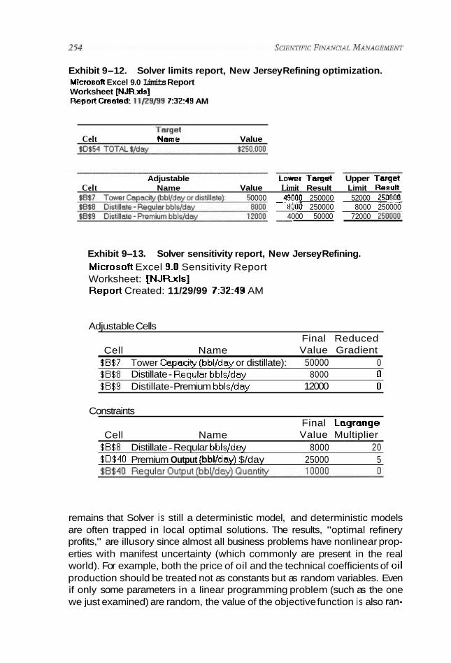
Exhibit 9-12. Solver limits report, New Jersey Refining optimization. Microsoft Excel 9.0 Limits Report Worksheet WJRxfs] Report ha ted: 11/23@9 7:32:49 AM
Celt ~ a m e Value
Adjustable Ltnver Targcrt Upper Targst Celt Name Value Limit Result Limit Resul
0000 -49000 250000 52000 250% 8000 250000 8000 250000 - 4000 50000 72000 2500if -
Exhibit 9-1 3. Solver sensitivity report, New Jersey Refining. Microsofl Excel 9.0 Sensitivity Report Worksheet: [NJR-xls] Reporl Created: 11/29/99 7:32r49 AM
Adjustable Cells Final Reduced
Cell Name Value Gradient $B$7 Tower Capacip [bbljday or distillate): 50000 0 $B$X Distillate - Reqular bbls/day 8000 0 $B$9 Distillate- Premium bblsjday 12000 0
Constraints Final Lagrange
Cell Name Value Multiplier $B$8 Distillate - Reqular bbls/day 8000 2 0 $0$40 Premium Output (bbl/day) $/day 25000 5
remains that Solver is still a deterministic model, and deterministic models are often trapped in local optimal solutions. The results, "optimal refinery profits," are illusory since almost all business problems have nonlinear prop- erties with manifest uncertainty (which commonly are present in the real world). For example, both the price of oil and the technical coefficients of oil production should be treated not as constants but as random variables. Even if only some parameters in a linear programming problem (such as the one we just examined) are random, the value of the objective function i s also ran-

Linear Programming, Optimization, and the CFO 255
Exhibit 9-1 4. New Jersey Refining optimization completed. - -
tkw ~ers-sy~k&ne&-- - Opbmtznb~n Completed
m a e ~ 9 i X f ~ m W e k - 1 Change Cells
. . . . - . - . . -. . - - -.
~ L 3 . a a t m Feedstock Input(bbVdeyj: 30000
Octane Conelimn1 RHS ii) Adual Odane (qi Rwsnue Wbl Total Revenue (Weyj
D181lllabon T w r Cataiy%cCracksr Regular Prsm~urn TOTAL
86 Onane ~0nsbai;;f RHS (i) 90 86 Amal Odene (a) 89 20 Revenue tibbl 25
200000 Told Revenue (Slduy) 625000
dom. Thus, when linear programming is applied to these problems, special techniques must also be used, and they cannot be the same for all problems.
Management must be concerned with the variance as well as the expected value of refinery profits. The question becomes how to modify the problem to allow for New Jersey's aversion toward risk. We can allow for pos- sible risk aversion by including in the objective function a term representing the variance of the refinery's profits. Unfortunately, if variance is introduced,

the objective function becomes nonlinear in the decision variables, and the problem can no longer be solved by linear programming methods.
Again, the nonlinear solution component of deterministic models is able to obtain only a locally optimal solution-a solution whose quality may be substantially inferior to the quality of the solutions provided by a robust sto- chastic optimization model.
Stochastic models can handle nonlinear relationships that are specifiable by the kinds of equations and formulas that are used in mathematical pro- gramming formulations. Conversely, deterministic optimization does not apply to nonlinear problems other than those that can be expressed in "classical" mathematical programming form. One of the most important issues deals with the ability of stochastic models such as OptQuest to solve a problem whose objective and constraining relationships can be captured only by means of a simulation, which, by definition, is beyond the capacity of any deterministic model to deal with. In addition, financial optimization in today's age of share- holder value should incorporate a combination of metaheuristic procedures from methods such as tabu search, neural networks, and scatter search. Only the best stochastic model i s vigorous enough to blend these technologies.
Nonlinear components can create a solution space with many local optimal solutions that might be significantly inferior to the true optimal solu- tion. Stochastic optimization can find global solutions for all types of objec- tives, especially complex objectives with many local, inferior solutions. This is important since global optimization finds the best solution from the set of all solutions. Local optimization (New Jersey Refining), on the other hand, finds the best solution from a set of solutions that are close to one another. In local optimization, the solution depends also on the starting point for the optimization. Global optimization wil l always find the same solution regard- less of the starting point, but it takes a lot more computational power. Con- versely, the refinery example found solutions that got trapped in the first rem- edy found, whether it happened to be a local or the true optimal solution. The problem with the Solver is that we just do not know.
Stochastic Optimization Modeling2
Stochastic programming is employed in energy and production planning, telecommunications, forest and fishery harvest management, engineering, and transportation, plus a much larger spectrum of financial applications, including financial modeling, asset-liability management, bond portfolio management, currency modeling, risk control, and probabilistic risk analysis.
Stochastically driven optimization models allow you to more realisti- cally represent the flow of random variables. Consider an optimization
2. This section was developed with the aid and support of many experts at Decisioneering. The author is greatly indebted to help and information supplied.

Linear Programming, Optimization, and the CFO 25 7
problem whereby you try to maximize an objective function over a feasible region. Suppose that the problem is very large, containing tens of thousands of variables, so that it is unrealistic for you to run sensitivities. Obtaining these optimal values generally requires that you search in an iterative or ad hoc fashion. This entails running a simulation for an initial set of values, ana- lyzing the results, changing more or more values, rerunning the simulation, and repeating this process until you find a satisfactory solution.
This process can be very tedious and time consuming even for small models, and it is far from clear how to adjust the variables from one simu- lation run to the next and so on. For example, a simulation run may con- tain only two decision variables. If each variable has 15 possible outcomes, trying each combination requires 225 simulation runs (152 alternatives). If each simulation takes only 1.7 seconds, then the entire process is com- pleted using only two minutes of computer time.
However, suppose that you are running a problem containing five decision variables. Trying all combinations requires 769,000 simulations (155 alternatives), or five days of computer time. It is clearly possible that complete enumeration might take weeks, months, or even years to com- plete. This will not happen with well-designed stochastic models (e.g., Decisioneering's OptQuest). OptQuest employs combinations of meta- heuristic procedures derived from systems like tabu search, neural net- works, and scatter search. Let's examine how this works.
Neural networks and log file options are germane when calculations are tedious, time consuming, and expensive, like most of the problems we run up against in finance. How does the neural network procedure work? The log file records solutions generated during the search. The neural net- work searches for solutions before a new solution is transmitted. The search in the log file is justified only when evaluation of solutions is com- putationally not viable and expensive.
In this way, the network filters out inferior solutions. After a series of initial iterations, the trained network predicts the output of the function evaluator based on the values of the decision variables. Once the training is complete, the network evaluates new solutions and predicts the output of the function evaluator. If the prediction indicates that the solution is "likely" to be inferior to the best known, then the function evaluator does not evaluate the solution.
Tabu Search3
OptQuest also employs tabu search techniques. Tabu search is a very efficient heuristic (or learning) process designed for tackling complex combinatorial
3. Extracted from an article on the subject by M. Laguna and F. Glover, Colorado Business Reviezu 61, no. 5 (September 1996).

problems in business and other domains. For background, consider two important ways in which computers solve quantitative problems. The first deals with programming formulas that manage information (input data). The software works through the formulas and produces a solution. In the second method, software works through the problem and makes slight changes in the data, but now the operation cycles the data over and over again until the final result is processed or a termination criterion is met.
For example, if you wanted to estimate compound interest, the first method would produce the first run answer: simple interest. The second (repetitive) method calculates the interest for the first year and then uses this to calculate the interest for the second year and so on. In 99% of finance problems, the repetitive method serves as the only alternative. In fact, repet- itive methods have the potential to assemble simple components to achieve remarkable levels of sophistication and complexity as we move toward opti- mizing real problems; a formula, as in the first example, may alternately become one of the pieces incorporated into a repetitive approach. Repetitive methods are commonly applied for the goals of finding the following:
A The best configuration of machines for production scheduling A The best investment portfolio A The best utilization of employees for workforce planning A The best location of facilities for commercial distribution A The best operating schedule for electrical power planning A The best assignment of medical personnel in hospital administration A The best setting of tolerances in manufacturing design A The best set of treatment policies in waste management A Many other business objectives
Tabu search has become a standard optimization process that is swiftly spreading to resource management, shareholder value-gap analysis, corpo- rate planning and control, process design, logistics, and technology planning.
OPTQUEST CASE STUDY
Oil Field Development4
Oil companies need to assess new fields or prospects where very little hard data exists. Based on seismic data, exploration experts can estimate the prob- ability distribution of the reserve size. With little actual data available, the discovery team wants to quantify and optimize the net present value (NPV) of the asset. You can simplify this analysis by representing the production profile by three phases:
4. Complements of OptQuest for Crystal Ball, version 1.0 manual, pp. 112-115. Reproduced with permission.

Linear Programming, Optimization, and the CFO 259
Phase Description
Buildup The period where you drill wells to gain enough production to fill the facilities.
Plateau After reaching the desired production rate (plateau), the period when you continue production at that rate as long as the reservoir pressure is constant and until you produce a certain fraction of the reserves. In the early stages of development, you can only estimate this fraction, and production above a certain rate influences plateau duration.
The period when production rates, P, decline by the same proportion in each time step, leading to an exponential function: P(t) - P(0) exp(-C*t), where t is the time since the plateau phase began and c is some constant.
Decline
Exhibit 9-15 displays the original spreadsheet of Oi l Field Development, C901 Field Development in the EXCEL Subdirectory. Our goal wil l be to maximize the Net Present Value of this project. A spreadsheet model for OptQuest is the same as a model for Crystal Ball with one exception: the OptQuest model has decision variables. After you define the assumptions, forecasts, and decision variables in Crystal Ball, you can begin the opti- mization process in OptQuest. Decision variables are the variables that you can control, such as we saw with the case, Perfect Portfolio Ltd. Recall, how- ever, that case was developed around Deterministic software, Excel's Solver. Now we wil l employ a stochastic approach by first defining a decision vari- able as follows:
1. Select a cell or range of cells. 2. Select value cells only. You cannot define a decision on a formula,
label, or blank cell. 3. Select Cell > Define Decision. 4. The Define Decision Variable dialog appears. 5. Complete the Define Decision Variable dialog. 6. Click on OK. 7. Repeat Steps 1-6 for each decision variable in your model. If you
selected a range of cells, repeat steps 4-6 to define the decision vari- able for each cell.
With estimates only for the total Stock Tank Oil Initially In Place (STOIIP = reserve size) and percentage recovery amounts, the objective i s to select a production rate, a facility size, and well numbers to maximize some finan- cial measure. The oil company wants to optimize an NPV value, which they are 90% confident of achieving or exceeding.
A high plateau rate does not lose any reserves, but it does increase costs with extra wells and larger facilities. However, facility costs per unit decrease

Exhibit 9-1 5 Oil field development original condition.
/m V W ~ S STOllP Recovery T~meto plateau Well rats Wells to drtll
Abbrevletlons Used aallht s~re mmbbls mlllton barrels
o f reserves annually
Rssswes Max plateau rate PIeteau mle Bulld up produdlon Plateau prndudion Piateau ends at Dedinefador Pmduaion life
630 00 mmbbls 204 97 mbd 15000 mbd 54 75 mrnbbls
354 75 mmbbls 8 48 years
02317 20 16 yeers
m ~ ~ F t o ~ n B a W e I"' "
with a larger throughput, so choosing the largest allowed rate and selecting a facility and number of wells to match might be appropriate.
Start Optimization
We are now ready to start optimization. The first step of this process is select- ing decision variables to optimize (Exhibit 9-1 6). The values of these deci- sion variables wil l change with each simulation until OptQuest finds values

Linear Programming, Optimization, and the CFO 261
Exhibit 9-1 6 Decision variable selection.
that yield the best objective. For some analyses, you might fix the values of certain decision variables and optimize the rest. OptQuest includes a wizard that leads you through the windows to complete for the optimization. The Decision Variable Selection window appears first, listing every decision vari- able defined in the Crystal Ball model. You select which decision variables to optimize. By default, all are selected. Optionally, change the lower and upper bounds for each decision variable. By default, OptQuest uses the lim- its you entered when you defined the decision variables. The tighter the bounds you specify, the fewer values OptQuest must search to find the opti- mal solution. However, this efficiency comes at the expense of missing the optimal solution if it lies outside the specified bounds. Readers interested in completing the next steps can visit Decisioneering's Internet site www.deci- sioneering. com.
Now let's look at few samples of the results (Exhibits 9-1 7 through 9-1 9) The Maximize Objective NPV Mean column indicates that the highest
NPV is 331,335. This result is optimized by drilling 16 wells with a plateau rate of 12.6 and facility size of 150. The Performance Graph window displays the trajectory of the search; that is, the rate at which the best objective value has changed during the course of the search. This is shown as a plot of the best objective values as a function of the number of trial solutions. As OptQuest runs, this window graphically displays the values listed in the Sta- tus And Solutions window.
Exhibit 9-5 reveals the Best, Average, Maximum solution and Standard Deviation. Included are NPV, Wells to drill, Plateau rate, and Facility size.
The simulation report (Exhibit 9-19) i s the result of a set of Crystal Ball trials. OptQuest finds the best values by running multiple simulations for dif- ferent sets of decision variable values.
(text continues on page 264)

Exhibit 9-1 7. Optimization is complete.
Exhibit 9-18. Solution analysis.

Linear Programming, Optimization, and the CFO
Exhibit 9-19. Oil field development simulation report.

The Optimization Log window displays details of the optimization and actual values of each decision variable, objective, and requirement for all the simulations run during the optimization, not just the best ones identified in the Status And Solutions window. Following i s the first page of the log (see Exhibit 9-20.). The actual log in this example runs many pages.
Exhibit 9-20. Optimization statistics.
Optimization File: UnNamed.opt Total Number of Simulations: 123 Number of Trials per Simulation: 1000 Confidence Testing is Activated Number of Simulations Run Maximum Number of Trials: 25 Number of Simulations Stopped by Precision Control: 0 Number of Simulations Stopped by Confidence Testing: 98 Neural Network Engaged after simulation: 40 Number of Simulations Avoided Due to Neural Network: 12 Population Size: 20
Simulation: 123
Values of Variables: Wells to drill: 15 Plateau rate: 12.26284658681 52 Facility size: 150
Objective: NPV: Mean: 327.22461 7756844
Simulation: 122
Values of Variables: Wells to drill: 16 Plateau rate: 13.6524622879758 Facility size: 150
Objective: NPV: Mean: 325.642486973133
Simulation: 121
Values of Variables: Wells to drill: 16 Plateau rate: 12.4949270283824 Facility size: 150

Linear Programming, Optimization, and the CFO
Numeric Computation and Visualization Optimization Modeling
Matlab
MATLAB is a technical computing environment for high-performance numeric computational and visualization. This product integrates numeric analysis, matrix computation, signal processing, and graphics where prob- lems and solutions are expressed just as they are written mathematically without traditional programming. The system is interactive, and its basic data elements consist of a matrix that does not require dimensioning. It enables the user to solve numeric problems in a much shorter time that writing a program in FORTRAN, BASIC, or C.
MATLAB also incorporates application-specific solutions called tool- boxes. These toolboxes include comprehensive collections of MATLAB functions called M-files. These files extend the environment to solve certain classes of problems. Optimization techniques and problems are contained in MATLAB's Optimization Toolbox.
The Ovtimization Toolbox contains routines that imvlement the most widely used methods for performing minimization or maximization on general nonlinear functions. These routines may be used to solve complex design problems in order to improve cost, reliability, and performance in a wide range of applications.
This software is highly respected in the financial community and has exten- sive numeric capabilities & d a fully extensible environment. The interactive nature of MATLAB allows optimization problems to be refined and adapted, providing the user with feedback and insight into a problem's "best" solution Functions and constraints are formulated and then solved using the functions in the Optimization Toolbox (see Table 9-3). A variety of examples show in detail how 6 use the functions contained in the toolbox. These examples also compare how various algorithms perform when solving sample problems.
The Optimization Toolbox features a variety of nonlinear optimiza- tion routines that are designed to work with scalars, vectors, and matrices. The function to be optimized can be written as a MATLAB function or as an expression. ~ e f a i l t optimization parameters are used extensively but can be changed through an optional parameter vector. Parameters can be passed directly to the functions, eliminating the need for global variables. Gradients are calculated automatically using an adaptive finite-difference method, unless they are supplied in a function. You can check supplied gradients against those calculated via finite differences. The toolbox also provides implementations of leading optimization algorithms:
A For unconstrained minimization: Nelder-Mead simplex search method and BFGS quasi-Newton method

Table 9-3. An example of some of the detail contained in the optimization toolbox function list.
Nonlinear Minimization of Functions
fminbnd Scalar bounded nonlinear function minimization fmincon Multidimensional constrained nonlinear minimization fminsearch Multidimensional unconstrained nonlinear minimization,
by Nelder-Mead direct-search method fminunc Multidimensional unconstrained nonlinear minimization fseminf Multidimensional constrained minimization, semi-infinite
constraints
Nonlinear Minimization of Multiobjective Functions
fgoalattain Multidimensional goal attainment optimization fminimax Multidimensional minimax optimization
Minimization of Matrix Problems
linprog Linear programming quadprog Quadratic programming
Controlling Defaults and Options
optimset Create or alter optimization OPTIONS structure optimget Get optimization paramzters from OPTIONS structure
Demonstrations of Large-Scale Methods
circustent Quadratic programming to find shape of a circus tent molecule Molecule conformation solution using unconstrained
nonlinear minimization optdeblur Image deblurring using bounded linear least scluares
Demonstrations of Medium-Scale Methods
optdemo tutdemo bandemo goaldemo dfildemo datdemo
Demonstration menu Tutorial walk-through Minimization of banana function Minimization of banana function Finite-precision filter design (requires signal processing) Fitting data to a curve
Goal-Attainment Utility Routines
goalfun Translates goal-attainment problem to constrained problem goalga Translates gradient in goal-ktainment problem
Linear Programming, Optimization, and the CFO 267
A For constrained minimization, minimax, multiobjective, and semi- infinite optimization: variations of the sequential quadratic pro- gramming method
A For nonlinear least-squares problems: Gauss-Newton and Levenberg- Marquardt methods
A For Linear and quadratic programming and constrained linear least- squares problems: projection method
Graphically, an optimization problem can be visualized as trying to find the lowest (or highest) point in a complex, highly contoured landscape. The program's features include the following:
A Unconstrained nonlinear minimization A Nonlinear least-squares and nonlinear data fitting A Nonlinear equation solving A Linear programming A Quadratic programming A Constrained nonlinear minimization A Constrained linear least squares A Minimax A Multiobjective optimization A Semi-infinite minimization
Chapter Nine References and Selected Readings
Books and Periodicals
Aliber, R. Z., and B. R. Bmce. (1991). Global portfolios :quantitative strategies for maximum per- formance. Homewood, 111.: Business One Irwin.
Althoen, S. C., and R. J. Bumcrot. (1976). Matrix methods infinite mathematics: An introduction with applications to business and industry. New York: Norton.
Calman, R. F. (1968). Linear programming and cash management: CASH ALPHA. Cambridge: Mass., MIT Press.
Charnes, A,, and W. W. Cooper. (1961). Management models and indusfrial applications of lin- ear programming. New York: John Wiley & Sons.
Dane, S. (1963-1974). Linear programming in industry: Theory and applications--an introduc- tion. Vienna: Springer.
Dorfman, R. (1951). Application of linear programming to the theory of thefirm, including an analysis of monopolisticfirms by non-linear programming. Berkeley and Los Angeles: Uni- versity of California Press.
Emmons, H., et al. (1989). Stom quantitative modeling for decision support. Oakland, Calif.: Holden-Day Inc. Quantitative modeling programs for business and engineering.

Ferguson, R. O., and L. F. Sargent. (1958). Linear programming: Fundamentals and applications. New York: McGraw-Hill.
Garvin, W. W. (1960). lntroduction to linear programming. New York: McGraw-Hill. Heady, E. O., and W. Candler. (1958). Linear programming methods. Ames: Iowa State College
Press. Ijiri, Y. (1993). Creative and innovative approaches to the science of management. Westport, Conn.:
Quorum Books. Koo, D. (1977). Elements of optimization, with applications in economics and business. New York:
Springer-Verlag. Kornbluth, J. S. H., and G. R. Salkin. (1987). The management of corporatefinancial assets:
Applications of mafhematical programming models. London: Academic Press. Kwak, N. K. (1973). Mathematical programming with business applications. New York:
McGraw-Hill. Lapin, L. L. (1976). Quantitative methods for business decisions. New York: Harcourt Brace
Jovanovich. Levin, R. I., and R. P. Lamone. (1969). Linear programming for management decisions. Home-
wood, Ill.,: Richard D. Irwin. Loomba, N. P. (1964). Linear programming: An introductory analysis. New York: McGraw-Hill. Moore, P. G., and S. D. Hodges. (1970). Programmingfor optimal decisions: Selected readings in
mathematical programming techniques for management problems. Harmondsworth: Pen- guin.
Myers, S. C. (1969). Linear programming forfinancial planning under uncertainty. Cambridge: MIT Press.
Naylor, T. H., et al. (1971). Introduction to linear programming: Methods and cases. Belmont, Calif.: Wadsworth.
Pogue, G. A., and R. N. Bussard. (1971). A linear programming model for short termjnancial planning under uncertainty. Cambridge: MIT Press.
Smith, D. (1973). Linear programming models in business. Stockport: Polytech Publishers. Stockton, R. S. (1963). Introduction to linear programming. Boston: Allyn and Bacon. Vajda, S. (1962). Readings in mathematical propmming. New York: John Wiey & Sons. Welem, U. P. Aggregate planning and control: A constrained non-linear programming approach.
Goteborg: Bas. Williams, N. (1967). Linear and non-Snear programming in industry. London: Pitman. Zenios, S. A. (1993). Financial optimization. Cambridge: Cambridge University Press. Ziemba, W. T., and R. G. Vickson. (1975). Stochastic optimization nlodels infinance. New York:
Academic Press.
Periodicals
Brown, Kate, and Richard Norgaard. (1992). "Modelling the telecommunication pricing decision." Decision Sciences, 23(3)673.
Cassou, Steven P. (1993). "Backward solving quarterly models with seasonal or annual shocks." Economic Modelling, 10(2)90.
Clarke, Peter. (1984). "Optimal solution? Try the linear programming way." Accountancy, 95(1096)119.
Clements, Dale W., and Richard A. Reid. (1994). "Analytical MS/OR tools applied to a plant closure." Interfaces, 24(2)1.
Crowder, Harlan, Ellis L. Johnson, and Manfred Padberg. (1983). "Solving large-scale zero- one linear programming problems." Operations Research, 31(5)803.
Deresky, Helen. (1981). "Analytical tools for increased productivity." Journal Of Systems Management, 32(7)28.

Linear Programming, Optimization, and the CFO 269
Elimam, Abdelghani A. (1996). "The use of linear programming in disentangling the bank- ruptcies of al-Manakh stock market crash." Operations Research, 44(5)665.
Erenguc, S. Selcuk. (1985). "A non-dual approach to sensitivity analysis-The right-hand- side case." Decision Sciences, 16(2)223.
Griffith, Stephen W. (1999). "Optimization software helps earn highest possible profits." Wood Technology, 126 (3)16.
Holloway, Clark; John A. Pearce, IT. (1982). "Computer assisted strategic planning." Long Range Planning, 15(4)56.
Ignizio, James P., and John H. Perlis. (1979). "Sequential linear goal programming: Imple- mentation via MPSX." Computers and Operations Research, 6(3)141.
Kee, Robert. (1994). "Linear programming as a decision aid for downsizing." Journal of Managerial Issues, 6(2)241.
Kennedy, Kristin T. (1998). "Multiple sourcing alternatives using nearly optimal prograrn- ming." Journal of Education for Business, 73(4)206.
Lee, Chau-Kwor. (1990). "Discriminant analysis using least absolute deviations." Decision Sciences, 21(1)86.
Matz, A. W. (1979/80). "Linear programming-The model solution." Telecom World, 31(4)32.
Mesko, Ivan, and Tjasa Mesko. (1994). "Fractional piecewise linear optimization of the busi- ness process including investments." Decision Support Systems, 12(3)213.
Okorougo, Noel C. (1983). "Accountants, business decisions and mathematical program- ming techniques." CA Magazine, 116(6)75.
Ong, S. L.. (1985). "Microcomputer application for constrained nonlinear optimization pro- gram." Iie Solutions, 17(7)24.
Roche, Maurice J. 91998). "Linearquadratic solution methods to non-linear stochastic models: Anote." The Manchester School, 66(1)118.
Rychel, Dwight F. (1982). "A case history of financial and operational modeling in corpo- rate planning." Computers and Indushial Engineering, 6(2)125.
Studt, Tim. (1994). "Optimization program speeds design of nonliiear systems: Nonlinear control design." Research and Development, 36(6)19.
Wiseman, Alex. 91998). "Operational research: A toolkit for effective decision-making." Management Accounting, 66(11)36.
Young, Martin R. (1998). "A minimax portfolio selection rule with linear programming solution." Management Science, 44(5)673.
Select Internet Library
Crystal Ball 2000 Professional's OptQuest technology provides an evolutionary step to this process by determining the optimal choice for a given business decision based upon multiple Crystal Ball simulations. OptQuest for Crystal Ball, the Crystal Ball Devel- oper Kit and Crystal Ball Extenders are tools that vastly increase the power of Crystal Ball. http://www.decisioneering.com/cbpro/info.htd.
Columbia University Computational Optimization Research Center Researchers specialize in the design and implementation of state-of-the-art algorithms for the solution of large-scale optimization problems arising from a wide variety of industrial and commercial applications. http://corc.ieor.columbia.edu/.
University of Baltimore Business Center Optimization with sensitivity analysis resources http://ubmail.ubalt.edu/-harsham/
refop/Refop.hhn. The Mathworks
MATLAB Optimization Toolbox provides tools for general and large-scale optimiza- tion of nonlinear problems. Additional tools are provided for linear programming,
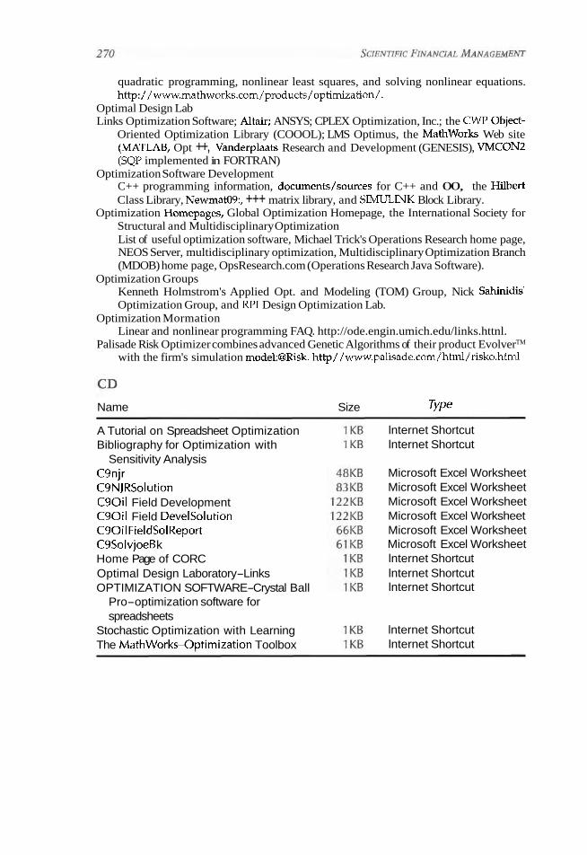
quadratic programming, nonlinear least squares, and solving nonlinear equations. http:/ /www.mathworks.com/products/optimization/.
Optimal Design Lab Links Optimization Software; Altair; ANSYS; CPLEX Optimization, Inc.; the CWP Object-
Oriented Optimization Library (COOOL); LMS Optimus, the Mathworks Web site (MATLAB, Opt ++, Vanderplaats Research and Development (GENESIS), VMCON2 (SQP implemented in FORTRAN)
Optimization Software Development C++ programming information, documents/sources for C++ and 00, the Hilbert Class Library, Newmat09:, +++ matrix library, and SIMULINK Block Library.
Optimization Homepages, Global Optimization Homepage, the International Society for Structural and Multidisciplinary Optimization List of useful optimization software, Michael Trick's Operations Research home page, NEOS Server, multidisciplinary optimization, Multidisciplinary Optimization Branch (MDOB) home page, OpsResearch.com (Operations Research Java Software).
Optimization Groups Kenneth Holmstrom's Applied Opt. and Modeling (TOM) Group, Nick Sahinidis' Optimization Group, and RPI Design Optimization Lab.
Optimization Mormation Linear and nonlinear programming FAQ. http://ode.engin.umich.edu/links.httnl.
Palisade Risk Optimizer combines advanced Genetic Algorithms of their product EvolverTM
with the firm's simulation mode1:QRisk. http/ /www.paliiade.com/html/risko.html
Name Size T Y P ~
A Tutorial on Spreadsheet Optimization Bibliography for Optimization with
Sensitivity Analysis C9njr C9NJRSolution C90il Field Development C90il Field DevelSolution C90ilFieldSolReport C9SolvjoeB k Home Page of CORC Optimal Design Laboratory-Links OPTIMIZATION SOFTWARE-Crystal Ball
Pro-optimization software for spreadsheets
Stochastic Optimization with Learning The Mathworks-Ootimization Toolbox
lnternet Shortcut lnternet Shortcut
Microsoft Excel Worksheet Microsoft Excel Worksheet Microsoft Excel Worksheet Microsoft Excel Worksheet Microsoft Excel Worksheet Microsoft Excel Worksheet lnternet Shortcut lnternet Shortcut lnternet Shortcut
lnternet Shortcut lnternet Shortcut

Risk Analysis of the Corporate
Entity and Operating Segments
COST OF CAPITAL INVOLVES TWO types of risk: systematic and unsystematic. Systematic risk is the risk of holding a market portfolio. Say that your firm's stock is one asset in an investor's portfolio. As the market moves, each individual asset comprising that portfolio is more or less affected. To the extent that your company's stock is affected by general market moves, the stock involves systematic risk. Specific risk is the risk that is unique to your firm, for example, the loss of a major contract, failure of an R&D effort, or the write-off of a large accounts receivable Unsystematic risk rep- resents the component of an asset's volatility that is uncorrelated with general market moves.
Unsystematic and systematic risk are not restricted to assets traded on financial markets. For example, when an insurance company sells home- owners insurance in a particular region, the insurer faces systematic risk from such risks as hurricanes or earthquakes. Such risks can impact many homes simultaneously The insurer also faces specific risk from risks such as fires or lightning strikes, which affect only individual homes. One of the benchmarks of stock market risk systematic risk is macroeconomic and industry risk.
The costs associated with both debt and equity financing are primar- ily a function of risk. Stakeholders require compensation in proportion to the risks they bear in financing. Additionally, the liquidity of the financing instrument (i.e., the relative ease of converting the instrument or assets underlying the instrument into cash) will also affect its cost. All else being equal, higher liquidity entails a lower cost of financing.
Identifying Systematic Risk
The Capital Asset Pricing Model
The Capital Asset Pricing Model (CAPM) and the more recent Arbitrage Pricing Theory help to estimate equity's required return (e.g., a firms cost of equity capital). The CAPM is associated with systematic risk. Essen- tially, the required return demanded by shareholders is equal to a risk-free return plus an additional risk premium to compensate the investor for market risk.
The riskiness of an asset portfolio, be it stock or alternatively a "bas- ket" of capital expansion projects, has direct implications for the required rate of return. Since investors generally hold portfolios of securities, it is reasonable to consider the riskiness of a security in terms of its contribu- tion to the riskiness of the portfolio rather than in terms of its riskiness if held in isolation.
The CAPM Equation
CAPM divides the risk of holding risky assets into systematic and specific risk. Systematic risk is the risk of holding the market portfolio. As the mar- ket moves, each individual asset is more or less affected. To the extent that any asset is affected by such general market moves, that asset entails sys- tematic risk. Specific risk is the risk that is unique to an individual asset. It represents the component of an asset's volatility that is uncorrelated with general market moves.
According to CAPM, the marketplace compensates investors for taking systematic risk but not for taking specific risk. This is because specific risk can be diversified away. When an investor holds the market portfolio, each individual asset in that portfolio entails specific risk, but through diversification, the investor's net exposure is just the system- atic risk of the market portfolio. (See "Perfect Portfolio Ltd example in Chapter 9.)
CAPM was first introduced by William Sharp in 1964. It extended Modern Portfolio Theory to introduce the notions of systematic and spe- cific risk. CAPM considers a simplified world where:
A There are no taxes or transaction costs. A All investors have identical investment horizons. A All investors have identical perceptions regarding the expected.
Returns, volatilities, and correlations of available risky investments.
In such a simple world, Tobin's superefficient portfolio (see Exhibit 10-1) must be the market portfolio. All investors will hold the market

Risk Analysis ofthe Corporate Entity and Operating Segments
Exhibit 10-1. The security market line.
R f Treasury bills
I j 0 0 1.5
market line
portfolio, leveraging or deleveraging it with positions in the risk-free asset. That is, in a competitive marketplace, risk premium investors require (Rj - Rf) in direct proportion to beta (P). This means that the investments that people make fall along a sloping line called the security market line (SML).
CAPM infers that the appropriate rate of return on a security is the sum of the rate available on a riskless investment plus a premium for risk actualized as a function of the investment's beta. For example, an invest- ment with a beta of .5 will generate half the expected risk premium, while investments having a beta of 2 will produce twice the expected risk pre- mium. In a two-investment world, the covariance of the returns that two securities generate is found. What we want to know is how two securities move with or against each other. If two securities move together, risk increases, as we realize quite quickly if we put two eggs in a basket and then drop the basket.
In the next section, "Corporate Analysis," we will develop a credit and bond rating working with an interactive computer model developed by the author.' The overall system is a linked matrix of 19 factors that combine to form a divisional risk grade (and bond rating). The model has a grading line of 1 to 10, whereby 1 is the best grade and 10 the worst. In certain cases, a grade of 10 will default the ov&rall grade to an unaccept- able 10.
In the section "Segment Analysis," the interactive model has been optimized to risk rate operating segments and/or divisions. The model incorporates S&P bond ratings into all the risk catagories from 1 through 10 and has been designed to be industry specific. However, S&P ratings are frequently updated and the one included are only examples. You can download updated ratings a subscription on basic from S&P or Moodys specific to your firm's operating segments and thus develop specific segment risk-rating worksheets for each of your operating divi- sions. ~ h e k a c r o s are included in the main model, and these can be eas- ily adapted.

Corporate Analysis
Introduction to Your Corporate Risk-Rating Interactive Model
Risk grading plays a leading role in the credit process of financial institu- tions. In this section, we will work through "rating" mirror image-the corporate perspective. The interactive risk-rating system-Corp- RiskModel.xls is designed to credit "rate" your firm so that you know how credit stakeholders-the suppliers of credit--decompose risk into its microcompoments. It is built across 10 points, from a triple A to a compa- rable D bond rating.
There are two major classifications of risk in any transaction. The first is risk associated with your firm as it looks at debt financing, and the sec- ond is risk associated with the structure of the deal that you plan to nego- tiate with credit suppliers, or the facility. Of the critical risk factors associ- ated with a transaction, the firm is the obligor; that is, obligor risk is centered on factors dealing with your firm's operating cash flows, debt capacity, asset/liability quality, valuation concerns, financial reporting, management, industry, economic and country risk factors, guarantees, and collateral. The collateral your firm offers may change its, say, relatively high expected default factors into low expected loss factors that can make or break a deal. For example, if your firm's expected default factor is 2% (2% Probability of default without collateral), putting up collateral that passes the risk-rating requirements, depending on the liquidity of the col- lateral, could reduce potential losses to near zero.
Facility risks are adjusted for factors such as your company's borrow- ing purpose, tenor of the credit facility, documentation, and portfolio risk includes such factors as how easily the credit can be sold or syndicated to investors. Your corporate risk score, combined with the financial institu- tion or investor' facility risk grade, forms the final risk grade.
The risk grade that is derived from this model will likely form the basis on which capital and loan provisions are calculated, developed, and assessed, allowing for the measurement of risk and reward standards via the debt stakeholder's risk-adjusted return on equity, return on assets, and - - other key firm ratios. These measurements serve as fundamental tools for pricing your deal as well as guides for resource allocation and active port-
*The corporate risk system was developed from an early prototype of a credit risk model I set up for a large international bank. The proprietary system that has since evolved at that bank has become a proficient tool to evaluate credit risk. Our corporate r isk system works well, but in a somewhat restricted environment. That said, the interactive corporate model included in the CD would never have been possible without the expertise and experience of credit officials at that institution. The author is deeply grateful to these outstanding professionals.

Risk Analysis of the Corporate Entity and Operating Segments 2 75
folio management and planning. By completing CorpRiskModel.xls, you will see how your financial institution, investment bank, or venture capi- talist breaks the firm's complex credit fabric into its most elemental parts and recasts them later in compelling logic.
Thus, the principles underlying the risk rating process are ongoing and involve, among other factors, the following:
A Initiating and maintaining your firm's obligor risk and facility risk ratings on a continuous basis
A Reviewing your firm's credit ratings by the financial institution's credit policy and credit audit areas to test for accuracy, consistency, and timeliness
A Combining with traditional policy in setting the company's rates and/or fees commensurate with your firm's risk level
A Determining the degree of lending officer service and monitoring your credit required
The Structure of a Credit Risk-Grading System
Debt rating represents a current assessment of the creditworthiness of an obligor with respect to specific obligations. These ratings may take into consideration obligors such as guarantors, issurers, or lessees. Ratings supplied by S&P or Moodys are usually based on likelihood of default, capacity and willingness to repay interest and principle payment, nature and provisions of the debt, protection afforded by the obligation in event of failure, and creditor rights in a reorganization. Default probabilities, as a measure, have evolved into a science. KMV ~www.kmv.com), a major player in measuring default risk, cites two critical ingredients to measure default probabilities: data and models. Models are the means by which data are transformed into expected default probabilities (EDF). Both default probabilities and bond rating are linked to credit grades as viewed in Table 10-1.
Risk definitions (Table 10-2) such as special mention, substandard assets, doubtful assets and loss assets are not left to financial institutions. Rather these definitions were issued by regulatory agencies including the Comp- troller of the Currency, the Federal Deposit Insurance Corporation, the Federal Reserve Board and the Office of Thrift Supervision.
System Overview: CorpRiskModel2
The model is a generic Industrial and Commercial Risk Grading work- sheet set up for corporate use. In the next section, you will learn to use a divisional/operating segment model. CorpRiskModel2 located in the Risk

Table 10-1. Comparing the credit grade to the bond rating and expected default frequency.
Credit EDF EDF EDF Grade Bond Rating Kev Words High Mean Low
AAA to AA- AA to A-
A+ to BBB+
BBB+ to BBB
EBB to BBB-
BBB- to BB-
World Class Organization 0.02 0.02 0.02 Excellent Access to Capital 0.13 0.02 0.02
Markets Cash Flow Trends Generally 0.27 0.06 0.03
Positive Leverage, Coverage Somewhat 0.87 0.1 6 0.08
Below Industry Average Lower-Tier Competitor;
Limited Access to Public Debt Markets
Narrow margins; Fully 0.52 0.24 Leveraged; Variable 2.65 Cash Flow
Cash Flow Vulnerable to 5.44 1.89 0.64 Downturns; Strained Liquidity; Poor Coverage
Special Mention (1) 19.06 2.89 2.85 Substandard (2) Doubtful (3)
Rating Subdirectory of the CD is a 10-point interactive system designed to provide maximum flexibility while maintaining ease of use. This is accom- plished in several ways. The workbook is menu driven, complete with interactive dialog boxes. There is no need to memorize commands. Simply select options from menus, click tabs at the bottom of the worksheets, or respond to dialogs that pop up on the screen. The system follows your work and points out errors.
Each section within the Industrial and Commercial Risk Grading interacts with other sections. Simply record the risk grade below each com- ponent. Cumulative grades are in most cases determined by the program. Readers are encouraged to "experiment" with the model but because this model is a highly sophisticated tool you should not expect to be proficient except after many trials.
Begin by doing the following:
1. Open the Risk Grading Workbook: CorpRiskModel.xls in the Risk Rating subdirectory of the CD.
2. A dialog box will appear. You can enter your name, the date, finan- cial institution, contact at financial institution, maximum exposure,

Risk Analysis of the Corporate Entity and Operating Segments 277
Table 10-2. Definitions of poor credit grades by the authorities.
Definitions issued Comptroller of the Currency by the Regulatory Federal Deposit insurance Corporation
Bodies as of Federal Reserve Board June 70, 1993 Office of lhrift Supervision
Special mention A special mention asset has potential weaknesses that deserve management's close attention. If left uncorrected, these potential weaknesses may result in deterioration of the repayment prospects for the asset or in the institution's credit position at some future date. Special mention assets are not adversely classified and do not expose an institution to sufficient risk to warrant
Doubtful assets
Loss assets
adverse classification. Substandard assets A substandard asset i s inadequately protected by the
current sound worth and paying capacity of the obligor or of the collateral pledged, if any. Assets so classified must have a well-defined weakness or weaknesses that jeopardize the liquidation of the debt. They are characterized by the distinct possibility that the firm will sustain some loss if the deficiencies are not corrected.
An asset classified doubtful has all the weaknesses inherent in one classified substandard with the added characteristic that the weaknesses make collection or liquidation in full, on the basis of currently existing facts, conditions, and values, highly questionable and improbable.
Assets classified loss are considered uncollectible and of such little value that their continuance as firmable assets is not warranted. This classification does not mean that the asset has absolutely no recovery or salvage value but rather that it is not practical or desirable to defer writing off this basically worthless asset even though partial recovery may be affected in the future.
a brief description o f the facility y o u are requesting, and the previ- ous credit grade. If guarantees o r collateral support the credit, check the box labeled Guarantees? and/or Collateral? If guarantees o r collateral are no t checked, they disappear f r om the system.
3. Select Risk I Obligor Financial Measures I Worksheet f r om the m a i n menu o r page the worksheet over. Complete the corporation's p r imary r isk measures labeled Modu le One--Your Firm's Pr imary Financial Measures.

Part 1: The Firm's Risk Rating
Section 1: Your Firm's Financial Measures (Worksheet: OPM1)
Exhibit 10-2 represents a sample page for reference. The model opens to S&P ratings linked to the manufacturing industry.
Exhibit 10-2A displays your firm's primary financial measures. These two pages are often most important in a risk rating system.
Included in Obligor financial measures, that are your firm's primary risk characteristics, are the following:
1. Operating cash flows 2. Debt capacity and financing flexibility 3. Asset quality 4. Valuation measures 5. Contingencies 6. Financial reporting 7. Management
Exhibit 10-2. f i e opening risk-rating worksheet and S&P ratio comparatives.

Risk Analysis of the Corporate Entity and Operating Segments 2 79
Exhibit 10-2A. Your firm's primary financial measures.
(continues)


Risk Analysis of the Corporate Entity and Operating Segments
Thii about the following:
Earnings and Operating Cash Flow 1. Are margins solid compared to the industry? 2. Are your firm's earnings stable, growing, &d of high quality? 3. Is cash flow magnitude sufficient to fund growth internally? 4. Is operating cash flow strong in relation to present and antici-
pated debt? 5. Is net cash flow from operations sufficient to cover most nondis-
cretionary outlays?
Debt Capacity and Financial Flexibility 1. Is leverage and coverage within the first quartile of your firm's
industry peer group? 2. What are your company's alternative sources of debt and equity
capital? 3. Does your firm have solid investment grade ratings? 4. Can your firm weather economic downturns? 5. Are debt maturities manageable? 6. Note: Since debt capacity is driven by cash flow, it would be
unusual for debt capacity/financing flexibility to get a better grade than cash flow.
Balance Sheet Quality and Structure 1. Are assets solid and fairly valued? 2. Does the liability structure match the asset structure? 3. Do assets show concentration of location or use? 4. Are liquidity margins narrow?
Valuation 1. Is there a healthy spread between the the firm's asset values, that is,
cash flow value (economic value) of assets (value of the corporate) and the market value of debt?
2. What is the spread between operating profit margin and the thresh- old margin? The threshold margin is the minimum profit margin required to increase shareholder value. See chapter 11.
3. Does your firm have hidden liabilities that may result in a sigrufi- cant erosion of shareholder value?
Contingencies 1. Are contingencies limited and easily controlled? 2. Is the potential impact on tangible new worth negligible? 3. Is the expected value of contingencies certain?
Financial Reporting and StrategiclBusiness Plans 1. Is an audit regularly completed by a reputable corporation? 2. Are your financial reports promptly issued to financial institutions? 3. Are financial statements accurate and complete? 4. Is your business plan accurate and complete? 5. Have you completed a valuation appraisal report? An valuation
appraisal template is included in chapter 11.
Management and Controls 1. Is management capable, now and for the foreseeable future? 2. Are strong operating and financial controls in place? 3. Does management have broad industry experience, good continu-
ity, and depth? 4. Is management tried and tested?
Guidelines for Completing the Worksheet: OFMI. First, examine each of the definitions corresponding to the columns (Grade, Bond Rating, and Expected Default Factor) and decide where your firm fits. Enter individual risk grades: Operating cash flows, debt capacity and financing flexibility, asset/liability quality, valuation measures, contingencies, and financial reporting and management (see Tables 10-3 and 104).
(Hint: You may want to unfreeze panes. Select Window, then click on Unfreeze Panes.)
Optional: Select Risk I Obligor Financial Measures I OFM Weights. Default numbers (or weights) provide a "weighted" OFM cumulative grade. You can accept or change weights that impact cumulative grades more in line with your credit. In any case, weights pertaining to operat- ing cash flows, debt capacity and financing flexibility, asset/liability quality, valuation measures, and management are not included in the boxes below. Table 10-5 a brief overview of the Obligor cumulative weighting system. This table is a sample cut-off. Readers may want to click in the formula cells to view the range of opportunities structured into the risk rating model. The following section illustrates how the weights work.
Using Weights to Determine the Firm's Cumulative Financial Risk Measures. Weights in the previous example (in columns) are set in default mode for illustration. However, you set the weights according to your percep- tion of the importance that each column has with repect to the other columns. The program brings together the previous categories that you examined and arrives at cumulative grade for each category. Weights are subjective. You are the firm's credit "expert," anticipating what your firm thinks about the firm's risk. You are, thus, in the best position to program the weights that promote the primary risk cumulative grades.

Risk Analysis of the Corporate Entity and Operating Segments 283
Table 10-3. Breakdown of category risk grade, cumulative risk grade, and option to accept or override preset cumulative grade weights: Obligor financial measure.
Operating Debt Capacity Asseff Cash and Financing Liability Valuation Flows Flexibility Quality Measures
Category risk grade 3 4 4 4 Cumulative risk grade 3 3.13 3.71 3.62 AccepWoverride
Table 10-4.
Contingencies Financial Reporting Management
Category risk grade 4 4 3 Cumulative risk grade 3.62 3.62 3.62 AccepWoverride 3.62 3.62
If your loan request is seasonal and you anticipate that the firm will look primarily to asset quality for repayment (with cash flow playing a minor role), you might weigh the cumulative grade (in column D) as, say, 2, 1, 7, 3.
Example 1: Assume that operating cash flow grade is 3, while debt capacity grade is 4. You feel that the default weights in column B (7 and 2) reflect the importance of cash flow to debt capacity since much of the firm's financing capacity is derived from cash flow. If weights are accepted, your firm's cumulative grade at this point is (7 * 3 ; 2 * 4)/ (7 + 3) = 2.9.
Example 2: Assume that operating cash flow grade is 2, debt capacity grade is 3, and asset/liability quality grade is 4. You argue that the default weights in column C (5,3, and 9) reflect the importance of operating cash flow and debt capacity to asset/liability. If weights are accepted, the cumu- lative grade is (5 + 2 + 3 * 3 + 9 *4)/(5 + 3 + 9) = 3.24.
Contingencies or Financial Reporting. These benchmarks are important to your firm. If unit grades fall below acceptable levels, the system assigns a cumulative Obligor grade equal to the grade assigned for that category. Contingencies or financial reporting grades of 5 or better usually have no impact on the cumulative grade; that is, contingencies and financial

Table 10-5. Identification of preset cumulative weights and formulas.
A B C D
Select or accept weights
Operating cash flows Debt capacity and
financing capacity Assetlliability quality Valuation Formulas: Cumulative
grade-weighted average
Operating Debt Capacity Cash Flows and Financing
Capacity 1 7
Asset Quality Valuation
5 3

Risk Analysis of the Corporate Entity and Operating Segments 285
reporting will never help a cumulative grade, but bad contingencies or financial reporting will hurt it. The following two boxes contain examples:
Contingencies Financial Reporting
Category risk grade (Cell N 106) 4 4
Cumulative risk grade = IF(N106>5,N106,~107) = IF(P106>5,10,N108) Acceptloverride =N107 =PI 07
The formula in the Contingencies box reads "If the category risk grade (cell N106) is worse than 5, let the cumulative risk grade default to the category Risk Grade. If the category Risk Grade is 5 or better, insert the cumulative risk grade into the Contingencies box." For example, in a worst-case sce- nario, if Contingencies were rated a 6, the cumulative grade would default to 6 (see Table 10-6).
The formula in the Financial Reporting box reads "If the category risk grade (cell P106) is worse than 5, let the cumulative risk grade default to 10. If the Category Risk Grade is 5 or better, insert the cumulative risk grade into the Financial Reporting box." For example, in a worst-case sce- nario, if Financial Reporting were rated a 6, the cumulative grade would default to 10:
Financial Re~ortinrr
Category risk grade (cell N106) 6 Cumulative risk grade 10 Accept/override 10
Table 10-6. Example of contingencies default classification.
Contingencies
Category risk grade (cell N106) 6 Cumulative risk grade 6 Acceptloverride 6
Contingencies
If you rate Contingencies 5 or better, the cumulative grade defaults to the previous (cumulative) grade, (3.62)
Category risk grade (cell N106) 4 Cumulative risk grade 3.62 +Acceptloverride 3.62

Note the Accept/Override row. You can decide on the weights and then protect them. Let's suppose that you allow one of your subordinates to complete the worksheet. Assume also that the worksheet accepted the default grade of 10 but your analyst felt that a 10 cumulative grade would be too harsh and entered a grade of 4 in the Accept/Override cell. The sys- tem will accept his or her decision, but a dialog will prompt for an expla- nation when data entry is verified:
Financial Reporting
Category risk grade (cell N106) 6 Cumulative risk grade 10 Acceptloverride 4
Subjective Measures Management depth is algorithmic (re: calculation of the cumulative grade). The default weighting, at 6 to 1, seems reasonable and sets management depth cumulative grade. Change the default weight if you disagree.
Example: The cumulative grade after you factor in financial report- ing is 4. The management depth grade is 6. You feel that the default rela- tionship (weight) of the cumulative grade to the management grade is 6 to 1. If you accept these weights, the cumulative grade is (6 * 4 + I* 6)/ (6 + 1) = 4.3.
Module 1: Your Firm's Primary Financial Measures, Short Examples
1. Your firm has good cash flow, but debt capacity is somewhat strained, and financial flexibility may be limited. You believe that a 5 credit grade is justified.
2. The cumulative grade was carried as a 4 before contingencies. The company has significant contingent liabilities of an uncertain nature such that an unfavorable event likely will occur before loan maturity. A substantial erosion of tangible net worth is likely. The program dropped cumulative grade to 7. You agree.
3. The firm operates near break even or has losses, financial reporting is poor (i.e., rating of 6 or 7 without qualification by a local accounting corporation whose reputation is &own, limited footnotes), and support is provided by soft comfort letter from Gennan parent. The computer dropped the cumulative grade to 10. You let the grade stand.
4. Let's suppose that your firm is engaged in medical therapy and was formed by the merger of three entities, is highly leveraged with modest or negative tangible net worth, and operates in a dynamic and growing industry (health care) where it is a major player (nurn- ber 1 or 2 in its market segments). As it consolidates its recent acqui- sitions, which creates economies of scale in terms of overhead and

Risk Analysis of the Corporate Entiv and Operating Segments 287
gives the entity a national presence, the company will generate suf- ficient profits and cash flow from volume increases (new patients) to offset lower prices dictated by managed care and pays back a recent term loan. The firm's revolver and subordinated debt will likely be refinanced. The company is publicly held and well regarded in the market, as is management, which you bet your last dollar is on the cutting edge. Suggest risk grade 4.
5. The firm has good profits and cash flow but limited financial flexi- bility because of high leverage. Stability of cash flows is helped by a contractual agreement with the former owner (a AAA credit). You believe that the terms go beyond the tenor that the firm will agree to. The facilities include an amortizing term loan and revolving credit with collateral (all assets) with a book value equal to out- standing at inception of the deal.
6. Let's suppose that you are proposing a 19-year lease transaction of a commercial jet with an exploding rate feature that is expected to be refinanced with 12 months by an equipment trust certificate. While there is no recourse to your firm, the plane is leased to one of the top two or three domestic carriers, giving you confidence in the cash flow-generating ability of the aircraft under lease. You feel strongly that a grade of 3 is appropriate for operating cash flow.
Section 2: Industry, Macroeconomic, and Environmental Risk
Included in this section are the following:
1. Industry segment 2. Position within industry 3. Macroeconomic and environmental factor 4. Country transfer risk
Industry Overview: An Analysis You are an expert in your industry. Indus- try analysis is crucial. You need to consider the impact that industry risk and peer position have on Obligor financial measures. Following is an extract of the 1994 Federal Reserve Loan Examination Manual dealing with the nuts and bolts of an industry audit. Your financing sources know this. You should also be familiar with these guidelines.
Federal Reserve Audit Guidelines'
A Attach an Standard Industrial Code (SIC) to every loan. A Define industry groups.
1. Source: Commercial Firm Examination Manual, Board of Governors, The Federal Reserve System, Division of Supervision and Regulation, December 1995.

A Assign a credit risk rating to every loan. A Distinguish between credit rating for firm versus credit rating for a
loan transaction.
Stages of Industry Analysis, Level 2: Analyze Industry Fundamentals
A Prepare industry studies for loan officers and for credit committees. A Evaluate credit risk exposure in relation to industry. A Identify firms, by industry. A Analyze individbal firm credits, by industry. A Perform comparative analysis of industries:
1. Analyze financial ratios. 2. Compare operating characteristics. 3. Understand financial and operating risks.
A Establish industry credit standards (loan structure, collateral cover- age, documentation requirements).
A Achieve functional independence but avoid isolation: 1. Remove responsibility for industry studies and analysis from the
loan officers. 2. Organize industry analysis under chief economist or senior
credit officer but preserve intelligence lines with lending personnel.
Stages of Industry Analysis, Level 3: Report Industry Concentrations
A Aggregate industry concentrations: 1. Use weighted average or percentiles of credit ratings aggregated
by industry. 2. Analyze risk of portfolio by industry.
A Establish an Industry Credit Policy Committee: 1. Review industry studies. 2. Analyze concentrations in relation to capital or loans. 3. Set loan limits. 4. Use for strategic planning purposes. 5. Identify growth industries and problem industries.
Stages of Industry Analysis, Level 4: Quantify Industry Risk
A Develop industry risk ratings for industry analysis. A Use an external model from an outside vendor. A Develop an internal model. A Use economic or industry data. A Use financial or bond market data as indicators of industry risk. A Compare industry risk ratings with the weighted average credit rat-
ing of the firm's exposure by industry.

Risk Analysis of the Corporate Entity and Operating Segments 289
A Run scenarios (commodity price changes, interest rate changes) to determine sensitivity of loan portfolio to outside shocks.
A Determine covariance of industries or interrelationships among industries.
Stages of Industry Analysis, Level 5: Incorporate Industry Analysis Into the Loan Portfolio
A Diversify the loan portfolio to reduce industry risk and industry concentrations.
A Distinguish between decision to originate loan and the decision to retain it for the portfolio.
A Use loan sales to reduce concentrations in the portfolio. A Sell loans to organized secondary markets. A Use industry risk systems:
1. To influence loan pricing. 2. To develop risk-adjusted rates of return measures. 3. To assign capital or loan loss reserves. 4. To conceptualize the loan portfolio like a securities portfolio.
Working with the Matrix: Industry and Economic/ Environmental Factors/Country Risk
First, Click on the INDUS tab or select Risk I Industry & Economic Measures I Worksheet. Review risk-rating definitions. Evaluate other industry risk factors listed here:
1. Does your firm operate in a strong and growing industry? 2. Is your firm a significant factor in the industry or market? 3. Are legal or regulatory climates favorable? 4. Is industry cyclically minimal? 5. Is the industry vulnerable to sudden economic or technological
change? 6. Is industry operating leverage modest? 7. Are labor problems minimal? 8. Is regulatory environment satisfactory? 9. Are long-term prospects favorable?
10. Does your firm rank in the first tier of the industry? 11. Is your firm's industry "focused," enjoying a meaningful market
share? 12. Are performance ratios generally better than industry peers?
You Should Also Consider Other Industry Factors:
1. Cyclicality 2. Seasonality

3. Regulatory Issues 4. Environmental Issues 5. Product Liability 6. Barriers to Entry 7. Technical Obsolescence 8. Commodity vs. Value Added 9. Manufacture vs. Service
10. Domestic reliance vs. International Sales Diversification 11. Government Contract Related Issues 12. Industry Life cycle
The system will calculate the "Correct" industry grade by combining your firm's industry grade with the firm's tier position. You simply enter a grade for the industry and a grade for your firm's industry tier position. The tier position listing is actually a quartile ranking. The first two grades, in the column titled Firm Rating, represents the top quartile, fol- lowed by the second, third, and fourth quartiles. For example, if you rate the industry 7 and industry position 5, the combined industry rating can be no better than 5. The firm's cumulative grade will default to the industy grade if the industry grade is worse than the firm's grade (see Exhibit 10-3).
Simply enter industry grade and industry position. The system takes these two numbers, completes the industry cumulative rating, and enters the rating on the 1ndustG worksheet.
Exhibit 10-3. Industry matrix.
I lndustry!Posilion Grid

Risk Analysis of the Corporate Entity and Operating Segments 291
Risk-grading factors range from dynamism and strength, political and social climate always supportive of business and industry, and unquestioned creditor rights to possible unfavorable movements, unfa- vorable creditor rights or legal environment, unsupportive political and social climate, poor creditor rights or legal environment, and unaccept- able risks.
Completing the Worksheet
Cell F H I
106 Category risk grade (worksheet) 4 7 3
107 Cumulative risk grade 3.62 3.62 7 5.33
108 AcceptIOverride 3.62 7 5.33 Risk Category Industry Position Macroeconomic and
segment within environmental industry factors
The formula driving the macroeconomic and environmental factors cumu- lative grade is = IFU106 > 6,J106,(7 " HI07 + R7 * J106)/(7 + R7)].
In plain English, the formula states that macroeconomic and environ- mental factors grades 1 to 5 leave no impact on the cumulative grade. Grades 6 or worse will have a negative impact on the cumulative grade. In addition, weight the cumulative grade to macroeconomic and environ- mental factors grade 7 to 1, that is, 7 times as important.
CountryITransfer Risk: An Analysis
Cross-Border Risks 1. What is country investment ranking? 2. What is the Interagency Country Exposure Review Committee
(ICERC) rating? 3. Has the ICERC rating improved or deteriorated over the past six
months? 4. What is the country's resource base in terms of natural resources,
human resources, and financial resources? 5. What is the outlook for domestic political stability? 6. What is the quality of economic and financial management? Does
the leadership have the political strength to implement decisions, particularly if they involve austerity measures?
7. What is the country's long-run development strategy? 8. Is industrial development based on efficiency or on support of pres-
tige projects or the economic interests of politically powerful groups?

9. Is economic growth financed largely by domestic revenues and savings or through foreign speculative investments?
10. Is inflation under control? 11. Are wage and price policies in line with productivity growth? 12. In looking at the outlook for the balance of payments, what is the
prognosis of current account, capital account, and debt service account improvements?
13. How are capital account deficits financed? World firm or bilateral aid programs? Firm loans?
Federal Reserve Audit Guidelines: Transfer (Country Risk)
Substandard
A A country is not complying with its external service obligations, as evidenced by arrears.
A The country is not in the process of adopting other suitable eco- nomic adjustment program.
A The country and its firm creditors have not negotiated a viable rescheduling and are unlikely to do so in the near future.
Value Impaired
A The country has not met rescheduling terms for over one year. A The country shows no definite prospects for an orderly restoration
of debt service in the near future.
Considerations
A Establish country exposure limits for credits. A Establish limits for distribution of loans by type and maturity. A Review concentrations of credit within countries. A Review international loan portfolio management objectives and
policies at least annually to determine whether they are compatible with changing market condition.
A Measure significant changes in country conditions and/or levels of exposure.
A Revised country limits in response to substantive changes in eco- nomic, political, and social conditions within particular countries.
A Reviewed country limits and updated at least annually. A Prior to granting additional advances or commitments, check out-
standings to appropriate country limits. A Lending officers cognizant of specific country limitations. A Clearly define procedures for exceeding country limits. A Have a periodic foreign call program for countries.

Risk Analysis of the Corporate Entity and Operating Segments 293
A Establish internal review system that determines that international risk assets outstanding and committed are within the firm's foreign exposure limits.
A Review country risk factors (economic, political, and social). A Obtain a continuing review of current country data obtained from
internal and external sources. A Analyze of economic, political, social, and other factors affecting
country risk. A Establish a formal reporting system on country risk. A Establish a country risk evaluation system recognizes exposure
from country to country on the basis of legally binding guarantees, collateral, or reallocation by office of responsibility.
A Establish reporting system that provides exposure data quickly and in sufficient detail to assess particular risks.
The formula driving the country transfer risk cumulative grade is = IF(LlO6 > 5,L106,107).
If the category risk grade is worse than 5, then the cumulative risk grade defaults to the category risk grade; otherwise, the macroeconomic and environmental factors cumulative grade carries over.
It follows that the performance of a firm cannot be isolated from the economic climate of the industry, or macroeconomic and country risk factors in which the major portion of its activities occurs. For this rea- son, these risk categories are essential in the evaluation of an obligor firm. Table 10-7, a cut from the respective page, summarizes perfor- mance in terms of (1) component or category risk grade, (2) cumulative risk grade with respect to (1) industry segment, (2) position within the industry, (3) macroeconomic and environmental factors, and (4) country or transfer risk.
Table 10-7. Industry, macroeconomic, and country risk summary.
Cell F H J 1
Row 106 Category risk grade (worksheet) 4 7 3 2
Row 107 Cumulative risk grade 3.62 3.62 7 5.33 5.33
Row 108 Accept/override 3.62 7 5.33 5.33
Risk Category Industry Position Macro- Country/ segment within economic and transfer
industry environmental risk factors
Section 3: Guarantees (Worksheet: GUAR3)
Guarantees: A n Analysis A guarantee is a written contract, agreement, or undertaking involving three parties. The first party, the guarantor, agrees to see that the performance of the second party, the guarantee, is fulfilled according to the terms of the contract, agreement, or undertaking. The third party is the creditor, or the party to benefit by the performance. For example, Party B makes a loan through his firm. The firm desires a guar- antor for this loan in case of default by B. B asks A to act a guarantor for his loan. A agrees and signs a guaranty agreement. A is the guarantor, B is the guarantee, and the firm is the creditor.
Note: For the purposes of a risk rating at Corporate, guarantees refer to third-party guarantees only; upstream guarantees of subsidiaries are not applicable, as are guarantees from principals.
The credit grade assigned to loans supported by third-party under- takings will lie somewhere between the firm rating and the guarantor rat- ing. Unconditional guarantees of payment will have considerably more impact than will a nonguarantees such as a comfort letter or "verbal assurance."
The Risk Grading Worksheet (GUAR3). Important Reminder: If the guaran- tee is less than loo%, you may want to complete a risk-rating form or check the bond rating for the guarantor before initiating this worksheet (remem- ber the bond rating will provide you with the expected default facto (EDF). Remember that if the l o k is not-supported by a guarantee, Excel removes the worksheet GUAR3.
For partial guarantees, GUAR3 generates a weighted risk rating. The weighted risk rating depends on prorate credit responsibility and the EDF for the obligor and guarantor (Table 10-8).
1. After you evaluate the guarantor (you may have to "guess" the risk rating from an implied bond rating or from another source), enter the Garantor's grade in the color-coded box: Enter Guarantor's Cumulative Grade. (Table 10-9)
2. The EDF obligor in basis points corresponds to the cumulative risk grade you determined thus far. You need to match the cumulative grade to the EDF and enter the EDF in the appropriate color coded box: Enter Expected Loss Factor Obligor in b.p. (Table 10-9)
3. Enter the Enter % Obligation: Obligator (Decimal) in the red coded box: Enter % Obligation: Obligator (Decimal). If, for example, the obligor is responsible for 98% of the obligation, 98% belongs to the obligor, and 2% belongs to the guarantor. (Table 10-9)
4. After completing a grading worksheet on the guarantor, enter the EDF in the correct red coded box: Enter Expected Default Factor Guarantor in b.pr. (Table 10-9)
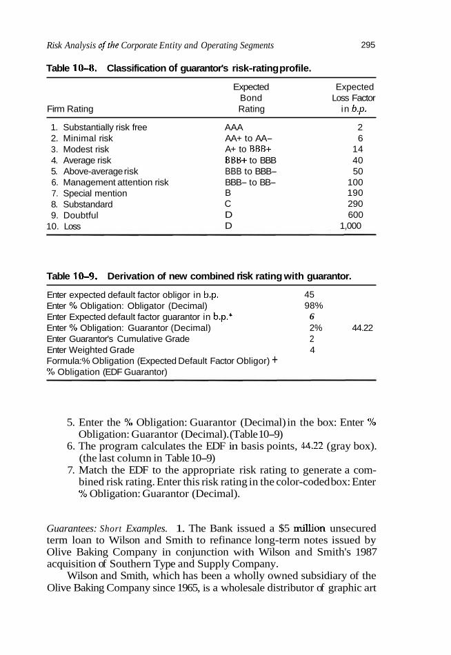
Risk Analysis ofthe Corporate Entity and Operating Segments 295
Table 10-8. Classification of guarantor's risk-rating profile.
Expected Expected Bond Loss Factor
Firm Rating Rating in b.p.
1. Substantially risk free AAA 2 2. Minimal risk AA+ to AA- 6 3. Modest risk A+ to BBB+ 14 4. Average risk BBB+ to BBB 40 5. Above-average risk BBB to BBB- 50 6. Management attention risk BBB- to BB- 100 7. Special mention B 190 8. Substandard C 290 9. Doubtful D 600
10. Loss D 1,000
Table 10-9. Derivation of new combined risk rating with guarantor.
Enter expected default factor obligor in b.p. 45 Enter % Obligation: Obligator (Decimal) 98% Enter Expected default factor guarantor in b.p.* 6 Enter % Obligation: Guarantor (Decimal) 2% 44.22 Enter Guarantor's Cumulative Grade 2 Enter Weighted Grade 4 Formula:% Obligation (Expected Default Factor Obligor) + % Obligation (EDF Guarantor)
5. Enter the % Obligation: Guarantor (Decimal) in the box: Enter % Obligation: Guarantor (Decimal). (Table 10-9)
6. The program calculates the EDF in basis points, 44.22 (gray box). (the last column in Table 10-9)
7. Match the EDF to the appropriate risk rating to generate a com- bined risk rating. Enter this risk rating in the color-coded box: Enter % Obligation: Guarantor (Decimal).
Guarantees: Short Examples. 1. The Bank issued a $5 million unsecured term loan to Wilson and Smith to refinance long-term notes issued by Olive Baking Company in conjunction with Wilson and Smith's 1987 acquisition of Southern Type and Supply Company.
Wilson and Smith, which has been a wholly owned subsidiary of the Olive Baking Company since 1965, is a wholesale distributor of graphic art

supplies, equipment, and chemicals to the printing industry. For year end 1993, Wilson and Smith contributed 4% of Olive's consolidated revenues and 22% of its net income. For the nine-month period ended 9/30/94, Wilson and Smith's sales increased 6.7% from the prior period to $98.9 million. The higher sales volume combined with consistent g&ss margins and continued control of operating expenses resulted in net income of $2.3 million compared to $1.4 million at 9/30/93. These trends are expected to continue given the company's emphasis on maintaining margins and improving profitability.
Olive Baking Company was incorporated in 1914 as a baking company . .
specializing in ~&~le-~or t ion pies, cakes, and cookies. Olive ~ d - son and Smith in 1965 for diversification vumoses. On a consolidated basis. total revenues and Net income for FY 1943 ;ere $246 million and $9.5 mil- lion, respectively. For the nine-month interim ended 9/30/94, consolidated revenues were $204 million, and net income was $7.4 million, up 5% and 9%, respectively, when compared to the similar period during FY 1993.
While both companies have performed consistently, Olive Baking remains the stronger of the two companies, on both a balance sheet and a profit-and-loss basis. On a consolidated basis, the company displays strong interest coverage, adequate debt service capacity, and a satisfactory leverage position. In addition, the $5 million unsecured term loan to Wil- son and Smith is guaranteed by Olive Baking Company. Historically, Olive has generated sufficient cash flow to meet current maturities and pay- ments of dividends. Cash flow from operations coupled with short-term borrowings are used to fund capital expenditures. Suggested firm rating, 5; suggested parent rating, 4; suggested risk rating, 4.
2. Company operates near break-even or has losses, financial report- ing is poor (i.e., rating of 6 or 7 without qualification by a local accounting corporation whose reputation is unknown, l i i t e d footnotes), and an unconditional guaranty is provided by a soft comfort letter from German parent. The computer dropped the cumulative grade to 10. However, the cumulative grade may improve when you evaluate guarantees.
Section 4: Loans Secured by Collateral (Worksheet: COLL4)
Loans Secured by Collateral: Issues and Analysis. Collateral is defined as property pledged as security for the satisfaction of a debt or other obliga- tion. The credit grade assigned to secured loans will depend on, among other things, the degree of coverage your firm offers its creditors, the eco- nomic life cycle of the collateral versus the term of the loan, possible con- straints of Liquidating the collateral, and of course, the bank's ability to skillfully and economically monitor and liquidate collateral. Evaluate the following:
1. What is its value compared to credit exposure? 2. What is its liquidity, or how quickly may its value be realized and
with what certainty?

Risk Analysis ofthe Corporate Entity and Operating Segments
3. Legal rights associated with the collateral?
Note: Collateral means tangible and intangible assets specifically pledged; it does not mean pledges of firms' stock or the pledge of stock of a sub- sidiary (domestic or foreign).
Federal Reserve Audit Guidelines: Collateral (with respect to the bank's position)
1. Is negotiable collateral held under joint custody? 2. Are receipts signed by the customer obtained and filed for released
collateral? 3. Are securities and commodities valued and margin requirements
reviewed at least monthly? 4. When the support rests on the cash surrender value of insurance
policies, is a periodic accounting received from the insurance com- pany and maintained with the policy?
5. Is a record maintained of entry to the collateral vault? 6. Are stock powers filed separately to bar negotiability and to deter
abstraction of both the security and the negotiating instrument? 7. Are securities out for transfer, exchange, and so on controlled by
prenumbered temporary vault-out tickets? 8. Has the bank instituted a system that
a. Ensures that security agreements are filed? b. Ensures that collateral mortgages are properly recorded? c. Ensures that title searches and property appraisals are per-
formed in connection with collateral mortgages? d. Ensures that insurance coverage (including loss payee clause) is
in effect on property covered by collateral mortgages? 9. Are acknowledgments received for pledged deposits held at other
banks? 10. Is an officer's approval necessary before collateral can be released
or substituted? 11. Does the bank have an internal review system that
a. Reexamines collateral items for negotiability and proper - assignment?
b. Checks values assigned to collateral when the loan is made and at frequent intervals thereafter?
c. Determines that items out on temporary vault-out tickets are authorized and have not been outstanding for an unreasonable length of time?
d. Determines that loan payments are promptly posted? 12. Are all notes assigned consecutive numbers and recorded on a note
register or sitnil& record? Do numbers on notes agree to those recorded on the register?

13. Are collection notices handled by someone not connected with loan processing?
14. In mortgage warehouse financing, does the firm hold the original mortgage note, trust deed, or other critical document, releasing only against payment?
15. Have standards been set for determining percentage advance to be made against acceptable receivables?
16. Are acceptable receivables defined? 17. Has the bank established minimum requirements for verification of
firm's accounts receivable and established minimum standards for documentation?
18. Have accounts receivable financing policies reviewed at least annu- ally to determine whether they are compatible with changing mar- ket conditions?
19. Have loan statements, delinquent accounts, collection requests, and past due notices been checked to the trial balances that are used in reconciling subsidiary records of accounts receivable financing loans with general ledger accounts?
20. Have inquiries about accounts receivable financing loan balances been received and investigated?
21. Is the bank in receipt of documents supporting recorded credit adjustments to loan accounts or accrued interest receivable accounts? Have these documents been checked or tested subsequently?
22. Are terms, dates, weights, description of merchandise, and so on shown on invoices, shipping documents, delivery receipts, and bills of lading? Are these documents scrutinized for differences?
23. Were payments from customers scrutinized for differences in invoice dates, numbers, terms, and so on?
24. Do bank records show, on a timely basis, a first lien on the assigned receivables?
25. Do loans granted on the security of the receivables also have an assignment of the inventory?
26. Does the bank verify the firm's accounts receivable or require inde- pendent verification on a periodic basis?
27. Does the bank require the firm to provide aged accounts receivable schedules on a periodic basis?
Completing the Collateral Worksheet (COLLA) At worse, collateral has no impact on the cumulative grade. Superior quality collateral will improve the cumulative grade by as many as four grade levels (see Exhibit 10-4).
Examples: Collateral 1. Glantz and Blake Corporation is a manufacturer of high-capacity disk drives. The firm receives a $15 million line of credit secured by accounts receivable, inventory, and equipment. The company has suffered substan-

Risk Analysis of the Corporate Entity and Operating Segments
Exhibit 1 0 4 . Collateral classification. MSSlFlCITlON I: WOMW UOUlD CIND REAMLY ITTA IWLE WUATERKmM DIFFEREN- SECURED WV
OTHER LESS UOUW ASSETS
SEcZmaY - - - W l G H E S T m U N T S RECENMLE O W / U O U I D * N O D N E W U E D f*G%-tZG% M G H E S T W M O F M Q ~ I L I Q U I D M D D N E R S I U E D 120%-150% FCEDPSSETS- PRlMEMD READILY -ABLE 14041.20GX REAL ESTAn-COMMERC19L WUATEWL EIS.ILY~~CCESSIBLE BY~~SSIWEES ORWK~UPINTS M n N G RIC%+mSON m U E R 4 L N O T m P J D E E D
- - - LEASEHOWIMP*-OMMEWS STOOCOF SUBSDWES W - T SmGK ON UNh SWEETS RECEWABLES. C Q N C E ~ M / d U E ~ N * B L E O W I N M m R V 0 3 N C E M R A T E O ~ U E G ~ O W L E O W R W ESTATE OUESnOWCE O C I I \ U I Y I N O M I * R r n M I W
tial losses over the last three years because of price reductions from its major competitors. The company is leveraged 2.5 times. Because of losses, extreme competition in the industry, and its leverage position, an obligor rating of 8 is warranted.
The firm's line, secured by high-quality and diversified accounts receivable (major corporations), equipment, and (high tech) inventory is on a controlled basis. Advances are made based on 70% of eligible down- stream receivables, 40% of foreign receivables, and 70% against the knock- down value of the equipment. Collections are controlled by lock box, and agings are received monthly with on-site audits at least three times a year. Turnover of receivables is 55 days. Due to advances being on a controlled basis, the quality of receivables a risk rating of 6 is warranted.
2. Subsidiary Securities is a regional broker/dealer that is a wholly owned subsidiary of Parent Mutual Life Insurance Company. Although Subsidiary Securities is a profitable, sound broker/dealer, the industry has shown signs of weakening. The firm receives a $10 million secured brokers line and a $5 million unsecured short-term line of credit.
Subsidiary is well capitalized and continues to maintain capital above SEC requirements. For the nine-month period ending 12/31/89, Sub- sidiary had excess net capital of $39 million. Net income for the nine- month period ending 12/31/94 totaled $11.7 million compared to $11.0 million in the prior period and $11.4 million for FYE 3/31/94. Rev- enues of $179 million are up 18% from the previous period.

Parent Mutual has over $4 billion in assets and carries an A+ rating from Best signifying solid financial condition. Additionally, Parent Mutual has the capacity to provide additional financial resources, if necessary. The facilities are short term in nature, and although unse- cured, our risk is minimized by the collateral that Subsidiary holds as a result of their strict margin requirements. Based on this, ratings are as follows:
Secured Line: Suggested Firm Rating 4 Suggested Risk Rating 3 Unsecured Line: Suggested Firm Rating 4 Suggested Risk Rating 4
3. Revolving credit to a U.S. subsidiary of a German company secured by borrowing base (75% receivables, 60% inventory). The bank relies on monthly borrowing base reports from the company. While the firm makes money, its financial flexibility is limited by modest debt capacity, and ulti- mate repayment lies in the ability of the German parent to provide financ- ing. You suggest a -1 improvement in the grade.
4. Loan secured by marketable fixed-income securities where the firm is unprofitable on a GAAP basis and where the bulk of assets besides the securities portfolio consists of undeveloped land in a fast-growing area of the United States with a market value considered well in excess of book value.
Part 2: Facility Risk Rating
Section 1: Purpose (Worksheet: PURPOSS)
Note: Facility risk rating should hold no surprises. Downgrades to the obligor risk rating will be the exception, not the rule. However, your firm might suffer a downgrade if the facility calls for unusual tenor, if docu- mentation is weak, if the loan's marketability has deteriorated, or if the purpose of the loan is inappropriate. So, be cautious and as watchful as you were completing the obligor section, your creditor certainly will be. Following are criteria to evaluate the purpose of the facility (Exhibit 10-5).
Section 2: Documentation (Worksheet: DOCUM6)
Example Unsecured loan to Latin American blue chip company to bridge capital markets transaction with repayment expected in 60 to 180 days. Financials are unaudited and provided from prospectus with information somewhat dated and incomplete. Documentation is satisfactory but lacks meaningful covenants. You decide -1 grade improvement is justified reflecting the short loan duration, (see Exhibit 104).

Risk Analysis of the Corporate Entity and Operating Segments 301
Exhibit 10-5. Facility grade, purpose of proposed facility.
FACIUW IS APPROPRIATE FOR BUSINESS MATCH FUNDING APPROWTE
FINANCING STR4TEGY NOTAPPROFRATE FOR OBLIGOR + 1 OBUGOR BORROWING SHORTTERM TO FINANCE CAPITAL REQUIREMENTS FAMUTY USED TO FINANCE EXCESSIVE DWIDENDS
UNSECURED FAClLrrY WHILE OTHER LENDERS HAVE M E BEST COLLATERAL BHF IS SUBORDINATED LENDER + 2
POOR LOAN SlRUCTCIRE
Section 3: Tenor (Worksheet: TENOR7)
Unusual Terms, Tenor, and Subordinated Position. From time to time and for various reasons, a bank may extend credit on terms or for a tenor that for a given firm subjects the firm to a greater level of risk than indicated by the obligor rating. The incremental risk should be reflected in a higher risk rating.
For example, an unsecured line of credit to a company with an obligor rating of 4 would not usually warrant a change in risk rating (the grade may actually improve in some cases with maturities under one year). However, a term loan of longer-than-usual tenor or with a bullet maturity or a weak loan agreement may warrant a 5 or worse credit risk rating.
Generally, term loans that amortize with equal installments up to three years leave the grade unchanged. Bullet and balloon term loans of the same tenor might be one grade worse, (see Exhibits 10-7 and 10-8).

302 SCIENTIPIC FINANCIAL MANAGEMENT
Exhibit 10-6. Facility grade, documentation matrix.
DOCUMENTATION CONFORMSTO NORMALLEGALSTANDAWS.
DOCUMEKTATION CLEARLY DOES NOTCONFORMTO NORMAL STANDARDS FROM *3 TO+ B
Exhibit 10-7. Facility grade, tenor matrix.
Section 4: Portfolio (Worksheet: PORTFOLI08)
The Summary Page. The summary page brings together the entire corpo- rate risk-rating system on one page. The summary page includes (1) matrix of each risk component and respective cumulative grade, change in c u m mulative grade, and unit grade; (2) table with corporate grade, corporate/ facility grade, and previous grade attached; (3) corporation's financial mea- sure cummulative grade weights; and (4) guarantor's matrix; chart dis- playing unit grades and cummulative grades, (see Exhibit 10-9).

Risk Analysis of the Corporate Entity and Operating Segments 303
Exhibit 10-8. Facility grade, portfolio matrix.
FACILITY HAS A NEUTRAL EFFECT ON BHPS WRTFOUO
FAClLlTYPROVIDES ADEQUATE OPPORTUNITIES INTHE SECONDARY MARKET
NONE
FACILITY HASA NEUTRLIL OR POSlliVE EFFECT ON BHPS PORTFOLIO FROMOTO-2 I FAClLlTY PROVlDES EXCEUENTOFPORTUNITIES IN THE SECONDARY LOAN MARKET
FACllN SlGNFlWNnY INCREASES WRTFOUO'S W O S U R E TO SYSTEMAnCRlSK
FACILITY REPRESENTSAN ILLIQUID ASSETPROVIDING FEW OPPORTUNITIES INTHE SECONDARY LOAN MsrRKEl
OBLIGOR AND FACILITY GRADE I 4 I
Corporate Segment Analysis
Systematic Risk: Pure Play Approach
You will need to find the cost of equity for a division or private company when the stock is not publically traded and thus not observable. The cost of equity is often the largest cost-of-capital component.
The first step involves finding a benchmark publicly traded company that produces a homogeneous or similar product or service. That is how the name "pure play" came to be: In a sense they are "pure plays," com- peting in an identical line of business. The next step is to use the stock returns to detemine the beta of each pure play firm. Finally, use these market-determined betas to estimate the beta of your division.
Data on Comparative Publicly Traded Companies
In selecting corporations for comparative purposes, you should be careful to use only comparable companies. Although the only restrictive require- ment as to comparable corporations specified in the statute is that their Lines of business be the same or similar, it is obvious that consideration

Exhibit 10-9. Risk rating summary page.
mmav Credit Grader
w s m iM OUi~mna&lm.ru.c [a -- 6 0 1.0 6.0 7.0 6 0
5.8 10261 5 0 5.2 ID.521 3.0 5 3 Dm 6 0 5.2 moo 2.0 63 LW 2 0 5 1 am t o 5.3 OOU 2 0 5 1 am 2 0 ElprredatauirFacorOauplkbp 8D I? t o o 20 a w g * a n ; o a s a t w m * 1 7m( I 2 LOB I 0 mpemPdOdl"llF.ol.rGu~aM~hk U
must be given to other relevant factors in order to obtain the most valid comparison possible.
For illustration, a corporation having one or more issues of preferred stock, bonds, or debentures in addition to its common stock should not be considered directly comparable to one having only common stock out- standing. In like manner, a company with a declining business and decreasing markets is not comparable to one with a record of current progress and market expansion.
Once you have selected the right comparatives, compile a list of the firms. Derive the following median beta and standard deviation. Then select one or two "true" benchmarks or the absolute best fit.
The pure play approach involves unlevering the homogeneous public firm's beta. This approach is very effective since unsystematic risk is "stripped away," leaving a beta benchmark of systematic risk. Next, gather research on the target firm's debt, equity, and tax rate. Finally, relever betas based on your division's capital structure and tax rate. The resulting beta

Risk Analysis of the Corporate Entity and Operating Segments 305
approximates the business unit's beta if it, were publically traded. Insert- ing the new beta back into the CAPM yields the divisions cost of equity.
Examples of Pine Play Formulas
P, = P L
11 + (1 - t)D/E$a,,,l
(Formula for unlevered beta)
P, = P,[1+ (1 - t)D/EDimSi0"
(Formula for relevered beta)
pu = The unlevered equity beta
p, = The levered equity beta
t = The corporate tax rate
D/E = The debt to equity ratio
Example: Assume that your comparative public company's beta is 1.10, D/E of the comparative is .6, t = .35, and D/E of division is .3.
Insert this result back into the CAPM to arrive at the cost of equity.
Unsystematic Risk: Divisional or Operating Segment Risk Rating
The cost of equity was handled by the pure play approach. Now we address the cost of debt for divisions and/or operating segments employ- ing risk rating. Divisional, or operating segment, risk rating should be a key part of corporate strategy. The divisional risk rating (or grading) sys- tem, like the corporate system, is an interactive process based on a 10-point review. However, before we start, let's examine why the need for segmen- tal information is important on two counts: corporate headquarters and from an investor's perspective:
A The size and relative importance of diversified companies pre- sented many problems for your company's investors.
A Both size and uncertainty of future cash flows affected by industries and countries that a operating segment operates in.
A Different industries and different countries have various profit potentials, degrees and types of risk, and growth opportunities.

A Different rates of return on investment and different capital needs are also likely to occur across the various segments of a business.
A Because of this diversification of operations, there is a demand for key segment information, especially systematic (macroeconomic) and unsystematic (divisional-specific) risk, turnover, and profits.
A Segmental data is typically provided for both geographical areas and lines of business.
A Segmental information allows you, the decision maker, to combine operating segment-specific information with external information with a more accurate assessment of both risk and potential for future growth.
You should examine business units with respect to the following:
A Default rate of its industry. A Spread over the base (government rate). As a proxy to default risk. A Hurdle rate of division (i.e., cost of capital). Whiie for most diversi-
fied companies such external yardsticks are not available, a com- prehensive risk-rating system can value the entity on a stand-alone- basis. Senior management and board of directors will usually ask for segment information to allow comparison of success of individ- ual segments with those of other companies.
A Problems are apparent, particularly with transfer pricing. A Segment data may be important with employees, creditors, and host
governments. For example, employees will also want information at the plant level, host governments at the individual country level, and creditors at the level of the individual subsidiary or legal entity.
Ruling of ISB, Analysis of Segmental Information: IAS 14; (1.1.83), requires a breakdown of segmental information meaning, analysis of trends, cost of investments, and obtaining information on international competitive mar- kets and producers. Your firm's creditor's will likely evaluate these points. They will at least consider them.
A The size and relative importance of diversified companies pre- sented many problems f o ~ the users of accounts.
A Financial executives are interested in the future cash flows they may obtain from investing in a operating segment and the risk or uncertainty of those cash flows.
A Both size and uncertainty of future cash flows are affected by indus- tries and countries that an operating segment operates in.
A Different industries and different countries have various profit potentials, degrees and types of risk, and growth opportunities.
Furthermore:
A Different rates of return on investment and different capital needs are also likely to occur across the various segments of a business.

Risk Analysis of the Corporate Entity and Operating Segments 307
A Because of diversification of operations, there is a demand for key segment information, especially turnover and profits.
A Segmental data is typically provided for both geographical areas and lines of business.
A Segmental information allows financial executives to combine operat- ing segment-specific information with external information with a more accurate assessment of both risk and potential for future growth.
A Compare segments to (1) benchmarks in other industries, (2) default rate of industry, (3) spread over the base (government rate), and (4) hurdle rate of division (i.e., cost of capital).
Problem: For most diversified companies, such external yardsticks are not available; thus, a risk rating is important. Also, segment data may be important with employees, creditors, and host govenunents. For example, employees will also want information at the plant level, host governments at the individual country level, and creditors at the level of the individual subsidiary or legal entity.
valuations -often involve multibusiness companies whose futures depend on successful management of the portfolio of business operations they are charged with. Segment multibusiness valuation is also useful for determining breakup value and assessing acquisition candidates. In gen- eral, the structure of a business unit analysis should be well planned and comprehensive. You should do the follo&ng:
1. Find "as is" discounted cash flow and compare this to current mar- ket value. The difference between the two represents the percep- tions or value gap.]
2. Try to close negative perceptions by internal improvements with increased operating margins, improved sales growth, and decreased working capital requirements and by selecting capital projects to achieve optimal results (and that means using real options).
3. Try to close negative perceptions by external improvements by shrinking the business or working out sell-offs, spin-offs, equity carve-outs, or acquisitions.
Valuing a multibusiness operating segment "as is" is the same as valuing a single business operating segment. Differences often exist in capital structure, cost of capital cash flows, and headquarters costs. Tom Copeland a partner of McKinsey & Co suggests2:
1. Break business units into its smallest components. 2. Try to allocate cash flows to business unit. 3. Select as many comparable companies as possible.
1 Tom Copeland, Tim Koller, Jack Murrin, Valuation: Measuring and Managing the Value of Companies, John Wiley & Sons, Inc. 1994. 2. IBID

308 SCIENTIFIC FINANCIAL MANAGEMENT
4. Use ratios (asset turnover ratios and so on) on comparable companies. 5. Use internal data and compare it with publicly available data on
comparable operating units. 6. Perform business unit valuations. 7. Identdy business unit cash flows. 8. Watch transfer pricing and taxation. 9. Allocate corporate overhead as accurately as possible.
10. Determine business unit tax rates and capital structure and cost of capital.
11. The capital structure of business unit should be consistent with comparable companies.
12. Develop bond ratings. 13. Debt-to-equity ratios vary from industry to industry. 14. Ensure that the capital structure reflects market rather than book
values. 15. Pay close attention to the cost of equity. It is often the capital struc-
ture's largest component.
A Dynamic Business Unit (Divisional) Analysis
Open SegmentRiskModel2.s. The model follows the same pattern as the corporate risk-rating model.
Chapter Ten References and Selected Readings
Books
R. A. Crowell. (1967). Earnings expectations, security valuation, and the cost ofequity capital. Duvigneau, J. C., and R. N. Prasad. (1984). Guidelines for calculating financial and economic
rates of returnfor DFC projects. Washington, D.C.: World Bank. Eisenbeis, R. A. (1978). Problems in applying discriminant analysis in credit scoring models.
Washington, D.C.: Board of Governors of the Federal Reserve System. Fortune, P. (1995). Debt capacity, tax exemption, and the municipal cost of capital: A reassessment
o f fhe new vim. Boston: Federal Reserve Bank of Boston. Hawkins, D. E, et al. (1983). Rating industrial bonds. Morristown, N.J.: Financial Executives
Research Foundation. Hutchison, G. S. (1971). The strategy of corporatefinancing New York: Presidents Publishing
House. Moon, C.-G., et al. (1991). Municipal bond ratingannlysis: Sample selectivity and simultaneous equa-
tions bias. Piscataway N.J.: Center for Urban Policy Research, Rutgers the State University. Portney, P. R., and J. I? Weyant. (1999). Discounting and intergenerational equity. Washington,
D.C.: Resources for the Future. Riahi-Belkaoui, A. (1983). Industrial bonds and the rating process. Westport, Conn.: Quorum
Books. Stulz, R. M., and National Bureau of Economic Research. (1999). Globalization of equity
markets and the cost of capital. Cambridge, Mass.: National Bureau of Economic Research.

Risk Analysis of the Corporate Entity and Operating Segments 309
Thomas, L. C., and Institute of Mathematics and Its Applications. (1992). Credit scoring and credit control: Based on the proceedings of a conference on credit scoring and credit control, organized by the Institute of Mathematics and its applications and held at the University of Edinburg in August 1989. Oxford: Oxford Universtiy Press.
Twentieth Century Fund, Task Force on Municipal Bond Credit Ratings, and J. E. Petersen. (1974). The rating game: Report. New York: Twentieth Century Fund.
Periodicals
Asarnow, Elliot. (1994/95). "Measuring the hidden risks in corporate loans." Commercial Lending Revimu, 10(1), 24.
Fons, Jerome S. (1994). "Using default rates to model the term shucture of credit risk'' Financial Analysts lournal, 50(5), 25.
Hoffman, Thomas. (1999). "Neural nets spot credit risks." Computerworld, 33(30), 38. Hyndman, Carl. (1994/95). "Are bank regulators ready for credit scoring of commercial
loans?" Commercial Lending Review, 10(1), 92. Hyndman, Carl R. (1996/97). "Internal models for measuring credit risks: Their impact on
capital needs." Commercial Lending Review, 12(1), 58. Laitinen, Erkki K. (1999). "Predicting a corporate credit analyst's risk estimate by logistic
and linear models." International Review of Financial Analysis, 8(2), 97. Lee, Peter. (1993). "Citi rates options on credit risk." Euromoney, June, p. 6. Marshall, Jeffrey. (1999). "Credit risk ratings examined." USBanker, 109(3), 12. Pedrosa, Monica. (1998). "Systematic risk in corporate bond credit spreads." Journal of Fixed
Income, 8(3), 7. Raiti, Lisa. (1993). "Rating enhanced derivative products companies." Financial Regulation
Report, March, p. 5. Treacy, William F. (1998). "Credit risk rating at large U.S. banks." Federal Resewe Bulletin,
84(11), 89. Whiteman, Louis. (1998). "Small banks say one-on-one beats credit scoring models." Amer-
ican Banker, October 8, p. 13. Zhai, Huaming. (1999). "Stochastic modelling and prediction of contractor default risk."
Construction Management and Economics, 17(5), 563.
Select Internet Library
The Alcar Group Inc. System Solutions: Debt Rater Plus combines market information with data analysis tools to give users the ability to estimate S&P debt ratings and how they might change under different financing and operating strategies. Users are also able to price loans and estimate the cost of debt for a company or division. Operating either as a stand- alone service or as a menu option with Alcar's software solution, the package allows users to estimate S&F bond ratings on the basis of common financial and industry inputs. http://www.alcatnet/index.htrnl.
The Alcar Group Inc. System Solutions: APT!Aost of Capital Calculator APT! helps users estimate the cost of capital. It combines a cost-of-capital-related database of over 6,000 companies with data analysis tools to provide users with a comprehensive approach to cost of capital estimation, peer group performance measurement, and capital structure analysis. The Capital Asset Pricing Model (CAPM) and Arbitrage Pricing Theory estimate the cost of equity from the database and correct the anomalies associated

with CAPM. The software provides users the ability to estimate the cost of debt by using cost-of-debt estimates for public companies in the database. The system can use readily available accounting and industry information to estimate S&P debt rat- ings and the cost of debt and can determine how they might change under different financing and operating strategies. APT! allows users to judge individual company, peer group, or industry performance by analyzing stock market returns over the previous quarter, year, and five years. It helps users identify appropriate capital structures by identifying industry and peer group average capital structures and predicting how bond ratings might change with capital structure. http:/ /www.alcatnet/index.html.
Name Size Type
CorpRiskModel2 634KB Microsoft Excel Worksheet Ratio98 249KB Microsoft Excel Worksheet SegmentRiskModel2 356KB Microsoft Excel Worksheet

A Primer on Shareholder Value
THE ESSENCE OF STRATEGY FORMLnAnON is to organize the combined disciplines of risk and valuation and to guide the corporation into a new and better future. The key to effective strategic planning, then, has to deal with two rel- evant dimensions: (1) responding to changes in the external environment and (2) creatively deploying internal resources to improve the competitive position of the firm.' The lack of alertness to changes dealing with measur- ing and implementing economic, competitive, technological and financial factors can become extremely detrimental for sustained growth and prof- itability. The key to success is to be able to quantify these factors and inte- grate them into corporate and shareholder valuation, strategic planning, and formulation. Most important, a technical planning process must be respon- sive to individual talents and capabilities that reside within the corporation.
Thus, the exponential growth of analytics interfacing with modern- day disciplines-simulation, stochastic optimization, and visual model- ing, to name a few-has dramatically shifted the corporate culture and promises to raise individual capabilities to new heights.
Indeed, as I have inferred throughout this book, valuations are blue- prints for long-term planning; short-term "chaotic" events, such as today's stock price, have a random component and are often only loosely tied to intrinsic value. And to think that not long ago, we looked stock price up in the Wall Street Journal, multiplied it by the number of shares outstanding, and sent the number to the boss-a corporate lamb going to slaughter.
Management may be under sigruficant pressure to deliver earnings to stockholders whether or not these short-term numbers support it. To make
1. Amoldo C. Hax, professor of management, Sloan School of Management, MIT.

matters worse, elasticity between earnings and stock prices has never been more pronounced. Some companies are playing an earnings game simply to jump the stock price. Only later does the truth surface, and by then, investors have shifted interest. With so much executive compensation tied to options, the power of the so-called positive spin (on stock prices) has never been more widespread. A common tactic for the less forthright is to publicize one set of results in a quarterly news release but then file a dif- ferent, usually less positive, earnings report with regulators weeks later. Another maneuver from those managers incapable of delivering on the promise of long-term maximization of shareholder value is vagueness. News releases boast blockbuster results, leaving investors unsure about what contributed to the big gains-until quarterly statements are filed.2
We leave chaos to the markets and return to intrinsic valuations that relate to the natural harmonic structure of the firm, its growth potential, and, on a technical note, the measure of its value drivers. Technology and financial management are sides of the same coin.
Methods
Most of us recognize that corporate value is a function of the firm's future cash flow potential and the risks (threats) of those future cash flows. It is these perceived risks or threats that help define the discounting factor used to measure cash flows in present value terms. Cash flow depends on the industry and the economic outlook for the business' products, current and future competition, sustainable competitive advantage, projected changes in demand, and the business' capacity to grow in light of its past financial and operational performance. Risk factors include the business' financial condition (the threat to profitability and cash flows, the magni- tude of financial and operational leverage, and ability to pay debt), man- agement's ability to sustain operations and profitability, market and indus- try trends and outlook, competitive forces, the economic environment, legal and regulatory issues, and contingent liabilities.
Indeed, shareholder value is about data, and plenty of it. Cash flow forecasts and risk assessment require more than in-depth research and good old-fashioned intuition and creativity; it calls for a special kind of due diligence-one that employs technology, structure, and purpose. It means actualizing value drivers with all the tools: from neural network and visual modeling on up. However, remember that no software replaces sound financial judgment or experienceit is not the wand but the magician.
With few exceptions, we no longer question whether math and statis- tics have any bottom-line impact on measuring performance. The fact remains that data gathering in areas such as productivity, consumer value,
2. Reported in the N m York Times, December 21,1999

A Primer on Shareholder Value 313
and business and financial performance are no longer viewed so much as extraneous overload. Rather, it has become a question of what data are being mined, what technology is capturing that mining, and what valua- tion model brings this all together. The scientific method is as much a part of valuation as it is in NASA exploration designs.
Yes, I suppose that traditional methods are indispensable to a com- plete story, but composite weighting (of valuation methods) has shifted away from earnings-based measures to discounted cash flow, fortified by a quantitative value driver analysis. Let's examine the different valuation methods in use today--some good, some not so good.
Valuation Methods
Book Values Reflect the Past
Book values, based on accounting numbers, reflect historical costs yielding only a vague approximation of real economic value. Moreover, book val- ues are affected by decisions made by management regarding depreciation and amortization rates, the capitalization or expensing of certain costs, and perceived asset impairment. These choices, and more, are made by man- agement in order to present the firm in the most favorable light. Say that a firm purchases a truck and after depreciating it over a period of time records it with a zero book value. If the truck is sold, chances are that the company will receive greater than zero for the truck as long as the truck can still operate. Thus, there is often little relationship between book and market values. Book value also ignores price fluctuations of real assets, such as real estate or timberland, as well as intangibles, such as goodwill, trademarks, franchise licenses, and patents, which can be strong cash providers.
Transaction Multiples
The fair market value of public companies are determined every day through the decisions made by many buyers and sellers of their publicly traded secu- rities. These minority interest values can easily be determined and can be adjusted for control premiums. Since there are generally several public com- panies that are similar to any given private company, the fair market value of comparable companies can generally be compared to private companies.
Comparable public companies often are different in size and perfor- mance to a target private company; it is generally necessary to compare a comparable company's fair market value to some performance measure, such as revenue, cash flow, or assets. This comparison generally results in a multiple that can then be applied to the same performance measure of the private company to derive the fair market value of the private company.
A firm whose equity has recently been sold in a market priced trans- action often provides a fairly good measure of minority interest value. If

the company is similar to a private company, performance indicators of the recently sold firm can be compared to the private company to estimate a "pro forma" market value along with an added premium for control.
The problem with transactions multiples is often the difficulty of locating comparable companies. Even firms listed in identical standard industrial code (SIC) classifications operate with opposing product lines or are diversified to some degree or other that can easily distort the picture. PricewaterhouseCoopers suggests that the value of using transaction mul- tiples is only as good as the comparability of the companies from which the analysis is based. The higher the degree of correlation between the operations in the peer group and our company, the more accurate the analysis. Some of the more significant attributes used to determine com- parability include the f~llowing:~
1. Type of product produced 2. Market segment to which the product is sold 3. Geographic area of operation 4. Positioning in marketplace 5. Influence of buyers/suppliers 6. Growth, historical and projected 7. Profitability 8. Leverage and liquidity 9. Diversification
Once the peer group has been identified, the companies should be adjusted to allow for comparability. Some of the more important adjust- ments include the f~llowing:~
A Extraordinary and nonrecurring items inventory policy: FIFO ver- sus LIFO
A Revenue recognition policy A Nonoperating assets A Excess marketable securities and cash A Contingent liabilities A Pension and other postemployrnent benefits funding and expense
policy
The price-to-earnings (P/E) ratio takes the stock price and divides it by the last four quarters' worth of earnings. For example, if a firm was trading at $10 a share, and $1.00 in trailing earnings per share, P/E is 15X:
3. PricewaterhouseCoopers Business Acquisitions and Leveraged Buyouts: Solutions for Busi- ness a 1993 publication for distribution to clients.

A Primer on Shareholder Vahe
$15 share price/$1.00 training EPS = 15 P/E
What must be remembered when using a P/E ratio is that a market "price" for a stock is based on expectations of the future performance, whereas earnings are a historical record of where the firm has been and how it per- formed. There are many permutations of P/Es using forecasted or trailing 12-month earnings. Another difficulty arises when using comparable P/Es for valuation a particular market sector may be temporarily mis- priced by overly optimistic or pessimistic investors thus skewing your val- uation estimates accordingly.
Firms may report low earnings yet produce impressive values because they are involved in research and product development or are recent entrants in high-growth industries. For valuation purposes, you can also consider the average industry P/E ratio to benchmark as long as the comparatives are homogeneous. Remember that earnings can be legally manipulated by changing accounting practices or manipulated to distort the truth. Earnings also disregard risk. Here is a case in point:5 I.D.T., a telecommunications services provider in Hackensack, New Jersey, put out a news release on October 14 "b~osting"~ about its "record" fourth-quarter revenues and those for the full year ended July 31, 1999. The stock rose 3.6% on the news. When I.D.T. filed its SEC report on November 4, several of the company's expenses were greater than they had been in the earnings news release. As a result, the company reported a much greater loss. While the company's news release said that it lost 15 cents a share in the fourth quarter, the SEC filings indicated a loss of 18 cents a share.
The firm said that an error was found in figures supplied by a sub- sidiary and was not intentional. Everyone can make a mistake, of course, but investors suspect that some errors may not be inadvertent. Accord- ingly, the SEC's accounting watchdog countered by suggesting (in the arti- cle) that investors should be far more skeptical about news releases. Cor- porate earnings releases have become such a good source of misinformation that SEC researchers use them to identify companies that may be playing accounting games.
The price-to-sales ratio takes the current market capitalization of a com- pany and divides it by the last 12 months of trailing revenues. The market capitalization is the current market value of a company, arrived at by mul- tiplying the current share price times the shares outstanding. This is the current price at which the market is valuing the company.
5. Reported in the N m York Times, December 20,1999. 6. New York Times reporter's word.

Liquidation Valuation Approach
Management's decision to divest a business unit can often be quantified by the spreads between cash flow and liquidation value. Hax and Majluf are proponents of the market value/liquidation value ratio.7 They suggest that business units may destroy value if the discounted value of cash flow reaches a critically low mass and the corporate resources they tie up could be better served elsewhere. Business units of this sort are "cash traps" involving a permanent negative cash flow that diminishes the contribution of other businesses having positive cash flows. Under such conditions, divestiture might be the most logical choice.
Liquidation is preceded by asset appraisals-tangible and intangible- including real estate, machinery and equipment, and inventory, trade- marks, patents, customer lists, proprietary systems, and customer con- tracts. Normally, there are at least three liquidation values:
1. Orderly liquidation value is the amount that the assets will generate if disposed of in the normal course of business, net of any liabilities. Disposals of equipment, in the normal course of events, are a good example of orderly liquidation value.
2. Not-so-orderly liquidation based on auction is associated with a forced sale of company assets (and expenses) at auction prices based on liquidation value.
3. Replacement value (or cost approach) represents the amount that it would cost a potential buyer (ongoing business) to duplicate the firm's assets at current market prices.
Valuation Based on Dividends
This method suggests that the value of equity is driven by dividends. Before the introduction of the Capital Asset Pricing Model and certainly well before the age of Amazon.com, the dividend valuation method, known as the Gordon Dividend Growth Model, was used extensively. This particular method applies to companies whose earnings and dividends are expected to increase each year. Although expected growth rates vary from company to company, dividend growth, in general, is expected to continue in the foreseeable future at about the same rate as that of the nominal gross national product. On this basis, it is expected that the average or "normal" company will grow at a rate of 4% to 6% a year, rising if the inflation rate increases.
By using the dividend growth model of estimating future dividends, the current stock value can also be determined. By finding the expected future cash flow stream of dividends, the present value of each dividend payment, and then the sum these present values, the value of the stock is

A Primer on Shareholder Value 31 7
deciphered. Thus, the intrinsic value of the stock is equal to the present value of the expected future dividends.
A few aspects of the dividend method require special consideration. First, for the stock to have a meaningful price, the required rate of return must be greater than the dividend growth rate. If they are equal, the stock price becomes infinite. If the firm's required rate of return falls below the dividend growth rate, shareholder value is negative. Both results are non- sense. Second, it is important to restate the assumptions underlying the dividend model because the model is derived under the assumption that the growth rate in dividends is constant into perpetuity.
The first difficulty that this model of valuation produces is in deter- mining the future growth rate-not an easy task. Then it must be assumed that this rate will be sustained forever. No company maintains a constant growth rate forever, especially if its current growth rate is high.
Finally, do dividends increase annual returns? It may appear from the model that the annual return rises when dividends increase, but life is not all that simple. An increase in dividends draws cash from investments, compelling management to raise funds through external sources to make the same investments. These decisions affect the financial leverage of the firm and thus the weighted average cost of capital that in turn serves as the discount rate to the growth model. As a firm moves further from its opti- mal debt equity balance, additional firm risk is introduced and must be paid for through higher returns to the providers of capital.
Discounted Cash Flow Approach (Going Concern)
Discounted cash flow is a valuation method that isolates the projected cash flow of a company available to service debt and provide a return to equity. The net present value of free cash flow to capital is computed over a pro- jected period based on the perceived risk of achieving the cash flow. An important point to remember is that free cash flow to equity must be dis- counted at the cost of equity and that free cash flow to the firm must be discounted at the weighted average cost of capital. The numerator and the denominator must be measuring the same thing in order for the correct answer to be achieved.
Discounted cash flow (DCF) valuation, the most frequently used, pro- vides a "going concern" value-the value driven by a company's future economic strength. The firm's value is determined by adding the present value of future cash flows for a specific forecast horizon (projection period) plus the present value of cash flow beyond the forecast horizon (residual or terminal value). Because so much of the firm valuation is contained in the residual or terminal value, this is seen by some as an inherent problem in a DCF calculation.
Thus, shareholder value is determined by discounting the cash flow streams by the weighted average cost of capital assigned to it, adding

unrealized and/or nonoperating asset values net of the expected value of contingencies, and then subtracting the market value of debt. There are a number of cash flow valuation benchmarks; including the following.
Cash Flow (EBITDA) and Noncash Charges
This is a common measure of value and defined as earnings before inter- est, taxes, depreciation, and amortization (EBITDA). Why look at earnings before interest, taxes, depreciation, and amortization? Interest income and expense, as well as taxes, are disregarded because cash flow quality, mag- nitude, and trends tend to focus on operations. Taxes are a function of deferred and current taxes along with tax codes and are disposed to dis- tortions and volatility. For example, a firm might enjoy a low rate one year but in the next taxes could increase substantially or earnings distorted by the sudden appearance of deferred tax credit.
Preparation
The Building Blocks of Valuation
In calculating value using shareholder value analysis, we are looking to determine value by estimating the following three "building blocks" of value:
1. Cash flow from operations 2. Long-term horizon 3. Risk and time value of money
Cash Flow from Operations
By concentrating on forecasting the company's operating cash flow, we are able to make a distinction between the operating and the fimcing deci- sions of the firm. Once cash flow is estimated, we can then take risk into account discounting those cash flows by the cost of capital (more on cost of capital later). The definition of cash flow is:
Sales - Operating Expenses - Depreciation Expense - Taxes on Operating Profit
Operating Profit (after tax) + Depreciation Expense - Fixed Capital Investment - Incremental Working Capital Investment
= Operating Cash Flow

A Primer on Shareholder Value 319
The estimation of cash flow involves the employment of forecast tech- niques that try to include the best possible information. When estimating company cash flow, it is not practical to estimate discrete cash flow to infinity for a going concern. Thus, a simplifying assumption must be made to estimate the value of cash flow generated after a discrete time horizon (or "forecast period"). Instead of considering value equal to the present value of a single stream of cash flow, think of it as the sum of the present value of cash flow from a discrete forecast horizon plus the present value of a "residual" value estimate. This presents us with the necessity of hav- ing to both develop an estimate of how long we forecast discrete cash flow for a company (i.e., forecast horizon) and make a simplifying assumption regarding the value of cash flow generated after the end of the forecast horizon (i.e., the residual value).
Choosing the Length of the Forecast Horizon
The length of the forecast horizon is not simply a "convenient" period of time in which management feels comfortable in estimating financial per- formance (i.e., the typical long-range planning period is three years) but a period that is based in the economics of the company and industry. As a
- -
result, we will refer to this time horizon as a company's value growth dura- tion (VGD). As will be demonstrated shortly in the section on value driver analysis, the VGD is as an important measure as any of the key value dri- vers (e.g., sales growth or operating margin).
As Michael E. Porter has emphasized, in a competitive market with free entry, firms cannot earn returns substantially than the cost of capital (hurdle rate) for long because that would encourage other firms to enter and drive down prices and thus returns? Normal accounting profits will be just enough to pay for the cost of capital and to compensate the owners for any unique inputs to production (e.g., management expertise) that they provide.
On the road to superprofits are barriers to entry, such as patents, economies of scale, research costs, product differentiation, and preferential access to scarce resources. Thus, the main assumption regarding the length of the forecast period is that it should be equal to the period that manage- ment expects the rate of return on its new investments to exceed the required rate of return (cost of capital) for the company or investment.
When estimating the appropriate VGD, management should consider the industry dynamics that will affect the firm's competitive position? The following is a short list of potential factors that can affect that position and the relevant effect on its VGD (we will discuss a technique referred to as
8. Michael E. Porter, Competitive Strategies, Techniques for Analyzing Industries and ~ o m ~ e t i t o r s (New York: The Free Press, 1980). 9. Porter provides a detailed methodology to estimate a company's competitive position. See ibid.

market signals analysis later to estimate what the stock market is estimating a company's specific VGD to be):
Existence of Effect on VGD
Proprietary technologies Lengthen Patented products Lengthen Limited product life cycle Shorten Established brands Lengthen Extensive distribution channels Lengthen Industry-wide price competition Shorten
Residual Value
Residual value represents the value of cash flow reasonably expected to extend beyond the forecast horizon. This value, also known as the terminal value, is calculated by multiplying the cash flow at the end of the forecast horizon (the first day of the residual period is the last day of the forecast horizon) by a multiple. Selected multiples commonly use the median mul- tiple of total invested capital to EBITDA of the firm or comparable compa- nies. The selected multiple may be discounted to reflect the company's performance or size characteristics relative to comparable companies. This is quite similar to dividing the cash flow by the weighted average cost of capital and including a growth factor.
Once the discrete forecast horizon cash flow is estimated, a simplify- ing assumption can be made regarding the cash flow generated after the forecast period. As was previously stated, the investment rate of return for new investments made during the VGD is greater than the cost of capital and thus will contribute to positive net present value (NPV). Thus, after the forecast period, the average rate of return on new investments will equal the cost of capital. understand that this is not necessarily a no- growth state; rather, the implication is that any post-forecast-period growth is not expected to increase shareholder value since the rate of return on these new investments equals the discount rate (i.e., cost of cap- ital). In any way of speaking, this is the same as a no-growth state. People think of growth in revenue terms; we are not saying or implying anything about revenues in the r = WACC VGD termination.
Incorporated in our discounted cash flow analysis, we will use the last forecast year's taxable operating profit (after-tax) as a proxy for continuing cash flow. The assumptions supporting the use of operating profit (after- tax) as the perpetuity cash flow instead of operating cash flow is as follows:
1. ,In growing capital-intensive firms, capital expenditures in any given year will be greater than depreciation expense.
2. Incremental fixed capital investment (the amount above depreci- ation expense necessary for new growth) and incremental work-

A Primer on Shareholder Value 321
ing capital investment have already been determined to return only the cost of capital and thus would not have any effect on the NPV of the firm if included. Thus, they are excluded to simplify the calculation.
The perpetuity method of calculating residual value is recommended in most cases, as it provides a methodology consistent with the shareholder value approach applied during the discrete forecast period. Of course, there may be cases in which a more aggressive assumption regarding the value impact from new investments is appropriate. Variations of the per- petuity method can be made to accommodate these alternate situations.
Market Signals Analysis
In order to estimate what the specific VGD should be for a given company (instead of speaking in relative terms), it is useful to gain insight into what the stock market is estimating the length of the horizon to be. Using mar- ket signals analysis, we can gain that insight. Having a reasonable handle on a company's forecasted cash flow and risk (i.e., cost of capital), we can "solve" for the known stock price. If our discrete period cash flow forecast is earning rates of returns above the cost of capital, we know that our esti- mate of value will increase by extending the forecast horizon. This, in essence, delays the time when the residual value assumptions (new investments earning only the cost of capital) will kick in.
This method obviously requires a publicly traded company for which to compare estimated value to stock market value. Privately held compa- nies (or divisions of public companies) can estimate their VGDs by per- forming similar analysis on publicly traded peer companies.
Value Driver Structure
When estimating shareholder value, it may be helpful for you to think about the three "building blocks" of value (i.e., cash flow, time horizon, and risk) in terms of what Alfred Rappaport refers to as value drivers.'O Reducing an unnecessarily detailed discounted cash flow analysis to a set of observable value drivers accomplishes two objectives. First, it simplifies the analysis without cutting any comers with regard to the estimation of the key determinants of value. Second, it allows for an understanding of the key aspects of a business most responsible for value creation (or value impact). This second point is important. Knowing what value driver(s) has the biggest impact on the business' value gives management a basis to for- mulate strategy to maximize the value of the firm. The seven observable value drivers are the following:
10. Alfred Rappaport, Creating Shareholder Value: The New Standard for Business Performance (New York: The Free Press, 1986).
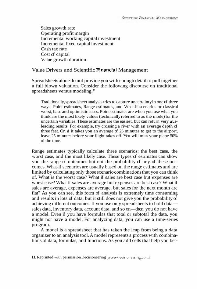
Sales growth rate Operating profit margin Incremental working capital investment Incremental fixed capital investment Cash tax rate Cost of capital Value growth duration
Value Drivers and Scientific Financial Management
Spreadsheets alone do not provide you with enough detail to pull together a full blown valuation. Consider the following discourse on traditional spreadsheets versus modeling."
Traditionally, spreadsheet analysis tries to capture uncertainty in one of three ways: Point estimates, Range estimates, and What-if scenarios or classical worst, base and optimistic cases. Point estimates are when you use what you think are the most likely values (technically referred to as the mode) for the uncertain variables. These estimates are the easiest, but can return very mis- leading results. For example, try crossing a river with an average depth of three feet. Or, if it takes you an average of 25 minutes to get to the airport, leave 25 minutes before your flight takes off. You will miss your plane 50% of the time.
Range estimates typically calculate three scenarios: the best case, the worst case, and the most likely case. These types of estimates can show you the range of outcomes but not the probability of any of these out- comes. What-if scenarios are usually based on the range estimates and are limited by calculating only those scenario combinations that you can think of. What is the worst case? What if sales are best case but expenses are worst case? What if sales are average but expenses are best case? What if sales are average, expenses are average, but sales for the next month are flat? As you can see, this form of analysis is extremely time consuming and results in lots of data, but it still does not give you the probability of achieving different outcomes. If you use only spreadsheets to hold data- sales data, inventory data, account data, and so on-then you do not have a model. Even if you have formulas that total or subtotal the data, you might not have a model. For analyzing data, you can use a time-series program.
A model is a spreadsheet that has taken the leap from being a data organizer to an analysis tool. A model represents a process with combina- tions of data, formulas, and functions. As you add cells that help you bet-
11. Reprinted with permission Decisioneering (www.decisioneering.com).
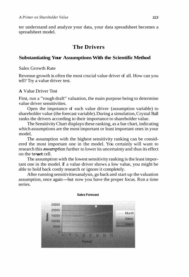
A Primer on Shareholder Value 323
ter understand and analyze your data, your data spreadsheet becomes a spreadsheet model.
The Drivers
Substantiating Your Assumptions With the Scientific Method
Sales Growth Rate
Revenue growth is often the most crucial value driver of all. How can you tell? Try a value driver test.
A Value Driver Test
First, run a "rough draft" valuation, the main purpose being to determine value driver sensitivities.
Open the impotance of each value driver (assumption variable) to shareholder value (the forecast variable). During a simulation, Crystal Ball ranks the drivers according to their importance to shareholder value.
The Sensitivity Chart displays these ranking, as a bar chart, indicating which assumptions are the most important or least important ones in your model.
The assumption with the highest sensitivity ranking can be consid- ered the most important one in the model. You certainly will want to research this assumption further to lower its uncertainty and thus its effect on the target cell. "
The assumption with the lowest sensitivity ranking is the least impor- tant one in the model. If a value driver shows a low value, you might be able to hold back costly research or ignore it completely.
After running sensitivities analysis, go back and start up the valuation assumption, once again-but now you have the proper focus. Run a time series.
Sales Forecast

Time-Series or Trend Forecasting
The objectives are to generate the right regression and to be ready to explain any errors or anomalies that appear in revenue forecast. Time- series anomalies are calculated by subtracting the forecast value for the actual value: Error = Forecast Revenue - Trend Revenue.
Time-series forecasting assumes that the historical data are a combi- nation of a pattern and some random error. There are two risks in extrap- olation that we might call mathematical and practical. In both cases, there is no sharp division between safe interpolation and dangerous extrapolation. Rather, there is a continually increasing danger of misinterpretation as rev- enues get further from their central value. Normally, prediction intervals get larger as revenues move further along in the forecast period.
In situations where sales really drive value, the time-series methods should not be ad hoc, which means do not guess. Since sales is usually the most important value driver, a much better approach to generate a time series is with Decisioneering's CB Predictor. The model breaks historical data into three componen~s-trend, seasonality, and error-while the Method Gallery provides the best choice (see Exhibit 11-1).
The for time-series forecasting methods are set automati- cally in CB Predictor (see Exhibit 11-1). The model automatically finds optimal parameters, unless you override this optimization by selecting to use User Defined parameters. As Exhibit 11-2 shows, there are four possibil- ities out of many contenders. However, in this case, the double moving average method was optimal. The criteria for optimal parameters included (1) root mean squared error (RMSE) which is an absolute error measure that squares the deviations to keep the positive and negative deviations from cancelling each other out (and tends to exaggerate large errors, which can help when comparing methods); (2) mean absolute deviation (MAD), an error statistic that average distance between each pair of actual and fitted data points, (3) mean abs~lute percentage error (MAPE) a relative error mea- sure that uses absolute values to keep the positive and negative errors from cancelling each other out and uses relative errors to let you compare forecast accuracy between time-series models; (4) Durbin-Watson tests for autocorrelation of one time lag. Autocorrelation describes a relationship or correlation between values of the same data series at different time peri- ods, while lag defines the offset when comparing a data series with itself. For autocorrelation, this refers to the offset of data that you choose when correlating a data series with itself); (5) Theil's Statistic which measures the root mean square error in relative terms. If Theil's Statistic is equal to 0 then the estimated forecasting model is a perfect fit; if Theil's Statistic is equal to 1, the predictive performance of the forecasting model is as bad as it could possibly be. A double moving average would be the best choice to time-series sales.

A Primer on Shareholder Value
Exhibit 11-1. Textile time-series: Setting up the time-series with CB Predictor
Exhibit 11-2. Methods table for shampoo sales. Methods Table for Shampoo Sales Created 7119199 at 2.50.15 PM
. . . - . . .. ... I W r n - (
Mrhods r/R,lnl. RMSE MAD M W E DdftinWals~n Tna~i's U Pe~iods Alpha Bela r - ..: ,... ; . . - , . . < , , V ~ : I ~ !to 4 31963 i s 1 8 2 4 4 s 2 r 11 393 0 354 fl 333
Multiple Regression
Double ~ b v i n ~ Average "
Single Exponenl~al Smoothing S~ngle Maving Average
Use multiple regression to predict sales from one or more independent variables. You may want to use multiple regression to determine how sen- sitive sales are to macroeconomic factors. For example, a textile manufac-
~ -~ ~-
1 7174.1 55278 15.527 2.882 0.662 7 3 8202.2 66E 22.312 2.543 0.814 0.448 2 7569.6 5953.6 19.503 2.676 0.803 2
turer is interested in the effect that textile imports have on the firm's sales. Using CB Predictor, we can see the data generated in Table 11-1 and [CD:MODELS\EXCEL\C11RegressImports\OrigResults]

Table 11-1. Time-series original data for textile regression example.
Year Sales Imports
Simulation
Without simulation, revenue changes (your first and usually most impor- tant value driver) will reveal only a single outcome, generally the most likely or average scenario. You define the possible values for revenues over the projection horizon with a probability distribution. The type of distrib- ution that you select is based on the conditions surrounding that variable or series of variables that combine to form your assumptio~ (see the hotel design problem that we look at shortly). To add this sort of function to an Excel spreadsheet, you would need to know the equation that represents the firm's revenue distribution. With Crystal Ball 2000, these equations are automatically calculated for you since the product can even fit a distribu- tion to any historical data that you might have. Let's run a simulation on sales product by the textile manufacture's sales produced by the previous example.
Certainty is the percentage chance that a particular forecast value would fall within a specified range. In the previous chart, you can see the certainty associated with fiscal 2000 sales falling between 153 and 170 at 95% confidence. Of the 1,000 trials that were run, certainty of sales falling below 140 is zero. Forecast results display result values for each forecast and the probability of any value. Exhibit 11-5 represents a sim- ulation run for the year 2000. The Gensis for the simulation is Exhibit 11-6, and includes input data: starting sales, growth rate, and standard deviation.

A Primer on Shareholder Value 32 7
Optimization
As we saw in chapter 9, optimization is a process that finds a best, or opti- mal, solution for your model. Here, our thoughts are directed to revenue, the value driver. N o t all spreadsheet models require optimization; how- ever, the technique is important when you actually control the variables
Exhibit 11-3. The results: Textile regression. (Report worksheet of C11 Regresslmports Workbook)
Report for Textile Regression Created: 12120199 at 5:14:29 PM
Summary: Number of series: 2 Periods to forecast: 4 Seasonality: none Error measure: RMSE
Series: lnports Range: C4:C17
Method: Multiple linear regression
Statistics: R2: 0.91 7 Adjusted R2: 0.91 00 SSE: 712090 F statistic: 132.46 F probability: 7.69E-8 Durbin-Watson: 0.978 No. of values: 14 Independent variables: 1 included out of 1 selected
Series Statistics: Mean: 2,431.3 Standard deviation: 812.0 Minimum: 1,336.0 Maximum: 3,546.0 Ljung-Box: 47:1087
Forecast:
Date Lower: 5% Forecast Upper: 95% 2000 2,650.0 3,081.5 3,513.1 2001 2,381.4 2,848.9 3,316.4 2002 2,106.2 2,616.2 3,126.2 2003 1,822.6 2,383.6 2,944.6
(continues)


A Primer on Shareholder Value
Forecast:
Date Lower: 5% Forecast Upper: 95% 2000 133.1 161.9 190.7
Method Errors:
Method RMSE MAD MAPE Best: Double exponential smoothing 16.262 11.992 10.21% 2nd: Single exponential smoothing 18.301 15.722 12.98% 3rd: Double moving average 18.405 13.769 8.89% 4th: Single moving average 18.99 16.931 13.97%
Method Statistics:
Method Durbln-Watson Theil's U Best: Double exponential smoothing 1.537 0.754 2nd: Single exponential smoothing- 1.602 1 3rd: Double moving average 1.426 0.789 4th: Single moving average 1.583 1
Method Parameters:
Method Parameter Value Best: Double exponential smoothing Alpha 0.45
eta 0.999 2nd: Single exponential smoothing Alpha 0.999 3rd: Double moving average Periods 3 4th: Single moving average Periods 1
affecting sales (e.g., advertising, production limits, or distribution chan- nels) and you want a maximum or minimum goal that relies on those variables.
Remember that optimization programs for spreadsheets, such as Solver, are good at finding the best combination of values that maxi- mize or minimize a goal. However, these programs are not set up to handle uncertainty, as they get lost in all the permutations of possible values and changing solutions if your valuation model introduces uncertainty.

Exhibit 11-4. C11 Sales Projection worksheet. Quarterly Sales Projection
Textile GPlllpBlly Inc. CXlarter Sart ing Sales G-owth S d Dev mding Sales fiscal Sales
first a r 2000 $40 5.00% 2.00% $42 Second Cl r 2000 $42 -2.502 2.00% $4 1
I Third CXr 2000 $4 1 2.00°
Suppose that you own several hotels and were considering remodel- ing one.12 You want to find the best combinations of rates and room sizes to maximize the revenue value driver (Exhibits 114 and 11-7). This is a straightforward optimization problem: maximize sales. Of course, you have to be careful. Just because sales reach high levels does not necessar- ily mean that you have maximized profits. Operating leverage is the determining factor-airlines with their breakeven load factor and hotels with their breakeven occupancy rate. You begin to set up your model but then realize that several key factors associated with market segmentation. Deluxe rooms and suites (Platinum) attract a business and high-income clientele, and midpriced high-end (Gold) and standard (Standard) attract family and other customers. Each market segmentation has its own price/demand elasticity:
Room Type Elasticity
Standard -3 Gold -1 Platinum -2
For example, a 1% decrease in the price of a standard room increases the number of rooms sold by 3%. Similarly, a 1% increase in the price will decrease the number of rooms sold by 3%. The price/elasticity are uncer- tain assumption variables. Standard optimization programs cannot handle
12. The hotel pricing optimization problem was developed by Decisioneering and repro- duced with their permission.

A Primer on Shareholder Value
Exhibit 11 -5. Quarterly sales projection, Textile Company Inc. simulation results.
Forecast: Fiscal 2000 Sales Cell: G8
Summary: Certainty level is 95.00%. Certainty range is from $153 to $170. Display range is from $1 49 to $1 72. Entire range is from $148 to $174. After 1,000 Trials, the standard error of the mean is $0.
Statistics: Trials Mean Median Mode Standard deviation Variance Skewness Kurtosis Coefficient of variability Range minimum Range maximum Range width Mean standard error
Forecast: Fiscal 2000 Sales
1,000 Trials Frequency Chart 10 outliers
.028 28
,021 21 % - n .- - i3
,014 14 f m P m 2 n ,007 , a
.ma o $149 $155 $160 $166 $172
Certainty is 95.00% from $153 to $170
these stochastic variables. Traditionally, you would have had to guess the values for these uncertain factors and hope for the best. Using simulation alone, you could run multiple simulations for price/demand elasticity and compare the results to total hotel revenue. However, did you try every possible combination of inputs? Of course, the answer is no.

Exhibit 11-6. Hotel pricing problem and options.
f --
400
-+ Capacity 450
The fact remains that you likely will need optimization if the revenue (value) driver is significant to value and the firm is empowered with high operating leverage. Capital may be at risk as the hotel tries to work out its remodeling strategies. To figure out its remodeling the hotel utilized OptQuest by Decisioneering:
Total number of simulations: 557 Number of trials per simulation: 100 Confidence testing is activated Number of simulations run maximum number of trials: 93 Number of simulations stopped by precision control: 0 Number of simulations stopped by confidence testing: 464 Neural network engaged after simulation: 40 Number of simulations avoided due to neural network: 165 Population size: 20

A Primer on Shareholder Value 333
Exhibit 11-7. Hotel design problem: Optimization is complete.
tandard $ 85.00 250 $ 21,250.M $ 98.00 100 $ 9,800.00 90 $ 9 697.96
Exhibit 11-8 displays the completed optimization solution gener- ated by OptQuest for Crystal Ball 2000. The software displayed the results of the best simulations in the solutions area of this window. The first best simulation is always either the suggested values used in your spreadsheet, if those values satisfy the constraints imposed, or the first constraint-feasible solution that OptQuest generates. As you can see (Exhibit 11-8) each time OptQuest identifies a better solution during the optimization, it adds a new line showing the new objective value and the values of the decision variables. Thus, the optimal price choices between standard, gold and platinum prices under the room demand constraint (located in the exhibit's third column) maximizes the mean of total revenue.
The simulations verdy that the probability of demand exceeding capacity is slightly under 20%.

Exhibit 11-8. Hotel design problem: Optimization is complete.
Forecast: Total room demand (cont'd) Cell: HI2
Percentiles:
Percentile 0%
10% 20% 30% 40% 50% 60% 70% 80% 90%
100%
Forecast: Total room demand Cell: HI2
Summary: Certainty level is 18.20%. Certainty range is from 450.00 to +infinity. Display range is from 41 0.00 to 470.00. Entire range is from 412.76 to 466.53. After 1,000 trials, the standard error of the mean is 0.35.
Statistics: Trials Mean Median Mode Standard deviation Variance Skewness Kurtosis Coefficient of variability Range minimum Range maximum Range width Mean standard error
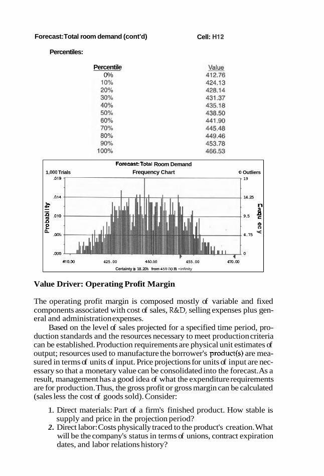
Forecast: Total room demand (cont'd)
Percentiles:
Percentile 0%
Cell: HI2
Forecast:Total Room Demand 1 ,COO Trials Frequency Chart 0 Outliers
,019 19
014 14.25
E .- - n .- a q ,010 9.5 f n e 2 rI
,005 4.75
,000 0
410.00 425.00 440.00 455.00 470.00
Certainty is 18.20% from 450.00 m +infinity
Value Driver: Operating Profit Margin
The operating profit margin is composed mostly of variable and fixed components associated with cost of sales, R&D, selling expenses plus gen- eral and administration expenses.
Based on the level of sales projected for a specified time period, pro- duction standards and the resources necessary to meet production criteria can be established. Production requirements are physical unit estimates of output; resources used to manufacture the borrower's product(s) are mea- sured in terms of units of input. Price projections for units of input are nec- essary so that a monetary value can be consolidated into the forecast. As a result, management has a good idea of what the expenditure requirements are for production. Thus, the gross profit or gross margin can be calculated (sales less the cost of goods sold). Consider:
1. Direct materials: Part of a firm's finished product. How stable is supply and price in the projection period?
2. Direct labor: Costs physically traced to the product's creation. What will be the company's status in terms of unions, contract expiration dates, and labor relations history?

3. Manufacturing overhead: All costs of manufacturing with the exception of direct material and direct labor costs. Are the costs associated with operating the facility enough to reach sales goals?
4. Changes in automation, substitution of capital for labor, and tech- nology and its effect on costs.
5. Plant capacity: Is it physically possible with the resources at hand to meet excepted production requirements?
6. Operating leverage: A high degree of operating leverage implies a relatively small change in sales and will result in a larger than pro- portionate change in net operating income. The ratio of variable costs to fixed costs will determine the degree of operating leverage.
Operating leverage can be defined more precisely in terms of the way a given change in sales volume affects net operating income. To measure the effect on profitability of a change in volume, we calculate the degree of oper- ating leverage, or the ratio of the percentage change in operating income to the percentage change in units sold or in total revenues.
Value Driver: Incremental Working Capital Investment
Incremental Working Capital Investment
The incremental working capital investment required for operations is defined as the increase in total current assets (excluding any marketable securities and other current assets not necessary to support operations) minus the increase in total current liabilities (excluding debt due and other nonoperating obligations).
When calculating operating cash flow, the reason that incremental working capital investment excludes the increase in marketable securities, current portion of long-term debt, and notes payable is that those items are financing issues and are not part of the cash required for operations.
Following is the rationale for excluding each of these items:
1. Marketable securities are not investments required for operations; rather, the increase in these investments is the result of a cash sur- plus generated by operations.
2. The current portion of long-term debt and notes payable represents sources of financing rather than a direct investment in working capital to support the operations of the firm. Excluding these items from working capital is essential in order to evaluate investment decisions independent of financing decisions.
Value Driver: Incremental Fixed Capital Investment
As we saw in chapter 3, the option pricing model and its ability to value capital allocation choices, thus assisting financial managers' real-world

A Primer on Shareholder Value 33 7
decision making, is no longer the province of commodity futures traders or something embedded in a fixed-income security. Options are the next logi- cal step from sensitivity and scenario analysis, decision trees, and expected probabilities with regard to NPV and internal rate of return analysis.
The techniques presented in chapter 3 allow the financial manager to properly assign and value the capital expenditure decision, whether it is the probability of success regarding proper capital allocation or the valu- ing of an option as it applies to project continuance or abandonment. The market value of a project can be seen as the combination of the standard NPV measurement plus the option of contracting or expanding the project in response to the market acceptance.
From the standpoint of the value driver itself, the incremental fixed capi- tal investment represents the portion of total capital expenditures necessary to support incremental sales. Thus, this value driver is defined as the capital expenditures in excess of depreciation expense (and net capitalized interest). Assumed here is that depreciation expense is assumed to approximate the cost of replacing equipment to maintain existing capacity. Net capitalized interest is excluded, as it is part of the financing decision, not the investment decision.
Depreciation expense, which is based on historical costs, may under- state the cost of replacing existing equipment when that cost has increased because of inflation and regdatory forces (i.e., environmental controls). However, the F ratio does account for higher replacement costs because they are captured in the estimate of (total) fixed capital investment.
Value Driver: Cash Tax Rate
As we look to discount forecasted (after-tax) operating cash flows, we must estimate a cash tax on operating profit instead of simply applying an effective tax rate to earnings before tax (EBT). Tax on operating profit represents the portion of total income taxes that is applicable to operating profit only, Tax on operating profit is the total taxes on taxable operating profit for a fiscal year that either have been paid by installments or are payable within 12 months.
Tax on operating profit is likely to be different than the actual amount payable to the taxingauthority because the actual amount payable will include taxes on nonoperating items. Consider the following reconciliation between the current tax provision and tax on operating profit:
Current provision for income taxes - Tax on nonoperating profit + Interest tax shield
Tax on operating profit
Note that for an interest-paying company, the cash tax on operating profit will be greater than the current tax provision by an amount equal to t*i (less tax on nonoperating profit), where T is the marginal tax rate and I is the firm's interest expense.

SCIENTIFIC FINANCIAL MANAGEMENT
Value Driver: Cost of Capital
Risk and the time value of money are embedded into the cost of capital. The cost of capital or discount rate should be an average of the company's cost of debt (on an after-tax basis) and cost of equity weighted at a market-based capital struc- ture. The target debt-tcquity ratio used in the weighting should mirror the anticipated, or target, capital strudure, as that is the mix of capital that will fund the forecasted cash flows. A detailed discussion on estimating this important measure is available in appendix two of this chapter. ~ ~ ~ e n d i c & that follow deal with valuation models appraisal reports and valuation optimization and output.
From Valuation Analytics to Application in Practice
Understanding the analytics driving valuation decisions arms management with a powerful tool. Now, for the first time, management has the requisite knowledge to enable it to determine the future value embedded in planned actions. The debate around what to do is honed dramatically by this new- found ability to estimate the value impact. This empowers management to make sound strategic decisions, to chart a positive value-creating course.
Our focus will shift from the analytics to practice. The final chapter, Chapter 12, introduces how these innovative concepts can lead to the actions that create the value management seeks. Translating analytic rigor embedded in scientific financial management into application in practice represents the synergy of the art and science of strategic management. Therefore, it is impor- tant to end the book with albeit a brief perspective into how leadership teams take their new knowledge into the competitive battle. These tools and frame- works operate at several levels. First, they set the total corporate portfolio con- text, summarizing the potential value impact of all the actions to be taken across the full set of businesses. It is a test of whether the strategies are robust enough to deliver sufficient value, and the effort can turn to implementation planning, or whether the result falls short. In that case, the strategy develop- ment cycle must be revisited. Second, the same analytics can translate the total result into strategic goals for the component businesses. Each business team can understand directly how its actions will contribute to the total and how it important is the effective execution of its strategies. Next, the tools work in set- ting strategic direction, and in monitoring its execution. This latter activity is becoming increasingly central to successful value creation. Perhaps at one time, long, long ago, strategies could be devised, then set in action, to be reviewed or updated on an attenuated cycle. Of course, this is no longer true. Competitive forces intrude with frequency, customer needs evolve rapidly, in sho~*t, strategies must be tightly monitored. An insightful set implementation metrics, directly connected to the robust valuation analytics, must be in place to allow rapid adjustments to the forces of change.
Thus, we enter the next stage of our journey to high, sustained value cre- ation. Understanding how to leverage these powerful value driver models and analybcs in practice allows management to convert potential value into value realized. This represents the destination on the journey begun in chapter 1.

Appendix One to Chapter 11
Mort Glantz Associates, Valuation Appraisal Outline1
I. Purpose of the valuation report A. Taxes; estate tax purposes
1. Address factors enumerated in Rev- enue Ruling 50-60
B. ESOP 1. Department of Labor Regulations
C. Lawsuit 1. Issues raised in relevant case law
precedents D. Strategic planning
1. Maximize shareholder value 2. Understand the mechanics of wealth creation 3. Identify and sell off unprofitable business
units i. Liquidation versus cash flow value
4. Purchase business E. Respond to offer to buy business
11. Scope and content of the valuation report A. Audience
1. Prospective parties at interest and their bene- ficiaries i. Internal use by officers and directors
a. Description of the company may be unnecessary or may allude only to cer- tain salient points that directly affect the valuation.
b. If audience is financially sophisticated, we can assume some knowledge of finance and accounting.
1 This outline was complied !?om many sources and used over the years to help clients develop valuations, quite successfully so. You may want to refine the appraisal to suit our goals. I wish I could thank the one or ones who came up with the prototype but I can't.
2. Representatives of any regulatory authorities involved
3. Judge and jury if there is existing or potential litigation
111. Organization A. Introduction
1. Description of the assignment i. Who was retained by whom to do the
appraisal a. Appraiser's statement of qualifications b. ~eviewer's judgments: or example, have I adequately
and convincingly supported the use of each discount rate, capitalization rate, and multiple used in the valuation? Is the conclusion consistent with the economic, industry, and financial statement analysis presented? Is the analysis and conclusion consistent with the stated purpose of the appraisal and standard of value, including any statutory, regulatory, or other legal requirements?
ii. Definition of the property being valued iii. Effective date of the appraisal iv. Purpose of the valuation
2. Summary description of the company i. For the reader's convenience, it is useful to include in the
introduction a brief statement of Robinson Textiles' business and location, some idea of its size, and possibly one or two salient or unique aspects of the company.
3. Capitalization and ownership i. Class or classes of stock and the distribution of ownership
4. Applicable standard of value (if appropriate) i. Internal Revenue Service Ruling 59-60 outlines the valuation
of closely held stocks and includes the following: a. Nature of business and history of enterprise b. Economic outlook and outlook of the specific industry c. Book value and financial condition d. Earning capacity - -
e. ~ i v i d e n d - ~ a ~ i n ~ capacity f. Intangibles, including goodwill g. Stock sales and size of the block to be valued h. Market price of publicly traded stock in
same or similar lines of business ii. Statutes governing dissolution or dissent-
ing stockholder actions (if any) a. Statement to that effect or summary
statement of interpretation of the case law from a financial analysis point of view
A Primer on Shareholder Value
5. Sources of information used in the appraisal i. List of financial statements and supporting schedules
that were examined, including the years studied for each statement a. Statement as to accountant's opinion
ii. Corporate tax returns (if appropriate) iii. Internally prepared budgets for the next 6 to 12 months iv. Facilities visited v. Equipment list and depreciation schedule (if appropriate)
vi. Inventory lists and receivables aging (if appropriate) vii. Stockholders' list as of December 31,1993 viii. Schedule of total owners' compensation (if appropriate) ix. Copies of leases x. Articles of incomoration and bv-laws
1
xi. Industry information and periodicals xii. Information on comparative publicly traded companies
from S&P Corporation records and SEC 10-Ks; various bro- kers reports on these companies
6. Valuation approach and conclusion i. Broad criterion or criteria used in reaching the valuation
conclusion ii. Brief statement of the conclusion
Description of the company 1. Background 2. Physical facilities 3. Product and/or services 4. Distribution channels 5. Sources of supply 6. Labor/capital intensive; operating leverage 7. ~ a n a ~ e m e n t
- -
8. Capitalization and ownership 9. Seasonality (if any) Industry data 1. Size of firm relative to competitors 2. Specialized segments of the market the
firm serves 3. Competitive strengths and weaknesses 4. Technology and production 5. Regulation 6. Industry phase
i. Mature phase: Product technology well established, markets saturated, and long-term growth in line with general econ- omy. Companies compete for market share on price basis
ii. Price-to-earnings ratio is down; thus, the equity market is less attractive to the company. Generally reduced need for financing.

7. Cyclicality i. Should be compared to a benchmark such as real GNP
growth and should consider both industry specific cycles and economic cycles
8. Entry barriers i. Economies of scale and other cost advantages, capital
requirements, intensity, product differentiation, access to dis- tribution channels, and regulations
9. Cost Structure i. Labor cost, material cost, capital intensity, economies of
scale, technological advantages/disadvantages, and operat- ing leverage
D. Economic data 1. Aspects of economic conditions that may have a bearing on the
firm's prospects i. Identify clearly macroeconomic variables that affect the
firms sales and gross profit margin E. Financial Analysis
1. Analysis of the latest fiscal year i. Income statement, balance sheet, cash flow, and ratios ii. Industry comparatives
2. Projection analysis i. Most likely projections; ratio, cash flow,
financial needs, and debt capacity analysis will show the firm has financial resources available and is viable
ii. Conse~at ive (worst-case) projection highlights a. Sales growth and gross margin pegged to historical five-
year lows; average collection and holding periods set at historical five-year highs
b. Analysis reinforces firm's viability given worst-case scenario F. Valuation analysis
1. Approaches i. Price: Revenues multiples ii. Capitalization of five-year average earnings
iii. Capitalization of projected earnings iv. Market capitalization: Book capitaliza-
tion multiples v. Price earnings and price book
vi. Transaction multiple approach vii. Liquidation value viii. Dividend model ix. Cash flow (while we will construct a
weighted average, discounted free cash flow model will carry a substantial weight)
A Primer an Shareholder Value
x. The forecast horizon a. Points we need to discuss to determine this extremely
important valuation determinant b. Proprietary technologies c. Limited product life cycle d. Distribution channels e. Industry-wide price competition
2. Residual value i. Once the discrete forecast horizon cash flows have been esti-
mated, we can make a simplifying assumption regarding the cash flow generated after the forecast period.
3. Cost of capital i. Textiles had a beta last year of 1.16. ii. We need to discuss the cost of debt, applying the cost of debt
to the firm's tax rate. 4. Value driver analysis
i. Sales growth ;ate ii. Incremental working capital investment
iii. Incremental fixed capital investment iv. Cash tax rate v. Cost of capital
5. Relative impact of key variables on share- holder value
6. Analysis of valuation ratios a. Threshold margin versus operating
profit margin b. Threshold spread
G. Simulations: "Proving the valuation is right on target" 1. Define assumptions
i. Understanding and working with value drivers ii. Selecting the right distribution to fit data
a. Fitting distributions to data iii. Correlations between independent variables and/or
between independent variable (s) and the forecast variable a. Responding to problems with correlated assumptions
2. Define forecast i. Determining the certainty level
a. Finding the probability that valuation falls within specific ranges
3. Developing a sensitivity check and working with sensitivity charts 4. Creating reports
H. Strategic planning: Optimizing the company's value 1. setting up and optimizing the linear programming model (OptQuest)
i. Defining decision variables and selecting decision variables to optimize
ii. Specifying constraints (value drivers) limitations

iii. Selecting the forecast objective: Maximize shareholder value by linear programming changes to value drivers
iv. Perform sensitivity analysis I. Conclusion
1. Summary of the valuation appraisal and recommendations
Valuation Appraisals and Business Plans SeIect Internet Library and SBA Source Contacts
1. Small Business Administration (SBA), The Business Plan: Road Map To Success, 9/97. The SBA provides a very through outline for a business plan you can easily download. This source is highly recommended. Use this model as a guide when developing the business plan for your business. http://www.sbaonline.sba.gov/ starting/businessplan.html
2. The Business Plan Road Map To Success, 9/97, a tutorial and self- paced activity for downloading or viewing as text version. The plan includes a case study "Someplace Fitness Center, March 1995" This through outline wasprepared with the assistance of The Center For Technology And Small Business Development Central Missouri State University. http://153.91.1.141 /sbdc/centsbdc/BUSPLAN.HTM
3. Howard University Small Business Development Center devel- oped a business plan entitled " Discover what to put in a business plan" http://www.ntia.doc.gov/opadhome/mtdpweb/ busplano.htm
4. Using Your Computer to Create A Winning Business plan was developed by Thomas Carroll which can be downloaded http: / /www.planmaker.com/about-bp.htrn1
5. A business plan is included in the October 1997-Sixth Edition Lansing Community College Small Business Development Center Counseling, Training, Research, and Advocacy for Michigan's small Business. U.S. Small Business Administration Small Business Devel- opment Center (SBA/SBDC) http://www.nemonline.org/ bus plan/
U.S. Small Business Administration
Besides developing valuation appraisals and business plans for clients, financial consultants may want to consider an excellent information resources list compiled by the U.S. Small Business Administration (SBA).' The SBA offers an extensive selection of information on most business management topics, from how to start a business to development of busi- ness plans (see above) to exporting your products. This information is
1. Source US Small Business Administration

A Primer on Sharelzolder Value 345
listed in "Resource Directory for Small Business Management." This can be obtained at any SBA office. On behalf of your clients, you may want to recommend the following free services:
1. Service Corps of Retired Executives (SCORE), a national organiza- tion sponsored by SBA of over 13,000 volunteer business executives who provide free counseling, workshops and seminars to prospec- tive and existing small business people.
2. Small Business Development Centers (SBDCs) sponsored by the SBA in partnership with state and local governments, the educa- tional community and the private sector. They provide assistance, counseling and training to prospective and existing business people.
3. Business Information Centers (BICs), offers state-of-the-art technol- ogy, informational resources and on-site counseling for start-up and expanding businesses to create business, marketing and other plans, do research, and receive expert training and assistance.
Many publications on business management and other related topics, some examined in this book are available from the Government Printing Office (GPO). GPO bookstores are located in 24 major cities and listed in the Yellow Pages under the "bookstore" heading. You or your clients can request a "Subject Bibliography" by writing to Government Printing Office, Superintendent of Documents, Washington, DC 20402-9328. Many federal agencies offer publications of interest to small businesses. There is a nominal fee for some, but most are free. Below is a selected list of gov- enunent agencies that provide publications and other services targeted to small businesses. To get their publications, contract the regional offices listed in the telephone directory or write to the addresses below:
A Consumer Information Center (CIC), P.O. Box 100, Pueblo, CO 81002. The CIC offers a consumer information catalog of federal publications.
A Consumer Product Safety Commission (CPSC), Publications Request, Washington, DC 20207. The CPSC offers guidelines for product safety requirements.
A U.S. Department of Agriculture (USDA), 12th Street and Indepen- dence Avenue, SW, Washington, DC 20250. The USDA offers publi- cations on selling to the USDA. Publications and programs on entrepreneurship are also available through county extension offices nationwide.
A U.S. Department of Commerce (DOC, Office of Business Liaison, 14th Street and Constitution Avenue, NW, Room 5898C, Washing- ton, DC 20230. DOC'S Business Assistance Center provides listings of business opportunities available in the federal government. This service also will refer businesses to different programs and services in the DOC and other federal agencies.

A U.S. Department of Treasury, Internal Revenue Service (IRS), P.O. Box 258, Richmond, VA 2326. The IRS offers information on tax requirements for small businesses.
A U.S. Environmental Protection Agency (EPA), Small Business Ombudsman (2131, Room 3423M, 401 M Street, S.W., Washington, DC 20460; 1-800-368-5888. The EPA offers more than 100 publica- tions designed to help small businesses understand how they can comply with EPA regulations.
A U.S. Food and Drug Administration (FDA), FDA Center for Food Safety and Applied Nutrition, 200 C Street, SW, Washington, DC 20204. The FDA offers information on packaging and labeling requirements for food and food-related products.
For More Information a librarian at the SEA can help both you or your clients locate the specific information you need in reference books. Most libraries have a variety of directories, indexes and encyclopedias that cover many business topics. They also have other resources, such as trade association information. Trade associations provide a valuable network of resources to their members through publications and services such as newsletters, conferences and seminars.
Business and professional magazines provide information that is more current than that found in books and textbooks. There are a number of indexes to help you find specific articles in periodicals. In addition to books and magazines, many libraries offer free workshops, lend skill- building tapes and have catalogues and brochures describing continuing education opportunities.

Appendix Two to Chapter 11
Ace Textile Production Corp.: Valuation, Simulation,
and Optimization (A Case Study for Valuation
Consultants and Appraisers) l
Ace Textile's valuation was developed using the Excel spreadsheet model accompanying a highly rated book: Valuation: Measuring and Managing the Value of Companies, (2nd ed.), by Copeland, Koller, and Munin (New York: John Wiley & Sons). While accompanying extracts are included as exhibits to this case, the valuation model itself and discussion of it has been excluded. However, you can purchase it from John Wiley & Sons at a nominal cost. The threshold spread and threshold margin: along with simulations using Deci- sioneering's Crystal Ball, supplement the basic valuations. In order to obtain relatively uncomplicated solutions to this case, we used Excel's Solver to maximize operating profit (that turned out to be the most important value driver) by limiting business risk associated with operating leverage. Recall that Solver provides a local optimal solution since the model is deterministic. Stochastically driven optimization models discussed in chapter 9 would have provided more realistic solutions. Also, the case was recast to meet generic requirements to hide the real company. Thus, the Capital Asset Pricing Model (CAPM) furnished the risk/reward framework. The use of CAPM was less than optimal; in the financial literature, the theory is quite sound, but in prac- tice the whole idea of divisional betas is not very practical. We will discuss this further when the problem comes up. The workbook for this case is C11 AceExcel Hard Copy located in the Excel subdirectory in the CD.
During the course of this discussion, we cover the following:
1. Forecasts of free cash flows during a 10-year explicit forecast period 2. Continuing value calculations for cash flows beyond the explicit
forecast period
1. Refer to appendix 1. 2. Developed by Alfred Rappaport in Creating Shareholder Value (New York: The Free Press, 1986).
34 7

3. Computation of the weighted average cost of capital utilizing the "pure play" approach
4. Maximizing operating margin by eliminating product lines, chang- ing the contribution of product segments to consolidated operating margin, while constraihing asset iolitility associated with opera; ing leverage
5. optimization reports provided by Solver 6. Simulation reports provided by Crystal Ball delineating value dri-
ver impact on shareholder value 7. Determining probabilities that the shareholder value falls below zero 8. The threshold marein as a tool to measure the effectiveness of man- "
agement strategy to add to or destroy shareholder value 9. Free cash flow, economic profit, and invested capital
The Company
Ace Textiles was founded in 1955. The company produces a number of diversified products in five operating segments. Ace's production and sales are divided into the operating segments: Shown in Table 11A-1.
Ace hired a consulting firm to provide operating guidance and a val- uation appraiser to map valuations. The team recommended that manage- ment improve the existing business with more efficient production meth- ods such as reducing excessive variable labor costs and increasing operating leverage. In short, operating segments will be reexamined, and some may be sold off.
Table 11A-1. Operating segments and operating leverage.
Operating Segments % of Operations Operating Leverage
Product Line Kappa 22.00/0 Very low. Labor is used almost exclusively in production. Low risk operation.
Product Line Epsilon 20.0% Moderate. Labor is predominate in production. Below average risk.
Product Line Sigma 10.0% Balanced. Labor and machines utilized aproximatel 50-50. Average risk.
Product Line Omega 10.0% High. Machines usuage greater than labor. Higher risk operation.
Product Line Lambda 38.0°/~/1 00% Extremely Low. All labor operation. Lowest operating margins, lowest risk.

A Primer on Shareholder Value 349
The team will provide a discounted cash flow valuation and run sim- ulations and optimizations that concentrate on (1) determining the operat- ing segments the business should highlight (decision variables), (2) maxi- mizing the combined operating margin and with it a pivotal link to shareholder value (objective variable), and (3) defining the major con- straint in this business, that is, the volatility component linked to operat- ing leverage. The restriction on operating variability is an important com- ponent to valuation because the firm's existing funded debt is sustained by low rates (low risk). If operating leverage (and asset volatility) were to increase beyond a measured tolerance acceptable to the lenders, the firm would be forced to bring in high-cost equity,
Summary
On balance, the firm's business risk is far lower than the industry average. Low business risk is associated with the firm's low fixed production costs (i.e., low operating leverage). However, this has had a negative effect on operating margins. If the firm were to augment operating leverage, mar- gins would almost certainly rise, but so too would business and financial risk. While the firm is willing to alter the distribution of its product line mix, management is not quite sure how to accomplish this. That is why the consultants were brought in.
The Valuation Process: The Valuation Summary
The explicit forecast period was 10 years (1995-2004), and the terminal value commenced at the beginning of year 2005. Table 11A-1 and Orig Valuation Worksheet shows the results. First, management explicitly forecasted free cash flows from 1995 to 2004. Present value was $4,738. Next, the firm estimated the present value of free cash flows from the year 2005 and beyond. This continuing value was worth $5,005. The total, $9,743, represents operating value. To this total nonoperating assets and the firm's excess pension assets were added in. The result (i.e., the value of the firm) is $9,941. From this total, the market value of debt ($4,500), retirement-related liability ($500), and preferred stock ($333) were deducted, resulting in equity value of $4,608.
Economic profit calculation of value yields the same results as the free cash flow method. Management discounted back to present value eco- nomic profit in the years 1995-2004 and subtracted from this total contin- uing value to arrive at the present value of economic profit ($294.9). Adding invested capital at the beginning of the projection period, $9,661, yielded operating value of $9,743, which, as you can see by examining Exhibit 11A-1 is equal to the flow method.
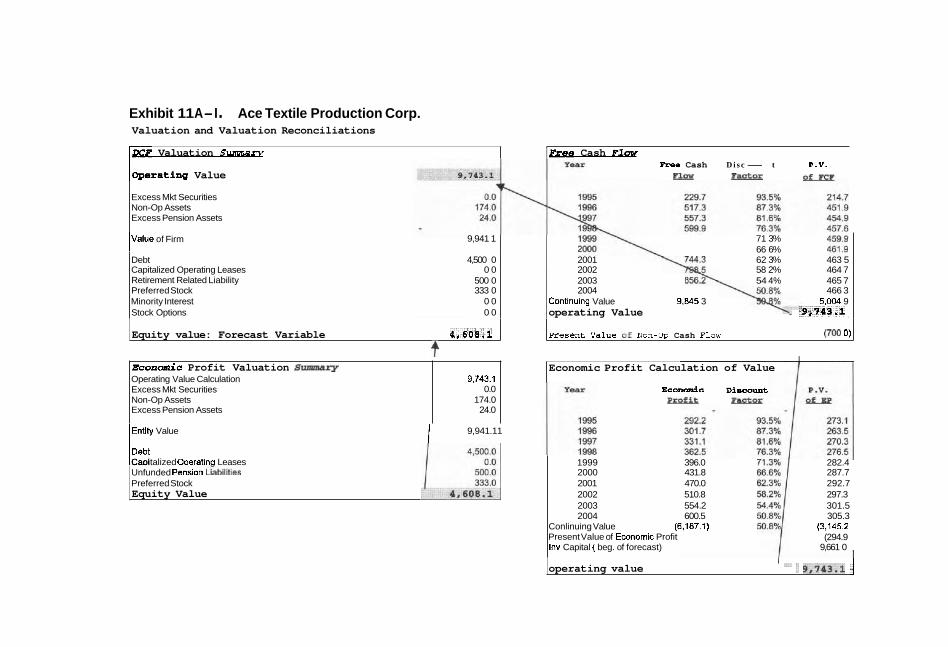
Exhibit 11 A-I . Ace Textile Production Corp. Valuation and Valuation Reconciliations
loperating Value
~DCF Valuation Sumnary
Excess Mkt Securities Non-Op Assets Excess Pension Assets
]Free Cash Flow
l ~ a l u e of Firm
Debt Capitalized Operating Leases Retirement Related Liability Preferred Stock Minority Interest Stock Options
Free Cash D i s c- t P.V.
EaT! 5?LEcE
9,941 1 71 3% 66 6%
4,500 0 2001 62 3% 463 5 0 0 2002 58 2% 464 7
500 0 2003 54 4% 465 7 333 0 2004 466 3
0 0 Contlnulng Value 9,845 3 5,004 9 0 0 operating Value .. pr74S.l
Equity value: Forecast Variable r,sda.i
I~nt i ty Value 1 9,941.11
present value of on-op Cash F ~ O W (700 0)
Economic Profit Valuation S u n r m a ~ Operating Value Calculation Excess Mkt Securities Non-Op Assets Excess Pension Assets
l ~ e b t Caoitalized Ooeratinc! Leases
9.743.1 0.0
174.0 24.0
Unfunded Pensoon ~Gblllt~es Preferred Stock Equity Value
I Economic Profit Calculation of Value
E c o d c Discount Ez&&
1999 396.0 282.4 2000 431.8 287.7 2001 470.0 292.7 2002 510.8 297.3 2003 554.2 301.5 2004 600.5 305.3
Conlinuing Value (6.187.1) (3.1452 Present Value of Economic Profit (294.9 Inv Capital ( beg. of forecast) 9,661 0
operating value I "c' : F,SS:$. "1

A Primer on Shareholder Value 331
The forecast assumptions were developed under uncertainty conditions. Assumption variables include revenue growth, cost of goods sold/revenues, selling, general and administration expenses/revenues, accounts receivable and inventory, capital expenditures and cost of capital. The distributions include triangular, d o r m and lognormal (see Exhibit llA-2).
The Income Statement Value Drivers4
Revenue
Revenue growth was held constant in order to disguise the real company and to test value driver sensitivities. Quantitative methods, reviewed in this and other chapters, would naturally be called into play with sales fol- lowing a cyclical pattern. In addition, macroeconomic factors (ignored here along with exogenous sensitivities) are normally a crucial element in deter- mining sales growth. Other external factors affecting each of the firm's operating segment revenue include but are not limited to industry demand, industry supply, competitor pricing policy, competitor advertising policy, cotton and other raw material cost and availability, fashion and technology, foreign textiles competition, substitutes, supply conditions, barriers of entry into industry, historical patterns, and customer order backlogs.
Controllable factors driving Ace Textile's revenue, such as decisions and policies set by management, are important components in any sales pro- jection. These include but are not restricted to product pricing, advertising, production policy, finished goods inventory policy, credit policy, and R. & D.
Cost of Goods Sold
This variable was also held constant to conceal the actual company and again to evaluate value driver importance. In reality, the consulting firm scrutinized and questioned the following factors:
1. Direct materials. 2. Direct labor--costs physically traced to each operating segment's
product line. 3. The firm's status with unions, contract expiration dates, and labor
relations history. 4. Manufacturing overhead, that is, all manufacturing costs with the
exception of direct material and direct labor costs. 5. Changes in automation, substitution of capital for labor, and tech-
nology and its effect on costs (operating leverage). 6. Plant capacity (the valuation appraisers questioned whether it was
physically possible with the resources on hand to meet production requirements; again the issue of operating leverage kept coming up).
(text continues on page 354)
4. Value drivers discussed here are represented in their qualitative dress only. That said, value driver (qualitative) aspects represented the "heart and mind" of the appropriate quantitative models from real options to optimization, discussed in chapters 3,7 and 9.

Exhibit 11 A-2. Ace Textile Production Corp. Forecast Aeeu~gtione - Baee Caee
Distrib- Minimum mmt Likely Y M w
utim 01 6 t - d
Deprec~atlon/Revenues Operating Margin
Working CapltaVRevenues
I Accounts Payable
I Prop Plant Equip
DepriLast Yr's GPPE Ret~rementsRast Yr's GPPE
FinancingIOther Ratios and Forecast Assumptions
Taxes EBlTTax Rate Marginal Tax Rate
Int Rate on Excess Mkt Secs Int Rate on Existing Debt Int Rate on Short.Term Debt Inl Rate on Long-Term Debt

F o r e c a s t Assurqpt ione - B a s e C a s e Forecast
2mu
1 Other Oper lnc!Exp Growth DepreciationIRevenues Operating Margin
I Other Current Assets Accounts Payable
Pmp Plant Eauip
Depr!Last Yr's GPPE RetiremenWLast Yr's GPPE
Flnanc~nglMher Ratos and Forecast Assumptions
EBlT Tax Rate Marginal Tax Rate
Int Rate on Excess Mkt Sea Int Rate on Existing Debt Int Rate on Short-Term Debt Int Rate on Long-Term Debt

7. Production department procedures and controls (actually the valu- ation appraisers determined that shareholder value suffered because management lacked an adept production master plan).
8. Domestic distribution. By rearranging Ace's distribution pattern and making appropriate shifts in production and warehousing loads, it might be possible without any change in facilities to increase company profits. The largest component in this improve- ment package could come from reduced materials and warehous- ing costs, direct labor saving, and plant overhead. If cost of goods sold emerged as the most critical of value drivers, production and warehousing loads would warrant significant strategic changes. On balance, several labor-intensive operating segments could be phased out, reduced, or strengthened.
The appraisers and management integrated real options analysis into the cost of-goods-sold analysis and this critical variable's link to equity value, considering three options: shutdown, the option to expand, and most important, the operating scale option since the firm has the flexibil- ity to expand or scale down operations.
For simulation runs, we assume that the appraisers projected 4.9% sales growth in 1995 and for the remainder of the projection horizon. The triangular distribution was reduced to a tight fit, 4.7% to 5.3%, with 4.9% set as most likely. Cost of goods sold along with selling (general and administration) were built around constricted triangular and uniform dis- tributions, respectively. Even under a tight distribution fit assumption, cost of goods sold turned out to be the most important value driver. Before adjustments, operating margin measured 6% over the long term.
Of all the expense items, operating costs are usually the easiest to control by means of a "Gw-fat" corporate die?. The key to properly limiting operat- ing costs would be to cut the "fat" without inhibiting the infrastructure of the organization. In other words, firms such as Ace Textile should not "down- size" to the point where operations become so inefficient that profits suffer (see Exhibit 11A-3 and the Orig Financial Worksheet).
Balance Sheet Drivers
Accounts Receivable
The firm's accounts receivable policy is closely tied to inventory since the two link up as components of the cash conversion cycle and together rep- resent the largest component of working capital (we see the importance of working capital to the calculation of the threshold margin).
The volume of credit sales and the average collection period deter- mine the level of accounts receivable for this firm. The average collection

Exhibit 11A-3. lncome statement and retained earnings for Ace Textile Production Corp 1992 Forecast Forecast Forecast
LSPZ 33,187.8
Forecast 1998
34.822.8 (28,670.8) (1.323.3)
x!B 1994 - 1995 1996 Revenues 24.789.0 26.462.0 28.729.0 30,144.4 31,629.5 Cost of Goods Sold Selling, Gen L Admin Expenses Depreciation Expense Other Oper IncomelExpense Operating lncome Amortization of Goodwill lnterest lncorne lnterest Expense Special ltems Earnlngs Before Taxes lncome Taxes Minority lnterest Income Before Extra ltems Extraordinary ltems Net lncome
Forecast Forecast Forecast Forecast Forecast Forecast 2004 -
46,470.7 (38.260.9) (1,765.9)
(109.5) (3,503.7) 2,830.7
0.0 193.1
(379.7) 0.0
2,574.2 (1,083.6)
0.0 1,490.5
0.0 1,490.5
Revenues Cost of Goods Sold Selling, Gen & Admin Expenses Depreciation Expense Other Oper InmmelExpense Operating lncome Amortization of Goodwill lnterest Income lnterest Expense Special ltems Earnings Before Taxes lncome Taxes Minority lnterest lncome Before Extra ltems Extraordinary Items NfA lncome
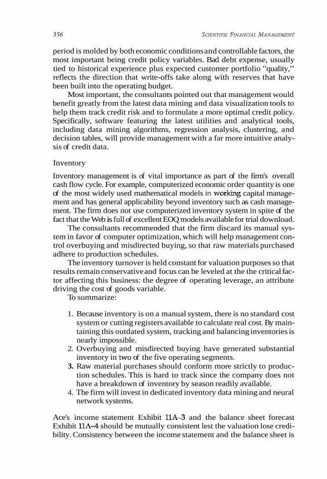
period is molded by both economic conditions and controllable factors, the most important being credit policy variables. Bad debt expense, usually tied to historical experience plus expected customer portfolio "quality," reflects the direction that write-offs take along with reserves that have been built into the operating budget.
Most important, the consultants pointed out that management would benefit greatly from the latest data mining and data visualization tools to help them track credit risk and to formulate a more optimal credit policy. Specifically, software featuring the latest utilities and analytical tools, including data mining algorithms, regression analysis, clustering, and decision tables, will provide management with a far more intuitive analy- sis of credit data.
Inventory
Inventory management is of vital importance as part of the firm's overall cash flow cycle. For example, computerized economic order quantity is one of the most widely used mathematical models in working capital manage- ment and has general applicability beyond inventory such as cash manage- ment. The firm does not use computerized inventory system in spite of the fact that the Web is full of excellent EOQ models available for trial download.
The consultants recommended that the firm discard its manual sys- tem in favor of computer optimization, which will help management con- trol overbuying and misdirected buying, so that raw materials purchased adhere to production schedules.
The inventory turnover is held constant for valuation purposes so that results remain conservative and focus can be leveled at the the critical fac- tor affecting this business: the degree of operating leverage, an attribute driving the cost of goods variable.
To summarize:
1. Because inventory is on a manual system, there is no standard cost system or cutting registers available to calculate real cost. By main- taining this outdated system, tracking and balancing inventories is nearly impossible.
2. Overbuying and misdirected buying have generated substantial inventory in two of the five operating segments.
3. Raw material purchases should conform more strictly to produc- tion schedules. This is hard to track since the company does not have a breakdown of inventory by season readily available.
4. The firm will invest in dedicated inventory data mining and neural network systems.
Ace's income statement Exhibit 11A-3 and the balance sheet forecast Exhibit l l A 4 should be mutually consistent lest the valuation lose credi- bility. Consistency between the income statement and the balance sheet is

A Primer on Shareholder Value 357
usually measured by the turnover ratios connecting accounts receivable to revenues and inventory to cost of goods sold. In Exhibit 11A-6 the two ratios were held constant at 16.4% and 25% (unfortunately to keep the results relatively simple).
A common forecasting error is the failure to adequately tie capital requirements to sales growth. When this happens, the turnover ratio increases rapidly, implying that sales is supported with inadequate capital- either that, or else the company is becoming inordinately efficient in its cap- ital utilization. The result is that the company will be overvalued because cash outflows for capital investment are underestimated. Ace's capital expenditures were held to .5% of revenue, consistent with the firm's low operating leverage. Later, in the optimization runs this will change.
We calculate free cash flow (Exhibit 11A-5 and the FCF & ECProf Work- sheet) starting with earnings before income and taxes (EBIT) net of taxes on EBIT to arrive at net operating profit less amoritization and taxes (NOPLAT). Adding back depreciation yields gross cash flow. Gross investments are deducted from this total to arrive at free cash flow. Exhibits llA-5 through llA-7 are printouts from the AceExcelHardCopy.xls file in the Models sub- directory of the CD. You can view these worksheets in the workbook.
Weighted Average Cost of Capital
To be consistent with the free cash flow approach to valuation, the cost of capital must
1. Comprise the cost of all sources of capital, debt, quasi-equity and equity because free cash flow embodies the residual cash available to all providers of capital.
2. Be computed after tax since free cash flow is stated after tax. 3. Employ market rates, not book, for each financing element.
A number of steps are involved in developing Ace Textiles's cost of capital:
1. Establish target market value for capital structure. 2. Make sure that future financing levels are evaluated carefully since
this could be different from current or past levels. 3. Estimate the current market value capital structure of the company. 4. Review capital structure of comparable companies. 5. Review management's approach to financing this business. 6. Estimate cost of nonequity financing.
Cost of debt also incorporates leases, interest, bond coupons, short-term debt, and leases. However, non-interest-bearing liability, such as accounts payable, are excluded from debt costs in order to steer clear of dissirnilar- ities and facilitate the valuation process. Indeed, non-interest-bearing lia- bilities have cost-of-capital characteristics like other forms of debt, but this
(text continues on page 368)

Exhibit 11A-4. Ace Textile Production Corp. Forecast Forecast Forecast Forecast
Balance Sheet 1992 - Perpertuity - 1992 - 1993 1994 - 1995 1998 W 1998
Inventories 6.907.0 3.997.0 7.506.0 7,5361 7.907.4 8.296.9 8.705.7 Other Current Assets Total Current Assets
Gross Prop Plant Equip 1.783.0 1.828.0 1,920.0 2,014.0 2.091.4 2.172.2 2.256.5 Accum. Depreciation (1.245.0) (1,255.0) (1,222.0) (1,260.4) (1.300.7) (1.342.5) (1,386.0) Net Propetty Plant and Equip 538.0 573.0 698.0 753.6 790.7 829.7 870.6 Other Operating Assets 1.517.0 1,673.0 125.0 0.0 0.0 0.0 0.0 Investments B Advances 206.0 1,100.0 0.0 0.0 0.0 0.0 0.0 Other Non-op Assets 380.0 480.0 174.0 174.0 174.0 174.0 174.0 Total Assets 14,302.0 15,748.0 13,451.0 14,396.1 15,292.2 16,269.2 17,333.1
Short Term Debt Accounts Payable Other Current L~abi itfes Total Current LlablNNes
Long Term Debt Other Non-Interest Liabilities
Preferred Stock Common Stock 8 Paid-in Capital Retained Earnings Total Common Equity Total Liabs and Equity

Forecast Forecast Forecast Forecast Forecast Forecast Balance Sheet 1992 - Perpertuity mi9 2000 m 2002 2003 Z!W
Inventories Other Currenl Assets Total Current Assets
Gross Prop Plant Equip Accum. Depreciation Net Properly Plant and Equip Other Operating Assets Investments &Advances Other Non-op Assets Total Assets
Short Term Debt Accounts Payable Other Current Liabilities Total Current Liabilities
Long Term Debt Other Non-Interest Liabilities
Preferred Stock Common Stock 8 Paid-in Capital Retained Earnings Total Common Equity Total Liabs and Equity

Exhibit 11A-5. Ace Textine Production Corp. free cash flow and economic profit for 1992-Perpetuity. Free Cash Flow Forecast Forecast Forecast Forecast Forecast
EBIT Taxes on EBlT NOPLAT Depreciation Gross Cash Flow
Increase in Worklng Capital Capital Expenditures lncr in Other Assets
Gross Investment 8.126.0 313.0 1777.0 815.6 592.9 621.3 651 .O 682.1
Non-operating Cash Flow Cash Flow Available to Investors
Financing Flow
AT Interest Income Incr/(Decr) Excess Mkt Sec AT Interest Expense Decr/(lncr) in Debt Decr/(lncr) in Preferred
Economic Profit
Return on Invested Capital WACC Spread
NOPLAT 851.0 681.0 801.1 968.5 1,029.7 1,094.9 1,164.0 1,237.0

Free Cash Flow
EBlT Taxes on EBlT NOPLAT Depreciation Gross Cash Flow
Increase in Working Capital Capital Expenditures lncr in Other Assets
Nonaperating Cash Flow Cash Flow Available to Investors
Financing Flow
AT Interest lnwrne Incr/(Decr) Excess Mkt Sec AT Interest Expense Decr/(lncr) in Debt Decr/(lncr) in Preferred
Economic Profit
Return on Invested Capital WACC Spread

Exhibit 11 A-6. Ace Textile Production Corp. operating ratios. Forecast 1995
Forecast lggg
Forecast Forecast
Igg7 rn
Operations Revenue Growth COGSlRevenues SGWRevenues Other Oper IncIExp Growth EBDlT Margin DepreciationlRevenues Operating Margin
Working CapitallRevenues Operating Cash Amounts Receivable Inventories Other Current Assets Accounts Payable Net Working Capital
Prop Plant Equip Input Values:
CapWRevs (Input, Mode 1) NPPWRevs (Input, Mode 2) DeprlLast Yr's GPPE RetirementslLast Y h GPPE
Calculated Values: Gross PPEIRevenues NPPElRevenues CapWRevenues Capital Expenditures (f) Depreciation Expense ($) Retirements ($)

Forecast
19P9 Forecast
2!m Forecast
m Forecast
2002 Forecast
m Forecast
2004 PerP
Operations Revenue Growth COGSlRevenues SG&/VRevenues Other Oper IncIExp Growth EBDlT Margin DepreciationlRevenues Operating Margin
Working CapitallRevenues Operating Cash Accounts Receivable Inventories Other Current Assets Accounts Payable Net Working Capital
Prop Plant Equip Input Values:
CapXiRevs (Input, Mode 1) NPPElRevs (input, Mode 2) DeprlLast Yes GPPE RetirementslLast Yr's GPPE
Calculated Values: Gross PPEIRwenues NPPElRevenues CapWRevenues Capllal Expendiures ($) Depreclatlon Expense ($1

Exhibit 11 A-7. Act Textile Production Corp.
Taxes EBlT Tax Rate Marginal Tax Rate
Int Rate on Excess Mkt Secs Int Rate on Existing Debt Int Rate on Short-Term Debt Int Rate on Long-Term Debt Int Rate on New L-T Debt Weighted Average Cost of Capital
Other Ratios Non-Op Income Growth Other AssetslRevenues Inv & Advances Growth Rate Non-Op Assets Growth Rate Other LiabslRevenues
Other Values (I) Special Items ($) Extraordinary items ($) Short Term Debt ($) Preferred Stock (5)
Key Operating Ratios EBlTlRevenues COGSIRevenues SGWRevenues DepreciationIRevenues Other Oper Inc/ExplRevenues EBlTlRevenues
financing/other ratios and forecase assumptions for 1992-Perpertuity. Forecast
1993 - rn Forecast 1996
Forecast m
Forecast m

Forecast 1999 -
Forecast ZOOD
Forecast 2PeZ
Forecast a
Forecast 2003
Forecast m F!=Q
Taxes EBlT Tax Rate Marginal Tax Rate
Int Rate on Excess Mht Secs Int Rate on Existing Debt Int Rate on Short-Term Debt Int Rate on Long-Term Debt Int Rate on New L-T Debt Welghted Average Cost of Capital
Other Ratios Non-Op Income Gmwth Other AssetsIRevenues Inv &Advances Growth Rate Non-Op Assets Growth Rate Other LiabsIRevenues
Other Values ( f ) Special ltems ($) Extraordinary ltems (5) Short Term Debt ($) Preferred Stock ($)
Key Operating Ratlos EBlTIRevenues COGSIRevenues SGWRevenues DepreciationlRevenues Other Oper lnclExplRevenues EBlTIRevenues
(continues)

Exhibit l l A-7. Continued. Forecast
1995 Forecast 199h
Forecast Em
Forecast 1998
Return on lnvested Capltal (BY) Net PPEIRevenues Working CapitallRevenues Net Other AssetsIRevenues Revenuesilnvested Capital Pre-Tax ROlC Cash Tax Rate After-Tax ROlC After-Tax ROlC (Incl. Goodwill)
Return on lnvested Cap (Avg) Net PPEIRevenues Working CapitalIRevenues Net Other AssetsIRevenues Revenuesilnvested Capita Pre-Tax ROlC Afler-Tax ROlC After-Tax ROlC (Incl. Goodwill)
Growth Rates Revenue Growth Rate EBlT Growth Rate NOPLAT Growth Rate Invested Capital Growth Rate
lnvestment Rates Gross Investment Rate Net lnvestment Rate
Flnanclng Coverage (EBITIlnterest) DebVTotal Cap (Book) Average ROE

Exhibit 1 lA-7. Continued. Forecast
2004 Forecast
Em Forecast
ZDOo Forecast
m Forecast
ZPPZ Forecast
m Return on Invested Capital (BY) Net PPEIRevenues Working CapitalIRevenues Net Other AssetsIRevenues Revenuesllnvested Capital Pre-Tax ROlC Cash Tax Rate Afler-Tax ROlC Afler-Tax ROlC (Incl. Goodwill)
Return on Invested Cap (Avg) Net PPElRevenues Working CapitalIRevenues Net Other AssetslRevenues Revenuesllnvested Capilal Pre-Tax ROlC Afler-Tax ROlC Aner-Tax ROlC (Incl. Goodwill)
Growth Rates Revenue Growth Rate EBlT Growth Rate NOPLAT Gmwth Rate Invested Capital Growth Rate
lnvestment Rates Gross Investment Rate Net Investment Rate
Flnanclng Coverage (EBlTllnterest) DebVrotal Cap (Book) Average ROE
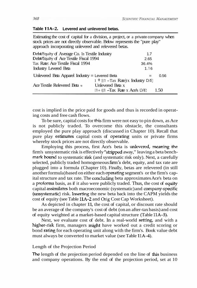
Table 11A-2. Levered and unlevered betas.
Estimating the cost of capital for a division, a project, or a private company when stock prices are not directly observable. Below represents the "pure play" approach incorporating unlevered and relevered betas.
DebVEquity of Average Co. In Textile Industry 1.7 DebVEquity of Ace Textile Fiscal 1994 2.65 Tax Rate: Ace Textile Fiscal 1994 36.4% Industry Levered Beta 1 .I 6
Unlevered Beta Apparel Industry = Levered Beta = 0.56 1 + [(I -Tax Rate) x Industry D/E]
Ace Textile Relevered Beta = Unlevered Beta x [I+ ((1 -Tax Rate x Ace's D/E) 1.50
cost is implied in the price paid for goods and thus is recorded in operat- ing costs and free cash flows.
To be sure, capital costs for this firm were not easy to pin down, as Ace is not publicly traded. To overcome this obstacle, the consultants employed the pure play approach (discussed in Chapter 10). Recall that pure play estimates capital costs of operating units or private firms whereby stock prices are not directly observable.
Employing this process, first Ace's beta is unlevered, meaning the firm's unsystematic risk is effectively "stripped away," leaving a beta bench- mark bound to systematic risk (and systematic risk only). Next, a carefully selected, publicly traded homogeneous firm's debt, equity, and tax rate are plugged into a formula (Chapter 10). Finally, betas are relevered (in still another formula) based on either each operating segment's or the firm's cap- ital structure and tax rate. The concluding beta approximates Ace's beta on a proforma basis, as if it also were publicly traded. Thus, the cost of equity capital assimilates both macroeconomic (systematic) and company-specific (unsystematic) risk. Inserting the new beta back into the CAPM yields the cost of equity (see Table 11A-2 and Orig Cost Cap Worksheet).
As depicted in chapter 11, the cost of capital, or discount rate should be an average of the company's cost of debt (on an after-tax basis) and cost of equity weighted at a market-based capital structure (Table 11A-3).
Next, we evaluate cost of debt. In a real-world setting, and with a higher-risk firm, managers might have worked out a credit scoring or bond rating for each operating unit along with the firm's. Book value debt must always be converted to market value (see Table 11A4).
Length of the Projection Period
The length of the projection period depended on the line of this business and company operations. By the end of the projection period, set at 10

A Primer on Shareholder Value 369
Table 11 A-3. Cost of capital calculation.
Instrument Before tx Aft tx % Product
Revolver Loan BV = MV 7.1 0% 4.52% 52.34% 2.36% LongTerm Debt including UP 7.65% 4.87% 7.04% 0.34O/0 Capital Lease Obligation
including UP 8.00% 5.09% 0.67% 0.03% Preferred Stock 8.00% 8.00% 2.58% 0.21 % Equity (See CAPM calculation
below) 11 .OO% 11.00% 37.37% 4.11% Managementighted Average
Cost of Capital 100.00% 7.06% ** Equity cost of capital: Capital Asset Pricing Model Assumptions Treasury 10 Year Rate 5.00% Market Risk Premium (Source KMV Corp) 4.00% Beta Textile Industry (Source (Financial Management) 1.16 Ace Textile's Relevered Beta (see below) 1.50 Capital Asset Pricing Model Formula = Treasury Rate + Market Risk Premium x Ace Textile's Beta .05 + .04 x 1.5 = 1 1.00% Tax rate 36.4%
Table 1 l A-4. Capitalization weights.
Value of debt Amount Percentage
Revolver Loan BV = MV 5062.0 52.34% Long Term Debt including CIP 680.6 7.04% Capital Lease Obligation including UP 64.6 0.67% Total Debt Value 5807.2
Equity Value: Preferred Stock 250.0 2.58% Equity 3614.0 37.37% Total Capitalization 9671.2 100.00%
years, operations are assumed to be at a mature and sustainable operating level so that a residual value can be easily estimated. "Growth" phenom- ena such as rapid revenue expansion, surges in operating margins, or unsettled working capital accounts should be behind the company. Five, 7- or 10-year projections are usual for companies projecting normal sales growth and profitability margins. Management and their valuation appraisers assumed that Ace will earn returns exceeding the cost of capi- tal during the explicit forecast period but that the company's rate of return on new invested capital equals the cost of capital in the residual period. Extending the forecast period leads to an increase in value, attributable to
the increase in rate-of-return assumptions. The important point to remem- ber is that the forecast period should be long enough to allow the business to achieve a state of operations by the end of the period.
Residual (Terminal) Value
The residual value of a firm is attributable to the period after the forecast period, which was assumed at the beginning of year 11. This component of valuation estimates the future value of the company at the end of the pro- jection period, $9,845, and discounts that value to the present, $5,005. The value of the company at the end of the projection period represented a sig- nificant portion of the firm's value. Terminal value depends on the under- lying assumptions and the length of the projection period in addition to the specifics of the business. Projection periods that are short place more emphasis on residual value. The methods of estimating residual value included (i.e., the real firm, not the one disguised here) liquidation value, book value, steady-state EBIT capitalization, and market multiple tech- niques. Management and their consultants determined that steady-state income capitalization was the most appropriate residual value determi- nant. Steady state assumes the following:
1. Net investment in fixed assets are zero, and capital expenditures equal disposals.
2. Net working capital requirements are zero, and sources of working capital equal uses of working capital.
3. The firm earns constant margins, maintains a constant capital turnover, and thus earns a constant return on invested capital.
4. All new investments earn a constant return.
Gross Cash Flow, Gross Investment, and Free Cash Flow
Ace's gross cash flow represents the total cash flow thrown off by the com- pany, or the internal cash provided for reinvestment. Gross cash flow includes net operating profit less amortization and taxes and depreciation. Gross cash flow internally finances gross investment. Gross investment includes working capital, capital expenditures, and net increases in other assets (nonoperating items are excluded from the calculation). Thus, the final result, free cash flow, represents the difference between gross cash flow and gross investment.
Change in Working Capital
Only operating working capital should be included. Nonoperating assets, excess marketable securities, and interest-bearing liabilities (short-term debt and the current portion of long-term debt) are excluded because they are pro- duced externally as financing activities and do not represent internally gen-

A Primer on Shareholder Value 3 71
Table 11A-5. Summary.
Optimal Strategy
Variance boundary tied to 4.0% I 4.9% 5.0% I 8.0% 8.1% 19.9% operating leverage and alllied with capital costs
Cost of capital 7.0% 8.1 % 12.0% CapXIRevs 0.4% 2.1% 3 .O% Actual variance 2.6% 8.0% 9.5% Operating margin 5.6% 6.9% 7.6% Shareholder value 4,608.1 5,339.8 26.9 Is operating margin greater Yes Yes No
than the threshold margin?
erated flows. Working capital changes equals changes in current assets (excluding marketable securities) net of changes in current liabilities (exclud- ing all funded debt, including the current portion of long-term debt).
NOPLAT
Net operating profit less adjusted taxes (NOPLAT) represents the afta-tax oper- ating profits of the company after adjusting the taxes to a cashbasis. Exhibit 11-8 and the Invested Capital Worksheet shows the calculation of the firm's NOPLAT and a reconciliation of NOPLAT to Ace's accounting net income.
Setting Up Optimization Runs
Optimization Engine
The CAPM was employed to maximize operating margin constrained by volatility. We assume a bit of editorial license by substituting operating margin for expected portfolio returns5 The firm's asset portfolio is subject to risk, and this is related to the interaction between fixed and variable costs (e.g., operating leverage unique to each product segment; note again hat cost of goods sold has been established as the key value driver). Cer- tainly, a disasterous cost-of-goods policy would indeed impact on asset risk and escalate finance distress probabilities. (See Exhibit llA-9, The Base Case Optimization Employing the CAPM.)
In a more factual setting, it is better to assess each operating segment's cash flow and then run discounted cash flow valuations on both a stand- alone (segment) and a combined or consolidated basis. However, this entails breaking down each unit into its smallest component and allocating cash flows accordingly, assessing differences in capital structure, cost of
5. The Ace Textile optimization model was derived and modified from an Excel template to illustrate how a stock portfolio is optimized.

Exhibit 11A-8. Ace Textile Production Corp. NOPLAT, NOPLAT reconciliation and invested capital for 1992-Perpetuity.
NOPUT Net Saieg - ~- ~-
Cost of Gwds Sold Selling, Gen 8Admin Expense Depretiation Expense OtheiO~er Inmme lEwn~e EBlT '1.641.5' '1.745i 1,655.6 1.972.6 2.096.8 2.227.5
Pmvfor nc Taxes Tax Shleld on Interest Exp Tax on Intere* Income Tax on Nanoperatlng lnmme Taxes on E81T
Net lnmme Add: ExVaotdinary Items Add: Sperjal Items A k r Tax
Miusled Nel Incame 683.3 732.7 605.6 684.0 968.2 1,058.7 Add: lnlereot Expense A k r Tax 236.3 286.8 265.8 265 6 286 8 265.8 T m l lnmme Avail lo Investors 919.5 998.4 1,071.4 1,1498 1,2340 1,324.4 Less Interest I n m e ARer-Tax 0.0 (17.7) (25.4) (34.8) (46.0) (59.2)
OpraUng Cumrnt Rsssts Non4oterest Bearing LiabilSss
opsrahny working Capita
NBt Pmprty Plant and Equipment 0th Assets Net of M e r Liabs Value 01 Operating Leases
Oprsting Invested Capital
F~recast Forecast Forecast Forssast NOPIAT Z W ZQ!Q 2Q!B ZPP4 F3iR Net Sales 40.227.4 42,209.2 44,286.7 46,4707 46.7602 Cod of Gwds Sald (33.120.5) (34,752.3) (36,4644) (38,2609) (40.145.9) Selling, Gen 8 Admin Expn- (1.528.6) (1.604.0) (1,6830) (1.766.9) (1,852.9) Depreciation Expense (97.5) (101.3) (105.3) (109 5) (113.9) Other Oper inmmdExpnse (3.1146) (3.239.4) (3.369.0) (3.503.7) P.MJ.9) EBlT 2.365.9 2.512.3 2.567.1 2.1130.7 3.003.7
Pmv for Inc Taxer Tax Shield on Interest Exp Tax on Interest lnmme Tax 11" Nonoprating lnmma Taxs on EBlT
Raconcilistion to Net lnwrne Net l m s Add: Extraordinary Items Add: Special items Alter Tax
Adjusted Net Income 1,1556 1.259.7 1.371.1 1,490.5 1,618.4 M d : Interest Expense ARer Tar 265.6 265.8 265.8 265.8 265.8 Total Income Avall lo Investors 1,427.4 1.525.4 1,636.9 1.758.3 1,884.2 Less: Interest Income ARer-Tax (74.5) (92.1) (112.3) (135.2) (161.0)

A Primer on Shareholder Value
Exhibit 11 A-8. Continued. Invested Capltal
Operating Current Assets Non-lnterest Bearing Liabilties
Operating Wohing Capital 13.2750 13,9290 14.6153 15,335.3 16,080.9
Net Property Piant and Equipnenl 1,0057 1.055 2 1,107.2 1.1616 1.2190 Other Asoets Net of Other Liabs (402 3) (422.1) (442.9) (464.7) (487 6) Valued Operabng Leases 0.0 0.0 0.0 0.0 0.0
Operating lnvesled Capital 13.878.4 14,6622 15,279.6 76,0324 16.822.3
Excess Mahetable Securities 2,632.7 3,208.6 3.862 3 4.6W.O 5,428.6 Goodwill 0.0 0.0 0.0 0.0 0.0 lnvestmentr a Advances 0 0 0.0 0 0 0.0 0.0
capital, and headquarters cost. The analysis required to accomplish a more authentic result is somewhat beyond the dimensions we allow in the case.
The CAPM permits the criteria for asset expansion decisions under uncertainty to be set out comprehensively and succinctly. With modifica- tions, the CAPM meets the criterion allowing for capital budgeting analy- sis. The market constants remain the same. The risk-measuring variable, beta, traditionally fixed to individual firms, holds for operating segments as well: Systematic risk is systematic risk. Drawn from the financial litera- ture, conditions that must hold if any project is deemed acceptable can be stated as shown in Exhibit 11A-10.
Consider the following: The expected return on the new project for ABC Inc. must exceed the pure rate of interest plus the market risk pre- mium adjusted by the project's beta, the measure of the individual pro- ject's systematic risk.6
The criterion in graphical terms is to accept projects that plot above the security market line and to reject all those that plot below the market line. Managers seek to find any number of projects, such as W and Y, with returns in excess of the levels required by the risk-return market equilib- rium relationship. When such projects are added to the firm's operations, the expected return on the firm's common stock (at its previous existing price) will be higher than required by the market line.
From this, we extrapolate to measure product lines (after optirniza- tion). Will the new product line mix preserve or destroy shareholder value?
First, set up the optimization run (Exhibits 11A-11 and llA-12):
Objective: Maximize combined operating margin. Set target cell to D16. Decision variables: Eliminate product lines and/or change contribu- tion to operating margin by changing cells D9:D13. Subject to the constraints: Variance limit (cell F16) = 8%, no product line can be negative, Cells D9:D13 > 0 and total investment (cells D9:D13) = 100.
6. See chapter 10.

0
8 g E 8 $ 8 1 2 ~ 2 2 2 2 . e s"
d d d d o o
C .- P
: 0
P 0 0 * g j z z 6 a z j $ z m 5
@ .E
2 Si! U 0 0 0 0 0 m ! q m t o ? 9 - : ~ e (g 0 0 7 - 0
Q Q m
2 $ $ 3 w C + . . C 0 I - .- s : t .N 9 : E 2;; = '2 g
+# g u . d - 8 1 ib
Y $ - s 2 f d m s m g f
0; 4 Z f . k g a 3 8 r m m m a m
P .E .I .S .P C)
C e o o o o g X Y C L t t t t c

A Primer on Shareholder Value
Exhibit 11A-10. Project betas: A criterion to either accept or reject projects.
Excepted Returns
I Acccept Y
Securlly Market Line
Pmled Betas
Risk Free Rate
The results suggest that based on assumptions set in this example, the firm will optimize operating margins with volatility constrained at no more than 8% requires the following changes:
Rsjecl X
1. Product Line Kappa Management is scaled down to 1% of the busi- ness from 22%.
2. Product Line Epsilon expands slightly to 21%. 3. Product Line Sigma jumps to 53% up considerably from its previ-
ous level of 10%. 4. Product Line Omega Increases to 25% from 10%. 5. Product Line Lambda is divested altogether.
Pl 82 03 I%
Then, test optimization (and the resulting valuation) utilizing Rapapport's threshold margin.
Ace Textile's Threshold Margin7
Quoting the author of the threshold margin:
The threshold margin represents the minimum operating profit margin a busi- ness needs to attain in a w period in order to maintain shareholder value in that period. Threshold ma>& is a new type of "break-even analysis," a value- oriented economic break-even analysis. Stated in yet another way, threshold margin represents the operating profit margin level at which the business will earn exactly its minimum acceptable rate of return, that is, its cost of capital.
7. The case will only provide Rappaport's threshold/margin structure that was developed in Excel. For a complete examination of this important valuation concept, the reader is referred to Rappaport's excellent and groundbreaking text.

Exhibit 11 A-11 . Project optimization: Use the CAPM approach outlined above.
Benchmark Industv Asset (Pwffofio) Operating Margins (Assumed)
Product Line Lambda

A Primer on Shareholder Value
Exhibit 11A-12. Microsoft Excel 9.0 answer report worksheet: [robMainSimAOptB.xls]Optimization report created: 1 /24/2000 7:07:17 pm Target Cell (Max)
Cell Name Original Value Final Value $0522 Opeating Margin 5.6% 6.9%
Constraints Cell Name Cell Value Formula Status Slack
$D$20 TOM Weght 100 0% $D$ZO=l Blndlng 0 $F$22 Variance _- 8 0% $F522<=0 08 Blndlng 0 $D$IS _Produci Line Kappa Welght - - _ _ _ _ __ _ - - _ 11% $D$15>=0--_ N d Blndl!g- - . . - ij:b _$D516-@Llne Epsilon Welght - 21 3&$D516>=0 Not Bm~dlnq 21 3% $0517 Product Lone Stgrna We~ghl - 53 0% $D517>-0 N d Blndlng 53 0% $0$18 Produd Llne Omega Welt-- 24 6% $D$18>=0 Not Blndlnq 24 8% $D$19 Product Llne Lambda Wetght 0 0% 5D$19>=0 Bind ng 0 0%
Exhibit 1 IA-13. Threshold margin formulas.
lncremental Fixed Capital Investment Formula % (Capital expenditures - Depreciation expense) / lncremental sales
lncremental Working Capital Investment Rate % Formula lncremental working capital investment I lncremental sales
lncremental Threshold Margin Formula (Incremental fixed plusworking capital investment rate) * (Cost of Capital)
(1 +Cost of capital) * (1 - Income tax rate)
Threshld Margin Formula Prior period operating profit + (lncremental threshold margin) * (Incremental Sales)
Prior period sales + lncremental sales
Instructing operating managers to invest in strategies that earn more than the cost of capital is not enough. To bridge valuation concepts of modem finance theory with the needs of corporate decision-makers, what is needed is an easily understood, operationally meaningful concept that enables managers to assess the value creation potential of alternative strategies. The threshold margin con- cept is particularly suited to facilitate this linkage because the operating profit margin has widespread acceptance from both security analysts and corporate management as an essential ratio for assessing operating profitability and effi- ciency. The threshold margin can be used to evaluate the past performance of a business so that management can establish performance targets for the future.8
Exhibits 11A-13 and 11A-14 depict the calculation of the threshold margin. (text continues on page 380)

Exhibit 1 IA-14. Threshold margin calculation. 1994 m s ises lw 1998
Cod d Capltal 8.1% 8.1% 8.1% 8.1% Cash Tax Rate 41.0% 41.056 41.01 41 .O% Operating Profit 1,269.0 2,088.0 2.417.5 2.570.7 2,732.8 Opsrating Margin Optlmked 6.946 7.6% 7.7% 7.8% Original Operating Margin Growth Rate Appned After 1995 (assumed unchanged) * 10.35% 1.34% 1.31%
lncremental Fixed Capital Investment Calculatlon % Capital Expenditures Depreciation Expenses Sales lncremental Sales lncremental Fixed Capital Investment X
lncremental Working Capital Investment Calculation Accounts Receivable Inventory Accounts Payable AcCnralS Tolal Net Working lnvestment lncremental Working Capital lnvestment
lncremental W I C lnvestment Rate % Calculatlan incremental Working Capital Investment 790.3 466.3 489.3 513.4
lncremental Threshold Margin Calculation lncremental Fixed Caoital Investment Plus Working Capital investment Rate Cost of CaDital
Threshld Margin Calculation Prior Period Operating Profit lncremental Threshold Margin Incremental Sales

Cost of Capital Cash Tax Rate Operating Profit Operatlng Margin Optimized Original Operating Margin Growth Rate Applled After 1995 (assumec
lncremental Fixed Capital Investment Calculation % Capital Expenditures Depreciation Expenses Sales lncremental Sales lncremental Fixed Capital lnvestment %
Incremental Working Capital lnvestment Calculation Accounts Receivable Inventory Accounts Payable Accruals Total Net Worbng lnvestment lncremental Working Capttal lnvestment
lncremental W I C Investment Rate % Calculation Incremental Working Capital Investment 538.7 565.2 593.1 622.3 653.0 685.1 718.9
Incremental Threshold Margin Calculation lncremental Fixed Capital lnvestment Plus Working Capital lnvestment Rate Cost of Capital
Threshld Margln Calculation Pr or Per 00 Opera1 na Profil Incremental ~hreshold Margin Incremental Sales 1.715.6 1800.1 I ~ R R R R 1 9 R 1 9 7 n 7 4 5 7 1 ~ 7 n 7 7 ~ ~ 5

The business has been optimally structured with shareholder value preserved. The measure of value added is the spread between the operat- ing margin and threshold margin (Exhibit llA-15).
Finally, the summary (Exhibit llA-16) reveals that the optimal vari- ance boundary allied with capital costs falls between 5.0% and 8.0%. The cost of capital under these conditions is expected to be 8.1% versus 12% of the variance boundary were to exceed 8.0%. Ideally, the relationship between capital expenditures and revenues falls out at 2.1% indicating that increasing operating leverage "just enough" will optimize shareholder value. Increasing operating leverage too fast is a value destroying strategy.
This analysis would have been difficult to perform without simula- tion which was utilized early on to test and structure the firm's operating and financing strategy (Exhibit llA-17). Exhibits llA-15 and llA--16 are in the Optimization Worksheet and you can view Exhibit llA-17 in the Orig. Sim Worksheet.

Exhibit 11 A-1 5. The new business optimized. New Operating Margin Spread Bv Substitutina O~tmimal O~eratlna Marain 1995 1996 1997 Threshold Margin 4.745% 6.975% 7.643% Optimal Operating Margln * 6.927% 7.643% 7.746% Operating Margin Spread (OM - TM) 2.181% 0.668% 0.103% Cost of Capital 8.10% 8.10% 8.10% Shareholder Value Preserved (OM > TM)? YES YES YES
New Operating Margin Spread Bv Substitutina O~tmimal O~eratina Marain 2001 2002 2003 2004 Threshold Margin 7.979% 8.063% 8.146% 8.229% Optimal Operating Margin * 8.147% 8.245% 8.342% 8.438% Operating Margin Spread (OM - TM) 0.168% 0.182% . 0.196% 0.209% Cost of Capital 8.10% 8.10% 8.10% 8.10% Shareholder Value Preserved (OM > TM)? E YES YES YES YES
1998 1999 2ooo 7.727% 7.811% 7.895% 7.848% 7.948% 8.048% 0.120% 0.137% 0.153% 8.10% 8.10% 8.10% YES YES YES
8.312% 8.533% 0.221% 8.10% YES

Exhibit 11 A-1 6. Summary.
Variance boundary alllied with capital costs Cost of capital CapX/Revs Actual variance
Optimal Strategy 4.0%<=4.9% 5.0%<=8.0% 8.1 %<=9.9%
12.0% 3.0%
8.0% 9.5%
* 1996 and beyond adjusted by original operating margin growth rate. **Assume the Company lost a big customer in 1996.

Exhibit 11A-17. Ace Textile Production Corp. the Crystal Ball simulation report-Base case.
Sensivlty Chart
Target Forecast Equlty Value
COGSlRevenuas -37
Inventories - 42
SGWJRevenues -.I6
Accounts Recsivable -.I0
Revenue Gmwth .07
CapXlRevs .08
Cost of Ca~ilal
-1 -0.5 b 0.5
Measured by Rank Correlation
l ~ o s t of Goods I Revenues
Valuation does not seem sensitive to PPBE (CapEx) and Cost of Capital Assumptions.
Forecast: Equity Value
Summary Certainly Level is 0.50% Certainly Range is from -Infinity to 0 Display Range is from -1497 to 10829 Entire Range is from -1497 to 11643 After 1,000 Trials, the Std. Error of the Mean is 73
Cell: C433
This means that there is a 50 basis point probability that shareholder value falls below zero. Thus, the EDF's or Expected Default Factor can be assumed. And from this, the bond rating.

-
C Frequency s " " , - B
5 6 ;

Assumption: Revenue Growth Cell: M 2 5 1
Triangular distribution with parameters: Minimum 4.7% Likeliest 4.8% Maximum 5.3%
Selected range is from 4.7% to 5.3%
The valuation is very sensitive to Cost of Goods Sold. Both the distribution and assumptions behind this variable
Assumption: COGS/Revenues will need to be rechecked and refined. Cell: M 2 5 2
Triangular distribution with parameters: Minimum 80.0% Likeliest 83.0% Maximum 84.0%
Selected range is from 80.0% to 84.0%
Assumption: SG&A/Revenues
Uniform distribution with parameters: Minimum Maximum
Cell: M 2 5 3
- ?m *A 4%
(continues)

Exhibit 11 A-17. Continued. Assumption: Accounts Receivable
Triangular distribution with parameters: Minimum 15.8% Likeliest 16.4% Maximum 17.0%
Selected range is from 15.8% to 17.0%
Cell: M263
Assumption: Inventories Cell: M264
Lognormal distribution with parameters: Mean 25.0% Standard Dev. 2.5%
Selected range is from 0.0% to +Infinity
Assumption: CapWRevs Cell: M272
Triangular distribution with parameters: Minimum 0.5% Likeliest 0.5% Maximum 0.6%
Selected range is from 0.5% to 0.6%
The valuation is not sensltive to cost o f capital. This is unusual. The distribution and assumptions behind
Assumption: Cost o f Capital this variable need t o be reexamined. Cell: M303
Triangular distribution with parameters: Minimum 6.7% Likeliest 7.0% Maximum 7.1%
Selected range is from 6.7% to 7.1%
Appendix Three to Chapter 11
The Alcar Group Incl
The valuation output for Sample Corporation, Strategic Plan 1999-2003 included in this appendix represents state of the art valuation. Alcar has generously provided their demonstration software included in the Alcar subdirectory of the CD. It may be a good idea to view this application before reviewing Sample Corporation output. For nearly two decades, Alcar has been providing financial software and services worldwide. Client base includes many of the Fortune 500 and top financial institutions. Provides a standardized framework within which to perform strategic financial planning; flexibility to customize the system to specific business structure and planning requirements; enhanced portfolio management capabilities with consolidation of existing businesses and potential acqui- sitions; a system that uses value-based metrics integration with current or future general ledger and database systems. Before you read over these exhibits, you may want to view the Alcar demo, "Alcar" on the CD to facil- itate data input and enhance reporting.
Key Features
A Historical and forecasted financial statement generation A Consolidation of any business unit structure and M&A deal structure A Valuation Analysis for strategic planning and M&A analysis A Funding Options to manage optimal capital structure/funding sur-
pluses and deficits A Sensitivity Analysis to determine impact of changes in assumptions
and key value drivers A Scenario Manager to generate unlimited scenarios A Analyze to drill down from report output to easily identify under-
lying assumptions and input errors A Report Custornization A Translation to and from any currency
1. Reproduced with permission The Alcar Group Inc.

SCIENTIFIC FINANCIAL MNAGEMENT
lnmms Smemed for Sample tnsayomed stategic Plan I998-2W2
~ u h o r ~ ~ c s r lmplernenb!ion SBMCBS amup SIC cow 4mO scensno. Bane Mlllionsoi Wllan
P l M U d Sales 466.24 512.40 524 15 667 5% 188.82 GIZ.BO 653 60 SCMce RdMnUB8 1.48630 1.519.20 1.701.50 1,88867 2.05865 2.223.34 2,60121
.................... ..... %b+8 1.83456 2,05160 2.225.68 2.418.24 1,66847 2.865.94 3.054.81 Diroounto 8 Relvrns 9 10 10 10 10.48 11.15 l l . 0 0 16.06 16.34
....... ... - .
Sales ( ~ e t ) 1,92511 Z.OZ150 2.21518 2.435.09 2.636.86 2.84967 3,038.47 Colt ol G O N S Sold 1,435.20 1.529.90 1.64699 1,773.53 1.906.90 2.053.48 2.199.46
- .... -- .- . - orass Prahl 490.24 49160 588.19 681.57 72978 766.40 839.01
Salary W n s e 156.20 16930 18314 146.71 158.91 171 86 183.29 Selllno Exo- 54.50 67.60 55 M 61.18 86.21 71 65 76.37
mprecidon Erpense mon~zanm Expense
operating Profit
Other Revsnues & Galna Gal" on Sab ot Assas oms, tmenne% s iausa o~videndr fmm Investments cost
Earnings W o i s Infere4 & Tarss
Total interest inmms
InieiM on Curr. Portion oi L-T Debt 0.00 0.00 0 00 0.00 0.00 0.00 0 0 0 Interas( an Revalvlng Uw of Cred) 0.00 0.00 5 40 0.00 0.00 0.00 0 00 lntema on senlor ~ e b t 12.40 14.60 26.78 25.63 30.58 28.88 32.96 lntsrsrt on Subomlnats ~ c b t 0 00 0.00 0.00 0.00 0.00 0.00 0.00
................. ................. ................... Interest on Total L-T D e n 12 40 1660 28.78 25.83 30.56 28.68 82 91 ~an-cash ~nts-t on senin D e n o DO 0.00 0.00 0.00 0.00 0.00 o 00
NEn.Cash In! on Total L-T Deb, Interest an hng-Term Dam' 0.0. Mhsr Interest Expense
Interest m n s e Interest Capitalized
Current P m . for In0 Tares (Excl. NOL) T u Refund
Current Pmvsm lor nmms Taxes Debmad R w l s l m fW incoma Tsrea
Pmvislon lor Inoorne Taxes 67.10 23.40 8493 101.90 106.16 11725 130.48 Ofher Tares 0.00 0.00 0 00 0.00 0.00 0.00 0.00
................ TOUl Tax- 67.80 23.40 84.91 101.90 10818 117.25 190.46
........ -- Income ltfw TT 102 61 106.35 128.84 153.38 160.05 177 39 198.05
Earnings fmm Invests: E ~ u w 0.00 0.00 (I DO 0.00 0.00 0 00 0 00 Mlnodlv Inlsrerf in l m m e D.00 0.00 0 00 0.00 0.00 0 00 D O 0 Erwaordlnsw Item (net 04 tax) 0.00 0.00 125 00 0.00 0.00 0.00 0.00
..................... ................... Net Income 10264 105.35 251.84 153.38 16005 17139 198.08
-========= ========-= ----- -....==-- ========= =======a ========== -=========

A Primer on Shareholder Value
Direct Cash flow for Sample Incorporated Strategic Plan 1998-2002
Author: A1c.1. ImplemenYtion Sewces Group SIC Code: 4800 scemno: Base
Prahrct Sale service Revenue.
Discounts & Return I W Sales (Net) lC& of Goods Sold
Saisw Ocpenre 169.30 133.54 146.77 158.91 171.96 183.29 5elling Expenra 57.80 55.64 61.16 66.21 71.65 Adminirtrat,"e Expenses
76.37 93.50 98.1 8 103.08 108.24 113.65 119.33
Total SG & A Expense 320.60 287.36 31 1.01 333.36 357.25 other Operating lncome/(~l~.)
378.99 0.00 0.00 0.00 0.00 0.00 0.W
Oepnciatlon Exwnse 55.10 66.06 111.06 144.06 149.82 154.40 Am0~iz8fim of Goodwdl 6.40 6.00 6.00 6.00 6.00 6.00 Amortizanon of Other lntang#bles 1.20 1.20 1 .ZO 0.90 0.00 0.00
~- Operating Profit 108.30 207.57 232.29 245.46 273.32 299.62
Amortization d Goodwill Depreciation Expense (Funds) Amonization of Other mtsng~blen Increase in Other Deferral.
Funds from Operatlana Before Tax Tow1 Taxes an operation.
l~unde from Dperatlons After Tax
lncrememal Wwklng Capital Investment Fired Capltal lnvesrmem imerert Cslliralired Addtion% to Land Additl0"l to G o o d ~ l l Addtlonr t o Other Intangibles Roceedsfrom Sale of Asrefs I ~ C R ~ S ~ in on-currem Operating ~ s r e r increase ~n Non-current Opraring bab~lity Carh Flow Adlustment: Source
(Ca~h Flow fmm Operations
Cash F im fmm Dperations Interest Expense NO"-Operating Sources Nowoperating User NowDperating 1nc-e Currenr NonaDemfing Taxer Carh Flow Adjusrment: source Preferred Divrdends
- ... -. . Net Carh ~ w l d e d Common ~ividendr
-~
/Funding Surplus I (Oeficl) (82.351 181.76 (50.601 (6.04) 106.05 174.99 1 Funding Surplur / (Deflc~t) (62.351
n on " lncreare m Rewiving ~ l n e of credit Increase m senor o e t Increase in Subordinate k b t
increase I" Total Lone rem oebr 103.20 Non-Cash Interest on Senior Debt 0.00 Non-Cash Interest on sub. ~ e b t 7.55
-. Non-Cash lnl. on Total L-T Debt 7 5 5.41
0.00 0.00 o a o 0 0 0 0.00 0.00 0.00
- - increase In Long-Term ~ e b t : ~xcerr 0 0 0 Increase in LOW-~enn ~unding ~~~~t 0.00 Praceedlfrom Sale of Preferred stock 1.50 Proceeds fmm Sales of Common stodr (par 7.90 lncr in ~ d d ' l PIC (cmn stock) 0.00 InCr. ,n Treasury Stock 0.00 Incr. In PIC from ~reasury stock 0.00
I iocr. in Cammon Stock ( ~ e i of ~rearury) 7.90 Affordable rnvldend 0.00
~ ~~
~-
Increase In To~ai Marketable Sgurrfnes 66.80 110.68 (8.321 (34.45) 141.89 155.00 ----------- ----------- --====----= --------- -=--------
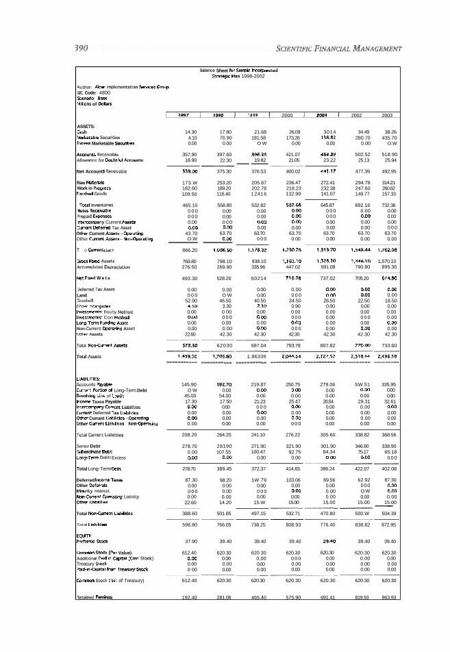
& W e Sheet b r Sample lmapoated Strategic Plan 1998-2002
AU~~OI: AIcar Iwlememavm Sewices ~ m u p SIC Code: 4800 Sosnatio: Base Mllllonr of OollaR
1 ID97 1 1998 1 1999 1 2000 1 2001 1 2002 1 2003
ASSETS: Csrh 14.30 17.80 21.68 26.09 3014 34.49 38.26 Maketable SecWes 4.10 70.90 181.58 173.26 138.82 280.70 435.70 kcerr. Marketable Securities 0.00 0.00 O W 0.00 0.00 0.00 O.W
A c m u m REce-ble 357.90 397.60 396.35 421.07 464.39 502.52 518.90 AlW,ace for Dwbtful Amunts 18.90 22.30 19.82 21.05 23.22 25.13 25.94
-. -- Net Account$ Rw&-,able 3 3 9 . ~ 375.30 376.53 400.02 441.17 477.39 492.95
Raw Matetiall 173.W 253.20 205.87 236.47 272.41 294.78 314.21 Work in Pmgrwr 182.60 189.20 202.78 218.23 232.38 247.60 260.82 Plntrhed G o d s 109.50 116.40 12416 132.99 141.07 149.77 157.33
Tolal ImWo"e0 465.10 558.80 532.82 587.a 645.87 692.16 732.36 Notes Recewrble 0 0 0 0.00 0.00 0.W 0 0 0 0.00 0.00 Pmpald Exp- 0 0 0 0.00 0.00 0.W 0 0 0 0.03 0.00 lntermmpany Current Arsets 0.00 0 0 0 0.W 0.W 0.00 0.00 0.00 current ~eferred ~ a x ~ 6 - t 0.00 O W 0.00 0.00 0.00 0.00 0 0 0 Ozher Current h t r - Operatiw 43.70 63.70 63.70 63.70 63.70 63.70 63.70 Other Currem Ametr - Nan-Operatinp O.W O W 0 0 0 0.00 0.00 0.00 0.00 -- T O ~ Cumnt &let? 866.20 1.086.50 1.176.32 1.250.76 1,319.70 1.548.44 1,762.98
Gmsr Fmrd b e t s 769.80 798.10 938.10 1,163.10 1.328.10 1.446.10 1,570.10 A d a t & Depm&l;m 276.50 269.90 335.96 447.02 591.08 790.90 895.30
Nel Fixed W e t s 493.30 528.20 60214 716.08 737.02 705.20 67.1.80
D e k r m T m l \ M 0.00 0.00 0.00 0.00 0.W 0.W 0.04 Land 0 0 0 O W 0.00 0 0 0 0.W 0.W 0.00 GaodVnl 52.90 46.50 40.50 34.50 28.50 22.50 18.50 Other lnm 4.50 3.30 2.10 0.90 0.00 0.00 0.00 1""ertments: Equ* M e w 0.00 0 00 0.00 0.00 0.00 0.00 0.00 ~werrmenrr: Con ~ e t h o d 0.W 0 0 0 0.00 0 0 0 0.00 0 0 0 0.00 LangTcm Funding Asset 0.00 0.00 0.00 0.00 0.00 0.00 0.00 ~ m ~ m e n t Opemrhg *rref 0.00 0.00 0.W 0 0 0 0.00 0.W 0.00 Other l\rYf.r 22.60 42.30 42.30 42.30 42.30 42.30 42.30
.- - ~ 0 t a 1 on-Curem &sets 573.30 62030 687.04 793.78 807.82 770.00 733.60 - - Total 1.439.50 1.706.80 1.86336 2,044.54 2.127.52 2,316.44 2498.58 ------- ---------- --------- ------=-=- *-------- --------- ------ UABILITIES: -untr Ryable 145.90 192.70 219.87 250.75 279.06 SW.51 335.95 Current mn'w al Long-Term Debt O W 0.00 0.W 0.W 0.00 0.00 0.00 Rewlnng line of Credlt 45.00 54.00 0.00 0.00 0.00 0.00 0.00 lnmme Taxes Payable 17.30 17.50 21.23 25.47 26.54 29.31 32.61 1ntermmpny cumen, Ml l i t le r 0.00 0.00 0 0 0 0.00 0.00 0.00 0.W current & f e d T ~ X Uabllaies 0.00 0.00 0.W 0.00 0.00 0.00 0.00 other Currant Uablller - Opnting 0.W 0.00 0.00 0.W 0.00 0.00 0.00 other current Llabllltler - ona ape rating 0.00 0.00 0.00 0 0 0 0.00 0.00 0.00
TOW cmnt ~ l a b l ~ t l e l 208.20 264.20 241.10 276.22 305.60 338.82 368.56
%"lor Debt 278.70 28190 271.90 321.90 301.90 346.90 338.90 Ylbardlnate Debt 0.00 107.55 100.47 92.75 84.34 75.17 65.18 i a n p T a m Debt Excess 0.W 0.W 0.00 0.00 0.W 0.W 0 0 0 -- -- - Total Long-Term DeM 278.70 389.45 372.37 414.65 386.24 422.07 402.08
Deferred Income Taxa 87.30 98.20 1W.79 103.06 69.56 62.92 87.30 Other D e f d r 0.00 0.00 0.00 0.00 0.00 000 0.00 Mirndty lntere* 0 0 0 0.00 0 0 0 0.W 0.00 O W 0.W m-cunent Dprating Llabllty 0.00 0.00 0.00 0.00 0.00 0.00 0.00 Other Uabllitler 22.60 14.20 15.W 15.00 15.00 15.00 15.00
-- -- - -- Total NoRCUmem Uabilier 388.60 501.85 497.15 532.71 470.80 500.W 504.39
- .- - Tote Lidblifie~ 596.80 766.05 738.25 808.93 776.40 838.82 872.95
E q m Preferred 5f-k 37.90 39.40 39.40 39.40 39.40 39.40 39.40
CDmmn Stock (Par Value) 612.40 620.30 620.30 620.30 620.30 620.30 620.30 ~ M # t m d Pald in Carnal (Cmn Sf&) 0.W 0.00 0.00 0 0 0 0.00 0.00 0.00 Treasury Stock 0.00 0.00 0.00 0.00 0.00 0.00 0.00 ParbmCapfal hclm T-ry Sreck 0 00 0.00 0.00 0.00 0.00 0.00 0.00 - -- -- - - Common St& (Net of Treasury) 612.40 620.30 620.30 620.30 620.30 620.30 620.30
& a n d EBmiME 192.40 281.06 465.40 575.90 691.41 819.93 963.93

A Primer on Shareholder Value 391
(in Millions of Dollars)
SBU A: Produd Price
SBU A: Cost -2.00%

Financial Ratlos for Zannple lmorponted 5tmegk Fbn 1998-2002
Amor: Altar impkrnentst!.Y Services Gmup SIC Code; 4800 Scenario: Base U l l i r n of ooi1an
-1997 I 1998 I 1999 I t o o n I roo1 I 2002 I 2003
PROFTTARFORMAWF RAMS: Gmpcl mtn Margln 25.46% 24.32% 25.65% 27.17% 27.68% 27.59% 27.61% Chnge in Net lrrame N/A 3.62% 136.79% -39.10% 4.35% 10.83% 11.65% Return on Sales 5.33% 5.26% 11.37% 6.30% 6.07% 6.22% 6.52% Return on Equity 12.75% 11.80% 23.20% 12.82% 12.20% 12.32% 12.5096 Return on Wet r or bverfrnent 7.9% 7.53% 8.25% 8.5796 8.6696 9.61% 8.90% Return on Net Auetr 9.34% 8.91% 9.47% 9.91% 10.11% 10.08% 10.44%
LEVERAGE RATIOS: OCbWEwIty Rafio (%) 44.93% 53.57% 37.93% 37.96% 32.45% 32.04% 27.87% Prekmd / Equity R s t i (96) 4.71% 4.37% 3.63% 3.2% 3.00% 2.74% 2.4% Deburotal Cspltal!%) 31.00% 34.88% 27.50% 27.51% 24.50% 24.27% 21.7% Preferred / Total Capifal(%) 3.25% 2.85% 2.63% 2.39% 2.27% 2.07% 1.94% Equity RBIb 55.91% 52.81% 58.27% 58.51% 61.65% 62.12% 63.46% Tlrner interert Eamd 14.689 6.859 6.124 8.568 8.150 9.643 9.841
A M RAMS: D8ys in Receivables 67.846 71.790 65.308 63.289 64.286 64.361 62.333 Days m Recevabks (4vg.) N/A 68.206 65.410 61.430 61.288 61.919 61.350 Dayrm Payabkr 37.105 45.974 48.727 51.747 53.415 54.748 55.751 Oayr in Payabler (AQ.) N/A 40.391 45.716 48.560 50.706 52.055 53.557 lnvenmv T m w e r 3.086 2.738 3.091 3.018 2.952 2.981 3.003 tnventov r u r n o ~ r (A"*) N/A 2.988 3.01 8 3166 3.092 3.084 3.088 Fimd Aaret TU- 3 903 3.827 3.679 3.401 3.577 4.041 4.503 Total W e t T v m o ~ r 1.338 1.1 84 1.189 1.191 1.239 1.229 1.217
UQIIOITY RATIOS: (hrrk Ratlo 1717 1.756 2.405 2.170 1.996 2.339 2.623 C u d Rafn 4.1 60 4.112 4.879 4.528 4.318 4.570 4.763 WorCing Capaal 658.00 822.30 935.22 974.53 1.014.09 1,209.62 1,39142 Oeera(ing WoeiW CBpUai 698.90 805.40 753.63 801.27 875.27 928.92 958.72
PER-SHARE DATA Earnings Per Share 7.354 7.616 18.456 11,108 11.606 12.900 14.442 Chacge in Earnings Per S a m (96) N/& 3.57% 147.33% 39.81% 4.48% 11.15% 11.95% Fully D l u t d Esrnlngs Per Share 7.354 7.616 18.456 11.108 11.606 12.900 14.142 O~ldends Par Share 0.933 1.000 4.698 2.862 2.986 3.310 3.695 Carh Flow Per Share WA 2.291 9.009 -1.691 1.867 10.528 15.691 Bod Veiue Pet Share 60.970 68284 -1.100 -1.212 -1.329 -1.459 -1.605
VALUE DMVERS: %ala 6 r a w ~ l ~ a f e (G) WA 4.99% 9.58% 9.93% 8.28% 8.09% 6.6296 Operating Profit Margin (P) 7.78% 4.65% 8.30% 10.49% 12.80% 10.40% 6.OLM lncrernmmal n x d ~apital lmerrment (F] WA 47.89% 38.18% 51.81% 10.39% -14.93% -16.12% mcrernentd woelns capital lnvenment (w) A 110.87% -26.73% 21.66% 36.71% 25.16% 15.80% Cash lncme Tax Rate (TC) 44.81% 13.29% 39.0996 39.36% 39.25% 33.29% 39.48% Cost of Capital (K l (%I 10.00% 10.0mt 10.00% 10.00% 10.00% 10.00% 10.00%
SHIIREHOLOFR VIVUE RAT05 Cum. W o l M Flwr N/A A 109.75 91.02 109.61 206.17 336.72 W of Readual Valve WA N/A 1.262.02 1,280.08 1.228.01 1.24(1.08 1.233.46 ------- Cum. W or ulrh Flow4 and Rcri&al Value N/A I 1.37137 1,371.10 1,337.82 1,446.25 1.570.18 ~ C L m ShrehoWcr Vdua 0.W 0.00 1.371.77 (0.68) (33.281 108.43 123.93 hcr. in Sharehalder Value 1%) N/A WA N/A -005% 2.43% 8.10% 8.57%
tqum ( m u ) VAUJE R A ~ O S Cum. W of oivdends N/A A 56.62 87.63 116.73 345.73 174.85 P i e m f V& OT EWY Re$& Vdue WA WA 912.80 898.86 875.20 859.23 864.67 ------- C m , w at hy and Equity Re.. Value NJA A 969.42 986.49 991.92 1.004.96 1,039.52 lncr. m DOM Value 0 0 0 0.00 969.42 17.07 5.43 13.03 34.56 lncr. m DOM Value Is0 N/A NIA N/A 1.7W 0.55% 1.31% 3.44%
ECOUOUK PROFK PATIOS h u m an InveaedCspral F) WA 7.67% 9.81% 9.4234 7.28% 9.56% 12.29% Economc Pmfit RROC % 100.00% -100.00% 10.00% 10.00% l 0 . M 10.00% 10.00%
~~~~~-~ W. Spread (ROIC - RROC) W l 100.00% 107.67% -0.19% -0.58% -2.72% -0.44% 2.29% Adlmted Baok Vabe 1.249.60 1,383.40 1.398.37 1.552.75 1,640.79 1.65662 1,650.02 ------- Emnomic Proflt 0.00 1,34540 (2.64) 18-13) (42.22) (7.18) 37.99
CUSTOM RATIOS: I Fared Charge Caerag 11.552 4.890 5.023 6.886 6.592 ' 8.0171 8.063
VBR B aier Gmmhmce 1998 N/A A 9.731 9.241 6.983 8.500

A Primer on Shareholder Value
Economic Profit Repon for Sample Incorporated Strategic Plan 1998-2002
Author Alcar Implementation Sewices Group SIC Code: 4800 Scenatio: Base Millions of Dollars
I~ resem Value of Residual Perpetuity
l ~ ~ t a l W of Economic Profit
Beginning Bmk Value Total Marketable Securities I long-~erm Fundinq Asset lnveitrnents in stocks and Bonds Valuation Adj. for Cost and Equlty Method: EP
l~conomic Pmfit Corporate Value
Market Value of Debt Underfunded Pension Liabilities Market Value of Other OMigatlons Valuation Adj. far Minority interest: EP
l~conomic Proflt Shareholder Value
Economic Profit Shareholder Value per Share Current Stock Price Premlum/Disc. Ouer/Under Current Stack Price (%)

Wue DWers for Sample hcwparaled Stntepis Man 1998-2002
Aurhar Alou implwnentstton Seivices Gmup SIC Code: 4800 Scenam: Bare Mlillonr of Dollars
1 1997 1 1998 1 1999 1 2000 1 ZOO! I 2002 I LO03
Sales Growth R n e (GI N/A 4.99% 9.58% 9.93% 8.28% 8.0% 662% Operating Profit Margn (P) 7.78% 4.65% 6.3096 10.49% 12.80% 10.4W 8.0m lncremenrai Faed Capital lnvstmem (F) A 17.89% 36.18% 51.81% 10.39% - 1 9 % -1612% Incremental Working Capital lnvertmrnr (W) WA 110.87% -26.73% 21.66% 36.71% 25.16% 15.8096 Cash inmme Tax Rate (Tc) 44.81% 13.29% 39.09% 39.36% 39.25% 39.29% 39.48% cost of capnal (K) (%I 1000% l a w % 1o.oow 10.00% 1000% 10.00% 10.0096
sales (Net1 1.92544 2,021.50 2.215.18 2,43509 2,636.68 2,849.87 3.038.47 Grorr Prahf 490.24 491.60 568.19 661.57 729.76 786.40 839.01 Grml Profit Margin 25.46% 24.32% 25.65% 27.17% 27.66% 27.59% 27.61% a~emtitin~ profit 143.24 108.30 207.57 232.29 215.46 273.32 299.62

A Primer on Shareholder Value 395
Equity Cash Flows and Shareholder Value for Sample Incorporated Strategic Plan 1998-2002
Author: Alcar Implementation Services Group SIC Code: 4800 Scenario: Base Millions of Dollars
Common Pres Value Cumul PV of Dividends Crnn Div Dividends
1999 62.96 56.62 56.62 2000 38.34 31.01 87.63 2001 40.01 29.10 1 16.73 2002 44.35 29.00 145.73 2003 49.51 29.1 2 174.85
Present Value of Equity Residual Value 864.67
Cum. PV of Div and Equity Res. Value 1,039.52
Market Value of Other Liabilities - DDM 125.00 Market Value of Other Assets - DDM 0.00
-- - Estimated Equity Value 914.52
Equity Value per Share 69.28 Current Stock Price 85.00 Premiurn/Discount Over/Under Market (96) -1 8.49%

Cash Flows and Shareholder Value for Sample Incorporated Strategic Plan 1998-2002
Author: Alcar Implementation Services Group SIC Code: 4800 Scenario: Downside Case Millions of Dollars
Pres Value Cumul PV Cash Flow Cash Flow Cash Flow
1999 120.72 109.75 109.75 2000 (22.67) (1 8.73) 91.02 2001 25.01 18.79 109.81 2002 141.07 96.36 206.1 7 2003 21 0.26 130.55 336.72
PV of Residual Value 1,233.46 ......-.-.----------
Cum. PV of Cash Flows and Residual Value 1,570.1 8
Total Marketable Securities 70.90 Long-Term Funding Asset 0.00 Investments in Stocks and Bonds 0.00 Valuation Adj. for Cost and Equity Method: SVA 0.00
Corporate Value 1,641.08
Market Value of Debt 550.00 Underfunded Pension Liabilities 125.00 Market Value of Other Obligations 0.00 Valuation Adj. for Minority Interest: SVA 0.00
Shareholder Value 966.08
Shareholder Value per Share (PV) 73.19 Current Stock Price 85.00 Premium/Disc. Over/Under Current Stock Price (%) -1 3.90%

A Primer on Shareholder Value 397
Chapter Eleven References and Selected Readings
Books
Bierman, H. (1999). Corporate financial strategy and decision making to increase shareholder value. New Hope, Pa.: Frank J. Fabozzi Associates.
Black, A. P. (1998). In search of shareholder value: Managing the drivers of peiformance. London: FT Pitman Publishing.
Booz Allen & Hamilton Inc. (1983). Creating shareholder value: A new mission for executive com- pensation: A study of corporate pofonnance, the market-valuation process, and executive pay trends in U.S. industry. New York: Bwz Allen & Hamilton Inc.
Clarke, C. J. (1993). Shareholder value: Key to corporate development. Oxford: Pergamon Press. Cleland, A. S., and A. V. Bruno. (1996). The market value process: Bridging customer and share-
holder value. San Francisco: Jossey-Bass. Fruhan, W. E. (1979). Financial strategy: Studies in the creation, transfer, and destruction of share-
holder value. Homewood, Ill.: Richard D. Irwin. Gill, R. S. (1998). Shareholder value in the multi-business corporation : strategy and nature of
diversification as indicators of performance. Knight, J. A. (1998). Value based management: Developing a systematic approach to creating share-
holder value. New York: McGraw-W. McTaggart, J. M., et al. (1994). The value imperative: Managing for superior shareholder returns.
New York: The Free Press. Montgomery, C. A., and M. E. Porter. (1991). Strategy: Seeking and securing competitive advan-
tage. Boston: Harvard Business School Press. Rappaport, A. (1986). Creating shareholder value: The new standard for business performance.
New York: The Free Press. Rappaport, A. (1998). Creating shareholder value: AguidefDr managers and investors. New York:
The Free Press. Rotemberg, J., et al. (1989). Shareholder value maximization and product market competition.
Cambridge: Sloan School of Management, Massachusetts Institute of Technology. Seely, M. (1984). The guide to maximizing shareholder value: Financial, managerial, and market-
ing techniques that pathfinding managements are using to raise the price of their stock. New York: Investor Access Press.
Srivastava, R. K., et al. (1997). Market-based assets and shareholder value: Aframauorkfor analy- sis. Cambridge, Mass.: Marketing Science Institute.
Periodicals
Anonymous. (1994). "Value is in the eye of the beholder." Management Accounting, 72(2)55. Barney, L. Dwayne, Jr. (1997). "Uncertainty and the comparative dynamics of stock price."
International Review of Economics and Finance, 6(4)405. Boer, F. Peter. (1994). "Linking R&D to growth and shareholder value." Research Technology
Management, 37(3)16. Hamel, Gary. (1998). "Strategy innovation amd the quest for value."Sloan Management
Review, 39(2)7. Kopcke, Richard W. (1997). "Are stocks overvalued?" New England Economic Review, Sep-
tember/October, 21. Mentzer, John T. (1999). "The impact of forecasting on return on shareholders's value." lour-
nal of Business Forecasting Methods and Systems, 18(3)8.

Piercy, Nigel F. (1998). "Facing the challenges of a new era in market-based strategic man- agement." Management Accounting, 76(5)18.
Weigel, John R. (1999). "An integrative financial statement approach to the strategy value chain." Journal ofFinancia1 Statement Analysis, 4(2)41.
Select Internet Library
Stem Stewart & Co. This global consulting f i specializes in helping client companies in the measurement and creation of shareholder wealth through the application of tools based on modem financial theory. The company pioneered the development of its proprietary EVA@ (Economic Value Added) framework, which offers a consistent approach to setting goals and measuring performance, communicating with investors, evaluating strate- gies, allocating capital, valuing acquisitions, and determining incentive bonuses that make managers think like owners. http://www.sternstewart.com/ssabout/ ove~ew.shtm1.
Name
About Stern Stewart & Co Overview Alcar Success Stories Alcar C11 AceExcelHardCopy Cl 1 eval C11 Hotel DesignSolution Cl 1 HotelSimReport C11 Regresslmports C11 Sales Projection The Alcar Croup Inc.
Size
1 KB 1 KB
541 KB 424KB 56KB 59KB 56KB
130KB 29KB 1 KB
Type
lnternet Shortcut lnternet Shortcut Application Microsoft Excel Worksheet Microsoft Excel Worksheet Microsoft Excel Worksheet Microsoft Excel Worksheet Microsoft Excel Worksheet Microsoft Excel Worksheet lnternet Shortcut
The Value-Growth Link1
by Thomas L. Doorely I11
CLEARLY, HIGH PERFORMANCE, THAT IS, superior value creation, is the core goal of the enterprise. Our research confirms that a well-crafted, effectively executed growth strategy is the superior route to that goal. Companies that grow outperform their slow growth counterparts by a wide margin. Thus, if value/performance is the goal, then growth must be the path.2
To underscore this conclusion, we have worked with the World Eco- nomic Forum (WEF) for the past five years to identify the top performing companies, globally (The most recent such list is contained in the WEF publication, WorldLink"). Beginning with a list of 25,000 companies, we idenhfy the top 200 in terms of the three measures of success for which cross-company, and cross-geography data is available, namely, growth (over three years to indicate sustainability) of:
A Revenues (real, corrected for inflation and currency)-an indicator of the creation of value for customers
A Job Creation-an indicator of employee opportunity creation and job satisfaction
A Investor Returns (total return to shareholders)-an indicator of investor confidence
Taken together the three metrics define a set of high-performance compa- nies, models of behavior in the search for enterprise success.
1. This material is based on the research and methodology contained in Mr. Doorley's book, Value-Creating Growth: How to Lift Your Company to the Next Level ofPetformance, (coauthored with John Donovan, San Francisco: Jossey-Bass, 1999) 2. This assumes, as discussed in Chapter 5, a sound capital structure, and no sustainable growth problems. Recall that rapid growth, fueled by high operating leverage (business risk), misguided management and a heavy debt overload (financial risk) can prove fatal if anticipated growth fizzled. 3. "What the Winners Can Teach Us," Thomas L. Doorley, 111, WorldLink, January/Febmary, 2000, pg. 127-138.

The results these companies generate represent high performance, indeed! Against the total database of 25,000, here's how the top 200 perform:
TOP 200 Full Database
Revenue growth 41 %/yr. 3 %/y r. Job creation 2 On/~/y r. 2 %/y r. Shareholder return 5 7 W y r . 6%/y r.
In each case the top 200 companies outperform the typical company by 10 to 13 times. This is spectacular performance.
Thus, our first message to those wishing to achieve high performance is:
A Growth is the superior strategy; it drives high levels of performance.
Spectacular Growth/Spectaeular Performance: A Global Phenomenon
As the "new economy" brings nations together, that is, intensifies the momentum already present for increasingly a one-global market economy, many value drivers jump across cultural barriers. The value-growth link is one such phenomenon. This relationship transcends local economies. Thus, the lessons developed in the chapters apply widely in the Americas, Europe, and Asia/Pacific. They are not localized curiosities. Here are the facts underlying this bold assertion.
The following Figure, 12-1, demonstrates the strength of the value- growth relationship for a set of nearly 4,000 North American companies. For every company-size category, as~revenue growth increases, investor value grows apace. (In this case the measure of investor returns is growth over five years of market capitalization.) For example, for the smallest-size company, less than $US 100 million, returns for those who grow revenues at 5 percent per year or less, is -3 percent per year. Returns become positive when revenue growth increases by five points (4 percent per year), and continues to rise as revenue growth increases, until it reaches an attractive level of 16 percent per year at a revenue growth of 15 percent plus. Double- digit revenue growth, for example, in excess of 10 percent per year, repre- sents a point of demarcation. That is, investor returns exceed 10 percent per year when revenue growth passes this mark. Generally speaking, a 10 per- cent per year return represents a reasonable return expectation for the equity investor during periods of low inflation. Thus, this level of revenue growth (double-digit) also should become the basic target for those com- panies focused on breaking out of the low performance category. In short, as management gathers its team to consider appropriate goals for perfor- mance across a three to five year planning horizon, the dialogue must begin with a discussion of how to reach or beat the double-digit revenue growth target. All else flows from this fundamental starting

The Value-Growth Link 40 1
Exhibit 12-1. The Revenue growth-value growth link, North America.
Average Annual MARKET VALUE GrowWI: North Amerka 5 Years: 1993-1998
High >IS%
Annual REVENUE 10-1 5% Growth 5 Years
1993-1998 5-1 0%
< 5%
Low c$lW Million $100 Million- $1 Bllllon- S 1 0 Billion
$1 Billion $10 Billion
DeloIth Company Size sourae compura,, s-n aaMi. N.%M> -"-
Bra~ton Associates
An object lesson is instructive here. I am working with the manage- ment team of a large process industry company from the midwestem region of the United States. Toward the end of 1999 the team was com- plaining about the low rate of growth of their share price. While the aver- age company for the S&P 500 group had seen its share price increase at about 20 percent per year, they were mired in a 3-5 percent growth trough, not nearly enough in their view. The explanations varied from being too remote from the money center of New York to analysts not taking time to understand the hard work they had done. In fact, as I pointed out, they were getting what they deserved. The rate of revenue growth was a drab 2-3 percent. As Figure 12-1 depicts, in a revenue size category of $US 1-10 billion, they were squarely in the low value growth zone. For a low rev- enue growth rate, they received a correspondingly low growth of their share price. ~ n d e r s t a d i n ~ these facts, the team has tumed from com- plaining to rebuilding its capability to grow. It is the correct orientation.
But, as noted, these value-growth relationships are not a peculiarity of the capital markets or other exogenous characteristics peculiar to North America. They are ubiquitous as Figure 12-2 demonstrates. The data is drawn from a group of 350 Australian companies (all public companies larger that $A 20 million). The figure has a slightly different appearance from its North American counterpart due to the lack of enough companies (Australia's economy is about 5 io 6 percent the size of NO& ~ G r i c a ' s

Exhibit 12-2. The Revenue growth-value growth link, Australia.
Average AnnualMARKET VALUE Growth: Australia 3 Years: 1996 - 1999
Annual REVENUE Growth 3Years 1996- 1998
< $100 million51 00 million - > 1 billion $1 billion
Company Slze
Deloitte Consulting B R X ~ O ~ AIIDtlates
economy) to populate the full set of cells in the matrix, thus for statistical validity the 4 x 4 version becomes a 3 x 3. Nonetheless, the pattern per- tains. For each company-size category, the growth of market value rises with the growth of revenues.
As we scan a variety of developed economies, we observe the same behavior with variations on the basic theme. For example, Asia/Pacific companies tend to survive longer periods of low performance. In America the benchmark follows the "grow or go" construct very sharply, while in Europe the differences in the extremes are muted. That is, in North Arner- ica the "winners" outscore the "losers" by wide margins, for example, three or four to one, as growth moves from less than 5 percent per year to 15 percent plus (companies of $US 10 billion or more). For the Euro region the variance runs about half that level.
Two other features of this data are instructive. First, while the steady increase in market value with growth might have been anticipated (although its broad validity is dramatic), the increase in the growth of mar- ket cap, at a constant level of growth surprises most. Sight along any row in either Figure 12-1 or 12-2. As company size increases, value growth increases as well. The explanation lies in most investors' perspectives on company size. The underlying conclusion: smaller companies are more volatile, thus riskier. Unfortunately, the data support this assertion. Com- panies under $US 100 million have much higher failure rates. Further, the

The Value-Growth Link 403
single most important determinant of a company's cost of capital is its size. As revenues increase, the cost of capital declines if unsystematic risk poses no concern. In essence smaller companies with higher risks must generate higher returns. -
Second, if we isolate the fastest growing companies, we again observe the concern investors have for scale. If Figure 12-1 were recast, breaking the revenue growth rates into three categories (below 30%/yr.; 30-6O0/0/yr.; 60%+/yr.) the increasing return pattern pertains for companies above $US 1 billion, and companies between $US 100 million and $1 billion, and $US 1 billion to $US 10 billion. However, for the companies whose annual rev- enues fall under $US 100 million, the trend reverses. Companies in this cat- egory, if they grow at 60%/year plus, face average returns at one-half the level achieved by those growing at 30-60%/yr. This is the only growth/size category where this condition occurs. This may seem sur- prising since young, fast growing companies are the most sought after by the investor. The value driver underscoring the reduced returns relates directly to concerns about sustainabilitf especially worries around whether or not the company has the infrastructure in place to meet the intensity of extremely high rates of growth. Thus, if they can sustain it, val- uations soar. However, small missteps lead to major value degradations.
Finally, these data represent broad-based patterns applicable across geographies as demonstrated above, but also across industry sectors. This is not merely the influence of a high technology boom. For example the largest company/highest growth &ategory for the North American com- panies does include technology stars such as Dell Computer and Cisco Systems, but also more traditional economy companies like Wal-Mart, Enron, and Citigroup. The Australian list includes less than 15 percent of the high growth/high return companies from technology sectors. In fact
- -
the fastest gowing, highest value-creating ~ustralian companies are Austrim and Futuris, which provide components to customers in basic industries.
Thus, the inescapable conclusion and our second message is:
A Growth represents the most consistent value driver.
Value-Creation Everywhere That Matters
Our work demonstrates the vitality of fast growing organizations across every dimension. For example, most companies perform annual surveys of employee satisfaction. Hewlett-Packard calls its survey the Employee Satisfaction Survey, Corning's survey is the Climate Survey, and Deloitte and Touche conducts the annual survey of performance on nine categories of HR (Human Resource) standards. Given the critical importance of the high talent, knowledgable worker at these and peer companies, it makes

sense to monitor how employees feel. Across many such organizations we track the change in employee satisfaction and find a direct relationship to the enterprise's rate of revenue growth. This result shines through in spite of a common complaint about pressure, intensity, and stress attendant to rapidly-growing organizations. In spite of these concerns, they report high and rising levels of satisfaction.
Exploring this apparent dichotomy, we find numerous programs embedded in company practice to assist the employee. They all work to find ways to make the lives of their people satisfying. They are careful to reward outstanding performers. However, few contend that satisfaction would stay high if growth declined sharply. Sustaining high growth is such a challenge that management has to operate on a meritocracy. Putting a lesser-qualified individual into a key slot would compromise perfor- mance. Thus, these organizations tend to exhibit low levels of office poli- tics. Further, the excitement that comes from winning in the marketplace is palpable. Growth tells the organization it is winning. W i i n g generates excitement and energy.
Customers love ~ their fast-growth partners as well. Our research demonstrates that the fast growers are more innovative. They bring out new products at one and a half to two times the rate of slow-growth sup- pliers. Further, their new product cycle times are two-thirds the norm. Customers love innovation. Thus, the growers are seen to create value for them. This translates directly into higher customer retention rates that in turn yield higher levels of profitability. Our analysis of client profitability across our own firm, as well as other service firms, confirms the link between the longevity of the client relationship and the profitability of that client; the longer the relationship, the more profitable the client. The value created for clients/customers in turn drives value for the innovative, that is, fast-growing company.
Thus, the third message for companies aspiring to high levels of per- formance is:
A High-growth companies are healthy, vital enterprises A They create value everywhere that matters.
Growth-Value: Cautionary Tales
Over the long term, as our analysis demonstrates, growth creates value. How- ever, at any time in the life cycle of a business (or a strategic business unit (SBU) within a larger corporate portfolio of businesses) growth may not be the indicated strategy. There are at least four times when growth will not pay off:
A When the commitment to growth does not match the level of opportunity. For example, when a new product is launched into very favorable demand conditions, yet the innovator does not pro-

The Value-Growth Link
Exhibit 12-3. Growth-Return Trade-off.
High
c. t $ .: m 8
5 ~2 g ? I
t jo
I a - c -.g
J. LOW 2W ~ n u m r < ~ a d c a p ~ o n * w n s > w t d c s r i w
Returns
b u m : A d a W f m m T . O w k y i n d I D D n , YUlp CmatFngGmvM M a v M L b I Y o l u ~ t o h e N u l L a s l o f
Bnxmn Illrodaer P e r b m s m i S s n kawUco:Jp*lsy8asr, ,9891, pg 19.
vide sufficient resources to capture the market. Untapped value becomes the prize of the fast follower.
A When the Valuable Formula is not well designed, allowing a com- petitor to trump the card of the first mover.
A If the enterprise is not prepared for growth. An early spurt of growth is not sustained.
A When debt levels are too high to support growth and the firm resists equity infusions.
A quantitative display across a set of business units in a company's port- folio can be used to focus attention on whether the time is right for growth for a specific SBU. Figure 12-3 represents such a figure. The vertical axis portrays investment intention (or actual investment if the figure displays current momentum, not future plans) for the SBUs versus the level of return on the horizontal. The return is a calculation, like Economic Value Added (EVA), of the businesses' return level relative to the cost of capital. If the SBU returns its capital charge or more, it lies to the right of the mid- point, if not, it falls to the left. Each of the quadrants of the matrix is labeled to depict what will happen, in shareholder value terms, at a given rate of investment. For example, Q1 is the Destroy Value cell. In essence, if returns are not above the cost of capital, why should a rationale investor invest? It is asking for investment of capital that will not generate a n attractive, or minimal yield.

Q2 and Q3 represent subtle messages. In Q2 as investment is with- drawn from the business, it begins to release value (the capital can be rede- ployed productively elsewhere). While not sustainable over the long term, it is the appropriate short-term path. Businesses static in Q3 represent a typical mistake. The business has cleared its capital cost hurdle, but is not growing. These sorts of businesses show favorable results but are conced- ing the future to more aggressive players. Of course, Q4 is the quadrant to which all businesses should aspire. Maximum value creation occurs here.
While Q4 is the destination, not all SBUs are located there. In such cases, the dashed line on the figure depicts the normative path for an SBU starting in Q1. So, a poorly performing SBU should first correct the "over- investment" problem, yielding people and cash to better-positioned busi- ness opportunities. As it does so, its momentum moves down toward 42. Its next step is to find its missing elements and correct them. That is, redesign its Valuable Formula to make it more compelling to customers or strengthen the weak links in its infrastructure, its capability to drive growth. As it accomplishes these tasks it moves further right, gradually crossing the cost of capital benchmark migrating into Q3. Once the SBU's leaders have confidence that the recent actions represent effective solu- tions to the problems, it is time to reallocate growth investment to the SBU and drive its performance into Q4.
In practice, of course, this migration does not occur without a signifi- cant effort. In fact, rarely will an SBU leader volunteer to concede resources. It is in the nature of a business leader to have faith that improved performance will occur any quarter. Thus, this figure should be utilized at a portfolio level. It should cause corporate leaders to raise ques- tions, challenge assumptions, and reallocate growth investment. The dis- play can serve as an effective tool in the search to maximize value creation. Along with the displays and tools discussed next, it plays a more central role in setting strategic direction than it does in monitoring its execution.
Metrics for Success: Guiding Implementation
Growth clearly drives value creation. However, a proper balance must be struck in order to find the strategically appropriate rate of growth. If growth is too slow, the full market demand is not met, opening up the opportunity for a fast following competitor to come to the fore, to gather a portion of the value otherwise available for the innovator. If growth is too fast, the company may not have sufficient growth capability to sustain momentum. Starbucks avoided an error of the first type in the early 1990s. Just as it was beginning to broaden its base of coffee bars from its origin in Seattle, it was approached by a Japanese partner to build a similar fran- chise in Japan and Asia Pacific. Wisely, Starbucks's management declined in order to take their Valuable Formula down the West Coast, then across
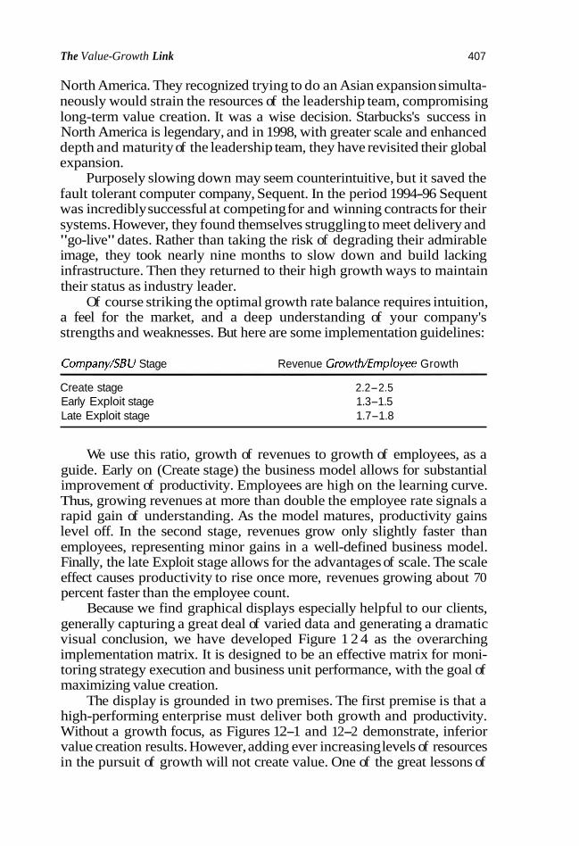
The Value-Growth Link 407
North America. They recognized trying to do an Asian expansion simulta- neously would strain the resources of the leadership team, compromising long-term value creation. It was a wise decision. Starbucks's success in North America is legendary, and in 1998, with greater scale and enhanced depth and maturity of the leadership team, they have revisited their global expansion.
Purposely slowing down may seem counterintuitive, but it saved the fault tolerant computer company, Sequent. In the period 1994-96 Sequent was incredibly successful at competing for and winning contracts for their systems. However, they found themselves struggling to meet delivery and "go-live" dates. Rather than taking the risk of degrading their admirable image, they took nearly nine months to slow down and build lacking infrastructure. Then they returned to their high growth ways to maintain their status as industry leader.
Of course striking the optimal growth rate balance requires intuition, a feel for the market, and a deep understanding of your company's strengths and weaknesses. But here are some implementation guidelines:
Cornpany/SBU Stage Revenue Growth/Ernployee Growth --
Create stage 2.2-2.5 Early Exploit stage 1.3-1.5 Late Exploit stage 1.7-1.8
We use this ratio, growth of revenues to growth of employees, as a guide. Early on (Create stage) the business model allows for substantial improvement of productivity. Employees are high on the learning curve. Thus, growing revenues at more than double the employee rate signals a rapid gain of understanding. As the model matures, productivity gains level off. In the second stage, revenues grow only slightly faster than employees, representing minor gains in a well-defined business model. Finally, the late Exploit stage allows for the advantages of scale. The scale effect causes productivity to rise once more, revenues growing about 70 percent faster than the employee count.
Because we find graphical displays especially helpful to our clients, generally capturing a great deal of varied data and generating a dramatic visual conclusion, we have developed Figure 1 2 4 as the overarching implementation matrix. It is designed to be an effective matrix for moni- toring strategy execution and business unit performance, with the goal of maximizing value creation.
The display is grounded in two premises. The first premise is that a high-performing enterprise must deliver both growth and productivity. Without a growth focus, as Figures 12-1 and 12-2 demonstrate, inferior value creation results. However, adding ever increasing levels of resources in the pursuit of growth will not create value. One of the great lessons of

408 SCIENTIFIC FINANCIAL MANAGEMENT
Exhibit 12-4. Performance Matrix: Value-Creating Growth.
Productivity Growth Focused Drhren
Goal Oriented (Lagging)
Leading lndlcators
Deloltte Consulting
Some Thomas L Oarley Ill, mn*inp ppen;, Branon Auociares ~ardlmoo
the downsizing era of the 1980s through the mid-1990s is the need to uti- lize all resources productively. Thus any useful implementation monitor- ing methodology must encompass both factors. These two elements then become the columns in the matrix.
The second premise is the role of targets. All businesses set goals or targets, which if achieved, represent the desired high-performance level. But, by their nature, goals are lagging indicators. A business must also set in place leading indicators, milestones, and goals that will define progress toward the ultimate. These two factors become the rows in Figure 124, rounding out the types of metrics required to guide the implementation of the business or enterprise strategy.
Each cell of the matrix must be constructed effectively in order to serve as a helpful implementation guide. Cell #1 (productivity/goals) is the segment of the matrix most comfortable for most management teams. Thus, for example, in the goal cell management records a CFROI (cash flow return on investment) target it believes is achievable by the business and yields an appropriate level of value creation. While an overall target number satisfices for corporate reporting, it should be broken into its com- ponents to influence SBU and field management behavior. Thus, CFROI can be fanned out into those elements (what we term a waterfall--data

The Value-Growth Link 409
cascading to more detail and to lower organizational levels) within control of successive levels of management, fo; example, an inventory turnover target for a manufacturing facility or a sales per person target for the
- -
re$onal sales organization: While a valuable guide, nonetheless these indicators lag input. Thus,
the next step is to convert cell #1 targets into the leading indicators of cell #2. In a simple sense any target that is meaningful for the relevant manager can be reset as a leading indicator by setting goals around rates of change. Thus, if inventory turnover needs improvement, a commitment to a re&- lar improvement allows progress to be monitored. But other types of lead- ing indicators work here as well. For example, a good indicator of improv- ing productivity within a sales force is the level of unplanned turnover. Experienced professionals build strong relationships with key customers, driving high customer retention rates, thus improving profitability.
The growth side of this matrix, cells #3 and #4, represent less familiar territory for most management teams. For some timenow (the unsavory legacy of the 1980s to the mid-1990s drive for productivity) most estab- lished companies have optimized management processes around tight control of resources. Growth is a new goal, and one with which too many teams struggle. Cell #3 then becomes a breakthrough. It serves to lift the sights of management to a longer and different horizon. Simply setting, and committing to, a specific growth target sets the team on a very differ- ent trajectory.
By reference to the evidence of Figures 12-1 and 12-2 above, the over- all corporate goal for cell #3 must be a revenue growth rate of 10-15 per- cent per yearm higher. Lower levels assign theenterprise to a mediocre level of value creation. The next task reauires allocating to each SBU a tar- " get that, in total, aggregates to the corporate target. Of course, consistent with Figure 12-3, some should have high growth targets, while others should shrink.
Cell #4 translates these goals (lagging indicators) into their leading indicator counterparts. For growth also there are a rich set of metrics avail- able. For example, customer retention presages higher sales levels. Moni- toring and setting targets for higher customer loyalty rates (or the inverse, lower customer defections) will precede higher rates of growth.
Once the four cells are rounded out they become the implementation- monitoring matrix. This is analogous to the Balanced S~orecard.~ In fact we recommend that the various elements of this display be coded to capture what behavior they intend to drive. Thus the elements should be identified according to whether or not they will impact growth or productivity, and are goal-oriented (lagging) metrics or are the leading indicator counterparts.
4. A Balanced Scorecard provides management with ways to track and evaluate imple- mentation of business strategy.

A client of ours, a global services company, uses these two figures to focus debate during the strategy development process, then to focus atten- tion during the implementation stages. They prepare a version of Fig- ure 12-3 that is historical. It plots for the SBUs how they have performed over the planning cycle, in this case, three years. This retrospective look (which is updated on a regular basis to monitor progress) portrays a stark picture of those SBUs that have gathered resources, but have not produced a positive CFROI. The CEO refers to the portrayal as "good constructive crit- icism" since it is fact-based and objective. The second iteration is a forward- looking projection. Now, the debate becomes more speculative. At issue is how the negative patterns of the past can be or will be reversed, or the pos- itive momentum sustained. From the information on the figures come a dis- cussion of customers, competitors, shifts in technology, and other factors central to the health of the businesses and the total enterprise. The conclu- sions are a reallocating of the available growth investment, and a re-plotting of the path of progress over the ensuing three years. This will allow the com- pany to project a rough forecast of the expected value creation these invest- ments, and this momentum should yield.
Armed with this broad strategy, the CEO then turns the attention of the SBU leaders to the development of Figure 1 2 4 . The goal levels for cells $1 and #3 are drawn from the results of the Figure 12-3 debate. The first task, then, is to translate total corporate productivity and growth goals into SBU specific targets; then, of course to build the leading indi- cators into the program. Leading indicators are critical since no leader- ship team can hold its breath, wait three years, and ask did we make it? Once defined this CEO monitors the leading indicators on a quarterly basis formally, and informally whenever a key element changes. The met- r i c ~ vary by type of business, especially by growth cycle stage. Thus, a very early Create stage business has many of its metrics designed to mea- sure input. Before results become apparent, the challenge is to gauge whether the resources are being invested at the programmed rate. At the midpoint of an Exploit stage business, the more classic measures of rates of change can be utilized. Importantly, the CEO leads the quarterly meet- ings. She believes she has much to contribute, but her leadership also sig- nals the importance of these implementation metrics. Incidentally, since growth via new products is a key to sustaining high growth, she is also the company's "chief growth officer," that is, she chairs the innovation task force as well.
A Vision: The Desired State
An intense desire for high performance lies at the heart of the enterprise. Since we can demonstrate that growth drives such high performance, and yields such high levels of value creation, then it must become the under-

The Value-Growth Link 41 1
lying principle for the management processes of the goal-driven company. To reap the rewards, growth promises management must lead with:
A An unyielding commitment to growth as the superior route to value creation
A Well-designed and executed Valuable Formulas, the strategic plat- forms for long-term growth
A The capability to sustain growth beyond the success of a hot prod- uct or the energy created by an especially charismatic leadership team
To embed these three elements of a growth system deep into and through- out the entire organization requires a set of implementation tools and frameworks such as described in this chapter and throughout the course of this book. Armed with them, and following their direction, the enter- prise can reach and sustain the high level of value creation it deserves.


Page numbers of tables, exhibif,etc. are in italics
Abandrmment options, 6 M . 63, bd Accounting. 313
cash flow, 117-118 Accounts payable, 122 Accounts receivable, 121 Accounts receivable risk, 10 A c m l s and tvxes payable. 122 Ace Textile Pmdurtion Corp
background, $47-48 balance sheet value drivers, 354-371,
355,358-367.368.369.371 forecast assumptions, 352-353 income statement value driven. 351,
154 351
376,377 threshold margin, 375,377,378379,
380,381,382,383-386 valuation summary, 349-51.350
Acquisitions, 31 Adaptable models, 208 Adaptwe system schematic diagram,
213. 214 ---
ADS (neural network consulting fir",), 11
Advanced cash flow, 117 Advanrcd vkmhation, 9 Advertwins 220 h a f t , 6< The Alcar Group Inc., Appendix 3 to
chapter 11,387,388-396 Alcar sofhvare, 11.87 Alcatel (telephone company), 174 Altman's Z yore, 155, I,%, 157 Amaron.mm, 316 Amencan opt im, 32.55.59.60 Amorfizatioian. 128.318
of bond premiums. 127 Amorhzahon rates, 313 Analys~s of cash flow, 121-127 Analytica, visual iinancial models, 88,
9&115 Anomall-, 9 Antimatter, 21 Appraisers, valuation, 347 Arbitrage W d n g Theory. 272 ARMA (autoregressive and moving
average) maiels, 170 Artificial intelligence, 2, 9 Asset apprai~ds. 316 k ~ e t diuertihlres, 121 Assets/sales ratio, 133-134 Astronomy. 21 At the money options, 32 Auchon, not+-orderly liquidation
based on, 316 Audit guidelines (Federal Reserve),
287-289 mllateral, 297-300.299 tr , \~fer (counq rrsk), 292-297,
293,295 Auskim, 403 Autocorrelation. 324 h x 0 ~ 11
Backpmpagation, neural n&orh, 209,210
Backlog., 126 Balance sheet value drivers, Ace Texextile,
354-371.355.358-367.368. 369. 371
Balanced Scorecard, 4C9 Bankers Tmst, Risk Management
Advisory (RMA) group, 175 Bar charts, 323 Bams and Mobile Publishing Corp.
example. Black-%holes model, 3S39.38.39
Bayesian probabilities, 208 Beef cattle mdusq , 22 Begin or forgo investment options, real
options, 67 Bell-shaoed curves. 21
steep, 25 Benchmarlang, 94,127,158 Berra, Yogi, 139 Best ase, 322 BFGS quasi-Newton method. 265 BlCs See Business Information Centen
(RICs), Small Business Administration (SBA)
Bifurcation diagram, 7 Binomial distribution. 202 B - d d d q m s , m Blntk Hulrs and Bobv Lln,onsm
(Hawklng), Black-Scholes model, 31,3340,41 B m and Mobile PublS-4~ Gorp.
" ~ p l e , 33-39,38,39 BMW Bank GmbH of Germany. 1213 BMW dcalcrs, 12 Bond premiums, 127 Bond Rater software, 11 Bond rating compared to credit
made. 276 B&'~&~S, n. 20.21~ BuOk vulucs, 313 Bouygues (telephone company), 174 Box-Jenkins methods, 140.141,
152-154.170 Buffet, Wanen, 117 Busmess cycles, 23.24 Bus~ness failures, 20 Business Lniormatian Centers (BICs),
SmaU b i n e s s Administration (SEA), 345
Business Plan Road Map to Sucres, Small Busmffs Adminishation (SBA), 344
Business plans, 344 Business and professional
magazines. 345 Business risk. See Risk analysis Butterfly effect, 7,8,21,22
Calculations of options value, Amendix A. 41-49
C~CUIUL >hain rule of, 210 Calls, ophons,31-32.31. 37.55 Capital Asset Pricing Model (CAPM), 5,
272-73.316.347.368.371 Capital budgeting rhedllle, 125
Capital cmt, 321,322,338,403 Capitd expenditures, 5556 Capital intensity, 20 Capital inveshnents, 55 Capital markets, 4 Cap~Cl-intensive projects 62 Ca~ital/output ratio (asseblsales),
is?-i~ Capitalization of costs, 313 Carmll, Thomas, "Using Your
Computer to Create a W m g Business Plan," 344
Case studies Dix Guage Carporation, 68-79 High Risk Inc., 131-137.131.137 How Street A ~ a h e n t s . 19M97.
190-197 Lntemational Drug corporation (IDC)
"Eigoxin Drug Project," 181-189, 183-187.189
Oil Field Development, @Quest, 25-
C a h 128 Cash conversion cyde, 124 Cash cow, 22 Cash flow. 117-138.312 - ~
~ c c o u ~ & ~ , 117-118 advanced, 117 analysis. 1 s 1 2 8 div~nonal, 117 EBITDA and noncash charges,
318,320 from operations, 318 grass operating cash flow (GOCF),
119,123-124 IAS 7, 118 in-depth cash flaw, 118-119 refilm on inveshnent (CPROI),
408,410 and shmhulder value, 118,127 statement, 119-123.120 and 5ustainable gmwth problems,
129-137 Cash tax rate, 322.337 Cash traps, 316 Cvsinos, 177 Causal models, 140,141,211 CB Predictor software, 144-146.145,
146.210.324.325 center f o ; ~ e c h n o ~ d ~ ~ and M
Business Devclopmmt, Central Missouti State Universily. "Someplace Fitness Center, March 1995," 344
Cenhal Missouri State Univerz-ity, Center for Technology and Small Business Development, 344
CEO. See Chief executive officer CFROI. Sn Cash flow. return on
inveohnent Chain rule of calculus, 210 Chaus thcury. 2.3.4-6
day-to-day business evmts, 21 definition, 4 grand design, 8 hvrmoruc shuriure, 5.8 in,t,ai departure point, 5

and pntfolio risk m a g m e t . 21 sensitive dependence of initla1
conditions, 7-8 Chi-square test. 170 Chief executive officer (CEO), 410 Choice variables, 235 CIC. See Consumer Information Ce Cism S y s t m , 403 Citinouo. 403 ~la&fication power, 217 C h a t e Survey, Coming, 403 Coefftcnent of deternunahon. 169 Collateal, 274
Federai Resene audit guidelines, 297-300.299
Collection periods, 124 Compensation, executive, 312 Cnmnetitinn. 20
nter
. . See olgo Linear onerammine
Computers, oific;, 8 5 Consolidated equity value, 117 Constrained optimization, 234 Constraints, Ihrearprogamming. 236 Conshuctive aiticism, 410 consuitvnts
financial, 94 in neural networks, 11-12 valuation 347
Consumer Wormation Center (CIC), 345 Consumer Pmduct Safety Commission
(CPSC), 345 Consumer value, 312 Contingent claim contracts, 31 Continuing education, 346 Contractual optionr, real options, 66 Copeland, Kaller, and Munin. Valuation:
Mensunng endMona& the Value of Conpan&, 347
Copeland, Tom, 307 Coming. Climate Survey. 403 C-rate bcmds, 219
See dso Rond ratings C-rate buyout, 86 Corporate h c e , 4 Corporate reshuchwhg, 94 Corporate risk anaiysis. 27S303
risk ratings, 11 risk system, 274 tisk-rating interactive model, 274-275
Corporate valuation anal+, 85 CorpRkkModeY. 275277 Correiation, 21
of Antimatter Beef Company with Matter Poultry Corp., 27-29,27,29
definition, 26 and ~cntfolio theory, 49
Cordation coeffiments, 168 Cost approach, 316 Cost of capital, 321,32,338,403 Country risk (transfer), Federal R-e
audit guidelines, 292-297.233.23s Covariance, 2629,26.27,29 Covadme (systematic) risk, 20 Cox-Rubinstein bimomid model,
5 w . 59 CFSC. See Consumer Product Safety
Commission Credit bureaus, 12 Credit card holder risk classification, 12 Credit card industry, 26,22&221 W i t gradecompared to bond raw 276 Credit grades, poor, 275, 277 Credit ratings, 11 Credit nsk model, 274 Crass-company data. 399 Cross-geography data, 399 Crasswhite, Carl, 144 Crystal BaU saftware, 26.77,lM. 174,
323,326,347 OptQuest, 234,25758,333 Piece of C a b Company, 175-180,
17&179
Customer retention. 404.409 Cydical b u m e s ~ ~ s , 26
Daily sham prices and reactive interdependence, 8
Daiwa Computer Services Co., Ltd., 219 Dew= Securities, 219 Data mining, 2,8, MO, 312 Databas, 9 DCF. See Discounted cash flow Debt. 126127
long- ten 126 Dcbt Gnandng. 274 Debt strudures, 06 Debt/equity ratio, 132-133,338 Decision making, and options, 30 Decision trees, 213,216217,216 Dcclsiun variables, h u r programming.
114-75
~ e d u i ; and options, 31 ' Dciault probabilities, 275 Default (unsystematic) tisk, 20 Deferred taxes. 125 Dell Computer, 403 Deloilte and Touche, HR (Human
Kesaume) standards. 403 Delta in ophons, 45 Dependent variables, 9 Deprrdatio~ 124,128,313,318,337 Derivative assets, 31 Deterministic linear programming. 236.
239,239 See& I.ineai programming
Digital signal processing (DSF), 222 "Digoxh Drug Project" case study,
International Drug corporation (IDC). 181-189, IZM86, 183
Dirly data, 9 Discounted cash flow @CF) approach
(going concern), 317-318 "Dkcm~er what to put in a bushes
plan," Howard University Small Business Development Center, 344
Distribution terms glorsuy, 197-204 Distributionr
namal. 24 See olvl Probability distributtons
Divenifiotian, 5,20,21 deiinitio", 22 portfolio management, 272
Dividend based valuation. 316317 Dividend Dayout. 134
kaiuation 316 Dividends, 124,127 Divisional sccounting checkkt, 127-128 Dividonal betar, 347 Divkional cash flow, 117 Divisional (dynamic business unit)
analysis, 308 Divisional or operating segment risk
rating, 305-308 Du Guage Corporation case study, 6&79 DOC. St% United States Deoarbmnt of
Cnmmerce Doorley, Thomas L., Ill and John
Donovan, Value-Creatinx Gmwtk: How to LiJf Your Cornpony to the N u t h l of Pmformance, 399
Double exponential smoothing, 166167 Double moving average, 166 Downside protection, 66 Domizine. 408 VSI'. See Digital signal processing DurbihWatsun tests, 324
and homnscedasacity, 170 Dynamic business unit (divisional)
analysis, 308 Dynamic systems, 4
E iormula, 160 &commerce start-up, on-line
demonstration, 112-113.112
Earning before tax (EBV, 337 Earmngs, 312 315 Farnrnes before mterest, taxes,
depreciation, and amormation (EBITDA), 318
Earnings trends, 123 Earthqiakes, 271 EBITDA See Earnings before interst,
taxes, depreciation, and amarriration
EBT. See Eamine before tax u
Econometric forecasting. 159 Econometric models, 140.141 F c < ~ I , , c > I M .v,lt n ~ . l l ~ ~ ~ ~ l g ~ ~ l r . ~ l ~ ~ ~ ~ . , 2 ~ C;onnmr 1un:l~nn. 21 Cconomr "alee added (E\'r\l 405 Economics, 4 EDA. Sm Exploratory &ta analysis EDF See Expected default pmbabilities Ei"steln,Albertr 21.39 Elastimty, 57,58,312 Electronic transfers. 92 Employee satisfaction, 403404 Employee Setisfaction Survey. Hewlett-
Packard, 493 En- prices, 20 Enran. 403 Environmental factom. 20,311 Enviromental I'mtectlon Agenc)
IFPAl ?dh \--- -,, - --
Environmental protection laws, 62 EPA. .% E n w t a l Pml&ionAgemy Eauitv. 127 E&G value. 86,316 E u h w , Neil R., 213 European options, 32-33,59 EX ante re-, 23.24 Excel, 38,41,80,94,95,129
neural networks. 22>228,22>226 Solver. 175, 347 spreadsheets, 223,326,347 sta6stical farecasting, 141-143.142. Iff3
Executive c a m p w t i o n 312 Expanding operations option, real
options, b 5 6 Expected cash flows, real options, 61 Erpffted default probabilities (EDF),
274,275 Expiration date, options, 32 Exploratory data analysis (EDA), 168 Exponentid and logarithmic curve ht,
14R-151 -~ ~-~
Exponential smoothing, 140,141 Exponential smmthing averages, 148,150 Exoonential smoothine methods. 167 - External enr,~ronment, 311 Extracting patterns, 2 Extreme value distribution, 200-201
. . -. ..~., . . . Facility risk rating, 30&303,301403 Fadin, &. 274 , . Fair m k e t value. 313 Fl\bH"L ",I! t t , ~ mtrmc?8ra. 55 FI.' Fto~~rlt I Tc t#hit lrnt F), 2U mA .;v r o d and D r u ~
Administration Federal w i t lnmmce Ccqm&iontiar 275 Federal Reserve audit guideiines,
7x7-7x9
Feigenbaum's fractal, 7 FFT See Fast Fouricuric Transform FlFO-to-LIFO changes, 128,314 Finahation, 2 Finance theory 19 Financial analysis, versus option
mlysis, 31 Financial consultants, 94 Financial forecasting, simulations
approach, 173-180

Financial options. See Options; Real options
Financial policy vvariables, 121 Financiai revolution, 2.19 F I,,,,, 4 ' c?,l,,,l<.,rv. 7 rlnanclng a<:,\ illes, deb!, 126127 I' rn r nsl rannc. 2:%2P7 ?;?-280
283-285 Fued-mset turnover, 126 Flexibility, rral options, 57 Fond and Drug Admmish.ation (FDA),
181,346 Fo-t assumpti-. Ace T d e , 352-353 Forecast horizon, 317,319,319-20 Foxasting future events, 9
See also Stahshcal fomastii Forecasting terms glossaly, 166170 F o m e 500,387 Fonuad-looking projection. 410 Fractals, 4.67.8
Feigenbaum's, 7 See also Multifractals
France Telemm, 174-175 Franchise licenses, 313 Free parameters, 208 Fuhre event forecaetmg, 9 Futum, 403 Fuzzy logic, 2,7,1243
and neural neiworks, 208
Gaim and losses, 128 Games of chamce, I77 Gamma, time lagged murrent
network, 228 Gamma distribution, 201 Gamma in options, 45.45.46 Gauss, Predetich, 198 Gauss-Newton method. 267 Gaussian distribution, 19b199 Generalized regressionneural networks
(GRNN), 218 Generic Bakery example, optimization
models. U7-38.239 Genesis, 2,3 Genehc algorithms, and neural
network., 208,209,217-221 Geometric distribution, 203 Geometric m e w 167 G c m m BMW B d GmbH, 12.13 Glabal mark* eonomy, 4 M 9 401,402 Global optimization, 256 Glossary of distribution t e rn , 197-204 Glossary of faremoting terms, 166170 Goals, 408 CCCF Sm, Gmss mcratinr cash flaw
~o06will. 128,313 Gordon Dividend Growth Model, 316 Government Printing Office (GPO),
"Subj& ~ibii&ra~hy,' ' 345 GPO. See Government Printing Office Grand deign, chaos thmly, 8 GRNN. See Generalized repssion
neural networks Gross margin, 126,335 Gmss operating cat.? flow (GOCn, 119,
12V124 Gron.th, 129
implementation for, 406410,408 long-term, 411 ;ind pnt-, 399.400-403.401.402
Harmonic smchire, chaos theory, 5 Hazbm, 175 Hawkmg. Stephen, Block Holes and Baby
Uniomes, 6 Hax. Amoldo C.. 311
negatively correlated risks, 22 and ootionr. 31
Hewlett-Packard, Employee Salidaction S w e y , 403
Hierarchies of models, 93,115 High Risk Inc., caseahdies, 131-137,
111. 137 Ho, Andrew,4 Hamosceda~tidty. 157 Hope Street Apartments case study.
19%197,19&197 Howard University S d Business
Development Center, "Discover what to put in a business plan," 344
HR (Human Resource) standards, Deloine and Touche, 403
Human brain, 10-11,12,209 Hurricanes, 271
1.45 7, cash flow, 118 ICERC rating. See interagagency Counhy
Exposure Rcv~ew Commitkee (ICERC) rating
If-then patterns, 9, 10 Impact analysis, 174 Implied binomial tree$, real options,
5F-60, 59 Imprudent exponential gmwlh, 129 In lhe money options, 32 In-depth cash flow, 116119 Income aatement, 128 Income statement value drivers,Ace
Textile, 351,354,355 Incremental fixed capital mvesment,
322,336337,337 Incremental working capital investment,
322,336 Independent variables, 9 Ind8erence mwes, 23 Individual talents and capabilities, 311 Industry charaderistics, 20 Industrv and economic/environmentaI
factors/counhy risk mahix, 289-292,290
I n d u s q life cycles, 20,l.W Induslry risk. 271 Inflation. 20,337 Influenee am, 9C102 Influence diagrams. 89.9Et105 Inform Software GmbH of Germany.
12. 1.7 ~nformati& influence, 98 Initial depamre point, chaos theory, 5 Innovation. 404 Input-output technology, static v m s
dynamic, 58 Intangible assets, 128,313,316 Integer variables, 235 Intelligent Arrap, visual financial
models, 93.94.115 1nIcr.m~mv~~ casqtura!+. muoc-I 274 l n l ~ r . ~ ~ ~ n ~ y Clt8rnl-y F L ~ I ~ I I T P Rev~ew
Commll:ce ICCERC) ram& 291 ~ ~~~,~
Interest rates, 20 real options, 61
Internal n t e of return, 5657 Internal resource, 311 Internal Revenue Sewice (IRS), 346 International Drug corporation (IDC).
"Digoxin l h g Kuject" case study, 181-189, IR.%lR7, I89
Internet, 85 on-line demonstration: eiommerce
start-up, 112-113.112 Inhinsic valuations, 312 Intinsic value options, 32 Inventory, 122,124
work-in-pmer~, 126 Inventory salability, 128 investment activities, 119,125-126 hvestment anaiysis, 4 Investment bankers, 31 Investment cost, real options 61 Investment nroiect cash flows and iaint
Investor re-, 399-400 1%. See Internal Revenue Service Issue equity 133
Jn in\mtay. SZe lust-iretime m inv-
loh m-oltun ?<P-~M lolnt rmlures. 21. 126 Ju.1-m-time (JmI mventory 134
K-means clustering. 218 Knowledge engineers. 200 Kohmen self-organizing feahue maps
(sorn), 222
Labeling requirements, 346 Lagging indicators 408,409 Lansing Comrnuruty College Small
Business Dewlopment Center, 344
Late payments, 124 ~eadership team, 411 Leading indicators, 408.409.410 Leaguer, 6me lagged recurrent
nehunrk. 22R . .. - ~ ~ ~ , --
Lea- options, real options, 66-67 Lease financing, 10 Lea-. 62 Lev&-Marpdt method, 267 Liabilihes and equlty, 128 Liao, Shu S., 156 Libraries, 346 LIFOt~FIFO changes, 128.314 Linear associalion, 26,140 Linear models, 7,85,86,209 Lincar ubjwlive functions. 2% Linear p m g r m u r i n ~ 175,233-270 cmtraints. 236 decision vi;iabies, ~ 3 5 deterministic iinee~mmamming. . -
239,239 objective function, U 6 3 6 a p e s t i o n 23?-34 aptimuatim models, 2 3 M 6 See also Optimization theory
~i~uidationvaiuatim appmach, 316 Liquidity of financing instrument, 271 Local optimuation, 256 1.0. file onti-. 257 -- ~r ~ ~. L o ~ c a l variables. 235 Lo@stic regre*on, 213 Lognormal disttibution. 199 Long-term debt, 126127,334 Long-term growth, 411 Long-term planning. 2,311 Long-tenn trends, stock market. 6 Lorenz. Edward, 7.8 Lotus 1-23,94 Lumlna Decision Systems, visual
financial models 88,93,96
MCA aftiviti-, 31 M c K i ~ e y & Company. 307 Mamecanomic conditions, 5,20,
21,271 Magariner business and
professional. 345 Maintenance yuMmmts, 62 Management, 208,311,313
and vision, 410-411 Management toals, 3 Mandelbrot, Benoit. 4 Mandelbrot set, 4,4 Mvrkct options, 58 Market signals analysis, 321 Market mends, 21 Market values, 313 Msiketabie securities. 336 Marketing, 20
t q e t . 22&22l Markowiu's efiicient frontier, 23 Mathmstica software, 87 Mathmatical formulas, 10 MATLAB mftware. 36,46, V, ,214
Optimasation Tdbox, 26567,266

Mean calcdatim forAn6matter Beef
Company, 24-2624 ealculatim for Matter Poultry Corp.,
26.26 Mean Absalub deviation (MAD), 324 Mean absolute percentage error
(MAW, 325 Mean and variants of each variable,
167-168 Measurement units. 91 Median, 167-168 M w . 31 Meritocracy, 404 Method Gallery, 324 Method of kart squares, 140 Microeconomic factors. 20 Milelones, 408 Minimum variance set. 23,23 Mining. 62 MIT. Slam Schwl of Management, 311 MW network. See Multilaver
~ o d e , i 6 7 ' Models, 322-323
See also Visual h c i a l mod& M d f i e d percentage of sales
(sensitivihes appmach), statistical forecasting, 16&166, 161-164.166
Module node. See Nodes Monte Carlo simulations, 24,69,70,77,
17>U)6 glossary of distribution terns, 197-204 Hope Street Apartments case sh~dy,
19&197,19&197 International Drug corporation (IDC)
"Digoxin Drug Roject" case study, 181-189,183-187.189
Moodys, 273,275 Morl Glantz Associates Valualion
Appraisal Outline, Appendix 1 to chapter 11,339-374
MOEB, Douglas. 156 Most likely case, 322 Movingaverages, 140,141,167 Mulbmibute decision analysis, 88 Multicollinearity. 158,159,174 Multidimensional visualization, 10 Multifractals, 19
See obo Fractals Multilayer perreptmn (MLP) network,
209-210,209,214,215,216,220,227 Multiple regredon, 325,326 Multivalued logic, 12
NASA, 90,313 NEC Corporation, 219 Negative binomial distribution, 202 Negatively correlated risk, hedging, 22 Nelder-Mad simplex search method, 265 Net cash prmided by operating
activities, 125 Net fixed assets. 125 Net income, 124 Net operating cash flow, 123 Net oprahng pmfit less adjusted tares
(NOPLAT),Ace Textile, 371, 372-373
Net present value, 56.57 Net-present-value (NPV) method,
63-65.32s321.337 Neural architechma, 218-219 Neural networks, 2,7,10-12,207-232,
257.312 badi-pr&gation, 209,210 background, 207-210 developing within Excel, 223-228,
22M26 and genetic algorithms, 217-221
neural architectures, 21M19 real-world financial applications,
219-221,220 multilayer perceptmn (MLF)
network, 209-210.209.214.215, 216,220,727
prkcipll component analysis (PCA), 220,222
radlal basis function (REF) nehvorks, 218,220
S&P 5W. 223-226,227-228
and stausuv 2 % 2 : i . 211. 2'6 theTC prohlcm 21>213.212 213 erne laneed r e - u m t nerrwrls. 228 ""
NeuroDimemian, Inc.. 213,217,223,227 NeuroSaluhons, 223,228 New Jerq Refin~ng lnc. example,
optimization models, 24756, 24&55
Nikkei index options, 32 Nods, 97-98.209 Nonlinear financial models, 7-9, 85 Nonlinear objective functions, 236 Nonlinear systems, 6,209 Namai dishibution, 24,19&199 Nut-ro-ordcrlv Pouidvtion based on . .
auction, 316 NF'V method. See Net-present-value
(NFV) method Numa F i c i s l Systems, 46 Numeric camput~tion and
vnuali&tion, optimization models, 26F67.266
Numeric Computation and Visualization Sohare, 46
Objective function linear programming, 2.1636
Obligor, 274,275 OCR. See Optical chancter recognition Office computers, 85 Office of Ihrift Supervision, 275 Oil Field Development OpQest case
shlliy. 25- Online demonstration, worn-e
start-uo. 112-113.112 Operafing cat.? shsources, 122. 124 Operating cash uses, 121-122.124 Operahng leverage, 336 Operating leverage risk, 66 Operating profit, 320 Operating profit margin, 322.33E-336 Operahng xalc ophons, real options, 65 Operating segmenh and leverage, Ace
Textile, 348 Optical character recognition (OCR),
210,211 Optmal portfolio, 23 Ophizahon
and s h d o l d e r value, 233 as value driver, 327-35,332,333,
33P335 Opbmilatian models. 23656
SPP nbo Linear pmgmmming Opth ia t ion runs, Ace Texble, 371-375,
374. 375. 376. 377 . . . Optimization theory, 19
Set ofso Liicar programming Optimization Toolbox, MAIZAR,
26Cr67,266 Option analysis, versus h a n d a l
analysis, 31 Option grantor, 32 Option seller, 32 Option writer, 32 Optionpricing mcdels 37
Cox-Rubinstein binomial model, 5MO. 59
Options. 3lL3Y. 312 Rams and Mobile Pubhshing Corp.
example, %39,38,39 Black-*holes model, 31,3340,41 calculations of options values,
6 1 4 4 .- ., calls, 31-32, 31 and default, 31 definitions, 31,45
differences between financial options and real options. 61
and hedging, 31 pub,31,31.32-33 user and importance of, 3C-31 see also ~ e a i o ~ t i o n s
OptQuest Crystal Ball, 234,257-58, 332,333 II'Y.,>",.C.,~~L,,~, 3s) OOI F N I C I r*.,. . I O ~ , , , .n~, 7-h ai
OIderly IhqutJaron value 31t1 Ou! oi the rnonc; ophon;. :2
Puckaging requirrmenb, 346 Palisade, Risk Ophmimr, 234 Pareto d~smbuhon, 202-203 Partial rmths, 12 Particle physics, 6 Patents. 313 Payables balances, 124 Payback period, 57 PCA. Sse PTimipal component analysis Pearson's r, 28 Peer review, 88 Pcrcenttge vaiationexplained, 170 Perfed Portfolio Ltd. example,
optimization models, 242-47. 24&47,272
Performance, 312-313 and growth, 399,400403,401,402
PE5 sm Prumsing clcmmts Pharmaceutical research, 181-189 Physics, 4 Piece of Cake Company. Crystal Ball
s o h a r e , 175-180.176179 Pipelines, 62 Point estimates, 322 Poisson dishibution, 203-204 Poor credit g a d e s 275,277 Porter, Michael E., 319 Portfolio management, 20.21-30.338
Anhmatter Bref Company, 22-24 diversification, 272 Matter Poultry Carp., 22.24.2630 optimal portfolio, 23 and risk analysis, 2 n st-<-testing, 19 theory of, 23,26,36,40,272
Poultry indusq, 22 PP&E. See Property. plant, equipment Predictability of systems, 6 Pricetoearnings (PIE) ratio, 314-315 Price-to-sala ratio, 315 Pricewaterhouse Coopers, 314 Prindpal component analysis (PCA),
220.222 Private companies, 313,314 "Pro forma'' market. 314 Probability dishibutions, 19
for Antimatter Beef Company and Matter Poultry Corp., 23-24.24. ?(I 111 --,--
Pmcessing element. (PEs), 215,216 Pmductivity, 312 Professional maearines. 346 w .
Profit margins, 134 Profit pruning. 134-135 Program Evaluation and Review
Technique PERT), U.S. N~T, 182
Projet a s h flows, 121,126 Project financing, 121 P~ojection period, 317 Property, plant, equipment @P&E),
119-120,128 Public companies. 313,321 Pure play approach, systematic risk,
3m3u5.304 Puts, options, 31.31.32-33.37
Quadratic equation, 23 Qualitative methods, statistical
forecasting, 140,141 Quantitative methods, 21, B9
ststistical forecastmg, 140.141

RbrD stage, 58 Radial basis M o n (RBF) network,
218.220 Random events. 2.3 Random movement in the stack market 5 Range estimates, 322 Rappaport, A M , 321,375 RBP networks. See Radial bmis function
(RBF) network Reactivation, 62 Reactive interdependence of daily share
prices, 8 Real options, 40.55-83.126
abandonment options, &ME begin or forgo invesment options, 67 binormal madpi, 58-60 mntraEtuai opttons, 66 definition 5E-56 differexes between financial options
and resl options, 61 Dix Guage Corporation case study.
*%79 .. . expanding operation9 aption, 6 4 5 flenbility. 57 implied binomial trees, 5$400 59 inionnation reauired and not
required, 60 leamine options, 6 4 6 7 - . O p ' d l rig i ~ d l ~ OprlOl*, <b<
sequencing or :ompound opnom, 67 shutdown ophons 65 switching options, 66 vcnus traditional methods, 57-58 see rlsn Options
Real variables, 235 Real-world financial applications,
219-221.220 Receivables, 128 Rewssions, 20.26 Reconniaance, 2 R-ion
logistic. 213 multiple, 151-159,213,214,214 simpie, 140 uslng Dedsioneering's CB Predictor,
146146,145,146 R-sion curve fitting 14b151 Remession models. 140.141.209 ~ e h a t i o n s , 20.33'7 '
Regulatory agendea 275 Renlacemnt value, 316 ~&erues, 124 Residual value, 317,319,32&21 "Resowe DirecMry for Small Business
Management," Small Business Adrmnishation ISBA), W 3 4 5
Rwpnue changes, 326 Revenue growth. 3 9 9 4 Rho in d o n s . 45 - - ~ - -r ~~~ ~, -~
Risk analvsis. 271510.349 . . corporate risk-rating interactive
model, 2%303 dynamic business m i l (divisional)
analysis, 308 segment analysis, 303-308 spdf ic risk, 271,272 systematic risk, 271-273 unsystematic risk, 271 &Y also Risk management
Risk factors, 312 Risk grading, 274 Risk management
assessment methods, 22 basic tmls of, 19-54 systematic (covariance) risk, 20 unsystematic (default) risk, 20 Risk Management Advlwry (RMA)
group. Bankers Trust, 175 Risk Optimizer, Palwade, 234 @Risk sohare , 174 Root mean squared ermr ( M E ) , 324 See alro Risk analysis
S&P.W, 2E-226.227-228,273,275,401 bles pow+, raw. 322,323 Salesinel fixed aqirn raho. 126 SBA.'S~ Small Business ~dminwhahon SBDCs. See Small Business Dwdopment
Centers (SBMS), Small Business Adminishatian (SBA)
SBUs. See Strategic business units Scientific financial management, 338
detinitioh 3 4 overview of book, 1 M 8 and value drivers, 322-323
kientific method, 321 Scientific research, 4 SCORE. See Service C o p of Retired
Executives (CORE), S m d Bwiness Admnistration (SBA)
SEC report, 315 Serurity market line (SML), 273 Segment analysis, ri& analysis, 3E-303 Seidler, Lee. 117 S e l f - q d z i n g featale maps (SOPMs),
220,222 Selforganizing maps (SOMs), 10,210,
21&219,220 Sensitive depend- of initial
conditions, chaos theory, 7 4 Sensitivities approach (modified
percentage of sales), statistical fmusting, 160-166.161-164.166
Sensitivity charts, 323 Sensitivity models, 173,174,236 Sequendng or compound options, real
options. 67 Sequent, 407 kqumtial quadratic programming
method, 267 Service Corps of Retired Executives
(SCORE), Small Business Adlnlnistratio" ISBA). 345
SES. See Single erpanential smmthing Set vadablrs, 235 Shareholder reams, 399400 Shareholder value, 3,55,80,94
and cash flow, 118,127 fmm valuation analytie~ to
application in practice, 338 and optimization. 233 preparation, 31&322 valuation methods, 311-320 value drivers, 321-338
Sharp, William, 272 Shelten horn lusscs, 22 Shortterm events, 2,311 Shutdown options, real options, 65 sm. See Standard Must r id Code Sigma. S e Standard deviation Signiiicance level (reliability), 9 Signiiicrmc test, 170 Simple moving averages, 141r148,
147,148 Simple regression, 140 Simulation, 2.9.24
of Antimatter Beef and Matter Poulhy, 24,25,29-30,29,30
and value drivers, 326,331,332 Simulation s o h a r e , 38,158 Sine qua non arrays, 7 single events, 2 Single exponential smwihing (SES), 167 Sloan Schml of Management, MIT, 311 Small Business Adminishation ISBA),
344-346 Busness mom^ cenrers (6101,345 Busirm? Plan Rmd Map to Sumes, 344 " R e s m e Directory fnr Small
Businm Management," 34-345 Service Corps of Retired Executives
(SCORE). 345 Small Business Development Centm
(SRDCs), 345 S m d Business Development Centers
(SBDC3, Small Business Administration (SBA), 345
SML. See Security market Lrne
Software, 85 Alcar. 11.87 Bond Rater, 11 CB Predictor, 146146,145,146,210,325 Dedsirmeerine. 87,257-58.347 fixed f ind-pmgrams, 9 Morm Software GmbH of Germany,
12,13 Lotus 1-2-3.94 Mathematica, 87 MATLAB, 36,46,87,234,265-67,266 for neural nehvorks, 210,219 Numeric Comoutation and
@ ~ i & 174 Risk Optimizer, 234 simulation, 38,158 Solver, 175,329 stochastic ophmization, 9 Valuc Planner, 11 for visual R n a d mod&, W,93 wizwhy. 10 &Y abo Crystal Ball software: Exeel
raftware Solver, Excel, 175,329.347 '"bmepluce Fitness Center, March
1995," Center for TRhnoIogy and S d Business Development, CenRal Missouri State University, 344
SoMs. See Self-organking maps Space pruprn , 90 spffific risk, zn, 272 SpeaJators, 31 Spreadsheets, 85.86.92-93
and Analyhm. 115 and d m e n t a t i o n , 94 Errel, 223 and neural networks, 208 traditional. 322 and visual models, 9&95,95,322
Square root of me v&riancr. 2.1 Standard dcvwrmcn of +mrh wrinhl,,. 1hR Sta~ncl.sni .I+,vm.ltlon (58gnlal. 21, 21
talrr~lalmons ior Anllmaner Beef U,mosnr. 2C26.2.1 -~~~ < ,.
mldstions for ~ a & Poulhy Cq., 26,26
Standard e m , 169 Standard ermr of the mean,26 Standard Indushial Code (SIC), 287,314 5tarbucks. 406407 Statistical forecasiing, 339172
Box-Jenkins. 152-154 casual models, 140, I41 econometric famasting, 159 Excel example, 141-143.142.143 exponential and logarithmic curve fit,
14&151 - -
148,150 glossary of forecasting lenm, 166170 mod&ed p m t a g e of d e s
(sensitivities appmach), 16&166, 117-111 I66 -"- A-A, ---
multiple regression, 154-159 qual~tatiw methods, 140,141 auantitative m M s . 140.141 ~" -
e o n using Densionnling's CB &didor, 144-146,145,146
simple moving averags. 146148, 147,148
time-seriesanalysis, 140.141 h e e r l e s or trend fom&n& 1*1a hend lines and curve fit mmlations in
Excel, 151-152,151,152,153,154 See aiso Fomaating future events
statistics. 39 - ~~ ~. and neural nehvorks. 213-217,214,216
Stochastic optimization models, 25657 Stochastic optimization software, 9 Stock analysts, 8

Stock market and the Black-Moles fonnula, 33 long-tern trends, 6 random movement in, 5 and risk analysis, 271
Stock pnre movmfnb, 21 Stock prices,311,312 Strategic business units (SBUs), 404 Strategic planning, 2,311,338,410 Smk price, options, 3233 "Subjrd Bibliogrephy," Government
P~inting Office (GPO), 345 Sum of square deviatiom, 169 Sustainable gowth problems, and cash
flow, 129-137 Switching options, real options, 66 Syllogism, 9 Sysiernatir (covariance) risk, 20 Systematic risk
Arbihage Pricing Theory, 272 Capital Asset Pricing Model (CAPM),
272-73 pure play approach, 30%M5,304
Systemic factnn, 20 Systems
dpamic, 4, 6 nonlinear. 6 predictability of, 6
t stabtic, 169-170 T C problem, neural networks, 210-213,
212.213 Tabu search. optimization models. 257-58 Tang~blc ass&, 316 Target marketing, 220,221 Taxation, 20 Taxes, 318,346
deferred, 125 Taxes payable, 122 Team effort, visual h c i a l mod&, 88,
9596 - -
T&ology revolution, 2.3,4,80,85,403 Terminel value, 317.320 Terminahon options, 60 Theirs Statistic. 324 Theta in options, 45 Threedimensional coordinate system, 9 Threedimensional methodology, 86,92 Threshold margin. Ace Textile, 375,377,
.378~379.380,381,382,385-386 Threshold spread and mugin, 347 T i e , real options, 61 T i e Delay. lime lagged recurrent
network. 228 Xme lagged recurrent networks, 228 T i e to expiration or enp*, optian?, 32 Tine value options, 32 T m e ~ r i e s analysis, 140,141,211 T i e ~ e r i e s prediction, 209 Tlrnpseties or bend famasting.
1@143,322,324-325,325 Tobin's superefficient padolio, 272,273 Towo Stock Exckange, 219 Top-do- organization, 93,115 Topix index options, 32
Toy indus- 175 Trade assomti-, 346 Trade discounts, 124 Trademarks, 313 Traditional finandal analysis
approaches, 2,313 Traditional methods versus real options,
57-58
T r a n ~ r t on rnultlplr.. 111-11 I T-~nrler t:oun? u k ) , Federal Ren.c
audlt mdellne. 292-297.293 ??5 Trend forecakg, 146143,324-325,'325 Trend lines and a w e fit correlations in
Excel, 151-152,152,152,153,154 Triangular dishibutian, 197-193 Truths, partial, 12 lko-dimensional sburmre, @.%?4 Type B uncertainty. triangular
distribution for, 198
Uncertainty and optimization, 236 real options. 61
Unccrtaintvd&tributions. 102-105. ro i1os
Unconsolidated investmene, 128 Unconsolidated subsidiaries, 121 Unconstrained optimization, 234 Uniform distribution, 200 Umted Statcs Depvrhnent of
Agriculture (USDA), 345 United States Deparment of Commerce
IWCI . 345 , ~ ~ , . ~ ~
Unsystematic risk, 271 divisional or operating segment risk
rahng, 305-308 Upside potential, 66 U.S. Navy, Rogram Evaluation and
Review Technique ( P q , 182 USDA. See United States Depepamnent of
Agriculture User defmed parameters, 324,325 "Using Your Computer to Create a
Winning Business Plan" (Carroll). 344
Utility theory, 88
Valuable Formulas, 405,411 Valuation: Mrasurinp and Mnmging the
Value qlcompanies (Copeland. Koller, and Mumin), 347
Valuation Appraisal Outline, 339347 Valuation mnrultanb, 347 Valuation methods, shareholder value,
311-318 Valuation summary, Ace Textile,
329-51.350 Valuations, inhinsic, 312 Value asse-ent, 2 Value driver test, 323 Value drive~s, 5% 86,312.32%328,351
in h e global market,+% and growth, 403 h o m e statement. 351,354,355
Value gap analyties, 85
Value growthduration (VGD), 319, 321,322
Value Planner software. 11 Value-Creating Growth: Hmu to Lx,R Your
Company to tk Next LmeI of Pmformann (Doorley and Donovan), 399
Value-growth link 399411 cautions, 404-406,405 employ- and C u s ~ e r s , 40- growth and performance, 400-403,
401.402 implementation, 40&410.408 v~sion and management, 41W11
Variability, 174 Vmiables, 235 Variance, 21,24
square root of, 24 Vector derivation. 211,212 vega in optiom, 45 Venhlre capitalisb, 66 VGD. See Value growth duration Vision and management, 41C-411 Visual hnancial models. EM16
A n a l y h , 88,90-115 background and deflnrtbn, 8647 building effective models, 8%92 comparing spreadsheet with visual
models, 94-95.95 developing the model step by step.
89, 9.%115 Intelligent Arrays, 93,94,115
. L t m h a Decision Systems, sB.93.96 on-line demonstration: e-commerce
start-up, 112-113.122 sofhvvre for. as. 93
Visualization advanced, 9 multidimensional, 10
Wal-Mart, 403 Wall Street journal. 21.311 W m 20 Waterfall (data cascade), 408-409 Weather forecasting, 6 7, R-9 WF. See World Economic F o m What-if scenarios, 322 wins: qruh. 22 WizWy softwarn, 10 Wwten, Dan, 217 Work-in-process inventory, 126 W o r k g capital 121-122 Working capital p o h , 86 World Economic F o m (WEF), 399 World financial markets, 19 World Wide Web, 85 WorldLink, 399 Worst case, 322 Wntr-downs, 124
Z (zeta) wore, 155,156,157
Copyright © 2022 FDOKUMEN