Étude de la structure et des propriétés SAR/QSAR de ...
182
MINISTERE DE L’ENSEIGNEMENT SUPERIEUR ET DE LA RECHERCHE SCIENTIFIQUE UNIVERSITE MOHAMED KHIDER BISKRA FACULTE DES SCIENCES EXACTES ET DES SCIENCES DE LA NATURE ET DE LA VIE Département des Sciences de la matière THESE Présentée par Mariem GHAMRI En vue de l’obtention du diplôme de : Doctorat en chimie Option : Chimie Moléculaire Devant la commission d’examen : Mr. Salah BELAIDI Prof. Univ. Biskra Président Mme. Dalal HARKATI Prof. Univ. Biskra Directrice de thèse Mr. Ammar DIBI Prof. Univ. Batna 1 Examinateur Mr. Lazhar BOUCHLALEG MC/A Univ. Batna 2 Examinateur Intitulée : Étude de la structure et des propriétés SAR/QSAR de quelques molécules à visée thérapeutique Soutenue le :13/01/2022
-
Upload
khangminh22 -
Category
Documents
-
view
1 -
download
0
Transcript of Étude de la structure et des propriétés SAR/QSAR de ...

MINISTERE DE L’ENSEIGNEMENT SUPERIEUR ET DE LA
RECHERCHE SCIENTIFIQUE
UNIVERSITE MOHAMED KHIDER BISKRA
FACULTE DES SCIENCES EXACTES ET
DES SCIENCES DE LA NATURE ET DE LA VIE
Département des Sciences de la matière
THESE
Présentée par
Mariem GHAMRI
En vue de l’obtention du diplôme de :
Doctorat en chimie
Option :
Chimie Moléculaire
Devant la commission d’examen :
Mr. Salah BELAIDI Prof. Univ. Biskra Président
Mme. Dalal HARKATI Prof. Univ. Biskra Directrice de thèse
Mr. Ammar DIBI Prof. Univ. Batna 1 Examinateur
Mr. Lazhar BOUCHLALEG MC/A Univ. Batna 2 Examinateur
Intitulée:
Étude de la structure et des propriétés SAR/QSAR de
quelques molécules à visée thérapeutique
Soutenue le :13/01/2022


MINISTRY OF HIGHER EDUCATION AND SCIENTIFIC RESEARCH
MOHAMED KHIDER BISKRA UNIVERSITY
FACULTY OF EXACT SCIENCES AND SCIENCES OF NATURE AND
LIFE
Matter Sciences Department
THESIS
Presented by
Mariem GHAMRI
In order to obtain the diploma of:
PhD in Chemistry
Option:
Molecular chemistry
In front of the thesis committee members:
Mr. Salah BELAIDI Prof. Biskra Univ. President
Mme. Dalal HARKATI Prof. Biskra Univ. Supervisor
Mr. Ammar DIBI Prof. Batna 1 Univ. Examiner
Mr. Lazhar BOUCHLALEG MC/A Batna 2 Univ. Examiner
Entitled:
Defended on : 13/01/2022
Study of the structure and SAR / QSAR
properties of some therapeutic molecules

To my dear parents
To my husband
To my siblings
To all those who are dear to me

Acknowledgements
First of all, I pray to Allah, the almighty for providing me this opportunity
and granting me the capability to proceed successfully.
At the outset, I would like to thank my supervisor Prof. Harkati Dalal for
providing me an opportunity to do my doctoral research under his supervision,
continuous support, encouragement throughout my research, and for his useful
comments and discussion to make my thesis complete.
I wish to extend my sincere thanks to Mr. Belaidi Salah, Professor at the
University of Biskra, for accepting to chair the dissertation of my thesis.
I would also like to thank the committee members, Mr.Ammar Diobi,
Professors at the University of Batna 1, and Mr. Lazhar Bouchlaleg at the
University of Batna 2, for agreeing to examine and judge my work.
I would like to thank all the members of group of computational and
pharmaceutical chemistry, LMCE Laboratory at Biskra University, with
whom I had the opportunity to work. They provided me a useful feedback and
insightful comments on my work.
I would like to express my special thanks to Prof. Houchlaf Majdi and his
team member Linguerri Roberto and Gilberte Chambaud from Gustave Eiffel
University for the help with a smile, the good hospitality and the good reception
during my training in their Multiscale Modeling and Simulation Lab.
Last, but not least, I would like to dedicate this thesis to my beloved parents
whom raised me with a love of science and supported me in all my pursuits, my
husband and my siblings for their love and continuous support – both spiritually
and materially.


Table of contents
ACKNOWLEDGMENTS
TABLE OF CONTENTS
LIST OF FIGURES
LIST OF TABLES
General Introduction 2
Chapter I: Drug discovery: finding a lead
I.Context: drug research 5
I.1 Research and Development (R&D) 6
I.1.1 Target identification and validation 6
I.1.1.1 Choosing a disease 6
I.1.1.1.1 General about cancer 6
I.1.1.1.1.1 Definition of cancer 7
I.1.1.1.2 Types of cancer 8
I.1.1.1.3 Distribution of cancer 9
I.1.1.1.4 Anticancer drugs 10
I.1.1.1.4.1 The various types of anticancer drugs and their mechanisms of action 10
I.1.1.1.4.2 Toxicity of anticancer drugs 12
I.1.1.1.5 Signs and symptoms 12
I.1.1.1.6 Treatment 13
I.1.1.1.6.1 Surgery 13
I.1.1.1.6.2 Radiotherapy 13
I.1.1.1.6.3 Medical treatment 13
I.1.1.1.6.4 Radiation therapy 13
I.1.1.1.6.5 Hormone therapy 13
I.1.1.1.6.6 Biological response modifier therapy 14

Table of contents
I.1.1.1.6.7 Immunotherapy 14
I.1.1.1.6.8 Bone marrow transplant 14
I.1.1.2 Choosing a drug target 14
I.1.1.2.1 Historical Overview 14
I.1.1.2.2 Drug targets 15
I.1.1.2.3 Discovering drug targets 16
I.1.1.3 Finding a lead compound 18
I.1.1.3.1 Generation of Hits and Leads 18
I.1.1.3.2 Screening on the targets 18
I.1.1.3.3 Phenotypical screening 19
I.1.1.4 Lead Optimization 19
I.1.1.4.1 Rationalize the selection 20
I.1.1.4.1.1 “Drug-like” compounds 20
I.1.1.4.1.2 "lead-like" compounds 21
I.1.2 Pre-clinical trials 22
I.1.3 Clinical tests 22
I.2. Limitations and failures 24
I.3. Medicinal Chemists Today 25
I.4 Conclusion 25
I.5 References 27
Chapter II
Part I: Computer in medicinal chemistry
II.1 Theoretical Background for Quantum Mechanical Calculations 35
II.1.1 Molecular mechanics 36
II.1.1.1 Introduction 36

Table of contents
II.1.1.1.1 Elongation energy 38
II.1.1.1.2. Bending energy 39
II.1.1.1.3. Torsional energy 39
II.1.1.1.4. Van der Waals energy 40
II.1.1.1.5. Electrostatic energy 41
II.1.1.2 Force Fields 42
II.1.1.3 Limitations of Molecular Mechanics 43
II.1.2 Quantum Mechanics 44
II.1.2.1 Introduction 44
II.1.2.2 HF and DFT Methods 45
II.1.2.3 Semi-empirical methods 46
II.1.2.4 Limitations of Quantum Mechanics 47
II.2 Choice of method 49
II.3 Minima search method 50
II.3.1 Introduction 50
II.3.2 Minimization algorithms
II.3.2.1 The "steepest descent" method
50
51
II.3.2.2. The conjugate gradient method 52
II.3.2.3. The Newton-Raphson method 52
II.3.2.4. The simulated annealing method 53
II.4 Molecular Modeling 53
II.4.1 Elements of Computational Chemistry 53
II.4.1.1 Drawing chemical structures 53
II.4.1.2 Three-dimensional structures 55
II.4.1.3 Molecular Structure Databases 56

Table of contents
II.4.1.4 Energy minimization 58
II.4.1.5 Molecular dimensions 59
II.4.2 Molecular properties 60
II.4.2.1 Geometric Parameters 61
II.4.2.1.1 Bond length 61
II.4.2.1.2 Valence angle 61
II.4.2.1.3 Dihedral Angle (Torsion angle) 62
II.4.3 Electronic Parameters 63
II.4.3.1 Atomic charges 63
II.4.3.2 Molecular electrostatic potentials 63
II.4.3.3 Molecular orbitals 65
II.4.3.4 Fukui functions 66
II.5. Studies of vibrational properties 67
II.5.1 Introduction 67
II.5.2 Theoretical aspects of infrared vibration spectroscopy 67
II.5.3 Principle of infrared spectroscopy 68
II.5.3.1 Electromagnetic radiation 68
II.5.3.2 Infrared 70
II.5.3.3 Infrared absorption 70
II.5.4 Theoretical aspects 72
II.5.4.1 Internal vibration modes 72
II.5.4.2 Classification of vibration modes 73
II.5.4.3 Factors that influence vibration frequencies 74
II.5.5 Application 75
II.6 Conclusion 75

Table of contents
Part II: Computer-Assisted Drug Design
II.1 Predictive Quantitative Structure–Activity Relationship Modeling 78
II.2. Principle of QSPR / QSAR methods 79
II.3 Key Quantitative Structure–Activity Relationship Concepts 80
II.3.1 Molecular Descriptors 82
II.3.3 Quantitative Structure–Activity Relationship Modeling Approaches 83
II.3.3.1 General Classification 83
II.3.3.2. General methodology of a QSPR / QSAR study 84
II.3.3.3 Transforming the Bioactivities 85
II.3.3.4 Determination of the Best Set of Descriptors Approaches 85
II.4 Building Predictive Quantitative Structure–Activity Relationship Models: The Approaches to Model
Validation
86
II.4.1 Data analysis methods 86
II.4.1.1 Neural networks 86
II.4.1.2 Multiple linear regression 88
II.4.1.2.1 Randomization test 90
II.4.2 Interpretation and validation of a QSPR / QSAR model 91
II.4.2.1 The Importance of Validation 91
II.4.2.1.1 Internal Validation 92
II.4.2.1.1.1 Least Squares Fit 92
II.4.2.1.1.2 Fit of the Model 93
II.4.2.1.2 External validation 94
II.5 Application of QSAR 95
II.6 References 96

Table of contents
Chapter III: Results and Discussion
III.1 Introduction 104
III.2 Structure, spectroscopy and electronic properties of carbazole and its derivatives 108
III.2.1 Carbazole structure and properties 109
III.3 Carbazole derivatives structures 120
III.4 CDCAs derivatives physicochemical properties, descriptors and drug-likeness scoring 123
III.5 QSAR modelling studies 129
III.5.1 Internal validation 129
III.5.2 External validation 130
III.5.3 Y-randomization 130
III.6 Multiple linear regression (MLR) 131
III.7 Artificial Neural Networks (ANN) 133
General Conclusion 137
APPENDIX 140
REFERENCES 160
ABSTRACT

List of Figures
Figure.I.1. The (simplified) process of drug discovery is divided into four major steps…...…5
Figure.I.2. Understanding cancer start…………………………………..……………….……7
Figure.I.3. How cancer spreads? ...............................................................................................8
Figure.I.4. National Ranking of Cancer as a Cause of Death at Ages <70 Years in 2019. The
numbers of countries represented in each ranking group are included in the
legend.....................................................................................................................10
Figure.I.5. 2D & 3D structure for Etoposide (VP-16)…….…………………………….…...15
Figure.I.6. Design of CDCAs as novel Topo II-targeting anticancer agents…….…….…….17
Figure.I.7. Success rate of phase I clinical trials in obtaining marketing authorization for the
ten largest pharmaceutical companies between 1991 and 2000. The success rate
varies according to the pathologies targeted…………………...……...…………24
Figure.II.8. An illustration of the various terms that contribute to a typical force field…….37
Figure.II.9. Elongation between two atoms………………………………………………….38
Figure.II.10. Deformation of valence angles………………………………………………...39
Figure.II.11. Dihedral angle formed by atoms 1-2-3-4……………………………………...40
Figure.II.12. Van der Waals energy curve…………………………………………………...41
Figure.II.13. Electrostatic interactions between two atoms………………………………….42
Figure .II.14. Drawing chemical structures………………………………………………….54
Figure .II.15. Conversion of a 2D drawing to a 3D model…………………………………..56
Figure.II.16. The Cambridge Crystallographic Data Centre (CCDC)……………………….57
Figure.II.17. The Protein Data Bank (PDB)…………………………………………………58
Figure.II.18. Diagram of energy minimization……………………………………………...59
Figure.II.19. Different methods of visualizing molecules…………………………………..60
Figure II.20. Molecular dimensions for adrenaline (3D Hyperchem)………………………60

List of Figures
Figure.II.21. Tetrahedral shape of CCl4……………………………………………………..62
Figure.II.22. Newman projection……………………………………………………………62
Figure.II.23. Ring variation on cromakalim………………………………………………...64
Figure.II.24. Bicyclic models in cromakalim study……...…………………………………64
Figure.II.25. Molecular electrostatic potentials (MEPs) of bicyclic models (III) and (IV)…65
Figure.II.26. HOMO and LUMO molecular orbitals for ethene…………………………….66
Figure.II.27. The various spectral domains of electromagnetic radiation……………….…..69
Figure.II.28. Movement of atoms during the phenomenon of vibration………………….....71
Figure.II.29. Movements associated with normal modes of vibration of a molecule containing
3 atoms………………………………………………………………………….74
Figure.II.30. Molecular descriptors and fingerprints are examples of strategies that allow
researchers to extract important information about compounds that can be used
in additional computer-aided drug design techniques, such as virtual screening,
quantitative-structure-activity relationship (QSAR)…………...….....……….81
Figure.II.31. Representation of a formal neuron…………………...………………………..86
Figure.II.32. Architecture of neural networks……………………………………………….86
Figure.II.33. Schematic overview of the QSAR process…..……………………………….. 95
Figure.III.34. Chemical structure of carbazole with atom numbering………………….…104
Figure.III.35. The Synthetic or natural carbazole derivatives induces cancer cells death
triggering the intrinsic apoptotic pathway by inhibition of Topoisomerase
II……………………………………………………………………………108
Figure.III.36. Dual descriptor (∆f) Vs Atoms ………………………….….………………120
Figure.III.37. Face and profile views of Compounds 1 and 3…………………….………..121
Figure.III.38. Generic leverage plot of observed [11] (Observed pIC50) versus predicted
(Predicted pIC50) activity according to the MLR model. The oblique line is the
diagonal……………………………………………………………………...132
Figure.III.39. The architecture (6-4-1) of the adopted ANN model………………………..134

List of Tables
Table.I.1. Overview of anticancer drugs……………………………………………………..11
Table.II.2. Molecular degrees of freedom…………………………………………………...73
Table.III.3. Chemical structure and experimental activity (pIC50 [125]) of the CDCAs under
study. pIC50 is log10(1/IC50). * denotes the compounds selected for external
validation (test set)…………...………………………………………………..105
Table.III.4. Equilibrium Geometrical Parameters (Bond lengths in Å and angles in degrees)
of carbazole in its electronic ground state. The numbering of the atoms is given
in Figure 34……………………………………………………………………109
Table.III.5. Comparison of the experimental and calculated anharmonic frequencies (ν, in
cm-1)) of carbazole. Computed at the B3LYP/6–311G(d,p) level of theory and
we give also the computing of IR intensity (I in (km/mol). Abbreviations used:
υ,stretching; υs, sym. stretching; υas, asym. stretching; b, in-plane-bending; g,
out-of-plane bending; Ben: Benzene; Pyr: pyrrole……………………………112
Table.III.6. Outermost molecular orbitals of carbazole and of its derivatives of interest in the
present study. E (in eV) corresponds to the energy HOMO – LUMO
gap……………………………………………………………………………..113
Table.III.7. Values of the Fukui functions of carbazole. See text for the definition of the
different terms…………………………………………………………………119
Table.III.8. Physicochemical properties of CDCAs derivatives. For each compound, we give
the energies of the HOMO (EHOMO in a.u.) and of the LUMO (ELUMO in a.u.), the
polarizability (Pol in Å3), the volume (V in Å3), the surface area grid (SAG in
Å3) and the hydration energy (HE in kcal/mol). * denotes the selected
compounds for external validation (test set)…………………………………..124
Table.III.9. Drug-likeness parameters and lipophilicity indices for the CDCAs under study.
See text for the definition of these parameters and their description……….…128
Table.III.10. Numerical parameters used to confirm the QSAR model validity. See text for
more details……………………………………………………………….....131
Table.III.11. Random MLR model parameters…………………………………………….132

General Introduction

General Introduction
2
Molecular modeling is a broad term encompassing different molecular
graphing and computational chemistry techniques to display, simulate, analyze,
calculate and store the properties of molecules; to determine the geometry of a
molecule and to evaluate the associated physicochemical properties.
The comparison of the biological activity of certain molecules and their structures has
made it possible in many cases to establish correlations between the structural
parameters and the properties of a molecule.
The majority of heterocycles play a very important therapeutic role. Due to their
biological interest, the chemistry of heterocycles is growing.
The majority of the heterocycles more to the complexes of therapeutic interest
currently used clinically were obtained by chemical modification from natural
molecules or by a total synthesis.
The research and synthesis of new chemical and biochemical compounds are today
often associated with a molecular modeling study. Thanks to the computer
development of recent years and the rise of intensive parallel computing in particular,
molecular modeling has become a real game.
Molecular modeling can be defined as an application of computing to create,
manipulate, calculate and predict molecular structures and associated properties.
There are many theoretical chemistry methods aimed at determining the physical or
chemical properties of isolated molecules, be they thermodynamic properties such as
binding enthalpies, relative energies of different conformers, or simulations of
infrared, Raman or electronic.
Two main classes of simulation methods can be distinguished: on the one hand
quantum chemistry methods that allow the precise determination of the electronic
properties of molecules, on the other hand molecular mechanics methods that are
based on empirical parameters that allow in particular to determine the structural
parameters and secondly these methods make it possible to calculate the
physicochemical parameters used in the QSAR study.
Quantitative Structure Activity Relationship (QSAR), as their names suggest,
sets up a mathematical relationship using data analysis methods, linking microscopic
molecular properties called descriptors, to an effect experimental (biological activity,
toxicity, affinity for a receptor), for a series of similar chemical compounds. The
starting point for such methods is the definition of empirical or theoretical molecular

General Introduction
3
descriptors. The latter take into account information on the structure and the
physicochemical characteristics of the molecules.
The choice of experimental reference databases is decisive in a QSAR study. It must
consist of reliable experimental data obtained by following a unique experimental
protocol. Indeed, the robustness of the model strongly depends on the base on which it
is based.
Finally, the link between the descriptors and the database is determined through
analysis tools such as multilinear regressions (MLRs), partial least squares (PLS)
regressions, neural networks, and component analysis.
The main objective of this study is to predict molecules of pharmaceutical
interest, ie to sort molecules before going to the experimental stage, or to interpret or
predict the biological activation of molecules already synthesized. So, look for the
preferred conformations by quantum and semi-empirical calculations of heterocyclic
compounds of pharmaceutical interest (eg: carbazole and chalcone....) whose majority
of derivatives are bioactive.
The effect of the substituents on their basic skeletons and the main structural motifs
will be examined, and qualitative and quantitative studies of the structure-activity
relationships, using the QSAR model, will be carried out in order to arrive at models
for some series of these heterocycles of pharmaceutical interest.

Chapter I
Drug discovery: finding a lead

Drug discovery : finding a lead
5
I. Context: drug research
Drug discovery is a multidisciplinary cycle that takes quite a while (10-20 years)
and costs a ton of cash. In the writing, there is an assortment of assessments for his
complete expense, which goes from $300 million to more than $1.75 billion dollars
[1]. DiMasi's investigation [2, 3], which is quite possibly frequently referred to,
puts the expense at around 802 million dollars, while a later report puts it at under
$12 million [4]. Nonetheless, most of the studies concur on the huge measure of
assets needed to finish a task, just as the continuous expansion in general
interaction costs, which were assessed to be 138 million dollars during the 1970s
and 300 million dollars during the 1980s [5]. To exacerbate the situation, the
achievement pace of drug industry projects stays low [6], and the quantity of new
drugs acquainted with the market has stayed stable, if not declining, since the year
2000 [5].
Subsequently, drug scientists are continually endeavoring to improve every one of
the means prompting the commercialization of a medication. Drug organizations,
for instance, are among the most universally contributed, with 10 to 20% of their
income put resources into innovative work (R&D)[7].
The whole drug research interaction can be separated into four significant stages,
as demonstrated in Figure 1. We'll portray them momentarily in the parts that
follow, with an attention on the stages for which the techniques introduced in this
theory were created.
Figure .1.The (simplified) process of drug discovery is divided into four major steps.
Gene TargetLead
validationLead
optimisationclinical Sales
Biology
Screening/ Modeling
Chemistry/ Toxicology
Years 3 5 7 9 12 13-25

Drug discovery : finding a lead
6
I.1. Research and Development (R&D)
One of the most goals of the R&D part is to deliver one or additional active and
innovative drug candidates with quantity amount of toxicity potential, giving them the
most effective probability of passing the next stages.
I.1.1. Target identification and validation
The initial step is to recognize at least one biological entities whose movement can
be regulated to give an advantageous impact with regard to a particular illness.
Because all following research will be predicated on the notion that these targets are
effectively related to the disease and that the medication's action would have a
favorable effect on humans, this phase is crucial. It's a lot more delicate because the
target's relevance to the targeted disease must be evaluated against the potential
negative consequences of modifying the target's activity. The search for new targets
has intensified since the human genome was sequenced and bioinformatics methods
for comparing sequences and protein structures were developed. Many authors have
also questioned the classic "one disease, one target, one drug" approach, claiming that
biological network regulation can compensate for a molecule's influence on its target
[8, 9], even if the molecule has a high chance of interacting with other proteins. Poly-
pharmacology [10] and chemogenomic are two new sciences that have arisen in recent
decades.
I.1.1.1. Choosing a disease
I.1.1.1.1. General about cancer
Cancer is one of the most important health problems of the current era and also a
leading cause of death among populations. Cancer can simply be defined as
unregulated cell division leading to a tumor formation in any part of the body. In its
natural course, tumor mass continues to grow invading the surrounding tissues and
finally tumor cells get access to the lymphatic and vascular systems spreading to
distant organs which results in metastasis. In order to be successful in the treatment of
cancer, early diagnosis, before the tumor spreads to the surrounding tissues or distant
organs, is mandatory. It is now known that most cancer types result from accumulation

Drug discovery : finding a lead
7
of multiple errors in DNA that may affect primarily the regulatory pathways in the
cell. Although the currently used treatment modalities are mainly directed to the
macroscopic destruction of the tumor mass, the presence of systemic dissemination
could not be denied and systemic treatments are widely used in order to control the
microscopic disease. Despite these advances in treatment, the development of new
strategies towards the correction of molecular impairments in the cell is indispensable.
I.1.1.1.1.1. Definition of cancer
Cancer is defined by the uncontrollable growth and spread of aberrant cells, as well as
apoptosis resistance. External agents or hereditary genetic factors are responsible for
its occurrence. When a cell's repair system allows the accumulation of microscopic
changes to escape, the cell becomes malignant.
Figure .2. Understanding cancer start.
This cell divides fast and uncontrolled, resulting in an organ tumor. Through blood
vessels and lymphatics, malignant cells can escape and spread to other tissues, causing
metastases [11].
Sometimes cells don’t grow, divide and die in the usual way. This may cause blood or
lymph fluid in the body to become abnormal, or form a lump called a tumour. A
tumour can be benign or malignant.

Drug discovery : finding a lead
8
Benign tumour: Cells are confined to one area and are not able to spread to other
parts of the body. This is not cancer.
Malignant tumour: This is made up of cancerous cells which have the ability to
spread by travelling through the bloodstream or lymphatic system (lymph fluid).
Carcinogenesis is separated into three stages: initiation, promotion, and tumor
progression [12].
Figure .3.How cancer spreads?
I.1.1.1.2 Types of cancer
Doctors divide cancer into types based on where it begins. Four main types of cancer
are:
Carcinomas: A carcinoma begins in the skin or the tissue that covers the surface
of internal organs and glands. Carcinomas usually form solid tumors. They are
the most common type of cancer. Examples of carcinomas include prostate
cancer, breast cancer, lung cancer, and colorectal cancer.
Sarcomas: A sarcoma begins in the tissues that support and connect the body. A
sarcoma can develop in fat, muscles, nerves, tendons, joints, blood vessels,
lymph vessels, cartilage, or bone.

Drug discovery : finding a lead
9
Leukemias: Leukemia is a cancer of the blood. Leukemia begins when healthy
blood cells change and grow uncontrollably. The 4 main types of leukemia are
acute lymphocytic leukemia, chronic lymphocytic leukemia, acute myeloid
leukemia, and chronic myeloid leukemia.
Lymphomas: Lymphoma is a cancer that begins in the lymphatic system. The
lymphatic system is a network of vessels and glands that help fight infection.
There are 2 main types of lymphomas: Hodgkin lymphoma and non-Hodgkin
lymphoma.
I.1.1.1.3Distribution of cancer
Cancer ranks as a leading cause of death and an important barrier to increasing life
expectancy in every country of the world. According to estimates from the World
Health Organization (WHO) in 2019, cancer is the first or second leading cause of
death before the age of 70 years in 112 of 183 countries and ranks third or fourth in a
further 23 countries (Fig. 4). Cancer's rising prominence as a leading cause of death
partly reflects marked declines in mortality rates of stroke and coronary heart disease,
relative to cancer, in many countries.
Overall, the burden of cancer incidence and mortality is rapidly growing
worldwide; this reflects both aging and growth of the population as well as changes in
the prevalence and distribution of the main risk factors for cancer, several of which are
associated with socioeconomic development. [13]

Drug discovery : finding a lead
10
Figure.4.National Ranking of Cancer as a Cause of Death at Ages <70 Years in 2019. The
numbers of countries represented in each ranking group are included in the legend.
I.1.1.1.4 Anticancer drugs
Anticancer agents are drugs that are used in chemo-therapies to treat cancer. It is
used alone or in combination. They want to stop cells from proliferating
uncontrollably because they have genetic and functional defects that set them apart
from healthy cells. This chemotherapy isn't meant to kill the tumor locally; rather, it's
meant to prevent tumor escape through the production of distant metastases [14].
I.1.1.1.4.1 The various types of anticancer drugs and their mechanisms of action
These compounds have been divided into three groups based on their
pharmacological mechanisms:
Cytotoxic anticancer drugs: The compounds employed in cytotoxic
chemotherapy vary in their modes of action and chemical family membership.
Alkylating agents, topoisomerase I and II inhibitors, microtubule poisons
(intercalating agents), antimetabolites, and splitting agents are the six primary
families.

Drug discovery : finding a lead
11
Targeted therapies: these are medications that operate on tumor cells at a
specific level of their function or development. Extracellular medications (such
as avastin, erbitux, etc.) are aimed against a membrane receptor located on the
tumor cell, whereas intracellular medications (such as: multikinases, glivec ...)
disrupt the proliferative signal transmission cell through enzymatic inhibition.
Other anticancer drugs: these are anticancer drugs with different modes of
action of two classes mentioned above.
Table 1: Overview of anticancer drugs.
DRUGS DRUGS DESCRIPTION
AVASTIN®
is a monoclonal anti-vascular endothelial growth factor antibody
used in combination with antineoplastic agents for the treatment
of many types of cancer.
ERBITUX® is an endothelial growth factor receptor binding fragment used to
treat colorectal cancer as well as squamous cell carcinoma of the
head and neck.
GLIVEC® is a tyrosine kinase inhibitor used to treat a number of leukemias,
myelodysplastic/myeloproliferative disease, systemic
mastocytosis,hypereosinophilic syndrome, dermatofibrosarcoma
protuberans, andgastrointestinal stromal tumors.
CABOMETYX® is a tyrosine kinase inhibitor used to treat advanced renal cell
carcinoma, hepatocellular carcinoma, and medullary thyroid
cancer. (multikinases inhibitors).
PLATINOL® is a platinum based chemotherapy agent used to treat various sarcomas, carcinomas, lymphomas, and germ cell tumors. (Alkylating agents).
ETOPOSIDE® is a podophyllotoxin derivative used to treat testicular and small
cell lung tumors. (topoisomerase I and II inhibitors)
AMSIDINE® is a cytotoxic agent used to induce remission in acute adult

Drug discovery : finding a lead
12
leukemia that is not adequately responsive to other
agents.(intercalating agents)
I.1.1.1.4.2 Toxicity of anticancer drugs
The many drugs used in chemotherapy procedures are not only harmful to tumor
cells, but they can also be toxic to healthy cells, particularly those that proliferate
quickly. Cardiotoxicity, neurotoxicity, nephrotoxicity, hepatotoxicity, alopecia,
dehydration, exhaustion, infertility, undernutrition, skin issues, allergies, and many
more are examples of toxic effects [15].
I.1.1.1.5 Signs and symptoms
No matter your age or health, it’s good to know the possible signs of cancer.
Common signs and symptoms of cancer in both men and women include:
- Pain. Bone cancer often hurts from the beginning. Some brain tumors cause
headaches that last for days and don’t get better with treatment. Pain can also be
a late sign of cancer.
- Weight loss without trying. Almost half of people who have cancer lose weight.
It’s often one of the signs that they notice first.
- Fatigue. If you’re tired all the time and rest doesn’t help.
- Fever. If it’s high or lasts more than 3 days. Some blood cancers, like
lymphoma, cause a fever for days or even weeks.
- Changes in your skin.
- Sores that don’t heal. Spots that bleed and won’t go away are also signs of skin
cancer.
- Cough or hoarseness that doesn’t go away. A cough is one sign of lung cancer,
and hoarseness may mean cancer of your voice box (larynx) or thyroid gland.
- Unusual bleeding. Cancer can make blood show up where it shouldn’t be.
Blood in your poop is a symptom of colon or rectal cancer. And tumors along
your urinary tract can cause blood in your urine.

Drug discovery : finding a lead
13
- Anemia. This is when your body doesn’t have enough red blood cells, which
are made in your bone marrow. Cancers like leukemia, lymphoma, and multiple
myeloma can damage your marrow. Tumors that spread there from other places
might crowd out regular red blood cells.
I.1.1.1.6 Treatment
The treatment of a cancer patient requires a multidisciplinary approach. It employs a
variety of techniques, the most well-known of which are surgery, radiation, and
chemotherapy. Its goal is to get rid of the cancerous tumor and prevent it from
spreading to other parts of the body [16].
I.1.1.1.6.1 Surgery
This method entails interfering directly at the tumor's level, i.e., removing the
tumor, either partially or completely. When the tumor is localized, it is usually the first
and most successful treatment.
I.1.1.1.6.2 Radiotherapy
It is a cancer treatment strategy based on the biological effect of ionizing radiation,
particularly high-energy X-rays. It tries to modify cancer cells' reproduction capability
by exposing them to high doses of radiation while maintaining as much healthy tissue
and surrounding organs as feasible. It can be given alone or in conjunction with
chemotherapy.
I.1.1.1.6.3 Medical treatment
Chemotherapy for cancer is designed to kill cells that are actively dividing. It is a
treatment that involves ingesting a medication that slows the growth of tumor cells in
an attempt to extend the patient's life expectancy and minimize pain from metastases.
I.1.1.1.6.4 Radiation therapy
This treatment kills cancer cells with high dosages of radiation. In some instances,
radiation may be given at the same time as chemotherapy.

Drug discovery : finding a lead
14
I.1.1.1.6.5 Hormone therapy
Sometimes hormones can block other cancer-causing hormones. For example, men
with prostate cancer might be given hormones to keep testosterone (which contributes
to prostate cancer) at bay.
I.1.1.1.6.6 Biological response modifier therapy
This treatment stimulates your immune system and helps it perform more
effectively. It does this by changing your body’s natural processes.
I.1.1.1.6.7 Immunotherapy
Sometimes called biological therapy, immunotherapy treats disease by using the
power of your body’s immune system. It can target cancer cells while leaving healthy
cells intact.
I.1.1.1.6.8 Bone marrow transplant
Also called stem cell transplantation, this treatment replaces damaged stem cells
with healthy ones. Prior to transplantation, you’ll undergo chemotherapy to prepare
your body for the process.
I.1.1.2 Choosing a drug target
I.1.1.2.1 Historical Overview
Heterocycles are common structural units in marketed drugs and in medicinal
chemistry targets in the drug discovery process. Over 80% of top small molecule drugs
by US retail sales in 2010 contain at least one heterocyclic fragment in their structures.
The one reason behind such high prevalence of oxygen, sulfur, and especially
nitrogen- containing rings in drug molecules is obvious. The research process that
leads to identification of an effective therapeutic treatment is largely based on
mimicking nature by "fooling" it in a very subtle way. Because heterocycles are the
core elements of a wide range of natural products such as nucleic acids, amino acids,
carbohydrates, vitamins, and alkaloids, medicinal chemistry efforts often evolve
around simulating such structural motifs. However, heterocycles play a much bigger

Drug discovery : finding a lead
15
role in the modern repertoire of medicinal chemists. Some of the drug properties that
can be modulated by a strategic inclusion of heterocyclic moiety into the molecule
include:
1) Potency and selectivity through bioisosteric replacements, 2) Lipophilicity, 3)
Polarity, and4) Aqueous solubility [17].
Heterocyclic Compounds
The IUPAC Gold Book describes heterocyclic compounds as:
Cyclic compounds having as ring members atoms of at least two different
elements, e.g. Carbazole, Carbazole Derivatives containing Chalcone
Analogues (CDCAs) [18].
Rings are considered as "heterocycles" only if they contain at least one atom
selected from halogen, N, O, S, Se or Te as a ring member. Heterocyclic rings
may be present as distinct entities or condensed, either with carbocycles or
among themselves.
I.1.1.2.2 Drug targets
The next step is to find an appropriate pharmacological target once a therapeutic
area has been identified (e.g., receptor, enzyme, or nucleic acid). It's evident that
knowing which biomacromolecules are involved in a given disease state is crucial.
This enables the medicinal research team to determine if agonists or antagonists for a
certain receptor or inhibitors for a certain enzyme should be developed. Many
chemotherapeutic agents have been shown to be promising cancer weapons.
Anticancer drugs as etoposide (Fig .5), doxorubixin, and amonafide, for example,
strongly inhibit topoisomerase II (Topo II) [19]. Topo II is one of the most promising
anticancer therapeutic targets because it can interfere with the enzyme-DNA complex,
causing persistent DNA damage and cell death [20]. Over the past 40 years,
topoisomerase inhibitors have been widely employed in the clinical treatment of
cancer. At least one drug that targets these enzymes is used in around half of all
chemotherapy regimens [21].

Drug discovery : finding a lead
16
Etoposide (VP-16)
Etoposide is an antitumor agent currently in clinical use for the treatment of small cell
lung cancer, testicular cancer and lymphomas. Since the introduction of etoposide in
1971, its mechanism of action and potent antineoplastic activity has served as the
impetus for intensive research activities in chemistry and biology. This drug acts by
stabilizing a normally transient DNA-topoisomerase II complex, thus increasing the
concentration of double-stranded DNA breaks. This phenomenon triggers mutagenic
and cell death pathways. The function of topoisomerase II is understood in some
detail, as is the mechanism of inhibition of etoposide at a molecular level. Etoposide
has shortcomings of limited neoplastic activity against several solid tumors such as
non-small cell lung cancer, cross-resistance to MDR tumor cell lines and low
bioavailability. The design and synthesis of etoposide analogs is an activity of
fundamental interest to the field of cancer chemotherapy.[22]
Figure .5. 2D & 3D structure for Etoposide (VP-16).
I.1.1.2.3 Discovering drug targets
If a drug or poison has a biological impact, that substance must have a molecular
target in the body. Previously, finding drug targets necessitated first finding the drug.

Drug discovery : finding a lead
17
Most Topo II inhibitors, like other anticancer drugs, have serious side effects,
including cardiotoxicity, specific luckemia, and multidrug resistance [23-25]. As a
result, finding new Topo II inhibitors in the form of CDCAs (carbazole derivatives
including chalcone analogs) with high efficacy and low toxicity is a hot topic of
research [26-31]. Many bioactive natural products and synthetic compounds with a
wide range of biological activities, including antimalarial, antibacterial, and anticancer
activity, contain the carbazole scaffold [32-34].
Furthermore, studies have revealed that carbazole derivatives may inhibit Topo II,
which could explain their antitumor effects [35, 36]. Modifications/substitutions of the
carbazole ring have become a hot focus in the development of novel Topo II-targeting
anticancer agents in recent years. For example (Figure 6), Compound 1 operates as a
possible non-intercalative Topo II catalytic inhibitor (Figure 6) [37]. Compound 2
showed substantial cytotoxicity against the HL-60 cell line as a Topo II catalytic
inhibitor [38].
NH
N
NH2
NH
O
O
OHHO
O
NH
HN
HN
O
O
O
O
N
O
R1
R1
NH
O
O
O
O
NH
N
O
O
O
O
N
N
OO
O
OCompound 1
Compound 2
Compound 4
Compound 5
Compound 6Compound 1
Figure.6. Design of CDCAs as novel Topo II-targeting anticancer agents.

Drug discovery : finding a lead
18
Compound 3 showed modest cytotoxicity against cancer cell lines when used as a
Topo II poison. These findings sparked a lot of interest in looking into carbazole
derivatives as a new type of potential anticancer drug that targets Topo II. Chalcone's
pharmacological activities, including anticancer, antioxidant, anti-inflammatory, and
anti-infective activity, piqued researchers' interest in the twenty-first century.
Compounds 4, 5, and 6 (Figure 6), which are naturally occurring and synthesized
chalcone analogs, are now being studied as cytotoxic agents. In several cancer cell
lines; these chemicals have been shown to suppress cancer cell proliferation and cause
apoptosis. Tubulin polymerization inhibition, apoptosis induction, and Topo II
inhibition have all been identified as modes of action for chalcone analogs. The
mechanism of action of the most bioactive substances was investigated further.
CDCAs appear to be non-intercalative Topo II catalytic inhibitors, certain CDCAs
showed significant cytotoxic activity with low micromolar IC50.[18]
I.1.1.3 Finding a lead compound
I.1.1.3.1 Generation of Hits and Leads
Once the target has been identified, the vast majority of drug development
projects move on to the screening stage. Its goal is to identify a first group of active
molecules, more commonly referred to as hits. During a screening test, a molecule
must have a certain level of activity (usually in the micromolar range) in order to be
identified as such. Because the precise value of the required level of activity is not
absolute, a hit will be defined as a molecule that demonstrated moderate or strong
activity during an experimental test. There are a variety of experimental methods
available for identifying hits. Today, high-throughput screening (HTS) [39-41] is most
likely the most widely used method in the pharmaceutical industry. There are two
main types of experimental screening. [5, 42-44].
I.1.1.3.2 Screening on the targets
Molecules are tested on relatively small biochemical systems, usually for their
affinity or ability to inhibit a certain protein. This is the most common sort of
screening because it allows you to test many molecules in a short amount of time and

Drug discovery : finding a lead
19
because it closely resembles the traditional pharmacological research paradigm: a
target / a drug.
I.1.1.3.3 Phenotypical screening
Molecules are tested on whole cells or animal models of a specific disease. They
are slower and more expensive, but they allow researchers to study molecule activity
in a cell-like environment and so achieve more goals. Several decades ago, this sort of
screening was widely used. It has gradually been phased out in favor of target
screening in order to save costs and shorten test times while increasing the number of
molecules tested. Moreover, a number of authors have recently highlighted its benefits
[42, 45, 46].
Once identified, the hits must be confirmed using more detailed testing,
primarily to ensure that the observed activity is not due to artefacts related to the
experimental method or the presence of impurities. A lead is a compound that has
demonstrated a moderate or significant activity and is considered a good place to start
looking for a potential drug candidate. After the effectiveness of the activity has been
confirmed, more advanced tests will be conducted. These studies will aim to determine
not only the activity of molecules (selectivity, low-concentration inhibition) but also
their physico-chemical properties (solubility, lipophilic, metabolic stability, etc.) in
order to select the most promising molecules. The selection of leads is a crucial step
because the rest of the project will be focused on the few molecules that are obtained.
Once a lead has been identified, and if it is successful, one or more molecules will be
submitted to the optimization stage, representing as many paths as feasible for the
discovery of a potential drug candidate.
I.1.1.4 Lead Optimization
During this stage, medicinal chemists will begin an iterative process in which
chemical alterations will be made to a few molecules obtained during screening in
order to improve the activity and properties of future drug candidates. The goal of this
step is to obtain some molecules with a high level of activity (the level of activity
depends on the project and the goal, with the goal being to maximize the ratio of

Drug discovery : finding a lead
20
activity to concentration) and appropriate Physicochemical, biological, and
toxicological properties.
This is by far the most difficult step, as it necessitates optimizing both activity and
other properties that will turn the molecule into a drug that is both effective and low
(or non-toxic). In general, multi-objective optimization is discussed, and numerous
studies have been conducted in this area, including in cheminformatics [47-49].
I.1.1.4.1 Rationalize the selection
The elimination of false selection allows for a reduction in the number of
unnecessary tests and hence significant cost savings. There are also methods for
selecting more precisely the components to test in order to reduce the chances of
success in relation to the project's goals.
I.1.1.4.1.1 “Drug-like” compounds
Ideally, only molecules with a high potential to become a drug should be tested: no
toxicity, high therapeutic efficacy, good absorption for oral prescription drugs, and so
on. In the absence of a universal definition or a perfect predictive method, numerous
studies have attempted to distinguish between a biologically active molecule and a
"drug-like" molecule that approaches the ideal drug [50-54].
Lipinski's [55]definition of the term "drug-like" is the most well-known. The
molecules with the best probability of being absorbed by voice oral satisfy at least
three of the following characteristics, based on compounds administered by voice oral
that passed phase 2 of clinical tests successfully:
Molecular weight < 500 Da,
LogP< 5,
Number of hydrogen bond acceptors < 10,
Number of hydrogen bond donors < 5.
With a similar specific goal, Veber et al [56]:
Polar surface area ≤140 Å2 and ≤10 rotatable bonds

Drug discovery : finding a lead
21
I.1.1.4.1.2 "lead-like" compounds
Despite being frequently associated with Lipinski's rules, the term "drug-like" is
quite vague and has thus been repurposed to describe more specific classes of
molecules. Numerous studies have been conducted, for example, in order to
distinguish between the leads of pharmaceuticals and other molecules. Once again, the
definition of a lead remains mostly speculative, and other studies have attempted to
establish analogous rules to Lipinski's. The concept stems from the observation that
molecules entering clinical trials are frequently more complicated and larger than the
leads from which they were derived [57-60]. As a result, more restrictive filters for
obtaining simpler compounds have been developed, the most famous of which is that
of Hann and Oprea[59]:
Molecular weight < 460 Da ;
−4 < Log P < 4, 2 ;
Log Sw>= −5 ;
rotatable bonds <10 ;
Number of hydrogen bond donors < 5 ;
Number of hydrogen bond acceptors <9 ;
Number of cycles <4 ;
Other criteria have recently been introduced as well. Hopkins et al.'s of "Ligand
Efficiency" [61]suggest that the ratio between liaison energy and the number of heavy
atoms is an effective measure for lead selection. It allows, for example, to distinguish
between an active and complicated molecule and a molecule with a similar activity but
a lower complexity, allowing for the selection of leads with a higher potential for
further modification. Further groups have proposed other indices of this sort, this time
taking into account the area of the polar topological surface or lipophilicity.

Drug discovery : finding a lead
22
I.1.2 Pre-clinical trials
After obtaining optimized "leads", the pre-clinical trials consist of numerous
studies aimed at qualifying the drug candidate from a pharmacological,
pharmacokinetic and toxicological point of view. The use of rational animal
experiments will allow consideration of the administration of the candidate drug in
humans during subsequent clinical trials. The aim of pharmacological studies is to
validate the mechanism of action of the candidate drug and to measure its activity in
experimental models of the pathology, in vitro and in vivo in animals.
Pharmacokinetic studies can describe the fate of a compound, its distribution,
absorption and metabolism, and then its elimination from the body. Toxicological
studies are used to determine the toxic doses of the drug candidate in the organism
studied (mainly mice or rats, more rarely cats, dogs, pigs, or primates) .[62, 63]
These data will help determine the doses to be administered to humans during clinical
trials and constitute a first approach in the study of potential adverse effects of the
candidate drug, allowing these effects to be monitored proactively. An ancillary part of
the pre-clinical development also consists of the assessment of the environmental risk
associated with the marketing of the candidate drug. All the information collected
during the pre-clinical trials will be compiled in a marketing authorization application
for the candidate drug. This will be closely studied by the competent health authorities
(in France, this is the National Medicines Safety Agency (ANSM) and the People
Protection Committee (CPP)), before authorizing, or no, the entry of the drug
candidate into the clinical trial phase.[62, 63]
I.1.3 Clinical tests
Clinical trials represent the most critical step in the drug design process,
whether or not validating several years of pre-clinical and extremely expensive
research. They are divided into four phases. The first three make it possible to
establish the efficacy and safety of the drug candidate in order to obtain Marketing
Authorization, while the fourth consists of the monitoring of side effects throughout
the period of marketing and use of the drug (pharmacovigilance phase ) .[64]The

Drug discovery : finding a lead
23
supervision of clinical trials by health authorities is very strict. In France, the informed
consent of volunteers is required and a national register kept by the ANSM lists all the
subjects, the amount of their compensation (capped at 4,500 euros per year to avoid
possible abuses), the date and duration of their protocols. During each phase, if
adverse reactions are detected, the clinical study may be terminated and the drug
candidate may be permanently discontinued.
Phase I is preliminary to the study of the efficacy of a drug candidate. It takes place on
a small number of healthy volunteers (20 to 80) and its sole objective is to assess the
tolerance or absence of any side effects associated with the administration of the
candidate drug. However, these trials can be offered to patients with treatment failure,
for whom the studied treatment represents the only chance of survival. Approximately
54% of the compounds tested in phase I will advance to the next phase.[65] Phase II
aims to determine the optimal dosage, the efficacy of the drug candidate at this dosage
and its short-term tolerance. It is generally carried out on a homogeneous group of 100
to 200 patients. Only 18% of the clinical trials started go on to phase III.[65]These
trials, on a larger scale, are carried out on several thousand patients representative of
the patient population for which the treatment is intended. These are controlled trials in
which the drug in development is compared either with an effective treatment already
on the market or with a placebo.
Phase III trials are most often carried out double-blind and with random draw:
the treatments or placebo are randomly assigned to patients and to the doctors in
charge of monitoring, without them being informed of what assignment they have
been subject to. This method avoids biases related to the patient management process,
commonly known as the "placebo effect". The complete clinical trial process results in
a Marketing Authorization being obtained for 11% of the drug candidates.[6, 65]
When Marketing Authorization is granted, the marketing and application of the
treatment can begin. Phase IV of clinical trials, also called pharmacovigilance, then
consists of monitoring the potential side effects of the treatment on all the patients who
benefit from it (large and heterogeneous population). In this context, physicians have

Drug discovery : finding a lead
24
the obligation to report the adverse effects described by their patients, which makes it
possible to quickly identify the emergence of new effects which would not have been
detected during clinical trials and guarantees greater safety. of use to patients.
I.2. Limitations and failures
Pharmaceutical research therefore faces major challenges, mainly scientific,
but also financial and political. The success rate of the clinical trial phases is about
11%, all types of pathologies combined.[6, 65] This varies according to the types of
pathologies, from around 5% for those involving the central nervous system to around
20% for cardiovascular disease (Figure 7) .[6]
Figure. 7. Success rate of phase I clinical trials in obtaining marketing authorization for the
ten largest pharmaceutical companies between 1991 and 2000. The success rate varies
according to the pathologies targeted.
These low success rates can be explained in several ways: pharmaceutical research
is currently focused on pathologies of great complexity (cancer, AIDS, etc.),
competition between different pharmaceutical companies is increasing in parallel with
standards of care and health authorities are becoming more demanding. In 1991, poor
pharmacokinetic characteristics of drug candidates were the leading cause of clinical
trial failure (40%). In 2000, pharmacokinetic problems represented only 10% of

Drug discovery : finding a lead
25
clinical trial failures. Today, the main causes of failure during clinical trial phases are
the lack of efficacy of compounds (30%) and their toxicity (30%). [6] The failures
linked to the lack of efficacy of compounds are more frequent when the animal models
used are not very predictive, in particular for pathologies of the central nervous system
and cancers, inducing high failure rates in phases II and III (Figure 7) .[6]
I.3. Medicinal Chemists Today
Medicinal chemists today are facing a serious challenge because of the increased
cost and enormous amount of time taken to discover a new drug ,and also because of
fierce competition amongst different drug companies.
Pharma Industry development became one of the important targets for different
Governments in the last three decades, especially with the tremendous achievements of
the multinational companies in this area of industry.
Challenges of this industry in third world have been increased; the discovery of a
new active marketed molecule costs millions of USD, which increase the problem we
are facing. Many worldwide companies have been merged to increase their ability in
new drug discovery area. Most of them on the other hand adopted new technologies to
discover and develop new drug entities, among these are computational and modeling
techniques, which help in decreasing the time and cost of discovery researches, that's
why importance of Computer Aided Drug Design and Molecular Modeling is
increasing nowadays[6].
I.4 Conclusion
It was discovered that chemical libraries were at the heart of the process of
developing drug candidates. With the passage of time and ever-increasing storage
capacities, the size of chemical libraries and the number of molecules available have
grown significantly. The management and analysis of such a large amount of data
necessitate the use of computer systems capable of implementing various data analysis
and composition selection strategies. In the following section, we will introduce the
field of discussing methods for responding to the issues raised in the previous section,
putting the work of this thesis into context.

References
26
[1] C.P. Adams, V.V.J.H.a. Brantner, Estimating the cost of new drug development: is it
really $802 million?, 25 (2006) 420-428.
[2] J.A.J.P. DiMasi, The value of improving the productivity of the drug development
process, 20 (2002) 1-10.
[3] J.A. DiMasi, R.W. Hansen, H.G.J.J.o.h.e. Grabowski, The price of innovation: new
estimates of drug development costs, 22 (2003) 151-185.
[4] C.P. Adams, V.V.J.H.e. Brantner, Spending on new drug development 1, 19 (2010) 130-
141.
[5] R.M.J.R.W.D.D. Rydzewski, Project Considerations, (2008) 175.
[6] I. Kola, J.J.N.r.D.d. Landis, Can the pharmaceutical industry reduce attrition rates?, 3
(2004) 711-716.
[7] H. Hernandez Guevara, F. Hervas, A. Tuebke, The 2011 EU Industrial R&D Investment
Scoreboard, in, Joint Research Centre (Seville site), 2011.
[8] S. Maslov, I.J.P.o.t.N.A.o.S. Ispolatov, Propagation of large concentration changes in
reversible protein-binding networks, 104 (2007) 13655-13660.
[9] H. Kitano, Towards a theory of biological robustness, in, John Wiley & Sons, Ltd
Chichester, UK, 2007.
[10] A.L.J.N.c.b. Hopkins, Network pharmacology: the next paradigm in drug discovery, 4
(2008) 682-690.
[11] M. Soulie, G. Portier, L.J.P.e.u.j.d.l.A.f.d.u.e.d.l.S.f.d.u. Salomon, Oncological principles
for local control of primary tumor, 25 (2015) 918-932.
[12] M. Gérin, P. Gosselin, S. Cordier, C. Viau, P. Quénel, La référence bibliographique de ce
document se lit comme suit: Gérin M, Band P (2003) Cancer. In: Environnement et santé
publique-Fondements et.
[13] H. Sung, J. Ferlay, R.L. Siegel, M. Laversanne, I. Soerjomataram, A. Jemal,
F.J.C.a.c.j.f.c. Bray, Global cancer statistics 2020: GLOBOCAN estimates of incidence and
mortality worldwide for 36 cancers in 185 countries, 71 (2021) 209-249.

References
27
[14] E. Apretna, F. Thiessard, G. Miremont-Salamé, F.J.O. Haramburu, Pharmacovigilance,
cancer et médicaments anticancéreux, 6 (2004) 66-71.
[15] N.T. Mason, N.I. Khushalani, J.S. Weber, S.J. Antonia, H.L. McLeod, Modeling the cost
of immune checkpoint inhibitor-related toxicities, in, American Society of Clinical Oncology,
2016.
[16] T.J. Yang, A.J.J.T.l.c.r. Wu, Cranial irradiation in patients with EGFR-mutant non-small
cell lung cancer brain metastases, 5 (2016) 134.
[17] A.D. McNaught, A. Wilkinson, Compendium of chemical terminology. IUPAC
recommendations, (1997).
[18] P.-H. Li, H. Jiang, W.-J. Zhang, Y.-L. Li, M.-C. Zhao, W. Zhou, L.-Y. Zhang, Y.-D.
Tang, C.-Z. Dong, Z.-S.J.E.j.o.m.c. Huang, Synthesis of carbazole derivatives containing
chalcone analogs as non-intercalative topoisomerase II catalytic inhibitors and apoptosis
inducers, 145 (2018) 498-510.
[19] A.M. Rahman, S.-E. Park, A.A. Kadi, Y.J.J.o.m.c. Kwon, Fluorescein hydrazones as
novel nonintercalative topoisomerase catalytic inhibitors with low DNA toxicity, 57 (2014)
9139-9151.
[20] M.D. Galsky, N.M. Hahn, B. Wong, K.M. Lee, P. Argiriadi, C. Albany, K. Gimpel-
Tetra, N. Lowe, M. Shahin, V.J.C.c. Patel, pharmacology, Phase 2 trial of the topoisomerase
II inhibitor, amrubicin, as second-line therapy in patients with metastatic urothelial
carcinoma, 76 (2015) 1259-1265.
[21] G. Capranico, J. Marinello, G.J.J.o.m.c. Chillemi, Type i DNA topoisomerases, 60
(2017) 2169-2192.
[22] P. Meresse, E. Dechaux, C. Monneret, E.J.C.m.c. Bertounesque, Etoposide: discovery
and medicinal chemistry, 11 (2004) 2443-2466.
[23] B. Li, Z.-Z. Yue, J.-M. Feng, Q. He, Z.-H. Miao, C.-H.J.E.j.o.m.c. Yang, Design and
synthesis of pyrido [3, 2-α] carbazole derivatives and their analogues as potent antitumour
agents, 66 (2013) 531-539.

References
28
[24] A.K. McClendon, N.J.M.R.F. Osheroff, M.M.o. Mutagenesis, DNA topoisomerase II,
genotoxicity, and cancer, 623 (2007) 83-97.
[25] N.J. Winick, R.W. McKenna, J.J. Shuster, N.R. Schneider, M.J. Borowitz, W.P.
Bowman, D. Jacaruso, B.A. Kamen, G.R.J.J.o.c.o. Buchanan, Secondary acute myeloid
leukemia in children with acute lymphoblastic leukemia treated with etoposide, 11 (1993)
209-217.
[26] M.S. Christodoulou, F. Calogero, M. Baumann, A.N. García-Argáez, S. Pieraccini, M.
Sironi, F. Dapiaggi, R. Bucci, G. Broggini, S.J.E.j.o.m.c. Gazzola, Boehmeriasin A as new
lead compound for the inhibition of topoisomerases and SIRT2, 92 (2015) 766-775.
[27] M.S. Christodoulou, N. Fokialakis, D. Passarella, A.N. García-Argáez, O.M. Gia, I.
Pongratz, L. Dalla Via, S.A.J.B. Haroutounian, m. chemistry, Synthesis and biological
evaluation of novel tamoxifen analogues, 21 (2013) 4120-4131.
[28] M.S. Christodoulou, M. Zarate, F. Ricci, G. Damia, S. Pieraccini, F. Dapiaggi, M. Sironi,
L.L. Presti, A.N. García-Argáez, L.J.E.j.o.m.c. Dalla Via, 4-(1, 2-diarylbut-1-en-1-yl)
isobutyranilide derivatives as inhibitors of topoisomerase II, 118 (2016) 79-89.
[29] N. Ferri, T. Radice, M. Antonino, E.M. Beccalli, S. Tinelli, F. Zunino, A. Corsini, G.
Pratesi, E.M. Ragg, M.L.J.B. Gelmi, m. chemistry, Synthesis, structural, and biological
evaluation of bis-heteroarylmaleimides and bis-heterofused imides, 19 (2011) 5291-5299.
[30] H. Matsumoto, M. Yamashita, T. Tahara, S. Hayakawa, S.-i. Wada, K. Tomioka, A.J.B.
Iida, m. chemistry, Design, synthesis, and evaluation of DNA topoisomerase II-targeted
nucleosides, 25 (2017) 4133-4144.
[31] M.S. Islam, S. Park, C. Song, A.A. Kadi, Y. Kwon, A.M.J.E.j.o.m.c. Rahman,
Fluorescein hydrazones: A series of novel non-intercalative topoisomerase IIα catalytic
inhibitors induce G1 arrest and apoptosis in breast and colon cancer cells, 125 (2017) 49-67.
[32] L. S Tsutsumi, D. Gündisch, D.J.C.t.i.m.c. Sun, Carbazole scaffold in medicinal
chemistry and natural products: a review from 2010-2015, 16 (2016) 1290-1313.
[33] V.R. PO, M.P. Tantak, R. Valdez, R.P. Singh, O.M. Singh, R. Sadana, D.J.R.a. Kumar,
Synthesis and biological evaluation of novel carbazolyl glyoxamides as anticancer and
antibacterial agents, 6 (2016) 9379-9386.

References
29
[34] B. Maji, K. Kumar, M. Kaulage, K. Muniyappa, S.J.J.o.m.c. Bhattacharya, Design and
synthesis of new benzimidazole–carbazole conjugates for the stabilization of human telomeric
DNA, telomerase inhibition, and their selective action on cancer cells, 57 (2014) 6973-6988.
[35] W. Wang, X. Sun, D. Sun, S. Li, Y. Yu, T. Yang, J. Yao, Z. Chen, L.J.C. Duan,
Carbazole aminoalcohols induce antiproliferation and apoptosis of human tumor cells by
inhibiting topoisomerase I, 11 (2016) 2675-2681.
[36] A.J.E.j.o.m.c. Głuszyńska, Biological potential of carbazole derivatives, 94 (2015) 405-
426.
[37] Y. Funayama, K. Nishio, K. Wakabayashi, M. Nagao, K. Shimoi, T. Ohira, S. Hasegawa,
N.J.M.R.F. Saijo, M.M.o. Mutagenesis, Effects of β-and γ-carboline derivatives on DNA
topoisomerase activities, 349 (1996) 183-191.
[38] Y. Hajbi, C. Neagoie, B. Biannic, A. Chilloux, E. Vedrenne, B. Baldeyrou, C. Bailly, J.-
Y. Mérour, S. Rosca, S.J.E.j.o.m.c. Routier, Synthesis and biological activities of new furo [3,
4-b] carbazoles: Potential topoisomerase II inhibitors, 45 (2010) 5428-5437.
[39] R. Macarron, M.N. Banks, D. Bojanic, D.J. Burns, D.A. Cirovic, T. Garyantes, D.V.
Green, R.P. Hertzberg, W.P. Janzen, J.W.J.N.r.D.d. Paslay, Impact of high-throughput
screening in biomedical research, 10 (2011) 188-195.
[40] J.W.J.I.J.H.T.S. Noah, New developments and emerging trends in high-throughput
screening methods for lead compound identification, 1 (2010) 141-149.
[41] L.M. Mayr, D.J.C.o.i.p. Bojanic, Novel trends in high-throughput screening, 9 (2009)
580-588.
[42] D.C. Swinney, J.J.N.r.D.d. Anthony, How were new medicines discovered?, 10 (2011)
507-519.
[43] A. Golebiowski, S.R. Klopfenstein, D.E.J.C.o.i.c.b. Portlock, Lead compounds
discovered from libraries: part 2, 7 (2003) 308-325.
[44] A. Golebiowski, S.R. Klopfenstein, D.E.J.C.o.i.c.b. Portlock, Lead compounds
discovered from libraries, 5 (2001) 273-284.

References
30
[45] S. Heller, A.J.J.o.C. McNaught, The status of the InChI project and the InChI trust, 2
(2010) 1-1.
[46] D.C. Ince, L. Hatton, J.J.N. Graham-Cumming, The case for open computer programs,
482 (2012) 485-488.
[47] S. Pickett, Multi-objective approaches to screening collection design and analysis of HTS
data, in: ABSTRACTS OF PAPERS OF THE AMERICAN CHEMICAL SOCIETY, AMER
CHEMICAL SOC 1155 16TH ST, NW, WASHINGTON, DC 20036 USA, 2005, pp. U770-
U771.
[48] S. Ekins, J.D. Honeycutt, J.T.J.D.d.t. Metz, Evolving molecules using multi-objective
optimization: applying to ADME/Tox, 15 (2010) 451-460.
[49] S.J. Lusher, R. McGuire, R. Azevedo, J.-W. Boiten, R.C. van Schaik, J.J.D.d.t. de Vlieg,
A molecular informatics view on best practice in multi-parameter compound optimization, 16
(2011) 555-568.
[50] M.S. Lajiness, M. Vieth, J.J.C.o.i.d.d. Erickson, development, Molecular properties that
influence oral drug-like behavior, 7 (2004) 470-477.
[51] I.J.M.r.r. Muegge, Selection criteria for drug‐like compounds, 23 (2003) 302-321.
[52] G. Vistoli, A. Pedretti, B.J.D.d.t. Testa, Assessing drug-likeness–what are we missing?,
13 (2008) 285-294.
[53] M.-Q. Zhang, B.J.C.o.i.b. Wilkinson, Drug discovery beyond the ‘rule-of-five’, 18
(2007) 478-488.
[54] P.D. Leeson, B.J.N.r.D.d. Springthorpe, The influence of drug-like concepts on decision-
making in medicinal chemistry, 6 (2007) 881-890.
[55] C.A. Lipinski, F. Lombardo, B.W. Dominy, P.J.J.A.d.d.r. Feeney, Experimental and
computational approaches to estimate solubility and permeability in drug discovery and
development settings, 23 (1997) 3-25.
[56] D.F. Veber, S.R. Johnson, H.-Y. Cheng, B.R. Smith, K.W. Ward, K.D.J.J.o.m.c. Kopple,
Molecular properties that influence the oral bioavailability of drug candidates, 45 (2002)
2615-2623.

References
31
[57] M.M. Hann, A.R. Leach, G.J.J.o.c.i. Harper, c. sciences, Molecular complexity and its
impact on the probability of finding leads for drug discovery, 41 (2001) 856-864.
[58] T.I. Oprea, A.M. Davis, S.J. Teague, P.D.J.J.o.c.i. Leeson, c. sciences, Is there a
difference between leads and drugs? A historical perspective, 41 (2001) 1308-1315.
[59] M.M. Hann, T.I.J.C.o.i.c.b. Oprea, Pursuing the leadlikeness concept in pharmaceutical
research, 8 (2004) 255-263.
[60] G.M. Keserü, G.M.J.n.r.D.D. Makara, The influence of lead discovery strategies on the
properties of drug candidates, 8 (2009) 203-212.
[61] A.L. Hopkins, C.R. Groom, A.J.D.d.t. Alex, Ligand efficiency: a useful metric for lead
selection, 9 (2004) 430-431.
[62] J.P. Hughes, S. Rees, S.B. Kalindjian, K.L.J.B.j.o.p. Philpott, Principles of early drug
discovery, 162 (2011) 1239-1249.
[63] A. Bender, J. Scheiber, M. Glick, J.W. Davies, K. Azzaoui, J. Hamon, L. Urban, S.
Whitebread, J.L.J.C. Jenkins, Analysis of pharmacology data and the prediction of adverse
drug reactions and off-target effects from chemical structure, 2 (2007) 861-873.
[64] D. Wang, A. Bakhai, Clinical trials: a practical guide to design, analysis, and reporting,
Remedica, 2006.
[65] S.M. Paul, D.S. Mytelka, C.T. Dunwiddie, C.C. Persinger, B.H. Munos, S.R. Lindborg,
A.L.J.N.r.D.d. Schacht, How to improve R&D productivity: the pharmaceutical industry's
grand challenge, 9 (2010) 203-214.

Chapter II
Part I: Computer in medicinal
chemistry

Computer in medicinal chemistry
33
All theoretical research is underpinned by two essential motivations:
understanding and forecasting, that is, understanding what has already been done and
forecasting what may be achievable. The forecast answers questions like: "What
would happen if ...?", Or "Can we do ...?" or “What would be the value of…?”. The
traditional answer would be to experiment. But at a time when the price of computer
calculations is continually falling, while chemicals, devices, skilled labor, etc.
continues to grow, it is increasingly interesting to exploit theoretical models of all
kinds to help design new chemical species [1].
The ambition of a theoretical chemist is to be able to predict, confirm or reinterpret the
experiment using molecular modeling. Indeed, the perseverance of researchers, and
above all the power of their computer resources, play in favor of theoretical chemistry,
and its field of application.
The research and synthesis of new chemical and biochemical compounds is often
associated today with a study by molecular modeling. Molecular modeling is a
commonly used methodology. For a little over thirty years, it has gradually established
itself as a tool of choice for the discovery and oriented design of new active molecules.
Previously, only systematic biological tests were performed on a large number of
molecules and, often, only luck made it possible to highlight an interesting lead [2].
Molecular modeling is a tool for researchers concerned with the structure and
reactivity of molecules. Knowing the structure of molecular edifices makes it possible
to understand what is achieved in a physical, chemical or biological transformation. It
can also make it possible to predict such transformations. Both understanding and
forecasting are greatly facilitated when one can visualize the structures. A molecule is
correctly described by its geometry and its thermodynamic properties. The
visualization must account for all of these characteristics. The essential question is to
represent a molecule on the screen as close as possible to "reality" [3].

Computer in medicinal chemistry
34
II.1 Theoretical Background for Quantum Mechanical Calculations
The goal of this chapter is to go over some uses of quantum mechanical
calculations in medicinal chemistry and drug design. These introductions, on the other
hand, will be kept to a bare minimum, focusing on the key differences between
methodologies and their known strengths and shortcomings in respect to medicinal
chemistry applications, with only one mathematical equation, probably to the relief of
the majority of readers.
The Schrödinger equation is the foundation of quantum mechanics, and it has a simple
eigenvalue problem form:
𝐻𝜓 = 𝐸𝜓
Even with today's computing power, this famous equation cannot be solved directly
for anything greater than hydrogen. As a result, a number of assumptions were devised
to allow for the quantum mechanical treatment of molecules of more immediate
concern to most chemists.
For example, the Born–Oppenheimer approximation treats atom nuclei as fixed, and
the Hartree–Fock (HF) approximation replaces the genuine electron– electron potential
description with an effective potential, thus eliminating electron correlation. Another is
the use of basis sets instead of actual electron integrals, which are designed to
approximate the structure of orbitals. For ab initio computations, the quality of these
basis sets is critical, and the larger they are and the more individual Gaussian functions
they contain, the better. The utility and correctness of calculations based on these
approximations are typically confirmed by comparison with experiment, especially for
molecular geometries and properties such as dipole moments, and the findings are
often surprisingly exact despite the use of these simplifications.
Some approximations, on the other hand, are more dubious, and the magnitude of
inaccuracy imposed is frequently unknown. Despite the use of a variety of
approximations, quantum mechanical calculations are often quite accurate and useful
in answering questions and defining molecule structures, characteristics, and
interactions that are crucial in medicinal chemistry. It should also be noted that some

Computer in medicinal chemistry
35
of these questions, such as those relating to chemical reactivity, molecular properties
such as nucleophilicity, electrophilicity, charge distribution, spin–orbit coupling,
dipole, and higher multipole moments relating to polarizability, infrared, Raman, and
NMR chemical shifts, circular dichroism, and magnetic susceptibility [4], must be
answered in the affirmative, the computational and medicinal chemist's only choice for
obtaining reliable predictions is quantum mechanical computations.
In contrast to molecular mechanics, quantum mechanical calculations are obtained
directly from the physical rules that affect molecular structure through an approximate
solution of the Schrödinger equation. Ab initio, DFT, and semiempirical approaches
are the three types of methodologies available. While ab initio and density functional
approaches do not need parametrization to solve the Schrödinger equation,
semiempirical methods use parameters to avoid having to compute some of the time-
consuming integrals that ab initio and DFT computations require. Furthermore,
semiempirical approaches only consider the valence electrons, and despite having
significantly fewer parameters than molecular mechanics methods, are also less
comprehensible. All three approaches (ab initio, DFT, and semiempirical) produce a
wave function that may be used to calculate all electrical properties [5].
II.1.1 Molecularmechanics
II.1.1.1 Introduction
Molecular modellers usually have a different goal in mind: they want a force field
that can be transmitted from molecule to molecule so that they may anticipate (for
example, the shape of a new molecule) using data from other molecules. They use the
bond notion and appeal to classical chemists' ideas that a molecule is made up of a
collection of bonded atoms; a large molecule contains the same qualities as small
molecules, and in various combinations [6].
Because of non-bonded van der Waals and Coulombic interactions, molecules are
described in terms of "bonded atoms," which have been distorted from some idealized
shape. The success of molecular mechanics models is determined by the geometrical
parameters' great transferability from one molecule to the next, as well as the
parameters' predictable dependency on atomic hybridization.

Computer in medicinal chemistry
36
Carbon-carbon single bond lengths, for example, are typically in the tiny range of 1.45
to 1.55, and grow in length as the “p character” of the carbon hybrids increases. As a
result, if the molecule has already been represented in terms of a certain valence
structure, it is possible to make a pretty accurate “guess” about molecular geometry in
terms of bond lengths, bond angles, and torsion angles. This group includes the vast
majority of organic compounds.
The “energy” of a molecule in molecular mechanics is described as a sum of
contributions from distortions in “ideal” bond distances (stretch contributions), bond
angles (bond contributions), and torsion angles (torsion contributions), as well as
contributions from “non-bonded” (van der Waals and Coulombic) interactions.
Figure .8. An illustration of the various terms that contribute to a typical force field.

Computer in medicinal chemistry
37
II.1.1.1.1 Elongation energy
Bonds between atoms in a molecular structure often tend to elongate or contract
(Figure 9).
Figure.9.Elongation between two atoms.
This deformation is governed as a first approximation by the “Hooke” law of spring
elongation. We can thus associate it with an energy of elongation of the form:
E(L) = 1/2[K1(L-Lo)²]
WhereK1: is the constant of elongation or constant of Hooke
Lo: the length of the reference link.
L: the length of the link in the model.
All of these elongation terms are summed over all of the bonds in the molecule.
A cubic term (L-Lo)3 is generally added for large deformations. The computation of
this energy thus imposes to know at least the two indissociable parameters (K1 and Lo)
which represent a subset of the force field. Indeed, it emerges from the serial
development of the mathematical expression of the Morse curve reflecting the existing
interaction between two atoms according to their respective distance [7].

Computer in medicinal chemistry
38
II.1.1.1.2. Bending energy
The fluctuation of atoms around their equilibrium position generates a
deformation of the valence angles (figure 10) [7].
Figure.10.Deformation of valence angles.
This phenomenon is governed by a bending energy which can be expressed in the
same forms as above, namely, to put it simply:
E() =1/2[Kf(- o)²]
Kf: bending constant
o: reference valence angle
: valence angle in the molecule
The pair (Kf, o) represents here again a subset of the force field.
II.1.1.1.3. Torsional energy
It concerns the dihedral angle formed by atoms 1-2-3-4. It notably takes into account
the 3D structure of the molecule (figure 11) [7].

Computer in medicinal chemistry
39
Figure.11.Dihedral angle formed by atoms 1-2-3-4.
The evaluation of this energy E (f) is done by a function developed in Fourier series.
E(f) = 1/2 [V1(1+cosf)+V2(1 - cos2f)+V3(1+cos3f)]
The dihedral angle (f) defines the twist around link 2-3.
V1, V2, V3 are the constants of the potential of torsional energy.
II.1.1.1.4. Van der Waals energy
This energy concerns atoms not linked to each other and not linked to a common
atom [8]. It consists of two parts, one repellent and the other attractive, and can be
expressed by the following equation[7]:
E(vdw)= e*[- C1(r*/r) 6 +C2 exp(-C3(r/r*)]
e * :energy parameter which characterizes the depth of the potential well at the
distance r *, also called "hardness".
r *: sum of the VdW radii of the interacting atoms.
r: interatomic distance.
C1, C2, C3: constants of the force field.
We can therefore represent this energy as a function of the interatomic distance "r" as
follows:

Computer in medicinal chemistry
40
Figure.12.Van der Waals energy curve.
II.1.1.1.5. Electrostatic energy
The electrostatic interactions can, in certain cases, take on a considerable
importance, in particular in the case of molecules comprising two or more
heteroatoms, Meyer et al [9], have proposed to introduce an electrostatic term even for
hydrocarbons. It can be expressed from the atomic charges or the dipole moments of
each bond [7].
In the first case:
E(e)= S q1q2 / D.d12
D: local dielectric constant of the medium
q1q2: atomic partial charges of atoms 1,2
d12: interatomic distance.
In the second:

Computer in medicinal chemistry
41
E(e) = m1 m2(cosX - 3cosa1 .cosb2) / D.r12-3
r: distance between the midpoints of the two links
m1, m2: respectively represent the dipole moments of the two bonds.
X: the angle between the two moment vectors.
a1, b2: angles formed respectively between µ1 and r and µ2 and r
Figure.13.Electrostatic interactions between two atoms.
II.1.1.2 Force Fields
Models of molecular mechanics differ in terms of the number and nature of terms
they include, as well as the details of their parameterization. The combination of
functional form and parameterization is known as a force field.
We have been vague so far about which variables are the ‘correct’ ones to take.
Chemists visualize molecules in terms of bond lengths, bond angles and dihedral
angles, yet this information is also contained in the set of Cartesian coordinates for the
constituent atoms. Both are therefore ‘correct’; it is largely a matter of personal choice
and professional training.
Spectroscopists have developed systematic simplifications to the force fields in order
to make as many as possible of the small terms vanish. If the force field contains only
‘chemical’ terms such as bond lengths, bond angles and dihedral angles, then it is
referred to as avalence force field (VFF). There are other types of force fields in the
literature, intermediate between the VFF and the general force field[10].

Computer in medicinal chemistry
42
With these principles in mind, many different force fields were build in professional
molecular modelling programs such as :Dreiding, MM1, MM2, Amber, OPLS…etc.
II.1.1.3 Limitations of Molecular Mechanics
The primary advantage of molecular mechanics models, is their simplicity. Except
for very small systems, computation cost is completely dominated by evaluation of
non-bonded van der Waals and Coulombic terms, the number of which is given by the
square of the number of atoms.
However, the magnitude of these terms falls off rapidly with increasing interatomic
distance and, in practice, computation cost scales linearly with molecular size for
sufficiently large molecules.
Molecular mechanics calculations may easily be performed on molecules
comprising several thousand atoms. Additionally, molecular mechanics calculations
are sufficiently rapid to permit extensive conformational searching on molecules
containing upwards of 100-200 atoms.
The fact that molecular mechanics models are parameterized may also be seen as
providing an advantage over quantum chemical models. It is possible, at least in
principle, to construct molecular mechanics models which will accurately reproduce
known experimental data, and hopefully will anticipate (unknown) data on closely-
related systems.
There are important limitations of molecular mechanics models. First, they are
limited to the description of equilibrium geometries and equilibrium conformations.
Because the mechanics “strain energy” is specific to a given molecule (as a measure of
how far this molecule deviates from its “ideal arrangement”). Two important
exceptions are: calculations involving isomers with exactly the same bonding, e.g.,
comparison of cis and trans-2-butene, and conformational energy comparisons, where
different conformers necessarily have exactly the same bonding.
In addition, molecular mechanics calculations reveal nothing about bonding or, more
generally, about electron distributions in molecules. As will become evident later,

Computer in medicinal chemistry
43
information about electron distributions is key to modeling chemical reactivity and
selectivity. There are however, important situations where purely steric effects are
responsible for trends in reactivity and selectivity, and here molecular mechanics
would be expected to be of somevalue.
Finally, it needs to be noted that molecular mechanics is essentially an
interpolation scheme, the success of which depends not only on good parameters, but
also on systematics among related molecules. Molecular mechanics models would not
be expected to be highly successful in describing the structures and conformations of
“new”) unfamiliar (molecules outside the range of parameterization [11].
II.1.2 Quantum Mechanics
II.1.2 .1 Introduction
There are two approaches to quantum mechanics. One is to follow the historical
development of the theory from the first indications that the whole fabric of classical
mechanics and electrodynamics should be held in doubt to the resolution of the
problem in the work of Planck, Einstein, Heisenberg, Schrödinger, and Dirac. The
other is to stand back at a point late in the development of the theory and to see its
underlying theoretical structure[12].Quantum mechanics can be thought of roughly as
the study of physics on very small length scales, although here are also certain
macroscopic systems it directly applies to. In quantum mechanics, particles have wave
like properties, and a particular wave equation, the Schrodinger equation, governs how
these waves behave.
What are we looking for in quantum mechanics? we search to solve the equation of
Schrödinger of an electron using Born-Oppenheimer approximations. We can use the
Born- Oppenheimer approximation to construct an electronic Hamiltonian, which
neglects the kinetic energy term of the nuclei since the weight of a typical nucleus is
thousands of times greater than that of an electron.

Computer in medicinal chemistry
44
This Hamiltonian is used in the Schrödinger equation describing the motion of the
electrons in the field of the fixed nuclei:
Solving this equation for the electronic wave function will produce the effective
nuclear potential function Eeff that depends on the nuclear coordinates and describes
the potential energy surface of the system.
For bond electronic problem, should satisfy two requirements: antisymmetricity and
normalization. should change sign when two electrons of the molecule interchange and
the integral of overall space should be equal to the number of electrons of the molecule
[13].
II.1.2.2 HF and DFT Methods
Many aspects of molecular structure and dynamics canbe modeled
usingclassicalmethods in the form of molecular mechanics and dynamics. The
classical force field is based on empirical results, averaged over a large number of
molecules. Because of this extensive averaging, the results can be good for standard
systems, but there are many important questions in chemistry that cannot at all be
addressed by means of this empirical approach. If one wants to know more than just
structure or other properties that are derived only from the potential energy surface, in
particular properties that depend directly on the electron density distribution, one has
to resort to a more fundamental and general approach: quantum chemistry. The same
holds for all non-standard cases for which molecular mechanics is simply not
applicable[14].In these methods, we use a set of basic functions from which we define
all the molecular orbitals of the chemical system studied by LCAO approximation
(linear combination of atomic orbitals).
The choice of basic orbital is essential for quantum chemistry calculations. There
are two types of basic functions mainly used in electronic structure calculations: The
Orbital Type Slater (STO) and those of Gaussian type (GTO).
The question here is, what basis to choose? Is it the biggest possible?

Computer in medicinal chemistry
45
The answer is: all depend of your studied system.
With the increase in computing power, the minimum size of a calculation base is
currently around 6-31G (d).
Double zeta at least.
With polarization at least on the heavy atoms.
Diffuse functions in the case of an anion or a system performing hydrogen
bonds or a system having free doublets.
A good basis: 6-31G** (or6-31++G**).
A very good basis: 6-311 ++ G (2df,2p).
II.1.2.3. Semi-empirical methods
In ab-initio methods almost all of the computation time is consumed by the
calculations of the integrals, and in order to reduce this computation time, it is
necessary to simplify the Roothann equations.
A semi-empirical method is a method in which part of the calculations necessary for
Hartree-Fock calculations are replaced by parameters fitted to experimental values (the
Hamiltonian is always parameterized by comparison with references). In general, all
these methods are very precise for given families of products similar to those used for
parameterization. Depending on the nature of the approximations used [15], there are
several variants:
CNDO / 2: (Complete Neglect of Differential Overlep) 1st semi-empirical
method, it was proposed by Pople, Segal and Santry in 1965. Method
presenting certain defects among others: it does not take into account Hund's
rule.
INDO: (Intermediate Neglect of Differential Overlap) Proposed by Pople,
Beveridge and Dobosh in 1967. It distinguishes between singlet states and
triplet states of a system by keeping the exchange integrals.
NDDO: method (Neglect of Diatomic Differential Overlap): proposed by Pople
in 1965. All bicenter bi-electronic integrals are retained.

Computer in medicinal chemistry
46
MINDO / 3: Proposed by Bingham, Dewar and Lo in 1975. Parameterization
carried out with reference to experimental results and not to initial results,
moreover the optimization algorithm used is very efficient (DavidonFletcher-
Powel). However, it overestimates the heat of formation of unsaturated systems
and underestimates that of molecules containing neighboring atoms with free
pairs.
MNDO: (Modified Neglect of Diatomic Overlap) Proposed by Dewar and
Thiel in 1977. Methods based on the NDDO (Neglect of Diatomic Differential
Overlap) approximation which consists in neglecting the differential overlap
between atomic orbitals on different atoms. This method does not deal with
transition metals and presents difficulties for conjugate systems.
AM 1: (Austrin Model 1) Proposed by Dewar in 1985. He tried to correct the
flaws of MNDO.
PM 3: (Parametric Method 3) Proposed by Stewart in 1989. Presents many
points in common with AM1, moreover there is still a debate concerning the
relative merits of parametrization of each of them.
SAM 1: (Semi-ab initio Model 1) The most recent method proposed by Dewar
in 1993. It includes electronic correlation.
II.1.2.4 Limitations of Quantum Mechanics
However, these methods draw back calculations could be sometimes very long,
the size of the system studied is limited and there must be very good calculation
equipment.
One of the major challenges for computer-aided drug design is that it is not governed
by the clear-cut rules of design in engineering, and hence, these methods do not
produce a finished product by a fully prescribed procedure. The limitations of the
rational computer aided drug design approach arise because of the complexity of the
biological processes involved in drug actions and metabolism at the molecular level
and the level of approximation that must be used in describing molecular
properties.[5]However, there is clear evidence in the literature that molecular modeling
and computer-aided drug design methods and also data analysis and chemoinformatics

Computer in medicinal chemistry
47
approaches have become very important tools for drug discovery and that they have
been successfully applied to medicinal chemistry,[16]particularly hit and lead
generation as well as at the lead development stages.[17-19] Accepting that molecular
modeling and chemoinformatics are useful techniques does however not sufficiently
explain why one needs quantum mechanical methods. This has been done by Clark in
a recent review, where he indicates that calculational techniques used to describe
molecules should be able to describe the intermolecular interactions adequately.
[20]He points out that this can only be achieved if the molecular electrostatics and the
molecular polarizability are described well. The former is responsible for strong
interactions and the latter is directly related to dispersion and other weak interactions.
Therefore, following this argument, molecular interactions of any type can only be
described adequately and accurately by using quantum mechanical calculations.
We will divide the application of quantum mechanical calculations to answer
medicinal chemistry related questions in a drug design environment into a total of four
sections on:
(1)the accurate calculation of molecular structure,
(2) the calculation of quantum mechanical descriptors for prediction of molecular
propertiesand QSAR, [21, 22]
(3) applications to chemical reactivity and the investigation of enzyme mechanisms,
and
(4) the calculation of interactions and binding energies of small molecules with
proteins.
This selection of topics is meant to reflect the main areas of interest to medicinal
chemists working in the field of drug discovery. It is noted that although there are a
great number of publications on the use of quantum mechanical calculations to
medicinal chemistry, however, a large number of them are retrospective studies
concerned with the validation of new technology rather than the prospective
application to problem solving and design of new chemical entity (NCEs).
Computer in medicinal chemistry
48
II.2 Choice of method
The method of calculation chosen depends on what calculation needs to be done,
as well as the size of the molecule. As far as size of molecule is concerned, ab initio
calculations are limited to molecules containing tens of atoms, semi-empirical
calculations on molecules containing hundreds of atoms, and molecular mechanics on
molecules containing thousands of atoms.
Molecular mechanics is useful for the following operations or calculations: [23]
• Energy minimization ;
• Identifying stable conformations;
• Energy calculations for specific conformations;
• Generating different conformations;
• Studying molecular motion.
Quantum mechanical methods are suitable for calculating the following:
• Molecular orbital energies and coefficients;
• Heat of formation for specific conformations;
• Partial atomic charges calculated from molecular orbital coefficients;
• Electrostatic potentials;
• Dipole moments;
• Transition state geometries and energies;
• Bond dissociation energies.
II.3 Minima search method
II.3.1 Introduction
Minimization sometimes results in hydrogens and doublets arranged around the
atom in impossible structural positions. This is often due to improper initial movement
of these light atoms when a strongly distorted structure is introduced.
This can also happen if you start with a planar structure. This is why the program
performs a "second pass" of minimization after having repositioned the light atoms.

Computer in medicinal chemistry
49
Another difficulty of minimization concerns the problem of the local minimum. The
constrained optimization routines indeed have the unfortunate tendency to find a
minimum energy closest to the input structure [24].
In general, bond distances and angles are properly minimized, so the local minimum
problem can boil down to optimizing dihedral angles (it takes a lot more energy to
deform a bond or valence angle by compared to a dihedral angle). The following
approaches aim to extract the molecule from its potential well.
Almost all minimization methods have at least one point in common: we start at a
given place in the hypersurface and work our way down to the nearest minimum,
without knowing whether this minimum is local or absolute. We must therefore
present to the computer several starting conformations, in the form of internal
coordinates, taking inspiration from molecular models [7].
II.3.2 Minimization algorithms
For a molecule comprising N atoms, the function to be minimized therefore
comprises 3N variables. Such a function generally comprises a global minimum and
local minimisa.
From the initial geometry, we look for the set of Cartesian coordinates which reduces
to a minimum the sum of all the energy contributions.
In principle, it suffices to take the first derivative of the steric energy with respect to
each of the degrees of freedom of the molecule and to find the place on the energetic
hypersurface where, for each coordinate ri, (dE / dri) = 0.
The procedures to achieve this goal are of two types: Some use only the slope of the
surface (first derivative), others, both this slope and the curvature of the surface (the
first and second derivatives).
II.3.2.1 The "steepest descent" method
The first minimization program that can perform geometry optimization is due to
Wiberg[25] and uses the steepest descent method. After having calculated the energy

Computer in medicinal chemistry
50
corresponding to an initial geometry, we move each atom individually according to its
three Cartesian coordinates and we recalculate the energy after each displacement.
This amounts to calculating the first derivative only. Then we move all the atoms over
a distance that depends on (dE / dri), and so on. This algorithm will therefore follow
the direction imposed by the dominant interatomic forces.
This is why it proves to be very effective in removing bad contacts or the main
stereochemical problems which exist in the coarse coordinates of a crystalline or
modeled structure, while disturbing the latter very little.
However, this random method is generally long towards the end of each minimization
cycle and convergence becomes very slow beyond the first cycles (oscillating
phenomena, energy rise).
In fact, the method consists in finding the direction of the greatest slope
during which the objective function F (x) decreases the most rapidly. The direction
followed will be that indicated by the opposite of the energy gradient, i.e. the direction
of the greatest slope of the energy function, which is the direction in which the energy
decreases the fastest, at least locally.
II.3.2.2. The conjugate gradient method
This method, based on the same principle as the previous one (direction opposite to
the energy gradient), also takes into account the previous steps, in order to more
precisely determine the direction and the pitch. For a quadratic energy surface,
function of 3N variables, this method converges in 3N not [26].
It retains good efficiency, but is more costly in computation time (a factor of 2
compared to "steepest descent"). The step is adjusted at each cycle to obtain the best
reduction in energy. The interest of this algorithm is to avoid an oscillatory behavior
around the minimum and to accelerate the convergence. However, it turns out to be
less efficient or even unusable (no convergence) for structures which present a lot of
bad contacts, such as structures averaged over the trajectory of a molecular dynamic.

Computer in medicinal chemistry
51
II.3.2.3. The Newton-Raphson method.
An additional improvement of convergence can still be obtained by having
recourse to a quadratic approximation Q of the function F, obtained by development in
series of Taylor [27].
The method consists in seeking at each step the minimum of the development at order
2 of the function F. This method known as "Newton-Raphson", uses the second
derivatives. Now we use this optimization technique instead. It evaluates the second
derivatives of molecular energy with respect to the geometric parameters and therefore
converges more quickly.
In summary, the complete optimization according to the Newton Raphson
method requires calculating the complete matrix of second derivatives (matrix of force
constants). This matrix contains 3N X 3N elements for a molecule of N atoms. The 3N
dimensions correspond to the three degrees of motion for each atom.
The optimization of the geometry however requires only 3N-6 degrees of freedom
since the three translations and the three rotations are not accompanied by changes of
energy. The force constants are then manipulated in the form of a matrix of second
derivatives.
II.3.2.4. The simulated annealing method.
The methods that we have just described have the particularity of making the
function F decrease at each step; these methods cannot thus escape the local minimum
close to the starting structure and consequently have a radius of convergence always
restricted. The “anneal” simulated annealing method, developed by Kirkpatrick [28],
allows the F function to increase momentarily in order to cross energy barriers and fall
back to a deeper minimum.
The crossing of these barriers makes it possible to go beyond the local minima in the
vicinity of the initial structure to explore more extensively the accessible

Computer in medicinal chemistry
52
conformational space, in order to discover deeper minima and more distant from the
initial structure than the minima. local.
In conclusion, a minimizer is a mathematical black box which remains an important
tool in the search for a minimum of energy. In general, several minimizers are used.
We go to a second or a third if it does not converge quickly enough. Everything also
depends on the number of variables or the number of variations in the connection
angle introduced.
II.4 Molecular Modeling
II.4.1 Elements of Computational Chemistry
II.4.1.1 Drawing chemical structures
Various software packages, such as ChemDraw, Hyperchem, MarvinSketch,
ChemWindow, and IsisDraw, are available which can be used to construct diagrams
quickly and to a professional standard.
For example, the diagrams in this thesis have all been prepared using the Hyperchem
package. Some drawing packages are linked to other items of software which allow
quick calculations of various molecular properties. For example, the following
properties for ‘adrenaline’ were obtained using Hyperchem and, gaussian: the
structure's correct IUPAC chemical name, molecular formula, molecular weight, exact
mass, and theoretical elemental analysis. It was also possible to get calculated
predictions of the compound’s 1H and 13C nuclear magnetic resonance (NMR)
chemical shifts, Energies of the HOMO and LUMO, melting point, freezing point, log
P value, molar refractivity, and heat of formation ect…( Fig.14)

Computer in medicinal chemistry
53
Figure .14.Drawing chemical structures.
A vast number of organic molecules are known. In order to distinguish one from
another, chemists give them names. There are two kinds of names: trivial and
systematic. Trivial names are often brand names (such as adrenaline). Trivial names
don’t give any real clue as to the structure of a molecule, unless you are the recipient
of divine inspiration. TheIUPAC systematic name for adrenaline is 1-(3,4
dihydroxyphenyl)-2-methylaminoethanol. Any professional scientist with training in
chemistry would be able to translate the systematic name into (Figure 14).
There are various conventions that we can follow when drawing chemical
structures, but the conventions are well understood amongst professionals. First of all,
we haven’t shown the hydrogen atoms attached to the benzene ring (or indeed the
carbon atoms within), and we have taken for granted that we understand that the
normal valence of carbon is four. Everyone understands that hydrogens are present,
and so we needn’t clutter up an already complicated drawing.
In the Figure 14 the benzene ring as alternate single and double bonds, yet we
understand that the CــــC bonds in benzene are all the same. This may not be the case
in the molecule shown; some of the bonds may well have more double bond character
than others and so have different lengths, but once again it is a well-understood
convention. Sometimes a benzene ring is given its own symbol Ph or Φ. Then again,
we drawn the NHMe and the OH groups as ‘composites’ rather than showing the

Computer in medicinal chemistry
54
individual OـــH and NـــH bonds, and so on. We followed to some extent the
convention that all atoms are carbon atoms unless otherwise stated.
Much of this is personal preference, but the important point is that no one with a
professional qualification in chemistry would mistake this drawing for another
molecule. Equally, given the systematic name, no one could possibly write down an
incorrect molecule.
The aim of this chapter is to show how chemistry is a well-structured
science, with a vast literature. There are a number of important databases that
contain information about syntheses, crystal structures, physical properties and
so on. Many databases use a molecular structure drawing as the key to their
information, rather than the systematic name. Structure drawing is therefore a
key chemical skill.
II.4.1.2 Three-dimensional structures
Molecular modelling software allows the chemist to construct a three-
dimensional (3D) molecular structure on the computer. There are several software
packages available, such as Chem3D, Alchemy, Sybyl, Hyperchem, Discovery Studio
Pro, Spartan, and CAChe. The 3D model can be made by constructing the molecule
atom by atom, and bond by bond. It is also possible to automatically convert a two-
dimensional (2D) drawing into a 3D structure, and most molecular modelling packages
have this facility. For example, the 2D structure of adrenaline in Fig. 15 was drawn in
ChemDraw, then copied and pasted into Chem3D, resulting in the automatic
construction of the 3D model shown. The 3D structures of a large number of small
molecules can also be accessed from the Cambridge Structural Database (CSD) and
downloaded. This database contains over 200,000 molecules which have been
crystallized and their structure determined by X-ray crystallography.

Computer in medicinal chemistry
55
Figure .15.Conversion of a 2D drawing to a 3D model.
II.4.1.3 Molecular Structure Databases
Molecular geometries can be determined for gas-phase molecules by microwave
spectroscopy and by electron diffraction. In the solid state, the field of structure
determination is dominated by X-ray and neutron diffraction and many crystal
structures are known. Also, nuclear magnetic resonance (NMR) also has a role to play,
especially for proteins.
Over the years, a vast number of molecular structures have been determined and there
are several well-known structural databases. One is the Cambridge Structural Database
(CSD)(http://ccdc.cam.ac.uk= ), which is supported by the Cambridge
Crystallographic Data Centre (CCDC). The CCDC was established in 1965 to
undertake the compilation of acomputerized data base containing comprehensive data
for organic and metal–organic compounds studied by X-ray and neutron diffraction. At
the time of writing, there are some 272 000 structures in the database[29].

Computer in medicinal chemistry
56
Figure.16.The Cambridge Crystallographic Data Centre (CCDC).
For each entry in the CSD, three types of information are stored. First, the
bibliographic information: who reported the crystal structure, where they reported it
and so on. Next comes the connectivity data; this is a list showing which atom is
bonded to which in the molecule. Finally, the molecular geometry and the crystal
structure. The molecular geometry consists of cartesian coordinates. The database can
be easily reached through the Internet, but individual records can only be accessed on
a fee-paying basis.
The Protein Data Bank (PDB) is the single worldwide repository for the processing
and distribution of three-dimensional biological macromolecular structural data. It is
operated by the Research Collaboratory for Structural Bioinformatics[30].
At the time of writing, there were19749 structures in the data bank, relating to
proteins, nucleic acids, protein–nucleic acid complexes and viruses. The databank is
available free of charge to anyone who can navigate to their site

Computer in medicinal chemistry
57
http://www.rcsb.org/.Information can be retrieved from the main website. A four-
character alphanumeric identifier, such as 1PCN, represents each structure. The PDB
database can be searched using a number of techniques, all of which are described in
detail at the homepage.
Figure.17.TheProteinDataBank(PDB).
II.4.1.4 Energy minimization
Whichever software program is used to create a 3D structure, a process called
energy minimization should be carried out once the structure is built. This is because
the construction process may have resulted in unfavorable bond lengths, bond angles,
or torsion angles. Unfavorable non-bonded interactions may also be present (i.e. atoms
from different parts of the molecule occupying the same region of space).[14]The
energy minimization process is usually carried out by a molecular mechanics program
which calculates the energy of the starting molecule, then varies the bond lengths,
bond angles, and torsion angles to create a new structure. The energy of the new
structure is calculated to see whether it is energetically more stable or not. If the

Computer in medicinal chemistry
58
starting structure is inherently unstable, a slight alteration in bond angle or bond length
will have a large effect on the overall energy of the molecule resulting in a large
energy difference (ΔE; Fig. 18 ).
The program will recognize this and carry out more changes, recognizing those which
lead to stabilization and those which do not. Eventually, a structure will be found
where structural variations result in only slight changes in energy—an energy
minimum. The program will interpret this as the most stable structure and will stop at
that stage.
Figure .18. Diagram ofenergy minimization.
II.3.1.5 Molecular dimensions
Once a structure has been energy minimized, it can be rotated in various axes to
study its shape from different angles. It is also possible to display the structure in
different formats (i.e. cylindrical bonds, wire frame, ball and stick, space-filling; Fig.
19).

Computer in medicinal chemistry
59
Figure .19. Different methods of visualizing molecules.
Once a 3D model of a structure has been constructed, it is a straightforward procedure
to measure all of its bond lengths, bond angles, and torsion (or dihedral) angles. These
values can be read from tables or by highlighting the relevant atoms and bonds on the
structure itself. The various bond lengths, bond angles, and torsion angles measured
for adrenaline are illustrated in Fig. 20. It is also a straightforward process to measure
the separation between any two atoms in a molecule.
Figure .20. Molecular dimensions for adrenaline (3D Hyperchem).
II.4.2 Molecular properties
Various properties of the 3D structure can be calculated once it has been built and
minimized. For example, the steric energy is automatically measured as part of the
minimization process and takes into account the various strain energies within the
molecule, such as bond stretching or bond compression, deformed bond angles,
deformed torsion angles, non-bonded interactions arising from atoms which are too

Computer in medicinal chemistry
60
close to each other in space, and unfavorable dipole–dipole interactions. The steric
energy is useful when comparing different conformations of the same structure, but the
steric energies of different molecules should not be compared.
II.4.2.1 Geometric Parameters
II.4.2.1.1 Bond length
Is the distance between atomic centers involved in a chemical bond. The notion of
bond length is defined differently in various experimental methods of determination of
molecular geometry; this leads to small (usually 0.01 – 0.02 Å) differences in bond
lengths obtained by different techniques. For example, in gas-phase electron-
diffraction experiments, the bond length is the interatomic distance averaged over all
occupied vibrational states at a given temperature. In an X-ray crystal structural
method, the bond length is associated with the distance between the centroids of
electron densities around the nuclei. In gas-phase microwave spectroscopy, the bond
length is an effective inter atomic distance derived from measurements on a number of
isotopic molecules, etc[31].
II.4.2.1.2 Valence angle
The shape of a molecule is determined by its Valence angles, the angles made by
the lines joining the nuclei of the atoms in the molecule. The bond angles of a
molecule, together with the bond lengths, define the shape and size of the molecule. In
Figure 21,we can see that there are six bond angles Cl-C ClinCCl4, all of which have
the same value.That bond angle,109.5°, is characteristic of a tetrahedron. In addition,
all four C-Cl bonds are of the same length (1.78 Å). Thus, the shape and size of CCl4
are completely described by stating that the molecule is tetrahedral with C-Cl bonds of
length 1.78 Å[31].

Computer in medicinal chemistry
61
Figure .21. Tetrahedral shape of CCl4.
II.4.2.1.3 Dihedral Angle (Torsion angle)
In a chain of atoms A-B-C-D, the dihedral angle between the plane containing
the atoms A,B,C and that containing B,C,D. In a Newman projection (Fig.22) the
torsion angle is the angle (having an absolute value between 0° and 180°) between
bonds to two specified (fiducial) groups, one from the atom nearer (proximal) to the
observer and the other from the further (distal) atom. The torsion angle between
groups A and D is then considered to be positive if the bond A-B is rotated in a
clockwise direction through less than 180° in order that it may eclipse the bond C-D: a
negative torsion angle requires rotation in the opposite sense[31].
Figure .22. Newman projection.

Computer in medicinal chemistry
62
Other properties for the structure can be calculated, such as Atomic charges, the
predicted electrostatic potential, Fukui function, and infrared vibrational frequencies.
Some of these are described in the following sections:
II.4.3 Electronic Parameters
II.4.3.1 Atomic charges
A main problem in comparing different point-charge models is the missing of
clearcriterion for the quality of the charges. This is probably the reason why so many
charge models have been suggested such as:
CHelpG: Produce charges fit to the electrostatic potential at points selected
according to the CHelpG scheme.
NBO: Requests a full Natural Bond Orbital analysis.
Mulliken: retains only the density terms involving pairs of basic functions on
different centers. HLY: Hu, Lu, and Yang charge fitting method.
Furthermore, different applications put different demands on the charges. For example,
in molecular dynamics, molecules move, so the charges must be able to describe the
electrostatics properly in all accessible points in the phase space, and they should also
be in variant to changes in the internal coordinates of the molecule [32-34].
II.4.3.2 Molecular electrostatic potentials
The molecular electrostatic potential (MESP) surface which is a plot of
electrostatic potential mapped onto the iso-electron density surface [35], the
importance of the MESP lies in the fact that it simultaneously displays the molecular
size and shape as well as positive, negative and neutral electrostatic potential regions
in terms of the electrostatic surface, which explain the investigation of the molecular
structure with its physiochemical property relationships also be useful in identifying
how compounds with different structures might line up to interact with corresponding
electron rich and electron-poor areas in a binding site [36, 37].
An example of how electrostatic potentials have been used in drug design can be seen
in the design of the cromakalim analogue (II; Fig.23), where the cyano aromatic ring
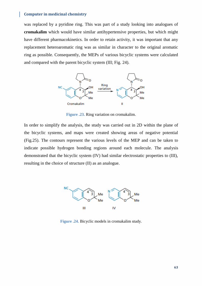
Computer in medicinal chemistry
63
was replaced by a pyridine ring. This was part of a study looking into analogues of
cromakalim which would have similar antihypertensive properties, but which might
have different pharmacokinetics. In order to retain activity, it was important that any
replacement heteroaromatic ring was as similar in character to the original aromatic
ring as possible. Consequently, the MEPs of various bicyclic systems were calculated
and compared with the parent bicyclic system (III; Fig. 24).
Figure .23. Ring variation on cromakalim.
In order to simplify the analysis, the study was carried out in 2D within the plane of
the bicyclic systems, and maps were created showing areas of negative potential
(Fig.25). The contours represent the various levels of the MEP and can be taken to
indicate possible hydrogen bonding regions around each molecule. The analysis
demonstrated that the bicyclic system (IV) had similar electrostatic properties to (III),
resulting in the choice of structure (II) as an analogue.
Figure .24. Bicyclic models in cromakalim study.

Computer in medicinal chemistry
64
Figure .25. Molecular electrostatic potentials (MEPs) of bicyclic models (III) and (IV).
II.4.3.3 Molecular orbitals
The most important orbitals in a molecule are the frontier molecular orbitals,
called highest occupied molecular orbital (HOMO) which explains the ionization
energy and lowest unoccupied molecular orbital (LUMO) which explains the electron
affinity in a molecule.
These orbitals determine the way the molecule interacts with other species including
the interactions between a ligand and its receptor [38]. Whereas, electrophilic and
nucleophilic attack will most likely occur at atoms where the coefficients of the
corresponding atomic orbitals in HOMO and LUMO, respectively, are large [39]. For
example, ethene can be shown to have 12 molecular orbitals. The highest occupied
molecular orbital (HOMO) and lowest unoccupied molecular orbital (LUMO) are
shown in Fig. 26.

Computer in medicinal chemistry
65
Figure .26.HOMO and LUMO molecular orbitals for ethene.
II.4.3.4 Fukui functions
The Fukui functions are some of these indexes. They represent a local reactivity of the
studied compounds. They are given by [40]:
where ρ(r) is the electronic density, N is the number of electrons and v(r) is a constant
external potential. The reactivity of an atom k in a molecule can be described, by a
condensed Fukui function fk. As ρ(r) is a discontinuous function of N, Yang and Parr
[41, 42]have proposed approximated atomic indices fk by applying the finite
difference approximation to the condensed electronic population on any atom. Three
indices were defined to describe nucleophilic, electrophilic, and radical attack. These
can be written respectively as:
f+(A) = [qN+1(A) - qN(A)]
f-(A) = [qN(A) - qN-1(A)]
f0(A)= [qN+1(A) - qN-1(A)] /2
qk(N): electronic population of k atom in neutral molecule.
qk(N+1): electronic population of k atom in anionic molecule.
qk(N-1): electronic population of k atom in cationic molecule.

Computer in medicinal chemistry
66
In this approximation, the indices depend widely on the used population analysis
approach. The electronic population around an atom k can be evaluated using
Mulliken[43], Hirshfield[44], or natural orbital [45]approximations. These indices are
some of the widely used local density functional descriptors to model chemical
reactivity and site selectivity [41, 46]. The atom with the highest Fukui indices is the
most reactive compared to the other atoms in the molecule.
II.5. Studies of vibrational properties
II.5.1. Introduction
Molecular modeling is essential for the interpretation and understanding of
experimental observations. In the molecular domain, all properties are related to the
nature and shape of the molecule. Being able to optimize the geometry of a molecule
by a theoretical model (quantum chemistry methods) is to approach its molecular
conformation observed experimentally [47, 48].
The object of this part of our work, which was oriented towards the search for a
molecular conformation of the calculated indole similar to that given by the
experiment, is to make a contribution to the understanding of the structural, vibrational
properties and electronics to exhibit the most stable molecular conformation and also
the arrangement and atomic environment of carbazole.
II.5.2. Theoretical aspects of infrared vibration spectroscopy
The movements of atoms in a molecule can be classified into three categories:
translations, rotations and vibrations. Nowadays, studies by vibrational spectroscopy
are, more and more, supplemented by calculations of quantum chemistry [49, 50].
In this case, the contribution of molecular modeling is very important to
understand reaction mechanisms or have access to chemical properties. Indeed, the
methods of quantum chemistry make it possible to model a very large number of
quantities characteristic of atomic or molecular systems or to simulate a wide variety

Computer in medicinal chemistry
67
of reaction processes. Also, the combination of these two techniques is proving to be
very powerful in explaining mechanistic details at the molecular level [51].
The main purpose of vibrational spectroscopy is the determination of the
vibrational frequencies of a molecule. These frequencies depend on the mass of the
atoms involved in the normal mode of vibration as well as the strength of the
interatomic bonds. Therefore, precise information about the structure of a molecule
can be deduced from a vibrational spectrum [52, 53].
Molecular vibrations take place at different frequencies (υ vib) which depend on the
nature of the bonds as well as their environment. These frequencies correspond to the
infrared range of electromagnetic radiation [54].
II.5.3. Principle of infrared spectroscopy
II.5.3.1. Electromagnetic radiation
Electromagnetic radiation consists of a beam of particles: photons, the
movement of which is described by means of equations of wave mechanics.
The latter has shown that light participates in both wave and particle properties. When
it collides with matter, it can be thought of as discrete packets of energy (quanta)
called photons [55]. The interactions between matter and a radiation to which it is
subjected are numerous. The most interesting and the most studied involve absorption
phenomena (molecules can absorb the energy quanta of certain radiations). In this
case, their fundamental energy states are altered by transition, or transition, to excited
states of higher energy. Each state of matter is quantified and excitation takes place by
absorption of a discrete amount of energy ΔE [56]. To be absorbed, the radiation must
be at the same frequency corresponding to this quantity of energy either: the recording
of the energy absorbed or transmitted according to the frequency or the wavelength,
constitutes the absorption spectrum of the compound in the spectral region of interest
[55, 57]. The frequency ν of an electromagnetic wave is related to its wavelength by
the relation [56, 57]:
ν = C/λ

Computer in medicinal chemistry
68
where C represents the speed of light propagation in vacuum and λ the wavelength.
The energy E of the radiation or photon is directly proportional to the frequency of the
electromagnetic wave or the field wave.
It is written: E = hν
Normally, a spectrum should appear as a succession of fine lines. In fact, there is for a
molecule a succession of energetic states close to each other.
Hence the obtaining of more or less broad peaks or absorption bands even with
equipment with high resolving power. The purpose of studying infrared spectra is most
often to characterize compounds or to verify their compliance with a reference sample.
Absorption in the infrared spectral region corresponds to transitions in the energies of
molecular vibrations.
Figure .27.The various spectral domains of electromagnetic radiation.
Quantum mechanics shows us that only vibrational transitions in which there
is variation in the dipole moment of the molecule, can cause an absorption peak in IR
to appear. Many lines are due to the different modes of vibration of the bonds.

Computer in medicinal chemistry
69
II.5.3.2. Infrared
Understood between the visible and the microwaves, the infrared is subdivided into
three parts: the near infrared located between 13,000 and 4,000 cm-1, the medium
infrared located between 4,000 and 200 cm-1, and the far infrared located between 200
and 10 cm-1[56]. Infrared spectroscopy is based on the study of the reactions between
matter and electromagnetic radiation. The latter can be defined by its frequency ν
expressed in hertz (Hz) or by its wave number, V is usually expressed in cm-1 or in
kayser. It represents the number of waves contained in the interval of 1 cm [57]. In our
investigation, we limited ourselves to the mid-infrared range (in the region of 4000 to
600 cm-1), this corresponds to energies ranging from 4 to 40 kJ.mol-1.
An infrared spectrum is complex. This complexity can be increased by the appearance
of additional bands due to the harmonics of the fundamental absorption frequencies νf
of lower intensity. They can be observed at 2νf, 3νf, or at frequency combination bands,
which correspond to the sum of two fundamental frequencies.
Fundamental bands may not appear in the following cases: the vibration does not
cause a variation in the dipole moment of the molecule, which often occurs in the case
of compounds with a very symmetrical structure; vibrations occur at very close
frequencies or at the same frequency; absorption is too low for the band to be visible.
II.5.3.3. Infrared absorption
Any molecule excited by electromagnetic radiation absorbs an amount of energy
and goes into an excited state. According to the mechanics, the absorption process is
quantified and only particular frequencies can be absorbed by the molecule.
Vibrational excitation can be considered simply by considering two atoms A1 and A2
united by a bond as being two masses connected by a spring (figure 28) which
stretches and relaxes at a certain frequency υ.

Computer in medicinal chemistry
70
Figure.28.Movement of atoms during the phenomenon of vibration
In this representation, the frequency of vibrations between the two atoms depends
both on the bond strength between them and on their atomic masses. It can be shown
that it is governed by the following Hooke's law which describes the motions of a
spring.
Ʋ՟ : vibrational frequency in wavenumbers (cm-1)
K: constant
f :force constant, indicating the stiffness of the spring (of the connection)
m1 and m2: values of the masses attached to the spring (masses of the united atoms)
This equation could lead us to think that each individual bond in a molecule
gives rise to a specific absorption band in the infrared spectrum. Which is not the case.
The energies of radiation absorption correspond to movements of elongation, or
deformation of most of the covalent bonds of molecules. In the process of absorption,
the frequencies of infrared radiation coincide with those of the natural vibrational
frequencies of molecules [58]. Not all bonds are capable of absorbing infrared energy
even if their frequency coincides perfectly with that of movement of the bond. Only
groups whose dipole moment varies during vibration are bonds which admit a dipole
movement are able to absorb infrared radiation [57].

Computer in medicinal chemistry
71
A bond must have an electric dipole which must oscillate at the same frequency as that
of the excitation radiation, so that energy can be transferred.
In the case of infrared spectroscopy the molecule absorbs infrared light if and only if
the dipole moment of the molecule changes during vibration [58].
The advantage with infrared is that it avoids unwanted photochemical or
luminescence reactions. Electromagnetic radiation in the infrared (located in the region
of 10,000 to 20 cm-1), causing a change in the vibrational level nevertheless leaves the
molecule at its fundamental electronic level [58, 59]. To understand the phenomenon
of atomic vibration, it must be visualized as the interaction of two particles linked
together by a spring [58]. When this spring is pulled and released, the two particles
enter into a stretching motion. The amplitude of their movement is not only a function
of the mass of the particles but also of the force of the spring (see figure 28). During
the vibration phenomenon, other movements can be described: stretching, folding,
twisting, swaying, shearing. In biological membranes, these movements become all the
more complex as the chemical structures of the membrane constituents are more
elaborate.
II.5.4. Theoretical aspects
II.5.4.1. Internal vibration modes
In a polyatomic molecule comprising N atoms, the atoms can perform oscillating
movements around their position of equilibrium. The rather weak oscillations of the
molecule cause small displacements of the atoms formed. In this case the harmonic
oscillation model is adapted to describe the movements of the atoms of the molecule.
In a molecule made up of N atoms, each atom is assigned three coordinates to define
its position. There by; an atom has three independent degrees of freedom of movement
in the three directions of space. This results in 3N degrees of freedom to describe the
motion of an entire molecule (Table 2). Of these 3N degrees of freedom, three are the
coordinates that define the position of the center of mass of the molecule (translational
degrees of freedom), and three other coordinates necessary to specify the molecular
orientation around the center of gravity. These represent the degrees of freedom of

Computer in medicinal chemistry
72
rotation. Note that a linear molecule has only two degrees, since rotation around the
molecular axis does not cause the nuclei to shift. In conclusion, a molecule with N
atoms has 3N-6 (3N 5 for a linear molecule) degrees of freedom, responsible for all
changes in the shape of the molecule without moving or rotating the center of gravity
of the molecule [60, 61].
Table.2. Molecular degrees of freedom
II.5.4.2. Classification of vibration modes
Vibrations can be classified into two categories: in-plane and out-of-plane [62, 63].
In the plane: we distinguish the elongation (ν) and the angular deformation (δ)
which can be either symmetrical (δs and νs), or antisymmetric (δas and νas).
Symmetric and antisymmetric angular deformations correspond to shearing or
rotational movements of three atoms forming the angle θ (Figure 29).
Out of plane: these are angular deformations outside a molecular plane that can
induce collective movement of the molecule corresponding to torsion (τ) or
sway (γ) movements.

Computer in medicinal chemistry
73
Figure.29. Movements associated with normal modes of vibration of a molecule containing
3 atoms.
II.5.4.3. Factors that influence vibration frequencies
Analysis of an IR spectrum most often carried out in solution or in the solid state
shows that a number of factors influence the vibration frequencies as well as their
intensities.
The intensity of the bands depends on the nature and polarity of the bond. The
vibration frequency, for its part, depends on the atoms constituting the bond, the
multiplicity of the bond and its environment. Generally speaking, bonds between light
atoms vibrate at a higher frequency than bonds between heavier atoms. The higher the
constant K (bond strength constant), the higher the vibration frequency.
The link environment can have an electronic or mechanical impact on the vibration of
this frequency. We will cite a few examples:
Electrical effects: The effects of electronegativity and conjugation can cause
significant shifts in vibration frequencies.
Hydrogen bond: For some functions such as –OH, -NH, -SH, there is the
possibility of hydrogen bond formation when they perceive in their molecular
neighborhood the presence of an electronegative atom. This results in an
elongation of the X-H bond and therefore a weakening of its force constant.

Computer in medicinal chemistry
74
Steric Effects: The frequency of a vibration depends on the steric constraints
associated with this vibrator. The vibration ν (C = O) occurs at a frequency so
much higher as the valence angle COC is small.
Mechanical coupling: When in a molecule vibration of the same nature are found in
the vicinity of one another, having an atom in common for example, they do not
vibrate independently of one another. As a result, the frequencies are affected
compared to those generally observed. This phenomenon is due to the existence of a
mechanical coupling.
II.5.5. Application
Infrared spectrometry [64]thus provides detailed information on:
The chemical structure of macromolecules and the composition of the polymer:
identification of the basic unit, branches, analysis of chain ends, determination
of the nature and concentration of additives, structural defects, impurities.
Intra- or intermolecular interactions, chain conformation, polymer crystallinity,
orientation of macromolecules.
Infrared spectrometry is also an effective tool for studying the structural
modifications of polymers resulting from chemical treatments, degradations or
aging of various origins.
II.6 Conclusion
Chemoinformatics and molecular modeling methods are among the recent
techniques now routinely applied in the research phases and in particular for the
management and analysis of chemical libraries. They certainly arouse as much hope as
they do criticism, but nevertheless constitute a very active line of research over the
past two decades. In this chapter, we have presented most of the methods used in
chemoinformatics for the analysis of chemical libraries. All of these concepts were
used during this thesis in order, on the one hand, to make our own contribution
through the creation of new methods allowing to characterize the chemical libraries
and on the other hand, to develop a software allowing to implement some of these
methods.

Part II:
Computer-Assisted Drug Design

Computer-Assisted drug design
76
What is computer-assisted drug design (CADD), and why is it important? There is no
clear definition, although a consensus view has emerged. Simply, CADD is the
coalescence of information on chemical structures, their properties, and their
interactions with biological macromolecules. Further, these data are transformed into
knowledge intended to aid in making better decisions for drug discovery and
development.
These are representative of some questions facing the current drug-design community
and significant applications of CADD.
Of the compounds included in our dataset, how many could be predicted to lack drug
likeproperties based on similarity in properties to known orally active drugs?
How many would be predicted to be inactive based on the known structure–activity
dataavailable on topoisomerase II inhibitors?
Given the structure–activity relationships (SARs) available on the inhibitors, what
could one determine regarding the active site of topoisomerase II?
What novel classes of compounds could be suggested based on the SAR of inhibitors,
or based on the new crystal structure of the complex?
Do the most potent compounds share a set of properties that can be identified and used
to optimize a novel lead structure?
Can a predictive equation relating properties and affinity for the isolated enzyme be
established?
II.1 Predictive Quantitative Structure–Activity Relationship Modeling
At the beginning of its over 40 years of existence as an independent area of
research,quantitative structure–activity relationship (QSAR) modeling was viewed
strictly as analytical physical chemical approach applicable only to small congeneric
series of molecules. The technique was first introduced by Hanschet al.[65]on the basis
of implications from linear free energy relationships in general and the Hammett
equation in particular. [66]
It is based upon the assumption that differences in physicochemical properties account
for the differences in biological activities of compounds. According to this approach,

Computer-Assisted drug design
77
the changes in physicochemical properties that affect the biological activities of a set
of congeners are of three major types: electronic, steric, and hydrophobic.[67]
The quantitative relationships between biological activity (or chemical property)
and the structural parameters could be conventionally obtained using multiple linear
regression (MLR) analysis. The fundamentals and applications of this method in
chemistry and biology have been summarized by Hansch and Leo.[67]This traditional
QSAR approach has generated many useful and, in some cases, predictive QSAR
equations and led to several documented drug discoveries.[68-70]
Many years of active research in QSAR have dramatically changed the breadth
and the depth of this field in all its components including the diversity of target
properties, descriptor types, data modeling approaches, and applications. The most
important changes in QSAR deal with a substantial increase in the size of data sets
available for the analysis and an increasing use of QSAR models as virtual screening
tools to discover biologically active molecules in chemical databases and virtual
chemical libraries.
II.2. Principle of QSPR / QSAR methods
The principle of the QSPR / QSAR methods is to establish a mathematical
relationship linking in a quantitative manner molecular properties, called descriptors,
with a macroscopic observable (biological activity, toxicity, physicochemical property,
etc.), for a series of similar chemical compounds. using data analysis methods. The
general form of such a model is as follows:
Property / Activity = f (D1, D2,…Dn ,,…)
D1, D2, Dn are descriptors of molecular structures.
The aim of such a method is to analyze structural data in order to detect the
determining factors for the property / activity being measured. To do this, different
types of statistical tools can be used:
- Simple and multiple linear regressions [71],
- Partial least squares regressions (PLS) [72],

Computer-Assisted drug design
78
- Decision trees [73],
- Neural networks [74-76],
- Genetic algorithms[77],
- Machine Vectors [76],
Once this relationship is established and validated, it can then be employed for the
prediction of the property / activity of new molecules, for which experimental values
are not available. Such models can also be used to better understand mechanisms and
modes of action.
II.3 Key Quantitative Structure–Activity Relationship Concepts
An inexperienced user or sometimes even an avid practitioner of QSAR could be
easily confused by the diversity of methodologies and naming conventions used in
QSAR studies. 2D or three-dimensional (3D) QSAR, variable selection or artificial
neural network (ANN) methods, Comparative molecular field analysis (CoMFA), or
binary QSAR present examples of various terms that may appear to describe totally
independent approaches, which cannot be generalized or even compared to each other.
In fact, any QSAR method can be generally defined as an application of mathematical
and statistical methods to the problem of finding empirical relationships (QSAR
models) of the form 𝑃𝑖 = 𝑘(𝐷1, 𝐷2, … 𝐷𝑛),where 𝑃𝑖 are biological activities (or other
properties of interest) of molecules, 𝐷1, 𝐷2, … 𝐷𝑛 are calculated (or, sometimes,
experimentally measured) structural properties (molecular descriptors) of compounds,
and 𝑘 is some empirically established mathematical transformation that should be
applied to descriptors to calculate the property values for all molecules.
The relationship between values of descriptors D and target properties P can be
linear (e.g., MLR as in the Hansch QSAR approach), where target property can be
predicted directly from the descriptor values, or nonlinear (such as ANNs or
classification QSAR methods) where descriptor values are used in characterizing
chemical similarity between molecules, which in turn is used to predict compound
activity.

Computer-Assisted drug design
79
The differences in various QSAR methodologies can be understood in terms of the
types of target property values, descriptors, and optimization algorithms used to relate
descriptors to the target properties and generate statistically significant models.
A- Target properties(regarded as dependent variables in statistical data modeling
sense) can generally be of three types:
(1) continuous, i.e., real values covering certain range, e.g., IC50, MIC values, or
binding constants.
(2) categorical related, classes of target properties covering certain range of values,
e.g., active and inactive compounds, frequently encoded numerically for the
purpose of the subsequent analysis as 1 (for active) or 0 (for inactive), or adjacent
classes of metabolic stability such as unstable, moderately stable, and stable.
(3) categorical unrelated, classes of target properties that do not relate to each
other in any continuum, e.g., compounds that belong to different pharmacological
classes, or compounds that are classified as drugs versus non drugs.
B- Chemical descriptors(or independent variables in terms of statistical data
modeling) can be typically classified into two types:
(1) continuous (i.e., range of real values, e.g., as simple as molecular weight or
many molecular connectivity indices); or
(2) categorical related (i.e., classes corresponding to adjacent ranges of real values,
e.g., counts of functional groups or binary descriptors indicating presence or
absence of a chemical functional group or an atom in a molecule).
Descriptors can be generated from various representations of molecules, e.g., 2D
chemical graphs or 3D molecular geometries, giving rise to the terms of 2D or 3D
QSAR, respectively.
C- Correlation methods(which can be used either with or without variable selection)
can be classified into two major categories:
(1) linear (e.g., linear regression (LR), or principal component regression (PCR),
or partial least squares (PLS)) or
(2) nonlinear (e.g., k nearest neighbor (kNN), recursive partitioning (RP), ANNs,
or support vector machines (SVMs). [78]

Computer-Assisted drug design
80
Figure .30.Molecular descriptors and fingerprints are examples of strategies that allow researchers to
extract important information about compounds that can be used in additional computer-aided drug
design techniques, such as virtual screening, quantitative-structure-activity relationship (QSAR).
In some cases, the types of biological data, the choice of descriptors, and the class
of optimization methods are closely related and mutually inclusive. For instance, MLR
can only be applied when a relatively small number of molecular descriptors are used
(at least five to six times less than the total number of compounds) and the target
property is characterized by a continuous range of values. The use of multiple
descriptors makes it impossible to use MLR due to a high chance of spurious
correlation [79]and requires the use of PLS or nonlinear optimization techniques.
II.3.1 Molecular Descriptors
Theoretical descriptors derived from physical and physico-chemical theories
show some natural overlap with experimental measurements. Several quantum
chemical descriptors, surface areas, and volume descriptors are examples of such
descriptors also having an experimental counterpart.
With respect to experimental measurements, the greatest recognized advantages of the
theoretical descriptors are usually (but not always) in terms of cost, time, and
availability.
Each molecular descriptor takes into account a small part of the whole chemical
information contained in to the real molecule and,asaconsequence,the number of
descriptors

Computer-Assisted drug design
81
iscontinuouslyincreasingwiththeincreasingrequestofdeeperinvestigationsonchemicalan
d biological systems. Different descriptors have independent methods or perspectives
to view a
molecule,takingintoaccountthevariousfeaturesofchemicalstructure.Moleculardescriptor
s have now become some of the most important variables used in molecular modeling,
and, consequently, managed by statistics, chemometrics, and chemoinformatics[80].
There are many different descriptors and many different kinds of classification
based on the effect (steric, hydrophobic, electronic, etc.) or based on its dimension that
called Descriptors Block, whereas we find four types of molecular descriptors 0D, 1D,
2D and 3D [80].
Molecular descriptors 0D, 1D: contains numbers of atoms, functional groups,
molecules properties, and charges (eg.MolecularWeight,
MolecularRefractivity,etc.).
Moleculardescriptors2D:containssimpledescriptorsandotherderivativesofalgorit
hms applied to a topological representation (eg. Number of Cl atoms, presence
of hydroxyl group,etc.).
Molecular descriptors 3D: contains descriptors derived from a geometric
representation also called geometric descriptors (eg. Molecular volume, Surface
area,etc.).
II.3.3 Quantitative Structure–Activity Relationship Modeling Approaches
II.3.3.1 General Classification
Many different approaches to QSAR have been developed since Hansch’s seminal
work. As briefly discussed above, the major differences between these methods can be
analyzed from two viewpoints:
(1) the types of structural parameters that are used to characterize molecular identities
starting from different representation of molecules, from simple chemical formulas to
3D conformations, and
(2) the mathematical procedure that is employed to obtain the quantitative relationship
between these structural parameters and biological activity.

Computer-Assisted drug design
82
Based on the origin of molecular descriptors used in calculations, QSAR methods can
be divided into three groups.
One group is based on a relatively small number (usually many times smaller than the
number of compounds in a data set) of physicochemical properties and parameters
describing hydrophobic, steric, electrostatic, etc. effects. Usually, these descriptors are
used as independent variables in multiple regression approaches. In the literature, these
methods are typically referred to as Hansch analysis.
A more recent group of methods is based on quantitative characteristics of molecular
graphs (molecular topological descriptors). Since molecular graphs or structural
formulas are ‘two dimensional,’ these methods are described as 2D QSAR. Most of
the 2D QSAR methods are based on graph theoretical indices. Although these
structural indices represent different aspects of molecular structures, and, what is
important for QSAR, different structures provide numerically different values of
indices, their physicochemical meaning is frequently unclear.
The third group of methods is based on descriptors derived from spatial (3D)
representation of molecular structures. Correspondingly, these methods are referred to
as 3D QSAR; they have become increasingly popular with the development of fast and
accurate computational methods for generating 3D conformations and alignments of
chemical structures. Perhaps the most popular example of 3D QSAR is CoMFA,
developed by Cramer et al.,[81]which has combined the power of molecular graphics
and PLS technique and has found wide applications in medicinal chemistry and
toxicity analysis.[82]
II.3.3.2. General Methodology of a QSPR / QSAR study
The general methodology of a QSAR / QSPR study is as follows:
a- Build up a database from reliable experimental measurements of the property or
activity of each compound.
b- Select the descriptors in relation to the property or activity studied.
c- Divide this database, randomly, into a training set which generally contains 2/3 of
the database and a test series (test set) consisting of the remaining 1/3.

Computer-Assisted drug design
83
d- Establish mathematical models using the learning series.
e- Characterize the models developed by their internal validation indices and check
their robustness by a randomization test (Randomization) of the dependent variable Y
(response).
f-Validate the models developed using the test series and calculate their statistical
parameters for external validation.
II.3.3.3 Transforming the Bioactivities
The main advantage of transforming data is to guarantee linearity, to achieve
normality, or to stabilize the variance. Several simple nonlinear regression
relationships can be made linear through the appropriate transformations. The simplest
and most common method of transforming [83]bioactivity data is to take the log or
negative log of the bioactivities to reduce the range of the data.
The method of creating Training and Test Sets that are representative of the population
is to choose molecules that represent all the molecules of interest based on molecular
structure and bioactivity. The number of molecules in the Test Set is determined (20%
of the total molecules in this study) and then all the molecules are placed in a table and
ordered based on bioactivities. With the table prepared, the extraction of the molecules
for the Test Set can begin through an iterative process starting at the top of the table.
II.3.3.4 Determination of the Best Set of Descriptors Approaches
Both 2D and 3D QSAR studies have focused on the development of optimal
QSAR models through variable selection. This implies that only a subset of available
descriptors of chemical structures, which are the most meaningful and statistically
significant in terms of correlation with biological activity, is selected.
The Stepwise Method Search selects a model by adding or removing individual
descriptors, a step at a time, based on their statistical significance. The end result of
this process is a single regression model, which makes it nice and simple.
The p-value for each term tests the null hypothesis that the coefficient is equal to zero
(no effect). A low p-value (< 0.05) indicates that you can reject the null hypothesis. In
other words, a descriptor that has a low p-value is likely to be a meaningful addition to

Computer-Assisted drug design
84
your model because changes in the descriptor's value are related to changes in the
response variable (bioactivity). Conversely, a larger (insignificant) p-value suggests
that changes in the descriptor are not associated with changes in the response.
II.4. Building Predictive Quantitative Structure–Activity Relationship Models:
The Approaches to Model Validation
II.4.1. Data analysis methods
To develop a QSPR / QSAR model we need a data analysis method, this method
allows to quantify the relationship between the property / Activity and the Structure
(descriptors).
There are several methods to build a model and analyze its statistical data, some are
linear such as multiple linear regression (MLR), partial least squares (PLS) regression,
others are nonlinear such as trees of decisions, neural networks… these methods are
available in software such as, Excel, Origin Microcal, Minitab, Statistica, SPSS, JMP,
R,…
The method used in our studies is the Multiple Linear Regression (MLR) and Neural
Networks (ANN) method.
II.4.1.1. Neural networks
The formal neural networks initiated in 1943 by Mc Culloch and Pitts are analogous to
biological nervous systems.[84]
Formal neurons (Figure 31) perform a linear combination of the inputs
received(descriptors), then apply to this value an activation function f, generally
nonlinear (sigmoidal, tangent, hyperbolic). The obtained value Y (biological activity)
is the output of the neuron.[85]

Computer-Assisted drug design
85
Figure.31.Representation of a formal neuron.
Xk (where k = 1, 2, …, n) are the input neurons (descriptors) and Wk
(where k = 0, 1, 2, …,n) are the weights. W0 is the weight associated with
an entry set at 1, called bias. The neuron equation looks like this:
Neurons alone perform fairly simple functions, and it is their combinations, called
neural networks, that make it possible to construct particularly interesting functions
(Figure 31).
Figure.32.Architecture of neural networks.

Computer-Assisted drug design
86
The architecture of neural networks consists of three layers:
o An input layer: made up of input neurons, their number is equal to the number
of input variables (descriptors) plus one (bias). Each neuron is connected to the
hidden neurons.
o A hidden layer: made up of a variable number of neurons. For each hidden
neuron, the network performs a weighted sum operation with the different
weights of each input neuron.
o An output layer: where the number of output neurons is equal to the number of
properties (activities) to be modeled.
Each connection between the neurons of the different layers is associated with a
weight. The number of weights then depends on the number of neurons in the hidden
layer, so it is possible to vary the complexity of the network by increasing or
decreasing the number of hidden neurons. To do this, data presentation cycles are
established via a learning algorithm. The one used in our approach is a
backpropagation algorithm.[86]
The principle of the back-propagation algorithm is to minimize the difference between
the calculated output (calculated activity) and the experimental values of the activity.
Defined in two stages, the algorithm propagates in a first stage the inputs (descriptors)
forward until obtaining an output (biological activity) calculated by the network. In a
second step, the calculated output is compared with the experimental value. The error
obtained by this comparison is then propagated back to the input layer by modifying
the weights of the neurons. This process is repeated until a negligible error is
obtained.[87]
II.4.1.2 Multiple linear regression
Multiple linear regression is the simplest statistical modeling method and the most
applied in studies of the structure-activity relationship [88]. The method was
popularized by Hanch by relating biological activity to experimental lipophilic,
electronic and steric properties for series of compounds.[89]

Computer-Assisted drug design
87
The RLM method is based on the assumption that there is a linear relationship
between a dependent variable Y (in our case the biological activity) and a series of n
independent variables Xi (here, the molecular descriptors)[90]. The objective is to
arrive at a mathematical equation of the form:
Where ai (i = 0, 1,…, n) are the coefficients of the regression.
Determining the equation from a data set of p samples is like solving a system of p
equations.
Or:
The residuals bi (i = 1, 2, ..., p) represent the model error,
yi (i = 1, 2,…, p) represent the dependent variables (activities),
xi (i = 1, 2,…, p) represent the independent variables (descriptors),
ai (i = 1, 2,…, p) represent the coefficients of the regression.
This set of equations can be written in the following matrix form:

Computer-Assisted drug design
88
Or in a condensed way:
Y = XA + B
Where Y, X, A, and B represent the property vector, the attribute matrix (descriptors),
the coefficient matrix, and the regression error matrix, respectively.
The RLM method then consists in choosing the coefficients ai so as to minimize
the sum of the squares of the differences between the calculated values of the property
and the experimental ones, the equation of the model therefore becomes:
Or in matrix form:
The coefficients can be obtained from the following matrix equation:
II.4.1.2.1. Randomization test
The randomization test is used by the modeler to assert that the good correlations,
between descriptors and activity, presented by the QSAR model are not due to luck.
To do this, the observations are randomly disorganized, for example ten times, by
randomly changing the activity column, but the descriptor columns remain
unchanged[91]. We therefore obtain ten models with specific statistical characteristics.
If the randomization of the observations leads to weak forecast models, this means that

Computer-Assisted drug design
89
the predictive capacities of the constructed QSAR model are not due to the
correlations of luck.[92]
II.4.2. Interpretation and validation of a QSPR / QSAR model
Once developed, the model must be interpreted by analyzing all the statistical
parameters of this model, its quality must also be studied, this quality is checked by
what is called validation. Its robustness, ie the influence of the compounds of the
training series on the model, is estimated by internal validation methods. In order to
estimate its predictive power, additional experimental data is needed to determine the
ability of the model to predict these values, this is called external validation. Finally, it
is important to know which type of molecules used with which model.
II.4.2.1. The Importance of Validation
The process of QSAR model development is divided into three key steps: (1) data
preparation, (2) data analysis, and (3) model validation. The implementation and
relative merit of these steps is generally determined by the researcher’s interests and
experience, and the availability of software. The resulting models are then frequently
employed, at least in theory, to design new molecules based on chemical features or
trends found to be statistically significant with respect to underlying biological
activity.
The first stage includes the selection of a data set for QSAR studies and the
calculation of molecular descriptors. The second stage deals with the selection of a
statistical data analysis technique, either linear or nonlinear such as MLR, PLS or
ANN. A variety of different algorithms and computer software are available for this
purpose. In all approaches, descriptors are considered as independent variables, and
biological activities as dependent variables.
Typically, the final part of QSAR model development is model validation, [93, 94]in
which estimates of the predictive power of the model are calculated. This predictive
power is one of the most important characteristics of QSAR models.
Ideally, it should be defined as the ability of the model to predict accurately the target
property (e.g., biological activity) of compounds that were not used in model

Computer-Assisted drug design
90
development.
Here, we are going to discuss about the validation parameters for the QSAR
models which are developed by multiple linear regression (MLR). Four tools of
assessing validity of QSAR models [95]are (i) cross-validation, (ii) bootstrapping, (iii)
randomization of the response data, and (iv) external validation. Where we are using
the data that created the model (an internal method) and using a separate data set (an
external method).
The methods of least squares fit (R²), cross validation (Q²) [96, 97], adjusted R²
(R²adj), chisquared test (χ²), rootmean-squared error (RMSE), bootstrapping and
scrambling (YRandomization) [98, 99]are internal methods of validating a model. The
best method of validating a model is an external method, such as evaluating the QSAR
model on a test set of compounds.
II.4.2.1.1. Internal Validation
II.4.2.1.1.1. Least Squares Fit
The most common internal method of validating the model is least squares fitting.
This method of validation is similar to linear regression and is the R2(squared
correlation coefficient) for the comparison between the predicted and experimental
activities. An improved method of determining R2is the robust straight line fit, where
data points are away from the central data points (essentially data points a specified
standard deviation away from the model) are given less weight when calculating the
R2. An alternative to this method is the removal of outliers (compounds from the
training set) from the dataset in an attempt to optimize the QSAR model and is only
valid if strict statistical rules are followed. The difference between the R2and R2adj
value is less than 0.3 indicates that the number of descriptors involved in the QSAR
model is acceptable. The number of descriptors is not acceptable if the difference is
more than 0.3.

Computer-Assisted drug design
91
Where, y and ŷ are the experimental and predicted bioactivity for an individual
compound in the training set, ymis the mean of the experimental bioactivities, and n is
the number of molecules in the set of data being examined. PRESS is the predictive
residual sum of the squares.
II.4.2.1.1.2 Fit of the Model
Fit of the QSAR models can be determined by the methods of chi-squared (χ2) and
root-mean squared error (RMSE). These methods are used to decide if the model
possesses the predictive quality reflected in the R2. The use of RMSE shows the error
between the mean of the experimental values and predicted activities. The chi squared
value exhibits the difference between the experimental and predicted bioactivities:
Large chi-square or RMSE values (≥0.5 and 1.0, respectively) reflect the model’s
poor ability to accurately predict the bioactivities even the model is having large
R2value (≥0.7).
For good predictive model the chi and RMSE values should be low (<0.5 and
<0.3, respectively). These methods of error checking can also be used to aid in
creating models and are especially useful in creating and validating models for
nonlinear data sets, such as those created with Artificial Neural Network (ANN) [100].
However, excellent values of R2, χ2and RMSE are not sufficient indicators of model
validity. Thus, alternative parameters must be provided to indicate the predictive
ability of models. In principle, two reasonable approaches of validation can be
envisaged one based on prediction and the other based on the fit of the predictor
variables to rearranged response variables.

Computer-Assisted drug design
92
II.4.2.1.2 External validation
Several authors have suggested that the only way to estimate the true predictive
power of a QSAR model is to compare the predicted and observed activities of an
(sufficiently large)external test set of compounds that were not used in the model
development [94, 101-104]. The problem in external validation is how can we select
the training and test set? Roy et al. clearly discussed that how we can solve this
problem in one of their article. [105]
To estimate the predictive power of a QSAR model, Golbraikh and Tropsha
recommended use of the following statistical characteristics of the test set [93]: (i)
correlation coefficient R between the predicted and observed activities; (ii) coefficients
of determination (R2) (predicted vs. observed activities r02, and observed vs. predicted
activities r0'); (iii) slopes k and k' of the regression lines through the origin. They
consider a QSAR model is predictive, if the following conditions are satisfied [93]:
The predictive ability of the selected model was also confirmed by external
R2test. A value ofR2test is greater than 0.6 may be taken as an indicator of good
external predictability.
Where �̅�𝑡𝑟 is the average value for the dependent variable for the training set. Kubinyi
et al[94], Novellino et al.[102], Norinder[103], and Golbraikh and
Tropsha[93]demonstrated that all of the above-mentioned criteria are necessary to
adequately assess the predictive ability of a QSAR model. Norinder suggest [103]that
the external test set must contain at least five compounds, representing the whole range
of both descriptor and activities of compounds included into the training set.

Computer-Assisted drug design
93
II.5. Application of QSAR
There are a large number of applications of QSAR models in industry, in university
research, in economics, in weather forecasting, …etc.
We report below some possible applications of QSAR models:
Rational identification of new leads with: optimization of pharmacological,
biocidal or pesticide activity.
Rational design of many products such as surfactants, perfumes, dyes and fine
chemicals.
The identification of dangerous compounds in the early stages of development.
Prediction of toxicity and side effects of new compounds.
The selection of compounds with optimal pharmacokinetic properties, be it
stability or availability in biological systems.

Computer-Assisted drug design
94
Figure.33. Schematic overview of the QSAR process.

References
[1] C. Larive, Apports combinés de l'expérimentation et de la modélisation à la compréhension de
l'alcali-réaction et de ses effets mécaniques, in, Ecole nationale des ponts et chaussees, 1997.
[2] A. Hamdouch, M.-H. Depret, Spatial Scales, Proximity and Institutional Logics: Outline of an
Evolutionary Approach of Technological Change Dynamics in Pharmaceuticals and Biotechnology
(Echelles spatiales, formes de proximite et logiques institutionnelles: Esquisse d'une approche co-
evolutionnaire des dynamiques de changement technologique dans la pharmacie et les
biotechnologies), (2008).
[3] F. Lerbet-Sereni, Expériences de la modélisation, modélisation de l'expérience, Harmattan, 2004.
[4] Y. Yamaguchi, H.F. Schaefer, Y. Osamura, J. Goddard, A New Dimension to Quantum Chemistry:
Analytic Derivative Methods in Ab Initio Molecular Electronic Structure Theory, Oxford University
Press, 1994.
[5] G.H. Loew, H.O. Villar, I.J.P.r. Alkorta, Strategies for indirect computer-aided drug design, 10
(1993) 475-486.
[6] A. Hinchliffe, Molecular modelling for beginners, John Wiley & Sons, 2003.
[7] S. Belaidi, Nouvelle approche de la stéréosélectivité dans les macrolides antibiotiques
dissymétriques, par la modélisation moléculaire, in, Batna, Université El Hadj Lakhder. Faculté des
sciences, 2002.
[8] N.L. Allinger, X. Zhou, J.J.J.o.M.S.T. Bergsma, Molecular mechanics parameters, 312 (1994) 69-
83.
[9] A. Meyer, F.J.J.o.c.c. Forrest, Towards the convergence of molecular‐mechanical force fields, 6
(1985) 1-4.
[10] R. Thomsen, M.H.J.J.o.m.c. Christensen, MolDock: a new technique for high-accuracy molecular
docking, 49 (2006) 3315-3321.
[11] W.J. Hehre, A guide to molecular mechanics and quantum chemical calculations, Wavefunction
Irvine, CA, 2003.
[12] P.W. Atkins, R.S. Friedman, Molecular Quantum Mechanics, OUP Oxford, 2011.
[13] A. KERASSA, Etude par la modélisation moléculaire des relations structures-propriétés de
quelques séries hétérocycliques bioactives, in, Université Mohamed Khider-Biskra, 2015.

References
96
[14] N.L. Allinger, Y.H. Yuh, J.H.J.J.o.t.A.C.S. Lii, Molecular mechanics. The MM3 force field for
hydrocarbons. 1, 111 (1989) 8551-8566.
[15] H.J.A.t.e.p. Dugas, quatrième édition, Librairie de l’Université de Montréal, Principes de base en
modélisation moléculaire, (1996).
[16] F.J.C.m.c. Ooms, Molecular modeling and computer aided drug design. Examples of their
applications in medicinal chemistry, 7 (2000) 141-158.
[17] K.H. Bleicher, H.-J. Böhm, K. Müller, A.I.J.N.r.D.d. Alanine, Hit and lead generation: beyond
high-throughput screening, 2 (2003) 369-378.
[18] G.J.D.D.T.T. Klebe, Lead identification in post-genomics: computers as a complementary
alternative, 1 (2004) 225-230.
[19] G.R. Marshall, T.I. Oprea, M.M.H.A.R. Leach, D.V. Green, M.R.C.L.H. Matter, D.H.B.M.R.
Gozalbes, F.B.S.L. Rogalski, I.M.G.W.J. Alvarez, C.L.C.D.M. Schnur, A.J. Tebben,
Chemioinformatics in drug discovery, Wiley Online Library, 2004.
[20] R. Clark, D. Sprous, J.J.P.S. Leonard, Barcelona, Rational Approaches to Drug Design, HD
Höltje, W, (2001) 475-485.
[21] C.J.D.D.R. Hansch, The physicochemical approach to drug design and discovery (QSAR), 1
(1981) 267-309.
[22] C.J.A.o.c.r. Hansch, Quantitative structure-activity relationships and the unnamed science, 26
(1993) 147-153.
[23] G.L. Patrick, An introduction to medicinal chemistry, Oxford university press, 2013.
[24] V. Brenner, Modelisation des forces intermoleculaires et caracterisation des hypersurfaces
d'energie potentielle. Applications a de petits agregats de van der waals, in, Paris 11, 1993.
[25] K.B.J.J.o.t.A.C.S. Wiberg, A scheme for strain energy minimization. Application to the
cycloalkanes1, 87 (1965) 1070-1078.
[26] W.H. Press, W.T. Vetterling, S.A. Teukolsky, B.P. Flannery, Numerical recipes, Cambridge
university press Cambridge, 1986.
[27] A. Warshel, S.J.T.J.o.C.P. Lifson, Consistent force field calculations. II. Crystal structures,
sublimation energies, molecular and lattice vibrations, molecular conformations, and enthalpies of
alkanes, 53 (1970) 582-594.

References
97
[28] V.N. Viswanadhan, A.K. Ghose, J.N.J.B.e.B.A.-P.S. Weinstein, M. Enzymology, Mapping the
binding site of the nucleoside transporter protein: a 3D-QSAR study, 1039 (1990) 356-366.
[29] Cambridge Crystallographic Data Centre (CCDC) database, http://www.ccdc.cam.ac.uk. , in.
[30] Official website of Protein Data Bank (PDB) : www.rcsb.org/pdb. .
[31] A.D. McNaught, A. Wilkinson, Compendium of chemical terminology. IUPAC
recommendations, (1997).
[32] K.B. Wiberg, P.R.J.J.o.C.C. Rablen, Comparison of atomic charges derived via different
procedures, 14 (1993) 1504-1518.
[33] J.G.J.C.p.l. Ángyán, Choosing between alternative MP2 algorithms in the self-consistent reaction
field theory of solvent effects, 241 (1995) 51-56.
[34] E. Sigfridsson, U.J.J.o.C.C. Ryde, Comparison of methods for deriving atomic charges from the
electrostatic potential and moments, 19 (1998) 377-395.
[35] O. Prasad, L. Sinha, N.J.J.A.M.S. Kumar, Theoretical Raman and IR spectra of tegafur and
comparison of molecular electrostatic potential surfaces, polarizability and hyerpolarizability of
tegafur with 5-fluoro-uracil by density functional theory, 1 (2010) 201-214.
[36] C. Ai, Y. Li, Y. Wang, Y. Chen, L.J.B. Yang, m.c. letters, Insight into the effects of chiral
isomers quinidine and quinine on CYP2D6 inhibition, 19 (2009) 803-806.
[37] R.K. Srivastava, V. Narayan, O. Prasad, L.J.J.C.P.R. Sinha, Vibrational, Structural and Electronic
properties of 6-methyl nicotinic acid by Density Functional Theory, 4 (2012) 3333-3341.
[38] H.B. Broughton, I.A.J.J.o.M.G. Watson, Modelling, Selection of heterocycles for drug design, 23
(2004) 51-58.
[39] I. Lessigiarska, Development of structure-activity relationships for pharmacotoxicological
endpoints relevant to European Union legislation, in, Liverpool John Moores University, 2006.
[40] G. Petersson, M.A.J.T.J.o.c.p. Al‐Laham, A complete basis set model chemistry. II. Open‐shell
systems and the total energies of the first‐row atoms, 94 (1991) 6081-6090.
[41] R.G. Parr, W.J.J.o.t.A.C.S. Yang, Density functional approach to the frontier-electron theory of
chemical reactivity, 106 (1984) 4049-4050.

References
98
[42] W. Yang, W.J.J.J.o.t.A.C.S. Mortier, The use of global and local molecular parameters for the
analysis of the gas-phase basicity of amines, 108 (1986) 5708-5711.
[43] R.S.J.T.J.o.C.P. Mulliken, Electronic population analysis on LCAO–MO molecular wave
functions. I, 23 (1955) 1833-1840.
[44] F.L.J.T.c.a. Hirshfeld, Bonded-atom fragments for describing molecular charge densities, 44
(1977) 129-138.
[45] A.E. Reed, F.J.T.J.o.c.p. Weinhold, Natural bond orbital analysis of near‐Hartree–Fock water
dimer, 78 (1983) 4066-4073.
[46] K.J.s. Fukui, Role of frontier orbitals in chemical reactions, 218 (1982) 747-754.
[47] F. Maseras, K.J.J.o.C.C. Morokuma, IMOMM: A new integrated ab initio+ molecular mechanics
geometry optimization scheme of equilibrium structures and transition states, 16 (1995) 1170-1179.
[48] S. Humbel, S. Sieber, K.J.T.J.o.c.p. Morokuma, The IMOMO method: Integration of different
levels of molecular orbital approximations for geometry optimization of large systems: Test for
n‐butane conformation and SN 2 reaction: RCl+ Cl−, 105 (1996) 1959-1967.
[49] E.B. Wilson, J.C. Decius, P.C. Cross, Molecular vibrations: the theory of infrared and Raman
vibrational spectra, Courier Corporation, 1980.
[50] X. Zhou, L. Wang, P.J.J.o.C. Qin, T. Nanoscience, Free vibration of micro-and nano-shells based
on modified couple stress theory, 9 (2012) 814-818.
[51] É. Biémont, Spectroscopie moléculaire: structures moléculaires et analyse spectrale, De Boeck
Supérieur, 2008.
[52] I. Taleb, Apport de la spectroscopie vibrationnelle, infrarouge et Raman, appliquée au sérum pour
le diagnostic de carcinome hépatocellulaire chez les patients atteints de cirrhose, in, Reims, 2013.
[53] A.C.E.Z.J.C.d.p. CIHLA, 12C 160, MAURICE KIBLER: NIVEAUX D'ÉNERGIE DES IONS
3d" PLACÉS DANS UN CHAMP CRIS-TALLIN DE SYMÉTRIE Caro Mlle FRANÇOISE
CALENDINI ET GUY MESNARD: NIVEAUX D'ÉNERGIE DE L'ION Ti3+ DANS UN CHAMP
CRISTALLIN DE SYMÉTRIE Cero, 21 (1966) 96.
[54] M. Dalibart, Spectroscopie Dans I'infrarouge, Ed. Techniques Ingénieur, 2000.
[55] J. Darnell, Biologie moléculaire de la cellule, (1993).

References
99
[56] Z. Szafran, R. Pike, M.J.I.N. Singh, Microscale Inorganic Chemistry, J. Wiley&Sons, (1991).
[57] F. BEAUDOIN, 1) Chimie organique expérimentale, (1991).
[58] M. Hamel, Influence de la variation de la température ambiante sur les vibrations induites par
effet de couronne, Université du Québec à Chicoutimi, 1991.
[59] M. Lutz, W.J.C. Mäntele, Vibrational spectroscopy of chlorophylls, (1991) 855-902.
[60] S.W. Shaw, C.J.J.o.s. Pierre, vibration, Normal modes of vibration for non-linear continuous
systems, 169 (1994) 319-347.
[61] T. Eicher, S. Hauptmann, A. Speicher, The chemistry of heterocycles: structures, reactions,
synthesis, and applications, John Wiley & Sons, 2013.
[62] Y. Morino, K.J.T.J.o.C.P. Kuchitsu, A note on the classification of normal vibrations of
molecules, 20 (1952) 1809-1810.
[63] Z. Konkoli, D.J.I.j.o.q.c. Cremer, A new way of analyzing vibrational spectra. I. Derivation of
adiabatic internal modes, 67 (1998) 1-9.
[64] J. Bartol, P. Comba, M. Melter, M.J.J.o.c.c. Zimmer, Conformational searching of transition
metal compounds, 20 (1999) 1549-1558.
[65] C. Hansch, R.M. Muir, T. Fujita, P.P. Maloney, F. Geiger, M.J.J.o.t.A.C.S. Streich, The
correlation of biological activity of plant growth regulators and chloromycetin derivatives with
Hammett constants and partition coefficients, 85 (1963) 2817-2824.
[66] L.P.J.C.r. Hammett, Some relations between reaction rates and equilibrium constants, 17 (1935)
125-136.
[67] C. Hansch, A. Leo, D. Hoekman, Exploring QSAR: fundamentals and applications in chemistry
and biology, American Chemical Society Washington, DC, 1995.
[68] D.B. Boyd, K.J.R.i.C.C. Lipkowitz, The computational chemistry literature, 2 (1991) 461-479.
[69] U. Norinder, T.J.A.p.n. Högberg, A quantitative structure-activity relationship for some dopamine
D2 antagonists of benzamide type, 4 (1992) 73-78.
[70] H. Van de Waterbeemd, N. El Tayar, B. Testa, H. Wikstroem, B.J.J.o.m.c. Largent, Quantitative
structure-activity relationships and eudismic analyses of the presynaptic dopaminergic activity and

References
100
dopamine D2 and. sigma. receptor affinities of 3-(3-hydroxyphenyl) piperidines and octahydrobenzo
[f] quinolines, 30 (1987) 2175-2181.
[71] J. Ghasemi, S. Saaidpour, S.D.J.J.o.M.S.T. Brown, QSPR study for estimation of acidity
constants of some aromatic acids derivatives using multiple linear regression (MLR) analysis, 805
(2007) 27-32.
[72] P. Geladi, B.R.J.A.c.a. Kowalski, Partial least-squares regression: a tutorial, 185 (1986) 1-17.
[73] A.J. Myles, R.N. Feudale, Y. Liu, N.A. Woody, S.D.J.J.o.C.A.J.o.t.C.S. Brown, An introduction
to decision tree modeling, 18 (2004) 275-285.
[74] A.F. Duprat, T. Huynh, G.J.J.o.c.i. Dreyfus, c. sciences, Toward a principled methodology for
neural network design and performance evaluation in QSAR. Application to the prediction of logP, 38
(1998) 586-594.
[75] I.V. Tetko, A.E.J.N.P.L. Villa, An enhancement of generalization ability in cascade correlation
algorithm by avoidance of overfitting/overtraining problem, 6 (1997) 43-50.
[76] J. Gasteiger, J.J.A.C.I.E.i.E. Zupan, Neural networks in chemistry, 32 (1993) 503-527.
[77] R.J.J.o.C.A.J.o.t.C.S. Leardi, Genetic algorithms in chemometrics and chemistry: a review, 15
(2001) 559-569.
[78] A. Kovatcheva, A. Golbraikh, S. Oloff, Y.-D. Xiao, W. Zheng, P. Wolschann, G. Buchbauer,
A.J.J.o.c.i. Tropsha, c. sciences, Combinatorial QSAR of ambergris fragrance compounds, 44 (2004)
582-595.
[79] J.G. Topliss, R.P.J.J.o.M.C. Edwards, Chance factors in studies of quantitative structure-activity
relationships, 22 (1979) 1238-1244.
[80] J.J.N.F.C.S. Leszczynski, Challenges and advances in computational chemistry and physics,
(2006) 1-680.
[81] R.D. Cramer, D.E. Patterson, J.D.J.J.o.t.A.C.S. Bunce, Comparative molecular field analysis
(CoMFA). 1. Effect of shape on binding of steroids to carrier proteins, 110 (1988) 5959-5967.
[82] H. Kubinyi, G. Folkers, Y.C. Martin, 3D QSAR in Drug Design: Volume 2: Ligand-Protein
Interactions and Molecular Similarity, Springer Science & Business Media, 1998.
[83] S. Chatterjee, A. Hadi, B.J.I. Price, New York, Regression analysis by example John Wiley &
Sons, (2000).

References
101
[84] W.S. McCulloch, W.J.T.b.o.m.b. Pitts, A logical calculus of the ideas immanent in nervous
activity, 5 (1943) 115-133.
[85] L. Douali, A. Schmitzer, D. Villemin, A. Jarid, D.J.P. Cherqaoui, c. news, Neural networks and
their applications in chemistry and biology, (2007) 131-144.
[86] D.W. Salt, N. Yildiz, D.J. Livingstone, C.J.J.P.s. Tinsley, The use of artificial neural networks in
QSAR, 36 (1992) 161-170.
[87] I.J.M.p.l.o.d.d.d.M.e.M. Ghania, Université Mentouri, Constantine, Fasculté des Sciences
Exactes., Publié le, Régression et modélisation par les réseaux de neurones, (2009) 49.
[88] R.J.R.l.b.e.p. Rakotomalala, Université Lumière Lyon, Pratique de la régression logistique, 2
(2011) 258.
[89] J. Confais, M. Le Guen, Premiers pas en régression linéaire avec SAS®, (2007).
[90] K. Roy, P.P.J.E.j.o.m.c. Roy, Comparative chemometric modeling of cytochrome 3A4 inhibitory
activity of structurally diverse compounds using stepwise MLR, FA-MLR, PLS, GFA, G/PLS and
ANN techniques, 44 (2009) 2913-2922.
[91] L. Eriksson, J. Jaworska, A.P. Worth, M.T. Cronin, R.M. McDowell, P.J.E.h.p. Gramatica,
Methods for reliability and uncertainty assessment and for applicability evaluations of classification-
and regression-based QSARs, 111 (2003) 1361-1375.
[92] P.J.Q. Gramatica, c. science, Principles of QSAR models validation: internal and external, 26
(2007) 694-701.
[93] A. Golbraikh, A.J.J.o.m.g. Tropsha, modelling, Beware of q2!, 20 (2002) 269-276.
[94] H. Kubinyi, F.A. Hamprecht, T.J.J.o.m.c. Mietzner, Three-dimensional quantitative similarity−
activity relationships (3d qsiar) from seal similarity matrices, 41 (1998) 2553-2564.
[95] A. Worth, T. Hartung, C.J.S. Van Leeuwen, Q.i.E. Research, The role of the European centre for
the validation of alternative methods (ECVAM) in the validation of (Q) SARs, 15 (2004) 345-358.
[96] A.R. Leach, A.R. Leach, Molecular modelling: principles and applications, Pearson education,
2001.
[97] J.J.J.o.t.A.s.A. Shao, Linear model selection by cross-validation, 88 (1993) 486-494.

References
102
[98] W. Svante, M. Sjöström, L.J.E.C.C. Erikson, Partial least squares projections to latent structures
(PLS) in chemistry, 3 (2002).
[99] A. Yasri, D.J.J.o.c.i. Hartsough, c. sciences, Toward an optimal procedure for variable selection
and QSAR model building, 41 (2001) 1218-1227.
[100] G. Schneider, P.J.P.i.b. Wrede, m. biology, Artificial neural networks for computer-based
molecular design, 70 (1998) 175-222.
[101] R. Guha, P.C.J.J.o.c.i. Jurs, modeling, Determining the validity of a QSAR model− a
classification approach, 45 (2005) 65-73.
[102] E. Novellino, C. Fattorusso, G.J.P.A.H. Greco, Use of comparative molecular field analysis and
cluster analysis in series design, 70 (1995) 149-154.
[103] U.J.J.o.c. Norinder, Single and domain mode variable selection in 3D QSAR applications, 10
(1996) 95-105.
[104] N.S. Zefirov, V.A.J.J.o.c.i. Palyulin, c. sciences, QSAR for boiling points of “small” sulfides.
Are the “high-quality structure-property-activity regressions” the real high quality QSAR models?, 41
(2001) 1022-1027.
[105] P.P. Roy, K.J.Q. Roy, C. Science, On some aspects of variable selection for partial least squares
regression models, 27 (2008) 302-313.

Chapter III
Results and Discussion

Result and discussion
104
Many researches have been carried out for the development of anticancer
drugs; nevertheless, no drug could achieve a parasitological cure and some of them
presented serious toxic side effects.
While, RESEARCHES NEVER END WITH NOTHING, some compounds were
found to be important candidates as inhibitors against topoisomerase II and cytotoxic
activity.
Therefore, following our interest in this field, we applied several computational
methods on the most effective Topo II candidates in order to, study structures and
properties of these ligands, evaluate their biological response and better understand
topoisomerase II inhibition mode.
To simplify our ideas, we divide this chapter to three big titles as fellow:
• Molecular Geometry, Electronic Properties, MPO Methods and Structure
Activity/Property Relationship Studies of carbazole derivatives containing
chalcone Analogues (CDCAs).
At first, we aim to study the Structure, spectroscopy and electronic properties of
carbazole subunit using DFT methods, Afterward, we extend a dataset of Carbazole
Derivatives containing Chalcone Analogues, in order to identify compounds with
higher potency, we study physicochemical properties, descriptors and drug-likeness
scoring.
• Quantitative Structure-Activity Relationships of Topo II inhibition activity
of carbazole derivatives containing chalcone analogues (CDCAs).
Next, in this part we develop QSAR models of CDCAs analogues with respect to their
topoisomerase II inhibition activities.

Result and discussion
105
III .1 Introduction
Carbazole is a tricyclic compound (figure 34) belonging to the general class of
nitrogen heterocycles. It possesses photoluminescent properties and good thermal
stabilities [1,2]due its extended π-conjugation and aromatic character. [1]Carbazole
derivatives exhibit interesting biological activities, with high potential for use as
antibacterial, antifungal, antiviral, antimalarial, anticancer and anti-Alzheimer agents.
[3,4]Additionally, carbazole-based compounds have potential applications for the
symptomatic and disease-modifying treatment of Parkinson’s disease. [5] Some
derivatives of carbazole, such as N-substituted carbazole–imidazole hybrids, N-
substituted carbazole imidazolium salts [6], N-thioalkylcarbazoles [7]and carbazole
aminoalcohols, [8]have shown anti-proliferative activity against several tumor cell
lines by a variety of mechanisms based on the inhibition of topoisomerase I and II
(Topo I and Topo II, respectively). Further, according to recent studies, [9,10] it has
been found that the carbazole scaffold functionalized with small substitution groups
leads to stabilization of the intramolecular G-quadruplex, thus inhibiting the
telomerase activity.
Figure .34.Chemical structure of carbazole with atom numbering.
A new set of Carbazole Derivatives containing Chalcone Analogues (CDCAs)
was reported by Li et al in 2018. [11]All these compounds (from 1 to 24, see Table 3)
possess a carbazole moiety connected to a chalcone group, with the only exception of

Result and discussion
106
compound 8, in which the phenyl group of chalcone is replaced by a thiophene unit.
Although etoposide (VP-16), here numbered as compound 25, is chemically different
from the other compounds in Table 3, it was chosen as a reference drug. Indeed, its use
as an efficient antineoplastic agent is well established since more than five decades.
[12,13] Li et al. showed that the carbazole subunit in these compounds acts as a
scaffold for Topo II inhibition, and that the chalcone moiety of CDCAs plays a key
role in anticancer activity. This CDCAs series exhibits also a strong Topo II inhibitory
and moderate cytotoxic activity against different tested cancer cell lines such as Hela,
HL-60, A549, and PC-3. The different inhibitory activity shown by these molecules in
laboratory studies is related to the differences in their molecular structures.
Table 3: Chemical structure and experimental activity (pIC50[11]) of the CDCAs under study.
pIC50 is log10(1/IC50). * denotes the compounds selected for external validation (test set).
N Structure pIC50 N Structure pIC50
1*
4.874 2
4.600
3
5.545 4*
5.209
5
4.574 6
4.888
7
6.658 8
4.787
9
4.623 10
5.038

Result and discussion
107
Computational chemistry and modelling are useful tools in modern pharmacological
and medicinal chemistry for both drug discovery and drug development. Indeed, their
interplay with biological sciences have resulted in a better understanding of the
mechanisms of action of drugs and body functions at the cellular and molecular levels.
Consequently, most research projects in the pharmaceutical industry start by
identifying a suitable target in the body and designing drugs able to interact with it.
Knowledge of the structure and function of the target, as well as the mechanisms by
which it interacts with drug molecules, is crucial to this approach. [14]In this respect,
Density Functional Theory (DFT) [15-17] is a very elegant approach to describe the
chemical processes and provides a powerful theoretical framework for the study of
both reactivity and selectivity [17]of medium-sized molecular systems. In addition, the
11
5.144 12*
5.195
13
5.265 14
4.525
15
3.573 16
5.413
17
6.013 18
5.666
19
5.411 20
6.174
21
5.485 22
5.343
23
4.788 24*
5.903

Result and discussion
108
Quantitative Structure-Activity Relationships (QSAR) approach attempts to establish a
mathematical relation between the physicochemical and structural properties of a
potential drug and its biological activity, [18]expressed in terms of pIC50. Thus, it
allows designing drug molecules with improved pharmacokinetic properties, reducing
the number of compounds to be tested and limiting development failures. [14]
In this paper, we carried out several benchmark computations on the structure
and spectroscopy of the carbazole subunit using the DFT technique. After comparison
to experiments, it turns out that the B3LYP/6–311 G(d,p) level is accurate enough to
derive accurate physicochemical properties and parameters for the 25 CDCA
derivatives identified in the recent work by Li et al. [11]In order to predict the
pharmacological activity of these compounds, we incorporated these parameters into
quantitative models based on two statistical methods: Multiple Linear Regression
(MLR) and Artificial Neural Network (ANN). As implemented, the present combined
QSAR-DFT approach [19-23] for the calculation of descriptors allows us to build
simpler (less parameterized) models, thus reducing the risk of over-parameterization,
for an easier and more direct interpretation of the drug activity at the
phenomenological level. In order to develop an accurate model capable of explaining
the role of CDCAs derivatives in chemotherapy, we have performed drug-like
calculations, evaluations of physicochemical properties and QSAR study of carbazole
derivatives containing chalcone analogues targeting Topo II inhibition (Figure 35) and
presenting strong cytotoxic activity. In addition, our model will facilitate the design of
new CDCAs for this purpose.

Result and discussion
109
Figure .35. The Synthetic or natural carbazole derivatives induces cancer cells death triggering
the intrinsic apoptotic pathway by inhibition of Topoisomerase II.
III .2 Structure, spectroscopy and electronic properties of carbazole and its
derivatives
The choice of the approach for electronic structure computations on a given
molecular system is crucial to accurateely describe its reactivity, selectivity and most
stable molecular conformation. Indeed, the latter is closely connected to the
identification of interactions between the drug and active site of the enzyme. Due to
the relatively large size of drug molecules, post Hartree-Fock ab initio computations
on these systems are out of reach. Instead, various studies showed that DFT
calculations on large molecules yield good results on different systems (organic,
inorganic, and organometallic ...) [23-26]at a reasonable computational cost. Indeed,
DFT takes into account the dynamic correlation of electrons [27], which is mandatory
for the accurate description of the structure and the spectroscopic properties of these
compounds. Hence, in this study we opted for DFT-based approaches. For instance,
computations were performed using gradient-corrected DFT with the Becke 3
exchange [28]and Lee-Yang-Parr correlation functions (B3LYP), in conjunction with
three different basis sets 6-31G+(d,p), 6-311G and 6-311G(d,p), as implemented in
GAUSSIAN 09 program package. [29]
III .2.1 Carbazole structure and properties
Prior to deriving the properties of the CDCAs of interest, we performed
geometry optimizations of the carbazole subunit in its electronic ground state. We
carried out these computations at the B3LYP/6-31G+(d,p), B3LYP/6-311G and
B3LYP/6-311G(d,p) levels of theory in order to select an appropriate atomic basis set
for the molecular systems studied herein. The results are listed in Table 2.

Result and discussion
110
Table 4: Equilibrium Geometrical Parameters (Bond lengths in Å and angles in degrees) of
carbazole in its electronicground state. The numbering of the atoms is given in
Figure 34.
DFT/B3LYP Exp. a)
Parameters 6-31G+(d.p) 6-311G 6-311G(d,p)
C1-C2 1.398 1.397 1.395 1.393
C1-C6 1.421 1.424 1.419 1.401
C1-N13 1.388 1.396 1.385 1.387
C2-C3 1.395 1.395 1.390 1.373
C2-H14 1.087 1.082 1.085 1.00
C3-C4 1.408 1.408 1.404 1.379
C3-H15 1.086 1.082 1.084 0.96
C4-C5 1.394 1.395 1.390 1.379
C4-H16 1.086 1.082 1.084 1.02
C5-C6 1.402 1.400 1.398 1.388
C5-H17 1.087 1.082 1.085 1.01
C6-C7 1.450 1.454 1.449 1.415
C7-C8 1.402 1.400 1.398 1.388
C7-C12 1.421 1.424 1.419 1.401
C8-C9 1.394 1.395 1.390 1.379
C8-H18 1.087 1.082 1.085 1.01
C9-C10 1.408 1.408 1.404 1.379
C9-H19 1.086 1.082 1.084 1.02
C10-C11 1.395 1.395 1.390 1.373
C10-H20 1.086 1.082 1.084 0.96
C11-C12 1.398 1.397 1.395 1.393
C11-H21 1.087 1.082 1.085 1.00
C12-N13 1.388 1.396 1.385 1.387
N13-H22 1.007 1.003 1.057 0.98
C2-C1-C6 121.9 121.8 121.8 122.3
C2-C1-N13 129.6 129.8 129.7 128.7
C6-C1-N13 108.4 108.3 108.4 109
C1-C2-C3 117.6 117.7 117.7 116.7
C1-C2-H14 121.4 121.3 121.3 121
C3-C2-H14 120.9 120.8 120.9 122
C2-C3-C4 121.3 121.2 121.3 122

Result and discussion
111
C2-C3-H15 119.2 119.3 119.2 119
C4-C3-H15 119.4 119.4 119.4 119
C3-C4-C5 120.7 120.7 120.7 121
C3-C4-H16 119.5 119.4 119.4 118
C5-C4-H16 119.8 119.8 119.8 121
C4-C5-C6 119.2 119.2 119.2 118.4
C4-C5-H17 120.3 120.3 120.3 124
C6-C5-H17 120.5 120.5 120.4 118
C1-C6-C5 119.2 119.2 119.2 119.7
C1-C6-C7 106.7 106.9 106.7 106.6
C5-C6-C7 134.0 133.9 134.1 133.7
C6-C7-C8 134.0 133.9 134.1 133.7
C6-C7-C12 106.7 106.9 106.7 106.6
C8-C7-C12 119.2 119.2 119.2 119.7
C7-C8-C9 119.2 119.2 119.2 118.4
C7-C8-H18 120.4 120.5 120.4 118
C9-C8-H18 120.3 120.3 120.3 124
C8-C9-C10 120.7 120.7 120.7 121
C8-C9-H19 119.8 119.8 119.8 121
C10-C9-H19 119.5 119.4 119.4 118
C9-C10-C11 121.3 121.2 121.3 122
C9-C10-H20 119.4 119.4 119.4 119
C11-C10-H20 119.2 119.3 119.2 119
C10-C11-C12 117.6 117.7 117.7 116.7
C10-C11-H21 120.9 120.8 120.9 122
C12-C11-H21 121.4 121.3 121.3 121
C7-C12-C11 121.9 121.8 121.8 122.3
C7-C12-N13 108.5 108.3 108.4 109
C11-C12-N13 129.6 129.8 129.7 128.7
C1-N13-C12 109.6 109.5 109.6 108.7
C1-N13-H22 125.2 125.2 125.8 125.65
C12-N13-H22 125.2 125.2 125.8 125.65
a. Ref. [30].
where a comparison is made between these theoretical data and the
experimental results by Gerkin and Reppart. [30] As expected, the larger basis set (i.e.

Result and discussion
112
6-311G(d,p)) performs better than the smaller ones. Indeed, a good agreement between
the experimental data and those deduced using the 6-311G(d,p) basis set is found. For
instance, deviations between the computed and measured distances are mostly in the
range 0.002-0.2 Å. For the angles, the differences between the two sets are mostly less
than 1°, except for a few ones that are 3.7° off. Such deviations may be related to the
gas phase structure (here) and the crystal structure of carbazole determined in Gerkin
and Reppart’s experiments. Overall, this basis set is reliable enough for the study of
the molecular and electronic structure of this molecule and of its derivatives. For
further confirmation, we computed the anharmonic frequencies of carbazole. Table 3
gives the computed values for the 60 normal modes of vibration of carbazole, together
with the comparison to the measured fundamentals by Bree and Zwarich. [31]Again, a
good agreement is found between the two sets of data, where the differences between
both sets are less than 30 cm-1, except for Ʋ1 (NH stretching), for which we computed
3501 cm-1, while Bree and Zwarich measured 3421 cm-1. In sum, we conclude that
B3LYP, in conjunction with the 6-311G(d, p) basis set, is accurate enough for
investigating the carbazole derivatives. In the following, this level of theory will be
used for the treatment of the structural and physicochemical properties of the CDCAs
of interest.
Table 5:Comparison of the experimental and calculated anharmonic frequencies (ν, in cm-1)) of
carbazole. Computed at the B3LYP/6–311G(d,p) level of theory and we give also the computing of IR
intensity (I in (km/mol). Abbreviations used:υ,stretching; υs, sym. stretching; υas, asym. stretching; b,
in-plane-bending; g, out-of-plane bending; Ben: Benzene; Pyr: pyrrole.
Sym Calculated Expa)
Assignment I
a1 3501 41.0 3421 υ NH (Ben)
3056 43.2 3084 υs CH (Ben)
3051 2.3 3077 υs CH (Ben)
3048 1.2 3055 υs CH (Ben)
3046 55.6 3039 υas CH (Ben)
1628 2.9 1625 β CCC (Ben) + υ CC (Pyr)

Result and discussion
113
1580 0.8 1576 υ C=C (Ben-Pyr)
1486 0.0 1481 υ CC (Pyr)
1449 27.1 1449 υ C=C (Ben-Pyr)
1340 8.2 1334 β CNC (Pyr) + υ C=C (Ben-Pyr)
1312 0.1 1288 υ CC (Pyr) + υ C=C (Ben)
1235 78.8 1205 υ C=C (Ben-Pyr) + υ CN (Pyr)
1162 4.6 1136 υ C=C (Ben-Pyr)
1113 2.3 1107 υ CC (Pyr) + CCC (Ben)
1021 0.3 1012 υ C=C (Ben)
932 3.6 910 γ CH (Ben)
851 0.0 856 γ CH (Ben) + γ CCC (Ben-Pyr)
755 47.3 747 γ CH (Ben) + γ CNH (Pyr)
642 0.5 658 CNC + CCC (Ben-Pyr)
426 10.4 425 γ CH (Ben) + γ NH (Pyr)
216 0.3 220 βCCC (Ben-Pyr)
a2
969 0.0
γ CH (Ben)
968 0.0
γ CH (Ben)
846 2.7
β CCN +β CCC (Ben-Pyr)
780 0.0 γ CH (Ben) + γ CCC (Pyr)
580 0.0
γ CH (Ben)
429 1.0
CCC + CCN (Ben-Pyr)
290 0.0
ring Ben
298 3.9 299 γ CH (Ben) + γ NH (Pyr)
107 3.0 104 CH (Ben)
b2
3059 0.3 3094 υas CH (Ben)
3048 10.6 3050 υs CH (Ben)
3027 5.5 3030 υ CH (Ben)
3013 1.6 2940 υ CH (Ben)
1582 1.5 1594 υ C=C (Ben-Pyr)
1495 15.0 1490 υ C=C (Ben) + υ CN (Pyr)
1465 30.0 1452 υ C=C (Ben-Pyr)
1395 21.2 1380 υ C=C (Ben) + υ CN (Pyr)
1324 29.4 1320 υ C=C (Ben-Pyr)
1281 1.7 1233 υ CN (Pyr)
1216 6.4 1204 υ C=C (Ben) + υ CN (Pyr)
1207 6.0 1158 υ C=C (Ben-Pyr)
1126 5.6 1118 υ C=C (Ben)
1031 0.3 1022 υ C=C (Ben)
1002 6.4 995 CCC (Ben)+ βCH (Ben)
844 1.3 835 γ CH (Ben)
741 0.0 737 CH (Ben)
627 5.9 616 βCCC (Ben-Pyr)
559 0.1 548 CCC (Ben)
510 3.5 505 β ringPyr
b1
1605 23.7
β CCC (Pyr) + υ C=C (Ben)
1169 0.5 1152 υ C=C (Ben)
937 0.1 926 γ CH (Ben)
882 0.2 880 β CNC +β CCC (Ben-Pyr)
749 0.1 741 CCC (Ben)
731 87.5 722 CH (Ben)
569 6.6 566 CH (Ben) + γ NH (Pyr)
444 0.0 445 γ CH (Ben) + γ CCC (Ben-Pyr)
342 70.7 310 NH ( pyr)
149 0.0 139 CH (Ben)

Result and discussion
114
a) The detection of these observed frequencies of the bands has been made in the gas state.[2]
Since carbazole is the scaffold for Topo II inhibition, we studied its reactivity.
A powerful practical model for describing chemical reactivity is the frontier molecular
orbital theory, which is useful to explain drug–receptor interactions. [32]These are
related to the overlap between the highest occupied molecular orbital (HOMO) and the
lowest unoccupied molecular orbital (LUMO) of the two molecular entities, which
provides information on their electron-donating and electron-withdrawing character,
[33]respectively. These molecular orbitals (MOs) are displayed in Table 6. This figure
shows that the HOMO and LUMO correspond to π bonding and anti-bonding MOs,
respectively, spreading over the whole carbazole molecule.
Table 6: Outermost molecular orbitals of carbazole and of its derivatives of interest in the
present study.E (in eV) corresponds to the energy HOMO – LUMO gap.
Compound HOMO LUMO E
Carbazole
4.73
Chalcone
4.13
1
3.47

Result and discussion
115
2
3.53
3
3.63
4
3.31
5
3.84
6
3.45

Result and discussion
116
7
3.50
8
3.70
9
3.65
10
3.65
11
3.76
12
3.41

Result and discussion
117
13
3.94
14
3.86
15
3.48
16
3.43
17
3.71
18
3.67

Result and discussion
118
19
3.42
20
3.67
21
3.75
22
3.75
23
3.46

Result and discussion
119
24
3.29
In addition, we analyzed the Fukui function of carbazole. This function
describes how the electron density responds to the change in the total number of
electrons and allows us to recognize the favored sites for electrophilic and nucleophilic
attacks. [17,34,35]The reactivity of an atom A in a molecule can be described by the
following condensed Fukui functions [17]:
f+(A) = [qN+1(A) - qN(A)]
f-(A) = [qN(A) - qN-1(A)]
f0(A)= [qN+1(A) - qN-1(A)] /2
where qN(A), qN+1(A) and qN-1(A) are the electronic populations of atom A in a neutral
molecule and in the corresponding anionic and cationic species, respectively. Atoms
with large values of f+(A), f-(A) and f0(A) in a given molecule will be more easily
attacked by nucleophiles, electrophiles and radicals, respectively.
We also computed the dual function, ∆f(r), [37] which is calculated as the difference
between the nucleophilic and electrophilic condensed Fukui functions:
∆f(A)=[f+(A) - f-(A)]
Thus, ∆f is positive for atoms that are more easily attacked by nucleophiles and
negative for those that are more easily attacked by electrophiles. [37]Results are given
in Table 7.
Table 7: Values of the Fukui functions of carbazole. See text for the definition of the different
terms.
Atoms q(N) q(N+1) q(N-1) f+ f- f0 ∆f
C1 0.2050 0.1950 0.1990 -0.0100 0.0060 -0.0020 -0.0160

Result and discussion
120
C2 -0.0660 0.0060 -0.1350 0.0720 0.0690 0.0705 0.0030
C3 -0.0960 -0.0750 -0.1590 0.0210 0.0630 0.0420 -0.0420
C4 -0.1110 -0.0580 -0.1120 0.0530 0.0010 0.0270 0.0520
C5 -0.0390 0.0070 -0.1290 0.0460 0.0900 0.0680 -0.0440
C6 -0.0920 -0.0710 -0.0940 0.0210 0.0020 0.0115 0.0190
C7 -0.0920 -0.0710 -0.0940 0.0210 0.0020 0.0115 0.0190
C8 -0.0390 0.0071 -0.1290 0.0461 0.0900 0.0681 -0.0439
C9 -0.1110 -0.0580 -0.1120 0.0530 0.0010 0.0270 0.0520
C10 -0.0960 -0.0750 -0.1590 0.0210 0.0630 0.0420 -0.0420
C11 -0.0660 0.0060 -0.1350 0.0720 0.0690 0.0705 0.0030
C12 0.2050 0.1950 0.1990 -0.0100 0.0060 -0.0020 -0.0160
N13 -0.5250 -0.4350 -0.5310 0.0900 0.0060 0.0480 0.0840
H14 0.0850 0.1430 0.0230 0.0580 0.0620 0.0600 -0.0040
H15 0.0910 0.1470 0.0240 0.0560 0.0670 0.0615 -0.0110
H16 0.0890 0.1520 0.0270 0.0630 0.0620 0.0625 0.0010
H17 0.0820 0.1330 0.0270 0.0510 0.0550 0.0530 -0.0040
H18 0.0820 0.1330 0.0270 0.0510 0.0550 0.0530 -0.0040
H19 0.0890 0.1520 0.0270 0.0630 0.0620 0.0625 0.0010
H20 0.0910 0.1470 0.0240 0.0560 0.0670 0.0615 -0.0110
H21 0.0850 0.1430 0.0230 0.0580 0.0620 0.0600 -0.0040
H22 0.2250 0.2770 0.1860 0.0520 0.0390 0.0455 0.0130
Apart from the hydrogens atoms, (Table 7,Figure 36) shows that negative ∆f values
are determined for the C1, C3, C5, C8, C10 and C12 atoms. This reveals that the ortho positions
of the aromatic cycles in carbazole are highly reactive with respect to electrophilic attacks. In
contrast, the other carbon atoms, except C2 and C11, of carbazole and especially the nitrogen

Result and discussion
121
atom present positive ∆f values. Therefore, these atomic centers are mostly subject to
nucleophilic attacks. We expect that the C2 and C11 atoms, i.e. those associated with the
largest f0 values (Table 7), will be the most probable sites for radical attacks.
Figure.36.Dual descriptor (∆f) Vs Atoms.
III .3 Carbazole derivatives structures
At first, we preoptimized the CDCAs to get minimal energy structures using the
Molecular Mechanics Force Field (MM+) followed by the semi-empirical AM1
method, with a convergence threshold of 0.01 kcal/Å in the gradient norm, as
implemented in the HyperChem (version 8.08) package. [38]This allowed us to
identify the most stable forms that were further optimized using the DFT B3LYP/6-
311++G(d,p) method. The resulting structures, in Cartesian coordinates, are displayed
in Table S1 (in Appendix). Close examination of this table reveals that the carbazole
subunit exhibits slight changes compared to the isolated carbazole, whereas the
chalcone part of the CDCAs either resembles the isolated chalcone or presents strong
changes. This justifies a posteriorithe choice of chalcone for the above-mentioned
benchmark computations.
-0.0600
-0.0400
-0.0200
0.0000
0.0200
0.0400
0.0600
0.0800
0.1000
C1 C2 C3 C4 C5 C6 C7 C8 C9 C10 C11 C12 N13 H14 H15 H16 H17 H18 H19 H20 H21 H22
Du
al
des
crip
tor
(∆f)
Atom numbering

Result and discussion
122
According to the structure of the chalcone moiety, we can easily classify the CDCAs
into two conformational types: i) Type 1 compounds, showing slight changes in the
chalcone subunit, and ii) Type 2 compounds, with a non-planar arrangement of the
enone/chalcone moiety.
Face view Profile view
Type 1
Compound 1
Type 2
Compound 3
Figure .37. Face and profile views of Compounds 1 and 3.

Result and discussion
123
The central part of Type 1 compounds, the one formed by the chalcone and
carbazole moieties, is almost planar. Type 1 molecules have similar shapes as
Compound 1, displayed in the upper part of Figure 37, and correspond to Compounds
1, 2, 4, 5, 6, 7, 12, 15, 16, 19 and 23. These molecules are stabilized by extended
electron conjugation over the aromatic rings of carbazole and chalcone through the
connecting enone. Type 2 molecules have similar shapes as Compound 3, displayed in
the lower part of Figure 37, and correspond to Compounds 3, 8, 9, 10, 11, 13, 14, 17,
18 20, 21, 22 and 24. The stabilization here is due to π-stacking interactions between
the phenyl of chalcone and the aromatic rings of carbazole. Indeed, the mesomerism
and the π-stacking interactions are in competition to lead to Type 1 or Type 2
compounds. Nevertheless, we cannot observe any clear relation between the structure
of these CDCAs and their measured biological activity (Table 3). For instance,
Compounds 15 and 7 have pIC50values of ~3.5 and 6.7 despite both of them being of
Type 1. Table 3 shows also that Compound 20 has a pIC50 of 6.174 close to that of
Compound 7, despite being of Type 2. Consequently, different shapes are obtained for
these CDCAs even if all of them possess similar biological and cytotoxic effects.
Therefore, the interaction of these CDCAs with Topo II should be more complex than
the commonly admitted key-lock mechanism, which is based on shape
complementarity between the substrate and enzymatic active site. We conclude that an
induced-fit mechanism is more plausible, where conformational fluctuations in the
enzyme-substrate complex should influence the dynamics of the inhibition process,
thus affecting the biological activity of the studied compounds.
III.4 CDCAs derivatives physicochemical properties, descriptors and drug-
likeness scoring
The molecular orbital theory is extremely useful for physicists and chemists. In
particular, the HOMO and LUMO of a chemical species are important for discussing
the molecular reactivity and can help to interpret the intermolecular protein-ligand
interactions. The DFT B3LYP/6-311G(d,p) method as implemented in Gaussian 09

Result and discussion
124
was employed to derive the outermost molecular orbitals (HOMO, LUMO and related
energies) of carbazole derivatives. These orbitals are displayed in Table 6. These
compounds have a HOMO/LUMO mostly localized on the carbazole and chalcone
moiety, respectively. Interestingly the HOMO-LUMO gap for all CDCAs is almost the
same (of ~ 3.5 eV).
In order to obtain validated QSAR models, several molecular descriptors,
encoding various information about size, hydrophilicity, electronic and topological
properties, were calculated using the Molecular Operating Environment (MOE)
[39]software and the QSAR Properties (version 8.0.6) module integrated in the
HyperChem package. The deduced properties correspond to molar weight (MW),
surface area grid (SAG), volume (V), molecular refractivity (MR), polarizability (Pol),
octanol-water partition coefficient (log10P), hydration energy (HE), hydrogen bond
donors (HBDs, counting the sum of all NH and OH groups), hydrogen bond acceptors
(HBA, counting all N and O atoms), number of rotatable bonds (Nbrot) and topological
polar surface area (TPSA). We also deduced the number of atoms (Natom) and the
number of heavy atoms (NH). These data are listed in Tables 8 and 9. These tables
show that large values of MR and Pol correspond to large values of V and MW, in
agreement with the Lorentz-Lorenz equation. [40] For example, Compound 24, the
one with the p-chlorophenyl and nitrophenyl groups, has rather large values of Pol
(68.74 Å3) and MR (149.41Å3), which are associated with large values of V (1409.29
Å3) and MW (466.92 amu). Whereas, Compound 1 has the smallest values of MR
(115.47 Å3) and Pol (55.05 Å3). HE is an important parameter connected to the
stabilization of molecules bearing polar groups and a great predictive index for
molecule accessibility in biologic media. [41,42]Compound 14 has the smallest |HE|
value (1.1 kcal/mol), while the largest |HE| values are observed for Compounds 24 and
25 (VP-16) (9.05 and 22.75 kcal/mol, respectively), which bear hydrophilic groups
(e.g. NO2, CO, CN, and OH).
Table 8:Physicochemical properties of CDCAs derivatives. For each compound, we give the
energies of the HOMO (EHOMO in a.u.) and of the LUMO (ELUMO in a.u.), the polarizability
(Pol in Å3), the volume (V in Å3), the surface area grid (SAG in Å3) and the hydration energy
(HE in kcal/mol). * denotes the selected compounds for external validation (test set).

Result and discussion
125
Compound EHOMO ELUMO Pol V SAG HE
1* -0.2052 -0.07763 55.05 953.84 559.04 -2.86
2 -019969 -0.06997 68.66 1177.74 678.02 -3.56
3 -0.20881 -0.0735 56.56 955.41 543.72 -2.47
4* -0.21087 -0.08925 57.82 1033.16 601.92 -2.29
5 -0.20883 -0.06771 58.42 1020.74 604.76 -7.10
6 -0.20716 -0.08021 54.94 962.56 566.94 -2.57
7 -0.20385 -0.07526 58.14 1007.58 584.98 -4.46
8 -0.20599 -0.06983 53.10 906.05 535.90 -3.12
9 -0.21001 -0.07562 57.43 983.06 557.22 -2.76
10 -0.21069 -0.07664 56.56 976.37 573.38 -2.70
11 -0.21046 -0.07214 56.56 992.69 584.95 -2.89
12* -0.20561 -0.08033 54.94 960.25 562.34 -2.68
13 -0.20507 -0.06008 62.84 1065.32 596.47 -5.22
14 -0.20475 -0.06289 61.24 1092.35 596.88 -1.10
15 -0.20476 -0.07672 58.84 1039.58 609.74 -3.87
16 -0.20417 -0.07786 58.03 1014.3 588.16 -1.55
17 -0.21414 -0.07771 66.59 1089.36 597.18 -3.76
18 -0.21053 -0.07575 69.79 1133.75 618.72 -2.92
19 -0.21022 -0.08467 66.70 1144.15 665.11 -4.04
20 -0.21105 -0.07607 66.59 1123.72 634.55 -3.92
21 -0.21356 -0.0757 66.48 1127.34 637.58 -3.72
22 -0.21514 -0.07723 66.59 1132.60 644.85 -4.02
23 -0.21404 -0.08698 68.21 1189.24 693.69 -3.74
24* -0.22107 -0.10003 68.74 1183.65 676.29 -9.05
25 (VP-16) -0.21034 -0.02485 82.80 1409.29 785.78 -22.75
Ideally, from a pharmacological point of view, a drug should be orally bioavailable.
The oral route is particularly praised especially for those drugs that have to be self-
administered by the patients on a continuous basis. [43]The quickest strategy for
assessing the drug-likeness of a given compound is to apply "rules" as a standard
guideline. Orally ingested drugs should, in general, obey Lipinski's rule of five,

Result and discussion
126
[44]which is summarized as: MW < 500; HBD < 5; log10P < 5; and HBAs < 10.
Additionally, Veber and Ghose’s rules complement the Lipinski’s one. For instance,
Veber et al. [45]
showed that compounds with Nbrot< 10 and TPSA < 140 Å2 present a good oral
bioavailability in rats. Also, Ghose et al. [46] suggested a qualifying range that could
be used in the development of drug-like chemical libraries, recommending the
following constraints: 160 ≤ MW ≤ 480; - 0.4 ≤ log10 P ≤ 5.6; 40 ≤ MR ≤ 130 and 20 ≤
Natom ≤ 70. In the following, we will discuss the oral bioavailability of the CDCAs of
interest in light of the parameters presented in Tables 8 and 9:
MW is closely connected to the molecular size. As the size of a compound
gets larger, a bigger cavity must be shaped in water to accommodate it, thus
decreasing the corresponding solubility. Growing MW reduces the
compound fixation at the surface of the intestinal epithelium, hence reducing
its absorption. In addition, a large molecular size obstructs passive diffusion
through the firmly pressed aliphatic side chains of the cellular bilayer
membrane. [47]Table 9 shows that all the considered compounds, except
Compound 25, verify both Ghose and Lipinski’s rules, because their MW
are in the 325 – 470 range. Most likely, all these compounds will easily pass
through cell membranes.
The relative hydrophilic/hydrophobic properties of a drug are crucial in
influencing its solubility, ADME (Absorption, Distribution, Metabolism,
and Excretion) properties, as well as pharmacological activity. Absorption in
the gastrointestinal tract is most effective when the drug has the right
balance of solubility in water and fat, which is the case for moderate values
of log10P (i.e. 0 < log10P < 3). If the drug is polar with low log10P
(hydrophilic), it will fail to penetrate across the intestinal epithelial cell
layer. Whereas if the molecule is nonpolar, with high log10P (hydrophobic),
it will dissolve in fat globules, leading to poor contact with the intestinal
walls and resulting in malabsorption. [14] As can be seen in Table 9, all
compounds present a log10P in this range, except Compounds 24 and 25,
which have out-of-range values of -2.22 and -4.27, respectively.

Result and discussion
127
TPSA of a molecule corresponds to the surface sum over every single polar
atom (e.g., oxygen, nitrogen), where we include also attached hydrogens.
Generally, a molecule with TPSA > 140 Å2 will have low oral absorption.
For the central nervous system, the upper limit of TPSA for the drug to cross
the blood-brain barrier is even reduced to 80 Å2. [48]Table 9 shows that the
TPSA values are in the range 22-40 for Compounds 1-23 and that
Compound 24 is still within the acceptable range (< 140 Å2), whereas
Compound 25 is out-of-range. The percentage of absorption (%ABS, Table
9) is related to TPSA via %ABS = 109 ± 0.345 x TPSA. [49]Except
Compound 25, %ABS values are close to 100%. Again, these compounds
should have good cellular plasmatic membrane permeability.
Nbrot counts any single bond bound to a nonterminal heavy atom and not
being part of a ring. [50,51]Table 9 shows that Nbrot is smaller than 8 for all
compounds. This is a signature of relatively good molecular flexibility,
which helps the drug to traverse the membrane and better interact with the
enzyme.
Ligand efficiency (LE = 1.4 x pIC50/NH) measures the potency per heavy
atom of a given compound, where, for drugs of comparable activity, the
smaller ones have greater LE than the larger ones. As can be seen in Table
9, Compounds 7, 3 and 11 have a rather small number of NH, and thus
possess relatively high LE values (of 0.358, 0.299, 0.277, 0.273), whereas
Compounds 15, 23, 25 have higher values of NH leading to small values of
LE (0.179, 0.209, 0.224). Hence, the latter ones may exhibit bad
physicochemical and ADME properties.
Lipophilic ligand efficiency (LLE = pIC50 – log10P) gives insight into the
interaction of a molecule with its own receptor, where low lipophilicity
should be maintained [52] for good interaction. Concerning the studied
series, Table 9 shows that all compounds have positive LLE values, which is
considered as a favorable quality to create highly efficient interactions with
the biological targets.

Result and discussion
128
In sum, the Lipinski, Veber and Ghose’s rules are verified by most of our compounds,
except number 25. Therefore, these compounds are ideal for oral bioavailability. They
have also large chance of achieving high intestinal permeability and solubility.
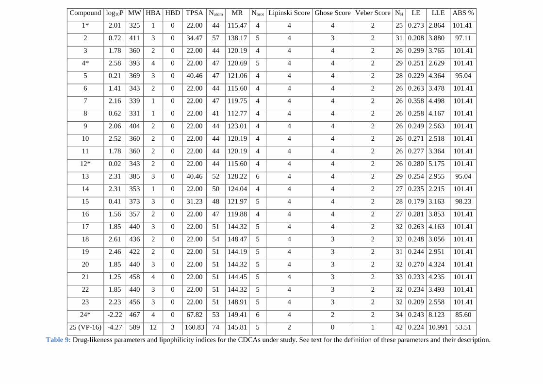
Compound log10P MW HBA HBD TPSA Natom MR Nbrot Lipinski Score Ghose Score Veber Score NH LE LLE ABS %
1* 2.01 325 1 0 22.00 44 115.47 4 4 4 2 25 0.273 2.864 101.41
2 0.72 411 3 0 34.47 57 138.17 5 4 3 2 31 0.208 3.880 97.11
3 1.78 360 2 0 22.00 44 120.19 4 4 4 2 26 0.299 3.765 101.41
4* 2.58 393 4 0 22.00 47 120.69 5 4 4 2 29 0.251 2.629 101.41
5 0.21 369 3 0 40.46 47 121.06 4 4 4 2 28 0.229 4.364 95.04
6 1.41 343 2 0 22.00 44 115.60 4 4 4 2 26 0.263 3.478 101.41
7 2.16 339 1 0 22.00 47 119.75 4 4 4 2 26 0.358 4.498 101.41
8 0.62 331 1 0 22.00 41 112.77 4 4 4 2 26 0.258 4.167 101.41
9 2.06 404 2 0 22.00 44 123.01 4 4 4 2 26 0.249 2.563 101.41
10 2.52 360 2 0 22.00 44 120.19 4 4 4 2 26 0.271 2.518 101.41
11 1.78 360 2 0 22.00 44 120.19 4 4 4 2 26 0.277 3.364 101.41
12* 0.02 343 2 0 22.00 44 115.60 4 4 4 2 26 0.280 5.175 101.41
13 2.31 385 3 0 40.46 52 128.22 6 4 4 2 29 0.254 2.955 95.04
14 2.31 353 1 0 22.00 50 124.04 4 4 4 2 27 0.235 2.215 101.41
15 0.41 373 3 0 31.23 48 121.97 5 4 4 2 28 0.179 3.163 98.23
16 1.56 357 2 0 22.00 47 119.88 4 4 4 2 27 0.281 3.853 101.41
17 1.85 440 3 0 22.00 51 144.32 5 4 4 2 32 0.263 4.163 101.41
18 2.61 436 2 0 22.00 54 148.47 5 4 3 2 32 0.248 3.056 101.41
19 2.46 422 2 0 22.00 51 144.19 5 4 3 2 31 0.244 2.951 101.41
20 1.85 440 3 0 22.00 51 144.32 5 4 3 2 32 0.270 4.324 101.41
21 1.25 458 4 0 22.00 51 144.45 5 4 3 2 33 0.233 4.235 101.41
22 1.85 440 3 0 22.00 51 144.32 5 4 3 2 32 0.234 3.493 101.41
23 2.23 456 3 0 22.00 51 148.91 5 4 3 2 32 0.209 2.558 101.41
24* -2.22 467 4 0 67.82 53 149.41 6 4 2 2 34 0.243 8.123 85.60
25 (VP-16) -4.27 589 12 3 160.83 74 145.81 5 2 0 1 42 0.224 10.991 53.51
Table 9: Drug-likeness parameters and lipophilicity indices for the CDCAs under study. See text for the definition of these parameters and their description.

Result and discussion
130
III.5 QSAR modelling studies
QSAR studies have proved their applicability in modern drug discovery
protocols. The goal of QSAR models is to establish quantitative relations connecting
the physicochemical properties of classes of drugs to their biological activity.
Typically, this involves the synthesis of a series of differently substituted analogue
compounds, and the study of how their biological activities depend on the
physicochemical properties of the substituents. [14]Several linear and nonlinear
statistical model-building methods have been applied to QSAR, [53]where the needed
physicochemical descriptors are treated as independent variables. We used both
multiple linear regressions (MLR) and artificial neural network (ANN), as
implemented in the software JMP 8.0.2 and XLSTAT, [54,55] to correlate these
parameters with the biological activities of CDCAs. For internal, external validation
and Y-randomization [56,57]of the QSAR model, we used different statistical
parameters such as:
(i) The leave-one-out cross-validation coefficient (R2cv(LOO)), used to predict
the internal validation of a model. The threshold for acceptability is
R2CV(LOO)> 0.5. [58]
(ii) The significance level (P-value). It should be < 0.05.
(iii) The square correlation coefficient for external validation (R2ext). It is taken
as a good indicator when its value is greater than 0.6. [58-60]
(iv) The PRESS/SSY ratio, where PRESS is the predicted residual sum of
squares and SSY is the sum of squares deviation. It should be smaller than
0.4. [61]
(v) The rm2 metric introduced by Roy et al. [62]It should be ensured that rm̅
2>
0.5 and Δrm2< 0.2 to prevent bias in model predictability. This applies to
both the training (internal validation) and the test (external validation) sets.
III.5.1.1 Internal validation
The internal validation of a QSAR model is carried out using a cross-validation
method, using the molecules from the training set. In this paper, we used the cross-

Result and discussion
131
validation leave-one-out (LOO) approach, where a large value of the cross-validated
squared correlation coefficient R2cv is considered as a proof of high predictive capacity
of the model. [58]
An acceptable Q2cv does not guarantee that the predicted activity values are close
to the observed ones, but simply attests that a good overall correlation exist between
them. So, to avoid this error and better highlight the predictability of the model, we
considered also the rm2 metrics, including average rm
2(LOO) (the average value of rm
2and
r′m2 ) and Δr2
m(LOO) (the absolute difference between rm2 and r’m
2)(Table 10), introduced
by Roy and colleagues. [62] For a good prediction of the QSAR model Δr2m(LOO)
should be less than 0.2, provided that the average value of rm2 is greater than 0.5.
III.5.1.2 External validation
External validation guarantees the predictability of the developed QSAR model
and its applicability to potential new drugs. The correlation between observed and
predicted data is measured by the R2ext metric (Table 10). According to Golbraikh and
Tropsha[58-60], the following criteria for the external validation, based on the
validation set, were adopted:
(i) R2ext> 0.6
(ii) (r2- r02/ r2) < 0.1 and 0.85 ≤ k ≤ 1.15 or (r2- r’0
2/ r2) < 0.1 and 0.85 ≤ k’ ≤ 1.15
(iii) |rm2 - r′m
2 | < 0.3
III.5.1.3 Y-randomization
Y-randomization [56] is a widely accepted validation technique used to check the
robustness of the models. In this validation approach, the values of the target variable
are randomly redistributed over the entire learning set and a new model is derived. The
whole operation is repeated several times. For robustness, the squared mean
correlation coefficient (R2r) of randomized models should be less than the squared
correlation coefficient (R2) of non-randomized ones. Based on the results of the

Result and discussion
132
randomization tests, the R2p (= R2√(R2 + Rr
2)) [53] value should be greater than 0.5 to
ensure that the good predictive capacity of the so-developed models is not reached by
mere chance.
III.6 Multiple linear regression (MLR)
Despite being the oldest, MLR still remains one of the most popular approaches
to build QSAR models. This is due to its simple practical use, ease of interpretation
and transparency. Indeed, the key algorithm is available and accurate predictions can
be provided. [63]The values of the calculated descriptors are those listed in Tables 8
and 9. Data were randomly divided into two groups: a training set (internal validation)
and a testing set (external validation). The significant correlation analysis between
Topo II inhibition activity and descriptors is represented by the following equation:
pIC50 = 6,759 - 0,135×TPSA + 0,314×Natom - 0,015×V -0,485×HE +
0,314×log10P…… (Eq.1)
Table 10: Numerical parameters used to confirm the QSAR model validity. See text for more
details.
Model Training set Test set
R2inter R2
cv ṝm2
(LOO) Δrm2
(LOO) RMSE PRESS/SST R2ext ṝm
2(test) Δrm
2(test) RMSE PRESS/SST
MLR 0.768 0.686 0.601 0.162 1.224 0.341 0.800 0.596 0.197 0.545 0.092
ANN 0.999 0.991 0.988 0.000 0.005 0.000 0.650 0.598 0.108 0.372 0.135
The statistical parameters of this model are listed in Table 10. The high values
of the correlation coefficient (R2) for the training set (R2inter= 0.768) and test set
(R2ext=0.800) indicate the significant correlation between different independent
variables with Topo II inhibition activity. In addition, Table 10 shows that RMSE and
PRESS/SSY ratio are low for both internal validation (= 0.341 < 0.4) and external
validation (= 0.092 < 0.4). This confirms the reliability of our model.

Result and discussion
133
Figure.38. Generic leverage plot of observed [11] (Observed pIC50) versus predicted
(Predicted pIC50) activity according to the MLR model. The oblique line is the
diagonal.
The model was checked by applying the Y-randomisation test. Several Y vector
random shuffles were performed and small average values of 0.1445 for R2 and -0.327
for Q2 (Table 11) were obtained after 1000 random tests, thus proving that the good
results of our original model are not due to chance correlation or structural dependence
of the training set.
Table 11:Random MLR model parameters.
Average R 0.3646
Average R2 0.1445
Average Q2 -0.327
cRp2 0.768

Result and discussion
134
For further testing the reliability and stability of our model (Eq.1), we used the
"Leave-One-Out" (LOO) technique. Again, the high value of cross-validation
correlation coefficient (R2CV = 0.686 > 0.5) for this model allows us to qualify it as
valid. [58]Other criteria such as parameters metric (rm̅2 and Δrm
2, Table 10) confirm
that this QSAR model is acceptable. The plot of the predicted values of biological
activity pIC50 vs. the experimental values is shown in Figure 38, which certifies once
more the validity of the predicted model.
Let us now analyze the coefficients in Eq.1. The positive values of log10P and
Natom indicate a promoter effect on Topo II inhibition activity. Indeed, any increase in
the octanol-water partition coefficient and number of atoms of the molecules causes an
increase in the biological activity. This is related to the stabilization of the polar
groups in the CDCAs and represents a good criterion for molecule accessibility in the
biologic medium. Also, since the octanol-water partition coefficient provides an
indication of the lipophilic character of the drug and its aptitude to cross the cell
membrane, it represents a key parameter to measure the drug inhibitory activity.
No contribution from the HOMO-LUMO gap appears in Eq.1. Thus, the model
is independent of this parameter. This may be related to the almost constant value of
this gap computed for all the CDCAs of interest, as noted earlier. Eq.1 does not
include any dependence on HBD since this parameter is zero for all compounds,
except Compound 25 (Table 9). Similarly, MR and HBA parameters seem to have no
influence on the biological activity, since they do not appear in our model.
III.7 Artificial Neural Networks (ANN)
ANN [64,65]is a popular nonlinear model, which is used to predict the
biological activity (i.e. IC50) of the datasets of therapeutic molecules. It presents
several benefits like better prediction, adaptation and generalization capacity beyond
the studied sample, and better stability of the coefficients. It is employed in complex
drug design, drug engineering and medicinal chemistry domains. [66]

Result and discussion
135
Figure .39.The architecture (6-4-1) of the adopted ANN model.
In this work, the neural network is a system of fully interconnected neurons
arranged in three layers. The input layer is made of six neurons, where each of them
receive one of the six descriptors selected from the correlation matrix of the model.
The intermediate (hidden) layer is composed of four neurons that form the deep
internal pattern that discovers the most significant correlations between predicted and
experimental data. One neuron constitutes the output layer, which returns the value of
IC50 (Figure 39). [67]
Figure .40.Correlation plot of observed (Observed pIC50) [11] versus predicted activity
(Predicted pIC50) calculated using ANN.

Result and discussion
136
As can be seen in Figure 40, a good agreement between experimental data and
predicted pIC50 issued from the ANN model is observed. Indeed, the statistical
parameters for this model, as given in Table 10, reveal a correlation coefficient close
to 1 (R2inter=0.999), associated with lower values of RMSE and PRESS/SSY for both
external and internal validations. Note that these parameters are better than those
found for the MLR model, indicating that the ANN one is more reliable. Furthermore,
the robustness of the model was further confirmed by the significant R2ext value of the
test data set (R2ext= 0.650). To further evaluate our model, we applied the Leave-One-
Out cross-validation method. The resulting rm̅2
(LOO), Δrm2
(LOO), rm̅2
(test), Δrm2
(test)
statistical criteria (Table 10) support the validity of our model, since they fall within
the ranges specified by Roy et al. [62]

General conclusion
137
General Conclusion

General conclusion
138
Using first principle methodologies, we studied the molecular structure and the
vibrational/electronic spectroscopic properties of the set of CDCAs recently synthetized by Li
et al. as potential Topo II inhibitors. We also characterized the carbazole subunit of these
CDCAs. Afterwards, we derived a set of physicochemical parameters for these compounds,
which are incorporated later into MPO, MLR and ANN methods for screening the
lipophilicity indices, structure-activity relationship and to construct a QSAR model. The
results indicate that these compounds have a 98% chance of being orally active. As can be
seen in Table 10, the ANN network has substantially better predictive capabilities compared
to MLR, leading to pIC50 values closer to the experimental determinations. Nevertheless, both
models remain satisfactory and exhibit a high predictive power, thus validating their use to
explore and propose new molecules as active inhibitors of Topo II.
Table .10. Measured [11] and predicted pIC50 using MLR and ANN methods. * denotes the
compounds selected for external validation (test set).
Compound MLR predicted pIC50 ANN predicted pIC50 Observed pIC50
1* 5.496 4.873 4.874
2 4.600 4.599 4.600
3 5.574 5.536 5.545
4* 5.166 5.209 5.209
5 4.456 4.573 4.574
6 5.039 4.886 4.888
7 6.466 6.656 6.658
8 4.953 4.804 4.787
9 5.031 4.623 4.623
10 5.245 5.039 5.038
11 4.864 5.138 5.144
12* 4.690 5.195 5.195
13 5.111 5.265 5.265
14 4.568 4.527 4.525
15 4.228 3.574 3.573
16 4.766 5.413 5.413
17 6.073 6.013 6.013

General conclusion
139
18 6.188 5.768 5.666
19 5.588 5.411 5.411
20 5.642 5.466 6.174
21 5.303 5.284 5.485
22 5.558 5.342 5.343
23 4.703 5.098 4.788
24* 0.427 5.898 5.903
The investigation of CDCAs at the microscopic level allows a screening of the
physicochemical properties related to their activity in biological media. In contrast to the
statement by Li et al., we did not notice any obvious relation between the incorporation of a
halogen on the chemical composition of these CDCAs and their biological activity. Our work
shows, however, that among the physicochemical parameters considered here, only log10P and
Natom play a role. These two parameters are connected with the flexibility of these compounds,
which seems increasing the Topo II inhibitory activity and more generally improves the
anticancer potency of these compounds. For instance, the coefficient in front of log10P in our
model (Eq.1) is positive and relatively large. This means that the flexibility of the CDCAs, by
facilitating cell membrane crossing, will enhance the Topo II inhibition. This may be related
to the mechanism of action of Topo II itself, which consists in a balanced flexibility-rigidity
associated with structural changes of the quaternary structure [68] of this enzyme during the
CDCA-Topo II-DNA interaction. These findings were already suggested by Guedes et al. [69]
This work discloses the phenomenological relations existing between potential biological
activities and molecular descriptors of a relatively large panel of compounds to be used as
Topo II inhibitors, and pave the way for specific investigations of their complex mechanisms
of action at a molecular dynamics level.

APPENDIX

Appendix
141
Table S1: Chemical structure of the investigated CDCAs (Table 1) as configured at the theory level of
B3LYP/6-311G(d,p). In Angstrom, we give the Cartesian coordinates (X,Y,Z). The number of the
atom in the structure and its atomic number, respectively, correspond to CN(Center Number) and AN
(Atomic Number).
N Molecular Structure Cartesian coordinates CN AN X Y Z
1
1 6 -0.000003050 0.000046017 0.000000586
2 6 0.000009707 -0.000001908 0.000016748
3 6 -0.000003806 0.000002246 -0.000009254
4 8 0.000007744 -0.000022231 -0.000002513
5 6 -0.000006171 -0.000031415 -0.000006993
6 6 -0.000001642 0.000006633 0.000006829
7 6 0.000001428 0.000002239 0.000003030
8 6 0.000002843 0.000001175 0.000003104
9 6 0.000006202 -0.000001955 -0.000001558
10 6 -0.000002367 -0.000004444 0.000004983
11 6 -0.000001696 -0.000004343 -0.000002963
12 6 0.000001241 0.000000475 -0.000003286
13 6 0.000002966 -0.000001139 0.000002132
14 6 -0.000003638 0.000008892 -0.000005424
15 6 0.000000664 -0.000004022 -0.000009217
16 6 -0.000004033 -0.000002056 0.000002141
17 7 -0.000003881 -0.000003033 0.000019400
18 6 -0.000010756 0.000003415 -0.000005437
19 6 -0.000001163 -0.000007095 -0.000000147
20 6 -0.000002334 0.000005217 0.000003301
21 6 0.000010187 -0.000002566 0.000013611
22 6 -0.000002590 0.000015244 -0.000001697
23 6 0.000004705 -0.000007651 -0.000004148
24 6 0.000001421 0.000004393 -0.000010450
25 6 -0.000002366 -0.000001141 0.000000919
26 1 -0.000001982 -0.000000900 -0.000001167
27 1 0.000002322 0.000000383 -0.000000748
28 1 0.000003833 -0.000001051 0.000000212
29 1 0.000003203 -0.000002667 0.000002383
30 1 0.000002952 -0.000002687 0.000001044
31 1 0.000000745 -0.000001871 0.000001063
32 1 0.000001546 0.000000716 -0.000001274
33 1 -0.000002432 0.000000461 -0.000003325
34 1 -0.000002370 -0.000000561 -0.000002722
35 1 -0.000001085 -0.000001607 -0.000003734
36 1 -0.000002025 0.000001164 -0.000004006
37 1 -0.000000086 0.000003956 0.000003030
38 1 0.000000588 0.000000411 0.000001401
39 1 0.000000561 -0.000001691 -0.000003108
40 1 -0.000001273 0.000001401 0.000000682
41 1 -0.000002250 0.000001394 -0.000000986
42 1 -0.000000617 0.000001449 -0.000000526
43 1 -0.000001582 0.000000758 -0.000001424
44 1 0.000000339 -0.000000002 -0.000000492

Appendix
142
2
1 6 0.000005387 -0.000004291 0.000005055
2 6 -0.000010761 -0.000000836 -0.000009164
3 6 0.000002187 -0.000000116 0.000009235
4 8 -0.000002039 -0.000001701 -0.000001332
5 6 0.000000563 0.000006155 0.000002983
6 6 -0.000002893 -0.000005957 -0.000001186
7 6 0.000010163 0.000000633 -0.000001397
8 6 -0.000013025 0.000000884 -0.000001906
9 6 0.000001471 -0.000002870 -0.000001129
10 6 0.000000979 0.000000460 -0.000001512
11 6 -0.000002885 0.000000903 -0.000001141
12 6 0.000001241 -0.000003722 -0.000002768
13 8 -0.000006310 0.000002407 0.000007805
14 6 0.000011419 0.000001828 -0.000007113
15 6 -0.000003881 -0.000001208 -0.000006346
16 7 0.000005697 0.000000083 0.000009302
17 6 -0.000000034 -0.000000185 -0.000000674
18 6 -0.000000526 0.000000430 -0.000001540
19 6 0.000000763 -0.000001891 0.000001662
20 6 -0.000001633 0.000004432 -0.000001487
21 6 -0.000000230 -0.000001176 -0.000000515
22 6 0.000000764 0.000001237 0.000000291
23 7 -0.000000637 -0.000009731 -0.000006108
24 6 0.000000173 0.000006351 0.000003561
25 6 -0.000000570 -0.000000985 0.000002625
26 6 -0.000000715 -0.000000172 0.000000424
27 6 0.000000294 0.000001569 -0.000002272
28 6 0.000001029 0.000003560 -0.000000204
29 6 0.000001304 -0.000005790 0.000000135
30 6 0.000001908 0.000004972 0.000003962
31 6 -0.000000009 0.000000505 0.000001836
32 1 0.000001095 0.000002038 0.000000116
33 1 -0.000000477 0.000000801 0.000002154
34 1 -0.000000579 0.000000581 0.000000512
35 1 -0.000000173 0.000000058 0.000000884
36 1 0.000000600 0.000001193 -0.000001678
37 1 0.000000266 -0.000000267 -0.000000440
38 1 -0.000001697 -0.000000939 -0.000002156
39 1 -0.000000049 0.000001418 -0.000001530
40 1 -0.000000988 0.000000958 -0.000001660
41 1 -0.000000035 0.000000265 -0.000001426
42 1 -0.000000035 0.000000240 -0.000000748
43 1 -0.000000894 -0.000001478 0.000000059
44 1 -0.000001051 -0.000000026 -0.000000076
45 1 0.000001538 0.000000578 0.000000977
46 1 0.000000254 0.000000002 -0.000000707
47 1 0.000000140 0.000000202 -0.000000846
48 1 -0.000000028 -0.000000064 -0.000002091
49 1 0.000000118 -0.000000411 -0.000001126
50 1 0.000000108 -0.000000189 0.000000669
51 1 0.000000021 0.000000105 0.000001935
52 1 0.000000547 0.000000935 0.000001451
53 1 -0.000001101 -0.000001152 -0.000001084
54 1 0.000001128 0.000000387 0.000002688
55 1 0.000000585 0.000000101 0.000000562
56 1 0.000000699 -0.000000653 0.000001224
57 1 0.000000816 -0.000000462 0.000001256

Appendix
143
3
1 6 -0.000002374 0.000007476 0.000004949
2 6 0.000002054 -0.000002553 -0.000004138
3 6 0.000001781 0.000003233 0.000001714
4 8 0.000001748 -0.000002198 -0.000001319
5 6 -0.000001364 0.000001494 0.000000223
6 6 -0.000001931 -0.000000292 -0.000000019
7 6 0.000000625 0.000003596 -0.000000494
8 6 0.000001917 -0.000004596 -0.000005448
9 6 0.000000256 0.000000398 0.000004834
10 6 -0.000001224 0.000000733 -0.000003669
11 7 -0.000005575 -0.000002626 -0.000007410
12 6 0.000008422 0.000011938 0.000000365
13 6 -0.000005594 -0.000008105 -0.000005551
14 6 0.000006020 0.000013871 0.000010474
15 6 0.000004224 -0.000008850 -0.000012944
16 6 -0.000007568 0.000002809 0.000006967
17 6 -0.000001471 -0.000001042 0.000005360
18 6 0.000000487 0.000001726 0.000000965
19 6 0.000001729 0.000000780 -0.000001226
20 6 0.000001918 -0.000009630 0.000003597
21 6 -0.000000113 0.000001721 0.000000444
22 6 -0.000000471 -0.000002961 0.000002398
23 6 -0.000000716 -0.000001259 -0.000000655
24 6 0.000000269 -0.000004837 0.000003692
25 6 -0.000001674 0.000005013 0.000000404
26 17 -0.000001129 -0.000002381 0.000001497
27 1 0.000000696 0.000000668 0.000002053
28 1 0.000001785 0.000000085 0.000001143
29 1 -0.000001276 0.000000258 -0.000001698
30 1 -0.000000889 0.000000322 -0.000000922
31 1 -0.000000302 -0.000000242 0.000000055
32 1 -0.000001018 0.000000843 -0.000001107
33 1 -0.000001468 -0.000004245 -0.000001668
34 1 0.000002528 0.000000933 0.000000111
35 1 0.000001925 -0.000001633 0.000000505
36 1 0.000000203 -0.000000605 -0.000000926
37 1 -0.000001016 0.000000861 -0.000001798
38 1 0.000000253 0.000001703 -0.000001758
39 1 0.000000037 0.000001681 -0.000001378
40 1 0.000000496 0.000001548 -0.000001383
41 1 -0.000000406 -0.000001817 0.000001532
42 1 -0.000001454 -0.000001223 0.000001198
43 1 -0.000000665 -0.000000942 0.000000464
44 1 0.000000324 -0.000001653 0.000000568

Appendix
144
4
1 6 -0.000000245 -0.000015843 0.000000210
2 6 -0.000002401 0.000001093 -0.000000207
3 6 -0.000000417 -0.000000467 0.000002526
4 8 -0.000003639 0.000006264 -0.000002060
5 6 0.000004245 0.000011963 0.000006543
6 6 -0.000001543 -0.000006354 -0.000002494
7 6 0.000004917 0.000001076 -0.000001337
8 6 -0.000003356 0.000003583 0.000005249
9 6 0.000000444 -0.000004398 -0.000000491
10 6 0.000001564 0.000000637 0.000000578
11 6 -0.000001944 0.000000809 0.000000800
12 9 0.000000538 -0.000000856 -0.000001947
13 9 0.000004028 -0.000000908 -0.000003148
14 9 0.000000921 -0.000001692 0.000005133
15 6 -0.000000333 0.000000610 -0.000002877
16 6 -0.000000538 -0.000000757 -0.000002757
17 6 -0.000001373 0.000000950 -0.000002915
18 6 0.000000322 -0.000001589 -0.000000629
19 6 -0.000000542 0.000000900 0.000000181
20 6 -0.000000380 0.000000327 -0.000003794
21 7 -0.000001036 -0.000002034 -0.000006681
22 6 0.000001327 0.000003093 0.000002785
23 6 -0.000000348 -0.000001088 0.000000036
24 6 0.000002724 0.000001074 0.000000806
25 6 -0.000001596 0.000000421 0.000003740
26 6 -0.000000742 0.000003271 -0.000003837
27 6 -0.000001544 -0.000000787 0.000002471
28 6 0.000000293 0.000001225 0.000002763
29 6 0.000000194 0.000000014 -0.000000486
30 1 0.000000418 0.000000071 0.000000134
31 1 -0.000000136 0.000000731 0.000002777
32 1 0.000001043 0.000000103 0.000002882
33 1 0.000000843 -0.000000491 0.000002367
34 1 0.000000315 -0.000000167 -0.000000046
35 1 -0.000000129 0.000000378 -0.000000595
36 1 -0.000000705 -0.000000345 -0.000003662
37 1 -0.000000373 -0.000000143 -0.000003847
38 1 -0.000000251 -0.000000050 -0.000001829
39 1 -0.000000360 -0.000000102 -0.000001482
40 1 -0.000000213 0.000000547 0.000002141
41 1 -0.000000489 0.000000486 0.000002563
42 1 0.000000398 -0.000000820 0.000000798
43 1 -0.000000833 0.000000359 -0.000000347
44 1 -0.000000636 0.000000477 -0.000000320
45 1 0.000000190 -0.000000257 0.000000363
46 1 0.000000767 -0.000000768 -0.000000694
47 1 0.000000608 -0.000000542 0.000000635
5
1 6 -0.000000917 0.000002148 0.000008893
2 6 0.000003255 0.000001271 0.000001916
3 6 0.000008782 0.000000812 -0.000000308
4 8 0.000000697 0.000002432 -0.000002872
5 6 -0.000000730 -0.000000215 0.000001289
6 6 -0.000000506 -0.000000282 0.000000693
7 6 0.000000158 -0.000001116 -0.000000112
8 6 -0.000002040 0.000000293 0.000004727
9 6 -0.000000977 -0.000001941 -0.000002262
10 6 -0.000000425 -0.000001220 0.000000695
11 7 0.000000789 0.000000843 0.000001810
12 6 0.000000051 -0.000002468 -0.000002802
13 6 -0.000001908 -0.000000064 0.000001955
14 6 0.000002927 0.000000667 0.000002162
15 6 -0.000009636 -0.000001427 -0.000003537
16 6 -0.000000238 -0.000002222 0.000000321
17 6 0.000004068 0.000003565 -0.000002278
18 6 -0.000000612 -0.000001321 0.000001087
19 6 -0.000000944 0.000000400 -0.000000221
20 8 0.000005673 0.000001600 0.000015939

Appendix
145
21 6 0.000009296 0.000008942 -0.000016977
22 8 -0.000007658 -0.000005574 -0.000001730
23 6 -0.000007464 -0.000008029 0.000019520
24 6 -0.000004329 0.000003487 -0.000027465
25 6 0.000014262 0.000006844 0.000009267
26 6 -0.000016985 -0.000010820 -0.000006638
27 6 0.000001716 0.000002631 -0.000011352
28 6 0.000007421 0.000004481 0.000005813
29 1 -0.000000072 -0.000001195 -0.000000209
30 1 -0.000000822 -0.000000312 -0.000000078
31 1 0.000000820 -0.000000992 0.000000472
32 1 0.000000284 -0.000001148 0.000000001
33 1 -0.000000408 0.000000005 -0.000000476
34 1 0.000000703 -0.000000088 0.000000325
35 1 0.000000539 0.000000726 -0.000000125
36 1 -0.000000563 -0.000000157 -0.000000086
37 1 -0.000000207 0.000000133 -0.000000517
38 1 -0.000000121 0.000000738 0.000000510
39 1 0.000000824 -0.000000528 0.000000913
40 1 0.000000207 -0.000000116 0.000001350
41 1 -0.000000347 -0.000000903 -0.000000185
42 1 -0.000000684 -0.000000563 0.000000885
43 1 -0.000000536 -0.000000500 -0.000000515
44 1 -0.000001539 0.000000708 0.000001319
45 1 -0.000001925 -0.000000769 -0.000001035
46 1 0.000000248 0.000001440 0.000001504
47 1 -0.000000128 -0.000000193 -0.000001585
6
1 6 -0.000012637 0.000029245 0.000006654
2 6 0.000015818 -0.000001369 0.000013279
3 6 -0.000006526 -0.000009624 -0.000006276
4 8 0.000011426 -0.000011925 -0.000000264
5 6 -0.000001131 -0.000020433 -0.000015415
6 6 0.000001827 0.000005072 0.000011336
7 6 0.000000334 -0.000001511 0.000003382
8 6 0.000013312 0.000007952 0.000001249
9 6 0.000005907 0.000000908 -0.000001180
10 6 -0.000008047 -0.000004047 0.000003204
11 9 -0.000002459 -0.000010057 0.000000683
12 6 -0.000001780 -0.000003358 -0.000004536
13 6 -0.000000180 0.000000580 -0.000004932
14 6 0.000002483 -0.000001438 0.000000547
15 6 -0.000006187 0.000008278 -0.000004855
16 6 0.000001178 -0.000003977 -0.000006192
17 6 -0.000004291 -0.000001583 -0.000000266
18 7 -0.000004314 -0.000002658 0.000008506
19 6 -0.000010476 0.000002919 -0.000000531
20 6 -0.000001292 -0.000003972 -0.000000796
21 6 -0.000004025 0.000002312 0.000004528
22 6 0.000005593 0.000010956 0.000000025
23 6 0.000000185 0.000004550 0.000003692
24 6 0.000006558 -0.000005177 -0.000000610
25 6 0.000000771 0.000004515 -0.000006641
26 6 -0.000001125 -0.000001359 0.000003236
27 1 -0.000001938 -0.000003190 0.000004858
28 1 0.000002180 0.000001582 0.000002257
29 1 0.000005617 0.000001497 0.000000683
30 1 0.000002284 -0.000003294 0.000002894
31 1 0.000000250 -0.000002619 -0.000000684
32 1 0.000002397 0.000000005 -0.000002329
33 1 -0.000002967 0.000000624 -0.000004794
34 1 -0.000003036 -0.000000532 -0.000004554
35 1 -0.000001874 -0.000001143 -0.000004468
36 1 -0.000002413 0.000001548 -0.000004187
37 1 0.000000529 0.000003549 0.000004318
38 1 0.000001078 0.000001421 0.000001953
39 1 -0.000000741 -0.000000054 -0.000002451
40 1 -0.000000141 0.000002356 0.000001477

Appendix
146
41 1 -0.000001888 0.000001773 -0.000001689
42 1 0.000000327 0.000001622 -0.000000745
43 1 -0.000001295 0.000000352 -0.000000904
44 1 0.000000707 -0.000000300 0.000000538
7
1 6 0.000000263 -0.000002846 -0.000000061
2 6 0.000000057 0.000001263 0.000001454
3 6 -0.000000105 -0.000000014 0.000002205
4 8 -0.000000484 0.000000472 0.000000514
5 6 0.000001578 0.000001591 0.000001030
6 6 0.000001485 -0.000000891 0.000001965
7 6 0.000001870 -0.000000647 0.000002021
8 6 0.000002336 -0.000001011 0.000000785
9 6 0.000001142 -0.000000428 -0.000000367
10 6 -0.000000286 -0.000001253 -0.000000290
11 6 0.000000685 -0.000001721 -0.000000341
12 6 -0.000001610 -0.000000111 -0.000003890
13 6 -0.000001307 -0.000000614 -0.000003975
14 6 -0.000001360 0.000000326 -0.000002911
15 6 -0.000000649 -0.000000220 -0.000002023
16 6 -0.000001581 0.000000551 -0.000003260
17 6 -0.000001707 0.000000138 -0.000002433
18 7 -0.000000783 0.000000627 0.000005274
19 6 -0.000000821 0.000001316 -0.000001670
20 6 -0.000000569 0.000000538 0.000002240
21 6 0.000000527 0.000001360 0.000002032
22 6 -0.000000304 0.000000776 0.000002185
23 6 -0.000000501 0.000001625 -0.000000504
24 6 -0.000001029 0.000000305 -0.000000936
25 6 -0.000001127 0.000000873 -0.000002612
26 6 -0.000000304 0.000000079 -0.000000031
27 1 0.000000663 0.000000006 0.000002617
28 1 0.000000455 0.000000969 0.000003472
29 1 0.000002328 -0.000000682 0.000002890
30 1 0.000002483 -0.000001231 0.000002457
31 1 0.000000670 -0.000000929 -0.000001067
32 1 0.000000104 -0.000000245 -0.000001055
33 1 0.000003080 -0.000001789 0.000001548
34 1 0.000002672 -0.000002170 0.000000060
35 1 0.000001829 -0.000000699 0.000001424
36 1 -0.000002052 -0.000000141 -0.000004895
37 1 -0.000001655 -0.000000446 -0.000004942
38 1 -0.000001002 -0.000000318 -0.000002879
39 1 -0.000001683 0.000000432 -0.000002716
40 1 -0.000000356 0.000001332 0.000002329
41 1 0.000000044 0.000001067 0.000003292
42 1 -0.000000156 -0.000000079 0.000000042
43 1 -0.000001343 0.000001538 0.000001100
44 1 -0.000001852 0.000001279 -0.000000681
45 1 -0.000000187 0.000000447 0.000000553
46 1 0.000000020 -0.000000275 -0.000000773
47 1 0.000000524 -0.000000153 0.000000823
8
1 6 0.000020849 -0.000000797 -0.000018457
2 6 -0.000013177 0.000010498 0.000001562
3 6 0.000008409 0.000009858 0.000000403
4 8 -0.000006825 -0.000001494 0.000007098
5 6 -0.000000087 0.000003333 0.000000326
6 6 -0.000001451 -0.000002032 -0.000000019
7 6 0.000001281 0.000000188 -0.000000194
8 6 0.000005854 0.000002389 -0.000002187
9 6 -0.000000450 -0.000001958 -0.000001315
10 6 0.000001476 -0.000000552 -0.000000727
11 7 -0.000002881 -0.000001632 0.000003013
12 6 0.000003321 0.000004800 -0.000003469
13 6 -0.000002343 -0.000005571 0.000001667
14 6 0.000002765 0.000010946 0.000004173
15 6 -0.000008291 -0.000016475 0.000001661
16 6 0.000005036 0.000003166 -0.000000526

Appendix
147
17 6 -0.000009241 -0.000003528 0.000000067
18 6 -0.000000006 0.000000117 -0.000002094
19 6 0.000000529 -0.000000282 0.000000519
20 6 -0.000003769 -0.000012050 0.000006869
21 16 -0.000004732 -0.000003182 0.000007910
22 6 -0.000000542 0.000012726 -0.000014923
23 6 0.000002310 0.000006492 -0.000004905
24 6 -0.000002343 -0.000007565 0.000016548
25 1 0.000002128 -0.000001572 -0.000000264
26 1 0.000000178 -0.000000560 0.000000706
27 1 0.000000067 -0.000000301 -0.000000466
28 1 -0.000000215 0.000000214 -0.000000915
29 1 -0.000000072 0.000000014 -0.000000655
30 1 -0.000000341 0.000000506 -0.000000771
31 1 0.000000175 0.000000970 -0.000000577
32 1 0.000001353 -0.000001930 0.000000604
33 1 -0.000000656 -0.000000430 -0.000000250
34 1 -0.000000113 -0.000000067 0.000000271
35 1 0.000000146 -0.000000086 0.000000180
36 1 0.000000020 0.000000436 -0.000000404
37 1 0.000000178 0.000000015 -0.000000329
38 1 0.000000332 0.000000136 -0.000000057
39 1 0.000001573 -0.000003697 0.000003122
40 1 -0.000001937 -0.000001353 -0.000001099
41 1 0.000001495 0.000000312 -0.000002097
9
1 6 0.000000458 -0.000016797 -0.000027164
2 6 -0.000009286 -0.000002275 0.000002749
3 6 0.000005989 0.000009311 0.000001144
4 8 0.000006042 -0.000001585 0.000007678
5 6 -0.000002159 0.000001702 -0.000000638
6 6 -0.000001610 0.000003897 -0.000000471
7 6 0.000002802 0.000003328 -0.000000746
8 6 -0.000006912 -0.000001436 -0.000005925
9 6 0.000003596 0.000000007 -0.000005410
10 6 -0.000002223 -0.000001883 -0.000001025
11 7 0.000001852 0.000000950 0.000004247
12 6 -0.000004530 -0.000000681 0.000005340
13 6 0.000001499 -0.000000026 -0.000001123
14 6 0.000002579 -0.000004577 0.000002726
15 6 -0.000002319 -0.000002621 -0.000000099
16 6 0.000000566 -0.000000037 -0.000003285
17 6 0.000007772 0.000004099 0.000005506
18 6 -0.000003750 0.000000428 -0.000001825
19 6 -0.000002603 0.000000771 -0.000002038
20 6 0.000001708 0.000016431 0.000023921
21 6 0.000002209 -0.000008924 -0.000001393
22 6 0.000001735 -0.000003179 0.000005431
23 6 -0.000001149 -0.000001686 -0.000001726
24 6 -0.000001737 0.000001079 -0.000000795
25 6 -0.000001839 0.000000812 -0.000006705
26 35 -0.000000400 -0.000001887 0.000000565
27 1 0.000004824 -0.000002851 -0.000001466
28 1 0.000001236 -0.000001810 -0.000000805
29 1 0.000000531 0.000002851 -0.000000679
30 1 0.000001493 0.000001464 -0.000000884
31 1 0.000000484 0.000000999 0.000001315
32 1 -0.000001085 0.000003142 0.000001069
33 1 -0.000000560 0.000000549 -0.000000172
34 1 -0.000000646 -0.000000502 -0.000001058
35 1 0.000001395 0.000000429 0.000001689
36 1 0.000000205 0.000002039 -0.000003675
37 1 -0.000001675 0.000001995 0.000002473
38 1 -0.000002579 0.000002262 0.000000136
39 1 -0.000000318 0.000000092 0.000000127
40 1 -0.000001424 -0.000000189 -0.000000229
41 1 -0.000000893 -0.000000997 0.000000795
42 1 -0.000001206 -0.000001482 -0.000000845

Appendix
148
43 1 0.000001390 -0.000001632 0.000000704
44 1 0.000000537 -0.000001581 0.000002563
10
1 6 -0.000013947 -0.000008364 0.000024202
2 6 -0.000002657 -0.000016791 -0.000010074
3 6 0.000005463 0.000011580 -0.000000548
4 8 0.000008547 0.000001360 -0.000010796
5 6 0.000000312 0.000001391 0.000002380
6 6 0.000001011 0.000000983 0.000000675
7 6 0.000000549 0.000000295 0.000001152
8 6 -0.000009502 -0.000001562 0.000001210
9 6 -0.000001728 0.000006856 -0.000006834
10 6 0.000000787 -0.000001214 0.000004555
11 7 0.000007110 -0.000007136 0.000018747
12 6 -0.000003074 -0.000002686 -0.000007821
13 6 -0.000001202 0.000000956 0.000004789
14 6 0.000001559 -0.000004744 -0.000001981
15 6 -0.000002210 -0.000000815 0.000002755
16 6 -0.000003984 -0.000004762 -0.000004497
17 6 0.000011295 0.000008160 0.000000988
18 6 -0.000004862 0.000003269 -0.000004812
19 6 -0.000003277 -0.000000467 0.000001415
20 6 0.000003873 0.000015963 -0.000022679
21 6 -0.000001179 -0.000002536 -0.000001030
22 6 0.000003545 -0.000004562 -0.000001827
23 6 -0.000000808 0.000002739 -0.000000452
24 6 0.000001462 0.000002690 -0.000003253
25 6 -0.000001479 -0.000003420 0.000007828
26 17 -0.000002148 0.000001844 -0.000000519
27 1 0.000004287 -0.000000324 -0.000000347
28 1 0.000000027 -0.000001567 -0.000001589
29 1 -0.000000262 0.000002044 0.000002498
30 1 0.000000720 0.000001617 0.000001935
31 1 0.000000890 0.000001494 0.000000181
32 1 -0.000000314 0.000001018 0.000001914
33 1 -0.000000198 -0.000000804 -0.000000392
34 1 0.000001232 -0.000001220 -0.000000504
35 1 0.000001874 0.000000653 0.000000617
36 1 -0.000000777 0.000000647 0.000000415
37 1 0.000000177 -0.000000377 0.000003050
38 1 -0.000001847 -0.000000823 0.000002025
39 1 -0.000001521 -0.000000099 0.000001956
40 1 -0.000001039 -0.000001125 0.000001001
41 1 -0.000000298 -0.000000795 -0.000001963
42 1 0.000000788 -0.000000293 -0.000001022
43 1 0.000001460 0.000000244 -0.000000266
44 1 0.000001344 0.000000685 -0.000003085
11
1 6 -0.000002954 0.000016443 -0.000012367
2 6 -0.000012066 0.000003650 0.000003206
3 6 0.000005797 -0.000001726 -0.000002509
4 8 0.000002263 -0.000004701 0.000001724
5 6 0.000000564 0.000000324 -0.000000401
6 6 -0.000000805 -0.000000784 0.000000829
7 6 0.000001161 -0.000001369 0.000000412
8 6 -0.000006983 0.000000333 0.000001223
9 6 0.000000479 0.000006460 0.000002178
10 6 0.000000869 -0.000000368 -0.000001694
11 7 0.000002216 -0.000011663 -0.000012554
12 6 -0.000002319 0.000005243 0.000004459
13 6 -0.000000061 -0.000000061 -0.000001563
14 6 0.000000647 0.000004526 -0.000000725
15 6 -0.000005754 -0.000002979 0.000005192
16 6 0.000001303 -0.000003627 -0.000002154
17 6 0.000005379 -0.000002074 0.000003654
18 6 0.000000017 0.000004542 0.000005120
19 6 -0.000000292 0.000000103 0.000000162
20 6 0.000011094 -0.000018236 0.000004400
21 6 -0.000007823 0.000010071 -0.000000258

Appendix
149
22 6 0.000004382 -0.000004301 -0.000001352
23 6 -0.000000811 0.000003326 0.000003693
24 6 -0.000001354 0.000000355 -0.000002733
25 6 0.000001659 0.000002724 0.000003179
26 17 0.000003331 -0.000002980 0.000001686
27 1 0.000001254 0.000000859 0.000001783
28 1 -0.000000119 -0.000002792 -0.000002899
29 1 -0.000000141 -0.000000016 0.000000001
30 1 -0.000000021 0.000000000 -0.000000100
31 1 -0.000000003 -0.000000015 0.000000071
32 1 -0.000000188 -0.000000163 0.000000188
33 1 -0.000000111 -0.000000393 0.000000288
34 1 -0.000000398 -0.000000489 0.000000246
35 1 -0.000000610 -0.000000281 -0.000000892
36 1 0.000000707 0.000000594 -0.000000138
37 1 0.000000156 0.000001018 -0.000000484
38 1 -0.000000129 -0.000000689 -0.000000343
39 1 -0.000000005 -0.000000343 -0.000000221
40 1 -0.000000097 -0.000000035 -0.000000051
41 1 0.000000096 0.000000452 -0.000000043
42 1 0.000000177 -0.000000265 -0.000000303
43 1 -0.000000174 -0.000000090 0.000000216
44 1 -0.000000332 -0.000000585 -0.000000126
12
1 6 -0.000003771 -0.000005174 0.000000741
2 6 0.000002717 0.000000045 -0.000000009
3 6 -0.000000715 -0.000001061 0.000002023
4 8 0.000000340 0.000000502 -0.000000522
5 6 0.000004466 0.000004597 -0.000000075
6 6 0.000000877 -0.000002481 0.000000319
7 6 0.000003539 -0.000000152 0.000000239
8 6 0.000000489 -0.000000044 0.000000488
9 6 0.000000993 -0.000002123 -0.000001605
10 6 0.000000230 -0.000000806 -0.000000459
11 9 0.000002069 -0.000000219 0.000001491
12 6 -0.000001090 -0.000000252 -0.000002206
13 6 -0.000001123 -0.000000486 -0.000002432
14 6 -0.000000846 -0.000000292 -0.000001429
15 6 -0.000001042 0.000000715 -0.000001349
16 6 -0.000000559 0.000000241 -0.000001061
17 6 -0.000001652 0.000000334 -0.000001320
18 7 -0.000001238 -0.000000436 -0.000000567
19 6 -0.000001033 0.000001148 0.000001462
20 6 -0.000000016 -0.000000442 0.000000956
21 6 0.000000404 0.000001063 0.000001240
22 6 0.000000625 0.000001572 0.000001399
23 6 -0.000000394 0.000001182 -0.000000090
24 6 0.000000165 -0.000000492 0.000000370
25 6 -0.000000580 0.000001689 0.000000955
26 6 -0.000000584 0.000000529 0.000000750
27 1 0.000000949 0.000000159 0.000001088
28 1 0.000000625 0.000000793 0.000002482
29 1 0.000002329 -0.000000863 0.000000841
30 1 0.000001936 -0.000001352 -0.000000691
31 1 0.000000657 -0.000000850 -0.000001340
32 1 0.000000228 -0.000000473 -0.000001286
33 1 -0.000001630 -0.000000362 -0.000002739
34 1 -0.000001206 -0.000000693 -0.000003049
35 1 -0.000000598 -0.000000642 -0.000002048
36 1 -0.000001534 0.000000208 -0.000001220
37 1 -0.000000539 0.000001308 0.000002190
38 1 0.000000027 0.000001017 0.000002576
39 1 -0.000000031 -0.000000542 -0.000000163
40 1 -0.000001454 0.000000937 0.000000951
41 1 -0.000001693 0.000000861 0.000000599
42 1 -0.000000511 0.000000784 0.000001140
43 1 -0.000000070 0.000000154 0.000000139
44 1 0.000000244 0.000000396 0.000001221

Appendix
150
13
1 6 -0.000003788 0.000011923 0.000010914
2 6 0.000003004 -0.000005077 -0.000006946
3 6 0.000007071 0.000007869 -0.000000638
4 8 -0.000001271 0.000001846 -0.000002419
5 6 -0.000002528 -0.000002486 -0.000000200
6 6 -0.000001007 0.000001144 -0.000003076
7 6 -0.000000395 0.000001349 -0.000001136
8 6 -0.000000026 -0.000002381 -0.000004144
9 6 -0.000000401 -0.000000929 0.000001853
10 6 -0.000001800 -0.000003096 -0.000000512
11 7 0.000006189 0.000001025 -0.000006550
12 6 -0.000008793 0.000001310 0.000001469
13 6 0.000007489 -0.000000395 0.000000662
14 6 0.000000548 -0.000002107 0.000001511
15 6 -0.000008884 -0.000003971 -0.000002006
16 6 0.000004861 0.000002081 -0.000002977
17 6 -0.000001242 -0.000000082 0.000003998
18 6 -0.000002359 -0.000000841 0.000004138
19 6 0.000000836 -0.000000824 0.000000647
20 6 0.000000778 -0.000006786 -0.000002920
21 6 0.000000467 0.000002953 0.000003182
22 6 -0.000003658 0.000003912 -0.000004733
23 6 0.000007476 -0.000007477 0.000002844
24 6 -0.000005745 0.000007880 -0.000000252
25 6 -0.000003004 -0.000001938 -0.000004169
26 8 0.000004409 -0.000002394 -0.000000391
27 6 0.000000649 0.000000977 0.000002668
28 8 -0.000001923 0.000000585 0.000004058
29 6 0.000001147 -0.000001352 -0.000000907
30 1 -0.000000851 0.000000290 0.000001410
31 1 -0.000001097 -0.000001002 -0.000001544
32 1 0.000001003 -0.000000984 -0.000000566
33 1 0.000000281 -0.000001979 -0.000000517
34 1 -0.000000679 -0.000001580 -0.000000701
35 1 0.000000166 0.000000169 -0.000000481
36 1 -0.000000901 0.000001506 -0.000000222
37 1 0.000000130 0.000000500 -0.000001069
38 1 -0.000000619 -0.000000482 -0.000000009
39 1 -0.000000551 0.000000915 -0.000001571
40 1 0.000000995 0.000000103 -0.000000171
41 1 0.000000481 0.000000652 0.000000294
42 1 0.000000815 0.000000364 0.000001855
43 1 -0.000000803 -0.000000178 0.000000941
44 1 -0.000001026 0.000001669 -0.000000438
45 1 0.000002173 -0.000001487 0.000000337
46 1 0.000000561 -0.000000474 0.000000502
47 1 -0.000000586 0.000000555 0.000001635
48 1 0.000000715 0.000000005 0.000000814
49 1 0.000000439 0.000000954 0.000001968
50 1 -0.000000144 -0.000001111 0.000001981
51 1 0.000001188 -0.000001232 -0.000000232
52 1 0.000000210 0.000000110 0.000001817

Appendix
151
14
1 6 0.000001667 -0.000015735 0.000012842
2 6 -0.000007798 -0.000002308 -0.000001298
3 6 0.000011391 0.000014491 0.000000457
4 8 0.000002293 0.000003062 -0.000006049
5 6 -0.000000899 -0.000000059 -0.000000207
6 6 -0.000000454 0.000002121 0.000000805
7 6 0.000001467 0.000001562 -0.000001736
8 6 -0.000008593 -0.000003864 0.000005984
9 6 0.000000466 0.000001895 -0.000004312
10 6 -0.000000726 -0.000001267 0.000002682
11 7 0.000009840 -0.000003859 0.000013148
12 6 -0.000010675 0.000001492 -0.000006164
13 6 0.000006301 -0.000000347 0.000002472
14 6 0.000001204 -0.000003627 -0.000003115
15 6 -0.000009749 -0.000008825 0.000001964
16 6 0.000001508 -0.000000759 -0.000002404
17 6 0.000008649 0.000006294 -0.000004788
18 6 -0.000004041 -0.000001189 -0.000004674
19 6 0.000000069 0.000000153 0.000000130
20 6 -0.000001978 0.000017268 -0.000013129
21 6 0.000002091 -0.000006538 -0.000000570
22 6 0.000000459 0.000000468 -0.000000674
23 6 0.000001090 -0.000002482 0.000001741
24 6 -0.000002651 0.000006949 -0.000002453
25 6 -0.000001473 -0.000005510 0.000007267
26 6 0.000001017 -0.000000809 -0.000001111
27 6 -0.000001080 0.000002311 -0.000000061
28 1 0.000002372 -0.000001205 -0.000002703
29 1 -0.000000073 -0.000002247 -0.000000261
30 1 0.000000688 0.000000820 0.000000917
31 1 0.000000487 0.000000531 -0.000000152
32 1 0.000000323 0.000000486 -0.000000749
33 1 -0.000000601 0.000000898 0.000000639
34 1 -0.000001107 -0.000000242 -0.000000078
35 1 -0.000000205 -0.000000636 0.000000583
36 1 0.000001030 0.000000269 -0.000000672
37 1 -0.000001190 0.000000547 0.000001403
38 1 -0.000000386 -0.000000072 0.000000487
39 1 -0.000000316 0.000000420 0.000001827
40 1 0.000000016 -0.000000810 0.000001320
41 1 -0.000000274 -0.000000998 0.000000379
42 1 -0.000000891 0.000000616 0.000000349
43 1 0.000000866 -0.000000060 0.000000307
44 1 0.000000186 0.000000904 -0.000002400
45 1 -0.000000391 -0.000000514 0.000000517
46 1 -0.000000946 -0.000000589 0.000000081
47 1 0.000000305 -0.000000097 0.000000578
48 1 0.000000518 0.000000641 0.000000295
49 1 0.000000327 0.000000465 0.000000577
50 1 -0.000000135 -0.000000015 0.000000006
15
1 6 0.000008162 -0.000017837 -0.000002323
2 6 -0.000008618 0.000001749 0.000001814
3 6 0.000003462 0.000005606 0.000004070
4 8 -0.000004583 0.000009666 0.000001028
5 6 0.000006219 0.000005729 0.000002135
6 6 0.000002048 -0.000000293 0.000000557
7 6 -0.000002021 -0.000000045 0.000003135
8 6 0.000002605 -0.000006838 0.000001376
9 6 0.000002066 0.000004350 -0.000000104
10 6 -0.000005643 -0.000002849 -0.000000297
11 8 0.000001601 0.000002401 -0.000003174
12 6 0.000002192 -0.000000875 0.000001785
13 9 0.000002910 -0.000002507 0.000002695
14 6 -0.000001375 0.000000353 -0.000004087
15 6 -0.000001188 -0.000000569 -0.000004317
16 6 -0.000001740 0.000000432 -0.000002903
17 6 -0.000001571 0.000000894 -0.000003899

Appendix
152
18 6 -0.000002307 0.000001679 -0.000001464
19 6 -0.000000140 0.000000232 -0.000003883
20 7 -0.000000135 -0.000004066 -0.000003559
21 6 -0.000000423 0.000006480 0.000002552
22 6 0.000000271 -0.000003034 0.000001121
23 6 0.000003904 0.000004264 0.000001864
24 6 -0.000003438 -0.000006545 0.000001449
25 6 -0.000002275 0.000004294 -0.000002787
26 6 -0.000001227 -0.000003745 0.000005198
27 6 0.000000651 0.000001757 0.000001376
28 6 0.000000245 -0.000000047 0.000000577
29 1 0.000000965 0.000000677 0.000002717
30 1 0.000000122 0.000000274 0.000004322
31 1 0.000001184 -0.000000202 0.000003825
32 1 -0.000001626 -0.000001355 -0.000001570
33 1 0.000000218 0.000000593 -0.000001462
34 1 0.000001864 -0.000001840 -0.000000326
35 1 0.000001475 -0.000001254 -0.000002355
36 1 0.000000720 0.000000729 -0.000000928
37 1 -0.000001524 0.000000188 -0.000005473
38 1 -0.000001372 -0.000000096 -0.000005786
39 1 -0.000000915 -0.000000222 -0.000002956
40 1 -0.000000860 0.000000458 -0.000002302
41 1 -0.000000025 0.000001265 0.000003651
42 1 -0.000000272 0.000000111 0.000004224
43 1 0.000000197 -0.000000523 0.000000982
44 1 -0.000000851 0.000001039 0.000001221
45 1 -0.000001245 0.000001267 -0.000000089
46 1 0.000000528 -0.000000144 0.000001435
47 1 0.000000741 -0.000000660 -0.000000477
48 1 0.000001028 -0.000000941 0.000001414
16
1 6 -0.000045981 0.000010417 0.000007197
2 6 0.000029447 0.000003099 -0.000009129
3 6 -0.000008299 -0.000016162 0.000010334
4 8 0.000018975 -0.000019707 -0.000004895
5 6 0.000011783 0.000016129 0.000000304
6 6 -0.000000773 -0.000001902 0.000010274
7 6 0.000001981 -0.000001122 0.000002517
8 6 -0.000004319 0.000003024 -0.000015453
9 6 0.000004196 0.000000391 0.000002266
10 6 -0.000004146 -0.000006013 0.000007164
11 6 0.000003411 -0.000000340 -0.000009531
12 9 0.000005892 -0.000001944 -0.000002636
13 6 -0.000000889 -0.000001060 -0.000001452
14 6 -0.000001215 0.000001388 -0.000001726
15 6 0.000001142 -0.000001150 0.000000353
16 6 -0.000004675 0.000001637 -0.000005046
17 6 0.000003352 -0.000006137 0.000000534
18 6 -0.000002512 0.000002081 -0.000004588
19 7 -0.000000425 0.000014976 -0.000014645
20 6 -0.000005627 -0.000012027 0.000005089
21 6 -0.000002767 0.000008520 -0.000002475
22 6 -0.000006083 -0.000006268 -0.000001475
23 6 0.000003053 0.000018874 0.000002072
24 6 0.000000019 -0.000007346 -0.000005711
25 6 0.000008771 0.000003940 0.000006565
26 6 -0.000009365 -0.000005478 0.000009425
27 6 0.000002067 0.000002490 -0.000001256
28 1 0.000000430 0.000000979 -0.000002610
29 1 0.000000919 0.000001964 0.000004487
30 1 -0.000000437 0.000000294 0.000000736
31 1 0.000000144 0.000000863 -0.000002054
32 1 0.000000686 0.000001030 -0.000001544
33 1 0.000002085 -0.000002011 0.000007931
34 1 0.000002524 -0.000002064 0.000004487
35 1 0.000000953 -0.000004709 0.000007382
36 1 -0.000001747 -0.000000281 -0.000002936

Appendix
153
37 1 -0.000001218 -0.000000613 -0.000002993
38 1 -0.000000974 -0.000000266 -0.000001759
39 1 -0.000000772 0.000000092 -0.000000958
40 1 0.000000115 0.000000404 0.000002602
41 1 0.000000154 0.000001431 0.000002856
42 1 -0.000000857 -0.000002615 0.000003101
43 1 0.000001337 0.000002117 -0.000002098
44 1 0.000001665 0.000002611 -0.000001544
45 1 -0.000000695 0.000001120 0.000000217
46 1 -0.000001115 -0.000000464 -0.000000335
47 1 -0.000000211 -0.000000193 0.000000956
17
1 6 -0.000002426 0.000000512 -0.000001029
2 6 0.000003871 -0.000004230 -0.000000769
3 6 -0.000000668 0.000000069 -0.000002333
4 8 -0.000000233 -0.000003485 0.000000333
5 6 0.000000567 0.000002480 -0.000001305
6 6 0.000000531 0.000001132 -0.000001280
7 6 0.000003705 0.000000467 -0.000004465
8 6 -0.000002795 0.000001789 0.000002567
9 6 -0.000002085 0.000003444 0.000000695
10 6 0.000001718 0.000002170 -0.000001161
11 7 0.000000662 0.000000794 -0.000000576
12 6 0.000000487 0.000002691 -0.000000466
13 6 -0.000000091 0.000001317 -0.000001033
14 6 0.000000548 -0.000000255 -0.000001757
15 6 0.000004925 0.000002046 0.000002105
16 6 -0.000001523 -0.000000331 -0.000001446
17 6 0.000003480 0.000001363 -0.000003112
18 6 -0.000000596 0.000000198 0.000000788
19 6 -0.000001982 0.000000606 0.000003147
20 6 0.000000434 -0.000001832 0.000000410
21 6 -0.000001943 0.000001494 0.000003204
22 6 -0.000003708 -0.000002963 0.000003655
23 6 -0.000001625 0.000000004 0.000000989
24 6 -0.000001826 0.000001897 0.000003303
25 9 -0.000002380 -0.000001266 0.000003616
26 6 0.000003365 0.000002225 -0.000000815
27 6 0.000000973 -0.000003409 -0.000001584
28 6 -0.000000179 -0.000002279 0.000002800
29 6 0.000000337 -0.000005042 -0.000001220
30 6 -0.000000010 -0.000000810 0.000001404
31 6 -0.000000122 -0.000004029 -0.000002394
32 17 -0.000000987 -0.000004137 0.000001964
33 1 0.000002336 0.000000653 -0.000005151
34 1 0.000002139 0.000000776 -0.000004704
35 1 0.000000279 0.000002317 -0.000000832
36 1 0.000002003 0.000001930 -0.000003008
37 1 0.000001388 0.000001655 -0.000001827
38 1 -0.000001096 0.000002199 0.000001197
39 1 -0.000001194 0.000000827 0.000000684
40 1 -0.000000695 0.000000659 0.000000188
41 1 0.000001942 0.000001206 -0.000001594
42 1 -0.000001364 0.000002538 0.000002037
43 1 -0.000001129 0.000002620 0.000000936
44 1 -0.000001162 -0.000000169 0.000000734
45 1 -0.000000768 -0.000002357 0.000001957
46 1 -0.000003034 0.000000365 0.000003996
47 1 -0.000002802 0.000002364 0.000002271
48 1 -0.000000100 -0.000001435 0.000000836
49 1 -0.000000489 -0.000003451 0.000000961
50 1 0.000001061 -0.000003572 -0.000001129
51 1 0.000002260 -0.000001755 -0.000001785

Appendix
154
18
1 6 -0.000002392 0.000013555 0.000007636
2 6 0.000007207 -0.000011040 -0.000003831
3 6 0.000005100 0.000006459 -0.000000324
4 8 -0.000000023 -0.000003003 -0.000000846
5 6 0.000001101 0.000002482 -0.000000903
6 6 0.000000857 0.000002000 -0.000001404
7 6 0.000004466 0.000001370 -0.000005038
8 6 -0.000008605 -0.000000599 0.000003877
9 6 -0.000000266 0.000006024 0.000002010
10 6 0.000001474 0.000001839 -0.000002278
11 7 0.000002565 0.000002603 -0.000000058
12 6 -0.000002266 0.000000728 -0.000004393
13 6 0.000001447 0.000000822 0.000001005
14 6 0.000000937 0.000001856 -0.000000863
15 6 -0.000002582 -0.000005279 -0.000002614
16 6 -0.000000011 0.000000760 0.000000741
17 6 0.000008415 0.000001377 -0.000004346
18 6 -0.000000286 -0.000000332 0.000001338
19 6 -0.000001681 0.000001335 0.000002701
20 6 -0.000000472 -0.000000986 -0.000000367
21 6 -0.000000248 0.000001780 0.000002938
22 6 -0.000004579 -0.000003042 0.000003553
23 6 -0.000000741 0.000000895 -0.000000185
24 6 -0.000001781 0.000002119 0.000003266
25 6 -0.000002067 -0.000000979 0.000002812
26 6 0.000001003 -0.000006924 -0.000009285
27 6 0.000000238 -0.000001164 0.000000563
28 6 -0.000000567 -0.000003584 -0.000001264
29 6 0.000000948 -0.000001392 0.000004590
30 6 -0.000000057 -0.000001550 -0.000000406
31 6 0.000000031 -0.000003433 -0.000000621
32 17 -0.000000468 -0.000005289 -0.000001661
33 1 0.000002172 -0.000000333 -0.000002414
34 1 0.000002080 0.000000056 -0.000003464
35 1 0.000000599 0.000002408 -0.000000620
36 1 0.000001919 0.000002006 -0.000002436
37 1 0.000001621 0.000001516 -0.000001220
38 1 -0.000001084 0.000002406 0.000001041
39 1 -0.000000799 0.000001238 0.000000172
40 1 -0.000000162 0.000000199 -0.000000899
41 1 0.000002204 0.000000856 -0.000002218
42 1 -0.000001567 0.000000837 0.000001512
43 1 -0.000000652 0.000002493 0.000000200
44 1 -0.000000758 -0.000000713 0.000000657
45 1 -0.000001618 -0.000001535 0.000001284
46 1 -0.000002876 0.000000725 0.000003264
47 1 -0.000002248 0.000002004 0.000001714
48 1 -0.000002918 -0.000001006 0.000003222
49 1 -0.000002158 -0.000001695 0.000002364
50 1 -0.000002516 -0.000001960 0.000002741
51 1 -0.000000081 -0.000001626 0.000000329
52 1 -0.000000495 -0.000002941 0.000000510
53 1 0.000001165 -0.000003279 -0.000000879
54 1 0.000001479 -0.000001063 -0.000001206

Appendix
155
19
1 6 -0.000003179 -0.000004704 -0.000002212
2 6 0.000000691 -0.000000251 -0.000002103
3 6 -0.000001217 -0.000003481 -0.000002897
4 8 0.000000038 0.000002903 -0.000000580
5 6 0.000002117 0.000005278 0.000001354
6 6 -0.000004231 -0.000001489 -0.000003837
7 6 -0.000001095 0.000002632 -0.000002350
8 6 -0.000003484 0.000002656 0.000000831
9 6 -0.000000807 0.000001560 0.000001566
10 6 -0.000002417 -0.000000564 0.000002849
11 17 -0.000003880 0.000001767 0.000000421
12 6 0.000003991 0.000000058 0.000006125
13 6 0.000003068 -0.000000274 0.000006591
14 6 0.000002183 0.000000187 0.000004771
15 6 0.000001686 0.000000936 0.000002697
16 6 0.000002557 -0.000000860 -0.000001209
17 6 0.000003027 0.000000239 0.000005295
18 7 0.000001582 -0.000004914 0.000005536
19 6 0.000000403 0.000003394 -0.000001969
20 6 0.000001122 -0.000004985 -0.000003302
21 6 0.000001985 0.000000647 -0.000004837
22 6 -0.000000571 0.000000028 -0.000002810
23 6 -0.000000159 0.000001902 0.000000619
24 6 0.000002093 -0.000003338 -0.000001075
25 6 0.000003032 0.000000489 -0.000003210
26 6 -0.000001858 -0.000001224 -0.000001074
27 6 0.000001656 0.000000741 -0.000001308
28 6 -0.000000477 0.000000050 0.000000789
29 6 -0.000003432 0.000000271 -0.000001114
30 6 -0.000002857 0.000002560 -0.000001329
31 6 -0.000001120 0.000000099 0.000001372
32 1 -0.000001443 -0.000001028 -0.000005491
33 1 -0.000000766 -0.000000990 -0.000005504
34 1 -0.000003112 0.000001386 -0.000003576
35 1 -0.000005191 0.000001708 -0.000002991
36 1 -0.000000615 0.000001037 0.000003404
37 1 0.000001049 0.000000910 0.000002411
38 1 0.000003971 -0.000000046 0.000007853
39 1 0.000003587 0.000000629 0.000008397
40 1 0.000002377 0.000000213 0.000004963
41 1 0.000003156 -0.000000968 0.000003462
42 1 0.000000206 -0.000001621 -0.000004634
43 1 -0.000000843 -0.000001634 -0.000006108
44 1 0.000000664 -0.000001686 0.000001022
45 1 0.000001663 -0.000002279 -0.000004437
46 1 0.000004526 -0.000002468 0.000000391
47 1 0.000001915 -0.000001769 -0.000000934
48 1 -0.000000561 0.000000029 -0.000001003
49 1 -0.000004038 0.000002389 -0.000000313
50 1 -0.000004656 0.000002539 0.000000050
51 1 -0.000002336 0.000001331 -0.000000563

Appendix
156
20
1 6 -0.000010461 0.000016231 -0.000007361
2 6 0.000014637 -0.000014618 0.000002000
3 6 -0.000001170 0.000001789 -0.000004260
4 8 0.000004174 -0.000002502 -0.000004488
5 6 -0.000003105 0.000004766 -0.000002149
6 6 -0.000000244 0.000003075 -0.000003505
7 6 -0.000001977 0.000005114 -0.000005393
8 6 0.000005202 0.000002079 -0.000001922
9 6 -0.000008326 0.000001064 0.000002255
10 6 0.000002420 0.000000820 -0.000004633
11 7 0.000005047 -0.000001778 -0.000007620
12 6 0.000008770 -0.000002520 0.000000806
13 6 0.000003684 0.000009600 0.000010511
14 6 -0.000000566 -0.000034796 -0.000020747
15 6 -0.000008057 0.000006183 0.000009135
16 6 0.000003806 0.000008259 -0.000006007
17 6 -0.000004801 0.000001445 -0.000002044
18 6 0.000000381 0.000008051 0.000009563
19 6 -0.000004571 -0.000005322 0.000000431
20 6 -0.000002040 -0.000003125 0.000002895
21 6 -0.000000224 -0.000003251 0.000005826
22 6 0.000002396 -0.000001407 0.000000499
23 6 0.000000995 -0.000005283 0.000000146
24 6 0.000002285 -0.000002019 0.000003931
25 9 -0.000001084 0.000003314 0.000002667
26 6 -0.000001317 -0.000008152 0.000009308
27 6 0.000003131 -0.000002004 0.000002046
28 6 -0.000001786 0.000001412 0.000003853
29 6 -0.000001447 0.000001724 0.000002154
30 6 -0.000002850 0.000002923 0.000003445
31 6 -0.000002149 -0.000001029 -0.000004592
32 17 -0.000003693 0.000003376 0.000004173
33 1 0.000002388 -0.000001740 -0.000006711
34 1 0.000002909 -0.000001146 -0.000003909
35 1 -0.000000905 0.000004286 -0.000002435
36 1 -0.000000140 0.000005163 -0.000005977
37 1 0.000000920 0.000002635 -0.000004259
38 1 -0.000000726 0.000002174 0.000001239
39 1 -0.000000888 -0.000001498 -0.000000928
40 1 0.000002063 0.000004896 0.000005480
41 1 0.000000251 0.000000292 -0.000003965
42 1 -0.000000943 -0.000000805 0.000001318
43 1 -0.000001755 0.000001419 0.000003617
44 1 -0.000000462 -0.000001721 0.000002644
45 1 0.000001411 -0.000005642 0.000003022
46 1 0.000001860 -0.000005571 0.000001758
47 1 0.000000979 -0.000002707 0.000001756
48 1 -0.000000911 -0.000000971 0.000002624
49 1 -0.000001968 0.000000351 0.000004686
50 1 -0.000002156 0.000003155 -0.000000437
51 1 0.000001016 0.000004013 -0.000000444

Appendix
157
21
1 6 -0.000000405 -0.000011249 0.000010399
2 6 -0.000005744 0.000003737 -0.000000983
3 6 0.000001887 0.000003888 0.000001620
4 8 0.000001215 0.000003370 -0.000005319
5 6 0.000001876 -0.000002588 0.000003209
6 6 0.000001575 -0.000003583 0.000004601
7 6 0.000002283 -0.000003540 0.000004833
8 6 -0.000001918 0.000001454 0.000000253
9 6 -0.000001162 -0.000002529 0.000001995
10 6 0.000001662 -0.000001043 0.000002696
11 7 0.000004155 0.000007453 -0.000002328
12 6 -0.000008551 -0.000003731 0.000005764
13 6 0.000005589 0.000000168 -0.000003261
14 6 -0.000001644 0.000001580 -0.000000142
15 6 -0.000005750 0.000000378 0.000004031
16 6 0.000002586 0.000001213 -0.000002558
17 6 0.000003305 -0.000002720 0.000006859
18 6 0.000000516 -0.000005367 -0.000001657
19 6 -0.000003558 0.000002285 0.000000103
20 6 -0.000002693 0.000003968 -0.000007759
21 6 -0.000000582 0.000002994 0.000001266
22 6 -0.000006290 0.000004968 0.000001528
23 6 0.000000116 0.000001675 -0.000002742
24 6 0.000000373 0.000000202 0.000002992
25 9 0.000000869 0.000000017 -0.000001982
26 9 -0.000003653 0.000004462 -0.000001514
27 6 0.000000971 0.000009514 -0.000009965
28 6 0.000000299 -0.000002821 -0.000000478
29 6 0.000001977 -0.000000967 -0.000003021
30 6 0.000002832 -0.000002909 -0.000003253
31 6 0.000000505 0.000000014 -0.000005088
32 6 0.000002070 -0.000001294 -0.000002516
33 17 0.000003356 -0.000002846 -0.000005397
34 1 -0.000000064 0.000000936 0.000000904
35 1 -0.000001145 0.000000283 0.000002588
36 1 0.000001567 -0.000003436 0.000004302
37 1 0.000001550 -0.000003288 0.000005767
38 1 0.000000636 -0.000002273 0.000005052
39 1 0.000000902 -0.000002465 0.000001197
40 1 -0.000001628 -0.000001199 -0.000002709
41 1 -0.000000512 0.000001952 -0.000000676
42 1 -0.000000203 -0.000001408 0.000004710
43 1 0.000000482 0.000000500 -0.000001689
44 1 0.000000832 -0.000000545 0.000000102
45 1 -0.000002795 0.000004072 -0.000003065
46 1 -0.000003064 0.000002912 0.000001775
47 1 -0.000001293 0.000000766 0.000001575
48 1 0.000001654 -0.000001063 0.000000142
49 1 0.000002634 -0.000002986 -0.000001525
50 1 0.000002432 -0.000000282 -0.000005911
51 1 -0.000000053 0.000001371 -0.000004725

Appendix
158
22
1 6 -0.000012863 -0.000009099 0.000027887
2 6 0.000002756 -0.000013252 -0.000003203
3 6 0.000007935 0.000014903 -0.000001548
4 8 0.000007442 0.000000303 -0.000003480
5 6 -0.000000807 0.000003577 -0.000003963
6 6 0.000000494 0.000002764 -0.000004499
7 6 -0.000001224 0.000001288 -0.000006273
8 6 -0.000010334 -0.000006657 -0.000000018
9 6 -0.000003356 0.000005126 -0.000002353
10 6 0.000004393 0.000003434 -0.000006987
11 7 0.000002643 0.000004218 -0.000010627
12 6 -0.000002608 -0.000006868 0.000004254
13 6 -0.000000980 0.000001033 0.000000281
14 6 -0.000000102 0.000000855 -0.000000186
15 6 -0.000004241 -0.000013322 -0.000002755
16 6 -0.000001410 -0.000002972 -0.000005079
17 6 0.000010015 0.000009661 0.000002429
18 6 0.000001716 -0.000002141 0.000002675
19 6 -0.000002959 0.000010913 -0.000001203
20 6 0.000001914 -0.000004708 -0.000000931
21 6 0.000003135 0.000000154 0.000009575
22 6 0.000000830 0.000002315 -0.000000097
23 6 0.000003441 -0.000009097 -0.000003395
24 6 0.000004726 -0.000007927 0.000006783
25 9 0.000002389 -0.000006123 0.000002352
26 6 0.000001470 0.000018347 -0.000020384
27 6 -0.000000416 -0.000009636 0.000009487
28 6 -0.000002641 0.000005337 -0.000000427
29 6 -0.000003411 -0.000000788 0.000007468
30 6 -0.000003030 0.000005126 -0.000002542
31 6 0.000000017 -0.000001166 0.000008547
32 17 -0.000004434 0.000004334 0.000002365
33 1 0.000002226 0.000000519 0.000001664
34 1 0.000000641 -0.000001830 -0.000003683
35 1 -0.000001821 0.000002048 -0.000004665
36 1 -0.000002080 0.000002812 -0.000006959
37 1 0.000000948 0.000002178 -0.000004680
38 1 -0.000001963 0.000000535 0.000000887
39 1 0.000000534 -0.000001540 0.000001031
40 1 0.000000663 -0.000001317 0.000001079
41 1 0.000001248 0.000001326 -0.000002015
42 1 -0.000000501 -0.000000886 -0.000000667
43 1 -0.000000604 -0.000000515 0.000002275
44 1 0.000000347 -0.000002561 0.000001877
45 1 0.000004086 -0.000003659 0.000000897
46 1 0.000003754 -0.000001739 -0.000001139
47 1 0.000000944 0.000000699 -0.000001955
48 1 -0.000000385 0.000000219 0.000003630
49 1 -0.000002314 -0.000000412 0.000006539
50 1 -0.000003036 0.000002987 0.000002723
51 1 -0.000003186 0.000001204 -0.000000994

Appendix
159
23
1 6 -0.000009834 -0.000006857 -0.000002839
2 6 0.000009038 0.000002586 0.000006305
3 6 -0.000007015 -0.000008730 -0.000014712
4 8 -0.000002497 -0.000001697 0.000003871
5 6 0.000005858 0.000008849 0.000000992
6 6 -0.000005227 -0.000004626 -0.000002866
7 6 -0.000000235 0.000003960 -0.000000914
8 6 -0.000003874 0.000003258 0.000003137
9 6 -0.000000604 0.000004765 0.000004444
10 6 -0.000009140 -0.000002254 0.000005158
11 17 -0.000004900 0.000001979 0.000002770
12 6 0.000003985 0.000000685 0.000004794
13 6 0.000003367 0.000000174 0.000005937
14 6 0.000002403 0.000000029 0.000006204
15 6 -0.000000643 0.000004978 -0.000003351
16 6 0.000000136 0.000000275 -0.000001835
17 6 0.000004772 0.000002228 0.000006240
18 7 0.000006410 -0.000015523 0.000003148
19 6 -0.000003067 0.000010156 0.000002565
20 6 0.000002128 -0.000008059 -0.000006362
21 6 0.000005773 0.000001489 -0.000003642
22 6 0.000002633 0.000002080 0.000009641
23 6 -0.000003804 0.000010742 -0.000008802
24 6 0.000006848 -0.000009023 0.000003010
25 6 0.000003318 0.000002070 -0.000002433
26 6 -0.000007825 -0.000005220 -0.000007610
27 6 0.000009262 0.000005482 -0.000009404
28 6 0.000003666 0.000000666 0.000009467
29 6 -0.000011309 -0.000011697 -0.000002113
30 6 0.000002240 0.000008997 -0.000010154
31 6 0.000000704 -0.000002752 0.000011497
32 17 -0.000002381 0.000003130 -0.000005556
33 1 -0.000003645 0.000000387 -0.000004389
34 1 -0.000001063 0.000000085 -0.000005363
35 1 -0.000004819 0.000002229 -0.000000762
36 1 -0.000006708 0.000001531 0.000000130
37 1 -0.000000401 0.000001331 0.000004623
38 1 0.000003114 0.000001870 0.000003166
39 1 0.000004537 -0.000000218 0.000006468
40 1 0.000004613 0.000001516 0.000007294
41 1 0.000003217 0.000001078 0.000004315
42 1 0.000003302 -0.000001381 0.000000579
43 1 -0.000000376 -0.000000471 -0.000003277
44 1 -0.000002097 -0.000002162 -0.000005870
45 1 0.000003609 -0.000001457 0.000002528
46 1 0.000002740 -0.000003374 -0.000004710
47 1 0.000002837 -0.000004225 -0.000001629
48 1 -0.000000282 -0.000002133 -0.000002521
49 1 -0.000001337 -0.000001357 -0.000005015
50 1 -0.000004530 0.000001659 -0.000000064
51 1 -0.000002898 0.000002952 -0.000002089

Appendix
160
24
1 6 -0.000001169 0.000002971 0.000001256
2 6 0.000000558 -0.000004440 -0.000008397
3 6 -0.000002299 0.000000481 0.000003322
4 8 0.000001275 0.000000700 0.000000477
5 6 -0.000001527 0.000000783 -0.000000479
6 6 -0.000000376 -0.000000834 -0.000000506
7 6 -0.000000376 0.000000338 -0.000001924
8 6 -0.000004703 -0.000002660 0.000001113
9 6 -0.000000840 0.000002756 0.000004446
10 6 0.000000616 -0.000001492 -0.000002517
11 7 -0.000000406 0.000003398 -0.000012724
12 6 0.000000975 -0.000003151 0.000003892
13 6 -0.000000978 0.000002216 0.000000398
14 6 0.000000927 -0.000005225 0.000000358
15 6 0.000002523 0.000006454 -0.000001820
16 6 -0.000003515 -0.000003802 -0.000004454
17 6 0.000005935 0.000004693 0.000000337
18 6 0.000001670 -0.000002552 0.000006920
19 6 -0.000000244 -0.000002865 -0.000001343
20 6 0.000000565 -0.000001022 0.000000137
21 6 0.000001896 -0.000002214 0.000002095
22 6 -0.000000483 -0.000000155 0.000000800
23 6 0.000000464 -0.000000287 -0.000000414
24 6 -0.000000478 -0.000000517 0.000001884
25 7 0.000006080 0.000002554 0.000006280
26 6 -0.000001235 0.000004290 -0.000005017
27 6 0.000000361 -0.000001772 0.000002183
28 6 -0.000002208 0.000001766 0.000000872
29 6 0.000002022 -0.000001648 0.000000684
30 6 -0.000001728 0.000005765 -0.000003113
31 6 -0.000000135 0.000000073 0.000006958
32 17 -0.000000944 0.000002438 0.000000502
33 1 -0.000000135 0.000000721 0.000001196
34 1 -0.000001174 -0.000000346 0.000002053
35 1 -0.000000160 -0.000000075 -0.000000567
36 1 -0.000000639 -0.000000153 -0.000001849
37 1 -0.000000375 -0.000000269 -0.000001062
38 1 0.000000664 -0.000000370 -0.000000122
39 1 0.000001233 -0.000000182 0.000000387
40 1 -0.000001129 -0.000000465 -0.000000004
41 1 0.000000103 0.000000367 -0.000000547
42 1 -0.000000444 0.000001147 -0.000000737
43 1 0.000000159 0.000000695 0.000001967
44 1 0.000001343 0.000000133 0.000001515
45 1 0.000000957 -0.000000256 0.000000932
46 1 0.000000578 -0.000002518 -0.000000270
47 1 0.000000844 -0.000000932 -0.000000266
48 1 -0.000000685 0.000001367 0.000000259
49 1 0.000000021 0.000001608 0.000001118
50 1 -0.000000664 0.000000928 0.000000322
51 1 -0.000001268 0.000000336 -0.000001383
52 8 -0.000001061 -0.000005883 -0.000002149
53 8 -0.000000389 -0.000002891 -0.000002999

References
161
[1] J.R. Stepherson, C.E. Ayala, T.H. Tugwell, J.L. Henry, F.R. Fronczek, R. Kartika,
Carbazole Annulation via Cascade Nucleophilic Addition–CyclizationInvolving 2-(Silyloxy)
pentadienyl Cation, J Org. Lett 18(12) (2016) 3002-3005.
[2] G.-M. Tang, R.-H. Chi, W.-Z. Wan, Z.-Q. Chen, T.-X. Yan, Y.-P. Dong, Y.-T. Wang, Y.-
Z. Cui, Tunable photoluminescent materials based on two phenylcarbazole-based dimers
through the substituent groups, J. Lumin 185 (2017) 1-9.
[3] A. Głuszyńska, Biological potential of carbazole derivatives, Eur. J. Med. Chem 94 (2015)
405-426.
[4] L. S Tsutsumi, D. Gündisch, D. Sun, Carbazole scaffold in medicinal chemistry and
natural products: a review from 2010-2015, J Curr. Top. Med. Chem 16(11) (2016) 1290-
1313.
[5] E. Asma, D. Banibrata, Y. Deepthi, X. Liping, A. Tamara, E.A.R. Maarten, K.D. Aloke
Design, Synthesis, and Pharmacological Characterization of Carbazole Based Dopamine
Agonists as Potential Symptomatic and Neuroprotective Therapeutic Agents for Parkinson’s
Disease, J ACS Chem. Neurosci 10 (2019) 396−411.
[6] L.-X. Liu, X.-Q. Wang, B. Zhou, L.-J. Yang, Y. Li, H.-B. Zhang, X.-D. Yang, Synthesis
and antitumor activity of novel N-substituted carbazole imidazolium salt derivatives, Sci. Rep
5 (2015) 13101.
[7] M.S. Sinicropi, D. Iacopetta, C. Rosano, R. Randino, A. Caruso, C. Saturnino, N. Muià, J.
Ceramella, F. Puoci, M. Rodriquez, N-thioalkylcarbazoles derivatives as new anti-
proliferative agents: synthesis, characterisation and molecular mechanism evaluation, J
Enzyme Inhib Med Chem 33(1) (2018) 434-444.
[8] W. Wang, X. Sun, D. Sun, S. Li, Y. Yu, T. Yang, J. Yao, Z. Chen, L. Duan, Carbazole
aminoalcohols induce antiproliferation and apoptosis of human tumor cells by inhibiting
topoisomerase I, J ChemMedChem 11(24) (2016) 2675-2681.
[9] A. Głuszyńska, B. Juskowiak, M. Kuta-Siejkowska, M. Hoffmann, S. Haider, Carbazole
ligands as c-myc G-quadruplex binders, Int. J. Biol. Macromol 114 (2018) 479-490.
[10] M.H. Kaulage, B. Maji, S. Pasadi, A. Ali, S. Bhattacharya, K. Muniyappa, Targeting G-
quadruplex DNA structures in the telomere and oncogene promoter regions by
benzimidazole‒carbazole ligands, Eur. J. Med. Chem 148 (2018) 178-194.
[11] P.-H. Li, H. Jiang, W.-J. Zhang, Y.-L. Li, M.-C. Zhao, W. Zhou, L.-Y. Zhang, Y.-D.
Tang, C.-Z. Dong, Z.-S. Huang, Synthesis of carbazole derivatives containing chalcone
analogs as non-intercalative topoisomerase II catalytic inhibitors and apoptosis inducers, Eur.
J. Med. Chem 145 (2018) 498-510.

References
162
[12] R. Fleming, A. Miller, C. Stewart, Etoposide: an update, J Clin Pharm 8(4) (1989) 274-
293.
[13] K. R. Hande, Etoposide: four decades of development of a topoisomerase II inhibitor.
Eur. J. Cancer 34, 1514-1521 (1998).
[14] G.L. Patrick, An Introduction to Medicinal Chemistry, OUP Oxford, United Kingdom,
2013.
[15] P.W. Ayers, J.S. Anderson, L.J. Bartolotti, Perturbative perspectives on the chemical
reaction prediction problem, Int. J. Quantum Chem 101(5) (2005) 520-534.
[16] P. Geerlings, F. De Proft, W. Langenaeker, Conceptual density functional theory, Chem.
Rev 103(5) (2003) 1793-1874.
[17] R.G. Parr, W. Yang, Density-Functional Theory of Atoms and Molecules, Oxford
University Press, New York, 1989.
[18] C. Hansch, R.M. Muir, T. Fujita, P.P. Maloney, F. Geiger, M. Streich, The correlation of
biological activity of plant growth regulators and chloromycetin derivatives with Hammett
constants and partition coefficients, J. Am. Chem. Soc 85(18) (1963) 2817-2824.
[19] M. Alloui, S. Belaidi, H. Othmani, N. E. Jaidane, M. Hochlaf, Imidazole derivatives as
angiotensin II AT1 receptor blockers: Benchmarks, drug-like calculations and quantitative
structure-activity relationships modeling, Chem. Phys. Lett. 696 (2018) 70-78.
[20] S. Boudergua, M. Alloui, S. Belaidi, M.M. Al Mogren, U.A.E. Ibrahim, M.Hochlaf,
QSAR Modeling and Drug-Likeness Screening for Antioxidant Activity of Benzofuran
Derivatives, J. Mol. Struct. 1189 (2019) 307-314.
[21] M. Manachou, Z. Gouid, Z. Almi, S. Belaidi, S. Boughdiri, M. Hochlaf, Pyrazolo [1, 5-
a][1, 3, 5] triazin-2-thioxo-4-ones derivatives as thymidine phosphorylase inhibitors:
Structure, drug-like calculations and quantitative structure-activity relationships (QSAR)
modeling, J. Mol. Struct. 1199 (2020) 127027.
[22] I. Almi, S. Belaidi, E. Zerroug, M. Alloui, R. B. Said, R. Linguerri, M. Hochlaf, QSAR
investigations and structure-based virtual screening on a series of nitrobenzoxadiazole
derivatives targeting human glutathione-S-transferases, J. Mol. Struct. (2020) 128015.
[23] LuanaJanaína de Campos, E.B.d. Melo, A QSAR study of integrase strand transfer
inhibitors based on a large set of pyrimidine, pyrimidone, and pyridopyrazine carboxamide
derivatives, J. Mol. Struct 1141 (2017) 252-260.
[24] M. Ghamali, S. Chtita, A. Ousaa, B. Elidrissi, M. Bouachrine, T. Lakhlifi, QSAR
analysis of the toxicity of phenols and thiophenols using MLR and ANN, J Taibah Univ Sci
11(1) (2017) 1-10.

References
163
[25] P. Maldivi, L. Petit, C. Adamo, V. Vetere, Theoretical description of metal–ligand
bonding within f-element complexes: A successful and necessary interplay between theory
and experiment, J C. R. Chim 10(10-11) (2007) 888-896.
[26] A. Toropova, A. Toropov, E. Benfenati, G. Gini, Co-evolutions of correlations for QSAR
of toxicity of organometallic and inorganic substances: an unexpected good prediction based
on a model that seems untrustworthy, J Chemometr. Intell. Lab 105(2) (2011) 215-219.
[27] J. Thijssen, Computational Physics, Cambridge University Press2007.
[28] A.D. Becke, Density‐functional thermochemistry. III. The role of exact exchange, J.
Chem. Phys 98(7) (1993) 5648-5652.
[29] M. Frisch, G. Trucks, H.B. Schlegel, G. Scuseria, M. Robb, J. Cheeseman, G. Scalmani,
V. Barone, B. Mennucci, G. Petersson, H.C. Nakatsuji, M.; Li, X., H.P.I. Hratchian, A. F.;
Bloino, J., G.S. Zheng, J. L., M.E. Hada, M.; Toyota, , R.H. K.; Fukuda, J., M.N. Ishida, T.,
Y.K. Honda, O.; Nakai, H.; Vreven, , J.A. T.; Montgomery, Jr.; Peralta, , F.B. J. E.; Ogliaro,
M., J.J.B. Heyd, E., K.N.S. Kudin, V. N., R.N. Kobayashi, J., K.R. Raghavachari, J.C.I. A.;
Burant, S. S, J.C. Tomasi, M.; Rega,, N.J.K. N.; Millam, M., J.E.C. Knox, J. B.; Bakken, V.,
C.J. Adamo, J.; Gomperts, R., R.E.Y. Stratmann, O., A.J.C. Austin, R., C.O. Pomelli, J. W.,
R.L.M. Martin, K., V.G.V. Zakrzewski, G. A., P.D. Salvador, J. J., S.D. Dapprich, A. D., Ö.F.
Farkas, J. B., J.V.C. Ortiz, J., D.J. Fox, Gaussian 09, Gaussian, Inc., Wallingford, CT (2009).
[30] R.E. Gerkin, W.J. Reppart, The structure of carbazole at 168 K, Acta Cryst 42(4) (1986)
480-482.
[31] A. Bree, R. Zwarich, Vibrational Assignment of Carbazole from Infrared, Raman, and
Fluorescence Spectra, J. Chem. Phys 49(8) (1968) 3344-3355.
[32] S. Premkumar, T. Rekha, R.M. Asath, T. Mathavan, A.M.F. Benial, Vibrational
spectroscopic, molecular docking and density functional theory studies on 2-acetylamino-5-
bromo-6-methylpyridine, Eur. J. Pharm. Sci 82 (2016) 115-125.
[33] K. Fukui, Role of frontier orbitals in chemical reactions, J Science 218(4574) (1982)
747-754.
[34] R. Parr, W. Yang, Density functional approach to the frontier-electron theory of chemical
reactivity, J. Am. Chem. Soc 106(14) (1984) 4049-4050.
[35] P.W. Ayers, R.G. Parr, Variational principles for describing chemical reactions: the
Fukui function and chemical hardness revisited, J. Am. Chem. Soc 122(9) (2000) 2010-2018.
[36] C. Morell, A. Grand, A. Toro-Labbe, New dual descriptor for chemical reactivity, J.
Phys. Chem 109(1) (2005) 205-212.
[37] F. Guégan, P. Mignon, V. Tognetti, L. Joubert, C. Morell, Dual descriptor and molecular
electrostatic potential: complementary tools for the study of the coordination chemistry of
ambiphilic ligands, Phys. Chem. Chem. Phys 16(29) (2014) 15558-15569.

References
164
[38] HyperChem, (Molecular modeling system) Hypercube, Inc., 1115NW, 4th Street,
Gainesville, FL 32601, USA (2008).
[39] MOE, Chemical Computing Group (CCG): Montreal, Canada
[40] P.V. Rysselberghe, Remarks concerning the Clausius-Mossotti law, J. Phys. Chem 36(4)
(1932) 1152-1155.
[41] G. Pèpe, G. Guiliani, S. Loustalet, P. Halfon, Hydration free energy a fragmental model
and drug design, Eur. J. Med. Chem 37(11) (2002) 865-872.
[42] T. Salah, S. Belaidi, N. Melkemi, N. Tchouar, Molecular Geometry, Electronic
Properties, MPO Methods and Structure Activity/Property Relationship Studies of 1, 3, 4-
Thiadiazole Derivatives by Theoretical Calculations, Rev. Theor. Sci 3(4) (2015) 355-364.
[43] V. Stella, R. Borchardt, M. Hageman, R. Oliyai, H. Maag, J. Tilley, Prodrugs:
Challenges and Rewards, Springer, New York, 2007.
[44] C.A. Lipinski, F. Lombardo, B.W. Dominy, P.J. Feeney, Experimental and
computational approaches to estimate solubility and permeability in drug discovery and
development settings, Adv. Drug Deliv. Rev 23(1-3) (1997) 3-25.
[45] D.F. Veber, S.R. Johnson, H.-Y. Cheng, B.R. Smith, K.W. Ward, K.D. Kopple,
Molecular properties that influence the oral bioavailability of drug candidates, J. Med. Chem
45(12) (2002) 2615-2623.
[46] A.K. Ghose, V.N. Viswanadhan, J.J. Wendoloski, A knowledge-based approach in
designing combinatorial or medicinal chemistry libraries for drug discovery. 1. A qualitative
and quantitative characterization of known drug databases, J. Comb. Chem 1(1) (1999) 55-68.
[47] K. Edward H, D. Li, Drug-like Properties: Concepts, Structure Design and Methods:
from ADME to Toxicity Optimization, Elsevier Science, United kingdom, 2008.
[48] L.J. Cseke, A. Kirakosyan, P.B. Kaufman, M.V. Westfall, Handbook of Molecular and
Cellular Methods in Biology and Medicine, CRC Press, USA, 2011.
[49] Y.H. Zhao, M.H. Abraham, J. Le, A. Hersey, C.N. Luscombe, G. Beck, B. Sherborne, I.
Cooper, Rate-limited steps of human oral absorption and QSAR studies, J Pharm Res 19(10)
(2002) 1446-1457.
[50] P.A. Bath, A.R. Poirrette, P. Willett, F.H. Allen, The extent of the relationship between
the graph-theoretical and the geometrical shape coefficients of chemical compounds, J. Chem.
Inf. Comput. Sci. 35(4) (1995) 714-716.
[51] K. Gohda, I. Mori, D. Ohta, T. Kikuchi, A CoMFA analysis with conformational
propensity: an attempt to analyze the SAR of a set of molecules with different conformational
flexibility using a 3D-QSAR method, J Comput Aided Mol Des 14(3) (2000) 265-275.

References
165
[52] R.G. Hill, Drug Discovery and Development: Technology in Transition, Elsevier Health
Sciences, London, 2012.
[53] F. Ghasemi, A. Mehridehnavi, A. Pérez-Garrido, H. Pérez-Sánchez, Neural network and
deep-learning algorithms used in QSAR studies: merits and drawbacks, Drug Discov. Today
23(10) (2018) 1784-1790.
[54] JMP.8.0.2, SAS Institute Inc, 2009.
[55] XLSTAT, Software, XLSTATCompany, (2013). http://www.xlstat.com.
(Accessed17.04.2020)
[56] H. Van Der Voet, Comparing the predictive accuracy of models using a simple
randomization test, Chemom. Intell. Lab. Syst., 25(2) (1994) 313-323.
[57] C. Rücker, G. Rücker, M. Meringer, Y-randomization and its variants in QSPR/QSAR, J.
Chem. Inf. Model, 47(6) (2007) 2345-2357.
[58] A. Golbraikh, A. Tropsha, Beware of q2!, J. Mol. Graph 20(4) (2002) 269-276.
[59] A. Golbraikh, A. Tropsha, Predictive QSAR modeling based on diversity sampling of
experimental datasets for the training and test set selection, J. Comput. Aided Mol. Des 16(5-
6) (2002) 357–369.
[60] A. Tropsha, P. Gramatica, V.K. Gombar, The importance of being earnest: validation is
the absolute essential for successful application and interpretation of QSPR models, QSAR
Com. Sci 22(1) (2003) 69-77.
[61] A. Srivastava, N. Shukla, QSAR based modeling on a series of lactam fused chroman
derivatives as selective 5-HT transporters, J. Saudi Chem. Soc 16(4) (2012) 405-412.
[62] P.P. Roy, K. Roy, On some aspects of variable selection for partial least squares
regression models, QSAR Comb. Sci. 27(3) (2008) 302-313.
[63] K. Roy, S. Kar, R.N. Das, A primer on QSAR/QSPR modeling: Fundamental concepts,
Springer, New York, 2015.
[64] S. Erić, M. Kalinić, A. Popović, M. Zloh, I. Kuzmanovski, Prediction of aqueous
solubility of drug-like molecules using a novel algorithm for automatic adjustment of relative
importance of descriptors implemented in counter-propagation artificial neural networks, Int.
J. Pharm 437(1-2) (2012) 232-241.
[65] R. Lowe, H.Y. Mussa, J.B. Mitchell, R.C. Glen, Classifying molecules using a sparse
probabilistic kernel binary classifier, J. Chem. Inf. Model 51(7) (2011) 1539-1544.
[66] C. Feng, S. Vijaykumar, Applications of artificial neural network modeling in drug
discovery, Clin. Exp. Pharmacol 2(3) (2012) 2-3.

References
166
[67] B.D. Ripley, Pattern Recognition and neural networks, Cambridge University Press, NY
United States, 1996.
[68] T.J. Wendorff, B.H. Schmidt, P. Heslop, C.A. Austin, J.M.J.J.o.m.b. Berger, The
structure of DNA-bound human topoisomerase II alpha: conformational mechanisms for
coordinating inter-subunit interactions with DNA cleavage, 424(3-4) (2012) 109-124.
[69] R.A. Guedes, N. Aniceto, M.A. Andrade, J.A. Salvador, R.C. Guedes, Chemical Patterns
of Proteasome Inhibitors: Lessons Learned from Two Decades of Drug Design, Int. J. Mol.
Sci 20(21) (2019) 5326.

Recently, a series of carbazole derivatives containing chalcone analogues (CDCAs) were synthetized
as potent anticancer agents and apoptosis inducers. These compounds target the inhibition of
topoisomerase II and present cytotoxic activities. After comparison to experiment, we validated the
use of B3LYP, a density functional theory-based approach, to describe the structure and molecular
properties of the carbazole subunit and CDCAs compounds of interest. Then, we derived relationships
between the chemical descriptors and activity of these carbazole derivatives using multi-parameter
optimization and quantitative structure activity relationships (QSAR) approaches. For the QSAR
studies, we used multiple linear regression and artificial neural network statistical modelling. Our
predicted activities are in good agreement with the experimental ones. We found that the most
important parameter influencing the activity of the considered compounds is the octanol-water
partition coefficient, highlighting the importance of flexibility as a key molecular parameter to favor
cell membrane crossing and enhance the action of these CDCAs against topoisomerase II. Our results
provide useful guidelines for designing new oral active CDCAs medicaments for cytotoxic inhibition.
Keywords: Carbazole derivatives; Topo II inhibition; Molecular structure; QSAR model.
Récemment, une série de dérivés du carbazole contenant des analogues de la chalcone (CDCA) ont été
synthétisés en tant qu'agents anticancéreux puissants et inducteurs de l'apoptose. Ces composés ciblent
l'inhibition de la topoisomérase II et présentent des activités cytotoxiques. Après comparaison à l'expérience,
nous avons validé l'utilisation de B3LYP, une approche basée sur la théorie fonctionnelle de la densité, pour
décrire la structure et les propriétés moléculaires de la sous-unité carbazole et des composés CDCA d'intérêt.
Ensuite, nous avons dérivé des relations entre les descripteurs chimiques et l'activité de ces dérivés de
carbazole en utilisant des approches d'optimisation multi-paramètres et de relations quantitatives structure-
activité (QSAR). Pour les études QSAR, nous avons utilisé une régression linéaire multiple et une
modélisation statistique des réseaux de neurones artificiels. Nos activités prédites sont en bon accord avec
celles expérimentales. Nous avons constaté que le paramètre le plus important influençant l'activité des
composés considérés est le coefficient de partage octanol-eau, soulignant l'importance de la flexibilité en tant
que paramètre moléculaire clé pour favoriser le franchissement de la membrane cellulaire et renforcer l'action
de ces CDCA contre la topoisomérase II. Nos résultats fournissent des lignes directrices utiles pour la
conception de nouveaux médicaments CDCA actifs oraux pour l'inhibition cytotoxique.
Mots clés : Dérivés du carbazole ; Inhibition de Topo II; Structure moleculaire; Modèle QSAR.