
A possible two-component structure of the non-perturbative Pomeron
Upload
khangminh22Category
view
4download
0
HAL Id: tel-01468540https://tel.archives-ouvertes.fr/tel-01468540
Submitted on 15 Feb 2017
HAL is a multi-disciplinary open accessarchive for the deposit and dissemination of sci-entific research documents, whether they are pub-lished or not. The documents may come fromteaching and research institutions in France orabroad, or from public or private research centers.
L’archive ouverte pluridisciplinaire HAL, estdestinée au dépôt et à la diffusion de documentsscientifiques de niveau recherche, publiés ou non,émanant des établissements d’enseignement et derecherche français ou étrangers, des laboratoirespublics ou privés.
Perturbative study of selected exclusive QCD processesat high and moderate energies
Renaud Boussarie
To cite this version:Renaud Boussarie. Perturbative study of selected exclusive QCD processes at high and moderateenergies. High Energy Physics - Phenomenology [hep-ph]. Université Paris Saclay (COmUE), 2016.English. NNT : 2016SACLS280. tel-01468540

NNT : 2016SACLS280
THÈSE DE DOCTORAT
DE L’UNIVERSITÉ PARIS-SACLAY
PRÉPARÉE À L’UNIVERSITÉ PARIS SUD
LABORATOIRE DE PHYSIQUE THÉORIQUE
École doctorale n564Physique en Île de France
Spécialité de doctorat: Physiquepar
M. RENAUD BOUSSARIEÉtude perturbative de différents processus exclusifs en QCD aux
énergies hautes et modérées
Thèse présentée et soutenue au LPT Orsay, le 23 septembre 2016.
Composition du Jury :
M. DAMIR BECIREVIC Directeur de Recherche (Président du jury)LPT Orsay
M. DMITRY IVANOV Professeur associé (Rapporteur)Sobolev Inst. of Mathematics
M. JAMAL JALILIAN-MARIAN Professeur (Rapporteur)Baruch College
M. FRANCK SABATIÉ Chercheur CEA (Examinateur)IRFU
M. LECH SZYMANOWSKI Professeur (Directeur de thèse)NCBJ Varsovie
M. SAMUEL WALLON Maître de Conférences (Directeur de thèse)LPT Orsay
M. FRANÇOIS GELIS Chercheur CEA (Invité)IPhT
M. STÉPHANE MUNIER Chercheur CNRS (Invité)CPhT


1
Acknowledgments
First I would like to thank my supervisors Lech Szymanowski and Samuel Wallon, whose impressiveknowledge, support and dedication made these three years of PhD an incredibly enriching experience. Iam also grateful to my close collaborators Andrey Grabovsky and Bernard Pire who provided me a stag-gering amount of additional information, respectively about small-x physics and about collinear physics.I would like to thank the consecutive directors of LPT Henk Hilhorst and Sébastien Descotes-Genon, aswell as the administrative team Mireille Calvet, Odile Heckenauer, Philippe Molle, Marie-Agnès Pouletand Jocelyne Raux for welcoming me and for their availability and their support, which made my work apleasant experience and allowed me to attend many conferences, schools and workshop during my threeyears of PhD.I am grateful to NCBJ Warsaw, Budker Institute of Nuclear Physics and the Novosibirsk State Universityfor their hospitality.I would also like to thank all the members of my jury for accepting to review my thesis and for their manyrelevant remarks and questions.Finally, I would like to thank Ian Balitsky, Guillaume Beuf, Michel Fontannaz and Heribert Weigert foruseful discussions, as well as Anselmino Mauro and Stefano Melis for providing us with the code weneeded to evaluate the uncertainties in the last part of this thesis.

2
Abstract
At high enough energies, QCD processes can be factorized into a hard part, which can be computedby using the smallness of the strong coupling to apply the perturbative Feynman diagram method, and anon-perturbative part which has to be fitted to experimental data, modeled or computed using other toolslike for example lattice QCD. However the smallness of the strong coupling in the perturbative part canbe compensated by large logarithms which arise from the cancellation of soft or collinear divergences,or by the presence of multiple kinematic scales. Such logarithmically-enhanced contributions must beresummed, leading to the DGLAP evolution at moderate energies and to the BFKL or B-JIMWLK equationin the high energy limit. For the largest energies gluon recombination effects lead to saturation, which canbe described in the color glass condensate (CGC) or shockwave formalism. In this thesis, we propose tostudy several exclusive perturbative QCD processes in order to get a better understanding of factorization,resummation and saturation effects.
In the first part we perform the first computation of an exclusive quantity at Next-to-Leading-Order(NLO) accuracy using the QCD shockwave formalism. We calculate the NLO amplitude for the diffractiveproduction of an open quark-antiquark pair, then we manage to construct a finite cross section usingthis amplitude by studying the exclusive diffractive production of a dijet. Precise phenomenological andexperimental analysis of this process should give a great insight on high energy resummation due to theexchange of a Pomeron in diffraction, which is naturally described by the resummation of logarithmsemerging from the soft divergences of high energy QCD. Our result holds as the center of mass energygrows towards the saturation scale or for diffraction off a dense target so one could use it to studysaturation effects.
In the second part we show how the experimental study of the photoproduction of a light meson anda photon at moderate energy should be a good probe for Generalized Parton Distributions (GPDs), one ofthe generalizations of the non-perturbative building blocks in collinear factorization. In principle such astudy would give access to both helicity-conserving and helicity-flip GPDs. We give numerical predictionsfor this process at JLAB@12GeV.

Contents
1 Résumé français 9
I Introduction 15
II Diffraction in the shockwave approach 21
2 An introduction to the shockwave formalism 232.1 The boosted gluonic field . . . . . . . . . . . . . . . . . . . . . . . . . . . . . . . . . . . . 242.2 Feynman rules in the shockwave field . . . . . . . . . . . . . . . . . . . . . . . . . . . . . . 25
2.2.1 Lagrangian . . . . . . . . . . . . . . . . . . . . . . . . . . . . . . . . . . . . . . . . 252.2.2 Quark propagator through the shockwave field . . . . . . . . . . . . . . . . . . . . 262.2.3 Feynman rules with a shockwave field . . . . . . . . . . . . . . . . . . . . . . . . . 30
2.3 B-JIMWLK equation for the dipole operator in D dimensions . . . . . . . . . . . . . . . . . 342.3.1 B-JIMWLK equation for the dipole operator in D dimensions in the coordinate space 342.3.2 B-JIMWLK equation for the dipole operator in D dimensions in the momentum space 38
3 Diffractive exclusive production of a foward dijet in the shockwave approach 413.1 Introduction . . . . . . . . . . . . . . . . . . . . . . . . . . . . . . . . . . . . . . . . . . . . 413.2 Definitions . . . . . . . . . . . . . . . . . . . . . . . . . . . . . . . . . . . . . . . . . . . . . 433.3 Leading order amplitude . . . . . . . . . . . . . . . . . . . . . . . . . . . . . . . . . . . . . 443.4 Next-to-Leading order amplitude . . . . . . . . . . . . . . . . . . . . . . . . . . . . . . . . 45
3.4.1 Color factors and Wilson line operators . . . . . . . . . . . . . . . . . . . . . . . . . 453.4.2 Computation steps . . . . . . . . . . . . . . . . . . . . . . . . . . . . . . . . . . . . 463.4.3 Diagram 2 : vertex correction . . . . . . . . . . . . . . . . . . . . . . . . . . . . . . 483.4.4 Diagram 3 dressed quark propagator . . . . . . . . . . . . . . . . . . . . . . . . . . 533.4.5 Diagram 4 : final state interaction . . . . . . . . . . . . . . . . . . . . . . . . . . . 563.4.6 Diagram 5 : gluon exchange through the shockwave field . . . . . . . . . . . . . . 583.4.7 Diagram 6 : dressed quark line through the shockwave field . . . . . . . . . . . . . 603.4.8 Total dipole contribution . . . . . . . . . . . . . . . . . . . . . . . . . . . . . . . . . 623.4.9 Total double-dipole contribution . . . . . . . . . . . . . . . . . . . . . . . . . . . . 623.4.10 Cancelling the UV divergence : renormalization . . . . . . . . . . . . . . . . . . . . 65
3.5 The γ∗ → qqg impact factor . . . . . . . . . . . . . . . . . . . . . . . . . . . . . . . . . . . 673.6 Construction of the γ∗P → qqP ′ cross section . . . . . . . . . . . . . . . . . . . . . . . . . 69
3.6.1 Results for the Born cross section . . . . . . . . . . . . . . . . . . . . . . . . . . . . 713.6.2 Dipole - dipole NLO cross section dσ1 . . . . . . . . . . . . . . . . . . . . . . . . . . 713.6.3 Dipole - double dipole cross section dσ2 . . . . . . . . . . . . . . . . . . . . . . . . 74
3.7 Cross section for the γ∗P → qqgP ′ transition . . . . . . . . . . . . . . . . . . . . . . . . . . 763.8 Cross section for the γ∗P → 2jets P ′ exclusive transition . . . . . . . . . . . . . . . . . . . 77
3.8.1 Jet cone algorithm and the soft and collinear divergence . . . . . . . . . . . . . . . 783.8.2 Preliminary remark . . . . . . . . . . . . . . . . . . . . . . . . . . . . . . . . . . . . 793.8.3 Collinear contribution . . . . . . . . . . . . . . . . . . . . . . . . . . . . . . . . . . 803.8.4 Soft contribution . . . . . . . . . . . . . . . . . . . . . . . . . . . . . . . . . . . . . 823.8.5 Summary . . . . . . . . . . . . . . . . . . . . . . . . . . . . . . . . . . . . . . . . . 84
3

4 Contents
4 Prospects 854.1 Phenomenological applications . . . . . . . . . . . . . . . . . . . . . . . . . . . . . . . . . 854.2 The γ∗ → ρ impact factor and the BFKL/BK correspondence . . . . . . . . . . . . . . . . . 86
4.2.1 Collinear factorization for the production of a light vector meson at leading twist . 864.2.2 Adapting the present results to the production of a ρ meson . . . . . . . . . . . . . 90
4.3 The NLO γ∗ → γ∗ cross section . . . . . . . . . . . . . . . . . . . . . . . . . . . . . . . . . 914.3.1 Adapting our results to the γ∗ → γ∗impact factor . . . . . . . . . . . . . . . . . . . 944.3.2 Contribution without vertices between two shockwaves . . . . . . . . . . . . . . . 954.3.3 Contribution with a vertex between the shockwaves . . . . . . . . . . . . . . . . . 954.3.4 Conclusion : computation method . . . . . . . . . . . . . . . . . . . . . . . . . . . 974.3.5 Open charm and charmonium production . . . . . . . . . . . . . . . . . . . . . . . 98
III Probing GPDs through the photoproduction of a ρ meson and a photon 1034.4 Introduction . . . . . . . . . . . . . . . . . . . . . . . . . . . . . . . . . . . . . . . . . . . . 1054.5 Kinematics . . . . . . . . . . . . . . . . . . . . . . . . . . . . . . . . . . . . . . . . . . . . 1064.6 Non-perturbative ingredients: DAs and GPDs . . . . . . . . . . . . . . . . . . . . . . . . . 108
4.6.1 GPD factorization . . . . . . . . . . . . . . . . . . . . . . . . . . . . . . . . . . . . . 1084.6.2 Distribution amplitudes for the ρ meson . . . . . . . . . . . . . . . . . . . . . . . . 1094.6.3 Generalized parton distributions . . . . . . . . . . . . . . . . . . . . . . . . . . . . 1094.6.4 Numerical modeling . . . . . . . . . . . . . . . . . . . . . . . . . . . . . . . . . . . 111
4.7 The Scattering Amplitude . . . . . . . . . . . . . . . . . . . . . . . . . . . . . . . . . . . . 1134.7.1 Analytical part . . . . . . . . . . . . . . . . . . . . . . . . . . . . . . . . . . . . . . 1134.7.2 Square of M‖ and M⊥ . . . . . . . . . . . . . . . . . . . . . . . . . . . . . . . . . 117
4.8 Unpolarized Differential Cross Section and Rate Estimates . . . . . . . . . . . . . . . . . . 1174.8.1 From amplitudes to cross sections . . . . . . . . . . . . . . . . . . . . . . . . . . . . 1174.8.2 Numerical evaluation of the scattering amplitudes and of cross sections . . . . . . . 1194.8.3 Fully differential cross sections . . . . . . . . . . . . . . . . . . . . . . . . . . . . . 1194.8.4 Single differential cross sections . . . . . . . . . . . . . . . . . . . . . . . . . . . . . 1204.8.5 Integrated cross sections and variation with respect to SγN . . . . . . . . . . . . . . 1214.8.6 Results for the chiral-odd case . . . . . . . . . . . . . . . . . . . . . . . . . . . . . . 123
4.9 Counting rates . . . . . . . . . . . . . . . . . . . . . . . . . . . . . . . . . . . . . . . . . . 1244.10 Conclusion . . . . . . . . . . . . . . . . . . . . . . . . . . . . . . . . . . . . . . . . . . . . 126
5 Conclusion 127
IV Appendices 129
A Finite part of the γ∗ → qq and γ∗ → qqg impact factors 131A.1 Finite part of the γ∗ → qq impact factor . . . . . . . . . . . . . . . . . . . . . . . . . . . . 131
A.1.1 Building-block integrals . . . . . . . . . . . . . . . . . . . . . . . . . . . . . . . . . 131A.1.2 Diagram 4 . . . . . . . . . . . . . . . . . . . . . . . . . . . . . . . . . . . . . . . . . 134A.1.3 Diagram 5 . . . . . . . . . . . . . . . . . . . . . . . . . . . . . . . . . . . . . . . . . 135A.1.4 Diagram 6 . . . . . . . . . . . . . . . . . . . . . . . . . . . . . . . . . . . . . . . . . 137
A.2 Finite part of the γ∗ → qqg impact factor . . . . . . . . . . . . . . . . . . . . . . . . . . . . 137A.2.1 LL photon transition . . . . . . . . . . . . . . . . . . . . . . . . . . . . . . . . . . . 138A.2.2 TL photon transition . . . . . . . . . . . . . . . . . . . . . . . . . . . . . . . . . . . 138A.2.3 TT photon transition . . . . . . . . . . . . . . . . . . . . . . . . . . . . . . . . . . . 140
A.3 Integral I(R,E) . . . . . . . . . . . . . . . . . . . . . . . . . . . . . . . . . . . . . . . . . . 141
B Computation details for part 2 143B.1 Contributions of the various diagrams . . . . . . . . . . . . . . . . . . . . . . . . . . . . . 143
B.1.1 Chiral-even sector . . . . . . . . . . . . . . . . . . . . . . . . . . . . . . . . . . . . 143B.1.2 Chiral-odd sector . . . . . . . . . . . . . . . . . . . . . . . . . . . . . . . . . . . . . 146
B.2 Integration over z and x . . . . . . . . . . . . . . . . . . . . . . . . . . . . . . . . . . . . . 147B.2.1 Building block integrals for the numerical integration over x . . . . . . . . . . . . . 147

Contents 5
B.2.2 Chiral-odd case . . . . . . . . . . . . . . . . . . . . . . . . . . . . . . . . . . . . . . 148B.2.3 Chiral-even case . . . . . . . . . . . . . . . . . . . . . . . . . . . . . . . . . . . . . 148
B.3 Some details on kinematics . . . . . . . . . . . . . . . . . . . . . . . . . . . . . . . . . . . 151B.3.1 Exact kinematics . . . . . . . . . . . . . . . . . . . . . . . . . . . . . . . . . . . . . 151B.3.2 Exact kinematics for ∆⊥ = 0 . . . . . . . . . . . . . . . . . . . . . . . . . . . . . . . 151B.3.3 Approximated kinematics in the Bjorken limit . . . . . . . . . . . . . . . . . . . . . 152
B.4 Phase space integration . . . . . . . . . . . . . . . . . . . . . . . . . . . . . . . . . . . . . 153B.4.1 Phase space evolution . . . . . . . . . . . . . . . . . . . . . . . . . . . . . . . . . . 153B.4.2 Method for the phase space integration . . . . . . . . . . . . . . . . . . . . . . . . . 155
B.5 Angular cut over the outgoing photon . . . . . . . . . . . . . . . . . . . . . . . . . . . . . 155

6 Contents

List of publications
Impact factor for high-energy two and three jets diffractive productionR.Boussarie, A.V.Grabovsky, L.Szymanowski, S.WallonarXiv:1405.7676[hep-ph]JHEP 1409 (2014) 026
Impact factor for high-energy two and three jets diffractive productionR.Boussarie, A.V.Grabovsky, L.Szymanowski, S.WallonarXiv:1503.01782[hep-ph]AIP Conf.Proc. 1654 (2015) 030005
Transverse momentum dependent (TMD) parton distribution functions: status and prospectsR.Angeles-Martinez et al.arXiv:1507.05267[hep-ph]Acta Phys.Polon. B46 (2015) no.12, 2501-2534
Production of a forward J/Ψ and a backward jet at the LHCR.Boussarie, B.Ducloué, L.Szymanowski, S.WallonarXiv:1511.02181[hep-ph]To be published in J.Phys.Conf.Ser.
Diffractive production of jets at high-energy in the QCD shock-wave approachR.Boussarie, A.V.Grabovsky, L.Szymanowski, S.WallonarXiv:1511.02785[hep-ph]To be published in J.Phys.Conf.Ser.
On γN → γρN ′ at large γρ invariant massR.Boussarie, B.Pire, L.Szymanowski, S.WallonarXiv:1511.04371[hep-ph]To be published in J.Phys.Conf.Ser.
Photon dissociation into two and three jets : initial and final state correctionsR.Boussarie, A.V.Grabovsky, L.Szymanowski, S.WallonarXiv:1512.00774[hep-ph]Acta Phys.Polon.Supp. 8 (2015) 897
Revealing transversity GPDs through the photoproduction of a photon and a ρR.Boussarie, B.Pire, L.Szymanowski, S.WallonarXiv:1602.01774[hep-ph]EPJ Web Conf. 112 (2016) 01006
On the one loop γ(∗) → qq impact factor and the exclusive diffractive cross section for the pro-duction of two or three jetsR.Boussarie, A.V.Grabovsky, L.Szymanowski, S.WallonarXiv:1606.00419[hep-ph]To be published in JHEP
7

8 Contents
Exclusive photoproduction of a γρ pair with a large invariant massR.Boussarie, B.Pire, L.Szymanowski, S.WallonarXiv:1609.03830[hep-ph]Submitted to JHEP
Photoproduction of a large invariant mass γρ pair at small momentum transferR.Boussarie, B.Pire, L.Szymanowski, S.WallonarXiv:1609.05144[hep-ph]

Chapter 1
Résumé français
La thèse présentée ici traite de différents processus exclusifs en Chromodynamique quantique (QCD),décrits à l’aide des outils de QCD perturbative, utilisables aux énergies hautes et modérément hautes.Ces outils reposent sur la factorisation des processus hadroniques en une partie dite dure, calculable àl’aide des méthodes habituelles des diagrammes de Feynman grâce à la petitesse de la constante de cou-plage de QCD αs permettant l’expansion perturbative en puissances αns , et une partie non perturbativequi requiert des méthodes différentes comme par exemple la QCD sur réseau, ou doit être contrainte parles données expérimentales.
L’introduction de ce manuscrit présente une description des différentes factorisations en QCD pertur-bative, qui seront mises en œuvre dans la thèse. Considérant un processus hadronique avec une énergieau centre de masse s et impliquant une échelle dure Q2, deux régimes cinématiques principaux peuventêtre distingués: le régime colinéaire aux énergies modérées s ∼ Q2 et le régime de Regge-Gribov auxplus hautes énergies s ≫ Q2. La factorisation colinéaire s’appliquant dans le premier cas met en jeu despartons d’impulsion colinéaire au hadron, et la factorisation dite kt s’appliquant dans le deuxième casimplique l’échangées de gluons de basse énergie (par rapport au hadron) avec un moment transversenon nul. La factorisation en QCD est liée à la présence de grands logarithmes après compensation de di-vergences infrarouges dans les observables physiques. En factorisation colinéaire les termes en αs ln(Q2)sont resommés par l’équation de Dokshitzer, Gribov, Lipatov, Altarelli, Parisi (DGLAP) et en factorisationkt par les termes en αs ln(s) sont resommés par l’équation de Balitsky, Fadin, Kuraev, Lipatov (BFKL) etpar ses extensions non-linéaires Balitsky, Kovchegov (BK) et Jalilian-Marian, Iancu, McLerran, Weigert,Leonidov, Kovner (JIMWLK) comprenant les effets de saturation gluonique aux énergies asymptotiques.
Dans la première partie de cette thèse, le formalisme dit des ondes de choc de QCD, l’extension non-linéaire de la factorisation kt, est dérivé en détail. Aux énergies asymptotiques, un nucléon se comportecomme un système très dense de gluons faiblement couplés. Dans le référentiel d’un projectile qui rencon-tre ce nucléon, ce projectile voit le champ de couleur effectif du nucléon qui possède alors une structurespatio-temporelle similaire à une onde de choc. Le formalisme en question étudie l’évolution de ce champeffectif avec effets de recombinaison des gluons (responsables des effets de saturation), et son couplageau projectile.Plus précisément le bloc non perturbatif de ce formalisme est constitué d’éléments de matrices du type〈P ′|W|P 〉, où P ′ (resp. P ) est l’état sortant (resp. entrant) de la cible hadronique et W est construit àpartir de lignes de Wilson
Uz ≡ T eig∫
dz+b−(z), (1.1)
constituées de gluons lents du champ bµ de la cible. Du point de vue du projectile, le couplage à ce champest instantané et eikonal : bµ(z) = δ(z+)b−(~z)nµ2 . Ce champ est le champ d’onde de choc, et il est possiblede dériver de manière effective les règles de Feynman nécessaires pour le calcul du facteur d’impact d’unprojectile en présence de ce champ.
Dans ce manuscrit les règles de Feynman effectives en présence du champ d’onde de choc sont ex-plicitées, et l’équation d’évolution BK-JIMWLK pour l’opérateur dipolaire Uzizj ≡ 1− 1
NcTr(UziU
†zj ) appa-
raissant dans un tel formalisme est redérivée en dimension quelconque, puis il est montré que la limite
9

10 Chapter 1. Résumé français
quadridimensionnelle du résultat correspond bien à l’équation telle qu’elle est présentée dans la littéra-ture
∂Uzizj∂η
=αsNc2π2
∫
d2~zk(~zi − ~zj)
2
(~zi − ~zk)2(~zk − ~zj)2[Uzizk + Uzkzj − Uzizj − UzizkUzkzj ], (1.2)
où η est la séparation de rapidité, un paramètre qui contrôle la séparation entre les gluons du facteurd’impact du projectile et les gluons de voie t provenant de la cible. Dans la limite linéaire où le termeen UzizkUzkzj est négligé, cette équation est équivalente à la formulation en espace des coordonnées del’équation BFKL.
Une fois les règles de Feynman et l’équation d’évolution définies, le calcul au premier ordre de préci-sion sous-dominant du facteur d’impact (partie dure en factorisation kt) d’un processus diffractif exclusifest fait en détail.
La diffraction en QCD est l’une des découvertes majeures du collisionneur HERA : il a été observéqu’environ 10% des événements γ∗p → X révélaient un intervalle de rapidité entre les particules pro-duites dans la zone de fragmentation du proton et les particules produites dans celle du photon virtuel.La présence de cet intervalle de rapidité nécessite de décrire la diffraction par l’échange d’une particuleeffective ayant les nombres quantiques du vide, le Pomeron. Deux modèles principaux ont été développéspour cet échange de Pomeron, l’un dans le cadre de la factorisation colinéaire et l’autre dans le cadre dela factorisation kt. Des analyses expérimentales récentes semblant favoriser le deuxième modèle dans lerégime de faible masse diffractive, le but du calcul présenté dans ce manuscrit est d’améliorer les résultatsthéoriques disponibles pour la description de la production diffractive exclusive d’une paire de jets versl’avant.
γ∗
e±e±
P
jet
jet
p Y
γ∗
e±e±
jet
pY
jet
Figure 1.1: Modèles pour la production diffractive d’un double jet vers l’avant : resolved Pomeron (gauche)et direct Pomeron (droite)
Pour ceci, l’amplitude complète à l’ordre sous-dominant est obtenue, l’échange d’un Pomeron en voiet étant décrit par l’action d’opérateurs dipolaire et double-dipolaire sur les états entrant et sortant de lacible hadronique, afin de pouvoir inclure les effets de saturation dans les prédictions numériques futuresbasées sur le résultat présenté ici.
Dans un premier temps les règles de Feynman effectives sont utilisées afin de construire le facteurd’impact pour la production diffractive vers l’avant d’une paire quark-antiquark (qq) au premier ordresous-dominant. Pour cela il est nécessaire de calculer le diagramme présenté ci-dessous et toutes lescorrections virtuelles à ce diagramme.
Ensuite celui pour la production diffractive vers l’avant d’un quark, un antiquark et un gluon (qqg)est calculé à l’ordre dominant, à partir des diagrammes ci-dessous et de leurs symétriques par l’échangequark-antiquark :

11
→ pγ
↑ p1
1
pq
−pq
y0
↓ p2
Figure 1.2: Facteur d’impact d’ordre dominant. Le bloc gris indique l’interaction avec le champ d’onde dechoc, avec transfert d’impulsions effectives p1 et p2.
→ pγ
ւ p2
տp1
տp3
−pqpg
pq
Figure 1.3: Diagrammes dominants pour l’amplitude γ∗ → qqg amplitude, avec échange effectifd’impulsions p1, p2 and p3.
Les deux facteurs d’impact obtenus sont combinés afin d’obtenir la description à l’ordre sous-dominantde la production diffractive exclusive d’une paire de jets vers l’avant avec la cinématique la plus générale.Tous les mécanismes d’annulation de l’ensemble des divergences sont présentés. Nous montrons commentl’équation d’évolution dipolaire permet d’annuler la divergence de rapidité et nous décrivons les effets dela renormalisation sur les divergences ultraviolettes. La divergence molle et colinéaire est annulée par laredéfinition des observables physiques via un algorithme de jet. Les divergences molle et colinéaire de lacontribution qqg sont isolées et réécrites de manière à faire apparaître leur forme habituelle où le termedominant est un facteur global, et enfin annulées par les divergences restantes de la contribution qq.
Nous obtenons ainsi une expression finie pour la section efficace d’un processus exclusif à l’ordre sous-dominant aux énergies asymptotiques avec effets de saturation gluonique. De très nombreuses autres ob-servables peuvent être obtenues à partir des deux facteurs d’impact avec production ouverte de qq ou qqgici obtenus, et plus généralement des techniques qui ont été développées dans ce but durant ce travail dethèse. Certaines de ces observables sont présentées pour leur intérêt théorique ou expérimental: sectionefficace totale γ∗p→ γ∗p, qui permettrait de vérifier par le calcul direct des résultats précédents obtenusindirectement et d’avoir accès à la trajectoire du Pomeron perturbatif à la précision sous-dominante ;facteur d’impact pour des processus diffractifs exclusifs tels que la production d’un méson ρ0 à l’ordresous-dominant, ou encore, sur le plan formel, clarification du lien entre le formalisme des ondes de chocet le formalisme historique plus classique BFKL, non-trivialement équivalent dans la limite où les effets

12 Chapter 1. Résumé français
de saturation gluonique sont négligeables. Sur le plan phénoménologique, l’intérêt principal du calculprésenté ici est la très grande variété des prédictions possibles dont il pourrait servir de base. En effet lagénéralité de la cinématique, l’utilisation du formalisme des ondes de choc valable jusqu’aux échelles desaturation, et le fait que, les divergences étant annulées, la factorisation est prouvée à l’ordre considéré,permettent de décrire le processus dans n’importe quel type de collisions : électron-proton, électron-ion,et collisions ultrapériphériques proton-proton et proton-ion, où le photon initial est émis par un hadronou un ion. En conséquence, ce résultat est utilisable aussi bien pour décrire des données existantes (parexemple les analyses récentes des données de HERA), pour obtenir des prédictions pour des expériencesen cours d’analyse ou prévues (par exemple au LHC ou à RHIC) ou pour des expériences futures (parexemple pour les projets futurs EIC ou LHeC). La grande précision des résultats de cette thèse devraitpermettre une meilleure description des mécanismes de resommation molle, et grâce à leur applicabilitéaux collisions impliquant aussi bien des hadrons que des ions lourds, une meilleure compréhension deseffets de saturation gluonique devrait en découler.
La deuxième partie de ce manuscrit traite de la question de la structure interne du proton via unprocessus exclusif aux énergies plus modérées. Nous y présentons une étude de faisabilité détaillée pourla photoproduction d’un méson ρ0 et d’un photon avec une grande masse invariante Mγρ constituantune échelle dure pour permettre l’application de la factorisation colinéaire. Il a été prouvé pour certainsprocessus que la factorisation colinéaire était applicable quel que soit l’ordre de précision du calcul dusous-processus partonique en puissance de αs. En rapprochant le processus proposé dans cette deuxièmepartie de deux d’entre eux, nous nous convaicons tout d’abord que la factorisation colinéaire devraits’appliquer dans notre cas. Nous procédons ainsi à la factorisation proprement dite, en une partie dureet deux éléments de matrice non-perturbatifs : une Amplitude de Distribution (DA) pour le méson et desDistributions de Partons Généralisées (GPD) pour le nucléon cible.
TH
π
φ φ
ρ
t′
M2γρ φ
ρ
t′
x+ ξ x− ξ
t
N N ′
M2γρ
GPD
TH
Figure 1.4: Similarité de la factorisation du processus étudié avec la Diffusion à Grand Angle γπ → γρ,en partie dure TH , DA φ et GPD.
Au twist dominant (ici terme dominant dans l’expansion en puissances de Mγρ), la DA du méson estpaire (resp. impaire) en termes de chiralité si sa polarisation est longitudinale (resp. transverse). Ilexiste en tout 8 GPDs possibles, dont 4 de chiralité paire et 4 de chiralité impaire. Par conservation de lachiralité, le processus permet donc théoriquement de mesurer les GPDs paires tout comme les impaires,selon la polarisation du méson. Nous nous plaçons pour notre étude à dans la limite quasi-diagonale,où l’impulsion échangée en voie t est négligeable. Dans cette limite, seulement 2 GPD paires et uneGPD impaire contribuent. Les diagrammes de Feynman avec les projections de Fierz correspondantes quiconstitutent la partie dure associée à chacun des cas sont calculés analytiquement.Dans le cadre de la factorisation colinéaire, le processus total s’écrit comme la convolution de la partiedure avec une DA et une GPD. La DA est une fonction de deux variables : la fraction z d’impulsion du

13
quark de la paire quark-antiquark constituant le ρ0 à l’ordre de précision considéré et une échelle defactorisation µF . Dans la limite où µF tend vers l’infini la DA a une forme analytique simple, que nousutilisons pour notre étude de faisabilité afin de faire la convolution de la partie dure avec la DA ana-lytiquement. Pour ce qui est de la GPD, nous nous basons sur l’ansatz de Radyushkin, qui permet demodéliser l’élément de matrice non-diagonal comme la convolution d’une Distribution de Parton (PDF)avec une fonction de profil. À partir de cette ansatz et de valeurs extraites expérimentalement pourles PDF, nous construisons des valeurs numériques pour les GPD, et nous faisons enfin la convolutionrestante avec la partie dure.
À partir de ces résultats, nous concluons notre étude de faisabilité dans le cas particulier d’une ex-périence à JLab@12GeV en proposant les sections efficaces différentielle et totale, ainsi qu’un taux decomptage prenant en compte les contraintes expérimentales de luminosité. Nous étudions également leseffets d’une coupure angulaire sur ces nombres, afin de vérifier que les caractéristiques du détecteur nesoient pas trop contraignantes.Les statistiques très prometteuses obtenues montrent que le processus considéré constitue une excellentefaçon d’extraire expérimentalement de l’information sur les GPD, avec ou sans renversement de l’hélicitédes quarks (suivant la polarisation du ρ0 produit. Cependant la différence de magnitude entre les con-tribution paire et impaire de chiralité implique qu’afin de mettre en évidence les GPD impaires (GPD detransversité, jusqu’ici expérimentalement inaccessibles), une étude théorique plus approfondie est néces-saire. L’étude serait aisément reproductible pour d’autres expériences (par exemple à COMPASS, au LHC,ou dans des futurs collisionneurs comme EIC ou LHeC). L’intérêt de la classe de processus ici étudiéeest de permettre de tester phénoménologiquement l’universalité des GPD, qui sont jusqu’à présent essen-tiellement étudiées dans le cadre de la diffusion Compton profondément virtuelle ou de la productionvirtuelle exclusive de mésons.
Le manuscrit présenté ici montre ainsi en quoi l’étude de quelques processus exclusifs peut permettred’adresser plusieurs questions fondamentale de la QCD : les effets de resommation à haute énergie, leseffets de saturation, et la physique non-perturbative liée à la structure interne du proton. Plusieursoutils théoriques ont été développés en vue de prédictions numériques précises dans un futur proche,et une étude complète de faisabilité aux prédictions prometteuses est présentée, reproductible pour denombreuses expériences.

14 Chapter 1. Résumé français

Part I
Introduction
15


17
Quantum Chromodynamics (QCD) is the quantum field theory of strong interactions. It is basedon the non-abelian gauge group SU(Nc), where Nc = 3 is the number of quark colors. It containsby itself a natural extension of the so-called naive parton model which was proposed by Feynman andBjorken [1, 2] as an explanation for the Bjorken scaling observed in inclusive Deep Inelastic Scattering(DIS) events at SLAC in the sixties. QCD successfully describes even the strangest properties of thestrong interaction. Indeed as shown by Wilczek, Politzer and Gross [3–5], QCD is an asymptotically freetheory due to its non-abelian character given the number of quark degrees of freedom we know. Thisexplains why partons in a strongly bound hadronic state behave like free particles. The major difficultyfor the theoretical description of QCD processes is due to confinement : the direct observation of partonsas isolated free particles is impossible, one can only observe colorless bound states formed by severalpartons. The mere existence of gluons was only proven in 1979 at PETRA. There are several ways ofcircumventing confinement to describe strong interaction processes, among which perturbative QCD.
When describing a QCD process using perturbation theory, at least two scales (which might be of thesame order) are involved : the center-of-mass energy s of the whole process and a hard scale Q2 > Λ2
QCD.Typically Q2 will be a photon virtuality, a squared transverse momentum, the squared mass of a heavyquark or the invariant mass of a subprocess. Perturbative QCD relies on the factorization of the totalprocess into a hard part and a non-perturbative part. The latter contains the long distance dynamics ofthe parton inside hadrons and it cannot be computed with the usual methods. One has to either fit itto the experimental data, build a phenomenological model or use methods like lattice QCD to obtain adescription of non-perturbative quantities. Factorization implies that these quantities must be universal,so experiments actually allow one to extract consistent information on the non-perturbative dynamics.The computation of the hard part relies on the smallness of the strong coupling constant αs(Q2) at hardenough scales, so that one can use the usual perturbative methods of Feynman diagrams. Howeverdue to the presence of infrared divergences, or in some cases to the presence of additional scales, largelogarithms tend to appear when computing hard parts. Indeed for example in dimensional regularization,quantities like
1
ǫ
(
Q2)ǫ
=1
ǫ+ ln
(
Q2)
+O(ǫ) (1.3)
will appear when considering collinear gluon dynamics in the massless quark limit. In an infrared andcollinearly safe observable, the 1
ǫ pole cancels, but the logarithms remain. Thus αs ln(
Q2)
terms arise.Large logarithms can compensate the smallness of the coupling constant, in which case these terms areof order 1. This means that the αs-expansion is not a completely valid one and one has to extract termsof type
αns lnp(
Q2)
(1.4)
at all orders of this expansion. There are two main kinematic regimes of perturbative QCD, leading totwo different formalisms : collinear factorization and kt-factorization. The first regime is the so-calledBjorken limit Q2 → ∞ at moderate s or equivalently at moderately small Bjorken x, given by x = Q2
s , andthe second one is the so-called Regge-Gribov or semihard limit s≫ Q2 or equivalently x→ 0.
The Bjorken limit of QCD is dominated by collinear dynamics : large logarithms of Q2 arise fromthe cancellation of collinear divergences. The resummation of such logarithms leads to the Dokshitzer-Gribov-Lipatov-Altarelli-Parisi (DGLAP) evolution equation [6–9] for the Parton Distribution Functions(PDFs) and to the Efremov-Radyushkin-Brodsky-Lepage evolution equation [10–12] for the DistributionAmplitudes (DAs). PDFs and DAs are the basic non-perturbative building blocks in the collinear factor-ization framework which is to be used in such kinematics. Factorization in the Bjorken limit at leadingtwist (i.e. for the dominant term in the 1
Q expansion) has been proven at all orders in αs in the hard partfor several processes, such as Deeply Virtual Compton Scattering (DVCS) [13, 14], i.e. γ∗p → γp , andDeeply Virtual Meson Production (DVMP) [15], i.e. γ∗p→ V p, where V is a light meson. Both processesare described in Fig. 1.5.

18
Q2
GPD
s
Q2
DA
GPD
s
Figure 1.5: Collinear factorization for DVCS (left) and DVMP (right). Generalized Parton Distributions(GPDs) are the non-forward extensions of PDFs
The behaviour of the PDFs as a function of x, measured at HERA, are shown in Fig.1.6. Such re-sults show that as the center-of-mass energy of the process grows, or equivalently as x decreases, thecontribution from exchanged gluons start dominating the process more and more.
0.2
0.4
0.6
0.8
1
-410 -310 -210 -110 1
HERAPDF2.0 NNLO uncertainties: experimental model parameterisation HERAPDF2.0AG NNLO
x
xf 2 = 10 GeV2f
µ
vxu
vxd
0.05)×xS (
0.05)×xg (
H1 and ZEUS
Figure 1.6: Parton distribution functions [H1 and ZEUS collaborations, 2015]
This is actually natural in the second main QCD factorization formalism. QCD in the Regge limit isdominated by soft gluon dynamics : large logarithms of x arise from the cancellation of soft divergences.Such αs ln(x) terms are resummed by the Balitsky-Fadin-Kuraev-Lipatov (BFKL) equation [16–19]. Oneof the most successful features of the BFKL approach is that it is consistent with pre-QCD results fromRegge theory. In Regge theory, which describes the strong interaction at small values of x, one canshow that processes are dominated by the exchange of an effective particle which carries the quantumnumbers of the vacuum, called the Pomeron. In the BFKL framework, a Pomeron is naturally describedas an effective ladder of t-channel gluons as shown in Fig. 1.7.

19
Q2
s
Figure 1.7: BFKL description of the γ∗p → γ∗p cross section. Black dots stand for Lipatov’s effectivevertex
Fig. 1.8 sums up what was adressed : for large Q2 and moderate s, collinear factorization appliesand one seems to probe point-like quarks (the transverse resolution is of order Q−1). As s grows, thetarget appears to become a denser and denser gluon medium, until at some point it becomes infinitelydense. This infinite density is of course a physically incomplete picture. In the BFKL formalism, it appearsmathematically via the violation of the Froissard bound. Indeed at large s, cross sections behave like apower of s
σ ∝ sαP (t)−1, (1.5)
where αP is the Pomeron intercept. This is compatible with the BFKL result
αP (0) = 1 +αs4Ncπ
ln(2) > 1. (1.6)
However it was shown by Froissart that the conservation of probability, as encoded through the unitarityof the S-matrix, requires the cross section to grow slower than ln2(s) [20]. Thus at very large center-of-mass energies, the BFKL picture is incomplete : one needs some kind of saturation effects to occur inorder to slow down the growth of the cross section with s.
SaturationQs
lnQ2
Y = ln 1x
DGLAP
BFK
L
Non
-per
turb
ativ
e
Figure 1.8: From collinear factorization to saturation
The idea to incorporate recombination terms through triple-Pomeron vertices (see Fig. 1.9) to obtainnon-linear terms in the evolution equation was first introduced by Gribov, Levin and Ryskin [21]. Suchan approach relies on the resummation of double logarithms αs ln(s) ln(Q2) and constitutes a first steptowards saturation.

20
Figure 1.9: “Fan” diagram involving a triple pomeron vertex
A more involved evolution equation was later derived by Balitsky in the so-called shockwave ap-proach [22–25] and by Jalilian-Marian, Iancu, McLerran, Weigert, Leonidov and Kovner (JIMWLK) in theso-called Color Glass Condensate (CGC) approach [26–34]. This Balitsky-JIMWLK (B-JIMWLK) equation(actually a hierarchy of equations, see part 2 of this thesis for further details) reduces, in the dipole oper-ator case and in the double logarithmic limit, to the GLR equation. Its large-Nc truncation was recoveredby Kovchegov using Mueller’s dipole formalism [35, 36]. It is estimated that the CGC formalism (orequivalently Balitsky’s shockwave formalism) must be applied instead of the BFKL formalism for valuesof Q2 outside the
Q2s (x) < Q2 <
Q4s (x)
Λ2QCD
(1.7)
range, whereQ2s (x) ≡
(
Ax−1)
13 Λ2
QCD is the saturation scale and A is the mass number of the target [37].The upper bound is linked to the fact that for too large values of Q2, kt-factorization is no longer the rightformalism to use.
In the first chapter of this thesis, we will study diffraction in the shockwave formalism. We will startby giving an introduction to Balitsky’s shockwave approach for CGC computations. We first derive thetools which are needed to compute impact factors in such a frame : the Feynman rules in the presenceof an external field built from slow gluons and the B-JIMWLK evolution equation for dipole operatorsin D dimension, both in coordinate and in momentum space. Then we will detail the computation ofthe impact factor for the diffractive open production of a quark-antiquark pair at NLO accuracy and theimpact factor for the diffractive open production of a quark, and antiquark and a gluon. From theseimpact factors, we will finally build the impact factor for the exclusive production of a dijet in diffractiveDIS with an emphasis on the mechanisms which are involved to cancel the divergences. We conclude bygiving a list of several possible phenomenological applications and theoretical extensions or adaptationsof our results.
In the second chapter, we will show how exclusive processes allow one to extract non-perturbativequantities experimentally. We will calculate the cross section for the photoproduction of a ρ meson and aphoton at leading twist and at leading order in αs and we make a full feasibility study for this process atJLAB@12GeV. We will detail the computation steps and the numerical methods which are used to obtainour estimates.

Part II
Diffraction in the shockwave approach
21


Chapter 2
An introduction to the shockwaveformalism
The shockwave formalism, or equivalently its CGC formulation, applies when one considers the scatteringof a dilute projectile on a dense target with high center-of-mass energy. The most straightforward exampleof such a CGC process would be DIS off a heavy ion, but DIS off a proton can also be described inthe shockwave formalism if the center of mass energy of the collision is large enough. Note that theCGC formalism can also be used in nucleus-nucleus collisions [38]. Let us consider such a process withsemihard kinematics s≫ Q2 ≫ Λ2
QCD, where Q2 is the hard scale of the process, so that kt-factorizationapplies. We will focus on diffractive DIS : our probe will be a photon with a large momentum along thep3 > 0 direction and the target will be a nucleon with a large momentum along the p3 < 0 direction. Weintroduce two lightcone vectors n1 and n2 as such :
n1 ≡ 1√2(1, 0⊥, 1) , n2 ≡ 1√
2(1, 0⊥,−1) , n+
1 = n−2 = (n1 · n2) = 1. (2.1)
For any vector p we denote
p+ = p− ≡ (p · n2) =1√2
(
p0 + p3)
, p+ = p− ≡ (p · n1) =1√2
(
p0 − p3)
, (2.2)
p = p+n1 + p−n2 + p⊥, (2.3)
so that(p · k) = pµkµ = p+k− + p−k+ + (p⊥ · k⊥) ≡ p+k− + p−k+ − (~p · ~k). (2.4)
In this chapter and in the next one, we will work in dimension D ≡ 2 + d ≡ 4 + 2ǫ, so the transversemomentum components will lay in a d-dimensional space. We will introduce a regularization scale µwith the dimension of a mass, since in dimensional regularization the coupling constant is a dimensionalquantity :
g0 = g µ−ǫ, αs0 = αs µ−2ǫ. (2.5)
With these lightcone notations and in the Regge limit the projectile momentum pp and the target mo-mentum pt will have large components respectively along n1 and along n2, so that :
p+p, p−t ∼
√
s
2. (2.6)
The B-JIMWLK picture is a kt-factorization formalism : the cross section is factorized into a projectileimpact factor and a target impact factor with the exchange of eikonal gluons with non-sense polarizationsin t-channel. The shockwave approach relies on the separation of the gluonic field depending on itsrapidity (see Fig. 2), in the spirit of the renormalization group : one integrates over the fast modes in theimpact factor, and the integration over the slow modes will lead to a renormalization equation for theeffective Wilson lines exchanged in t-channel.
23

24 Chapter 2. An introduction to the shockwave formalism
p+ < eηp+p
p+ > eηp+p
Figure 2.1: Rapidity separation
When considering the projectile, gluons with positive +-momentum above a certain cutoff eηp+p(η < 0) will contribute to the quantum corrections to the impact factor while the gluons with +-momentumlower than this cutoff will act as an external field and will be treated as Wilson line operators. The quan-tum corrections to the Wilson lines will lead to the resummation of logarithms, which contribute to theB-JIMWLK evolution equation for the Wilson lines. This evolution equation then allows one to get ridof the non-physical cutoff eηp+p and is the non-linear extension of the BFKL equation in the shockwavepicture.
The B-JIMWLK equation was derived at LL accuracy in [22–34]. Its large Nc limit (or equivalently itsmean field approximation) was derived in Mueller’s dipole picture in [35, 36]. Progress has been madetowards a general NLL description of the evolution equation in Balitsky’s picture in [39], and the JIMWLKHamiltonian is known at NLL accuracy [40]. B-JIMWLK evolution is now known explicitly at LL and NLLaccuracy for the dipole operator [41–44], for the 3-point operator [45,46] and for 4-point operators [47–51]. Some progress has been made towards moderate-x extensions of B-JIMWLK in [52,53]. In the CGCpicture for a dense target, "next-to-eikonal" and "next-to-next-to-eikonal" A−1−corrections have beencomputed in [54,55].
Throughout this chapter, we will develop some techniques to compute projectile impact factors. Wewill write the complete set of Feynman rules for such a computation, then we will derive the B-JIMWLKevolution equation in D dimensions in coordinate space and in momentum space.
2.1 The boosted gluonic field
Let us consider a gluon field bµ0 (z) in the target rest frame. We go to the projectile rest frame by a Lorentztransformation with velocity β along the z+ axis. We introduce the new coordinates as :
(
x+, x−, ~x)
≡ (z+
Λ, Λz−, ~z ) , (2.7)
Λ ≡√
1 + β
1− β. (2.8)
Then the gluonic field in the new frame bµ reads :
b+(
x+, x−, ~x)
=1
Λb+0 (Λx
+,x−
Λ, ~x ) ,
b−(
x+, x−, ~x)
= Λb−0 (Λx+,x−
Λ, ~x ) , (2.9)
bi(
x+, x−, ~x)
= bi0(Λx+,x−
Λ, ~x ) .
We will assume that the field vanishes at infinity. Then for a very large boost, the right-hand side ofEq. (2.9) involves the field at close to infinite lightcone time x+, which then vanishes for both the + and

2.2. Feynman rules in the shockwave field 25
i components of the field. Thus up to a Λ−1 correction, one can write :
b+(
x+, x−, ~x)
= 0 ,
b−(
x+, x−, ~x)
= Λb+0 (Λx+,x−
Λ, ~x ) , (2.10)
bi(
x+, x−, ~x)
= 0 .
The − component of the field loses any dependence on x− since for large Λ it will always be evaluatedat x− = 0. One can trivially check via the action on a test function that for any integrable function F ,
limΛ→∞
ΛF (Λx) ∝ δ (x) . (2.11)
Thus we can finally write
bµ(
x+, x−, ~x)
= b−(
x+, ~x)
nµ2 ≡ δ(
x+)
B (~x )nµ2 . (2.12)
Let us now consider the collision of our projectile with a large momentum pp along p+ on a target with alarge momentum pt along p− and with mass mt. Then the energy of the target in the projectile’s frame is
E =mt
√
1− β2=
p+t + p−t√2
∼ p−t√2. (2.13)
Hence the boost to go from the target frame to the projectile frame is of order
β ∼ 1− m2t
(p−t )2. (2.14)
Thus
Λ ∼√2p−tm. (2.15)
Hence basically
Λ ∼√
s
mt(2.16)
when p+p ∼ p−t ∼√
s2 . This is the reason why we will always consider Λ−1 corrections to be of order
1√s
hence negligible. When computing a projectile impact factor, the field from the target will thus bedescribed as an external field with the form of Eq. (2.12). This is the picture we will use from now on.
2.2 Feynman rules in the shockwave field
2.2.1 Lagrangian
The QCD Lagrangian L reads :
L = −1
4FaµνFaµν + iψDψ (2.17)
= Lfree − gfabc (∂µAaν)(
AµbAνc)
− 1
4g2fabcfade
(
AaµAb
νAµdAνe)
+iψ(
−igtaAa)
ψ, (2.18)
where we separated the interacting part and the non-interacting part Lfree. Throughout this thesis, wewill use the notation k ≡ γµkµ. Let us split the gluonic field into the internal field Aµ and the externalfield bµ :
Aaµ = Aaµ + baµ . (2.19)

26 Chapter 2. An introduction to the shockwave formalism
Using the fact that bµbµ ∝ n22 = 0, one gets :
L = −gfabc[((
Ab · ∂)
Aa +(
bb · ∂)
Aa)
· (Ac + bc) +((
Ab · ∂)
ba +(
bb · ∂)
ba)
· Ac]
−1
4g2fabcfade
[((
Aa · Ad)
+(
bd ·Aa)) ((
Ab ·Ae)
+(
be ·Ab)
+(
bb ·Ae))
+(
ba ·Ad) ((
Ab · Ae)
+(
be · Ab)
+(
bb · Ae))]
+iψ[
−igta(
Aa + ba)]
ψ . (2.20)
Using the lightcone gauge (n2 · A) = 0 simplifies this Lagrangian a great deal since in that case (b ·A) = 0.It becomes :
L = −gfabc(
Ab · ∂)
(Aa ·Ac)− 1
4g2fabcfade
[(
Aa · Ad) (
Ab ·Ae)]
+iψ[
−igtaAa]
ψ (2.21)
−gfabc(
bb · ∂)
(Aa · Ac) + gta(
ψbaψ)
.
The part where the internal field interacts with the shockwave field thus reads :
Lint = −gfacbb−cgαβ[
Aaα∂Abβ∂x−
]
+ g(
ψtabaψ)
. (2.22)
2.2.2 Quark propagator through the shockwave field
z0 z3z2z1
Figure 2.2: Quark propagator with 2 interactions with the external field
Using the Lagrangian in Eq. (2.22) one can write the propagator for a quark interacting twice with theexternal field while propagating from point z0 at negative lightcone time to point z3 at positive lightconetime (Fig. 2.2) :
G (z3, z0) |z+3 >0>z+0=
∫
dDz2dDz1G0 (z32)
[
igb− (z2) γ+]
G0 (z21)[
igb− (z1) γ+]
G0 (z10)
=
∫
dDz2dDz1
[
igb− (z2) igb− (z1)
]
∫
dDp3
(2π)D
dDp2
(2π)D
dDp1
(2π)D
×G0 (p3) γ+G0 (p2) γ
+G0 (p1) (2.23)
× exp [−i (p3 · z3) + i (p3 − p2) · z2 + i (p2 − p1) · z1 + i (p1 · z0)] .
Here, G0 is the free quark propagator. b− (z) does not depend on z− so one can integrate w.r.t. z−2 and z−1to get the explicit conservation of the + component of the momentum δ
(
p+3 − p+2)
δ(
p+2 − p+1)
. Then :
G (z3, z0) |z+3 >0>z+0= (2π)
2∫
dz+2 dz+1 d
d~z2dd~z1[
igb−(
z+2 , ~z2)
igb−(
z+1 , ~z1)]
(2.24)
×∫
dp+∫
dd~p3
(2π)Ddd~p2
(2π)Ddd~p1
(2π)Dexp
[
i (~p3 · ~z32) + i (~p2 · ~z21) + i (~p1 · ~z10)− ip+z−30]
×∫
dp−3i (p+γ− + p3⊥)
2p+(
p−3 − ~p 23 −i02p+
) exp[
−ip−3 z+32]

2.2. Feynman rules in the shockwave field 27
×∫
dp−2 γ+ i (p+γ− + p2⊥)
2p+(
p−2 − ~p 22 −i02p+
)γ+ exp[
−ip−2 z+21]
×∫
dp−1i (p+γ− + p1⊥)
2p+(
p−1 − ~p 21 −i02p+
) exp[
−ip−1 z+10]
.
Note that throughout this thesis, every integral written without bound is taken from −∞ to +∞. Astraightforward pole integration gives :
G (z3, z0) |z+3 >0>z+0= (2π)
5∫
dz+2 dz+1 d
d~z2dd~z1[
igb−(
z+2 , ~z2)
igb−(
z+1 , ~z1)]
(2.25)
×∫
dp+θ(
p+)
θ(
z+32)
θ(
z+21)
θ(
z+10)
exp[
−ip+z−30]
×∫
dd~p3
(2π)D
(p+γ− + p3⊥)
2p+exp
[
−i z+32
2p+
(
~p3 −p+
z+32~z32
)2
−(
p+
z+32
)2
~z 232 − i0
]
×∫
dd~p2
(2π)Dγ+ exp
[
−i z+21
2p+(
~p 22 − i0
)
+ i (~p2 · ~z21)]
×∫
dd~p1
(2π)D
(p+γ− + p1⊥)
2p+exp
[
−i z+10
2p+
(
~p1 −p+
z+10~z10
)2
−(
p+
z+10
)2
~z 210 − i0
]
.
We saw previously that up to a 1√s
correction, b− (z+, ~z ) ∝ δ (z+). Thus the ~p2 gaussian integral shrinks
into a δ function up to 1√s, which allows one to show explicitely that the interaction with the shockwave
field occurs at a single transverse coordinate. To make the ~p3 and ~p1 gaussian integrals converge, let us
note that z+32p+ > 0. One can replace i0 by i0C for any positive C. This way one can manipulate the i0
factors :
−i z+32
2p+
[
(
~p3 −p+
z+32~z32
)2
−(
p+
z+32
)2
~z 231 − i0
]
(2.26)
= −i z+32
2p+
[
(
~p3 −p+
z+32~z32
)2
− i0
−(
p+
z+32
)2(
~z 231 + i0
)
]
= −i z+32
2p+(1− i0)
(
~p3 −p+
z+32~z32
)2
+ ip+
2z+32
(
~z 231 + i0
)
.
A similar trick can be used for ~p1. Thus one finally ends up with three convergent transverse integrations.Performing them gives :
G (z3, z0) |z+3 >0>z+0=
∫
dz+2 dz+1 d
d~z2dd~z1[
igb−(
z+2 , ~z2)
igb−(
z+1 , ~z1)] δ (~z21)
4 (2π)2D−3
(2.27)
×(
γ− +z31⊥z+32
)
γ+(
γ− +z10⊥z+10
)∫
dp+(−2iπp+
z+32
)d2(−2iπp+
z+10
)d2
×θ(
p+)
θ(
z+32)
θ(
z+21)
θ(
z+10)
× exp
[
−ip+z−30 + ip+
2z+32
(
~z 231 + i0
)
+ ip+
2z+10
(
~z 210 + i0
)
]
= iΓ (D − 1)
4 (2π)D−1
∫
dz+2 dz+1 d
d~z1[
igb−(
z+2 , ~z1)
igb−(
z+1 , ~z1)]
(2.28)
×(
z+3 γ− + z31⊥
)
γ+(
−z+0 γ− + z10⊥)
(
−z+3 z+0)D2
θ(
z+32)
θ(
z+21)
θ(
z+10)
(
−z−30 +~z 231+i0
2z+3− ~z 2
10+i0
2z+0
)D−1.
Let us define
U(2)~z = (ig)2
∫
dz+2 dz+1 θ(
z+32)
θ(
z+21)
θ(
z+10)
b−(
z+2 , ~z)
b−(
z+1 , ~z)
. (2.29)

28 Chapter 2. An introduction to the shockwave formalism
Then
G (z3, z0) |z+3 >0>z+0= i
Γ (D − 1)
4 (2π)D−1
∫
dd~z1U(2)~z1
(
z+3 γ− + z31⊥
)
γ+(
−z+0 γ− + z10⊥)
(
−z+3 z+0)D2
(
−z−30 +~z 231
2z+3− ~z 2
10
2z+0+ i0
)D−1. (2.30)
The physical interpretation of this expression is not obvious, although it was now proven that the quarkfield interacts instantly and at a single transverse point with the external gluonic field. The followingcomputation will give a more meaningful, although less complete, expression. Let us define
G (z3, z0) |z+3 >0>z+0≡ −
∫
dDz1δ(
z+1)
G0 (z31) γ+G0 (z10) θ
(
z+3)
θ(
−z+0)
U(2)~z1
, (2.31)
and compare it to our result for G (z3, z0). One has :
G (z3, z0) |z+3 >0>z+0=
[
Γ(
D2
)
2πD2
]2∫
dz−1 dd~z1U
(2)~z1
(
z+3 γ− + z31⊥
)
γ+(
−z+0 γ− + z10⊥)
(
−2z+3 z−31 + ~z 2
31 + i0)D2(
2z+0 z−10 + ~z 2
10 + i0)D2
.
(2.32)
One now has to use the Schwinger representation for the denominators :
1
(A± i0)n=
(∓i)nΓ(n)
∫ +∞
0
dα(αn−1)e±iα(A±i0). (2.33)
Integrating straightforwardly w.r.t. z−1 then w.r.t. one of the Schwinger parameters, one gets :
G (z3, z0) |z+3 >0>z+0= − (−i)D
4πD−1
∫
dd~z1
(
−z+3
z+0
)
d2(
z+3 γ− + z31⊥
)
γ+(
−z+0 γ− + z10⊥)
z+0
×U (2)~z1
∫ +∞
0
dα1 (α1)dexp
[
iα1
(
−2z+3 z−30 + ~z 2
31 −z+3z+0~z 210 + i0
)]
. (2.34)
Integrating w.r.t. the Schwinger parameter now gives :
G (z3, z0) |z+3 >0>z+0=
iΓ (D − 1)
4 (2π)D−1
∫
dd~z1
(
z+3 γ− + z31⊥
)
γ+(
−z+0 γ− + z10⊥)
(
−z+3 z+0)D2
×θ(
z+3)
θ(
−z+0)
U(2)~z1
(
−z−30 +~z 231
2z+3− ~z 2
10
2z+0+ i0
)D−1. (2.35)
The comparison with Eq. (2.30) allows us to conclude :
G (z3, z0) |z+3 >0>z+0= G (z3, z0) |z+3 >0>z+0
. (2.36)
We thus found a second expression for G (z3, z0). The physical interpretation of Eq. (2.31) is very clear.The quark propagator can be decomposed in three parts : first the quark propagates from z0 to z1, thenit interacts instantly at z+1 = 0 with the external field, then it propagates again from z1 to z3. Let us notethat U (2)
~z is actually the (ig)2 term in the (ig)-expansion of the Wilson line
[
z+3 , z+0
]
~z= P exp
[
ig
∫ z+3
z+0
dz+b−(
z+, ~z)
]
, (2.37)
where P is the time-ordered product. It is then easy to generalize G (z3, z0) as follows :
G (z3, z0) |z+3 >0>z+0=
∫
dDz1δ(
z+1)
G0 (z31) γ+G0 (z10)
[
z+3 , z+0
]
~z1. (2.38)

2.2. Feynman rules in the shockwave field 29
The recursion goes as follows : let us define G(n) (z3, z0) the propagator with n interactions with the
external field and[
z+3 , z+0
](n)
~z1the (ig)n term in the expansion of
[
z+3 , z+0
]
~z1and suppose we proved
G(n) (z3, z0) |z+3 >0>z+0=
∫
dDz1δ(
z+1)
G0 (z31) γ+G0 (z10)
[
z+3 , z+0
](n)
~z1. (2.39)
Then
G(n+1) (z3, z0) |z+3 >0>z+0=
∫
dDz2G0 (z32)[
igγ+b− (z2)]
G(n) (z2, z0) (2.40)
= (ig)
∫
dDz2dDz1b
− (z2) δ(
z+1) [
G0 (z32) γ+G0 (z21) γ
+G0 (z10)]
×θ(
z+2) [
z+2 , z+0
](n)
~z1. (2.41)
The integration is exactly the same as before :
G(n+1) (z3, z0) |z+3 >0>z+0=
∫
dDz1δ(
z+1) [
G0 (z31) γ+G0 (z10)
]
(2.42)
× (ig)
∫
dz+2 θ(
z+32)
θ(
z+2)
θ(
−z+0)
b−(
z+2 , ~z1) [
z+2 , z+0
](n)
~z1.
Given the definition (2.37) of the Wilson lines, it is now straightforward that
G(n+1) (z3, z0) |z+3 >0>z+0=
∫
dDz1δ(
z+1) [
G0 (z31) γ+G0 (z10)
]
θ(
z+3)
θ(
−z+0) [
z+3 , z+0
](n+1)
~z1. (2.43)
This ends the proof of recursivity of this property.We proved the n = 2 step already, and the n = 1 step is trivial. Let us prove the n = 0 step by setting theWilson lines to identity in Eq. (2.34) :
G(0) (z3, z0) |z+3 >0>z+0= − (−i)D
4πD−1
∫
dd~z1
(
−z+3
z+0
)
d2(
z+3 γ− + z31⊥
)
γ+(
−z+0 γ− + z10⊥)
z+0
×∫ +∞
0
dα1 (α1)dexp
[
iα1
(
−2z+3 z−30 + ~z 2
31 −z+3z+0~z 210 + i0
)]
. (2.44)
By shifting ~z1 to get a gaussian and integrating, this becomes :
G(0) (z3, z0) |z+3 >0>z+0= − (−i)D
4πD−1z+0
(
−z+3
z+0
)
d2∫ +∞
0
dα1 (α1)d2 (2.45)
[
−2z+3 z+0
(
γ−)
− 2z+3 z
+0
z+30(z30⊥)−
z+3 z+0 ~z
230
(
z+30)2
(
γ+)
+ id
2
z+0α1z
+30
(
γ+)
]
× exp
[
iα1
(
−2z+3 z−30 +
z+3z+30
~z 230 + i0
)](−iπz+0z+30
)
d2
.
The last integration finally gives :
G(0) (z3, z0) |z+3 >0>z+0=
iΓ(
D2
)
2πD2
z30
(−z230 + i0)D2
(2.46)
= G0 (z3, z0) .
This ends our proof. Let us finally define
U~z ≡ [−∞, +∞]~z (2.47)
= P exp
[
ig
∫ +∞
−∞dz+b−
(
z+, ~z)
]
,

30 Chapter 2. An introduction to the shockwave formalism
and its Fourier transform
U(p⊥) ≡∫
ddz⊥ei(p⊥·z⊥)U~z (2.48)
Let us note that for z+1 z+0 > 0,
[
z+1 , z+0
]
~z= 1 and for z+1 z
+0 < 0,
[
z+1 , z+0
]
~z= U~z.
Indeed b− (z) ∝ δ (z+) so if the z+ integration does not cross the z+ = 0 line it is null and if it doesone can add the integrations from −∞ to z+0 and from z+1 to +∞ for free. For this reason, we will workwith U~z rather than
[
z+0 , z+1
]
~zthroughout most of this thesis. The complete set of Feynman rules in the
presence of the shockwave field can be derived using the same steps as used in the previous derivation.They are all presented in the following section.
2.2.3 Feynman rules with a shockwave field
In this section, we will present the whole set of Feynman rules for computations in the shockwave for-malism. We will not give details on their derivation, which is very similar to the previous computation.We will always distinguish two cases : for the propagators, we will write the free propagators when theparton propagates between two points with the same lightcone time sign so that it does not cross theshockwave, and the propagator through the shockwave field in the other cases ; for the external lineswe will write the free external lines when the particle is emitted at a point with positive lightcone timeso that it does not cross the shockwave field, and the external line through the shockwave field when itis emitted at negative lightcone time. The color indices are not explicitly written. In the free quantitiesthey are the usual ones and in the presence of the shockwave field they are carried by the Wilson lines,which are in the fundamental representation for quarks and antiquarks and in the adjoint representationfor gluons.
Free propagators
Note that there is no unambiguous definition for the free gluon propagator in the coordinate space dueto the 1
p+ gauge pole.
xp
p
G0 (p) =ip
p2 + i0(2.49)
G0 (x) =Γ(
D2
)
2πD2
ix
(−x2 + i0)D2
(2.50)
Gµν0 (p) =−i
p2 + i0
[
gµν − pµnν2 + pνnµ2p+
]
(2.51)
Figure 2.3: Free propagators
We will sometimes use the following notation for the gluonic propagator :
dµν(p) ≡ dµν0 (p)− nµ2nν2
(p+)2p2, (2.52)
dµν0 (p) ≡ gµν⊥ − pµ⊥nν2 + pν⊥n
µ2
p+− nµ2n
ν2
(p+)2~p2. (2.53)

2.2. Feynman rules in the shockwave field 31
Propagators through the shockwave field
x1x0 x2
p1 p2
Figure 2.4: Quark propagator through the shockwave field
G (x2, x0) |x+2 >0>x+
0= −
∫
dDx1δ(x+1 )U~x1
G0(x21)γ+G0(x10) (2.54)
=iΓ (d+ 1)
4 (2π)d+1
∫
dd~x1U~x1
x21γ+x10
(
−x+0 x+2)D2
(
−x−20 −~x 210
2x+0
+~x 221
2x+2
+ i0)d+1
(2.55)
=
∫
dp+1 ddp1⊥
(2π)d+1
∫
dp+2 ddp2⊥
(2π)d+1e−ix
−
2 p+2 −i(p2⊥·x2⊥)eix
−
0 p+1 +i(p1⊥·x0⊥)2πδ(p+12)θ(p
+2 )
×eix+
2
p22⊥+i0
2p+2 e
−ix+0
p21⊥+i0
2p+1
γ−p+2 + p2⊥2p+2
γ+U(p21⊥)γ−p+1 + p1⊥
2p+1, (2.56)
x1x2 x0
p1 p2
Figure 2.5: Antiquark propagator through the shockwave field
G (x2, x0) |x+0 >0>x+
2= −
∫
dDx1δ(x+1 )U
†~x1G0(x21)γ
+G0(x10) (2.57)
= − iΓ (d+ 1)
4 (2π)d+1
∫
dd~x1U †~x1x21γ
+x10(
−x+0 x+2)D2
(
x−20 +~x 210
2x+0
− ~x 221
2x+2
+ i0)d+1
(2.58)
= −∫
dp+1 ddp1⊥
(2π)d+1
∫
dp+2 ddp2⊥
(2π)d+1e−ix
−
0 p+2 −i(p2⊥·x0⊥)eix
−
2 p+1 +i(p1⊥·x2⊥)2πδ(p+12)θ(p
+2 )
×eix+
0
p22⊥
+i0
2p+2 e
−ix+2
p21⊥
+i0
2p+1
γ−p+1 + p1⊥2p+1
γ+U †(p12⊥)γ−p+2 + p2⊥
2p+2. (2.59)

32 Chapter 2. An introduction to the shockwave formalism
x0 x1 x2
p1 p2
Figure 2.6: Gluon propagator through the shockwave field
Gµν (x2, x0) |x+2 >0>x+
0= − Γ (d)
2 (2π)d+1
∫
dd~x1
[
x+2 gα⊥µ − xα21⊥n2µ
]
U~x1
[
−x+0 g⊥αν − x10⊥αn2ν
]
(
−x+0 x+2)d2+1
(
−x−20 +~x 221
2x+2
− ~x 210
2x+0
+ i0)d
(2.60)
= −∫
dp+1 ddp1⊥
(2π)d+1
∫
dp+2 ddp2⊥
(2π)d+1e−ip
+2 x
−
2 +ip+1 x−
0 e−i(p2⊥·x2⊥)+i(p1⊥·x0⊥) (2.61)
×π δ(p+12)θ(p
+2 )
p+1eip22⊥+i0
2p+2
x+2 −i p
21⊥+i0
2p+1
x+0d0µα(p
+2 , p2⊥)U(p21⊥)g
αδ⊥ d0δν(p
+1 , p1⊥) ,
Free external lines
p
x0
p
x0
p
x0
u (p, x0) |x+0 >0 = θ
(
p+) up√
2p+ei(p·x0) (2.62)
v (p, x0) |x+0 >0 = θ
(
p+) vp√
2p+ei(p·x0) (2.63)
ǫ∗µ (p, x0) |x+0 >0 = θ
(
p+) ǫ∗µ√
2p+ei(p·x0) (2.64)
Figure 2.7: Free external lines
External lines through the shockwave field
x1x0
pq
~p1
Figure 2.8: Quark line through the shockwave field

2.2. Feynman rules in the shockwave field 33
[u (pq, x0)]a0>x+
0=
(−i)d2
2 (2π)d2
(
p+q
−x+0
)
d2
θ(
p+q)
θ(
−x+0)
∫
dd~x1(
Ua~x1
)
(2.65)
upq√
2p+q
γ+−x+0 γ− + x10⊥
−x+0exp
[
ip+q
(
x−0 − ~x 210
2x+0+ i0
)
− i (~pq · ~x1)]
=θ(
p+q)
θ(
−x+0)
√
2p+q
∫
dd~p1
(2π)dexp
[
ip+q x−0 + ix+0
(
~p 2q1 − i0
2p+q
)
− i (~pq1 · ~x0)]
(2.66)
[Ua (~p1)] upqγ+(
p+q γ− + pq1⊥
)
2p+q
x1x0
pq
~p1
Figure 2.9: Antiquark line through the shockwave field
[v (pq, x0)]a0>x+
0= − (−i) d2
2 (2π)d2
(
p+q
−x+0
)d2
θ(
p+q)
θ(
−x+0)
∫
dd~x1
(
Ua†~x1
)
(2.67)
exp
[
ip+q
(
x−0 − ~x 210
2x+0+ i0
)
− i (~pq · ~x1)] −x+0 γ− + x10⊥
−x+0γ+
vpq√
2p+q
= −θ(
p+q)
θ(
−x+0)
∫
dd~p1
(2π)d
[
Ua† (−~p1)]
(2.68)
exp
[
ip+q x−0 + ix+0
(
~p 2q1 − i0
2p+q
)
− i (~pq1 · ~x0)]
(
p+q γ− + pq1⊥
)
2p+qγ+
vpq√
2p+q
x1x0
pg
~p1
Figure 2.10: Gluon line through the shockwave field

34 Chapter 2. An introduction to the shockwave formalism
[ǫ∗ν (pg, x0)]ab0>x+
0=
(−i)d2
(2π)d2
(
p+g
−x+0
)
d2
θ(
p+g)
θ(
−x+0) ǫ∗pgσ√
2p+g
(2.69)
∫
dd~x1(
Uab~x1
)
[−x+0 gσ⊥ν − xσ10⊥n2ν
−x+0
]
exp
[
ip+g
(
x−0 − ~x 210
2x+0+ i0
)
− i (~pg · ~x1)]
= θ(
p+g)
θ(
−x+0) ǫ∗pgσ√
2p+g
∫
dd~p1
(2π)dexp
[
ip+g(
x−0 + i0)
+ ix+02p+g
~p 2g1 − i (~pg1 · ~x0)
]
[
Uab (~p1)]
(
gσ⊥ν −pσg1⊥p+g
n2ν
)
. (2.70)
2.3 B-JIMWLK equation for the dipole operator in D dimensions
2.3.1 B-JIMWLK equation for the dipole operator in D dimensions in the coordi-nate space
Let us decompose the external field at rapidity η1 = η +∆η as follows :
b−η+∆η (z) = b−η (z) + b−∆η (z) , (2.71)
where
b−∆η (z) ≡∫
dDp
(2π)De−i(p·z)b− (p) θ
(
eη+∆ηp+p − p+)
θ(
p+ − eηp+p)
(2.72)
= O (∆η)
contains the gluons with +-momenta between eηp+p and eη+∆ηp+p . Let us rewrite the definition of theWilson lines (2.37) :
[
x+, y+]η1
~z=∑
N
∫ y+
x+
dz+1 (ig) b−η1(
z+1 , ~z)
∫ z+1
x+
dz+2 (ig) b−η1(
z+2 , ~z)
...
∫ zN−1
x+
dz+N (ig) b−η1(
z+N , ~z)
(2.73)Expanding this equation in the second order in igb∆η and using the fact that
[
z+i , z+j
]η
~z= 1 if z+i z
+j > 0,
one can get :
[
x+, y+]η+∆η
~z=
[
x+, y+]η
~z+ (ig)
∫ y+
x+
dz+1[
x+, z+1]η
~zb−∆η
(
z+1 , ~z) [
z+1 , y+]η
~z(2.74)
+(ig)2∫ y+
x+
dz+1 dz+2
[
x+, z+1]η
~zb∆η
(
z+1 , ~z) [
z+1 , z+2
]η
~zb∆η
(
z+2 , ~z) [
z+2 , y+]η
~zθ(
z+21)
.
Let us consider the matrix element for two eikonal lines moving through the shockwave field at rapid-ity η1 = η + ∆η and with a color singlet interaction with the external field. When computing such amatrix element 〈0|... [x+, y+]η+∆η
~z ...|0〉 at small ∆η, the bη fields will be considered as classical, and theb∆η fields will contribute to the quantum fluctuations leading to the evolution equation. In our case
one line will involve [−∞, +∞]η+∆η~z1
and the other one will involve(
[−∞, +∞]η+∆η~z2
)†. The quantum
corrections involving b∆η fields will lead to 10 Feynman diagrams to be computed. Among these 10 Feyn-man diagrams, 4 involve contributions where the b∆η gluon is emitted before the z+ = 0 lightcone time
and reabsorbed after this line, thus involving an additional adjoint Wilson line(
Uη~z3
)ab
when the gluon
crosses the shockwave field as shown in Fig. 2.11

2.3. B-JIMWLK equation for the dipole operator in D dimensions 35
~z1
~z2
~z3B
~z1
~z2
~z3A
~z1
~z2
~z3C
~z1
~z2
~z3D
z+1
z+2 z+1
z+2
z+1 z+2
z+1 z+2
Figure 2.11: Double dipole contribution to the B-JIMWLK evolution of the dipole operator
The propagator built from b∆η fields reads :
(
Gµν∆η
)ab
= (−i)d∫
dd~z3
(2π)d+1
(U~z3)ab∫ eη+∆η
eηdp+
(p+)d−1
2(
−z+2 z+1)d2+1
(2.75)
× exp
[
−ip+
z−21 −~z 221
2z+2+~z 231
2z+1− i0
]
(~z23 · ~z31) (nµ2nν2) .
The contribution from diagram A then reads
IA = (ig) (−ig)µ−2ǫ
∫ 0
−∞dz+1
∫ +∞
0
dz+2 (2.76)
×Tr(
[
+∞, z+1]η
~z1tb[
z+1 , −∞]η
~z1
[
−∞, z+2]η
~z2ta[
z+2 , +∞]η
~z2
)
(G∆η)ab
=(−i)d g2µ−2ǫ
2 (2π)d+1
Tr(
Uη~z1tbUη†~z2 t
a)
∫
dd~z3
(
Uη~z3
)ab∫ eη+∆η
eηdp+
(
p+)d−1
(2.77)
×∫ 0
−∞
dz+1(
−z+1)d2+1
∫ +∞
0
dz+2(
z+2)d2+1
exp
[
−ip+
z−21 −~z 223
2z+2+~z 231
2z+1− i0
]
(~z23 · ~z31)
=g2µ−2ǫ2d
[
Γ(
d2
)]2
2 (2π)d+1
∫
dd~z3(~z23 · ~z31)
(~z 223)
d2 (~z 2
31)d2
[
Tr(
Uη~z1tbUη†~z2 t
a)(
Uη~z3
)ab] ∫ eη+∆η
eη
dp+
p+e−ip
+(z−21−i0).
Thus
IA ∼ g2µ−2ǫ2d[
Γ(
d2
)]2
2 (2π)d+1
∫
dd~z3(~z23 · ~z31)
(~z 223)
d2 (~z 2
31)d2
[
Tr(
Uη~z1tbUη†~z2 t
a)(
Uη~z3
)ab]
(∆η) . (2.78)
The contribution from diagram B can be obtained from diagram A by performing (ig) ↔ (−ig) and~z2 ↔ ~z1. Then one can easily show that IB = IA. Diagram C reads
IC = (−ig)2 µ−2ǫ
∫ 0
−∞dz+1
∫ +∞
0
dz+2 Tr(
[
−∞, z+2]η
~z2ta[
z+2 , z+1
]η
~z2tb[
z+1 , +∞]η
~z2[+∞, −∞]
η~z2
)
(G∆η)ba
= (−ig)2 µ−2ǫ
∫ 0
−∞dz+1
∫ +∞
0
dz+2 Tr(
taUη†~z2 tbUη~z1
)
(−i)d∫
dd~z3
(2π)d+1
(
Uη~z3
)ba
(2.79)

36 Chapter 2. An introduction to the shockwave formalism
×∫ eη+∆η
eηdp+
(p+)d−1
2(
−z+2 z+1)d2+1
exp
[
−ip+
z−21 −~z 232
2z+2+~z 232
2z+1− i0
]
(~z23 · ~z32)
∼ g2µ−2ǫ[
Γ(
d2
)]22d
2 (2π)d+1
∫
dd~z3Tr(
taUη†~z2 tbUη~z1
)(
Uη~z3
)ba 1
(~z 232 + i0)
d−1(∆η) . (2.80)
Diagram D is then obtained from diagram C by performing (ig) ↔ (−ig) and ~z2 ↔ ~z1. It reads
ID =g2µ−2ǫ
[
Γ(
d2
)]22d
2 (2π)d+1
∫
dd~z3Tr(
taUη†~z2 tbUη~z1
)(
Uη~z3
)ba 1
(~z 231)
d−1(∆η) . (2.81)
Finally the total contribution with the gluon crossing the shockwave reads :
IR ≡ (IA + IB + IC + ID) (2.82)
=αsµ
−2ǫ∆η[
Γ(
d2
)]2
πd
∫
dd~z3Tr(
taUη~z1tbUη†~z2
)(
Uη~z3
)ab
(2.83)
×[
2 (~z23 · ~z31)(~z 2
23)d2 (~z 2
31)d2
+1
(~z 223)
d−1+
1
(~z 231)
d−1
]
.
Let us consider the total dipole contribution. To get it explicitely, one should compute the followingdiagrams :
~z1
~z2
~z1
~z2
~z1
~z2
~z1
~z2
~z1
~z2
~z1
~z2
Figure 2.12: Dipole contribution to the B-JIMWLK evolution of the dipole operator
However it can be obtained without any computation. It must have the form :
IV ≡ CV Tr(
Uη~z1Uη†~z2
)
. (2.84)
Let us develop the Wilson lines at the lowest order in IR by setting Uη~z1,2,3 = 1 :
IR → αsµ−2ǫ∆η
[
Γ(
d2
)]2
πdN2c − 1
2
∫
dd~z3
[
2 (~z23 · ~z31)(~z 2
23)d2 (~z 2
31)d2
+1
(~z 223)
d−1+
1
(~z 231)
d−1
]
. (2.85)
Now let us notice that if all the Wilson lines are set to 1 in the total contribution must vanish :
(IR + IV ) |Uη~z1,2,3
→1 = 0 . (2.86)
Indeed we are computing the linear term in the ∆η expansion of the dipole operator. When every Wilsonline is set to 1, any dependence on η disappears so this term in the expansion in exactly 0. Thus :
CV = −αsµ−2ǫ∆η
[
Γ(
d2
)]2
πdN2c − 1
2Nc
∫
dd~z3
[
2 (~z23 · ~z31)(~z 2
23)d2 (~z 2
31)d2
+1
(~z 223)
d−1+
1
(~z 231)
d−1
]
. (2.87)

2.3. B-JIMWLK equation for the dipole operator in D dimensions 37
Hence the dipole contribution reads :
IV = −αsµ−2ǫ∆η
[
Γ(
d2
)]2
πdN2c − 1
2Nc
∫
dd~z3
[
2 (~z23 · ~z31)(~z 2
23)d2 (~z 2
31)d2
+1
(~z 223)
d−1+
1
(~z 231)
d−1
]
Tr(
Uη~z1Uη†~z2
)
. (2.88)
One concludes by taking the ∆η → 0 limit :
∂ Tr(
Uη~z1Uη†~z2
)
∂η=
αsµ−2ǫ[
Γ(
d2
)]2
πd
∫
dd~z3
[
Tr(
Uη~z1tbUη†~z2 t
a)
(U~z3)ab − N2
c − 1
2NcTr(
Uη~z1Uη†~z2
)
]
×[
2 (~z23 · ~z31)(~z 2
23)d2 (~z 2
31)d2
+1
(~z 223)
d−1+
1
(~z 231)
d−1
]
. (2.89)
Let us introduce the dipole operators
Uηij = 1− 1
NcTr(
Uη~ziUη†~zj
)
. (2.90)
First let us note that(
Uη~z3
)ab
= 2Tr(
taUη~z3tbUη†~z3
)
, (2.91)
which can be shown easily by using the definition of the action of the operator in the adjoint representa-tion on an element of the group :
(
Uη~z3
)ab
tb = Uη~z3taUη†~z3 , (2.92)
where the operators on the right hand side are in the fundamental representation. By multiplying this onthe right by a fundamental matrix tc and by taking the trace, one obtains Eq. (2.91). Using Eq. (2.91)and the Fierz identity
(
taij)
(takl) =1
2δilδjk −
1
2Ncδijδkl , (2.93)
we can show that
Tr(
Uη~z1tbUη†~z2 t
a)(
Uη~z3
)ab
− N2c − 1
2NcTr(
Uη~z1Uη†~z2
)
= 2Tr(
taUη~z3tbUη†~z3
)
Tr(
taUη~z1tbUη†~z2
)
− N2c − 1
2NcTr(
Uη~z1Uη†~z2
)
(2.94)
= 2
[
1
2δinδjm − 1
2Ncδijδmn
] [
1
2δkqδpl −
1
2Ncδklδpq
]
×(
Uη~z3
)
jk
(
Uη†~z3
)
li
(
Uη~z1
)
np
(
Uη†~z2
)
qm− N2
c − 1
2NcTr(
Uη~z1Uη†~z2
)
(2.95)
=1
2
[
Tr(
Uη~z1Uη†~z3
)
Tr(
Uη~z3Uη†~z2
)
−NcTr(
Uη~z1Uη†~z2
)]
(2.96)
=N2c
2[Uη12 − Uη13 − Uη32 + Uη13 Uη32] . (2.97)
The evolution equation finally reads :
∂ Uη12∂η
=αsNc
[
Γ(
d2
)]2 (µ2)1− d
2
2πd(2.98)
×∫
dd~z3 [Uη13 + Uη32 − Uη12 − Uη13 Uη32][
2 (~z23 · ~z31)(~z 2
23)d2 (~z 2
31)d2
+1
(~z 223)
d−1+
1
(~z 231)
d−1
]
.

38 Chapter 2. An introduction to the shockwave formalism
For D = 4 one recovers the usual B-JIMWLK equation for the dipole operator
∂ Uη12∂η
=αsNc2π2
∫
d2~z3
(
~z 212
~z 223~z
231
)
[Uη13 + Uη32 − Uη12 − Uη13 Uη32] . (2.99)
This equation involves a double dipole operator U13 U32, which can only be described as the product oftwo dipole operators in the mean-field (or large Nc) approximation. In general, one should also usethe evolution equation for this new operator, which will involve another operator and so on and soforth. Thus Eq. (2.98) is not a closed equation. One should actually solve an infinity of equations, knowas Balitsky’s hierarchy of equations. The JIMWLK equation in its hamiltonian form allows for a morecompact definition of this hierarchy. In the large Nc limit, Eq. (2.99) reduces to the closed Balitsky-Kovchegov equation.
2.3.2 B-JIMWLK equation for the dipole operator in D dimensions in the momen-tum space
Let us introduce the Fourier transform of the dipole and double dipole operators :
Uηij (~p1, ~p2) ≡∫
dd~z1dd~z2e
−i(~p1·~z1)−i(~p2·~z2) Uη12 , (2.100)
and
Uη13 Uη32 (~p1, ~p2, ~p3) (2.101)
≡∫
dd~z1dd~z2d
d~z3 Uη13 Uη32e−i(~p1·~z1)−i(~p2·~z2)−i(~p3·~z3) .
Then the B-JIMWLK equation for the dipole operator can be rewritten as
∂ Uη12∂η
=αsNc
[
Γ(
d2
)]2
2πd (µ2)d−22
∫
dd~z1dd~z2d
d~z3 [Uη13 + Uη32 − Uη12 − Uη13 Uη32]
×[
2 (~z23 · ~z31)(~z 2
23)d2 (~z 2
31)d2
+1
(~z 223)
d−1+
1
(~z 231)
d−1
]
e−i(~p1·~z1)−i(~p2·~z2)
=αsNc
[
Γ(
d2
)]2
2πd (µ2)d−22
∫
dd~z1dd~z2d
d~z3
∫
dd~q1dd~q2d
d~q3
(2π)3d
[
Uη13 + Uη32 − Uη12 − Uη13 Uη32]
(~q1, ~q2, ~q3)
×[
2 (~z23 · ~z31)(~z 2
23)d2 (~z 2
31)d2
+1
(~z 223)
d−1+
1
(~z 231)
d−1
]
e−i(~p1·~z1)−i(~p2·~z2)+i(~q1·~z1)+i(~q2·~z2)+i(~q3·~z3) (2.102)
We will need the expressions for the following integrals :
∫
dd~z
(~z 2)nei(~p·~z) =
(−i)nΓ (n)
∫ +∞
0
dα(
αn−1)
∫
dd~z exp[
iα(
~z 2 + i0)
+ i (~p · ~z)]
=(−i)n (iπ) d2
Γ (n)
∫ +∞
0
dα(
αn−1− d2
)
exp
[
−i ~p2
4α(1− i0)
]
=(−i)n (iπ) d2
Γ (n)
∫ +∞
0
dβ(
β−1+ d2−n
)
exp
[
−i ~p2
4β (1− i0)
]
=πd2 Γ(
d2 − n
)
Γ (n)
(
4
~p 2
)d2−n
, (2.103)

2.3. B-JIMWLK equation for the dipole operator in D dimensions 39
and∫
dd~z
(~z 2)nei(~p·~z)~z =
(−i)nΓ (n)
∫ +∞
0
dα(
αn−1)
∫
dd~z exp[
iα(
~z 2 + i0)
+ i (~p · ~z)]
~z
=(−i)n (iπ) d2
Γ (n)
∫ +∞
0
dα(
αn−1− d2
)
exp
[
−i ~p2
4α(1− i0)
](
− ~p
2α
)
=(−i)n (iπ) d2
Γ (n)
∫ +∞
0
dβ(
βd2−n
)
exp
[
−i ~p2
4β (1− i0)
](
−~p2
)
=iπ
d2 Γ(
d2 − n+ 1
)
Γ (n)
(
~p
2
)(
4
~p 2
)d2−n+1
. (2.104)
Then one gets :
∂ Uη12∂η
(~p1, ~p2) =αsNc
[
Γ(
d2
)]2
2πd (µ2)d−22
∫
dd~q1dd~q2d
d~q3
(2π)2d
[
Uη13 + Uη32 − Uη12 − Uη13 Uη32]
(~q1, ~q2, ~q3) (2.105)
×[
−2
∫
dd~z13dd~z23
(~z23 · ~z13)(~z 2
23)d2 (~z 2
31)d2
e−i(~p1−~q1)·~z13−i(~p2−~q2)·~z23δ (~p1 + ~p2 − ~q1 − ~q2 − ~q3)
+
∫
dd~z231
(~z 223)
d−1exp [−i (~p2 − ~q2) · ~z23] (2π)d δ (~p1 − ~q1) δ (~p2 − ~q2 − ~q3)
+
∫
dd~z311
(~z 231)
d−1exp [−i (~q3 · ~z31)] (2π)d δ (~p1 − ~q1 − ~q3) δ (~p2 − ~q2)
]
One finally gets the D-dimensional momentum space expression for the B-JIMWLK dipole evolutionequation :
∂ Uη12∂η
(~p1, ~p2) = 2αsNc(
µ2)1−d
2
∫
dd~q1dd~q2d
d~q3
(2π)2d
δ (~p1 + ~p2 − ~q1 − ~q2 − ~q3)
×[
Uη13 + Uη32 − Uη12 − Uη13 Uη32]
(~q1, ~q2, ~q3) (2.106)
×
2(~p1 − ~q1) · (~p2 − ~q2)
(~p1 − ~q1)2(~p2 − ~q2)
2 +πd2 Γ(
1− d2
) [
Γ(
d2
)]2
Γ (d− 1)
δ (~p1 − ~q1)[
(~p2 − ~q2)2]1− d
2
+δ (~p2 − ~q2)
[
(~p1 − ~q1)2]1− d
2
.

40 Chapter 2. An introduction to the shockwave formalism

Chapter 3
Diffractive exclusive production of afoward dijet in the shockwaveapproach
3.1 Introduction
For several decades diffraction has been one of the most intriguing phenomena of strong interaction. TheHERA research program has shown for the first time that diffractive processes in the semi-hard regimecan be measured and studied based on QCD, giving one of the main tools to access the internal dynamicsof the nucleon in a regime of very high gluon densities1. One of the most important discoveries of HERAis the fact that about 10 % of the γ∗p → X deep inelastic scattering (DIS) events reveal a rapidity gapbetween the proton remnants and the hadrons coming from the fragmentation region of the initial virtualphoton, as shown in Fig. 3.1 : the extra data compared to predictions consist of such events.
Figure 3.1: H1 and ZEUS results for DIS
This subset of events, called diffractive deep inelastic scattering (DDIS), are of type γ∗p → X Y [58–65], where Y is the outgoing proton or one of its low-mass excited states, and X is the diffractive finalstate. Apart from the inclusive DDIS data, one can further focus on more exclusive observables, likediffractive jet(s) or meson production.
Due to the existence of a rapidity gap between X and Y , it is natural to describe diffraction through aPomeron exchange in the t−channel between theseX and Y states. This is a common concept underlyingthe approaches to describe diffraction within perturbative QCD.
In the collinear factorization framework, justified by the existence of a hard scale (the photon virtual-ityQ2 in DIS), a QCD factorization theorem for diffraction was derived [66]. Similarly to DIS off a proton,
1For reviews, see Refs. [56,57].
41

42 Chapter 3. Diffractive exclusive production of a foward dijet in the shockwave approach
one has to introduce diffractive structure functions, which are convolutions of coefficient functions withdiffractive parton distributions. In this resolved Pomeron model, such distributions describe the partoniccontent of the Pomeron, similarly to the usual parton distribution functions for proton in DIS.
γ∗
e±e±
P
jet
jet
p Y
γ∗
e±e±
jet
pY
jet
Figure 3.2: Resolved (left panel) and direct Pomeron (right panel) contributions to dijet production.
At higher energies, it is natural to model the diffractive events by a direct Pomeron contributioninvolving the coupling of a Pomeron with the diffractive state X of invariant mass M. For low values ofM2, X can be modeled by a qq pair, while for larger values of M2, the cross section with an additionalproduced gluon, i.e. X = qqg, is enhanced. Based on such a model, with a simplified two-gluon exchangepicture for the Pomeron, a good description of HERA data for diffraction was achieved [67]. Interestingly,the qq component with a longitudinally polarized photon plays a crucial role in the region of smalldiffractive mass M , although it is a twist-4 contribution. It is a typical signature of such models.
In this direct Pomeron contribution, the qqg diffractive state has been studied in two particular limits.First, at large Q2, a collinear approximation can be used, based on the fact that the transverse momentumof the gluon is much smaller than the transverse momentum of the emitter [68–70]. Second, for verylarge M2, contributions with a strong ordering of longitudinal momenta are enhanced [71, 72]. Thesetwo limiting results were combined in a single model, and applied to HERA data for DDIS in [73].
This chapter is based on our work in [74,75] towards a complete next-to-leading order (NLO) descrip-tion of the direct coupling of the Pomeron to the diffractive X state. To be more specific, the Pomeronshould be understood here as a color singlet QCD shockwave, in the spirit of Balitsky’s high energyoperator expansion [22–25] or in its color glass condensate formulation [26–34].
In our first publication on this subject [74], we computed the γ(∗) → qqg impact factor and rederivedthe γ(∗) → qq impact factor, both at tree level2. In this chapter, we will detail the complete computation ofthe virtual contributions which can be found in [75] 3, and we will compute the one-loop γ(∗) → qq impactfactor. We emphasize that in these results, the impact factors are computed without any soft or collinearapproximation for the emitted gluon, in contrast with the results reported until now in the literature. Thispresents an important step towards a consistent description of inclusive DDIS, or exclusive diffractive dijetproduction, in the fragmentation region of the scattered photon, i.e. in the forward rapidity region, withNLO precision. Since the results we derive are obtained in the QCD shockwave approach, and dependon the total available center-of-mass energy, the present framework is rather general and can have manyapplications. Indeed, below the saturation regime, one might describe the t−channel exchanged statein the linear BFKL regime [16–19], here with NLL precision [78–81]. At higher energies beyond thesaturation limit, the Wilson-line operators evolve with respect to rapidity according to the B-JIMWLKhierarchy as described in the previous chapter.
We calculate the matrix element for the γ(∗) → qq transition in the shockwave background of thetarget. It depends on the target via the matrix elements of the two Wilson line operators Uij and UikUkj
2Here the photon can be either on-shell or off-shell, hence the notation γ(∗).3Partial results of the present study were also presented in Refs. [76,77].

3.2. Definitions 43
defined in Eq. 2.90 between the in and out target states. For hadronic targets these matrix elements areto be described by some models. For example for the dipole operator there are several saturation models,inspired by the Golec-Biernat and Wüsthoff model [82, 83], while for the quadrupole operator we arenot aware about any such model at the moment. These Wilson line operators can also be calculated assolutions of their NLO B-JIMWLK evolution equations with the initial conditions at the rapidity of thetarget. In the linear limit (BFKL) for forward scattering these solutions are known analytically with arunning coupling [84, 85]. In addition, in the low density regime one can always linearize the secondWilson line operator and write the cross section in terms of matrix elements of color dipoles only.
Here we will focus on the details of the coupling of these Wilson-line operators to the diffractive statewith general semihard kinematics. The various possible regimes for phenomenological applications willbe the subject of future studies.
Next, motivated by the phenomenological importance of our results, we study in detail the crosssection for exclusive dijet production in diffraction, as was recently reported by ZEUS [86], and we showexplicitely how these cancellations occur in a detailed way. For this purpose, we derive the differentialcross section for the γ∗P → qqP ′ transition. Taking the corresponding matrix element from Ref. [74]we also calculate the γ∗P → qqgP ′ cross section. Combining them, we will write the γ∗P → 2jets P ′
exclusive cross section in the small cone approximation.This chapter is organized as follows. The next section contains the definitions and the kinematics.
Then we briefly introduce the basic notations and reproduce the LO γ(∗) → qq impact factor. Section 3.4gives the general expression for the γ(∗) → qq impact factor at one-loop accuracy. Section 3.5 gives theγ(∗) → qqg impact factor at Born order in arbitrary dimensions. Section 3.6 gives the γ(∗)P → qqP ′
cross section at leading and next-to-leading order. Section 3.7 gives the γ(∗)P → qqgP ′ cross section atleading order. Section 3.8 gives the final result for exclusive γ∗P → dijetP ′ transition, showing explicitlythe cancellation of divergencies, based on the two previous sections. Some possible phenomenologicalapplications and theoretical extensions or adaptations will be described in the next chapter.
3.2 Definitions
For a moment, we will consider the open production of partons, the conversion into jets will be discussedlater in this chapter. We denote the initial photon vector as pγ , and the outgoing quark and antiquarkvectors as pq, and pq. In the real correction, an additional external gluon is emitted. Its momentum willbe denoted as pg. We will focus on diffraction off a proton P which remains intact after the interaction4.We denote the initial and final proton momenta as p0 and p′0. We consider semihard kinematics with thehard scale
s = (pγ + p0)2 ≫ |p2γ |, M2
P , |p200′ |. (3.1)
MP is the proton mass. The semihard scale comes from either the photon virtuality |p2γ |, the momentumtransfer |p200′ |, or the invariant mass of the produced jets. In such kinematics one can write
s ≃ 2p+γ p−0 , (3.2)
and choose the reference frame wherep+γ , p
−0 ∼ √
s. (3.3)
In the case of our process, we write
p+γ ∼ p+q ∼ p+q ≫ p+0 , p′+0 , p−0 ≫ p−γ , p
−q , p
−q . (3.4)
The longitudinal momentum fractions of the qq pair are defined by
p+q
p+γ≡ xq,
p+q
p+γ≡ xq. (3.5)
For simplicity we consider a forward photon with virtuality Q and no transverse momentum :
~pγ = 0, pµγ = p+γ nµ1 − Q2
2p+γnµ2 , Q2 ≡ −p2γ > 0. (3.6)
4Our calculation can be used for other processes later on with minor modifications

44 Chapter 3. Diffractive exclusive production of a foward dijet in the shockwave approach
We will denote its transverse polarization as εT . Its longitudinal polarization vector reads
εαL =p+γQnα1 +
Q
2p+γnα2 . (3.7)
We work in the shockwave formalism in the light-cone gauge A · n2 = 0 and in dimension D ≡ 2 + d ≡4 + 2ǫ. The Feynman rules for this formalism can be read in Section 2.2.3. To construct the crosssection after calculating the impact factor one has to integrate w.r.t. the field b generated by the proton.Technically it means that one has to treat the field b as an operator and use the matrix element of thetotal Wilson operator between the proton states
Ui · · · → 〈P ′p′0|T (Ui . . . )|Pp0 〉. (3.8)
For simplicity of the notations we will still use the operator U instead of its matrix element during thecalculation of the impact factor, and return to the matrix element later on. In our computation we do notneed the β−function correction since renormalization effects start at the next-to-next-to leading orderin the impact factor. We also introduce a regularization cutoff α for the spurious light cone singularityp+g → 0. Evolving the operators Uρr from rapidities ρ = α to ρ = eη with the help of the BK equation willallow us to cancel rapidity singularities, as shown in Section 3.4.9.
3.3 Leading order amplitude
→ pγ
↑ p1
1
pq
−pq
y0
↓ p2
Figure 3.3: LO impact factor. The momenta p1 and p2 go from the shockwave to the quark and antiquark.
The matrix element for the EM current in the shockwave background reads
Mα = −ieq∫
dDy0e−i(pγ ·y0)√
2p+γ
δnl√Nc
〈0|T (blpq(apq )nψ (y0) γαψ (y0) e
i∫
Li(z)dz)|0〉sw. (3.9)
Here a and b are the quark and antiquark annihilation operators, eq is the quark electric charge, and δnl√Nc
is the projector on the color singlet. To shorten the notation we will work throughout this thesis with thereduced matrix element Tαdefined by :
Mα ≡ −ieq√
2p+γ
−iδ(p+q + p+q − p+γ )√Nc (2π)
D−3√
2p+q
√
2p+q
Tα. (3.10)

3.4. Next-to-Leading order amplitude 45
Its expression at LO is obtained using the Feynman rules in the shockwave background as found inSection 2.2.3. The result can be written as
Tα0 =
∫
ddp1⊥ddp2⊥δ(pq1⊥ + pq2⊥ − pγ⊥)Tr[U(p1⊥)U
†(−p2⊥)]Φα0 (p1⊥, p2⊥) . (3.11)
After subtraction of the noninteracting part one gets
Tα0 ≡ Tα0 − Tα0 |U1,U2→1 (3.12)
= −Nc∫
ddp1⊥ddp2⊥δ(pq1⊥ + pq2⊥ − pγ⊥)U12Φ
α0 (p1⊥, p2⊥) , (3.13)
where U12 is the dipole operator as defined in Eq. (2.90). When computing a cross section rather than animpact factor, one must act on the target with this operator as in Eq. (3.8). The function
Φα0 ≡ Φα0 (p1⊥, p2⊥) (3.14)
is the LO impact factor and we will often suppress its dependence on variables for brevity. Its componentshave the following form, with x ≡ xq and x = 1− x = xq :
Φ+0 = −p
+γ
p−γΦ−
0 =2xxp+γ
~p 2q1 + xxQ2
(upqγ+vpq ), (3.15)
Φi0 =upq ((1− 2x)piq1⊥ + 1
2 [pq1⊥, γi])γ+vpq
~p 2q1 + xxQ2
. (3.16)
This can be shown straightforwardly by writing using the expressions for the quark and antiquark lines inthe shockwave field. The first equality in Eq. (3.15) holds thanks to the electromagnetic gauge invariance,which will allow us to deduce the − component of the impact factor from its + component.
3.4 Next-to-Leading order amplitude
Diagram 2 Diagram 3 Diagram 4
Diagram 5 Diagram 6
Figure 3.4: NLO diagrams
There are 8 one-loop diagrams contributing to the matrix element T1. Five of them are presented inFig. 3.4. The remaining ones can be obtained from diagrams 3, 5 and 6 via the substitution pq ↔ pq,uq ↔ vq, p1 ↔ p2, which we will denote (q ↔ q).
3.4.1 Color factors and Wilson line operators
For virtual diagrams, the projector on the color singlet is δim√Nc, where i and m are the respective colors
of the quark and the antiquark. There are two kinds of virtual diagrams. The diagrams of each kind will

46 Chapter 3. Diffractive exclusive production of a foward dijet in the shockwave approach
all involve the same Wilson line operator. For diagrams without the gluon crossing the shockwave afterprojecting on the color singlet state the Wilson line operator will be :
C1 = [U (~p1)]ij (ta)jk (t
a)kl[
U † (−~p2)]
lm
δim√Nc
(3.17)
=1√Nc
(
N2c − 1
2Nc
)
Tr[
U (~p1)U† (−~p2)
]
. (3.18)
For diagrams with the gluon crossing the shockwave one has to use Eq. (2.91) and the Fierz identity. TheWilson line operator will read
C2 =1√Nc
(ta)ij [U (~p1)]jk(
tb)
kl
[
U † (−~p2)]
li
[
Uab (~p3)]
(3.19)
=2√Nc
(ta)ij (ta)mn
(
tb)
kl
(
tb)
pq[U (~p1)]jk
[
U † (−~p2)]
li[U (~p3)]np
[
U † (~p3)]
qm(3.20)
=1
2√Nc
[
δinδjm − 1
Ncδijδmn
] [
δkqδlp −1
Ncδklδpq
]
[U (~p1)]jk[
U † (−~p2)]
li[U (~p3)]np
[
U † (~p3)]
qm
=1
2√Nc
(
Tr[
U (~p1)U† (~p3)
]
Tr[
U (~p3)U† (−~p2)
]
− 1
NcTr[
U (~p1)U† (−~p2)
]
)
=1
2√Nc
(
Tr[
U (~p1)U† (~p3)
]
Tr[
U (~p3)U† (−~p2)
]
−NcTr[
U (~p1)U† (−~p2)
])
+1√Nc
(
N2c − 1
2Nc
)
Tr[
U (~p1)U† (−~p2)
]
(3.21)
By subtracting the non-interacting part where all Wilson lines are identity and using the dipole and doubledipole operators as defined in Eq. (2.100) and Eq. (2.101), one can write the two color structures as :
C′1 ≡ C1 − C1|U→1 (3.22)
= −√
Nc
(
N2c − 1
2Nc
)
U12 , (3.23)
C′2 ≡ C2 − C2|U→1 (3.24)
= −√
NcNc2
[
U13 + U32 − U12 − U13 U32
]
(3.25)
−√
Nc
(
N2c − 1
2Nc
)
U12 .
Similarly to the LO impact factor, we will thus write :
Tα1 = −αsNcΓ(1− ǫ)
(4π)1+ǫ
∫
ddp1⊥ddp2⊥
δ(pq1⊥ + pq2⊥ − pγ⊥)
(
N2c − 1
Nc
)
[
U12
]
Φα1
+Nc
∫
ddp3⊥(2π)d
δ(pq1 + pq2 − pγ⊥ − p3⊥)[
U13 + U32 − U12 − U13 U32
]
Φα2
. (3.26)
From Eq. (3.24) one can see that the diagrams in which the gluon crossed the z+ = 0 line will contributeto both Φα1 and Φα2 , while the other ones will contribute only to Φα1 .
3.4.2 Computation steps
Assuming the gauge invariance of the impact factor, we will restrict ourselves to computing Φ+D and
ΦiD⊥for some diagrams. The contribution Φ−D from a gauge invariant set of diagrams D is then deduced
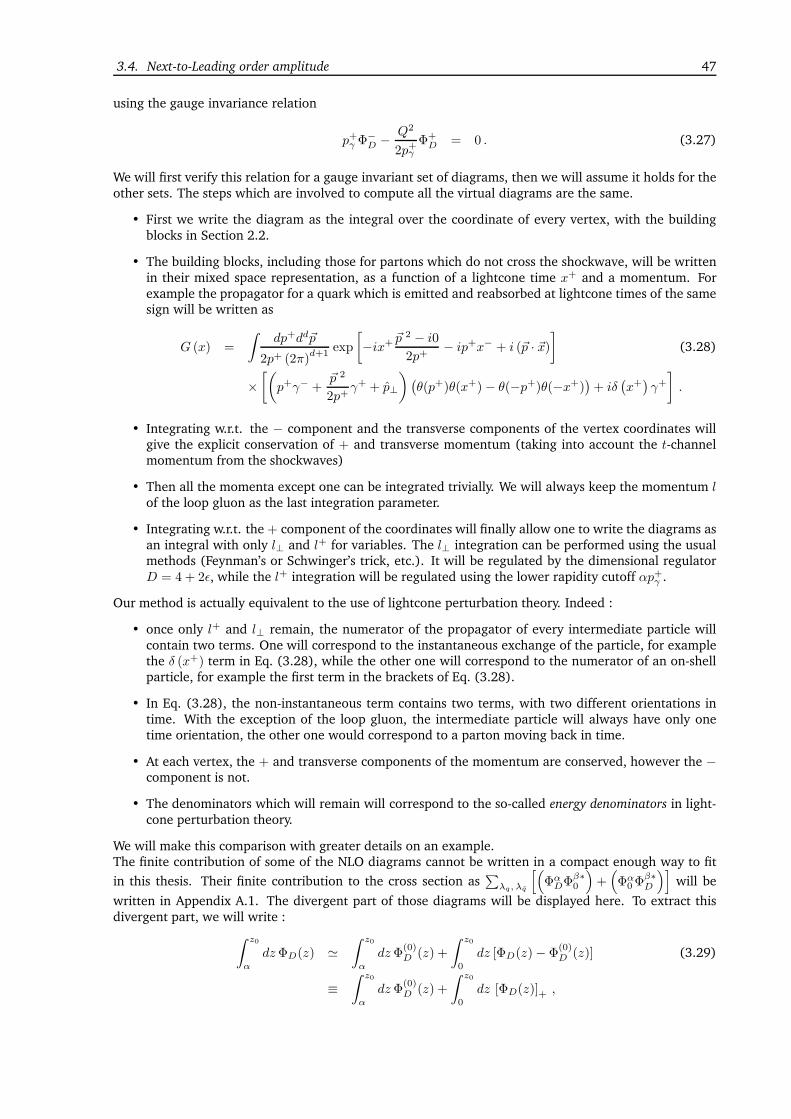
3.4. Next-to-Leading order amplitude 47
using the gauge invariance relation
p+γ Φ−D − Q2
2p+γΦ+D = 0 . (3.27)
We will first verify this relation for a gauge invariant set of diagrams, then we will assume it holds for theother sets. The steps which are involved to compute all the virtual diagrams are the same.
• First we write the diagram as the integral over the coordinate of every vertex, with the buildingblocks in Section 2.2.
• The building blocks, including those for partons which do not cross the shockwave, will be writtenin their mixed space representation, as a function of a lightcone time x+ and a momentum. Forexample the propagator for a quark which is emitted and reabsorbed at lightcone times of the samesign will be written as
G (x) =
∫
dp+dd~p
2p+ (2π)d+1
exp
[
−ix+ ~p2 − i0
2p+− ip+x− + i (~p · ~x)
]
(3.28)
×[(
p+γ− +~p 2
2p+γ+ + p⊥
)
(
θ(p+)θ(x+)− θ(−p+)θ(−x+))
+ iδ(
x+)
γ+]
.
• Integrating w.r.t. the − component and the transverse components of the vertex coordinates willgive the explicit conservation of + and transverse momentum (taking into account the t-channelmomentum from the shockwaves)
• Then all the momenta except one can be integrated trivially. We will always keep the momentum lof the loop gluon as the last integration parameter.
• Integrating w.r.t. the + component of the coordinates will finally allow one to write the diagrams asan integral with only l⊥ and l+ for variables. The l⊥ integration can be performed using the usualmethods (Feynman’s or Schwinger’s trick, etc.). It will be regulated by the dimensional regulatorD = 4 + 2ǫ, while the l+ integration will be regulated using the lower rapidity cutoff αp+γ .
Our method is actually equivalent to the use of lightcone perturbation theory. Indeed :
• once only l+ and l⊥ remain, the numerator of the propagator of every intermediate particle willcontain two terms. One will correspond to the instantaneous exchange of the particle, for examplethe δ (x+) term in Eq. (3.28), while the other one will correspond to the numerator of an on-shellparticle, for example the first term in the brackets of Eq. (3.28).
• In Eq. (3.28), the non-instantaneous term contains two terms, with two different orientations intime. With the exception of the loop gluon, the intermediate particle will always have only onetime orientation, the other one would correspond to a parton moving back in time.
• At each vertex, the + and transverse components of the momentum are conserved, however the −component is not.
• The denominators which will remain will correspond to the so-called energy denominators in light-cone perturbation theory.
We will make this comparison with greater details on an example.The finite contribution of some of the NLO diagrams cannot be written in a compact enough way to fit
in this thesis. Their finite contribution to the cross section as∑
λq, λq
[(
ΦαDΦβ∗0
)
+(
Φα0Φβ∗D
)]
will be
written in Appendix A.1. The divergent part of those diagrams will be displayed here. To extract thisdivergent part, we will write :
∫ z0
α
dzΦD(z) ≃∫ z0
α
dzΦ(0)D (z) +
∫ z0
0
dz [ΦD(z)− Φ(0)D (z)] (3.29)
≡∫ z0
α
dzΦ(0)D (z) +
∫ z0
0
dz [ΦD(z)]+ ,

48 Chapter 3. Diffractive exclusive production of a foward dijet in the shockwave approach
where we explicitly extract the non-integrable part Φ(0)D of ΦD, writing ΦD(z) = Φ
(0)D (z) + O(ln z) for
z → 0, z being the + momentum fraction of the gluon : z ≡ l+
p+γwith l the gluon momentum. What we
call the divergent part of ΦD will be made of the first term in the right-hand side of Eq. (3.29) and the 1ǫ
dimensional pole in the second term.
3.4.3 Diagram 2 : vertex correction
pγ
pq
pq
~p1
~p2
l
Figure 3.5: Vertex correction
Using the mixed space representation for the propagators and external lines, one can write :
Mα2 =
−ieq√
2p+γ
(ig)2∫
dDy0dDy1d
Dy2θ(
−y+0)
θ(
−y+1)
θ(
−y+2)
ui (pq, y2) γµtaG (y20) γ
αG (y01) γν (3.30)
×tavm (pq, y1)Gµν (y21) exp [−i (pγ · y0)]δmi√Nc
=−ieq√
2p+γ
(ig)2∫
dDy0dDy1d
Dy2θ(
−y+0)
θ(
−y+1)
θ(
−y+2)
(
N2c − 1
2Nc√Nc
)
θ(
p+q)
θ(
p+q)
√
2p+q 2p+q
(3.31)
×∫
dd~p1
(2π)d
dd~p2
(2π)d
(
−NcU12
)
∫
dp+dd~p
2p+ (2π)d+1
dk+dd~k
2k+ (2π)d+1
dl+dd~l
2l+ (2π)d+1
× exp[
i(
p+q − p+ − l+)
y−2 + i(
p+q + l+ + k+)
y−1 + i(
p+ − p+γ − k+)
y−0 − ip−γ y+0
]
× exp[
i(
~p+~l− ~pq1
)
· ~y2 − i(
~k +~l + ~pq2
)
· ~y1 − i(
~p− ~k)
· ~y0]
× exp
[
iy+1
(
~p 2q2 − i0
2p+q
)
− iy+01
(
~k 2 − i0
2k+
)
− iy+20
(
~p 2 − i0
2p+
)
+ iy+2
(
~p 2q1 − i0
2p+q
)
− iy+21
(
~l 2 − i0
2l+
)]
×upqγ+(
p+q γ− + pq1⊥
)
2p+qγµ
×[(
p+γ− +~p 2
2p+γ+ + p⊥
)
(
θ(p+)θ(y+20)− θ(−p+)θ(y+02))
+ iδ(
y+20)
γ+]
γα
×[(
k+γ− +~k 2
2k+γ+ + k⊥
)
(
θ(k+)θ(y+01)− θ(−k+)θ(y+10))
+ iδ(
y+01)
γ+
]
×γν(
p+q γ− + pq2⊥
)
2p+qγ+vpq
×[
[
θ(
l+)
θ(
y+21)
− θ(
−l+)
θ(
y+12)]
(
g⊥µν −l⊥µn2ν + l⊥νn2µ
l+−
~l 2
(l+)2n2µn2ν
)
− 2iδ(
y+21)
l+
]
.

3.4. Next-to-Leading order amplitude 49
Integrating w.r.t. y−2 , y−1 , y−0 , ~y2, ~y1 and ~y0 to get + and transverse momentum conservation at eachvertex, then after a trivial integration w.r.t. p+, ~p, k+ and ~k, one obtains :
Mα2 =
iNceq√
2p+γ
(ig)2
(
N2c − 1
2Nc√Nc
)
θ(
p+q)
θ(
p+q)
√
2p+q 2p+q
∫
dd~p1
(2π)d
dd~p2
(2π)dU12 (3.32)
×∫
dl+dd~l
2l+δ(
p+q + p+q − p+γ)
δ (~pq1 + ~pq2)
2(
p+q − l+)
2(
−p+q − l+)
×∫ 0
−∞dy+2 exp
−iy+2
(
~pq1 −~l)2
− i0
2(
p+q − l+) − ~p 2
q1 − i0
2p+q+~l 2 − i0
2l+
×∫ 0
−∞dy+1 exp
iy+1
~p 2q2 − i0
2p+q+
(
~pq1 −~l)2
− i0
2(
−p+q − l+) +
~l 2 − i0
2l+
×∫ 0
−∞dy+0 exp
−iy+0
p−γ +
(
~pq1 −~l)2
− i0
2(
−p+q − l+) −
(
~pq1 −~l)2
− i0
2(
p+q − l+)
×upqγ+(
p+q γ− + pq1⊥
)
2p+qγµ
[
(
(
p+q − l+)
γ− +
(
~pq1 −~l)2
2(
p+q − l+)γ+ + pq1⊥ − l⊥
)
×(
θ(p+q − l+)θ(y+20)− θ(l+ − p+q )θ(y+02))
+ iδ(
y+20)
γ+
]
γα
×[
(
(
−p+q − l+)
γ− +
(
~pq1 −~l)2
2(
−p+q − l+)γ+ + pq1⊥ − l⊥
)
(
θ(−p+q − l+)θ(y+01)− θ(p+q + l+)θ(y+10))
+iδ(
y+01)
γ+
]
γν(
p+q γ− + pq2⊥
)
2p+qγ+vpq
[
(
g⊥µν −l⊥µn2ν + l⊥νn2µ
l+−
~l 2
(l+)2n2µn2ν
)
×[
θ(
l+)
θ(
y+21)
− θ(
−l+)
θ(
y+12)]
− 2iδ(
y+21)
l+n2µn2ν
]
.
Let us now show that, as physically expected, the cases where y+10 < 0 or y+20 < 0 (which means the gluonis emitted from the quark or the antiquark before the photon splits) cancel.
For example let us consider the case where y+20 < 0.
• In this case, one needs l+ > p+q . Then θ (−l+) = 0 since p+q > 0 so the term with θ(
y+12)
inthe gluon numerator cancels. So does the term with θ
(
y+01)
in the antiquark numerator, sinceθ(
−p+q − l+)
= θ(
p+q − l+ − p+γ)
and p+γ > 0.
• It is also easy to cancel the term with δ(
y+12)
in the gluon numerator :
– Due to the presence of the square of γ+ (which is 0), the term with δ(
y+01)
in the antiquarkpropagator then cancels.
– The remaining term contains θ(
−y+01)
= θ(
y+20)
.
– Thus this contribution requires both y+20 > 0 and y+20 < 0, which is impossible.
• Thus the only remaining term in the gluon numerator contains a θ(
y+21)
factor. Hence this termcontains an overall θ
(
y+21)
θ(
y+02)
. This is excluded by the antiquark numerator since we canceledthe contribution where y+1 < y+0 : everything cancels.
One can thus conclude : the term with y+0 > y+2 cancels. The θ(
−y+10)
contribution can be cancelled with
a similar reasoning. Hence 5 cases remain. Let us introduce M (1)α2 , M
(2)α2 , M (3)α
2 , M (4)α2 and M
(5)α2 ,

50 Chapter 3. Diffractive exclusive production of a foward dijet in the shockwave approach
which will correspond respectively to the cases where y+2 > y+1 > y+0 , y+1 > y+2 > y+0 , y+2 = y+1 > y+0 ,y+1 > y+2 = y+0 and y+2 > y+1 > y+0 . In lightcone perturbation theory, they would be drawn diagramaticallyas follows :
y+2 > y+1 > y+0 y+1 > y+2 > y+0 y+2 = y+1 > y+0
y+1 > y+2 = y+0 y+2 > y+1 = y+0
Figure 3.6: Lightcone perturbation theory description of diagram 2. In the first figure, the vertical dashedlines stand for the energy denominators, as described in the following.
The propagators which are crossed with a bar represent the instantaneous propagator in lightconeperturbation theory.Let us consider the first case. We then need the following integral :
∫ 0
−∞dy+0 exp
iy+0
(
~pq1 −~l)2
− i0
2(
p+q − l+) −
(
~pq1 −~l)2
− i0
2(
p+q − l+ − p+γ) − p−γ
(3.33)
×∫ 0
y+0
dy+2 exp
iy+2
~p 2q1 − i0
2p+q−~l 2 − i0
2l+−
(
~pq1 −~l)2
− i0
2(
p+q + l+)
×∫ y+2
y+0
dy+1 exp
iy+1
~p 2q2 − i0
2p+q−
(
~pq1 −~l)2
− i0
2(
p+q + l+) +
~l 2 − i0
2l+
=i
(
~p 2q1−i02p+q
+~p 2q1−i02p+q
− p−γ
)(
~l 2−i02l+ +
~p 2q1−i02p+q
+(~pq1−~l )
2−i02(p+q −l+)
− p−γ
)(
(~pq1−~l )2−i0
2(p+q −l+)+
(~pq1−~l )2−i0
2(p+q +l+)− p−γ
) .
Let us consider the same contribution in lightcone perturbation theory. In this case, the denominator forthe diagram is made of the so-called energy denominators. Such denominators can be written as
Dn =
(
∑
i
E(i)n
)
− E0 , (3.34)
where E(i)n is the lightcone energy (i.e. p−) of the i-th particle in the n-th intermediate Fock state, and E0
is the energy of the initial Fock state (i.e. p−γ ). In the present case there will be 3 of them (representedby the vertical dashed lines in the first diagram in Fig. 3.6), and they will read :
D1 =
(
~pq1 −~l)2
− i0
2(
p+q − l+) +
(
~pq2 +~l)2
− i0
2(
p+q + l+) − p−γ , (3.35)

3.4. Next-to-Leading order amplitude 51
D2 =~l 2 − i0
2l++~p 2q2 − i0
2p+q+
(
~pq1 −~l)2
− i0
2(
p+q − l+) − p−γ , (3.36)
D3 =~p 2q1 − i0
2p+q+~p 2q2 − i0
2p+q− p−γ . (3.37)
These are exactly the denominators in Eq. (3.33). This ends our comparison with lightcone perturbationtheory. After integration w.r.t. : y+2 , y+1 and y+0 we finally get for the 5 contributions to diagram 2 inFig. 3.6 :
M(1)α2 =
−eqNc√
2p+γ
(ig)2
(
N2c − 1
2Nc√Nc
)
θ(
p+q)
θ(
p+q)
√
2p+q 2p+q
∫
dd~p1
(2π)d
dd~p2
(2π)d
(
U12
)
(
~p 2q1−i02p+q
+~p 2q1−i02p+q
− p−γ
) (3.38)
×∫ p+q
0
dl+
2l+δ(
p+q + p+q − p+γ)
δ (~pq1 + ~pq2)
2(
p+q − l+)
2(
p+q + l+)
∫
dd~lupqγ
+(
p+q γ− + pq1⊥
)
2p+q
×γµ[
(
p+q − l+)
γ− +(~pq1−~l )
2
2(p+q −l+)γ+ +
(
pq1⊥ − l⊥)
]
γα
(
~l 2−i02l+ +
~p 2q1−i02p+q
+(~pq1−~l )
2−i02(p+q −l+)
− p−γ
)(
(~pq1−~l )2−i0
2(p+q −l+)+
(~pq1−~l )2−i0
2(p+q +l+)− p−γ
)
×
(
−p+q − l+)
γ− +
(
~pq1 −~l)2
2(
−p+q − l+)γ+ +
(
pq1⊥ − l⊥)
γν
×(
p+q γ− + pq2⊥
)
γ+vpq
2p+q
(
g⊥µν −l⊥µn2ν + l⊥νn2µ
l+−
~l 2
(l+)2n2µn2ν
)
,
M(2)α2 = M
(1)α2 |(q↔q) , (3.39)
where (q ↔ q) stands for (1 ↔ 2, xq ↔ xq, ~pq ↔ ~pq).
M(3)α2 =
−eqNc√
2p+γ
(ig)2
(
N2c − 1
2Nc√Nc
)
θ(
p+q)
θ(
p+q)
√
2p+q 2p+q
∫
dd~p1
(2π)d
dd~p2
(2π)d
(
U12
)
(
~p 2q1−i02p+q
+~p 2q2−i02p+q
− p−γ
) (3.40)
×∫ p+q
−p+q
dl+
(l+)2
δ(
p+q + p+q − p+γ)
δ (~pq1 + ~pq2)
2(
p+q − l+)
2(
p+q + l+)
∫
dd~l
×upqγ
+[
(
p+q − l+)
γ− +(
pq1⊥ − l⊥)]
γα[
(
−p+q − l+)
γ− +(
pq1⊥ − l⊥)]
γ+vpq(
−p−γ − (~pq1−~l )2−i0
2(−p+q −l+)+
(~pq1−~l )2−i0
2(p+q −l+)
) ,
M(4)α2 =
−eqNc√
2p+γ
(ig)2
(
N2c − 1
2Nc√Nc
)
θ(
p+q)
θ(
p+q)
√
2p+q 2p+q
∫
dd~p1
(2π)d
dd~p2
(2π)d
(
U12
)
(
~p 2q2−i02p+q
+~p 2q1−i02p+q
− p−γ
) (3.41)
×∫ 0
−p+q
dl+
2l+
∫
dd~lδ(
p+q + p+q − p+γ)
δ (~pq1 + ~pq2)
2(
p+q − l+)
2(
p+q + l+)
×upqγ
µ⊥γ
+γα[
−(
p+q + l+)
γ− − (~pq1−~l )2
2(p+q +l+)γ+ +
(
pq1⊥ − l⊥)
]
(
− (~pq1−~l )2−i0
2(−p+q −l+)+
~p 2q1−i02p+q
− ~l 2−i02l+ − p−γ
)
×γν(
p+q γ− + pq2⊥
)
2p+qγ+vpq
(
g⊥µν −l⊥µn2ν
l+
)
,

52 Chapter 3. Diffractive exclusive production of a foward dijet in the shockwave approach
and finally
M(5)α2 = M
(4)α2 |(q↔q) . (3.42)
The l⊥ integration is now straightforward, we will not detail it. The integral w.r.t. l+ is badly divergentas it is written. One has to restore the rapidity cutoff θ
(
|l+| − αp+γ)
in the expressions above beforeperforming this integration. After performing those two integrations and quite a bit of Dirac algebra, onecan finally show that the contribution of this diagram to the + impact factor reads :
Φ+1 |2 =
1
2Φ+
0
[
2π2
3− 2Li2
(
x
x− 1
)
− 2Li2
(
x
x− 1
)
− 8 + 3
(
1
ǫ− ln
(
µ2
Q2
))
(3.43)
+ − ln2( x
x
)
+ ln2(xx
α2
)
+ 2 ln(xx
α2
)
ln
(
µ2
Q2
)
− 2
ǫln(xx
α2
)
]
.
The dilogarithms can be rewritten in terms of logarithms by using several identities :
Li2
(
x
x− 1
)
+ Li2
(
x
x− 1
)
= Li2
(
1− 1
x
)
+ Li2
(
1− 1
x
)
(3.44)
= − ln2 (x)
2− Li2 (x)−
ln2 (x)
2− Li2 (x)
= − ln2 (x)
2− ln2 (x)
2− π2
6+ ln (x) ln (x)
= −1
2ln2( x
x
)
− π2
6.
Thus :
Φ+1 |2 = Φ+
0
[
π2
2− 4 +
3
2ǫ− 3
2ln
(
µ2
Q2
)
+1
2ln2(xx
α2
)
+ ln(xx
α2
)
ln
(
µ2
Q2
)
− 1
ǫln(xx
α2
)
]
.(3.45)
Similarly one can get :
Φ−1 |2 =
1
2xxΦ−
0
[
−3xx ln
(
~p 2q1 + xxQ2
xxQ2
)
+ 6xx− π2
3
(
xx+ 4~p 2q1
Q2
)
(3.46)
+14~p 2q1
Q2− ~p 2
q1
Q2ln2(xx
α2
)
+
(
~p 2q1 + xxQ2
Q2
)
ln2( x
x
)
+2xx ln
(
~p 2q1 + xxQ2
Q2
)
ln(xx
α2
)
+[
2 ln(xx
α2
)
− 3]
(
2~p 2q1
Q2+ xx
)(
1
ǫ+ ln
(
~p 2q1 + xxQ2
µ2
))
+3~p 2q1
Q2ln (xx)− 2
(
~p 2q1
Q2+ xx
)
ln (xx) ln(xx
α2
)
]
,
and
Φi1⊥|2 = Φi0⊥
[
−4 +1
2ln2(xx
α2
)
+π2
2−
ln(xx
α2
)
− 3
2
(3.47)
×(
~p 2q1 + xxQ2
~p 2q1
)
ln
(
~p 2q1 + xxQ2
xxQ2
)
+ ln
(
Q2
µ2
)
+1
ǫ
]
.

3.4. Next-to-Leading order amplitude 53
3.4.4 Diagram 3 dressed quark propagator
pγ
pq
pq
~p1
~p2
l
Figure 3.7: Dressed quark propagator
The contribution from diagram 3 in Fig. 3.4 reads
Mα3 =
−ieq√
2p+γ
(ig)2∫
dDy2dDy1d
Dy0ui (pq, y2) γµG0 (y21) γνG0 (y10) γαvm (pq, y0) (3.48)
×Gµν0 (y21)δim√Nc
e−i(pγ ·y0)
=iNceq√
2p+γ
(ig)2∫
dDy2dDy1d
Dy0
∫
dd~p1
(2π)d
dd~p2
(2π)d
(
N2c − 1
2Nc√Nc
)
U12θ(
−y+2)
θ(
−y+0)
(3.49)
×θ(
p+q)
θ(
p+q)
√
2p+q 2p+q
∫
dp+dd~p
2p+ (2π)d+1
∫
dk+dd~k
2k+ (2π)d+1
∫
dl+dd~l
2l+ (2π)d+1
upqγ+(
p+q γ− + pq1⊥
)
2p+qγµ
×[(
p+γ− +~p 2
2p+γ+ + p⊥
)
(
θ(p+)θ(y+21)− θ(−p+)θ(y+12))
+ iδ(
y+21)
γ+]
γν
×[(
k+γ− +~k 2
2k+γ+ + k⊥
)
(
θ(k+)θ(y+10)− θ(−k+)θ(y+01))
+ iδ(
y+10)
γ+
]
γα
×(
p+q γ− + pq2⊥
)
2p+qγ+vpq
[(
g⊥µν −l⊥µn2ν + l⊥νn2µ
l+−
~l 2
(l+)2n2µn2ν
)
×[
θ(
l+)
θ(
y+21)
− θ(
−l+)
θ(
y+12)]
− 2iδ(
y+21)
l+n2µn2ν
]
× exp[
i(
p+q − l+ − p+)
y−2 + i(
p+ + l+ − k+)
y−1 + i(
k+ + p+q − p+γ)
y−0]
× exp[
−i(
~pq1 −~l− ~p)
· ~y2 + i(
~k −~l− ~p)
· ~y1 − i(
~pq2 + ~k)
· ~y0]
× exp
[
iy+2
(
~p 2q1 − i0
2p+q−~l 2 − i0
2l+− ~p 2 − i0
2p+
)
+ iy+1
(
~p 2 − i0
2p++~l 2 − i0
2l+−~k 2 − i0
2k+
)]
× exp
[
iy+0
(
~p 2q2 − i0
2p+q+~k 2 − i0
2k+− p−γ
)]
.
The expression as we wrote it might seem mathematically undefined due to the presence of products ofdistributions, like
[
δ(
y+21)]2
.. Let us note that it is only our compact way of writing a distinction of thecases
(
y+2 > y+1 , y+2 = y+1 , y
+2 < y+1
)
. One could perform the simultaneous Fourier transform of the twopropagators between y2 and y1 a more careful way and obtain terms like δ′(y+21). However it is actuallyeasy to see that when y+2 = y+1 the gamma structure cancels and when y+2 < y+1 one gets a contradiction

54 Chapter 3. Diffractive exclusive production of a foward dijet in the shockwave approach
like 0 > l+ > p+q > 0. Hence the seemingly ill-defined quantities do not contribute to our process.Integrating w.r.t. y−2 , y−1 , y−0 , ~y2, ~y1 and ~y0 to get + and transverse momentum conservation at eachvertex, then after a trivial integration w.r.t. p+, ~p, k+ and ~k, one obtains :
Mα3 =
iNceq√
2p+γ
(ig)2∫
dy+2 dy+1 dy
+0 θ(
−y+2)
θ(
−y+0)
θ(
y+21)
∫
dd~p1
(2π)d
dd~p2
(2π)d
(
N2c − 1
2Nc√Nc
)
U12(3.50)
×θ(
p+q)
θ(
p+q)
√
2p+q 2p+q
1
2p+q
∫ p+q
0
dl+
2l+2(
p+q − l+)
∫
dd~lupqγ+(
p+q γ− + pq1⊥
)
2p+qγµ
×
(
p+q − l+)
γ− +
(
~pq1 −~l)2
2(
p+q − l+)γ+ +
(
pq1⊥ − l⊥)
γν
×[(
p+q γ− +
~p 2q1
2p+qγ+ + pq1⊥
)
θ(p+q )θ(y+10) + iδ
(
y+10)
γ+
]
×γα(
p+q γ− + pq2⊥
)
2p+qγ+vpqδ
(
p+q + p+q − p+γ)
δ (~pq1 + ~pq2)
×[
g⊥µν −l⊥µn2ν + l⊥νn2µ
l+−
~l 2
(l+)2n2µn2ν
]
× exp
iy+2
~p 2q1 − i0
2p+q−~l 2 − i0
2l+−
(
~pq1 −~l)2
− i0
2(
p+q − l+)
× exp
iy+1
(
~pq1 −~l)2
− i0
2(
p+q − l+) +
~l 2 − i0
2l+− ~p 2
q1 − i0
2p+q
× exp
[
iy+0
(
~p 2q2 − i0
2p+q+~p 2q1 − i0
2p+q− p−γ
)]
.
Distinguishing the two cases y+1 > y+0 and y+1 = y+0 gives two contributions :
M(1)α3 = − Nceq
√
2p+γ
(ig)2∫
dd~p1
(2π)ddd~p2
(2π)d
(
N2c − 1
2Nc√Nc
) U12(
~p 2q1−i02p+q
+~p 2q2−i02p+q
− p−γ
) (3.51)
×θ(
p+q)
θ(
p+q)
√
2p+q 2p+q
1
2p+q
∫ p+q
0
dl+
2l+2(
p+q − l+)
∫
dd~l δ(
p+q + p+q − p+γ)
δ (~pq1 + ~pq2)
×upqγ+(
p+q γ− + pq1⊥
)
2p+qγµ
(
p+q − l+)
γ− +
(
~pq1 −~l)2
2(
p+q − l+)γ+ +
(
pq1⊥ − l⊥)
×γν(
p+q γ− +
~p 2q1
2p+qγ+ + pq1⊥
)
γα(
p+q γ− + pq2⊥
)
2p+qγ+vpq
×g⊥µν − l⊥µn2ν+l⊥νn2µ
l+ − ~l 2
(l+)2n2µn2ν
(
~p 2q2−i02p+q
+~l 2−i02l+ +
(~pq1−~l )2−i0
2(p+q −l+)− p−γ
)(
~p 2q2−i02p+q
+~p 2q1−i02p+q
− p−γ
) ,
and
M(2)α3 =
Nceq√
2p+γ
(ig)2∫
dd~p1
(2π)d
dd~p2
(2π)d
(
N2c − 1
2Nc√Nc
) U12(
~p 2q1−i02p+q
+~p 2q2−i02p+q
− p−γ
) (3.52)

3.4. Next-to-Leading order amplitude 55
×θ(
p+q)
θ(
p+q)
√
2p+q 2p+q
1
2p+q
∫ p+q
0
dl+
2l+2(
p+q − l+)δ(
p+q + p+q − p+γ)
δ (~pq1 + ~pq2)
×∫
dd~lupqγ+(
p+q γ− + pq1⊥
)
2p+q
(
γ⊥ν −l⊥νl+
γ+)
×
[
(
p+q − l+)
γ− +(
pq1⊥ − l⊥)]
γ⊥νγ+γα(
p+q γ− + pq2⊥
)
γ+vpq
2p+q
(
~p 2q2−i02p+q
+~l 2−i02l+ +
(~pq1−~l )2−i0
2(p+q −l+)− p−γ
) .
Again the integration w.r.t. l⊥ is easy and it will not be detailed. The diagram for the dressed antiquarkpropagator can be obtained from this one by the symmetrization (q ↔ q). One can finally show thatdiagram 3 and its symmetric contribute to Φα1 as :
Φ+1 |3+(q↔q) = Φ+
0
[
1
2ln2( x
x
)
− 1
2ln2(xx
α2
)
+ ln (xx) ln(xx
α2
)
+ 7− 3
ǫ− 2
π2
3(3.53)
+2
ln
(
~p 2q1 + xxQ2
xxµ2
)
+1
ǫ
ln(xx
α2
)
− 3
2ln
((
~p 2q1 + xxQ2
)2
xxµ4
)]
,
Φ−1 |3+(q↔q) =
Φ−0
xx
[
−~p2q1
Q2
(
ln
(
(
~p 2q1 + xxQ2
)2
xxµ4
)
+2
ǫ
)
ln(xx
α2
)
− 7~p 2q1
Q2+ 3
~p 2q1
Q2ln
(
~p 2q1 + xxQ2
µ2
)
,
−3
2
~p 2q1
Q2ln (xx) +
3
ǫ
~p 2q1
Q2+ 2
π2
3
~p 2q1
Q2
1
2
~p 2q1
Q2ln2(xx
α2
)
− 1
2
~p 2q1
Q2ln2( x
x
)
]
. (3.54)
Φi1⊥|3+(q↔q) = Φi0⊥
[
1
2ln2( x
x
)
+
ln(xx
α2
)
− 3
2
ln
((
~p 2q1 + xxQ2
)2
xxµ4
)
(3.55)
−1
2ln2(xx
α2
)
+2
ǫln(xx
α2
)
+ 7− 3
ǫ− 2
π2
3
]
.
By adding Eq. (3.45) one gets the total virtual correction before the shockwave :
Φ+1 |2 +Φ+
1 |3+(q↔q) = Φ+0
[
1
2ln2( x
x
)
+ 3− π2
6+
ln
(
(
~p 2q1 + xxQ2
)2
xxµ2Q2
)
+1
ǫ
ln(xx
α2
)
− 3
2
]
,
(3.56)
Φ−1 |2 + Φ−
1 |3+(q↔q) = Φ−0
[
1
2ln2( x
x
)
+ 3− π2
6+
ln
((
~p 2q1 + xxQ2
)2
xxµ2Q2
)
+1
ǫ
ln(xx
α2
)
− 3
2
]
,
(3.57)and
Φi1⊥|2 +Φi1⊥|3+(q↔q) = Φi0⊥
[
1
2ln2( x
x
)
− π2
6+ 3 +
ln(xx
α2
)
− 3
2
(3.58)
×
ln
(
~p 2q1 + xxQ2
µ2
)
−(
xxQ2
~p 2q1
)
ln
(
~p 2q1 + xxQ2
xxQ2
)
+1
ǫ
]
.
This set of diagrams is gauge invariant, as can be explicitly checked using the gauge invariance propertyof the leading order impact factor Φα0 in the longitudinal case.

56 Chapter 3. Diffractive exclusive production of a foward dijet in the shockwave approach
3.4.5 Diagram 4 : final state interaction
pγ
pq
pq
~p1
~p2
Figure 3.8: Final state interaction
The computation method is the same as before. One gets :
Mα4 =
−ieq√
2p+γ
(ig)2∫
dDy2dDy1d
Dy0
(
upq)
i√
2p+q
ei(pq·y2)θ(
p+q)
γµG (y2, y0) γαe−i(pγ ·y0) (3.59)
×G (y0, y1) γν
(
vpq)
m√
2p+q
ei(pq·y1)θ(
p+q)
Gµν0 (y21)δim√Nc
=eqNc√
2p+γ
(ig)2 θ(
p+q)
θ(
p+q)
√
2p+q 2p+q
(
N2c − 1
2Nc√Nc
)∫
dd~p1(2π)d
dd~p2(2π)d
(
U12
)
(3.60)
×∫
dl+dd~l
2l+δ(
p+q + p+q − p+γ)
δ (~pq1 + ~pq2)(
(~pq1−~l )2−i0
2(p+q −l+)+
(~pq2+~l )2−i0
2(p+q +l+)− p−γ
)θ(
p+q − l+)
θ(
p+q + l+)
∫
dy+2 dy+1 θ(
y+2)
θ(
y+1)
×upqγµγ−(
p+q − l+)
+(
pq⊥ − l⊥)
2(
p+q − l+) γ+
γ−(
p+q − l+)
+(
pq1⊥ − l⊥)
2(
p+q − l+) γα
×γ−(
p+q + l+)
+(
pq2⊥ + l⊥)
2(
p+q + l+) γ+
γ−(
p+q + l+)
+(
pq⊥ + l⊥)
2(
p+q + l+) γνvpq
×[
[
θ(
l+)
θ(
y+21)
− θ(
−l+)
θ(
y+12)]
(
g⊥µν −l⊥µn2ν + l⊥νn2µ
l+−
~l 2
(l+)2n2µn2ν
)
− 2iδ(
y+21)
l+n2µn2ν
]
× exp
iy+2
~p 2q
2p+q−
(
~pq −~l)2
− i0
2(
p+q − l+) −
~l 2 − i0
2l+
+ iy+1
~p 2q
2p+q−
(
~pq +~l)2
− i0
2(
p+q + l+) +
~l 2 − i0
2l+
.
There are 3 contributions M (1)α4 , M (2)α
4 and M(3)α4 corresponding respectively to y+2 > y+1 > y+0 , y+1 >
y+2 > y+0 , y+2 = y+1 > y+0 . As for the previous diagrams M (2)α4 =M
(1)α1 |(q↔q). The other two read :
M(1)α4 =
−Nceq√
2p+γ
(ig)2 θ(
p+q)
θ(
p+q)
√
2p+q 2p+q
(
N2c − 1
2Nc√Nc
)∫
dd~p1(2π)d
dd~p2(2π)d
(
U12
)
(3.61)
×∫ p+q
0
dl+
2l+
∫
dd~lδ(
p+q + p+q − p+γ)
δ (~pq1 + ~pq2)(
(~pq1−~l )2−i0
2(p+q −l+)+
(~pq2+~l )2−i0
2(p+q +l+)− p−γ
)

3.4. Next-to-Leading order amplitude 57
×upqγµγ−(
p+q − l+)
+(
pq⊥ − l⊥)
2(
p+q − l+) γ+
γ−(
p+q − l+)
+(
pq1⊥ − l⊥)
2(
p+q − l+) γα
×γ−(
p+q + l+)
+(
pq2⊥ + l⊥)
2(
p+q + l+) γ+
γ−(
p+q + l+)
+(
pq⊥ + l⊥)
2(
p+q + l+) γνvpq
×g⊥µν − l⊥µn2ν+l⊥νn2µ
l+ − ~l 2
(l+)2n2µn2ν
(
~p 2q
2p+q+
~p 2q
2p+q− (~pq−~l )
2−i02(p+q −l+)
− (~pq+~l )2−i0
2(p+q +l+)
)(
~p 2q
2p+q− (~pq−~l )
2−i02(p+q −l+)
− ~l 2−i02l+
) ,
and
M(3)α4 =
Nceq√
2p+γ
(ig)2 θ(
p+q)
θ(
p+q)
√
2p+q 2p+q
(
N2c − 1
2Nc√Nc
)∫
dd~p1(2π)d
dd~p2(2π)d
(
U12
)
(3.62)
×∫
dl+dd~l
(l+)2δ(
p+q + p+q − p+γ)
δ (~pq1 + ~pq2) θ(
p+q − l+)
θ(
p+q + l+)
(
~p 2q
2p+q+
~p 2q
2p+q− (~pq−~l )
2−i02(p+q −l+)
− (~pq+~l )2−i0
2(p+q +l+)
)(
(~pq1−~l )2−i0
2(p+q −l+)+
(~pq2+~l )2−i0
2(p+q +l+)− p−γ
)
×upqγ+γ−(
p+q − l+)
+(
pq1⊥ − l⊥)
2(
p+q − l+) γα
γ−(
p+q + l+)
+(
pq2⊥ + l⊥)
2(
p+q + l+) γ+vpq .
The l⊥ integral is far more complicated than the one in the previous diagrams due to the presence of 3denominators with an l⊥ dependence in M
(1)α4 and M
(2)α4 . However let us note that one denominator
can be reduced to ~l 2 ater a simple shift on ~l. Indeed :
~p 2q
2p+q−
(
~pq −~l)2
− i0
2(
p+q − l+) −
~l 2 − i0
2l+= − p+q
2l+(
p+q − l+)
(
~l − l+
p+q~pq
)2
. (3.63)
We will need similar integrals in most of the other diagrams, so we will define the following generalintegrals :
Ik1 (~q1, ~q2, ∆1, ∆2) ≡ 1
π
∫
dd~l(
lk⊥)
[
(~l − ~q1)2 +∆1
] [
(~l − ~q2)2 +∆2
]
~l 2, (3.64)
I2(~q1, ~q2, ∆1, ∆2) ≡ 1
π
∫
dd~l[
(~l − ~q1)2 +∆1
] [
(~l − ~q2)2 +∆2
] , (3.65)
Ik3 (~q1, ~q2, ∆1, ∆2) ≡ 1
π
∫
dd~l(
lk⊥)
[
(~l − ~q1)2 +∆1
] [
(~l − ~q2)2 +∆2
] , (3.66)
Ijk(~q1, ~q2, ∆1, ∆2) ≡ 1
π
∫ dd~l(
lj⊥lk⊥
)
[
(~l − ~q1)2 +∆1
] [
(~l − ~q2)2 +∆2
]
~l 2. (3.67)
These integrals are computed in Appendix A.1.1.Let us start with a remark : once ~l has been shifted, there is no divergence when the shifted ~l ap-
proaches ~0. Indeed this would correspond exactly to a divergence emerging when the gluon is collinearto the quark, which should be absent from such a diagram : collinear divergences occur when the gluonis emitted and reabsorbed by the parton to which it is collinear.
Let us rewrite the third line and the gluonic tensor in Eq. (3.60), and set ~l → l+
p+q~pq :
upqγµ
(
pq − l)
2(
p+q − l+)γ+dµν0 (l) (3.68)
→ upq (γµpqγ+)
2p+q
(
gµν⊥ −pµq⊥n
ν2 + pνq⊥n
µ2
p+q−
~p 2q
(
p+q)2n
µ2n
ν2
)
.

58 Chapter 3. Diffractive exclusive production of a foward dijet in the shockwave approach
Using the Dirac equation one can write by anticommutation of the Dirac matrices γµpq → 2pqµ. Thenone only has to notice that the new gluonic tensor is dµν0 (pq), which is exactly canceled by pqµ. Thus asexpected there is at least a linear dependence in l⊥ in the numerator of this diagram once l⊥ has beenshifted, which is the reason why we will not need the integral which is similar to Eq. (3.64) but with 1in the numerator. The only divergences from this diagram are actually soft divergences for α = + andα = i. For α = − this diagram contains a UV divergence which should cancel when we construct a gaugeinvariant quantity (i.e. adding the dipole contributions of diagrams 5 and 6). However as we statedbefore we will not compute the α = − contribution. They is no way of writing the final Dirac structureand the finite result for this diagram which would be compact enough to fit in this thesis. Instead, wewill present the result for the contribution of this diagram to the cross section once in Appendix A.1. Wewill only write explicitly the divergent part of this diagram here. One gets :
(
Φ+1 |4)
div=
1
2Φ+
0
[
ln2(xx
α2
)
− ln2( x
x
)
+ 2 ln(xx
α2
)
ln
(
(
~p 2q1 + xxQ2
)2
Q2 (x~pq − x~pq)2
)
+ iπ
]
(3.69)
+upqC4‖vpq
(
Φi1⊥|4)
div=
1
2Φi0⊥
[
ln2(xx
α2
)
− ln2( x
x
)
+ 2 ln(xx
α2
)
(3.70)
×
ln
(
xx(
~p 2q1 + xxQ2
)
(x~pq − x~pq)2
)
− xxQ2
~p 2q1
ln
(
~p 2q1 + xxQ2
xxQ2
)
+ iπ
]
+(
upqC4i⊥ vpq
)
,
where C4‖ and C4i
⊥ are finite expressions.
3.4.6 Diagram 5 : gluon exchange through the shockwave field
pγ
pq
pq
~p1
~p2
~p3
Figure 3.9: Gluon exchange through the shockwave field
This diagram reads :
Mα5 =
−ieq√
2p+γ
(ig)2∫
dDy2dDy1d
Dy0
(
upq)
i√
2p+q
ei(pq·y2)θ(
p+q)
γµG (y2, y0) γαe−i(pγ ·y0)G0 (y01) γ
νvm (pq, y1)
×Gµν (y21)δim√Nc
(3.71)
=−ieq(ig)2√
2p+γ
√
Nc
∫
ddp1⊥(2π)d
dd~p2
(2π)ddd~p3(2π)d
[
Nc2
(
U13 + U32 − U12 − U13 U32
)
+ (2π)d(
N2c − 1
2Nc
)
U12δ (~p3)
]
×θ(
p+q)
θ(
p+q)
√
2p+q 2p+q
∫
dy+1 dy+0 θ(
−y+1)
θ(
−y+0)
δ(
p+q + p+q − p+γ)
δ (~pq1 + ~pq2 − ~p3) (3.72)
×∫ p+q
0
dl+
2l+
∫
dd~lupqγµγ−(
p+q − l+)
+ pq⊥ − l⊥
2(
p+q − l+) γ+
γ−(
p+q − l+)
+(
pq1⊥ − l⊥)
2(
p+q − l+) γα

3.4. Next-to-Leading order amplitude 59
×
(
p+q + l+)
γ− +
(
~pq1 −~l)2
2(
p+q + l+)γ+ − pq1⊥ + l⊥
θ(y+10) + iδ
(
y+10)
γ+
γν
×(
p+q γ− + pq2⊥
)
2p+qγ+vpq
1
2(
p+q + l+)
(
g⊥µβ − lβ⊥l+n2µ
)(
gβ⊥ν −lβ⊥ − pβ3⊥
l+n2ν
)
× i(
p−q − ~l 2−i02l+ − (~pq−~l )
2−i02(p+q −l+)
) exp
iy+0
(
~pq1 −~l)2
− i0
2(
p+q − l+) −
(
~pq1 −~l)2
− i0
2(
−p+q − l+) − p−γ
× exp
iy+1
~p 2q2 − i0
2p+q+
(
~pq1 −~l)2
− i0
2(
−p+q − l+) +
(
~l − ~p3
)2
− i0
2l+
.
There are two contributions :
M(1)α5 =
∫
ddp1⊥(2π)d
dd~p2
(2π)d
dd~p3(2π)d
[
Nc2
(
U13 + U32 − U12 − U13 U32
)
+ (2π)d(
N2c − 1
2Nc
)
U12δ (~p3)
]
×−(ig)2eq√
2p+γ
√
Ncθ(
p+q)
θ(
p+q)
√
2p+q 2p+q
δ(
p+q + p+q − p+γ)
δ (~pq1 + ~pq2 − ~p3)
∫ p+q
0
dl+
2l+
∫
dd~l (3.73)
×upqγµγ−(
p+q − l+)
+ pq⊥ − l⊥
2(
p+q − l+) γ+
γ−(
p+q − l+)
+(
pq1⊥ − l⊥)
2(
p+q − l+) γα
×
(
p+q + l+)
γ− +
(
~pq1 −~l)2
2(
p+q + l+)γ+ − pq1⊥ + l⊥
γν(
p+q γ− + pq2⊥
)
2p+qγ+vpq
1
2(
p+q + l+)
×
(
g⊥µβ − lβ⊥
l+ n2µ
)(
gβ⊥ν −lβ⊥−pβ3⊥l+ n2ν
)
(
p−q − ~l 2−i02l+ − (~pq−~l )
2−i02(p+q −l+)
)(
(~pq1−~l )2−i0
2(p+q −l+)− (~pq1−~l )
2−i02(−p+q −l+)
− p−γ
)
× 1(
~p 2q2−i02p+q
+(~l−~p3)
2−i02l+ +
(~pq1−~l )2−i0
2(p+q −l+)− p−γ
) ,
and
M(2)α5 =
∫
ddp1⊥(2π)d
dd~p2
(2π)d
dd~p3(2π)d
[
Nc2
(
U13 + U32 − U12 − U13 U32
)
+ (2π)d(
N2c − 1
2Nc
)
U12δ (~p3)
]
× (ig)2eq√
2p+γ
√
Ncθ(
p+q)
θ(
p+q)
√
2p+q 2p+q
δ(
p+q + p+q − p+γ)
δ (~pq1 + ~pq2 − ~p3) (3.74)
×∫ p+q
0
dl+
2l+
∫
dd~lupqγµγ−(
p+q − l+)
+ pq⊥ − l⊥
2(
p+q − l+) γ+
γ−(
p+q − l+)
+(
pq1⊥ − l⊥)
2(
p+q − l+) γα
×γ+(
γ⊥µ − l⊥l+ n2µ
)
vpq(
~p 2q
2p+q− ~l 2−i0
2l+ − (~pq−~l )2−i0
2(p+q −l+)
)(
(~pq1−~l )2−i0
2(p+q −l+)+
~p 2q2−i02p+q
+(~l−~p3)
2−i02l+ − p−γ
)
1
2(
p+q + l+) .
Similarly to diagram 4, the l⊥ integration requires quite some work. However it will involve the sametype of integrals as before. Indeed by performing the shift ~l → ~l − l+
p+q~pq, one can reduce one of the
denominators to ~l 2. Then using the same arguments as before one can show that there is at least alinear dependence in l⊥ in the numerator. The explicit finite result for this diagram can be found in

60 Chapter 3. Diffractive exclusive production of a foward dijet in the shockwave approach
Appendix A.1. After adding the diagram which is symmetric to this one w.r.t. the exchange of the quarkand the antiquark, the contributions to Φα1 and Φα2 read :
(
Φ+1 |5)
div= −1
2Φ+
0
[
ln2(xx
α2
)
− ln2( x
x
)
+ 2 ln(xx
α2
)
ln
((
~p 2q1 + xxQ2
)2
xxQ4
)]
+ upqC51‖vpq , (3.75)
(
Φi1⊥|5)
div= −1
2Φi0⊥
[
ln2(xx
α2
)
− ln2( x
x
)
+ 2 ln(xx
α2
)
(
−2xxQ2
~p 2q1
ln
(
~p 2q1 + xxQ2
xxQ2
)
+ ln (xx)
)]
+upqC5i1⊥vpq , (3.76)
(
Φ+2 |5)
div=
2xxp+γ(
upqγ+vpq
) (
~p 23 − ~p 2
q2 − ~p 2q1 − 2xxQ2
)
(
~p 2q1 + xxQ2
) (
~p 2q2 + xxQ2
)
− xxQ2~p 23
ln(xx
α2
)
ln
[(
~p 2q1 + xxQ2
) (
~p 2q2 + xxQ2
)
xxQ2~p 23
]
+upqC52‖vpq , (3.77)
(
Φi2⊥|5)
div= = ln
(xx
α2
)
upq (piq1⊥(1− 2x) +
1
2[pq1⊥, γ
i⊥])γ
+vpq (3.78)
×[
1
~p 2q1
ln
(
~p 2q1 + xxQ2
xxQ2
)
− ~p 2q2 + xxQ2
(
~p 2q1 + xxQ2
) (
~p 2q2 + xxQ2
)
− xxQ2~p 23
× ln
((
~p 2q1 + xxQ2
) (
~p 2q2 + xxQ2
)
xxQ2~p 23
)]
+ (q ↔ q)
+ upqC5i2⊥vpq ,
where C52‖ and C5i
2⊥ are finite and so are C51‖ ≡ C5
2‖|~p3→~0 and C5i1⊥ ≡ C5i
2⊥|~p3→~0.
3.4.7 Diagram 6 : dressed quark line through the shockwave field
pγ
pq
pq
~p1
~p2
~p3
Figure 3.10: Dressed quark line through the shockwave field
With the usual computation method we get :
Mα6 =
−ieq√
2p+γ
(ig)2∫
dDy2dDy1d
Dy0
(
upq)
iθ(
p+q)
√
2p+q
ei(pq·y2)−i(pγ ·y0)γµG (y2, y1) γνG0 (y10) γ
αvm (pq, y0)
× δim√Nc
Gµν (y2, y1) (3.79)
=ieq(ig)
2
√
2p+γ
√
Nc
∫
dd~p1(2π)d
dd~p2
(2π)d
dd~p3(2π)d
[
Nc2
(
U13 + U32 − U12 − U13 U32
)
+ (2π)d(
N2c − 1
2Nc
)
U12δ (~p3)
]
×θ(
p+q)
θ(
p+q)
√
2p+q 2p+q
δ(
p+q + p+q − p+γ)
δ (~pq1 + ~pq2 − ~p3)
∫
dy+1 dy+0 θ(
−y+1)
θ(
−y+0)
(3.80)

3.4. Next-to-Leading order amplitude 61
× 1
2p+q
∫ p+q
0
dl+
2l+
∫
dd~lupqγµγ−(
p+q − l+)
+(
pq⊥ − l⊥)
2(
p+q − l+) γ+
γ−(
p+q − l+)
+(
pq1⊥ − l⊥)
2(
p+q − l+) γν
×[(
p+q γ− +
~p 2q2
2p+qγ+ − pq2⊥
)
θ(y+10) + iδ(
y+10)
γ+
]
γαp+q γ
− + pq2⊥
2p+qγ+vpq
× i(
p−q − ~l 2−i02l+ − (~pq−~l )
2−i02(p+q −l+)
) exp
iy+1
(
~pq1 −~l)2
− i0
2(
p+q − l+) +
(
~l − ~p3
)2
− i0
2l+− ~p 2
q2 − i0
2p+q
× exp
[
iy+0
(
~p 2q2 − i0
2p+q+~p 2q2 − i0
2p+q− p+γ
)]
(
g⊥µβ − l⊥βl+
n2µ
)(
gβ⊥µ −l⊥β − p3⊥β
l+
)
.
There are two contributions :
M(1)α6 =
eq√
2p+γ
(ig)2√
Nc
∫
dd~p1(2π)d
dd~p2
(2π)d
dd~p3(2π)d
×[
Nc2
(
U13 + U32 − U12 − U13 U32
)
+ (2π)d(
N2c − 1
2Nc
)
U12δ (~p3)
]
×θ(
p+q)
θ(
p+q)
√
2p+q 2p+q
δ(
p+q + p+q − p+γ)
δ (~pq1 + ~pq2 − ~p3)(
~p 2q2−i02p+q
+~p 2q2−i02p+q
− p−γ
) (3.81)
× 1
2p+q
∫ p+q
0
dl+
2l+
∫
dd~lupqγµγ−(
p+q − l+)
+(
pq⊥ − l⊥)
2(
p+q − l+) γ+
γ−(
p+q − l+)
+(
pq1⊥ − l⊥)
2(
p+q − l+) γν
×(
p+q γ− +
~p 2q2
2p+qγ+ − pq2⊥
)
γαp+q γ
− + pq2⊥
2p+qγ+vpq
×
(
g⊥µβ − l⊥βl+ n2µ
)(
gβ⊥ν −l⊥β−p3⊥β
l+ n2ν
)
(
p−q − ~l 2−i02l+ − (~pq−~l )
2−i02(p+q −l+)
)(
(~pq1−~l )2−i0
2(p+q −l+)+
(~l−~p3)2−i0
2l+ +~p 2q2−i02p+q
− p−γ
) ,
and
M(2)α6 = i
ieq√
2p+γ
(ig)2√
Nc
∫
dd~p1(2π)d
dd~p2
(2π)ddd~p3(2π)d
×[
Nc2
(
U13 + U32 − U12 − U13 U32
)
+ (2π)d(
N2c − 1
2Nc
)
U12δ (~p3)
]
×θ(
p+q)
θ(
p+q)
√
2p+q 2p+q
δ(
p+q + p+q − p+γ)
δ (~pq1 + ~pq2 − ~p3)1
2p+q
∫ p+q
0
dl+
2l+
∫
dd~l (3.82)
×upqγµγ−(
p+q − l+)
+(
pq⊥ − l⊥)
2(
p+q − l+) γν⊥γ
+γαp+q γ
− + pq2⊥
2p+qγ+vpq
(
g⊥µν −l⊥νl+
n2µ
)
× 1(
p−q − ~l 2−i02l+ − (~pq−~l )
2−i02(p+q −l+)
)(
(~pq1−~l )2−i0
2(p+q −l+)+
(~l−~p3)2−i0
2l+ +~p 2q2−i02p+q
− p−γ
) .
The l⊥ integration is a usual straightforward 2-denominator integration, then the l+ integral can beperformed, distinguishing the cases with or without δ (~p3).
The contribution of this diagram and its symmetric w.r.t. the exchange of the quark and the antiquark

62 Chapter 3. Diffractive exclusive production of a foward dijet in the shockwave approach
to Φα1 and Φα2 reads :
(
Φ+1 |6)
div=
xxp+γ (upqγ+vpq )
~p 2q1 + xxQ2
[
ln2(xx
α2
)
− ln2( x
x
)
− 2 ln(xx
α2
)
(
ln
(
(
~p 2q1 + xxQ2
)2
xxµ4
)
+2
ǫ
)
+6
ǫ
]
+upqC61‖vpq , (3.83)
(
Φi1⊥|6)
div=
1
2Φi0⊥
[
ln2(xx
α2
)
− ln2( x
x
)
− 2 ln(xx
α2
)
(
ln
((
~p 2q1 + xxQ2
)2
xxµ4
)
+2
ǫ
)
+6
ǫ
]
(3.84)
+upqC6i1⊥vpq ,
(
Φ+2 |6)
div= −xxp
+γ (upqγ
+vpq )
~p 2q1 + xxQ2
[
4 ln( x
α
)
(
1
ǫ+ ln
(
~p32
µ2
))
− 3
ǫ
]
+ upqC62‖vpq + (q ↔ q) , (3.85)
(
Φi2⊥|6)
div= −
upq (piq1⊥(1− 2x) + 1
2 [pq1⊥, γi⊥])γ
+vpq
~p 2q1 + xxQ2
[
2 ln( x
α
)
(
1
ǫ+ ln
(
~p 23
µ2
))
− 3
2ǫ
]
(3.86)
+upqC6i2⊥vpq + (q ↔ q) ,
where C62‖ and C6i
2⊥ are finite, and so are C61‖ ≡ C6
2‖|~p3→~0 and C6i1⊥ ≡ C6i
2⊥|~p3→~0.
3.4.8 Total dipole contribution
Summing the contributions from all diagrams involving U12 finally gives :
Φα1 =SV2
Φα0 +Φα1R , (3.87)
where the singular term reads
SV2
=
[
ln(xx
α2
)
− 3
2
] [
ln
(
xxµ2
(x~pq − x~pq)2
)
− 1
ǫ
]
+ iπ ln(xx
α2
)
+1
2ln2(xx
α2
)
− π2
6+ 3 , (3.88)
and the regular terms read
Φ+1R =
3
2Φ+
0 ln
(
x2x2µ4Q2
(x~pq − x~pq)2(
~p 2q1 + xxQ2
)2
)
+ upq (C4‖ + C5
1‖ + C61‖)vpq , (3.89)
and
Φi1R =3
2Φi0
[
ln
(
xxµ4
(x~pq − x~pq)2( ~pq12 + xxQ2)
)
− xxQ2
~p 2q1
ln
(
xxQ2
~p 2q1 + xxQ2
)]
+ upq (C4i⊥ + C5i
1⊥ + C6i1⊥)vpq . (3.90)
Note that the iπ ln(
xxα2
)
term will never contribute, since in the cross sections SV2 will actually always
appear as 12 (SV + S∗
V ). In appendix A we will write the expressions for C4‖ and C4i
⊥ , and for C52‖, C5i
2⊥,C6
2‖ and C6i2⊥. The corresponding C1 coefficients are trivial to obtain by writing Cn1‖,⊥ = Cn2‖,⊥|~p3→~0.
3.4.9 Total double-dipole contribution
Cancelling the rapidity divergence : B-JIMWLK dipole evolution The divergent part of the virtualamplitude contains a rapidity divergence of the form ln (α) in the double-dipole contribution of diagrams5 and 6. Such terms have to be absorbed into the renormalized Wilson operators with the help of theBK equation. Indeed the LO contribution as defined in Eq. (3.12) involves the Wilson line operators atrapidity ln (α). We thus have to use the B-JIMWLK evolution for these operators from the non-physicalcutoff α to the rapidity divide eη, by writing
Ueη
~x = Uα~x +
∫ eη
α
dρ
(
∂Uρ~x∂ρ
)
. (3.91)

3.4. Next-to-Leading order amplitude 63
Let us note that the B-JIMWLK equation is of order αs so Uα~x can be directly replaced by Ueη
~x in NLOcorrections to impact factors without concern. Plugging this Eq. (3.91) into Eq. (3.12) and using thedipole B-JIMWLK equation (2.106) allows one to evolve the LO dipole contribution into an NLO double-dipole contribution. This contribution reads :
〈Tα0 〉η =
∫
ddp1⊥ddp2⊥δ(pq1⊥ + pq2⊥ − pγ⊥)Φ
α0 (p1⊥, p2⊥)
× ln(eη
α)δ(k1⊥ + k2⊥ + k3⊥ − p1⊥ − p2⊥)2αsµ
2−d∫
ddk1⊥ddk2⊥ddk3⊥(2π)2d
×[
−2(k1⊥ − p1⊥) · (k2⊥ − p2⊥)
(k1 − p1)2⊥(k2 − p2)2⊥
+πd2Γ(1 − d
2 )Γ(d2 )
2
Γ(d− 1)
(
δ(k2⊥ − p2⊥)
(−(k1 − p1)2⊥)1− d
2
+δ(k1⊥ − p1⊥)
(−(k2 − p2)2⊥)1− d
2
)]
× [Tr(U1U†3 )Tr(U3U
†2 )−NcTr(U1U
†2 )](k1⊥,k2⊥, k3⊥). (3.92)
After integrating w.r.t. p2⊥ and renaming the variables, we get
〈Tα0 〉η =
∫
ddp1⊥ddp2⊥ddp3⊥(2π)d
δ(pq1⊥ + pq2⊥ − p3⊥ − pγ⊥)
× ln(eη
α)2αsµ
2−d∫
ddp⊥(2π)d
Φα0 (p1⊥ + p⊥, p2⊥ + p3⊥ − p⊥)
×[
2(p⊥ · (p⊥ − p3⊥))
p2⊥(p− p3)2⊥+πd2 Γ(1− d
2 )Γ(d2 )
2
Γ(d− 1)
(
δ(p⊥ − p3⊥)
(−p2⊥)1−d2
+δ(p⊥)
(−(p− p3)2⊥)1− d
2
)]
× [Tr(U1U†3 )Tr(U3U
†2 )−NcTr(U1U
†2 )](p1⊥,p2⊥, p3⊥). (3.93)
Integrating w.r.t. p⊥, one can get the contribution from this convolution :
Φ+BK (p1⊥, p2⊥, p3⊥) = −4xxp+γ (upqγ
+vpq ) ln
(
eη
α
)
(3.94)
×[
(
ln
(
~p 23
µ2
)
+1
ǫ
)
(
−1
~p 2q1 + xxQ2
+−1
~p 2q2 + xxQ2
)
+~p 23 − ~p 2
q1 − ~p 2q2 − 2xxQ2
(~p 2q1 + xxQ2)(~p 2
q2+ xxQ2)− xx~p 2
3 Q2ln
(
(~p 2q1 + xxQ2)(~p 2
q2 + xxQ2)
xx~p 23 Q
2
)]
in the longitudinal case, and
ΦiBK = −2 ln
(
eη
α
)
upq
(
(1− 2x)piq1⊥ +1
2[pq1⊥, γ
i⊥]
)
γ+vpq
×[
−1
~p 2q1 + xxQ2
(
ln
(
~p 23
µ2
)
+1
ǫ
)
+1
~p 2q1
ln
(
~p 2q1 + xxQ2
xxQ2
)
−~p 2q2 + xxQ2
(~p 2q1 + xxQ2)(~p 2
q2 + xxQ2)− xx~p 23 Q
2
× ln
(
(~p 2q1 + xxQ2)(~p 2
q2 + xxQ2)
xx~p 23 Q
2
)]
+ (q ↔ q)
(3.95)
in the transverse case. Combining this subtraction term with the results from diagrams 5 and 6 inEqs. (3.77-3.78) and (3.85-3.86), we can cancel the lnα rapidity divergence and obtain the actual double-

64 Chapter 3. Diffractive exclusive production of a foward dijet in the shockwave approach
dipole part Φ′2 = Φ2 +ΦBK of the impact factor :
Φ′+2 = 2p+γ (upqγ
+vpq )
xx(~p 23 − ~p 2
q2 − ~p 2q1 − 2xxQ2)
(~p 2q2 + xxQ2)
(
~pq12 + xxQ2
)
− xxQ2~p 23
× ln( xx
e2η
)
ln
(
(~p 2q2 + xxQ2)
(
~p 2q1 + xxQ2
)
xxQ2~p 23
)
−(
xx
~p 2q1 + xxQ2
[
2 ln( x
eη
)
(
1
ǫ+ ln
(
~p 23
µ2
))
− 3
2ǫ
]
+ (q ↔ q)
)
+ upq (C52‖ + C6
2‖)vpq (3.96)
in the longitudinal case, or
Φ′i2 =
upq (piq1⊥(1− 2x) +
1
2[pq1⊥, γ
i⊥])γ
+vpq
(
−1
~p 2q1 + xxQ2
×[
2 ln( x
eη
)
(
1
ǫ+ ln
(
~p 23
µ2
))
− 3
2ǫ
]
+ ln( xx
e2η
)
×[
1
~p 2q1
ln
(
~p 2q1 + xxQ2
xxQ2
)
−~p 2q2 + xxQ2
(
~p 2q1 + xxQ2
)
(~p 2q2 + xxQ2 − xxQ2~p 2
3 )
× ln
((
~p 2q1 + xxQ2
) (
~p 2q2 + xxQ2
)
xxQ2~p 23
)])
+ (q ↔ q)
+ upq (C5i2⊥ + C6i
2⊥)vpq (3.97)
in the transverse case. These impact factors still contain 1ǫ terms, although by construction they should
not have any IR, UV or collinear singularity. These poles are artificial UV poles and already appear inthe momentum representation of the B-JIMWLK equation for the dipole operator (2.106). They originatefrom the fact that when we define the Fourier transform of the double-dipole Wilson line operator intoits momentum space representation straightforwardly in Eq. (2.101), we do not take into account itsproperty of vanishing when r3 = r2 or r3 = r1. This property reveals in the convolution of the impactfactor and the operator (2.101) killing all the artificial singularities. Indeed, the divergent terms dependonly on ~p1 and are independent of ~p3 and ~p2 (up to a (1↔2) permutation). Writing those terms as F (p1⊥)and convoluting them as in Eq. (3.26) gives
∫
ddp1⊥ddp2⊥d
dp3⊥δ(pq1 + pq2 − pγ⊥ − p3⊥)F (p1⊥)
× [tr(U1U†3 )tr(U3U
†2 )−Nctr(U1U
†2 )](p1⊥,p2⊥, p3⊥)
=
∫
ddp1⊥ddp3⊥d
dr1⊥ddr2⊥d
dr3⊥
× F (p1⊥) ei(r1⊥·p1⊥)+ir2⊥·(pq1⊥+pqγ⊥)+i(p3⊥·r32⊥)[tr(U1U
†3 )tr(U3U
†2 )−Nctr(U1U
†2 )]
∼∫
ddp1⊥ddr1⊥d
dr2⊥F (p1⊥) ei(r1⊥·p1⊥)+ir2⊥·(pq1⊥+pqγ⊥)
×∫
ddr3⊥δ(r32⊥)[tr(U1U†3 )tr(U3U
†2 )−Nctr(U1U
†2 )] = 0. (3.98)
Thus the artificially divergent part
F (p1⊥) =xx
~p 2q1 + xxQ2
[
2 ln( x
eη
) 1
ǫ− 3
2ǫ
]
(3.99)
will cancel once convoluted, so it can be omitted. For a more involved discussion about such terms, seeRef. [87]. The same computation can allow one to omit the ln(µ2) contribution. However, we will keepit so that no dimensional log appears, keeping in mind that there is no actual µ dependence. Therefore

3.4. Next-to-Leading order amplitude 65
hereafter we will use
Φ′+2 = 2p+γ (upqγ
+vpq )
xx(~p 23 − ~p 2
q2 − ~p 2q1 − 2xxQ2)
(~p 2q2 + xxQ2)
(
~p 2q1 + xxQ2
)
− xxQ2~p 23
× ln( xx
e2η
)
ln
(
(~p 2q2 + xxQ2)
(
~p 2q1 + xxQ2
)
xxQ2~p 23
)
+
(
−2xx
~p 2q1 + xxQ2
ln( x
eη
)
ln
(
~p 23
µ2
)
+ (q ↔ q)
)
+ upq (C52‖ + C6
2‖)vpq , (3.100)
and
Φ′i2 =
upq (piq1⊥(1− 2x) +
1
2[pq1⊥, γ
i⊥])γ
+vpq
(
−2
~p 2q1 + xxQ2
ln( x
eη
)
ln
(
~p 23
µ2
)
+ ln( xx
e2η
)
[
1
~p 2q1
ln
(
~p 2q1 + xxQ2
xxQ2
)
− ~p 2q2 + xxQ2
(
~p 2q1 + xxQ2
)
(~p 2q2 + xxQ2)− xxQ2~p 2
3
× ln
((
~p 2q1 + xxQ2
) (
~p 2q2 + xxQ2
)
xxQ2~p 23
)])
+ (q ↔ q)
+ upq (C5i2⊥ + C6i
2⊥)vpq . (3.101)
3.4.10 Cancelling the UV divergence : renormalization
The virtual correction as we computed it contains both UV and IR divergences. The usual way of cancelingthem is to first use the renormalization of the colored fields in the NLO amplitude to cancel the UVdivergence and then build an infrared and collinearly safe observable by adding the appropriate realcorrections to cancel the IR divergence.
In this section, we will show how renormalization is not actually needed when the external lines aremassless quarks, even in non-covariant gauges. In this case, the UV divergence in the NLO amplitude willbe canceled by IR divergences in the real correction.
k
p
Figure 3.11: Quark self energy
Let us compute a quark self energy diagram, keeping in mind that we want to apply it to an externalmassless quark later on. It reads
Σ (p) = (ig)2
(
N2c − 1
2
)∫
dDkγµ(
p− k)
γν
(k2 + i0)[
(p− k)2 + i0]
[
gµν −kµn2ν + kνn2µ
k+θ(
k+0 −∣
∣k+∣
∣
)
]
, (3.102)
where we introduced a general cutoff k+0 to deal with the spurious lightcone gauge pole (k+)−1.There are only two vectors to project the result on. Let us write :
Σ (p) ≡ Σpp+Σnn2 . (3.103)
Then one has
1
4Tr[
pΣ (p)]
= Σpp2 +Σnp
+ (3.104)
1
4Tr[
γ+Σ (p)]
= Σpp+. (3.105)

66 Chapter 3. Diffractive exclusive production of a foward dijet in the shockwave approach
Thus after a trivial evaluation of Dirac traces and using Feynman’s trick, one gets :
Σp = (ig)2(2−D)
(
N2c − 1
2p+
)∫
dDk(
p2 − p.k)
(k2 + i0)[
(p− k)2+ i0
]
= (ig)2(2−D)
(
N2c − 1
2p+
)∫ 1
0
dα
∫
dDk(
p2 − p.k)
[
(k − αp)2+ ααp2 + i0
]2 . (3.106)
For an on-shell quark after performing a shift on k the integral becomes a scaleless integral ∝∫
dDk(−k2−i0)2 .
In dimensional regularization such an integral is set by zero as follows. Let us first perform the right Wickrotation to go to Euclidean space :
∫
dDk
(−k2 − i0)2 = i
∫
dDkE
(k2E)2
= iSD−1
∫ +∞
0
dkE (kE)D−5
, (3.107)
where SD−1 = 2πD2
Γ(D2 )is the surface of the D-sphere. Let us separate the IR sector and the UV sector by
introducing an arbitrary cutoff Λ :
∫ +∞
0
dkE (kE)D−5 = lim
kIR→0, kUV→+∞
[
∫ Λ
kIR
dkE (kE)D−5 +
∫ kUV
Λ
(kE)D−5
]
. (3.108)
In dimension D = 4+ 2ǫ, one needs ǫ to be positive in the IR sector and negative in the UV sector. Let usthen introduce ǫIR > 0 and ǫUV < 0. Then :
∫ +∞
0
dkE (kE)D−5
= limkIR→0, kUV→+∞
[
1
2ǫIR
(
Λ2ǫIR − k2ǫIRIR
)
+1
2ǫUV
(
k2ǫUVUV − Λ2ǫUV)
]
=Λ2ǫIR
2ǫIR− Λ2ǫUV
2ǫUV. (3.109)
Now we want to take the ǫUV/IR → 0 limit, getting the pole
∫ +∞
0
dkE (kE)D−5 → 1
2ǫIR− 1
2ǫUV. (3.110)
The mere principle of dimensional regularization is to find the analytic continuation for any expressionat ǫ = 0. The constraints ǫIR > 0 and ǫUV < 0 can then be dropped, and we will write ǫIR = ǫUV = ǫ.Then our scaleless integral can be set to 0. We conclude :
Σp = 0 . (3.111)
The gauge term is cancelled using the same principle except for one term. From Eq. (3.104) one gets :
Σn = (ig)2
(
N2c − 1
2p+
)∫
dDk
(k2 + i0)[
(p− k)2 + i0] (3.112)
×[
(2−D)(
p2 − p.k)
− 2p+ (p.k)− 2k+p2 + 2 (p.k) p+ − 2k2p+
k+θ(
k+0 −∣
∣k+∣
∣
)
]
.
Using the exact same argument as before for scaleless integrals, one can cancel any term without k+ inthe denominator. Thus we can write :
Σn = (ig)2 (N2c − 1
)
∫
dDk
(k2 + i0)[
(p− k)2+ i0
]
[
k2 − 2 (p.k)
k+
]
θ(
k+0 −∣
∣k+∣
∣
)
. (3.113)

3.5. The γ∗ → qqg impact factor 67
Writing the numerator in the brackets as (p− k)2 − p2 and dropping the p2 term since we want to put the
quark on the mass shell at the end, we get :
Σn = (ig)2 (N2c − 1
)
∫
dDk
k+ (k2 + i0)θ(
k+0 −∣
∣k+∣
∣
)
. (3.114)
This is a scaleless (tadpole) integral so it has to cancel. The previous argument based on dimensionalregularization is however not sufficient due to the spurious 1
k+ pole. The trick is now to perform thetransverse integration first :
Σn = (ig)2 (N2c − 1
)
∫
dk+
k+θ(
k+0 −∣
∣k+∣
∣
)
∫
dk− (−1)
∫
dd~k[
~k2 − 2k+k− − i0]
= (ig)2 (N2c − 1
)
∫
dk+
k+θ(
k+0 −∣
∣k+∣
∣
)
∫
dk− (−1)Γ
(
1− d
2
)
πd2−1
[−2k+k− − i0]1− d
2
(3.115)
Now let us separate the 4 different cases for the signs of k+ and k− :
Σn = g2(
N2c − 1
)
Γ
(
1− d
2
)
πd2−1 (3.116)
×[
∫ +∞
k+0
dk+
k+
∫ +∞
0
dk−(
2k+k−)d2−1
e−iπ(d2−1)
+
∫ +∞
k+0
dk+
k+
∫ 0
−∞dk−
(
−2k+k−)d2−1
+
∫ −k+0
−∞
dk+
k+
∫ +∞
0
dk−(
−2k+k−)d2−1
+
∫ −k+0
−∞
dk+
k+
∫ 0
−∞dk−
(
2k+k−)d2−1
e−iπ(d2−1)
]
.
By performing the right changes of variables to get the final integration over (k+, k−) ∈[
k+0 , +∞]
×[0, +∞] for every term, one can easily see that those terms will cancel two by two. This way one cancancel the spurious tadpole integral.
The conclusion is now that one can completely cancel the quark self energy in the case of a masslesson-shell quark, by setting ǫIR = ǫUV . Thus throughout our computation we will set Z2 = 1, i.e. wewill not renormalize the quarks. Our statement will be that the UV divergence in the virtual amplitudeis then canceled by the IR divergence in the real amplitude, which is unusual but exactly equivalent tokeeping Z2 6= 1 and by its action turning the 1
ǫUVdivergence into a 1
ǫIR, then canceling 1
ǫIRwith actual
IR divergences.
3.5 The γ∗ → qqg impact factor
We will now derive the γ∗ → qqg impact factor. Later in this thesis it will be used to construct a welldefined cross section for dijet production, free of the soft and the collinear singularities. The IR finitenessof the cross-section is discussed in details in Section 3.8. The complete expression for the γ∗ → qqgcross section is included in Appendix A.2. The computation of this impact factor in dimension 4 wasalready presented in [74]. For the purpose of the present study we need its divergent part in dimensionD, therefore we will rewrite our results for an arbitrary value of D. The corresponding matrix elementfor the EM current in the shockwave background reads
M ′α=−ieq∫
dDy0e−i(pγ ·y0)√
2p+γ
√
2
N2c − 1
(tr)nl 〈0|T (blpq(apq )ncrpgψ (y0) γαψ (y0) e
i∫
Li(z)dz)|0〉sw , (3.117)

68 Chapter 3. Diffractive exclusive production of a foward dijet in the shockwave approach
→ pγ
ւ p2
տp1
տp3
−pqpg
pq
Figure 3.12: Diagrams for the γ∗ → qqg amplitude. The momenta p1, p2 and p3 go from the shockwaveto the quark, antiquark and gluon.
where c is the gluon annihilation operator and√
2N2c−1 (t
r)nl is the projector on the color singlet. We label
the emitted gluon momentum as
pµg = xgp+γ n
µ1 +
−p2g⊥2xgp
+γnµ2 + pµg⊥. (3.118)
Again, we will work with the reduced matrix element T ′α
M ′α =−ieq√
2p+γ
√
2
N2c − 1
−iδ(p+q + p+q + p+g − p+γ )
(2π)D−3
√
2p+q
√
2p+q
√
2p+g
T ′α, (3.119)
which after subtraction of the noninteracting part can be parametrized as
T ′α = −gµ−ǫNc
∫
ddp1⊥ddp2⊥
δ(pq1⊥ + pq2⊥ + pg⊥)
(
N2c − 1
Nc
)
U12Φα3 (3.120)
+ Nc
∫
ddp3⊥(2π)d
δ(pq1⊥ + pq2⊥ + pg3⊥)[
U13 + U32 − U12 − U13 U32
]
Φα4
.
There are four diagrams contributing to the matrix element T ′. Two of them are shown in Fig. 3.12, theremaining one are obtained from them by the substitution pq ↔ pq, uq ↔ vq, p1 ↔ p2 and the reversal ofthe order of the gamma matrices, which we will denote (q ↔ q). The expressions for the amplitudes inD-dimensional space with a longitudinal photon read
Φ+4 =
p+γ upq [2xqgµν⊥ + xg(γ
ν⊥γ
µ⊥)]γ
+vpqε∗g⊥µ(xgpq1ν⊥ − xqpg3ν⊥)
xqxg(xq + xg)(
Q2 +~p 2q2
xq(1−xq)
)(
Q2 +~p 2q1
xq+
~p 2q2
xq+
~p 2g3
xg
) − (q ↔ q) , (3.121)
and
Φ+3 = Φ+
4 |p3=0 +
− xgp+γ upq ε
∗g(pq + pg)γ
+vpq
xq(~pg − xgxq~pq)2
(
Q2 +~p 2q2
xq(1−xq)
) + (q ↔ q)
(3.122)
≡ Φ+4 |p3=0 + Φ+
3 . (3.123)
For a transverse photon, they read
Φi4⊥ =ǫ∗g⊥µupqγ
+
2xqxq (xq + xg)(
Q2 +~p2q2
xq(1−xq)
)(
Q2 +~p2q1xq
+~p2q2xq
+~p2g3xg
) (3.124)
×[
xqxqQ2(γµ⊥γ
i⊥) + (pq1⊥γ
µ⊥γ
i⊥pq2⊥) + 4
xqxgpiq2⊥(xqp
µg3⊥ − xgp
µq2⊥)
−2xqxgpµg3⊥(γ
i⊥pq2⊥) + 2xqp
iq2⊥(pq2⊥γ
µ⊥)− 2xqp
iq2⊥(pq1⊥γ
µ⊥)
]
vpq − (q ↔ q) ,

3.6. Construction of the γ∗P → qqP ′ cross section 69
and
Φi3 = Φi4|p3=0 +
−xgupq ε
∗g(pq + pg)γ
+(γi⊥pq2⊥ − 2xqpiq2⊥)vpq
2xqxq (1− xq) (~pg − xgxq~pq)2
(
Q2 +~p 2q2
xq(1−xq)
) + (q ↔ q)
(3.125)
≡ Φi4|p3=0 + Φi3 . (3.126)
3.6 Construction of the γ∗P → qqP ′ cross section
Let us define the reduced matrix element A3 such that the γ∗P → qqP ′ cross section reads
dσ =1
4s(2π)Dδ(D)(pγ + p0 − pq − pq − p′0)|A3|2dρ3. (3.127)
We will need the parametrization of the proton matrix elements in the shockwave background
〈P ′(p′0)|T (tr(U z⊥
2U †− z
⊥
2
)−Nc)|P (p0)〉 ≡ 2πδ(p−00′)Fp0⊥p′0⊥(z⊥) ≡ 2πδ(p−00′)F (z⊥), (3.128)
〈P ′(p′0)|T (tr(U z2U †x)tr(UxU
†− z
2)−Nctr(U z
2U †− z
2))|P (p0)〉
≡ 2πδ(p−00′)Fp0⊥p′0⊥(z⊥, x⊥) ≡ 2πδ(p−00′)F (z⊥, x⊥). (3.129)
We dropped the dependence on the proton transverse momenta p0⊥ and p′0⊥ for convenience, and weassumed the following proton state normalization :
〈P ′(p′0)|P (p0)〉 = (2π)D−1δ(p−00′)δD−2⊥ (p00′⊥)δsP sP ′
(3.130)
The corresponding Fourier transforms read∫
ddz⊥ei(z⊥·p⊥)F (z⊥) ≡ F(p⊥), (3.131)
∫
ddz⊥ddx⊥e
i(p⊥·x⊥)+i(z⊥·q⊥)F (z⊥, x⊥) ≡ F(q⊥, p⊥). (3.132)
These hadronic matrix elements naturally appear when we insert the Wilson line operators between theproton states and we extract the overall momentum conservation delta functions. The matrix element forthe dipole operator reads
〈P ′(p′0)|T (tr(U1U†2 )−Nc)[p1⊥, p2⊥]|P (p0)〉
= (2π)dδ(p1⊥ + p2⊥ + p0′0⊥)
∫
ddz⊥ei(z
⊥·p12⊥)
2 〈P ′(p′0)|T (tr(U z⊥
2U †− z
⊥
2
)−Nc)|P (p0)〉. (3.133)
For the double dipole operator the analogous formula has the form :
〈P ′(p′0)|T (tr(U1U†3 )tr(U3U
†2 )−Nctr(U1U
†2 ))[p1⊥,p2⊥, p3⊥]|P (p0)〉 (3.134)
= (2π)dδ(p1⊥ + p2⊥ + p3⊥ + p0′0⊥)
×∫
ddz⊥ddx⊥e
i(z
⊥·p12⊥)
2 +i(p3⊥·x⊥)〈P ′(p′0)|T (tr(U z2U †x)tr(UxU
†− z
2)−Nctr(U z
2U †− z
2))|P (p0)〉.
In our kinematics, momentum conservation reads
δ(D)(pγ + p0 − pq − pq − p′0) = δ(p−00′)δ(p+q + p+q − p+γ )δ
(d)(pq⊥ + pq⊥ − pγ⊥ + p0′0⊥), (3.135)
with the phase space measure
dρ3 =dp+q d
dpq⊥
2p+q (2π)d+1
dp+q ddpq⊥
2p+q (2π)d+1
dp′−0 ddp′0⊥2p′−0 (2π)d+1
. (3.136)

70 Chapter 3. Diffractive exclusive production of a foward dijet in the shockwave approach
The reduced matrix element A3 includes the LO and NLO dipole contributions and the NLO double dipolecontribution, as defined in section 3. It reads :
A3 =−2p−0 eqεα√Nc (2π)
D−4
∫
ddp1⊥ddp2⊥
×[
δ(pq1⊥ + pq2⊥ − pγ⊥)
Φα0 + αsΓ(1 − ǫ)
(4π)1+ǫ
N2c − 1
NcΦα1
F
(p12⊥2
)
+ αsΓ(1− ǫ)
(4π)1+ǫ
∫
ddp3⊥(2π)d
δ(pq1⊥ + pq2⊥ − pγ⊥ − p3⊥)Φα2 F
(p12⊥2
, p3⊥)
]
. (3.137)
Since the photon in the initial state can appear with different polarizations, we construct the densitymatrix from the cross sections
dσJI =
(
dσLL dσLTdσTL dσTT
)
, dσTL = dσ∗LT . (3.138)
Each element of this matrix has an LO contribution dσ0, an NLO contribution dσ1 involving two dipoleoperators and an NLO contribution dσ2 involving a dipole operator and a double-dipole operator.
dσJI = dσ0JI + dσ1JI + dσ2JI . (3.139)
The leading order cross section can be written as
dσ0JI =αemQ
2q
(2π)4(d−1)
Nc
(
p−0)2
2xxs2dxdxddpq⊥d
dpq⊥δ (1− x− x)(
εIβε∗Jγ
)
×∫
ddp1⊥ddp2⊥d
dp1′⊥ddp2′⊥δ (pq1⊥ + pq2⊥) δ (p11′⊥ + p22′⊥)
× Φβ0 (p1⊥, p2⊥)Φγ∗0 (p1′⊥, p2′⊥)F
(p12⊥2
)
F∗(p1′2′⊥
2
)
. (3.140)
The dipole × dipole NLO cross section is given by
dσ1JI = αsΓ (1− ǫ)
(4π)1+ǫ
(
N2c − 1
Nc
)
αemQ2q
(2π)4(d−1)
Nc
(
p−0)2
2xxs2dxdxddpq⊥d
dpq⊥δ (1− x− x)(
εIβε∗Jγ
)
×∫
ddp1⊥ddp2⊥d
dp1′⊥ddp2′⊥δ (pq1⊥ + pq2⊥) δ (p11′⊥ + p22′⊥)F
(p12⊥2
)
F∗(p1′2′⊥
2
)
×[
Φβ1 (p1⊥, p2⊥)Φγ∗0 (p1′⊥, p2′⊥) + Φβ0 (p1⊥, p2⊥)Φ
γ∗1 (p1′⊥, p2′⊥)
]
. (3.141)
We can separate this cross section into its divergent part and its convergent part. To get the convergentpart, one only has to replace Φ1 in Eq. (3.141) by Φ1R from Eq. (3.87) and to set ǫ to 0. The remainingdivergent part reads
(dσ1JI)div = αsΓ(1 − ǫ)
(4π)1+ǫ
(
N2c − 1
2Nc
)
(SV + S∗V ) dσ0JI . (3.142)
Replacing Φ2 by the contribution Φ′2 from Eqs. (3.100, 3.101) which includes the B-JIMWLK evolution
(see the discussion in Section 3.4.9), one gets a non-divergent dipole × double dipole NLO contribution,which reads
dσ2JI = αsΓ (1− ǫ)
(4π)1+ǫ
αemQ2q
(2π)4(d−1)
Nc
(
p−0)2
2xxs2dxdxddpq⊥d
dpq⊥δ (1− x− x)(
εIβε∗Jγ
)
×∫
ddp1⊥ddp2⊥d
dp1′⊥ddp2′⊥
ddp3⊥ddp3′⊥
(2π)d
δ (pq1⊥ + pq2⊥ − p3⊥) δ (p11′⊥ + p22′⊥ + p33′⊥)
×[
Φ′β2 (p1⊥, p2⊥, p3⊥)Φ
γ∗0 (p1′⊥, p2′⊥)F
∗(p1′2′⊥
2
)
F
(p12⊥2
, p3⊥)
δ (p3′⊥)
+Φ′γ∗2 (p1′⊥, p2′⊥, p3′⊥)Φ
β0 (p1⊥, p2⊥)F
(p12⊥2
)
F∗(p1′2′⊥
2, p3′⊥
)
δ (p3⊥)]
. (3.143)
This expression is now finite so one can set ǫ = 0.

3.6. Construction of the γ∗P → qqP ′ cross section 71
3.6.1 Results for the Born cross section
Using Eqs. (3.15) and (3.16) and summing over helicities of the quark and the antiquark, one gets
∑
helicities
Φ+0 (p1⊥, p2⊥)Φ
+0 (p
′1⊥, p
′2⊥) =
32(p+γ )4x3x3
(~p 2q1 + xxQ2)(~p 2
q1′ + xxQ2), (3.144)
∑
helicities
Φ+0 (p1⊥, p2⊥)Φ
i0(p
′1⊥, p2′⊥)
∗ =16(p+γ )
3x2x2piq1′⊥(1− 2x)
(~p 2q1 + xxQ2)(~p 2
q1′ + xxQ2), (3.145)
and
∑
helicities
Φi0(p1⊥, p2⊥)Φk0(p
′1⊥, p2′⊥)
∗ =8(p+γ )
2xx[(1 − 2x)2gri⊥glk⊥ − grk⊥ gli⊥ + grl⊥g
ik⊥ ]pq1⊥rpq1′⊥l
(~p 2q1 + xxQ2)(~p 2
q1′ + xxQ2). (3.146)
As a result, the LO density matrix elements read
dσ0LL =4αemQ
2q
(2π)4Ncdxdxd2pq⊥d
2pq⊥δ(1− x− x)x2x2Q2
×∣
∣
∣
∣
∣
∫
d2p1⊥~p 2q1 + xxQ2
F(p1q⊥ +pqq⊥2
)
∣
∣
∣
∣
∣
2
, (3.147)
dσ0TL =2αemQ
2q
(2π)4Ncdxdxd2pq⊥d
2pq⊥δ(1− x− x)xx(1− 2x)Q
×[
∫
d2p1⊥~p 2q1 + xxQ2
F(p1q⊥ +pqq⊥2
)
] [
∫
d2p′1⊥(ε⊥ · pq1′⊥)~p 2q1′ + xxQ2
F(p1′q⊥ +pqq⊥2
)
]∗
, (3.148)
and
dσ0TT =αemQ
2q
(2π)4Ncdxdxd2pq⊥d
2pq⊥δ(1− x− x)[(1 − 2x)2gki⊥ glj⊥ − gkj⊥ g
li⊥ + gkl⊥ g
ij⊥ ]
×[
∫
d2p1⊥(ε⊥ipq1⊥k)
~p 2q1 + xxQ2
F(p1q⊥ +pqq⊥2
)
][
∫
d2p′1⊥(ε⊥jpq1′⊥l)
~p 2q1′ + xxQ2
F(p1′q⊥ +pqq⊥2
)
]∗
. (3.149)
3.6.2 Dipole - dipole NLO cross section dσ1
LL photon transition
Combining Eqs. (3.141), (3.87) and (3.15), and summing over the polarization components ε+Φ−0 +ε
−Φ+0
with the help of the gauge invariance relation Φ−0 = Q2
2(p+γ )2Φ
+0 , we get
dσ1LL = αsΓ(1− ǫ)
(4π)1+ǫ
(
N2c − 1
2Nc
)
(SV + S∗V )dσ0LL
+αsQ
2
4π
(
N2c − 1
Nc
)
αemQ2q
(2π)4Ncdxdxd2pq⊥d
2pq⊥δ(1− x− x)
×∫
d2p1⊥d2p2⊥d
2p′1⊥d2p′2⊥δ(pq1⊥ + pq2⊥)
δ(p11′⊥ + p22′⊥)
~p 2q1′ + xxQ2
F
(p12⊥2
)
F∗(p1′2′⊥
2
)
×[
6x2x2
~p 2q1 + xxQ2
ln
(
x2x2µ4Q2
(x~pq − x~pq)2(~p 2q1 + xxQ2)2
)
+(p−0 )
2
s2p+γtr((C4
‖ + C51‖ + C6
1‖)pqγ+pq)
]
+ h.c. (3.150)

72 Chapter 3. Diffractive exclusive production of a foward dijet in the shockwave approach
We will parametrize the finite contribution of the C functions using the + prescription as defined inEq. 3.29 :
(p−0 )2
s2p+γtr(C4
||pqγ+pq) =
∫ x
0
dz [(φ4)LL]+ + (q ↔ q) , (3.151)
and(p−0 )
2
s2p+γtr(Cn1||pqγ
+pq) =
∫ x
0
dz [(φn)LL]+ |~p3=~0 + (q ↔ q) , (3.152)
where n = 5 or 6. The expressions for (φn)LL are given in Appendix A.1. For n = 6 the integral can beperformed analytically to the end, so that :
(p−0 )2
s2p+γtr(C6
1||pqγ+pq) =
−2x2x3~p 21
(~p 2q1 + xxQ2 − x~p 2
1 )2ln
(
xxQ2 + ~p 2q1
x~p 21
)
+2x2x2
~p 2q1 + xxQ2
[
4 Li2
(
~p 2q1 + xxQ2 − x~p 2
1
~p 2q1 + xxQ2
)
+ 3 ln
(
~p 21
µ2
)
− 8
]
+2x2x2
~p 2q1 + xxQ2 − x~p 2
1
[
3 ln
(
~p 2q1 + xxQ2
x~p 21
)
+ 1
]
+ (q ↔ q). (3.153)
LT photon transition
Using the same method as for the LL component, we get
dσ1TL = αsΓ(1− ǫ)
(4π)1+ǫ
(
N2c − 1
2Nc
)
(SV + S∗V ) dσ0TL
+αsQ
(4π)
(
N2c − 1
Nc
)
αemQ2q
(2π)4Ncdxdxd2pq⊥d
2pq⊥δ(1− x− x)ε∗Ti
×∫
d2p1⊥d2p2⊥d
2p′1⊥d2p2′⊥δ(pq1⊥ + pq2⊥)δ(p11′⊥ + p22′⊥)F
(p12⊥2
)
F∗(p1′2′⊥
2
)
×[
(p−0 )2
s2tr((C′4i
⊥ + C′5i1⊥ + C′6i
1⊥)pqγ+pq)
†
~p 2q1 + xxQ2
+3xx(1− 2x)piq1′⊥
(~p 2q1 + xxQ2)(~p 2
q1′ + xxQ2)
×(
ln
(
x3x3µ8Q2(x~pq − x~pq)−4
(~p 2q1 + xxQ2)2(~p 2
q1′ + xxQ2)
)
− xxQ2
~p 2q1′
ln
(
xxQ2
~p 2q1′ + xxQ2
))
+(p−0 )
2
s2
tr((C4‖ + C5
1‖ + C61‖)pq(γ
ipq1′⊥ − 2xpiq1′⊥)γ+pq)
2p+γ xx(
~p 2q1′ + xxQ2
)
. (3.154)
Once more we will parametrize the contributions from the C functions, as
(p−0 )2tr(C4
||pq((1 − 2x)piq1′⊥ − 12 [pq1′⊥, γ
i⊥])γ
+pq)
s2p+γ=
∫ x
0
dz[(φ4)iLT ]+ + (q ↔ q) , (3.155)
(p−0 )2tr(Cn1||pq((1− 2x)piq1′⊥ − 1
2 [pq1′⊥, γi⊥])γ
+pq)
s2p+γ=
∫ x
0
dz[(φn)iLT ]+|~p3=~0 + (q ↔ q) , (3.156)
and(p−0 )
2
s2tr(C4i
⊥ pqγ+pq) =
∫ x
0
dz[(φ4)iTL]+ + (q ↔ q) , (3.157)
(p−0 )2
s2tr(Cni1⊥pqγ
+pq) =
∫ x
0
dz[(φn)iTL]+|~p3=~0 + (q ↔ q) , (3.158)
with n = 5, 6. The values for (φn) are given in Appendix A.1. The contribution from diagram 6 can becomputed to the end :
(p−0 )2tr(C6
1||pq((1− 2x)piq1′⊥ − 12 [pq1′⊥, γ
i⊥])γ
+pq)
s2p+γ= (1− 2x)piq1′⊥
(p−0 )2
s2p+γtr(C6
1||pqγ+pq), (3.159)

3.6. Construction of the γ∗P → qqP ′ cross section 73
and
(p−0 )2
s2tr(C6i
1⊥pqγ+pq) =
−xx(1− 2x)p iq1⊥~p 2q1 + xxQ2 − x~p 2
1
ln
(
x~p 21
~p 2q1 + xxQ2
)
+xx(1 − 2x)piq1⊥~p 2q1 + xxQ2
[
4Li2
(
x~p 21
~p 2q1 + xxQ2
+ 1
)
+ 3 ln
(
~p 21
µ2
)
− 8
]
+−xxpi1⊥3~p 2
1
[
π2 − 6Li2
(
x~p 21
~p 2q1 + xxQ2
+ 1
)]
+ xx(
xpiq1⊥ − xpiq⊥)
×(
−x~p 21
(~p 2q1 + xxQ2 − x~p 2
1 )2ln
(
x~p 21
~p 2q1 + xxQ2
)
+1
(~p 2q1 + xxQ2 − x~p 2
1 )
[
2 ln
(
x~p 21
~p 2q1 + xxQ2
)
− 1
])
+ (q ↔ q). (3.160)
TT photon transition
The cross section for the TT transition reads
dσ1TT = αsΓ(1− ǫ)
(4π)1+ǫ
(
N2c − 1
2Nc
)
(SV + S∗V ) dσ0TT (3.161)
+αs4π
(
N2c − 1
Nc
)
αemQ2q
(2π)4Nc
dxdxd2pq⊥d2pq⊥δ(1− x− x)(εTiε
∗Tk)
×∫
d2p1⊥d2p2⊥d
2p′1⊥d2p′2⊥δ(pq1⊥ + pq2⊥)δ(p11′⊥ + p22′⊥)F
(p12⊥2
)
F∗(p1′2′⊥
2
)
×
3
2
pq1⊥rpq1′⊥l(~p 2q1 + xxQ2)(~p 2
q1′ + xxQ2)[(1− 2x)2gri⊥g
lk⊥ − grk⊥ gli⊥ + grl⊥g
ik⊥ ]
×[
ln
(
xxµ4
(x~pq − x~pq)2(~p 2q1 + xxQ2)
)
− xxQ2
~p 2q1
ln
(
xxQ2
~p 2q1 + xxQ2
)]
+(p−0 )
2
2s2xx
tr[(C4i⊥ + C5i
1⊥ + C6i1⊥)pq(p
jq1′⊥(1− 2x)− 1
2 [pq1′⊥ , γj ]γ+pq]
~p 2q1′ + xxQ2
+ h.c.|p1↔p′1i↔k
.
The C functions are given by :
(p−0 )2
2s2tr(C4i
⊥ pq(pjq1′⊥(1− 2x)− 1
2[pq1′⊥, γ
j⊥])γ
+pq) =
∫ x
0
dz[
(φij4 )TT
]
++ (q ↔ q) , (3.162)
and
(p−0 )2
2s2tr(Cni1⊥pq(p
jq1′⊥(1− 2x)− 1
2[pq1′⊥, γ
j⊥])γ
+pq) =
∫ x
0
dz[
(φijn )TT]
+|~p3=~0 + (q ↔ q) , (3.163)
with n = 5 , 6. The values for φn are given in Appendix A.1. The contribution from diagram 6 finallyreads :
(p−0 )2
s2tr(C6i
1⊥pq(pkq1′⊥(1− 2x)− 1
2[pq1′⊥, γ
k⊥])γ
+pq)
= xx[
gik⊥ (~p1 · ~pq1′) + pk1⊥piq1′⊥ + (2x− 1)pi1⊥p
kq1′⊥
]
×[
−x2~p 21
(~p 2q1 + xxQ2 − x~p 2
1 )2ln
(
x~p 21
~p 2q1 + xxQ2
)
+x
~p 2q1 + xxQ2 − x~p 2
1
[
2 ln
(
x~p 21
~p 2q1 + xxQ2
)
− 1
]

74 Chapter 3. Diffractive exclusive production of a foward dijet in the shockwave approach
+2
~p 21
(
π2
6− Li2
(
~p 2q1 + xxQ2 − x~p 2
1
~p 2q1 + xxQ2
))]
− xx[
piq1⊥pkq1′⊥(1− 2x)2 − gik⊥ (~pq1 · ~pq1′)− pkq1⊥p
iq1′⊥
]
×[
−1
~p 2q1 + xxQ2 − x~p 2
1
(
1− 3 ln
(
x~p 21
~p 2q1 + xxQ2
))
− 1
~p 2q1 + xxQ2
(
3 ln
(
~p12
µ2
)
+ 4Li2
(
~p 2q1 + xxQ2 − x~p 2
1
~p 2q1 + xxQ2
)
− 8
)
+−x~p 2
1
(~p 2q1 + xxQ2 − x~p 2
1 )2ln
(
x~p 21
~p 2q1 + xxQ2
)]
+ (q ↔ q) . (3.164)
3.6.3 Dipole - double dipole cross section dσ2
LL photon transition
dσ2LL =αsQ
2
4π
αemQ2q
(2π)4Nc
dxdxd2pq⊥d2pq⊥δ(1− x− x)
×∫
d2p1⊥d2p2⊥d
2p′1⊥d2p′2⊥
∫
d2p3⊥
(2π)2 δ(pq1⊥ + pq2⊥ − p3⊥)δ(p11′⊥ + p22′⊥ + p3⊥)
× 1
~p 2q1′ + xxQ2
F
(p12⊥2
, p3⊥)
∫
F∗(p1′2′⊥
2
)
×(
4xx
xx(~p 23 − ~p 2
q2 − ~p 2q1 − 2xxQ2)
(~p 2q2 + xxQ2)(~p 2
q1 + xxQ2)− xxQ2~p 23
× ln( xx
e2η
)
ln
(
(~p 2q2 + xxQ2)
(
~p 2q1 + xxQ2
)
xxQ2~p 23
)
−(
2xx
~p 2q1 + xxQ2
ln( x
eη
)
ln
(
~p 23
µ2
)
+ (q ↔ q)
)
+Q2(p−0 )
2
p+γ s2tr((C5
2‖ + C62‖)pqγ
+pq)
)
+ h.c. (3.165)
We will write(p−0 )
2
s2p+γtr(Cn2||pqγ
+pq) =
∫ x
0
dz [(φn)LL]+ + (q ↔ q) , (3.166)
with n = 5, 6. The values for φn are given in Appendix A.1.
LT photon transition
dσ2TL =αsQ
4π
αemQ2q
(2π)4Nc
dxdxd2pq⊥d2pq⊥δ(1− x− x)
∫
d2p1⊥d2p2⊥d
2p′1⊥d2p′2⊥ (3.167)
×∫
d2p3⊥d2p′3⊥(2π)2
δ(pq1⊥ + pq2⊥ + pg3⊥)δ(p11′⊥ + p22′⊥ + p33′⊥)
× ε∗Ti
[
δ(p′3⊥)
~p 2q1′ + xxQ2
F
(p12⊥2
, p3⊥)
F∗(p1′2′⊥
2
)
×(
2(1− 2x)piq1′⊥
xx(~p 23 − ~p 2
q2 − ~p 2q1 − 2xxQ2)
(~p 2q2 + xxQ2)(~p 2
q1 + xxQ2)− xxQ2~p 23
ln( xx
e2η
)
× ln
(
(~p 2q2 + xxQ2)
(
~p 2q1 + xxQ2
)
xxQ2~p 23
)

3.6. Construction of the γ∗P → qqP ′ cross section 75
−(
2xx
~p 2q1 + xxQ2
ln( x
eη
)
ln
(
~p 23
µ2
)
+ (q ↔ q)
)
+(p−0 )
2
2s2xxp+γtr[(C5
2‖ + C62‖)pq(p
iq1′⊥(1− 2x)− 1
2[pq1′⊥ , γ
i])γ+pq]
)
+δ(p3⊥)
~p 2q1 + xxQ2
F
(p12⊥2
)
F∗(p1′2′⊥
2, p3′⊥
)
×(
2xx(1− 2x)p iq1′⊥
(
−2
Q2 + xx~p 2q1′
ln( x
eη
)
ln
(
~p 23′
µ2
)
+ ln( xx
e2η
)
[
−~p 2q2′ + xxQ2
(~p 2q1′ + xxQ2)(~p 2
q2′ + xxQ2)− xxQ2~p 23′
× ln
(
(~p 2q1′ + xxQ2)(~p 2
q2′ + xxQ2)
xxQ2~p 23′
)
+1
~p 2q1′
ln
(
~p 2q1′ + xxQ2
xxQ2
)])
+ (q ↔ q)
+(p−0 )
2
s2tr((C′5i
2⊥ + C′6i2⊥)pqγ
+pq)∗)]
.
Again we will write(p−0 )
2
s2tr(Cni2⊥pqγ
+pq) =
∫ x
0
dz[
(φin)LT]
+dz + (q ↔ q) , (3.168)
and
(p−0 )2
s2p+γtr(Cn2||pq(p
iq1′⊥(1 − 2x)− 1
2[pq1′⊥, γ
i⊥])γ
+pq) =
∫ x
0
dz[
(φin)TL]
++ (q ↔ q) . (3.169)
The values for (φ5,6)LT and (φ5,6)TL are given in Appendix A.1.
TT photon transition
dσ2TT =αs4π
αemQ2q
(2π)4Nc
dxdxd2pq⊥d2pq⊥δ(1 − x− x)
∫
d2p1⊥d2p2⊥d
2p′1⊥d2p′2⊥
∫
d2p3⊥
(2π)d
×(εTiε
∗Tj)
~p 2q1′ + xxQ2
[
F
(p12⊥2
, p3⊥)
F∗(p1′2′⊥
2
)
δ(pq1⊥ + pq2⊥ − p3⊥)δ(p11′⊥ + p22′⊥ + p3⊥)
×(
pq1′⊥lpq1⊥k[(1− 2x)2gki⊥ glj⊥ − gkj⊥ g
li⊥ + gkl⊥ g
ij⊥ ]
(
−2
~p 2q1 + xxQ2
ln( x
eη
)
ln
(
~p 23
µ2
)
+ ln( xx
e2η
)
[
1
~p 2q1
ln
(
~p 2q1 + xxQ2
xxQ2
)
−~p 2q2 + xxQ2
(~p 2q1 + xxQ2)(~p 2
q2 + xxQ2)− xxQ2~p 23
× ln
(
(~p 2q1 + xxQ2)(~p 2
q2 + xxQ2)
xxQ2~p 23
)])
+ (q ↔ q)
+(p−0 )
2
2s2xxtr((C5i
2⊥ + C6i2⊥)pq[p
jq1′⊥(1− 2x)− 1
2[pq1′⊥ , γ
j])γ+pq]
)
+ h.c.|p1,p3↔p′1,p′
3i↔j
]
. (3.170)
As for the other contributions, we will write
(p−0 )2
2s2tr(Cni2⊥pq(p
jq1′⊥(1− 2x)− 1
2[pq1′⊥, γ
j⊥])γ
+pq) =
∫ x
0
dz[
(φijn )TT]
+dz + (q ↔ q) . (3.171)
The expressions of (φij5 )TT and (φij6 )TT can be found in Appendix A.1.

76 Chapter 3. Diffractive exclusive production of a foward dijet in the shockwave approach
3.7 Cross section for the γ∗P → qqgP ′ transition
As in Section 3.6 we define a reduced matrix element A4 such that the γ∗P → qqgP ′ cross section reads
dσ(qqg) =1
4s(2π)Dδ(D)(pγ + p0 − pq − pq − pg − p′0)|A4|2dρ4 , (3.172)
where
δ(D)(pγ + p0 − pq − pq − pg − p′0) = δ(p−00′)δ(p+q + p+q + p+g − p+γ )
× δ(d)(pq⊥ + pq⊥ + pg⊥ − pγ⊥ + p0′0⊥) , (3.173)
with the 4-body phase space measure
dρ4 =dp+q d
dpq⊥
2p+q (2π)d+1
dp+q ddpq⊥
2p+q (2π)d+1
dp+g ddpg⊥
2p+g (2π)d+1
dp′−0 ddp′0⊥2p′−0 (2π)d+1
. (3.174)
The reduced matrix element can be derived from Section 3.5 and reads
A4 =−eq2p−0 εα(2π)
D−4
√
2
N2c − 1
gµ−ǫ∫
ddp1⊥ddp2⊥
δ(pq1⊥ + pq2⊥ + pg⊥)
(
N2c − 1
Nc
)
F(p12⊥2
)Φα3
+
∫
ddp3⊥(2π)d
δ(pq1⊥ + pq2⊥ + pg3⊥)F(p12⊥2
, p3⊥)Φα4
. (3.175)
This cross section has a contribution dσ3 with 2 dipole operators, a contribution dσ4 with a dipole operatorand a double dipole operator, and a contribution dσ5 with 2 double dipole operators,
dσ(qqg) = dσ3 + dσ4 + dσ5. (3.176)
The dipole × dipole contribution reads
dσ3JI =αsµ2ǫ
(
N2c − 1
Nc
)
αemQ2q
(2π)4(d−1)Nc
(p−0 )2
s2xqxq(εIαε
∗Jβ)
× dxq dxq ddpq⊥ d
dpq⊥dxgd
dpg⊥xg(2π)d
δ(1− xq − xq − xg)
×∫
ddp1⊥ddp2⊥d
dp′1⊥ddp′2⊥δ(pq1⊥ + pq2⊥ + pg⊥)δ(p11′⊥ + p22′⊥)
× Φα3 (p1⊥, p2⊥)Φβ∗3 (p′1⊥, p
′2⊥)F
(p12⊥2
)
F∗(p1′2′⊥
2
)
. (3.177)
The dipole × double dipole contribution reads
dσ4JI =αsµ2ǫ
αemQ2q
(2π)4(d−1)Nc
(p−0 )2
s2xqxq(εIαε
∗Jβ)dxqdxqd
dpq⊥ddpq⊥
dzddpg⊥z(2π)d
δ(1− xq − xq − xg)
×∫
ddp1⊥ddp2⊥d
dp′1⊥ddp′2⊥
ddp3⊥ddp′3⊥(2π)
dδ(pq1⊥ + pq2⊥ + pg3⊥)δ(p11′⊥ + p22′⊥ + p33′⊥)
×[
Φα3 (p1⊥, p2⊥)Φβ∗4 (p′1⊥, p
′2⊥, p
′3⊥)F
(p12⊥2
)
F∗(p1′2′⊥
2, p′3⊥
)
δ(p3⊥)
+ Φα4 (p1⊥, p2⊥, p3⊥)Φβ∗3 (
p1′2′⊥2
)F(p12⊥
2, p3⊥
)
F∗(p1′2′⊥
2
)
δ(p′3⊥)]
, (3.178)
and the double dipole × double dipole contribution is given by
dσ5JI =αsµ2ǫ
αemQ2q
(2π)4(d−1)
(p−0 )2
s2xqxq
(εIαε′Jβ)
N2c − 1
dxqdxqddpq⊥d
dpq⊥dzddpg⊥z(2π)d
δ(1− xq − xq − xg)
×∫
ddp1⊥ddp2⊥d
dp′1⊥ddp′2⊥
ddp3⊥ddp′3⊥(2π)
2dδ(pq1⊥ + pq2⊥ + pg3⊥)δ(p11′⊥ + p22′⊥ + p33′⊥)
×Φα4 (p1⊥, p2⊥, p3⊥)Φβ∗4 (p′1⊥, p
′2⊥, p
′3⊥)F
(p12⊥2
, p3⊥)
F∗(p1′2′⊥
2, p′3⊥
)
. (3.179)

3.8. Cross section for the γ∗P → 2jets P ′ exclusive transition 77
We present the results for the products ΦaΦ∗b in Appendix B in D-dimensional space. They can be used
directly in dimension 4 to describe the exclusive production of 3 jets. The cross sections here seem tohave a singularity for xg = 0. The dipole dipole part dσ3 describes gluon emission after the shockwave.Therefore it is natural for this term to have soft and collinear divergences as will be discussed in the nextsection. However, each dσ3,4,5 also gets logarithmically large terms from the gluons with fixed transverse
momenta integrated over a large area ~p 2
s ≪ xg ≪ 1 . To apply these formulas for the exclusive productionof 3 jets one has to restrict the xg integration with the rapidity cutoff θ(xg − eη) from the definition ofthe impact factor and use it only for the fast gluons (jets). As a result, the cross section gets an explicitdependence on the rapidity cutoff of the 3 observed jets. The situation is different in more inclusivecases when one has to integrate over the produced gluon. Since the xg integration gives a ln (s) factor,one has to resum all such contributions. One can do it via the evolution equation for the double dipoleoperator with a color singlet projector following the logic of [88]. However, since the main motivation ofthe present thesis is to study the production of a dijet with NLO accuracy, in the next section we will onlyextract the soft and collinear divergences in these real terms to construct a well defined cross section forthis process.
3.8 Cross section for the γ∗P → 2jets P ′ exclusive transition
The expressions for γ∗ → qq and γ∗ → qqg impact factors can be used to construct IR stable crosssections for dijet production. Whatever the experimental conditions are, one has to combine the qq andqqg production cross sections obtained above to cancel the soft and collinear singularities in the virtualpart. They cancel with the singular contribution of qqg production arising from the emitted gluon phasespace area where the gluon is soft or collinear to the quark or the antiquark. We will explicitly showthis cancellation on the example of the γ∗P → 2jetsP ′ exclusive production cross section experimentallystudied in [86]. By exclusive production we understand that only two jets and the scattered protonare seen in the detector and there is nothing else. Since we want our result for the cross section to bedifferential only in the jet momenta, we integrate over the transverse momentum of the outgoing protonas before. We define jets using the small cone algorithm, as in [89].
Figure 3.13: Jet formed by a quark and a gluon
Let us define a jet cone radius R2. For convenience, we will assume that R2 ≪ 1. Two given partonsi, k with respective momenta pi and pk will form a jet with a momentum equal to the sum of theirmomenta if they both satisfy the following condition :
∆φ2i,k +∆Y 2i,k < R2 , (3.180)
where ∆φi,k is the azimuthal angle difference between parton i (resp. k) and the jet, and ∆Yi,k is therapidity difference between the parton and the jet. The jet momentum will be given by
pJ = xJp+γ n
µ1 +
(
p−i + p−k)
nµ2 + pµJ⊥, xJ = xi + xk, ~pJ = ~pi + ~pk . (3.181)
In the small cone limit, p−i + p−k ∼ ~p 2J
2p+γ xJup to a O(R) correction so the jet is on-shell in this approxima-
tion. The azimuthal angle and rapidity differences read :
∆φi,k = arccos(~pJ · ~pi,k)|~pJ | |~pi,k|
, ∆Yi,k =1
2lnx2J~p
2i,k
x2i,k~p2J
. (3.182)

78 Chapter 3. Diffractive exclusive production of a foward dijet in the shockwave approach
Introducing the variable
~∆ik =xi~pk − xk~pixi + xk
, (3.183)
which approaches 0 when the partons are collinear, expanding Eq. (3.182) in terms of ~∆ik, we get thecondition for the partons to be inside the cone :
~∆2ik < R2 min
(
x2ix2J,x2kx2J
)
~p 2J . (3.184)
We are now studying the exclusive production of dijets, thus there are only two kinds of contributions :either one of the jets contains two of the produced partons, or the gluon is too soft to be detected. Let usnow focus on the first kind of contributions.
First let us note that any non-collinearly divergent diagram will be subdominant in terms of the Rexpansion. Indeed the way we will obtain the first kind of contribution is the following : if particles i andj constitute the first jet J and particle k constitutes the second jet K, we will make the following changeof variables :
dxidxjdxkdd~pid
d~pjdd~pk → dxid
d~∆ij
(
dxJdd~pJdxKd
d~pK)
, (3.185)
(
xJ , ~pJ , xK , ~pK , ~∆ij
)
≡(
xi + xj , ~pi + ~pj , xk, ~pk,xixJ~pj −
xjxJ~pi
)
. (3.186)
The Jacobian for this transformation is 1. The condition for particles i and j to be in the cone of J inEq. (3.184) will restrict the integration w.r.t. ~∆ij , so what one gets will have the form :
(
Φαn1Φβ∗n2
)
∝∫
dd~∆ijθ
[
R2 min
(
x2ix2J,x2jx2J
)
~p 2J − ~∆2
ij
]
[
Fαβn1n2(~∆ij)
]
. (3.187)
The generic function F will then be expanded around ~∆ij = ~0 by writing
Fαβn1n2(~∆ij) ≡
[
Fαβn1n2(~∆ij)
]
col
~∆2ij
+[
Fαβn1n2(~∆ij)
]
0+O(~∆ij). (3.188)
Then the integral becomes :
(
Φαn1Φβ∗n2
)
∝ 2πd2
Γ(
d2
)
[
Fαβn1n2(~∆ij)
]
col
d− 2+
[
Fαβn1n2(~∆ij)
]
0
dmin
(
x2ix2J,x2jx2J
)
~p 2J R
2
[
R2 min
(
x2ix2J,x2jx2J
)
~p 2J
]d2−1
(3.189)Thus the diagram combinations with
(
Fαβn1n2
)
col= 0 are always suppressed by a factor R2.
3.8.1 Jet cone algorithm and the soft and collinear divergence
To clarify how the cone algorithm allows one to cancel the soft and collinear divergence for our process,let us consider a more general algorithm. Let us define a jet distribution J (pJ , pK), where pJ and pKare the jet momenta. The cross section for the production of jets can be written as the convolution of thejet distribution and the differential cross section for the production of partons. For example when thefirst jet is made of a gluon and a quark, we can write
dσ(qg, q)jets =
∫
dxqdxqdxgdd~pqd
d~pqdd~pgJ (pq + pg, pq) dσpartons (pq, pq, pg) . (3.190)
Let us define Ωq and Ωq the areas of integration w.r.t. pg where the gluon is collinear respectively to thequark or the antiquark, and Ωs the area of integration where the gluon is soft. Then the jet cross section

3.8. Cross section for the γ∗P → 2jets P ′ exclusive transition 79
can be rewritten using the simple remark Ωs ∩ Ωq ∩ Ωq = Ωs \ ((Ωs ∩ Ωq) ∪ (Ωs ∩ Ωq)) :
dσjets =
∫
dxqdxqdd~pqd
d~pq
∫
Ωq
dxgdd~pg [J (pq + pg, pq) + J (pq, pq + pg)] (3.191)
+
∫
Ωq
dxgdd~pg [J (pq, pq + pg) + J (pq + pg, pq)]
+
∫
Ωs∩Ωq∩Ωq
dxgdd~pg [J (pq, pq) + J (pq, pq)]
dσpartons (pq, pq, pg) .
=
∫
dxqdxqdd~pqd
d~pq dσpartons (pq, pq, pg)
∫
Ωs
dxgdd~pg [J (pq, pq) + J (pq, pq)] (3.192)
+
∫
Ωq
dxgdd~pg [J (pq + pg, pq)− θ(pg ∈ Ωs)J (pq, pq) + J (pq, pq + pg)− θ(pg ∈ Ωs)J (pq, pq)]
+
∫
Ωq
dxgdd~pg [J (pq, pq + pg)− θ(pg ∈ Ωs)J (pq, pq) + J (pq + pg, pq)− θ(pg ∈ Ωs)J (pq, pq)]
.
One can now easily see that the divergence arising when the gluon is both soft and collinear to thequark or the antiquark is canceled by the use of the jet algorithm through the cancellation of terms likeJ (pq + pg, pq) − θ(pg ∈ Ωs)J (pq, pq) in the soft limit. We will show this cancellation explicitely in thefollowing pages in our formalism.
3.8.2 Preliminary remark
To obtain the γ∗P → 2jets P ′ cross section from the γ∗P → qq P ′ cross section, one only have to makethe change of variables (pq, pq) → (pJ , pK), where pJ and pK are the jet momenta, and then apply the(J ↔ K) symmetry.
We will show in the following pages that the divergent terms in the real part only arise from thesquare of Φα3 . However for completeness we computed all the contributions to the cross section fromthe real diagrams. Such contributions can be used to go beyond the small cone approximation in ourcomputation, or to compute other cross sections, e.g. for the exclusive production of a trijet among otherpossibilities. Obtaining the squared real part is a fastidious but straightforward task. It can be done withthe massive use of the following remark :
Tr (γn1γn2 ...γnp) = gn1n2Tr (γn3 ...γnp)−gn1n3Tr (γn2γn4 ...γnp)+...+gn1npTr (γn2γn3 ...γnp−1) . (3.193)
Given that g++ = g+i = g−− = g−i = 0 and that all the outgoing partons are on-shell and the t-channelmomenta are purely transverse, most of the terms in the right-hand side of Eq. (3.193) will cancel untileverything is reduced to a sum of traces of 4 and 6 transverse gamma matrices. Then those are takenexplicitely and recombined. In this work, this task was done by hand then checked using FeynCalc tocompute the exclusively transverse traces. Independently, it was computed using Mathematica and it waschecked that all the results coincide. All the expressions for the traces are in Appendix A.2 of this thesis,but in this part we will need the expressions for the square of Φα3 , which are given below :
∑
λq, λq, sg
[
Φ+3 (~p1, ~p2) Φ
+∗3 (~p1′ , ~p2′)
]
(3.194)
=8xqxq
(
p+γ)4 (
dx2g + 4xq (xq + xg))
(xq + xg)2(
Q2 +~p 2q2
xq(1−xq)
)
(
Q2 +~p 2q2′
xq(1−xq)
)
~∆2qg
− 8xqxq(
p+γ)4 (
2xg − dx2g + 4xqxq)
(xq + xg) (xq + xg)
(
Q2 +~p 2q2′
xq(1−xq)
)
(
Q2 +~p 2q1
xq(1−xq)
)
(
~∆qg · ~∆qg
~∆2qg~∆2qg
)
+ (q ↔ q) ,

80 Chapter 3. Diffractive exclusive production of a foward dijet in the shockwave approach
∑
λq, λq , sg
[
Φi3 (~p1, ~p2) Φ+∗3 (~p1′ , ~p2′)
]
(3.195)
=4xq
(
p+γ)3
(xq + xg)2(xq + xg)
(
Q2 +~p 2q2
xq(1−xq)
)
(
Q2 +~p 2q1′
xq(1−xq)
)
(
∆qg⊥µ∆qg⊥ν~∆2qg~∆2qg
)
×[
xg (4xq + xgd− 2)(
pµq2⊥giν⊥ − pνq2⊥g
µi⊥
)
− (2xq − 1) (4xqxq + xg(2− xgd)) gµν⊥ piq2⊥
]
− 4xq(
p+γ)3
(2xq − 1)(
x2gd+ 4xq (xq + xg))
piq2⊥
(xq + xg)3(
Q2 +~p 2q2
xq(1−xq)
)
(
Q2 +~p 2q2′
xq(1−xq)
)
~∆2qg
+ (q ↔ q) ,
and finally∑
λq , λq, sg
[
Φi3 (~p1, ~p2) Φk∗3 (~p1′ , ~p2′)
]
(3.196)
=−2(
p+γ)2
(xq + xg)2 (xq + xg)
2(
Q2 +~p 2q2
xq(1−xq)
)
(
Q2 +~p 2q1′
xq(1−xq)
)
(
∆qg⊥µ∆qg⊥ν~∆2qg~∆2qg
)
xg((d − 4)xg − 2)
×[
pνq1′⊥
(
pµq2⊥gik⊥ + pkq2⊥g
µi⊥
)
+ gµν⊥(
(~pq1′ · ~pq2)gik⊥ + piq1′⊥pkq2⊥)
− gνk⊥ piq1′⊥pµq2⊥ − gµi⊥ g
νk⊥ (~pq1′ · ~pq2)
]
− gµν⊥
×[
(2xq − 1) (2xq − 1) pkq1′⊥piq2⊥ (4xqxq + xg(2 − xgd)) + 4xqxq
(
(~pq1′ · ~pq2)gik⊥ + piq1′⊥pkq2⊥)]
+(
pµq1′⊥pνq2⊥g
ik⊥ − pµq1′⊥p
kq2⊥g
νi⊥ − piq1′⊥p
νq2⊥g
µk⊥ − gµk⊥ gνi⊥ (~pq1′ · ~pq2)
)
× xg((d− 4)xg + 2) + xg (2xq − 1) (xgd+ 4xq − 2)(
gµk⊥ pνq1′⊥ − gνk⊥ pµq1′⊥
)
piq2⊥
+ xg (2xq − 1) pkq1′⊥ (4xq + xgd− 2)(
gνi⊥ pµq2⊥ − gµi⊥ p
νq2⊥
)
−2xq
(
p+γ)2 (
x2gd+ 4xq (xq + xg))
(
(~pq2 · ~pq2′)gik⊥ − (1− 2xq)2piq2⊥p
kq2′⊥ + piq2′⊥p
kq2⊥
)
xq (xq + xg)4(
Q2 +~p 2q2
xq(1−xq)
)
(
Q2 +~p 2q2′
xq(1−xq)
)
~∆2qg
+ (q ↔ q) .
3.8.3 Collinear contribution
Considering expressions (3.121), (3.122), (3.124), and (3.125) for the impact factors and the remarkin (3.189) one can now see that only the square of diagrams without the gluon crossing the shockwavewill contribute in the small cone approximation. Indeed if the gluon is collinear to the emitter beforethey both cross the shockwave, the interaction with the shockwave will spoil their collinearity before thegluon is reabsorbed. The diagrams giving the first kind of real contributions to the cross section will thusbe the ones in Fig. 3.14.
Figure 3.14: Small-R contributions to the cross section
Additionally the contribution where the gluon constitutes a jet by itself and the quark-antiquark pairconstitutes the second jet, as in Fig. 3.15, is also suppressed since it is not collinearly divergent.

3.8. Cross section for the γ∗P → 2jets P ′ exclusive transition 81
Figure 3.15: R-suppressed contribution
When the first jet J is formed by the quark and the gluon and the second jet K is formed by theantiquark, using the jet variables (3.185) and the small cone limit the collinearly divergent squaredimpact factor reads :
∑
λq, λq , sg
[
Φ+3 (~p1, ~p2) Φ
+∗3 (~p1′ , ~p2′)
]
col→
8xK(
p+γ)4
(xJ − xg)[
x2gd+ 4 (xJ − xg) xJ]
x2J
(
Q2 +~p 2K2
xJxK
)(
Q2 +~p 2K2′
xJxK
)
~∆2qg
, (3.197)
∑
λq, λq, sg
[
Φi3 (~p1, ~p2) Φ+∗3 (~p1′ , ~p2′)
]
col=
4 (xJ − xK)(
p+γ)3piK2⊥ (xJ − xg)
[
x2gd+ 4 (xJ − xg)xJ]
x3J
(
Q2 +~p 2K2
xJxK
)(
Q2 +~p 2K2′
xJxK
)
~∆2qg
,
(3.198)and∑
λq, λq, sg
[
Φi3 (~p1, ~p2) Φk∗3 (~p1′ , ~p2′)
]
col(3.199)
= −2(
p+γ)2[
(~pK2 · ~pK2′)gik⊥ − (xJ − xK)2 piK2⊥p
kK2′⊥ + piK2′⊥p
kK2⊥
]
(xJ − xg)[
x2gd+ 4 (xJ − xg)xJ]
xKx4J
(
Q2 +~p 2K2
xJxK
)(
Q2 +~p 2K2′
xJxK
)
~∆2qg
.
The other contributions can be obtained by the (q ↔ q) and (J ↔ K) symmetries. It is easy to see thatthe LO contribution can can be factorized in these results, as follows :
∑
λq , λq, sg
[
Φα3 (~p1, ~p2) Φβ∗3 (~p1′ , ~p2′)
]
col=
(xJ − xg)[
x2gd+ 4 (xJ − xg)xJ]
4x3J~∆2qg
∑
helicities
Φα0 (~p1, ~p2)Φα0 (~p1′ , ~p2′) .
(3.200)Adding the phase space factors and integrating, one obtains :
dσ′3JI |col = αs
Γ(1 − ǫ)
(4π)1+ǫ
(
N2c − 1
2Nc
)
(nJ + nK) dσ′0JI , (3.201)
where nJ is proportional to the “number of jets in the quark" :
nJ ≡ (4π)1+ǫ
Γ(1− ǫ)
∫ xJ
α
dxg2xg
∫
~∆ 2qg<
R2~p 2J
x2J
min(x2g,(xJ−xg)2)
dd ~∆qg
(2π)dµ−2ǫ
2p+J 2p+q
tr(pqγµpJγ
ν)dµν(pg)
(p−q + p−g − p−J )2
= 4
∫ xJ
α
xJdxgxg(xJ − xg)
µ−2ǫ
Γ(1− ǫ)πd2
∫
~∆ 2qg<
R2~p 2J
x2J
min(x2g,(xJ−xg)2)
dd~∆qg
× 1
4
(xJ − xg)[
x2gd+ 4xJ (xJ − xg)]
x3J~∆2qg
. (3.202)
nK is obtained through the (J ↔ K) symmetry. After a straightforward integration, one can show :
nJ + nK = 4
[
ln(xJxK
α2
)
− 3
2
1
2ln
(
R4~p 2J ~p
2K
µ4
)
+1
ǫ
− 1
2ln2(xJxK
α2
)
+1
2ln
(
xJxK
)
ln
(
xK~p2J
xJ~p 2K
)
− π2
3+
7
2+ ln(8)
]
. (3.203)

82 Chapter 3. Diffractive exclusive production of a foward dijet in the shockwave approach
3.8.4 Soft contribution
Similarly to the collinear divergence, the soft divergence arises from the diagrams where the gluon isemitted after the z+ = 0 line. Indeed if a soft gluon is emitted before the shockwave, its energy is notsufficient for it to reach the z+ = 0 before being reabsorbed. Thus such a contribution belongs to thevirtual dipole term. Hence the real diagrams contributing to the soft divergence are those in Fig. 3.16.
Figure 3.16: Soft contribution to the cross section
The soft limit can be taken by writingpg = xgu , (3.204)
where u is of order unity and |xg| ≪ xq , xq is small. Then Eqs. (3.194), (3.195) and (3.196) becomerespectively :
∑
λq, λq , sg
[
Φ+3 (~p1, ~p2) Φ
+∗3 (~p1′ , ~p2′)
]
(3.205)
=32xJxK
(
p+γ)4
(
Q2 +~p 2K2
xJxK
)(
Q2 +~p 2K2′
xJxK
)
(
~pJxJ
− ~pKxK
)2
x2g
(
~u− ~pJxJ
)2 (
~u− ~pKxK
)2 ,
∑
λq, λq , sg
[
Φi3 (~p1, ~p2) Φ+∗3 (~p1′ , ~p2′)
]
(3.206)
=16 (xJ − xK)
(
p+γ)3piK2⊥
(
Q2 +~p 2K2
xJxK
)(
Q2 +~p 2K2′
xJxK
)
(
~pJxJ
− ~pKxK
)2
x2g
(
~u− ~pJxJ
)2 (
~u− ~pKxK
)2 ,
and∑
λq, λq, sg
[
Φi3 (~p1, ~p2) Φk∗3 (~p1′ , ~p2′)
]
(3.207)
= −8(
p+γ)2[
(~pK2 · ~pK2′)gik⊥ − (xJ − xK)
2piK2⊥p
kK2′⊥ + piK2′⊥p
kK2⊥
]
xJxK
(
Q2 +~p 2K2
xJxK
)(
Q2 +~p 2K2′
xJxK
)
(
~pJxJ
− ~pKxK
)2
x2g
(
~u− ~pJxJ
)2 (
~u− ~pKxK
)2 .
It is now easy to extract the leading order cross section by writing :
∑
λq, λq , sg
[
Φα3 (~p1, ~p2) Φβ∗3 (~p1′ , ~p2′)
]
=
(
~pJxJ
− ~pKxK
)2
x2g
(
~u− ~pJxJ
)2 (
~u− ~pKxK
)2
∑
helicities
Φα0 (~p1, ~p2)Φβ0 (~p1′ , ~p2′) . (3.208)

3.8. Cross section for the γ∗P → 2jets P ′ exclusive transition 83
By adding the phase space factors, one can then rewrite the soft cross section as :
dσ′3JI |soft = dσ′
0JIαsN2c − 1
2Nc
Γ(1− ǫ)
(4π)1+ǫS, S ≡ (4π)1+ǫ
Γ(1− ǫ)
∫
dxg(
xd−3g
)
∫
dd~u
(2π)d
4(
~pJxJ
− ~pKxK
)2
(
~u− ~pJxJ
)2 (
~u− ~pKxK
)2 ,
(3.209)or with a more explicit physical meaning :
S ≡ (4π)1+ǫ
Γ(1− ǫ)
∫∣
∣
∣
∣
pµq(pq · pg)
− pµq(pq · pg)
∣
∣
∣
∣
2dxgxg
dd~pg(2π)d
.
To describe an exclusive quantity, we need to introduce an energy resolution E and integrate out thegluons with an energy too small for it to be detected. Thus the soft gluon integration region consists in :
ωg =1
2
(
p+g + p−g)
< E ≪ p+γ , (3.210)
so that
xg
(
1 +~u 2
(p+γ )2
)
<2E
p+γ≪ 1. (3.211)
Thus :
S =
∫ 2E
p+γ
α
dxg(
xd−3g
)
∫
~u 2<(p+γ )2( 2E
xgp+γ−1)
µ−2ǫdd~u
Γ(1 − ǫ)πd2
4(
~pJxJ
− ~pKxK
)2
(
~u− ~pJxJ
)2 (
~u− ~pKxK
)2 . (3.212)
We have restored the rapidity cutoff α which will of course play a role to regularize the soft divergence.However, in the sum nJ + nK + S the region with a gluon both soft and collinear to the quark or to theantiquark is calculated twice. To avoid double counting we restrict the integration in S so that the gluonssit outside the cones (3.184). The integration region then reads
Ω =
~u 2 < (p+γ )2
(
2E
xgp+γ− 1
)
∩ Ωnc , (3.213)
Ωnc ≡
(
~u− ~pJxJ
)2
>R2~p 2
J
x2J
∩
(
~u− ~pKxK
)2
>R2~p 2
K
x2K
. (3.214)
Let us denote S′ the new definition of S with this integration area :
S′ ≡ 4
∫ 2E
p+γ
α
dxgxg
∫
Ω
d~u
π
4(
~pJxJ
− ~pKxK
)2
(
~u− ~pJxJ
)2 (
~u− ~pKxK
)2
= 4
∫ 2E
p+γ
α
dxgxg
∫
Ωnc
d~u
π
4(
~pJxJ
− ~pKxK
)2
(
~u− ~pJxJ
)2 (
~u− ~pKxK
)2 + 4 I(R,E)
= 4 ln
(
2E
αp+γ
)
ln
(
(~pJxK − xJ~pK)4
(R2~p 2J x
2J )(R
2~p 2Kx
2K)
)
+ 4 I(R,E) , (3.215)
where we defined
I(R,E) ≡ −∫ 2E
p+γ
0
dxgxg
∫
~u 2>(p+γ )2( 2E
xgp+γ−1)∩Ωnc
d~u
π
(
~pJxJ
− ~pKxK
)2
(
~u− ~pJxJ
)2 (
~u− ~pKxK
)2 . (3.216)
The integral I(R,E) is convergent and depends neither on α nor on ǫ. In Appendix A.3, we show thatthis integral gives a contribution which is suppressed by a factor 1/s. Finally,
S′ = 4 ln
(
2E
αp+γ
)
ln
(
(~pJxK − xJ~pK)4
(R2~p 2J x
2J )(R
2~p 2Kx
2K)
)
. (3.217)

84 Chapter 3. Diffractive exclusive production of a foward dijet in the shockwave approach
Combining Eqs. (3.203) and (3.217) we have
S′ + nJ + nK = 2
[
ln
(
(xK~pJ − xJ~pK)4
x2Jx2KR
4~p 2J ~p
2K
)
ln
(
4E2
xJxK(p+γ )2
)
+ 2 ln(xJxK
α2
)
(
1
ǫ− ln
(
xJxKµ2
(xK~pJ − xJ~pK)2
))
− ln2(xJxK
α2
)
+3
2ln
(
16µ4
R4~p 2J ~p
2K
)
− ln
(
xJxK
)
ln
(
xJ~p2K
xK~p 2J
)
− 3
ǫ− 2π2
3+ 7
]
. (3.218)
Adding the singular part of the virtual correction (3.88), one finally cancels the lnα and 1ǫ divergences
and gets :
SR = S′ + nJ + nK + SV + S∗V = 4
[
1
2ln
(
(xK~pJ − xJ~pK)4
x2Jx2KR
4~p 2K~p
2J
)(
ln
(
4E2
xJxK(p+γ )2
)
+3
2
)
+ ln (8)− 1
2ln
(
xJxK
)
ln
(
xJ~p2K
xK~p 2J
)
+13− π2
2
]
. (3.219)
This is the main result of this study : we managed to build a finite cross section for the exclusive diffractiveproduction of a dijet at NLO accuracy and with general kinematics using the shockwave formalism in thesmall jet cone approximation. To get this IR-safe cross section, one has to take the qq production crosssection from section 6, rename the quark momenta
(pq, pq) → (pJ , pK),
and substitute SV + S∗V → SR in Eq. (3.150) for the LL transition, in Eq. (3.154) for the LT transition,
and in Eq. (3.161) for the TT transition.
3.8.5 Summary
Using the QCD shockwave approach [22, 90, 91], we have performed the first full computation of anexclusive cross section with NLO accuracy in the shockwave approach. We have shown in a detailed waythe cancellation of UV, soft, collinear and rapidity divergences. All our results were obtained without anyapproximation, with general semihard kinematics: i.e. for nonzero incoming photon virtuality, arbitraryt−channel momentum transfer and invariant mass of the produced state. In the next chapter, we willpresent a short but detailed list of several studies which could be based on our result or on our computa-tion methods. First, we will describe how one could give phenomenological predictions for our process,and how to extend it for other phenomenological applications. We will then give hints on how to extendor rewrite our work for more theoretical problems.

Chapter 4
Prospects
Quite a lot of phenomenological and theoretical developments can be pursued based on our study. Inthis chapter, we will focus on a list of some such prospects, and we will detail how we believe they couldbe performed. First we will discuss the possible phenomenological applications of our process. Thenwe will explain how to adapt our computation to the production of a light meson instead of jets, andthe theoretical problem at stake. We will then focus on the NLO γ∗ → γ∗ impact factor. First we willexplain how previous computations were done to emphasize that although some results exist, none wereobtained through a completely explicit NLO computation1. Then we will give details on how we believe atthe moment one could recover this impact factor from our results. Finally we will discuss the extensionsof our computation for massive quarks with an emphasis on charmonium production. We will motivateand discuss this by summing up part of another work of ours [93] on the production of a forward J/Ψand a backwards jet at the LHC.
4.1 Phenomenological applications
The phenomenological applications of our results are multiple, and we expect them to improve essentiallythe precision of models based on the kT−factorization picture, since several observables could now bemade accessible theoretically with NLO accuracy. Indeed, it is known that adding the NLO correctionto Born impact factors have major effects in BFKL predictions. The only available process for whichsuch a complete NLO description was obtained [94–99] is Mueller-Navelet dijet production [100]. Inparticular, the azimuthal decorrelation was recently extracted by CMS [101] and confronted with its verygood theoretical description of Refs. [102, 103]. Furthermore, the fact that the state exchanged in thet−channel in our computation is very general allows one to study not only the linear BFKL regime, butalso saturation effects in a proton or in a nucleus with NLO accuracy.
First, the NLO impact factor of the present thesis could be used as it is to describe the exclusivediffractive electroproduction of a dijet [86], and it can easily be adapted to non-exclusive dijet diffrac-tive electroproduction by ignoring the energy resolution E when performing the integral w.r.t. the gluonmomentum in the sector of the phase space where the gluon is outside the jet cones. This process wasstudied at HERA [104]. In the limit Q2 → 0, our general result could be also applied to the diffractivephotoproduction of jets [105, 106], with a hard scale given for example by the invariant mass of theproduced state. A precise comparison of the future NLO BFKL predictions with the NLO collinear fac-torization approach could be performed [107, 108]. More generally at future ep and eA colliders likeEIC [109] and LHeC [110], a large set of observables will give a possibility to enter the saturation regimein a controllable way, since the saturation scale becomes perturbative for large center-of-mass energyand/or large values of A. This includes photoproduction of heavy quarkonia, exclusive diffractive pro-duction of light mesons, e.g. ρ−meson, either in electroproduction or photoproduction at large t. Inparticular diffractive dijet production is considered as a very promising observable to probe the colorglass condensate and more generally to perform proton and nucleus tomography at low x, in connectionto Wigner distributions. Our result might be a first step to go beyond the recent LO analyses [111,112].
Second, before the advent of future high energy and high luminosity ep and eA colliders, ultrape-ripheral collisions (UPCs) at high energy which provide a source of photons from a projectile proton or
1We are however aware that such a computation was started by the author of [92]
85

86 Chapter 4. Prospects
nucleus are perfect playgrounds in order to probe the high-energy partonic content of the target pro-ton or nucleus. These are already accessible at the LHC. In particular during the Run I of the LHC, theLHCb collaboration have measured exclusive photoproduction of J/ψ and ψ(2S) mesons [113, 114] inpp collision (later extended to Υ in Ref. [115]), while the ALICE collaboration measured this process inpPb [116] and PbPb [117–119] collisions. CMS very recently released a similar analysis for PbPb [120].The physics potential of UPCs will improve very significantly thanks to several very forward detectorswhich are installed, under test, or planned in each of the four LHC experiments, in particular the CMS-TOTEM Proton Spectrometer, AD-ALICE, HERSCHEL at LHCb and AFP at ATLAS [121]. For example, thediffractive protoproduction of a large invariant mass dijet could be studied in UPC during Run II at theLHC 2.
4.2 The γ∗ → ρ impact factor and the BFKL/BK correspondence
After applying a suitable adaptation of our results, one can obtain the NLO impact factor for the γ∗ρtransition in arbitrary kinematics, therefore extending the result of [123]. At leading twist, this processis dominated by the γL → ρL transition, transitions with other polarizations are twist-3 contributions.The impact factor for the transition γ∗T → ρT in the forward limit was obtained at LO in Ref. [124,125],including both the kinematical twist 3 (the so-called Wandzura Wilczek (WW) [126] contribution, wherethe Fock state of the produced meson is only made of a qq pair) and the genuine twist 3 contributions(i.e. including a qqg Fock state).The present result opens the way to a computation of LO γ∗ → ρ transitions for arbitrary polarizationsand kinematics (using our γ(∗) → qqg Born order result), as well as of the NLO γ(∗) → ρ impact factor inthe WW approximation, using our one-loop γ(∗) → qq result.In the following section, we will show how to adapt our results for the leading twist γL → ρL transitionthen we will discuss a fundamental question at stake.
4.2.1 Collinear factorization for the production of a light vector meson at leadingtwist
Let us study the γ∗gg → ρ amplitude, where ρ is supposed to be longitudinally polarized and the photonhas a large virtuality Q2 which will be our hard scale. We choose the frame so that the momentum p ofthe ρ meson has null transverse components and is along nµ1 :
pµ = p+nµ1 +m2ρ
p+nµ2 ∼ p+nµ1 . (4.1)
The amplitude for this process reads :
i (2π)D δ (p− p1 − p2 − q)A = 〈V (p)| Hint |g (p1) g (p2) γ (q)〉 , (4.2)
where Hint is the interaction hamiltonian. Then :
i (2π)Dδ (p− p1 − p2 − q)A (4.3)
=∑
f
(ief) (ig)2∫
dDz2dDz1d
Dz0
×〈V (p)| P[
ψf (z2)taAag(z2)ψf (z2)ψf (z1)t
bAbg(z1)ψf (z1)ψf (z0)Aγ(z0)ψf (z0)]
∣
∣ga(p1)gb(p2)γ(q)
⟩
.
Here f is a flavor index. In the following for readability we will not write it, and we will mention in theend how flavor should be included in the computation.
2In the usual collinear picture, a recent study of this process has been performed in Ref. [122].

4.2. The γ∗ → ρ impact factor and the BFKL/BK correspondence 87
q l
k
pq
pq
p2
p1
p
Figure 4.1: Example of one diagram for the γ∗gg → ρ transition. p1 and p2 are incoming momenta.
For example the diagram in Fig. 4.1 reads :
i (2π)Dδ (p− p1 − p2 − q)A (4.4)
= (ieq) (ig)2∫
dDz2dDz1d
Dz0e−i(p1·z1)−i(p2·z2)−i(q·z0)
×∫
dDk
(2π)D
dDl
(2π)De−i(k·z10)−i(l·z02)
[
taε1G0 (k) tbεqG0 (l) ε2
]ij
αβ〈V (p)| ψiα (z1)ψjβ (z2) |0〉 ,
where (i, j) are color indices and (α, β) are spinor indices. Here we assumed that the gluons are on-shellfor simplicity in this toy model. In a kt-factorization computation, the polarization vectors εi must bereplaced by non-sense polarizations ∝ n2 of off-shell gluons.First, let us write the Fierz identity in color space as follows :
[
taε2G0 (k) tbε1G0 (l) εq
]mn
αβψiα (z1)ψ
jβ (z2) δ
imδjn (4.5)
=[
taε2G0 (k) tbε1G0 (l) εq
]mn
αβψiα (z1)ψ
jβ (z2)
[
2 (tc)ij (tc)nm +
1
Ncδijδmn
]
Due to the color neutrality of the meson state, the first term in the right hand side of Eq. (4.5) cancels.Then one gets :
[
taε1G0 (k) tbεqG0 (l) ε2
]mn
αβψiα (z1)ψ
jβ (z2) δ
imδjn
= [ε1G0 (k) εqG0 (l) ε2]αβ ψα (z1)ψβ (z2)δab
2Nc, (4.6)
where we defined ψα (z1)ψβ (z2) ≡ ψiα (z1)ψiβ (z2). The Fierz identity in spinor space relies on the
decomposition of the sixteen Dirac matrices on the following basis :
ΓS = I, ΓP = iγ5,
ΓV µ = γµ, ΓAµ = γµγ5, (4.7)
Γµν =i
2[γµ, γν ] .
The elements of this basis will be written as Γλ, with λ a generalized index. Their inverses(
Γλ)−1 ≡ Γλ
read :
ΓS = ΓS , ΓP = −ΓP ,
ΓV µ = ΓVµ , ΓAµ = ΓAµ , (4.8)
Γµν = Γµν .

88 Chapter 4. Prospects
aa
bb
aa
bb
Γλ Γλ=
Figure 4.2: Factorization in spinor space
The Fierz identity in spinor space reads
δaαδbβ =1
4(Γλ)βα
(
Γλ)
ab. (4.9)
The Fierz matrices being a basis of the spinor space, any matrix X of this space can be written asX = xλΓ
λ, and the previous identity allows one to check easily that
X =1
4Tr (XΓλ) Γ
λ. (4.10)
Applying this identity allows one to write :
[ε1G0 (k) εqG0 (l) ε2]αβ ψα (z1)ψβ (z2)δab
2Nc(4.11)
=δab
8Nc
[
ψ (z1) Γλψ (z2)]
Tr[
ε1G0 (k) εqG0 (l) ε2Γλ]
.
One gets :
i (2π)Dδ (p− p1 − p2 − q)A
=δab
8Nc(ieq) (ig)
2∫
dDz2dDz1d
Dz0e−i(p1·z1)−i(p2·z2)−i(q·z0) 〈V (p)| ψ (z1) Γλψ (z2) |0〉
×∫
dDk
(2π)D
dDl
(2π)De−i(k·z10)−i(l·z02)Tr
[
ε1G0 (k) εqG0 (l) ε2Γλ]
. (4.12)
Chirality conservation implies that once convoluted with the hard part, the meson matrix element will becanceled for every Fierz structure except for ΓV µ and ΓAµ, as can be trivially seen when considering thetrace in Eq. (4.12).Collinear factorization relies on the expansion around the lightcone direction for the meson matrix ele-ment. One can show that the axial matrix element starts at the 1st order in this Q−1-expansion whilethe vector matrix element which starts at the 0th order. For a process such as γ∗gg → ρ the leadingcontribution comes from the vector matrix element.
Thus for the production of a longitudinally polarized meson at leading twist, only the vector termΓλ = γλ will contribute.Finally, the translation invariance of such a matrix element allows one to write
〈ρ (p)| ψ (z1) γµψ (z2) |0〉 = ei(p·z2) 〈ρ (p)| ψ (z1 − z2) γµψ (0) |0〉 . (4.13)
One concludes :
δ (p− p1 − p2 − q)A = −i δab (ieq) (ig)
2
8Nc (2π)D
∫
dDz2dDz1d
Dz0e−i(p1·z1)−i(p2·z2)−i(q·z0)ei(p·z2)
× 〈V (p)| ψ (z1 − z2) γµψ (0) |0〉
×∫
dDk
(2π)D
dDl
(2π)De−i(k·z10)−i(l·z02)Tr [ε1G0 (k) εqG0 (l) ε2γ
µ] . (4.14)

4.2. The γ∗ → ρ impact factor and the BFKL/BK correspondence 89
Integrating w.r.t. z0, performing the change of variables (z1, z2) → (z1 + z2, r ≡ z1 − z2), integratingw.r.t. (z1 + z2) and finally w.r.t. k gives :
δ (p− p1 − p2 − q)A = −i δab (ieq) (ig)
2
8Nc
∫
dDr 〈ρ (p)| ψ (r) γµψ (0) |0〉 δ (q + p1 − p+ p2)
×∫
dDl
(2π)De−i(l+p−p2)·rTr [ε1G0 (l + q) εqG0 (l) ε2γ
µ] . (4.15)
Let us shift l so that it represents the momentum pq of the “external quark” : l → pq ≡ l + q + p1.
δ (p− p1 − p2 − q)A = −i δab (ieq) (ig)
2
8Nc
∫
dDr 〈ρ (p)| ψ (r) γµψ (0) |0〉 δ (q + p1 − p+ p2)
×∫
dDpq
(2π)De−i(pq·r)Tr [ε1G0 (pq − p1) εqG0 (pq − p1 − q) ε2γ
µ] . (4.16)
We thus managed to factorize our process into a non-perturbative bilocal meson operator
〈ρ (p)| ψ (z1 − z2) γµψ (0) |0〉 (4.17)
and a hard part
Hµ (pq, p− pq) ≡ −i δab (ieq) (ig)
2
8Nc (2π)D
Tr [ε1G0 (pq − p1) εqG0 (pq − p1 − q) ε2γµ] (4.18)
as such :
δ (p− p1 − p2 − q)A =
∫
dDr 〈ρ (p)| ψ (r) γµψ (0) |0〉 δ (p− p1 − p2 − q)
×∫
dDpq
(2π)De−i(pq·r)Hµ (pq, p− pq) . (4.19)
In the spirit of collinear factorization, one then assumes that the − and transverse components of pq arenegligible in the hard part, since the hard scale Q2 is propagating along n1 and the quark is collinear tothe meson.Then one can trivially integrate w.r.t. p−q and ~pq to get :
δ (p− p1 − p2 − q)A =
∫
dDr 〈ρ (p)| ψ (r) γµψ (0) |0〉 δ (p− p1 − p2 − q) δ(
r+)
δ (~r)
×∫
dp+q
(2π)De−i(p
+q r
−)Hµ[
p+q n1,(
p+ − p+q)
n1
]
. (4.20)
Thus the mesonic matrix element is evaluated in the limit where r is along the lightcone : r ∝ n2. Sucha limit for this operator was derived in [127,128] :
〈ρ (p)| ψ (r) γµψ (0) |0〉 |r2=0 = pµfV
∫ 1
0
dxeix(p·r)φ‖ (x) , (4.21)
where φ‖ (x) is the Distribution Amplitude of the longitudinal meson. Then integrating w.r.t. r and w.r.t.p+q gives :
δ (p− p1 − p2 − q)A =fV
(2π)D−1
δ (p− p1 − p2 − q)
∫ 1
0
dxφ‖ (x) (p ·H)[
xp+n1, (1− x) p+n1
]
. (4.22)

90 Chapter 4. Prospects
Q2
H φ(x)
xp
(1− x)p
p
Figure 4.3: Factorization for the production of a light meson
Thus the leading twist amplitude for the production of a light longitudinal vector meson is obtainedby first computing the amplitude for the production of an open qq pair with respective momenta xp andxp3 with the right Fierz projection, and integrating the result multiplied by the DA of the meson φ‖ (x)over x ∈ [0, 1]. See Fig. 4.3.This procedure must be applied for each quark flavor contributing to the meson’s wavefunction, then theircontributions must be combined. For example for the production of a ρ0 meson, whose wavefunctionis |uu〉−|dd〉√
2, the amplitude must be computed for f = u and f = d, and combined with the factors 1√
2
and −1√2. For such a simple process, one can compute it once by using an effective quark charge eq ≡ eu−ed√
2
but for more complicated processes involving several DAs or GPDs as in part 2 of this thesis, this effectivecharge does not exist and one must compute each contribution to the end.
4.2.2 Adapting the present results to the production of a ρ meson
Similarly to the toy model studied in the previous section, we can adapt our results for the NLO γ∗p→ qqpcross section to the production of a longitudinal light vector meson at leading twist by studying the limitwhere the quark and the antiquark are collinear, carrying the momenta xpV and xpV , where pV is themeson’s momentum. The presence of logarithms of type
ln[
(x~pq − x~pq)2]
(4.23)
whose argument cancels exactly when the quark and the antiquark are collinear in our result is the signthat the integration w.r.t. the transverse momentum of the loop gluon should be performed after ap-plying the new kinematics. Then the integral will give rise to divergent terms from the collinear limit.Such terms should then be absorbed into the ERBL evolution of the meson’s DA. Apart from that, thecomputation is very similar to our calculation for the open qq production.
Obtaining such a result would extend the study in [123] to the non-forward case. Additionally, thiswould be the first impact factor known at NLO accuracy in both the BFKL and the B-JIMWLK pictures.The correspondence between the BFKL formalism and the linearized BK formalism with NLL accuracy isa non-trivial question. The kernels for both approaches were shown to be equivalent for color neutralprocesses : they are formulated as different representations of the same kernel. The difference lies inthe ambiguity in the definition of evolution kernels at NLO accuracy : there is always a possibility toredistribute radiative corrections between the kernel and the impact factors. Thus the equivalence mustactually be true for cross sections, or for kernels and impact factors up to the action of an operator.Schematically :
ΦBK ⊗KBK ⊗ Φ′BK = (ΦBFKLO)⊗
(
O†KBFKLO)
⊗(
O†ΦBFKL)
. (4.24)
The operator O was derived for the kernel equivalence, but its action on impact factors was not checkedyet4. Thus knowing an impact factor with NLO accuracy in both the BFKL and the B-JIMWLK approacheswould allow a consistency check between the two formalisms.
3p in considered to be lightlike (up to a mρQ
correction) when computing the hard part.4For more detailed discussions about this subject, the reader is referred to [87,129,130]

4.3. The NLO γ∗ → γ∗ cross section 91
4.3 The NLO γ∗ → γ∗ cross section
DIS experiments at HERA were among the strongest motivations for the study of QCD in the Regge limit.However studies with LO accuracy in the kt-formalism only allowed for qualitative descriptions of theDIS data : the predicted low x evolution seems to be faster than the observed evolution5 Thus higherorder corrections to the γ∗p→ γ∗p cross section should be computed.The photon impact factor was derived in the shockwave approach [90, 91], then the DIS cross sectionwas obtained based on this result [133] and a phenomenological study [134] based on this cross sectionseemed to fail to describe LEP2 data.We believe that one could recover the NLO γ∗ → γ∗ impact factor from our results. Such a computationwould be a useful consistency check of the previous results for this impact factor, in particular for thedipole contribution, which was obtained indirectly in [90, 91]. In this section, we will carefully describethe method used in [90,91], then we will show how to adapt our results to check its validity range.The first step is to separate the dipole and double dipole contributions.
First computation : the double dipole contribution
z2
z3
z1
z2
z3
z1
z2
z3
z1
z2
z3
z1
Figure 4.4: Double dipole contribution to the γ∗ → γ∗ cross section at NLO
Like for our computation, using color neutrality in t-channel and subtracting the non-interacting partallows one to write the double-dipole contribution, consisting of the diagrams in Fig. 4.4, as
σµν2 =
∫
dd~z1dd~z2d
d~z3Iµν2 (~z1, ~z2, ~z3)[
Tr(
U~z1U†~z3
)
Tr(
U~z3U†~z2
)
−NcTr(
U~z1U†~z2
)]
(4.25)
+
∫
dd~z1dd~z2
[∫
dd~z3
(
N2c − 1
Nc
)
Iµν2 (~z1, ~z2, ~z3)
]
[
Tr(
U~z1U†~z2
)
−Nc
]
.
For this computation too one can separate this quantity into two contributions by introducing
Iµν1 (~z1, ~z2) ≡[∫
dd~z3
(
N2c − 1
Nc
)
Iµν2 (~z1, ~z2, ~z3)
]
. (4.26)
The first term in Eq. (4.25) will be the full double dipole contribution, while Eq. (4.26) will be includedin the single dipole contribution.For the same physical reasons as in the previous chapter, the only divergence which appears in the doubledipole contribution is the rapidity divergence. Thus computing the diagrams above does not requiredimensional regularization, only the rapidity regulator must be kept.
5Although recent studies [131, 132] involving collinearly resummed versions of the B-JIMLWK kernel give more optimisticresults.

92 Chapter 4. Prospects
In 4 dimensions, the gluon propagator can be written a convenient way as follows :
Gµν (z2, z0) |z+2 >0>z+0=
8
i
∫
d4z1
(2π)4δ(
z+1) gα⊥µz
+21 − zα21⊥n2µ
(z221 − i0)2 U~z1
1∂∂z−0
z+10g⊥αν − zα10⊥n2ν
(z210 − i0)2 , (4.27)
where
1∂∂z−0
f(
z−0)
≡∫
dk+
2πθ(
σ − k+)
∫
due−ik
+(z−0 −u)
−ik+ f(
z+0)
. (4.28)
In this formula, k is the actual physical momentum of the gluon and σ is the rapidity cutoff. Giventhe definitions in Section 2.2 and Eq. (4.27) one can now easily isolate the vertex integrations. Let usconsider one of the two qqg vertices :
z0
z3
z1z
Figure 4.5: qqg vertex
The integration w.r.t. the coordinate of the vertex in Fig. 4.5 is proportional to
Jα ≡∫
d4z G0 (z1 − z) γµG0 (z − z0)gα⊥µ − (z3 − z)
α⊥ n2µ
[
(z3 − z)2 − i0]2 (4.29)
∝∫
d4zz1 − z
[
(z1 − z)2 − i0
]2
(
z+3 − z+)
γα⊥[
(z3 − z)2 − i0
]2 − (z3 − z)α⊥ γ+
[
(z3 − z)2 − i0
]2
z − z0[
(z − z0)2 − i0
]2(4.30)
Thus with a change of variable, one can reduce this vertex integral to the following quantity :
J µν (x, y) ≡∫
d4zx− z
(x− z)4
[
γµzν
z4− γν
zµ
z4
]
z − y
(z − y)4 . (4.31)
The way this integral is computed in [90, 91] relies heavily on the dimension : in 4 dimensions one canuse the conformal transformation zµ → z′µ ≡ zµ
z2 to get rid of one denominator. Indeed if one definesx′ ≡ x
x2 and y′ ≡ yy2 , J becomes :
J µν (x, y) = x′4y′4∫
d4z′z′2
(x′ − z′)4 (z′ − y′)4
(
x′
x′2− z′
z′2
)
(γµz′ν − γνz′µ)
(
z′
z′2− y′
y′2
)
.(4.32)
Such an integral can now be taken with the usual computation methods. It can be done to the end indimension 4 and without any regulator by cancelling potentially divergent terms through the (µ↔ ν)antisymmetry property. Finally we obtain6 :
J µν (x, y) =−iπ2
x2y2 (x− y)2
[
x
(
xµ
x2γν − xν
x2γµ)
y + x
(
yµ
y2γν − yν
y2γµ)
y
+1
2x (γµγν − γνγµ)− 1
2(γµγν − γνγµ) y + 2
xµyν − yµxν
(x− y)2(x− y)
]
.
This integral was used in our first paper [74] to obtain the amplitude for the diffractive production of aquark, an antiquark and a gluon, which was also computed in [135] to construct the cross section for theexclusive production of 3 partons.In [90, 91], the authors use this integral twice then integrate w.r.t. the +-momentum of the gluon withthe rapidity cutoff, then use one step of B-JIMWLK evolution to get a finite expression for the doubledipole contribution to the γ∗ → γ∗ impact factor.The single dipole contribution is then obtained indirectly.
6The -i factor corrects a misprint in [90].

4.3. The NLO γ∗ → γ∗ cross section 93
Single dipole contribution
The total dipole contribution reads
σµν1 =
∫
dd~z1dd~z2
[
Iµν1 (~z1, ~z2) + Iµν1 (~z1, ~z2)] [
Tr(
U~z1U†~z2
)
−Nc
]
. (4.33)
It contains the contribution I in which the gluon crosses the external field but does not interact, andthe one I in which the gluon does not cross the z+ = 0 line, such as the diagrams in Fig. 4.6 and theircomplex conjugates.
z2
z3
z1
z2
z3
z1
z2
z3
z1
Figure 4.6: Dipole contribution to the γ∗ → γ∗ cross section at NLO
The trick used in [90, 91] is now to study the non-interacting term which was subtracted before.Indeed the sum of all diagrams must reduce, when the shockwaves are set to identity, to the 2-loopscorrection to the gluon polarization tensor, which happens to be proportional to its 1-loop correction :
∫
dd~z1dd~z2
[
Iµν1 (~z1, ~z2) + Iµν1 (~z1, ~z2)]
= Πµν2−loop . (4.34)
=3αs4π
CFΠµν1−loop (4.35)
=3αs4π
CF
∫
dd~z1dd~z2 Iµν0 (~z1, ~z2) , (4.36)
where Iµν0 is the leading order contribution to the process.From this, the authors deduce that
σµν1 =
∫
dd~z1dd~z2
[
Iµν1 (~z1, ~z2) + Iµν1 (~z1, ~z2)] [
Tr(
U~z1U†~z2
)
−Nc
]
(4.37)
=3αs4π
CF
∫
dd~z1dd~z2 Iµν0 (~z1, ~z2)
[
Tr(
U~z1U†~z2
)
−Nc
]
. (4.38)
It would be interesting to check the validity of this method with a more completely explicit NLO calcula-tion for the γ∗ → γ∗ impact factor. We are not aware of any such computation available at the moment.There was another attempt at computing it in [136] using lightcone perturbation theory. However theauthor of [136] also used an indirect method to obtain the dipole contribution and this method turnedout to be incomplete, as explained by the author himself in [92].A new calculation was started by the same author and some preliminary results were discussed.It would be interesting to obtain this result and to check the methods used in [90, 91] by adapting ourcomputation to the γ∗ → γ∗ impact factor.

94 Chapter 4. Prospects
4.3.1 Adapting our results to the γ∗ → γ∗impact factor
Wilson line operators
With open quark and antiquark color indices i and j , the leading order amplitude involves
(
C0
)
ij=
(
U1U†2
)
ij. (4.39)
Let us consider the dipole and double dipole contributions to the NLO amplitude and to the real correctionwith open color indices :
j
i
j
i
Figure 4.7: Example of two non-singlet virtual contributions
j
i
a
j
i
a
Figure 4.8: Example of two non-singlet real contributions
The virtual and real color factors now read :
(
CV1
)
ij=
(
N2c − 1
2Nc
)
(
C0
)
ij, (4.40)
(
CV2
)
ij=
1
2
[
Tr(
U1U†3
)(
U3U†2
)
ij−Nc
(
U1U†2
)
ij
]
+(
CV1
)
ij, (4.41)
(
CR1
)a
ij=
(
taU1U†2
)
ij, (4.42)
(
CR2
)a
ij=
(
U1U†3 taU3U
†2
)
ij(4.43)
It is easy to check that by subtracting the non-interacting term and adding the projections on the colorsinglet one would recover Eqs. (3.22) and (3.24). We will subtract the non-interacting term for eachdiagram and study the parts with and without the shockwave separately. Schematically we will write thenon-interacting term with a double dashed line. For example instead of diagram 2 we will compute thedifference in Fig. 4.9.

4.3. The NLO γ∗ → γ∗ cross section 95
j
i
j
i
−
Figure 4.9: Contribution from diagram 2
4.3.2 Contribution without vertices between two shockwaves
Let us consider a contribution with two shockwaves and without a vertex between the shockwaves.
x0 x′0
M Mpq
x1 x′1
Figure 4.10: Shockwave merging
Using the expressions for the quark lines through the shockwave field, one obtains for this contribu-tion :
I0 =∑
λq
∫
dp+q dd~pq
(2π)d+1
[∫
dDx0u (pq, x0)M (x0)
] [∫
dDx′0u (pq, x′0)M (x′0)
]∗(4.44)
=
∫
dDx′0dDx0θ
(
−x+0)
θ (−x′0)∫
dd~x1dd~x′1
(
U~x1U †~x′
1
)
×∫
dp+q dd~pq
(2π)d+1
θ(
p+q) 1
4 (2π)d
(
p+q
−x+0
)
d2(
p+q
−x′+0
)
d2
(4.45)
×Tr
[
M∗ (x1)−x′+0 γ− + x1′0′⊥
−x′+0γ+
pq
2p+qγ+
−x+0 γ− + x10⊥−x+0
M (x0)
]
× exp
[
ip+q
(
x−0 − ~x 210
2x+0+ i0
)
− ip+q
(
x′−0 − ~x 21′0′
2x′+0+ i0
)
+ i (~pq · ~x1′)− i (~pq · ~x1)]
.
The only dependence on ~pq is in the exponential given that γ+ pq
2p+qγ+ = γ+. Then integrating w.r.t. ~pq
gives a δ (~x1 − ~x′1). Using the same argument for the antiquark lines, one also gets a δ (~x2 − ~x′2). Thus byunitarity of the Wilson lines this contribution reduces to the non-interacting one so it does not need to becomputed.
4.3.3 Contribution with a vertex between the shockwaves
Let us consider a general inclusive cross section with a quark-gluon vertex between two shockwaves withthe non-interacting term taken out. We will show that the virtual and the real contributions cancel exactly

96 Chapter 4. Prospects
each other.The virtual correction reads :
x1
x0p2
q2
p1
q1
p
p3
x3
M Mx2
Figure 4.11: Virtual contribution
IV =∑
λp
∫
dp+dd~p
(2π)d+1
[
(ig)
∫
dDx2dDx1d
Dx0Mν (x1, x0)up
√
2p+θ(
p+)
ei(p·x2)γµG (x2, x0)Gµν (x2, x1)
]
×[∫
dDx3u (p, x3)M (x3)
]∗. (4.46)
Using the expressions for Feynman rules in the shockwave field and after a few straightforward integra-tions, one can get :
IV =
∫
dDx3dDx1d
Dx0
∫
dd~p3
(2π)d
dd~p1(2π)d
dd~p2(2π)d
dd~q1(2π)d+1
(4.47)
×∫
dp+dd~p
(2π)d+1
[U (~p− ~p3)]∗[U (~p21)] [U (~p− ~p2 − ~q1)] θ
(
p+)
×∫
dp+2
∫
dx+2 θ(
−x+0)
θ(
−x+1)
θ(
x+2)
θ(
−x+3)
θ(
p+ − p+2)
θ(
p+2)
× − (ig)
(2p+)2 (
2p+2)2
2(
p+ − p+2)
Tr[
pγµp2γ+(
p+2 γ− + p1⊥
)
Mν (x1, x0)M∗ (x3)(
p+γ− + p3⊥)
γ+]
×d0µα⊥
(
p+ − p+2 , ~p− ~p2)
dα⊥
0ν
(
p+ − p+2 , ~q1)
× exp
[
ix+2
(
~p2
2p+− ~p22 − i0
2p+2− (~p− ~p2)
2 − i0
2(
p+ − p+2)
)
+ ix+0~p21 − i0
2p+2+ ix+1
~q21 − i0
2(
p+ − p+2) − ix+3
(
~p23 − i0
2p+
)
]
× exp[
ip+x−13 − ip+2 x−10 − i (~p1 · ~x0)− i (~q1 · ~x1) + i (~p3 · ~x3)
]
.
The real contribution reads :
x1
x0p2
q2
p1
q1
p p3
x3
M Mx2
Figure 4.12: Real contribution

4.3. The NLO γ∗ → γ∗ cross section 97
IR =∑
λp, sq2
∫
dp+2 dd~p2
(2π)d+1
dq+2 dd~q2
(2π)d+1
[∫
dDx1dDx0u (p2, x0)Mµ (x1, x0) ǫ
∗ν (q2, x1)
]
(4.48)
×
(ig)
∫
dDx3dDx2
up2√
2p+2
γµei(p2·x2)θ(
p+2) ǫ∗q2µ√
2q+2
ei(q2.x2)θ(
q+2)
G (x2, x3)M (x3)
∗
.
Again after a couple straightforward manipulations, we can show :
IR =
∫
dDx3dDx1d
Dx0
∫
dd~p3(2π)d
dd~p2
(2π)d
dd~p1
(2π)d
dd~q1
(2π)d+1
(4.49)
×∫
dp+dd~p
(2π)d+1[U (~p− ~p3)]
∗[U (~p21)] [U (~p− ~p2 − ~q1)] θ
(
p+)
×∫
dp+2
∫
dx+2 θ(
−x+0)
θ(
−x+1)
θ(
x+2)
θ(
−x+3)
θ(
p+ − p+2)
θ(
p+2)
× (ig)
(2p+)2 (
2p+2)2
2(
p+ − p+2)
Tr[
M∗ (x3)(
p+γ− + p3⊥)
γ+pγµp2γ+(
p+2 γ− + p1⊥
)
Mν (x1, x0)]
×(
g⊥µσ +p⊥σ − p2⊥σp+ − p+2
n2µ
)(
gσ⊥ν −qσ1⊥
p+ − p+2n2ν
)
× exp
[
ix+2
(
~p 2 − i0
2p+− ~p 2
2
2p+2− (~p− ~p2)
2
2(
p+ − p+2)
)]
× exp
[
ix+0
(
~p 21 − i0
2p+2
)
+ ix+1
(
~q 21
2(
p+ − p+2)
)
− ix+3
(
~p 23 − i0
2p+
)
]
× exp[
ip+x−13 − ip+2 x−10 − i (~p1 · ~x0)− i (~q1 · ~x1) + i (~p3 · ~x3)
]
.
By cyclicity of the trace and using the explicit expressions for the gluonic tensors in Eq. (4.47), one cannow see that
IR = −IV . (4.50)
This is a very general result : in an inclusive cross section the vertices which are after the shockwavein the amplitude will only contribute when one of the shockwaves around the vertex is set to identity,either in the amplitude or in the complex conjugate amplitude. For our process, there is an additional linewhich does not have a vertex between its two shockwave interactions. Using the previous results, one canconclude that it will contribute to the non-interacting part. As a conclusion, one gets that contributionswith a vertex between the shockwaves must only be taken into account when the shockwaves are set toidentity in the amplitude or in the complex conjugate amplitude.
4.3.4 Conclusion : computation method
One can use the remarks in the two previous subsections to conclude that we only have to compute thecontributions with all the shockwaves in the amplitude or in the complex conjugate amplitude set toidentity. For example, diagrams 2 and 5 will contribute as shown in Fig. 4.13.

98 Chapter 4. Prospects
Figure 4.13: Contributions from diagram 2 and diagram 5 to NLO DIS
In practice setting the shockwaves to identity on one side means projecting the Wilson line operatorson the other side on the color singlet state (without the additional 1√
Ncfactor). This is coherent with the
fact that γ∗ → γ∗ is of course a color neutral process. As a result of this remark, the operators involvedin such a computation are the same as those involved in ours at the level of the amplitude. To obtain theγ∗ → γ∗ at NLO accuracy in the shockwave formalism, one should then take our results for the γ∗ → qqimpact factor in Section 3.6 and for the Γ∗ → qqg impact factor in Section 3.7, set all the Wilson lineoperators to identity either in the amplitude or in the complex conjugate amplitude, and integrate overthe phase space of the produced particles.
4.3.5 Open charm and charmonium production
Adding a mass : open charm production
Adapting the Feynman rules with the shockwave field from Section 2.2 to the case of massive quarks isactually a straightforward task in mixed space and in momentum space representations of the buildingblocks. For example the quark propagator in mixed space given by Eq. (2.56) becomes
G (x2, x0) |x+2 >0>x+
0=
∫
dp+1 ddp1⊥
(2π)d+1
∫
dp+2 ddp2⊥
(2π)d+1e−ix
−
2 p+2 −i(p2⊥·x2⊥)eix
−
0 p+1 +i(p1⊥·x0⊥)2πδ(p+12)θ(p
+2 )
×eix+
2
p22⊥−m2+i0
2p+2 e
−ix+0
p21⊥−m2+i0
2p+1
γ−p+2 + p2⊥ +m
2p+2γ+U(p21⊥)
γ−p+1 + p1⊥ +m
2p+1.
(4.51)
Then every step until the evaluation of integrals (3.64-3.67) can be adapted without any concern. Theintegrals, however, become more complicated. We believe that contrary to our result, which is written asa finite integral over one real parameter, the result in the massive case will finally be written as a finiteintegral over two real parameters. The cancellation of divergences will be different due to the absence ofcollinear divergences and to the presence of quark mass renormalization terms.
Apart from these remarks, the main computation steps are the same for massive quarks. By adding amass to our result for the NLO qq production impact factor, one immediately gets the impact factor forthe production of massive quarks. With further adjustments, one could also get the NLO impact factorfor the production of a charmonium, for example a J/ψ meson.
Charmonium production
Although J/ψ mesons were first observed more than 40 years ago, the theoretical mechanism for theirproduction is still to be fully understood and the validity of some models remains a subject of discussions7.
7For recent reviews see for example [137,138]

4.3. The NLO γ∗ → γ∗ cross section 99
The two main competing models for charmonium production are the Color Evaporation Model (CEM) andthe Non-Relativistic QCD (NRQCD) formalism.
The Color Evaporation Model relies on the local duality hypothesis, which states that a heavy quarkpair QQ with an invariant mass below the threshold for the production of a pair of the lightest mesonwhich contains Q will eventually produce a bound QQ state after a series of randomized soft interactionsbetween its production and its confinement in 1
N2c
cases, independently of its color and spin. The 1N2c
factor corresponds to the probability for the pair to be in a color singlet state after such a series ofrandomized color rotations. It is assumed that the distribution between all possible charmonium states isuniversal.
Thus the way one should compute the cross section for J/ψ production in the CEM consists in com-puting all Feynman diagrams for the production of an open cc pair, summing over all spins and colors,and integrating w.r.t. the invariant mass of the pair from the (2mc)
2 threshold to the D meson massthreshold (2mD)
2. Then one must add the supposedly universal fraction FJ/ψ which corresponds to thefactor 1
N2c
times the probability for the charmonium state to be a J/ψ among all the possible charmoniumstates. This assertion relies on the additional hypothesis that the number of J/ψ mesons produced abovethe (2mD)
2 threshold is negligible when compared to the quantity produced below it. To sum up, in theCEM the cross section for the production of a J/ψ is related to the cross section for the production of acc pair via :
σJ/ψ = FJ/ψ
∫ 4m2D
4m2c
dM2 dσccdM2
, (4.52)
where M2 is the invariant mass of the cc pair and the value for the fraction FJ/ψ must be taken fromprevious data fits, see for example [139].
As a conclusion if one relies on the CEM, one could directly obtain the cross section for J/ψ productionfrom the massive extension of our results by integrating w.r.t. the invariant mass of the charm pair.
Adapting our results to an NRQCD computation requires more involved steps. This formalism relieson the expansion of the onium wavefunction w.r.t. the velocity of its constituents :
|J/ψ〉 = O(1)∣
∣
∣QQ[3S(1)1 ]⟩
+O(v)∣
∣
∣QQ[3S(8)1 ]g
⟩
+O(v2). (4.53)
It is assumed that all the non-perturbative physics is encoded in this wavefunction. Note that there is norigorous proof of NRQCD factorization between a hard part and the wavefunction at all orders, and thegeneral relative importance of the terms in the expansion of the wavefunction remains unknown.The NRQCD formalism is quite similar to the collinear factorization framework. One computes the hardpart for the production of a collinear quark-antiquark pair with the right quantum numbers and uses thecorresponding effective vertices, obtained from the NRQCD expansion. For example the effective vertexfor the first term in Eq. 4.53 reads :
vjβ(q2)uiα(q1) →
δij
4Nc
( 〈O1〉J/ψm
)12 [
ε∗J/ψ(kJ/ψ +M)]
αβ, (4.54)
which corresponds the transition from a quark and an antiquark of mass m with respective Lorentzindices α and β, respective colors i and j and respective momenta q1 and q2 to a J/ψ with momentumkJ/ψ, polarization εJ/ψ and mass M . In the lowest orders in the NRQCD expansion, one can use M = 2mand kJ/ψ = 2q1 = 2q2 ≡ 2q. The operator O1 arises from the non relativistic hamiltonian, and its vacuumexpectation value can be fitted to data, for example via its contribution to the J/ψ → µ+µ− decay rate.Similarly the effective vertex for the second term in Eq. 4.53 reads :
[
vjβ(q2)uiα(q1)
]a
→taji4Nc
( 〈O8〉J/ψm
)12 [
ε∗J/ψ(kJ/ψ +M)]
αβ. (4.55)
For example if one considers a process like γ∗p → J/ψp, charge parity conservation implies that thereare two types of hard parts to compute. The first term in Eq. 4.53 (to which we will refer as the colorsinglet contribution) must be convoluted with the hard part for the production of a quark-antiquark pairin the color singlet state and a gluon, and the second term in Eq. 4.53 (to which we will refer as the colorsinglet contribution) must be convoluted with the hard part for the production of a quark-antiquark pairin the color octet state without the additional gluon.

100 Chapter 4. Prospects
As stated before, there is no general estimate of the relative importance of the color singlet contributionand the color octet contribution once convoluted with the hard part.In a work in progress8, we have been studying the production of a forward J/ψ and a backward jet at theLHC. The description we used for this process is very similar to the BFKL description of Mueller-Naveletjets, as shown by squaring the amplitude in Fig. 4.14 : one collinear parton is extracted from each hadronthrough a PDF, and the hard part is factorized using the usual kt-factorization picture : two impact factorsand a BFKL Green’s function linked via off-shell non-sense gluons with non-zero transverse momenta.
x1
J/Ψ
x2
k2
k1
Φ1
G
Φ2
Figure 4.14: The kt-factorized amplitude for the production of a forward J/ψ meson and a backward jet.
The so-called production vertex for the J/ψ (which once squared and integrated becomes the upperimpact factor) can be described via NRQCD, in which case both the color singlet and the color octetcontribution must be taken into account. Our present results for this study, which incorporate the NLOjet production vertex the NLL BFKL Green’s function and the J/ψ production vertex at LO accuracy, tendto show that the color octet contribution (hence the second term in the wavefunction expansion 4.53)dominates the process. This can be seen by considering the diagrams involved for each contribution asshown in Figs. 4.16 and 4.15.
αp2 + k1
q
x1p1 x1p1
αp2 + k1
q
Figure 4.15: Two examples out of the six diagrams contributing to J/ψ production from a cc pair in thecolor singlet state.
8see [93] for a preview

4.3. The NLO γ∗ → γ∗ cross section 101
αp2 + k1
x1p1 x1p1
αp2 + k1
Figure 4.16: Two examples out of the three diagrams contributing to J/ψ production from a cc pair inthe color octet state.
If one considers a process where the transverse momentum of the J/ψ meson is rather large, it iseasy to see that the diagram with the triple gluon vertex will dominate the whole process : the othercontributions are suppressed by a 1
~k 2J/ψ
factor when compared to this one.
Thus there are processes where the color octet contribution may be sufficient to describe the data.Let us note that for a process involving on-shell gluons in t-channel, the triple-gluon-vertex diagram isexcluded by the Landau-Yang theorem, which is the reason why the color singlet contribution will not besubdominating.
While fully adapting the NLO computation described in the first part of this thesis to the production ofa J/ψ meson using NRQCD would be impossible due to the presence of the additional gluon in the colorsinglet contribution, by selecting a process in which the color octet contribution is expected to dominateone should be able to give a good estimate of the J/ψ impact factor. For example if one wants to adaptthe computation in this thesis to the process studied in [93], one should add a mass to the quarks andmake them collinear, and replace the incoming virtual photon by an on-shell gluon. Such an adaptationis non-straightforward and the required B-JIMWLK evolution will not be the dipole evolution anymore,yet it should be feasible from our results.

102 Chapter 4. Prospects

Part III
Probing GPDs through thephotoproduction of a ρ meson and a
photon
103


4.4. Introduction 105
4.4 Introduction
The near forward photoproduction of a pair of particles with a large invariant mass is a case for a naturalextension of collinear QCD factorization theorems which have been much studied for near forward deeplyvirtual Compton scattering (DVCS) and deeply virtual meson production [140–145]. In the present chap-ter, we study the case where a wide angle Compton scattering subprocess γ(qq) → γρ characterized bythe large scaleMγρ (the invariant mass of the final state) factorizes from generalized parton distributions.This large scale Mγρ is related to the large transverse momenta transmitted to the final photon and tothe final meson, the pair having an overall small transverse momentum. This opens a new way to theextraction of these GPDs and thus to check their universality.
The study of such processes was initiated in Ref. [146, 147], where the process under study was thehigh energy diffractive photo- (or electro-) production of two vector mesons, the hard probe being thevirtual "Pomeron" exchange (and the hard scale being the virtuality of this pomeron), in analogy with thevirtual photon exchange occuring in the deep inelastic electroproduction of a meson. A similar strategyhas also been advocated in Ref. [148–150] to enlarge the number of processes which could be used toextract information on GPDs.
The process we study here9
γ(∗)(q) +N(p1) → γ(k) + ρ0(pρ, ερ) +N ′(p2) , (4.56)
is sensitive to both chiral-even and chiral-odd GPDs due to the chiral-even (resp. chiral-odd) character ofthe leading twist distribution amplitude (DA) of ρL (resp. ρT ).
Its experimental study should not present major difficulties to large acceptance detectors such as thosedeveloped for the 12 GeV upgrade of JLab. The estimated rate depends of course much on the magnitudeof the generalized parton distributions, but we show that the experiment is feasible under reasonableassumptions based on their relations to usual parton distributions and to lattice [153–156] calculations.
Let us briefly comment on the extension of the existing factorization proofs in the framework of QCDto our process. The argument is two-folded.
TH
π
φ φ
ρ
t′
M2γρ φ
ρ
t′
x+ ξ x− ξ
t
N N ′
M2γρ
GPD
TH
Figure 4.17: a) Factorization of the amplitude for the process γ + π → γ + ρ at large s and fixed angle(i.e. fixed ratio t′/s); b) replacing one DA by a GPD leads to the factorization of the amplitude forγ +N → γ + ρ+N ′ at large M2
γρ .
The now classical proof of factorization of exclusive scattering at fixed angle and large energy [157]allows to write the leading twist amplitude for the process γ + π → γ + ρ as the convolution of amesonic distribution amplitude and a hard scattering subprocess amplitude γ + (q + q) → γ + (q + q)with the meson state replaced by a collinear quark-antiquark pair. This is described in Fig. 4.17a. The
9Some of the results presented here have been reported previously [151,152].

106
demonstration of the absence of any pinch singularity (which is the weak point of the proof for thegeneric case A+B → C +D) has been proven in the case of interest here [158].
We extract from the factorization procedure of the exclusive meson electroproduction amplitude nearthe forward region [15] the right to replace in Fig. 4.17a the lower left meson distribution amplitude by aN → N ′ GPD, and thus get Fig. 4.17b. Indeed the same collinear factorization property bases the validityof the leading twist approximation which replaces either the meson wave function by its distributionamplitude or the N → N ′ transition to its GPDs. A slight difference is that light cone fractions (z, 1− z)leaving the DA are positive, but the corresponding fractions (x + ξ, ξ − x) may be positive or negativein the case of the GPD. Our calculation will show that this difference does not spoil the factorizationproperty, at least at the (leading) order at which we are working here.
The analogy to the timelike Compton scattering process [159–161]:
γ(∗)N → γ∗N ′ → µ+µ−N ′ , (4.57)
where the lepton pair has a large squared invariant mass Q2, is quite instructive. Although the photon-meson pair in our process (4.56) has a more complex momentum flow, one may draw on this analogy toascribe the role of the hard scale to the photon-meson pair invariant mass.
In order for the factorization of a partonic amplitude to be legitimate, one should avoid the dangerouskinematical regions where a small momentum transfer is exchanged in the upper blob, namely smallt′ = (k − q)2 or small u′ = (pρ − q)2, and the region where strong final state interactions betweenthe ρ meson and the nucleon are dominated by resonance effects, namely where the invariant massM2ρN ′ = (pρ + pN ′)2 is not large enough.This chapter is organized as follows. In Section 4.5, we clarify the kinematics we are interested in
and set our conventions. Section 4.6 is devoted to the presentation of our model for DAs and GPDs.Then, in Section 4.7, we describe the scattering amplitude of the process under study in the frameworkof QCD factorization. Section 4.8 presents our results for the unpolarized differential cross section inthe kinematics of quasi-real photon beams at JLab where SγN ∼ 6-22 GeV2 . Finally, in Section 4.9 wegive estimates of expected rates at JLab. In appendices, we describe several technical details required byanalytical and numerical aspects of our calculations.
As a final remark in this introduction, let us stress that our discussion applies as well to the case ofelectroproduction where a moderate virtuality of the initial photon may help to access the perturbativedomain with a lower value of the hard scale Mγρ.
4.5 Kinematics
We study the exclusive photoproduction of a vector meson ρ0 and a real photon on a polarized or unpo-larized proton or neutron target
γ(q, εq) +N(p1, λ) → γ(k, εk) + ρ0(pρ, ερ) +N ′(p2, λ′) , (4.58)
in the kinematical regime of large invariant mass Mγρ of the final photon and meson pair and smallmomentum transfer t = (p2 − p1)
2 between the initial and the final nucleons. Roughly speaking, thesekinematics mean moderate to large, and approximately opposite, transverse momenta of the final photonand meson. Our conventions are the following. We define
Pµ =pµ1 + pµ2
2, ∆µ = pµ2 − pµ1 , (4.59)
and decompose momenta on a Sudakov basis as
vµ = a nµ + b pµ + vµ⊥ , (4.60)
with p and n the lightcone vectors
pµ =
√s
2(1, 0, 0, 1) nµ =
√s
2(1, 0, 0,−1) p · n =
s
2, (4.61)
andvµ⊥ = (0, vx, vy, 0) , v2⊥ = −~v2t . (4.62)
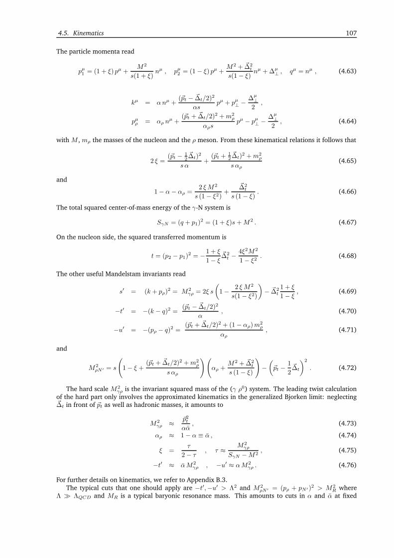
4.5. Kinematics 107
The particle momenta read
pµ1 = (1 + ξ) pµ +M2
s(1 + ξ)nµ , pµ2 = (1 − ξ) pµ +
M2 + ~∆2t
s(1− ξ)nµ +∆µ
⊥ , qµ = nµ , (4.63)
kµ = αnµ +(~pt − ~∆t/2)
2
αspµ + pµ⊥ − ∆µ
⊥2
,
pµρ = αρ nµ +
(~pt + ~∆t/2)2 +m2
ρ
αρspµ − pµ⊥ − ∆µ
⊥2, (4.64)
with M , mρ the masses of the nucleon and the ρ meson. From these kinematical relations it follows that
2 ξ =(~pt − 1
2~∆t)
2
s α+
(~pt +12~∆t)
2 +m2ρ
s αρ(4.65)
and
1− α− αρ =2 ξM2
s (1− ξ2)+
~∆2t
s (1− ξ). (4.66)
The total squared center-of-mass energy of the γ-N system is
SγN = (q + p1)2 = (1 + ξ)s+M2 . (4.67)
On the nucleon side, the squared transferred momentum is
t = (p2 − p1)2 = −1 + ξ
1− ξ~∆2t −
4ξ2M2
1− ξ2. (4.68)
The other useful Mandelstam invariants read
s′ = (k + pρ)2 = M2
γρ = 2ξ s
(
1− 2 ξ M2
s(1− ξ2)
)
− ~∆2t
1 + ξ
1− ξ, (4.69)
−t′ = −(k − q)2 =(~pt − ~∆t/2)
2
α, (4.70)
−u′ = −(pρ − q)2 =(~pt + ~∆t/2)
2 + (1− αρ)m2ρ
αρ, (4.71)
and
M2ρN ′ = s
(
1− ξ +(~pt + ~∆t/2)
2 +m2ρ
s αρ
)(
αρ +M2 + ~∆2
t
s (1− ξ)
)
−(
~pt −1
2~∆t
)2
. (4.72)
The hard scale M2γρ is the invariant squared mass of the (γ ρ0) system. The leading twist calculation
of the hard part only involves the approximated kinematics in the generalized Bjorken limit: neglecting~∆t in front of ~pt as well as hadronic masses, it amounts to
M2γρ ≈ ~p2t
αα, (4.73)
αρ ≈ 1− α ≡ α , (4.74)
ξ =τ
2− τ, τ ≈ M2
γρ
SγN −M2, (4.75)
−t′ ≈ αM2γρ , −u′ ≈ αM2
γρ . (4.76)
For further details on kinematics, we refer to Appendix B.3.The typical cuts that one should apply are −t′,−u′ > Λ2 and M2
ρN ′ = (pρ + pN ′)2 > M2R where
Λ ≫ ΛQCD and MR is a typical baryonic resonance mass. This amounts to cuts in α and α at fixed

108
M2γρ, which can be translated in terms of u′ at fixed M2
γρ and t. These conditions boil down to a safekinematical domain (−u′)min 6 −u′ 6 (−u′)max which we will discuss in more details in Section 4.8.
In the following, we will choose as independent kinematical variables t, u′,M2γρ .
Due to electromagnetic gauge invariance, the scattering amplitude for the production of a ρT mesonwith chiral-odd GPDs and the scattering amplitude for the production of a ρL meson with chiral-evenGPDs are separately gauge invariant, up to the well known corrections of order ∆T√
swhich have been
much studied for the DVCS case [162, 163]. We choose the axial gauge pµ εµk = 0 and parametrize the
polarization vector of the final photon in terms of its transverse components
εµk = εµk⊥ − εk⊥ · k⊥p · k pµ , (4.77)
while the initial photon polarization is simply written as
εµq = εµq⊥ . (4.78)
We will use the transversity relation pρ · ερ = 0 to express the polarization of the ρ meson in terms of onlyits transverse components and its component along n, using
n · ερ =1
αρ
[
p2⊥αρs
(p · ερ) + (p⊥ · ερ⊥)]
. (4.79)
4.6 Non-perturbative ingredients: DAs and GPDs
In this section, we describe the way the non-perturbative quantities which enter the scattering amplitudeare parametrized.
4.6.1 GPD factorization
GPDs are the non-forward extensions of PDFs. The way one factorizes a process with a GPD is very similarto the DA factorization scheme we introduced in 4.2.1 : the hard part and the non-perturbative part arefactorized in spinor space and in color space using Fierz identities. Factorization in the space of momentais a bit more involved. It can be shown that such a process can be written as the convolution of a hardpart, computed with a pair of collinear on-shell partons carrying respective momenta (x+ ξ)p (incoming)and (x− ξ)p (outgoing), where ξ is the skewness parameter, and a GPD, integrated over x ∈ [−1, 1]. Seefigure 4.18.
Hardpart
Γλ
Γλ
GPD
p2p1
(x+ ξ)p (x− ξ)p
Figure 4.18: Collinear factorization involving a GPD
Thus for our process which combines the factorization of a DA and of a GPD, the amplitude is writtenas the integral over (x, z) ∈ [−1, 1]× [0, 1] of the product of the hart part, a GPD (depending on x and ξ)and a DA (depending on z). The exact formulae can be found in section 4.7.We will now describe the expressions used for the non-perturbative matrix elements, and extract ourparameterization for the GPDs and the DAs.

4.6. Non-perturbative ingredients: DAs and GPDs 109
4.6.2 Distribution amplitudes for the ρ meson
The chiral-even lightcone DA for a longitudinally polarized vector meson ρ0L is defined, at the leadingtwist 2, by the matrix element [127]
〈0|u(0)γµu(x)|ρ0(pρ, ερL)〉 =1√2pµρfρ0
∫ 1
0
dz e−izpρ·x φ‖(z), (4.80)
with fρ0 = 216MeV, while the chiral-odd lightcone DA for the transversely polarized meson vector ρ0T isdefined as:
〈0|u(0)σµνu(x)|ρ0(pρ, ερ±)〉 =i√2(εµρ± p
νρ − ενρ± p
µρ)f
⊥ρ
∫ 1
0
dz e−izpρ·x φ⊥(z), (4.81)
where εµρ± is the ρ-meson transverse polarization and with f⊥ρ = 160 MeV. The factor 1√
2takes into
account the quark structure of the ρ0−meson: |ρ0〉 = 1√2(|uu〉 − |dd〉). We shall use the asymptotic form
for the normalized functions φ‖ and φ⊥
φ‖(z) = 6z(1− z) ,
φ⊥(z) = 6z(1− z) . (4.82)
4.6.3 Generalized parton distributions
The chiral-even generalized parton distributions of a parton q (here q = u, d) in the nucleon target (λ andλ′ are the lightcone helicities of the nucleons with respective momenta p1 and p2) are defined by [164]:
〈p(p2, λ′)| q(
−y2
)
γ+q(y
2
)
|p(p1, λ)〉 (4.83)
=
∫ 1
−1
dx e−i2x(p
+1 +p+2 )y− u(p2, λ
′)
[
γ+Hq(x, ξ, t) +i
2mσ+α∆αE
q(x, ξ, t)
]
u(p1, λ) ,
and
〈p(p2, λ′)| q(
−y2
)
γ+γ5q(y
2
)
|p(p1, λ)〉 (4.84)
=
∫ 1
−1
dx e−i2x(p
+1 +p+2 )y− u(p2, λ
′)
[
γ+γ5Hq(x, ξ, t) +1
2mγ5∆+ Eq(x, ξ, t)
]
u(p1, λ) .
The transversity generalized parton distribution of a quark q is defined by:
〈p(p2, λ′)| q(
−y2
)
i σ+jq(y
2
)
|p(p1, λ)〉 (4.85)
=
∫ 1
−1
dx e−i2x(p
+1 +p+2 )y− u(p2, λ
′)[
i σ+jHqT (x, ξ, t) + . . .
]
u(p1, λ) ,
where . . . denote the remaining three chiral-odd GPDs which contributions are omitted in the presentanalysis.
We parametrize the GPDs in terms of double distributions (DDs) [165]
Hq(x, ξ, t = 0) =
∫
Ω
dβ dα δ(β + ξα− x)Fq(β, α, t = 0) , (4.86)
where Fq is a generic quark DD and Ω = |β| + |α| 6 1 is its support domain. A D-term contribution,necessary to be completely general while fulfilling the polynomiality constraints, could be added. In ourparameterization, we do not include such an arbitrary term. Note that similar GPD parameterizationshave been used in Ref. [166].
As shown in Section 4.7.2, with a good approximation we will only use the three GPDs H, H and HT .We adhere on Radyushkin-type parameterization and write the unpolarized DD f q and the transversityDD f qT in the form
f q(β, α, t = 0) = Π(β, α) q(β)Θ(β) −Π(−β, α) q(−β)Θ(−β) , (4.87)

110
and [148]f qT (β, α, t = 0) = Π(β, α) δq(β)Θ(β) −Π(−β, α) δq(−β)Θ(−β) , (4.88)
while the polarized DD f q reads
f q(β, α, t = 0) = Π(β, α)∆q(β)Θ(β) + Π(−β, α)∆q(−β)Θ(−β) , (4.89)
where Π(β, α) = 34(1−β)2−α2
(1−β)3 is a profile function and q, q are the quark and antiquark unpolarizedparton distribution functions (PDFs), ∆q, ∆q, are the quark and antiquark polarized PDFs and δq, δq arethe quark and antiquark transversity PDFs.
We now give specific formulas for the three GPDs which will be used in the present study. The GPDHq reads
Hq(x, ξ, t = 0) = Θ(x > ξ)
∫1−x1−ξ
−1+x1+ξ
dy3
4
(1− x+ ξy)2 − y2
(1 − x+ ξy)3q(x− ξy)
+ Θ(ξ > x > −ξ)[
∫ xξ
−1+x1+ξ
dy3
4
(1− x+ ξy)2 − y2
(1− x+ ξy)3q(x− ξy)
−∫
1+x1+ξ
xξ
dy3
4
(1 + x− ξy)2 − y2
(1 + x− ξy)3q(−x+ ξy)
]
− Θ(−ξ > x)
∫1+x1+ξ
− 1+x1−ξ
dy3
4
(1 + x− ξy)2 − y2
(1 + x− ξy)3q(−x+ ξy) . (4.90)
Similarly, the transversity GPD HqT reads
HqT (x, ξ, t = 0) = Θ(x > ξ)
∫1−x1−ξ
−1+x1+ξ
dy3
4
(1 − x+ ξy)2 − y2
(1− x+ ξy)3δq(x − ξy)
+ Θ(ξ > x > −ξ)[
∫ xξ
−1+x1+ξ
dy3
4
(1 − x+ ξy)2 − y2
(1− x+ ξy)3δq(x− ξy)
−∫
1+x1+ξ
xξ
dy3
4
(1 + x− ξy)2 − y2
(1 + x− ξy)3δq(−x+ ξy)
]
− Θ(−ξ > x)
∫1+x1+ξ
− 1+x1−ξ
dy3
4
(1 + x− ξy)2 − y2
(1 + x− ξy)3δq(−x+ ξy) , (4.91)
while the Hq GPD reads
Hq(x, ξ, t = 0) = Θ(x > ξ)
∫1−x1−ξ
−1+x1+ξ
dy3
4
(1 − x+ ξy)2 − y2
(1− x+ ξy)3∆q(x − ξy)
+ Θ(ξ > x > −ξ)[
∫ xξ
−1+x1+ξ
dy3
4
(1 − x+ ξy)2 − y2
(1− x+ ξy)3∆q(x − ξy)
+
∫1+x1+ξ
xξ
dy3
4
(1 + x− ξy)2 − y2
(1 + x− ξy)3∆q(−x+ ξy)
]
+ Θ(−ξ > x)
∫1+x1+ξ
− 1+x1−ξ
dy3
4
(1 + x− ξy)2 − y2
(1 + x− ξy)3∆q(−x+ ξy) . (4.92)
Since our process selects the exchange of charge conjugation C = −1 in the t−channel, we now considerthe corresponding valence GPDs
Hq(−)(x, ξ, t) = Hq(x, ξ, t) +Hq(−x, ξ, t) (4.93)
and
Hq(−)T (x, ξ, t) = Hq
T (x, ξ, t) +HqT (−x, ξ, t) (4.94)

4.6. Non-perturbative ingredients: DAs and GPDs 111
which have the symmetry properties Hq(−)(x, ξ, t) = Hq(−)(−x, ξ, t) and Hq(−)T (x, ξ, t) = H
q(−)T (−x, ξ, t),
as well as the valence GPD
Hq(−)(x, ξ, t) = Hq(x, ξ, t) − Hq(−x, ξ, t) , (4.95)
which has the antisymmetry property Hq(−)(x, ξ, t) = −Hq(−)(−x, ξ, t) .Introducing the symmetric valence distributions
qval(x) = θ(x)[q(x) − q(x)] + θ(−x)[q(−x) − q(−x)] (4.96)
and
δqval(x) = θ(x)[δq(x) − δq(x)] + θ(−x)[δq(−x) − δq(−x)] , (4.97)
and the antisymmetric valence distribution
∆qval(x) = θ(x)[∆q(x) −∆q(x)] − θ(−x)[∆q(−x) −∆q(−x)] , (4.98)
the set of GPDs which we use in our computation of the scattering amplitude reads
1
2Hq(−)(x, ξ, t = 0) =
1
2
[(
Θ(x > ξ)
∫1−x1−ξ
−1+x1+ξ
dy3
4
(1− x+ ξy)2 − y2
(1− x+ ξy)3qval(x− ξy)
+ Θ(ξ > x > −ξ)∫ x
ξ
−1+x1+ξ
dy3
4
(1− x+ ξy)2 − y2
(1− x+ ξy)3qval(x− ξy)
)
+ (x↔ −x)] , (4.99)
1
2Hq(−)T (x, ξ, t = 0) =
1
2
[(
Θ(x > ξ)
∫1−x1−ξ
−1+x1+ξ
dy3
4
(1− x+ ξy)2 − y2
(1− x+ ξy)3δqval(x− ξy)
+ Θ(ξ > x > −ξ)∫ x
ξ
−1+x1+ξ
dy3
4
(1 − x+ ξy)2 − y2
(1− x+ ξy)3δqval(x− ξy)
)
+ (x↔ −x)] , (4.100)
and
1
2Hq(−)(x, ξ, t = 0) =
1
2
[(
Θ(x > ξ)
∫1−x1−ξ
−1+x1+ξ
dy3
4
(1− x+ ξy)2 − y2
(1− x+ ξy)3∆qval(x− ξy)
+ Θ(ξ > x > −ξ)∫ x
ξ
−1+x1+ξ
dy3
4
(1− x+ ξy)2 − y2
(1− x+ ξy)3∆qval(x− ξy)
)
− (x↔ −x)] . (4.101)
4.6.4 Numerical modeling
For the various PDFs, we neglect any QCD evolution (in practice, we take a fixed factorization scaleµ2F = 10 GeV2) and we use the following models:
• For xq(x), we rely on the GRV-98 parameterization [167], as made available from the Durhamdatabase. We neglect the uncertainty of this parameterization, considering only the central valueset of parameters.
In Fig. 4.19, we show the resulting GPDs Hu(−) and Hd(−) for ξ = .1 corresponding in our processto the typical value SγN = 20 GeV2 and M2
γρ = 3.5 GeV2.
• For x∆q(x) , we rely on the GRSV-2000 parameterization [168], as made available from the Durhamdatabase. Two scenarios are proposed in this parameterization: the “standard”, i.e. with flavor-symmetric light sea quark and antiquark distributions, and the “valence” scenario with completelyflavor-asymmetric light sea densities. We use both of them in order to evaluate the order of magni-tude of the theoretical uncertainty.
In Fig. 4.20, we show the resulting GPDs Hu(−) and Hu(−) for ξ = .1 corresponding in our processto the typical value SγN = 20 GeV2 and M2
γρ = 3.5 GeV2.

112
- 1.0 - 0.5 0.0 0.5 1.0
2
4
6
8
10
12
14
x
Hu(−)(x, ξ)
- 1.0 - 0.5 0.0 0.5 1.0
2
4
6
8
x
Hd(−)(x, ξ)
Figure 4.19: Models for the GPDs Hu(−) and Hd(−) for ξ = .1, a value corresponding to SγN = 20 GeV2
and M2γρ = 3.5 GeV2.
- 1.0 - 0.5 0.5 1.0
- 3
- 2
- 1
1
2
3
x
Hu(−)(x, ξ)
- 1.0 - 0.5 0.5 1.0
- 1.0
- 0.5
0.5
1.0
x
Hd(−)(x, ξ)
Figure 4.20: Models for the GPDs Hu(−) and Hd(−) for ξ = .1, a value corresponding to SγN = 20 GeV2
and M2γρ = 3.5 GeV2.
• For xδq(x) we rely on a parameterization performed for TMDs (based on a fit of azimuthal asym-metries in semi-inclusive deep inelastic scattering), from which the transversity PDFs xδq(x) areobtained as a limiting case [169]. These transversity PDFs are parametrized as
δq(x) =1
2N Tq (x)[q(x) + ∆(x)] (4.102)
with
N Tq (x) = NT
q xα(1− x)β
(α+ β)(α+β)
ααββ. (4.103)
Since this parameterization itself relies on the knowledge of xq(x) and x∆q(x), we will evaluate theuncertainty on these PDFs by two means: first by passing from the “standard” to the “valence” po-larized PDFs (see above), second by performing a variation of the set of parameters NT
q , α, β, usingthe χ2 distribution of these parameters as used in Ref. [169]10. We further discuss our procedurein Section 4.8.6.
In Fig. 4.21, we show the resulting GPDs Hu(−)T and Hd(−)
T for ξ = .1 corresponding in our processto the typical value SγN = 20 GeV2 and M2
γρ = 3.5 GeV2.
10We thank S. Melis for providing us the complete set of parameters with the corresponding χ2 distribution.
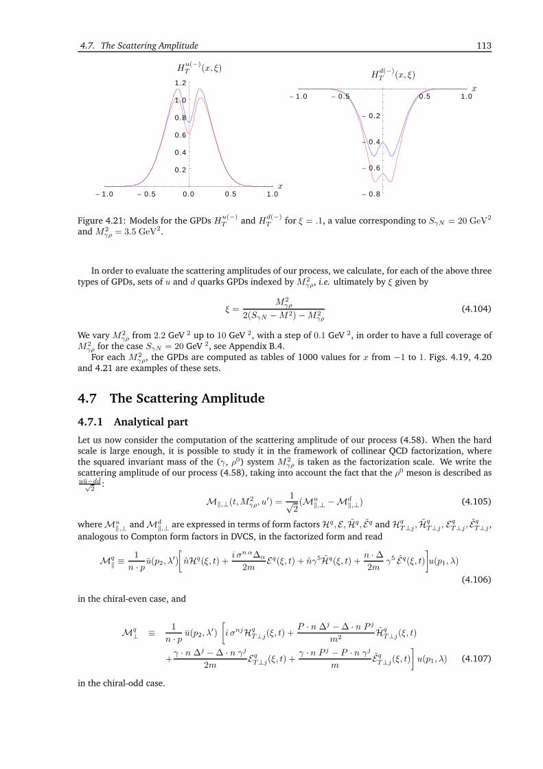
4.7. The Scattering Amplitude 113
- 1.0 - 0.5 0.0 0.5 1.0
0.2
0.4
0.6
0.8
1.0
1.2
x
Hu(−)T (x, ξ)
- 1.0 - 0.5 0.5 1.0
- 0.8
- 0.6
- 0.4
- 0.2
x
Hd(−)T (x, ξ)
Figure 4.21: Models for the GPDs Hu(−)T and Hd(−)
T for ξ = .1, a value corresponding to SγN = 20 GeV2
and M2γρ = 3.5 GeV2.
In order to evaluate the scattering amplitudes of our process, we calculate, for each of the above threetypes of GPDs, sets of u and d quarks GPDs indexed by M2
γρ, i.e. ultimately by ξ given by
ξ =M2γρ
2(SγN −M2)−M2γρ
(4.104)
We vary M2γρ from 2.2 GeV 2 up to 10 GeV 2, with a step of 0.1 GeV 2, in order to have a full coverage of
M2γρ for the case SγN = 20 GeV 2, see Appendix B.4.For each M2
γρ, the GPDs are computed as tables of 1000 values for x from −1 to 1. Figs. 4.19, 4.20and 4.21 are examples of these sets.
4.7 The Scattering Amplitude
4.7.1 Analytical part
Let us now consider the computation of the scattering amplitude of our process (4.58). When the hardscale is large enough, it is possible to study it in the framework of collinear QCD factorization, wherethe squared invariant mass of the (γ, ρ0) system M2
γρ is taken as the factorization scale. We write thescattering amplitude of our process (4.58), taking into account the fact that the ρ0 meson is described asuu−dd√
2:
M‖,⊥(t,M2γρ, u
′) =1√2(Mu
‖,⊥ −Md‖,⊥) (4.105)
where Mu‖,⊥ and Md
‖,⊥ are expressed in terms of form factors Hq, E , Hq, Eq and HqT⊥j , H
qT⊥j , E
qT⊥j, E
qT⊥j ,
analogous to Compton form factors in DVCS, in the factorized form and read
Mq‖ ≡ 1
n · p u(p2, λ′)
[
nHq(ξ, t) +i σnα∆α
2mEq(ξ, t) + nγ5Hq(ξ, t) +
n ·∆2m
γ5 Eq(ξ, t)]
u(p1, λ)
(4.106)
in the chiral-even case, and
Mq⊥ ≡ 1
n · p u(p2, λ′)
[
i σnjHqT⊥j(ξ, t) +
P · n ∆j −∆ · n P jm2
HqT⊥j(ξ, t)
+γ · n ∆j −∆ · n γj
2mEqT⊥j(ξ, t) +
γ · n P j − P · n γjm
EqT⊥j(ξ, t)
]
u(p1, λ) (4.107)
in the chiral-odd case.

114
For convenience, we now define
Mq(t,M2γρ, pT ) = ≡
∫ 1
−1
dx
∫ 1
0
dz T q(t,M2γρ, pT , x, z) . (4.108)
A1 A2 A3 A4 A5
B1 B2 B3 B4 B5
Figure 4.22: Half of the Feynman diagrams contributing to the hard amplitude. In the chiral-odd case,A3, A4 and B1, B5 are the only contributing diagrams (the red diagrams cancel in this case).
The scattering sub-process is described at lower twist by 20 Feynman diagrams, but using the q ↔ q(anti)symmetry properties allows one to compute only 10 of them, shown in Fig. 4.22, then deduce theremaining contributions by substituting (x, z) ↔ (−x, 1− z).In the case of (γ, ρL) production all the diagrams contribute. In the case of (γ, ρ⊥) production, due to thechiral-odd structure of DAs and GPDs, there are only 8 non-vanishing diagrams, out of which one onlyneeds to compute B1, A3, A4 and B5.
We now discuss diagram B1 in some details, and give the results for the other diagrams in Ap-pendix B.1.
The chiral-even scattering amplitudes for longitudinally polarized ρ0 described by the DA (4.80) in-volve both the vector GPDs (4.84) and the axial GPDs (4.85). We now give the detailed expressionsfor T q CEV (B1), T
qCEA (B1), for a quark with flavor q and for diagram B1 in Feynman gauge. The vector
amplitude reads
T q CEV (B1) =1
i
tr(tata)
(4N)2fρ φ||(z) (−ieQq)2 (−ig)2 i2 (−i)
× trD
[
pρε∗k
k + zpρ(k + zpρ)2 + iǫ
γµq + (x + ξ)p
(q + (x+ ξ)p)2 + iǫεq p γµ
1
(zpρ + (x− ξ)p)2 + iǫ
]
× 2
su(p2, λ
′)
[
nHq(x, ξ, t) +i
2mσnα∆α E
q(x, ξ, t)
]
u(p1, λ) (4.109)
= Cq CE trVD [B1] φ||(z)2
su(p2, λ
′)
[
n Hq(x, ξ, t) +i
2mσnα∆α E
q(x, ξ, t)
]
u(p1, λ) ,
which includes all non trivial factors (vertices as well as quark and gluon propagators) of the hard partof diagram B1. Here, Cq CE is a common coefficient for all diagrams involving vector and axial GPDs,reading
Cq CE =4
9fρ αem αs π
2Q2q . (4.110)

4.7. The Scattering Amplitude 115
The trace reads:
trVD [B1] = trD
[
pρε∗k
k + zpρ(k + zpρ)2 + iǫ
γµq + (x+ ξ)p
(q + (x+ ξ)p)2 + iǫεq p γµ
1
(zpρ + (x− ξ)p)2 + iǫ
]
=8s[
−sξα (εq⊥ · ε∗k⊥) + zα (εq⊥ · pρ⊥) (ε∗k⊥ · pρ⊥)
]
((k + zpρ)2 + iǫ)((q + (x+ ξ)p)2 + iǫ)((zpρ + (x− ξ)p)2 + iǫ), (4.111)
=4[
−α2ξsTA + zTB]
ααξs2zz (x− ξ + iǫ) (x+ ξ + iǫ).
We introduced the two tensor structures that will appear in chiral-even diagrams in the vector sector:
TA = (εq⊥ · ε∗k⊥) ,TB = (εq⊥ · p⊥)(p⊥ · ε∗k⊥). (4.112)
Similarly one can write in the axial sector:
T qCEA (B1) =1
i
tr(tata)
(4N)2fρ φ||(z) (−ieQq)2 (−ig)2 i2 (−i)
× trD
[
pρε∗k
k + zpρ(k + zpρ)2 + iǫ
γµq + (x+ ξ)p
(q + (x+ ξ)p)2 + iǫεq p γ
5 γµ1
(zpρ + (x − ξ)p)2 + iǫ
]
× 2
su(p2, λ
′)
[
γ5 n Hq(x, ξ, t)− n ·∆2m
γ5 Eq(x, ξ, t)
]
u(p1, λ) (4.113)
= Cq CE trAD [B1] φ||(z)2
su(p2, λ
′)
[
γ5 n Hq(x, ξ, t)− n ·∆2m
γ5 Eq(x, ξ, t)
]
u(p1, λ) ,
with
trAD [B1] = trD
[
pρε∗k
k + zpρ(k + zpρ)2+iǫ
γµq + (x+ ξ)p
(q + (x+ ξ)p)2 + iǫεq p γ
5 γµ1
(zpρ + (x− ξ)p)2+iǫ
]
= − 8i
ααρ
[
α (εq⊥ · pρ⊥) ǫpn pρ⊥ ε∗
k⊥ − (α+ 2zαρ) (ε∗k⊥ · pρ⊥) ǫp n pρ⊥ εq⊥
]
((k + zpρ)2 + iǫ)((q + (x+ ξ)p)2 + iǫ)((zpρ + (x− ξ)p)2 + iǫ)
=−4i [(α+ 2αz)TA5 − αTB5 ]
αα2ξs3zz (x− ξ + iǫ) (x+ ξ + iǫ), (4.114)
where we introduced the two tensor structures which will appear in chiral-even diagrams in the axialsector:
TA5 = (p⊥ · ε∗k⊥) ǫnp εq⊥ p⊥ ,
TB5 = (p⊥ · εq⊥) ǫnpε∗
k⊥ p⊥ . (4.115)
The chiral-odd (CO) scattering amplitude involving quark of flavor q (q = u, d) corresponding todiagram B1 in Feynman gauge has the form:
T q CO(B1) = − 1
i
tr(tata)
(8N)2i 2f⊥
ρ φ⊥(z) (−ieQq)2 (−ig)2 i2 (−i)
trD
[
pρε∗ρε
∗k
(k + zpρ)
(k + zpρ)2 + iǫγµ
q + (x + ξ)p
(q + (x+ ξ)p)2 + iǫεq p γ⊥j γµ
1
(zpρ + (x− ξ)p)2 + iǫ
]
2
su(p2, λ
′)[
σnjHqT (x, ξ, t)
]
u(p1, λ)
= Cq CO trCOD [B1]j φ⊥(z)2
su(p2, λ
′)[
iσnjHqT (x, ξ, t)
]
u(p1, λ), (4.116)
whereCq CO = −2
9f⊥ρ αem αs π
2Q2q (4.117)

116
is a common coefficient for all diagrams involving chiral-odd DA and GPD, and
trCOD [B1]j = (4.118)
trD
[
pρε∗ρε
∗k
(k + zpρ)
(k + zpρ)2 + iǫγµ
q + (x+ ξ)p
(q + (x+ ξ)p)2 + iǫεq p γ⊥j γµ
1
(zpρ + (x − ξ)p)2 + iǫ
]
includes all non trivial factors (vertices as well as quark and gluon propagators) of the hard part ofdiagram B1. The calculation of traces over γ-matrices leads to the expression
trCOD [B1]j =8s[
(q · p)εq⊥ j
(
pρ · ε∗k ε∗ρ · k − sξ ε∗k · ε∗ρ)
− ǫk ε∗
k pρ ε∗
ρ ǫq εq p νg⊥νj]
((k + zpρ)2 + iǫ) ((zpρ + (x− ξ)p)2 + iǫ)((q + (x + ξ)p)2 + iǫ)
=TB⊥j
2αξs3zz (x+ ξ + iǫ) (x− ξ + iǫ). (4.119)
Here TB⊥j is one of the two tensor structures which will appear in chiral-odd diagrams,
T iA⊥ ≡ (p · k) εi∗k⊥[
(εq · pρ) (q · ε∗ρ)− (q · pρ) (εq · ε∗ρ)]
− ǫpρ ε∗
ρ q εq ǫp ν k ε∗
kgi⊥ν
=−8s
α
αεi∗k⊥[
−2αξ(
p · ǫ∗ρ)
(p⊥ · εq⊥) + (p⊥ · εq⊥)(
p⊥ · ε∗ρ⊥)
+ ααξs(
εq⊥ · ε∗ρ⊥)]
−αεi∗ρ⊥ [α (α− 2) ξs (εq⊥ · ε∗k⊥)− (p⊥ · εq⊥) (p⊥ · ε∗k⊥)] (4.120)
+pi⊥[
−2α2ξpi⊥(
p · ǫ∗ρ)
(εq⊥ · ε∗k⊥) +(
p⊥ · ε∗ρ⊥)
(εq⊥ · ε∗k⊥)− α(
ε∗k⊥ · ε∗ρ⊥)
(p⊥ · εq⊥)]
+εiq⊥[
2α2ξ(
p · ǫ∗ρ)
(p⊥ · ε∗k⊥)−(
p⊥ · ε∗ρ⊥)
(p⊥ · ε∗k⊥) + αα (α− 2) ξs(
ε∗k⊥ · ε∗ρ⊥)]
,
the other one being
T iB⊥ ≡ (q · p) εiq⊥[
(pρ · ε∗k) (ε∗ρ · k)− sξ (ε∗k · ε∗ρ)]
− ǫk ε∗
k pρ ε∗
ρ ǫq εq p νgi⊥ν (4.121)
=8s
αα
αεi∗ρ⊥ [(p⊥ · εq⊥) (p⊥ · ε∗k⊥)− α (2α− 1) ξs (εq⊥ · ε∗k⊥)]
+αεi∗k⊥[
α (2α− 1) ξs(
εq⊥ · ε∗ρ⊥)
+ 2ξ(
p · ǫ∗ρ)
(p⊥ · εq⊥) + (p⊥ · εq⊥)(
p⊥ · ε∗ρ⊥)]
+εiq⊥[
2αξ(
p · ǫ∗ρ)
(p⊥ · ε∗k⊥)−(
p⊥ · ε∗ρ⊥)
(p⊥ · ε∗k⊥)− ααξs(
ε∗k⊥ · ε∗ρ⊥)]
+pi⊥[
2αξ(
p · ǫ∗ρ)
(εq⊥ · ε∗k⊥)− α(
p⊥ · ε∗ρ⊥)
(εq⊥ · ε∗k⊥)− α(
εq⊥ · ε∗ρ⊥)
(p⊥ · ε∗k⊥)]
.
Here, we expressed these two tensor structures in terms of the transverse polarization vectors and of(p · ερ), using Eqs. (4.77-4.79), for later convenience.
At the dominant twist, the sum over the transverse polarizations of the rho meson can be written as
∑
pol
εµρεν∗ρ = −gµν + pµρp
νρ
m2ρ
, (4.122)
when computing the square of the chiral odd amplitude. The second term of this sum, which arises mainlyfrom the longitudinal polarization, does not contribute at leading twist. We thus note that (p · ερ) termsin the tensor structures will not contribute to the cross section since when summed over the transversepolarizations at the dominant twist they will produce terms involving the scalar product of p either witha transverse vector or with itself, which is null in both cases.
In a similar way we obtain the expressions for the remaining independent diagrams: A1, A2, A3, A4,A5, B2, B3, B4, B5 in the chiral-even sector and A3, A4 and B5 in the chiral-odd sector. We show theseresults in Appendix B.1.
The integral with respect to z is trivially performed in the case of a DA expanded in the basis ofGegenbauer polynomials. The expressions for the case of two asymptotical DAs φ‖ and φ⊥, which we onlyconsider in the present article, are given explicitly in Appendix B.2, and expressed as linear combinationof building blocks.
The integration with respect to x, for a given set of GPDs, (which can be our model described inSection 4.6 or any other model), is then reduced to the numerical evaluation of these building blockintegrals.

4.8. Unpolarized Differential Cross Section and Rate Estimates 117
4.7.2 Square of M‖ and M⊥
In the forward limit ∆⊥ = 0 = P⊥, one can show that the squares of M‖ and of M⊥ read after summingover nucleon helicities:
Mq‖M
q′∗‖ ≡
∑
λ′, λ
Mq‖(λ, λ
′)Mq′∗‖ (λ, λ′) (4.123)
= 8(1− ξ2)(
Hq(ξ, t)Hq′∗(ξ, t) + Hq(ξ, t)Hq′∗(ξ, t))
− 4 ξ2(
Eq(ξ, t)Eq′∗(ξ, t) + Eq(ξ, t)Eq′∗(ξ, t))
− 8 ξ2(
Hq(ξ, t)Eq′∗(ξ, t) +Hq′∗(ξ, t)Eq(ξ, t) + Hq(ξ, t)Eq′∗(ξ, t) + Hq′∗(ξ, t)Eq(ξ, t))
,
and
Mq⊥M
q′∗⊥ ≡
∑
λ′, λ
Mq⊥(λ, λ
′)Mq′∗⊥ (λ, λ′) (4.124)
= 8
[
−(1− ξ2)Hq iT (ξ, t)Hq′j ∗
T (ξ, t)− ξ2
1− ξ2[ξ Eq iT (ξ, t)− Eq iT (ξ, t)][ξ Eq
′j∗T (ξ, t)− Eq
′j∗T (ξ, t)]
+ ξ
HqiT (ξ, t)[ξ E
q′jT (ξ, t)− Eq
′jT (ξ, t)]∗ +Hq′i∗
T (ξ, t)[ξ EqjT (ξ, t)− EqjT (ξ, t)]]
g⊥ij .
For moderately small values of ξ, these become:
Mq‖M
q′∗‖ = 8
(
Hq(ξ, t)Hq′∗(ξ, t) + Hq(ξ, t) Hq′∗(ξ, t))
, (4.125)
Mq⊥M
q′∗⊥ = −8Hq i
T (ξ, t)Hq′j ∗T (ξ, t) g⊥ij . (4.126)
Hence we will restrict ourselves to Hq, Hq and HqT to perform our estimates of the cross section11.
4.8 Unpolarized Differential Cross Section and Rate Estimates
4.8.1 From amplitudes to cross sections
We isolate the tensor structures of the form factors as
Hq(ξ, t) = HqA(ξ, t)TA +Hq
B(ξ, t)TB , (4.127)
Hq(ξ, t) = HqA(ξ, t)TA5 + Hq
B(ξ, t)TB5 , (4.128)
Hq iT (ξ, t) = Hq
TA(ξ, t)T iA⊥ +Hq
TB(ξ, t)T iB⊥. (4.129)
These coefficients can be expressed in terms of the sum over diagrams of the integral of the product oftheir traces, of GPDs and DAs, as defined and given explicitly in Appendix B.2. They read :
HqA =
1
sCq CEN q
A , (4.130)
HqB =
1
s2Cq CEN q
B , (4.131)
HqA5
=1
s3Cq CEN q
A5, (4.132)
HqB5
=1
s3Cq CEN q
B5, (4.133)
and
HqT A =
1
s3Cq CON q
T A , (4.134)
HqT B =
1
s3Cq CON q
T B . (4.135)
11In practice, we keep the first line in the r.h.s. of Eq. (4.123) and the first term in the r.h.s of Eq. (4.124).

118
For the specific case of our process, it is convenient to define the total form factors as follows:
H(ξ, t) ≡ Hu(ξ, t)−Hd(ξ, t) , (4.136)
H(ξ, t) ≡ Hu(ξ, t)− Hd(ξ, t) , (4.137)
HiT (ξ, t) ≡ Hu i
T (ξ, t)−Hd iT (ξ, t) , (4.138)
from which we isolate the tensor structures
H(ξ, t) = HA(ξ, t)TA +HB(ξ, t)TB , (4.139)
H(ξ, t) = HA5(ξ, t)TA5 + HB5(ξ, t)TB5 , (4.140)
HiT (ξ, t) = HTA(ξ, t)T
iA⊥ +HTB (ξ, t)T
iB⊥. (4.141)
In this study, we are interested in the unpolarized cross section. As a result, we will need the squaredform factors after summation over all the polarizations (outgoing γ and ρ, incoming γ):
|H(ξ, t)|2 ≡∑
λkλq
H(ξ, t, λk, λq)H(ξ, t, λk, λq) (4.142)
= 2|HA(ξ, t)|2 + p4⊥|HB(ξ, t)|2 + p2⊥ [HA(ξ, t)H∗B(ξ, t) +H∗
A(ξ, t)HB(ξ, t)] ,
|H(ξ, t)|2 ≡∑
λkλq
H(ξ, t, λk, λq) H∗(ξ, t, λk, λq) (4.143)
=s2p4⊥4
|HA5(ξ, t)|2 + |HB5(ξ, t)|2,
|HT (ξ, t)|2 ≡ −g⊥i j∑
λkλqλρ
HiT (ξ, t, λk, λq, λρ)Hj∗
T (ξ, t, λk, λq, λρ) (4.144)
= 512ξ2s4(
α4|HTA(ξ, t)|2 + |HTB (ξ, t)|2)
.
We now define the averaged squared amplitude |M|2, which includes the factor 1/4 coming from theaveraging over the polarizations of the initial particles. Collecting all the prefactors (including a factor of22 for the missing half of the set of diagrams and a factor of 1/2 from the square of the ρ0 wave function,see Eq. (4.105)), which reads
1
s2228(1− ξ2)
(
Cq CE(OD))2 1
23,
we have the net result (factorizing out the coefficient for the u−quark), for the chiral-even case
|MCE |2 =4
s2(1− ξ2)
(
CuCE)2
2
∣
∣
∣
∣
NuA − 1
4NdA
∣
∣
∣
∣
2
+p4⊥s
2 ∣∣
∣
∣
NuB − 1
4NdB
∣
∣
∣
∣
2
(4.145)
+p2⊥s
([
NuA − 1
4NdA
] [
NuB − 1
4NdB
]∗+ c.c.
)
+p4⊥4s2
∣
∣
∣
∣
NuA − 1
4NdA
∣
∣
∣
∣
2
+p4⊥4s2
∣
∣
∣
∣
NuB − 1
4NdB
∣
∣
∣
∣
2
,
while for the chiral-odd case, we get
|MCO|2 =2048
s2ξ2(1 − ξ2)
(
CuCO)2
α4
∣
∣
∣
∣
NuT A − 1
4NdT A
∣
∣
∣
∣
2
+
∣
∣
∣
∣
NuT B − 1
4NdT B
∣
∣
∣
∣
2
. (4.146)
The differential cross section as a function of t, M2γρ, −u′ then reads
dσ
dt du′ dM2γρ
∣
∣
∣
∣
−t=(−t)min=
|M|232S2
γNM2γρ(2π)
3. (4.147)

4.8. Unpolarized Differential Cross Section and Rate Estimates 119
4.8.2 Numerical evaluation of the scattering amplitudes and of cross sections
Above, we have reduced the calculation of the cross sections, see Eq. (4.147), to the numerical evaluationof the coefficients (B.62), (B.63), (B.43), (B.44), (B.45), (B.46). These coefficients are expressed as linearcombinations of numerical integrals, listed in Appendix B.2.
Our central set of curves, displayed below, is obtained for SγN = 20 GeV2, with M2γρ varying in the
range 2.10 GeV2 < M2γρ < 9.47 GeV2 (this latter value comes from the vanishing of the phase-space
in −t, as shown in Appendix B.4, see Eq. (B.115)) with a 0.1 GeV2 step.For each of these values ofM2
γρ, we chose 100 values of −u′, linearly varying from (−u′)min = 1 GeV2
up to (−u′)maxMax as defined by Eq. (B.111).For each of these couples of values of (M2
γρ,−u′ , ) we compute each of the numerical coefficientsNuA, N
dA, N
uB, N
dB and Nu
A, NdA, N
uB, N
dB for the chiral-even case, as well as the coefficients
NuT A, N
dT A, N
uT B, N
dT B for the chiral-odd case, using the sets of GPDs indexed by M2
γρ and computed asexplained in Section 4.6.3.
This whole set of dimensionless numerical coefficients allows us to perform the various phenomeno-logical studies discussed in the next subsections.
4.8.3 Fully differential cross sections
Let us first discuss chiral-even results, showing in parallel the proton and neutron target cases.We first analyze the various contributions to the differential cross section in the specific kinematics:
M2γρ = 4 GeV2, SγN = 20 GeV2, −t = (−t)min as a function of −u′. The dependency with respect to SγN
will be discussed in Section 4.8.5.In Fig. 4.23, we show the relative contributions of the u− and d−quark GPDs (adding the vector
and axial contributions), which interfere in a destructive way because of the flavor structure of theρ0 = uu−dd√
2. The d−quark contribution is of course more important for the neutron target case.
1 .0 1 .5 2 .0 2 .50 .0
0 .5
1 .0
1 .5
2 .0
2 .5
3 .0
3 .5
−u′(GeV2)
dσevendM2
γρd(−u′)d(−t)(nb ·GeV−6)
1 .0 1 .5 2 .0 2 .50 .0
0 .2
0 .4
0 .6
0 .8
1 .0
−u′(GeV2)
dσevendM2
γρd(−u′)d(−t)(nb ·GeV−6)
Figure 4.23: Differential cross section for a photon and a longitudinally polarized ρ meson production,for the proton (left) and the neutron (right), at M2
γρ = 4 GeV2. Both vector and axial GPDs are included.In black the contributions of both u and d quarks, in blue the contribution of the u quark, and in greenthe contribution of the d quark. Solid: “valence” model, dotted: “standard” model. This figure showsthe dominance of the u-quark contribution due to the charge effect. Note that the interference betweenu−quark and d−quark contributions is important and negative.
In Fig. 4.24, we show the relative contributions of the GPDs H and H involving vector and axialcorrelators. The vector contribution dominates. The two parameterizations of the axial GPD Hq(x, ξ, t)give quite different results, the one corresponding to the unbroken sea (“standard”) scenario being lessnegligible than the other one (“valence”). As a simple calculation shows, there is no interference effectbetween H and H contributions due to lack of a sufficient number of transverse momenta in the tensorstructures.
Fig. 4.25 shows the dependence on M2γρ. The production of the γρ pair with a large value of M2
γρ
is severely suppressed as anticipated. However, the −u′ range allowed by our kinematical requirements

120
1 .0 1 .5 2 .0 2 .50 .0
0 .5
1 .0
1 .5
2 .0
2 .5
−u′(GeV2)
dσevendM2
γρd(−u′)d(−t)(nb ·GeV−6)
1 .0 1 .5 2 .0 2 .50 .00
0 .05
0 .10
0 .15
0 .20
0 .25
0 .30
−u′(GeV2)
dσevendM2
γρd(−u′)d(−t)(nb ·GeV−6)
Figure 4.24: Differential cross section for a photon and a longitudinally polarized ρ meson production,for the proton (left) and the neutron (right), at M2
γρ = 4 GeV2. Both u and d quark contributionsare included. In black the contributions of both vector and axial amplitudes, in blue the contributionof the vector amplitude, and in green the contribution of the axial amplitude. Solid: “valence” model,dotted: “standard” model. This figure shows the dominance of the vector GPD contributions. There is nointerference between the vector and axial amplitudes.
is narrower for smaller values of M2γρ. The two curves for each value of M2
γρ correspond to the twoparameterizations of H(x, ξ, t), the lines corresponding to the unbroken sea scenario lying above theother one.
1 2 3 4 50
1
2
3
4
5
−u′ (GeV2)
dσevendM2
γρd(−u′)d(−t)(nb ·GeV−6)
1 2 3 4 50 .0
0 .1
0 .2
0 .3
0 .4
0 .5
0 .6
0 .7
−u′ (GeV2)
dσevendM2
γρd(−u′)d(−t)(nb ·GeV−6)
Figure 4.25: Differential cross section for a photon and a longitudinally polarized ρ meson production,for the proton (left) and the neutron (right), as a function of −u′, for M2
γρ = 3, 4, 5, 6 GeV2 (resp. inblack, red, blue, green). Solid: “valence” model, dotted: “standard” model.
4.8.4 Single differential cross sections
To get an estimate of the total rate of events of interest for our analysis, we first get the M2γρ dependence
of the differential cross section integrated over u′ and t,
dσ
dM2γρ
=
∫ (−t)max
(−t)mind(−t)
∫ (−u′)max
(−u′)min
d(−u′) F 2H(t)× dσ
dt du′dM2γρ
∣
∣
∣
∣
−t=(−t)min. (4.148)
Since this is mostly an order of magnitude estimate, we use a simple factorized universal dipole t−dependenceof GPDs,
FH(t) =C2
(t− C)2, (4.149)

4.8. Unpolarized Differential Cross Section and Rate Estimates 121
with C = 0.71 GeV2. For a more precise study dedicated to an impact picture of the nucleon [170–175], amore sophisticated approach [176] should be used. The domain of integration over u′ and t is discussedin detail in Appendix B.4.
The differential cross section we obtain dσ/dM2γρ is shown in Fig. 4.26 for various values of SγN
covering the JLab-12 energy range. These cross sections show a maximum around M2γρ ≈ 3 GeV2, for
most energy values.
3 4 5 6 7 8 9
0 .05
0 .10
0 .15
0 .20
0 .25
0 .30
M2γρ (GeV2)
dσevendM2
γρ
(nb ·GeV−2)
3 4 5 6 7 8 9
0 .005
0 .010
0 .015
0 .020
0 .025
0 .030
0 .035
M2γρ (GeV2)
dσevendM2
γρ
(nb ·GeV−2)
Figure 4.26: Differential cross section dσ/dM2γρ for a photon and a longitudinally polarized ρ meson
production, on a proton (left) or neutron (right) target. The values of SγN vary in the set 8, 10, 12, 14,16, 18, 20 GeV2. (from 8: left, brown to 20: right, blue), covering the JLab energy range. Here, we usethe “valence” scenario.
4.8.5 Integrated cross sections and variation with respect to SγN
For SγN = 20 GeV2, the integration over M2γρ of our above results within our allowed kinematical region,
here 2.10 GeV2 < M2γρ < 9.47 GeV2 (see Appendix B.4), allows to obtain the cross sections σproton
odd ≃0.54 pb and σproton
even ≃ 0.76 nb for the proton, and σneutronodd ≃ 0.42 pb and σneutron
even ≃ 0.084 nb for theneutron.
The variation with respect to SγN could be obtained by following the whole chain of steps describedabove. However, this can be obtained almost directly. Our aim is now to show that the only knowledgeof the set of numerical results computed for a given value of SγN , which we take in practice as SγN =
20 GeV2, is sufficient to deduce a whole set of results for any arbitrary smaller values of SγN . The keypoints are the following.
First, the amplitudes only depend on α, ξ and on the GPDs (which are computed as grids indexed byξ). Since α = −u′/M2
γρ , it is thus possible to use exactly the set of already computed amplitudes if oneselects the same set of (α, ξ)
Second, one should note that to a given value of
ξ =M2γρ
2(SγN −M2)−M2γρ
(4.150)
corresponds an infinite set of couples of values (M2γρ, SγN) .
In practice, we use our set of results obtained for SγN = 20 GeV2 , indexed by M2γρ and −u′.
Then, choosing a new value of SγN , we obtain a set of values of M2γρ indexed by the set of values of
M2γρ (which vary from 2.2 up to 10 GeV2, with a 0.1 GeV2 step), through the relation
M2γρ =M2
γρ
SγN −M2
SγN −M2, (4.151)
which is deduced from Eq. (4.150), and for each of these M2γρ a set of values of −u′ , using the relation
−u′ = M2γρ
M2γρ
(−u′) . (4.152)

122
which gives the indexation of allowed values of −u′ as function of known values of (−u′).It is now easy to check that this mapping from a given SγN to a lower SγN provides a set of (M2
γρ,−u′)which exhaust the required domain.
Consider first the range in M2γρ. From Eq. (B.109), which defines the minimal value of M2
γρ, inde-pendent of SγN , this value is mapped to a smaller value than required, when passing from SγN to SγN .From Eq. (B.115), it is possible to show that M2
γρMax is mapped to a value M2γρMax slightly larger than
the new required value M ′2γρMax (this comes from the little dependency of M with respect to SγN). Thus,
the mapping covers the whole required domain in M2γρ (with a negligible loss of precision since a few
points are mapped outside the domain and thus cut).Now, let us consider the range in −u′. Again, since the minimal value (−u′)min is fixed, this value is
mapped to a smaller value than required, when passing from SγN to SγN . Concerning the maximal value(−u′)maxMax, from Eq. (B.111) it is a linear function of M2
γρ of the form
(−u′)maxMax = −A+M2γρ , (4.153)
with A > 0. The mapping of M2γρ leads to the maximal required value
(−u′)′maxMax = −A+ M2γρ . (4.154)
But the mapping in −u′ will transform (−u′)maxMax to
(−u′)maxMax =M2γρ
M2γρ
(−A+M2γρ) = −AM
2γρ
M2γρ
+ M2γρ , (4.155)
which shows that the maximal value (−u′)maxMax of (−u′) obtained from the mapping is larger than the
needed (−u′)′maxMax, since −A < −A M2γρ
M2γρ< 0.
We have thus shown that one can obtain the dependency of amplitudes and thus of cross sections forthe whole range in SγN from a single set of computation (at SγN = 20 GeV2), thus avoiding the use of avery large amount of CPU time.
Then, for the obtained cross section which was obtained at a given value of SγN , the integration overthe (−t,−u′) phase-space and then over M2
γρ is performed similarly to SγN = 20 GeV2 case. One finallygets the integrated cross section shown in Fig. 4.27 for the proton and neutron targets, and for bothparameterizations of the axial GPDs12. These cross sections prove that our process is measurable in thetypical kinematical conditions and integrated luminosity of a JLab@12GeV experiment. Counting rateson a proton target are predicted to be one order of magnitude larger than on a neutron target.
5 10 15 20
0 .2
0 .4
0 .6
0 .8
SγN(GeV2)
σeven (nb)
5 10 15 20
0 .02
0 .04
0 .06
0 .08
0 .10
SγN(GeV2)
σeven (nb)
Figure 4.27: Integrated cross section for a photon and a longitudinally polarized ρ meson production, ona proton (left) or neutron (right) target. The solid red curves correspond to the “valence” scenario whilethe dashed blue curves correspond to the “standard” one.
12A quadratic extrapolation is performed for the small domain above SγN = 20 GeV2.

4.8. Unpolarized Differential Cross Section and Rate Estimates 123
4.8.6 Results for the chiral-odd case
Let us now pass to the chiral-odd case, where a transversely polarized ρ meson is produced together withthe photon. This process now probes the chiral-odd transversity quark distributions which are connectedto the transversity PDFs.
In order to evaluate the theoretical uncertainty in the chiral-odd sector, for each of the two parameter-izations of the transversity PDFs, we use a set of 1500 trials with their value of the χ2 test, as provided bythe authors of Ref. [169], between −2σ and +2σ. Their 9-parameters χ2 distribution (see the appendixof Ref. [177] for details) is given by
Pχ2(x) =e−x/2x7/2
105√2π
(4.156)
We further renormalize this distribution in order to include on one hand the fact that the 1500 trialsonly cover the [−2σ,+2σ] interval, and on the other hand discretization corrections. We then create ahistogram of these configurations, with a distribution weighted by the above described renormalized χ2
distribution. This weighted histogram allows us to finally compute the −2σ and +2σ values of the cross-section. We perform this analysis at −u′ = 1 GeV2 and for three typical values of M2
γρ (2.2, 4, 6 GeV2),for the “standard” scenario. We then extract the two typical configurations which gives cross-section closeto the −2σ and +2σ values, which we now use both for the “standard” and “valence” scenarios in orderto evaluate the typical theoretical uncertainty.
Fig. 4.28 shows the M2γρ dependence of this cross section, both for the proton and the neutron.
Similarly to the chiral-even case, the production of the γρ pair with a large value of M2γρ is severely
suppressed. Similarly, the −u′ range allowed by our kinematical requirements is narrower for smallervalues of M2
γρ. Comparing the chiral-even case, see Figs. 4.23, 4.24, 4.25 and the chiral-odd case, seeFig. 4.28, one should note the very different behaviors of the differential cross section when varying −u′.In the case of a proton probe, we show in Fig. 4.28 (left) as error bands the maximal and minimal valuesof the cross-section (the maximal values are obtained with the “standard” trial at +2σ and the minimalvalues with the “valence” trial at −2σ).
1 2 3 4 50 .0
0 .5
1 .0
1 .5
2 .0
2 .5
3 .0
3 .5
−u′(GeV2)
dσodddM2
γρd(−u′)d(−t)(pb ·GeV−6)
1 .0 1 .5 2 .0 2 .5 3 .0 3 .5 4 .0 4 .5 5 .00 .0
0 .5
1 .0
1 .5
2 .0
−u′(GeV2)
dσodddM2
γρd(−u′)d(−t)(pb ·GeV−6)
Figure 4.28: Differential cross section for the production of a photon and a transversally polarized ρ me-son, for a proton target (left) and a neutron target (right), as a function of −u′, for M2
γρ = 3, 4, 5, 6 GeV2
(resp. in black, red, blue, green). The error bands on the l.h.s. panel (proton) correspond to the proce-dure discussed in the text. For the neutron, we only show the results for the “valence” case.
Similarly to the chiral-even case, we perform the integration in the (−t,−u′) phase-space. The differ-ential cross section dσodd/dM
2γρ we obtain is shown in Fig. 4.29 for SγN = 20 GeV2, with the different
sets of results depending on the sets of transversity PDFs which we use, as explained above.In Fig. 4.30, we show the differential cross section dσodd/dM2
γρ for various values of SγN covering theJLab-12 energy range. These cross sections show a maximum around a similar range of M2
γρ ≈ 3 GeV2,for most energy values.
Finally, the dependency of the integrated cross section with respect to SγN is shown in Fig. 4.31, bothfor proton and neutron, for the two “valence” and “standard” scenarios.

124
2 4 6 8 100 .00
0 .05
0 .10
0 .15
0 .20
M2γρ (GeV2)
dσodddM2
γρ
(pb ·GeV−2)
Figure 4.29: Differential cross section dσ/dM2γρ for a photon and a transversally polarized ρ meson
production on a proton target for SγN = 20 GeV2. The various curves differ with respect to the ansatzfor the PDFs δq used to build the GPD HT . The dotted curves correspond to the “standard” polarizedPDFs while the solid curves use the “valence” polarized PDFs. The deep-blue and red curves are centralvalues while the light-blue and orange ones are the results obtained at ±2σ.
3 4 5 6 7 8 9
0 .05
0 .10
0 .15
0 .20
0 .25
0 .30
M2γρ(GeV2)
dσodddM2
γρ
(pb ·GeV−2)
Figure 4.30: Differential cross section dσ/dM2γρ for a photon and a transversally polarized ρ meson
production on a proton target. The values of SγN vary in the set 8, 10, 12, 14, 16, 18, 20 GeV2. (from 8:left, brown to 20: right, blue), covering the JLab energy range. We use here the “valence” scenario.
4.9 Counting rates
Using the Weizsäcker-Williams distribution, one can obtain counting rates. This distribution is givenby [178,179]
f(x) =αem
2π
2m2ex
(
1
Q2max
− 1− x
m2ex
2
)
+
(
(1− x)2 + 1)
lnQ2
max(1−x)m2ex
2
x
, (4.157)
where x is the fraction of energy lost by the incoming electron, me is the electron mass and Q2max is the
typical maximal value of the virtuality of the echanged photon, which we take to be 0.1 GeV2. Using theexpression for x as a function of the incoming electron energy Ee
x[SγN ] =SγN −M2
2EeM, (4.158)

4.9. Counting rates 125
5 10 15 20
0 .1
0 .2
0 .3
0 .4
0 .5
0 .6
SγN (GeV2)
σodd (pb)
5 10 15 20
0 .1
0 .2
0 .3
0 .4
SγN (GeV2)
σodd (pb)
Figure 4.31: Integrated cross section for a photon and a transverse ρmeson production, on a proton (left)or neutron (right) target, as a function of SγN . The solid red curves correspond to the “valence” scenariowhile the dashed blue curves correspond to the “standard” one.
one can easily obtain integrated cross sections at the level of the eN process, using the relation
σeN =
∫
σγN (x) f(x) dx =
∫ SγN max
SγN crit
1
2EeMσγN (x[SγN ]) f(x[SγN ]) dSγN . (4.159)
The shape of the integrand
F (SγN) =1
2EeMσγN (x[SγN ]) f(x[SγN ]) (4.160)
of Eq. (4.159) is shown in Fig. 4.32.
0 5 10 15 200 .0000
0 .0002
0 .0004
0 .0006
0 .0008
SγN (GeV2)
Feven(SγN ) (nb ·GeV−2)
0 5 10 15 200 .0000
0 .0002
0 .0004
0 .0006
0 .0008
0 .0010
SγN (GeV2)
Fodd(SγN ) (pb ·GeV−2)
Figure 4.32: Shape of the integrand of σeN , as a function of the invariant mass of the hadronic producedstate, on a proton target. Left: longitudinally polarized ρ meson production. Right: transverse ρ mesonproduction. In solid-red: “valence”. In dashed-blue: “standard”.
Up to now we discussed the photoproduction of a γρ pair without paying attention to the origin ofthe initial quasi-real photon. If it is emitted by a lepton beam, like in electroproductive DVCS, one shouldalso consider Bethe-Heitler-type processes, in which the final real photon is emitted by the lepton beam.Let us however note that this mechanism involves an off-shell photon of momentum q, since in this caseq2 = (pρ+∆)2 ≈ −2ξsαρ is large. Thus the Bethe-Heitler mechanism involves scattering amplitudes withfour hard propagators, whereas the photoproduction mechanism considered so far involves only threehard propagators. We therefore expect the Bethe-Heitler contribution to be suppressed. A more precisediscussion is left for the future.

126
At this point, we did not include any experimental constraint on the angular coverage of the final stateparticles. We discuss this issue in Appendix B.5, taking the constraints of JLab Hall B into account, andshowing that this does not affect our predictions. We also show that a binning in the outgoing photonangle could help to enhance the chiral-odd versus chiral-even ratio, in particular for observables whichare sensitive to the interference of the two amplitudes, beyond the scope of the present study.
We can now give our predictions for the counting rates. With an expected luminosity L = 100 nb−1s−1
we obtain for 100 days of run: 7.5 103 ρT and 3.4 106 ρL .
4.10 Conclusion
The analysis of the γN → γρ0N ′ process in the generalized Bjorken kinematics where GPD factorizationis expected to hold in a collinear QCD approach has shown interesting features.
Firstly, although any helicity state of the vector meson is populated at the same level in the twistexpansion of the amplitude, the production of longitudinally polarized vector mesons turns out to benumerically dominant. This mostly comes from the difference in the normalization of chiral odd versuschiral even GPDs, as shown in our modelization (see Figs. 4.19-4.21). If our model underestimates thechiral odd GPDs (which might well be the case, since the constraints on the transversity distributions arestill quite indirect), the data rates for ρT production will be higher.
Secondly, the magnitude of the cross section is large enough for the process to be analyzed in aquite detailed way by near-future experiments at JLab with photon beams originating from the 12 GeVelectron beam. Detectors in Hall B, C and D seem to be perfectly suited for this study. A more detailedstudy is needed to decide on the feasibility of the experiment when taking into account of all detectionefficiencies.
We restricted our analysis to unpolarized cross sections; this may be complemented by a computationof various polarization observables.
A NLO calculation should first confirm the validity of the factorization hypothesis for this process, andestimate the effects on the amplitude. Let us stress that, contrary to the DVCS (and TCS) case wheregluon contributions turn out to be important at this level [161,180], the charge conjugation property ofthe process studied here protects us from these contributions. We may thus expect that NLO correctionswill be under control, without the necessity of a resummation procedure.
To conclude, the cross section of our process is a factor 400 more than the γP → Pe+e− process, forsimilar values of the hard scale, for which experimental proposals have been approved at JLab, Thus, thestudy of our process appears feasible experimentally and promises to bring new important constraints onGPD physics.
We would like to mention that a similar study could be performed in principle in the Compass experi-ment at CERN where SγN ∼ 200 GeV2 and at LHC in ultraperipheral collisions [121], as well as in futureelectron proton collider projects like EIC [109] and LHeC [110].

Chapter 5
Conclusion
In this work we studied several exclusive processes as a way to get a better insight on some of the funda-mental questions of QCD : resummation effects, saturation effects and non-perturbative physics.
The study which was performed in the first part of this thesis constitutes the first computation of theNLO impact factor for an exclusive process using the shockwave formalism.Due to the fact that it was obtained with completely general kinematics, it is a strong basis for a lot ofprecision phenomenology at asymptotic energies. Very few processes have been described with such ac-curacy in the kt-factorization formalism, hence we expect our result to improve greatly our understandingof QCD in its Regge limit. The use of the shockwave approach rather than the BFKL formalism allows ourresults to hold when considering processes in eA collisions. Thus it is a step towards precision physics inthe saturation regime, where non-linear effects become important.Our computation opened a way for similar NLO computations in the shockwave approach. In this thesiswe presented how to adapt our results for the computation of the γ∗ → γ∗ impact factor and we showedhow to obtain the impact factor for the production of an open cc pair and for the production of a char-monium in some cases. Moreover, we showed how to adapt the present computation to the productionof a light vector meson and how such a result would allow one to verify previous results for the corre-spondence between the linearized BK equation and the BFKL equation.
In the second part of this thesis, we performed the full feasibility study for the photoproductionof a ρ meson and a photon, giving numerical predictions for JLab@12GeV. We expect the proposedprocess to be a probe of GPDs, the non-forward extension of the non-perturbative building blocks incollinear factorization. The original idea behind our study was to probe transversity GPDs which arechiral-odd, hence elusive, quantities. Our results hint that the chiral-odd contribution to this processis highly suppressed, thus hard to probe experimentally, however a more involved study which wouldinclude the density matrix of the final state may lead to more optimistic predictions in the future. In anycase, our process constitutes a very good way of probing the usual GPDs, for universality checks and fornew constraints on these quantities. Our results can be extended in the future to the electroproductioncase by adding Bethe-Heitler contributions in which the photon in the final state is emitted by the electron,and a NLO computation could be performed in order to check the validity of the factorization hypothesisfor this process.
127

128 Chapter 5. Conclusion

Part IV
Appendices
129


Appendix A
Finite part of the γ∗ → qq and γ∗ → qqgimpact factors
A.1 Finite part of the γ∗ → qq impact factor
A.1.1 Building-block integrals
Throughout this section, we will need the following integrals
Ik1 (~q1, ~q2, ∆1, ∆2) ≡ 1
π
∫
dd~l(
lk⊥)
[
(~l − ~q1)2 +∆1
] [
(~l − ~q2)2 +∆2
]
~l 2, (A.1)
I2(~q1, ~q2, ∆1, ∆2) ≡ 1
π
∫
dd~l[
(~l − ~q1)2 +∆1
] [
(~l − ~q2)2 +∆2
] , (A.2)
Ik3 (~q1, ~q2, ∆1, ∆2) ≡ 1
π
∫
dd~l(
lk⊥)
[
(~l − ~q1)2 +∆1
] [
(~l − ~q2)2 +∆2
] , (A.3)
Ijk(~q1, ~q2, ∆1, ∆2) ≡ 1
π
∫ dd~l(
lj⊥lk⊥
)
[
(~l − ~q1)2 +∆1
] [
(~l − ~q2)2 +∆2
]
~l 2. (A.4)
The arguments of these integrals will be different for each diagram so we will write them explicitly beforegiving the expression of each diagram, but we will ommit them in the equations for reader’s convenience.Explicit results for the first 3 integrals in Eqs. (A.1-A.4) are obtained by a straightforward Feynmanparameter integration. Let us compute explicitely Ik1 as an example : Let us first use Feyman’s trick andshift l⊥ to get textbook integrals :
Ik1 ≡ 1
π
∫
dd~llk⊥
[
(
~l − ~q1
)2
+∆1
] [
(
~l − ~q2
)2
+∆2
]
[
~l2 − i0]
(A.5)
=2
π
∫ 1
0
dα1dα2
∫
dd~l(
lk⊥)
[
(
~l − α1~q1 − α2~q2
)2
+ α1~q 21 + α2~q 2
2 − (α1~q1 + α2~q2)2 + α1∆1 + α2∆2
]3
=2
π
∫ 1
0
dα1dα2
∫
dd~lα1q
k1⊥ + α2q
k2⊥
[
~l 2 + α1~q 21 + α2~q 2
2 − (α1~q1 + α2~q2)2+ α1∆1 + α2∆2
]3
=Γ(
3− d2
)
πd2
π
∫ 1
0
dα1dα2α1q
k1⊥ + α2q
k2⊥
[
α1~q 21 + α2~q 2
2 − (α1~q1 + α2~q2)2+ α1∆1 + α2∆2
]3− d2
. (A.6)
131

132 Appendix A. Finite part of the γ∗ → qq and γ∗ → qqg impact factors
Now let us make the following change of variables :
(α1, α2) → (ρ, η) , (A.7)
α1 ≡ rρ , (A.8)
α2 ≡ r (1− ρ) . (A.9)
Then :
Ik1 =Γ(
3− d2
)
πd2
π
∫ 1
0
drdρρqk1⊥ + (1− ρ) qk2⊥
[
ρ~q 21 + (1− ρ) ~q 2
2 + ρ∆12 +∆2 − r (~q2 + ρ~q12)2]3−d
2(
r1−d2
)
,(A.10)
where ∆ij = ∆i−∆j . Let us note that this integral is actually a convergent integral, so one can set d = 2in the right hand side. Then one can perform the ρ integration :
Ik1 =Γ(
3− d2
)
πd2
π
∫ 1
0
drdρρqk1⊥ + (1− ρ) qk2⊥
[
r − ρ~q 21 +(1−ρ)~q 2
2 +ρ∆12+∆2
(~q2+ρ~q12)2
]2
(~q2 + ρ~q12)4
(A.11)
=Γ(
3− d2
)
πd2
π
∫ 1
0
dρρqk12⊥ + qk2⊥
[ρ (~q 21 − ~q 2
2 +∆12) + (~q 22 +∆2)] [−~q 2
12ρ2 + ρ (~q 2
12 +∆12) + ∆2].(A.12)
Let us define the two roots of the second denominator :
ρ1 =
(
~q 212 +∆12
)
−√
(~q 212 +∆12)
2+ 4~q 2
12∆2
2~q 212
(A.13)
ρ2 =
(
~q 212 +∆12
)
+
√
(~q 212 +∆12)
2+ 4~q 2
12∆2
2~q 212
. (A.14)
Then :
Ik1 = − 1
~q 212 (~q
21 − ~q 2
2 +∆12)
∫ 1
0
dρρqk12⊥ + qk2⊥
[
ρ+(~q 2
2 +∆2)(~q 2
1 −~q 22 +∆12)
]
(ρ− ρ1) (ρ− ρ2)
(A.15)
= − 1
~q 212 (~q
21 − ~q 2
2 +∆12) (ρ1 − ρ2)(A.16)
×
1
ρ1 +(~q 2
2 +∆2)(~q 2
1 −~q 22 +∆12)
∫ 1
0
dρ
(
ρ1qk12⊥ + qk2⊥
)
(ρ− ρ1)+
∫ 1
0
dρ
(~q 22 +∆2)
(~q 21 −~q 2
2 +∆12)qk12⊥ − qk2⊥
[
ρ+(~q 2
2 +∆2)(~q 2
1 −~q 22 +∆12)
]
− 1
ρ2 +(~q 2
2 +∆2)(~q 2
1 −~q 22 +∆12)
∫ 1
0
dρ
(
ρ2qk12⊥ + qk2⊥
)
(ρ− ρ2)+
∫ 1
0
dρ
(~q 22 +∆2)
(~q 21 −~q 2
2 +∆12)qk12⊥ − qk2⊥
[
ρ+(~q 2
2 +∆2)(~q 2
1 −~q 22 +∆12)
]
= − 1
~q 212 (~q
21 − ~q 2
2 +∆12)
ρ1qk12⊥ + qk2⊥
(
ρ1 +(~q 2
2 +∆2)(~q 2
1 −~q 22 +∆12)
)
(ρ1 − ρ2)
ln
(
1− ρ1−ρ1
)
(A.17)
−(
~q 22 +∆2
)
qk1⊥ −(
~q 21 +∆1
)
qk2⊥
(~q 21 − ~q 2
2 +∆12)
(
ρ1 +(~q 2
2 +∆2)(~q 2
1 −~q 22 +∆12)
)(
ρ2 +(~q 2
2 +∆2)(~q 2
1 −~q 22 +∆12)
) ln
(
~q 21 +∆1
~q 22 +∆2
)

A.1. Finite part of the γ∗ → qq impact factor 133
− ρ2qk12⊥ + qk2⊥
(
ρ2 +(~q 2
2 +∆2)(~q 2
1 −~q 22 +∆12)
)
(ρ1 − ρ2)
ln
(
1− ρ2−ρ2
)
.
One can simplify this expression by using the following properties of the two roots :
ρ1ρ2 = −∆2
~q 212
, (A.18)
ρ1 + ρ2 =
(
~q 212 +∆12
~q 212
)
, (A.19)
ρ1 =1
2
(
~q 212 +∆12
~q 212
)
+1
2(ρ1 − ρ2) , (A.20)
ρ2 =1
2
(
~q 212 +∆12
~q 212
)
− 1
2(ρ1 − ρ2) .
One finally gets :
Ik1 =qk1⊥
2 [~q 212 (~q
21 +∆1) (~q 2
2 +∆2)− (~q 21 − ~q 2
2 +∆12) (~q 21 ∆2 − ~q 2
2 ∆1)]
×
(
~q 22 +∆2
)
~q 212 + ~q 2
2 (∆1 +∆2) + ∆2
(
∆21 − 2~q 21
)
(ρ1 − ρ2) ~q 212
ln
[( −ρ11− ρ1
)(
1− ρ2−ρ2
)]
+(
~q 22 +∆2
)
ln
[
∆2
(
~q 21 +∆1
)2
∆1 (~q 22 +∆2)
2
]
+ (1 ↔ 2)
. (A.21)
I2 and Ik3 only require textbook integrals. They read :
I2 =1
~q 212 (ρ1 − ρ2)
ln
[( −ρ11− ρ1
)(
1− ρ2−ρ2
)]
, (A.22)
and
Ik3 =
(
~q 212 +∆12
)
qk1 +(
~q 221 +∆21
)
qk22 (ρ1 − ρ2) (~q 2
12)2
ln
[( −ρ11− ρ1
)(
1− ρ2−ρ2
)]
− qk122~q 2
12
ln
(
∆1
∆2
)
. (A.23)
Please note that in some cases the real part of ∆1 or ∆2 will be negative so the previous results canacquire an imaginary part from the imaginary part ± i0 of the arguments.The last integral in Eq. (A.4) can be expressed in terms of the other ones by writing
Ijk = I11
(
qj1⊥qk1⊥
)
+ I12
(
qj1⊥qk2⊥ + qj2⊥q
k1⊥
)
+ I22
(
qj2⊥qk2⊥
)
, (A.24)
Then by projecting the previous relation on the (jk)-tensors formed by qj1⊥ and qk2⊥and solving for(I11, I12, I22) gives :
I11 =
(
~q 22
)2 (q1⊥jq1⊥kIjk
)
− 2~q 22 (~q1 · ~q2)
(
q1⊥jq2⊥kIjk)
+ (~q1 · ~q2)(
q2⊥jq2⊥kIjk)
[
~q 21 ~q
22 − (~q1 · ~q2)2
]2 , (A.25)
I12 =−~q 2
2 (~q1 · ~q2)(
q1⊥jq1⊥kIjk)
+(
~q 21 ~q
22 + (~q1 · ~q2)2
)
(
q1⊥jq2⊥kIjk)
− ~q 21 (~q1 · ~q2)
(
q2⊥jq2⊥kIjk)
[
~q 21 ~q
22 − (~q1 · ~q2)2
]2 ,
(A.26)
I22 =(~q1 · ~q2)2
(
q1⊥jq1⊥kIjk)
− 2~q 21 (~q1 · ~q2)
(
q1⊥jq2⊥kIjk)
+(
~q 21
)2 (q2⊥jq2⊥kIjk
)
[
~q 21 ~q
22 − (~q1 · ~q2)2
]2 . (A.27)

134 Appendix A. Finite part of the γ∗ → qq and γ∗ → qqg impact factors
Let us make the following remark :
(
r1kIjk)
= − 1
π
∫ dd~l(
~q1 ·~l)(
lj⊥
)
[
(~l − ~q1)2 +∆1
] [
(~l − ~q2)2 +∆2
]
~l 2(A.28)
=
1
2π
∫
dd~llj⊥
[
(~l − ~q2)2 +∆2
]
~l 2
− 1
2Ij3 − 1
2
(
~q 21 +∆1
)
Ij1 (A.29)
= −1
2
[
qj2⊥~q 22
ln
(
∆2
~q 22 +∆2
)
+ Ij3 +(
~q 21 +∆1
)
Ij1
]
, (A.30)
and similarly
(
r2kIjk)
= −1
2
[
qj1⊥~q 21
ln
(
∆1
~q 21 +∆1
)
+ Ij3 +(
~q 22 +∆2
)
Ij1
]
. (A.31)
Applying these in Eqs. (A.25-A.27) allows one to conclude :
I11 = −1
2
[
~q 22 q1⊥k − (~q1 · ~q2) q2⊥k
]
[
~q 21 ~q
22 − (~q1 · ~q2)2
]2 (A.32)
×[(
~q1 · ~q2~q 21
)
ln
(
~q 21 +∆1
∆1
)
qk1⊥ + (~q2 · ~q21) Ik3 +
~q 22 (~q1 · ~q12) + ∆1~q
22 −∆2 (~q1 · ~q2)
Ik1
]
,
I12 =−1
4[
~q 21 ~q
22 − (~q1 · ~q2)2
] ln
(
~q 21 +∆1
∆1
)
(A.33)
+~q 22 (~q1 · ~q2)
2[
~q 21 ~q
22 − (~q1 · ~q2)2
]2
[(
~q 21 +∆1
) (
q1⊥kIk1
)
+(
q1⊥kIk3
)]
−(
~q 21 ~q
22
)
+ (~q1 · ~q2)2
4[
~q 21 ~q
22 − (~q1 · ~q2)2
]2
[(
~q 22 +∆2
) (
q1⊥kIk1
)
+(
q1⊥kIk3
)]
+ (1 ↔ 2) ,
I22 = I11|(1↔2) . (A.34)
This last expression makes it seem that there is a singularity when ~q1 and ~q2 are collinear or anticollinear.However, this singularity is non-physical and only appears when projecting on the particular basis of 2-dimensional symmetric tensors (qj1q
k1 , q
j1qk2+q
j2qk1 , q
j2qk2 ). One can show that it disappears when projecting
on the non-minimal basis (qj1qk1 , q
j1qk2 + qj2q
k1 , q
j2qk2 , g
jk⊥ ). For a further study, the reader is referred to the
appendix in [181].
A.1.2 Diagram 4
Here the integrals from section (A.1) will have the following arguments :
~q1 = ~p1 −(
x− z
x
)
~pq, ~q2 =
(
x− z
x
)
(x~pq − x~pq) ,
∆1 = (x− z) (x+ z)Q2, ∆2 = −x (x+ z)
x (x− z)~q 22 − i0 . (A.35)
Let us write the impact factors in terms of these variables. They read :(longitudinal NLO) × (longitudinal LO) contribution :
(φ4)LL = −4(x− z)(x+ z)
z[−x(x− z)(z + 1)I2 + q2⊥k(2x
2 − (2x− z)(z + 1))Ik1 ] , (A.36)

A.1. Finite part of the γ∗ → qq impact factor 135
(longitudinal NLO) × (transverse LO) contribution :
(φ4)jLT = (1− 2x)pq1′
j⊥ (φ4)LL − 4(x− z)(x+ z)(1− 2x+ z)[(~q2 · ~pq1′)gj⊥k + qj2⊥pq1′⊥k]I
k1 , (A.37)
(transverse NLO) × (longitudinal LO) contribution :
(φ4)iTL = 2[(x− x− z)qi2⊥q1⊥k + (−8xx− 6xz + 2z2 + 3z + 1)qj1⊥q2⊥k]I
k1
− 2[4x2 − x(3z + 5) + (z + 1)2]q2⊥kIik + (x− x− z) (~q2 · ~q1) Ii
+ I2[(x− x− z)qi2⊥ + x(2(x− z)2 − 5x+ 3z + 1)qi1⊥]
− x[2(x− z)2 − 5x+ 3z + 1]Ii3
+xx(1− 2x)
z[2q2⊥kI
ik + Ii3 − qi1⊥(2q2⊥kIk1 + I2)] , (A.38)
(transverse NLO) × (transverse LO) contribution :
(φ4)ijTT =
[
(x− x− 2z)(x− x− z)(~q2 · ~pq1′)qi1⊥ + (z + 1)((~q1 · ~q2) piq1′⊥ − (~q1 · ~pq1′)qi2⊥)]
Ij1
+ 2x[q2⊥k − (x− z)q1⊥k](piq1′⊥I
jk − gij⊥pq1′⊥lIkl)
+ 2(x− z)[(2x+ z)(~q2 · ~pq1′)− x(~q1 · ~pq1′)]Iij
+ [(1 − z)((~q1 · ~pq1′)qj2⊥ − (~q2 · ~pq1′)qj1⊥)− (1− 2x)(x− x+ z) (~q1 · ~q2) pjq1′⊥]Ii1− 2
[
(x− z)(xqj1⊥ − (2x+ z)qj2⊥)pq1′⊥k
+ (1 − 2x)(
4x2 − (3z + 5)x+ (z + 1)2)
q2⊥kpq1′j⊥
]
Iik
− x (x− x)(
2(x− z)2 − 5x+ 3z + 1)
pjq1′⊥Ii3
+ x (x+ z) (piq1′⊥Ij3 − gij⊥pq1′⊥kI
k3 )
+ I2
[
gij⊥ ((1− z)(~q2 · ~pq1′)− x(1 + x− z)(~q1 · ~pq1′))
+ ((1 − z)qj2⊥ − x(1 + x− z)qj1⊥)pq1′i⊥
− (x− x)(
(x− x+ z)qi2⊥ − x(
2(x− z)2 − 5x+ 3z + 1)
qi1⊥)
pq1′j⊥
]
+ Ik1
[
gij⊥ ((x− x+ z)(~q1 · ~pq1′)q2⊥k + (1 − z)(~q2 · ~pq1′)q1⊥k − (z + 1) (~q1 · ~q2) pq1′⊥k)
+ qj1⊥((x − x+ z)q2⊥kpiq1′⊥ − (z + 1)qi2⊥pq1′⊥k)
+ qj2⊥((x − x− 2z)(x− x− z)qi1⊥pq1′⊥k + (1− z)q1⊥kpq1′i⊥)
− (1− 2x)((1 − 2x+ z)qi2⊥q1⊥k − (2z2 + 3z − x(8x+ 6z) + 1)qi1⊥q2⊥k)pq1′j⊥
]
+xx
z
[
(x− x)2pjq1′⊥(2q2⊥kIik + Ii3 − qi1⊥(I2 + 2q2⊥kI
k1 ))
+ piq1′⊥(qj1⊥(I2 + 2q2⊥kI
k1 )− 2q2⊥kI
jk − Ij3)
+ gij⊥((~q1 · ~pq1′)(I2 + 2q2⊥kIk1 ) + pq1′⊥k(2q2⊥lI
kl + Ik3 ))]
. (A.39)
A.1.3 Diagram 5
Here the integrals from section (A.2) will have the following arguments :
~q1 = ~pq1 −z
x~pq, ~q2 =
(
x− z
x
)
~p3 −z
x~p1 , (A.40)
∆1 =z(x− z)
x2x(~p 2q2 + xxQ2), ∆2 = (x− z)(x+ z)Q2 , (A.41)
With such variables, it is easy to see that the argument in the square roots in Eq. (A.14) is a full square,so that
ρ1 = −xxQ2
~p 2q2
, ρ2 =x(x + z)
x(x− z). (A.42)

136 Appendix A. Finite part of the γ∗ → qq and γ∗ → qqg impact factors
In terms of the variables in Eq. (A.40), the impact factors read :(longitudinal NLO) × (longitudinal LO) :
(φ5)LL =4(x− z)(−2x(x+ z) + z2 + z)
xz
[
x(x− z)I2 − (zq1⊥k − x (x+ z) q2⊥k) Ik1
]
, (A.43)
(longitudinal NLO) × (transverse LO) :
(φ5)jLT = (x− x)pjq1′⊥ (φ5)LL
+4(x− z)(x− x− z)
x
(
zqk1⊥ − x(x + z)qk2⊥)
pq1′⊥l(
gj⊥kIl1 − gl⊥kI
j1
)
, (A.44)
(transverse NLO) × (longitudinal LO) :
(φ5)iTL = 2
[
(x− x− z) (~q1 · ~q2)− x(x − z)2Q2 + (z
x− x)~q 2
1
]
Ii1
+2
x
[
xq2⊥k(−8xx− 6xz + 2z2 + 3z + 1) + 2q1⊥k(2xz − 2x2 + x− z2)]
qi1⊥Ik1
+ 2qi2⊥q1⊥k(x− x− z)Ik1 + 2x
x(x(8x− 3)− 6xz + 2z2 + z)Ii1
+2
x
[
xqi2⊥(x− x− z) + qi1⊥(8x3 − 6x2(z + 2) + x(z + 3)(2z + 1)− 2z2)
]
I2
− 4
x
[
(x− z)(x+ z)q1⊥k + x(4x2 − x(3z + 5) + (z + 1)2)q2⊥k]
Iik
− 4
zxx(x− x)
[
q2⊥kIik + Ii3 − qi1⊥
(
q2⊥kIk1 + I2
)]
, (A.45)
(transverse NLO) × (transverse LO) :
(φ5)ijTT = −2(x− z)
[ z
x(~q1 · ~pq1′)− (2x+ z)(~q2 · ~pq1′)
]
Iij
+[
−x(x− z)2Q2piq1′⊥ + (x− x+ 2z)(x− x+ z)(~q2 · ~pq1′)qi1⊥− (~q1 · ~pq1′)((z + 1)qi2⊥ − 2
z
x(2x− z)qi1⊥)
+ ((z + 1) (~q1 · ~q2)−(
x+z
x
)
~q 21 )piq1′⊥
]
Ij1
− 2x
x(xq2⊥k + (x− z)q1⊥k)
(
gij⊥pq1′⊥lIkl − pq1′
i⊥I
jk)
+[
x (x− x) (x− z)2Q2pjq1′⊥ − (z − 1)(~q1 · ~pq1′)qj2⊥
+ (z − 1)(~q2 · ~pq1′)qj1⊥ +x− x
x
(
(x2 − z)~q 21 + x(x − x+ z)(~q1 · ~q2)
)
pkq1′⊥
]
Ii1
+ 2
[
x− x
x
(
x(4x2 − (3z + 5)x+ (z + 1)2)q2⊥k + (x− z)(x+ z)q1⊥k)
pjq1′⊥
− x− z
x
(
x(2x− z − 2)qj2⊥ + zqj1⊥
)
pq1′⊥k
]
Iik
+x (x− x)
x
(
2z2 − 6xz + z + x(8x− 3))
pjq1′⊥Ii3
+
[
(x− x)
(
(x− x+ z)qi2⊥ +
(
6(z + 2)x− 8x2 − (z + 3)(2z + 1) + 2z2
x
)
qi1⊥
)
pjq1′⊥
+ (1 − z)(gij⊥(~q2 · ~pq1′) + qk2⊥piq1′⊥) + (2x+ z − 3)(gik⊥ (~q1 · ~pq1′) + qk1⊥p
iq1′⊥)
]
I2
+(
3x+ z − z
x
)
piq1′⊥Ik3 − x
x(3x− z)gij⊥pq1′⊥kI
k3
+[
(x− x)pjq1′⊥
(x− x+ z)qi2⊥q1⊥k − (2z2 − 6xz + 3z − 8xx+ 1)q2⊥kqi1⊥
− 2(x− x+ 2z − z2
x)q1⊥kq
i1⊥
+ x(x− z)2Q2gij⊥pq1′⊥k

A.2. Finite part of the γ∗ → qqg impact factor 137
+ (1− z)q1⊥k(gij⊥ (~q2 · ~pq1′) + qj2⊥p
iq1′⊥)
+ ((x− x+ z)q2⊥k − 2q1⊥k) (gij⊥ (~q1 · ~pq1′) + qj1⊥p
iq1′⊥)
+ gij⊥
((
x+z
x
)
~q 21 − (z + 1)(~q1 · ~q2)
)
pq1′⊥k
+(
(x − x− 2z)(x− x− z)qi1⊥qj2⊥ − (z + 1)qi2⊥q
j1⊥ + 2(2x− z)
z
xqi1⊥q
j1⊥
)
pq1′⊥k]
Ik1
+2xx
z
[
(x− x)2pjq1′⊥(q2⊥kIik + Ii3)− piq1′⊥(q2⊥kI
jk + Ik3 ) + gij⊥pq1′⊥k(q2⊥lIkl + Ik3 )
+ (I2 + q2⊥kIk1 )(
gij⊥(~q1 · ~pq1′) + qj1⊥piq1′⊥ − (1− 2x)2qi1⊥p
jq1′⊥
)]
. (A.46)
A.1.4 Diagram 6
For this diagram we will introduce the variable
~q =
(
x− z
x
)
~p3 −z
x~p1 . (A.47)
Then the impact factors read :(longitudinal NLO) × (longitudinal LO) :
(φ6)LL = −4xx2J0 , (A.48)
(longitudinal NLO) × (transverse LO) :
(φ6)jLT = (1 − 2x)pjq1′⊥(φ6)LL , (A.49)
(transverse NLO) × (longitudinal LO) :
(φ6)iTL = 2x
[
(1 − 2x)piq2⊥J0 − J i1⊥]
, (A.50)
(transverse NLO) × (transverse LO) :
(φ6)ijTT = x
[
(x − x)2piq2⊥pjq1′⊥ − gij⊥(~pq2 · ~pq1′)− piq1′⊥p
jq2⊥
]
J0
+ x[
(x− x)pjq1′⊥gi⊥k − pq1′⊥kg
ij⊥ + piq1′⊥g
j⊥k
]
Jk1⊥ . (A.51)
We introduced
Jk1⊥ =(x− z)2
x2qk⊥~q 2
ln
(
~p 2q2 + xxQ2
~p 2q2 + xxQ2 + x2x
z(x−z)~q2
)
, (A.52)
and
J0 =z
x(~p 2q2 + xxQ2)
− 2x(x− z) + z2
xz(~p 2q2 + xxQ2)
ln
(
x2xµ2
z(x− z)(~p 2q2 + xxQ2) + x2x~q 2
)
. (A.53)
A.2 Finite part of the γ∗ → qqg impact factor
Here we present the convoluted impact factors from section 5.

138 Appendix A. Finite part of the γ∗ → qq and γ∗ → qqg impact factors
A.2.1 LL photon transition
Φ+4 (~p1, ~p2, ~p3)Φ
+∗4 (~p1′ , ~p2′ , ~p3) =
8(
p+γ)4
x2g
(
~p 2q2′
xq(1−xq) +Q2
)(
Q2 +~p 2q1′
xq+
~p 2q2′
xq+
~p 2g3′
xg
)
×
xq(
x2gd+ 4xq (xq + xg))
(xq~pg3 − xg~pq1) · (xq~pg3′ − xg~pq1′)
xq (xq + xg)2(
~p 2q2
xq(1−xq) +Q2)(
Q2 +~p 2q1
xq
~p 2q2
xq+
~p 2g3
xg
)
− (4xqxq + 2xg − x2gd)(xq~pg3 − xg~pq2) · (xq~pg3′ − xg~pq1′)
(xq + xg) (xq + xg)(
~p 2q1
xq(1−xq) +Q2)(
Q2 +~p 2q1
xq
~p 2q2
xq+
~p 2g3
xg
)
+ (q ↔ q). (A.54)
Now (q ↔ q) stands for pq ↔ pq, p(′)1 ↔ p
(′)2 , xq ↔ xq.
Φ+3 (~p1, ~p2)Φ
+∗3 (~p1′ , ~p2′) = Φ+
4 (~p1, ~p2, ~0)Φ+∗4 (~p1′ , ~p2′ , ~0) +A++ +B++. (A.55)
Here the first term in the r.h.s. is responsible for the emission of the gluon before crossing the shockwave,A describes the emission after the shockwave and B is the interference term. A and B are given by :
A++ =8xq
(
p+γ)4 (
x2gd+ 4xq (xq + xg))
xq(~pg − xgxq~pq)2
(
~p 2q2
xq(1−xq) +Q2)
(
~p 2q2′
xq(1−xq) +Q2
)
−8(
p+γ)4 (
2xg − x2gd+ 4xqxq)
(~pg − xgxq~pq) · (~pg − xg
xq~pq)
(~pg − xgxq~pq)2(~pg − xg
xq~pq)2
(
~p 2q1
xq(1−xq) +Q2)
(
~p 2q2′
xq(1−xq) +Q2
) + (q ↔ q) , (A.56)
and
B++ =
8(
p+γ)4
xg (xq + xg)
(
~p 2q2′
xq(1−xx) +Q2
)(
Q2 +~p 2q1′
xq+
~p 2q2′
xq+
~p 2g
xg
)
×
xq (4xqxq + xg(2− xgd)) (~pg − xgxq~pq) · (~pg − xg
xq~pq1′)
(~pg − xgxq~pq)2
(
~p 2q1
xq(1−xq) +Q2)
−xq(
x2gd+ 4xq (xq + xg))
(~pg − xgxq~pq) · (~pg − xg
xq~pq1′)
(~pg − xgxq~pq)2
(
~p 2q2
xq(1−xq) +Q2)
+ (q ↔ q)
+ (1 ↔ 1′, 2 ↔ 2′). (A.57)
A.2.2 TL photon transition
Φi4(~p1, ~p2, ~p3)Φ+∗4 (~p1, ~p2, ~p3) =
−4(
p+γ)3
(
Q2 +~p 2q1
xq+
~p 2q2
xq+
~p 2g3
xg
)
(
Q2 +~p 2q1′
xq+
~p 2q2′
xq+
~p 2g3′
xg
)
×
xg
(
(~P · ~pq1)Gi⊥ − (~G · ~pq1)P i⊥)
(xgd+ 4xq − 4)− (~G · ~P )piq1⊥ (2xq − 1)(
4 (xq − 1)xq − x2gd)
xqx2g (xq + xg)3(
Q2 +~p 2q1
xq(1−xq)
)
(
Q2 +~p 2q1′
xq(1−xq)
)
+xg
(
(~P · ~pq1)Hi⊥ − ( ~H · ~pq1)P i⊥
)
(xgd+ 4xq − 2)− ( ~H · ~P )piq1⊥ (2xq − 1) (xg(2− xgd) + 4xqxq)
xqx2g (xq + xg) (xq + xg)2
(
Q2 +~p 2q2′
xq(1−xq)
)
(
Q2 +~p 2q1
xq(z+xq)
)

A.2. Finite part of the γ∗ → qqg impact factor 139
+Hi
⊥ (xg(xgd+ d− 2) + xq (2− 4xq))xq
xg (xq + xg)2(xq + xg)
(
Q2 +~p 2q2′
xq(1−xq)
)
+ (q ↔ q). (A.58)
Here
Gi⊥ = xqpig3′⊥ − xgp
iq2′⊥, Hi
⊥ = xqpig3′⊥ − xgp
iq1′⊥, P i⊥ = xqp
ig3⊥ − xgp
iq2⊥. (A.59)
Similarly to the longitudinal to longitudinal photon transition, we write
Φi3(~p1, ~p2)Φ+∗3 (~p1′ , ~p2′) = Φi4(~p1, ~p2, ~0)Φ
+∗4 (~p1′ , ~p2′ , ~0) +Ai+ +Bi+ , (A.60)
where A and B are now given by
Ai+ =4xq
(
p+γ)3
~∆2qg~∆2qg (xq + xg)
2(xq + xg)
(
~p 2q2
xq(1−xq) +Q2)
(
~p 2q1′
xq(1−xq) +Q2
)
×[
xg (4xq + xgd− 2)(
∆iqg⊥(~pq2 · ~∆qg)−∆i
qg⊥(~pq2 · ~∆qg))
+(2xq − 1) (~∆qg · ~∆qg)piq2⊥ (4xqxq + xg(2− xgd))
]
−4xq
(
p+γ)3
(2xq − 1)(
x2gd+ 4xq (xq + xg))
piq2⊥
~∆2qg (xq + xg)
3(
~p 2q2
xq(1−xq) +Q2)
(
~p 2q2′
xq(1−xq) +Q2
) + (q ↔ q) (A.61)
and
Bi+ = 4(
p+γ)3
∆iqg⊥xqxq
(
x2gd+ xgd− 2xg + 2xq − 4xqxq)
~∆2qg (xq + xg)
2(xq + xg)
(
Q2 +~p 2q1
xq+
~p 2q2
xq+
~p 2g
xg
)
(
Q2 +~p 2q2′
xq(1−xq)
)
−( ~J · ~∆qg)p
iq2⊥
(
x2gd+ 4xq (xq + xg))
(1− 2xq) + xg
(
( ~J · ~pq2)∆iqg⊥ − (~pq2 · ~∆qg)J
i⊥
)
(xgd+ 4xq − 4)
xg (xq + xg)3 ~∆2
qg
(
Q2 +~p 2q1′
xq+
~p 2q2′
xq+
~p 2g
xg
)
(
Q2 +~p 2q2
xq(1−xq)
)
(
Q2 +~p 2q2′
xq(1−xq)
)
−xq
(
xg
(
( ~K · ~pq2)∆iqg⊥−(~pq2 · ~∆qg)K
i⊥
)
(xgd+ 4xq − 2)+( ~K · ~∆qg)piq2⊥(1− 2xq)(xg(xgd− 2)−4xqxq)
)
xqxg (xq + xg)2(xq + xg) ~∆2
qg
(
Q2 +~p 2q1′
xq+
~p 2q2′
xq+
~p 2g
xg
)
(
Q2 +~p 2q2
xq(1−xq)
)
(
Q2 +~p 2q1′
xq(1−xq)
)
−xg
(
(~pq1 · ~∆qg)Xi⊥ − ( ~X · ~pq1)∆i
q⊥
)
(xgd+ 4xq − 2) + ( ~X · ~∆qg)piq1⊥ (1− 2xq) (xg(xgd− 2)− 4xqxq)
xg ~∆2qg (xq + xg) (xq + xg)
2(
Q2 +~p 2q1
xq+
~p 2q2
xq+
~p 2g
xg
)
(
Q2 +~p 2q2′
xq(1−xq)
)
(
Q2 +~p 2q1
xq(1−xq)
)
+xg
(
( ~X · ~pq1)∆iqg⊥−(~pq1 · ~∆qg)X
i⊥
)
(xgd+ 4xq − 4)−( ~X · ~∆qg)piq1⊥ (2xq − 1)
(
4 (xq − 1)xq − x2gd)
xg (xq + xg)3 ~∆2
qg
(
Q2 +~p 2q1
xq+
~p 2q2
xq+
~p 2g
xg
)(
Q2 +~p 2q1
xq(1−xq)
)
(
Q2 +~p 2q1′
xq(1−xq)
)
+ (q ↔ q) . (A.62)
Here we used the following variables :
X i⊥ = xqp
ig⊥ − xgp
iq2⊥ = P i⊥|p3=0, J i⊥ = xqp
ig⊥ − xgp
iq1′⊥ = Hi
⊥|p′3=0,
Ki⊥ = xqp
ig⊥ − xgp
iq2′⊥ = Gi⊥|p′3=0 . (A.63)

140 Appendix A. Finite part of the γ∗ → qq and γ∗ → qqg impact factors
A.2.3 TT photon transition
Φi4(~p1, ~p2, ~p3)Φk4(~p1′ , ~p2′ , ~p3′)
∗=
(
p+γ)2
(
Q2 +~p 2q1
xq+
~p 2q2
xq+
~p 2g3
xg
)
(
Q2 +~p 2q1′
xq+
~p 2q2′
xq+
~p 2g3′
xg
)
×
−gik⊥ xqxq (dxg + d− 2 + 2xq)
(xq + xg)2(xq + xg)
−2P k⊥p
iq1⊥ (1− 2xq)
xg (xq + xg)2(
Q2 +~p 2q1
xq(1−xq)
)
(
(d− 2)xg − 2xqxq + xg
+xgd+ 2xqxq + xg
)
−2(
gik⊥ (~P · ~pq1) + P i⊥pkq1⊥
)
xg (xq + xg)2(
Q2 +~p 2q1
xq(1−xq)
)
(
(d− 4)xg − 2xqxq + xg
+(d− 2)xg − 2xq
xq + xg
)
− 1
xqxqx2g (xq + xg)2(xq + xg)
2
(
Q2 +~p 2q2′
xq(1−xq)
)
(
Q2 +~p 2q1
xq(1−xq)
)
( ~H · ~P )[
piq1⊥pkq2′⊥ (1− 2xq)
× (1− 2xq) (xg(2− xgd) + 4xqxq) + (gik⊥ (~pq1 · ~pq2′) + pkq1⊥piq2′⊥) (xg(2− (d− 4)xg) + 4xqxq)
]
+ ((d − 4)xg − 2)[
xg( ~H · ~pq2′)(gik⊥ (~P · ~pq1) + P i⊥pkq1⊥) + xgH
k⊥
(
(~P · ~pq1)piq2′⊥ − (~pq1 · ~pq2′)P i⊥)]
+ ((d − 4)xg + 2)[
xgHi(
(~P · ~pq2′)pkq1⊥ − (~pq1 · ~pq2′)P k⊥)
+ xg( ~H · ~pq1)(gik⊥ (~P · ~pq2′) + P k⊥piq2′⊥)
]
+ 2xg
(
( ~H · ~pq2′)P k⊥ − (~P · ~pq2′)Hk⊥
)
piq1⊥ (1− 2xq) (xgd+ 4xq − 2)
− 1
xqxqx2g (xq + xg)4(
Q2 +~p 2q1
xq(1−xq)
)
(
Q2 +~p 2q1′
xq(1−xq)
) xg ((d− 4)xg − 4xq)
×[
gik⊥
(
(~G · ~pq1′)(~P · ~pq1)− (~G · ~pq1)(~P · ~pq1′))
+ (~pq1 · ~pq1′)(
Gi⊥Pk⊥ −Gk⊥P
i⊥)
+ 2(~G · ~pq1′)(
P i⊥pkq1⊥ + P k⊥p
iq1⊥ (1− 2xq)
)
− 2(~G · ~pq1)(
P k⊥piq1′⊥ + P i⊥p
kq1′⊥ (1− 2xq)
)
]
+ (~G · ~P )[
pkq1⊥piq1′⊥ − piq1⊥p
kq1′⊥ (1− 2xq)
2 + gik⊥ (~pq1 · ~pq1′)]
(
x2gd+ 4xq (xq + xg))
]
+ (1 ↔ 1′, 2 ↔ 2′, 3 ↔ 3′, i↔ k)) + (q ↔ q). (A.64)
Once more we write
Φi3(~p1, ~p2)Φk∗3 (~p1′ , ~p2′) = Φi4(~p1, ~p2, ~0)Φ
k∗4 (~p1′ , ~p2′ , ~0) +Aik +Bik. (A.65)
Then
Aik =−2(
p+γ)2
~∆2qg~∆2qg (xq + xg)
2(xq + xg)
2(
~p 2q2
xq(1−xq) +Q2)
(
~p 2q1′
xq(1−xq) +Q2
) xg((d− 4)xg − 2)
×[
(~pq1′ · ~∆qg)(
(~pq2 · ~∆qg)gik⊥ +∆i
qg⊥pkq2⊥
)
− (~∆qg · ~∆qg)(
(~pq1′ · ~pq2)gik⊥ + piq1′⊥pkq2⊥)
+ ∆kqg⊥p
iq1′⊥(~pq2 · ~∆qg)−∆i
qg⊥∆kqg⊥(~pq1′ · ~pq2)
]
+ (~∆qg · ~∆qg)
×[
(2xq − 1) (2xq − 1) pkq1′⊥piq2⊥ (4xqxq + xg(2 − xgd)) + 4xqxq
(
(~pq1′ · ~pq2)gik⊥ + piq1′⊥pkq2⊥)]
+(
(~pq1′ · ~∆qg)(
(~pq2 · ~∆qg)gik⊥ +∆i
qg⊥pkq2⊥
)
+∆kqg⊥p
iq1′⊥(~pq2 · ~∆qg)−∆k
qg⊥∆iqg⊥(~pq1′ · ~pq2)
)
×xg((d− 4)xg + 2) + xg (2xq − 1) (xgd+ 4xq − 2) piq2⊥
(
∆kqg⊥(~pq1′ · ~∆qg)−∆k
qg⊥(~pq1′ · ~∆qg))
+ xg (2xq − 1) pkq1′⊥ (4xq + xgd− 2)(
∆iqg⊥(~pq2 · ~∆qg)−∆i
qg⊥(~pq2 · ~∆qg))
−2xq
(
p+γ)2 (
x2gd+ 4xq (xq + xg))
(
(~pq2 · ~pq2′)gik⊥ − (1− 2xq)2 piq2⊥p
kq2′⊥ + piq2′⊥p
kq2⊥
)
xq ~∆2qg (xq + xg)
4(
~p 2q2
xq(1−xq) +Q2)
(
~p 2q2′
xq(1−xq) +Q2
)

A.3. Integral I(R,E) 141
+ (q ↔ q) , (A.66)
and
Bik =
2(
p+γ)2
~∆2qg
(
Q2 +~p 2q1
xq+
~p 2q2
xq+
~p 2g
xg
)
(
Q2 +~p 2q2′
xq(1−xq)
)
×[
((d− 2)xg − 2xq) xq
(xq + xg)3
(
gik⊥ (~pq2′ · ~∆qg) + piq2′⊥∆kqg⊥ + pkq2′⊥∆
iqg⊥ (1− 2xq)
)
+xq
(
((d− 4)xg − 2xq)(
gik⊥ (~pq2′ · ~∆qg) + piq2′⊥∆kqg⊥
)
+ pkq2′⊥∆iqg⊥ (xgd+ 2xq) (1− 2xq)
)
(xq + xg)2(xq + xg)
− 1
xqxg (xq + xg)2 (xq + xg)
2(
Q2 +~p 2q1
2
xq(1−xq)
) xg((d − 4)xg + 2)
×[
piq1⊥
(
(~pq2′ · ~∆qg)Xk⊥ − ( ~X · ~pq2′)∆k
qg⊥
)
(2xq − 1)− ( ~X · ~pq2′)(
gik⊥ (~pq1 · ~∆qg) + pkq1⊥∆iqg⊥
)
−Xk⊥
(
(~pq1 · ~∆qg)piq2′⊥−(~pq1 · ~pq2′)∆i
qg⊥
)]
+ 4xqxg (1− 2xq) piq1⊥
(
(~pq2′ · ~∆qg)Xk⊥ − ( ~X · ~pq2′)∆k
qg⊥
)
+ xg (1− 2xq) (xgd+ 4xq − 2) pkq2′⊥
(
(~pq1 · ~∆qg)Xi⊥ − ( ~X · ~pq1)∆i
qg⊥
)
− xg((d− 4)xg − 2)
×[(
gik⊥ ( ~X · ~pq1) +X i⊥p
kq1⊥
)
(~pq2′ · ~∆qg) +(
( ~X · ~pq1)piq2′⊥ − (~pq1 · ~pq2′)X i⊥
)
∆kqg⊥
]
+ ( ~X · ~∆qg)piq1⊥p
kq2′⊥ (1− 2xq) (1− 2xq) (xg(xgd− 2)− 4xqxq)
− ( ~X · ~∆qg)(
gik⊥ (~pq1 · ~pq2′) + pkq1⊥piq2′⊥
)
(xg(2− (d− 4)xg) + 4xqxq)
− 1
xqxg (xq + xg)4(
Q2 +~p 2q2
xq(1−xq)
) xg (xgd+ 4xq − 4) [(1− 2xq)
×(
pkq2′⊥
(
(~pq2 · ~∆qg)Vi⊥ − (~V · ~pq2)∆i
qg⊥
)
+ piq2⊥
(
(~V · ~pq2′)∆kqg⊥ − (~pq2′ · ~∆qg)V
k⊥
))
+V k⊥
(
(~pq2 · ~∆qg)piq2′⊥ − (~pq2 · ~pq2′)∆i
qg⊥
)
+(
(~pq2 · ~pq2′)V i⊥ − (~V · ~pq2)piq2′⊥)
∆kqg⊥
+ gik⊥
(
(~V · ~pq2′)(~pq2 · ~∆qg)− (~V · ~pq2)(~pq2′ · ~∆qg))
+ pkq2⊥
(
(~V · ~pq2′)∆iqg⊥ − (~pq2′ · ~∆qg)V
i⊥
)]
+ (~V · ~∆qg)(
piq2⊥pkq2′⊥ (1− 2xq)
2 − gik⊥ (~pq2 · ~pq2′)− pkq2⊥piq2′⊥
)
(
x2gd− 4xq (xq − 1))
]
+ (1 ↔ 1′, 2 ↔ 2′, i↔ k)) + (q ↔ q). (A.67)
Here we introducedV i⊥ = xqp
ig⊥ − xgp
iq1⊥. (A.68)
A.3 Integral I(R,E)
Here we will consider the integral (3.216)
I(R,E) ≡ −∫ 2E
p+γ
0
dz
z
∫
~u 2>(p+γ )2(
2E
zp+γ−1
)
∩Ωnc
d~u
π
(~pjxj
− ~pjxj)2
(~u− ~pjxj)2(~u − ~pj
xj)2, (A.69)
where
Ωnc =
(
~u− ~pjxj
)2
>R2~p 2
j
x2j
∩
(
~u− ~pjxj
)2
>R2~p 2
j
x2j
, (A.70)

142 Appendix A. Finite part of the γ∗ → qq and γ∗ → qqg impact factors
see Eq. (3.213). Introducing the variable y = 2Ezp+γ
− 1, one gets
I(R,E) = −∫ +∞
0
dy
y + 1
∫
~u 2>y(p+γ )2∩Ωnc
d~u
π
(
~pjxj
− ~pjxj
)2
(
~u− ~pjxj
)2 (
~u− ~pjxj
)2 . (A.71)
The change of the integration order plus integration w.r.t. y yields
I(R,E) = −∫
Ωnc
d~u
π
(
~pjxj
− ~pjxj
)2
(
~u− ~pjxj
)2 (
~u− ~pjxj
)2 ln
(
1 +~u 2
(p+γ )2
)
. (A.72)
Next, introducing
v = max
(∣
∣
∣
∣
~pjxj
∣
∣
∣
∣
,
∣
∣
∣
∣
~pjxj
∣
∣
∣
∣
)
, (A.73)
one can split the integration area into 2 parts
Ωnc = Ωnc1 ∪Ωnc2 , Ωnc1 = ~u 2 < (2v)2 ∩Ωnc, Ωnc2 = ~u 2 > (2v)2. (A.74)
In the first domain ~u 2
(p+γ )2< (2v)2
(p+γ )2= O
(
1s
)
. Hence one can estimate this integral by putting this maximal
value into the logarithm and expanding it
∫
Ωnc1
d~u
π
(
~pjxj
− ~pjxj
)2
(
~u− ~pjxj
)2 (
~u− ~pjxj
)2 ln
(
1 +~u 2
(p+γ )2
)
< O
(
1
s
)∫
Ωnc1
d~u
π
(
~pjxj
− ~pjxj
)2
(
~u− ~pjxj
)2 (
~u− ~pjxj
)2 . (A.75)
Although the integral in the r.h.s. of this inequality contains lnR, we neglect terms ∼ O(
lnRs
)
in theRegge limit. In the second domain one can write
∫
Ωnc2
d~u
π
(
~pjxj
− ~pjxj
)2
(
~u− ~pjxj
)2 (
~u− ~pjxj
)2 ln
(
1 +~u 2
(p+γ )2
)
<
∫
Ωnc2
d~u
π
(
~pjxj
− ~pjxj
)2
(u − v)4ln
(
1 +~u 2
(p+γ )2
)
∼ O
(
v 2
(p+γ )2
)
= O
(
1
s
)
, (A.76)
where the latter integral is easy to take. Finally,
I(R,E) = O
(
lnR
s
)
. (A.77)
Therefore we neglect this contribution.

Appendix B
Computation details for part 2
B.1 Contributions of the various diagrams
For completeness, we present here the formulae for the contributions of the various diagrams of Fig. 4.22.
B.1.1 Chiral-even sector
Vector case
trVD [A1] = trD
[
pρε∗k
zpρ + k
(zpρ + k)2 + iǫεq
zpρ + k − q
(zpρ + k − q)2 + iǫγµ p γµ
1
(−zpρ − (x − ξ)p)2 + iǫ
]
=8zsα
[
2z−1α (εq⊥ · pρ⊥)(ε∗k⊥ · pρ⊥)− sξ(εq⊥ · ε∗k⊥)
]
((zpρ + k)2 + iǫ)((zpρ + k − q)2 + iǫ)((−zpρ − (x− ξ)p)2 + iǫ)(B.1)
=2 [αξsTA − (z − z)TB]
ααξ2s2zz (x− ξ + iǫ),
trVD [A2] = trD
[
pρεqzpρ − q
(zpρ − q)2 + iǫε∗k
zpρ + k − q
(zpρ + k − q)2 + iǫγµ p γµ
1
(−zpρ − (x− ξ)p)2 + iǫ
]
=8zsα
[
2z−1α (εq⊥ · pρ⊥)(ε∗k⊥ · pρ⊥) + sξα(εq⊥ · ε∗k⊥)
]
((zpρ − q)2 + iǫ)((zpρ + k − q)2 + iǫ)((−zpρ − (x− ξ)p)2 + iǫ)(B.2)
=2[
α2ξsTA + (z − z)TB]
α2αξ2s2zz (x− ξ + iǫ),
trVD [A3] = trD
[
pρεqzpρ − q
(zpρ − q)2 + iǫγµ
(x+ ξ)p− k
((x + ξ)p− k)2 + iǫε∗k p γµ
1
(zpρ + (x− ξ)p)2 + iǫ
]
=8sα
[
− zα (εq⊥ · pρ⊥) (ε∗k⊥ · pρ⊥)− sξ(εq⊥ · ε∗k⊥)
]
((zpρ − q)2 + iǫ)(((x + ξ)p− k)2 + iǫ)((zpρ + (x− ξ)p)2 + iǫ)(B.3)
=−4 [αξsTA + zTB]
α2αξs2zz (x+ ξ − iǫ) (x− ξ + iǫ),
trVD [A4] = trD
[
pρεqzpρ − q
(zpρ − q)2 + iǫγµpε∗k
k + (x − ξ)p
(k + (x− ξ)p)2 + iǫγµ
1
(zpρ − q − (x+ ξ)p)2+iǫ
]
=8s [−z (εq⊥ · pρ⊥) (ε∗k⊥ · pρ⊥)− sξ ααρ (εq⊥ · ε∗k⊥)]
((zpρ − q)2 + iǫ)((k + (x − ξ)p)2 + iǫ)((zpρ − q − (x+ ξ)p)2 + iǫ)(B.4)
=4 [ααξsTA + zTB]
α2ξs2z (x− ξ + iǫ) [(x+ ξ + iǫ)− z (2αξ + α (x+ ξ + iǫ))],
143

144 Appendix B. Computation details for part 2
trVD [A5] = trD
[
pρεqzpρ − q
(zpρ − q)2 + iǫγµpγµ
−zpρ − k
(−zpρ − k)2 + iǫε∗k
1
(zpρ − q − (x+ ξ)p)2 + iǫ
]
=8s[
(z−z)(zα−1)α (εq⊥ · pρ⊥) (ε∗k⊥ · pρ⊥) + sξ α (εq⊥ · ε∗k⊥)
]
((zpρ − q)2 + iǫ)((−zpρ − k)2 + iǫ)((zpρ − q − (x+ ξ)p)2 + iǫ)(B.5)
=2[
−α2ξsTA + (1− 2z) (1− αz)TB]
α2ξ2s2zz [(x+ ξ + iǫ)− z (2αξ + α (x+ ξ + iǫ))],
trVD [B2]
= trD
[
pργµ q + (x+ ξ)p− k
(q + (x + ξ)p− k)2 + iǫε∗k
q + (x+ ξ)p
(q + (x+ ξ)p)2+iǫεq p γµ
1
(−zpρ − (x− ξ)p)2 + iǫ
]
=4s2(x − ξ)α(εq⊥ · ε∗k⊥)
(q + (x+ ξ)p− k)2 + iǫ)((q + (x+ ξ)p)2 + iǫ)((−zpρ − (x − ξ)p)2 + iǫ)(B.6)
=4TA
αzs (x+ ξ + iǫ) (x− ξ + iǫ),
trVD [B3]
= trD
[
pργµ q + (x+ ξ)p− k
(q + (x+ ξ)p− k)2 + iǫεq
(x+ ξ)p− k
((x+ ξ)p− k)2 + iǫε∗k p γµ
1
(−zpρ − (x − ξ)p)2+iǫ
]
= − 4s2αα(x− ξ)(εq⊥ · ε∗k⊥)((q + (x+ ξ)p− k)2 + iǫ)(((x + ξ)p− k)2 + iǫ)((−zpρ − (x− ξ)p)2 + iǫ)
(B.7)
=4TA
αzs (x+ ξ − iǫ) (x− ξ + iǫ),
trVD [B4]
= trD
[
pργµ q + (x + ξ)p
(q + (x+ ξ)p)2 + iǫεq pε
∗k
(x− ξ)p+ k
((x − ξ)p+ k)2 + iǫγµ
1
(zpρ + k + (x− ξ)p)2 + iǫ
]
=8s2ξα(εq⊥ · ε∗k⊥)
((q + (x+ ξ)p)2 + iǫ)(((x− ξ)p+ k)2 + iǫ)((zpρ + k + (x− ξ)p)2 + iǫ)(B.8)
=8ξTA
(x− ξ + iǫ) (x+ ξ + iǫ) s [(x+ ξ + iǫ)− z (2αξ + α (x+ ξ + iǫ))],
trVD [B5]
= trD
[
pργµ q + (x + ξ)p
(q + (x+ ξ)p)2 + iǫεqpγµ
−zpρ − k
(−zpρ − k)2 + iǫε∗k
1
(zpρ + k + (x− ξ)p)2 + iǫ
]
=8s[
zα (εq⊥ · pρ⊥) (ε∗k⊥ · pρ⊥) + sξαρ (εq⊥ · ε∗k⊥)
]
((q + (x+ ξ)p)2 + iǫ)((−zpρ − k)2 + iǫ)((zpρ + k + (x − ξ)p)2 + iǫ), (B.9)
=4 [ααξsTA + zTB]
αξs2z (x+ ξ + iǫ) [(x+ ξ + iǫ)− z (2αξ + α (x+ ξ + iǫ))].
Axial case
trAD [A1]
= trD
[
pρε∗k
zpρ + k
(zpρ + k)2 + iǫεq
zpρ + k − q
(zpρ + k − q)2 + iǫγµ p γ5 γµ
1
(−zpρ − (x− ξ)p)2 + iǫ
]

B.1. Contributions of the various diagrams 145
=8i zα
[
(1− 2α)(εq⊥ · pρ⊥) ǫp n pρ⊥ ε∗k⊥ + (ε∗k⊥ · pρ⊥) ǫpn pρ⊥ εq⊥]
((zpρ + k)2 + iǫ)((zpρ + k − q)2 + iǫ)((−zpρ − (x− ξ)p)2 + iǫ)
=2i [TA5 − (α− α)TB5 ]
αα2ξ2s3zz (x− ξ + iǫ), (B.10)
trAD [A2]
= trD
[
pρεqzpρ − q
(zpρ − q)2 + iǫε∗k
zpρ + k − q
(zpρ + k − q)2 + iǫγµ p γ5 γµ
1
(−zpρ − (x− ξ)p)2 + iǫ
]
= − 8iz[
(εq⊥ · pρ⊥) ǫpn pρ⊥ ε∗k⊥ − 2−αα (ε∗k⊥ · pρ⊥) ǫpn pρ⊥ εq⊥
]
((zpρ − q)2 + iǫ)((zpρ + k − q)2 + iǫ)((−zpρ − (x− ξ)p)2 + iǫ)
=2i [(α− 2)TA5 + αTB5 ]
α2α2ξ2s3zz (x− ξ + iǫ), (B.11)
trAD [A3]
= trD
[
pρεqzpρ − q
(zpρ − q)2 + iǫγµ
(x+ ξ)p− k
((x + ξ)p− k)2 + iǫε∗k p γ
5 γµ1
(zpρ + (x− ξ)p)2 + iǫ
]
=8i[(
−2z + 1αρ
)
(εq⊥ · pρ⊥) ǫp n pρ⊥ ε∗k⊥ − 1αρ
(ε∗k⊥ · pρ⊥) ǫpn pρ⊥ εq⊥]
((zpρ − q)2 + iǫ)(((x+ ξ)p− k)2 + iǫ)((zpρ + (x− ξ)p)2 + iǫ)
=4i [TA5 − (1− 2αz)TB5 ]
α2α2ξs3zz (x− ξ + iǫ) (x+ ξ − iǫ), (B.12)
trAD [A4]
= trD
[
pρεqzpρ − q
(zpρ − q)2 + iǫγµpγ5ε∗k
k + (x − ξ)p
(k + (x− ξ)p)2 + iǫγµ
1
(zpρ − q − (x+ ξ)p)2 + iǫ
]
=8i[
(1− 2z) (εq⊥ · pρ⊥) ǫpn pρ⊥ ε∗
k⊥ + (ε∗k⊥ · pρ⊥) ǫp n pρ⊥ εq⊥]
((zpρ − q)2 + iǫ)((k + (x− ξ)p)2 + iǫ)((zpρ − q − (x+ ξ)p)2 + iǫ)
=4i [TA5 + (1− 2z)TB5 ]
α2ξs3z (x− ξ + iǫ) [(x+ ξ + iǫ)− z (2αξ + α (x+ ξ + iǫ))], (B.13)
trAD [A5]
= trD
[
pρεqzpρ − q
(zpρ − q)2 + iǫγµp γ5 γµ
−zpρ − k
(−zpρ − k)2 + iǫε∗k
1
(zpρ − q − (x + ξ)p)2 + iǫ
]
=8i[
2z(1−α)−11−α (εq⊥ · pρ⊥) ǫpn pρ⊥ ε∗k⊥ + 1+(1−α)(1−2z)
α(1−α) (ε∗k⊥ · pρ⊥) ǫp n pρ⊥ εq⊥]
((zpρ − q)2 + iǫ)((−zpρ − k)2 + iǫ)((zpρ − q − (x + ξ)p)2 + iǫ)
=2i [(2− α− 2αz)TA5 − α (1− 2αz)TB5 ]
α2αξ2s3zz [(x+ ξ + iǫ)− z (2αξ + α (x+ ξ + iǫ))], (B.14)
trAD [B2] = trD
[
pρ γµ q + (x+ ξ)p− k
(q + (x + ξ)p− k)2 + iǫε∗k
q + (x+ ξ)p
(q + (x+ ξ)p)2 + iǫεq p γ
5 γµ
× 1
(−zpρ − (x− ξ)p)2 + iǫ
]
=4i x−ξξα
[
(εq⊥ · pρ⊥) ǫp n pρ⊥ ε∗k⊥ − (ε∗k⊥ · pρ⊥) ǫp n pρ⊥ εq⊥]
((q + (x+ ξ)p− k)2 + iǫ)((q + (x+ ξ)p)2 + iǫ)((−zpρ − (x− ξ)p)2 + iǫ)
=4i [TA5 − TB5 ]
αα2ξs3z (x− ξ + iǫ) (x+ ξ + iǫ), (B.15)

146 Appendix B. Computation details for part 2
trAD [B3] = trD
[
pρ γµ q + (x+ ξ)p− k
(q + (x+ ξ)p− k)2 + iǫεq
(x+ ξ)p− k
((x + ξ)p− k)2 + iǫε∗k p γ
5 γµ
× 1
(−zpρ − (x− ξ)p)2 + iǫ
]
=4i x−ξξ
[
(εq⊥ · pρ⊥) ǫp n pρ⊥ ε∗k⊥ − (ε∗k⊥ · pρ⊥) ǫpn pρ⊥ εq⊥]
((q + (x + ξ)p− k)2 + iǫ)(((x+ ξ)p− k)2 + iǫ)((−zpρ − (x− ξ)p)2 + iǫ)
=−4i [TA5 − TB5 ]
αα2ξs3z (x− ξ + iǫ) (x+ ξ − iǫ), (B.16)
trAD [B4] = trD
[
pργµ q + (x+ ξ)p
(q + (x + ξ)p)2 + iǫεq p γ
5 ε∗k(x− ξ)p+ k
((x − ξ)p+ k)2 + iǫγµ
× 1
(zpρ + k + (x− ξ)p)2 + iǫ
]
=8i
1−α[
(εq⊥ · pρ⊥) ǫp n pρ⊥ ε∗k⊥ − (ε∗k⊥ · pρ⊥) ǫp n pρ⊥ εq⊥]
((q + (x+ ξ)p)2 + iǫ)(((x− ξ)p+ k)2 + iǫ)((zpρ + k + (x − ξ)p)2 + iǫ)
=8i [TA5 − TB5 ]
ααs3 (x− ξ + iǫ) (x+ ξ + iǫ) [(x+ ξ + iǫ)− z (2αξ + α (x+ ξ + iǫ))], (B.17)
trAD [B5] = trD
[
pργµ q + (x+ ξ)p
(q + (x+ ξ)p)2 + iǫεqpγ
5γµ−zpρ − k
(−zpρ − k)2 + iǫε∗k
× 1
(zpρ + k + (x− ξ)p)2 + iǫ
]
= −8i
α
[
(2z − 1) (ε∗k⊥ · pρ⊥) ǫp n pρ⊥ εq⊥ − (εq⊥ · pρ⊥) ǫpn pρ⊥ ε∗k⊥]
((q + (x+ ξ)p)2 + iǫ)((−zpρ − k)2 + iǫ)((zpρ + k + (x− ξ)p)2 + iǫ)
=4i [(1− 2z)TA5 − TB5 ]
αξs3z (x+ ξ + iǫ) [(x+ ξ + iǫ)− z (2αξ + α (x+ ξ + iǫ))]. (B.18)
B.1.2 Chiral-odd sector
trCOD [A3]j
= trD
[
pρε∗ρεq
zpρ − q
(zpρ − q)2 + iǫγµ
(x+ ξ)p− k
((x + ξ)p− k)2 + iǫε∗k p γ⊥ j γµ
1
(zpρ + (x− ξ)p)2 + iǫ
]
=16[
(p · k) ε∗k⊥j(
(εq · pρ) (q · ε∗ρ)− (q · pρ) (εq · ε∗ρ))
− ǫpρ ε∗
ρ q εq ǫp ν k ε∗
kg⊥νj]
(((x + ξ)p− k)2 + iǫ)2 ((zpρ − q)2 + iǫ)2 ((z pρ + (x− ξ)p)2 + iǫ)2(B.19)
=TA⊥j
2α2αs3ξzz (x− ξ + iǫ) (x+ ξ − iǫ)
trCOD [A4]j
= trD
[
pρε∗ρεq
zpρ − q
(zpρ − q)2 + iǫγµpγ⊥ j ε
∗k
k + (x− ξ)p
(k + (x− ξ)p)2 + iǫγµ
1
(zpρ − q − (x+ ξ)p)2 + iǫ
]
=16[
(p · k) ε∗k⊥j(
(εq · pρ) (q · ε∗ρ)− (q · pρ) (εq · ε∗ρ))
− ǫpρ ε∗
ρ q εq ǫp ν k ε∗
kg⊥νj]
((k + (x− ξ)p)2 + iǫ)2 ((zpρ − q)2 + iǫ)2 (((x+ ξ)p− zpρ + q)2 + iǫ)2(B.20)
= − TA⊥j2α2ξs3z (x− ξ + iǫ) [(x+ ξ + iǫ)− z (2αξ + α (x+ ξ + iǫ))]

B.2. Integration over z and x 147
trCOD [B5]j =
trD
[
pρε∗ρ γ
µ q + (x+ ξ)p
(q + (x+ ξ)p)2 + iǫεqpγ⊥ jγµ
−zpρ − k
(−zpρ − k)2 + iǫε∗k
1
(zpρ + k + (x− ξ)p)2 + iǫ
]
= 24s εq⊥ j
(
(pρ · ε∗k) (ε∗ρ · k)− sξ (ε∗k · ε∗ρ))
− ǫk ε∗
k pρ ε∗
ρ ǫq εq p νg⊥νj
((−zpρ − k)2 + iǫ) ((zpρ − q − (x− ξ)p)2 + iǫ)((q + (x+ ξ)p)2 + iǫ)(B.21)
=TB⊥j
2ξs3z (x+ ξ + iǫ) [(x+ ξ + iǫ)− z (2αξ + α (x+ ξ + iǫ))].
B.2 Integration over z and x
B.2.1 Building block integrals for the numerical integration over x
Here, we list the building block integrals which are involved in the numerical evaluation of the scatteringamplitudes. Consider a generic GPD f. We define
Ia[f ] =
∫ 1
−1
1
(−ξ + x+ iǫ)(2ξ + α(−ξ + x+ iǫ))f(x, ξ) dx , (B.22)
Ib[f ] =
∫ 1
−1
1
(2ξ + (1− α)(−ξ + x+ iǫ))2f(x, ξ) dx , (B.23)
Ic[f ] =
∫ 1
−1
ln(
ξ+x+iǫα(−ξ+x+iǫ)
)
(2ξ + α(−ξ + x+ iǫ))3f(x, ξ) dx , (B.24)
Id[f ] =
∫ 1
−1
ln(
ξ+x+iǫα(−ξ+x+iǫ)
)
(2ξ + α(−ξ + x+ iǫ))2f(x, ξ) dx , (B.25)
Ie[f ] =
∫ 1
−1
1
−ξ + x+ iǫf(x, ξ) dx , (B.26)
If [f ] =
∫ 1
−1
1
ξ + x+ iǫf(x, ξ) dx , (B.27)
Ig[f ] =
∫ 1
−1
1
ξ + x− iǫf(x, ξ) dx , (B.28)
Ih[f ] =
∫ 1
−1
ln(
ξ+x+iǫα(−ξ+x+iǫ)
)
2ξ + α(−ξ + x+ iǫ)f(x, ξ) dx , (B.29)
Ii[f ] =
∫ 1
−1
1
2ξ + α(−ξ + x+ iǫ)f(x, ξ) dx , (B.30)
Ij [f ] =
∫ 1
−1
1
(−ξ + x+ iǫ)(ξ + x+ iǫ) (2ξ + α(−ξ + x+ iǫ))f(x, ξ) dx , (B.31)
Il[f ] =
∫ 1
−1
1
(ξ + x+ iǫ) (2ξ + α(−ξ + x+ iǫ))f(x, ξ) dx , (B.32)
Ik[f ] =
∫ 1
−1
1
(ξ + x+ iǫ) (2ξ + α(−ξ + x+ iǫ))2 f(x, ξ) dx . (B.33)
Each of these integrals are finite and are evaluated numerically, using our models for the various involvedGPDs. After computing this set of integrals, the evaluation of the scattering amplitude is straightforwardusing the decomposition given in the two next subsections. Below, we will not indicate the function f ,since it is obvious from the context.

148 Appendix B. Computation details for part 2
B.2.2 Chiral-odd case
For the chiral-odd case, diagrams A3 and A4 contribute to the structure T iA⊥ while diagrams B1 and B5
contribute to the structure T iB⊥. Thus, writing
trCOD [A3]i + trCOD [A4]
i = TCOA T iA⊥ (B.34)
and
trCOD [B1]i + trCOD [B5]
i = TCOB T iB⊥ , (B.35)
we get
TCOA φ(z) =1
s3
[
3(1− z)
α2ξ(ξ − x− iǫ)(α(−ξ + x+ iǫ) + (1− z)(2ξ + (1− α)(−ξ + x+ iǫ)))
− 3
αα2ξ(ξ − x− iǫ)(ξ + x− iǫ)
]
(B.36)
and
TCOB φ(z) =1
s3
[
− 3
(1− α)ξ(ξ − x− iǫ)(ξ + x+ iǫ)
+3z
ξ(ξ + x+ iǫ)(α(−ξ + x+ iǫ) + (1− z)(2ξ + (1− α)(−ξ + x+ iǫ)))
]
. (B.37)
The integral with respect to z is trivially performed in the case of a DA expanded in the basis of Gegen-bauer polynomials. We restrict ourselves to the case of an asymptotic DA φ(z) = 6zz for which onegets
∫ 1
0
TCOA φ(z) dz =1
s3
[
− 3
αα2ξ(ξ − x− iǫ)(ξ + x− iǫ)(B.38)
+3
α2ξ(ξ − x− iǫ)(2ξ + (1− α)(−ξ + x+ iǫ))+
3 ln(
ξ+x+iǫα(−ξ+x+iǫ)
)
αξ(2ξ + (1− α)(−ξ + x+ iǫ))2
,
and∫ 1
0
TCOB φ(z) dz =1
s3
[
− 3
(1− α)ξ(ξ − x− iǫ)(ξ + x+ iǫ)(B.39)
− 3
ξ(ξ + x+ iǫ)(2ξ + (1− α)(−ξ + x+ iǫ))+
3 ln(
ξ+x+iǫα(−ξ+x+iǫ)
)
ξ(2ξ + (1− α)(−ξ + x+ iǫ))2
.
Let us note that the last term in the previous expressions (B.38) and (B.39) might seem to have a doublepole when x = − 1+α
α ξ− iǫ. However the logarithm cancels under such conditions, so this pole is actuallya simple pole.
Writing the integrals with respect to x of the product of (B.38) and (B.39) with the GPD HqT (xξ) in
terms of building block integrals, we have the dimensionless coefficients
N qT A ≡ s3
∫ 1
−1
∫ 1
0
TCOA φ(z) dz HT (x, ξ) dx = − 3
α2ξIa +
3
αξId +
3
2α2αξ2(Ie − Ig) , (B.40)
and
N qT B ≡ s3
∫ 1
−1
∫ 1
0
TCOB φ(z) dz HT (x, ξ) dx = −3
ξIl +
3
ξId +
3
2αξ2(Ie − If ) . (B.41)
B.2.3 Chiral-even case
For the chiral-even case, we only present the result in terms of building block integrals after integrationover z and integration over x when multiplied by GPDs.

B.2. Integration over z and x 149
Vector part
From the symmetry of φ(z), the integration over z of the product of diagrams A1 and A2 with φ(z) leadsto vanishing TB parts (their TB components are antisymmetric) and to identical TA parts.
We decompose the trace involved in a diagram diag as
trVD[diag] = T VA [diag]TA + T VB [diag]TB , (B.42)
and we denote the dimensionless coefficients
N qA[diag] ≡ s
∫ 1
−1
∫ 1
0
T VA [diag]φ(z) dz H(x, ξ) dx , (B.43)
N qB[diag] ≡ s2
∫ 1
−1
∫ 1
0
T VB [diag]φ(z) dz H(x, ξ) dx . (B.44)
For further use, we define the coefficient obtained when summing over the set of diagrams Ak and Bk
N qA ≡
∑
diag
N qA[diag] (B.45)
and
N qB ≡
∑
diag
N qB[diag] . (B.46)
We get for diagrams Ak
N qA[A1] = N q
A[A2] =2
αξIe , (B.47)
N qA[A3] = − 2
ααξ(Ie − Ig) , (B.48)
N qA[A4] =
4α
α(Ia − αId) , (B.49)
N qA[A5] = −2
ξIh (B.50)
and
N qB[A3] = − 1
α2αξ2(Ie − Ig) , (B.51)
N qB[A4] =
2
α2ξIa −
4
αξIb −
8
αIc +
4
αξId , (B.52)
N qB[A5] =
8
αξIb +
16
αIc −
4(1 + α)
ααξId . (B.53)
For diagrams Bk we obtain for the TA part
N qA[B1] = −2α
αξ(Ie − If ) , (B.54)
N qA[B2] =
1
αξ(Ie − If ) , (B.55)
N qA[B3] =
1
αξ(Ie − Ig) , (B.56)
N qA[B4] = 4ξ(Ij + 2αIk − 2αIc) , (B.57)
N qA[B5] = 4α(Id − Il) , (B.58)
and for the non-vanishing TB part
N qB[B1] =
1
ααξ2(Ie − If ) , (B.59)
N qB[B5] = − 6
αξIl + 8Ik −
4
ξIb −
8
αIc +
4
ααξId . (B.60)

150 Appendix B. Computation details for part 2
Axial part
We decompose the trace involved in a diagram diag as
trAD[diag] = TAA5[diag]TA5 + TAB5
[diag]TB5 , (B.61)
and we denote the dimensionless coefficients
N qA5
[diag] ≡ s3∫ 1
−1
∫ 1
0
TAA5[diag]φ(z) dz Hq(x, ξ) dx , (B.62)
N qB5
[diag] ≡ s3∫ 1
−1
∫ 1
0
TAB5[diag]φ(z) dz Hq(x, ξ) dx . (B.63)
Similarly to the vector case, we define the coefficient obtained when summing over the set of diagramsAk and Bk
N qA5
≡∑
diag
N qA5
[diag] (B.64)
and
N qB5
≡∑
diag
N qB5
[diag] . (B.65)
We get for diagrams Ak
N qA5
[A1] = − 2i
αα2ξ2Ie , (B.66)
N qA5
[A2] =2i(2− α)
α2α2ξ2Ie , (B.67)
N qA5
[A3] = − 2i
α2α2ξ2(Ie − Ig) , (B.68)
N qA5
[A4] = − 4i
α2ξ(Ia − αId) , (B.69)
N qA5
[A5] = − 8i
ααξId +
2i
ααξ2Ih −
4i
α2ξ2Ii (B.70)
and
N qB5
[A1] =2i(1− 2α)
αα2ξ2Ie , (B.71)
N qB5
[A2] =2i(1− 2α)
αα2ξ2Ie , (B.72)
N qB5
[A3] = − 2i
αα2ξ2(Ie − Ig) , (B.73)
N qB5
[A4] = − 8i
αξIb −
16i
αIc +
4i(1 + α)
ααξId , (B.74)
N qB5
[A5] = − 8i
αξId +
2i
ααξ2Ih −
4i
αξ2Ii . (B.75)
For diagrams Bk we obtain for the TA5 part
N qA5
[B1] =2i
αα2ξ2(Ie − If ) , (B.76)
N qA5
[B2] = − i
αα2ξ2(Ie − If ) , (B.77)
N qA5
[B3] =1
2ξ(Ie − Ig) , (B.78)
N qA5
[B4] = − 4i
ααIj −
8i
αIk +
8i
αIc , (B.79)
N qA5
[B5] = − 8i
αξIb −
16i
αIc +
4i
αξId +
4i
ααξId , (B.80)

B.3. Some details on kinematics 151
and for the TB5 part
N qB5
[B1] =2i
α2ξ2(Ie − If ) , (B.81)
N qB5
[B2] = − i
αα2ξ2(Ie − If ) , (B.82)
N qB5
[B3] =i
αα2ξ2(Ie − Ig) , (B.83)
N qB5
[B4] = N qA5
[B4] , (B.84)
N qB5
[B5] = − 4i
αξ(Id − Il) . (B.85)
B.3 Some details on kinematics
In this section we give further useful expressions for kinematics.
B.3.1 Exact kinematics
Combining Eqs. (4.68) and (4.69) one gets
M2γρ − t = 2ξs
(
1− 2ξM2
s(1 − ξ2)
)
+4ξ2M2
1− ξ2= 2ξs . (B.86)
From Eq. (4.67), one gets
s =SγN −M2
1 + ξ, (B.87)
so that we finally obtain
τ ≡ M2γρ − t
SγN −M2=
2ξ
1 + ξ, (B.88)
and thus
ξ =τ
2− τ. (B.89)
B.3.2 Exact kinematics for ∆⊥ = 0
In the case ∆⊥ = 0 ,we now provide the exact formulas in order to get the set of parameters s, ξ, α, αρ, ~p 2, (−t)min
as functions of Mγρ, SγN ,−u′ .In the limit ∆⊥ = 0, Eq. (4.69) reads, using Eq. (B.87),
M2γρ =
2ξ
1 + ξ
(
1− 2ξ
1− ξM2
)
(B.90)
with M2 =M2/(SγN −M2) and M2γρ =M2
γρ/(SγN −M2). Thus, ξ is solution of the quadratic equation
ξ2(M2γρ − 2− 4M2) + 2ξ − M2
γρ = 0 (B.91)
the solution to be kept being
ξ =−1 +
√
1 + M2γρ(M
2γρ − 2− 4M2)
M2γρ − 2− 4M2
. (B.92)
The value of (−t)min is obtained by setting ~∆t = 0 in Eq. (4.68), i.e.
(−t)min =4ξ2M2
1− ξ2. (B.93)

152 Appendix B. Computation details for part 2
Combined with Eqs. (B.89) and (B.88) one easily see that (−t)min is obtained from the solution of
T 2(1 + M2) + T (2M2 M2γρ + M2
γρ − 1) + M2 M4γρ = 0 (B.94)
with T = (−t)min/(SγN −M2), the solution to be kept being
(−t)min =1− M2
γρ(1 + 2M2)−√
1 + M2γρ(M
2γρ − 2− 4M2)
2(1 + M2)(SγN −M2) . (B.95)
From Eq. (4.71) we have
~p 2t = −m2
ρ + αρ(m2ρ − u′) (B.96)
so that using Eq. (4.65) which now reads
2 ξ =~p 2t
s α+~p 2t +m2
ρ
s αρ, (B.97)
we obtain
2 ξ = −αρα
u′
s− 1− αρ
αsm2ρ −
u′
s+mρ
s. (B.98)
Eq. (4.66) reads
αρ = 1− α− 2 ξM2
s (1− ξ2). (B.99)
so that
α =1
2ξs
(
−u′ − 2 ξM2
s (1− ξ2)(−u′ +m2
ρ)
)
. (B.100)
Thus, computing ξ through Eq. (B.92) and then s through Eq. (B.87), Eq. (B.100) allows to compute thevalue of α . The value of αρ is then obtained using Eq. (B.99). Finally, ~p 2
t is computed using Eq. (B.96).
B.3.3 Approximated kinematics in the Bjorken limit
In this limit, Mγρ and SγN are parametrically large, and s is of the order of SγN . Neglecting ~∆2t , m
2ρ, t
and M2 in front of s, (except in the definition of τ where we keep as usual M2 in the denominator ofEq. (B.88)), we thus have
M2γρ ≈ 2ξs ≈ ~p2t
αα, (B.101)
αρ ≈ 1− α ≡ α , (B.102)
ξ =τ
2− τ, τ ≈ M2
γρ
SγN −M2, (B.103)
−t′ ≈ αM2γρ , −u′ ≈ αM2
γρ . (B.104)
The skewedness ξ thus reads
ξ =M2γρ
2SγN − 2M2 −M2γρ
(B.105)
and the parameter s is given, using Eq. (B.87), by
s = SγN −M2 − M2γρ
2. (B.106)

B.4. Phase space integration 153
B.4 Phase space integration
B.4.1 Phase space evolution
0 .0 0 .1 0 .2 0 .3 0 .4 0 .50 .0
0 .2
0 .4
0 .6
0 .8
1 .0
1 .2
−t
−u′
0 .0 0 .1 0 .2 0 .3 0 .4 0 .50 .0
0 .2
0 .4
0 .6
0 .8
1 .0
1 .2
1 .4
−t
−u′
0 .0 0 .1 0 .2 0 .3 0 .4 0 .50 .0
0 .5
1 .0
1 .5
2 .0
−t
−u′
0 .0 0 .1 0 .2 0 .3 0 .4 0 .50
1
2
3
4
−t
−u′
0 .0 0 .1 0 .2 0 .3 0 .4 0 .50
1
2
3
4
5
6
7
−t
−u′
0 .0 0 .1 0 .2 0 .3 0 .4 0 .50
2
4
6
8
−t
−u′
Figure B.1: Evolution of the phase space for Mγρ = 2.2 GeV2 (up left), M2γρ = 2.5 GeV2 (up center),
Mγρ = 3 GeV2 (up right), Mγρ = 5 GeV2 (down left), Mγρ = 8 GeV2 (down center), Mγρ = 9 GeV2
(down right).
The phase space integration in the (−t,−u′) plane should take care of several cuts. This phase spaceevolves with increasing M2
γρ from a triangle to a trapezoid, as shown in Fig. B.1. These two cases and thecorresponding parameters are displayed in Figs. B.2 and B.3.
0 .0 0 .1 0 .2 0 .3 0 .4 0 .50 .0
0 .2
0 .4
0 .6
0 .8
1 .0
1 .2
1 .4
−t
−u′
(−t)max
(−u′)min
(−u′)maxMax
(−t)min(−u′)
−u′
(−t)inf
Figure B.2: Triangle-like phase space, illustrated for the case of Mγρ = 2.5 GeV2.
Let us discuss these various cuts with some details. First, since we rely on factorization at large angle,we enforce the two constraints −u′ > (−u′)min , and −t′ > (−t′)min , and take (−u′)min = (−t′)min =1 GeV2 . The first constraint is the red line in Figs. B.2 and B.3, while the second, using the relationM2γρ + t′ + u′ = t+m2
ρ, is given by
−u′(−t) = −t−m2ρ +M2
γρ − (−t′)min , (B.107)
and shown as a blue line.
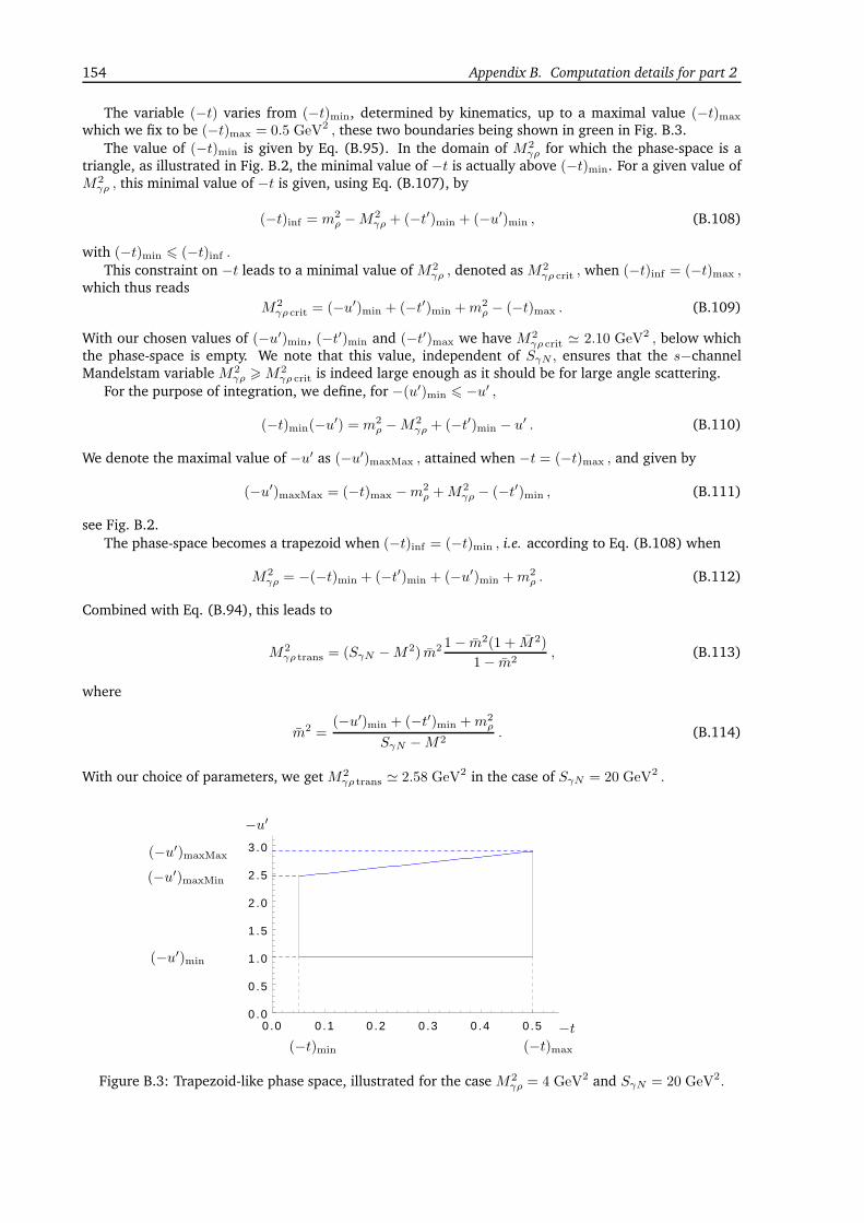
154 Appendix B. Computation details for part 2
The variable (−t) varies from (−t)min, determined by kinematics, up to a maximal value (−t)max
which we fix to be (−t)max = 0.5 GeV2 , these two boundaries being shown in green in Fig. B.3.The value of (−t)min is given by Eq. (B.95). In the domain of M2
γρ for which the phase-space is atriangle, as illustrated in Fig. B.2, the minimal value of −t is actually above (−t)min. For a given value ofM2γρ , this minimal value of −t is given, using Eq. (B.107), by
(−t)inf = m2ρ −M2
γρ + (−t′)min + (−u′)min , (B.108)
with (−t)min 6 (−t)inf .This constraint on −t leads to a minimal value of M2
γρ , denoted as M2γρ crit , when (−t)inf = (−t)max ,
which thus readsM2γρ crit = (−u′)min + (−t′)min +m2
ρ − (−t)max . (B.109)
With our chosen values of (−u′)min, (−t′)min and (−t′)max we have M2γρ crit ≃ 2.10 GeV2 , below which
the phase-space is empty. We note that this value, independent of SγN , ensures that the s−channelMandelstam variable M2
γρ >M2γρ crit is indeed large enough as it should be for large angle scattering.
For the purpose of integration, we define, for −(u′)min 6 −u′ ,
(−t)min(−u′) = m2ρ −M2
γρ + (−t′)min − u′ . (B.110)
We denote the maximal value of −u′ as (−u′)maxMax , attained when −t = (−t)max , and given by
(−u′)maxMax = (−t)max −m2ρ +M2
γρ − (−t′)min , (B.111)
see Fig. B.2.The phase-space becomes a trapezoid when (−t)inf = (−t)min , i.e. according to Eq. (B.108) when
M2γρ = −(−t)min + (−t′)min + (−u′)min +m2
ρ . (B.112)
Combined with Eq. (B.94), this leads to
M2γρ trans = (SγN −M2) m2 1− m2(1 + M2)
1− m2, (B.113)
where
m2 =(−u′)min + (−t′)min +m2
ρ
SγN −M2. (B.114)
With our choice of parameters, we get M2γρ trans ≃ 2.58 GeV2 in the case of SγN = 20 GeV2 .
0 .0 0 .1 0 .2 0 .3 0 .4 0 .50 .0
0 .5
1 .0
1 .5
2 .0
2 .5
3 .0
−t
−u′
(−t)min (−t)max
(−u′)min
(−u′)maxMin
(−u′)maxMax
Figure B.3: Trapezoid-like phase space, illustrated for the case M2γρ = 4 GeV2 and SγN = 20 GeV2.

B.5. Angular cut over the outgoing photon 155
Above this value, the phase-space is a trapezoid, illustrated in Fig. B.3. This trapezoid reduces to anempty domain when (−t)min = (−t)max . From the solution of Eq. (B.94), this occurs for
M2γρMax = (SγN −M2)
−(1 + 2M2)(−t)max +√
(−t)max((−t)max + 4M2)
2M2, (B.115)
with M2 = M2/(SγN −M2) and (−t)max = (−t)max/(SγN −M2) . With our choice of parameters, weget M2
γρMax ≃ 9.47 GeV2 in the case of SγN = 20 GeV2 . This value decreases with decreasing values ofSγN .
The minimal value of SγN is obtained from the constraint M2γρ crit = M2
γρMax and equals SγNcrit ≃5.87 GeV2 .
Finally, let us briefly discuss the invariant mass M2ρN ′ , which should be restricted to be far above any
possible resonance. Using Eq. (4.72), for a given value of SγN , a careful study of the allowed phasespace shows that M2
ρN ′ is minimal when −u′ = (−u′)maxMax and M2γρ =M2
γρMax, and for ~∆t and ~pt anti
collinear, with |~∆t| being the value corresponding to −t = (−t)max . This minimal value increases withSγN . Its minimal value is thus obtained when SγN = SγNcrit, this value being M2
ρN ′Min ≃ 3.4 GeV2 whichis far above the resonance region.
B.4.2 Method for the phase space integration
Using the above described phase-space, the integrated cross section reads
dσ
dM2γρ
= θ(M2γρ crit < M2
γρ < M2γρ trans) (B.116)
×∫ (−u′)maxMax
(−u′)min
d(−u′)∫ (−t)max
(−t)min(−u′)
d(−t)F (t)2 dσ
dM2γρd(−u′)d(−t)
∣
∣
∣
∣
(−t)min
+ θ(M2γρ trans < M2
γρ < M2γρMax)
×
∫ (−u′)maxMin
(−u′)min
d(−u′)∫ (−t)max
(−t)min
d(−t)F (t)2 dσ
dM2γρd(−u′)d(−t)
∣
∣
∣
∣
(−t)min
+
∫ (−u′)maxMax
(−u′)maxMin
d(−u′)∫ (−t)max
(−t)min(−u′)
d(−t)F (t)2 dσ
dM2γρd(−u′)d(−t)
∣
∣
∣
∣
(−t)min
.
Using our explicit dipole ansatz for F (t), see Eq. (4.149), we obtain
dσ
dM2γρ
=C4
3
[
θ(M2γρ crit < M2
γρ < M2γρ trans) (B.117)
×∫ (−u′)maxMax
(−u′)min
d(−u′)[
1
((−t)max − C)3− 1
((−t)min(−u′)− C)3
]
dσ
dM2γρd(−u′)d(−t)
∣
∣
∣
∣
(−t)min
+ θ(M2γρ trans < M2
γρ < M2γρMax)
×
[
1
((−t)max − C)3− 1
((−t)min − C)3
]∫ (−u′)maxMin
(−u′)min
d(−u′) dσ
dM2γρd(−u′)d(−t)
∣
∣
∣
∣
(−t)min
+
∫ (−u′)maxMax
(−u′)maxMin
d(−u′)[
1
((−t)max − C)3− 1
((−t)min(−u′)− C)3
]
dσ
dM2γρd(−u′)d(−t)
∣
∣
∣
∣
(−t)min
]
,
which is our building formula for the numerical evaluation of integrated cross sections.
B.5 Angular cut over the outgoing photon
In order to take into account limitations of detection of the produced photon, it is necessary to know thephoton scattering angle in the rest frame of the nucleon target. The incoming nucleon momentum pµ1 in

156 Appendix B. Computation details for part 2
0 10 20 30 400 .00
0 .02
0 .04
0 .06
0 .08
0 .10
−
θ
1
σeven
dσevendθ
0 5 10 15 20 25 30 350 .00
0 .05
0 .10
0 .15
θ
1
σeven
dσevendθ
0 5 10 15 20 25 300 .00
0 .05
0 .10
0 .15
0 .20
θ
1
σeven
dσevendθ
Figure B.4: Angular distribution in the chiral-even case. Up, left: SγN = 10 GeV2, for M2γρ = 3 GeV2
(solid blue) and M2γρ = 4 GeV2 (dotted red). Up, right: SγN = 15 GeV2, for M2
γρ = 3 GeV2 (solidblue), M2
γρ = 4 GeV2 (dotted red) and M2γρ = 5 GeV2 (dashed green). Down: SγN = 20 GeV2, for
M2γρ = 3 GeV2 (solid blue), M2
γρ = 4 GeV2 (dotted red) and M2γρ = 5 GeV2 (dashed green).
Eq. (4.63) and the one in its rest frame pµ1rf = (M, 0, 0, 0) are related by the longitudinal boost along zaxis characterized by the rapidity ζ such that, in the Bjorken limit,
cosh ζ =1
2
[
M√s(1 + ξ)
+
√s(1 + ξ)
M
]
. (B.118)
The incoming photon flies almost towards the −z axis, in the light-cone and in the rest frame, so that thescattering angle θ of the produced photon in the nucleon rest frame with respect to this direction satisfies
tan θ = − 2Ms(1 + ξ) ‖ ~pt − ~∆t2 ‖
−α(1 + ξ)2s2 + (~pt − ~∆t2 )2M2
. (B.119)
Using the relation α = M2γρ/(−u′), see Eq. (B.104), one gets from this expression tan θ as a function of
−u′, which we formally write
tan θ = f(−u′) . (B.120)
From this relation, θ being positive, one should take
for tan θ > 0, θ = arctan(tan θ), (B.121)
for tan θ < 0, θ = π + arctan(tan θ) , (B.122)
where tan θ is given by Eq. (B.119).

B.5. Angular cut over the outgoing photon 157
0 10 20 30 400 .00
0 .05
0 .10
0 .15
0 .20
θ
1
σodd
dσodddθ
0 10 20 30 400 .00
0 .05
0 .10
0 .15
0 .20
0 .25
θ
1
σodd
dσodddθ
0 10 20 30 400 .00
0 .05
0 .10
0 .15
0 .20
0 .25
0 .30
0 .35
θ
1
σodd
dσodddθ
Figure B.5: Angular distribution in the chiral-odd case. Up, left: SγN = 10 GeV2, for M2γρ = 3 GeV2
(solid blue) and M2γρ = 4 GeV2 (dotted red). Up, right: SγN = 15 GeV2, for M2
γρ = 3.5 GeV2 (solidblue), M2
γρ = 5 GeV2 (dotted red) and M2γρ = 6.5 GeV2 (dashed green). Down: SγN = 20 GeV2, for
M2γρ = 4 GeV2 (solid blue), M2
γρ = 6 GeV2 (dotted red) and M2γρ = 8 GeV2 (dashed green).
For simplicity, we now perform our analysis in the case ~∆t = 0, and thus write
tan θ = − 2Ms(1 + ξ) pt−α(1 + ξ)2s2 + ~p 2
tM2, (B.123)
where pt =‖~pt‖ .Using the formulas given in Sec. B.3.3, one can compute α as a function of θ . One gets
for tan θ > 0, α =(1 + ξ + τ) τ tan2 θ + a
(
1 +√1 + tan2 θ
)
(1 + ξ + τ )2 tan2 θ + 2a, (B.124)
for tan θ < 0, α =(1 + ξ + τ) τ tan2 θ + a
(
1−√1 + tan2 θ
)
(1 + ξ + τ )2 tan2 θ + 2a, (B.125)
where
a =4M2
γρ
s, (B.126)
τ =2ξ
1 + ξ
M2γρ
s= τ
M2γρ
s, (B.127)
thus providing −u′ as a function of θ using −u′ = αM2γρ, see Eq. (B.104).

158 Appendix B. Computation details for part 2
The angular distribution of the produced photon can easily be obtained from the differential cross-section by using the relation
dθ
d(−u′) =f ′(−u′)
1 + f2(−u′) (B.128)
so that we get
1
σ
dσ
dθ=
1
σ
dσ
d(−u′)d(−u′)dθ
=1
σ
dσ
d(−u′)1 + f2(−u′[θ])f ′(−u′[θ]) . (B.129)
The obtained angular distribution is shown in Fig. B.4 for the chiral-even case, and in Fig. B.5 for thechiral-odd case. In the chiral-even case, the obtained angular distribution is an increasing function of θ,while in the chiral-odd case, it decreases with increasing θ. In both cases, the distributions are dominatedby moderate values of θ.
2 .0 2 .5 3 .0 3 .5 4 .00 .00
0 .05
0 .10
0 .15
0 .20
0 .25
M2γρ (GeV2)
dσevendM2
γρ
(nb ·GeV−2)
2 3 4 5 6 70 .00
0 .05
0 .10
0 .15
0 .20
0 .25
0 .30
M2γρ (GeV2)
dσevendM2
γρ
(nb ·GeV−2)
2 3 4 5 6 7 8 90 .00
0 .05
0 .10
0 .15
0 .20
0 .25
0 .30
M2γρ (GeV2)
dσevendM2
γρ
(nb ·GeV−2)
Figure B.6: The differential cross section dσeven
dM2γρ
. Solid red: no angular cut. Other curves show the
effect of an upper angular cut θ for the out-going γ: 35° (dashed blue), 30° (dotted green), 25° (dashed-dotted brown), 20° (long-dashed magenta), 15° (short-dashed purple) and 10° (dotted black). Up, left:SγN = 10 GeV2. Up, right: SγN = 15 GeV2. Down: SγN = 20 GeV2.
In practice, at JLab, in Hall B, the outgoing photon could be detected with an angle between 5° and35° from the incoming beam.
The effect of an upper angular cut can be seen in Fig. B.6 for the chiral-even case, and in Fig. B.7 forthe chiral-odd case. As seen from Figs. B.4 and B.5, it mainly affects the low SγN domain. In particular,the effect of the JLab 35° upper cut remains negligible as shown in Figs. B.6 and B.7, both for the chiral-even and chiral-odd cases.
One should note that using cuts on θ, it is possible to reduce dramatically the contribution of thechiral-even contribution, in particular in the region of SγN around 20 GeV2, while moderately reducingthe chiral-odd contribution. Putting additional cuts on M2
γρ, like M2γρ > 6 GeV2, allows to increase the

B.5. Angular cut over the outgoing photon 159
2 .0 2 .5 3 .0 3 .5 4 .00 .00
0 .05
0 .10
0 .15
0 .20
0 .25
0 .30
M2γρ (GeV2)
dσodddM2
γρ
(pb ·GeV−2)
2 3 4 5 6 70 .00
0 .05
0 .10
0 .15
0 .20
M2γρ (GeV2)
dσodddM2
γρ
(pb ·GeV−2)
2 3 4 5 6 7 8 90 .00
0 .02
0 .04
0 .06
0 .08
0 .10
0 .12
M2γρ (GeV2)
dσodddM2
γρ
(pb ·GeV−2)
Figure B.7: The differential cross section dσodd
dM2γρ
. Solid red: no angular cut. Other curves show the
effect of an upper angular cut θ for the out-going γ: 35° (dashed blue), 30° (dotted green), 25° (dashed-dotted brown), 20° (long-dashed magenta), 15° (short-dashed purple) and 10° (dotted black). Up, left:SγN = 10 GeV2. Up, right: SγN = 15 GeV2. Down: SγN = 20 GeV2.
ratio odd versus even from ∼ 1/900 to ∼ 1/40, keeping about 3% of the chiral-odd contribution, fortypically SγN between 18 GeV2 and the maximal value 21.5 GeV2. This in principle would lead, dealingwith observables sensitive to the interference between the chiral-odd and the chiral-even contributions,to a relative signal of the order of 15%.

160 Appendix B. Computation details for part 2

Bibliography
[1] R. P. Feynman, Very high-energy collisions of hadrons, Phys. Rev. Lett. 23 (1969) 1415–1417.
[2] J. D. Bjorken, Asymptotic Sum Rules at Infinite Momentum, Phys. Rev. 179 (1969) 1547–1553.
[3] D. J. Gross and F. Wilczek, ULTRAVIOLET BEHAVIOR OF NON-ABELIAN GAUGE THEORIES, Phys.Rev. Lett. 30 (1973) 1343–1346.
[4] D. J. Gross and F. Wilczek, Asymptotically Free Gauge Theories. 1, Phys. Rev. D8 (1973)3633–3652.
[5] H. D. Politzer, RELIABLE PERTURBATIVE RESULTS FOR STRONG INTERACTIONS?, Phys. Rev. Lett.30 (1973) 1346–1349.
[6] V. N. Gribov and L. N. Lipatov, Deep inelastic e p scattering in perturbation theory, Sov. J. Nucl.Phys. 15 (1972) 438–450.
[7] L. N. Lipatov, The parton model and perturbation theory, Sov. J. Nucl. Phys. 20 (1975) 94–102.
[8] G. Altarelli and G. Parisi, Asymptotic freedom in parton language, Nucl. Phys. B126 (1977) 298.
[9] Y. L. Dokshitzer, Calculation of the Structure Functions for Deep Inelastic Scattering and e+e−
Annihilation by Perturbation Theory in Quantum Chromodynamics, Sov. Phys. JETP 46 (1977)641–653.
[10] A. V. Efremov and A. V. Radyushkin, Factorization and Asymptotical Behavior of Pion Form-Factorin QCD, Phys. Lett. B94 (1980) 245–250.
[11] G. R. Farrar and D. R. Jackson, The Pion Form-Factor, Phys. Rev. Lett. 43 (1979) 246.
[12] G. P. Lepage and S. J. Brodsky, Exclusive Processes in Quantum Chromodynamics: EvolutionEquations for Hadronic Wave Functions and the Form-Factors of Mesons, Phys. Lett. B87 (1979)359–365.
[13] X.-D. Ji and J. Osborne, One-loop corrections and all order factorization in deeply virtual Comptonscattering, Phys. Rev. D58 (1998) 094018, [hep-ph/9801260].
[14] J. C. Collins and A. Freund, Proof of factorization for deeply virtual Compton scattering in QCD,Phys. Rev. D59 (1999) 074009, [hep-ph/9801262].
[15] J. C. Collins, L. Frankfurt, and M. Strikman, Factorization for hard exclusive electroproduction ofmesons in QCD, Phys. Rev. D56 (1997) 2982–3006, [hep-ph/9611433].
[16] V. S. Fadin, E. A. Kuraev, and L. N. Lipatov, On the Pomeranchuk Singularity in Asymptotically FreeTheories, Phys. Lett. B60 (1975) 50–52.
[17] E. A. Kuraev, L. N. Lipatov, and V. S. Fadin, Multi - Reggeon Processes in the Yang-Mills Theory, Sov.Phys. JETP 44 (1976) 443–450.
[18] E. A. Kuraev, L. N. Lipatov, and V. S. Fadin, The Pomeranchuk Singularity in Nonabelian GaugeTheories, Sov. Phys. JETP 45 (1977) 199–204.
161

162 Bibliography
[19] I. I. Balitsky and L. N. Lipatov, The Pomeranchuk Singularity in Quantum Chromodynamics, Sov. J.Nucl. Phys. 28 (1978) 822–829.
[20] M. Froissart, Asymptotic behavior and subtractions in the Mandelstam representation, Phys. Rev.123 (1961) 1053–1057.
[21] L. V. Gribov, E. M. Levin, and M. G. Ryskin, Semihard Processes in QCD, Phys. Rept. 100 (1983)1–150.
[22] I. Balitsky, Operator expansion for high-energy scattering, Nucl. Phys. B463 (1996) 99–160,[hep-ph/9509348].
[23] I. Balitsky, Factorization for high-energy scattering, Phys. Rev. Lett. 81 (1998) 2024–2027,[hep-ph/9807434].
[24] I. Balitsky, Factorization and high-energy effective action, Phys. Rev. D60 (1999) 014020,[hep-ph/9812311].
[25] I. Balitsky, Effective field theory for the small-x evolution, Phys. Lett. B518 (2001) 235–242,[hep-ph/0105334].
[26] J. Jalilian-Marian, A. Kovner, A. Leonidov, and H. Weigert, The BFKL equation from the Wilsonrenormalization group, Nucl. Phys. B504 (1997) 415–431, [hep-ph/9701284].
[27] J. Jalilian-Marian, A. Kovner, A. Leonidov, and H. Weigert, The Wilson renormalization group forlow x physics: Towards the high density regime, Phys. Rev. D59 (1999) 014014, [hep-ph/9706377].
[28] J. Jalilian-Marian, A. Kovner, and H. Weigert, The Wilson renormalization group for low x physics:Gluon evolution at finite parton density, Phys. Rev. D59 (1999) 014015, [hep-ph/9709432].
[29] J. Jalilian-Marian, A. Kovner, A. Leonidov, and H. Weigert, Unitarization of gluon distribution inthe doubly logarithmic regime at high density, Phys. Rev. D59 (1999) 034007, [hep-ph/9807462].
[30] A. Kovner, J. G. Milhano, and H. Weigert, Relating different approaches to nonlinear QCD evolutionat finite gluon density, Phys. Rev. D62 (2000) 114005, [hep-ph/0004014].
[31] H. Weigert, Unitarity at small Bjorken x, Nucl. Phys. A703 (2002) 823–860, [hep-ph/0004044].
[32] E. Iancu, A. Leonidov, and L. D. McLerran, Nonlinear gluon evolution in the color glass condensate.I, Nucl. Phys. A692 (2001) 583–645, [hep-ph/0011241].
[33] E. Iancu, A. Leonidov, and L. D. McLerran, The renormalization group equation for the color glasscondensate, Phys. Lett. B510 (2001) 133–144, [hep-ph/0102009].
[34] E. Ferreiro, E. Iancu, A. Leonidov, and L. McLerran, Nonlinear gluon evolution in the color glasscondensate. II, Nucl. Phys. A703 (2002) 489–538, [hep-ph/0109115].
[35] Y. V. Kovchegov, Small-x F2 structure function of a nucleus including multiple pomeron exchanges,Phys. Rev. D60 (1999) 034008, [hep-ph/9901281].
[36] Y. V. Kovchegov, Unitarization of the BFKL pomeron on a nucleus, Phys. Rev. D61 (2000) 074018,[hep-ph/9905214].
[37] E. Iancu, K. Itakura, and L. McLerran, Geometric scaling above the saturation scale, Nucl. Phys.A708 (2002) 327–352, [hep-ph/0203137].
[38] F. Gelis, T. Lappi, and R. Venugopalan, High energy factorization in nucleus-nucleus collisions,Phys. Rev. D78 (2008) 054019, [arXiv:0804.2630].
[39] I. Balitsky and G. A. Chirilli, Rapidity evolution of Wilson lines at the next-to-leading order, Phys.Rev. D88 (2013) 111501, [arXiv:1309.7644].
[40] A. Kovner, M. Lublinsky, and Y. Mulian, Jalilian-Marian, Iancu, McLerran, Weigert, Leonidov,Kovner evolution at next to leading order, Phys. Rev. D89 (2014), no. 6 061704,[arXiv:1310.0378].

Bibliography 163
[41] I. Balitsky, Quark contribution to the small-x evolution of color dipole, Phys. Rev. D75 (2007)014001, [hep-ph/0609105].
[42] Y. V. Kovchegov and H. Weigert, Triumvirate of Running Couplings in Small-x Evolution, Nucl.Phys. A784 (2007) 188–226, [hep-ph/0609090].
[43] I. Balitsky and G. A. Chirilli, Next-to-leading order evolution of color dipoles, Phys. Rev. D77 (2008)014019, [arXiv:0710.4330].
[44] I. Balitsky and G. A. Chirilli, NLO evolution of color dipoles in N=4 SYM, Nucl. Phys. B822 (2009)45–87, [arXiv:0903.5326].
[45] R. E. Gerasimov and A. V. Grabovsky, Evolution equation for 3-quark Wilson loop operator, JHEP04 (2013) 102, [arXiv:1212.1681].
[46] I. Balitsky and A. V. Grabovsky, NLO evolution of 3-quark Wilson loop operator, JHEP 01 (2015)009, [arXiv:1405.0443].
[47] F. Dominguez, A. H. Mueller, S. Munier, and B.-W. Xiao, On the small-x evolution of the colorquadrupole and the WeizsÃd’ckerâASWilliams gluon distribution, Phys. Lett. B705 (2011) 106–111,[arXiv:1108.1752].
[48] J. Jalilian-Marian and Y. V. Kovchegov, Inclusive two-gluon and valence quark-gluon production inDIS and pA, Phys. Rev. D70 (2004) 114017, [hep-ph/0405266]. [Erratum: Phys.Rev.D71,079901(2005)].
[49] A. Dumitru and J. Jalilian-Marian, Two-particle correlations in high energy collisions and the gluonfour-point function, Phys. Rev. D81 (2010) 094015, [arXiv:1001.4820].
[50] A. Dumitru and J. Jalilian-Marian, Forward dijets in high-energy collisions: Evolution of QCDn-point functions beyond the dipole approximation, Phys. Rev. D82 (2010) 074023,[arXiv:1008.0480].
[51] A. V. Grabovsky, On the low-x NLO evolution of 4 point colorless operators, JHEP 09 (2015) 194,[arXiv:1507.0862].
[52] I. Balitsky and A. Tarasov, Rapidity evolution of gluon TMD from low to moderate x, JHEP 10(2015) 017, [arXiv:1505.0215].
[53] I. Balitsky and A. Tarasov, Gluon TMD in particle production from low to moderate x,arXiv:1603.0654.
[54] T. Altinoluk, N. Armesto, G. Beuf, M. Martà nez, and C. A. Salgado, Next-to-Eikonal corrections inthe CGC, PoS DIS2014 (2014) 089.
[55] T. Altinoluk, N. Armesto, G. Beuf, and A. Moscoso, Next-to-next-to-eikonal corrections in the CGC,JHEP 01 (2016) 114, [arXiv:1505.0140].
[56] M. Wusthoff and A. D. Martin, The QCD description of diffractive processes, J. Phys. G25 (1999)R309–R344, [hep-ph/9909362].
[57] G. Wolf, Review of High Energy Diffraction in Real and Virtual Photon Proton scattering at HERA,Rept. Prog. Phys. 73 (2010) 116202, [arXiv:0907.1217].
[58] H1 Collaboration, A. Aktas et. al., Diffractive deep-inelastic scattering with a leading proton atHERA, Eur. Phys. J. C48 (2006) 749–766, [hep-ex/0606003].
[59] H1 Collaboration, A. Aktas et. al., Measurement and QCD analysis of the diffractive deep- inelasticscattering cross-section at HERA, Eur. Phys. J. C48 (2006) 715–748, [hep-ex/0606004].
[60] ZEUS Collaboration Collaboration, S. Chekanov et. al., Dissociation of virtual photons in eventswith a leading proton at HERA, Eur. Phys. J. C38 (2004) 43–67, [hep-ex/0408009].

164 Bibliography
[61] ZEUS Collaboration, S. Chekanov et. al., Study of deep inelastic inclusive and diffractive scatteringwith the ZEUS forward plug calorimeter, Nucl. Phys. B713 (2005) 3–80, [hep-ex/0501060].
[62] F. Aaron, C. Alexa, V. Andreev, S. Backovic, A. Baghdasaryan, et. al., Measurement of the crosssection for diffractive deep-inelastic scattering with a leading proton at HERA, Eur. Phys. J. C71(2011) 1578, [arXiv:1010.1476].
[63] H1 Collaboration Collaboration, F. Aaron et. al., Inclusive Measurement of DiffractiveDeep-Inelastic Scattering at HERA, Eur. Phys. J. C72 (2012) 2074, [arXiv:1203.4495].
[64] ZEUS Collaboration Collaboration, S. Chekanov et. al., Deep inelastic scattering with leadingprotons or large rapidity gaps at HERA, Nucl. Phys. B816 (2009) 1–61, [arXiv:0812.2003].
[65] H1 Collaboration, ZEUS Collaboration Collaboration, F. Aaron et. al., Combined inclusivediffractive cross sections measured with forward proton spectrometers in deep inelastic ep scatteringat HERA, Eur. Phys. J. C72 (2012) 2175, [arXiv:1207.4864].
[66] J. C. Collins, Proof of factorization for diffractive hard scattering, Phys. Rev. D57 (1998)3051–3056, [hep-ph/9709499].
[67] J. Bartels, J. R. Ellis, H. Kowalski, and M. Wusthoff, An analysis of diffraction in deep-inelasticscattering, Eur. Phys. J. C7 (1999) 443–458, [hep-ph/9803497].
[68] M. Wusthoff, Photon diffractive dissociation in deep inelastic scattering, PhD (1995).
[69] E. Gotsman, E. Levin, and U. Maor, Diffractive leptoproduction of small masses in QCD, Nucl. Phys.B493 (1997) 354–396, [hep-ph/9606280].
[70] M. Wusthoff, Large rapidity gap events in deep inelastic scattering, Phys. Rev. D56 (1997)4311–4321, [hep-ph/9702201].
[71] J. Bartels, H. Jung, and M. Wusthoff, Quark - anti-quark gluon jets in DIS diffractive dissociation,Eur. Phys. J. C11 (1999) 111–125, [hep-ph/9903265].
[72] J. Bartels, H. Jung, and A. Kyrieleis, Massive c anti-c g: Calculation in diffractive DIS and diffractiveD* production at HERA, Eur. Phys. J. C24 (2002) 555–560, [hep-ph/0204269].
[73] C. Marquet, A Unified description of diffractive deep inelastic scattering with saturation, Phys. Rev.D76 (2007) 094017, [arXiv:0706.2682].
[74] R. Boussarie, A. V. Grabovsky, L. Szymanowski, and S. Wallon, Impact factor for high-energy twoand three jets diffractive production, JHEP 09 (2014) 026, [arXiv:1405.7676].
[75] R. Boussarie, A. V. Grabovsky, L. Szymanowski, and S. Wallon, On the one loop γ(∗) → qq impactfactor and the exclusive diffractive cross sections for the production of two or three jets,arXiv:1606.0041.
[76] R. Boussarie, A. V. Grabovsky, L. Szymanowski, and S. Wallon, Diffractive production of jets athigh-energy in the QCD shock-wave approach, in Photon 2015: International Conference on theStructure and Interactions of the Photon and the 21th International Workshop on Photon-PhotonCollisions and International Workshop on High Energy Photon Linear Colliders Novosibirsk, Russia,June 15-19, 2015, 2015. arXiv:1511.0278.
[77] R. Boussarie, A. Grabovsky, L. Szymanowski, and S. Wallon, Photon dissociation into two and threejets: initial and final state corrections, Acta Phys. Polon. Supp. 8 (2015) 897, [arXiv:1512.0077].
[78] V. S. Fadin and L. N. Lipatov, BFKL pomeron in the next-to-leading approximation, Phys. Lett. B429(1998) 127–134, [hep-ph/9802290].
[79] M. Ciafaloni and G. Camici, Energy scale(s) and next-to-leading BFKL equation, Phys. Lett. B430(1998) 349–354, [hep-ph/9803389].
[80] V. Fadin and R. Fiore, Non-forward BFKL pomeron at next-to-leading order, Phys. Lett. B610(2005) 61–66, [hep-ph/0412386].

Bibliography 165
[81] V. S. Fadin and R. Fiore, Non-forward NLO BFKL kernel, Phys. Rev. D72 (2005) 014018,[hep-ph/0502045].
[82] K. J. Golec-Biernat and M. Wusthoff, Saturation effects in deep inelastic scattering at low Q2 and itsimplications on diffraction, Phys. Rev. D59 (1999) 014017, [hep-ph/9807513].
[83] K. Golec-Biernat and M. Wusthoff, Saturation in diffractive deep inelastic scattering, Phys. Rev. D60(1999) 114023, [hep-ph/9903358].
[84] G. A. Chirilli and Y. V. Kovchegov, Solution of the NLO BFKL Equation and a Strategy for Solvingthe All-Order BFKL Equation, JHEP 06 (2013) 055, [arXiv:1305.1924].
[85] A. V. Grabovsky, On the solution to the NLO forward BFKL equation, JHEP 09 (2013) 098,[arXiv:1307.3152].
[86] ZEUS Collaboration, H. Abramowicz et. al., Production of exclusive dijets in diffractive deepinelastic scattering at HERA, Eur. Phys. J. C76 (2016), no. 1 16, [arXiv:1505.0578].
[87] V. Fadin, R. Fiore, A. Grabovsky, and A. Papa, Connection between complete and Moebius forms ofgauge invariant operators, Nucl. Phys. B856 (2012) 111–124, [arXiv:1109.6634].
[88] C. Marquet and H. Weigert, New observables to test the Color Glass Condensate beyond the large-Nclimit, Nucl. Phys. A843 (2010) 68–97, [arXiv:1003.0813].
[89] D. Y. Ivanov and A. Papa, The next-to-leading order forward jet vertex in the small-coneapproximation, JHEP 1205 (2012) 086, [arXiv:1202.1082].
[90] I. Balitsky and G. A. Chirilli, Photon impact factor in the next-to-leading order, Phys. Rev. D83(2011) 031502, [arXiv:1009.4729].
[91] I. Balitsky and G. A. Chirilli, Photon impact factor and kT -factorization for DIS in thenext-to-leading order, Phys. Rev. D87 (2013) 014013, [arXiv:1207.3844].
[92] G. Beuf, Dipole factorization for DIS at NLO I: Loop correction to the photon to quark-antiquarklight-front wave-functions, arXiv:1606.0077.
[93] R. Boussarie, B. DuclouÃl’, L. Szymanowski, and S. Wallon, Production of a forward J/psi and abackward jet at the LHC, in Photon 2015: International Conference on the Structure andInteractions of the Photon and the 21th International Workshop on Photon-Photon Collisions andInternational Workshop on High Energy Photon Linear Colliders Novosibirsk, Russia, June 15-19,2015, 2015. arXiv:1511.0218.
[94] D. Colferai, F. Schwennsen, L. Szymanowski, and S. Wallon, Mueller Navelet jets at LHC - completeNLL BFKL calculation, JHEP 12 (2010) 026, [arXiv:1002.1365].
[95] B. Ducloué, L. Szymanowski, and S. Wallon, Confronting Mueller-Navelet jets in NLL BFKL withLHC experiments at 7 TeV, JHEP 1305 (2013) 096, [arXiv:1302.7012].
[96] F. Caporale, D. Y. Ivanov, B. Murdaca, and A. Papa, Mueller-Navelet small-cone jets at LHC innext-to-leading BFKL, Nucl. Phys. B877 (2013) 73–94, [arXiv:1211.7225].
[97] F. Caporale, B. Murdaca, A. Sabio Vera, and C. Salas, Scale choice and collinear contributions toMueller-Navelet jets at LHC energies, Nucl. Phys. B875 (2013) 134–151, [arXiv:1305.4620].
[98] F. Caporale, D. Yu. Ivanov, B. Murdaca, and A. Papa, Brodsky-Lepage-Mackenzie optimalrenormalization scale setting for semihard processes, Phys. Rev. D91 (2015), no. 11 114009,[arXiv:1504.0647].
[99] F. G. Celiberto, D. Yu. Ivanov, B. Murdaca, and A. Papa, Mueller-Navelet jets at LHC: BFKL versushigh-energy DGLAP, Eur. Phys. J. C75 (2015), no. 6 292, [arXiv:1504.0823].
[100] A. H. Mueller and H. Navelet, An Inclusive Minijet Cross-Section and the Bare Pomeron in QCD,Nucl. Phys. B282 (1987) 727.

166 Bibliography
[101] CMS Collaboration, V. Khachatryan et. al., Azimuthal decorrelation of jets widely separated inrapidity in pp collisions at
√s = 7 TeV, Submitted to: JHEP (2016) [arXiv:1601.0671].
[102] B. DuclouÃl’, L. Szymanowski, and S. Wallon, Evidence for high-energy resummation effects inMueller-Navelet jets at the LHC, Phys. Rev. Lett. 112 (2014) 082003, [arXiv:1309.3229].
[103] F. Caporale, D. Yu. Ivanov, B. Murdaca, and A. Papa, MuellerâASNavelet jets in next-to-leadingorder BFKL: theory versus experiment, Eur. Phys. J. C74 (2014), no. 10 3084, [arXiv:1407.8431].[Erratum: Eur. Phys. J.C75,no.11,535(2015)].
[104] H1 Collaboration Collaboration, F. Aaron et. al., Measurement of Dijet Production in DiffractiveDeep-Inelastic Scattering with a Leading Proton at HERA, Eur. Phys. J. C72 (2012) 1970,[arXiv:1111.0584].
[105] ZEUS Collaboration Collaboration, S. Chekanov et. al., Diffractive photoproduction of dijets in epcollisions at HERA, Eur. Phys. J. C55 (2008) 177–191, [arXiv:0710.1498].
[106] H1 Collaboration Collaboration, F. Aaron et. al., Diffractive Dijet Photoproduction in ep Collisionsat HERA, Eur. Phys. J. C70 (2010) 15–37, [arXiv:1006.0946].
[107] M. Klasen and G. Kramer, Factorization breaking in diffractive dijet photoproduction, Eur. Phys. J.C38 (2004) 93–104, [hep-ph/0408203].
[108] M. Klasen and G. Kramer, Review of factorization breaking in diffractive photoproduction of dijets,Mod. Phys. Lett. A23 (2008) 1885–1907, [arXiv:0806.2269].
[109] D. Boer et. al., Gluons and the quark sea at high energies: Distributions, polarization, tomography,arXiv:1108.1713.
[110] LHeC Study Group Collaboration, J. L. Abelleira Fernandez et. al., A Large Hadron ElectronCollider at CERN: Report on the Physics and Design Concepts for Machine and Detector, J. Phys. G39(2012) 075001, [arXiv:1206.2913].
[111] T. Altinoluk, N. Armesto, G. Beuf, and A. H. Rezaeian, Diffractive Dijet Production in Deep InelasticScattering and Photon-Hadron Collisions in the Color Glass Condensate, Phys. Lett. B758 (2016)373–383, [arXiv:1511.0745].
[112] Y. Hatta, B.-W. Xiao, and F. Yuan, Probing the Small-x Gluon Tomography in Correlated HardDiffractive Dijet Production in DIS, Phys. Rev. Lett. 116 (2016), no. 20 202301,[arXiv:1601.0158].
[113] LHCb Collaboration, R. Aaij et. al., Exclusive J/ψ and ψ(2S) production in pp collisions at√s = 7
TeV, J. Phys. G40 (2013) 045001, [arXiv:1301.7084].
[114] LHCb Collaboration, R. Aaij et. al., Updated measurements of exclusive J/ψ and ψ(2S) productioncross-sections in pp collisions at
√s = 7 TeV, J. Phys. G41 (2014) 055002, [arXiv:1401.3288].
[115] LHCb Collaboration, R. Aaij et. al., Measurement of the exclusive Îe production cross-section in ppcollisions at
√s = 7 TeV and 8 TeV, JHEP 09 (2015) 084, [arXiv:1505.0813].
[116] ALICE Collaboration, B. B. Abelev et. al., Exclusive J/ψ photoproduction off protons inultra-peripheral p-Pb collisions at
√sNN = 5.02 TeV, Phys. Rev. Lett. 113 (2014), no. 23 232504,
[arXiv:1406.7819].
[117] ALICE Collaboration, E. Abbas et. al., Charmonium and e+e− pair photoproduction at mid-rapidityin ultra-peripheral Pb-Pb collisions at
√sNN=2.76 TeV, Eur. Phys. J. C73 (2013), no. 11 2617,
[arXiv:1305.1467].
[118] ALICE Collaboration, B. Abelev et. al., Coherent J/ψ photoproduction in ultra-peripheral Pb-Pbcollisions at
√sNN = 2.76 TeV, Phys. Lett. B718 (2013) 1273–1283, [arXiv:1209.3715].
[119] ALICE Collaboration, J. Adam et. al., Coherent ψ(2S) photo-production in ultra-peripheral Pb Pbcollisions at
√sNN = 2.76 TeV, Phys. Lett. B751 (2015) 358–370, [arXiv:1508.0507].

Bibliography 167
[120] CMS Collaboration, V. Khachatryan et. al., Coherent J/Psi photoproduction in ultra-peripheral PbPbcollisions at sqrt(s[NN]) = 2.76 TeV with the CMS experiment, arXiv:1605.0696.
[121] LHC Forward Physics Working Group Collaboration, e. Royon, C. et. al., LHC Forward Physics, .
[122] V. Guzey and M. Klasen, Diffractive dijet photoproduction in ultraperipheral collisions at the LHC innext-to-leading order QCD, JHEP 04 (2016) 158, [arXiv:1603.0605].
[123] D. Y. Ivanov, M. I. Kotsky, and A. Papa, The impact factor for the virtual photon to light vectormeson transition, Eur. Phys. J. C38 (2004) 195–213, [hep-ph/0405297].
[124] I. V. Anikin, D. Yu. Ivanov, B. Pire, L. Szymanowski, and S. Wallon, On the description of exclusiveprocesses beyond the leading twist approximation, Phys. Lett. B682 (2010) 413–418,[arXiv:0903.4797].
[125] I. V. Anikin, D. Yu. Ivanov, B. Pire, L. Szymanowski, and S. Wallon, QCD factorization of exclusiveprocesses beyond leading twist: gamma*T —> rho(T) impact factor with twist three accuracy, Nucl.Phys. B828 (2010) 1–68, [arXiv:0909.4090].
[126] S. Wandzura and F. Wilczek, Sum Rules for Spin Dependent Electroproduction: Test of RelativisticConstituent Quarks, Phys. Lett. B72 (1977) 195–198.
[127] P. Ball and V. M. Braun, The ρ Meson Light-Cone Distribution Amplitudes of Leading Twist Revisited,Phys. Rev. D54 (1996) 2182–2193, [hep-ph/9602323].
[128] P. Ball, V. M. Braun, Y. Koike, and K. Tanaka, Higher twist distribution amplitudes of vector mesonsin QCD: Formalism and twist three distributions, Nucl. Phys. B529 (1998) 323–382,[hep-ph/9802299].
[129] V. S. Fadin, R. Fiore, and A. V. Grabovsky, On the discrepancy of the low-x evolution kernels, Nucl.Phys. B820 (2009) 334–363, [arXiv:0904.0702].
[130] V. Fadin, R. Fiore, and A. Grabovsky, Matching of the low-x evolution kernels, Nucl. Phys. B831(2010) 248–261, [arXiv:0911.5617].
[131] E. Iancu, J. D. Madrigal, A. H. Mueller, G. Soyez, and D. N. Triantafyllopoulos,Collinearly-improved BK evolution meets the HERA data, Phys. Lett. B750 (2015) 643–652,[arXiv:1507.0365].
[132] J. L. Albacete, Resummation of double collinear logs in BK evolution versus HERA data,arXiv:1507.0712.
[133] G. A. Chirilli and Y. V. Kovchegov, γ∗γ∗ Cross Section at NLO and Properties of the BFKL Evolutionat Higher Orders, JHEP 05 (2014) 099, [arXiv:1403.3384]. [Erratum: JHEP08,075(2015)].
[134] D. Yu. Ivanov, B. Murdaca, and A. Papa, The γ∗γ∗ total cross section in next-to-leading order BFKLand LEP2 data, JHEP 10 (2014) 058, [arXiv:1407.8447].
[135] A. Ayala, M. Hentschinski, J. Jalilian-Marian, and M. E. Tejeda-Yeomans, Polarized 3 partonproduction in inclusive DIS at small x, arXiv:1604.0852.
[136] G. Beuf, NLO corrections for the dipole factorization of DIS structure functions at low x, Phys. Rev.D85 (2012) 034039, [arXiv:1112.4501].
[137] G. T. Bodwin, E. Braaten, E. Eichten, S. L. Olsen, T. K. Pedlar, and J. Russ, Quarkonium at theFrontiers of High Energy Physics: A Snowmass White Paper, in Community Summer Study 2013:Snowmass on the Mississippi (CSS2013) Minneapolis, MN, USA, July 29-August 6, 2013, 2013.arXiv:1307.7425.
[138] N. Brambilla et. al., Heavy quarkonium: progress, puzzles, and opportunities, Eur. Phys. J. C71(2011) 1534, [arXiv:1010.5827].
[139] M. Bedjidian et. al., Hard probes in heavy ion collisions at the LHC: Heavy flavor physics, 2004.hep-ph/0311048.

168 Bibliography
[140] K. Goeke, M. V. Polyakov, and M. Vanderhaeghen, Hard Exclusive Reactions and the Structure ofHadrons, Prog. Part. Nucl. Phys. 47 (2001) 401–515, [hep-ph/0106012].
[141] M. Diehl, Generalized parton distributions, Phys. Rept. 388 (2003) 41–277, [hep-ph/0307382].
[142] A. V. Belitsky and A. V. Radyushkin, Unraveling hadron structure with generalized partondistributions, Phys. Rept. 418 (2005) 1–387, [hep-ph/0504030].
[143] S. Boffi and B. Pasquini, Generalized parton distributions and the structure of the nucleon, Riv.Nuovo Cim. 30 (2007) 387, [arXiv:0711.2625].
[144] V. D. Burkert and M. Diehl, Generalized parton distributions, . In *Close, Frank (ed.) et al.:Electromagnetic interactions and hadronic structure* 359-423.
[145] M. Guidal, Generalized Parton Distributions and deep virtual Compton scattering, Prog. Part. Nucl.Phys. 61 (2008) 89–105.
[146] D. Y. Ivanov, B. Pire, L. Szymanowski, and O. V. Teryaev, Probing chiral-odd GPD’s in diffractiveelectroproduction of two vector mesons, Phys. Lett. B550 (2002) 65–76, [hep-ph/0209300].
[147] R. Enberg, B. Pire, and L. Szymanowski, Transversity GPD in photo- and electroproduction of twovector mesons, Eur. Phys. J. C47 (2006) 87–94, [hep-ph/0601138].
[148] M. El Beiyad, B. Pire, M. Segond, L. Szymanowski, and S. Wallon, Photoproduction of a pi rhoTpair with a large invariant mass and transversity generalized parton distribution, Phys. Lett. B688(2010) 154–167, [arXiv:1001.4491].
[149] S. Kumano, M. Strikman, and K. Sudoh, Novel two-to-three hard hadronic processes and possiblestudies of generalized parton distributions at hadron facilities, Phys. Rev. D80 (2009) 074003,[/05.1453].
[150] A. B. Larionov and M. Strikman, Exploring QCD dynamics in medium energy γA semiexclusivecollisions, arXiv:1606.0076.
[151] R. Boussarie, B. Pire, L. Szymanowski, and S. Wallon, On γN → γρN ′ at large γρ invariant mass,in Photon 2015: International Conference on the Structure and Interactions of the Photon and the21th International Workshop on Photon-Photon Collisions and International Workshop on HighEnergy Photon Linear Colliders Novosibirsk, Russia, June 15-19, 2015, 2015. arXiv:1511.0437.
[152] R. Boussarie, B. Pire, L. Szymanowski, and S. Wallon, Revealing transversity GPDs through thephotoproduction of a photon and a ρ meson, EPJ Web Conf. 112 (2016) 01006,[arXiv:1602.0177].
[153] LHPC, SESAM Collaboration, P. Hagler, J. W. Negele, D. B. Renner, W. Schroers, T. Lippert, andK. Schilling, Moments of nucleon generalized parton distributions in lattice QCD, Phys. Rev. D68(2003) 034505, [hep-lat/0304018].
[154] QCDSF Collaboration, M. Gockeler, R. Horsley, D. Pleiter, P. E. L. Rakow, A. Schafer,G. Schierholz, and W. Schroers, Generalized parton distributions from lattice QCD, Phys. Rev. Lett.92 (2004) 042002, [hep-ph/0304249].
[155] QCDSF Collaboration, M. Gockeler et. al., Quark helicity flip generalized parton distributions fromtwo-flavor lattice QCD, Phys. Lett. B627 (2005) 113–123, [hep-lat/0507001].
[156] QCDSF Collaboration, M. Gockeler et. al., Transverse spin structure of the nucleon from lattice QCDsimulations, Phys. Rev. Lett. 98 (2007) 222001, [hep-lat/0612032].
[157] G. P. Lepage and S. J. Brodsky, Exclusive Processes in Perturbative Quantum Chromodynamics, Phys.Rev. D22 (1980) 2157.
[158] G. R. Farrar, G. Sterman, and H. yi Zhang, Absence of Sudakov factors in large anglephotoproduction and Compton scattering, Phys. Rev. Lett. 62 (1989) 2229.

Bibliography 169
[159] D. Mueller, D. Robaschik, B. Geyer, F. M. Dittes, and J. Horejsi, Wave functions, evolution equationsand evolution kernels from light-ray operators of QCD, Fortschr. Phys. 42 (1994) 101,[hep-ph/9812448].
[160] E. R. Berger, M. Diehl, and B. Pire, Timelike Compton scattering: Exclusive photoproduction oflepton pairs, Eur. Phys. J. C23 (2002) 675–689, [hep-ph/0110062].
[161] B. Pire, L. Szymanowski, and J. Wagner, NLO corrections to timelike, spacelike and double deeplyvirtual Compton scattering, Phys. Rev. D83 (2011) 034009, [arXiv:1101.0555].
[162] I. V. Anikin, B. Pire, and O. V. Teryaev, On the gauge invariance of the DVCS amplitude, Phys. Rev.D62 (2000) 071501, [hep-ph/0003203].
[163] V. Braun, A. Manashov, and B. Pirnay, Finite-t and target mass corrections to deeply virtualCompton scattering, Phys. Rev. Lett. 109 (2012) 242001, [arXiv:1209.2559].
[164] M. Diehl, Generalized parton distributions with helicity flip, Eur. Phys. J. C19 (2001) 485–492,[hep-ph/0101335].
[165] A. V. Radyushkin, Double distributions and evolution equations, Phys. Rev. D59 (1999) 014030,[hep-ph/9805342].
[166] S. Goloskokov and P. Kroll, Transversity in hard exclusive electroproduction of pseudoscalar mesons,Eur. Phys. J. A47 (2011) 112, [arXiv:1106.4897].
[167] M. Gluck, E. Reya, and A. Vogt, Dynamical parton distributions revisited, Eur. Phys. J. C5 (1998)461–470, [hep-ph/9806404].
[168] M. Gluck, E. Reya, M. Stratmann, and W. Vogelsang, Models for the polarized parton distributionsof the nucleon, Phys. Rev. D63 (2001) 094005, [hep-ph/0011215].
[169] M. Anselmino, M. Boglione, U. D’Alesio, S. Melis, F. Murgia, and A. Prokudin, Simultaneousextraction of transversity and Collins functions from new SIDIS and e+e- data, Phys. Rev. D87(2013) 094019, [arXiv:1303.3822].
[170] M. Burkardt, Impact parameter dependent parton distributions and off- forward parton distributionsfor zeta → 0, Phys. Rev. D62 (2000) 071503, [hep-ph/0005108].
[171] J. P. Ralston and B. Pire, Femto-photography of protons to nuclei with deeply virtual Comptonscattering, Phys. Rev. D66 (2002) 111501, [hep-ph/0110075].
[172] M. Diehl, Generalized parton distributions in impact parameter space, Eur. Phys. J. C25 (2002)223–232, [hep-ph/0205208].
[173] M. Burkardt, Transverse deformation of parton distributions and transversity decomposition ofangular momentum, Phys. Rev. D72 (2005) 094020, [hep-ph/0505189].
[174] M. Diehl and P. Hagler, Spin densities in the transverse plane and generalized transversitydistributions, Eur. Phys. J. C44 (2005) 87–101, [hep-ph/0504175].
[175] A. Mukherjee, D. Chakrabarti, and R. Manohar, Chiral Odd Generalized Parton Distributions inPosition Space, AIP Conf. Proc. 1149 (2009) 533–538, [arXiv:0902.1461].
[176] M. Diehl and P. Kroll, Nucleon form factors, generalized parton distributions and quark angularmomentum, Eur. Phys. J. C73 (2013), no. 4 2397, [arXiv:1302.4604].
[177] M. Anselmino, M. Boglione, U. D’Alesio, A. Kotzinian, S. Melis, F. Murgia, A. Prokudin, andC. Turk, Sivers Effect for Pion and Kaon Production in Semi-Inclusive Deep Inelastic Scattering, Eur.Phys. J. A39 (2009) 89–100, [arXiv:0805.2677].
[178] P. Kessler, The Weizsacker-Williams Method and Similar Approximation Methods in QuantumElectrodynamics, Acta Phys. Austriaca 41 (1975) 141–188.

170 Bibliography
[179] S. Frixione, M. L. Mangano, P. Nason, and G. Ridolfi, Improving the Weizsacker-Williamsapproximation in electron - proton collisions, Phys. Lett. B319 (1993) 339–345, [hep-ph/9310350].
[180] H. Moutarde, B. Pire, F. Sabatie, L. Szymanowski, and J. Wagner, On timelike and spacelike deeplyvirtual Compton scattering at next to leading order, arXiv:1301.3819.
[181] A. V. Bogdan and A. V. Grabovsky, Radiative corrections to the Reggeized quark - Reggeized quark -gluon effective vertex, Nucl. Phys. B773 (2007) 65–83, [hep-ph/0701144].

Titre : Étude perturbative de différents processus exclusifs en QCD aux énergies hautes et modérées Mots clés : Processus exclusifs, Chromodynamique quantique perturbative, kt-factorisation, B-JIMWLK, Factorisation colinéaire, Jets vers l’avant Résumé : Aux énergies assez hautes, les processus de Chromodynamique Quantique (QCD) peuvent être factorisés en une partie dite dure, calculable via la méthode perturbative des diagrammes de Feynman grâce à la petitesse de la constante de couplage, et une partie non-perturbative qui doit être obtenue expérimentalement, modelée ou calculée à partir d’autres méthodes comme par exemple la QCD sur réseau. Cependant, la petitesse de la constante de couplage de QCD dans la partie perturbative peut être compensée par de grands logarithmes émergeant de la compensation de divergences molles ou colinéaires, ou de la présence de plusieurs échelles cinématiques. De telles contributions logarithmiquement compensées doivent être resommées, afin d’obtenir l’équation d’évolution DGLAP aux énergies modérées et l’équation BFKL ou B-JIMWLK dans la limite des très hautes énergies. Aux énergies les plus hautes, des effets de recombinaison gluonique mènent à la saturation, qui peut être décrite avec le formalisme des ondes de choc de QCD, ou CGC. Dans cette thèse, l’étude de certains processus exclusifs décrits via la QCD perturbative est proposée, afin d’améliorer la compréhension de la factorisation en QCD, et des effets de resommation et de saturation. Dans la première partie de ce manuscrit, le premier calcul d’une quantité exclusive au premier ordre sous-dominant (NLO) effectué à l’aide du formalisme des ondes de choc de QCD est détaillé. L’amplitude pour la production ouverte d’une paire quark-antiquark y est dérivée, puis la manière de construire une section efficace finie pour la production exclusive d’un double jet vers l’avant dans un processus diffractif à partir de cette amplitude est décrite. Une étude précise phénoménologique et expérimentale de ce processus devrait permettre une grande avancée dans la compréhension des effets de resommation, via ici l’échange d’un Pomeron en diffraction, objet naturellement décrit par la resommation de logarithmes provenant de la compensation de divergences molles aux hautes énergies. Le résultat présenté ici est valable lorsque l’énergie dans le centre de masse du processus hadronique approche la limite de saturation ou pour des collisions impliquant des ions lourds. En conséquence, une telle étude serait une bonne méthode d’analyse des effets de saturation. Dans la deuxième partie, il est montré que l’étude expérimentale de la photoproduction d’un méson léger et d’un photon aux énergies modérées constitue un bon moyen d’accéder aux Distributions de Partons Généralisées (GPDs), l’une des généralisations des quantitées non-perturbatives apparaissant en factorisation colinéaire. En principe, une telle étude devrait donner accès aux GPDs conservant l’hélicité, mais aussi aux GPDs renversant l’hélicité, encore jamais observées expérimentalement. Une étude de faisabilité complète pour ce processus à JLab@12GeV est détaillée.
Title: Perturbative study of selected exclusive QCD processes at high and moderate energies Keywords: Exclusive processes, Perturbative Quantum Chromodynamics, kt-factorization, B-JIMWLK, Collinear factorization, Forward jets Abstract: At high enough energies, QCD processes can be factorized into a hard part, which can be computed by using the smallness of the strong coupling to apply the perturbative Feynman diagram method, and a non-perturbative part which has to be fitted to experimental data, modeled or computed using other tools like for example lattice QCD. However the smallness of the strong coupling in the perturbative part can be compensated by large logarithms which arise from the cancellation of soft or collinear divergences, or by the presence of multiple kinematic scales. Such logarithmically-enhanced contributions must be resummed, leading to the DGLAP evolution at moderate energies and to the BFKL or B-JIMWLK equation in the high energy limit. For the largest energies gluon recombination effects lead to saturation, which can be described in the color glass condensate (CGC) or shockwave formalism. In this thesis, we propose to study several exclusive perturbative QCD processes in order to get a better understanding of factorization, resummation and saturation effects. In the first part we perform the first computation of an exclusive quantity at Next-to-Leading-Order (NLO) accuracy using the QCD shockwave formalism. We calculate the NLO amplitude for the diffractive production of an open quark-antiquark pair, then we manage to construct a finite cross section using this amplitude by studying the exclusive diffractive production of a dijet. Precise phenomenological and experimental analysis of this process should give a great insight on high energy resummation due to the exchange of a Pomeron in diffraction, which is naturally described by the resummation of logarithms emerging from the soft divergences of high energy QCD. Our result holds as the center of mass energy grows towards the saturation scale or for diffraction off a dense target so one could use it to study saturation effects. In the second part we show how the experimental study of the photoproduction of a light meson and a photon at moderate energy should be a good probe for Generalized Parton Distributions (GPDs), one of the generalizations of the non-perturbative building blocks in collinear factorization. In principle such a study would give access to both helicity-conserving and helicity-flip GPDs. We give numerical predictions for this process at JLAB@12GeV.
Université Paris-Saclay Espace Technologique / Immeuble Discovery Route de l’Orme aux Merisiers RD 128 / 91190 Saint-Aubin, France
Copyright © 2022 FDOKUMEN