arX

iv:h

ep-t

h/02

1126

1v1

27

Nov

200

2

CERN-TH/2002-345TAUP-2718-02hep-th/0211261

Perturbative Computation of Glueball

Superpotentials for SO(N) and USp(N)

Harald Itaa ∗ Harald Niedera † and Yaron Oza b ‡

a Raymond and Beverly Sackler Faculty of Exact SciencesSchool of Physics and Astronomy

Tel-Aviv University , Ramat-Aviv 69978, Israel

bTheory Division, CERNCH-1211 Geneva 23, Switzerland

Abstract

We use the superspace method of hep-th/0211017 to prove thematrix model conjecture for N=1 USp(N) and SO(N) gauge theories infour dimensions. We derive the prescription to relate the matrix modelto the field theory computations. We perform an explicit calculationof glueball superpotentials. The result is consistent with field theoryexpectations.

November 2002∗e-mail: ita@post.tau.ac.il†e-mail: harald@post.tau.ac.il‡e-mail: yaronoz@post.tau.ac.il, Yaron.Oz@cern.ch

1 Introduction

In a recent series of seminal papers [1, 2, 3] Dijkgraaf and Vafa proposed

a matrix model approach for calculating holomorphic quantities in N = 1

supersymmetric field theories in four dimensions. Their proposal has been

tested in a variety of contexts [4]-[8] and extended to theories with flavors

[9]-[12]. These techniques have been also applied to four-dimensional N = 2

supersymmetric gauge theories [13]. Other interesting features of this ap-

proach have been discussed in [14, 15] and an analysis beyond the planar

limit has been performed in [16]. In [17] the Konishi anomaly was used to

elucidate the connection of the effective superpotential to the matrix model.

A field theoretic proof of the conjecture of Dijkgraaf and Vafa was given

in [18]. In this paper it has been shown that superspace techniques can be

used to compute the perturbative part of the glueball super-potential in U(N)

N = 1 gauge theories with one adjoint chiral superfield. The gauge sector

was treated as background. As noted already by Dijkgraaf et al the line of

argument should apply equally well to the gauge groups USp(N) and SO(N).

The aim of this paper is to extend the known methods and verify the claim.

We consider one adjoint chiral superfield in an external gauge field with

N = 1 supersymmetry. We wish to calculate the effective superpotential

of the glueball superfield after integrating over the chiral superfield. The

calculation has to be done by summing Feynman diagrams for the dynamical

field. The Feynman diagrams can be organized in an expansion in terms of

a small glueball superfield. We prove that as in the case of a U(N) gauge

group the computation of the Feynman graphs simplifies to graphs of a zero

dimensional field theory, as proposed in [3].

However, the precise prescription to relate the matrix model partition

function to the effective super-potential has to be adapted. Applying our

results, we will calculate the perturbative superpotential up to order three

in the glueball field for a quartic tree level superpotential. We will find a

numerical disagreement with the original conjecture.

The paper is organized in seven sections. In section two we define the

theory and the observable we want to study. We then summarize briefly the

superspace calculations of [18]. In section three we review the convenient

1

language for the perturbative calculations. In section four we argue that

only Feynman graphs (in double line notation) on S2 and RP 2 contribute to

the perturbative calculations. In section five we prove that the field theory

calculation can be reduced to a matrix model computation. The explicit

prescription to relate field theory and matrix model computations is then

discussed in section six. The final section contains an example computation

as well as a discussion of the result. In the appendix we have included details

about the double line notation for SO(N) and USp(N) and sample calcula-

tions with methods to calculate Feynman graphs with insertions developed

and used in section four and five.

2 Review of Superspace

We start with a short review of the superspace calculation performed in

[18]. This calculation does not depend on the gauge group and we will

therefore restrict ourselves to those aspects which are most important for

our subsequent analysis.

The starting point is the following four dimensional action for a massive

chiral superfield Φ coupled to an external gauge field with the self interaction

determined by the gauge invariant super-potential W (Φ)

S(Φ, Φ) =

∫

d4xd4θΦeV Φ +

∫

d4xd2θW (Φ) + h.c. . (1)

where, following the conventions given in [19], the gauge field strength is

given by

Wα = iD2e−V DαeV . (2)

We are looking for the perturbative part1 of the effective superpotential of

this system

∫

d2θ W pert.eff (S) (3)

as a function of the (traceless) external glueball superfield S ∼ WαWα. The

full effective superpotential also includes the Veneziano-Yankielowicz term

1Here perturbative means perturbative in the field S, as is common in the literature

on this subject.

2

[22]. As we will see W pert.eff can be calculated from summing a certain subset

of Feynman graphs.

For the perturbative analysis we should take into account the holomor-

phic propagator 〈ΦΦ〉 as well as the anti-holomorphic propagator⟨

ΦΦ⟩

and

the mixed propagator⟨

ΦΦ⟩

. However, as argued in [18], by holomorphy

arguments we are led to the conclusion that the superpotential for a chi-

ral glueball superfield cannot depend on the coefficients of the anti-chiral

superpotential and thus only holomorphic propagators contribute.

This was put to use in [18] by choosing the following simple quadratic

form for the anti-chiral superpotential

W(

Φ)

=1

2mΦ2 . (4)

This choice allows to integrate out the anti-chiral superfield Φ. Furthermore

by taking into account that we are looking for the effective potential of a

constant glueball superfield S ∼ WαWα it is shown in [18] that one ends up

with the action

S =

∫

d4xd2θ

(

−1

2mΦ (� − iWαDα)Φ + Wtree (Φ)

)

, (5)

where m is the mass term that appeared in the anti-chiral superpotential (4).

The chiral tree-level superpotential will take the form

Wtree (Φ) =m

2Φ2 + interactions . (6)

As was mentioned above and as is shown explicitly in [18] the path integral

does not depend on m and we will set m = 1. This turns out to be the most

convenient value for m if we want to follow the approach of [18] and evaluate

the partition function perturbatively. This leads to

1

p2 + m + Wαπα(7)

for the momentum space propagator. Note that after Fourier transform-

ing the fermionic superspace directions the derivative Dα is given by the

fermionic momentum πα

Dα = −iπα. . (8)

3

3 The Perturbative Computation

As was shown for planar diagrams in [18], Feynman amplitudes for the ob-

servable (3) in the field theory (1) with gauge group U(N) and Φ in the ad-

joint representation simplify drastically, when written in terms of Schwinger

parameters. Actually, the simplification allows to reduce calculations to that

of matrix models. Similar reasoning will be possible for the gauge groups

SO(N) and USp(N). In this section we will introduce the Schwinger param-

eterization, perform integrations over bosonic loop momenta and point out

the peculiarities of the fermionic momentum integration.

Given a Feynman graph, we can write its propagators (7) as integrals

over Schwinger parameters si, where the index i runs over the edges of the

Feynman diagram,∫ ∞

0

dsi exp[

−si(p2i + Wα

i πiα + m)]

. (9)

Now the momentum integrals are Gaussian integrals and can be evaluated.

To this end we express the momenta pi, that flow through the i-th propagator

in terms of loop momenta ka2

pi =∑

a

Liaka . (10)

With the conventions

Mab(s) =∑

i

siLiaLib (11)

the integral over the bosonic momenta in all loops can be performed

Zboson =

∫ l∏

a=1

d4ka

(2π)4exp

[

−∑

a,b

kaMab(s)kb

]

=1

(4π)2l

1

(det M(s))2. (12)

It will turn out later, that the factor (det M(s))−2 gets canceled by the

integral over the fermionic momenta π.

Also, we integrate over the fermionic loop momenta. With the relation

πiα =∑

a

Liaκaα (13)

2Throughout this letter we will use the following conventions for indices: indices i, j, ...

denote the various propagators, indices a, b, ... denote loops and the indices m, n, ... denote

index loops.

4

between the fermionic momentum πiα running through the i-th propagator

and the fermionic loop momentum κaα, the fermionic integral takes the form

∫

∏

a

d2κa exp

[

−∑

i

si

(

∑

a

Wαi Liaκaα

)]

. (14)

The fields Wiα =∑

A WαATA

Rep(i) are matrix-valued and are inserted on the

i-th edge of the Feynman diagram in the representation Rep(i) of the field

propagating through this edge. From now on we will consider one propagat-

ing field transforming in the adjoint representation.

4 Reduction to S2 and RP 2 Graphs.

In this section we will review why only the graphs on S2 and RP 2 contribute

to the effective superpotential. We will give the explicit form of the Feynman

amplitudes that contribute to the superpotential for SO(N) and USp(N).

4.1 Why S2 and RP 2 Graphs.

To understand why only S2 and RP 2 graphs contribute we have to consider

the Wα insertions and the fermionic integrals (14) in more detail.

The ’t Hooft double line notation helps to handle the insertions Wα for

the SO(N) and USp(N) gauge groups. However, for these groups the prop-

agators are represented not only by parallel lines, but also by crossed lines.

As a consequence of the crossed lines ’t Hooft diagrams can be associated to

orientable and non orientable Riemann surfaces.

The ’t Hooft diagrams at l loops have at most h = l +1 holes (including

the outer boundary for planar diagrams). The diagrams with l loops that

do not have less than l holes are the planar ones and the non orientable

ones, that can be drawn on RP 2. We will see shortly why these are the only

relevant diagrams for our calculation.

We want to calculate the effective potential for the traceless glueball

superfield S. The perturbative expansion of the potential includes graphs

with multiple insertions of W on the index loops. For example, inserting W

am times on the index loop m will give an overall factor∏

m

Tr(Wam) , (15)

5

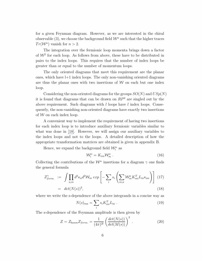
for a given Feynman diagram. However, as we are interested in the chiral

observable (3), we choose the background field Wα such that the higher traces

Tr(Wn) vanish for n > 2.

The integration over the fermionic loop momenta brings down a factor

of W2 for each loop. As follows from above, these have to be distributed in

pairs to the index loops. This requires that the number of index loops be

greater than or equal to the number of momentum loops.

The only oriented diagrams that meet this requirement are the planar

ones, which have l+1 index loops. The only non-vanishing oriented diagrams

are thus the planar ones with two insertions of W on each but one index

loop.

Considering the non-oriented diagrams for the groups SO(N) and USp(N)

it is found that diagrams that can be drawn on RP 2 are singled out by the

above requirement. Such diagrams with l loops have l index loops. Conse-

quently, the non-vanishing non-oriented diagrams have exactly two insertions

of W on each index loop.

A convenient way to implement the requirement of having two insertions

for each index loop is to introduce auxiliary fermionic variables similar to

what was done in [18]. However, we will assign our auxiliary variables to

the index loops and not to the loops. A detailed description of how the

appropriate transformation matrices are obtained is given in appendix B.

Hence, we expand the background field Wαi as

Wαi = KimW

αm . (16)

Collecting the contributions of the Wα insertions for a diagram γ one finds

the general formula

Zγferm. :=

∫

∏

a,m

d2κad2Wm exp

[

−∑

i

si

(

∑

m,a

WαmKT

miLiaκaα

)]

(17)

= det(N(s))2, (18)

where we write the s-dependence of the above integrands in a concise way as

N(s)ma =∑

i

siKTmiLia . (19)

The s-dependence of the Feynman amplitude is then given by

Z = ZbosonZferm. =1

(4π)2l

(

det(N(s))

det(M(s))

)2

. (20)

6

4.2 Perturbative Superpotential

Before we turn to the evaluation of Z we pause for a while to write the

Feynman amplitudes in terms of the notation we have developed so far.

We use the definition for the glueball superfield

S =1

32π2Tr[WαWα] , (21)

to express the amplitudes in terms of S. The amplitude corresponding to a

planar diagram γ can then be written as

Aγplanar = N h cγ

(

16π2S)h−1

∫

∏

i

dsi e−simZ(γ, s) . (22)

N comes from the summation over the free index loop. This factor is the

same as for U(N). The factor h is combinatorial and counts the number of

ways to pick one free index loop out of a total of h. Finally, cγ denotes the

multiplicity of the graph γ.

For a diagram γ on RP 2 we have

BγRP 2 = σ cγ

(

16π2S)h∫

∏

i

dsi e−simZ(γ, s) . (23)

This general amplitude exhibits some important differences compared to the

planar amplitude (22). First, we do not have any index loop without inser-

tions. Therefore, the factor N , that we have in the planar case is absent.

Secondly, the factor σ, which takes the values ±1, serves to distinguish the

group SO(N) from USp(N). This is due to the fact that the propagator for

the adjoint of USp(N) also includes the skew-symmetric USp(N) invariant

J whose insertions give an overall minus sign for the USp(N) as compared

to SO(N) for the RP 2 diagrams. The details are given in appendix A.

In terms of these amplitudes the perturbative part of the effective su-

perpotential is given as a function of S as

W pert.eff (S) =

∑

γ

(Aγplanar + Bγ

RP 2) . (24)

The amplitudes can be generated from a zero-dimensional field theory if

Z(γ, s) is independent of s. This has been shown for U(N) gauge group in

[18]. Similarly the s-dependence vanishes for SO(N) and USp(N), as we will

show in the next section.

7

5 Proof Of Matrix Model Conjecture

In this section we calculate the value of the ratio λ of the fermionic to the

bosonic determinant,

λ =

(

det(N(s))

det(M(s))

)2

. (25)

We will show that the ratio λ does not depend on the Schwinger parameters

si and we will calculate its value explicitly for an arbitrary Feynman graph

on S2 as well as on RP 2. We find that λ = 1 on S2 and λ = 4 on RP 2.

For the following it will be convenient to think of RP 2 as a disk with

opposite points on the boundary identified.

In order to actually calculate (25) we will now relate the matrix L to

the matrix K, by introducing index loop momenta bm through ~k = O~b. We

find the simple relation K = LO, which allows to calculate λ,

λ = det(O)2. (26)

That is, the Schwinger parameters cancel.

Furthermore, we will show that det(O) = 2 holds for all graphs on RP 2,

whereas det(O) = 1 for all graphs on S2 .

The problem of calculating O factorizes into two sub-problems: An ar-

bitrary graph on RP 2 looks like a planar graph with lines emerging from the

boundary loop. These lines cross the boundary of the disk, enter the disk

at the opposite boundary point and, finally, fuse the boundary loop again.

So a graph actually separates into two parts: The boundary loop with the

emerging lines and the interior of the planar graph. Suppressing the interior,

the generic exterior part is shown in Figure 1. The two parts of the graphs

can be treated separately. Of course, graphs on S2 are treated implicitly, by

suppressing the contribution of the exterior graph.

5.1 The Interior Graph.

As just mentioned the interior graph looks exactly like a planar graph, with

the outer loop omitted. Now in planar graphs the interior index momenta ~b

are exactly the loop momenta ~k such that from

pi = Liaka = Kimbm , (27)

8

3

1

2

n

b b

b

1b

2 3

n

k

kk

k

1k

1b

Figure 1: Star-diagram for generic graph on RP 2. The labels bi denote the

momenta associated to the index loops. The loop momenta are denoted by

ka.

we see that K = L. The index i runs over propagators that do not cross the

boundary of the disk, and the indices a and m label the loops and the index

lines, which are actually the same.

We use the matrix O introduced above for the basis change from the

loop momenta ka to the index momenta bm,

bm = O−1maka . (28)

According to the factorization into interior and exterior graph O splits as

O =

(

Oint. 00 Oext.

)

. (29)

For the interior momenta we just argued that the matrix Oint. obeys Oint. =

1. Now we turn to the calculation of Oext..

9

5.2 The Exterior Graph

By definition (16) the index loop momenta bm are related to the propagator

momenta pi like

pi = Kimbm . (30)

Here m, i run from 1 to n, the number of twisted propagators. 3 The index

loop momenta, on the other hand, give the loop momenta ka. As can be read

off from Figure 1, the momenta flowing in the index lines bi are related to

the momenta in the canonical loops ki like

k1 = b1 + bn, (31)

kl = bl − bl−1, l 6= 1 . (32)

Thus we find the identity

KO−1 = L . (33)

Plugging this relation into the definitions of M(s) = LT SL and N(s) =

KT SL, we find, as promised

λ = det(O)2 . (34)

It is easy to calculate the determinant of O for arbitrary n. The value is

det(O) = 1 + (−1)n+1(−1)n−1 = 2 . (35)

Hence, the value of the factor λ is

λ =

(

det(N(s))

det(M(s))

)2

= det(O)2 = 4 . (36)

6 Discussion of Matrix Model Conjectures

After the cancellation of the fermionic and bosonic measures, the integrals

over the Schwinger parameters (7) are given by

∫ L∏

i=1

dsie−sim =

1

mL. (37)

3Twisted propagators are propagators that cross the boundary of the disk.

10

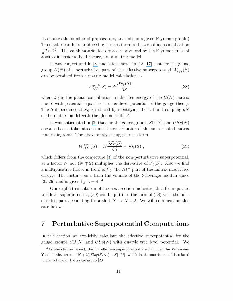
(L denotes the number of propagators, i.e. links in a given Feynman graph.)

This factor can be reproduced by a mass term in the zero dimensional actionm2Tr[Φ2]. The combinatorial factors are reproduced by the Feynman rules of

a zero dimensional field theory, i.e. a matrix model.

It was conjectured in [3] and later shown in [18, 17] that for the gauge

group U(N) the perturbative part of the effective superpotential Weff(S)

can be obtained from a matrix model calculation as

W pert.eff (S) = N

∂F0(S)

∂S, (38)

where F0 is the planar contribution to the free energy of the U(N) matrix

model with potential equal to the tree level potential of the gauge theory.

The S dependence of F0 is induced by identifying the ’t Hooft coupling gN

of the matrix model with the glueball-field S.

It was anticipated in [3] that for the gauge groups SO(N) and USp(N)

one also has to take into account the contribution of the non-oriented matrix

model diagrams. The above analysis suggests the form

W pert.eff (S) = N

∂F0(S)

∂S+ λG0(S) , (39)

which differs from the conjecture [3] of the non-perturbative superpotential,

as a factor N not (N ∓ 2) multiplies the derivative of F0(S). Also we find

a multiplicative factor in front of G0, the RP 2 part of the matrix model free

energy. The factor comes from the volume of the Schwinger moduli space

(25,26) and is given by λ = 4. 4

Our explicit calculation of the next section indicates, that for a quartic

tree level superpotential, (39) can be put into the form of (38) with the non-

oriented part accounting for a shift N → N ∓ 2. We will comment on this

case below.

7 Perturbative Superpotential Computations

In this section we explicitly calculate the effective superpotential for the

gauge groups SO(N) and USp(N) with quartic tree level potential. We

4As already mentioned, the full effective superpotential also includes the Veneziano-

Yankielowicz term −(N ∓ 2)[Slog(S/Λ3) − S] [22], which in the matrix model is related

to the volume of the gauge group [23].

11

compare the contribution of non-orientable Feynman diagrams and planar

ones. We will find a relation between the planar and the non-oriented con-

tributions leading to a simplification of the matrix model description (39).

7.1 General Prescription

With the results of the preceding sections at hand we can now rewrite the

amplitudes in (24). We get

Aγplanar = N h cγ

(

1

m

)L

Sh−1 (40)

for a given planar Feynman diagram γ. For the non-oriented diagrams we

obtain

BγRP 2 = σλRP 2 cγ

(

1

m

)L

Sh . (41)

We note that the powers of 16π2 in (22,23), are canceled by (4π)2l coming

from the bosonic momentum integration (12). (Remember that the number

of loops l is related to the number of index loops h by l = h−1 for the planar

and l = h for the non-oriented diagrams.)

7.2 Explicit Calculations

We explicitly apply the rules from above to calculate the perturbative part

of the super-potential for the tree level super-potential

Wtree(Φ) =m

2TrΦ2 + 2g TrΦ4 . (42)

The combinatorial factors cγ in equations (40,41) receive contributions 5

(1/2)L from the propagators (49,55) and a factor of 2g from each vertex.

The total is given by

cγ =

(

1

2

)L

(2g)V × (combinatorics) . (43)

5L,V and F will in the following denote the number of propagators, i.e. links, vertices

and faces of a given Feynman graph. Furthermore we will use the relation 2V = L for the

Φ4 interaction.

12

O(g )2

2 −4 1

−8−82

2 8

16 −32 −32

32−3216

1O(g )

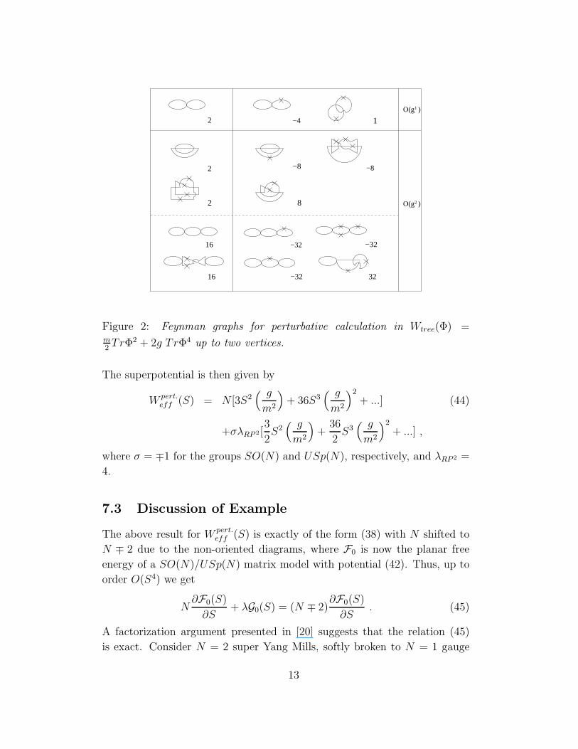
Figure 2: Feynman graphs for perturbative calculation in Wtree(Φ) =m2TrΦ2 + 2g TrΦ4 up to two vertices.

The superpotential is then given by

W pert.eff (S) = N [3S2

( g

m2

)

+ 36S3( g

m2

)2

+ ...] (44)

+σλRP 2[3

2S2( g

m2

)

+36

2S3( g

m2

)2

+ ...] ,

where σ = ∓1 for the groups SO(N) and USp(N), respectively, and λRP 2 =

4.

7.3 Discussion of Example

The above result for W pert.eff (S) is exactly of the form (38) with N shifted to

N ∓ 2 due to the non-oriented diagrams, where F0 is now the planar free

energy of a SO(N)/USp(N) matrix model with potential (42). Thus, up to

order O(S4) we get

N∂F0(S)

∂S+ λG0(S) = (N ∓ 2)

∂F0(S)

∂S. (45)

A factorization argument presented in [20] suggests that the relation (45)

is exact. Consider N = 2 super Yang Mills, softly broken to N = 1 gauge

13

theory by a quartic tree level potential. It was argued in [20] that the value

at the minimum of the effective superpotentials for SO(2KN − 2K + 2) (or

USp(2KN + 2K − 2)) gauge groups is related to the value at the minimum

of the effective superpotential of SO(2N) (or USp(2N)) as

W 2KN∓2K±2eff (g, m) = KW 2N

eff (g, m) , (46)

for a fixed quartic potential Wtree(Φ) = m/2 TrΦ2 + 2g TrΦ4. The value

of the effective superpotential, calculated from the N = 1 approach and the

N = 2 approach are related as shown in [21].

Applying the factorization (46) suggest for this example that

W pert.eff (S) = (N ∓ 2)

∂F0(S)

∂S. (47)

Acknowledgments We would like to thank O. Aharony, U. Fuchs, T.

Sakai, J. Sonnenschein for valuable discussions. The research was supported

by the US-Israel Binational Science Foundation. The research of H.I.is

supported by the TMR European Research Network.

14

A Double line notation

A.1 Double line notation for SO(N)

It is convenient to represent the Lie algebra of SO(N) by antisymmetric

N × N matrices Mmn, with the condition Mmn = −Mnm. In this notation

adjoint fields are real antisymmetric N × N matrices

Φmn = −Φmn, (48)

and their free propagator in momentum space is proportional to the

projector Pkl mn = 12(δkmδln − δlmδkn),

〈ΦklΦmn〉 ∼1

2(δkmδln − δlmδkn) . (49)

In double line notation we get figure 3. The ends of the lines represent

k

l

m

n

k

l

m

n

1/2

Figure 3: The propagator of SO(N) in double line notation.

indices and the lines represent ’deltas’.

Next we will consider insertions of the gauge fields

exp(−s[Wα, · ]πα) , (50)

in the double line notation. A simple commutator [W, · ] gives

δkmWln −Wmkδln . (51)

Pictorially the index contractions are drawn as in figures 4. If we use the

property Wkm = −Wmk of the representation (48) so(N), we can rewrite

the commutator as

δkmWln + Wkmδln (52)

and in double line notation the second term is denoted by figure 5 For the

exponent (50) this generalizes to

δkm [exp(−sWπ)]ln + [exp(−sWπ)]km δln. (53)

The generalization of the above diagrams is straightforward.

15

Wk

l

m

n W

k

l

m

n

Figure 4: The insertion of a commutator [W, · ] of W ∈ so(N) in double

line notation.

Wk

l

m

n W

k

l

m

n

Figure 5: The insertion of a commutator [W, · ] of W ∈ so(N) in double

line notation, after applying the property Wkm = −Wmk.

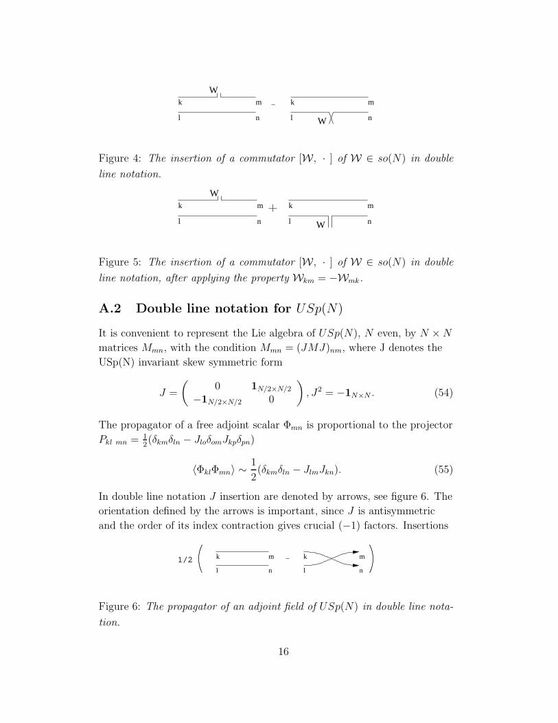
A.2 Double line notation for USp(N)

It is convenient to represent the Lie algebra of USp(N), N even, by N × N

matrices Mmn, with the condition Mmn = (JMJ)nm, where J denotes the

USp(N) invariant skew symmetric form

J =

(

0 1N/2×N/2

−1N/2×N/2 0

)

, J2 = −1N×N . (54)

The propagator of a free adjoint scalar Φmn is proportional to the projector

Pkl mn = 12(δkmδln − JloδomJkpδpn)

〈ΦklΦmn〉 ∼1

2(δkmδln − JlmJkn). (55)

In double line notation J insertion are denoted by arrows, see figure 6. The

orientation defined by the arrows is important, since J is antisymmetric

and the order of its index contraction gives crucial (−1) factors. Insertions

1/21/2 k

l

m

n

k

l

m

n

Figure 6: The propagator of an adjoint field of USp(N) in double line nota-

tion.

16

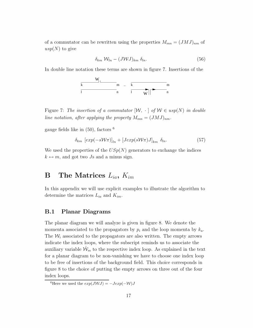
of a commutator can be rewritten using the properties Mmn = (JMJ)nm of

usp(N) to give

δkm Wln − (JWJ)km δln. (56)

In double line notation these terms are shown in figure 7. Insertions of the

Wk

l

m

n

k

l

m

nW

Figure 7: The insertion of a commutator [W, · ] of W ∈ usp(N) in double

line notation, after applying the property Mmn = (JMJ)nm.

gauge fields like in (50), factors 6

δkm [exp(−sWπ)]ln + [Jexp(sWπ)J ]km δln. (57)

We used the properties of the USp(N) generators to exchange the indices

k ↔ m, and got two Js and a minus sign.

B The Matrices Lia, Kim

In this appendix we will use explicit examples to illustrate the algorithm to

determine the matrices Lia and Kim.

B.1 Planar Diagrams

The planar diagram we will analyze is given in figure 8. We denote the

momenta associated to the propagators by pi and the loop momenta by ka.

The Wi associated to the propagators are also written. The empty arrows

indicate the index loops, where the subscript reminds us to associate the

auxiliary variable Wm to the respective index loop. As explained in the text

for a planar diagram to be non-vanishing we have to choose one index loop

to be free of insertions of the background field. This choice corresponds in

figure 8 to the choice of putting the empty arrows on three out of the four

index loops.6Here we used the exp(JWJ) = −Jexp(−W)J

17

p W1 1

12

p W4 4

p W2 2

k2 k

k

1

3

p W3 3

3

Figure 8: Planar Feynman diagram with loop momenta ka, propagator mo-

menta pi, insertions Wi and three out of four index loops, indicated by empty

arrows. The outer index loop is chosen to be free of insertions of Wi.

The matrix Lia gives the expansion of the propagator momenta in terms of

the loop momenta. For the graph in Figure 8 we can make the following

choice

p1 = k1, p2 = k2, p3 = k3 . (58)

Furthermore momentum conservation at the vertices implies that p3 = p4

and thus p4 = k3. Hence, the matrix Lia is given by

L =

1 0 00 1 00 0 10 0 1

(59)

Some straightforward algebra then gives for the product si(LT )aiLib

s1 0 00 s2 00 0 s3 + s4

. (60)

In order to obtain the matrix Kim we just need to read off from the

diagram the contributions of each index loop to a given Wi taking into

account the mutual orientation. This is done in the following way. Starting

with W1 we notice that there is only a contribution from the first index

loop. Moreover, we have chosen the orientation of the index loop to be the

18

same as the orientation of p1, such that we can write

W1 = W1 . (61)

A similar reasoning applies to the remaining Wi such that the matrix K

relating the Wi to the auxiliary variables Wm according to Wi = KimWm is

given by

K =

1 0 00 1 00 0 10 0 1

, (62)

which equals the matrix L as claimed in [18].

B.2 Non-Oriented Diagrams

B.2.1 The first non-oriented diagram

The first non-oriented diagram we will discuss is given in figure 9. The

notation is the same as in the planar case. The only difference is that now

due to the twist in one of the propagators the number of index loops is the

same as the number of momentum loops and we do not have any free index

loop.

The matrix Lia is easily seen to be the same as in the planar diagram of

figure 9. The matrix Kim on the other hand is modified. Applying the same

strategy as in the planar case we find that now W1 will receive

contributions not only from index loop 1 but also from index loop 3. The

orientation of index loop 1 is again chosen to be the same as the orientation

of the momentum p1, whereas index loop 3 is oriented in the opposite way.

The contribution from index loop 3 will therefore come with a negative sign

and we can write

W1 = W1 − W3 . (63)

For W2 we obtain a similar result and for W3, W4 we find that the third

index loop contributes twice at a time with a negative sign leading to

W3 = −2W3 = W4 . (64)

19

12

p W4 4

p W

p W

2 2

3 3

k2 k

k

1

3

p W1 1

33

3

3

Figure 9: Non-orientable Feynman diagram with loop momenta ka, propa-

gator momenta pi, insertions Wi and three index loops, indicated by empty

arrows.

Thus, the matrix K reads

K =

1 0 −10 1 −10 0 −20 0 −2

, (65)

and the matrix si(KT )niLib is given by

s1 0 00 s2 0

−s1 −s2 −2(s3 + s4)

. (66)

B.2.2 The second non-oriented diagram

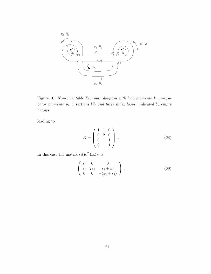
Our second non-oriented diagram is drawn in figure 10.

The matrix K for this diagram is again obtained by applying the above

algorithm. Reading off the contributions of the index loops we find

W1 = W1 + W2, (67)

W2 = 2W2,

W3 = W2 + W3,

W4 = W2 + W3 ,

20

1

3

2

p W4 4

p W

p W

2 2

3 3

k2 k

k

1

3

p W1 1

2

2

Figure 10: Non-orientable Feynman diagram with loop momenta ka, propa-

gator momenta pi, insertions Wi and three index loops, indicated by empty

arrows.

leading to

K =

1 1 00 2 00 1 10 1 1

. (68)

In this case the matrix si(KT )niLib is

s1 0 0s1 2s2 s3 + s4

0 0 −(s3 + s4)

. (69)

21

References

[1] R. Dijkgraaf and C. Vafa, “Matrix models, topological strings, and

supersymmetric gauge theories,” Nucl. Phys. B 644 (2002) 3

[arXiv:hep-th/0206255].

[2] R. Dijkgraaf and C. Vafa, “On geometry and matrix models,” Nucl.

Phys. B 644 (2002) 21 [arXiv:hep-th/0207106].

[3] R. Dijkgraaf and C. Vafa, “A perturbative window into

non-perturbative physics,” arXiv:hep-th/0208048.

[4] N. Dorey, T. J. Hollowood, S. Prem Kumar and A. Sinkovics, “Exact

superpotentials from matrix models,” arXiv:hep-th/0209089.

[5] N. Dorey, T. J. Hollowood, S. P. Kumar and A. Sinkovics, “Massive

vacua of N = 1* theory and S-duality from matrix models,”

arXiv:hep-th/0209099.

[6] F. Ferrari, “On exact superpotentials in confining vacua,”

arXiv:hep-th/0210135.

[7] H. Fuji and Y. Ookouchi, “Comments on effective superpotentials via

matrix models,” arXiv:hep-th/0210148.

[8] D. Berenstein, “Quantum moduli spaces from matrix models,”

arXiv:hep-th/0210183.

[9] R. Argurio, V. L. Campos, G. Ferretti and R. Heise, “Exact

superpotentials for theories with flavors via a matrix integral,”

arXiv:hep-th/0210291.

[10] J. McGreevy, “Adding flavor to Dijkgraaf-Vafa,”

arXiv:hep-th/0211009.

[11] I. Bena and R. Roiban, “Exact superpotentials in N = 1 theories with

flavor and their matrix model formulation,” arXiv:hep-th/0211075.

[12] Y. Demasure and R. A. Janik, “Effective matter superpotentials from

Wishart random matrices,” arXiv:hep-th/0211082.

22

[13] S. G. Naculich, H. J. Schnitzer and N. Wyllard, “The N = 2 U(N)

gauge theory prepotential and periods from a perturbative matrix

model calculation,” arXiv:hep-th/0211123.

[14] R. Dijkgraaf, S. Gukov, V. A. Kazakov and C. Vafa, “Perturbative

analysis of gauged matrix models,” arXiv:hep-th/0210238.

[15] R. Gopakumar, “N = 1 theories and a geometric master field,”

arXiv:hep-th/0211100.

[16] A. Klemm, M. Marino and S. Theisen, “Gravitational corrections in

supersymmetric gauge theory and matrix models,”

arXiv:hep-th/0211216.

[17] F. Cachazo, M. R. Douglas, N. Seiberg and E. Witten, “Chiral rings

and anomalies in supersymmetric gauge theory,”

arXiv:hep-th/0211170.

[18] R. Dijkgraaf, M. T. Grisaru, C. S. Lam, C. Vafa and D. Zanon,

“Perturbative computation of glueball superpotentials,”

arXiv:hep-th/0211017.

[19] S. J. Gates, M. T. Grisaru, M. Rocek and W. Siegel, “Superspace, Or

One Thousand And One Lessons In Supersymmetry,” Front. Phys. 58

(1983) 1 [arXiv:hep-th/0108200].

[20] H. Fuji and Y. Ookouchi, “Confining phase superpotentials for SO/Sp

gauge theories via geometric transition,” arXiv:hep-th/0205301.

[21] F. Cachazo and C. Vafa, “N = 1 and N = 2 geometry from fluxes,”

arXiv:hep-th/0206017.

[22] G. Veneziano and S. Yankielowicz, “An Effective Lagrangian For The

Pure N=1 Supersymmetric Yang-Mills Theory,” Phys. Lett. B 113

(1982) 231.

[23] H. Ooguri and C. Vafa, “Worldsheet derivation of a large N duality,”

Nucl. Phys. B 641 (2002) 3 [arXiv:hep-th/0205297].

23