O 618785 N/A N/A
261
ENGINEERING CHANGE NOTICE Paga 1 of _ O 618785 ProJ. ECN 2. ECN Category (mark one) Supplemental Direct Revision Change ECN Temporary Standby p Cancel/Void 3. Originator's Name, Organization, HSIN, and Telephone No. T. H. Brown, R2-12, 373-4437 6. Project Title/No./Uork Order No. Supporting Document for the Historical Tank Content "Estimate "Tb"f 9. Document Numbers Changed by this ECN (includes sheet no. and rev.) WHC-SD-WM-ER-319, Rev. 0 4. USQ Required? [] Yes [ X ] No 7. Bldg./Sys./Fac. No. 2750/200E 10. Related ECN No(s). N/A 02/13/97 8. Approval Designator N/A 11. Related PO No. N/A 12a. Modification Uork [] Yes (fill out Blk. 12b) [X] No (NA Blks. 12b, 12c, 12d) 12b. Uork Package No. N/A 12c. Modification Work Complete N/A Design Authority/Cog. Engineer Signature & Date 12d. Restored to Original Condi- tion (Temp, or Standby ECN only) N/A Design Authority/Cog. Engineer Signature S Date 13a. Description of Change 13b. Design Baseline Document? [] Yes [X] No 1. Complete rewrite and update of the introduction section. 2. Added HTCE and Supporting Document flow diagram. 3. Added SE quadrant tank farms timeline diagram. 4. Updated and restructured waste and level history plots. 5. Removed temperature data tables since they are available on PC-SACS. 6. Removed drywell data, plots and well layout diagram. 7. Removed chemical and radionuciide sample data and laboratory reports. 8. Removed unknown tank transfer plots from LANL. 9. Added the Hanford Tank Chemical and Radionuclide Inventories: HWD Model, inventory estimate tables. Rev. 4, 14a. Justification (mark one) Criteria Change [] Design Improvement [X] Environmental [] As-Found [] faci litate Const [] Const. Error/Omission [] Facility Deactivation [] Design Error/Omission [] 14b. Justification Details To update the supporting document with more complete historical and tank inventory information. 15. Distribution (include name, MSIN, and no. of copies) See attached distribution sheet. SE STjMjP A-7900-013-2 (05/96) GEF095 A-79OO-O13-1
-
Upload
khangminh22 -
Category
Documents
-
view
0 -
download
0
Transcript of O 618785 N/A N/A

ENGINEERING CHANGE NOTICEPaga 1 of _
O 618785ProJ.ECN
2. ECN Category(mark one)
SupplementalDirect RevisionChange ECNTemporaryStandby
pCancel/Void
3. Originator's Name, Organization, HSIN,and Telephone No.
T. H. Brown, R2-12, 373-44376. Project Title/No./Uork Order No.
Supporting Document for theHistorical Tank Content
"Estimate "Tb"f9. Document Numbers Changed by this ECN
(includes sheet no. and rev.)
WHC-SD-WM-ER-319, Rev. 0
4 . USQ Required?
[ ] Yes [ X ] No
7. Bldg./Sys./Fac. No.
2750/200E
10. Related ECN No(s).
N/A
02/13/978. Approval Designator
N/A
11. Related PO No.
N/A12a. Modification Uork
[] Yes (fill out Blk.
12b)[X] No (NA Blks. 12b,
12c, 12d)
12b. Uork PackageNo.
N/A
12c. Modification Work Complete
N/A
Design Authority/Cog. EngineerSignature & Date
12d. Restored to Original Condi-tion (Temp, or Standby ECN only)
N/A
Design Authority/Cog. EngineerSignature S Date
13a. Description of Change 13b. Design Baseline Document? [] Yes [X] No
1. Complete rewrite and update of the introduction section.2. Added HTCE and Supporting Document flow diagram.3. Added SE quadrant tank farms timeline diagram.4. Updated and restructured waste and level history plots.5. Removed temperature data tables since they are available on PC-SACS.6. Removed drywell data, plots and well layout diagram.7. Removed chemical and radionuciide sample data and laboratory reports.8. Removed unknown tank transfer plots from LANL.9. Added the Hanford Tank Chemical and Radionuclide Inventories: HWD Model,
inventory estimate tables.Rev. 4,
14a. Justification (mark one)
Criteria Change [] Design Improvement [X] Environmental []
As-Found [] faci litate Const [] Const. Error/Omission []
Facility Deactivation []
Design Error/Omission []
14b. Justification Details
To update the supporting document with more complete historical and tank inventoryinformation.
15. Distribution (include name, MSIN, and no. of copies)
See attached distribution sheet.SE STjMjP
A-7900-013-2 (05/96) GEF095
A-79OO-O13-1

ENGINEERING CHANGE
16. DesignVer i f icat ionRequi red
[ ] Yes[X] No
19. Change Impactthai: wi 11 be
SDD/DD
Functional Design Crit
Operating Specificatio
Criticality Specificatio
17. Cost Impact
ENGINEERING
Additional [ ] $Savings [ ] $
NOTICE
Additional
Savings
Review: Indicate the related documents (other
Page 2
INSTRUCTION
[] $
of 2
1. ECN (use no. from pg. 1)
61878518. Schedule Impact (days )
Improvement r 1
Delay r "1
than the engineering documents identif ied on side 1)affected by the change described in Block 13. Enter the affectec
[ ]
[ ][3N
Conceptual Design Report 1" ]
Equipment Spec.
Const. Spec.
Procurement Spec.
Vendor Information
OM Manual
FSAR/SAR
Safety Equipment List
[ ][ ][ ][ ][ ][ ][ ]
Radiation Work Permit • i
Environmental Impact Statement r "1Environmental Report
Environmental Permit
20. Other Affecteindicate that
[ ][ ]
Seismic/Stress Analysis
Stress/Design Report
Interface Control Drawing
Calibration Procedure
Installation Procedure
Maintenance Procedure
Engineering Procedure
Operating Instruction
Operating Procedure
Operational Safety Require
IEFD Drawing
Cell Arrangement Drawing
Fac. Proc. Samp. Schedule
Inspection Plan
Inventory Adjustment Req
r j[ ][ ][ ][ ][ ]r j[ ][ ]
ment [ ]
[ ]
[ ]
[][ ]
est r "I
d Documents: (NOTE: Documents listed below wi l l not be revised
document number in Block 20.Tank Calibration Manual
Health Physics Procedure
Spares Multiple Unit Listing
Test Procedures/Specification
Component Index
ASME Coded Item
Human Factor Consideration
Computer Software
Electric Circuit Schedule
ICRS Procedure
Process Control Manual/Plan
Process Flow Chart
Purchase Requisition
Tickler File
N/A
by this ECN.) Signatures belokthe signing organization has been notified of other affected documents listed below.
Document Number/Revision
N/A
21. Approvals
Design Authority
Cog. Eng. T. M.
Cog. Mgr. J. W.
QA
Safety
Envi ron.
Other
Signature
Caiimann QOCasn-vnuin
Document Number/Revision
Date
•?/7/? 7^ 3///'/ 7
Design Agent
PE
QA
Safety
Design
Environ.
Other
Lead Engineer
Project Mgr C
DEPARTMENT OF
Signature or
[ ][ ][ ][ ][ ][ ][ ][ ][ ][ ][ ][ ][][][ ][X]
Document Number Revision
Signature 0 0 ^ - ^ -J. L. Stroup °<JD^gctt$t4j^ 5
o ~~
J. U. Funk t « / - F«X " j j. H. Brevick tylriiirt< h atENERGY
a C o n t r o l Number t h a tt racks the Approval Signature
ADDITIONAL
Date
Mil
A-7900-013-3 (05/96) GEF096

HNF-SD-WM-ER-319, Rev. 1
Supporting Document for the Historical TankContent Estimate for SY-Tank Farm
C. H. Brevick, J. L. Stroup, J. W. FunkFluor Daniel Northwest Inc., Richland, WA 99352U.S. Department of Energy Contract DE-AC06-96RL13Z00
EDT/ECN: 618785 UC: 2070Org Code: 408 Charge Code: E18675B&R Code: EW3120074 Total Pages: i<;y
Key Words: Southeast quadrant, Historical Tank Content Estimate, tankfarms, tank level, tank temperture, aerial photos, in-tank montages,TLM, SMM, waste temperature plots, inventory estimates, riser locations
Abstract: This Supporting Document provides historical in-depthcharacterization information on SY-Tank Farm, such as historical wastetransfer and level data, tank physical information, temperature plots,liquid observation well plots, chemical analyte and radionuclideinventories for the Historical Tank Content Estimate Report for theSoutheast Quadrant of the Hanford 200 Areas.
TRADEMARK DISCLAIMER. Reference herein to any specific commercial product, process, or service bytrade name, trademark, manufacturer, or otherwise, does not necessarily constitute or imply itsendorsement, recommendation, or favoring by the United States Government or any agency thereof orits contractors or subcontractors.
Printed in the United States of America. To obtain copies of this document, contact: DocumentControl Services, P.O. Box 950, MaiIstop H6-08, Richland UA 99352, Phone (509) 372-2420;Fax (509) 376-4989.
Release Approval 7Date Release Stamp
Approved for Public Release
A-6400-073 (01/97) GEF321

RECORD OF REVISION(1) Document Number
HNF-SD-WM-ER-319 Page 1
(2) Ti t le
Supporting Document for the Historical Tank Content Estimate for SY-Tank Farm
CHANGE CONTROL RECORD
(3) Revision
01 RS
(4) Description of Change - Replace, Add, and Delete Pages
<7> I n i t i a l issue, EDT 612789, 09/13/951. Complete rewrite and update of introduction section,2. Added HTCE and Supporting Document flow diagram.3. Added SE quadrant tank farms timeline diagram.4. Updated and restructured waste and level history plots.5. Removed temperature data tables.6. Removed drywell data tables and plots.7. Removed sample data and reports.8. Removed unknown tank transfer plots.9. Added more extensive tank waste inventory tables, HDW
Model, Rev. 4
Incorporates ECN No. 618785
Authorized for Release(5) Coq. Enqr.
T. M. Brown
T. M. Brown
(6) Coq. Mqr. Date
S. J. Eberlein
W. J . Cammann
i'7/17
A-7320-005 <08/91) UEF168

HNF-SD-WM-ER-319,Rev. 1
SUPPORTING DOCUMENT FOR THEHISTORICAL TANK CONTENT ESTIMATE
FOR
SY TANK FARM
Prepared for
Lockheed Martin Hanford Corporation
February 1997
Prepared by
J. W. FunkR. G. HaleG. A. LisleC. V. Salois
M. R. Umphrey
Fluor Daniel NorthwestRichland, Washington

HNF-SD-WM-ER-319, Rev. 1
SUPPORTING DOCUMENT FOR THEHISTORICAL TANK CONTENT
ESTIMATE FOR
S Y TANK FARM
WORK ORDER El 8675
APPROVED:
Fluor Daniel Northwest
Te^Jmical Documents
Lead Engineer
De^gn Agent /
Project Manager
Lockheed Martin Hanford Corporation
sAA 7' Da'te
Date
3/V?7Date
" Date
3/7/17T^hnical Lead, TWRS DQO, Models and Inventory Date

HNF-SD-WM-ER-319,Rev. 1
ACKNOWLEDGMENTS
A project of the this magnitude would not be possible without thehelp of a significant number of persons and organizations. FluorDaniel Northwest, would like to acknowledge the contributions madeby our Los Alamos National Laboratory counterparts: Stephen F.Agnew, Kenneth A. Jurgensen, Robert A. Corbin, Tomasita B.Duran, Bonnie L. Young, Theodore P. Ortiz, John FitzPatrick, andJames Boyer. Also, Todd Brown, Brett Simpson and Jerry Cammannof Lockheed Martin Hanford Corporation are recognized for theircontributions.

HNF-SD-WM-ER-319,Rev. 1
INFORMATION FEEDBACK CARD
SUPPORTING DOCUMENT FOR THE HISTORICALTANK CONTENT ESTIMATE FOR
SY TANK FARM
COMMENTS AND CONTRIBUTIONS
The reader is requested to use this card to comment on this document, report any discrepancies, orcontribute new information to improve the accuracy and content of the document. Please use thespace provided, add additional pages if necessary, and return the comments to the person noted at theaddress listed below.
Send Comments to: Mr. Jerry W. CammannLockheed Martin Hanford CorporationTWRS DQO, Models and InventoryP.O. Box 1970, MSINR2-12Richland, WA 99352

HNF-SD-WM-ER-319,Rev. 1
TABLE OF CONTENTS
1.5
1.6
1.7
1.8
1.0 Introduction • 11.0.1 Purpose 11.0.2 Scope 1.0.3 Approach 5
1.1 Safety Issues 5.1.1 Watch List Safety Issues 5.1.2 Non-Watch List Safety Issues 5.1.3 Occurrences 6
1.2 Waste Generating Plants and Processes 6.2.1 Plants Processes 6.2.2 Waste Management Operations 10.2.3 Miscellaneous Waste Sources and Equipment 11
1.2.4 Time Lines 121.3 Waste and Level History 17
1.3.1 Source of Data 171.3.2 Development of Data 171.3.3 Assumptions 191.3.4 Quality of Data 19
1.4 Temperatures 19.4.1 Surveillance Techniques 19.4.2 Source of Data 20.4.3 Development of Data 20.4.4 Assumptions 21.4.5 Quality of Data 22
Waste Surface Level 22.5.1 Surveillance Techniques 22.5.2 Source of Data 23.5.3 Development of Data 24.5.4 Assumptions 24.5.5 Quality of Data 24
Riser Configuration 251.6.1 Source of Data 251.6.2 Development of Data 251.6.3 Assumptions 261.6.4 Quality of Data 26Photographs and Montages 26
.7.1 Source of Data 26
.7.2 Development of Data 26
.7.3 Quality of Data 27Inventory Estimates 27
.8.1 Source of Data 27
.8.2 Development of Data 27

HNF-SD-WM-ER-319,Rev. 1
2.0 SYTankFarm 282.0.1 SY Tank Farm Information 282.0.2 SY Tank Farm Waste and Level History 282.0.3 SY Tank Farm Temperature History 282.0.4 SY Tank Farm Occurrences 282.0.5 SY Tank Farm Current Status 282.0.6 SY Tank Farm Photograph and Montages 282.0.7 SY Tank Farm Inventory Estimates 29
2.1 Tank 241-SY-101 302.1.1 Waste and Level History of Tank 241-SY-101 302.1.2 Temperature History of Tank 241-SY-101 302.1.3 Occurrences for Tank 241-SY-101 312.1.4 Current Status of Tank 241-SY-101 312.1.5 Interior Montage of Tank 241-SY-101 312.1.6 Inventory Estimate of Tank 241-SY-101 31
2.2 Tank 241-SY-102 322.2.1 Waste and Level History of Tank 241-SY-102 322.2.2 Temperature History of Tank 241-SY-102 322.2.3 Occurrences for Tank 241-SY-102 322.2.4 Current Status of Tank 241-SY-102 322.2.5 Interior Montage of Tank 241-SY-102 332.2.6 Inventory Estimate of Tank 241-SY-102 33
2.3 Tank 241-SY-103 342.3.1 Waste and Level History of Tank 241-SY-103 342.3.2 Temperature History of Tank 241-SY-103 342.3.3 Occurrences for Tank 241-SY-103 342.3.4 Current Status of Tank 241-SY-103 352.3.5 Interior Montage ofTank 241-SY-103 352.3.6 Inventory Estimate ofTank 241-SY-103 35
APPENDICES
Appendix A GlossaryAppendix B ReferencesAppendix C Waste and Level History Sketches and DataAppendix D Temperature GraphsAppendix E Waste Surface Level GraphsAppendix F Riser Configuration Sketches and TablesAppendix G Tank Farm Photograph and Tank MontagesAppendix H Inventory Estimates

HNF-SD-WM-ER-319,Rev. 1
TRADEMARKS
Microsoft Excel is a registered trademark of Microsoft Corporation.
ENRAF is a registered trademark of Delft Instruments.
AutoCAD is a registered trademark of Autodesk, Inc.

HNF-SD-WM-ER-319,Rcv. 1
1.0 Introduction
1.0.1 Purpose
The purpose of this historical characterization document is to present the synthesized summariesof the historical records concerning the physical characteristics, radiological, and chemical compositionof mixed wastes stored in underground double-shell tanks and the physical conditions of these tanks.The double-shell tanks are located on the United States Department of Energy's Hanford Site,approximately 25 miles northwest of Richland, Washington. The document will be used to assist incharacterizing the waste in the tanks in conjunction with the current program of sampling and analyzingthe tank wastes. Los Alamos National Laboratory (LANL) developed computer models that used thehistorical data to attempt to characterize the wastes and to generate estimates of each tank's inventory.A historical review of the tanks may reveal anomalies or unusual contents that could be critical tocharacterization and post characterization activities.
This document was developed by reviewing the operating plant process histories, waste transferdata, and available physical and chemical data from numerous resources. These resources weregenerated by numerous contractors from 1945 to the present.
Waste characterization, the process of describing the character or quality of a waste, is requiredby Federal law (Resource Conservation and Recovery Act [RCRA]) and state law (WashingtonAdministrative Code [WAC] 173-303, Dangerous Waste Regulations). Characterizing the waste isnecessary to determine methods to safely retrieve, transport, and/or treat the wastes.
This document is not intended for use as a total design basis document. Further investigationsof the information may be required before using this data for design purposes or safety analysis.
1.0.2 Scope
The scope of this document covers available information about the wastes contained in thedouble-shell tanks in the SY Tank Farm. Waste transfer and level data, tank physical information, andsurveillance data of tanks and wastes have been compiled for this document. The inventory estimatesof waste types and volumes generated by the computer modeling programs developed by LANL areincluded also. A summary of this information is contained in the Historical Tank Content Estimate(HTCE) for the Southeast Quadrant of the Hanford 200 Areas (Brevick et al., 1997). The SoutheastQuadrant (SE Quadrant) document covers six double-shell tank farms. Five of the tank farms, AN, AP,AW, AY and AZ, are located in the 200 East Area and are shown on the map in Figure 1. The othertank farm, SY, is located in the 200 West Area and is shown on the map in Figure 2. A flow diagramshowing the relationships between the sources of data, the HTCE, and the supporting documents is inFigure 3.
This document also includes information on the safety issues affecting the tanks and the plantsand processes that produced the waste in the underground waste storage tanks.
- 1 -

HNF-SD-WM-ER-319. Rev. 1
7THST r;l*> J a-M-AR f
C Plant CStrontiun Senlworks)—^ \DST (^
Legend
Boundories ——. .—-
Railroad
Sirigle-Sheli Tank - SST
Double-Shell Tank - DST
Figure 1. 200 East Area.
- 2 -

HNF-SD-WM-ER-319. Rev. 1
Legend
Tanks O
Boundaries •
Railroad
Single-Shell Tank - SST
Double-Shell Tank - DST
Figure 2. 200 West Area.
- 3 -

HNF-SD-WM-ER-319,Rev. 1
HISTORICALDATA
INVENTORY ESTIMATES
(Afiew et «l., 1997)
SUPPORTING
DOCUMENT
AN
TANK FARM
(Brcvick ct il., 1997»)
SUPPORTING
DOCUMENT
AY
TANK FARM
(Breviek et •!., 1997d)
SUPPORTING
DOCUMENT
AP
TANK FARM
(Brivick it •!., 1997b)
SUPPORTING
DOCUMENT
AZ
TANK FARM(Breviek el >L, 1997e)
SUPPORTING
DOCUMENT
AW
TANK FARM
(Brevick et •!., 1997c)
SUPPORTING
DOCUMENT
SY
TANK FARM
HTCE
SE QUADRANT(Brevick et al., 1997f)
HISTORICAL TANK CONTENT ESTIMATE
Figure 3 HTCE and Supporting Document Flow Diagram
- 4 -

HNF-SD-WM-ER-319,Rev. 1
1.0.3 Approach
This document was compiled from work performed by Fluor Daniel Northwest (FDNW), LANL,and Lockheed Martin Hanford Corporation (LMHC). FDNW reviewed the historical records ofthe tanks and incorporated the inventory estimates and models of waste layers in the tanks beingdeveloped by LANL into this document.
1.1 Safety Issues
The safety issues that affect the tanks can be divided into two groups: watch list and non-watchlist. The watch lists are listings of tanks believed to pose potential safety hazards to workers, theenvironment, and the public. Non-watch list issues are of concern because of their possible effect onworkers and the environment. Occurrences are unusual events on the Hanford Site that sometimes arerelated to safety issues.
1.1.1 Watch List Safety Issues
Watch list safety issues for these tanks were identified as "issues/situations that contain mostof the necessary conditions that could lead to worker (onsite) or offsite radiation exposure through anuncontrolled release of fission products" under Public Law 101-510, Section 3137, of the NationalDefense Authorization Act of Fiscal Year 1991 (i.e., the Wyden Amendment). As of September 1996,32 single-shell tanks and 6 double-shell tanks are on watch lists. See the Approach for Tank SafetyCharacterization of Hanford Site Waste (Eberlein et al., 1995) for more information on the watch listissues.
1.1.2 Non-Watch List Safety Issues
Non-watch list issues include safety hazards such as leaking tanks. Tank leaks are a safetyhazard because of their potential to release chemicals and radioactive liquids into the ground.Corrosion is the main cause of tank leaks. Three other safety issues that do not require a watch list andcontinual monitoring under the Wyden Amendment include criticality, tank bumps, and toxic vaporreleases. The following sections provide a general description of the different non-watch list safetyissues. See the Hanford Site Tank Farm Facilities Interim Safety Basis (Leach and Stahl, 1993)formore information.
• CorrosionCorrosion is the most probable degradation mechanism of the steel tank liners resulting from
contact with liquid, liquid-vapor, vapor, and solid phases of the wastes. The corrosion mechanisms thatreduce the thickness of the carbon steel liners can be divided into two categories: localized and generalor uniform. Localized corrosion occurs on a localized area of the liner surface. Some of the localizedcorrosion mechanisms include pitting corrosion, stress corrosion cracking, and crevice corrosion.General or uniform corrosion occurs over the entire liner surface. Corrosion of the steel tank liners mayinvolve more than one of these mentioned mechanisms. Corrosion is a safety issue because it has thepotential to degrade the tank liner to the point of causing a leak or, more seriously, structural failureof the tank. Either condition could release contamination to the environment.
- 5 -

HNF-SD-WM-ER-319,Rcv. 1
• CriticalityCriticality is a self-sustained, nuclear chain reaction that can occur when a sufficient mass of
fissile material is present in the proper configuration along with a neutron source to start the nuclearreaction. Criticality in the tank farms has been declared an unreviewed safety question, even thoughthe Hanford Site Tank Farm Facilities Interim Safety Basis (Leach and Stahl, 1993) indicates that a"nuclear criticality accident in the tank farms is probably not an imminent risk." The unreviewed safetyquestion on criticality in the tank farms remains because the inventory of fissile material and itsdistribution within the tanks cannot be confirmed as being within the approved safety envelope definedin the current safety analysis reports. Criticality is a safety issue because of the potential to releasecontamination to the environment.
• Tank BumpsA tank bump is the sudden pressurization of the tank. This phenomenon occurs when solids
overheat in the lower portion of the tank followed by uncontrolled mixing of these solids. The stirredhot solids rapidly transfer heat to the liquid in the tank, some of which quickly vaporizes. The rapidvapor generation causes a sudden internal tank pressurization that causes a bump. Uncontrolled mixingof heated solids can occur when an airlift circulator fails allowing the solids to heat up followed byrapid startup of the airlift circulator which causes rapid mixing. Uncontrolled mixing can also occurwhen a natural "rollover" of waste occurs in the tank. Tank bumps are a safety issue because of theirpotential to release contamination to the environment.
• Toxic Vapor ReleasesToxic vapor releases are a recently analyzed safety concern at the Hanford Site. The entire issue
of toxic gas releases at the tank farms is being investigated (Leach and Stahl, 1993).
1.1.3 Occurrences
Over the years, unusual events (occurrences) have occurred at the SY Tank Farm. Anoccurrence is an event that falls outside the normal operating, maintenance and/or constructionprocedures of the tank farm. Occurrences have been documented by various reporting methodsincluding unusual occurrences reports, off-normal reports, event fact sheets, and occurrence reports.The occurrence documentation that could be located was evaluated for its significance in determiningthe waste content of the tanks. The types of occurrences considered significant are those involvingsurface level changes and temperature changes.
1.2 Waste Generating Plants and Processes
1.2.1 Plants Processes
Brief descriptions and histories of the plants and processes that generated waste now containedin the single-shell and double-shell tanks are presented in alphabetical order. Typically, the name ofthe plant and the process are synonymous. The dates and events described in the following briefhistories are presented on time lines in Figures 4 and 5. Although not all of the processes listed belowcontributed waste directly to tanks in the Southeast Quadrant, the waste they generated could have beentransferred indirectly from tank to tank.
- 6 -

HNF-SD-WM-ER-319,Rev. 1
• A Plant (PUREX)The Plutonium Uranium Extraction (PUREX) plant (i.e., A Plant) began operating in
January 1956 (Gerber, 1993a). "The PUREX process is an advanced solvent extraction process thatuses a tributyl phosphate in kerosene solvent for recovering uranium and plutonium from nitric acidsolutions of irradiated uranium. Nitric acid is used instead of metallic nitrates to promote the extractionof uranium and plutonium from aqueous phase to an organic phase." (Wilson and Reep, 1991, p. B-4).Two campaigns of the Thorex process were conducted in 1966 and 1971 (Jungfleisch, 1984). TheThorex process recovered B3U from thorium irradiated in the Hanford Site reactors(Wilson and Reep, 1991). PUREX reprocessed aluminum-clad fuel elements and zirconium alloy-cladfiiel elements, and provided plutonium for research reactor development, safety programs, and defense.Also, PUREX recovered slightly enriched uranium to be recycled as fuel in reactors generatingelectricity and plutonium (Rockwell, 1985). PUREX was put on standby in 1972 (Gerber, 1993a).
The PUREX plant was restarted in November 1983 but was shut down in December 1988 (seeFigure 4). The plant was shut down due to the lack of steam pressure needed to operate the supportbackup safety equipment. There was a brief stabilization run in early 1990. In October 1990, PUREXwas placed on standby by Secretary of Energy James Watkins. DOE issued the final closure order inDecember 1992 (Gerber, 1993b).
• B PlantB Plant used the bismuth phosphate process at first, and later changed its processing capabilities
to strontium and cesium fractionation. The bismuth phosphate process "separated plutonium fromuranium and the bulk of fission products in irradiated fuel by co-precipitation with bismuth phosphatefrom a uranium nitrate solution. The plutonium was then separated from fission products by successiveprecipitation cycles using bismuth phosphate and lanthanum fluoride. The plutonium was isolated asa peroxide and, after dissolving in nitric acid, was concentrated as plutonium nitrate. The wastecontaining the uranium from which the plutonium had been separated, was made alkaline (neutralized)and stored in underground single-shell tanks. Other acid waste (which included most of the fissionproducts) generated by this process was neutralized and stored in other single-shell tanks" (Wilson andR.eep, 1991, p. B-3). "Some of the strontium and cesium fission products were removed (fractionated)from the waste and separately isolated to reduce the heat generation in the tanks. B Plant . . . wasmodified in 1968 to permit removal of these fission products by a combination of precipitation, solventextraction, and ion-exchange steps. The residual acid waste from the processing was neutralized andstored in single-shell tanks" (Wilson and Reep, 1991, pp. B-4 and B-5).
B Plant began its first batch run on April 13, 1945 (Anderson, 1990), and was shutdown in 1952(Gerber, 1993b) (see Figure 4). Shortly after the renovations to B Plant were completed inDecember 1955, the 4X Program was abandoned. The 4X Program "planned to utilize the capabilitiesof all four Hanford processing plants (B, T, REDOX, and PUREX)" (Gerber, 1993b, p. 12); however,the large production and economic efficiency of the PUREX plant caused the 4X Program to beabandoned (Gerber, 1993b). B Plant restarted in 1968 to recover cesium and strontium from storedliquid waste. Cesium and strontium recovery was completed in September 1983 and February 1985,respectively (Rockwell, 1985).
» 225-B (WESF)The Waste Encapsulation and Storage Facility (WESF) converted solutions of cesium and
strontium nitrates recovered in B Plant to strontium fluoride and cesium chloride solids that are doubly
- 7 -

HNF-SD-WM-ER-319,Rev. 1
encapsulated in metal (Ballinger and Hall, 1991). "Strontium and cesium capsules have been used inapplications of fission byproducts for gamma and heat sources" (Wilson and Reep, 1991, p. B-S).
WESF was constructed in 1974 (see Figure 4). The process optimization for cesium andstrontium was completed in 1978 arid 1981, respectively (Rockwell, 1985). The cesium processingended in 1983 and strontium encapsulation in 198S. The capsule return program started in 1988 andended in 1995 (Gerber, 1996).
• C Plant (Strontium Semiworks)The Strontium or Hot Semiworks Facility (i.e., C Plant) began operating in 1952 as a hot pilot
plant for the REDOX process (see Figure 4). In 1954, the plant was converted to a pilot plant for thePUREX process and continued operating until 1956 (Ballinger and Hall, 1991). "The process building(201-C) contains three hot cells equipped only for contact maintenance and is supported by an aqueousmakeup and control building (271-C) and a solvent handling building (276-C). The facility alsoincludes a fiberglass exhaust filter and a 200-ft stack." (PNL, 1991, Vol. 1, p. 3.6). In 1960, the plantwas reactivated as a pilot plant used to recover ""Sr, '"Pm, and l44Cs from PUREX waste. The plantwas shut down in 1967 and the building and the site have been decontaminated and decommissioned(PNL, 1991).
• S Plant (REDOX)The Reduction and Oxidation extraction (REDOX) plant (i.e., S Plant) began processing on
January 9, 1952 (Anderson, 1990) (see Figure 4). "The REDOX extraction process was a second-generation recovery process and the first process to recover both plutonium and uranium. It used acontinuous solvent extraction process to extract plutonium and uranium from dissolved fuel into amethyl isobutyl ketone (hexone) solvent. The slightly acidic wastestream contained the fissionproducts and large quantities of aluminum nitrate that were used to promote the extraction of plutoniumand uranium. This waste was neutralized and stored in single-shell tanks. The volume of high-levelwaste from this process was much smaller than that from the bismuth phosphate process, but larger thanthat from the PUREX process" (Wilson and Reep, 1991, pp. B-3 and B-4). REDOX operated until1967 (Rockwell, 1985).
• T PlantT Plant was the first full-scale separations plant at the Hanford Site. T Plant used the bismuth
phosphate process to separate plutonium from uranium and the bulk of fission products in irradiatedfuel (B Plant used the same process). "The waste containing the uranium from which the plutoniumhad been separated was made alkaline (neutralized) and stored in underground single-shell tanks. Otheracid waste (which included most of the fission products) generated by this process was neutralized andstored in other single-shell tanks" (Wilson and Reep, 1991, p. B-3).
T Plant began operating in 1944 (Rockwell, 1985) as a separations plant and continued untilMarch 1956 (Gerber, 1994) (see Figure 5). T Plant's mission was changed in 1957 to the repair andhigh-level decontamination of equipment (Rockwell, 1985). T Plant was converted to a "centraldecontamination facility for the site. As such, failed and contaminated equipment was assessed andeither repaired or discarded there for over three decades" (Gerber, 1994, p. 1). Early decontaminationoperations used steam, sand, chemicals, and detergents. "Smaller equipment pieces were immersed indecontamination solutions in 'thimble tanks,' and larger pieces were flushed with water, chemicalsolutions, sand-blasted, steam-blasted, high-pressure sprayed (using pressures up to 10,000 pounds per
- 8 -

HNF-SD-WM-ER-319,Rev. 1
square inch), and/or scrubbed with detergents. During the initial years, a strong nitric acid flush(approximately 60%) usually began' the decontamination process, followed by a caustic wash withsodium hydroxide combined with sodium phosphate, boric acid, versene, sodium dichromate, sodiumtartrate, or sodium citrate. However, it was learned that versene and tartrate, in particular, adverselyaffected the ability of soil cribs to absorb the rinsate materials. High-pressure sprays often used1,1,1 trichloroethane or perchloroethylene, and detergents generally were chloride-based. By the mid-1960s, commercially prepared and trademarked chemical mixtures had replaced most of the simplerchemicals used in the early years. Many commercial products were based on oxalic acid, phosphates,nitric acid-ferrous ammonium sulfate combinations, potassium permanganate, and sodium bisulfate,with some unknown additives" (Gerber, 1994, pp. 40-42). The facility was modified in 1978 to storepressurized water reactor (PWR) core II fuel assemblies (Rockwell, 1985).
• U PlantU Plant (221-U) was built as one of three original bismuth phosphate process facilities, but it
was not used for that purpose. U Plant was modified extensively and used for the uranium recoveryprocess, operating from 19S2 to 1958 (see Figure 5). Uranium in waste from the bismuth phosphateprocess initially was stored in the single-shell tanks. Later, the waste was sluiced, dissolved in nitricacid, and processed through a solvent extraction process using tributyl phosphate in kerosene to recoverthe uranium. The process was similar to that used later in the plutonium-uranium extraction (PUREX)process except that plutonium was not recovered. The acid waste from the uranium recovery processwas made alkaline and returned to single-shell tanks. The tributyl phosphate waste was treated withpotassium ferrocyanide as a cesium and strontium scavenger. The recovery process resulted in anincrease in nonradioactive salts and a small increase in waste volume (Wilson and Reep, 1991).
• 224-U (UOj, Uranium Trioiide Plant)The 224-U Building was converted to a uranium trioxide (UO3) plant that began operating in
1952 (see Figure 5). The UO3 plant was capable of handling the uranyl nitrate hexahydrate (UNH)stream from REDOX, U Plant, and PUREX. "The basic UO3 process, calcining, consisted ofconcentrating and then heating liquid UNH until it converted to a stable, orange-yellow powder. Thenitric acid in the UNH solution could be recovered in the same process. The UO3 powder was the basematerial needed for the manufacture of uranium hexafluoride (UF6), the primary feed material for theUnited States' gaseous diffusion plants. Because the largest of these plants was located in Ohio andTennessee, it was considered safer to ship the material across the country in powder rather than inliquid form" (Gerber, 1993b, pp. 33-34). The UO3 plant was shut down in 1972, but restarted in 1984.Since 1984, there have been 17 campaigns at the plant averaging 8 days each. Final deactivation of theplant was ordered in 1992. In April 1993, the UO3 plant resumed operations to convert 200,000 gallonsof remaining UNH to UO3 powder. A final deactivation plan was written in the summer of 1993(Gerber, 1993b).
• Z Plant (PFP, Plutonium Finishing Plant)The Plutonium Finishing Plant (PFP) or Z Plant, previously called Plutonium Recovery and
Finishing Operations, processed plutonium and prepared plutonium products. "Waste from this plantcontained only minor amounts of fission products but did contain low concentration of plutonium andother transuranic elements and was high in metallic nitrates. Initially, this waste was discharged viacribs to soil columns, which absorbed the transuranic elements and retained them close to the point ofdischarge. Beginning in 1973, waste from PFP was stored with other waste in underground tanks"(Wilson and Reep, 1991, p. B-4). "Three types of feed materials are processed at the PFP to produce
- 9 -

HNF-SD-WM-ER-319,Rev. 1
plutonium metal. Feed material types are handled differently in different process lines . . . .Historically, the main feed for the PFP was purified plutonium nitrate solution that was producedelsewhere in a fuel reprocessing plant. This feed was charged directly to one of the main process lines,which was initially a glovebox line. The glovebox line was replaced by remote mechanical lines, whichwere upgraded over the years. In time, processes were added to handle rework and scrap plutonium.These processes were used to convert the rework and scrap materials into a purified plutonium nitratesolution that could be handled by the main process" (Duncan and Mayancsik, 1993, pp. 2-1-2-2).
In July 1949, PFP began operations with a glovebox line (see Figure 5). The remote mechanicalA line replaced the glovebox line in May 1953. Installment of the Recuplex Facility at PFP wascompleted in April 1955. The remote mechanical C line was installed in July 1960. InSeptember 1961, the 232-Z Building had an incinerator and leaching equipment installed. In June1964, the Plutonium Reclamation Facility (PRF) replaced the functions of the Recuplex Facility.Fabrication of plutonium metal nuclear weapon components ceased at the PFP in December 1965. InApril 1973, the 232-Z Incinerator was shut down and the remote mechanical C line was placed onstandby. The PRF was placed on standby in February 1979, and the remote mechanical A line wasshutdown in December 1979. In January 1984, the PRF was restarted for a series of campaigns. Theremote mechanical C line was restarted in June 1985 for a series of campaigns. In September 1986,operations at PFP were halted for nine months. This partial listing of the process history in the PFP isfrom Duncan et al. (1993).
1.2.2 Waste Management Operations
This section describes the different methods used to concentrate waste in the 200 Areas.Evaporating, and in-tank solidification are methods used to reduce the volumes of supernate. Briefdescriptions and histories of the operations are presented in alphabetical order. The events and datesdescribed in the brief histories are presented on a time line (Figure 6).
• 242-A Evaporator-Crystallizer"The program objective was to reduce the volume of tanked waste liquors through the boiloff
of water. This was accomplished by boiling the liquor in an enclosed vessel at reduced pressure. Theevaporation was carried out until a slurry containing about 30 wt% solids was formed. The slurry wasreturned to underground waste tanks for cooling, crystallization, and settling. The principal productsof waste solidification have been large volumes of sodium nitrate salt cakes and waste liquors that arerich in sodium hydroxide and sodium aluminate" (Wilson and Reep, 1991, p. B-5).
The 242-A Evaporator-Crystallizer began operating on March 18, 1977 (Anderson, 1990)(see Figure 6). In 1981, the evaporator was shut down for ten months to tie AW Tank Farm into theprocess (Rockwell, 1985). The evaporator was shut down in 1989 because of regulatory issues, but wasrestarted in 1994 after extensive modifications (Gerber, 1996).
• 242-B Evaporator"The first type of waste solidification facility, the 242-B and 242-T Concentrators, was
originally used for concentration of bismuth phosphate process waste. In 1951, they began toconcentrate cladding/first cycle waste. These concentrators were steam-heated pot evaporatorsoperated outside the waste tanks and at atmospheric pressure. The liquors were partially boiled down
- 1 0 -

HNF-SD-WM-ER-319,Rev. 1
and cycled to underground waste storage tanks" (Jungfleisch, 1984, p. 1-5). This evaporator ran forapproximately four years (Anderson, 1990) (see Figure 6).
• 242-S Evaporator-CrystallizerThe 242-S Evaporator-Crystallizer was designed to boil off water from the waste in an enclosed
vessel at reduced pressure, similar to the 242-A Evaporator-Crystallizer. "The evaporation was carriedout until a slurry containing about 30 wt% solids was formed. The slurry was returned to undergroundwaste tanks for cooling, crystallization, and settling. The principal products of waste solidification havebeen large volumes of sodium nitrate salt cakes and waste liquors that are rich in sodium hydroxide andsodium aluminate" (Wilson and Reep, 1991, p. B-5). The evaporator began operating onNovember 1, 1973 (Anderson, 1990) and was shut down in 1981 (Gerber, 1996) (see Figure 6).
• 242-T EvaporatorThe 242-T Evaporator, like the 242-B Evaporator, began operating in 1951 (Gerber, 1992) to
reclaim nonboiling waste storage capacity in existing tanks (see Figure 6). The evaporator was shutdown in the summer of 1955 and modified for tributyl phosphate scavenging (Godfrey, 1965), althoughscavenging was never performed in this evaporator. The evaporator was restarted onDecember 3, 1965, and operated until April 15, 1976 (Anderson, 1990).
• In-Tank SolidificationThe in-tank solidification systems immobilized high level wastes, that were not self-boiling, by
concentrating the waste directly inside the tanks to form radionuclide-bearing salt cakes (Shefcik,1964). The first in-tank solidification unit (ITS-1) and the second in-tank solidification unit (ITS-2)operated in tanks in the BY Tank Farm (Caudill, 1965 and 1967). ",..[O]ne used a hot air sparge(ITS-1) and the other used an immersed electrical heater (ITS-2). The ITS-1 operations were conductedin individual tanks. The ITS-2 concentrations were performed by heating the contents of one tank andmoving the heated liquor through a series of other tanks" (Wilson and Reep, 1991, p. B-5).
ITS units 1 and 2 began operating on March 19, 1965, and February 17, 1968, respectively(see Figure 6). ITS-1 was converted to a cooler for ITS-2 on August 24, 1971. Both units were shutdown on June 30, 1974 (Anderson, 1990).
1.2.3 Miscellaneous Waste Sources and Equipment
Wastes from various other sources on the Hanford Site have been added to the tanks. Somewastes are from the 300 Area, the 100 Area production reactors, various laboratories, and catch tanks.
• Critical Mass LaboratoriesThe critical mass laboratories were used to study the physics of plutonium solutions and solids
to avoid accidently creating a criticality or self-sustained nuclear reaction. The first facility beganoperating in the 120 Building near 100 F in April 1950 and closed in December 1951. Thesecondfacility, the 209-E Building, was located next to the Strontium Semiworks and began operatingin July 1961 (Ballinger and Hall, 1991). The plutonium used in the lab was reprocessed in PUREX.
• 244-AR, -BXR, and -CR Process VaultsThree of the process vaults are the 244-AR Vault, the 244-BXR Vault, and the 244-CR Vault.
These vaults were composed of several process vessels or tanks used to prepare waste for treatment or
- 1 1 -

HNF-SD-WM-ER-319,Rev. 1
storage. Specific wastes from tanks can be pumped temporarily to the vaults and later sent directly todesired tanks or processing facilities.
The AR Vault, located north and west of the A Tank Farm, was constructed in 1966. The vaultfacilities include a canyon building with process cells containing tanks. The AR Vault has been onstandby since 1978 (Leach and Stahl, 1993).
The 244-BXR Vault, located south of the BX Tank Farm began, operating in 1952(Rodenhizer, 1987) and became inactive in 1956. The waste in the vault was difficult to handle so thevault was jetted with high-pressure steam in 1976. The 244-BXR Vault was used to process sludge inthe recovery of uranium from bismuth phosphate metal waste in the tanks (Rodenhizer, 1987).
The 244-CR Vault, constructed in 1952, is located south of the C Tank Farm (Leach andStahl, 1993). Salt-well waste from the C Tank Farm is interimly stored in the CR Vault. The 244-CRVault was used to process sludge in the recovery of uranium from bismuth phosphate metal waste inthe tanks (Rodenhizer, 1987).
• 204-AR and 204-S Railroad Car FacilitiesThe 204-AR rail car unloading facility built in 1981 (Leach and Stahl, 1993), replaced the 204-S
rail car unloading facility. The facilities were built for pumping liquid radioactive waste from tank carsand sending the waste to 200 East Area tank farms (Leach and Stahl, 1993).
1.2.4 Time Lines
Time lines presented on the following pages represent many of the events that occurred duringthe history of the major plants and waste management operations on the Hanford Site. These are thesame events as those described in the description of each facility. The plants, associated processes, andmethods for managing waste are the main sources of the wastes stored in the tanks. Abbreviations aredefined in the preceding text and in the glossary in Appendix A.
One time line represents the history of each of the tank farms in the Southeast Quadrant of the200 East and 200 West Areas (Figure 7). The events represented include the dates of construction foreach tank and the individual tank's entry into service.
- 1 2 -

PLANTS / PROCESS - TIME LINE
HNF-SD-WM-ER-319. Rev. 1
A PLANT / PUREX
B PLANT
225-B / WESF
C PLANT/STRONTIUM SEMIWORKS
S PLANT / REDOX
STARTUP
V
STARTUP
V
4X PROGRAM ABANDONED-
RENOVATIONS COMPLETED
STARTUP OFPILOT PLANTFOR REDOXPROCESS
THOREX PROCESSCAMPAIGNS
2 MONTH 5 MONTHDURATION DURATION
V V
STANDBY/UPGRADES
RESTARTED ASCESIUM &STRONTIUM
REMOVER
STARTUP WASTEENCAPSULATION
SHUTDOWN OFSTRONTIUM & CESIUMRECOVERY
i
STRONTIUMPROCESS
OPTIMIZATIONPi FTP
CESIUM PROCESSOPTIMIZATION
COMPLETED
CESIUM PROCESSENDED
STARTUP OF CAPSULERETURN PROGRAM
STARTUP OFPILOT PLANTFOR PUREXPROCESS
STARTUP OF ISTRONTIUM & CESIUMRECOVERY
STARTUPV
1944 45~\ 1 1 r~
50 55" 1 1 1 T"
60
SHUTDOWN
y
65 70 75 80~ i 1 1 i 1 i i 1 r~
85 90 95
FIGURE 4
- 13 -

HNF-SD-WM-ER-319, Rev. 1
PLANTS / PROCESS - TIME LINE
T PLANT
U PLANT
224-U(UOj. URANIUMTRIOX1DE PLANT)
Z PLANT/(PFP PLUTONIUMFINISHING PLANT)
STA RTUP ASSEPARATION FACILITYFOR IRRADIATEDPRODUCTIONREACTOR FUEL
v_SHUT
STARTUPV
STARTUP\7
STARTUP ASHIGH-LEVELDECONTAMINATION &REPAIR FACILITY
X7\7
DOWN
SHUTDOWNV
i REMOTE MECHANICALGLOVE BOX ^ — "A" LINE STARTSLINE STARTS \
\7_ Y yv i
GLOVE BOX \ / STARTUP OFLINE ENDS—* L
STARTUP OF RE MOTEpMECHANICAL "C" LINE
SHUTDOWN
v
SHUTDOWf'
^
MODIFIED FORSTORAGE OF
PWR CORE I IFUEL ASSEMBLIES
V 1
OF INCINERATOR
RESTAR1
V
Ic REMOTE RE
FINAL
1
DEACTIVATIONPLANS WRITTEN j
FINAL DEACTIVATION /ORDERS ISSUED — , /
1 / /17 STARTUPS / i
AVE. 8 DAYS EACH ^7 ^
START OF PLUTONIUM RECLAMATIONv-MECHANICAL "C" LINE ON STANDBY •— FACILITY FOR SERIES OF CAMPAIGNS
STARTUP OF PLUTONIUM \ SHUTDOWN OF REMOTE \| r—RECLAMATION FACILITY \ MECHANICAL "A" LINE-—- \
\ \
Y V V// STARTUP
Y\ SHUTDOWN
\
\
OF PLUTONIUMRECUPLEX SOLVENT / INCINERATOR >— METAL NUCLEAR WEAPONEXTRACTION ' — & LEACH COMPONENTS FABRICATION
FACILITIE
/ \
S7 <7 * •
-^PLUTONIUM RECLAMATIONFACILITY ON STANDBY
PFP HALTED<— FOR 9 MTHS
\\
V \
f RESTART OF REMOTE<— MECHANICAL "C" LINE FOR
SERIES OF CAMPAIGNS
1944 45 50 55 60 65 70 75 80 85 90 95
FIGURE 5
- 14 -

HNF-SD-WM-ER-319, Rev. 1
WASTE MANAGEMENT - TIME LINE
242-A EVAPORATORCRYSTALLIZER
242-B EVAPORATOR
242-S EVAPORATORCRYSTALLIZES
242-T EVAPORATOR
IN-TANKSOLIDIFICATION UNIT #1[BY-TANK FARM]
IN-TANKSOLIDIFICATION UNIT #2[BY-TANK FARM]
1944 45
STARTUP SHUTDOWN
V V
STARTUP SHUTDOWN
50 55
STARTUP
vSHUTDOWN/UPGRADED RESTARTED
S 2SHUTDOWN 10 MONTHSFOR TIE- IN TO AW TANK FARM
STARTUPV I
SHUTDOWNJT7
SHUTDOWN
_2 yBECOMES COOLER FOR
IN-TANK SOLIDIFICATION UNIT j !2
STARTUP
v
60~i 1 1 r-
65 70
FIGURE 6
75 80 85 90 95
- 15 -

HNF-SD-WM-ER-319, Rev. 1
SE QUADRANT TANK FARMS - TIMELINELEGEND:
V INTO SERVICE(WELTY. 1988)
I CONSTRUCTION PERIOD(WELTY, 1988)
AN FARM(7 DOUBLE-SHELL TANKS)
AP FARM(8 DOUBLE-SHELL TANKS)
AW FARM(6 DOUBLE-SHELL TANKS)
AY FARM(2 DOUBLE-SHELL TANKS)
AZ FARM(2 DOUBLE-SHELL TANKS)
SY FARM(3 DOUBLE-SHELL TANKS)
1945 50 55 60 65 95 2000
FIGURE 7
-16-

HNF-SD-WM-ER-319,Rev. 1
1.3 Waste and Level History
The Waste and Level History section is presented by a combination of two methods and isrepresented by sketches shown in Appendix C. The first method presents a graph of waste levels versustime for each tank. The waste levels graphed include the total waste level and the solid waste level.The waste level graphs also include information on transfers, level adjustments, photographs, and afew other miscellaneous items. The second method presents a time line that is made up of two parts.One part of the time line shows how the classification of the waste has changed for each tank. Theother part of the timeline shows the primary additions for each tank. The time line and the waste levelgraphs for a given tank have been arranged so that the time axis for each method correlates with oneanother.
1.3.1 Source of Data
The references used to create the total waste level graph and the solid waste level graph for eachlevel history graph are listed below in chronological order beginning with the oldest documents.Anderson (1990) was the source used for level information from when the tanks entered service untilthe end of 1980. Level information from 1981 to the 3rd quarter of 1996 was taken from a series ofdocuments that basically contain the same type of information. These documents have been givenvarious titles over the years but they all reflect the monthly waste status (i.e., waste volumes) for all thetanks. Beginning in 1981, these "monthly waste status reports" have been authored by the followingpeople: O.C. Mudd; O.C. Mudd and D.C. McCann; D.C. McCann; D.C. McCann and T.S. Vail; T.S.Vail; T.S. Vail and G.D. Murry; T.S. Vail and G.J. Carter; G.J. Carter; G.A. Escobar; J.M. Thurman;and B.M. Hanlon. The last "monthly waste status report" reviewed was for September 30, 1996(Hanlon, 19961). See Appendix B for more complete reference information. All monthly waste statusreports after January 1981 are included in the references.
The only reference for the transfer information is Agnew et al. (1995). Agnew et al. containsinformation for all the tanks.
Level adjustment dates were taken from various monthly waste status reports. For morecomplete reference information on level adjustments, refer to the Waste and Level History sketches inAppendix C where the references for these level adjustments have been identified.
The photographic information was taken from Appendix G of this document.
The information on the time lines came from two sources. The reference for the Waste TypesTime Line was Anderson (1990). The information contained on the Primary Additions Time Line wastaken from Agnew et al. (1995).
1.3.2 Development of Data
The total waste level graphs and the solids waste level graphs were developed from wastevolume information from Anderson (1990) and the "monthly waste status reports." Anderson compileda listing of total waste volumes and solids waste volumes for all the tanks on a quarterly basis prior toJanuary 1981. Since Anderson's document is a compilation of the monthly waste status reports priorto January 1981, specific monthly waste status reports were reviewed when typographical errors were
- 1 7 -

HNF-SD-WM-ER-319,Rev. 1
found. In order to continue the compilation of data on a quarterly basis after January 1981, the totalwaste volumes and the solids waste volumes were taken from the March, June, September, andDecember editions of the reports. The waste volumes were converted into equivalent waste levelsbased upon the Hanford Site accepted formula for SY Farm. The following Hanford Site acceptedformula has been applied for all volume to surface level conversions:
Total Gallons _ , , ,= total Inches
2750 Gallons
Inch
The "0" reference point for the total waste levels and the solids waste levels are at the bottom insideof the tank. The waste levels have been rounded to the nearest thousand gallons (Kgal). The quarterlywaste volumes and associated waste levels have been arranged in tables and are titled the "LevelHistory" tables. These tables were developed within Microsoft Excel* and are presented inAppendix C.
The total waste level graphs, and the solids waste level graphs were all created withinAutoCAD*. In order to expedite the creation of these graphs, script files were generated from theinformation contained within the Level History tables. The script files were generated by arrangingthe waste level information and the corresponding dates from the Level History tables into a Cartesiancoordinate system (i.e., x, y coordinates). The script files allowed AutoCAD* to automatically generatethe graphs on the Waste and Level History sketches.
Transfer information was taken from the spreadsheets located in Appendix F of the Waste Statusand Transaction Record Summary for the Southeast Quadrant (Agnewetal., 1995). Twocolumnsinthe spreadsheet were reviewed to determine the information that would appear on the sketches. The firstcolumn reviewed was the "Type" column. The Type column describes the type of transaction thatoccurred in a tank. The type of transactions that were reviewed were the transactions that Agnew etal. labeled as "REC" or "SEND." Agnew et al. used these two labels to indicate whether the tank wasreceiving waste from another tank or sending waste to another tank respectively. If the Type columnindicated either an REC or SEND, then the "DWXT" column was reviewed to identify which tank hadreceived or sent the waste. The tanks listed in the DWXT column that corresponded to an REC orSEND from the Type column were the tanks added to the sketches. For more details about the transferinformation, see Agnew et al. (1995).
The Waste Types Time Line information was taken from the "Type Waste" column of the WasteStatus Summary tables from Anderson (1990). The information taken from Anderson (1990) representsthe waste type classification for the waste in the tanks. Since Anderson's document is a compilationof the monthly waste status reports prior to January 1981, specific monthly waste status reports werereviewed when typographical errors were found. The vertical lines on the time line are boundariesbetween which the waste in the tank was classified as a certain type. It does not necessarily indicatethat the waste in the tank was classified as a certain type over the entire period of time. For moredetails on the waste type classifications, see Anderson (1990). The vertical lines are spaced a minimumof three years apart.
- 1 8 -

HNF-SD-WM-ER-319,Rev. 1
The Primary Additions Time Line information was taken from the spreadsheets located inAppendix F of the Waste Status and Transaction Record Summary for the Southeast Quadrant (Agnewet al., 1995). Two columns in the spreadsheet were reviewed to determine the information that wouldappear on the time line. The first column reviewed was the "Type" column. The Type columndescribes the type of transaction that occurred in a tank. The type of transactions that were reviewedwere the transactions that Agnew et al. labeled as "XIN" or "xin." Agnew et al. used these two labelsto indicate an addition of primary waste to a tank. According to Agnew et al., XIN is an addition ofprimary waste from a plant and xin is a transaction that was derived. If the Type column indicatedeither an XIN or xin, then the "DWXT" column was reviewed for the type of waste added to the tank.The waste types defined in the DWXT column that corresponded to an XIN or xin from the Typecolumn were the waste types placed on the time line. The vertical lines on the Primary Additions TimeLine are boundaries between which the types of wastes identified have been added to the tanks at leastonce. It does not necessarily indicate that the types of wastes identified were added to the tank overthe entire period of time. For more details on the waste types added, see Agnew et al.(1995). Thevertical lines are spaced a minimum of three years apart.
1.3.3 Assumptions
The waste volume information taken from the various monthly waste status reports required anassumption in order to apply the waste volume information to waste level formulas. The actual totalwaste surface and the actual solid waste surface were assumed to be flat and level.
1.3.4 Quality of Data
The total waste level graphs and the solids waste level graphs on the Waste and Level Historysketches were developed by using the Hanford Site accepted waste-volume-to-waste-level formulas.However, there are some limitations with the formulas that affect the waste level results. The formulasdo not account for construction tolerances on the tanks, the true geometric configuration of the tanks,and the irregularities in the surface of the solid wastes.
The total waste level graphs and the solids waste level graphs were developed from the monthlywaste status reports. The frequency with which these references have their volume information updatedis not consistent with the frequency with which the waste surface level readings of the SACS databaseare updated. Therefore, a discrepancy may be noticed between the total waste level graphs of the Wasteand Level History sketches in Appendix C and the waste surface level graphs in Appendix E.
1.4 Temperatures
1.4.1 Surveillance Techniques
The temperatures of the double-shell tanks in SY Tank Farm are monitored with thermocouples.Thermocouples are simple devices that develop a millivoltage when parts of the thermocouple areexposed to temperature differentials. The millivoltage can be converted to a temperature reading basedupon a specific voltage-versus-temperature curve inherent to the type of thermocouple being used. Atypical double-shell tank contains approximately 100 thermocouples at a variety of locations. Theselocations include the structural concrete of the tank foundation, walls, and dome; the insulating concretein the base; the primary steel liner; and the tank waste and vapor space. Only temperature data from
- 19-

HNF-SD-WM-ER-319, Rev. 1
the thermocouples located in the tank's waste and vapor space were used in this document. Thethermocouples located in the tank's waste and vapor space are used to monitor interior tanktemperatures. These thermocouples are attached to fabricated assemblies called a thermocouple treeor a multi-functional instrument tree. The number of thermocouples attached to one of these treesvaries as a function of the depth of the tank as well as the tree's design. For trees with multiplethermocouples, the thermocouples are spaced at intervals along the tree so that a vertical temperatureprofile of the tank's waste and vapor space can be developed. The trees are installed in a riser and leftin place inside the tank. If necessary, the trees can be removed from the tank.
1.4.2 Source of Data
There were two sources of temperature data for the tank waste and vapor space. One source forthe temperature data was from the Lockheed Martin Hanford Corporation's Surveillance AnalysisComputer System (SACS). SACS is a database that stores temperature data for many of thethermocouples in a double shell tank (e.g. those in the foundation, walls, primary liner, waste and vaporspace, etc.) along with other types of surveillance data. Only the data from the thermocouples in thetank's waste and vapor space were taken and used in this document. The SACS database also containsoperator notes about particular conditions that may have existed at the time individual surveillance datawere recorded. For this document, PCSACS software on a personal computer was the user interfaceto the SACS database via the Hanford Local Area Network (HLAN). The data from the SACSdatabase can also be accessed from the World Wide Web at http://twins.pnl.gov:8001/TCD/main.html.The SACS database was queried back to 1950 for temperature data.
The other source for the temperature data was the Lockheed Martin Hanford Corporation'sComputer Automated Surveillance System (CASS). CASS is a database that stores temperature datafor most of the thermocouples in a double shell tank (e.g., those in the foundation, walls, primary liner,waste and vapor space, etc.). Only the thermocouples located in the tank's waste and vapor space wereused in this document. The CASS stores the temperature data on magnetic tape.
1.4.3 Development of Data
The interior tank temperature data (i.e. tank waste and vapor space temperature data), from theSACS data base were imported into spreadsheets (Microsoft Excel"). The data were rearranged ontoseparate spreadsheets depending on the data qualifier assigned by the SACS custodians. The SACSdatabase custodians labeled the interior tank temperature data using three data qualifiers or categories.The categories are good (G), transcribed (T), and suspect (S). Only the G and the T data were importedfrom SACS. The imported G and T data were used to develop graphs of individual thermocouple data.The graphs were developed within Microsoft Excel* spreadsheets. There were two conditions aboutthe temperature data that were evaluated before the graphs of individual thermocouple data weredeveloped. The first condition evaluated was the number of data points from a particular thermocouple.If a thermocouple had five or fewer data points, then a graph was not developed for that particularthermocouple. The second condition evaluated was the time span between consecutive data points.If the time span between consecutive data points was greater than 36 months, then the graph was shownas discontinuous across the span (see Appendix D). Temperature data from the CASS database wasnot graphed with the temperature data from the SACS database. The operator notes contained in SACSabout particular conditions that may have existed at the time the temperature data was recorded were
- 2 0 -

HNF-SD-WM-ER-319,Rev. 1
not reviewed for this document. These notes can be retrieved off of SACS on a case by case basis fromeither the HLAN or the World Wide Web.
The interior tank temperature data (i.e. tank waste and vapor space temperature data), from theCASS data base were imported into spreadsheets (Microsoft Excel*). The temperature data from theCASS data base has not been verified nor validated by Lockheed Martin Hanford Corporation (LMHC).Because verification and validation by LMHC has not been performed on the CASS data, there is a verywide range of temperature values for each tank. Only temperature values between 45° F and 250° Fwere included in this document. All other temperature values were not used. The temperature valuesbetween 45° F and 250 °F were used to develop graphs of individual thermocouple data. The graphswere developed within Microsoft Excel* spreadsheets. There were two conditions about thetemperature data that were evaluated before the graphs of individual thermocouple data weredeveloped. The first condition evaluated was the number of data points from a particular thermocouple.If a thermocouple had five or fewer data points, then a graph was not developed for that particularthermocouple. The second condition evaluated was the time span between consecutive data points.If the time span between consecutive data points was greater than 36 months, then the graph was shownas discontinuous across the span (see Appendix D). Temperature data from the SACS database wasnot graphed with the temperature data from the CASS database.
The thermocouple elevations identified on the individual thermocouple graphs were determinedfrom design drawings listed in the narratives and from the Thermocouple Status Single Shell andDouble Shell Tanks (Tran, 1993). Tran's document contains design drawing references along withthermocouple elevations. If the design drawings listed in Tran's document could be verified for theindividual tanks, then the thermocouple elevations listed by Tran were used. If the design drawingslisted in Tran's document could not be verified for an individual tank or if design drawings could notbe located, then the thermocouple elevations were labeled as unknown. If Tran's document lackedinformation about thermocouple elevations for a particular tank and design drawings were located, thenthe thermocouple elevations were labeled as approximate.
Undocumented, as well as some documented changes, and/or modifications to the thermocoupletree designs and multi-functional instrument tree designs may have occurred at some tanks.Consideration of these changes and/or modifications, however, depended on whether properdocumentation on the change and/or modification was located. Proper documentation of a changeand/or modification is documentation that has been recorded and filed with the appropriate HanfordSite document control stations. If proper documentation of a change and/or modification could not belocated, then the changes and/or modifications were not considered.
1.4.4 Assumptions
Thermocouple elevations are assumed to be measured from the bottom of the tank, directlybelow the thermocouple tree.
The transcribed data points from the SACS database are data points that have not been verifiedor validated by Lockheed Martin Hanford Corporation. Transcribed data were assumed to be good dataand were included on the graphs of individual thermocouple and in the statistics. Individual judgementswere not made on particular transcribed data points within the SACS database even though they had
- 2 1 -

HNF-SD-WM-ER-319,Rev. 1
a high probability of being suspect. Verification and/or validation of the data from the SACS databaseis not the function of this document.
The temperature data from the CASS database has not been verified nor validated by LockheedMartin Hanford Corporation. An assumption was required that defined what data was good and whatdata was not good. The assumption was made that the temperature values that fell within the range of45° and 250° were good temperature.values and were included in the individual thermocouple graphs.The lower limit of 45° was selected due to the issue mentioned in the Data Quality Section. The Upperlimit of 250° was chosen because this was the value used as the process design criteria (Leach andStahl, 1993).
The design drawings listed in each of the tank temperature narratives are assumed to be thedesign drawings that reflect the thermocouple tree design or the multi-functional instrument treeconsidered in this document.
1.4.5 Quality of Data
The quality of the interior tank temperature data from the SACS database is noted by the threecategory labels assigned by the custodians of the SACS database. The good and suspect data pointshave been verified and/or validated by Lockheed Martin Hanford Corporation. The transcribed datapoints have not been reviewed by Lockheed Martin Hanford Corporation. The transcribed data couldbe classified as either good or suspect at a later date.
This document has treated the transcribed data from the SACS database as good data. However,an area where the transcribed data points have a high probability of being suspect is when thetemperature data values are below 45 to 50°F. The approximate temperature of the soil surroundingthe tanks is 45 to 50°F and the soil will prevent the temperature of the tank from dropping below thispoint. Some of the tanks have many data points below the 45 to 50°F range, and these data pointsshould be evaluated carefully as to whether or not they should be considered as good data points.
The temperature data from the CASS database has not been verified nor validated by LockheedMartin Hanford Corporation. The data could be classified as either good or suspect at a later date.
1.5 Waste Surface Level
1.5.1 Surveillance Techniques
One of four types of waste surface level devices is used to monitor waste surface levels in thedouble-shell tanks in SY Tank Farm: a level indicating transmitter or Food Instrument Corporation(FIC) gauge; a level indicator assembly or manual tape; an ENRAF® 854 ATG Liquid LevelIndicator/Transmitter; and an ENRAF* 872 Radar Level Gauge.
The Food Instrument Corporation gauge is based on conductivity. A plummet is lowered intothe tank. When the plummet contacts an electrically conducting surface that is in contact with the edgeof the tank, a circuit is completed between the probe and the tank which is grounded to the instrument.This triggers the drive motor to stop and the motor brake to engage. The brake is held for 60 seconds,before the motor raises the plummet. The plummet is raised until the circuit is broken. The FIC can
- 2 2 -

HNF-SD-WM-ER-319,Rev. 1
be read automatically, manually, or both. The automatic FIC reading is automatically read in the fieldand loaded on to the Surveillance Analysis Computer System (SACS). FIC readings are also readmanually in the field and entered into the SACS.
The manual tape flake boxes are used for measuring waste levels manually. A hand crank onthe flake box is used to lower the tape probe until a electrical conducting surface is contacted and acircuit is completed between the tank and the instruments (similar to the FIC gauge). If the circuit isnot completed, the probe is lowered until the tape is slack; then, a measurement is recorded.
The ENRAF* 854 ATG Liquid Level Indicator/Transmitter has been installed on several tanksand will eventually replace the old level measurement devices. The ENRAF* 854 ATG is amicroprocessor controlled waste surface level gauge. Level detection is based on the principle ofbuoyancy of a non-floating polyethylene displacer. The displacer is attached to a stainless steelmeasuring wire. The measuring wire is attached to a measuring drum which is fixed to a riser of knownelevation. The weight of the displacer is entered into the memory of a force transducer. A secondweight of about 0.35 to 0.53 ounces less than the actual weight of the displacer is entered into thetransducer as the control point. An electronic servomechanism turns the measuring drum causing thedisplacer to move. As the displacer comes in contact with the surface in question, the displacer willexert a smaller force on the transducer due to buoyancy. The displacer is lowered until the forceexerted on the transducer is equal to the control point. By knowing the elevations of the riser and tankbottom, and the distance from the riser to the surface of the waste, the surface level of the waste canbe determined. If the surface level changes, the displacer will be raised or lowered by the measuringdrum depending on the force exerted on the transducer relative to the control point. The ENRAF* canbe read automatically, manually or both. The automatic ENRAF* reading is loaded on the LockheedMartin Hanford Corporation Surveillance Analysis Computer System (SACS). Manual ENRAF*readings maybe taken at any time of day and are manually entered into the SACS.
The ENRAF* 872 Radar Level Gauge has been installed on 241-SY-101 only. The ENRAF*872 Radar Level gauge (manual radar in appendix E) uses synchronized pulse type radar principles.The ENRAF* 872 is fixed to a riser on known elevation. A 9.5 to 10 Ghz band signal is sent down theriser. When the radar wave reaches a reflective surface, a return wave (or echo) is created. By knowingthe wave frequency and the time required for the wave to return the point of origin, the distancebetween the radar gauge and the reflective surface can be determined. Since the elevations of the tankbottom and riser are known, the waste surface level can be determined.
1.5.2 Source of Data
The data recorded from January 1, 1991, to January 13, 1997, for the waste surface levels wereobtained from the Lockheed Martin Hanford Corporation's Surveillance Analysis Computer System(SACS) database. SACS is a database that stores waste surface level data along with other types ofsurveillance data. The SACS database-also contains operator notes about particular conditions that mayhave existed at the time individual surveillance data were recorded. For this document, PCSACSsoftware on a personal computer was the user interface to the SACS database via the Hanford LocalArea Network (HLAN) The data from the SACS database can also be accessed from the World WideWeb at http://twins.pnl.gov:8001/TCD/main.html.
- 2 3 -

HNF-SD-WM-ER-319, Rev. 1
1.5.3 Development of Data
Waste surface level data imported from the SACS database into spreadsheets (Microsoft Excel*)were rearranged onto separate spreadsheets depending on the data qualifier assigned by SACScustodians. The SACS database custodians label the waste surface level data using three data qualifiersor categories. The categories are good (G), transcribed (T), and suspect (S). The waste surface leveldata were then filtered to remove all the S data, leaving only the G and T data.
If a device had a total of five or more good and transcribed data points, a graph was createddisplaying this device. All devices were graphed on one graph to show the possible measurementdifferences between devices. If the tank has more than one device to measure the waste surface level,an individual graph was made to display the data from each device. The graphs show waste levelversus time. The data are displayed using the best representative scale on the y axis. The safety limitmaximum waste surface level is placed in the title of each graph (Heubach, 1995). The currentinformation on the waste surface levels is in Appendix E. The maximum and minimum waste surfacelevel readings, along with the respective dates, are summarized in each tanks Current Status Section.
1.5.4 Assumptions
The data obtained from PCSACS database are the best available data. The data qualitydesignation, instrument type, and level measurement are accurate. The devices are in good conditionand give accurate readings if the following assumptions are made: internal tank temperature changesdo not cause the tape, wire, or probe to change length; the tape, wire, or probe is straight; the surfaceprofile of the waste is flat; and changes in atmospheric temperature do not affect the portions of themeasuring device exposed to the atmosphere.
1.5.5 Quality of Data
Waste surface level readings may be affected by plummet (i.e., manual tape) error, flushingwater accumulation, waste surface irregularities, or gas generation. Crystalline wastes (i.e., salt cake)can build up gradually on the end of the plummet and contact the waste which indicates a false surfacelevel increase. Significant level discrepancies occur when the encrusting waste breaks off or when themeasuring instrument plummet is flushed to remove the encrusting salt cake. Flushing the FIC gauge,manual tapes, or any other equipment may cause accumulated wash water to collect under the plummetwhich can also indicate a false increase in the overall volume of waste within the tank. Waste surfacelevel readings are often difficult to obtain from tanks with a relatively dry waste surface of salt cake.Some tanks have crystalline waste built up on internal tank equipment (e.g., pumps, thermocouples, andother protruding equipment). As the supernatant liquid is pumped from the tanks, the crystallinestructure may remain attached to the equipment and be suspended above the liquid. Therefore, anaccurate waste surface level measurement would be difficult if the breakup of the crystalline structurewere inconsistent and a nonuniform waste surface were created. Steel tapes or wires that are bent orwarped from operation or those discarded on the waste surface are other sources of altered surface levelreadings.
Data from the SACS database were obtained electronically from the Lockheed Martin HanfordCorporation surveillance group and were plotted. The data are actual waste surface level readingsrecorded from the surveillance equipment and may not match the data used in the Waste and Level
- 2 4 -

HNF-SD-WM-ER-319,Rev. 1
History sketches of Appendix C If the surveillance equipment in a particular tank riser has beenremoved from service, the readings may show a level change when a new instrument and/or riser isused, especially if the waste surface shows severe heterogeneity. The SACS database contains operatornotes about particular conditions that may have existed at the time individual surveillance data wererecorded.
The data used to produce the plots and the data obtained from the surveillance group have beenverified as identical. However, errors in the data prior to the exchange of information could still exist.Employees of Lockheed Martin Hanford Corporation qualified the data with G, S, and T for good,suspect, and transcribed, respectively. Data that is labeled transcribed has not been validated or verifiedby Lockheed Martin Hanford Corporation. The criteria for determining data labeled good or suspectare unknown.
1.6 Riser Configuration
1.6.1 Source of Data
The riser configuration sketches and tables in this document were compiled from design and/oras-built drawings including engineering change notices dated before February 7, 1997, the Double-Shell Underground Waste Storage Tanks Riser Survey (Salazar, 1994), and Waste Tank RisersAvailable for Sampling (Lipnicki, 1996).
1.6.2 Development of Data
There are two sketches and a table for each tank in Appendix F that show the approximate riserlocations, construction materials, dimensions, and riser function. The sketches were developed fromthe design and/or as-built drawings. Salazar (1994) only had information for 241-SY-102. Salazar(1994), when applicable, was used as a guide; however, the design and/or as-built drawings andengineering change notices take precedence. An engineering change notice (ECN, CEO, FCN) is a toolused to change a drawing without creating a new drawing revision. If an above ground survey of thetank has been done, Soil Load Above Hanford Waste Storage Tanks (Pianka, 1995) was used for thegrade elevation; otherwise, the design and/or as-built drawings grade elevation was used. If the gradeelevation was not listed on the design and/or as-built drawings or Pianka (199S), the sketches read"Approximate Grade Elevation Not Available". The tables in Appendix F contain the riser number,diameter, sampling, and description of each riser and nozzle. The riser number and diameter on thedesign and/or as-built drawings' figure is compared to the design and/or as-built drawings' table andSalazar (1994). If there was a discrepancy between the design and/or as-built drawings, a note wasmade either on the sketch or at the end of the table. If there were any discrepancies between the designand/or as-built drawings and Salazar (1994), the design and/or as-built drawings and engineeringchange notices take precedence; however, a note was made below the table briefly describing thediscrepancy. If there was a discrepancy between the design and/or as-built drawings' figure and thedesign and/or as-built drawings' table, a note was made below the table briefly describing thediscrepancy. The sampling column lists risers that are tentatively available for sampling (Lipnicki,1996). The description and comment column describes the riser's intended use and, if applicable, givesin parentheses the date, number and a brief explanation of the pertaining engineering change notices.The intent of the description and comment column was to provide a historical use of the riser along withproviding the current use of the riser.
- 2 5 -

HNF-SD-WM-ER-319,Rev. 1
1.6.3 Assumptions
The design and/or as-built drawings are the best available data. All the engineering changenotices written against the referenced drawings are released and accurate. Since figures or sources werenot listed in Lipnicki (1996), the riser numbers labeled tentatively available for sampling are assumedto be the same as the riser numbers listed in Salazar (1994) for 241-SY-102, and the same as the risernumbers of the design and/or as-built drawings for 241-SY-101 and 241-SY-103.
1.6.4 Quality of Data
The riser configuration section of this document is a mixture of data from three main sources:design and/or as-built drawings, Double-Shell Underground Waste Storage Tanks Riser Survey(Salazar, 1994), and Waste Tank Risers Available for Sampling (Lipnicki, 1996). The three sources donot always agree. Salazar (1994) and Lipnicki (1996) reference the design and/or as-built drawings intheir respective documents. The design and/or as-built drawings contain a plan view of the tank domeand a table explaining the function of each riser. Sometimes the plan view and the table within adrawing and information between drawings do not match. If there was a discrepancy, a comment wasmade either below the table or next to the affected sketch for that tank. Other design and/or as-builtdrawings show a cross-sectional view of the tank. Changes made to the structure of a tank may nothave been documented by an engineering change notice. The sketches and tables are intended to givethe reader information as to: approximate location of risers and equipment; approximate dimensions;construction material; diameter of risers; number of risers; and what equipment each riser mightcontain. The sketches are not to scale.
1.7 Photographs and Montages
1.7.1 Source of Data
The photographs include an aerial photograph of the tank farm and a photographic montage ofeach tank interior (see Appendix G). All of the photographs were obtained from Boeing ComputerServices Richland-Photography (now Lockheed Martin Services, Inc.-Photography). The aerialphotographs were reviewed in January 1996 to determine the clearest and most recent representationof the SY Tank Farm to be used in this document. The montages were created from sets of interior tankphotographs. These sets were also reviewed in January 1996 to determine which ones were the clearestand most recent photographs available. Only interior tank photographs representing the waste surfacewere used. In some cases, existing montages were the clearest and most recent; therefore, a newmontage was not created.
1.7.2 Development of Data
The tank farm aerial photograph was labeled to show tank orientation, identifiable equipment,and structures. The clearest and most recent montage of the tank interior was labeled to showidentifiable monitoring equipment, piping, and risers. A table was also developed listing aerialphotograph numbers, interior tank montage numbers, photographic set numbers, and the date (seeAppendix G).
- 2 6 -

HNF-SD-WM-ER-319,Rcv. 1
1.7.3 Quality of Data
The interior tank photographs may not represent the actual colors of the waste surface due topossible alteration of colors during copying of the original photographs. To see the colors of theoriginal montage, an original may be ordered through Lockheed Martin Services, Inc.-Photography.Radiation can also affect the film distorting the apparent colors of the waste. Some tanks had foggingproblems in the vapor space which prevented use of the latest photographs. The montage may notreflect the current waste level and waste type due to pumping, additions, mixing, and/or settling of thewaste after the photographs were taken. Also, the equipment configuration may not reflect tankupgrades and/or maintenance.
1.8 Inventory Estimates
The Inventory Estimates developed by Los Alamos National Laboratory (LANL) are presentedin Appendix H along with LANL's approach and development sections. The Inventory Estimatespresented in this document represent an estimated waste content of the tanks in SY Tank Farm basedon an inventory estimate date of December 31, 1993.
1.8.1 Source of Data
The Inventory Estimates, and the approach and development sections presented in this documentare from the Hanford Tank Chemical and Radionuclide Inventories: HDW Model Rev. 4 (Agnew etal, 1997).
1.8.2 Development of Data
The data presented in Appendix H were selectively taken from the Hanford Tank Chemical andRadionuclide Inventories: HDW Model Rev. 4 (Agnew et al., 1997) document to include the InventoryEstimates for SY Tank Farm. The introduction to Agnew's document is included in its entirety. TheInventory Estimates (Agnew et al., 1997, Appendix E) were included for only SY Tank Farm.
- 2 7 -

HNF-SD-WM-ER-319,Rev. 1
2.0 SY Tank Farm
2.0.1 SY Tank Farm Information
The SY Tank Farm is located south of 14th Street and north of S Tank Farm in the 200 WestArea. The farm contains three flat bottom design, double-shell tanks built in 1974 through 1976(Welty, 1988). The 100 series tanks are 75 feet in diameter with an operating capacity of 1,160,000gallons (Hanlon, 19961). The tanks are constructed of a primary steel liner, a secondary steel liner, anda reinforced concrete shell. Insulating refractory has been placed between the primary and secondarysteel liners at the bottom. On the sides, there is a two and a half foot annulus between the primary andsecondary steel liner (see sketches in Appendix F). The tanks were designed to hold waste at amaximum temperature of 250°F (Leach and Stahl, 1993). The dome of each tank is penetrated by risersvarying in diameter from 4 to 42 inches.
2.0.2 SY Tank Farm Waste and Level History
The Waste and Level History sketches in Appendix C present the waste history and level historyof SY Tank Farm.
2.0.3 SY Tank Farm Temperature History
Interior tank temperature data for SY Tank Farm is quite limited compared to the span of timein which the tanks have been operating. Information about the various temperature monitoring devicesand their locations throughout history is also quite limited. The information that was available camefrom the Surveillance Analysis Computer System (SACS) database and the Computer AutomatedSurveillance System (CASS) database.
2.0.4 SY Tank Farm Occurrences
No significant occurrences are associated with SY Tank Farm.
2.0.5 SY Tank Farm Current Status
The tanks in SY Tank Farm entered service in 1977 (Welty, 1988). This date may vary in otherdocuments. The total waste volume for all of the tanks is approximately 2,454,000 gallons as ofSeptember 30,1996. Tanks 241-SY-101, -102, and -103 are all categorized as sound (Hanlon, 19961).See Appendix E for waste surface level graphs. The risers tentatively available for sampling are listedin Appendix F.
2 0.6 SY Tank Farm Photograph and Montages
The photographs for SY Tank Farm include an aerial photograph of the farm and a montage ofinterior tank photographs for each tank. The aerial photograph shows the tank orientation, equipment,and structures. The interior tank photographs were arranged into montages to show the waste surface,monitoring equipment, piping, and risers in each tank. The photographs and a table listing thephotographs, montage numbers, photograph set numbers, and dates of the photographs in this documentare in Appendix G.
- 2 8 -

HNF-SD-WM-ER-319,Rev. 1
2.0.7 SY Tank Farm Inventory Estimates
The Inventory Estimates from the Hanford Tank Chemical andRadionuclide Inventories: HDWModel Rev. 4 (Agnew et al., 1997) for SY Tank Farm are presented in Appendix H.
- 2 9 -

HNF-SD-WM-ER-319,Rev. 1
2.1 Tank241-SY-101
2.1.1 Waste and Level History of Tank 241-SY-101
The Waste and Level History sketch in Appendix C presents the waste history and level historyofTank241-SY-101.
2.1.2 Temperature History of Tank 241-SY-101
Interior tank temperature data for Tank 241-SY-101 were recorded by 50 thermocouplesattached to 2 multi-functional instrument trees and 1 thermocouple tree. Drawing H-2-85122, Rev. 3,shows the design of the 2 multi-functional instrument trees. Drawing H-2-85122, Rev 3, also indicatesthat the multi-functional instrument trees are located in risers 17B and 17C with 22 thermocouples each.The Surveillance Analysis Computer System (SACS) indicates that the multi-functional instrumenttrees are located in risers 17B and 17C with 22 thermocouples each. Drawing H-2-37762, Rev. 2,indicates that the 1 thermocouple tree was designed as shown on Drawing H-2-34304, Sht. 1, Rev. 6with 18 thermocouples. Drawing H-2-37757 Sht. 1, Rev. 13, however, indicates that the thermocoupletree has been removed from riser 4A. The Computer Automated Surveillance System (CASS) hadtemperature data from the thermocouple tree that was located in riser 4A. In the past, other risers andequipment may have been used to monitor the temperature in the tank. However, the 2 multi-functionalinstrument trees in risers 17B and 17C and the 1 thermocouple tree that was located in riser 4A are theonly sources of temperature data for this document.
The temperature data were obtained from the SACS database on December 17, 1996. The SACSdatabase contained three file types for temperature data: a historical file, a file with temperature datalabeled "EMBD", and 2 files with temperature data tied to risers 17B and 17C. Since there was no wayto correlate the data in the historical file with a particular thermocouple, thermocouple tree, multi-functional instrument tree, or riser, data from this file were not included in this document. Temperaturedata labeled "EMBD" were from the thermocouples located through out the double shell tank (e.g. thosein the foundation, walls, primary liner, etc.). The temperature data labeled "EMBD" was not used sincethe data did not come from thermocouples located in the tank's waste and vapor space. Only data fromthe files that tied the temperature data to risers 17B and 17C were used from the SACS database in thisdocument.
Graphs of individual thermocouple data are presented in Appendix D. A graph was created foreach thermocouple from the SACS database except for thermocouple 19 in riser 17C. Thermocouple19 in riser 17C was not graphed because there was no data available for the thermocouple. Thethermocouple tree that was located in riser 4A had 18 thermocouples. However, the CASS databaseonly had temperature data for 7 of the thermocouples. Therefore, only 7 graphs were created with theCASS data. It is assumed that thermocouple TE-101-SY-37 was located at the bottom of thethermocouple tree and thermocouples TE-101-SY-54 was located at the top. This assumption isconsistent with the other tanks of this tank farm. Due to the lack of Lockheed Martin HanfordCompany's verification or validation of the temperature data in the CASS database, the statisticalinformation was only taken from the temperature data in the SACS database. The following statisticalinformation was taken from all 43 thermocouples. The maximum temperature was 123.4°F taken bythermocouples 17 and 18 in riser 17C on November 25 1995. The minimum temperature was 66.92°F
-30-

HNF-SD-WM-ER-319,Rev. 1
taken by thermocouple 22 in riser 17C on January 31,1996. The maximum and minimum temperaturesare labeled as good data points within the SACS. The average temperature for all the thermocouplesis l l3°F.
2.1.3 Occurrences for Tank 241-SY-101
No significant occurrences are associated with Tank 241-SY-101.
2.1.4 Current Status of Tank 241-SY-101
Tank241-SY-101 entered service in 1977 (Welty, 1988) and as of September 30, 1996, storesapproximately 1,114,000 gallons of waste (Hanlon, 19961). The minimum waste surface level was 389inches on September 14, 1992. The maximum waste surface level was 419.75 inches onOctober 25,1991. See Appendix E for details on waste surface level. The tank is listed as a sound tank(Hanlon, 19961). A plan view in Appendix F depicts the approximate riser locations as of February 7,1997. Tank 241-SY-101 has 58 risers with six tentatively available for sampling: four 4-inch risers(Nos. 11A, 17B, 22A and 23A) and two 12-inch risers (Nos. 7B and 13A) (Lipnicki, 1996).
2.1.5 Interior Montage of Tank 241-SY-101
The clearest and most recent set of interior tank photographs was taken on April 12, 1989. Otherinterior tank photographs are available, but only the photographs showing the waste surface were usedto create a montage. The montage has labels identifying some of the monitoring equipment, piping,and risers in the tank. The montage and photographic information are shown in Appendix G.
2.1.6 Inventory Estimate of Tank 241-SY-101
The Inventory Estimate from the Hanford Tank Chemical and Radionuclide Inventories: HDWModel Rev. 4 (Agnew et al., 1997) for Tank 241-SY-101 is presented in Appendix H.
-31 -

HNF-SD-WM-ER-319,Rev. 1
2.2 Tank241-SY-102
2.2.1 Waste and Level History of Tank 241-SY-102
The Waste and Level History sketch in Appendix C presents the waste history and level historyofTank241-SY-102.
2.2.2 Temperature History of Tank 241-SY-102
Interior tank temperature data for Tank 241-SY-102 were recorded by 18 thermocouples.Drawing H-2-37762, Rev. 2, indicates that the thermocouple tree is designed as shown on DrawingH-2-34304, Sht. 1, Rev. 6 with 18 thermocouples. The Surveillance Analysis Computer System(SACS) and the Computer Automated Surveillance System (CASS) indicates that the thermocouple treeis located in riser 4A with 18 thermocouples. In the past, other risers and equipment may have beenused to monitor the temperature in the tank. However, the thermocouple tree located at riser 4A is theonly source of temperature data for this document.
The temperature data were obtained from the SACS database on December 17,1996. The SACSdatabase contained three file types for temperature data: a historical file, a file with temperature datalabeled "EMBD", and a file with temperature data tied to riser 4A. Since there was no way to correlatethe data in the historical file with a particular thermocouple, thermocouple tree, or riser, data from thisfile were not included in this document. Temperature data labeled "EMBD" were from thethermocouples located through out the double shell tank (e.g. those in the foundation, walls, primaryliner, etc.). The temperature data labeled "EMBD" was not used since the data did not come fromthermocouples located in the tank's waste and vapor space. Only data from the file that tied thetemperature data to riser 4A were used in this document.
Graphs of individual thermocouple data are presented in Appendix D. A graph was created foreach thermocouple from the SACS database. The CASS database only had temperature data for 7 ofthe thermocouples. Therefore, only 7 graphs were created with the CASS data. The SACS data andthe CASS data were not combined. Due to the lack of Lockheed Martin Hanford Company'sverification or validation of the temperature data in the CASS database, the statistical information wasonly taken from the temperature data in the SACS database. The following statistical information wastaken from all 18 thermocouples. The maximum temperature was 71.42°F taken by thermocouple 1on September 6,1995. The minimum temperature was 52.16°F taken by thermocouple 7 on February3, 1996. The maximum and minimum temperatures are labeled as good data points within the SACS.The average temperature for all the thermocouples is 63 °F.
2.2.3 Occurrences for Tank 241-SY-102
No significant occurrences are associated with Tank 241-SY-102.
2.2.4 Current Status of Tank 241-SY-102
Tank 241-SY-102 entered service in 1977 (Welty, 1988) and as of September 30, 1996, storesapproximately 593,000 gallons of waste (Hanlon, 19961). The minimum waste surface level was131.75 inches on August 10, 1995. The maximum waste surface level was 289.25 inches on
-32-

HNF-SD-WM-ER-319,Rev. 1
June 5, 1995. See Appendix E for details on waste surface level. The tank is listed as a sound tank(Hanlon, 19961). A plan view in Appendix F depicts the approximate riser locations as of February 7,1997. Tank 241-SY-102 has 59 risers with six tentatively available for sampling: four 4-inch risers(Nos. 11A, 17B, 22A and 23A) and two 12-inch risers (Nos. 7A and 13A) (Lipnicki, 1996).
2.2.5 Interior Montage of Tank 241-SY-102
The clearest and most recent set of interior tank photographs was taken on April 29, 1981. Otherinterior tank photographs are available, but only the photographs showing the waste surface were usedto create a montage. The montage has labels identifying some of the monitoring equipment, piping,and risers in the tank. The montage and photographic information are shown in Appendix G.
2.2.6 Inventory Estimate of Tank 241-SY-102
The Inventory Estimate from the Hanford Tank Chemicaland Radionuclide Inventories: HDWModel Rev. 4 (Agnew et al., 1997) for Tank 241-SY-102 is presented in Appendix H
- 3 3 -

HNF-SD-WM-ER-319,Rev. 1
2.3 Tank241-SY-103
2.3.1 Waste and Level History of Tank 241-SY-103
The Waste and Level History sketch in Appendix C presents the waste history and level historyor'Tank241-SY-103.
2.3.2 Temperature History of Tank 241-SY-103
Interior tank temperature data for Tank 241-SY-103 were recorded by 40 thermocouplesattached to 1 multi-functional instrument tree and 1 thermocouple tree. Drawing H-2-85122, Rev. 3,shows the design of the multi-functional instrument tree. Drawing H-2-85122, Rev 3, also indicatesthat the multi-functional instrument tree is located in riser 17B with 22 thermocouple. The SurveillanceAnalysis Computer System (SACS) indicates that the multi-functional instrument tree is located in riser17B with 22 thermocouples. Drawing H-2-37762, Rev. 2, indicates that the thermocouple tree isdesigned as shown on Drawing H-2-34304, Sht. 1, Rev. 6 with 18 thermocouples. The SACS and theComputer Automated Surveillance System (CASS) indicates that the thermocouple tree is located inriser 4A with 18 thermocouples. In the past, other risers and equipment may have been used to monitorthe temperature in the tank. However, the multi-functional instrument tree located at riser 17B and thethermocouple tree located at riser 4A are the only sources of temperature data for this document.
The temperature data were obtained from the SACS database on December 17,1996. The SACSdatabase contained three file types for temperature data: a historical file, a file with temperature datalabeled "EMBD", and 2 files with temperature data tied to risers 17B and 4A. Since there was no wayto correlate the data in the historical file with a particular thermocouple, thermocouple tree, multi-functional instrument tree, or riser, data from this file were not included in this document. Temperaturedata labeled "EMBD" were from the thermocouples located through out the double shell tank (e.g. thosein the foundation, walls, primary liner, etc.). The temperature data labeled "EMBD" was not used sincethe data did not come from thermocouples located in the tank's waste and vapor space. Only data fromthe files that tied the temperature data to risers 17B and 4A were used in this document.
Graphs of individual thermocouple data are presented in Appendix D. A graph was created foreach thermocouple from the SACS database. The CASS database only had temperature data for 7 ofthe thermocouples. Therefore, only 7 graphs were created with the CASS data. The SACS data andthe CASS data were not combined. Due to the lack of Lockheed Martin Hanford Company'sverification or validation of the temperature data in the CASS database, the statistical information wasonly taken from the temperature data in the SACS database. The following statistical information wastaken from all 40 thermocouples. The maximum temperature was 116.6°F taken by thermocouple 5in riser 17B on February 6,1995. The minimum temperature was 73 °F taken by thermocouples 16 and19 in riser 17B on April 23, 1995. The maximum and minimum temperatures are labeled as good datapoints within the SACS. The average temperature for all the thermocouples is 90°F.
2.3.3 Occurrences for Tank 241-SY-103
No significant occurrences are associated with Tank 241-SY-103.
- 3 4 -

HNF-SD-WM-ER-319,Rev. 1
2.3.4 Current Status of Tank 241-SY-103
Tank241-SY-103 entered service in 1977 (Welty, 1988) and as of September 30, 1996, storesapproximately 747,000 gallons of waste (Hanlon, 19961). The minimum waste surface level was269 inches on January 5 and 16, 1997. The maximum waste surface level was 286.25 inches onJanuary 5, 1995. See Appendix E for details on waste surface level. The tank is listed as a sound tank(Hanlon, 19961). A plan view in Appendix F depicts the approximate riser locations as of February 7,1997. Tank 241-SY-103 has 58 risers with six tentatively available for sampling: four 4-inch risers(Nos. 11A, 17B, 22A and 23A) and two 12-inch risers (Nos. 7B and 13A) (Lipnicki, 1996).
2.3.5 Interior Montage of Tank 241-SY-103
The clearest and most recent set of interior tank photographs was taken on October 1, 1985.Other interior tank photographs are available, but only the photographs showing the waste surface wereused to create a montage. The montage has labels identifying some of the monitoring equipment,piping, and risers in the tank. The montage and photographic information are shown in Appendix G.
2.3.6 Inventory Estimate of Tank 241-SY-103
The Inventory Estimate from the Hartford Tank Chemical and Radionuclide Inventories: HDWModel Rev. 4 (Agnew et al., 1997) for Tank 241-SY-103 is presented in Appendix H
- 3 5 -

HNF-SD-WM-ER-319,Rev. 1
GLOSSARY
This glossary of Hanford terminology has been compiled from numerous sources. A lot of theterms have come from Anderson (1990), Jungfleisch (1984) and Agnew et al. (1997). Thesedefinitions may conflict with other sources.
1C
1C1
1C2
lCFeCN
224
2C
2C1
2C2
AlSltCk
Airlift Circulator(ALC)
First-cycle decontamination waste from the bismuth phosphate(BiPO4) process at B and T Plants consisting of by-productsco-precipitated from a solution containing plutonium (contains10% of the original fission product activity and 2% of theproducts). By-product cake solution was mixed with productwaste and neutralized with 50% caustic. Coating waste fromremoving aluminum fuel element cladding was added andcomprised about 24% of the waste.
First-cycle decontamination waste from the bismuth phosphate(BiPO4) process, 1944-49 (LANL defined waste #3)
First-cycle decontamination waste from the bismuth phosphate(BiPO4) process, 1950-56 (LANL defined waste #4)
Ferrocyanide sludge produced by in-plant scavenging of 1Csupernatant wastes (LANL defined waste #12)
224-U Waste. LaF3 finishing waste from BiPO4 process anduranium recovery in the 224 buildings by T Plant and B Plantand the Plutonium Finishing Plant (LANL defined waste #7)
Second-cycle decontamination waste from the bismuthphosphate (BiPOJ process at B and T Plants (see second-cycledecontamination waste)
Second-cycle decontamination waste from the bismuthphosphate (BiPO4) process, 1944-49 (LANL defined waste #5)
Second-cycle decontamination waste from the bismuthphosphate (BiPO4) process, 1950-56 (LANL defined waste #6)
Salt cake waste generated from the 242-A Evaporator-Crystallizer from 1977 until 1980.
A device installed in aging waste tanks to promote mixing ofthe supernate. By maintaining motion within the body of theliquid, the circulators minimize superheat buildup and,consequently, minimize tank bumps.
A-l

HNF-SD-WM-ER-319,Rev. 1
AR
BG
BL
BNW
BSLTCK
BYSLTCK
CASS
Catch Tanks
CEM
CCPLX
CPLX
Crib
CSR
CVR
CW
Washed PUREX sludge from the 244-AR Vault (LANLdefined waste #31)
High-level waste from PUREX acidified waste processedthrough B Plant to extract strontium (LANL defined waste#32)
Below grade
B Plant low-level waste beginning 1968 (LANL defined waste#33)
Battelle Northwest Laboratory waste
Salt cake waste generated from the 242-B Evaporator, 1951 -53(LANL defined waste #41)
Salt cake waste generated from in-tank solidification units 1and 2 in BY Tank Farm, 1965-74 (LANL defined waste #44)
Computer Automated Surveillance System
Small capacity single-shell tanks associated with diversionboxes and diverter stations. The tanks are designed to receiveany transfer line clean out, spills or leakage from the boxes, orleakage from the adjacent pipe encasement.
Cement (LANL defined waste #37)
Complexant Concentrate
Complexed Waste
An underground structure filled with aggregate designed toreceive liquid waste, usually through a perforated pipe. Thefiltration and ion exchange properties of the soil in and aroundthe crib were used to contain the radionuclides.
Waste (supernate) from cesium recovery of tank supernate atB Plant (LANL defined waste #35)
Cover
Coating (cladding) waste produced at PUREX from dissolutionof Zircaloy or aluminum fuel cladding.
A-2

HNF-SD-WM-ER-319,Rev. 1
CWP1
CWP2
CWP/ZR
CWR1
CWR2
CWZR1
CWZR2
DE
DSS
DSSF
DST
DW
EB
ENRAF
EVAP
Evaporator Feed
Coating (cladding) waste (PUREX); (LANL defined waste#21, CWP/A1, 1956-60)
Cladding (coating) waste (PUREX), (LANL defined waste#22, CWP/A1, 1961-72)
Now called PD or NCRW
REDOX cladding (coating) waste, (LANL defined waste #15,CWR/A1, 1952-60)
Coating (cladding) waste (REDOX), (LANL defined waste#16, CWL/A1 with some Zr, 1961-72)
Coating (cladding) waste (PUREX), Zircaloy cladding;1968-72 (LANL defined waste #23)
Coating (cladding) waste (PUREX), Zircaloy cladding;1983-88 (LANL defined waste #47); see NCRW and PD; alsoknown as CWP/ZR2
Diatomaceous Earth; Diatomite (SiO2); a light friable siliceousmaterial derived from diatom (algal) remains; added to someunderground waste storage tanks to absorb residual liquids.(LANL defined waste #36)
Double-shell slurry; is a concentrate of DSSF.
Double-shell slurry feed; Waste concentrated in evaporatorsuntil the solution is nearly saturated with sodium aluminatewithout exceeding receiver tank composition limits. This formis not as concentrated as double-shell slurry.
Double-Shell Tank
Decontamination waste; a wash solution from equipmentdecontamination at T Plant (LANL defined waste #39)
Evaporator bottoms; a slurry from the evaporators
Waste surface level device
Evaporator feed (post 1976 designation)
Any waste liquid that can be concentrated to form salt cake;e.g., aged waste, low heat waste, dilute interstitial liquor, andother radioactive waste solutions.
A-3

FIC
GAS
HDRL
HLO
HS
IX
Level Adjustment
Mixed Waste
MW
MW1
MW2
N
HNF-SD-WM-ER-319,Rev. 1
Food Instrument Corporation, waste surface level device
Slurry growth as a result of gas generation
Hanford defense residual liquor; late 1970s designation forterminal liquors remaining after evaporation; includescomplexed and noncomplexed waste, partially neutralizedwaste, and DSSF (see RESID).
Hanford Laboratory Operations; also, Hanford laboratoryoperations waste; laboratory waste from the 300 Area
Hot Semiworks (C Plant); a pilot facility with a variety ofoperations. Also, Hot or Strontium Semiworks waste (LANLdefined waste #28); see SSW.
Ion exchange waste from the cesium recovery process atB Plant
Any update in the waste inventory (or tank level) in a tank.The adjustments usually result from surveillance observationsor historical investigations.
Waste containing both radioactive and hazardous (dangerousas defined in WAC 173-303) waste.
Waste from the bismuth phosphate process (which extractedplutonium) containing all the uranium, approximately 90% ofthe original fission product activity, and approximately 1% ofthe product. This waste was brought to the neutral point with50% caustic and then treated with an excess of sodiumcarbonate. This procedure yielded almost completely solublewaste at a minimum total volume. The exact composition ofthe carbonate compounds was not known, but was assumed tobe a uranium phosphate carbonate mixture. The term "metal"was the code word for plutonium.
Metal waste from BiPO4, 1944-49 (LANL defined waste #1,same as MW)
Metal waste from BiPO4, 1950-56 (LANL defined waste #2,same as MW)
Phosphate decontamination waste from N Reactor (LANLdefined waste #40)
A-4

HNF-SD-WM-ER-319,Rev. 1
NCAW
NCPLX
NCRW
NIT
Non-Complexed
OBSVPort
OWW
OWW1
OWW2
0WW3
P
PI
P2
P21
P3
P/CP
PASF
Neutralized current acid waste, primary high-level wastestream from PUREX process (LANL defined waste #45,formerly P3, 1983-88)
Non-complexed waste; general term for supernates and saltwell liquors that did not contain organic complexants.
Neutralized cladding removal waste, same as CWP/Zr (LANLdefined waste # 47, formerly CWZr2).
HNO3/KMNO4 solution added during evaporator operation(LANL defined waste #38)
General waste term applied to all Hanford Site liquors notidentified as complexed (containing organics).
Observation Port
Organic Wash Waste; The solvent used in PUREX was treatedbefore reuse by washing with potassium permanganate andsodium carbonate, followed by dilute nitric acid.
Organic wash waste, 1956-62, also known as CARB (LANLdefined waste #24)
Organic wash waste, 1963-67 (LANL defined waste #25)
Organic wash waste, 1968-72 (LANL defined waste #26)
High-level neutralized acid waste from PUREX
PUREX high-level waste, 1956-62 (LANL defined waste #17)
PUREX high-level waste, 1963-67 (LANL defined waste #18)
1968-1972, assigned to P2. (LANL defined waste #19)
1983-1988, now called PXNAW or NCAW. (LANL definedwaste #45)
Riser is recessed below a concrete pad with an access plate atgrade
PUREX ammonia scrubber feed (LANL defined waste #48)
A-5

HNF-SD-WM-ER-319,Rev. 1
PFeCNl
PFeCN2
PL
PL1
PL2
PNF
Primary Addition
PXMSC
PXNAW
R
Rl
R2
RESID
Riser
RIX
RSLTCK
SISltCk
Ferrocyanide sludge produced by in-plant scavenging (using0.005 M ferrocyanide) of waste from uranium recovery (LANLdenned waste #9)
Same as PFeCNl except 0.0025 M ferrocyanide used (LANLdefined waste #10)
Low-level waste from PUREX
PUREX low-level waste (LANL defined waste #20)
1983-88, now called PXMSC, among other things. (LANLdefined waste #46)
Partial Neutralization Feed. Indicates addition of nitric acid atan evaporator in an attempt to produce more salt cake duringvolume reduction.
An addition of waste from a specific plant or process vault.
Dilute, non-complexed waste from PUREX misc. streams(LANL defined waste #46, formerly PL2)
Aging waste from PUREX high level waste; see NCAW(LANL defined waste #45, formerly P3, 1983-88)
High-level waste from REDOX
REDOX waste, 1952-57 (LANL defined waste #13)
REDOX waste, 1958-66 (LANL defined waste #14)
Hanford defense residual liquor (see HDRL)
A vertical pipe through a tank dome (access to the tankinterior).
REDOX ion exchange waste produced at B Plant by extractingcesium from REDOX supernate
Salt-cake waste from the REDOX concentrator (LANL definedwaste #43)
Salt cake waste generated from the 242-SEvaporator/Crystallizer from 1973 until 1976.
A-6

HNF-SD-WM-ER-319,Rev. 1
S2SltSlr
SACS
SHMS
SMM
SMP
Sound
SRR
SSW
Supernatant or Supernate
SWLIQ
T1SLTCK
T2SLTCK
Tank Farm
TBP
TFeCN
Salt cake waste generated from the 242-SEvaporator/Crystallizer from 1977 until 1980.
Surveillance Analysis Computer System
Standard Hydrogen Monitoring System
Supernatant Mixing Model (created at LANL) that calculatesthe composition of tank liquids and concentrates as linearcombinations of supernates.
Sludge measuring port
The integrity classification of a waste storage tank for whichsurveillance data indicate no loss of liquid attributed to abreach of integrity.
Sluiced PUREX sludge from A and AX Tank Farms sent to BPlant to recover strontium from 1967-76 (LANL defined waste#34). The sludge returned from B Plant was sent to the ARVault and the supernate was sent to 241-C-105.
Strontium Semiworks waste; produced from the strontiumextraction process at the Strontium Semiworks after 1961
Liquid floating above the solids in the waste storage tanks.Supernate is usually derived by subtracting the solids levelmeasurement from the liquid level measurement.
Dilute, non-complexed waste from the 200 East Area Single-Shell Tanks
Salt-cake waste generated from the 242-T Evaporator, 1951-56(LANL denned waste #42)
Salt-cake waste generated from the 242-T Evaporator, 1965-76
An area containing underground storage tanks for storingwaste.
Tributyl phosphate, a solvent used in the uranium extractionprocess at U Plant; also, a waste which is sometimes calleduranium recovery waste (UR).
Ferrocyanide sludge produced by in-tank or in-farmscavenging (LANL defined waste #11)
A-7

HNF-SD-WM-ER-319,Rev. 1
TH1
TH2
Thermocouple
Thermocouple Tree
TLM
UNK
UR
Watch List Tank
WESF
WTR
Thoria high-level or cladding waste, 1966 (LANL definedwaste #29, formerly TH66)
Thoria high-level or cladding waste, 1970 (LANL definedwaste #30, formerly TH70)
Thermocouples are simple devices that develop a millivoltagewhen parts of the thermocouple are exposed to temperaturedifferentials. The millivoltage can be converted to atemperature reading based upon a specific voltage versustemperature curve inherent to the type of thermocouple beingused. Thermocouples are attached to a fabricated assemblycalled a thermocouple tree.
Thermocouples are attached to a fabricated assembly called athermocouple tree. The number of thermocouples attached tothe tree varies as a function of the depth of the tank as well asthe thermocouple tree design. For trees with multiplethermocouples, the thermocouples are spaced at intervals alongthe tree so that a vertical temperature profile of the tanks wasteand vapor space can be developed. The thermocouple tree isinstalled in a riser and left in place inside the tank.
Tank Layer Model (created at LANL and derived from WasteStatus and Transaction Record Summary (Agnewetal., 1995)database) models the volumes of wastes in the tanks.
Unknown
Uranium recovery operation in U Plant, 1952-57. Createduranium recovery waste (UR) (LANL defined waste #8), alsoknown as tributyl phosphate (TBP) waste, and FeCN(scavenging wastes). See TFeCN and PFeCN.
An underground storage tank requiring special safetyprecautions because the tank potentially could release high-level radioactive waste if uncontrolled increases in pressure ortemperature occur. Special restrictions have been placed onthe tanks by "Safety Measures for Waste Tanks at HanfordNuclear Reservation," Section 3137, National DefenseAuthorization Act for Fiscal Year 1991, November 5, 1990,Public Law 101-501 (also called the Wyden Amendment).
Waste Encapsulation and Storage Facility
Water; flush water from miscellaneous sources.
A-8

HNF-SD-WM-ER-319, Rev. 1
Wyden Amendment See watch list tank.
Z Waste discharged from Z Plant (PFP) (LANL definedwaste #27)
A-9

HNF-SD-WM-ER-319,Rev. 1
REFERENCES
Agnew, S.F., R.A. Corbin, T.B. Duran, K.A. Jurgensen, T.P. Ortiz, and B.L. Young; September 1995;Waste Status and Transaction Record Summary for the Southeast Quadrant, WHC-SD-WM-TI-669,Rev. 1; Los Alamos National Laboratory, Los Alamos, New Mexico.
Agnew, S.F., J. Boyer, R.A. Corbin, T.B. Duran, J. FitzPatrick, K.A. Jurgensen, T.P. Ortiz, and B.L.Young; 1997; Hanford Tank Chemical and Radionuclide Inventories: HDW Model Rev. 4;LA-UR-96-3860; Los Alamos National Laboratory, Los Alamos, New Mexico.
Anderson, J.D.; June 1990; A History of the 200 Areas Tank Farms, WHC-MR-0132; WestinghouseHanford Company, Richland, Washington.
Ballinger, MY., and R.B. Hall; March 1991; A History of Major Hanford Facilities and ProcessesInvolving Radioactive Material; PNL-6964 HEDR; Pacific Northwest Laboratory, Richland,Washington.
Brevick, C.H., and J. L. Stroup, February 1997a; Supporting Document for the Historical Tank ContentEstimate for AN Tank Farm; HNF-SD-WM-ER-314, Rev. 1; Fluor Daniel Northwest, Inc., Richland,Washington.
Brevick, C.H., and J. L. Stroup; February 1997b; Supporting Document for the Historical Tank ContentEstimate for AP Tank Farm; HNF-SD-WM-ER-315, Rev. 1; Fluor Daniel Northwest, Inc., Richland,Washington.
Brevick, C.H., and J. L. Stroup; February 1997c; Supporting Document for the Historical Tank ContentEstimate for AW Tank Farm; HNF-SD-WM-ER-316, Rev. 1; Fluor Daniel Northwest, Inc., Richland,Washington.
Brevick, C.H., and J. L. Stroup; February 1997d; Supporting Document for the Historical Tank ContentEstimate for AY Tank Farm; HNF-SD-WM-ER-317, Rev. 1; Fluor Daniel Northwest, Inc., Richland,Washington.
Brevick, C.H., and J. L. Stroup; February 1997e; Supporting Document for the Historical Tank ContentEstimate for AZ TankFarm; HNF-SD-WM-ER-318, Rev. 1; Fluor Daniel Northwest, Inc., Richland,Washington.
Brevick, C.H., and J. L. Stroup; February 1997f; Historical Tank Content Estimate for the SoutheastQuadrant of the Hanford 200 Areas; HNF-SD-WM-ER-350, Rev. 1; Fluor Daniel Northwest, Inc.,Richland, Washington.
Brevick, C.H., L. A. Gaddis, and W. W. Pickett; June 1995; Historical Tank Content Estimate for theSoutheast Quadrant of the Hanford 200 Areas; WHC-SD-WM-ER-350, Rev. Oa; ICF Kaiser Hanford,Richland, Washington.
Brevick, C.H., L.A. Gaddis, and S. D. Consort; September 1995; Supporting Document for theHistorical Tank Content Estimate for SY Tank Farm; WHC-SD-WM-ER-319, Rev. 0; ICF KaiserHanford, Richland, Washington.
B-l

HNF-SD-WM-ER-319,Rev. 1
Carter, G.J.; May 1986a; Waste Status Summary, April 1986; RHO-RE-SR-14; Rockwell HanfordOperations, Richland, Washington.
Carter, G.J.; June 1986b; Waste Status Summary, May 1986; RHO-RE-SR-14; Rockwell HanfordOperations, Richland, Washington
Carter, G.J.; July 1986c; Waste Status Summary, June 1986; RHO-RE-SR-14; Rockwell HanfordOperations, Richland, Washington.
Carter, G.J.; August 1986d; Waste Status Summary, July 1986; RHO-RE-SR-14; Rockwell HanfordOperations, Richland, Washington.
Carter, G.J.; September 1986e; Waste Status Summary, August 1986; RHO-RE-SR-14; RockwellHanford Operations, Richland, Washington.
Carter, G.J.; October 1986f; Waste Status Summary, September 1986; RHO-RE-SR-14; RockwellHanford Operations, Richland, Washington.
Caudill H.L.; June 1965; Design Criteria for a Second In-Tank Waste Solidification System;RL-SEP-499; General Electric Company, Richland, Washington.
Caudill H.L.; March 1967; Design Criteria Modifications for Increased Capacity in the First In-TankSolidification System, ISO-869; Isochem, Inc., Richland, Washington.
Duncan, D.R., B.A. Mayancsik, J.A. Pottmeyer, E.J. Vejvoda, J.A. Reddick, KM. Sheldon, and M.I.Weyns; February 1993; Characterization of Past and Present Solid Waste Streams from the PlutoniumFinishing Plant; WHC-EP-0621; Westinghouse Hanford Company, Richland, Washington.
Eberlein, S. J., J. E. Meacham, H. Babad, R. J. Cash, G. T. Dukelow, D. W. Hamilton, G. D. Johnson,J. W. Osborne, M. A. Payne, and D. A. Sherwood; March 1995; Approach for Tank SafetyCharacterization of Hanford Site Waste; WHC-EP-0843; Westinghouse Hanford Company, Richland,Washingtion.
Escobar, G.A.; December 1986a; Waste Status Summary, October 1986; RHO-RE-SR-14; RockwellHanford Operations, Richland, Washington.
Escobar, G.A; December 1986b; Waste Status Summary, November 1986; RHO-RE-SR-14; RockwellHanford Operations, Richland, Washington.
Escobar, G.A.; January 1987a; Waste Status Summary, December 1986; RHO-RE-SR-14; RockwellHanford Operations, Richland, Washington.
Escobar, G.A.; February 1987b; Waste Status Summary, January 1987; RHO-RE-SR-14; RockwellHanford Operations, Richland, Washington.
Gerber, M.S.; September 1992; Legend and Legacy: Fifty Years of Defense Production at the HanfordSite; WHC-MR-0293, Rev. 2; Westinghouse Hanford Company, Richland, Washington.
B-2

HNF-SD-WM-ER-319,Rev. 1
Grerber, M.S.; October 1993a; The Hanford Site: An Anthology of Early Histories; WHC-MR-0435;Westinghouse Hanford Company, Richland, Washington.
Gerber, M.S.; November 1993b, A Brief History of the PUREXand UO3 Facilities; WHC-MR-0437;Westinghouse Hanford Company, Richland, Washington.
Gerber, M.S.; April 1994; Dramatic Change at T Plant; WHC-MR-0452; Westinghouse HanfordCompany, Richland, Washington.
Gerber, M.S.; 1996; Correspondence to C.V. Salois of ICF Kaiser Hanford; Westinghouse HanfordCompany, Richland, Washington.
Godfrey, W.L.; June 1965; 242-TEvaporator Facility, Information Manual; RL-SEP-396; HanfordAtomic Products Operation, General Electric Company, Richland, Washington.
Hanlon, B.M.; March 1990a; Tank Farm Surveillance and Waste Status Summary Report for November1989; WHC-EP-0182-20; Westinghouse Hanford Company, Richland, Washington.
Hanlon, B.M.; March 1990b; Tank Farm Surveillance and Waste Status Summary Report for December1989; WHC-EP-0182-21; Westinghouse Hanford Company, Richland, Washington.
Hanlon, B.M.; March 1990c; Tank Farm Surveillance and Waste Status Summary Report for January1990; WHC-EP-0182-22; Westinghouse Hanford Company, Richland, Washington.
Hanlon, B.M.; April 1990d; TankFarm Surveillance and Waste Status Summary Report for February1990; WHC-EP-0182-23; Westinghouse Hanford Company, Richland, Washington.
Hanlon, B.M.; June 1990e; Tank Farm Surveillance and Waste Status Summary Report for March1990; WHC-EP-0182-24; Westinghouse Hanford Company, Richland, Washington.
Hanlon, B.M.; June 1990f; TankFarm Surveillance and Waste Status Summary Report for April 1990;WHC-EP-0182-25; Westinghouse Hanford Company, Richland, Washington.
Hanlon, B.M.; August 1990g; Tank Farm Surveillance and Waste Status Summary Report for May1990; WHC-EP-0182-26; Westinghouse Hanford Company, Richland, Washington.
Hanlon, B.M.; September 1990h; TankFarm Surveillance and Waste Status Summary Report for June1990; WHC-EP-0182-27; Westinghouse Hanford Company, Richland, Washington.
Hanlon, B.M.; November 1990i; TankFarm Surveillance and Waste Status Summary Report for July1990; WHC-EP-0182-28; Westinghouse Hanford Company, Richland, Washington.
Hanlon, B.M.; January 1991a; TankFarm Surveillance and Waste Status Summary Report for August1990; WHC-EP-0182-29; Westinghouse Hanford Company, Richland, Washington.
Hanlon, B.M.; January 1991b; Tank Farm Surveillance and Waste Status Summary Report forNovember 1990; WHC-EP-0182-32; Westinghouse Hanford Company, Richland, Washington.
B-3

HNF-SD-WM-ER-319,Rev. 1
Hanlon, B.M.; February 1991c; Tank Farm Surveillance and Waste Status Summary Report forSeptember 1990, WHC-EP-0182-30; Westinghouse Hanford Company, Richland, Washington.
Hanlon, B.M.; February 199 Id; Tank Farm Surveillance and Waste Status Summary Report for October1990; WHC-EP-0182-31; Westinghouse Hanford Company, Richland, Washington.
Hanlon, B.M.; February 1991e; Tank Farm Surveillance and Waste Status Summary Report for January1991, WHC-EP-0182-34; Westinghouse Hanford Company, Richland, Washington.
Hanlon, B.M.; April 199 If; Tank Farm Surveillance and Waste Status Summary Report for December1990; WHC-EP-0182-33, Westinghouse Hanford Company, Richland, Washington.
Hanlon, B.M.; May 1991g; TankFarm Surveillance and Waste Status Summary Report for February1991; WHC-EP-0182-35; Westinghouse Hanford Company, Richland, Washington.
Hanlon, B.M.; June 1991h; Tank Farm Surveillance and Waste Status Summary Report for March1991; WHC-EP-0182-36; Westinghouse Hanford Company, Richland, Washington.
Hanlon, B.M.; July 1991i; TankFarm Surveillance and Waste Status Summary Report for April 1991;WHC-EP-0182-3 7; Westinghouse Hanford Company, Richland, Washington.
Hanlon, B.M.; August 1991j; TankFarm Surveillance and Waste Status Summary Report for May1991; WHC-EP-0182-38; Westinghouse Hanford Company, Richland, Washington.
Hanlon, B.M.; September 19911c; TankFarm Surveillance and Waste Status Summary Report for June1991; WHC-EP-0182-39; Westinghouse Hanford Company, Richland, Washington.
Hanlon, B.M.; September 19911; TankFarm Surveillance and Waste Status Summary Report for July1991; WHC-EP-0182-40; Westinghouse Hanford Company, Richland, Washington.
Hanlon, B.M.; October 1991m; TankFarm Surveillance and Waste Status Summary Report for August1991; WHC-EP-0182-41; Westinghouse Hanford Company, Richland, Washington.
Hanlon, B.M.; November 1991n; Tank Farm Surveillance and Waste Status Summary Report forSeptember 1991; WHC-EP-0182-42; Westinghouse Hanford Company, Richland, Washington.
Hanlon, B.M.; January 1992a; TankFarm Surveillance and Waste Status Summary Report for October1991; WHC-EP-0182-43; Westinghouse Hanford Company, Richland, Washington.
Hanlon, B.M.; February 1992b; Tank Farm Surveillance and Waste Status Summary Report forNovember 1991; WHC-EP-0182-44; Westinghouse Hanford Company, Richland, Washington.
Hanlon, B.M.; March 1992c; Tank Farm Surveillance and Waste Status Summary Report for December1991; WHC-EP-0182-45; Westinghouse Hanford Company, Richland, Washington.
Hanlon, B.M.; April 1992d; TankFarm Surveillance and Waste Status Summary Report for January1992; WHC-EP-0182-46; Westinghouse Hanford Company, Richland, Washington.
B-4

HNF-SD-WM-ER-319,Rev. 1
Hanlon, B.M.; May 1992e; Tank Farm Surveillance and Waste Status Summary Report for February1992, WHC-EP-0182-47; Westinghouse Hanford Company, Richland, Washington.
Hanlon, B.M.; June 1992f; TankFarm Surveillance and Waste Status SummaryReport forMarch 1992;WHC-EP-0182-48; Westinghouse Hanford Company, Richland, Washington.
Hanlon, B.M.; July 1992g; Tank Farm Surveillance and Waste Status Summary Report for April 1992;WHC-EP-0182-49; Westinghouse Hanford Company, Richland, Washington.
Hanlon, B.M.; August 1992h; Tank Farm Surveillance and Waste Status Summary Report for May1992; WHC-EP-0182-50; Westinghouse Hanford Company, Richland, Washington.
Hanlon, B.M.; September 1992i; Tank Farm Surveillance and Waste Status Summary Report for June1992; WHC-EP-0182-51; Westinghouse Hanford Company, Richland, Washington.
Hanlon, B.M.; October 1992J; Tank Farm Surveillance and Waste Status Summary Report for July1992; WHC-EP-0182-52; Westinghouse Hanford Company, Richland, Washington.
Hanlon, B.M.; November 1992k; Tank Farm Surveillance and Waste Status Summary Report forAugust 1992; WHC-EP-0182-53; Westinghouse Hanford Company, Richland, Washington.
Hanlon, B.M.; December 19921; Tank Farm Surveillance and Waste Status Summary Report forSeptember 1992; WHC-EP-0182-54; Westinghouse Hanford Company, Richland, Washington.
Hanlon, B.M.; January 1993a; Tank Farm Surveillance and Waste Status Summary Report for October1992; WHC-EP-0182-55; Westinghouse Hanford Company, Richland, Washington.
Hanlon, B.M.; February 1993b; Tank Farm Surveillance and Waste Status Summary Report forNovember 1992; WHC-EP-0182-56; Westinghouse Hanford Company, Richland, Washington.
Hanlon, B.M.; February 1993c; Tank Farm Surveillance and Waste Status Summary Report forDecember 1992; WHC-EP-0182-57; Westinghouse Hanford Company, Richland, Washington.
Hanlon, B.M.; March 1993d; Tank Farm Surveillance and Waste Status Summary Report for January1993; WHC-EP-0182-58; Westinghouse Hanford Company, Richland, Washington.
Hanlon, B.M.; April 1993e; Tank Farm Surveillance and Waste Status Summary Report for February1993; WHC-EP-0182-59; Westinghouse Hanford Company, Richland, Washington.
Hanlon, B.M.; May 1993f; TankFarm Surveillance and Waste Status Summary Report for March 1993;WHC-EP-0182-60; Westinghouse Hanford Company, Richland, Washington.
Hanlon, B.M.; July 1993g; TankFarm Surveillance and Waste Status Summary Report for April 1993;WHC-EP-0182-61; Westinghouse Hanford Company, Richland, Washington.
Hanlon, B.M.; August 1993h; Tank Farm Surveillance and Waste Status Summary Report for May1993; WHC-EP-0182-62; Westinghouse Hanford Company, Richland, Washington.
B-5

HNF-SD-WM-ER-319,Rev. 1
Hanion, B.M.; October 1993i; Tank Farm Surveillance and Waste Status Summary Report for June1993; WHC-EP-0182-63; Westinghouse Hanford Company, Richland, Washington.
Hanion, B.M.; November 1993J; Tank Farm Surveillance and Waste Status Summary Report for July1993; WHC-EP-0182-64; Westinghouse Hanford Company, Richland, Washington.
Hanion, B.M.; December 1993k; Tank Farm Surveillance and Waste Status Summary Report for August1993; WHC-EP-0182-65; Westinghouse Hanford Company, Richland, Washington.
Hanion, B.M.; January 1994a; Tank Farm Surveillance and Waste Status Summary Report forSeptember 1993; WHC-EP-0182-66; Westinghouse Hanford Company, Richland, Washington.
Hanion, B.M.; January 1994b; Tank Farm Surveillance and Waste Status Summary Report for October1993; WHC-EP-0182-67; Westinghouse Hanford Company, Richland, Washington.
Hanion, B.M.; February 1994c; Tank Farm Surveillance and Waste Status Summary Report forNovember 1993; WHC-EP-0182-68; Westinghouse Hanford Company, Richland, Washington.
Hanion, B.M.; April 1994d; TankFarm Surveillance and Waste Status Summary Report for December1993; WHC-EP-0182-69; Westinghouse Hanford Company, Richland, Washington.
Hanion, B .M.; May 1994e; Tank Farm Surveillance and Waste Status Summary Report for January1994; WHC-EP-0182-70; Westinghouse Hanford Company, Richland, Washington.
Hanion, B.M.; May 1994f; Tank Farm Surveillance and Waste Status Summary Report for February1994; WHC-EP-0182-71; Westinghouse Hanford Company, Richland, Washington.
Hanion, B.M.; June 1994g; Tank Farm Surveillance and Waste Status Summary Report for March1994; WHC-EP-0182-72; Westinghouse Hanford Company, Richland, Washington.
Hanion, B.M.; July 1994h; TankFarm Surveillance and Waste Status Summary Report for April 1994;WHC-EP-0182-73; Westinghouse Hanford Company, Richland, Washington.
Hanion, B.M.; August 1994i; Tank Farm Surveillance and Waste Status Summary Report for May1994; WHC-EP-0182-74; Westinghouse Hanford Company, Richland, Washington.
Hanion, B.M.; September 1994J; TankFarm Surveillance and Waste Status Summary Report for June1994; WHC-EP-0182-75; Westinghouse Hanford Company, Richland, Washington.
Hanion, B.M.; November 1994k; Waste Tank Summary for Month Ending July 31, 1994;WHC-EP-0182-76; Westinghouse Hanford Company, Richland, Washington.
Hanion, B.M.; November 19941; Waste Tank Summary for Month Ending August 31, 1994;WHC-EP-0182-77; Westinghouse Hanford Company, Richland, Washington.
Hanion, B.M.; November 1994m; Waste Tank Summary for Month Ending September 30, 1994;WHC-EP-0182-78; Westinghouse Hanford Company, Richland, Washington.
B-6

HNF-SD-WM-ER-319,Rev. 1
Hanlon, B.M.; December 1994n; Waste Tank Summary for Month Ending October 31, 1994;WHC-EP-0182-79; Westinghouse Hanford Company, Richland, Washington.
Hanlon, B.M.; January 1995a; Waste Tank Summary for Month Ending November 30, 1994,WHC-EP-0182-80; Westinghouse Hanford Company, Richland, Washington.
Hanlon, B.M.; February 1995b; Waste Tank Summary for Month Ending December 31, 1994;WHC-EP-0182-81; Westinghouse Hanford Company, Richland, Washington.
Hanlon, B.M.; March 1995c; Waste Tank Summary for Month Ending January 31, 1995;WHC-EP-0182-82; Westinghouse Hanford Company, Richland, Washington.
Hanlon, B.M.; April 1995d; Waste Tank Summary for Month Ending February 28, 1995;WHC-EP-0182-83; Westinghouse Hanford Company, Richland, Washington.
Hanlon, B.M.; May 1995e; Waste Tank Summary for Month Ending March 31, 1995;WHC-EP-0182-84; Westinghouse Hanford Company, Richland, Washington.
Hanlon, B.M.; June 1995f; Waste Tank Summary for Month Ending April 30, 1995; WHC-EP-0182-85;Westinghouse Hanford Company, Richland, Washington.
Hanlon, B.M.; July 1995g; Waste Tank Summary for Month Ending May 31, 1995; WHC-EP-0182-86;Westinghouse Hanford Company, Richland, Washington.
Hanlon, B.M.; August 1995h, Waste Tank Summary for Month Ending June 30, 1995;WHC-EP-0182-87; Westinghouse Hanford Company, Richland, Washington.
Hanlon, B.M.; September 1995i; Waste Tank Summary for Month Ending July 31, 1995;WHC-EP-0182-88, Westinghouse Hanford Company, Richland, Washington.
Hanlon, B.M.; October 1995J; Waste Tank Summary for Month Ending August 31, 1995;WHC-EP-0182-89; Westinghouse Hanford Company, Richland, Washington.
Hanlon, B.M.; December 1995k; Waste Tank Summary for Month Ending September 30, 1995;WHC-EP-0182-90; Westinghouse Hanford Company, Richland, Washington.
Hanlon, B.M.; January 1996a; Waste Tank Summary for Month Ending October 31, 1995;WHC-EP-0182-91; Westinghouse Hanford Company, Richland, Washington.
Hanlon, B.M.; February 1996b; Waste Tank Summary for Month Ending November 30, 1995;WHC-EP-0182-92; Westinghouse Hanford Company, Richland, Washington.
Hanlon, B.M.; February 1996c, Waste Tank Summary for Month Ending December 31, 1995;WHC-EP-0182-93; Westinghouse Hanford Company, Richland, Washington.
Hanlon, B.M.; April 1996d; Waste Tank Summary for Month Ending January 31, 1996;WHC-EP-0182-94; Westinghouse Hanford Company, Richland, Washington.
B-7

HNF-SD-WM-ER-319,Rev. 1
Hanlon, B.M.; April 1996e; Waste Tank Summary for Month Ending February 29, 1996;WHC-EP-0182-95; Westinghouse Hanford Company, Richland, Washington.
Hanlon, B.M.; May 1996f; Waste Tank Summary for Month Ending March 31, 1996;WHC-EP-0182-96; Westinghouse Hanford Company, Richland, Washington.
Hanlon, B.M.; June 1996g; Waste Tank Summary for Month Ending April 30, 1996;WHC-EP-0182-97; Westinghouse Hanford Company, Richland, Washington.
Hanlon, B.M.; August 1996h; Waste Tank Summary for Month Ending May 31, 1996;WHC-EP-0182-98; Westinghouse Hanford Company, Richland, Washington.
Hanlon, B.M.; September 1996i; Waste Tank Summary for Month Ending June 30, 1996;WHC-EP-0182-99; Westinghouse Hanford Company, Richland, Washington.
Hanlon, B.M.; September 1996j; Waste Tank Summary for Month Ending July 31, 1996;WHC-EP-0182-100; Westinghouse Hanford Company, Richland, Washington.
Hanlon, B.M.; October 1996k; Waste Tank Summary for Month Ending August 31, 1996;WHC-EP-0182-101; Westinghouse Hanford Company, Richland, Washington.
Hanlon, B.M.; November 19961; Waste Tank Summary for Month Ending September 30, 1996;WHC-EP-0182-102; Westinghouse Hanford Company, Richland, Washington.
Heubach, E. C. II; April 1995; Double-Shell Tank Interim Operational Safety Requirements;WHC-SD-WM-OSR-016, Rev. OB; Westinghouse Hanford Company, Richland, Washington.
HEW; January 11, 1944; CVI, Specifications for Construction of Composite Storage Tanks Bldg.No. 241, Project 9536; CVI 73550; Hanford Engineer Works, Richland, Washington.
Jungfleisch, F.M.; March 1984; Preliminary Estimation of the Waste Inventories in Hanford TanksThrough 1980; SD-WM-TI-057; Rockwell Hanford Operations, Richland, Washington.
Leach, C.E., and S.M. Stahl; August 1993; Hanford Site Tank Farm Facilities Interim Safety Basis,Volumes 1 and 2; WHC-SD-WM-ISB-001; Westinghouse Hanford Company, Richland, Washington.
Lipnicki, J.; June 1996; Waste Tank Risers Available for Sampling, WHC-SD-WM-TI-710, Rev. 3;Westinghouse Hanford Company, Richland, Washington.
McCann, D C ; August 1981a; Waste Status Summary, July 1981; RHO-CD-14; Rockwell HanfordOperations, Richland, Washington.
McCann, D C ; September 1981b; Waste Status Summary, August 1981; RHO-CD-14; RockwellHanford Operations, Richland, Washington.
McCann, D C ; October 1981c; Waste Status Summary, September 1981; RHO-CD-14; RockwellHanford Operations, Richland, Washington.
B-8

HNF-SD-WM-ER-319,Rev. 1
McCann, D C ; November 1981d; Waste Status Summary, October 1981, RHO-CD-14; RockwellHanford Operations, Richland, Washington.
McCann, D C ; December 1981e; Waste Status Summary November 1981, RHO-RE-SR-14; RockwellHanford Operations, Richland, Washington.
McCann, D C ; April 1982a; Waste Status Summary, March 1982, RHO-RE-SR-14; Rockwell HanfordOperations, Richland, Washington.
McCann, D C ; May 1982b; Waste Status Summary, April 1982, RHO-RE-SR-14; Rockwell HanfordOperations, Richland, Washington.
McCann, D C ; June 1982c; Waste Status Summary, May 1982, RHO-RE-SR-14; Rockwell HanfordOperations, Richland, Washington.
McCann, D C ; July 1982d; Waste Status Summary, June 1982, RHO-RE-SR-14; Rockwell HanfordOperations, Richland, Washington.
McCann, D C ; August 1982e; Waste Status Summary, July 1982, RHO-RE-SR-14; Rockwell HanfordOperations, Richland, Washington.
McCann, D C ; September 1982f; Waste Status Summary, August 1982, RHO-RE-SR-14; RockwellHanford Operations, Richland, Washington.
McCann, D C ; October 1982g; Waste Status Summary, September 1982, RHO-RE-SR-14; RockwellHanford Operations, Richland, Washington.
McCann, D C ; November 1982h; Waste Status Summary, October 1982, RHO-RE-SR-14; RockwellHanford Operations, Richland, Washington.
McCann, D C ; December 1982i; Waste Status Summary, November 1982, RHO-RE-SR-14; RockwellHanford Operations, Richland, Washington.
McCann, D C ; January 1983a; Waste Status Summary, December 1982, RHO-RE-SR-14; RockwellHanford Operations, Richland, Washington.
McCann, D C ; February 1983b; Waste Status Summary, January 1983, RHO-RE-SR-14; RockwellHanford Operations, Richland, Washington.
McCann, D C ; March 1983c; Waste Status Summary, February 1983; RHO-RE-SR-14; RockwellHanford Operations, Richland, Washington.
McCann, D C ; April 1983d; Waste Status Summary, March 1983, RHO-RE-SR-14; Rockwell HanfordOperations, Richland, Washington.
McCann, D C ; May 1983e, Waste Status Summary, April 1983, RHO-RE-SR-14; Rockwell HanfordOperations, Richland, Washington.
B-9

HNF-SD-WM-ER-319,Rcv. 1
McCann, D C ; June 1983f; Waste Status Summary, May 1983, RHO-RE-SR-14; Rockwell HanfordOperations, Richland, Washington.
McCann, D C ; July 1983g; Waste Status Summary, June 1983, RHO-RE-SR-14; Rockwell HanfordOperations, Richland, Washington.
McCann, D C ; August 1983h; Waste Status Summary, July 1983, RHO-RE-SR-14; Rockwell HanfordOperations, Richland, Washington.
McCann, D C ; September 1983i; Waste Status Summary, August 1983; RHO-RE-SR-14; RockwellHanford Operations, Richland, Washington.
McCann, D C ; October 1983j; Waste Status Summary, September 1983; RHO-RE-SR-14; RockwellHanford Operations, Richland, Washington.
McCann, D.C.; November 1983k; Waste Status Summary, October 1983; RHO-RE-SR-14; RockwellHanford Operations, Richland, Washington.
McCann, D.C.; December 19831; Waste Status Summary, November 1983; RHO-RE-SR-14; RockwellHanford Operations, Richland, Washington.
McCann, D.C.; January 1984a; Waste Status Summary, December 1983; RHO-RE-SR-14; RockwellHanford Operations, Richland, Washington.
McCann, D C ; February 1984b; Waste Status Summary, January 1984; RHO-RE-SR-14; RockwellHanford Operations, Richland, Washington.
McCann, D C ; March 1984c; Waste Status Summary, February 1984; RHO-RE-SR-14; RockwellHanford Operations, Richland, Washington.
McCann, D C ; April 1984d; Waste Status Summary, March 1984; RHO-RE-SR-14; Rockwell HanfordOperations, Richland, Washington.
McCann, D C ; May 1984e; Waste Status Summary, April 1984; RHO-RE-SR-14; Rockwell HanfordOperations, Richland, Washington.
McCann, D C ; June 1984f; Waste Status Summary, May 1984; RHO-RE-SR-14; Rockwell HanfordOperations, Richland, Washington.
McCann, D C ; July 1984g; Waste Status Summary, June 1984; RHO-RE-SR-14; Rockwell HanfordOperations, Richland, Washington.
McCann, D C ; August 1984h; Waste Status Summary, July 1984; RHO-RE-SR-14; Rockwell HanfordOperations, Richland, Washington.
McCann, D C , and T.S. Vail; September 1984i; Waste Status Summary, August 1984; RHO-RE-SR-14;Rockwell Hanford Operations, Richland, Washington.
B-10

HNF-SD-WM-ER-319,Rev. 1
McCann, D C , and T.S. Vail; October 1984j; Waste Status Summary, September 1984,RHO-RE-SR-14; Rockwell Hanford Operations, Richland, Washington.
McCann, D C , and T.S. Vail; November 1984k; Waste Status Summary, October 1984;RHO-RE-SR-14; Rockwell Hanford Operations, Richland, Washington.
McCann, D C , and T.S. Vail; December 19841; Waste Status Summary, November 1984;RHO-RE-SR-14; Rockwell Hanford Operations, Richland, Washington.
McCann, D C , and T.S. Vail; January 1985a; Waste Status Summary, December 1984;RHO-RE-SR-14; Rockwell Hanford Operations, Richland, Washington.
McCann, D C , and T.S. Vail; February 1985b; Waste Status Summary, January 1985; RHO-RE-SR-14;Rockwell Hanford Operations, Richland, Washington.
McCann, D C , and T.S. Vail; March 1985c; Waste Status Summary, February 1985; RHO-RE-SR-14;Rockwell Hanford Operations, Richland, Washington.
Mudd, O.C.; February 1981a; Waste Status Summary, January 1981; RHO-CD-14; Rockwell HanfordOperations, Richland, Washington.
Mudd, O.C.; March 1981b; Waste Status Summary, February 1981; RHO-CD-14; Rockwell HanfordOperations, Richland, Washington.
Mudd, O.C.; April 1981c; Waste Status Summary, March 1981; RHO-CD-14; Rockwell HanfordOperations, Richland, Washington.
Mudd, O.C.; May 1981d; Waste Status Summary, April 1981; RHO-CD-14; Rockwell HanfordOperations, Richland, Washington.
Mudd, O.C.; June 1981e; Waste Status Summary, May 1981; RHO-CD-14; Rockwell HanfordOperations, Richland, Washington.
Mudd, O.C, and D C McCann; July 1981f; Waste Status Summary, June 1981; RHO-CD-14; RockwellHanford Operations, Richland, Washington.
Pianka, E.W.; December 7, 1995; Soil Load above Hanford Waste Storage Tanks;WHC-SD-WM-TI-665, Rev. OB; Westinghouse Hanford Company, Richland, Washington.
PNL; 1991; Resource Book — Decommissioning of Contaminated Facilities at Hanford; PNL-7008(originally BNWL-MA-88 in 1975, then PNL-MA-588); Battelle Pacific Northwest Laboratories,Richland, Washington.
Rockwell; August 1985; 200 Areas Fact Book, Rockwell Hanford Company, Richland, Washington.
Rodenhizer, D.G.; 1987; Hanford Waste Tank Sluicing History; SD-WM-TI-302; WestinghouseHanford Company, Richland, Washington.
B-ll

HNF-SD-WM-ER-319,Rev. 1
Salazar, B. E.; May 1994; Double-Shell Underground Waste Storage Tanks Riser Survey; WHC-SD-RE-TI-093, Rev. 4; Westinghouse Hanford Company, Richland, Washington.
Shefcik, J.J.; December 1964; Process Specifications for In-Tank Solidification of RadiochemicalWastes; RL-SEP-115; General Electric Company, Richland, Washington.
Thurman, J.M.; March 1987a; Waste Status Summary, February 1987; RHO-RE-SR-14; RockwellHanford Operations, Richland, Washington.
Thurman, J.M.; April 1987b; Waste Status Summary, March 1987; RHO-RE-SR-14; Rockwell HanfordOperations, Richland, Washington.
Thurman, J.M.; May 1987c; Waste Status Summary, April 1987; RHO-RE-SR-14; Rockwell HanfordOperations, Richland, Washington.
Thurman, J.M.; June 1987d; Waste Status Summary, May 1987; RHO-RE-SR-14; Rockwell HanfordOperations, Richland, Washington.
Thurman, J.M.; July 1987e; Waste Status Summary, June 1987; RHO-RE-SR-14; Rockwell HanfordOperations, Richland, Washington.
Thurman, J.M.; August 1987f; Waste Status Summary for July 1987; WHC-SP-OO38-1; WestinghouseHanford Company, Richland, Washington.
Thurman, J.M.; September 1987g; Waste Status Summary for August 1987; WHC-SP-0038-2;Westinghouse Hanford Company, Richland, Washington.
Thurman, J.M.; October 1987h; Waste Status Summary for September 1987; WHC-SP-0038-3;Westinghouse Hanford Company, Richland, Washington.
Thurman, J.M.; November 1987i; Waste Status Summary for October 1987; WHC-SP-0038-4;Westinghouse Hanford Company, Richland, Washington.
Thurman, J.M.; December 1987j; Waste Status Summary for November 1987; WHC-SP-0038-5;Westinghouse Hanford Company, Richland, Washington.
Thurman, J.M.; January 1988a; Waste Status Summary for December 1987; WHC-SP-0038-6;Westinghouse Hanford Company, Richland, Washington.
Thurman, J.M.; February 1988b; Waste Status Summary for January 1988; WHC-SP-0038-7;Westinghouse Hanford Company, Richland, Washington.
Thurman, J.M.; March 1988c; Waste Status Summary for February 1988; WHC-SP-0038-8;Westinghouse Hanford Company, Richland, Washington.
Thurman, J.M.; April 1988d; Waste Status Summary for March 1988; WHC-SP-0038-9; WestinghouseHanford Company, Richland, Washington.
B-12

HNF-SD-WM-ER-319,Rev. 1
Thurman, J.M.; June 1988e; Tank Farm Surveillance and Waste Status Summary Report for April 1988;WHC-EP-0182-1; Westinghouse Hanford Company, Richland, Washington.
Thurman, J.M.; August 1988f; Tank Farm Surveillance and Waste Status Summary Report for May1988; WHC-EP-0182-2; Westinghouse Hanford Company, Richland, Washington.
Thurman, J.M.; August 1988g; Tank Farm Surveillance and Waste Status Summary Report for June1988; WHC-EP-0182-3; Westinghouse Hanford Company, Richland, Washington.
Tliurman, J.M.; September 1988h; Tank Farm Surveillance and Waste Status Summary Report for July1988; WHC-EP-0182-4; Westinghouse Hanford Company, Richland, Washington.
Tliurman, J.M.; December 1988i; Tank Farm Surveillance and Waste Status Summary Report forAugust 1988; WHC-EP-0182-5; Westinghouse Hanford Company, Richland, Washington.
Thurman, J.M.; December 1988j; Tank Farm Surveillance and Waste Status Summary Report forSeptember 1988; WHC-EP-0182-6; Westinghouse Hanford Company, Richland, Washington.
Thurman, J.M.; December 1988k; Tank Farm Surveillance and Waste Status Summary Report forOctober 1988; WHC-EP-0182-7; Westinghouse Hanford Company, Richland, Washington.
Thurman, J.M.; January 1989a; Tank Farm Surveillance and Waste Status Summary Report forNovember 1988; WHC-EP-0182-8; Westinghouse Hanford Company, Richland, Washington.
Thurman, J.M.; January 1989b; Tank Farm Surveillance and Waste Status Summary Report forDecember 1988; WHC-EP-0182-9; Westinghouse Hanford Company, Richland, Washington.
Thurman, J.M.; March 1989c; Tank Farm Surveillance and Waste Status Summary Report for January1989; WHC-EP-0182-10; Westinghouse Hanford Company, Richland, Washington.
Tliurman, J.M.; April 1989d; Tank Farm Surveillance and Waste Status Summary Report for February1989; WHC-EP-0182-11; Westinghouse Hanford Company, Richland, Washington.
Thurman, J.M.; May 1989e; Tank Farm Surveillance and Waste Status Summary Report for March1989; WHC-EP-0182-12; Westinghouse Hanford Company, Richland, Washington.
Thurman, J.M.; June 1989f; Tank Farm Surveillance and Waste Status Summary Report for April 1989;WHC-EP-0182-13; Westinghouse Hanford Company, Richland, Washington.
Thurman, J.M.; July 1989g; Tank Farm Surveillance and Waste Status Summary Report for May 1989;WHC-EP-0182-14; Westinghouse Hanford Company, Richland, Washington.
Thurman, J.M.; August 1989h; Tank Farm Surveillance and Waste Status Summary Report for June1989; WHC-EP-0182-15; Westinghouse Hanford Company, Richland, Washington.
Thurman, J.M.; September 1989i; Tank Farm Surveillance and Waste Status Summary Report for July1989; WHC-EP-0182-16; Westinghouse Hanford Company, Richland, Washington.
B-13

HNF-SD-WM-ER-319,Rcv. 1
Thurman, J.M.; October 1989j; Tank Farm Surveillance and Waste Status Summary Report for August1989, WHC-EP-0182-17; Westinghouse Hanford Company, Richland, Washington.
Thurman, J.M.; November 1989k; Tank Farm Surveillance and Waste Status Summary Report forSeptember 1989, WHC-EP-0182-18; Westinghouse Hanford Company, Richland, Washington.
Thurman, J.M.; February 1990; Tank Farm Surveillance and Waste Status Summary Report for October1989, WHC-EP-0182-19; Westinghouse Hanford Company, Richland, Washington.
Tran, T.T.; April 27, 1993; Thermocouple Status Single-Shell and Double-Shell Waste Tanks,WHC-SD-WM-TI-553; Westinghouse Hanford Company, Richland, Washington.
U.S. DOE; December 1987; EIS, Disposal ofHanford Defense High Level, Transuranic, and TankWastes, Vols. 1-5; DOE/EIS-0113; Department of Energy, Richland, Washington.
Vail, T.S.; April 1985a; Waste Status Summary, March 1985, RHO-RE-SR-14; Rockwell HanfordOperations, Richland, Washington.
Vail, T.S.; May 1985b; Waste Status Summary, April 1985; RHO-RE-SR-14; Rockwell HanfordOperations, Richland, Washington.
Vail, T.S.; June 1985c; Waste Status Summary, May 1985; RHO-RE-SR-14; Rockwell HanfordOperations, Richland, Washington.
Vail, T.S.; July 1985d; Waste Status Summary, June 1985; RHO-RE-SR-14; Rockwell HanfordOperations, Richland, Washington.
Vail, T.S.; August 1985e; Waste Status Summary, July 1985; RHO-RE-SR-14; Rockwell HanfordOperations, Richland, Washington.
Vail, T.S.; September 1985f; Waste Status Summary, August 1985; RHO-RE-SR-14; Rockwell HanfordOperations, Richland, Washington.
Vail, T.S.; October 1985g; Waste Status Summary, September 1985; RHO-RE-SR-14; RockwellHanford Operations, Richland, Washington.
Vail, T.S.; November 1985h; Waste Status Summary, October 1985; RHO-RE-SR-14; RockwellHanford Operations, Richland, Washington.
Vail, T.S., and G.D. Murry; December 1985i; Waste Status Summary, November 1985;RHO-RE-SR-14; Rockwell Hanford Operations, Richland, Washington.
Vail, T.S., and G.D. Murry; January 1986a; Waste Status Summary, December 1985; RHO-RE-SR-14;Rockwell Hanford Operations, Richland, Washington.
Vail, T.S., and G.D. Murry; February 1986b; Waste Status Summary, January 1986; RHO-RE-SR-14;Rockwell Hanford Operations, Richland, Washington.
B-14

HNF-SD-WM-ER-319,Rev. 1
Vail, T.S., and G.J. Carter; March 1986c; Waste Status Summary, February 1986, RHO-RE-SR-14;Rockwell Hanford Operations, Richland, Washington.
Vail, T.S., and G.J. Carter; April 1986d; Waste Status Summary, March 1986; RHO-RE-SR-14;Rockwell Hanford Operations, Richland, Washington.
Welty, R.K.; September 1988, Waste Storage Tank Status and Leak Detection Criteria;WHC-SD-WM-TI-356, Vols. 1 and 2; Westinghouse Hanford Company, Richland, Washington.
Wilson, G.R., and I.E. Reep; December 1991; A Plan to Implement Remediation of Waste Tank SafetyIssues at the Hanford Site; WHC-EP-0422, Rev. 1; Westinghouse Hanford Company, Richland,Washington.
B-15

HNF-SD-WM-ER-319. Rev. 1
WASTE TYPESTIME LINE(ANDERSON 1990)
PRIMARY ADDITIONSTIME LINE(AGNEW 1995)
CCPLX:DSS:HDRL:RESID:
264--
240"-
6"-
1 92- -
1 68" •
1 44" -
1 20" -
96" -•
72" --
48"--
24"--
0"70 71 72 73 74 75 76 77 78 79 80 81 82 83 8
YEARS
CONSTRUCTED 1974-1976NOMINAL CAPACITY: 1,160,000 GALFLAT BOTTOM TANK75 FOOT DIAMETER DOUBLE-SHELL TANK
REFERENCES
ooo
AGNEW 1995HANLON 19961HANLON 1992dMcCANN AND VAIL
NOTES:1) TRANSFER SOURCES AND DESTINATIONS
ARE NOT AVAILABLE FOR ALL LEVELCHANGES. FOR MORE DETAILS ABOUTTRANSFER INFORMATION SEEAGNEW 1995.
GLOSSARY OF WASTE TERMS:FOR MORE COMPLETE DEFINIT IONSSEE APPENDIX A.
CCPLX: COMPLEXANT CONCENTRATEDSS: DOUBLE-SHELL SLURRY CONCENTRATEGAS: SLURRY GROWTHHDRL: HANFORD DEFENSE RESIDUAL LIQUORRESID: HANFORD DEFENSE RESIDUAL LIQUORUNK: UNKNOWNWTF<: WATER
LEGENDTOTAL WASTE LEVEL (SUPERNATE)SOLIDS LEVEL
SY TANK FARMPLAN
U.S. DEPARTMENT OF ENERGYRichland Operations Office
FLUOR DANIEL NORTHWEST241-SY-101 DOUBLE-SHELL TANK
WASTE & LEVEL HISTORY 1977-1996SOUND/INACTIVE TANKWATCH LIST: HYDROGEN
BSLDG NO.
241 ES-TKS-E175j jOB NO. [sHEET
2/9

- * - * - * -1 - • K> K> I-O N) N> Oi OJ W O J . _ . . _ . _ . .
O KJ - ^ CT"> CO O KJ - ^ Cn 00 O SJ ^ Q~i 00 O hO -^ . Q^ L L _ V L I _ x IN
f—v FO J^ * J ^o —* —* —* —i TO ho ro FO OJ OJ OJ fjj _t -F r L L I
LEVEL ININCHES-H—I—I—I—I—I—I—I—I—HH—KH—h •I" I l : l — H I I
103, U-102, U-105, SX-106)*(TO S-103, U-107, S-107, S-10D"
i i : i
(TO S-102, S-103, U-111)(FROM S-101, S-103, S-107. TX-103,TX-110, SX-101. S-102. U-11D*(TO S-103, U-107, SX-106, SY-1031*(FROM S-101, S-102, SX-102,SX-103, SX-104, SX-105, SX-106,S-103, U-107, U-111, S-107)*
AZ-10D*
(TO AN-102, AN-103)
(TO AN-103, AW-102)*
TO AY-102 *
TO AZ-102*LEVEL ADJUSTMENT (10/84r
LEVEL ADJUSTMENT (5/87)
I I I I I I I I
CD g
S
CO1I
CO
CD
to
SIft- •<
Si•So
j>>O<rno_ o o 2: > Od
oO 0 *
SI>o > oozzI5S> - * CD2- (DID
CTi<>
—
torn
rn~n70
momm
si^iz n| *j:;TR
LiN
AL
B0
OO
T
«O>rn
mz _|^i
19761.16
DO
UB
r- O
T1 oLA OX O
—1>2
~nO
-n(/a
i

HNF-SD-WM-ER-319. Rev. 1
WASTE TYPESTIME LINE(ANDERSON 1990)
PRIMARY ADDITIONSTIME LINE(AGNEW 1995)
CCPLX:RESID:
UNK:WTR:
GAS:WTR:
GAS:SWLIQ:UNK:WTR:
VOLUME(K GALLONS)
70 71 72 73 74 75 76 77 78 79 81 82 83 84 85
YEARS
TANK INFO:CONSTRUCTED 1974-1976NOMINAL CAPACITY: 1,160,000 GALFLAT BOTTOM TANK75 FOOT DIAMETER DOUBLE-SHELL TANK
REFERENCES
• AGNEW 1995o HANLON 19961
« « McCANN 1981d
NOTES:1) TRANSFER SOURCES AND DESTINATIONS
ARE NOT AVAILABLE FOR ALL LEVELCHANGES. FOR MORE DETAILS ABOUTTRANSFER INFORMATION SEEAGNEW 1995.
GLOSSARY OF WASTE TERMS:FOR MORE COMPLETE DEFINITIONSSEE APPENDIX A.
CCPLX: COMPLEXANT CONCENTRATEDSS: DOUBLE-SHELL SLURRY CONCENTRATEGAS: SLURRY GROWTHRESID: HANFORD DEFENSE RESIDUAL LIQUORSWLIQ: DILUTE, NON-COMPLEXED WASTEUNK: UNKNOWNWTR: WATER
LEGENDTOTAL WASTE LEVEL (SUPERNATE)SOLIDS LEVEL
SY TANK FARMPLAN
U.S. DEPARTMENT OF ENERGYRichiand Operations Olfice
FLUOR DANIEL NORTHWEST241-SY-103 DOUBLE-SHELL TANK
WASTE & LEVEL HISTORY 1977-1996SOUND/INACTIVE TANKWATCH LIST: HYDROGEN
241 ES-TKS-E177C-5

HNF-SD-WM-ER-319, Rev. 1
241-SY-101 LEVEL HISTORY
Year
1-19772341-19782341-19792341-19802341-19812341-19822
CO
41-19832341-19842341-19852341-19862341-19872341-19882341-1989
Total(K gal)
02632716536628028778698728728978729138898911131113111191119112311231123112011201123113011201120111711311119112711441124112811211128112811341138112911321123112911251150114611461131
Total(in)
09699237241292319316317317326317332323324411411407407408408408407407408411407407406411407410416409410408410410412414411412408411409418417417411
SolidsIK gal)
01326114114114135135135135696696696696696696696696696696696696696696696696696696696696696112611261126112611211121112111211121112111211121112111211121112111211121
Solids(in)
05941414149494949253253253253253253253253253253253253253253253253253253253253253409409409409408408408408408408408408408408408408408408
C-4

HNF-SD-WM-ER-319, Rev. 1
241-SY-101 LEVEL HISTORY
Year
2341-1990
2341-1991
2341-1992
2341-1993
2341-1994
2341-1995
2341-1996
23
Total
IK gal)
113611301127114211421129112111241121112110901119113411081124112011181110110211001100109710971100110811101109111111121114
Totalfin)
413411410415415411408409408408396407412403409407407404401400400399399400.403404403404404405
Solids(K gal)
11211121112111211121112111211121112111211090109010901090109010901090109010901090109010901090109010901090109010904141
Solids(in)
4084084084084084084084084084083963963963963963963963963963963963963963963963963963961515
C-5

241-SY-102 LEVEL HISTORY
HNF-SD-WM-ER-319, Rev. !
Year
1-19772341-19782341-19792
341-19802341-19812341-19822341-19832341-19842341-19852341-19862341-19872341-19882341-1989
Total(K gall
02165150549941461699195971154971701398615659718671222714490975693207433622954133376630857499796546694891563563923447566697320454523618757824901
Total(in)
07919184181151224367135356353255145224240261244812601783552527515722634748137.229312181289199252324205205336163206253116165190225275300328
Solids(K gall
0002187877783838310583105105105105105105105105105105105105105105105105105105105415252525252525252547171717171717171
Solids(in)
0008323228303030383038383838383838383838383838383838383838151919191919191919202626262626262626
C-6

HNF-SD-WM-ER-319, Rev. 1
241-SY-102 LEVEL HISTORY
Year
2341-1990
2341-1991
2341-1992
2341-1993
2341-1994
2341-1995
2341-1996
23
Total
(K gall
1002511534572577586582603638641641677676674672727726725732747763763761784793381380414512593
Total(in)
364186194208210213212219232233233246246245244264264264266272277277277285288139138151186216
Solids(K gal)
717171717171717171717171717171717171717171717171717171717171
Solids(in)
262626262626262626262626262626262626262626262626262626262626
C-7

241-SY-103 LEVEL HISTORY
HNF-SD-WM-ER-319,Rev. 1
Year
1-19772341-19782341-19792341-19802341-19812341-19822341-19832341-19842341-19852341-19862341-19872341-19882341-1989
Total
(K gal)
0274274274937937960963954954960954960837121545534523523517517523526526526718525521521523523523521550572595587587583587591587589587587607721730738
Total
(in)
010010010034134134935034734734934734930444198194190190188188190•191
191191261191189189190190190189200208216213213212.213215213214213213221262265•268
Solids
IK gal)
000000000000000135534523523517517517517517517517517517517517517521521521521577577577577577577577'all577577577577577577
Solids
(in)
00000000000000049194190190188188188188188188188188188188188188189189189189210210210210210210210210210210210210210210
C-8

HNF-SD-WM-ER-319, Rev. 1
241-SY-103 LEVEL HISTORY
Year
2341-19902341-19912341-19922341-19932341-19942341-19952341-199623
Total(K gal)
745753751751751755751748747749749747749751747746751764758744746748750747747744744753748747
Total(in)
271274273273273275273272272272272272272273272271273278276271271272273272272271271274272272
Solids(K gal)
577577577577577577577577577577577577577577577577577577577577577577577577577577577577366366
Solids(in)
210210210210210210210210210210210210210210210210210210210210210210210210210210210210133133
C-9

HNF-SD-WM-ER-319, Rev. 1
160
130
100 -
70
241-SY-101Thermocouple 1 Riser 17B
Elevation 0.33 ft.
40Jan-82 Jan-85 Jan-88 Jan-91
Date
-H
Jan-94 Jan-97
160 T
130 -
S 100
70 -
241-SY-101Thermocouple 2 Riser 17B
Elevation 1.33 ft.
40Jan-82 Jan-85 Jan-88 Jan-91
Date
- t -
Jan-94 Jan-97
Data obtained from LMHC Surveillance Analysis Computer System (SACS), Dec 17, 1996.D-l

HNF-SD-WM-ER-319, Rev. 1
160 T
130
100
70 -
40Jan-82
241-SY-101
Thermocouple 3 Riser 17BElevation 2.33 ft.
Jan-85 Jan-88 Jan-91
Date
-H
Jan-94 Jan-97
160 T
130
I 100
70 -
40Jan-82
241-SY-101Thermocouple 4 Riser 17B
Elevation 4.33 ft.
Jan-85 Jan-88 Jan-91
Date
Jan-94 Jan-97
Data obtained from LMHC Surveillance Analysis Computer System (SACS), Dec 17, 1996.D-2

HNF-SD-WM-ER-319, Rev. 1
160 -r
130
100
70 -
40Jan-82
241-SY-101Thermocouple 5 Riser 17B
Elevation 6.33 ft.
Jan-85 Jan-88 Jan-91
Date
Jan-94 Jan-97
160 -r
130 -
Is ioo-
70 --
40Jan-82
241-SY-101
Thermocouple 6 Riser 17BElevation 8.33 ft.
Jan-85 Jan-88 Jan-91
Date
Jan-94 Jan-97
Data obtained from LMHC Surveillance Analysis Computer System (SACS), Dec 17, 1996.D-3

HNF-SD-WM-ER-319, Rev. 1
160 T
130
100
I70
40Jan-82
241-SY-101Thermocouple 7 Riser 17B
Elevation 9.33 ft.
Jan-85 Jan-88 Jan-91
Date
Jan-94 Jan-97
160 T
130 -
100 -
70 -
241-SY-101Thermocouple 8 Riser 17B
Elevation 10.33 ft.
40Jan-82 Jan-85 Jan-88 Jan-91
Date
Jan-94 Jan-97
Data obtained from LMHC Surveillance Analysis Computer System (SACS), Dec 17, 1996.D-4

HNF-SD-WM-ER-319, Rev. 1
160
130
100-
70
241-SY-101Thermocouple 9 Riser 17B
Elevation 12.33 ft.
40Jan-82 Jan-85 Jan-88 Jan-91
Date
-+-Jan-94 Jan-97
160 T
130 -
100 -
70 -
241-SY-101
Thermocouple 10 Riser 17BElevation 14.33 ft.
40
Jan-82 Jan-85 Jan-88 Jan-91
Date
Jan-94 Jan-97
Data obtained from LMHC Surveillance Analysis Computer System (SACS), Dec 17, 1996.D-5

HNF-SD-WM-ER-319, Rev. 1
160
130 --
100 -
70 -
40Jan-82
241-SY-101
Thermocouple 11 Riser 17BElevation 16.33 ft.
- t -
Jan-85 Jan-88 Jan-91 Jan-94
Date
Jan-97
160 T
130 -
I 100-
70
40Jan-82
241-SY-101Thermocouple 12 Riser 17B
Elevation 17.33 ft.
Jan-85 Jan-88 Jan-91
Date
Jan-94 Jan-97
Data obtained from LMHC Surveillance Analysis Computer System (SACS), Dec 17, 1996.D-6

HNF-SD-WM-ER-319, Rev. 1
160 T
130 -
100
70
40
Jan-82
241-SY-101Thermocouple 13 Riser 17B
Elevation 18.33 ft.
Jan-85 Jan-88 Jan-91
Date
Jan-94 Jan-97
160 T
130 -
Si 100 -
70 -
40Jan-82
241-SY-101Thermocouple 14 Riser 17B
Elevation 19.33 ft.
Jan-85 Jan-88 Jan-91
Date
Jan-94H
Jan-97
Data obtained from LMHC Surveillance Analysis Computer System (SACS), Dec 17, 1996.D-7

HNF-SD-WM-ER-319, Rev. 1
160 T
130
£i 100 -
70 -
241-SY-101Thermocouple 15 Riser 17B
Elevation 20.33 ft.
40Jan-82 Jan-85 Jan-88 Jan-91
Date
Jan-94 Jan-97
160
130
100 -
70 -
40Jan-82
241-SY-101Thermocouple 16 Riser 17B
Elevation 22.33 ft.
Jan-85 Jan-88 Jan-91
Date
Jan-94 Jan-97
Data obtained from LMHC Surveillance Analysis Computer System (SACS), Dec 17, 1996.D-8

HNF-SD-WM-ER-319, Rev. 1
160 T
130 -
100 -
70 -
40Jani-82
241-SY-101
Thermocouple 17 Riser 17BElevation 24.33 ft.
Jan-85 Jan-88 Jan-91
Date
H
Jan-94 Jan-97
160 T
130 -
100 -
70
40Jan-82
241-SY-101
Thermocouple 18 Riser 17BElevation 26.33 ft.
Jan-85 Jan-88 Jan-91
Date
H
Jan-94 Jan-97
Data obtained from LMHC Surveillance Analysis Computer System (SACS), Dec 17, 1996.D-9

HNF-SD-WM-ER-319, Rev. 1
160 T
130
G:o
£100
70 -
241-SY-101
Thermocouple 19 Riser 17BElevation 28.33 ft.
40
Jan-82 Jan-85 Jan-88 Jan-91
Date
Jan-94 Jan-97
160
130 -
SI 100
70 -
40Jan-82
241-SY-101Thermocouple 20 Riser 17B
Elevation 30.33 ft.
Jan-85 Jan-88 Jan-91
Date
H
Jan-94 Jan-97
Data obtained from LMHC Surveillance Analysis Computer System (SACS), Dec 17, 1996.D-10

HNF-SD-WM-ER-319, Rev. 1
130 -
5 100 -
70 -
40Jan-82
241-SY-101
Thermocouple 21 Riser 17BElevation 32.66 ft.
Jan-85 Jan-88 Jan-91
Date
Jan-94 Jan-97
1 6 0
130
100-
70 -
241-SY-101Thermocouple 22 Riser 17B
Elevation 33.50 ft.
• m40Jan-82 Jan-85
-H
Jan-88 Jan-91
Date
Jan-94 Jan-97
Data obtained from LMHC Surveillance Analysis Computer System (SACS), Dec 17, 1996.D-l l

HNF-SD-WM-ER-319, Rev. 1
160
130 -
100 -
70 -
241-SY-101
Thermocouple 1 Riser 17CApproximate Elevation 0.33 ft.
40Jan-82 Jan-85 Jan-88 Jan-91
Date
Jan-94 Jan-97
160 T
130
100
70 -
241-SY-101
Thermocouple 2 Riser 17CApproximate Elevation 1.33 ft.
40Jan-82 Jan-85 Jan-88 Jan-91
Date
Jan-94 Jan-97
Data obtained from LMHC Surveillance Analysis Computer System (SACS), Dec 17, 1996.D-12

HNF-SD-WM-ER-319, Rev. 1
160 T
130 -
£i 100
70 -
40
Jan 82
241-SY-101
Thermocouple 3 Riser 17CApproximate Elevation 2.33 ft.
Jan-85 Jan-88 Jan-91
Date
H
Jan-94 Jan-97
160 T
130
£S 100
70 -
241-SY-101Thermocouple 4 Riser 17C
Approximate Elevation 4.33 ft.
40Jan-82 Jan-85 Jan-88 Jan-91
Date
-H
Jan-94 Jan-97
Data obtained from LMHC Surveillance Analysis Computer System (SACS), Dec 17, 1996.D-13

HNF-SD-WM-ER-319, Rev. 1
160 T
130 -
100 -
70 -
40Jani-82
241-SY-101Thermocouple 5 Riser 17C
Approximate Elevation 6.33 ft.
Jan-85 Jan-88 Jan-91
Date
Jan-94-H
Jan-97
160 j
130 -
100 -
70 --
40Jani-82
241-SY-101Thermocouple 6 Riser 17C
Approximate Elevation 8.33 ft.
Jan-85 Jan-88 Jan-91
Date
Jan-94H
Jan-97
Data obtained from LMHC Surveillance Analysis Computer System (SACS), Dec 17, 1996.D-14

HNF-SD-WM-ER-319,Rev. 1
160 T
130
S 100
70
40Jan-82
241-SY-101Thermocouple 7 Riser 17C
Approximate Elevation 9.33 ft.
Jan-85 Jan-88 Jan-91
Date
Jan-94 Jan-97
160 x
130 -
100 -
70 -
40Jani-82
241-SY-101
Thermocouple 8 Riser 17CApproximate Elevation 10.33 ft.
Jan-85 Jan-88 Jan-91
Date
Jan-94 Jan-97
Data obtained from LMHC Surveillance Analysis Computer System (SACS), Dec 17, 1996.D-15

HNF-SD-WM-ER-319, Rev. 1
160 T
130
uTO
£100 -
70 -
40Jan-82
241-SY-101
Thermocouple 9 Riser 17CApproximate Elevation 12.33 ft.
Jan-85 Jan-88 Jan-91
Date
Jan-94 Jan-97
160 T
130 -
100 -
70 -
40Jan-82
241-SY-101Thermocouple 10 Riser 17C
Approximate Elevation 14.33 ft.
Jan-85 Jan-88 Jan-91
Date
Jan-94 Jan-97
Data obtained from LMHC Surveillance Analysis Computer System (SACS), Dec 17, 1996.D-16

HNF-SD-WM-ER-319, Rev. 1
160 T
130 -
100 -
70 -
40Jan -82
241-SY-101Thermocouple 11 Riser 17C
Approximate Elevation 16.33 ft.
-+- -+-Jan-85 Jan-88 Jan-91
Date
Jan-94 Jan-97
160
130 -
S 100
70
40Jan-82
241-SY-101Thermocouple 12 Riser 17C
Approximate Elevation 17.33 ft.
Jan-85 Jan-88 Jan-91
Date
Jan-94 Jan-97
Data obtained from LMHC Surveillance Analysis Computer System (SACS), Dec 17, 1996.D-17

HNF-SD-WM-ER-319, Rev. 1
160 T
130 -
100
70
40Jan-82
241-SY-101
Thermocouple 13 Riser 17CApproximate Elevation 18.33 ft.
Jan-85 Jan-88 Jan-91
Date
Jan-94 Jan-97
160 T
130 -
100
70
40Jan-82
241-SY-101
Thermocouple 14 Riser 17CApproximate Elevation 19.33 ft.
Jan-85 Jan-88 Jan-91
Date
Jan-94-H
Jan-97
Data obtained from LMHC Surveillance Analysis Computer System (SACS), Dec 17, 1996.D-18

HNF-SD-WM-ER-319, Rev. 1
160 T
130 -
I 100-
70 -
40Jan-82
241-SY-101Thermocouple 15 Riser 17C
Approximate Elevation 20.33 ft.
Jan-85 Jan-88 Jan-91
Date
Jan-94 Jan-97
160 T
130
100
70 -
40Jan-82
241-SY-101
Thermocouple 16 Riser 17CApproximate Elevation 24.33 ft.
Jan-85 Jan-88 Jan-91
Date
Jan-94 Jan-97
Data obtained from LMHC Surveillance Analysis Computer System (SACS), Dec 17, 1996.D-19

HNF-SD-WM-ER-319, Rev. 1
160 T
130 -
100
70 -
40Jan-82
241-SY-101Thermocouple 17 Riser 17C
Approximate Elevation 26.33 ft.
Jan-85 Jan-88 Jan-91
Date
Jan-94
-H
Jan-97
160
130 -
100
70 •
40Jan-82
241-SY-101Thermocouple 18 Riser 17C
Approximate Elevation 28.33 ft.
Jan-85 Jan-88 Jan-91
Date
Jan-94 Jan-97
Data obtained from LMHC Surveillance Analysis Computer System (SACS), Dec 17, 1996.D-20

HNF-SD-WM-ER-319, Rev. 1
130 -
a.
100 -
70 -
241-SY-101Thermocouple 20 Riser 17C
Approximate Elevation 32.67 ft.
-+-40Jan-82 Jan-85 Jan-88 Jan-91
Date
Jan-94 Jan-97
130
100
70 -
4 0
241-SY-101Thermocouple 21 Riser 17C
Approximate Elevation 33.50 ft.
-+-Jan-82 Jan-85 Jan-88 Jan-91
Date
Jan-94 Jan-97
Data obtained from LMHC Surveillance Analysis Computer System (SACS), Dec 17, 1996.D-21

HNF-SD-WM-ER-319, Rev. 1
1 OU ~r
130 -
100
70 -
241-SY-101Thermocouple 22 Riser 17C
Approximate Elevation 35.58 ft.
40Jan-82 Jan-85 Jan-88 Jan-91
Date
Jan-94 Jan-97
Data obtained from LMHC Surveillance Analysis Computer System (SACS), Dec 17, 1996.D-22

HNF-SD-WM-ER-319, Rev. 1
280 :
250 :
220 :
°L 190 i
| 160 :
i 130 ;l_ j
100;
70;
f
Jan-82
280 i
250 :
220;
u.°. 190 ;
£ :| 160 :
i 130 :
1- ;100 :
70 :
1
Jan-82
241-SY-101
Thermocouple TE-101-SY-37 Riser 4AElevation Unknown
Jan-85 Jan-88 Jan-91 Jan-94 Jan-97
Date
241-SY-101
Thermocouple TE-101-SY-39 Riser 4AElevation Unknown
.iJan-85 Jan-88 Jan-91 Jan-94 Jan-97
Date
Data obtained from LMHC Computer Automated Surveillance System (CASS).D-23

HNF-SD-WM-ER-319, Rev. 1
280 -
250 -
220 ;
£. 190 -2f 160 :
| 130 -\- z
100;
70 :
An«HJ —
Jan-82
280 i
250 •
220 :
°. 190 ;
I 160
1 130 :
100 :
70 :
fin "
I
\ ,
*fU "i
Jan-82
241-SY-101
Thermocouple TE-101-SY-41 Riser 4AElevation Unknown
i j i 1 |
Jan-85 Jan-88 Jan-91 Jan-94 Jan-97
Date
241-SY-101Thermocouple TE-101-SY-43 Riser 4A
Elevation Unknown
Tims
1 1 1 1 1
Jan-85 Jan-88 Jan-91 Jan-94 Jan-97
Date
Data obtained from LMHC Computer Automated Surveillance System (CASS).D-24

HNF-SD-WM-ER-319, Rev. 1
280 :•
250 :•
220 :_-
Z. 190 :
£| 160
I 130 }t-
100
70 v40
Jan-82
241-SY-101
Thermocouple TE-101-SY-45 Riser 4AElevation Unknown
Jan-85 Jan-88 Jan-91 Jan-94
Date
Jan-97
280 :
250 :-
220 '--
C :
S. 190 :•
| 160-
§ 130 :
t- :100 ;-70 i
40Jan-82
241-SY-101Thermocouple TE-101-SY-46 Riser 4A
Elevation Unknown
Jan-85 Jan-88 Jan-91
Date
Jan-94 Jan-97
Data obtained from LMHC Computer Automated Surveillance System (CASS).D-25

HNF-SD-WM-ER-319, Rev. 1
241-SY-101
Thermocouple TE-101-SY-49 Riser 4A„„„ Elevation UnknownZOKJ - -
250 :-
220 :•
190 :
160 ;
130:
100 :
70 L S40 -i 1 -
Jan-82 Jan-85 Jan-88 Jan-91 Jan-94 Jan-97
Date
Data obtained from LMHC Computer Automated Surveillance System (CASS).D-26

HNF-SD-WM-ER-319, Rev. 1
160
130
u.O
i 100oa.1
70
j
-
-
Jan-82
160 -
nper
atur
e (°
F)
8 8
70 -
Jan-82
Jan-85
Jan-85
241-SY-102
Thermocouple 1Elevation 0.74 ft.
Jan-88 Jan-91
Date
241-SY-102
Thermocouple 2Elevation 2.74 ft.
Jan-88 Jan-91
Date
Jan-94
Jan-94
* ^
Jan-97
Jan-97
Data obtained from LMHC Surveillance Analysis Computer System (SACS), Dec 17, 1996.D-27

HNF-SD-WM-ER-319, Rev. 1
160
130 -
| 100 -<1>
70 -
40Jan-82 Jan-85
241-SY-102
Thermocouple 3Elevation 4.74 ft.
-+-Jan-88 Jan-91
Date
Jan-941
Jan-97
160 T
130 -•
% 100
70 -
40Jan-82 Jan-85
241-SY-102Thermocouple 4
Elevation 6.74 ft.
-+-Jan-88 Jan-91
Date
-+-Jan-94 Jan-97
Data obtained from LMHC Surveillance Analysis Computer System (SACS), Dec 17, 1996.D-28

HNF-SD-WM-ER-319, Rev. 1
em p
erat
ure
(c
r -
u_o
£
1H
160 i
130
100
70 -
Jan-82
160 -
130 -
100
70 -
Jan-82
Jan-85
Jan-85
241-SY-102
Thermocouple 5Elevation 8.74 ft.
Jan-88 Jan-91
Date
241-SY-102
Thermocouple 6Elevation 10.74 ft.
Jan-88 Jan-91
Date
Jan-94
Jan-94
Jan-97
VJan-97
Data obtained from LMHC Surveillance Analysis Computer System (SACS), Dec 17, 1996.D-29

HNF-SD-WM-ER-319,Rev. 1
160 T
130 -
5 100 -
70 -
40Jan-82 Jan-85
241-SY-102Thermocouple 7Elevation 12.74 ft.
-+-Jan-88 Jan-91
Date
H
Jan-94 Jan-97
160 n
130 -
100 -
70 -
40Jan-82
-+-Jan-85
241-SY-102
Thermocouple 8Elevation 14.74 ft.
-+-Jan-88 Jan-91
Date
Jan-94 Jan-97
Data obtained from LMHC Surveillance Analysis Computer System (SACS), Dec 17, 1996.D-30

HNF-SD-WM-ER-319, Rev. 1
160
130 -
100
70 -
40Jan-82 Jan-85
160 T
130 -
100
70 --
40Jan-82 Jan-85
241-SY-102
Thermocouple 9Elevation 16.74 ft.
Jan-88 Jan-91
Date
241-SY-102
Thermocouple 10Elevation 18.74 ft.
Jan-88 Jan-91
Date
-+-Jan-94 Jan-97
Jan-94 Jan-97
Data obtained from LMHC Surveillance Analysis Computer System (SACS), Dec 17, 1996.D-31

HNF-SD-WM-ER-319, Rev. 1
Tem
pera
ture
(°F
u.o
1
Ter
160 -
130 -
100
70
Jan-82
160
130 -
100
70
Jan-82
Jan-85
Jan-85
241-SY-102Thermocouple 11
Elevation 20.74 ft.
Jan-88 Jan-91
Date
241-SY-102Thermocouple 12
Elevation 22.74 ft.
Jan-88 Jan-91
Date
V
Jan-94
Jan-94
Jan-97
Jan-97
Data obtained from LMHC Surveillance Analysis Computer System (SACS), Dec 17, 1996.D-32

HNF-SD-WM-ER-319, Rev. 1
160 -
130
o
a 100 -
i-
70
Jan-82
160 -i
empe
ratu
re (°
F)
o
uo
o
70
Jan-82
Jan-85
Jan-85
241-SY-102Thermocouple 13
Elevation 24.74 ft.
Jan-88 Jan-91
Date
241-SY-102Thermocouple 14
Elevation 26.74 ft.
Jan-88 Jan-91
Date
V
Jan-94
Jan-94
Jan-97
Jan-97
Data obtained from LMHC Surveillance Analysis Computer System (SACS), Dec 17, 1996.D-33

HNF-SD-WM-ER-319, Rev. 1
160 T
130 --
100 -
70 -
40Jan-82 Jan-85
241-SY-102
Thermocouple 15Elevation 28.74 ft.
Jan-88 Jan-91
Date
Jan-94 Jan-97
160 x
130 -
a 100
70
40Jan-82 Jan-85
241-SY-102
Thermocouple 16Elevation 30.74 ft.
Jan-88 Jan-91
Date
Jan-94 Jan-97
Data obtained from LMHC Surveillance Analysis Computer System (SACS), Dec 17, 1996.D-34

HNF-SD-WM-ER-319,Rev. 1
o
Tem
per a
tur
empe
ratu
re (°F
|
h-
160 -
130
•
100 -
70
Jan-82
160 -
130 -
100 -
70
Jan-82
Jan-85
Jan-85
241-SY-102
Thermocouple 17Elevation 34.74 ft.
Jan-88 Jan-91
Date
241-SY-102
Thermocouple 18Elevation 38.74 ft.
Jan-88 Jan-91
Date
\/\AJan-94 Jan-97
Jan-94 Jan-97
Data obtained from LMHC Surveillance Analysis Computer System (SACS), Dec 17, 1996.D-35

HNF-SD-WM-ER-319,Rev. 1
250 -
220 ;
mpe
ratu
re (°
F)
CO
0)
CO
o
o
o
100
70 ;
-
Jan-82
250 i
220 :
_ 190;
^ 160 ;
3 :
1 1 3 0 ;
100 ;
70 j
Jan-82
241-SY-102
Thermocouple TE-102-SY-37Elevation 0.74 ft.
Jan-85 Jan-88 Jan-91
Date
241-SY-102
Thermocouple TE-102-SY-39Elevation 4.74 ft.
Jan-85 Jan-88 Jan-91
Date
Jan-94
Jan-94
Jan-97
Jan-97
Data obtained from LMHC Computer Automated Surveillance System (CASS).D-36

HNF-SD-WM-ER-319, Rev. 1
250 :
220 :
190 :
£ 160 :
3 I
1 130 :
100 :
70 ;
Jan-82
250
220 ;
Tem
pera
ture
(°F
)
O
CO
O>
C
O
o
o
o
o
70 :
Jan-82
241-SY-102
Thermocouple TE-102-SY-41Elevation 8.74 ft.
•
Jan-85 Jan-88 Jan-91
Date
241-SY-102
Thermocouple TE-102-SY-43Elevation 12.74 ft.
t
Jan-85 Jan-88 Jan-91
Date
Jan-94
Jan-94
Jan-97
Jan-97
Data obtained from LMHC Computer Automated Surveillance System (CASS).D-37

HNF-SD-WM-ER-319, Rev. 1
250 T
220 '--
190 y
0 ;
£ 160 y
1 130 '-•
100 ;
70 :
40
Jan-82
241-SY-102
Thermocouple TE-102-SY-45Elevation 16.74 ft.
Jan-85 Jan-88 Jan-91
Date
Jan-94 Jan-97
250 T
220 :-
190
160 :-
, 130 y
100 \-
70 ;
40Jan-82
241-SY-102
Thermocouple TE-102-SY-46Elevation 18.74 ft.
Jan-85 Jan-88 Jan-91
Date
Jan-94 Jan-97
Data obtained from LMHC Computer Automated Surveillance System (CASS).D-38

HNF-SD-WM-ER-319, Rev. 1
o
I
250 -
220 :
190 :
-
160 :
130 :
100 :
70 ;
Jan-82
241-SY-102
Thermocouple TE-102-SY-49Elevation 24.74 ft.
L
Jan-85 Jan-88 Jan-91
Date
Jan-94 Jan-97
Data obtained from LMHC Computer Automated Surveillance System (CASS).D-39

HNF-SD-WM-ER-319, Rev. 1
160 T
130 -
100 --
70 -
241-SY-103
Thermocouple 1 Riser 4AElevation 0.74 ft.
40Jan-82 Jan-85 Jan-88 Jan-91
Date
-H
Jan-94 Jan-97
160 T
130
100 -
70 -
40Jan-82
241-SY-103
Thermocouple 2 Riser 4AElevation 2.74 ft.
Jan-85 Jan-88 Jan-91
Date
Jan-94 Jan-97
Data obtained from LMHC Surveillance Analysis Computer System (SACS), Dec 17, 1996.D-40

HNF-SD-WM-ER-319, Rev. 1
160 T
130 -
100 -
70 -
241-SY-103
Thermocouple 3 Riser 4AElevation 4.74 ft.
40
Jan-82 Jan-85 Jan-88 Jan-91
Date
Jan-94 Jan-97
160 T
130 -
100 -
70 -
241-SY-103Thermocouple 4 Riser 4A
Elevation 6.74 ft.
40Jan-82 Jan-85 Jan-88 Jan-91
Date
-H
Jan-94 Jan-97
Data obtained from LMHC Surveillance Analysis Computer System (SACS), Dec 17, 1996.D-41

HNF-SD-WM-ER-319, Rev. 1
160 T
130
5 100V
70 -•
160 T
130
100 -
70
241-SY-103
Thermocouple 5 Riser 4AElevation 8.74 ft.
40
Jan-82 Jan-85 Jan-88 Jan-91
Date
241-SY-103Thermocouple 6 Riser 4A
Elevation 10.74 ft.
40Jan-82 Jan-85 Jan-88 Jan-91
Date
Jan-94 Jan-97
Jan-94 Jan-97
Data obtained from LMHC Surveillance Analysis Computer System (SACS), Dec 17, 1996.D-42

HNF-SD-WM-ER-319, Rev. 1
160 T
130 -
S 100
I70 -
241-SY-103Thermocouple 7 Riser 4A
Elevation 12.74 ft.
40Jan-82 Jan-85 Jan-88 Jan-91
Date
H
Jan-94 Jan-97
160 T
130 -
100 -
70 -
241-SY-103Thermocouple 8 Riser 4A
Elevation 14.74 ft.
40Jan-82 Jan-85 Jan-88 Jan-91
Date
Jan-94 Jan-97
Data obtained from LMHC Surveillance Analysis Computer System (SACS), Dec 17, 1996.D-43

HNF-SD-WM-ER-319, Rev. 1
160 T
130 -
100 -
70 -•
40Jan-82
241-SY-103
Thermocouple 9 Riser 4AElevation 16.74 ft.
Jan-85 Jan-88 Jan-91
Date
Jan-94 Jan-97
160 T
130 -
100 -•
70
241-SY-103
Thermocouple 10 Riser 4AElevation 18.74 ft.
40 -I iJan-82 Jan-85
1 1Jan-88 Jan-91
Date
Jan-94 Jan-97
Data obtained from LMHC Surveillance Analysis Computer System (SACS), Dec 17, 1996.D-44

HNF-SD-WM-ER-319, Rev. 1
160
130 -
O
emp
erat
ui
8
70 -
*tu
Jan-82
160
130
(do
)
0
j i o o -a.
70 -
*HJ n
Jan-82
241-SY-103
Thermocouple 11 Riser 4AElevation 20.74 ft.
Jan-85 Jan-88 Jan-91
Date
241-SY-103
Thermocouple 12 Riser 4AElevation 22.74 ft.
Jan-85 Jan-88 Jan-91
Date
Jan-94
Jan-94
1
Jan-97
Jan-97
Data obtained from LMHC Surveillance Analysis Computer System (SACS), Dec 17, 1996.D-45

HNF-SD-WM-ER-319, Rev. 1
160 T
130 -
100
I70 -
40Jan-82
241-SY-103
Thermocouple 13 Riser 4AElevation 24.74 ft.
Jan-85 Jan-88 Jan-91
Date
V\A
H
Jan-94 Jan-97
160 T
130
100
70 -
241-SY-103
Thermocouple 14 Riser 4AElevation 26.74 ft.
40Jan-82 Jan-85 Jan-88 Jan-91
Date
1
Jan-94 Jan-97
Data obtained from LMHC Surveillance Analysis Computer System (SACS), Dec 17, 1996.D-46

HNF-SD-WM-ER-319, Rev. 1
160 T
130 -
100 -
70
160 T
130
100 --
I70 -
40Jan-82
241-SY-103
Thermocouple 15 Riser 4AElevation 28.74 ft.
40Jan-82 Jan-85 Jan-88 Jan-91
Date
241-SY-103Thermocouple 16 Riser 4A
Elevation 30.74 ft.
Jan-85 Jan-88 Jan-91
Date
H
Jan-94 Jan-97
V\A
Jan-94 Jan-97
Data obtained from LMHC Surveillance Analysis Computer System (SACS), Dec 17, 1996.D-47

HNF-SD-WM-ER-319,Rev. 1
160
130 -
100
70 --
40Jani-82
241-SY-103
Thermocouple 17 Riser 4AElevation 34.74 ft.
Jan-85 Jan-88 Jan-91
Date
V\A
Jan-94 Jan-97
160
130 -
100 -
70
40
Jani-82
241-SY-103Thermocouple 18 Riser 4A
Elevation 38.74 ft.
- t -
Jan-85 Jan-88 Jan-91
Date
\/\A
Jan-94 Jan-97
Data obtained from LMHC Surveillance Analysis Computer System (SACS), Dec 17, 1996.D-48

HNF-SD-WM-ER-319, Rev. 1
130 -
S 100 -
70 -
241 -SY-103
Thermocouple 1 Riser 17BApproximate Elevation 0.33 ft.
40
Jan-82 Jan-85
H
Jan-88 Jan-91
Date
Jan-941
Jan-97
130 -
IS 100 -
70 -
40Jan-82
241-SY-103
Thermocouple 2 Riser 17BApproximate Elevation 1.33 ft.
Jan-85 Jan-88 Jan-91
Date
Jan-94 Jan-97
Data obtained from LMHC Surveillance Analysis Computer System (SACS), Dec 17, 1996.D-49

HNF-SD-WM-ER-319, Rev. 1
130 -
S 100 -•
70 -
40Jan-82
241-SY-103
Thermocouple 3 Riser 17BApproximate Elevation 2.33 ft.
1
Jan-85 Jan-88 Jan-91
Date
Jan-94 Jan-97
130 -
100 -
70 --
40Jan-82
241-SY-103
Thermocouple 4 Riser 17BApproximate Elevation 4.33 ft.
Jan-85 Jan-88 Jan-91
Date
Jan-94 Jan-97
Data obtained from LMHC Surveillance Analysis Computer System (SACS), Dec 17, 1996.D-50

HNF-SD-WM-ER-319, Rev. 1
160 T
130 -
S 100 -
70 -
40Jan-82
241-SY-103Thermocouple 5 Riser 17B
Approximate Elevation 6.33 ft.
Jan-85 Jan-88 Jan-91
Date
Jan-94 Jan-97
160 T
130
100 --
70
40Jan-82
241-SY-103
Thermocouple 6 Riser 17BApproximate Elevation 8.33 ft.
Jan-85 Jan-88 Jan-91
Date
Jan-94 Jan-97
Data obtained from LMHC Surveillance Analysis Computer System (SACS), Dec 17, 1996.D-51

HNF-SD-WM-ER-319, Rev. 1
160 -
130 -
(do
)
Tem
pera
ture
8
70 -
40 •Jan-82
160 -,
130 -
(do
)
nper
atur
e
8
70 -
Ant*\j
Jan-82
241-SY-103
Thermocouple 7 Riser 17BApproximate Elevation 9.33 ft.
Jan-85 Jan-88 Jan-91
Date
241-SY-103
Thermocouple 8 Riser 17BApproximate Elevation 10.33 ft.
_ _ _ I 1 j
Jan-85 Jan-88 Jan-91
Date
1Jan-94
-L
IJan-94
V
1Jan-97
I
Jan-97
Data obtained from LMHC Surveillance Analysis Computer System (SACS), Dec 17, 1996.D-52

HNF-SD-WM-ER-319,Rev. 1
160 T
130 -
100
70
40Jan-82
241-SY-103Thermocouple 9 Riser 17BApproximate Elevation 12.33 ft.
Jan 85 Jan-88 Jan-91
Date
-H
Jan-94 Jan-97
160 T
130 -
Ei 100 -
70 -
40Jani-82
241-SY-103Thermocouple 10 Riser 17B
Approximate Elevation 14.33 ft.
1
Jan-85 Jan-88 Jan-91
Date
Jan-94 Jan-97
Data obtained from LMHC Surveillance Analysis Computer System (SACS), Dec 17, 1996.D-53

HNF-SD-WM-ER-319, Rev. 1
160 -
130 -
(do)
np
erat
ui
8
70 -
*tu
Jan-82
160 -i
130 -
o
a
Tem
per
atu
i
8
70 -
Jan-82
241-SY-103
Thermocouple 11 Riser 17BApproximate Elevation 1633 ft.
I I
Jan-85 Jan-88 Jan-91
Date
241-SY-103
Thermocouple 12 Riser 17BApproximate Elevation 17.33 ft.
I | i
Jan-85 Jan-88 Jan-91
Date
|
Jan-94
r
i,I
Jan-94
Jan-97
|
Jan-97
Data obtained from LMHC Surveillance Analysis Computer System (SACS), Dec 17, 1996.D-54

HNF-SD-WM-ER-319, Rev. 1
160 T
130
100 --
70 -
241-SY-103Thermocouple 13 Riser 17B
Approximate Elevation 18.33 ft.
40Jan-82 Jan-85 Jan-88 Jan-91
Date
wJan-94 Jan-97
160 T
130 -
100 --
70 --
241-SY-103
Thermocouple 14 Riser 17BApproximate Elevation 19.33 ft.
40Jan-82 Jan-85 Jan-88 Jan-91
Date
Jan-94 Jan-97
Data obtained from LMHC Surveillance Analysis Computer System (SACS), Dec 17, 1996.D-55

HNF-SD-WM-ER-319, Rev. 1
160
130 -
uTo
Tem
pera
ture
o
70
40 -
Jan-82
160 i
130 -
o
np
erat
ure
8
70
*HJ -1
Jan-82
241-SY-103Thermocouple 15 Riser 17B
Approximate Elevation 20.33 ft.
Jan-85 Jan-88 Jan-91
Date
241-SY-103
Thermocouple 16 Riser 17BApproximate Elevation 24.33 ft.
1 1 j
Jan-85 Jan-88 Jan-91Date
Jan-94
Jan-94
1
Jan-97
ifcA
i
Jan-97
Data obtained from LMHC Surveillance Analysis Computer System (SACS), Dec 17, 1996.D-56

HNF-SD-WM-ER-319,Rev. 1
160 T
130 -
S 100
i 70 --
160 T
130
100
70
241-SY-103
Thermocouple 17 Riser 17BApproximate Elevation 26.33 ft.
40Jan-82 Jan-85 Jan-88 Jan-91
Date
241-SY-103Thermocouple 18 Riser 17B
Approximate Elevation 28.33 ft.
40Jan-82 Jan-85 Jan-88 Jan-91
Date
Jan-94 Jan-97
Jan-94 Jan-97
Data obtained from LMHC Surveillance Analysis Computer System (SACS), Dec 17, 1996.D-57

HNF-SD-WM-ER-319, Rev. 1
160 T
130 --
I 100
70 -
40Jan-82
241-SY-103
Thermocouple 19 Riser 17BApproximate Elevation 30.33 ft.
Jan-85 Jan-88 Jan-91
Date
-H
Jan-94 Jan-97
160 T
130
100 -
70 --
241-SY-103
Thermocouple 20 Riser 17BApproximate Elevation 32.67 ft.
40Jan-82 Jan-85 Jan-88 Jan-91
Date
Jan-94 Jan-97
Data obtained from LMHC Surveillance Analysis Computer System (SACS), Dec 17, 1996.D-58

HNF-SD-WM-ER-319, Rev. 1
160
130
100 -
70
40Jan-82
241 -SY-103
Thermocouple 21 Riser 17BApproximate Elevation 33.50 ft.
Jan-85 Jan-88 Jan-91
Date
Jan-94 Jan-97
160 T
130 --
a.
I100 --
70 --
40Jan-82
241-SY-103Thermocouple 22 Riser 17B
Approximate Elevation 35.58 ft.
Jan-85 Jan-88 Jan-91
Date
Jan-94 Jan-97
Data obtained from LMHC Surveillance Analysis Computer System (SACS), Dec 17, 1996.D-59

HNF-SD-WM-ER-319, Rev. 1
250 T
220 -_•
190
£ 160
1I 130 4-
100 :
70 :
40Jan-82
241-SY-103Thermocouple TE-103-SY-37
Elevation 0.74 ft.
-H
Jan-85 Jan-88 Jan-91
Date
Jan-94
1
Jan-97
250 T
220 '-
190uTo
~£ 1 6 0 '-•
I 130 v
100 i
70 :
40Jan-82
241-SY-103Thermocouple TE-103-SY-39
Elevation 4.74 ft.
-I
Jan-85 Jan-88 Jan-91
Date
1
Jan-94 Jan-97
Data obtained from LMHC Computer Automated Surveillance System (CASS).D-60

HNF-SD-WM-ER-319, Rev. 1
250 :-
220 v
190 v
160 '--
130 :
100
70 ;
40Jan-82
241-SY-103
Thermocouple TE-103-SY-41Elevation 8.74 ft.
Jan-85 Jan-88 Jan-91
Date
Jan-94 Jan-97
250 ;
220 :
190 -
160 :
130 ;
100 '-_•
70 I-
40Jan-82
241-SY-103
Thermocouple TE-103-SY-43Elevation 12.74 ft.
Jan-85 Jan-88 Jan-91
Date
Jan-94-H
Jan-97
Data obtained from LMHC Computer Automated Surveillance System (CASS).D-61

HNF-SD-WM-ER-319,Rev. 1
250 -
220
_ 1 9 0 :LL ^
2> 160 :
3
| 130 ;
100 :
70 ;
40 -Jan-82
250 i
220 1
_ 190 :
o
2 160 ;
3 -
! 130 :
ioo;
70 '-,
*¥\J ~\
Jan-82
L_
241-SY-103
Thermocouple TE-103-SY-45Elevation 16.74 ft.
I j I
Jan-85 Jan-88 Jan-91
Date
241-SY-103
Thermocouple TE-103-SY-46Elevation 18.74 ft.
1 J 1Jan-85 Jan-88 Jan-91
Date
Jan-94
1Jan-94
Jan-97
1Jan-97
Data obtained from LMHC Computer Automated Surveillance System (CASS).D-62

HNF-SD-WM-ER-319, Rev 1
250 ;
220 '--
190 '--tZTO
» 160 \-
2 -
g. 130 :
100 :-
70 :
40Jan 82
241-SY-103
Thermocouple TE-103-SY-49Elevation 24.74 ft.
Jan-85 Jan-88 Jan-91 Jan-94 Jan-97
Date
Data obtained from LMHC Computer Automated Surveillance System (CASS).D-63

241-SY-101Waste Surface LevelMaximum Waste Level 422 In.
-Auto ENRAF
-Auto FIC
-Manual ENRAF
-Manual FIC
-Manual Radar
-Manual Tape
Jan-91 Jul-91 Jan-92 Jul-92 Jan-93 Jul-93 Jan-94 Jul-94 Jan-95 Jul-95 Jan-96 Jul-96 Jan-97 Jul-97
Date
Data obtained from LMHC Surveillance Analysis Computer System (SACS], January 23, 1997.

HNF-SD-WM-ER-319, Rev. 1
430 -
4 2 5 -
4 2 0 -
415
I (i
nch
es)
8
o
>2 400-
395
390
385 *
380Jan-91
430
425
420
415 -
•JS 4 1 0 -
o
§405
2 400
395
390
385
330
r/n
Jan-91
Jan-92
/
\ /
Jan-92
•
241-SY-101Waste Surface LevelMaximum Waste Level 422 in.
Jan-93 Jan-94 Jan-95 Jan-96
Date
241-SY-101Waste Surface LevelMaximum Waste Level 422 in.
\ Aw\
Jan-93 Jan-94 Jan-95 Jan-96
Date
* Auto ENRAF
Jan-97 Jan-98
— — A u t o FIC |
Jan-97 Jan-98
Data obtained from LMHC Surveillance Analysis Computer System (SACS), January 23, 1 997.
E-2

HNF-SD-WM-ER-319,Rev. 1
430 -
425 -
420 -
415 -
3 410
1=405
_3 400
395
390-
385
380 •
Jan-91
430 n
425
420
415
]g 410
1. '3 400 -1
395-
390 -
385
u
380 A
Jan-91
Jan-92
k »/>y
I
Jan-92
241-SY-101Waste Surface LevelMaximum Waste Level 422 in.
_ _ | — '
F^Jan-93 Jan-94 Jan-95 Jan-96
Date
241-SY-101Waste Surface LevelMaximum Waste Level 422 in.
Bv A
—i 1 1 1
Jan-93 Jan-94 Jan-95 Jan-96
Date
m
- Manual ENRAF |
Jan-97 Jan-98
4w
—•—Manual Fie]
Jan-97 Jan-98
Data obtained from LMHC Surveillance Analysis Computer System ISACS), January 23, 1997.
E-3

HNF-SD-WM-ER-319,Rev. 1
380 -
Jan-91
241-SY-101Waste Surface LevelMaximum Waste Level 422 in.
Manual Radar]
Jan-92 Jan-93 Jan-94 Jan-95
Date
241-SY-101Waste Surface LevelMaximum Waste Level 422 In.
-Manual Tape
Jan-91 Jan-92 Jan-93 Jan-94 Jan-95 Jan-96 Jan-97 Jan-98
• Date
Data obtained from LMHC Surveillance Analysis Computer System (SACSI, January 23, 1997.
E-4

241-SY-102Waste Surface LevelMaximum Waste Level 422 in.
Auto FICManual ENRAFManual FICManual Tape
Jan-91 Jul-91 Jan-92 Jul-92 Jan-93 Jul-93 Jan-94 Jul-94 Jan-95 Jul-95 Jan-96 Jul-96 Jan-97 Jul-97
Data obtained from LMHC Surveillance Analysis Computer System ISACSI, January 23, 1997.

HNF-SD-WM-ER-319,Rev. 1
300 -
280
260
240
1 (in
ches)
2 180
160-
140
120-
100 -
I
Jan-91
300
280 •
260
240
1 (in
ches
)
a
2 180-
160 -
140 -
120 -
Jan-91
Jan-92
Jan-92
241-SY-102Waste Surface LevelMaximum Waste Level 422 in.
Jan-93 - Jan-94 Jan-95 Jan-96
Date
241-SY-102Waste Surface LevelMaximum Waste Level 422 in.
Jt /
Jan-93 Jan-94 Jan-95 Jan-96
Date
Auto FIC
Jan-97 Jan-98
fr—A— Manual ENRAF j
Jan-97 Jan-98
Data pbtained from LMHC Surveillance Analysis Computer System (SACS], January 23 , 1997 .
E-6

HNF-SD-WM-ER-319, Rev. 1
241-SY-102Waste Surface Level
3 0 0 Maximum Waste Level 422 in.
280
260
240
Leve
l (in
ches
)
8 8
g
160
140
120
_ ^ —
|—•— Manual FIC
Jan-91 Jan-92 Jan-93 Jan-94 Jan-95 Jan-96 Jan-97 Jan-98Date
241-SY-102Waste Surface LevelMaximum Waste Level 422 in.
280
260 -
240
I 2 2 0 ,••§ 200 -
2 130
160-
140
120
J "J '
J ft
j — • — Manual Tapej
Jan-91 Jan-92 Jan-93 Jan-94 Jan-95 Jan-96 Jan-97 Jan-98Date
Data obtained from LMHC Surveillance Analysis Computer System (SACS], January 23, 1997.
E-7

290
287
284
281
278
/el (inches)
272
266 H
263
%
Jan-91
241-SY-103Waste Surface LevelMaximum Waste Level 422 in.
I/iMf
Jul-91 Jan-92 Jul-92 Jan-93 Jul-93 Jan-94 Jul-94 Jan-95 Jul-95 Jan-96
Date
Auto FIC
-A—Manual ENRAF
—•—Manual FIC
-•—Manual Tape
Jul-96 Jan-97 Jul-97
Data obtained from LMHC Surveillance Analysis Computer System (SACS], January 23, 1997.

HNF-SD-WM-ER-319, Rev. 1
290 -r
287 -
284
281
$ 278
•s§275>2 272-
269
266-
263
Jan-91
287
284 -
281
S 278
Level
260 -I
Jan-91
Jan-92
Jan-92
241-SY-103Waste Surface LevelMaximum Waste Level 422 in.
Jan-93 Jan-94 Jan-95 Jan-96
Date
241-SY-103Waste Surface LevelMaximum Waste Level 422 in.
Jan-93 Jan-94 Jan-95 Jan-96
Date
j AutoFIC
Jan-97 J n-98
n—A— Manual ENRAF
Jan-97 Jan-98
Data obtained from LMHC Surveillance Analysis Computer System (SACS), January 23, 1997.
E-9

HNF-SD-WM-ER-319,Rev. 1
290 -
287
284
281
g 278 •
o§275
j» 272
269
266
263
Jan-91
290 i
287
284
281
I 278
§ 275
2 272,1
269
266 -
263 -
Jan-91
Jan-92
Jan-92
241-SY-103Waste Surface LevelMaximum Waste Level 422 in.
vvJan-93 Jan-94 Jan-95 Jan-96
Date
241-SY-103Waste Surface LevelMaximum Waste Level 422 in.
•A
Jan-93 Jan-94 Jan-95 Jan-96
Date
—•—Manual FIC
Jan-97 Jan-98
k
—•—Manual Tape
Jan-97 Jan-98
Data obtained from LMHC Surveillance Analysis Computer System (SACSI, January 23, 1997.
E-10

HNF-SD-WM-ER-319, Rev. 1
Intentionally left blank.
F-l

241-SY-101HNF-SD-WM-ER-319, Rev. 1
LEAK DETECTION PIT241-SY-01C
I INSTR ENCL
-r A kits n - r o ^ n i r\/^ A -r-r r\k i
TANK RISER LOCATION - Rev-7Approximate Grade Elevation 204.84m [672.04ft]
(Pianka 1995)
9.52mm [3/8in] -Steel Liner
12.7mm [1 /2 in ] -Steel Liner
r 0.38m [1.25ft]) Concrete Dome
9.52mm [3/8inJ-Secondary Steel Liner
0.46m [1.5ft] —Concrete Shell
12.7mm [1 /2 in l -Primary Steel Liner
19.05mm [3/4in] —Primary Steel Liner
22.23mm [7/8in] -Primary Steel Liner
- 22.86m [75.00ft] -
12.7mm [1/2in]— / / , . , „ . Mini-/Secondary Steel Liner / p r i m a " s t T e 7 Liner
12.7mm [1/2in] - / 9.52mm [3/8in] -Primary Steel Liner Secondary Steel Liner
user
; — 0.76m [2.50ft]Annulus
3.92m 12.85ft]
[35.1 Iff]
Primary Tank Bottom Elevation -188.17m [617.34ft]
L 203.2mm [Sin]Insulating Refractory
Ref: H-2-37706. Rev.2H-2-37772, Rev.2H-2-72213. Rev.2
NOT TO SCALE
F-2

HNF-SD-WM-ER-319, Rev. 1
241-SY-lOlNO.**
1A
1B
1C
2A
3A
4
5A
5B
6A
6B
7A
7B
8A
8B
8C
8D
9A
9B
9C
9D
10A
10B
1OC
10D
11A
11B
12A
13A
14A
15A
16A
17A
17B
DIA.
4"
4"
4"
4"
12"
4"
42"
42"
24"
24"
12"
12"
4"
4"
4"
4"
6"
6"
6"
6"
8"
8"
8"
8"
4"
4"
42"
12"
4"
4"
4"
4"
4"
SAMPLING*
X
X
X
X
DESCRIPTION AND COMMENTSSLUDGE MEASUREMENT [Removed sludge level guage ECN-112008 10/22/90]SLUDGE MEASUREMENT [Removed sludge level guage ECN-112008 10/22/90]LIQUID LEVELSLUDGE MEASUREMENT [Removed sludge level guage ECN-112008 10/22/90]RISER FOR SN PUMP & SPARE
THERMOCOUPLE PROBE
CONSTRUCTION OPENING & RISER FOR SN PUMP
CONSTRUCTION OPENING & RISER FOR SN PUMP
ANNULUS ACCESS
ANNULUS ACCESSTANK VENT, SPECIFIC GRAVITY & SPARE ON H-2-37773,Rev.7 & TANK VENT ON H-2-37745, Rev.4TANK VENT, SPECIFIC GRAVITY & SPARE
AIR INLET TO TANK INSULATION
AIR INLET TO TANK INSULATION
AIR INLET TO TANK INSULATION
AIR INLET TO TANK INSULATION
AIR INLET TO ANNULUS
AIR INLET TO ANNULUS
AIR INLET TO ANNULUS
AIR INLET TO ANNULUS
ANNULUS AIR OUTLET
ANNULUS AIR OUTLET
ANNULUS AIR OUTLET
ANNULUS AIR OUTLET
TANK PRESSURE & SPARE
TANK PRESSURE & SPARESN ADD & SLURRY DISTRIBUTOR ON H-2-37773, Rev.7AND HMT PUMP INSTALLED ON H-2-81 5006, Sht.1, Rev.2OBSERVATION PORT
CONDENSATE ADDITION OR SPARE
PUMP PIT DRAIN & SN RETURN
ENCASEMENT & VALVE PIT DRAIN OR SPARESLUDGE MEASUREMENT [Removed sludge level guage ECN-112008 10/22/90]SLUDGE MEASUREMENT [Removed sludge level guage ECN-112008 10/22/90]
F-3

HNF-SD-WM-ER-319,Rev. 1
241-SY-lOlN O . * * || DIA.
17C
18A
18B
18C
18D
18E
18F
18G
18H
18J
18K
18L
19A
19B
20A
20B
20C
20D
20E
20F
21A
22A
23A
25
25
4"
4"
4"
4"
4"
4"
4"
4"
4"
4"
4"
4"
12"
12"
4"
4"
4"
4"
4"
4"
12"
4"
4"
20"
20"
SAMPLING* || DESCRIPTION AND COMMENTS
X
X
SLUDGE MEASUREMENT [Removed sludge level guage ECN-112008 10/22/90]
ANNULUS INSPECTION
ANNULUS INSPECTION
ANNULUS INSPECTION
ANNULUS INSPECTION
ANNULUS INSPECTION
ANNULUS INSPECTION
ANNULUS INSPECTION
ANNULUS INSPECTION
ANNULUS INSPECTION
ANNULUS INSPECTION
ANNULUS INSPECTION
ANNULUS ACCESS
ANNULUS ACCESS
ANNULUS INSTRUMENT LEADS
ANNULUS INSTRUMENT LEADS
ANNULUS INSTRUMENT LEADS
ANNULUS INSTRUMENT LEADS
ANNULUS INSTRUMENT LEADS
ANNULUS INSTRUMENT LEADS
ANNULUS PUMP OUT
FEED PIT DRAIN & SPARE
SLUDGE MEASUREMENT [Removed sludge level guage ECN-112008 10/22/90]
HEAT TREAT VENT
HEAT TREAT VENT
Ref: Lipnicki 1996, H-2-37745, Rev.4, H-2-37773, Rev.7, H-2-37801, Rev.6,H-2-72213, Rev.2, H-2-815006, Sht.1, Rev.2.
If there was a discrepancy between the documents and the drawings, the drawings took precedence.Comments placed in [] denote Engineering Change Notices (ECN) made against the reference drawings.
* Denotes risers tentatively available for sampling (Lipnicki 1996).
* * Alpha-numeric numbering from H-2-72213, Rev.2.
F-4

HNF-SD-WM-ER-319,Rev. 1
Intentionally left blank.
F-5

HNF-SD-WM-ER-319, Rev. 1
241-SY-1G2SHMS CABINET*
20C 19B
i LEAK DETECTION PITD [ 241-SY-02C
ANNULUS PUMPPIT 241-SY-02B
TANK RISER LOCATIONApproximate Grade Elevation 204.87m [672.14ft]
(Pianka 1995)
9.52mm [3/8in]Steel Line
12.7mm [1 /2 in ] -Steel Liner
9.52mm [3/8in]Secondary Steel Liner
0.46m [1.5ft] —Concrete Shell
12.7mm [1/2ln]-^Primary Steel Liner
19.05mm [3/4in]—^Primary Steel Liner
22.23mm [7/8in] -^Primary Steel Liner
12.7mm [ 1 / 2 i n ] -Secondary Steel Liner
12.7mm [1/2iniPrimary Steel Liner
^ r- 0.3E\ ; Con.
m [1.25ft]icrete Dome
lH-2-72213] Rev.2* ECN-W-369-64
3.92m 12.85ft]
22.86m [75.00ft]-
• — 0.76m [2.50ft]Annulus
[35.11 ft]
25.4mm [1 in ]^Primary Steel Liner
9.52mm [3/8in] -Secondary Steel Liner
NOT TO SCALE
F-6
Primary Tank Bottom Elevation -188.17m [617.34ft]
203.2mm [8in]Insulating Refractory
Ref: H-2-37706. Rev.2H-2-37772. Rev.2H-2-72213. Rev.2

HNF-SD-WM-ER-319, Rev. 1
241-SY-102NO.**
1A
I B
1C
2A
3A
4
5A
5B
6A
6B
7A
7B
8A
8B
8C
8D
9A
9B
9C
9D
10A
1OB
10C
10D
11A
11B
12A
13A
14A
15A
16A
17A
17B
17C
18A
18B
DIA.
4 "
4 "
4 "
4 "
12"
4 "
4 2 "
4 2 "
2 4 "
2 4 "
12"
12"
4 "
4 "
4 "
4 "
6"
6"
6"
6"
8"
8"
8"
8"
4 "
4 "
4 2 "
12"
4 "
4 "
4 "
4 "
4 "
4 "
4 "
4 "
SAMPLING* || DESCRIPTION AND COMMENTS
X
X
X
X
SLUDGE MEASUREMENT
SLUDGE MEASUREMENT
SLUDGE MEASUREMENT
LIQUID LEVEL
RISER FOR SN PUMP & SPARE
THERMOCOUPLE PROBE
CONSTRUCTION OPENING & RISER FOR SN PUMP
CONSTRUCTION OPENING & RISER FOR SN PUMP
ANNULUS ACCESS
ANNULUS ACCESSTANK VENT, SPECIFIC GRAVITY & SPARE ON H-2-37773,Rev.7 SPECIFIC GRAVITY ON H-2-37802, Rev.8TANK VENT, SPECIFIC GRAVITY & SPARE ON H-2-37773,Rev.7 & TANK VENT ON H-2-37745, Rev.4AIR INLET TO TANK INSULATION
AIR INLET TO TANK INSULATION
AIR INLET TO TANK INSULATION
AIR INLET TO TANK INSULATION
AIR INLET TO ANNULUS
AIR INLET TO ANNULUS
AIR INLET TO ANNULUS
AIR INLET TO ANNULUS
ANNULUS AIR OUTLET
ANNULUS AIR OUTLET
ANNULUS AIR OUTLET
ANNULUS AIR OUTLET
TANK PRESSURE & SPARE
TANK PRESSURE & SPARE
SN ADD & SLURRY DISTRIBUTOR
OBSERVATION PORT
CONDENSATE ADDITION OR SPARE
PUMP PIT DRAIN & SN RETURN
ENCASEMENT & VALVE PIT DRAIN / SPARE
SLUDGE MEASUREMENT
SLUDGE MEASUREMENT [SHMS ECN-W-369-64 11/01/96]
SLUDGE MEASUREMENT
ANNULUS INSPECTION
ANNULUS INSPECTION
F-7

HNF-SD-WM-ER-319, Rev. 1
241-SY-102NO.**
18C
18D
18E
18F
18G
18H
18J
18K
18L
19A
19B
20A
20B
20C
20D
20E
20F
21A
22A
23A
24A
25
25
DIA.
4"
4"
4"
4"
4"
4"
4"
4"
4"
12"
12"
4"
4"
4"
4"
4"
4"
12"
4"
4"
12"
20"
20"
SAMPLING* || DESCRIPTION AND COMMENTS
X
X
ANNULUS INSPECTION
ANNULUS INSPECTION
ANNULUS INSPECTION
ANNULUS INSPECTION
ANNULUS INSPECTION
ANNULUS INSPECTION
ANNULUS INSPECTION
ANNULUS INSPECTION
ANNULUS INSPECTION
ANNULUS ACCESS
ANNULUS ACCESS
ANNULUS INSTRUMENT LEAD
ANNULUS INSTRUMENT LEAD
ANNULUS INSTRUMENT LEAD
ANNULUS INSTRUMENT LEAD
ANNULUS INSTRUMENT LEAD
ANNULUS INSTRUMENT LEAD
ANNULUS PUMP OUT
FEED PIT DRAIN & SPARE
SLUDGE MEASUREMENT
RISER FOR SN PUMP
HEAT TREAT VENT
HEAT TREAT VENT
Ref: Salazar 1994, Lipnicki 1996, H-2-37745, Rev.4, H-2-37773, Rev.7,H-2-37802, Rev.8, H-2-72213, Rev.2
If there was a discrepancy between the documents and the drawings, the drawings took precedence.Comments placed in [I denote Engineering Change Notices (ECNI made against the reference drawings.
* Denotes risers tentatively available for sampling (Lipnicki 1996).
** Alpha-numeric numbering from H-2-72213, Rev.2.
F-8

HNF-SD-WM-ER-319, Rev. 1
Intentionally left blank.
F-9

HNF-SD-WM-ER-319, Rev. 1
241-SY-1LEAK DETECTION PIT
• L, 241-5Y-03C
INSTR ENCL
19A 20F
TANK RISER LOCATION Ref: H-i-igJI:Approximate Grade Elevation 204.78m [671.84ft]
(Pianka 1995)
12.7mm [1/2in]Steel Liner
9.52mm [3/8in]Steel Liner
9.52mm [ 3 / B l n l ^Secondary Steel Liner
0.46m [1.5ft] —Concrete Shell
12.7mm [1/2in]-Primary Steel Liner
I 9.05mm [3 /4 i n ] -Primary Steel Liner
22.23mm [7/8in] -Primary Steel Liner
i- 0.38m [1.25ft]| Concrete Dome
-22.86m [75.00ft]
12.7mm [1/2in]— 'Secondary Steet Liner
12.7mm [1/2in] -Primary Steel Liner
/ 25.4mm IVmWPrimary Steel Liner
9.52mm [3/8in]Secondary Steel Liner
3.92m [12.85ft]
:— 0.76m [2.50ft]Annulus
[35.11ft]
Primary Tank Bottom Elevation -^188.17m [617.34ft]
203.2mm [8in]Insulating Refractory
Ref: H-2-37706.H-2-37772.H-2-72213.
Rev.2Rev.2Rev.2
NOT TO SCALEF-10

HNF-SD-WM-ER-319, Rev. 1
241-SY-103NO.** || DIA.
1A
I B
1C
2A
3A
4
5A
5B
6A
6B
7A
7B
8A
8B
8C
8D
9A
9B
9C
9D
10A
10B
IOC
1OD
11A
11B
12A
13A
14A
15A
16A
17A
17B
17C
18A
18B
4"
4 "
4 "
4 "
12"
4 "
4 2 "
4 2 "
2 4 "
2 4 "
12"
12"
4 "
4 "
4 "
4 "
6"
6"
6"
6"
8"
8"
8"
8"
4 "
4 "
4 2 "
12"
4 "
4 "
4 "
4 "
4 "
4"
4 "
4 "
SAMPLING*
X
X
X
X
DESCRIPTION AND COMMENTS
SLUDGE MEASUREMENT
SLUDGE MEASUREMENT
SLUDGE MEASUREMENT
LIQUID LEVEL
RISER FOR SN PUMP & SPARE
THERMOCOUPLE PROBE
CONSTRUCTION OPENING & RISER FOR SN PUMP
CONSTRUCTION OPENING & RISER FOR SN PUMP
ANNULUS ACCESS
ANNULUS ACCESSTANK VENT, SPECIFIC GRAVITY & SPARE ON H-2-37773,Rev.7 & TANK VENT ON H-2-37745, Rev.4TANK VENT, SPECIFIC GRAVITY, SPARE
AIR INLET TO TANK INSULATION
AIR INLET TO TANK INSULATION
AIR INLET TO TANK INSULATION
AIR INLET TO TANK INSULATION
AIR INLET TO ANNULUS
AIR INLET TO ANNULUS
AIR INLET TO ANNULUS
AIR INLET TO ANNULUS
ANNULUS AIR OUTLET
ANNULUS AIR OUTLET
ANNULUS AIR OUTLET
ANNULUS AIR OUTLET
TANK PRESSURE & SPARE
TANK PRESSURE & SPARE
SN ADD & SLURRY DISTRIBUTOR
OBSERVATION PORT
CONDENSATE ADDITION OR SPARE
PUMP PIT DRAIN & SN RETURN
ENCASEMENT & VALVE PIT DRAIN / SPARE
SLUDGE MEASUREMENT
SLUDGE MEASUREMENT
SLUDGE MEASUREMENT
ANNULUS INSPECTION
ANNULUS INSPECTION
F-1J

HNF-SD-WM-ER-319, Rev. 1
241-SY-103NO.**
18C
18D
18E
18F
18G
18H
18J
18K
18L
19A
19B
20A
20B
20C
20D
20E
20F
21A
22A
23A
25
25
DIA.
4 "
4 "
4 "
4 "
4 "
4 "
4 "
4 "
4 "
12"
12"
4 "
4 "
4 "
4 "
4 "
4 "
12"
4 "
4 "
2 0 "
2 0 "
SAMPLING*
X
X
DESCRIPTION AND COMMENTS
ANNULUS INSPECTION
ANNULUS INSPECTION
ANNULUS INSPECTION
ANNULUS INSPECTION
ANNULUS INSPECTION
ANNULUS INSPECTION
ANNULUS INSPECTION
ANNULUS INSPECTION
ANNULUS INSPECTION
ANNULUS ACCESS
ANNULUS ACCESS
ANNULUS INSTRUMENT LEAD
ANNULUS INSTRUMENT LEAD
ANNULUS INSTRUMENT LEAD
ANNULUS INSTRUMENT LEAD
ANNULUS INSTRUMENT LEAD
ANNULUS INSTRUMENT LEAD
ANNULUS PUMP OUT
FEED PIT DRAIN & SPARE
SLUDGE MEASUREMENT
HEAT TREAT VENT
HEAT TREAT VENT
Ref: Lipnicki 1996, H-2-37745, Rev.4, H-2-37773, Rev.7,
H-2-37803, Rev.5, H-2-72213, Rev.2
If there was a discrepancy between the documents and the drawings, the drawings took precedence.
Comments placed in [I denote Engineering Change Notices {ECN) made against the reference drawings.
* Denotes risers tentatively available for sampling (Lipnicki 1996).
** Alpha-numeric numbering from H-2-72213, Rev.2.
F-12

HNF-SD-WM-ER-319, Rev. 1
SY TANK FARM PHOTOS
TANK*
SY Farm Aerial Photo
241-SY-101
241-SY-102
241-SY-103
MONTAGE *
N/A
94080233-9CN
94080233-14CN
94080233-35CN
ORIGINAL PHOTO SET #
93030994-320CN
89041306
95924
8506952
DATE
N/A
4/12/89
4/29/81
10/1/85
G-l

F-K:>-1*M-iiS"j]<*. Rs
Y T A N K - A R M

X-O:9. Hsv. I
2'-,'


HNF-SD-WM-ER-319,Rev. 1
Hanford Tank Chemical and Radionuclide Inventories:HDW Model Rev. 4
Stephen F. AgnewJames BoyerRobert A. CorbinTomasita B. DuranJohn R. FitzPatrickKenneth A. JurgensenTheodore P. OrtizBonnie L Young
Chemical Science and Technology DivisionLos Alamos National LaboratoryLos Alamos, NM 87S4S
Jamuary 1997
Executive SummaryThis estimate for the chemical and radionuclide compositions of the 177 Hanford High Level
Waste storage tanks is the fourth major revision in a developing model called the Hanford Defined Waste(HDW) model. The particular aspects of Rev. 4 are an expansion of the radionuclides considered fromfour to forty-six and the inclusion of variability estimates for each analyte within the predictions. Allestimates are valid up to 1-1-94 for transactions and radionuclide decay. The HDW model is composed offour parts:
1) compilation of transaction records for all the tanks called the Waste Status and Transaction RecordSummary (WSTRS);
2) derivation called the Tank Layer Model (TLM) of solids histories for each tank based on primaryadditions of waste;
3) calculation of supernatant blending and concentration with the Supernatant Mixing Model (SMM);and
4) combination of process information along with some transaction information to derive compositionsfor about fifty Hanford Defined Wastes (HDW's), each of which has both sludge and supernatantlayers.
All of this information is combined together in a spreadsheet format to produce total chemical andradionuclide compositions for each tank's waste as well as a composition for its TLM and SMM blends.Furthermore, each tank's inventory is also represented by a linear combination of TLM sludges and SMMsupernatants, each expressed in kgal of original waste. Thus, the genealogy of each tank's waste can betraced back to the plant and process from which it derived. These estimates comprise some 33 non-radioactive species, 4 properties (density, water wt%, TOC wt%, sludge void fraction), and 46radionuclides. The 33 non-radioactive species in the model are Na, Al, Fe, Cr, Bi, La, Hg, Zr, Pb, Ni,Sr(stable), Mn, Ca, K, OH, nitrate, nitrite, carbonate, phosphate, sulfate, silicate, F, Cl, citrate, EDTA,HEDTA, glycolate, acetate, oxalate, DBP, butanol, ammonia, and ferrocyanide. The forty-sixradionuclides are: H-3, C-14, Ni-59, Ni-63, Co-60, Se-79, Sr-90, Y-90, Zr-93, Nb-93m, Tc-99, Ru-106, Cd-113m, Sb-125, Sn-126, 1-129, Cs-134, Cs-137, Ba-137m, Sm-151, Eu-152, Eu-154, Eu-155, Ra-226, Ra-228, Ac-227, Pa-231, Th-229, Th-232, U-232, U-233, U-234, U-235, U-236, U-238, U-Total (M), Np-237, Pu-238, Pu-239, Pu-240, Pu-241, Pu-242, Pu-Total (g/L), Am-241, Am-243, Cm-242, Cm-243, Cm-244. Note that Y-90 and Ba-137m are both short-lived daughters of Sr-90and Cs-137, respectively, and that total Pu is calculated as g/L and total U as mol/L The fiveradionuclides H-3, C-14, Ni-59, Ni-63, and Co-60 are impurities activated by neutron capture in thereactor fuel or fuel cladding.
Also reported are total site inventories for Double Shell (DST's), Single Shell (SST's), as well asthe total inventory of waste placed into cribs and trenches from the waste tanks during the history ofHanford. These estimates do not cover all waste additions to cribs since many streams went into the cribsdirectly from the plants. Such streams as stack scrubbing and process condensates were often sentdirectly to cribs from the plants.
H-1

HNF-SD-WM-ER-319,Rev. 1
AcknowledgmentsA project of this nature would not be possible were it not for the help of a great number of
people. They are Todd Brown, Brett Simpson, and Bob Watrous (LMHC) for the help with data gathering,Stacey Hartley (PNNL) for comments on model results, Ray Daubert and Richard Anema (Ogden Envir.)for data validation, and Jerry Koreski and Jim Strode (LMHC) for the Operational Waste Volume Projectiondocument, George Borsheim (WHC-retired) for many useful suggestions, as well as a great number ofother people at PMHC and PNNL for their generous help.
This work was performed under the auspices of the Department of Energy and was funded byDOE-RL under the Tank Waste Remediation Program's Characterization Project at Project ManagementHanford Company.
Microsoft, Excel, and Visual C++ are all registered trademarks of Microsoft, Inc.
H-2

HNF-SD-WM-ER-319,Rev. 1
Table of Contents
Executive Summary i
I. Background 1
II. Approach 3
lla. Approach—Waste Status and Transaction Record Summary 5Cascade transfersTransaction orderingHDW evaporator modelResolution of unknown transactionsLevel discrepanciesVerification of WSTRS
lib. Approach—Tank Layer Model (TLM) &Sludge accumulation from primary wasteSaltcake accumulationDiatomaceous earth/cementSolids not included in TLM
He. Approach—Supernatant Mixing Model (SMM) 10SMMandTLM output tablesImplementation of SMMTransaction processingAncillary information
lid. Approach—Hanford Defined Wastes (HDW) Compositions 1 3Three methods for establishing defined wastesKnowledge Of ProcessChemicals Used / Waste Volume ProducedAnalysis of Characteristic WasteMethod used for HDW model
Review of Campaigns 1 6Overview 16BiPO4 campaign 16Uranium recovery 20Redox 22Purex primary process 26Purex to Hot Semi-Works 30Purex to B Plant Cs-137 recovery 31Purex to B Plant Sr-90 recovery 32Purex to thorium campaigns 34Purex to Z Plant 36Diatomaceous earth 36Cement 36Other wastes 36
Methodo logy 3 7Radionuclideinventories 37Deriving solids volume percent 38Precipitation of solids 41Calculating density 46Ion balance calculation 47TOC and wt% H2O 47Evaporator operations 49
242-Band First 242-TS and SX Farms self-concentrationA and AX Farms self-concentration
H-3

HNF-SD-WM-ER-319,Rev. 1
In Tank Solidification (ITS) campaign in BY FarmAcid additions during evaporator runs
Radiolysis ol nitrate to nitrite to ammonia 52Degradation of organic 53Corrosion source term for Fe, Cr, Ni 55Silicate source terms 55Calcium impurity source term 55Chloride and potassium impurity source term 56Lead source terms 56Tritium losses 56
I I I . Variabilities for HDW Model Estimates 5 7Quantification of process variabilityHDW variability due to variations in analyte solubilitiesTransaction variabilityVariability due to waste heterogeneity
IV. Calculating Tank Inventories from HDW Compositions 6 6
V . Results and History of Revisions 6 6
V I . Uses and Limitations of HDW Model Estimates 6 8
AppendicesA. HDW ListB. HDW Compositions SpreadsheetC. TLM Working SpreadsheetD. SMM and TLM Composition Tables for all TanksE. HDW Model Inventories for 177 TanksF. Glossary of Hanford TerminologyG. HDW Compositions Spreadsheet EquationsH. Tank Waste Transaction Statistics
H-4

HNF-SD-WM-ER-319,Rev. 1
I. BackgroundOne of the most important tasks associated with the Hanford waste tanks is an adequate
estimation of those tank's contents. Such estimates are very important for four reasons: 1) To establishsafety limits during intrusive activities; 2) To establish a planning basis for future disposal; 3) To allowassays from one tank's waste to be used to validate, compare, and assess hazards among other tank'swith similar waste inventories; and 4) To make sense out of the highly variable results that often comefrom a tank's waste assays, it is necessary to couch assay results in terms of the particular process andstorage history of each tank.
It is clear that direct assays of tank wastes will always be an important and ongoing need for theHanford tanks. However, it is equally clear that it will not be possible to adequately address all wasteissues by sampling and assay alone. Obtaining a set of samples that is representative of the wasteheterogeneity within a tank is undoubtedly the most difficult aspect of deriving tank inventories fromassays alone. Both the extremely heterogeneous nature of tank waste and the limited access providedby riser pathways to waste in these seventy-five foot diameter underground tanks contribute todifficulties in using assays alone to derive tank inventories. There are safety issues, such as elevatedamounts of soluble organic in dry nitrate waste in inaccessible regions of a tank that are difficult to addressby sampling alone.
The High Level radioactive Waste (HLW) generated at Hanford from 1945 until 1989 all derivedfrom the chemical dissolution and extraction of plutonium and uranium (and some thorium andneptunium) from reactor fuel elements (see Hanford Timeline Fig. 1). Over these years, the extractionsevolved through three different processes. The first process was a bismuth phosphate (BiPO<)precipitation, which operated from 1945 until 1956 in B and T Plants. This method was eventuallysupplanted by a more efficient method that involved contacting a methyl isobutyl ketone (hexone)organic phase with an aqueous aluminum nitrate solution of plutonium and uranium from dissolved fuelslugs. This process was known as Redox and operated from 1952 to 1966 in the Redox or S Plant. TheRedox process was later replaced by Purex, a much-improved solvent extraction based on an organicphase that was a mixture of NPH (normal-paraffinic hydrocarbon or kerosene) and TBP (tributylphosphate) contacting an aqueous nitric acid solution of plutonium and uranium. Purex began in 1956 atHanford, and ran until 1972, then restarted in 1983 and ran until 1988. All Purex operations wereperformed in the Purex Plant, or A Plant.
The wastes from each of these three processes were neutralized and placed into 75' and 25'diameter storage tanks, but a variety of further processing occurred with the wastes after this initialdisposal. This further processing, which was usually concentration of waste by evaporation of water,resulted in new wastes that were then returned to the tanks. The difficulty of using only process plantknowledge and tank transaction records to estimate the contents of each of the waste tanks is obvious,and is compounded by the often inadequate and conflicting records that have been kept for Hanfordtanks.
There are over a thousand analytical assays of existing tank waste with the assays forsupematants being most numerous. Analytical assays of solids layers within a given tank have proven tobe quite variable as solid wastes within the tanks are often highly stratified, with both vertical andhorizontal heterogeneities. Unless a tank's waste is homogeneous, one needs to determine the verticaland lateral distributions of those waste layers within the tank—otherwise it is not possible to derive a tankinventory from assays. The distribution of waste layers derives from the fact that the tank "remembers"when and how waste solids were added and removed as well as how subsequent operations affected thewaste layers that were already within the tank.
Thus, two tanks could very well have identical inventories but different waste distributions, whichcould lead to a misinterpretation of sample results. Without independent knowledge of those wastedistributions, it would be impossible to know that the two tanks actually had identical inventories. Thedifficulties in deriving tank inventories from limited sample information are compounded by other factors,such as less than 100% recovery for cores, the limited number of sampling points for each tank, and thefact that the same risers that are available for sampling are the fill and removal points of the tank. The filland removal points are exactly where the greatest waste heterogeneities often lie.
H-5

HNF-SD-WM-ER-319,Rev. 1
Hanford TimelineProcesses*
„ . „ „ '45 '50 '55 '60 '65 70 75 '80 '85 '90 '95B1PO4 • , , ; wai
Hot Semiworks
PFP.Z Plant.Pyffix
ThoriumSr Semiworks—BPIant—Cs Recovery :Sr from PAWSr from PAS
..WESF
Evaporators:-242-B242-T
Reactors:'50 '55 '60 '65 70 75 '80
•45 '85 '90 '95
Fig. 1. Hanford Timeline.
H-6

HNF-SD-WM-ER-319,Rev. 1
II. ApproachThe Hanford Defined Waste (HDW) model is described in Fig. 2 (Schematic of Overall Strategy).
The model begins with a process and transaction dataset that derives from a variety of sources. From thisdataset, a balanced tank-by-tank quarterly summary transaction spreadsheet is derived called the WasteStatus and Transaction Record Summary (WSTRS). At the end of each quarter, all tanks' volumes arereconciled with their reported status at that time and in the process, unknown transactions are recordedto accommodate otherwise unexplained gains or losses at the end of each quarter.
Using these fill records, the Tank Layer Model (TLM) provides a definition of the sludge and saltcake layers within each tank. The TLM is a volumetric and chronological description of tank inventorybased on a defined set of waste solids layers. Each solids layer is attributed to a particular waste additionor process, and any solids layers that have unknown origin are assigned as such and contribute to theuncertainty of that tank's inventory. The TLM simply associates each layer of sludge within a tank with aprocess waste addition. As indicated in (Fig. 2), the TLM analysis depends only on information fromWSTRS.
The Supernatant Mixing Model (SMM) is an algorithm written in C++ and installed as aspreadsheet macro under Excel (a Dynamic Linked Library or dll module) that calculates the supernatantconcentrates within each of the tanks. The SMM uses information from both WSTRS and the TLM anddescribes supernatant concentrates in terms of original waste volume in kgal (1 kgal = 1,000 gal) for eachof the process waste additions. The original waste volume in addition to the present tank volume give theamount of concentration (water removal) or dilution that a tank has seen in its history.
The WSTRS, TLM, and SMM altogether determine each tank's waste inventory as a linearcombination of HDW sludge and supernatant volumes (TLM and SMM volumes). In order to provideinformation on the elemental composition of each tank, the HDW compositions describe each wastestream based on process historical information. Each HDW has both supernatant and sludge layers andderives its total waste volume from WSTRS and its sludge volume from the TLM. Thus, the HDWcompositions depend on all prior model components—process/transaction dataset, WSTRS, TLM, andSMM.
Each tank's total inventory is then calculated as superposition of waste components as
'
tanki =where
slVoli suVoli
tank;hdwjsl
hdwjsu
tlmjjsmmjjsIVoljsuVolj
= composition vector for tank i= composition vector for HDW sludge j= composition vector for HDW supernatant j= kgal of hdw sludge j for tank i= kgal of hdw supematant j for tanki= sludge kgal for tank i= supernatant concentrate kgal for tank i.
H-7

HNF-SD-WM-ER-319,Rev. 1
WSTRS—WasteStatus andTransactionRecord Summary—tank farm
transactionsfrom 1944-pres. ..
TLM—Solids byTank Layer Model—sludges |SMM—salt cakes—layer chronology
Process/Transaction Dataset
SMM—Liquids bySupernatant MixingModel—assume ideal mixing—sum of HDW su's—concentration factor ..•
• HDW—HanfordDefined Wastes
—two layers for each HDW- 4 8 HDW's
> 7BiPO4> 5 Uranium Recovery> 4Redox> 21 Purex> 2Thoria> 4 Salt Cakes> detomaceous earth (DE)> cement (CEM)> DWandN
.. > NIT
v combine TLM, SMK/L-with HDW
Tank Inventory Estimates
Fig. 2. Schematic of overall strategy.
The first term is the TLM solids inventory and is reported as
s l _ Jtank?' =
slVoli
while the second term is the SMM inventory reported as
H-8

HNF-SD-WM-ER-319,Rev. 1
suVol,
These inventory estimates for each tank also appear in the Historical Tank Content Estimate (HTCE)reports for each of four quadrants.1
Ma. Approach—Waste Status and Transaction Record SummaryThe WSTRS is an Excel spreadsheet of qualified fill records2 with information extracted from
Jungfleisch-833 and Anderson-914, and checked by Ogden Environmental and LANL against quarterlysummary reports and the Logbook Dataset.5 The WSTRS reports, although largely representative of thewaste histories of the tanks, are nevertheless incomplete in that there are a number of unrecordedtransactions that have occurred for many tanks. Included within the WSTRS report, then, is a comparisonof the tank volume that is calculated based on the fill records that are present in WSTRS with themeasured volume of each tank. This comparison is made for each quarter to record any unknown wasteadditions or removals that may have occurred during that quarter.
After 1980, the Waste Volume Projection (WVP) project has provided an excellent set of orderedtransactions.
The Rev. 3 and 4 estimates include new information from the Logbook Dataset that was notincluded with previous versions and have extensive changes in the latter four evaporator campaigns:242-S (S1 and S2) and 242-A (A1 and A2). The Logbook Dataset contains extremely detailed tank levelinformation from about 1975 to 1992 and has allowed Rev. 3/4 to accommodate the blending thatoccurred during these campaigns. In Rev. 1, each campaign's waste was blended over many years ofoperation, then concentrated in one single step and distributed over all the bottoms receivers. Incontrast, Rev. 3/4 blends the evaporator concentrates on about a quarterly basis thereby providing muchbetter representation of these evaporator campaigns.
—Cascade transfersCascade lines were underground 3" pipes between tanks that were generally offset one foot of
elevation between tanks. These lines allowed a tank to overflow into the next tank in the cascade series,and then from that tank to the next, and so on, from two to six tanks total in a given cascade series.WSTRS includes explicit transactions for each cascade transfer based on the following rules. If a tank'sTotal_vol exceeds its rated capacity, then check to see if a CSEND SET and CREC SET pair are presentin the records of Tank_n and Trans_tank, respectively. If a pair is present, insert a "send" and "rec" pair oftransactions of the appropriate volume. When cascading out to a crib "send" and "outx" pair are inserted.In the SE Quadrant (i.e. for DSTs) there is no cascading.
—Transaction orderingThe chronological ordering of the transactions in WSTRS prior to 1981 is not clearly defined.
Hanford's quarterly summarization of transactions tended to truncate much of the individual transactionordering information. From 1976 to 1981, the Logbook Dataset was used to help re-establish transaction
1Brevick, C. H., et al., "Historical Tank Content Estimate of the Northeast (Southwest, Northwest, Southeast)Quadrant of the Hanford 200 East Area," WHC-SD-WM-ER-349 thru 352, Rev. 0, June 1994.2 (a) Agnew, S. F., et al., "Waste Status and Transaction Record Summary for the NE Quadrant" WHC-SD-WM-TI-615, Rev. 1, October 1994. (b) Agnew, S. F., et al. "Waste Status and Transaction Record Summary tor the SWQuadrant," WHC-SD-WM-TI-614, Rev. 1, October 1994. (c) Agnew, S. F., et al. "Waste Status and TransactionRecord Summary for the NW Quadrant," WHC-SD-WM-TI-669, Rev. 1, October 1994.3(a) Jungfleisch, F. M. "Hanford High-Level Defense Waste Characterization—A Status Report," RH-CD-1019, July1980. (b) Jungfleisch, F. M. "Supplementary Information for the Preliminary Estimation of Waste Tank Inventoriesin Hanford Tanks through 1980," SD-WM-TI-058, June 1983. (c) Jungfleisch, F. M. "Preliminary Estimation ofWaste Tank Inventories in Hantord Tanks through 1980," SD-WM-TI-057, March 1984.4Anderson, J. D. "A History of the 200 Area Tank Farms," WHC-MR-0132, June 1990.5Agnew, S.F.; Corbin, R.A.; Duran, T.B.; Jurgensen, K.A.; Ortiz, T.P. "Hantord Tank Logbook Dataset," LA-UR-96-3387, September 1996.
H-9

HNF-SD-WM-ER-319,Rev. 1
order and to resolve many other transaction questions. Transactions with no additional information (i.e.pre-1976) were arranged in the following order for each quarter:
1) Xin's from primary sources2) Tank to tank transfers not involved in evaporator operations3) Tank to tank transfers involved in evaporator feeds4) Concentration of wastes involved in evaporators5) Tank to tank transfers for the bottoms receivers6) Outx's to processes and cribs (no condensates)
Some corrections to this initial order were required to prevent the total volume of the tanks fromgoing negative and to minimize tank overfills. Further corrections will be necessary as more informationas to the segregation of the organic wastes is compiled.
The transaction order for post-1980 transactions were left as represented by the WVP report.Many of these dates are summaries of transactions and some are nominal, so there exists the possibilitythat some reordering may be necessary as more information on these transactions surface.
—HDW evaporator modelAn essential part of defining the waste history of Hanford wastes is understanding the operation
of the many evaporator campaigns at Hanford, since the greatest uncertainties within WSTRS areassociated with evaporator campaigns. In other words, the volume reductions and continuous transfersof concentrates and condensates that occurred during these campaigns are not very well represented inWSTRS.
Much of the transaction information associated with evaporator operations was derived byJungfleisch-83 with several models for various evaporator campaigns that were embedded within theWSTRS Rev. 1 data set.
In the WVP data set, the evaporation model transferred a volume from the feed tank to a bottomsreceiver tank. The volume received by the bottoms receiver tank, however, would be less than thevolume sent from the feed tank. This difference was the condensate that was evaporated, which was notspecifically included.
In WSTRS Rev. 2, 3 and 4, all evaporator transactions are assumed to take place from theevaporator feed tank. Therefore, all implicit condensate that is evaporated from the feed tank is explicitlyincluded as transactions from the feed lank to a crib. We have inserted these condensate transactionsfor the feed tank and have changed the transaction volume (when necessary) to be equal to the volumereceived in the bottoms tank. This same model has been imposed on all evaporator operations atHanford within WSTRS. The Logbook Dataset has given much more detailed insight into thetransactions in the later evaporator campaigns.
This evaporator model reduces significantly the unknown transactions for the history of Hanfordoperations. One must bear in mind, though, that the assumptions that have been made are meant to beapproximations that allow the bounding of waste compositions for all site operations. We have found, forexample, that the transaction order within each quarter is not well defined and our assumptions about thatorder are very approximate.
—Resolution of unknown transactionsTransactions from the Logbook Dataset were added to WSTRS to resolve the many unexplained
level changes for each quarter according to a set of rules resulting in an updated WSTRS that is known asRev. 4. This unknown transaction resolution was only completed for all unknowns larger than 50 kgal,although many smaller transaction unknowns were accommodated as well. The following rules wereused for unknown transaction resolution for the various transaction types:

HNF-SD-WM-ER-319,Rev. 1
Evaporator feed and bottoms receivers:During an evaporator campaign, unknown waste transfers at the end of each quarter are
resolved by sending wastes to or receiving wastes from an evaporator feed tank for tanksidentified as either bottoms receivers or feed tanks for those campaigns.6
Self-concentrating tanks:Certain tanks in S, SX, A, and AX farms were allowed to self-concentrate. Any losses or
additions to these tanks are assigned to condensate or water, respectively.
Sluicing receivers:For tanks associated with a sluicing campaign (either UR or SRR), unknown transactions
are resolved by either sending or receiving from the sluicing receiver tank for that campaign.Unassigned losses from the sluicing receivers, then, are sent directly to the process.
Salt-well pumping and stabilization:If an unknown loss occurs during salt well pumping stabilization of a tank, then the
unknown is resolved by sending waste to the active salt well receiver at that time.
Historical use of tank:If none of the above rules apply, then the historical use of the tank is used to assign the
transaction. For example, C-105 was used as a supernatant feed tank for the CSR campaign andsupplied -1,500 kgal per quarter for several years. However, there is one quarter (1971q2)where C-105 loses 1,748 kgal without an assigned transaction. Because of C-105's processhistory, this transaction is assigned to CSR feed. Likewise, there are a number of largesupernatant losses in A and AX Farms during sluicing for sludge recovery. These supernatantlosses are assigned as feed to AR, which are the slurries transferred to AR Vault for solidsseparation, washing, dissolution, and feed to SRR.
There are volume reductions among the S and SX Farm tanks in the fifties and early sixties. Weattribute these losses to the Redox waste self-concentrating tanks and these tanks also accumulatedsolids as they concentrated, which we assign as Redox salt cake. Likewise, the Purex waste tanks in Aand AX Farms were self-concentrating, but no salt cake formed from this self-concentration. Volumelosses for such tanks are assigned as condensate transactions out of the tank and additions are assignedas water in.
The two Purex cladding waste (CWP) cascades, B-103 and B-109 had large unknown transfers in1963q4. These were resolved by transferring supematants to A-102, which was the staging tank for AFarm sluicing as well as a feed for the self-boiling tanks in A and AX Farms. Excess volume added to A-102 amounts to over 2,000 kgal in '63q4, which is assumed to have been associated with the sluicingrequired for initial feed to HS or SSW (Hot or Strontium Semiworks), and eventually ended up blendedinto the A/AX self-boiling tanks. Likewise, other later excess losses that accumulated in A-102 areassumed to have been used as feed for the self-boiling tanks in A/AX Farms.
Sluicing of A and AX Farms resulted in many unrecorded transactions for these tanks during thatperiod. As shown in Evaporation and Cs/Sr Extraction Campaigns (Table 9), we have resolved all largetransactions by creating transactions between tanks and the sluicing receiver in A and AX Farms asindicated in (Table 9). The sluicing receivers evolved from A-102, A-106, to AX-103 over the course ofthe campaign.
For each of the evaporator campaigns, we have identified the feed and bottoms receivers. Allunknown transactions for the feed and bottoms receivers are sent to or received from the evaporatorfeed tank. This allows us to resolve all evaporator campaign transactions and to therefore track the wastecompositions as a function of time.
6Agnew, S.F.; Corbin, R. A.; Boyer, J.; Duran, T.; Jurgensen, K.; Ortiz, T.; Young, B. "History of Organic Carbon inHanford HLW Tanks: HDW Model Rev. 3," LA-UR-96-989, March 1996.
H-11

HNF-SD-WM-ER-319,Rev. 1
Cross-site transfer tanks S-107 to/from BX-104 and BX-105 were used to transfer wastes backand forth to and from west and east areas prior to 1981. We assume this linkage was used for most crosssite transactions between East and West areas.
C-96.
—Level discrepanciesThere are a certain number of level discrepancies that have occurred and are noted in App. C, p.
—Verification of WSTRSValidation for the WSTRS and WVP datasets was performed by Ogden Environmental of
Richland. WA. Reference documentation was provided for each transaction that Ogden verified.Validation information for all tanks is shown in (Table 1) with the numbers and percents validated fortransactions and transaction volumes in all quadrants prior to Jan. 1981. Validation for DST's in after Jan.1981 is provided by the Waste Volume Projection data source.
Validation
XIN'sOUTX's.REC's
Table 1.for All Quadrants for Transactions prior to Jan.
NumberValidated /
Total1952/32362083/3624
Basis%
Validated60%57%
Volume BasisValidated /
Total279,577/443,102551,857/895,564
1981.(kqal)
%Validated
63%62%
' Other statistics for WSTRS transactions are shown in App. H, Table H-1.
lib. Approach—Tank Layer Model (TLM)The TLM uses the past fill history of each tank to derive an estimate of the types of solids that
reside within those tanks. The TLM7'8 is generated by reconciling the reported solids levels from WSTRSfor each tank as shown in (App. C) with the solids volume per cent expected for each primary wasteaddition (App. A). Note that a solid's model has already been extensively used at Hanford to estimatesludge and salt cake accumulation, the results of which are reported monthly in the Tank FarmSurveillance and Waste Status Summary Report for November 19939.
There are some tanks that the HDW model assumes a different waste inventory than that reportedin Hanlon. These differences come about because of the difficulties that are often encountered indetermining the remaining inventory in tanks with large surface heterogeneities. Also shown in (App. C),then, are a list of tanks for with their Hanlon volumes and their adjusted volumes used for the HDWestimates. The sources of these discrepancies are a series of reports about stabilized tanks.10
The TLM is a volumetric and chronological description of tank inventory based on the HDWsludges and salt cakes. Each solids layer is attributed to a particular waste addition or process, and anysolids layers that have unknown origin are assigned as such and contribute to the uncertainty of thattank's inventory. The TLM simply associates layers of solids within each tank with a waste addition or aprocess campaign.
7(a) Brevick, C. H., et al., "Supporting Document for the Historical Tank Content Estimate for A Tank Farm," WHC-SD-WM-ER-308, Rev. 0, June 1994. Likewise, reports and numbers for each farm are as follows: AX is 309, B is310, BXis311, BY is 312, C is 313, S is 323, SX is 324, and U is 325. These supporting documents contain much ofthe detailed information for each tank farm in a concise format, all released as Rev. 0 in June 1994.8Agnew, S. F., et al. "Tank Layer Model (TLM) lor Northeast, Southwest, and Northwest Quadrants," LA-UR-94-4269, February 1995.9Hanlon, B. M. "Tank Farm Surveillance and Waste Status and Summary Report for November 1993, "WHC-EP-0182-68, February 1994, published monthly.10 (a) Swaney S L "Waste Level Discrepancies between Manual Level Readings and Current Waste Inventory forSingle-Shell Tanks," Internal Memo 7C242-93-038, Dec. 10, 1993. (b) Boyles, V. C. Boyles "Single Shell TankStabilization Record," SD-RE-TI-176 Rev. 3, July 1992. (c) Welty, R. K. "Waste Storage Tank Status and LeakDetection Criteria," SD-WM-TI-356, September 1988.
H-12

HNF-SD-WM-ER-319,Rev. 1
The TLM uses the information obtained from the transaction history for each tank to predict solidsaccumulations. These predictions are made for three categories of waste tanks.
The first category involves primary waste additions, which are the waste additions from processplants directly into a waste tank. The primary waste transactions are used along with solids volume reportsfor each tank to derive an average volume per cent solids for each HDW type. The solids accumulationsare then assigned to a particular HDW for the tanks where the solids information is missing orinconsistent.
A second category of waste is that where solids accumulate as a result of evaporativeconcentration of supernatants. All solids that accumulate in such tanks occur after they have beendesignated as "bottoms" receivers. These solids are assigned to one of four salt cakes, which aredefined as blends over entire evaporator campaigns. The four salt cakes are BSItCk, T1 SltCk, BYSItCk,and RSItCk, and are all defined as HDW's. The latter five evaporator campaigns T2, S1, S2, A1, and A2 allresult in waste concentrates that are defined differently for each tank within the SMM. These solids areexplained in the section "Solids not included in TLM."
The third category of waste is where solids accumulate due to tank to tank transfers of solids.This category allows solids to cascade from tank to tank, or accounts for solids lost during routinetransfers as was common with decladding wastes CWR and CWP as well as 1C and FeCN sludges.
The results of the TLM analysis are a description of each tank's solids in terms of sludge and saltcake layers. Although interstitial liquid is incorporated within the composition for sludges and salt cakes,any residual supernatants that reside in these tanks above the solids are described by the SMM. Theoutput of the TLM, then, can only be used to predict the inventory of the sludges and each of four saltcakes that reside within waste tanks. These TLM results are inserted into the WSTRS record and areused by the SMM in considering excluded volumes for mixing of waste supernatants.
Not all of the transactions that have occurred in the past are faithfully recorded by the WSTRSdata set. Therefore, WSTRS is an incomplete document with many missing transactions. However, thetwo critical pieces of information that are used in the TLM analysis are the primary waste additions and thesolids level measurements, both of which are well represented in WSTRS.
The missing transactions largely involve tank-to-tank transfers within WSTRS. These missingtransactions, which are salt cake, salt slurry, and supernatant, do lead to a larger uncertainty for thecompositions of the concentrated products from evaporator operations. As many as 25% of alltransactions may be missing from this data set, perhaps as many as 60-80% of these missing transactionsare associated with the evaporator operations. Although this information might be recovered in thefuture, the HDW model strategy at this time resolves as many of these unknown transactions as possiblewith the rules stated above.
—Sludge accumulation from primary wasteThe TLM analysis associates a solids volume percent (vol%) with each primary waste stream.
These solids vol% are those that are consistent with the solids volumes reported in Anderson-91 bycomparing those solids accumulations with the primary waste additions that are recorded in WSTRS. Theresult of this analysis is a solids volume percent for each waste type with a range of uncertainty associatedwith the inherent variability of the process.
Not all of the waste types have adequate solids reports associated with them. For these wastetypes, a nominal value is assigned based on similarity to other waste types where there exists a solidsvol%. For example, a total of 810 kgal of Hot Semi-Works waste (HS) was added to several tanks in CFarm, but these additions only constituted a small fraction of the total solids present in any of these tanks.Therefore, a nominal 5 vol% solids is assigned for that waste type.
Each TLM spreadsheet table shows the primary waste additions and the solids from thoseadditions based on the characteristic vol% for that waste type. The TLM compares this prediction with thesolids level reported for the tank and indicates either an unknown gain or loss for this tank. Once a layer is"set" in the tank, its volume appears in the "Pred. layer" column and the type in "Layer type" column, thus
H-13

HNF-SD-WM-ER-319,Rev. 1
comprising a chronological layer order from the bottom o1 a tank to the top, where each layer is describedin terms of a volume and a type. Note that lateral variations are not accounted for in this model, and onlyderive an average layer thickness. The lateral distribution, in some cases, can be quite extreme.
There are two main sources for variations in the solids vol% for each waste type. First, there is aninherent variability in each process stream, which is largely attributable to process variations. Second,solids can be added to or removed from tanks by inadvertent (or purposeful) entrainment during othersupernatant transfers. In addition to these sources of variation, there are a number of other minorsources of solids changes such as compaction, subsidence following removal of salt well liquid, anddissolution of soluble salts by later dilute waste additions. Other solids variations may be due tometathesis and other chemical reactions within the tanks, such as degradation of organic complexantsover time.
The TLM assigns solids changes to variability when they fall within the range established. If achange in solids falls outside of this range, the TLM associates the gain or loss of solids with a wastetransfer to or from another tank or to dissolution of soluble salts in the upper existing solids layers.
—Saltcake accumulationOnce a tank becomes a "bottoms" receiver, the TLM assumes from that point on that any solids
that accumulate are salt cake or salt slurry. Salt cake can be any one of four different types, depending onwhich evaporator campaign created it. These are: 1) B for 242-B, 2) T1 for early 242-T, 3) BY for ITS #1and #2 in BY Farm, and 4) R for Redox self-concentrating tanks. Overview of Hanford Waste Volume(Table 3) describes the various evaporator campaigns that resulted in concentration of waste andprecipitation of solids at Hanford. For salt cake accumulation, the TLM assumes that all of the solidsreported are salt cake. Two Other minor evaporation campaigns involved use of Redox and B Plantevaporators for tank wastes. These minor campaigns have been associated with T2 or S1 campaigns,respectively.
The HDW model assigns waste of the five later campaigns for 242-T, 242-S, and 242-Aevaporators as concentrates within the SMM. These later concentrates correspond roughly to what isknown as double-shell slurry ( DSS) or double-shell slurry feed (DSSF), although their early concentratesare often referred to as salt cake as well.
—Diatomaceous earth/cementDiatomaceous Earth, an effective and efficient waste sorbent material, was added to the following
waste storage tanks BX-102 (1971), SX-113 (1972), TX-116 (1970), TX-117 (1970), TY-106 (1972), andU-104 (1972). The additions of diatomaceous earth were used to immobilize residual supernatant liquidin tanks where the liquid removal by pumping was not feasible. The conversion factor in the TLM forDiatomaceous Earth (DE) is 0.16 kgal/ton and Cement (CEM) or (CON) is 0.12 kgal/ton. The CEM wastewas only added to one tank, BY-105 (1977).
—Solids not included in TLMThe TLM predicts the salt cake layers for the B, early T, BY, and R evaporator campaigns. These
are HDW wastes and are defined on a campaign basis. The concentrated supernatants associated withthe A, S, and latter T evaporator campaigns are treated as free supernatants and thus defined by theSMM. The SMM tracks the concentration and mixing of these supematants on a tank-by-tank quarterlybasis. This is necessary due to the complexity of the latter evaporator scenarios and waste types.
lie. Approach—Supernatant Mixing Model (SMM)The SMM calculates the composition of supernatant concentrates within each tank. The result is a
table of waste in kgal of original HDW supematants for each of the tanks (see App. D). The SMM is a verycritical part of the definition of waste in double-shell tanks (DST's) where a large fraction of supernatantsnow reside. The Supernatant Mixing Model Block Diagram (Fig.3) illustrates the SMM approach. Afundamental assumption within the SMM is the ideal and complete mixing of each tank's supernatantfollowing each transaction. In this approach, the volume of TLM solids layers within each tank areexcluded from mixing with any supernatant additions. However, any solids that form as a result of wasteconcentration within the SMM are treated as if they were liquid.
H-14

HNF-SD-WM-ER-319,Rev. 1
Supernatant Mixing ModelBlock Diagram
start in 1945q1read transaction record:
Transaction ListData Set
tankid (tank,1-177, outx's, 178-216), year, quartertransaction type (xin=1 ,rec=2,cond=3,outx=4,stat=5)transaction volume(trans, tank, 1-177),(trans.loc, 178-216),(DWXT, 207-261)
ixin:! add volume to tanki add waste to SMM HDWI add HDW solids to tank's TLM, subtract from SMM| rec:i add volume to receiver: add scaled SMM vector to recTanki subtract volume from sender tank: subtract scaled SMM vector from sendTank
; cond:| subtract volume from tank _: add to cond waste destination
: outx:j subtract volume from tank: subtract from SMM vectori add scaled SMM vector to waste destination
; stat:i if stat>vol: add volume to tank! add unknown to SMM HDW• log to descrepancy file; if stat<voii subtract volume from tanki log to descrepancy file
r SMM Data Set ^
1W5 MW1 MW2 1C1 1C2 ..
1M6 MW1 MW2 1C1 1C2
*-102
U-204I
| [
1947 MW1 MW2 1C1 1C2
1993A-101A-102
J-204
MW1 MW? 1C! 1C?
. PASF
i end of evaporator campaign:i calculate campaign input waste volume' calculate campaign reduced waste volumei distribute salt cake to bottoms tanks, add to TLM, subtract from SMM
next transaction
end in 1993q4Fig. 3. Block Diagram of SMM algorithm.
The SMM module reads transaction information from WSTRS, sorts it to an absolutechronological order, and performs a transaction by transaction accounting of all of the tank wastesupernatant for the history of Hanford. The SMM provides a description of each tank's supernatantconcentrate as a linear combination of Hanford Defined Waste (HDW) supematants. The HDW type isspecified within WSTRS for each transaction from plant to tank. This HDW supernatants within a tank
H-15
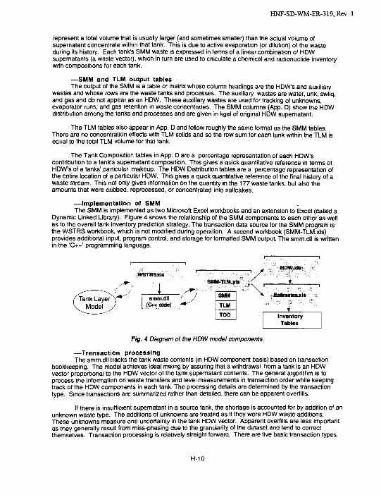
HNF-SD-WM-ER-319,Rev. 1
represent a total volume that is usually larger (and sometimes smaller) than the actual volume ofsupernatant concentrate within that tank. This is due to active evaporation (or dilution) of the wasteduring its history. Each tank's SMM waste is expressed in terms of a linear combination of HDWsupernatants (a waste vector), which in turn are used to calculate a chemical and radionuclide inventorywith compositions for each tank.
—SMM and TLM output tablesThe output of the SMM is a table or matrix whose column headings are the HDW's and auxiliary
wastes and whose rows are the waste tanks and processes. The auxiliary wastes are water, unk, swliq,and gas and do not appear as an HDW. These auxiliary wastes are used for tracking of unknowns,evaporator runs, and gas retention in waste concentrates. The SMM columns (App. D) show the HDWdistribution among the tanks and processes and are given in kgal of original HDW supernatant.
The TLM tables also appear in App. D and follow roughly the same format as the SMM tables.There are no concentration effects with TLM solids and so the row sum for each tank within the TLM isequal to the total TLM volume for that tank.
The Tank Composition tables in App. D are a percentage representation of each HDW'scontribution to a tank's supernatant composition. This gives a quick quantitative reference in terms ofHDW's of a tanks' particular makeup. The HDW Distribution tables are a percentage representation ofthe entire location of a particular HDW. This gives a quick quantitative reference of the final history of awaste stream. This not only gives information on the quantity in the 177 waste tanks, but also theamounts that were cribbed, reprocessed, or concentrated into saltcakes.
—Implementation of SMMThe SMM is implemented as two Microsoft Excel workbooks and an extension to Excel (called a
Dynamic Linked Library). Figure 4 shows the relationship of the SMM components to each other as wellas to the overall tank inventory prediction strategy. The transaction data source for the SMM program isthe WSTRS workbook, which is not modified during operation. A second workbook (SMM-TLM.xls)provides additional input, program control, and storage for formatted SMM output. The smm.dll is writtenin the 'C++' programming language.
WSTHSxIS
ismm.dll
(C++ code)
1
SMM-TUtxIs /
/ * " . I 1 Vi /. » -
SMM
TLM
TOD
HDWjds
Eslmatesjcls
InventoryTables
Fig. 4 Diagram of the HDW model components.
—Transaction processingThe smm.dll tracks the tank waste contents (in HDW component basis) based on transaction
bookkeeping. The model achieves ideal mixing by assuring that a withdrawal from a tank is an HDWvector proportional to the HDW vector of the tank supernatant contents. The general algorithm is toprocess the information on waste transfers and level measurements in transaction order while keepingtrack of the HDW components in each tank. The processing details are determined by the transactiontype. Since transactions are summarized rather than detailed, there can be apparent overfills.
If there is insufficient supernatant in a source tank, the shortage is accounted for by addition of anunknown waste type. The additions Of unknowns are treated as if they were HDW waste additions.These unknowns measure one uncertainty in the tank HDW vector. Apparent overfills are less importantas they generally result from miss-phasing due to the granularity of the dataset and tend to correctthemselves. Transaction processing is relatively straight forward. There are five basic transaction types.
H-16

HNF-SD-WM-ER-319,Rev. 1
1) The XIN and xin transactions represent the transfer of waste from process to storage and simply recordthe transfer of HDW waste to the storage tanks. The xin designation identifies an assumed rather than adocumented transaction. 2)The REC and rec transactions are tank to tank or tank to process transactionswith the rec designating an assumed transaction. 3)The outx is a transfer to process or CRIB and isessentially another variation of the REC transaction. The last three transactions move HDW wastevectors between tanks and processes. 4)The cond transaction removes water from the tank withoutchanging the HDW waste vector. 5)The stat transaction serves to realign the tank volume with physicalmeasurements.
—Ancillary informationIn addition to the tank compositions, the SMM also generates a variety of other important
information. These include volumes of waste from assumed transactions, total traffic in a tank, traffic fromassumed transactions, and various other information.
lid. Approach—Hanford Defined Wastes (HDW) CompositionsThe determination of chemical and radionuclide concentrations for each of the HDW's begin with
inputs of radionuclides and stable chemicals, both of which are used to define the total species in eachwaste stream as shown by the Block Diagram of HDW Spreadsheet (Fig. 5). These total species are thenseparated into two layers, a sludge and a supernatant, that result in different concentrations of speciesfor the two layers.
Each species is precipitated according to a single point solubility. Ions precipitated in more thanone salt are simply successively precipitated. Thus, the solids that precipitate are merely representativeand are not meant to reflect the actual solids distribution. Because the supernatant is also present in theinterstices of the sludge layer, this "supernatant" is included as part of the sludge composition. Thesolubility of each species is set by a macro that when run on the HDW spreadsheet, adjusts the fractionprecipitated parameter so that the supernatant concentration is equal to or less than the target solubility.
The sludge and supernatant compositions are each expressed in mol/L for the stable chemicals,with water and TOC as wt% and radionuclides in uCi/g and Ci/L, respectively. Each waste is kept in ionand mass balance according to the oxidation states assumed for that species. The sludge andsupernatant layers are also expressed in terms of ppm composition. However, the mass balances arelimited by differences among water, oxide, and hydroxide with the various solids to only within ±2%.
—Three methods for establishing defined wastesThere are three distinct methods that have been used by previous workers to set the
concentrations of each component in the various waste streams at Hanford. These three methods arebased on either one or a combination of (1 (knowledge of process, (2)chemical used and waste volumeproduced, and (3)analysis of characteristic waste. However, while these methods provide necessaryinformation for waste stream definition, these methods do not provide sufficient information to define thewaste streams.
That is, once the component concentrations (i.e. source terms) are determined for each of theHDW's, one still needs to determine two critical pieces of information to calculate the actual compositionsof solids and supernatant components within each tank. That is, one needs to know the solubility of eachcomponent in the supernatant as well as the total solids volume percent for that waste stream. With thesetwo additional parameters the waste stream source terms can be related to what is in each tank thatreceived those wastes.
Furthermore, the model that we have developed for the HDW compositions uses representativevalues for the speciation of the components in the solids phases. In other words, the solids thatprecipitate within the HDW model are those listed in Methodology (see below). For example, phosphatesolubility is determined by the ranges observed in tank supernatants, but the solid phases thatprecipitate are limited to a combination of BiPC>4, Na3PO4>10H2O, and Na3PC>4»12H2O, depending onthe circumstances of the waste stream. We argue that this approach adequately approximates the majorfeatures of each solids layer without the complexity that undoubtedly exists in the actual waste sludge.
H-17

HNF-SD-WM-ER-319,Rev. 1
Block Diagram of HDW Spreadsheet
Campaign Information, pp. V-3—fuel processed—exposure—total waste—average waste rate—Pu extraction efficiency—nuclide source terms—solids vol%—CSR input
•
[Chemicals Added, pp. 4-6—mostly based on tons fuel—others concentration—NaOH added to neutralize
'p. 1 refers to Appendix pageswith HDW spreadsheets.
Species Total (mol/L), pp. 7-9
repeat untilsu* species
match targets
(mol/L), pp. 10-12
{ Supernatant (mol/L), pp. 13-15 ~)
Solids Cone. (mol/L), pp. 16-18 )
( Solids Volume (cc/L), pp. 19-21 )
solubility macroor by hand
(tsu = supernatant)
Fraction Precipitated as solids, pp. 22-24 )
i.( Sludge (ppm), pp. 25-27 )
I(Supernatant (ppm), pp. 29-30 )
calculate blendsas weighted
averages of HDWsu's
Supernatant to Evaporator Campaigns,Nitrate to Nitrite to Ammonia Radioiysis,
AR and CSR Waste Blends, pp. 31 -33
Fig. 5. Block Diagram of HDW spreadsheet.
H-18

HNF-SD-WM-ER-319,Rev. 1
Another example is Cs-137, which is precipitated within our model formally as the zero valent metal, whenin fact we fully realize that it is actually precipitated as a monopositive cation as some kind of salt.
—Knowledge Of ProcessBasically, this strategy uses process information, such as flowsheets, to derive waste
compositions based on a process.driver. At Hanford, the driver for HLW was tons of uranium fuelprocessed per quarter. Therefore, based on this feed, a certain amount of waste was generated for agiven Hanford process, such as Purex, and expressed as gallons of waste per ton fuel.
The advantages of this strategy are its simplicity and straightforward application to waste streams.The disadvantages are that often the flowsheet information is incorrect or incomplete. In fact, ancillary orcleanup operations not described explicitly within the flowsheet can end up creating larger wastevolumes, and add different constituents to the waste as well.
Specifically, actual waste volumes usually differ from predicted waste volumes based onflowsheet information, and it is not clear how to scale the composition of the primary stream. For example,if a Purex flowsheet indicates that 51 gal. of P waste is generated per ton of uranium, but actually 275gal/ton occurred, how do the constituents within the stream scale? Is the additional volume just water?
—Chemicals Used/Waste Volume ProducedThis approach uses observed waste stream volumes, both liquid and settled solids, to establish
an actual waste generation rate in gallons of waste per ton of uranium processed for each waste stream.Thus, volume conservation is enforced from the beginning. Then, total chemicals added duringprocessing allows one to unambiguously derive average waste compositions. Thus, total mass is alwaysconserved with this approach. (Note that this is the approach that Allen used11 in his report in 1976.)
The disadvantage of this approach is that it concentrates on only the total amount of chemicalused during a campaign. There is often limited information about how the chemicals used changedduring a campaign. As a result, while this Chemicals Used/Waste Produced approach provides anaccurate average waste composition, variations in the compositions of the waste streams are notrepresented unless one has independent information about the amounts of chemicals used during eachof those process variations within the campaigns.
—Analysis of Characteristic WasteDeriving waste inventories from analytical information of course begs the whole issue of
determining a waste type composition. If a tank's waste is fairly homogeneous, straightforward samplingand analysis will provide an inventory for that tank. The real issue, then, is how can the information froman analysis of tank A's waste be used to predict the contents of tank B. On the one hand, direct analyticalinformation constitutes the bottom line for any tank inventory. On the other hand, there are mitigatingfactors that show that this approach also has severe limitations.
Sampling has been and will continue to be a very uncertain source of waste compositioninformation for many different reasons, not the least of which is that it is a very difficult and expensivething to achieve for 177 tanks. For example, pulling a sample from a waste tank is in and of itself a verydifficult task, but even when that is done, the question of whether that sample is representative of thetank waste is sometimes impossible to answer—even with additional sampling.
Then, there are the inevitable analytical errors that derive from the procedures used tohomogenize, dissolve, and finally analyze each sample. And there is the over arching uncertainty, oncethese other issues are resolved, of exactly which waste type a tank's waste is representative. In otherwords, given that SY-101 is a mixture of DSS and CC wastes, what does the analysis of that tank's wastetell us about either of these two waste types?
—Method used for HDW modelWe believe that the Chemicals Used/Waste Produced approach is the best for defining waste
compositions, therefore, will favor that method. However, much use will be made of Knowledge of
11 Allen, G. K. "Estimated Inventories of Chemicals Added to Underground Waste Tanks, 1944 through 1977," ARH-CD-6108, March 1976.
H-19

HNF-SD-WM-ER-319,Rev. 1
Process, since it is necessary to change the manner in which the chemicals are partitioned in the wastestream over the years in order to account for changes in the process. Unfortunately, these two sourcesof information are often in severe disagreement. For example, there was 3.3 Mmol (1 Mmol = one millionmoles) of citrate reportedly used in B Plant, but the flowsheets suggest that 32 Mmol would have beenused, based on the flowsheet concentration and volumes of waste produced. We do not feel that it willever be possible to resolve all of these discrepancies between these two sources of information.Therefore, we will only use Knowledge of Process to account for notable changes in the wasteprocesses. For example, in 1962, the Purex waste (termed P) decreased from 844 gal/ton to 288gal/ton—a factor of 2.9 reduction. Obviously there was a change in the process in 1962 that had adramatic affect on the volume of P waste that was generated. At that same time, CWP volume stayed at291 gal/ton, but OWW volume went from 108 gal/ton to 336 gal/ton, an increase of a factor of 3.1.
Review of Campaigns—OverviewSome 496 million gallons of waste was placed into single-shell and double-shell tanks at Hanford
from 1944 to 1988, shown in an overview of Hanford waste volumes Table 2. This amount includes MetalWaste (MW) that was reprocessed in U Plant from 1952-56 and Purex sludge and supernatants that werereprocessed in B Plant 1967-76. After reprocessing and water additions, there was a net of 347 milliongallons of waste placed into various tanks. Then, 301 million gallons were removed by evaporation. Thecondensate was placed in cribs while 86 million gallons of waste was placed into cribs either directly orfollowing scavenging operations, leaving 46 million gallons of waste in the tanks from the 1944-80 era.
Since that time, another 30 million gallons of waste has been generated and concentrated to 15million gallons of waste as of January 1994, leaving 61 million gallons of waste in Hanford waste tanks. Ofthis amount, 36 million gallons of waste are now in single-shell tanks (all derive from the early era), whilethe 25 million gallons of waste reside in the double-shell tanks (deriving from both eras), as shown in anOverview of Hanford Waste Volumes (Table 2).
—BiPC>4 campaignThe bismuth phosphate process began in T Plant in December 1944, and in B Plant in April
1945. This process ran until 1952 in B Plant and until 1956 in T Plant and generated some 98,000 kgalof MW, 1C, 2C, and 224 wastes. The Farms T, TX, and TY were used for wastes from T Plant, while B, BX,and BY were used for wastes from B Plant. The term Metal Waste (MW) derived from the code word forPlutonium during the war years, "metal." The other terms 1C, 2C, and 224 represent the wastes from firstcycle, second cycle, and the plutonium finishing operation in building "224."
These wastes were generated from 1944 to 1956 and the HDW compositions reflect those ofAnderson, Jungfleisch, Schneider, and Place. A summary of the wastes generated during this campaignare shown in App. B and a synopsis for the BiPO, process is illustrated in Bismuth Phosphate ProcessSynopsis (Fig. 6).
Anderson-91 reported that, starting in September 1947, second cycle decontamination wastefrom T Plant was to be cribbed or placed in the ground, at which time the BiPO4 process had beenrunning some two-and-a-half years. Then in February 1948, second cycle wastes from B Plant weredirectly cribbed as well. Thus, the -2,400 gal/ton waste rate shown in (App. B) for 2C waste probablyreflects the fact that a large portion of the 2C waste had already gone into the ground at T Plant.
Around 1950, there was an abrupt change in both the 1C and 2C waste rates. The 2C rateincreased from -2,400 to an average of -4,600 gal/ton, nearly twice the volume rate that it had been.Moreover, in 1954 the rate actually peaked at 25,000 gal/ton, as shown in Waste rates for BiPO4 (Fig. 7).During this same period, the actual amount of fuel that was processed was quite low, as shown in theBiPO4 Waste History (Fig. 8)., therefore, there is not a large effect on the average rate over the period1950-56. Anderson-91 noted that canyon cell drainage waste, previously disposed of to dry well via 361Settling Tank, was added to 2C after 1951, and that stack drainage (from decladding off gas?) wascombined with 2C up until 1951. If this change in volume were due to this drainage waste, it suggeststhat some 12,043 kgal of drainage waste was cribbed at B and T Plants from 1945-51. Likewise, therewas a change in the solids volume per cent for 2C waste, which we estimate to have been 6.8 vol% from1945-49 and 3.4 vol% from 1950-56.
H-20

HNF-SD-WM-ER-319,Rev. 1
Table 2.Overview of Hartford Waste Volumes*
total waste generated 1944-80less MW sluicedless P sludge sluicedless P/R/B supernatants to B Plant
net waste after reprocessingless 2C and 224 to cribless 1C to cribless 1C/UR/FeCN scavenged to crib
net waste after cribbingless water added and evaporatedless condensate (recorded) water to cribless further evaporator reduction
net waste remaining from 1944-80sludgesalt cakeother liquids
total waste generated 1981-88| less volume evaporated
net waste remainingsludge from '83-88other liquids from '83-88waste from 1944-80
total waste 1-1-94SSTDST
kgal
35,800900
26,500
30,00012,40043,300
74,50043,900182,900
14,00019,00013,000
15,000
1,10013,90046,000
36,00025,000
kgal496,200
433,000
347,300
46,000
30,000
15,000
61,000
'As of 1-1-1994.
The main receiver of 2C waste from T Plant was T-110, which cascaded to T-111 and T-112, andthen to various cribs. From B Plant, 2C waste was placed into B-110, which cascaded to B-111 and fi-l l 2. All told, 21,000 kgal of 2C was cribbed from T-112, and 4,700 cribbed from B-112.
The 1C vol% solids increased rather dramatically from 14 vol% from 1945-47 to 25 vol% from1947-51 as shown in the section Methodology (Table 5), while the waste rate only increased from-3,700 gal/ton to -4,900 gal/ton from pre 1950 to post 1950 (App. B) and Waste Rates for BiP04 (Fig. 7).We do not completely understand this change in 1C solids per cent, but it is important in the solidslayering predictions. We assume in our model that the change in solids volume per cent was due to areduction in sodium hydroxide added to neutralize the waste stream. With less sodium hydroxide, morealuminum precipitates as the oxide and less remains in solution as aluminate. Accordingly, we adjust thecaustic downward for 1C2 versus 1C1, and adjust the fraction aluminum precipitated as oxideaccordingly. Note that the 1C2 waste rate was quite variable during its period, ranging from 1,800 to6,800 gal./ton fuel, while the 1C1 waste rate ranged from 2,000 to 4,000 gal./ton during its period.
Anderson-91 reported that alkaline coating removal waste (CW) was combined with 1C forstorage, and that stack drainage was combined with 1C after May 1951. Whether either of these wasteshad anything to do with the waste rate changes is uncertain at this time. In any event, 1C wastes werelargely added to T-107, U-107, B-107, and C-107 overfilled to the corresponding tanks in a three tankcascade.
H-21

HNF-SD-WM-ER-319,Rev. 1
fuel elements
Bismuth Phosphate Process Synopsis
- cladding dissolution ^ ^ » fuel dissolution -
dissolve Bi(Pu)PO4Pu(IV) to Pu(VI)
dissolve Bi(Pu)PO4Pu(IV) to Pu(VI)
Fig. 6. Diagram of BiPOt process.
• Pu02(OH)2
I'224' wastel
Prior to being welded in their jackets, the fuel slugs were coated with a bronze layer (Cu and Sn)up until about 1952 or so and neither of these elements are currently within the HDW chemicals added.During most of the aluminum cladding operation, though, lead dips instead of bronze were used for fuelslugs which is included with the cladding waste definition.
The 1C supernatant was not generally cribbed, although Anderson-91 reported that 4,807 kgalof 1C supernatant and 1,938 kgal of 1C evaporator bottoms were cribbed. The SMM and TLMcomposition tables (App. D) show some 12,439 kgal of original 1C HDW supematants were placed intocribs during this time. This increased volume of original supernatants over and above the actual volumesent to the crib is because the cribbing of concentrated 1C supematants. Other 1C supernatants were"scavenged" in TY Farm during the ferrocyanide campaign. These scavenging operations resulted inproduction of ferrocyanide sludges that are termed ICFeCN in the defined waste list HDW CompositionSpreadsheets (App. B) in waste type #12 and now reside in TY-101 and TY-103.
Waste from the plutonium concentration facility, so-called "224" waste, was generated by aPlutonium finishing process known as the Lanthanum Fluoride process. According to Anderson-91, allthe 224 wastes were cribbed at the plant, and therefore never entered the waste farm. However,WSTRS (and even Anderson-91 waste summaries) show that some "224" waste was placed into thefarms. In particular, WSTRS reported 1,220 kgal of "224" waste was added to T-110, -111,-112 from1951-53, 173 kgal was added to T-201, -202, -203, and -204, and another 372 kgal was added to B-204,-203, -202 from 1952-56. It is not clear why only this amount of "224" ended up in the farms. It ispossible, for example, that only accumulated sludges and not the all of the waste was placed into wastetanks, or perhaps there was some process upset that occurred.
H-22

HNF-SD-WM-ER-319,Rev. 1
Waste Rates for BiP04
10,000 -p
8,000 - •
§ 6,000 - •
co
"5™ 4,000 - \
2,000 - •
tyfrhfi-2C V
1944 1946 1948 1950 1952
year
1954 1956 1958
Fig. 7. Waste volume rates for B1PO4 campaign.
The solids amount tor "224" waste is very uncertain at this time, but an estimate for the solidsfraction comes from the percent water reported1* from an analysis of T-111 waste. Note that some 154kgal of solids accumulated in B-204, -203, -202, and -201, while only 372 kgal was recorded as havingbeen added to this cascade by WSTRS, for a 41 vol% solids. This solids content is very high and it isprobable that much more than 372 kgal was actually added to this cascade. In particular, estimates of percent solids obtained by using an 80 wt% water would be 4 vol%, which would suggest that more like3,900 kgal was added to this cascade. Likewise, some 124 kgal solids accumulated in T-203, -202, -201,-204, while only 173 kgal "224" is recorded as having been added to this cascade. Using a nominal 4vol% solids, this actual volume added to the T-200 cascade would have been more like 4,300 kgal. Thus,we have assumed that a total of 8,300 kgal of "224" waste was placed into these various cascades overthe history of this process.
The compositions of the BiPC>4 wastes came from Anderson-91, Jungfleisch-84, Allen-76, and
other information.13'14 Anderson states that 1C waste contained 10% of fission products and 2C had
12Preliminary analysis of T-111 courtesy of Roger Bean, PNL.13no author "Hanford Technical Manual," HW-10475, May 1944.
H-23

HNF-SD-WM-ER-319,Rev. 1
1%, but this description does not further define the partitioning of fission products, such as Sr-90 versusCs-137. Therefore, we have partitioned both C-137 and Sr-90 as 35% into MW, 58.6% into 1C waste,6% into 2C, and 0.6% into 224. The remaining radionuclides are partitioned as 88.9, 10, 1.0, and 0.1%,respectively.
B1PO4 Waste History
4o,ooo -r
- 30,000 - -
i 20,000 - -
10,000 - -
- MW
— 2C
1C
* •
short tons fuel
1944 1946 1948 1950 1952year
1954 1956 1958
Fig. 8. Total waste volumes from B1PO4 campaign
—Uranium recoveryThe BiPO4 process did not remove uranium from the process stream. A second campaign, the
uranium recovery campaign, began that involved sluicing the MW tanks and extracting the uranium fromthose wastes. This uranium campaign involved U Plant and a process that was based on a TBP/NPHsolvent extraction, and produced a waste that has been referred to as TBP. This report, however, it istermed UR waste to make clear the distinction among the process wastes that involved the chemical,TBP. A description of the overall uranium recovery process is shown in (Fig. 9).
The uranium recovery campaign began in 1954 and recovered the MW that was stored in B, C,BX, BY, T, TX, and U Farms. This campaign reportedly produced about two gallons of waste for eachgallon of MW that was processed (actually -2.5 by WSTRS, adding UR, PFeCNI, PFeCN2). Therefore,more waste was created than could be accommodated by the tank farms and a scavenging programbased on the precipitation of Na2NiFe(CN)6 within the waste stream to scavenge or entrap the Cs-137began. With the Cs-137 precipitated in the sludge, the supernatant was then placed into the ground incribs or trenches. As a result, about 30,000 kgal of scavenged waste was sent to the cribs following an in-
14 Kupfer, M.J.; Boldl, A.L; Higley, B.A.; Lambert, S.L.; Orme, R.M.; Place, D.E.; Shelton, L.W.; Watrous, R.A.;Borsheim, G.L.; Colton, N.G.; LeClair, M.D.; Schuiz, W.W.; Hedengren, D.C.; Winward, R.T. "Standard Inventoriesof Chemicals and Radionuclides in Hanford Site Tank Wastes," WHC-SD-WM-TI-740 Draft, September 1996.

HNF-SD-WM-ER-319,Rev. 1
plant addition of ferrocyanide and 12,000 kgal was sent to the crib with in-farm or CR-Vault addition offerrocyanide see Overview of Hanford Waste Volumes, Table 2.
Uranium Recovery Process Synopsis
— tank sluicing-
tank sludge, a ^ dissolution / • supernatant to U Plant —,supernatant, *-m T X R B X R C X R v a u | t s
caustic leach \ „ |residual solids back to tanks? |
• TBP/NPHU(VI)
U Plant Extraction-
more cycles for uranium purification
aq.\ concentration and neutralization • |UR to waste tanks|
canyon cell drainage -^^s^ FeCN
carbonatewash
vessel clean-out / , A
/ I su, \ .u
|FeCN to waste tanks | c n ° s
—organic washing
aC|> , to makeup and recycle
organic °rg-
\TBP/NPH aq.
to crib?
Fig. 9. Uranium Recovery process synopsis.
Evidently, there were heel remnants of MW solids in many of the tanks following sluicing and asmuch as 40 kgal of solids remained in some tanks following sluicing operations. We assume that some ofthese heels were left behind because of expediency and not because the solids weren't sluicable.However, there were reports of hard pan forming in well-aged MW sludges and the suggestion was that avery hard uranium carbonate phase was formed in aged MW sludges. The Uranium Recovery manualstates15 that although sluicing and then acid digesting MW sludge in tank farm vaults was the baselineprocess, dissolution of uranium in caustic water and/or sodium carbonate solutions would also beattempted within the waste tanks. It is not clear, though, what happened to the sludge remnants thatwould have resulted following acid digestion in TXR, BXR, and CR tank farm vaults during feedpreparation of recovered MW sludge. We have found that more than 15-20% of the expected 4,309 kgalof MW sludge still remain as heels within various tanks. We have used the reported sludge levels for MWas 12 vol%, although values as high as 25 vol% were mentioned in the Uranium Recovery manual.
15no author "Uranium Recovery Technical Manual," HW-19140, November 1951, section 1.1, p. 109.
H-25

HNF-SD-WM-ER-319,Rev. 1
Although the solubility of the uranium/carbonate complex in MW supematants was reported inthe UR manual to be 0.11 M, that same source also claimed that 75% of the uranium was present as asolid in the sludge. Our calculations show that if 75% of the uranium were in the sludge, a supernatant ofonly 0.04 M U would result. If we assume that the 0.11 M solubility point is correct (uranium solubility is-0.004 M for typical tank waste supematants), this would have meant that only 35 % of the uranium was inMW sludge. Thus, we suggest that caustic sludge leaching may have been performed in the later stagesof the Uranium Recovery Campaign in lieu of actual sludge removal and acid digestion in the vaults.
For these MW heels, we have assumed that 80% of the plutonium and strontium and 95% of thecesium associated with MW sludge were removed and ended up in the uranium recovery wastes as eitherUR, PFeCNI, and PFeCN2 sludges, while the remainder of the plutonium and strontium remained withthe MW heels. There were frequent problems with pump failures and other difficulties sluicing the so-called "hard-pan" out of tanks with well-aged MW, as previously detailed.16 It is possible that thesedifficulties resulted in some expediency with regards to the MW heel remnants that were left within thetanks.
For UR waste, there is a problem with the composition—it is not consistent with expectationsbased on the flowsheet. This is shown by the phosphate levels, for example, which lead to a solidsvolume per cent that is much larger than that observed for this waste. We assume that the decision toleave many MW solids in the waste tanks was based on the teachability of uranium from the solids. That is,agitation of the solids with a basic carbonate solution should have been sufficient to leach the uraniumout of the solids and into the supernatant. The supernatant could then be passed on to UraniumRecovery for processing, and therefore preventing the unnecessary transfer of large amounts of solids.
Since only supernatants were scavenged for TFeCN and 1 CFeCN wastes, there were very smallamounts of plutonium and Sr-90 in these wastes and we have neglected them. We have used a Cs-137concentration identical to that of the supernatant of UR and 1C wastes, respectively.
The compositions of the UR wastes were taken from Anderson-91 and Jungfleisch-84, but theferrocyanide sludges were defined17 from Borscheim and Simpson. Also used to some extent was theUranium Recovery Manual.18 However, we have found that there is evidently some double counting ofspecies within the MW and UR waste streams. That is, the 810 Mmols of NaNC>3 mentioned by Allenevidently included the NaNO3 added during MW. Therefore, many estimates of the total sodium used forthese two processes are in error since they add these two source terms together. Likewise, Allen shows50 Mmols of Na3PO4 added during UR, when no phosphate at all was actually added during the uraniumrecovery campaign. All of the phosphate was actually carried over from the BiPO4 operation. Therefore,there has been some double counting of added chemicals in past estimates of site inventories.
—RedoxThe Redox process was based on the extraction or salting out of plutonium and uranium from an
aqueous aluminum nitrate solution into an organic phase, methyl isobutyl ketone also known as hexonein the Redox Process Synopsis (Fig. 10). Anderson-91 describes the various stages in the developmentof the Redox process, which began in January 1952 at S or Redox Plant.
According to Anderson, waste was originally generated at 4,378 galAon in 1952, and that ratewas reduced to 594 gal/ton in 1966. We have found by analyzing the fill records, on the other hand, thatthe waste rate peaked at around 4,600 gal/ton in 1952 and after around 1958, leveled off to around1,100 gal/ton.
16Rodenhizer, D. G. "Hanlord Waste Tank Sluicing History," WM-TI-302, September 1987.17Borsheim, G. L. and Simpson, R. C. "An Assessment of the Inventories of the Ferrocyanide Watchlist Tanks,"WHC-SD-WM-ER-133, October 1991.18no author -Uranium Recovery Technical Manual," HW-19140, November 1951.
H-26

HNF-SD-WM-ER-319,Rev. 1
Redox Process Synopsis
-fuel decladding and dissolution •
Fo(NH2SO3)2
•Pu and U partitioning and purification
S U •• more cycles for uranium purification
'
1AP <
hexone \adjust to Pu(IV) < Pu(lll)
UjVJ) _aq;v1AW •• concentration and neutralization
fission productscanyon cell drainage
more cycles for plutonium purification'
-„ , *
[R to waste tanksl
vessel clean-out *
waterwash
—organic washing--
' to makeup and recycle
organic °r8-hexone aq.
\ ,to D-13 waste collection tank I
Fig. 10. Redox process synopsis.
Thus, there were essentially two eras for the Redox waste, the first era from 1952-58 averaged2,106 gal/ton, followed by a reduction to 1,119 gal/ton from 1959-66 as shown in the Waste VolumeRates for Redox Campaign (Fig. 11) and the HDW Model Inventories for 177 Tanks (App. E). We do finda waste rate as low as 500 gal/ton in the last quarter of 1966, but averaged for all 1966, the last full year ofoperation, Redox generated waste at the rate of 1,085 gal/ton.
We have also found that the cladding waste generation rate CWR was fairly constant at 266±30gal/ton over the entire history of Redox, as opposed to a remark by Anderson-91, that cladding wastevolumes were cut in half in 1956-57. We have found no such decrease in CWR waste rates averaged forany year of operation over the entire Redox campaign. There are some 980 kgal of CWR that is reportedby WSTRS after all fuel was no longer processed in Redox in mid 1966 see Total Waste Volumes forRedox Campaign (Fig. 12). We assume that the fuel slugs from this decladding operation were actuallyprocessed in Purex Plant.
Prior to being welded in their jackets, the fuel slugs were coated with a bronze layer (Cu and Sn)up until 1952. Neither of these elements are currently within the HDW chemicals added and so are notincluded in the cladding waste estimates. Subsequently, lead dips were used instead of bronze for fuelslugs and lead is in the cladding waste chemicals added.
Anderson-91 also mentions that Redox processed some Zircaloy cladded fuel, which came fromN-Reactor. However, Jungfleisch indicated that the first Zircaloy cladding waste was created in Sept.1967, and Redox plant shut down in 1966. Other sources (HWN-1991, p. 130) have indicated, on theother hand, that some 269 tons of Zircaloy clad fuel was indeed processed in Redox in 1966. Since thelast cladding waste from Redox (CWR) was place in S-107 in 1967q1, and we expect that some 18 kgal ofCWZn sludge would be in the layers of this tank.
H-27

HNF-SD-WM-ER-319,Rev. 1
The early solids accumulation in Redox waste tanks during 1952-8 is associated with the erawhere the Redox waste rate underwent substantial change, as noted before. These tanks were also self-concentrating the waste, which increases the tanks'solids load even further. We have used a value ofsolids volume per cent of 4.4 vol%, which is based on accumulations in SX-105 and SX-111, neither ofwhich tanks were reported to have undergone significant self-concentration over the period in question.These solids per cents are derived based on consistency with the 2.3 vol% that we have found for thesecond Redox period, R2.
3UUU -
4500 -
4000 -
3500 -
3000 -
ga
l/to
nro
2000 -
1500 -
1000 -
500 -
0 -
: i
•1
(1 • FVRCC
•'"•h; U. i .; U J . J\• "" "" U"""" m'A
1 1 • • • ' i ' ' ' • i '• CWR
1 • ' 1 ' •
1950 1955 1960year
1965 1970
Fig. 11. Waste volume rates for Redox campaign.
For the second Redox period, solids accumulation in Redox waste dropped to 2.3±1.3 vol%,even as the waste rate dropped from 2,106 to 1,119 gal/ton from R1 to R2 (App. B).
Many tanks in S and SX Farms were allowed to self-concentrate therefore accumulated solids inexcess of those from the primary additions. In particular, S-101, S-104, and S-107 were all primaryreceivers of R1 waste and were reported as self-concentrating waste tanks. Unfortunately, we do nothave enough information to always differentiate between the two types of solids accumulation within thewaste tanks. However S-110 was also a primary receiver of R1, but never was reported to have reachedboiling. If we assume that the solids for R1 were actually 4.5 vol%, that would provide an estimate for the
H-28

HNF-SD-WM-ER-319,Rcv. 1
concentrated solids, RSItCk, in S-101, S-104, and S-107. Thus, we assume that R waste has an implicitcomponent within it that we attribute to the concentrate.
Tank SX-109 accumulated 14 vol% solids from its 1,756 kgal Redox waste. An analysis211 of thefill history of this tank reveals that it self-concentrated the Redox supernatants, and therefore depositedsalt cake. Consequently, we attribute much of the solids accumulation in SX-109 to this salt accumulationand not to Redox sludge. We find that a series of tanks accumulated this Redox salt cake, whichamounted to 1,065 kgal in a number of tanks in S and SX Farms. This resulted in a particular waste typeRSItCk, which is #43 in (App. B).
40000 -r
35000 - -
30000 - -
o 25000 - -
* 20000 - -o
1 15000 - ->
10000 - •
5000 - -
1950
-R/RCC
.I'1'1"1'1"•I1
1955 1960 1965 1970
yearFig. 12. Total waste volumes for Redox campaign.
Compositions of Redox wastes were taken from Anderson-91, Jungfleisch-84, Allen-76, as wellas published flowsheets.19 However, there is a difficulty in the amount of silica that is present in theRedox waste tanks is far greater than the amount that is listed as being present in the flowsheet. Wehave found a similar excessive silica source for Purex and other processes. Thus, we have added anamount of silica to the Redox waste that amounts to 50 mol Si per ton of fuel processed. The fuel that
19(a) no author "Redox Technical Manual," HW-18700, July 1951. (b) Crawley, D. T.; Harmon, M. K. "RedoxChemical Flowsheet HW-No.6," October 1960, HW-66203. (c) Isaacson, R. E. "Redox Chemical Flowsheets HWNo.7 and HW No.8," RL-SEP-243, January 1965. (d) Jenkins, C. E.; Foster, C. B. "Synopsis of Redox PlantOperations," RHO-CD-505-RD-DEL, July 1978, declassified with deletions.
H-29

HNF-SD-WM-ER-319,Rev. 1
was processed did actually have a silica component, which is listed in the published flowsheets as 21 molSi/ton. At the present time, we cannot explain why the silica is actually much larger.
The amount of iron present in Redox sludge reflects the process vessel corrosion source termthat we have found is a significant contribution to the Purex sludges. We have not found any informationabout the process vessel corrosion rates during the Redox campaign and have therefore assumed thatthe rates are identical with Purex.
—Purex primary processThe Purex process was based on the extraction or salting out of an aqueous plutonium and
uranium nitric acid solution into a tributyl phosphate/normal paraffinic hydrocarbon (TBP/NPH) organicphase Purex Process Synopsis (Fig. 13). Purex came on line in January 1956 in A Plant or Purex Plantafter having run as a pilot in the Hot Semi-Works (C Plant). The Purex campaigns and the subsequentprocessing that occurred in B Plant produced the most complicated combination of wastes at Hanford.We have found twenty-one distinct waste types that have derived from the Purex campaign from 1956-88.
Purex Process Synopsis
r-fuel decladding and dissolution-
fuel elements
HNQjFe(NO3)3
II
x» TBP/NPHHAP <
/ * aq.TBP/NPH \
adjust to Pu(IV) ^ PU(III)
HAW > " "fission products
—Pu and U (and Np) partitioning and purification—
"• more cycles for uranium purification
carbonatewash
"organic washing •
•• more cycles tor plutonium purification;
acid recovery, denitration, neutralization -f\P to waste tanks I
canyon cell drainage
vessel clean-outPL to waste tanksl
a t \ - to makeup and recycle
organic ?r9-TBP/NPH aq.
lOWW to waste tanksl
Fig. 13. Synopsis of Purex process wastes.
An analysis of the waste history shows that there were three eras for the Purex process. From1956 until 1962, the Purex high level waste rate averaged 877 gal/ton, OWW 150 gal/ton and CWP 346gal/ton, although there is a large variability associated with the P waste rate. Also in this period, we aremissing OWW (actually called CARB) for the years 1959 and 1961. During this period, there was a largevariability in the waste rate of Purex as compared with other operations as well as other periods of Purex.The waste rate for P waste peaked at 1,400 gal/ton in 1960, and again at 1,000 gal/ton. These wasterates suggest that the OWW wastes were actually routed to P waste receivers in 1959 and 1961. In fact,
H-30

HNF-SD-WM-ER-319,Rev. 1
Anderson-91 mentions that OWW were added to boiling waste tanks until 1969, and Jungfleisch-84states that for some unspecified period, P and OWW were mixed together.
In 1960-61, it was reported20 that a sulfate strike (i.e. precipitation) was used in Purex Plant toprecipitate Sr-90 and separate it from the other fission products in HAW. The P waste rate reportedlywent from 53 gal/ton to 193 gal/ton during this time. Thus, we suggest that the increase in waste rates in1960-61 may have been due to a combination of this sulfate strike and redirection of the OWW streams.We have not, however, included any strontium depletion for this P waste. Evidently, this impure productwas worked up later in either HS or B Plant operations.
The Purex waste receivers in 1959-61 were A and AX Farms. We suggest that the redirection ofthe OWW to these farms was due to the desire to concentrate these wastes by self-boiling. However,successive failures of two tanks in A Farm due to overheating evidently modified that strategy, and fromthen on, OWW was placed into other receivers and reduced in separate operations. There was a sizableself-concentration that occurred in A and AX Farms as a result of this self-boiling. However, unlike theRedox self-concentration campaign, no salt cake accumulated as a result of Purex waste self-concentration. Therefore, the volume reduction that occurred is accounted in other evaporatorcampaigns.
From 1963-67, the average waste rate for Purex decreased by a factor of two from 877 to 378gal/ton while that for OWW rose by a factor of three from 150 to 391 gal/ton as compared to the period1956-62. These changes in waste rates coincided with two fundamental changes for the Purex process.In Sept. 1962, the solutions from the second cycle uranium extraction were recycled instead of sent tothe waste tanks and in Sept. 1963, sugar denitration was introduced, which reduced the nitric acid inHAW and therefore the amount of caustic that was needed to neutralize the waste. During 1962-67, theStrontium Semi-Works facility was directly processing PAW as well. The variability of the Purex waste rateremained fairly high during this period of operation. The inherent amount of high level waste generatedby the Purex operation (i.e. HAW) was quite small, on the order of 50 gal/ton, and we suggest that othermore a periodic sources, such as vessel cleanout and canyon drainage wastes, now began to dominateover the primary process waste.
Another spike in the P waste rate occurred in 1966, where the rate climbed to 900 gal/ton. Wedo not yet know why. See Waste Volume Rates for Purex Campaign (Fig. 14).
Finally, from 1968-72 the Purex HAW stream was sent directly to B Plant for strontium removaland so very little P waste was added to the tank farms after 1967. Eventually, this waste appears as BPlant high and low level wastes (B and BL). On the other hand, OWW increased once again during thislatter era to 575 gal/ton.
We assume that the CWP/AI waste rate for the period 1961 -72 remained at 346 gal/ton, which isthe rate that occurred for 1956-60. During the period 1968-72, some 708 tons of Zircaloy N-Reactor fuelwas processed in Purex (and 269 tons went to Redox, as noted above), and the waste rate for this Zirflexprocess (termed CW/Zr) was much higher than CWP/AI. In fact, a later flowsheet projected21 927 gal/tonfor Zirflex waste, although the rate we calculate from WSTRS would have been 1,650 gal/ton, providedthat the CWP/AI rate was 346 gal/ton. Since the two types of cladding wastes, CWP/AI and CWP/Zr werenot segregated, i.e. both were added to C-104 during 1968-72, we have simply proportioned theCWP/AI and CWP/Zr waste solids accordingly over this period.
^Monthly summaries, 1959-60.21 Allen, G. K.; Jacobs, L. L; Reberger, D.W. "Purex Flowsheet—Reprocessing N Reactor Fuels," PFD-P-020-00001, Sept. 1982.
H-31

waste rate (gal/ton)
o o o) 1 1 1
waste rate (gal/ton)-* - 1 fo 10
8
waste rate (gal/ton)

HNF-SD-WM-ER-319,Rev. 1
Lead dips were used for coating fuel slugs before placing them into aluminum jackets. As aresult, lead is a part of the cladding waste chemicals added.
The solids volume per cent for the CWZR1 waste of this period is assumed to be the same asCWZR2, which was 10.5 vol%, for the '83-'88 campaign. Moreover, there are indications that significantamounts of mercury were added to the dissoiver solution to limit the emission of 1-131 during dissolutionof the fuel cladding. We have included mercury additions in our definition of cladding wastes. For totalwaste volumes for Purex campaign see (Fig.15).
80,000 T
-tons fuel
xLilu—•—P i——CWP/CWZr2 ,«->•"
1965 1975 1985Year
Fig. 15. Total waste volumes for Purex campaign.
The composition of Purex waste was taken from several sources. An early flowsheet22 was usedfor the first era, a second flowsheet23 was used for N Reactor fuels, and a later flowsheet24 was used thatupdated the Purex process for N Reactor fuels. These compositions were adjusted to account for thechanges in waste volume that are recorded in WSTRS combined with the total chemicals used reportedby Allen-76. Basically, we have taken the waste rate of 50 gal/ton for all of the process chemicals exceptiron and silica, and diluted those chemicals to the observed waste rates of either 877 or 378 gal/ton.
^Swift, W. H.; Irish, E. R. "Purex Two Cycle Flowsheet, Revision No.1," October 1957, HW-52389-DEL,declassified with deletions.23Jeppson, D. W. "Purex Flowsheet Reprocessing N Reactor Fuels," November 1976, ARH-F-103."Al len, G. K.; Jacobs, L. L. "Purex Flowsheet Reprocessing N Reactor Fuels," September 1982, PFD-P-020-0001.
H-33

HNF-SD-WM-ER-319,Rev. 1
For both iron and silica, we have used Allen-76 to set the total chemicals used and the ChemicalsUsed/Waste Produced approach to define the waste compositions for these two species. This Siamount is on the order of 130-160 mol Si/ton fuel which is much larger than the 21 mol Si/ton fuelreported in various flow sheets. The concentration of SiO2 in the waste stream from the plants amountsto 3,000 to 6,000 ppm, which is very large compared to a normal impurity level that is expected from hardwater, which is on the order of 20-30 ppm.
Estimates of organic loss during solvent processing25 have shown 8.4 gal organic per ton of fuelprocessed during Purex. For a 70/30 mixture of NPHATBP, this suggests a loss of 2.5 gal TBP/ton fuelprocessed. We then assume that all of this TBP is hydrolyzed to DBP and butanol and place those in thecorresponding waste streams.
The waste rate for PL2 (PXMISC in WVP notation) amounts to nearly 3,000 gal/ton of fuelprocessed for the '83-'88 campaign. Since no OWW was reported at all during this period (flowsheetvalues suggest -400 gal/ton fuel), we assume that PL2 is actually a combination of both PL1 and OWW,despite the fact that the 3,000 gal/ton value is substantially larger than the 400 gal/ton expected from theflowsheet. The weighting that we have used is as follows:
PL2 chemicals added = (2100 * PL1 + 800 * OWW3) / 2900
The P3 waste (Neutralized Current Acid Waste, NCAW) is derived from flowsheet values that arescaled to the actual waste volume. For example, neutralized ZAW flowsheets predict 160 gal/ton, whilethe actual volume sent to the tanks averaged 288 gal/ton. We therefore scale all neutralized ZAWflowsheet chemicals by 160/288 = 0.556 (i.e. assumed dilution).
The sugar denitration of acid ZAW used a sugar solution that would have resulted in about 25 gTOC/L of waste had it not reacted with the nitric acid. Complete consumption of the sugar was assumed,which reduced the HNO3 from 2.8 to 0.95 M in the waste, with the carbon lost as CO2. An estimate of theamount of sugar used in this process is that 160 gal/ton of fuel processed at 0.18 mol/L and 47,767 tonsfuel processed is 5.2e6 mols sucrose, or 1,800 MT . During this denitration, an anti-foam agent was usedto keep the solution from foaming. The amount added was 2.2 fl.oz/ton fuel, which amounts to about 6e-5 M Si in the waste stream, assuming the anti-foam agent is 3 wt% Si. However, we have previouslyfound that the Si amounts in Purex waste are significantly greater than this. Accordingly, we use a valueof 0.092 M Si in the P3 waste stream.
—Purex to Hot Semi-WorksThe Hot Semi-Works or C Plant was used as a pilot for both Redox and Purex in the 1950's and
was then used as a pilot for strontium extraction in the 1960's prior to B Plant as shown in the HanfordTimeline (Fig. 1). Purex HAW was processed26 with this pilot and only a fairly small amount of waste wasgenerated, amounting to 1,003 kgal over the years 1962-67. We do not know exactly how much HAWwas processed for the whole campaign, but for the first hot run in 1962,16 kgal of HAW was processedresulting in 50 kgal of waste. If we assume that the rest of the campaign progressed with the same wasterates, then 1,003 / 50 x 16 = 321 kgal of PAW were processed in the Hot Semi-Works Plant,corresponding to 321 kgal / 0.3 kgal/ton = 1,070 tons of fuel. During the period 1962-67, on the otherhand, about 25,000 tons of fuel were processed, so the amount of PAW processed in the Semi-Worksamounted to a relatively small fraction of the total PAW waste.
According to the report for this first hot run, about 1.04 MCi Sr-90 was extracted from 1.2 MCi Sr-90 total within the crude PAW (it not clear if this includes the Y-90 daughter) leaving 0.14 MCi Sr-90 in thewaste. Scaling this by the ratio of overall waste with just this run (1,003/50), suggests that 2.8 MCi Sr-90were left in the waste over the entire campaign, or 1.4 MCi, decayed to 1994.
25Camaioni, D. M.; Samuels, W- D.; Lenihan, B. D.; Clauss, S. A.; Wahl, K.L.; Campbell, J. A. "Organic TanksSafety Program Waste Aging Studies," PNL-10161, Nov. 1994.26Richardson, G. L; Schultz, W. W.; Mendel, J. E.; Burns, R. E.; Rushbrook, P. R.; Alford, M. D.; Cooley, C. R."Hot Semiworks Strontium-90 Recovery Program, ParM: Program Synopsis, Part 2: Technical Basis, Part 3:Laboratory Studies, Part 4: Cold Semiworks, Part 5: Hot Semiworks Runs" HW-72666-RD, February-November1962.
H-34

HNF-SD-WM-ER-319,Rev. 1
Another indication of the Sr-90 concentration in HS waste comes from a report of C-112 samplingin 1993, the very top layer of which was SSW sludge and was ~6 Ci/L. If we assume that all HS sludgewas nominally 6 Ci/L Sr-90, this results in an HS waste inventory of 0.45 MCi Sr-90 (decayed to 1994) inHS sludge, which is a factor of three less than the amount estimated by the hot run report.
The chemical composition of HS from the Lucas27 draft report, disagrees with the informationfrom the first hot run report, and we have used this hot run report to define our HS waste. However, thereis no Pu or Cs-137 in this waste, and the Pb concentration of 0.034 M results in a very high Pb value inthe sludge. Therefore, we arbitrarily choose to adjust the Pb down by a factor of ten to 0.0034 M. Wehave also added an amount of Pu to the waste that is volume-scaled to the P2 waste stream.
Although there are records of HS and SSW wastes being added to C-107,-108,-109,-111,-112,there was another addition of 200 kgal of these semi-works wastes to the C-200 series tanks as well.Anderson-91 assigns the waste in tanks C-201, -202, -203, and -204 to SSW and HS and notes startingdates for HS additions in 1955 and 1956, even though we have otherwise no information about the fillhistory of the C Farm 200-series tanks following the MW sluicing. Therefore, there were undoubtedlyunrecorded additions of HS as early as May 1955, which would have been during the Purex pilotoperation in the C Plant. Further additions occurred in 1966 from SSW to C-204, which were presumablydecontamination operations for C Plant, and then all of the C-200 tanks were pumped to their sludgeheels in 1970 and 1977.
—Purex to B Plant Cs-137 recoveryAlthough B Plant was used from 1945-1952 for the BiPO4 process, it was later reconfigured for
the cesium and strontium extraction campaign. From 1967 to 1976, B Plant extracted strontium fromboth Purex acid waste (PAW) (from Purex Plant) and Purex sludges (sluiced from A and AX Farms), andextracted cesium from a variety of neutralized supernatants taken from the tank farms.
Our model for the cesium recovery approximates the feed for this campaign by deriving volumesof waste supernatant that was processed from the tank farms. In (App. B) we show the nominalcomposition of the feed for CSR along with the sum of supernatants from which it was derived. Note thatmany concentrated wastes were processed during this campaign and we find that the averageconcentration factor was -2.7 for the CSR feed. The following equation represents the majority of thecontributions to the CSR waste in terms of other HDW supernatants:
CSR in =0.34 P1 + 0.11 P2 + 0.11 B + 0.05 AR + 0.07 R1 + 0.03 R2 + 0.21 OWW
as well as 0.08 as other wastes (see App. D). This equation represents a deconvolution of wastes thatare actually partof concentrated waste blends such as RSItCk and BYSItCk.
Supernatants were fed to the cesium recovery process through C-105, which was the stagingtank for the caustic sludge washing in AR vault. All total, 45% of the CSR feed was Purex supernatants,21% organic wash waste, and 10% Redox supematants, with the balance being other wastes. The CSRwaste blend was concentrated on average by a factor of 2.7 prior to CSR processing but the HDW modeldoes not account for any solids in the CSR feed. As a result, the CSR blend is only an approximation ofthe true feed for CSR.
There were two different processes for extracting Cs-137. The first was a chromatographicextraction of Cs-137 onto zeolites from the caustic supernatants that were drawn from various tankwastes. We find that 92% of the Cs-137 was extracted from these supernatants with this process. Thesecond process by which Cs-137 was extracted was by precipitation of Cs-137 with phosphotungsticacid added to the HAW acid feed that was obtained directly from Purex plant. This process evidentlyproduced the B and BL wastes. Finally, the crude cesium product purification produced additional B andBL wastes as well.
27Lucas, G. E. "Waste Types in Hanford Single-Shell Tanks," WHC-SD-ER-TI-001, draft report, 1989.
H-35

HNF-SD-WM-ER-319,Rev. 1
—Purex to B Plant Sr-90 recoveryThe strontium recovery operation was much more complex than the cesium recovery as shown in
(Fig. 16). The origin of the complexant wastes at Hanford are attributed to this process. The wastevolumes from the various processes are shown in (Fig. 17). Note that the production of B and BL wastesevidently derived from PAW (or HAW) processing, although we do not know the volume processed. Weestimate that about 4,000 kgal of PAW would have been processed in B Plant from 1968-72, whichresulted in the production of 11,763 kgal of B and 4,000 kgal of BL wastes (App. E). There was about397 kgal of P and 1,233 kgal of PL placed in waste tanks during this time, some of which was then sluicedfor the later Sr-90 extraction from PAS (Purex Acidified Sludge).
Although sluicing operations began to send sludge to AR Vault in 1967, the production of SRRwaste did not begin until 1973. We cannot explain this time difference, but note the SRR waste cameprimarily from the purification of the Sr product. The Cs-137 recovery operation, on the other hand, ranfairly consistently from 1967 to 1973, and then slowed down substantially after that time. There were twodifferent processes for separating cesium from waste, depending on whether the waste was alkaline oracidic. For neutralized or alkaline supernatants Purex Sludge Supernatant (PSS), resins were used toextract cesium. For acidic supernatants, phosphotungstic acid was used to precipitate the cesium beforeneutralization.
B waste from PAW
B L low level waste from all operations
AR solids "washed" P sludge. Also used to derive SRR.
SRR strontium recovery waste from sluiced P sludge—based on washed Purexsludge plus added EDTA, HEDTA, and glycolate.
CSR waste from cesium recovery from supernatants—not a characteristic wastetype, but rather a supernatant from which the 137Cs has been removed.Need only to add citrate to supernatants to track this component.
The amount of Cs-137 and Sr-90 extracted during this campaign has been reported28 and isshown in Table 3 The Partitioning Following CSR and SRR. The difference is very important, since that isthe residual Cs-137 and Sr-90 that is present in the waste tanks. We have assumed that the residual Sr-90 is distributed among P, AR, SRR, B, BL, and HS wastes, while the residual Cs-137 is distributedamong CSR and B wastes.
Overall, the campaign succeeded in extracting 42% of the Sr-90 from various wastes. Since Bwaste derived from the extraction of Sr-90 from PAW, we assume that 80% of that Sr-90 was extractedand 20% ended up in B waste. With this assumption in hand, we find that 27% of the Sr-90 in neutralizedPurex sludge ended up in the WESF capsules, while the remaining was distributed as shown in Table 3.
There are some 4.3 MCi Sr-90 (decayed to 1993q4) for which we can not yet account. It is notclear at this time if this "missing" Sr-90 was actually extracted from the sludge and shipped off site or isotherwise present on the site and its apparent absence indicates an inaccuracy in our model. Forexample, increasing the solubility of the Sr-90 in the wastes would naturally accommodate more Sr-90 inconcentrates of waste supernatants. Another possibility is that there is unaccounted Sr-90 within andunderneath damaged tank A-105. That there is a significant heat source underneath this tank isindicated by the very high temperatures within a lateral well underneath the tank as well as the high domespace temperature for the tank itself. The "missing" 4.3 MCi would amount to a -100,000 Btu/hr heatsource, which would presumably be more than enough to raise the lateral-well temperature to the -212°Freported today. Therefore, some or all of the missing Sr-90 may be in or under A-105.
28ORNL document (no author), "Integrated Data Base for 1991: U. S. Spent Fuel and Radioactive WasteInventories, Projections, and Characteristics," DOE/RW-0006, Rev. 7, 1991, Mike Cooney is Hanford contact.
H-36

HNF-SD-WM-ER-319,Rev. 1
Two tanks that are key in containing the amount of Sr-90 in BL waste are C-106 and B-101.Independent estimates of tank waste heat loads from tank temperatures suggest that C-106 is100,000±20,000 Btu/hr, while B-101 is around 14,000±6,000 Btu/hr. Strontium-90 levels in BL alsoimpact the heat load in AY-102, since this tank was a primary receiver for B Plant non-complexed waste inthe years 1981 -8. We have assigned this B Plant waste as BL. The solvent washing waste from B Plantoperations evidently ended up as BL waste. Therefore, the solvent residues from this process ended upin these tanks.
In particular, recent assays of sludge grab samples from C-106 show residual di-2-ethylhexylphosphate in BL sludge. Evidently, this extractant preferentially remained with the sludge particlesupon neutralization of waste from B Plant, since the amounts of TBP and NPH residues in the sludge aremuch less than the proportions used in the process.
Strontium Recovery Process Synopsis
-tank sluicing
t a n k s l u d 9 e . .. acid dissolution / • supernatant to B Plantsupernatant, i n A R v a u | t \
• | residual solids back to tanks as AR |
| add HAW from Purex •
|- B Plant Extraction -
phosphotungstic ^ C s preCjpitate product/ acid
supernatant * Sr-90 product/ . . EDTA D2EHP/TBP/NPH
HNCh, Sr — °f°k -aq.-HEDTA — << sr extract g |yC 0 |a t e aq.
» D2EHPA-BP/NPH \ . ,o,2+ < |SRR to waste tanks |
aq.concentration and neutralization • |B, BL to waste tanks]
canyon cell drainage'
vessel clean-out
-organic washingcarbonate
wash
aq.\ * to makeup and recycle
organic o r g .D2EHPATBP/NPH <
aq.
Fig. 16. Strontium recovery process synopsis.
The strontium extraction process as applied to tank sludges required the sluicing and aciddissolution of Purex sludges in AR vault. The dissolution of these sludges did not proceed exactly as
H-37

HNF-SD-WM-ER-319,Rev. 1
planned, in that the sedimentation rates of the washed sludges in tank AR-002 evidently varied widely,which resulted in the inadvertent transfer of AR solids from AR-002 to C-106. Furthermore, there weresome acid insoluble solids that resulted which had to be neutralized and returned to the tank farms aswell. These AR solids had very high levels of strontium, which resulted in high heat loads being placedinto C-106, C-103, and A-106. We have defined AR waste Defined Waste #31, (App. A) as essentially aPurex sludge with all of the soluble components removed. We have estimated that about 166 kgal of ARsludge still remains distributed around A, AX, and C Farms.
Of the 981 kgal of P/PL sludge that was placed into the tanks, 99 kgal remains as P/PL sludgeand 166 kgal remains as AR sludge, leaving 716 kgal of sludge processed as PAS in B Plant. However,we estimate that only 201 kgal of solids accumulated from BL and SRR waste additions in the tank farmand therefore can only account for roughly 28% of the solids that were processed in B Plant. At this timeit is not clear whether the complexants present in SSR waste mitigated sludge formation for this waste orif we simply have an incomplete record of the transfers for this type of waste.
Table 3. Partitioning following CSR and SRR.
DKPRO and ORIGEN2
encapsulatedsent off-site
residual in B Plant
HDW in tanks
HDW in soil"
total accounted
site unaccounted
MCi' Cs-137120
66
2.9
3.7
45.61.4
119.6
0.4
MCi' Sr-90104
26
5.0
1.0
61.51.1
94.6
9.4
kW heat
615
65
kW in tanks
615
'All values decayed to January 1994, MCi's do not include daughters but kW heatcalculation does include Ba-137m and Y-90 daughters.Includes capsules at WESF as well as capsules otherwise in use.Leak estimates range as much as a factor of two larger than this.
Compositions of B Plant waste streams are derived from Jungfleisch-84, as well as published flowsheetinformation and total chemicals used reported in Allen-76. The solubility of Sr-90, Pu, and Fe have beenincreased in SRR and CSR wastes by a factor of four (see Partitioning following CSR and SRR, Table 3),which is consistent with the presence of complexants in these two waste streams. We have notincreased the solubility of any other components in these waste streams although we expect that manyother metal ions will also have enhanced solubility in these wastes.
—Purex to thorium campaignsThere were two thorium campaigns that ran in the Purex facility. The first ran in 1966 and
involved a very low burnup (1.7 MWD/ton) of only 191 tons of fuel and generated 443 kgal of waste, all ofwhich was placed into C-102. The second campaign ran in 1970 and involved 390 tons of fuel at a veryhigh burnup of 1,606 MWD/ton, generated 912 kgal of waste, and was all placed into C-104. All of the Puvalues in (App. B) for TH1 and TH2 wastes are actually for U-233, not Pu, while the U concentrations referto Th-232, not U-238, the normal isotope of uranium. The details of these thorium campaigns are notclear enough to discern the amount of fission products present within each fuel. Therefore, the fissionproducts are added in the same manner as with other HLW.
H-38

HNF-SD-WM-ER-319, Rev. 1
16,000 ••
=" 12,000 • •
8,000 • •
4,000--
-tons fuel since 1967
> — •—kgal B
. " —»—kgal BL
X •n ia iL>*i» •••••'« —•—kgal P/PL
o -;I.J.,.'^—i \ H1967 1972 1977
Year
1982 1987
3,000 • -
£. 2,000 • •o>
= 1,000 - •o>
1967
30,000 T
1967
1972
•liiiiiiiirniiMiiMiHMiCV
kgal SRR
(p14< ,.<«•«• — k g a l SL for SRR
1977
Year
1982 1987
kgal SU for CSR
1987
Fig. 17. Total waste volumes for B Plant campaign.
H-39

HNF-SD-WM-ER-319,Rev. 1
This leaves 0.9 MCi of Sr-90 into C-104, which increases this tanks heating by a factor of three orfour. The predicted heat load based on this amount of Sr-90 is 31,000 Btu/hr as opposed to thepredicted 8,000 Btu/hr based on tank temperatures. At this time, we do not understand thisdiscrepancy.
The volume per cent solids for these thoria wastes is uncertain, since such small amounts weregenerated. Therefore, a nominal value of 5.8 vol% is assumed, which corresponds to a void fraction of0.63 in the precipitated sludge layer.
—Purex to Z PlantEstimates for Z Plant wastes are complicated by the fact that the two receiver tanks, SY-102 and
TX-118, were both evaporator feed tanks and therefore the Z waste was co-mingled with precipitated saltaccumulations from recycle additions to these feed tanks. Some 1,910 kgal of Z waste was added to TX-118 from 1973-76 and during this time, TX-118 was an active feed tank for 242-T evaporator. Therefore,it is likely that any sludge from the Z waste would have been distributed around the TX Farm bottomsreceivers.
From 1981-88,1,656 kgal Z waste was added to SY-102. During that time, SY-102 was nolonger an active feed tank for 242-S, but only a cross site supernatant transfer tank for to the 242-Aevaporator feed tank, AW-102. Thus, the sludge that accumulated in SY-102 from Z waste largely stillremains within this tank. However, a bottom remnant of accumulated salts still remains in SY-102 from therecycle additions during the 1976-80 242-S operation. The addition of this dilute Z waste evidentlyeroded or redissolved a substantial layer of this precipitated salt as well as mingling the Z sludge with thatsalt layer.
—Diatomaceous earthDiatomaceous earth is a highly effective and inexpensive absorbent and was used in six tanks at
Hanford in an attempt to sequester residual liquids within those tanks. These tanks are BX-102, SX-113,U-104, TX-116, TX-117, and TY-106. We have used a reported29 composition and density to establishthe composition of DE layer, which is included within the TLM. This reference suggests that the DE is0.651 kgal/ton (packed) and composed almost entirely of silica, (SiC-2), with some minor amounts of Al,Fe, and Ca. However, we have included two equivalents of NaOH in the composition, since our modelassumes the form of silica in all tanks is waterglass, Na2SiO3. Note that the authors of the diatomaceousearth report also found that after two years, the form of silica within each of this tanks converted from SiO2to waterglass and some small amount of cancrinite, NaAISiO,}.
—CementWe have used a composition for Type 1 Portland cement30 to represent the 63 tons of cement
that was added to BY-105 in 1972. This cement was added in an attempt to sequester the residual fluidswithin BY-105 tank, which was a suspected leaker. Evidently, the cement did not set in the high-caustic,high-salt liquid and no further additions of cement were made to this or any other tank. Type 1 Portlandcement is 46 wt% Ca, 10 wt% Si, with the balance being oxygen, Al, Fe, Ca, Mg, sulfate, and water.Since the basic constituent of cement is calcium silicate, (CaSiC>3), we are able to adapt it to ourcomposition vectors. We assume that the cement was added with a specific volume of 0.13 kgal/ton, fora total amount of 8 kgal added to BY-105. As far as we know, this is the only addition of cement to anytank at Hanford.
—Other wastes:N phosphate waste from N-Reactor decontamination
DW various decontamination wastes, mainly from T Plant.
29Buckingham, J. S.; Metz, W. P. "Characterization of the Effects of Diatomaceous Earth Additions to HanfordTanks,'1 WHC-MR-0302 (ARH-CD-222), Dec. 1974.30Helmuth, R. A.; Miller, F. M.; O'Conner, T. R.; Greening, N.R. "Cement," Encyclopedia of Composite Materials andComponents, M. Grayson, Ed., 1983, p. 273.
H-40

HNF-SD-WM-ER-319,Rev. 1
Salt Slurry estimated from a chemical model by precipitation of soluble salts followingconcentration via evaporator. DSS derives from the supernatants of a variety ofwastes following evaporation of water.
For certain evaporator campaigns, an average blend is derived, concentrated, and redistributed amongthe bottoms receivers as salt cake and supernatant. These wastes are:
BSItCkTiSltCkRSItCkBYSItCk
Other blended concentrates are listed in the HDW rev. 2, but not used as an HDW in the inventoryestimates. The SMM keeps track of all of later concentrates on a tank by tank basis. (These were used inHDW Rev. 1.)
T2SltCkSISItCkS2SltslrAiSltCkA2SltslrBP/Cplx Complexant waste from B Plant 1981 -8, assigned SRR.BP/NCplx non-complexant waste from B Plant 1981-8, assigned BL.
There are various other waste designations that appear in Hanford documentation. Here is a list and towhat they have been assigned.
LW, HLO, BNW various lab wastes, assigned to waterCSKW don't know what this is yet, assigned to waterCARB same as OWW55-62EB same as salt cakes or SMM concentratesIX folded into salt cakes, same as CSRNCPL not actually a waste typeTL Terminal Liquor, same as DSSHDRL Hanford Defense Residual Liquor, same as DSSRESD residual liquor, can be same as DSSRIX Redox ion exchange, same as CSRRSN same as supernatant from R, sent to CSRSIX S Plant ion exchange, same as RIX, assigned to CSRSRS Sr Solids, same as AR solidsDSSDSSFCPLXCC
Methodology—Radionuclide inventoriesThe radionuclide sources terms are those published31 as a result of an ORIGEN2 calculation for
each of -1,400 fuel batches that have been processed at Hanford in the past. This calculation includedsome extraction and other processing as a secondary model termed DKPRO. In particular, thepartitioning of Am-241 is somewhat complicated by the fact that its primary parent is Pu-241. Therefore,Am-241 in waste derives from both Am-241 present in the fuel being processed as well as the Pu-241residue in the waste at the time of processing. Most of the Pu-241 (T1/2 = 14 year) isotope, which is theprimary parent of Am-241, was extracted by the process and passed on to other facilities within theWeapons Complex. Therefore, only the residual Pu-241 within the waste that has subsequently
31Watrous, R.A.; Schmitroth, F. "Radionuclide Sources Term for Hantord Site," in preparation.
H-41

HNF-SD-WM-ER-319,Rev. 1
decayed to Am-241 (along with Am-241 originally present in the waste) now constitute the Am-241 totalin waste tanks.
The starting point in the ORIGEN2 calculation are the tons of fuel processed in each fuel batchand the MWD's exposure for that fuel. Radionuclides associated with certain campaign periods are thensummed as per the HDW campaigns shown in App. B with various reprocessing factors included in App.B, which show how various radionuclides partitioned within each of the processes.
One difficulty in assigning radionuclides to various HDW's is the fact that two large wastereprocessing operations occurred at Hanford. The radionuclides in BiPO4 waste were partitioned amongMW1, MW2, 1C1,1C2,2C1.2C2, and 224 HDW's, where 1C waste by and large also contained thecladding waste radionuclides. The Uranium Recovery campaign, the first reprocessing, then retrievedMW sludge and supernatant from the BiPO4 process and produced a new set of wastes as a result.
The radionuclides in MW were then distributed among the MW remnants as well as the UraniumRecovery campaign HDW's: UR, PFeCNI, PFeCN2, TFeCN, and ICFeCN. Further complicating thispartitioning is the fact that TFeCN was actually derived from UR waste supernatants, i.e. it represents yetanother reprocessing step.
The second major reprocessing was the sluicing of Purex sludges in A and AX Farms, theirdissolution in AR Vault and the further extraction of Sr-90 and Cs-137 in B Plant. Thus, the radionuclidesfrom Purex operation were passed on to these reprocessing streams and were partitioned into CSR, B,BL, AR, and SRR wastes as shown in the partitioning table. The original Purex process also producedPL, PL2, OWW1, OWW2, OWW3, CWR1, CWR2, CWZrt, and CWZr2. These wastes also received someshare of the original waste radionuclides.
The HDW model does not partition any radionuclides to OWW1, OWW2, and OWW3 (organicwash wastes). Since these wastes were nearly always combined with P1 and P2 wastes in the tanks, thisdoes not result in a very large error. In contrast, during the '83-'88 Purex campaign, the organic washwaste termed PL2, was kept segregated from P3. The HDW does therefore partition Pu and U to thiswaste as shown in the radionuclide partition table in App. B..
Plutonium losses to waste increased dramatically for the Zirflex process. While the Pu losses tocladding and HAW were each about 0.4%, totaling roughly 1.0% for aluminum clad fuel, the total lossesfor the Zirflex process were around 3.0%. The HDW model assumes a 1% loss to each of P3, CWZri,CWZr2, and PL2 for the Pu processed with Zirflex. This loss suggests that the sludge in AZ-101 shouldbe on the order of 12 uCi/g Pu-239/240, whereas limited sample results suggest only 2-4 (iCi/g (Rapko,Lametta and Wagner, Sept. 1996, show 6.1 u.Ci/g dry, HDW is 55 wt% water yielding 2.7 u.Ci/g wet). Ifthese sample results are representative of the mean sludge value, it would suggest much lower Pulosses to waste than 1%.
Table 4. PlutoniumWaste
BiPO4-CW
CWR
CWPCWZri and CWZr2
(fuel sluq) LossPu % loss
0.4
0.4
0.41.0
Durinq Decladding.sourceassumed
1965 flowsheet
assumedassumed
—Deriving solids volume percentIt is necessary to derive or assign a characteristic solids or sludge volume per cent for each waste
type. This is done by one of two means. First, we attempt to use the fill and solids volume histories ofvarious tanks to derive a characteristic solids vol% for a given waste type. Following the reported solidsvolumes for those tanks as a function of total primary waste added, then, gives a vol% solids in astraightforward manner as shown in (Tables 5a-f).
H-42

HNF-SD-WM-ER-319,Rev. 1
For waste types with insufficient solids information, we begin the TLM analysis with a nominalvol% solids for those waste types and at the end of the analysis, produce a total solids for those wastetypes which is usually distributed among several tanks. This total solids value then forms the basis of anadjusted solids vol%, and we repeat the analysis until the values converge producing our best estimatefor the solids vol%. The wastes AR, HS, B, BL, and SRR all have very small solids remnants distributedamong a handful of tanks. The resultant solids vol% has a greater uncertainty for these waste types.
The solids vol% is a very important parameter, since it determines the sludge void fraction andtherefore the amount of interstitial liquid within each waste sludge. It also bounds the amount ofprecipitated solids, since it is very unlikely that a sludge will have a void fraction any less than about 0.30-0.40.
Certain wastes, DW, N, OWW1, OWW2, 0WW3, and CSR have no solids by definition. No solidsare precipitated in these waste streams and therefore all their material is carried by their supernatants intoconcentrate receivers as determined by the SMM.
Table 5a. 1C Waste vol% Solids.tank
B-107C-110T-107
avg.
BX-107C-107TX-109U-110
avg.
start
194519461945
1945
1948194719491946
1947
qtr
2
2
1
1
3
1
1
3
1
end
194619471947
1947
1951194719501951
1951
qtr.
2
4
4
4
2
4
2
1
2
waste type
1C
1C
1C
1 C
1C
1C
1C
1C
1 C
pri.vol.
159015891590
4769
1590158830321394
7604
acc.sol.
220
231
201
6 5 2
437
399
722
336
1894
vol%
13.814.512.6
13.7
27.525.123.824.1
24.9
tank_n
SX-105SX-111
SX-110SX-113SX-115
year
19551956
196619581960
qtr
22
223
Tablelinealdate
1966.31958.31960.5
5b. Redox Solids.kgalCWR
kgalRedox
961963
1621487967
3075
Ace.solids
4341
621010
82
vol%
4.54.3
4.4
3.82.11.0
2.7
comments
4.5 R1
2.3 R2
H-43

HNF-SD-WM-ER-319, Rev. 1
Table 5c. In Plant PFeCN/1 and PFeCN/2 Ferrocyanide Sludges.
FeCN Mpri. vol.acc.sed.
vol% sed.FeCN sed.
densitypred. wetexothermpred. dryexotherm
PFeCN/10.00510901
403
3.7
0.141.4542
106
PFeCN/20.002522460
718
3.2
0.0781.4524
61
unitsM
kgalkgalvol%
Mg/cm3cal/g
cal/g
HDW totals
3336111153.4 .
B&S totals
3386113934.1
units
kgalkgalvol%
Table 5d. In-Tank (or in-farm) TFeCN Waste vol% Solids.waste type
TFeCN
TFeCN
tank
C-108C-109C-111C-112
avg.
primaryvolume
1034295427324442
11162
accumul.solids
15443567
161
vol% solids
1.51.51.31.5
1.4
tankA-101A-102A-103A-104AX-104
avg.
A-106AX-101AY-101C-104
start19561956195619591966
1956
1960196819711970
Table 5e.qtr.
11233
1
4224
end19731961196019611969
1973
1962196919711976
Purex P Waste vol% Solids.qtr.43
3
4
2
4
22
4
2
waste typePPPPP
P
PPPP
pri.vol.45457138381367651202
23463
146040
14
91
acc.sol.83
102
102
171
47
5 0 5
118
777?
77
vol%1.81.42.72.53.9
2.2
8.199
7?
77
H-44

HNF-SD-WM-ER-319,Rev. 1
Table 5f.tankC-101C-103C-104C-105C-106
avg.
C-102C-104C-104
C-102C-107C-108C-111C-112
start19601960195619571958
1956
196019691970
19651961196119571960
Purex Claddinqqtr.
4
2
1
3
2
1
3
4
2
3
3
2
1
3
e n d
19621960195719601960
1965
196519701972
19691962196119601961
qtr.2
4
2
2
2
2
2
1
3
4
2
2
4
2
Waste (CWP)waste type
CWP/AICWP/AICWP/AICWP/AICWP/AI
CWP/AI
CWP/AICWP/ZrCWP/AI
CWP/AI&ZrCWP/AICWP/AICWP/AICWP/AI
Waste vol% Solids.pri.vol.
66047911183130420
5807
53555353816
64481364502347254
ace.sol.563590
26228
471
184
108
77??77777?
vol%8.57.38.18.46.7
8.1
3.4
2.5
7???7?777?
—Precipitation of solidsThe solids that precipitate in each waste is set by adjusting the fraction precipitated parameter so
that the solubility of that component falls within the correct range. That range is set for each componentby an analysis of data from supernatant samples from the tank farm and evaporator operations. Byplotting the concentrations of species that have been measured for tank supernatants, we obtain alimiting solubility32 of a species as well as its range of solubility. These values provide the method bywhich we partition the solids in the waste into supernatant and sludge fractions. However, theconcentration of those solids in the sludge layer is dependent on the solids volume per cent for thatwaste as well. The concentration of each component in the sludge depends on a combination of threefactors—concentration of precipitated solids, concentration of supernatant, and volume per cent solids.
Aluminum is a special case and is precipitated in two stages. We assume that duringneutralization, a set fraction of the aluminum precipitates as aluminum oxy/hydroxide before the solublealuminum ends up as AI(OH)4" in solution. Therefore, the fraction of aluminum precipitated as oxide isadjusted in our model, both to produce reasonable void fractions (0.6 to 0.7) in the precipitate and tocorrespond to sludge analyses for those waste types. The aluminum remains in solution as aluminateand only precipitates when the aluminate solubility limit is reached see Solubility Limits (Table 7). Thisoccurs following concentration of waste as a result of evaporator operation.
Jungfleisch-84 referenced a report by Barney33 that said below 1.6 M hydroxide, AI(OH>3precipitates, while above 1.6 M hydroxide, sodium aluminate precipitates. Later work reported34 that, forthe range 2.0-6.5 M hydroxide, the aluminate solubility decreased as the square of the hydroxide molarity(with no correction for activity). Aluminate solubility in this report ranged from a high of 2.3 M with 2 Mhydroxide to a low of -0.9 M with 6 M hydroxide. This suggests that while AI(OH)3 precipitates at neutralpH, as hydroxide increases, aluminate solubility peaks at hydroxide concentrations between 1.6 and 2.0
32Agnew, S. F. and Watkin, J. G. "Estimation of Limiting Solubilities for Ionic Species in Hanford Waste TankSupemates," LA-UR-94-3590, October 1994.33Barney. G. S. "Vapor-Liquid Solids Phase Equilibrium of Radioactive Sodium Salt Waste at Hanford," ARH-ST-133, January 1976.34Reynolds, D. A.; Herting, D. L. "Solubilities of Sodium Nitrate, Sodium Nitrite, and Sodium Aluminate in SimulatedNuclear Waste," RHO-RE-ST-14P, May 1984.
H-45

HNF-SD-WM-ER-319, Rev. 1
M. At its maximum, then, aluminate concentration lies between 2.0 and 2.5 M. But note that as aluminateprecipitates, one equivalent of sodium hydroxide also precipitates. Therefore, as the solution isconcentrated and the aluminate solubility limit is reached, the hydroxide and sodium concentrations arebuffered at that concentration by the aluminate.
These rules for aluminum are necessary since we are often lacking the exact details associatedwith the waste neutralization process for each of the waste types. Depending on the rate of addition, thestirring time, the excess hydroxide, and so on, very different fractions of the aluminum will precipitate asoxyhydroxides. The wastes that are most affected by this rule are 1C, R, CWR, and CWP.
Once the solid volume per cent is derived, we use it along with the precipitated solids to calculatethe void fraction for a given sludge. The composition of each sludge, then, is a combination ofprecipitated solids and interstitial liquid, while the composition of the supernatant is simply what remainsin solution. The supernatant and the interstitial liquid are one and the same at the time of precipitation.After the sludge is placed into a tank, we assume that the interstitial liquid remembers what it was, even ifthe supernatant layer has been altered by later waste additions or removals.
The solubility limit for Sr-90 in SRR and CSR was increased from 0.034 to 0.091 Ci/L. This wasdone because analyses of complexant waste tanks clearly show greater solubility for a number of cations,including Sr-90. Such an increase in Sr-90 solubility is also consistent with the heat distribution in tankswith SRR sludge.
H-46

HNF-SD-WM-ER-319,Rev. 1
Table 6a. Chemicals Added and Species Precipitated.chemicalsaddedHNO3
AI(NO3)3NaAIO2
Fe(HSO4)2Fe(NO3)3
Na2CrO4
BiPO4
ZrO(OH)2
NISO4
NaOHNaNO2
Na2CO3
Na3PO4
Na2SO4
Na2SiO3Na2SiF6
NaFNaCILa(NO3)3NH3
definedprecipitatesNaNO3
(AI2O3.3H2O)/2
NaAIO2
FeO(OH)(Na2SO4)
Cr(OH)3
BiPO4
Na3PO4.10H2ONa3PO4.12H2OZrO(OH)2
Ni(OH)2
Na2NiFe(CN)'6.6H20
NaN02
Na2CO3.7H2O
CaCO3.6H2OBiPO4Na3PO4.10H2O
Na3PO4.12H2O
Na2SO4
Na2SiO3Na2SiO3NaFNaFNaCILaF3
OH's
1.5
4
3
3
2
6
H20's
0
3
0
0.5
1.5
0
10122
1
6.6
0.50
7
6010
12
10
00
0000
comments
Sodium nitrate precipitates as a result of evaporatorconcentration of neutralized wastes.A set fraction of aluminum always precipitates asoxide upon neutralization, generally about 7%, butas hiqh as 60% for cladding waste.Only after concentration does aluminateprecipitate.Iron is added as Fe(ll) and Fe(lll) but is precipitatedonly as Fe(lll), producing hydrogen and hydroxide.Note iron also in FeCN.Chromium is added as VI, but precipitated as III,consuminq water.Phosphate precipitates first as BiPO4, then as thesodium 12 hydrate. After evaporatorconcentration, the sodium 10 hydrate precipitates.
Zirconium actually derives from Zirconium alloycladding.Nickel first precipitated as ferrocyanide, then ashydroxide.
Not precipitated.Precipitates as a result of evaporatorconcentration.Only the sodium seven and calcium six hydratesprecipitate in this model.
See BiPO4 for phosphate details.Na is used as surrogate for whatever cation actuallyprecipitates.Na is used as surrogate for whatever cation actuallyprecipitates.Even though metathesis is likely, Na is used ascation surrogate.Once again, Na is used as surrogate for cation.Assume all SiF hydrolyzes to silicate.
Use Na as cation surrogate.Not precipitated.Precipitated as La2O3 "224" waste.Not precipitated.
H-47

HNF-SD-WM-ER-319,Rev. 1
Table 6b. Chemicals Added andchemicalsaddedKNO3
Ca(NO3)2KMnO4
Sr(NO3)2PbSO4H3C6H5O7H4EDTAH3HEDTAHglycolateHacetateH2oxalateNa4Fe(CN)6
DBP
tritiumC-14Sr-90Tc-991-131Cs-137Np-237U
Pu
definedprecipitatesNaNO3
CaCO3.6H2OMnO2
Sr(OH)2Pb(OH)2 (Na2SO4)Na3cit.5H2ONa4EDTANa3HEDTA
Na AcetateNa 2 OxalateNa2NiFe(CN)^6.6H20dibutyl phosphateH-3Na2CO3Sr-90Tc-991-131Cs-137Np-237UO2(OH)2-6H2O
Pu
OH'S H2O'S
0
60
11500000
6.6
0
7
Species Precipitated (contd.).comments
Potassium is not precipitated in model, onlypresent in interstitial liquid.Another sink for carbonate.Manganese is added as VII, but precipitated as IV,consuminq water.non radioactive strontium only.
Not precipitated.Not precipitated.Not precipitated.Not precipitated.Not precipitated.Precipitated in "224" waste.Always precipitated as sodium nickel ferrocyanidesix hydrate.Not precipitated.Not precipitated but lost to condensate.Follows carbonate.Precipitate formally as metal, neglect oxidation.Not precipitated.Not precipitated.Precipitate formally as metal, neglect oxidation.Not precipitated.Precipitated as U(VI) by consuming water andproducina hydroxide.Precipitated formally as metal, neglectingoxidation.
H-48

HNF-SD-WM-ER-319,Rev. 1
solidsNaNO3NaNO2NaCINaF
Sr(OH)2Na2CO3Na3PO4Na2SO4Na2SiO3NaAIO2FeO(OH)Cr(OH)3MnO2BiPO4Pb(OH)2La2O3HgONa 2 OxalateCaCO3.6H2ONi(OH)2ZrO(OH)2Co-60Se-79Sr-90Zr-93Nb-93mRu-106Cd-113mSb-125Sn-126Sm-151Eu-154Ra-226Ac-227Pa-231Th-232U-TotalPu-TotalAm-241Cm-244
note11
2
2 , /22221
2,63222
2 , /4,7
22,7
255
2,6555555555555
2,72,62,6
5
Tablesol. limit
2.83.1
0.240.002
0.40.150.35
0.0341.6
0.0020.12
0.0090.004
0.00160
0.000010.0050.009
0.00180.003
1.00E-042.00E-06
0.0341.00E-057.00E-065.00E-096.00E-051.90E-023.00E-06
0.0075.00E-046.20E-113.60E-102.00E-097.00E-07
0.0041.48E-043.00E-051.00E-07
7.
MM
MMMMMMMMMMMMMMMMMM
Ci/LCi/LCi/LCi/LCi/LCi/LCi/LCi/LCi/LCi/LCi/LCi/LCi/LCi/LCi/L
M
g/LCi/LCi/L
Solubilityrsd9.69%8.75%
16.13%5.11%6.07%!7.75%
10.87%25.22%
3.77%22.83%21.93%15.71%7.93%
23.26%
5.11%5.83%
19.907.5.11%6.68%
36.18%36.18%
7.36%36.18%36.18%36.18%36.18%36.18%36.18%36.18%36.18%36.18%36.18%36.18%36.18%
5.11%36.18%36.18%36.18%
Limits and-1 rsd
2.53E+002.83E+00
2.01 E-011.90E-033.76E-011.38E-013.12E-012.54E-021.54E+001.54E-039.37E-027.59E-033.68E-031.23E-03
9.49E-064.71 E-037.21 E-031.71 E-032.80E-036.38E-051.28E-063.15E-026.38E-064.47E-063.19E-093.83E-051.21E-021.91E-064.47E-033.19E-043.96E-112.30E-101.28E-094.47E-073.80E-039.45E-051.91E-056.38E-08
Variabilities.1 rsd
3.07E+003.37E+00
2.79E-012.10E-034.24E-011.62E-013.88E-014.26E-021.66E+002.46E-031.46E-011.04E-024.32E-031.97E-03
1.05E-055.29E-031.08E-021.89E-033.20E-031.36E-042.72E-063.65E-021.36E-059.53E-066.81E-098.17E-052.59E-024.09E-069.53E-036.81 E-048.44E-114.90E-102.72E-099.53E-074.20E-032.02E-044.09E-051.36E-07
-1.96 rsd2.27E+002.57E+00
1.64E-011.80E-033.52E-011.27E-012.75E-011.72E-02
1.48E+001.11 E-036.84E-026.23E-033.38E-038.71E-04
9.00E-064.43E-035.49E-031.62E-032.61 E-032.91 E-055.82E-072.91 E-022.91 E-062.04E-061.45E-091.75E-055.53E-038.73E-072.04E-031.45E-041.80E-111.05E-105.82E-102.04E-073.60E-034.31 E-058.73E-062.91 E-08
1.96 rsd3.33E+003.63E+00
3.16E-012.20E-034.48E-011.73E-014.25E-015.08E-02
1.72E+002.89E-031.72E-01
1.18E-024.62E-032.33E-03
1.10E-055.57E-031.25E-021.98E-033.39E-031.71 E-043.42E-063.89E-021.71 E-051.20E-058.55E-091.03E-043.25E-025.13E-061.20E-028.55E-041.06E-106.15E-103.42E-091.20E-064.40E-032.53E-045.13E-051.71E-07
1 Solubility limit set by assays of concentrates (Ref. 32). Variabilities of nitrate and nitrite determined by variation ofupper quartile while variation of aluminate set by variation of Na.2Solubiiity limits set by solubility report (Ref. 32) and variabilities determined by upper quartile statistics.3Chromium solubility set at four times value in Rev. 3. This is consistent with chromium as chomate.4Oxalate set by S. Barney, "Solubilities of Organic Carbon" report, 1996.5Solubility limit set by arbitrarily distributing radionuciide approximately 50% in sludges and 50% in concentrates,while variabilities set by Pu.6) Solubilities increased by factor of four for SRR and CSR wastes to account for presence of compiexants.7) Variabiiites for cations based on hydroxide and anions on sodium, scaled as a solubility product.
H-49

HNF-SD-WM-ER-319,Rev. 1
—Calculating densityAn equation derived from previous work to calculate the density of the supernatant is based on
fitting the densities of a series of solutions reported by Herting and Reynolds35 with a minimal parameterset. This equation is:
density (g / cm3) = 1+0.038 * [Na+] + 0.07 * [AI(OH)4-] - 0.015 * [ free OH"].
All concentrations are in mol/L and are uncorrected for activity. This expression calculates density within±0.2 g/cm3 for 400 of 400 analytical results.
An alternative calculation for density that is much more accurate (±0.01 g/cm3) is as follows (allconcentrations in mol/L):
density (g/cm3) = 1+ 0.0206 [Na+] - 9.96e-4 [Na+]2
+ 0.0794 [AIJ - 0.0200 [Al]2
+ 8.52e-4 [OH"] + 0.00404 [OH")2
+ 0.0394 [NO3I + 2e-4 [NO3-]2
+ 0.074 [NO2"] - 0.0146 [NO2"]2
However, this expression comes with ten parameters as opposed to just three for the firstexpression. We will use the simpler expression for the HDW.
The density of the sludge phase is calculated using that of the interstitial liquid, its fraction, andeach of the solid phases with their corresponding densities. The void fraction is calculated by summingthe volumes of all of the solids that have precipitated and subtracting that from the solids volume per centparameter for that waste type. Generally, void fractions in the range 0.2 to 0.8 are possible for sludges,with the range 0.4-0.7 most likely. Void fractions below this range are highly suspect, while those abovethe range imply an increasingly flocculant precipitate.
Examples of the spreadsheet calculation for aluminum in supernatant and sludge are shown as
suAl = inAI * (1 -frAI02-frAI203)/(1-(1-voidFr)'vol%Solids/100)
slAI = SIAIO2 + SIAI2O3 + suAl * voidFr
wheresuAl mol/L of Al in supernatantslAI mol/L of Al in sludgefrAI2O3 fraction of aluminum precipitated as AI2O3fr AIO2 fraction of aluminum precipitated as NaAIC>2inAI mol/L of total aluminum in waste streamvoidFr liquid void fraction of sludgevol%Solids volume percent solids in waste streamSIAIO2 mol/L of NaAIO2 solids precipitated in sludgeSIAI2O3 mol/L of aluminum in precipitated alumina solids, AI2O3.
In cases where there is little or no aluminum precipitate, the aluminum concentration in the supernatant isactually greater than that in the total waste stream. This occurs because of the excluded volume of thesolids within the sludge layer reduces the total volume of supernatant in the waste, thereby increasingthe concentration of all soluble species over that in the total waste stream. This volume exclusioninduced increase in concentration is a part of the HDW model.
35Reynolds, D. A.; Herting, D. L. "Solubilities ot Sodium Nitrate, Sodium Nitrite, and Sodium Aluminate in SimulatedNuclear Waste," RHO-RE-ST-14, May 1984.
H-50

HNF-SD-WM-ER-319,Rev. 1
—Ion balance calculationIon balance is calculated for each HDW sludge and supernatant. The result is shown in the row
labeled "balance." The ion balance for the sludge layers is calculated as:
sludge ion balance = Na + Al*3 + Fe*3 + Cr*3 + Bi*3 + La*3 + Hg*2 + Zr*4+ Pb"2 + Ni'2 + Sr'2 + Mn*4 + Ca*2 + K + U*6
- [OH(t0tal)+NO3+NO2+C03*2+PO4*3+SO4*2+SiO3"2+F+CI+C6H5O7*3+EDTA*4+HEDTA*3+glycolate+acetate+oxalate'2+Fe(CN)6*4]
Note in particular that silicon is always counted as silicate, S1O32", zirconium is counted at the free4+ ion, not zirconyl, ZrO2", aluminum is counted as the 3+ cation, not as aluminate, and uranium iscounted as 6+, not uranyl, UO2
2+. Therefore, the total hydroxide reported within the sludge includeshydroxides bound to all species except Si. The free hydroxide value reported for sludges is thehydroxide concentration associated with only the interstitial liquid.
The ion balance for the supernatant is calculated slightly differently since the hydroxide value inthe supernatant does not include the hydroxide ion complexed to the aluminum. The supernatant ionbalance is calculated as:
supernatant ion balance = Na - Al + Fe*3 + Cr*3 + Bi*3 + La*3 + Hg*2 + Zr*4+ Pb*2 +Ni*2 + Sr'2 +Mn*4 + Ca*2 +K + U*6
- [OH + NO3 + NO2 + CO3'2 + PO4*3 + SO4*2+SiO3"2+ F + Cl + C6H5O7*3+ EDTA'4 + HEDTA*3 + glycolate + acetate + oxalate*2]
Therefore, the hydroxide reported for the supernatants does not include either that bound tothe aluminate nor that bound to silicate. All other ligated hydroxides are included within the supernatanthydroxide value. The supernatant hydroxide within the interstices of the sludge appears as freehydroxide.
—TOC and wt% H2OThese values are calculated in a straightforward manner. Note that the wt% water for a solution
can be derived from its density and the total grams of dissolved species. The wt% of the sludge that ofthe solution as well as the various solid phases have specific states of hydration for the various solidphases that are defined within the speciation. The equation for the solution is:
wt% H2O = (1 - grams dissolved species / grams per L solution) * 100
while that of the solids is that of the interstitial liquid plus the waters of hydration of the solids. Note thatsilicate and aluminate will consume or produce water depending on their speciation. For example,
AI(OH)4- <—> AIO2" + 2 H2O
SiO32" + H2O <—> SiO2(OH)2
2'
SiF62- + 6OH" —> SiO2(OH)2
2- + 2 H2O + 6P.
The two equivalents of water for AI(OH)4" are counted in the supernatant water wt%, since themolecular weight used is for AIO2'. Likewise, one half equivalent of water from dissolved hydroxide isincluded, since
NaOH <—> 1/2 Na2O + 1/2 H2O.
For the precipitated solids, the waters of hydration that are included for the sludge wt% water arethose shown in Table 5e. The sludge wt% water comprises both the waters of hydration of precipitatedsolids and the water from the interstitial liquid, which is that calculated for the supernatant.
H-51

HNF-SD-WM-ER-319,Rev. 1
Other species either consume or produce water or hydroxide because of changes in oxidationstate. These are
CrO42" + 5/2 H2O —> Cr(OH)3 + 2 OH" + 3/4 O2
Fe(HSO4)2 + 4 OH- —> Fe(OH)3 + 2SO42" + H2O + H2
MnO4" +1/2 H2O —> MnO2 +OH" +3/4O2.
Note that the stable form for Cr in caustic nitrate is in fact the chromate, Cr(VI)O42, not Cr(lll)(OH)4"(see reaction A). In the HDW model, however, all chromium is assumed to be present as Cr(lll). Also, inhigh hydroxide and nitrate simulants, there are reports36 of NO2 production upon addition of Fe3+. Oneexplanation for this observation is that these waste concentrates oxidize Fe3+ to Fe6+ resulting in theferrate ion Fe(VI)O42", not ferric Fe(lll)O2- as shown in reaction B since this results in production of NOX
(i.e. N2O4).
Cr(lll)(OH)4- + 4OH" —> Cr(VI)O42" + 4H2O + 3e" 0.13 V(1 N NaOH)
3/2 (NO3" + H2O + 2e' —> NO2" + 2OH" 0.01 V)
A. Cr(lll)(OH)4- + 3/2NO3 + OH" —> Cr(VI)O42- + 3/2NO2" + 5/2H2O 0.145 V (1 N NaOH)
Fe(lll)O2- + 4OH" —> Fe(VI)O42" + 2H2O + 3e" -0.55 V (10 N NaOH)
1/2 (NO3" + H2O + 2e" —> NO2" + 2OH" 0.01 V)2 (NO3- + 2H+ + e" —> 1/2N2O4 + H ^ 0.405 V)
B. Fe(lll)O2- + 5/2NO3- + 1/2H2O—> Fe(VI)O42- + N2O4 + 1/2NO2" + OH" 0.26 V (10 N NaOH)
where relevant and related standard reduction potentials are (by CRC)
NO3- + H2O + 2e" —> NO2" + 2OH" 0.01 V
NO2" + H2O + 2e" —> 1/2N2O2- + 2OH" -0.09 V
I C H ^ C ^ + 3H+ + 2e" —> N(OH)H3+ 0.25 V
N(OH)H3+ + 2H+ + 2e" —> NrV + H2O 1.35 V
NO3-+ 2H+ + e" —>1/2N2O4+ H2O 0.405 V
NO3" + H2O + e" —> 1/2N2O4 + 2OH" -0.425 V
H2O+ e- —> H2 + OH" -0.414 V
H+ + e" —> H2 0.00 V
Fe(lll)O2- + 4OH" —> Fe(VI)O42- + 2H2O + 3e" -0.55 V (10 N NaOH)
36 Scheete, R.A., personal communication.
H-52

Cr(lll)(OH)4- + 40H" —> Cr(VI)O42- + 4H2O + 3e"
HNF-SD-WM-ER-319,Rev. 1
0.13 V(1 NNaOH).
The implication with these observations is that chromate and ferrate are the thermodynamicallymore stable forms of these ions in the concentrated caustic/nitrate wastes typical of Hanford. There is acompetition between the precipitation of iron(lll) oxyhydroxide and its oxidation to ferrate duringneutralization of acid waste prior to placing into waste tanks. If the iron(lll) oxyhydroxide is trapped in asludge, later reaction with concentrated caustic/nitrate solutions will produce NOx. Therefore, futuresludge washing under caustic conditions should be considering the possibility of such an occurrence.
The TOC is calculated using the equivalent of organic carbon present in each molecule as shownin Table 8. Also shown is a list of tentative ratios of measured to predicted TOC's to facilitate comparisonof HDW calculated TOC's with measured values. For example, only roughly one half of the organiccarbon that is predicted in ferrocyanide actually shows up in a measured TOC.
species
EDTAHEDTA
qlycolatecitrateacetateoxalate
TBPNPH
hexoneFeCN
Table 8. Grams Organicg organic carbon
per mol120120247224241441446072
Carbon per molmeas./pred.
0.80.81.01.01.01.01.01.01.00.5
Species.measured g carbon
per mol9696247224121441446072
—Evaporator operationsThere have been a variety of evaporator operations at Hanford, as shown in Table 9. These
campaigns involved various facilities and tanks as follows:
• separate in-farm evaporators (242-B, 242-T, 242-S, or 242-A);• use of either B or Redox Plant evaporators for tank supernatants;• in-tank heaters as in BY Farm; and• boiling waste self-concentration in S, SX, A, and AX Farms.
Each of these operations involved heating the waste and accumulating and separately disposingthe condensate. The concentrate (or bottoms) are then transferred to various waste tanks (bottomstanks) and the salts within the concentrate are allowed to accumulate in those tanks (as salt cake).
We have adopted a strategy with the 242-T (1950s), 242-B, Redox self-concentrates, and BYFarm ITS campaigns wherein all waste input to each of these campaigns is blended to produce one saltcake and one supernatant for each campaign. The HDW blends for each of these campaigns is shown in(App. B). These definitions allow for later reconcentration of previously concentrated supernatants fromeach campaign.
For all of the other evaporator campaigns, we have used the SMM to allow the prediction of aconcentrated blend of HDW supernatants for each tank. However, we have nevertheless calculated theblended feeds for other evaporator campaigns as shown in App. B.
In principle, there are two states of hydration tor each of the salt cakes—wet (i.e. as created) andin various stages of hydration. In fact, Allen reported two sets of values for salt cakes from 242-S(S1 SItCk) bottoms receivers—one set for low water contents (3-5 wt%) and a second set for larger watercontents (-15-30 wt%). However, Allen did not report density measurements for any of his samples, and
H-53

HNF-SD-WM-ER-319,Rev. 1
therefore we do not know the solid fraction of any of those samples. All salt cakes reported here are keptwith the water contents that resulted when they were formed. I.e., the HDW model does not include anydrying of the waste in the waste tanks other than that associated with one of the evaporator campaigns.
Table 9.Evaporation and Cs/Sr Extraction Campaiqns
Evaporator
242-T242-BRedox self-cone.A/AX self-cone.HS or SSW
Redox PlantITS proto.ITS#1
ITS#2
B Plant Cell23242-T242-S242-A
242-S242-A
A-102sluicingA-106sluicingAX-103sluicingC S R
S R R
st.date
195119511952
1960
1961
196719651966
1967
1967
196519721976
19771981
1963
1969
1974
19671969
2
4
4
1
4
4
4
4
4
4
21
4
2
1
4
1
en.date
195519541965
1965
1965
197219661971
1976
1967
197619771980
19801991
1969
1973
1977
19791977
3
4
2
3
2
1
4
1
1
4
4
1
4
3
1
2
Tank(s)
TX-118B-106
S/SX Farms
A/AX Farms
C-109,C-111, C-112S-107 feed
BY-101BY-102,
BY-103feedBY-112,
BY-109 feedB-112 teed,
B-111 bottomsTX-118 feedS-102 feedA-102 feed
SY-102feedAW-102 feed
A-102
A-106 si to AR.sufeeds C-105
AX-103 si to AR.sufeeds C-105
C-105 su feedA-106 si feed
kgal out
8,0608,0488,240
9,585
20,01421,12620,465
7,79310,794
kgalreduction
7,8497,8618,400
38,111
42,24234,6427,405
7,0008,053
kgal saltcake764
786
514
3887
587451231073
totals 161,563 18,937
*242-B and First 242-TThese evaporators both began in 1951 with 242-B running through 1953, and 242-T running
through 1956. They were primarily used to concentrate 1C and UR waste supematants. Anderson-91reported 242-B reduced 6,027 to 1,151 kgal (80.9 vol% reduction), while 242-T, in two passes, reduced8,638 to 1,546 kgal (82.1 vol% reduction).
The WSTRS transaction records, on the other hand, show different total numbers. WSTRSshows that 242-B reduced 15,089 to 7,240 kgal (52.0 vol% reduction) and that 242-T reduced 18,191 to8,330 kgal (54.2 vol% reduction). Anderson-91 actually reports the total waste volume reduction for 242-B as 7,172 kgal, and that for 242-T as 9,181 kgal, or a total volume reduction of 16,353 kgal, while ourvolume reduction is 17,710 kgal for this same period. Our main difference with Anderson-91 is with thetotal volume processed. Note that our estimates are not broken down by 1C, 2C, or UR supernatants.
H-54

HNF-SD-WM-ER-319,Rev. 1
Our estimate in fact comprise all three. We have found that some 786 kgal salt cake was formed in B Farmas a result of 242-B operation, or 6.1 vol% of the original volume, and 764 kgal was formed for 242-T.
• S and SX Farms self-concentrationAs shown in Table 5b, tanks in S and SX Farms that had been filled with waste from the Redox
plant were allowed to boil and self-concentrate. We have found that there are a number of tanks in whichthe salts from this concentration accumulated and we have termed that waste RSItCk, Redox Salt Cake.These sixteen tanks are: S-101, -104, -107, -110, and SX-101, -102, -103, -104,-107,-108, -109, -110,-111,-112,-114, -115. The composition of RSItCk is a blend of all of the supematants that were fed intoany of these tanks during the years noted in Table 5b. Thus, this blend of the concentrate will actually bedistributed among all of these tanks.
*A and AX Farms self-concentrationCorresponding to the self-boiling tanks in S and SX Farms for Redox wastes, there were a series
of self-boiling tanks in A and AX Farms as well. However, no salt precipitates formed as a result of theirconcentration and so there are no salt cake remnants formed. However, the supernatants didconcentrate appreciably. Then, the supernatants were recovered; their Cs-137 extracted; and thesupernatants returned to the waste tanks, where they were then concentrated. The self-concentratingtanks are: A-101, -102, -103, -104, -105, while the remaining tanks in A and AX, although equipped forboiling waste, never actually boiled.
*ln Tank Solidification (ITS) campaign in BY FarmIn 1965, a prototype heater was placed into BY-101 and the demonstration of evaporation driven
by in tank heaters was performed. In 1966, a second heater was placed into BY-102 with tank BY-103acting as a primary feed tank. The strategy of this campaign was to circulate the feed to the heated tankand then from there transferred to other tanks in BY Farm. As the concentrate cooled, the idea was tosolidify an entire series of waste tanks by continuously recycling the concentrate around this loop.
Finally, in 1966 a third heater was placed into BY-112 with BY-109 acting as primary feed. Duringthis third heater's operation, the heater in BY-102 was used as a cooler instead and hot concentrate fromBY-112 was routed then to BY-102. The ITS campaign ended in 1976 and resulted in about 38 milliongallons of volume reduction and the formation of 3,887 kgal of salt cake, BYSItCk.
*Acid additions during evaporator runsFrom 1977 through 1980, a series of acid/permanganate additions were performed during 242-S
evaporator runs which were designated NIT (neutralization in transfer) by Jungfleisch or PNF (partialneutralization of feed) by Anderson, Evidently, this campaign was an attempt to precipitate more sodiumas the nitrate salt and thereby enhance the solidification of the waste within the bottoms receivers. Foreach NIT transaction, Jungfleisch started with that volume of the receiving tank, adjusted the hydroxideof that volume to a maximum of 0.9 M by adding nitric acid, and finally increased the concentration ofNaNC>3 by 0.3 M and KMnC>4 by 1.3e-3 M. This volume was then added back to the tank and mixed withthe waste already in the tank. This model was meant to simulate the actual NIT additions that occurredcontinuously during an evaporator run. For example, WSTRS reports that 52 kgal of NIT was added toSY-102 during this campaign see (Table 10) and NIT was also added to S-102, S-103, SX-106, U-102, U-103, U-107, U-111.
These transactions also added to each waste stream a variable amount of nitric acid thatdepended on the tank waste composition at the time of the addition. In the HDW, we have assumed thatthe composition of the NIT was on average 0.5 M HNO3, as well as the other two components, 0.3 MNaNO3 and 0.0013 M KMnC>4. It is not clear how much nitric acid was actually added during each of theseruns nor is it clear that the hydroxide that is bound to the aluminate ion is included in this neutralizationscheme.
H-55

HNF-SD-WM-ER-319,Rev. 1
Evatank
SY-102U-102U-103S-103U-107S-102U-111
SX-106kgal Total
porator Partialkgal NIT
5229262201096317138654
Table 10.Neutralization (PNF)
from1977.751977.751977.75
19781978
1979.51979.51980.5
1977.75
Campaiqnto
1977.751978
1977.751980.751980.751979.751979.51980.75
1980.75
—Radiolysis of nitrate to nitrite to ammoniaA previous report37 has shown a yield of 4.5 molecules of nitrite in 2 M nitrate solutions per 100
eV of absorbed dose (G = 4.5). If we express this in terms of cesium and/or strontium radiolysis, a 1 Ci/L(or 3.7e10 Bq/L) solution of these species would correspond to 4.5 molecules nitrite /100 eV / (2 Mnitrate) x 1.1e6 eV / decay x 1 Ci/L x 3.7e10 decays / sec / Ci x 3.16e7 sees / year / 6.023e23 molecules /mol which is
= 0.048 mol NO2"/mol N03-/O/yr.
For a waste tank at 0.5 Ci/L and 2.5 M nitrate, this would amount to 0.06 M nitrite produced per year. ForSY-101, this suggests that from 1981 to present, there has been -0.8 M nitrite created by radiolysis. Ofcourse, the decay of the radionuclides must also be taken into account for any long term radiolysis.
We have not been able to locate a G value for ammonia production from nitrite. We assumetherefore that there is some channel for which nitrite undergoes further radiolysis to hyponitrite,hydroxlammine, and finally ammonia as
rad. rad. rad. rad.NO3- —> NO2- —> NO' —> H2NOH —> NH3.
Ammonia production for SY-101 has been reported38 to be 2.4 mol NI-13/year, which suggeststhat the actual ammonia production from radiolysis of nitrite is only 7% that of the radiolysis of nitrate tonitrite. We further assume that ammonia production for SY-101 exceeds that of radiolysis alone by factorof three, which is the amount of hydrogen gas production over that of radiolysis alone (because of thepresence of comptexant). Therefore, we derive a value of
1.2e-3 mol NH3/1T10I NO2"/Ci/yr.
Production of ammonia from nitrite is assumed to proceed as
NO2" + 2H2O —> NH3 + OH" + 3/2 O2
where the hyponitrite and hydroxylamine intermediates are presumed to be short lived. Therefore, foreach mol ammonia produced, two mols water are consumed and one mol of hydroxide and three halvesmols oxygen are produced. Ammonia production is accumulated in each waste as NH3 and no solubilitylimit is imposed. Therefore, all of the ammonia that has been produced for the entire history of a tank'swaste remains within that waste in the HDW model.
37Hyder, M. L. "The Hadiolysis of Aqueous Nitrate Solutions," J. Phys. Chem., 69, 1858-65, 1965.38Norton, J. D. and Pederson, L.R. •Ammonia in Simulated Hanford Double-Shell Tank Wastes: Solubility andEffects on Surface Tension." PNL-10173, Sept. 1994.
H-56

HNF-SD-WM-ER-319,Rev. 1
To account for decay of the Cs-137 and Sr-90, we have used the expression
= (Cs-137 + Sr-90)' t-|/2/LN(2)*(EXP(1994-camp.yr.)*LN(2)/ti/2)-1)
and have used an average half life of 29.15 years. This expression provides the total dose of a waste inCi.-yr.'s when the Cs-137 and Sr-90 are expressed in 1994 curies. This does not account for any otherradionuclide source terms besides Cs-137, Sr-90, and their daughters. For example, we have notaccounted for any of the short-lived fission products in green waste.
—Degradation of organicThe HDW model does not include any degradation of organic residues. However, there is ample
indication that the organic residues have degraded in tanks over time. Presumably, the degradation oforganic complexants proceeds at different rates for the different organics and their decompositionproducts and many of these rates are uncertain see Degradation of Organics in Waste Tanks (Table 11).There has been much suggestion that the organics that were passed through the 242-T evaporator weresubstantially degraded. This evaporator operated at 100°C and the residence times were on the order of13 hours.
species
C6H5O7-—C4H4O6EDTA—-
HEDTA—
NTA—
glycolate-acetate-oxalate—TBP
OBP
D2EHP
butanol
NPH
CCI4hexone
Fe(CN)6—-
Table 11. Degradation of Orqamcs insynonyms
citrate
tartrale
(-OOCCH2)2NC2H4N(CH2COO-)2ethylenediamine tetraacetate
1,2-dinitrilo(N,N,N',N'-tetraacetato) ethaneethylene dinitrilo tetraacetate
N,N'-1,2-ethane(diylbis[N-caboxymethyl]) glycineedetate
(HOCH2CH2)(-OOCCH2)NC2H4N(CH2COO-)2
hydroxyethyl ethylenediamine triacetateN(CH2COO-)3nitrilotriacetate
HOCHCOO-
CH3CCX>
-CX3CCOO-
OP(OC4H9)3tributyl phosphate
phosphoric acid, tributyl esterOP(OC4H9)2O-
dibutyl phosphatephosphoric acid, dibutvl esterOP(OC2H3(C2H5)(C4H9))2O-
di-2-ethvlhexyl phosphateC4H9OH
butyl alcoholCH3(CH2)10CH3
normal paraffinic hydrocarbondodecane
carbon tetrachloride
CH3(CO)CH(CH3)3
methyl isobutyl ketone3.3-dimethvl butan-2-one
ferrocyanide
Waste Tanksdecomp. mol frac.
/ year•?
??
1
?
0
0
0
0.2
1
1
0.1
criticalfactor
evap.
radiolysis
H-57

HNF-SD-WM-ER-319,Rev. 1
Based on three measurements for tank AN-107 over a 10 year period, we can estimate anorganic decomposition as mol fraction TOC per Ci/L-yr of dose. This number is Q.06 mol fraction per Ci/L-yr of dose.
A scheme that uses a minimum set of "representative reactions" to represent the degradation oforganics is shown below. Note that the reactions of this scheme do not need to be "real," but onlyrepresentative of the overall system. Such a scheme is more amenable to using partial information andnaturally allows the conservation of mass, once the reactions are balanced. Such a minimum set mightbe, for example, the following (which are not balanced):
citrate" + 2 H2O —> 3 glycolate"
acetate" + NO3" —> glycolate" + NO2"
glycolate" + 2 NO3" + OH" —> oxalate2" + 2 NO2" + H2 + H2O
glycolate" + 2 NO2" —> oxalate2- + N2O + H2 + OH"
oxalate2" + NO3" + 2 OH" —> 2 CO32- + NO2" + H2O
EDTA4" + H2O + 2 NO3- + OH" —> NTA3" + 2 glycolate- + NH3 + 2 NO2'
HEDTA3" + 3 NO3- + 2 OH" —> NT A3" + 2 glycolate- + NH3 + 3 NO2"
NTA3' + 3H2O —> 3 glycolate- + NH3
TBP —> H3PO4 + butanol
butanol —> evaporates
NPH —> evaporates
CCI4 —> evaporates
hexone —> evaporates
FeCN —> Fe3* + 6CN"
CN" + NO3- —> CNO" + NO2-
CNO" + H2O + OH" —> CO32- + H2N-OH
H2N-OH + H2 —> NH3 + H2O
H2N-OH + NO2" —> N2O + OH" + H2O
NH3 + NO3- —> N2O + OH" + H2O
N2O + 2/3 NH3 —> 4/3 N2 + H2O
N2O + H2 —> N2 + H2O
C12H22Oii(sucrose) + 24HNO3— >12CO2 + 11 H2O + 24 HNO2
H-58

HNF-SD-WM-ER-319,Rev. 1
C12H22O11 (sucrose) + 24 HNO2 —> 12 CO2 + 23 H2O + 12 N2O
C12H22O11 (sucrose) + 24 N2O —> 12 CO2 + 11 H2O + 24 N2
—Corrosion source term for Fe, Cr, NiWe have found that the iron concentrations in Hanford sludges are much higher than can be
accounted for with the iron that was added during processing. Therefore, we have added an additionaliron source that we attribute to corrosion of process vessels and lines primarily within a plant. In order toadd this source term, we needed to derive a corrosion source term.
A previous report38 has suggested that about 1,200 g of iron are produce per ton of fuelprocessed, with about one half of this coming from iron in the fuel element itself while the other halfderives largely from corrosion of various process equipment that has been in contact with the solution.Over the history of Hanford, approximately 108,000 tons of fuel have been processed. This wouldsuggest that about 2.3 Mmol of Fe would be due to this source.
We have found, on the other hand, that the "extra" source of iron is much larger than this. In fact,we estimate that 10-15 Mmol of iron, which is about as much as was added during processing, must havecome from various pieces of equipment that were used in processing and transporting waste. This isequivalent to 0.04 M iron in the 390,000 kgal of waste that has been generated at Hanford totaling 341metric tons of iron.
With the iron fixed at 0.04 M, we can estimate both chromium and nickel assuming that thesource term is stainless steel 304. We have used Cr = 0.2 x Fe while Ni = 0.1 x Fe, which is close toreported ranges for this alloy.40
We have reduced the corrosion source term for the B1PO4 and all decladding processes to 40%of this value. This value was chosen such that analytical results for these classes of wastes agreed withpredictions generated by the model and also because we expect that these processes would haveproduced much less corrosion because of the involved lower acid or caustic processing.
—Silicate source termsThere were many different sources of silicate in waste streams. We have found, though, that a
particular source that has been often overlooked is the silicate that derived from silicone anti-foamingagents used in the sugar denitration of the Purex acid waste prior to its neutralization and disposal totanks.
—Calcium impurity source termThe primary source of calcium in the waste is another mystery at this time. We estimate that there
is some 28 Mmol of calcium in Hanford wastes (based on extrapolation of analytical data on sludges to alltanks), but have only accounted for 4 Mmol by flowsheet additions. Thus, we do not have a source termfor 24 Mmol of calcium. In order to provide an estimate for calcium, we have considered three additionalsources.
First, the calcium may have derived from the fuel elements themselves. This amount of calcium in108,000 tons of fuel would amount to 1 wt% Ca, which is not listed at all as a component of N-Reactorfuel.41 Calcium would be a potential component of the silica binder that is used in the fuel elements, butwe have not found any reference to calcium in the fuel.
A second source of calcium would be that added as needed during operation to control the Sr-90 in solution. Although such additions are not documented in any of the flowsheets that we haveexamined, there are anecdotal references to calcium additions to precipitate as a phosphate orcarbonate, enhancing Sr-90 decontamination of solutions.
39Van der Cook, R. E. and Walser, R. L. "Purex Alternate Reductant Study," ARH-1649, June 1970.40CRC Handbook of Chemistry and Physics, 58th ed., 1977-78."'Chapter five "Fuel Element Dissolution and Waste Treatment Technology," WHC-SP-0479.
H-59

HNF-SD-WM-ER-319, Rev. 1
Another possible source for the calcium is a larger than expected amount of Ca in the sodiumhydroxide that was used to neutralize the waste stream. There were approximately 1,927 Mmol NaOHadded to the various waste streams. We have assumed that it was added as a 50 wt% caustic solution at30 ppm Ca (0.0012 M), which only amounts to a fraction of a Mmol Ca. If, on the other hand, we assumedthat all of the Ca came from NaOH solution, the solution would have been 5 wt% Ca. This seems like anunreasonably large amount of Ca in the neutralization stream.
Crushed limestone (CaCC>3) rock was often used in holding tanks prior to release of condensateand other water sources to cribs and trenches. However, we have no indication that any of this limestoneended up in waste tanks. Twenty Mmol of CaCC>3 would amount to 2,000 metric tons of limestone.
A final calcium source would be that in normal water. The level of calcium in ground water atHanford is 20-40 ppm (that of the Columbia River is -30 ppm) which is equivalent to 7.5e-4 M Ca. Theprocess solutions used in plant operation were normally deionized, but there were undoubtedly manyflush and cleaning water additions that used simple tap water. The volume of waste at Hanford excludingreprocessing is 433,000 kgal (Table 2). We estimate that there is on the order of 24 Mmol Ca in theHanford waste tanks, which amounts to 0.015 M Ca (-600 ppm). Therefore, the amount of calcium isgreater than a factor of twenty greater than we can explain based on calcium in hard water. Combinedwith the fact that the process solutions, which constitute a large fraction of the total waste produced, weredeionized is inconsistent with hard water as being the calcium source.
We will nevertheless assume for the purposes of our estimates that the calcium source wasdistributed across most all process solutions and that it amounted to 0.015 M Ca in these original wastes.We suggest that the most probable source for this calcium was rinse and flush water, with added calciumfor Sr-90 decontamination being a second factor.
—Chloride and potassium impurity source termsThe primary source of chloride and potassium in the waste is from the added sodium hydroxide.
The reported chloride amounts are added in each waste stream according to the reported ppm of CI" inthe NaOH feed. Chloride impurities in NaOH are reported to be 1 wt%. This amounts to a chlorideinventory of 28 Mmol, as opposed to the chloride in process additions—around 1 Mmol CI" added duringthe Uranium Recovery campaign.
We use a value of potassium in NaOH of around 0.5 wt%, which results in a potassium inventoryof 15 Mmols for all tanks.
—Lead source terms (and neglect of copper and zinc)The only recorded use of lead in process was with the Hot Semi-Works or C Plant. Thus, there is
lead in HS waste. We have also determined, though, that after 1954 the fuel slugs were dipped into alead bath prior to their being dipped into the aluminum silicide bonding agent and then welded into thecladding. This bonding agent, then, contained some amount of lead, which we have estimated based ondescriptions of this process and assuming a one micron layer of residual Pb on the fuel slugs. This addedan additional source term for lead in CWR1, CWR2, CWP1, and CWP2. Since prior to 1954 a bronze dip(Cu and Zn) was used in place of the lead dip, no adjustments were made to the 1C1 or 1C2, whichinclude the cladding waste from those periods. Note that the HDW model does not include either copperor zinc and so this source term is completely neglected for 1C1 and 1C2.
—Tritium lossesThere are a variety of sources for tritium in the fuel that was processed at Hanford. The HDW model
assumes that all tritium is present as tritiated water, HTO, and therefore is tost as condensate whenever wasteis concentrated by active evaporation. The tritium in each HDW supernatant is therefore reduced by ratioingthe sodium concentration of the supernatant to 12 M. This method then assumes a water loss that is in directproportion to a final waste that is 12 M Na. Note that all HDW sludges retain the original amount of tritium(decayed to 1 -1 -94) without any other losses.
H-60

HNF-SD-WM-ER-319,Rev. 1
III. Variabilities for HOW Model EstimatesThere are four different potential sources for disagreement between HDW model and assay
estimates for tank waste: model, parameter, transaction, and sampling:
• Model: Approximations and assumptions used within the HDW model result in model dependentvariability, termed model errors. This variability is the only irreducible source of variability within theHDW model. In other words, if there are incorrect data or parameters within the HDW model, itsestimates will be "wrong" but the model itself may very well still be "valid." Specifically, a discrepancybetween HDW model and assay results may be due to the assumption of single-point solubility for ananalyte, which would be a model error. As long as the solubility parameter represented the meansolubility point for all HDW wastes, the parameter itself would be correct.
• Parameter: A parameter within the HDW model source term may be incorrect, such as an incorrectanalyte solubility limit. Each solubility limit represents the mean value for all HDW wastes. Forexample, the Pu solubility is assumed to be 30 nCi/L for all HDW Rev. 3, but new informationsuggests that 9 nCi/L (the value used in Rev. 4) is a more representative single point solubility for Puin the absence of complexants. This error, then, would be a solubility point parameter error. Anotherkind of parameter error is associated with HDW model source terms. For example, the HDW Rev. 3used a value of 0.22 M for Al in 1C waste, which suggests an aluminum amount of 2,500 molsAl/short ton fuel processed. However, other process knowledge suggests that the actual amount ofaluminum present in the cladding waste was 1,100 mols Al/short ton fuel (adjusted value for Rev. 4).This difference amounts to a source term parameter error.
• Transaction: This is a symmetric volume error that involves at least a pair of tanks. If waste from a tankor process did not go into the designated tank, then it has to go into some other tank. Therefore, twoor more tanks are affected by such a waste transaction error. This type of error tends to average outfor supernatants in the limit of large numbers of transaction (shown below). On the other hand, it canhave very dramatic consequences on tank sludge inventory.
• Sampling: A particularly vexing source of discrepancy in comparisons of HDW model estimates withassays is caused by waste heterogeneity, termed a sampling error. Waste heterogeneity can make itdifficult if not impossible to obtain a set of waste samples from a tank that adequately represent thattank's heterogeneity. Not only are there vertical layers of waste within each tank, but the distributionof those waste layers about the tank can be extremely irregular as well. Waste heterogeneity not onlymakes comparisons with HDW model results difficult, it also bedevils attempts to use waste assays toestablish tank inventories. In addition, limited access by risers and incomplete recovery during coresampling further complicate the interpretation of sample assays.
The HDW model Rev. 4 only includes two sources of variability, process and solubility. Thesetwo sources of variability should account for the vast majority of variation outside of heterogeneity. TheHDW model calculates the variation of each of 33 processes (see Table 12) at ±1.00 RSD to provide 2scenarios. Then, it calculates another 2 scenarios for 24 analyte solubilites varied as a group by ±1 RSDalong with 16 analyte solubilities varied independently (see Table 7), for another 32 scenarios. In all, 36scenarios of 48 HDW's provides 1,728 variations for each analyte for each waste tank at ±1 RSD. Themaximum and minimum variations are selected from this set to represent the ±1 RSD variation and thenanother 1,728 variations are calculated for ±1.96 RSD (95% Cl) and their maximum and minimum thendetermine the ±1.96 RSD.
Among these trials, -12 of the 1,728 variations for ±1.96 resulted in unphysical waste sludgesand were therefore rejected. That is, the amount of material in the waste stream for certain trialsexceeded the solids volume for those wastes given the solubility of its constituents. Within the HDWmodel, a negative void fraction is an indication of too many solids for the specified solids volume percentof the waste.
—Quantification of process variabilityEach of the forty-eight HDW compositions varies with time. This variation in composition has a
variety of causes but can be represented as a linear trend and a variation about that trend. The variation
H-61

HNF-SD-WM-ER-319,Rev. 1
of each process is assumed to be caused by process waste dilution although there is undoubtedly acomponent of rework processing, for the purposes of the HDW model, rework variability is ignored.
This variation is particular for each waste and is volume dependent. That is, the larger the volumeof an HDW that exists within a given tank, the smaller will be the variability of that estimate and the morerepresentative will that tanks volume be of that waste type. As an example, see Fig. 18, which is a plot ofwaste rates for the Redox campaign. There are fourteen tanks in S and SX Farms that hold nearly all ofthe R1 sludge, averaging 75 kgal each. Thus, each tank's sludge represents about two quarters worth ofaccumulation and the variability is 12% at one RSD, ranging from 10-16% per tank depending on exactlyhow much sludge is in a given tank.
Most of the R2 waste sludge is on average distributed 30 kgal each among 7 tanks. At 30 kgal, thevariability will be 13%, and will range from 10-16% for that set of tanks as well. It is interesting to note thatdespite the very different Redox campaigns, the waste rate variabilities are very similar between R1 andR2.
The waste rate variability represents a dilution of all species while the waste rate trend does notchange the chemical composition at all, since chemicals added remain proportional to waste volume. Onthe other hand, there will be a bias in the radionuclide concentration through a campaign as a result of thewaste rate trend. Radionuclides will be more dilute early in the campaign and more concentrated late inthe campaign. Thus, there is an extra source of variability for radionuclides within each campaign that istied to the waste rate trend parameter.
For example, the waste rate trend for R1 is ±73% of the mean over the campaign, which places aneffective RSD for the radionuclides at ±50%. Thus, while the chemical composition variability for thesetanks is within an RSD of ±12%, the radionuclides vary with an RSD of ±50%. The HDW model does notaccount for this extra variation in radionuclides. Since only R1 waste shows this kind of extreme wasterate trend, the neglect of this effect should not be a bounding source of variability for any waste exceptR1.
Starting with the hypothesis that the waste rate variability is the most direct measure of processvariability and therefore of HDW compositional variability, the two sources of waste rate variability are:
1) Rework processing. For a given amount of fuel processed during a campaign, early batches neededto be reworked more often than later batches because the separations failed to achieve thenecessary decontamination or separation factors. Note that for rework, the chemicals in the wastescale linearly with the waste volume but the radionuclides will be diluted by increasing rework;
2) Ancillary processing resulting in primary waste dilution. There are many ancillary waste streams thatderive from various cell cleanup and vessel cleanout activities. These activities by and large add verylittle or no chemicals or radionuclides to the waste stream. Therefore, to a first approximation, thisvariability simply dilutes or concentrates the waste stream. This dilution or concentration simplychanges the relative supernatant and sludge inventories of each component.
The HDW approach completely neglects chemical source term variability, which derives frommeasurement errors during processing. This variability is in the range 3-5% and should therefore bebounded by the two variability sources noted above.
The variability of every process waste rate will actually be a combination of rework and ancillaryprocessing and there is little information about the precise nature of this combination. Assuming that theamount of chemicals used scales linearly with the volume of the waste produced for rework processing,the waste compositions within each tank will actually be independent of the amount of process rework(radionuclides, as noted above, will be reduced in concentration by the increase in rework.)
H-62

HNF-SD-WM-ER-319,Rev. 1
5000 -j-
4500 -1
4000 - 1
3500 - '•
3000 . 1;
2500 . :;
2000 -1
1500 -'•
1000 -'.
500 . 1
0 -
1950
R12,100 gal/ton ±12% RSD/qtr with -7.0%/qtr trend4.5 vol% avg. solids
R21,100 gal/ton ±12% RSD/qtr1.9 vol% avg. solids
1955year
1965:
-CWR
1970
volume ofsediments
203kgal SX-105,7,8,R2 10,11,12,14
SX-101,3,4,5,7,8,9,11,12,13,14,15
1,128 kgalR1
S-101,2,4,7,10
Fig. 18. Derivation of process variability and trend and relation to sludge layers.
H-63

HNF-SD-WM-ER-319,Rev. 1
This approach subtracts a linear trend from each waste rate due to rework over the period of acampaign and makes the assumption that the resultant variability of the waste composition is whollyattributable to ancillary processing. This results in waste composition variabilities that should be equal toor greater than the true waste composition variabilities. In principle, the HDW model would need moreinformation to assign the correct fraction of waste rate variability to process rework.
With these assumptions in hand, an uncertainty for each HDW can be derived by resolving eachanalyte for its upper and lower limits. An RSD (Relative Standard Deviation) for each HDW results in a setof upper and lower compositions for each component of each HDW. Note that these relative variabilitieswill be different in general from the overall RSD for each HDW. This is because of the fact that thesolution concentrations of semi-soluble species are directly linked to their sludge inventories. The set ofprocess variabilities is shown in Table 12.
Table 12. Process Variabilities.HDW type
MW1MW21C11C22C12C2224
UFVTBPR1R2
CWR1CWR2
P1P2
PL1CWP1CWP2CWZrt
owwiOWW20WW3
zHS
TH1TH2
BBL
SRRP3
PL2CWZr2PASF
1 RSDper 52 kgal*
7.9%12.6%15.6%26.0%15.4%12.6%14.0%63.9%13.3%7.9%16.6%0.5%26.8%33.9%11.1%9.6%36.5%36.5%16.8%6.7%10.8%29.9%9.7%33.9%33.9%43.7%27.9%39.0%15.3%29.5%50.3%7.0%
1.96 RSDper 52 kgal*
15.5%24.7%30.6%51.0%30.2%24.7%27.4%99.0%26.1%15.5%32.5%1.0%
52.5%66.4%21.8%18.8%71.5%71.5%32.9%13.1%21.2%58.6%19.0%66.4%66.4%85.7%54.7%76.4%30.0%57.8%98.6%13.7%
1 RSDperqtr
7.0%11.3%14.4%22.8%23.6%15.5%
t61.5%14.2%25.1%30.4%6.7%
32.6%43.4%65.0%13.3%96.7%
t76.5%48.9%102.6%107.5%
t163.6%65.1%93.8%72.2%91.5%77.8%96.0%
trendperqtr
0.4%-0.6%-1.3%-3.6%-1.9%0.2%
7.4%-5.7%-1 .1%-6.0%3.8%-0.4%0.6%
-16.2%-1.9%3.7%
7.3%1.0%8.7%-5.7%
14.0%-2.0%-7.2%10.5%4.3%2.6%-3.5%
waste ratekgal/qtr
7668175886324481OO0
2090929325100
67.9956463132305556
25558243380.5
128183153
63.1377262528
solids ratekgal/qtr
92.098.080.615730.534.0
58.641.86.28.12.021.018.02.924.716.1
0.30.60.41.9
0.61.24.02.57.527.53.2
"Given a 19" core^Variabilities for 224, CWZM
segment,HS, TH1
equivalent to 52 kgal average volume in 75' dia. tank.and TH2 assigned to 2C, CWP2, SRR, P2, and P2, respectively.
Finally, there is a fundamental correspondence that relates a tank's waste volume to acorresponding waste stream variability. That is, if a tank contains 75 kgal of a waste sludge, then thewaste rate variability must be calculated for the time that it took to deposit that 75 kgal of sludge.
This is a very important point. A manifestation of waste heterogeneity within a tank is that the largerthe waste sample taken from a tank, the more representative that sample will be to the mean value for thatwaste type. The waste rate variability quantifies that relationship. It means that the smaller the sample of
H-64

HNF-SD-WM-ER-319,Rev. 1
waste in an assay, the larger the margin will be for comparison of that assay to the HDW estimates.Conversely, the larger the amount of waste sampled, the better it will represent the tank's waste and thesmaller will be the margin for HDW estimate comparisons.
Because the variations of some materials result in changes in precipitated fractions, there is thepossibility that an analyte distribution will "fold" and that the 1.96 RSD variation results in less analytevariation in a waste sludge than does a 1.0 RSD variation. This can occur for soluble analytes in sludgeswhen a waste stream process variation results in a decrease in void fraction. Such a reduction in voidfraction then works against the increase in analyte concentration, reducing whatever increase occurred.
The expression for a sludge analyte is
totAnal f Anal
hdwf1Anal = ^ ii + —•- '—1000 pf ff1 1000 p f
and for soluble analytes, fjAnal = 0 and so the first term is zero. In the second term, as long as the sludgeliquid void fraction does not change when the waste stream analyte concentration is increased, thesoluble analyte will experience the same variation as all the other species within the waste. However, ifthe void fraction decreases as a result of a change in the fraction precipitated of semi-soluble species,then an increase in the analyte concentration for that waste will be partially mitigated by a correspondingdecrease in void fraction. For extremely severe decreases in void fraction, void fraction reduction canactually dominate and decrease the soluble analyte concentration in the sludge layer.
—HDW variability due to variations in analyte solubilitiesThe HDW model assumes a single point solubility for each analyte regardless of what other
species are present in solution. In reality a given analyte can potentially have quite different solubilitiesfor different waste streams and as a result, the assumption of single point solubilities produces a sourceof variability within the HDW model.
For a given waste stream, the solubility variability of each component within that stream is notsignificant compared to the variation of analyte solubilities among HDW's. The variability for each analyte'ssolubility, then, represents the potential ranges of that analyte's solubility among HDW's. The HDWmodel assumption of a single solubility for each analyte among all HDW's dominates the variability of theHDW estimates for those analytes. Those variabilities are shown in Table 7.
The solubility variation is assumed to affect wastes volumetrically and randomly. As long as theparticular HDW supernatant is adequately represented in the solubility dataset, its true solubility shouldfall within the uncertainty calculation for all tanks. A solubility variation of one RSD represents theuncertainty of predicting an analyte among the set of HDW's and therefore among the set of waste tanks.
Each of the analytes and radionuclides has a variability that can be calculated based on either oneof two parameters: one RSD (relative standard deviation) of process variability or one RSD of analytesolubility. Depending on the particular details of each waste stream, either one of these sources ofvariability can dominate the variability of any of the HDW's species. If the concentration basis is inventorylimited (i.e. no analyte is precipitated) then the process variability dominates that species' variability.
Therefore, it is necessary to partition all analytes according to their upper and lower limits at oneRSD of either solubility or process dilution variabilities. In addition, we need to derive a 1.96 SD or 95%confidence limit for each of these variabilities. This is because of the sometimes extremely non-normaldistributions that result for particular cases. For example, lowering Pu solubility from 30 to 6 (iCi/L for2C1, a factor of six, raises the sludge Pu concentration by a factor of twelve, from 0.011 to 0.13 uCi/g in2C1 sludge. This is caused by the fact that no Pu precipitates in the sludge at all at 30 uCi/L while 60% isprecipitated at 6 jiCi/L solubility. As an analyte solubility decreases to the point where precipitationoccurs for a given HDW, the analyte sludge concentration increases roughly in proportion to the ratio oftotal waste to sludge volumes for that HDW. This means that the concentration of a sludge analyte canvary quite dramatically provided the solubility limit is exceeded and the sludge volume fraction is small.
H-65

HNF-SD-WM-ER-319, Rev. 1
2C1 Pu Sludge Concentrationvs. Solubility Limit
20 25 30 35 40Pu Solubility (
Fig. 19. Plot of the Pu concentration for 2C1 sludge versus the Pu solubility limit.
This is illustrated in (Fig. 19), where a plot of the Pu concentration for 2C1 sludge versus the Pusolubility limit shows that the sludge concentration remains constant until Pu begins to precipitate at 16.3u.Ci/L. In the solubility regime above 16.3 uCi/L, Pu is present only in the interstitial liquid of the sludge.In the Pu solubility regime below 16.3 uCi/L, Pu partitions increasingly to the sludge and the sludge Puconcentration is directly proportional to the solubility limit with a slope proportional to the inverse of thesolids fraction. Thus, changes in the Pu solubility for a waste once it precipitates result in changes in thePu sludge concentration that are proportional to the inverse of the solids fraction for that waste. Thecalculation tor the HDW supernatant Pu concentrations is
hdwj,suPu _ hdw;o tP
This expression defines the supernatant concentration following precipitation of fp" fraction oftotal Pu for the jth HDW. The denominator accounts for the excluded volume of the solids that precipitatefrom the waste stream and therefore are no longer part of the solution. The sludge concentration iscalculated as
hdwfJ rVOld
' 1000 pf i f 1000 pf
where the first term is the contribution to the sludge Pu due to Pu solids and the second term is thecontribution to the sludge Pu due to interstitial liquid. The sludge concentration is expressed on a massbasis, nCi/g, and the inverse dependence on the sludge volume fraction, f', occurs in the first term.
For Pu concentrations that fall below its solubility limit, the first term is zero since the fractionprecipitated is zero as
ff" = 0, hdw|o t P u < Pu solubility
It, on the other hand, the Pu concentration exceeds its solubility limit, the first term is non zero since thefraction precipitated is greater than zero as
H-66

HNF-SD-WM-ER-319,Rev. 1
fuPu
wherehdwjotPu > Pu solubility
andh d w j s l p u = Pu concentration for HDW sludge j in (iCi/g,
h d w j s u P u = Pu concentration for HDW supernatant j in u.Ci/L,h d w j t o t P u _ t o t a | p u concentration for HDW j in u.Ci/L,fPuj = fraction of total Pu precipitated for HDW j ,P**j = liquid void fraction for jth HDW sludge,Pj = solids volume fraction for HDW j ,p"\ = sludge density for HDW j ,p j = supernatant density for HDW j .
The above expressions all neglect the volume and mass of the Pu solids within the sludge.
Reported Pu concentrations for B-110 sludge, which contains 2C1 and 2C2 sludges are 0.13nCi/g. Therefore, this particular tank's sludge is consistent with a Pu solubility of -6 u.Ci/L.
The upper quartile of the supernatant solubility data set is assumed to represent saturationconditions for the entire population of HDW wastes. By further assuming that this upper quartilerepresents a normal distribution with a corresponding mean and standard deviation, these solubilitystatistics can be applied to each HDW in order to propagate a variability due to this solubility.
This distribution is assumed to be valid for HDW's that correspond to the mean total waste volumeper waste, 9,028 kgal or 2.2%. The variation in solubility is for the population of HDW's and if any HDWsupernatant is not well represented, then its distribution may exceed the nominal values used here. Ifthe sampling rate of each HDW supernatant is proportional to its volume fraction of site wastes, there willbe an increase in uncertainty for wastes with small volume fractions and a decrease in uncertainty forwastes with larger volume fractions. For example, since 2C1 waste represents 2.2% of the total HDWvolume, the solubility data variability should represent this waste without adjustment.
Any comparison of HDW estimates with assay data must compare data across more than one tankin order to effectively sample the same population of wastes for which the HDW model solubilityvariabilities are derived. As a result, quantitative comparisons of HDW model variability must be madeacross more than one tank. In addition, comparisons must be performed on both concentration andinventory bases. This is because the population upon which solubility variability is based represents alltanks, those with large inventories as well as those with small inventories. Only comparisons among alltanks, then, will test this source of variability.
—Transaction variabilityThere are three contributions to transaction variability; evaporator blending, concentrate
carryover, and of course, inaccurate transaction information. As regards to inaccurate information, it is notpossible to derive meaningful uncertainty estimates about what is not known. Therefore, variabilityestimates are only possible for the first two contributions.
Evaporator blending and concentrate carryover are now both approximations used within theHDW model. Evaporator blending assumes that all of the waste feed for a given time can be blendedtogether and reduced in volume as a blend and then transferred to a bottoms receiver. In reality, thisprocess was continuous volume reduction with continuous feed.
Concentrate carryover is the result of an approximation within the HDW model whereby a liquidthat is removed and recycled to an evaporator from a bottoms receiver is assumed to be homogeneous
H-67

HNF-SD-WM-ER-319,Rev. 1
mixture of the entire concentrate inventory of that tank. This approximation is very good for dilute wastesbut increasingly invalid as wastes are reconcentrated in subsequent campaigns. In reality, wasteconcentrates are returned to bottoms receivers from an evaporator and allowed to cool, sediment, andgel. As a result, the residual liquid that is removed from these tanks, reblended, and further concentratedis not identical with a homogeneous blend. The HDW model then allows concentrated waste to be"carried over" into later receivers because of its blending assumptions. This represents a second majorsource of variability within the model, but it only affects concentrated wastes.
In fact, the SMM model variability is strongly associated with concentrate carry over. Sendingmore concentrated waste from slurry receivers into the next generation of evaporator receivers increasessodium and nitrate concentrations in later waste receivers over that that actually occurs. For example,suppose concentration of a waste blend results in a product with an average sodium concentration of 12M. Following addition of this mixture to a slurry receiver, precipitation and sedimentation would producetwo layers of waste: perhaps two-thirds of the volume as a settled solids layer at 13 M Na and one-third ofthe volume as a supernatant layer at 10 M Na.
The supernatant layer is then removed, reconcentrated, and placed into another tank. The resultis a 20% over estimation by the HDW model of Na (12 M instead of 10 M) in this second generation ofconcentrates and an 8% underestimation in the slurry remnant (12 versus 13 M). If the overconcentrationbias were propagated again, this third generational error would be 44% (1.22) even though the tankwastes of previous generations would still each only be subject to an 8% underestimate (12 M instead of13 M). The concentrate carry over error manifests itself primarily in overconcentration in second and thirdgeneration slurry receivers that are removed and distinct from the original slurry receivers. For example,tank AN-105 has an HDW estimated Na of 18.1 M and was involved in blending and concentratingsecond and third generation concentrates. Therefore, the HDW model estimate may be greater than isnow actually in the tank by 20-44%.
The effect of random transaction errors is largely damped as the number of transactionsincreases as shown below. HDW model estimate is based upon the sum products of the SMM and TLMmatrices within the corresponding HDW composition vectors as
tank; = -J-
tlmjjhdWjSl £ smmjjhdWjSI
j
slVoli suVoli
wheretank| = composition vector for tank i
hdwjs' = composition vector for HDW sludge j
hdw|su = composition vector for HDW supernatant jtlmjj = kgal of hdw sludge j for tank ismmij = kgal of hdw supernatant j for tank isIVolj = sludge kgal for tank isuVolj = supernatant concentrate kgal for tank i.
Introducing variabilities into the calculation for each analyte results in
^ s m m . . . . suNa ~suNa.• 5jj ) (hdwj + Oj
suVoljwhere
i = ith tank,j = jth HDW,tankjsuNa = Na concentration in supernatant concentrate for ith tank,
H-68

HNF-SD-WM-ER-319,Rev. 1
AisuNa
smmjj
d j j s m m
ndwjsuNa
djsuNa
suVoli
variation in SMM Na for ith tank,kgal of jth hdw supernatant for ith tank,variation in smm volume for ith tank and jth HDW,Na concentration for jth HDW supernatant,variation in supernatant Na for jth HDW,supernatant concentrate kgal for ith tank.
Insofar as incomplete blending and transaction misdirection act as random variations among thecomponents of an SMM matrix column vector, the sum of those variations is zero,
2 , sij = oi
This is simple a statement that if waste volume doesn't go to one tank, it must go to another. With furthertransactions, these random variations average to zero for each tank's SMM components. If we supposemultiple transactions result in an accumulation of these random blending errors over k transactions, theresult is
where
j s u N atankjAjsuNa
smmy
j
hdwjsuNa
suVoli
suVoli
ith tank,jth HDW,kth transaction,Na concentration in supernatant concentrate for ith tank,
variation in SMM Na for ith tank,kgal of jth hdw supernatant for ith tank,
variation in smm volume for ith tank and jth HDW,
Na concentration for jth HDW supernatant,
variation in supernatant Na for jth HDW,supernatant concentrate kgal for ith tank.
For k sufficiently large, we expect that
= 0
or that the sum of random blending and misdirection errors for a sufficiently large number of transactionswill be zero. Incomplete waste blending, then, leads to a source of variability that is actually minimized asthe number of transactions associated with those waste elements increases.
An increase in the reported liquid level of a tank that is not associated with a waste transaction isassigned to an unknown waste addition, which results in an accumulation of an UNK waste type within theSMM. Such unknowns can be due to a number of factors including undocumented waste or wateradditions, thermal expansion, slurry growth due to gas entrapment, apparent liquid increases due tosolids slumping from higher levels, rainwater intrusions, or simply due to errors in measurement of wastevolume. Within the HDW model estimates, these unknown assignments are simply attributed to water.
Unexplained decreases in tank inventory are always assumed to be due to loss of water (i.e.concentration of the waste) or gas. Therefore, no inventory except water is ever lost because of
H-69

HNF-SD-WM-ER-319,Rev. 1
unassigned inventory losses. Unassigned losses from waste tanks are due to undocumented wasteremoval, water evaporation, thermal contraction due to cooling, collapse following entrapped gas ventingfrom slurries, subsidence of waste following salt well pumping, undocumented leaks, and of course,measurement errors. Note that leaks that have been assigned to inventory losses are tracked within theHDW model.
—Variability due to waste heterogeneityTwo important geometric demarcations of waste heterogeneity are vertical and lateral within each
tank. Although vertical and lateral heterogeneities are manifestations of the same waste fragments, it isnevertheless useful to discuss them separately.
Vertical heterogeneity: The primary causes of vertical heterogeneity are changes in kinds ofwaste that are added to each tank. A secondary source of vertical heterogeneity is due to processvariations within each HDW layer. However, much of this source of variability is already accounted byinclusion of process variability in the HDW model.
Lateral heterogeneity: There are many causes for lateral heterogeneity within each waste tankbut it is important to recognize that lateral heterogeneity is simply another manifestation of verticalheterogeneity. That is, as the process history changed and evolved for each tank, the lateral distributionof waste fragments around a tank also changed and evolved. Several specific origins of lateral wasteheterogeneity are:
salt-well pumping and subsequent solids slumping,localized sedimentation and slumping,redissolution of precipitated salts,salt domes, holes, and floating crusts,liquid pools under risers, andwall scale and ledges.
It is important to recognize the factthat the HDW model does not account for much of this sourceof waste variation. Some of the components of vertical variation are implicit in the TLM and SMM layerdescriptions, but there is no allowance for lateral heterogeneity within the HDW model at all.
IV. Calculating Tank Inventories from HDW CompositionsFinal tank inventory estimates are derived by using amounts for each of the HDW sludge and
supernatants present in each tank. These amounts are derived separately for the tank sludges andsupernatants. The sludge layers are assigned by the Tank Layer Model (TLM), where the total volumesof waste types and corresponding solids volume per cent for each of those wastes are used. This resultsin layers of sludges that are expressed in kgal and have a chronology or order within the tank. However,the lateral heterogeneity present in many tanks precludes interpreting these layers as necessarily flat andlevel. For the supernatants and their concentrates, the Supernatant Mixing Model (SMM) provides acomposition in terms of a combination of HDW supernatants. Unlike the TLM, though, there is nochronology to the HDW componentswithin the SMM since the SMM assumes ideal and complete mixingwithin each tank following a transaction.
These derived compositions can then be compared to analytical results from sampling events,taking into account the unsampled dish volume, as well as any segment recoveries less then100%—merely weight that particular layer with a lower factor. Lateral inhomogeneities, however, are still abig problem when a comparison between the historical fill data and measured data is performed. Onceagain, the HDW model does not account for lateral heterogeneities.
V. Results and History of RevisionsAppendix E shows the composition and inventory for each of the 177 Hanford Waste tanks.
Each tank is described by three tables and each table comprises three columns of information. Twocolumns describe the analyte concentrations as mol/L and ppm and the third column expresses the tankinventory in kg or MCi (1 MCi = 1e6 Ci). The three tables represent TLM solids blend, SMM liquids blend,and total composite tank concentrations and inventories. The TLM solids composition and inventoryrepresents the volume average blend of all of the TLM solids layers. Note that among the TLM solids
H-70

HNF-SD-WM-ER-319,Rev. 1
definitions are four salt cake concentrates: B, T1, R, and BY. Therefore, the TLM solids inventorydefinition includes sludges and some salt cake.
The second table for each tank represents the SMM composite inventory for liquids andconcentrates. This table represents inventories from evaporator concentrates termed T2, S1, S2, A1,and A2. Note that these concentrates actually include a lot of solids but are treated nevertheless ashomogeneous mixtures that can be pumped, blended, and moved to other tanks as though they wereliquid.
The HDW model provided its first estimates in June of 1994 as Rev. 0 for the NE and SWquadrants. This early revision was based on single waste types for salt cake and salt slurry for the entiresite. Revision 1 was actually the first complete site inventory and was completed in Fall of 1994 for thethree SST quadrants, NE, SW, and NW, while Rev. 1 for the DST SE quadrant was completed in March1995. These estimates included many bug fixes and other corrections and also included additions forprocess vessel corrosion source terms (adds Fe, Cr, and Ni) as well as a hard water Ca source term.However, the Cs-137 and Sr-90 inventories were calculated too high by about 20% and all evaporatorcampaigns were blended into multi-year composites. These evaporator blends were an improvementover the single waste types for salt cake and salt slurry in Rev. 0, but still represented an approximation forindividual tanks. Essentially, these evaporator blends were excellent representations of the total wasteinto a campaign and its total volume reduction, but were distributed across perhaps ten or twentydifferent slurry receivers that were involved in each campaign.
The next step with the HDW Estimates, Rev. 2, was an attempt to express the five laterevaporator campaigns on a tank by tank basis. The SMM provided the waste concentrate history step bystep throughout each of the evaporator campaigns. Revision 2.1 represents a bug fix in the spreadsheetthat incorrectly calculated water and TOC and another problem with miscalculation in SX Farm. Thisrevision was based on the HDW Rev. 2 compositions, which had improved the Cs-137 and Sr-90inventory calculation and had included chloride and potassium source terms that piggyback on the NaOHadditions. Various other bug fixes and changes and additions were a mercury source term used in thedeciadding process, adjustments on the wastes from UR (Uranium Recovery), slight realignments of 1Cand 2C waste campaigns, and other minor changes. Revision 2 also reduced the process vesselcorrosion source term (Fe, Ni, Cr) for early BiPO4 wastes and deciadding wastes consistent with the factthat these processes were much less corrosive than either Purex or Redox.
The Rev. 2.1 estimates nevertheless had some problems. The most significant problem was theincomplete transaction records for the later evaporator campaigns caused incorrect distribution of wasteconcentrates. In particular, some tanks were impossibly over concentrated (Na in excess of 16-17 mol/L),while other slurry receivers were more dilute than they should have been. It was clear that there weresevere problems in waste misdirection with Rev. 2.
To correct these problems, the Rev. 3 extensively modified WSTRS by adjusting the evaporatortransactions to blend on a per quarter basis and for some quarters, wastes have been blended on aneven finer time scale. This improvement in the transaction record was largely accomplished by use of theLogbook Dataset5, derived from date provided by ICF Kaiser for WHC. Also used is an extensive set ofreports from evaporator operations for 242-S and 242-T. Unfortunately, there was a lack of detailedinformation about the 242-T evaporator operation.
The overall inventories for the analytes have not changed significantly except for lead,manganese, and oxalate. Lead site inventories increased dramatically in Rev. 3 since these estimatesincluded the lead coating that covered each fuel slug. This turns out to be a major source of lead in thewaste tanks and the total lead inventory increased from 3 to 280 MT. There was also an error in theconcentration of manganese in 0WW2, which upon correction lowered the manganese site inventoryfrom 219 to 39 MT. The oxalate inventory increased from 23 to 69 MT because of a decrease in itssolubility limit. Since 224 waste supernatant was all cribbed, decreasing oxalate solubility retains more inthe waste tanks and this waste was the only process oxalate source term.
H-71

HNF-SD-WM-ER-319,Rev. 1
VI. Uses and Limitations of HDW Model EstimatesThe HDW Model Rev. 4 estimates represent a Hanford site inventory based on process history
that is compatible with the waste types, compositions, and processing history of the site. These total siteestimates will not change appreciably in the future unless the waste source terms for the various wastestreams change, but it is possible that corrections in the transaction record will alter the inventoryestimates of individual tanks. All estimates are valid as of 1-1-94 and Sr-90 and Cs-137 are both decayedto the same date. Therefore, these estimates do not account for the latest evaporator campaign in '95-'96, which moved and blended large amounts of waste supernatants in the DST's.
The HDW estimates are the first complete, total, ion, and mass balanced inventory estimates yetprovided on a per tank basis. As such, they have immediately shown that site sodium inventory has beentraditionally overestimated by about one third. Whereas previous site estimates for sodium were around71,000 MT (MT = metric tonnes), the HDW estimate show only 48,000 MT are actually now in either theDST's or the SST's. This difference is largely due to the large amount of waste supernatant that was sentto crib, which contained some 20,000 MT of Na, but is also due to more subtle double counting of wastestream chemicals that has occurred in past site estimates.
The HDW model estimates have also shown an increase in the iron and chromium inventories,which the HDW model now estimates at 1,830 MT (1,610 in the SST's and 220 in the DST's) ascompared to previous site estimates of 710-730 MT. These total site estimates are shown in (App. E)along with estimates for individual tanks.
The site inventory estimates include totals for waste sent to the cribs as well as totals for leakswith measurable volume losses. Note that the leaks from waste tanks are a small fraction of the totalinventory sent to the ground, constituting only 10% of the 2.2 MCi of Cs/Sr activity and only 2% of the 48kg of Pu that was sent to the soil column. Thus, the amount of activity intentionally sent to the soil columnis much greater than the activity inadvertently placed into the ground by leaks and spills. However, recentwork has suggested that some leak inventories have been severely underestimated. *
There are still problems with these estimates. The evaporator blending and SMM approachesnaturally produce blended averages for waste supematants that were processed during each quarter.The actual blending that occurred during these quarters may not be represented very well in thisapproximation. This blending error then contributes to the overall variability in the waste predictions.
Another problem with the HDW model is that precipitated solids from waste concentration do notremain in the slurry receiver during evaporator runs. That is, liquid that is drawn from each bottoms tankfollowing cooling is always removed as a blend of the total concentrate. This leads to an underconcentration of the bottoms receiver and correspondingly an over concentration of tanks that receiveand further blend and concentrate the recycled liquors. This effect systematically shifts concentrate fromearly receivers to later receivers and therefore increases the variability of the estimates by introducing asystematic bias in early versus late concentrates.
There are a number of chemical and physical constraints within the HDW model. For example,ion and mass balance are imposed, waste neutralization is assumed for all wastes (except NIT), voidfraction must never fall below some reasonable minimum value (-0.20), and the water wt% must also besome reasonable amount (>~20 wt%). It is useful to also realize that both nitrate and nitrite areprecipitated as per their original concentrations. Subsequently, nitrate and nitrite both undergo radiolysisat a rate that depends on the activity of the waste. Therefore, the nitrate and nitrite concentrations willboth be lower than that for when they first precipitated. In general, then, nitrate will be increasinglyundersaturated and nitrite will be increasingly over its saturation point.
As noted above (see water wt%), the HDW estimates do not include any drying of the waste thatmay have occurred within a tank but not part of an evaporator campaign. Notably, tanks in SX Farm havebeen on active ventilation to keep the sludges cool for a number of years and therefore have dried outconsiderably. The combination of active ventilation and high heat load combine with these tanks to
42 Agnew, S.F. and Corbin, R.A "Analysis ol SX Farm Leak Histories—Historical Leak Model (HLM)," LA-UR-96-3537, October 1996.
H-72

HNF-SD-WM-ER-319,Rev. 1
produce some of the driest waste inventories at Hanford. This phenomenon is not represented at allwithin the HDW model.
The derivation of tank inventories from tank assay information is no less a challenge than thatundertaken here wrth the HDW model. The extremely heterogeneous wastes within each tankcomplicate the collection of a representative set of samples, compounded by limited access to the tankwaste. Therefore, comparisons between inventory estimates based on waste assays with those of theHDW model actually involve comparing one model with another model and both models have significantvariabilities. Whereas assay variabilities are derived for one tank's waste, HDW estimate variabilitiesactually cover groups of tanks. Therefore, comparisons between the HDW model and assays are moreeffective if they are made among groups of tanks with similar process histories. Such tank groupingstrategies can be very important in comparisons between assay data and HDW predictions.
Determinations of variability for waste assays involve the variation of analyte concentration as afunction of position within each waste tank. Normally, this variation is assumed to represent a randompopulation and is reported on a log-normal scale. This distribution of analyte concentrations is only validin principle for that tank's waste. The HDW analyte variation on the other hand really pertains to a group oftanks with similar process histories. As a result, HDW variations do not have quite the same meaning asdo variations derived from tank waste assays.
H-73

HNF-SD-WM-ER-319, Rev. 1
HDW Model Rav. 4
PhysicalPropertiesTotal TLM WastHeat LoadBulk DensityVoid FractionWater wt%TOC wf/4 C (wet
ChemicalConstituents
AI3*
L»3+
Zr ( u ZrO(OH)2)
Ni2+
Sr2+
c2?K+
OH-
NO2-
CO32-
PO43-
SO42-
Si (as S1O32-)
Cl-
EDTA4-
HEDTA3-
glyeolile-
OM1«K2-
DBP
butanol
NH3
Fe{CN)64-
O(kg)
OfltW)
O(g/cc)
0
0
mole/L
0
»
0
0
-
0
0
0
00000
0
_
0
0
0
0
o0
Double-Shell Tank 241-SY-10TLM Solids Composite
(0 kgal)
(0 BTU/hr)
—
—
ppm
°0
°0
0
o0
0
o00
0
0
o0
0
00
o0
—
„
—
—
kg
«
0
o0
o0
0
o0
o
0
_
0
0
o0
o0
nventory Estimate*
-95 CI—
o0
0
0
0
-95 O(mole/L)
0
0
0
0
0
0
0
0
0
0
0
0
0
0
0
0
0
0
0
0
0
-67 CI—
0
0
0
0
0
-67 CI(mole/L)
0
0
0
0
0
0
0
0
0
0
0
0
0
0
0
0
0
0
0
0
0
+67 CI—
0
0
0
0
0
+67 CI(mole/L)
0
0
0
a
0
0
0
0
0
0
0
0
0
0
0
0
0
0
0
0
0
+95 CI
0
0
0
0
0
+95 CI(mole/L)
0
0
0
0
0
0
0
0
0
0
0
0
0
0
0
0
0
0
0
0
0
•Unknowns in tank solids inventory are astigned by Ttnk Layering Model (TLM)
H-74

HNF-SD-WM-ER-319, Rev. 1
HDW Modal Rev. 4
Double-Shell Tank 241-SY-101
SMM Composite Inventory Estimate
Physical
Properties
Total SMM Wast
Heat Load
Bulk Density*
Water wt%
rOC wt% C (wet
Chemical
Constituents
Na+
A13+
F«3+ (total Fe)
Bi3+
La3+
Hg2+
Zr ( u ZiO(OH)2)
Pb2+
Ni2+
Sr2+
Mn4+
Ca2+
K+
NO3-
NO2-
CO32-
PO43-
SO42-
Si (ai SiQ32-)
Cl-
C6HSO73-
EDTA4-
HEDTA3-
glycoiate-
acetite-
oxalm2-
DBP
butanol
NH3
Fe(CN>64-
-95 CI ^7 Cl +67 Cl +95 CI
7.45E+O6(kg)
1] 8(kW)
1 79 (g/cc)
21.3
1 04
(I.1OE-H)3kg>l)
(4.04E+O4 BTU/hr)
—
....
mok/l. ppm
1*5
2.13
1.48E-02
r 1.82&O3
6.1SE-O5P "t.3J&3)S
3.36&O4
I 35E-O3
8.SSE-O3
" 0
5.22^03
8.68E-O2
6 54
3.16
0.602
0123
0.333
0.105
89SE^Q
I" 0.321
3.79E-O2
2.53E-O2
4.78E-02
0.134
9.25E-O3
806E-05
2.5SE-O2
2.5SE-O2
0.113
0
2.38E+OS
3.21E+O4
461
212
4.77
1.38
17.1
156
282
0
160
1.O2E+O3
1.90E+O3
2.27E+O5
8.12E-HM
2.O2E-MM
6.54E+O3
1.79E-MM
1.65E-+O3
950
6.3SE+O3
4.00E+O3
4.08E+O3
7.32E+O3
5.61E+O3
305
3.96
2.99E+O3
106E+O3
I.08E+C3
0
—
—
....
kg1.77E+06
2.39E+O5
3.43E+O3
1.58E+O3
35.6
10.3
128
1.16E+03
2.10E4O3
0
1.19E+O3
7.57E+O3
1.41E+O4
1.69E+O6
6.05E«)S
1.50E+O5
4.87E+O4
1.33E+O5
1.23E+O4
7.O8E+O3
4.73E+O4
2.98E+O4
3 04E+04
5.45E+O4
4.18E+O4
2.27E+O3
29.5
2.23E+O4
7.87E+O3
8.0IE+O3
0
—
I l l
1.73
18.5
0638
.95 CI
(mole/I.)
1.97
1.21E-O2
1.66E-03
446E-O5
1.I4E-O5
3.O6E-O4
1.09E-03
8.I9E-O3
0
3.95E-O3
4.15E-02
790E-02
602
2.62
0.106
0.262
8.68E-02
7.54E-02
3.46E-02
7.48E-03
1.21E-02
9.02E-02
7.62E-O3
7.14E-05
2.10E-O2
2.1OE-O2
9.27E-02
0
—
11.5
1.76
19.7
0 83^
-67 Cl
(mnle/I.)
2.05
I.34E-O2
I74E413
5.28E-O5
I.19E-O5
3.17E-O4
1.21E-O3
S.3BE43
0
4.S7E-O3
434E-O2
8.27E-O2
6.33
2.87
0.112
0.296
9.57E-O2
S. I3E-O2
3.62E-02
1.62E-O2
2.95E-O2
0.112
842E-O3
7.59E-O5
2.32E-O2
2.32E-O2
0.101
0
—
12.2
1.82
22.9
1 24
+67 a
(mole/I.)
2.21
1 61E-02
190E-03
7.02E-O5
1.25E-O5
3.4SE-O4
1.48E-03
868E-03
0
5.87E-03
4.73E-02
9.11E-02
6.63
3.44
0.126
0.37]
0.114
9.64E-02
396E-02
345E-O2
6.62E-02
0 156
1.0IE-02
8.53E-O5
2.77E-02
2.T7E-O2
0.129
0
12.6
1 84
24.9
1 44
+9S CI
(muh/L)
2.29
174E-02
1 98E-03
7 86E-OS
1.26E-O5
3.6SE-O4
1.61E-O3
87BE-O3
0
6.50E-03
4.92E-O2
9.51E-02
6.72
3 71
0.129
0.404
0.123
0.102
4 I2E-O2
4.35E-O2
8.41E-02
0.178
1.09E-02
898E-O5
2.99E-02
2.99E-O2
0.148
0
•Density is calculated based on Na, OH-, and AIO2-.
tWater wt% derived from the difference of density and total diuolved species.
H-75

HNF-SD-WM-ER-319, Rev. 1
HOW Model Rev. 4
Double-Shell Tank 241-SY-101
Total Inventory Estimate*
Physical
Properties
Total Waste
Heat Load
Bulk Densityt
TOO wt% C (wet
Chemical
Constituents
Na+
A13+
Fe3+(total Fe)
Cr3+
Bi3+
L»3+
Hg2+
Zr(asZrO(OH)2)
Pb2+
Ni2+
Sr2+
Mn4+
Ci2+
K+
OH-
NO3-
NO2-
CO32-
PO43-
SO42-
Si (at SiO32-)
Cl-
C6H5O73-
EDTA4-
HEDTA3-
glycolaw-
acetate-
oxtl«e2-
DBP
buUnol
NH3
Fe<CN)64-
-95 CI -67 Cl +*7 Cl +95 CI7.45E+O6 (kg)
HB(kW)
1.79 (g/sc)
1.04
(1 10E-H)3kg*l)
(4.04E+O4 BTU/hr)
_ .
mok/L ppmIS.5
2.13
i 48E-02
6.186
1.82E-O3
6.15E-O5
i IJMS3.36E-O4"
1 35E-O3
8.58E-O3
5.22E-03
4.S3E-02
8 6SE-OI
12.8
6.S4
3 16
0.602
S.m0.333
0.105
8.95E-02
0.321
3.79E-O2
253E-O2
'i.7SE-O2
0.134
9.25E-O3
8.06iEV)5
2.55E-O2
2.55EJ)2
0113
0
2.38E-H15
3.21 E+04
461
5.4OE+O3
212
477
1.38
17.1
156
2S2
0
160
1.02E+O3
1.90E+O3
1.21E+O5
2.27E-HJ5
B.12E+O4
2.02E+O4
6.54E+O3
1.79E+O4
1.65E+O3
950
6.35E-+O3
4.00E+O3
4.O8E+O3
7.32E+O3
5.6IE-M>3
305
3.96
2.99E+03
1.O6E+O3
I.O8E-+O3
0
—
—
__
kg
2.39E+O5
3.43E+O3
4.03E-KM
1 58E+O3
35.6
10.3
128
1.I6E+O3
2.10E+O3
0
1.19E-K)3
7.57E-K)3
1.41E+04
9.04E+OS
1 69E+O6
6.05E+O5
1 5OE+O5
4.87E-HM
1.33E+O5
1.23E+fl4
7.O8E+O3
4.73E+O4
2.98E+04
3.04E+04
5.45E+O4
4.18E+04
2.27E+O3
29.5
2.23E+O4
7.87E+O3
8.01E+O3
0
—
11.1
1.73
0 638
-95 CI
(mole/L)
I.2IE-02
0 157
1.66E-O3
446E-05
I.14E-05
3.O6E-O4
109E-03
8.19E-03
0
3.9SE-03
4.1SE-02
7.90E-02
6.02
2.62
0.544
0106
0.262
S.6SE-02
7MEJ)2
0.290
3.46E-02
7.48E-03
1.21E-02
9.02E-02
7.62E-O3
7I4E^5
2.10E-02
2.10E-02
9.27E-O2
0
—
11.5
1.76
0 815
-67 CI
(mole/L)
1.34E-02
0 173
1.74E-O3
5.28E-O5
1.I9E-05
3.I7E-04
I.21E-O3
8.38E-O3
0
4.57E-O3
4.34E-02
8.27E-02
6.33
2.87
0.570
0.112
0.296
9.57E-02
8.13E-02
0.302
3.62E-02
162E432
2.95E-O2
0.112
S.42E-03
7.59E-O5
2.32E-02
2.32E-02
0.101
0
—
12.2
1.82
124
126
1.84
144
+67 Cl +9S Ct(mole/L) (mole/L)
1 6IE-02
0 191
1 90E-03
7.02E-O5
1.25E-O5
348E-O4
I48E^33
S68E-O3
O
5B7E-O3
4 73E-02
9 11E-02
6.63
3.44
0642
0 126
0371
0.114
964E-02
0335
3 96E-O2
3 45E^)2
6 62E-02
0.156
1 OIE-02
853E-O5
2.77E-02
2 77E-02
0.129
0
1 74E-02
0 196
1 98E-03
7.86E-O5
1.26E-05
3.65E-O4
1.6IE-03
878E-O3
0
6.50E-03
4.92E-02
95IE-O2
6.72
3.71
0651
0 129
0.404
0.123
0.102
0.348
4.12E-02
435E-O2
B.41E-O2
0.178
1 09E-02
898E-05
299E^)2
2.99E-02
0.148
0
•Unknowns in tank solids inventoiy are assigned by Tank Layering Model (TLM).
tWater wt% denvedi from the difference of density and total dissolved species.
H-76

HNF-SD-WM-ER-319, Rev. 1
HOW Model Rev. 4
PhysicalPropertiesTotal TLM WastHeat LoudBulk DensityVoid FractionWater wt%rOC wt% C (wet
RadiologicalConstituents
C-14Ni-59Ni-63Co-60Se-79Sr-90
Zr-93Nb-93m
Ru-106Cd-113mSb-125Sn-1261-129Cs-134Cs-137Ba-I37mSm-tSl
Eu-154Eu-155Ra-226Ra-228Ac-227Pa-231Th-229Th-232U-232U-233U-234
U-236
Np-237>u-238
Pu-239Pu-240Pu-241•u-242Am-241Am-243Cm-242Cm-243Cm-244
TotalsPuU
o(kg)0(kWO(g/cc)
0
Ci/L
0
Q
0
0
0
Q
00
000000000
00000000000
0
0
Q
0000D
0000
MOftfl.)
0
Double-Shell Tank 241-SY-10TLM Solids Composite Inventory Estimate*
-95 ci(Okgal)
(OBTU/hr)™ j
—
CCI/J
0
0
0
0
0
0
0
0
0
0
0
0
0
0
0
0
MCfe
___—
a0
0
5
0
0
0
•
0
0
0
„
°o
o0
1
—
0
0
0
0
0
-95 CI(Cl/L)
0
0
0
0
0
0
0
0
0
0
0
0
0
0
0
0
-95 CI(Mor8/L)
0
0
-67 CI__
0
0
0
0
0
-67 CI(Ci/L)
o0
0
0
0
0
0
0
0
0
0
0
0
0
0
0
-67 CI (Morg/L)
0
0
+67 CI_
0
0
0
0
0
+67 CI(Cl/L)
0
0
0
0
0
0
0
0
0
0
0
0
0
0
0
0
+67 CI (Morg/L)
0
0
+95 CI__
0
0
0
0
0
+95 CI(Ci/L)
0
0
0
0
0
0
0
0
0
0
0
0
0
0
0
0
+95 CI(MorR/U
0
0
'Unknowns in tank solids inventory are assigned by Tank Layering Model (TLM).
H-77

HNF-SD-WM-ER-319, Rev. 1
HDW Model Rev. 4
Double-Shell Tank 241-SY-101
SMM Composite Inventory Estimate
Physical
Properties
Total SMM Wasl
Heal Load
Bulk Density*
Water wt%f
TCX: wt% C (wet
Radiological
Constituents
H-3
C-14
Ni-59
Ni-63
Co-60
Se-79
Sr-9O
Y-90
Zr-93
Nb-93m
Tc-99
Ru-106
Cd-I13m
Sb-125
Sn-126
1-129
Cs-134
Ca-137
Ba-137m
Sm-151
Eu-152
Eu-154
Eu-ISS
Ra-226
Ra-228
Ac-227
Pa-231
Th-229
Th-232
U-232
U-233
U-234
U-235
U-236
U-238
Np-237
•u-238
Pu-239
Pu-240
Pu-241
Pu-242
Am-241
Am-243
Cm-242
Cm-243
Cm-244
Totab
Pu
U
-95 Cl -67 Cl +67 <:i +95 C'l
7.45E+O6 (kg)
l l . l ( kW)
1.79<g/cc)
213
1 04
{l.]0E+O3kgal>
(4.04E-MM BTU/hr)
—
....
__
—
—
—
_ _
111
1 73
0638
_ _
11 S
1.76
0 83*
_ .
12.2
1.82
1 24
. _
12.6
1 84
1 44
-95 Cl -67 Cl +67 Cl +95 Cl
Ci/L UO/R CI <CVL) (Ci/L) (CI/L) (Ci/1.)
131E-O4
489B-O5
3 13E-06
3.O7E-O4
548E-OS
4.87E-O6
0.164
0.164
2.39E-O5
1.73E-O5
3 4SE-04
I00E-0B
126E-O4
2.3SE-O4
736E-06
671E-07
405E-06
0.371
0351
1.71E-O2
5.9IE-06
8.96E-04
3.51E-O4
2.05E-10
2O8E-O7
1 3OE-O9
600E-09
4 87E-09
1 40E-08
I06E-06
4O5E-O6
1 I4E-06
462E-08
3S9E-O8
1 34E-06
126E-06
2.07E-06
7O2E-O5
12OE-O5
1 40E-04
7 72E-10
8.29E-O5
2 96E-09
2.25E-O7
209E-08
2.O2E-O7
0.185
2.73E-02
1 75E-O3
0172
3.O6E-O2
2.72E^13
91.6
91.6
1.34E-02
9.6SE-03
0.194
S.59E-06
7.06E-02
0.133
4.IIE-03
3 75E-O4
2.26E-O3
207
196
9.58
J3OE-O3
0 501
0.196
U5E-O7
1 16E-04
7.27E-07
3.35E-O6
2.72E-06
7 84E-O6
S.91E-O4
226E-03
637E-O4
2SSE-O5
2 00E-OS
746E-04
703E-O4
1 15E-O3
3.92E-02
6.68E-03
7.84E-O2
4.63E-02
1.65E-06
1.26E-04
1.17E-05
1 13E-O4
1,38E-H>3
204
13.0
1.2IE+O3
228
20.3
6 83E+O5
6 83E+OS
W.S
72.1
1 45E+03
4.16E-02
526
989
30.6
2.79
168
1 54E+06
1.46E-KNS
7.14E+O4
24.6
3.73E+O3
146E+O3
8 J4E-O4
0.865
5 4IE-O3
2.5OE-O2
2.O3E-O2
S.S4E-O2
4.40
16.9
4.75
0.192
0.149
5.56
5.24
860
292
49.8
584
345
1.23E-02
0938
8.70E-O2
0.841
I69E-04
I49E-O5
1S3E-06
1.49E-O4
1.59E-05
2.70E-06
0.153
8 89EJM
I.3OE-O5
9.72E-06
2 21E-O4
4.96E-09
6.UE-O5
690E-05
4.10E-06
4.26E-07
I70E4)6
0.334
0282
9.54E-O3
3.22E-O6
3.53E-O4
igiEJM
USE-10
8.88E-OS
9.IOE.10
3.S3E-O9
226E-09
7.45E-O9
5.B1E-07
223E-06
1 10E-06
4.44E-OS
345E-OS
I.29E-06
tME-07
1.5SE-O6
5.77E-05
9 63E-O6
1.07E-O4
5 98E-O5
2.24E-09
1.15E-07
1.04&O8
9.34E-08
1 69E-04
149E-0S
1.53E-O6
I.49E-04
1 59E-O5
2.70E-O6
0.158
S.89E-O2
1.30E-O5
9.72E-06
2.83E44
4.96E-09
6.13E-05
6.90E^I5
4.I0E-06
546E-07
3.36E-O6
0.352
0282
9.54E-03
3.22E-06
3.53E-O4
1.91E-O4
I.38E-IO
1.47E-07
9.10E-I0
3.83E-09
3.54E^»
1.07E-08
8.14E-07
312E-06
1.I2E-06
4.53E-08
3.53E-O8
1.32E-06
I.05E-O6
I82E-06
638E-O5
1 OSE-05
I.23E-04
7.11E-05
2.SSE-O9
1.1SE-07
1.O4E-08
9.34E-08
3 45E-O4
4 96E^)5
3.21E-06
3 ISE-04
5 59E-O5
5.66E-06
0.169
0 169
2.78E-O5
2.01 E-OS
4A3E-QA
1.I1E-08
1.50E-O4
243E-O4
8 54E-O6
798E-07
4 74E-O6
0.390
0369
1.99E-02
64IE-06
1.09E-03
3.81E-O4
2 30E-I0
2.78E-07
1.44E-O9
679E-O9
642E-09
174E-08
1.34E-06
5 I3E-06
1 I6E-O6
4.71E-O8
3.64E-08
1.36E-O6
1.47E-06
231E-O6
7.6SE-O5
1 3IE-O5
I.57E-O4
9.47E-O5
3 38E-O9
2 44E-07
2-26E-O8
2 39E-O7
363E-O4
S.O3E-O5
3.29E-06
3.23E-O4
5.69E-O5
6.41E-O6
0.175
0.175
3 16E-05
2.27E^)5
476E-04
1.2IE-O8
1.73E-O4
2.49E-O4
9.67E-06
9.20E-07
542E-O6
0.409
0387
2.25E-02
689E-O6
1.17E-O3
4 1IE-O4
2.53E-1O
3.53E-O7
1.58E-O9
7 54E-O9
8 06E-O9
206E-O8
1.64E-06
629E-06
1.18E-O6
4.77E-08
3.70E-08
1.37E-O6
1.68E-06
2.55E-O6
8 26E-05
I43E-O5
1.74E-04
106E-04
374E-O9
2.63E-07
2.42E^)8
2.62E-07
-9S Ct +95 Cl(Mor -67CI(M+67CI(M (Mor
M fig/g kg g/L) «rg/L) org/L) g/L>S 59E-O4 (g/L)
I.30E-02
—
1.73E+O3
3 58
129E+O4
6.23E-O4 1 7 39E-04
I25E-O2J 1.28E-O2
9 79E-04
1 33E-O2
1.O9E-O3
1.35E-O2
is calculated based on Na, OH-, and A1O2-.
tWatcr wt% derived from the difference of density and total dissolved species.
H-78

HNF-SD-WM-ER-319, Rev. 1
HDW Model Rev. 4
Double-Shell Tank 241-SY-101
Total Inventory Estimate*
Physical
Properties
Total Waste
Heat Load
Bulk Densityt
Water wt%t
rOC wt% C (wei
Radiological
Constituents
H-3
C-14
Ni-S9
Ni-63
Co-60
Se-79
Sr-90
Y-90
Zr-93
Nb-93m
Tc-99
Ru-106
Cd-113m
Sb-125
Sn-126
1-129
Cs-134
Ct-137
Ba-I37m
Sm-lSl
Eu-152
Eu-154
Eu-155
Ra-226
*a-228
Ac-227
Pa-231
Th-229
Th-232
U-232
U-233
U-234
U-235
U-236
U-238
Np-237
Pu-238
Pu-239
Pu-240
Pu-241
Am-241
Am-243
Cm-242
Cm-243
Cm-244
TotalsPu
U
-95 CI -67 C:i +67 CI +95 CI
7.4SE+O6 (kg)
l l . t (kW)
1.79(g/cc)
21.3
1 04
(I.10E+O3kg»l)
(4 04E+04 BTU/hr)_ .
—
....
—
—
™
_ -
- _ .
—
11 I
1.73
18.5
0 638
__
11. S
1.76
19.7
0 835
—
12.2
1 82
22.9
1 24
-_.
12.6
1.84
24.9
1 44
-95 CI -67 CI +67 CI +95 CICI/L Mo/g a (Ci/u (Ci/u <CI/L> (ci/u
3.31E-O4
4.89E-05
3.I3E-O6
307E-O4
5.48E-O5
4.87E-O6
0.164
0.164
2J9E-O5
1.73E-O5
3.48E-O4
1.00B-08
I.26E-O4
2.38E-O4
7.36B-O5
6.71E-O7
4.05E-06
0.371
0 351
1.71E-02
5.91E-06
8.96E-O4
3.51E-O4
2.05E-10
2.08E-07
1 30E-09
6.00E-09
4.87E-09
1.40E-O8
1.06E-06
4.O5E-O6
1.14E-O6
4.62E-08
3.S9E-4W
1.34E-O6
1.26E-06
2.07E-06
7.02E-O5
1 2OE-O5
I40E-04
8.29E-OS
2.96E-09
2.25E-07
2.09E-08
2.02E-07
0 1B5
2.73E-02
1.7SE-O3
0.172
3.06E-02
2.72E-O3
916
916
I34E-O2
9 6SE-O3
0.194
5.S9E-06
7.06E-02
0.133
4.IIE-03
3.7SE-04
2.26E-03
207
196
9 58
3.30E-O3
0.501
0 196
1.15E-07
1.I6E-04
7.27E-07
3.3SE-O6
2.72E-O6
7.ME-O6
59IE-O4
2.I6E-03
6.37E-04
2.5SE-0S
2.00E-0S
7.46E-04
7.03E-O4
I.15E-O3
3.92E-02
6 68E-O3
784E-02
4.63E-02
16SE-06
1 26E-O4
1.I7E-05
1.I3E-O4
1.38E-HB
204
13.0
I.2SE+O3
228
20.3
6.S3E+OS
6.83E+0S
99.S
72.1
1.45E-HB
4.16E-O2
526
989
30.6
2.79
16.8
1.54E+06
1 46E+O6
7.14E+O4
24.6
3.73E+O3
1 46E+O3
8.54E-04
0.865
S.42E-03
2.5OE-02
2.03E-02
5.84E-02
4.40
16.9
4.75
0.192
0.149
5.56
5.24
8.60
498
584
3«
0.938
0841
I69E-04
1 49E-0S
1.SJE-06
1 49E-O4
1.59E-OS
2.70E-O6
0.153
889E-02
1.30E-O5
972E-O6
2.2IE-O4
4.96E-09
6 13E-O5
6.90E-O5
4.I0E-06
4.26E-07
270E-06
0.334
0.282
9 54E-O3
3.22E-06
3.53E-O4
1.91E-04
1.3SE-10
8.8SE-08
9.I0E-IO
3.83E-O9
2.26E-O9
7.4SE-09
5.81E-O7
2.23E-O6
1.10E-06
444E-08
34SE-O8
1.29E-06
8.44E^)7
1 SSE-06
5.77E-O5
9.63E-06
1.07E-04
5.98E-O5
2.24E-O9
1.15E-O7
1.O4E-O8
9.34E-08
1.69E-04
1.49E-05
1.53E-O6
1.49E-04
I.59E-O5
270E-06
0.158
S.89E-02
1.30E-O5
9.72E-O6
2.S1E-O4
4.96E-09
6I3E-O5
6.90E-05
4.I0E-O6
S.46E-07
3.36E-06
0.352
0.282
9.54E-03
3-22E-O6
3.53E-O4
I.9IE-O4
I.38B-I0
1.47E-O7
9.10E-10
3.83E-O9
3.54E-O9
1.07E-08
8.14E-O7
3.12E-O6
I.12E-06
4.53E-O8
3S3E-O8
1-32E-06
I.OSE-06
I.S2E-O6
6.38E-O5
1.O8E-O5
1.23E-O4
7.11E-O5
2.S8E-O9
I.15E-O7
I04E-08
9.34E-08
3.45E-O4
4.96E-05
3.2IE-O6
3.15E-O4
5 59E-05
566E-O6
0.169
0.169
2.78E-O5
2.01E-O5
4.I3E-O4
1.I1E-08
1.50E-04
2.43E-O4
8.54E-O6
7.98E-07
4.74E-06
0.390
0.369
1 99E-02
6.41E-06
109E-O3
3.81E-O4
2 30E-I0
2.78E-07
1.44E-09
6.79E-O9
642E-O9
1 74E-O8
1.34E-06
5 13E-06
1.16E-06
4.71E-08
3.64E-08
1 36E-O6
1.47E-06
Z3IE-O6
76SE-O5
1.3 IE-OS
1.57E-O4
947E-05
3.38E-O9
2.44E-07
2.26E-OB
2 39E-07
363E-O4
S.O3E-O5
3.29E-06
3.23E-O4
5.69E-05
6 41E-06
0.175
0.175
3.16E-O5
2.27E-O5
4.76E-O4
1.21E-O8
1.73E-O4
2.49E-O4
967E-06
9.20E-07
542E-O6
0.409
0.387
2.25E-02
6.89E-06
I.17E-03
4 11E-O4
2.53E-I0
3.53E-O7
1.58E-O9
7.54E-09
8O6E-O9
2.O6E-08
1.64E-06
6.29E-06
1.I8E-06
4.77E-O8
3.70E-08
1 37E-O6
1.68E-06
2.55E-O6
8.26E^t5
1 43E-O5
1.74E-O4
106E-04
374E-09
2.63E-O7
2.42E-O8
2.62E-O7
.95 CI +95 CI(M«r -67a(M+67CI(M (Mor
M m't kg RO.J org^,) orgfl.) &t)B.59E-04 (g/L)| — 3.58 623E-O4
1.25E-O2
7.39E-O4
1 28E-02
9.79E-O4
1.33E-O2
1.O9E-O3
1.3SE-O2
is in tank solids inventory are assigned by Tank Layering Model (TLM).: average for density, mass average Water wt% and TOC wt% C.
H-79

HNF-SD-WM-ER-319, Rev. 1
HDW Model Rev. 4
Double-Shell Tank 24I-SY-1O2TLM Solids Composite Inventory Estimate*
PhysicalPropertiesTotal TLM WastHeal LoadBulk DensityVoid Fraction
rOC wt% C (wet
ChemicalConstituents
Ni+
AI3+
Fe3+ (total Fe)
Cr3+
Bi3+
L»3+
Hg2+
Zr ( u ZrO(OH)2)
Pb2+
Ni2+
Sr2+
Mn4+
C*2+
K+
0H-
NO3-
NO2-
CO32-
PO43-
SO42-
Si ( u SIO32-)
Cl-
C6H5O73-
EDTA4-
HEDTA3-
elycolite-
•cettte-
oxiiite2-
DBP
butanol
NH3
Fe(CN)64-
-95 a -67 Cl +67 CI +95 CI4.94E+O5 (kg)
0.514 (kW)
1.84 (g/cc)
0.545
0820
(70.9 kg*])
(1.76E-M)3BTU/hf)
—
—
—
_ _
0.285
1.62
0.452
0416
—
0.392
1.72
0.491
0 620
0 621
1 93
0.610
1 00
_ _
0 729
201
0.666
1 17
-95 a -67 CI +67 CI +95 CImole/L ppm kg (mole/L) (mele/L) (mole/L) (mole/L)
13.8
5.53
0.873
0.136
3.36E-03
988E-06
1.42E-O5
3.76E-O4
1 29E-O3
643E-02
0
1.39E-O3
0.220
7.84E-02
247
360
243
0.656
0.199
0.383
433E-O2
7.08E-02
9.56E-02
3.22E-02
I.94E-02
3.64E-02
0.105
7.S2E-03
1 29E-OS
2.J3E-O2
2.33E-O2
4.86E-02
0
1 72E+O5
8.1IE+O4
Z.65E+O4
3.86E+O3
382
0.746
1.55
186
145
2.05E+O3
0
41.5
4.79E-+O3
1.67E-W3
2.29E+O5
I.21E*OS
6.0SE-HM
214E+O4
I.02E-HH
2.00E+O4
661
730
I.ME-KI3
3.30E*O3
3 04E+O3
S.43E+O3
4.27E+O3
251
0.619
2.67E-W3
940
449
0
8.50E+O4
4.01E-KM
1.3IE+O4
I.90E+O3
189
0.368
0.765
9.20
71.8
I.0IE+O3
20.5
2.37E+O3
823
1.13E-+O5
5.98E+O4
3.O0E+O4
1.06E-HM
5.06E4O3
9.87E+03
326
361
909
1.63E+O3
1.50E+O3
2.68E+03
2.11E4O3
124
0.306
I.32E+03
464
222
0
8.42
498
0.830
0.112
2ME-O3
67OE-O6
I.2SE-O5
2 50E-O4
7.05E-04
3 03E-O2
9 83E4M
7.62E^)2
4 50E-O2
21.3
2.39
1.26
0.470
0.137
0.174
2.38E-O2
4.O4E-O2
S.S2E-02
2.46E-02
4.93E-O3
S.O5E-O3
367E-02
5S3E-O3
1 1SE-05
1.65E-02
165E-O2
2.31E-O2
0
10.9
5.27
0.860
0.123
3.10E-63
S.22E-O6
1.35E-O5
3.07E-O4
9.92E-O4
S25E-O2
1 18E-O3
0.161
5.96E-02
23.0
3.00
1.78
0.550
0.165
0.261
3.34E-O2
5.45E-O2
7.45E-O2
2.S2E-O2
1.1BE-02
2.15E-O2
689E-02
6.75E-O3
I.22E-05
1.97E-02
1.97E-02
3.44E-02
0
16.1
5.77
0.880
0.144
3 63E-O3
1 14E-05
149E-0S
4.36E-O4
1S9E-O3
657E-O2
160E-O3
0.247
9.84E-02
26.3
460
3.03
0.762
0.209
0.516
5.26E-02
B47E-O2
0115
356E-02
2.70E-O2
5 13E-O2
0.140
884E-03
1 37E-O5
2 65E-02
265E-02
6 42E-0I
0
IS 1
6.01
0887
0.149
3.88E-O3
I3OE-O5
1 55E-O5
499E-04
IS8E-O3
6 70E-O2
180E-O3
0.273
0.116
27.9
4.05
3 58
0.807
0.218
0.609
6.08E-02
S84E^)2
0 127
3.89E-02
3 45E-02
6 59E-02
0.174
IOIE-02
1 44E-05
298E-02
298E42
8 15E-O2
0
ink wlids inventory ve usigned by Tank Uyering Model (TLM).
H-80

HNF-SD-WM-ER-319,Rev. 1
HDW Model Rev. 4
Double-Shell Tank 241-SY-102SMM Composite Inventory Estimate
PhysicalPropertiesTotal SMM WastHeal LoadBulk Density*
Water wt%rOC wt% C (wcl
ChemicalConstituents
Na+
AI3+
Fe3+ (toul Fe)
Cr3+
Bi3+
L«3+
Hg2+
Zr<»*ZrO(OH)2)
Pb2+
Ni2+
Mn4+
C»2+
K+
OH-
NO3-
NO2-
CO32-
PO43-
SO42-
Si ( u SiO32->
Cl-
C6H5O73-
EDTA4-
HEDTA3-
glycolMe-
icettte-
oxilite2-
DBP
bjunol
NH3
Fe(CN)64-
-95 Cl -67 CI +67 Cl +95 Cl2.62E+O6 (kg)
1 43E-O3(kW)1.03 (g/cc)
94.9
5 74F.-O4
<676kg»l)
(4 87 BTU/hr)
—
—
—
—
—
1.32E-O3
1 01
949
3 S4E-04
—
1 38E-O3
1.02
949
4 77E-O4
—
147E-O3
1 03
96.2
fi71E^M
1.54E-O3
1 03
97.4
7 67E-M
-95 CI -67 Cl +67 Cl +95 Clmole/L ppm k% (mok/L) (mole/L) <mole/L) (mole/1.)
0.629
3.SIE-O2
I24E-03
S21E-O3
3.67E-07
3.79E-O9
278E-O9
9.97E-08
3 49EJJ7
1 1IE-03
3.50E-O6
S.57E-O3
2.25E-O3
0.222
0.461
1 40E-O2
2 98E-02
7.7SE-O5
298E-03
2.47E-05
2.29E-OS
1.50E-02
] OJE-OS
7.10E-06
1.27E-05
6.S2E-0S
4.82E-06
4.96E-09
755E-O6
7.55E-O6
2"90E-0S
0
1 41E+O4
1 00E+O3
67.5
264
749E-02
S 13E-O4
5 44E-O4
887E^I3
7.04E-02
63.8
0.118
218
85 8
3.67E+O3
279E+04
628
1 74E+03
7.18
279
0675
0424
517
1.90
1.99
3.39
4.77
0.277
4.26E-04
1.S5
0.546
0.481
0
37OE-HM
2.63E-K)3
177
69)
0 196
1.35E-O3
I.43E-O3
2.33E-02
0 185
167
0 492
S72
225
964E-HB
7.32E-MM
1.65E+O3
4.58E-H>3
18.8
733
1.77
1.11
1 36E-HB
4.99
5.23
8.90
12.5
0728
1.12E-03
4.06
1.43
1.26
0
0.315
I.59E-02
8.19E-O4
4.3SE-O3
3.42E-07
2S1E-O9
265E-O9
7.58E-O8
283E-O7
I.O3E-O3
2.O7E-O6
3 93E-O3
1 13E-O3
0.108
0234
I.28E-O2
1.35E-O2
6.O9E-O5
2.3SE-O3
2.05E-O5
1.94E-05
7 08E-O3
8.26E-06
2.33E-O6
3.14E-O6
3.78E-O5
3.79E-O6
4.43E-09
6.59E46
6.S9E-06
1-74E-0S
0
0468
2.67E^)2
1.02E-03
4.78E-03
3.54E-O7
3.29E-09
2.73E-O9
967E-O8
3.ISE-O7
1.07E-03
277E-06
4.73E-O3
1.68E-O3
0.163
0.345
U4E-O2
2I6E-02
6.90E-05
2.67E-O3
2.25E-05
2I6E-0S
1.09E-02
9.26E-06
4 66E-06
7S0E-06
5.12E-05
4 23E-06
469E-09
7 01E-O6
7.01E-06
2.3OE-O5
0
0629
3.82E-O2
1.45E-O3
5.21E^)3
380E-07
4.29E-O9
2.83E-O9
1.O3E-O7
3.82E^)7
1.16E-03
4.23E-O6
6.41E-03
2.26E-O3
0.222
0.461
1.41E-02
3.06E4J2
8.60E^)S
2.99E-03
2.68E-O5
2.43E-05
1.50E^)2
1.I4E-O5
9.55E^)6
1 76E-OS
7.92E*S
5.45E^)6
5.23E-O9
8 14E>06
8.14E-O6
3 S1E-05
0
0 629
3 8IE-02
1.66E-03
5.21E-O3
3.92E-07
478E-09
287E-O9
1.06E-07
4.15E-O7
1.20E-O3
4.73E-06
7.22E-03
2.25E-03
0223
0462
1.41E-02
3.I4E-O2
9.4 IE-OS
2.99E-03
286E-0S
2.64E-05
1.50E-02
1.24E-05
1 20E-OS
224E-0S
925E-O5
642E-06
S49E-O9
9.02E-06
9 02E-O6
4 1IE-05
0
'Density is calculated based on Na, OH-, and AIO2-.tWater wt% derived from the difference of density and total diuolved species
H-81

HNF-SD-WM-ER-319, Rev. 1
HDW Model Rev. 4
Double-Shell Tank 241-SY-102
Total Inventory Estimate*
PhysicalPropertiesTotal WasteHeat LoadBulk Density!
Water wt%tTOC wt% C (wet
ChemicalConstituents
N«+
A13+
Fe3+ (total Fe)
Cr3+
Bi3+
L«3+
Hg2+
Zr ( u ZrO(OH)2)
Pb2+
Ni2+
Mn4+
Ca2+
K+
OH-
NO3-
NO2-
CO32-
PO43-
SO42-
Si ( u SiO32-)
Cl-
C6H5O73-
EDTA4-
HEDTA3-
glycoUle-
•cetate-
oxtlMe2-
DBP
butanol
NH3
Fe<CN)64-
-9S CI -67 CI +67 CI +95 CI3.12E+O6(kg)
0.516 (kW;U0(g/cc)
84.0
0 130
(747 kgll)
(1.76E+O3BTU/hr)
—
—
_
—
—
_ .
0.286
1.08
818
5 95E-02
0.394
1 09
82 8
9 34E-02
0.622
1.11
85.5
0 166
0.731
t 12
869
0 200
-95 CI -67 CI +67 CI +95 CImole/L ppm kg (mole/L) (mole/U (mole/I,) (mole/I,)
I.B8
0S60
84OE-O2
I.77E-02
3.I9E-O4
9.41E-07
1 35E-O6
3 58E-O5
1.23E-04
7.11E-O3
1.35E-O4
259E-02
9A&E-02
2.5S
0.759
0.244
892E-02
1 89E-02
3 90E-02
4.13E-O3
674E-03
2.26E42
3.O6E-O3
1 S5E-O3
3.47E-03
1.00E-02
747E-O4
1 23E-06
222E-O3
222E-O3
4.64E-O3
0
3.9IE-KM
1 37E+O4
4.25E+O3
83)
60.5
0.119
0.246
2.96
23.1
379
6.73
942
336
3.93E+O4
427E-HM
1.02E+O4
I.63E-KI3
3.40E+O3
105
116
727
525
484
863
680
40.0
9.S4E-O2
423
149
71.5
0
1.22E+O5
4.27E-+O4
1.33E+O4
2.60E-W3
189
0.370
0.767
9.22
72.0
1.I8E+O3
21.0
294E403
l.OSE+03
1.23E+O5
1.33E+O5
3.17E+O4
5.0HE+O3
1.06E+O4
328
362
2.27E+O3
1.64E+03
1.51E+O3
2.69E+O3
2.12E+O3
125
0.307
1 32E+O3
466
223
0
0.S07
7.99E-02
1.S3E-O2
2.70E-04
639E-07
1.22E-O6
2.38E-05
6.72E-O5
3.87E-03
9.64E-05
121E-02
6.31E-03
2.22
O.S27
0.132
1J1E-02
1.92E-02
228E-O3
3I5E-O3
I46E-02
235E-O3
4.75E-04
7.76E-04
3S4E-O3
5S8E-O4
109E-06
1 S7E-O3
1.S7E-O3
2.22E-O3
0
0.535
8.28E-02
I.64E-02
2.94E-04
7.84E-07
I.28E-O6
293E-O5
945E-O5
5.99E^»3
I.ISE-04
2.04E-02
7.69E-03
2.39
0640
0.181
1.57E-02
2.75E-02
3.2OE-O3
5.I9E-O3
1 85E-O2
2.69E-03
1.13E-O3
2.05E-O3
660E-03
6.45E-O4
I.I6E-06
188E-O3
18SE-03
3 29E-O3
0
0.5S2
846E-02
I.B4E-02
3 45E-O4
I.09E-06
I42E-06
4 15E-05
1 51E-O4
7.23E-O3
I.55E-O4
2.B2E-O2
1.I4E-02
2.70
0.845
0.301
1.99E-02
5.I7E-O2
5.O1E-O3
806E-03
2.44E-02
338E-03
2.57E-O3
4.88E-O3
1.34E-02
843E-O4
1.30E-O6
2.53E-O3
2.53E-O3
6 12E-O3
0
0.604
8.52E-02
1 89E-02
369E-O4
1.23E-O6
1.48E-O6
47SE-O5
1.7SE-O4
7.34E-03
1.74E-O4
3O4E-02
1.31E-O2
2.85
0.802
0 352
0.104
2.08E-O2
604E-02
S79E^)3
8.41E-O3
2.56E^)2
3.70E-O3
3.2BE-O3
6.27E-O3
1 66E-02
9.58E-04
1.37E-O6
284E-03
2.84E-O3
7 76E-O3
0
•Unknowns in tank solids inventory are assigned by Tank Layering Model (TLM).tWater wt% derived from the difference of density and total dissolved species.
H-82

HNF-SD-WM-ER-319, Rev. 1
HDW Model Rev. 4
Double-Shell Tank241-SY-102
TLM Solids Composite Inventory Estimate*
Physical
Properties
Total TLM Wast
Heat Load
Bulk Density
Void Fraction
Water wt%
rOCwt%C(wet
Radiological
Constituents
H-3
C-14
Ni-59
Ni-63
Co-60
Se-79
Sr-90
Y-90
Zr-93
Nb-93m
Tc-99
Ru-106
Cd-113m
Sb-125
Sn-126
1-129
Cs-137
Ba-137m
Sm-151
Eu-154
Ra-226
Ra-228
Ac-227
Pa-231
Th-229
Th-232
U-232
U-233
U-234
U-235
U-236
U-238
Np-237
Pu-238
Pu-239
Pu-240
Pu-241
V242
Am-241
Am-243
Cm-242
:m-243
Cm-244
TotalsPu
U
4 94E+O5 (kg)
0.514 (kW)
1.84 (g/cc)
0.545
25.5
Cl/L
276E-O4
3.57E-O5
6I1E-07
60IE-0S
2.5SE-O5
2.27E-O6
4 47E-02
4.4SE-02
I1IE-O5
S.13E-O6
3.17E-O4
429E-09
5.77E-O5
1.12E-O4
3.43E-O6
6.12E-07
0.345
0.326
8.O0E-03
4.02E-04
t.OlE-IO
7 2 IE-OS
6.23E-10
279E-O9
1.75E-O9
79SE-09
1.74E-07
668E-07
3 74E-O7
1 57E-O8
899E-09
4.61E-07
1.I6E-06
562E-O7
984E-O3
246E-03
3 78E-O5
2.O4E-10
1 04E-O2
2.50E-09
228E-I0
4 65E-I2
1 35E-IO
M
0.172(g/L>
(70.9 legal)
(1.76E+O3BTU/hr)
—
—
.. . .
0.150
1.94E-02
3.32E-O4
3.27E-O2
1.39E-O2
1.Z3E-O3
24.3
24.3
6 05E-03
4.42E-03
0.172
2.33E-O6
3.13E-O2
6 09E-02
II7E-03
3 33E-O4
187
177
4.35
0.218
55IE-O8
3ME-0S
3.39E-O7
I.52E-O6
9.52EM
4.33E-O6
9.45E-O5
3 63E-O4
2.03E-O4
8.SIE-O6
4.89E-06
2.50E-D4
6.29E-04
3.06E-04
5.34
1.33
2.05E-OI
I.1IE-07
5.63
1.36E-O6
1.24E-07
2 53E-09
7.36E-08
577
—
—
—
—-
a74.0
9.59
0.164
161
6.S4
0.609
1 20E+04
1.20E+O4
2.99
2. IS
85.1
1.I5E-O3
15.S
30.1
0.921
0.164
9.2SE+O4
8.75E-MM
2.15E-H)3
108
2.72E-O5
1 94E-02
1.67E-O4
749E-04
4.70E-04
2.I4E-O3
4.67E-O2
0.179
0.100
4.20E-03
2.41E-03
0.124
0.311
0151
2.64E+O3
659
10.1
548E-0S
2.78E+O3
6.70E-04
6.UE-O5
1.2SE-O6
3.63E-05
1(8
461
-95 C\
0.285
1.62
0.452
17 8
0416
-95 CI
(Cl/L)
0
o0
0
0
0
34OE-O2
0
0
0
1.46E-04
0
0
0
0
2.82E-07
0.178
0
0
0
0
0
0
0
0
0
1.09E-07
4.17E-07
3.29E-07
1.39E-0S
7.S0E-O9
4.22E-07
5.69E47
278E-O7
965E-03
2 4IE-03
I.93E-O5
9.96E-11
9.71E-03
7.24E-10
0
0
0
•95 CI
(Mar
0 169
3.95E-O3
-67 CI
. _
0.392
1.72
0.491
21.2
0 62(1
-67 a(Cl/L)
0
0
0
0
0
0
409E-02
0
0
0
226E-O4
0
0
0
0
4.37E-07
0.253
0
0
0
0
0
0
0
0
0
1.37E-07
5.28E-07
3.53E-O7
14SE-O8
8 46E-09
440E-O7
844E-07
4 17E-O7
9.78E-O3
2.44E-03
2.S3E-O5
1.51E-10
1.02E-02
1 S9E-09
0
0
0
• H i 7 C I
—-
0.621
1.93
0.610
31 7
l on
+«7 a
(CUL)
2 80E-04
3.60E-05
6.39E-O7
6.29E-05
2.57E-O5
2 8IE-O6
4.B3E-02
4 73E-O2
1.38E-O5
l.OOE-05
4 07E-04
S38E*9
7I0E-O5
1.I3E-O4
4.24E-O6
7.85E-07
0.424
0.328
99OE-03
4 97E-O4
1 33E-1O
7 27E-O8
8 23E-10
3 4OE-O9
1 76E-09
9.7OE-O9
2 15E-O7
823E-07
393E*7
1 64E-O8
944E-09
4 79E-O7
1 47E-06
709E-07
9S8E-03
247E-03
4 73E-05
2.59E-10
1.O5E-O2
347E-09
2 3OE-IO
4 70E-I2
1.37E-1O
-67CI(M+67d(Mor g/L) or R/L)
0.171
4 22E-03
0.173
4 68E-03
+95 CI
0.729
2.01
0.666
38.0
1 17
+95 CI
(Cl/L)
2.80E-O4
3.61E-OS
6.65E-07
6.55E-05
2.57E-O5
3.27E-O6
5.12E-02
4.98E-02
1 6OE-O5
1 16E-05
495E-O4
639E-O9
8.21E-O5
1 I3E-O4
494E-06
9.56E-07
0.506
0.329
1 I5E-02
S.39E-O4
1 60E-10
7 33E4)B
9 68E-10
3.93E-O9
I 78E-O9
1 14E-08
2.58E-07
990E-07
4 I0E-07
1 71E-O8
985E-O9
494E-07
1.77E-06
8.51E-O7
993E-03
2 4SE-03
5 66E-05
3.12E-1O
1 O7E-O2
4.41E-O9
2.33E-10
4 76E-I2
1 38E-I0
+95 CI
<Mor
g/^>0.173
487E-O3
'Unknowns in tank solids inventory are assigned by Tank Layering Model (TLM).
H-83

HNF-SD-WM-ER-319,Rev. 1
HDW Model Rev. 4
Double-Shell Tank 241-SY-102
SMM Composite Inventory Estimate
Physical
Properties
Total SMM Wast
Heat Load
Bulk Density*
Water wl%t
Radiological
Constituents
H-3
C-14
Ni-59
Ni-63
Co-<0
Se-79
Sr-90
Y-90
Zr-93
Nb-93m
Tc-99
Cd-113m
Sb-125
Sn-126
1-129
Cs-134
Cs-I37
Ba-137m
Sm-151
Eu-152
Eu-154
Eu-155
Ra-226
Ra-228
Ac-227
Pa-231
Th-229
Th-232
U-232
U-233
U-234
U-235
U-236
U-238
Np-237
Pu-238
Pu-239
Pu-240
Pu-241
Hi-242
Am-241
Am-243
Cm-242
Cm-243
Cm-244
TotabPu
U
-95 C:i -67 Cl +67 CI +95 CI
2.62E+O6 (kg)
] .43E-03 (kW)
1.03 (g/cc
94.9
S74E-04
(676 kgil)
(4.87 BTU/hr)
_ _
—
Ci/L uO/f
677E-08
9.28E-O9
5 29E-10
5.I1E-O8
1.19E-08
1 09E-09
3 4OE-O5
3 4OE-O5
5.29E-09
3.S8E-OQ
698E-08
2.69E-08
619E-08
I.66E-09
1 35E-IO
8.SSE-O9
7O1E-O5
6.63E-0S
3 86E-06
1.34E-09
195E-07
8.23E-0S
4 66E-I4
8 95E-M
2S7E-13
1 23E-12
207E-12
9.25E-I2
284E-I0
I.09E-Q9
3.89E-10
1.S1E-11
2.24E-11
392E-10
2 47E-I0
8 79E-10
1.28E-O6
3.18E-07
7S3E-08
1 -HIE-13
44KE-06
1 04E-12
4 99E-11
4.WE-12
4 99E-11
660E-05
905E-06
5.16E-O7
S.OBE-OS
I.16E-O5
1 06E-06
3.32E-02
3.32E-O2
S.16E-O6
3 78E-06
6.SIE-O5
2.62E-OS
6 04E-05
1.62E-06
1.32E-07
8.66E-06
684E-02
647E-O2
3.76E-O3
IJIE-06
190EJM
8.02E-OS
4.S5E-I1
872E-O8
2.79E-I0
1.20E-49
I.02E-W
9.02E-09
2.77E-07
I.06E-06
3.79E-O7
147E-04
2.I9E-08
3.83E-O7
2.41E-07
8S7E-07
I24E-O1
3 10E-04
7.34E-OS
4.37E-01
1.01E-D9
4 86E-O8
477E-09
486E-OS
_ _
. _
a0.173
2.37E-02
1.35E-O3
0.133
3.04E-02
2.79E-03
87.0
S7.1
I.35E-O2
9.93E-03
0.179
6.87E-02
0.159
4.2SE-03
3.45E-O4
2.27E-02
179
170
9 8S
3.44E-O3
0.498
0.211
1.I9E-07
2.29E-04
7.33E-O7
3.14E-O6
5 31E-06
2.37&O5
7.26E-O4
2.78E-O3
9.95E4M
3.87E4S
S.74E-0S
1.00E-03
6 32E-O4
2.2SE-O3
3.27
0.8 IS
0.193
11 5
2.6SE-O6
1.28E-O4
I.25E-O5
I.28E-04
1.32E-O3
1 01
949
3 ME-04
-95 CI
(Ci/L)
484E-08
S.25E-O9
3.4OE-10
3 33E-O8
7.27E-09
8.34E-10
12IE-0S
2.51E-05
400E-09
2.98E-09
S48E-O8
191E-08
4.2OE-O8
1.28E-09
106E-10
6.67E-09
6.29E-O5
S.S9E-0S
2.96E-06
1.02E-09
1.30E-O7
6.33E-O8
3S7E-14
3 01E-I1
2 23E-13
971E-13
7 03E-13
I.91E-12
2.11E-10
8.07E-10
3.00E-10
1 17E-11
1.S1E-1I
3 31E-10
1 98E-10
S76E-10
3.83E-07
9.50E-O8
4.44E-08
I.32E-06
6.16E-I3
3 68E-11
3 6SE-12
3.22E-11
I38E-O3
1.02
949
4 77E-04
-67 CI
(O/L)
4 84E-08
S25E-O9
3.40E-10
333E-O8
7.27E^S
834E-10
3 34E-O5
2.5IE-05
400E-09
2.98E49
62IE-08
19IE-08
4I0E-08
1.28E-O9
I20E-10
7 7SE-O9
6 59E-05
5.59E-05
296E-06
I02E-09
I.3OE-07
6.33E-O8
386E-14
3 01E-11
2.4OE-13
9.71E-13
7O3E-13
1.91E-12
2 46E-10
944E-I0
363E-I0
143E-N
2 07E-11
378E-10
222E-10
7.24E-10
I.21E-O7
204E-07
59SE-OB
287E-O6
8.09E-13
3.68E-11
3 65E-I2
3.7OE-11
1 47E-03
1.03
96.2
6 71E-04
1 54E-O3
1.03
97.4
7 67E-O4
+67 Cl +95 CI
(CI/L) (Cl/L)
7.16E-08
943E-O9
S.39E-I0
530E-O8
1 22E-O8
1 I8E-09
347E-05
347E-0S
5 75E-O9
4.21E-09
7 79E-08
297E-08
644E-08
ISOE-09
1 5IE-10
I00E-08
7.38E-O5
695E-O5
4 19E-06
1 48E-O9
2 18E-O7
9.04E-08
J.22E-14
1.00E-10
3 I9E-13
1 32E-12
2 31E-12
1 I3E-11
327E-IO
125E-O9
3 98E-10
1 S5E-11
2 32E-11
3 99E-10
2 74E-10
103E-O9
173E-O6
4 32E-07
9 11E-08
3 99E-13
6 10E-06
1 3OE-12
5 49E-I1
5 35E-12
S89E-11
7.6 IE-OS
9S8E-O9
5.48E-10
5 39E-O8
1 24E-0B
1.27EJ»
3.53E-O5
3S1E-0S
6.20E-09
4.S2E-O9
8.90E-O8
323E-O8
668E-08
1ME-09
1 72E-I0
1 1 IE-OS
794E-0S
7.26E-OS
4.S0E-O6
160E-O9
2.27E-07
983E-O8
5.24E-I4
1.12E-10
3.19E-I3
141E-I2
2.S7E-I2
1.32E-11
3.73E-1O
143E-O9
4.08E-10
1 58E-11
2 4OE-11
4.05E-10
3 10E-I0
1.I8E-O9
2.17E-06
5.42E-07
1 O6E-O7
45SE-13
7.6SE-06
1.52E-I2
5.98E-11
5.79E-12
6 75E-11
*9S GI +95 CI
(M«r -«7CI(M+67CI(M (Mor
M w/x kg tt/L) org/L) org/L) g/L>
2.23E-OS (g/L)| —3.S6E-O61 O.B95
569E-02
2.35
6.64E-O6
3.09E-06
I43E-OS
3.67E-O6
3.O2E-O5
3 94E-06
3.79E-05
4.02E-06
•Density is calculated based on Na, OH-, and AIO2-.
tWater wt% derived from the difference of density and total dissolved species.
H-84

HNF-SD-WM-ER-319, Rev. 1
HDW Model Rev. 4
Double-Shell Tank 241-SY-102
Total Inventory Estimate*
PhysicalPropertiesTotal WasteHeat LoadBulk Densityt
Water wt%trOC wt% C (wet
RatUologicslConstituentsH-3C-14
Ni-59
Ni-63
Co-60
Se-79
Sr-9O
Y-90
Zr-93
Nb-93m
Tc-99
Ru-106
Cd-I13m
5b-125
Sn-126
1-129
Cs-134
Cs-137
Ba-137m
Sm-151
Eu-152
Eu-154
Eu-155
Ra-226
Ra-228
Ac-227
Pa-231
Th-229
Th-232
U-232
U-233
U-234
U-235
U-238
Np-237
Pu-238
Pu-239
Pu-240
Pu-241
Pu-242
Am-241
Am-243
Cm-242
Cm-243
Cm-244
TotalsPuU
-95 CI -67 Cl +67 CI +95 Ci3I2E+O6(kg>
O5l6ftW>
UOfe/ec)
84.0
0 130
(747 kgal)
(l.76E+€3BTU/hr)
_ _
„ .
_ .
—
—
„
0.286
1.08
81.8
5 95E-O2
_ .
0.394
1 09
82.8
9 34E-02
_ _
0 622
1.11
85.5
0 166
_ _
0.731
1.12
869
0 200
-95 Cl -67 CI +67 CI +95 CIOO. nO/g Ci (CW,) (CM.) (CM.) (O/L)
2.62E-O5
3.40E-06
5.85E-O8
5.75E-O6
2.43E-O6
2.16E-O7
4.28E-0J
4.28E-03
I06E-O6
7.75E-O7
3 02E-O5
4.10E-10
5.5OE-O6
I07E-O5
3.27E-07
5.82E-O8
3.19E-O7
3.28E-O2
3.10E-O2
763E-O4
2.63E-07
3.83E-O5
I.56E-O5
9 67E-I2
693E-09
5 94E-M
266E-I0
I68E-I0
766E-I0
1 68E-O8
643E-08
3.58E-O8
1 5QE-O9
4.41E-O8
1.I0E-07
5.42E-O8
9.35E-O4
2.31E-O4
3 65E-06
1 97E-1I
9.H7E-O4
2.38E-H)
6.67E-11
4 87E-12
S 80E-11
2.38E-02
3.O8E-O3
5.3OE-O5
S.22E-O3
2.2OE-O3
I.96E-04
3.88
3.88
9.63E-O4
7.O2E-O4
274E4B
3.72E-O7
4.99E-O3
970E-03
2.97E-04
5.28E-OS
2 89E-O4
29.7
2S.1
0.692
2.39E-O4
3.47E-O2
1.42E-O2
8.77E-09
6.28E-06
S.39E-08
241E-07
I.52E-07
6.94E-07
1.S2E-0S
5.83E-O5
3.2SE-OS
1.36E-06
4.OOE-O5
9.98E-0S
4.9 IE-OS
0.847
0.212
3.3IE-O3
I79E-O8
0.895
2.16E-07
6OSE-08
442E-09
S.26E-O8
74.1
961
0.165
16.3
6.S7
I.2IE+O4
1.21E+O4
3.00
2.19
85 3
I.16E-03
15.5
30.2
0.925
0.165
0.901
9.27E+O4
8.77E-+O4
2.16E+O3
0.744
108
44.2
2.73E-O5
1 96E-02
1 68E-O4
7.53E-O4
4.75E-O4
2.16E-03
4.74E-O2
0.182
0.101
4.24E-03
0.125
0.311
0.153
2.64E-K)3
660
10.3
5.57E-O5
2.79E+O3
6.72E-O4
1.89E-O4
1.3SE-0S
1.64E-04
6 13E-O8
840E-09
4.79E-10
471E-08
I.0SE-O8
3.26E-O3
3.08E-05
479E-O9
3.S1E-O9
1 39E-O5
2.65E-12
2 4JE-O8
S61E-O8
1.50E-09
2.69E-08
8.O3E-O9
169E-02
6.00E-05
349E-06
I.22E-O9
1 76E-07
7.45E-O8
4.22E-14
8 I0E-11
2.S9E-13
1.1IE-12
I.88E-12
1.06E-08
4 06E-O8
3.I6E-O8
1.33E-O9
4.04E-08
5.42E-08
2.72E-08
917E-O4
2.29E-O4
190E-06
9.76E-12
9.25E-O4
6 96E-1I
4.S1E-1I
3.74E-12
4.20E-I1
6.I3E-O8
840E-09
4.79E-I0
4.71E-08
1.O8E-O8
3.91E^)3
3.O8E-O5
4 79E-09
3S1E-O9
2.16E-O5
2.65E-12
243E-O8
5 61E-O8
l.SOE-09
4.16E-O8
8.03E-O9
2.41E-02
6.00E-OS
3.49E-06
1.22E-O9
1.76E-07
7.45E-08
422E-14
8.I0E-1I
2.59E-13
1.11E-12
1.88E-I2
1.33E-0S
5.11E-O8
33SE48
I.42E-09
4.21E-O8
8 03E-O8
404E-0B
9I9E-O4
2.32E-O4
2.75E-O6
1 46E-I1
9.6SE-O4
451E-11
3.74E-12
45IE-11
2.66E-05
3.42E-O6
6.I1E-O8
6.01 E-06
2.45E-O6
2.68E-O7
4.61E-03
4.52E-O3
I.32E-O6
9.56E-O7
387E-O5
5.13E-1O
6.76E-06
l.OSE-05
4.04E-O7
7.47E-08
3.21E-O7
4.03E-O2
3.12E-O2
9.43E-O4
2.65E-O7
4.73E-OS
1.57E-OS
1.27E-11
698E-09
7 83E-H
3.24E-1O
1.69E-10
2.06E-08
7.91E-O8
3.76E-O8
1.S7E-09
4.S8E-O8
1.40E-O7
68IE-0S
939E-04
2.34E-O4
4.56E-O6
2.49E-11
1.00E-03
7.13E-I1
5.28E-12
6 61E-11
2.66E-05
3.43E-06
636E-08
6.26E-06
2.45E-O6
3.IIE-07
4.89E-O3
4.76E-03
1.52E-O6
1 1IE-06
47IE-05
6.09E-10
7.81 E-06
1.O8E-O5
4.70E-07
9.09E-08
3.22E-07
4.8IE-02
3.13E-O2
1.10E-03
2.65E-07
5.I3E-O5
1.58E-05
1 53E-11
7.03E-O9
92IE-11
3.74E-I0
1.70E-10
109E-09
2.47E-O8
9.49E-08
3.92E-08
1.64E-O9
4.73E-08
1.68E-07
8.16E-08
9.42E-04
2.3SE-O4
5.44E-O6
2.99E-11
1.01E-03
7.57E-11
7.40E-1I
*95 CI +95 CI(MOr -67C1(M+67CI(M (Mor
M fig/g H t/L} or*/L) orgft.) &L)1 63E-02 (sfL)\ — 46.2
2871 60E-02
3.78E-O4
1.62E-02
4.04E-04
1 64E-02
4 48E-O4
I 65E-O2
4.66E-04
*Unknowiu
tVolut
i tank solids inventory
:rage for density, mass average
igned by Tank Layering Model (TI
Water wt% and TOC wt% C.
H-85

HNF-SD-WM-ER-319, Rev. 1
HDW Model Rev. 4
Double-Shell Tank 241-SY-103TLM Solids Composite Inventory Estimate*
PhysicalPropertieslotal 1LM WastHeat LoadBulk DensityVoid FractionWater wt%TOC wt% C (wet
ChemicalConstituents
NB+
A13+
Fe3+ (total Fej
Cr3+
Bi3+
L«3+
Zr ( u ZrfXOHK)
Pb2+
Ni2+
Sr2+
Mn4+
Ci2+
OH-
NO2-
CO32-
PO43-
SO42-
Si(a»SiO32-)
Cl-
C6H5O73-
EDTA4-
glycolMe-
acetite-
oxmlue2-
DBP
buunol
NH3
Fe(CN)64-
-95 Cl -67 Cl +67 Cl +95 CI"(kg)
0(kW)0(g/cc)
°
molc/l,
0
60
0
0
0
0
0
0
0
0
0
0
0
0
0
0
0
0
0
(Okgal)
(0 BTU/hr)
—
—
_ _
ppm
0
0
0
0
°0
0
0
0
0
0
0
0
0
0
0
0
0
—
—-
_ _
kg
1 o
0
0
°0
0
0
o0
o0
0
0
0
—
0
0
0
0
0
-95 a(mole/L)
0
0
0
0
0
0
0
0
0
0
0
0
0
0
0
0
—
0
0
0
0
0
-67 CI(mole/I.)
0
0
0
0
0
0
0
0
0
0
0
0
0
0
0
0
0
0
0
0
0
+67 CI< mole/1.)
0
0
0
0
0
0
0
0
0
0
0
0
0
0
0
0
0
0
0
0
0
+95 Cl(molc/l.)
0
0
0
0
0
0
0
0
0
0
0
0
0
0
0
0
•Unknowns in tank solid* inventory ire usigned by Tank Layering Model (TLM)
H-86

HNF-SD-WM-ER-319,Rev. 1
HDW Model Rav. 4
Double-Shell Tank 241-SY-103SMM Composite Inventory Estimate
Physical
Total SMM WastHeal LoadBulk Density*
Water wt%TOT wt% C (wet
ChemicalConstituents
N>+
A13+
Fe3+ (total Fe)
Cr3+
Bi3+
U3+
Hg2+
Zt ( u ZrO(OH)2)
Pb2+
Ni2+
Sr2+
Mn4+
Ct2*
K+
OH-
NO3-
CO32-
PO43-
SO42-
Si (is SIO32-)
F-
Cl-
C6H5O73-
EDTA4-
HEDTA3-
glycol.te-
icetate-
oxal«e2-
DBP
buianol
NH3
Fe(CN)64-
-95 Cr -67 Cl +67 Cl +95 CI4.53E-H>6 (kg)
6.10(kW)1.61 (g/cc)
32.8
0 923
(744 kgil)
(2.08E+O4 BTU/hr)
—
—
—
....
1.56
30 3
0.563
—
1.59
31.4
0 739
—
1.63
342
1 11
—
1 65
35.8
1 28
-95 Cl -67 Cl +67 Cl +95 CImole/L ppm kg (mole/L) (mole/L) (molc/L) <mole/L)
14.2
1.68
1.08E-O2
0.143
1.34E-O3
3.76E-O5
9.40E-06
2.36E-O4
1O8E-O3
6 3OE-O3
0
4 07E-O3
3 33E-O2
6.64E-02
997
4.94
0.460
9.25E-02
0.2J7
789E-O2
6 7IE-02
0.246
2.93E-02
2.07E-02
3 84E-02
0.102
9 8IE-O3
4 92E-05
2.06E-02
2.06E-02
S.18E-O2
0
2.03E+O5
2.82E-KM
375
4.62E+O3
174
3.24
1 17
13.4
139
230
0
139
830
1.61E+O3
l.OSE+05
1.90E+O5
1.71E+04
S.46E+O3
1.53E-KM
1.38E-KJ3
792
S.41E-K>3
3.44E+03
3.7IE-KB
6.54E-H>3
4.7SE+O3
360
2.69
2.WE+O3
948
t63
0
9.20E+O5
1.28E+O5
1.70E+O3
2.09E+O4
789
14.7
S.31
60.6
630
IO4E-HJ3
629
3.76E+O3
7.31E-«)i
4.77E-H)5
8.62E+O5
7.77E+O4
2.48E-HH
6.24E-K>3
3.S9E-K13
2.45E+O4
1.56E-KM
1.68E+04
2.96E+O4
2.ISE-HM
1.63E+O3
12.2
1.22E-+O4
4.30E+O3
3.91E-+O3
0
13.1
1.57
S.94E-03
0.121
1.23E-O3
2 73E-O5
8.8IE-O6
2 15E-04
S.9SE-O4
6.03E-O3
3.17E-03
3O7E^12
6.O9E-O2
9.28
4.58
0418
8.06E-02
6.6IE-02
5.74E-02
2.69E-02
6.37E-O3
9.67E-03
7.05E-O2
8.66E-03
4.36E-05
I.74E-02
1.74E-02
6.73E-02
0
13.7
1.63
9.85E-O3
0.133
1.2BE-O3
3.23E-OS
9.15E-06
2.23E-O4
987E-04
6.I6E-O3
3 6IE-O3
3.2OE-O2
6.3SE-O2
9.60
4.79
0.438
S.48E-02
7.24E-O2
6.1SE-02
2.81E-O2
1.34E-O2
2.37E-02
8.58E-O2
9.22E-O3
4.64E-05
1.9OE-O2
1.9OE-O2
7.3OE-O2
0
14.7
1.75
1 18E-02
0 147
140E-O3
4.29E-05
9 53E-O6
2.44E-O4
1 17E-O3
637E-03
4.52E-03
3 47E-O2
694E-O2
10.3
5.01
0488
9.47E-02
85SE-O2
7 I9E-02
3O5E-O2
2SIE-O2
5 32E-O2
0.118
1.O4E-O2
52IE^)5
2 22E-O2
2 22E-O2
9.29E-02
0
15 1
1.80
1.27E-O2
0.151
1.45E-O3
4.79E-0S
965E-O6
2.56E-O4
I26E-03
6.44E-03
496E-O3
3 6OE-O2
7.22E-02
10.5
5.07
0495
9.67E-02
9 I8E-O2
7.57E-02
3 16E-02
3.53E-O2
6.76E-02
0.133
1 I4E-O2
5 48E-05
2.37E-O2
2.37E-O2
0.106
0
•Density is calculated based on Na, OH-, and A1O2-.fWater wt% derived from the difference of density and total dissolved species.
H-87

HNF-SD-WM-ER-319, Rev. 1
HDW Model RBV. 4
Double-Shell Tank 241 -S Y-103Total Inventory Estimate*
PhysicalPropertiesTotal WasteHeat LoadBulk Ocnsityt
Water wt%tfOC wt% C (wet
ChemicalConstituents
Na+
AI3+
Fe3+ (total Fe)
Cr3+
BI5+
U3+
Hg2+
Zr ( u ZtO(OH)2)
Pb2+
Ni2+
Sr2+
Mn4+
Ca2+
K+
OH-
NO3-
NO2-
CO32-
PO43-
SO42-
Si (at SJO32-)
F-
Cl-
C6H5O73-
EDTA4-
HEDTA3-
glycolue-
•ceMte-
oxalate2-
DBP
butsnol
NH3
Fs(CN)64-
-95 Cl -67 Cl +67 Cl +95 Cl4 53E+O6 (kg)
6.IO(kW)
1.61 (g/CC)
32.8
0 « 3
(744 legal)
(2.08E+O4 BTU/hr)
—
—
—
—
—
5.74
1.56
OSfti
593
1.59
0 739
™
6.29
1.63
1.11
__
646
1.65
1 2S
-9S Cl -67 O +67 Cl +95 Clmole/L ppm kg (mole/L) (mole/L) (mote/L) (male/!.)
142
1.68
1.0BE-02
0141
1.34E-O3
3.76E-0S
9.40E-O6
236E-04
1.08E-O3
6.3OE-O3
4.07E-03
333E-O2
6.64E-02
9.97
4.94
2.4T
0460
9.25E-O2
0.257
7.S9E-02
6.71E-O2
0.2«
2.93E-O2
2.07E-02
3.B4E-O2
0.102
KCJE-OJ
4.92E4)5
2.06E-O2
206E-02
8.18E-O2
0
2.O3E+O5
2.S2E+O4
375
4.62E+03
174
3.24
1.17
13.4
139
230
0
139
830
1.61E-KO
1.0SE-HK
1.90E-K15
7.07E-KW
1 7IE+O4
5.46E+03
I.53E+O4
1.38E+O3
792
5.41E-WJ
3.44E+O3
3.71E+O3
6 54E+O3
4.75E+O3
2.69
2.69E+O3
948
863
0
9.2OE+O5
1 28E+O5
1 70E+O3
2 09E-KM
789
14 7
5.31
606
630
1.O4E+O3
0
629
3.76E+O3
7.31E+O3
4.77E+O5
8.62E+O5
3.20E+O5
7.77E+<M
2.48E-HH
6.9SE+O4
6.24E+O3
3.S9E+O3
2.45E+O4
1.56E+O4
1.68E+O4
296E+04
2.15E+O4
1.63E+03
12.2
1.22E-HM
4.30E+O3
3.91E+O3
0
13.1
1.57
8.94E-O3
0.121
1.23E-O3
273E-O5
8.S1E-O6
2.15E-O4
8.98E-04
6.03E-O3
0
307E-O2
6.09E-02
4 58
2.09
0.4 IS
8.06E-02
0.207
6.61E42
S.74E^>2
0.224
2.69E-02
6.37E-03
9.67E-03
7.O5E-O2
8.66E-03
4.36E-O5
1.74E-02
1.74E-O2
6.73E-02
0
13.7
1.63
985E-O3
0.133
1.28E-O3
3 23E-O5
9 15E-O6
2.23E-O4
9.87E-O4
6.16E-03
0
3.61E-03
3.20E-O2
63SE-02
4.79
2.27
0.438
B4»E-OI
0.231
7.24E-02
6.15E-02
0.233
2.81E-O2
1.34E-O2
2.37E-O2
8.58E-02
9.22E-0J
4.64E-05
1.90E-02
1.90E-02
7.30E-O2
0
14.7
1.75
1.18E-02
0 147
1 40E-03
429E-05
953E-O6
2.44E-O4
1 17E-03
6.37E-03
0
4.52E-03
3.47E-02
6.94E-O2
5.01
2.67
0488
9.47E-02
0.284
8.55E-O2
7.19E-02
0.256
3.O5E-O2
I.81E-02
5.32E-O2
0.118
I.04E-02
5.2IE-O5
2.22E-O2
2.22E-02
9.29E^)2
0
15 1
ISO
I.27E^)2
0.151
1 45E-O3
4.79E-05
9.65E-O6
256E-O4
1.26E-03
6 44E-03
0
4.96E-03
3.60E-02
7.22E-O2
5.07
2.86
0495
967E-02
0.307
9.I8E-02
7.57E-02
0.265
3.16E-O2
3.53E-O2
6 76E-02
0.133
1 I4E-O2
548E-05
2.37E-O2
2.37E-02
0.106
O
•Unknowns in tank solids inventory are assigned by Tank Layering Model (TLM).tWater wt% derived from the difference of density and total diuolved species.
H-88

HNF-SD-WM-ER-319, Rev. 1
HDW Model Rev. 4
PhysicalPropertiesTotal TLM WastHeat LoadBulk DensityVoid FractionWater wt%rOC wt% C (wet
RadiologicalConstituentsH-3C-14Ni-39Ni-63Co-60
Sr-90Y-90Zr-93
Tc-99Ru-106Cd-113mSb-125Sn-1261-129Cs-134Cs-137Ba-B7m
Eu-152Eu-154Eu-135Ra-226Ra-228Ac-227
Th-229Th-232U-232U-233
U-235U-236
Np-237Pu-238
Pu-240Pu-241
Am-241Am-243:m-242Cm-243Cm-244
TotalsPuU
O(kg)
o(k\v;0(g/cc)
0
0
Cl/L00000
0
0
0
0
0
0000000
000000
000
00
0
00
00000
M0<g/L)
0
Double-Shell Tank 241-SY-10TLM Solids Composite Inventory Est
-95 CI(Okpl)
(0 BTU/hr)
__——— j
ttO/g
0
0
0
0
0
0
0
0
0
0
0
0
0
0
0
___
——
a
o-
o0
0
o0
0
•
o
H0°
0
kE1 0
_1
_
0
0
0
0
0
-95 CI
0
0
0
0
0
0
0
0
D
0
0
0
0
0
0
-95 CI(Mor
0
0
mate*
-67 CI_ .
0
0
0
0
0
-67 CI{CM.)
o
0
0
0
0
0
0
0
0
0
0
0
0
0
0
-67 a (Morg/L)
0
0
+67 CI™
0
0
0
0
0
+67 CI(Ci/I.)
0
0
0
0
0
0
0
0
0
0
0
0
0
0
0
+67 CI (Mor g/L)
0
0
+95 CI__
0
0
0
0
0
+95 CI(Ci/I.)
0
0
0
0
0
0
0
0
0
0
0
0
0
0
0
+95 CI(Morg/L)
0
0
•Unknowns in tank solids inventory are assigned by Tank Layering Model (TLM).
H-89

HNF-SD-WM-ER-319, Rev. 1
HDW Model Rev. 4
Double-Shell Tank 241 -S Y-103
SMM Composite Inventory Estimate
Physical
Total SMM Wast
Heat Load
Bulk Density*
Water wt%t
rOC wt% C (wet
Radiological
Constituents
H-3
C-14
Ni-59
Ni-63
Co-60
Se-79
Sr-90
Y-90
Zr-93
Nb-93m
Tc-99
Ru-106
Cd-U3m
Sb-125
Sn-126
1-129
Cs-134
Cs-137
Ba-137m
Sm-ISI
Eu-152
Eii-154
Eu-155
Ra-226
Ra-228
Ac-227
Pa-231
Th-229
Th-232
U-232
U-233
U-234
U-235
U-236
U-238
Jp-237
Pu-238
Pu-239
Pu-240
»u-241
Pu-242
Am-241
Am-243
Cm-242
Cm-243
Cm-244
Totals
Pu
U
-95 CI -67 CI +67 C:i +95 CI
4.53E-H)6(kg)
6.10 (kW)
1.61 (g/ec]
32.8
0 923
(744kgal)
(2 08E+O4 BTU/hr)
_ _
_ .
—
_
_ _
_ _
—
—-
5.74
1.56
30.3
0 563
_ _
5.93
1.59
31.4
0 715
_
6.29
1.63
34.2
1 11
_ _
6 46
1 65
35.8
1.28
-95 CI -67 CI +67 CI +95 CI
Ci/L ttCVt Ci (Ci/L) (Ci/L) (Ci/L) (CM.)
2.54E-O4
3.74E-05
2.3IE-O6
2 27E-04
4.27E-O5
3.72E-O6
0.123
0 123
183E-O5
1.32E-O5
2.70E-O4
7.66E-O9
9.71E-O5
1.S6E-O4
5.62E-06
S.20E-O7
3.19E-06
0286
0.271
1.31E-02
4.51E-06
6.90E-04
2.6RE-O4
l.SSE-10
1.9SE-07
9.76E-10
4.53E-09
4.61E-09
I.63E-O8
8.54E-07
3.28E-O6
848E-O7
3.43E-08
2.67E-08
1.02E-06
9.73E-07
1.54E-06
5.23 E-05
8.92E-06
I.O5E-O4
5.75E-1O
6.28E-0S
2.24E-O9
1.67E-07
1S5E-O8
1.46E-07
0 158
2.32E-02
1.44E-03
0 141
2.6SE-O2
2.31E-O3
76.3
76.3
1 I4E-02
8.22E-O3
0.168
4.76E-06
603E-O2
0.115
3 49E-O3
3.23E-O4
1.98E-O3
178
168
B.14
2.8OE-O3
0.429
0.166
9.62E-08
I.2JE-O4
6.06E-07
2.8IE-O6
2.87E-06
1.0IE4S
S.3IE-D4
2.O4E-03
S.27E-04
2.13E-0S
1.66E-05
6.31E-04
6.04E-O4
9.S6E-04
3.2SE-O2
SME-03
6.SIE-02
3.57E-07
3.90E-02
1.39E-O6
104E-04
96IE-06
9.ME-05
715
10S
6.51
639
120
10.5
3 46E+05
3 46E+05
51.5
37.3
759
2.I6E-02
273
523
15 S
1 46
9 00
8 06E+05
7.62E-KI5
3 69E+04
12 7
1.94E+O3
755
4.36E-O4
0.556
2.75E-03
1.28E-02
1.3OE-O2
4.5SE-02
2.41
9.22
2.39
9.6SE-02
7.S2E-O2
2.86
2.74
4.33
147
25.1
295
1.62E-03
632E-O3
0.470
4.36E^)2
0.412
1.40E-04
1.34E-O5
1.I9E-O6
1 15E-04
1.53E-O5
2 19E-06
0115
7.00E-02
1 06E-O5
7 88EM16
1.S0E-O4
4.1IE-09
S.12E-0S
6.72E-05
3.33E-O6
3.47E-07
2I1E-06
0.260
0219
7.74E-O3
2.62E-O6
3.08EMM
155E-W
1.07E-10
I.14E-07
3.00E-09
2.79E-09
892E-09
5.21 E-07
2.00E-06
3.3OE-O8
9.87E-07
6SIE-07
1.20E-06
435E4)5
7.2SE-O6
8.14E-O5
435E-I0
466E-05
I.73E-O9
8.92E-08
806E-09
699E-08
I4OE-O4
1 34E-O5
I 19E-O6
1.15E-O4
1 53E-O5
2.19E-06
0 119
700E-02
1.06E-O5
788E-06
2.24E-O4
4.1 IE-09
5 12E-O5
6.72E-O5
3 33E-O6
4.32E-O7
264E^)6
0273
0219
7.74E-03
262E-06
3.0SE-O4
I.55E-04
1 07E-10
1.38E-O7
3OOE-O9
3 24E-09
892E-09
6.B4E-O7
2.62E-06
336E-08
263E-08
1 OOE-06
8.24E-07
136E-O6
479E-O5
8.09E-06
9.28E-05
5.O4E-1O
5.45E-O5
1.98E-09
S92E-O8
806E-O9
6.99E-OS
2 65E-O4
3 79E-O5
2.37E-06
2 32E-O4
4.35E-O5
4.27E-06
0 127
0 127
2 I0E-05
1 52E-O5
3 I6E-O4
845E-O9
1 14E-04
191E-04
6 45E-0G
6 09E^)7
3 75E-O6
0.300
0284
1 5OE-O2
49IE-06
8.28E-04
292E-O4
1 72E-10
2 47E-07
1 08E-09
508E-09
5 7OE-O9
186E-0S
I05E46
4 03E-O6
3 50E-O8
2.71E-O8
103E-O6
1 I2E-O6
1.71E-06
56SE-O5
9 75E-06
1 17E-O4
646E-I0
7 I1E-05
2 54E-O9
1 82E-07
168E-08
1 72E-07
2 79E-O4
3 84E-05
2 42E-O6
2.38E-04
444E-05
480E-06
0.130
0.130
2.37E-O5
1.70E-OS
360E-04
9.I7E-09
1.3OE-O4
1.95E-04
7.2SE-06
69SE-O7
430E-06
0.313
0296
1.69E-02
5.30E-06
8S4E-O4
3.16E^)4
1.S8E-10
2.99E-07
1 17E-09
561E-09
68SE-09
2.O9E-O8
1.26E-O6
484E-O6
3.53E-O8
2.75E-08
1.04E-06
1.27E-06
1.88E-O6
6.11E-O5
IO5E-O5
1.28E-04
7.I5E-IO
7.91E-05
280E-O9
1.97E-07
1.82E-O8
1 89E-07
*9S CI +95 CI<M»r -67CI(M+67CI(M (Mor
M W/8 kK «/L> «r«/L) org/L) g/L}6.36E-O4 (g/L)| ~
968E-03 | 1.43E-H13
1.79
6.49E+O3
4.70E-O4
9.31E-O3
5.51E-O4
9.48E-03
7.20E-O4
989E-03
SOIE-04
9 98E-03
•Density is calculated based on Na, OH-, and AIO2-.
tWater wt% derived from the difference of density and total dissolved species
H-90

HNF-SD-WM-ER-319, Rev. 1
HOW Model Rav. 4
Double-Shell Tank 241-SY-103
Total Inventory Estimate*
Physical
Properties
Total Waste
Heat Load
Bulk Densityf
Waterwt%t
TOO wt% C (wet
RadlologkMl
Constituents
H-3
C-14
Ni-59
Ni-63
Co-60
Se-79
Sr-90
Y-90
Zr-93
Nb-93m
Tc-99
Ru-106
Cd-113m
Sb-125
Sn-126
I-129
Cs-134
Cs-137
Ba-137m
Sm-151
Eu-152
Eu-154
Eu-155
Ra-226
Ra-228
Ac-227
Pa-231
Th-229
Th-232
U-232
U-233
U-234
U-235
U-236
U-238
Np-237
Pu-238
Pu-239
V240
Pu-241
Am-241
Am-243
Cm-242
Cm-243
Cm-244
Totals
Pu
U
-95 Cl -67 Cl +67 Cl +95 CI
4 53E+O6 (kg)
6.10(kW)
1 61 (g/cc)
32 8
0.921
(744 kg.l)
(2.08E+O4 BTU/hr)
—
—
—
S.74
1.56
30.3
0 563
„
5 93
1.59
31 4
0 739
_ .
6 29
1 63
34.2
1 II
_
6.46
1.65
35.8
1 28
-95 CI -67 CI +67 CI +95 CI
Ci/L MCi/g CJ (Ci/L) <CW.) <C1/I.) (Ci/I.)
2.54E-O4
3.74E-OS
2 3IE-O6
2.27E-O4
427E-05
3.72E-06
0.123
0.123
L 83E-O5
I 32E-05
2.7OE-04
7 66E-09
9.7 IE-OS
I.86E-04
5.62E-06
5.20E-07
3 I9E-06
0.286
0.271
1J1E-02
4 5IE-06
690E-O4
2 6SE-04
1.55E-1O
1 98E-07
9.76E-10
4.53E-O9
4.61E-09
1 63E-08
8.54E-O7
3.28E-06
8.48E-O7
3 43E-O8
2.67E-08
1.02E-O6
9.73E-07
1.54E-06
5.23E-O5
8.92E-O6
1 .OSE-04
6.2BE-O5
2.24E-09
1 67E-07
1.55E-O8
1.46E-07
0158
2J2E-O2
1 44E-03
0.141
2.65E-02
2.3IE-O3
763
763
I.14E-O2
822E-O3
0.168
4.76E-06
6.03E-02
0.1 IS
3.49E-O3
3.Z3E-O4
1.98E-03
178
168
8.14
2.8OE-O3
0.429
0.166
962E-08
I23E-O4
2S1E-O6
2.B7E-O6
1.01E-05
5.31E-O4
2O4E-O3
5.27E-O4
2 13E-OS
I66E-0S
6 3IE-O4
6.04E-O4
956E-04
3.2SE-O2
5 54E-O3
6SIE-02
3.9OE-O2
139E-06
I04E-O4
9.6IE-06
9.O9E-05
715
105
6.S1
639
120
10 5
3.46E+O5
346E+O5
51.5
37.3
759
2.16E-02
273
523
15.8
1.46
900
8O6E+O5
762E+O5
3.69E+O4
12.7
1.94E+O3
7SS
4.36E-O4
0.556
1.2SE-02
1.30E-02
4.S8E-02
2.41
9.22
2.39
96SE-O2
7.S2E-O2
2 86
2.74
4.33
147
295
m6.32E-03
0.470
4.36E-02
0.412
1.40E-04
1.34E-O5
1.I9E-O6
1.I5E-O4
1.53E-O5
2.I9E-O6
0.115
7.00E^J2
1.06E-05
7.88E-06
1.8OE-O4
4.11H-09
S.12E-0S
6.72E-OS
3.33E-O6
3.47E-07
2.11E-06
0.260
0.219
7.74E-03
2.62E-O6
3.0SE-04
1.5SE-04
1.07E-10
1.14E-07
3.OOE-O9
2.79E-O9
R.92E-O9
S.21E-O7
200E-06
8 17E-07
3.3OE-O8
2.S8E-O8
987E-07
6.81E-07
1 20E-06
4.35E-O5
7.28E-O6
8.14E-0S
4.66E-05
I.73E-O9
8.92E-OS
8.O6E-O9
6.99E-08
140E-04
134E-O5
1 19E-06
1.15E-04
1 53E-O5
2.19E-06
0.119
1.06E-05
7.g8E-06
2.24E-04
4.11E-09
S 12E-O5
6.72E-05
3.33E-O6
4.32E-07
264E-06
0.273
0.219
7.74E-03
2.62E-06
3.O8E-O4
1.55E-O4
1 07E-I0
1.38E-O7
3 00E-O9
3 24E-09
S92E-09
6.84E-07
2.62E-O6
8.33E-O7
336E-OS
2.63E-O8
1.00E-06
824E-O7
1 36E-O6
4.79E-O5
8.09E-06
9 28E-05
54SE-O5
1.98E-O9
B.92E-O8
B06E-09
6.99E-0B
265E-O4
3.79E-05
2.37E-O6
2.32E-O4
4.35E-O5
4.27E-O6
0.127
2.1OE-O5
1 52E-O5
3.16E«4
845EJW
I.14E-04
I9IE-04
645E-06
6.09E-07
3 7SE-O6
0.300
0.284
1.50E-O2
4.91E-06
82SE-O4
2.92E-04
1.72E-10
2.47E-07
1.08E-09
5.08E-O9
5.70E-09
1S6E-O8
1 05E-O6
4.O3E-O6
865E-07
3 5OE-OS
2.71E-O8
1.03E-06
1.12E-06
171E-O6
S68E-05
975E-06
1.17E-04
7 11E-O5
2.54E-O9
1.82E-07
1.68E-08
1 72E-07
2.79E-O4
3.84E-O5
2 42E-O6
2.38E-O4
4 44E-0S
4.8OE-O6
0.130
2.37E-0S
I.70E-0S
360E-04
9 17E-09
I.30E-04
1 9SE-04
7.25E-06
6.95E-07
430E-06
0.313
0.296
1.69E-02
530E-O6
8.S4E-O4
3 I6E-04
18SE-10
2.99E-07
1.17E-09
5.61E-09
685E-09
2.09E-08
1.26E-06
4.84E-06
8.74E-07
3.S3E-O8
2.75E-O8
1.04E-06
1.27E-O6
I.88E-06
6.1 IE-OS
1.O5E-O5
1.28E-O4
7 91E-05
2.S0E-O9
1 97E-07
1 82E-O8
189E-07
-95 CI +95 CI(M»r -67CI(M+67O(M (Mor
M MX/K H VL} org/L) orji/LI g/L)6.36E-04 (g/L)
9.68E-03
1 79 470E-04
9 3IE-O3
55IE-04
9 48E-03
7.20E-O4
9.89E-03
8.01E-04
9 98E-O3
•Unknowns in tank solids inventory are assigned by Tank Layering Model (TLM).
•Volume average for density, mass average Water wt% and TOC wt% C.
H-91

HNF-SD-WM-ER-319, Rev. 1
To
Distribution
Project Title/Work Order
Supporting Document forContent Estimate Report
Name
thefor
DISTRIBUTION SHEETFrom
C. H. Brevick
Southeast QuadrantSY-Tank Farm/E18675
MSIN
Historical Tank
TextWith AllAttach.
Text
Page 1 of 1
DateMarch 7, 1997
EDTNo.
ECN No.618785
Only Attach./Appendix
Only
EDT/ECNOnly
Department of Energy Richland OperationsJ. F. Thompson S7-54
Fluor Daniel Northwest Inc.C. H. BrevickJ. W. FunkL. A. GaddisE. D. JohnsonEngr. Publications
Lockheed Martin Hanford CompanyT. M. BrownJ. W. CammannM. L. DexterJ. W. HuntG. JansenG. M. KoreskiB. C. SimpsonA. E. Young
Lockheed Martin Services Inc.Central FilesDocument Control
Pacific Northwest National LaboratoryT. L. TraubK. D. WiemersP. D. Whitney
S3-10S3-09S3-04S3-09E6-63
R2-12R2-12Rl-51R2-12H6-34R2-11R2-12R2-12
A3-88Rl-29
H2-53K6-51K5-12
XXXX
XXXXXXXX
XX
XXX
Los Alamos National LaboratoryS. F AgnewLos Alamos National LaboratoryCST-14, MS-J586Bikini Atoll Rd, SM30Los Alamos, NM 87545
Los Alamos Technical AssociatesT. T. Tran903 Bradley BoulevardRichland, Washington 99352
A-6000-135 (01/93) UEF067