ETAP: Energy-aware Timing Analysis of Intermittent Programs

ETAP: Energy-aware Timing Analysis of Intermittent Programs

FERHAT ERATA, Yale University, USA

ARDA GOKNIL, SINTEF Digital, Norway

EREN YILDIZ, Ege University, Turkey

KASIM SINAN YILDIRIM, University of Trento, Italy

RUZICA PISKAC, Yale University, USA

JAKUB SZEFER, Yale University, USA

GÖKÇIN SEZGIN, UNIT Information Technologies R&D Ltd., Turkey

Energy harvesting battery-free embedded devices rely only on ambient energy harvesting that enables stand-alone and sustainable

IoT applications. These devices execute programs when the harvested ambient energy in their energy reservoir is sufficient to

operate and stop execution abruptly (and start charging) otherwise. These intermittent programs have varying timing behavior

under different energy conditions, hardware configurations, and program structures. This paper presents Energy-aware Timing

Analysis of intermittent Programs (ETAP), a probabilistic symbolic execution approach that analyzes the timing and energy behavior

of intermittent programs at compile time. ETAP symbolically executes the given program while taking time and energy cost models for

ambient energy and dynamic energy consumption into account. We evaluated ETAP on several intermittent programs and compared

the compile-time analysis results with executions on real hardware. The results show that ETAP’s normalized prediction accuracy is

99.5%, and it speeds up the timing analysis by at least two orders of magnitude compared to manual testing.

CCS Concepts: • Software and its engineering→ Software maintenance tools; Software maintenance tools; • Computing

methodologies→Model development and analysis; Symbolic and algebraic algorithms; •Computer systems organization

→ Embedded software.

Additional Key Words and Phrases: Intermittent computing, energy harvesting, symbolic execution, timing and energy estimation

ACM Reference Format:

Ferhat Erata, Arda Goknil, Eren Yıldız, Kasım Sinan Yıldırım, Ruzica Piskac, Jakub Szefer, and Gökçin Sezgin. 2022. ETAP: Energy-aware

Timing Analysis of Intermittent Programs. 1, 1 (February 2022), 24 pages. https://doi.org/XXXXXXX.XXXXXXX

1 INTRODUCTION

Advancements in energy-harvesting circuits and ultra-low-power microelectronics enable modern battery-free devices

that operate by using only harvested energy. Recent works have demonstrated several promising applications of these

devices, such as battery-free sensing [22, 29, 32] and autonomous robotics [68]. These devices also pave the way for

Authors’ addresses: Ferhat Erata, Yale University, Connecticut, USA, [email protected]; Arda Goknil, SINTEF Digital, Oslo, Norway, arda.goknil@

sintef.no; Eren Yıldız, Ege University, Izmir, Turkey, [email protected]; Kasım Sinan Yıldırım, University of Trento, Trento, Italy, kasimsinan.yildirim@

unitn.it; Ruzica Piskac, Yale University, Connecticut, USA, [email protected]; Jakub Szefer, Yale University, Connecticut, USA, [email protected];

Gökçin Sezgin, UNIT Information Technologies R&D Ltd., Izmir, Turkey, [email protected].

Permission to make digital or hard copies of all or part of this work for personal or classroom use is granted without fee provided that copies are not

made or distributed for profit or commercial advantage and that copies bear this notice and the full citation on the first page. Copyrights for components

of this work owned by others than ACM must be honored. Abstracting with credit is permitted. To copy otherwise, or republish, to post on servers or to

redistribute to lists, requires prior specific permission and/or a fee. Request permissions from [email protected].

© 2022 Association for Computing Machinery.

Manuscript submitted to ACM

Manuscript submitted to ACM 1

arX

iv:2

201.

1143

3v2

[cs

.SE

] 3

Feb

202

2

https://doi.org/XXXXXXX.XXXXXXX

2 Ferhat Erata, Arda Goknil, Eren Yıldız, Kasım Sinan Yıldırım, Ruzica Piskac, Jakub Szefer, and Gökçin Sezgin

MCU Pro�le

Intermittent Program

Charging Model

2

3

Energy-Aware Timing Analysis

Solar PanelHarvesterCapacitorTarget MCU

1

Ener

gy

Time

Operating

OperatingRe

char

ging

Rech

argi

ngETAP

Execution Time (us)

Prob

abili

ty

int main() { for(;;) { sample(); checkpoint(); compare(); compress(); checkpoint(); send(); }}

PROGRAM

Timing Behaviour

EnvironmentPower Pro�le

4

Pow

er

Time

Fig. 1. The execution time of an intermittent program depends on energy-harvesting dynamics, capacitor size, the power consumptionof the target microcontroller (MCU), and checkpoint overhead. Without hardware deployment, ETAP predicts timing behavior of anintermittent program.

new stand-alone, sustainable applications and systems, such as body implants [26] and long-lived wearables [65], where

continuous power is not available and changing batteries is difficult.

Battery-free devices can harvest energy from several sporadic and unreliable ambient sources, such as solar [49],

radio-frequency [29], and even plants [34]. The harvested energy is accumulated in a tiny capacitor that can only store

a marginal amount of energy. The capacitor powers the microcontroller, sensors, radio, and other peripherals. These

components drain the capacitor frequently. When the capacitor drains out, the battery-free device experiences a power

failure and switches to the harvesting of energy to charge itself. When the stored energy is above a threshold, the

device reboots and becomes active again to compute, sense, and communicate. Successive charge-discharge cycles lead

to frequent power failures, and in turn, intermittent execution of programs. Each power failure leads to the loss of the

device’s volatile state, i.e., registers, memory, and peripheral properties.

To countermeasure power failures and execute programs intermittently so that the computation can progress and

memory consistency is preserved, researchers developed two recovery approaches supported by runtime environments.

The first one is to store the volatile program state into non-volatile memory with checkpoints placed in the program

source [6, 7, 31, 33, 39, 42, 54, 66]. Another one is the task-based programming model [13, 41, 68], in which programs

are a collection of idempotent and atomic tasks. Several studies extended these recovery approaches by considering

different aspects, e.g., I/O support [56], task scheduling [32, 43], adaptation [45], and timely execution [30, 35].

Considerable research has been devoted to compile-time analysis to find bugs and anomalies of intermittent pro-

grams [44, 59] and structure them (via effective task splitting and checkpoint placement) based on worst-case energy

consumption analysis [1, 14]. Despite these efforts, no attention has been paid to analyzing the timing behavior of


ETAP: Energy-aware Timing Analysis of Intermittent Programs 3

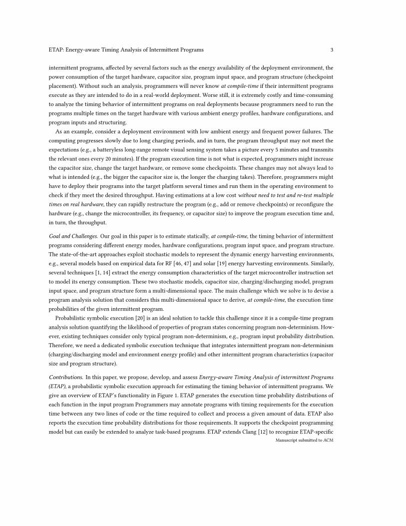
intermittent programs, affected by several factors such as the energy availability of the deployment environment, the

power consumption of the target hardware, capacitor size, program input space, and program structure (checkpoint

placement). Without such an analysis, programmers will never know at compile-time if their intermittent programs

execute as they are intended to do in a real-world deployment. Worse still, it is extremely costly and time-consuming

to analyze the timing behavior of intermittent programs on real deployments because programmers need to run the

programs multiple times on the target hardware with various ambient energy profiles, hardware configurations, and

program inputs and structuring.

As an example, consider a deployment environment with low ambient energy and frequent power failures. The

computing progresses slowly due to long charging periods, and in turn, the program throughput may not meet the

expectations (e.g., a batteryless long-range remote visual sensing system takes a picture every 5 minutes and transmits

the relevant ones every 20 minutes). If the program execution time is not what is expected, programmers might increase

the capacitor size, change the target hardware, or remove some checkpoints. These changes may not always lead to

what is intended (e.g., the bigger the capacitor size is, the longer the charging takes). Therefore, programmers might

have to deploy their programs into the target platform several times and run them in the operating environment to

check if they meet the desired throughput. Having estimations at a low cost without need to test and re-test multiple

times on real hardware, they can rapidly restructure the program (e.g., add or remove checkpoints) or reconfigure the

hardware (e.g., change the microcontroller, its frequency, or capacitor size) to improve the program execution time and,

in turn, the throughput.

Goal and Challenges. Our goal in this paper is to estimate statically, at compile-time, the timing behavior of intermittent

programs considering different energy modes, hardware configurations, program input space, and program structure.

The state-of-the-art approaches exploit stochastic models to represent the dynamic energy harvesting environments,

e.g., several models based on empirical data for RF [46, 47] and solar [19] energy harvesting environments. Similarly,

several techniques [1, 14] extract the energy consumption characteristics of the target microcontroller instruction set

to model its energy consumption. These two stochastic models, capacitor size, charging/discharging model, program

input space, and program structure form a multi-dimensional space. The main challenge which we solve is to devise a

program analysis solution that considers this multi-dimensional space to derive, at compile-time, the execution time

probabilities of the given intermittent program.

Probabilistic symbolic execution [20] is an ideal solution to tackle this challenge since it is a compile-time program

analysis solution quantifying the likelihood of properties of program states concerning program non-determinism. How-

ever, existing techniques consider only typical program non-determinism, e.g., program input probability distribution.

Therefore, we need a dedicated symbolic execution technique that integrates intermittent program non-determinism

(charging/discharging model and environment energy profile) and other intermittent program characteristics (capacitor

size and program structure).

Contributions. In this paper, we propose, develop, and assess Energy-aware Timing Analysis of intermittent Programs

(ETAP), a probabilistic symbolic execution approach for estimating the timing behavior of intermittent programs. We

give an overview of ETAP’s functionality in Figure 1. ETAP generates the execution time probability distributions of

each function in the input program Programmers may annotate programs with timing requirements for the execution

time between any two lines of code or the time required to collect and process a given amount of data. ETAP also

reports the execution time probability distributions for those requirements. It supports the checkpoint programming

model but can easily be extended to analyze task-based programs. ETAP extends Clang [12] to recognize ETAP-specific



configurations and uses LLVM compiler [36]. It employs libraries of R environment [53] for symbolic computations

and SMT [15] solver to detect infeasible paths. Our symbolic execution technique is designed not to be specific to any

microcontroller architecture.

We compared our analysis to the program executions in a radio-frequency energy-harvesting testbed setup. The

evaluation results show that ETAP’s normalized prediction accuracy is 99.5%. To summarize, our contributions include:

(1) Novel Analysis Approach.We introduce a novel probabilistic symbolic execution approach that predicts the

execution times of intermittent programs and their timing behavior considering intermittent execution dynamics.

(2) New Analysis Tool.We introduce the first compile-time analysis tool that enables programmers to analyze the

timing behavior of their intermittent programs without target platform deployment.

(3) Evaluation on Real Hardware. ETAP correctly predicts the execution time of intermittent programs with a

maximum prediction error less than 1.5% and speeds up the timing analysis by at least two orders of magnitude

compared to manual testing.

We share ETAP as a publicly available tool with the research community. We believe that ETAP is a significant attempt

to provide the missing design-time analysis tool support for developing intermittent applications.

2 MOTIVATION AND BACKGROUND

A typical battery-free device such as WISP [58], WISPCam [48], Engage [16], and Camaroptera [49] includes (i) an

energy harvester converting incoming ambient energy into electric current, (ii) energy storage, typically a capacitor, to

store the harvested energy to power electronics, and (iii) an ultra-low-power microcontroller orchestrating sensing,

computation, and communication. The microcontrollers in these platforms, e.g., MSP430FR series [63], comprise a

combination of volatile (e.g., SRAM) and non-volatile (e.g., FRAM [64]) memory to store data that will persist upon

power failures.

2.1 Programming Intermittent Systems

Battery-free platforms operate intermittently due to frequent power failures. Several programming models (supported

by runtimes) have been proposed to mitigate the effects of unpredictable power failures and enable computation progress

while preserving memory consistency (e.g., [13, 35, 68]). Generally speaking, these models backup the volatile state of

the processor into the non-volatile memory so that the computation can be recovered from where it left upon reboot.

Moreover, memory consistency should also be ensured so that the backed-up state in the non-volatile memory will not

be different from the volatile one, or vice versa.

Programming models for intermittent computing have two classes. Checkpointing systems [35] snapshot the volatile

state, i.e., the values of registers, stack, and global variables, in persistent memory at specific points—either defined

by the programmer at compile-time or decided at runtime. Thanks to checkpoints, the state of the computation can

be recovered after a power failure using the snapshot of the system state. Task-based systems [13, 68] employ a static

task-based model. The programmer decomposes a program into a collection of tasks at compile-time and implements a

task-based control flow (connecting task outputs with task inputs). The runtime keeps track of the active task, restarts

it upon recovery from intermittent power failures, guarantees its atomic completion, and then switches to the next task

in the control flow.



Due to different ambient energy(and charging times), the same program spends different times to execute even on the samehardware

PROGRAMint main() { ... int a[N]; int b[K]; int out[NK+1]; ... for(i=0;i<NK+1;i++) for(j=0;j<K;j++){ out[i]+=a[i+j]*b[K-j-1]; } checkpoint();}

Ener

gy

Time

Slow Charging

Operating

Operating

Recharging

Recharging

Programexecution

checkpoint

5 checkpoints are taken

Ener

gy

10 checkpoints are taken

Time

Fast Charging

Recharging

Operating

Operating

Operating

Recharging

Recharging

Fig. 2. Dynamics of Intermittent Execution. A sample application composed of matrix multiplication in a nested loop. The run-timebehavior of the intermittent program (e.g., execution time) depends on the environmental factors (e.g., ambient energy), checkpointplacement and overhead, and the target platform (e.g., power consumption and capacitor size).

2.2 The Need for Timing Behavior Analysis

Using existing intermittent programming models, programmers mainly focus on the progress, memory consistency,

and functional correctness of their programs. Without analyzing the timing behavior affected by several factors,

programmers cannot be sure if their intermittent programs meet throughput expectations in a deployment environment.

Figure 2 depicts how the execution time of a checkpointed code changes under different environmental conditions.

In high-energy environments, the capacitor charges faster, the program progresses quickly, the checkpoints are

triggered more frequently, and the execution needs a shorter time. The same program takes much longer in low-energy

environments. The device is mostly off to charge its capacitor and becomes active only for a short time to perform

computation.

Some runtime environments, e.g., [30, 35, 68], support the expression of timeliness in program source and check if

sensing and computation are handled timely at runtime. They can catch the sensor readings that lost their timeliness due

to power failures and long charging times, throw away these values, or omit their computation. Even though catching

data and computation expiration is beneficial, programmers have no opinion, at compile-time, on how their programs

behave. For instance, sensor readings and computations might expire continuously in specific energy harvesting

conditions due to a wrong checkpoint placement or insufficient capacitor size. The runtime environments can catch

these expirations to prevent unnecessary processing and save precious harvested energy. However, the program does

not produce any meaningful results due to frequent data expirations. With timing behavior analysis, programmers

will know, in advance, how their programs will execute on the target environment (e.g., if there will be frequent data

expirations) and perform the necessary actions to let their programs meet their expectations.



2.3 Factors Affecting Timing Behavior

Energy Harvesting Environment. The availability of ambient energy sources is unpredictable. The harvested energy

depends on several factors, such as the energy source type (e.g., solar or radiofrequency), distance to the energy source,

and the efficiency of the energy harvesting circuit. A probabilistic model of the energy harvesting environment can be

derived based on observations and profiling [19, 46, 47]. When incoming power is strong enough, the capacitor charges

rapidly, and the device becomes available quickly after a power failure. At low input power, the charging is slower and

takes more time.

Energy Storage. The interaction between the capacitor and the processor in battery-free devices plays a crucial role in

the program execution time. When the capacitor is fully charged, the device turns on and starts program execution.

When the stored energy in the capacitor drops below a threshold, the device dies. One of the factors that affect the

device on time is the capacitor size. If the capacitor size is large, the device has more energy to spend until the power

failure, but charging the capacitor takes more time. Prior works, e.g., [46], proposed models that capture the charging

behavior of capacitors.

Target Platform. The power requirements of the target platform affect the end-to-end delay of the program execution.

A program might take a long time to finish on platforms with high power requirements since the capacitor discharges

faster. Hence, the program might drain the capacitor more frequently (since instructions consume more energy in a

shorter time). Therefore, the device is interrupted by frequent power failures, and it is unavailable and charging its

capacitor for long periods. We can model the target platform by using the instruction-level energy consumption profiles,

as suggested in [1, 14].

Intermittent Runtime. The programming model and the underlying runtime affect the execution time of intermittent

programs. For instance, the checkpointing overhead is architecture-dependent since the number of registers and the

volatile memory size change from target to target. Moreover, checkpoint placement is also crucial: the more frequent

the checkpoints are, the more energy consumed, but less computation is lost upon a power failure.

Program Inputs. Intermittent program inputs are mostly the sensor readings that depend on the environmental phe-

nomena. Different inputs lead to different execution flow, and in turn, energy consumption. The energy consumption

affects the frequency of power failures and the charging time.

2.4 A Probabilistic Approach for Timing Analysis

The challenge is to devise a technique that facilitates the compile-time timing analysis of intermittent programs

considering the factors mentioned above. Since these factors can be represented using stochastic models [1, 14, 19,

46, 47], probabilistic symbolic execution—a static analysis technique calculating the probability of executing parts of a

program [20]—becomes an excellent fit for timing behavior analysis.

Symbolic execution analyzes a program to discover which program inputs execute which program parts. It searches

the execution tree of a program using symbolic values for program inputs. It generates from the execution tree program

paths with a path condition, i.e., a conjunction of constraints on program inputs. When symbolic execution reaches

a node of the execution tree, it evaluates the path condition describing the path from the root to that node. If the

condition is satisfiable, it continues in that branch of the tree. If not, the branch is known to be unreachable. The output

of satisfiability checking is either 0 or 1. The values 0 and 1 are rough approximations of the probability that the path



Time and Energy CostProfiles of the Target

MCU

Ambient Energy Profile

Generation of CostModel: Binary

Analysis & ProgramTransformation

CapacitorSize

main.paths

main.llvm

main.c1

Inte

rmitt

ent P

rogr

am

cost.R

Time

Power

msp430

Sensor Input Distribution

ProbabilisticSymbolic Execution

with Cost Model

2 Energy-AwareProbabilistic

Symbolic Executionof Program Paths

3

Timing Distributions and Reports

1mF

int main() { for(;;) { sample(); checkpoint(); compare(); compress(); checkpoint(); send(); }}

(us)

Prob

abili

ty

(us)

Tim

ing

Fig. 3. ETAP Overview.

condition is true. Probabilistic symbolic execution estimates finer approximations of the probability of path conditions

being true [20]. One way is to count the number of solutions to a path condition (model counting [24]) and divide it by

the product of input domain.

3 ETAP: SYSTEMS OVERVIEW

The process in Figure 3 presents an overview of ETAP. Its steps are fully automated. Sections 5-7 provide details of

each step. In Step 1, ETAP takes an intermittent program, and time and energy cost profiles of the target architecture

(main.c and msp430 in Figure 3). It automatically generates a cost model with the program having split program blocks

in LLVM IR [36] (cost.R and main.ll). The cost model is an R specification having LLVM program blocks to which time

and energy costs are assigned as probabilistic cost expressions.

We designed our symbolic execution technique not to be specific to any microcontroller architecture and instruction

set. Therefore, our symbolic execution runs not on microcontroller instructions but the program blocks in LLVM

IR. This design choice contributes to the scalability of ETAP since generating paths on program block-level leads to

fewer divergent (power failure paths) to be analyzed. ETAP needs the time and energy cost profiles of the instruction

types of each new target architecture platform organized under addressing modes. In Section 8, we derived the cost

profiles for the MSP430FR5994 platform [63] through empirical data collection. It is a one-time effort for each new

platform. Symbolic execution on program blocks may lead to coarse approximations of energy costs in the explored

paths. Therefore, in Step 1, ETAP automatically splits blocks having outlier energy costs (maximum outliers) among all

the program block energy costs.

In Step 2, ETAP symbolically executes the program blocks in LLVM IR (main.ll) with the cost model (cost.R) to

generate program paths and path execution probabilities (main.paths) based on the sensor input distribution. In Step 3,

ETAP takes the ambient energy profile, capacitor size, program paths, and path execution probabilities as input. Each



#pragma etap timing "Norm(8517.05, 0.01)" //us#pragma etap energy "Norm(14.560, 0.02)" //uj#pragma etap harvest "Norm(10.54, 0.23)" //ms#pragma etap capacitor max(750uj) #pragma etap capacitor min(520uj) #pragma etap checkpointvoid checkpoint() {...};

int main() { int data; while (1) { sample(&data); #pragma etap expires(1.5s) if (classify(data)) send(&data); }}

#include "checkpoint.h"

int classify(int data) { #pragma etap expires(40ms) #pragma distr "data <- Mixing(Binom(40, 0.4), 15 + Binom(30, 0.6), mixCoeff = c(0.7, 0.3))" int result = -1; checkpoint(); if (data < 21) { result = featurize(data); // checkpoint(); } else if (data > 27) { result = alert(); // checkpoint(); } else error(); #pragma etap reachability(30ms) checkpoint(); return result;}

1

234

567891011121314151617

checkpoint.h

main.c

4

1

2

3

Sensor InputDistribution

Capacitor Size

CheckpointingOverheads

Timing Report

Time

1.6s

expires1.5s timing

requirement

datasample

reportedtiming

behaviour

Vmax

Vminenergy

budg

etE = 1/2 x C x (Vmax - Vmin)2

1 4

1 2 3 4ProgramVariant 2

ProgramVariant 1

2 3ProgramVariant 3

EnergyHarvesting Time

Fig. 4. Example Intermittent Program with ETAP Pragmas.

path is symbolically executed with stochastic ambient energy to estimate execution time probability distributions of

program paths and functions for intermittent execution.

4 SPECIFICATION OF ETAP INPUTS

Engineers specify ETAP inputs (e.g., timing requirements and probability distributions of sensor inputs) via the ‘#pragma’

directive [21]. Figure 4 presents an example intermittent program (main.c) and a header file (checkpoint.h) for the

checkpoint operation. The runtime environment provides the header file [35], which programmers extend with pragmas

for the time and energy cost distributions of the checkpoint operation (𝜏𝑐𝑝 , 𝐸𝑐𝑝 ), ambient energy harvesting time profile

(𝜏ℎ𝑎𝑟𝑣𝑒𝑠𝑡 ) and capacitor size (𝐸𝑚𝑖𝑛, 𝐸𝑚𝑎𝑥 ).

The main function of the example program samples, classifies and sends the input data in a loop (main.c); each loop

iteration should execute in less than 1.5 second ( ‘#pragma etap expires(1.5s)’ in main.c). Function classify interprets

input data, alerts users, or reports an error (Lines 2-17). It should finish in less than 40 milliseconds (Line 3). It has

two checkpoints (Lines 6 and 15); the second checkpoint should be reached from the first checkpoint in less than



30 milliseconds (‘#pragma etap reachability(30ms)’ in Line 14). The "reachability" pragma is to get the probability

distribution of reaching at the specified checkpoint. The “expires” pragma is to get the probability distribution of timing

at the specified point. The input distribution is discretized and modeled (‘#pragma distr’ in Line 4). It is the mixture of

two signals following the binomial distribution (Binom(40, 0.4) and Binom(30, 0.6)).

5 GENERATION OF COST MODELS

ETAP generates a cost model with the intermittent program that has split program blocks in LLVM IR (Step 1 in

Figure 3). It employs Clang [12] to compile the input program into the LLVM IR code. Each checkpoint call needs to be

the first instruction in its basic block because the symbolic execution returns to the beginning of the basic block for a

power failure. Therefore, ETAP splits checkpoint calls, which are not the first instruction, from their basic blocks.

The LLVM IR code is compiled into the assembly code for the target hardware architecture. ETAP performs a binary

analysis to map the hardware instructions in the assembly code to the basic blocks. It calculates the time and energy

cost distributions of each basic block. To do so, it convolves the cost distributions of all instructions in that block

based on their types and addressing modes (see Table 2). Some basic blocks may need much more energy than other

basic blocks, which may lead to coarse approximations of energy costs of the program paths. To have a better energy

approximation, ETAP performs a semantic- and cost-preserving program transformation. It automatically splits blocks

having outlier energy costs (i.e., maximum outliers) among all the program block energy costs for each function in the

program. We use the IQR method [38] to detect the outlier blocks in terms of energy costs and obtain the threshold

value. Considering the threshold, ETAP splits blocks having cost more than 𝑄3 + 1.5(𝐼𝑄𝑅) (𝑄3 is the third quartile, and

𝐼𝑄𝑅 is the interquartile range).

Figure 5 presents the control flow graph (CFG) of classify in Figure 4 (with four checkpoints). Time and energy costs

are modeled as normal distributions and encoded in an R specification (cost.R in Figure 3). Each node represents a basic

block. Blocks a and b, c and d, and g and h were initially single blocks ETAP splits into two as the checkpoint calls were

not the first instruction. No blocks are split for the threshold.

6 PROBABILISTIC PATH EXPLORATION

ETAP symbolically executes the basic blocks with the cost models in the R environment with depth-first search (Step 2

in Figure 3). It generates program paths and their execution probabilities for program execution without power failures.

The program paths are later re-executed symbolically with stochastic ambient energy to estimate its execution time

probability distribution for intermittent execution (see Section 7).

Algorithm 1: DFS for Probabilistic Path Exploration

1 Blocks(𝑝𝑎𝑡ℎ)← Blocks(𝑝𝑎𝑡ℎ) ⊕ Name(𝑐𝑢𝑟𝑟 )

2 Timing(𝑝𝑎𝑡ℎ)← Timing(𝑝𝑎𝑡ℎ) ∗ Get(𝐶𝑜𝑠𝑡𝑠 , 𝑐𝑢𝑟𝑟 )3 Eval(Instructions(𝑐𝑢𝑟𝑟 ), 𝑒𝑛𝑣)

4 foreach 𝑠𝑢𝑐𝑐 in Successors(𝑐𝑢𝑟𝑟 ) do

5 𝑝𝑟𝑜𝑏 ← 𝑝𝑟𝑜𝑏 × BranchProbability(𝑐𝑢𝑟𝑟 , 𝑠𝑢𝑐𝑐 , 𝑒𝑛𝑣)

6 if 𝑝𝑟𝑜𝑏 > 0 ∧ ¬IsMaxLoopReached then

7 𝑃𝑎𝑡ℎ𝑠 ← Dfs(𝑃𝑎𝑡ℎ𝑠 ,𝐶𝑜𝑠𝑡𝑠 , (𝑏, 𝑠𝑢𝑐𝑐 , 𝑝𝑟𝑜𝑏) , CloneEnv(𝑒𝑛𝑣),𝑝𝑎𝑡ℎ)

8 return 𝑃𝑎𝑡ℎ𝑠 ⊕ ( Blocks(𝑝𝑎𝑡ℎ), 𝑝𝑟𝑜𝑏, Timing(𝑝𝑎𝑡ℎ) )



entry

checkpoint.1

F T

if.then:%1 = load i16, i16* %data.addrcall void @featurize(i16 %1)store i16 1, i16* %resultbr label %if.end4

0.648

if.else

T F

0.352

checkpoint.2

0.648

if.then2

0.2937

if.else3

0.05833

checkpoint.4

0.648

checkpoint.3

0.2937

if.end

0.05833

0.2937

0.352

derived from the sum of the distributionof the number of microcontroller cyclesrequired by each assembly instructioncorresponding to the basic block.

... MOV.B #20, R12 CMP.W @R1, R12 { JL .L2 MOV.W @R1, R12 CALL #featurize MOV.W #1, 2(R1) BR #.L3 .L2: MOV.B #27, R12 CMP.W @R1, R12 { JGE .L4 CALL #alert MOV.W #0, 2(R1) BR #.L3 ...

LLVM IR(variant 2)

𝞃(if.then) ~ Normal(12.06, 0.01)

MSP

430

asse

mbl

y<<maps>>

Time and Energy Cost Profiles

(MSP430FR5994)

derived from the sum of the distributionof the amount of energy expended by amicroprocessor for each instructioncorresponding to the basic block.

Timing Model (𝞃) µs

@classify(data)

𝙀(if.then) ~ Normal(29.44, 1.24)Energy Model (𝙀) nj

<<generates>>

a

b

c

d

g

e

f

h

i

j

1

4

2

3

Fig. 5. CFG of Function classify and its Cost Models.

entry checkpoint.1 if.else if.then2 checkpoint.3 if.end checkpoint.4

a c fb d e

1 43

𝞅2: a ➞ a ➞ b ➞ c, 𝞈2

𝞅3: a ➞ b ➞ a ➞ b ➞ c, 𝞈3

𝞅4: a ➞ b ➞ c ➞ a ➞ b ➞ c, 𝞈4

𝞅1: a ➞ b ➞ c, 𝞈 1 𝞅1: d ➞ e ➞ f, 𝞈 1

𝞅2: d ➞ d ➞ e, 𝞈2

𝞅3: d ➞ e ➞ d ➞ e, 𝞈3

call site

𝝿2 𝜔2 : 0.294

Region 1 Region 2 Region 3

Fig. 6. An Example Path derived for Normal Execution and its Analysis for Intermittent Execution.

ETAP calculates the path execution probability and the execution time probability distribution for each program path

in the function to be analyzed. Algorithm 1 gives the depth-first search for probabilistic path exploration.

ETAP adds the visited (current) basic block of the CFG to the path (Line 1). It convolves the execution time probability

distribution of the path and the execution time cost distribution of the visited block (Line 2). The block instructions in



the path environment are evaluated to decide which successor block to take in which branching conditions (Line 3).

ETAP models path execution environments with instances of a symbolic memory model in which LLVM instructions

are probabilistically interpreted. For instance, in the LLVM instruction ‘%𝑖𝑛𝑐 = add nsw i16 %i.0, 1’, if ‘%i’ is a random

variable (r.v.) that follows a discrete probability distribution, the 16-bit integer register %𝑖𝑛𝑐 becomes an r.v., %𝑖𝑛𝑐 ∼ %i.0

+1, through linear location-scale transformation [8]. If the instruction was among two registers, ‘%𝑖𝑛𝑐 = add nsw i16

%i.0, %i.1’ and in that ‘%i.0’ and ‘%i.1’ are independent r.v.s, the expression would be interpreted as the sum (integral)

of two r.v.s (convolution) [8]. The path execution probability is a conditional probability and recalculated for each

new successor block. The new path probability is the multiplication of the current path probability and the branch

probability for the successor basic block (Line 5). Figure 5 shows the probabilities in the example CFG. The paths are

recursively explored until the path probability is equal to zero or the maximum number of iterations for a loop is

reached (Line 6-7).

LLVM operators on distributions are overloaded to produce transformed distributions. When symbolic execution has

reached a branch point, ETAP integrates the probability function of the transformed distribution that the execution

branches on over the region of interest. This tells us the probability of taking that branch. After stepping over a branch

point, we perform state forking, similar to mainstream symbolic execution engines [5, 10], and update the random

variables in the symbolic environment of the path with the information gained.

Linear transformations of named distributions have mostly analytical solutions; however, we need to employ

computational approaches if the transformation is non-linear (e.g., a logarithmic transformation). This is also the case

for convolution operations. For instance, the sum of two independent normally distributed (Gaussian) random variables

also follows a normal distribution, with its mean being the sum of the two means, and its variance being the sum of the

two variances; on the other hand, the sum of two random variables, which follow Uniform and Normal distributions

respectively, cannot be expressed with a closed-form expression, and therefore, in these cases, ETAP approximates

these probabilities using numerical methods.

For function classify in Figure 5, ETAP explores three paths i.e., 𝜋1: ‘𝑎 → 𝑏 (𝑐𝑝) → 𝑐 → 𝑑 (𝑐𝑝) → 𝑒 (𝑐𝑝)’, 𝜋2:‘𝑎 → 𝑏 (𝑐𝑝) → 𝑓 → 𝑔 → ℎ(𝑐𝑝) → 𝑖 → 𝑒 (𝑐𝑝)’, and 𝜋3: ‘𝑎 → 𝑏 (𝑐𝑝) → 𝑓 → 𝑗 → 𝑖 → 𝑒 (𝑐𝑝)’ where 𝑐𝑝 indicates

the blocks with the checkpoint operation. It calculates path execution probabilities (or weights) associated with each

path (𝜔1 = 0.648, 𝜔2 = 0.058, and 𝜔3 = 0.294). The nodes labeled with small letters represent the basic blocks (e.g.,

𝑎, 𝑏, 𝑐). Each basic block is heat-map colored based on its execution probability. Each path has an execution time

probability distribution (𝜏1, 𝜏2, and 𝜏3) that represents the path’s timing behavior while it is continuously powered. It is

the convolution of the execution time cost distribution of the basic blocks along the path. Since the timing behavior is

compositional when there is no power failure, ETAP considers checkpoint (𝜏𝑐𝑝 ) and other function calls in the program

path (𝜏𝑎𝑙𝑒𝑟𝑡 , 𝜏𝑓 𝑒𝑎𝑡𝑢𝑟𝑖𝑧𝑒 , and 𝜏𝑒𝑟𝑟𝑜𝑟 ) while convolving the cost distributions as follows:

𝜏1 ∼ 𝑎(𝜏) ∗ 𝑏 (𝜏) ∗ 𝜏𝑐𝑝 ∗ 𝑐 (𝜏) ∗ 𝜏𝑓 𝑒𝑎𝑡𝑢𝑟𝑖𝑧𝑒 ∗ 𝑑 (𝜏) ∗ 𝜏𝑐𝑝 ∗ 𝑒 (𝜏) ∗ 𝜏𝑐𝑝𝜏2 ∼ 𝑎(𝜏) ∗ 𝑏 (𝜏) ∗ 𝜏𝑐𝑝 ∗ 𝑓 (𝜏) ∗ 𝑔(𝜏) ∗ 𝜏𝑎𝑙𝑒𝑟𝑡 ∗ ℎ(𝜏) ∗ 𝜏𝑐𝑝 ∗ 𝑖 (𝜏) ∗ 𝑒 (𝜏) ∗ 𝜏𝑐𝑝𝜏3 ∼ 𝑎(𝜏) ∗ 𝑏 (𝜏) ∗ 𝜏𝑐𝑝 ∗ 𝑓 (𝜏) ∗ 𝑗 (𝜏) ∗ 𝜏𝑒𝑟𝑟𝑜𝑟 ∗ 𝑖 (𝜏) ∗ 𝑒 (𝜏) ∗ 𝜏𝑐𝑝

The execution time probability distribution of function classify for program execution without power failures is a

convex combination of all the timing distributions of its execution paths: 𝜏𝑐𝑙𝑎𝑠𝑠𝑖 𝑓 𝑦 ∼ 𝜔1𝜏1 +𝜔2𝜏2 +𝜔3𝜏3. It is a univariate

mixture distribution and represents the timing behavior of the function while the energy is plentiful in the environment.



1mF

20000 40000 60000

0.00

000.

0004

0.00

08

20000 40000 60000

0.0

0.2

0.4

0.6

0.8

1.0

prob

abili

ty

95% Confidence Interval (19232.09, 36178.86, 68914.2)

(a) 1mF Capacitor - Program Variant 1

20000 40000 60000 80000

0e+0

02e

−04

4e−0

46e

−04

20000 40000 60000 80000

0.0

0.2

0.4

0.6

0.8

1.0

prob

abili

ty


(b) 1mF Capacitor - Program Variant 2

0 20000 40000 60000 80000

0.00

000.

0004

0.00

08

20000 40000 60000

0.0

0.2

0.4

0.6

0.8

1.0

prob

abili

ty


(c) 1mF Capacitor - Program Variant 3

2mF

20000 40000 60000 80000

0.00

000.

0004

0.00

08

20000 40000 60000 80000

0.0

0.2

0.4

0.6

0.8

1.0

prob

abili

ty


(d) 2mF Capacitor - Program Variant 1

20000 60000 100000

0.00

000.

0004

0.00

08

20000 40000 60000 80000

0.0

0.2

0.4

0.6

0.8

1.0

prob

abili

ty


(e) 2mF Capacitor - Program Variant 2

10000 30000 50000 70000

0.00

000.

0004

0.00

08

20000 40000 60000 80000

0.0

0.2

0.4

0.6

0.8

1.0

prob

abili

ty


(f) 2mF Capacitor - Program Variant 3

5mF

20000 60000 100000

0.00

000.

0004

0.00

08

20000 60000 100000

0.0

0.2

0.4

0.6

0.8

1.0

prob

abili

ty


(g) 5mF Capacitor - Program Variant 1

20000 60000 100000

0.00

000.

0004

0.00

08

20000 60000 100000

0.0

0.2

0.4

0.6

0.8

1.0

prob

abili

ty


(h) 5mF Capacitor - Program Variant 2

20000 60000 100000

0.00

000.

0004

0.00

080.

0012

20000 60000 100000

0.0

0.2

0.4

0.6

0.8

1.0

prob

abili

ty


(i) 5mF Capacitor - Program Variant 3

Fig. 7. Reports of the Execution Time Probability Distributions (PDF and CDF) of Function classify after symbolically executing with1MHz clock-rate under 3 different capacitor type and 3 different checkpoint placements with the given 𝜏harvest profiles.

7 ENERGY-AWARE ANALYSIS OF PROGRAM PATHS

ETAP symbolically executes each program path with stochastic ambient energy to estimate its execution time probability

distribution for intermittent execution (Step 3 in Figure 3). Figure 6 presents an example path without power failures (𝜋2:

‘𝑎(𝑐𝑝) → 𝑏 → 𝑐 → 𝑑 (𝑐𝑝) → 𝑒 → 𝑓 (𝑐𝑝)’ where 𝑐𝑝 indicates the blocks with the checkpoint operation) and illustrates

its energy-aware symbolic analysis. We relabel the blocks in path 𝜋2 to increase the readability in Figure 6. We also

initiate the symbolic analysis from block 𝑎 to simplify the presentation.

The analysis starts with a non-deterministic initial capacitor energy budget, i.e., a uniform random variable on

the interval of the capacitor’s maximum and minimum thresholds, 𝐸𝑖𝑛𝑖𝑡 ∼ 𝑈𝑛𝑖 𝑓 (𝐸𝑚𝑖𝑛, 𝐸𝑚𝑎𝑥 ). ETAP divides the

path into regions between two sequential checkpoints and between the beginning/end of the path and the first/last

checkpoint in the path (‘𝑎 → 𝑏 → 𝑐’, ‘𝑑 → 𝑒’, and ‘𝑓 ’). The path is analyzed region by region. The power failure

probabilities are calculated for each block in the first region based on the initial capacitor energy distribution (𝐸𝑖𝑛𝑖𝑡 ).

If a power failure is probable, ETAP creates a path which returns to the checkpoint block. In addition to the initial

program path in the first region in Figure 6 (𝜑1: ‘𝑎 → 𝑏 → 𝑐’), three new paths are derived for power failures (e.g., 𝜑3:

‘𝑎 → ¤𝑏 → 𝑎 → 𝑏 → 𝑐’ where the power failure occurs in block 𝑏). Each new path has only one power failure because

ETAP reports non-terminating ones [14] that need more energy than the capacitor size.



Table 1. Timing Report of ‘#pragma etap expires(40ms)’ for the given configuration space in Figure 7.

Conf. Timing Probability Meets Timing Confidence Intervals (ms)𝑃𝑟 (𝜏𝑐𝑙𝑎𝑠𝑠𝑖 𝑓 𝑦 ≤ 40𝑚𝑠) Req.? 95% CI 90% CI 80% CI

(a) 0.691 ✗ [19.2, 68.9] [21.8, 68.7] [22.1, 68.3]

(b) 0.546 ✗ [19.2, 86.1] [39.4, 85.9] [30.7, 85.7]

(c) 0.732 ✗ [10.6, 68.9] [11.0, 68.7] [22.0, 68.2]

(d) 0.838 ✓ [19.2, 78.7] [21.6, 78.4] [22.0, 70.9]

(e) 0.751 ✗ [19.2, 95.9] [30.2, 95.7] [30.6, 90.4]

(f) 0.857 ✓ [10.6, 78.7] [10.9, 78.3] [22.0, 70.0]

(g) 0.934 ✓ [19.1, 93.3] [19.5, 90.4] [22.0, 25.5]

(h) 0.895 ✓ [19.1, 116 ] [19.5, 110 ] [30.5, 104 ]

(i) 0.943 ✓ [10.6, 92.9] [10.9, 84.3] [21.9, 25.4]

For each path, ETAP subtracts the energy cost distributions of program blocks from the capacitor energy through

convolution; it sums (convolves) the time cost distributions of the blocks. The result is the time and energy cost

distributions of the paths in the first region (𝜏1, 𝜏2, 𝜏3, 𝜏4, 𝐸1, 𝐸2, 𝐸3, and 𝐸4). To reduce the number of convolution

operations in the next region, ETAP derives univariate mixture distributions (e.g., 𝜏𝑚𝑖𝑥1 ) from the cost distributions

of the paths with power failure (e.g. in region 1, 𝜏𝑚𝑖𝑥1 ∼ (𝜔2𝜏𝜑2∗ 𝜔3𝜏𝜑3

∗ 𝜔4𝜏𝜑4) ∗ 𝜏ℎ𝑎𝑟𝑣𝑒𝑠𝑡 , where 𝜔2, 𝜔3, and 𝜔4 are

failure probabilities). These distributions are input time costs for the paths in the next region derived from the power

failure paths in the current region (e.g., 𝜑2 ∼ 𝜏𝑚𝑖𝑥1 ∗ 𝑑𝜏 ∗ (𝑑𝜏 ∗ 𝑒𝜏 ) for 𝜑2 in the second region in Figure 6).

The current capacitor energy distribution is calculated for each path in the first region. For the capacitor energy of the

path without power failure, ETAP subtracts the energy cost distributions of the blocks from the initial capacitor energy

distribution through convolution, i.e., 𝐸𝑐𝑢𝑟𝑟𝑒𝑛𝑡 ∼ 𝐸𝑖𝑛𝑖𝑡 ∗−(𝑎𝜖 ∗𝑏𝜖 ∗𝑐𝜖 ). In the power failure paths, the capacitor is chargedup to the maximum threshold energy level during power failure (sleep mode). Therefore, while calculating their capacitor

energy, ETAP considers the maximum energy the capacitor can store, e.g., 𝐸𝑐𝑢𝑟𝑟𝑒𝑛𝑡 ∼ 𝐸𝑚𝑎𝑥 ∗ −(𝑎𝜏 ∗ 𝑏𝜏 ∗ 𝑎𝜏 ∗ 𝑏𝜏 ∗ 𝑐𝜏 )for path 𝜑3: ‘𝑎 → 𝑏 → 𝑎 → 𝑏 → 𝑐’. It uses the final program paths, capacitor energy levels, and cost distributions

of the current region as the initial parameters of the next region. The same mixture and convolution operations are

repeated in each new region. In the last region, the final energy and time probability distributions are obtained for the

path under analysis (see Region 3 in Figure 6).

As we described above, ETAP obtains the execution time probability distributions of each path of the function under

analysis. These distributions are also used to generate reports on how likely timing requirements are met (see the 2nd

column in Table 1). ETAP symbolically executes each path of the function in Figure 5 for intermittent execution. The

mixture distribution of the execution time distributions of these paths is the execution time probability distribution of

the function.

Figure 7 shows the reports of the execution time probability distributions of function classify for intermittent

execution under three different capacitor types (1mF, 2mF, and 5mF) and three different checkpoint placements (variant

1, variant 2, and variant 3 in Figure 4). The first functions in Figure 7 are the probability density function (PDF), and the

second ones are the cumulative distribution function (CDF). As shown in Table 1, ETAP also generates a report for each

configuration.

When the capacitor size increases, the probability of failure paths decrease for all variants, which is expected.

Configurations (d), (f), (g), (h), and (i) in Figure 7 satisfy the timing requirement (see Line 3 in Figure 4) with 0.8



probability (𝑃𝑟 (𝜏𝑐𝑙𝑎𝑠𝑠𝑖 𝑓 𝑦 ≤ 40𝑚𝑠) > 0.8). If we increase the capacitor size from 2mF to 5mF, the probability of meeting

the requirement becomes 0.9 for all variants. This increase our confidence in meeting the requirement, especially for

configurations (g), (h), and (i). Program variants 1 and 3 have more stable timing behavior compared to variant 2 (less

divergent timing behavior in the probability distributions), and variant 3 performs slightly better than variant 1 for all

confidence intervals. Therefore, we can conclude that it would be better to use 5mF capacitor powering the program

variant 3 for function classify (see (f)). 5mF capacitor has a higher energy level, and the probability of meeting the

timing requirement would be higher due to less power failure probability. However, bigger capacitors would require

more time to store enough energy to power up the application, which would decrease the sampling rate of the sensing

application. In this analysis, the setup harvests energy from the emitted radio frequency (RF) signals at a distance of

40cm. The charging time distributions of the capacitors we used are given in 95% confidence intervals as follows:

40cm distance 1mF 2mF 5mF

𝜏ℎ𝑎𝑟𝑣𝑒𝑠𝑡 [9.48ms, 11.95ms] [18.99ms, 25.64ms] [41.47ms, 57.53ms]

We can conclude that it would be better to minimize the capacitor size while meeting the timing requirement. Also, a

2mF capacitor would be the optimal selection for this setup under the given timing requirement and energy profile.

8 EVALUATION

We now evaluate our prototype to demonstrate that: (i) ETAP correctly predicts the execution time of intermittent

programs and (ii) it significantly reduces the analysis time and efforts.

8.1 Testbed Setup

Target Platform. We used TI’s MSP430FR5994 LaunchPad [63] development board as a target platform. The operating

frequency of the microcontroller (MCU) was set to 1 MHz for our testbed experiments, however, we also investigated

4MHz, 8MHz, and 16MHz clock-rates. The MCU supports 20-bit registers and 20-bit addresses to access an address

space of 1 MB. To infer instruction-level energy consumption and obtain timing models, we used TI’s EnergyTrace

software [61] sampling the energy consumption of programs at runtime by using the specialized debugger circuitry on

the development board. The precision of EnergyTrace was limited due to its low sampling rate.

Checkpoint Implementation. This MCU has 256 KB of FRAM (non-volatile memory) to store data that persists when

there is no power. It also includes 4 KB of SRAM (volatile memory) to store program variables with automatic scope.

We implemented (i) a checkpoint routine (checkpoint()) that copies the volatile computation state (20-bit general-

purpose registers, program counter, and 4KB SRAM) into FRAM and (ii) a recovery routine (recovery()) that restores the

computation state after a power failure by using the latest successful checkpoint data. The energy and timing costs of

these routines are constant. We configured ETAP with these costs by using pragmas, as shown in Figure 4.

Energy Harvesting Tools. We used the Powercast TX91501- 3W power transmitter [51] emitting radio frequency (RF)

signals at 915 MHz center frequency. The transmitter was connected to a P2110-EVB receiver [52] co-supplied with a 6.1

dBi patch antenna. The receiver harvested energy from the emitted RF signals to power the MSP430FR5994 launchpad

board. We used Arduino Uno [3] with 10-bit ADC (analog to digital converter) to measure the instantaneous harvested

power by P2110-EVB receiver.



Table 2. Stochastic Cost Models of the MSP430 Instruction Set Architecture based on Formats and Addressing Modes.

Addressing Example Timing Energy

Modes Instructions Models (`𝑠) Models (𝑛𝑗 )

Format I Double Operand

00 0 mov r5, r9 𝑁 (1.02, 0.01) 𝑁 (4.52, 0.62)

00 1 add r5, 3(r9) 𝑁 (3.02, 0.01) 𝑁 (7.08, 0.62)

01 0 mov 2(r5),r7 𝑁 (3.02, 0.01) 𝑁 (6.97, 0.62)

01 1 add 3(r4), 6(r9) 𝑁 (5.02, 0.01) 𝑁 (10.1, 0.62)

10 0 and @r4, r5 𝑁 (2.02, 0.01) 𝑁 (5.80, 0.62)

10 1 xor @r5, 8(r6) 𝑁 (4.02, 0.01) 𝑁 (8.33, 0.62)

11 0 mov #20, r9 𝑁 (2.02, 0.01) 𝑁 (5.55, 0.62)

11 1 mov @r9+, 2(r4) 𝑁 (4.02, 0.01) 𝑁 (8.34, 0.62)

Format II Single Operand

00 push r5 𝑁 (3.01, 0.01) 𝑁 (8.34, 0.62)

01 call 2(r7) 𝑁 (4.02, 0.01) 𝑁 (10.1, 0.62)

10 push @r9 𝑁 (3.52, 0.01) 𝑁 (8.33, 0.62)

11 call #81h 𝑁 (4.02, 0.01) 𝑁 (10.1, 0.62)

Format III Special Instructions

Jxx jmp r5, r9 Constant(2) 𝑁 (5.8, 0.62)

mult. call #_mspabi_mpyi 𝑁 (15.94, 0.27) 𝑁 (16.38, 0.23)

div. call #_mspabi_divu 𝑁 (16.39, 0.23) 𝑁 (16.68, 0.17)

Host Platform. We run ETAP on an Intel Core i7-9750H CPU @ 2.60GHz × 12 core machine with 32 GiB RAM. ETAP

used one core and 16 GiB memory on average. The memory consumption was relatively high, mainly due to the

symbolic computation introduced by our benchmarks.

8.2 Profiling Target Platform and Energy Environment

The target platform and energy environment profiling is a one-time effort and eliminates the need for continuous target

deployment and on-the-fly analysis efforts.

Profiling Target Platform. ETAP runs on the platform-independent LLVM instruction set [37]. There is no one-to-one

correspondence between the LLVM instruction set and the target architecture instruction set. Therefore, we employed a

block-based mapping strategy as mentioned in Section 5. In the cost model generation step of ETAP (Step 1 in Figure 3),

the target hardware instructions were automatically mapped into the LLVM basic blocks. The time and energy cost

distributions of each basic block were calculated through the hardware instruction cost distributions.

We used the Saleae logic analyzer [57] and EnergyTrace tool to collect the energy and timing costs of the MSP430

instructions from the MSP430FR5994 Launchpad at 1MHz clock frequency. Table 2 presents a simplified version of

the cost model we used to predict basic block costs. MSP430 is a 16-bit RISC instruction-set architecture with no

data-cache [1]. It has 27 native and 24 emulated instructions. Our analysis shows that the energy and timing costs of

the instructions depend on the formats and addressing modes. The MSP430 architecture has seven modes to address

its operands: register (00), indexed (01), absolute (10), immediate (11), symbolic, register indirect, and register indirect

auto increment. The timing and energy behavior of each instruction highly depends on the these addressing modes,



18.2

18.4

18.6

18.8

19.0

19.2

0 250 500 750 1000

9.8

10.0

10.2

10.4

10.6

10.8

0 250 500 750 1000

5.8

6.0

6.2

6.4

6.6

6.8

0 250 500 750 1000

Samples

Seconds

100cm : 𝞃harvest ~ N(6.09, 0.06)

120cm : 𝞃harvest ~ N(10.22, 0.08)

140cm : 𝞃harvest ~ N(18.59, 0.18)

Fig. 8. RF energy profiles: charging-time samples for a 50mF supercapacitor at different distances.

which we can group as double operand instructions (Format I), single operand instructions (Format II), and special

instructions (Format III) [62]. We sampled the addressing modes and their combinations grouped by their formats, and

then statistically inferred the distribution of sample means employing bootstrapping method [38].

Apart from those instructions, we modeled the subroutines, call #mspabi_mpyi and call #mspabi_divu, generated by

the compiler since MSP430 does not have a hardware multiplier and divider. Besides, we derived regression models for

call #memset and call #memcopy intrinsic functions. For call #memcopy, the stochastic models for timing and energy

are #memcpy𝜏 ∼ 𝑁 (13.06, .01) ∗ 𝑐 · 𝑁 (9.06, .01) and #memcpy𝜖 ∼ 𝑁 (35.04, 1.38) ∗ 𝑐 · 𝑁 (24.21, 1.24) where 𝑐 is theexplanatory variable for the number of data words copied.

Energy Profiles of the Environment. ETAP requires the ambient energy profile and the capacitor size to infer power

failure rates and the off- and on-times of the device. Therefore, we collected the ADC samples of the instantaneously

received power from different setups for 20 seconds. We created different settings by placing the RF power transmitter

and receiver in line of sight at different distances. The measurements were repeated ten times for each setup. Using the

energy profile and energy equation of capacitors (𝐸 = 1/2 ·𝐶 ·𝑉 2), one can infer a bootstrapping distribution [38] to

model the average waiting time required to charge a capacitor with the given voltage threshold. We run our benchmarks

using energy harvesting hardware. Since the instantaneous power obtained from energy harvesting devices varies

depending on the distance between the receiver and the transmitter, we chose three different distances in our testbed

(100cm, 120cm, and 140cm). Figure 8 presents the energy profiles sampled at these distances. The MCU starts to operate

intermittently at 100cm to the transmitter. The harvested power significantly decreases after 120cm, and the MCU dies

quite frequently.

8.3 Evaluation Results

We used four benchmarks having different computation demands and memory access frequency affecting the execution

time (see Table 3). In particular, our benchmarks implement network algorithms and data filtering in real IoT and Edge

computing applications.

ETAP Prediction Accuracy. We compared ETAP’s predictions to the actual measurements obtained from the testbed (see

Section 8.1 for the evaluation setup). The difference between the ETAP estimation and the actual measurements varies



Table 3. Benchmarks. Instructions and block counts are derived while MSP430 is continuously-powered.

Benchmark # of Instructions # of Blocks # of Power Source

Static Dynamic Static Dynamic Failure Paths

BitCount 566 103702 66 7439 922 [25]

CRC 92 1568 17 408 363 [25]

Dijkstra 282 24585 36 2884 592 [25]

FIR Filter 390 144400 13 1880 175 [2]

Table 4. Prediction for Intermittent Execution Times compared with Actual Measurements (`–mean, 𝜎–standard deviation).

Benchmark Distance Actual Measure. (𝑚s) ETAP Prediction (𝑚s) Error

(cm) ` 𝜎 ` 𝜎 in %

BitCount <100 6150.038 0.013 6145.405 0.003 0.075

100 33550.353 19.919 33693.902 99.793 0.4279

120 99815.832 1008.207 99618.170 303.237 0.0197

140 206575.550 219.747 206546.729 267.430 0.0143

CRC <100 3689.654 0.001 3690.537 0.001 0.022

100 23337.998 23.339 23655.506 29.708 1.3605

120 54626.126 771.290 54048.093 154.173 1.0582

140 95888.740 1369.499 96297.124 421.776 0.4259

Dijkstra <100 3212.243 0.013 3201.285 0.006 0.341

100 27136.569 459.938 27469.100 56.679 1.2254

120 40455.846 636.112 40506.445 74.279 0.1251

140 73032.293 88.785 73026.767 156.892 0.0076

FIR Filter <100 7282.946 0.019 7277.968 0.004 0.068

100 51716.969 33.936 51664.758 173.920 0.1010

120 97558.188 98.225 97702.685 136.667 0.1481

140 163037.556 138.595 163634.595 481.34 0.3662

between 0.007% and 1.3% (see Table 4). Despite the limitations of our measurement devices, and in turn, coarse-grained

ambient energy profiles, ETAP predicted the power failure probabilities with high accuracy. Since the device starts to

operate continously at a distance of less than 100cm, the prediction error significantly decreases to at most 0.34% and at

least 0.022%. Moreover, it accurately modeled the charging and discharging times by using the probabilistic distribution

of the ambient energy. Note that the prediction accuracy of ETAP depends on the accuracy of the hardware cost models,

and the ambient energy profile.

The prediction errors in Table 4 (e.g., ETAP’s predictions for CRC and Dijkstra are less accurate at closer distances to

the energy harvester) are due to our imperfect probabilistic models. Moreover, ETAP does not consider the fact that the

battery-free device is simultaneously charging while discharging. Therefore, as the distance gets longer, the amount of

charge loaded on the capacitor during the discharge period decreases, and the predictions become more accurate.

Summary. ETAP predicted the execution time of RF-powered intermittent programs almost perfectly. We

observed a reasonable maximum prediction error during our evaluation, which was less than 1.5%.



Table 5. Time Study for Intermittent Execution. ETAP’s automated analysis compared to manual experiment times.

Benchmark ETAP Analysis Harv. Profile Experiment Time (s) Cap.

Time (s) Time (s) 100 cm 120 cm 140 cm size

Bitcount 54 200 1698 5042 10412 50mF

CRC 5 200 1249 2797 3895 50mF

Dijkstra 24 200 1391 2029 3842 50mF

Fir Filter 26 200 2591 4897 8203 50mF

ETAP Analysis Time. To assess how significantly ETAP reduces the analysis time and efforts, we measured the time

required to deploy an RF-powered application onto our testbed (see Section 8.1), run the application 50 times, and

collect a sufficient amount of data to reason about the timing behavior through statistical sampling. The 4th

column in

Table 5 presents the time it takes for the experimental measurements at each distance and excludes the manual analysis

efforts such as data extraction and preparation for data analysis.

As shown in Table 5, the manual experiment time increases as the number of power failures during intermittent

operation increases (as the distance from the transmitter increases) while ETAP’s analysis time does not change

with regard to distances of the harvesting kit, and it mainly depends on the number of dynamic program blocks and

instruction counts (see Table 3). Moreover, ETAP checks the likelihood of a power failure after each block, which

increases its analysis time. ETAP appreantly requires less manual effort and is significantly faster than manual testing.

ETAP performed more precise path-based symbolic analysis at least 100 times faster than experimental measurements

under low energy harvesting conditions.

Summary. ETAP speeds up the timing analysis of intermittent programs by at least two orders of magnitude

and eliminates the burden of the manual data analysis effort.

9 RELATEDWORK

We present prior work that relates to our approach in the context of intermittent computing, timing and energy analysis

of intermittent programs, and probabilistic program analysis.

Timing Analysis of Intermittent Programs. Some runtimes provide programming constructs to assign timestamps to

sensed data and check if the data expire. InK [68] is a reactive task-based runtime that employs preemptive and power

failure-immune scheduling for timing constraints of task threads. Mayfly [30] makes the passing of time explicit,

binding data to the time it was collected, and keeping track of data and time through power failures. TICS [35] provides

programming abstractions for handling the passing of time through intermittent failures and making decisions about

when data can be used or thrown away. Different from these runtimes, ETAP predicts the timing behavior of intermittent

programs before deployment and introduces zero overhead.

Energy Analysis of Intermittent Programs. CleanCut [14] detects non-terminating tasks in a task-based intermittent

program. To do so, it samples the energy consumption of program blocks with a special debugging hardware and over

approximates path-based energy consumption. Similar to CleanCut, EPIC [1] traverses control-flow graph to compute

best- and worst-case estimates of dynamic energy consumption for a given intermittent program. ETAP similarly

analyze the energy costs of paths but considers precise program semantics and knows execution probabilities of each



path by means of probabilistic symbolic execution. In fact, profiling is a one-time effort for each target and has intrinsic

support for detection of forward-progress violations. ETAP’s main goal is to perform energy-aware timing analysis to

reason about timing behavior of intermittent programs.

Other Analysis Tools for Intermittent Programs. IBIS [59] performs a static taint analysis to detect bugs caused by

non-idempotent I/O operations in intermittent systems. ScEpTIC [44] has similar objectives as IBIS, i.e., detecting

intermittent bugs. Ocelot [60] enforces intermittent programs written rust language to maintain temporal consistency.

Those tools are complementary and can be used with ETAP to detect such intermittence bugs. But none of these tools

perform timing analysis of intermittent programs. Moreover, ETAP is a novel probabilistic program analysis approach.

Probabilistic Program Analysis. Various probabilistic symbolic execution techniques have been proposed in the literature

(e.g., [9, 11, 17, 18, 20, 40, 50]). Geldenhuys et al. [20] propose probabilistic symbolic execution as an extension of

Symbolic PathFinder [50]. Luckow et al. [40] extend probabilistic symbolic execution to compute a scheduler resolving

program non-determinism to maximize the property satisfaction probability. Chen et al. [11] employ probabilistic

symbolic execution to generate a performance distribution that captures the input probability distribution over the

execution times of the program. Filieri et al. [18] extract failure and success program paths to be used for probabilistic

reliability assessment against constraints representing subsets of all input variables range over finite discrete domains.

All these techniques consider only typical program non-determinism, e.g., program input probability distribution. They

analyze the control flow of continuously powered program execution, and they do not consider the power-failure-

induced control flow. To analyze the power-failure-induced control flow, we need symbolic execution at the IR- (e.g.,

LLVM and VEX) or at the binary level, which is not supported by the current probabilistic symbolic execution engines.

Therefore, it is not feasible to exploit, integrate or reuse the existing techniques for the analysis of intermittent programs.

Our goal is to overcome this problem and develop a dedicated probabilistic symbolic execution technique that analyzes

the control flow graph of the intermittent programs. That’s why we introduce power-failure-induced edges, and we use

the charging/discharging model, environment energy profile, and other intermittent program characteristics (capacitor

size and program structure).

10 DISCUSSION

Comparison to simple stochastic simulation. Stochastic simulations may not cover all execution paths, since they

randomly generate simulation inputs and simulate the program based on these input values. In order to execute all

possible paths, we would need to perform a large number of simulation runs. Even then, there might still be some paths

that have not been examined, and it is not always possible to give a good estimate how many simulations we need to

obtain a result accurate enough. Contrarily, ETAP employs probabilistic symbolic execution to get the absolute path

frequency by using probability distributions, rather than randomly generating inputs and executing the program paths.

This is a more accurate approach compared to simulation, since we are guaranteed to cover all execution paths needed

to analyze the timing behavior of the intermittent program.

Scalability of probabilistic symbolic execution. We do not expect serious scalability issues for ETAP analyzing intermittent

programs running on batterless devices since these programs are relatively small by nature. This is also whywe chose our

benchmarks among the most common benchmarks that are widely accepted by the intermittent computing community

(e.g., [13, 14]). We already presented the analysis times for the four applications in Table 5’s ETAP Analysis Time



column. The Bitcount benchmark took about a minute. We also believe that a thorough scalability analysis will be

beneficial to understand the limits of ETAP in terms of the maximum program size that we can analyze as of now.

The prediction accuracy achieved by ETAP in the unpredictable nature of energy harvesting. The environment models that

have more inherent variability will influence the accuracy and precision of the prediction negatively such as energy

modeling with mobile transmitter or receiver or both. But the focus of ETAP is not on generating the environment model,

but on performing the analysis given user-provided model. The user can provide a more sophisticated probabilistic

model for incoming profiles, bimodal, mixture, etc. On the other hand, the RF profile is not stable, it is actually chaotic.

But it can be modeled with a Gaussian distribution easily at certain distances (by applying bootstrapping method on

energy traces) as long as the testbed and the RF source are not mobile. We model the environmental energy profile in

terms of the average waiting time required to fully charge a capacitor with specific capacitance values on the harvester

kit. For instance, the average waiting time required to charge a 50mF capacitor varies from 8 seconds to 9.5 seconds

at 100 cm away from the RF source. And the more the testbed is positioned away from the source, the waiting time

exponentially increases.

Dealing with loops. If the program has a bounded-loop, simply unrolling the loop would be sufficient; however, there

might be conditions data-dependent upon the program’s input that result in branch points in the computation tree.

In these cases, the path exploration algorithm (Algorithm 1) traverses the loop until the probability of branching

approaches zero. Our computation tree might have infinite depth, as some loops may be unbounded. Therefore, ETAP

terminates analysis after exploring a user-provided limit (Line 6 in Algorithm 1). In addition, all the benchmarks used

in the paper include loops.

Timing requirements. Timing requirements are optional inputs of ETAP. Without timing requirements, ETAP reports the

timing distribution of each function in the LLVM module. Programmers only provide the function to be analyzed, and

ETAP generates distributions for the timing and energy consumption of that function. If a more fine-grained analysis is

needed, timing requirements can be input to get a quantification report about the success rate of the requirements.

Ambient energy profile. In designing ETAP, we assume that programmers follow a what-if analysis and evaluate

checkpoint placement and timing behavior of functions under different ambient energy profiles. For instance, three

profiles can be sufficient to make judgments for the solar energy harvesting case: high, medium, and low, representing

environmental effects that gradually vary from sunny to cloudy conditions. In rare cases, it would be useful to provide

a perfect ambient energy model.

Energy cost model. Our evaluation shows that our energy cost model is already sufficient to perform an accurate

timing analysis of intermittent programs. We observed less than 2% estimation error with our approach considering the

benchmarked applications. Therefore, we did not see any reason to devise or incorporate a better model. It is possible

to integrate better models (i.e., more accurate probability distributions that can provide a fine-grained representation

of the pipelining and cache effects) into ETAP to increase the analysis accuracy. Considering the focus of our paper

(i.e., probabilistic symbolic execution approach and intermittent computing) proposing a better energy cost model is

orthogonal to our contributions.

Requirement of hardware support and cost of energy profiling. ETAP can use probabilistic or analytical models derived

from either the real measurements conducted on the hardware, or directly provided (for example, by a hardware vendor).

There are many open-source energy harvesting and power consumption traces available, e.g., [55]. Therefore, ETAP



users can analyze their programs without the need for any hardware measurements, as long as they are provided via

some of the mentioned means.

Using energy approximation. One may argue that compile-time analysis using energy cost approximations (e.g., [4]) can

be employed to predict the execution time of intermittent programs. Approximating the energy consumption of a code

block can only give the time it takes to execute it continuously. The code block can be interrupted at any point during its

execution, and there are extra recovery operations due to power failures. This situation leads to power-failure-induced

control flow, which is highly dynamic. Therefore, it is impossible to infer the execution time by using simple energy

consumption approximations. And, we need a custom technique to infer the execution time concerning the dynamic

power-failure induced control flow.

Drift between distributions. There might be a drift between the distributions at measurement versus deployment time. It

may not always be possible to know the exact energy harvesting and sensor input distributions in the field. Therefore,

we design ETAP to give programmers insight into how their intermittent programs behave under different ambient

energy and sensor input conditions. Programmers are expected to use ETAP with different sensor input and energy

harvesting distributions and estimate the timing behavior of their programs.

MSP430. As MSP430 is a de facto standard for intermittent computing, we target the MSP430 instruction set and its

implementation, the MSP430FR5994 board, to assess ETAP. We empirically show that the energy and timing behavior of

the instruction set could be modeled through sampling distributions. In the future, we will explore more sophisticated

chips.

11 CONCLUSION

We presented a novel static analysis approach, ETAP, that estimates the timing behavior of intermittent programs,

affected by several factors such as ambient energy, the power consumption of the target hardware, capacitor size,

program input space, and program structure. Considering the effects of power failures, ETAP symbolically executes the

given program to generate the execution time probability distributions of each function in the program. To do so, it

requires probabilistic energy and timing cost models of the target platform, capacitor size, and program input space.

Our evaluation showed that ETAP exhibits a worst-case prediction accuracy of 99.6% for a set of benchmark codes.

Using the output of ETAP, programmers can follow a what-if analysis, e.g., reconfiguring the hardware and/or

restructuring their program to ensure the desired timing behavior of their program. This what-if analysis is currently

manual and not guided. As future work, we plan to employ metaheuristic algorithms [23, 67] to guide the analysis

[27, 28].

ACKNOWLEDGMENTS

This work was partially supported by the SINTEF project G-IoT (Green Internet of Things), funded by the basic funding

through Research Council of Norway.

REFERENCES[1] Saad Ahmed, Muhammad Nawaz, Abu Bakar, Naveed Anwar Bhatti, Muhammad Hamad Alizai, Junaid Haroon Siddiqui, and Luca Mottola.

Demystifying energy consumption dynamics in transiently powered computers. ACM Transactions on Embedded Computing Systems (TECS),19(6):1–25, 2020.



[2] Mario Almeida, Stefanos Laskaridis, Ilias Leontiadis, Stylianos I. Venieris, and Nicholas D. Lane. Embench: Quantifying performance variations of

deep neural networks across modern commodity devices. In the 3rd International Workshop on Deep Learning for Mobile Systems and Applications(EMDL’19), page 1–6, 2019.

[3] Arduino. Arduino uno rev-3. https://store.arduino.cc/usa/arduino-uno-rev3, 2021. Last accessed: Aug. 10, 2021.

[4] Sara S Baghsorkhi and Christos Margiolas. Automating efficient variable-grained resiliency for low-power iot systems. In Proceedings of the 2018International Symposium on Code Generation and Optimization (CGO’18), pages 38–49, 2018.

[5] Roberto Baldoni, Emilio Coppa, Daniele Cono D’elia, Camil Demetrescu, and Irene Finocchi. A survey of symbolic execution techniques. ACMComputing Surveys (CSUR), 51(3):1–39, 2018.

[6] Domenico Balsamo, Alex S Weddell, Anup Das, Alberto Rodriguez Arreola, Davide Brunelli, Bashir M Al-Hashimi, Geoff V Merrett, and Luca Benini.

Hibernus++: a self-calibrating and adaptive system for transiently-powered embedded devices. IEEE Transactions on Computer-Aided Design ofIntegrated Circuits and Systems, 35(12):1968–1980, 2016.

[7] Naveed Anwar Bhatti and Luca Mottola. Harvos: Efficient code instrumentation for transiently-powered embedded sensing. In the 16th ACM/IEEEInternational Conference on Information Processing in Sensor Networks (IPSN’17), pages 209–220, 2017.

[8] Joseph K Blitzstein and Jessica Hwang. Introduction to probability. Crc Press, 2019.[9] Mateus Borges, Antonio Filieri, Marcelo d’Amorim, and Corina S Păsăreanu. Iterative distribution-aware sampling for probabilistic symbolic

execution. In the 10th Joint Meeting on Foundations of Software Engineering (ESEC/FSE’15), pages 866–877, 2015.[10] Cristian Cadar and Martin Nowack. Klee symbolic execution engine in 2019. International Journal on Software Tools for Technology Transfer, pages

1–4, 2020.

[11] Bihuan Chen, Yang Liu, and Wei Le. Generating performance distributions via probabilistic symbolic execution. In the 38th International Conferenceon Software Engineering (ICSE’16), pages 49–60, 2016.

[12] Clang. Clang: a c language family frontend for LLVM. https://clang.llvm.org/, 2021.

[13] Alexei Colin and Brandon Lucia. Chain: tasks and channels for reliable intermittent programs. In the 31st annual ACM Conference on Object-OrientedProgramming, Systems, Languages and Applications (OOPSLA’16), pages 514–530, 2016.

[14] Alexei Colin and Brandon Lucia. Termination checking and task decomposition for task-based intermittent programs. In the 27th InternationalConference on Compiler Construction (CC’18), pages 116–127, 2018.

[15] Leonardo De Moura and Nikolaj Bjørner. Z3: An efficient smt solver. In International conference on Tools and Algorithms for the Construction andAnalysis of Systems, pages 337–340. Springer, 2008.

[16] Jasper de Winkel, Vito Kortbeek, Josiah Hester, and Przemysław Pawełczak. Battery-free game boy. Proceedings of the ACM on Interactive, Mobile,Wearable and Ubiquitous Technologies, 4(3):1–34, 2020.

[17] Matthew B Dwyer, Antonio Filieri, Jaco Geldenhuys, Mitchell Gerrard, Corina S Păsăreanu, and Willem Visser. Probabilistic program analysis. In

International Summer School on Generative and Transformational Techniques in Software Engineering, pages 1–25. Springer, 2015.[18] Antonio Filieri, Corina S Păsăreanu, and Willem Visser. Reliability analysis in symbolic pathfinder. In the 35th International Conference on Software

Engineering (ICSE’13), pages 622–631. IEEE, 2013.[19] Kai Geissdoerfer, Raja Jurdak, Brano Kusy, and Marco Zimmerling. Getting more out of energy-harvesting systems: Energy management under

time-varying utility with preact. In the 18th International Conference on Information Processing in Sensor Networks (IPSN’19), pages 109–120, 2019.[20] Jaco Geldenhuys, Matthew B Dwyer, and Willem Visser. Probabilistic symbolic execution. In the 21st International Symposium on Software Testing

and Analysis (ISSTA’12), pages 166–176, 2012.[21] GNU. The Pragma Directive. https://gcc.gnu.org/onlinedocs/cpp/Pragmas.html, 2021.

[22] Graham Gobieski, Brandon Lucia, and Nathan Beckmann. Intelligence beyond the edge: Inference on intermittent embedded systems. In the 24thInternational Conference on Architectural Support for Programming Languages and Operating Systems (ASPLOS’19), pages 199–213, 2019.

[23] David E Goldberg and John Henry Holland. Genetic algorithms and machine learning. Machine Learning, 1988.[24] Carla P Gomes, Ashish Sabharwal, and Bart Selman. Model counting. In Handbook of satisfiability, pages 633–654. IOS press, 2009.[25] Matthew R Guthaus, Jeffrey S Ringenberg, Dan Ernst, Todd M Austin, Trevor Mudge, and Richard B Brown. Mibench: A free, commercially

representative embedded benchmark suite. In the 4th annual IEEE international Workshop on Workload Characterization (WWC’01), pages 3–14.IEEE, 2001.

[26] Philipp Gutruf, Vaishnavi Krishnamurthi, Abraham Vázquez-Guardado, Zhaoqian Xie, Anthony Banks, Chun-Ju Su, Yeshou Xu, Chad R Haney,

Emily A Waters, Irawati Kandela, et al. Fully implantable optoelectronic systems for battery-free, multimodal operation in neuroscience research.

Nature Electronics, 1(12):652–660, 2018.[27] Mark Harman and Bryan F Jones. Search-based software engineering. Information and software Technology, 43(14):833–839, 2001.[28] Mark Harman, Phil McMinn, Jerffeson Teixeira de Souza, and Shin Yoo. Search based software engineering: Techniques, taxonomy, tutorial. In

Empirical Software Engineering and Verification - International Summer Schools, LASER 2008-2010, Revised Tutorial Lectures, volume 7007 of LectureNotes in Computer Science, pages 1–59. Springer, 2010.

[29] Josiah Hester and Jacob Sorber. Flicker: Rapid prototyping for the batteryless internet-of-things. In the 15th ACM Conference on Embedded NetworkSensor Systems (SenSys’17), pages 19:1–19:13, 2017.

[30] Josiah Hester, Kevin Storer, and Jacob Sorber. Timely execution on intermittently powered batteryless sensors. In the 15th ACM Conference onEmbedded Networked Sensor Systems (SenSys’17), pages 1–13, 2017.


https://store.arduino.cc/usa/arduino-uno-rev3

https://clang.llvm.org/

https://gcc.gnu.org/onlinedocs/cpp/Pragmas.html


[31] Matthew Hicks. Clank: Architectural support for intermittent computation. ACM SIGARCH Computer Architecture News, 45(2):228–240, 2017.[32] Bashima Islam and Shahriar Nirjon. Zygarde: Time-sensitive on-device deep inference and adaptation on intermittently-powered systems. Proceedings

of the ACM on Interactive, Mobile, Wearable and Ubiquitous Technologies, 4(3):1–29, 2020.[33] Hrishikesh Jayakumar, Arnab Raha, and Vijay Raghunathan. Quickrecall: A low overhead hw/sw approach for enabling computations across power

cycles in transiently powered computers. In the 27th International Conference on VLSI Design and 13th International Conference on Embedded Systems,pages 330–335. IEEE, 2014.

[34] Christos Konstantopoulos, Eftichios Koutroulis, Nikolaos Mitianoudis, and Aggelos Bletsas. Converting a plant to a battery and wireless sensor with

scatter radio and ultra-low cost. IEEE Transactions on Instrumentation and Measurement, 65(2):388–398, 2015.[35] Vito Kortbeek, Kasim Sinan Yildirim, Abu Bakar, Jacob Sorber, Josiah Hester, and Przemysław Pawełczak. Time-sensitive intermittent computing

meets legacy software. In the 25th International Conference on Architectural Support for Programming Languages and Operating Systems (ASPLOS’20),pages 85–99, 2020.

[36] Chris Lattner and Vikram Adve. Llvm: A compilation framework for lifelong program analysis & transformation. In the International Symposium onCode Generation and Optimization (CGO’04), pages 75–86. IEEE, 2004.

[37] LLVM. LLVM language reference manual. https://llvm.org/docs/LangRef.html, 2021.

[38] Robin H Lock, Patti Frazer Lock, Kari Lock Morgan, Eric F Lock, and Dennis F Lock. Statistics: Unlocking the power of data. John Wiley & Sons, 2020.

[39] Brandon Lucia and Benjamin Ransford. A simpler, safer programming and execution model for intermittent systems. In the 36th annual ACMSIGPLAN conference on Programming Language Design and Implementation (PLDI’15), pages 575–585, 2015.

[40] Kasper Luckow, Corina S Păsăreanu, Matthew B Dwyer, Antonio Filieri, and Willem Visser. Exact and approximate probabilistic symbolic execution

for nondeterministic programs. In the 29th ACM/IEEE international conference on Automated software engineering (ASE’14), pages 575–586, 2014.[41] Kiwan Maeng, Alexei Colin, and Brandon Lucia. Alpaca: intermittent execution without checkpoints. In the 32nd annual ACM Conference on

Object-Oriented Programming, Systems, Languages and Applications (OOPSLA’17), pages 1–30, 2017.[42] Kiwan Maeng and Brandon Lucia. Adaptive dynamic checkpointing for safe efficient intermittent computing. In 13th {USENIX} Symposium on

Operating Systems Design and Implementation ({OSDI} 18), pages 129–144, 2018.[43] Kiwan Maeng and Brandon Lucia. Adaptive low-overhead scheduling for periodic and reactive intermittent execution. In the 41st ACM SIGPLAN

Conference on Programming Language Design and Implementation (PLDI’20), pages 1005–1021, 2020.[44] Andrea Maioli, Luca Mottola, Muhammad Hamad Alizai, and Junaid Haroon Siddiqui. On intermittence bugs in the battery-less internet of things

(wip paper). In the 20th ACM SIGPLAN/SIGBED International Conference on Languages, Compilers, and Tools for Embedded Systems (LCTES’19), pages203–207, 2019.

[45] Amjad Yousef Majid, Carlo Delle Donne, Kiwan Maeng, Alexei Colin, Kasim Sinan Yildirim, Brandon Lucia, and Przemysław Pawełczak. Dynamic

task-based intermittent execution for energy-harvesting devices. ACM Transactions on Sensor Networks (TOSN), 16(1):1–24, 2020.[46] Deepak Mishra, Swades De, and Kaushik R Chowdhury. Charging time characterization for wireless rf energy transfer. IEEE Transactions on Circuits

and Systems II: Express Briefs, 62(4):362–366, 2015.[47] M Yousof Naderi, Kaushik R Chowdhury, and Stefano Basagni. Wireless sensor networks with rf energy harvesting: Energy models and analysis. In

2015 IEEE Wireless Communications and Networking Conference (WCNC), pages 1494–1499. IEEE, 2015.[48] Saman Naderiparizi, Aaron N Parks, Zerina Kapetanovic, Benjamin Ransford, and Joshua R Smith. Wispcam: A battery-free rfid camera. In IEEE

International Conference on RFID (RFID’15), pages 166–173. IEEE, 2015.[49] Matteo Nardello, Harsh Desai, Davide Brunelli, and Brandon Lucia. Camaroptera: A batteryless long-range remote visual sensing system. In the 7th

International Workshop on Energy Harvesting and Energy-Neutral Sensing Systems (ENSsys’19), pages 8–14, 2019.[50] Corina S Păsăreanu and Neha Rungta. Symbolic pathfinder: symbolic execution of java bytecode. In the 25th IEEE/ACM international conference on

Automated software engineering (ASE’10), pages 179–180, 2010.[51] Powercast Corp. Powercast hardware. http://www.powercastco.com, 2021. Last accessed: Aug. 10, 2021.

[52] Powercast Corp. Powercast hardware. https://www.powercastco.com/wp-content/uploads/2016/11/p2110-evb1.pdf, 2021. Last accessed: Aug. 10,

2021.

[53] R Core Team. R: A Language and Environment for Statistical Computing. R Foundation for Statistical Computing, Vienna, Austria, 2017.

[54] Benjamin Ransford, Jacob Sorber, and Kevin Fu. Mementos: System support for long-running computation on RFID-scale devices. In the 16thinternational conference on Architectural support for programming languages and operating systems (ASPLOS’11), pages 159–170, 2011.

[55] RAWDAD. The columbia/enhants dataset. https://crawdad.org/columbia/enhants/20110407/, 2022. Last accessed: 2022.

[56] Emily Ruppel and Brandon Lucia. Transactional concurrency control for intermittent, energy-harvesting computing systems. In the 40th ACMSIGPLAN Conference on Programming Language Design and Implementation (PLDI’19), pages 1085–1100, 2019.

[57] Saleae. Saleae logic pro 16 analyzer. https://support.saleae.com/datasheets-and-specifications/datasheets, 2021. Last accessed: Aug. 10, 2021.

[58] Alanson P Sample, Daniel J Yeager, Pauline S Powledge, Alexander V Mamishev, and Joshua R Smith. Design of an rfid-based battery-free

programmable sensing platform. IEEE Transactions on Instrumentation and Measurement, 57(11):2608–2615, 2008.[59] Milijana Surbatovich, Limin Jia, and Brandon Lucia. I/o dependent idempotence bugs in intermittent systems. In the 34th annual ACM Conference on

Object-oriented Programming, Systems, Languages and Applications (OOPSLA’19), pages 1–31, 2019.[60] Milijana Surbatovich, Limin Jia, and Brandon Lucia. Automatically enforcing fresh and consistent inputs in intermittent systems. In Proceedings of

the 42nd ACM SIGPLAN International Conference on Programming Language Design and Implementation, pages 851–866, 2021.


https://llvm.org/docs/LangRef.html

http://www.powercastco.com

https://www.powercastco.com/wp-content/uploads/2016/11/p2110-evb1.pdf

https://crawdad.org/columbia/enhants/20110407/

https://support.saleae.com/datasheets-and-specifications/datasheets


[61] Texas Instruments. EnergyTrace Technology. https://www.ti.com/tool/energytrace, 2021.

[62] Texas Instruments. MSP datasheet. https://www.ti.com/sc/docs/products/micro/msp430/userguid/as_5.pdf, 2021.

[63] Texas Instruments. MSP430FR5994 Mixed-Signal Microcontroller. https://www.ti.com/product/MSP430FR5994, 2021.

[64] Texas Instruments, Inc. FRAM faqs. http://www.ti.com/lit/ml/slat151/slat151.pdf, 2021. Last accessed: 2021.

[65] Hoang Truong, Shuo Zhang, Ufuk Muncuk, Phuc Nguyen, Nam Bui, Anh Nguyen, Qin Lv, Kaushik Chowdhury, Thang Dinh, and Tam Vu. Capband:

Battery-free successive capacitance sensing wristband for hand gesture recognition. In the 16th ACM Conference on Embedded Networked SensorSystems (SenSys’18), pages 54–67, 2018.

[66] Joel Van Der Woude and Matthew Hicks. Intermittent computation without hardware support or programmer intervention. In the 12th {USENIX}Symposium on Operating Systems Design and Implementation ({OSDI} 16), pages 17–32, 2016.

[67] Peter JM Van Laarhoven and Emile HL Aarts. Simulated annealing. In Simulated annealing: Theory and applications, pages 7–15. Springer, 1987.[68] Kasım Sinan Yıldırım, Amjad Yousef Majid, Dimitris Patoukas, Koen Schaper, Przemyslaw Pawelczak, and Josiah Hester. InK: Reactive kernel for

tiny batteryless sensors. In the 16th ACM Conference on Embedded Networked Sensor Systems (SenSys’18), pages 41–53, 2018.


https://www.ti.com/tool/energytrace

https://www.ti.com/sc/docs/products/micro/msp430/userguid/as_5.pdf

https://www.ti.com/product/MSP430FR5994

http://www.ti.com/lit/ml/slat151/slat151.pdf

ETAP: Energy-aware Timing Analysis of Intermittent Programs

Documents

Transcript of ETAP: Energy-aware Timing Analysis of Intermittent Programs