Electronic copy available at: http://ssrn.com/abstract=1757081

Estimation Risk, Learning and the Equity

Premium

by

Evgenia Gvozdeva and Praveen Kumar1

This Version: January 15, 2011

1Russell Investments and the C.T. Bauer College of Business, University of Houston, respectively.Address correspondence to Praveen Kumar, 334 Melcher Hall, University of Houston, Houston,TX 77204; email: pkumar@uh.edu. We thank Ravi Bansal, John Cochrane, Timothy Cogley,Darrell Duffi e, Satish Iyengar, Jay Kadane, Alan Kirman, Andrew Lo, Debbie Lucas, Chris Murray,Maureen O’Hara, Lubos Pastor, Monika Piazzesi, Natalia Piqueira, Tom Sargent, Rauli Susmel,Stuart Turnbull, Amir Yaron, and especially, John Campbell for helpful comments or discussionson the issues addressed in this paper.

Electronic copy available at: http://ssrn.com/abstract=1757081

Abstract

We examine the e¤ects of estimation risk and Bayesian learning on equilibrium asset prices

when there is uncertainty about both the �rst and second moments of consumption and

dividend growth rates. For the 1891-2007 period, our model generates a sizeable average

annual equity premium, relatively low average risk-free rate and a high mean Sharpe ratio

that approximates the data average with (1) low risk aversion, (2) non-persistent (i.i.d.)

growth rates, (3) power utility, (4) di¤use (or non-pessimistic) priors, and (5) �nite posterior

moments. Learning does not produce a monotonically declining equity premium and shocks

to growth rates can induce sharp �uctuations in the market returns even after one hundred

years of data. For reducing the discrepancy between the equilibrium outcomes and the data,

variations in the prior estimation risk with respect to consumption � but not dividend �

growth are at least as e¤ective as variations in risk aversion, or in the intertemporal elasticity

of substitution, or in the persistence of growth rates.

Keywords: Estimation risk, Bayesian learning, Equity premium, Convergence, Persis-

tence

JEL Codes: C11, D53, D83, E21, G12

Electronic copy available at: http://ssrn.com/abstract=1757081

1 Introduction

Economic agents are typically uncertain about the structural parameters of processes that

govern the evolution of economic fundamentals and learn about these parameters based on

their observations.1 As these fundamental processes ultimately determine the distribution

of asset returns, it follows that, in making their portfolio decisions, agents face estimation

risk along with the intrinsic investment risk of assets.2 In principle, investors should de-

mand compensation for the estimation risk in addition to the risk-premium for the intrinsic

investment risk. The crucial question is whether this additional risk-premium is su¢ ciently

large to help explain the equity premium puzzle (Mehra and Prescott, 1985; Weil, 1989)?

In a general equilibrium setting, we examine the e¤ects of estimation risk and learning

on asset prices. The representative consumer has recursive preferences that distinguish be-

tween risk aversion and the intertemporal elasticity of substitution (IES) (Epstein and Zin,

1989) in an economy where the equilibrium returns on the market and the risk-free asset are

driven by the aggregate consumption and dividends growth processes (Campbell, 1996). To

isolate the e¤ects of estimation risk, we assume initially that the consumption and dividend

growth rates are i.i.d. Gaussian processes with no persistence component. The representa-

tive consumer is uncertain about the means and the volatilities of both consumption and

dividend growth rates and learns about these parameters from observed growth rates based

1For example, based on their analysis of long run stock volatility, Pastor and Stambaugh (2009) concludethat even after observing over two hundred years of data investors do not know the values of the parametersthat govern the processes generating returns.

2A large literature analyzes the implications of estimation risk on optimal investment allocation and long-term risks (e.g., Barry, 1971; Bawa et al., 1979; Kandel and Stambaugh, 1996; Barberis, 2000; Brennan andXia, 2001; and Pastor and Stambaugh, 2009). Barry and Brown (1985) and Kumar et al. (2008) examinethe implications of estimation risk for the single-period equilibrium capital asset pricing model. Studiesexamining the e¤ects of structural uncertainty on dynamic asset prices include Veronesi (2000), Weitzman(2007), Cogley and Sargent (2008), and Bakshi and Skoulakis (2009).

1

on di¤use (Normal-Wishart) priors. The Bayes-consistent posterior moments of the growth

rates are stochastic; thus, we generate endogenously time-varying expected growth rates and

�uctuating economic uncertainty.

For the 1891-2007 period, our model generates an average annual equity premium of

3.4%, an average risk-free rate of 2.4% and a mean Sharpe ratio of 29% (which is close to

the mean value from the data) when the coe¢ cient of relative risk aversion is less than 4;

the IES is close to 1; and there is no persistence in the consumption and dividend growth

rates. Notably, we obtain these model statistics even when we: emphasize parsimony of

parameters; use di¤use (and hence non-pessimistic) priors over the sample period; employ

realistic calibrations based on a relatively tight �t between the prior moments and their

historical counterparts for the entire sample period; and ensure a �nite risk premium by

approximating the posterior bivariate t-distribution with a multi-variate normal distribution

(with well-de�ned moments).3

The equilibrium average equity premium generated by our model is substantially larger

than that generated by either rational expectations models with comparable parameteriza-

tion (e.g., Bansal and Yaron, 2004) or by models with parameter uncertainty that impose

exogenous bounds on posterior consumption volatility (e.g., Bakshi and Skoulakis, 2010).4

Moreover, we obtain a sizeable equilibrium risk-premium by requiring di¤use prior beliefs of

3The t-distribution can be considered as a normal distribution with in�nite degrees of freedom (seeDeGroot, 1970). This approach allows us to avoid imposing exogenous bounds on posterior volatilities (seeBakshi and Skoulakis, 2010).

4With a risk aversion of 7.5 and IES of 1.5, and calibrating on data from 1928-1998, Bansal and Yaron(2004) generate an average equity premium of 0:1% when growth rates follow a random walk. Bakshi andSkoulakis (2010) consider parameter uncertainty in a model where asset prices are driven by consumptiongrowth and there is uncertainty about its volatility. When they bound the posterior volatility estimate by50%, they generate an average equity premium of 0.13% with a risk aversion of 3.

2

consumers over the entire study period (1891-2007), in contrast to Cogley and Sargent (2008)

who start the representative consumer with a pessimistic prior during the Great Depression.5

We obtain results that are distinct from the literature because, to our knowledge, this is

the �rst study to consider the e¤ects of estimation risk on asset prices when (1) consumption

and dividends are distinct processes and (2) the representative consumer is uncertain with

respect to both the �rst and second moments of these processes. The broader uncertainty

that we examine is central to our results.6 In particular, estimation risk with respect to each

moment of the growth rates adds to the equilibrium equity premium (but subtracts from the

equilibrium risk-free rate). Moreover, higher posterior estimates of growth rate volatilities

lower the reliability of inference on the unknown mean growth rates, adding to the economic

uncertainty.

The relatively richer setting of our model allows us to consider other salient economic

aspects of the e¤ects of estimation risk on asset prices. Shocks to the prior means of the

growth rates have transient e¤ects on the posterior means and insigni�cant e¤ects on equi-

librium asset prices, but shocks to the prior uncertainty have e¤ects that are more persistent

and a strong impact on the equity premium and the risk-free rate. Consequently, estimation

risk does not decline monotonically (or pointwise) in time with learning, i.e., there is no

monotonic convergence to a low equity premium. But learning does tend to smooth out the

time-variations in the equilibrium (or ex ante) equity premium and its long-term trend is

lower than that of the realized market excess returns, which is consistent with other studies

5In Cogley and Sargent (2008), the representative consumer learns about the parameters of the transitionmatrix of consumption growth rates.

6For example, Weitzman (2007) and Bakshi and Skoulakis (2010) consider models where equilibriumconsumption is indistinct from dividends and there is uncertainty only about the volatility of the consumptiongrowth rate.

3

that estimate the equity premium from fundamentals (Fama and French, 2002; Campbell,

2007). However, shocks to growth rates can induce relatively sharp �uctuations (in the

equity premium) even after one hundred years of data.

We also examine whether risk aversion (or the IES) and estimation risk have isomorphic

e¤ects on asset pricing, i.e., we address the question: Is the introduction of parameter uncer-

tainty tantamount to increasing risk aversion through the �back door?�We �nd signi�cant

di¤erences in the e¤ects of varying estimation risk versus risk aversion. If the IES is larger

than 1, then shocks that increase the prior uncertainty on the growth rates induce a ��ight to

safety�that results in substantially lower risk-free rates, higher equity premium, signi�cantly

higher volatility of the risk-free rates, but lower volatility of market returns. In contrast,

shocks that increase risk aversion, while increasing the equity premium and lowering the

interest rates, do not a¤ect the volatility of the risk free rates in a similar way. Moreover,

the e¤ects of raising the prior uncertainty on the asset pricing moments are proportionately

greater than those from raising risk aversion.

In addition, we consider separately the e¤ects of varying prior uncertainty with respect

to consumption or dividend growth rates: the former e¤ectively increases the uncertainty

regarding the pricing kernel, while the latter ampli�es uncertainty regarding the payo¤s.

Raising the prior uncertainty with respect to consumption growth rates increases the equity

premium and the risk-free rate volatility but lowers the risk-free rate and market volatility.

The reason is that the representative consumer responds to higher prior uncertainty on con-

sumption growth by demanding a greater risk-premium and substituting portfolio demand

towards the riskless asset. However, if we decrease prior uncertainty with respect to divi-

4

dend growth, ceteris paribus, we obtain a higher equity premium, while the risk-free rate is

e¤ectively unchanged; but raising this uncertainty lowers the risk free rate, while leaving the

equity premium essentially unchanged.7

Finally, we extend the analysis to the case where the growth rates follow a VAR process

and the structural parameter uncertainty extends to the persistence parameters of the growth

processes. We �nd that an autoregressive growth structure does not improve the model per-

formance per se. Rather, this performance is highly sensitive to the representative consumer�s

prior estimate of growth rate persistence. Moreover, the e¤ects of raising the prior uncer-

tainty and estimates of persistence reinforce each other; the model generates a high average

equity premium and an average risk-free rate that is even lower than the observed rate when

we raise the prior estimates of persistence and volatility.

We organize the paper as follows. Section 2 speci�es the general model and describes the

derivation of the equilibrium asset pricing moments. Section 3 describes the data and the

selection of the parameters. Section 4 presents the results when the growth processes are

i.i.d., while Section 5 does so when the growth processes follow a VAR process. Section 6

examines the long run behavior of the equilibrium equity premium and Section 7 concludes.

7These results are consistent with the ambiguous relationship between investment and precision (of thebeliefs) that is highlighted in the literature (Veronesi, 2000; Kumar, 2006).

5

2 The General Model

2.1 Preferences and Investment Opportunities

We assume that the representative consumer has recursive preferences that allow for sep-

aration of risk aversion from the intertemporal elasticity of substitution (Epstein and Zin,

1989). Assets are traded in a frictionless market. Conditional on the information set at date

t; �t; the gross return on asset i; Ri;t+1; satis�es (see Epstein and Zin, 1989):

E[��G� �

c;t+1R�(1��)c;t+1 Ri;t+1j�t] = 1; (1)

where Gc;t+1 is the aggregate gross growth rate of per-capita consumption and Rc;t+1 is

the gross return on an unobservable asset that pays out the aggregate consumption as its

dividends. 0 < � < 1 is a time discount factor, � � [(1� ) ]=[ �1], where � 0 is the risk

aversion parameter and � 0 the intertemporal elasticity of substitution (IES) parameter.

We follow Campbell (1996) and treat aggregate consumption and aggregate dividends

as two separate processes, implicitly assuming that the representative agent has access to

labor income. The market portfolio (or the �market�) delivers the aggregate dividends as

its payout. The gross return on the market is between dates t and t+ 1 is Rm;t+1.

The representative consumer�s information set (�t) includes the observed history of ag-

gregate consumption and dividend growth rates, viz., fGc;�g�=1;t and fGd;�g�=1;t: We will

henceforth use lowercase letters to denote the logarithm of associated variables.

6

2.2 Dynamics and Information Structure

To facilitate intuition on the e¤ects of structural uncertainty and learning on the equilibrium

asset prices, we �rst assume that the growth rates follow a contemporaneously correlated

random walk with an unknown drift. We subsequently generalize this speci�cation and allow

the growth rates to follow a bivariate vector autoregressive (VAR) process with a lag.

The stochastic laws of motion of the consumption and dividend growth rates, gt =

[gc;t; gd;t]0; are given by:

gt = �+ "t; (2)

where � = [�c; �d]0 are constant parameters and "t = ["c;t; "d;t]

0 are shocks that are i.i.d.

Normal with zero mean and constant precision matrix " = [!ij]; i; j 2 fc; dg; i.e., "t is an

independent white noise vector. We allow the growth rate shocks ("t) to be contemporane-

ously correlated. Thus, conditional on (�;"), the consumption and dividend growth rates

have a bivariate normal distribution with mean vector � and the precision matrix ".

We assume that the representative agent knows neither the mean vector � nor the pre-

cision matrix ". However, the agent can learn about these parameters by observing the

realized values of the growth rates over time.

2.3 Bayesian Learning: Prior Beliefs and Updating

We take the Bayesian perspective and assume that the representative consumer�s prior beliefs

on the joint distribution of (�; ") belong to the Normal-Wishart family. That is, given a

vector �0 = [�0;c; �0;d]0, a symmetric 2 � 2 positive-de�nite matrix �0 = [�0;ij], i; j = c; d;

7

and a scalar b, the prior beliefs are p(�;") = N2(� �0;")Wi2(" b;�0): Here, N2 is the

bivariate Normal distribution with the mean vector �0 and precision matrix " and Wi2 is

the 2-dimensional Wishart distribution with b degrees of freedom and the scale matrix �0:

The marginal prior probability distributions on the mean growth rates and their precision

are: p(�) = t2

�� �0; b�

�10 ; 2b

�and p(") = Wi2

�" b;�0

�, respectively (see Bernardo

and Smith, 1994, pp 435). Here, t2 is the bivariate t-distribution. The unconditional ex-

pectations on the mean growth rates and the precision matrix are therefore E[�] = �0 and

E["] = b��10 ; respectively; and the unconditional variance-covariance matrix of the mean

growth rates is Var[�] = 2(2b� 2)�1�0:

Of course, the representative consumer is really interested in predicting the growth rates,

because the growth rates directly impact the distribution of returns through the Euler equa-

tion (1). Our assumptions on the distribution of growth rates (cf. (2)) and the Normal-

Wishart speci�cation of the prior beliefs imply that the prior marginal density of the growth

rates is also a bivariate t-distribution (Bernardo and Smith, 1994, pp 441):

p(g) = t2

�g �0;

(2b� 1)4

��10 ; 2b� 1�

(3)

Thus, the unconditional expectations on the growth rates are E[g] = �0, while the uncon-

ditional variance-covariance matrix of the growth rates is Var[g] = 4(2b� 3)�1�0:

We will let gt = (g1; :::;gt) denote the observed history of growth rates at time t;

the associated sample mean vector and covariance matrix are gt =1t

Pt�=1 g� and �t =

8

1t�1Pt

�=1(g� � gt)(g� � gt)�, respectively. Furthermore, we put

�t(gt) =

�0 + tgt1 + t

; �t(gt) = �0 +

(t� 1)2

�t +t

2(1 + t)(�0 � gt)(�0 � gt)� (4)

Under or assumptions, the marginal posterior beliefs of (�;") are:

p(�jgt) = t2

�� �t(g

t);(1 + t)

2(2b+ t� 1)��1t (gt); 2b+ t� 1

�;

p("jgt) = Wi2

�"

2b+ t

2;�t(g

t)

�(5)

From (2) and (5), we can can derive the predictive (or the transition) distribution for gt+1

given gt in analytic form:

p(gt+1jgt) = t2

�gt+1 �t(g

t);1 + t

2(2 + t)(2b+ t� 1)��1t (gt); 2b+ t� 1

�(6)

The predictive distribution of the growth rates is thus a bivariate t-distribution. It follows

therefore that E[gt+1 gt] = �t(gt) and Var[gt+1 gt] =

2(2+t)1+t

(2b + t � 3)�1�t(gt). The pre-

dictive expected growth rates and the predictive variance-covariance matrix are stochastic

because they are weighted averages of the prior and sample moments. In particular, the

conditional variance is not monotonically declining over time, but depends on the realized

sample covariance matrix.

9

2.4 Equilibrium Characterization

We focus our analysis on characterizing the average market risk-premium E(Rm;t � Rf;t);

the average risk-free rate E(Rf;t� 1); the market volatility �m; the volatility of the risk-free

rate �f ; and the Sharpe ratio of the equity premium S = E(Rm;t �Rf;t)=�(Rm;t �Rf;t):

The solution procedure for these quantities is conceptually straightforward and we brie�y

summarize it here for completeness. We rewrite the Euler condition (1) as

E[exp(� ln(�)� �

gc;t+1 + (� � 1)rc;t+1 + ri;t+1) �t] = 1 (7)

We then �rst solve for the return on the unobservable asset, rc;t+1, i.e., when ri;t+1 = rc;t+1.

It is convenient to express rc;t+1 in terms of the price-consumption ratio Zc;t = Pc;t=Ct and

the consumption growth rate, gc;t+1 = ln�Ct+1Ct

�, viz.,

rc;t+1 = ln

�1 + Zc;t+1

Zc;t

�+ gc;t+1 (8)

The price-consumption ratio can then be solved from the modi�ed Euler equation:

E[exp(� ln(�) + �(1� 1

)gc;t+1 + � ln

1 + Zc;t+1Zc;t

) �t] = 1 (9)

Given frc;t+1g; we then solve for the return on the market, rm;t+1: As in (8), we can express

rm;t+1 in terms of the price-dividend ratio, Zm;t = Pm;t=Dt and dividend growth rate, gd;t+1 =

ln�Dt+1Dt

�; i.e., rm;t+1 = ln

�1+Zm;t+1Zm;t

�+ gd;t+1; and then use the Euler equation to solve for

the price-dividend ratio:

10

E[exp(� ln(�)� �

gc;t+1 + (� � 1)rc;t+1 + ln

1 + Zm;t+1Zm;t

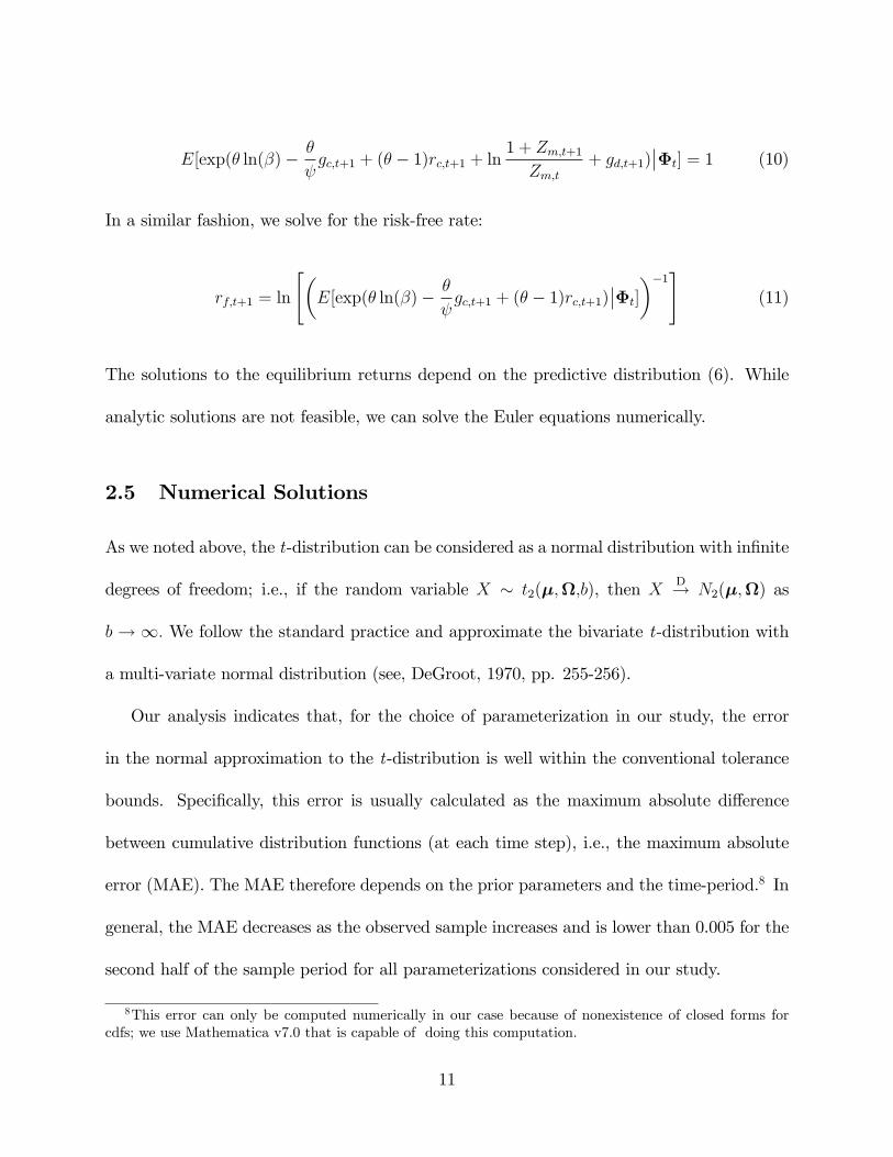
+ gd;t+1) �t] = 1 (10)

In a similar fashion, we solve for the risk-free rate:

rf;t+1 = ln

"�E[exp(� ln(�)� �

gc;t+1 + (� � 1)rc;t+1) �t]

��1#(11)

The solutions to the equilibrium returns depend on the predictive distribution (6). While

analytic solutions are not feasible, we can solve the Euler equations numerically.

2.5 Numerical Solutions

As we noted above, the t-distribution can be considered as a normal distribution with in�nite

degrees of freedom; i.e., if the random variable X � t2(�;;b), then XD! N2(�;) as

b ! 1: We follow the standard practice and approximate the bivariate t-distribution with

a multi-variate normal distribution (see, DeGroot, 1970, pp. 255-256).

Our analysis indicates that, for the choice of parameterization in our study, the error

in the normal approximation to the t-distribution is well within the conventional tolerance

bounds. Speci�cally, this error is usually calculated as the maximum absolute di¤erence

between cumulative distribution functions (at each time step), i.e., the maximum absolute

error (MAE). The MAE therefore depends on the prior parameters and the time-period.8 In

general, the MAE decreases as the observed sample increases and is lower than 0.005 for the

second half of the sample period for all parameterizations considered in our study.

8This error can only be computed numerically in our case because of nonexistence of closed forms forcdfs; we use Mathematica v7.0 that is capable of doing this computation.

11

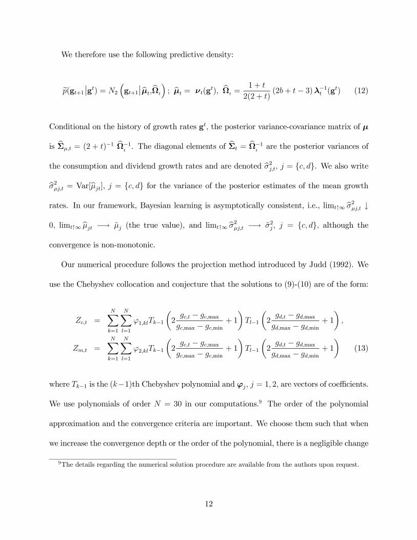
We therefore use the following predictive density:

ep(gt+1 gt) = N2

�gt+1 b�t;bt

�; b�t = �t(g

t); bt =1 + t

2(2 + t)(2b+ t� 3)��1t (gt) (12)

Conditional on the history of growth rates gt; the posterior variance-covariance matrix of �

is b��;t = (2 + t)�1 b�1t. The diagonal elements of b�t = b�1

tare the posterior variances of

the consumption and dividend growth rates and are denoted b�2j;t; j = fc; dg. We also writeb�2�j;t = Var[b�jt]; j = fc; dg for the variance of the posterior estimates of the mean growth

rates. In our framework, Bayesian learning is asymptotically consistent, i.e., limt"1 b�2�j;t #0; limt"1 b�jt �! ~�j (the true value), and limt"1 b�2�j;t �! ~�2j ; j = fc; dg; although the

convergence is non-monotonic.

Our numerical procedure follows the projection method introduced by Judd (1992). We

use the Chebyshev collocation and conjecture that the solutions to (9)-(10) are of the form:

Zc;t =NXk=1

NXl=1

'1;klTk�1

�2gc;t � gc;maxgc;max � gc;min

+ 1

�Tl�1

�2gd;t � gd;maxgd;max � gd;min

+ 1

�;

Zm;t =

NXk=1

NXl=1

'2;klTk�1

�2gc;t � gc;maxgc;max � gc;min

+ 1

�Tl�1

�2gd;t � gd;maxgd;max � gd;min

+ 1

�(13)

where Tk�1 is the (k�1)th Chebyshev polynomial and 'j; j = 1; 2; are vectors of coe¢ cients.

We use polynomials of order N = 30 in our computations.9 The order of the polynomial

approximation and the convergence criteria are important. We choose them such that when

we increase the convergence depth or the order of the polynomial, there is a negligible change

9The details regarding the numerical solution procedure are available from the authors upon request.

12

in the results.10

3 Data and Selection of Parameters

3.1 Data

To obtain the longest possible consistent data series on yearly aggregate consumption and

dividends, stock index prices and risk-free rates, we take annual data on consumption, risk-

free interest rates, Standard and Poor�s Composite Stock Price Index values, and dividends

from Robert Shiller�s website, starting from 1890.11 We update the data using the personal

consumption series from the national economic accounts of the Bureau of Economic Analysis

(BEA), population estimates from the U.S. Census Bureau, and interest rate series from the

Federal Reserve Board. We de�ate all nominal quantities using the Consumer Price Index

(CPI). Our data on consumption and dividend growth rates covers 1890-2007 while our

market returns data covers 1891-2007, which will therefore be the period for which we will

simulate our model.

We display the summary statistics for the data in Table 1. For the entire period 1891-

2007, the average yearly equity premium is 6.01%; the average risk-free rate is 1.93%; the

volatility of the market return is 18.18%; the risk-free rate volatility is 5.84%; and the Sharpe

ratio is 0.3.

A number of studies have highlighted the time-variation in the equity premium and the

10For robustness, we also try another numerical solution procedure where we conjecture the solution tothe price-consumption and price-dividend ratios (cf. (13)) as a function of the agent�s estimates. The resultsare very similar.11These data can be accessed at http://www.econ.yale.edu/~shiller/data.htm.

13

volatility of asset returns (e.g., Mehra and Prescott, 1985; Cogley and Sargent, 2008). We

take the agnostic approach and split our sample into one-half, i.e., the �rst half of the sample

covers 1891-1949, while the second covers 1950-2007. Both the yearly average consumption

and dividend growth rates are higher in the second half of the sample period compared to the

�rst half, but their volatility is lower. Meanwhile, market returns are higher on average, but

less volatile, in the second half compared to the �rst. However, the risk-free rate is lower on

average and less volatile in the second half compared to the �rst. Consequently, the yearly

average equity premium is higher, but its volatility is lower, in the second half compared to

the �rst. Consequently, the Sharpe ratio of the equity premium is also higher on average in

the second half. We will use these historical statistics as benchmarks for comparison with

the statistics generated by our model.

3.2 Calibration

3.2.1 Consumer Preference Parameters

We take the representative investor to be reasonably patient, with � = 0:99; a calibration

that is consistent with the business cycle and asset pricing literatures. However, there is a

substantial debate in the literature on the calibration of the relative risk aversion parameter

( ). Mehra and Prescott (1985) and Kocherlakota (1996) put an upper bound of 10 for

a reasonable calibration of : But Brandt et al. (2004) use a coe¢ cient of relative risk

aversion of 4: Moreover, based both on thought experiments and evidence from realistic

decision making situations, the literature argues for even lower values of (e.g., Rabin,

2000; Ljungqvist and Sargent, 2004). To highlight the role of structural uncertainty, we

14

therefore choose relatively low values of , namely, 1:2 and 3:6; but we conduct the major

portion of our analysis when = 1:2:

There is also a debate in the literature regarding the appropriate calibration of the IES

parameter. While Bansal and Yaron (2004) argue that plausible values for the IES parameter

should exceed 1, the estimates in some earlier studies are considerably smaller. We use values

between 0:5 and 2, namely, : 0:6; 0:8; 1:2; 2; but the bulk of our analysis is conducted with

the IES parameter set at 1:2: The calibration of risk aversion and the IES together determine

whether the representative consumer prefers early or late resolution of uncertainty; in our

calibrations, the agent prefers early resolution of uncertainty for all combinations of ( ; )

except for = 1:2 and = 0:6; 0:8.

3.2.2 Baseline Prior Parameters

We turn now to the selection of parameters for the prior beliefs regarding the unknown

structural parameters of the growth rates. For the reasons articulated at the outset, we

emphasize (1) parsimony of parameters, (2) vague initial knowledge or di¤use priors for the

representative consumer, and (3) realistic calibrations so that there is a tighter �t between

the sample moments of the prior distribution with their historical (or observed) counterparts.

For the sake of parsimony, we choose �0 so that the unconditional covariance of con-

sumption and dividend growth rates is zero, i.e., the representative consumer starts with a

prior belief of zero contemporaneous correlation between consumption and dividend growth

rates. For the vague initial knowledge or di¤use prior, we choose the prior degrees of freedom

(b) to be as small as possible, i.e., b = 2 (the rank of the covariance matrix). Finally, for

15

a realistic calibration, we run 10,000 simulations from the Normal-Wishart distribution for

consumption and dividend growth paths, each of size 118, because our data comprise of 118

(annual) observations. We then select the initial parameters that yield simulated sample

moments that approximate closely the mean and volatilities of growth rates in the data.

Our calibration approach results in the following baseline prior parameters (Case 1):

�0 = (0:02; 0:01); �0 =

0BB@0:001 0

0 0:01

1CCA : This calibration implies that the unconditional

expectations on the true mean growth rates of consumption and dividends are 2% and

1%, respectively; these correspond reasonably closely to their corresponding mean values of

2:05% and 1:30% in the data (see Table 1). The unconditional standard deviations of the

consumption and dividend growth rates (derived from Var[g] =4(2b�3)�1�0) are 6:32% and

20:00%, respectively (compared with the corresponding values of 3:51% and 11:43% in the

data). And while the realized correlation between annualized consumption and dividend

growth rates is 0.33 in our sample period, we restrict the prior correlation to be zero for the

sake of parameter parsimony.

As a further check on realistic calibration, we require that the historical (or the observed)

moments fall in the 50% con�dence intervals of the data simulated from the prior distrib-

ution, rather than in the more conventionally used 95% con�dence intervals. Simulations

based on the baseline prior parameters have the following statistical properties: the 50%

con�dence intervals for the unconditional mean and standard deviation of the consump-

tion growth rates are (�1:07%; 5:21%) and (2:74%; 9:80%), respectively; the corresponding

intervals for the unconditional mean and standard deviation of the dividend growth rates

are (�9:28%; 10:92%) and (8:47%; 30:61%), respectively; and the 50% con�dence interval

16

for the unconditional correlation between the consumption and dividend growth rates is

(�0:72; 0:71). That is, the observed �rst two moments of consumption and dividend growth

rates are in the 50% con�dence intervals of the simulated data.

3.2.3 Alternative Prior Parameters

Judicious perturbations around the baseline prior parameters clarify the e¤ects of (1) greater

prior uncertainty overall, (2) di¤erential prior uncertainty with respect to the consumption

and dividend growth rates, and (3) more pessimistic (or optimistic) initial priors.

To examine the e¤ects of raising generally the prior uncertainty, we maintain the un-

conditional expected growth rates, i.e., �0 = (0:02; 0:01) and the degrees of freedom b = 2:

However, we amplify the variance of the growth rates by a common factor of 10; that is,

the diagonal elements of �0 now take the values of (0:01; 0:1): These prior parameters thus

imply higher growth rate volatility than observed for the overall sample. We refer to this

parameterization as Case 2.12

But do the prior beliefs on the volatility of consumption and dividend growth rates have a

symmetric e¤ect on equilibrium asset prices? To examine this important issue, in Case 3, we

maintain �0 = (0:02; 0:01) and b = 2: However, we parameterize �0 such that the diagonal

elements are (0:001; 0:1); i.e., we maintain the unconditional prior volatility of consumption

growth rates (as in the baseline parameterization), but amplify the unconditional variance

of the dividend growth rates by a factor of 10: Conversely, in Case 4, we maintain the prior

variance of the dividend growth rate, but amplify that of the consumption growth rate by a

12For expositional convenience, we do not provide the statistical properties of the arti�cial data generatedfrom the alternative prior parameters.

17

factor of 10; i.e., the diagonal elements of �0 are (0:01; 0:01).

We study the e¤ects of pessimistic or optimistic priors on asset pricing by varying the

unconditional expectations on the mean growth rates. In Case 5, we incorporate pessimistic

beliefs by setting �0 = (0:01; 0:005), so that unconditional expectations of the mean growth

rates are one-half of the benchmark parameterization. Symmetrically, we address optimistic

priors by setting, in Case 6, �0 = (0:06; 0:03); so that the unconditional expectations of the

mean growth rates are 3 times the prior means in the benchmark parameterization. Finally,

to examine the e¤ects of pessimistic priors and greater structural uncertainty simultaneously,

in Case 7, we set �0 = (0:01; 0:005) and the diagonal elements of �0 to be (0:01; 0:1):

3.3 E¤ects of Prior Parameters on Posterior Beliefs

The sample size of our simulations is not very big because we have only 118 observations (to

align with the data). It is possible therefore that the choice of the prior can substantially

in�uence the outcomes. Figure 1 graphs the posterior means of consumption and dividend

growth rates for the cases where �0 = (0:02; 0:01), i.e., Cases 1 through 4. We �nd that the

the in�uence of the initial parameters evaporates very fast in both cases.

Turning to the posterior second moments, Figure 2 presents graphically the time-varying

posterior standard deviations of the consumption and dividend growth rates for the bench-

mark parameterization (Case 1). A comparison of Figures 1 and 2 indicates that the e¤ects

of the prior parameters governing the volatility of growth rates appear to be more persistent

than the e¤ects of prior parameters that determine the unconditional expectations.

This suggests that variations in the prior second moments will likely have greater e¤ects

18

on equilibrium asset prices compared with variations in the prior �rst moments. The reason

is that the higher are the posterior standard deviations of consumption and dividend growth

rates, the lower is the reliability of the estimates for the means of the growth rates, i.e.,

the greater is the economic uncertainty. We note that Weitzman (2007) and Bakshi and

Skoulakis (2010) also emphasize the implications of learning on the unknown volatility, but

the more general structural uncertainty framework of our study suggests that the e¤ects of

greater prior volatility are ampli�ed ex post when the mean growth rates are also unknown.

4 Results

4.1 Baseline Prior Parameters

Table 2 presents the results with the baseline prior parameterization (Case 1) for various

combinations of risk aversion and the IES parameters. We present the results for the entire

sample and for the two subperiods. We focus our discussion �rst on the results for the entire

sample, and then examine the di¤erences across the two subperiods.

We �nd that the model is able to generate sizeable risk-premia, relatively low risk-free

rates, and high market volatility and the Sharpe ratio for the risk-premium when the risk

aversion is less than 4 and the IES parameter is just above 1. For example, with a risk aversion

of 3.6 and IES parameter set at 1.2, the model generates an average annual equity risk

premium of 3:4% and an average annual risk-free rate of 2:2%; compared to the corresponding

observed values of 6% and 1:9%; respectively. Moreover, with this con�guration, the market

volatility is 12.3% and the Sharpe ratio is 0:3, compared to the observed values of 18.2% and

19

0.3, respectively. However, the volatility of the risk-free rate is lower than the observed value

by almost two orders of magnitude. We note that the model generates an equity premium of

over 3% and a risk-free rate of 2:3% even when the risk aversion is reduced to 1:2 (keeping

the IES �xed at 1:2).

For a �xed IES, increasing the risk aversion raises the equity premium and the Sharpe

ratio, but lowers the risk-free rate. However, raising the risk aversion depresses the mar-

ket volatility generated by the model still further, which is counterfactual since it increases

the gap between the observed and the model-generated data. Moreover, untabulated re-

sults indicate that when the risk aversion is 10, the upper bound prescribed by Mehra and

Prescott (1985) and Kocherlakota (1996), our model generates a negative average risk free

rate. Meanwhile, larger values of IES raise the equity premium, the risk free rate volatility,

and the Sharpe ratio; they also lower the risk free rate. While these e¤ects of raising the IES

bring the model results closer to the observed values, larger IES parameters do not increase

market volatility.

Comparing the equilibrium asset pricing moments generated by our model with those

produced by rational expectations models with similar consumer preferences and growth dy-

namics is instructive, because such comparisons help clarify the role of structural uncertainty

and learning. Weil (1989) uses Epstein-Zin recursive preferences in the Mehra and Prescott

(1985) endowment economy where consumption growth follows a Markov chain. With an

IES of 2 and risk aversion of 5, Weil�s model generates an equity premium of 0:51% and a

risk-free rate of 5:79%. In comparison, we generate a substantially higher risk-premium and

lower risk-free rate with lower con�gurations of risk aversion and IES.

20

But an even a closer comparison is with Bansal and Yaron (1994) because they also

use recursive preferences, distinguish between aggregate consumption and dividend growth

processes, and present results for the case where growth rates follow an i.i.d. Gaussian

process, although their model calibration is based on the 1928-1998 sample period. With a

risk aversion of 7:5 and IES of 1:5, and assuming a contemporaneous correlation in monthly

growth rates of 0:25; they generate an equity premium of 0:08%:With the same con�guration

of risk aversion and IES, they generate a risk premium of about 4% when they assume

persistence in growth rates and �uctuating uncertainty. In comparison, our model generates

an equity premium of 3:4% with a lower con�guration of risk aversion and IES, i.e., 3:6 and

1:2, respectively, even with an i.i.d. growth process.

Thus, with structural uncertainty and Bayesian learning, we endogenously arrive at equi-

librium asset prices that mimic, or at least are close to, rational expectations models with

persistent growth rates and �uctuating uncertainty. The reason is that learning also produces

e¤ects that are stochastic and persistent. For example, because posterior beliefs are mar-

tingales, raising the posterior precision has long-term e¤ects since it improves the expected

reliability of inferences on the mean growth rates over the horizon. But the e¤ects of learning

are also uncertain because, under our assumptions, the posterior beliefs are stochastic.

In a similar vein, other aspects of the results (that are displayed Table 2) suggest that

the e¤ects of structural uncertainty and learning on asset pricing are distinct from those

of varying risk aversion and the IES. Notice that lowering substantially the risk aversion

does not generate corresponding reductions in the equity premium when the representative

consumer is learning about the unknown structural parameters of the growth rates. For

21

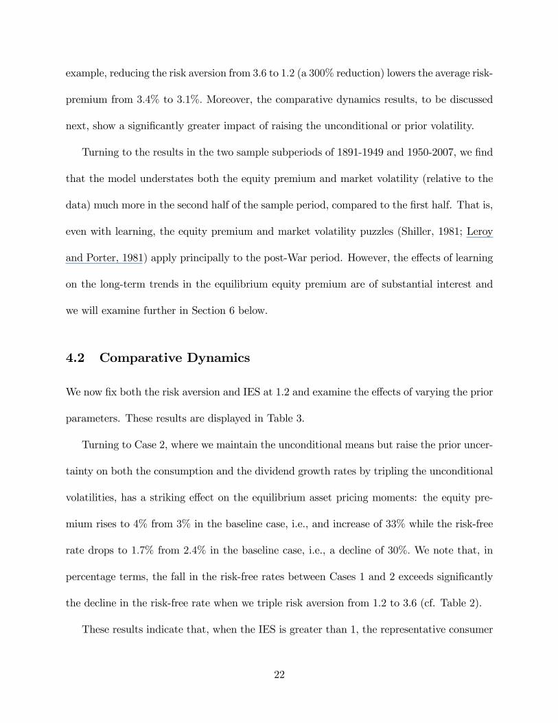
example, reducing the risk aversion from 3:6 to 1:2 (a 300% reduction) lowers the average risk-

premium from 3:4% to 3:1%: Moreover, the comparative dynamics results, to be discussed

next, show a signi�cantly greater impact of raising the unconditional or prior volatility.

Turning to the results in the two sample subperiods of 1891-1949 and 1950-2007, we �nd

that the model understates both the equity premium and market volatility (relative to the

data) much more in the second half of the sample period, compared to the �rst half. That is,

even with learning, the equity premium and market volatility puzzles (Shiller, 1981; Leroy

and Porter, 1981) apply principally to the post-War period. However, the e¤ects of learning

on the long-term trends in the equilibrium equity premium are of substantial interest and

we will examine further in Section 6 below.

4.2 Comparative Dynamics

We now �x both the risk aversion and IES at 1.2 and examine the e¤ects of varying the prior

parameters. These results are displayed in Table 3.

Turning to Case 2, where we maintain the unconditional means but raise the prior uncer-

tainty on both the consumption and the dividend growth rates by tripling the unconditional

volatilities, has a striking e¤ect on the equilibrium asset pricing moments: the equity pre-

mium rises to 4% from 3% in the baseline case, i.e., and increase of 33% while the risk-free

rate drops to 1:7% from 2:4% in the baseline case, i.e., a decline of 30%: We note that, in

percentage terms, the fall in the risk-free rates between Cases 1 and 2 exceeds signi�cantly

the decline in the risk-free rate when we triple risk aversion from 1.2 to 3.6 (cf. Table 2).

These results indicate that, when the IES is greater than 1, the representative consumer

22

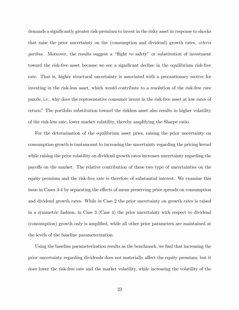
demands a signi�cantly greater risk-premium to invest in the risky asset in response to shocks

that raise the prior uncertainty on the (consumption and dividend) growth rates, ceteris

paribus. Moreover, the results suggest a ��ight to safety� or substitution of investment

toward the risk-free asset because we see a signi�cant decline in the equilibrium risk-free

rate. That is, higher structural uncertainty is associated with a precautionary motive for

investing in the risk-less asset, which would contribute to a resolution of the risk-free rate

puzzle, i.e., why does the representative consumer invest in the risk-free asset at low rates of

return? The portfolio substitution toward the riskless asset also results in higher volatility

of the risk-less rate, lower market volatility, thereby amplifying the Sharpe ratio.

For the determination of the equilibrium asset pries, raising the prior uncertainty on

consumption growth is tantamount to increasing the uncertainty regarding the pricing kernel

while raising the prior volatility on dividend growth rates increases uncertainty regarding the

payo¤s on the market. The relative contribution of these two type of uncertainties on the

equity premium and the risk-free rate is therefore of substantial interest. We examine this

issue in Cases 3-4 by separating the e¤ects of mean preserving prior spreads on consumption

and dividend growth rates. While in Case 2 the prior uncertainty on growth rates is raised

in a symmetric fashion, in Case 3 (Case 4) the prior uncertainty with respect to dividend

(consumption) growth only is ampli�ed, while all other prior parameters are maintained at

the levels of the baseline parameterization.

Using the baseline parameterization results as the benchmark, we �nd that increasing the

prior uncertainty regarding dividends does not materially a¤ect the equity premium; but it

does lower the risk-free rate and the market volatility, while increasing the volatility of the

23

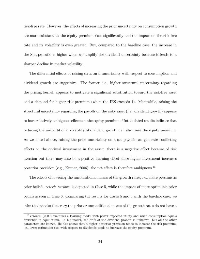
risk-free rate. However, the e¤ects of increasing the prior uncertainty on consumption growth

are more substantial: the equity premium rises signi�cantly and the impact on the risk-free

rate and its volatility is even greater. But, compared to the baseline case, the increase in

the Sharpe ratio is higher when we amplify the dividend uncertainty because it leads to a

sharper decline in market volatility.

The di¤erential e¤ects of raising structural uncertainty with respect to consumption and

dividend growth are suggestive. The former, i.e., higher structural uncertainty regarding

the pricing kernel, appears to motivate a signi�cant substitution toward the risk-free asset

and a demand for higher risk-premium (when the IES exceeds 1). Meanwhile, raising the

structural uncertainty regarding the payo¤s on the risky asset (i.e., dividend growth) appears

to have relatively ambiguous e¤ects on the equity premium. Untabulated results indicate that

reducing the unconditional volatility of dividend growth can also raise the equity premium.

As we noted above, raising the prior uncertainty on asset payo¤s can generate con�icting

e¤ects on the optimal investment in the asset: there is a negative e¤ect because of risk

aversion but there may also be a positive learning e¤ect since higher investment increases

posterior precision (e.g., Kumar, 2006); the net e¤ect is therefore ambiguous.13

The e¤ects of lowering the unconditional means of the growth rates, i.e., more pessimistic

prior beliefs, ceteris paribus, is depicted in Case 5, while the impact of more optimistic prior

beliefs is seen in Case 6. Comparing the results for Cases 5 and 6 with the baseline case, we

infer that shocks that vary the prior or unconditional means of the growth rates do not have a

13Veronesi (2000) examines a learning model with power expected utility and when consumption equalsdividends in equilibrium. In his model, the drift of the dividend process is unknown, but all the otherparameters are known. He also shows that a higher posterior precision tends to increase the risk-premium,i.e., lower estimation risk with respect to dividends tends to increase the equity premium.

24

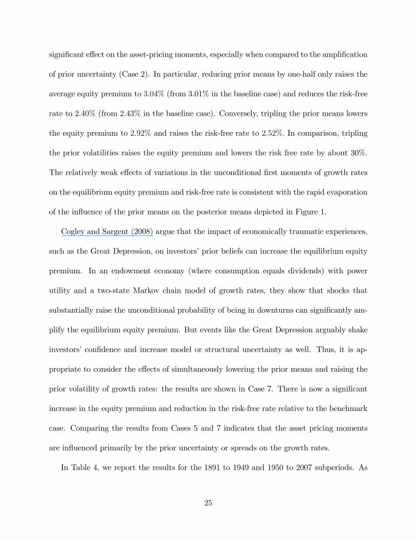
signi�cant e¤ect on the asset-pricing moments, especially when compared to the ampli�cation

of prior uncertainty (Case 2). In particular, reducing prior means by one-half only raises the

average equity premium to 3:04% (from 3.01% in the baseline case) and reduces the risk-free

rate to 2:40% (from 2:43% in the baseline case). Conversely, tripling the prior means lowers

the equity premium to 2:92% and raises the risk-free rate to 2:52%: In comparison, tripling

the prior volatilities raises the equity premium and lowers the risk free rate by about 30%.

The relatively weak e¤ects of variations in the unconditional �rst moments of growth rates

on the equilibrium equity premium and risk-free rate is consistent with the rapid evaporation

of the in�uence of the prior means on the posterior means depicted in Figure 1.

Cogley and Sargent (2008) argue that the impact of economically traumatic experiences,

such as the Great Depression, on investors�prior beliefs can increase the equilibrium equity

premium. In an endowment economy (where consumption equals dividends) with power

utility and a two-state Markov chain model of growth rates, they show that shocks that

substantially raise the unconditional probability of being in downturns can signi�cantly am-

plify the equilibrium equity premium. But events like the Great Depression arguably shake

investors�con�dence and increase model or structural uncertainty as well. Thus, it is ap-

propriate to consider the e¤ects of simultaneously lowering the prior means and raising the

prior volatility of growth rates: the results are shown in Case 7. There is now a signi�cant

increase in the equity premium and reduction in the risk-free rate relative to the benchmark

case. Comparing the results from Cases 5 and 7 indicates that the asset pricing moments

are in�uenced primarily by the prior uncertainty or spreads on the growth rates.

In Table 4, we report the results for the 1891 to 1949 and 1950 to 2007 subperiods. As

25

in Table 2, we �nd that the equity premium and the market and risk-free rate volatilities

generated by the various prior parameterization models understate the corresponding mo-

ments in the data more in the second half of the sample, compared to the �rst. And while

some of the models generate an average risk-free rate that is lower than the observed aver-

age in the �rst half of the sample (Cases 2, 4, and 7), all the models overstate the average

risk-free rate relative to the data in the second half. Finally, the gap between the observed

model-generated market and risk-free rate volatilities remains especially large in the second

half for all the prior parameterizations.

5 Vector Autoregressive (VAR) Growth Rates

Amain conclusion of the foregoing analysis is that a model with structural uncertainty on the

moments of i.i.d. Normal consumption and growth rates can generate a substantial equity

premium and low risk-free rates, even when preferences approximate the power utility and

the risk aversion is low, and even when the prior parameters are calibrated realistically over

the entire period of 1891-2007.

However, the recent literature emphasizes the e¤ects of persistence in growth rates on

asset pricing (Bansal and Yaron, 2004). In this section, we examine the implications of

learning on asset prices when the growth processes are not i.i.d. but, rather, the consumption

and dividend growth rates, g� = [gc;� ; gd;� ]0�=2;:::

, follow a bivariate vector autoregressive

(VAR) process with one lag:

g� = a+ g��1B+ u� ; (14)

26

where, a = [ac; ad]0, B = [bij], i; j = c; d, and u� = [uc;� ; ud;� ]

0 are shocks that are i.i.d.

Normal with zero mean and precision matrix u.

It is convenient to stack the observations and rewrite (14) as

G = XD+U; (15)

where, G = [gj� ]; j = c; d; � = 2; :::; t; is a (t� 1)� 2 matrix; X is a (t� 1)� 3 matrix whose

�rst column consists of ones and whose other elements are [gj� ]; j = c; d; � = 1; :::; t � 1;

U = [uj� ]; j = c; d; � = 2; :::; t is a (t� 1)� 2 matrix; and D =

0BB@ ac bcc bdc

ad bcd bdd

1CCA0

.

Let the subscript k denote the k-th column vector. Then, Gk = XDk + Uk; k = 1; 2:

Hence, we can stack the columns in (15) and �nally rewrite (14) as g = (IX)d+u; where,

u � N2t�2

�u 0;u I

�:

5.1 Learning

Following Kadiyala and Karlsson (1997) and Sims and Zha (1998), we use a Normal-Wishart

prior for the whole system of VAR coe¢ cients. Under a Normal-Wishart prior, the prior

distribution of coe¢ cients is normal d u � N6

�d �;u D

�and u � Wi2

�u b;�0

�,

i.e., a 2-dimensional Wishart distribution with parameters b and �0, so that E[u b;�0] =

b��10 . Using this prior for the parameters, at each step t; we estimate the coe¢ cients needed

for prediction at time t+ 1 as

bDt = (D +X0X)�1(D�+X0G) (16)

27

bu;t = (t+ b)(G0G� bD0t(X

0X+D)bDt +�0D�+ �0)

�1 (17)

Here, � =

0BB@ �1 �2 �3

�4 �5 �6

1CCA0

. Now, let us put egt = [1; gc;t; gd;t]0 and use the predictive distri-bution ep(gt+1 gt) = N2

�gt+1 b�t; bt

�; where b�t = bD0

tegt and bt = bu;t:5.2 Parameter Selection

As before, we take the representative consumer�s subjective discount rate, �, to be 0:99. To

focus the exposition, and to facilitate comparison with the i.i.d. growth case (Section 4), we

perform the computations for a risk aversion of 1.2 and IES of 1.2.

We apply the same desideratum for the choice of prior parameters that we employed in

the case of i.i.d. growth. Speci�cally, to ensure vague initial knowledge for the representative

consumer, we �x the degrees of freedom b = 4, the minimum number of degrees of freedom for

our setting. For parsimony, we take �0 to be a diagonal matrix, as before. In a similar vein,

in our baseline parameterization here, we assume that while the representative consumer

allows for the autoregressive structure of the consumption and dividend growth rates, the

initial estimate of persistence is zero for both growth rates. And we choose the matrix D

in such a way that there is almost no learning on the VAR coe¢ cients.

Speci�cally, our baseline prior parameters (denoted as Set 1) are as follows: for�, we set

�1 = 0:02; �4 = 0:01, and 0 for all other values; the diagonal elements of �0 are (0:002; 0:03);

and D is a symmetric 3� 3 diagonal matrix with the common value of 10 on the diagonal.

In general, the lower are the values of the diagonal elements of D; the faster is the learning

on the persistence coe¢ cients of the growth rates.

28

The arti�cial data simulated from the prior distribution with the baseline parameters

have the following statistical properties: the 50% con�dence intervals for the unconditional

consumption growth mean and standard deviation are (1:34%; 2:65%) and (2:19%; 4:14%),

respectively; the 50% con�dence intervals for the unconditional dividend growth mean and

standard deviation are (�1:61%; 3:69%) and (8:77%; 16:32%), respectively; the 50% con-

�dence interval for the unconditional correlation between the consumption and dividend

growth rates is (�0:42; 0:42). Let us recall again that the mean value and standard devia-

tion of the realized consumption growth rates are 2:05% and 3:51%, respectively. The mean

value and standard deviation of the realized dividend growth rates are 1:30% and 11:43%,

respectively. The correlation between the realized consumption and dividend growth rates

is 0:33: In sum, the observed sample moments lie in the 50% con�dence intervals of the

simulated data from the baseline parameterization.

For the comparative dynamics analysis, we consider �rst the e¤ects of changing the prior

estimates on the persistence of growth rates. Thus, in Set 2, we raise the representative

consumer�s initial estimates of the persistence of consumption and dividends growth rates.

In this case, �2 = 0:9; �6 = 0:9, and 0 for all other values. D is the same as in Set 1, while

the diagonal elements of �0 are set to maintain the unconditional volatilities of the same

magnitude as in Set 1. We then consider the e¤ects of asymmetric initial estimates of growth

persistence. In Set 3, the initial estimate of the consumption growth persistence is higher

than that of dividends, i.e., �2 = 0:8; �6 = 0:4: But all other parameters are maintained at

the baseline parameterization level.

Next, we examine the interaction between prior uncertainty and the representative con-

29

sumer�s perceptions of persistence. In Set 4, we raise the prior uncertainty on the growth

rates but maintain the other parameters at the baseline levels; this implies, in particular,

that while the representative consumer allows for the autoregressive structure of the growth

rates, the initial estimate of persistence is zero for both the growth rates. But in Set 5,

we raise the prior volatilities of the growth rates and the representative consumer�s prior

estimates of the growth persistence (i.e., choose � as in Set 2).

We have seen above the di¤erential e¤ects of prior uncertainty regarding the consumption

and dividend growth rates. In Set 6, we examine the situation where the prior uncertainty

with respect to consumption growth is greater than that with respect to dividends (and the

initial estimate of growth persistence is zero). In Set 7, we examine a similar asymmetry

in the prior uncertainty on growth rates, but assume that the initial estimate of growth

persistence is high.

5.3 E¤ects of Prior Parameters on Posterior Beliefs

It is instructive to examine the e¤ects of the prior estimates of persistence on the posterior

beliefs. Figure 3 graphs the time-varying posterior means of the growth rates for Sets 2, 5, and

7, where the representative consumer has a high initial estimate of persistence. Comparing

Figure 3 with Figure 1 (where there is no persistence) suggests that the higher is the initial

estimate of persistence, the more volatile are the posterior means. Of course, greater posterior

volatility in means does not necessarily imply higher average equity premium; however, we

do expect posterior volatility of means to be associated with greater market volatility, ceteris

paribus.

30

Next, Figure 4 presents graphically the time-varying posterior volatilities of the growth

rates for the prior parameter Set 2. Comparing Figure 4 with Figure 2, we �nd that the

posterior volatility estimates are more sensitive to information innovations when the initial

persistence estimates are higher. Meanwhile, a comparison of the di¤erences between Sets

1 and 2 with those between Sets 4 and 5 is informative of the interaction between the prior

uncertainty and persistence estimates. We �nd that the di¤erence between the posterior

volatilities associated with low and high initial estimates of persistence are greater when

we raise the prior uncertainty. That is, the e¤ects of raising prior uncertainty on posterior

second moments appear to be ampli�ed with higher initial estimates of persistence.

5.4 Results

We numerically solve for the equilibrium asset-pricing moments for parameter Sets 1-7. We

display the results in Table 5.

For the baseline parameterization (Set 1), where the representative consumer allows for

the auto-regressive growth structure but the prior estimate of growth rate persistence is zero,

the average equity premium is 2.86% and the average risk free rate is 2.54%. Comparing the

results for Set 1 with the corresponding equilibrium asset pricing moments for the baseline

parameterization case for i.i.d. growth (Case 1, Table 3), we �nd that the VAR growth

structure does not improve model performance per se; i.e., our model with i.i.d. growth

processes does better than the VAR case when we keep the prior estimate of persistence very

low. We turn now to the comparative dynamics analysis when we vary the prior uncertainty

and the prior estimate of persistence.

31

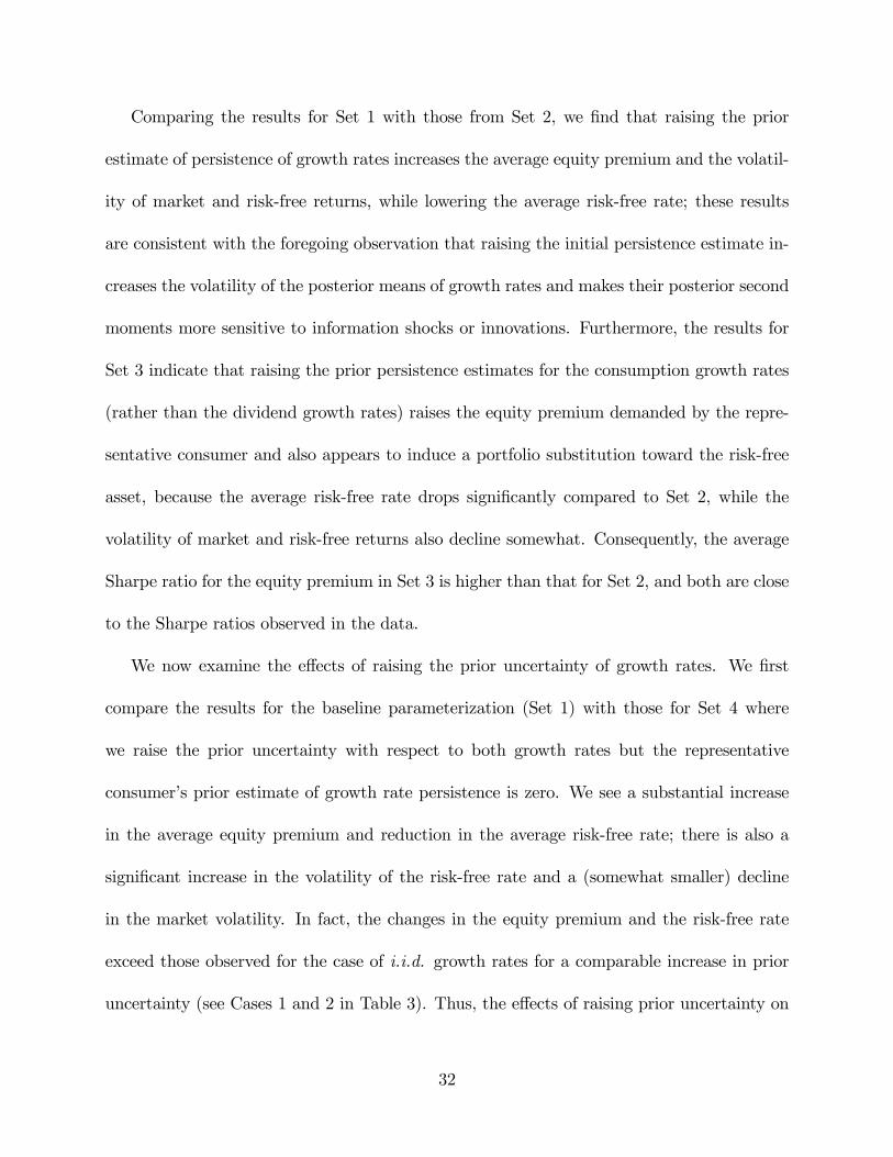
Comparing the results for Set 1 with those from Set 2, we �nd that raising the prior

estimate of persistence of growth rates increases the average equity premium and the volatil-

ity of market and risk-free returns, while lowering the average risk-free rate; these results

are consistent with the foregoing observation that raising the initial persistence estimate in-

creases the volatility of the posterior means of growth rates and makes their posterior second

moments more sensitive to information shocks or innovations. Furthermore, the results for

Set 3 indicate that raising the prior persistence estimates for the consumption growth rates

(rather than the dividend growth rates) raises the equity premium demanded by the repre-

sentative consumer and also appears to induce a portfolio substitution toward the risk-free

asset, because the average risk-free rate drops signi�cantly compared to Set 2, while the

volatility of market and risk-free returns also decline somewhat. Consequently, the average

Sharpe ratio for the equity premium in Set 3 is higher than that for Set 2, and both are close

to the Sharpe ratios observed in the data.

We now examine the e¤ects of raising the prior uncertainty of growth rates. We �rst

compare the results for the baseline parameterization (Set 1) with those for Set 4 where

we raise the prior uncertainty with respect to both growth rates but the representative

consumer�s prior estimate of growth rate persistence is zero. We see a substantial increase

in the average equity premium and reduction in the average risk-free rate; there is also a

signi�cant increase in the volatility of the risk-free rate and a (somewhat smaller) decline

in the market volatility. In fact, the changes in the equity premium and the risk-free rate

exceed those observed for the case of i.i.d. growth rates for a comparable increase in prior

uncertainty (see Cases 1 and 2 in Table 3). Thus, the e¤ects of raising prior uncertainty on

32

growths rates are ampli�ed in the VAR case, even when the representative consumer starts

with a very low estimate of persistence.

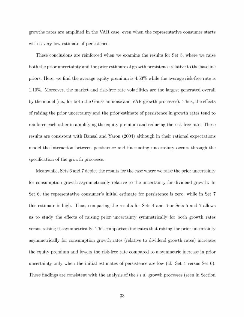
These conclusions are reinforced when we examine the results for Set 5, where we raise

both the prior uncertainty and the prior estimate of growth persistence relative to the baseline

priors. Here, we �nd the average equity premium is 4.63% while the average risk-free rate is

1.10%. Moreover, the market and risk-free rate volatilities are the largest generated overall

by the model (i.e., for both the Gaussian noise and VAR growth processes). Thus, the e¤ects

of raising the prior uncertainty and the prior estimate of persistence in growth rates tend to

reinforce each other in amplifying the equity premium and reducing the risk-free rate. These

results are consistent with Bansal and Yaron (2004) although in their rational expectations

model the interaction between persistence and �uctuating uncertainty occurs through the

speci�cation of the growth processes.

Meanwhile, Sets 6 and 7 depict the results for the case where we raise the prior uncertainty

for consumption growth asymmetrically relative to the uncertainty for dividend growth. In

Set 6, the representative consumer�s initial estimate for persistence is zero, while in Set 7

this estimate is high. Thus, comparing the results for Sets 4 and 6 or Sets 5 and 7 allows

us to study the e¤ects of raising prior uncertainty symmetrically for both growth rates

versus raising it asymmetrically. This comparison indicates that raising the prior uncertainty

asymmetrically for consumption growth rates (relative to dividend growth rates) increases

the equity premium and lowers the risk-free rate compared to a symmetric increase in prior

uncertainty only when the initial estimates of persistence are low (cf. Set 4 versus Set 6).

These �ndings are consistent with the analysis of the i.i.d. growth processes (seen in Section

33

5) because the persistence there is trivially zero.

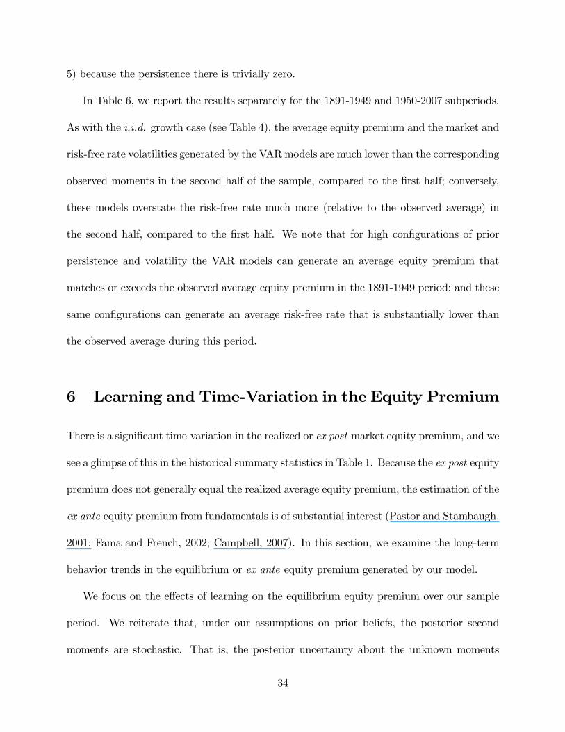
In Table 6, we report the results separately for the 1891-1949 and 1950-2007 subperiods.

As with the i.i.d. growth case (see Table 4), the average equity premium and the market and

risk-free rate volatilities generated by the VARmodels are much lower than the corresponding

observed moments in the second half of the sample, compared to the �rst half; conversely,

these models overstate the risk-free rate much more (relative to the observed average) in

the second half, compared to the �rst half. We note that for high con�gurations of prior

persistence and volatility the VAR models can generate an average equity premium that

matches or exceeds the observed average equity premium in the 1891-1949 period; and these

same con�gurations can generate an average risk-free rate that is substantially lower than

the observed average during this period.

6 Learning and Time-Variation in the Equity Premium

There is a signi�cant time-variation in the realized or ex post market equity premium, and we

see a glimpse of this in the historical summary statistics in Table 1. Because the ex post equity

premium does not generally equal the realized average equity premium, the estimation of the

ex ante equity premium from fundamentals is of substantial interest (Pastor and Stambaugh,

2001; Fama and French, 2002; Campbell, 2007). In this section, we examine the long-term

behavior trends in the equilibrium or ex ante equity premium generated by our model.

We focus on the e¤ects of learning on the equilibrium equity premium over our sample

period. We reiterate that, under our assumptions on prior beliefs, the posterior second

moments are stochastic. That is, the posterior uncertainty about the unknown moments

34

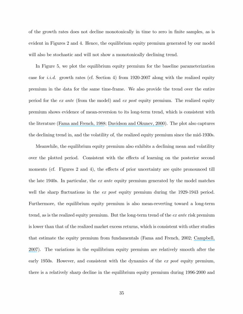
of the growth rates does not decline monotonically in time to zero in �nite samples, as is

evident in Figures 2 and 4. Hence, the equilibrium equity premium generated by our model

will also be stochastic and will not show a monotonically declining trend.

In Figure 5, we plot the equilibrium equity premium for the baseline parameterization

case for i.i.d. growth rates (cf. Section 4) from 1920-2007 along with the realized equity

premium in the data for the same time-frame. We also provide the trend over the entire

period for the ex ante (from the model) and ex post equity premium. The realized equity

premium shows evidence of mean-reversion to its long-term trend, which is consistent with

the literature (Fama and French, 1988; Davidson and Okunev, 2000). The plot also captures

the declining trend in, and the volatility of, the realized equity premium since the mid-1930s.

Meanwhile, the equilibrium equity premium also exhibits a declining mean and volatility

over the plotted period. Consistent with the e¤ects of learning on the posterior second

moments (cf. Figures 2 and 4), the e¤ects of prior uncertainty are quite pronounced till

the late 1940s. In particular, the ex ante equity premium generated by the model matches

well the sharp �uctuations in the ex post equity premium during the 1929-1943 period.

Furthermore, the equilibrium equity premium is also mean-reverting toward a long-term

trend, as is the realized equity premium. But the long-term trend of the ex ante risk premium

is lower than that of the realized market excess returns, which is consistent with other studies

that estimate the equity premium from fundamentals (Fama and French, 2002; Campbell,

2007). The variations in the equilibrium equity premium are relatively smooth after the

early 1950s. However, and consistent with the dynamics of the ex post equity premium,

there is a relatively sharp decline in the equilibrium equity premium during 1996-2000 and

35

a relatively sharp up-tick after 2000.

In Figure 6, we plot the equilibrium equity premium for the VAR case for 1920-2007,

when the prior estimates of growth rate volatility and persistence are high. The time-series

behavior of the equilibrium equity premium is similar to that seen in Figure 5 except that

here the �uctuations are relatively sharp compared to the i.i.d. case even toward the end of

the plotted period.

We conclude that, while learning smooths out the time-variations in the equilibrium

equity premium over time, shocks to consumption and dividend growth rates can still induce

relatively sharp �uctuations even after one hundred years of data (from 1890s to the 1990s).

7 Summary and Conclusions

Economic agents are typically uncertain about the structural parameters of processes that

govern the evolution of economic fundamentals, which ultimately determine the distribution

of asset returns, and learn about these parameters based on their observations. That is, they

face estimation risk along with the intrinsic investment risk of assets. In a general equilib-

rium setting where the representative consumer has recursive preferences, and distinguishing

between aggregate consumption and dividends, we examine the implications of estimation

risk and Bayesian learning asset pricing when both the �rst and second moments of con-

sumption and dividend growth rates are unknown. The representative consumer updates

conditional on the observed history of growth rates. To guard against generating results

through over-�tting or optimization of prior parameters, we emphasize parsimony of para-

meters; vague initial knowledge or di¤use priors; and realistic calibration with respect to a

36

study period that extends from 1891-2007.

Our model generates sizeable values for the equilibrium equity premium, relatively low

values for the equilibrium risk-free rates, and mean Sharpe ratios that approximate those

observed in the data, even when preferences approximate the power utility, risk aversion is

low, and there is no persistence in shocks to growth rates. These statistics are signi�cantly

larger than rational expectations models with comparable parameterization, and arise even

though we use di¤use (rather than pessimistic) priors and multivariate Normal posterior

predictive distributions with �nite moments. Modeling structural uncertainty broadly with

respect to all the parameters of the growth processes and distinguishing between aggregate

consumption and dividends are central to obtaining the relatively high risk premium for

estimation risk. We also �nd that estimation risk does not decline monotonically in time

with learning, i.e., there is no monotonic convergence to a low equity premium. While

learning does tend to smooth out the time-variations in the equilibrium equity premium,

shocks to growth rates can induce relatively sharp �uctuations (in the equity premium)

even after one hundred years of data. Finally, our framework allows us to highlight the

di¤erential e¤ects on equilibrium asset prices of varying (1) prior beliefs, (2) risk aversion,

(3) the intertemporal elasticity of substitution, and (4) the dynamics of the growth rates.

Overall, our study indicates that the parameterization of estimation risk is important

for asset pricing, comparable in its e¤ects to the choice of risk aversion and intertemporal

elasticity of substitution. In particular, variations in prior estimation risk appear at least

as e¤ective as variations in risk aversion or the IES in terms of reducing the discrepancy

between the equilibrium outcomes from the model and the data.

37

References

Abel, A., 2002, �An Exploration of the E¤ects of Pessimism and Doubt on Asset Returns,�Journal

of Economic Dynamics and Control, 26, 1075-1092.

Bakshi, G., and G. Skoulakis, 2010, �Do Subjective Expectations Explain Asset Pricing Puzzles,�

Journal of Financial Economics 98, 117-140.

Bansal, R., and A. Yaron, 2004, �Risks for the Long Run: A Potential Resolution of Asset Pricing

Puzzles�, Journal of Finance, 59, 1481-1509.

Barro, R., 2006, �Rare Disasters and Asset Markets in the Twentieth Century,�Quarterly Journal

of Economics, 121, 823�866.

Barry, C., 1974, �Portfolio Analysis under Uncertain Means, Variances, and Covariances,�Journal

of Finance, 29, 515-522.

Barry, C., and S. Brown, 1985, �Di¤erential Information and Security Market Equilibrium�, Journal

of Financial and Quantitative Analysis, 20, 407-422.

Bawa, V., S. Brown, and R. Klein, 1979, Estimation Risk and Optimal Portfolio Choice, Amster-

dam: North Holland.

Bernardo, J., and A. Smith, 1994, Bayesian Theory, Chichester: Wiley.

Brandt, M., Q. Zeng, and L. Zhang, 2004, �Equilibrium Stock Return Dynamics under Alternative

Rules of Learning about Hidden States�, Journal of Economic Dynamics and Control, 28, 1925-

1954.

Brennan, M., and Y. Xia, 2001, �Stock Price Volatility and Equity Premium�, Journal of Monetary

Economics, 47, 249-283.

Cagetti, M., L. Hansen, T. Sargent, and N. Williams, 2002, �Robustness and Pricing with Uncertain

Growth,�Review of Financial Studies, 15, 363-404.

Campbell, J., 1996, �Understanding Risk and Return�, Journal of Political Economy, 104, 298-345.

Campbell, J., 2007, �Estimating the Equity Premium�, Working Paper, Harvard University.

Campbell, J., and J. Cochrane, 1999, �By Force of Habit: A Consumption-based Explanation of

Aggregate Stock Market Behavior�, Journal of Political Economy, 107, 205-251.

Cecchetti, S. P. Lam, and N. Mark, 2000, �Asset Pricing with Distorted Beliefs: Are Equity Returns

Too Good to Be True?�, American Economic Review, 90, 787-805.

38

Cogley, T., and T. Sargent, 2008, �The Market Price of Risk and the Equity Premium: A Legacy

of the Great Depression?�, Journal of Monetary Economics, 55, 454-476.

Constantinides, G., 1990, �Habit Formation: A Resolution of the Equity Premium Puzzle�, Journal

of Political Economy, 98, 519-543.

Constantinides, G., and D. Du¢ e, 1996, �Asset Pricing with Heterogeneous Consumers�, Journal

of Political Economy, 104, 219-240.

Davidson, I., and J. Okunev, 2000, �Modeling the Equity Premium in the Long Term,�Working

Paper, University if Warwick.

DeGroot, M., 1970, �Optimal Statistical Decisions,�New York: McGraw-Hill.

Epstein, L., and S. Zin, 1989, �Substitution, Risk Aversion, and the Temporal Behavior of Con-

sumption and Asset Returns: A Theoretical Framework�, Econometrica, 57, 937-969.

Fama, E., and K. French, 1988, �Dividend Yields and Expected Stock Returns,�Journal of Financial

Economics, 22, 3-25.

Fama, E., and K. French, 2002, �The Equity Premium,�Journal of Finance, 57, 637-659.

Hansen, L., and T. Sargent, 2006, �Fragile Beliefs and the Price of Model Uncertainty�, Working

Paper, New York University and University of Chicago.

Heaton, J., and D. Lucas, 1996, �Evaluating the E¤ects of Incomplete Markets on Risk Sharing

and Asset Pricing�, Journal of Political Economy, 104, 443-487.

Judd, K., 1992, �Projection Methods for Solving Aggregate Growth Models,�Journal of Economic

Theory, 58, 410-452.

Kadiyala, K. and S. Karlsson, 1997, �Numerical Methods for Estimation and Inference in Bayesian

VAR-models�, Journal of Applied Econometrics, 12, 99-132.

Kandel, S., and R. Stambaugh, 1991, �Asset Returns and Intertemporal Preferences,�Journal of

Monetary Economics, 27, 39-71.

Kandel, S., and R. Stambaugh, 1996, �On the Predictability of Stock Returns: An Asset-allocation

Perspective�, Journal of Finance, 51, 385-424.

Kocherlakota, N., 1996, �The Equity Premium: It�s Still a Puzzle,�Journal of Economic Literature,

34, 42-71.

Kumar, P., 2006, �Learning about Investment Risk: The E¤ects of Structural Uncertainty on

Dynamic Investment and Consumption�, Journal of Economic Behavior & Organization, 60, 205-

39

229.

Kumar, P., S. Sorescu, R. Boehme, and B. Danielsen, 2008, �Estimation Risk, Information, and

the Conditional CAPM: Theory and Evidence�, Review of Financial Studies, 21, 1037-1075.

Ljungqvist, L., and T. Sargent, 2004, �Recursive Macroeconomic Theory,�Cambridge, MA: MIT

Press.

LeRoy, S., and R. Porter, 1981, �The Present-Value Relation: Tests Based on Implied Variance

Bounds,�Econometrica, 49, 555-574.

Mehra, R., 2008, �The Equity Premium Puzzle: A Review,�Foundations and Trends in Finance,

2, 1-81.

Mehra, R., and E. Prescott, 1985, �The Equity Premium: A Puzzle�, Journal of Monetary Eco-

nomics, 15, 145-161.

Pastor, L., and R. Stambaugh, 2001, �The Equity Premium with Structural Breaks,� Journal of

Finance, 56, 1207-1239.

Pastor, L., and R. Stambaugh, 2009, �Are Stocks Really Less Volatile in the Long Run,�Working

Paper, University of Chicago.

Rabin, M. 2000, �Risk Aversion and Expected-Utility Theory: A Calibration Theorem,�Econo-

metrica, 68, 1281-1292.

Rietz, T. , 1988, �The Equity Premium: A Solution�, Journal of Monetary Economics, 22, 117�131.

Shiller, R. 1981, �Do Stock Prices Move Too Much to Be Justi�ed by Subsequent Changes in

Dividends?�, American Economic Review, 71, 421-436.

Sims, C., and T. Zha, 1998, �Bayesian Methods for Dynamic Multivariate Models�, International

Economic Review, 39, 949-968.

Veronesi, P., 2000, �How does Information Quality A¤ect Stock Returns?�, Journal of Finance, 55,

807-837.

Weil, P., 1989, �The Equity Premium Puzzle and the Risk-free Rate Puzzle�, Journal of Monetary

Economics, 24, 401-421.

Weitzman, M., 2007, �Subjective Expectations and Asset-return Puzzles�, American Economic

Review, 97, 1102-1130.

40

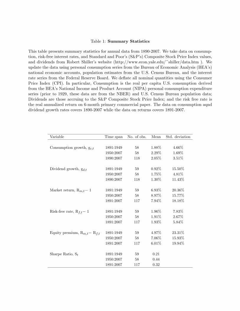
Table 1: Summary Statistics

This table presents summary statistics for annual data from 1890-2007. We take data on consump-tion, risk-free interest rates, and Standard and Poor�s (S&P�s) Composite Stock Price Index values,and dividends from Robert Shiller�s website (http://www.econ.yale.edu/~shiller/data.htm ). Weupdate the data using personal consumption series from the Bureau of Economic Analysis (BEA�s)national economic accounts, population estimates from the U.S. Census Bureau, and the interestrate series from the Federal Reserve Board. We de�ate all nominal quantities using the ConsumerPrice Index (CPI). In particular, Consumption is the real per capita U.S. consumption derivedfrom the BEA�s National Income and Product Account (NIPA) personal consumption expenditureseries (prior to 1929, these data are from the NBER) and U.S. Census Bureau population data;Dividends are those accruing to the S&P Composite Stock Price Index; and the risk free rate isthe real annualized return on 6-month primary commercial paper. The data on consumption aqnddividend growth rates covers 1890-2007 while the data on returns covers 1891-2007.

Variable Time span No. of obs. Mean Std. deviation

Consumption growth, gc;t 1891:1949 58 1.88% 4.66%1950:2007 58 2.29% 1.69%1890:2007 118 2.05% 3.51%

Dividend growth, gd;t 1891:1949 59 0.92% 15.50%1950:2007 58 1.75% 4.81%1890:2007 118 1.30% 11.43%

Market return, Rm;t� 1 1891:1949 59 6.93% 20.36%1950:2007 58 8.97% 15.77%1891:2007 117 7.94% 18.18%

Risk-free rate, Rf;t� 1 1891:1949 59 1.96% 7.83%1950:2007 58 1.91% 2.67%1891:2007 117 1.93% 5.84%

Equity premium, Rm;t� Rf;t 1891:1949 59 4.97% 23.31%1950:2007 58 7.06% 15.93%1891:2007 117 6.01% 19.94%

Sharpe Ratio, St 1891:1949 59 0.211950:2007 58 0.441891:2007 117 0.32

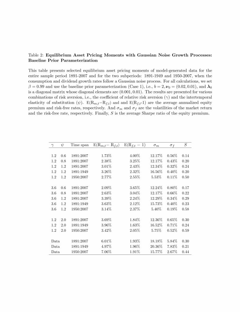
Table 2: Equilibrium Asset Pricing Moments with Gaussian Noise Growth Processes:Baseline Prior Parameterization

This table presents selected equilibrium asset pricing moments of model-generated data for theentire sample period 1891-2007 and for the two subperiods: 1891-1949 and 1950-2007, when theconsumption and dividend growth rates follow a Gaussian noise process. For all calculations, we set� = 0:99 and use the baseline prior parameterization (Case 1), i.e., b = 2;�0 = (0:02; 0:01); and �0is a diagonal matrix whose diagonal elements are (0:001; 0:01). The results are presented for variouscombinations of risk aversion, i.e., the coe¢ cient of relative risk aversion ( ) and the intertemporalelasticity of substitution ( ). E(Rm;t�Rf;t) and and E(Rf;t-1) are the average annualized equitypremium and risk-free rates, respectively. And �m and �f are the volatilities of the market returnand the risk-free rate, respectively. Finally, S is the average Sharpe ratio of the equity premium.

Time span E(Rm;t� Rf;t) E(Rf;t � 1) �m �f S

1.2 0.6 1891:2007 1.73% 4.00% 12.17% 0.56% 0.141.2 0.8 1891:2007 2.38% 3.25% 12.17% 0.43% 0.201.2 1.2 1891:2007 3.01% 2.43% 12.34% 0.32% 0.241.2 1.2 1891:1949 3.26% 2.32% 16.56% 0.40% 0.201.2 1.2 1950:2007 2.77% 2.55% 5.53% 0.11% 0.50

3.6 0.6 1891:2007 2.09% 3.65% 12.24% 0.80% 0.173.6 0.8 1891:2007 2.63% 3.04% 12.17% 0.66% 0.223.6 1.2 1891:2007 3.39% 2.24% 12.29% 0.34% 0.293.6 1.2 1891:1949 3.63% 2.12% 15.73% 0.40% 0.233.6 1.2 1950:2007 3.14% 2.37% 5.40% 0.19% 0.58

1.2 2.0 1891:2007 3.69% 1.84% 12.36% 0.65% 0.301.2 2.0 1891:1949 3.96% 1.63% 16.52% 0.71% 0.241.2 2.0 1950:2007 3.42% 2.05% 5.75% 0.52% 0.59

Data 1891:2007 6.01% 1.93% 18.18% 5.84% 0.30Data 1891:1949 4.97% 1.96% 20.36% 7.83% 0.21Data 1950:2007 7.06% 1.91% 15.77% 2.67% 0.44

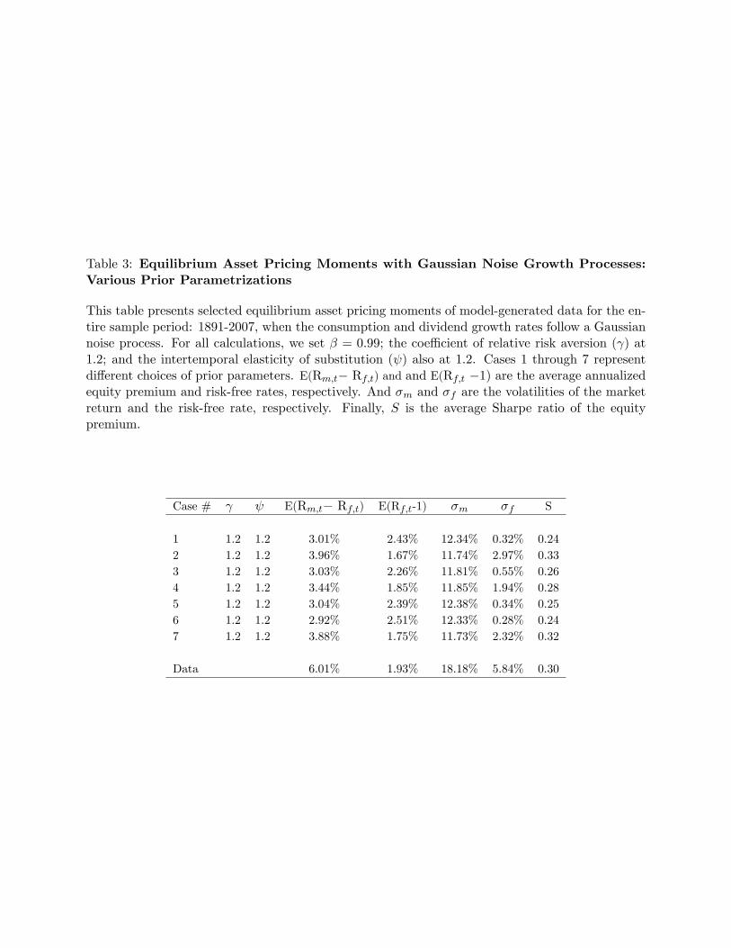
Table 3: Equilibrium Asset Pricing Moments with Gaussian Noise Growth Processes:Various Prior Parametrizations

This table presents selected equilibrium asset pricing moments of model-generated data for the en-tire sample period: 1891-2007, when the consumption and dividend growth rates follow a Gaussiannoise process. For all calculations, we set � = 0:99; the coe¢ cient of relative risk aversion ( ) at1.2; and the intertemporal elasticity of substitution ( ) also at 1.2. Cases 1 through 7 representdi¤erent choices of prior parameters. E(Rm;t� Rf;t) and and E(Rf;t �1) are the average annualizedequity premium and risk-free rates, respectively. And �m and �f are the volatilities of the marketreturn and the risk-free rate, respectively. Finally, S is the average Sharpe ratio of the equitypremium.

Case # E(Rm;t� Rf;t) E(Rf;t-1) �m �f S

1 1.2 1.2 3.01% 2.43% 12.34% 0.32% 0.242 1.2 1.2 3.96% 1.67% 11.74% 2.97% 0.333 1.2 1.2 3.03% 2.26% 11.81% 0.55% 0.264 1.2 1.2 3.44% 1.85% 11.85% 1.94% 0.285 1.2 1.2 3.04% 2.39% 12.38% 0.34% 0.256 1.2 1.2 2.92% 2.51% 12.33% 0.28% 0.247 1.2 1.2 3.88% 1.75% 11.73% 2.32% 0.32

Data 6.01% 1.93% 18.18% 5.84% 0.30

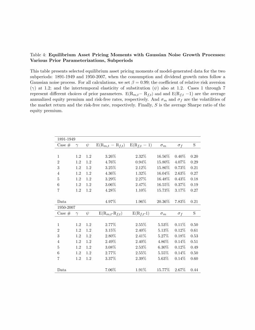
Table 4: Equilibrium Asset Pricing Moments with Gaussian Noise Growth Processes:Various Prior Parameterizations, Subperiods

This table presents selected equilibrium asset pricing moments of model-generated data for the twosubperiods: 1891-1949 and 1950-2007, when the consumption and dividend growth rates follow aGaussian noise process. For all calculations, we set � = 0:99; the coe¢ cient of relative risk aversion( ) at 1.2; and the intertemporal elasticity of substitution ( ) also at 1.2. Cases 1 through 7represent di¤erent choices of prior parameters. E(Rm;t� Rf;t) and and E(Rf;t �1) are the averageannualized equity premium and risk-free rates, respectively. And �m and �f are the volatilities ofthe market return and the risk-free rate, respectively. Finally, S is the average Sharpe ratio of theequity premium.

1891-1949Case # E(Rm;t � Rf;t) E(Rf;t � 1) �m �f S

1 1.2 1.2 3.26% 2.32% 16.56% 0.40% 0.202 1.2 1.2 4.76% 0.94% 15.80% 4.07% 0.293 1.2 1.2 3.25% 2.12% 15.86% 0.73% 0.214 1.2 1.2 4.36% 1.32% 16.04% 2.63% 0.275 1.2 1.2 3.29% 2.27% 16.48% 0.43% 0.186 1.2 1.2 3.06% 2.47% 16.55% 0.37% 0.197 1.2 1.2 4.28% 1.10% 15.73% 3.17% 0.27

Data 4.97% 1.96% 20.36% 7.83% 0.211950-2007Case # E(Rm;t-Rf;t) E(Rf;t-1) �m �f S

1 1.2 1.2 2.77% 2.55% 5.53% 0.11% 0.502 1.2 1.2 3.15% 2.40% 5.13% 0.12% 0.613 1.2 1.2 2.80% 2.41% 5.27% 0.18% 0.534 1.2 1.2 2.49% 2.40% 4.86% 0.14% 0.515 1.2 1.2 3.08% 2.53% 6.30% 0.12% 0.496 1.2 1.2 2.77% 2.55% 5.55% 0.14% 0.507 1.2 1.2 3.37% 2.39% 5.63% 0.14% 0.60

Data 7.06% 1.91% 15.77% 2.67% 0.44

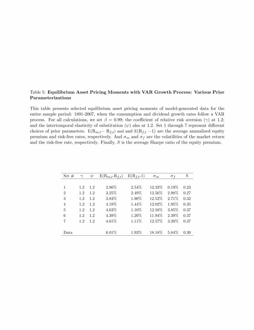
Table 5: Equilibrium Asset Pricing Moments with VAR Growth Process: Various PriorParameterizations

This table presents selected equilibrium asset pricing moments of model-generated data for theentire sample period: 1891-2007, when the consumption and dividend growth rates follow a VARprocess. For all calculations, we set � = 0:99; the coe¢ cient of relative risk aversion ( ) at 1.2;and the intertemporal elasticity of substitution ( ) also at 1.2. Set 1 through 7 represent di¤erentchoices of prior parameters. E(Rm;t� Rf;t) and and E(Rf;t �1) are the average annualized equitypremium and risk-free rates, respectively. And �m and �f are the volatilities of the market returnand the risk-free rate, respectively. Finally, S is the average Sharpe ratio of the equity premium.

Set # E(Rm;t-Rf;t) E(Rf;t-1) �m �f S

1 1.2 1.2 2.86% 2.54% 12.33% 0.19% 0.232 1.2 1.2 3.25% 2.49% 12.56% 2.98% 0.273 1.2 1.2 3.83% 1.90% 12.52% 2.71% 0.324 1.2 1.2 4.19% 1.44% 12.02% 1.95% 0.355 1.2 1.2 4.63% 1.10% 12.58% 3.85% 0.376 1.2 1.2 4.39% 1.20% 11.94% 2.39% 0.377 1.2 1.2 4.61% 1.11% 12.57% 3.20% 0.37

Data 6.01% 1.93% 18.18% 5.84% 0.30

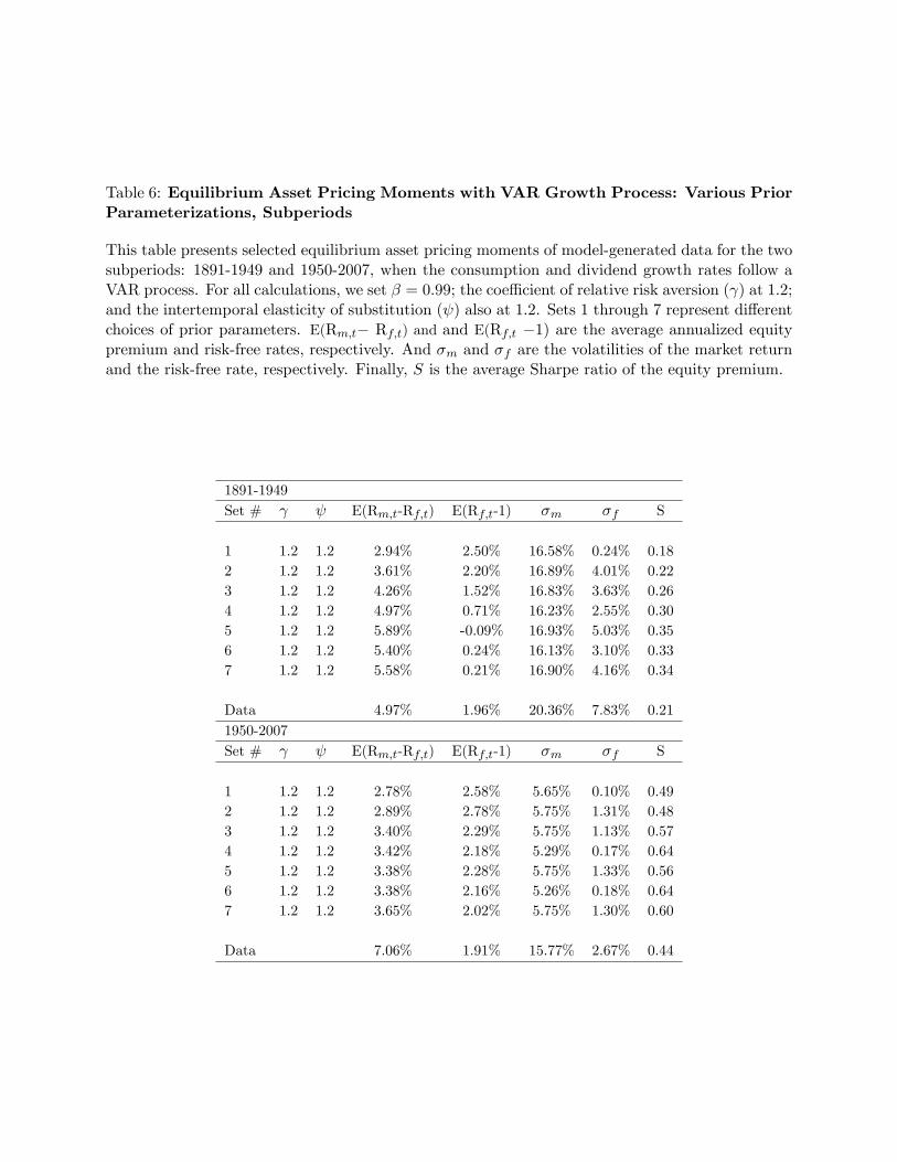
Table 6: Equilibrium Asset Pricing Moments with VAR Growth Process: Various PriorParameterizations, Subperiods

This table presents selected equilibrium asset pricing moments of model-generated data for the twosubperiods: 1891-1949 and 1950-2007, when the consumption and dividend growth rates follow aVAR process. For all calculations, we set � = 0:99; the coe¢ cient of relative risk aversion ( ) at 1.2;and the intertemporal elasticity of substitution ( ) also at 1.2. Sets 1 through 7 represent di¤erentchoices of prior parameters. E(Rm;t� Rf;t) and and E(Rf;t �1) are the average annualized equitypremium and risk-free rates, respectively. And �m and �f are the volatilities of the market returnand the risk-free rate, respectively. Finally, S is the average Sharpe ratio of the equity premium.

1891-1949Set # E(Rm;t-Rf;t) E(Rf;t-1) �m �f S

1 1.2 1.2 2.94% 2.50% 16.58% 0.24% 0.182 1.2 1.2 3.61% 2.20% 16.89% 4.01% 0.223 1.2 1.2 4.26% 1.52% 16.83% 3.63% 0.264 1.2 1.2 4.97% 0.71% 16.23% 2.55% 0.305 1.2 1.2 5.89% -0.09% 16.93% 5.03% 0.356 1.2 1.2 5.40% 0.24% 16.13% 3.10% 0.337 1.2 1.2 5.58% 0.21% 16.90% 4.16% 0.34

Data 4.97% 1.96% 20.36% 7.83% 0.211950-2007Set # E(Rm;t-Rf;t) E(Rf;t-1) �m �f S

1 1.2 1.2 2.78% 2.58% 5.65% 0.10% 0.492 1.2 1.2 2.89% 2.78% 5.75% 1.31% 0.483 1.2 1.2 3.40% 2.29% 5.75% 1.13% 0.574 1.2 1.2 3.42% 2.18% 5.29% 0.17% 0.645 1.2 1.2 3.38% 2.28% 5.75% 1.33% 0.566 1.2 1.2 3.38% 2.16% 5.26% 0.18% 0.647 1.2 1.2 3.65% 2.02% 5.75% 1.30% 0.60

Data 7.06% 1.91% 15.77% 2.67% 0.44

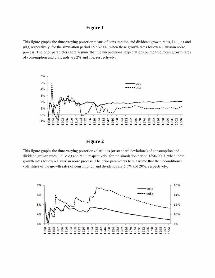
Figure 1

This figure graphs the time-varying posterior means of consumption and dividend growth rates, i.e., μc,t and μd,t, respectively, for the simulation period 1890-2007, when these growth rates follow a Gaussian noise process. The prior parameters here assume that the unconditional expectations on the true mean growth rates of consumption and dividends are 2% and 1%, respectively.

Figure 2

This figure graphs the time-varying posterior volatilities (or standard deviations) of consumption and dividend growth rates, i.e., σ c,t and σ d,t, respectively, for the simulation period 1890-2007, when these growth rates follow a Gaussian noise process. The prior parameters here assume that the unconditional volatilities of the growth rates of consumption and dividends are 6.3% and 20%, respectively.

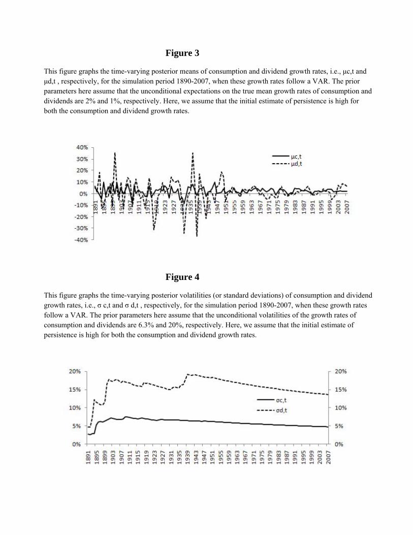
Figure 3

This figure graphs the time-varying posterior means of consumption and dividend growth rates, i.e., μc,t and μd,t , respectively, for the simulation period 1890-2007, when these growth rates follow a VAR. The prior parameters here assume that the unconditional expectations on the true mean growth rates of consumption and dividends are 2% and 1%, respectively. Here, we assume that the initial estimate of persistence is high for both the consumption and dividend growth rates.

Figure 4

This figure graphs the time-varying posterior volatilities (or standard deviations) of consumption and dividend growth rates, i.e., σ c,t and σ d,t , respectively, for the simulation period 1890-2007, when these growth rates follow a VAR. The prior parameters here assume that the unconditional volatilities of the growth rates of consumption and dividends are 6.3% and 20%, respectively. Here, we assume that the initial estimate of persistence is high for both the consumption and dividend growth rates.

Figure 5

This figure plots the equilibrium annual equity premium generated by the model for the simulation period 1920-2007, when the growth rates follow a Gaussian noise process. The prior parameters here assume that the unconditional expectations on the true mean growth rates of consumption and dividends are 2% and 1%, respectively, while the unconditional volatilities of the growth rates of consumption and dividends are 6.3% and 20%, respectively. We also plot the annual realized equity premium.

Figure 6

This figure plots the equilibrium annual equity premium generated by the model for the simulation period 1920-2007, when the growth rates follow a VAR. Here, we raise the prior uncertainty about the growth rates compared to the prior parameters assumed in Figure 8. But we also assume that the initial estimate of persistence is high for both the consumption and dividend growth rates. We also plot the annual realized equity premium.

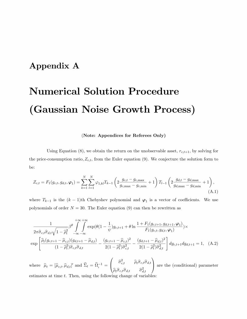
Appendix A

Numerical Solution Procedure

(Gaussian Noise Growth Process)

(Note: Appendices for Referees Only)

Using Equation (8), we obtain the return on the unobservable asset, rc;t+1; by solving for

the price-consumption ratio; Zc;t; from the Euler equation (9). We conjecture the solution form to

be:

Zc;t = F1(gc;t; gd;t;'1) =

NXk=1

NXl=1

'1;klTk�1

�2gc;t � gc;maxgc;max � gc;min

+ 1

�Tl�1

�2gd;t � gd;maxgd;max � gd;min

+ 1

�;

(A.1)

where Tk�1 is the (k � 1)th Chebyshev polynomial and '1 is a vector of coe¢ cients. We use

polynomials of order N = 30. The Euler equation (9) can then be rewritten as

1

2�b�c;tb�d;tq1� b�2t ��+1Z�1

+1Z�1

exp(�(1� 1

)gc;t+1 + � ln

1 + F1(gc;t+1; gd;t+1;'1)

F1(gc;t; gd;t;'1))�

exp

"b�t(gc;t+1 � b�c;t)(gd;t+1 � b�d;t)(1� b�2t )b�c;tb�d;t �

(gc;t+1 � b�c;t)22(1� b�2t )b�2c;t �

(gd;t+1 � b�d;t)22(1� b�2t )b�2d;t

#dgc;t+1dgd;t+1 = 1; (A.2)

where b�t = [b�c;t; b�d;t]0 and b�t = b�1t=

0@ b�2c;t b�tb�c;tb�d;tb�tb�c;tb�d;t b�2d;t1A are the (conditional) parameter

estimates at time t. Then, using the following change of variables:

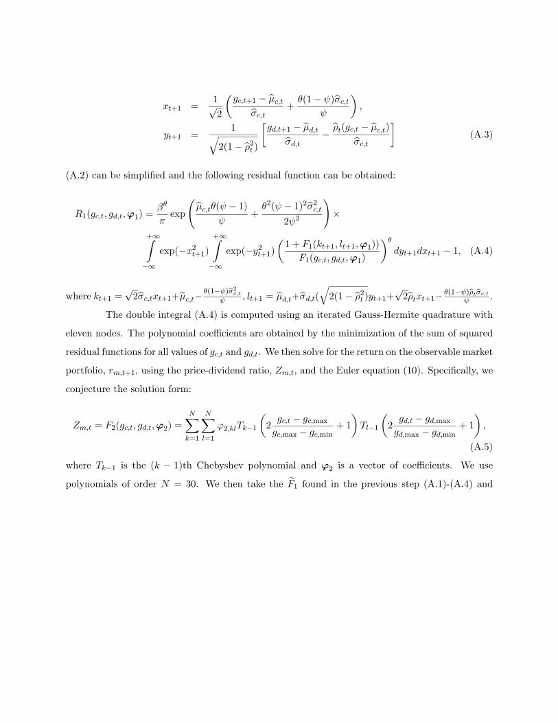
xt+1 =1p2

�gc;t+1 � b�c;tb�c;t +

�(1� )b�c;t

�;

yt+1 =1q

2(1� b�2t )�gd;t+1 � b�d;tb�d;t �

b�t(gc;t � b�c;t)b�c;t�

(A.3)

(A.2) can be simpli�ed and the following residual function can be obtained:

R1(gc;t; gd;t;'1) =��

�exp

b�c;t�( � 1)

+�2( � 1)2b�2c;t

2 2

!�

+1Z�1

exp(�x2t+1)+1Z�1

exp(�y2t+1)�1 + F1(kt+1; lt+1;'1))

F1(gc;t; gd;t;'1)

��dyt+1dxt+1 � 1; (A.4)

where kt+1 =p2b�c;txt+1+b�c;t� �(1� )b�2c;t

; lt+1 = b�d;t+b�d;t(q2(1� b�2t )yt+1+p2b�txt+1� �(1� )b�tb�c;t :

The double integral (A.4) is computed using an iterated Gauss-Hermite quadrature with

eleven nodes. The polynomial coe¢ cients are obtained by the minimization of the sum of squared

residual functions for all values of gc;t and gd;t. We then solve for the return on the observable market

portfolio, rm;t+1, using the price-dividend ratio, Zm;t; and the Euler equation (10). Speci�cally, we

conjecture the solution form:

Zm;t = F2(gc;t; gd;t;'2) =

NXk=1

NXl=1

'2;klTk�1

�2gc;t � gc;maxgc;max � gc;min

+ 1

�Tl�1

�2gd;t � gd;maxgd;max � gd;min

+ 1

�;

(A.5)

where Tk�1 is the (k � 1)th Chebyshev polynomial and '2 is a vector of coe¢ cients. We use

polynomials of order N = 30. We then take the eF1 found in the previous step (A.1)-(A.4) and

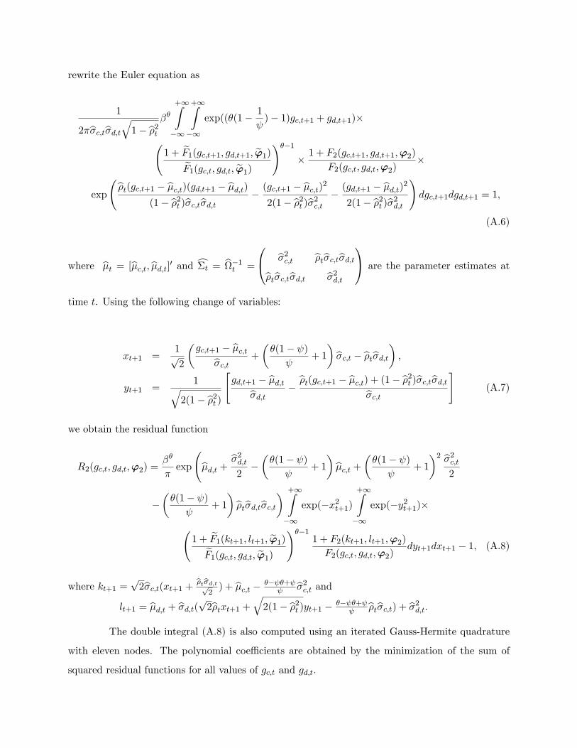
rewrite the Euler equation as

1

2�b�c;tb�d;tq1� b�2t ��+1Z�1

+1Z�1

exp((�(1� 1

)� 1)gc;t+1 + gd;t+1)�

1 + eF1(gc;t+1; gd;t+1; e'1)eF1(gc;t; gd;t; e'1)

!��1� 1 + F2(gc;t+1; gd;t+1;'2)

F2(gc;t; gd;t;'2)�

exp

b�t(gc;t+1 � b�c;t)(gd;t+1 � b�d;t)(1� b�2t )b�c;tb�d;t �

(gc;t+1 � b�c;t)22(1� b�2t )b�2c;t �

(gd;t+1 � b�d;t)22(1� b�2t )b�2d;t

!dgc;t+1dgd;t+1 = 1;

(A.6)

where b�t = [b�c;t; b�d;t]0 and c�t = b�1t =

0@ b�2c;t b�tb�c;tb�d;tb�tb�c;tb�d;t b�2d;t1A are the parameter estimates at

time t. Using the following change of variables:

xt+1 =1p2

�gc;t+1 � b�c;tb�c;t +

��(1� )

+ 1

�b�c;t � b�tb�d;t� ;yt+1 =

1q2(1� b�2t )

"gd;t+1 � b�d;tb�d;t �

b�t(gc;t+1 � b�c;t) + (1� b�2t )b�c;tb�d;tb�c;t#

(A.7)

we obtain the residual function

R2(gc;t; gd;t;'2) =��

�exp

b�d;t + b�2d;t2 ���(1� )

+ 1

�b�c;t + ��(1� ) + 1

�2 b�2c;t2

���(1� )

+ 1

�b�tb�d;tb�c;t� +1Z�1

exp(�x2t+1)+1Z�1

exp(�y2t+1)�

1 + eF1(kt+1; lt+1; e'1)eF1(gc;t; gd;t; e'1)

!��11 + F2(kt+1; lt+1;'2)

F2(gc;t; gd;t;'2)dyt+1dxt+1 � 1; (A.8)

where kt+1 =p2b�c;t(xt+1 + b�tb�d;tp

2) + b�c;t � �� �+

b�2c;t andlt+1 = b�d;t + b�d;t(p2b�txt+1 +q2(1� b�2t )yt+1 � �� �+

b�tb�c;t) + b�2d;t.The double integral (A.8) is also computed using an iterated Gauss-Hermite quadrature

with eleven nodes. The polynomial coe¢ cients are obtained by the minimization of the sum of

squared residual functions for all values of gc;t and gd;t.

The risk-free interest rate rf;t+1 can be obtained using the following formula:

rf;t+1 = ln((E[��G

� �

c;t+1R��1)c;t+1j�t])�1) = ln

�E[exp(� ln(�)� �

gc;t+1 + (� � 1)rc;t+1)j�t]

��1!

= ln

0@0@ 1

2�b�c;tb�d;tq1� b�2t ��+1Z�1

+1Z�1

1 + eF1(gc;t+1; gd;t+1; e'1)eF1(gc;t; gd;t; e'1)

!��1�

exp((�(1� 1

)� 1)gc;t+1 + gd;t+1)� exp

"b�t(gc;t+1 � b�c;t)(gd;t+1 � b�d;t)(1� b�2t )b�c;tb�d;t �

(gc;t+1 � b�c;t)22(1� b�2t )b�2c;t �

�(gd;t+1 � b�d;t)22(1� b�2t )b�2d;t

#dgc;t+1dgd;t+1

!�11A (A.9)

Using the following change of variables,

xt+1 =1p2b�c;t

�gc;t+1 � b�c;t + ��(1� )

+ 1

�b�2c;t� ;yt+1 =

1q2(1� b�2t )

�gd;t+1 � b�d;tb�d;t �

b�t(gc;t+1 � b�c;t)b�c;t�; (A.10)

we can rewrite the previous formula as

rf;t+1 = ln

��

�exp

���(1� )

+ 1

�b�c;t + ��(1� ) + 1

�2 b�2c;t2

!�

+1Z�1

exp(�x2t+1)+1Z�1

exp(�y2t+1) 1 + eF1(kt+1; lt+1; e'1)eF1(gc;t; gd;t; e'1)

!(��1)dyt+1dxt+1

1A�11CA ; (A.11)

where, kt+1 =p2b�c;txt+1 + b�c;t � � �(1� ) + 1

� b�2c;t andlt+1 = b�d;t + b�d;t(p2b�txt+1 +q2(1� b�2t )yt+1 � � �(1� ) + 1

�b�tb�c;t).

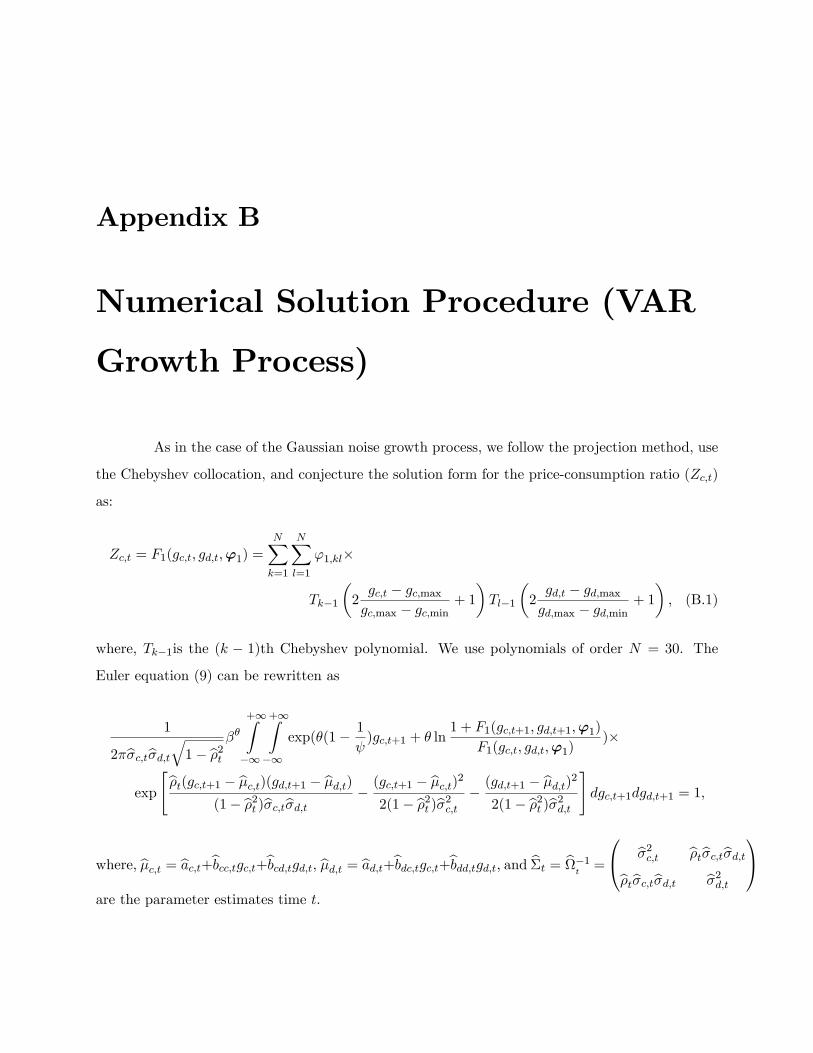
Appendix B

Numerical Solution Procedure (VAR

Growth Process)

As in the case of the Gaussian noise growth process, we follow the projection method, use

the Chebyshev collocation, and conjecture the solution form for the price-consumption ratio (Zc;t)

as:

Zc;t = F1(gc;t; gd;t;'1) =NXk=1

NXl=1

'1;kl�

Tk�1

�2gc;t � gc;maxgc;max � gc;min

+ 1

�Tl�1

�2gd;t � gd;maxgd;max � gd;min

+ 1

�; (B.1)

where, Tk�1is the (k � 1)th Chebyshev polynomial. We use polynomials of order N = 30. The

Euler equation (9) can be rewritten as

1

2�b�c;tb�d;tq1� b�2t ��+1Z�1

+1Z�1

exp(�(1� 1

)gc;t+1 + � ln

1 + F1(gc;t+1; gd;t+1;'1)

F1(gc;t; gd;t;'1))�

exp

"b�t(gc;t+1 � b�c;t)(gd;t+1 � b�d;t)(1� b�2t )b�c;tb�d;t �

(gc;t+1 � b�c;t)22(1� b�2t )b�2c;t �

(gd;t+1 � b�d;t)22(1� b�2t )b�2d;t

#dgc;t+1dgd;t+1 = 1;

where, b�c;t = bac;t+bbcc;tgc;t+bbcd;tgd;t, b�d;t = bad;t+bbdc;tgc;t+bbdd;tgd;t; and b�t = b�1t =

0@ b�2c;t b�tb�c;tb�d;tb�tb�c;tb�d;t b�2d;t1A

are the parameter estimates time t.

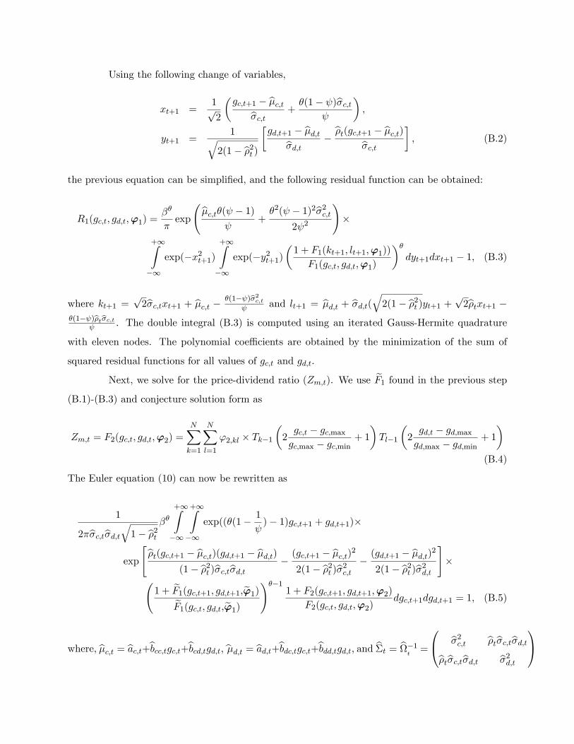
Using the following change of variables,

xt+1 =1p2

�gc;t+1 � b�c;tb�c;t +

�(1� )b�c;t

�;

yt+1 =1q

2(1� b�2t )�gd;t+1 � b�d;tb�d;t �

b�t(gc;t+1 � b�c;t)b�c;t�; (B.2)

the previous equation can be simpli�ed, and the following residual function can be obtained:

R1(gc;t; gd;t;'1) =��

�exp

b�c;t�( � 1)

+�2( � 1)2b�2c;t

2 2

!�

+1Z�1

exp(�x2t+1)+1Z�1

exp(�y2t+1)�1 + F1(kt+1; lt+1;'1))

F1(gc;t; gd;t;'1)

��dyt+1dxt+1 � 1; (B.3)

where kt+1 =p2b�c;txt+1 + b�c;t � �(1� )b�2c;t

and lt+1 = b�d;t + b�d;t(q2(1� b�2t )yt+1 + p2b�txt+1 ��(1� )b�tb�c;t

. The double integral (B.3) is computed using an iterated Gauss-Hermite quadrature

with eleven nodes. The polynomial coe¢ cients are obtained by the minimization of the sum of

squared residual functions for all values of gc;t and gd;t.

Next, we solve for the price-dividend ratio (Zm;t). We use eF1 found in the previous step(B.1)-(B.3) and conjecture solution form as

Zm;t = F2(gc;t; gd;t;'2) =

NXk=1

NXl=1

'2;kl � Tk�1�2gc;t � gc;maxgc;max � gc;min

+ 1

�Tl�1

�2gd;t � gd;maxgd;max � gd;min

+ 1

�(B.4)

The Euler equation (10) can now be rewritten as

1

2�b�c;tb�d;tq1� b�2t ��+1Z�1

+1Z�1

exp((�(1� 1

)� 1)gc;t+1 + gd;t+1)�

exp

"b�t(gc;t+1 � b�c;t)(gd;t+1 � b�d;t)(1� b�2t )b�c;tb�d;t �

(gc;t+1 � b�c;t)22(1� b�2t )b�2c;t �

(gd;t+1 � b�d;t)22(1� b�2t )b�2d;t

#�

1 + eF1(gc;t+1; gd;t+1;e'1)eF1(gc;t; gd;t;e'1)

!��11 + F2(gc;t+1; gd;t+1;'2)

F2(gc;t; gd;t;'2)dgc;t+1dgd;t+1 = 1; (B.5)

where, b�c;t = bac;t+bbcc;tgc;t+bbcd;tgd;t, b�d;t = bad;t+bbdc;tgc;t+bbdd;tgd;t; and b�t = b�1t =

0@ b�2c;t b�tb�c;tb�d;tb�tb�c;tb�d;t b�2d;t1A

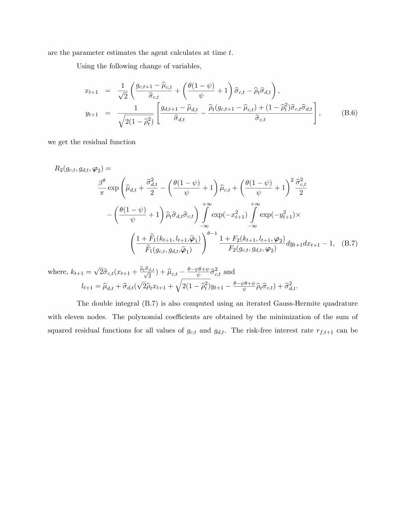
are the parameter estimates the agent calculates at time t.

Using the following change of variables,

xt+1 =1p2

�gc;t+1 � b�c;tb�c;t +

��(1� )

+ 1

�b�c;t � b�tb�d;t� ;yt+1 =

1q2(1� b�2t )

"gd;t+1 � b�d;tb�d;t �

b�t(gc;t+1 � b�c;t) + (1� b�2t )b�c;tb�d;tb�c;t#; (B.6)

we get the residual function

R2(gc;t; gd;t;'2) =

��

�exp

b�d;t + b�2d;t2 ���(1� )

+ 1

�b�c;t + ��(1� ) + 1

�2 b�2c;t2

���(1� )

+ 1

�b�tb�d;tb�c;t� +1Z�1

exp(�x2t+1)+1Z�1

exp(�y2t+1)�

1 + eF1(kt+1; lt+1;e'1)eF1(gc;t; gd;t;e'1)

!��11 + F2(kt+1; lt+1;'2)

F2(gc;t; gd;t;'2)dyt+1dxt+1 � 1; (B.7)

where, kt+1 =p2b�c;t(xt+1 + b�tb�d;tp

2) + b�c;t � �� �+

b�2c;t andlt+1 = b�d;t + b�d;t(p2b�txt+1 +q2(1� b�2t )yt+1 � �� �+

b�tb�c;t) + b�2d;t.The double integral (B.7) is also computed using an iterated Gauss-Hermite quadrature

with eleven nodes. The polynomial coe¢ cients are obtained by the minimization of the sum of

squared residual functions for all values of gc;t and gd;t. The risk-free interest rate rf;t+1 can be

obtained using the following formula:

rf;t+1 = ln((E[��G

� �

c;t+1R��1)c;t+1j�t])�1)

= ln

�E[exp(� ln(�)� �

gc;t+1 + (� � 1)rc;t+1)j�t]

��1!

= ln

0@0@ 1

2�b�c;tb�d;tq1� b�2t ��+1Z�1

+1Z�1

1 + eF1(gc;t+1; gd;t+1;e'1)eF1(gc;t; gd;t;e'1)

!��1�

exp

"b�t(gc;t+1 � b�c;t)(gd;t � b�d;t)(1� b�2t )b�c;tb�d;t �

(gc;t+1 � b�c;t)22(1� b�2t )b�2c;t �

(gd;t+1 � b�d;t)22(1� b�2t )b�2d;t

#�

exp((�(1� 1

)� 1)gc;t+1 + gd;t+1)dgc;t+1dgd;t+1

��1!(B.8)

Using the following change of variables:

xt+1 =1p2b�c;t

�gc;t+1 � b�c;t + ��(1� )

+ 1

�b�2c;t� ;yt+1 =

1q2(1� b�2t )

�gd;t+1 � b�d;tb�d;t �

b�t(gc;t+1 � b�c;t)b�c;t�

(B.9)

we can rewrite the previous formula as

rf;t+1 = ln

��

�exp

���(1� )

+ 1

�b�c;t + ��(1� ) + 1

�2 b�2c;t2

!�

+1Z�1

exp(�x2t+1)+1Z�1

exp(�y2t+1) 1 + eF1(kt+1; lt+1;e'1)eF1(gc;t; gd;t;e'1)

!(��1)dyt+1dxt+1

1A�11CA ; (B.10)

where, kt+1 =p2b�c;txt+1 + b�c;t � � �(1� ) + 1

� b�2c;t andlt+1 = b�d;t + b�d;t(p2b�txt +q2(1� b�2t )yt+1 � � �(1� ) + 1

�b�tb�c;t).

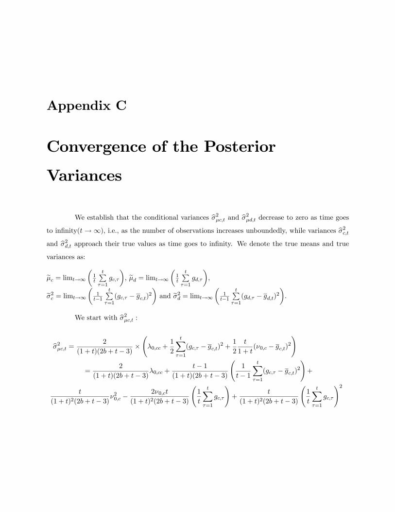
Appendix C

Convergence of the Posterior

Variances

We establish that the conditional variances b�2�c;t and b�2�d;t decrease to zero as time goesto in�nity(t!1), i.e., as the number of observations increases unboundedly, while variances b�2c;tand b�2d;t approach their true values as time goes to in�nity. We denote the true means and truevariances as:

e�c = limt!1

�1t

tP�=1

gc;�

�, e�d = limt!1

�1t

tP�=1

gd;�

�,

e�2c = limt!1

�1t�1

tP�=1(gc;� � gc;t)2

�and e�2d = limt!1

�1t�1

tP�=1(gd;� � gd;t)2

�.

We start with b�2�c;t :b�2�c;t = 2

(1 + t)(2b+ t� 3) � �0;cc +

1

2

tX�=1

(gc;� � gc;t)2 +1

2

t

1 + t(�0;c � gc;t)2

!

=2

(1 + t)(2b+ t� 3)�0;cc +t� 1

(1 + t)(2b+ t� 3)

1

t� 1

tX�=1

(gc;� � gc;t)2!+

t

(1 + t)2(2b+ t� 3)�20;c �

2�0;ct

(1 + t)2(2b+ t� 3)

1

t

tX�=1

gc;�

!+

t

(1 + t)2(2b+ t� 3)

1

t

tX�=1

gc;�

!2

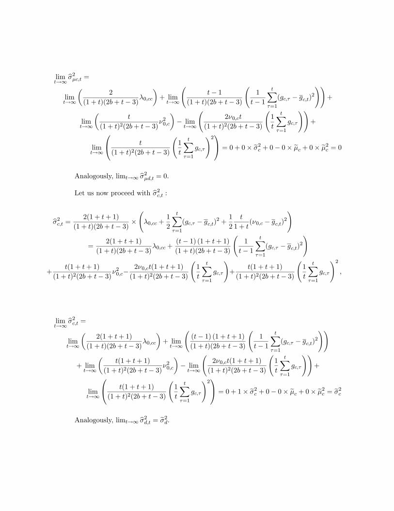
limt!1

b�2�c;t =limt!1

�2

(1 + t)(2b+ t� 3)�0;cc�+ limt!1

t� 1

(1 + t)(2b+ t� 3)

1

t� 1

tX�=1

(gc;� � gc;t)2!!

+

limt!1

�t

(1 + t)2(2b+ t� 3)�20;c

�� limt!1

2�0;ct

(1 + t)2(2b+ t� 3)

1

t

tX�=1

gc;�

!!+

limt!1

0@ t

(1 + t)2(2b+ t� 3)

1

t

tX�=1

gc;�

!21A = 0 + 0� e�2c + 0� 0� e�c + 0� e�2c = 0Analogously, limt!1 b�2�d;t = 0:Let us now proceed with b�2c;t :

b�2c;t = 2(1 + t+ 1)

(1 + t)(2b+ t� 3) � �0;cc +

1

2

tX�=1

(gc;� � gc;t)2 +1

2

t

1 + t(�0;c � gc;t)2

!

=2(1 + t+ 1)

(1 + t)(2b+ t� 3)�0;cc +(t� 1) (1 + t+ 1)(1 + t)(2b+ t� 3)

1

t� 1

tX�=1

(gc;� � gc;t)2!

+t(1 + t+ 1)

(1 + t)2(2b+ t� 3)�20;c�

2�0;ct(1 + t+ 1)

(1 + t)2(2b+ t� 3)

1

t

tX�=1

gc;�

!+

t(1 + t+ 1)

(1 + t)2(2b+ t� 3)

1

t

tX�=1

gc;�

!2;

limt!1

b�2c;t =limt!1

�2(1 + t+ 1)

(1 + t)(2b+ t� 3)�0;cc�+ limt!1

(t� 1) (1 + t+ 1)(1 + t)(2b+ t� 3)

1

t� 1

tX�=1

(gc;� � gc;t)2!!

+ limt!1

�t(1 + t+ 1)

(1 + t)2(2b+ t� 3)�20;c

�� limt!1

2�0;ct(1 + t+ 1)

(1 + t)2(2b+ t� 3)

1

t

tX�=1

gc;�

!!+

limt!1

0@ t(1 + t+ 1)

(1 + t)2(2b+ t� 3)

1

t

tX�=1

gc;�

!21A = 0 + 1� e�2c + 0� 0� e�c + 0� e�2c = e�2cAnalogously, limt!1 b�2d;t = e�2d: