Measuring the equity risk premium with dividend discount ...

MEASURING THE EQUITY RISK PREMIUM WITH DIVIDEND DISCOUNT MODELS

2022

Julio Gálvez

Documentos Ocasionales N.º 2207


Julio Gálvez (*)

BANCO DE ESPAÑA

Documentos Ocasionales. N.º 2207

June 2022

(*) Macro-financial Analysis and Monetary Policy Department, Banco de España. I thank Roberto Blanco, Alberto Fuertes, Sergio Mayordomo and Carlos Thomas for their helpful comments and suggestions. I am particularly grateful to Francisco Alonso Sánchez and Emilio Muñoz de la Peña for their help with data collection and construction. E-mail for correspondence: [email protected]. This article is solely my responsibility and does not reflect the views of the Banco de España or the Eurosystem.

The Occasional Paper Series seeks to disseminate work conducted at the Banco de España, in the performance of its functions, that may be of general interest.

The opinions and analyses in the Occasional Paper Series are the responsibility of the authors and, therefore, do not necessarily coincide with those of the Banco de España or the Eurosystem.

The Banco de España disseminates its main reports and most of its publications via the Internet on its website at: http://www.bde.es.

Reproduction for educational and non-commercial purposes is permitted provided that the source is acknowledged.

© BANCO DE ESPAÑA, Madrid, 2022

ISSN: 1696-2230 (on-line edition)

Abstract

This paper assesses the estimation of the so-called equity risk premium, i.e. the expected

return on equities in excess of the risk-free rate, using the dividend discount model as the

organizing framework. I compare the equity risk premium estimates from different dividend

discount models in terms of the in-sample and out-of-sample forecasting ability across

different time horizons. Using data from the Eurostoxx 50 from 2001-2021, I find that

equity risk premium estimates exhibit similar dynamics, and are elevated during periods

of high uncertainty, such as the onset of the COVID-19 pandemic. Moreover, I find that the

three-stage dividend discount model, which divides earnings growth into an extraordinary,

transitional and steady-state phase, performs the best in terms of forecasting ability.

Keywords: expected returns, equity risk premium, dividend discount model, return

predictability.

JEL classification: G10, G12, G15.

Resumen

Este trabajo evalúa la estimación de la prima de riesgo de la renta variable, es decir, el

rendimiento esperado de la renta variable por encima del tipo libre de riesgo, utilizando

el modelo de descuento de dividendos como marco organizativo. Comparo las estimaciones

de la prima de riesgo de la renta variable a partir de diferentes modelos de descuento de

dividendos en términos de la capacidad de previsión dentro y fuera de la muestra a través

de diferentes horizontes temporales. Utilizando datos del EURO STOXX 50 de entre 2001 y

2021, encuentro que las estimaciones de la prima de riesgo de la renta variable muestran una

dinámica similar, y son elevadas durante los períodos de alta incertidumbre, como el inicio de

la pandemia de COVID-19. Además, encuentro que el modelo de descuento de dividendos

en tres etapas, que divide el crecimiento de los beneficios en una fase extraordinaria,

otra de transición y otra de estado estable, es el que mejor funciona en términos de

capacidad de previsión.

Palabras clave: rentabilidad esperada, prima de riesgo de la renta variable, modelo de

descuento de dividendos, previsibilidad de la rentabilidad.

Códigos JEL: G10, G12, G15.

Contents

Abstract 5

Resumen 6

1 Introduction 8

2 The equity risk premium and the dividend discount model 10

3 Estimating the dividend discount model 12

3.1 Measurement of the discount rate 12

3.2 Constant vs. multiple growth rates 15

3.3 Measurement of cash flows 20

4 Conclusion 22

References 23

Appendix A catalog of dividend discount models 24

BANCO DE ESPAÑA 8 DOCUMENTO OCASIONAL N.º 2207

1 Introduction

The equity risk premium (ERP) is arguably one of the most fundamental quantities in asset

pricing, both for theoretical and practical reasons. From a theoretical standpoint, the ERP

reflects the market price of equity risk. It is also regarded as a measure of aggregate

risk aversion, and an important part of the asset allocation decisions of institutional and

individual investors. More recently, the equity risk premium has been used as a gauge of

financial stability1, or as a leading indicator of economic activity (see, for example, Duarte

and Rosa (2015)).

One of the more popular methods to estimate the equity risk premium used in

practice is the dividend discount model, first popularized by Gordon (1962). The basic

intuition of all dividend discount models is that the value of a stock is determined by the cash

flows it provides to shareholders. The popularity behind this approach is due to its relative

simplicity compared to other modelling approaches, and its consistency with no-arbitrage

conditions (assuming that assets are fairly priced). However, despite its simplicity, the

estimates of the ERP from dividend discount models can differ based on the assumptions

one makes on future earnings growth. To this end, the purpose of this paper is to study which

dividend discount model yields the most accurate estimate of the equity risk premium from

a forecasting perspective. Moreover, it investigates other issues related to the estimation of

the equity risk premium via dividend discount models.

To do so, this paper takes the workhorse H-model of Fuller and Hsia (1984)2

as a starting point and studies different issues related to the dividend discount model’s

implementation. First, I analyze the effect of different proxies of the risk-free rate, and the

use of the entire yield curve on the estimation of the equity risk premium. Second, I compare

the evolution of the equity risk premium under the assumption that future dividends grow

at a constant rate (i.e., constant growth models), as opposed to models that assume that

dividend growth can be divided into distinct phases (i.e., multiple growth models). Moreover,

following Li et al. (2013) and Chin and Polk (2015), I assess the in-sample and out-of-sample

predictive power of the equity risk premium measures in forecasting future excess returns

of the Eurostoxx 50 at different horizons. Third, I study the effect of the inclusion of share

buybacks in the measurement of dividends, and its subsequent impact on the estimation of

the equity risk premium.

The main results of the estimations are the following. First, I find that under the

lens of the workhorse H-model and the two-stage model, different proxies for the interest

rate or the use of the entire yield curve to represent discount rates do not have a significant

effect on the resulting estimates of the equity risk premium. Second, comparing constant

1 See, for example, the Financial Stability Report of the Federal Reserve Board, and the Financial Stability Report of the Bank of England.

2 The Fuller and Hsia (1984) model builds on the Gordon (1962) model by assuming that the growth of dividends in the future can be divided into two phases: an extraordinary phase and a steady state phase.

https://www.federalreserve.gov/publications/may-2021-asset-valuations.htm

https://www.bankofengland.co.uk/financial-stability-report/2021/december-2021

https://www.bankofengland.co.uk/financial-stability-report/2021/december-2021


and multiple growth models, I find that while both classes of models present similar

dynamics, estimates of the equity risk premium from the three-stage and four-stage models,

which divide the growth phases of dividends into an extraordinary, transitional and steady

state phase3, are more sensitive to the proxy variables for the growth rates in earnings

expectations, as exhibited by higher levels of the equity risk premium during the Dot-com

crisis. Moreover, studying the in-sample and out-of-sample predictive power of the different

dividend discount models, I show that the three-stage model outperforms the benchmark

H-model in terms of forecasting accuracy in short and long horizons. Third, the inclusion of

share buybacks results in higher estimates of the equity risk premium in COVID-19 periods,

which makes it the preferable model for estimation, and leads to a similar forecasting

performance as a model where I measure cash flows by dividends.

The rest of the paper is organized as follows. Section 2 provides a brief review of

the equity risk premium and the general version of the dividend discount model. Section 3

discusses the comparison of the models according to the different dimensions described

earlier. Section 4 concludes.

3 The stages of the dividend discount model can be divided into three phases: a first stage usually called the extraordinary phase, where growth in cash flows is at a high rate, a transition phase wherein growth slows down, and a steady-state phase, which is a phase when firms reach a stable growth rate.


2 The equity risk premium and the dividend discount model

The equity risk premium can be defined, as in Duarte and Rosa (2015), as the excess return

that investors expect to receive to hold risky equities over riskless bonds. In particular, one

can define the equity risk premium at a given time horizon k, ERPt+k, as:

ERPt+k = Et [ Rt+k ] – RFt+k

In this equation, the risk-free rate, RFt+k, is observed by the investor. The main

challenge in measuring the equity risk premium is that the expected return on equities,

Et [Rt+k], is unobserved, and must be inferred from observable data, which necessitates the need

for a model. To this end, I adopt the dividend discount model, which is one of the workhorse

frameworks of stock valuation. All variants of the dividend discount model posit that the

price of the stock is determined by the future cash flows it provides to its shareholders; as

such, the dividend discount model is a forward-looking model. One can connect equity

prices to dividend expectations and the equity risk premium (Dison and Rattan (2017)). To

see this, note that the return on equities can be expressed as:

[ ][ ] [ ]

.P

DEPERE

t

1tt1tt1tt

+++

+=+1

One can then express the price of equities as:

[ ] [ ].

1 + RF + ERP

DEPE

t t

Pt1tt1tt ++ +

=

This formula shows that the price of equities today is the sum of investors’ expectations

of future prices Pt+1, and their expectations of future dividends and other shareholder payments

Dt+1, discounted by the cost of equity. This cost can be divided into two parts: the risk-free rate

RFt, which is the time value of money, and the equity risk premium ERPt.

As Dison and Rattan (2017) note, the formula above is only for one period. They

argue that if one applies a similar argument for subsequent periods, the price of a stock can

then be expressed as the following sum:

[ ].

(1 + RF + ERP )

DE

t t

Ptktt +

= ∑∞

= 1k

k

To estimate the equity risk premium from this formula, one must find the value of the

term ERP that makes the projected stream of future dividends equal to the current equity

price. Hence, this value is referred to as the market-implied equity risk premium.


There are several advantages from estimating the equity risk premium from dividend

discount models. First, the model is consistent with no-arbitrage conditions. Second,

the dividend discount model is relatively easy to implement. The main challenges in the

calculation of the equity risk premium from these models are: (i.) the discount rate applied

in the estimation, (ii.) the use of constant vs. multiple growth rate models, and (iii.) the

importance of share buybacks.


3 Estimating the dividend discount model

In this section, I illustrate the different issues related to estimating the equity risk premium

from the dividend discount model.

3.1 Measurement of the discount rate

One potential issue with respect to the estimation of the equity risk premium is the variable

used to measure discount rates. In particular, in this article, I investigate two salient issues

related to the discount rate: first, I look at the extent to which different measures of the risk-

free rate will yield different estimates of the equity risk premium. Second, I study the extent

to which the use of the entire yield curve changes the resulting estimates of the equity

risk premium.

To see the impact of different risk-free rate measures, I consider the H-model of

Fuller and Hsia (1984), which is a simplified version of the two-stage dividend discount

model, a multiple-stage model that assumes that future dividend growth can be divided into

an extraordinary phase and a steady-state phase4. It has been widely used as the workhorse

model due to the fact that it implies a closed-form solution. Specifically, the price of a stock

can be shown to have the following formula (Fuller and Hsia 1984, p. 51):

[ ].

ERP + rf − g

(1 + g ) + H (g − g )D

n

Pn na

=

The assumption in this formula is that dividends initially grow at a rate ga, but that

this rate changes linearly over the following periods5 until it converges H periods later to a

long-term growth gn. As the model has a closed-form solution, one can then express the

equity risk premium as:

[ ] + g − rf P

(1 + g ) + H (g − g )DnERP n na=

In this expression, [ ] + g − rf P

(1 + g ) + H (g − g )DnERP n na= is the initial dividend yield. In the implementation of the model,

I assume that H is equal to 5 years, as in Geis et al. (2018)6, ga is the mean medium-to-long

term expected growth rate of earnings from I/B/E/S, and gn is the expected long-term growth

rate of GDP from the ECB Survey of Professional Forecasters. In this exercise, I compare

three different risk-free rates: the EONIA OIS rate at a 10-year horizon, the French 10-year

government bond rate, and the German 10-year government bond rate.

4 Another interpretation of the H-model is that of a simplified version of the three-stage model. In this case, the parameter H governs the transition from the extraordinary phase to the steady-state phase. The derivation of the H-model from this perspective is shown in Fuller and Hsia (1984), p. 52.

5 Unless otherwise specified, a period is equal to a year.

6 Fernandez Lafuerza and Mencia (2021) also use H = 5 as their parameter in the estimation of the cost of bank equity in Europe.


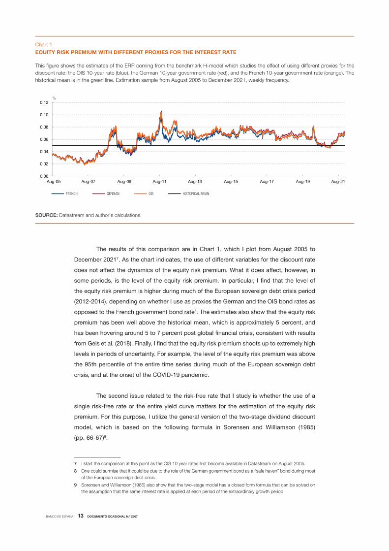
The results of this comparison are in Chart 1, which I plot from August 2005 to

December 20217. As the chart indicates, the use of different variables for the discount rate

does not affect the dynamics of the equity risk premium. What it does affect, however, in

some periods, is the level of the equity risk premium. In particular, I find that the level of

the equity risk premium is higher during much of the European sovereign debt crisis period

(2012-2014), depending on whether I use as proxies the German and the OIS bond rates as

opposed to the French government bond rate8. The estimates also show that the equity risk

premium has been well above the historical mean, which is approximately 5 percent, and

has been hovering around 5 to 7 percent post global financial crisis, consistent with results

from Geis et al. (2018). Finally, I find that the equity risk premium shoots up to extremely high

levels in periods of uncertainty. For example, the level of the equity risk premium was above

the 95th percentile of the entire time series during much of the European sovereign debt

crisis, and at the onset of the COVID-19 pandemic.

The second issue related to the risk-free rate that I study is whether the use of a

single risk-free rate or the entire yield curve matters for the estimation of the equity risk

premium. For this purpose, I utilize the general version of the two-stage dividend discount

model, which is based on the following formula in Sorensen and Williamson (1985)

(pp. 66-67)9:

7 I start the comparison at this point as the OIS 10 year rates first become available in Datastream on August 2005.

8 One could surmise that it could be due to the role of the German government bond as a “safe haven” bond during most of the European sovereign debt crisis.

9 Sorensen and Williamson (1985) also show that the two-stage model has a closed form formula that can be solved on the assumption that the same interest rate is applied at each period of the extraordinary growth period.

This figure shows the estimates of the ERP coming from the benchmark H-model which studies the effect of using different proxies for the discount rate: the OIS 10-year rate (blue), the German 10-year government rate (red), and the French 10-year government rate (orange). The historical mean is in the green line. Estimation sample from August 2005 to December 2021, weekly frequency.

EQUITY RISK PREMIUM WITH DIFFERENT PROXIES FOR THE INTEREST RATEChart 1

SOURCE: Datastream and author's calculations.

0.00

0.02

0.04

0.06

0.08

0.10

0.12

Aug-05 Aug-07 Aug-09 Aug-11 Aug-13 Aug-15 Aug-17 Aug-19 Aug-21

FRENCH GERMAN OIS HISTORICAL MEAN

%


.(1 + ERP + rf )

D

t

Pta0

= +∑A

= 1k

k

(1 + g )k

(1 + ERP + rf )

D

n

a n0

A (rf + ERP − g )n n

(1 + g ) (1 + g )k

As in the H-model, the two-stage model assumes that there are two stages of

growth: an extraordinary period of growth (from time t = 1 to A), followed by a stable phase

from time A onwards. Compared to the H-model, the discount rate applied can be different

at each period of the extraordinary phase, or it can be the same risk-free rate throughout

the entire period. As the yield curve contains information about how investors expect future

interest rates to evolve over time, in this section, I study whether introducing the yield curve

leads to changes in the estimated equity risk premium.

The results of this comparison are in Chart 2, which I plot from June 2001 to

December 2021. I illustrate the effect of using the yield curve for case of French government

bonds, as for the latter there exists the most complete set of interest rates for different

time horizons available from Datastream10. In this implementation, I choose A = 5, which

corresponds to the extraordinary period in the H-model above. This implies that the risk free

rates I am using are the 1 year to 5-year French government bond rates (when I use the entire

yield curve) and the 10-year interest rate for the steady state period, and the 10-year rate

10 In the case of the German sovereign bonds, complete information for rates with maturities of 1 year to 10 years are available from Datatream from June 2002, while in the case of the EONIA OIS, the complete information from Datastream is only available from August 2005.

This graph compares estimates of the equity risk premium coming from the two-stage model, assuming that the risk free rate is the same throughout all periods (blue) and that the risk free rate can be approximated with the entire yield curve (red). The risk-free rate in this estimation is the French interest rate. The estimation sample is from June 2001 to December 2021, weekly frequency.

COMPARING SINGLE INTEREST RATES VS. THE YIELD CURVEChart 2


0.00

0.02

0.04

0.06

0.08

0.10

0.12

May-01 May-03 May-05 May-07 May-09 May-11 May-13 May-15 May-17 May-19 May-21

SINGLE RATE YIELD CURVE

%


(for the single interest rate). As the figure illustrates, using the yield curve to represent the

discount rate does not result in substantial changes, as the resulting estimate of the equity

risk premium remains practically the same.

3.2 Constant vs. multiple growth rates

Another issue is related to the assumption made on the growth rate of cash flows. Dividend

discount models are typically divided into two categories: constant growth models and

multiple-stage growth models. Constant growth models, such as the Gordon growth model,

assume that dividends grow at a constant rate over time. Moreover, the model assumes that

the growth rates of cash flows is equal to the risk-free rate. The multiple-stage models build

on the Gordon growth model by assuming that growth rates vary over time. In this article, I

compare results from an implementation of the Gordon growth model, and three different

multiple-stage models: the H-model and the two-stage model introduced earlier, the three-

stage model of Sorensen and Williamson (1985), and two additional models: the four-stage

model, and the five-stage model. The rest of the multiple stage models are different from

the two-stage models that we have considered earlier in the text in that they introduce more

phases in the dividend discount model. Specifically, the three-stage model introduces a

transitional phase between the extraordinary growth phase and the steady state phase11. The

four stage model is distinct from the three stage model in that it distinguishes the first year

of earnings growth12, while the five-stage model divides the extraordinary phase into three

separate years, to take into account the possibility of different growth rates for each year in

the extraordinary phase13. The summary of the models, and their specific assumptions, are

in Table 1. I provide more details on the models in the Appendix to this article.

The estimates of the equity risk premium are shown in Chart 3. In the implementation

of these models, I work with the entire yield curve for all the multiple stage models. I find that,

while the estimates present similar dynamics, there are certain differences in the levels of

the variables. In particular, I find that the three-stage and four-stage models present higher

estimates of the equity risk premium during the Dot-com crisis. This is primarily due to

the influence of the period of extraordinary growth (short-term growth) in both the three-

stage and four-stage models. To show this , I decompose the equity risk premium into the

following components: short-term growth, medium-term growth, long-term growth, interest

rates, and dividends14. As Chart 4 indicates, the weight of the short-term growth is higher,

compared to the other components.

11 I use the growth rate in earnings per share over the next 12 months as the variable for the extraordinary growth phase (Datastream: A12GRO), the medium-to-long term growth rates for the transitional phase (Datastream: ALTMN), and the expected long term growth rate of GDP from the ECB Survey of Professional Forecasters as the growth rate for the steady state phase. To remove outliers in the variables, I smooth them using a locally weighted linear regression.

12 To distinguish the first year of growth from the other phases, I use the weighted average one year forward EPS growth. (Datastream: AF1GRO).

13 The growth rates for the first three years of growth are the weighted average one year forward EPS growth (AF1GRO), two year forward EPS (AF2GRO), and three year forward EPS (AF3GRO). The growth rate for the transitional phase is the medium-to-long term growth rates (ALTMN) and the steady-state growth rate is that expected GDP growth rate from the ECB Survey of Professional Forecasters. To remove outliers in the variables, I smooth them using a locally weighted linear regression.

14 To decompose the equity risk premium, I linearize the stock price formula of both the three-stage and four-stage models.


Though the models present similar dynamics, to select the model that can be used

for policy analysis, I need a formal criterion to compare the different estimates of the equity

risk premium. In this regard, I study their ability to forecast excess returns, following Li et

al. (2013) and Chin and Polk (2015). The rationale behind this is due to the interpretation of

the ERP as the expected future excess returns. As Pastor et al. (2008) note, the implied ERP

from dividend discount models is a good proxy for time-varying expected returns. Given

The following table illustrates the assumptions on the dividend discount models that were estimated. The first column provides the model name, the second column provides the stages, the third column describes the extraordinary phase (whether the model permits one, and itslength), the fourth column describes the transitional phase (whether the model permits one, and the length), and the fifth column indicates whether the model features a steady state phase. Y = yes, N = no.

DIVIDEND DISCOUNT MODEL ASSUMPTIONSTable 1

SOURCE: Banco de España.

Y/N Length Y/N Length

Constant growth 1 N N/A N N/A Y

YA/NNsraey 01Y2ledom-H

Two stage 2 Y 10 years N N/A Y

Three stage 3 Y 5 years Y 5 years Y

Four stage 4 Y 1st year distinguished from the suceeding 5 years

Y 5 years Y

Five stage 5 Y distinguishes first three years

Y 7 years Y

Number of stages

Model nameSteady state phase

(Y/N)

Extraordinary phase Transitional phase

This graph compares the estimates of the equity risk premium from constant and multiple growth models. The models estimated are the constant growth (brown), the H-model (aqua), the two-stage (blue), the three-stage -model (red), the four stage model (orange) and the five stage model (green). The estimation sample is from June 2001 to December 2021, weekly frequency.

COMPARING SINGLE VS. MULTIPLE STAGE MODELSChart 3


TWO STAGE THREE STAGE FOUR STAGE FIVE STAGE H-MODEL CONSTANT GROWTH

%

0.00

0.02

0.04

0.06

0.08

0.10

0.12

May-01

May-02

May-03

May-04

May-05

May-06

May-07

May-08

May-09

May-10

May-11

May-12

May-13

May-14

May-15

May-16

May-17

May-18

May-19

May-20

May-21


that it can be considered as a proxy for expected returns, Li et al. (2013) investigate the

usefulness of the ERP as a predictive variable of excess returns. Relative to Li et al. (2013),

I assess which dividend discount model performs best in terms of forecast accuracy.

To do so, I estimate the following regression with average k-period returns

as the dependent variable regressed on individual predictor variables Xt at time

t: .k

rt, t + k = a + bX + e t t + k In this equation, rt, t+k is the cumulative sum of the monthly total

log excess returns15 on a -period horizon, wherein is equal to 3, 6, 12, 24 and 36 months.

The predictor variable Xt is each of the estimates of the equity risk premium from the different

models. I then study the in-sample and out-of-sample predictive power via the Diebold-

Mariano (1995) test, wherein the benchmark model that I consider is the H-model. I first

present the regression results in Table 2 below.

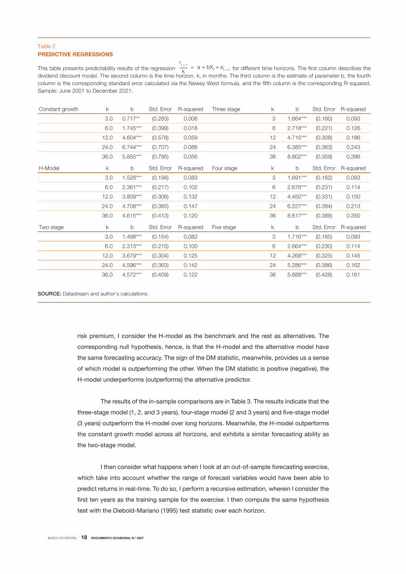
As the results indicate, the equity risk premium estimates are in general predictive

of future excess returns across all horizons. The resulting R2’s are also more or less in line

with previous literature16. Moreover, the results also indicate that across all horizons, the

three-stage model performs the best in terms of explanatory power. I now look at the in-

sample predictive power by conducting the Diebold-Mariano (1995) test over each horizon.

The Diebold-Mariano (1995) test is a test of the predictive accuracy of two competing

models. As the H-model has been the workhorse model for the estimation of the equity

15 Excess returns here are computed from the EUROSTOXX 50 price index, which does not include dividends reinvested.

16 For example, in the case of the dividend discount models, the results of Li et al. (2013) indicate that the adjusted R-squared’s of the in-sample predictability regressions range from 0.07 (for a three-month horizon) to 0.27 (for a three-year horizon).

This figure decomposes the equity risk premium estimated from the three-stage model and the four-stage models into their respective components. Data from June 2001 to December 2021, weekly frequency.

EQUITY RISK PREMIUM DECOMPOSITIONChart 4


-0.10

-0.05

0.00

0.05

0.10

0.15

2001 2003 2005 2007 2009 2011 2013 2015 2017 2019 2021

%

1 THREE STAGE MODEL

-0.10

-0.05

0.00

0.05

0.10

0.15

2001 2003 2005 2007 2009 2011 2013 2015 2017 2019 2021

%

2 FOUR STAGE MODEL

INTEREST RATES DIVIDEND YIELD LONG TERM GROWTH MEDIUM TERM GROWTH SHORT TERM GROWTH FIRST YEAR


risk premium, I consider the H-model as the benchmark and the rest as alternatives. The

corresponding null hypothesis, hence, is that the H-model and the alternative model have

the same forecasting accuracy. The sign of the DM statistic, meanwhile, provides us a sense

of which model is outperforming the other. When the DM statistic is positive (negative), the

H-model underperforms (outperforms) the alternative predictor.

The results of the in-sample comparisons are in Table 3. The results indicate that the

three-stage model (1, 2, and 3 years), four-stage model (2 and 3 years) and five-stage model

(3 years) outperform the H-model over long horizons. Meanwhile, the H-model outperforms

the constant growth model across all horizons, and exhibits a similar forecasting ability as

the two-stage model.

I then consider what happens when I look at an out-of-sample forecasting exercise,

which take into account whether the range of forecast variables would have been able to

predict returns in real-time. To do so, I perform a recursive estimation, wherein I consider the

first ten years as the training sample for the exercise. I then compute the same hypothesis

test with the Diebold-Mariano (1995) test statistic over each horizon.

This table presents predictability results of the regression for different time horizons. The first column describes the dividend discount model. The second column is the time horizon, k, in months. The third column is the estimate of parameter b, the fourth column is the corresponding standard error calculated via the Newey-West formula, and the fifth column is the corresponding R-squared. Sample: June 2001 to December 2021.

PREDICTIVE REGRESSIONSTable 2


Constant growth k b Std. Error R-squared Three stage k b Std. Error R-squared

390.0)061.0(***466.13600.0)382.0(**717.00.3

621.0)122.0(***817.26810.0)993.0(***547.10.6

681.0)803.0(***517.421950.0)875.0(***406.40.21

342.0)363.0(***583.642680.0)707.0(***447.60.42

693.0)953.0(***208.863650.0)597.0(***558.50.63

H-Model k b Std. Error R-squared Four stage k b Std. Error R-squared

390.0)261.0(***196.13380.0)651.0(***825.10.3

411.0)132.0(***676.26201.0)712.0(***163.20.6

051.0)133.0(***054.421231.0)603.0(***908.30.21

312.0)483.0(***722.642741.0)563.0(***807.40.42

053.0)883.0(***716.863021.0)314.0(***516.40.63

Two stage k b Std. Error R-squared Five stage k b Std. Error R-squared

390.0)561.0(***617.13280.0)451.0(***894.10.3

411.0)032.0(***466.26001.0)512.0(***313.20.6

541.0)523.0(***862.421521.0)403.0(***976.30.21

261.0)683.0(***682.542241.0)363.0(***695.40.42

161.0)824.0(***886.563221.0)904.0(***275.40.63

= a + bXt + et + k

rt + 1

k


The results of this estimation are in Table 4. As the table indicates, the three-stage

model performs better than the H-model across all horizons. The four stage model, while it

outperforms the H-model over a 6-month horizon and over long horizons (1 and 2 years),

is outperformed by the H-model at a horizon of three months. The five-stage model also

exhibits the same pattern; it has superior forecasting performance at short horizons, but

it performs poorly at long horizons. The constant growth model outperforms the H-model

in short horizons, but performs poorly at long horizons. Finally, the two-stage model is

outperformed by the H-model across all horizons.

In sum, the evidence in this section suggests that the three-stage model performs

best out of all the candidate dividend growth models, as it yields the highest R-squared,

has predictive power both in-sample and out-of-sample that outperforms the benchmark

H-model.

The table presents the Diebold-Mariano (1995) test statistic, and the corresponding p-value, for the in-sample predictability test. Each row corresponds to the predictive variable in question, which is the model-implied equity risk premium coming from a constant growth model or a multiple stage model. Each column corresponds to the time horizon considered.

IN-SAMPLE PREDICTABILITY RESULTSTable 3


DM p-value DM p-value DM p-value DM p-value DM p-value

Constant growth -2.40 0.02 -2.32 0.02 -1.89 0.10 -2.79 0.02 -2.08 0.04

Two stage -0.48 0.63 -1.29 0.13 -3.14 0.00 -1.52 0.13 -0.08 0.93

Three stage 0.37 0.71 0.87 0.38 1.86 0.06 2.34 0.02 4.64 0.00

Four stage 0.42 0.64 0.42 0.62 0.39 0.70 1.82 0.07 4.64 0.00

Five stage 1.10 0.27 1.46 0.15 1.24 0.25 1.57 0.11 4.78 0.00

k = 3 k = 6 k = 12 k = 24 k = 36

OUT-OF-SAMPLE PREDICTABILITY RESULTSTable 4


DM p-value DM p-value DM p-value DM p-value DM p-value

Constant growth 1.37 0.17 1.96 0.05 0.11 0.91 -1.04 0.30 -3.48 0.00

Two stage -1.21 0.26 -2.81 0.04 -2.20 0.03 -4.00 0.00 -1.99 0.05

Three stage 2.45 0.01 2.93 0.00 3.16 0.00 4.15 0.00 2.41 0.02

Four stage -8.12 0.00 2.83 0.00 3.08 0.00 3.63 0.00 0.66 0.51

Five stage 1.29 0.18 2.64 0.01 3.14 0.08 -2.89 0.00 -5.48 0.00

k = 3 k = 6 k = 12 k = 24 k = 36

The table presents the Diebold-Mariano (1995) test statistic, and the corresponding p-value, for the out-of-sample predictability test. Each row corresponds to the predictive variable in question, which is the model-implied equity risk premium coming from a constant growth model or a multiple stage model. Each column corresponds to the time horizon considered.


3.3 Measurement of cash flows

Most estimations of the equity risk premium using the dividend discount model use dividends

to measure pay-outs to shareholders. However, dividends may be a poor proxy for expected

cash flows from holding equities, especially if firms compensate their shareholders through

other forms. One such compensation is via share buybacks. Though the use of this tool as

compensation has historically been of secondary importance, there has been a recent rise

in share repurchases, both in the US and in Europe, as firms “aim to signal to investors a

positive long-term outlook”.17 Moreover, the inclusion of share buybacks has been shown to

have some impact in the estimation of the equity risk premium (see e.g., Geis et al. (2018)

and Dison and Rattan (2017)).

To see the impact of the inclusion of share buybacks, I compute the equity risk

premium via the three-stage model. Specifically, I compare the results of a model wherein

I work with dividends and a model wherein I combine dividends and share buybacks18.

Chart 5 shows the estimates for the three-stage dividend discount model from September

2010 to November 2021, as information on buybacks is only available on these dates19. The

17 See “Buybacks Hit Record After Pulling Back in 2020”, by Karen Langley, published in the Wall Street Journal on December 21, 2021 edition (for the US), and “European Banks Boost Payouts With $5 Billion in New Buybacks” by Nicolas Comfort, published in Bloomberg on October 29, 2021 edition (for Europe).

18 I follow Ilmanen (2011) by modifying the aggregate dividend pay-out ratio as the following formula: DP = (D + S)/MC, where D is the total dividends, S is the total share buybacks issued, and MC is the total market capitalization. One challenge that I encountered is the calculation of the modified version of the dividend yield with share buybacks. The model that I implement uses variables that I mostly observe at a weekly frequency, including the market capitalization. However, I only observe dividends and share buybacks available at a yearly frequency. To compute the implied dividend yield, hence, I perform a linear interpolation that makes use of weekly information on the dividend yield that is available from Datastream.

19 I perform the same exercise for the rest of the dividend discount models, and the results are similar.

This graph compares the estimates of the equity risk premium coming from the three-stage dividend discount model, wherein the relevant change comes from the measurement of cash flows. The blue line corresponds to a model where I use only dividends to measure cash flows, while the red line includes share buybacks. The estimation period is from September 2010 to November 2021, weekly frequency.

EFFECTS OF THE MEASUREMENT OF DIVIDENDSChart 5


0.00

0.02

0.04

0.06

0.08

0.10

0.12

Sep-10 Sep-11 Sep-12 Sep-13 Sep-14 Sep-15 Sep-16 Sep-17 Sep-18 Sep-19 Sep-20 Sep-21

DIVIDENDS ONLY DIVIDENDS WITH BUYBACKS

%


results indicate that while the estimates of the equity risk premium present similar dynamics,

the estimates of the risk premium that includes share buybacks presented higher levels

of the equity risk premium at the onset of the COVID-19 pandemic.

To determine which model presents more reliable estimates of the equity risk

premium from a forecasting perspective, I repeat the same in-sample and out-of-sample

forecasting exercise20; however, instead of considering the first ten years as the training

sample, I consider the first five years, given sample availability. The results indicate that both

models present similar forecasting performance21; however, the model with share buybacks

is the more preferable model given that the corresponding equity risk premium estimates

reflect the increase in payments of share buybacks by firms during the COVID-19 pandemic.

20 The regression results indicate that both variables are positive and significant at the 1 percent level across all horizons. Results are available upon request.

21 Results are available upon request. The results for the forecasting exercise were done for a three, six and one-year horizon as the sample length is not enough to perform tests on the two and three year horizons.


4 Conclusion

In this paper, I assess the estimation of the equity risk premium using data from the

Eurostoxx 50 from 2001-2021, with the dividend discount model as the empirical framework.

In particular, I study three main issues encountered in the estimation of the equity risk

premium: (i.) the effect of proxies for the risk-free rate and the yield curve; (ii.) comparing

constant growth and multiple growth models, and (iii.) the inclusion of share buybacks in the

estimation of dividend yields.

This article obtains the following findings. First, in the context of the workhorse

H-model and the two-stage model, I find that using different proxies for the risk-free rate,

or the use of the entire yield curve, do not imply significant changes to the estimates of the

equity risk premium. Second, comparing constant and multiple growth models, I find that

most multiple growth models present similar dynamics. However, comparing the explanatory

power (via predictive regressions) and the in-sample and out-of-sample forecasting power, I

find that the three-stage model shows better forecast accuracy in comparison with the other

models both in short and long horizons. Finally, looking at the measurement of cash flows,

the inclusion of share buybacks presents in estimates of the equity risk premium that present

similar dynamics; however, the preferred model to estimate the equity risk premium is the

model with share buybacks, as it reflects the additional shareholder payments in terms of

buybacks during the COVID-19 pandemic.


References

Chin, M., and C. Polk (2015). A forecast evaluation of expected equity returns measures, Working Paper, Bank of

England.

Diebold, F. X., and R. Mariano (1995). “Comparing Predictive Accuracy”, Journal of Business and Economic

Statistics, pp. 253-265.

Dison, W., and A. Rattan (2017). “An improved model for understanding equity prices”, Quarterly Bulletin Q2, Bank

of England, pp. 86-97.

Duarte, F., and C. Rosa (2015). “The Equity Risk Premium: A Review of Models”, FRB NY Economic Policy Review,

pp. 39-57.

Fuller, R., and C.-C. Hsia (1984). “A Simplified Common Stock Valuation Model”, Financial Analysts Journal,

pp. 49-56.

Geis, A., D. Kapp and K. L. Kristiansen (2018). “Measuring and interpreting the cost of equity in the euro area”,

ECB Economic Bulletin, Issue 4.

Gordon, M. J. (1962). “The Savings, Investment, and Valuation of a Corporation”, Review of Economics and

Statistics, pp. 37-51.

Ilmanen, A. (2011). Expected Returns: An Investor’s Guide to Harvesting Market Rewards, London, John Wiley &

Sons.

Li, Y., D. T. Ng and B. Swaminathan (2013). “Predicting market returns using aggregate implied cost of capital”,

Journal of Financial Economics, pp. 419-436.

Pastor, L., M. Sinha and B. Swaminathan (2008). “Estimating the Intertemporal Risk-Return Tradeoff Using the

Implied Cost of Capital”, Journal of Finance, pp. 2859-2897.

Sorensen, E. H., and D. A. Williamson (1985). “Some Evidence on the Value of Dividend Discount Models”,

Financial Analysts Journal, pp. 60-69.


Appendix A catalog of dividend discount models

This appendix outlines the different dividend discount models used in the estimation of the

equity risk premium in this article. I first start with the discussion of the constant growth

models, and then proceed with the discussion of the multiple growth models.

Constant growth model. The constant growth model assumes that future cash

flows grow at a rate g in perpetuity. Hence, the constant growth model implies that we can

simplify the dividend discount model into:

.rf + ERP − g

DPt

t=

In this model, we can then compute a closed-form solution for the equity risk

premium: + g − rf. P DERP = The typical assumption is to assume that g = rf, which leaves

the dividend yield as the measure of the equity risk premium.

Two-stage model. The two-stage model assumes that there are two phases: an

extraordinary phase of growth, where dividends grow at a rate ga and a stable phase, where

dividends grow at a rate gn. The price of a stock can then be shown to be equal to the

following quantity (Sorensen and Williamson (1984)):

.(1 + ERP + rf )

DPt DA

a0= +∑

A

= 1t

∑∞

= A + 1t

t

(1 + g )t t − A

(1 + ERP + rf )

n

t

(1 + g )

In this formulation, the first sum is the extraordinary phase, while the second sum is

the stable phase. One can then compute the geometric progression in the stable phase to

obtain the following sum:

.(1 + ERP + rf )

DPt

a0= +∑

A

= 1t

t (1 + ERP + rf )A

(1 + g )t D a0 (1 + g )t

(rf + ERP + g )

n

n

(1 + g )

In this equation, D0 is the initial dividend, ga is the extraordinary growth rate, and gn

is the stable growth rate. A is a parameter that represents the end period of extraordinary

growth. In the empirical implementation comparing the effect of the yield curve, I set

A = 5, while in the comparison of the different multiple stage models, I set A = 10, to facilitate

comparisons. To compute the implied equity risk premium, I minimize the difference22

between the model-implied price-dividend ratio (which I observe at a weekly frequency),

and the observed price-dividend ratio: DPPmin

2

modelERP

−D . In the estimation, I

22 In the implementation of the minimization problem, I utilize the fzero and lsqnonlin optimization routines in Matlab. One issue that I found out is that the minimization problem is sensitive to starting points. To ensure that I obtain reasonable results, I use the estimates from the H-model as a starting point.


assume that ga is the mean estimate of long-term EPS growth, and gn is the long-term GDP

expectations coming from the ECB Survey of Professional forecasters.

H-model. The H-model is a modification of the two-stage model that assumes that

the transition from the extraordinary phase to the stable phase of growth moves linearly,

governed by the parameter H). The price of a stock then is:

[ ].

ERP + rf − g

(1 + g ) + H (g − g )D

n

Pn na

=t

The model can then be simplified to have the following formula:

[ (1 + g ) + H (g − g )] + g − rf. P DERP = n n n a In the implementation of the model, I take H = 5.

Three-stage model. The three stage model that I describe here is based on the

exposition in Sorensen and Williamson (1984). The model is composed of three phases: an

extraordinary phase (with growth rate ga, a transition phase (with growth rate gb, and a stable

phase (with growth rate gn). The formula is:

.

(1 + ERP + rf )

DPt

a0= +

+

∑A

= 1t

t

(1 + ERP + rf )B

(1 + g )t

D a0 (1 + g )A

D a0 (1 + g ) n(1 + g )A

(rf + ERP − g )

b

n

(1 + g )

∑B

= A + 1t

t − A

B − A

(1 + ERP + rf )

b

t

(1 + g )

As in the two-stage model, I minimize the difference between the model implied

price-dividend ratio and the observed one in the data. In this estimation, I take as ga the

expected growth rate in EPS over the next 12 months, gb as the mean estimates of long term

EPS growth, and gn is the long term nominal GDP expectations coming from the ECB Survey

of Professional forecasters. In the empirical implementation, A = 5 and B = 10.

Four stage model. The four stage model is one where I permit the division of the

first year from the rest of the years in the three stage model. The resulting formula is:

.

1 + ERP + rf

DPt

10=

+ +

+

∑A

= 2t

(1 + ERP + rf )B

(1 + g )

n(1 + g )

(rf + ERP − g )

b

n

(1 + g )B − A

t − 1

(1 + ERP + rf )t

~

D 1 a0 (1 + g ) (1 + g )~ ~

A − 1D 1 a0 (1 + g ) (1 + g )~ ~ ∑

B

= A + 1t

t − A

(1 + ERP + rf )

b

t

(1 + g )

A − 1D 1 a0 (1 + g ) (1 + g )~ ~


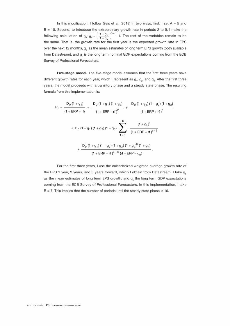
In this modification, I follow Geis et al. (2018) in two ways; first, I set A = 5 and

B = 10. Second, to introduce the extraordinary growth rate in periods 2 to 5, I make the

following calculation of a a g : g = ~ ~ 1 + g b

1 + g a− 1

1/4 . The rest of the variables remain to be

the same. That is, the growth rate for the first year is the expected growth rate in EPS

over the next 12 months, gb as the mean estimates of long term EPS growth (both available

from Datastream), and gn is the long term nominal GDP expectations coming from the ECB

Survey of Professional Forecasters.

Five-stage model. The five-stage model assumes that the first three years have

different growth rates for each year, which I represent as g1, g2, and g3. After the first three

years, the model proceeds with a transitory phase and a steady state phase. The resulting

formula from this implementation is:

.

(1 + ERP + rf)

DPt

10= +

+

+(1 + ERP + rf )3 + B

(1 + g )

n(1 + g )

(rf + ERP − g )

b

n

(1 + g )B

D 1 2 30 (1 + g ) (1 + g ) (1 + g ) ∑B

= 1t

t

(1 + ERP + rf )

b

t + 3

(1 + g )

D 1 2 30 (1 + g ) (1 + g ) (1 + g )

(1 + ERP + rf )2

D 1 20 (1 + g ) (1 + g )+

(1 + ERP + rf )3

D 1 2 30 (1 + g ) (1 + g ) (1 + g )

For the first three years, I use the calendarized weighted average growth rate of

the EPS 1 year, 2 years, and 3 years forward, which I obtain from Datastream. I take gb

as the mean estimates of long term EPS growth, and gn the long term GDP expectations

coming from the ECB Survey of Professional Forecasters. In this implementation, I take

B = 7. This implies that the number of periods until the steady state phase is 10.

BANCO DE ESPAÑA PUBLICATIONS

OCCASIONAL PAPERS

2030 ÁNGEL GÓMEZ-CARREÑO GARCÍA-MORENO: Juan Sebastián Elcano – 500 años de la Primera vuelta al mundo en

los billetes del Banco de España. Historia y tecnología del billete.

2031 OLYMPIA BOVER, NATALIA FABRA, SANDRA GARCÍA-URIBE, AITOR LACUESTA and ROBERTO RAMOS: Firms and

households during the pandemic: what do we learn from their electricity consumption?

2032 JÚLIA BRUNET, LUCÍA CUADRO-SÁEZ and JAVIER J. PÉREZ: Contingency public funds for emergencies: the lessons

from the international experience. (There is a Spanish version of this edition with the same number).

2033 CRISTINA BARCELÓ, LAURA CRESPO, SANDRA GARCÍA-URIBE, CARLOS GENTO, MARINA GÓMEZ and ALICIA

DE QUINTO: The Spanish Survey of Household Finances (EFF): description and methods of the 2017 wave.

2101 LUNA AZAHARA ROMO GONZÁLEZ: Una taxonomía de actividades sostenibles para Europa.

2102 FRUCTUOSO BORRALLO, SUSANA PÁRRAGA-RODRÍGUEZ and JAVIER J. PÉREZ: Taxation challenges of population

ageing: comparative evidence from the European Union, the United States and Japan. (There is a Spanish version of this

edition with the same number).

2103 LUIS J. ÁLVAREZ, M.ª DOLORES GADEA and ANA GÓMEZ LOSCOS: Cyclical patterns of the Spanish economy

in Europe. (There is a Spanish version of this edition with the same number).

2104 PABLO HERNÁNDEZ DE COS: Draft State Budget for 2021. Testimony before the Parliamentary Budget Committee,

4 November 2020. (There is a Spanish version of this edition with the same number).

2105 PABLO HERNÁNDEZ DE COS: The independence of economic authorities and supervisors. The case of the Banco

de España. Testimony by the Governor of the Banco de España before the Audit Committee on Democratic Quality /

Congress of Deputies, 22 December 2020. (There is a Spanish version of this edition with the same number).

2106 PABLO HERNÁNDEZ DE COS: The Spanish pension system: an update in the wake of the pandemic. Banco

de España contribution to the Committee on the Monitoring and Assessment of the Toledo Pact Agreements.

2 September 2020. (There is a Spanish version of this edition with the same number).

2107 EDUARDO BANDRÉS, MARÍA-DOLORES GADEA and ANA GÓMEZ-LOSCOS: Dating and synchronisation of

regional business cycles in Spain. (There is a Spanish version of this edition with the same number).

2108 PABLO BURRIEL, VÍCTOR GONZÁLEZ-DÍEZ, JORGE MARTÍNEZ-PAGÉS and ENRIQUE MORAL-BENITO: Real-time

analysis of the revisions to the structural position of public finances.

2109 CORINNA GHIRELLI, MARÍA GIL, SAMUEL HURTADO and ALBERTO URTASUN: The relationship between pandemic

containment measures, mobility and economic activity. (There is a Spanish version of this edition with the same number).

2110 DMITRY KHAMETSHIN: High-yield bond markets during the COVID-19 crisis: the role of monetary policy.

2111 IRMA ALONSO and LUIS MOLINA: A GPS navigator to monitor risks in emerging economies: the vulnerability dashboard.

2112 JOSÉ MANUEL CARBÓ and ESTHER DIEZ GARCÍA: El interés por la innovación financiera en España. Un análisis

con Google Trends.

2113 CRISTINA BARCELÓ, MARIO IZQUIERDO, AITOR LACUESTA, SERGIO PUENTE, ANA REGIL and ERNESTO

VILLANUEVA: Los efectos del salario mínimo interprofesional en el empleo: nueva evidencia para España.

2114 ERIK ANDRES-ESCAYOLA, JUAN CARLOS BERGANZA, RODOLFO CAMPOS and LUIS MOLINA: A BVAR toolkit to

assess macrofinancial risks in Brazil and Mexico.

2115 ÁNGEL LUIS GÓMEZ and ANA DEL RÍO: The uneven impact of the health crisis on the euro area economies in 2020.

(There is a Spanish version of this edition with the same number).

2116 FRUCTUOSO BORRALLO EGEA and PEDRO DEL RÍO LÓPEZ: Monetary policy strategy and inflation in Japan. (There

is a Spanish version of this edition with the same number).

2117 MARÍA J. NIETO and DALVINDER SINGH: Incentive compatible relationship between the ERM II and close cooperation

in the Banking Union: the cases of Bulgaria and Croatia.

2118 DANIEL ALONSO, ALEJANDRO BUESA, CARLOS MORENO, SUSANA PÁRRAGA and FRANCESCA VIANI: Fiscal

policy measures adopted since the second wave of the health crisis: the euro area, the United States and the United

Kingdom. (There is a Spanish version of this edition with the same number).

2119 ROBERTO BLANCO, SERGIO MAYORDOMO, ÁLVARO MENÉNDEZ and MARISTELA MULINO: Impact of the

COVID-19 crisis on Spanish firms’ financial vulnerability. (There is a Spanish version of this edition with the same number).

2120 MATÍAS PACCE, ISABEL SÁNCHEZ and MARTA SUÁREZ-VARELA: Recent developments in Spanish retail electricity

prices: the role played by the cost of CO2 emission allowances and higher gas prices. (There is a Spanish version of this


2121 MARIO ALLOZA, JAVIER ANDRÉS, PABLO BURRIEL, IVÁN KATARYNIUK, JAVIER J. PÉREZ and JUAN LUIS VEGA: The

reform of the European Union’s fiscal governance framework in a new macroeconomic environment. (There is a Spanish

version of this edition with the same number).

2122 MARIO ALLOZA, VÍCTOR GONZÁLEZ-DÍEZ, ENRIQUE MORAL-BENITO and PATROCINIO TELLO-CASAS: Access

to services in rural Spain. (There is a Spanish version of this edition with the same number).

2123 CARLOS GONZÁLEZ PEDRAZ and ADRIAN VAN RIXTEL: The role of derivatives in market strains during the COVID-19

crisis. (There is a Spanish version of this edition with the same number).

2124 IVÁN KATARYNIUK, JAVIER PÉREZ and FRANCESCA VIANI: (De-)Globalisation of trade and regionalisation: a survey of

the facts and arguments.

2125 BANCO DE ESPAÑA STRATEGIC PLAN 2024: RISK IDENTIFICATION FOR THE FINANCIAL AND MACROECONOMIC

STABILITY: How do central banks identify risks? A survey of indicators.

2126 CLARA I. GONZÁLEZ and SOLEDAD NÚÑEZ: Markets, financial institutions and central banks in the face of climate

change: challenges and opportunities.

2127 ISABEL GARRIDO: The International Monetary Fund’s view of social equity throughout its 75 years of existence. (There is a

Spanish version of this edition with the same number).

2128 JORGE ESCOLAR and JOSÉ RAMÓN YRIBARREN: European Central Bank and Banco de España measures against

the effects of COVID-19 on the monetary policy collateral framework, and their impact on Spanish counterparties.


2129 BRINDUSA ANGHEL, AITOR LACUESTA and FEDERICO TAGLIATI: 2021 Survey of Small Enterprises’ Financial

Literacy: Main Results. (There is a Spanish version of this edition with the same number).

2130 PABLO HERNÁNDEZ DE COS: Testimony before the Congress of Deputies Budget Committee on 25 October 2021

and before the Senate Budget Committee on 30 November 2021 in relation to the Draft State Budget for 2022.


2131 LAURA AURIA, MARKUS BINGMER, CARLOS MATEO CAICEDO GRACIANO, CLÉMENCE CHARAVEL, SERGIO

GAVILÁ, ALESSANDRA IANNAMORELLI, AVIRAM LEVY, ALFREDO MALDONADO, FLORIAN RESCH, ANNA MARIA

ROSSI and STEPHAN SAUER: Overview of central banks’ in-house credit assessment systems in the euro area.

2132 JORGE E. GALÁN: CREWS: a CAMELS-based early warning system of systemic risk in the banking sector.

2133 ALEJANDRO FERNÁNDEZ CEREZO and JOSÉ MANUEL MONTERO: A sectoral analysis of the future challenges

facing the spanish economy. (There is a Spanish version of this edition with the same number).

2201 MANUEL A. PÉREZ ÁLVAREZ: New allocation of special drawing rights. (There is a Spanish version of this edition with

the same number).

2202 PILUCA ALVARGONZÁLEZ, MARINA GÓMEZ, CARMEN MARTÍNEZ-CARRASCAL, MYROSLAV PIDKUYKO

and ERNESTO VILLANUEVA: Analysis of labor flows and consumption in Spain during COVID-19.

2203 MATÍAS LAMAS and SARA ROMANIEGA: Designing a price index for the Spanish commercial real estate market.


2204 ÁNGEL IVÁN MORENO BERNAL and TERESA CAMINERO GARCÍA: Analysis of ESG disclosures in Pillar 3 reports.

A text mining approach.

2205 OLYMPIA BOVER, LAURA CRESPO and SANDRA GARCÍA-URIBE: Household indebtedness according to the Spanish

survey of household finances and the central credit register: a comparative analysis. (There is a Spanish version of this


2206 EDUARDO GUTIÉRREZ, ENRIQUE MORAL-BENITO and ROBERTO RAMOS: Dinámicas de población durante el

COVID-19. (There is a Spanish version of this edition with the same number).

2207 JULIO GÁLVEZ: Measuring the equity risk premium with dividend discount models.

Measuring the equity risk premium with dividend discount ...

Documents

Transcript of Measuring the equity risk premium with dividend discount ...