
Monotone Iterative Method for ψ-Caputo Fractional Differential ...
Upload
independentCategory
view
0download
0
Estimation of a k−monotone density, part 3:limiting Gaussian versions of the problem;
invelopes and envelopes
Fadoua Balabdaoui 1 and Jon A. Wellner 2
University of Washington
September 2, 2004
AbstractLet k be a positive integer. The limiting distribution of the nonparametric
maximum likelihood estimator of a k−monotone density is given in terms of a smoothstochastic process Hk described as follows: (i) Hk is everywhere above (or below) Yk,the k− 1 fold integral of two-sided standard Brownian motion plus (k!/(2k)!)t2k whenk is even (or odd). (ii) H(2k−2)
k is convex. (iii) Hk touches Yk at exactly those pointswhere H(2k−2)
k has changes of slope. We show that Hk exists if a certain conjectureconcerning a particular Hermite interpolation problem holds.
The process H1 is the familiar greatest convex minorant of two-sided Brownianmotion plus (1/2)t2, which arises in connection with nonparametric estimation of amonotone (1-monotone) function. The process H2 is the “invelope process” studiedin connection with nonparametric estimation of convex functions (up to a scaling ofthe drift term) in Groeneboom, Jongbloed, and Wellner (2001a). We therefore refer toHk as an “invelope process” when k is even, and as an “envelope process” when k isodd. We establish existence of Hk for all non-negative integers k under the assumptionthat our key conjecture holds, and study basic properties of Hk and its derivatives.Approximate computation of Hk is possible on finite intervals via the iterative (2k−1)spline algorithm which we use here to illustrate the theoretical results.
1 Research supported in part by National Science Foundation grant DMS-02033202 Research supported in part by National Science Foundation grants DMS-0203320, and NIAID grant
2R01 AI291968-04AMS 2000 subject classifications. Primary: 62G05; secondary 60G15, 62E20.Key words and phrases. asymptotic distribution, completely monotone, canonical limit, direct
estimation problem, Gaussian, inverse estimation problem, k−convex, k−monotone, mixture model,monotone
1

Outline
1. Introduction
2. The Main Result
3. The processes Hc,k on [−c, c]
3.1 Existence and characterization of Hk,c for k even 9 - 233.2 Existence and characterization of Hk,c for k odd 24 - 28
4. Tightness as c →∞4.1 Existence of points of touch 28 - 364.2 Tightness 36 - 47
5. Completion of the proof of the main theorem 48 - 69
6. Appendix 69 - 70
2

1 Introduction
Consider the following nonparametric estimation problem: X1, . . . , Xn is a sample froma density g0 with the property that g(k−1)
0 is monotone on the support of the distributionof the Xi’s where k ≥ 1 is a fixed integer. Before proceeding further, we describe theseclasses of densities more precisely. For k = 1, D1 is the class of all decreasing (non-increasing) densities with respect to Lebesgue measure on R+ = (0,∞). For integersk ≥ 2, the class Dk is the collection of all densities with respect to Lebesgue measure onR+ for which (−1)jg(j)(x) is nonnegative, nonincreasing, and convex for all x ∈ R+ andj = 0, . . . , k − 2. Another way to describe these shape constrained classes is in termsof scale mixtures of Beta(1, k) densities: it is known that the classes Dk correspondexactly to the classes of densities that can be represented as
g(x) =∫ ∞
0
k
yk(y − x)k−1
+ dF (y)
for some distribution function F on R+. For example, when k = 1 the class of monotonedecreasing densities D1 corresponds exactly to the class of all scale mixtures of theuniform, or Beta(1, 1), density; and when k = 2, the class of convex decreasing densitiescorresponds to the class of all scale mixtures of the (triangular) Beta(1, 2) density.These correspondences for non-negative functions are due to Williamson (1956) (seealso Gneiting (1999)), and those results carry-over to the class of densities consideredhere as has been known for k = 1 and k = 2, and as shown in general by Levy (1962)for arbitrary k ≥ 1.
As noted, the case k = 1 corresponds to g ∈ D1, the class of monotone decreasingdensities. In this case the nonparametric maximum likelihood estimator is the well-known Grenander estimator, given by the left-continuous slopes of the least concavemajorant of the empirical distribution function. It is well known that if g′0(t0) < 0 andg′0 is continuous in a neighborhood of t0, the Grenander estimator gn satisfies
n1/3(gn(t0)− g0(t0))(12g(t0)|g′(t0)|)1/3
→d 2Z ≡ H(1)1 (0)
where 2Z is the slope at zero of the greatest convex minorant H1 of {W (t) + t2 :t ∈ R} where W is standard two-sided Brownian motion starting at zero; this is dueto Prakasa Rao (1969), and was reproved by Groeneboom (1985) and Kim andPollard (1990). The results of Groeneboom (1985), (1989) yield methods forcomputing the exact distribution of Z; see e.g. Groeneboom and Wellner (2001).
The case k = 2, corresponding to g being a convex and decreasing density, wastreated by Groeneboom, Jongbloed, and Wellner (2001a), Groeneboom,
Jongbloed, and Wellner (2001b). Assuming that g(2)0 (t0) > 0, they showed that
the nonparametric maximum likelihood estimator gn of g satisfies(n2/5(gn(t0)− g(t0))n1/5(g′n(t0)− g′(t0))
)→d
(c2,0(g)H(2)
2 (0)c2,1(g)H(3)
2 (0)
)
3

where (H(2)2 (0), H(3)
2 (0)) are the second and third derivatives at 0 of the invelope H2
of Y2 as described in Theorem 2.1 of Groeneboom, Jongbloed, and Wellner(2001a) (referred to hereafter as GJW) and c2,0(g) = (g(2)(t0)g2(t0)/24)1/5, c2,1(f) =(g(2)(t0)3g(t0)/243)1/5. Existence and uniqueness of the process H2 was establishedin GJW. Our reason for using a “tilde” over the H here is to distinguish the processH ≡ H2 of Groeneboom, Jongbloed, and Wellner (2001a) (where the driftterm was of the form t4 at the level of the process Y2) from the process H2 here (wherethe drift term is taken to be t4/12 for k = 2 and of the form (k!/(2k)!)t2k for generalk in order to make the problem more stable for k large).
Our goal in this paper is to establish existence and uniqueness of the correspondinglimit processes Hk for all integers k ≥ 3. In the companion paper Balabdaoui andWellner (2004c) we show that the nonparametric maximum likelihood estimator gn
of the k−monotone density g with g(k)(t0) '= 0 satisfies
nk/(2k+1)(gn(t0)− g0(t0))n(k−1)/(2k+1)(g(1)
n (t0)− g(1)(t0))···
n1/(2k+1)(g(k−1)n (t0)− g(k−1)(t0))
→d
ck,0(g)H(k)k (0)
ck,1(g)H(k+1)k (0)···
ck,k−1(g)H(2k−1)k (0)
where Hk is the invelope or envelope process described in Theorem 2.1 of the nextsection and where
ck,j(g) = g(t0)k−j2k+1
{(−1)kg(k)(t0)
k!
} 2j+12k+1
for j = 0, . . . , k − 1 .
For further background concerning the statistical problem, see Balabdaoui andWellner (2004a), and for computational issues, see Balabdaoui and Wellner(2004b).
Our proof of existence of the processes Hk on R for k ≥ 3 proceeds by establishingexistence of appropriate processes Hc,k on [−c, c] for each c > 0, and then showingthat these processes and their first 2k − 2 derivatives are tight in C[−K, K] for fixedK > 0 as c → ∞. The key step in proving this tightness is essentially showing thattwo successive jump points τ−c and τ+
c of two successive jump points of H(2k−1)c,k to the
left and right of 0 satisfy τ+c − τ−c = Op(1) as k →∞. We show in section 4 that this
is equivalent to
τ+c − τ−c = Op(c−1/(2k+1)) (1.1)
in a re-scaled version of the problem, and that in this re-scaled setting the problemis essentially the same problem arising in the finite-sample problem discussed aboveand in more detail in Balabdaoui and Wellner (2004c). We call the problem
4

of showing that (1.1) holds the “gap problem”. In Section 4, we show that whenk > 2, the solution of the “gap problem” reduces to a conjecture concerning a“non-classical” Hermite interpolation problem via odd-degree splines. To put theinterpolation problem encountered in the section 4 in context, it is useful to reviewbriefly the related complete Hermite interpolation problem for odd-degree splines whichis more “classical” and for which error bounds uniform in the knots are now available.
Given a function f ∈ C(k−1)[0, 1] and an increasing sequence 0 = t0 < t1 < · · · <tm < tm+1 = 1 where m ≥ 1 is an integer, it is well-known that there exists a uniquespline, called the complete spline and denoted here by Cf , of degree 2k − 1 withinterior knots t1, · · · , tm that satisfies the 2k + m conditions{
(Cf)(ti) = f(ti), i = 1, · · · ,m(Cf)(l)(t0) = f (l)(t0), (Cf)(l)(tm+1) = f (l)(tm+1), l = 0, · · · , k − 1;
see Schoenberg (1963), de Boor (1974), or Nurnberger (1989), page 116, forfurther discussion. If f ∈ C(2k)[0, 1], then there exists ck > 0 such that
sup0<t1<···<tm<1
‖f − Cf‖∞ ≤ ck‖f (2k)‖∞. (1.2)
This “uniform in knots” bound in the complete interpolation problem was firstconjectured by de Boor (1973) in (1972) for k > 4 as a generalization that goesbeyond k = 2, 3 and 4 for which the result was already established (see also de Boor(1974)). However, it took more than 25 years to prove de Boor’s conjecture; the proofof (1.2) is due to Shadrin (2001). By a scaling argument, the bound (1.2) impliesthat, if f ∈ C(2k)[a, b], a < b ∈ R, the interpolation error in the complete Hermiteinterpolation problem is uniformly bounded in the knots, and that the bound is of theorder of (b− a)2k.
One key property of the complete spline interpolant Cf is that (Cf)(k) is the LeastSquares approximation of f (k) when f (k) ∈ L2([0, 1]); i.e., if Sk(t1, · · · , tm) denotes thespace of splines of order k (degree k − 1) and interior knots t1, · · · , tm, then∫ 1
0
((Cf)(k) − f (k)(x)
)2dx = min
S∈Sk(t1,···,tm)
∫ 1
0
(S(x)− f (k)(x)
)2dx (1.3)
(see e.g. Schoenberg (1963), de Boor (1974), Nurnberger (1989)).Consequently, if L∞ denotes the space of bounded functions on [0, 1], then the properlydefined map
C(k)[0, 1] → Sk(t1, · · · , tm)f (k) *→ (Cf)(k)
is the restriction of the orthoprojector, denoted here by PSk(t), where t = (t1, · · · , tm),from L∞ to L∞ with respect to the inner product 〈g, h〉 =
∫ 10 g(x)h(x)dx. de Boor
5
(1974) pointed out that, in order to prove the conjecture, it is enough to prove that
supt‖PSk(t)‖∞ = sup
tsup
g
‖PSk(t)(g)‖∞‖g‖
is bounded, and this was successfully achieved by Shadrin (2001).The Hermite interpolation problem which arises naturally in Section 2 appears to be
another variation of Hermite interpolation problems via odd-degree splines, which hasnot yet been studied in the approximation theory or spline literature. More specifically,if f is some real-valued function in C(j)[0, 1] for some j ≥ 2, 0 = t0 < t1 < · · · < t2k−4 <t2k−3 = 1 is a given increasing sequence, then there exists a unique spline Hf of degree2k − 1 and interior knots t1, · · · , t2k−4 satisfying the 4k − 4 conditions
(Hf)(ti) = f(ti), and (Hf)′(ti) = f ′(ti), i = 0, · · · , 2k − 3.
Note that the spline Hf matches not only the value of the function at the knots butalso the value of its first derivative. Thus we should expect the interpolation error tobe smaller than in the complete interpolation, and this gives hope that boundednessof the interpolation error also holds in this uncommon problem.
Here is our conjecture concerning a “uniform in knots” error bound for the Hermiteinterpolant H.
Conjecture 1.1 Let a = x0 < x1 < · · · < x2k−3 = b be 2k − 2 arbitrary points and1 ≤ r ≤ 2k− 1. Suppose that f that is a function that is r-times differentiable on [a, b]except for a finite number of points. If Hf denotes the unique interpolating spline ofdegree 2k − 1 that solves the Hermite problem:
Hf(xj) = f(xj), and (Hf)′(xj) = f ′(xj)
for j = 0, · · · , 2k − 3, then there exists a constant C > 0 (depending only on k) suchthat
supt∈[a,b]
|Hf(t)− f(t)| ≤ Cω(f (r); b− a) (b− a)r
where ω(f (r); ·) is the modulus of continuity of f (r) on [a, b]:
ω(h; δ) = sup{|h(t2)− h(t1)| : t1, t2 ∈ [a, b], |t2 − t1| ≤ δ}.
2 The Main Result
Suppose that k ≥ 1 and let W be a two-sided Brownian motion starting from 0 at 0.Define the Gaussian processes {Yk(t) : t ∈ R} by
Yk(t) =
{ ∫ t0
∫ sk−1
0 · · · ∫ s2
0 W (s1)ds1 · · · dsk−1 + k!(2k)! t
2k, t ≥ 0 ,∫ 0t
∫ 0sk−1
· · · ∫ 0s2
W (s1)ds1 · · · dsk−1 + k!(2k)! t
2k , t < 0 ,
6

and set Xk(t) ≡ Y (k−1)k (t) = W (t) + (k + 1)−1tk+1 for t ∈ R. Thus
dXk(t) = tkdt + dW (t) ≡ fk,0(t)dt + dW (t)
where fk,0 is monotone for k = 1, convex for k = 2, and, for k ≥ 3 the (k − 2)-thderivative f (k−2)
k,0 (t) = (k!/2)t2 is convex. Thus we can consider “estimation” of thefunction fk,0 in Gaussian noise dW (t) subject to the constraint of convexity of f (k−2)
(or monotonicity of f in the case k = 1).Here is our main result.
Theorem 2.1 If k = 1, 2 or if k ≥ 3 and Conjecture 1.1 holds, there exists analmost surely uniquely defined stochastic process Hk characterized by the four followingconditions:
(i) (−1)k(Hk(t)− Yk(t)) ≥ 0, t ∈ R.
(ii) Hk is 2k-convex; i.e. H(2k−2)k exists and is convex.
(iii) For any t ∈ R, Hk(t) = Yk(t) if and only if H(2k−2)k changes slope at t;
equivalently, ∫ ∞
−∞(Hk(t)− Yk(t)) dH(2k−1)
k (t) = 0 .
(iv) If k is even, lim|t|→∞(H(2j)k (t) − Y (2j)
k (t)) = 0 for j = 0, · · · , (k − 2)/2; if k isodd, limt→∞(Hk(t) − Yk(t)) = 0 and lim|t|→∞(H(2j+1)
k (t) − Y (2j+1)k (t)) = 0, for
j = 0, · · · , (k − 3)/2.
Note that Hk is below Yk for k odd (and hence is an “envelope”), while Hk lies aboveYk for k even (and hence is an “invelope”, a term that was coined by Groeneboom,Jongbloed, and Wellner (2001a) to describe the situation in the case k = 2).One can view H(k)
k ≡ fk as an “estimator” of fk,0, and H(k+j)k as estimators of f (j)
k,0 ,j = 1, . . . , k − 1.
Note that in Balabdaoui and Wellner (2004c), section 3, the drift term in thelimiting process is equal to (−1)k (k!/(2k)!) t2k, and hence a slightly different versionof Theorem 2.1 is needed:
Corollary 2.1 Suppose that k = 1, 2 or k ≥ 3 and Conjecture 1.1 holds. If Zk is the(k − 1)-fold integral of two-sided Brownian motion + (−1)k (k!/(2k)!) t2k, then thereexists an almost surely uniquely defined stochastic process Gk characterized by the fourfollowing conditions:
(i) Gk(t) ≥ Zk(t) ≥ 0, t ∈ R.
(ii) (−1)kGk is 2k-convex.
7

(iii) For any t ∈ R, Gk(t) = Zk(t) if and only if G(2k−2)k changes slope at t;
equivalently, ∫ ∞
−∞(Gk(t)− Zk(t)) dH(2k−1)
k (t) = 0 .
(iv) If k is even, lim|t|→∞(G(2j)k (t) − Z(2j)
k (t)) = 0 for j = 0, · · · , (k − 2)/2; if k isodd, limt→∞(Gk(t) − Zk(t)) = 0 and lim|t|→∞(G(2j+1)
k (t) − Z(2j+1)k (t)) = 0, for
j = 0, · · · , (k − 3)/2.
Proof. Since for all k ≥ 1, (−1)kWd= W , it follows that (−1)kZk
d= Yk, or Zkd=
(−1)kYk. From Theorem 2.1, it follows that the process Gk =a.s. (−1)kHk is almostsurely uniquely defined by the conditions (i)-(iv) of Corollary 2.1. !
Remark 2.1 It follows from the proof that (G(k)k (0), . . . , G(2k−1)
k (0)) d=(−1)k(H(k)
k (0), . . . ,H(2k−1)k (0)). Thus these random vectors have the same distribution
for all even k. For k = 1 this gives G(1)1 (0) d= (−1)H(1)
1 (0) d= H(1)1 (0) since the
distribution of H(1)1 (0) is known to be symmetric about 0 from Groeneboom (1989).
[Conjecture: (G(k)k (0), . . . , G(2k−1)
k (0)) d= (H(k)k (0), . . . ,H(2k−1)
k (0)) for all k odd aswell. ]
Our proof of Theorem 2.1 proceeds along the general lines of the proof for the casek = 2 in Groeneboom, Jongbloed, and Wellner (2001a). We first establishthe existence and give characterizations of processes Hc,k on [−c, c], we then show thatthese processes are tight and converge to the limit process Hk as c → ∞. But thereare a number of new difficulties and complications. For example, we have not yetfound analogues of the “mid-point relations” given in Lemma 2.4 and Corollary 2.2 ofGroeneboom, Jongbloed, and Wellner (2001a). Those arguments are replacedby new results involving perturbations by B-splines. Several of our key results forthe general case involve the theory of splines as given in Nurnberger (1989) andDeVore and Lorentz (1993). Some of the arguments sketched in Groeneboom,Jongbloed, and Wellner (2001a) are given in more detail (and greater generality)here. Throughout the remainder of this paper we assume that Conjecture 1.1 holds.The tightness claims in this paper all depend on the validity of Conjecture 1.1.
This paper is organized as follows: In section 3 we establish existence and givecharacterizations of processes Hc,k on compact intervals [−c, c] as solutions of certainminimization problems that can be viewed in terms of “estimation” of the “canonical”k−convex function tk and its derivatives in Gaussian white noise dW (t). Theseproblems are slightly different for k even and k odd due to the different boundaryconditions involved, and hence are treated separately for even and odd k’s. In section4 we establish tightness of the processes Hc,k and derivatives H(j)
c,k for j ∈ {1, . . . , 2k−1}
8

as c → ∞. These arguments rely on the crucial fact that two successive changes ofslope τ+
c and τ−c of H(2k−2)c,k to the right and left of a fixed point t satisfy τ+
c −t = Op(1)and t− τ−c = Op(1) as c →∞. In section 5 we combine the results from sections 3 and4 to complete the proof of Theorem 2.1.
3 The processes Hc,k on [−c, c]
To prepare for the proof of Theorem 2.1, we first consider the problem of minimizingthe criterion function
Φc(f) =12
∫ c
−cf2(t)dt−
∫ c
−cf(t)dXk(t) (3.1)
over the class of k-convex functions on [−c, c] and which satisfy two different sets ofboundary conditions depending on the parity of k. We will start by considering thecase k even, k > 2.
3.1 Existence and Characterization of Hc,k for k even
Throughout this subsection k is assumed to be an even integer, k > 2 (since the casek = 2 is covered by Groeneboom, Jongbloed, and Wellner (2001a)). Let c > 0and m1 and m2 ∈ Rl, where k = 2l. Consider the problem of minimizing Φc overCk,m1,m2
the class of k-convex functions satisfying
(f (k−2)(−c), · · · , f (2)(−c), f(−c)) = m1 and (f (k−2)(c), · · · , f (2)(c), , f(c)) = m2.
Proposition 3.1 The functional Φc admits a unique minimizer in Ck,m1,m2.
We preface the proof of the proposition by the following lemma:
Lemma 3.1 Let g be a convex function defined on [0, 1] such that g(0) = k1 andg(1) = k2 where k1 and k2 are arbitrary real constants. If there exists t0 ∈ (0, 1) suchthat g(t0) < −M , then g(t) < −M/2 on the interval [tL, tU ] where
tL =k1 + M/2k1 + M
t0, tU =(k2 + M/2)t0 + M/2
k2 + M.
Proof. Since g is convex, it is below the chord joining the points (0, k1) and (t0,−M)and the chord joining the points (t0,−M) and (1, k2). We can easily verify thatthese chords intercept the horizontal line y = −M/2 at the points (tL,−M/2) and(tU ,−M/2) where tL and tU are as defined in the lemma. !
9

Proof of Proposition 3.1 We first prove that we can restrict ourselves to the classof functions
Ck,m1,m2,M ={
f ∈ Ck,m1,m2, f (k−2) > −M
}for some M > 0. Without loss of generality, we assume that f (k−2)(−c) ≥ f (k−2)(c);i.e., m1,1 ≥ m1,2. Now, by integrating f (k−2) twice (k ≥ 4), we have
f (k−4)(x) =∫ x
−c(x− s)f (k−2)(s)ds + α1(x + c) + α0, (3.2)
where α0 = f (k−4)(−c) = m1,2 and
α1 =(
f (k−4)(c)− f (k−4)(−c)−∫ c
−c(c− s)f (k−2)(s)ds
)/(2c)
=(
m2,2 −m1,2 −∫ c
−c(c− s)f (k−2)(s)ds
)/(2c).
Using the change of variable x = (2t− 1)c, t ∈ [0, 1], and denoting
dk−2(t) = f (k−2) ((2t− 1)c)−m1,1
we can write, for all t ∈ [0, 1]
f (k−4) ((2t− 1)c)
= (2c)2(∫ t
0(t− s)dk−2(s)ds− t
∫ 1
0(1− s)dk−2(s)ds
)+ (2c)2m1,1
(∫ t
0(t− s)ds− t
∫ 1
0(1− s)ds
)+ (m2,2 −m1,2)t + m1,2
= (2c)2(
(t− 1)∫ t
0s dk−2(s)ds− t
∫ 1
t(1− s)dk−2(s)ds
)+ (2c)2m1,1
(t2 − t
2
)+ (m2,2 −m1,2)t + m1,2.
If there exists x0 ∈ [−c, c] such that −3M/2 + m1,1 < f (k−2)(x0) < −M + m1,1 forM > 0 large, then −3M/2 < dk−2(t0) < −M where x0 = (2t0 − 1)c. Let tL and tU bethe same numbers defined in Lemma 3.1.
Now, since dk−2 ≤ 0 on [0, 1] (recall that it was assumed that f (k−2)(−c) >f (k−2)(c)), we have for all 0 ≤ t ≤ 1
f (k−4) ((2t− 1)c) ≥ (2c)2m1,1
(t2 − t
2
)+ (m2,2 −m1,2)t + m1,2
10
and in particular, if t ∈ [tL, tU ], we have
f (k−4) ((2t− 1)c) ≥ (2c)2(1− t)∫ t
tL
s (−dk−2)(s)ds (3.3)
+ (2c)2m1,1
(t2 − t
2
)+ (m2,2 −m1,2)t + m1,2
≥ M(2c)2
2(1− t)
∫ t
tL
s ds + (2c)2m1,1
(t2 − t
2
)+ (m2,2 −m1,2)t + m1,2
=M(2c)2
4(1− t)(t2 − t2L) + (2c)2m1,1
(t2 − t
2
)+ (m2,2 −m1,2)t + m1,2.
Hence, if k = 4, this implies that∫ tUtL
f2 ((2t− 1)c) dt is of the order of M2. In fact, ifM is chosen to be large enough so that the term in (3.3) is positive for all t ∈ [tL, tU ],it is easy to establish that, using the fact that 1− t ≥ 1− tU and t + tL ≥ 2tL∫ tU
tL
f2 ((2t− 1)c) dt ≥ α2M2 + α1M
where α2 = c4(1− tU )2(2tL)2(tU − tL)3/3, and
α1 =12
(m1,1(2c)2
2
∫ tU
tL
(1− t)(t2 − t2L)(t2 − t)dt
+ (m2,2 −m1,2)∫ tU
tL
t(1− t)(t2 − t2L)dt + m1,2
∫ tU
tL
(1− t)(t2 − t2L)dt
).
But α2 does not vanish as M →∞ since tL → t0/2, tU → (t0+1)/2 and tU−tL → 1/2.Therefore, for k = 4, if there exists x0 such that f (2)(x0) < −M , then we can find realconstants c2 > 0, c1 and c0 such that
Φc(f) =12
∫ c
−cf2(t)dt−
∫ c
−cf(t)dX4(t)
≥ c
∫ tU
tL
f2 ((2t− 1)c) dt−∫ c
−cf(t)dX4(t) (3.4)
≥ c2M2 + c1M + c0,
since the second term in (3.4) is of the order of M . Indeed, using integration by parts,we can write∫ c
−cf(t)dX4(t) = X4(c)f(c)−X4(−c)f(−c)−
∫ c
−cf ′(t)X4(t)dt
11
where for all t ∈ (−c, c)
f ′(t) =∫ t
−cf (2)(s)ds +
(m2,2 −m1,2 −
∫ c
−c(c− s)f (2)(s)ds
)/(2c).
Hence,
|f ′(t)| ≤ 3M
2
∫ t
−cds +
(|m2,2 −m1,2| + 3M
2
∫ c
−c(c− s)ds
)/(2c)
≤ 6M c +|m2,2 −m1,2|
2c
and ∣∣∣∣ ∫ c
−cf(t)dX4(t)
∣∣∣∣ ≤ (12Mc + |m2,2 −m1,1| + |m1,2| + |m2,2|) sup[−c,c]
|X4(t)|.
This implies that the functions in Ck,m1,m2have to be bounded in order to be possible
candidates for the minimization problem.
Suppose now that k > 4. In order to reach the same conclusion, we are going toshow that in this case too, there exist constants c2 > 0, c1, and c0 such that
12
∫ c
−cf2(t)dt−
∫ c
−cf(t)dXk(t) ≥ c2M
2 + c1M + c0.
For this purpose we use induction. Suppose that for 2 ≤ j < k/2, there exists apolynomial P1,j whose coefficients depend only on c and the first j components of m1
and m2 such that we have for all t ∈ [0, 1]
(−1)jf (k−2j) ((2t− 1)c) ≥ P1,j(t),
and suppose that there exists a polynomial Qj depending only on tL and c such thatQj > 0 on (tL, tU ) and lastly P2,j a polynomial whose coefficients depend on tL, c andthe first j components of m1 and m2 such that for all t ∈ [tL, tU ], we have
(−1)jf (k−2j) ((2t− 1)c) ≥ MQj(t) + P2,j(t).
By integrating f (k−2j) twice, we have
f (k−2j−2)(x) =∫ x
−c(x− s)f (k−2j)(s)ds + α1,j(x + c) + α0,j ,
where α0,j = f (k−2j−2)(−c) = m1,j+1 and
α1,j =(
f (k−2j−2)(c)− f (k−2j−2)(−c)−∫ c
−c(c− s)f (k−2j−2)(s)ds
)/(2c)
=(
m2,j+1 −m1,j+1 −∫ c
−c(c− s)f (k−2j−2)(s)ds
)/(2c).
12

For 2 ≤ j < k/2, we denote
dk−2j(t) = f (k−2j) ((2c− 1)t) , for t ∈ [0, 1].
By the same change of variable we used before, we can write for all t ∈ [0, 1]
(−1)jf (k−2j−2)(c(2t− 1))
= (2c)2(∫ t
0(t− s)(−1)jdk−2j(s)ds− t
∫ 1
0(1− s)(−1)jdk−2j(s)ds
)+ (m2,j+1 −m1,j+1)t + m1,j+1
= (2c)2(
(t− 1)∫ t
0s(−1)jdk−2j(s)ds− t
∫ 1
t(1− s)(−1)jdk−2j(s)ds
)+ (m2,j+1 −m1,j+1)t + m1,j+1.
Hence, by using the induction hypothesis, we have for all t ∈ [0, 1]
(−1)jf (k−2j−2) ((2t− 1)c) ≤ (2c)2(
(t− 1)∫ t
0sP1,j(s)ds− t
∫ 1
t(1− s)P1,j(s)ds
)+ (m2,j+1 −m1,j+1)t + m1,j+1
which is equivalent to
(−1)j+1f (k−2j−2) ((2t− 1)c) ≥ (2c)2(
(1− t)∫ t
0sP1,j(s)ds + t
∫ 1
t(1− s)P1,j(s)ds
)− (m2,j+1 −m1,j+1)t−m1,j+1 = P1,j+1(t),
and if t ∈ [tL, tU ]
(−1)jf (k−2j−2) ((2t− 1)c)
≤ (2c)2(
(t− 1)∫ tL
0sP1,j(s)ds + (t− 1)
∫ t
tL
s(MQj(s) + P2,j(s))ds
− t
∫ 1
t(1− s)P1,j(s)ds
)+ (m2,j+1 −m1,j+1)t + m1,j+1.
This can be rewritten
(−1)j+1f (k−2j−2) ((2t− 1)c) ≥ (2c)2(
M(1− t)∫ t
tL
sQj(s)ds + (1− t)∫ tL
0sP1,j(s)ds
+ (1− t)∫ t
tL
P2,j(s)ds + t
∫ 1
t(1− s)P1,j(s)ds
)− (m2,j+1 −m1,j+1)t−m1,j+1
= MQj+1(t) + P2,j+1(t),
13
where P1,j+1, P1,j+1 and Qj+1 satisfy the same properties assumed in the inductionhypothesis. Therefore, there exist two polynomials P and Q such that for all t ∈ [tL, tU ],
(−1)k/2f ((2t− 1)c) ≥ MQ(t) + P (t)
and Q > 0 on (tL, tU ). Thus, for M chosen large enough
Φc(f) ≥ M2∫ tU
tL
Q2(t)dt + Op(M)
since it can be shown using induction and similar arguments as for the case k = 4 that∣∣∣∣ ∫ c
−cf(t)dXk(t)
∣∣∣∣ = Op(M).
We conclude that there exists some M > 0 such that we can restrict ourselves to thespace Ck,m1,m2,M while searching for the minimizer of Φc.
Let us endow the space Ck,m1,m2,M with the distance
d(g, h) = ‖g(k−2) − h(k−2)‖∞ = supt∈[−c,c]
|g(k−2)(t)− h(k−2)(t)|.
d is indeed a distance since d(g, h) = 0 if an only if g(k−2) and h(k−2) are equal on[−c, c] and hence g = h using the boundary conditions; i.e., g(k−2p)(±c) = h(k−2p)(±c),for 2 ≤ p ≤ k/2.
Consider a sequence (fn)n in Ck,m1,m2,M . Denote gn = f (k−2)n . Since (gn)n is
uniformly bounded and convex on the interval [−c, c], there exists a subsequence (gk)k
of (gn)n and a convex function g such that g(−c) = m1,1, g(c) = m2,1, g ≥ −M and(gk)k converges uniformly to g on [−c, c] (e.g. Roberts and Varberg (1973), pages17 and 20). Define f as the (k−2)-fold integral of the limit g that satisfies f (k−4)(−c) =m1,2, · · · , f(−c) = m1,k−2 and f (k−4)(c) = m2,2, · · · , f(c) = m2,k−2. Then, f belongs toCk,m1,m2,M and d(fk, f) → 0, as k → ∞. Thus, the space
(Ck,m1,m2,M , d)
is compact.It remains to show now that Φc is continuous with respect to d and that the minimizeris unique. Fix a small ε > 0 and consider f and g two elements in Ck,m1,m2,M .
|Φc(g)− Φc(f)| =∣∣∣∣12
∫ c
−c
(g2(t)− f2(t)
)dt−
∫ c
−c(g(t)− f(t)) dXk(t)
∣∣∣∣≤ 1
2
∣∣∣∣ ∫ c
−c
(g2(t)− f2(t)
)dt
∣∣∣∣ +∣∣∣∣ ∫ c
−c(g(t)− f(t)) dXk(t)
∣∣∣∣.Suppose that k = 4. By using the expression obtained in (3.2), we can write
g(t)− f(t) =∫ t
−c(t− s)
(g(2)(s)− f (2)(s)
)ds + α1(t + c), t ∈ [−c, c]
14

where
α1 = −∫ c
−c(c− s)
(g(2)(s)− f (2)(s)
)ds/(2c)
since f(±c) = g(±c) and f (2)(±c) = g(2)(±c). Therefore, for all t ∈ [−c, c], we have
|g(t)− f(t)| ≤(∫ t
−c(t− s)ds
)d(f, g) +
(∫ c−c(c− s)ds
2c
)(t + c)d(f, g)
=(
(t + c)2
2+
(2c)2
2(t + c)
2c
)d(f, g)
≤(
(2c)2
2+
(2c)2
2
)d(f, g)
= (2c)2d(f, g).
Also, we obtain using the same expression
|f(t)| ≤(∫ t
−c(t− s)ds +
∫ c
−c(c− s)ds
)max (|m1,1|, |m2,1|,M) + |m1,2| + |m2,2|
≤ 4 c2 max (|m1,1|, |m2,1|,M) + |m1,2| + |m2,2|
for all t ∈ [−c, c] and the same inequality holds for g. By denoting
K0 = 4 c2 max (|m1,1|, |m2,1|,M) + |m1,2| + |m2,2|,
it follows that
12
∣∣∣∣ ∫ c
−c
(g2(t)− f2(t)
)dt
∣∣∣∣ ≤ 12
∫ c
−c|g(t) + f(t)| · |g(t)− f(t)|dt
≤ K0
∫ c
−c|g(t)− f(t)|dt
≤ (2c)K0 supt∈[−c,c]
|g(t)− f(t)|
≤ (2c)3K0 d(f, g). (3.5)
Now, using integration by parts and again the fact that f(±c) = g(±c), we can write∫ c
−c(g(t)− f(t)) dXk(t) = −
∫ c
−c
(g′(t)− f ′(t)
)Xk(t)dt (3.6)
But,
(g′(t)− f ′(t)
)− (g′(−c)− f ′(−c)
)=
∫ t
−c
(g(2)(s)− f (2)(s)
)ds (3.7)
15

for all t ∈ [−c, c]. On the other hand, we obtain using integration by parts
−∫ c
−c(c− s)
(g(2)(s)− f (2)(s)
)ds/(2c) = g′(−c)− f ′(−c). (3.8)
By the triangle inequality, we obtain
|g′(t)− f ′(t)| ≤ |g′(−c)− f ′(−c)| +∫ t
−c|g(2)(s)− f (2)(s)|ds
≤∫ c
−c(c− s)|g(2)(s)− f (2)(s)|ds/(2c) +
∫ t
−c|g(2)(s)− f (2)(s)|ds
≤ 2c
2d(f, g) + (t + c)d(f, g)
≤(
2c
2+ 2c
)d(f, g) = (3c)d(f, g). (3.9)
Combining (3.5) and (3.9), it follows that
|Φc(g)− Φc(f)| ≤(
(2c)3K0 + (3c)∫ c
−c|Xk(t)|dt
)d(f, g).
Now, let k > 4 be an even integer. We have
g(k−4)(t)− f (k−4)(t) =∫ t
−c(t− s)
(g(k−2)(s)− f (k−2)(s)
)ds + α1(t + c), t ∈ [−c, c]
where
α1 = −∫ c
−c(c− s)
(g(k−2)(s)− f (k−2)(s)
)ds/(2c)
we obtain, applying the same techniques used for k = 4, that∣∣∣∣g(k−4)(t)− f (k−4)(t)∣∣∣∣ ≤ (2c)2 d(f, g), t ∈ [−c, c].
By induction and using the fact that for j = 3, · · · , k/2
g(k−2j)(t)− f (k−2j)(t) =∫ t
−c(t− s)
(g(k−2j+2)(s)− f (k−2j+2)(s)
)ds + α1,j(t + c),
for t ∈ [−c, c] where
α1,j = −∫ c
−c(c− s)
(g(k−2j+2)(s)− f (k−2j+2)(s)
)ds/(2c),
16

it follows that
supt∈[−c,c]
|g(k−2j)(t)− f (k−2j)(t)| ≤ (2c)2j−2 d(f, g),
and in particular
supt∈[−c,c]
|g(t)− f(t)| ≤ (2c)k−2 d(f, g).
Now, notice that the identities in (3.6), (3.7), (3.8), and the inequality in (3.9) continueto hold. It follows that there exist constants Kk−2j > 0, j = 2, · · · , k/2 such that forall t ∈ [−c, c]
|f (k−2j)(t)|, |g(k−2j)(t)| ≤ Kk−2j
where for j = 3, · · · , k/2
Kk−2j ≤ 4 c2Kk−2j+2 + |m2,j −m1,j | + |m1,j |.
On the other hand, we have
|g′(t)− f ′(t)| ≤ |g′(−c)− f ′(−c)| +∫ t
−c|g(2)(s)− f (2)(s)|ds
≤∫ c
−c(c− s)|g(2)(s)− f (2)(s)|ds/(2c) +
∫ t
−c|g(2)(s)− f (2)(s)|ds
≤ 2c
2(2c)k−4 d(f, g) + (t + c)(2c)k−4 d(f, g)
≤(
(2c)k−3
2+ (2c)k−3
)d(f, g)
=32(2c)k−3 d(f, g)
and hence
|Φc(g)− Φc(f)| ≤(
(2c)k−1K0 + (3/2)(2c)k−3∫ c
−c|Xk(t)|dt
)d(f, g).
We conclude that the functional Φc admits a minimizer in the class Cm1,m2,M and hencein Cm1,m2
. This minimizer is unique by the strict convexity of Φc. !
The next proposition gives a characterization of the minimizer.
17

Proposition 3.2 The function fc,k ∈ Ck,m1,m2is the minimizer of Φc if and only if
Hc,k(t) ≥ Yk(t), t ∈ [−c, c], (3.10)
and ∫ c
−c(Hc,k(t)− Yk(t)) df (k−1)
c,k (t) = 0, (3.11)
where Hc,k is the k-fold integral of fc,k satisfying
Hc,k(−c) = Yk(−c),H(2)c,k (−c) = Y (2)
k (−c), · · · ,H(k−2)c,k (−c) = Y (k−2)
k (−c),
and
Hc,k(c) = Yk(c),H(2)c,k (c) = Y (2)
k (c), · · · ,H(k−2)c,k (c) = Y (k−2)
k (c).
Our proof of Proposition 3.2 will use the following lemma.
Lemma 3.2 Let t0 ∈ [−c, c]. The probability that there exists a polynomial P of degreek such that
P (t0) = Yk(t0), P ′(t0) = Y ′k(t0), · · · , P (k−1)(t0) = Y (k−1)
k (t0) (3.12)
and satisfies P ≥ Yk or P ≤ Yk in a small neighborhood of t0 (right (resp. left)neighborhood if t0 = −c (resp. t0 = c)) is equal to 0.
Proof. Without loss of generality, we assume that 0 ≤ t0 < c. As a consequence ofBlumenthal’s 0-1 law and the Markov property of a Brownian motion, the probabilitythat a straight line intercepting a Brownian motion W at the point (t0,W (t0)) is aboveor below W in a neighborhood of t0 is equal to 0 since W crosses the horizontal liney = W (t0) infinitely many times in such neighborhood with probability 1 (see e.g.Durrett (1984), (5), page 14). Suppose that there exist δ > 0 and a polynomialP satisfying the condition in (3.12) and P (t) ≥ Yk(t) for all t ∈ [t0, t0 + δ] (the caseP ≤ Yk can be handled similarly). Denote ∆ = P − Yk. Using the condition in (3.12)and successive integrations by parts, we can establish for all t ∈ R the identity
P (t)− Yk(t) =∫ t
t0
(t− s)k−2
(k − 2)!∆(k−1)(s)ds.
Moreover, we have for all t ∈ [t0, t0 + δ]∫ t
t0
(t− s)k−2
(k − 2)!∆(k−1)(s)ds ≥ 0. (3.13)
18

This implies that there exists a subinterval [t0 + δ1, t0 + δ2] ⊂ [t0, t0 + δ] such that
∆(k−1)(t) = P (k−1)(t)− Y (k−1)k (t) ≥ 0, t ∈ [t0 + δ1, t0 + δ2] (3.14)
since otherwise, the integral in (3.13) would be strictly negative. But a polynomial Pof degree k satisfying (3.12) can be written as
P (t) = Yk(t0) + Y ′k(t0)(t− t0) + · · · + Y (k−1)
k (t0)(t− t0)k−1
(k − 1)!+ P (k)(t0)
(t− t0)k
k!,
and therefore, it follows from the inequality in (3.14) that
Y (k−1)k (t0) + P (k)(t0)(t− t0) ≥ Y (k−1)
k (t), t ∈ [t0 + δ1, t0 + δ2] ,
or equivalently
W (t0) +1
k + 1tk+10 + P (k)(t0)(t− t0) ≥ W (t) +
1k + 1
tk+1, t ∈ [t0 + δ1, t0 + δ2].
The latter event occurs with probability 0 since the law of the process {W (t) + tk+1
k+1 :t ∈ [0, c]) is equivalent to the law of the Brownian motion process {W (t) : t ∈ [0, c]},and the result follows. !Proof of Proposition 3.2. Let fc,k be a function in Ck,m1,m2
satisfying (3.10) and(3.11). To avoid conflicting notations, we replace fc,k by f . For an arbitrary functiong in Ck,m1,m2
, we have
g2 − f2 = (g − f)2 + 2f(g − f) ≥ 2f(g − f), (3.15)
and therefore
Φc(g)− Φc(f) ≥∫ c
−cf(t) (g(t)− f(t)) dt−
∫ c
−c(g(t)− f(t)) dXk(t) .
Using the fact that H(j)c,k is the (k − j)-fold integral of f for j = 1, · · · , k,
g(2i)(±c) = f (2i)(±c), for i = 0, · · · , (k − 2)/2
and
H(2j)c,k (±c) = Y (2j)
k (±c), for j = 0, · · · , (k − 2)/2 ,
we obtain, using successive integrations by parts,∫ c
−cf(t) (g(t)− f(t)) dt−
∫ c
−c(g(t)− f(t)) dXk(t)
19

=[ (
H(k−1)c,k (t)− Y (k−1)
k (t))
(g(t)− f(t))]c
−c
−∫ c
−c
(H(k−1)
c,k (t)− Y (k−1)k (t)
) (g′(t)− f ′(t)
)dt
= −∫ c
−c
(H(k−1)
c,k (t)− Y (k−1)k (t)
) (g′(t)− f ′(t)
)dt
= −[ (
H(k−2)c,k (t)− Y (k−2)
k (t))
(g′(t)− f ′(t))]c
−c
+∫ c
−c
(H(k−2)
c (t)− Y (k−2)k (t)
) (f ′′(t)− f ′′c (t)
)dt
=∫ c
−c
(H(k−2)
c,k (t)− Y (k−2)k (t)
) (g′′(t)− f ′′(t)
)dt
...
=∫ c
−c(Hc,k(t)− Yk(t))
(dg(k−1)(t)− df (k−1)(t)
)which yields, using the condition in (3.11),∫ c
−cf(t) (g(t)− f(t)) dt−
∫ c
−c(g(t)− f(t)) dXk(t)
=∫ c
−c(Hc,k(t)− Yk(t)) dg(k−1)(t).
Using condition (3.10) and the fact that g(k−1) is nondecreasing, we conclude that
Φc(g) ≥ Φc(f).
Since g was arbitrary, f is the minimizer. In the previous proof, we used implicitlythe fact that f (k−1) and g(k−1) exist at −c and c. Hence, we need to check thatsuch an assumption can be made. First, notice that with probability 1, there existsj ∈ {1, · · · , k − 1} such that H(j)
c,k (c) '= Y (j)k (c). If such a j does not exist, it will follow
that there exists a polynomial P of degree k such that
P (i)(c) = Y (i)k (c), for i = 0, · · · , k − 1
and P (t) ≥ Yk(t), for t in a left neighborhood of c. Indeed, using Taylor expansion ofHc,k at the point c, we have for some small δ > 0 and u ∈ [c− δ, c)
Hc,k(u)
= Hc,k(c) + H ′c,k(c)(u− c) + · · · + H(k−1)
c,k (c)(k − 1)!
(u− c)k−1 +H(k)
c,k (c)k!
(u− c)k
+ o((u− c)k)
20
= Yk(c) + Y ′k(c)(u− c) + · · · + Y (k−1)
k (c)(k − 1)!
(u− c)k−1 +H(k)
c,k (c)k!
(u− c)k
+ o((u− c)k)≥ Yk(u).
Hence, there exists δ0 > 0 such that the polynomial P given by
P (u) = Yk(c) + Y ′k(c)(u− c) + · · · + Y (k−1)
k (c)(k − 1)!
(u− c)k−1 +H(k)
c,k (c) + 1k!
(u− c)k
satisfies P ≥ Yk on [c− δ0, c). But by Lemma 3.2, we know that the probability of thelatter event is equal to 0.
Consider j0 the smallest integer in {1, · · · , k − 1} such that H(j0)c,k (c) '= Y (j0)
k (c).
Notice first that j0 has to be odd. Besides, since Hc,k ≥ Yk, H(j0)c,k (c) '= Y (j0)
k (c) implies
H(j0)c,k (c) < Y (j0)
k (c), and by continuity there exists a left neighborhood [c−δ, c) of c such
that H(j0)c,k (t) < Y (j0)
k (t) for all t ∈ [c− δ, c). Hence, if we suppose that g(k−1)(t) → ∞as t ↑ c, where g ∈ Ck,m1,m2
then∫ u
c−δg(k−1)(t)
(H(j0)
c,k (t)− Y (j0)k (t)
)dt → −∞ as u ↑ c.
Now, if j0 = k − 1 we have∫ c
c−δg(k−1)(t)
(H(k−1)
c,k (t)− Y (k−1)k (t)
)dt
=[g(k−2)(t)
(H(k−1)
c,k (t)− Y (k−1)k (t)
) ]c
c−δ
−∫ c
c−δg(k−2)(t)f(t)dt +
∫ c
c−δg(k−2)(t)dXk(t)
and hence
limu↑c
∫ c
c−δg(k−1)(t)(Hc,k(t)− Yk(t))dt = g(k−2)(c)(H(k−1)
c,k (c)−Xk(c))
−g(k−2)(c− δ)(H(k−1)c,k (c− δ)−Xk(c− δ))
−∫ c
c−δg(k−2)(t)f(t)dt +
∫ c
c−δg(k−2)(t)dXk(t)
> −∞.
Therefore, when t ↑ c, g(k−1)(t) converges to a finite limit and we can assume thatg(k−1)(c) is finite. Using a similar arguments, we can show that limt↓−c g(k−1)(t) > −∞.The same conclusion is reached when j0 < k − 1.
21
Now, suppose that f minimizes Φc over Ck,m1,m2. Fix a small ε > 0 and let t ∈
(−c, c). We define the function ft,ε on [−c, c] by
ft,ε(u) = f(u) + ε
((u− t)k−1
+
(k − 1)!+ αk−1
(u + c)k−1
(k − 1)!
+ αk−3(u + c)k−3
(k − 3)!+ · · · + α1(u + c)
)= f(u) + εpt(u)
satisfying
p(2i)t (±c) = 0, for i = 0, · · · , (k − 2)/2. (3.16)
For this choice of a perturbation function, we have for all u ∈ [−c, c]
f (k−2)t,ε (u) = f (k−2)(u) + ε ((u− t)+ + αk−1(u + c)) .
Thus, for any ε > 0, f (k−2)t,ε is the sum of two convex functions and so it is convex. The
condition (3.16) ensures that ft,ε remains in the class Ck,m1,m2and the parameters αj ,
j = 1, 3, · · · , k − 1 are uniquely determined:
αk−1 = −(c− t)2c
αk−3 = −αk−1(2c)3
3!− (c− t)3
3!...
α1 = −αk−1(2c)k−1
(k − 1)!− · · ·− α3
(2c)3
3!− (c− t)k−1
(k − 1)!.
Since f is the minimizer of Φc, we have
limε↘0
Φc(fε,t)− Φc(f)ε
≥ 0.
On the other hand,
limε↘0
Φc(fε,t)− Φc(f)ε
=∫ c
−cf(u)pt(u)du−
∫ c
−cpt(u)dXk(u)
=[(
H(k−1)c,k (u)− Y (k−1)
k (u))
pt(u)]c
−c
−∫ c
−c
(H(k−1)
c,k (u)− Y (k−1)k (u)
)p′t(u)du
= −[(
H(k−2)c,k (u)− Y (k−2)
k (u))
p′t(u)]c
−c
+∫ c
−c
(H(k−2)
c,k (u)− Y (k−2)k (u)
)p(2)
t (u)du
22

=∫ c
−c
(H(k−2)
c,k (u)− Y (k−2)k (u)
)p(2)
t (u)du
...
=∫ c
−c(Hc,k(u)− Yk(u)) dp(k−1)
t (u)du
= Hc,k(t)− Yk(t) ,
and therefore the condition in (3.10) is satisfied.
Similarly, consider the function fε defined as
fε(u) = f(u) + ε
(f(u) + βk−1
(u + c)k−1
(k − 1)!+ βk−2
(u + c)k−2
(k − 2)!+ · · · + β1(u + c) + β0) .
= f(u) + εh(u)
Notice first that,
f (k−2)ε (u) = (1 + ε)f (k−2)(u) + εβk−1(u + c)
which is convex for |ε| > 0 sufficiently small. In order to have fε in the class Cε,m1,m2,
we choose βk−1,βk−2, · · · ,β0 such that
h(2i)(±c) = 0, for i = 0, · · · , (k − 2)/2.
It is easy to check that the latter conditions determine βk−1, · · · ,β0 uniquely. Thus,we have
0 = limε→0
Φc(fε)− Φc(f)ε
=∫ c
−cf(u)h(u)du−
∫ c
−ch(u)dXk
=∫ c
−c
(H(k−1)
c,k (u)− Y (k−1)k (u)
)h′(u)du
...
=∫ c
−c(Hc,k(u)− Yk(u)) dh(k−1)(u)
=∫ c
−c(Hc,k(u)− Yk(u)) df (k−1)(u)
and hence condition (3.11) is satisfied. !
23

3.2 Existence and Characterization of Hc,k for k odd
In the previous section, we proved that the minimization problem for k = 2 studiedin Groeneboom, Jongbloed, and Wellner (2001a) can be generalized naturallyfor any even k > 2. For k odd, the problem remains to be formalized. For theparticular case k = 1, it is very well known that the stochastic process involved in thelimiting distribution of the MLE of a monotone density at a fixed point x0 (under someregularity conditions) is determined by the slope at 0 of the greatest convex minorantof the process (W (t)+ t2, t ∈ R). In this case, a “switching” relationship was exploitedas a fundamental tool to derive the asymptotic distribution of the MLE. It is based onthe observation that if gn is the MLE (the Grenander estimator); i.e., the left derivativeof the greatest concave majorant of the empirical distribution Gn based on an i.i.d.sample from the true monotone density, then for a fixed a > 0[
sup{
s ≥ 0 : Gn(s)− as is maximal}]
=[gn(t) ≤ a
](see Groeneboom (1985)). A similar relationship is currently unknown when k > 1.The difficulty is apparent already for k = 2 and hence there was a need to formalizethe problem differently.
As we did for even integers k ≥ 2, we need to pose an appropriate minimizationproblem for odd integers k > 1. Wellner (2003) revisited the case k = 1 andestablished a necessary and sufficient condition for a function in the class of monotonefunctions g such that ‖g‖∞,[−c,c] ≤ K to be the minimizer of the functional
Ψc(g) =12
∫ c
−cg2(t)dt−
∫ c
−cg(t)d(W (t) + t2)
(see Theorem 3.1 in Wellner (2003)). However, the characterization involves twoLagrange parameters which makes the resulting optimizer hard to study. Wellner(2003) pointed out that when K = Kc →∞, the Lagrange parameters will vanish asc → ∞. Here we define the minimization problem differently. Let k > 1 be an oddinteger, c > 0, m0 ∈ R and m1 and m2 ∈ Rl where k = 2l+1. Consider the problem ofminimizing the same criterion function Φc introduced in (3.1) over the class Ck,m0,m1,m2
of k-convex functions satisfying
(f (k−2)(−c), · · · , f (1)(−c)) = m1 and (f (k−2)(c), · · · , f (1)(c)) = m2,
and f(c) = m0.
Proposition 3.3 Φc defined in (3.1) admits a unique minimizer in the classCk,m0,m1,m2
.
Proof. The proof is very similar to the one we used for k even. !
24

The following proposition gives a characterization for the minimizer. Although thetechniques are similar to those developed for k even, we prefer to give a detailed proofin order to show clearly the differences between the cases k even and k odd.
Proposition 3.4 The function fc,k ∈ Ck,m0,m1,m2is the minimizer of Φc if and only
if
Hc,k(t) ≤ Yk(t), t ∈ [−c, c] (3.17)
and ∫ c
−c(Hc,k(t)− Yk(t)) df (k−1)
c,k (t) = 0, (3.18)
where Hc,k is the k-fold integral of fc,k satisfying
Hc,k(−c) = Yk(−c),H(2)c,k (−c) = Y (2)
k (−c), · · · ,H(k−3)c,k (−c) = Y (k−3)
k (−c),
Hc,k(c) = Yk(c),H(2)c,k (c) = Y (2)
k (c), · · · ,H(k−3)c,k (c) = Y (k−3)
k (c),
and
H(k−1)c,k (−c) = Y (k−1)(−c).
Proof. To avoid conflicting notations, we replace fc,k by f . Let f be a function inCk,m0,m1,m2
satisfying (3.17) and (3.18). Using the inequality in (3.15), we have for anarbitrary function g in Ck,m0,m1,m2
Φc(g)− Φc(f) ≥∫ c
−cf(t) (g(t)− f(t)) dt−
∫ c
−c(g(t)− f(t)) dXk(t).
Using the fact that H(j)c,k is the (k − j)-fold integral of f for j = 1, · · · , k and the fact
that
g(c) = f(c), H(k−1)c,k (−c) = Y (k−1)
k (−c) ,
g(2i+1)(±c) = f (2i+1)(±c), for i = 0, · · · , (k − 3)/2 ,
and
H(2j)c,k (±c) = Y (2j)
k (±c), for j = 0, · · · , (k − 3)/2 ,
25
we obtain by successive integrations by parts∫ c
−cf(t) (g(t)− f(t)) dt−
∫ c
−c(g(t)− f(t)) dXk(t)
=[(
H(k−1)c,k (t)− Y (k−1)
k (t))
(g(t)− f(t))]c
−c
−∫ c
−c
(H(k−1)
c,k (t)− Y (k−1)k (t)
) (g′(t)− f ′(t)
)dt
= −∫ c
−c
(H(k−1)
c,k (t)− Y (k−1)k (t)
) (g′(t)− f ′(t)
)dt
= −[(
H(k−2)c,k (t)− Y (k−2)
k (t)) (
g′(t)− f ′(t)) ]c
−c
+∫ c
−c
(H(k−2)
c,k (t)− Y (k−2)k (t)
) (g′′(t)− f ′′(t)
)dt
=∫ c
−c
(H(k−2)
c,k (t)− Y (k−2)k (t)
) (g′′(t)− f ′′(t)
)dt
...
= −∫ c
−c
(Hc,k(t)− Yk(t)
) (dg(k−1)(t)− df (k−1)(t)
).
This yields, using the condition in (3.18),∫ c
−cf(t) (g(t)− f(t)) dt−
∫ c
−c(g(t)− f(t)) dXk(t)
= −∫ c
−c
(Hc,k(t)− Yk(t)
)dg(k−1)(t) .
Now, using condition (3.17) and the fact that g(k−1) is nondecreasing, we conclude thatΦc(g) ≥ Φc(f) and that f is the minimizer of Φc.
Conversely, suppose that f minimizes Φc over the class Ck,m0,m1,m2. Fix a small
ε > 0 and let t ∈ (−c, c). We define the function ft,ε on [−c, c] by
ft,ε(u) = f(u) + ε
((u− t)k−1
+
(k − 1)!+ αk−1
(u + c)k−1
(k − 1)!+ αk−3
(u + c)k−3
(k − 3)!
+ · · · + α2(u + c)2
2!+ α0
)= f(u) + εpt(u)
satisfying
p(2i+1)t (±c) = 0, for i = 0, · · · , (k − 3)/2 (3.19)
26

and
pt(c) = 0. (3.20)
For this choice of a perturbation function, we have for all u ∈ [−c, c]
f (k−2)t,ε (u) = f (k−2)(u) + ε((u− t)+ + αk−1(u + c)).
Thus, ft,ε is convex for any ε > 0 as a sum of two convex functions. The conditions(3.19) and (3.20) ensures that ft,ε remains in the class Ck,m0,m1,m2
and the parametersαk−1,αk−3, · · · ,α0 are uniquely determined:
αk−1 = −(c− t)2c
αk−3 = − 12c
(αk−1
(2c)3
3!+
(c− t)3
3!
)...
α2 = − 12c
(αk−1
(2c)k−2
(k − 2)!+ · · · + α4
(2c)3
3!+
(2c)k−2
(k − 2)!
)α0 = −
(αk−1
(2c)k−1
(k − 1)!+ · · · + α2
(2c)2
2!+
(c− t)k−1
(k − 1)!
).
Since f is the minimizer of Φc, we have
limε↘0
Φc(fε)− Φc(f)ε
≥ 0.
But
limε↘0
Φc(fε)− Φc(f)ε
=∫ c
−cf(u)pt(u)du−
∫ c
−cpt(u)dXk(u)
=[(
H(k−1)c,k (u)− Y (k−1)
k (u))
pt(u)]c
−c
−∫ c
−c
(H(k−1)
c,k (u)− Y (k−1)k (u)
)p′t(u)du
= −[(
H(k−2)c,k (u)− Y (k−2)
k (u))
p′t(u)]c
−c
+∫ c
−c
(H(k−2)
c,k (u)− Y (k−2)k (u)
)p(2)
t (u)du
...
= −∫ c
−c
(Hc,k(u)− Yk(u)
)dp(k−1)
t (u)
= − (Hc,k(t)− Yk(t)) ,
27

and therefore the condition in (3.17) is satisfied. Similarly, consider the function fε
defined as
fε(u) = f(u) + ε
(f(u) + βk−1
(u + c)k−1
(k − 1)!+ βk−2
(u + c)k−2
(k − 2)!+ · · · + β1(u + c) + β0
)= f(u) + εh(u).
Notice first that,
f (k−2)ε (u) = (1 + ε)f (k−2)(u) + εβk−1(u + c)
which is convex for |ε| small enough. In order to have fε in the class Cm0,m1,m2, we
choose the coefficients βk−1,βk−2, · · · ,β0 such that
h(2i+1)(±c) = 0, for i = 0, · · · , (k − 3)/2 ,
and h(c) = 0. It is easy to check that the previous equations admit a unique solution.Thus, we have
0 = limε→0
Φc(fε)− Φc(f)ε
=∫ c
−cf(u)h(u)du−
∫ c
−ch(u)dXk(u)
=∫ c
−c
(H(k−1)
c,k (u)− Y (k−1)k (u)
)h′(u)du
...
= −∫ c
−c(Hc,k(u)− Yk(u)) dh(k−1)(u)
= −∫ c
−c(Hc,k(u)− Yk(u)) df (k−1)(u),
and hence condition (3.18) is satisfied. !
4 Tightness as c →∞4.1 Existence of points of touch
Although the characterizations given in Propositions 3.2 and 3.4, indicate that f (k−2)c,k
is piecewise linear and the k-fold integral of fc,k touches Yk whenever f (k−2)c,k changes
its slope, they do not provide us with any information about the number of the jumppoints of f (k−1)
c,k . It is possible, at least in principle, that f (k−1)c,k does not have any jump
point, in which case f (k−2)c,k is a straight line. However, if we take
m1 = m2 =(
k!2!
c2,k!4!
c4, · · · , ck
)28

when k is even, and
m0 = ck , m1 = m2 =(
k!2!
c2,k!4!
c4, · · · , k!(k − 1)!
ck−1
)when k is odd, then with an increasing probability, Hc,k and Yk have to touch eachother in (−c, c) as c →∞. The next proposition establishes this basic fact.
Proposition 4.1 Let ε > 0 and consider m1, m2, and m0 as specified above accordingto whether k is even or odd. Then, there exists c0 > 0 such that the probability thatHc,k and Yk have at least one point of touch is greater than 1− ε for c > c0; i.e.,
P (Yk(τ) = Hc,k(τ) for some τ ∈ [−c, c]) → 1, as c →∞ .
Proof. We start with k even. If Hc,k and Yk do not touch each other at any point in(−c, c), it follows that Hc,k is a polynomial of degree 2k− 1 in which case Hc,k is fullydetermined by
H(2i)c,k (±c) = Y (2i)
k (±c), for i = 0, · · · , (k − 2)/2
H(2i)c,k (±c) =
k!(2k − 2i)!
c2k−2i, for i = k/2, · · · , (2k − 2)/2.
If we write the polynomial Hc,k as
Hc,k(t) =α2k−1
(2k − 1)!t2k−1 +
α2k−2
(2k − 2)!t2k−2 + · · · + α1t + α0,
then α2k−1 = 0 since H(2k−2)c,k (−c) = H(2k−2)
c,k (c). Because of the same symmetry,α2k−3 = α2k−5 = · · · = αk+1 = 0. Furthermore, it is easy to establish after somealgebra that the coefficients α2k−2,α2k−4, · · · ,αk are given by
α2k−2 =k!2!
c2,
and for j = 2, · · · , k/2.
α2k−2j =k!
(2j)!c2j −
(α2k−2
(2j − 2)!c2j−2 + · · · + α2k−2j+2
2!c2
)For αk−1, · · · ,α0, we have different expressions:
αk−1 =Y (k−2)
k (c)− Y (k−2)k (−c)
2c,
29
αk−2 =Y (k−2)
k (−c) + Y (k−2)k (c)
2−
(α2k−2
k!ck + · · · + αk
2!c2
)which can be viewed as the starting values for αk−2j−1 and αk−2j−2 given by
αk−2j−1 =Y (k−2j−2)
k (c)− Y (k−2j−2)k (−c)
2c−
(αk−1
(2j + 1)!c2j + · · · + αk−2j+1
3!c2
),
and
αk−2j−2 =Y (k−2j−2)
k (c) + Y (k−2j−2)k (−c)
2−
(α2k−2
(k + 2j)!ck+2j + · · · + αk−2j
2!c2
)for j = 1, · · · , (k − 2)/2.
Let Vk denote the (k − 1)-fold integral of two-sided Brownian motion; i.e.,
Yk(t) = Vk(t) +k!
(2k)!t2k, t ∈ R.
We also introduce a2k−2j , for j = 1, · · · , k defined by
a2k−2j = α2k−2j , for j = 1, · · · , k/2 (4.1)
and
a2k−2j = α2k−2j − V (2k−2j)k (−c) + V (2k−2j)
k (c)2
, for j = (k + 2)/2, · · · , k. (4.2)
The coefficients a2k−2j , for j = 2, · · · , k are given by the following recursive formula
a2k−2j =k!
(2j)!c2j −
(a2k−2
(2j − 2)!c2j−2 + · · · + a2k−2j+2
2!c2
),
with
a2k−2 =k!2!
c2.
Now, using the expressions in (4.1) and (4.2), we can write the value of Hc,k at thepoint 0, Hc,k(0), as a function of the derivatives of Vk at the boundary points −c andc and the aj ’s:
Hc,k(0) = α0
=Yk(c) + Yk(−c)
2−
(α2k−2
(2k − 2)!c2k−2 + · · · + α2
2!c2
)−
(a2k−2
(2k − 2)!+ · · · + ak
k!
)30
−(
V (2)k (c) + V (2)
k (−c)2
+ak−2
(k − 2)!
)ck−2
− · · ·−(
V (k−2)k (c) + V (k−2)
k (−c)2
+a2
2!
)c2
=Vk(c) + Vk(−c)
2−
(V (2)
k (c) + V (2)k (−c)
2
)c2
2!
− · · ·−(
V (k−2)k (c) + V (k−2)
k (−c)2
)ck−2
(k − 2)!
+k!2!
c2k −(
a2k−2
(2k − 2)!c2k−2 +
a2k−4
(2k − 4)!c2k−4 + · · · + a2
2!
)=
Vk(c) + Vk(−c)2
−(
V (2)k (c) + V (2)
k (−c)2
)c2
2!
− · · ·−(
V (k−2)k (c) + V (k−2)
k (−c)2
)ck−2
(k − 2)!+ a0.
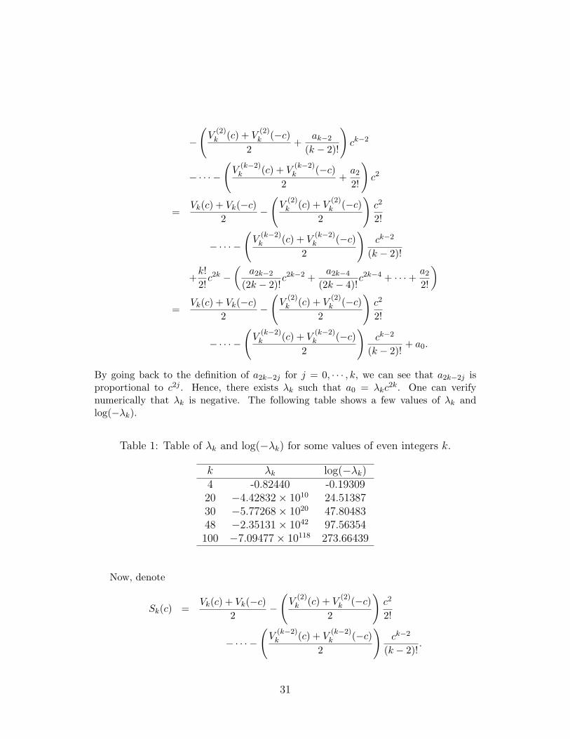
By going back to the definition of a2k−2j for j = 0, · · · , k, we can see that a2k−2j isproportional to c2j . Hence, there exists λk such that a0 = λkc2k. One can verifynumerically that λk is negative. The following table shows a few values of λk andlog(−λk).
Table 1: Table of λk and log(−λk) for some values of even integers k.
k λk log(−λk)4 -0.82440 -0.1930920 −4.42832× 10¹⁰ 24.5138730 −5.77268× 10²⁰ 47.8048348 −2.35131× 1042 97.56354100 −7.09477× 10118 273.66439
Now, denote
Sk(c) =Vk(c) + Vk(−c)
2−
(V (2)
k (c) + V (2)k (−c)
2
)c2
2!
− · · ·−(
V (k−2)k (c) + V (k−2)
k (−c)2
)ck−2
(k − 2)!.
31
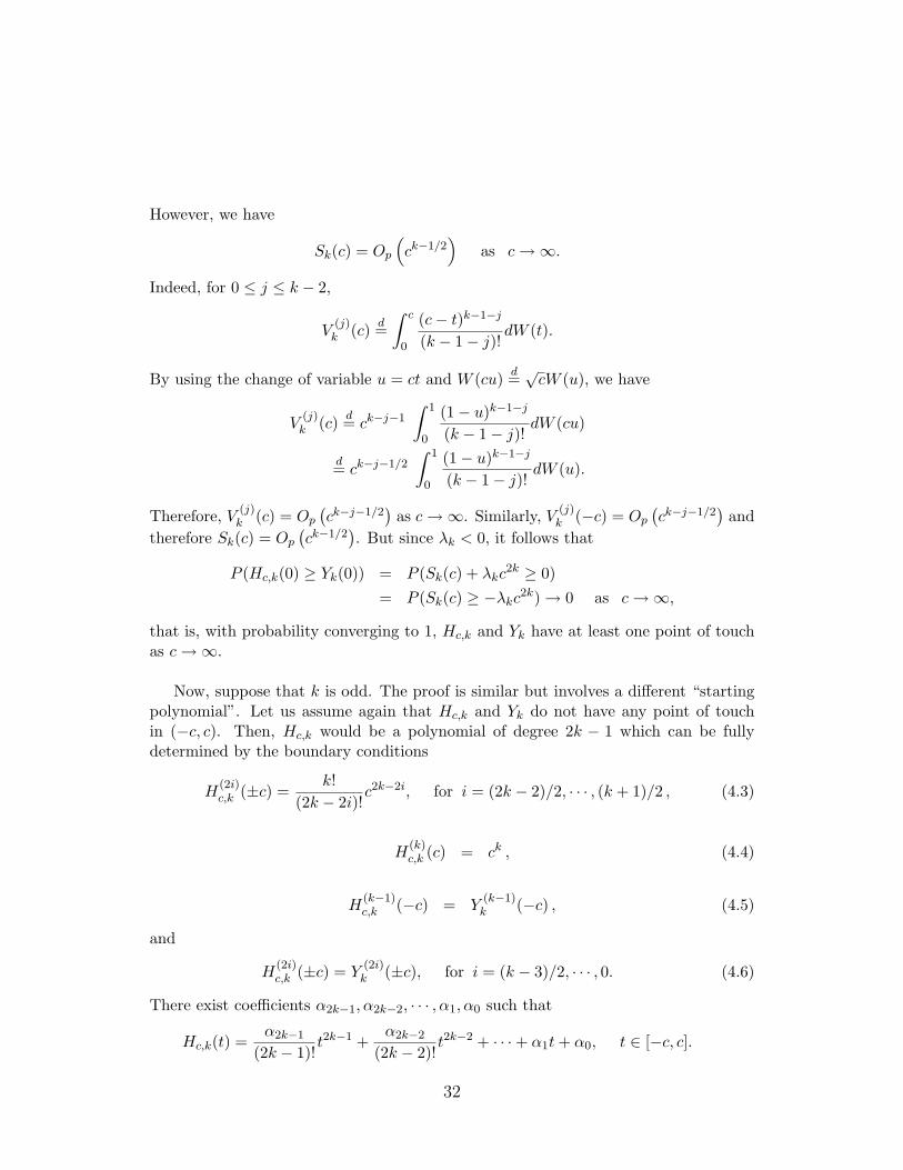
However, we have
Sk(c) = Op
(ck−1/2
)as c →∞.
Indeed, for 0 ≤ j ≤ k − 2,
V (j)k (c) d=
∫ c
0
(c− t)k−1−j
(k − 1− j)!dW (t).
By using the change of variable u = ct and W (cu) d=√
cW (u), we have
V (j)k (c) d= ck−j−1
∫ 1
0
(1− u)k−1−j
(k − 1− j)!dW (cu)
d= ck−j−1/2∫ 1
0
(1− u)k−1−j
(k − 1− j)!dW (u).
Therefore, V (j)k (c) = Op
(ck−j−1/2
)as c →∞. Similarly, V (j)
k (−c) = Op(ck−j−1/2
)and
therefore Sk(c) = Op(ck−1/2
). But since λk < 0, it follows that
P (Hc,k(0) ≥ Yk(0)) = P (Sk(c) + λkc2k ≥ 0)
= P (Sk(c) ≥ −λkc2k) → 0 as c →∞,
that is, with probability converging to 1, Hc,k and Yk have at least one point of touchas c →∞.
Now, suppose that k is odd. The proof is similar but involves a different “startingpolynomial”. Let us assume again that Hc,k and Yk do not have any point of touchin (−c, c). Then, Hc,k would be a polynomial of degree 2k − 1 which can be fullydetermined by the boundary conditions
H(2i)c,k (±c) =
k!(2k − 2i)!
c2k−2i, for i = (2k − 2)/2, · · · , (k + 1)/2 , (4.3)
H(k)c,k (c) = ck , (4.4)
H(k−1)c,k (−c) = Y (k−1)
k (−c) , (4.5)
and
H(2i)c,k (±c) = Y (2i)
k (±c), for i = (k − 3)/2, · · · , 0. (4.6)
There exist coefficients α2k−1,α2k−2, · · · ,α1,α0 such that
Hc,k(t) =α2k−1
(2k − 1)!t2k−1 +
α2k−2
(2k − 2)!t2k−2 + · · · + α1t + α0, t ∈ [−c, c].
32

The boundary conditions in (4.3) imply that α2k−1 = α2k−3 = · · · = αk+2 = 0. Also,using the same conditions we obtain that
α2k−2 =k!2!
c2
and for 2 ≤ j ≤ (k − 1)/2
α2k−2j =k!
(2j)!c2j −
(α2k−2
(2j − 2)!+ · · · + α2k−2j+2
2!c2
).
The “one-sided” conditions (4.4) and (4.5) imply that for j = 1, · · · , (k − 1)/2
αk = ck −(
α2k−2
(k − 2)!ck−2 + · · · + αk+3
(k + 3)!c3 + αk+1c
)and
αk−1 = Y (k−1)k (−c)−
(α2k−2
(k − 1)!ck−1 + · · · + αk+1
2!c2 − αkc
)respectively. Finally, using the boundary conditions in (4.6) we obtain that
αk−2j =Y (k−2j−1)
k (c)− Y (k−2j−1)k (−c)
2c−
(αk
(2j + 1)!c2j + · · · + αk−2j+2
3!c3
)and
αk−2j−1 =Y (k−2j−1)
k (−c) + Y (k−2j−1)k (c)
2−
(α2k−2
(k + 2j − 1)!ck+2j−1 + · · · + αk−2j+1
2!c2
)for j = 1, · · · , (k − 1)/2.
Let Vk continue to denote the (k − 1)-fold integral of two-sided Brownian motionand consider a2k−2, a2k−4, · · · , ak+1, ak, ak−1, · · · , a0 given by
a2k−2j = α2k−2j , for j = 1, · · · , (k − 1)/2
ak = ck −(
a2k−2
(k − 2)!+ · · · + ak+3
3!c3 + ak+1c
)
ak−1 =k!
(k + 1)!ck+1 −
(a2k−2
(k − 1)!ck−1 + · · · + αk+1
2!c2 − akc
),
and
ak−2j−1 =k!
(k + 2j + 1)!ck+2j+1 −
(a2k−2
(k + 2j − 1)!ck+2j−1 + · · · + ak−2j+1
2!c2
)33
for j = 1, · · · , (k − 1)/2. It follows that
Hc,k(0) = α0
=Yk(−c) + Yk(c)
2−
(α2k−2
(2k − 2)!c2k−2 +
α2k−4
(2k − 4)!c2k−4 + · · · + α2
2!c2
)=
Vk(−c) + Vk(c)2
−(
Vk(−c) + Vk(c)2
)c2
2!
− · · ·−(
Vk(−c) + Vk(c)2
)ck−2
(k − 2)!+ a0
= Sk(c) + a0
where
a0 =k!
(2k)!c2k −
(a2k−2
(2k − 2)!c2k−2 + · · · + a2
2!c2
).
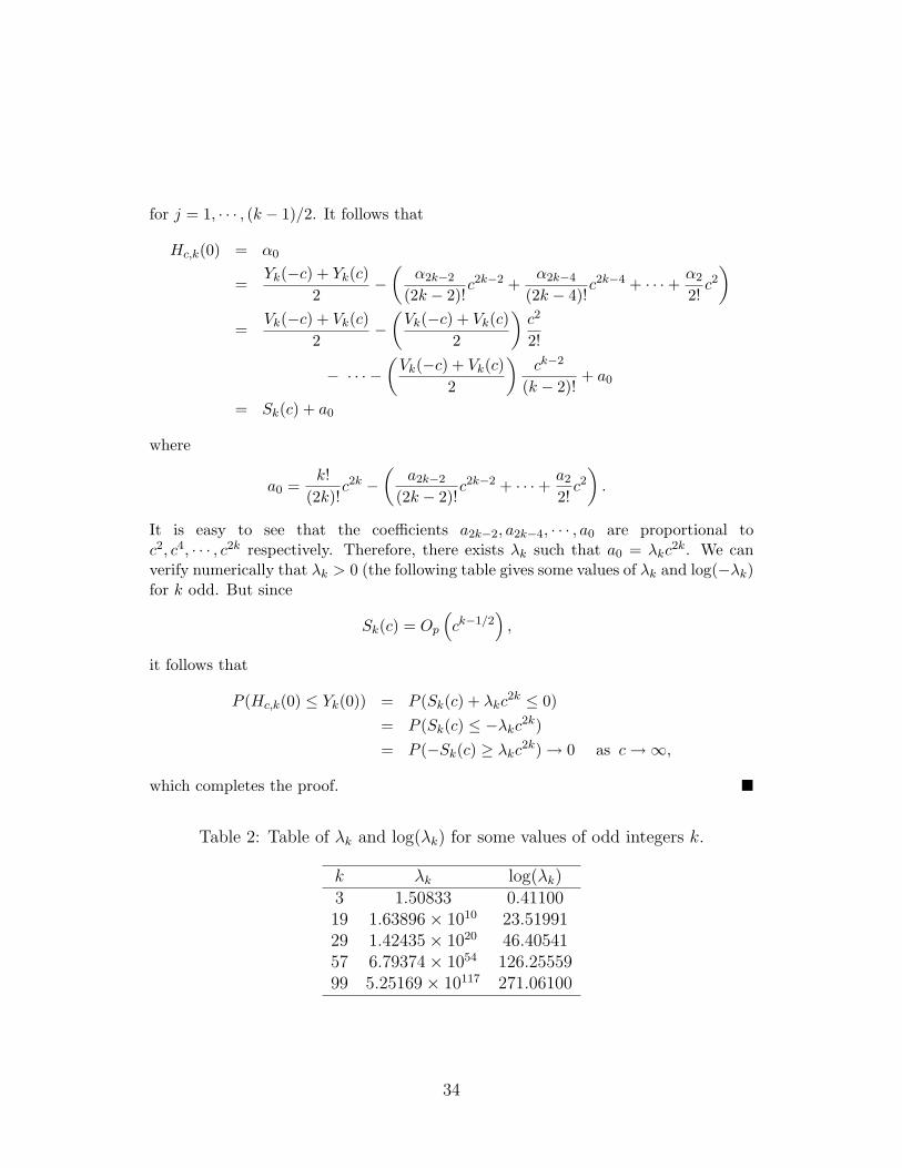
It is easy to see that the coefficients a2k−2, a2k−4, · · · , a0 are proportional toc2, c4, · · · , c2k respectively. Therefore, there exists λk such that a0 = λkc2k. We canverify numerically that λk > 0 (the following table gives some values of λk and log(−λk)for k odd. But since
Sk(c) = Op
(ck−1/2
),
it follows that
P (Hc,k(0) ≤ Yk(0)) = P (Sk(c) + λkc2k ≤ 0)
= P (Sk(c) ≤ −λkc2k)
= P (−Sk(c) ≥ λkc2k) → 0 as c →∞,
which completes the proof. !
Table 2: Table of λk and log(λk) for some values of odd integers k.
k λk log(λk)3 1.50833 0.4110019 1.63896× 10¹⁰ 23.5199129 1.42435× 10²⁰ 46.4054157 6.79374× 1054 126.2555999 5.25169× 10117 271.06100
34

Corollary 4.1 Fix ε > 0 and let t ∈ (−c, c). There exists c0 > 0 such that theprobability that the process Hc,k touches Yk at two points of touch τ− and τ+ beforeand after the point t is larger than 1− ε for c > c0.
Proof. We focus on k even as the arguments are very similar for k odd. Considerfirst t = 0. We know by Proposition 4.1 that, with very large probability, there existsat least one point of touch (before or after 0) as c → ∞. By symmetry of two-sidedBrownian motion originating at 0 and hence by that of the process Yk, there exist twopoints of touch before and after 0 with very large probability as c → ∞. Now, fixt0 '= 0 and consider the problem of minimizing
Φc,t0(f) =12
∫ c+t0
−c+t0
f2(t)dt−∫ c+t0
−c+t0
f(t)dXk(t)
=12
∫ c+t0
−c+t0
f2(t)dt−∫ c+t0
−c+t0
f(t)(tkdt + dW (t))
over the class of k-convex functions satisfying
f (k−2)(−c + t0) =k!2!
(−c + t0)2, f (k−4)(−c + t0) =k!4!
(−c + t0)4, · · · , f(−c + t0) = (−c + t0)k
and
f (k−2)(c + t0) =k!2!
(c + t0)2, f (k−4)(c + t0) =k!4!
(c + t0)4, · · · , f(c + t0) = (c + t0)k.
Since adding any constant to −c and c is irrelevant to the original minimizationproblem, all the above results hold and in particular that of existence of two points oftouch τ− and τ+ before and after 0 with increasing probability as c →∞.
But using the change of variable u = t− t0, Φc,t0 can be rewritten as
Φc,t0(f) =12
∫ c
−cf2(u + t0)du−
∫ c+t0
−c+t0
f(t)(tkdt + dW (t))
=12
∫ c
−cf2(u + t0)du−
∫ c
−cf(u + t0)((u + t0)kdt + dW (u + t0))
d=12
∫ c
−cg2(u)du−
∫ c
−cg(u)((u + t0)kdt + dW (u)) (4.7)
where in (4.7), we used stationarity of the increments of W and g(u) = f(u + t0) isk-convex satisfying the above boundary conditions at −c and c. From the latter form ofΦc,t0 , we can see that the “ true” k-convex is now (t+ t0)k defined on [−c, c]. However,the “estimation” problem is basically the same expect and hence there exist two pointsof touch before and after t0 with increasing probability as c →∞. !
35

4.2 Tightness
One very important element in proving the existence of the process Hk is tightnessof the process Hc,k and its (2k − 1) derivatives when c → ∞. The process Hk canbe defined as the limit of Hc,k as c → ∞ the same way Groeneboom, Jongbloed,and Wellner (2001a) did for the special case k = 2. In the latter case, tightnessof the process Hc,2 and its derivatives H ′
c,k, H(2)c,k , and H(3)
c,k was implied by tightnessof the distance between the points of touch of Hc,2 with respect to Y2. The authorscould prove using martingale arguments, that for a fixed ε > 0, there exists M > 0independent of t such that for any fixed t ∈ (−c, c),
lim supc→∞
P([t− τ− > M ] ∩ [τ+ − t > M ]
) ≤ ε (4.8)
where τ− and τ+ are respectively the last point of touch before t and the first point oftouch after t.
Before giving any further details about the difficulties of proving such a propertywhen k > 2, we explain the difference between the result proven in (4.8) and the onestated in Lemma 4.4 and Corollary 4.2. By the first result, we only know that not bothpoints of touch τ− and τ+ are “out of control” whereas our result implies that they bothstay within a bounded distance from the point t with very large probability as c →∞.Therefore, we are claiming a stronger result than the one proved by Groeneboom,Jongbloed, and Wellner (2001a). Intuitively, tightness has to be a commonproperty of both the points of touch and this can be seen by using symmetry of theprocess Yk. Indeed, since the latter has the same law whether the Brownian motionW “runs” from −c to c or vice versa, it is not hard to be convinced that tightness ofone point of touch implies tightness of the other. It should be mentioned here thatfor proving the existence of two points of touch before and after any fixed point t, theauthors claimed that this follows from arguments that are similar to the ones used toshow existence of at least one point of touch. We tried to reproduce such arguments butwe found the situation somehow different. In fact, we found that the arguments usedin the proof of Lemma 2.1 in Groeneboom, Jongbloed, and Wellner (2001a)cannot be used similarly to prove the existence of two points of touch unless one ofthese points of touch is “under control”. More formally, we need to make sure thatthe existing point of touch is tight; i.e., there exists some M > 0 independent of tsuch that the distance between t and this point of touch is bounded by M with a largeprobability as c → ∞. We find that it is simpler to use a symmetry argument as inCorollary 4.1 to make the conclusion.
As mentioned before, proving tightness was the most crucial point that led in theend to showing the existence of the process H2. Groeneboom, Jongbloed, andWellner (2001a) were able to prove it by using martingale arguments but moreimportantly the fact that the process Hc,2, which is a cubic spline, can be explicitlydetermined on the “excursion” interval [τ−, τ+]. Indeed, in the special case of k = 2,the four conditions Hc,2(τ−) = Y2(τ−), Hc,2(τ+) = Y2(τ+) and H ′
c,2(τ−) = Y ′2(τ−),
36

H ′c,2(τ+) = Y2(τ+), implied by the fact that H2,c ≥ Y2, yield a unique solution. The
same conditions hold true for k > 2 but are obviously not enough to determine the(2k−1)-th spline Hc,k. To do so, it seems inevitable to consider the whole set of pointsof touch along with the boundary conditions at −c and c, which is rather infeasiblesince, in principle, the locations of the other points of touch are unknown. However,we shall see that we only need 2k − 2 points to be able to determine the spline Hc,k
completely. For k > 2, it seems that the Gaussian problem becomes less local as weneed more than one excursion interval in order to study the properties of Hc,k and itsderivatives at a fixed point. Although the special case k = 2 gives a lot of insight intothe general problem, the arguments by Groeneboom, Jongbloed, and Wellner(2001a) cannot be readapted directly for the general case of k > 2. In the proof ofLemma 4.4, we skip many technical details as the tightness problem is very similar tothe gap problem for the LSE and MLE studied in great detail in Balabdaoui andWellner (2004c). We will also restrict ourselves to k even as the case k odd can behandled similarly.
In order to make use of the techniques developed in Balabdaoui and Wellner(2004c) for solving the gap problem, it is very helpful to first change the minimizationproblem from its current version to a rescaled version. Now consider minimizing
12
∫ c1
2k+1
−c1
2k+1
g2(t)dt−∫ c
12k+1
−c1
2k+1
g(t)(tkdt + dW (t)) (4.9)
over the class of k-convex functions on [−c1/(2k+1), c1/(2k+1)] satisfying
g(c1
2k+1 ) = ck
2k+1 , g′′(c1
2k+1 ) =k!
(k − 2)!c
k−22k+1 , · · · , g(k−2)(c
12k+1 ) =
k!(2)!
c2
2k+1 .
Now using the change of variable t = c1/(2k+1)u, we can write
12
∫ c1
2k+1
−c1
2k+1
g2(t)dt−∫ c
12k+1
−c1
2k+1
g(t)dXk(t)
d= c1
2k+112
∫ 1
−1g2(c
12k+1 u)du−
∫ 1
−1g(c
12k+1 u)(c
k+12k+1 ukdu + dW (c
12k+1 u))
d= c1
2k+112
∫ 1
−1g2(c
12k+1 u)du−
∫ 1
−1g(c
12k+1 u)
(c
k+12k+1 ukdu + c
12(2k+1) dW (u)
)d= c
12k+1
12
∫ 1
−1g2(c
12k+1 u)du−
∫ 1
−1g(c
12k+1 u)
(c
k+12k+1 ukdu + c
12(2k+1)
√c
dW (u)√c
)d= c
12k+1
12
∫ 1
−1g2(c
12k+1 u)du−
∫ 1
−1g(c
12k+1 u)
(c
k+12k+1 ukdu + c
k+12k+1
dW (u)√c
)d= c
12k+1
(12
∫ 1
−1g2(c
12k+1 u)du−
∫ 1
−1g(c
12k+1 u)c
k2k+1
(ukdu +
dW (u)√c
)).
37

If we set
g(c1
2k+1 u) = ck
2k+1 h(u) ,
then the problem is equivalent to minimizing(12
∫ 1
−1c
2k2k+1 h2(u)du−
∫ 1
−1c
2k2k+1 h(u)
(ukdu +
dW (u)√c
))or simply minimizing
12
∫ 1
−1h2(u)du−
∫ 1
−1h(u)
(ukdu +
dW (u)√c
), (4.10)
over the class of k-convex function on [−1, 1] satisfying
h(±1) = 1, h′′(±1) =k!
(k − 2)!, · · · , h(k−2)(±1) =
k!2!
. (4.11)
With this new criterion function, the situation is very similar to the “ finite sample”problem treated in Balabdaoui and Wellner (2004c). Indeed, as the Gaussiannoise vanishes at a rate of 1/
√c as c → ∞, one can view tkdt + dW (t)/
√c as a
“continuous” analogue to dGn(t) where Gn is the empirical distribution of X1, . . . , Xn
i.i.d. with k−monotone density g0, and where the true k-monotone density is replacedby the k-convex function tk. Existence and characterization of the minimizer ofthe criterion function in (4.10) with the boundary conditions (4.11) follows fromarguments the same arguments used in the original problem. Furthermore, if hc
denotes the minimizer, we claim that the number of jump points of h(k−1)c that are
in the neighborhood of a fixed point t increases to infinity, and the distance betweentwo successive jump points is of the order c−1/(2k+1) as c →∞. To establish this result,we need the following definition and lemma:
Definition 4.1 Let f be a sufficiently differentiable function on a finite interval [a, b],and t1 ≤ · · · ≤ tm be m points in [a, b]. The Lagrange interpolating polynomial is theunique polynomial P of degree m− 1 which passes through (t1, f(t1)), · · · , (tm, f(tm)).Furthermore, P is given by its Newton form
P (t) =m∑
j=1
f(tj)m∏
k=1k )=j
(t− tk)(tj − tk)
or Lagrange form
P (t) = f(t1) + (t− t1)[t1, t2]f + · · · + (t− t1) · · · (t− tm)[t1, · · · , tm]f
where [x1, · · · , xp]g denotes the divided difference of g of order p; (see, e.g., de Boor(1978), page 2, Nurnberger (1989), page 24, or DeVore and Lorentz (1993),page 120.
38

Lemma 4.1 Let g be an m-convex function on a finite interval [a, b]; i.e., g(m−2) existsand is convex on (a, b), and let lm(g, x, x1, · · · , xm) be the Lagrange polynomial of degreem− 1 interpolating g at the points xi, 1 ≤ i ≤ m, where a < x1 ≤ x2 ≤ · · · ≤ xm < b.Then
(−1)m+i (g(x)− lm(g, x, x1, · · · , xm)) ≥ 0, x ∈ [xi, xi+1], i = 1, · · · ,m− 1.
Proof. See, e.g., Ubhaya (1989), (a), page 235 or Kopotun and Shadrin (2003),Lemma 8.3, page 918. !
The following lemma gives consistency of the derivatives of the LS solution. It isvery crucial for proving tightness of the distance between successive points of touch ofHc,k and Yk.
Lemma 4.2 For j ∈ {0, · · · , k − 1} and t ∈ R, we have∣∣∣∣h(j)c (t)− k!
(k − j)!tk−j
∣∣∣∣ → 0, almost surely as c →∞.
Proof. We will prove the result for t = 0 as the arguments are similar in the generalcase. Let us denote
ψc(h) =12
∫ 1
−1h2(t)dt−
∫ 1
−1h(t)dHc(t)
where
dHc(t) = tkdt +dW (t)√
c.
Since hc is the minimizer of ψc, then
limε→0
ψ(hc + εhc)− ψ(hc)ε
= 0
implying that ∫ 1
−1h2
c(t)dt =∫ 1
−1hc(t)dHc(t). (4.12)
Also, for any k-convex function g defined on (−1, 1) that satisfies the boundaryconditions in (4.11), we have
limε↘0
ψ((1− ε)hc + εg)− ψ(hc)ε
≥ 0
39

and therefore∫ 1
−1(g(t)− hc(t))hc(t)dt−
∫ 1
−1(g(t)− hc(t))dHc(t) ≥ 0. (4.13)
Let us denote h0(t) = tk, dH0(t) = h0(t)dt, and dHc(t) = hc(t)dt. If we take g = h0 in(4.13), it follows that∫ 1
−1(hc(t)− h0(t))d(Hc(t)−Hc(t)) ≤ 0. (4.14)
Now the equality in (4.12) can be rewritten as√∫ 1
−1h2
c(t)dt =∫ 1
−1uc(t)dHc(t)
where uc = hc/‖hc‖2 is a k-convex function on [−1, 1] such that
‖uc‖2 = 1, and u(2j)c (±1) =
k!(k − 2j)!‖hc‖2
for j = 0, · · · , (k − 2)/2.
We want to show that the function limc→∞ hc(t) = h0(t) for all t ∈ (−1, 1). Let ustake c = c(n) = n. We start by showing that the sequence (hn)n is uniformly boundedon (−1, 1); i.e., there exists a constant M > 0 independent of n such that ‖hn‖∞ < M
for all n ∈ N. Suppose it is not. This implies that (h(k−2)n )n is not bounded because if
it was, we can find M > 0 such that for all n > 0,
|h(k−2)n (t)| ≤ M,
for t ∈ (−1, 1). By integrating h(k−2)n twice and using the boundary conditions at −1
and 1, it follows that
h(k−4)n (t) =
∫ t
−1(t− s)h(k−2)
n (s)ds−(
12
∫ 1
−1(1− s)h(k−2)
n (s)ds
)(t + 1) +
k!2!
and therefore
‖h(k−4)n ‖∞ ≤ 2M + 2M +
k!2!
= 4M +k!2!
.
By induction, it follows that (hn)n has to be bounded. We conclude that h(k−2)n is not
bounded. Now, using convexity of h(k−2)n and the same arguments of Proposition 3.1,
this implies that we can find a subsequence (hn′)n′ such that limn′→∞ ‖hn′‖2 = ∞.Therefore,
limn′→∞
u(2j)n′ (−1) = lim
n′→∞u(2j)
n′ (1) = 0.
40

for j ∈ {0, · · · , (k − 2)/2}.In the limit, the derivatives of un′ are “pinned down” at ±1 and this implies that
for large n′, u(2j)n′ (±), j = 0, · · · , (k− 1)/2 stay close to 0. On the other hand, we know
that ‖un′‖∞ = 1. Therefore, the convex function u(k−2)n has to be uniformly bounded
by the same arguments of Proposition 3.1. It follows that there exists M > 0 such that‖un′‖∞ < M . By Arzela-Ascoli’s theorem, we can find a subsequence (un′′)n′′ and afunction u such that
limn′′→∞
un′′(t) = u(t)
for all t ∈ (−1, 1). But since∫ 1−1 |u|dH0(t) ≤ 2M/(k + 1) < ∞, it follows that
limn′′→∞
∫ 1
−1un′′(t)dHn′′(t) =
∫ 1
−1u(t)dH0(t) < ∞. (4.15)
But recall that ∫ 1
−1un′′(t)dHn′′(t) = ‖hn′′‖22 →∞
as n′′ → ∞. Since this contradicts the result in (4.15), it follows that there existsM > 0 such that ‖hn‖∞ < M .
Now, we can find a subsequence (hnl)nl and a function h such that
limnl→∞
hnl(t) = h(t)
for t ∈ (−1, 1). By Fatou’s lemma, we have∫ 1
−1(h(t)− h0(t))2dt ≤ lim inf
nl→∞
∫ 1
−1(hnl(t)− h0(t))2dt.
On the other hand, it follows from (4.14) that∫ 1
−1(hnl(t)− h0(t))d(Hnl(t)−Hnl(t)) ≤ 0.
Thus we can write∫ 1
−1(hnl(t)− h0(t))2dt
=∫ 1
−1(hnl(t)− h0(t))d(Hnl(t)−H0(t))
=∫ 1
−1(hnl(t)− h0(t))d(Hnl(t)−Hnl(t)) +
∫ 1
−1(hnl(t)− h0(t))d(Hnl(t)−H0(t))
≤∫ 1
−1(hnl(t)− h0(t))d(Hnl(t)−H0(t)) →a.s. 0, as nl →∞,
41

since hnl − h0 is bounded and∫ 1−1 h0(t)dt < ∞ (which implies that hnl − h0 has an
envelope ∈ L1(H0)). We conclude that∫ 1
−1(h(t)− h0(t))2dt ≤ 0
and therefore h ≡ h0 on (−1, 1). Since the choice c(n) = n is irrelevant for thearguments above, we make the same conclusion with any other increasing sequencecn such that cn → ∞. It follows that limc→∞ hc(t) = h0(t) . What should also beretained from the above arguments is the uniform boundedness of the derivatives ofh(l)
c , l = 1, · · · , k − 2. This is not guaranteed in general but k-convexity plays togetherwith the fact that h(2j
c , j = 1, · · · , (k−2)/2 have fixed values at −1 and 1 play a crucialrole. A proof of this fact follows from using induction and arguments that are similarto the ones used in the proof of Proposition 3.1.
Now, fix t = 0. We will show that we have also consistency of the derivatives of hc.For that, consider x0, x1, · · · , xk−1 < 1 to be k points such that 0 = x0 ≤ x1 ≤ · · · ≤xk−1. By taking m = k and i = 2 in Lemma 4.1, we have for all t ∈ [x1, x2]
hc(t) ≥ hc(x0) + (t− x0)hc[x0, x1]+ · · · + (t− x0)(t− x1) · · · (t− xk−2)hc[x0, x1, · · · , xk−1]. (4.16)
If we take x0 = x1, then the inequality in (4.16) can be rewritten as
hc(t) ≥ hc(x0) + (t− x0)h′c(x0) + (t− x0)2hc[x0, x0, x2]+ · · · + (t− x0)2(t− x2) · · · (t− xk−2)hc[x0, x0, x2 · · · , xk−1]
or equivalently
h′c(x0) ≤ hc(t)− hc(x0)t− x0
− (t− x0)(
hc[x0, x0, x2]
+ · · · + (t− x2) · · · (t− xk−2)hc[x0, x0, x2 · · · , xk−1])
.
since t ≥ x0. Furthermore, since |h′c(x0)| is bounded, we can find a sequence (hn)n
such that the divided differences hn[x0, x0, x2], · · · , hn[x0, x0, x2, · · · , xk−1] converge tofinite limits as n →∞. For instance, we have
hn[x0, x0, x2] =1
x2 − x0
(hn(x2)− hn(x1)
x2 − x0− h′n(x0)
).
If we denote l(x0) = limn→∞ h′n(x0), then
limn→∞ hn[x0, x0, x2] =
1x2 − x0
(h0(x2)− h0(x1)
x2 − x0− l(x0)
).
42

The same reasoning can be applied for the remaining divided differences. By lettingn →∞ and then t ↘ x0, it follows that
lim supn→∞
h′n(x0) ≤ h′0(x0); i.e.,
lim supn→∞
h′n(0) ≤ h′0(0).
Now, we need to exploit the inequality from above and for that consider x−1 ≤ x0 ≤x1 ≤ · · · ≤ xk−2 to be k points, where x0 = 0 and x1, · · · , xk−2 can be taken to be thesame as before. For all t ∈ [x1, x2], we have
hc(t) ≤ hc(x−1) + (t− x−1) hc[x−1, x0]+ · · · + (t− x−1)(t− x0) · · · (t− xk−3) hc[x−1, x0 · · · , xk−2].
In this case, we have i = 3 (see Lemma 4.1). If we take x−1 = x0 = x1, then for allt ∈ [x0, x2] we have
h′c(x0) ≥ hc(t)− hc(x0)t− x0
− (t− x0)(
(t− x0)h′′c (x0)
2
+ · · · + (t− x0)2 · · · (t− xk−3) hc[x0, x0, x0 · · · , xk−2])
.
Using the fact that |h′′c (x0)| is bounded and the same reasoning as before, we obtainthat
lim infn→∞ h′n(x0) ≥ h′0(x0); i.e.,
lim infn→∞ h′n(0) ≥ h′0(0).
Combining both inequalities, we can write
h′0(0) ≤ lim infn→∞ h′n(0) ≤ lim sup
n→∞h′n(0) ≤ h′0(0)
and hence limc→∞ h′c(0) = h′0(0). An induction argument can be used to show thatconsistency holds true for h(j)
c (0), j = 2, · · · , k− 2. As for the last derivative, we applythe well-known chord inequality satisfied by convex functions: For all h > 0, we have
h(k−2)c (0)− h(k−2)
c (−h)−h
≤ h(k−1)c (0−) ≤ h(k−1)
c (0+) ≤ h(k−2)c (h)− h(k−2)
c (0)h
.
We obtain the result by letting c →∞ and then h ↘ 0. !
Before we state the main lemma of this section, we give first a characterization forthe minimizer hc:
43

Lemma 4.3 Let Y 1c be the process defined on [−1, 1] by
Y 1c (t) d=
1√c
∫ t0
(t−s)k−1
(k−1)! dW (s) + k!(2k)! t
2k, if t ∈ [0, 1]1√c
∫ 0t
(t−s)k−1
(k−1)! dW (s) + k!(2k)! t
2k, if t ∈ [−1, 0)
and H1c be the k-fold integral of hc that satisfies the boundary conditions
d2jH1c
dt2j|t=±c =
d2jY 1c
dt2j|t=±c,
for j = 0, · · · , (k − 2)/2. The minimizer hc is characterized by the conditions:
H1c (t) ≥ Y 1
c (t), for all t ∈ [−1, 1]
and ∫ 1
−1
(H1
c (t)− Y 1c (t)
)dh(k−1)
c (t) = 0.
Proof. The arguments are very similar to those used in the proof of Lemma 3.2. !
Lemma 4.4 Let t be a fixed point in (−1, 1) and suppose that Conjecture 1.1 holds.If τ−c and τ+
c are the last (first) point of touch between of H1c and Y 1
c before (after) t,then
τ+c − τ−c = Op(c−1/(2k+1)).
Proof. For the equivalent form of the minimization problem the problem isclosely related to that of the LS problem for estimating a k-monotone density (seeBalabdaoui and Wellner (2004c)), we can apply the result obtained in Lemma2.8 of Balabdaoui and Wellner (2004c). In fact, consistency of h(k−1)
c at thepoint t and the fact that h0(t) = tk is k-times differentiable with h(k)
0 (t) = k! > 0force the number of points of change of slope of h(k−2)
c to increase to infinity almostsurely as c → ∞. If τc,0 < · · · < τc,2k−3 are 2k − 2 jump points of h(k−1
c that are in asmall neighborhood of t, then H1
c is a polynomial spline of degree 2k − 1 and simpleknots τc,0, · · · , τc,2k−3. Furthermore, Hc is the unique solution of the following Hermiteproblem:
H1c (τj) = Y 1
c (τj), and (H1c )′(τj) = (Y 1
c )′(τj)
for j = 0, · · · , 2k − 3. By Lemma 2.8 of Balabdaoui and Wellner (2004c), itfollows that
τc,2k−3 − τc,0 = Op(c−1/(2k+1)).
44
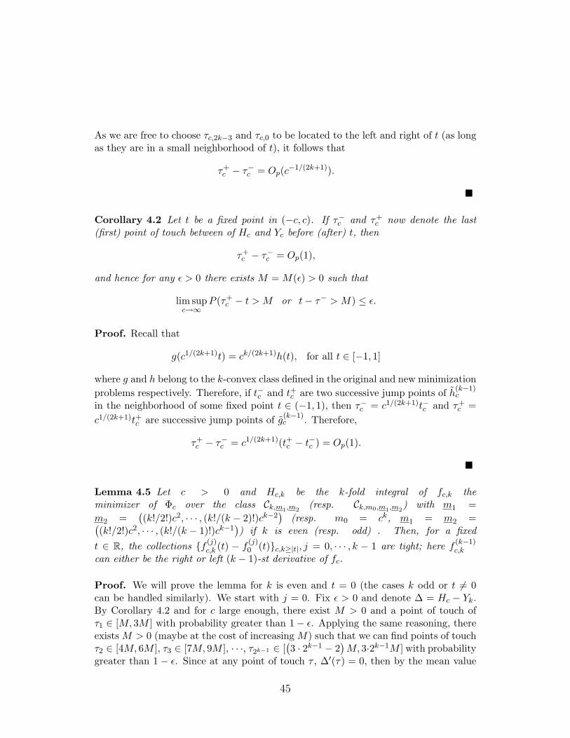
As we are free to choose τc,2k−3 and τc,0 to be located to the left and right of t (as longas they are in a small neighborhood of t), it follows that
τ+c − τ−c = Op(c−1/(2k+1)).
!
Corollary 4.2 Let t be a fixed point in (−c, c). If τ−c and τ+c now denote the last
(first) point of touch between of Hc and Yc before (after) t, then
τ+c − τ−c = Op(1),
and hence for any ε > 0 there exists M = M(ε) > 0 such that
lim supc→∞
P (τ+c − t > M or t− τ− > M) ≤ ε.
Proof. Recall that
g(c1/(2k+1)t) = ck/(2k+1)h(t), for all t ∈ [−1, 1]
where g and h belong to the k-convex class defined in the original and new minimizationproblems respectively. Therefore, if t−c and t+c are two successive jump points of h(k−1)
c
in the neighborhood of some fixed point t ∈ (−1, 1), then τ−c = c1/(2k+1)t−c and τ+c =
c1/(2k+1)t+c are successive jump points of g(k−1)c . Therefore,
τ+c − τ−c = c1/(2k+1)(t+c − t−c ) = Op(1).
!
Lemma 4.5 Let c > 0 and Hc,k be the k-fold integral of fc,k theminimizer of Φc over the class Ck,m1,m2
(resp. Ck,m0,m1,m2) with m1 =
m2 =((k!/2!)c2, · · · , (k!/(k − 2)!)ck−2
)(resp. m0 = ck, m1 = m2 =(
(k!/2!)c2, · · · , (k!/(k − 1)!)ck−1)) if k is even (resp. odd) . Then, for a fixed
t ∈ R, the collections {f (j)c,k (t) − f (j)
0 (t)}c,k≥|t|, j = 0, · · · , k − 1 are tight; here f (k−1)c,k
can either be the right or left (k − 1)-st derivative of fc.
Proof. We will prove the lemma for k is even and t = 0 (the cases k odd or t '= 0can be handled similarly). We start with j = 0. Fix ε > 0 and denote ∆ = Hc − Yk.By Corollary 4.2 and for c large enough, there exist M > 0 and a point of touch ofτ1 ∈ [M, 3M ] with probability greater than 1− ε. Applying the same reasoning, thereexists M > 0 (maybe at the cost of increasing M) such that we can find points of touchτ2 ∈ [4M, 6M ], τ3 ∈ [7M, 9M ], · · ·, τ2k−1 ∈ [
(3 · 2k−1 − 2
)M, 3·2k−1M ] with probability
greater than 1 − ε. Since at any point of touch τ , ∆′(τ) = 0, then by the mean value
45

theorem, there exist τ (2)1 ∈ (τ1, τ2), τ (2)
2 ∈ (τ3, τ4), · · ·, τ (2)2k−2 ∈ (τ2k−1−1, τ2k−1) such that
∆(2)(τ (2)j ) = 0, j = 1, · · · , 2k−2. By applying the mean value theorem successively k−3
more times, we can find τ (k−1)1 < τ (k−1)
2 ∈ [M, 3 · 2k−1M ] such that ∆(k−1)(τ (k−1)i ) =
0, i = 1, 2 and τ (k−1)2 − τ (k−1)
1 ≥ M . Finally, there exists τ (k) = ξ1 ∈ (τ (k−1)1 , τ (k−1)
2 )such that
f (k)c,k (ξ1) = H(k)
c (ξ1)
=H(k−1)
c,k (τ (k−1)2 )−H(k−1)
c,k (τ (k−1)1 )
τ (k−1)2 − τ (k−1)
1
=Y (k−1)
k (τ (k−1)2 )− Y (k−1)
k (τ (k−1)1 )
τ (k−1)2 − τ (k−1)
1
=W (τ (k−1)
2 )−W (τ (k−1)1 )
τ (k−1)2 − τ (k−1)
1
+1
k + 1
(τ (k−1)2
)k+1 −(τ (k−1)1
)k+1
τ (k−1)2 − τ (k−1)
1
and therefore
|f (k)c,k (ξ1)| ≤
∣∣∣W (τ (k−1)2 )−W (τ (k−1)
1 )∣∣∣
M+
(3 2k−1M
)k
≤ C
M+
(3 · 2k−1M
)k
for some constant C = C(M) > 0 by tightness of W and stationarity of its increments,and using the fact that yk+1−xk+1 = (y−x)(xk +xk−1y+ · · ·+yk). In general, we canfind k− 2 points ξ1 < · · · < ξk−2 to the right of 0 such that ξ1 ∈ [M, 3M ], the distancebetween any ξi and ξj , i '= j is at least M and fc,k(ξi) is tight for i = 1, · · · , k − 2.Similarly and this time to the left of 0, we can find two points of touch ξ−2 < ξ−1 suchthat ξ−1 ∈ [−3 · 2k−1M,−M ], ξ−1 − ξ−2 ≥ M and fc,k(ξ−1) and fc(ξ−2) are tight. Intotal, we have k points that are at least M -distant from each other and we are readyto apply Lemma 4.1. Hence, if we take g = fc,k, m = k, i = 2, and x1 = ξ−2, x2 = ξ−1,x3 = ξ1, · · ·, xk = ξk−2, we have for all t ∈ (ξ−1, ξ1)
fc,k(t) ≥ fc,k(ξ−2) + (t− ξ−2) [ξ−2, ξ−1]fc,k + (t− ξ−2)(t− ξ−1) [ξ−2, ξ−1, ξ1]fc,k
+ · · · + (t− ξ−2)(t− ξ−1) · · · (t− ξk−3) [ξ−2, ξ−1 · · · , ξk−2]fc,k.
In particular, when t = 0 we have
fc,k(0) ≥ fc,k(ξ−2)− ξ−2 [ξ−2, ξ−1]fc,k + ξ−2ξ−1 [ξ−2, ξ−1, ξ1]fc,k
+ · · · + (−1)k−1ξ−2ξ−1 · · · ξk−3 [ξ−2, ξ−1, · · · , ξk−2]fc,k
46

which is tight by construction of ξi, i = −2,−1, 1, · · · , k − 2. Now, by adding a pointξk−1 to the right and ξk−2 such that ξk−1 − ξk−2 ≥ M and considering the pointsξ−1, ξ1, · · · , ξk−1, we apply Lemma 4.1 (with i = 1) to bound fc,k(0) by above:
fc,k(0) ≤ fc,k(ξ−1)− ξ−1 [ξ−1, ξ1]fc,k + ξ−1ξ1[ξ−1, ξ1, ξ2]fc,k
+ · · · + (−1)k−1ξ−1ξ1 · · · ξk−2[ξ−1, ξ1, · · · , ξk−1]fc,k
which is again tight.Now if j = 1, · · · , k − 3, the argument is entirely similar where k − j is the number
of points of touch needed to prove tightness. For j = k − 2, we can bound f (k−2)c,k (0)
from above by considering two points of touch ξ−1 ≤ −M and M ≤ ξ1 and usingconvexity of f (k−2)
c,k (which follows also from Lemma 4.1 in the particular case where g
is convex). To bound f (k−2)c,k (0) from below, we use a similar argument as in the proof
of Proposition 3.1. Finally, for j = k − 1, consider again ξ−1 and ξ1. By convexity off (k−2)
c,k , we have
f (k−2)c,k (0)− f (k−2)
c,k (ξ−1)ξ−1
≤ f (k−1)c,k (0−) ≤ f (k−1)
c,k (0+) ≤ f (k−2)c,k (ξ1)− f (k−2)
c,k (0)ξ1
hence,
|f (k−1)c,k (0)| ≤ max
{∣∣∣∣f (k−2)c,k (0)− f (k−2)
c,k (ξ−1)ξ−1
∣∣∣∣, ∣∣∣∣f (k−2)c,k (ξ1)− f (k−2)
c,k (0)ξ1
∣∣∣∣}which is bounded with large probability by tightness of f (k−2)
c,k (t), t ∈ (−c, c) andconstruction of ξ−1 and ξ1. !
5 Completion of the Proof of Theorem 2.1
We use similar arguments as in the proof of Theorem 2.1 in Groeneboom,Jongbloed, and Wellner (2001a) and for convenience, we adopt their notation.We assume here that k is even since the arguments are very similar for k odd. Form > 0 fixed, consider the semi-norm
‖H‖m = supt∈[−m,m]
{|H(t)| + |H ′(t)| + · · · + |H(2k−2)(t)|}
on the space of (2k−2)−continuously differentiable functions defined on R. By Lemma4.5, we know if we take c(n) = n that the collection {f (k−2)
n,k (t)−f (k−2)0 (t)}n>M is tight
for any fixed t ∈ [−M,M ], in particular for t = 0. Furthermore, by the same lemma, weknow that the collections {f (k−1)
n,k (t−)} and {f (k−1)n,k (t+)} are also tight for t ∈ [−M,M ].
47

By monotonicity of f (k−1)n,k , it follows that the sequence
(f (k−2)
n,k
)has uniformly bounded
derivatives on [−M,M ]. Therefore, by Arzela-Ascoli, the sequence(f (k−2)
n,k |[−M,M ])
has a subsequence(f (k−2)
nl,k|[−M,M ]
)≡
(H(2k−2)
nl,k|[−M,M ]
)converging in the
supremum metric on C[−M,M ] to a bounded convex function on [−M,M ]. By thesame theorem, we can find a further subsequence
(H(2k−3)
np,k |[−M,M ])
converging in thesame metric to a bounded function on [−M,M ]. Applying Arzela-Ascoli (2k−3) times,we can find a further subsequence
(Hnq ,k|[−M,M ]
)that converges in the supremum
metric on C[−M,M ].Now, fix m in N and let n > m. For any sequence (Hn,k), we can find a
subsequence (Hnj ,k) so that (Hnj ,k|[−m,m]) converges in the metric ‖H‖m to a limitH(m)
k that is (2k)−convex on [−m,m]; i.e., its (2k − 2)-th derivative, f (m)k , is convex
on [−m,m]. Finally, by a diagonal argument, we can extract from any sequence (Hn,k)a subsequence (Hnj ,k) converging to a limit Hk in the topology induced by the semi-norms ‖H‖m,m ∈ N. The limit Hk is clearly 2k-convex. Besides, it preserves byconstruction the properties (3.10) and (3.11) in the characterization of Hn,k ≡ Hc(n),k.On the other hand, since H(j)
n,k(±c) = Y (jk (±c) for j = 0, 2, · · · , k, it follows that
lim|t|→∞H(j)k (t) − Y (j)
k (t) = 0 for j = 0, 2, · · · , k. Thus Hk satisfies the conditions(i)-(iv) of Theorem 2.1. It remains only to show that this process is unique. !
To prove uniqueness of Hk, we need the following lemma:
Lemma 5.1 Let Gk be a 2k-convex function on R that satisfies
lim|t|→∞
(G(k−2)k (t)− Y (k−2)
k (t)) = 0
if k is even, and
lim|t|→∞
(G(k−3)k (t)− Y (k−3)
k (t)) = 0
if k is odd. Let gk = G(k)k and fix ε > 0. Then,
(i) For any fixed M2 ≥ M1 > 0, and a and b such that |a| < |b| are large enough andM2 ≥ |b|− |a| ≥ M1, we can find a positive constant K = K(ε,M1,M2) such that
P (‖G(j)k − Y (j)
k ‖[a,b] > K) ≤ ε
for j = 0, · · · , k − 1.
(ii) For any fixed M2 ≥ M1 > 0, and a and b such that |a| < |b| are large enough andM2 ≥ |b|− |a| ≥ M1, we can find a positive constant K = K(ε,M1,M2) such that
P (‖g(j)k − f (j)
0,k‖[a,b] > K) ≤ ε
for j = 0, · · · , k − 1, where f0,k(t) = tk.
48

Proof. We develop the arguments only in the case of k even (k odd can be handledsimilarly). We start by proving (ii) and for that we fix δ > 0. Without loss of generality,we can take M1 = M2 = M . Since limt→∞(G(k−2)
k (t)−Y (k−2)k (t)) = 0, then there exists
A > 0 such that
|G(k−2)k (t)− Y (k−2)
k (t)| < δ
for all t > A. Let t0 > A and t1 = t0 +M , and t2 = t0 +2M , where M is some positiveconstant. By the mean value theorem, there exists ξ ∈ (t0, t1) such that
G(k−1)k (ξ)− Y (k−1)
k (ξ) =(G(k−2)
k (t1)− Y (k−2)k (t1))− (G(k−2)
k (t0)− Y (k−2)k (t0))
t1 − t0(5.17)
and hence ∣∣∣∣G(k−1)k (ξ)− Y (k−1)
k (ξ)∣∣∣∣ ≤ 2δ
M.
From now on, we take δ = 1. For all t ∈ [t1, t2], we can write
G(k−2)k (t)− Y (k−2)
k (t) = G(k−2)k (t1)− Y (k−2)
k (t1) +∫ t
t1
(G(k−1)(s)− Y (k−1)k (s))ds
= G(k−2)k (t1)− Y (k−2)
k (t1) +∫ t
t1
∫ s
ξd(G(k−1)(u)− Y (k−1)
k (u))ds
+(t− t1)(G(k−1)k (ξ)− Y (k−1)
k (ξ))
= G(k−2)k (t1)− Y (k−2)
k (t1) +∫ t
t1
∫ s
ξ(gk(u)− f0,k(u))duds
+∫ t
t1
∫ s
ξdW (u)ds + (t− t1)(G
(k−1)k (ξ)− Y (k−1)
k (ξ))
(5.18)
and hence
inft∈[t0,t2]
|gk(t)− f0,k(t)| <8(6 + M C/2)
M2(5.19)
where C = C(M, ε) such that
P (|W (t)| < C, t ∈ [0, 2M ]) > 1− ε.
Indeed, from (5.18), we have for all t ∈ [(t1 + t2)/2, t2]∣∣∣∣ ∫ t
t1
∫ s
ξ(gk(u)− f0,k(u))duds
∣∣∣∣49

≤∣∣∣∣G(k−2)
k (t)− Y (k−2)k (t)
∣∣∣∣ +∣∣∣∣G(k−2)
k (t1)− Y (k−2)k (t1)
∣∣∣∣+
∫ t
t1
|W (s)−W (ξ)|dsdu + (t− t1)∣∣∣∣G(k−1)
k (ξ)− Y (k−1)k (ξ)
∣∣∣∣≤ 2 + (t− t1) C + 2M
2M
, using stationarity of the increments of W
= 6 + M C/2 (5.20)
with probability greater than 1− ε. Now, since
infy∈[t0,t2]
|gk(y)− f0,k(y)| ≤∣∣∣∣ ∫ t
t1
∫ s
ξ(gk(u)− f0,k(u))duds
∣∣∣∣/ ∫ t
t1
∫ s
ξduds
≤∣∣∣∣ ∫ t
t1
∫ s
ξ(gk(u)− f0,k(u))duds
∣∣∣∣/ ∫ t
t1
∫ s
t1
duds, since ξ ≤ t1
= 2∣∣∣∣ ∫ t
t1
∫ s
ξ(gk(u)− f0,k(u))duds
∣∣∣∣/(t− t1)2
≤ 8M2
∣∣∣∣ ∫ t
t1
∫ s
ξ(gk(u)− f0,k(u))duds
∣∣∣∣, since t− t1 ≥ M/2,
(5.21)
the inequality in (5.19) follows by combining (5.20) and (5.21).Now, consider two other points to the left of t2, t3 = t0 + 3M and t4 = t0 + 4M .
By using similar arguments, we can find ξ0 ∈ [t0, t2] and ξ1 ∈ (t2, t3) such that∣∣∣∣g0(ξ0)− f0,k(ξ0)∣∣∣∣ = inf
u∈[t0,t2]
∣∣∣∣g0(u)− f0,k(u)∣∣∣∣
and
G(k−1)k (ξ1)− Y (k−1)
k (ξ1) =(G(k−2)
k (t3)− Y (k−2)k (t3))− (G(k−2)
k (t2)− Y (k−2)k (t2))
t3 − t2.
For t ∈ [(t3 + t4)/2, t4], we can write
G(k−2)k (t)− Y (k−2)
k (t) = G(k−2)k (t3)− Y (k−2)
k (t3) +∫ t
t3
∫ s
ξ1
∫ u
ξ0
(g′k(y)− f ′0,k(y))dyduds
+(g′k(ξ0)− f ′0,k(ξ0))∫ t
t3
∫ s
ξ1
duds +∫ t
t3
∫ s
ξ1
dW (u)ds
+(t− t3)(G(k−1)k (ξ1)− Y (k−1)
k (ξ1)).
As argued above, we can find a constant D > 0 depending on M and ε such that
infu∈[t0,t4]
∣∣∣∣g′k(u)− f ′0,k(u)∣∣∣∣ < D
50

with probability greater than 1 − ε. By induction, we can show that there exist aninteger pk > 0 and a constant Dk > 0 depending on M and ε such that
infu∈[t0,tpk ]
∣∣∣∣g(k−2)k (u)− f (k−2)
0,k (u)∣∣∣∣ < Dk
with probability greater than 1− ε and where tpk = t0 + pkM .By repeating the arguments above, we can find ξk,1 ∈ [t0, tpk ] and and ξk,2 ∈
[tpk + M, t2pk + M ] (maybe at the cost of increasing t0) such that∣∣∣∣g(k−2)k (ξk,1)− f (k−2)
0,k (ξk,1)∣∣∣∣ = inf
u∈[t0,tpk ]
∣∣∣∣g(k−2)k (u)− f (k−2)
0,k (u)∣∣∣∣
and ∣∣∣∣g(k−2)k (ξk,2)− f (k−2)
0,k (ξk,2)∣∣∣∣ = inf
u∈[tpk+M,t2pk+M ]
∣∣∣∣g(k−2)k (u)− f (k−2)
0,k (u)∣∣∣∣.
On the other hand, we can assume (at the cost of increasing t0) that t0 − M > A.By assumption, Gk is 2k-convex and hence g(k−2)
k is convex. It follows that, for t ∈[t0 −M, t0], we have
g(k−1)k (t) ≤ g(k−2)
k (ξk,2)− g(k−2)k (ξk,1)
ξk,2 − ξk,1
≤ f (k−2)0,k (ξk,2)− f (k−2)
0,k (ξk,1) + 2Dk
ξk,2 − ξk,1
≤ f (k−1)0,k (ξk,2) +
2Dk
M,
where g(k−1)k is either the left or left (k − 1)-st derivative. Therefore,
g(k−1)k (t)− f (k−1)
0,k (t) ≤ f (k−1)0,k (ξk,2)− f (k−1)
0,k (t) +2Dk
M
= k!(ξk,2 − t) +2Dk
M
= k!(ξk,2 − t0 + t0 − t) +2Dk
M
≤ k!(pk + 1) M +2Dk
M.
Similarly, at the cost of increasing t0 or Dk (or both), we can find t−pk , and ξk,−2 < ξk,−1
to the left of t0 −M such that∣∣∣∣g(k−2)k (ξk,−1)− f (k−2)
0,k (ξk,−1)∣∣∣∣ = inf
u∈[t−pk ,t0]
∣∣∣∣g(k−2)k (u)− f (k−2)
0,k (u)∣∣∣∣ < Dk
51

and∣∣∣∣g(k−2)k (ξk,−2)− f (k−2)
0,k (ξk,−2)∣∣∣∣ = inf
u∈[t−2pk,t−pk−M ]
∣∣∣∣g(k−2)k (u)− f (k−2)
0,k (u)∣∣∣∣ < Dk.
It follows that,
g(k−1)k (t) ≥ g(k−2)
k (ξk,−1)− g(k−2)k (ξk,−2)
ξk,−1 − ξk,−2
≥ f (k−2)0,k (ξk,−2)− f (k−2)
0,k (ξk,−1)− 2Dk
ξk,−1 − ξk,−2
≥ f (k−1)0,k (ξk,−2)− 2Dk
M
and therefore,
g(k−1)k (t)− f (k−1)
0,k (t) ≥ f (k−1)0,k (ξk,−2)− f (k−1)
0,k (t)− 2Dk
M
= k!(ξk,−2 − t)− 2Dk
M
= −k!(−ξk,−2 + (t0 −M)− (t0 −M) + t)− 2Dk
M
≥ −k!(pk + 1) M − 2Dk
M.
It follows that
‖g(k−1)k − f (k−1)
0,k ‖[t0−M,t0] ≤ k!(pk + 1) M +2Dk
M
with probability greater than 1− ε.By applying the same arguments above (maybe at the cost of increasing either pk
or t0), we can find a constant Ck > 0 depending only on M and ε such that
‖g(k−1)k − f (k−1)
0,k ‖[t−pk−M,tpk+M ] < Ck.
But, we can write
g(k−2)k (t)− f (k−2)
0,k (t) = g(k−2)k (ξk,−1)− f (k−2)
0,k (ξk,−1) +∫ t
ξk,−1
(g(k−1)k (s)− f (k−1)
0,k (s))ds
for all t ∈ [t−pk −M, tpk + M ]. It follows that∣∣∣∣g(k−2)k (t)− f (k−2)
0,k (t)∣∣∣∣ ≤ Dk + (t− ξk,−1)Ck
≤ Dk + 2M(1 + pk)Ck
52

for t ∈ [t−pk −M, tpk + M ], or
‖g(k−2)k − f (k−2)
0,k ‖[t−pk−M,tpk+M ] < Dk + 2M(1 + pk)Ck
with probability greater than 1−ε. By induction, we can prove that there exists Kk > 0depending only on M and ε such that
‖g(j)k − f (j)
0,k‖[t−pk−M,tpk+M ] < Kk
for j = 0, · · · , k − 3.Now to prove (i) for j = k − 1, we consider again [t0, t1] and ξ ∈ (t0, t1) given by
(5.17). We write
G(k−1)k (t)− Y (k−1)
k (t) = G(k−1)k (ξ)− Y (k−1)
k (ξ) +∫ t
ξd(G(k−1)
k (s)− Y (k−1)k (s))
= G(k−1)k (ξ)− Y (k−1)
k (ξ) +∫ t
ξ(gk(s)− f0,k(s))ds + W (t)−W (ξ),
for t ∈ [t0, t1]. It follows that
‖G(k−1)k (t)− Y (k−1)
k ‖[t0,t1] ≤ 2M
+ K(t− ξ) + C
≤ 2δ
M+ KM + C,
with probability greater than 1 − ε, where K is the constant given in (i) and C > 0satisfies
P (|W (u)| > C, u ∈ [0,M ]) ≤ ε.
For 0 ≤ j ≤ k − 2, the result follows using induction. !
When Gk ≡ Hk, then we can prove a result that is stronger than that of Lemma5.1:
Lemma 5.2 Let Hk be the stochastic process constructed in the proof of Theorem 2.1.Let f0,k be again the function defined on R by
f0,k(t) = tk,
and a < b in R. Then for any fixed 0 < ε < 1):
(i) There exists an M = Mε independent of t such that
P (t− τ− > M, τ+ − t > M) < ε
where τ− and τ+ are respectively the last point of touch of Hk and Yk before tand the first point of touch after t.
53

(ii) There exists an M depending only on b−a and ε such that for j = 0, · · · , k−1
P (‖H(j)k − Y (j)
k ‖[a,b] > M) < ε, (5.22)
(iii) There exists an M depending only on b−a and ε such that for j = k, · · · , 2k−1
P (‖H(j)k − f (j)
0,k‖[a,b] > M) < ε, (5.23)
where H(2k−1)k denotes either the left or the right (2k − 1)-th derivative of Hk. When
j = k, (5.23) specializes to
P (‖fk − f0,k‖[a,b] > M) < ε,
where fk = H(k)k .
To prove the above lemma, we need the following result:
Lemma 5.3 Let ε > 0 and x ∈ R. We can find M > 0, K > 0, D > 0 independent ofx and (k+1+j) points of touch of Hk with respect to Yk, x < τ1 < · · · < τk+1+j < x+Ksuch that τi′ − τi > M, 1 ≤ i < i′ ≤ k + 1 + j, and the event
inft∈[τ1,τk+1+j ]
|f (j)k (t)− f (j)
0,k(t)| ≤ D
occurs with probability greater than 1− ε for all j = 0, · · · , k − 1 (for j = k − 1, f (k−1)k
should be read either as the left or right (k − 1)-st derivative).
Proof. We restrict ourselves to the case of k even. We start by proving the sameresult for fc,k, the solution of the LS problem.
Let j = 0. For ease of notation, we omit the subscripts k in fc,k and f0,k. Fix x > 0(the case x < 0 can be handled similarly) and let c > 0 be large enough so that we canfind (k + 1) points of touch after the point x, τ1,c, · · · , τk+1,c, that are separated by atleast M from each other. Consider the event
inft∈[τ1,c,τk+1,c]
|fc(t)− f0(t)| ≥ D (5.24)
and let B be the B-spline of order k − 1 with support [τ1,c, τk+1,c]; i.e., B is given by
B(t) = (−1)kk
((t− τ1,c)k−1
+∏j )=1(τj,c − τ1,c)
+ · · · + (t− τk,c)k−1+∏
j )=k(τj,c − τk,c)
);
(see Lemma 2.1 of Balabdaoui and Wellner (2004c)). Let |η| > 0 and considerthe perturbation function p = B. Recall that p ≡ 0 on (−∞, τ1,c) ∪ (τk+1,c,∞). It iseasy to check that for |η| small enough, the perturbed function
fc,η(t) = fc(t) + ηp(t)
54

is in the class Cm1,m2, with
m1 = m2 =(
ck, · · · , k!2!
c2
).
Indeed, p was chosen so that it satisfies p(j)(τ1,c) = p(j)(τk+1,c) = 0 for 0 ≤ j ≤ k − 2,which guarantees that the perturbed function fc,η belongs to Ck−2(−c, c). Also, theboundary conditions at −c and c are satisfied since p is equal to 0 outside the interval[τ1,c, τk+1,c]. Finally, since p is a spline a degree k − 1, the function f (k−2)
c,η is alsopiecewise linear and one can check that it is nonincreasing and convex for very smallvalues of |η|. It follows that
limη→0
Φc(fc,η)− Φc(fc)η
= 0
which yields ∫ τk+1,c
τ1,c
p(t)fc(t)dt−∫ τk+1,c
τ1,c
p(t)(dW (t) + f0(t)dt) = 0 ,
or equivalently ∫ τk+1,c
τ1,c
p(t)(fc(t)− f0(t))dt =∫ τk+1,c
τ1,c
p(t)dW (t).
For any ω in the event (5.24), we have∣∣∣∣∣∫ τk+1,c
τ1,c
p(t)dW (t)
∣∣∣∣∣ ≥ D
∫ τk+1,c
τ1,c
p(t)dt = D (5.25)
where in (5.25), we used the fact that B integrates to 1. But we can find D > 0large enough such that the probability of the previous event is very small. Indeed, letGx0,M,K be the class of functions g such that
g(t) ={
(t− y1)k−1+∏
j )=1(yj − y1)+ · · · + (t− y1)k−1
+∏j )=k(yj − yk)
}1[y1,yk+1](t),
where x0 ≤ y1 < · · · < yk+1 ≤ x0 + K and yj − yi ≥ M for 1 ≤ i < j ≤ k + 1 and Mand K are two positive constants independent of x0. Define
Wg =∫ ∞
−∞g(t)dW (t), for g ∈ Gx0,M,K .
The process {Wg : g ∈ Gx0,M,K} is a mean zero Gaussian process, and for any g andh in the class Gx0,M,K , we have
V ar (Wg −Wh) = E (Wg −Wh)2 =∫ ∞
−∞(g(t)− h(t))2 dt.
55

and therefore, if we equip the class Gx0,M,K with the standard deviation semi-metric dgiven by
d2(g, h) =∫
(g(t)− h(t))2 dt,
the process (Wg, g ∈ Gx0,M,K) is sub-Gaussian with respect to d; i.e., for any g and hin Gx0,M,K and x ≥ 0
P (|Wg −Wh| > x) ≤ 2e−12x2/d2(g,h).
In the following, we will get an upper bound of the covering number N(ε,Gx0,M,K , d)for the class Gx0,M,K when ε > 0. For this purpose, we first note that for any g and hin Gx0,M,K
d2(g, h) ≤∫ x0+K
x0
(g(t)− h(t))2 dt = K
∫ x0+K
x0
(g(t)− h(t))2 dQ(t)
where Q is the probability measure corresponding to the uniform distribution on[x0, x0 + K]; i.e.,
dQ(t) =1K
1[x0,x0+K](t)dt,
and therefore, it suffices to find an upper bound for the covering number of the classGx0,M,K with respect to L2(Q).
Any function in class Gx0,M,K is a sum of functions of the form
gj(t) ={
(t− yj)k−1+∏
j′ )=j(yj′ − yj)
}1[y1,yk+1](t),
over j ∈ {1, · · · , k}. Denote by Gx0,M,K,j the class of functions gj . Taking ψ(t) = tk+,we have by Lemma 2.6.16 in van der Vaart and Wellner (1996) that the classof functions {t *→ ψ(t − yj), yj ∈ R} is VC-subgraph with VC-index equal to 2 andtherefore the class of functions {t *→ ψ(t − yj), t, yj ∈ [x0, x0 + K]}, G1
x0,M,K,j say, isalso VC-subgraph with VC-index equal 2 and admits Kk−1 as an envelope. Therefore,by Theorem 2.6.7 of van der Vaart and Wellner (1996), there exists C1 > 0 andK1 > 0 (here K1 = 2) such that for any 0 < ε < 1 and for all j ∈ {1, · · · , k}
N(ε,G1x0,M,K,j , L2(Q)) ≤ C1
(1ε
)K1
.
where C1 and K1 are independent of x0. On the other hand, since yj − yi ≥ M , thefunctions
t *→ 1∏j′ )=j(yj′ − yj)
1[y1,yk+1](t)
56

indexed by the yj ’s are all bounded by the constant 1/Mk and form a VC-subgraphclass with a VC-index that is smaller than 5 and more importantly that is independentof x0. Denote this class by G2
x0,M,K,j . By the same theorem of van der Vaart andWellner (1996), there exist C2 > 0 and K2 (here K2 ≤ 8) also independent of x0
such that
N(ε,G2x0,M,K,j , L2(Q)) ≤ C2
(1ε
)K2
for 0 < ε < 1. By Lemma 16 of Nolan and Pollard (1987), it follows there existsC3 > 0 and K3 > 0 independent of x0 such that
N(ε,Gx0,M,K , L2(Q)) ≤ C3
(1ε
)K3
for all 0 < ε < 1 and therefore
N(ε,Gx0,M,K , d) ≤ C3KK3/2
(1ε
)K3
.
Using the fact that the packing number D(ε,Gx0,M,K , d) ≤ N(ε/2,Gx0,M,K , d) andCorollary 2.2.8 of van der Vaart and Wellner (1996), it follows that there existsa constant C > 0, D > 0, and a (the diameter of the class) independent of x0 suchthat for
E supg∈Gx0,M,K
|Wg| ≤ E|Wg0 | + C
∫ a
0
√1 + D log
(1ε
)dε
where the integral on the right side converges and g0 is any element in the class Gx0,M,K
and we can take, e.g.,
g0(t) =1
Mk
((t− x0)k−1
+ + (t− x0 −M)k−1+ + · · · + (t− x0 − (k − 1)M)k−1
+
)1[x0,x0+kM ](t)
where y1 = x0, y2 = x0 + M, · · · , yk+1 = x0 + kM . By a change of variable, we have
E|Wg0 | =1
MkE
∣∣∣∣ ∫ kM
0
(tk−1+ + · · · + (t− (k − 1)M)k−1
+
)dW (t)
∣∣∣∣which is clearly independent of x0. Now, we can write
P (|Wp| > λ) ≤ P ( supg∈Gx0,M,K
|Wg| > λ)
≤ E supg∈Gx0,M,K
|Wg|/λ, by Markov’s inequality
≤(
E|Wg0 | + C
∫ a
0
√1 + D log
(1ε
)dε
)/λ → 0 as λ →∞.
57

Now, let c(n) = n and fn, and τ1,n, · · · , τk+1,n are the LS solution on [−n, n] and(k + 1) points of touch to the left of x. Also, let ξn ∈ [τ1,n, τk+1,n] the point where theinfimum of the function fn − f0 is attained. By tightness of the points of touch, wecan find subsequences (τ1,nl , · · · , τk+1,nl
) and (ξnl) that converge to (τ1, · · · , τk+1) andξ respectively. By the same arguments used in the construction of Hk, there exists afurther subsequence (fnp) which converges to fk in the supremum norm on the space ofcontinuous functions on [−K, K]. On the other hand, it is easy to see that τ1, · · · , τk+1
are points of touch of Hk with respect to Yk that are to the right of x and to the leftof x + K. Furthermore, τi′ − τi ≥ M , for 1 ≤ i < i′ ≤ k + 1. For ease of notation, wereplace np by n. We have
|fk(ξ)− f0(ξ)| ≤ |fn(ξn)− f0(ξn)| + |f0(ξn)− f0(ξ)|+ |fn(ξn)− fk(ξn)| + |fk(ξn)− fk(ξ)|.
By the arguments used above, we know that there exists D > 0 independent of x thatbounds the first term from above with large probability as n → ∞. To control thesecond and fourth terms, we use the fact that ξn → ξ and continuity of f0 and fk.Therefore, we can find an integer N1 > 0 that might depend on x such that for alln ≥ N1, we have
max{|fk(ξn)− fk(ξ)|, |f0(ξn)− f0(ξ)|} ≤ D.
Finally, using the fact that ξn ∈ [−K, K] and that fn converges uniformly to fk on[−K, K], we can find an integer N2 > 0 that might depend on x such that for alln ≥ N2, we have
|fn(ξn)− fk(ξn)| ≤ D.
It follows that with large probability, there exists ξ ∈ [τ1, τk+1] such that
|fk(ξ)− f0(ξ)| ≤ 3D,
or equivalently
inft∈[τ1,τk+1]
|fk(t)− f0(t)| ≤ 3D.
For j > 1, we take the perturbation function pj to be
pj = q(j)j ,
where qj = Bj , the B-spline of degree k− 1 + j with k + 1 + j knots taken to be pointsof touch that are at least M distant from each other; i.e.,
qj(t) = Bj(t)
= (−1)k+j(k + j)
((t− τ1,n)k+j−1
+∏j )=1(τj,n − τ1,n)
+ · · · + (t− τk+j,n)k+j−1+∏
j )=k+j(τj,n − τk+j,n)
).
58

The function pj is a valid perturbation function and therefore we have∫ τk+1+j,n
τ1,n
pj(t)(fn(t)− f0(t))dt =∫ τk+1+j,n
τ1,n
pj(t)dW (t).
By successive integrations by parts and using the fact that q(i)j (τ1,n) = q(i)
j (τk+1+j,n) = 0for i = 0, · · · , j − 1 (note that is also verified for i = j, · · · , k + j − 2), we obtain∫ τk+1+j,n
τ1,n
(−1)jqj(t)(f (j)n (t)− f (j)
0 (t))dt =∫ τk+1+j,n
τ1,n
pj(t)dW (t).
The proof follows from arguments which are similar to those used for j = 0. !Proof of Lemma 5.2 Fix ε > 0 small. (i) follows from tightness of the pointsof touch of Hc,k and Yk and the construction of Hk. Indeed, there exists M > 0independent of t and two points of touch τ−n and τ+
n between the processes Hn,k andYk such that τ−n ∈ [t− 3M, t−M ] and τ+
n ∈ [t + M, t + 3M ] with probability greaterthan 1 − ε. Then, we can find a subsequence nj such that τ−nj
→ τ−, τ+nj→ τ+,
‖Hnj ,k −Hk‖[t−3M,t+3M ] → 0. Therefore, we have
Hnj ,k(τ−nj) → Hk(τ−), and Hnj ,k(τ+
nj) → Hk(τ+)
as nj →∞. But by continuity of Yk, we have
Yk(τ−nj) → Yk(τ−) and Yk(τ+
nj) → Yk(τ+).
It follows that Hk(τ−) = Yk(τ−) and Hk(τ+) = Yk(τ+); i.e., τ− and τ+ are points oftouch of Hk and Yk occurring before and after t respectively. Furthermore, we havet − 3M ≤ τ− ≤ t −M < t + M ≤ τ+ ≤ t + 3M . These points of touch might not besuccessive but it is clear that (i) will hold for successive points of touch.
Let [a, b] ⊂ R be a finite interval. We prove (ii) and (iii) only when k is even as thearguments are very similar for k odd. We start with proving (iii) and for that we fixt ∈ [a, b]. Using the same type of arguments used in proof of Lemma 5.3, we can findD > 0 independent of t and a point ξ1 > b such that
|f (k−2)k (ξ1)− f (k−2)
0 (ξ1)| ≤ D.
with large probability. Using again the same kind of arguments, we can find anotherpoint ξ2 such that ξ2 − ξ1 ≥ M and
|f (k−2)k (ξ2)− f (k−2)
0 (ξ2)| ≤ D
maybe at the cost of increasing D and where M > 0 is a constant that is independentof t. By tightness of the points of touch, we know that there exists K > 0 such that
59

0 ≤ ξ1 − b ≤ ξ2 − b ≤ K with large probability. By convexity of f (k−2)k , we have
f (k−1)k (t) ≤ f (k−2)
k (ξ2)− f (k−2)k (ξ1)
ξ2 − ξ1
≤ f (k−2)0 (ξ2)− f (k−2)
0 (ξ1) + 2D
ξ2 − ξ1
≤ f (k−1)0 (ξ2) +
2D
M,
where f (k−1)k is either the left or right (k − 1)st derivative. Therefore,
f (k−1)k (t)− f (k−1
0 (t) ≤ f (k−1)0 (ξ2)− f (k−1)
0 (t) +2D
M
= k!(ξ2 − t) +2D
M
= k!(ξ2 − b + b− t) +2D
M
≤ k! (K + b− a) +2D
M.
Similarly, we can find two points ξ−2 and ξ−1 this time to the left of a such that theevents ξ−1−ξ−2 ≥ M , max{|f (k−2)
k (ξ−2)−f (k−2)0 (ξ−2)|, |f (k−2)
k (ξ−1)−f (k−2)0 (ξ−1)|} ≤ D
and a −K ≤ ξ−2 < ξ−1 <≤ a occur with very large probability maybe at the cost ofincreasing one of the constants M , K or D. Then it follows that
f (k−1)k (t) ≥ f (k−2)
k (ξ−1)− f (k−2)k (ξ−2)
ξ−1 − ξ−2
≥ f (k−2)0 (ξ−1)− f (k−2)
0 (ξ−2)− 2D
ξ−1 − ξ−2
≥ f (k−1)0 (ξ−2)− 2D
M,
and hence
f (k−1)k (t)− f (k−1)
0 (t) ≥ f (k−1)0 (ξ−2)− f (k−1)
0 (t)− 2D
M
= k!(ξ−2 − t)− 2D
M
= −k!(t− a + a− ξ−2)− 2D
M
≥ −k! (b− a + K)− 2D
M.
It follows that with large probability we have for all t ∈ [a, b]
|f (k−1)k (t)− f (k−1)
0 (t)| ≤ k! (K + b− a) +2D
M
60

and it is clear that the bound in the inequality depends only on b−a. Thus by applyinga similar argument on [a, b+K], we can find a constant C > 0 depending only on b−aand K such that
‖f (k−1)k − f (k−1)
0 ‖[a,b+K] < C.
Now, by writing
(f (k−2)k (t)− f (k−2)
0 (t))− (f (k−2)k (ξ1)− f (k−2)
0 (ξ1)) =∫ t
ξ1
(f (k−1)
k (s)− f (k−1)0 (ds)
)ds.
It follows that
|f (k−2)k (t)− f (k−2)
0 (t)| ≤ |f (k−2)k (ξ1)− f (k−2)
0 (ξ1)| + (ξ1 − t)‖f (k−1)k − f (k−1)
0 ‖[a,b+K]
≤ D + (K + b− a)C.
Using induction and Lemma 5.3, we can show (iii) for j = 0, · · · , k − 3.Now to show (ii), we start with j = k − 1; i.e., for t ∈ [a, b] and ε > 0,we want to
show that we can find M = M(ε) > 0 such that
P (‖H(k−1)k (t)− Y (k−1)
k (t)‖[a,b] > M) ≤ ε.
But, we know that we can find M1 > 0 and K > 0 independent of any t ∈ [a, b] andtwo points ξ1 ≤ ξ2 to the right of b such that ξ2 − ξ1 ≥ M1, b ≤ ξ1 < ξ2 ≤ b + K and
H(k−2)k (ξ1) = Y (k−2)
k (ξ1) and H(k−2)k (ξ2) = Y (k−2)
k (ξ2).
The existence of such points follows from applying the mean value theorem repeatedlyto a number of points of touch and also using tightness. Using again the mean valuetheorem, we can find ξ ∈ (ξ1, ξ2) such that
H(k−1)k (ξ) = Y (k−1)
k (ξ).
Now, we can write for any t ∈ [a, b]
H(k−1)k (t)− Y (k−1)
k (t)
=(H(k−1)
k (t)− Y (k−1)k (t)
)−
(H(k−1)
k (ξ)− Y (k−1)k (ξ)
)=
∫ t
ξd(H(k−1)
k (s)− Y (k−1)k (s))
=∫ t
ξ(fk(s)− f0(s))ds−
∫ t
ξdW (s)
=∫ t
ξ(fk(s)− f0(s))ds− (W (t)−W (ξ)).
61

By stationarity of the increments of W and since 0 ≤ ξ−t ≤ b−a+K, the second termcan be bounded with large probability by a constant dependent of on K and b− a. Asfor the first term, we know by (iii) that there exists M2 depending only on b− a suchthat ‖fk − f0‖[a,b+K] < M2 with large probability. Therefore,∣∣∣∣ ∫ t
ξ(fk(s)− f0(s))ds
∣∣∣∣ ≤ M2(ξ − t) ≤ M2(b− a + K).
It follows that, with large probability, we can find a constant C > 0, depending onlyon b− a and K such that
‖H(k−1)k − Y (k−1)
k ‖[a,b+K] < C.
Now, by writing
H(k−2)k (t)− Y (k−2)
k (t) = H(k−2)k (t)− Y (k−2)
k (t)− (H(k−2)k (ξ1)− Y (k−2)
k (ξ1))
=∫ t
ξ1
(H(k−1)k (s)− Y (k−1)
k (s))ds,
it follows that
‖H(k−2)k − Y (k−2)
k ‖[a,b] ≤ (b− a + K)C.
For 0 ≤ j ≤ k − 3, we use induction together with tightness of the distance betweenpoints of touch and the mean value theorem. !
Now we use Lemma 5.1 to complete the proof of Theorem 2.1 by showing that Hk
determined by (i) - (iv) of Theorem 2.1 is unique. Suppose that there exists anotherprocess Gk that satisfies the properties (i) - (iv) of Theorem 2.1. As the proof followsalong similar arguments for k odd, we only focus here on the case where k is even. Fixn > 0 and let a−n,2 < a−n,1 be two points of touch between Hk and Yk to the left of−n, such that a−n,1 − a−n,2 > M . Also, consider bn,1 < bn,2 to be two points of touchbetween Hk and Yk to the right of n such that bn,2 − bn,1 > M . There exists K > 0independent of n such that −n−K < a−n,2 < a−n,1 < −n and n < bn,1 < bn,2 < n+Kwith large probability. For a k-convex function f and real arbitrary points a < b , wedefine φa,b(f) by
φa,b(f) =12
∫ b
af2(t)dt−
∫ b
af(t)dXk(t).
For ease of notation, we omit the subscript k in Hk and Gk. Let h = H(k), g = G(k)
and a < b be two points of touch between H and Yk. Then we have
φa,b(g)− φa,b(h)
=12
∫ b
a(g(t)− h(t))2dt +
∫ b
a(g(t)− h(t))h(t)dt−
∫ b
a(g(t)− h(t))dXk(t)
=12
∫ b
a(g(t)− h(t))2dt +
∫ b
a(g(t)− h(t))d(H(k−1) − Y (k−1)
k ).
62

This yields, using successive integrations by parts,
φa,b(g)− φa,b(h)
=12
∫ b
a(g(t)− h(t))2dt
+((H(k−1)(b)− Y (k−1)
k (b))(g(b)− h(b))
− (H(k−1)(a)− Y (k−1)k (a))(g(a)− h(a))
)−
((H(k−2)(b)− Y (k−2)
k (b))(g′(b)− h′(b))
− (H(k−2)(a)− Y (k−2)k (a))(g′(a)− h′(a))
)...+
((H ′(b)− Y ′
k(b))(g(k−2)(b)− h(k−2)(b))
− (H ′(a)− Y ′k(a))(g(k−2)(a)− h(k−2)(a))
)(5.26)
−((H(b)− Yk(b))(g(k−1)(b−)− h(k−1)(b−))
− (H(a)− Yk(a))(g(k−1)(a+)− h(k−1)(a+)))
(5.27)
+∫ b
a(H(t)− Yk(t))d(g(k−1)(t)− h(k−1)(t))
where the terms in (5.26) and (5.27) are equal to 0 and last term can be rewritten as∫ b
a(H(t)− Yk(t))d(g(k−1)(t)− h(k−1)(t)) =
∫ b
a(H(t)− Yk(t))dg(k−1)(t) ≥ 0
using the characterization of H. Now, if we take c and d to be arbitrary points (notnecessarily points of touch of H and Yk), we get
φc,d(h)− φc,d(g)
=12
∫ d
c(h(t)− g(t))2dt
+((G(k−1)(d)− Y (k−1)
k (d))(h(d)− g(d))− (G(k−1)(c)− Y (k−1)k (c))(h(c)− g(c))
)−
((G(k−2)(d)− Y (k−2)
k (d))(h′(d)− g′(d))− (G(k−2)(c)− Y (k−2)k (c))(h′(c)− g′(c))
)...+
((G(d)− Yk(d))(h(k−1)(d)− g(k−1)(d))− (G(c)− Yk(c))(h(k−1)(c)− g(k−1)(c))
)+
∫ d
c(G(t)− Yk(t))dh(k−1)(t).
63

Now, let a = a−n,1, b = bn,1, c = a−n,2 and b = bn,2 and let Jn = [a−n,1, a−n,2] andKn = [bn,1, bn,2]. Then, we have
φa−n,1,bn,1(g)− φa−n,1,bn,1(h) + φa−n,2,bn,2(h)− φa−n,2,bn,2(g) (5.28)
≥ 12
∫ bn,1
a−n,1
(g(t)− h(t))2dt +12
∫ bn,2
a−n,2
(g(t)− h(t))2dt
+k−1∑j=2
[(H(j)(t)− Y (j)
k (t)) (
g(j−2)(t)− h(j−2)(t)) ]bn,1
a−n,1
+k−1∑j=2
[(G(j)(t)− Y (j)
k (t)) (
h(j−2)(t)− g(j−2)(t)) ]bn,2
a−n,2
.
On the other hand,
φa−n,1,bn,1(g)− φa−n,1,bn,1(h) + φa−n,2,bn,2(h)− φa−n,2,bn,2(g) (5.29)
=12
∫Jn∪Kn
(g2(t)− h2(t)
)dt−
∫Jn∪Kn
(g(t)− h(t)) dXk(t)
=12
∫Jn∪Kn
(g(t)− h(t)) (g(t)− f0(t)) dt
+12
∫Jn∪Kn
(g(t)− h(t)) (h(t)− f0(t)) dt−∫
Jn∪Kn
(g(t)− h(t)) dW (t)
where f0(t) = tk.As in Groeneboom, Jongbloed, and Wellner (2001a), we first suppose that
limn→∞
∫ n
−n(g(t)− h(t))2 dt < ∞. (5.30)
This implies that
lim|t|→∞
(g(t)− h(t)) = 0.
Since g and h are at least (k − 2) times differentiable, g − h is a function of uniformlybounded variation on Jn and Kn. Therefore, using the fact that the respective lengthsof Jn and Kn are Op(1) which follows from Lemma 5.2 (i), and the same arguments inpage 1640 of Groeneboom, Jongbloed, and Wellner (2001a), we get that
lim infn→∞
∫Jn∪Kn
(g(t)− h(t)) dW (t) = 0
almost surely. The hypothesis in (5.30) implies that
limn→∞
∫ a−n,2
a−n,1
(g(t)− h(t))2 dt → 0, as n →∞.
64

On the other hand, we can write using integration by parts,∫ a−n,2
a−n,1
(g′(t)− h′(t)
)2dt
=[
(g(t)− h(t))(g′(t)− h′(t)
) ]a−n,2
a−n,1
−∫ a−n,2
a−n,1
(g(t)− h(t))(g′′(t)− h′′(t)
)dt
and therefore∫ a−n,2
a−n,1
(g′(t)− h′(t)
)2dt
≤ 2‖g − h‖[a−n,1,a−n,2] × ‖g′ − h′‖[a−n,1,a−n,2]
+(a−n,2 − a−n,1)‖g − h‖[a−n,1,a−n,2] × ‖g′′ − h′′‖[a−n,1,a−n,2]
which converges to 0 as n → ∞ with arbitrarily high probability since the length ofJn = [a−n,1, a−n,2],
‖g′ − h′‖[a−n,1,a−n,2] and ‖g′′ − h′′‖[a−n,1,a−n,2]
are Op(1) uniformly in n by Lemma 5.1 (ii).Consider now the sequence of functions (ψn)n defined on [0, 1] as
ψn(t) = g′((a−n,2 − a−n,1)t + a−n,1)− h′((a−n,2 − a−n,1)t + a−n,1), 0 ≤ t ≤ 1.
Using the same arguments above, it is easy to see that ‖ψn‖[0,1] and ‖ψ′n‖[0,1] are Op(1)and therefore, by Arzela-Ascoli’s theorem, we can find a subsequence (n′) and ψ suchthat
‖ψn′ − ψ‖[0,1] → 0, as n →∞.
But ψ ≡ 0 on [0, 1]. Indeed, first note that∫ 1
0ψ2
n(t)dt =1
a−n,2 − a−n,1
∫ a−n,2
a−n,1
(g′(t)− h′(t)
)2dt → 0, as n →∞.
Therefore, since ∫ 1
0ψ2(t)dt ≤ lim inf
n→∞
∫ 1
0ψ2
n(t)dt
it follows that ∫ 1
0ψ2(t)dt = 0
65

and ψ ≡ 0, by continuity. We conclude that from every subsequence (ψn′)n′ , wecan extract a further subsequence (ψn′′)n′′ that converges to 0 on [0, 1]. Thus,limn→∞ ‖ψn‖[0,1] = 0. It follows that
‖g′ − h′‖[a−n,1,a−n,2] → 0, as n →∞with large probability. If k ≥ 5, we can show by induction that for all j = 4, · · · , k − 1we have
limn→∞ ‖g
(j−2) − h(j−2)‖[a−n,1,a−n,2] = 0
with large probability, and the same thing holds when (a−n,1, a−n,2) is replaced by(bn,2, bn,1). On the other hand, by Lemma 5.1 (i), we know that there exists D > 0such that
max{‖H(j) − Y (j)
k ‖[a−n,1,a−n,2], ‖G(j) − Y (j)k ‖[a−n,1,a−n,2]
}≤ D
with arbitrarily high probability, for j = 0, · · · , k − 1. To see that, consider the firstterm (the second term is handled similarly) and fix ε > 0. There exist K > 0 (maybedifferent from the one considered above) independent of n such that have
P ([a−n,1, a−n,2] ⊆ [−n−K,−n]) ≥ 1− ε/2
and D > 0 depending only on K (and therefore independent of n) such that
P (‖H(j) − Y (j)k ‖[−n−K,−n] ≤ D) ≥ 1− ε/2.
It follows that
P (‖H(j) − Y (j)k ‖[a−n,1,a−n,2] > D)
= P (‖H(j) − Y (j)k ‖[a−n,1,a−n,2] > D, [a−n,1, a−n,2] ⊆ [−n−K,−n])
+P (‖H(j) − Y (j)k ‖[a−n,1,a−n,2] > D, [a−n,1, a−n,2] '⊆ [−n−K,−n])
≤ P (‖H(j) − Y (j)k ‖[−n−K,−n] > D) + P ([a−n,1, a−n,2] '⊆ [−n−K,−n])
< ε/2 + ε/2= ε.
Using similar arguments, we can show
max{‖H(j) − Y (j)
k ‖[bn,2,bn,1], ‖G(j) − Y (j)k ‖[bn,2,bn,1]
}= Op(1)
uniformly in n. Therefore, we conclude that with large probability, we have
k−1∑j=0
[(H(j)(t)− Y (j)
k (t)) (
g(j−2)(t)− h(j−2)(t)) ]bn,1
a−n,1
→ 0,
66
andk−1∑j=0
[(G(j)(t)− Y (j)
k (t)) (
h(j−2)(t)− g(j−2)(t)) ]bn,2
a−n,2
→ 0
as n →∞. Finally, by the same arguments used in Groeneboom, Jongbloed, andWellner (2001a), we have
lim infn→∞
∫Jn∪Kn
(g(t)− h(t)) (g(t)− f0(t)) dt = 0,
and
lim infn→∞
∫Jn∪Kn
(g(t)− h(t)) (h(t)− f0(t)) dt = 0.
almost surely. From (5.28) and (5.29), we have
12
∫ bn,1
a−n,1
(g(t)− h(t))2 dt +12
∫ bn,2
a−n,2
(g(t)− h(t))2 dt → 0, as n →∞,
which implies that
12
∫ bn,1
a−n,1
(g(t)− h(t))2 dt +12
∫ bn,2
a−n,2
(g(t)− h(t))2 dt ≥∫ n
−n(g(t)− h(t))2 dt → 0
as n →∞. But the latter is impossible if g '= h.Now, suppose that
limn→∞
∫ n
−n(g(t)− h(t))2 dt = ∞.
We can write ∫Jn∪Kn
(g(t)− h(t)) dW (t)
=∫
Jn∪Kn
((g(t)− f0(t))− (h(t)− f0(t))) dW (t)
and by Lemma 5.1 (ii), we have
lim infn→∞
∫Jn∪Kn
(g(t)− h(t)) dW (t) < ∞
almost surely. By the same result and using the same techniques as in Groeneboom,Jongbloed, and Wellner (2001a), we have
lim infn→∞
{ ∫Jn∪Kn
(g(t)− h(t)) (g(t)− f0(t)) dt
}2
< ∞
67
and
lim infn→∞
{ ∫Jn∪Kn
(g(t)− h(t)) (h(t)− f0(t)) dt
}2
< ∞.
Finally, we havek−1∑j=0
[(H(j)(t)− Y (j)
k (t)) (
g(j−2)(t)− h(j−2)(t)) ]bn,1
a−n,1
=k−1∑j=0
[(H(j)(t)− Y (j)
k (t)) ((
g(j−2)(t)− f (j−2)0 (t)
)−
(h(j−2)(t)− f (j−2)
0 (t))) ]bn,1
a−n,1
is tight and the same thing holds if we replace H by G and (a−n,1, bn,1) by (a−n,2, bn,2).This implies that
limn→∞
∫ n
−n(g(t)− h(t))2 dt < ∞
which is in contradiction with the assumption made above.We conclude that for arbitrarily large n, g ≡ h on [−n, n] and hence g ≡ h on
R. Using condition (iv) satisfied by both processes H and G, the latter implies thatH ≡ G on R. Indeed, since H(k) ≡ G(k), there exist α and β such that
H(k−2)(t)−G(k−2)(t) = α + βt, for t ∈ R.
But by condition (iv), lim|t|→∞(H(k−2)(t)−G(k−2)(t)) = 0 which implies that α = β = 0and hence H(k−2) ≡ G(k−2). The result follows by induction. !
6 Appendix: Gaussian scaling relations
Let W be a two-sided Brownian motion process starting from 0, and define the familyof processes {Yk,a,σ : a > 0, σ > 0} for k a nonnegative integer
Yk,a,σ(t) = σ
∫ t
0· · ·
∫ s2
0W (s1)ds1 · · · dsk−1 + at2k
when t ≥ 0 and analogously when t < 0. Let Hk,a,σ be the envelope/invelope processcorresponding to Yk,a,σ. In this paper we have taken Yk,k!/(2k)!,1 ≡ Yk to be the standardor “canonical” version of the family of processes {Yk,a,σ : a > 0,σ > 0}, and we havedefined the envelope or invelope processes Hk in terms of this choice of Yk. Since theusual choice in the previous literature has been to take Yk,1,1 as the canonical process(see e.g. GJW for the case k = 2 and Groeneboom (1989) for the case k = 1), it isuseful to relate the distributions of these different choices of “canonical” via Brownianscaling arguments.
68

Proposition 6.1 (Scaling of the processes Yk,a,σ and the invelope or envelope processesHk,a,σ).
Yk,a,σ(t) d= σ(σ
a
) 2k−12k+1
Yk,1,1
((a
σ
) 22k+1
t
)as processes for t ∈ R, and hence also
Hk,a,σ(t) d= σ(σ
a
) 2k−12k+1
Hk,1,1
((a
σ
) 22k+1
t
)as processes for t ∈ R.
Corollary 6.1 For the derivatives of the invelope/envelope processes Hk,a,σ it followsthat (
H(j)k,a,σ(t), j = 0, . . . , 2k − 1
)d=
(σ
(σ
a
) 2k−1−2j2k+1
H(j)k,1,1
((a
σ
) 22k+1
t
), j = 0, . . . , 2k − 1
).
In particular,(H(k)
k,a,σ(t), . . . ,H(2k−1)k,a,σ (t)
)d=
(σ
2k2k+1 a
12k+1 H(k)
k,1,1
((a
σ
) 22k+1
t
), . . . ,σ
22k+1 a
2k−12k+1 H(2k−1)
k,1,1
((a
σ
) 22k+1
t
)).
Corollary 6.2 For the particular choice a = k!/(2k)! and σ = 1,(H(j)
k,k!/(2k)!,σ(t), j = 0, . . . , 2k − 1)
d=
(σ
((2k)!k!
) 2k−1−2j2k+1
H(j)k,1,1
((k!
(2k)!
) 22k+1
t
), j = 0, . . . , 2k − 1
).
Corollary 6.3 (i) When k = 1 and j = 1,
H(1)1 (t) ≡ H(1)
1,1/2,1(t)d= 2−1/3H(1)
1,1,1(t/2) ≡ 2−1/3H(1)1 (t/2)
where H1 ≡ H1,1,1.
(ii) When k = 2, j = 2, 3,
(H(2)2 (t),H(3)
2 (t)) ≡(H(1)
2,1/12,1(t),H(3)2,1/12,1(t)
)d=
((12)−1/5H(1)
2,1,1((12)−2/5t), (12)−3/5H(3)2,1,1((12)−2/5t)
)≡
((12)−1/5H(1)
2 ((12)−2/5t), (12)−3/5H(3)2 ((12)−2/5t)
)where H2 ≡ H2,1,1.
69

Acknowledgements: We gratefully acknowledge helpful conversations with Carl deBoor, Nira Dyn, Tilmann Gneiting, and Piet Groeneboom.
References
Balabdaoui, F. and Wellner, J. A. (2004a). Estimation of a k-monotone density,part 1: characterizations, consistency, and minimax lower bounds. TechnicalReport , Department of Statistics, University of Washington. Available at:http://www.stat.washington.edu/www/research/reports/2004/.
Balabdaoui, F. and Wellner, J. A. (2004b). Estimation of a k-monotonedensity, part 2: algorithms for computation and numerical results. TechnicalReport , Department of Statistics, University of Washington. Available at:http://www.stat.washington.edu/www/research/reports/2004/.
Balabdaoui, F. and Wellner, J. A. (2004c). Estimation of a k-monotonedensity, part 4: limit distribution theory and the spline connection. TechnicalReport , Department of Statistics, University of Washington. Available at:http://www.stat.washington.edu/www/research/reports/2004/.
de Boor, C. (1973). The quasi-interpolant as a tool in elementary polynomial splinetheory. In Approximation Theory (Austin, TX, 1973), 269-276. Academic Press,New York.
de Boor, C. (1974). Bounding the error in spline interpolation. SIAM Rev. 16, 531- 544.
de Boor, C. (1978). A Practical Guide to Splines. Springer-Verlag, New York.DeVore, R. A. and Lorentz, G. G. (1993). Constructive Approximation. Springer-
Verlag, Berlin.Durrett, R. (1984). Brownian Motion and Martingales in Analysis. Wadsworth,
Belmont.Gneiting, T. (1999). Radial positive definite functions generated by Euclid’s hat. J.
Multivariate Analysis 69, 88 - 119.Groeneboom, P. (1985). Estimating a monotone density. Proceedings of the Berkeley
Conference in Honor of Jerzy Neyman and Jack Kiefer, Vol. II. Lucien M. LeCamand Richard A. Olshen eds. Wadsworth, New York. 529-555.
Groeneboom, P. (1989). Brownian motion with a parabolic drift and Airy functions.Probability Theory and Related Fields 81, 79 - 109.
Groeneboom, P., Jongbloed, G., and Wellner, J. A. (2001a). A canonical process forestimation of convex functions: The “invelope” of integrated Brownian motion+t4. Ann. Statist. 29, 1620-1652.
Groeneboom, P., Jongbloed, G., and Wellner, J. A. (2001b). Estimation of convexfunctions: characterizations and asymptotic theory. Ann. Statist. 29, 1653-1698.
70
Groeneboom, P. and Wellner J.A. (2001). Computing Chernoff’s distribution.Journal of Computational and Graphical Statistics. 10, 388-400.
Kim, J. and Pollard, D. (1990). Cube root asymptotics. Ann. Statist. 18, 191-219.Kopotun, K. and Shadrin, A. (2003). On k−monotone approximation by free knot
splines. SIAM J. Math. Anal. 34, 901-924.Levy, P. (1962). Extensions d’un theoreme de D. Dugue et M. Girault. Z.
Wahrscheinlichkeitstheorie verw. Gebiete 1, 159 - 173.Nolan, D. and Pollard, D. (1987). U-processes: rates of convergence. Ann. Statist.
15, 780 - 799.Nurnberger, G. (1989). Approximation by Spline Functions. Springer-Verlag, New
York.Prakasa Rao, B. L. S. (1969). Estimation of a unimodal density. Sankya Series A
31, 23 - 36.Roberts, A. W. and Varberg, D. E. (1973). Convex Functions. Academic Press, New
York.Schoenberg, I. J. (1963). On interpolation by spline functions and its minimal
property. In Proceedings at the Conference held at the Mathematical ResearchInstitute at Oberwolfach, August 4-10, 1963. Birkhauser Verlag Basel, 109-128.
Shadrin, A. Yu. (2001). The L∞-norm of the L2-spline projector is boundedindependently of the knot sequence: A proof a de Boor’s conjecture. Acta Math.187, 59-137.
Ubhaya, V. (1989). Lp approximation from nonconvex subsets of special classes offunctions. J. Approximation Theory 57, 223 - 238.
van der Vaart, A. W. and Wellner, J. A. (1996). Weak Convergence and EmpiricalProcesses. Springer, New York.
Wellner, J. A. (2003). Gaussian white noise models: some results for monotonefunctions. In Crossing Boundaries: Statistical Essays in Honor of Jack Hall. IMSLecture Notes-Monograph Series 43, 87-104.
Williamson, R. E. (1956). Multiply monotone functions and their Laplacetransforms. Duke Math. J. 23, 189 - 207.
University of WashingtonStatisticsBox 354322Seattle, Washington 98185-4322U.S.A.e-mail: [email protected]
University of WashingtonStatisticsBox 354322Seattle, Washington 98195-4322U.S.A.e-mail: [email protected]
71
Copyright © 2022 FDOKUMEN