estimating the fatigue damage of steel catenary risers in the ...
375
ESTIMATING THE FATIGUE DAMAGE OF STEEL CATENARY RISERS IN THE TOUCHDOWN ZONE by Lucile M. Quéau MSc A thesis submitted for the degree of Doctor of Philosophy The University of Western Australia School of Civil, Environmental and Mining Engineering July 2015
-
Upload
khangminh22 -
Category
Documents
-
view
0 -
download
0
Transcript of estimating the fatigue damage of steel catenary risers in the ...

ESTIMATING THE FATIGUE DAMAGE OF
STEEL CATENARY RISERS IN THE
TOUCHDOWN ZONE
by
Lucile M. Quéau
MSc
A thesis submitted for the degree of
Doctor of Philosophy
The University of Western Australia School of Civil, Environmental and Mining
Engineering July 2015


Published work: The bibliographical details of published work were updated in the entire thesis in March 2015.
Quéau, L.M., Kimiaei, M., Randolph, M.F. (2011). Dynamic amplification factors for response analysis of steel catenary risers at touch down areas. In: Proceedings of the 21st International Offshore and Polar Engineering Conference, Hawaii, USA, vol. II, pp. 1-8.
Chapter 2.
Quéau, L.M., Kimiaei, M., Randolph, M.F. (2013). Dimensionless groups governing response of steel catenary risers. Ocean Engineering, Elsevier, 74, pp. 247-259.
Chapter 3. Quéau, L.M., Kimiaei, M., Randolph, M.F. (2014). Analytical estimation of static stress range in steel catenary risers at touchdown area and its application with dynamic amplification factors. Ocean Engineering, Elsevier, 88, pp. 63-80.
Chapter 4. Quéau, L.M., Kimiaei, M., Randolph, M.F. (2014). Artificial neural network development for stress analysis of steel catenary risers: Sensitivity study and approximation of static stress range. Applied Ocean Research, Elsevier, 48, pp. 148-161.
Chapter 6. Quéau, L.M., Kimiaei, M., Randolph, M.F. (2015). Approximation of the maximum dynamic stress range in steel catenary risers using artificial neural networks. Engineering Structures, Elsevier, 92, pp. 172-185.
Chapter 7. Quéau, L.M., Kimiaei, M., Randolph, M.F. (2015). Sensitivity studies of steel catenary riser fatigue damage in the touchdown zone using an efficient simplified framework for stress range evaluation. Ocean Engineering, Elsevier, 96, pp. 295-311.
Chapter 8. Quéau, L.M., Kimiaei, M., Randolph, M.F. (2013). Lazy wave catenary risers: scaling factors and analytical approximation of the static stress range in the touchdown zone. In: Proceedings of the ASME 32nd International Conference on Ocean, Offshore and Arctic Engineering, OMAE2013-10273, Nantes, France.
Appendix A2.

Estimating the fatigue damage of SCRs in the TDZ
Centre for Offshore Foundation Systems i
THESIS FORMAT AND AUTHORSHIP In accordance with the University of Western Australia’s regulations regarding
Research Higher Degrees, this thesis is presented as a series of papers, “these may be
papers that have been published, manuscripts that have been submitted for publication
but not yet accepted, manuscripts that could be submitted, or any combination of these”
(UWA, Graduate Research School, 2014). The bibliographical details of the work and
where it appears in the thesis are outlined below. Overall, the candidate is the lead
author on all publications arising (or that will arise) from this research and is
responsible for more than 90% of the content presented in the thesis.
Chapter 2: Quéau, L.M., Kimiaei, M., Randolph, M.F. (2011). Dynamic
amplification factors for response analysis of steel catenary risers at touch down
areas. In: Proceedings of the 21st International Offshore and Polar Engineering
Conference, Hawaii, USA, vol. II, pp. 1-8.
The candidate planned and carried out the numerical analyses, and interpreted the
results under the supervisions of the co-authors. A full initial draft was prepared
by the candidate and revised by the candidate following the suggestions and
comments from the co-authors.
Chapter 3: Quéau, L.M., Kimiaei, M., Randolph, M.F. (2013). Dimensionless
groups governing response of steel catenary risers. Ocean Engineering, Elsevier,
74, pp. 247-259.
The candidate planned and carried out the numerical analyses, and interpreted the
results under the supervisions of the co-authors. A full initial draft was prepared
by the candidate and revised by the candidate following the suggestions and
comments from the co-authors.
Chapter 4: Quéau, L.M., Kimiaei, M., Randolph, M.F. (2014). Analytical
estimation of static stress range in steel catenary risers at touchdown area and its
application with dynamic amplification factors. Ocean Engineering, Elsevier, 88,
pp. 63-80.
The development of the analytical model and its implementation in MATLAB
was performed solely by the candidate. The candidate planned and carried out the
Estimating the fatigue damage of SCRs in the TDZ
Centre for Offshore Foundation Systems ii
numerical analyses and interpreted the results. A full initial draft was prepared by
the candidate and revised by the candidate following the suggestions and
comments from the co-authors.
Chapter 5: Artificial neural network development for stress analysis of steel
catenary risers: A pilot study.
The developments of (i) the Python and OrcFxAPI scripts, (ii) the
modeFRONTIER and OrcaFlex files, (iii) the artificial neural networks and (iv)
the MATLAB standalone application, presented in this paper were performed
solely by the candidate. A full initial draft was prepared by the candidate and
revised by the candidate following the suggestions and comments from the
supervisors.
Chapter 6: Quéau, L.M., Kimiaei, M., Randolph, M.F. (2014). Artificial neural
network development for stress analysis of steel catenary risers: Sensitivity study
and approximation of static stress range. Applied Ocean Research, Elsevier, 48,
pp. 148-161.
The developments of (i) the Python and OrcFxAPI scripts, (ii) the
modeFRONTIER and OrcaFlex files, (iii) the artificial neural networks and (iv)
the MATLAB standalone application, presented in this paper were performed
solely by the candidate. A full initial draft was prepared by the candidate and
revised by the candidate following the suggestions and comments from the co-
authors.
Chapter 7: Quéau, L.M., Kimiaei, M., Randolph, M.F. (2015). Approximation of
the maximum dynamic stress range in steel catenary risers using artificial neural
networks. Engineering Structures, Elsevier, 92, pp. 172-185.
The developments of (i) the Python and OrcFxAPI scripts, (ii) the
modeFRONTIER and OrcaFlex files, (iii) the artificial neural networks and (iv)
the MATLAB standalone application, presented in this paper were performed
solely by the candidate. A full initial draft was prepared by the candidate and
revised by the candidate following the suggestions and comments from the co-
authors.

Estimating the fatigue damage of SCRs in the TDZ
Centre for Offshore Foundation Systems iii
Chapter 8: Quéau, L.M., Kimiaei, M., Randolph, M.F. (2015). Sensitivity studies
of steel catenary riser fatigue damage in the touchdown zone using an efficient
simplification framework for stress range evaluation. Ocean Engineering,
Elsevier, 96, pp. 295-311.
The candidate planned and carried out the analyses, and interpreted the results
under the supervision of the co-authors. The development of the MATLAB
standalone application used in this paper was performed solely by the candidate.
A full initial draft was prepared by the candidate and revised by the candidate
following the suggestions and comments from the co-authors.
The stated contributions above have been agreed with the co-authors and full permission
has been granted by each co-author to include the relevant papers within this thesis.
Lucile M. Quéau
Asst/Prof. Mehrdad Kimiaei
W/Prof. Mark F. Randolph
I certify that, except where specific reference is made in the text to the work of others,
the contents of this thesis are original and have not been submitted to any other
university.
(Lucile M. Quéau)
Estimating the fatigue damage of SCRs in the TDZ
Centre for Offshore Foundation Systems iv
ABSTRACT
One of the most common type of risers to convey fluids between seabed and sea
surface in deep water are steel catenary risers (SCRs) as they are a cost effective
solution. However, they are highly sensitive to environmental loading, resulting in
fatigue issues in the touchdown zone (TDZ).
The fatigue design of SCRs in the TDZ is challenging and suffers mainly from
two major drawbacks, as follows:
(i) A high level of uncertainty is present in the fatigue design of SCRs due to
limited understanding of the influence of the large number of parameters on
the structural response of SCRs. These parameters pertain for instance to the
geometry and the structural properties of SCRs, to the environmental loading
and to the seabed characteristics.
(ii) A series of time consuming numerical simulations are usually performed to
assess the stress range occurring in SCRs and deduce the fatigue damage.
This approach is inefficient, particularly for the early stages of design where
optimisation studies are performed to establish values of input parameters
that provide optimal performance.
This thesis seeks to address these two shortcomings through numerical analyses,
ultimately aiming to propose a simplifying approach for the early stages of fatigue
design of SCRs in the TDZ. The simplification under development is based initially on
dynamic amplification factors (DAFs). DAFs quantify the amplification of stress due to
dynamic effects when compared with the static response. The simplification relies on
the ability to evaluate the static response and the DAF value through simple methods,
and deduce the dynamic response from them.
As a preliminary step, the usefulness of the overall approach was tested with a
pilot study. Encouraging results were found, leading the way to a number of other
successive steps. Since the biggest challenge was to know the value of DAF, it was
necessary to perform sensitivity studies to provide a quantitative guidance on how each
parameter affects the fatigue damage and the DAF.
Dimensional analysis was undertaken initially as it is a pre-requisite to conduct
pertinent sensitivity studies and enabled identification of important dimensionless
groups of parameters for fatigue design. Suitable dimensionless groups were proposed
and validated by comparing the response of similar SCR systems defined by appropriate
scaling of parameters.
Estimating the fatigue damage of SCRs in the TDZ
Centre for Offshore Foundation Systems v
Prior to performing the complex sensitivity studies, the focus was turned to simple
prediction of the static response of SCRs as this is another building block of the
simplified approach examined in the thesis. An existing analytical model was extended
to assess the static response of SCRs under perturbations due to harmonic motions of
the floating system and was found to accurately evaluate the static response. This model
used a boundary layer solution in the vicinity of the touchdown point and a Winkler
type soil model.
A large database comprising tens of thousands of cases was then created using an
in-house automation subroutine to capture the relative effects of the input dimensionless
groups and their interactions on fatigue damage. The response surface method was used
with artificial neural networks to approximate at first the static stress range results, and
then the more complicated dynamic results. The use of artificial neural networks led to
the definition of an efficient simplification framework that was tested on a series of case
studies derived from in-service SCRs. It is shown to predict the fatigue life of selected
example SCRs in the TDZ well. The usefulness of the proposed framework was also
demonstrated by using it to perform a series of sensitivity studies and to optimise the
fatigue life of an example SCR.
The research covered in this thesis improves the knowledge of the structural
response of SCRs and proposes efficient strategies to simplify the early stages of fatigue
design of SCRs in the TDZ. Using innovative techniques, it is shown that preliminary
fatigue design has the potential to be reduced to a matter of minutes without
significantly compromising the accuracy of the predicted fatigue life.
Estimating the fatigue damage of SCRs in the TDZ
Centre for Offshore Foundation Systems vi
ACKNOWLEDGEMENTS
There are many people to thank for their direct or indirect contributions to this
thesis. Their many varied types of input played a role towards the thesis completion and
the skills gained in the past couple of years.
I would like to express my gratitude towards my supervisors W/Prof. Mark
Randolph and Asst/Prof. Mehrdad Kimiaei for their guidance and giving me enough
freedom throughout the thesis to follow a path involving statistics and the use of
artificial neural network; I enjoyed discovering these techniques. I very gratefully
acknowledge W/Prof. Mark Randolph for the insightful advice and for making time at
the necessary turning points of this thesis which have rendered the completion possible.
Thanks to Asst/Prof. Mehrdad Kimiaei, I am convinced that the knowledge you have
helped me acquire in recent years will be useful for the rest of my working life.
Many thanks to W/Prof. Mark Cassidy for answering my very first email to
COFS, it was the kick start of the ‘PhD and Australian’ adventure, a good one overall!
Also thanks to all the other fellow staffs and students; in particular, thanks to Dr. Megan
Walske, Dr. Cristina Vulpe, Lisa Melvin, Assoc/Prof. Britta Bienen, Asst/Prof Nathalie
Boukpeti, Assoc/Prof. Daniela Ciancio, Prof. Susan Gourvenec, Prof. Yuxia Hu, Emma
Leitner and Asst/Prof. Shiaohuey Chow for the laughs, invaluable advice,
encouragements and enthusiasm. I am also grateful to Asst/Prof. Scott Draper, W/Prof.
David White and W/Prof. Mike Efthymiou for the valuable discussions and assistance
and to Prof. Christophe Gaudin for giving me the opportunity to teach. This PhD would
not have been possible without the financial assistance of COFS and the University of
Western Australia (through the Scholarship for International Research Fees (SIRF) and
the University International Stipend (UIS)), and the Lloyd’s Register Foundation (LRF)
Top-Up Scholarship for which I am extremely thankful. Lloyd’s Register Foundation
helps to protect life and property by supporting engineering-related education, public
engagement and the application of research. Further thanks to the members of the
Centre for Applied Statistics at UWA (that I met through the postgraduate clinic
activity) for the statistical advice, and to the Graduate Education Officers, Dr. Krystyna
Haq in particular.

Estimating the fatigue damage of SCRs in the TDZ
Centre for Offshore Foundation Systems vii
On a different note, I am deeply indebted to the staff of the UWA Sport and
Recreation Association. I could not thank enough Colin Thurlow, Bruce Meakins,
Jordan McCarthy and Jeannette Meakins, for their trust and support into sending me
competing in alpine skiing for the very first participation of UWA in the Australian
University Championship Snow Sport (2013). Also thanks to the fantastic group fitness
instructors of UWA Sports, Yasmin, Laura and Helen especially, for providing a
refreshing escape from all the numbers, many codes and excel files that filled my days
during this research.
Last but certainly not least, thanks to my friends outside UWA and family over
the past few years. Hannah, Cam, Grace, Simon and Will, thanks for sticking around. I
owe a big thanks to Henning, the past few years would not have been the same and this
thesis might well not have existed without him. Massive thanks to my sister Laurie and
Pierre-Yves for their invaluable support and extreme patience, especially towards the
end of the thesis where various matters added on to the challenge of submitting the
thesis. Finally, many thanks to my entire family for understanding and supporting my
choices throughout the PhD and my entire education, as these choices kept on leading
me further away from them.

Estimating the fatigue damage of SCRs in the TDZ
Centre for Offshore Foundation Systems viii
TABLE OF CONTENTS THESIS FORMAT AND AUTHORSHIP ..................................................................... I
ABSTRACT…… ........................................................................................................... IV
ACKNOWLEDGEMENTS.......................................................................................... VI
TABLE OF CONTENTS .......................................................................................... VIII
LIST OF TABLES ..................................................................................................... XIV
LIST OF FIGURES ................................................................................................. XVII
NOMENCLATURE ................................................................................................. XXII
ABBREVIATIONS ............................................................................................... XXVII
CHAPTER 1 INTRODUCTION .......................................................................... 1-11.1 STEEL CATENARY RISERS: A SOLUTION TO DEEP WATER EXPLORATION ...................................................................................................... 1-11.2 THE NEED FOR FURTHER RESEARCH ............................................... 1-21.3 THESIS OBJECTIVES ................................................................................ 1-31.4 THESIS ORGANISATION .......................................................................... 1-41.5 LITERATURE REVIEW ........................................................................... 1-10
1.5.1 The need for deep water development ................................................... 1-101.5.2 Pipeline and riser design for deep water use .......................................... 1-141.5.3 Steel catenary risers (SCRs) ................................................................... 1-15
1.5.3.1 Overview ......................................................................................... 1-151.5.3.2 Loading of SCRs ............................................................................. 1-191.5.3.3 The riser-soil interaction ................................................................ 1-22
1.5.4 Fatigue of SCRs ..................................................................................... 1-261.5.5 Analysis of SCR response ...................................................................... 1-27
1.5.5.1 Structural analysis methodology .................................................... 1-281.5.5.2 Modeling the riser-soil interaction ................................................. 1-291.5.5.3 Analytical solutions ........................................................................ 1-37
1.5.6 State of the art of the sensitivity studies of SCR fatigue damage .......... 1-461.5.7 The need for simplified fatigue design methods .................................... 1-491.5.8 Concluding remarks ............................................................................... 1-50

Estimating the fatigue damage of SCRs in the TDZ
Centre for Offshore Foundation Systems ix
CHAPTER 2 DYNAMIC AMPLIFICATION FACTORS FOR RESPONSE ANALYSIS OF STEEL CATENARY RISERS AT TOUCH DOWN AREAS ..... 2-1
2.1 ABSTRACT ................................................................................................... 2-12.2 INTRODUCTION ......................................................................................... 2-22.3 MODEL DESCRIPTION ............................................................................. 2-32.4 DAF DEFINITION ........................................................................................ 2-72.5 NUMERICAL RESULTS ............................................................................. 2-9
2.5.1 DAF sensitivity to heave amplitude and motion periods ......................... 2-92.5.2 DAF sensitivity to soil stiffness ............................................................. 2-13
2.6 CONCLUSIONS .......................................................................................... 2-15
CHAPTER 3 DIMENSIONLESS GROUPS GOVERNING RESPONSE OF STEEL CATENARY RISERS .................................................................................... 3-1
3.1 ABSTRACT ................................................................................................... 3-13.2 INTRODUCTION ......................................................................................... 3-23.3 DIMENSIONAL ANALYSIS THEORY .................................................... 3-43.4 DIMENSIONAL ANALYSIS OF SCR RESPONSE ................................. 3-6
3.4.1 Main assumptions .................................................................................... 3-63.4.2 Choice of pertinent variables ................................................................... 3-73.4.3 Determining the dimensionless groups .................................................. 3-10
3.5 NUMERICAL MODELS FOR VERIFICATION OF THE RELEVANCE OF DIMENSIONLESS GROUPS ........................................................................ 3-13
3.5.1 Linear seabed model .............................................................................. 3-133.5.2 Nonlinear seabed model ......................................................................... 3-19
3.6 VALIDATION OF DIMENSIONLESS GROUPS .................................. 3-203.6.1 Results for the linear seabed model ....................................................... 3-20
3.6.1.1 SCRs geometry ................................................................................ 3-203.6.1.2 Axial stress ...................................................................................... 3-233.6.1.3 Stress range .................................................................................... 3-25
3.6.2 Results for the nonlinear seabed model ................................................. 3-303.7 POTENTIAL APPLICATIONS OF FRAMEWORK ............................. 3-323.8 CONCLUSIONS .......................................................................................... 3-34
CHAPTER 4 ANALYTICAL ESTIMATION OF STATIC STRESS RANGE IN OSCILLATING STEEL CATENARY RISERS AT TOUCH DOWN AREAS AND ITS APPLICATION WITH DYNAMIC AMPLIFICATION FACTORS ... 4-1
4.1 ABSTRACT ................................................................................................... 4-14.2 INTRODUCTION ......................................................................................... 4-24.3 ANALYTICAL ASSESSMENT OF AXIAL STRESS IN SCRS .............. 4-54.4 EXTENDED MODEL FOR AXIAL STRESS RANGE IN STATIC RESPONSE OF SCRS ............................................................................................. 4-9

Estimating the fatigue damage of SCRs in the TDZ
Centre for Offshore Foundation Systems x
4.4.1 Static loading characteristics .................................................................... 4-94.4.2 Estimation of SCR response under imposed displacement .................... 4-104.4.3 Evaluation of the stress range ................................................................ 4-11
4.5 VALIDATION OF THE ANALYTICAL MODEL ................................. 4-114.5.1 Description of the SCR configurations selected for verifying the analytical predictions ............................................................................................................ 4-124.5.2 Results at equilibrium ............................................................................ 4-154.5.3 Results under static motion .................................................................... 4-18
4.6 SENSITIVITY ANALYSIS OF THE STATIC RESPONSE OF SCRS USING THE EXTENDED THREE-FIELDS MODEL ..................................... 4-21
4.6.1 Description of the SCR configurations selected for the sensitivity analyses ................................................................................................................ 4-234.6.2 Effect of the individual variation of the dimensionless groups within each group ................................................................................................................ 4-28
4.6.2.1 Effect of the displacement amplitude relative to water depth ( 2) .. 4-284.6.2.2 Effect of the riser outside diameter relative to water depth ( 5) .... 4-294.6.2.3 Effect of the riser outside diameter relative to wall thickness ( 6) . 4-294.6.2.4 Effect of the riser unit submerged weight ( 7) ................................ 4-294.6.2.5 Effect of the riser tension ( 9) ......................................................... 4-304.6.2.6 Effect of the soil stiffness ( 11) ........................................................ 4-304.6.2.7 Effect of the water depth ( 15) ......................................................... 4-31
4.6.3 Relative sensitivity of the cases from the three distinct groups ............. 4-334.7 CONCLUSIONS .......................................................................................... 4-37
CHAPTER 5 ARTIFICIAL NEURAL NETWORK DEVELOPMENT FOR STRESS ANALYSIS OF STEEL CATENARY RISERS: A PILOT STUDY ....... 5-1
5.1 ABSTRACT ................................................................................................... 5-15.2 INTRODUCTION ......................................................................................... 5-25.3 ASSUMPTIONS AND OVERALL METHODOLOGY ........................... 5-55.4 OVERVIEW OF THE METHODS USED IN THIS STUDY ................... 5-8
5.4.1 Design of experiment (DoE) .................................................................... 5-85.4.2 Artificial neural networks (ANNs) .......................................................... 5-9
5.4.2.1 Overview ........................................................................................... 5-95.4.2.2 Structure of the artificial neural network used in this study .......... 5-11
5.5 ANN DEVELOPMENT FOR SCR FATIGUE DESIGN ........................ 5-145.5.1 In-house automation subroutine ............................................................. 5-145.5.2 Database characteristics ......................................................................... 5-15
5.5.2.1 Boundaries of the design space: ranges of the dimensionless groups ........................................................................................................ 5-155.5.2.2 Mapping of the design space: generation of the database ............. 5-17
Estimating the fatigue damage of SCRs in the TDZ
Centre for Offshore Foundation Systems xi
5.5.3 Training and testing sets......................................................................... 5-195.6 COMPARISON OF ANN AND POLYNOMIAL FIT PERFORMANCE ................................................................................................ 5-20
5.6.1 Amplitude of the maximum stress range ............................................... 5-205.6.2 Location of the maximum stress range .................................................. 5-21
5.7 CONCLUSIONS .......................................................................................... 5-25
CHAPTER 6 ARTIFICIAL NEURAL NETWORK DEVELOPMENT FOR STRESS ANALYSIS OF STEEL CATENARY RISERS: SENSITIVITY STUDY AND APPROXIMATION OF STATIC STRESS RANGE ..................................... 6-1
6.1 ABSTRACT ................................................................................................... 6-16.2 INTRODUCTION ......................................................................................... 6-26.3 RELATIVE EFFECT OF THE DIMENSIONLESS GROUPS AND THEIR INTERACTIONS ....................................................................................... 6-7
6.3.1 Database characteristics ........................................................................... 6-86.3.2 The analysis of means (ANOM) method ................................................. 6-96.3.3 Relative effects of the dimensionless groups ......................................... 6-13
6.3.3.1 Effect of the dimensionless groups only .......................................... 6-136.3.3.2 Effect of the dimensionless groups and their interactions .............. 6-16
6.4 ESTABLISHING AN ARTIFICIAL NEURAL NETWORK FOR STRESS RANGE ESTIMATION ........................................................................ 6-23
6.4.1 Additional cases for RSM development ................................................ 6-246.4.2 Selection of the training and testing sets ................................................ 6-276.4.3 Development of an approximation of Max TDZ/E using ANNs .......... 6-30
6.4.3.1 First approximation ........................................................................ 6-306.4.3.2 Refinement of the approximation .................................................... 6-306.4.3.3 Example of application: design charts ........................................... 6-35
6.5 CONCLUSIONS .......................................................................................... 6-37
CHAPTER 7 APPROXIMATION OF THE MAXIMUM DYNAMIC STRESS RANGE IN STEEL CATENARY RISERS USING ARTIFICIAL NEURAL NETWORKS .......................................................................................................... 7-1
7.1 ABSTRACT ................................................................................................... 7-17.2 INTRODUCTION ......................................................................................... 7-27.3 INITIAL DATABASE CHARACTERISTICS ........................................... 7-6
7.3.1 Selected ranges of the dimensionless groups ........................................... 7-67.3.2 Cases forming the overall database .......................................................... 7-87.3.3 Training and testing sets......................................................................... 7-13
7.4 DEVELOPMENT OF AN APPROXIMATION OF THE MAXIMUM STRESS RANGE USING THE INITIAL DATABASE ..................................... 7-15
7.4.1 Selected architecture for the approximation .......................................... 7-15
Estimating the fatigue damage of SCRs in the TDZ
Centre for Offshore Foundation Systems xii
7.4.2 Refinement of ANNs inherent to Approximation 4 ............................... 7-197.4.3 Performance of Approximation 4 .......................................................... 7-22
7.5 REFINEMENT OF THE APPROXIMATION FOR PART OF THE DESIGN SPACE BY EXPANDING THE DATABASE .................................... 7-22
7.5.1 Detailed analysis of the initial database on the selected part of the design space ................................................................................................................ 7-257.5.2 Improved database characteristics ......................................................... 7-297.5.3 New approximation on this part of the design space ............................. 7-31
7.6 APPLICATION OF THE FRAMEWORK IN FATIGUE DESIGN CASE STUDIES ................................................................................................................. 7-32
7.6.1 SCR configurations and loading conditions .......................................... 7-327.6.2 Fatigue life evaluation ............................................................................ 7-35
7.7 CONCLUSIONS .......................................................................................... 7-39
CHAPTER 8 SENSITIVITY STUDIES OF STEEL CATENARY RISER FATIGUE DAMAGE IN THE TOUCHDOWN ZONE USING AN EFFICIENT SIMPLIFIED FRAMEWORK FOR STRESS RANGE EVALUATION .............. 8-1
8.1 ABSTRACT ................................................................................................... 8-18.2 INTRODUCTION ......................................................................................... 8-28.3 THE SIMPLIFIED FRAMEWORK ........................................................... 8-7
8.3.1 Selected range of applicability ................................................................. 8-78.3.2 Framework characteristics ..................................................................... 8-108.3.1 Performance of the ANN framework ..................................................... 8-11
8.4 SENSITIVITY STUDIES USING THE ANN FRAMEWORK ............. 8-138.4.1 Effect of the imposed displacement amplitude ( 2) and velocity ( 4) ... 8-14
8.4.1.1 Maximum stress range in the TDZ.................................................. 8-148.4.1.2 DAF ................................................................................................ 8-15
8.4.2 Effect of the soil stiffness ( 11) for various imposed displacement characteristics ....................................................................................................... 8-19
8.4.2.1 Maximum stress range in the TDZ.................................................. 8-198.4.2.2 DAF ................................................................................................ 8-19
8.4.3 Effect of the water depth ( 15) for various hang-off angles and imposed displacement characteristics ................................................................................. 8-22
8.4.3.1 Maximum stress range in the TDZ.................................................. 8-258.4.3.2 DAF ................................................................................................ 8-26
8.4.4 Effect of the outside diameter (Do) for various wall thicknesses and imposed displacement characteristics .................................................................. 8-27
8.4.4.1 Maximum stress range in the TDZ.................................................. 8-288.4.4.2 DAF ................................................................................................ 8-29
8.5 OPTIMISATION OF THE FATIGUE LIFE USING THE ANN FRAMEWORK ...................................................................................................... 8-35
Estimating the fatigue damage of SCRs in the TDZ
Centre for Offshore Foundation Systems xiii
8.6 CONCLUSIONS .......................................................................................... 8-40
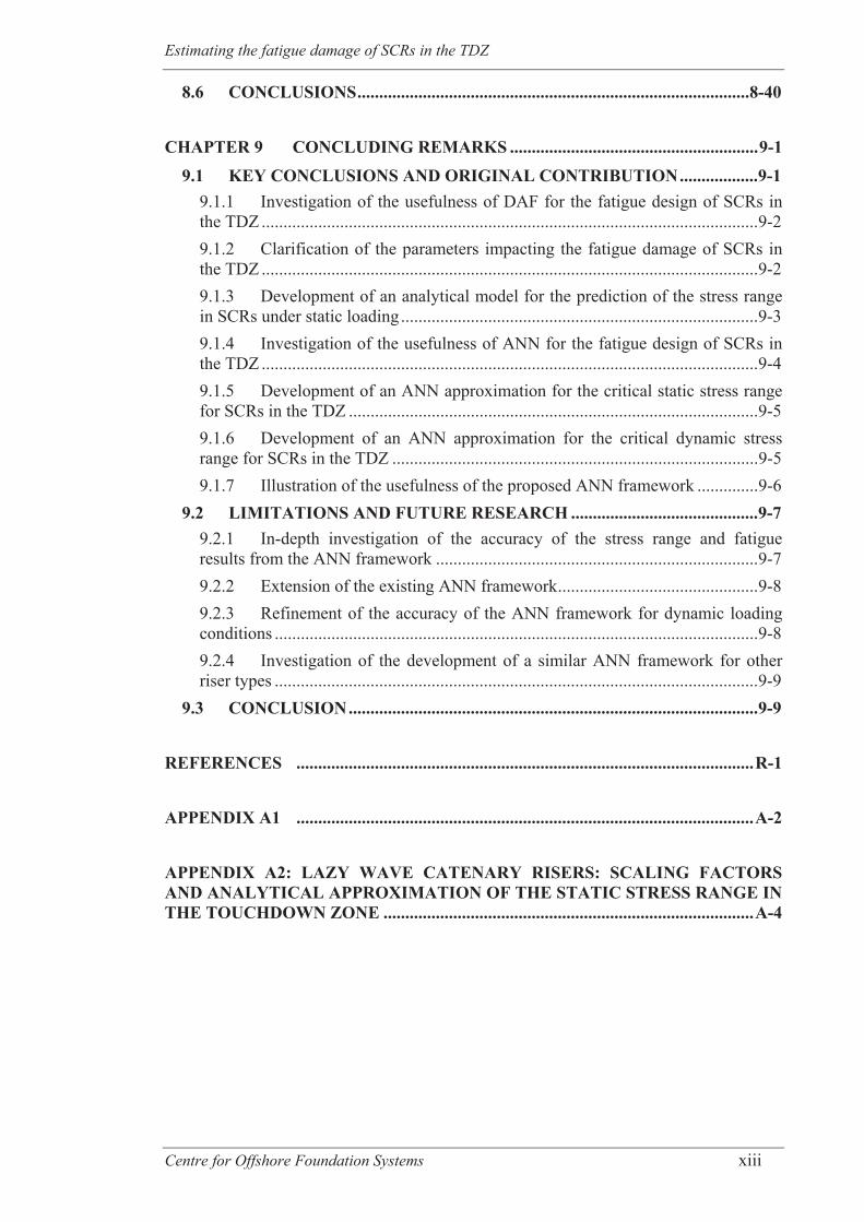
CHAPTER 9 CONCLUDING REMARKS ......................................................... 9-19.1 KEY CONCLUSIONS AND ORIGINAL CONTRIBUTION .................. 9-1
9.1.1 Investigation of the usefulness of DAF for the fatigue design of SCRs in the TDZ .................................................................................................................. 9-29.1.2 Clarification of the parameters impacting the fatigue damage of SCRs in the TDZ .................................................................................................................. 9-29.1.3 Development of an analytical model for the prediction of the stress range in SCRs under static loading .................................................................................. 9-39.1.4 Investigation of the usefulness of ANN for the fatigue design of SCRs in the TDZ .................................................................................................................. 9-49.1.5 Development of an ANN approximation for the critical static stress range for SCRs in the TDZ .............................................................................................. 9-59.1.6 Development of an ANN approximation for the critical dynamic stress range for SCRs in the TDZ .................................................................................... 9-59.1.7 Illustration of the usefulness of the proposed ANN framework .............. 9-6
9.2 LIMITATIONS AND FUTURE RESEARCH ........................................... 9-79.2.1 In-depth investigation of the accuracy of the stress range and fatigue results from the ANN framework .......................................................................... 9-79.2.2 Extension of the existing ANN framework .............................................. 9-89.2.3 Refinement of the accuracy of the ANN framework for dynamic loading conditions ............................................................................................................... 9-89.2.4 Investigation of the development of a similar ANN framework for other riser types ............................................................................................................... 9-9
9.3 CONCLUSION .............................................................................................. 9-9
REFERENCES ......................................................................................................... R-1
APPENDIX A1 ......................................................................................................... A-2
APPENDIX A2: LAZY WAVE CATENARY RISERS: SCALING FACTORS AND ANALYTICAL APPROXIMATION OF THE STATIC STRESS RANGE IN THE TOUCHDOWN ZONE ..................................................................................... A-4
Estimating the fatigue damage of SCRs in the TDZ
Centre for Offshore Foundation Systems xiv
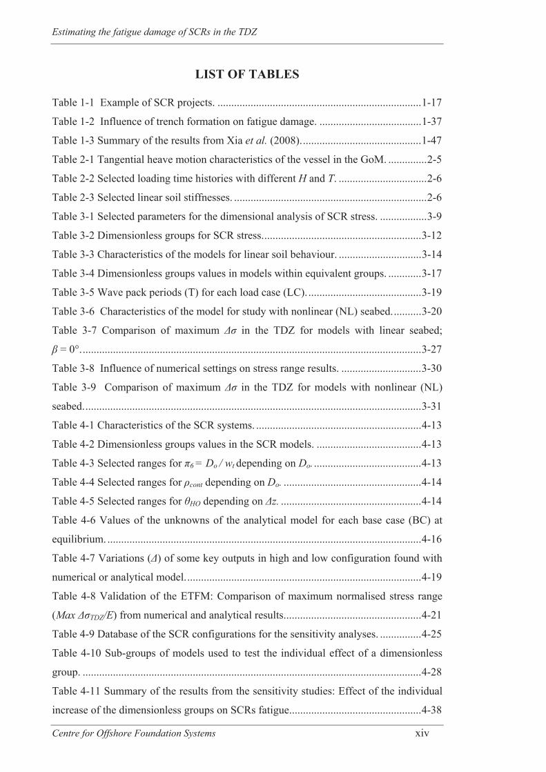
LIST OF TABLES
Table 1-1 Example of SCR projects. .......................................................................... 1-17
Table 1-2 Influence of trench formation on fatigue damage. ..................................... 1-37
Table 1-3 Summary of the results from Xia et al. (2008). ........................................... 1-47
Table 2-1 Tangential heave motion characteristics of the vessel in the GoM. .............. 2-5
Table 2-2 Selected loading time histories with different H and T. ................................ 2-6
Table 2-3 Selected linear soil stiffnesses. ...................................................................... 2-6
Table 3-1 Selected parameters for the dimensional analysis of SCR stress. ................. 3-9
Table 3-2 Dimensionless groups for SCR stress. ......................................................... 3-12
Table 3-3 Characteristics of the models for linear soil behaviour. .............................. 3-14
Table 3-4 Dimensionless groups values in models within equivalent groups. ............ 3-17
Table 3-5 Wave pack periods (T) for each load case (LC). ......................................... 3-19
Table 3-6 Characteristics of the model for study with nonlinear (NL) seabed. .......... 3-20
Table 3-7 Comparison of maximum in the TDZ for models with linear seabed;
= 0°. ........................................................................................................................... 3-27
Table 3-8 Influence of numerical settings on stress range results. ............................. 3-30
Table 3-9 Comparison of maximum in the TDZ for models with nonlinear (NL)
seabed. .......................................................................................................................... 3-31
Table 4-1 Characteristics of the SCR systems. ............................................................ 4-13
Table 4-2 Dimensionless groups values in the SCR models. ...................................... 4-13
Table 4-3 Selected ranges for 6 = Do / wt depending on Do. ....................................... 4-13
Table 4-4 Selected ranges for cont depending on Do. .................................................. 4-14
Table 4-5 Selected ranges for HO depending on z. ................................................... 4-14
Table 4-6 Values of the unknowns of the analytical model for each base case (BC) at
equilibrium. .................................................................................................................. 4-16
Table 4-7 Variations ( ) of some key outputs in high and low configuration found with
numerical or analytical model. ..................................................................................... 4-19
Table 4-8 Validation of the ETFM: Comparison of maximum normalised stress range
(Max TDZ/E) from numerical and analytical results. ................................................. 4-21
Table 4-9 Database of the SCR configurations for the sensitivity analyses. ............... 4-25
Table 4-10 Sub-groups of models used to test the individual effect of a dimensionless
group. ........................................................................................................................... 4-28
Table 4-11 Summary of the results from the sensitivity studies: Effect of the individual
increase of the dimensionless groups on SCRs fatigue. ............................................... 4-38
Estimating the fatigue damage of SCRs in the TDZ
Centre for Offshore Foundation Systems xv
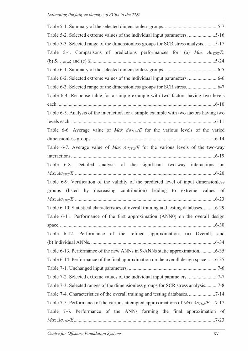
Table 5-1. Summary of the selected dimensionless groups. .......................................... 5-7
Table 5-2. Selected extreme values of the individual input parameters. ..................... 5-16
Table 5-3. Selected range of the dimensionless groups for SCR stress analysis. ........ 5-17
Table 5-4. Comparisons of predictions performances for: (a) Max TDZ/E;
(b) Sn_critical; and (c) St. .................................................................................................. 5-24
Table 6-1. Summary of the selected dimensionless groups. .......................................... 6-5
Table 6-2. Selected extreme values of the individual input parameters. ....................... 6-6
Table 6-3. Selected range of the dimensionless groups for SCR stress. ........................ 6-7
Table 6-4. Response table for a simple example with two factors having two levels
each. ............................................................................................................................. 6-10
Table 6-5. Analysis of the interaction for a simple example with two factors having two
levels each. ................................................................................................................... 6-11
Table 6-6. Average value of Max TDZ/E for the various levels of the varied
dimensionless groups. .................................................................................................. 6-14
Table 6-7. Average value of Max TDZ/E for the various levels of the two-way
interactions. .................................................................................................................. 6-19
Table 6-8. Detailed analysis of the significant two-way interactions on
Max TDZ/E. ................................................................................................................ 6-20
Table 6-9. Verification of the validity of the predicted level of input dimensionless
groups (listed by decreasing contribution) leading to extreme values of
Max TDZ/E. ................................................................................................................ 6-23
Table 6-10. Statistical characteristics of overall training and testing databases. ......... 6-29
Table 6-11. Performance of the first approximation (ANN0) on the overall design
space. ............................................................................................................................ 6-30
Table 6-12. Performance of the refined approximation: (a) Overall; and
(b) Individual ANNs. ................................................................................................... 6-34
Table 6-13. Performance of the new ANNs in 9-ANNs static approximation. ........... 6-35
Table 6-14. Performance of the final approximation on the overall design space. ...... 6-35
Table 7-1. Unchanged input parameters. ....................................................................... 7-6
Table 7-2. Selected extreme values of the individual input parameters. ....................... 7-7
Table 7-3. Selected ranges of the dimensionless groups for SCR stress analysis. ........ 7-8
Table 7-4. Characteristics of the overall training and testing databases. ..................... 7-14
Table 7-5. Performance of the various attempted approximations of Max TDZ/E. ... 7-17
Table 7-6. Performance of the ANNs forming the final approximation of
Max TDZ/E ................................................................................................................. 7-23
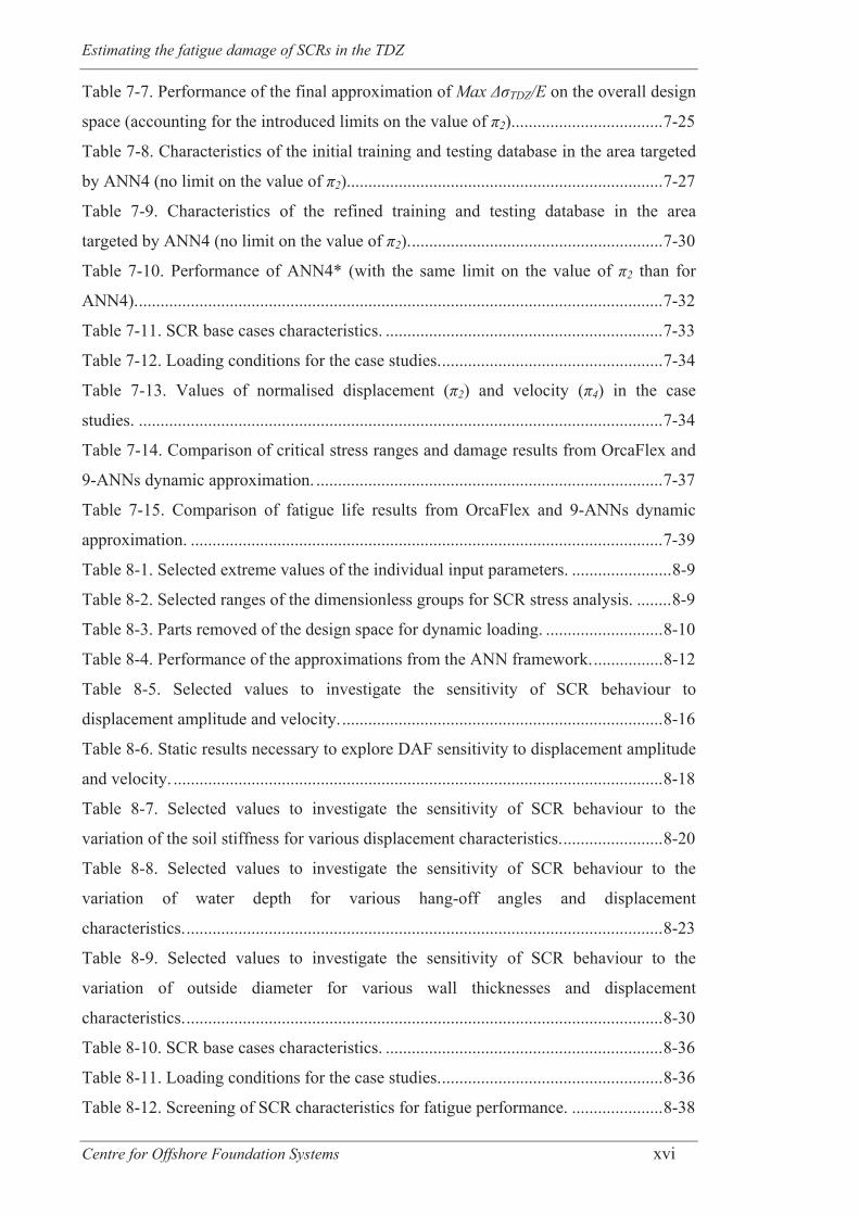
Estimating the fatigue damage of SCRs in the TDZ
Centre for Offshore Foundation Systems xvi
Table 7-7. Performance of the final approximation of Max TDZ/E on the overall design
space (accounting for the introduced limits on the value of 2). .................................. 7-25
Table 7-8. Characteristics of the initial training and testing database in the area targeted
by ANN4 (no limit on the value of 2)......................................................................... 7-27
Table 7-9. Characteristics of the refined training and testing database in the area
targeted by ANN4 (no limit on the value of 2). .......................................................... 7-30
Table 7-10. Performance of ANN4* (with the same limit on the value of 2 than for
ANN4). ......................................................................................................................... 7-32
Table 7-11. SCR base cases characteristics. ................................................................ 7-33
Table 7-12. Loading conditions for the case studies. ................................................... 7-34
Table 7-13. Values of normalised displacement ( 2) and velocity ( 4) in the case
studies. ......................................................................................................................... 7-34
Table 7-14. Comparison of critical stress ranges and damage results from OrcaFlex and
9-ANNs dynamic approximation. ................................................................................ 7-37
Table 7-15. Comparison of fatigue life results from OrcaFlex and 9-ANNs dynamic
approximation. ............................................................................................................. 7-39
Table 8-1. Selected extreme values of the individual input parameters. ....................... 8-9
Table 8-2. Selected ranges of the dimensionless groups for SCR stress analysis. ........ 8-9
Table 8-3. Parts removed of the design space for dynamic loading. ........................... 8-10
Table 8-4. Performance of the approximations from the ANN framework. ................ 8-12
Table 8-5. Selected values to investigate the sensitivity of SCR behaviour to
displacement amplitude and velocity. .......................................................................... 8-16
Table 8-6. Static results necessary to explore DAF sensitivity to displacement amplitude
and velocity. ................................................................................................................. 8-18
Table 8-7. Selected values to investigate the sensitivity of SCR behaviour to the
variation of the soil stiffness for various displacement characteristics. ....................... 8-20
Table 8-8. Selected values to investigate the sensitivity of SCR behaviour to the
variation of water depth for various hang-off angles and displacement
characteristics. .............................................................................................................. 8-23
Table 8-9. Selected values to investigate the sensitivity of SCR behaviour to the
variation of outside diameter for various wall thicknesses and displacement
characteristics. .............................................................................................................. 8-30
Table 8-10. SCR base cases characteristics. ................................................................ 8-36
Table 8-11. Loading conditions for the case studies. ................................................... 8-36
Table 8-12. Screening of SCR characteristics for fatigue performance. ..................... 8-38
Estimating the fatigue damage of SCRs in the TDZ
Centre for Offshore Foundation Systems xvii
LIST OF FIGURES Figure 1-1. Example of SCR configuration ................................................................... 1-1
Figure 1-2. Thesis organisation chart ............................................................................. 1-5
Figure 1-3. The increasing trend in deep water production (Total, 2014) ................... 1-12
Figure 1-4. Deep water reserves in billions of barrels (Total, 2014) ........................... 1-13
Figure 1-5. Deep water developments (BBC, 2010) .................................................... 1-13
Figure 1-6. Schematic representation of a SCR ........................................................... 1-16
Figure 1-7. Example of riser types derived from the standard SCR: (a) Lazy S; (b) Lazy
wave; (c) Steep S; (d) Steep wave; and (e) Compliant vertical access (Bai, 2001;
Martins et al., 2013) ..................................................................................................... 1-19
Figure 1-8. Floater motions (Kongsberg, 2014) .......................................................... 1-20
Figure 1-9. Example of RAOs for a semisubmersible (OrcaFlex, 2014) ..................... 1-21
Figure 1-10. Touchdown point (TDP) movements (Thethi and Moros, 2001) ............ 1-21
Figure 1-11. Trench characteristics: (a) Definitions; (b) Shape of the end of the trench
near the trench mouth; (c) Shape of the trench mouth; (d) Shape of the trench in buried
zone; and (e) Shape of the trench near the surface zone (Bridge and Howells, 2007) 1-25
Figure 1-12. Variation of first order fatigue damage with elastic seabed stiffness (Thethi
and Moros, 2001) ......................................................................................................... 1-30
Figure 1-13. Scheme of the trend in the riser-soil interaction research ....................... 1-31
Figure 1-14. Soil model penetration modes (Randolph and Quiggin, 2009) ............... 1-33
Figure 1-15. Nonlinear soil model characteristics for different modes (Randolph and
Quiggin, 2009) ............................................................................................................. 1-34
Figure 1-16. Trench out of plane profile (Bridge and Howells, 2007) ........................ 1-35
Figure 1-17. One-sided trench model (Bridge and Howells, 2007) ............................. 1-35
Figure 1-18. Scheme of the simplest analytical model (Lenci and Callegari, 2005) ... 1-41
Figure 1-19. Scheme of the “elastic soil and cable” model from Lenci and Callegari
(2005) ........................................................................................................................... 1-42
Figure 1-20. Scheme of the “beam and cable” model from Lenci and Callegari
(2005) ........................................................................................................................... 1-43
Figure 2-1. 2D view of the SCR model.......................................................................... 2-4
Figure 2-2. Schematic view of a typical loading time history ....................................... 2-6
Figure 2-3. along the riser for WP3 and WP13 in loading time history number 2 and
Base Case model ............................................................................................................ 2-8
Figure 2-4. in the TDZ for WP3 and WP13 in loading time history number 2 and
Estimating the fatigue damage of SCRs in the TDZ
Centre for Offshore Foundation Systems xviii
Base Case model ............................................................................................................ 2-8
Figure 2-5. Maximum stress ranges in the TDZ versus tangential heave amplitudes (in
Base Case model) ......................................................................................................... 2-11
Figure 2-6. Maximum stress ranges in the TDZ versus tangential heave amplitudes for
realistic vessel motions ................................................................................................ 2-11
Figure 2-7. DAF versus tangential heave amplitudes (in Base Case model) ............... 2-12
Figure 2-8. DAF versus tangential heave amplitudes for realistic vessel motions ...... 2-12
Figure 2-9. Max TDZ for different soil stiffnesses: (a) H = 0.1 m; (b) H = 0.6 m; (c) H
= 3 m; (d) H = 5 m; (e) H = 8 m; and (f) H = 13 m ..................................................... 2-14
Figure 2-10. DAF curves for different soil stiffnesses: (a) H = 0.1 m; (b) H = 0.6 m; (c)
H = 3 m; (d) H = 5 m; (e) H = 8 m; and (f) H = 13 m ................................................. 2-15
Figure 3-1 SCR geometry and key parameters: (a) Side view of SCR configuration; (b)
Riser cross-section; and (c) One cycle of sinusoidal input motion ................................ 3-8
Figure 3-2 SCR shapes in (a) Equivalent group 1; (b) Equivalent group 2; and (c)
Equivalent group 3 ....................................................................................................... 3-17
Figure 3-3 Normalised SCR shapes in (a) Equivalent group 1; (b) Equivalent group 2;
and (c) Equivalent group 3 ........................................................................................... 3-21
Figure 3-4 Declination results for Equivalent group 1: (a) Normalised time,
18 = 0.25; (b) Normalised time, 18 = 0.75; and (c) Normalised arc length, Sn = 0 .... 3-23
Figure 3-5 Dimensional analysis results for (a) Equivalent group 1; (b) Equivalent
group 2; and (c) Equivalent group 3: Comparison of normalised stress during one cycle
of motion; = 0° and 16 = 0 ....................................................................................... 3-24
Figure 3-6 Normalised stress range distributions for (a) Equivalent group 1; (b)
Equivalent group 2; and (c) Equivalent group 3; = 0° .............................................. 3-26
Figure 3-7 Seabed responses at TDP for nonlinear soil model ................................... 3-31
Figure 3-8 Normalised trench profiles for nonlinear soil model ................................ 3-31
Figure 3-9 Normalised linear soil stiffness ( 11) effect on dynamic amplification;
= 0° ............................................................................................................................ 3-33
Figure 4-1 Scheme of the three-fields model proposed by Lenci and Callegari
(2005) ............................................................................................................................ 4-7
Figure 4-2 Characteristics of the input displacement: (a) One cycle of sinusoidal input
motion; and (b) Scheme of the simplification of the displacement at the hang-off point
(HOP) on the example of the “high” configuration ....................................................... 4-9
Figure 4-3 Flowchart for the pre-processing and postprocessing of OrcaFlex
models .......................................................................................................................... 4-14
Estimating the fatigue damage of SCRs in the TDZ
Centre for Offshore Foundation Systems xix
Figure 4-4 Normalised SCR shapes for the three base cases (BCs): (a) Global view;
(b) Zoom around the HOP; and (c) Zoom around the TDP ......................................... 4-15
Figure 4-5 Comparison of the normalised shapes: (a) BC1; (b) BC2; and (c) BC3 .... 4-17
Figure 4-6 Comparison of the normalised stresses for BC1 at equilibrium: (a) Direct
tensile stress, a; (b) Normalised bending stress, | m|; and (c) Axial stress, t ............ 4-17
Figure 4-7 Comparison of the normalised stresses for BC2 at equilibrium: (a) Direct
tensile stress, a; (b) Normalised bending stress, | m|; and (c) Axial stress, t ........... 4-18
Figure 4-8 Comparison of the normalised stresses for BC3 at equilibrium: (a) Direct
tensile stress, a; (b) Normalised bending stress, | m|; and (c) Axial stress, t ............ 4-18
Figure 4-9 Comparison of the displaced and equilibrium normalised shape in the TDZ:
(a) BC1; (b) BC2; and (c) BC3 .................................................................................... 4-19
Figure 4-10 Comparison of distribution of the normalised stress range, t / E, in the
TDZ: (a) BC1; (b) BC2; and (c) BC3 .......................................................................... 4-21
Figure 4-11 Results from the sensitivity analyses using the analytical model (ETFM):
Effect of (a) 2 = H/ z; (b) 5 = Do/ z; (c) 6 = Do / wt; (d) 7 = p / (E z); (e) To_catenary
/ (E z2); (f) π11 = ks / E ; and (g) 15 = g z steel / E ................................................... 4-32
Figure 4-12 Relative sensitivity of the three groups of SCR configurations: (a) 2;
(b) 5; (c) 6; (d) 7; (e) 9; (f) 11; and (g) 15 ............................................................ 4-36
Figure 5-1 SCR geometry and key parameters: (a) Side view of SCR configuration; and
(b) Riser cross-section (Quéau et al., 2013) ................................................................... 5-6
Figure 5-2 Architecture of the one hidden layer backpropagation neural network used in
this study ...................................................................................................................... 5-11
Figure 5-3 Flowchart for the use of the trained artificial neural network based on
modeFRONTIER calculations ..................................................................................... 5-13
Figure 5-4 Flowchart of the sensitivity analyses ......................................................... 5-14
Figure 5-5 Scatter plot for the input dimensionless groups ......................................... 5-20
Figure 5-6 Correlation between OrcaFlex results and response surface predictions of the
value of: (a) Max TDZ/E ; (b) Sn_critical and (c) St using (1) a polynomial fit, (2) an ANN
and (3) the catenary equation (if appropriate) .............................................................. 5-23
Figure 6-1 SCR geometry and key parameters: (a) Side view of SCR configuration; and
(b) Riser cross-section (Quéau et al., 2013) ................................................................... 6-6
Figure 6-2 Example of response graph ........................................................................ 6-10
Figure 6-3 Example of interaction graph .................................................................... 6-12
Figure 6-4 Effect of the dimensionless groups ........................................................... 6-15
Figure 6-5 Effects of the dimensionless groups and their two-way interactions on
Estimating the fatigue damage of SCRs in the TDZ
Centre for Offshore Foundation Systems xx
variation of Max TDZ/E ............................................................................................. 6-21
Figure 6-6 Detailed analysis of the two-way interactions with notable contributions . 6-22
Figure 6-7 Scatter plot of selected cases: (a) Individual dimensionless groups; and
(b) Two-way interactions ............................................................................................. 6-26
Figure 6-8 Structure of the approximation using nine ANNs ...................................... 6-32
Figure 6-9 Example of design charts showing the sensitivity of Max TDZ/E_approx to
variations of (1) 2,(2) 9 and (3) 11 for various 15 values corresponding to: (a) z
between 400 m and 950- m; (b) z between 950+ m and 1500- m and (c) z between
1500+ m and 2000 m .................................................................................................... 6-37
Figure 7-1 Flowchart of the automation subroutine for dynamic loading conditions ... 7-4
Figure 7-2 SCR geometry and key parameters: (a) Side view of SCR configuration; and
(b) Riser cross-section (Quéau et al., 2013)................................................................... 7-5
Figure 7-3 Scatter plot of selected cases: (a) Individual dimensionless groups; and
(b) Pairs of dimensionless groups ................................................................................ 7-12
Figure 7-4 Structure of the 9-ANNs dynamic approximation ..................................... 7-21
Figure 7-5 Scatter plot of the cases selected initially (in blue) and the additional cases
(in red) in the area targeted by ANN4: (a) Individual dimensionless groups; and
(b) Pairs of dimensionless groups ................................................................................ 7-28
Figure 8-1 SCR geometry and key parameters: (a) Side view of SCR configuration; and
(b) Riser cross-section (Quéau et al., 2013)................................................................... 8-5
Figure 8-2 Flowchart of the ANN framework ............................................................... 8-5
Figure 8-3 Sensitivity of Max TDZ_dyn / E to the variation of the loading amplitude ( 2)
and velocity ( 4), accounting for the design criteria between H and T:
(a) 0.1 m ≤ H < 1 m; (b) 1 m ≤ H < 3.5 m; (c) 3.5 m ≤ H < 5.5 m;
and (d) 5.5 m ≤ H ≤ 7.5 m ............................................................................................ 8-17
Figure 8-4 Sensitivity of DAF to the variation of the loading amplitude ( 2) and velocity
( 4), accounting for the design criteria between H and T:
(a) 0.1 m ≤ H < 1 m; (b) 1 m ≤ H < 3.5 m; (c) 3.5 m ≤ H < 5.5 m; and
(d) 5.5 m ≤ H ≤ 7.5 m .................................................................................................. 8-18
Figure 8-5 Sensitivity of Max TDZ_dyn / E to the variation of the displacement
velocity ( 4) for various soil stiffnesses ( 11) and displacement amplitudes:
(a) 2 = 0.44E-3; (b) 2 = 1.84E-3; (c) 2 = 3.67E-3; and (d) 2 = 5.31E-3.................. 8-21
Figure 8-6 Sensitivity of DAF to the variation of the displacement velocity ( 4) for
various soil stiffnesses ( 11) and displacement amplitudes: (a) 2 = 0.44E-3;
(b) 2 = 1.84E-3; (c) 2 = 3.67E-3; and (d) 2 = 5.31E-3 ............................................. 8-22
Estimating the fatigue damage of SCRs in the TDZ
Centre for Offshore Foundation Systems xxi
Figure 8-7 Sensitivity of Max TDZ_sta / E to the variation of the water depth ( 15) for
various hang-off angles ( HO) and displacement characteristics: (a) H = 0.55 m;
(b) H = 2.25 m; (c) H = 4.50 m; and (d) H = 6.50 m ................................................... 8-24
Figure 8-8 Sensitivity of Max TDZ_dyn / E to the variation of the water depth ( 15) for
various hang-off angles ( HO) and displacement characteristics: (a) H = 0.55 m and
T = 12 s; (b) H = 2.25 m and T = 13.5 s; (c) H = 4.50 m and T = 15 s; and
(d) H = 6.50 m and T = 16.5 s ...................................................................................... 8-25
Figure 8-9 Sensitivity of DAF to the variation of the water depth ( 15) for various hang-
off angles ( HO) and displacement characteristics: (a) H = 0.55 m and T = 12 s;
(b) H = 2.25 m and T = 13.5 s; (c) H = 4.50 m and T = 15 s;
and (d) H = 6.50 m and T = 16.5 s ............................................................................... 8-27
Figure 8-10 Sensitivity of Max TDZ_sta / E to the variation of outside diameter (Do) for
various wall thicknesses (wt) and displacement characteristics: (a) H = 0.55 m;
(b) H = 2.25 m; (c) H = 4.50 m; and (d) H = 6.50 m ................................................... 8-32
Figure 8-11 Sensitivity of Max TDZ_dyn / E to the variation of outside diameter (Do) for
various wall thicknesses (wt) and displacement characteristics: (a) H = 0.55 m and
T = 12 s; (b) H = 2.25 m and T = 13.5 s; (c) H = 4.50 m and T = 15 s;
and (d) H = 6.50 m and T = 16.5 s ............................................................................... 8-33
Figure 8-12 Sensitivity of DAF to the variation of outside diameter (Do) for various wall
thicknesses (wt) and displacement characteristics: (a) H = 0.55 m and T = 12 s;
(b) H = 2.25 m and T = 13.5 s; (c) H = 4.50 m and T = 15 s; and (d) H = 6.50 m and
T = 16.5 s ...................................................................................................................... 8-34

Estimating the fatigue damage of SCRs in the TDZ
Centre for Offshore Foundation Systems xxii
NOMENCLATURE
a Penetration resistance parameter in Chapter 3 and parameter of S-N curve in Chapter 1
Ai, Ao Internal and external cross section areas b Penetration resistance parameter b1 Bias on hidden unit of an ANN b2 Bias on output unit of an ANN c1 to c12 Unknown in the TFM and ETFM CA Added mass coefficient CAn Normal added mass coefficient CAa Axial added mass coefficient CAa buoyc Axial added mass coefficient of buoyancy catenary CAn buoyc Normal added mass coefficient of buoyancy catenary CD Drag coefficient CDa Axial drag coefficient CDa buoyc Axial drag coefficient of buoyancy catenary CDn Normal drag coefficient CDn buoyc Normal drag coefficient of buoyancy catenary d Damage for individual sea state Df Diameter of floater Di Inside diameter Do Outer diameter E Young’s modulus f , fi General notation for functions fb Soil buoyancy factor fsuc Suction resistance ratio g Gravity acceleration h Displacement
H Heave amplitude (also referred to as tangential heave amplitude in Chapter 2)
I Second moment of area k Curvature ks Soil stiffness K Nondimensional soil rigidity parameter Kmax Normalised maximum stiffness Lf Length of floater LevelA , Level B Level of factor A and B LevelA x B Level of the interaction between factor A and B
L1 or L1_eq Horizontal distance between TDP and BLE at equilibrium in the TFM and ETFM
L2 or L2_eq Horizontal distance between BLE and HOP at equilibrium in the TFM and ETFM
L1_disp Horizontal distance between TDP and BLE in displaced configuration in the TFM and ETFM
L2_disp Horizontal distance between BLE and HOP in displaced configuration in the TFM and ETFM
m Parameter of S-N curve min, max General notation for minimum and maximum M Bending moment Mmax Maximum bending moment
Estimating the fatigue damage of SCRs in the TDZ
Centre for Offshore Foundation Systems xxiii
Approximated bending moment in the TFM and ETFM
M1 Bending moment in the zone where the riser is in contact with the seabed in the TFM and ETFM
M2 Bending moment in the boundary layer zone in the TFM and ETFM
Max TDZ General notation for the maximum axial stress range occurring in the TDZ regardless of loading condition (or Max zz TDZ in Appendix A2)
Max TDZ_sta , Max TDZ dyn
Maximum axial stress range occurring in the touchdown zone under static and dynamic loading.
Max TDZ /E General notation of maximum strain occurring in the TDZ
Max TDZ/E ¯¯¯¯¯¯¯¯¯¯¯ Average value of Max TDZ /E
Max TDZ /E_ANN Maximum strain occurring in the TDZ approximated with an ANN
Max TDZ /E_approx General notation for an approximation of Max TDZ /E
Max TDZ /E_OrcaFlex Maximum strain occurring in the TDZ calculated in OrcaFlex
Max TDZ /E_Polynomial fit Maximum strain occurring in the TDZ approximated with a polynomial fit
MinInput , MaxInput Vectors with minimum and maximum values of the inputs for training an ANN
MinOutput , MaxOutput Minimum and maximum values of the output in training set of an ANN
n Number of occurrence of a sea state n1 Net input signal of the hidden unit of an ANN n2 Net input signal of the output unit of an ANN N Number of cycles of loading to failure NI Number of inputs of an ANN NLevel A , NLevel B Number of level for factor A and B Nn Number of neurons in the hidden layer of an ANN p Unit submerged weight pbuoyc Unit submerged weight of buoyancy catenary Pf Pitch between centre of floater Pi, Po Internal and external pressures Q1 General notation of an output Q2, ..., Qn General notation of inputs Rc Concentrated reaction force at the TDP s Arc length su Shear strength sum Soil undrained shear strength at mudline S Shear force
Approximated shear force in the TFM and ETFM
Sblt or Sblt_eq Total length of the boundary layer zone at equilibrium in the TFM and ETFM
Sblt_disp Total length of the boundary layer zone in displaced configuration in the TFM and ETFM
Sbuoyct Total length of buoyancy catenary in the TFM and ETFM
Scritical Arc length of Max TDZ measured from the HOP
Sct or Sct_eq Total length of catenary at equilibrium in the TFM and ETFM
Estimating the fatigue damage of SCRs in the TDZ
Centre for Offshore Foundation Systems xxiv
Sct_disp Total length of catenary in displaced configuration in the TFM and ETFM
Shoct Total length of hang-off catenary in the TFM and ETFM Sn Normalised arc length
Sn_critical General notation for the normalised arc length of Max
TDZ
Sn_critical_ANN Normalised arc length of Max TDZ approximated with an ANN
Sn_critical_OrcaFlex Normalised arc length of Max TDZ calculated with OrcaFlex
Sn_critical_Polynomial fit Normalised arc length of Max TDZ approximated with a polynomial fit
St General notation for the arc length to TDP at equilibrium
St_ANN Arc length to TDP at equilibrium approximated with an ANN
St OrcaFlex Arc length to TDP at equilibrium assessed in OrcaFlex
St_Polynomial fit Arc length to TDP at equilibrium approximated with a polynomial fit
S1 Shear force in the zone where the riser is in contact with the seabed in the TFM and ETFM
S2 Shear force in the boundary layer zone in the TFM and ETFM
t Time T Cyclic period
Approximated effective tension in the TFM and ETFM
TBLE Constant traction on the laid beam in the TFM and ETFM
Te Effective tension To General notation for the horizontal tension component
To_catenary Horizontal tension component calculated through a standard catenary equation
To OrcaFlex Horizontal tension component assessed in OrcaFlex Tw Wall tension TDPdisp TDP in displaced configuration in the TFM and ETFM TDPeq TDP at equilibrium in the TFM and ETFM V Shear force Vmax Maximum shear force at equilibrium wi General notation of the weights of an ANN in Chapter 5 wt Wall thickness
w1 Vertical downward displacement in the section in contact with the soil or weights from the input unit to the hidden unit in Chapter 5
w2 Vertical upward displacement in boundary layer or weights from the hidden unit to the output unit in Chapter 5
WPdyn Wave pack with motion period of T, tangential heave amplitude of H, in a model with soil stiffness of ks
WPsta Wave pack with motion period of 1000 s, tangential heave amplitude of H, in a model with soil stiffness of ks
x, x1 to x5 Horizontal distances measured from TDPeq in the TFM and ETFM
Estimating the fatigue damage of SCRs in the TDZ
Centre for Offshore Foundation Systems xxv
xHOP_eq , xHOP_disp Horizontal coordinate of the HOP at equilibrium and in displaced configuration in the TFM and ETFM
xdisp Horizontal distance measured from TDPdisp in the TFM and ETFM
X Vector of inputs for training an ANN Xi General notation of the inputs of an ANN
Xn Normalised horizontal coordinate or normalised vector of inputs for training an ANN in Chapter 5
Xt General notation for the horizontal offset to TDP at equilibrium
Xt_High , Xt_Low Horizontal offset to TDP in high and low configuration in the ETFM
Xt_OrcaFlex Horizontal offset to TDP at equilibrium assessed in OrcaFlex
ybuoyc Vertical displacement in buoyancy catenary yhoc Vertical displacement in hang-off catenary yn Normalised output signal of an ANN ytdc Vertical displacement in touchdown catenary y1 Output signal sent to output unit of an ANN z Elevation from the seabed
zdisp Elevation from the seabed in displaced configuration in the TFM and ETFM
ZHOP Depth of HOP below the sea surface
zHOP_eq, zHOP_disp Vertical coordinate of the HOP at equilibrium and in displaced configuration in the TFM and ETFM
Zn Normalised vertical coordinate
Scale factor in Chapter 3, parameter of the TFM in Chapter 4 and Appendix A2
Angular position on the SCR circumference for stress checking
1 Parameter of the TFM and ETFM , 1, 2 Unknown in the TFM and ETFM General notation of a variation
hx , hz Horizontal and vertical component of the imposed displacement in the TFM and ETFM
Mmax Variation between the maximum values of bending moment in the TDZ during a cycle of loading
Sblt Variation of the total length of the boundary layer zone under a cycle of static loading in the ETFM
St Variation of arc length to TDP under a cycle of static loading in the ETFM
Stdct Variation of the total length of the touchdown catenary under a cycle of static loading in the ETFM
Stress range (or zz in Appendix A2)
T Variation of the horizontal component of the tension under a cycle of static loading in the ETFM
HO Variation of the hang-off angle under a cycle of static loading in the ETFM
xTDP Maximum TDP relocation under a cycle of loading m Motion direction relative to the hang-off angle
Xt Variation of the horizontal offset to TDP under a cycle of static loading in the ETFM
Estimating the fatigue damage of SCRs in the TDZ
Centre for Offshore Foundation Systems xxvi
z Vertical difference between HOP and seabed
Z_disp V Vertical difference between HOP and seabed in a displaced configuration in the ETFM
Parameter of the TFM and ETFM Characteristic length rep Normalised repenetration offset after uplift suc Normalised suction decay distance μ Friction coefficient Poisson’s ratio SCR angle from the vertical m Angle of the motion (with the vertical) HO Hang-off angle HO disp Hang-off angle in displaced configuration in the ETFM
* SCR angle from the vertical for x = L1 in the TFM and ETFM
i General notation for dimensionless groups Soil undrained shear strength gradient cont Density of riser content soil Saturated soil density steel Density of steel water Water density Axial stress or general notation for stresses in Chapter 4 a Direct tensile stress
high , low General notation for stresses in high and low configuration in the ETFM
m Bending stress (or M in Appendix A2)
max , min Maximum and minimum stress occurring at a given location during one cycle of motion
t Axial stress in Chapter 4 (or zz in Appendix A2)
Estimating the fatigue damage of SCRs in the TDZ
Centre for Offshore Foundation Systems xxvii
ABBREVIATIONS
ANN Artificial neural network ANOM Analysis of mean BC Base case BLE Boundary layer end boe Barrels of oil equivalent C Case CARISIMA Catenary riser/soil interaction model for global riser analysis COFS Centre for Offshore Foundation Systems DAF Dynamic amplification factor DoE Design of experiment DP Drag point ETFM Extended three-fields model FE Finite element FPSO Floating production storage and offloading unit G Group GoM Gulf of Mexico HCR Highly compliant rigid HOP Hang-off point JIP Joint industry project LC Load case LP Lift point LWR Lazy wave riser MAE Mean absolute error MT Model test NL Nonlinear RAO Response amplitude operator RMSE Root mean squared error ROV Remotely operated vehicle RSM Response surface method SCR Steel catenary riser STRIDE Steel risers for deep water environments TDP Touchdown point TDZ Touchdown zone TFM Three-fields model UWA University of Western Australia VIV Vortex induced vibration WP Wave pack WoA West of Africa


Estimating the fatigue damage of SCRs in the TDZ
Centre for Offshore Foundation Systems 1-1
CHAPTER 1 INTRODUCTION
1.1 STEEL CATENARY RISERS: A SOLUTION TO DEEP WATER
EXPLORATION
Since the early 1990s, oil and gas exploration and production have increased and have
moved into deeper waters, nowadays reaching depths greater than 2000 m. Deep water
reservoirs are thought to contain an estimated 6% to 7% of the resources of
hydrocarbons worldwide, which represents the global consumption of barrels over five
to seven years (Total, 2014; BP, 2014). Ocean deeps are a hostile environment with
high pressure levels and very low temperatures that called for technological innovation
from the oil and gas industry to provide suitable solutions. New types of risers (pipes
used to convey hydrocarbons between subsea facility and floating offshore facility) had
to be developed to replace the conventional flexible risers that were not always a viable
solution in these new ambient conditions. This context led to the emergence of the steel
catenary risers (SCRs) which, as their name indicates, are risers made of steel and with
a catenary shape. An illustration of a typical SCR is shown in Figure 1-1.
Figure 1-1. Example of SCR configuration

Chapter 1: Introduction
Centre for Offshore Foundation Systems 1-2
The first SCR was installed in 1994 in the Gulf of Mexico in a water depth of 872 m,
hanging from the Auger tension leg platform (Mekha, 2001). SCRs are simple to install
and connect with other subsea facilities (Howells, 1995; Serta et al., 1996) and are
regarded as one of the most cost effective option among the various riser concepts. For
instance, using SCRs instead of flexible risers led to cost savings of around US 70
million in the Marlim and Albacora Fields (Serta et al., 1996). Nowadays, SCRs are
very commonly used in deep water.
1.2 THE NEED FOR FURTHER RESEARCH
Different engineering issues exist for SCRs and fatigue design is one of the most
significant challenges. Two critical fatigue areas are generated by vessel motions and
hydrodynamic loading; they are located near the vessel hang-off point (HOP) and in the
touchdown zone (TDZ – the area of riser-soil interaction (Bridge, 2005)) (Sen and
Hesar, 2007; Kimiaei et al., 2010). An accurate estimation of fatigue damage is crucial
as SCR failure can have significant environmental and economic effects. Moreover,
interventions or repairs in deep water are very complex (Campbell, 1999; Bai and Bai,
2005; Fu and Yang, 2010; Total, 2014).
Design uncertainties arise because of a limited understanding of the influence of the
factors contributing to fatigue, like geometry, structural behaviour, environmental
loading and seabed properties for instance. In order to accommodate the unknowns
SCRs are currently designed for fatigue with a factor of safety rated at 10 (Campbell,
1999; Langner, 2003; Abelanet et al., 2013). This high factor of safety highlights a
significant level of uncertainty in the current design guidelines and, hence, signals
possible scope for improvement. Designing SCRs with such a factor of safety may lead
to uneconomical solutions and therefore to higher consumption of resources.

Chapter 1: Introduction
Centre for Offshore Foundation Systems 1-3
In addition, the assessment of SCR fatigue life in the TDZ is made through numerical
simulations that incur considerable computational costs due to the nonlinearities of SCR
systems (Xia et al., 2008; DNV-OS-F201, 2010). Therefore, for the early stages of
design of SCRs a simplified method would be more convenient. The development of a
simple method is indeed encouraged in an existing guideline, although care must be
paid to the loss of accuracy balancing other advantages (DNV-OS-F201, 2010).
1.3 THESIS OBJECTIVES
The main aim of this research is to develop a simplified fatigue analysis and design
framework for the early stages of fatigue design of SCRs in the TDZ, by removing the
need to perform the time consuming numerical analyses traditionally involved in SCR
design. This thesis also intends to increase the general understanding of the static and
dynamic response of SCRs in the TDZ as this will assist the development of a suitable
simplified framework. Getting insights on SCR behaviour will also help the oil and gas
industry to reduce the level of conservatism, hereby providing a more economical
fatigue design for SCRs.
Although seabed modelling plays an important role in the fatigue design of SCRs, most
of the work carried out in the thesis uses a linear soil model. Indeed, considering riser-
soil interaction introduces additional sources of nonlinearity to the SCR system, and
hence additional input parameters, leading to more complex studies and interpretation of
the results. It is therefore outside of the scope of this research to develop a simplified
fatigue design approach using a nonlinear soil model or to propose ameliorations of
seabed modelling.
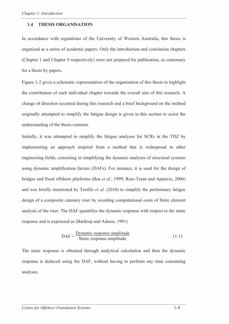
Chapter 1: Introduction
Centre for Offshore Foundation Systems 1-4
1.4 THESIS ORGANISATION
In accordance with regulations of the University of Western Australia, this thesis is
organised as a series of academic papers. Only the introduction and conclusion chapters
(Chapter 1 and Chapter 9 respectively) were not prepared for publication, as customary
for a thesis by papers.
Figure 1-2 gives a schematic representation of the organisation of this thesis to highlight
the contribution of each individual chapter towards the overall aim of this research. A
change of direction occurred during this research and a brief background on the method
originally attempted to simplify the fatigue design is given in this section to assist the
understanding of the thesis contents.
Initially, it was attempted to simplify the fatigue analyses for SCRs in the TDZ by
implementing an approach inspired from a method that is widespread in other
engineering fields, consisting in simplifying the dynamic analyses of structural systems
using dynamic amplification factors (DAFs). For instance, it is used for the design of
bridges and fixed offshore platforms (Bea et al., 1999; Ruiz-Teran and Aparicio, 2006)
and was briefly mentioned by Teofilo et al. (2010) to simplify the preliminary fatigue
design of a composite catenary riser by avoiding computational costs of finite element
analysis of the riser. The DAF quantifies the dynamic response with respect to the static
response and is expressed as (Barltrop and Adams, 1991)
DAF = Dynamic response amplitude
Static response amplitude (1-1)
The static response is obtained through analytical calculation and then the dynamic
response is deduced using the DAF, without having to perform any time consuming
analyses.
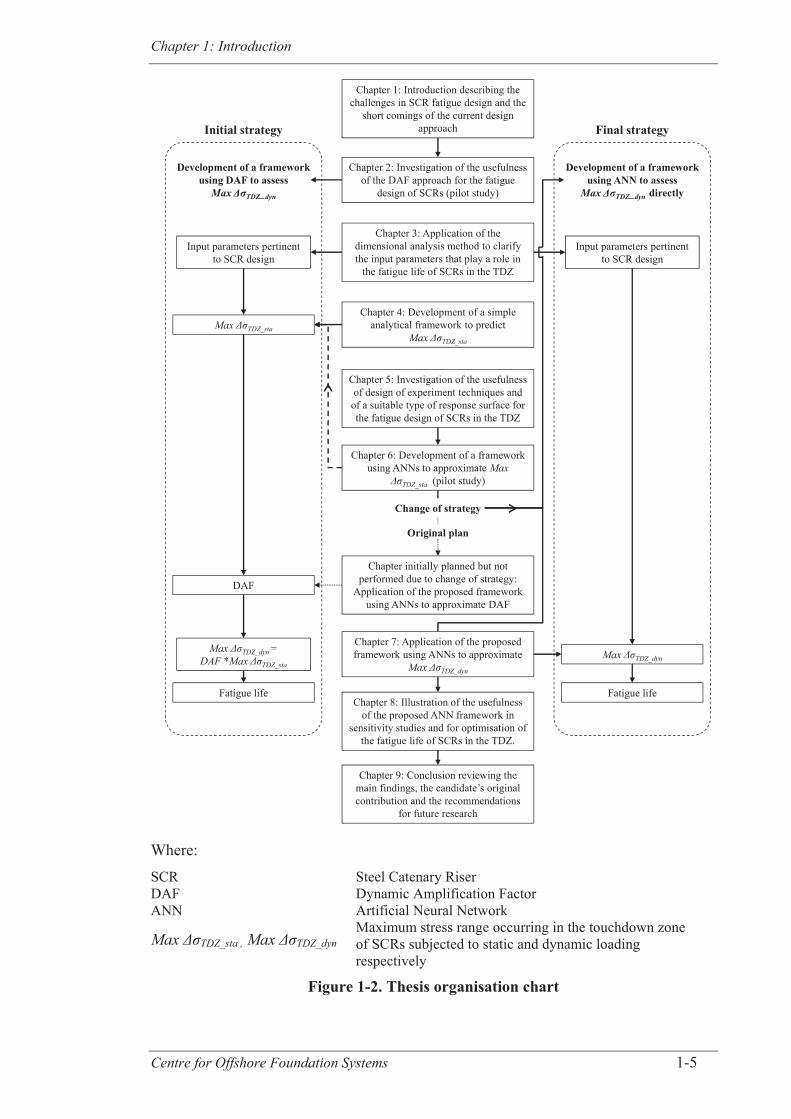
Chapter 1: Introduction
Centre for Offshore Foundation Systems 1-5
Where:
SCR Steel Catenary Riser DAF Dynamic Amplification Factor ANN Artificial Neural Network
Max TDZ_sta , Max TDZ_dyn Maximum stress range occurring in the touchdown zone of SCRs subjected to static and dynamic loading respectively
Figure 1-2. Thesis organisation chart
Chapter 1: Introduction describing the challenges in SCR fatigue design and the
short comings of the current design approach
Chapter 2: Investigation of the usefulness of the DAF approach for the fatigue
design of SCRs (pilot study)
Chapter 3: Application of the dimensional analysis method to clarify the input parameters that play a role in
the fatigue life of SCRs in the TDZ
Chapter 4: Development of a simple analytical framework to predict
Max TDZ_sta
Chapter 5: Investigation of the usefulness of design of experiment techniques and of a suitable type of response surface for the fatigue design of SCRs in the TDZ
Chapter 6: Development of a framework using ANNs to approximate Max
TDZ_sta (pilot study)
Chapter initially planned but not performed due to change of strategy:
Application of the proposed framework using ANNs to approximate DAF
Chapter 9: Conclusion reviewing the main findings, the candidate’s original contribution and the recommendations
for future research
Input parameters pertinent to SCR design
Max TDZ_sta
DAF
Max TDZ_dyn =DAF *Max TDZ_sta
Fatigue life
Chapter 7: Application of the proposed framework using ANNs to approximate
Max TDZ_dyn
Initial strategy
Input parameters pertinent to SCR design
Max TDZ_dyn
Fatigue life
Development of a framework using ANN to assess
Max ΔσTDZ_dyn directly
Development of a framework using DAF to assess
Max ΔσTDZ_dyn
Final strategy
Change of strategy
Original plan
^
Chapter 8: Illustration of the usefulness of the proposed ANN framework in
sensitivity studies and for optimisation of the fatigue life of SCRs in the TDZ.
^

Chapter 1: Introduction
Centre for Offshore Foundation Systems 1-6
Several steps were undertaken to implement the DAF approach for the fatigue design of
SCRs in the TDZ (Chapter 2 to Chapter 6). The fundamental challenge in this approach
is to determine the value of the DAF and Chapter 5 and Chapter 6 report preliminary
steps towards the development of a framework able to fulfil this purpose. However, it
was found in the course of this research that the innovative methods developed with the
intention of predicting the value of DAF could also be applied to the maximum dynamic
stress range in the TDZ without adding more complexity. Since the critical dynamic
stress range controls the fatigue damage, it is also more convenient for future
applications to propose a framework approximating its value directly. To meet the main
research goal, the final strategy implemented in the thesis (Chapter 7) was therefore to
define a simple and efficient framework to assess the critical dynamic stress range in the
TDZ, which is an even simpler approach than the DAF approach attempted initially.
A summary of the work presented in each chapter is outlined below1:
Chapter 1 is the introductory chapter. It explains how the steel catenary riser
technology answers some of the current industry needs and presents the challenges
associated with SCR fatigue design. This chapter shows the objectives of the thesis
and the way it is organised to reach these goals. As the thesis is prepared as a series
of papers, the detailed literature review specific to each chapters is included in the
individual chapters. Nonetheless, a brief literature review is included in this chapter
to give an overview of previous research on structural analysis and fatigue design of
SCR in the TDZ, highlight the shortcomings of the current design approach and
introduce some of the methods used throughout the thesis.
1 For convenience, some of the information is repeated within various chapters since Chapters 2 to 8 were
prepared to stand alone as published papers. Also, self-references to unpublished work (prepared for
publication) have been adjusted to refer here to the unpublished thesis chapter.

Chapter 1: Introduction
Centre for Offshore Foundation Systems 1-7
Chapter 2 is a pilot study published as a peer-reviewed conference paper that
investigates the usefulness of the DAF approach for the fatigue design of SCRs.
DAF, at this stage, is assumed to be a function of the amplitude and period of the
loading and the soil stiffness (neglecting the influence of other input parameters).
The sensitivity of the maximum amplitude of the stress range in the TDZ (which
controls the fatigue life) and of the DAF to the variations of these three key input
parameters is investigated. This chapter indicates that DAF could be a suitable
approach to simplify the fatigue design of SCRs.
Quéau, L.M., Kimiaei, M., Randolph, M.F. (2011). Dynamic amplification factors
for response analysis of steel catenary risers at touch down areas. In: Proceedings of
the 21st International Offshore and Polar Engineering Conference, Hawaii, USA,
vol. II, pp. 1-8. (Chapter 2)
Chapter 3 presents the application of the dimensional analysis method to clarify the
input parameters that play a role in the structural response of SCRs in the TDZ. In
this chapter, published as a journal paper, the complete list of dimensionless groups
is researched and tested through numerical simulations. Various models of SCRs are
scaled to get the same values of dimensionless groups from different values of input
parameters. Normalised static and dynamic loads are applied to the SCR systems and
normalised stress ranges are compared to validate the list of dimensionless groups.
This study provides the basis for the sensitivity studies performed at a later stage in
the thesis.
Quéau, L.M., Kimiaei, M., Randolph, M.F. (2013). Dimensionless groups governing
response of steel catenary risers. Ocean Engineering, Elsevier, 74, pp. 247-259.
(Chapter 3)
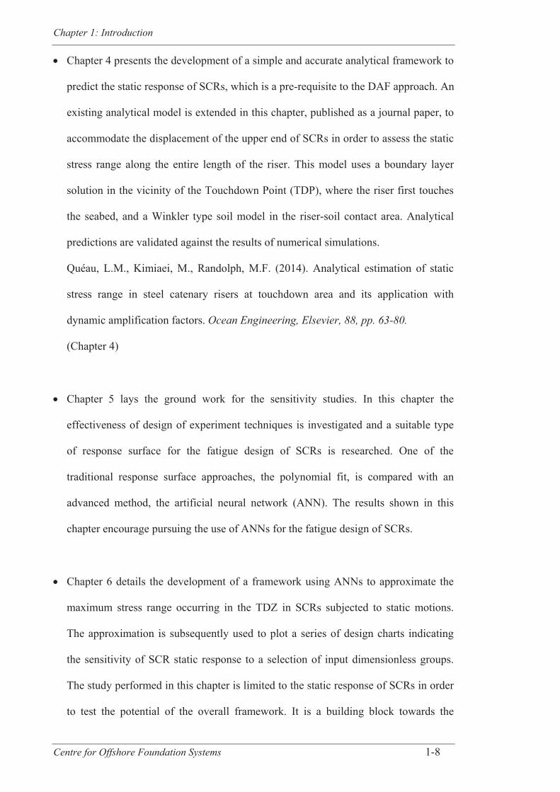
Chapter 1: Introduction
Centre for Offshore Foundation Systems 1-8
Chapter 4 presents the development of a simple and accurate analytical framework to
predict the static response of SCRs, which is a pre-requisite to the DAF approach. An
existing analytical model is extended in this chapter, published as a journal paper, to
accommodate the displacement of the upper end of SCRs in order to assess the static
stress range along the entire length of the riser. This model uses a boundary layer
solution in the vicinity of the Touchdown Point (TDP), where the riser first touches
the seabed, and a Winkler type soil model in the riser-soil contact area. Analytical
predictions are validated against the results of numerical simulations.
Quéau, L.M., Kimiaei, M., Randolph, M.F. (2014). Analytical estimation of static
stress range in steel catenary risers at touchdown area and its application with
dynamic amplification factors. Ocean Engineering, Elsevier, 88, pp. 63-80.
(Chapter 4)
Chapter 5 lays the ground work for the sensitivity studies. In this chapter the
effectiveness of design of experiment techniques is investigated and a suitable type
of response surface for the fatigue design of SCRs is researched. One of the
traditional response surface approaches, the polynomial fit, is compared with an
advanced method, the artificial neural network (ANN). The results shown in this
chapter encourage pursuing the use of ANNs for the fatigue design of SCRs.
Chapter 6 details the development of a framework using ANNs to approximate the
maximum stress range occurring in the TDZ in SCRs subjected to static motions.
The approximation is subsequently used to plot a series of design charts indicating
the sensitivity of SCR static response to a selection of input dimensionless groups.
The study performed in this chapter is limited to the static response of SCRs in order
to test the potential of the overall framework. It is a building block towards the
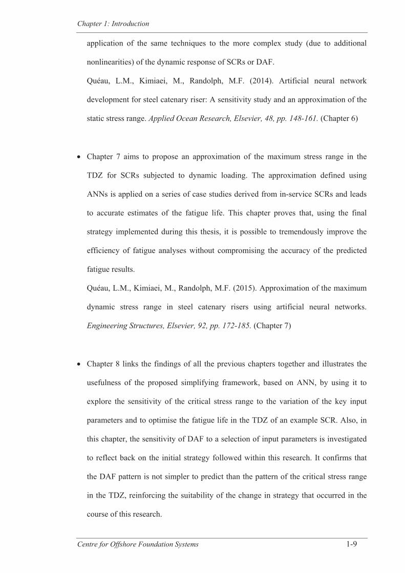
Chapter 1: Introduction
Centre for Offshore Foundation Systems 1-9
application of the same techniques to the more complex study (due to additional
nonlinearities) of the dynamic response of SCRs or DAF.
Quéau, L.M., Kimiaei, M., Randolph, M.F. (2014). Artificial neural network
development for steel catenary riser: A sensitivity study and an approximation of the
static stress range. Applied Ocean Research, Elsevier, 48, pp. 148-161. (Chapter 6)
Chapter 7 aims to propose an approximation of the maximum stress range in the
TDZ for SCRs subjected to dynamic loading. The approximation defined using
ANNs is applied on a series of case studies derived from in-service SCRs and leads
to accurate estimates of the fatigue life. This chapter proves that, using the final
strategy implemented during this thesis, it is possible to tremendously improve the
efficiency of fatigue analyses without compromising the accuracy of the predicted
fatigue results.
Quéau, L.M., Kimiaei, M., Randolph, M.F. (2015). Approximation of the maximum
dynamic stress range in steel catenary risers using artificial neural networks.
Engineering Structures, Elsevier, 92, pp. 172-185. (Chapter 7)
Chapter 8 links the findings of all the previous chapters together and illustrates the
usefulness of the proposed simplifying framework, based on ANN, by using it to
explore the sensitivity of the critical stress range to the variation of the key input
parameters and to optimise the fatigue life in the TDZ of an example SCR. Also, in
this chapter, the sensitivity of DAF to a selection of input parameters is investigated
to reflect back on the initial strategy followed within this research. It confirms that
the DAF pattern is not simpler to predict than the pattern of the critical stress range
in the TDZ, reinforcing the suitability of the change in strategy that occurred in the
course of this research.

Chapter 1: Introduction
Centre for Offshore Foundation Systems 1-10
Quéau, L.M., Kimiaei, M., Randolph, M.F. (2015). Sensitivity studies of steel
catenary riser fatigue damage in the touchdown zone using an efficient simplification
framework for stress range evaluation. Ocean Engineering, Elsevier, 96, pp. 295-
311. (Chapter 8)
Chapter 9 is the conclusion chapter. It reviews the main findings presented in each
chapter, discusses the limitations of the current results and presents some suggestions
for future investigations.
1.5 LITERATURE REVIEW
1.5.1 The need for deep water development
The work performed in this thesis aims at significantly improving the fatigue design of
SCRs, through the development of a simplified design approach and the amelioration of
the knowledge of SCR behaviour. As SCRs were created to suit deep water
requirements, this section gives an explanation of the reasons behind the recent shift of
the oil and gas industry focus from shallow water towards deep water and presents the
challenges that arise in these new water depths.
Most of the world nowadays is fully reliant on a tremendous energy consumption,
whether it is for transportation, heating, plastic production etc... One of the primary
sources of energy comes from hydrocarbons. They are produced over millions of years
through decomposition of organic materials (such as shell fragments, algae, marine
creatures etc…) trapped in underground reservoirs that can be found using seismic data
(Shell, 2014; Woodside, 2014a). To face the ever increasing global demand, the oil and
gas industry has exploited both onshore and offshore reservoirs but the most profitable
and easily accessible resources have already been exhausted or will be exhausted soon.
This awareness has brought industry focus on new reservoirs located offshore in deep

Chapter 1: Introduction
Centre for Offshore Foundation Systems 1-11
water (from 400 m or to 1500 m) and some into even deeper water, the “ultra deep
water”. Indeed, 330 billion barrels of oil equivalent (boe) are believed to lie in these
reservoirs which represent five to seven years of the consumption worldwide (Total,
2014). These reservoirs were ignored in the past due to the technical complexity, the
high risk and the costs involved in their exploration but gained in popularity due to the
depletion of the most readily reachable reservoirs (PR Newswire, 2013).
The conquest of deep water reservoir exploration started in the late 1970s but took off in
the 1990s when about a third of the 58 giant discoveries of this decade were made in
deep water (Pettingill, 2002). Currently, deep water production represents roughly 7%
of the production worldwide whereas onshore is responsible for 60 % and shallow water
for 33% (Nelson et al., 2013; BP, 2014; Total, 2014).The production coming from deep
water has significantly increased in the past decade, as illustrated in Figure 1-3 and
further growth is planned, as for the time being only 38% of the deep water reserves are
used for production (Nelson et al., 2013). Although there is a common agreement on the
increasing trend, the predictions vary depending on the sources: some forecast the
production to double and reach 16 million boe per day, equivalent to 9% of the global
production, by 2020 (Nelson et al., 2013; Total, 2014) whereas others state that the
production will not reach these figures until 2030 (BP, 2014). The main deep water sites
are located in Gulf of Mexico (GoM), Brazil, West Africa (WoA), Angola and
Australia. An illustration of the deepwater reserves, as of 2009, is shown in Figure 1-4
and can be correlated with the number of deep water fields and the development areas
presented in Figure 1-5.
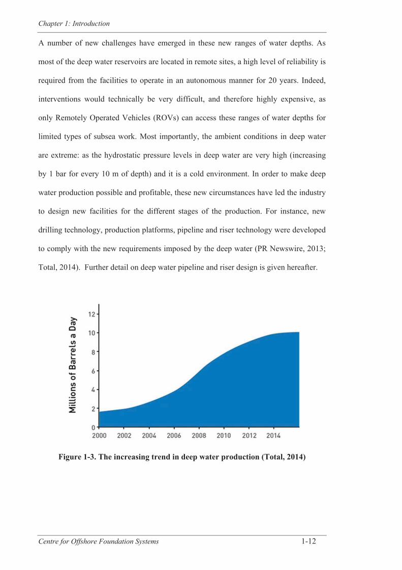
Chapter 1: Introduction
Centre for Offshore Foundation Systems 1-12
A number of new challenges have emerged in these new ranges of water depths. As
most of the deep water reservoirs are located in remote sites, a high level of reliability is
required from the facilities to operate in an autonomous manner for 20 years. Indeed,
interventions would technically be very difficult, and therefore highly expensive, as
only Remotely Operated Vehicles (ROVs) can access these ranges of water depths for
limited types of subsea work. Most importantly, the ambient conditions in deep water
are extreme: as the hydrostatic pressure levels in deep water are very high (increasing
by 1 bar for every 10 m of depth) and it is a cold environment. In order to make deep
water production possible and profitable, these new circumstances have led the industry
to design new facilities for the different stages of the production. For instance, new
drilling technology, production platforms, pipeline and riser technology were developed
to comply with the new requirements imposed by the deep water (PR Newswire, 2013;
Total, 2014). Further detail on deep water pipeline and riser design is given hereafter.
Figure 1-3. The increasing trend in deep water production (Total, 2014)
Chapter 1: Introduction
Centre for Offshore Foundation Systems 1-13
Figure 1-4. Deep water reserves in billions of barrels (Total, 2014)
Figure 1-5. Deep water developments (BBC, 2010)
Chapter 1: Introduction
Centre for Offshore Foundation Systems 1-14
1.5.2 Pipeline and riser design for deep water use
Since the focus of the riser design in this thesis is limited to the fatigue design, only a
general background on riser design is presented in this section to provide the reader with
an understanding of the key design parameters and locate the framework developed in
this research within the design process. Emphasise on the fatigue design of SCRs will
be given in a later stage (see section 1.5.4).
Offshore pipelines are used to transport oil, gas and water between subsea facilities,
production facility platforms and the shore plants. A riser is a “pipe that connects an
offshore floating production structure or a drilling rig to a sub-sea system either for
production purposes such as drilling, production, injection and export or for drilling,
completion and workover purposes” (Tenaris, 2014a). Pipelines and risers are designed
to answer the specific needs of a project and the choice of their key design parameters,
which are the diameter, the wall thickness and the material, is affected by a number of
conditions, such as the reservoir pressure and temperature, the fluid properties, the soil
properties and the oceanographic conditions (Bai, 2001; Guo et al., 2005). In deep
water, pipeline and riser design evolved to sustain the very high external pressures and
face the flow insurance issues resulting from the formation of hydrates (crystal solid
formed from molecule of gas encapsulated into a cage created by water molecules with
a structure similar to ice (Total, 2014)). The wall thickness is determined to withstand
internal pressure and the external hydrostatic pressures according to several criteria
described in various design codes. The most renown standards and recommended
practices for riser design are from the American Society of Mechanical Engineers (e.g.
ASME B31 codes, B31.4 in particular (2012)), Det Norske Veritas (e.g. DNV-OS-F201,
2010), the International Standardization Organisation (e.g. ISO 13623:2009, 2009) or
the American Petroleum Institute (e.g. API RP 1111 (2011); API RP 2RD (2013)).

Chapter 1: Introduction
Centre for Offshore Foundation Systems 1-15
Several successive steps are performed in the design of pipelines and risers; they are the
conceptual engineering, preliminary engineering and detail engineering phases (Bai,
2001; Guo et al., 2005). The conceptual engineering phase aims to highlight the
constraints of a project, to ensure of the technical feasibility, to screen the non-viable
options and to give an estimate of the cost. During the preliminary engineering phase,
the pipeline size and grade are determined so that the pipe sections can be ordered, the
design is verified against design codes and the relevant paperwork is developed for
authority applications. Finally, the detailed engineering phase confirms the design
established beforehand and tackles all the tasks related to the procurement and
construction (Bai, 2001; Guo et al., 2005). The framework developed in this thesis
mainly targets the conceptual engineering or preliminary engineering phases and is well
suited for screening purposes.
1.5.3 Steel catenary risers (SCRs)
1.5.3.1 Overview
There is a wide range of riser types for the various needs of the offshore industry. In
shallow water, flexible risers were traditionally used but in deep water their use was
compromised due to their limited capacity to withstand external pressure. This is why
steel catenary risers (SCRs) were developed (Serta et al., 1996; Campbell, 1999; Vieira
et al., 2008). Even though in the past couple of years some companies have developed
new types of flexible risers able to suit the deep water and ultra deep water needs
(Technip, 2014), SCRs, or other riser types derived from the standard SCRs, have been
and remain among the most common types of risers for deep water applications since
the 1990s (Vieira et al., 2008; Song and Stanton, 2009).
The steel catenary risers are curved risers connected almost vertically to floating
offshore facilities through flexible joints and laid horizontally on the seabed, as
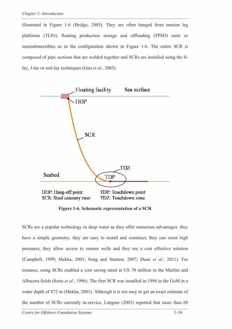
Chapter 1: Introduction
Centre for Offshore Foundation Systems 1-16
illustrated in Figure 1-6 (Bridge, 2005). They are often hanged from tension leg
platforms (TLPs), floating production storage and offloading (FPSO) units or
semisubmersibles as in the configuration shown in Figure 1-6. The entire SCR is
composed of pipe sections that are welded together and SCRs are installed using the S-
lay, J-lay or reel-lay techniques (Guo et al., 2005).
Figure 1-6. Schematic representation of a SCR
SCRs are a popular technology in deep water as they offer numerous advantages: they
have a simple geometry, they are easy to install and construct, they can resist high
pressures, they allow access to remote wells and they are a cost effective solution
(Campbell, 1999; Mekha, 2001; Song and Stanton, 2007; Duan et al., 2011). For
instance, using SCRs enabled a cost saving rated at US 70 million in the Marlim and
Albacora fields (Serta et al., 1996). The first SCR was installed in 1994 in the GoM in a
water depth of 872 m (Mekha, 2001). Although it is not easy to get an exact estimate of
the number of SCRs currently in-service, Langner (2003) reported that more than 60
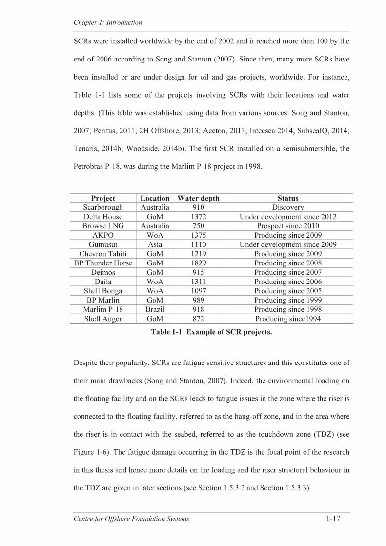
Chapter 1: Introduction
Centre for Offshore Foundation Systems 1-17
SCRs were installed worldwide by the end of 2002 and it reached more than 100 by the
end of 2006 according to Song and Stanton (2007). Since then, many more SCRs have
been installed or are under design for oil and gas projects, worldwide. For instance,
Table 1-1 lists some of the projects involving SCRs with their locations and water
depths. (This table was established using data from various sources: Song and Stanton,
2007; Peritus, 2011; 2H Offshore, 2013; Aceton, 2013; Intecsea 2014; SubseaIQ, 2014;
Tenaris, 2014b; Woodside, 2014b). The first SCR installed on a semisubmersible, the
Petrobras P-18, was during the Marlim P-18 project in 1998.
Project Location Water depth Status Scarborough Australia 910 Discovery Delta House GoM 1372 Under development since 2012 Browse LNG Australia 750 Prospect since 2010
AKPO WoA 1375 Producing since 2009 Gumusut Asia 1110 Under development since 2009
Chevron Tahiti GoM 1219 Producing since 2009 BP Thunder Horse GoM 1829 Producing since 2008
Deimos GoM 915 Producing since 2007 Daila WoA 1311 Producing since 2006
Shell Bonga WoA 1097 Producing since 2005 BP Marlin GoM 989 Producing since 1999
Marlim P-18 Brazil 918 Producing since 1998 Shell Auger GoM 872 Producing since1994
Table 1-1 Example of SCR projects.
Despite their popularity, SCRs are fatigue sensitive structures and this constitutes one of
their main drawbacks (Song and Stanton, 2007). Indeed, the environmental loading on
the floating facility and on the SCRs leads to fatigue issues in the zone where the riser is
connected to the floating facility, referred to as the hang-off zone, and in the area where
the riser is in contact with the seabed, referred to as the touchdown zone (TDZ) (see
Figure 1-6). The fatigue damage occurring in the TDZ is the focal point of the research
in this thesis and hence more details on the loading and the riser structural behaviour in
the TDZ are given in later sections (see Section 1.5.3.2 and Section 1.5.3.3).

Chapter 1: Introduction
Centre for Offshore Foundation Systems 1-18
Other riser types derived from the standard SCRs
Although the framework presented in this thesis is mainly applied to SCRs, it has a
greater scope of applications as it could lay the ground work for future extension to
other riser concepts, as detailed in Appendix A2. An overview of some of the other riser
types is given in this section on the example of the riser concepts derived from the
standard SCR technology.
These other riser types are for instance the lazy wave, steep wave, lazy S, steep S and
compliant vertical access risers (Bai, 2001; Guo et al., 2005; Martins et al., 2013), as
shown in Figure 1-7. In the lazy S and steep S configuration a subsea buoy, respectively
fixed to a structure on the seabed and buoyant, is implemented along the riser length in
order to reduce the motion in the TDZ. The buoyancy section is added on a longer
length of the riser to position the riser into its desired shape in the lazy wave and steep
wave risers that are derived from the lazy S and steep S risers respectively. Another
riser type is the compliant vertical access riser that differs from the previously
mentioned risers as it allows a vertical access to the well. All these riser configurations
have the advantage over the standard SCR to reduce the tension at the HOP. They also
usually have a better fatigue life than the standard SCRs due to the reduction of the
motions transmitted to the TDZ and are used when standard SCRs are not viable.
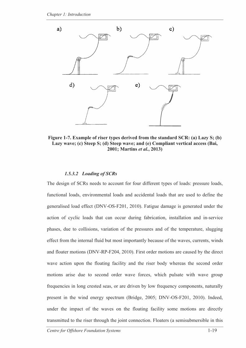
Chapter 1: Introduction
Centre for Offshore Foundation Systems 1-19
Figure 1-7. Example of riser types derived from the standard SCR: (a) Lazy S; (b) Lazy wave; (c) Steep S; (d) Steep wave; and (e) Compliant vertical access (Bai,
2001; Martins et al., 2013)
1.5.3.2 Loading of SCRs
The design of SCRs needs to account for four different types of loads: pressure loads,
functional loads, environmental loads and accidental loads that are used to define the
generalised load effect (DNV-OS-F201, 2010). Fatigue damage is generated under the
action of cyclic loads that can occur during fabrication, installation and in-service
phases, due to collisions, variation of the pressures and of the temperature, slugging
effect from the internal fluid but most importantly because of the waves, currents, winds
and floater motions (DNV-RP-F204, 2010). First order motions are caused by the direct
wave action upon the floating facility and the riser body whereas the second order
motions arise due to second order wave forces, which pulsate with wave group
frequencies in long crested seas, or are driven by low frequency components, naturally
present in the wind energy spectrum (Bridge, 2005; DNV-OS-F201, 2010). Indeed,
under the impact of the waves on the floating facility some motions are directly
transmitted to the riser through the joint connection. Floaters (a semisubmersible in this
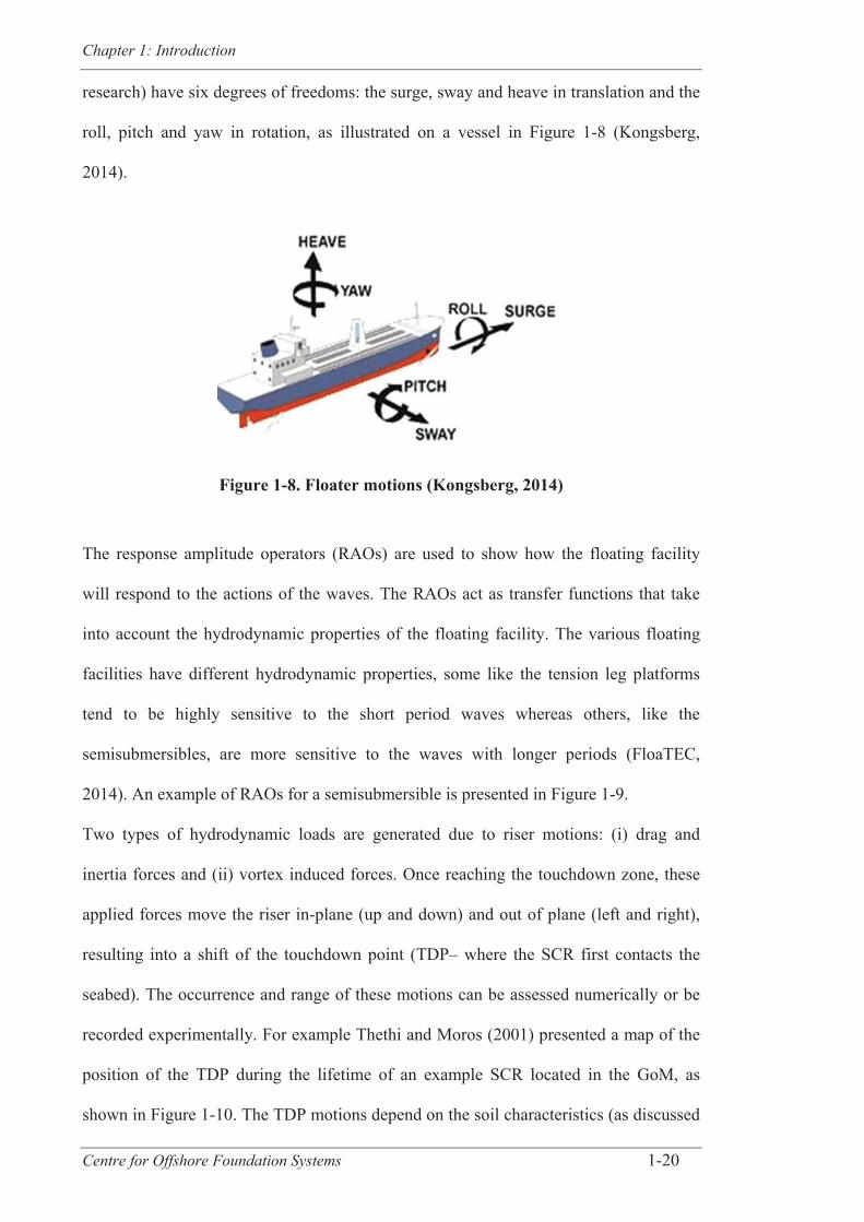
Chapter 1: Introduction
Centre for Offshore Foundation Systems 1-20
research) have six degrees of freedoms: the surge, sway and heave in translation and the
roll, pitch and yaw in rotation, as illustrated on a vessel in Figure 1-8 (Kongsberg,
2014).
Figure 1-8. Floater motions (Kongsberg, 2014)
The response amplitude operators (RAOs) are used to show how the floating facility
will respond to the actions of the waves. The RAOs act as transfer functions that take
into account the hydrodynamic properties of the floating facility. The various floating
facilities have different hydrodynamic properties, some like the tension leg platforms
tend to be highly sensitive to the short period waves whereas others, like the
semisubmersibles, are more sensitive to the waves with longer periods (FloaTEC,
2014). An example of RAOs for a semisubmersible is presented in Figure 1-9.
Two types of hydrodynamic loads are generated due to riser motions: (i) drag and
inertia forces and (ii) vortex induced forces. Once reaching the touchdown zone, these
applied forces move the riser in-plane (up and down) and out of plane (left and right),
resulting into a shift of the touchdown point (TDP– where the SCR first contacts the
seabed). The occurrence and range of these motions can be assessed numerically or be
recorded experimentally. For example Thethi and Moros (2001) presented a map of the
position of the TDP during the lifetime of an example SCR located in the GoM, as
shown in Figure 1-10. The TDP motions depend on the soil characteristics (as discussed
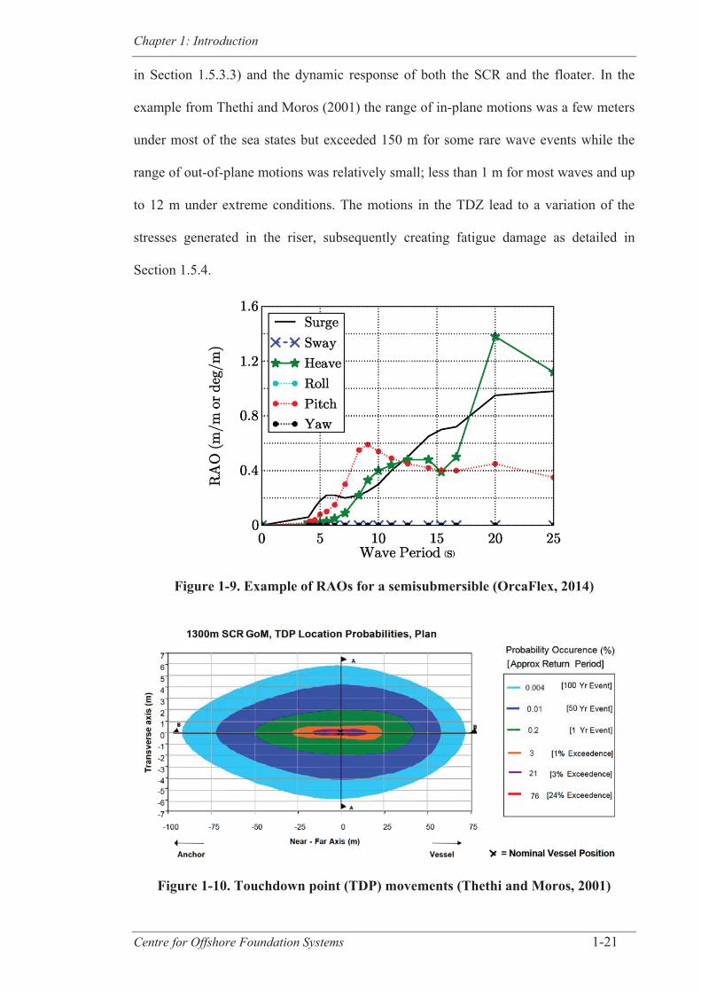
Chapter 1: Introduction
Centre for Offshore Foundation Systems 1-21
in Section 1.5.3.3) and the dynamic response of both the SCR and the floater. In the
example from Thethi and Moros (2001) the range of in-plane motions was a few meters
under most of the sea states but exceeded 150 m for some rare wave events while the
range of out-of-plane motions was relatively small; less than 1 m for most waves and up
to 12 m under extreme conditions. The motions in the TDZ lead to a variation of the
stresses generated in the riser, subsequently creating fatigue damage as detailed in
Section 1.5.4.
Figure 1-9. Example of RAOs for a semisubmersible (OrcaFlex, 2014)
Figure 1-10. Touchdown point (TDP) movements (Thethi and Moros, 2001)
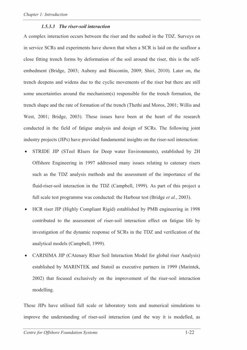
Chapter 1: Introduction
Centre for Offshore Foundation Systems 1-22
1.5.3.3 The riser-soil interaction
A complex interaction occurs between the riser and the seabed in the TDZ. Surveys on
in service SCRs and experiments have shown that when a SCR is laid on the seafloor a
close fitting trench forms by deformation of the soil around the riser, this is the self-
embedment (Bridge, 2003; Aubeny and Biscontin, 2009; Shiri, 2010). Later on, the
trench deepens and widens due to the cyclic movements of the riser but there are still
some uncertainties around the mechanism(s) responsible for the trench formation, the
trench shape and the rate of formation of the trench (Thethi and Moros, 2001; Willis and
West, 2001; Bridge, 2003). These issues have been at the heart of the research
conducted in the field of fatigue analysis and design of SCRs. The following joint
industry projects (JIPs) have provided fundamental insights on the riser-soil interaction:
STRIDE JIP (STeel RIsers for Deep water Environments), established by 2H
Offshore Engineering in 1997 addressed many issues relating to catenary risers
such as the TDZ analysis methods and the assessment of the importance of the
fluid-riser-soil interaction in the TDZ (Campbell, 1999). As part of this project a
full scale test programme was conducted: the Harbour test (Bridge et al., 2003).
HCR riser JIP (Highly Compliant Rigid) established by PMB engineering in 1998
contributed to the assessment of riser-soil interaction effect on fatigue life by
investigation of the dynamic response of SCRs in the TDZ and verification of the
analytical models (Campbell, 1999).
CARISIMA JIP (CAtenary RIser Soil Interaction Model for global riser Analysis)
established by MARINTEK and Statoil as executive partners in 1999 (Marintek,
2002) that focused exclusively on the improvement of the riser-soil interaction
modelling.
These JIPs have utilised full scale or laboratory tests and numerical simulations to
improve the understanding of riser-soil interaction (and the way it is modelled, as
Chapter 1: Introduction
Centre for Offshore Foundation Systems 1-23
explained in Section 1.5.5.2). Results from these JIPs and other published literature
have led to a common agreement that the riser-soil interaction influences the stress
variations in SCRs, although it is still unclear if it is beneficial or detrimental to the
fatigue life of SCRs and this will be addressed in Section 1.5.5.2.
Mechanisms responsible for the formation of a trench
The exact trenching mechanisms are not fully understood yet but they are thought to be
a combination of the soil plastic deformation generated by riser motions, the effect of
the seabed on the riser deflections, mobilising suction during uplift for instance, and the
pumping action of water around the riser (Thethi and Moros, 2001; Bridge et al., 2003;
Langner, 2003; Clukey et al., 2008). The term pumping refers to the acceleration of the
water particles out of the trench when the riser goes down and back in when the riser
lifts up. This pumping action causes erosion of the soil inside the trench and the eroded
soil is redeposited in a looser condition which degrades the soil stiffness (Clukey et al.,
2007). The water helps also to dislodge this already degraded soil and transports the
sediment out of the trench. Moreover, the lateral movements of the riser degrade the
strength of the soil forming the trench walls and widen the trench mouth (Thethi and
Moros, 2001).
Trench shape
Trenches have a 3D geometry and surveys carried out by ROVs suggest that the depth
and the width of trenches vary over the length of the TDZ. Trenches have a curved
profile and the depth, measured below the mudline, is likely to be maximum at the
vessel nominal TDP position (Thethi and Moros, 2001). The zone where the riser is
within the trench is called the buried zone whereas the zone where the riser exits the
trench (towards the anchor) is called the surface zone, as shown in Figure 1-11a.
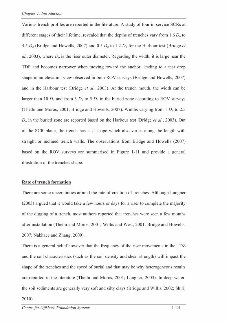
Chapter 1: Introduction
Centre for Offshore Foundation Systems 1-24
Various trench profiles are reported in the literature. A study of four in-service SCRs at
different stages of their lifetime, revealed that the depths of trenches vary from 1.6 Do to
4.5 Do (Bridge and Howells, 2007) and 0.5 Do to 1.2 Do for the Harbour test (Bridge et
al., 2003), where Do is the riser outer diameter. Regarding the width, it is large near the
TDP and becomes narrower when moving toward the anchor, leading to a tear drop
shape in an elevation view observed in both ROV surveys (Bridge and Howells, 2007)
and in the Harbour test (Bridge et al., 2003). At the trench mouth, the width can be
larger than 10 Do and from 3 Do to 5 Do in the buried zone according to ROV surveys
(Thethi and Moros, 2001; Bridge and Howells, 2007). Widths varying from 1 Do to 2.5
Do in the buried zone are reported based on the Harbour test (Bridge et al., 2003). Out
of the SCR plane, the trench has a U shape which also varies along the length with
straight or inclined trench walls. The observations from Bridge and Howells (2007)
based on the ROV surveys are summarised in Figure 1-11 and provide a general
illustration of the trenches shape.
Rate of trench formation
There are some uncertainties around the rate of creation of trenches. Although Langner
(2003) argued that it would take a few hours or days for a riser to complete the majority
of the digging of a trench, most authors reported that trenches were seen a few months
after installation (Thethi and Moros, 2001; Willis and West, 2001; Bridge and Howells,
2007; Nakhaee and Zhang, 2009).
There is a general belief however that the frequency of the riser movements in the TDZ
and the soil characteristics (such as the soil density and shear strength) will impact the
shape of the trenches and the speed of burial and that may be why heterogeneous results
are reported in the literature (Thethi and Moros, 2001; Langner, 2003). In deep water,
the soil sediments are generally very soft and silty clays (Bridge and Willis, 2002; Shiri,
2010).
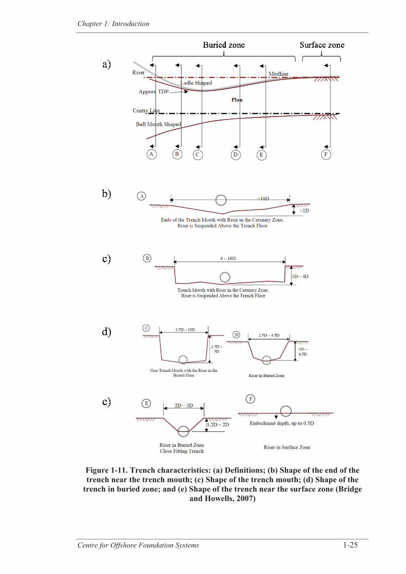
Chapter 1: Introduction
Centre for Offshore Foundation Systems 1-25
Figure 1-11. Trench characteristics: (a) Definitions; (b) Shape of the end of the trench near the trench mouth; (c) Shape of the trench mouth; (d) Shape of the
trench in buried zone; and (e) Shape of the trench near the surface zone (Bridge and Howells, 2007)
Chapter 1: Introduction
Centre for Offshore Foundation Systems 1-26
1.5.4 Fatigue of SCRs
Under repetition of cyclic loading, cracks may initiate in the welds used to assemble the
pipe sections along SCRs and propagate, causing fatigue damage and potential failure.
The fatigue life is defined as “the number of stress cycles at a particular magnitude
required to cause fatigue failure” (DNV-RP-C203, 2010) but is usually expressed in a
number of years based on the number of occurrence of the stress cycles per year. SCRs
are traditionally designed for 25 years or more with a safety factor of 10 to cover all the
unknowns from material strength and oceanographic loadings (Willis and West, 2001;
Langner, 2003).
The fatigue of SCRs should be assessed by considering all of the causes of fatigue
damage; they are for instance the first order and second order wave motions, the VIVs,
the thermal and pressures changes, the fabrication and installation phases (Langner,
2003; DNV-RP-F204, 2010). This research examines the fatigue damage due to first
order wave motions which usually has the highest contribution to overall fatigue life
and therefore only the relevant literature is addressed here. A deterministic fatigue
approach (time domain analysis) is used to assess the fatigue damage, as it is more
appropriate for structural systems presenting nonlinearities (Patel and Seyed, 1995;
Mekha, 2001; Song and Stanton, 2009; DNV-OS-F201, 2010).
The entire wave scatter diagram is divided into representative blocks with one
associated sea state (represented through a regular wave with given height and period)
per block that constitutes the loading and represents all the sea states from this block
(DNV-RP-F204, 2010). The cyclic stress, or stress range, generated under the action of
a sea state is then used to assess the fatigue damage. Also, for SCRs only the cyclic
component of the stress matters as they are welded structures (i.e. the value of the mean
stress is irrelevant) (DNV-RP-C203, 2010). The nominal stress, as a combination of
axial and bending stresses, can be used for estimation of fatigue induced damage in
Chapter 1: Introduction
Centre for Offshore Foundation Systems 1-27
SCRs (Campbell 1999; DNV-RP-F204, 2010). It is usually determined through Finite
Element (FE) analyses, analytical solutions or experiments, as detailed in Section 1.5.5.
Once the amplitude of the stress range ( ) is known, an S-N curve is used to determine
the number of cycles of loading that would lead to failure (N) under this loading
condition. An S-N curve is generally defined by the following equation:
log N=log a-m log where can be adjusted if necessary with a stress concentration
factor and a and m are parameters determined through fatigue tests (DNV-RP-F204,
2010). The damage (d) for each sea state is then calculated as per: d=n/N, where n is
the number of occurrence of the sea state under study. This procedure is followed for
every selected sea state for the blocks of the wave scatter diagram. The individual
damages are then linearly accumulated using the Palmgren-Miner rule to obtain the total
damage ratio. The fatigue life of the system is the inverse of the total damage ratio.
This procedure is reported in DNV-RP-C203 (2010) as being the general procedure for
deterministic fatigue analysis. It is seen that the accurate evaluation of the stress range is
a fundamental step in the fatigue design and it is the focal point of this thesis.
1.5.5 Analysis of SCR response
The analysis of SCR response is complex due to the nonlinearities, caused for instance
by the loading, as the hydrodynamic forces vary depending on the riser motions, and
most importantly arising from the riser-soil-fluid interaction occurring in the TDZ. The
treatment of the nonlinearities is therefore a key element in SCR analysis. Analytical
calculations, numerical simulations or physical testing are the available methods to
analyse SCR response and estimate the fatigue life. FE analysis is the most common
approach in numerical simulations of SCRs but it is encouraged in a riser guideline to
compare FE results against analytical results, in particular for the prediction of the SCR
configuration to verify that mass and shape are appropriately modelled (DNV-OS-F201,
Chapter 1: Introduction
Centre for Offshore Foundation Systems 1-28
2010). A review of the FE approach, with the available software for SCR analysis, is
performed at first. The following section then gives an overview of the riser-soil
interaction modelling in FE software, along with the experimental work performed to
understand the phenomenon that should be captured in models and the advanced
analytical solutions for treatment of the riser-soil interaction. The last section deals with
the analytical solutions developed to analyse the overall SCR response.
1.5.5.1 Structural analysis methodology
The structural response of SCRs is usually assessed by FE modelling of the entire
system and then conducting dynamic nonlinear time domain analyses after performing
an initial static analysis to establish the equilibrium configuration (before application of
any motion) (DNV-OS-F201, 2010). These time domain analyses are very time
consuming and simplified methods are sometimes used to improve computational
efficiency (Campbell 1999; Xia et al., 2008; DNV-OS-F201, 2010); this will be the
focus of Section 1.5.7.
Generic finite element analysis software (e.g. Abaqus (Dassault systèmes, 2014) or
ANSYS (ANSYS, 2014)) can be used to perform SCR analyses but specialised marine
analysis programs are also available, such as:
- OrcaFlex (Orcina, 2011)
- Flexcom (MCSKenny, 2014)
- Deeplines (Principia, 2014)
- Riflex (Marintek, 2014; DNV GL, 2014)
- Sesam DeepC (DNV GL, 2014)
Specialised software are user friendly and may offer better computational times than
general purpose FE software. However, they are sometimes limited in their applications
for detail modelling of some particular aspect of SCR design, such as for the soil
modelling, as the users cannot readily access the code and implement their own

Chapter 1: Introduction
Centre for Offshore Foundation Systems 1-29
modified solution (Shiri, 2010). In this thesis, all FE analyses are carried out using
OrcaFlex software. It is a “marine dynamics program developed by Orcina for static
and dynamic analysis of a wide range of offshore systems, including all types of marine
risers (rigid and flexible), global analysis, moorings, installation and towed systems”
(Orcina, 2011).
1.5.5.2 Modeling the riser-soil interaction
The main concepts of the riser soil interaction and the mechanisms involved were
presented in Section 1.5.3.3. A review of the FE modelling of this interaction is
performed here. However, most of the work carried out in this research is using simple
linear soil models as the aim is to test at first the relevance of the simplified approach
for fatigue design of SCRs under development in this thesis, without adding the
complexities introduced by the more advanced nonlinear soil models. Hence, only a
succinct review of the advanced modelling methods is presented.
The conventional practice in fatigue design of SCRs is to use an horizontal and flat
linear model for seabed response as it simplifies structural analyses but also because the
riser-soil interaction is still not fully understood. In this approach, a linear spring is used
to replicate the seabed response and therefore the seabed resistance is proportional to
the penetration of the pipe into the seabed. It is accepted that this simple model cannot
capture the realistic soil behaviour. In recent years, the research has focused into
developing more advanced soil models (e.g. Bai, 2001; Thethi and Moros, 2001; Clukey
et al., 2007; De Amicis et al., 2007; Xia et al., 2008; Randolph and Quiggin, 2009;
Kimiaei et al., 2010). Riser-soil interaction issues have also attracted a lively interest
because it was shown that soil modelling was significantly influencing fatigue life
predictions (Thethi and Moros, 2001; Bridge et al., 2004; Clukey et al , 2005, Natarajan
et al., 2007; Randolph and Quiggin, 2009). It is now well established that for structural
analyses with linear soil models, the stiffer the soil, the shorter the fatigue life of the
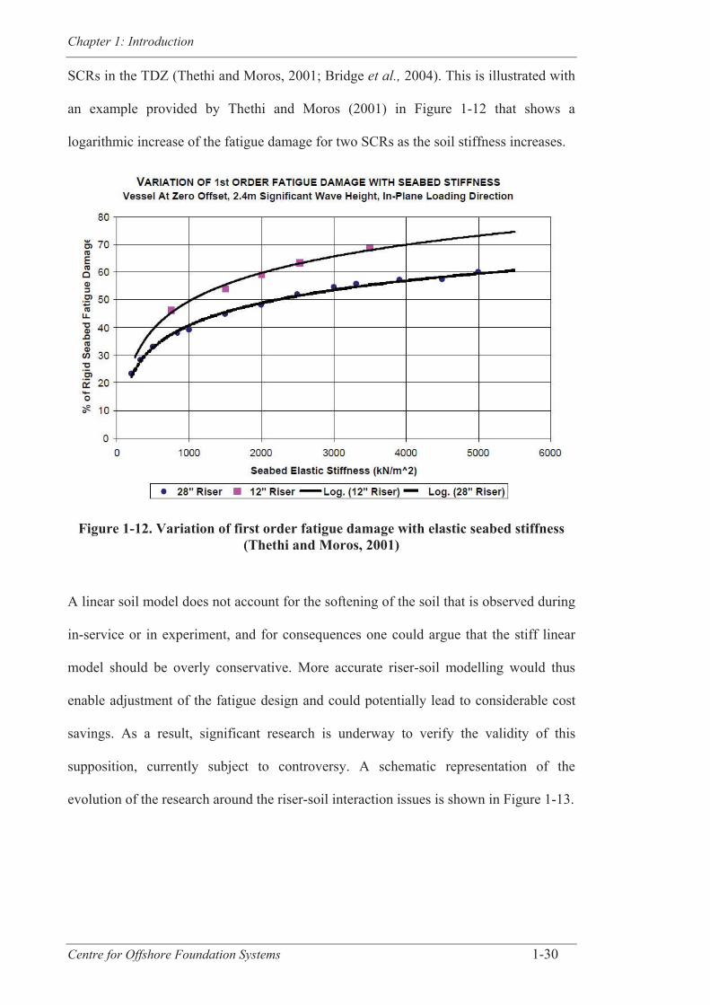
Chapter 1: Introduction
Centre for Offshore Foundation Systems 1-30
SCRs in the TDZ (Thethi and Moros, 2001; Bridge et al., 2004). This is illustrated with
an example provided by Thethi and Moros (2001) in Figure 1-12 that shows a
logarithmic increase of the fatigue damage for two SCRs as the soil stiffness increases.
Figure 1-12. Variation of first order fatigue damage with elastic seabed stiffness (Thethi and Moros, 2001)
A linear soil model does not account for the softening of the soil that is observed during
in-service or in experiment, and for consequences one could argue that the stiff linear
model should be overly conservative. More accurate riser-soil modelling would thus
enable adjustment of the fatigue design and could potentially lead to considerable cost
savings. As a result, significant research is underway to verify the validity of this
supposition, currently subject to controversy. A schematic representation of the
evolution of the research around the riser-soil interaction issues is shown in Figure 1-13.
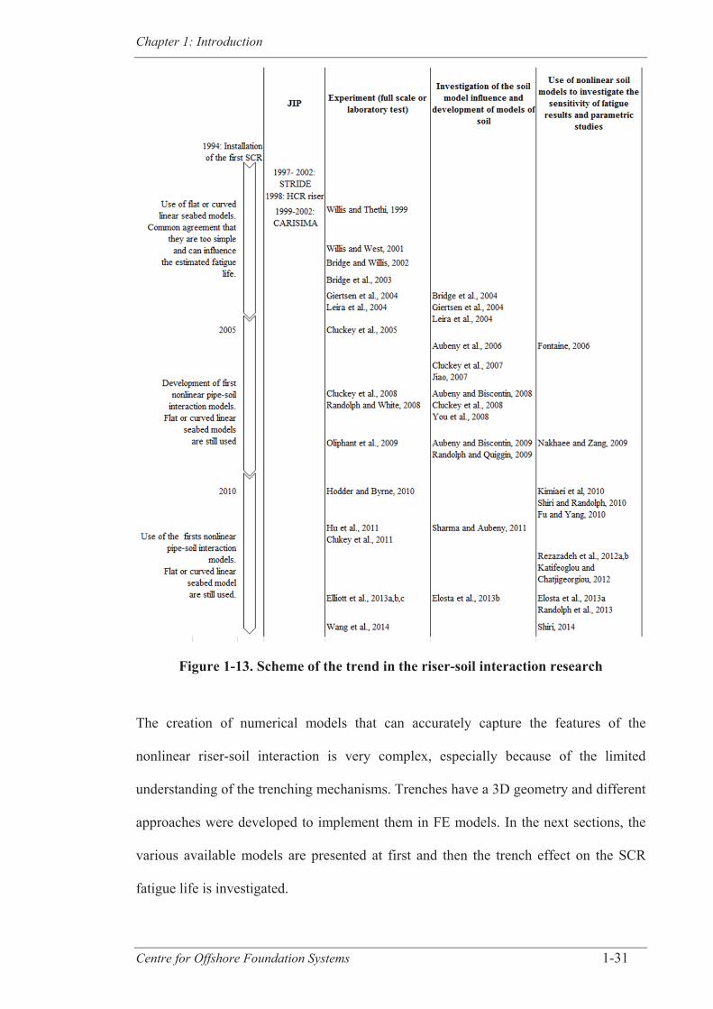
Chapter 1: Introduction
Centre for Offshore Foundation Systems 1-31
Figure 1-13. Scheme of the trend in the riser-soil interaction research
The creation of numerical models that can accurately capture the features of the
nonlinear riser-soil interaction is very complex, especially because of the limited
understanding of the trenching mechanisms. Trenches have a 3D geometry and different
approaches were developed to implement them in FE models. In the next sections, the
various available models are presented at first and then the trench effect on the SCR
fatigue life is investigated.
Chapter 1: Introduction
Centre for Offshore Foundation Systems 1-32
Development of the nonlinear soil models
The most common approach to replicate the trench influence relies on the development
of a nonlinear seabed model aiming to create the trench through incremental
degradation of soil properties and embedment of the SCR under application of cyclic
loading. The data from the JIPs and other published literature have contributed to the
development of existing nonlinear soil models. Most of the marine analysis software
now have a built-in nonlinear soil model. Riflex has a nonlinear soil model that was
developed based on the data from the CARISIMA JIP (Giertsen et al., 2004; Leira et
al., 2004) whereas the model in OrcaFlex was developed by Randolph and Quiggin
(2009). However, the accuracy of the CARISIMA model should be investigated further
for a wider range of riser configurations (Leira et al., 2004) and Randolph and Quiggin
(2009) encouraged further studies to improve their proposed seabed model which is
“still experimental” (Orcina, 2011). Deeplines and Flexcom also proposed a nonlinear
soil model (Fontaine, 2006; MCS Kenny, 2008; Principia, 2014). Aubeny and Biscontin
(2008, 2009) and Jiao (2007) have provided an analytical model intended for future
implementation in a commercial software package for riser analysis (Sharma and
Aubeny, 2011) and different formulations of soil stiffness were proposed by Bridge et
al. (2004) to account for the nonlinear pipe-soil interaction.
Numerous experiments have also been performed to provide greater understanding of
the phenomenon that should be captured, sometimes on full scale or large models (e.g.
Bridge et al., 2003; Hodder and Byrne, 2010; Wang et al., 2014), centrifuge tests of
riser sections (e.g. Hu et al., 2011; Elliott et al., 2013a, b, c) or experiments using T-bar
apparatus or small riser sections (e.g. Clukey et al., 2005; Clukey et al., 2008; Randolph
and White, 2008; Oliphant et al. 2009). These experiments have provided insights on
the effect of the separation between riser and soil, cyclic loading, strength and stiffness
reduction, remoulding, suction, pore pressure variation and rate of embedment. In this
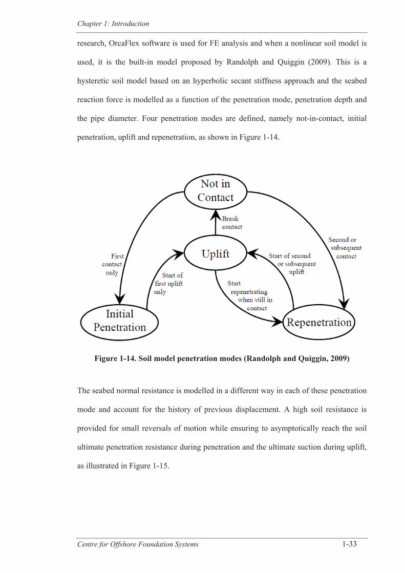
Chapter 1: Introduction
Centre for Offshore Foundation Systems 1-33
research, OrcaFlex software is used for FE analysis and when a nonlinear soil model is
used, it is the built-in model proposed by Randolph and Quiggin (2009). This is a
hysteretic soil model based on an hyperbolic secant stiffness approach and the seabed
reaction force is modelled as a function of the penetration mode, penetration depth and
the pipe diameter. Four penetration modes are defined, namely not-in-contact, initial
penetration, uplift and repenetration, as shown in Figure 1-14.
Figure 1-14. Soil model penetration modes (Randolph and Quiggin, 2009)
The seabed normal resistance is modelled in a different way in each of these penetration
mode and account for the history of previous displacement. A high soil resistance is
provided for small reversals of motion while ensuring to asymptotically reach the soil
ultimate penetration resistance during penetration and the ultimate suction during uplift,
as illustrated in Figure 1-15.

Chapter 1: Introduction
Centre for Offshore Foundation Systems 1-34
Figure 1-15. Nonlinear soil model characteristics for different modes (Randolph and Quiggin, 2009)
Trench implementation by initial change in seabed geometry
Another approach to implement a trench is to modify the geometry of the seabed. A
curved seabed can be used to match the in-plane geometry of the trench in conjunction
with a rigid, elastic or nonlinear seabed and this approach was used by Giersten et al.
(2004), Leira et al. (2004) and Clukey et al. (2007) for example. Various ways to
choose the trench initial profile are reported in the literature. For instance a seven order
polynomial fit was proposed by Langner (2003) and a quadratic exponential trench
shape by Shiri (2014). Shiri (2010) also suggested to get an initial trench profile
consistent with the SCR shape and to apply a severe sea state during an appropriate
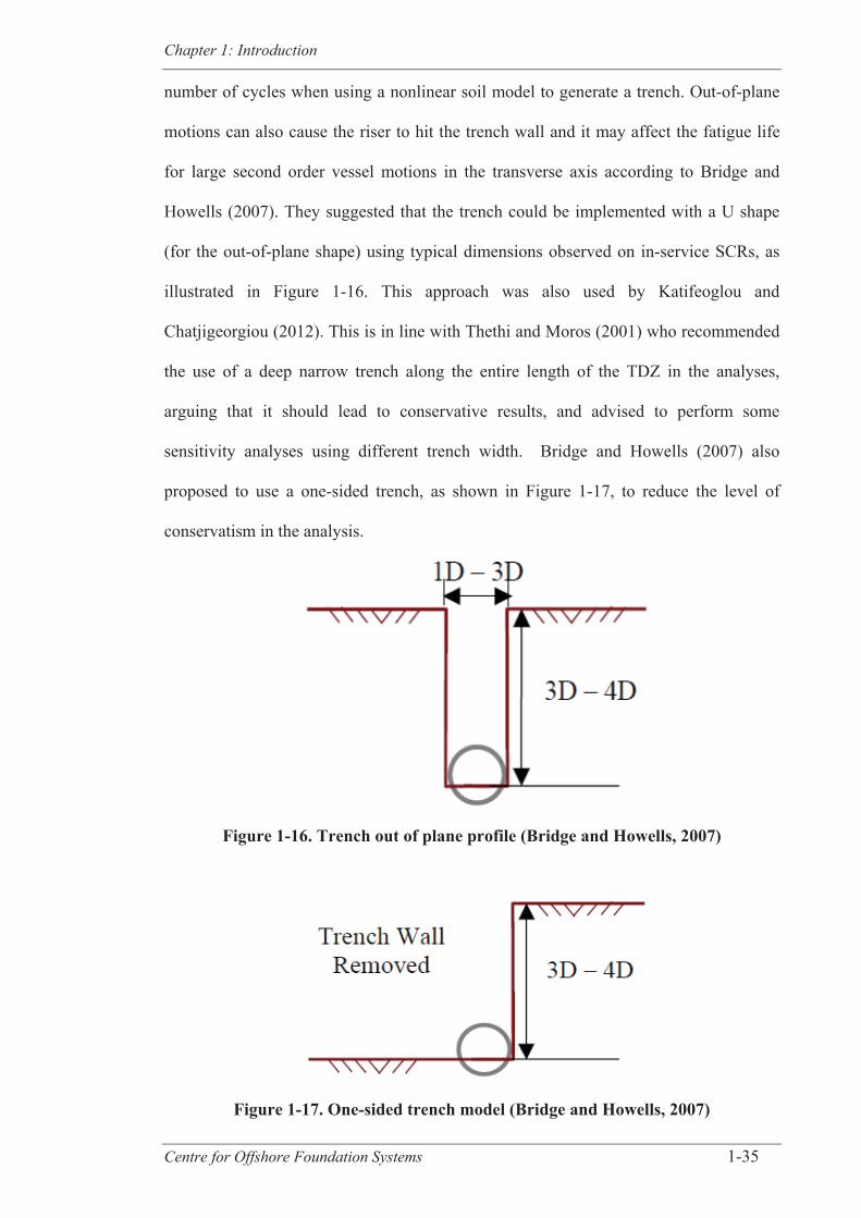
Chapter 1: Introduction
Centre for Offshore Foundation Systems 1-35
number of cycles when using a nonlinear soil model to generate a trench. Out-of-plane
motions can also cause the riser to hit the trench wall and it may affect the fatigue life
for large second order vessel motions in the transverse axis according to Bridge and
Howells (2007). They suggested that the trench could be implemented with a U shape
(for the out-of-plane shape) using typical dimensions observed on in-service SCRs, as
illustrated in Figure 1-16. This approach was also used by Katifeoglou and
Chatjigeorgiou (2012). This is in line with Thethi and Moros (2001) who recommended
the use of a deep narrow trench along the entire length of the TDZ in the analyses,
arguing that it should lead to conservative results, and advised to perform some
sensitivity analyses using different trench width. Bridge and Howells (2007) also
proposed to use a one-sided trench, as shown in Figure 1-17, to reduce the level of
conservatism in the analysis.
Figure 1-16. Trench out of plane profile (Bridge and Howells, 2007)
Figure 1-17. One-sided trench model (Bridge and Howells, 2007)
Chapter 1: Introduction
Centre for Offshore Foundation Systems 1-36
Riser-soil interaction influence on fatigue of SCRs
It is seen that although the nonlinear riser-soil interaction models still requires further
investigations, the nonlinear soil models that were developed already capture some of
the complex features of the soil behaviour that were neglected by the traditional and
simple linear soil model. Hence, they provide an opportunity to improve the assessment
of the fatigue life of SCRs in the TDZ. However, some literature nowadays relates
contradictory findings on the effect of the riser-interaction on the fatigue life of SCRs
and a summary of the results is shown in Table 1-2. It highlights the lack of trend and
the importance of this debate for SCR design. Some authors have argued that the trench
shape leads to a decrease of the curvature in the TDZ and should thereby reduce the
fatigue damage whereas others have warned that the contact with the trench walls or the
soil suction may increase the fatigue damage and therefore the linear soil model might
not be conservative. Whilst the results from numerical simulations have been presented
by researchers to support some of the above views, Shiri and Randolph (2010) and Shiri
(2014) argue that the possible heterogeneity in loading application and in trench
modelling may be the source of the discrepancy. Indeed, they argued that minor
differences in trench geometry can lead to major differences in results and have
encouraged the development of trench profiles close to the riser shape and this is also
noted by Randolph et al. (2013). However, Rezazadeh et al. (2012a) argues that even
with the implementation of an initial trench profile compatible with the riser shape, it is
very hard to decide if the fatigue will increase or decrease. Elosta et al. (2013a) showed
that the choice of geotechnical parameters for the nonlinear seabed model has a major
influence on the fatigue life and may be a source of confusion.
To summarise, although current findings diverge on the effect of trenches on the fatigue
life, there is a global agreement on the need for more studies to develop a greater
understanding of the mechanisms responsible for trench formation and the rate of
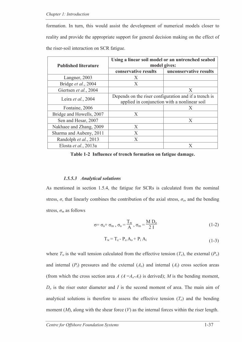
Chapter 1: Introduction
Centre for Offshore Foundation Systems 1-37
formation. In turn, this would assist the development of numerical models closer to
reality and provide the appropriate support for general decision making on the effect of
the riser-soil interaction on SCR fatigue.
Published literature Using a linear soil model or an untrenched seabed
model gives: conservative results unconservative results
Langner, 2003 X Bridge et al., 2004 X
Giertsen et al., 2004 X
Leira et al., 2004 Depends on the riser configuration and if a trench is applied in conjunction with a nonlinear soil
Fontaine, 2006 X Bridge and Howells, 2007 X
Sen and Hesar, 2007 X Nakhaee and Zhang, 2009 X Sharma and Aubeny, 2011 X
Randolph et al., 2013 X Elosta et al., 2013a X
Table 1-2 Influence of trench formation on fatigue damage.
1.5.5.3 Analytical solutions
As mentioned in section 1.5.4, the fatigue for SCRs is calculated from the nominal
stress, , that linearly combines the contribution of the axial stress, a, and the bending
stress, m as follows
σ= σa+ σm , σa = TwA , σm =
M Do2 I (1-2)
Tw = Te - Po Ao + Pi Ai (1-3)
where Tw is the wall tension calculated from the effective tension (Te), the external (Po)
and internal (Pi) pressures and the external (Ao) and internal (Ai) cross section areas
(from which the cross section area A (A =Ao-Ai) is derived); M is the bending moment,
Do is the riser outer diameter and I is the second moment of area. The main aim of
analytical solutions is therefore to assess the effective tension (Te) and the bending
moment (M), along with the shear force (V) as the internal forces within the riser length.
Chapter 1: Introduction
Centre for Offshore Foundation Systems 1-38
Various analytical solutions ranging in complexity and accuracy, in particular for
statically loaded systems, have been proposed for the study of SCR response. Analytical
formulations in the time domain or in the frequency domain have also been developed
to capture the dynamic response of SCRs, in particular for the study of the Vortex
Induced Vibrations (VIVs), which is outside of the scope of this thesis (e.g. Aranha et
al., 1997; Pesce et al., 1998a; Pesce et al., 2006; Chatjigeorgiou, 2010). However, FE
methods are the most common approach for the dynamic analyses of SCRs
(Chatjigeorgiou, 2013) and therefore the review of the analytical techniques for
dynamic response is left out intentionally. Also, since the initial simplified fatigue
design approach, under development in this research, relies partly on the analytical
determination of the static stress range in SCRs, the analytical solutions able to
approximate SCR stress distribution at equilibrium (i.e. before application of any
motions) and SCR response under cyclic static loading are of prime interest. They are
the focus of Chapter 4 and only an overview is given in this section.
Static configuration
Various solutions developed to get an analytical approximation of an SCR configuration
and the stress distributions at equilibrium are presented hereafter. Analytical models
considering either a rigid soil or a linear elastic seabed are reviewed here, as they are
respectively the simplest approach and the type of soil model used most frequently
throughout this research.
Some authors have also developed a plastic seabed model especially to deal with lay
effects during installation (Palmer, 2008a; Yuan et al., 2012) but this is outside of the
scope of this research.
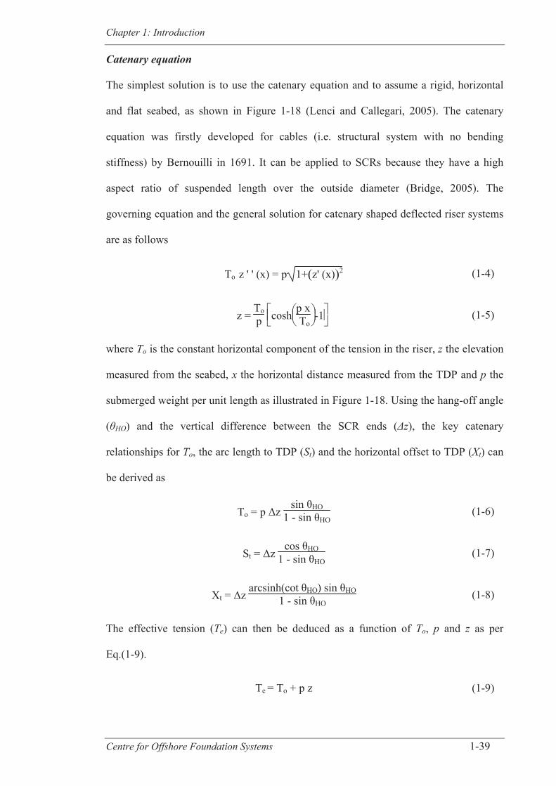
Chapter 1: Introduction
Centre for Offshore Foundation Systems 1-39
Catenary equation
The simplest solution is to use the catenary equation and to assume a rigid, horizontal
and flat seabed, as shown in Figure 1-18 (Lenci and Callegari, 2005). The catenary
equation was firstly developed for cables (i.e. structural system with no bending
stiffness) by Bernouilli in 1691. It can be applied to SCRs because they have a high
aspect ratio of suspended length over the outside diameter (Bridge, 2005). The
governing equation and the general solution for catenary shaped deflected riser systems
are as follows
To z ' ' (x) = p 1+( )z' (x) 2 (1-4)
z = Top cosh
p x To
-1 (1-5)
where To is the constant horizontal component of the tension in the riser, z the elevation
measured from the seabed, x the horizontal distance measured from the TDP and p the
submerged weight per unit length as illustrated in Figure 1-18. Using the hang-off angle
( HO) and the vertical difference between the SCR ends ( z), the key catenary
relationships for To, the arc length to TDP (St) and the horizontal offset to TDP (Xt) can
be derived as
To = p Δz sin θHO
1 - sin θHO (1-6)
St = Δz cos θHO
1 - sin θHO (1-7)
Xt = Δz arcsinh(cot θHO) sin θHO
1 - sin θHO (1-8)
The effective tension (Te) can then be deduced as a function of To, p and z as per
Eq.(1-9).
Te = To + p z (1-9)
Chapter 1: Introduction
Centre for Offshore Foundation Systems 1-40
Indeed, Te is the resultant between the cumulative pipe weight and the horizontal
component of the tension which (trivially) leads to Eq.(1-10). Eq. (1-11) is then derived
by using Eq. (1-5) and knowing that ds = (dx2+dz2)0.5. Implementing the expression of
the arc length s based on Eq. (1-11) in Eq. (1-10) and considering that
To cosh (p x/To) = z p +To (from Eq.(1-5)) subsequently leads to Eq.(1-9).
Te = To 2+(p s)2 (1-10)
s = Top sinh
p x To
(1-11)
For riser tubular sections (with negligible bending stiffness), it is possible to
approximate the bending moment along the riser length by Eq. (1-12), where E is the
Young’s modulus and k the curvature defined as per Eq. (1-13) (Bridge, 2005; Lenci
and Callegari, 2005).
M = k E I (1-12)
k =z ' ' (x)
[ ]1+ z ' ' (x)3/2
(1-13)
The concentrated soil reaction force at the TDP (Rc) when using a rigid seabed is given
by (Aranha et al., 1997; Bridge et al., 2004; Bridge, 2005)
Rc =p E I To
(1-14)
The simplicity of this analytical model makes it an attractive option for designers but its
applicability is limited due to the discontinuity of the bending moment at the TDP
resulting from the rigid soil assumption. Also, the effect of the bending stiffness is not
rigorously accounted for and this is why elastic soil models and boundary layer
solutions were subsequently developed, as detailed hereafter.

Chapter 1: Introduction
Centre for Offshore Foundation Systems 1-41
Figure 1-18. Scheme of the simplest analytical model (Lenci and Callegari, 2005)
Elastic soil model
Lenci and Callegari (2005) proposed to model the riser as a cable in the suspended zone
prior the TDP and as a beam on a Winkler-type deformable soil in the laid part in order
to obtain the continuity of the bending moment. This is illustrated in Figure 1-19. In this
model, namely the “elastic soil and cable” model, the vertical downward displacement
(w1) is linked to the riser bending stiffness (EI) and submerged weight (p), the unknown
constant traction on the laid beam (To) and the soil stiffness (ks) through the following
relationship
EI w1ꞌꞌꞌꞌ(x) – To w1ꞌꞌ(x)+ks w1(x)=p (1-15)
Eq. (1-15) is established under the linear theory of flexure and is valid by considering
that w1 is small because of the high stiffness of the soil. The solution of this equation
and the derivation of the bending moment and effective tension are presented in detail in
Chapter 4. The drawback of this model is that the shear force is not continuous at the
TDP. A simpler version of this model was presented by Shiri and Sadeghi (2012). Using
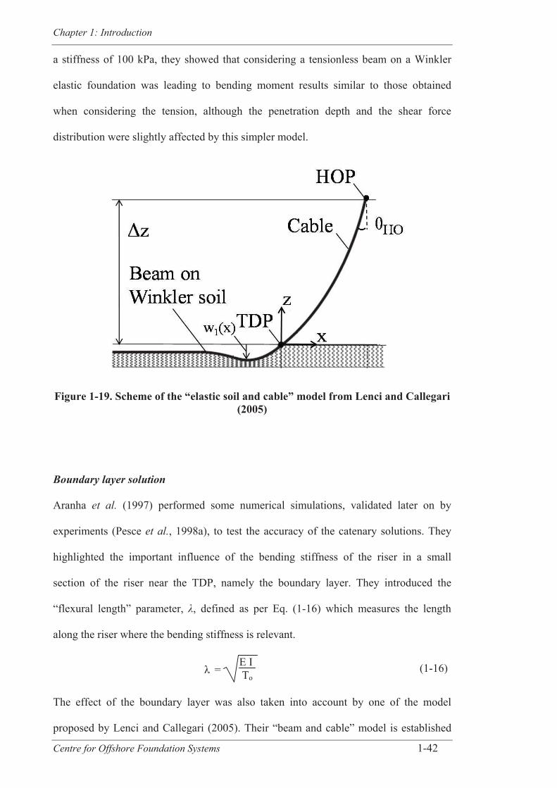
Chapter 1: Introduction
Centre for Offshore Foundation Systems 1-42
a stiffness of 100 kPa, they showed that considering a tensionless beam on a Winkler
elastic foundation was leading to bending moment results similar to those obtained
when considering the tension, although the penetration depth and the shear force
distribution were slightly affected by this simpler model.
Figure 1-19. Scheme of the “elastic soil and cable” model from Lenci and Callegari (2005)
Boundary layer solution
Aranha et al. (1997) performed some numerical simulations, validated later on by
experiments (Pesce et al., 1998a), to test the accuracy of the catenary solutions. They
highlighted the important influence of the bending stiffness of the riser in a small
section of the riser near the TDP, namely the boundary layer. They introduced the
“flexural length” parameter, , defined as per Eq. (1-16) which measures the length
along the riser where the bending stiffness is relevant.
λ = E I To
(1-16)
The effect of the boundary layer was also taken into account by one of the model
proposed by Lenci and Callegari (2005). Their “beam and cable” model is established
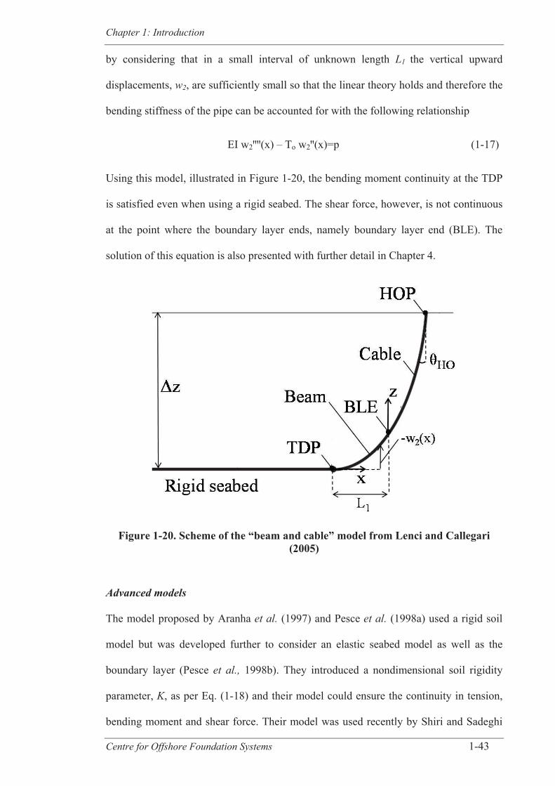
Chapter 1: Introduction
Centre for Offshore Foundation Systems 1-43
by considering that in a small interval of unknown length L1 the vertical upward
displacements, w2, are sufficiently small so that the linear theory holds and therefore the
bending stiffness of the pipe can be accounted for with the following relationship
EI w2ꞌꞌꞌꞌ(x) – To w2ꞌꞌ(x)=p (1-17)
Using this model, illustrated in Figure 1-20, the bending moment continuity at the TDP
is satisfied even when using a rigid seabed. The shear force, however, is not continuous
at the point where the boundary layer ends, namely boundary layer end (BLE). The
solution of this equation is also presented with further detail in Chapter 4.
Figure 1-20. Scheme of the “beam and cable” model from Lenci and Callegari (2005)
Advanced models
The model proposed by Aranha et al. (1997) and Pesce et al. (1998a) used a rigid soil
model but was developed further to consider an elastic seabed model as well as the
boundary layer (Pesce et al., 1998b). They introduced a nondimensional soil rigidity
parameter, K, as per Eq. (1-18) and their model could ensure the continuity in tension,
bending moment and shear force. Their model was used recently by Shiri and Sadeghi
Chapter 1: Introduction
Centre for Offshore Foundation Systems 1-44
(2012) who found a good agreement with FE analysis.
K = ks λ4 E I =
ks λ2 To
= ks E ITo
2 (1-18)
Another advanced model was proposed by Lenci and Callegari (2005) which differs
from the one from Pesce et al. (1998b) as they did not use the singular perturbation
theory. Lenci and Callegari (2005) established an advanced model, namely the “three
field model”, by dividing the riser into three sections and combining the various
solutions that they proposed (i.e. “elastic soil and cable”, “beam and cable” and
“catenary” as mentioned previously) to account for the effect of the bending stiffness of
the riser near the TDP and consider an elastic soil. This advanced model produces
continuous tension, bending moment and also shear force and compares well with FE
results, as shown in Chapter 4. However, to ensure the continuity in tension they had to
restrain the value of the tension to a constant value within the boundary layer which
generates minor inconsistencies with numerical solutions. This is one of the
shortcomings of their model, and this is also explained within Chapter 4.
Static response of SCRs under cyclic loads
It was previously mentioned in Section 1.4 that one aspect of the DAF approach
developed initially in this thesis is to determine analytically the static response of SCRs
subjected to cyclic loads and little research has been found in the literature on this topic.
Shiri and Hashemi (2012) have suggested using the model developed by Pesce et al.
(1998b) to predict the maximum stress range in the TDZ under a cycle of static loading.
They noted that if the change in axial tension in the TDZ is neglected, then the
maximum static stress range in the TDZ (Max TDZ_sta) that controls the fatigue
damage in SCRs can be estimated from Eq. (1-19).
Max ΔσTDZ ~ ΔMmax Do
2 I (1-19)
Chapter 1: Introduction
Centre for Offshore Foundation Systems 1-45
where Mmax is the variation between the maximum values of bending moment in the
TDZ occurring when the vessel is in near and far positions. They subsequently observed
that it is the shift in stress distribution under a cycle of load that causes fatigue damage
and since the shear force distribution “does not change much” when the motion is
applied, they proposed to assess the variation of bending moment by multiplying the
maximum shear force found initially when the SCR is at equilibrium (Vmax) by the
maximum TDP relocation occurring during the cycle of static loading ( xTDP), leading
to Eq. (1-20).
Max ΔσTDZ_sta ~ Vmax ΔxTDP Do
2 I (1-20)
They used the boundary layer solution developed by Pesce et al. (1998b) to find the
value of Vmax , as per Eq. (1-21)
Vmax = p λ K0.25
2+ K0.25 (1-21)
where and K are defined as per Eq. (1-16) and Eq. (1-18) respectively.
Regarding the evaluation of xTDP , they used the simple catenary model with a rigid
soil. In the methodology developed by Shiri and Hashemi (2012) and also used by
Rezazadeh et al. (2012b), the effect of the tension is neglected and it relies on the
assumption that the variation of bending moment can only be evaluated by multiplying
Vmax and xTDP. It uses a mixture of parameters extracted from boundary layer based
models where bending stiffness of the riser is taken into account (such as shear force)
and the other parameters from simple catenary equations which neglect the bending
stiffness of the riser. Hence, the applicability of this method might be limited to some
SCR configurations where the boundary layer zone is small.
A different approach is undertaken in this research. It uses exclusively the three-field
model proposed by Lenci and Callegari (2005) so that the soil stiffness and the
boundary layer effect are accounted for in every step of the method. It is therefore
Chapter 1: Introduction
Centre for Offshore Foundation Systems 1-46
expected to produce more reliable results for a wider range of SCR configurations and
more details on the development of this analytical model are presented in Chapter 4.
1.5.6 State of the art of the sensitivity studies of SCR fatigue damage
Despite their simple geometry, SCRs have a complex behaviour due to the
nonlinearities impacting their structural response. Sensitivity studies are used to
increase the knowledge of the influence of the design parameters on the fatigue life. For
instance, in the early stages of SCRs use, Campbell (1999) encouraged the application
of sensitivity analyses to “quantify and bound” the uncertainties in design parameters.
Indeed, sensitivity analyses aim to quantify the effect of the variation of an input or a
group of inputs on the output(s) of interest, which for fatigue design of SCRs in the
TDZ is the maximum induced stress range. A wide range of inputs enters SCR fatigue
design and this is examined in detail in Chapter 3. The inputs related to the SCR
configuration, riser section, the loading applied on the SCR, physical properties and the
soil characteristics are of main interest for the fatigue design of SCRs and some
published numerical studies have already investigated their effects.
Xia et al. (2008) investigated the effect of the hang-off angle, the internal diameter and
the wall thickness on the distribution of static and dynamic stresses in SCRs. For this
purpose, they used a base case SCR in a water depth of 1000 m and assumed a simple
linear elastic soil model. The results of their study are summarised in Table 1-3. The
results on the effect of the hang-off angle are in contradiction with the results published
by Bhat et al. (2004) who stated that an increase of the hang-off angle would improve
the fatigue life. However, they mentioned the potential for a threshold in the value of
hang-off angle above which the fatigue performance would drop. The effect of the
loading parameters on the SCR response was investigated by Kimiaei et al. (2010)
based on an SCR in a water depth of 1000 m using the nonlinear soil model developed

Chapter 1: Introduction
Centre for Offshore Foundation Systems 1-47
by Randolph and Quiggin (2009). They investigated the influence of the wave periods
and motion amplitudes by varying the wave periods from 1 s to 20 s and applying a
displacement to the riser hang-off point, referred to as the heave amplitude, equal to
either 0.8 m or 2 m. They concluded that by increasing the amplitude of the wave
period, the SCR response will asymptotically approach the static response of the system
and that, for a short wave period, a large dynamic amplification effect could be
observed. These conclusions were valid for both values of heave amplitudes. They also
examined the effect of the order of application of the waves which impacts fatigue
results when using a nonlinear soil model but could not conclude on the order that
would be the most critical for fatigue design. This issue was also studied by Shiri and
Randolph (2010). Other published sensitivity studies also considered the use of a
nonlinear soil model and examined the influence of the nonlinear soil parameters on
fatigue results. For instance, Shiri and Randolph (2010) studied the influence of the
suction ratio and of a parameter that controls the repenetration after an uplift motion of
the riser in the nonlinear soil model established by Randolph and Quiggin (2009). Using
the same nonlinear soil model, Elosta et al. (2013a) varied the maximum normalised
stiffness to understand its impact on the fatigue life and found that increasing it will
shorten the fatigue life. When using a linear soil model, it was shown during the
STRIDE JIP and reported by Bridge et al. (2004) that a softer soil will decrease the
fatigue damage.
With an increase of the varied input
the:
Varied input Range Maximum static stress
Maximum dynamic stress range Comments
Hang-off angle, HO 10 ° to 18 ° Decreases Increases N/A
Internal diameter, Di
0.203 m to 0.508 m Increases Decreases wt kept
unchanged Wall
thickness, wt 0.026 m to
0.036 m Decreases Decreases Di kept unchanged
Table 1-3 Summary of the results from Xia et al. (2008).
Chapter 1: Introduction
Centre for Offshore Foundation Systems 1-48
It is seen that insufficient data is available in the literature to get a solid understanding
of SCR behaviour. In fact, a recent offshore standard for riser design commented on the
lack of sensitivity studies for soil properties particularly where their value is uncertain
(DNV-OS-F201, 2010). A few studies have been published since then but have used
limited ranges of the parameters and most of them followed a technique that consists in
varying only the input of interest and leaving the other inputs unchanged, fixed to an
arbitrary value. This approach is called the one-factor-at-a-time approach in the field of
statistics that deals with the design of experiment (DoE) (e.g. Peace, 1993). The main
drawback in the previously published studies is that the effects of some potential
interactions between input parameters cannot necessarily be captured and therefore the
conclusions may be misleading and only valid for the particular tested base cases.
Indeed, interaction refers to the fact that the effect of an input on the output results
might be different depending on the level of one or several other input variables (Peace,
1993). This highlights the fact that SCR studies should be performed in a way that
enhances the applicability of the results for a wide range of SCRs configurations and
loading characteristics in order to provide designers with useful and reliable conclusions
that should still be valid for their own SCR case study. This is one of the key difficulties
in SCR studies and it has not received enough attention in the numerical analyses found
so far in the published literature. This observation is in line with Bhat et al. (2004) who
noticed that “engineers are often asked to assess the feasibility of SCRs outside the
limits of what has been done to-date”. The awareness of this limiting factor in the
published literature has been an underlying driver throughout this thesis and every effort
was made to maximise the applicability of the results. That is why it is proposed at first
to apply a dimensional analysis (see Chapter 3) and then to conduct the sensitivity
studies using the identified dimensionless groups and varying them on large ranges, as
detailed in Chapter 5 to Chapter 8. Also, in contrast with the published literature on
Chapter 1: Introduction
Centre for Offshore Foundation Systems 1-49
SCRs, DoE techniques were reviewed in detail in this thesis to reflect on the pre-
processing of the database that should be developed for the sensitivity studies. Other
pre-processing methods than the one-factor-at-a-time approach can be applied, such as
the fractional factorial design, the full factorial design or methods based on random
algorithms, depending on the purpose pursued with the analyses and more details can be
found in Chapter 5. Artificial intelligence tools are used with artificial neural network
for the post-processing of the results. As addressed in detail in Chapter 5, some of these
advanced tools were used recently in riser design, mainly for the optimization of the
design of LWRs or compliant access risers (Tanaka and Martins, 2011; Wang et al.,
2011; Martins et al., 2012, 2013; Yang et al., 2012) and seem well suited to assist the
sensitivity studies for SCRs too. Chapter 5, Chapter 6 and Chapter 7 present the
application of these tools in SCR design.
1.5.7 The need for simplified fatigue design methods
It is common to research simple and robust methods to approximate the solution to any
complex and/or time consuming problem. For instance, a simplified procedure for the
fatigue design of flexible risers, based on the use of analytical models, was proposed by
Martins and Pesce (2002) to provide a comparison tool for the early stages of design
and reduce the computational cost. As mentioned previously, the nonlinear dynamic
time domain analyses that are used to assess the stress range in SCRs in the traditional
FE approach involves high computational costs. Techniques aiming to reduce the
computational effort are therefore encouraged (DNV-OS-F201, 2010). However, even
though some example simplifications are mentioned in a recent riser standard (DNV-
OS-F201, 2010), it is also reminded that “any use of simplified modelling and/or
analysis techniques should be verified by more advanced modelling and /or analyses”
and that “a trade-off between computational efficiency and model uncertainty will
Chapter 1: Introduction
Centre for Offshore Foundation Systems 1-50
always be involved when strategies for cost effective analysis are decided”. Hence,
simplifying techniques are well suited for the improvement of the early stages of design
but should be complemented by riser analysis in the stages of detailed design.
Simplifying approaches may aim to reduce the time needed for the numerical
simulations and/or propose a different approach to assess the stress range in SCRs
(DNV-OS-F201, 2010). For instance, a simplification method that improves
computational efficiency is to study the floater motions and the riser response
separately. The floater motions under given wave loadings are computed at first. They
can then conveniently be applied to the SCRs as imposed displacements (DNV-OS-
F201, 2010). This method is used throughout the thesis and more details are given in
Chapter 2 and Chapter 3. In addition, a recent paper from Rezazadeh et al. (2012b)
highlighted the need for the industry to have a “simplified and robust solution” for the
early stages of a project. In this respect they proposed to use the analytical model
developed by Pesce et al. (1998b) and Shiri and Hashemi (2012) to rapidly obtain an
estimate of the fatigue damage in SCRs for static loading only.
With similar intention to Martins and Pesce (2002) or Rezazadeh et al. (2012b) in
fulfilling the need from the industry for an efficient and simple fatigue design method,
this research aims to develop a simple approach to replace the traditional fatigue design
procedure during the early stages of fatigue design of SCRs in the TDZ.
1.5.8 Concluding remarks
An overview of the context of this research was provided in this section, highlighting
the current crucial role of SCRs for the oil and gas industry, presenting the shortcoming
of their traditional design approach and detailing the limits in the knowledge of the
riser-soil interaction and their structural response. It establishes the background for the
work presented in the succeeding chapters.
Estimating the fatigue damage of SCRs in the TDZ
Centre for Offshore Foundation Systems 2-1
CHAPTER 2 DYNAMIC AMPLIFICATION FACTORS FOR
RESPONSE ANALYSIS OF STEEL CATENARY RISERS AT
TOUCH DOWN AREAS
2.1 ABSTRACT
Steel catenary risers (SCRs) are one of the most popular and cost effective types of
risers for deep water field developments. There are different complex issues for
engineering of riser systems, with fatigue design, particularly in the touch down area,
one of the most challenging for SCRs. Traditional fatigue designs, which are mainly
based on the static response of risers lying on linear seabed springs, usually lead to
overly conservative results. Recent availability of advanced numerical software
packages using nonlinear riser-soil interaction models has provided an opportunity to
improve fatigue design approaches. In general, SCRs are known as dynamic and fatigue
sensitive structures. In this paper, dynamic and static responses of a particular SCR
system are investigated. The main aim of this pilot study is to explore the usefulness of
the DAF (dynamic amplification factor) approach for dynamic response of SCR
systems, which are basically nonlinear structural systems. The sensitivity of the DAFs
to some of the key input parameters is investigated with the main parameters considered
being: amplitude of the vessel motions, period of the vessel motions and soil stiffness. It
is shown that vessel motions (amplitudes and periods) can significantly influence the
DAF, while the soil stiffness has no major effect on it.
Chapter 2: Dynamic amplification factors...
Centre for Offshore Foundation Systems 2-2
2.2 INTRODUCTION
In the last two decades, oil and gas exploration and production in deep water offshore
fields have increased and have moved into deeper waters (more than 2000 m in the Gulf
of Mexico). The deep water developments are pushing riser technology to the limit and
steel pipes, rather than flexible pipes, are now the most common approach. Steel
catenary risers (SCRs) are regarded as one of the most cost effective types of risers
among the different riser concepts, allowing large diameter or production from remote
wells. Different engineering issues exist for SCRs when used in deep water and fatigue
design is the most complicated challenge (Campbell, 1999; Aggarwal et al., 2007).
Unlike risers connected to fixed platforms, SCRs connected to floating structures are
subjected to much greater dynamic forces due to motions of the floating structures and
hydrodynamic loads on the body of the riser (Mekha, 2001). These dynamic stresses
result in two critical fatigue areas: At the vessel hang-off point and in the touchdown
zone (TDZ) (Kimiaei et al., 2010). The structural response of SCRs in the TDZ is
complex and highly sensitive to nonlinear riser-soil interaction. Therefore in structural
analyses of SCRs, time domain simulations are more appropriate than frequency domain
analyses to capture possible nonlinearities (Mekha, 2001). In advanced engineering
approaches for fatigue design of SCRs, dynamic nonlinear time history analyses may be
carried out. Dynamic simulations of structural systems such as SCRs with geometrical
and material sources of nonlinearities need high computational effort and are very time
consuming (Xia et al., 2008). However, predicting the shape and general forces on an
SCR in a static analysis is a relatively simple process and can be achieved
approximately by solving the standard catenary equations and allowing for the boundary
layer near the TDZ (Bridge et al., 2003; Lenci and Callegari, 2005).
Quantification of the dynamic response, relative to the static response, can be
represented in a dimensionless form by defining dynamic amplification factors (DAF)
Chapter 2: Dynamic amplification factors...
Centre for Offshore Foundation Systems 2-3
expressed as (Barltrop and Adams, 1991):
DAF = Dynamic response amplitude
Static response amplitude (2-1)
Use of DAFs is widespread for linear structural systems as a simplification of structural
dynamic analyses. By knowing the DAF value and the static response amplitude of a
system, the dynamic response amplitude of the system can easily be evaluated. In such
an approach, there is obviously no need for complicated and time consuming dynamic
analyses.
In general, SCRs are structural systems with both geometrical and material
nonlinearities in the TDZ. This paper presents a pilot study performed to explore the
usefulness and the possible applications of the DAF approach for SCRs. Results of
dynamic time history analyses of an example SCR system are presented and compared
with the static response in the TDZ. Dynamic amplification factors are determined and
the sensitivity of the results to some of the key input parameters in fatigue analysis is
investigated accordingly. The main parameters considered are: amplitude of the floater
motions, cyclic period of the floater motions and soil stiffness.
2.3 MODEL DESCRIPTION
The example configuration used for SCR response analysis in this paper is shown in
Figure 2-1. It is the same configuration adopted by Kimiaei et al. (2010). It is a 9 inch
diameter (0.228 m) pipe with 1 inch wall thickness (0.025 m), bending stiffness of 17.7
MNm2 and submerged weight of 0.82 kN/m. The total length of the SCR is 1600 m, and
it is connected to the pontoon of a semisubmersible in 1000 m water depth at the Gulf of
Mexico (GoM). At the top-end connection of the riser to the platform, a flexjoint with
linear stiffness of 10 kNm/deg is incorporated. The mean departure angle of the riser
measured from the downward vertical is of 10 °, so that the riser touchdown point
(TDP) is at approximately 1180 m arc length from the top end. Orcaflex software
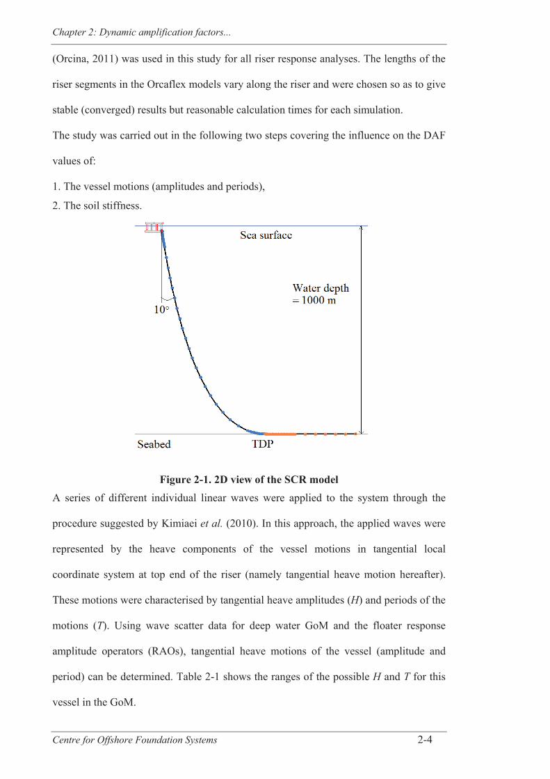
Chapter 2: Dynamic amplification factors...
Centre for Offshore Foundation Systems 2-4
(Orcina, 2011) was used in this study for all riser response analyses. The lengths of the
riser segments in the Orcaflex models vary along the riser and were chosen so as to give
stable (converged) results but reasonable calculation times for each simulation.
The study was carried out in the following two steps covering the influence on the DAF
values of:
1. The vessel motions (amplitudes and periods),
2. The soil stiffness.
Figure 2-1. 2D view of the SCR model A series of different individual linear waves were applied to the system through the
procedure suggested by Kimiaei et al. (2010). In this approach, the applied waves were
represented by the heave components of the vessel motions in tangential local
coordinate system at top end of the riser (namely tangential heave motion hereafter).
These motions were characterised by tangential heave amplitudes (H) and periods of the
motions (T). Using wave scatter data for deep water GoM and the floater response
amplitude operators (RAOs), tangential heave motions of the vessel (amplitude and
period) can be determined. Table 2-1 shows the ranges of the possible H and T for this
vessel in the GoM.
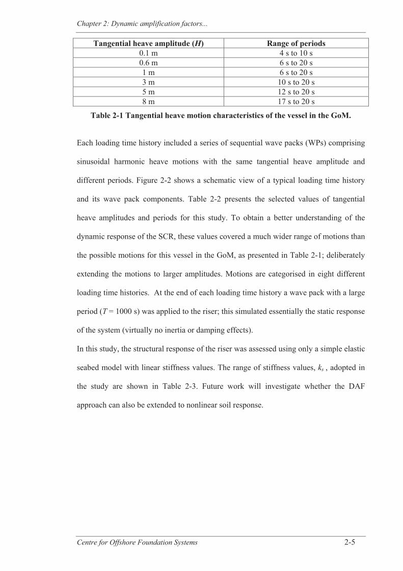
Chapter 2: Dynamic amplification factors...
Centre for Offshore Foundation Systems 2-5
Tangential heave amplitude (H) Range of periods 0.1 m 4 s to 10 s 0.6 m 6 s to 20 s 1 m 6 s to 20 s 3 m 10 s to 20 s 5 m 12 s to 20 s 8 m 17 s to 20 s
Table 2-1 Tangential heave motion characteristics of the vessel in the GoM.
Each loading time history included a series of sequential wave packs (WPs) comprising
sinusoidal harmonic heave motions with the same tangential heave amplitude and
different periods. Figure 2-2 shows a schematic view of a typical loading time history
and its wave pack components. Table 2-2 presents the selected values of tangential
heave amplitudes and periods for this study. To obtain a better understanding of the
dynamic response of the SCR, these values covered a much wider range of motions than
the possible motions for this vessel in the GoM, as presented in Table 2-1; deliberately
extending the motions to larger amplitudes. Motions are categorised in eight different
loading time histories. At the end of each loading time history a wave pack with a large
period (T = 1000 s) was applied to the riser; this simulated essentially the static response
of the system (virtually no inertia or damping effects).
In this study, the structural response of the riser was assessed using only a simple elastic
seabed model with linear stiffness values. The range of stiffness values, ks , adopted in
the study are shown in Table 2-3. Future work will investigate whether the DAF
approach can also be extended to nonlinear soil response.
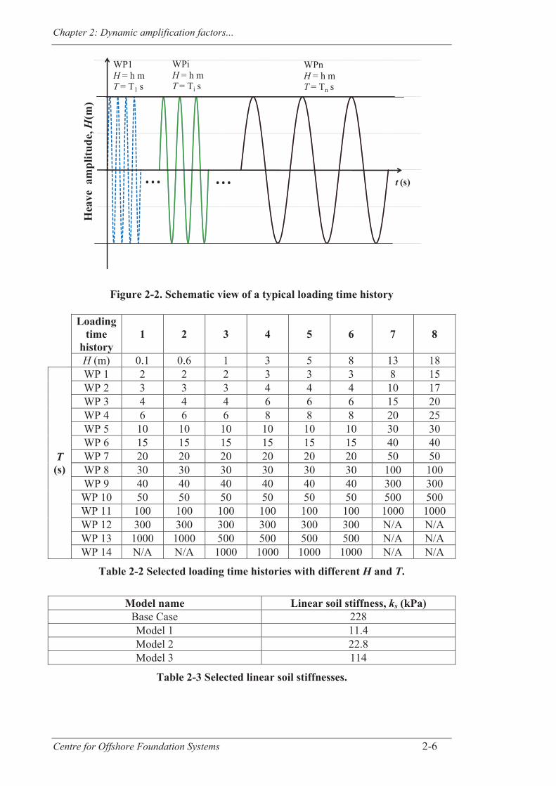
Chapter 2: Dynamic amplification factors...
Centre for Offshore Foundation Systems 2-6
Figure 2-2. Schematic view of a typical loading time history
Loading
time history
1 2 3 4 5 6 7 8
H (m) 0.1 0.6 1 3 5 8 13 18
T (s)
WP 1 2 2 2 3 3 3 8 15 WP 2 3 3 3 4 4 4 10 17 WP 3 4 4 4 6 6 6 15 20 WP 4 6 6 6 8 8 8 20 25 WP 5 10 10 10 10 10 10 30 30 WP 6 15 15 15 15 15 15 40 40 WP 7 20 20 20 20 20 20 50 50 WP 8 30 30 30 30 30 30 100 100 WP 9 40 40 40 40 40 40 300 300 WP 10 50 50 50 50 50 50 500 500 WP 11 100 100 100 100 100 100 1000 1000 WP 12 300 300 300 300 300 300 N/A N/A WP 13 1000 1000 500 500 500 500 N/A N/A WP 14 N/A N/A 1000 1000 1000 1000 N/A N/A
Table 2-2 Selected loading time histories with different H and T.
Model name Linear soil stiffness, ks (kPa) Base Case 228 Model 1 11.4 Model 2 22.8 Model 3 114
Table 2-3 Selected linear soil stiffnesses.
t (s)
Hea
ve a
mpl
itude
,H(m
)
WPnH = h mT = Tn s
WPiH = h mT = Ti s
WP1H = h mT = T1 s
... ...
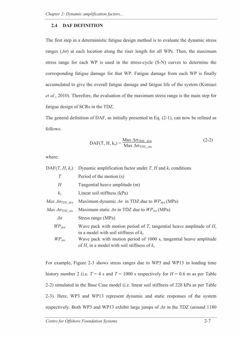
Chapter 2: Dynamic amplification factors...
Centre for Offshore Foundation Systems 2-7
2.4 DAF DEFINITION
The first step in a deterministic fatigue design method is to evaluate the dynamic stress
ranges ( ) at each location along the riser length for all WPs. Then, the maximum
stress range for each WP is used in the stress-cycle (S-N) curves to determine the
corresponding fatigue damage for that WP. Fatigue damage from each WP is finally
accumulated to give the overall fatigue damage and fatigue life of the system (Kimiaei
et al., 2010). Therefore, the evaluation of the maximum stress range is the main step for
fatigue design of SCRs in the TDZ.
The general definition of DAF, as initially presented in Eq. (2-1), can now be refined as
follows:
DAF(T, H, ks) = Max ΔσTDZ_dyn Max ΔσTDZ_sta
(2-2)
where:
DAF(T, H, ks) Dynamic amplification factor under T, H and ks conditions
T Period of the motion (s)
H Tangential heave amplitude (m)
ks Linear soil stiffness (kPa)
Max TDZ_dyn Maximum dynamic in TDZ due to WPdyn (MPa)
Max TDZ_sta Maximum static in TDZ due to WPsta (MPa)
Stress range (MPa)
WPdyn Wave pack with motion period of T, tangential heave amplitude of H, in a model with soil stiffness of ks
WPsta Wave pack with motion period of 1000 s, tangential heave amplitude of H, in a model with soil stiffness of ks
For example, Figure 2-3 shows stress ranges due to WP3 and WP13 in loading time
history number 2 (i.e. T = 4 s and T = 1000 s respectively for H = 0.6 m as per Table
2-2) simulated in the Base Case model (i.e. linear soil stiffness of 228 kPa as per Table
2-3). Here, WP3 and WP13 represent dynamic and static responses of the system
respectively. Both WP3 and WP13 exhibit large jumps of in the TDZ (around 1180
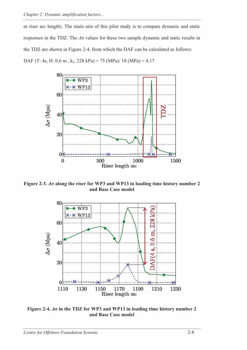
Chapter 2: Dynamic amplification factors...
Centre for Offshore Foundation Systems 2-8
m riser arc length). The main aim of this pilot study is to compare dynamic and static
responses in the TDZ. The values for these two sample dynamic and static results in
the TDZ are shown in Figure 2-4, from which the DAF can be calculated as follows:
DAF (T: 4s, H: 0.6 m , ks: 228 kPa) = 75 (MPa)/ 18 (MPa) = 4.17
Figure 2-3. Δσ along the riser for WP3 and WP13 in loading time history number 2 and Base Case model
Figure 2-4. Δσ in the TDZ for WP3 and WP13 in loading time history number 2 and Base Case model
Chapter 2: Dynamic amplification factors...
Centre for Offshore Foundation Systems 2-9
2.5 NUMERICAL RESULTS
2.5.1 DAF sensitivity to heave amplitude and motion periods
In the first step of this study, DAF values for the given tangential heave amplitudes and
the given motion periods were evaluated. In this regard, eight different loading time
histories (as presented in Table 2-2) were applied individually on the Base Case model.
Maximum stress ranges in the TDZ for each WP were evaluated and then DAF values
were calculated.
The effects of the tangential heave amplitudes and periods on the maximum stress
ranges in the touchdown zone (Max TDZ) are represented in Figure 2-5. The results
show that larger tangential heave amplitudes (H) lead in overall to greater Max TDZ for
both dynamic and static responses. An increasing and then a decreasing trend in the
Max TDZ values is observed for all H ≥ 1 m cases, whereas a continuous decreasing
trend is seen for all H < 1 m cases. Moreover, for all H ≥ 1 m cases a peak value is seen
at a particular period that increases with the magnitude of the tangential heave
amplitude. This can be considered as an indication of resonance in the overall response
of the SCR where the loading period is equal or very close to the fundamental period of
the system. There is no source of material nonlinearity in this model but it is still a
nonlinear model from geometrical perspectives (riser-soil contact area varies during
each single motion of the riser) and from loading perspectives (since hydrodynamic
forces on the riser depend on the riser motions). That is why for increasing loading on
the system (i.e. increasing tangential heave amplitudes) increasing resonance periods are
observed in Figure 2-5. It should be noted that, as mentioned in above, the range of the
selected H and T in Figure 2-5 does not necessarily represent realistic seastates for the
motions of this vessel in the GoM. In this pilot study, they cover a wider range than the
real possible ranges for H and T in order to obtain a clear picture of the overall dynamic
response of the SCRs and the corresponding DAFs. That is why for the larger H values

Chapter 2: Dynamic amplification factors...
Centre for Offshore Foundation Systems 2-10
unreasonably large Max TDZ can be observed in Figure 2-5.
Figure 2-6 shows Max TDZ if only the realistic ranges of H and T (as per Table 2-1,
with the period ranges extended to a minimum of 10 s and 15 s for H = 5 m and H = 8 m
respectively) are selected. Comparison between Figure 2-5 and Figure 2-6 shows that
the resonance of the SCR, which occurs at a particular period beyond the selected range
of the periods in Figure 2-6, can be missed if the dynamic response of this SCR is
explored only over the realistic range of H and T.
Variations of DAF values with motions presented in Table 2-2 are shown in Figure 2-7.
The resonance of the SCR system is also observed in these DAF plots. It is seen that
both small and large heave motions (H ≤ 0.6 m and H ≥ 13 m respectively) lead to very
large DAFs (up to a maximum of 14) whereas moderate heave motions
(0.6 m < H < 13 m) lead to smaller DAFs (maximum of 9). It should be noted that, as
per Eq. (2-2), the DAF is proportional to Max TDZ_dyn and inversely proportional to
Max TDZ_sta. Referring to Figure 2-5, large DAFs for large heave motions (H ≥ 13 m)
are mainly due to large Max TDZ_dyn, while large DAFs for small heave motions (H ≤
0.6 m) arise from small Max TDZ_sta. Figure 2-8 represents the variations of DAF
values for the realistic range of the vessel motions (as per Table 2-1). It is seen that the
DAF, for this particular SCR system, is inversely proportional to the period for all
vessel motions. Furthermore, the DAF varies inversely with the tangential heave
amplitude for H ≤ 3 m but increases with increasing tangential heave amplitude for H >
3 m.
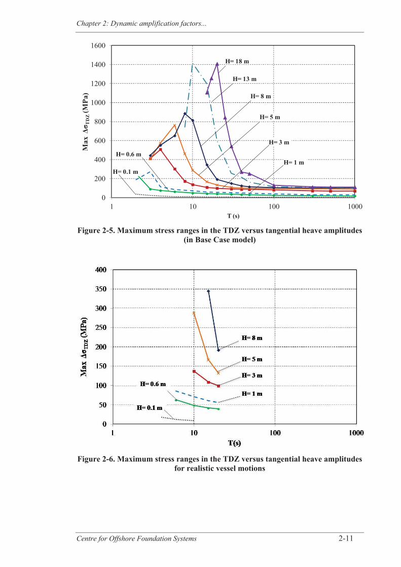
Chapter 2: Dynamic amplification factors...
Centre for Offshore Foundation Systems 2-11
Figure 2-5. Maximum stress ranges in the TDZ versus tangential heave amplitudes (in Base Case model)
Figure 2-6. Maximum stress ranges in the TDZ versus tangential heave amplitudes for realistic vessel motions
0
200
400
600
800
1000
1200
1400
1600
1 10 100 1000
Max
Δσ T
DZ
(MPa
)
T (s)
H= 8 m
H= 18 m
H= 13 m
H= 5 m
H= 3 m
H= 1 mH= 0.6 m
H= 0.1 m
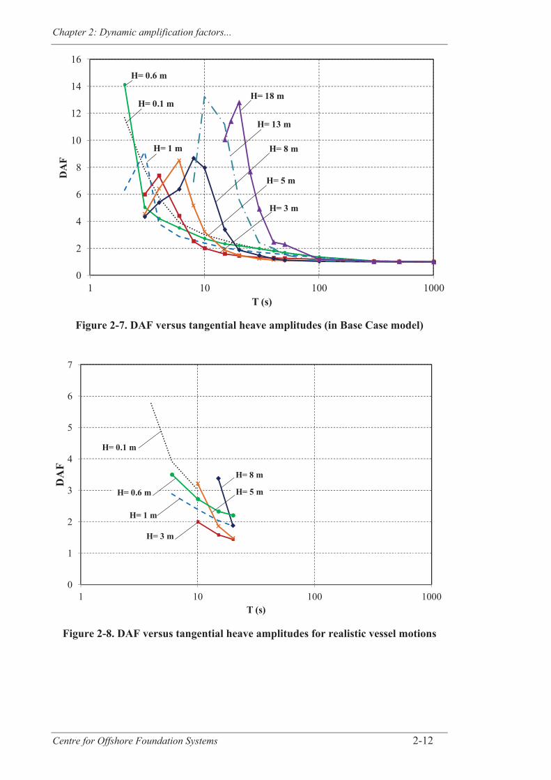
Chapter 2: Dynamic amplification factors...
Centre for Offshore Foundation Systems 2-12
Figure 2-7. DAF versus tangential heave amplitudes (in Base Case model)
Figure 2-8. DAF versus tangential heave amplitudes for realistic vessel motions
0
2
4
6
8
10
12
14
16
1 10 100 1000
DA
F
T (s)
H= 8 m
H= 18 m
H= 13 m
H= 5 m
H= 3 m
H= 1 m
H= 0.6 m
H= 0.1 m
0
1
2
3
4
5
6
7
1 10 100 1000
DA
F
T (s)
H= 3 m
H= 1 m
H= 0.6 m
H= 0.1 m
H= 8 m
H= 5 m
Chapter 2: Dynamic amplification factors...
Centre for Offshore Foundation Systems 2-13
2.5.2 DAF sensitivity to soil stiffness
Effects of soil stiffness (ks) on DAF values were investigated in the second part of this
study. Only linear soil models (similar to what is commonly used in traditional fatigue
design of SCRs) were used in the Orcaflex numerical simulations here. The soil
stiffness values selected in this parametric study are summarised in Table 2-3.
Figure 2-9 presents the effects of the soil stiffness on the maximum for tangential
heave amplitudes of 0.1 m, 0.6 m, 3 m, 5 m, 8 m and 13 m. It is seen that, for all of
these, the stiffer soil model (higher ks) will result in higher maximum for all different
periods. This means that, for traditional linear soil models, higher soil stiffness will lead
to more conservative fatigue results (lower fatigue life). This is consistent with the
results from Bridge et al. (2004).
Figure 2-10 shows the effects of soil stiffness on DAF values for different tangential
heave amplitudes. It is observed that soil stiffness has no major influence on the overall
trend of the DAF plots or on their corresponding resonance periods either. For long
periods (T ≥ 15 s), there is almost no difference between DAFs for different soil
stiffness values. However, for short periods (T < 15 s), a different concept is observed
depending on the tangential heave amplitude: for small tangential heave amplitudes
(H ≤ 5 m), the softer soil shows a slightly higher DAF which contrasts with the results
for higher tangential heave amplitudes (H > 5 m). For the realistic range of the motions
of this vessel (Table 2-1), the overall difference between DAF values at a given period
for different soil stiffnesses is less than or equal to 10 %.
Further studies need to be performed to explore the effect of these DAF differences on
the fatigue life of the SCR system. However, if the impact on the fatigue life is
negligible, DAF could be investigated only for a given soil stiffness; which would
considerably simplify the approach.
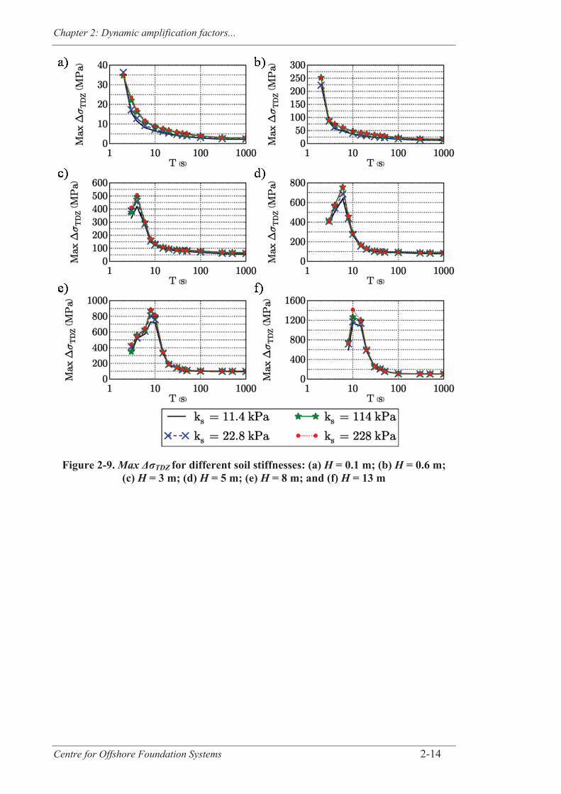
Chapter 2: Dynamic amplification factors...
Centre for Offshore Foundation Systems 2-14
Figure 2-9. Max ΔσTDZ for different soil stiffnesses: (a) H = 0.1 m; (b) H = 0.6 m; (c) H = 3 m; (d) H = 5 m; (e) H = 8 m; and (f) H = 13 m
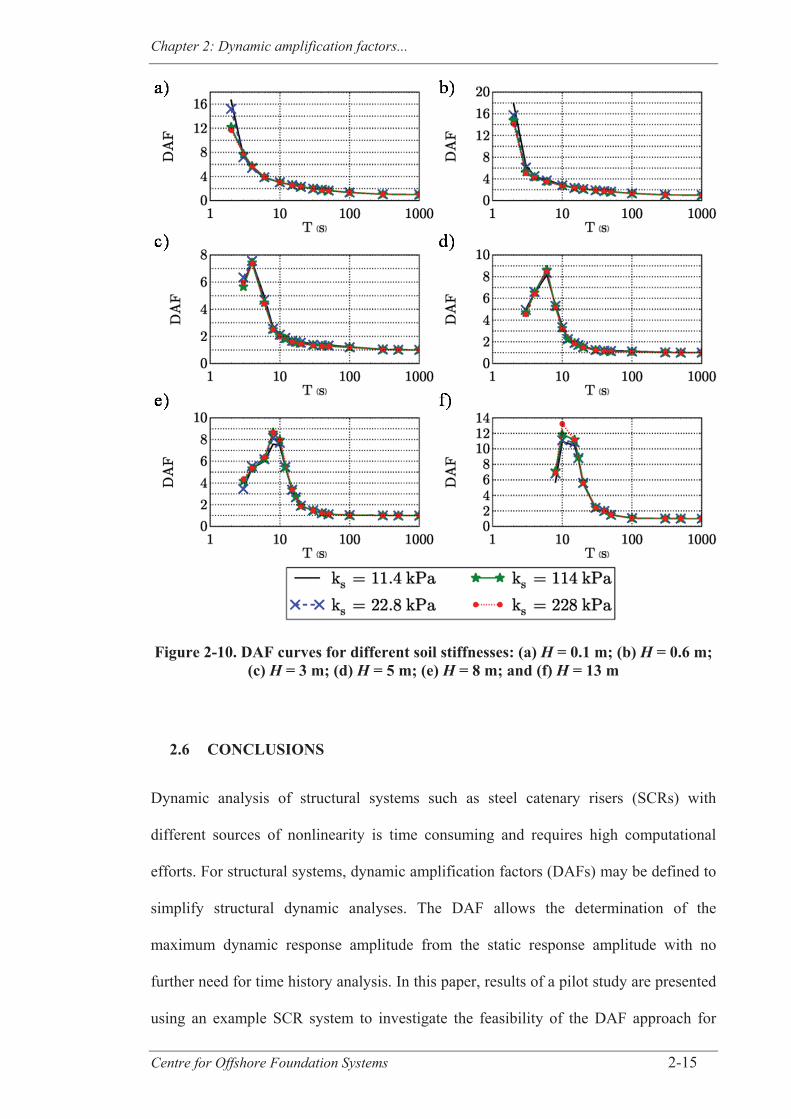
Chapter 2: Dynamic amplification factors...
Centre for Offshore Foundation Systems 2-15
Figure 2-10. DAF curves for different soil stiffnesses: (a) H = 0.1 m; (b) H = 0.6 m; (c) H = 3 m; (d) H = 5 m; (e) H = 8 m; and (f) H = 13 m
2.6 CONCLUSIONS
Dynamic analysis of structural systems such as steel catenary risers (SCRs) with
different sources of nonlinearity is time consuming and requires high computational
efforts. For structural systems, dynamic amplification factors (DAFs) may be defined to
simplify structural dynamic analyses. The DAF allows the determination of the
maximum dynamic response amplitude from the static response amplitude with no
further need for time history analysis. In this paper, results of a pilot study are presented
using an example SCR system to investigate the feasibility of the DAF approach for
Chapter 2: Dynamic amplification factors...
Centre for Offshore Foundation Systems 2-16
SCRs, which are nonlinear systems. DAF sensitivity to floater motions and soil stiffness
was investigated. The study revealed that:
Higher tangential heave amplitudes led to higher maximum stress ranges for both
dynamic and static results.
DAF curves for different tangential heave amplitudes exhibited resonance periods
that depended on the magnitude of the perturbation of the SCR system. The
resonance concept and dependency of the DAF on the floater motions (tangential
heave and period) need more detailed studies in the future.
The stiffer soil generated higher maximum stress range for both dynamic and static
cases. Higher soil stiffness led to more conservative results with reduced fatigue life.
Soil stiffness had no major effect on the DAF curves or on the resonance periods,
associated with each tangential heave amplitude. Therefore, DAF could be defined as
independent from the soil stiffness, but further work is needed to validate this result.
In general, the DAF approach seems to be a reasonable approach for determination of
maximum dynamic response of nonlinear SCR systems. Certain other key parameters in
fatigue analysis, such as the hang-off angle and other riser characteristics (weight per
unit length, bending stiffness, etc.) and the nonlinear soil behaviour may influence the
DAF and further analyses are needed to quantify the effects of these system parameters.
Ultimately, the aim of future studies is to express DAFs in an appropriately non-
dimensional manner with respect to the SCR system parameters and the applied
motions.
Estimating the fatigue damage of SCRs in the TDZ
Centre for Offshore Foundation Systems 3-1
CHAPTER 3 DIMENSIONLESS GROUPS GOVERNING
RESPONSE OF STEEL CATENARY RISERS
3.1 ABSTRACT
Steel catenary risers (SCRs) are one of the most cost effective type of risers in deep
water, but their design, particularly in the touchdown zone (TDZ), is challenging.
Design uncertainties arise due to limited understanding of the influence of various
parameters on the SCR response, pertaining to the SCR geometry and structural
properties, environmental loading and the seabed characteristics. An improved
framework that provides quantitative guidance on how each parameter affects the
overall structural response, and in particular fatigue damage in the touchdown zone,
would facilitate design and increase confidence in the use of SCRs.
This paper details the application of dimensional analysis to SCR behaviour. Suitable
dimensionless groups are proposed and validated through a series of numerical tests,
comparing the response of similar SCR systems defined by appropriate scaling of
parameters. Due to the fundamental effect of the seabed response on fatigue damage,
two types of soil models are considered in the study: a linear and a nonlinear model.
The study provides a framework for design of SCRs, facilitating sensitivity analyses,
enabling better control on parameters and reducing the number of simulations required.
Chapter 3: Dimensionless groups governing response of SCRs
Centre for Offshore Foundation Systems 3-2
3.2 INTRODUCTION
Offshore exploration and production of oil and gas continue to increase and move into
ever deeper water. As a result, conventional flexible risers have largely been replaced
by steel catenary risers (SCRs), which are one of the most cost effective types of risers
(Campbell, 1999; Bai and Bai, 2005). Fatigue design of SCRs is a complex and crucial
challenge as SCR failure would have significant environmental and economic
consequences. Vessel motions and hydrodynamic loading result in two critical fatigue
areas: at the vessel hang-off point, and in the touchdown zone (TDZ – the area of
dynamic riser-soil interaction (Bridge, 2005)). Indeed, in the TDZ, cyclic motions of the
SCR lead to complex interactions between the seabed and the riser. In most design,
numerical analysis of riser-soil interaction is based on a linear soil model, although
difficulties in assessing suitable values of soil stiffness, which have been shown to vary
with the amplitude of cyclic displacement (Clukey et al., 2005, 2007, 2008), have
encouraged development of more sophisticated nonlinear soil models (Bridge and
Howells, 2007; Aubeny and Biscontin, 2009; Randolph and Quiggin, 2009). The riser-
soil interaction is complicated by the likelihood of extreme soil degradation in the
touchdown zone during significant storms, with intervening periods where
reconsolidation of the soil will occur. This type of behaviour is not captured by existing
soil models, although recent experimental data suggests gradual hardening of the soil
following initial cyclic degradation, with diminishing effects of each episode of cyclic
motions (Hodder et al., 2013).
Despite previous parametric studies, there is still limited understanding of the effect of
individual parameters pertaining to soil response, riser characteristics (e.g. material
properties, geometry etc.) and environmental loading, on SCR fatigue design (Xia et al.,
2008; Kimiaei et al., 2010). Sensitivity studies to investigate the influence of
parameters, particularly where their value is uncertain, are recommended in riser design
Chapter 3: Dimensionless groups governing response of SCRs
Centre for Offshore Foundation Systems 3-3
guidelines (DNV-OS-F201, 2010), in order to improve understanding of the overall
SCR behaviour, provide more accurate modelling and increase confidence in design.
To conduct pertinent sensitivity analyses, it is necessary to identify the dimensionless
groups of parameters that influence key response variables (Palmer, 2008b), which are
typically the pipe stress or curvature for overall integrity, and the cyclic stress range for
fatigue assessment. Establishment of these groups can be achieved by performing
dimensional analysis. As noted by Pesce et al. (1998b), non-dimensional parameters are
intrinsically “generally valid”. A limited set of dimensionless groups have been used in
analytical studies of SCRs (Pesce et al., 1998b, 2006), for the post processing of results
from numerical analyses (Pesce et al., 1998b; Randolph and White, 2008; Aubeny and
Biscontin, 2009) and recently in the scaling of a riser model to ensure similarity in
modal responses, and hence overall riser dynamics (Rateiro et al., 2012). However, for
more robust dimensional analysis, it is necessary to identify the entire set of
dimensionless groups pertinent to a problem (Taylor, 1974). Sensitivity analyses consist
in investigating, and ideally quantifying, the effects that changes in one or more
dimensionless group of input parameters have on a specific dimensionless group of
output parameters. For SCRs, dependencies between variables are not systematically
obvious. Indeed some care is needed in choosing an appropriate set of dimensionless
groups. Modification of a particular input parameter may otherwise lead to unwanted
changes in several dependent dimensionless groups, which impedes interpretation of
results due to a combination of contributions. An appropriate complete set of
dimensionless groups allows clarification of relationships between parameters, thus
facilitating pre-processing of input data and post-processing of results. It also provides a
framework for meaningful comparisons of SCR behaviour.
The principal purpose of this paper is to establish an appropriate and complete list of
dimensionless groups governing SCR static and dynamic response to motions applied at
Chapter 3: Dimensionless groups governing response of SCRs
Centre for Offshore Foundation Systems 3-4
the hang-off point. This study is part of ongoing research aiming to simplify fatigue
design of SCR systems by means of dynamic amplification factors (DAFs) (Quéau et
al., 2011). DAFs allow the determination of maximum dynamic response amplitudes
directly from the analytically derived static response, reducing the need to perform time
consuming dynamic analyses in the early stages of design. The usefulness of this
approach in SCR studies has been explored previously by the authors through pilot
sensitivity analyses for a few key input parameters (Quéau et al., 2011). Defining the
entire set of dimensionless groups that impact SCR behaviour will assist future
sensitivity analyses aimed at establishing quantitative relationships between input and
output dimensionless groups. Dimensional analysis, using the traditional -theorem, is
applied to the structural response of SCRs, considering both linear and nonlinear soil
models. The study is mainly focused on fatigue design in the touchdown zone and,
therefore, the cyclic stress range and DAF are of primary interest. The logic behind the
selection of the dimensionless groups is presented first, and then numerical analyses are
performed to verify that all the dimensionless groups have been identified.
3.3 DIMENSIONAL ANALYSIS THEORY
Dimensional analysis aims to clarify dependencies between magnitudes of quantities
pertaining to a physical problem by considering their dimensions. The method is based
on the principle of homogeneity, which states that equations involving magnitudes of
quantities must be dimensionally homogeneous (Massey, 1971). Dimensional analysis
is particularly suitable for the study of complex phenomena, involving numerous
independent variables for instance, for which complete theoretical treatment is
challenging (Massey, 1971; Taylor, 1974; Palmer, 2008b).
Chapter 3: Dimensionless groups governing response of SCRs
Centre for Offshore Foundation Systems 3-5
This method is used when researching a relation of the form expressed as:
Q1 = f(Q2, Q3, ..., Qn) (3-1)
where Q1 represents the magnitude of the output and Qi are the magnitudes of the inputs
pertinent to the problem; f stands for “some function of” (Massey, 1971). The first step
of the method is to select the appropriate initial quantities (output and inputs). This task
is challenging as it is necessary that one and only one relationship exists between the
quantities selected (Taylor, 1974; Palmer, 2008b). The second step consists of grouping
the original quantities into dimensionless groups, i , in order to form a new
relationship, such as:
1 = f ( 2 3, n-m) (3-2)
which contains all the information of Eq. (3-1) (Taylor, 1974). The number of
independent dimensionless groups that can be formed is determined using the Vaschy-
Buckingham (or ) theorem. It states that “if m is the number of distinct fundamental
magnitudes required to express the dimensional formulae of all the n magnitudes, then
these n magnitudes may be grouped into n-m independent dimensionless terms”
(Massey, 1971). Several mathematical methods exist to find preliminary dimensionless
groups. As any combination of dimensionless groups is also dimensionless, these
preliminary dimensionless groups may be combined together to obtain more meaningful
groups for the purpose of a particular study.
Although dimensional analysis alone cannot usually lead to the complete solution of a
problem, it does increase understanding and can guide the design of experiments and
numerical simulations. Moreover, the influence of certain variables, as well as some
direct relationships, may emerge from the analysis (Massey, 1971; Taylor, 1974;
Palmer, 2008b).
Chapter 3: Dimensionless groups governing response of SCRs
Centre for Offshore Foundation Systems 3-6
3.4 DIMENSIONAL ANALYSIS OF SCR RESPONSE
3.4.1 Main assumptions
The study has adopted some minor idealisations and simplifications in order to render
the problem manageable, while still allowing broad application:
1. The study is restricted to 2D conditions, with SCRs response under in-plane
motions only.
2. Loading of SCRs is represented by harmonic motions of the floating vessels
through the procedure suggested by Kimiaei et al. (2010). Linear waves
identified as the wave packs (WPs) constitute the input motions. They are
represented by application of a time varying sinusoidal motion of the vessel,
making an angle m with the vertical and characterised by heave amplitude (H)
and period (T) of the motion (i.e. maximum input velocity of 2 H/T).
3. The choice of seabed model is of prime importance when studying the fatigue
life of SCRs in the TDZ, as it can affect analysis results (Bridge and Howells,
2007; Clukey et al., 2007). The study focuses on elastic seabed response, where
the soil is characterised by a linear stiffness (linear seabed model hereafter).
However, equivalent dimensionless groups are also proposed for the nonlinear
seabed model of Randolph and Quiggin (2009). Linear seabed models are easy
to use, and indeed represent current industry practice. However, they are limited
in their ability to accommodate realistic soil response, where the secant stiffness
decreases with increasing magnitude of displacement. Nonlinear soil models are
relatively new and although they capture some important features of the riser-
soil interaction (e.g. variation of soil stiffness, soil suction during uplift etc.)
their utilisation is more problematic (e.g. Bridge and Howells, 2007).
4. The current profile in the sea column is omitted (simplification also used by
Rateiro et al., 2012), the drag coefficient is set to a constant value and the
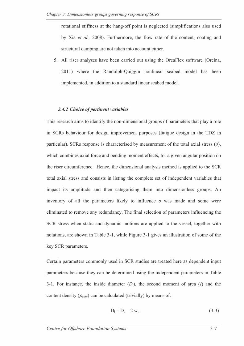
Chapter 3: Dimensionless groups governing response of SCRs
Centre for Offshore Foundation Systems 3-7
rotational stiffness at the hang-off point is neglected (simplifications also used
by Xia et al., 2008). Furthermore, the flow rate of the content, coating and
structural damping are not taken into account either.
5. All riser analyses have been carried out using the OrcaFlex software (Orcina,
2011) where the Randolph-Quiggin nonlinear seabed model has been
implemented, in addition to a standard linear seabed model.
3.4.2 Choice of pertinent variables
This research aims to identify the non-dimensional groups of parameters that play a role
in SCRs behaviour for design improvement purposes (fatigue design in the TDZ in
particular). SCRs response is characterised by measurement of the total axial stress ( ),
which combines axial force and bending moment effects, for a given angular position on
the riser circumference. Hence, the dimensional analysis method is applied to the SCR
total axial stress and consists in listing the complete set of independent variables that
impact its amplitude and then categorising them into dimensionless groups. An
inventory of all the parameters likely to influence was made and some were
eliminated to remove any redundancy. The final selection of parameters influencing the
SCR stress when static and dynamic motions are applied to the vessel, together with
notations, are shown in Table 3-1, while Figure 3-1 gives an illustration of some of the
key SCR parameters.
Certain parameters commonly used in SCR studies are treated here as dependent input
parameters because they can be determined using the independent parameters in Table
3-1. For instance, the inside diameter (Di), the second moment of area (I) and the
content density ( cont) can be calculated (trivially) by means of:
Di = Do – 2 wt (3-3)
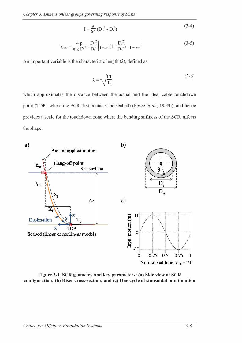
Chapter 3: Dimensionless groups governing response of SCRs
Centre for Offshore Foundation Systems 3-8
I = π64 (Do
4 - Di4)
(3-4)
ρcont = 4 p
π g Di2 -
Do2
Di2 ρsteel (1 -
Di2
Do2) - ρwater
(3-5)
An important variable is the characteristic length ( ), defined as:
λ = EITo
(3-6)
which approximates the distance between the actual and the ideal cable touchdown
point (TDP– where the SCR first contacts the seabed) (Pesce et al., 1998b), and hence
provides a scale for the touchdown zone where the bending stiffness of the SCR affects
the shape.
Figure 3-1 SCR geometry and key parameters: (a) Side view of SCR configuration; (b) Riser cross-section; and (c) One cycle of sinusoidal input motion
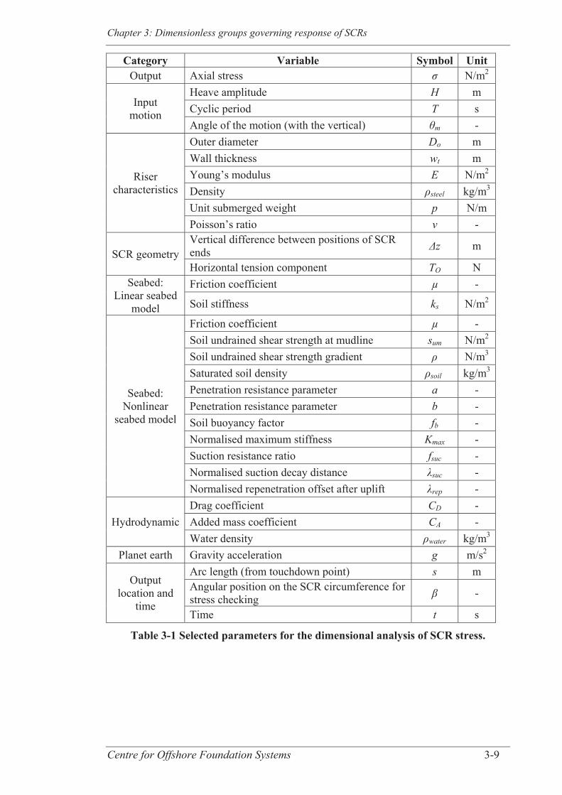
Chapter 3: Dimensionless groups governing response of SCRs
Centre for Offshore Foundation Systems 3-9
Category Variable Symbol Unit Output Axial stress N/m2
Input motion
Heave amplitude H m Cyclic period T s Angle of the motion (with the vertical) m -
Riser characteristics
Outer diameter Do m Wall thickness wt m Young’s modulus E N/m2 Density steel kg/m3
Unit submerged weight p N/m Poisson’s ratio -
SCR geometry Vertical difference between positions of SCR ends z m
Horizontal tension component TO N Seabed:
Linear seabed model
Friction coefficient μ -
Soil stiffness ks N/m2
Seabed: Nonlinear
seabed model
Friction coefficient μ - Soil undrained shear strength at mudline sum N/m2 Soil undrained shear strength gradient N/m3 Saturated soil density soil kg/m3
Penetration resistance parameter a - Penetration resistance parameter b - Soil buoyancy factor fb - Normalised maximum stiffness Kmax - Suction resistance ratio fsuc - Normalised suction decay distance suc - Normalised repenetration offset after uplift rep -
Hydrodynamic Drag coefficient CD - Added mass coefficient CA - Water density water kg/m3
Planet earth Gravity acceleration g m/s2
Output location and
time
Arc length (from touchdown point) s m Angular position on the SCR circumference for stress checking -
Time t s
Table 3-1 Selected parameters for the dimensional analysis of SCR stress.
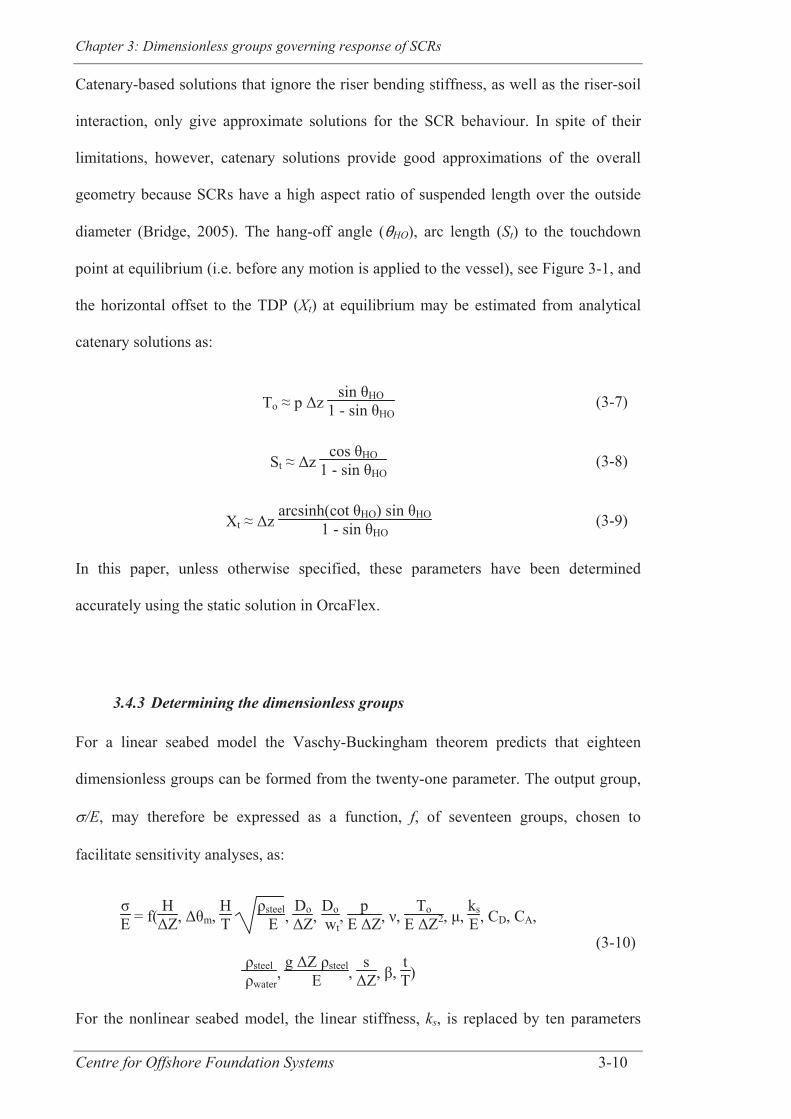
Chapter 3: Dimensionless groups governing response of SCRs
Centre for Offshore Foundation Systems 3-10
Catenary-based solutions that ignore the riser bending stiffness, as well as the riser-soil
interaction, only give approximate solutions for the SCR behaviour. In spite of their
limitations, however, catenary solutions provide good approximations of the overall
geometry because SCRs have a high aspect ratio of suspended length over the outside
diameter (Bridge, 2005). The hang-off angle ( HO), arc length (St) to the touchdown
point at equilibrium (i.e. before any motion is applied to the vessel), see Figure 3-1, and
the horizontal offset to the TDP (Xt) at equilibrium may be estimated from analytical
catenary solutions as:
To ≈ p Δz sin θHO
1 - sin θHO (3-7)
St ≈ Δz cos θHO
1 - sin θHO (3-8)
Xt ≈ Δz arcsinh(cot θHO) sin θHO
1 - sin θHO (3-9)
In this paper, unless otherwise specified, these parameters have been determined
accurately using the static solution in OrcaFlex.
3.4.3 Determining the dimensionless groups
For a linear seabed model the Vaschy-Buckingham theorem predicts that eighteen
dimensionless groups can be formed from the twenty-one parameter. The output group,
/E, may therefore be expressed as a function, f, of seventeen groups, chosen to
facilitate sensitivity analyses, as:
σE = f(
HΔZ, Δθm,
HT
ρsteel E ,
DoΔZ,
Do wt
, p
E ΔZ, ν, To
E ΔZ2, μ, ksE, CD, CA,
ρsteel ρwater
, g ΔZ ρsteel
E , s
ΔZ, β, tT)
(3-10)
For the nonlinear seabed model, the linear stiffness, ks, is replaced by ten parameters
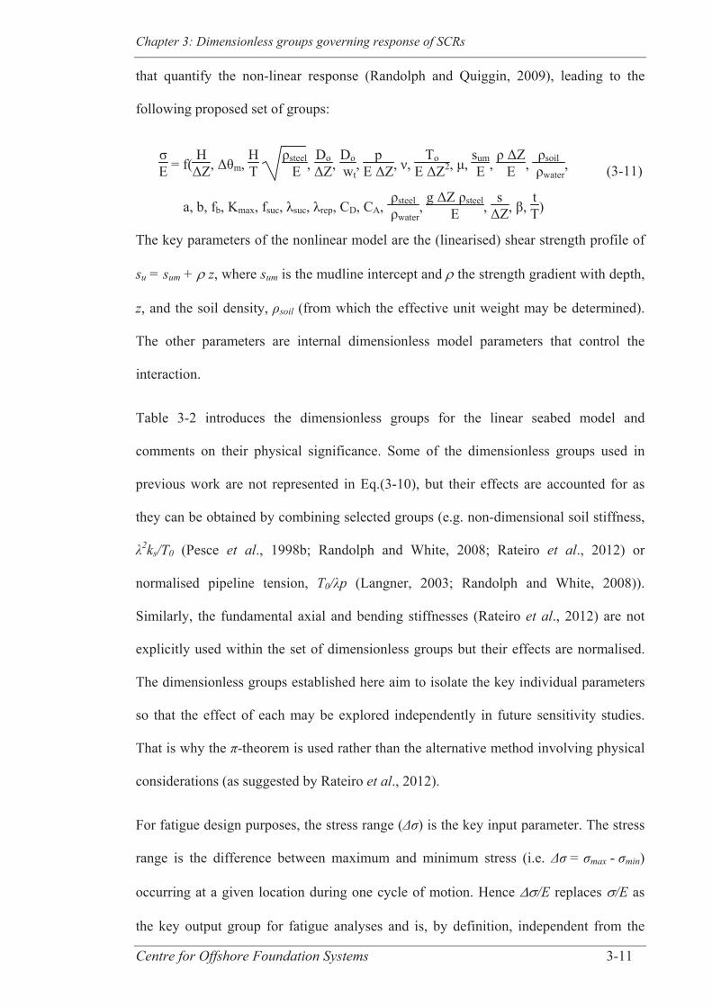
Chapter 3: Dimensionless groups governing response of SCRs
Centre for Offshore Foundation Systems 3-11
that quantify the non-linear response (Randolph and Quiggin, 2009), leading to the
following proposed set of groups:
σE = f(
HΔZ, Δθm,
HT
ρsteel E ,
DoΔZ,
Do wt
, p
E ΔZ, ν, To
E ΔZ2, μ, sumE ,
ρ ΔZE ,
ρsoil ρwater
,
a, b, fb, Kmax, fsuc, λsuc, λrep, CD, CA, ρsteel
ρwater, g ΔZ ρsteel
E , s
ΔZ, β, tT)
(3-11)
The key parameters of the nonlinear model are the (linearised) shear strength profile of
su = sum + z, where sum is the mudline intercept and the strength gradient with depth,
z, and the soil density, soil (from which the effective unit weight may be determined).
The other parameters are internal dimensionless model parameters that control the
interaction.
Table 3-2 introduces the dimensionless groups for the linear seabed model and
comments on their physical significance. Some of the dimensionless groups used in
previous work are not represented in Eq.(3-10), but their effects are accounted for as
they can be obtained by combining selected groups (e.g. non-dimensional soil stiffness,
2ks/T0 (Pesce et al., 1998b; Randolph and White, 2008; Rateiro et al., 2012) or
normalised pipeline tension, T0/ p (Langner, 2003; Randolph and White, 2008)).
Similarly, the fundamental axial and bending stiffnesses (Rateiro et al., 2012) are not
explicitly used within the set of dimensionless groups but their effects are normalised.
The dimensionless groups established here aim to isolate the key individual parameters
so that the effect of each may be explored independently in future sensitivity studies.
That is why the -theorem is used rather than the alternative method involving physical
considerations (as suggested by Rateiro et al., 2012).
For fatigue design purposes, the stress range ( ) is the key input parameter. The stress
range is the difference between maximum and minimum stress (i.e. = max - min)
occurring at a given location during one cycle of motion. Hence /E replaces /E as
the key output group for fatigue analyses and is, by definition, independent from the
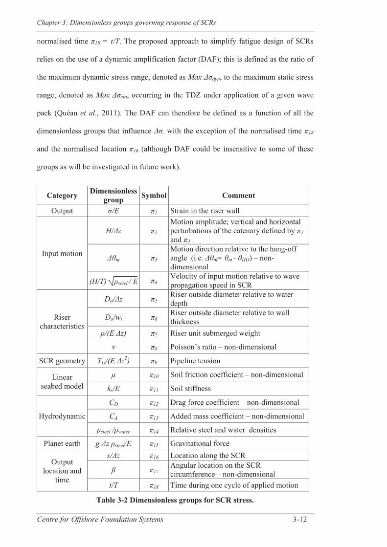
Chapter 3: Dimensionless groups governing response of SCRs
Centre for Offshore Foundation Systems 3-12
normalised time 18 = t/T. The proposed approach to simplify fatigue design of SCRs
relies on the use of a dynamic amplification factor (DAF); this is defined as the ratio of
the maximum dynamic stress range, denoted as Max dyn, to the maximum static stress
range, denoted as Max sta, occurring in the TDZ under application of a given wave
pack (Quéau et al., 2011). The DAF can therefore be defined as a function of all the
dimensionless groups that influence , with the exception of the normalised time 18
and the normalised location 16 (although DAF could be insensitive to some of these
groups as will be investigated in future work).
Category Dimensionless group Symbol Comment
Output /E 1 Strain in the riser wall
Input motion
H/ z 2 Motion amplitude; vertical and horizontal perturbations of the catenary defined by 2 and 3
m 3 Motion direction relative to the hang-off angle (i.e. m= m - HO) – non-dimensional
(H/T) steel / E 4 Velocity of input motion relative to wave propagation speed in SCR
Riser characteristics
Do/ z 5 Riser outside diameter relative to water depth
Do/wt 6 Riser outside diameter relative to wall thickness
p/(E z) 7 Riser unit submerged weight
8 Poisson’s ratio – non-dimensional
SCR geometry TO/(E z2) 9 Pipeline tension
Linear seabed model
10 Soil friction coefficient – non-dimensional
ks/E 11 Soil stiffness
Hydrodynamic
CD 12 Drag force coefficient – non-dimensional
CA 13 Added mass coefficient – non-dimensional
steel / water 14 Relative steel and water densities
Planet earth g z steel/E 15 Gravitational force
Output location and
time
s/ z 16 Location along the SCR
17 Angular location on the SCR circumference – non-dimensional
t/T 18 Time during one cycle of applied motion
Table 3-2 Dimensionless groups for SCR stress.
Chapter 3: Dimensionless groups governing response of SCRs
Centre for Offshore Foundation Systems 3-13
3.5 NUMERICAL MODELS FOR VERIFICATION OF THE
RELEVANCE OF DIMENSIONLESS GROUPS
A series of numerical analyses were performed to verify results of the dimensional
analysis with respect to the total axial stress and stress range for SCRs, and at the same
time establish the relative accuracy of the dynamic analysis software OrcaFlex.
Validation of the dimensionless groups was performed by comparing the strain ( /E)
and strain range ( /E) for different SCR models that have identical values of
dimensionless groups in Eq. (3-10) and Eq. (3-11), but obtained through different values
of input variables.
3.5.1 Linear seabed model
Three distinct base cases (BCs) are defined (BC1, BC2 and BC3) and, for each of them,
several model tests (MTs) with distinct sets of input parameters but the same
dimensionless group values for the particular BC, were established: MT1-1, MT2-1,
MT3-1 for BC1; MT1-2, MT2-2 for BC2; and MT1-3, MT2-3 for BC3. Two MTs are
defined for both BC2 and BC3 whereas an additional MT (MT3-1) is used for BC1 for
specific reasons detailed later on. Therefore, three groups of equivalent models are
defined (equivalent groups 1, 2 and 3). Table 3-3 summarises the values of the input
parameters used to define the ten models as well as values of some key dependent
parameters. In all these analyses, the vessel motion was applied parallel to the riser
tangential line at the hang-off point (i.e. m set to zero). This is based on the findings
of Kimiaei et al. (2010), that the tangential component of motion alone could
adequately represent the fatigue damage resulting from wave loading in the TDZ, but
the restriction does not affect the conclusions from this paper.
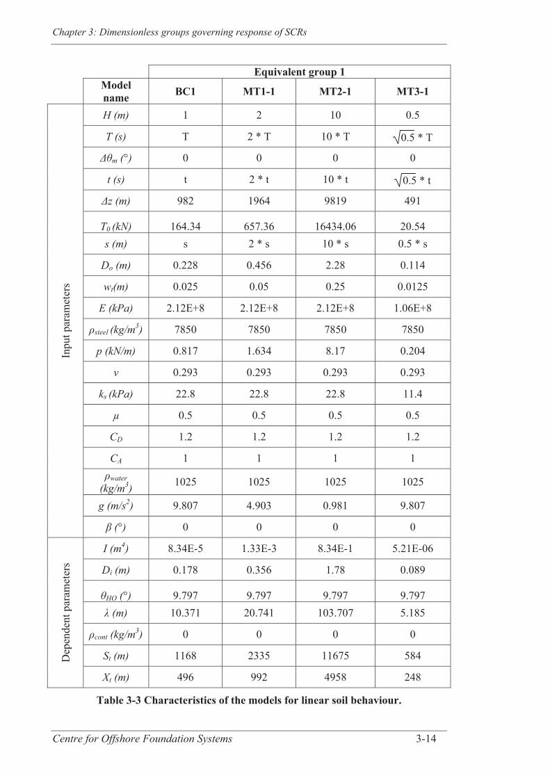
Chapter 3: Dimensionless groups governing response of SCRs
Centre for Offshore Foundation Systems 3-14
Equivalent group 1
Model name BC1 MT1-1 MT2-1 MT3-1
Inpu
t par
amet
ers
H (m) 1 2 10 0.5
T (s) T 2 * T 10 * T 0.5 * T
m (°) 0 0 0 0
t (s) t 2 * t 10 * t 0.5 * t
z (m) 982 1964 9819 491
T0 (kN) 164.34 657.36 16434.06 20.54 s (m) s 2 * s 10 * s 0.5 * s
Do (m) 0.228 0.456 2.28 0.114
wt(m) 0.025 0.05 0.25 0.0125
E (kPa) 2.12E+8 2.12E+8 2.12E+8 1.06E+8
steel (kg/m3) 7850 7850 7850 7850
p (kN/m) 0.817 1.634 8.17 0.204
0.293 0.293 0.293 0.293
ks (kPa) 22.8 22.8 22.8 11.4
μ 0.5 0.5 0.5 0.5
CD 1.2 1.2 1.2 1.2
CA 1 1 1 1
water (kg/m3) 1025 1025 1025 1025
g (m/s2) 9.807 4.903 0.981 9.807
(°) 0 0 0 0
Dep
ende
nt p
aram
eter
s
I (m4) 8.34E-5 1.33E-3 8.34E-1 5.21E-06
Di (m) 0.178 0.356 1.78 0.089
HO (°) 9.797 9.797 9.797 9.797 (m) 10.371 20.741 103.707 5.185
cont (kg/m3) 0 0 0 0
St (m) 1168 2335 11675 584
Xt (m) 496 992 4958 248
Table 3-3 Characteristics of the models for linear soil behaviour.
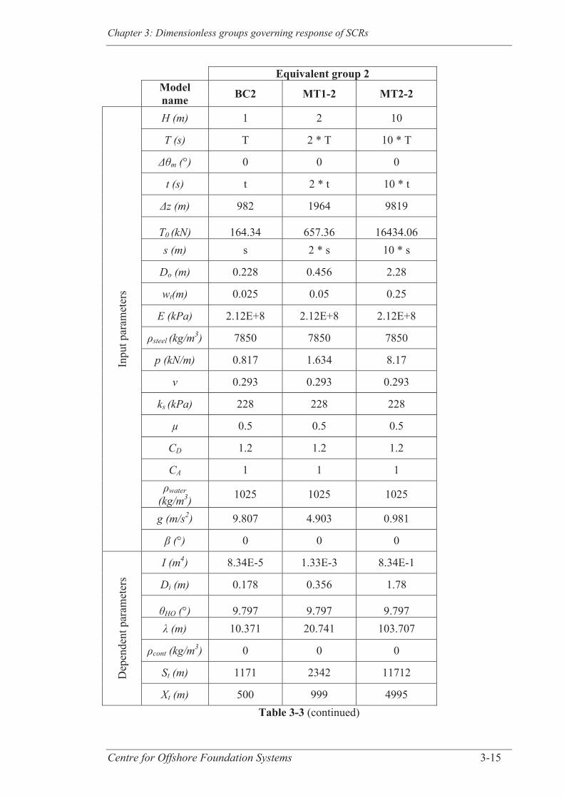
Chapter 3: Dimensionless groups governing response of SCRs
Centre for Offshore Foundation Systems 3-15
Equivalent group 2
Model name BC2 MT1-2 MT2-2
Inpu
t par
amet
ers
H (m) 1 2 10
T (s) T 2 * T 10 * T
m (°) 0 0 0
t (s) t 2 * t 10 * t
z (m) 982 1964 9819
T0 (kN) 164.34 657.36 16434.06 s (m) s 2 * s 10 * s
Do (m) 0.228 0.456 2.28
wt(m) 0.025 0.05 0.25
E (kPa) 2.12E+8 2.12E+8 2.12E+8
steel (kg/m3) 7850 7850 7850
p (kN/m) 0.817 1.634 8.17
0.293 0.293 0.293
ks (kPa) 228 228 228
μ 0.5 0.5 0.5
CD 1.2 1.2 1.2
CA 1 1 1
water (kg/m3) 1025 1025 1025
g (m/s2) 9.807 4.903 0.981
(°) 0 0 0
Dep
ende
nt p
aram
eter
s
I (m4) 8.34E-5 1.33E-3 8.34E-1
Di (m) 0.178 0.356 1.78
HO (°) 9.797 9.797 9.797 (m) 10.371 20.741 103.707
cont (kg/m3) 0 0 0
St (m) 1171 2342 11712
Xt (m) 500 999 4995 Table 3-3 (continued)
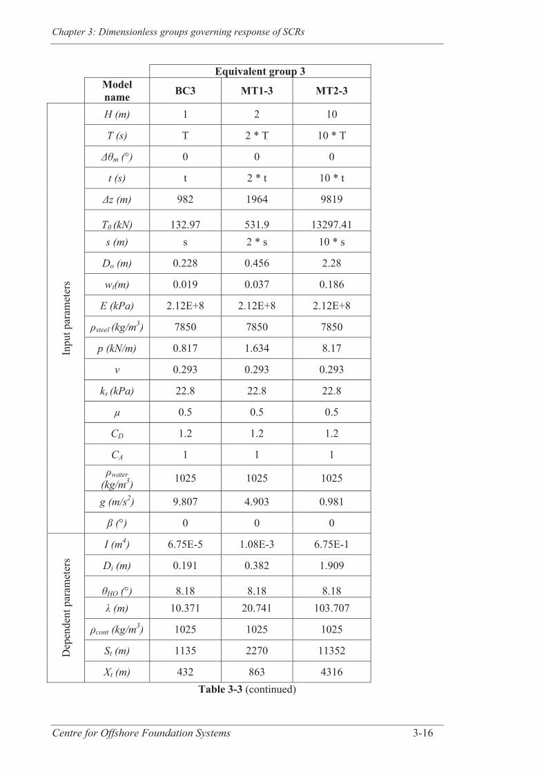
Chapter 3: Dimensionless groups governing response of SCRs
Centre for Offshore Foundation Systems 3-16
Equivalent group 3
Model name BC3 MT1-3 MT2-3
Inpu
t par
amet
ers
H (m) 1 2 10
T (s) T 2 * T 10 * T
m (°) 0 0 0
t (s) t 2 * t 10 * t
z (m) 982 1964 9819
T0 (kN) 132.97 531.9 13297.41 s (m) s 2 * s 10 * s
Do (m) 0.228 0.456 2.28
wt(m) 0.019 0.037 0.186
E (kPa) 2.12E+8 2.12E+8 2.12E+8
steel (kg/m3) 7850 7850 7850
p (kN/m) 0.817 1.634 8.17
0.293 0.293 0.293
ks (kPa) 22.8 22.8 22.8
μ 0.5 0.5 0.5
CD 1.2 1.2 1.2
CA 1 1 1
water (kg/m3) 1025 1025 1025
g (m/s2) 9.807 4.903 0.981
(°) 0 0 0
Dep
ende
nt p
aram
eter
s
I (m4) 6.75E-5 1.08E-3 6.75E-1
Di (m) 0.191 0.382 1.909
HO (°) 8.18 8.18 8.18 (m) 10.371 20.741 103.707
cont (kg/m3) 1025 1025 1025
St (m) 1135 2270 11352
Xt (m) 432 863 4316 Table 3-3 (continued)
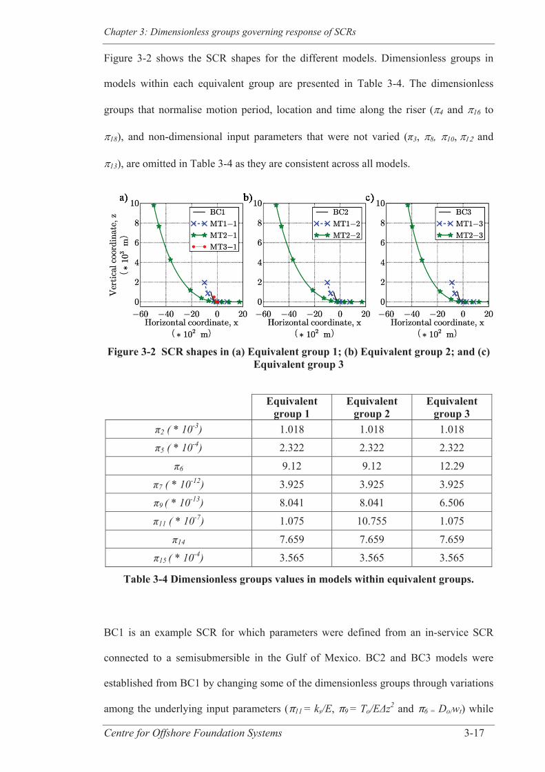
Chapter 3: Dimensionless groups governing response of SCRs
Centre for Offshore Foundation Systems 3-17
Figure 3-2 shows the SCR shapes for the different models. Dimensionless groups in
models within each equivalent group are presented in Table 3-4. The dimensionless
groups that normalise motion period, location and time along the riser ( 4 and 16 to
18), and non-dimensional input parameters that were not varied ( 3, 8, 10, and
13), are omitted in Table 3-4 as they are consistent across all models.
Figure 3-2 SCR shapes in (a) Equivalent group 1; (b) Equivalent group 2; and (c)
Equivalent group 3
Equivalent group 1
Equivalent group 2
Equivalent group 3
2 ( * 10-3) 1.018 1.018 1.018
5 ( * 10-4) 2.322 2.322 2.322
6 9.12 9.12 12.29
7 ( * 10-12) 3.925 3.925 3.925
9 ( * 10-13) 8.041 8.041 6.506
11 ( * 10-7) 1.075 10.755 1.075
14 7.659 7.659 7.659
15 ( * 10-4) 3.565 3.565 3.565
Table 3-4 Dimensionless groups values in models within equivalent groups.
BC1 is an example SCR for which parameters were defined from an in-service SCR
connected to a semisubmersible in the Gulf of Mexico. BC2 and BC3 models were
established from BC1 by changing some of the dimensionless groups through variations
among the underlying input parameters ( 11 = ks/E, 9 = To/E z2 and 6 = Do/wt) while
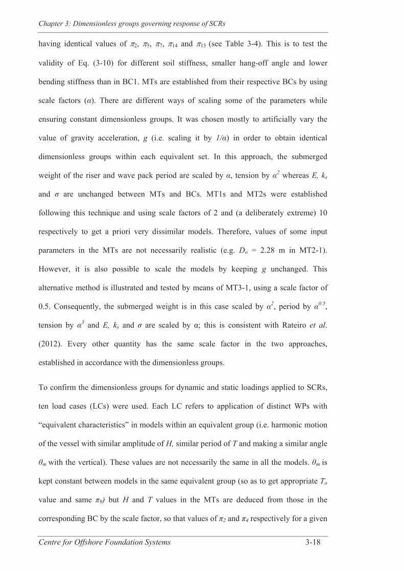
Chapter 3: Dimensionless groups governing response of SCRs
Centre for Offshore Foundation Systems 3-18
having identical values of 2, 5, 7, 14 and 15 (see Table 3-4). This is to test the
validity of Eq. (3-10) for different soil stiffness, smaller hang-off angle and lower
bending stiffness than in BC1. MTs are established from their respective BCs by using
scale factors ( ). There are different ways of scaling some of the parameters while
ensuring constant dimensionless groups. It was chosen mostly to artificially vary the
value of gravity acceleration, g (i.e. scaling it by 1/ ) in order to obtain identical
dimensionless groups within each equivalent set. In this approach, the submerged
weight of the riser and wave pack period are scaled by , tension by 2 whereas E, ks
and are unchanged between MTs and BCs. MT1s and MT2s were established
following this technique and using scale factors of 2 and (a deliberately extreme) 10
respectively to get a priori very dissimilar models. Therefore, values of some input
parameters in the MTs are not necessarily realistic (e.g. Do = 2.28 m in MT2-1).
However, it is also possible to scale the models by keeping g unchanged. This
alternative method is illustrated and tested by means of MT3-1, using a scale factor of
0.5. Consequently, the submerged weight is in this case scaled by 2, period by 0.5,
tension by 3 and E, ks and are scaled by α; this is consistent with Rateiro et al.
(2012). Every other quantity has the same scale factor in the two approaches,
established in accordance with the dimensionless groups.
To confirm the dimensionless groups for dynamic and static loadings applied to SCRs,
ten load cases (LCs) were used. Each LC refers to application of distinct WPs with
“equivalent characteristics” in models within an equivalent group (i.e. harmonic motion
of the vessel with similar amplitude of H, similar period of T and making a similar angle
m with the vertical). These values are not necessarily the same in all the models. m is
kept constant between models in the same equivalent group (so as to get appropriate To
value and same 9) but H and T values in the MTs are deduced from those in the
corresponding BC by the scale factor, so that values of 2 and 4 respectively for a given
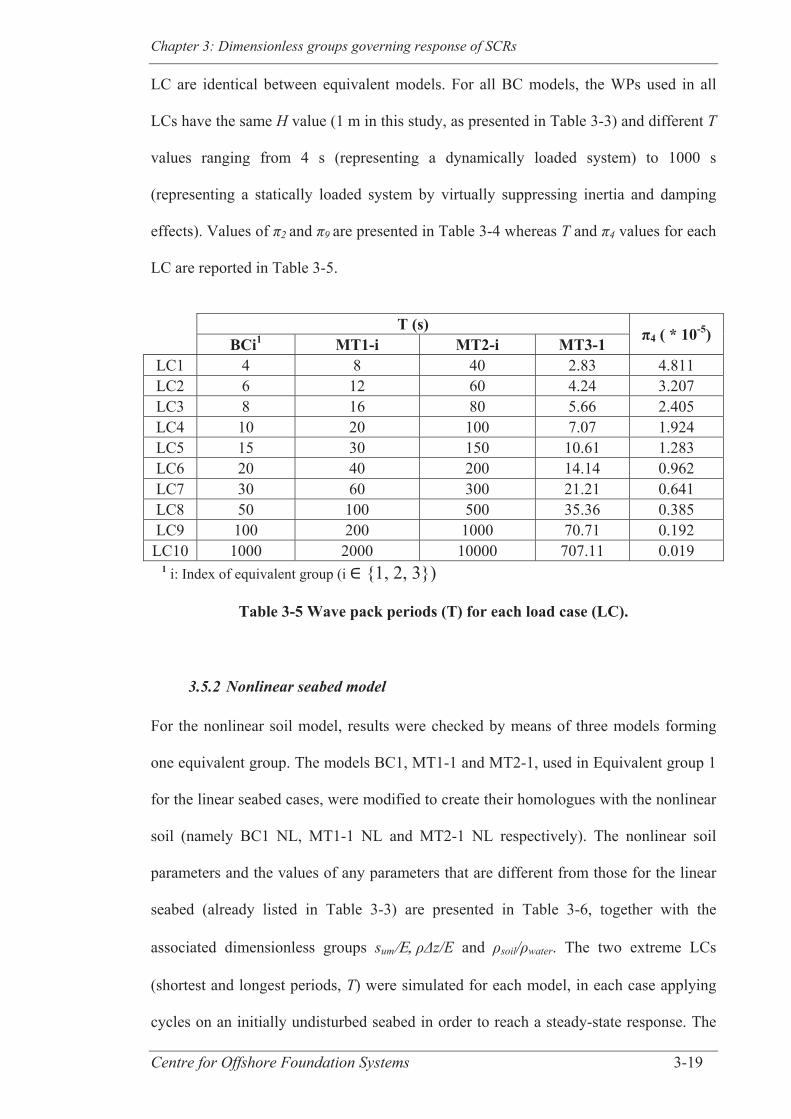
Chapter 3: Dimensionless groups governing response of SCRs
Centre for Offshore Foundation Systems 3-19
LC are identical between equivalent models. For all BC models, the WPs used in all
LCs have the same H value (1 m in this study, as presented in Table 3-3) and different T
values ranging from 4 s (representing a dynamically loaded system) to 1000 s
(representing a statically loaded system by virtually suppressing inertia and damping
effects). Values of 2 and 9 are presented in Table 3-4 whereas T and 4 values for each
LC are reported in Table 3-5.
T (s) π4 ( * 10-5) BCi1 MT1-i MT2-i MT3-1
LC1 4 8 40 2.83 4.811 LC2 6 12 60 4.24 3.207 LC3 8 16 80 5.66 2.405 LC4 10 20 100 7.07 1.924 LC5 15 30 150 10.61 1.283 LC6 20 40 200 14.14 0.962 LC7 30 60 300 21.21 0.641 LC8 50 100 500 35.36 0.385 LC9 100 200 1000 70.71 0.192
LC10 1000 2000 10000 707.11 0.019 1 i: Index of equivalent group (i {1, 2, 3})
Table 3-5 Wave pack periods (T) for each load case (LC).
3.5.2 Nonlinear seabed model
For the nonlinear soil model, results were checked by means of three models forming
one equivalent group. The models BC1, MT1-1 and MT2-1, used in Equivalent group 1
for the linear seabed cases, were modified to create their homologues with the nonlinear
soil (namely BC1 NL, MT1-1 NL and MT2-1 NL respectively). The nonlinear soil
parameters and the values of any parameters that are different from those for the linear
seabed (already listed in Table 3-3) are presented in Table 3-6, together with the
associated dimensionless groups sum z/E and soil/ water. The two extreme LCs
(shortest and longest periods, T) were simulated for each model, in each case applying
cycles on an initially undisturbed seabed in order to reach a steady-state response. The
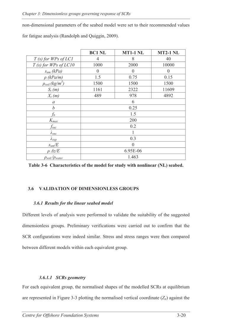
Chapter 3: Dimensionless groups governing response of SCRs
Centre for Offshore Foundation Systems 3-20
non-dimensional parameters of the seabed model were set to their recommended values
for fatigue analysis (Randolph and Quiggin, 2009).
BC1 NL MT1-1 NL MT2-1 NL
T (s) for WPs of LC1 4 8 40 T (s) for WPs of LC10 1000 2000 10000
sum (kPa) 0 0 0 (kPa/m) 1.5 0.75 0.15
soil (kg/m3) 1500 1500 1500 St (m) 1161 2322 11609 Xt (m) 489 978 4892
a 6 b 0.25 fb 1.5
Kmax 200 fsuc 0.2
suc 1 rep 0.3
sum/E 0 z/E 6.95E-06
soil / water 1.463
Table 3-6 Characteristics of the model for study with nonlinear (NL) seabed.
3.6 VALIDATION OF DIMENSIONLESS GROUPS
3.6.1 Results for the linear seabed model
Different levels of analysis were performed to validate the suitability of the suggested
dimensionless groups. Preliminary verifications were carried out to confirm that the
SCR configurations were indeed similar. Stress and stress ranges were then compared
between different models within each equivalent group.
3.6.1.1 SCRs geometry
For each equivalent group, the normalised shapes of the modelled SCRs at equilibrium
are represented in Figure 3-3 plotting the normalised vertical coordinate (Zn) against the

Chapter 3: Dimensionless groups governing response of SCRs
Centre for Offshore Foundation Systems 3-21
normalised horizontal coordinate (Xn) of the nodes located along each SCR (note the
markers in Figure 3-3 are only used to differentiate the curves and do not represent
corresponding nodes in the different models). Zn is defined as Zn = z/ z and Xn as
Xn = x/Xt where z and x are the vertical and horizontal coordinates of the nodes
measured from the TDP, as illustrated in Figure 3-1. It is seen that for models within
each equivalent group, the SCR shapes correlate well once normalised, whereas they are
evidently different in Figure 3-2, prior to normalisation.
Figure 3-3 Normalised SCR shapes in (a) Equivalent group 1; (b) Equivalent
group 2; and (c) Equivalent group 3
Although only an approximation, the catenary solution for the SCR shape also predicts
these similarities. The solution may be expressed as:
z = Top cosh
p xTo
- 1 (3-12)
This expression may be rewritten, using dimensionless groups, as:
Zn = π9π7
cosh arcsinh 1 + 2 π9/π7
π9/π7 Xn - 1 (3-13)
The two dimensionless groups, 7 and 9 were identical for all models within each
equivalent group, therefore giving identical normalised shapes in Figure 3-3. The
smaller hang-off angle for Equivalent group 3 has the effect of increasing the curvature
of the SCR shape (and decreasing the horizontal tension at TDP).
Chapter 3: Dimensionless groups governing response of SCRs
Centre for Offshore Foundation Systems 3-22
The declination angle (angle between the riser’s longitudinal axis and the vertical axis)
at any location along the riser length has also been compared for the different models
for dynamic and static loading cases, as illustrated in Figure 3-4a,b for Equivalent group
1. The normalised times 18 were chosen arbitrarily as 0.25 and 0.75, corresponding to
the vessel being at its highest and lowest positions respectively (see Figure 3-1c). To
investigate the declination distribution along the complete riser, it is convenient to
normalise the location as Sn = s/St. It is found that the declination angle at any
normalised location on the riser is similar. Also, declination angle for a given location
during an entire cycle of dynamic and static motion (i.e. 18 = t/T ranging from 0 to 1)
was compared for Equivalent group 1, as shown in Figure 3-4c. The normalised location
for comparison of results was chosen arbitrarily at the equilibrium TDP (Sn = 0), which
is typically close to the position of maximum fatigue damage. Variations of declination
angle are similar during the entire cycle of sinusoidal motion. Therefore, it seems that
normalised shapes are similar for the undisturbed SCRs and stay similar during a given
sinusoidal perturbation applied at the SCR hang-off point. From this, it is inferred that
SCR normalised displacements are the same between equivalent models. Shifting of the
TDP is a fundamental aspect of the SCR response, as it drives curvature variations that
lead to fatigue damage (Pesce et al., 2006). Similar changes in horizontal tension, arc
length to TDP, curvature and, hence, similar structural responses should be predicted
when the parameters are scaled through the defined non-dimensional groups. Testing of
Eq. (3-10) is performed through detailed investigation of the SCR absolute riser strain
( /E) and, then, of SCR strain range ( /E).
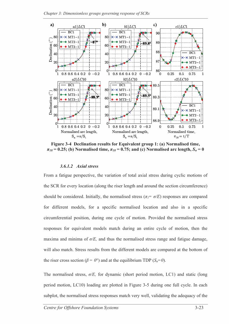
Chapter 3: Dimensionless groups governing response of SCRs
Centre for Offshore Foundation Systems 3-23
Figure 3-4 Declination results for Equivalent group 1: (a) Normalised time,
π18 = 0.25; (b) Normalised time, π18 = 0.75; and (c) Normalised arc length, Sn = 0
3.6.1.2 Axial stress
From a fatigue perspective, the variation of total axial stress during cyclic motions of
the SCR for every location (along the riser length and around the section circumference)
should be considered. Initially, the normalised stress ( 1= /E) responses are compared
for different models, for a specific normalised location and also in a specific
circumferential position, during one cycle of motion. Provided the normalised stress
responses for equivalent models match during an entire cycle of motion, then the
maxima and minima of /E, and thus the normalised stress range and fatigue damage,
will also match. Stress results from the different models are compared at the bottom of
the riser cross section ( = 0°) and at the equilibrium TDP (Sn=0).
The normalised stress, /E, for dynamic (short period motion, LC1) and static (long
period motion, LC10) loading are plotted in Figure 3-5 during one full cycle. In each
subplot, the normalised stress responses match very well, validating the adequacy of the

Chapter 3: Dimensionless groups governing response of SCRs
Centre for Offshore Foundation Systems 3-24
dimensionless groups in Eq. (3-10).
Figure 3-5 also indicates the effect of the input excitation period (T) on the time (t)
when the maximum and minimum axial stress occur during each motion cycle. For the
statically loaded case (LC10) in each equivalent group, the normalised stress response is
directly in phase with the input sinusoidal motion, with the maximum stress after one
quarter of a cycle when the vessel is at its highest position (see Figure 3-1c). Input
motion and stress response are, however, not in phase at the selected location for the
dynamically loaded case (LC1). The dynamic characteristics of the system have caused
a time lag between the maximum stress in the SCR and the maximum input motion, but
have also led to the minimum stress advancing relative to the lowest position of the
vessel.
Figure 3-5 Dimensional analysis results for (a) Equivalent group 1; (b) Equivalent group 2; and (c) Equivalent group 3: Comparison of normalised stress during one
cycle of motion; β = 0° and π16 = 0
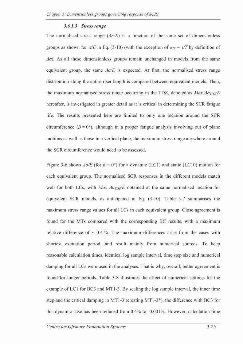
Chapter 3: Dimensionless groups governing response of SCRs
Centre for Offshore Foundation Systems 3-25
3.6.1.3 Stress range
The normalised stress range ( /E) is a function of the same set of dimensionless
groups as shown for /E in Eq. (3-10) (with the exception of 18 = t/T by definition of
). As all these dimensionless groups remain unchanged in models from the same
equivalent group, the same /E is expected. At first, the normalised stress range
distribution along the entire riser length is compared between equivalent models. Then,
the maximum normalised stress range occurring in the TDZ, denoted as Max TDZ/E
hereafter, is investigated in greater detail as it is critical in determining the SCR fatigue
life. The results presented here are limited to only one location around the SCR
circumference ( = 0°), although in a proper fatigue analysis involving out of plane
motions as well as those in a vertical plane, the maximum stress range anywhere around
the SCR circumference would need to be assessed.
Figure 3-6 shows /E (for = 0°) for a dynamic (LC1) and static (LC10) motion for
each equivalent group. The normalised SCR responses in the different models match
well for both LCs, with Max TDZ/E obtained at the same normalised location for
equivalent SCR models, as anticipated in Eq. (3-10). Table 3-7 summarises the
maximum stress range values for all LCs in each equivalent group. Close agreement is
found for the MTs compared with the corresponding BC results, with a maximum
relative difference of ~ 0.4 %. The maximum differences arise from the cases with
shortest excitation period, and result mainly from numerical sources. To keep
reasonable calculation times, identical log sample interval, time step size and numerical
damping for all LCs were used in the analyses. That is why, overall, better agreement is
found for longer periods. Table 3-8 illustrates the effect of numerical settings for the
example of LC1 for BC3 and MT1-3. By scaling the log sample interval, the inner time
step and the critical damping in MT1-3 (creating MT1-3*), the difference with BC3 for
this dynamic case has been reduced from 0.4% to -0.001%. However, calculation time
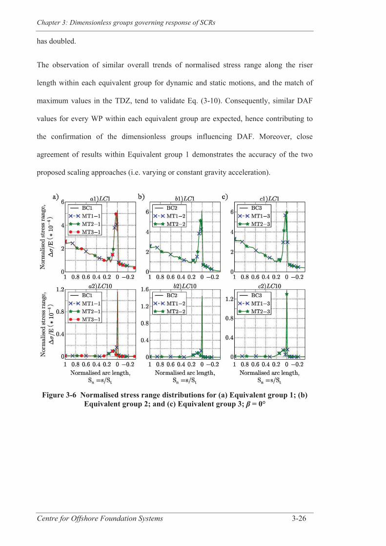
Chapter 3: Dimensionless groups governing response of SCRs
Centre for Offshore Foundation Systems 3-26
has doubled.
The observation of similar overall trends of normalised stress range along the riser
length within each equivalent group for dynamic and static motions, and the match of
maximum values in the TDZ, tend to validate Eq. (3-10). Consequently, similar DAF
values for every WP within each equivalent group are expected, hence contributing to
the confirmation of the dimensionless groups influencing DAF. Moreover, close
agreement of results within Equivalent group 1 demonstrates the accuracy of the two
proposed scaling approaches (i.e. varying or constant gravity acceleration).
Figure 3-6 Normalised stress range distributions for (a) Equivalent group 1; (b)
Equivalent group 2; and (c) Equivalent group 3; β = 0°
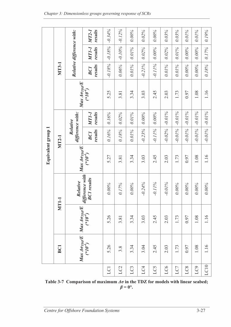
Chapter 3: Dimensionless groups governing response of SCRs
Centre for Offshore Foundation Systems 3-27
Equ
ival
ent g
roup
1
MT
3-1
Rel
ativ
e di
ffer
ence
with
:
MT2
-1
resu
lts
-0.3
4%
-0.1
2%
0.00
%
0.02
%
0.00
%
0.03
%
0.03
%
0.01
%
0.01
%
0.19
%
MT1
-1
resu
lts
-0.1
8%
-0.1
0%
0.01
%
0.02
%
0.00
%
0.02
%
0.01
%
0.00
%
0.00
%
0.17
%
BC
1 re
sults
-0.1
8%
0.06
%
0.01
%
-0.2
1%
-0.1
1%
0.01
%
0.01
%
0.00
%
0.00
%
0.18
%
Max
Δσ T
DZ/
E
(*10
-4)
5.25
3.81
3.34
3.03
2.45
2.03
1.73
0.97
1.08
1.16
MT
2-1 R
elat
ive
diff
eren
ce w
ith:
MT1
-1
resu
lts
0.16
%
0.02
%
0.01
%
0.00
%
0.00
%
-0.0
1%
-0.0
1%
-0.0
1%
-0.0
1%
-0.0
1%
BC
1 re
sults
0.16
%
0.18
%
0.01
%
-0.2
3%
-0.1
1%
-0.0
2%
-0.0
1%
-0.0
1%
-0.0
1%
-0.0
1%
Max
Δσ T
DZ/
E
(*10
-4)
5.27
3.81
3.34
3.03
2.45
2.03
1.73
0.97
1.08
1.16
MT
1-1 R
elat
ive
diff
eren
ce w
ith
BC
1 re
sults
0.00
%
0.17
%
0.00
%
-0.2
4%
-0.1
1%
-0.0
1%
0.00
%
0.00
%
0.00
%
0.00
%
Max
Δσ T
DZ/
E
(*10
-4)
5.26
3.81
3.34
3.03
2.45
2.03
1.73
0.97
1.08
1.16
BC
1
Max
Δσ T
DZ/
E
(*10
-4)
5.26
3.8
3.34
3.04
2.45
2.03
1.73
0.97
1.08
1.16
LC1
LC2
LC3
LC4
LC5
LC6
LC7
LC8
LC9
LC10
Table 3-7 Comparison of maximum Δσ in the TDZ for models with linear seabed; β = 0°.
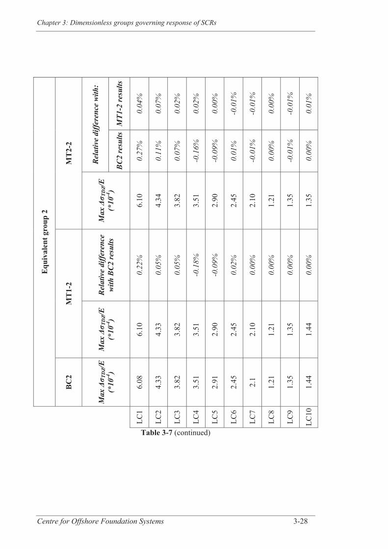
Chapter 3: Dimensionless groups governing response of SCRs
Centre for Offshore Foundation Systems 3-28
Equ
ival
ent g
roup
2
MT
2-2
Rel
ativ
e di
ffer
ence
with
:
MT1
-2 re
sults
0.04
%
0.07
%
0.02
%
0.02
%
0.00
%
-0.0
1%
-0.0
1%
0.00
%
-0.0
1%
0.01
%
BC
2 re
sults
0.27
%
0.11
%
0.07
%
-0.1
6%
-0.0
9%
0.01
%
-0.0
1%
0.00
%
-0.0
1%
0.00
%
Max
Δσ T
DZ/
E
(*10
-4)
6.10
4.34
3.82
3.51
2.90
2.45
2.10
1.21
1.35
1.35
MT
1-2
Rel
ativ
e di
ffer
ence
w
ith B
C2
resu
lts
0.22
%
0.05
%
0.05
%
-0.1
8%
-0.0
9%
0.02
%
0.00
%
0.00
%
0.00
%
0.00
%
Max
Δσ T
DZ/
E
(*10
-4)
6.10
4.33
3.82
3.51
2.90
2.45
2.10
1.21
1.35
1.44
BC
2
Max
Δσ T
DZ/
E
(*10
-4)
6.08
4.33
3.82
3.51
2.91
2.45
2.1
1.21
1.35
1.44
LC1
LC2
LC3
LC4
LC5
LC6
LC7
LC8
LC9
LC10
Table 3-7 (continued)
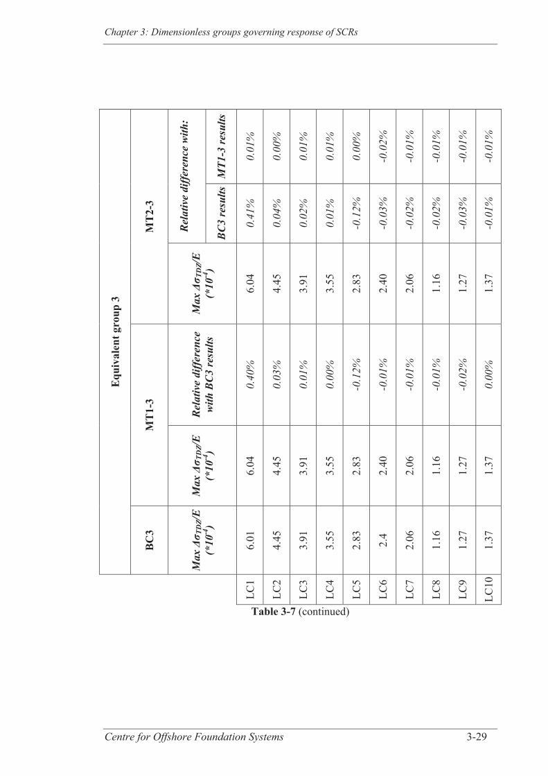
Chapter 3: Dimensionless groups governing response of SCRs
Centre for Offshore Foundation Systems 3-29
Equ
ival
ent g
roup
3
MT
2-3
Rel
ativ
e di
ffer
ence
with
:
MT1
-3 re
sults
0.01
%
0.00
%
0.01
%
0.01
%
0.00
%
-0.0
2%
-0.0
1%
-0.0
1%
-0.0
1%
-0.0
1%
BC
3 re
sults
0.41
%
0.04
%
0.02
%
0.01
%
-0.1
2%
-0.0
3%
-0.0
2%
-0.0
2%
-0.0
3%
-0.0
1%
Max
Δσ T
DZ/
E
(*10
-4)
6.04
4.45
3.91
3.55
2.83
2.40
2.06
1.16
1.27
1.37
MT
1-3
Rel
ativ
e di
ffer
ence
w
ith B
C3
resu
lts
0.40
%
0.03
%
0.01
%
0.00
%
-0.1
2%
-0.0
1%
-0.0
1%
-0.0
1%
-0.0
2%
0.00
%
Max
Δσ T
DZ/
E
(*10
-4)
6.04
4.45
3.91
3.55
2.83
2.40
2.06
1.16
1.27
1.37
BC
3
Max
Δσ T
DZ/
E
(*10
-4)
6.01
4.45
3.91
3.55
2.83
2.4
2.06
1.16
1.27
1.37
LC1
LC2
LC3
LC4
LC5
LC6
LC7
LC8
LC9
LC10
Table 3-7 (continued)
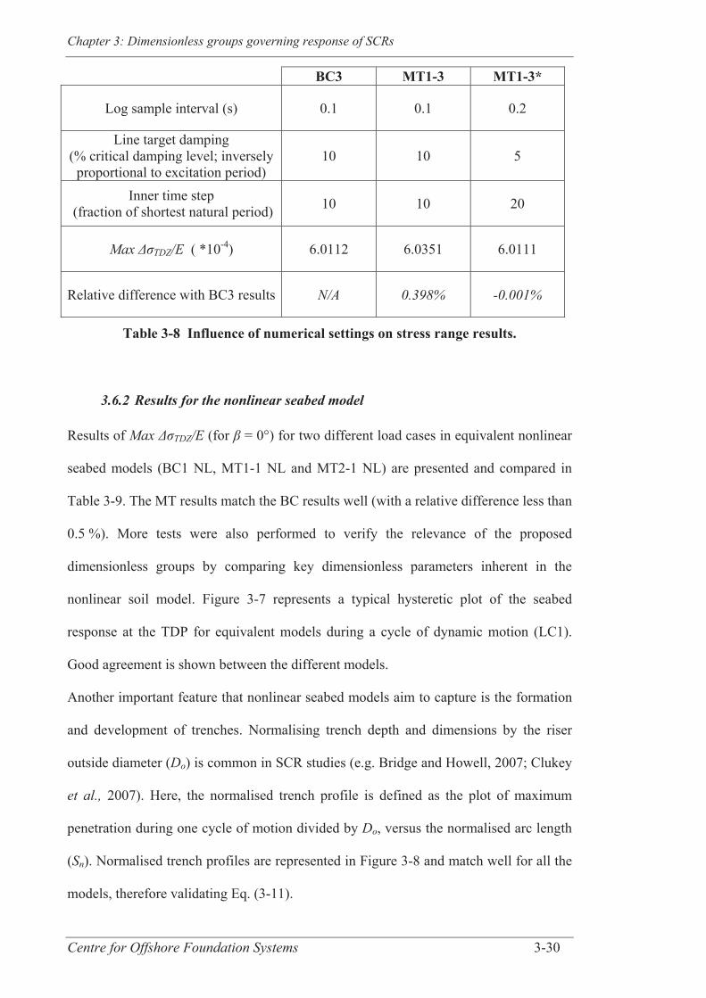
Chapter 3: Dimensionless groups governing response of SCRs
Centre for Offshore Foundation Systems 3-30
BC3 MT1-3 MT1-3*
Log sample interval (s) 0.1 0.1 0.2
Line target damping (% critical damping level; inversely
proportional to excitation period) 10 10 5
Inner time step (fraction of shortest natural period) 10 10 20
Max TDZ/E ( *10-4) 6.0112 6.0351 6.0111
Relative difference with BC3 results N/A 0.398% -0.001%
Table 3-8 Influence of numerical settings on stress range results.
3.6.2 Results for the nonlinear seabed model
Results of Max TDZ/E (for = 0°) for two different load cases in equivalent nonlinear
seabed models (BC1 NL, MT1-1 NL and MT2-1 NL) are presented and compared in
Table 3-9. The MT results match the BC results well (with a relative difference less than
0.5 %). More tests were also performed to verify the relevance of the proposed
dimensionless groups by comparing key dimensionless parameters inherent in the
nonlinear soil model. Figure 3-7 represents a typical hysteretic plot of the seabed
response at the TDP for equivalent models during a cycle of dynamic motion (LC1).
Good agreement is shown between the different models.
Another important feature that nonlinear seabed models aim to capture is the formation
and development of trenches. Normalising trench depth and dimensions by the riser
outside diameter (Do) is common in SCR studies (e.g. Bridge and Howell, 2007; Clukey
et al., 2007). Here, the normalised trench profile is defined as the plot of maximum
penetration during one cycle of motion divided by Do, versus the normalised arc length
(Sn). Normalised trench profiles are represented in Figure 3-8 and match well for all the
models, therefore validating Eq. (3-11).
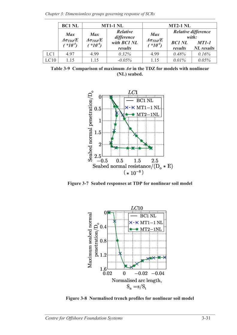
Chapter 3: Dimensionless groups governing response of SCRs
Centre for Offshore Foundation Systems 3-31
BC1 NL MT1-1 NL MT2-1 NL
Max ΔσTDZ/E ( *10-4)
Max ΔσTDZ/E ( *10-4)
Relative difference
with BC1 NL results
Max ΔσTDZ/E ( *10-4)
Relative difference with:
BC1 NL results
MT1-1 NL results
LC1 4.97 4.99 0.32% 4.99 0.48% 0.16% LC10 1.15 1.15 -0.05% 1.15 0.01% 0.05%
Table 3-9 Comparison of maximum Δσ in the TDZ for models with nonlinear (NL) seabed.
Figure 3-7 Seabed responses at TDP for nonlinear soil model
Figure 3-8 Normalised trench profiles for nonlinear soil model

Chapter 3: Dimensionless groups governing response of SCRs
Centre for Offshore Foundation Systems 3-32
3.7 POTENTIAL APPLICATIONS OF FRAMEWORK
Establishment of suitable non-dimensional groups will assist future numerical and
experimental studies investigating SCR dynamics. Indeed, defining appropriate scaling
allows for optimisation of the number of simulations, as similar stress range and,
therefore, similar fatigue life can be predicted with models having the same non-
dimensional groups. Moreover, although the non-dimensional groups impacting the
stress range have been identified, their individual contributions to the stress range
amplitude have yet to be determined. This represents the next stage, where sensitivity
analyses will be undertaken, with the results synthesised to allow the dynamic stress
range to be expressed directly in terms of the non-dimensional groups listed in Eq.
(3-10). The non-dimensional groups presented in this paper will also assist future
studies aiming to quantify DAF sensitivity to SCR system parameters and
environmental loading, and hence will contribute in simplifying structural analyses of
SCRs.
Figure 3-9 illustrates how dimensionless groups can be used to investigate the
sensitivity of the fatigue life of SCRs to a chosen non-dimensional input (or group of
non-dimensional inputs), considering for example the effect of the normalised linear soil
stiffness ( 11). The variation of maximum normalised stress ranges against normalised
excitation periods ( 4), which reflect the maximum velocity of the riser motion, as well
as the DAF for equivalent groups 1 and 2 (i.e. BC1 and BC2), are shown in Figure 3-9.
The soil stiffness is the only difference between BC1 and BC2 ( 11 = ks/E for BC2 is 10
times higher than for BC1). Figure 3-9a confirms that increasing the soil stiffness has a
significant effect on amplification of the induced maximum stress range and therefore
reduction of the fatigue life of the system, as noted previously in the literature (e.g.
Bridge et al., 2004). Also, it is shown in Figure 3-9b that, overall, DAF sensitivity to the
non-dimensional soil stiffness is limited. Differences between DAF values at a given 4
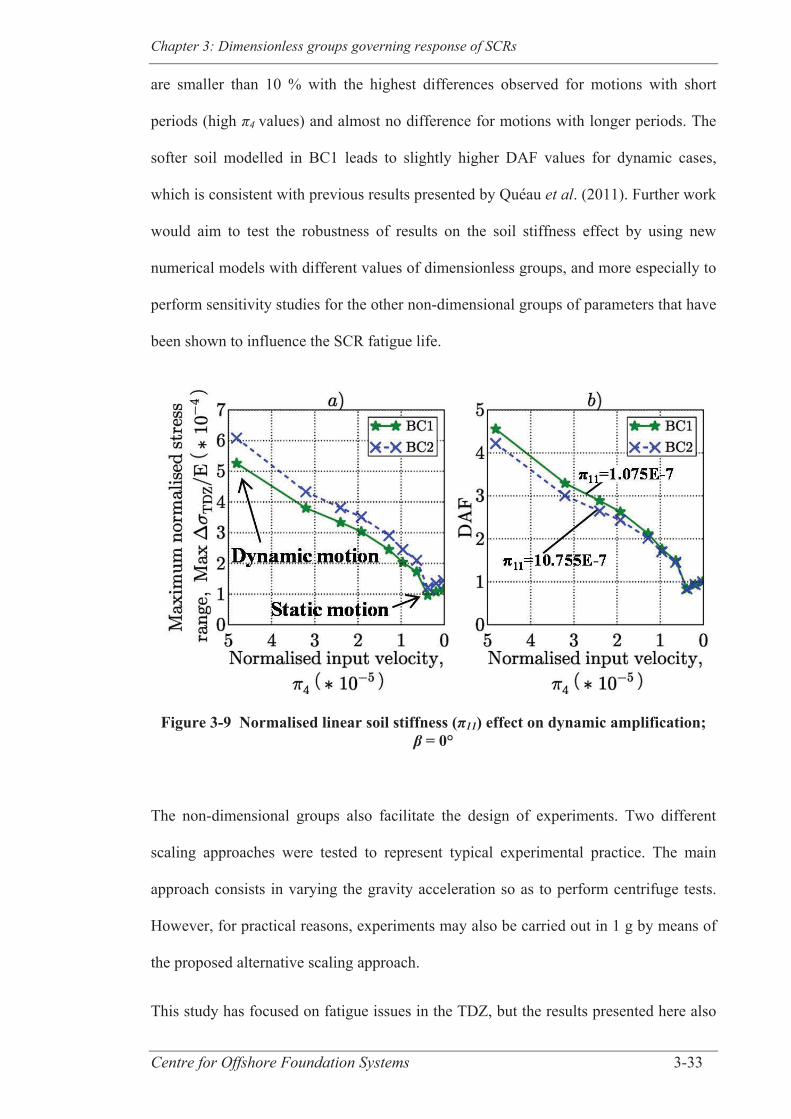
Chapter 3: Dimensionless groups governing response of SCRs
Centre for Offshore Foundation Systems 3-33
are smaller than 10 % with the highest differences observed for motions with short
periods (high 4 values) and almost no difference for motions with longer periods. The
softer soil modelled in BC1 leads to slightly higher DAF values for dynamic cases,
which is consistent with previous results presented by Quéau et al. (2011). Further work
would aim to test the robustness of results on the soil stiffness effect by using new
numerical models with different values of dimensionless groups, and more especially to
perform sensitivity studies for the other non-dimensional groups of parameters that have
been shown to influence the SCR fatigue life.
Figure 3-9 Normalised linear soil stiffness (π11) effect on dynamic amplification;
β = 0°
The non-dimensional groups also facilitate the design of experiments. Two different
scaling approaches were tested to represent typical experimental practice. The main
approach consists in varying the gravity acceleration so as to perform centrifuge tests.
However, for practical reasons, experiments may also be carried out in 1 g by means of
the proposed alternative scaling approach.
This study has focused on fatigue issues in the TDZ, but the results presented here also
Chapter 3: Dimensionless groups governing response of SCRs
Centre for Offshore Foundation Systems 3-34
establish dynamic similarity along the entire riser. Hence the proposed dimensionless
groups could be used for other problems such as analysis of vortex induced vibration
(VIV). However, for VIV studies it may be more appropriate to: (i) use a varying drag
coefficient, and therefore scale the Reynolds number through scaling of the water
kinematic viscosity (as length and velocity are already similar with the defined non-
dimensional groups), (ii) account for the effect of structural damping and scale it
accordingly (Rateiro et al., 2012).
3.8 CONCLUSIONS
It is commonly acknowledged that uncertainties are present in SCR design, and it
remains difficult to quantify the level of accuracy in fatigue estimates. In consequence,
design guidelines recommend that sensitivity analyses are performed for any given
design, varying the key parameters that govern SCR behaviour. The study developed in
this paper details the application of dimensional analysis to identify the entire set of
non-dimensional groups that control the normalised stress and stress ranges within an
SCR. The aim has been to facilitate sensitivity analyses, and also to lay the ground work
for subsequent studies to evaluate functional relationships between the input non-
dimensional groups and the output normalised stress ranges and resulting dynamic
amplification factors. This has the potential to simplify the estimation of SCR fatigue
life within the touchdown zone.
Non-dimensional groups influencing the dynamic and static response of SCRs to top
excitations, and subsequently the DAF values, were identified for linear and nonlinear
seabed models. The study was limited to in-plane motions of the riser resulting from
sinusoidal motion of the vessel. Appropriate scaling factors were determined in order to
obtain equivalent models with similar shapes and structural responses for a given input
motion. The proposed non-dimensional groups will allow improvement of riser

Chapter 3: Dimensionless groups governing response of SCRs
Centre for Offshore Foundation Systems 3-35
sensitivity analyses through better control on input parameters, reduction in the number
of simulations, together with easier comparisons and interpretation of the results. The
groups will also assist in the planning of 1 g and centrifuge experiments through
appropriate scaling of parameters that play a critical role in riser behaviour.
Detailed investigation of the influence of each dimensionless group on the dynamic
stress ranges and fatigue life of SCR systems is currently underway, using the validated
non-dimensional groups from this study.

Chapter 4: Analytical estimation of static stress range...
Centre for Offshore Foundation Systems 4-1
CHAPTER 4 ANALYTICAL ESTIMATION OF STATIC STRESS
RANGE IN OSCILLATING STEEL CATENARY RISERS AT
TOUCH DOWN AREAS AND ITS APPLICATION WITH DYNAMIC
AMPLIFICATION FACTORS
4.1 ABSTRACT
Steel catenary risers (SCRs) are dynamically sensitive structures and their fatigue
design in the touchdown zone is challenging. The dynamic response of SCRs is
traditionally assessed by performing a series of long time history analyses but a
simplifying approach has recently been proposed. The simple method is based on the
use of dynamic amplification factors that quantify the dynamic response for a given
perturbation at the hang-off point relative to the static response. The determination of
the static response of SCRs is therefore a prerequisite to this approach.
In this paper, an existing analytical model is extended to accommodate the displacement
at the hang-off point of the SCR and predict the static stress range. The results of this
analytical model are validated against numerical simulations. Then, using this simple
and efficient analytical model, various sensitivity analyses are performed to explore the
impact of key dimensionless groups on the static stress range in the touchdown zone.
Chapter 4: Analytical estimation of static stress range...
Centre for Offshore Foundation Systems 4-2
4.2 INTRODUCTION
Steel catenary risers (SCRs) have been used extensively in the past decades for offshore
oil and gas developments in deep water. They are a cost effective solution but are very
sensitive to the hydrodynamic loading and the vessel motions, which generate fatigue
damage concentrated at the vessel hang-off point (HOP – where the riser is connected to
the floating facility) and in the touchdown zone (TDZ – the area of dynamic riser soil
interaction (Bridge, 2005)) (Campbell, 1999; Bai and Bai, 2005). An accurate
estimation of the fatigue life of SCRs is fundamental as failure would have high
economical and environmental impacts. The structural response of SCRs is usually
assessed by carrying out dynamic time history analyses but they are time consuming
and they need high computational effort (Xia et al., 2008). In an attempt to simplify the
early stages of fatigue design (i.e. conceptual or preliminary design stages), the authors
have proposed an approach based on dynamic amplification factors (DAFs) (Quéau et
al., 2011). DAFs are defined as the ratio of the maximum dynamic stress range to the
maximum static stress range occurring in the TDZ under application of given wave
packs. They are an efficient alternative to explicit numerical analysis as they allow
determination of the maximum dynamic response amplitudes directly from the static
response. The dimensionless groups of input parameters influencing the DAF values can
be deduced from those impacting the axial stress occurring in SCRs, merely omitting
the groups that involve time and position within the SCR. Thus the relevant groups for
axial stress ( t) and DAF may be expressed as (Quéau et al., 2013)
σtE = f1(
HΔz, Δθm,
HT
ρsteel E ,
DoΔz,
Do wt
, p
E Δz, ν, To
E Δz2, μ, ksE, CD, CA,
ρsteel ρwater
, g Δz ρsteel
E , s
Δz, β, tT )
(4-1)
Chapter 4: Analytical estimation of static stress range...
Centre for Offshore Foundation Systems 4-3
DAF = f2(HΔz, Δθm,
HT
ρsteel E ,
DoΔz,
Do wt
, p
E Δz, ν, To
E Δz2, μ, ksE, CD, CA,
ρsteel ρwater
, g Δz ρsteel
E )
(4-2)
where:
H, T Heave amplitude and period of the input motion
m Angle of the motion relative to the hang-off angle ( HO)
z Vertical difference between hang-off point and seabed (directly
related to water depth based on HOP location on the vessel)
E Young’s modulus
steel , water Steel and water densities
Do, wt Riser outer diameter and wall thickness
p Unit submerged weight
Poisson’s ratio
To Horizontal tension component
ks Soil stiffness
Soil friction coefficient
CD, CA Drag and added mass coefficients
g Gravity acceleration
s Arc length (measured from the touchdown point (TDP))
Angular position on the SCR circumference
t Time
The main aim of this paper is to establish an accurate analytical method to assess the
static response of oscillating SCRs, as this is a fundamental input for the DAF approach.
A simple analytical method commonly used to estimate the overall geometry of SCRs
relies on the catenary based solutions that were developed for cables and which neglect
bending stiffness and riser-soil interaction (Bridge, 2005). They provide a good
approximation because SCRs have a high aspect ratio of suspended length over outside
diameter. However, more sophisticated techniques are required to capture the shear
force, bending moment and stress distributions in SCRs, in particular near the
Chapter 4: Analytical estimation of static stress range...
Centre for Offshore Foundation Systems 4-4
touchdown point (TDP), where the riser bending stiffness and the soil stiffness will
impact the riser profile.
Aranha et al. (1997) and Pesce et al. (1998a,b) proposed more complex analytical
equations to smooth the curvature variation close to the TDP by taking into account the
riser bending stiffness in a small section near the TDP that is referred to as the
“boundary layer”. The length of the boundary layer zone is indicated by the flexural
length parameter = (EI/To)0.5, where I is the second moment of area (Love, 1892). One
of their models can also account for the effect of a linear soil stiffness (Pesce et al.,
1998b). This model was used by Shiri and Hashemi (2012) to estimate the maximum
fatigue damage in the TDZ at least in an approximate way. However, Shiri and Hashemi
(2012) neglected the effect of tension in the SCR and also approximated the maximum
variation of bending moment as the product of the maximum shear force in the SCR,
before application of any motion, with the maximum range of motion of the TDP for the
given cycle. In addition, while the model from Pesce et al. (1998b) was used to estimate
the maximum shear force, the maximum range of motion of the TDP was assessed by
means of standard catenary relationships, thus neglecting the effect of the riser bending
stiffness.
By contrast, the model developed in this paper accounts for a linear soil stiffness and the
boundary layer effect systematically. It also evaluates the maximum static stress range
by assessing the static stress distribution along the riser length, combining changes in
both tension and bending moment, when the HOP is relocated under a cycle of static
loading.
The model is based on the “three-fields model” (TFM) from Lenci and Callegari (2005)
that is able to model continuous displacement, slope, tension (approximately), bending
moment and shear force everywhere along the riser length for SCRs in an equilibrium
configuration (i.e. before any motion is applied). This model has been adopted here and
Chapter 4: Analytical estimation of static stress range...
Centre for Offshore Foundation Systems 4-5
any reference to the TFM acknowledges the work of Lenci and Callegari (2005). The
TFM is extended in order to accommodate the displacement of the hang-off point and
predict the static stress range along the riser length. For validation, results of the
extended analytical model are compared with numerical simulations. Also, the proposed
extended model is used to evaluate the sensitivity of the static stress range in SCRs to
the dimensionless groups of input parameters as part of on-going research on the DAF
approach. This will assist the future sensitivity analyses aiming to establish quantitative
relationships between the dimensionless groups and the DAF.
The following assumptions are used to simplify this study: it is limited to 2D conditions
with no account taken of the current profile in the sea column, the soil friction, the
rotational stiffness at the HOP, the flow rate of the contents and the coating. Also, it is
chosen to work at a fixed position around the SCR circumference, = 0° corresponding
to the bottom of the riser, for the post-processing of the numerical models.
4.3 ANALYTICAL ASSESSMENT OF AXIAL STRESS IN SCRS
The TFM divides the riser into three zones having different behaviour: (i) the suspended
part away from the TDP where the standard catenary relationships developed for cables
are used, (ii) the boundary layer zone (suspended part of the riser close to the TDP),
where the riser bending stiffness is taken into account, and (iii) the zone where the riser
is in contact with the soil and where a Winkler-type deformable soil model is used. An
illustration of the TFM and the relevant notations are presented in Figure 4-1. Using the
TFM, the riser elevation measured from the seabed, z, can be calculated through the
following system of equations:
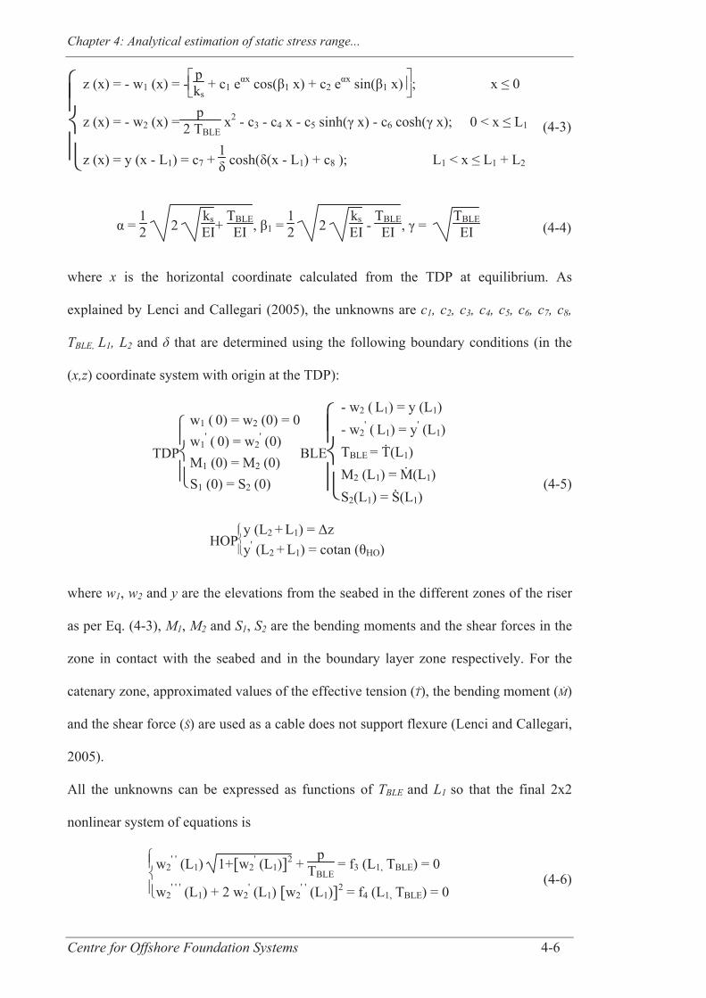
Chapter 4: Analytical estimation of static stress range...
Centre for Offshore Foundation Systems 4-6
z (x) = - w1 (x) = -pks
+ c1 eαx cos(β1 x) + c2 eαx sin(β1 x) ; x ≤ 0
z (x) = - w2 (x) =p
2 TBLE x2 - c3 - c4 x - c5 sinh(γ x) - c6 cosh(γ x); 0 < x ≤ L1
z (x) = y (x - L1) = c7 + 1δ cosh(δ(x - L1) + c8 ); L1 < x ≤ L1 + L2
(4-3)
α = 12 2
ksEI+
TBLEEI , β1 =
12 2
ksEI -
TBLEEI , γ =
TBLEEI (4-4)
where x is the horizontal coordinate calculated from the TDP at equilibrium. As
explained by Lenci and Callegari (2005), the unknowns are c1, c2, c3, c4, c5, c6, c7, c8,
TBLE, L1, L2 and that are determined using the following boundary conditions (in the
(x,z) coordinate system with origin at the TDP):
TDP
w1 ( 0) = w2 (0) = 0w1
' ( 0) = w2' (0)
M1 (0) = M2 (0)S1 (0) = S2 (0)
BLE
- w2 ( L1) = y (L1)- w2
' ( L1) = y' (L1)TBLE = Ṫ(L1)M2 (L1) = Ṁ(L1)S2(L1) = Ṡ(L1)
HOPy (L2 + L1) = Δzy' (L2 + L1) = cotan (θHO)
(4-5)
where w1, w2 and y are the elevations from the seabed in the different zones of the riser
as per Eq. (4-3), M1, M2 and S1, S2 are the bending moments and the shear forces in the
zone in contact with the seabed and in the boundary layer zone respectively. For the
catenary zone, approximated values of the effective tension ( ), the bending moment ( )
and the shear force ( ) are used as a cable does not support flexure (Lenci and Callegari,
2005).
All the unknowns can be expressed as functions of TBLE and L1 so that the final 2x2
nonlinear system of equations is
w2' ' (L1) 1+[ ]w2
' (L1) 2 + p
TBLE = f3 (L1, TBLE) = 0
w2' ' ' (L1) + 2 w2
' (L1) [ ]w2' ' (L1) 2 = f4 (L1, TBLE) = 0
(4-6)
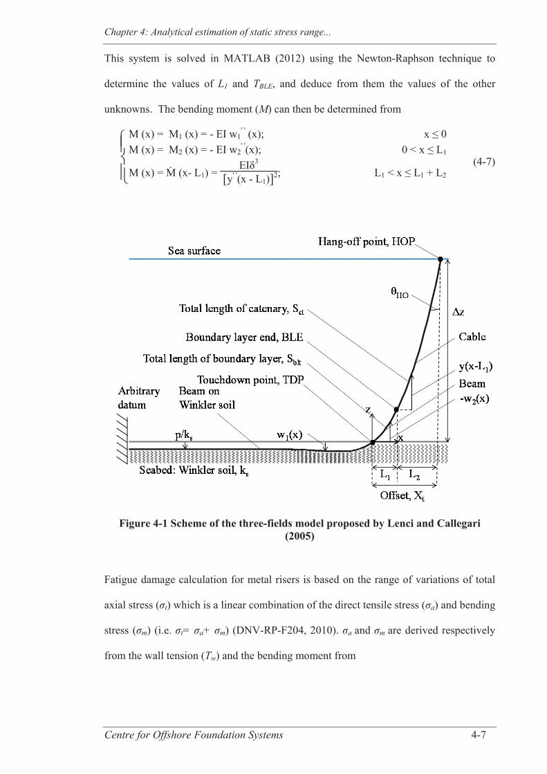
Chapter 4: Analytical estimation of static stress range...
Centre for Offshore Foundation Systems 4-7
This system is solved in MATLAB (2012) using the Newton-Raphson technique to
determine the values of L1 and TBLE, and deduce from them the values of the other
unknowns. The bending moment (M) can then be determined from
M (x) = M1 (x) = - EI w1' ' (x); x ≤ 0
M (x) = M2 (x) = - EI w2' '(x); 0 < x ≤ L1
M (x) = Ṁ (x- L1) = EIδ3
[ ]y' '(x - L1) 2; L1 < x ≤ L1 + L2
(4-7)
Figure 4-1 Scheme of the three-fields model proposed by Lenci and Callegari (2005)
Fatigue damage calculation for metal risers is based on the range of variations of total
axial stress ( t) which is a linear combination of the direct tensile stress ( a) and bending
stress ( m) (i.e. t= a+ m) (DNV-RP-F204, 2010). a and m are derived respectively
from the wall tension (Tw) and the bending moment from
Chapter 4: Analytical estimation of static stress range...
Centre for Offshore Foundation Systems 4-8
σa = TwA , σm =
M Do2 I (4-8)
where A is the cross section area derived from the external (Ao) and internal (Ai) cross
section areas. Tw is calculated from the effective tension (Te), the external (Po) and
internal (Pi) pressures and the cross section areas through the following relationships:
Tw = Te - Po Ao + Pi Ai
Po = g ρwater (Zw - Do2 - z) , Pi = g ρcont (Δz - z)
Δz = Zw – ZHOP - Do2
(4-9)
where ZHOP is the depth of the hang-off point below the sea surface (taken as 18 m in all
the later numerical models in this study). The adjustments of Do/2 reflect the fact that in
the numerical models all the positions are calculated at the centre of the nodes.
In the TFM the effective tension is given by: Te = = p2 z'' in the catenary zone and
Te =TBLE elsewhere. Note that the assumption of TBLE being constant through the
boundary layer is necessary in order to obtain analytical solutions. Equating TBLE to the
tension in the catenary at x = L1 was adopted by Lenci and Callegari (2005) in order to
provide continuity in tension, although that assumption then leads to a gradually
increasing mismatch of the tension in the boundary layer compared with the horizontal
component of tension (To) in the catenary. Since the bending stress is the primary
contribution to the axial stress, with the direct tensile stress playing a minor role (e.g.
Shiri and Hashemi, 2012), this small offset in effective tension is not expected to have a
major influence on the axial stress results. However, an alternative is to adjust the
estimate of the true tension in the boundary layer zone and in the zone where the riser is
in contact with the seabed by taking Te as TBLE sin */sin , where is the SCR angle
from the vertical (equalling * at x = L1).
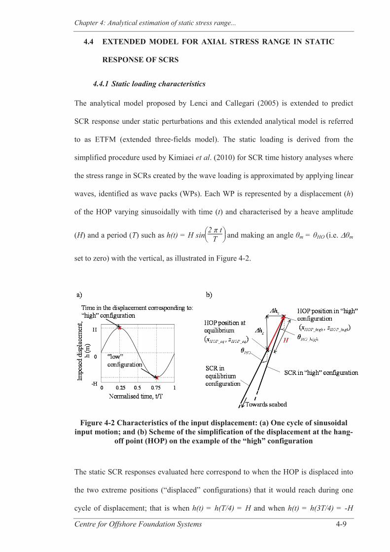
Chapter 4: Analytical estimation of static stress range...
Centre for Offshore Foundation Systems 4-9
4.4 EXTENDED MODEL FOR AXIAL STRESS RANGE IN STATIC
RESPONSE OF SCRS
4.4.1 Static loading characteristics
The analytical model proposed by Lenci and Callegari (2005) is extended to predict
SCR response under static perturbations and this extended analytical model is referred
to as ETFM (extended three-fields model). The static loading is derived from the
simplified procedure used by Kimiaei et al. (2010) for SCR time history analyses where
the stress range in SCRs created by the wave loading is approximated by applying linear
waves, identified as wave packs (WPs). Each WP is represented by a displacement (h)
of the HOP varying sinusoidally with time (t) and characterised by a heave amplitude
(H) and a period (T) such as h(t) = H sin2 t
T and making an angle m = HO (i.e. m
set to zero) with the vertical, as illustrated in Figure 4-2.
Figure 4-2 Characteristics of the input displacement: (a) One cycle of sinusoidal input motion; and (b) Scheme of the simplification of the displacement at the hang-
off point (HOP) on the example of the “high” configuration
The static SCR responses evaluated here correspond to when the HOP is displaced into
the two extreme positions (“displaced” configurations) that it would reach during one
cycle of displacement; that is when h(t) = h(T/4) = H and when h(t) = h(3T/4) = -H
Chapter 4: Analytical estimation of static stress range...
Centre for Offshore Foundation Systems 4-10
(referred to as “high” and “low” configurations of the SCR respectively). The
illustration in Figure 4-2b shows an example “high” configuration.
Therefore, if xHOP_eq and zHOP_eq are the horizontal and vertical coordinates of the hang-
off point at equilibrium in the reference (x, z) - coordinate system having its origin at the
equilibrium TDP (TDPeq), then the coordinates of the HOP in displaced configuration
(xHOP_disp, zHOP_disp) in this coordinate system are defined by
xHOP_disp = xHOP_eq + Δhx, zHOP_disp = zHOP_eq + Δhz (4-10)
where
Δhx = H sin(θHO); Δhz = H cos(θHO) in high configurationΔhx = - H sin(θHO); Δhz = - H cos(θHO) in low configuration
(4-11)
4.4.2 Estimation of SCR response under imposed displacement
The TFM can predict the shape, tension, moment and stress distribution of SCRs before
application of any displacement providing I, E, p, ks, z and HO are known. In a
displaced configuration with Z_disp = z + hz, the hang-off angle ( HO_disp) must be
resolved by observing that the overall length of the SCR in the equilibrium and
displaced configurations is unchanged. This leads to
Δhx = ΔXt - ΔSt (4-12)
where Xt is the offset to TDP, St is the arc length to TDP at equilibrium and denotes a
variation. Thus, using the notations introduced in Figure 4-1
Δhx = ΔL1 + ΔL2 - ΔSblt - ΔSct (4-13)
where
ΔL1 = L1_disp - L1_eq, ΔL2 = L2_disp - L2_eq
ΔSblt = Sblt_disp - Sblt_eq, ΔSct = Sct_disp - Sct_eq (4-14)
Chapter 4: Analytical estimation of static stress range...
Centre for Offshore Foundation Systems 4-11
Since ds = 1+dzdx
2 dx, Sblt and Sct can be determined theoretically by analytical or
numerical integration, for example
Sct = 1δ [ ]sinh ( )δ L2 + c8 - sinh(c8) (4-15)
where the subscripts “_disp” and “_eq” are omitted to simplify the notations since this
relationship is valid for the equilibrium and the displaced configurations.
4.4.3 Evaluation of the stress range
The nonlinear system of equations in Eq. (4-6) is solved for both, high and low
configurations in their own coordinate systems (xdisp, zdisp), having its origin at the new
displaced TDP (TDPdisp). Ultimately, direct tensile stress results ( a_high, a_low), bending
stress results ( m_high, m_low) and the deduced axial stress results ( t_high, t_low) are
expressed per arc length in the common coordinate system of arc length originating at
the equilibrium TDP (TDPeq). For each arc length, the stress range can therefore be
evaluated using the relationship below
Δσ = max (σhigh, σlow) – min (σhigh, σlow) (4-16)
where refers to either a, m or t for a given arc length.
4.5 VALIDATION OF THE ANALYTICAL MODEL
Three distinct SCR configurations are selected to compare the results from numerical
simulations and the three-fields model. Comparisons are performed initially for the
equilibrium configuration, and then under static motion, in order to assess the accuracy
of the proposed extended analytical model (ETFM).

Chapter 4: Analytical estimation of static stress range...
Centre for Offshore Foundation Systems 4-12
4.5.1 Description of the SCR configurations selected for verifying the
analytical predictions
Three different base cases (BCs) with distinct input parameters are defined to compare
the results of the ETFM with the results of the numerical simulations performed in
OrcaFlex software (Orcina, 2012). The characteristics of each BC are presented in Table
4-1. BC1 is derived from an in-service SCR connected to a semisubmersible in the Gulf
of Mexico. The two other BCs are established to test the analytical model for SCR
systems having different values of input parameters and forming distinct values of
dimensionless groups, shown in Table 4-2. The horizontal component of the tension can
be approximated conveniently using the standard catenary equation, so that
To_catenary = p ΔZ sin (θHO)
1-sin(θHO) (4-17)
To_catenary is then used to assess the value of and of the dimensionless tension ( 9). The
following input parameters are kept constant for all the SCR configurations used in this
paper: = 0.293, μ = 0, steel = 7850 kg/m3, water = 1025 kg/m3, E =2.12E+8 kPa,
g = 9.81 m/s2. Also, the criteria presented in Table 4-3, Table 4-4 and Table 4-5 are
defined to assist in the choice of the varied input parameter values. Indeed, in an effort
to work with realistic SCR configurations, the selected ranges of the riser outside
diameter to wall thickness ratio ( 6 = Do / wt) vary depending on the value of Do, small
hang-off angle values are used for deep waters but larger values are chosen for
shallower water depths, and the choice of content density depends on the value of the
outside diameter to represent the large gas risers and the smaller liquid pipes.
To increase the efficiency of the use of OrcaFlex software for pre-processing and post
processing the numerical models, a Python script communicating with OrcaFlex
through OrcFxAPI (Orcina, 2012) was developed. The flowchart of this script is shown
in Figure 4-3. All the numerical models have a regular and very fine segmentation of
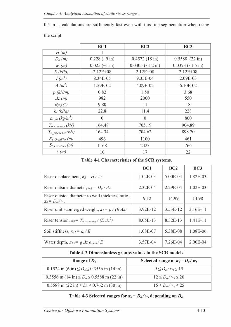
Chapter 4: Analytical estimation of static stress range...
Centre for Offshore Foundation Systems 4-13
0.5 m as calculations are sufficiently fast even with this fine segmentation when using
the script.
BC1 BC2 BC3 H (m) 1 1 1 Do (m) 0.228 (~9 in) 0.4572 (18 in) 0.5588 (22 in) wt (m) 0.025 (~1 in) 0.0305 (~1.2 in) 0.0373 (~1.5 in)
E (kPa) 2.12E+08 2.12E+08 2.12E+08 I (m4) 8.34E-05 9.35E-04 2.09E-03 A (m2) 1.59E-02 4.09E-02 6.10E-02
p (kN/m) 0.82 1.50 3.68 z (m) 982 2000 550 HO (°) 9.80 11 18
ks (kPa) 22.8 11.4 228 cont (kg/m3) 0 0 800
To_catenary (kN) 164.48 705.19 904.89 To_OrcaFlex (kN) 164.34 704.62 898.70 Xt_OrcaFlex (m) 496 1100 461 St_OrcaFlex (m) 1168 2423 766
(m) 10 17 22
Table 4-1 Characteristics of the SCR systems.
BC1 BC2 BC3
Riser displacement, 2 = H / z 1.02E-03 5.00E-04 1.82E-03
Riser outside diameter, 5 = Do / z 2.32E-04 2.29E-04 1.02E-03
Riser outside diameter to wall thickness ratio, 6 = Do / wt
9.12 14.99 14.98
Riser unit submerged weight, 7 = p / (E z) 3.92E-12 3.53E-12 3.16E-11
Riser tension, 9 = To_catenary / (E z2) 8.05E-13 8.32E-13 1.41E-11
Soil stiffness, 11 = ks / E 1.08E-07 5.38E-08 1.08E-06
Water depth, 15 = g z steel / E 3.57E-04 7.26E-04 2.00E-04
Table 4-2 Dimensionless groups values in the SCR models.
Range of Do Selected range of π6 = Do / wt
0.1524 m (6 in) ≤ Do ≤ 0.3556 m (14 in) 9 ≤ Do / wt ≤ 15
0.3556 m (14 in) ≤ Do ≤ 0.5588 m (22 in) 12 ≤ Do / wt ≤ 20
0.5588 m (22 in) ≤ Do ≤ 0.762 m (30 in) 15 ≤ Do / wt ≤ 25
Table 4-3 Selected ranges for 6 = Do / wt depending on Do.
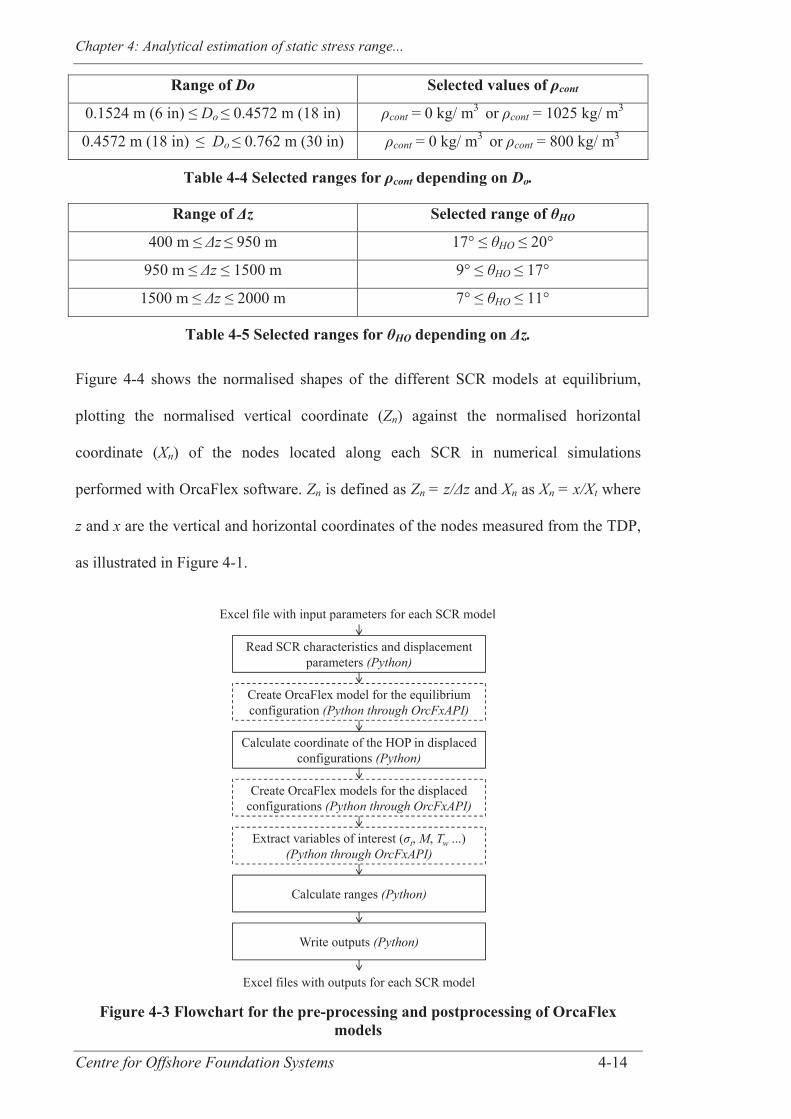
Chapter 4: Analytical estimation of static stress range...
Centre for Offshore Foundation Systems 4-14
Range of Do Selected values of ρcont
0.1524 m (6 in) ≤ Do ≤ 0.4572 m (18 in) cont = 0 kg/ m3 or cont = 1025 kg/ m3
0.4572 m (18 in) ≤ Do ≤ 0.762 m (30 in) cont = 0 kg/ m3 or cont = 800 kg/ m3
Table 4-4 Selected ranges for ρcont depending on Do.
Range of Δz Selected range of θHO
400 m ≤ z ≤ 950 m 17° ≤ HO ≤ 20°
950 m ≤ z ≤ 1500 m 9° ≤ HO ≤ 17°
1500 m ≤ z ≤ 2000 m 7° ≤ HO ≤ 11°
Table 4-5 Selected ranges for θHO depending on Δz. Figure 4-4 shows the normalised shapes of the different SCR models at equilibrium,
plotting the normalised vertical coordinate (Zn) against the normalised horizontal
coordinate (Xn) of the nodes located along each SCR in numerical simulations
performed with OrcaFlex software. Zn is defined as Zn = z/ z and Xn as Xn = x/Xt where
z and x are the vertical and horizontal coordinates of the nodes measured from the TDP,
as illustrated in Figure 4-1.
Figure 4-3 Flowchart for the pre-processing and postprocessing of OrcaFlex models
Excel file with input parameters for each SCR model
Excel files with outputs for each SCR model
Read SCR characteristics and displacement parameters (Python)
Create OrcaFlex model for the equilibrium configuration (Python through OrcFxAPI)
Calculate coordinate of the HOP in displaced configurations (Python)
Create OrcaFlex models for the displaced configurations (Python through OrcFxAPI)
Extract variables of interest ( t, M, Tw ...) (Python through OrcFxAPI)
Calculate ranges (Python)
Write outputs (Python)
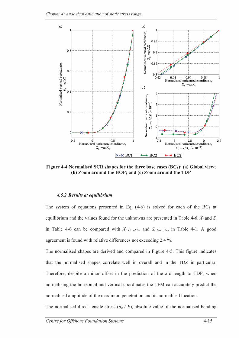
Chapter 4: Analytical estimation of static stress range...
Centre for Offshore Foundation Systems 4-15
Figure 4-4 Normalised SCR shapes for the three base cases (BCs): (a) Global view; (b) Zoom around the HOP; and (c) Zoom around the TDP
4.5.2 Results at equilibrium
The system of equations presented in Eq. (4-6) is solved for each of the BCs at
equilibrium and the values found for the unknowns are presented in Table 4-6. Xt and St
in Table 4-6 can be compared with Xt_OrcaFlex and St_OrcaFlex in Table 4-1. A good
agreement is found with relative differences not exceeding 2.4 %.
The normalised shapes are derived and compared in Figure 4-5. This figure indicates
that the normalised shapes correlate well in overall and in the TDZ in particular.
Therefore, despite a minor offset in the prediction of the arc length to TDP, when
normalising the horizontal and vertical coordinates the TFM can accurately predict the
normalised amplitude of the maximum penetration and its normalised location.
The normalised direct tensile stress ( a / E), absolute value of the normalised bending
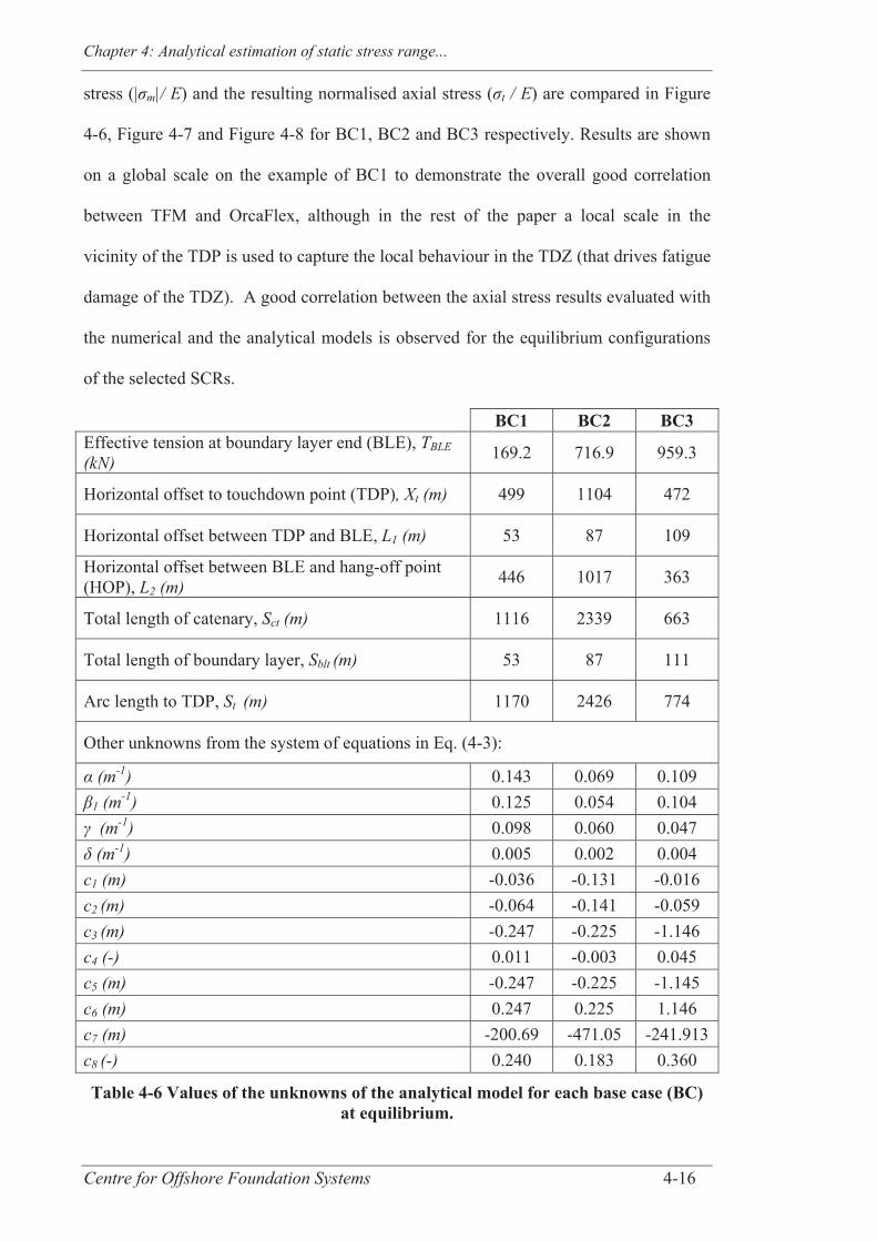
Chapter 4: Analytical estimation of static stress range...
Centre for Offshore Foundation Systems 4-16
stress (| m|/ E) and the resulting normalised axial stress ( t / E) are compared in Figure
4-6, Figure 4-7 and Figure 4-8 for BC1, BC2 and BC3 respectively. Results are shown
on a global scale on the example of BC1 to demonstrate the overall good correlation
between TFM and OrcaFlex, although in the rest of the paper a local scale in the
vicinity of the TDP is used to capture the local behaviour in the TDZ (that drives fatigue
damage of the TDZ). A good correlation between the axial stress results evaluated with
the numerical and the analytical models is observed for the equilibrium configurations
of the selected SCRs.
BC1 BC2 BC3 Effective tension at boundary layer end (BLE), TBLE (kN) 169.2 716.9 959.3
Horizontal offset to touchdown point (TDP), Xt (m) 499 1104 472
Horizontal offset between TDP and BLE, L1 (m) 53 87 109
Horizontal offset between BLE and hang-off point (HOP), L2 (m) 446 1017 363
Total length of catenary, Sct (m) 1116 2339 663
Total length of boundary layer, Sblt (m) 53 87 111
Arc length to TDP, St (m) 1170 2426 774
Other unknowns from the system of equations in Eq. (4-3):
(m-1) 0.143 0.069 0.109 1 (m-1) 0.125 0.054 0.104 (m-1) 0.098 0.060 0.047 (m-1) 0.005 0.002 0.004
c1 (m) -0.036 -0.131 -0.016 c2 (m) -0.064 -0.141 -0.059 c3 (m) -0.247 -0.225 -1.146 c4 (-) 0.011 -0.003 0.045 c5 (m) -0.247 -0.225 -1.145 c6 (m) 0.247 0.225 1.146 c7 (m) -200.69 -471.05 -241.913 c8 (-) 0.240 0.183 0.360
Table 4-6 Values of the unknowns of the analytical model for each base case (BC) at equilibrium.
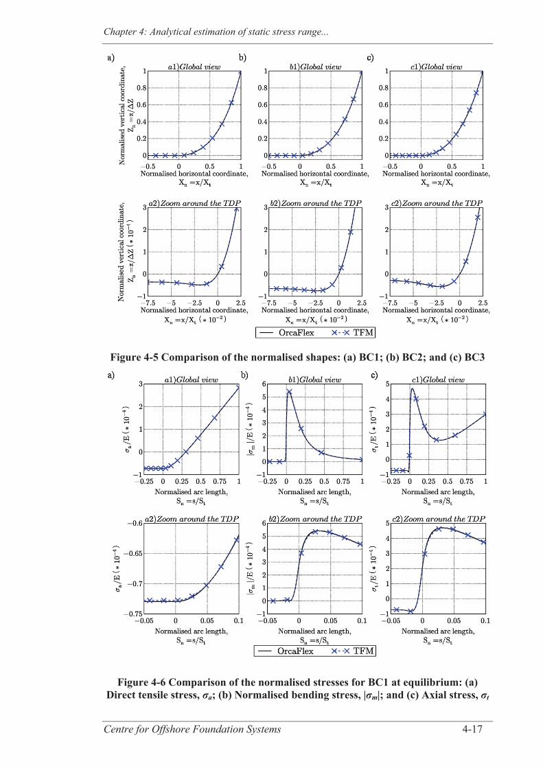
Chapter 4: Analytical estimation of static stress range...
Centre for Offshore Foundation Systems 4-17
Figure 4-5 Comparison of the normalised shapes: (a) BC1; (b) BC2; and (c) BC3
Figure 4-6 Comparison of the normalised stresses for BC1 at equilibrium: (a) Direct tensile stress, σa; (b) Normalised bending stress, |σm|; and (c) Axial stress, σt
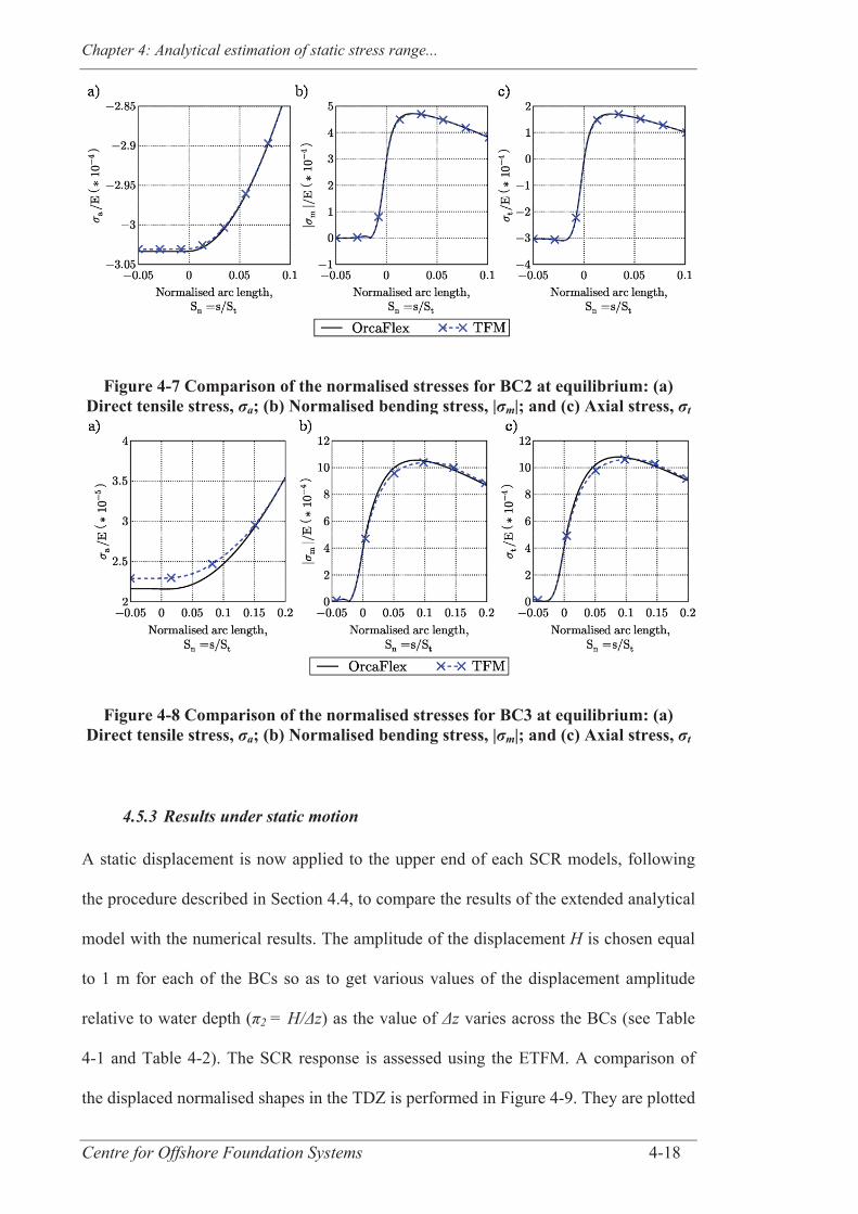
Chapter 4: Analytical estimation of static stress range...
Centre for Offshore Foundation Systems 4-18
Figure 4-7 Comparison of the normalised stresses for BC2 at equilibrium: (a) Direct tensile stress, σa; (b) Normalised bending stress, |σm|; and (c) Axial stress, σt
Figure 4-8 Comparison of the normalised stresses for BC3 at equilibrium: (a)
Direct tensile stress, σa; (b) Normalised bending stress, |σm|; and (c) Axial stress, σt
4.5.3 Results under static motion
A static displacement is now applied to the upper end of each SCR models, following
the procedure described in Section 4.4, to compare the results of the extended analytical
model with the numerical results. The amplitude of the displacement H is chosen equal
to 1 m for each of the BCs so as to get various values of the displacement amplitude
relative to water depth ( 2 = H/ z) as the value of z varies across the BCs (see Table
4-1 and Table 4-2). The SCR response is assessed using the ETFM. A comparison of
the displaced normalised shapes in the TDZ is performed in Figure 4-9. They are plotted
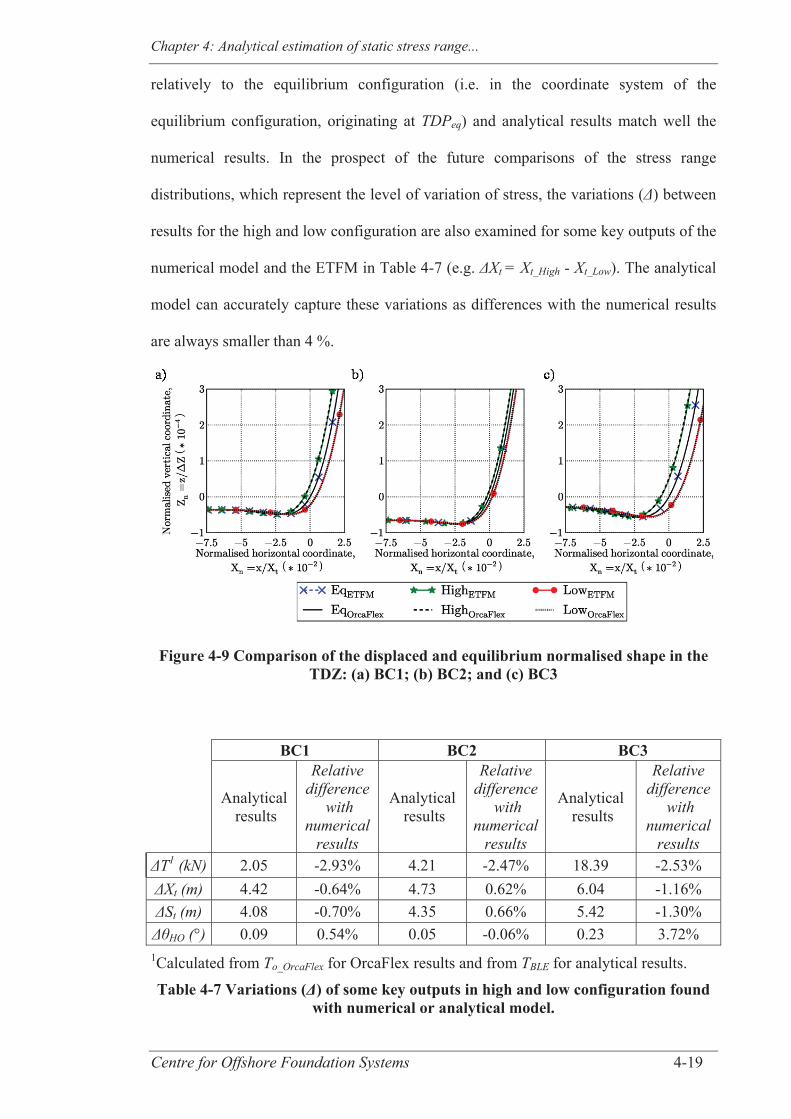
Chapter 4: Analytical estimation of static stress range...
Centre for Offshore Foundation Systems 4-19
relatively to the equilibrium configuration (i.e. in the coordinate system of the
equilibrium configuration, originating at TDPeq) and analytical results match well the
numerical results. In the prospect of the future comparisons of the stress range
distributions, which represent the level of variation of stress, the variations ( ) between
results for the high and low configuration are also examined for some key outputs of the
numerical model and the ETFM in Table 4-7 (e.g. Xt = Xt_High - Xt_Low). The analytical
model can accurately capture these variations as differences with the numerical results
are always smaller than 4 %.
Figure 4-9 Comparison of the displaced and equilibrium normalised shape in the TDZ: (a) BC1; (b) BC2; and (c) BC3
BC1 BC2 BC3
Analytical results
Relative difference
with numerical
results
Analytical results
Relative difference
with numerical
results
Analytical results
Relative difference
with numerical
results T1 (kN) 2.05 -2.93% 4.21 -2.47% 18.39 -2.53% Xt (m) 4.42 -0.64% 4.73 0.62% 6.04 -1.16% St (m) 4.08 -0.70% 4.35 0.66% 5.42 -1.30% HO (°) 0.09 0.54% 0.05 -0.06% 0.23 3.72%
1Calculated from To_OrcaFlex for OrcaFlex results and from TBLE for analytical results.
Table 4-7 Variations (Δ) of some key outputs in high and low configuration found with numerical or analytical model.
Chapter 4: Analytical estimation of static stress range...
Centre for Offshore Foundation Systems 4-20
The normalised axial stress distributions in the TDZ are compared in Figure 4-10 and
the normalised arc length Sn =s/St (where St is the arc length to TDPeq) is used for
convenience. The amplitude of the peak of normalised stress range found with
numerical analyses, its location and the shape of the peak are well approximated by the
extended analytical model. A detailed analysis of the maximum values of the
normalised stress range (Max TDZ/E) is performed in Table 4-8. The ETFM
underestimates systematically the critical normalised stress range although differences
are small (< 5.5 %) and in a range of magnitude that Lenci and Callegari (2005) have
mentioned to be “negligible in practical applications”. Table 4-8 also reports the values
of Max TDZ /E estimated with the approach proposed by Shiri and Hashemi (2012). It
is seen that although their model approximates quite well the numerical results, the
differences tend to increase for the BCs with higher value (see Table 4-1). This is
believed to be a consequence of the use of the catenary equation within their model and
may become an issue for SCRs with larger values of , limiting the applicability of their
approach.
It is therefore concluded that the proposed extended model derived from the three-fields
model of Lenci and Callegari (2005), the ETFM, is a simple analytical tool that can give
an accurate prediction of the static stress range in SCR systems under the assumptions
used in this paper. It could be used to assess the maximum static response in the TDZ,
which is a prerequisite to the DAF approach previously proposed by the authors (Quéau
et al., 2011). The ETFM can also conveniently assist the sensitivity studies of the static
response of oscillating SCRs by removing the time consuming numerical simulations
and the need of a commercial marine software, as shown hereafter.

Chapter 4: Analytical estimation of static stress range...
Centre for Offshore Foundation Systems 4-21
Figure 4-10 Comparison of distribution of the normalised stress range, Δσt / E, in the TDZ: (a) BC1; (b) BC2; and (c) BC3
Max ΔσTDZ / E obtained with : BC1 BC2 BC3 ETFM (this study) 1.13E-04 5.41E-05 1.75E-04 Relative difference with numerical results -2.57% -0.65% -5.50% Model from Shiri and Hashemi (2012) 1.14E-04 5.84E-05 1.66E-04 Relative difference with numerical results -1.68% 7.24% -10.19%
Table 4-8 Validation of the ETFM: Comparison of maximum normalised stress range (Max ΔσTDZ/E) from numerical and analytical results.
4.6 SENSITIVITY ANALYSIS OF THE STATIC RESPONSE OF
SCRS USING THE EXTENDED THREE-FIELDS MODEL
It is proposed in this section to assess the sensitivity of the normalised static stress range
( t /E) to the individual variation of some of the dimensionless groups presented in the
introduction (see Eq. (4-1)). Under the assumptions of the study ( = 0, m = 0), the
key dimensionless groups that may have an impact on the static stress range are the
following:
Riser displacement, 2 = H / z
Riser outside diameter, 5 = Do / z
Riser outside diameter to wall thickness ratio, 6 = Do / wt
Riser unit submerged weight, 7 = p / (E z)
Riser tension, π9 = To / (E z2)

Chapter 4: Analytical estimation of static stress range...
Centre for Offshore Foundation Systems 4-22
Soil stiffness, 11 = ks / E
Water depth, 15 = g z steel / E
For real life applications, it would be useful to study the effects of simultaneous
variations of some of the dimensionless groups as well as (or sometimes in place of)
studying the individual variations only. However, the main purpose of the sensitivity
studies performed in this paper is to illustrate a potential application of the proposed
ETFM while getting preliminary insights on the sensitivity of the SCR response; hence
the study is limited to the effects of individual variations here. A future paper will aim
to present in-depth sensitivity studies.
Different aspects of the distribution of t/E along the riser length are discussed when
performing the sensitivity studies. The amplitude of the peak of normalised stress in the
TDZ (Max TDZ/E) is the key output for this study as it governs the fatigue life of the
SCRs. The location of the critical node (exhibiting the maximum value of t/E) and the
shape of the t /E profile are also discussed for their importance in design or
maintenance purposes. For instance, the shape of the profile indicates how the fatigue
damage is spread along the riser and is useful when relocating the TDP purposely in
operation (Campbell, 1999; Kavanagh and Galvin, 2012).
The effect of the variation of a given dimensionless group is tested systematically on
three groups of different SCR configurations derived from the three BCs defined
previously in order to increase the robustness of the results (more details on the SCR
configurations are given in Section 4.5.1). Indeed, there may be some interactions
between the dimensionless groups and, by working with three groups having various
values of dimensionless groups, the chances of detecting an interaction are increased.
Interaction refers to the fact that the variation of a dimensionless group could have an
effect on the output (Max TDZ/E) that depends on the value of some of the other
dimensionless groups (i.e. “An interaction occurs when two or more factors acting

Chapter 4: Analytical estimation of static stress range...
Centre for Offshore Foundation Systems 4-23
together have a different effect on the quality characteristic than the effect of each
factor acting individually” (Peace, 1993)). However, due to the selected criteria for the
choice of input parameters (see Table 4-3, Table 4-4 and Table 4-5), it is not always
possible to achieve the same level of variation for a particular dimensionless group in
each of the three groups. Hence, care should be taken when comparing the normalised
stress results from the different groups. This is why results are presented first for each of
the groups, and then the relative sensitivity of cases within each group is investigated.
The extended three-fields model (ETFM) is used to perform the sensitivity analyses but,
as a further validation, results are also checked against numerical predictions (see
Appendix A1). Despite an overall tendency to underestimate by a negligible amount the
maximum normalised stress range evaluated in OrcaFlex software, the analytical model
captures correctly the effect of the variation of each dimensionless group for all the new
cases.
4.6.1 Description of the SCR configurations selected for the sensitivity
analyses
New SCR configurations are considered and the complete list of new cases is presented
in Table 4-9. Table 4-10 presents the sub-groups of cases that test the effects of the
variation of either 2, 5, 6, 7, 9, 11 or 15. The new cases are created by modifying
the values of some of the input parameters of each of the three BCs and form three
groups (group 1, group 2 and group 3). The naming of a new case refers to the group it
pertains to (e.g. G1C1 is the first case (C1) of group 1 (G1) and is created from BC1).
All the new cases follow the criteria presented in Table 4-3, Table 4-4 and Table 4-5.
However, to ensure compliance with the screening criteria when varying input
parameter(s) within sub-groups, the unvaried dimensionless groups do not necessarily
all have the value of the dimensionless groups of the BC from the relevant group. Also,

Chapter 4: Analytical estimation of static stress range...
Centre for Offshore Foundation Systems 4-24
unrealistic values of the content density are sometimes used to keep the riser unit
submerged weight ( 7) unchanged across specific cases (e.g. an unrealistic value of the
content density is used in G1C3 to get the same submerged weight as in G1C5 in order
to get the same 7). As for the definition of the BCs, the values of dimensionless tension
measured by 9 for the new cases are calculated using To_catenary.
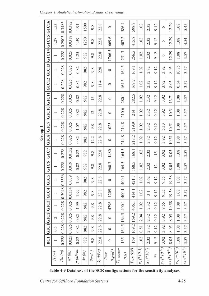
Chapter 4: Analytical estimation of static stress range...
Centre for Offshore Foundation Systems 4-25
Gro
up 1
G
1C16
1.53
0.34
83
0.03
82
1.91
1500
9.8
22.8
0
586.
4
598.
7
1.02
2.32
9.12
6
12.2
9
1.08
5.45
G1C
15
1.27
0.29
03
0.03
18
1.59
1250
9.8
22.8
669.
6
407.
2
415.
8
1.02
2.32
9.12
6
12.2
9
1.08
4.54
G1C
14
1
0.22
8
0.02
5
1.25
982
9.8
22.8
1766
.5
251.
3
256.
5
1.02
2.32
9.12
6
12.2
9
1.08
3.57
G1C
13
1
0.22
8
0.02
5
0.82
982
9.8
228 0
164.
5
169.
1
1.02
2.32
9.12
3.92
8.05
10.7
5
3.57
G1C
12
1
0.22
8
0.02
5
0.82
982
9.8
11.4
0
164.
5
169.
2
1.02
2.32
9.12
3.92
8.05
0.54
3.57
G1C
11
1
0.22
8
0.02
5
0.82
982
15
22.8
0
280.
1
282.
5
1.02
2.32
9.12
3.92
13.7
1
1.08
3.57
G1C
10
1
0.22
8
0.02
5
0.82
982
12
22.8
0
210.
6
214
1.02
2.32
9.12
3.92
10.3
1.08
3.57
G1C
9
1
0.22
8
0.02
5
1.07
982
9.8
22.8
1025
214.
8
219.
9
1.02
2.32
9.12
5.13
10.5
1
1.08
3.57
G1C
8
1
0.22
8
0.02
5
0.82
982
12.2
22.8
0
214.
8
218.
2
1.02
2.32
9.12
3.92
10.5
1
1.08
3.57
G1C
7
1
0.22
8
0.01
52
0.82
982
9.8
22.8
1480
164.
5
168.
1
1.02
2.32
15
3.92
8.05
1.08
3.57
G1C
6
1
0.22
8
0.01
9
0.82
982
9.8
22.8
960.
3
164.
5
168.
5
1.02
2.32
12
3.92
8.05
1.08
3.57
G1C
5
1
0.35
56
0.03
9
1.99
982
9.8
22.8
0
400.
1
421.
7
1.02
3.62
9.12
9.55
19.5
8
1.08
3.57
G1C
4
1
0.30
48
0.03
34
1.99
982
9.8
22.8
1209
400.
1
414.
1
1.02
3.1
9.12
9.55
19.5
8
1.08
3.57
G1C
3
1
0.22
8
0.02
5
1.99
982
9.8
22.8
4796
400.
1
406.
1
1.02
2.32
9.12
9.55
19.5
8
1.08
3.57
G1C
2
2
0.22
8
0.02
5
0.82
982
9.8
22.8
0
164.
5
169.
2
2.04
2.32
9.12
3.92
8.05
1.08
3.57
G1C
1
0.5
0.22
8
0.02
5
0.82
982
9.8
22.8
0
164.
5
169.
2
0.51
2.32
9.12
3.92
8.05
1.08
3.57
BC
1
1
0.22
8
0.02
5
0.82
982
9.8
22.8
0 165
169
1.02
2.32
9.12
3.92
8.05
1.08
3.57
H (m
)
Do
(m)
wt (
m)
p (k
N/m
)
z (m
)
HO
(°)
k s (k
Pa)
cont
(kg/
m3 )
T o_c
aten
ary
(kN
) T B
LE (k
N)
2 (*
10-3
)
5 (*1
0-4)
6
7 (*1
0-12 )
9 (*1
0-13 )
11 (*
10-7
)
15 (*
10-4
)
Table 4-9 Database of the SCR configurations for the sensitivity analyses.
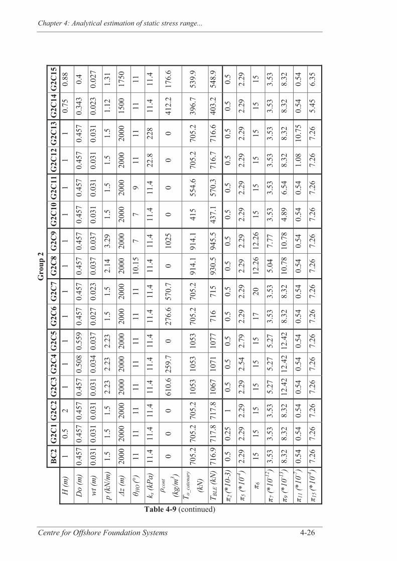
Chapter 4: Analytical estimation of static stress range...
Centre for Offshore Foundation Systems 4-26
Gro
up 2
G
2C15
0.
88
0.4
0.02
7
1.31
1750
11
11.4
176.
6
539.
9
548.
9
0.5
2.29
15
3.53
8.32
0.54
6.35
G2C
14
0.75
0.34
3
0.02
3
1.12
1500
11
11.4
412.
2
396.
7
403.
2
0.5
2.29
15
3.53
8.32
0.54
5.45
G2C
13
1
0.45
7
0.03
1
1.5
2000
11
228 0
705.
2
716.
6
0.5
2.29
15
3.53
8.32
10.7
5
7.26
G2C
12
1
0.45
7
0.03
1
1.5
2000
11
22.8
0
705.
2
716.
7
0.5
2.29
15
3.53
8.32
1.08
7.26
G2C
11
1
0.45
7
0.03
1
1.5
2000
9 11.4
0
554.
6
570.
3
0.5
2.29
15
3.53
6.54
0.54
7.26
G2C
10
1
0.45
7
0.03
1
1.5
2000
7 11.4
0 415
437.
1
0.5
2.29
15
3.53
4.89
0.54
7.26
G2C
9 1
0.45
7
0.03
7
3.29
2000
7 11.4
1025
914.
1
945.
5
0.5
2.29
12.2
6
7.77
10.7
8
0.54
7.26
G2C
8 1
0.45
7
0.03
7
2.14
2000
10.1
5
11.4
0
914.
1
930.
5
0.5
2.29
12.2
6
5.04
10.7
8
0.54
7.26
G2C
7 1
0.45
7
0.02
3
1.5
2000
11
11.4
570.
7
705.
2
715
0.5
2.29
20
3.53
8.32
0.54
7.26
G2C
6 1
0.45
7
0.02
7
1.5
2000
11
11.4
276.
6
705.
2
716
0.5
2.29
17
3.53
8.32
0.54
7.26
G2C
5 1
0.55
9
0.03
7
2.23
2000
11
11.4
0
1053
1077
0.5
2.79
15
5.27
12.4
2
0.54
7.26
G2C
4 1
0.50
8
0.03
4
2.23
2000
11
11.4
259.
7
1053
1071
0.5
2.54
15
5.27
12.4
2
0.54
7.26
G2C
3 1
0.45
7
0.03
1
2.23
2000
11
11.4
610.
6
1053
1067
0.5
2.29
15
5.27
12.4
2
0.54
7.26
G2C
2 2
0.45
7
0.03
1
1.5
2000
11
11.4
0
705.
2
717.
8
1 2.29
15
3.53
8.32
0.54
7.26
G2C
1 0.
5
0.45
7
0.03
1
1.5
2000
11
11.4
0
705.
2
717.
8
0.25
2.29
15
3.53
8.32
0.54
7.26
BC
2 1
0.45
7
0.03
1
1.5
2000
11
11.4
0
705.
2
716.
9
0.5
2.29
15
3.53
8.32
0.54
7.26
H (m
)
Do
(m)
wt (
m)
p (k
N/m
)
z (m
)
HO
(°)
k s (k
Pa)
cont
(kg/
m3 )
T o_c
aten
ary
(kN
) T B
LE (k
N)
2 (*
10-3
)
5 (*1
0-4)
6
7 (*1
0-12 )
9 (*1
0-13 )
11 (*
10-7
)
15 (*
10-4
)
Table 4-9 (continued)
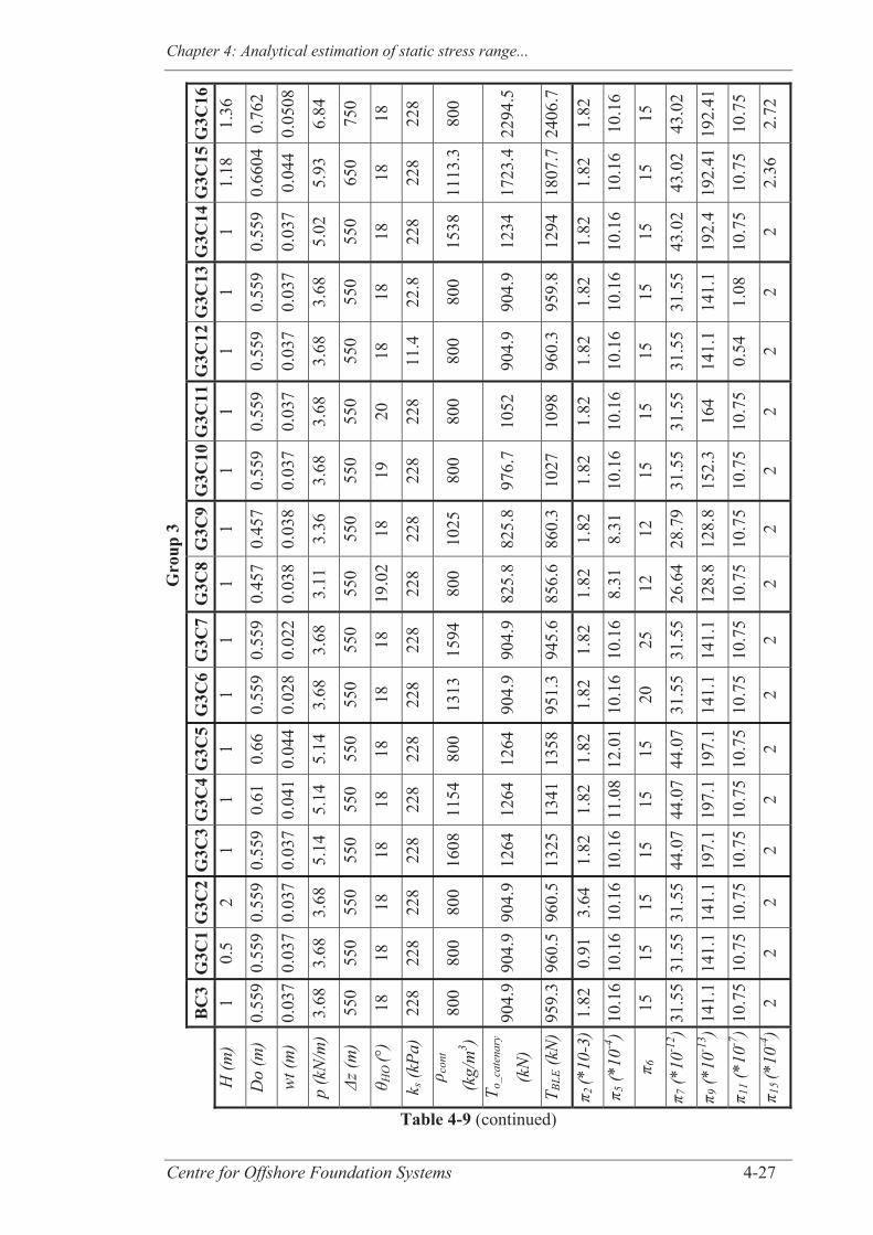
Chapter 4: Analytical estimation of static stress range...
Centre for Offshore Foundation Systems 4-27
Gro
up 3
G
3C16
1.
36
0.76
2
0.05
08
6.84
750
18
228
800
2294
.5
2406
.7
1.82
10.1
6
15
43.0
2
192.
41
10.7
5
2.72
G3C
15
1.18
0.66
04
0.04
4
5.93
650
18
228
1113
.3
1723
.4
1807
.7
1.82
10.1
6
15
43.0
2
192.
41
10.7
5
2.36
G3C
14
1
0.55
9
0.03
7
5.02
550
18
228
1538
1234
1294
1.82
10.1
6
15
43.0
2
192.
4
10.7
5
2
G3C
13
1
0.55
9
0.03
7
3.68
550
18
22.8
800
904.
9
959.
8
1.82
10.1
6
15
31.5
5
141.
1
1.08
2
G3C
12
1
0.55
9
0.03
7
3.68
550
18
11.4
800
904.
9
960.
3
1.82
10.1
6
15
31.5
5
141.
1
0.54
2
G3C
11
1
0.55
9
0.03
7
3.68
550
20
228
800
1052
1098
1.82
10.1
6
15
31.5
5
164
10.7
5
2
G3C
10
1
0.55
9
0.03
7
3.68
550
19
228
800
976.
7
1027
1.82
10.1
6
15
31.5
5
152.
3
10.7
5
2
G3C
9 1
0.45
7
0.03
8
3.36
550
18
228
1025
825.
8
860.
3
1.82
8.31
12
28.7
9
128.
8
10.7
5
2
G3C
8 1
0.45
7
0.03
8
3.11
550
19.0
2
228
800
825.
8
856.
6
1.82
8.31
12
26.6
4
128.
8
10.7
5
2
G3C
7 1
0.55
9
0.02
2
3.68
550
18
228
1594
904.
9
945.
6
1.82
10.1
6
25
31.5
5
141.
1
10.7
5
2
G3C
6 1
0.55
9
0.02
8
3.68
550
18
228
1313
904.
9
951.
3
1.82
10.1
6
20
31.5
5
141.
1
10.7
5
2
G3C
5 1 0.66
0.04
4
5.14
550
18
228
800
1264
1358
1.82
12.0
1
15
44.0
7
197.
1
10.7
5
2
G3C
4 1 0.61
0.04
1
5.14
550
18
228
1154
1264
1341
1.82
11.0
8
15
44.0
7
197.
1
10.7
5
2
G3C
3 1
0.55
9
0.03
7
5.14
550
18
228
1608
1264
1325
1.82
10.1
6
15
44.0
7
197.
1
10.7
5
2
G3C
2 2
0.55
9
0.03
7
3.68
550
18
228
800
904.
9
960.
5
3.64
10.1
6
15
31.5
5
141.
1
10.7
5
2
G3C
1 0.
5
0.55
9
0.03
7
3.68
550
18
228
800
904.
9
960.
5
0.91
10.1
6
15
31.5
5
141.
1
10.7
5
2
BC
3 1
0.55
9
0.03
7
3.68
550
18
228
800
904.
9
959.
3
1.82
10.1
6
15
31.5
5
141.
1
10.7
5
2
H (m
)
Do
(m)
wt (
m)
p (k
N/m
)
z (m
)
HO
(°)
k s (k
Pa)
cont
(kg/
m3 )
T o_c
aten
ary
(kN
) T B
LE (k
N)
2 (*
10-3
)
5 (*1
0-4)
6
7 (*1
0-12 )
9 (*1
0-13 )
11 (*
10-7
)
15 (*
10-4
)
Table 4-9 (continued)
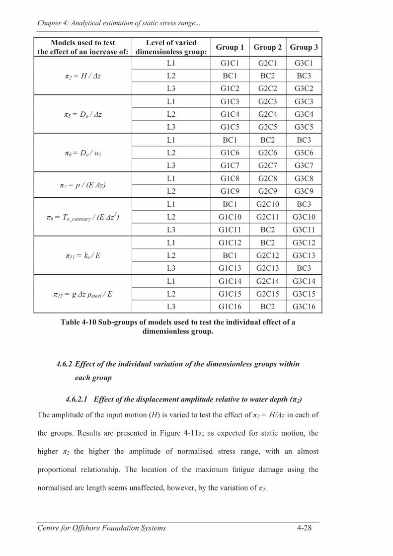
Chapter 4: Analytical estimation of static stress range...
Centre for Offshore Foundation Systems 4-28
Models used to test the effect of an increase of:
Level of varied dimensionless group: Group 1 Group 2 Group 3
2 = H / z L1 G1C1 G2C1 G3C1 L2 BC1 BC2 BC3 L3 G1C2 G2C2 G3C2
5 = Do / z L1 G1C3 G2C3 G3C3 L2 G1C4 G2C4 G3C4 L3 G1C5 G2C5 G3C5
6 = Do / wt L1 BC1 BC2 BC3 L2 G1C6 G2C6 G3C6 L3 G1C7 G2C7 G3C7
7 = p / (E z) L1 G1C8 G2C8 G3C8 L2 G1C9 G2C9 G3C9
9 = To_catenary / (E z2) L1 BC1 G2C10 BC3 L2 G1C10 G2C11 G3C10 L3 G1C11 BC2 G3C11
11 = ks / E L1 G1C12 BC2 G3C12 L2 BC1 G2C12 G3C13 L3 G1C13 G2C13 BC3
15 = g z steel / E L1 G1C14 G2C14 G3C14 L2 G1C15 G2C15 G3C15 L3 G1C16 BC2 G3C16
Table 4-10 Sub-groups of models used to test the individual effect of a dimensionless group.
4.6.2 Effect of the individual variation of the dimensionless groups within
each group
4.6.2.1 Effect of the displacement amplitude relative to water depth (π2)
The amplitude of the input motion (H) is varied to test the effect of 2 = H/ z in each of
the groups. Results are presented in Figure 4-11a; as expected for static motion, the
higher 2 the higher the amplitude of normalised stress range, with an almost
proportional relationship. The location of the maximum fatigue damage using the
normalised arc length seems unaffected, however, by the variation of 2.
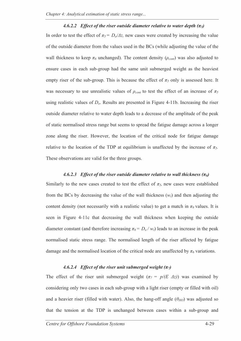
Chapter 4: Analytical estimation of static stress range...
Centre for Offshore Foundation Systems 4-29
4.6.2.2 Effect of the riser outside diameter relative to water depth (π5)
In order to test the effect of 5 = Do/ z, new cases were created by increasing the value
of the outside diameter from the values used in the BCs (while adjusting the value of the
wall thickness to keep 6 unchanged). The content density ( cont) was also adjusted to
ensure cases in each sub-group had the same unit submerged weight as the heaviest
empty riser of the sub-group. This is because the effect of 5 only is assessed here. It
was necessary to use unrealistic values of cont to test the effect of an increase of 5
using realistic values of Do. Results are presented in Figure 4-11b. Increasing the riser
outside diameter relative to water depth leads to a decrease of the amplitude of the peak
of static normalised stress range but seems to spread the fatigue damage across a longer
zone along the riser. However, the location of the critical node for fatigue damage
relative to the location of the TDP at equilibrium is unaffected by the increase of 5.
These observations are valid for the three groups.
4.6.2.3 Effect of the riser outside diameter relative to wall thickness (π6)
Similarly to the new cases created to test the effect of 5, new cases were established
from the BCs by decreasing the value of the wall thickness (wt) and then adjusting the
content density (not necessarily with a realistic value) to get a match in 9 values. It is
seen in Figure 4-11c that decreasing the wall thickness when keeping the outside
diameter constant (and therefore increasing 6 = Do / wt) leads to an increase in the peak
normalised static stress range. The normalised length of the riser affected by fatigue
damage and the normalised location of the critical node are unaffected by 6 variations.
4.6.2.4 Effect of the riser unit submerged weight (π7)
The effect of the riser unit submerged weight ( 7 = p/(E z)) was examined by
considering only two cases in each sub-group with a light riser (empty or filled with oil)
and a heavier riser (filled with water). Also, the hang-off angle ( HO) was adjusted so
that the tension at the TDP is unchanged between cases within a sub-group and
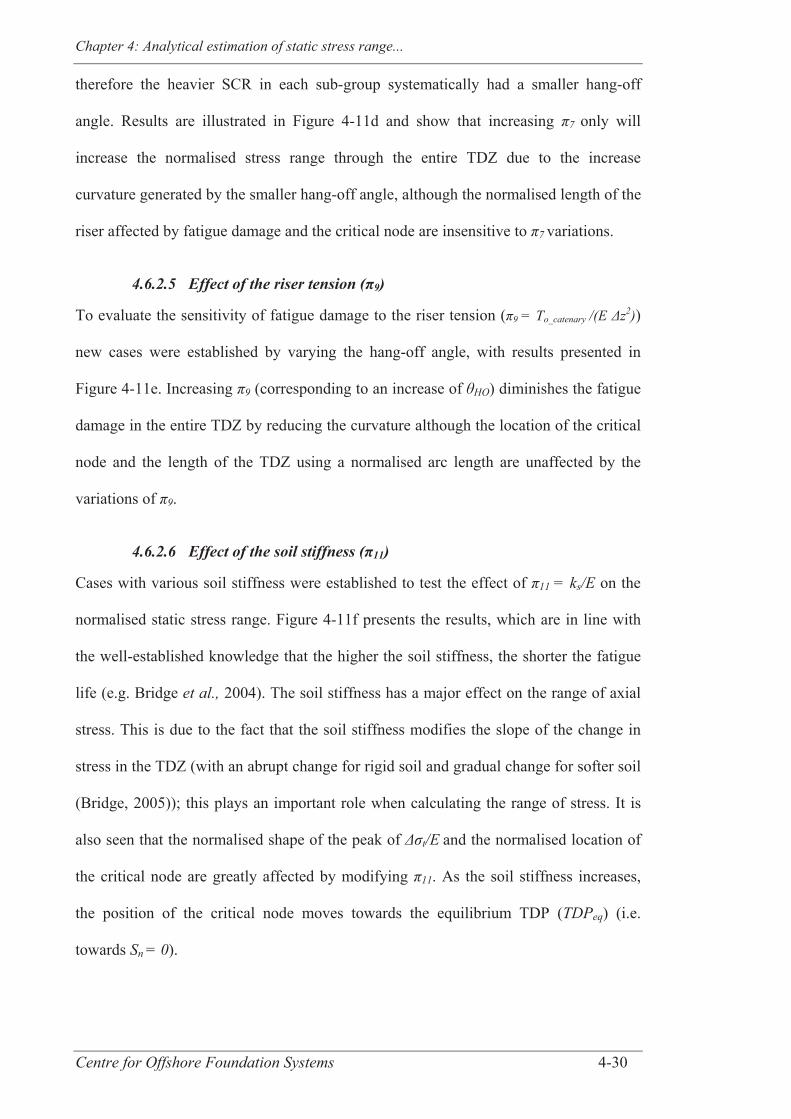
Chapter 4: Analytical estimation of static stress range...
Centre for Offshore Foundation Systems 4-30
therefore the heavier SCR in each sub-group systematically had a smaller hang-off
angle. Results are illustrated in Figure 4-11d and show that increasing 7 only will
increase the normalised stress range through the entire TDZ due to the increase
curvature generated by the smaller hang-off angle, although the normalised length of the
riser affected by fatigue damage and the critical node are insensitive to 7 variations.
4.6.2.5 Effect of the riser tension (π9)
To evaluate the sensitivity of fatigue damage to the riser tension ( 9 = To_catenary /(E z2))
new cases were established by varying the hang-off angle, with results presented in
Figure 4-11e. Increasing 9 (corresponding to an increase of HO) diminishes the fatigue
damage in the entire TDZ by reducing the curvature although the location of the critical
node and the length of the TDZ using a normalised arc length are unaffected by the
variations of 9.
4.6.2.6 Effect of the soil stiffness (π11)
Cases with various soil stiffness were established to test the effect of 11 = ks/E on the
normalised static stress range. Figure 4-11f presents the results, which are in line with
the well-established knowledge that the higher the soil stiffness, the shorter the fatigue
life (e.g. Bridge et al., 2004). The soil stiffness has a major effect on the range of axial
stress. This is due to the fact that the soil stiffness modifies the slope of the change in
stress in the TDZ (with an abrupt change for rigid soil and gradual change for softer soil
(Bridge, 2005)); this plays an important role when calculating the range of stress. It is
also seen that the normalised shape of the peak of t/E and the normalised location of
the critical node are greatly affected by modifying 11. As the soil stiffness increases,
the position of the critical node moves towards the equilibrium TDP (TDPeq) (i.e.
towards Sn = 0).

Chapter 4: Analytical estimation of static stress range...
Centre for Offshore Foundation Systems 4-31
4.6.2.7 Effect of the water depth (π15)
As g, E and steel were constant in the study, the variation of 15 = g z steel /E
corresponds to a variation of z. New cases were created by modifying z compared to
their respective BCs and by scaling the other parameters appropriately to keep 2, 5, 6,
7, 9 and 11 constant (unrealistic values of cont are used for this purpose). The
normalised stress range results are compared in Figure 4-11g. The distributions of t/E
against the normalised arc length are similar for every case in each of the groups.
Hence, it seems that t/E is insensitive to the individual variation of 15.
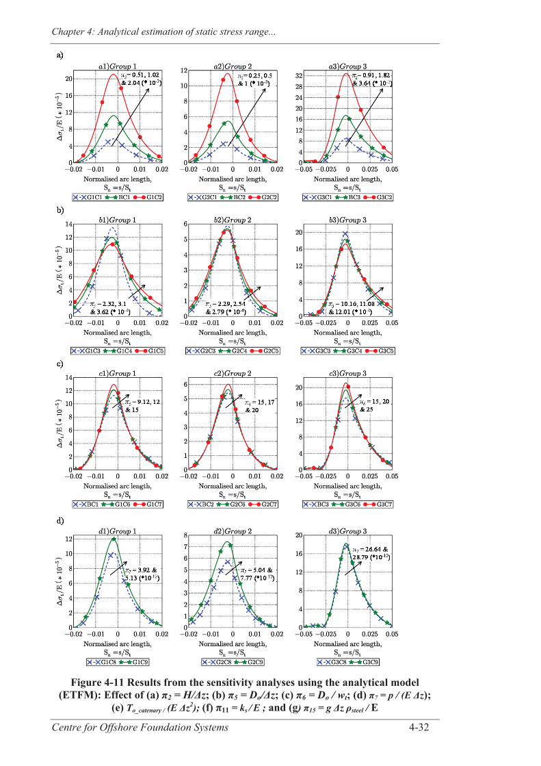
Chapter 4: Analytical estimation of static stress range...
Centre for Offshore Foundation Systems 4-32
Figure 4-11 Results from the sensitivity analyses using the analytical model (ETFM): Effect of (a) π2 = H/Δz; (b) π5 = Do/Δz; (c) π6 = Do / wt; (d) π7 = p / (E Δz);
(e) To_catenary / (E Δz2); (f) π11 = ks / E ; and (g) π15 = g Δz ρsteel / E
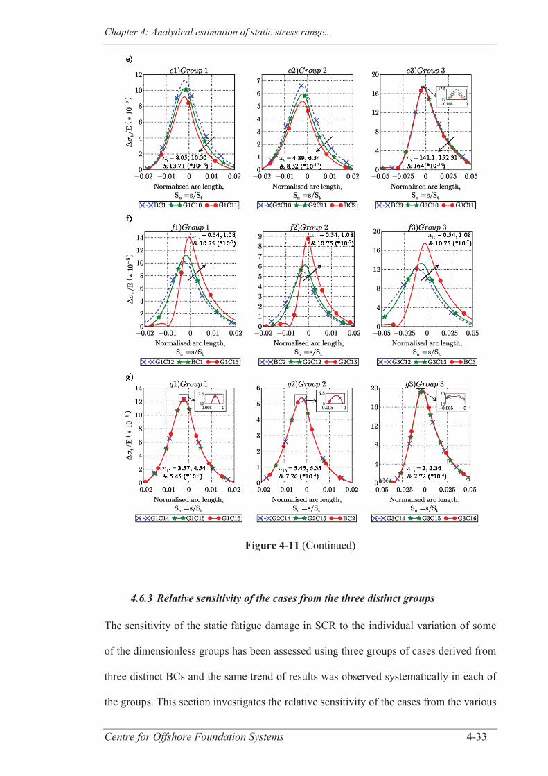
Chapter 4: Analytical estimation of static stress range...
Centre for Offshore Foundation Systems 4-33
Figure 4-11 (Continued)
4.6.3 Relative sensitivity of the cases from the three distinct groups
The sensitivity of the static fatigue damage in SCR to the individual variation of some
of the dimensionless groups has been assessed using three groups of cases derived from
three distinct BCs and the same trend of results was observed systematically in each of
the groups. This section investigates the relative sensitivity of the cases from the various

Chapter 4: Analytical estimation of static stress range...
Centre for Offshore Foundation Systems 4-34
groups by focusing on the variation of output relative to the variation of input. The
variation of input for a given case testing the level Lj of one of the tested dimensionless
group k in a particular group Gi (with j {1, 2, 3}, k {2, 5, 6, 7, 9, 11, 15} and
i {1, 2, 3}) is defined by k GiLj / k GiL1 where k GiLj refers to the value of k in this
particular case and k GiL1 is the lowest value of k within the corresponding sub-group.
Using similar notations, the variation of output is defined as
(Max TDZ/E / 2)GiLj / (Max TDZ/E / 2)GiL1. The maximum normalised stress range
(Max TDZ/E) is divided by the normalised magnitude of the perturbation ( 2).
Figure 4-12 illustrates the results for each of the varied dimensionless groups with the
gradients of the curves representing the sensitivity of each case. Overall, SCR responses
exhibit a linear behaviour to imposed static motion. Similar trends are observed for 6,
7 and 15 for all three groups. The fact that the responses of cases from the three groups
show the same sensitivity to individual variations of these dimensionless groups
suggests that 6, 7 and 15 may not interact with the other dimensionless groups that
have a different value in the three groups at least for the ranges tested. All three groups
also seem to be insensitive to the individual variation of 15, as mentioned in the
previous section. For 2, 5, 9 and 11, different sensitivities are observed between all
or some of the groups and suggest potential interactions with other dimensionless
groups. A more extensive study is currently in progress, using artificial neural networks,
extending the limited cases studied here and also assessing the complex interactions
between the different dimensionless groups.
The observations here are limited to the individual variation of dimensionless groups
and are only valid for the static case. They may be altered due to simultaneous variation
of a selection of dimensionless groups and due to dynamic effects (e.g. influence of drag
forces, resonance effects etc…). Moreover, the normalised arc length (Sn) has been used
in this section to ease comparisons, because the main focus of the study is to estimate
Chapter 4: Analytical estimation of static stress range...
Centre for Offshore Foundation Systems 4-35
the fatigue life in the TDZ (through evaluation of the maximum normalised stress
range). Therefore, the results do not indicate how the arc length to TDP is modified due
to the individual variation of selected dimensionless groups, which would also be of
interest for practical applications. Further investigation will be performed when moving
to the next step of this research, beyond the scope of this paper, which aims for more
accurate quantification of the SCR dynamic response and DAFs.
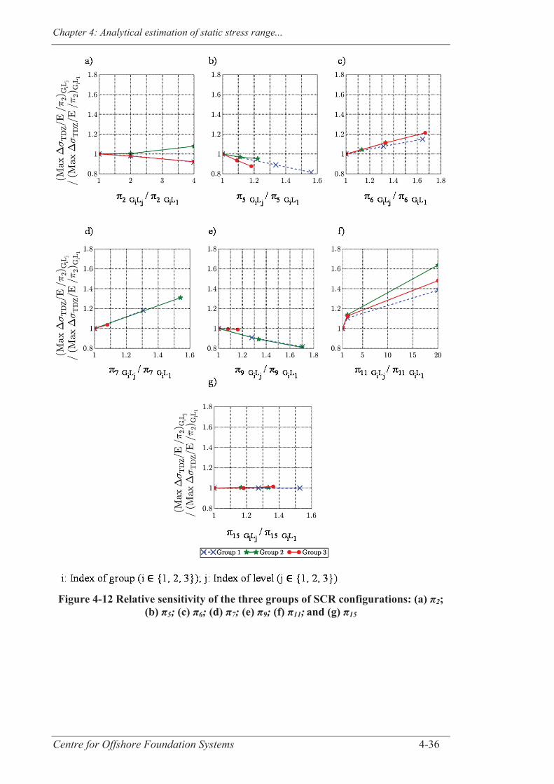
Chapter 4: Analytical estimation of static stress range...
Centre for Offshore Foundation Systems 4-36
Figure 4-12 Relative sensitivity of the three groups of SCR configurations: (a) π2; (b) π5; (c) π6; (d) π7; (e) π9; (f) π11; and (g) π15
Chapter 4: Analytical estimation of static stress range...
Centre for Offshore Foundation Systems 4-37
4.7 CONCLUSIONS
An extension of the analytical “three-fields model” defined by Lenci and Callegari
(2005) that accounts for the boundary layer effect in the TDZ is proposed in this paper
to estimate the static stress range occurring in oscillating SCRs. The analytical model
has been established in an attempt to simplify fatigue design of SCRs through the DAF
approach. It provides a simple and efficient tool to estimate the static response of SCRs
accurately. Validation of the analytical model was performed by comparison against
numerical simulations using OrcaFlex.
The analytical model was also used to obtain initial results on the sensitivity of the static
stress range to individual variations of some of the dimensionless groups and results are
summarised in Table 4-11. With the selected values of input dimensionless groups, it
was found that:
The lowest maximum value of the normalised stress range in the TDZ (i.e.
increase the fatigue life of SCRs) occurs by maximising the riser outside
diameter ( 5) and tension ( 9) and minimising the riser displacement ( 2),
outside diameter to wall thickness ratio ( 6), unit submerged weight ( 7) and
the soil stiffness ( 11).
The location of the critical node relative to the equilibrium TDP is insensitive to
the individual variations of all of the tested dimensionless groups except for the
soil stiffness 11.
The normalised width of the critical fatigue damage zone in the TDZ relative to
the equilibrium TDP is mainly sensitive to the soil stiffness ( 11) and the riser
outside diameter ( 5).
Future work will aim to assess how these results are altered (i) due to dynamics effects,
(ii) when considering other values for the dimensionless groups, as well as (iii) when
testing the effect of simultaneous variations of the dimensionless groups to detect
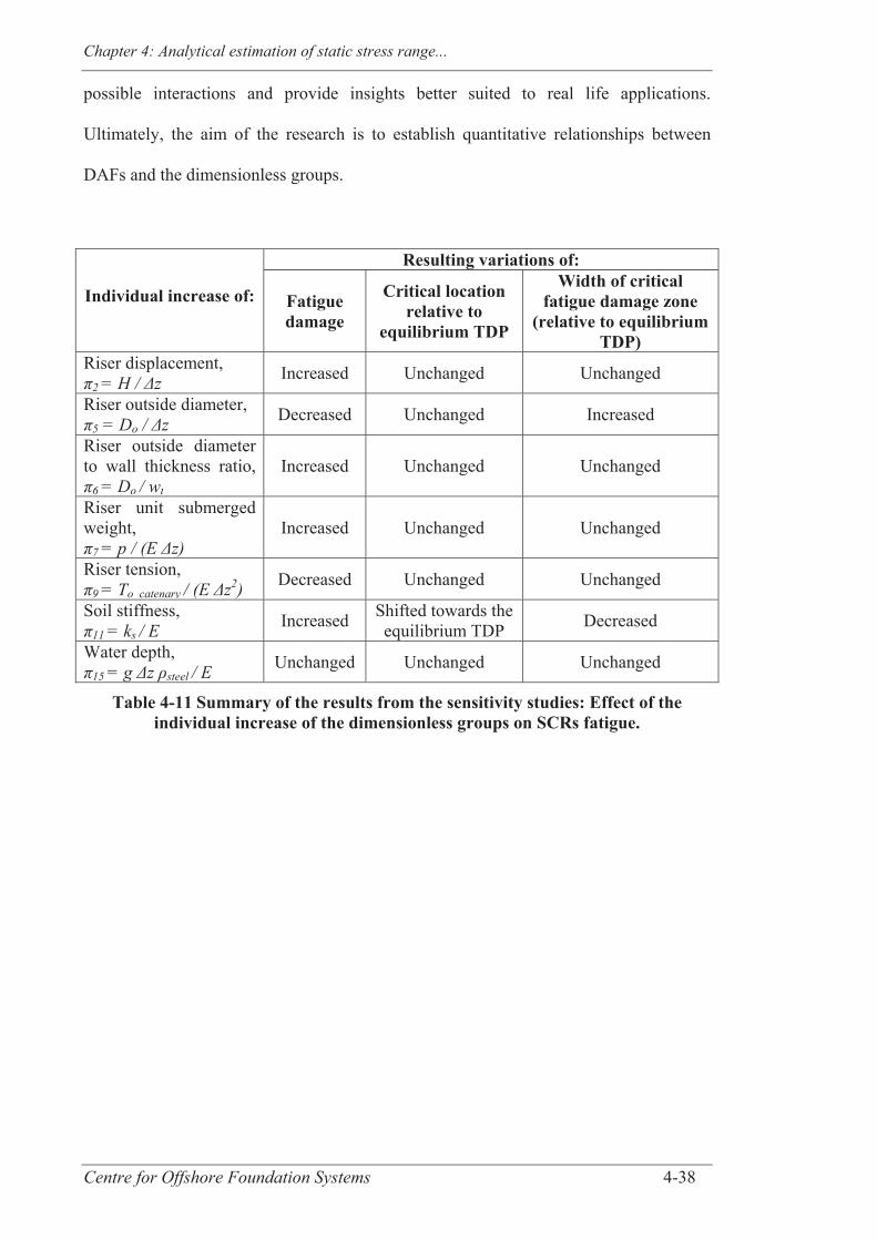
Chapter 4: Analytical estimation of static stress range...
Centre for Offshore Foundation Systems 4-38
possible interactions and provide insights better suited to real life applications.
Ultimately, the aim of the research is to establish quantitative relationships between
DAFs and the dimensionless groups.
Individual increase of:
Resulting variations of:
Fatigue damage
Critical location relative to
equilibrium TDP
Width of critical fatigue damage zone
(relative to equilibrium TDP)
Riser displacement, 2 = H / z Increased Unchanged Unchanged
Riser outside diameter, 5 = Do / z Decreased Unchanged Increased
Riser outside diameter to wall thickness ratio,
6 = Do / wt Increased Unchanged Unchanged
Riser unit submerged weight,
7 = p / (E z) Increased Unchanged Unchanged
Riser tension, 9 = To catenary / (E z2) Decreased Unchanged Unchanged
Soil stiffness, 11 = ks / E Increased Shifted towards the
equilibrium TDP Decreased
Water depth, 15 = g z steel / E Unchanged Unchanged Unchanged
Table 4-11 Summary of the results from the sensitivity studies: Effect of the individual increase of the dimensionless groups on SCRs fatigue.

Estimating the fatigue damage of SCRs in the TDZ
Centre for Offshore Foundation Systems 5-1
CHAPTER 5 ARTIFICIAL NEURAL NETWORK DEVELOPMENT
FOR STRESS ANALYSIS OF STEEL CATENARY RISERS: A
PILOT STUDY
5.1 ABSTRACT
The large number of parameters involved in the design of steel catenary risers (SCRs)
makes assessment of fatigue life challenging, particularly in the touchdown zone (TDZ).
Sensitivity analyses are necessary to gain a greater understanding of the influence of
parameters on fatigue damage. Previous research by the authors clarified the list of input
parameters influencing SCR fatigue damage and grouped them into dimensionless
groups to facilitate sensitivity analyses.
This paper explores how the use of artificial neural networks (ANNs), based on a
database pre-processed using design of experiment (DoE) techniques, can assist
sensitivity analyses. The database is established using marine analysis software
OrcaFlex, linked to optimisation software modeFRONTIER through an in-house
interface developed in the Python programming language. A substantial database
capturing the wide ranges of the dimensionless groups encountered in realistic SCR
applications is established. Approximations of the amplitude of the peak stress range in
the TDZ and its location are investigated through a traditional polynomial fit method
and compared with the more advanced ANN approach. It is shown that using ANNs
provides a quick and simple tool that outperforms the polynomial fit approach in
predicting the maximum stress range and its critical location for fatigue design of SCRs.
Chapter 5: ANN development for stress analysis of SCRs: A pilot study
Centre for Offshore Foundation Systems 5-2
5.2 INTRODUCTION
Steel catenary risers (SCRs) are a common deepwater riser option due to their
robustness, reliability, simplicity and low manufacturing cost (Campbell, 1999; Bai and
Bai, 2005). However, they are fatigue sensitive systems. The touchdown zone (TDZ –
the area of dynamic riser-soil interaction (Bridge, 2005)) in particular is prone to high
fatigue damage. Numerous parameters, ranging from soil response, riser characteristics
and environmental loading are known to impact the fatigue performance of SCRs but
there is a lack of quantitative guidance on how each parameter affects the fatigue
damage. To increase confidence in SCR fatigue design and gain a greater understanding
of the influence of these parameters on the fatigue damage, it is necessary to conduct a
series of sensitivity analyses.
This paper discusses the approaches that can be used to perform future sensitivity
analyses in order to find the most appropriate techniques for SCR fatigue design. The
usefulness of the design of experiment (DoE) methods in the definition of a valid
database and of the response surface method for post-processing the results is explored.
Two types of response surfaces are used: first a traditional approach consisting of fitting
a polynomial equation to the results by minimising the deviation from the results
through the least squares method, and then a more advanced artificial intelligence tool,
the artificial neural network (ANN), is applied. The aim is to examine if the ANN
approach can benefit SCR design. The use of ANN is not common for SCR design,
even though the DoE method and some optimisation techniques, based potentially on
another tool from the artificial intelligence field, the genetic algorithm, have been used
previously in riser design (Larsen and Hanson, 1999; Yang and Li, 2010; Martins et al.,
2012, 2013; de Pina et al., 2013) and for lazy wave risers in particular (Vieira et al.,
2003, 2008; Lima et al, 2005; Wang et al., 2011; Yang et al., 2012; Erlend Voie and
Sødahl, 2013). However, the ANN approach has been applied successfully in other
Chapter 5: ANN development for stress analysis of SCRs: A pilot study
Centre for Offshore Foundation Systems 5-3
engineering fields, e.g. in geotechnical engineering (Shahin et al., 2002, 2004) or in
hydrological engineering (Tokar and Johnson, 1999).
ANNs are used for a very wide range of applications, aiding interpretation of either
measured data from real life observations or experiments, or analytical solutions,
capturing the relationship between inputs and output(s) (e.g. Shahin et al., 2002). They
are also used in computer aided design, for the preliminary design of structures in order
to reduce computational cost and provide a rapid appreciation of the structural
behaviour (Gunaratnam and Gero, 1994; Rogers, 1994; Mukherjee and Deshpande,
1995; Szewczyk and Noor, 1996; Adeli, 2001; de Pina et al., 2013) or for sensitivity
and nonlinear analysis of structures (Szewczyk and Noor, 1997; Adeli, 2001; de Pina et
al., 2013). The latter applications seem particularly suitable for SCR design and
motivated this pilot study.
Indeed, this study is part of ongoing research aiming to simplify preliminary fatigue
design of SCRs by removing the need to perform time consuming simulations involved
in the evaluation of the critical dynamic stress range occurring in the TDZ (i.e.
maximum stress range in the TDZ, Max TDZ). The critical dynamic stress range
controls the fatigue damage that arises due to the variation of axial stress ( ), combining
axial force and bending moment effects, under cycles of imposed motion. The
simplification relies on the use of dynamic amplification factors (DAFs) that quantify
the dynamic response with respect to the static response (Quéau et al., 2011). The
ultimate aim is to define an approximation of the DAF so that an estimate of the critical
dynamic stress range can conveniently be back calculated. The static response needs to
be evaluated first to successfully apply this method and several authors have proposed
analytical solutions with a varying level of complexity and accuracy (Pesce et al.,
1998a; Lenci and Callegari, 2005; Shiri and Hashemi, 2012; Quéau et al., 2014a).
Despite the existence of these analytical tools it is proposed to test the usefulness of the

Chapter 5: ANN development for stress analysis of SCRs: A pilot study
Centre for Offshore Foundation Systems 5-4
implemented methodology on the static response of SCRs in this paper. This is a
preliminary step towards the sensitivity studies and the application of the best type of
response surface to more complicated dynamic perturbations (which are too complex to
be solved through analytical solutions) as part of the DAF approach.
It is commonly acknowledged that using dimensionless groups will enhance the
pertinence of sensitivity analyses (Pesce et al., 1998a ; Palmer, 2008b) and it was shown
by Gunaratnam and Gero (1994) that performing a dimensional analysis and using
dimensionless groups to train an ANN led to improved performance by reducing the
size of the design space. Hence, the dimensionless groups formed from the parameters
pertaining to riser characteristics, hydrodynamics, environmental loading and soil
response that were shown to impact the stress range in SCRs (Quéau et al., 2013)
constitute the input for the sensitivity analyses. The main output is the maximum stress
range in the touchdown zone normalised by the Young’s Modulus (Max TDZ/E), as it
drives fatigue damage, but its normalised location (Sn_critical) is also investigated. Sn_critical
is defined as Sn_critical = Scritical / St where Scritical is the location of the maximum stress
range measured from the hang-off point and St is the arc length to the touchdown point
(TDP) in the equilibrium configuration (i.e. before application of any motion), and
therefore an approximation of St needs to be investigated too. In reality the design
parameters and consequently the dimensionless groups vary over large ranges.
Therefore it is necessary to simulate a significant amount of cases, each defining a
particular SCR configuration and loading conditions, in order to get meaningful results.
A database of 4800 cases is defined for this pilot study. An in-house interface coded in
the Python programming language (Python Software Foundation, 2009) is developed,
linking the optimisation software modeFRONTIER (Esteco, 1999) and the marine
analysis software OrcaFlex (Orcina, 2012) in order to automate the numerical analyses.
More details on the overall methodology and the assumptions of this study are presented
Chapter 5: ANN development for stress analysis of SCRs: A pilot study
Centre for Offshore Foundation Systems 5-5
initially. Next, an overview of the DoE method and of the ANN theory is given,
followed by the development of the approximations using a polynomial fit and an ANN
for each of the selected outputs (e.g. Max TDZ/E, Sn_critical and St )..
5.3 ASSUMPTIONS AND OVERALL METHODOLOGY
This study is conducted under the simplifying assumptions presented in Quéau et al.
(2013). It is a 2D study limited to the SCR response under in-plane motions only with
the loading applied by imposing a displacement to the floating vessel. The current
profile in the sea column, the flow rate of the contents, the coating and the structural
damping are not taken into account and the hang-off point is pinned. As mentioned
previously, it is limited to static perturbations, and also, a linear soil response (defined
by a spring stiffness) is adopted even though in the future the approach could be
extended to nonlinear soil models.
Under these assumptions and using the notations from Quéau et al. (2013), it was
decided to develop approximations of Max TDZ/E and Sn_critical as functions of 2, 5,
6, 7, 9, 11 and 15. The definition of these dimensionless groups is given in Table 5-1
while an illustration of some of the SCR design parameters is shown in Figure 5-1. Note
that arc lengths originate at the hang-off point. Table 5-1 also lists the dimensionless
groups that were kept constant in this study and indicates that the stress range is always
measured at = 17 = 0°, even though in a more detailed fatigue analysis the stress range
should also be assessed at = 180°. Also, the displacement of the floating vessel is
always applied in an axis parallel to the riser at the hang-off point (HOP), which is why
m = 0°. This is based on the findings from Kimiaei et al. (2010) that the tangential
component of motion alone could adequately represent the fatigue damage resulting
from wave loading. The study is limited to static cases, which is why the dimensionless
groups that normalise the time ( 18), the input velocity ( 4) and corresponding to the

Chapter 5: ANN development for stress analysis of SCRs: A pilot study
Centre for Offshore Foundation Systems 5-6
drag coefficient ( 12) and added mass coefficient ( 13) are irrelevant here, as reported in
Table 5-1. Gravity acceleration (g = 9.81 m/s2), Young’s Modulus for the SCR
(E = 2.12E8 kPa), water density ( water = 1.025 te/m3) and steel density
( steel = 7.85 te/m3) remain unchanged in the study.
Figure 5-1 SCR geometry and key parameters: (a) Side view of SCR configuration; and (b) Riser cross-section (Quéau et al., 2013)
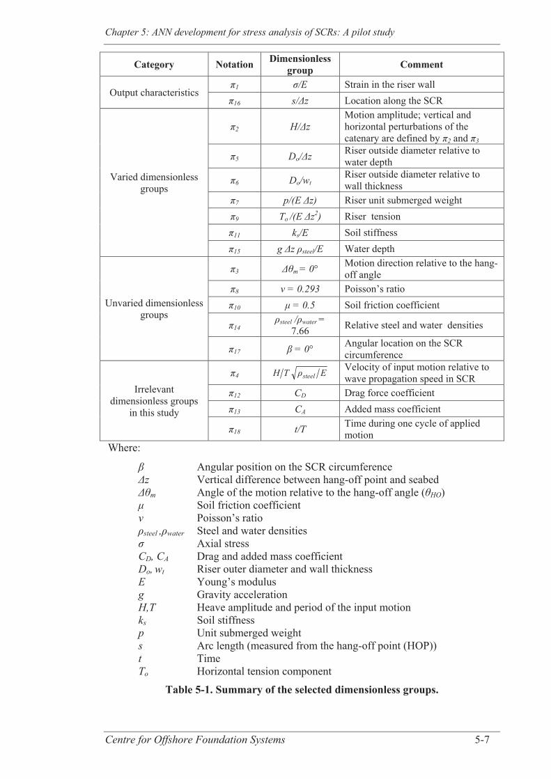
Chapter 5: ANN development for stress analysis of SCRs: A pilot study
Centre for Offshore Foundation Systems 5-7
Category Notation Dimensionless group Comment
Output characteristics 1 /E Strain in the riser wall
16 s/ z Location along the SCR
Varied dimensionless groups
2 H/ z Motion amplitude; vertical and horizontal perturbations of the catenary are defined by 2 and 3
5 Do/ z Riser outside diameter relative to water depth
6 Do/wt Riser outside diameter relative to wall thickness
7 p/(E z) Riser unit submerged weight
9 To /(E z2) Riser tension
11 ks/E Soil stiffness
15 g z steel/E Water depth
Unvaried dimensionless groups
3 m = 0° Motion direction relative to the hang-off angle
8 = 0.293 Poisson’s ratio
10 = 0.5 Soil friction coefficient
14 steel / water = 7.66 Relative steel and water densities
17 = 0° Angular location on the SCR circumference
Irrelevant dimensionless groups
in this study
4 ETH steel Velocity of input motion relative to wave propagation speed in SCR
12 CD Drag force coefficient
13 CA Added mass coefficient
18 t/T Time during one cycle of applied motion
Where:
Angular position on the SCR circumference z Vertical difference between hang-off point and seabed
m Angle of the motion relative to the hang-off angle ( HO) Soil friction coefficient Poisson’s ratio steel , water Steel and water densities Axial stress
CD, CA Drag and added mass coefficient Do, wt Riser outer diameter and wall thickness E Young’s modulus g Gravity acceleration H,T Heave amplitude and period of the input motion ks Soil stiffness p Unit submerged weight s Arc length (measured from the hang-off point (HOP)) t Time To Horizontal tension component
Table 5-1. Summary of the selected dimensionless groups.

Chapter 5: ANN development for stress analysis of SCRs: A pilot study
Centre for Offshore Foundation Systems 5-8
5.4 OVERVIEW OF THE METHODS USED IN THIS STUDY
5.4.1 Design of experiment (DoE)
Design of experiment (DoE) is a method of planning experiments to “maximize the
knowledge gained from experimental data” (Esteco, 1999) through a limited number of
experiments and which relies on statistical techniques for data analysis (Peace, 1993;
Park, 1996). The method encompasses numerous types of design approaches suited for
different applications (Peace, 1993; Fowlkes and Crevelling, 1995; Park, 1996; Esteco,
1999; Montgomery, 2013). A detailed discussion of the different approaches, as applied
to SCR fatigue, has been provided by Martins et al. (2013), with the three main ones
summarised briefly below.
1. One-factor-at-a-time approach
This approach is traditionally used and consists in investigating the effect of each factor
in turn assuming fixed levels of the other design variables (e.g. Xia et al., 2008; Kimiaei
et al., 2010; Shiri and Randolph, 2010; Elosta et al., 2013a ; Quéau et al., 2014a). It is a
very slow process and it can lead to unreliable results as the approach ignores
interaction between factors.
2. Factorial approach
In a full factorial approach, all the possible combinations of factors are simulated and
therefore all the interactions are accounted for. For a complex problem such as here, the
number of analyses rapidly becomes impractical since it increases exponentially with
the number of dimensionless groups. Even a fractional factorial approach, focusing on
particular combinations of groups, may become onerous, and may introduce bias in the
results (Fowlkes and Crevelling, 1995).
Chapter 5: ANN development for stress analysis of SCRs: A pilot study
Centre for Offshore Foundation Systems 5-9
3. Random approach
The database can be generated by random choices of values for the dimensionless
groups, while taking care to spread the points throughout the design space. Additional
points may be added, following the initial choice, to facilitate this (Esteco, 1999).
The one-factor-at-a-time and full or fractional factorial approaches are mainly used for
parametric studies aiming to identify the relative effect of the variable and interactions
on a particular output while algorithms that generate random or quasi-random points are
useful to support the training of a response surface.
5.4.2 Artificial neural networks (ANNs)
5.4.2.1 Overview
The response surface methodology can be used to estimate the value of an output for a
combination of inputs that had not yet been tested, based on a database of training cases
(Esteco, 1999; Box and Draper, 2007; Martins et al., 2013; Montgomery, 2013).
Various models exist ranging from classical models, such as a polynomial
approximation, to more advanced models, such as the ANNs.
An ANN is a mathematical model used to capture the complex relationship between a
group of inputs and outputs and is a powerful interpolation tool, particularly suitable for
“hard-to-learn problems and when there is no formal underlying theory for the solution
of the problem” (Adeli, 2001). An important feature of ANNs is their ability to learn the
relationship between inputs and outputs through the database used to train them without
the need to have any prior knowledge on the nature of this relationship.
The structure of ANNs is inspired from biological neural networks, with layers of
‘neurons’ (or nodes) receiving ‘signals’ for each node in the preceding layer and
Chapter 5: ANN development for stress analysis of SCRs: A pilot study
Centre for Offshore Foundation Systems 5-10
generating an output that is passed to each node in a subsequent layer (Fausett, 1994).
The architecture of ANNs varies from a single layer net (only the layer of output nodes,
reacting directly to the input nodes) to multilayer nets, having one or more hidden layers
of nodes between the input nodes and the layer of output nodes (Figure 5-2). Multilayer
nets are used to solve more complex problems that can learn more complicated
mappings, but the use of only one hidden layer is sufficient for most applications
(Fausett, 1994). The number of nodes composing the hidden layer is a key parameter in
ANNs architecture as it controls the number of degrees of freedom. A sufficient number
is necessary to capture the signals accurately and avoid underfitting. However, too many
nodes may lead to overfitting (i.e. use of too many neurons in the hidden layer
compared with the amount of information contained in the training set) and will
increase the time necessary to train an ANN (noting that computational time to use
ANNs is trivial regardless of the training time).
During the training phase of an ANN, appropriate weights are researched to enable the
nodes to transmit appropriate signals and hence achieve the targeted outputs for the
given inputs forming the selected database (so-called supervised training). If the ANN is
used for a new input pattern, which was not in the list of input patterns for which the
ANN was trained, then the ANN uses the determined weights to assess the outputs.
Hence, an independent testing database should be used to validate the ANN, once
trained, to ensure satisfactory performance throughout the desired range of input values
(Fausett, 1994; Gurney, 1997).
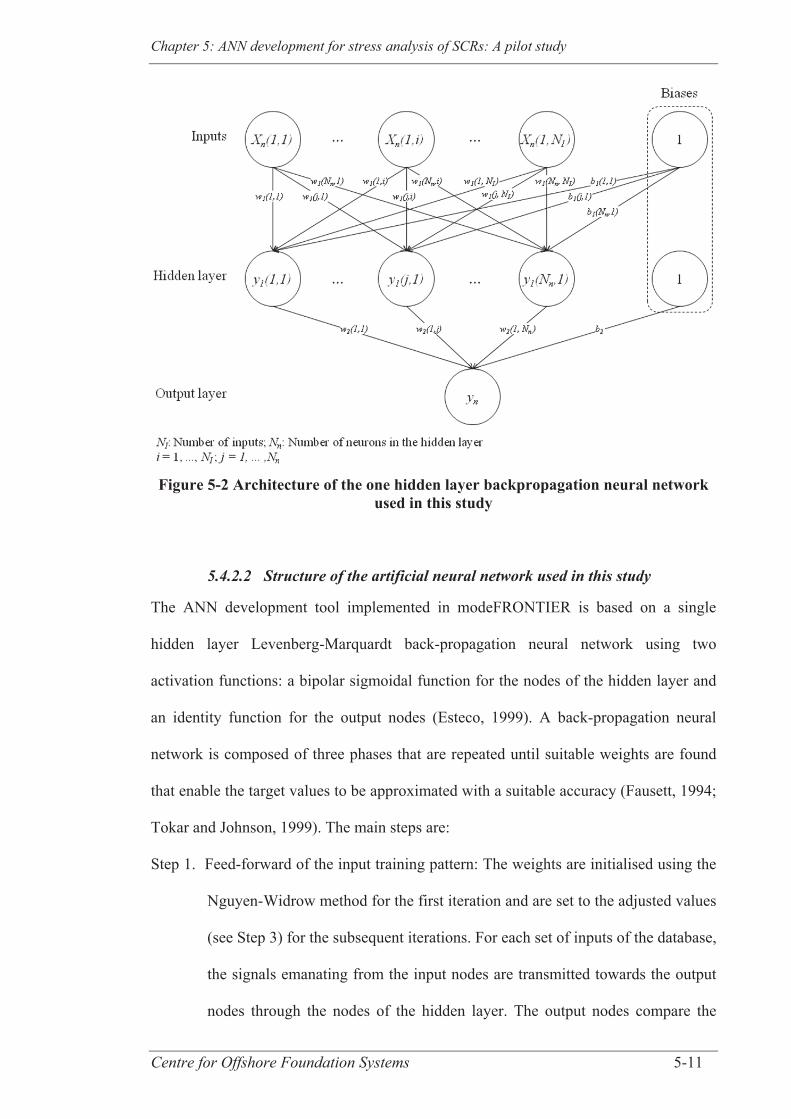
Chapter 5: ANN development for stress analysis of SCRs: A pilot study
Centre for Offshore Foundation Systems 5-11
Figure 5-2 Architecture of the one hidden layer backpropagation neural network
used in this study
5.4.2.2 Structure of the artificial neural network used in this study
The ANN development tool implemented in modeFRONTIER is based on a single
hidden layer Levenberg-Marquardt back-propagation neural network using two
activation functions: a bipolar sigmoidal function for the nodes of the hidden layer and
an identity function for the output nodes (Esteco, 1999). A back-propagation neural
network is composed of three phases that are repeated until suitable weights are found
that enable the target values to be approximated with a suitable accuracy (Fausett, 1994;
Tokar and Johnson, 1999). The main steps are:
Step 1. Feed-forward of the input training pattern: The weights are initialised using the
Nguyen-Widrow method for the first iteration and are set to the adjusted values
(see Step 3) for the subsequent iterations. For each set of inputs of the database,
the signals emanating from the input nodes are transmitted towards the output
nodes through the nodes of the hidden layer. The output nodes compare the
Chapter 5: ANN development for stress analysis of SCRs: A pilot study
Centre for Offshore Foundation Systems 5-12
values of their computed signals with the target values and determine the
associated errors.
Step 2. Backpropagation of the errors: errors are sent to previous layers. A detailed
presentation of this step is well covered in published literature, for instance by
de Pina et al. (2013).
Step 3. Adjustments of weights: weights for all layers are adjusted simultaneously
based on the errors and activation functions used.
Figure 5-2 shows the structure of the ANN and its notations (using matrix notations).
Once the ANN is trained and validated, the net can be used following a procedure
similar to the feed-forward phase mentioned in Step 1 and detailed hereafter. The
flowchart for the use of the ANN, based on modeFRONTIER calculations, is presented
in Figure 5-3. ModeFRONTIER normalises the input vector prior to applying the ANN
based on the ranges for each input. The input vector (X) comprises the selection of
dimensionless groups that impact the static stress range in SCRs, as discussed earlier,
and therefore the number of input, NI, equals 7. The normalised input vector (Xn) is used
with the weights of the input nodes (w1) to determine the net input signal of the hidden
layer (n1). The first activation function is applied to n1 to obtain the output signal of the
nodes from the hidden layers (y1). Subsequently, the weights of the nodes from the
hidden layer (w2) and y1 are computed to assess the net input signal of the output (n2).
Biases are used during calculations and are inherent to the ANN. They act in a similar
manner to the weights for nodes that would always have an output of 1. The second
activation function is used to obtain the output yn in a normalised scale [-1;1]. The
estimated value of the output is then calculated using the extreme values of the output
across the training database.
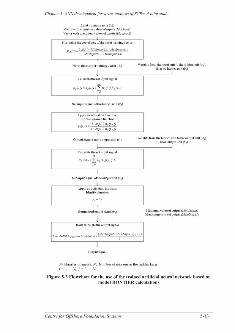
Chapter 5: ANN development for stress analysis of SCRs: A pilot study
Centre for Offshore Foundation Systems 5-13
Figure 5-3 Flowchart for the use of the trained artificial neural network based on
modeFRONTIER calculations

Chapter 5: ANN development for stress analysis of SCRs: A pilot study
Centre for Offshore Foundation Systems 5-14
5.5 ANN DEVELOPMENT FOR SCR FATIGUE DESIGN
5.5.1 In-house automation subroutine
The flowchart of the analyses is presented in Figure 5-4. MATLAB (2012) is used to
generate the database of cases, defined by their dimensionless group values, and then to
back calculate the corresponding individual input parameters. These parameters, along
with the values of the constant dimensionless groups and other input parameters, are
passed to in-house Python code that communicates with OrcaFlex through the
OrcFxAPI programming language (Python Software Foundation, 2009; Orcina, 2012) to
pre-process the numerical models, run the simulations and post-process the models.
Figure 5-4 Flowchart of the sensitivity analyses
modeFRONTIER:- Coordinate Matlab and OrcaFlex(through Python)- Store and analyse the output
MATLAB:Generate the database of realistic combination of
the varied dimensionless groups
MATLAB:Calculate the individual input parameters
Python with OrcFxAPI code:Pre-process and post process the numerical models
to get 1 results for 17 = 0 and all 16
OrcaFlex:Run the numerical models
Constant input parameters and dimensionless groups:
E, g, steel, water, 3 , 8 , 10 , 14
Approximations of the outputs
modeFRONTIER:Fit the experimental points with a response surface
Dimensionless groups:2 , 5 , 6 , 7, 9 , 11 , 15
Outputs:Max TDZ / E , Sn_critical , St
Input parameters: cont, p, To, Do, wt, ks, H, z
Chapter 5: ANN development for stress analysis of SCRs: A pilot study
Centre for Offshore Foundation Systems 5-15
The procedure followed to simulate the static cases is the same as in Quéau et al.
(2014a): For every cases of the database, a model of the SCR configuration at the
equilibrium position is created first. This model is used to assess the value of the arc
length to TDP (St). From this first model, two other models are derived by displacing
the position of the hang-off point (HOP) by +H and –H (in an axis parallel to the
tangential line of the riser at the HOP for the equilibrium position, since m = 0°).
Stress results are extracted in these two models to get 1 results at 17 = 0° for all 16
values in the two displaced configurations. Then, the stress range is calculated by taking
the difference of each pair of 1 results (at a given 16) and the maximum in the
touchdown is sought (Max TDZ/E). Its location (Scritical) is used with St to calculate
Sn_critical. The values of Max TDZ/E, Sn_critical and St are stored by modeFRONTIER for
further analysis.
5.5.2 Database characteristics
5.5.2.1 Boundaries of the design space: ranges of the dimensionless groups
The extreme values of the key individual input parameters involved in SCR design are
presented in Table 5-2. Rather than using constant minimum and maximum values for
the wall thickness (wt), the content density ( cont) and the horizontal tension component
(To), a series of design criteria were used to select appropriate values depending on the
values of other input parameters (this is referred to as the “sliding level” technique in
the DoE method (Fowlkes and Crevelling, 1995)). These criteria were implemented to
constrain the design space to realistic combinations of the individual input parameters.
The selected ranges and design criteria were derived from currently operating in-service
SCRs and SCR configurations presented in the literature. Hence, the choice of value for
wt depends on the value of Do and the choice of cont also depends on Do to represent
large gas risers and smaller pipes for liquids. The value of To is controlled by the value
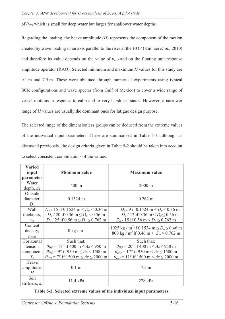
Chapter 5: ANN development for stress analysis of SCRs: A pilot study
Centre for Offshore Foundation Systems 5-16
of HO which is small for deep water but larger for shallower water depths.
Regarding the loading, the heave amplitude (H) represents the component of the motion
created by wave loading in an axis parallel to the riser at the HOP (Kimiaei et al., 2010)
and therefore its value depends on the value of HO and on the floating unit response
amplitude operator (RAO). Selected minimum and maximum H values for this study are
0.1 m and 7.5 m. These were obtained through numerical experiments using typical
SCR configurations and wave spectra (from Gulf of Mexico) to cover a wide range of
vessel motions in response to calm and to very harsh sea states. However, a narrower
range of H values are usually the dominant ones for fatigue design purpose.
The selected range of the dimensionless groups can be deduced from the extreme values
of the individual input parameters. These are summarised in Table 5-3, although as
discussed previously, the design criteria given in Table 5-2 should be taken into account
to select consistent combinations of the values.
Varied input
parameter Minimum value Maximum value
Water depth, z 400 m 2000 m
Outside diameter,
Do 0.1524 m 0.762 m
Wall thickness,
wt
Do / 15 if 0.1524 m ≤ Do < 0.36 mDo / 20 if 0.36 m ≤ Do < 0.56 m Do / 25 if 0.56 m ≤ Do ≤ 0.762 m
Do / 9 if 0.1524 m ≤ Do ≤ 0.36 m Do / 12 if 0.36 m < Do ≤ 0.56 m
Do / 15 if 0.56 m < Do ≤ 0.762 m Content density,
cont 0 kg / m3 1025 kg / m3 if 0.1524 m ≤ Do ≤ 0.46 m
800 kg / m3 if 0.46 m < Do ≤ 0.762 m
Horizontal tension
component, To
Such that: HO = 17° if 400 m ≤ z < 950 m HO = 9° if 950 m ≤ z < 1500 m
HO = 7° if 1500 m ≤ z ≤ 2000 m
Such that: HO = 20° if 400 m ≤ z ≤ 950 m
HO = 17° if 950 m < z ≤ 1500 m HO = 11° if 1500 m < z ≤ 2000 m
Heave amplitude,
H 0.1 m 7.5 m
Soil stiffness, ks
11.4 kPa 228 kPa
Table 5-2. Selected extreme values of the individual input parameters.
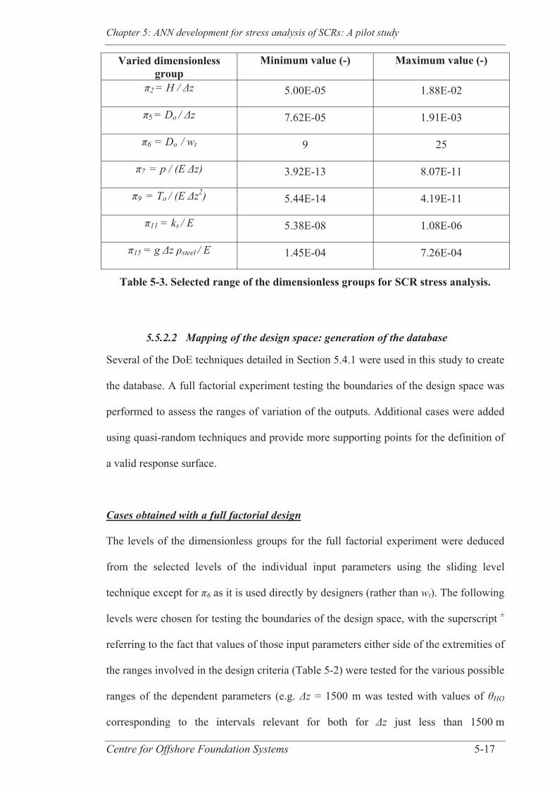
Chapter 5: ANN development for stress analysis of SCRs: A pilot study
Centre for Offshore Foundation Systems 5-17
Varied dimensionless group
Minimum value (-) Maximum value (-)
2 = H / z 5.00E-05 1.88E-02
5 = Do / z 7.62E-05 1.91E-03
6 = Do / wt 9 25
7 = p / (E z) 3.92E-13 8.07E-11
9 = To / (E z2) 5.44E-14 4.19E-11
11 = ks / E 5.38E-08 1.08E-06
15 = g z steel / E 1.45E-04 7.26E-04
Table 5-3. Selected range of the dimensionless groups for SCR stress analysis.
5.5.2.2 Mapping of the design space: generation of the database
Several of the DoE techniques detailed in Section 5.4.1 were used in this study to create
the database. A full factorial experiment testing the boundaries of the design space was
performed to assess the ranges of variation of the outputs. Additional cases were added
using quasi-random techniques and provide more supporting points for the definition of
a valid response surface.
Cases obtained with a full factorial design
The levels of the dimensionless groups for the full factorial experiment were deduced
from the selected levels of the individual input parameters using the sliding level
technique except for 6 as it is used directly by designers (rather than wt). The following
levels were chosen for testing the boundaries of the design space, with the superscript ±
referring to the fact that values of those input parameters either side of the extremities of
the ranges involved in the design criteria (Table 5-2) were tested for the various possible
ranges of the dependent parameters (e.g. z = 1500 m was tested with values of HO
corresponding to the intervals relevant for both for z just less than 1500 m
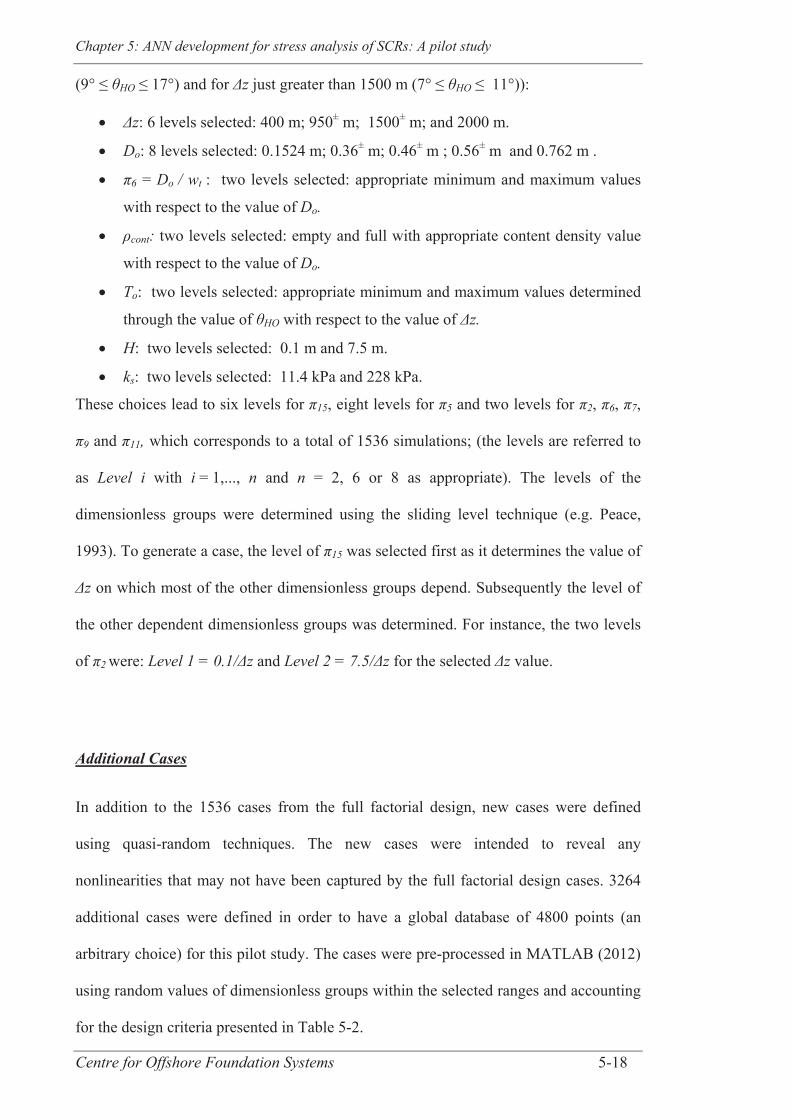
Chapter 5: ANN development for stress analysis of SCRs: A pilot study
Centre for Offshore Foundation Systems 5-18
(9° ≤ HO ≤ 17°) and for z just greater than 1500 m (7° ≤ HO ≤ 11°)):
z: 6 levels selected: 400 m; 950± m; 1500± m; and 2000 m.
Do: 8 levels selected: 0.1524 m; 0.36± m; 0.46± m ; 0.56± m and 0.762 m .
6 = Do / wt : two levels selected: appropriate minimum and maximum values
with respect to the value of Do.
cont: two levels selected: empty and full with appropriate content density value
with respect to the value of Do.
To: two levels selected: appropriate minimum and maximum values determined
through the value of HO with respect to the value of z.
H: two levels selected: 0.1 m and 7.5 m.
ks: two levels selected: 11.4 kPa and 228 kPa.
These choices lead to six levels for 15, eight levels for 5 and two levels for 2, 6, 7,
9 and 11, which corresponds to a total of 1536 simulations; (the levels are referred to
as Level i with i = 1,..., n and n = 2, 6 or 8 as appropriate). The levels of the
dimensionless groups were determined using the sliding level technique (e.g. Peace,
1993). To generate a case, the level of 15 was selected first as it determines the value of
z on which most of the other dimensionless groups depend. Subsequently the level of
the other dependent dimensionless groups was determined. For instance, the two levels
of 2 were: Level 1 = 0.1/ z and Level 2 = 7.5/ z for the selected z value.
Additional Cases
In addition to the 1536 cases from the full factorial design, new cases were defined
using quasi-random techniques. The new cases were intended to reveal any
nonlinearities that may not have been captured by the full factorial design cases. 3264
additional cases were defined in order to have a global database of 4800 points (an
arbitrary choice) for this pilot study. The cases were pre-processed in MATLAB (2012)
using random values of dimensionless groups within the selected ranges and accounting
for the design criteria presented in Table 5-2.
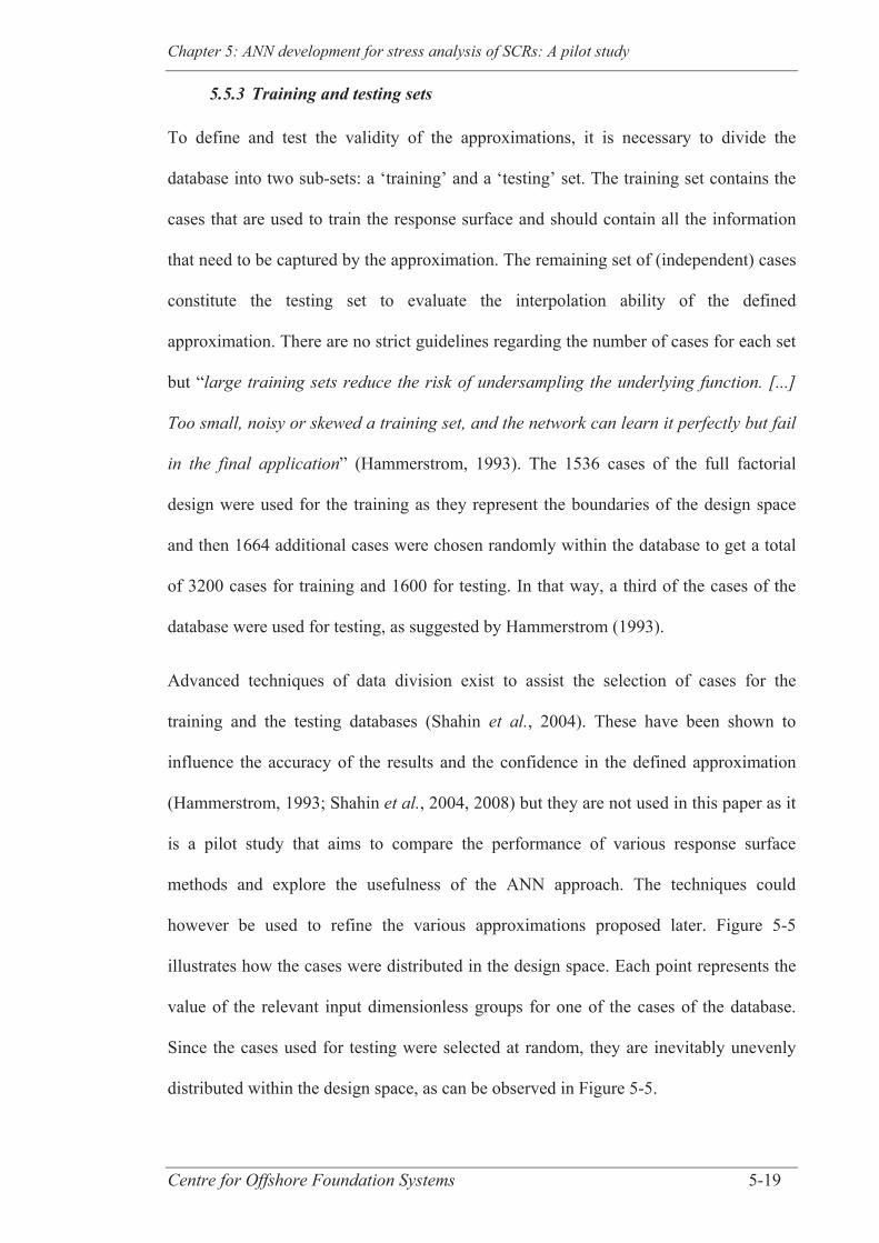
Chapter 5: ANN development for stress analysis of SCRs: A pilot study
Centre for Offshore Foundation Systems 5-19
5.5.3 Training and testing sets
To define and test the validity of the approximations, it is necessary to divide the
database into two sub-sets: a ‘training’ and a ‘testing’ set. The training set contains the
cases that are used to train the response surface and should contain all the information
that need to be captured by the approximation. The remaining set of (independent) cases
constitute the testing set to evaluate the interpolation ability of the defined
approximation. There are no strict guidelines regarding the number of cases for each set
but “large training sets reduce the risk of undersampling the underlying function. [...]
Too small, noisy or skewed a training set, and the network can learn it perfectly but fail
in the final application” (Hammerstrom, 1993). The 1536 cases of the full factorial
design were used for the training as they represent the boundaries of the design space
and then 1664 additional cases were chosen randomly within the database to get a total
of 3200 cases for training and 1600 for testing. In that way, a third of the cases of the
database were used for testing, as suggested by Hammerstrom (1993).
Advanced techniques of data division exist to assist the selection of cases for the
training and the testing databases (Shahin et al., 2004). These have been shown to
influence the accuracy of the results and the confidence in the defined approximation
(Hammerstrom, 1993; Shahin et al., 2004, 2008) but they are not used in this paper as it
is a pilot study that aims to compare the performance of various response surface
methods and explore the usefulness of the ANN approach. The techniques could
however be used to refine the various approximations proposed later. Figure 5-5
illustrates how the cases were distributed in the design space. Each point represents the
value of the relevant input dimensionless groups for one of the cases of the database.
Since the cases used for testing were selected at random, they are inevitably unevenly
distributed within the design space, as can be observed in Figure 5-5.
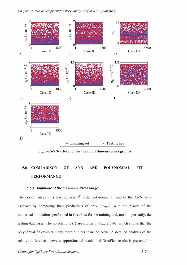
Chapter 5: ANN development for stress analysis of SCRs: A pilot study
Centre for Offshore Foundation Systems 5-20
Figure 5-5 Scatter plot for the input dimensionless groups
5.6 COMPARISON OF ANN AND POLYNOMIAL FIT
PERFORMANCE
5.6.1 Amplitude of the maximum stress range
The performances of a least squares 7th order polynomial fit and of the ANN were
assessed by comparing their predictions of Max TDZ/E with the results of the
numerical simulations performed in OrcaFlex for the training and, most importantly, the
testing databases. The correlations (r) are shown in Figure 5-6a, which shows that the
polynomial fit exhibits many more outliers than the ANN. A detailed analysis of the
relative differences between approximated results and OrcaFlex results is presented in
Chapter 5: ANN development for stress analysis of SCRs: A pilot study
Centre for Offshore Foundation Systems 5-21
Table 5-4a. Lower root mean squared errors (RMSE) and mean absolute errors (MAE)
are found with the ANN than with the polynomial fit. Also, the range of relative
differences is much smaller when using the ANN. With the current ANN
approximation, 76% of the cases of the training set have a negligible relative difference
(i.e. within 5% error (Lenci and Callegari, 2005)) and 93% for the testing set against
73% and 66% for the training and testing set respectively using the polynomial fit.
These results reflect the strong ability of the ANN to learn from the data used for
training, which is a further indication of the superior performance offered by this
approach over the polynomial fit approach. It also shows that the ANN approach seems
well suited for pursuing the definition of an approximation of Max TDZ/E. More work
could however be carried out to improve the accuracy of the current approximation in
order to use it reliably in place of numerical analysis for the early stages of design. A
power law fit was also examined but it led to poorer correlations (r) than a polynomial
fit between approximated and OrcaFlex results for the training and the testing sets (with
1- r ~ 1E-2) and so is not reported here.
5.6.2 Location of the maximum stress range
An approximation of the normalised location of the node exhibiting the maximum
fatigue damage in the TDZ (Sn_critical) is explored first and an approximation of the arc
length to TDP (St) is developed subsequently to ensure that an approximation of the
critical location can be back calculated. It is common practice to use the following
simple catenary equation to predict the value of St, with St = z cos HO /(1 - sin HO).
However, this relationship ignores the soil stiffness as well as the bending stiffness of
the riser, both of which were shown to influence the results in a small zone near the
seabed (referred to as the boundary layer (Pesce et al., 1998a ; Lenci and Callegari,
2005)). It is therefore useful to develop an approximation to predict the value of St.

Chapter 5: ANN development for stress analysis of SCRs: A pilot study
Centre for Offshore Foundation Systems 5-22
In a similar manner as for Max TDZ/E, the correlation between OrcaFlex results and
the polynomial and the ANN approximations are shown in Figure 5-6b for Sn_critical and
Figure 5-6c for St with more details in Table 5-4b,c. Even though the ANN exhibits
some outliers for Sn_critical, the results for the testing set clearly indicate that its
interpolation abilities outperform the polynomial fit. Relative differences on the
prediction of Sn_critical are relatively small even when using the polynomial fit but it is
important to notice that due to the scale of Sn_critical , differences of the order 4% can
represent an error of more than 1000 m when back calculating the final predicted value
of the critical fatigue location (Scritical), measured from the HOP as convenient from a
design perspective. When using the ANN approximation, the maximum absolute
relative difference that was found represents an error of roughly 30 m and therefore it
may also need further refinement.
Even if the polynomial fit approximates well the values of St for the cases used for
training, it is not able to offer a reasonable approximation for the cases used for testing.
For instance, as seen in Figure 5-6c1, it can lead to (unrealistic) negative estimates of St.
The ANN offers consistently good performances for training and testing sets. The
performance of the catenary equation is also tested for the entire database and, as
expected, it provides a close match with OrcaFlex results, although the ANN
approximation outperforms the simple catenary equation.
The three ANNs developed to evaluate approximations of Max TDZ/E, St and Sn_critical
under the assumptions of the study (selected ranges and design criteria) have been
implemented in a MATLAB code that can be supplied as a standalone application by
contacting the corresponding author. However, the aim of the application is to illustrate
the work performed in this paper and, it does not have sufficient accuracy to be used in
place of numerical or advanced analytical analysis at this stage. Future work will refine
the ANN algorithm further to allow direct application for estimation of fatigue damage.
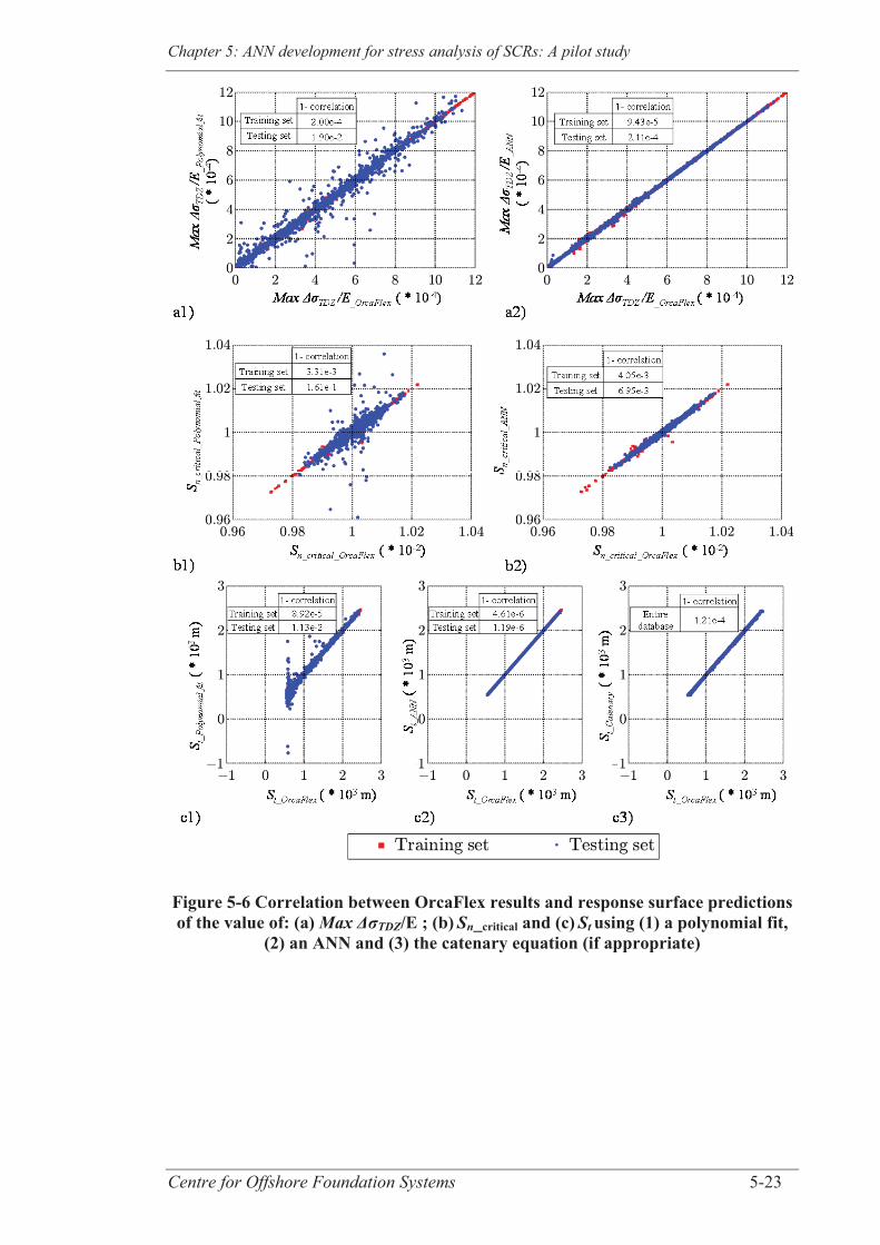
Chapter 5: ANN development for stress analysis of SCRs: A pilot study
Centre for Offshore Foundation Systems 5-23
Figure 5-6 Correlation between OrcaFlex results and response surface predictions of the value of: (a) Max ΔσTDZ/E ; (b) Sn_critical and (c) St using (1) a polynomial fit,
(2) an ANN and (3) the catenary equation (if appropriate)
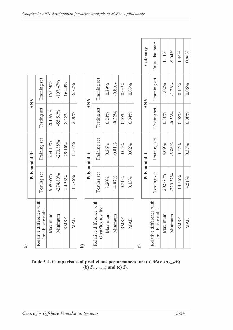
Chapter 5: ANN development for stress analysis of SCRs: A pilot study
Centre for Offshore Foundation Systems 5-24
Cat
enar
y
Entir
e da
taba
se
1.11
%
-9.0
4%
1.44
%
0.96
%
AN
N Tr
aini
ng se
t
153.
50%
-1
07.4
7%
16.4
4%
6.82
%
AN
N Tr
aini
ng se
t
0.39
%
-0.8
0%
0.04
%
0.03
%
AN
N Tr
aini
ng se
t
1.02
%
-1.2
6%
0.11
%
0.06
%
Test
ing
set
201.
99%
-5
5.51
%
8.18
%
2.00
%
Test
ing
set
0.24
%
-0.2
2%
0.05
%
0.04
%
Test
ing
set
0.36
%
-0.3
3%
0.08
%
0.06
%
Poly
nom
ial f
it
Trai
ning
set
234.
17%
-2
70.8
8%
29.1
0%
11.6
4%
Poly
nom
ial f
it
Trai
ning
set
0.36
%
-0.8
1%
0.04
%
0.02
%
Po
lyno
mia
l fit
Trai
ning
set
4.69
%
-3.8
6%
0.57
%
0.37
%
Test
ing
set
969.
65%
-2
74.8
0%
44.3
8%
11.8
6%
Test
ing
set
3.20
%
-4.0
7%
0.21
%
0.13
%
Test
ing
set
202.
61%
-2
29.3
2%
13.5
6%
4.51
%
a) Rel
ativ
e di
ffer
ence
with
O
rcaF
lex
resu
lts:
Max
imum
M
inim
um
RM
SE
MA
E
b) Rel
ativ
e di
ffer
ence
with
O
rcaF
lex
resu
lts:
Max
imum
M
inim
um
RM
SE
MA
E
c) Rel
ativ
e di
ffer
ence
with
O
rcaF
lex
resu
lts:
Max
imum
M
inim
um
RM
SE
MA
E
Table 5-4. Comparisons of predictions performances for: (a) Max ΔσTDZ/E; (b) Sn_critical; and (c) St.
Chapter 5: ANN development for stress analysis of SCRs: A pilot study
Centre for Offshore Foundation Systems 5-25
5.7 CONCLUSIONS
A numerical study aiming to explore the usefulness of the design of experiment
techniques and the artificial neural network approach for SCR design was conducted in
this paper using a database of 4800 SCR configurations under static loading. An in-
house sub-routine linking OrcaFlex software with the optimisation software
ModeFRONTIER was developed in this regard. Overall, using the proposed database
with 1536 cases selected through a full factorial design and an additional 3264 cases
chosen at random, it was found that the ANN approach is well suited for prediction of
the amplitude of the peak stress range and its location and greatly outperforms the
traditional polynomial fit approach. The proposed approximation of Max TDZ/E using
the ANN approach does however need further refinement to reduce the range of relative
differences with OrcaFlex results. An ANN was also developed to predict the value of
the arc length to TDP and was also found to offer better predictions than the usual
simple catenary equation, with [-1%; +1%] and ~[-9%;+1%] relative differences from
OrcaFlex results for the ANN and for the catenary equation respectively.
Future work will aim to verify that a higher level of accuracy can be reached using the
proposed framework, by exploring the effects on overall performance of a larger
database and the use of more advanced techniques of data division for the choice of the
cases constituting the training and testing sets. Ultimately, the proposed framework
should be extended to dynamic perturbations of SCRs in order to test out its suitability
in simplifying the preliminary fatigue design of SCRs in the TDZ.

Estimating the fatigue damage of SCRs in the TDZ
Centre for Offshore Foundation Systems 6-1
CHAPTER 6 ARTIFICIAL NEURAL NETWORK DEVELOPMENT
FOR STRESS ANALYSIS OF STEEL CATENARY RISERS:
SENSITIVITY STUDY AND APPROXIMATION OF STATIC
STRESS RANGE
6.1 ABSTRACT
Fatigue design of steel catenary risers (SCRs) is an important challenge especially in the
touchdown zone (TDZ). Numerous parameters affect the fatigue damage in the TDZ,
including those pertaining to riser motions, riser characteristics and soil properties. So
far, only a few sensitivity studies have been published with limited applications,
considering small ranges, investigating only a selection of input parameters or failing to
examine the interactions between input parameters.
This paper aims to test the robustness of previous research and extend the ranges of the
input parameters for SCR systems under static loading, by means of numerical
simulations. An approximation of the critical stress range in the TDZ defined by the
authors previously in Chapter 5 was refined to assist the sensitivity studies. A large
database was created using an automation subroutine coded in Python programming
language that links the marine analysis software OrcaFlex and the optimisation software
modeFRONTIER. Design of experiment techniques were used for post-processing and
quantify the relative effects of the various dimensionless groups and their interactions.
An approximation using a series of artificial neural networks is presented; it
successfully approximates over 99% of the cases of the database with an accuracy of
5%.
Chapter 6: ANN development for stress analysis of SCRs: Sensitivity...
Centre for Offshore Foundation Systems 6-2
6.2 INTRODUCTION
Fatigue damage of steel catenary risers (SCR) is influenced by a large number of
parameters, rendering SCR fatigue design a challenging task, particularly in the
touchdown (TDZ) - the area of dynamic riser-soil interaction (Bridge, 2005). Previous
parametric studies have investigated the individual effects of some of these parameters,
such as the effect of the hang-off angle, the inside diameter and the wall thickness (Xia
et al., 2008), the effect of the soil parameters when using a nonlinear soil model (Shiri
and Randolph, 2010; Kimiaei et al., 2010; Elosta et al., 2013a) or the effect of the
loading parameters (Kimiaei et al., 2010). The individual effects of the dimensionless
groups that were shown to influence the fatigue damage in SCRs (Quéau et al., 2013)
were also examined (Quéau et al., 2014a). These studies used the one-factor-at-a-time
approach where only one of the input parameters is varied and the other input
parameters are fixed to arbitrary values. This approach can however lead to
misinterpretation of the results by failing to capture the potential effects of interactions
between input parameters (“an interaction occurs when two or more factors acting
together have a different effect on the quality characteristic than the effect of each
factor acting individually” Peace, 1993). The robustness of previous published results
should therefore be tested and the ranges of some of the input parameters extended. The
work reported here is consistent with advice in riser design guidelines (DNV-OS-F201,
2010) to investigate the influence of different parameters, particularly where their value
is uncertain. A more quantitative understanding of the effects of input parameters on the
maximum stress range will assist the use and refinement of current numerical models
and consequently will improve confidence in SCR fatigue design.
Fatigue damage in the touchdown zone arises due to the variation of axial stress under
cycles of imposed motion, resulting mainly from the action of waves on the floating
facility. The fatigue life in the TDZ is controlled by the maximum stress range
Chapter 6: ANN development for stress analysis of SCRs: Sensitivity...
Centre for Offshore Foundation Systems 6-3
(Max TDZ) occurring there for a given motion, accounting for the number of cycles,
and evaluating the cumulative fatigue damage over the full range of motion. For this
reason, one of the objectives of this paper is to evaluate the relative effects of the input
dimensionless groups and their interactions on the variation of Max TDZ, considering
large ranges of the relevant groups. The key dimensionless groups for fatigue design of
SCRs are selected as the inputs for the sensitivity studies rather than the individual input
parameters to enhance the applicability of this research (Pesce et al., 1998b; Palmer,
2008b; Quéau et al., 2013).
The main purpose of this paper, however, is to develop an efficient method able to
approximate the maximum stress range in the TDZ in order to assist sensitivity studies.
A pilot study describe in Chapter 5 aimed to determine what model of response surface
was best suited for SCR fatigue design and demonstrated the usefulness of the artificial
neural network (ANN) approach. In this paper, the response surface method (RSM)
using the ANN approach is applied to refine the approximation of the maximum stress
range in the TDZ normalised by the Young’s Modulus (Max TDZ/E as defined in
Chapter 5) and achieve a reasonable level of accuracy, defined here as a relative
difference of 15% between the ANN predictions and the results from OrcaFlex
(Orcina, 2012) simulations over the entire selected ranges of the input dimensionless
groups. For this purpose, additional cases (i.e. particular combinations of SCR
configuration and loading condition) were added to the original database of 4800 cases
developed in Chapter 5 using the same in-house subroutine to automate pre-processing,
running and post-processing of the numerical models.
In total, 57,023 cases were used with the aim of representing the majority of realistic
SCR configurations and static loading conditions. Such a large database was developed
to increase the chances of capturing all underlying interactions between the
dimensionless groups. Also, the training and testing sets were selected using an
Chapter 6: ANN development for stress analysis of SCRs: Sensitivity...
Centre for Offshore Foundation Systems 6-4
improved technique that leads to similar statistical properties between the two sets of
cases. This ensures that the testing set gives a reliable representation of the training set
(assuming the training set itself is a reliable representation of the design space) in order
to test the accuracy of the approximation within the entire design space. Once a suitable
approximation was achieved, it was used to obtain a series of design charts.
This study is currently limited to static loading only (no inertia or damping effects),
although it forms part of ongoing research aiming to simplify fatigue design of SCRs in
the conceptual and basic design stages by using dynamic amplification factors (DAFs)
to quantify the dynamic response in the TDZ relative to the static response (Quéau et
al., 2011). Future work will extend the ANN approach directly to dynamic conditions,
accounting for hydrodynamic and inertia effects as longitudinal and transverse waves
travel along the riser. The study is limited to the SCR response under in-plane motions
only with the motions applied by imposing a displacement to the floating vessel. The
current profile in the sea column, rotational stiffness at the hang-off point, flow rate of
the contents, pipe coating and structural damping are not taken into account. A
summary of the dimensionless group definitions and their physical definitions is shown
in Table 6-1 while an illustration of the key parameters is shown in Figure 6-1. Since
the study is limited to static loading, the dimensionless groups presented in Quéau et al.
(2013) related to the velocity of imposed motion, time within a cycle of applied motion
or to the hydrodynamic coefficients (as current is also neglected) are not relevant here.
The ranges for the individual input parameters along with relevant design criteria are
summarised in Table 6-2, with the resulting ranges for the dimensionless groups given
in Table 6-3). Gravity acceleration (g = 9.81 m/s2), Young’s Modulus for the SCR
(E = 2.12E8 kPa), water density ( water = 1.025 te/m3) and steel density
( steel = 7.85 te/m3) remain unchanged in the study.
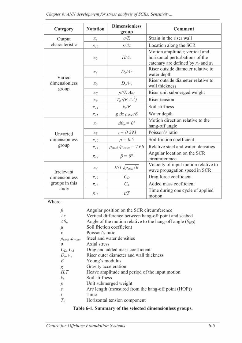
Chapter 6: ANN development for stress analysis of SCRs: Sensitivity...
Centre for Offshore Foundation Systems 6-5
Category Notation Dimensionless group Comment
Output characteristic
1 /E Strain in the riser wall 16 s/ z Location along the SCR
Varied dimensionless
group
2 H/ z Motion amplitude; vertical and horizontal perturbations of the catenary are defined by 2 and 3
5 Do/ z Riser outside diameter relative to water depth
6 Do/wt Riser outside diameter relative to wall thickness
7 p/(E z) Riser unit submerged weight 9 To /(E z2) Riser tension
11 ks/E Soil stiffness 15 g z steel/E Water depth
Unvaried dimensionless
group
3 m = 0° Motion direction relative to the hang-off angle
8 = 0.293 Poisson’s ratio 10 = 0.5 Soil friction coefficient 14 steel / water = 7.66 Relative steel and water densities
17 = 0° Angular location on the SCR circumference
Irrelevant dimensionless groups in this
study
4 ETH steel Velocity of input motion relative to wave propagation speed in SCR
12 CD Drag force coefficient 13 CA Added mass coefficient
18 t/T Time during one cycle of applied motion
Where:
Angular position on the SCR circumference z Vertical difference between hang-off point and seabed
m Angle of the motion relative to the hang-off angle ( HO) Soil friction coefficient Poisson’s ratio steel , water Steel and water densities Axial stress
CD, CA Drag and added mass coefficient Do, wt Riser outer diameter and wall thickness E Young’s modulus g Gravity acceleration H,T Heave amplitude and period of the input motion ks Soil stiffness p Unit submerged weight s Arc length (measured from the hang-off point (HOP)) t Time To Horizontal tension component
Table 6-1. Summary of the selected dimensionless groups.
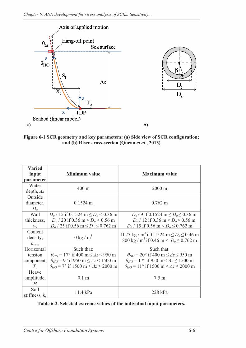
Chapter 6: ANN development for stress analysis of SCRs: Sensitivity...
Centre for Offshore Foundation Systems 6-6
Figure 6-1 SCR geometry and key parameters: (a) Side view of SCR configuration; and (b) Riser cross-section (Quéau et al., 2013)
Varied input
parameter Minimum value Maximum value
Water depth, z 400 m 2000 m
Outside diameter,
Do 0.1524 m 0.762 m
Wall thickness,
wt
Do / 15 if 0.1524 m ≤ Do < 0.36 mDo / 20 if 0.36 m ≤ Do < 0.56 m Do / 25 if 0.56 m ≤ Do ≤ 0.762 m
Do / 9 if 0.1524 m ≤ Do ≤ 0.36 m Do / 12 if 0.36 m < Do ≤ 0.56 m
Do / 15 if 0.56 m < Do ≤ 0.762 m Content density,
cont 0 kg / m3 1025 kg / m3 if 0.1524 m ≤ Do ≤ 0.46 m
800 kg / m3 if 0.46 m < Do ≤ 0.762 m
Horizontal tension
component, To
Such that: HO = 17° if 400 m ≤ z < 950 m HO = 9° if 950 m ≤ z < 1500 m
HO = 7° if 1500 m ≤ z ≤ 2000 m
Such that: HO = 20° if 400 m ≤ z ≤ 950 m
HO = 17° if 950 m < z ≤ 1500 m HO = 11° if 1500 m < z ≤ 2000 m
Heave amplitude,
H 0.1 m 7.5 m
Soil stiffness, ks
11.4 kPa 228 kPa
Table 6-2. Selected extreme values of the individual input parameters.
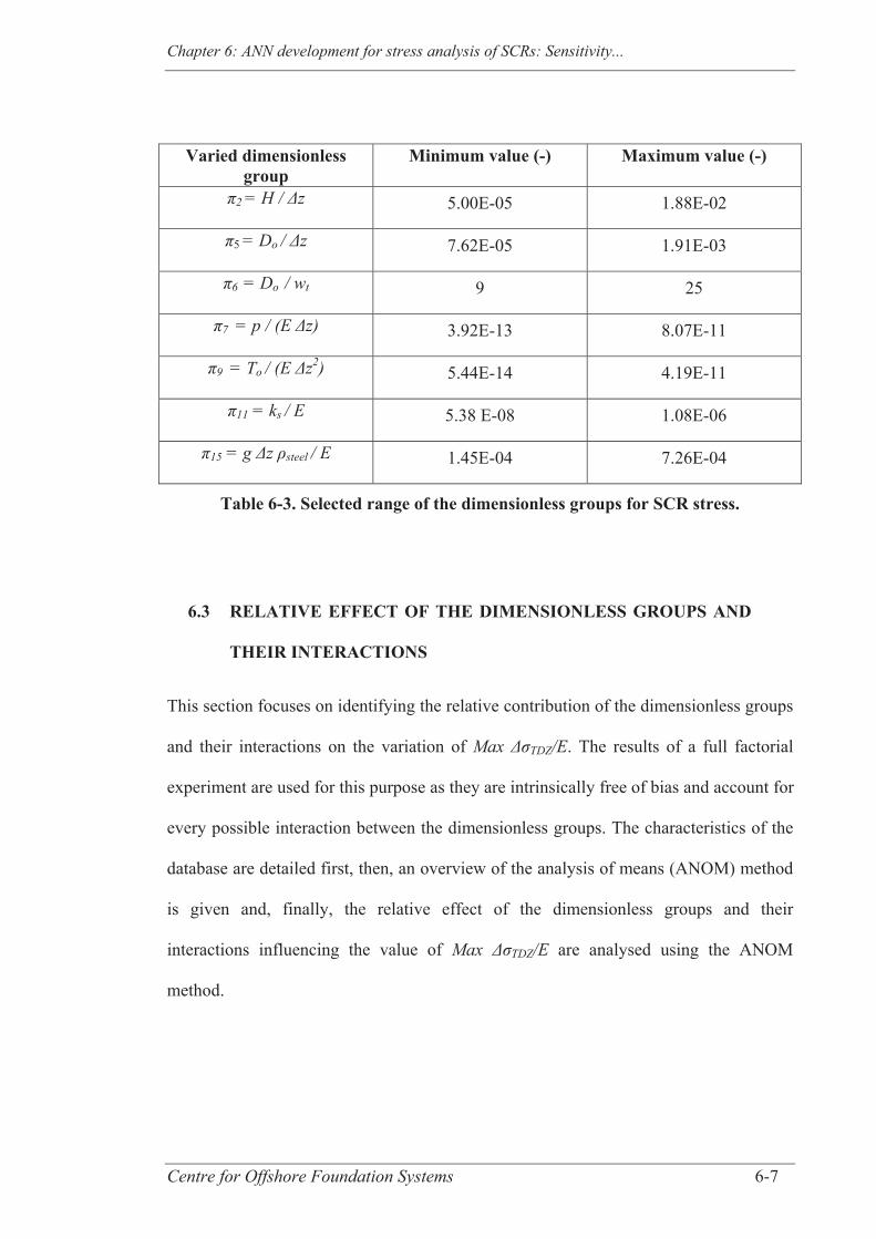
Chapter 6: ANN development for stress analysis of SCRs: Sensitivity...
Centre for Offshore Foundation Systems 6-7
Varied dimensionless group
Minimum value (-) Maximum value (-)
2 = H / z 5.00E-05 1.88E-02
5 = Do / z 7.62E-05 1.91E-03
6 = Do / wt 9 25
7 = p / (E z) 3.92E-13 8.07E-11
9 = To / (E z2) 5.44E-14 4.19E-11
11 = ks / E 5.38 E-08 1.08E-06
15 = g z steel / E 1.45E-04 7.26E-04
Table 6-3. Selected range of the dimensionless groups for SCR stress.
6.3 RELATIVE EFFECT OF THE DIMENSIONLESS GROUPS AND
THEIR INTERACTIONS
This section focuses on identifying the relative contribution of the dimensionless groups
and their interactions on the variation of Max TDZ/E. The results of a full factorial
experiment are used for this purpose as they are intrinsically free of bias and account for
every possible interaction between the dimensionless groups. The characteristics of the
database are detailed first, then, an overview of the analysis of means (ANOM) method
is given and, finally, the relative effect of the dimensionless groups and their
interactions influencing the value of Max TDZ/E are analysed using the ANOM
method.

Chapter 6: ANN development for stress analysis of SCRs: Sensitivity...
Centre for Offshore Foundation Systems 6-8
6.3.1 Database characteristics
A set of 1536 cases, based on a full factorial design to capture the boundaries of the
design space (Chapter 5) are used to study the relative effect of the dimensionless
groups on Max TDZ/E. These cases correspond to the following levels of the input
parameters (i.e. level – choice of value), with the superscript ± referring to the fact that
values of those input parameters on each side of the extremities of the ranges involved
in the design criteria (Table 6-2) were tested for the various possible ranges of the
dependent parameters (for instance z = 1500 m was tested with values of HO
corresponding to the intervals relevant to both z just less than 1500 m (9° ≤ HO ≤ 17°)
for and z just greater than 1500 m (7° ≤ HO ≤ 11°)):
z: 6 levels selected: 400 m; 950± m; 1500± m; and 2000 m.
Do: 8 levels selected: 0.1524 m; 0.36± m; 0.46± m; 0.56± m and 0.762 m.
6 = Do / wt : two levels selected: appropriate minimum and maximum values
with respect to the value of Do.
cont: two levels selected: empty and full with appropriate content density value
with respect to the value of Do.
To: two levels selected: appropriate minimum and maximum values determined
through the value of HO with respect to the value of z.
H: two levels selected: 0.1 m and 7.5 m.
ks: two levels selected: 11.4 kPa and 228 kPa.
These choices lead to six levels for 15, eight levels for 5 and two levels for 2, 6, 7,
9 and 11 and hence the 1536 cases; (the levels are referred to as Level i with i = 1,..., n
and n = 2, 6 or 8 as appropriate). The levels of the dimensionless groups were
determined using the sliding level technique (e.g. Peace, 1993) with the level of some of
the dimensionless groups linked to the level of others (for instance, the two levels of 2
were: Level 1 = 0.1/ z and Level 2 = 7.5/ z for the selected z value).

Chapter 6: ANN development for stress analysis of SCRs: Sensitivity...
Centre for Offshore Foundation Systems 6-9
6.3.2 The analysis of means (ANOM) method
The ANOM method is a technique of data analysis that can be used when the output is
“a continuously measurable variable” (Peace, 1993). It is applied to clarify the relative
effects of the factors (the input dimensionless groups here) and their interactions but
also to establish the combination of factors that should lead to the targeted results, for
instance minimising Max TDZ/E in this study (Peace, 1993; Fowlkes and Crevelling,
1995).
For convenience, the method is illustrated for a simple example analysing the variation
of an output Y which is a function of two factors, say A and B, having two levels each
(NLevel_A = NLevel_B = 2). Their interaction is referred to as A x B and its levels (LevelA x B)
are determined based on the levels of A and B (LevelA and LevelB ) from
LevelA x B = Max (NLevel_A , NLevel_B)
- mod Max (NLevel_A , NLevel_B) (LevelA + LevelB) (6-1)
The ANOM method relies on the calculation of the average value of the output for the
various selected levels of the factors and their interactions. Once these average values
have been calculated, the effects representing the variation between the maximum and
minimum average results found for the various levels can be deduced; those are then
used to rank the factors and interactions. Results are usually summarised in a response
table as per Table 6-4. They can also be represented graphically, as shown in Figure 6-2
using the notations introduced in Table 6-4 and where Y ¯ is the overall average value of
the output. Comparison of the gradients indicates the relative importance of the
contribution of the factors and interactions in the variation of the output when using the
graphical representation (Peace, 1993).
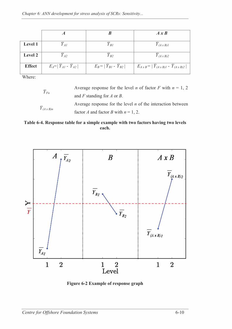
Chapter 6: ANN development for stress analysis of SCRs: Sensitivity...
Centre for Offshore Foundation Systems 6-10
A B A x B
Level 1 Y ¯A1 Y ¯B1 Y ¯(A x B)1
Level 2 Y ¯A2 Y ¯B2 Y ¯(A x B)2
Effect EA=|Y ¯A1 - Y ¯A2 | EB = |Y ¯B1 - Y ¯B2 | EA x B = |Y ¯(A x B)1 - Y ¯(A x B)2 |
Where:
Y ¯FnAverage response for the level n of factor F with n = 1, 2
and F standing for A or B.
Y ¯(A x B)nAverage response for the level n of the interaction between
factor A and factor B with n = 1, 2.
Table 6-4. Response table for a simple example with two factors having two levels each.
Figure 6-2 Example of response graph
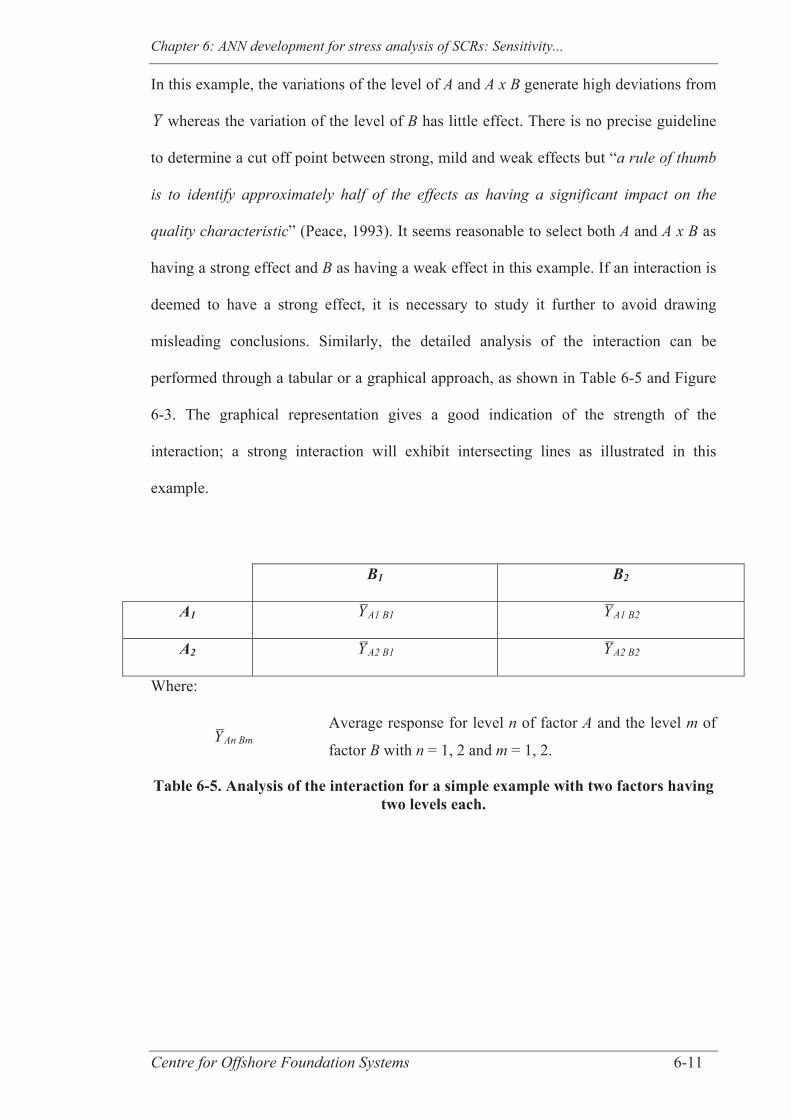
Chapter 6: ANN development for stress analysis of SCRs: Sensitivity...
Centre for Offshore Foundation Systems 6-11
In this example, the variations of the level of A and A x B generate high deviations from
Y ¯ whereas the variation of the level of B has little effect. There is no precise guideline
to determine a cut off point between strong, mild and weak effects but “a rule of thumb
is to identify approximately half of the effects as having a significant impact on the
quality characteristic” (Peace, 1993). It seems reasonable to select both A and A x B as
having a strong effect and B as having a weak effect in this example. If an interaction is
deemed to have a strong effect, it is necessary to study it further to avoid drawing
misleading conclusions. Similarly, the detailed analysis of the interaction can be
performed through a tabular or a graphical approach, as shown in Table 6-5 and Figure
6-3. The graphical representation gives a good indication of the strength of the
interaction; a strong interaction will exhibit intersecting lines as illustrated in this
example.
B1 B2
A1 Y ¯A1 B1 Y ¯A1 B2
A2 Y ¯A2 B1 Y ¯A2 B2
Where:
Y ¯An BmAverage response for level n of factor A and the level m of
factor B with n = 1, 2 and m = 1, 2.
Table 6-5. Analysis of the interaction for a simple example with two factors having two levels each.

Chapter 6: ANN development for stress analysis of SCRs: Sensitivity...
Centre for Offshore Foundation Systems 6-12
Figure 6-3 Example of interaction graph
At this point, it is possible to judge what level of the factors would give the best targeted
results. For instance, if the aim is to minimise the value of Y, it is expected that
choosing Level 1 for A and Level 1 for B will give the best results. The choice of level
for A is determined first as A was shown to have the greatest effect on the variations of
Y in Table 6-4 and Figure 6-2 whereas it is necessary to account for the detailed analysis
of the interaction to select the best level for B. Indeed, it is seen that if the interaction
was neglected in this study, Figure 6-2 would indicate that B should be set to Level 2 in
order to minimise the results. However, it is seen in Figure 6-3 that providing that Level
1 is selected for A, then it is better to select Level 1 for B too. This simple example
illustrates the potential issues that may arise if interactions are neglected (Peace, 1993).
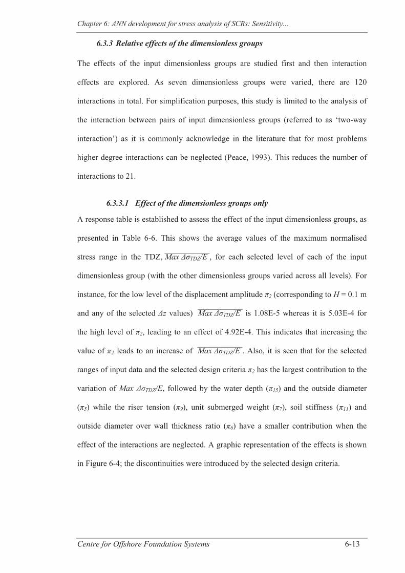
Chapter 6: ANN development for stress analysis of SCRs: Sensitivity...
Centre for Offshore Foundation Systems 6-13
6.3.3 Relative effects of the dimensionless groups
The effects of the input dimensionless groups are studied first and then interaction
effects are explored. As seven dimensionless groups were varied, there are 120
interactions in total. For simplification purposes, this study is limited to the analysis of
the interaction between pairs of input dimensionless groups (referred to as ‘two-way
interaction’) as it is commonly acknowledge in the literature that for most problems
higher degree interactions can be neglected (Peace, 1993). This reduces the number of
interactions to 21.
6.3.3.1 Effect of the dimensionless groups only
A response table is established to assess the effect of the input dimensionless groups, as
presented in Table 6-6. This shows the average values of the maximum normalised
stress range in the TDZ, Max TDZ/E ¯¯¯¯¯¯¯¯¯¯¯, for each selected level of each of the input
dimensionless group (with the other dimensionless groups varied across all levels). For
instance, for the low level of the displacement amplitude 2 (corresponding to H = 0.1 m
and any of the selected z values) Max TDZ/E ¯¯¯¯¯¯¯¯¯¯¯ is 1.08E-5 whereas it is 5.03E-4 for
the high level of 2, leading to an effect of 4.92E-4. This indicates that increasing the
value of 2 leads to an increase of Max TDZ/E ¯¯¯¯¯¯¯¯¯¯¯. Also, it is seen that for the selected
ranges of input data and the selected design criteria 2 has the largest contribution to the
variation of Max TDZ/E, followed by the water depth ( 15) and the outside diameter
( 5) while the riser tension ( 9), unit submerged weight ( 7), soil stiffness ( 11) and
outside diameter over wall thickness ratio ( 6) have a smaller contribution when the
effect of the interactions are neglected. A graphic representation of the effects is shown
in Figure 6-4; the discontinuities were introduced by the selected design criteria.
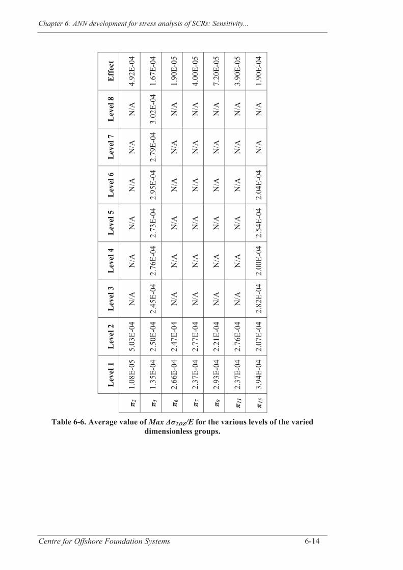
Chapter 6: ANN development for stress analysis of SCRs: Sensitivity...
Centre for Offshore Foundation Systems 6-14
Eff
ect
4.92
E-04
1.67
E-04
1.90
E-05
4.00
E-05
7.20
E-05
3.90
E-05
1.90
E-04
Lev
el 8
N/A
3.02
E-04
N/A
N/A
N/A
N/A
N/A
Lev
el 7
N/A
2.79
E-04
N/A
N/A
N/A
N/A
N/A
Lev
el 6
N/A
2.95
E-04
N/A
N/A
N/A
N/A
2.04
E-04
Lev
el 5
N/A
2.73
E-04
N/A
N/A
N/A
N/A
2.54
E-04
Lev
el 4
N/A
2.76
E-04
N/A
N/A
N/A
N/A
2.00
E-04
Lev
el 3
N/A
2.45
E-04
N/A
N/A
N/A
N/A
2.82
E-04
Lev
el 2
5.03
E-04
2.50
E-04
2.47
E-04
2.77
E-04
2.21
E-04
2.76
E-04
2.07
E-04
Lev
el 1
1.08
E-05
1.35
E-04
2.66
E-04
2.37
E-04
2.93
E-04
2.37
E-04
3.94
E-04
π 2
π 5
π 6
π 7
π 9
π 11
π 15
Table 6-6. Average value of Max ΔσTDZ/E for the various levels of the varied dimensionless groups.

Chapter 6: ANN development for stress analysis of SCRs: Sensitivity...
Centre for Offshore Foundation Systems 6-15
Figure 6-4 Effect of the dimensionless groups
Although some input parameters are project specific, it is concluded that the following
actions, whenever possible, will tend to decrease Max TDZ/E (listed in order of
importance):
- decrease of 2 (reflecting the amplitude of motion) as expected under static
loading since it reduces the variations of curvature in the TDZ;
- increase of the water depth ( 15), which is consistent with Mekha (2001) who
stated that “in deeper water, the heave motion of a floating support structure
will have less detrimental fatigue effect on the SCRs”;
- decrease of the outside diameter ( 5);
- increase of the riser tension ( 9) as it reduces the curvature variation in the TDZ;
- decrease of the riser unit submerged weight ( 7) as it reduces the curvature
variation in the TDZ;

Chapter 6: ANN development for stress analysis of SCRs: Sensitivity...
Centre for Offshore Foundation Systems 6-16
- decrease of the soil stiffness ( 11), since it reduced the maximum shear force
hence the change in bending moment in the TFZ - a well established result:
e.g. Bridge et al., (2004);
- increase of the ratio of outside diameter over wall thickness ( 6) (although the
contribution of 6 seems to be minor).
The results for 5, 6 and 15 differ from those presented by Quéau et al. (2014a) where
it was concluded that an individual increase of 5 and an individual decrease of 6 will
decrease Max TDZ/E and that Max TDZ/E was insensitive to the individual variations
of 15. This highlights the importance of the method selected to perform the sensitivity
analysis. Indeed, Quéau et al. (2014a) used a one-factor-at-a-time approach and
therefore only varied one of the dimensionless groups while the others were kept
unchanged (by appropriately adjusting the individual input parameters). The nuance in
that approach is that results are limited to the particular selected values and to the
individual variations. By contrast, the work conducted in this paper uses a more robust
approach as the effect of each dimensionless group is assessed through various
combinations of the other dimensionless groups. The trend of the results, tested on
many more combinations, is consequently much more generalisable and less likely to be
specific to a particular region of the design space. However, the effect of the two-way
interactions is now investigated to avoid any misinterpretations; as Martins et al. (2013)
mentioned, “it is necessary to evaluate the interaction effect between design variables
before any conclusion is taken”.
6.3.3.2 Effect of the dimensionless groups and their interactions
The effects of the two-way interactions were determined, as presented in Table 6-7.
Input dimensionless groups and their two-way interactions are ranked based on the
value of their effects (see Figure 6-5). It is seen that 2 and 15 still have a major
contribution but a strong interaction is detected between them, as well as between 2 and
Chapter 6: ANN development for stress analysis of SCRs: Sensitivity...
Centre for Offshore Foundation Systems 6-17
5, 5 and 11 etc. ... Following the rule of thumb of selecting roughly half of the effects
as significant parameters and based on the marked drop in the effect values between 2 x
9 and 7, it was decided to choose 2 x 9 as the dividing point. A more detailed
analysis of the strong interactions was then performed.
In a similar manner than for the effects of the dimensionless groups, the average values
of Max TDZ/E for every combination of levels for each selected pair of dimensionless
groups were calculated, as presented in Table 6-8. For example, Max TDZ/E ¯¯¯¯¯¯¯¯¯¯¯ in cases
where 2 and 15 are both at their lowest level is 1.78e-5. An illustration of the results is
shown in Figure 6-6. Normalised coordinates are established for convenience by
dividing the results for each level (Lj) of one of the dimensionless groups (say q) by the
minimum value of Max TDZ/E ¯¯¯¯¯¯¯¯¯¯¯ found amongst all levels (Li) of that group for the
given level of the other dimensionless group (say p) of the interaction under
consideration, noted Min p qLj with p, q in {2, 5, 6, 7, 9, 11, 15} and i, j in {1, 2,..., 8}.
In that way all responses are tied to a minimum value unity and the use of similar scales
for the y-axis allows the strength of each interaction to be assessed visually.
Results are overall consistent with those of the study of the effects of the dimensionless
groups only, even though the observed reduction or increase of Max TDZ/E ¯¯¯¯¯¯¯¯¯¯¯
sometimes can be enhanced when two dimensionless group acts together. For instance,
an increase of 15 decreases Max TDZ/E ¯¯¯¯¯¯¯¯¯¯¯ and this decrease is even more important if
2 is low (Figure 6-6a) or 9 is high (Figure 6-6j); however, the rate of the decrease
seems unaffected by the level of 7, 11 or 6 (Figure 6-6g, h and i). Also, higher 9
leads to reduced Max TDZ/E ¯¯¯¯¯¯¯¯¯¯¯ and this effect is more pronounced if 2 is high (Figure
6-6k). Studying the two-way interactions revealed more complex behaviour regarding
the choice of 5. Indeed, it seems that increasing 5 will lead to an increase of
Max TDZ/E ¯¯¯¯¯¯¯¯¯¯¯ for high 2 values while it would eventually lead to a decrease of
Max TDZ/E ¯¯¯¯¯¯¯¯¯¯¯ for low 2 (Figure 6-6b). Care should therefore be taken when selecting
Chapter 6: ANN development for stress analysis of SCRs: Sensitivity...
Centre for Offshore Foundation Systems 6-18
the value of 5 and further studies may investigate where the threshold between these
different behaviours lies. In general though, an increase of 5 seems to contribute most
commonly towards an increase of Max TDZ/E ¯¯¯¯¯¯¯¯¯¯¯ and even more so if 11, 7 and 9 are
high and 6 are low (Figure 6-6c, e, f and d).
Based on these observations on the average values of the output, it would be expected to
achieve minimum and maximum values of Max TDZ/E for the levels of the input
dimensionless groups presented in Table 6-9, as was confirmed in the simulations.
These results give a greater understanding of SCR behaviour under static loading and
can assist designers although they are restricted by the following limitations: (i) they
were derived from the selected levels of the input dimensionless groups and therefore
they could fail to capture some potential non-linearity or effects that occur for levels
other than those selected; and (ii) they were established by investigating the average
values of the output Max TDZ/E (as per the DoE method) and hence local behaviours
might not be captured well. This is why more cases were added to the current database
and a response surface investigated over the entire selected ranges of the input
dimensionless group in the following section.
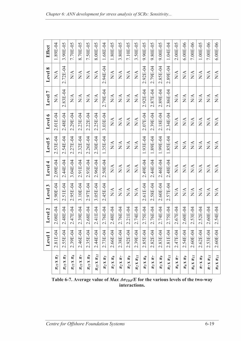
Chapter 6: ANN development for stress analysis of SCRs: Sensitivity...
Centre for Offshore Foundation Systems 6-19
Eff
ect
1.89
E-04
3.90
E-05
7.70
E-05
8.70
E-05
7.50
E-05
8.00
E-05
1.68
E-04
1.80
E-05
3.80
E-05
7.10
E-05
3.50
E-05
9.90
E-05
9.80
E-05
9.00
E-05
1.04
E-04
2.00
E-05
6.00
E-06
7.00
E-06
1.00
E-05
7.00
E-06
6.00
E-06
Lev
el 8
N
/A
2.72
E-04
N/A
N/A
N/A
N/A
2.94
E-04
N/A
N/A
N/A
N/A
2.92
E-04
2.79
E-04
2.85
E-04
2.89
E-04
N/A
N/A
N/A
N/A
N/A
N/A
Lev
el 7
N
/A
2.83
E-04
N/A
N/A
N/A
N/A
2.79
E-04
N/A
N/A
N/A
N/A
2.92
E-04
2.87
E-04
2.89
E-04
2.86
E-04
N/A
N/A
N/A
N/A
N/A
N/A
Lev
el 6
2.
01E-
04
2.48
E-04
2.29
E-04
2.23
E-04
2.22
E-04
2.25
E-04
3.03
E-04
N/A
N/A
N/A
N/A
2.07
E-04
2.39
E-04
2.18
E-04
2.34
E-04
N/A
N/A
N/A
N/A
N/A
N/A
Lev
el 5
2.
53E-
04
2.54
E-04
2.27
E-04
2.32
E-04
2.26
E-04
2.30
E-04
1.35
E-04
N/A
N/A
N/A
N/A
1.93
E-04
1.89
E-04
1.99
E-04
1.85
E-04
N/A
N/A
N/A
N/A
N/A
N/A
Lev
el 4
2.
09E-
04
2.44
E-04
3.04
E-04
2.91
E-04
2.93
E-04
2.96
E-04
2.50
E-04
N/A
N/A
N/A
N/A
2.49
E-04
2.44
E-04
2.46
E-04
2.48
E-04
N/A
N/A
N/A
N/A
N/A
N/A
Lev
el 3
3.
90E-
04
2.51
E-04
2.95
E-04
3.10
E-04
2.97
E-04
3.05
E-04
2.45
E-04
N/A
N/A
N/A
N/A
2.61
E-04
2.58
E-04
2.60
E-04
2.57
E-04
N/A
N/A
N/A
N/A
N/A
N/A
Lev
el 2
2.
08E-
04
2.48
E-04
2.47
E-04
2.39
E-04
2.68
E-04
2.41
E-04
2.76
E-04
2.48
E-04
2.76
E-04
2.21
E-04
2.74
E-04
2.75
E-04
2.76
E-04
2.74
E-04
2.75
E-04
2.67
E-04
2.60
E-04
2.53
E-04
2.52
E-04
2.60
E-04
2.54
E-04
Lev
el 1
2.
81E-
04
2.55
E-04
2.39
E-04
2.46
E-04
2.35
E-04
2.44
E-04
2.73
E-04
2.66
E-04
2.38
E-04
2.92
E-04
2.39
E-04
2.85
E-04
2.82
E-04
2.83
E-04
2.81
E-04
2.47
E-04
2.54
E-04
2.60
E-04
2.62
E-04
2.53
E-04
2.60
E-04
π 15 x
π 2
π 15 x
π 5
π 15 x
π 6
π 15 x
π 7
π 15 x
π 9
π 15
x π 1
1
π 2 x
π5
π 2 x
π6
π 2 x
π7
π 2 x
π9
π 2 x
π11
π 5
x π
6 π 5
x π
7 π 5
x π
9 π 5
x π
11
π 6 x
π7
π 6 x
π9
π 6 x
π11
π 7
x π
9 π 7
x π
11
π 9 x
π11
Table 6-7. Average value of Max ΔσTDZ/E for the various levels of the two-way interactions.
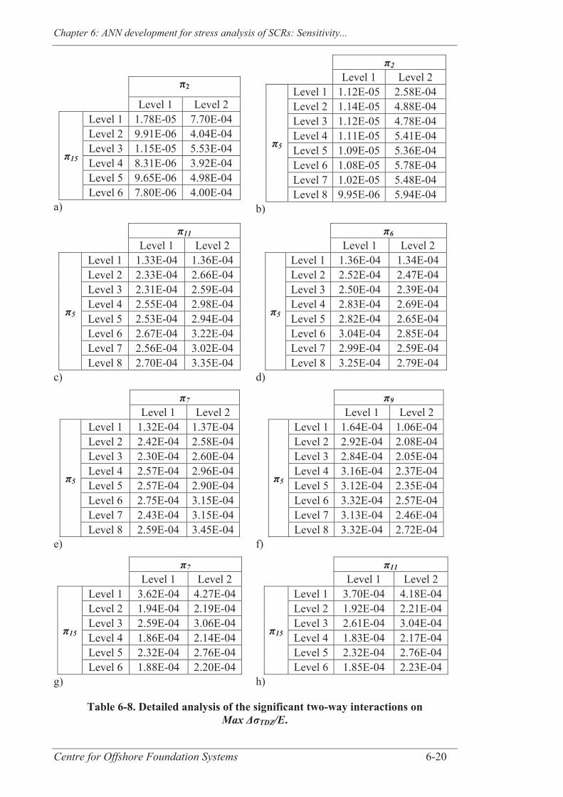
Chapter 6: ANN development for stress analysis of SCRs: Sensitivity...
Centre for Offshore Foundation Systems 6-20
π2
Level 1 Level 2
π15
Level 1 1.78E-05 7.70E-04 Level 2 9.91E-06 4.04E-04 Level 3 1.15E-05 5.53E-04 Level 4 8.31E-06 3.92E-04 Level 5 9.65E-06 4.98E-04 Level 6 7.80E-06 4.00E-04
a)
π2 Level 1 Level 2
π5
Level 1 1.12E-05 2.58E-04 Level 2 1.14E-05 4.88E-04 Level 3 1.12E-05 4.78E-04 Level 4 1.11E-05 5.41E-04 Level 5 1.09E-05 5.36E-04 Level 6 1.08E-05 5.78E-04 Level 7 1.02E-05 5.48E-04 Level 8 9.95E-06 5.94E-04
b)
π11 Level 1 Level 2
π5
Level 1 1.33E-04 1.36E-04 Level 2 2.33E-04 2.66E-04 Level 3 2.31E-04 2.59E-04 Level 4 2.55E-04 2.98E-04 Level 5 2.53E-04 2.94E-04 Level 6 2.67E-04 3.22E-04 Level 7 2.56E-04 3.02E-04 Level 8 2.70E-04 3.35E-04
c)
π6 Level 1 Level 2
π5
Level 1 1.36E-04 1.34E-04 Level 2 2.52E-04 2.47E-04 Level 3 2.50E-04 2.39E-04 Level 4 2.83E-04 2.69E-04 Level 5 2.82E-04 2.65E-04 Level 6 3.04E-04 2.85E-04 Level 7 2.99E-04 2.59E-04 Level 8 3.25E-04 2.79E-04
d)
π7 Level 1 Level 2
π5
Level 1 1.32E-04 1.37E-04Level 2 2.42E-04 2.58E-04Level 3 2.30E-04 2.60E-04Level 4 2.57E-04 2.96E-04Level 5 2.57E-04 2.90E-04Level 6 2.75E-04 3.15E-04Level 7 2.43E-04 3.15E-04Level 8 2.59E-04 3.45E-04
e)
π9 Level 1 Level 2
π5
Level 1 1.64E-04 1.06E-04 Level 2 2.92E-04 2.08E-04 Level 3 2.84E-04 2.05E-04 Level 4 3.16E-04 2.37E-04 Level 5 3.12E-04 2.35E-04 Level 6 3.32E-04 2.57E-04 Level 7 3.13E-04 2.46E-04 Level 8 3.32E-04 2.72E-04
f)
π7 Level 1 Level 2
π15
Level 1 3.62E-04 4.27E-04Level 2 1.94E-04 2.19E-04Level 3 2.59E-04 3.06E-04Level 4 1.86E-04 2.14E-04Level 5 2.32E-04 2.76E-04Level 6 1.88E-04 2.20E-04
g)
π11 Level 1 Level 2
π15
Level 1 3.70E-04 4.18E-04 Level 2 1.92E-04 2.21E-04 Level 3 2.61E-04 3.04E-04 Level 4 1.83E-04 2.17E-04 Level 5 2.32E-04 2.76E-04 Level 6 1.85E-04 2.23E-04
h)
Table 6-8. Detailed analysis of the significant two-way interactions on Max ΔσTDZ/E.
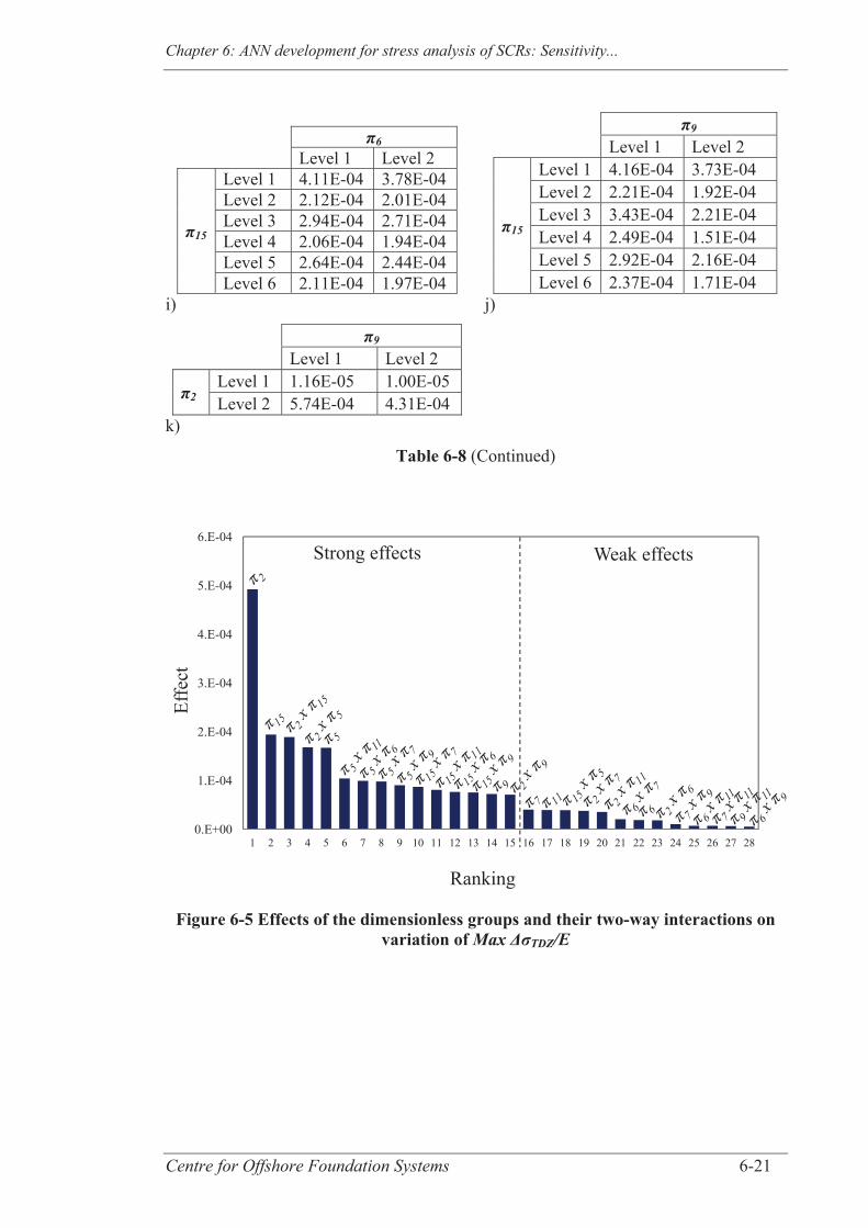
Chapter 6: ANN development for stress analysis of SCRs: Sensitivity...
Centre for Offshore Foundation Systems 6-21
π6 Level 1 Level 2
π15
Level 1 4.11E-04 3.78E-04 Level 2 2.12E-04 2.01E-04 Level 3 2.94E-04 2.71E-04 Level 4 2.06E-04 1.94E-04 Level 5 2.64E-04 2.44E-04 Level 6 2.11E-04 1.97E-04
i)
π9 Level 1 Level 2
π15
Level 1 4.16E-04 3.73E-04 Level 2 2.21E-04 1.92E-04 Level 3 3.43E-04 2.21E-04 Level 4 2.49E-04 1.51E-04 Level 5 2.92E-04 2.16E-04 Level 6 2.37E-04 1.71E-04
j)
π9 Level 1 Level 2
π2 Level 1 1.16E-05 1.00E-05 Level 2 5.74E-04 4.31E-04
k)
Table 6-8 (Continued)
Figure 6-5 Effects of the dimensionless groups and their two-way interactions on variation of Max ΔσTDZ/E
0.E+00
1.E-04
2.E-04
3.E-04
4.E-04
5.E-04
6.E-04
1 2 3 4 5 6 7 8 9 10 11 12 13 14 15 16 17 18 19 20 21 22 23 24 25 26 27 28
Ranking
Effe
ct
Strong effects Weak effects
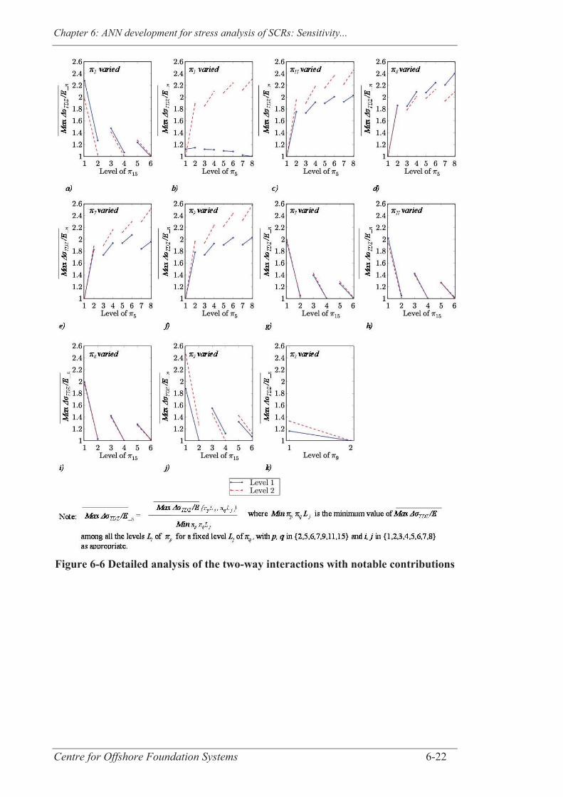
Chapter 6: ANN development for stress analysis of SCRs: Sensitivity...
Centre for Offshore Foundation Systems 6-22
Figure 6-6 Detailed analysis of the two-way interactions with notable contributions

Chapter 6: ANN development for stress analysis of SCRs: Sensitivity...
Centre for Offshore Foundation Systems 6-23
Combination of input dimensionless groups predicted to
lead to:
the minimum value of
Max ΔσTDZ/E the maximum value of
Max ΔσTDZ/E π2 Level 1 Level 2 π15 Level 6 Level 1 π5 Level 8 Level 8 π9 Level 2 Level 1 π7 Level 1 Level 2 π11 Level 1 Level 2 π6 Level 2 Level 1
Actual Max ΔσTDZ/E value 4.19E-06 1.21E-03
Match with extreme value? Yes Yes
Table 6-9. Verification of the validity of the predicted level of input dimensionless groups (listed by decreasing contribution) leading to extreme values of
Max ΔσTDZ/E.
6.4 ESTABLISHING AN ARTIFICIAL NEURAL NETWORK FOR
STRESS RANGE ESTIMATION
In an effort to maximise the applicability and pertinence of the results from this study, it
is fundamental that the selected database encompasses most of the realistic SCR
configurations and static loading conditions and that it provides sufficient support for
the training of a response surface to achieve an accurate approximation of Max TDZ/E.
For this purpose, additional cases are defined and an artificial neural network is
developed.
For clarity, the notation Max TDZ/E _approx is introduced to refer to the approximated
value of maximum value of normalised stress range (by contrast with the reference
value Max TDZ/E calculated using OrcaFlex).
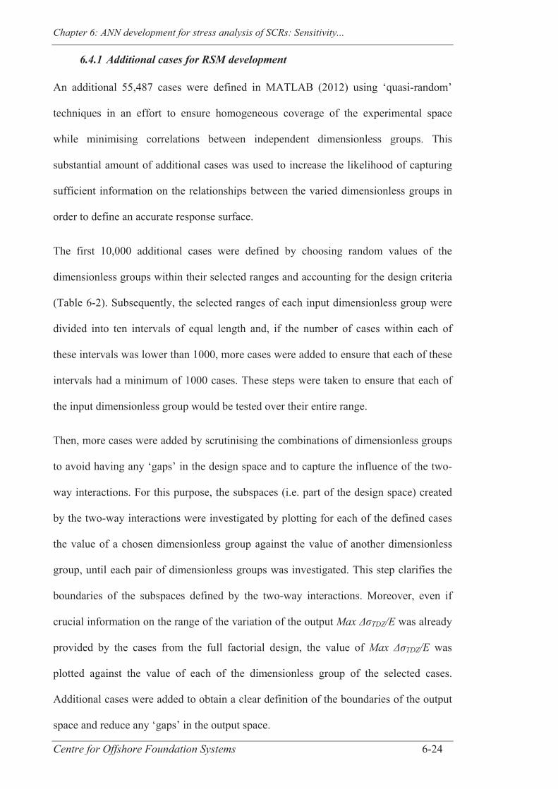
Chapter 6: ANN development for stress analysis of SCRs: Sensitivity...
Centre for Offshore Foundation Systems 6-24
6.4.1 Additional cases for RSM development
An additional 55,487 cases were defined in MATLAB (2012) using ‘quasi-random’
techniques in an effort to ensure homogeneous coverage of the experimental space
while minimising correlations between independent dimensionless groups. This
substantial amount of additional cases was used to increase the likelihood of capturing
sufficient information on the relationships between the varied dimensionless groups in
order to define an accurate response surface.
The first 10,000 additional cases were defined by choosing random values of the
dimensionless groups within their selected ranges and accounting for the design criteria
(Table 6-2). Subsequently, the selected ranges of each input dimensionless group were
divided into ten intervals of equal length and, if the number of cases within each of
these intervals was lower than 1000, more cases were added to ensure that each of these
intervals had a minimum of 1000 cases. These steps were taken to ensure that each of
the input dimensionless group would be tested over their entire range.
Then, more cases were added by scrutinising the combinations of dimensionless groups
to avoid having any ‘gaps’ in the design space and to capture the influence of the two-
way interactions. For this purpose, the subspaces (i.e. part of the design space) created
by the two-way interactions were investigated by plotting for each of the defined cases
the value of a chosen dimensionless group against the value of another dimensionless
group, until each pair of dimensionless groups was investigated. This step clarifies the
boundaries of the subspaces defined by the two-way interactions. Moreover, even if
crucial information on the range of the variation of the output Max TDZ/E was already
provided by the cases from the full factorial design, the value of Max TDZ/E was
plotted against the value of each of the dimensionless group of the selected cases.
Additional cases were added to obtain a clear definition of the boundaries of the output
space and reduce any ‘gaps’ in the output space.

Chapter 6: ANN development for stress analysis of SCRs: Sensitivity...
Centre for Offshore Foundation Systems 6-25
The final database reached a total of 57,023 cases and an illustration of the values of the
dimensionless groups for the entire database is given in Figure 6-7a. Also, the subspaces
created by the two-way interactions between dimensionless groups or between the
output and the dimensionless groups are presented in Figure 6-7b. It is seen that the
overall design space has a very complex shape due to the design criteria introduced
between input dimensionless groups or design variables. A high density is obtained with
the current choice of database, which will enhance the accuracy when training and
testing the ANN.
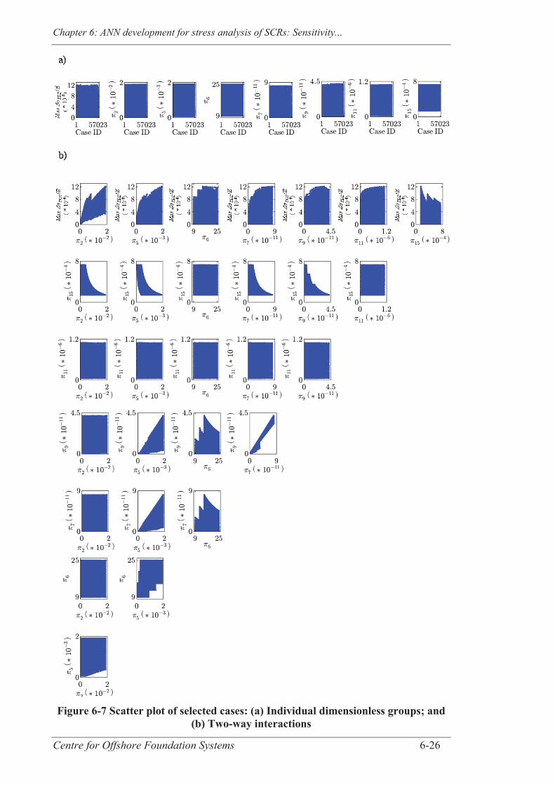
Chapter 6: ANN development for stress analysis of SCRs: Sensitivity...
Centre for Offshore Foundation Systems 6-26
Figure 6-7 Scatter plot of selected cases: (a) Individual dimensionless groups; and (b) Two-way interactions
Chapter 6: ANN development for stress analysis of SCRs: Sensitivity...
Centre for Offshore Foundation Systems 6-27
6.4.2 Selection of the training and testing sets
The entire database needs to be divided into a training and a testing set and the choice of
cases forming these two subsets may impact the performance of the defined ANN
(Hammerstrom, 1993; Shahin et al., 2004; de Pina et al., 2013). Several techniques
varying in complexity can be used to form the training and testing sets. The simplest
method is to select the cases at random although this method has some obvious
drawbacks: the testing set may require extrapolation of the ANN outside the training
space and some parts of the design space may not be approximated or tested as well as
others. An improved method is the ‘statistically consistent’ approach (Shahin et al.,
2004) that aims for the training and testing sets to have similar statistical characteristics
(i.e. range of variation, mean and standard deviation). It is indeed crucial that the testing
set gives a reliable representation of the design space to assess with confidence the
interpolation abilities of the ANN. More advanced methods exist such as the self-
organising map and fuzzy clustering approaches (Shahin et al., 2004). The ‘statistically
consistent’ approach is used in this paper although the more advanced techniques could
be used in the future.
An initial selection of the fundamental cases (extreme values) that should form part of
the training and testing set was performed and then a trial and error procedure was
followed to reduce the differences between the statistical characteristics of the two data
sets. The extreme values define the boundaries of the design space and it is essential to
include some in the training set to avoid extrapolations when using the trained ANN
(Tokar and Johnson, 1999; Shahin et al, 2004). This is why all the cases from the full
factorial design of the extreme values were by default included into the training set.
Moreover, it was shown earlier that the design space has a complex shape due to the
various selected design criteria and therefore numerous cases with combinations of
dimensionless group on the boundaries of the two-way interactions were selected for

Chapter 6: ANN development for stress analysis of SCRs: Sensitivity...
Centre for Offshore Foundation Systems 6-28
training.
Finally, 35,000 cases were selected for the training set and 22,023 for the testing set,
which is consistent with the common practice of using about a third of the available data
for testing (Hammerstrom, 1993; Shahin et al., 2004). The statistical characteristics of
both databases are presented in Table 6-10. It is seen that the output and the input
dimensionless groups in both databases have similar ranges of variation, mean and
standard deviation. Hence, the testing database seems to be an accurate representation of
the training database and is suitable to test the ANN.
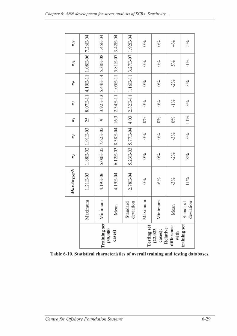
Chapter 6: ANN development for stress analysis of SCRs: Sensitivity...
Centre for Offshore Foundation Systems 6-29
π 15
7.26
E-04
1.45
E-04
3.42
E-04
1.92
E-04
0%
0%
4%
5%
π 11
1.08
E-06
5.38
E-08
5.81
E-07
3.27
E-07
0%
0%
5%
-1%
π 9
4.19
E-11
5.44
E-14
1.05
E-11
1.16
E-11
0%
0%
-2%
3%
π 7
8.07
E-11
3.92
E-13
2.34
E-11
2.32
E-11
0%
0%
-1%
3%
π 6
25
9 16.3
4.03
0%
0%
0%
11%
π 5
1.91
E-03
7.62
E-05
8.38
E-04
5.77
E-04
0%
0%
-3%
3%
π 2
1.88
E-02
5.00
E-05
6.12
E-03
5.23
E-03
0%
0%
-2%
8%
Max
ΔσTD
Z/E
1.21
E-03
4.19
E-06
4.19
E-04
2.78
E-04
0%
-6%
-3%
11%
Max
imum
Min
imum
Mea
n
Stan
dard
de
viat
ion
Max
imum
Min
imum
Mea
n
Stan
dard
de
viat
ion
Tra
inin
g se
t (3
5,00
0 ca
ses)
Tes
ting
set
(22,
023
case
s):
Rel
ativ
e di
ffer
ence
w
ith
trai
ning
set
Table 6-10. Statistical characteristics of overall training and testing databases.
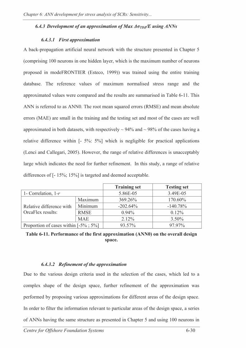
Chapter 6: ANN development for stress analysis of SCRs: Sensitivity...
Centre for Offshore Foundation Systems 6-30
6.4.3 Development of an approximation of Max ΔσTDZ/E using ANNs
6.4.3.1 First approximation
A back-propagation artificial neural network with the structure presented in Chapter 5
(comprising 100 neurons in one hidden layer, which is the maximum number of neurons
proposed in modeFRONTIER (Esteco, 1999)) was trained using the entire training
database. The reference values of maximum normalised stress range and the
approximated values were compared and the results are summarised in Table 6-11. This
ANN is referred to as ANN0. The root mean squared errors (RMSE) and mean absolute
errors (MAE) are small in the training and the testing set and most of the cases are well
approximated in both datasets, with respectively ~ 94% and ~ 98% of the cases having a
relative difference within [- 5%: 5%] which is negligible for practical applications
(Lenci and Callegari, 2005). However, the range of relative differences is unacceptably
large which indicates the need for further refinement. In this study, a range of relative
differences of [- 15%; 15%] is targeted and deemed acceptable.
Training set Testing set 1- Correlation, 1-r 5.86E-05 3.49E-05
Relative difference with OrcaFlex results:
Maximum 369.26% 170.60% Minimum -202.64% -140.78% RMSE 0.94% 0.12% MAE 2.12% 3.50%
Proportion of cases within [-5% ; 5%] 93.57% 97.97%
Table 6-11. Performance of the first approximation (ANN0) on the overall design space.
6.4.3.2 Refinement of the approximation
Due to the various design criteria used in the selection of the cases, which led to a
complex shape of the design space, further refinement of the approximation was
performed by proposing various approximations for different areas of the design space.
In order to filter the information relevant to particular areas of the design space, a series
of ANNs having the same structure as presented in Chapter 5 and using 100 neurons in
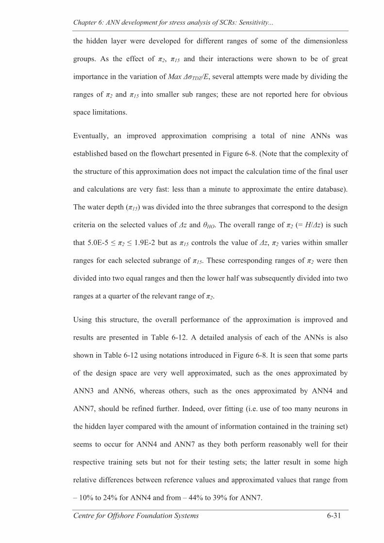
Chapter 6: ANN development for stress analysis of SCRs: Sensitivity...
Centre for Offshore Foundation Systems 6-31
the hidden layer were developed for different ranges of some of the dimensionless
groups. As the effect of 2, 15 and their interactions were shown to be of great
importance in the variation of Max TDZ/E, several attempts were made by dividing the
ranges of 2 and 15 into smaller sub ranges; these are not reported here for obvious
space limitations.
Eventually, an improved approximation comprising a total of nine ANNs was
established based on the flowchart presented in Figure 6-8. (Note that the complexity of
the structure of this approximation does not impact the calculation time of the final user
and calculations are very fast: less than a minute to approximate the entire database).
The water depth ( 15) was divided into the three subranges that correspond to the design
criteria on the selected values of z and HO. The overall range of 2 (= H/ z) is such
that 5.0E-5 ≤ 2 ≤ 1.9E-2 but as 15 controls the value of z, 2 varies within smaller
ranges for each selected subrange of 15. These corresponding ranges of 2 were then
divided into two equal ranges and then the lower half was subsequently divided into two
ranges at a quarter of the relevant range of 2.
Using this structure, the overall performance of the approximation is improved and
results are presented in Table 6-12. A detailed analysis of each of the ANNs is also
shown in Table 6-12 using notations introduced in Figure 6-8. It is seen that some parts
of the design space are very well approximated, such as the ones approximated by
ANN3 and ANN6, whereas others, such as the ones approximated by ANN4 and
ANN7, should be refined further. Indeed, over fitting (i.e. use of too many neurons in
the hidden layer compared with the amount of information contained in the training set)
seems to occur for ANN4 and ANN7 as they both perform reasonably well for their
respective training sets but not for their testing sets; the latter result in some high
relative differences between reference values and approximated values that range from
– 10% to 24% for ANN4 and from – 44% to 39% for ANN7.

Chapter 6: ANN development for stress analysis of SCRs: Sensitivity...
Centre for Offshore Foundation Systems 6-32
Figure 6-8 Structure of the approximation using nine ANNs
A trial and error approach was followed to train new ANNs, ANN4* and ANN7* for
these particular areas of the design space using fewer neurons. The characteristics of the
final ANNs, using 50 neurons for ANN4* and 55 for ANN7*, are shown in Table 6-13.
The performance of these two new ANNs for the training sets are slightly compromised
(although still within a reasonable accuracy) but their interpolation ability have
improved notably and the extreme values of relative difference are now within the
acceptable range.
To summarise, the final approximation, referred to as ‘9-ANNs static approximation’
hereafter, has the structure presented in Figure 6-8 but uses ANN4* and ANN7* in
place of ANN4 and ANN7 respectively, with the individual performances of the ANNs
shown in Table 6-12 and Table 6-13. The overall performance of the 9-ANNs static
approximation is assessed with results presented in Table 6-14. A very good level of
2 , 3, 5 , 6 , 7 , 8, 9 , 10, 11 , 14, 15 , 17, E, g, steel , water
400 * (g steel / E) ≤ 15 < 950 * (g steel / E)Or
15 = 950 * (g steel / E) and HO ≥ 17 °
15 < 1500 * (g steel / E)Or
15 = 1500 * (g steel / E) and HO ≥ 9 °
Yes No
2 9.43E-3
2 2.44E-3
ANN1 ANN3
2 3.98E-3
2 1.05E-3
ANN6ANN2 ANN4 ANN5
2 2.53E-3
2 6.69E-4
ANN7 ANN9ANN8
Yes No
Yes No
Yes No Yes No Yes No
Yes No Yes No
Max TDZ /E_approx
1.05e-4 2 1.88e-2
6.67e-5 2 7.89e-3 5.00e-5 2 5.00 e-3
5.00e-5 2 7.89e-3

Chapter 6: ANN development for stress analysis of SCRs: Sensitivity...
Centre for Offshore Foundation Systems 6-33
accuracy is obtained as only 0.15% and 0.08% of the cases used for training and for
testing respectively are approximated with relative differences outside [- 5%: 5%].
Moreover, the range of relative difference is reasonably small, with the differences
ranging from about -12% to 13% for the training set and from about -11% to 8% for the
testing set. The 9-ANNs static approximation is implemented in a MATLAB code
(including all the relevant weights and bias matrices of the nine ANNs). It can be
supplied as a standalone application by contacting the corresponding author. Note that
this approximation was developed under a number of assumptions and for SCR
configurations defined with values of input dimensionless groups within the selected
ranges and respecting the selected design criteria, as shown in Table 6-2 and Table 6-3.
The literature reports various analytical models that were developed to serve the same
purpose of evaluating the static stress range in SCRs (Pesce et al., 1998b; Lenci and
Callegari, 2005; Shiri and Hashemi, 2012 and Quéau et al., 2014a). The most advanced
models account for the bending stiffness of the riser in a small section near the
touchdown point (where the riser starts to be in contact with the seabed). They usually
involve a number of unknowns that can be determined by solving a nonlinear system of
equations, using for instance the iterative Newton-Raphson technique (Lenci and
Callegari, 2005; Quéau et al., 2014a). Hence, although an obvious drawback of the
proposed approximation based on ANNs is that it acts like a “black box”, it is a very
straightforward approach that is even faster than the use of analytical and numerical
models as it does not involve any iterative or structural analysis procedures.
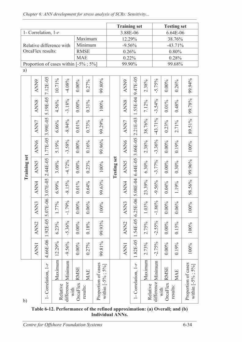
Chapter 6: ANN development for stress analysis of SCRs: Sensitivity...
Centre for Offshore Foundation Systems 6-34
Training set Testing set 1- Correlation, 1-r 3.88E-06 6.64E-06
Relative difference with OrcaFlex results:
Maximum 12.29% 38.76% Minimum -9.56% -43.71% RMSE 0.26% 0.80% MAE 0.22% 0.28%
Proportion of cases within [-5% ; 5%] 99.90% 99.68% a)
Tra
inin
g se
t
AN
N9
7.12
E-05
10.7
1%
-4.0
8%
0.00
%
0.27
%
99.8
0%
Tes
ting
set
AN
N9
9.47
E-05
2.38
%
-5.7
5%
0.00
%
0.26
%
99.9
4%
AN
N8
5.19
E-05
4.56
%
-3.1
8%
0.00
%
0.31
%
100%
AN
N8
1.55
E-04
7.12
%
-3.5
4%
0.01
%
0.48
%
99.7
8%
AN
N7
3.99
E-05
6.06
%
-8.9
4%
0.01
%
0.73
%
99.2
9%
AN
N7
2.21
E-03
38.7
6%
-43.
71%
0.23
%
2.71
%
89.5
1%
AN
N6
1.77
E-05
5.19
%
-3.5
8%
0.00
%
0.16
%
99.9
6%
AN
N6
3.06
E-05
2.38
%
-3.3
6%
0.00
%
0.19
%
100%
AN
N5
2.44
E-05
3.08
%
-4.7
2%
0.00
%
0.23
%
100%
AN
N5
6.44
E-05
6.30
%
-3.7
7%
0.00
%
0.30
%
99.9
6%
AN
N4
3.07
E-05
6.99
%
-8.1
5%
0.01
%
0.64
%
99.6
3%
AN
N4
5.08
E-04
23.3
9%
-9.5
6%
0.04
%
1.19
%
98.5
6%
AN
N3
5.07
E-06
1.77
%
-1.7
9%
0.00
%
0.06
%
100%
AN
N3
6.25
E-06
1.03
%
-1.8
6%
0.00
%
0.06
%
100%
AN
N2
1.92
E-05
6.23
%
-5.3
6%
0.00
%
0.18
%
99.9
3%
AN
N2
1.54
E-05
2.75
%
-2.5
5%
0.00
%
0.15
%
100%
AN
N1
4.66
E-06
12.2
9%
-9.5
6%
0.00
%
0.27
%
99.8
1%
AN
N1
1.82
E-05
2.73
%
-2.7
5%
0.00
%
0.19
%
100%
1-
Cor
rela
tion,
1-r
Max
imum
Min
imum
RM
SE
MA
E
Prop
ortio
n of
cas
es
with
in [-
5% ;
5%]
1-
Cor
rela
tion,
1-r
Max
imum
Min
imum
RM
SE
MA
E
Prop
ortio
n of
cas
es
with
in [-
5% ;
5%]
Rel
ativ
e di
ffer
ence
w
ith
Orc
aFle
x re
sults
:
Rel
ativ
e di
ffer
ence
w
ith
Orc
aFle
x re
sults
:
b)
Table 6-12. Performance of the refined approximation: (a) Overall; and (b) Individual ANNs.
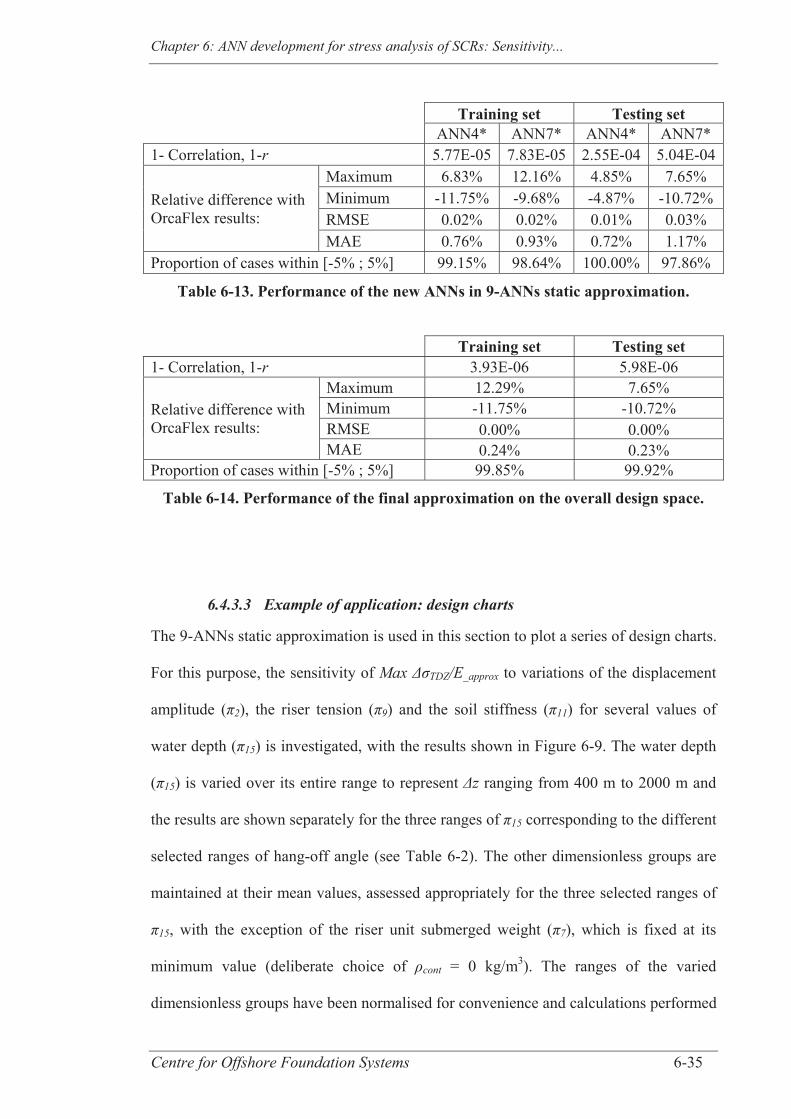
Chapter 6: ANN development for stress analysis of SCRs: Sensitivity...
Centre for Offshore Foundation Systems 6-35
Training set Testing set ANN4* ANN7* ANN4* ANN7*
1- Correlation, 1-r 5.77E-05 7.83E-05 2.55E-04 5.04E-04
Relative difference with OrcaFlex results:
Maximum 6.83% 12.16% 4.85% 7.65% Minimum -11.75% -9.68% -4.87% -10.72% RMSE 0.02% 0.02% 0.01% 0.03% MAE 0.76% 0.93% 0.72% 1.17%
Proportion of cases within [-5% ; 5%] 99.15% 98.64% 100.00% 97.86%
Table 6-13. Performance of the new ANNs in 9-ANNs static approximation.
Training set Testing set 1- Correlation, 1-r 3.93E-06 5.98E-06
Relative difference with OrcaFlex results:
Maximum 12.29% 7.65% Minimum -11.75% -10.72% RMSE 0.00% 0.00% MAE 0.24% 0.23%
Proportion of cases within [-5% ; 5%] 99.85% 99.92%
Table 6-14. Performance of the final approximation on the overall design space.
6.4.3.3 Example of application: design charts
The 9-ANNs static approximation is used in this section to plot a series of design charts.
For this purpose, the sensitivity of Max TDZ/E_approx to variations of the displacement
amplitude ( 2), the riser tension ( 9) and the soil stiffness ( 11) for several values of
water depth ( 15) is investigated, with the results shown in Figure 6-9. The water depth
( 15) is varied over its entire range to represent z ranging from 400 m to 2000 m and
the results are shown separately for the three ranges of 15 corresponding to the different
selected ranges of hang-off angle (see Table 6-2). The other dimensionless groups are
maintained at their mean values, assessed appropriately for the three selected ranges of
15, with the exception of the riser unit submerged weight ( 7), which is fixed at its
minimum value (deliberate choice of cont = 0 kg/m3). The ranges of the varied
dimensionless groups have been normalised for convenience and calculations performed
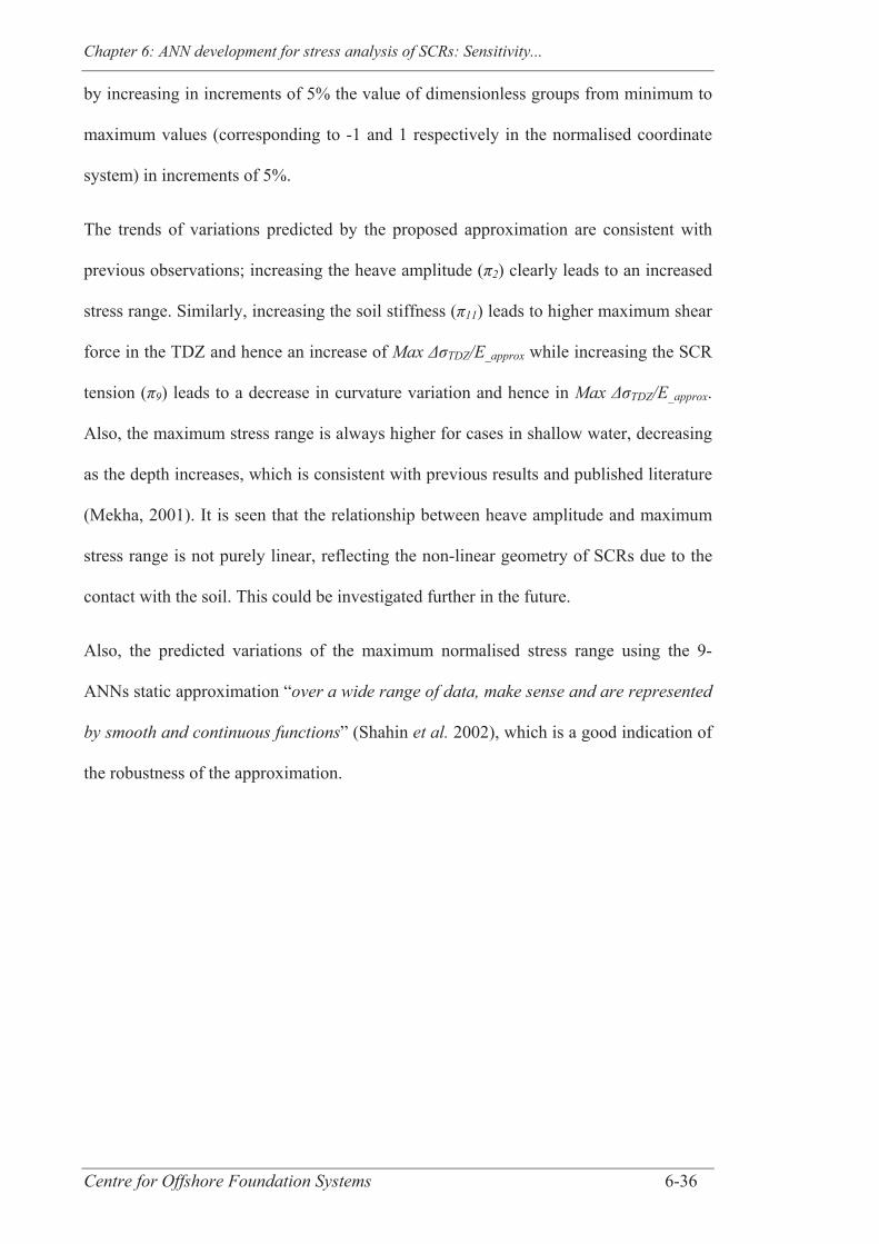
Chapter 6: ANN development for stress analysis of SCRs: Sensitivity...
Centre for Offshore Foundation Systems 6-36
by increasing in increments of 5% the value of dimensionless groups from minimum to
maximum values (corresponding to -1 and 1 respectively in the normalised coordinate
system) in increments of 5%.
The trends of variations predicted by the proposed approximation are consistent with
previous observations; increasing the heave amplitude ( 2) clearly leads to an increased
stress range. Similarly, increasing the soil stiffness ( 11) leads to higher maximum shear
force in the TDZ and hence an increase of Max TDZ/E_approx while increasing the SCR
tension ( 9) leads to a decrease in curvature variation and hence in Max TDZ/E_approx.
Also, the maximum stress range is always higher for cases in shallow water, decreasing
as the depth increases, which is consistent with previous results and published literature
(Mekha, 2001). It is seen that the relationship between heave amplitude and maximum
stress range is not purely linear, reflecting the non-linear geometry of SCRs due to the
contact with the soil. This could be investigated further in the future.
Also, the predicted variations of the maximum normalised stress range using the 9-
ANNs static approximation “over a wide range of data, make sense and are represented
by smooth and continuous functions” (Shahin et al. 2002), which is a good indication of
the robustness of the approximation.
Chapter 6: ANN development for stress analysis of SCRs: Sensitivity...
Centre for Offshore Foundation Systems 6-37
Figure 6-9 Example of design charts showing the sensitivity of Max ΔσTDZ/E_approx to variations of (1) π2,(2) π9 and (3) π11 for various π15 values corresponding to: (a)
Δz between 400 m and 950- m; (b) Δz between 950+ m and 1500- m and (c) Δz between 1500+ m and 2000 m
6.5 CONCLUSIONS
This paper has presented a detailed analysis of the input dimensionless groups
influencing the variations of the maximum normalised stress range in the TDZ for
SCRs. For this purpose, an extensive database of 57,023 SCR configurations under
static loading was created to cover a wide range of applications. The numerical models
were created and post-processed by means of an in-house interface developed between
the optimisation software modeFRONTIER and the marine analysis software OrcaFlex
through the programming language Python. Design of experiments techniques were
used to assist the selection of cases forming the database in the aim of studying the
relative effects of the input dimensionless groups and their interactions, and then,
Chapter 6: ANN development for stress analysis of SCRs: Sensitivity...
Centre for Offshore Foundation Systems 6-38
training a response surface and defining a suitable approximation of Max TDZ/E using
ANNs.
The study of the average results for various levels of input dimensionless groups and
interactions showed that the normalised amplitude of the loading ( 2) and the
normalised water depth ( 15) have the greatest contribution to the variation of Max
TDZ/E. It was found that high vessel motion ( 2), submerged weight ( 7), soil stiffness
( 11) and low outside diameter over wall thickness ratio ( 6), pipeline tension ( 9) and
water depth ( 15) were detrimental to SCR fatigue life in the TDZ. Also, a strong
interaction leading to opposite effects was detected between 2 and the normalised
outside diameter ( 5): an increase of 5 leads to an increase of Max TDZ/E for high 2
but eventually to a slight decrease for low 2.
An approximation of Max TDZ/E was researched and the best results were found when
using a total of nine ANNs. These various ANNs were developed for different regions
of the design space depending on the values of heave amplitude and water depth. The
extreme values of relative errors when comparing the results from the approximation
with the results from OrcaFlex reached 13% and over 99% of the cases (used either for
testing or training) were approximated with a negligible relative difference for practical
applications (within 5% (Lenci and Callegari, 2005)).The robustness of the
approximation was validated further by means of a series of design charts that presented
coherent results with smooth variations. The proposed approximation is however only
strictly valid for SCR cases having input dimensionless groups within the selected
ranges and respecting the selected design criteria, although these ranges could be
enlarged in future work.
Although limited to static perturbation only, the framework developed in this paper
provides guidance to assist preliminary fatigue design of SCRs and demonstrated the
potential power of combining automated calculations, DoE methods and ANNs in SCR

Chapter 6: ANN development for stress analysis of SCRs: Sensitivity...
Centre for Offshore Foundation Systems 6-39
fatigue design. It lays the ground work for subsequent investigation of the dynamic
response, with the prospect of simplifying the early stages of SCR fatigue design using
dynamic amplification factors.

Estimating the fatigue damage of SCRs in the TDZ
Centre for Offshore Foundation Systems 7-1
CHAPTER 7 APPROXIMATION OF THE MAXIMUM DYNAMIC
STRESS RANGE IN STEEL CATENARY RISERS USING
ARTIFICIAL NEURAL NETWORKS
7.1 ABSTRACT
Exploiting deep water hydrocarbon reserves is nowadays the focal point of the oil and
gas industry and steel catenary risers (SCRs) are the most common means of
transporting fluids between seabed and sea surface in deep water. SCRs are fatigue
sensitive structures and an adequate assessment of their fatigue damage is essential as
interventions in deep water are extremely challenging. Their fatigue life is evaluated by
means of complicated and time consuming numerical analyses that are not well suited
for the early stages of design where many different configurations have to be
investigated to select an optimised setup. Simplified analysis and design strategies
would improve the efficiency of these screening tasks.
The study proposed in this paper is part of on-going research that has followed an
incremental approach towards the definition of a simplified fatigue design procedure for
SCRs in the touchdown zone. The steps have included first establishing relevant
dimensionless groups of the input parameters, validating an artificial neural network
approach for estimating stress changes under quasi-static conditions, and now extending
that approach for dynamic conditions. The sensitivity of fatigue damage to various input
parameters is explored using a database of more than 40,000 cases that have been
generated through an in-house automation subroutine. An approximation of the
maximum stress range in the TDZ is established using a series of artificial neural
networks and predicts well the fatigue life of selected example SCRs.

Chapter 7: Approximation of the maximum dynamic...
Centre for Offshore Foundation Systems 7-2
7.2 INTRODUCTION
The depletion of shallow water hydrocarbon reserves has focused the oil and gas
industry increasingly on reserves in deep water, where steel catenary risers (SCRs)
represent the most widely used option to convey the oil and gas from subsea to the
surface. The main drawbacks of SCRs however is their high sensitivity to
environmental loading that generates fatigue damage, especially in the area where the
riser is in contact with the seabed, namely the touchdown zone (TDZ) (e.g. Bridge,
2005, Elosta et al., 2014). An accurate estimation of SCR fatigue life is fundamental to
ensuring riser integrity over the life of the project while keeping costs low.
The fatigue damage is often estimated through time domain analyses to account for
SCR nonlinearities (material and geometrical for instance) and by performing a series of
time consuming numerical simulations (Mekha, 2001; Xia et al., 2008; DNV-OS-F201,
2010). A riser design standard (DNV-OS-F201, 2010) therefore encourages the use of
simplifying techniques, especially for the early stages of design, to improve the
efficiency of computer analyses and support engineering judgement. It states that
“numerous simplified analyses will normally produce more information regarding
overall static and dynamic system behaviour when compared to a reduced number of
advanced analyses.”
In light of these facts and recommendations, the authors have been aiming to develop a
simplified riser fatigue analysis procedure for the early stages of SCR design, avoiding
the need to perform time consuming analyses. The present paper details part of that
research, focusing on defining an approximation of the maximum dynamic stress range
of SCRs in the TDZ (Max TDZ) valid for a wide range of input parameters. Max TDZ
is used as, together with the number of cycles of each magnitude of motion applied, it
controls the fatigue damage. The method followed to develop the approximation is the
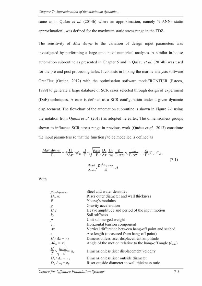
Chapter 7: Approximation of the maximum dynamic...
Centre for Offshore Foundation Systems 7-3
same as in Quéau et al. (2014b) where an approximation, namely ‘9-ANNs static
approximation’, was defined for the maximum static stress range in the TDZ.
The sensitivity of Max TDZ to the variation of design input parameters was
investigated by performing a large amount of numerical analyses. A similar in-house
automation subroutine as presented in Chapter 5 and in Quéau et al. (2014b) was used
for the pre and post processing tasks. It consists in linking the marine analysis software
OrcaFlex (Orcina, 2012) with the optimisation software modeFRONTIER (Esteco,
1999) to generate a large database of SCR cases selected through design of experiment
(DoE) techniques. A case is defined as a SCR configuration under a given dynamic
displacement. The flowchart of the automation subroutine is shown in Figure 7-1 using
the notation from Quéau et al. (2013) as adopted hereafter. The dimensionless groups
shown to influence SCR stress range in previous work (Quéau et al., 2013) constitute
the input parameters so that the function f to be modelled is defined as
Max TDZ E = f(
HΔz, Δθm,
HT
ρsteel E ,
DoΔz,
Do wt
, p
E Δz, ν, To
E Δz2, μ, ksE, CD, CA,
ρsteel ρwater
, g Δz ρsteel
E ,β)
(7-1)
With
steel , water Steel and water densities Do, wt Riser outer diameter and wall thickness E Young’s modulus g Gravity acceleration H,T Heave amplitude and period of the input motion ks Soil stiffness p Unit submerged weight To Horizontal tension component
z Vertical difference between hang-off point and seabed s Arc length (measured from hang-off point) H / z = 2 Dimensionless riser displacement amplitude
m = 3 Angle of the motion relative to the hang-off angle ( HO) HT steel
E = 4 Dimensionless riser displacement velocity
Do / z = 5 Dimensionless riser outside diameter Do / wt = 6 Riser outside diameter to wall thickness ratio
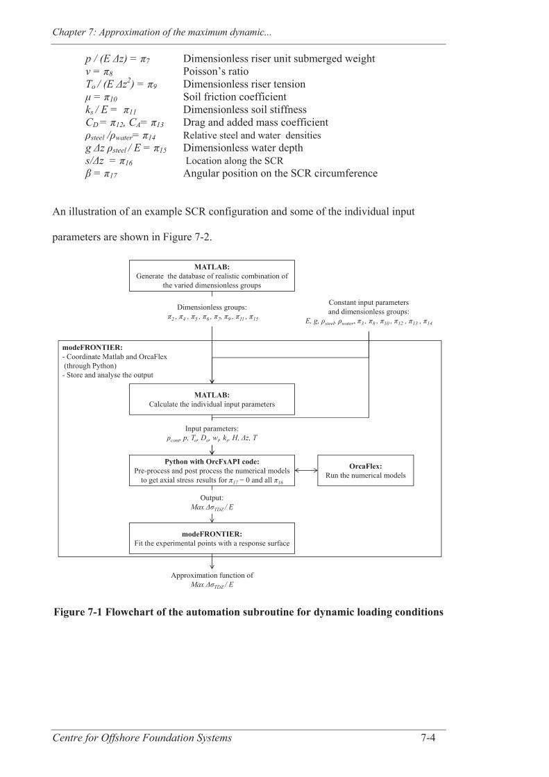
Chapter 7: Approximation of the maximum dynamic...
Centre for Offshore Foundation Systems 7-4
p / (E z) = 7 Dimensionless riser unit submerged weight = 8 Poisson’s ratio
To / (E z2) = 9 Dimensionless riser tension = 10 Soil friction coefficient
ks / E = 11 Dimensionless soil stiffness CD = 12, CA= 13 Drag and added mass coefficient
steel / water= 14 Relative steel and water densities g z steel / E = 15 Dimensionless water depth s/ z = 16 Location along the SCR
= 17 Angular position on the SCR circumference
An illustration of an example SCR configuration and some of the individual input
parameters are shown in Figure 7-2.
Figure 7-1 Flowchart of the automation subroutine for dynamic loading conditions
modeFRONTIER:- Coordinate Matlab and OrcaFlex(through Python)- Store and analyse the output
MATLAB:Generate the database of realistic combination of
the varied dimensionless groups
MATLAB:Calculate the individual input parameters
Python with OrcFxAPI code:Pre-process and post process the numerical models
to get axial stress results for 17 = 0 and all 16
OrcaFlex:Run the numerical models
Constant input parameters and dimensionless groups:
E, g, steel, water, 3 , 8 , 10 , 12 , 13 , 14
Approximation function of Max TDZ / E
modeFRONTIER:Fit the experimental points with a response surface
Dimensionless groups:2 , 4 , 5 , 6 , 7, 9 , 11 , 15
Output:Max TDZ / E
Input parameters: cont, p, To, Do, wt, ks, H, z, T
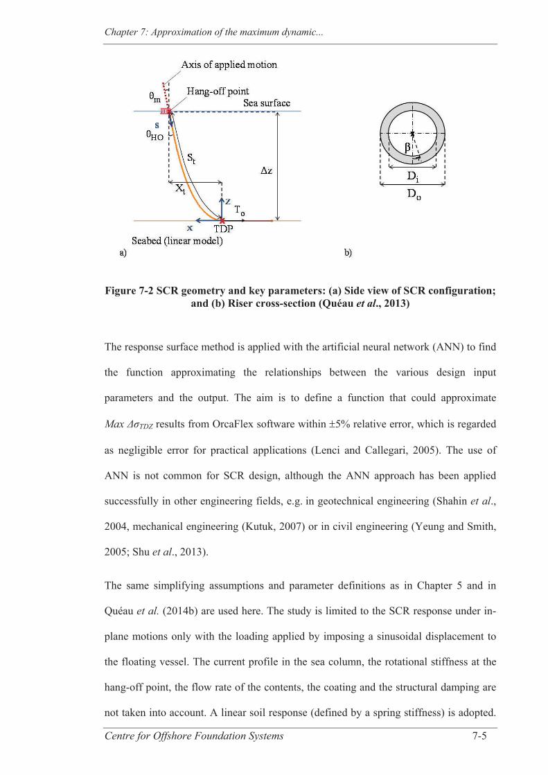
Chapter 7: Approximation of the maximum dynamic...
Centre for Offshore Foundation Systems 7-5
Figure 7-2 SCR geometry and key parameters: (a) Side view of SCR configuration; and (b) Riser cross-section (Quéau et al., 2013)
The response surface method is applied with the artificial neural network (ANN) to find
the function approximating the relationships between the various design input
parameters and the output. The aim is to define a function that could approximate
Max TDZ results from OrcaFlex software within 5% relative error, which is regarded
as negligible error for practical applications (Lenci and Callegari, 2005). The use of
ANN is not common for SCR design, although the ANN approach has been applied
successfully in other engineering fields, e.g. in geotechnical engineering (Shahin et al.,
2004, mechanical engineering (Kutuk, 2007) or in civil engineering (Yeung and Smith,
2005; Shu et al., 2013).
The same simplifying assumptions and parameter definitions as in Chapter 5 and in
Quéau et al. (2014b) are used here. The study is limited to the SCR response under in-
plane motions only with the loading applied by imposing a sinusoidal displacement to
the floating vessel. The current profile in the sea column, the rotational stiffness at the
hang-off point, the flow rate of the contents, the coating and the structural damping are
not taken into account. A linear soil response (defined by a spring stiffness) is adopted.
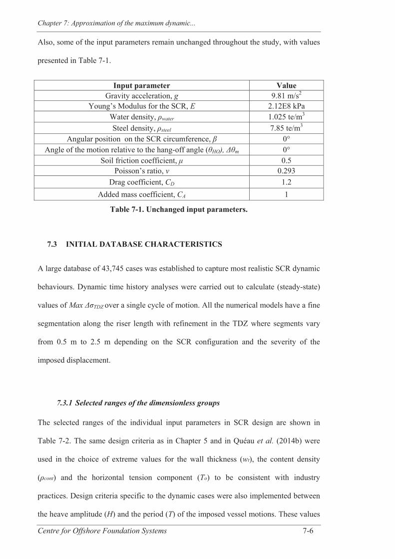
Chapter 7: Approximation of the maximum dynamic...
Centre for Offshore Foundation Systems 7-6
Also, some of the input parameters remain unchanged throughout the study, with values
presented in Table 7-1.
Input parameter Value Gravity acceleration, g 9.81 m/s2
Young’s Modulus for the SCR, E 2.12E8 kPa Water density, water 1.025 te/m3 Steel density, steel 7.85 te/m3
Angular position on the SCR circumference, 0° Angle of the motion relative to the hang-off angle ( HO), m 0°
Soil friction coefficient, 0.5 Poisson’s ratio, 0.293
Drag coefficient, CD 1.2 Added mass coefficient, CA 1
Table 7-1. Unchanged input parameters.
7.3 INITIAL DATABASE CHARACTERISTICS
A large database of 43,745 cases was established to capture most realistic SCR dynamic
behaviours. Dynamic time history analyses were carried out to calculate (steady-state)
values of Max TDZ over a single cycle of motion. All the numerical models have a fine
segmentation along the riser length with refinement in the TDZ where segments vary
from 0.5 m to 2.5 m depending on the SCR configuration and the severity of the
imposed displacement.
7.3.1 Selected ranges of the dimensionless groups
The selected ranges of the individual input parameters in SCR design are shown in
Table 7-2. The same design criteria as in Chapter 5 and in Quéau et al. (2014b) were
used in the choice of extreme values for the wall thickness (wt), the content density
( cont) and the horizontal tension component (To) to be consistent with industry
practices. Design criteria specific to the dynamic cases were also implemented between
the heave amplitude (H) and the period (T) of the imposed vessel motions. These values
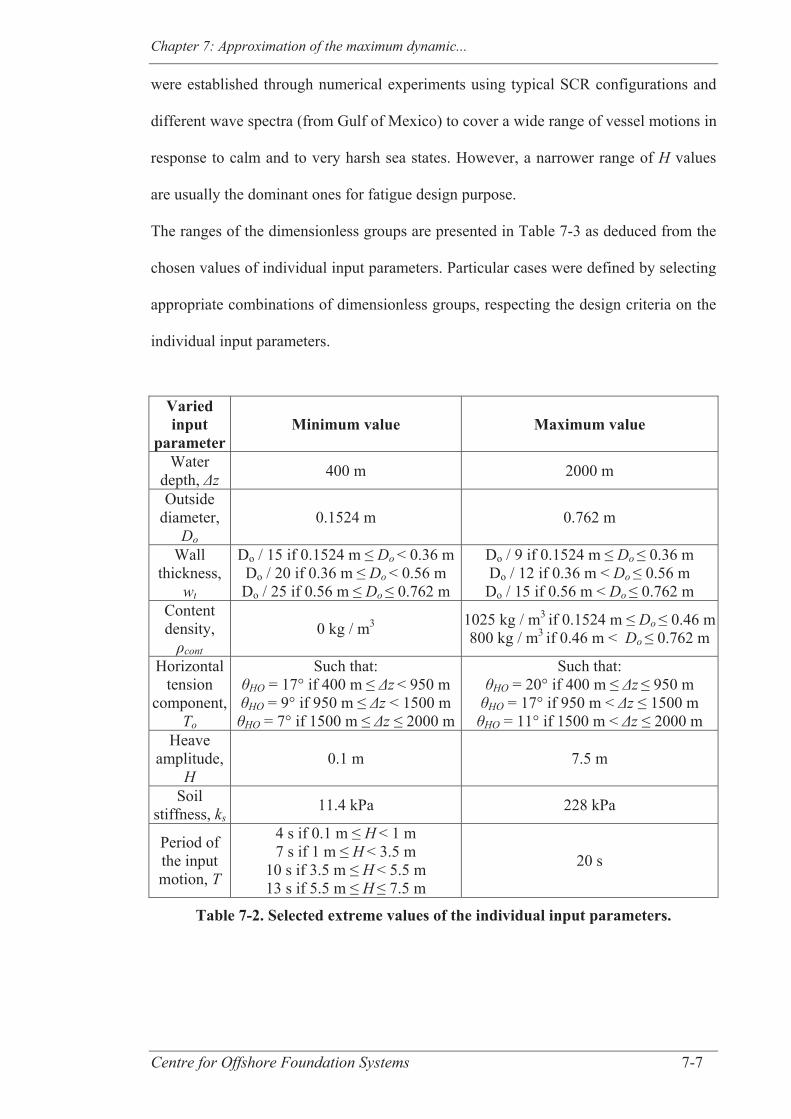
Chapter 7: Approximation of the maximum dynamic...
Centre for Offshore Foundation Systems 7-7
were established through numerical experiments using typical SCR configurations and
different wave spectra (from Gulf of Mexico) to cover a wide range of vessel motions in
response to calm and to very harsh sea states. However, a narrower range of H values
are usually the dominant ones for fatigue design purpose.
The ranges of the dimensionless groups are presented in Table 7-3 as deduced from the
chosen values of individual input parameters. Particular cases were defined by selecting
appropriate combinations of dimensionless groups, respecting the design criteria on the
individual input parameters.
Varied input
parameter Minimum value Maximum value
Water depth, z 400 m 2000 m
Outside diameter,
Do 0.1524 m 0.762 m
Wall thickness,
wt
Do / 15 if 0.1524 m ≤ Do < 0.36 mDo / 20 if 0.36 m ≤ Do < 0.56 m Do / 25 if 0.56 m ≤ Do ≤ 0.762 m
Do / 9 if 0.1524 m ≤ Do ≤ 0.36 m Do / 12 if 0.36 m < Do ≤ 0.56 m Do / 15 if 0.56 m < Do ≤ 0.762 m
Content density,
cont 0 kg / m3 1025 kg / m3 if 0.1524 m ≤ Do ≤ 0.46 m
800 kg / m3 if 0.46 m < Do ≤ 0.762 m
Horizontal tension
component, To
Such that: HO = 17° if 400 m ≤ z < 950 m HO = 9° if 950 m ≤ z < 1500 m
HO = 7° if 1500 m ≤ z ≤ 2000 m
Such that: HO = 20° if 400 m ≤ z ≤ 950 m
HO = 17° if 950 m < z ≤ 1500 m HO = 11° if 1500 m < z ≤ 2000 m
Heave amplitude,
H 0.1 m 7.5 m
Soil stiffness, ks
11.4 kPa 228 kPa
Period of the input motion, T
4 s if 0.1 m ≤ H < 1 m 7 s if 1 m ≤ H < 3.5 m
10 s if 3.5 m ≤ H < 5.5 m 13 s if 5.5 m ≤ H ≤ 7.5 m
20 s
Table 7-2. Selected extreme values of the individual input parameters.
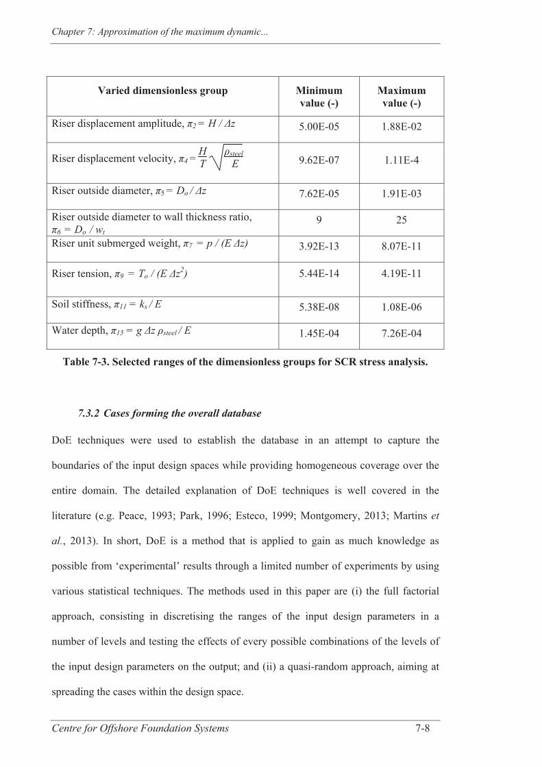
Chapter 7: Approximation of the maximum dynamic...
Centre for Offshore Foundation Systems 7-8
Varied dimensionless group Minimum value (-)
Maximum value (-)
Riser displacement amplitude, 2 = H / z 5.00E-05 1.88E-02
Riser displacement velocity, 4 = HT steel
E 9.62E-07 1.11E-4
Riser outside diameter, 5 = Do / z 7.62E-05 1.91E-03
Riser outside diameter to wall thickness ratio, 6 = Do / wt
9 25
Riser unit submerged weight, 7 = p / (E z) 3.92E-13 8.07E-11
Riser tension, 9 = To / (E z2) 5.44E-14 4.19E-11
Soil stiffness, 11 = ks / E 5.38E-08 1.08E-06
Water depth, 15 = g z steel / E 1.45E-04 7.26E-04
Table 7-3. Selected ranges of the dimensionless groups for SCR stress analysis.
7.3.2 Cases forming the overall database
DoE techniques were used to establish the database in an attempt to capture the
boundaries of the input design spaces while providing homogeneous coverage over the
entire domain. The detailed explanation of DoE techniques is well covered in the
literature (e.g. Peace, 1993; Park, 1996; Esteco, 1999; Montgomery, 2013; Martins et
al., 2013). In short, DoE is a method that is applied to gain as much knowledge as
possible from ‘experimental’ results through a limited number of experiments by using
various statistical techniques. The methods used in this paper are (i) the full factorial
approach, consisting in discretising the ranges of the input design parameters in a
number of levels and testing the effects of every possible combinations of the levels of
the input design parameters on the output; and (ii) a quasi-random approach, aiming at
spreading the cases within the design space.
Chapter 7: Approximation of the maximum dynamic...
Centre for Offshore Foundation Systems 7-9
A total of 12,288 cases were obtained with a full factorial design while the remaining
cases were obtained through quasi-random techniques. The full factorial design cases
were derived from the cases developed for the static study (Quéau et al., 2014b).
Additional levels of H and two levels for T were selected to account for the selected
design criteria on the extreme values of T, as presented in Table 7-2. This led to the
following levels, with the superscript ± referring to the fact that values of those input
parameters either side of the extremities of the ranges involved in the design criteria
were tested for the various possible ranges of the dependent parameters (e.g. z = 1500
m was tested with values of HO corresponding to the intervals relevant for both z just
less than 1500 m (9° ≤ HO ≤ 17°) and z just greater than 1500 m (7° ≤ HO ≤ 11°)):
z: 6 levels selected: 400 m; 950± m; 1500± m; and 2000 m.
Do: 8 levels selected: 0.1524 m; 0.36± m; 0.46± m; 0.56± m and 0.762 m.
6 = Do / wt : two levels selected: appropriate minimum and maximum values
with respect to the value of Do.
cont: two levels selected: empty and full with appropriate content density value
with respect to the value of Do.
To: two levels selected: appropriate minimum and maximum values determined
through the value of HO with respect to the value of z.
H: eight levels selected: 0.1 m; 1± m; 3.5± m; 5.5± m and 7.5 m.
ks: two levels selected: 11.4 kPa and 228 kPa.
T: two levels selected: appropriate minimum value determined through the value
of H and a maximum value of 20 s.
As a result, there are two levels for the dimensionless soil stiffness ( 11) and six levels
for the dimensionless water depth ( 15), which in turn determine the relevant eight levels
for the dimensionless displacement amplitude ( 2) and outside diameter ( 5) and the two
levels for the dimensionless tension ( 9), subsequently leading to the appropriate two
levels for the dimensionless displacement velocity ( 4), outside diameter over wall
thickness ratio ( 6) and dimensionless submerged weight ( 7). This number of selected

Chapter 7: Approximation of the maximum dynamic...
Centre for Offshore Foundation Systems 7-10
levels corresponds to a total of 12,288 combinations.
The relationships between the input dimensionless groups and Max TDZ/E are
expected to be more complex for the present dynamic study than for the previous static
study (Quéau et al., 2014b) due to the additional nonlinearities introduced by the
hydrodynamic forces and the dynamic amplifications effects for example. For this
reason it would seem reasonable to define an overall database having at least the same
size as the database established for the static study (i.e. ~ 57,000 cases). However,
dynamic analyses of SCRs are much more time consuming than static analyses and the
resulting simulation files occupy a large amount of disk space (as noted also by Xia et
al. (2008)). The number of additional cases obtained with quasi-random techniques was
therefore mostly limited by the computational resources available for this study. A total
of 31,457 additional cases were added using quasi-random techniques leading to an
overall database of 43,745 cases, representing a total of about four months of
calculation (automated pre-processing, running of the simulations and post-processing
of the simulation files) and a hard disk occupation of 6TB, using a specially selected
high performance computer with a Microsoft Windows Seven operating system, an Intel
Core i7 [email protected] processor, a memory of 24 GB and able to run twelve cases at a
time. This initial database could be expanded in future work, depending on the
performance of the results obtained, as discussed later on in the paper.
An illustration of the values of the dimensionless groups for the entire database is given
in Figure 7-3a showing the coverage of the design space. The figure indicates that the
database encompasses cases able to test the entire ranges of every dimensionless group.
Nonetheless, the output design space does not seem completely well captured by the
database as there seems to be irregular high values of Max TDZ/E with isolated spot
values. This could come from the selected combination of dimensionless groups within
the cases of the database. Results of a more detailed investigation are shown in Figure
Chapter 7: Approximation of the maximum dynamic...
Centre for Offshore Foundation Systems 7-11
7-3b where the subspaces created by every possible pair of dimensionless groups among
themselves and with the output (Max TDZ/E) are represented. The complex shapes are
due to the various selected design criteria. Figure 7-3b shows that the subspaces created
by the pair of dimensionless groups are well populated. However, the boundaries of the
subspaces created between the output and 2, 5, 6 and 11 are rather ill-defined with
several outliers observed. This could indicate that more cases in these targeted areas
would be needed to accurately capture the underlying relationships between
dimensionless groups. Despite these observations, the current database is used to get
some first insights on the viability and accuracy of the overall approach. Future work
could, if necessary, aim at refining the method and the selected ranges for the
dimensionless groups using the knowledge gained from the present study.
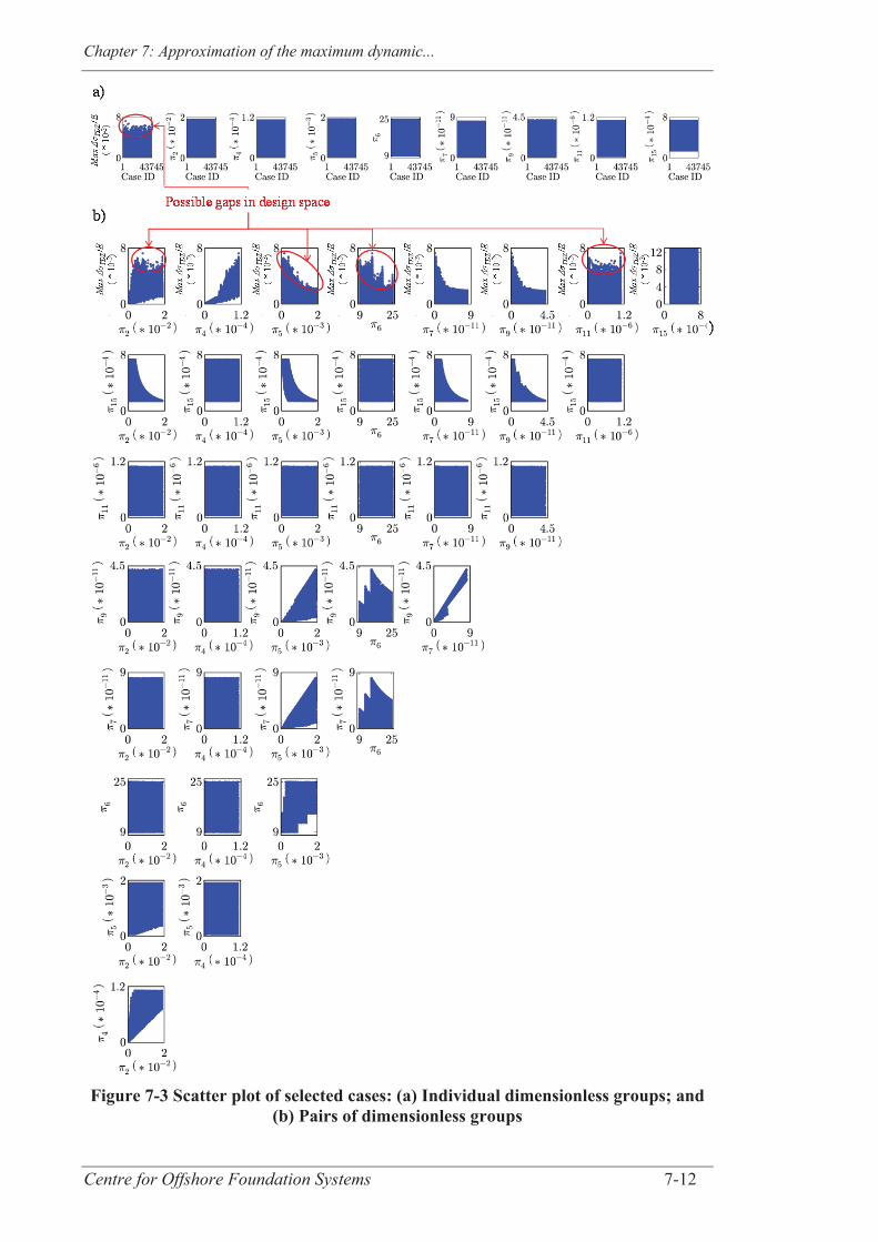
Chapter 7: Approximation of the maximum dynamic...
Centre for Offshore Foundation Systems 7-12
Figure 7-3 Scatter plot of selected cases: (a) Individual dimensionless groups; and (b) Pairs of dimensionless groups
Chapter 7: Approximation of the maximum dynamic...
Centre for Offshore Foundation Systems 7-13
7.3.3 Training and testing sets
The database needs to be divided into a training set and a testing set. The training set is
used to train the ANN and should contain all the information that needs to be captured
by the approximation while the testing set aims at evaluating the interpolation ability of
the defined approximation. Accepted practice is to use about two thirds of a database for
training and the remaining cases for testing (Hammerstrom, 1993; Shahin et al., 2004).
It was decided to use all of the cases of the full factorial design for training and select
additional cases in order to get similar statistical properties between the training and the
testing set. This is called a statistically consistent method and was used successfully for
the static study (Quéau et al., 2014b) and in other fields of application (e.g. Shahin et
al., 2004). It is important that the testing set gives a good representation of the overall
design space to obtain reliable results when evaluating the performance of the trained
ANN (otherwise some potential marginally inaccurate areas could be undetected). A
trial-and-error approach is used to get acceptable statistics for the two sets.
A total of 29,200 cases were used for training and 14,545 for testing, with the
characteristics of both sets summarised in Table 7-4. Extreme values of the input
dimensionless groups are presented for the two sets and differences in average values
and standard deviations are mainly small (despite a relatively large difference in
standard deviation for the soil stiffness ( 11)). Regarding the output, the statistics of the
testing set are similar to those of the training set, although extreme values are not
strictly matched.
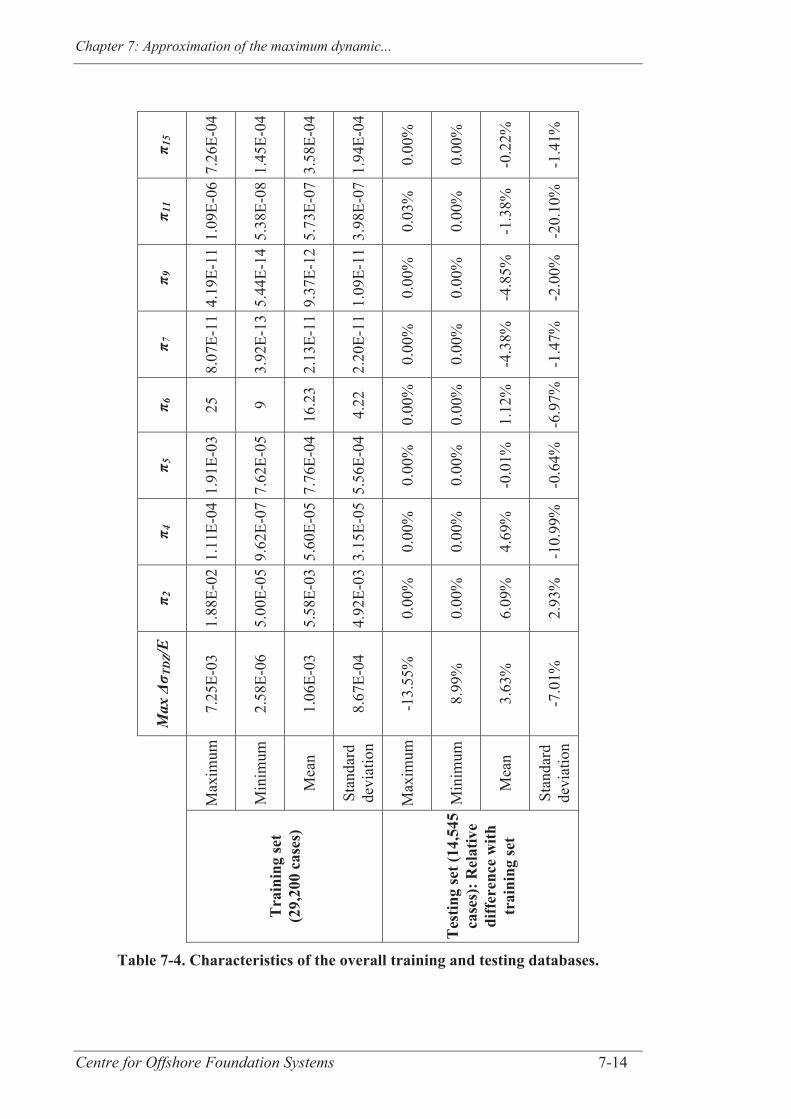
Chapter 7: Approximation of the maximum dynamic...
Centre for Offshore Foundation Systems 7-14
π 15
7.26
E-04
1.45
E-04
3.58
E-04
1.94
E-04
0.00
%
0.00
%
-0.2
2%
-1.4
1%
π 11
1.09
E-06
5.38
E-08
5.73
E-07
3.98
E-07
0.03
%
0.00
%
-1.3
8%
-20.
10%
π 9
4.19
E-11
5.44
E-14
9.37
E-12
1.09
E-11
0.00
%
0.00
%
-4.8
5%
-2.0
0%
π 7
8.07
E-11
3.92
E-13
2.13
E-11
2.20
E-11
0.00
%
0.00
%
-4.3
8%
-1.4
7%
π 6
25
9
16.2
3
4.22
0.00
%
0.00
%
1.12
%
-6.9
7%
π 5
1.91
E-03
7.62
E-05
7.76
E-04
5.56
E-04
0.00
%
0.00
%
-0.0
1%
-0.6
4%
π 4
1.11
E-04
9.62
E-07
5.60
E-05
3.15
E-05
0.00
%
0.00
%
4.69
%
-10.
99%
π 2
1.88
E-02
5.00
E-05
5.58
E-03
4.92
E-03
0.00
%
0.00
%
6.09
%
2.93
%
Max
Δσ T
DZ/
E
7.25
E-03
2.58
E-06
1.06
E-03
8.67
E-04
-13.
55%
8.99
%
3.63
%
-7.0
1%
Max
imum
Min
imum
Mea
n
Stan
dard
de
viat
ion
Max
imum
Min
imum
Mea
n
Stan
dard
de
viat
ion
Tra
inin
g se
t (2
9,20
0 ca
ses)
Tes
ting
set (
14,5
45
case
s): R
elat
ive
diff
eren
ce w
ith
trai
ning
set
Table 7-4. Characteristics of the overall training and testing databases.

Chapter 7: Approximation of the maximum dynamic...
Centre for Offshore Foundation Systems 7-15
7.4 DEVELOPMENT OF AN APPROXIMATION OF THE
MAXIMUM STRESS RANGE USING THE INITIAL DATABASE
7.4.1 Selected architecture for the approximation
The ANN development tool implemented in modeFRONTIER, as used when
developing an approximation of the critical static stress range (Quéau et al., 2014b), is
used here by default. It is based on a one-hidden layer Levenberg-Marquardt back-
propagation neural network with a maximum number of neurons in the hidden layer of
100. In the static study (Quéau et al., 2014b), some of the ranges of the dimensionless
groups were subdivided into smaller ranges to improve the level of accuracy of the
resulting ANNs. The same approach was followed for the dynamic cases here as, at
first, a single ANN was trained for the overall database, but the accuracy of the resulting
approximation (Approximation 1), was insufficient.
The results of the various attempts are reported in Table 7-5; they allow identification of
the parts of the design space that need further attention. At this stage, the selected
indicators of performance for the developed ANNs are: (i) the extreme values of their
relative errors with the results obtained from OrcaFlex simulations for the training and
testing sets; and (ii) the proportion of cases within 5% relative errors. Due to the large
range of relative errors obtained with Approximation 1, Approximation 2 was defined
by training three ANNs for the groups of cases within each of the three selected ranges
of z, leading to various ranges for HO (low: 400 m ≤ z < 950 m, medium:
950 m ≤ z < 1,500 m and high: 1,500 m ≤ z ≤ 2,000 m). The cases from the training
and testing sets falling within these three intervals of z were used to train and test the
three new ANNs.
Most of the input dimensionless groups depend on z, which is why it was selected for
an initial division of the design space. Approximation 2 was an improvement compared
with Approximation 1 but yet did not reach sufficient accuracy. Further divisions were
Chapter 7: Approximation of the maximum dynamic...
Centre for Offshore Foundation Systems 7-16
added within each of the three groups defined for Approximation 2, this time depending
on the value of the riser displacement ( 2) to form Approximation 3. Cases were
separated into two groups at the middle of the appropriate intervals of variation of 2
(i.e. lower and upper half of 2 depending on the range of z) leading to six ANNs. An
additional division at one-eighth of the appropriate ranges of 2 was made in
Approximation 4, which is formed by nine ANNs and has a similar structure as the final
approximation defined for the static cases (‘9-ANNs static approximation’ in Quéau et
al. (2014b)). Approximations 3 and 4 showed that, regardless of the value of z, the
accuracy of the fit improved with the increase of 2, but yet the accuracy for the low
values of 2 was insufficient. Further subdivisions on 2 values where attempted but did
not lead to better results.
To explore the performance of other subdivisions, another strategy was used for
Approximations 5 and 6, which have the same structure as Approximations 3 and 4
respectively but with subdivisions based on the value of the imposed displacement
velocity ( 4) due to its fundamental role for the dynamic cases. This approach did not
offer better performance and led to over fitting some areas of the design space. Over
fitting happens when an ANN can accurately predict the results for the training set but
cannot interpolate correctly; it is not able to generalise from the trends given by the
training set and thus offers poor performance for the testing set. This could arise from
the use of too many neurons in the hidden layer or from poor quality of the data used for
training.
Both of the more advanced approximations using nine ANNs therefore needed further
refinements. It was chosen to try to refine Approximation 4 in order to get a similar
architecture as for the approximation developed for the static cases (Quéau et al.,
2014b).

Chapter 7: Approximation of the maximum dynamic...
Centre for Offshore Foundation Systems 7-17
Tes
ting
Prop
ortio
n of
cas
es w
ith
erro
rs w
ithin
±5
%
79%
86%
76
%
76%
77
%
99%
70
%
64%
78
%
79%
23
%
87%
99
%
29%
76%
64%
31
%
77%
79
%
Rel
ativ
e di
ffer
ence
w
ith O
rcaF
lex
resu
lts
Min
imum
-487
%
-73%
-1
31%
-2
73%
-7
2%
-14%
-1
33%
-5
7%
-233
%
-35%
-1
95%
-4
3%
-14%
-3
55%
-35%
-57%
-2
65%
-3
1%
-35%
Max
imum
952%
503%
93
1%
415%
36
6%
32%
50
7%
56%
17
8%
30%
64
7%
53%
32
%
1281
%
44%
56%
29
3%
38%
30
%
Tra
inin
g
Prop
ortio
n of
cas
es w
ith
erro
rs w
ithin
±5
%
72%
83%
73
%
74%
75
%
100%
72
%
95%
81
%
96%
58
%
90%
10
0%
79%
89%
95%
81
%
96%
96
%
Rel
ativ
e di
ffer
ence
w
ith O
rcaF
lex
resu
lts
Min
imum
-185
0%
-622
%
-447
%
-623
%
-701
%
-5%
-7
38%
-1
4%
-195
%
-29%
-5
17%
-3
5%
-5%
-1
50%
-23%
-14%
-9
0%
-36%
-2
9%
Max
imum
2015
%
1001
%
712%
83
0%
1099
%
4%
757%
14
%
404%
38
%
694%
37
%
4%
185%
22%
14%
15
6%
13%
38
%
Reg
ion
of th
e de
sign
spac
e
Entir
e de
sign
spac
e
Low
z (
400
m ≤
z <
950
m)
Med
ium
z (
950
m ≤
z <
150
0 m
) H
igh
z (15
00 m
≤
z 2
000
m)
Low
z,
Low
er h
alf
2 Lo
w
z, H
ighe
r hal
f 2
Med
ium
z,
Low
er h
alf
2 M
ediu
m
z, H
ighe
r hal
f 2
Hig
h z,
Low
er h
alf
2 H
igh
z, H
ighe
r hal
f 2
Low
z,
Low
er 1
/8
2 Lo
w
z, R
emai
ning
low
er h
alf
2 Lo
w
z, H
ighe
r hal
f 2
Med
ium
z,
Low
er 1
/8
2 M
ediu
m
z, R
emai
ning
low
er h
alf
2 M
ediu
m
z, H
ighe
r hal
f 2
Hig
h z,
Low
er 1
/8
2 H
igh
z, R
emai
ning
low
er h
alf
2 H
igh
z, H
ighe
r hal
f 2
Num
ber
AN
N
1 3 6 9
Com
men
t
Ove
rall
data
base
z spl
it 3
way
s
z spl
it 3
way
s, su
bseq
uent
2
split
2
way
s
z spl
it 3
way
s, su
bseq
uent
2 s
plit
3 w
ays
App
roxi
mat
ion
1 2 3 4
Table 7-5. Performance of the various attempted approximations of Max ΔσTDZ/E.
Chapter 7: Approximation of the maximum dynamic...
Centre for Offshore Foundation Systems 7-18
38%
96%
36%
82%
41%
86%
9%
28%
96%
8%
11%
82%
13
%
21%
86%
-122
%
-27%
-451
%
-35%
-141
%
-35%
-337
%
-107
%
-27%
-142
6%
-303
%
-35%
-4
67%
-133
%
-35%
540%
25%
2177
%
59%
291%
32%
1496
%
159%
25%
1751
%
185%
59%
78
9%
77%
32%
66%
97%
85%
86%
87%
91%
69%
100%
97%
92%
100%
86%
92
%
100%
91%
-508
%
-19%
-137
%
-39%
-73%
-31%
-254
%
-5%
-19%
-42%
-2%
-39%
-6
0%
-1%
-31%
421%
29%
105%
30%
166%
26%
282%
5%
29%
66%
3%
30%
50
%
5%
26%
Low
z,
Low
er h
alf
4
Low
z,
Hig
her h
alf
4
Med
ium
z,
Low
er h
alf
4
Med
ium
z,
Hig
her h
alf
4
Hig
h z,
Low
er h
alf
4
Hig
h z,
Hig
her h
alf
4
Low
z,
Low
er 1
/8
4
Low
z,
Rem
aini
ng lo
wer
hal
f 4
Low
z,
Hig
her h
alf
4
Med
ium
z,
Low
er 1
/8
4 M
ediu
m
z, R
emai
ning
low
er h
alf
4 M
ediu
m
z, H
ighe
r hal
f 4
Hig
h z,
Low
er 1
/8
4
Hig
h z,
Rem
aini
ng lo
wer
hal
f 4
Hig
h z,
Hig
her h
alf
4
6 9
z spl
it 3
way
s, su
bseq
uent
4
split
2
way
s
z spl
it 3
way
s, su
bseq
uent
4
split
3
way
s
5 6
Table 7-5 (Continued)

Chapter 7: Approximation of the maximum dynamic...
Centre for Offshore Foundation Systems 7-19
7.4.2 Refinement of ANNs inherent to Approximation 4
In view of the performance of Approximation 4 in Table 7-5, the subspaces at the
lowest end of the riser displacement ( 2) intervals for each range of z were the prime
target for refinement as they presented the poorest performances. MATLAB (2012) was
used for refinement as it offers more freedom than modeFRONTIER in the choice of
ANN type and architecture. For instance, using MATLAB it is possible to test the effect
of an addition of one or several hidden layers to the ANN architecture, a feature not
available in modeFRONTIER. The number of neurons was varied following a trial-and-
error approach to find an optimum solution. The number of hidden layers was also
varied but it was shown not to improve the performance of the approximations.
The best results were achieved by using only one hidden layer (as used by default
originally), 50 neurons for the ANNs used for the lowest intervals of 2 for the low and
medium range of z and 20 neurons for the lowest intervals of 2 for the high range of
z. However, it was necessary to exclude the very low 2 values (representing very
small motion amplitudes as a proportion of the water depth) from the range of
application of the ANNs where high discrepancies between OrcaFlex and the
approximation were found in the training and in the testing set. This was the case for
2 ≤ 6.88E-4 for the low range of z, 2 ≤ 1.89E-4 for the medium range of z and for
2 ≤ 1.27E-4 for the high range of z. (These values correspond to the lowest 1/32nd of
the overall selected range of variation for 2 for the low range of z and the lowest
1/64th of the overall selected range of variation for 2 for the medium and high ranges of
z.) These values were however used for training the ANNs as excluding them from the
training set decreased the performances on the rest of the selected ranges of 2.
The refined Approximation 4 has the architecture presented in Figure 7-4 and introduces
the notations for the ANNs. ANN1 corresponds to the ANN having 50 neurons in its
hidden layer and developed for the region of the design space indicated as ‘Low z,
Chapter 7: Approximation of the maximum dynamic...
Centre for Offshore Foundation Systems 7-20
Lower 1/8 2’ in Table 7-5. ANN2 and ANN3 both have the default number of neurons
in their hidden layer (i.e. 100) and correspond respectively to the regions of the design
space indicated as ‘Low z, Remaining lower half 2’ and ‘Low z, Higher half 2’ in
Table 7-5. ANN4, ANN5 and ANN6 are the homologues of ANN1, ANN2 and ANN3
respectively in the selected medium range of water depth as are ANN7, ANN8 and
ANN9 in the selected high range of water depth. When using this approximation, it
takes only a couple of minutes to get an evaluation of Max TDZ/E for the entire
database (by contrast with the four months of calculation taken for the creation of the
database with numerical analyses).

Chapter 7: Approximation of the maximum dynamic...
Centre for Offshore Foundation Systems 7-21
Figure 7-4 Structure of the 9-ANNs dynamic approximation
2 ,
3, 4,
5 ,
6 ,
7 ,
8, 9
,10
,11
,12
,13
, 14
, 15
, E, g
, st
eel ,
wat
er
400
* (g
st
eel/
E) ≤
15
<95
0 *
(g
stee
l/ E
)O
r15
= 9
50 *
(g
stee
l/ E
) and
H
O≥
17 ° 15 <
1500
* (g
st
eel/
E)
Or
15 =
150
0 *
(g
stee
l/ E
) and
H
O≥
9 °
Yes
No
2 9
.43E
-3
2 2
.44E
-3
AN
N1
(50
neur
ons
in h
idde
n la
yer)
AN
N3
(100
neu
rons
in
hid
den
laye
r)
2 3
.98E
-3
2 1
.05E
-3
AN
N6
(100
neu
rons
in
hid
den
laye
r)
AN
N2
(100
neu
rons
in
hid
den
laye
r)
AN
N4
(50
neur
ons
in h
idde
n la
yer)
AN
N5
(100
neu
rons
in
hid
den
laye
r)
2 2
.53E
-3
2 6
.69E
-4
AN
N7
(20
neur
ons
in h
idde
n la
yer)
AN
N9
(100
neu
rons
in
hid
den
laye
r)
AN
N8
(100
neu
rons
in
hid
den
laye
r)
Yes
No
Yes
No
Yes
No
Yes
No
Yes
No
Yes
No
Yes
No
Appr
oxim
atio
n of
Max
TD
Z /E
1.05
e-4
2 1
.88e
-2
6.67
e-5
2 7
.89e
-35.
00e-
5 2
5.0
0 e-
3
5.00
e-5
2 7
.89e
-3
N/A
2 6
.88E
-4
Yes
No
2 1
.89E
-42
1.2
7E-4
Yes
No
Yes
No
N/A
N/A
Chapter 7: Approximation of the maximum dynamic...
Centre for Offshore Foundation Systems 7-22
7.4.3 Performance of Approximation 4
The individual performances of each of the inherent ANNs are illustrated in Table 7-6,
using notations introduced in Figure 7-4 while the performance of the overall
approximation is presented in Table 7-7. The root mean squared errors (RMSE) and
mean absolute errors (MAE) are evaluated too as a further indication of the performance
of the ANNs. For the testing set, the RMSE and MAE are low and there are ~ 96 % and
~ 80 % of the cases within 15 % and 5 % relative difference with OrcaFlex results
respectively. The defined ANNs forming Approximation 4 therefore provide a good
basis for a first approximation as part of this pilot study since, despite some marginal
high values of relative differences within some ANNs, a large proportion of the cases of
the database are within a negligible range of error.
7.5 REFINEMENT OF THE APPROXIMATION FOR PART OF THE
DESIGN SPACE BY EXPANDING THE DATABASE
The focus is now brought to part of the design space where some of the marginally high
relative differences between estimated and OrcaFlex stress range results were observed.
Additional cases were added to the initial database in this part of the design space to
explore the effect of refining the database on improvement of the ANN approximation,
prior to testing its accuracy on fatigue predictions. The refinement is applied only on the
part of the design space initially targeted by ANN4 (i.e. without the limit on 2), which
corresponds to 950 m ≤ z < 1,500 m, 9° ≤ HO ≤ 17° and 6.67E-5 ≤ 2 ≤ 1.05E-3. This
is an arbitrary choice based on (a) the fact that z was set to 982 m in the SCR base case
used by the authors (Quéau et al., 2011, 2013), corresponding to the medium range of
selected z and (b) that, within this range of z, the area corresponding to
6.67E-5 ≤ 2 ≤ 1.05E-3 presented the least accurate results. The initial database
comprised 2,338 cases in this part of the design space.
Chapter 7: Approximation of the maximum dynamic...
Centre for Offshore Foundation Systems 7-23
Tra
inin
g se
t
AN
N9
2.48
E-03
37.5
4%
-28.
53%
0.07
%
1.72
%
95.8
8%
99.1
9%
99.6
9%
AN
N8
2.10
E-03
13.2
7%
-35.
98%
0.06
%
1.58
%
96.1
3%
99.5
2%
99.8
2%
AN
N71
1.12
E-03
27.8
0%
-35.
25%
0.23
%
3.39
%
78.2
3%
95.8
1%
98.6
3%
AN
N6
8.57
E-04
13.9
6%
-14.
37%
0.06
%
1.82
%
94.9
2%
99.7
3%
99.7
3%
AN
N5
1.58
E-03
22.4
2%
-22.
72%
0.13
%
2.46
%
88.5
9%
97.7
9%
99.1
8%
AN
N41
2.44
E-03
88.0
1%
-47.
72%
0.43
%
3.97
%
74.3
0%
91.3
7%
97.3
6%
AN
N3
1.23
E-04
4.33
%
-4.8
4%
0.00
%
0.39
%
100.
00%
100.
00%
100.
00%
AN
N2
2.22
E-03
36.8
1%
-34.
73%
0.15
%
2.31
%
89.6
4%
96.7
4%
98.7
1%
AN
N11
1.37
E-02
124.
83%
-40.
44%
1.61
%
7.11
%
60.6
8%
80.0
6%
87.4
5%
1- C
orre
latio
n, 1
-r
Max
imum
Min
imum
RM
SE
MA
E
±5%
±10%
±15%
Rel
ativ
e di
ffer
ence
w
ith O
rcaF
lex
resu
lts
Prop
ortio
n of
cas
es
with
err
ors w
ithin
:
1 (with introduced limit on the value of π2).
Table 7-6. Performance of the ANNs forming the final approximation of Max ΔσTDZ/E.
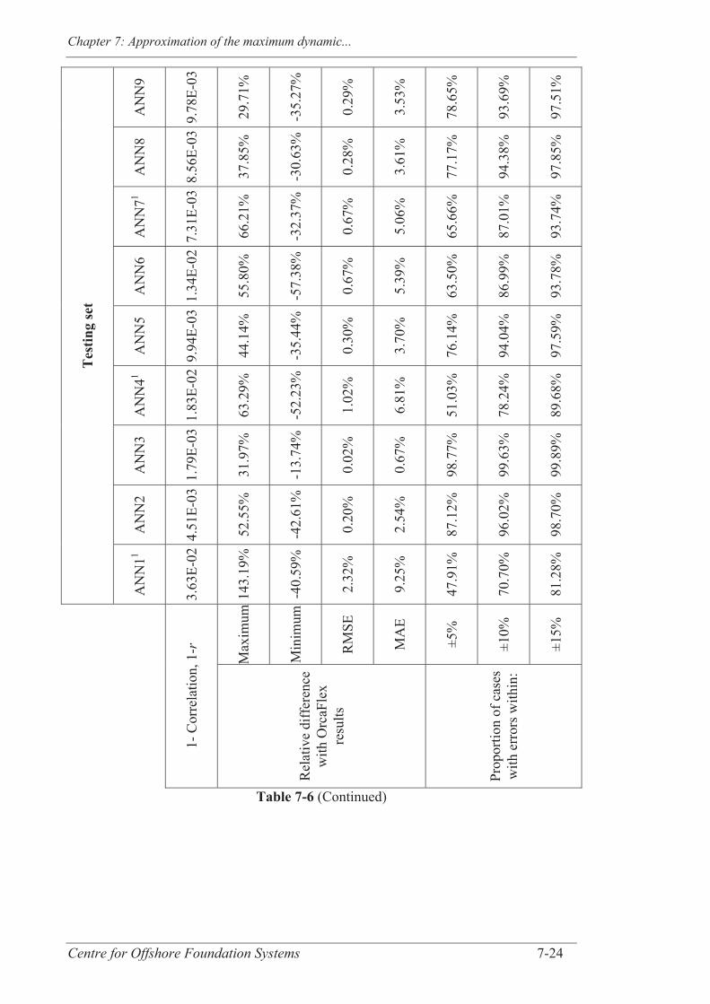
Chapter 7: Approximation of the maximum dynamic...
Centre for Offshore Foundation Systems 7-24
Tes
ting
set
AN
N9
9.78
E-03
29.7
1%
-35.
27%
0.29
%
3.53
%
78.6
5%
93.6
9%
97.5
1%
AN
N8
8.56
E-03
37.8
5%
-30.
63%
0.28
%
3.61
%
77.1
7%
94.3
8%
97.8
5%
AN
N71
7.31
E-03
66.2
1%
-32.
37%
0.67
%
5.06
%
65.6
6%
87.0
1%
93.7
4%
AN
N6
1.34
E-02
55.8
0%
-57.
38%
0.67
%
5.39
%
63.5
0%
86.9
9%
93.7
8%
AN
N5
9.94
E-03
44.1
4%
-35.
44%
0.30
%
3.70
%
76.1
4%
94.0
4%
97.5
9%
AN
N41
1.83
E-02
63.2
9%
-52.
23%
1.02
%
6.81
%
51.0
3%
78.2
4%
89.6
8%
AN
N3
1.79
E-03
31.9
7%
-13.
74%
0.02
%
0.67
%
98.7
7%
99.6
3%
99.8
9%
AN
N2
4.51
E-03
52.5
5%
-42.
61%
0.20
%
2.54
%
87.1
2%
96.0
2%
98.7
0%
AN
N11
3.63
E-02
143.
19%
-40.
59%
2.32
%
9.25
%
47.9
1%
70.7
0%
81.2
8%
1- C
orre
latio
n, 1
-r
Max
imum
Min
imum
RM
SE
MA
E
±5%
±10%
±15%
Rel
ativ
e di
ffer
ence
w
ith O
rcaF
lex
resu
lts
Prop
ortio
n of
cas
es
with
err
ors w
ithin
:
Table 7-6 (Continued)

Chapter 7: Approximation of the maximum dynamic...
Centre for Offshore Foundation Systems 7-25
Training set Testing set 1- Correlation, 1-r 1.12E-03 4.26E-03
Relative difference with OrcaFlex results:
Maximum 124.83% 143.19% Minimum -47.72% -57.38%
RMSE 0.20% 0.40% MAE 2.14% 3.32%
Proportion of cases with errors within:
±5% 90.54% 80.40% ±10% 97.02% 93.00% ±15% 98.60% 96.67%
Table 7-7. Performance of the final approximation of Max ΔσTDZ/E on the overall design space (accounting for the introduced limits on the value of π2).
7.5.1 Detailed analysis of the initial database on the selected part of the
design space
Two strategies were implemented to select the additional cases and extend the database.
On the one hand the training set size was increased to capture the relationships better
between the input dimensionless groups and the output; on the other hand, more cases
were added to the testing set to match the statistics of the training set defined in this part
of the design space, and improve the assessment of the interpolation ability of the
trained ANN. (The statistically consistent approach was used for the overall training and
testing sets and therefore does not necessarily guarantee similar statistical consistency
for the training and testing sets formed by the subsequent divisions of the design space,
depending on the value of the riser displacement ( 2) and water depth ( 15).)
Plots shown in Figure 7-5 were used to assist the selection of the additional cases. The
blue parts of Figure 7-5 represent the cases of the current database in this reduced part
of the overall design space whereas the red parts illustrate the additional cases, as
discussed in Section 7.5.2. Plots are similar to those in Figure 7-3, with the diagrams in
Figure 7-5a representing values of either the output or a particular input dimensionless
group for each case, and in Figure 7-5b the output value for each value of the various
input dimensionless groups, or pairs of values of different input dimensionless groups,
within the reduced part of the overall design space.
Chapter 7: Approximation of the maximum dynamic...
Centre for Offshore Foundation Systems 7-26
Figure 7-5a shows that the ranges of the input dimensionless groups are not always
covered homogenously, for instance more cases simulating values within the higher end
of the ranges for the riser submerged weight ( 7) and the riser tension ( 9) could be
added for a better accuracy since isolated high values of 7 and 9 were detected. It is
(trivially) an easier task to map the input design space appropriately than the output
space and Figure 7-5b gives a further indication on the location of the ‘gaps’ within the
part of the design space under study. For instance, the soil stiffness ( 11) is completely
independent from any of the other input dimensionless group, which means that, ideally,
the scatters should cover a rectangular shaped area in each of the subplots representing
the choice of soil stiffness in conjunction with another input dimensionless group.
Additional cases in the highest end of the ranges of the riser submerged weight ( 7) and
the riser tension ( 9) for the entire range of soil stiffness ( 11), or in the highest end of
the ranges of the riser velocity ( 4) and the riser outside diameter ( 5) for the entire
range of soil stiffness, could hence be defined to enhance performance. Similarly, the
riser velocity is independent from all the other input dimensionless groups with the
exception of the riser displacement ( 2) and therefore the subspaces formed by the level
of the riser velocity and any other dimensionless groups (other than 2) should have a
rectangular shaped area too to improve the quality of the database; and so on by
considering the other pairs of dimensionless groups. These observations provide a first
basis for the selection of additional cases.
The quality of the training and testing set in this part of the design space was then
investigated to refine further the database and the performance of the subsequent
approximation. A detailed analysis of the cases from the training and testing databases
for the selected part of the design space is performed in Table 7-8. The table shows that
1,727 cases were selected for training and 611 for testing. The statistics of the training
and testing sets are compared, revealing target areas for improvements. For example,
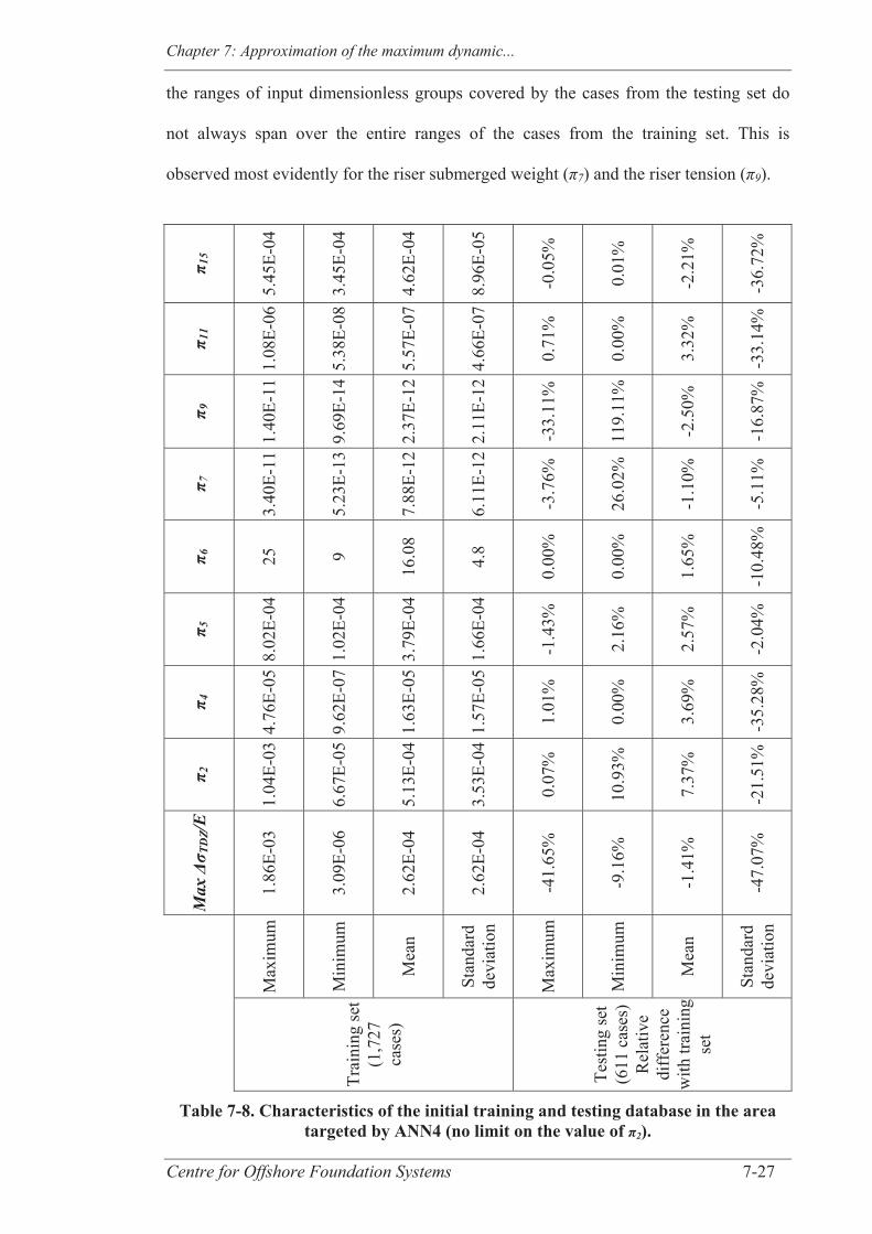
Chapter 7: Approximation of the maximum dynamic...
Centre for Offshore Foundation Systems 7-27
the ranges of input dimensionless groups covered by the cases from the testing set do
not always span over the entire ranges of the cases from the training set. This is
observed most evidently for the riser submerged weight ( 7) and the riser tension ( 9).
π 1
5
5.45
E-04
3.45
E-04
4.62
E-04
8.96
E-05
-0.0
5%
0.01
%
-2.2
1%
-36.
72%
π 11
1.08
E-06
5.38
E-08
5.57
E-07
4.66
E-07
0.71
%
0.00
%
3.32
%
-33.
14%
π 9
1.40
E-11
9.69
E-14
2.37
E-12
2.11
E-12
-33.
11%
119.
11%
-2.5
0%
-16.
87%
π 7
3.40
E-11
5.23
E-13
7.88
E-12
6.11
E-12
-3.7
6%
26.0
2%
-1.1
0%
-5.1
1%
π 6
25
9
16.0
8
4.8
0.00
%
0.00
%
1.65
%
-10.
48%
π 5
8.02
E-04
1.02
E-04
3.79
E-04
1.66
E-04
-1.4
3%
2.16
%
2.57
%
-2.0
4%
π 4
4.76
E-05
9.62
E-07
1.63
E-05
1.57
E-05
1.01
%
0.00
%
3.69
%
-35.
28%
π 2
1.04
E-03
6.67
E-05
5.13
E-04
3.53
E-04
0.07
%
10.9
3%
7.37
%
-21.
51%
Max
Δσ T
DZ/
E
1.86
E-03
3.09
E-06
2.62
E-04
2.62
E-04
-41.
65%
-9.1
6%
-1.4
1%
-47.
07%
Max
imum
Min
imum
Mea
n
Stan
dard
de
viat
ion
Max
imum
Min
imum
Mea
n
Stan
dard
de
viat
ion
Trai
ning
set
(1,7
27
case
s)
Test
ing
set
(611
cas
es)
Rel
ativ
e di
ffer
ence
w
ith tr
aini
ng
set
Table 7-8. Characteristics of the initial training and testing database in the area targeted by ANN4 (no limit on the value of π2).
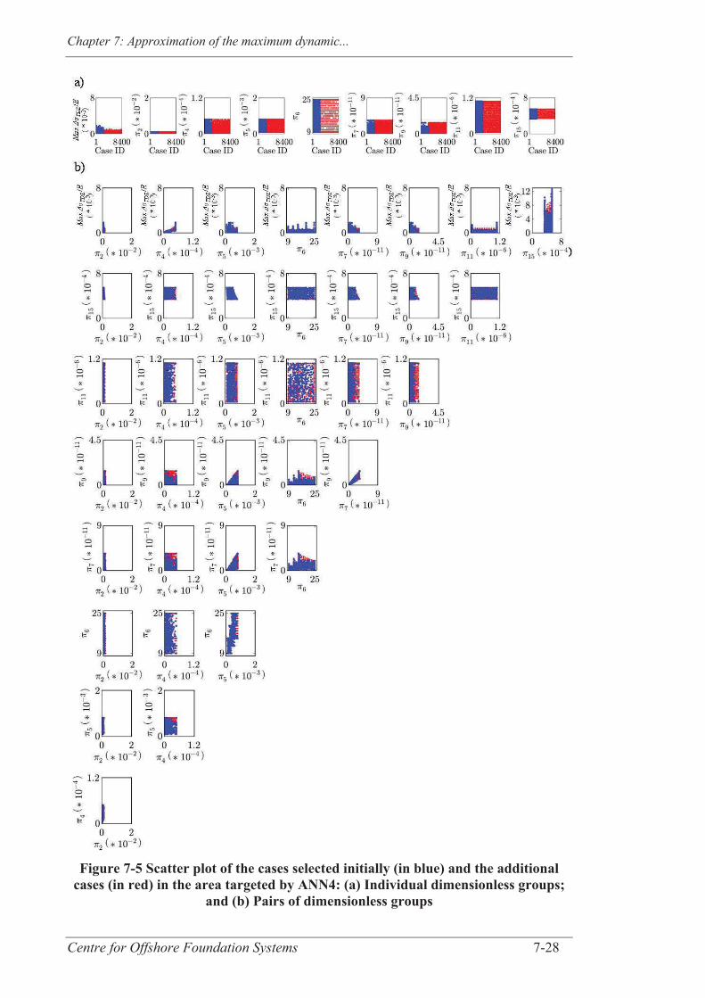
Chapter 7: Approximation of the maximum dynamic...
Centre for Offshore Foundation Systems 7-28
Figure 7-5 Scatter plot of the cases selected initially (in blue) and the additional cases (in red) in the area targeted by ANN4: (a) Individual dimensionless groups;
and (b) Pairs of dimensionless groups
Chapter 7: Approximation of the maximum dynamic...
Centre for Offshore Foundation Systems 7-29
7.5.2 Improved database characteristics
The original database of 2,338 cases in the selected part of the design space was
extended to 8,377 cases, with 5,797 for training and 2,580 for testing. The additional
cases were established based on the observed gaps in the design space with Figure 7-5
showing the scatter plot of the values of the input dimensionless groups and output for
the extended database. In Figure 7-5b, the cases of the initial database (in blue) are
represented on top of the cases of the extended database (in red) to highlight the gaps
that the new cases are now filling.
The allocation of cases to the training or the testing set was performed following a trial-
and-error approach aiming to obtain similar statistics between both improved sets, as
per the approach applied for the overall design space. Table 7-9 summarises the results
obtained with the larger database in the selected part of the design space. The improved
training and testing set now have similar statistics, especially for the input design space,
and have the potential to improve further the quality of the proposed approximation.
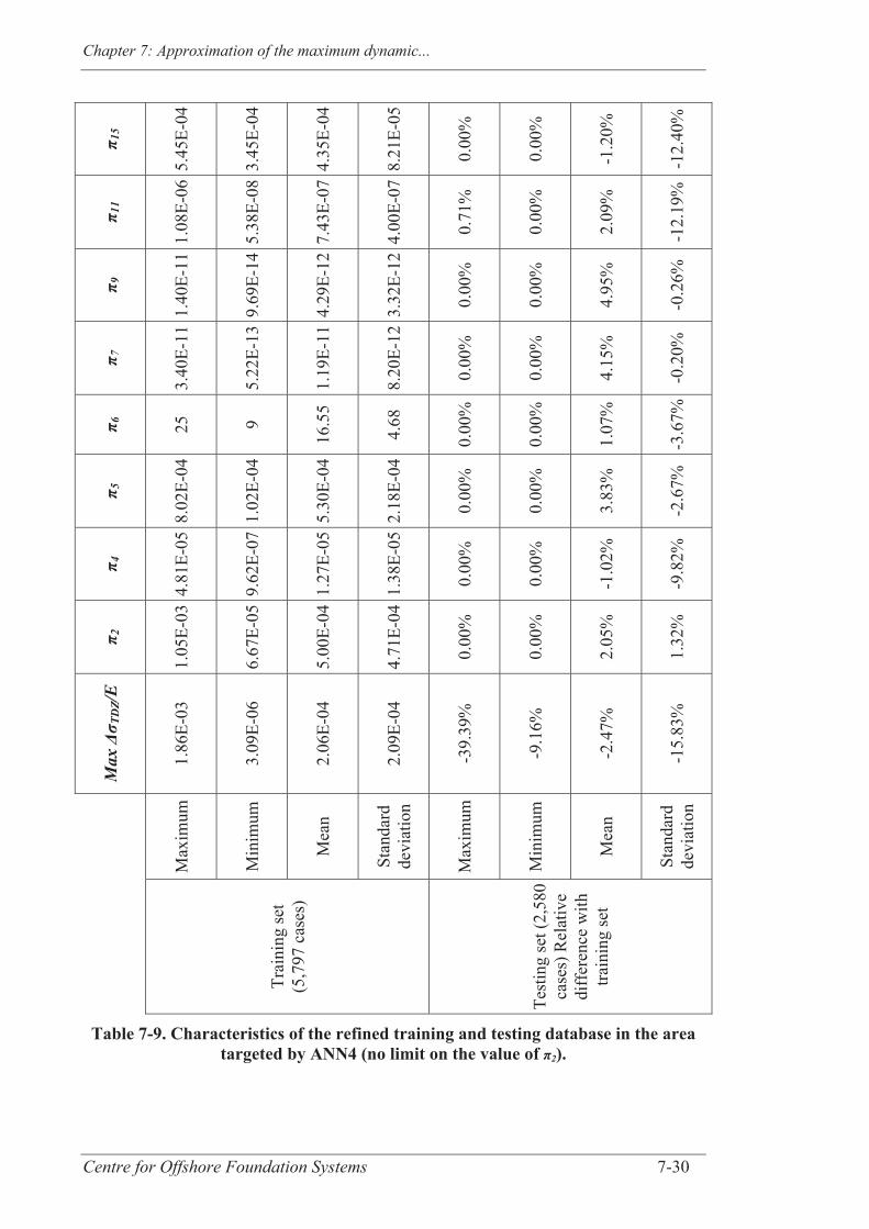
Chapter 7: Approximation of the maximum dynamic...
Centre for Offshore Foundation Systems 7-30
π 1
5
5.45
E-04
3.45
E-04
4.35
E-04
8.21
E-05
0.00
%
0.00
%
-1.2
0%
-12.
40%
π 11
1.08
E-06
5.38
E-08
7.43
E-07
4.00
E-07
0.71
%
0.00
%
2.09
%
-12.
19%
π 9
1.40
E-11
9.69
E-14
4.29
E-12
3.32
E-12
0.00
%
0.00
%
4.95
%
-0.2
6%
π 7
3.40
E-11
5.22
E-13
1.19
E-11
8.20
E-12
0.00
%
0.00
%
4.15
%
-0.2
0%
π 6
25
9
16.5
5
4.68
0.00
%
0.00
%
1.07
%
-3.6
7%
π 5
8.02
E-04
1.02
E-04
5.30
E-04
2.18
E-04
0.00
%
0.00
%
3.83
%
-2.6
7%
π 4
4.81
E-05
9.62
E-07
1.27
E-05
1.38
E-05
0.00
%
0.00
%
-1.0
2%
-9.8
2%
π 2
1.05
E-03
6.67
E-05
5.00
E-04
4.71
E-04
0.00
%
0.00
%
2.05
%
1.32
%
Max
Δσ T
DZ/
E
1.86
E-03
3.09
E-06
2.06
E-04
2.09
E-04
-39.
39%
-9.1
6%
-2.4
7%
-15.
83%
Max
imum
Min
imum
Mea
n
Stan
dard
de
viat
ion
Max
imum
Min
imum
Mea
n
Stan
dard
de
viat
ion
Trai
ning
set
(5,7
97 c
ases
)
Test
ing
set (
2,58
0 ca
ses)
Rel
ativ
e di
ffer
ence
with
tra
inin
g se
t
Table 7-9. Characteristics of the refined training and testing database in the area targeted by ANN4 (no limit on the value of π2).
Chapter 7: Approximation of the maximum dynamic...
Centre for Offshore Foundation Systems 7-31
7.5.3 New approximation on this part of the design space
A new ANN, referred to as ANN4*, was trained and tested using the improved training
and testing sets. As for ANN4, it was trained in MATLAB and comprised one hidden
layer with 50 neurons. The limit on the value of the riser displacement ( 2) was re-
introduced at this stage to be consistent with ANN4 allowing their performances to be
compared appropriately. Only cases with values of 2 higher than 1.89E-4 (and less than
1.05E-3) are therefore considered here. The performance of ANN4* is assessed using
the results shown in Table 7-10, where the new testing set was also used with ANN4 to
enhance comparison between ANN4 and ANN4*.
The quality of the results shown in Table 7-10 for ANN4 has decreased compared with
the results presented in Table 7-6, and Table 7-10 shows that some high differences
with OrcaFlex results on the value of Max TDZ/E were not captured when using the
initial testing set. This emphasises the significance of the choice of cases for the testing
set.
ANN4* is indeed found to be a better approximation than ANN4, offering better
correlation, reduced interval of relative difference and higher number of cases within
low range of relative differences with OrcaFlex results, confirming that the steps
undertaken in Sections 7.5.1 and 7.5.2 have contributed to refining the quality of the
approximation in this part of the design space.
The current best approximation, namely “9-ANNs dynamic approximation”, has
therefore the structure presented in Figure 7-4 with ANN4* in place of ANN42. Even
though the accuracy of the 9-ANNs dynamic approximation does not reach the original
criterion of errors within 5% of errors for the entire design space, the benefits of the
approach for practical purposes (i.e. fatigue life predictions) is investigated next.
2 The 9-ANNs dynamic approximation can be provided as a standalone application by contacting the
corresponding author.

Chapter 7: Approximation of the maximum dynamic...
Centre for Offshore Foundation Systems 7-32
ANN4* ANN4
Refined training set Refined testing set Refined testing set
1- Correlation, 1-r 1.96E-03 5.85E-03 8.54E-02
Relative difference with
OrcaFlex results:
Maximum 207.86% 129.31% 314.42% Minimum -45.02% -61.48% -86.15%
RMSE 0.68% 0.94% 7.07% MAE 3.96% 5.10% 15.51%
Proportion of cases with
errors within:
±5% 77.75% 71.84% 34.01% ±10% 92.40% 88.04% 56.18% ±15% 95.99% 93.41% 68.48%
Table 7-10. Performance of ANN4* (with the same limit on the value of π2 than for ANN4).
7.6 APPLICATION OF THE FRAMEWORK IN FATIGUE DESIGN
CASE STUDIES
The current best approximation (9-ANNs dynamic approximation) is now applied on a
series of case studies to assess its accuracy for prediction of fatigue life using a
deterministic approach (as appropriate for structural systems presenting nonlinearities
(Patel and Seyed, 2005)). In light of the refinements performed in Section 7.5, this
section focuses on the part of the design space corresponding to the selected medium
range of water depth (i.e. 950 m ≤ z < 1,500 m).
7.6.1 SCR configurations and loading conditions
The first case study, namely Base Case 1 (BC1), is performed with the usual SCR base
case used by the authors (as per BC1 in Quéau et al. (2013)). Its input parameters and
corresponding dimensionless groups are shown in Table 7-11. The base case is derived
from an in-service SCR connected to a semisubmersible in the Gulf of Mexico (GoM).
Four additional base cases, namely BC2, BC3, BC4 and BC5, were defined in order to
test the accuracy of the 9-ANNs dynamic approximation for different riser setups (i.e.
input data from different areas of the design space). The input parameters and
corresponding dimensionless groups of these base cases are also presented in Table
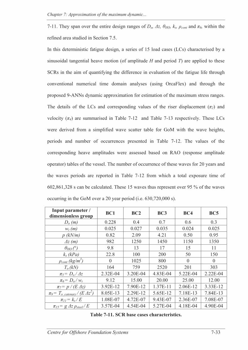
Chapter 7: Approximation of the maximum dynamic...
Centre for Offshore Foundation Systems 7-33
7-11. They span over the entire design ranges of Do, z, HO, ks, cont and 6, within the
refined area studied in Section 7.5.
In this deterministic fatigue design, a series of 15 load cases (LCs) characterised by a
sinusoidal tangential heave motion (of amplitude H and period T) are applied to these
SCRs in the aim of quantifying the difference in evaluation of the fatigue life through
conventional numerical time domain analyses (using OrcaFlex) and through the
proposed 9-ANNs dynamic approximation for estimation of the maximum stress ranges.
The details of the LCs and corresponding values of the riser displacement ( 2) and
velocity ( 4) are summarised in Table 7-12 and Table 7-13 respectively. These LCs
were derived from a simplified wave scatter table for GoM with the wave heights,
periods and number of occurrences presented in Table 7-12. The values of the
corresponding heave amplitudes were assessed based on RAO (response amplitude
operator) tables of the vessel. The number of occurrence of these waves for 20 years and
the waves periods are reported in Table 7-12 from which a total exposure time of
602,861,328 s can be calculated. These 15 waves thus represent over 95 % of the waves
occurring in the GoM over a 20 year period (i.e. 630,720,000 s).
Input parameter / dimensionless group BC1 BC2 BC3 BC4 BC5
Do (m) 0.228 0.4 0.7 0.6 0.3 wt (m) 0.025 0.027 0.035 0.024 0.025
p (kN/m) 0.82 2.09 4.21 0.50 0.95 z (m) 982 1250 1450 1150 1350 HO (°) 9.8 13 17 15 11
ks (kPa) 22.8 100 200 50 150 cont (kg/m3) 0 1025 800 0 0
To (kN) 164 759 2520 201 303 5 = Do / z 2.32E-04 3.20E-04 4.83E-04 5.22E-04 2.22E-04 6 = Do / wt 9.12 15.00 20.00 25.00 12.00
7 = p / (E z) 3.92E-12 7.90E-12 1.37E-11 2.06E-12 3.33E-12 9 = To_catenary / (E z2) 8.05E-13 2.29E-12 5.65E-12 7.18E-13 7.84E-13
11 = ks / E 1.08E-07 4.72E-07 9.43E-07 2.36E-07 7.08E-07 15 = g z steel / E 3.57E-04 4.54E-04 5.27E-04 4.18E-04 4.90E-04
Table 7-11. SCR base cases characteristics.

Chapter 7: Approximation of the maximum dynamic...
Centre for Offshore Foundation Systems 7-34
Load Case (LC)
Wave height (m)
Heave Amplitude
H (m)
Period T (s)
Number of occurrence
for 20 years
LC1 1 0.0043 3 156673082 LC2 1 0.15 8 10946661 LC3 1 0.25 13 1132827 LC4 1 0.39 18 305883 LC5 3 0.44 8 2795859 LC6 3 0.76 13 130073 LC7 3 1.17 18 16564 LC8 8 1.17 8 68228 LC9 13 1.91 8 2073
LC10 8 2.02 13 7409 LC11 8 3.12 18 607 LC12 13 3.29 13 647 LC13 18 4.55 13 92 LC14 13 5.06 18 47 LC15 18 7.01 18 4
3 Value of H outside of the selected range of displacement.
Table 7-12. Loading conditions for the case studies.
Load Case (LC)
π2= H / Δz π4=
HT
ρsteel E BC1 BC2 BC3 BC4 BC5
LC1 4.39E-06 3.45E-06 2.97E-06 3.75E-06 3.19E-06 2.76E-07 LC2 1.49E-04 1.17E-04 1.01E-04 1.27E-04 1.09E-04 3.53E-06 LC3 2.58E-04 2.02E-04 1.75E-04 2.20E-04 1.87E-04 3.75E-06 LC4 3.97E-04 3.12E-04 2.69E-04 3.39E-04 2.89E-04 4.16E-06 LC5 4.48E-04 3.52E-04 3.03E-04 3.82E-04 3.26E-04 1.06E-05 LC6 7.73E-04 6.07E-04 5.24E-04 6.60E-04 5.62E-04 1.12E-05 LC7 1.19E-03 9.35E-04 8.06E-04 1.02E-03 8.66E-04 1.25E-05 LC8 1.19E-03 9.38E-04 8.09E-04 1.02E-03 8.69E-04 2.82E-05 LC9 1.94E-03 1.52E-03 1.31E-03 1.66E-03 1.41E-03 4.58E-05
LC10 2.06E-03 1.62E-03 1.40E-03 1.76E-03 1.50E-03 3.00E-05 LC11 3.17E-03 2.49E-03 2.15E-03 2.71E-03 2.31E-03 3.33E-05 LC12 3.35E-03 2.63E-03 2.27E-03 2.86E-03 2.44E-03 4.87E-05 LC13 4.64E-03 3.64E-03 3.14E-03 3.96E-03 3.37E-03 6.74E-05 LC14 5.16E-03 4.05E-03 3.49E-03 4.40E-03 3.75E-03 5.41E-05 LC15 7.14E-03 5.61E-03 4.84E-03 6.10E-03 5.19E-03 7.50E-05
Table 7-13. Values of normalised displacement (π2) and velocity (π4) in the case studies.

Chapter 7: Approximation of the maximum dynamic...
Centre for Offshore Foundation Systems 7-35
7.6.2 Fatigue life evaluation
The dynamic time history analyses were carried out using OrcaFlex to assess the value
of Max TDZ for each of the LCs. The results are compared with the estimations from
the 9-ANNs dynamic approximation in Table 7-14. Some of the first LCs correspond to
small displacement amplitudes ( 2) which are outside the selected ranges and therefore
ANN4* was used in extrapolation for these LCs as indicated in Table 7-14. For the LCs
within the selected range of application of the 9-ANNs dynamic approximation, the
differences in stress range are small overall, ranging mainly from 0 % to 10 % relative
difference with marginal higher differences of up to 45% (e.g. LC4 in BC3).
Extrapolated stress range results vary in accuracy from 0% (for LC1 of BC3) relative
difference with OrcaFlex results up to 214% (for LC1 of BC4).
Based on the number of wave occurrences presented in Table 7-12, the fatigue damage
created by each of the LCs was calculated by using the D-type S-N curve for seawater
below (DNV-RP-C203, 2011)
Log10 (N) = 11.764 – 3 * log10 (Max TDZ) for N ≤ 106 cycles
Log10 (N) = 15.606 – 5 * log10 (Max TDZ) for N > 106 cycles(7-2)
Due to the nonlinear relationship between the stress range and the damage introduced
by the number of occurrences of the wave and number of allowable cycles, for some
cases small relative differences on Max TDZ can lead to high differences on damage
for an individual load case. This is observed, for instance, for LC6 in BC1 or LC5 in
BC4 where only -5% and 9% relative differences in Max TDZ respectively lead to
-21% and 52 % relative differences in the damage. As the fatigue life is the inverse of
the sum of the individual damage contribution for each LC, small errors in the estimated
Max TDZ for a load case that has a high contribution to the global damage can have a
high impact on the estimated fatigue life (e.g. for LC5 in BC4) and vice versa for a load
case that does not contribute much to the global damage (e.g. for LC1 in BC4).

Chapter 7: Approximation of the maximum dynamic...
Centre for Offshore Foundation Systems 7-36
However, the positive and negative errors in damage contribution from each load case
tend to balance out so that the total damage estimated shows much smaller error than
the individual components. In addition, the relative accuracy for the load cases that
dominate fatigue damage (typically LC5 to LC10) is generally much better than for the
small amplitude load cases.
The fatigue lives of the five BCs are calculated and results are summarised in Table
7-15. The estimated fatigue lives using 9-ANNs dynamic approximation are all
reasonably close to those calculated using conventional time history analysis using
OrcaFlex directly, thus demonstrating the benefits and usefulness of the ANN method.
All BCs have an estimated fatigue life within 16 % relative differences with the results
derived from OrcaFlex calculations, with most BCs within 10 % relative difference.
Based on the damage calculated from OrcaFlex stress range results, LC8 and LC5
correspond to the waves having the highest contributions to the global damage for all
BCs. The damage for LC5 was not as well estimated in BC4 than in the other base cases
(with a notable overestimation), which is why the fatigue life of BC4 approximated by
the ANN approach is less than the fatigue life calculated based on OrcaFlex results by a
larger amount than for the other base cases.
Using the 9-ANNs dynamic approximation, it takes less than 1 minute of calculation to
obtain the results presented in Table 7-15 (since the time taken to develop the
approximation by training the ANNs does not impact the final application time).
Although it is hard to estimate accurately the time necessary to obtain equivalent results
from OrcaFlex, since it will vary between users and on the available computer
resources, it could take about a day to pre-process the numerical models, simulate them
and post-process the results. The ANN approach therefore provides excellent efficiency
for estimation of fatigue life for different SCR configurations.

Chapter 7: Approximation of the maximum dynamic...
Centre for Offshore Foundation Systems 7-37
BC1 Max TDZ Damage (per year)
Comment Load Case (LC)
OrcaFlex results (kPa)
Relative difference of
approximated results
with OrcaFlex
From OrcaFlex
results
Relative difference of
approximated results
with OrcaFlex
LC1 3865 -92% 1.75E-06 -100% ANN4* in extrapolation
LC2 12428 -10% 4.21E-05 -41% ANN4* in extrapolation
LC3 12562 8% 4.59E-06 49% ANN4* LC4 19899 -18% 1.24E-05 -62% ANN4* LC5 35733 0% 2.11E-03 1% ANN4* LC6 43023 -5% 2.48E-04 -21% ANN4* LC7 54723 -1% 1.05E-04 -3% ANN5 LC8 78648 0% 2.66E-03 0% ANN5 LC9 113481 -3% 2.73E-04 -9% ANN5
LC10 92026 -4% 5.20E-04 -11% ANN5 LC11 105007 -11% 6.33E-05 -30% ANN5 LC12 129713 -9% 1.27E-04 -26% ANN5 LC13 203586 17% 6.99E-05 60% ANN6 LC14 158484 22% 1.69E-05 81% ANN6 LC15 303366 12% 1.01E-05 39% ANN6
BC2
LC1 3179 -9% 6.60E-07 -37% ANN4* in extrapolation
LC2 15820 -2% 1.41E-04 -8% ANN4* in extrapolation
LC3 12705 40% 4.86E-06 441% ANN4* LC4 21464 -1% 1.81E-05 -5% ANN4* LC5 43809 -2% 5.85E-03 -12% ANN4* LC6 46000 5% 3.47E-04 25% ANN4* LC7 57842 -2% 1.39E-04 -11% ANN4* LC8 86502 1% 3.98E-03 4% ANN4* LC9 123219 0% 3.49E-04 -1% ANN5
LC10 95801 1% 5.87E-04 2% ANN5 LC11 106566 1% 6.62E-05 3% ANN5 LC12 130580 1% 1.30E-04 2% ANN5 LC13 179976 2% 4.83E-05 7% ANN5 LC14 146000 7% 1.32E-05 21% ANN6 LC15 239519 1% 4.95E-06 4% ANN6
Table 7-14. Comparison of critical stress ranges and damage results from OrcaFlex and 9-ANNs dynamic approximation.

Chapter 7: Approximation of the maximum dynamic...
Centre for Offshore Foundation Systems 7-38
BC3
LC1 6226 0% 1.90E-05 1% ANN4* in extrapolation
LC2 18709 2% 3.25E-04 9% ANN4* in extrapolation
LC3 25505 -28% 1.58E-04 -81% ANN4* in extrapolation
LC4 13878 44% 2.04E-06 516% ANN4* LC5 45639 5% 7.17E-03 28% ANN4* LC6 53654 -8% 7.49E-04 -35% ANN4* LC7 54921 -1% 1.07E-04 -3% ANN4* LC8 89338 -1% 4.38E-03 -3% ANN4* LC9 128822 -15% 3.99E-04 -38% ANN5
LC10 98707 -13% 6.42E-04 -33% ANN5 LC11 108790 -8% 7.04E-05 -22% ANN5 LC12 136854 -6% 1.49E-04 -17% ANN5 LC13 188674 -1% 5.57E-05 -2% ANN5 LC14 149770 2% 1.42E-05 5% ANN5 LC15 216207 3% 3.64E-06 9% ANN6
BC4
LC1 2298 214% 1.30E-07 30250% ANN4* in extrapolation
LC2 12212 15% 3.85E-05 97% ANN4* in extrapolation
LC3 15962 10% 1.52E-05 63% ANN4* LC4 18561 21% 8.73E-06 155% ANN4* LC5 34516 9% 1.77E-03 52% ANN4* LC6 42736 6% 2.40E-04 32% ANN4* LC7 51885 7% 8.07E-05 41% ANN4* LC8 73211 -1% 1.86E-03 -6% ANN4* LC9 120783 -7% 3.29E-04 -19% ANN5
LC10 90457 -2% 4.94E-04 -5% ANN5 LC11 109975 0% 7.27E-05 1% ANN5 LC12 140176 1% 1.61E-04 5% ANN5 LC13 223958 13% 9.31E-05 45% ANN5 LC14 184855 12% 2.67E-05 39% ANN6 LC15 323508 -3% 1.22E-05 -7% ANN6
Table 7-14 (Continued)
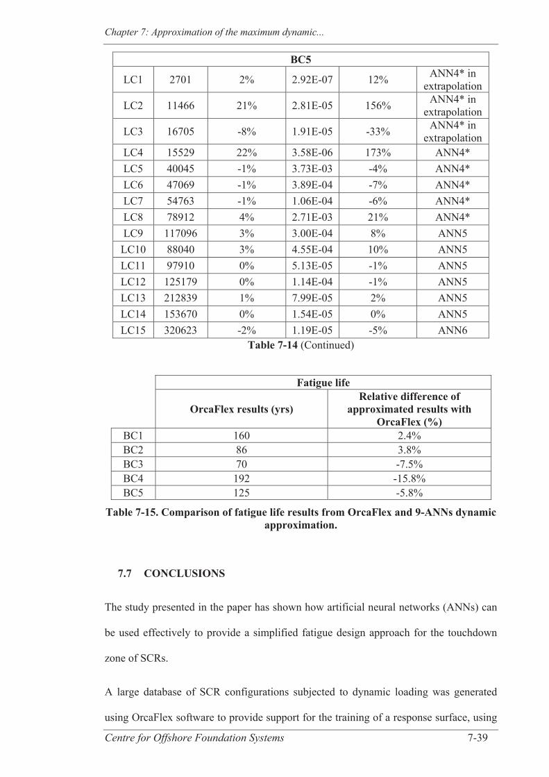
Chapter 7: Approximation of the maximum dynamic...
Centre for Offshore Foundation Systems 7-39
BC5
LC1 2701 2% 2.92E-07 12% ANN4* in extrapolation
LC2 11466 21% 2.81E-05 156% ANN4* in extrapolation
LC3 16705 -8% 1.91E-05 -33% ANN4* in extrapolation
LC4 15529 22% 3.58E-06 173% ANN4* LC5 40045 -1% 3.73E-03 -4% ANN4* LC6 47069 -1% 3.89E-04 -7% ANN4* LC7 54763 -1% 1.06E-04 -6% ANN4* LC8 78912 4% 2.71E-03 21% ANN4* LC9 117096 3% 3.00E-04 8% ANN5
LC10 88040 3% 4.55E-04 10% ANN5 LC11 97910 0% 5.13E-05 -1% ANN5 LC12 125179 0% 1.14E-04 -1% ANN5 LC13 212839 1% 7.99E-05 2% ANN5 LC14 153670 0% 1.54E-05 0% ANN5 LC15 320623 -2% 1.19E-05 -5% ANN6
Table 7-14 (Continued)
Fatigue life
OrcaFlex results (yrs) Relative difference of
approximated results with OrcaFlex (%)
BC1 160 2.4% BC2 86 3.8% BC3 70 -7.5% BC4 192 -15.8% BC5 125 -5.8%
Table 7-15. Comparison of fatigue life results from OrcaFlex and 9-ANNs dynamic approximation.
7.7 CONCLUSIONS
The study presented in the paper has shown how artificial neural networks (ANNs) can
be used effectively to provide a simplified fatigue design approach for the touchdown
zone of SCRs.
A large database of SCR configurations subjected to dynamic loading was generated
using OrcaFlex software to provide support for the training of a response surface, using
Chapter 7: Approximation of the maximum dynamic...
Centre for Offshore Foundation Systems 7-40
ANNs. The size of the database was limited by the time taken to run each of the cases in
OrcaFlex. Design of experiment methods were applied when generating the database to
capture the complex relationships between the eight selected input dimensionless groups
and the output (Max TDZ). Different ANN configurations were tested and a
framework comprising nine ANNs was selected since it was able to estimate the critical
stress range results for the majority of the cases of the database within 5 % relative
difference with numerical results. A refinement of the quality of the database was
applied for part of the design space to explore the effect of the size of training and
testing sets and the choice of cases within these sets on the performance of the
approximation. The current best ANN approximation (accounting for the refinement of
the database in part of the design space), referred to as ‘9-ANNs dynamic
approximation’, was used to assess the fatigue lives of example SCRs under a selected
small wave scatter diagram inspired from realistic GoM data. The ANN approximation
was found to predict well the fatigue results, with a maximum discrepancy of 16 % on
the predicted fatigue life.
This pilot study has demonstrated that fatigue life calculations for the touchdown zone
of SCRs may potentially be reduced to a matter of minutes using the proposed ANN
framework, without compromising much on the level of accuracy, and without the need
for advanced numerical analyses. Once ‘trained’, the ANN approximation may be used
conveniently by any external user and could represent a major improvement in
efficiency of SCR fatigue estimations, particularly for the early stages of design where
optimisation studies are needed to establish values of input parameters that provide
optimal performance.

Estimating the fatigue damage of SCRs in the TDZ
Centre for Offshore Foundation Systems 8-1
CHAPTER 8 SENSITIVITY STUDIES OF STEEL CATENARY
RISER FATIGUE DAMAGE IN THE TOUCHDOWN ZONE
USING AN EFFICIENT SIMPLIFIED FRAMEWORK FOR
STRESS RANGE EVALUATION
8.1 ABSTRACT
Steel catenary risers (SCRs) are widely used in deep water. Several sources of
nonlinearities make SCR fatigue design challenging. Limited understanding of the
influence of the various input parameters on the structural response of SCRs leads to
unnecessarily high conservatism in design. Also, time consuming numerical simulations
are usually performed to assess SCR fatigue damage which is inefficient, especially for
early design stages.
A simplified framework for fatigue analysis of SCRs in the touchdown zone (TDZ) has
been developed previously, using artificial neural networks. The approach may be used
to efficiently estimate maximum static and dynamic stress ranges in the TDZ, from
which the fatigue damage can be deduced. Comparison of the maximum static and
dynamic stress changes for a given input motion allows quantification of the dynamic
amplification factor (DAF). This paper explores the sensitivity of the maximum
dynamic stress ranges and DAF to the key dimensionless groups of input parameters
and also certain individual input parameters. The study illustrates the usefulness of the
proposed framework in understanding SCR behaviour in the TDZ, providing guidance
on optimisation of SCR design from a fatigue perspective. The paper also reflects on the
potential benefits of using DAFs for SCR fatigue design.
Chapter 8: Sensitivity studies of SCR fatigue damage...
Centre for Offshore Foundation Systems 8-2
8.2 INTRODUCTION
Oil and gas developments in deep water commonly use steel catenary risers (SCRs) to
transfer fluids between seabed and sea surface as they are a cost effective solution.
Under the action of environmental loading a complex interaction is created in the
touchdown zone (TDZ – the dynamic area of riser-soil interaction (Bridge, 2005)) and
fatigue damage is generated. Fatigue design is a major challenge for SCRs as there is a
lack of understanding of the influence of the various input parameters on the fatigue
damage, leading to unnecessary conservatism. Fatigue damage is usually evaluated by
running time consuming numerical simulations. This approach is inefficient, especially
for the early stages of design where optimisation studies are required to find values of
input parameters leading to the best performance. A simple approach able to provide
quantitative guidance on how the input parameters impact the static and dynamic
response of SCRs in the TDZ, thus allowing rapid evaluation of the fatigue damage in
the TDZ, would be better suited for initial design. The development of such an approach
was indeed encouraged in a recent standard for the design of offshore risers (DNV-OS-
F201, 2010).
A program of research (Chapter 2 to Chapter 7) has been undertaken by the authors with
the ultimate aim of proposing a simplified fatigue analysis and design framework for
SCRs in the TDZ. The original intention was to use the dynamic amplification factor
(DAF) approach for dynamic response of SCRs, since it is used widely for
simplification of structural dynamic analyses for linear structural systems (e.g. Barltrop
and Adams, 1991; Bea et al., 1999; Ruiz-Teran and Aparicio, 2006). DAFs quantify the
amplification of stress due to dynamic effects when compared with the static response.
The simplification relies on the ability to evaluate the static response and the DAF
values through simple methods, and hence deduce the dynamic response. However,
SCR behaviour is impacted by geometrical and material nonlinearities in the TDZ and
Chapter 8: Sensitivity studies of SCR fatigue damage...
Centre for Offshore Foundation Systems 8-3
therefore the usefulness of the DAF approach for SCR design was explored first.
The study is limited to 2D conditions where the current profile in the sea column, the
rotational stiffness at the hang-off point (HOP), the coating and the flow rate of the
content are not taken into account. Only the case of a linear soil model, horizontal and
flat seabed is investigated here. Also, an illustration of the main input parameters is
given in Figure 8-1 and the following parameters remain unchanged in the study:
Gravity acceleration (g = 9.81 m/s2),
Young’s modulus and Poisson’s ratio for the SCR (E = 2.12E8 kPa, = 0.293),
Water and steel density ( water = 1.025 te/m3; steel = 7.85 te/m3),
Soil friction coefficient ( = 0.5),
Hydrodynamic coefficients (CD = 1.2; CA = 1), Angular position on the SCR circumference ( = 0°), Angle of the motion relative to the hang-off angle ( m = m - HO = 0°, as
detailed hereafter).
The loading of SCRs is represented by harmonic motions of the floating vessel through
the procedure suggested by Kimiaei et al. (2010), where a time varying sinusoidal
motion of the vessel, making an angle m with the vertical and characterised by heave
amplitude (H) and period (T) of the motion (i.e. maximum input velocity of 2 H/T) is
applied. The vessel is always a semisubmersible in this study, with its motion applied
parallel to the riser tangential line at the hang-off point (hence m set to zero). This is
based on the findings from Kimiaei et al. (2010) that, with a semisubmersible, the
tangential component of motion alone could adequately represent the fatigue damage
resulting from wave loading in the TDZ.
Under these assumptions, a pilot study was performed, defining the DAF for SCRs as:
DAF = Max TDZ_dyn/ Max TDZ_sta where Max TDZ_sta and Max TDZ_dyn are the
maximum stress ranges occurring in the TDZ under static and dynamic loading
respectively (Quéau et al., 2011). Since the study indicated that the DAF approach was
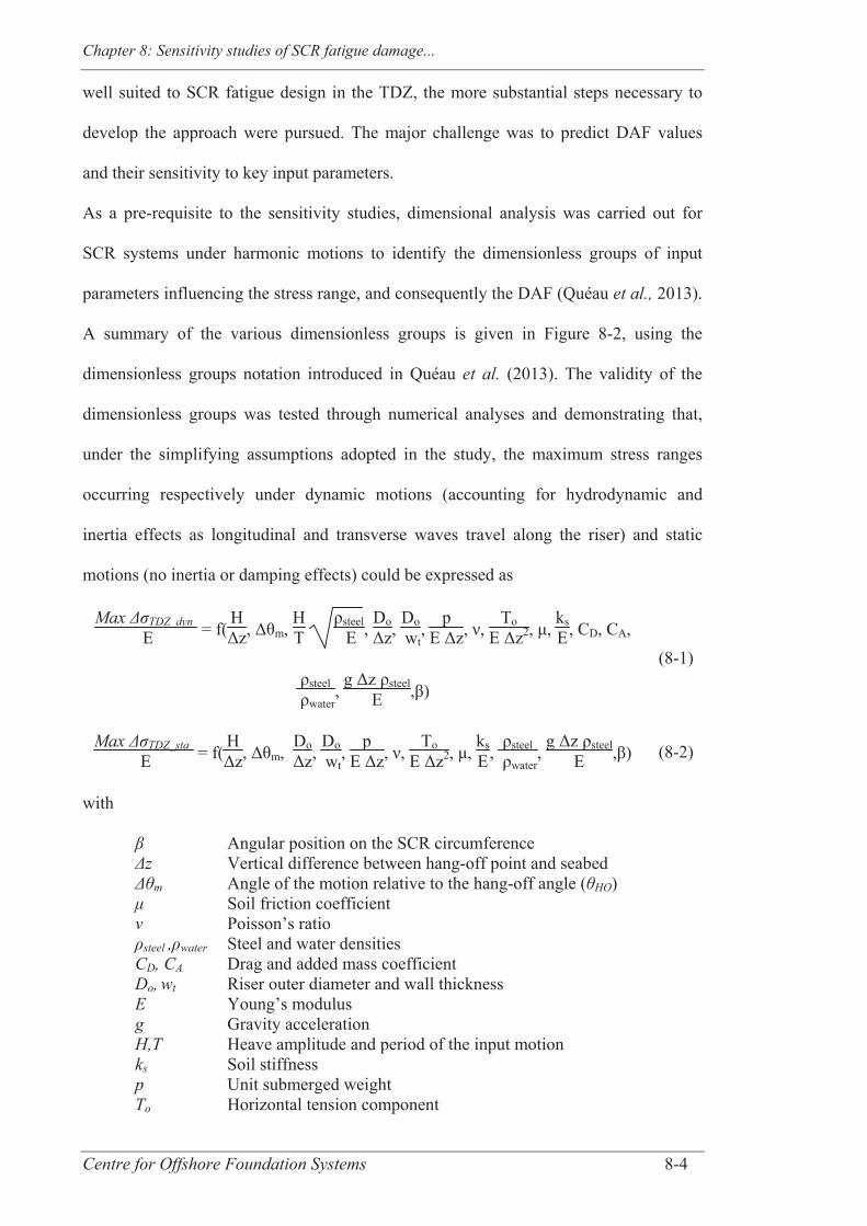
Chapter 8: Sensitivity studies of SCR fatigue damage...
Centre for Offshore Foundation Systems 8-4
well suited to SCR fatigue design in the TDZ, the more substantial steps necessary to
develop the approach were pursued. The major challenge was to predict DAF values
and their sensitivity to key input parameters.
As a pre-requisite to the sensitivity studies, dimensional analysis was carried out for
SCR systems under harmonic motions to identify the dimensionless groups of input
parameters influencing the stress range, and consequently the DAF (Quéau et al., 2013).
A summary of the various dimensionless groups is given in Figure 8-2, using the
dimensionless groups notation introduced in Quéau et al. (2013). The validity of the
dimensionless groups was tested through numerical analyses and demonstrating that,
under the simplifying assumptions adopted in the study, the maximum stress ranges
occurring respectively under dynamic motions (accounting for hydrodynamic and
inertia effects as longitudinal and transverse waves travel along the riser) and static
motions (no inertia or damping effects) could be expressed as
Max TDZ_dyn E = f(
HΔz, Δθm,
HT
ρsteel E ,
DoΔz,
Do wt
, p
E Δz, ν, To
E Δz2, μ, ksE, CD, CA,
ρsteel ρwater
, g Δz ρsteel
E ,β)
(8-1)
Max TDZ_sta E = f(
HΔz, Δθm,
DoΔz,
Do wt
, p
E Δz, ν, To
E Δz2, μ, ksE,
ρsteel ρwater
, g Δz ρsteel
E ,β) (8-2)
with
Angular position on the SCR circumference z Vertical difference between hang-off point and seabed
m Angle of the motion relative to the hang-off angle ( HO) Soil friction coefficient Poisson’s ratio steel , water Steel and water densities
CD, CA Drag and added mass coefficient Do, wt Riser outer diameter and wall thickness E Young’s modulus g Gravity acceleration H,T Heave amplitude and period of the input motion ks Soil stiffness p Unit submerged weight To Horizontal tension component
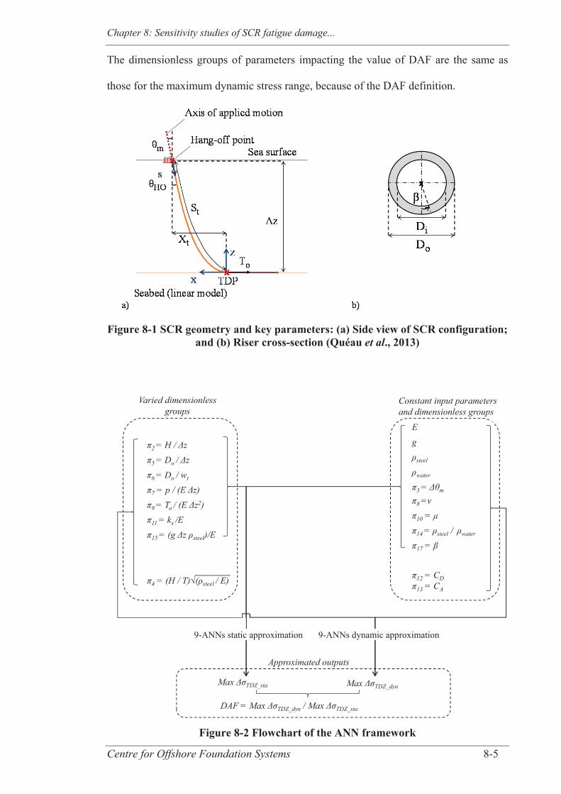
Chapter 8: Sensitivity studies of SCR fatigue damage...
Centre for Offshore Foundation Systems 8-5
The dimensionless groups of parameters impacting the value of DAF are the same as
those for the maximum dynamic stress range, because of the DAF definition.
Figure 8-1 SCR geometry and key parameters: (a) Side view of SCR configuration; and (b) Riser cross-section (Quéau et al., 2013)
Figure 8-2 Flowchart of the ANN framework
Constant input parameters and dimensionless groups
Max TDZ_dyn
Varied dimensionless groups
Max TDZ_sta
Approximated outputs
DAF = Max TDZ_dyn / Max TDZ_sta
2 = H / z
5 = Do / z
6 = Do / wt
7 = p / (E z)
9 = To / (E z2)
11 = ks /E
15 = (g z steel)/E
4 = (H / T) ( steel / E)
Eg
steel
water
3 = m
8 =
10 =
14 = steel / water
17 =
12 = CD
13 = CA
9-ANNs static approximation 9-ANNs dynamic approximation

Chapter 8: Sensitivity studies of SCR fatigue damage...
Centre for Offshore Foundation Systems 8-6
Throughout the study, numerical analysis of the SCR system has been carried out using
the dynamic analysis software OrcaFlex (Orcina, 2011). Approximate, but accurate,
analytical solutions can evaluate the static response (and maximum static stress range)
of an SCR (Quéau et al., 2014a). However, since it is complex to develop analytical
solutions able to accuractely evaluate the dynamic response of SCRs in time domain,
the approach has been to develop artificial neural networks (ANNs), trained using the
numerical results from OrcaFlex. This approach was validated initially for the static
response (Quéau et al., 2014b) before embarking on the dynamic response.
Extensive sensitivity studies were performed to capture SCR behaviour in the TDZ for
many thousands of different configurations, loading conditions, riser properties etc...
(Quéau et al., 2014b, 2015b). The sensitivity studies were originally intended to
increase the understanding of SCR behaviour and predict the DAF value using an
advanced mathematical tool, the artificial neural network (ANN). Since the same
amount of computational effort was required for approximating the relationships
between either Max TDZ_dyn or DAF, it was decided to use the ANN tool to capture the
relationships between the input dimensionless groups and Max TDZ_dyn directly.
Indeed, this is essentially more convenient for the final user in future applications (the
maximum dynamic stress range being directly linked to the fatigue damage). The
development of such a framework was performed in Chapter 5 to Chapter 7.
The main aim of this paper is to link together all of the previous steps of the study,
focusing on two distinct aspects:
(i) After presenting the ANN framework (Section 8.3), it is used to efficiently
explore the sensitivity of the maximum stress range in the TDZ to variations
of some of the input dimensionless groups and individual parameters
(Section 8.4); the results are then used to optimise an example SCR system
in respect of the fatigue life (Section 8.5).
Chapter 8: Sensitivity studies of SCR fatigue damage...
Centre for Offshore Foundation Systems 8-7
(ii) Reflecting back on the initial strategy of combining the static response with a
dynamic amplification factor, the ANN framework is used to examine the
sensitivity of the DAF to some of the input dimensionless groups and
individual parameters (Section 8.4). The key question to resolve is whether
the DAF (together with the static response) is more predictable than the
maximum dynamic stress range in the TDZ directly, and thus would offer a
more robust design approach, just as commonly used for other types of
structural design involving dynamic response.
8.3 THE SIMPLIFIED FRAMEWORK
8.3.1 Selected range of applicability
Under the assumptions of the study, there are respectively seven and eight key input
dimensionless groups influencing respectively the maximum stress ranges in the TDZ
for SCRs under static and dynamic conditions. These dimensionless groups are as
follows (using dimensionless groups notation detailed in Figure 8-2 (Quéau et al.,
2013)):
Riser displacement, 2 = H / z
Riser displacement velocity, 4 =(H/T) steel/ E (only for dynamic motion)
Riser outside diameter, 5 = Do / z
Riser outside diameter to wall thickness ratio, 6 = Do / wt
Riser unit submerged weight, 7 = p / (E z)
Riser tension, π9 = To / (E Δz2)
Soil stiffness, 11 = ks / E
Water depth, 15 = g z steel / E
To develop a simplified, but broadly applicable framework it was necessary to select
wide ranges for these key input dimensionless groups, which define the design space,
corresponding to wide ranges of the inherent individual input parameters. The selected
Chapter 8: Sensitivity studies of SCR fatigue damage...
Centre for Offshore Foundation Systems 8-8
ranges are presented in Table 8-1 and Table 8-2. A series of criteria, referred to as
“design criteria” as presented in Table 8-1, were implemented between some of the
input parameters and dimensionless groups to select realistic combinations of
dimensionless groups when defining SCR configurations and loading conditions. For
instance, small hang-off angles were considered for deep water and larger for shallower
water to match with industry practices. The riser displacement characteristics were
derived from in-service conditions of a typical semisubmersible vessel under calm to
harsh seastates in the Gulf of Mexico (GoM).
For the dynamic motion, small parts of the design space had to be excluded since it was
not possible at this stage to define an approximation of the relationships between the
input dimensionless groups and the maximum normalised stress range in the TDZ with
a sufficient level of accuracy in these areas, as discussed later. These areas are
summarised in Table 8-3. Further details on the choice of ranges can be found in
Chapters 4 to 7.
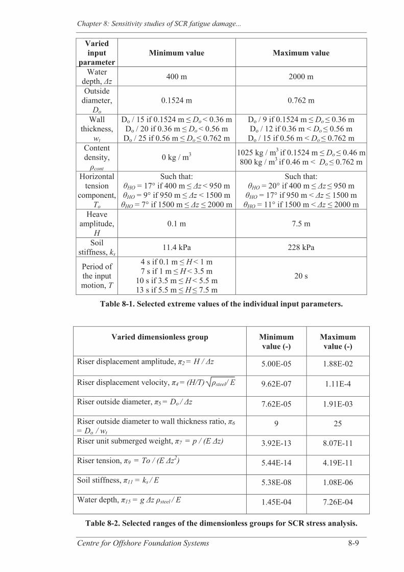
Chapter 8: Sensitivity studies of SCR fatigue damage...
Centre for Offshore Foundation Systems 8-9
Varied input
parameter Minimum value Maximum value
Water depth, z 400 m 2000 m
Outside diameter,
Do 0.1524 m 0.762 m
Wall thickness,
wt
Do / 15 if 0.1524 m ≤ Do < 0.36 mDo / 20 if 0.36 m ≤ Do < 0.56 m Do / 25 if 0.56 m ≤ Do ≤ 0.762 m
Do / 9 if 0.1524 m ≤ Do ≤ 0.36 m Do / 12 if 0.36 m < Do ≤ 0.56 m Do / 15 if 0.56 m < Do ≤ 0.762 m
Content density,
cont 0 kg / m3 1025 kg / m3 if 0.1524 m ≤ Do ≤ 0.46 m
800 kg / m3 if 0.46 m < Do ≤ 0.762 m
Horizontal tension
component, To
Such that: HO = 17° if 400 m ≤ z < 950 m HO = 9° if 950 m ≤ z < 1500 m
HO = 7° if 1500 m ≤ z ≤ 2000 m
Such that: HO = 20° if 400 m ≤ z ≤ 950 m
HO = 17° if 950 m < z ≤ 1500 m HO = 11° if 1500 m < z ≤ 2000 m
Heave amplitude,
H 0.1 m 7.5 m
Soil stiffness, ks
11.4 kPa 228 kPa
Period of the input motion, T
4 s if 0.1 m ≤ H < 1 m 7 s if 1 m ≤ H < 3.5 m
10 s if 3.5 m ≤ H < 5.5 m 13 s if 5.5 m ≤ H ≤ 7.5 m
20 s
Table 8-1. Selected extreme values of the individual input parameters.
Varied dimensionless group Minimum value (-)
Maximum value (-)
Riser displacement amplitude, 2 = H / z 5.00E-05 1.88E-02
Riser displacement velocity, 4 = (H/T) steel/ E 9.62E-07 1.11E-4
Riser outside diameter, 5 = Do / z 7.62E-05 1.91E-03
Riser outside diameter to wall thickness ratio, 6 = Do / wt
9 25
Riser unit submerged weight, 7 = p / (E z) 3.92E-13 8.07E-11
Riser tension, 9 = To / (E z2) 5.44E-14 4.19E-11
Soil stiffness, 11 = ks / E 5.38E-08 1.08E-06
Water depth, 15 = g z steel / E 1.45E-04 7.26E-04
Table 8-2. Selected ranges of the dimensionless groups for SCR stress analysis.
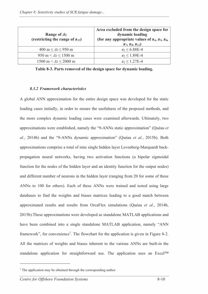
Chapter 8: Sensitivity studies of SCR fatigue damage...
Centre for Offshore Foundation Systems 8-10
Range of Δz (restricting the range of π15)
Area excluded from the design space for dynamic loading
(for any appropriate values of π4, π5, π6, π7, π9, π11)
400 m ≤ z ≤ 950 m 2 ≤ 6.88E-4 950 m < z ≤ 1500 m 2 ≤ 1.89E-4
1500 m < z ≤ 2000 m 2 ≤ 1.27E-4
Table 8-3. Parts removed of the design space for dynamic loading.
8.3.2 Framework characteristics
A global ANN approximation for the entire design space was developed for the static
loading cases initially, in order to ensure the usefulness of the proposed methods, and
the more complex dynamic loading cases were examined afterwards. Ultimately, two
approximations were established, namely the “9-ANNs static approximation” (Quéau et
al., 2014b) and the “9-ANNs dynamic approximation” (Quéau et al., 2015b). Both
approximations comprise a total of nine single hidden layer Levenberg-Marquardt back-
propagation neural networks, having two activation functions (a bipolar sigmoidal
function for the nodes of the hidden layer and an identity function for the output nodes)
and different number of neurons in the hidden layer (ranging from 20 for some of these
ANNs to 100 for others). Each of these ANNs were trained and tested using large
databases to find the weights and biases matrices leading to a good match between
approximated results and results from OrcaFlex simulations (Quéau et al., 2014b,
2015b).These approximations were developed as standalone MATLAB applications and
have been combined into a single standalone MATLAB application, namely “ANN
framework”, for convenience1. The flowchart for the application is given in Figure 8-2.
All the matrices of weights and biases inherent to the various ANNs are built-in the
standalone application for straightforward use. The application uses an Excel™
1 The application may be obtained through the corresponding author.
Chapter 8: Sensitivity studies of SCR fatigue damage...
Centre for Offshore Foundation Systems 8-11
interface so that a user can simply copy and paste a dataset (i.e. series of dimensionless
groups’ combinations defining SCR configurations and loading conditions, as per the
“Varied dimensionless groups” in Figure 8-2) and automatically obtain the maximum
stress range corresponding to the static and dynamic loading of the specified SCRs and
loading conditions (as per the “Approximated outputs” in Figure 8-2). The standalone
application performs matrix multiplications based on the input values and the built-in
matrices of weights and biases to calculate the maximum stress range results (Quéau et
al., 2014b, 2015b), and therefore the time taken to develop the approximations does not
impact the time necessary to assess the outputs with the ANN framework application.
The fatigue damage can then be evaluated directly from the dynamic results. The ANN
framework application also reports DAF values, evaluated using the static and dynamic
results obtained with the 9-ANNs static and dynamic approximations.
8.3.1 Performance of the ANN framework
The ANN framework application is very efficient, taking about 1 minute to estimate the
outputs (Max TDZ_sta , Max TDZ_dyn and DAF) for ~ 50,000 cases (different SCR
configurations with given static or dynamic loading conditions) and without the need for
any specialised software. It is difficult to quantify accurately the time saving impact of
the ANN framework since the time necessary to obtain stress range results from marine
analysis software (such as OrcaFlex, as used here) will vary from user to user,
depending on the experience of the user, the performance of the computer used to run
the simulations and on the efficiency of pre- and post-processing the numerical models.
The last aspect may be streamlined by the use of automation sub-routines (as shown in
Chapters 5 to 7). However, four months of calculation were necessary here to obtain the
results for the entire database using OrcaFlex running on a high performance computer.
The proposed simplified framework represents therefore a tremendous time saving in
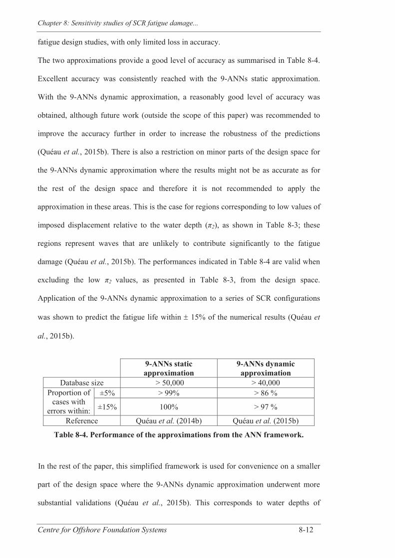
Chapter 8: Sensitivity studies of SCR fatigue damage...
Centre for Offshore Foundation Systems 8-12
fatigue design studies, with only limited loss in accuracy.
The two approximations provide a good level of accuracy as summarised in Table 8-4.
Excellent accuracy was consistently reached with the 9-ANNs static approximation.
With the 9-ANNs dynamic approximation, a reasonably good level of accuracy was
obtained, although future work (outside the scope of this paper) was recommended to
improve the accuracy further in order to increase the robustness of the predictions
(Quéau et al., 2015b). There is also a restriction on minor parts of the design space for
the 9-ANNs dynamic approximation where the results might not be as accurate as for
the rest of the design space and therefore it is not recommended to apply the
approximation in these areas. This is the case for regions corresponding to low values of
imposed displacement relative to the water depth ( 2), as shown in Table 8-3; these
regions represent waves that are unlikely to contribute significantly to the fatigue
damage (Quéau et al., 2015b). The performances indicated in Table 8-4 are valid when
excluding the low 2 values, as presented in Table 8-3, from the design space.
Application of the 9-ANNs dynamic approximation to a series of SCR configurations
was shown to predict the fatigue life within 15% of the numerical results (Quéau et
al., 2015b).
9-ANNs static approximation
9-ANNs dynamic approximation
Database size > 50,000 > 40,000 Proportion of
cases with errors within:
±5% > 99% > 86 %
±15% 100% > 97 %
Reference Quéau et al. (2014b) Quéau et al. (2015b)
Table 8-4. Performance of the approximations from the ANN framework.
In the rest of the paper, this simplified framework is used for convenience on a smaller
part of the design space where the 9-ANNs dynamic approximation underwent more
substantial validations (Quéau et al., 2015b). This corresponds to water depths of
Chapter 8: Sensitivity studies of SCR fatigue damage...
Centre for Offshore Foundation Systems 8-13
950 m < Δz ≤ 1500 m (and therefore 3.45E-4 < 15 ≤ 5.45E-4), riser displacement
2 > 1.89E-4 (due to the comment on lower accuracy and fatigue relevance for low riser
displacement) and corresponding ranges for 4, 5, 6, 7, 9, 11 .
8.4 SENSITIVITY STUDIES USING THE ANN FRAMEWORK
The simplified framework is now used to shed light on the sensitivity of the maximum
stress range in SCRs in the TDZ and of the DAF to the variation of some of the key
input dimensionless groups of parameters. The resulting sensitivities are benchmarked
against results from published literature. There are many ways to vary the key input
dimensionless groups and individual parameters and this paper illustrates the usefulness
of the ANN framework by considering a selection of examples of individual and
simultaneous variations of the key input dimensionless groups and individual input
parameters. The first two examples, testing the effect of the displacement characteristics
and the soil stiffness on the maximum stress range in the TDZ, aim to demonstrate that
the ANN framework can reproduce expected and known trends to validate further its
accuracy. Building on from these two examples, two further examples derived from
published studies performed using the traditional approach (i.e. numerical simulations)
are presented to illustrate the usefulness of the ANN framework in validating published
trends for new ranges of the inputs.
Throughout this section and wherever possible based on (i) the tested variations, (ii) the
selected values for the input parameters and dimensionless groups, and (iii) the design
criteria among them, the unvaried dimensionless groups and individual parameters are
fixed to their appropriate mean value, except for 7 the value of which is determined
based on the water depth and the riser unit submerged weight for an empty riser (for
convenience). The term ‘appropriate’ implies that the design criteria between individual
Chapter 8: Sensitivity studies of SCR fatigue damage...
Centre for Offshore Foundation Systems 8-14
input parameters and dimensionless groups, as shown in Table 8-2, are respected and
refers to the mean values accounting for the selected range of water depth:
950 m < z ≤ 1500 m (or 3.45E-4 < 15 ≤ 5.45E-4). Moreover, the reported values of the
horizontal component of the tension (To) is assessed by using one of the common
catenary equations: To = p z sin ( HO)/(1-sin( HO)).
8.4.1 Effect of the imposed displacement amplitude (π2) and velocity (π4)
The effect of the imposed riser displacement amplitude ( 2) and velocity ( 4) on SCR
behaviour in the TDZ is investigated first. For this purpose, H and T were varied within
the four selected ranges of H and corresponding T values. Table 8-5 summarises the
selected values of the individual input parameters and dimensionless groups that were
used for this example. A series of design charts showing the sensitivity of
Max TDZ_dyn/E and DAF to variations of 2 and 4 were established, as illustrated in
Figure 8-3 and Figure 8-4 respectively. The range of 4 was normalised in the subplots
for convenience, using the extreme (max) and minimum (min) values shown in Table
8-5 (so that Normalised 4 = (2* 4 – max – min) / (max – min)). Results are discussed
next, for the maximum stress range in the TDZ first and then for the DAF.
8.4.1.1 Maximum stress range in the TDZ
Increasing the velocity ( 4) by keeping the displacement amplitude constant ( 2),
thereby reducing the period of the imposed displacement (T), leads to an increase of
Max TDZ_dyn/E. Also, the higher the displacement amplitude, the higher the maximum
stress range in the TDZ (i.e. increase of fatigue damage) since it generates higher
variations of the curvature in the TDZ. These trends are observed for the four ranges of
H and corresponding T values selected and show that no resonance effects were
detected for the SCR configuration under study.

Chapter 8: Sensitivity studies of SCR fatigue damage...
Centre for Offshore Foundation Systems 8-15
8.4.1.2 DAF
The values of maximum stress range found under static loading (Max TDZ_sta/E) using
the simplified framework are shown in Table 8-6. They were used to calculate the DAF
values from Max TDZ_dyn/E results presented in Figure 8-3. Figure 8-4 indicates that
the DAF increases with increasing velocity of the imposed displacement. Also, it tends
to confirm an interesting trend of the DAF sensitivity that was already noted at the pilot
study stage of this research (Quéau et al., 2011). For low displacement amplitudes, DAF
varies inversely with the displacement amplitude, whereas it increases with increasing
displacement amplitude for higher heave amplitude values; Figure 8-4b captures the
transition between these opposing trends.
Interestingly, DAF values do not decrease down to unity in any of the plots presented in
Figure 8-4, indicating that the SCR under study did not reach its static response for the
selected displacements and wave periods. To some extent, this is consistent with the
results obtained during the pilot study (Quéau et al., 2011). Even though the selected
values for the input parameters and dimensionless groups are not all identical in this
paper to those selected for the pilot study, DAF values of unity were only reached in the
pilot study when considering imposed displacements with a period (T) greater than 20 s.
That limit is beyond the highest limit selected for T here and also when defining the
ANN framework (see Table 8-1 and Chapters 5 to 7).
The similarity of the observed trends when using the ANN framework to those of the
pilot study, when DAF sensitivity was investigated using results from numerical
simulations, further validates the framework.
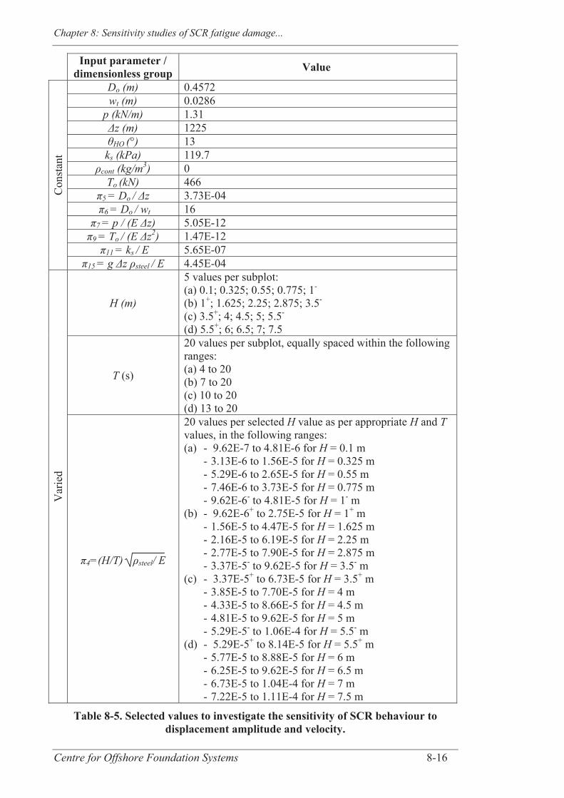
Chapter 8: Sensitivity studies of SCR fatigue damage...
Centre for Offshore Foundation Systems 8-16
Input parameter /
dimensionless group Value C
onst
ant
Do (m) 0.4572 wt (m) 0.0286
p (kN/m) 1.31 z (m) 1225 HO (°) 13
ks (kPa) 119.7 cont (kg/m3) 0
To (kN) 466 5 = Do / z 3.73E-04
6 = Do / wt 16 7 = p / (E z) 5.05E-12
9 = To / (E z2) 1.47E-12 11 = ks / E 5.65E-07
15 = g z steel / E 4.45E-04
Var
ied
H (m)
5 values per subplot: (a) 0.1; 0.325; 0.55; 0.775; 1- (b) 1+; 1.625; 2.25; 2.875; 3.5- (c) 3.5+; 4; 4.5; 5; 5.5- (d) 5.5+; 6; 6.5; 7; 7.5
T (s)
20 values per subplot, equally spaced within the following ranges: (a) 4 to 20 (b) 7 to 20 (c) 10 to 20 (d) 13 to 20
4=(H/T) steel/ E
20 values per selected H value as per appropriate H and T values, in the following ranges: (a) - 9.62E-7 to 4.81E-6 for H = 0.1 m
- 3.13E-6 to 1.56E-5 for H = 0.325 m - 5.29E-6 to 2.65E-5 for H = 0.55 m - 7.46E-6 to 3.73E-5 for H = 0.775 m - 9.62E-6- to 4.81E-5 for H = 1- m
(b) - 9.62E-6+ to 2.75E-5 for H = 1+ m - 1.56E-5 to 4.47E-5 for H = 1.625 m - 2.16E-5 to 6.19E-5 for H = 2.25 m - 2.77E-5 to 7.90E-5 for H = 2.875 m - 3.37E-5- to 9.62E-5 for H = 3.5- m
(c) - 3.37E-5+ to 6.73E-5 for H = 3.5+ m - 3.85E-5 to 7.70E-5 for H = 4 m - 4.33E-5 to 8.66E-5 for H = 4.5 m - 4.81E-5 to 9.62E-5 for H = 5 m - 5.29E-5- to 1.06E-4 for H = 5.5- m
(d) - 5.29E-5+ to 8.14E-5 for H = 5.5+ m - 5.77E-5 to 8.88E-5 for H = 6 m - 6.25E-5 to 9.62E-5 for H = 6.5 m - 6.73E-5 to 1.04E-4 for H = 7 m - 7.22E-5 to 1.11E-4 for H = 7.5 m
Table 8-5. Selected values to investigate the sensitivity of SCR behaviour to displacement amplitude and velocity.
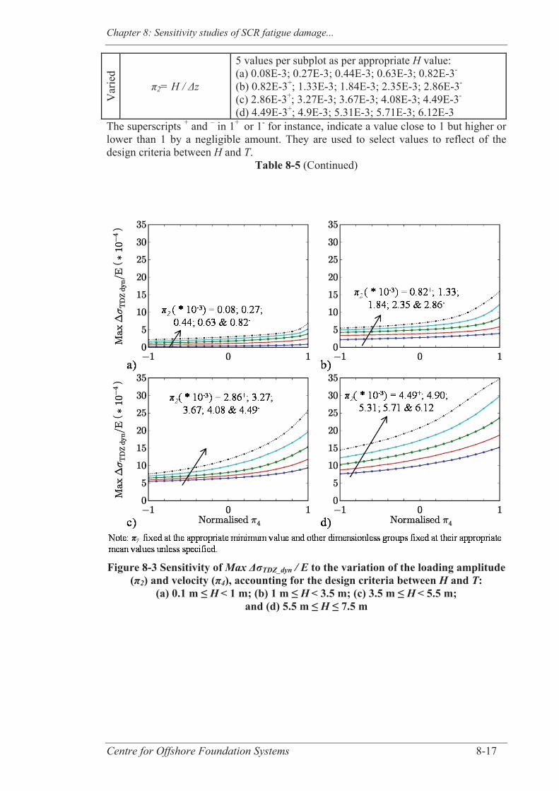
Chapter 8: Sensitivity studies of SCR fatigue damage...
Centre for Offshore Foundation Systems 8-17
Var
ied
2= H / z
5 values per subplot as per appropriate H value: (a) 0.08E-3; 0.27E-3; 0.44E-3; 0.63E-3; 0.82E-3-
(b) 0.82E-3+; 1.33E-3; 1.84E-3; 2.35E-3; 2.86E-3-
(c) 2.86E-3+; 3.27E-3; 3.67E-3; 4.08E-3; 4.49E-3-
(d) 4.49E-3+; 4.9E-3; 5.31E-3; 5.71E-3; 6.12E-3 The superscripts + and – in 1+ or 1- for instance, indicate a value close to 1 but higher or lower than 1 by a negligible amount. They are used to select values to reflect of the design criteria between H and T.
Table 8-5 (Continued)
Figure 8-3 Sensitivity of Max ΔσTDZ_dyn / E to the variation of the loading amplitude
(π2) and velocity (π4), accounting for the design criteria between H and T: (a) 0.1 m ≤ H < 1 m; (b) 1 m ≤ H < 3.5 m; (c) 3.5 m ≤ H < 5.5 m;
and (d) 5.5 m ≤ H ≤ 7.5 m
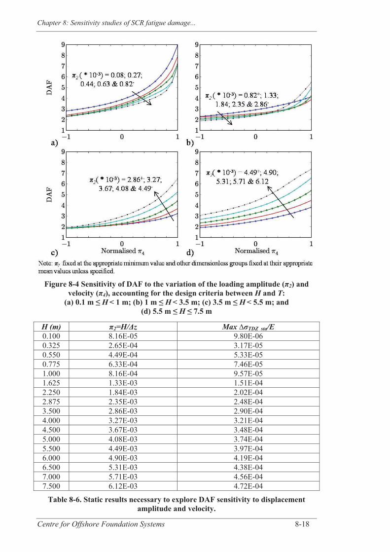
Chapter 8: Sensitivity studies of SCR fatigue damage...
Centre for Offshore Foundation Systems 8-18
Figure 8-4 Sensitivity of DAF to the variation of the loading amplitude (π2) and
velocity (π4), accounting for the design criteria between H and T: (a) 0.1 m ≤ H < 1 m; (b) 1 m ≤ H < 3.5 m; (c) 3.5 m ≤ H < 5.5 m; and
(d) 5.5 m ≤ H ≤ 7.5 m
H (m) π2=H/Δz Max ∆σTDZ sta/E 0.100 8.16E-05 9.80E-06 0.325 2.65E-04 3.17E-05 0.550 4.49E-04 5.33E-05 0.775 6.33E-04 7.46E-05 1.000 8.16E-04 9.57E-05 1.625 1.33E-03 1.51E-04 2.250 1.84E-03 2.02E-04 2.875 2.35E-03 2.48E-04 3.500 2.86E-03 2.90E-04 4.000 3.27E-03 3.21E-04 4.500 3.67E-03 3.48E-04 5.000 4.08E-03 3.74E-04 5.500 4.49E-03 3.97E-04 6.000 4.90E-03 4.19E-04 6.500 5.31E-03 4.38E-04 7.000 5.71E-03 4.56E-04 7.500 6.12E-03 4.72E-04
Table 8-6. Static results necessary to explore DAF sensitivity to displacement amplitude and velocity.
Chapter 8: Sensitivity studies of SCR fatigue damage...
Centre for Offshore Foundation Systems 8-19
8.4.2 Effect of the soil stiffness (π11) for various imposed displacement
characteristics
This example focuses on the effect of the soil stiffness ( 11) on SCR behaviour in the
TDZ for various characteristics of the imposed displacement. The values of the
individual input parameters and dimensionless groups used for this purpose are
summarised in Table 8-7 and the design charts are shown in Figure 8-5 and Figure 8-6
for Max TDZ_dyn/E and DAF respectively.
8.4.2.1 Maximum stress range in the TDZ
The overall trend of the results presented in Figure 8-5 is for increasing values of
Max TDZ_dyn/E with increasing soil stiffness, which is consistent with other published
work (e.g. Bridge et al., 2004; Quéau et al., 2011). The trend results from higher contact
forces and greater curvature variation in the TDZ with increasing soil stiffness. There
are minor fluctuations in Figure 8-5d where higher soil stiffness locally gives lower
values of Max TDZ_dyn/E for low values of displacement velocity. This may however
indicate local inaccuracy of the ANN framework rather than an indication of a different
trend for the results in that area. As is true for any simplified approach (DNV-OS-F201,
2010), engineering judgement is required when interpreting results from the proposed
framework to differentiate between results indicating a change in SCR behaviour and
those affected by slight inaccuracies of the simplified framework.
8.4.2.2 DAF
DAF increases with increasing velocity of the imposed displacement, as observed for all
selected values of soil stiffness and displacement amplitude (see Figure 8-6). Except for
high velocity values (i.e. low period of imposed displacement), DAF is almost
insensitive to the soil stiffness. This confirms the trend observed in Quéau et al. (2011)
with other values of input parameters and dimensionless groups (e.g. different values of
water depth, riser diameter and wall thickness, hang-off angle etc...).
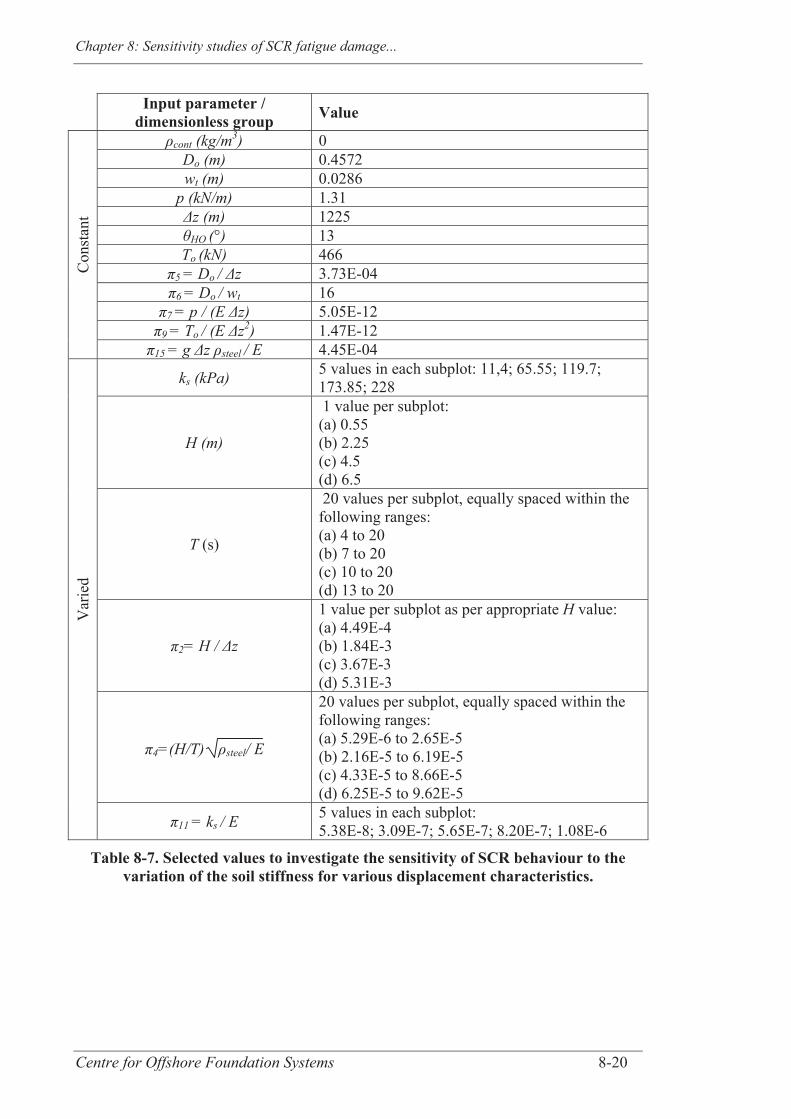
Chapter 8: Sensitivity studies of SCR fatigue damage...
Centre for Offshore Foundation Systems 8-20
Input parameter /
dimensionless group Value
Con
stan
t
cont (kg/m3) 0 Do (m) 0.4572 wt (m) 0.0286
p (kN/m) 1.31 z (m) 1225 HO (°) 13
To (kN) 466 5 = Do / z 3.73E-04 6 = Do / wt 16
7 = p / (E z) 5.05E-12 9 = To / (E z2) 1.47E-12
15 = g z steel / E 4.45E-04
Var
ied
ks (kPa) 5 values in each subplot: 11,4; 65.55; 119.7; 173.85; 228
H (m)
1 value per subplot: (a) 0.55 (b) 2.25 (c) 4.5 (d) 6.5
T (s)
20 values per subplot, equally spaced within the following ranges: (a) 4 to 20 (b) 7 to 20 (c) 10 to 20 (d) 13 to 20
2= H / z
1 value per subplot as per appropriate H value: (a) 4.49E-4 (b) 1.84E-3 (c) 3.67E-3 (d) 5.31E-3
4=(H/T) steel/ E
20 values per subplot, equally spaced within the following ranges: (a) 5.29E-6 to 2.65E-5 (b) 2.16E-5 to 6.19E-5 (c) 4.33E-5 to 8.66E-5 (d) 6.25E-5 to 9.62E-5
11 = ks / E 5 values in each subplot: 5.38E-8; 3.09E-7; 5.65E-7; 8.20E-7; 1.08E-6
Table 8-7. Selected values to investigate the sensitivity of SCR behaviour to the variation of the soil stiffness for various displacement characteristics.
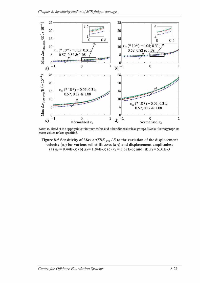
Chapter 8: Sensitivity studies of SCR fatigue damage...
Centre for Offshore Foundation Systems 8-21
Figure 8-5 Sensitivity of Max ΔσTDZ_dyn / E to the variation of the displacement
velocity (π4) for various soil stiffnesses (π11) and displacement amplitudes: (a) π2 = 0.44E-3; (b) π2 = 1.84E-3; (c) π2 = 3.67E-3; and (d) π2 = 5.31E-3
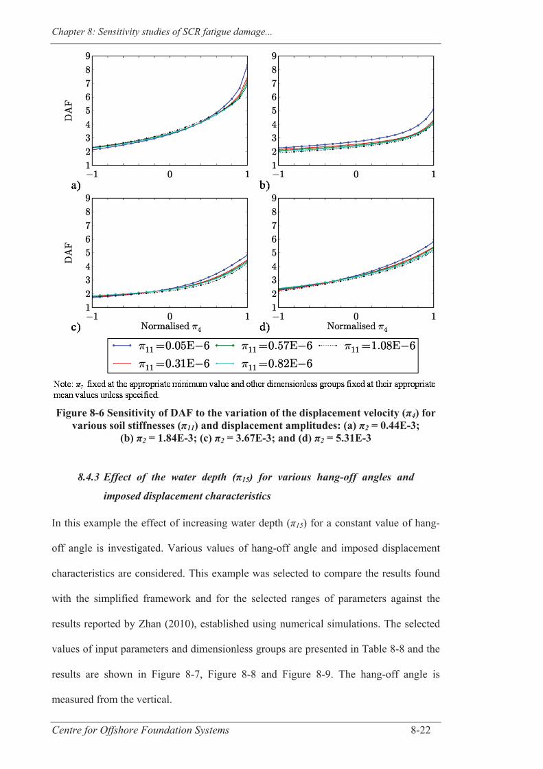
Chapter 8: Sensitivity studies of SCR fatigue damage...
Centre for Offshore Foundation Systems 8-22
Figure 8-6 Sensitivity of DAF to the variation of the displacement velocity (π4) for
various soil stiffnesses (π11) and displacement amplitudes: (a) π2 = 0.44E-3; (b) π2 = 1.84E-3; (c) π2 = 3.67E-3; and (d) π2 = 5.31E-3
8.4.3 Effect of the water depth (π15) for various hang-off angles and
imposed displacement characteristics
In this example the effect of increasing water depth ( 15) for a constant value of hang-
off angle is investigated. Various values of hang-off angle and imposed displacement
characteristics are considered. This example was selected to compare the results found
with the simplified framework and for the selected ranges of parameters against the
results reported by Zhan (2010), established using numerical simulations. The selected
values of input parameters and dimensionless groups are presented in Table 8-8 and the
results are shown in Figure 8-7, Figure 8-8 and Figure 8-9. The hang-off angle is
measured from the vertical.
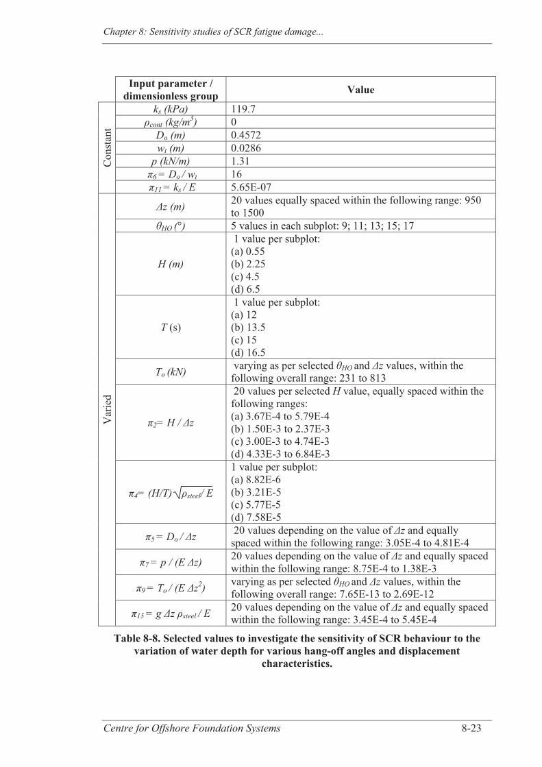
Chapter 8: Sensitivity studies of SCR fatigue damage...
Centre for Offshore Foundation Systems 8-23
Input parameter / dimensionless group Value
Con
stan
t ks (kPa) 119.7
cont (kg/m3) 0 Do (m) 0.4572 wt (m) 0.0286
p (kN/m) 1.31 6 = Do / wt 16 11 = ks / E 5.65E-07
Var
ied
z (m) 20 values equally spaced within the following range: 950 to 1500
HO (°) 5 values in each subplot: 9; 11; 13; 15; 17
H (m)
1 value per subplot: (a) 0.55 (b) 2.25 (c) 4.5 (d) 6.5
T (s)
1 value per subplot: (a) 12 (b) 13.5 (c) 15 (d) 16.5
To (kN) varying as per selected HO and z values, within the following overall range: 231 to 813
2= H / z
20 values per selected H value, equally spaced within the following ranges: (a) 3.67E-4 to 5.79E-4 (b) 1.50E-3 to 2.37E-3 (c) 3.00E-3 to 4.74E-3 (d) 4.33E-3 to 6.84E-3
4= (H/T) steel/ E
1 value per subplot: (a) 8.82E-6 (b) 3.21E-5 (c) 5.77E-5 (d) 7.58E-5
5 = Do / z 20 values depending on the value of z and equally spaced within the following range: 3.05E-4 to 4.81E-4
7 = p / (E z) 20 values depending on the value of z and equally spaced within the following range: 8.75E-4 to 1.38E-3
9 = To / (E z2) varying as per selected HO and z values, within the following overall range: 7.65E-13 to 2.69E-12
15 = g z steel / E 20 values depending on the value of z and equally spaced within the following range: 3.45E-4 to 5.45E-4
Table 8-8. Selected values to investigate the sensitivity of SCR behaviour to the variation of water depth for various hang-off angles and displacement
characteristics.
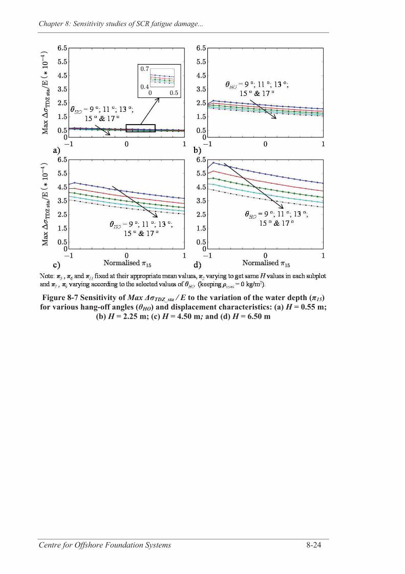
Chapter 8: Sensitivity studies of SCR fatigue damage...
Centre for Offshore Foundation Systems 8-24
Figure 8-7 Sensitivity of Max ΔσTDZ_sta / E to the variation of the water depth (π15)
for various hang-off angles (θHO) and displacement characteristics: (a) H = 0.55 m; (b) H = 2.25 m; (c) H = 4.50 m; and (d) H = 6.50 m
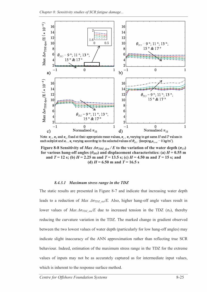
Chapter 8: Sensitivity studies of SCR fatigue damage...
Centre for Offshore Foundation Systems 8-25
Figure 8-8 Sensitivity of Max ΔσTDZ_dyn / E to the variation of the water depth (π15) for various hang-off angles (θHO) and displacement characteristics: (a) H = 0.55 m
and T = 12 s; (b) H = 2.25 m and T = 13.5 s; (c) H = 4.50 m and T = 15 s; and (d) H = 6.50 m and T = 16.5 s
8.4.3.1 Maximum stress range in the TDZ
The static results are presented in Figure 8-7 and indicate that increasing water depth
leads to a reduction of Max TDZ_sta/E. Also, higher hang-off angle values result in
lower values of Max TDZ_sta/E due to increased tension in the TDZ ( 9), thereby
reducing the curvature variation in the TDZ. The marked change in gradient observed
between the two lowest values of water depth (particularly for low hang-off angles) may
indicate slight inaccuracy of the ANN approximation rather than reflecting true SCR
behaviour. Indeed, estimation of the maximum stress range in the TDZ for the extreme
values of inputs may not be as accurately captured as for intermediate input values,
which is inherent to the response surface method.
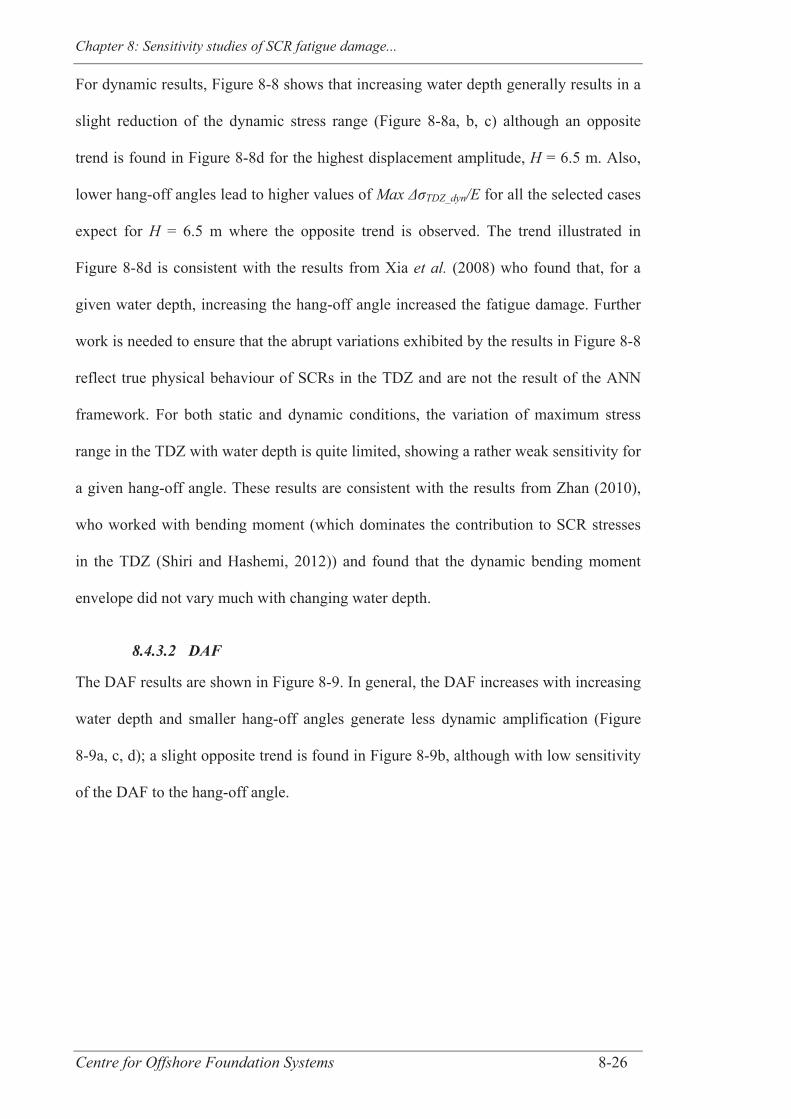
Chapter 8: Sensitivity studies of SCR fatigue damage...
Centre for Offshore Foundation Systems 8-26
For dynamic results, Figure 8-8 shows that increasing water depth generally results in a
slight reduction of the dynamic stress range (Figure 8-8a, b, c) although an opposite
trend is found in Figure 8-8d for the highest displacement amplitude, H = 6.5 m. Also,
lower hang-off angles lead to higher values of Max TDZ_dyn/E for all the selected cases
expect for H = 6.5 m where the opposite trend is observed. The trend illustrated in
Figure 8-8d is consistent with the results from Xia et al. (2008) who found that, for a
given water depth, increasing the hang-off angle increased the fatigue damage. Further
work is needed to ensure that the abrupt variations exhibited by the results in Figure 8-8
reflect true physical behaviour of SCRs in the TDZ and are not the result of the ANN
framework. For both static and dynamic conditions, the variation of maximum stress
range in the TDZ with water depth is quite limited, showing a rather weak sensitivity for
a given hang-off angle. These results are consistent with the results from Zhan (2010),
who worked with bending moment (which dominates the contribution to SCR stresses
in the TDZ (Shiri and Hashemi, 2012)) and found that the dynamic bending moment
envelope did not vary much with changing water depth.
8.4.3.2 DAF
The DAF results are shown in Figure 8-9. In general, the DAF increases with increasing
water depth and smaller hang-off angles generate less dynamic amplification (Figure
8-9a, c, d); a slight opposite trend is found in Figure 8-9b, although with low sensitivity
of the DAF to the hang-off angle.
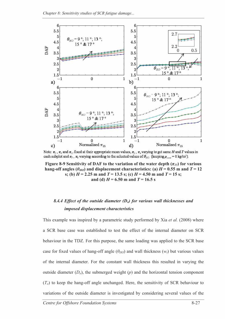
Chapter 8: Sensitivity studies of SCR fatigue damage...
Centre for Offshore Foundation Systems 8-27
Figure 8-9 Sensitivity of DAF to the variation of the water depth (π15) for various hang-off angles (θHO) and displacement characteristics: (a) H = 0.55 m and T = 12
s; (b) H = 2.25 m and T = 13.5 s; (c) H = 4.50 m and T = 15 s; and (d) H = 6.50 m and T = 16.5 s
8.4.4 Effect of the outside diameter (Do) for various wall thicknesses and
imposed displacement characteristics
This example was inspired by a parametric study performed by Xia et al. (2008) where
a SCR base case was established to test the effect of the internal diameter on SCR
behaviour in the TDZ. For this purpose, the same loading was applied to the SCR base
case for fixed values of hang-off angle ( HO) and wall thickness (wt) but various values
of the internal diameter. For the constant wall thickness this resulted in varying the
outside diameter (Do), the submerged weight (p) and the horizontal tension component
(To) to keep the hang-off angle unchanged. Here, the sensitivity of SCR behaviour to
variations of the outside diameter is investigated by considering several values of the
Chapter 8: Sensitivity studies of SCR fatigue damage...
Centre for Offshore Foundation Systems 8-28
wall thickness and also for various displacement characteristics (and corresponding
values of p and To), therefore exploring wider ranges of the input parameters. The
values of dimensionless groups and individual input parameters used for this purpose
are shown in Table 8-9. Results are presented in Figure 8-10, Figure 8-11 and Figure
8-12 and are discussed below.
8.4.4.1 Maximum stress range in the TDZ
In order to compare the results against the findings from Xia et al. (2008), the effect of
the variation of the outside diameter on the maximum stress range occurring in the TDZ
is illustrated for static and dynamic loading in Figure 8-10 and Figure 8-11 respectively.
In general, increasing the outside diameter for a given wall thickness tends to increase
Max TDZ_sta/E, which is consistent with the results from Xia et al. (2008). However, it
seems that for low values of the displacement amplitude a slight opposite trend may be
found (Figure 8-10a). Greater wall thickness systematically leads to higher
Max TDZ_sta/E in this example since it results in higher value of submerged weight ( 7)
and therefore an increase of curvature in the TDZ.
Regarding dynamic loading, Max TDZ_dyn/E also increases with increasing outside
diameter for most of the selected cases, although it decreases for high displacement
amplitude and low wall thickness (Figure 8-11d). In their case study, Xia et al. (2008)
found that the fatigue damage for dynamic loading decreased with increasing outside
diameter for a given wall thickness. Further work is therefore needed to validate the
observed trends and find the values of input parameters that lead to a change of trends.
Another complex behaviour is also noted depending on the value of the displacement
amplitude: for low displacement amplitude, the higher the wall thickness, the greater the
fatigue damage (Figure 8-11a, b), whereas the reverse is true for higher values of
displacement amplitude (Figure 8-11c, d). This illustrates the usefulness of the
Chapter 8: Sensitivity studies of SCR fatigue damage...
Centre for Offshore Foundation Systems 8-29
simplified framework for the early stages of design where designers can optimise values
of wall thickness and outside diameter for the waves that contribute most to the overall
fatigue damage under the given wave scatter diagram.
8.4.4.2 DAF
Based on the maximum stress ranges in the TDZ, DAF sensitivity to the variation of
outside diameter depends on the imposed displacement characteristics. For low
displacement amplitude, DAF increases with increasing outside diameter and is higher
for greater wall thickness values (Figure 8-12a, b). However, for higher displacement
amplitudes, DAF decreases with increasing outside diameter and lower wall thicknesses
lead to higher DAF values (Figure 8-12c, d). Large DAF values in excess of 16 are
observed for the highest selected displacement amplitude, the lowest selected wall
thickness and the lowest selected outside diameter.
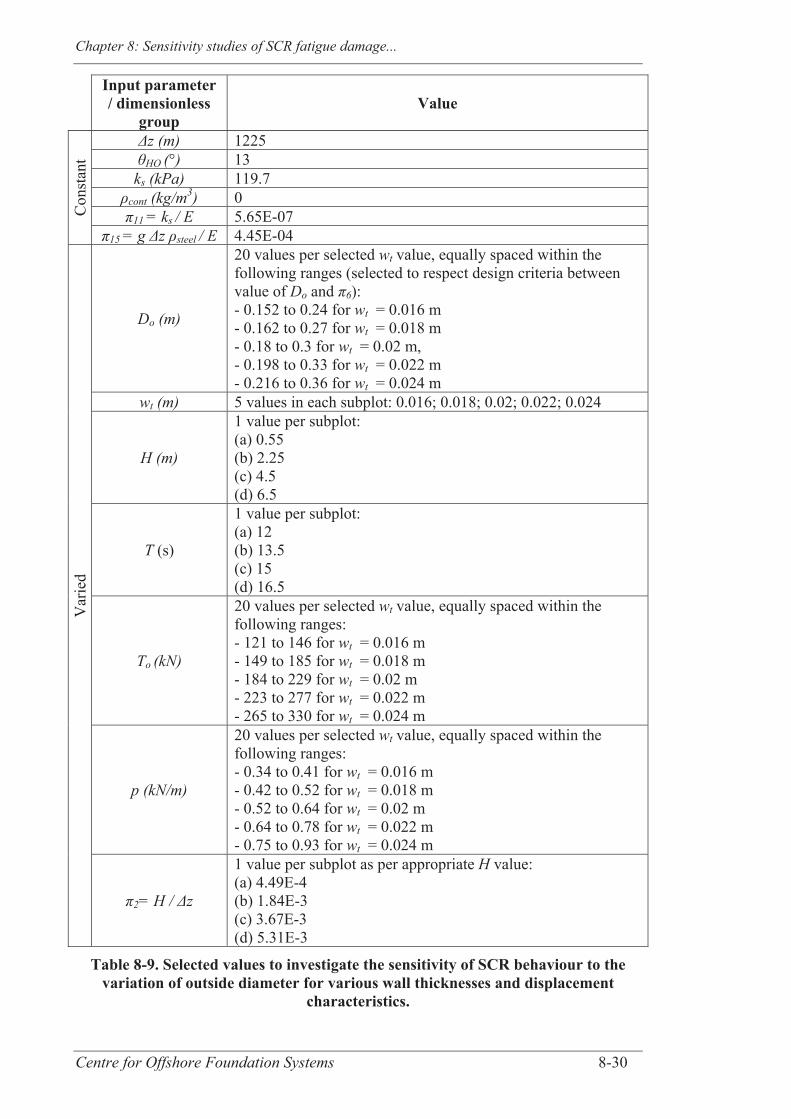
Chapter 8: Sensitivity studies of SCR fatigue damage...
Centre for Offshore Foundation Systems 8-30
Input parameter / dimensionless
group Value
Con
stan
t
z (m) 1225 HO (°) 13
ks (kPa) 119.7 cont (kg/m3) 0 11 = ks / E 5.65E-07
15 = g z steel / E 4.45E-04
Var
ied
Do (m)
20 values per selected wt value, equally spaced within the following ranges (selected to respect design criteria between value of Do and 6): - 0.152 to 0.24 for wt = 0.016 m - 0.162 to 0.27 for wt = 0.018 m - 0.18 to 0.3 for wt = 0.02 m, - 0.198 to 0.33 for wt = 0.022 m - 0.216 to 0.36 for wt = 0.024 m
wt (m) 5 values in each subplot: 0.016; 0.018; 0.02; 0.022; 0.024
H (m)
1 value per subplot: (a) 0.55 (b) 2.25 (c) 4.5 (d) 6.5
T (s)
1 value per subplot: (a) 12 (b) 13.5 (c) 15 (d) 16.5
To (kN)
20 values per selected wt value, equally spaced within the following ranges: - 121 to 146 for wt = 0.016 m - 149 to 185 for wt = 0.018 m - 184 to 229 for wt = 0.02 m - 223 to 277 for wt = 0.022 m - 265 to 330 for wt = 0.024 m
p (kN/m)
20 values per selected wt value, equally spaced within the following ranges: - 0.34 to 0.41 for wt = 0.016 m - 0.42 to 0.52 for wt = 0.018 m - 0.52 to 0.64 for wt = 0.02 m - 0.64 to 0.78 for wt = 0.022 m - 0.75 to 0.93 for wt = 0.024 m
2= H / z
1 value per subplot as per appropriate H value: (a) 4.49E-4 (b) 1.84E-3 (c) 3.67E-3 (d) 5.31E-3
Table 8-9. Selected values to investigate the sensitivity of SCR behaviour to the variation of outside diameter for various wall thicknesses and displacement
characteristics.
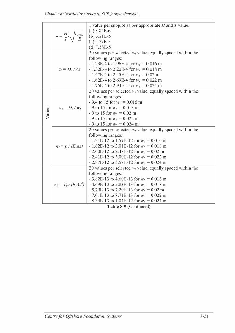
Chapter 8: Sensitivity studies of SCR fatigue damage...
Centre for Offshore Foundation Systems 8-31
Var
ied
4= HT steel
E
1 value per subplot as per appropriate H and T value: (a) 8.82E-6 (b) 3.21E-5 (c) 5.77E-5 (d) 7.58E-5
5 = Do / z
20 values per selected wt value, equally spaced within the following ranges: - 1.23E-4 to 1.96E-4 for wt = 0.016 m - 1.32E-4 to 2.20E-4 for wt = 0.018 m- 1.47E-4 to 2.45E-4 for wt = 0.02 m - 1.62E-4 to 2.69E-4 for wt = 0.022 m - 1.76E-4 to 2.94E-4 for wt = 0.024 m
6 = Do / wt
20 values per selected wt value, equally spaced within the following ranges: - 9.4 to 15 for wt = 0.016 m - 9 to 15 for wt = 0.018 m - 9 to 15 for wt = 0.02 m - 9 to 15 for wt = 0.022 m - 9 to 15 for wt = 0.024 m
7 = p / (E z)
20 values per selected wt value, equally spaced within the following ranges: - 1.31E-12 to 1.59E-12 for wt = 0.016 m - 1.62E-12 to 2.01E-12 for wt = 0.018 m- 2.00E-12 to 2.48E-12 for wt = 0.02 m - 2.41E-12 to 3.00E-12 for wt = 0.022 m - 2.87E-12 to 3.57E-12 for wt = 0.024 m
9 = To / (E z2)
20 values per selected wt value, equally spaced within the following ranges: - 3.82E-13 to 4.60E-13 for wt = 0.016 m - 4.69E-13 to 5.83E-13 for wt = 0.018 m- 5.79E-13 to 7.20E-13 for wt = 0.02 m - 7.01E-13 to 8.71E-13 for wt = 0.022 m - 8.34E-13 to 1.04E-12 for wt = 0.024 m
Table 8-9 (Continued)

Chapter 8: Sensitivity studies of SCR fatigue damage...
Centre for Offshore Foundation Systems 8-32
Figure 8-10 Sensitivity of Max ΔσTDZ_sta / E to the variation of outside diameter (Do) for various wall thicknesses (wt) and displacement characteristics: (a) H = 0.55 m;
(b) H = 2.25 m; (c) H = 4.50 m; and (d) H = 6.50 m
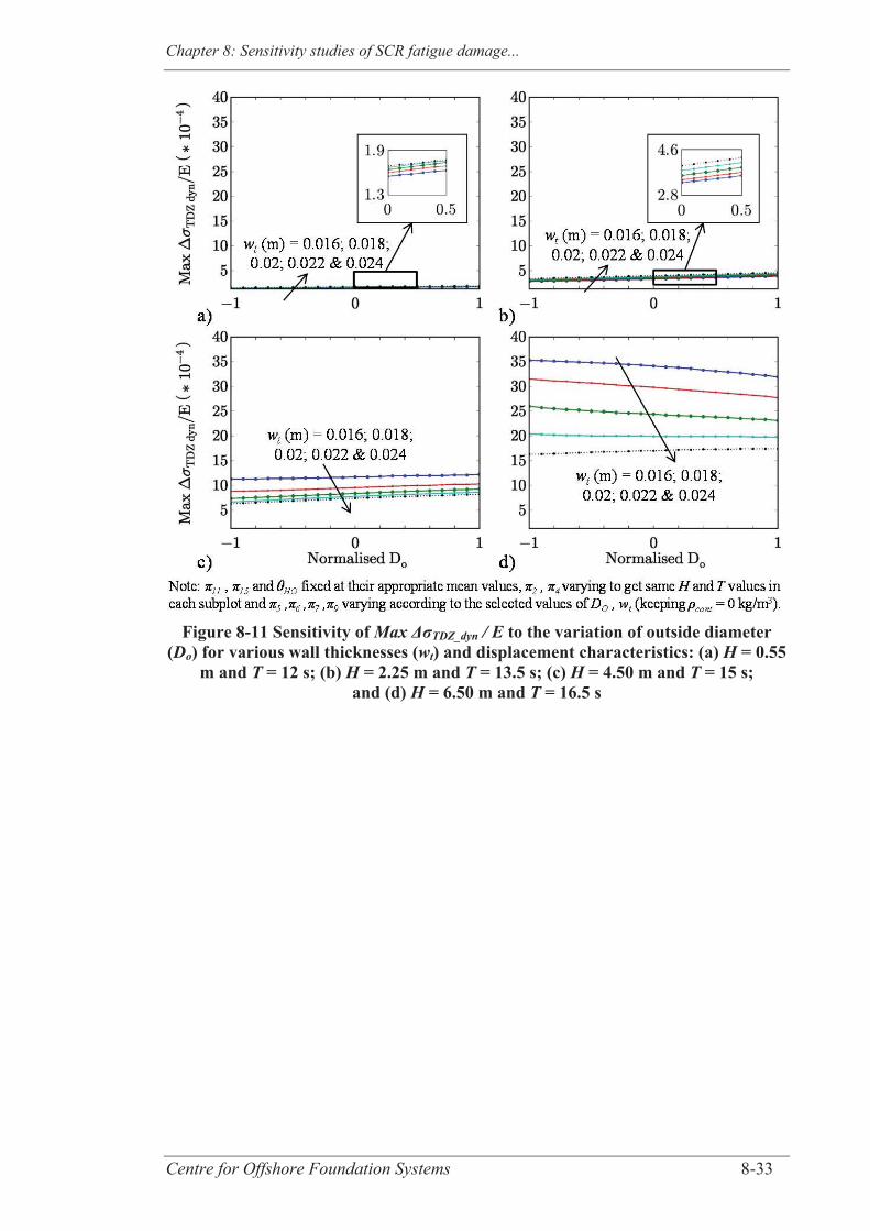
Chapter 8: Sensitivity studies of SCR fatigue damage...
Centre for Offshore Foundation Systems 8-33
Figure 8-11 Sensitivity of Max ΔσTDZ_dyn / E to the variation of outside diameter
(Do) for various wall thicknesses (wt) and displacement characteristics: (a) H = 0.55 m and T = 12 s; (b) H = 2.25 m and T = 13.5 s; (c) H = 4.50 m and T = 15 s;
and (d) H = 6.50 m and T = 16.5 s
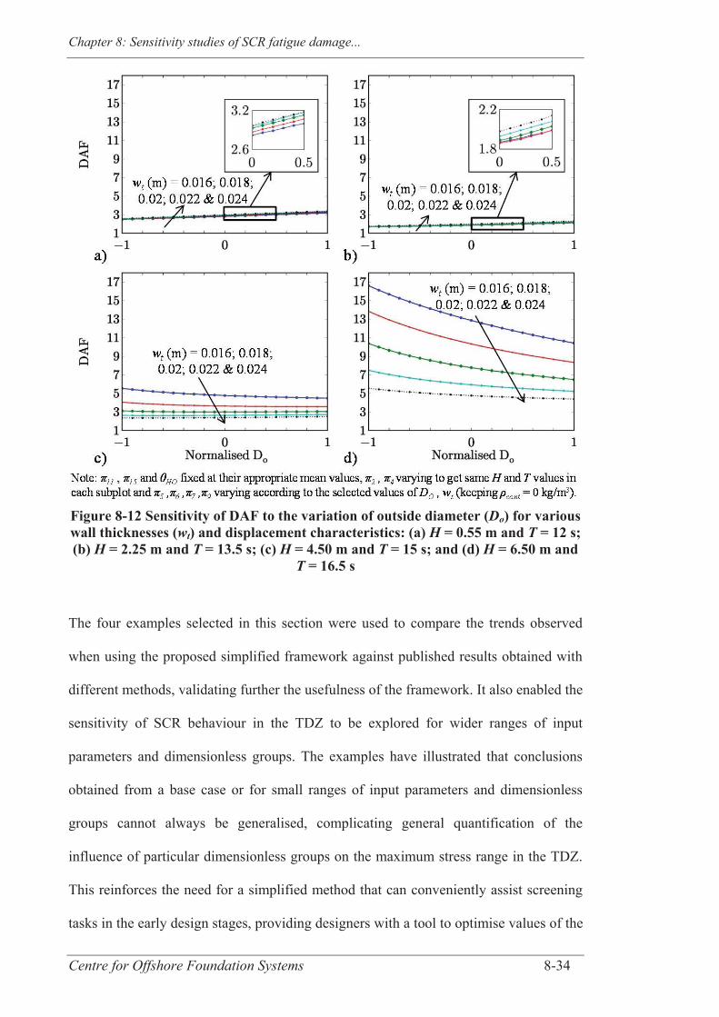
Chapter 8: Sensitivity studies of SCR fatigue damage...
Centre for Offshore Foundation Systems 8-34
Figure 8-12 Sensitivity of DAF to the variation of outside diameter (Do) for various wall thicknesses (wt) and displacement characteristics: (a) H = 0.55 m and T = 12 s; (b) H = 2.25 m and T = 13.5 s; (c) H = 4.50 m and T = 15 s; and (d) H = 6.50 m and
T = 16.5 s
The four examples selected in this section were used to compare the trends observed
when using the proposed simplified framework against published results obtained with
different methods, validating further the usefulness of the framework. It also enabled the
sensitivity of SCR behaviour in the TDZ to be explored for wider ranges of input
parameters and dimensionless groups. The examples have illustrated that conclusions
obtained from a base case or for small ranges of input parameters and dimensionless
groups cannot always be generalised, complicating general quantification of the
influence of particular dimensionless groups on the maximum stress range in the TDZ.
This reinforces the need for a simplified method that can conveniently assist screening
tasks in the early design stages, providing designers with a tool to optimise values of the
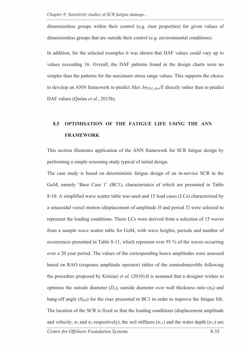
Chapter 8: Sensitivity studies of SCR fatigue damage...
Centre for Offshore Foundation Systems 8-35
dimensionless groups within their control (e.g. riser properties) for given values of
dimensionless groups that are outside their control (e.g. environmental conditions).
In addition, for the selected examples it was shown that DAF values could vary up to
values exceeding 16. Overall, the DAF patterns found in the design charts were no
simpler than the patterns for the maximum stress range values. This supports the choice
to develop an ANN framework to predict Max TDZ_dyn/E directly rather than to predict
DAF values (Quéau et al., 2015b).
8.5 OPTIMISATION OF THE FATIGUE LIFE USING THE ANN
FRAMEWORK
This section illustrates application of the ANN framework for SCR fatigue design by
performing a simple screening study typical of initial design.
The case study is based on deterministic fatigue design of an in-service SCR in the
GoM, namely ‘Base Case 1’ (BC1), characteristics of which are presented in Table
8-10. A simplified wave scatter table was used and 15 load cases (LCs) characterised by
a sinusoidal vessel motion (displacement of amplitude H and period T) were selected to
represent the loading conditions. These LCs were derived from a selection of 15 waves
from a sample wave scatter table for GoM, with wave heights, periods and number of
occurrences presented in Table 8-11, which represent over 95 % of the waves occurring
over a 20 year period. The values of the corresponding heave amplitudes were assessed
based on RAO (response amplitude operator) tables of the semisubmersible following
the procedure proposed by Kimiaei et al. (2010).It is assumed that a designer wishes to
optimise the outside diameter (Do), outside diameter over wall thickness ratio ( 6) and
hang-off angle ( HO) for the riser presented in BC1 in order to improve the fatigue life.
The location of the SCR is fixed so that the loading conditions (displacement amplitude
and velocity, 2 and 4 respectively), the soil stiffness ( 11) and the water depth ( 15) are
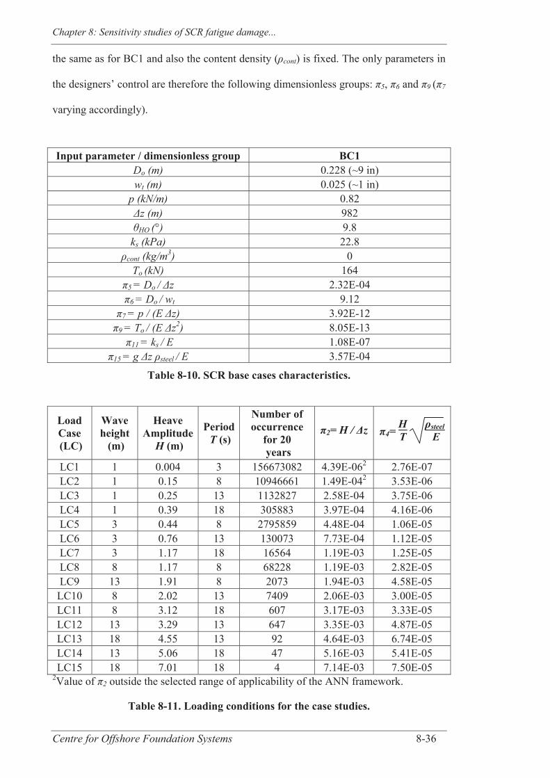
Chapter 8: Sensitivity studies of SCR fatigue damage...
Centre for Offshore Foundation Systems 8-36
the same as for BC1 and also the content density ( cont) is fixed. The only parameters in
the designers’ control are therefore the following dimensionless groups: 5, 6 and 9 ( 7
varying accordingly).
Input parameter / dimensionless group BC1 Do (m) 0.228 (~9 in) wt (m) 0.025 (~1 in)
p (kN/m) 0.82 z (m) 982 HO (°) 9.8
ks (kPa) 22.8 cont (kg/m3) 0
To (kN) 164 5 = Do / z 2.32E-04
6 = Do / wt 9.12 7 = p / (E z) 3.92E-12
9 = To / (E z2) 8.05E-13 11 = ks / E 1.08E-07
15 = g z steel / E 3.57E-04
Table 8-10. SCR base cases characteristics.
Load Case (LC)
Wave height (m)
Heave Amplitude
H (m)
Period T (s)
Number of occurrence
for 20 years
π2= H / Δz π4= HT
ρsteel E
LC1 1 0.004 3 156673082 4.39E-062 2.76E-07 LC2 1 0.15 8 10946661 1.49E-042 3.53E-06 LC3 1 0.25 13 1132827 2.58E-04 3.75E-06 LC4 1 0.39 18 305883 3.97E-04 4.16E-06 LC5 3 0.44 8 2795859 4.48E-04 1.06E-05 LC6 3 0.76 13 130073 7.73E-04 1.12E-05 LC7 3 1.17 18 16564 1.19E-03 1.25E-05 LC8 8 1.17 8 68228 1.19E-03 2.82E-05 LC9 13 1.91 8 2073 1.94E-03 4.58E-05 LC10 8 2.02 13 7409 2.06E-03 3.00E-05 LC11 8 3.12 18 607 3.17E-03 3.33E-05 LC12 13 3.29 13 647 3.35E-03 4.87E-05 LC13 18 4.55 13 92 4.64E-03 6.74E-05 LC14 13 5.06 18 47 5.16E-03 5.41E-05 LC15 18 7.01 18 4 7.14E-03 7.50E-05
2Value of 2 outside the selected range of applicability of the ANN framework.
Table 8-11. Loading conditions for the case studies.
Chapter 8: Sensitivity studies of SCR fatigue damage...
Centre for Offshore Foundation Systems 8-37
The example sensitivity studies in the previous section demonstrated that loading
conditions might lead to different choices of recommended values of HO , Do and wt in
order to decrease the maximum dynamic stress range in the TDZ. The fatigue life is
based on the cumulative damage from each LC of a wave scatter diagram, and the
damage is non-linearly related to the maximum dynamic stress range in the TDZ
through the allowable number of occurrence. It is therefore necessary to find the
combination of HO, Do and 6 values leading to the least overall damage to find the
optimum fatigue life. For the sake of simplicity, it is assumed that the designer has the
choice between three values for each of the inputs, as follows:
HO can take a value of 9.8° (as for BC1), 13° or 17°.
Do can take a value of 0.228 m (as for BC1), 0.25 m or 0.35 m.
6 can take a value of 9.12 (as for BC1), 12 or 15.
Since there are three possible choices for each of three inputs, 27 possible designs result
for the SCR. The ANN framework is applied to investigate the fatigue lives of the SCRs
formed by the 27 combinations of inputs, with results shown in Table 8-12. Fatigue
results are assessed using the DNV S-N curve type D for seawater (DNV-RP-C203,
2011). Under those circumstances, by keeping Do and 6 to their values in BC1 and
increasing HO to 17° the fatigue life can be increased from 163 to 722 years, improving
fatigue performance by a factor greater than 4.
This illustrates how the proposed ANN framework can assist screening design tasks in
finding combinations of input parameters that optimise fatigue performance, although
other practical considerations may affect the final selection of input parameters. In
practice, the ANN framework may be used in conjunction with optimisation software in
order to consider many more choices for the input parameters.
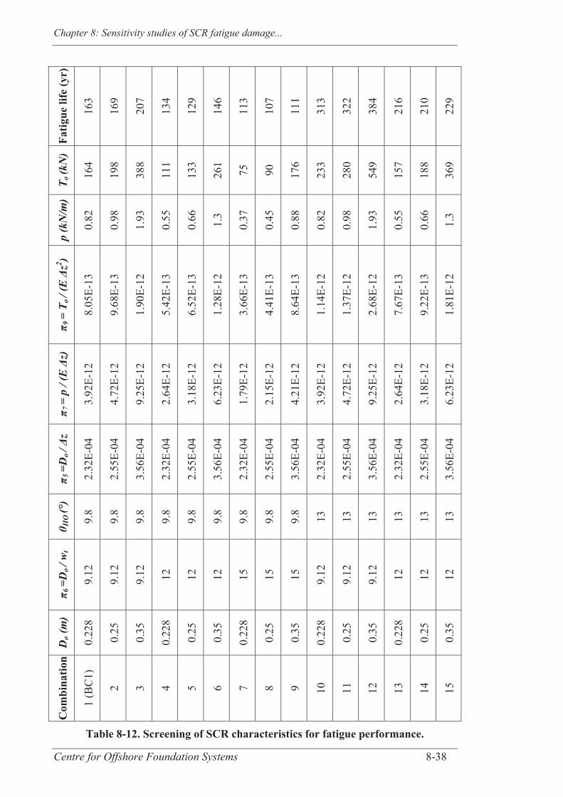
Chapter 8: Sensitivity studies of SCR fatigue damage...
Centre for Offshore Foundation Systems 8-38
Fa
tigue
life
(yr)
163
169
207
134
129
146
113
107
111
313
322
384
216
210
229
T o (k
N)
164
198
388
111
133
261
75
90
176
233
280
549
157
188
369
p (k
N/m
)
0.82
0.98
1.93
0.55
0.66
1.3
0.37
0.45
0.88
0.82
0.98
1.93
0.55
0.66
1.3
π 9 =
To / (
E Δ
z2 )
8.05
E-13
9.68
E-13
1.90
E-12
5.42
E-13
6.52
E-13
1.28
E-12
3.66
E-13
4.41
E-13
8.64
E-13
1.14
E-12
1.37
E-12
2.68
E-12
7.67
E-13
9.22
E-13
1.81
E-12
π 7 =
p /
(E Δ
z)
3.92
E-12
4.72
E-12
9.25
E-12
2.64
E-12
3.18
E-12
6.23
E-12
1.79
E-12
2.15
E-12
4.21
E-12
3.92
E-12
4.72
E-12
9.25
E-12
2.64
E-12
3.18
E-12
6.23
E-12
π 5 =
Do / Δ
z
2.32
E-04
2.55
E-04
3.56
E-04
2.32
E-04
2.55
E-04
3.56
E-04
2.32
E-04
2.55
E-04
3.56
E-04
2.32
E-04
2.55
E-04
3.56
E-04
2.32
E-04
2.55
E-04
3.56
E-04
θ HO
(°)
9.8
9.8
9.8
9.8
9.8
9.8
9.8
9.8
9.8 13
13
13
13
13
13
π 6 =
Do / w
t
9.12
9.12
9.12
12
12
12
15
15
15
9.12
9.12
9.12
12
12
12
Do (
m)
0.22
8
0.25
0.35
0.22
8
0.25
0.35
0.22
8
0.25
0.35
0.22
8
0.25
0.35
0.22
8
0.25
0.35
Com
bina
tion
1 (B
C1)
2 3 4 5 6 7 8 9 10
11
12
13
14
15
Table 8-12. Screening of SCR characteristics for fatigue performance.
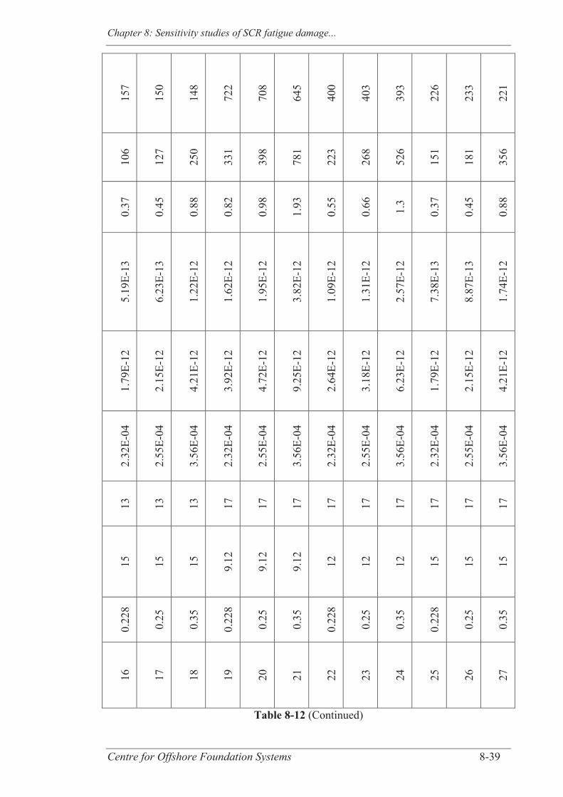
Chapter 8: Sensitivity studies of SCR fatigue damage...
Centre for Offshore Foundation Systems 8-39
157
150
148
722
708
645
400
403
393
226
233
221
106
127
250
331
398
781
223
268
526
151
181
356
0.37
0.45
0.88
0.82
0.98
1.93
0.55
0.66
1.3
0.37
0.45
0.88
5.19
E-13
6.23
E-13
1.22
E-12
1.62
E-12
1.95
E-12
3.82
E-12
1.09
E-12
1.31
E-12
2.57
E-12
7.38
E-13
8.87
E-13
1.74
E-12
1.79
E-12
2.15
E-12
4.21
E-12
3.92
E-12
4.72
E-12
9.25
E-12
2.64
E-12
3.18
E-12
6.23
E-12
1.79
E-12
2.15
E-12
4.21
E-12
2.32
E-04
2.55
E-04
3.56
E-04
2.32
E-04
2.55
E-04
3.56
E-04
2.32
E-04
2.55
E-04
3.56
E-04
2.32
E-04
2.55
E-04
3.56
E-04
13
13
13
17
17
17
17
17
17
17
17
17
15
15
15
9.12
9.12
9.12
12
12
12
15
15
15
0.22
8
0.25
0.35
0.22
8
0.25
0.35
0.22
8
0.25
0.35
0.22
8
0.25
0.35
16
17
18
19
20
21
22
23
24
25
26
27
Table 8-12 (Continued)
Chapter 8: Sensitivity studies of SCR fatigue damage...
Centre for Offshore Foundation Systems 8-40
8.6 CONCLUSIONS
This paper has illustrated the usefulness of the simplified framework based on artificial
neural networks (ANNs) developed previously (Chapters 6 and 7) for SCR design with
respect to fatigue in the TDZ.
A series of sensitivity studies were performed by varying a selection of dimensionless
groups and individual input parameters to illustrate the trends in SCR behaviour.
Estimated trends were benchmarked against published results to validate further the
accuracy of the ANN framework. The sensitivity studies explored wider ranges of the
inputs and showed how misinterpretations can arise from generalising the trends
obtained from more restricted studies, since the effect of certain inputs on the maximum
stress range in the TDZ may depend on the value of other inputs. For this reason, and
because the fatigue life depends on the cumulative damage for a given wave scatter
diagram, optimisation of an SCR design with respect to fatigue must consider the
overall level of damage rather than individual load cases. The usefulness of the ANN
framework for such optimisation was illustrated by a simple example.
The sensitivity of DAF values, quantifying the dynamic amplification compared with
static results, was also investigated. It was shown that values of DAF as high as 16
could occur with the selected examples and that the DAF pattern was no easier to
predict than the pattern of the maximum dynamic stress range in the TDZ directly.
Estimating the fatigue damage of SCRs in the TDZ
Centre for Offshore Foundation Systems 9-1
CHAPTER 9 CONCLUDING REMARKS
The focus of this thesis has been to define a simplifying fatigue assessment approach for
the early stages of design and improve the understanding of the behaviour of steel
catenary risers in the touchdown zone. The research has combined extensive numerical
analyses with analytical work, statistical and mathematical techniques, to perform the
various incremental steps necessary to the development of a simplified framework for
the fatigue analysis of SCRs in the TDZ. The proposed framework, using artificial
neural networks, has been shown to achieve accurate prediction of fatigue life results
and fatigue damage trends on a series of examples.
The main conclusions and findings arising from this research and the directions for
future work are summarised in this final chapter.
9.1 KEY CONCLUSIONS AND ORIGINAL CONTRIBUTION
The key conclusions resulting from this thesis are summarised in this section. As a
whole, they represent a substantial and original contribution to the knowledge of the
structural response and estimation of the fatigue damage of steel catenary risers in the
touchdown zone.
Dynamic analysis of steel catenary risers is time consuming and requires high
computational efforts due to the different sources of nonlinearity involved in their
structural response. The thesis critically examined the viability of defining a simplified
framework for the fatigue design of SCRs in the TDZ. The initial strategy for
simplification developed within this thesis was based on the use of dynamic
amplification factors (DAFs) since DAFs were successfully used to simplify the
structural dynamic analyses in other engineering fields. Chapter 2 to Chapter 6 therefore
explored various steps necessary to the implementation of the DAF approach for SCRs.
Chapter 9: Concluding remarks
Centre for Offshore Foundation Systems 9-2
Building on the knowledge acquired mainly from the work reported within Chapter 3,
Chapter 5 and Chapter 6, a framework using artificial neural network to efficiently
predict the critical dynamic stress range, directly, was established and is reported in
Chapter 7. Chapter 8 subsequently illustrated the usefulness of this framework and
reflected back on the original intention of using DAFs for simplification of dynamic
analyses of SCRs in the TDZ.
Since all the chapters represent incremental steps towards the main research aim of
simplifying the fatigue analysis of SCRs in the TDZ, the major findings are organised
accordingly and are summarised next, based on the findings from each individual
chapter.
9.1.1 Investigation of the usefulness of DAF for the fatigue design of
SCRs in the TDZ
A pilot study was performed (Chapter 2) in order to get the first insights on the
usefulness of DAF for the fatigue design of SCRs in the TDZ. A definition for the DAF
was proposed, as the ratio between the critical dynamic and static stress ranges in the
TDZ. The sensitivity of DAFs to vessel motions (amplitudes and periods), and soil
stiffness were examined through numerical simulations and it was found that vessel
motions could significantly influence the DAF, while the soil stiffness had no major
effect on it. The DAF approach seemed well suited for the simplification of SCR
dynamic analysis at this stage.
9.1.2 Clarification of the parameters impacting the fatigue damage of
SCRs in the TDZ
Fatigue design of SCRs in the TDZ is a complex challenge that is at the heart of current
research in the field of riser design. Despite the large interest in understanding the role
of design parameters in the level of stress range in the TDZ, there is still a lack of clear
guidance and of simple approaches able to conveniently produce information on SCR
Chapter 9: Concluding remarks
Centre for Offshore Foundation Systems 9-3
behaviour.
The study presented in Chapter 3 laid out the basis for pertinent sensitivity studies by
clarifying the dimensionless groups of input parameters influencing the dynamic and
static response of SCRs. A comprehensive set of numerical simulations was performed
to validate the proposed dimensionless groups and allow for a better control on the input
parameters, a wider scope of application of the results from numerical simulations and
easier comparison and interpretation of the results.
The input parameters related to the SCR geometry and structural properties,
environmental loading and the seabed characteristics were examined. When modelling
the seabed with a linear soil model, a final selection of 18 dimensionless groups formed
by 21 independent input parameters was established. The key dimensionless groups
influencing the response of SCRs identified among them were the normalised riser
displacement, velocity, outside diameter, unit submerged weight and tension
(accounting for the effect of the hang-off angle), the outside diameter to wall thickness
ratio, and the normalised soil stiffness and water depth.
9.1.3 Development of an analytical model for the prediction of the stress
range in SCRs under static loading
Since it is essential for the DAF approach to have the ability to determine the critical
static stress range in the TDZ, preferably through a simple method, and since published
literature did not provide this pre-requisite with a sufficient level of accuracy, an
analytical model able to fulfil this purpose was developed. Chapter 4 therefore focused
on extending an existing analytical model, using a boundary layer solution in the
vicinity of the touchdown point and a Winkler type soil model in the riser-soil contact
area, tailoring the model to the need of this study. Numerical simulations in OrcaFlex
software were performed to validate the results of this model, namely the Extended
Three Fields Model (ETFM). A good level of accuracy was reached so that the ETFM
Chapter 9: Concluding remarks
Centre for Offshore Foundation Systems 9-4
provides a simple and efficient analytical tool for the evaluation of the critical static
stress range in the TDZ.
9.1.4 Investigation of the usefulness of ANN for the fatigue design of
SCRs in the TDZ
The main challenge in the development of a simplified method using DAF was to
produce a database providing sufficient information on the relationships between the
dimensionless groups of inputs (as found in Chapter 3) and the DAF values, and to find
a way to capture these relationships. For these purposes, a series of sensitivity studies,
testing the effects of variation of the key input dimensionless groups on the structural
response of SCRs, were conducted and the ability of the response surface method in
approximating these relationships was also investigated.
Most published sensitivity studies in the field of riser design have only been carried out
for small ranges of some of the input parameters, hereby limiting their scope. The thesis
attempted to increase the knowledge of SCR behaviour for a broad range of input
parameters, encompassing most of the realistic SCR applications, in order to develop a
simplified approach with a wide range of applicability. Traditional methods applied
within published sensitivity studies were usually not suited to consider large ranges of
input parameters and to account for the effect of the interactions between the input
parameters. It was therefore necessary to investigate a suitable approach to perform the
sensitivity studies and post-process their results. This was the main concern of the pilot
study reported in Chapter 5.
The in-house automation sub-routine that was developed to generate the numerical
models providing the necessary information for the sensitivity studies, was presented in
this chapter. It was shown on a database of 4800 SCR configurations under static
loading that design of experiment techniques could conveniently assist the definition of
the database. Also, the usefulness of the artificial neural network, which is an advanced
Chapter 9: Concluding remarks
Centre for Offshore Foundation Systems 9-5
mathematical tool of the response surface method, was tested and seemed well suited to
the simplification of fatigue analysis of SCRs in the TDZ.
9.1.5 Development of an ANN approximation for the critical static stress
range for SCRs in the TDZ
Based on the promising results from Chapter 5, Chapter 6 was concerned with the
expansion of the database to refine the approximation of the critical static stress range
defined within Chapter 5. Chapter 6 was another preliminary step towards the
application of the proposed ANN approach to the more complex prediction of DAF
values, or of the critical dynamic stress range in the TDZ as was decided ultimately.
An ANN approximation of the maximum static stress range in SCRs (evaluated here
through numerical simulations using the marine analysis software OrcaFlex) was
developed successfully using a database of over 50,000 SCR configurations under static
loading conditions. The proposed approximation, comprising nine ANNs, can evaluate
over 99% of the cases of the database with an accuracy of 5% compared with the
results from OrcaFlex. The outcomes of Chapter 6 provided sufficient confidence in the
ANN approach to examine the dynamic loading conditions using similar methods.
9.1.6 Development of an ANN approximation for the critical dynamic
stress range for SCRs in the TDZ
Months of calculations were necessary to develop a large database of more than 40,000
SCR configurations under dynamic loading and support the training of a response
surface using ANN, and this part of the research was presented in Chapter 7. It was
found at this stage of the research that using ANNs, it was possible to capture the
relationships between the input dimensionless groups (as found in Chapter 3) and the
critical dynamic stress range of SCRs in the TDZ directly. As a consequence, the overall
strategy of this research shifted slightly since it was found more convenient for future
applications to use a framework able to predict the critical dynamic stress range in the
Chapter 9: Concluding remarks
Centre for Offshore Foundation Systems 9-6
TDZ in a straightforward manner (rather than obtaining an evaluation through DAF).
An approximation was defined having similar architecture to the approximation
developed to estimate the critical static stress range in the TDZ (in Chapter 6) was
defined. It is also composed of nine ANNs and is able to estimate the majority of the
cases of the database (> 80 %) within 5% errors with OrcaFlex results. Further
strategies aiming to further improve the accuracy of the approximation were proposed
and applied on part of the design space to confirm their beneficial effect on
performances. Using this refined approximation, the fatigue lives of a series of example
SCRs were estimated within only a few minutes of simple computational works and
were found to be within a negligible range of errors with the results derived from
OrcaFlex calculations.
The findings from this chapter proved that by using the proposed approximation and
approaches, it is possible to tremendously shorten the fatigue design calculations for
SCRs in the TDZ for the early stages of design where a minor compromise on accuracy
is acceptable.
9.1.7 Illustration of the usefulness of the proposed ANN framework
The final technical chapter of the thesis drew all of the previous steps of this research
together by illustrating the usefulness of the proposed ANN framework. It provided
insights on the sensitivity of the structural response of SCRs in the TDZ and shed light
on how the proposed ANN framework could be used in the screening tasks aiming at
optimising the fatigue life of SCRs in the TDZ.
A series of sensitivity studies were performed using the ANN framework. The trends
obtained for the critical stress range in the TDZ compared well against published
results, although by selecting wider ranges of the input parameters it was shown how
generalising from a limited number of results, derived from sensitivity studies
Chapter 9: Concluding remarks
Centre for Offshore Foundation Systems 9-7
performed only on some of the input parameters or considering small ranges of the input
parameters, could sometimes lead to misinterpretations. The sensitivity of DAF to the
variation of input parameters was also investigated and results were consistent with the
preliminary results presented during the pilot study stage of this research (Chapter 2),
further validating the performance of the developed ANN framework. The obtained
trends confirmed that the DAF pattern was not simpler to predict than the pattern of the
critical dynamic stress range, reinforcing the shift of strategy that occurred in the
research (Chapter 7).
In addition, the ANN framework was applied to an example fatigue optimisation study
to illustrate how it can assist the selection of an improved setup for SCRs to improve the
fatigue life in the TDZ.
9.2 LIMITATIONS AND FUTURE RESEARCH
9.2.1 In-depth investigation of the accuracy of the stress range and
fatigue results from the ANN framework
The performance of the ANN framework for practical purposes was investigated by
using it to evaluate the fatigue life of example SCRs (Chapter 7) and its usefulness for
SCR design was illustrated through a series of sensitivity studies, exploring the effects
of the variation of the key input dimensionless groups or input parameters on the
structural response of SCRs (Chapter 8). It could be worth evaluating the fatigue life of
more example SCRs and using different wave scatter diagram to increase the
understanding of the performance of the ANN framework and quantify further its
accuracy. Further sensitivity studies, considering different values of the input
dimensionless groups and individual parameters, could also be performed using the
ANN framework to shed more light on the structural response of SCRs.
Chapter 9: Concluding remarks
Centre for Offshore Foundation Systems 9-8
9.2.2 Extension of the existing ANN framework
A number of assumptions and simplifications were adopted in this research to render the
problem manageable. For example, the study was limited to 2 D conditions, the current,
flow rate of the content and coating were not accounted for, the floater was limited to
the case of a semisubmersible and a deterministic approach was used for the loading,
represented by an imposed displacement to the upper end of the SCRs. Also, a linear
soil model was used mostly throughout the thesis (as per common practice), whereas it
is generally agreed that this model is too simple to capture the complex seabed
interactions occurring in the TDZ. In the future, it could therefore be desirable to extend
the present work to other types of floaters, stochastic loadings, and to include the effect
of the current, using a nonlinear soil model for instance, in order to enlarge the scope of
applicability of the ANN framework.
9.2.3 Refinement of the accuracy of the ANN framework for dynamic
loading conditions
A good level of accuracy was reached overall by the ANN framework for the estimation
of the critical dynamic stress range occurring in SCRs in the TDZ but some marginal
cases with high relative differences with numerical results were observed, signalling
margins for future improvement. It could be worth expanding the database in the future
and/or investigating the effect of using more advanced data division algorithms (e.g.
self-organising map or fuzzy clustering for instance) on the performance of the
approximated results.
Since the structure of the overall approximation (with the nine ANNs) led to good
performances overall, improvement of the inherent ANNs could be performed
separately and a statistically consistent approach could be used on each of the training
and testing sets of the ANNs, similar to what was performed for part of the design space
in Chapter 7. In turn, these recommendations might improve the robustness of the
Chapter 9: Concluding remarks
Centre for Offshore Foundation Systems 9-9
proposed framework.
9.2.4 Investigation of the development of a similar ANN framework for
other riser types
The framework developed throughout the thesis explored the applicability and ability of
a simplified approach using ANNs, to efficiently and accurately estimate the results
from time consuming dynamic simulations involved in fatigue design of SCRs. This
was performed in order to provide a final user with a convenient tool (based on ANNs)
that fulfils the role of the numerical simulations, and replaces them, for the early stages
of design where a compromise on the level of accuracy is acceptable. The design of
other structural systems may benefit from the use of such a framework since the time
and cost for running dynamic simulations are usually important limiting factors.
Dynamic simulations generally require high computational efforts with the availability
of a licence for the software used to run the simulations. The present framework could
therefore be developed for other riser types, such as lazy wave risers (LWRs). As a
digression, a study was indeed performed (when the strategy was still to use DAF for
simplification) in order to broaden the scope of application of some of the findings to
the LWRs since they can be an alternative to SCRs and this is presented in Appendix
A2. The proposed framework could however also be applied beyond the riser fatigue
design applications, to other subsea structures or other, potentially completely different,
applications.
9.3 CONCLUSION
This thesis proves that by using innovative techniques the fatigue analysis of SCRs in
the TDZ can be performed in a time efficient manner without significantly
compromising the accuracy of the predicted fatigue results. The simplified framework

Chapter 9: Concluding remarks
Centre for Offshore Foundation Systems 9-10
defined during this research and described in the thesis assists the understanding of SCR
behaviour in the TDZ and provides a convenient tool for the screening and optimisation
tasks performed in the early stages of fatigue design of SCRs.
Estimating the fatigue damage of SCRs in the TDZ
Centre for Offshore Foundation Systems R-1
REFERENCES
2H Offshore (2013). 2H Offshore awarded SCR detailed design project with LLOG
exploration company. Houston, March 2013. Web source:
www.2hoffshore.com/news/96-2h-offshore-awarded-scr-detailed-design-project-
with-llog-exploration-company
Abelanet, M., Karunakaran, D., Jones, R., Eyssautier, S., White, P. (2013). Deepwater
steel catenary risers require attention to fatigue factors. Online edition of Offshore
magazine. Web source: www.offshore-mag.com/articles/print/volume-73/issue-
10/engineering-construction-installation/deepwater-steel-catenary-risers-require-
attention-to-fatigue-factors.html
Aceton (2013). 2H Offshore wins detailed design project with LLOG. Press release in
Rigzone. Web source: www.rigzone.com/news/article.asp?a_id=124723
Adeli, H. (2001). Neural networks in civil engineering:1989-2000. Computer-aided civil
and infrastructure engineering, pp.126-142.
Aggarwal, R.K., Godinot, H., Schutz, R.W., Quintanilla, H., Mourelle, M.M, Vargas, P.,
Portesan, G., Schamuhn, S., Kristoffersen, S., Else, M., Izquierdo, A., Sches, C.
(2007). Development and qualification of alternate solutions for improved fatigue
performance of deepwater steel catenary risers. In: Proceedings of the Int. Conf. on
Offshore Mechanics and Arctic Engineering, San Diego, California, OMAE 2007-
29325.
Anderson Fonteles Teofilo, F. P. (2010). Preliminary design of composite catenary
risers using optimization techniques. Mecanica computacional, Buenos Aires,
Argentina, vol XXIX, pp. 7927-7948.
ANSYS (2014). Web source: www.ansys.com
References
Centre for Offshore Foundation Systems R-2
API (2013) API Standard 2RD Dynamic risers for floating production systems.
American Petroleum Institute, Washington, USA.
API (2011) API RP 1111, Recommended practice for the design, construction,
operation and maintenance of offshore hydrocarbon pipelines (limit state design).
American Petroleum Institute, Washington, USA.
Aranha, J. A. P., Martins, C. A., Pesce, C. P. (1997). Analytical approximation for the
dynamic bending moment at the touchdown point of a catenary riser. Int. J. of
Offshore and Polar Engineering, Vol. 7, No. 4, pp. 293-300.
ASME (2012). ASME B31.4 Pipeline transportation systems for liquid hydrocarbons
and other liquids. The American Society of Mechanical Engineers, New York,
USA.
Aubeny, C., Biscontin, G. (2008). Interaction model for steel compliant riser on soft
seabed. In: Proceedings of the Offshore Technology Conf., Houston, Texas, USA,
OTC19493.
Aubeny, C., Biscontin, G. (2009). Seafloor-riser interaction model. Int. J. of
Geomechanics, ASCE, Vol. 9, No. 3, p.133-141.
Bai, Y. (2001). Pipeline and risers. Ocean Engineering Book Series, Elsevier, USA.
Bai, Y., Bai, Q. (2005). Subsea pipelines and risers, 1st ed. Elsevier, Oxford, UK.
Barltrop, N.D.P., Adams, A.J. (1991). Dynamics of fixed marine structures. Butterworth-
Heinemann, Marine Technology Directorate.
BBC (2010). Web source: www.bbc.co.uk/news/10298342
Bea, R.G., Xu, T., Stear, J., Ramos, R. (1999). Wave forces on decks of offshore
platforms. J. of waterway, port, coastal and ocean enginnering, pp. 136-144.
References
Centre for Offshore Foundation Systems R-3
Bhat, S., Dutta, A., Wu, J., Sarkar, I. (2004). Pragmatic solutions to touchdown zone
fatigue challenges in steel catenary risers. In: Proceedings of the Offshore
Technology Conf., Houston, USA, OTC 16627.
Box, G. E. P., Draper, N.R. (2007). Response surfaces, mixtures, and ridge analyses (2nd
edition). John Wiley & sons, Inc.
BP, (2014). Web source: www.bp.com/en/global/corporate/sustainability/the-energy-
future/the-energy-challenge/deepwater-oil-and-gas.html
Bridge, C., Willis, N. (2002). Steel catenary risers-results and conclusions from large
scale simulations of seabed interaction. In: Proceedings of the Int. Conf. on Deep
Offshore Technology, PennWell.
Bridge, C., Howells, H., Toy, N., Parke, G., Woods, R. (2003). Full scale model tests of a
steel catenary riser. In: Proceedings of the Int. Conf. on Fluid Structure Interaction,
Cadiz, Spain.
Bridge, C., Laver, K., Clukey, E., Evans, T. (2004). Steel catenary riser touchdown
point vertical interaction models. In: Proceedings of the Offshore Technology
Conf., Houston, USA, OTC 16628.
Bridge, C. (2005). Effects of seabed interaction on steel catenary risers. PhD thesis,
University of Surrey.
Bridge, C., Howells, H. (2007). Observations and modelling of steel catenary risers
trenches. In: Proceedings of the 17th Int. Offshore and Polar Engineering Conf.,
Lisbon, Portugal, ISOPE-2007-468, pp. 803 - 813.
Campbell, M. (1999). The complexities of fatigue analysis for deepwater risers. In:
Proceedings of the Deepwater Pipeline Technology Conf., New Orleans, USA.

References
Centre for Offshore Foundation Systems R-4
Chatjigeorgiou, I. (2010). Three dimensional nonlinear dynamics of submerged,
extensible catenary pipes conveying fluid and subjected to end-imposed
excitations. Int. J. of nonlinear mechanics, Elsevier, 45, pp. 667 - 680.
Chatjigeorgiou, I. (2013). Second-order nonlinear dynamics of catenary pipelines: a
frequency domain approach. Computers and structures, Elsevier, 123, pp. 1 - 14.
Clukey, E.C., Haustermans, L., Dyvik, R. (2005). Model tests to simulate riser-soil
interaction effects in touchdown point region. In: Proceedings of the Int.
Symposium on Frontiers in Offshore Geotechnics, Perth, Australia, pp. 651 - 658.
Clukey E.C., Ghosh, R., Mokarala, P., Dixon, M. (2007). Steel catenary riser (SCR)
design issues at touch down area. In: Proceedings of the 17th Int. Offshore and
Polar Engineering Conf., Lisbon, Portugal, pp. 814 - 819.
Clukey, E.C., Young, A.G., Dobias, J.R., Garmon, G.R. (2008). Soil response and
stiffness laboratory measurements of SCR pipe/soil interaction. In: Proceedings of
the Offshore Technology Conf., Houston, OTC 19303.
Clukey, E.C., Tognarelli, M.A., Li, G., Ghosh, R., Phillips, R., Zakeri, A. Elliot, B.J.,
Bhattacharyya, A., Sun, Q. (2011). Simulation of SCR behaviour at touchdown
zone- Part II: testing of a sectional SCR model in a geotechnical centrifuge. In:
Proceedings of the Offshore Technology Conf., Houston, OTC 22569.
Dassault systemes (2014). Abaqus Unified FEA. Web source: www.3ds.com/products-
services/simulia/portfolio/abaqus/overview/
De Amicis, L., Mahoney, G., Grealish, F., Connaire, A. (2007). SCR designs rise to the
challenge. Offshore magazine. Web source: www.offshore-
mag.com/articles/print/volume-67/issue-9/subsea/scr-designs-rise-to-the-
challenge.html
References
Centre for Offshore Foundation Systems R-5
de Pina, A. C., de Pina, A. A., Albercht, C.H., de Lima, B.S.L.P., Jacob, B.P. (2013).
ANN-based surrogate models for the analysis of mooring lines and risers. Applied
Ocean Research, 41, pp. 76 - 86.
DNV GL (2014). Web source: http://www.dnv.com/services/software/products_list/
DNV-RP-C203 (April 2010). Recommended Practice, Fatigue design of offshore steel
structures. Det Norske Veritas, Hovik, Norway.
DNV-RP-C203 (October 2011). Recommended Practice, Fatigue design of offshore
steel structures. Det Norske Veritas, Hovik, Norway.
DNV-OS-F201 (October 2010). Offshore standard, Dynamic Risers. Det Norske
Veritas, Hovik, Norway.
DNV-RP-F204 (October 2010). Recommended Practice, Riser fatigue. Det Norske
Veritas, Hovik, Norway.
Duan, M., Chen, J., Li, Z. (2011). Mechanics of deepwater steel catenary riser,
Numerical Analysis- Theory and Applicaation, Prof. Jan Awrejcewicz (Ed.),
ISBN: 978-953-307-389-7, InTech, Web source:
www.intechopen.com/books/numerical-analysis-theory-and-
application/mechanics-of-deepwater-steel-catenary-riser
Elliott, B., Phillips, R., Macneill, A., Barrett, J. (2013a). Response of an SCR to 3-axis
motions in the touchdown zone. Rio Pipeline Conf. and Exposition, Rio de
Janeiro, Brazil, IBP1041_13.
Elliott, B.J., Zakeri, A., Macneill, A., Phillips, R., Clukey, E.C., Li, G. (2013b).
Centrifuge modelling of steel catenary risers at touchdown zone part I:
Development of novel centrifuge experimental apparatus. Ocean Engineering,
Elsevier, 60, pp. 200 - 207.
References
Centre for Offshore Foundation Systems R-6
Elliott, B.J., Zakeri, A., Barrett, J., Hawlader, B., Li, G., Clukey, E.C. (2013c).
Centrifuge modelling of steel catenary risers at touchdown zone part II:
Assessment of centrifuge test results using kaolin clay. Ocean Engineering,
Elsevier, 60, pp. 208 - 218.
Elosta, H., Huang, S., Incecik, A. (2013a). Seabed interaction modelling effects on the
global response of catenary pipeline: a case study. In: Proceedings of the 32nd Int.
Conf. on Offshore Mechanics and Arctic Engineering, Nantes, France,
OMAE2013-10782.
Elosta, H., Huang, S., Incecik, A. (2013b). Dynamic response of steel catenary riser
using a seabed interaction under random loads. Ocean Engineering, Elsevier, 69,
pp. 34 - 43.
Elosta, H., Huang, S., Incecik, A. (2014).Trenching effects on structural safety assessment
of integrated riser/semisubmersible in cohesive soil, Engineering Structures,
Elsevier, vol. 77, pp. 57-64.
Erlend Voie, P. , Sødahl, N. (2013). Optimisation of steel catenary risers. In:
Proceedings of the 32nd Int. Conf. on Ocean, Offshore and Artic Engineering,
Nantes, France, OMAE2013-10107.
Esteco (1999). modeFRONTIER 4 user manual. www.esteco.com/modefrontier, Italy.
Fausett, L. (1994). Fundamentals of neural networks: architectures, algorithms and
applications, Prentice-Hall, Inc., New Jersey, USA.
FloaTEC (2014). Deepwater floating production systems-an overview. Web source:
www.floatec.com/images/Deepwater-Floater-Intro.pdf
Fontaine, E. (2006). SCR-soil interaction;Effect on fatigue life and trenching. In:
Proceedings of the 16th Int. Offshore and Polar Engineering Conf., San
Francisco, California, USA, pp.60 - 67.

References
Centre for Offshore Foundation Systems R-7
Fowlkes W.Y., Creveling C.M. (1995). Engineering methods for robust design using
Taguchi methods in technology and product development, Addison-Wesley
publishing company.
Franciss, R., Ribeiro, E. (2004). Analyses of a large diameter steel lazy wave riser for
ultra deepwater in campos basin. In: Proceedings of the 23rd Int. Conf. on
Offshore Mechanics and Arctic Engineering, Vancouver, Canada, OMAE2004-
51176.
Fu, J., Yang, H. (2010). Fatigue characteristic analysis of deepwater steel catenary risers
at the touchdown point. China Ocean Engineering, Vol. 24, No. 2, pp. 291 - 304.
Giertsen, E., Verley, R., Schroder, K. (2004). Carisima:A catenary riser/soil interaction
model for global riser analysis. In: Proceedings of the 23rd Int. Conf. on Offshore
Mechanics and Arctic Engineering, Vancouver, Canada, OMAE2004-51345.
Gunaratnam, D. J. & Gero, J. S. (1994). Effect of representation on the performance of
neural networks in structural engineering applications. Microcomputers in Civil
Engineering, 9 (2), pp. 97 - 108.
Guo, B., Song, S., Chacko, J., Ghalambor, A. (2005). Offshore pipelines. Gulf
Professional Publishing, Elsevier, USA.
Gurney, K. (1997). An introduction to neural networks, UCL Press Limited, London,
UK.
Hammerstrom, D. (1993). Working with neural networks, IEEE Spectrum, 30(7), pp. 46
- 53.
Hodder, M.S., White, D.J., Cassidy, M.J. (2008). Centrifuge modelling of riser-soil
stiffness degradation in the touchdown zone of a steel catenary riser. In:
Proceedings of the 27th Int. Conf. on Offshore Mechanics and Arctic Engineering,
Estoril, Portugal, OMAE2008-57302, pp. 241 - 249.
References
Centre for Offshore Foundation Systems R-8
Hodder, M.S., Byrne, B.W. (2010). 3D experiments investigating the interaction of a
model SCR with the seabed. Applied ocean research, Elsevier, 32, pp. 146 - 157.
Hodder, M. S, White, D.J., Cassidy, M.J. (2010). Analysis of soil strength degradation
during episodes of cyclic loading, illustrated by the T-bar penetration test. Int. J.
of Geomechanics, ASCE, pp. 117 - 123.
Hodder, M.S., White, D.J., Cassidy, M.J. (2013). An effective stress framework for the
variation in penetration resistance due to episodes of remoulding and
reconsolidation. Géotechnique 63, No. 1, pp. 30 - 43.
Howells, H. (1995). Advances in steel catenary riser design. In: Proceedings of the 2nd
Annual Int. Forum on Deepwater Technology (DEEPTEC), Aberdeen.
Hu, H.J.E, Leung, C.F., Chow, Y.K., Palmer, A.C. (2011). Centrifuge modelling of
SCR vertical motion at touchdown zone. Ocean Engineering, Elsevier, 38, pp.
888 - 899.
Intecsea (2014). Scarborough pre-feed. Web source: www.intecsea.com/project-
experience/australia-newzealand/119-scarborough-pre-feed
ISO (2009) ISO13623:2009, Petroleum and natural gas industries, pipeline
transportation systems. The Int. Standardization Organisation.
Jiao, Y. (2007). Nonlinear load-deflection models for seabed interaction with steel
catenary risers. Texas A&M University: M.Sc. Thesis in Civil Engineering.
Katifeoglou, S.A, Chatjigeorgiou, I. K. (2012). Dynamic interaction of catenary risers
with the seafloor. Applied ocean research, Elsevier, 38, pp. 1 - 15.
Kavanagh, K., Galvin, C. (2012). Achieving feasible SCRs in harsh environments, a
multi-project review of alternative approaches for improving SCR fatigue and
strength performance, oral presentation at Deep Offshore Technology conf.,
Perth, Australia.
References
Centre for Offshore Foundation Systems R-9
Kimiaei, M., Randolph, M.F., Ting, I. (2010). A parametric study on effects of
environmental loadings on fatigue life of steel catenary risers (using a nonlinear
cyclic riser-soil interaction model). In: Proceedings of the 29th Int. Conf. on
Ocean, Offshore and Artic Engineering, Shanghai, China, OMAE2010-21153.
Kongsberg (2014). Dynamic positioning- basic principles. Web source:
www.km.kongsberg.com/ks/web/nokbg0240.nsf/AllWeb/BD306BBB3E7DA73F
C1256DAB00353083?OpenDocument
Kutuk, M.A., Atmaca, N., Guzelbey, I.H. (2007). Explicit formulation of SIF using
neural networks for opening mode of fracture. Engineering Structures, Elsevier,
vol. 29, pp. 2080 - 2086.
Langner, C. (2003). Fatigue life improvment of steel catenary risers due to self-
trenching at the touchdown point. In: Proceedings of the Offshore Technology
Conf., Houston, Texas, OTC 15104.
Larsen, C.M., Hanson, T. (1999). Optimization of catenary risers. J. of Offshore
Mechanics and Arctic Engineering, ASME, vol. 121, pp. 90 - 94.
Leira, B.J., Passano, E., Karunakaran, D., Farnes, K.A., Giertsen, E. (2004). Analysis
guidelines and application of a riser-soil interaction model including trench
effects. In: Proceedings of the 23rd Int. Conf. on Offshore Mechanics and Arctic
Engineering, Vancouver, Canada, OMAE2004-51527.
Lenci, S., Callegari, M. (2005). Simple analytical models for the J-lay problem. Acta
Mechanica, 178, pp. 23 - 29.
Li, S., Nguyen, C. (2010). Dynamic response of deepwater lazy wave catenary riser. In:
Proceedings of the Deep Offshore Technology Int. Conf.

References
Centre for Offshore Foundation Systems R-10
Lima, B.S.L.P., Jacob, B.P., Ebecken, N.F.F. (2005). A hybrid fuzzy/genetic algorithm
for the design of offshore oil production risers. Int. J. for Numerical Methods in
Engineering, 64, pp. 1459 - 148.
Love, A.E.H. (1892). A treatise on mathematical theory of elasticity. Cambridge
University Press.
Marintek. (2002). Review Norwegian marine technology research institute, 1 April
2002. The CARISIMA JIP. Web source:
www.sintef.no/upload/MARINTEK/PDF-filer/Review/Review_1-April-2002.pdf
Marintek (2014). Riflex. Web source: www.sintef.no/home/MARINTEK-old/Software-
developed-at-MARINTEK/RIFLEX/
Martins, M.A.L., Lages, E.N., Silveira, E.S.S. (2012). Optimal design approach of
compliant vertical access risers. In: Proceedings of the 22nd Int. Offshore and
Polar Engineering Conf., Rhodes, Greece, pp. 123 - 130.
Martins, M.A.L., Lages, E.N., Silveira, E.S.S. (2013). Compliant vertical access riser
assessment: DOE analysis and dynamic response optimization. Applied Ocean
Research, Elsevier, 41, pp. 28 - 40.
Martins, C.A., Pesce, C.P. (2002). A simplified procedure to assess the fatigue-life of
flexible risers. In: Proceedings of the 12th Int. Offshore and Polar Engineering
Conf., Kitakyushu, Japan, pp. 179 - 186.
Massey, B.S.(1971). Units, dimensional analysis and physical similarity. University
College London, Van Nostrand Reinhold Company, London.
MATLAB version 7.14.0 (2012). The MathWorks Inc., Natick, Massachusetts, USA.
MCS Kenny (2014). Flexcom. Web source: www.mcskenny.com/software-
solutions/flexcom.html

References
Centre for Offshore Foundation Systems R-11
Mekha, B.B. (2001). New frontiers in the design of steel catenary risers for floating
production systems, J. of Offshore Mechanics and Arctic Engineering, Vol 123, pp
153 - 158.
Montgomery, D.C. (2013). Design and analysis of experiments (8th edition). John Wiley
& sons, Inc.
Mukherjee, A., Deshpande, J. M. (1995). Modeling initial design process using artificial
neural networks, J. of Computing in Civil Engineering, ASCE, 9 (3), pp. 194 -
200.
Nakhaee, A., Zhang, J. (2009). Trenching effects on dynamic behaviour of steel catenary
riser. Ocean Engineering, Elsevier, 37, pp. 277 - 288.
Natarajan, S., Podskarbi, M., Karayaka, M., Howells, H. (2007). Deepwater SPAR steel
catenary riser monitoring strategy. In: Proceedings of the 26th Int. Conf. on
Offshore Mechanics and Arctic Engineering, San Diego, California, USA,
OMAE2007-29344.
Nelson, K., DeJesus, M., Chakhmakhchev, A., Manning, M. (2013). Deepwater operators
look to new frontiers, Offshire magazine. Web source: www.offshore-
mag.com/articles/print/volume-73/issue-5/international-report/deepwater-operators-
look-to-new-frontiers.html
Oliphant, J., Maconochie, A., White, D., Bolton, M. (2009). Trench interaction forces
during lateral SCR movement in deepwater clays. In: Proceedings of the Offshore
Technology Conf., Houston, Texas, USA, OTC 19944.
Orcina (2012). OrcaFlex User Manual 9.5d. www.orcina.com,UK.
Orcina (2011). OrcaFlex User Manual 9.5a. www.orcina.com,UK.
Palmer, A.C. (2008a). Touchdown indentation of the seabed. Applied ocean research,
Technical note, Elsevier, 30, pp. 235 - 238.

References
Centre for Offshore Foundation Systems R-12
Palmer, A.C. (2008b). Dimensional analysis and intelligent experimentation. Singapore,
World Scientific.
Patel, M.H., Seyed, F.B. (1995). Review of flexible riser modelling and analysis
techniques. Engineering Structures, Butterworth Heinemann, vol. 17, No. 4, pp.
293 - 304.
Park, S.H. (1996). Robust Design and Analysis for Quality Engineering, Charpman &
Hall.
Peace G. S. (1993). Taguchi methods, a hands-on approach to quality engineering. 3rd
printing, Addison-Wesley Publishing Company, Massachusetts, USA.
Peritus (2011). Media release: Peritus awarded Woodside Browse SCR engineering by
Modec. 100211-Woodside-Browse-SCR-engineering-MODEC. Web source:
www.docstoc.com/docs/113005380/100211-Woodside-Browse-SCR-
Engineering-MODEC
Pesce, C.P., Aranha, J.A.P, Martins, C.A., Ricardo, O.G.S., Silva, S. (1998a). Dynamic
curvature in catenary risers at the touchdown point region: an experimental study
and the analytical boundary-layer solution. Int. J. of Offshore and Polar
Engineering, vol. 8, No. 4, pp. 303 - 310.
Pesce, C.P., Aranha, J.A.P, Martins, C.A. (1998b). The soil rigidity effect in the
touchdown boundary-layer of a catenary riser: static problem. In: Int. Offshore
and Polar Engineering Conf., Montreal, Canada, vol. II, pp. 207 - 213.
Pesce, C. P., Martins, C. A., Silveira, L.M.Y. (2006). Riser-soil interaction: local
dynamics at TDP and a discussion on the eigenvalue and the VIV problems. J. of
Offshore Mechanics and Arctic Engineering, Vol. 128, pp. 39 - 55.

References
Centre for Offshore Foundation Systems R-13
Pettingill, H.S., YPF, R. Weimer, P (2002) World-wide deepwater exploration and
production: Past, present and future. In: Proceedings of the Offshore Technology
Conf., Houston, Texas, OTC 14024.
Principia (2014). Deeplines-global analysis of risers, moorings and flowlines. Web
source: www.principia.fr/expertise-fields-software-products-deeplines-126.html
PR Newswire, (2013). Deepwater Activity Statistics - New Discoveries Worldwide
Driving Deepwater E&P Activity and Demand for Semisubmersibles and
Drillships. Web source: www.prnewswire.com/news-releases/deepwater-activity-
statistics---new-discoveries-worldwide-driving-deepwater-ep-activity-and-demand-
for-semisubmersibles-and-drillships-211945511.html
Python Software Foundation (2009). Python Language Reference, version 2.6.
Quéau, L.M., Kimiaei, M., Randolph, M.F. (2011). Dynamic amplification factors for
response analysis of steel catenary risers at touch down areas. In: Proceedings of
the 21st Int. Offshore and Polar Engineering Conf., Hawaii, USA, vol. II, pp.1- 8.
Quéau, L.M., Kimiaei, M., Randolph, M.F. (2013). Dimensionless groups governing
response of steel catenary risers. Ocean Engineering, Elsevier, 74, pp. 247 - 259.
Quéau, L.M., Kimiaei, M., Randolph, M.F. (2014a). Analytical estimation of static
stress range in oscillating steel catenary risers at touchdown area and its
application with dynamic amplification factors. Ocean Engineering, Elsevier, 88,
pp. 63-80.
Quéau, L.M., Kimiaei, M., Randolph, M.F. (2014b).Artificial neural network
development for stress analysis of steel catenary risers: Sensitivity study and
approximation of static stress range. Applied Ocean Research, Elsevier, 48, pp.
148-161.

References
Centre for Offshore Foundation Systems R-14
Quéau, L.M., Kimiaei, M., Randolph, M.F. (2015a). Sensitivity studies of steel catenary
riser fatigue damage in the touchdown zone using an efficient simplification
framework for stress range evaluation. Ocean Engineering, Elsevier, 96, pp. 295-
311.
Quéau, L.M., Kimiaei, M., Randolph, M.F. (2015b). Approximation of the maximum
dynamic stress range in steel catenary risers using artificial neural networks.
Engineering Structures, Elsevier, 92, pp. 171-185.
Randolph, M.F., White, D. J. (2008). Pipeline embedment in deep water: processes and
quantitative assessment. In: Proceedings of the Offshore Technology Conf.,
Houston, USA, OTC 19128.
Randolph, M. F. (2009). Platform, pipeline and subsea technology. Lectures on
pipeline-seabed interaction, School of Civil and Resource Engineering, Centre for
Offshore Foundation Systems, The University of Western Australia.
Randolph, M.F., Quiggin, P. (2009). Non-linear hysteretic seabed model for catenary
pipeline contact. In: Proceedings of the 28th Int. Conf. on Ocean, Offshore and
Artic Engineering, Hawaii, USA, OMAE2009-79259.
Randolph, M.F., Bhat, S., Jain. S., Mekha, B. (2013). Modeling the touchdown zone
trench and its impact on SCR fatigue life. In: Proceedings of the Offshore
Technology Conf., Houston, USA, OTC 23975.
Rateiro, F., Pesce, C.P., Gonçalves, R.T, Franzini, G.R., Fujarra, A.L.C., Salles, R.,
Mendes, P. (2012). Risers model tests: Scaling methodology and dynamic
similarity. In: Proceedings of the 22nd Int. Offshore and Polar Engineering Conf.,
Rhodes, Greece, pp. 439 - 445.

References
Centre for Offshore Foundation Systems R-15
Rezazadeh, K., Shiri, H., Zhang, L., Bai, Y. (2012a). Seabed trench formation and its
impact on fatigue life of steel catenary risers in touchdown area. In: Proceedings
of the 22nd Int. Offshore and Polar Engineering Conf., Rhodes, Greece, pp. 268 -
274.
Rezazadeh, K., Shiri, H., Zhang, L., Bai, Y. (2012b). Fatigue generation mechanism in
touchdown area of steel catenary risers in nonlinear hysteretic seabed. Research J.
of Applied Sciences, Engineering and Technology, Maxwell Scientific
Organization,4(24), pp. 5591 - 5601.
Rogers, J. L. (1994). Simulating structural analysis with neural network, J. of
Computing in Civil Engineering, ASCE, 8 (2), pp. 252 - 265.
Roveri, F.E., Martins, C.A., Balena, R. (2005). Parametric analysis of a lazy wave steel
riser. In: Proceedings of the 24th Int. Conf. on Ocean, Offshore and Arctic
Engineering, Halkidiki, Greece, OMAE2005-67128.
Ruiz-Teran, A.M., Aparicio, A.C. (2006). Dynamic amplification factors in cable-
stayed structures. Elsevier, J. of sound and vibration, 300, pp. 197 - 216.
Senra, S.F., Mourelle, M.M., Andrade, E.Q., Torres, A.L.F.L. (2011). Challenges faced
in the design of SLWR configuration for the pre-salt area. In: Proceedings of the
30th Int. Conf. on Ocean, Offshore and Arctic Engineering, Rotterdam, The
Netherlands, OMAE2011-49096.
Sen, T. K., Hesar, M. (2007). Riser soil interaction in soft clay near the touchdown
zone. In: Proceedings of the Offshore Technology Conf., Houston, Texas, USA,
OTC 18896.
Serta, O.B., Mourelle, M.M., Grealish, F.W., Harbert, S.J., Souza, L.F.A. (1996). Steel
catenary riser for the Marlim Field FPS P-XVIII. In: Proceedings of the Offshore
Technology Conf., Houston, Texas, USA, OTC 8069.

References
Centre for Offshore Foundation Systems R-16
Sharma, P.P., Aubeny, C.P. (2011). Advances in pipe-soil interaction methodology and
application for SCR fatigue design. In: Proceedings of the Offshore Technology
Conf., Houston, Texas, USA, OTC 21179.
Shahin, M. A., Jaksa, M. B., Maier, H. R. (2002). Artificial neural network-based
settlement prediction formula for shallow foundations on granular soils.
Australian geomechanics, pp. 45 - 52.
Shahin, M. A., Maier, H. R., Jaksa, M. B. (2004). Data division for developing neural
networks applied to geotechnical engineering. J. of computing in civil
engineering, ASCE, Vol. 18, No. 2.
Shahin, M. A., Jaksa, M. B., Maier, H. R. (2008). State of the art of artificial neural
networks in geotechnical engineering. Electronic J. of Geotechnical Engineering.
Shell (2014). Web source: www.shell.com/global/future-energy/deepwater/deepwater-
technology.html, s01.static-shell.com/content/dam/shell/static/future-
energy/downloads/deepwater-meeting-demand/deepwater-meetingdemand.pdf
and www.shell.us/aboutshell/projects-locations/gulf-of-mexico-
deepwater/deepwater-101.html
Shiri, H. (2010). Influence of seabed response on fatigue performance of steel catenary
risers in the touchdown zone. PhD Thesis, the University of Western Australia,
Perth, Australia.
Shiri, H., Randolph, M.F. (2010). The influence of seabed response on fatigue
performance of steel catenary risers in touchdown zone. In: Proceedings of the
29th Int. Conf. on Ocean, Offshore and Artic Engineering, Shanghai, China,
OMAE2010-20051.

References
Centre for Offshore Foundation Systems R-17
Shiri, H., Hashemi, H. (2012). Simplified approximation of peak fatigue damage in the
touchdown area of steel catenary risers based on seabed soil rigidity. In:
Proceedings of the 22nd Int. Offshore and Polar Engineering Conf., Rhodes,
Greece, pp. 287 - 294.
Shiri, H., Sadeghi, A. (2012). Seabed interaction effects on stress distribution along the J-
lay pipelines. In: Proceedings of the 22nd Int. Offshore and Polar Engineering
Conf., Rhodes, Greece, pp. 311 - 318.
Shiri, H. (2014). Influence of seabed trench formation on fatigue performance of steel
catenary risers in touchdown zone. Marine Structures, Elsevier, 36, pp. 1 - 20.
Shu, J., Zhang, Z., Gonzalez, I., Karoumi, R. (2013). The application of a damage
detection method using artificial neural network and train-induced vibrations on a
simplified railway bridge model. Engineering Structures, Elsevier, vol. 52, pp.
408 - 421.
Silveira, L.M.Y., Martins, C. A. (2004). A numerical method to solve the static problem
of a catenary riser. In: Proceedings of the 23rd Int. Conf. on Offshore Mechanics
and Arctic Engineering, Vancouver, Canada, OMAE2004-51390.
Song, R., Stanton, P. (2007). Advances in deepwater steel catenary riser technology
state-of-the-art:Part I-Design. In: Proceedings of the 26th Int. Conf. on Ocean,
Offshore and Artic Engineering, San Diego, California, USA, OMAE2007-29329.
Song, R., Stanton, P. (2009). Advances in deepwater steel catenary riser technology
state-of-the-art:Part II-Analysis. In: Proceedings of the 28th Int. Conf. on Ocean,
Offshore and Artic Engineering, Honolulu, Hawaii, USA, OMAE2009-79405.
SubseaIQ, (2014). Offshore field development projects. Web source:
subseaiq.com/data/default.aspx
Szewczyk, Z. P., Noor, A. K. (1996). A hybrid neurocomputing/numerical strategy for
nonlinear structural analysis, Computers and Structures, 58 (4), pp. 661 - 677.

References
Centre for Offshore Foundation Systems R-18
Szewczyk, Z. P., Noor, A. K. (1997). A hybrid numerical/ neurocomputing strategy for
sensitivity analysis of nonlinear structures, Computers and Structures, 65 (6), pp.
869 - 880.
Tanaka, R.L., Martins, C.A. (2011). Parallel dynamic optimization of steel risers. J. of
Offshore Mechanic and Arctic Engineering, Vol. 133, pp.011302_1 - 011302_9.
Taylor, E.S. (1974). Dimensional analysis for engineers, Massachusetts Institute of
Technology, Clarendon Press, Oxford.
Technip, (2014). Web source: www.technip.com/en
(www.technip.com/en/press/technip-wins-two-contracts-ultra-deep-water-fields-
and-helps-petrobras-push-back-subsea-fronti and
www.technip.com/sites/default/files/technip/publications/attachments/Flexible_pi
pe_April_2013_Web.pdf)
Tenaris, (2014a). Web source:
www.tenaris.com/en/Products/OffshoreLinePipe/Risers.aspx
Tenaris, (2014b). A proven track-record of deep –water accomplishements. Web source:
www.tenaris.com/en/Products/OffshoreLinePipe/TrackRecord.aspx
Teofilo, F. A. P., Parente Junior, E., Melo, A., Holanda, A., Silva, R. (2010).
Preliminary design of composite catenary risers using optimization techniques.
Mecanica computacional, Buenos Aires, Argentina, Vol XXIX, pp. 7927 - 7948.
Thethi, R., Moros, T. (2001). Soil interaction effects on simple catenary riser response. In:
Proceedings of the Deepwater Pipeline and Riser Technology Conf., Houston,
Texas.
Tokar, A.S., Johnson, P.A. (1999). Rainfall-runoff modelling using artificial neural
networks, J. of Hydrologic engineering, ASCE, 4(3), pp. 232 - 239.
Total, (2014). Web source: total.com/en/energies-expertise/oil-gas/exploration-
production/strategic-sectors/deep-offshore

References
Centre for Offshore Foundation Systems R-19
UWA (2014). Graduate Research School, web source:
http://www.postgraduate.uwa.edu.au/students/thesis/series
Vieira, I., Lima, B.S.L.P., Jacob, B.P. (2008). Optimization of steel catenary risers for
offshore oil production using artificial immune system. ICARIS 2008, Springer-
Verlag Berlin Heidelberg 2008, pp.254 - 265.
Vieira, I.N., Lima, B.S.L.P., Evsukoff, A.G., Jacob, B.P. (2003). Application of genetic
algorithms to the synthesis of riser configurations. In: Proceedings of the 22nd Int.
Conf. on Ocean, Offshore and Artic Engineering, Cancun, Mexico, OMAE2003-
37231.
Wang, A., Yang, H., Li, H. (2011). Multiobjective optimization for dynamic umbilical
installation using non-dominated sorting genetic algorithm. In: Proceedings of the
30th Int. Conf. on Ocean, Offshore and Arctic Engineering, Rotterdam, The
Netherlands, OMAE2011-49148.
Wang, L., Zhang, J., Yuan, F., Li, K. (2014). Interaction between catenary riser and soft
seabed: large scale indoor tests. Applied ocean research, Elsevier, 45, pp.10 - 21.
Willis, N.R.T., Thethi, K.S. (1999). Stride JIP: Steel risers in deepwater environments –
progress summary. In: Proceedings of the Offshore Technology Conf., Houston,
Texas, USA, OTC 10974.
Willis, N.R.T., West, P.T.J. (2001). Interaction between deepwater catenary risers and a
soft seabed: Large scale sea trials. In: Proceedings of the Offshore Technology
Conf., Houston, Texas, USA, OTC 13113.
Woodside (2014a). Web source: www.woodside.com.au/Our-Business/North-West-
Shelf/Pages/default.aspx, video: “From plant to plan”.
Woodside (2014b). Browse LNG, Web source: www.woodside.com.au/our-
business/browse/Pages/default.aspx
References
Centre for Offshore Foundation Systems R-20
Xia, J., Das, P.K., Karunakaran, D. (2008). A parametric study for a semi/SCR system
in northern North Sea. Ocean Engineering, Elsevier, 35, pp. 1686 - 1699.
Yang, H., Wang, A., Li, H. (2012). Multi-objective optimization for deepwater dynamic
umbilical installation analysis. Sci. China-Phys. Mech. Astron., 55, pp. 1445 -
1453.
Yang, H., Li, H. (2010). Optimization design for deepwater risers with fatigue
constraints. In: Proceedings of the 20th Int. Offshore and Polar Engineering Conf.
(ISOPE), Beijing, China, pp. 176 - 181.
Yeung, W.T., Smith, J.W. (2005). Damage detection in bridges using neural networks
for pattern recognition of vibration signatures. Engineering Structures, Elsevier,
vol. 27, pp. 685 - 698.
You. J., Biscontin, G., Aubeny, C.P. (2008) Seafloor interaction with steel catenary
risers. In: Proceedings of the 18th Int. Offshore and Polar Engineering Conf.,
Vancouver, Canada, pp. 110 - 117.
Yuan, F., Wang, L., Guo, Z., Xie, Y. (2012). Analytical analysis of pipeline-soil
interaction during J-lay on a plastic seabed with bearing resistrance proportional
to depth. Applied ocean research, Elsevier, 36, pp. 60 - 68.
Yue, B., Campbell, M., Walters, D., Thompson, H., Raghavan, Kamaldev (2010).
Improved SCR design for dynamic vessel applications. In: Proceedings of the
29th Int. Conf. on Ocean, Offshore and Arctic Engineering, Shanghai, China,
OMAE2010-20406.
Zhan, J.P. (2010). Review and verification of marine riser analysis programs: global
response analysis. Thesis supervised by Prof. B. J. Leira, Norwegian University of
Science and Technology (NTNU), Department of Marine Technology.

Appendix
Centre for Offshore Foundation Systems A-1
APPENDIX
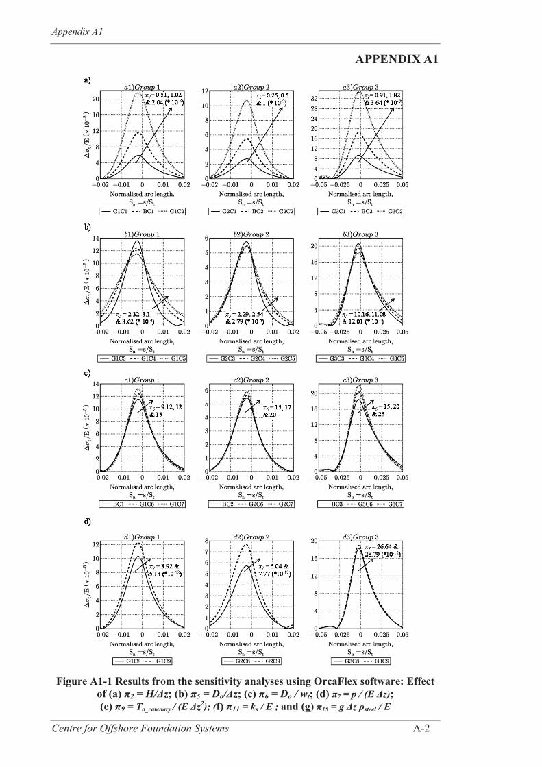
Appendix A1
Centre for Offshore Foundation Systems A-2
APPENDIX A1
Figure A1-1 Results from the sensitivity analyses using OrcaFlex software: Effect
of (a) π2 = H/Δz; (b) π5 = Do/Δz; (c) π6 = Do / wt; (d) π7 = p / (E Δz); (e) π9 = To_catenary / (E Δz2); (f) π11 = ks / E ; and (g) π15 = g Δz ρsteel / E
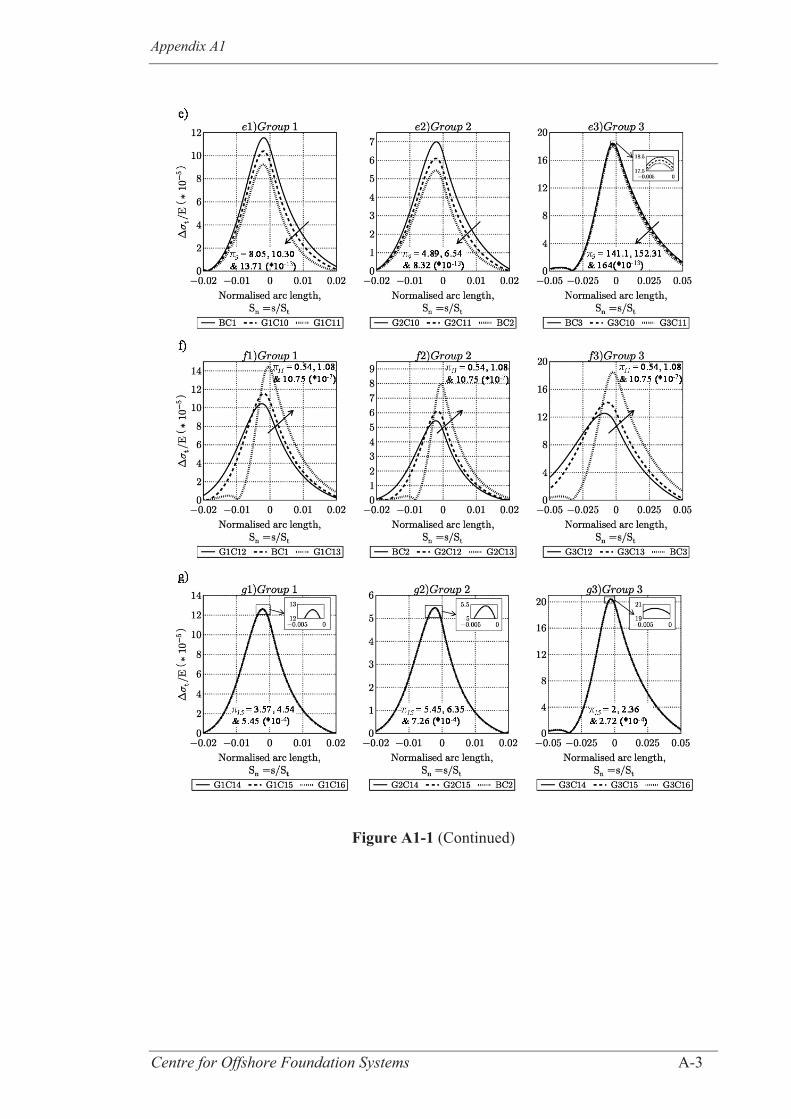
Appendix A1
Centre for Offshore Foundation Systems A-3
Figure A1-1 (Continued)
Appendix A2
Centre for Offshore Foundation Systems A-4
APPENDIX A2: LAZY WAVE CATENARY RISERS: SCALING
FACTORS AND ANALYTICAL APPROXIMATION OF THE
STATIC STRESS RANGE IN THE TOUCHDOWN ZONE
A2.1. ABSTRACT
Offshore exploration and production of oil and gas continue to increase and move into
ever deeper water. Steel catenary risers (SCRs) are one of the most cost effective type of
risers in deep water. However, high sensitivity to vessel motions and hydrodynamic
loading in the touchdown zone may limit the feasibility of SCR applications. In recent
years, there has been a growing interest in the use of Lazy-wave catenary riser (LWR)
due to their better fatigue performance in the touchdown zone through the damping
effect of the buoyancy section.
The design of LWR involves numerous parameters that lead to a wide range of
configurations. Each of these configurations needs to be evaluated against several
criteria with respect to geometry, strength and fatigue for instance. This paper presents
how tools recently proposed to improve the design of standard SCRs can be extended to
benefit LWR applications. The dimensionless groups governing the structural response
of LWRs are established in the aim of easing sensitivity analysis to key input
parameters for LWR design, assisting experiments and reducing the number of
numerical simulations. Moreover, the DAF (dynamic amplification factor) approach for
dynamic response which has previously been explored for SCRs could also be used to
simplify design of LWRs. As DAF relies on the analytical determination of static
response, this framework shows that analytical boundary layer solutions in conjunction
with the use of a Winkler type soil model can efficiently and accurately predict the
static stress range of LWRs observed in the TDZ.

Appendix A2
Centre for Offshore Foundation Systems A-5
A2.2. INTRODUCTION
In recent years, steel catenary risers (SCRs) have been used extensively as the oil and
gas exploration continues to move into ever deeper waters. SCRs are an attractive
options due to their simple geometry, ease of construction and installation and are a
cost-effective option (Yue et al., 2010). However, SCRs are fatigue sensitive structures,
especially in the zone where the riser first touches the seabed: the touchdown zone
(TDZ) (Campbell, 1999; Bai and Bai, 2005). For this reason, SCRs are not always a
viable option in ultra deep water and lazy wave catenary risers (LWRs) or shaped SCRs
can be good alternatives. LWRs are SCRs with a buoyant section that is used to improve
fatigue performance by de-coupling and damping the motions of the vessel at the sea
surface from the motions of the TDZ and to reduce the top loads (Franciss and Ribeiro,
2004; Roveri et al., 2005; Yue et al., 2010; Senra et al., 2011). An illustration is
provided in Figure A2-1. The buoyancy catenary is obtained by adding a series of
floaters to the riser, see Figure A2-2. Therefore, its hydrodynamic properties and
submerged weight (pbuoyc) are deduced from those of the riser and floaters. Shaped
SCRs are degenerated LWRs with less buoyancy and no sag bend or arch bend in order
to avoid flow assurance problem (Li and Nguyen, 2010; Yue et al., 2010).
Numerous parameters are involved in the design of LWRs that leads to the examination
of a wide range of possible configurations during the early stages of design (e.g.
feasibility of a project). Optimisation techniques are usually employed to select the best
configuration(s) with respect to strength and fatigue performance but they are time
consuming (Roveri et al., 2005; Yue et al., 2010; Senra et al., 2011). Therefore, simple
analytical methods would improve preliminary design of LWRs.
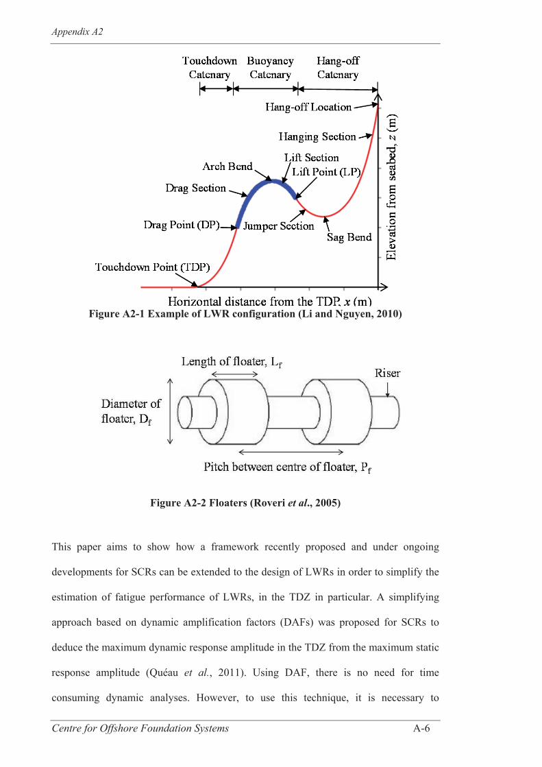
Appendix A2
Centre for Offshore Foundation Systems A-6
Figure A2-1 Example of LWR configuration (Li and Nguyen, 2010)
Figure A2-2 Floaters (Roveri et al., 2005)
This paper aims to show how a framework recently proposed and under ongoing
developments for SCRs can be extended to the design of LWRs in order to simplify the
estimation of fatigue performance of LWRs, in the TDZ in particular. A simplifying
approach based on dynamic amplification factors (DAFs) was proposed for SCRs to
deduce the maximum dynamic response amplitude in the TDZ from the maximum static
response amplitude (Quéau et al., 2011). Using DAF, there is no need for time
consuming dynamic analyses. However, to use this technique, it is necessary to
Appendix A2
Centre for Offshore Foundation Systems A-7
(i) assess the sensitivity of DAF values to input parameters entering design of LWRs in
order to evaluate the DAF and to (ii) estimate the static response of LWRs.
Similarly to the approach undertaken for the standard SCRs (Quéau et al., 2014), a
dimensional analysis is performed at first. This is to clarify the groups of parameters
that influence the stress range of LWRs in order to assist the future sensitivity studies
applied to the DAF. Then, an analytical model that considers the boundary layer
phenomena in the TDZ and uses a Winkler type deformable soil is derived to get an
estimation of the static stress range occurring in LWRs, which is a prerequisite to the
DAF approach. The scaling factors and the analytical model are validated against results
from numerical simulations performed with one of the commercially available software
used for marine analysis: OrcaFlex (Orcina, 2012).
The study is limited to 2D conditions where the current profile in the sea column, the
rotational stiffness at the hang-off point (HOP), the coating and the flow rate of the
content are not taken into account. Also, only the case of a linear soil model, horizontal
and flat seabed is investigated here.
A2.3. DIMENSIONAL ANALYSIS
The estimation of the fatigue life of LWRs relies initially on the measurement of the
total axial stress ( zz). Hence, the list of independent parameters that impact zz when
static and dynamic motions are applied to the vessel is established and dimensionless
groups are formed to determine the appropriate scaling factors. The selected parameters
are presented in Table A2-1. They are derived from the parameters that were shown to
impact the total axial stress in SCRs (Quéau et al., 2013) by addition of the parameters
inherent to the buoyancy catenary. This is to appropriately scale the drag, inertia and the
submerged weight of the buoyancy catenary (deduced from floaters and riser
characteristics). The output zz /E may then be expressed as a function f1 of the
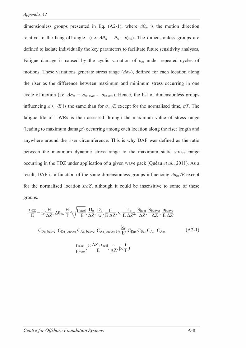
Appendix A2
Centre for Offshore Foundation Systems A-8
dimensionless groups presented in Eq. (A2-1), where m is the motion direction
relative to the hang-off angle (i.e. m = m - HO). The dimensionless groups are
defined to isolate individually the key parameters to facilitate future sensitivity analyses.
Fatigue damage is caused by the cyclic variation of zz under repeated cycles of
motions. These variations generate stress range ( zz), defined for each location along
the riser as the difference between maximum and minimum stress occurring in one
cycle of motion (i.e. zz = zz max - zz min). Hence, the list of dimensionless groups
influencing zz /E is the same than for zz /E except for the normalised time, t/T. The
fatigue life of LWRs is then assessed through the maximum value of stress range
(leading to maximum damage) occurring among each location along the riser length and
anywhere around the riser circumference. This is why DAF was defined as the ratio
between the maximum dynamic stress range to the maximum static stress range
occurring in the TDZ under application of a given wave pack (Quéau et al., 2011). As a
result, DAF is a function of the same dimensionless groups influencing zz /E except
for the normalised location s/ Z, although it could be insensitive to some of these
groups.
σZZE = f1(
HΔZ, Δθm,
HT
ρsteel E ,
DoΔZ,
Do wt
, p
E ΔZ, ν, To
E ΔZ2, Shoct ΔZ,
Sbuoyct ΔZ ,
pbuoycE ΔZ,
CDn_buoyc, CDa_buoyc, CAn_buoyc, CAa_buoyc, μ, ksE, CDn, CDa, CAn, CAa,
ρsteel ρwater
, g ΔZ ρsteel
E , s
ΔZ, β, tT )
(A2-1)
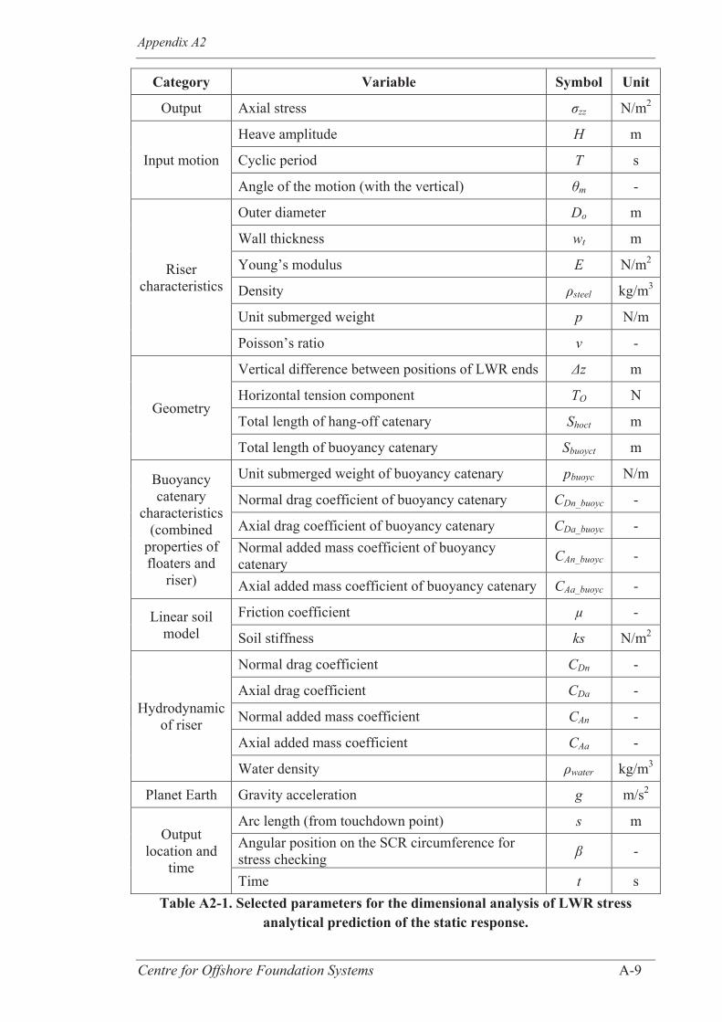
Appendix A2
Centre for Offshore Foundation Systems A-9
Category Variable Symbol Unit
Output Axial stress zz N/m2
Input motion
Heave amplitude H m
Cyclic period T s
Angle of the motion (with the vertical) m -
Riser characteristics
Outer diameter Do m
Wall thickness wt m
Young’s modulus E N/m2
Density steel kg/m3
Unit submerged weight p N/m
Poisson’s ratio -
Geometry
Vertical difference between positions of LWR ends z m
Horizontal tension component TO N
Total length of hang-off catenary Shoct m
Total length of buoyancy catenary Sbuoyct m
Buoyancy catenary
characteristics (combined
properties of floaters and
riser)
Unit submerged weight of buoyancy catenary pbuoyc N/m
Normal drag coefficient of buoyancy catenary CDn_buoyc -
Axial drag coefficient of buoyancy catenary CDa_buoyc - Normal added mass coefficient of buoyancy catenary CAn_buoyc -
Axial added mass coefficient of buoyancy catenary CAa_buoyc -
Linear soil model
Friction coefficient μ -
Soil stiffness ks N/m2
Hydrodynamic of riser
Normal drag coefficient CDn -
Axial drag coefficient CDa -
Normal added mass coefficient CAn -
Axial added mass coefficient CAa -
Water density water kg/m3
Planet Earth Gravity acceleration g m/s2
Output location and
time
Arc length (from touchdown point) s m Angular position on the SCR circumference for stress checking -
Time t s Table A2-1. Selected parameters for the dimensional analysis of LWR stress
analytical prediction of the static response.
Appendix A2
Centre for Offshore Foundation Systems A-10
A2.4. ANALYTICAL PREDICTION OF THE STATIC RESPONSE
Different analytical models have been proposed to capture the stress distribution in
SCRs or LWRs. Their complexity varies and the simplest analytical model consists in
ignoring the bending stiffness of the riser and using equations developed for cables. For
instance, Li and Nguyen (2010) have shown how to apply this method to LWRs.
However, it was shown that in a small section of the riser close to the TDP, referred to
as the boundary layer zone, the effect of the bending stiffness on the stress distribution
is not negligible (Aranha et al.,1997; Pesce et al, 1998b). The standard cable equations
can be corrected using the boundary layer correction and this was performed for LWRs
by Roveri et al. (2005) and Silveira and Martins (2004) on the case of a rigid soil
model.
Lenci and Callegari (2005) have also proposed a series of analytical models to predict
the stress distribution in SCRs during J-lay operations and the most advanced of their
models considers the boundary layer phenomena and uses a deformable soil model. This
analytical model is called the “Three-fields model” (TFM) and divides the riser into
three sections with different behaviours: from the HOP to a point called the boundary
layer end (BLE) the riser is modeled as a cable. From the BLE to the TDP, the bending
stiffness of the riser is taken into account by modeling the riser as a beam under linear
theory (assuming small vertical displacements). Then, in the zone between TDP and the
end of the SCR, where the riser is in contact with the seabed, a Winkler type deformable
soil is used.
This model was chosen for its completeness and clarity and was extended in order to
accommodate the displacement of the HOP to simulate the static response of SCRs and
assess the static stress range in the TDZ (Quéau et al., 2013). This extended analytical
model based on the TFM from Lenci and Callegari (2005) is referred to as the ETFM.
In this paper, the ETFM is applied to LWRs to predict the stresses at equilibrium and
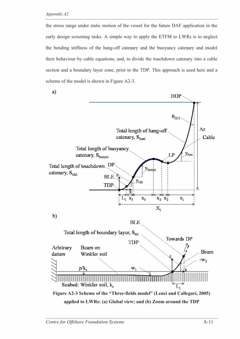
Appendix A2
Centre for Offshore Foundation Systems A-11
the stress range under static motion of the vessel for the future DAF application in the
early design screening tasks. A simple way to apply the ETFM to LWRs is to neglect
the bending stiffness of the hang-off catenary and the buoyancy catenary and model
their behaviour by cable equations; and, to divide the touchdown catenary into a cable
section and a boundary layer zone, prior to the TDP. This approach is used here and a
scheme of the model is shown in Figure A2-3.
Figure A2-3 Scheme of the “Three-fields model” (Lenci and Callegari, 2005)
applied to LWRs: (a) Global view; and (b) Zoom around the TDP
Appendix A2
Centre for Offshore Foundation Systems A-12
The governing equations are presented in Eq. (A2-2), where x is the horizontal
coordinate measured from the equilibrium TDP (the position of the TDP before
application of any motions to the HOP) and w1, w2, ytdc, ybuoyc and yhoc are the vertical
displacements in the various sections of LWRs. The suffixes tdc, buoyc and hoc respectively
stand for touchdown catenary, buoyancy catenary and hang-off catenary. I is the second
moment of area and TBLE (the constant traction on the laid beam), , 1 and 2 are
unknowns. Other relevant notations are introduced in Figure A2-3 or Table A2-1.
Due to a lack of degrees of freedom this model will, however, not assure the continuity
of shear force and bending moment, and therefore of the stress at the drag point (DP)
and at the lift point (LP). Another approach that would add some degrees of freedom
would consist in considering the boundary layer phenomenon occurring near LP and
DP, although this would lead to a more complex analytical model and longer calculation
times. As the aim of this framework is to develop a simple and efficient tool to get an
approximation of the fatigue life of LWRs in the TDZ for the early design stages, the
later approach is not used in this paper. It is assumed that, as for the HOP, the boundary
layer phenomenon could be neglected at LP and DP providing analytical results are
sufficiently accurate and this is checked later in the paper.
A2.4.1 Solution at equilibrium
The general solutions of the equations presented in Eq. (A2-2) are shown in Eq. (A2-3).
They define the elevation from the seabed z depending on the value of the horizontal
coordinate x and are all expressed in the (x,z) coordinate system which originates at the
equilibrium TDP. There are 22 unknowns: c1 to c12, , 1, 2, TBLE, L1 and x1 to x5. They
are determined by means of the boundary conditions presented in Eq. (A2-5), where the
bending moment M, the shear force S and the effective tension Te are defined for each
sections of the riser as per Eq. (A2-6), (A2-7) and (A2-8) respectively. As cables do not
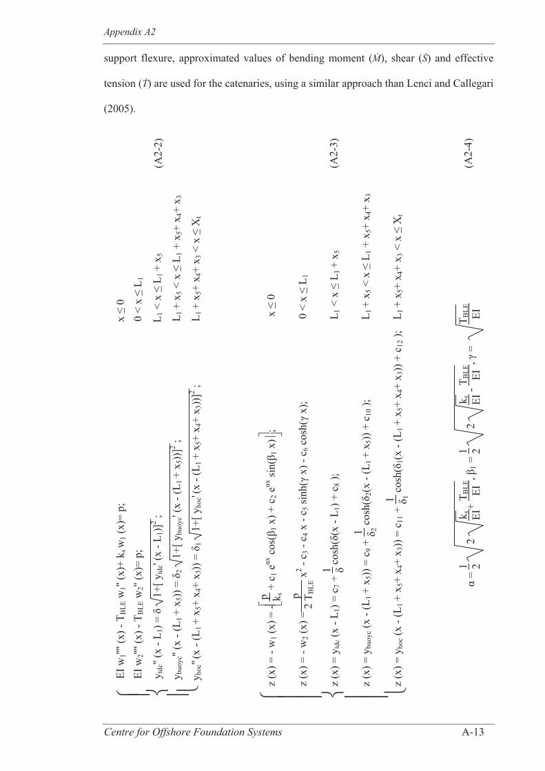
Appendix A2
Centre for Offshore Foundation Systems A-13
support flexure, approximated values of bending moment ( ), shear ( ) and effective
tension ( ) are used for the catenaries, using a similar approach than Lenci and Callegari
(2005).
(A2-
2)
(A2-
3)
(A2-
4)
EI w
1'''' (
x) -
T BLE
w1''
(x)+
ks w
1 (x)
= p;
x ≤
0 E
I w2''
'' (x)
- T B
LE w
2'' (x
)= p
;
0 <
x ≤
L 1 y
tdc''
(x -
L 1) =
δ
1+[ y
tdc'
(x -
L 1)]
2 ;
L 1 <
x ≤
L1 +
x 5
ybu
oyc''
(x -
(L1
+ x 5
)) =
δ2
1+[ y
buoy
c' (x
- (L
1 +
x 5))
]2 ;
L 1
+ x
5 < x
≤ L
1 + x
5+ x
4+ x
3
yho
c'' (x -
(L1 +
x 5+
x 4+
x 3))
= δ
1 1+
[ yho
c' (x -
(L1
+ x 5
+ x 4
+ x 3
))]2 ;
L
1 +
x 5+
x 4+
x 3 <
x ≤
Xt
z (x
) = -
w1 (
x) =
-p k s
+ c
1 eαx
cos
(β1 x
) + c
2 eαx
sin(
β 1 x
) ;
x
≤ 0
z (x
) = -
w2 (
x) =
p 2
TB
LE x
2 - c 3
- c 4
x -
c 5 si
nh(γ
x) -
c6 c
osh(
γ x)
;
0 <
x ≤
L1
z (x
) = y
tdc (
x - L
1) =
c7 +
1 δ cos
h(δ(
x - L
1) +
c8 )
;
L 1
< x
≤ L
1 +
x 5
z (x
) = y
buoy
c (x
- (L 1
+ x
5)) =
c9 +
1 δ 2 c
osh(
δ 2(x
- (L
1 +
x 5))
+ c
10 );
L
1 +
x 5 <
x ≤
L1 +
x5+
x4+
x3
z (x
) = y
hoc (
x - (
L 1 +
x5+
x4+
x3)
) = c
11 +
1 δ 1 c
osh(
δ 1(x
- (L
1 +
x 5+
x 4+
x 3))
+ c
12 );
L
1 +
x 5+
x 4+
x 3 <
x ≤
Xt
α =
1 2 2
k s EI+
T BLE EI
, β1 =
1 2 2
k s EI -
T BLE EI
, γ =
T B
LE EI

Appendix A2
Centre for Offshore Foundation Systems A-14
(A2-
5)
(A2-
6)
HO
P y h
oc (X
t) =
ΔZy h
oc ' (
Xt)
= co
tan
(θH
O)
LP
y hoc
(L1+
x5 +
x 4 +
x 3)=
ybu
oyc (
L 1+
x 5 +
x 4 +
x 3)
y hoc
' (L 1
+ x 5
+x 4
+x 3
)= y
buoy
c' (L
1+ x
5 +x 4
+x 3
)Ṫ h
oc (L
1+ x
5 +x 4
+x 3
)= Ṫ
buoy
c (L 1
+ x 5
+x 4
+x 3
) D
P y b
uoyc
(L1+
x5)
= y t
dc (L
1+ x
5)y b
uoyc
' (L 1
+ x 5
)= y
tdc'
(L1+
x5)
Ṫ buo
yc (L
1+ x
5)=
Ṫ tdc
(L1+
x5)
BLE
- w2 (
L1)
= y
tdc (
L 1)
- w2'
( L1)
= y
tdc'
(L1)
T BLE
= Ṫ
tdc (
L 1)
M2 (
L 1) =
Ṁtd
c (L 1
)S 2
(L1)
= Ṡ
tdc (
L 1)
TD
P
w1 (
0) =
w2 (
0) =
0w
1' ( 0
) = w
2' (0
)M
1 (0)
= M
2 (0)
S 1 (0
) = S
2 (0)
M (x
) = M
1 (x)
= -
EI w
1'' (x
);
x ≤
0M
(x) =
M2 (
x) =
- EI
w2''
(x);
0 <
x ≤
L 1
M (x
) = Ṁ
tdc (
x - L
1) =
EI
δ3
[]
y tdc
''(x
- L1)
2;
L 1 <
x ≤
L1 +
x 5
M (x
) = Ṁ
buoy
c (x
- (L 1
+ x
5)) =
EI
δ23
[]
y buo
yc''(
x - (
L 1+
x 5))
2;
L 1
+ x
5 < x
≤ L
1 + x
5+ x
4+ x
3
M (x
) = Ṁ
hoc (
x - (
L 1 +
x5+
x4+
x3)
) =
EIδ 1
3
[]
y hoc
'' (x
- (L 1
+ x 5
+ x 4
+ x 3
))2;
L 1
+ x
5+ x
4+ x
3 < x
≤ X
t

Appendix A2
Centre for Offshore Foundation Systems A-15
(A2-
7)
(A2-
8)
S (x
) = S
1 (x)
= -
EI w
1''' (
x);
x
≤ 0
S (x
) = S
2 (x)
= -
EI w
2''' (
x);
0 <
x ≤
L 1
S (x
) = Ṡ
tdc (
x - L
1) =
- 2
EI δ
6
y tdc
' (x
- L1)
[]
y tdc
'' (x -
L 1)
4;
L 1 <
x ≤
L1 +
x 5
S (x
) = Ṡ
buoy
c (x
- (L 1
+ x
5)) =
- 2
EI δ
26
y buo
yc' (x
- (L
1+ x
5))
[]
y buo
yc''(
x - (
L 1+
x 5))
4;
L 1
+ x
5 < x
≤ L
1 + x
5+ x
4+ x
3
S (x
) = Ṡ
hoc (
x - (
L 1 +
x5+
x4+
x3)
) = -
2 E
I δ16
y h
oc'(x
- (L
1+ x
5+ x
4+ x
3))
[]
y hoc
''(x
- (L 1
+ x 5
+ x 4
+ x 3
))4;
L1 +
x 5+
x 4+
x 3 <
x ≤
Xt
T e (x
) = T
BLE
;
x
≤ 0
T e (x
) = T
BLE
;
0
< x
≤ L 1
T e (x
) = Ṫ
tdc (
x - L
1) =
p δ2 y
tdc '' (
x- L
1);
L 1
< x
≤ L
1 +
x 5
T e (x
) = Ṫ
buoy
c (x
- (L 1
+ x
5)) =
p b
uoyc
δ22
ybu
oyc '' (
x - (
L 1+
x 5))
;
L 1
+ x
5 < x
≤ L
1 + x
5+ x
4+ x
3
T e (x
) = Ṫ
hoc (
x - (
L 1 +
x5+
x4+
x3)
) =
p δ12 y
hoc '' (
x- (L
1+ x
5+ x
4+ x
3));
L 1
+ x
5+ x
4+ x
3 < x
≤ X
t

Appendix A2
Centre for Offshore Foundation Systems A-16
Also, the total lengths of the hang-off catenary and of the buoyancy catenary are
determined through integration of the elevation z and are as per Eq. (A2-9):
Shoct = 1δ1
[ ]sinh( )δ1 (x1 + x2) + c12 - sinh(c12)
Sbuoyct = 1δ2
[ ]sinh( )δ2 (x3 + x4) + c10 - sinh(c10)
(A2-9)
Finally, the two more equations needed are found by observing that the extrema of ybuoyc
and yhoc are found when their derivatives are null and therefore:
x2= - c12δ1
, x3= - c10δ2
(A2-10)
Hence, there are 22 unknowns and 22 equations so that all unknowns can be determined
to assess the elevation, bending moment, effective tension and shear distributions at
equilibrium. It was shown by Lenci and Callegari (2005) that TBLE and L1 are found by
solving the nonlinear algebraic system presented in Eq. (A2-11), through the Newton-
Raphson technique (or other methods):
w2'' (L1) 1+[ ]w2' (L1) 2 + p
TBLE = f2 (L1, TBLE) = 0
w2''' (L1) + 2 w2' (L1) [ ]w2'' (L1) 2 = f3 (L1, TBLE) = 0 (A2-11)
The total axial stress that is used to get the fatigue life of LWRs combines the direct
tensile stress ( a) and bending stress ( M) (i.e. ZZ= a+ M) defined as follows:
σa = Tw
Ao - Ai , σM =
M Do2 I (A2-12)
Tw = Te - Po Ao + Pi Ai (A2-13)
where Tw is the wall tension, Pi, Po are the internal and external pressures and Ai, Ao are
the internal and external cross section areas.
A2.4.2 Solution under static motion
The static response of LWRs is assumed to be derived from the LWR stress
distributions when the HOP is moved in the two extreme positions that it would reach
Appendix A2
Centre for Offshore Foundation Systems A-17
under a cycle of sinusoidal static motion (at T/4 and 3T/4). These two positions are
referred to as “high” and “low” position respectively. In such an approach, the axial
stress range is calculated by differentiating the maximum (max) and minimum (min)
values of axial stress ( ZZ) found when the HOP is in high and low position, using
Eq. (A2-14):
Δσzz = max (σzz high, σzz low) – min (σzz high, σzz low) (A2-14)
Providing I, E, p, ks, Z, HO, pbuoyc, Shoct and Sbuoyct are known, the analytical model can
predicts the axial stress distribution. The only two of these parameters affected by HOP
motions are Z and HO. The new vertical elevation between the LWR ends can be
deduced from the amplitude (H) and the direction of the applied motion ( m). Therefore,
one additional unknown: the new hang-off angle, has to be determined to find the
elevation, shear, bending moment, effective tension and stress in displaced
configuration. The additional equation needed for solving is found by observing that the
overall length of the LWR is unchanged (Randolph, 2009), which leads to:
Δhx = ΔXt - ΔSt (A2-15)
where hx is the horizontal component of the imposed displacement (known), Xt the
offset to TDP and St the total arc length to TDP.
The variation of arc length to TDP ( St) between configuration at equilibrium and one
of the displaced configuration (HOP displaced either in high or low position) comes
from variations of the total length of the touchdown catenary ( Stdct) and the total length
of the boundary layer zone ( Sblt) as the total length of the hang-off catenary and of the
buoyancy catenary are unchanged (i.e. St = Stdct+ Sblt).
The total length of the touchdown catenary can be assessed by integration and gives Eq.
(A2-16) whereas, to ease calculations, an approximation is used to solve the integration
presented in Eq. (A2-17) and get the value of the total length of the boundary layer zone
Sblt. The Taylor series of 1+f4(x) about 0 is used with a fourth order approximation,
Appendix A2
Centre for Offshore Foundation Systems A-18
which is only valid if f4(x)= (p
TBLE x - c4 - c5 cosh( x) - c6 sinh( x))2 <<1 for all
x [0, L1]; this condition is always verified in the examples presented in this paper.
Stdct = 1δ [ ]sinh ( )δ x5 + c8 - sinh(c8) (A2-16)
Sblt =
0
L1
1+p
TBLE x - c4 - c5 γ cosh(γ x) - c6 γ sinh(γ x) 2dx (A2-17)
A2.5. DESCRIPTION OF NUMERICAL MODELS
Several LWR configurations are defined to validate the proposed dimensionless groups
and the ETFM. There are two ways to implement the buoyancy catenary into numerical
models, referred to as “Lazy wave discrete” and “Lazy wave distributed” (Orcina,
2012). The first approach is more realistic as the buoyancy catenary is modeled by
adding discrete modules to the riser whereas the second approach consists in using a
line with the equivalent properties of riser and floaters. The “Lazy wave discrete”
approach is used in the paper (although it may be interesting to also use the second
approach in future work). Two distinct base cases (BCs) are established (BC1 and
BC2). Both BCs have a buoyant section with the same properties and the same length
but its location is different between BC1 and BC2 to get a lower sag bend in BC2. An
illustration of the BCs is given in Figure A2-4. The two configurations are
superimposed to display their geometrical differences. The detail of their characteristics
is summarised in Table A2-2 (the reported values of the arc length to TDP at
equilibrium (St) and the offset to TDP at equilibrium (Xt) are those found in OrcaFlex
models). The variables that are kept to a constant value across the paper are shown in
Table A2-3.
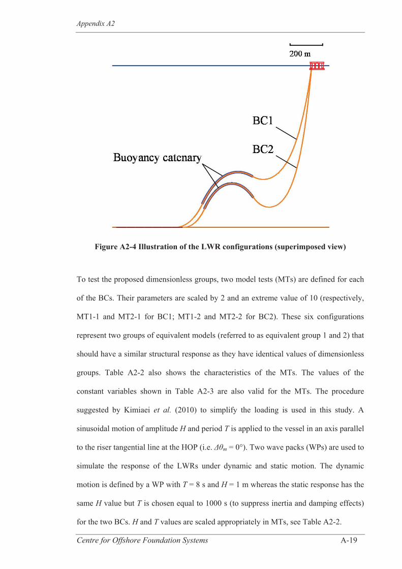
Appendix A2
Centre for Offshore Foundation Systems A-19
Figure A2-4 Illustration of the LWR configurations (superimposed view)
To test the proposed dimensionless groups, two model tests (MTs) are defined for each
of the BCs. Their parameters are scaled by 2 and an extreme value of 10 (respectively,
MT1-1 and MT2-1 for BC1; MT1-2 and MT2-2 for BC2). These six configurations
represent two groups of equivalent models (referred to as equivalent group 1 and 2) that
should have a similar structural response as they have identical values of dimensionless
groups. Table A2-2 also shows the characteristics of the MTs. The values of the
constant variables shown in Table A2-3 are also valid for the MTs. The procedure
suggested by Kimiaei et al. (2010) to simplify the loading is used in this study. A
sinusoidal motion of amplitude H and period T is applied to the vessel in an axis parallel
to the riser tangential line at the HOP (i.e. m = 0°). Two wave packs (WPs) are used to
simulate the response of the LWRs under dynamic and static motion. The dynamic
motion is defined by a WP with T = 8 s and H = 1 m whereas the static response has the
same H value but T is chosen equal to 1000 s (to suppress inertia and damping effects)
for the two BCs. H and T values are scaled appropriately in MTs, see Table A2-2.

Appendix A2
Centre for Offshore Foundation Systems A-20
To validate the proposed analytical model (ETFM), BC1 and BC2 are used but this time
the seabed friction is ignored (i.e. = 0). Input parameters of the BCs presented in
Table A2-2 are used in the ETFM to assess the static responses of the LWRs and
compare them with OrcaFlex results.
A2.6. RESULTS
A2.6.1 Validation of the dimensionless groups
Numerical models from the two equivalent groups are used to validate the suitability of
the dimensionless groups. To ensure that geometrical similarity is observed between
BCs and corresponding MTs, the normalised shapes, defined as the plot of the
normalised vertical coordinate Zn = z/ Z against the normalised horizontal coordinate
Xn = x/Xt are shown in Figure A2-5 (where markers are only used to differentiate the
curves and do not represent corresponding nodes in the different models). A good
correlation is observed for both of the equivalent groups. The dynamic and static
motions are applied to the LWRs configurations and the normalised stress range
( zz /E) in the TDZ are compared in Figure A2-6. Identical distributions are found. A
detailed investigation of the maximum values of normalised stress range in the TDZ
(Max zz TDZ/E) for the different models is performed in Table A2-4 and indicates very
minor differences between models within the same equivalent groups (≤ 0.41 %).
Hence, it is concluded that the proposed dimensionless groups are able to appropriately
scale the numerical models for dynamic and static response of LWRs.
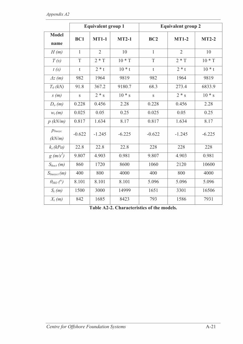
Appendix A2
Centre for Offshore Foundation Systems A-21
Equivalent group 1 Equivalent group 2
Model
name BC1 MT1-1 MT2-1 BC2 MT1-2 MT2-2
H (m) 1 2 10 1 2 10
T (s) T 2 * T 10 * T T 2 * T 10 * T
t (s) t 2 * t 10 * t t 2 * t 10 * t
z (m) 982 1964 9819 982 1964 9819
T0 (kN) 91.8 367.2 9180.7 68.3 273.4 6833.9
s (m) s 2 * s 10 * s s 2 * s 10 * s
Do (m) 0.228 0.456 2.28 0.228 0.456 2.28
wt (m) 0.025 0.05 0.25 0.025 0.05 0.25
p (kN/m) 0.817 1.634 8.17 0.817 1.634 8.17
pbuoyc
(kN/m) -0.622 -1.245 -6.225 -0.622 -1.245 -6.225
ks (kPa) 22.8 22.8 22.8 228 228 228
g (m/s2) 9.807 4.903 0.981 9.807 4.903 0.981
Shoct (m) 860 1720 8600 1060 2120 10600
Sbuoyct (m) 400 800 4000 400 800 4000
HO (°) 8.101 8.101 8.101 5.096 5.096 5.096
St (m) 1500 3000 14999 1651 3301 16506
Xt (m) 842 1685 8423 793 1586 7931
Table A2-2. Characteristics of the models.
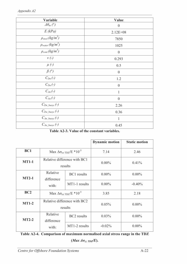
Appendix A2
Centre for Offshore Foundation Systems A-22
Variable Value m (°) 0
E (kPa) 2.12E+08 steel (kg/m3) 7850 water (kg/m3) 1025 cont (kg/m3) 0
(-) 0.293 μ (-) 0.5
(°) 0 CDn (-) 1.2 CDa (-) 0 CAn (-) 1 CAa (-) 0
CDn_buoyc (-) 2.26 CDa_buoyc (-) 0.36 CAn_buoyc (-) 1 CAa_buoyc (-) 0.45
Table A2-3. Value of the constant variables.
Dynamic motion Static motion
BC1 Max Δσzz TDZ/E *10-5 7.14 2.46
MT1-1 Relative difference with BC1
results 0.00% 0.41%
MT2-1 Relative
difference
with:
BC1 results 0.00% 0.00%
MT1-1 results 0.00% -0.40%
BC2 Max Δσzz TDZ/E *10-5 3.85 2.18
MT1-2 Relative difference with BC2
results 0.05% 0.00%
MT2-2 Relative
difference
with:
BC2 results 0.03% 0.00%
MT1-2 results -0.02% 0.00%
Table A2-4. Comparison of maximum normalised axial stress range in the TDZ
(Max Δσzz TDZ/E).
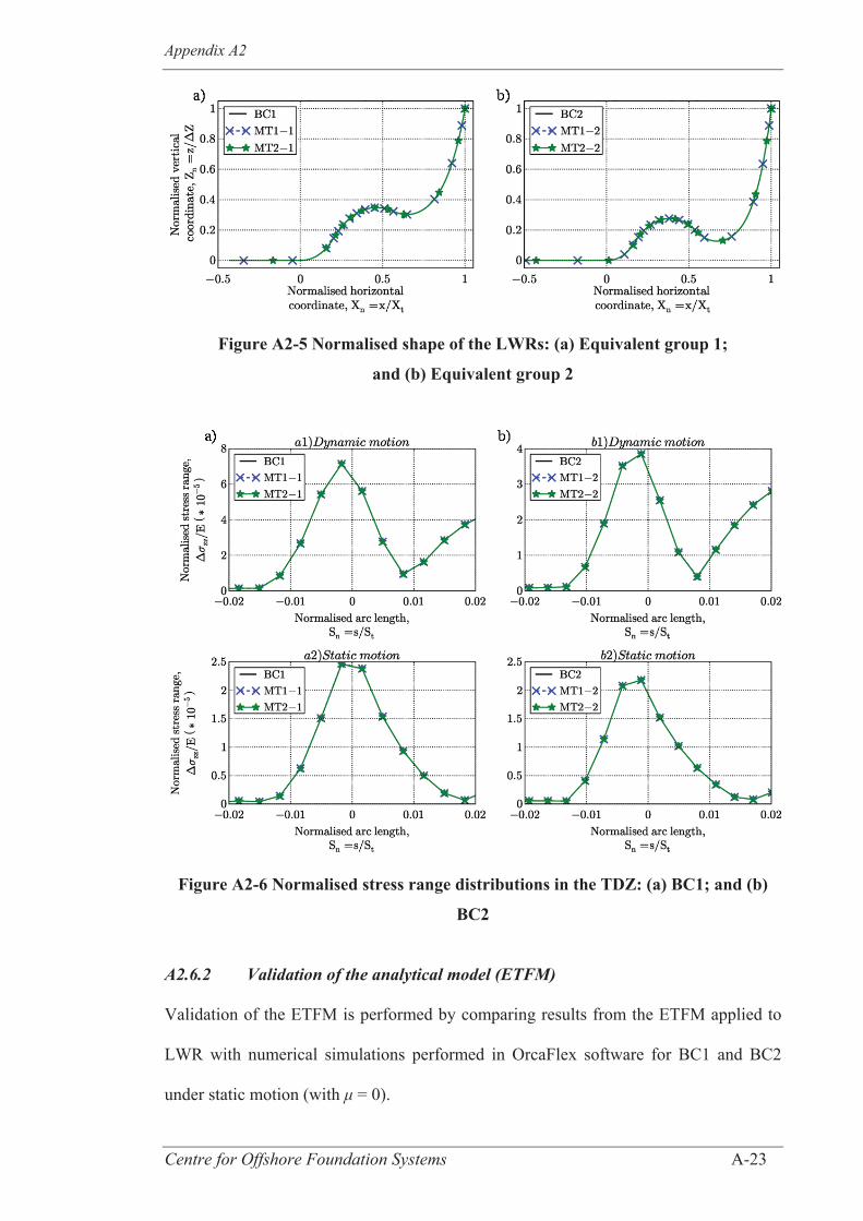
Appendix A2
Centre for Offshore Foundation Systems A-23
Figure A2-5 Normalised shape of the LWRs: (a) Equivalent group 1;
and (b) Equivalent group 2
Figure A2-6 Normalised stress range distributions in the TDZ: (a) BC1; and (b)
BC2
A2.6.2 Validation of the analytical model (ETFM)
Validation of the ETFM is performed by comparing results from the ETFM applied to
LWR with numerical simulations performed in OrcaFlex software for BC1 and BC2
under static motion (with = 0).
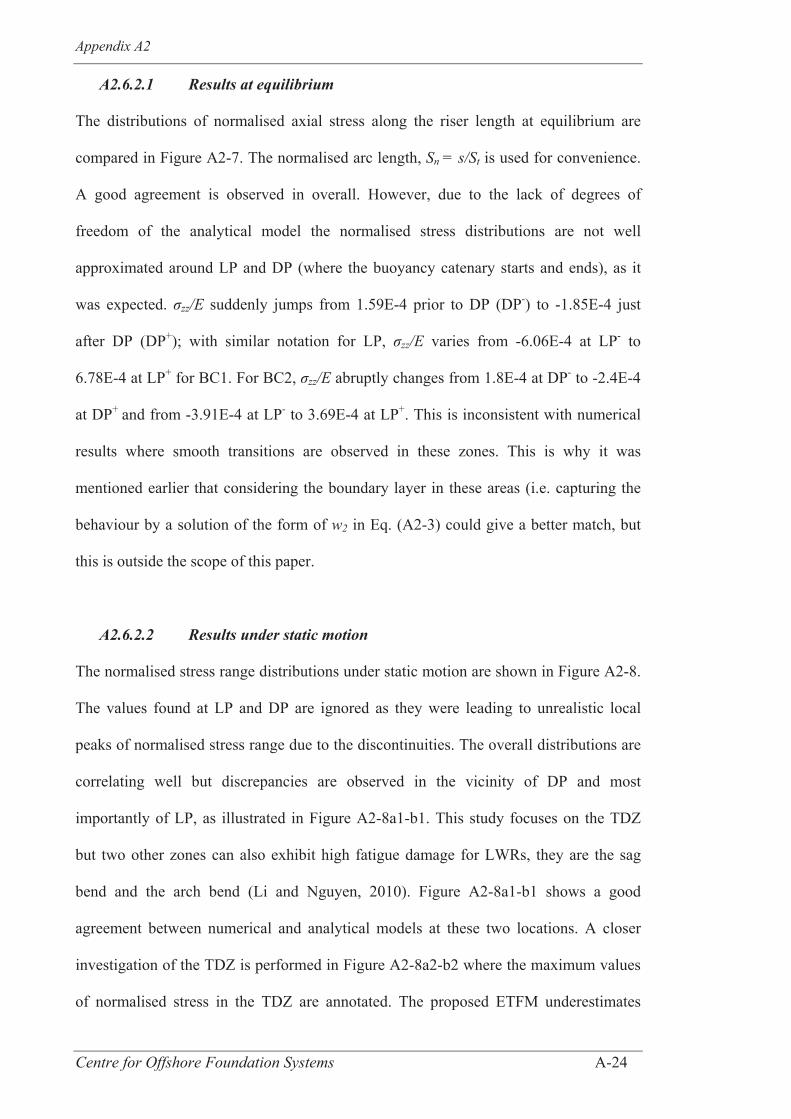
Appendix A2
Centre for Offshore Foundation Systems A-24
A2.6.2.1 Results at equilibrium
The distributions of normalised axial stress along the riser length at equilibrium are
compared in Figure A2-7. The normalised arc length, Sn = s/St is used for convenience.
A good agreement is observed in overall. However, due to the lack of degrees of
freedom of the analytical model the normalised stress distributions are not well
approximated around LP and DP (where the buoyancy catenary starts and ends), as it
was expected. zz/E suddenly jumps from 1.59E-4 prior to DP (DP-) to -1.85E-4 just
after DP (DP+); with similar notation for LP, zz/E varies from -6.06E-4 at LP- to
6.78E-4 at LP+ for BC1. For BC2, zz/E abruptly changes from 1.8E-4 at DP- to -2.4E-4
at DP+ and from -3.91E-4 at LP- to 3.69E-4 at LP+. This is inconsistent with numerical
results where smooth transitions are observed in these zones. This is why it was
mentioned earlier that considering the boundary layer in these areas (i.e. capturing the
behaviour by a solution of the form of w2 in Eq. (A2-3) could give a better match, but
this is outside the scope of this paper.
A2.6.2.2 Results under static motion
The normalised stress range distributions under static motion are shown in Figure A2-8.
The values found at LP and DP are ignored as they were leading to unrealistic local
peaks of normalised stress range due to the discontinuities. The overall distributions are
correlating well but discrepancies are observed in the vicinity of DP and most
importantly of LP, as illustrated in Figure A2-8a1-b1. This study focuses on the TDZ
but two other zones can also exhibit high fatigue damage for LWRs, they are the sag
bend and the arch bend (Li and Nguyen, 2010). Figure A2-8a1-b1 shows a good
agreement between numerical and analytical models at these two locations. A closer
investigation of the TDZ is performed in Figure A2-8a2-b2 where the maximum values
of normalised stress in the TDZ are annotated. The proposed ETFM underestimates
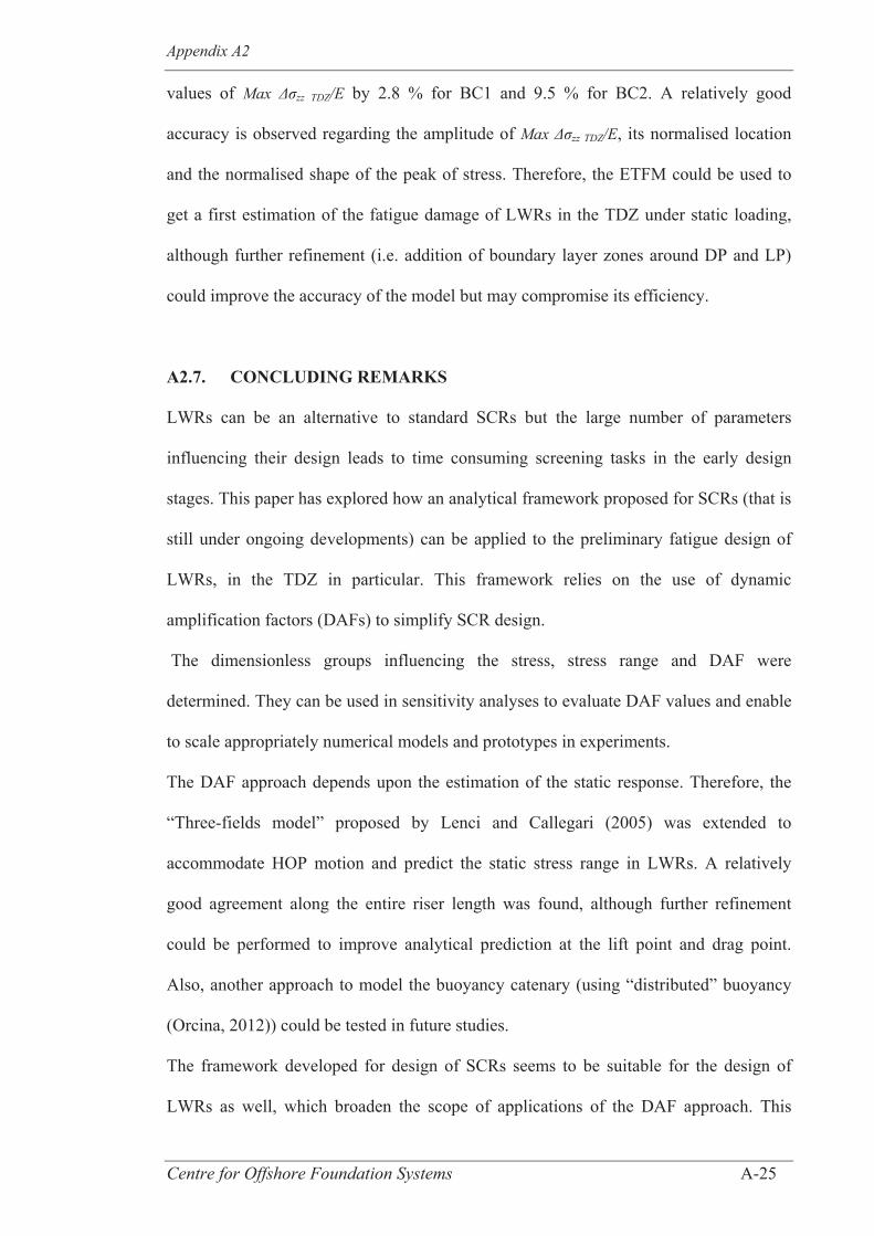
Appendix A2
Centre for Offshore Foundation Systems A-25
values of Max zz TDZ/E by 2.8 % for BC1 and 9.5 % for BC2. A relatively good
accuracy is observed regarding the amplitude of Max zz TDZ/E, its normalised location
and the normalised shape of the peak of stress. Therefore, the ETFM could be used to
get a first estimation of the fatigue damage of LWRs in the TDZ under static loading,
although further refinement (i.e. addition of boundary layer zones around DP and LP)
could improve the accuracy of the model but may compromise its efficiency.
A2.7. CONCLUDING REMARKS
LWRs can be an alternative to standard SCRs but the large number of parameters
influencing their design leads to time consuming screening tasks in the early design
stages. This paper has explored how an analytical framework proposed for SCRs (that is
still under ongoing developments) can be applied to the preliminary fatigue design of
LWRs, in the TDZ in particular. This framework relies on the use of dynamic
amplification factors (DAFs) to simplify SCR design.
The dimensionless groups influencing the stress, stress range and DAF were
determined. They can be used in sensitivity analyses to evaluate DAF values and enable
to scale appropriately numerical models and prototypes in experiments.
The DAF approach depends upon the estimation of the static response. Therefore, the
“Three-fields model” proposed by Lenci and Callegari (2005) was extended to
accommodate HOP motion and predict the static stress range in LWRs. A relatively
good agreement along the entire riser length was found, although further refinement
could be performed to improve analytical prediction at the lift point and drag point.
Also, another approach to model the buoyancy catenary (using “distributed” buoyancy
(Orcina, 2012)) could be tested in future studies.
The framework developed for design of SCRs seems to be suitable for the design of
LWRs as well, which broaden the scope of applications of the DAF approach. This
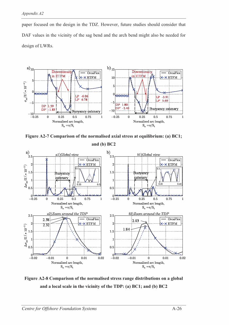
Appendix A2
Centre for Offshore Foundation Systems A-26
paper focused on the design in the TDZ. However, future studies should consider that
DAF values in the vicinity of the sag bend and the arch bend might also be needed for
design of LWRs.
Figure A2-7 Comparison of the normalised axial stress at equilibrium: (a) BC1;
and (b) BC2
Figure A2-8 Comparison of the normalised stress range distributions on a global
and a local scale in the vicinity of the TDP: (a) BC1; and (b) BC2