Estimating numbers of whole individuals from collections of body parts: a taphonomic limitation of...

Palcobiolo~~y, 20(2), 1994, pp. 245-258

Estimating numbers of whole individuals from collections of body parts: a taphonomic limitation of the paleontological record

Norman L. Gilinsky and J Bret Bennington 1

Abstract.-Paleoecologists have long sought to obtain estimates of the sizes of extinct populations. However, even in ideal cases, accurate counts of individuals have been hampered by the fact that many organisms disarticulate after death and leave their remains in the form of multiple, separated parts. We here analyze the problem of estimating numbers of individuals from collections of parts by developing a general counting theory that elucidates the major contributing variables. We discover that the number of unique individuals of a particular species that are represented in a fossil collection can be described by an intricate set of relationships among (1) the number of body parts that were recovered, (2) the number of body parts that were possessed by organisms belonging to that species, and (3) the number of individuals of that species that served as the source of the parts from which the paleontological sample was obtained (the size of the "sampling domain"). The "minimum number of individuals" and "maximum number of individuals" methods currently used by paleontologists to count individuals emerge as end members in our more general counting theory. The theory shows that the numbers of individuals of a species that are represented in a sample of body parts is fully tractable, at least in a theoretical sense, in terms of the variables just mentioned. The bad news is that the size of the "sampling domain" for a species can never be known exactly, thus placing a very real limit on our ability to count individuals rigorously. The good news is that one can often make a reasonable guess regarding the size of the sampling domain, and can therefore make a more thoroughly informed choice regarding how to estimate numbers of individuals. By isolating the variables involved in determining the numbers of individuals in paleontological samples, we are led to a better appreciation of the limits, and the possibilities, that are inherent in the fossil record.

Norman L. Gilinsky and \ Bret Benningtotl.' Department of Geological Sciences, Virginia Polytechnic Institute and State University, Blacksburg, Virginia 24061

'Present address: Department of Geology, 114 Hofstra University, Hempstead, New York 11550

Accepted: June 24, 1993

Introduction

One of paleoecology's most enduring goals has been to use the fossil record to obtain "snapshots" of populations and communities from the geological past. Given these snapshots, quantitative ecological principles- garnered from the study of modern communities-could be applied to give us an understanding of the nature of communities in the past, the frequency distributions of species that lived in those communities, the tro- phic relations among ancient organisms, and the spatial distributions of past populations. Furthermore, by examining sequences of such biological snapshots, the paleoecologist could, ideally, create a kind of ecological motion pic- ture, frame by frame, that would lead to a rich understanding of community evolution over a time scale that could not be approached

by ecologists working with modern-day organisms. Of course, certain kinds of organisms would not be preserved, but the relative coarseness of paleontological sampling as compared to what is possible in the Recent would be more than compensated for by the vastly greater temporal scale that could be examined by paleontologists. Parsons and Brett (1991: p. 22) expressed this ideal vividly by describing paleontologists as yearning "to restore the flesh and blood of fossil remains, and thereby to depict in detail the appear- ance, and analyze the interactions and dynamics, of ancient communities."

A means for counting unique individuals would seem to be a minimal prerequisite for obtaining paleontological snapshots, because only with such counts would it be possible to study such phenomena as biomass, popu-

(a 1994 The Paleontological Society. All rights resewed. 0094-8373/94/2002-0010/$1 .00

246 NORMAN L. GILINSKY AND J BRET BENNINGTON

lation dynamics, predator-prey ratios, among others, quantitatively in the fossil record. A big problem in obtaining counts of individuals from an assemblage of fossils is the fact that most fossils are preserved as disarticulated body parts. Do 28 clam valves from a single species represent 14 clams, or 28, or some number in between, for instance? In an effort to see if an accurate means for counting unique individuals could be devised, and eventually applied, we used computer sim- ulations and mathematical analysis to develop what is effectively a counting theory that isolates the relevant variables and elucidates their intricate relationships. To foreshadow the conclusions below, we discover that the number of unique individuals (of a species) in an assemblage is a function of three basic variables: (1) the number of body parts of that species that are preserved in the assemblage, (2) the number of body parts that comprised that organism in life, and (3) the number of organisms of that species that were poten- tially available to be sampled by the pale- ontologist (what we define below as the "sampling domain"). Given values for these variables, the theory tells us that the statis- tically expected number of unique individuals can be determined unambiguously.

In practice, however, it will be effectively impossible to obtain a rigorous estimate of the size of the sampling domain and, therefore, it will be impossible to get a rigorous estimate of the number of unique individuals in an assemblage (unless, of course, all of the individuals were preserved in an articulated state). So the bad news, as we shall show, is a rigid limit to the resolving power of the fossil record. We regard this limit as a kind of taphonomic law, in the sense of Efremov (1940). This "law of numerical indeterminan- cy" also explains why previous efforts at counting unique individuals have delimited only the extremes (maximum and minimum numbers of individuals) in the continuum of possibilities. The good news is that the theory also tells us that we nonetheless may be able to estimate the number of unique individuals so long as the size of the sample relative to the size of the sampling domain is known at least roughly. When the size of the sample is small relative to the size of the sampling do-

main, for instance, a very reasonable estimate of the number of unique individuals can be obtained simply by counting each body part as a unique individual. Fortunately, given that many samples of invertebrates are collected from highly fossiliferous beds, this "maximum number of individuals method" will apply frequently in paleoecological work.

Most fossil assemblages obtained even from thin beds are both time-averaged and locally transported (see Kidwell and Bosence [I9911 for an extensive review). The theory developed here applies to these cases and, in fact, to all cases where the aim is to estimate the number of unique individuals in an assemblage. But when time-averaging or local transport are significant, we caution that the counts will not be estimates of the original population sizes, only estimates of the numbers of unique individuals represented in the collections. These numbers, nonetheless, may be of interest in some kinds of studies. The theory also applies to assemblages that were produced during a catastrophic burial, where the number of fossils that are actually preserved in the sediment may be isomorphous with the number of organisms in the living population. Such assemblages might be very rare indeed but, if they exist, the theory developed here may help to estimate the numbers of organisms in once-living populations. Hallam (1972) has termed these kinds of assemblages "census populations."

Perhaps our most important conclusion, however, is that there is nothing more practical than theory. For the theory developed here isolates the important variables related to counting unique individuals, locates the one variable (the size of the sampling domain) that prohibits rigorous estimation of the numbers of unique individuals in assemblages, pinpoints a very real taphonomic limit to the resolving power of the fossil record, and hints at conditions under which we can do the counting anyway.

The Problem

Vertebrate paleontologists, including stu- dents of human evolution, have frequently run up against the problem of counting disarticulated individuals in their efforts to obtain approximate shapshots of ancient terres-

COUNTING UNIQUE INDIVIDUALS 247

trial communities. A specific instance is exemplified by Klein's (1980) work on mammalian faunas from Upper Pleistocene and Holocene archaeological sites in South Afri- ca, where one of the pieces of information desired for each site is the frequency of oc-

. currence of each mammalian species. In fact, Klein (1980: p. 226) points out that estimates of species frequencies are "[tlhe most widely used numerical data in archaeological faunal analysis." The problem, even when one can assume that the fossil deposit is distorted nei- ther by time- nor space-averaging, is that individual mammals are preserved as disarticulated body parts. If the body parts of individuals are scattered, as they normally are to some extent (even if transport into or out of the area of the site is unimportant), then counting the number of unique individuals becomes a non-trivial matter. It is unlikely that all body parts from all individuals represented in the sample will be recovered and, furthermore, it is unlikely that the parts that are recovered can all be assigned to particular individuals.

Two basic approaches to the problem have been tried. The first has been to sort the bones by species, and then to assume that each bone in the sample for a species represents a unique individual of that species. By this method, one hundred recovered bones for a species means one hundred unique individuals. Since this approach maximizes the number of possible individuals, we call it the XNI approach (for "maximum Number of Individuals"). As Klein mentions, the method would almost certainly overestimate the actual number of individuals in the assemblage because some individuals surely contributed more than a single bone. The second approach, sometimes called the "Minimum Number of Individu- als" method, or MNI, first groups the bones by species, then by bone type, and then estimates the number of individuals for a species as the number needed to account for the most common type of bone. For instance, if the most common bone in the sample for a species is the left femur, the MNI is defined as being equal to the number of left femurs. This method will tend to underestimate the actual number of individuals due (in this case) to unrecovered left femurs. A modification of

this approach would be to estimate the number of individuals as the MNI plus an additional number of individuals to account for those that contributed some bones to the sample, but no femurs. However this modification assumes that bone elements can be con- fidently matched, an assumption that is usually not warranted.

With a little reflection more complications come to mind, but all of the approaches that have been tried to compensate for these complications really amount to attempts to patch up estimates based on the two main approaches mentioned above. Klein (1980) gives a more complete treatment of the practical aspects of the problem than we do here, and Badgely (1986), Behrensmeyer (1991), and Shipman (1981) discuss the problem as well. Holtzman (1979) published a thoughtful analysis of several approaches to counting both vertebrate and invertebrate fossils, including the MNI, and his analysis is relevant to the question at hand, but the emphasis was on estimating relative abundance and not the number of individuals per se. Since the XNI and MNI approaches give us only the extremes in the spectrum of possible counting conventions for estimating numbers of individuals, the obvious question that arises is whether we can do better than simply to isolate the extremes. Can we develop a method that will give us the "right" answer or, at least, a rigorously defensible best-estimate?

We have thus far described the problem from the standpoint of vertebrates because vertebrate paleontologists have frequently encountered it in actual empirical work, and because the problem is so readily brought to light given that, with so many bones for each individual, the XNI and MNI methods give such radically different estimates for the same data. Invertebrate paleontologists have been less mindful of the problem, but some sense of concern is hinted at by the fact that invertebrate paleontologists, too, apply counting conventions in their own work. Many research workers when counting clams, for instance, do so by estimating the number of individuals as the number of left, or right, valves in the collection, whichever is larger (e.g., Miller et al. 1992). This procedure is precisely the MNI approach, but this time


applied to organisms with only two body parts. Other workers count all of the valves in the collection (for a particular species), a procedure that is exactly analogous to counting up all of the bones in the vertebrate case (the XNI approach). (A third method is to count half the number of valves, but this number, ironically, is usually smaller than the MNI!) Despite the different organisms involved, the basic problem of counting individuals is the same. For organisms with multiple body parts, the best that has been achieved thus far has been minimum and maximum estimates of the numbers of individuals, even though it is obvious that both estimates are almost always wrong.

We attempt here to analyze the problem of counting individuals more abstractly than has been done before. By doing so, we can attack the basic question perhaps more rigorously, from first principles. Accordingly, the work is mathematical, but the mathematics are not difficult. We begin with the problem of counting organisms with two body parts (we use clams as our focal organisms), but we do so only to keep things simple. We emphasize that the theory generalizes to organisms with larger numbers of parts, including vertebrates. The conclusions are given in detail later, but we mention at the outset that by thinking of the problem abstractly, as a problem in counting theory, we are able to determine precisely why it is that paleontologists have thus far been limited to estimating only the extremes of the possible numbers of individuals sampled from a population, and why only in rare cases will it be possible to do much better. We regard explicit awareness of this limitation of the fossil record, rigorously defined, as a practical contribution in itself, a kind of taphonomic "law." On a more hope- ful note, however, there may be some circumstances under which this limitation might be breached, and we shall discuss this aspect as well.

A Simulation Approach

Motizlation and Example.-If we have a collection of clam valves on hand, and we are interested in estimating rigorously the number of unique individuals that are represent-

ed by the collection of valves, we need to know the mathematical relationship between the number of valves in a collection and the number of unique individuals. If we had that relationship, we could calculate the estimated number of unique individuals in our collection, or we could obtain the number of unique individuals graphically. (We assume in this case that it is impossible or impractical to try to match all of the valves, and that we need to approach the problem from a mathematical standpoint. We mention later that it might be possible to test the model proposed here by actually collecting specimens and trying to match the valves.) As mentioned earlier, some paleontologists have applied the MNI approach to this problem, thereby estimating the number of unique individuals as the number of left or right valves, whichever is larger. Others have used the XNI approach, simply counting each valve as an individual. So previous research workers /lave assumed specific mathematical relationships (as have vertebrate paleontologists), but those relationships delimit only the extremes. Our aim is a more sophisticated mathematical relationship, one that accounts for the entire range of possible estimates, not just the extremes.

One way to explore the unknown relationship is to create a hypothetical population of clams, to obtain variously-sized samples of valves from this population, and to see how many unique individuals are represented in the samples. This approach is illustrated in figure 1. It amounts to establishing a population of articulated clams (100 in this case), labeling both valves of each clam with the same number (both valves of clam #l are labeled 1; both valves of clam #2 are labeled 2, etc.), disarticulating the valves, throwing them in a barrel, . . . stirring well, . . . and then sampling. To find out how many unique clams are represented by 20 valves, for instance, 20 valves are sampled randomly from the barrel, and the number of unique numbers is counted. The number of unique numbers is the number of unique clams. In performing the experiment repeatedly, one would immedi- ately encounter the problem of statistical sampling error, in the sense that different samples of 20 valves would give different

COUNTING UNIQUE INDIVIDUALS

Take a population of 1 0 0 clams w i t h numbered l e f t and r i gh t valves ...

.. . d isar t iculate and m i x we1 I...

repeatedly sample 20 valves and count the number of unlque clams ...

P

. . . . . . . - 20 valves. 19 unlque clams -

I 29 valves, 20 unrque clams 20 valves, I 8 unlque clams

1 LV J ~ I V C ; I , I 7 ~ I I I ~ U C ~ 1 0 1 1 1 3

... and construct a nistogram o f the I resul ts.

Mean

Number of unique clams

FIGURE 1. Cartoon illustration of a sampling experiment to determine the expected number of unique individuals that are represented in a collection of clam valves. In the experiment, both valves of each of 100 clams are labeled with the same number. The clams are then disarticulated, and the valves are mixed well in a barrel by one of the authors. Twenty valves are then sampled from the barrel randomly, and the number of unique clams represented in the sample is then determined. By performing this experiment many times, the distribution of numbers of unique clams can be obtained, and the expected number of unique clams for 20 valves can be estimated as the mean of the distribution. In the cartoon, about 19 unique individuals are expected when 20 valves are sampled from a collection of valves from 100 clams.

numbers of individuals. But the numbers ob- The expected number of individuals for 20 . tained from repeated samples would define valves can also be obtained with high accu-

a distribution (illustrated at the bottom of fig. racy using a computer simulation. The set of I), from which an expected (or mean) value clams that are to serve as the source of the of the number of unique clams could be ob- sample of valves we call the sampling do- tained, along with confidence intervals about main. This number is equivalent to the num- that expectation. ber of clams in the barrel of figure 1, and is

250 NORMAN L. GILINSKY AND J BRET BENNlNGTON

CLAM 1

2

3

4

BEK>RE AFTER

L R L R

+ &

FIGURE 2. A simulation approach to the problem of determining the relationship between number of valves in a collection and the number of unique individuals. The 100 by 2 array on the left (labeled "BEFORE), filled with Os, represents the unsampled left and right valves of 100 clams. Twenty valves are then sampled randomly, with the randomly sampled valves being represented on the right side of the diagram (labeled "AFTER") by Is in the array. The number of unique clams is then counted simply by counting the number of rows that contain one or more Is (the arrows).

analogous to the number of individual clams that are represented in the volume of rock (or sediment) from which a real paleontological collection is made. In the computer simulation the sampling domain is represented as an array, as shown on the left side of figure 2, and n = 20 valves are selected randomly from the array (selected valves are depicted as Is). For the set of valves that are sampled, the number of unique clams in the collection can be easily obtained (the arrows in the figure). Repeating the simulation N times (for N reasonably large) allows the mean (or expected) number of individuals to be calculated for a sample size of n = 20 valves. For sample sizes other than 20 values, the simulation can be run again for different valves of n.

Table 1 gives the results of a simulation run under the protocol described above, for a range of sample sizes n. Since the number of

TABLE 1. Relationship between the number of valves in a collection and the expected number of unique clams represented. Expected number of unique clams was obtained by simulating the process of sampling 0, 10, 20, . . . valves from a collection of 200 valves (100 complete individuals). The simulation for each sample size was run 1000 times. SE is the standard error of the expected number of unique clams.

Number o l Ex ected number

valves ofunique clams Variance SE

clams in the sampling domain was 100, up to 200 valves were available for sampling. For each sample size (we chose n = 0, 10, 20,. . . 200), the sampling procedure outlined above was performed N = 1000 times. So the expected number of unique clams for a given sample size n of valves is equal to the mean number of clams that were identified in the N = 1000 iterations of sampling (i.e., the 1000 "collections").

For a collection size of n = 20 valves (the original problem posed above), and with the size of the sampling domain set at 100 clams (200 valves), the collection size n is fairly small relative to the size of the sampling domain, so each new valve collected has a high probability of representing a new, unique clam. This probability continually decreases as additional valves are removed, but it nonetheless remains quite high as long as only a small sample is being extracted from the whole (in this case, 10% of the valves). As a result, the expected number of unique clams is about 19 for a sample size of 20 valves (table 1). At large collection size, after some 190 valves

COUNTING UNIQUE INDIVIDUALS 25 1

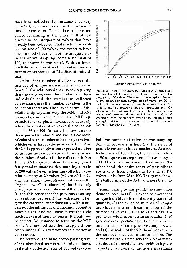
have been collected, for instance, it is very urrlikely that a new valve will represent a unique new clam. This is because the ten valves remaining in the barrel will almost always be counterparts of valves that have already been collected. That is why, for a collection size of 190 valves, we expect to have encountered virtually all of the unique clams * in the entire sampling domain (99.7830 of 100, as shown in the table). With an inter- mediate collection size of 100 valves, we ex- ? pect to encounter about 75 different individ- 5 uals. 0 20 4 0 60 80 100 120 140 160 180 200

A plot of the number of valves versus the number of unique individuals is shown in NUMBER OF VALVES IN THE SAMPLE

figure 3. The relationship is curved, implying FIGURE 3. Plot of the expected number of unique clams that the ratio between the number of unique as a function of the number of valves in a sample for the

individuals and the of collected range 0 to 200 valves. The size of the sampling domain is 100 clams. For each sample size of valves 10, 20, . . .

valves changes as the number of valves in the 190, 200, the number of unique clams was determined collection increases. The curved nature of the relationship explains why the MNI and XNI approaches are inadequate. The MNI approach, for example, is the exact estimate only when the number of valves in the collection equals 199 or 200, for only in these cases is the expected number of individuals correctly calculated as the number of left or right valves, whichever is larger (the answer is 100). And the XNI approach gives the expected number of unique individuals correctly only when the number of valves in the collection is 0 or 1. The XNI approach does, however, give a fairly good estimate (with a sampling domain of 200 valves) even when the collection contains as many as 20 valves (where XNI = 20, and the simulation-obtained estimate-the "right answern-is about 19), but it is only strictly correct at a sample size of 0 or 1 valves. It is in this sense that the previous counting conventions represent the extremes. They give the correct expectations only within one valve of the minimum and maximum possible sample sizes. And, you have to use the right method even at these extremes. It would not be correct, for instance, to settle on the MNI

. or the XNI method, and then to apply it rou- tinely under all circumstances as a matter of convention.

The width of the band encompassing 95% of the simulated numbers of unique clams, peaks at a collection size of 100 valves (one

1000 times. The dotted curves span approximately 95% of the numbers obtained in these determinations. The accuracy of the expected number of clams (the solid curve), obtained from the standard error of the mean, is high enough that the error bars about those numbers would be nearly invisible at this scale.

half the number of valves in the sampling domain) because it is here that the range of possible outcomes is at a maximum. At a collection size of 100 valves, there can be as few as 50 unique clams represented or as many as 100. At a collection size of 10 valves, on the other hand, the entire range of possibilities spans only from 5 clams to 10 and, at 190 valves, only from 95 to 100. The graph shows this ballooning of the 95% band near the mid- dle.

Summarizing to this point, the simulation demonstrates that (1) the expected number of unique individuals is an inherently statistical quantity, (2) the expected number of unique individuals is a nonlinear function of the number of valves, (3) the MNI and XNI approaches (which assume a linear relationship) give correct expectations only near the minimum and maximum possible sample sizes, and (4) the width of the 95% band varies with the number of valves in the collection. The curve in figure 3 is precisely the kind of mathematical relationship we are seeking; it gives expected numbers of unique individuals


A: CLAMS

0 , . . . , . . . , . . . , . . . , . . . 0 400 800 1200 1600 2000

NUMBER OF VALVES IN SAMPLE

loo0 - 13: CHITINS m 1000

800-

SW

0 400 800 1200 1600 2000

NUMBER OF PLATES IN SAMPLE

FIGURE 4. Plots of the relationship between the number of valves and the expected number of unique individuals for sampling domains of several sizes for both clams (A) and chitins (B).

across the entire range of possible sample sizes.

The influence of the Size of the Sampling Do- main.-The graph in figure 3 can be used to obtain best-estimates (expectations) of the numbers of unique individuals for the range of collection sizes drawn from a sampling domain of 100 clams (200 valves). Unfortunate- ly, however, the curve shown in the figure is not the only one that is possible. In fact, the shape of the curve depends strongly on the size of the sampling domain, that is, the number of clams in the barrel. This can be appre- ciated readily by imagining an infinitely large

sampling domain. With an infinitely large sampling domain, the probability of any valve in a sample being the counterpart of any other valve in the sample approaches zero, no matter how many valves are collected. In that case, the curve relating the number of individuals to the number of valves will be linear, with a slope of 1, and with each valve representing a new individual. At the other extreme, with very small sampling domains, the probability of a new valve being the counterpart of one that has already been sampled quickly becomes large as new valves are sampled, and the curve relating the number of individuals to the number of valves rapidly becomes strongly concave down. The implication is that there is not one curve describing the relationship between the number of valves and the expected number of unique individuals; rather, there must be a family of curves, one for each sampling domain.

Figure 4A shows the curves for sampling domains of several sizes. The simulation suc- ceeds in establishing a graphical means of specifying rigorously the expected number of unique individuals that are represented in a collection of valves. But, unfortunately, that number is a function not only of the number of valves in the collection, but also of the size of the sampling domain. As we shall discuss below, practical applications of the theory are only possible when the size of the sampling domain is known, or when certain assumptions can be made regarding the relation between the size of the sample and the size of the sampling domain.

A Generalization to More Than Two Body Parts.-Although we motivated the discussion using vertebrates, we have thus far re- stricted the mathematical analysis to the case of bivalved organisms, specifically clams. In- deed, the above analysis applies to any organism that has two body parts. But the counting theory also generalizes easily to organisms with more than two parts by ex- tending the array in figure 2 out to 3, 4, or more, columns, each column representing an additional body part. By selecting specimens (say, of bones) from this larger array, one can generate curves relating the number of bones in a collection to the expected number of


unique individuals in much the same way as with the case of bivalved organisms discussed previously. To be strictly applicable without modification, the different body parts would need to have equal probabilities of being recovered. While probably true for typical bivalves, this is certainly not true for dinosaur bones! Actual practical applications would have to adjust the simulation algorithm to account for the different recovery probabilities.

Figure 4B illustrates an example of a multi- part generalization to chitins where the recovery probability of the eight plates can be regarded as roughly the same. For comparative purposes, we made the axes of figures 4A and 4B the same. For clams (fig. 4A), a collection of 300 valves from a sampling domain of 500 clams is expected to yield about 255 unique individuals. But for chitins, a collection of 300 plates from a sampling domain of 500 chitins is expected to yield only 232 individuals. We shall return to this graph below.

An Analytical Approach: The Rarefaction Connection

The simulation approach described above generates curves relating number of individuals to number of body parts in a manner that is intuitively appealing. After all, sampling valves from a barrel is readily seen as analogous to collecting fossils from an outcrop. But, in fact, the very same curves can also be regarded as specific instances of rarefaction curves. Rarefaction analysis is usually applied to counts of organisms and species, rather than to valves and clams. It begins with the observed number of organisms and the observed number of species. A graph is then constructed to express the relationship between the number of organisms and the number of species for hypothetical sample sizes smaller than the observed sample size, under the assumption that the observed sample served as the source of the hypothetical smaller samples. This curve, which is called a rarefaction curve, allows species richnesses for different collecting sites or habitats to be compared even though one sample might be smaller than the other (Sanders 1968).

The equation for calculating the expected number of species E(S,) for a specified number n of organisms is:

where Z is the total number of organisms in the actual collection, Z, is the number of organisms observed to belong to species i, and S is the total number of species in the actual collection (Hurlbert 1971; Simberloff 1974; Heck et al. 1975). The variance (Var [S,]) of the expected number of species (Heck et al. 1975) is given by:

The same theory can also be applied to the expected number of individuals in a sample obtained from a larger sampling domain. Let us suppose that the source of our sample contains S clams (rather than S species), each of which has Z, = 2 valves. This would be precisely analogous to a case where there were S species each with Z, = 2 organisms (unusual, but conceivable). Therefore, the rarefaction equation applied to clams with two valves apiece must give the curve for the expected number of unique clams for various collec-

254 NORMAN L. ClLlNSKY AND J BRET BENNINGTON

tion sizes of tr valves, just as the equation applied to counts of species and organisms would give the expected number of species for various sample sizes of n fossil organisms. That is, the problem of counting unique clams is a special case of rarefaction analysis. Fur- thermore, the size S of the source population of clams is what we defined earlier as the size of the sampling domain. The mathematical theory of rarefaction, with all Z, = 2 and with S being the size of the sampling domain, therefore provides the same curves as those obtained above using simulation.

A straightforward analytical generalization to organisms with more than two body parts is possible with the rarefaction approach. For clams, Z, = 2 because each clam i had two body parts. For organisms with more than two body parts, all that is needed is to set Z, equal to the new number of body parts (for chitins, Z, = 8), and to apply equations (1) and (2) above. But, as before, the theory is only strictly correct when the different body parts have identical preservation probabilities.

Discussion

The Bad Nezcrs: The Problem of the Samplirlg Domain.-An ideal solution to the problem of the number of unique individuals would have been a single curve relating that number to the observed number of body parts. This curve would have provided a means to estimate rigorously the numbers of individuals in a way that the XNI and MNI methods could not. Unfortunately, the solution is not nearly so simple because a third variable, the size of the sampling domain, needs to be taken into account. The size of the sampling domain, as mentioned before, is the number of individuals represented in the statistical universe from which the actual collection was drawn. In developing the above counting theory, that number was defined a priori. But in actual practice, all we really know is how many specimens Z we have in our collection; we don't know how many specimens comprised the pool from which the collection was drawn. That is, we don't know the size of the sampling domain.

The following hypothetical case illustrates the problem. Suppose that one were to iden-

tify a thin layer of rock (or sediment) in the field and, from this layer, collect 80 clam valves. The largest number of unique individuals that could be represented is 80, and the smallest is 40. But, all other things being equal, whether the best estimate is closer to 80 or to 40 depends on the size of the sampling domain, that is, the total number of clams that are represented in the volume of rock from which our sample was collected. (As usual, we assume that all of the valves are disarticulated and that we are not willing or able to match them.) If the sampling domain included 50 individuals, or 100 individuals, or 1000 individuals, then the corresponding best estimates of the number of unique individuals for 80 valves would be 48.081, 64.120, and 77.857, respectively. Clearly the best estimate is crucially dependent upon the size of the sampling domain, but we simply do not know what that size is, so we do not know which curve to use. This indetermi- nancy is the bad news; the inability to specify the size of the sampling domain is what pre- vents us from estimating rigorously the number of unique individuals in a sample.

Some Good Neuis: We Might Be Able to Guess When the XNI is Appropriate.-Even though it is not possible to determine exactly which of the family of curves to use, it may be possible to make certain assumptions that can lead to an informed choice. For instance, the curves in figure 4A (the clam case) show that the relationship between the number of valves and the number of individuals is approximately linear at first and then becomes concave down as the number of valves in the collection approaches the total number in the sampling domain. This pattern occurs because the first few valves collected from even a moderately fossiliferous bed will only rare- ly be counterparts of valves that have already been collected (assuming a well-mixed sample). Only after many valves have been sampled, relative to the total in the sampling domain, will valve counterparts start to appear with high frequency. This suggests that it might be appropriate to assume a near-linear relation between number of valves and number of individuals, at least when the number of valves in the collection is small relative to


the total number of clams remaining in the rock. This assumption would imply that each valve in the collection can be counted as a unique individual; that is, it implies that the XNI approach would be valid.

As can be seen from the curves on figure 4A, the assumption of linearity is good for any sized sampling domain, provided that the number of valves in the collection relative to the size of the sampling domain remains small. But the length of the near-linear phase of each curve (and thus the region where the XNI applies) decreases markedly as the sampling domain shrinks. For this reason, we have estimated (using simulation) the sample size at which the assumption of linearity breaks down for a two-valved organism (clam) and for an eight-valved organism (chitin) for each of several sampling-domain sizes. In figure 5, the line labeled "clams" is the approximate locus of all points at which the estimate of the expected number of individuals obtained by assuming linearity (that is, by counting each valve as a unique individual) reaches a maximum error of 10%. For instance, if the sampling domain contains 600 clams (the ver- tical dotted line), then one can count each valve as a unique individual (the XNI approach) for sample sizes of up to as many as 204 valves (the horizontal dotted line that intersects the solid line for clams) and be assured that the error in the estimate does not exceed 10%. For chitins (the lower line), if the sampling domain contains 600 valves, one can count each plate as a unique individual for sample sizes of up to 132 plates (the horizontal dotted line that intersects the solid line for chitins) and be assured that the error in the estimate does not exceed 10%. Considered from another standpoint, if one has 100 clam valves in hand, the number of unique clams can be estimated as 100 (the horizontal line of alternating dashes and dots), with 10% error at most, so long as the sampling domain is at least 294 (where the horizontal line intersects the solid line for clams). But if one has 100 chitin plates in hand, the number of unique chitins can be estimated as 100 (the horizontal line of alternating dashes and dots), with 10% error at most, only if the sampling domain is at least as large as 455.

350 - 300 -

250 - -

220-

150 - SLOPE - .22

0 200 400 600 800 1000

NUMaER OF INDIVIDUALS IN SAMPLING DOMAIN

FIGURE 5. Plots, for bivalves and chitins, of the lines defining the approximate 10% error limits for applying the XNI method to a collection. For clams, estimating the number of individuals as being approximately equal to the number of valves will result in 10% error at most, so long as the number of valves does not exceed 34% (the slope) of the total number of clams in the sampling domain. For chitins, estimating the number of individuals as being approximately equal to the number of plates will result in 10% error at most, so long as the number of valves does not exceed 22% of the total number of chitins in the sampling domain. For example, with a sampling domain of 600, one may count up to 204 valves (clams) or 132 plates (chitins) and the error will not exceed 10%. On the other hand, for a collection of 100 valves, one can estimate 100 clams (i.e., use the XNI method) so long as the sampling domain 2294; for 100 chitin plates the sampling domain would have to equal at least 455 for the same to hold true.

The slopes of the lines in figure 5 give the general rule for the two types of organisms. One can estimate the number of unique clams as being equal to the number of valves in the collection (the XNI approach), with no greater than 10% error, as long as the number of valves in the collection is smaller than about 34% of the total number of clams in the sampling domain. Likewise, one can estimate the number of unique chitins as being equal to the number of plates in the collection, with no greater than 10% error, as long as the number of plates in the collection is smaller than about 22% of the total number of chitins in the sampling domain. Of course, this general relationship could also be determined for organisms with other numbers of body parts, although we have not done so here.

In general, the 10% error lines have lesser slopes for organisms with greater numbers of


body parts, meaning that the curves relating numbers of parts sampled versus number of individuals (such as those in fig. 4) recline more and more for multiple-part organisms. This fact has an important implication from the standpoint of obtaining relative abun- dances of unique individuals from the fossil record. As already mentioned, given 100 clam valves, one can apply the XNI approach to clam valves without more than 10% error so long as the size of the sampling domain is at least as large as 294. A sampling domain of this size (or larger) is probably reasonable much of the time for clams. But for the same number of chitin plates, the XNI approach is within 10% error only if the size of the sampling domain is at least as large as 455. Since many cases can be imagined where the sampling domain requirements for applying the XNI might be met for clams but not for chitins, it follows that the method used for estimating the numbers of clams and chitins (and other organisms as well, of course) must depend on the kind of organism being considered. That is, using the XNI (for instance) for all of the different kinds of organisms in an assemblage might result in invalid assessments of relative frequencies of unique individuals. We do not attempt a detailed recipe for making unbiased assessments of relative frequencies here, but we do wish to mention that such assessments are not straightforward. Holtzman (1979) deals with the problem of estimating relative frequencies from another perspective.

In actual practice, one might be able to guess whether the sample size is small relative to the number of individuals in the sampling domain by considering the approximate ratio of parts sampled to the total number of parts that could have been sampled. If the recovery of identifiable parts is modest relative to the density of a fossiliferous bed, then one can usually assume that the sampling domain is large relative to the size of the sample, and estimate the number of unique individuals as being approximately equal to the number of parts.

More Good News: The Relationship to Distur- bance.-Another hint to the effective size of the sampling domain and, therefore, which

curve in figure 4A to use (for clams), comes from a consideration of the amount of disturbance that is in evidence in the sediment from which the fossils are obtained. Consider a case where the valves have been disturbed and where considerable local transport has occurred. Some of the valves preserved in the sample were probably transported into the collection site from elsewhere within the habitat, other valves that originated within the collection site were probably transported out. In a case such as this, if the collection site was small relative to the average distance of transport, then the chances are small that any valve would remain near its counterpart, so the size of the sampling domain would almost certainly be approximately equal to the total number of valves preserved at the collection site. It follows, therefore, that a reasonable inference would be simply to count each valve as a single individual. In general, the more disturbance there is, the higher the probability that each valve will represent a unique individual at a given collection site. However we caution, as we did earlier, that the number of individuals of a species that are represented in an assemblage is not the same thing as the number of individuals in the once-living community, except under special circumstances.

In contrast, now consider a case where the fossils were very little disturbed. In this case, one can reasonably assume that most valves and valve counterparts are preserved some- where at the collection site being examined and that the size of the sampling domain is smaller than in the disturbed case. If the sampling domain is small, it follows that one of the lower curves in figure 4A apply, and that only the first few valves retrieved from the rocks can be regarded as unique individuals. With a small domain, it may not take very many valves to begin to move into the concave down region of the curve (see the curves for 50 and 100 in fig. 4A, for instance) where, in the limit of all valves in the sampling domain becoming part of the collected sample, the number of individuals will approach the MNI. An extreme case would be where a living community were suddenly buried by a single event of sedimentation, and where all


of the clams were preserved in an articulated state. Here, the number of individuals in the collection is the MNI, as the theory predicts. Again, while it is not possible to choose the appropriate curve from figure 4A exactly, it is possible to make an informed choice based upon independent criteria (in this case, an assessment of the amount of disturbance to which the fossils have been subject), and to choose which approach-the MNI or XNI- would be the more appropriate. To obtain an assessment of disturbance one can use the many criteria outlined, for example, in Brett and Baird (1986).

Although it is beyond the scope of the present paper, we mention that an empirical test of some of the principles developed here might be practical. For instance, one could characterize the amount of disturbance to which a particular assemblage was subjected by using the criteria described in Brett and Baird (1986), avoiding the use of the test organisms (say, the clams) in the characteriza- tion. Then the clams could be exhaustively sampled from the sediment, and the number of unique individuals that are actually there could be determined by going through the laborious process of comparing each valve to every other valve. If the amount of disturbance determined by criteria independent of the test organisms (the clams) was great, the prediction would be that the size of the sampling domain was large, and that the number of unique individuals would best be estimated by making use of one of the higher curves in figure 4A. With considerable disturbance, the relationship between number of individuals and number of valves might be linear, or nearly so. Conversely, low-disturbance assemblages would predict that the size of the sampling domain was small, and that the number of unique individuals would best be estimated using the lower curves in figure 4A, where the number of unique individuals rapidly approaches the MNI value with increas-

, ing sample size. No-disturbance environments (which may not exist in a strict sense) should find many bivalves still articulated. Clearly, in this last case, the number of unique individuals is exactly equal to the MNI. In effect, by designing the experiment thought-

fully, using a set of assemblages characterized by magnitude of disturbance, in each case sampling exhaustively (from a specified volume of sediment or rock) and matching valves, one might be able to develop general, disturbance-related criteria for choosing the right curve. Of course this test would strictly apply only to the test organism (bivalves in the case described), but it would at least give a hint regarding how far one might be able to go in applying the theory developed here.

Summary and Conclusions

Paleoecology has long sought to apply ecological concepts to fossil populations, an aim that often entails estimates of the sizes of fossil populations. Such estimates cannot be ac- curately obtained for most fossil assemblages because they are time-averaged. But even where time-averaging does not distort the relative sizes of populations, efforts to count biological individuals have been hampered by the problem of dealing with multiple body parts. The two general approaches to the problem that have been attempted previously define only the extremes in the range of possible ways of counting individuals. The work undertaken here places the MNI and XNI approaches into the context of a general mathematical theory of counting multi-part individuals. The theory shows that the relationship between number of individuals and number of body parts is nonlinear, with the shape of the curve relating the two variables being a function of yet a third variable: the size of the sampling domain. The good news is that the expected number of unique individuals can be rigorously obtained for a specified size of sampling domain. The bad news is that the size of the sampling domain can never be rigorously specified. It is for precisely this reason that the best that has been done thus far is to estimate numbers of individuals using the XNI and MNI approaches. The XNI approach effectively assumes that the sampling domain is infinitely large, or at least that it is much larger than the number of body parts in the fossil assemblage. And the MNI approach effectively assumes that the sampling domain is the smallest possible, for the assemblage under


consideration, for only at the smallest sam- Acknowledgments pling domain does the MNI method give estimates that even approach the correct value. So the theory developed here functions to clarify the nature of the problem of counting unique individuals, and to pinpoint why we have not been able to progress much further than the MNI and XNI methods.

The counting theory does not provide a recipe for counting unique individuals, but it does give some hints regarding more accurate counts. For instance, if the actual sample of valves (or plates, etc.) is much smaller than the total number of individuals that were preserved in the sampling area (and one can often tell simply by collecting from the rock), then the theory prescribes counting each valve as a unique individual (the sample falls in the near-linear part of one of the curves in fig. 4). Conversely, if the size of the sample is large relative to the size of the sampling domain, e.g., if sampling is exhaustive, then the theory tells us that counting each valve as an individual is not appropriate; the sample probably falls out on the flattened part of the curve.

One of the roles of taphonomy is to define the limits of resolution of the paleontological record, for instance, to define just how closely we might be able to come to obtaining that coveted ecological snapshot. Counting unique individuals and thereby obtaining that "class portrait" for a fossil community might seem to be one of the minimal prerequisites for obtaining such a snapshot. But the theory developed here demonstrates that the problem of the size of the sampling domain places real taphonomic limits on our ability to resolve ancient communities. These limits might be breached, as discussed above, by making certain realistic assumptions regarding the sampling domain. But this number, by its very nature, can never be rigorously obtained.

- We thank R. K. Bambach for discussing the

topic of this paper with us. We also thank H. Cummins, A. Miller, C. Peterson, and an anonymous reviewer (twice) for their con- structive criticisms.

Literature Cited

Badgely, C. E. 1986. Taphonomy of mammalian fossil remains from Siwalik rocks of Pakistan. Paleobiology 12:l 19-142.

Behrensmeyer, A. K. 1991. Terrestrial vertebrateaccumulations. Pp. 291-335 in P. A. Allison and D. E. G. Briggs, eds. Taphon- omy: releasing the data locked in the fossil record. Plenum, New York.

Brett, C. E., and G. C. Baird. 1986. Comparative taphonomy: a kev to paleoenvironmental interpretation based on fossil preservation. Palaios 1907-227.

Efremov, J. A. 1940. Taphonomy: a new branch of paleontology. Pan-American Geologist 7431-93.

Hallam, A. 1972. Models involving population dynamics. Pp. 62-80 in T. J. M. Schopf, ed. Models in paleobiology. Freeman, Cooper, San Francisco.

Heck, K. L., Jr., G. Van Belle, and D. S. Simberloff. 1975. Explicit calculation of the rarefaction diversity measurement and the determination of sufficient sample size. Ecology 56:1459-1461.

Holtzrnan, R. C. 1979. Maximum likelihood estimation of fossil assemblage composition. Paleobiology 5:77-89.

Hurlbert, S. H. 1971. The nonconcept of species diversity: a critique and alternative parameters. Ecology 52:577-586.

Kidwell, S. M., and D. W. J. Bosence. 1991. Taphonorny and time-averaging of marine shelly faunas. Pp. 116-209 in P. A. Allison and D. E. G. Briggs, eds. Taphonomy: releasing the data locked in the fossil record. Plenum, New York.

Klein, R. G. 1980. The interpretation of mammalian faunas from stone-age archeological sites, with special reference to sites in the Southern Cape Province, South Africa. Pp. 223-246 in A. K. Behrensmeyer and A. P. Hill, eds. Fossils in the making: vertebrate taphonomy and paleoecology. University of Chi- cago Press.

Miller, A. I., G. Llewellyn, K. M. Parsons, H. Cummins, M. R. Boardman, B. J. Greenstein, and D. K. Jacobs. 1992. Effect of Hurricane Hugo on molluscan skeletal distributions, Salt River Bay, St. Croix, U. S. Virgin Islands. Geology 20:23-26.

Parsons, K. M., and C. E. Brett. 1991. Taphonomic processes and biases in modern marine environments: an actualistic perspective on fossil assemblage preservation. Pp. 22-65 in S. K. Donovan, ed. The processes of fossilization. Columbia Uni- versity Press, New York.

Sanders, H. L. 1968. Marine benthic diversity: a comparative study. American Naturalist 102:243-282.

Shipman, P. 1981. Life history of a fossil. Harvard University Press, Cambridge.

Simberloff, D. S. 1974. Permo-Triassicextinctions: effects of area on biotic equilibrium. Journal of Geology 82:267-274.

Estimating numbers of whole individuals from collections of body parts: a taphonomic limitation of...

Documents

Transcript of Estimating numbers of whole individuals from collections of body parts: a taphonomic limitation of...