This article was downloaded by: [University of Lethbridge]On: 24 July 2014, At: 11:36Publisher: Taylor & FrancisInforma Ltd Registered in England and Wales Registered Number: 1072954 Registered office: MortimerHouse, 37-41 Mortimer Street, London W1T 3JH, UK

Econometric ReviewsPublication details, including instructions for authors and subscription information:http://www.tandfonline.com/loi/lecr20

Estimating mixtures of normal distributions viaempirical characteristic functionKien C. Tran aa Department of Economics 9 Campus Drive University of Saskatchewan Saskatoon ,Saskatchewan, S7N 5A5, CanadaPublished online: 21 Mar 2007.

To cite this article: Kien C. Tran (1998) Estimating mixtures of normal distributions via empirical characteristicfunction, Econometric Reviews, 17:2, 167-183, DOI: 10.1080/07474939808800410

To link to this article: http://dx.doi.org/10.1080/07474939808800410

PLEASE SCROLL DOWN FOR ARTICLE

Taylor & Francis makes every effort to ensure the accuracy of all the information (the “Content”)contained in the publications on our platform. However, Taylor & Francis, our agents, and our licensorsmake no representations or warranties whatsoever as to the accuracy, completeness, or suitability for anypurpose of the Content. Any opinions and views expressed in this publication are the opinions and viewsof the authors, and are not the views of or endorsed by Taylor & Francis. The accuracy of the Contentshould not be relied upon and should be independently verified with primary sources of information.Taylor and Francis shall not be liable for any losses, actions, claims, proceedings, demands, costs,expenses, damages, and other liabilities whatsoever or howsoever caused arising directly or indirectly inconnection with, in relation to or arising out of the use of the Content.

This article may be used for research, teaching, and private study purposes. Any substantial or systematicreproduction, redistribution, reselling, loan, sub-licensing, systematic supply, or distribution in anyform to anyone is expressly forbidden. Terms & Conditions of access and use can be found at http://www.tandfonline.com/page/terms-and-conditions

ECONOMETRIC REVIEWS, 17(2), 167- 183 (1998)

ESTIMATING MIXTURES OF NORMAL DISTRIBUTIONS VIA EMPIRICAL CHARACTERISTIC FUNCTION

Kien C. Tran

Department of Economics 9 Campus Drive

University of Saskatchewan Saskatoon, Saskatchewan

Canada, S7N 5A5

Key Words and Phrases: constrained Maximum-likelihood; empirical characteristic function; grid points; mixtures of normal distribution; moment generating function; Monte Carlo simulation.

E L Classification: C13, C15

ABSTRACT

This paper uses the empirical characteristic function (ECF) procedure to estimate the parameters of mixtures of normal distributions. Since the characteristic function is uniformly bounded, the procedure gives estimates that are numerically stable. It is shown that, using Monte Carlo simulation, the finite sample properties of the ECF estimator are very good, even in the case where the popular maximum likelihood estimator fails to exist. An empirical application is illustrated using the monthly excess return of the NYSE value-weighted index.

167

Copyright 0 1998 by Marcel Dekker, Inc.

Dow

nloa

ded

by [

Uni

vers

ity o

f L

ethb

ridg

e] a

t 11:

36 2

4 Ju

ly 2

014

I. INTRODUCTION

TRAN

One of the best-known problems that occurs in applied research is the mixture of two or more normal distributions; see, for example, Bhattacharya (1966), Cohen (1967), Day (1969), Odell and Basu (1976), Hosmer (1973), Quandt (1975), Quandt and Rarnsey (1978), Schmidt (1982), and Titterington et al.

(1985). In the general case, we have a random variable y such that

y - N(P,,c?) with probability hi, i = 1,2, ..., k (1) k

where hi = 1 (hi,pi,w:) are (3k-1) unknown parameters. i= 1

Alternatively, one can extend the problem in (1) to the regression case where we allow for the means to depend on some explanatory variables, in which case it is referred as the "switching regressions" problem. For simplicity, we shall restrict our attention to the case where the number of mixtures is two. This problem is irregular in the sense that without any further restrictions the likelihood function is unbounded. Computational difficulties, therefore, may be encountered in practice. There are a couple of well-known facts about the problem worth noting. First, unlike other mixtures, the parameters are identified (Teicher (1961, 1963)), and secondly, the parameters can be estimated consistently by the method of moments (Cohen (1967), Day (1969)), the constrained maximum likelihood (Hathaway (l985), Phillips (199 I)), and the

method of moment generating function (Quandt and Ramsey (1978), Schmidt (1982)).

In this paper, we introduce an alternative method of estimating the parameters of a normal mixtures model. The procedure is similar to that of the Quandt and Ramsey (1978) method of moment generating function (hereafter MGF), except we replace the sample moment generating function by the characteristic function. This method was formally proposed by Feuerverger and Mureika (1979, Heathcote (1977). There are several advantages of using the characteristic function. One is that the characteristic function is uniformly bounded, and thus it should lead to greater numerical stability. Furthermore, the characteristic function is applicable to cases where the moment generating function fails to exist, as with certain fat-tailed distributions.

Dow

nloa

ded

by [

Uni

vers

ity o

f L

ethb

ridg

e] a

t 11:

36 2

4 Ju

ly 2

014

ESTIMATING MIXTURES OF NORMAL DISTRIBUTIONS VIA ECF 169

The paper is organized as follows. Section 2 outlines the estimation procedures using the characteristic function approach and offers detailed discussion of its asymptotic properties. Section 3 provides some Monte Carlo evidence of the finite sample properties of the estimator discussed in section 2. An empirical application is presented in Section 3. Section 4 concludes the paper and offers some suggestions for future research.

The empirical characteristic function (hereafter ECF) procedure has been previously investigated by Paulson, Holcomb and Leitch (1975), Heathcote (l977), Feuerverger and Mureika (1977, Bryan and Paulson (l983), Feuerverger and McDunnough (1981a, 1981b), and most recently Feuerverger (1990)l. These papers are mostly confined to the theoretical properties of the procedure, and very few have examined the application of the technique, except for the stable law family, which has been considered extensively. In this section we will examine the application of the ECF procedure to the case of mixtures of normal distributions.

Suppose we have a random sample of size n from the distribution as given in equation (1) with k = 2; these observations are denoted as y., j =

1 1,2,. .. ,n. Define the characteristic function (CF) of y. as follows:

J

c(t,@ = E[up(ify)I

and the empirical characteristic function (ECF) as

Feuerverger and McDunnough (1981a, 1981 b) and Feuerverger (1990) extend the procedure to estimate the stationary time series and stationary stochastic process models.

Dow

nloa

ded

by [

Uni

vers

ity o

f L

ethb

ridg

e] a

t 11:

36 2

4 Ju

ly 2

014

TRAN

(3)

2 where i = (-1)'" (the imaginary number), e = (A, p,, (i, rl, 3, and t are the fixed grid points, which can be discrete or continuous. Now, separating c(t,e) and C (t) into their real (Re) and imaginary (Zm) parts and evaluating at m grid points, tl,t2,. . . ,tm, we have

where

~ r n c(tk,e) = ~ i n ( p ~ e r p ( - i r2Q 1 + +l-~sin(p~tpexp(- + ria D

Re C (t> = n-l E cos(tkyi) j= 1

n

Im Cn(t> = nil sin(tkyi) , for k = 1,2, ..., m j= l

From Feuerverger and McDunnough (1981a) we know that nln(2 - F(e)) is asymptotically normal with mean zero and a (2m x 2m) covariance matrix:

where the elements in the partitions associated with tl and tk are given by (for notational simplicity we suppress e in c(t,e)):

Dow

nloa

ded

by [

Uni

vers

ity o

f L

ethb

ridg

e] a

t 11:

36 2

4 Ju

ly 2

014

ESTIMATING MIXTURES OF NORMAL DISTRIBUTIONS VIA ECF

Furthermore, if we define

then (11) can be thought of as the nonlinear regression with a nonscalar covariance matrix, where Z (t) serves as the dependent variable and F(t,e)

serves as the right-hand-side explanatory function. Hence, for a given set of grid points tl,t2, ..., tm, an efficient estimator of e, which we will denote as ECF estimator 6, can be found by minimizing c(t)*hlc(t), where 6 is a consistent estimator of n. The asymptotic properties of 8 have been examined by Feuerverger and McDunnough (1981a, 1981b) with the basic result stated in the following proposition.

Proposition I: Let tl,t2, ... , t k distinct Fred grid points. ;I;he ECF m

estimator of e, 8, is strongly consistent and asymptotically normal with

covariance matrix n-I [ . A ' ~ A .]' where An = .

It is clear that, from proposition 1, the asymptotic efficiency of the ECF procedure depends essentially on the choice of {t.). Feuerverger and

J McDunnough (1981b) argue that, for some cases, one can obtain full asymptotic efficiency of the procedure (in terms of achieving the Cramer-Rao lower bound) by selecting the grid points {t.) to be sufficiently fme and extended. A more

J detailed discussion on the choice of {t.) is given below.

J Note that it is important to recognize that the ECF estimator can be

viewed as a special class of the generalized method of moments (GMM) estimator given by Hansen (1982), with, possibly, fractional complex moments. To see this, let q(tk,e) = [exp(ityj) - c(t,,e)], where c(tk,e) is defined as in (8). Then it follows that E[q(t,@)] = 0. This forms the basis of m moments conditions for the GMM estimator. Replacing the population moments with the sample moments, the GMM estimator can be obtained by minimizing the quadratic objective function i(t,e)'wi(t,e), where i(t,e) is the m vector of sample mean of qj(\,e) and W is some weighting matrix defrned so as to ensure that the sample orthogonality conditions are made as close as possible to zero.

Dow

nloa

ded

by [

Uni

vers

ity o

f L

ethb

ridg

e] a

t 11:

36 2

4 Ju

ly 2

014

TRAN

Choice of (t.) J

The successful application of ECF as well as the MGF procedures rest on the choice of 5 and this choice can be examined in two ways. First, given the value of m, an optimal set t,, . . . ,t, can in principle be found by minimizing

the size of the asymptotic covariance matrix (or its determinant), evaluated at some preliminary value of the estimated parameters, as suggested by Schmidt

(1982). Feuerverger and McDunnough (1981b) further suggested that the t's should be chosen to be equally spaced, that is, taking t. = rj, for j =

J 1,2,. ..,m and r to be some real constant. The optimal value of r is then used to update the estimates and, if desired, this can be iterated until both the estimates and r converge.

Second, for the case of the MGF estimator, Schmidt (1982) pointed out that, by increasing m and thereby increasing the flexibiity of the method, one can increase the efficiency. In fact, he conjectured that as m approaches infinity, the asymptotic variance of the estimator approaches the Crarner-Rao lower bound. Thus, the task of determining the optimal value of m will not be

trivial and it may depend on the finite sample properties of the estimator, which at the present are unknown. We found similar results for the case of the ECF estimator, as one might expect, since the MGF and the CF contain the same information as the distribution function of the population.

3.1. Experimental Design

To evaluate the performance of the ECF technique in finite samples, several sampling experiments were carried out. Samples of size n = 50 and 100 of the random variable were generated according to (2). Table 1 summarizes the seven experiments undertaken, specifying their parameter values and sample size. All the cases examined here have been studied by either Quandt and Ramsey (1978) or Schmidt (1982). Each experiment was replicated as many times as required to produce 1000 successfully replications; the minimization was performed with the DFP @avidon-Fletcher-Powell) algorithm and the computation was terminated if the length of the gradient fell below lo-'. All the computations were done using GAUSS386 Version 2.1. on a 486DXII-50 PC. A small

Dow

nloa

ded

by [

Uni

vers

ity o

f L

ethb

ridg

e] a

t 11:

36 2

4 Ju

ly 2

014

ESTIMATING MIXTURES OF NORMAL DISTRIBUTIONS VIA ECF 173

TABLE 1 Summary Characteristics of Experiments

Case

Parameters 1 2 3 4 5 6 7

experiment on the effect of the starting values of e showed that the ECF procedure was insensitive to reasonable initial guesses. Consequently, the true parameter values were used as the starting values. Also, in all experiments, the value of r was set to 0.4.

3.2. Simulation Results

Table 2 displays the bias and the mean squares error values of the coefficient estimiates by the ECF methods. Table 2 shows that the ECF estimator performs reasonably well. There are several interesting features in Table 2 worth noting. First, increasing the variance of one component led to a deterioration in the quality of the estimates (Cases 1 and 2). Second, increasing the sample size improved the accuracy of the estimates (Cases 3 and 4). Third, asymmetrical mixtures with common variances (Case 4 and 5) generally increased (albeit slightly) the inaccuracy of the estimate of both the mean and the variance of the component with the lower mixture proportion. Finally, when the two distributions in the mixture were similar (Case 6), the quality of the estimates diminished. Comparison of the estimated standard errors - computed as the square root of the asymptotic variances, using the optimal value of t, evaluated at the estimated values of the parameter, with

Dow

nloa

ded

by [

Uni

vers

ity o

f L

ethb

ridg

e] a

t 11:

36 2

4 Ju

ly 2

014

TRAN

TABLE 2 Sampling Statistics: Bias and MSE*

Case

Bias

MSE

Bias

MSE

Bias

MSE

Bias

MSE

Bias

MSE

Monte Carlo standard e m n are given in parentheses.

Dow

nloa

ded

by [

Uni

vers

ity o

f L

ethb

ridg

e] a

t 11:

36 2

4 Ju

ly 2

014

ESTIMATING MIXTURES OF NORMAL DISTRIBUTIONS VIA ECF 175

TABLE 3 Ratios of Estimated Standard Errors (Evaluated at the Optimal r) to Sample

Standard Deviations

Case

Parameter 1 2 3 4 5 6 7

h .9291 .9696 1.0020 1.0527 1.0472 .6834 3983

'5 1.0086 .8261 1.0403 .9533 1.1061 ,0933 1.0453

"2 1.0799 1.3622 .9424 .9167 1.0869 .6397 1.3271

Q 2 1

.9110 .6728 .9432 .9192 9054 S188 3126

Q 2 2

1.0387 1.7047 1.0056 1.0565 1.2354 .6999 1.8993

the sample standard deviations over the replications for the corresponding coefficients (Table 3) - indicates that, with the exception of Case 6, there was a small to moderate variability in the accuracy with which the sampling variability was approximated by the asymptotic formula.

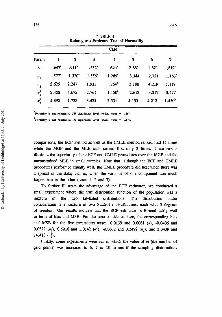
Table 4 reports the Kolmogorov-Smirnov test for normality of the ECF estimators. At a 5 percent significance level, normality is rejected in 24 out of 35 possible cases. However, a comparison of Case 3 with Case 4 shows that doubling the sample size greatly improved the fit of the normal distribution. Normality tends to be strongly rejected in Case 5, in which the mixtures were highly asymmetrical with equal variances, as well as in Case 6, in which the component densities were extremely similar.

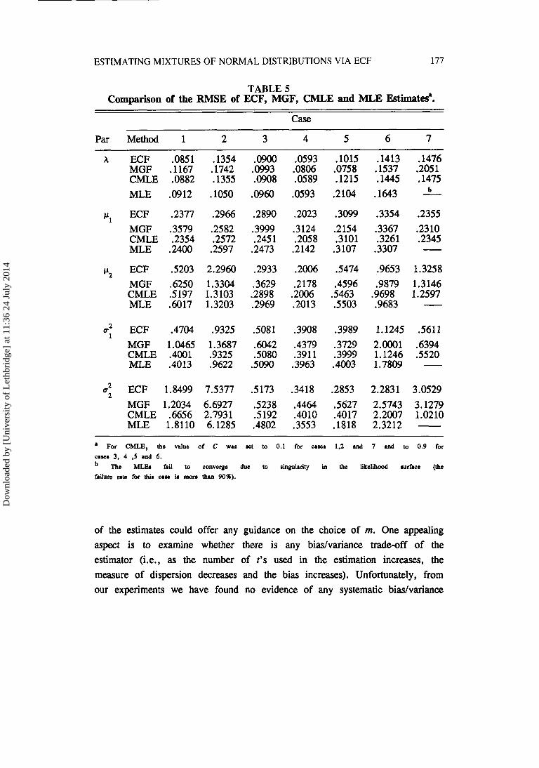
To examine the performance of the ECF estimator relative to other available estimators, Table 5 presents a comparison of the root mean squared

errors (RMSE) of the ECF, MGF, CMLE and MLE estimates for the seven cases.

First, note that when the two components of the mixtures are not well separated, as in Case 7, the MLE procedure seems to have serious problems in estimating the parameters. Previous simulation studies by Hosmer (1973) have shown that one would need a sample size of at least n = 250 in order to get reliable estimates. As for the remaining six cases, out of 30 possible

Dow

nloa

ded

by [

Uni

vers

ity o

f L

ethb

ridg

e] a

t 11:

36 2

4 Ju

ly 2

014

176 TRAN

TABLE 4 Kolmogorov-Smirnov Test of Normality

Case

'Normality in not rejected at 5% significance level (critical value = 1.36). b~o-lity is not rejected at 1% signifi-e level (oritid value = 1.67).

comparisons, the ECF method as well as the CMLE method ranked first 11 times while the MGF and the MLE each ranked first only 3 times. These results illustrate the superiority of the ECF and CMLE procedures over the MGF and the unconstrained MLE in small samples. Note that, although the ECF and CMLE

procedures performed equally well, the CMLE procedure did best when there was

a spread in the data; that is, when the variance of one component was much larger than in the other (cases 1, 2 and 7).

To further illustrate the advantage of the ECF estimator, we conducted a

small experiment where the true distribution function of the population was a mixture of the two fat-tailed distributions. The distribution under consideration is a mixture of two Student t distributions, each with 5 degrees of freedom. Our results indicate that the ECF estimator performed fairly well in term of bias and MSE. For the case considered here, the corresponding bias

and MSE for the five parameters were: -0.0139 and 0.0061 (A), -0.0406 and 0.0527 (p,), 0.5016 and 1.0142 (v:), -0.0672 and 0.3492 (Q, and 2.3439 and 14.413 (0-3.

Finally, some experiments were run in which the value of m (the number of grid points) was increased to 6, 7 or 10 to see if the sampling distributions

Dow

nloa

ded

by [

Uni

vers

ity o

f L

ethb

ridg

e] a

t 11:

36 2

4 Ju

ly 2

014

ESTIMATING MIXTURES OF NORMAL DISTRIBUTIONS VIA ECF 177

TABLE 5 Comparison of the RMSE of ECF, MGF, CMLE and MLE Estites'.

Case

Par Method 1 2 3 4 5 6 7

h ECF .OW1 .I354 MGF .I167 .I742 CMLE .0882 .I355 MLE .0912 .lo50

Ir 1 ECF .2377 .2966 MGF .3579 .2582 CMLE .2354 .2572 MLE .2400 .2597

Ir2 ECF 5203 2.2960 MGF .6250 1.3304 CMLE S197 1.3103 MLE ,6017 1.3203

c2 ECF .4704 .9325 1

MGF 1.0465 1.3687 CMLE .4001 .9325 MLE .4013 .9622

d ECF 1.8499 7.5377 2

MGF 1.2034 6.6927 CMLE .6656 2.7931 MLE 1.8110 6.1285

- - -

a For CMLE, the value of C was let to 0.1 for caner 1.2 and 7 and to 0.9 for cases 3, 4 ,5 and 6.

The MLEJ fail to converge due to singularity in the likelihood surface (the failure rate for thim caw ia mom than 90%).

of the estimates could offer any guidance on the choice of m. One appealing aspect is to examine whether there is any bias/va.riance trade-off of the estimator (i.e., as the number of t's used in the estimation increases, the measure of dispersion decreases and the bias increases). Unfortunately, from our experiments we have found no evidence of any systematic biaslvariance

Dow

nloa

ded

by [

Uni

vers

ity o

f L

ethb

ridg

e] a

t 11:

36 2

4 Ju

ly 2

014

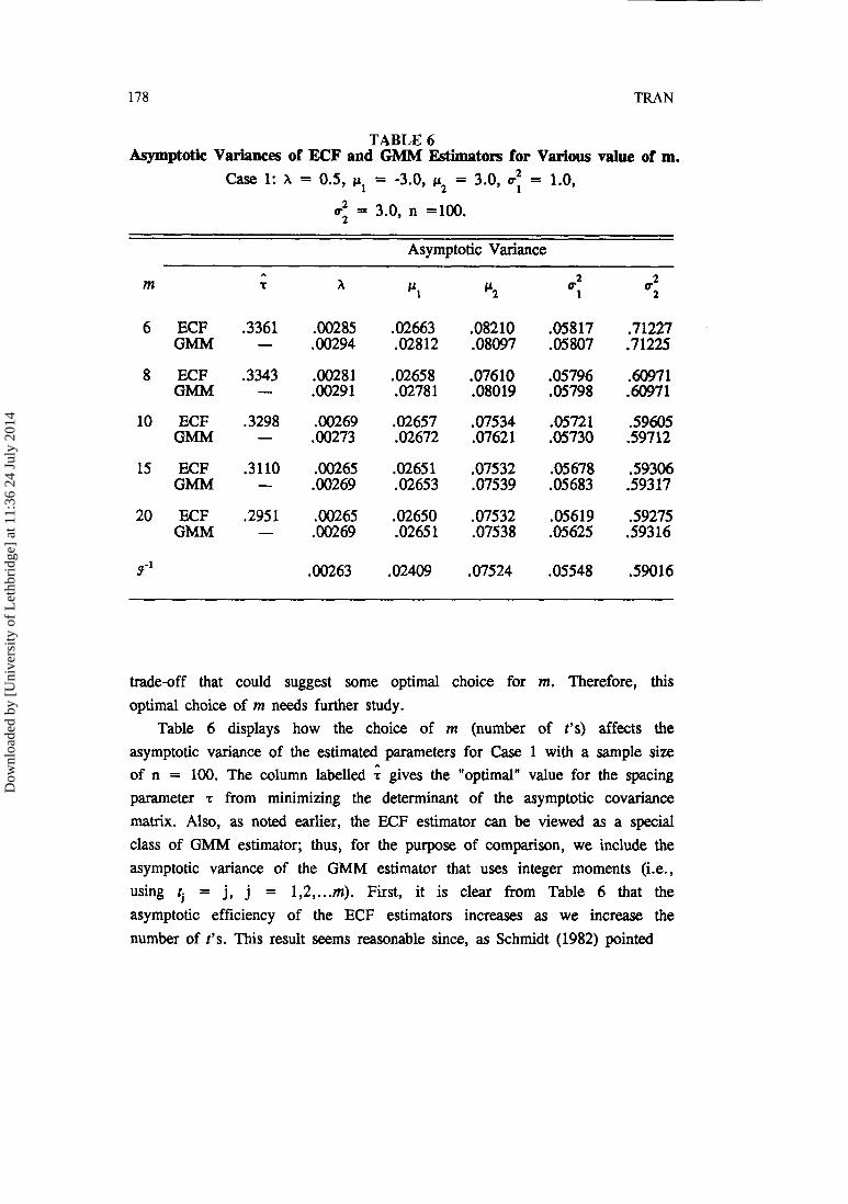
TABLE 6 Asymptotic Variances of ECF and GMM Estimators for Various value of m.

Case 1: h = 0.5, pl = -3.0, p2 = 3.0, 0: = 1.0,

r2 2 = 3.0, n =100.

Asymptotic Variance

6 ECF GMM

8 ECF GMM

10 ECF GMM

15 ECF GMM

20 ECF GMM

trade-off that could suggest some optimal choice for m. Therefore, this optimal choice of m needs further study.

Table 6 displays how the choice of m (number of t's) affects the asymptotic variance of the estimated parameters for Case 1 with a sample size of n = 100. The column labelled ; gives the "optimal" value for the spacing parameter r from minimizing the determinant of the asymptotic covariance matrix. Also, as noted earlier, the ECF estimator can be viewed as a special class of GMM estimator; thus, for the purpose of comparison, we include the asymptotic variance of the GMM estimator that uses integer moments (i.e., using $ = j, j = 1,2, ... m). First, it is clear from Table 6 that the asymptotic efficiency of the ECF estimators increases as we increase the number of t's. This result seems reasonable since, as Schmidt (1982) pointed

Dow

nloa

ded

by [

Uni

vers

ity o

f L

ethb

ridg

e] a

t 11:

36 2

4 Ju

ly 2

014

ESTIMATING MIXTURES OF NORMAL DISTRIBUTIONS VIA ECF 179

out for the case of the MGF estimator, increasing m is equivalent to adding extra observations to the generalized least squares regression and hence the asymptotic efficiency could never decrease. In fact, as m -+ a, Schmidt

conjectured (and also provided some evidence) that the asymptotic variance of the MGF estimators approaches the Cramer-Rao lower bound2. Our result also supports this conjucture for the case of the ECF estimators. Also, it is

interesting to note that as m increases the optimal spacing between the t

values uniformly declines. This striking result is somewhat counterintuitive since, for a smaller r , the asymptotic covariance matrix, (A'dA)", is

almost singular. However, the determinant of ( A ' ~ A ) - ' is small when r is small, so, as m increases, smaller values of r can indeed be optimal.

Second, the ECF estimator with an optimal choice of r seems to be more efficient than the GMM estimator, at least for the case considered here. However, the efficiency gain from using the ECF estimator is relatively small.

IV. AN EMPIRICAL APPLICATION

To illustrate the techniques discussed in this paper we now consider a simple empirical example relating the form of the distribution of stock returns. A vast number of studies have found evidence of significant kurtosis (fat-tails) in stock returns; see, for example, Bera and Higgins (1992) and Bolerslev et al. (1992) for recent surveys. Findings such as these have been commented on for decades and have led to an interest in mixtures models as a way of explaining the observed significant fat-tails. Kon (1984) successfully used the discrete mixture of two or more normal distribution to model the behavior of 30 Dow Jones industrial stocks; the estimations were carried out using the maximum likelihood method.

In this section, our main concern is the estimation technique, so we will

consider only the discrete mixtures of two normal distributions. The data used for the estimation are monthly excess returns (in percentages) of the NYSE value-weighted index over the period 1926101 to 1989112. There are 768 observations.

2 Following Schmidt (1982) the information matrix is evaluated by simulation. Specifically, 50,000 drawings were made from the particular mixture distribution, and for each drawing the second derivative matrix was calculated; these 50,000 second derivative matrices were then averaged to get the information matrix.

Dow

nloa

ded

by [

Uni

vers

ity o

f L

ethb

ridg

e] a

t 11:

36 2

4 Ju

ly 2

014

180 TRAN

TABLE 7 ECF, MGF, CMLE and MLE Estimates of Monthly Excess Returns of

the NYSE Value-Weighted Index*

Parameter ECF MGF CMLE MLE

f-statistics are ahown in parenthelta below the coefficient estimates.

Estimates using the ECF technique were computed using 10 equally spaced grid points, with the spacing parameter, t, initially set at 0.25. Table 7

reports the estimates of the 5 parameters of interest. For comparison purposes, we also report the MGF with an optimal set of t,, ..., t,,, CMLE and MLE estimates. Note that the ECF estimates reported here are the final estimates using the optimal grid points discussed earlier. The estimates are interesting for three reasons. First, for all procedures, the estimate of the mixture parameter, h, is greater than 0.5, implying an asymmetric mixture distribution for the monthly excess returns. Second, though the estimates of the parameters in the first component are nearly the same for all procedures, there are striking differences between the estimates of the parameters in the second component. For the ECF, MGF and CMLE procedures, the estimate of the mean, 5, is statistically significant and approximately 4 times larger than

Dow

nloa

ded

by [

Uni

vers

ity o

f L

ethb

ridg

e] a

t 11:

36 2

4 Ju

ly 2

014

ESTIMATING MIXTURES OF NORMAL DISTRIBUTIONS VIA ECF 181

for the MLE estimate, and the estimate of the variance o: is about half as large. The final interesting aspect of the estimates, and following Christie (1983), is that approximately 28% of the excess returns are drawn from the higher variance distribution. This distribution represents information events while the other 72% excess returns are drawn from the distribution of noninformation rarndom variables.

V. CONCLUSION

This paper uses the empirical characteristic function procedure for estimating the parameters of normal mixtures distribution. The Monte Carlo study showed that the procedure produces estimates with good finite sample properties, even in the case where the maximum likelihood estimator fails to exist. The ECF method can be successfully applied to the real data set and can provide some interesting interpretation.

One important problem remaining is the choice of the number of fmed grid points. This has been shown to be a difficult problem, even in the finite sample, since asymptotically more t's are preferred to less. Thus, the technique used in this paper can be viewed as providing an alternative method to the maximum likelihood approach.

ACKNOWLEDGEMENTS

I would like to thank John L. Knight, Anil Bera, Robin Carter, Bruce Hansen, Ian MacLeod, and Harry Paarsch for their comments. I am also grateful to an Associate Editor and two anonymous referees for constructive comments and suggestions that led to substantial improvement of the paper. The GAUSS code for the constrained EM algorithm provided by Robert F. Phillips is greatly appreciated. Financial support from the University of Saskatchewan President SSHRC is gratefully acknowledged. The usual disclaimer applies.

REFERENCES

Bhattacharya, C. G. (1966), "A simple method of resolution of a distribution into Gaussian components, " Biometrics 23, 115-135.

Bollerslev, T., R. Y. Chou and K. F. Kroner (1992), "ARCH model in finance, a review of the theory and empirical evidence," Journal of Econometrics 52, 5-59.

Dow

nloa

ded

by [

Uni

vers

ity o

f L

ethb

ridg

e] a

t 11:

36 2

4 Ju

ly 2

014

182 TRAN

Bera, A. K. and M. L. Higgins (1992), "ARCH models: properties estimation and testing," Journal of Economic Surveys 7, 1-62.

Bryant, J. L. and A. S. Paulson (1983), "Estimation of mixing proportions via distance between characteristic functions, " Communications in Statistics-Theory and Method 12, 1009-1029.

Christie, A. (1983), "On information arrival and hypothesis events studies," Working Paper, University of Rochester.

Cohen, A. C. (1967), "Estimation in mixtures of two normal distributions," Biometrika 56, 15-28.

Day,N. E. (1969), "Estimating the components of a mixture of normal distributions, " Biometrika 56, 463-474.

Feuerverger, A., and R. Mureika (1977), "The empirical characteristic function and its applications," The Annals of Statistics 5, 88-97.

Feuerverger, A. and P. McDumough (1981a), "On some fourier methods for inference," Journal of the American Statistical Association 76, 379-386.

Feuerverger, A. and P. McDunnough (1981b), "On the efficiency of empirical characteristic function procedures," Journal of the Royal Statistical Society B 43, 20-27.

Feuerverger, A. (1990), "An efficiency result for the empirical characteristic function in stationary time-series models," Canadian Journal of Statistics 18, 155-161.

Hansen, L. P. (1982), "Large Sample Properties of Generalized Method of Moments Estimators," Econometrica, 50, 1029-1054.

Hathaway, R.J. (1985), "A constrained formulation of maximum-likelihood estimation for normal mixture distributions," Annals of Statistics 13, 795-800.

Hathway, R. J. (1986), "A constrained EM algorithm for univariate normal mixtures," Journal of Statistical Computation and Simulation 23, 211-230.

Heathcote, C. R. (1977), "Integrated mean square error estimation of parameters, " Biometrika 64, 255-264.

Hosmer, D. W. Jr. (1973), "On the MLE of the parameters of a mixture of two normal distributions when sample size is small," Communications in Statistics 1, 217-227.

Kiefer, J., and J. Wolfowitz (1956), "Consistency on the maximum likelihood estimator in the presence of many nuisance parameters," The Annals of Mathematical Statistics 27, 887-906.

Kiefer, N. M. (1978), "Discrete parameter variation: efficiency estimation of a switching regression model," Econometrica 46, 427-434.

Dow

nloa

ded

by [

Uni

vers

ity o

f L

ethb

ridg

e] a

t 11:

36 2

4 Ju

ly 2

014

ESTIMATING MIXTURES OF NORMAL DISTRIBUTIONS VIA ECF 183

Kon,S. J. (1984), "Models of stock returns-a comparison," The Journal of Finance 39, 147-165.

Lindsay, B. G. and P. Basak (1993), "Multivariate normal mixtures: a fast consistent method of moment," Journal of the American Statistical Association 88, 468-476.

Newcomb, S. (1886), "A generalize theory of the combination of observations so as to obtain the best result," American Journal of Mathematics 8, 343- 366.

Odell, P. L., and J. P. Basu (1976), "Concerning several methods for estimating crop acreages using remote sensing data," Communication in Statistics A 5, 1091-1114.

Phillips, R. F. (1991), "A constrained maximum-likelihood approach to estimating switching regressions, " Journal of Econometrics 48, 24 1-262.

Quandt, R. E. (1972), "A new approach to estimating switching regressions," Journal of the American Statistical Association 67, 306-310.

Quandt, R. E. and J. B. Ramsey (1978), "Estimating mixtures of normal distributions and switching regressions," Journal of the American Statistical Association 73, 730-738.

Schmidt, P. (1982), "An improved version of the Quandt-Ramsey MGF estimator for mixtures of normal distributions and switching regressions," Econometrics 50, 501-5 16.

Teicher, H. (1961), "Identifiability of mixtures," The Annals of Mathematical Statistics 32, 244-248.

Teicher, H. (1963), "Identifiability of finite mixtures," The Annals of Mathematical Statistics 34, 1265-1269.

Titterington, D. M., A. F. M. Smith and U. E. Makov (1985), Statistical analysis of finite mixture distribution, John Wiley & Son Ltd.

Tran, K. C. (1996), "Estimating Mixtures of Normal Distributions via Empirical Characteristic Function," University of Saskatchewan Working Paper #96-1.

Dow

nloa

ded

by [

Uni

vers

ity o

f L

ethb

ridg

e] a

t 11:

36 2

4 Ju

ly 2

014