Georgia State University Georgia State University

ScholarWorks @ Georgia State University ScholarWorks @ Georgia State University

Economics Dissertations

8-8-2007

Essays on Tax Evasion Essays on Tax Evasion

Edward Batte Sennoga

Follow this and additional works at: https://scholarworks.gsu.edu/econ_diss

Part of the Economics Commons

Recommended Citation Recommended Citation Sennoga, Edward Batte, "Essays on Tax Evasion." Dissertation, Georgia State University, 2007. https://scholarworks.gsu.edu/econ_diss/18

This Dissertation is brought to you for free and open access by ScholarWorks @ Georgia State University. It has been accepted for inclusion in Economics Dissertations by an authorized administrator of ScholarWorks @ Georgia State University. For more information, please contact scholarworks@gsu.edu.

PERMISSION TO BORROW In presenting this dissertation as a partial fulfillment of the requirements for an advanced degree from Georgia State University, I agree that the Library of the University shall make it available for inspection and circulation in accordance with its regulations governing materials of this type. I agree that permission to quote from, to copy from, or to publish this dissertation may be granted by the author or, in his or her absence, the professor under whose direction it was written or, in his or her absence, by the Dean of the Andrew Young School of Policy Studies. Such quoting, copying, or publishing must be solely for scholarly purposes and must not involve potential financial gain. It is understood that any copying from or publication of this dissertation which involves potential gain will not be allowed without written permission of the author.

____________________________________ Signature of the Author

NOTICE TO BORROWERS All dissertations deposited in the Georgia State University Library must be used only in accordance with the stipulations prescribed by the author in the preceding statement. The author of this dissertation is: Edward Batte Sennoga Department of Economics Andrew Young School of Policy Studies Georgia State University P.O. Box 3992 Atlanta, GA 30302-3992 The director of this dissertation is: Professor James R. Alm Department of Economics Andrew Young School of Policy Studies Georgia State University P.O. Box 3992 Atlanta, GA 30302-3992 Users of this dissertation not regularly enrolled as students at Georgia State University are required to attest acceptance of the preceding stipulations by signing below. Libraries borrowing this dissertation for the use of their patrons are required to see that each user records here the information requested. Type of use Name of User Address Date (Examination only or copying)

ESSAYS ON TAX EVASION

BY

EDWARD BATTE SENNOGA

A Dissertation Submitted in Partial Fulfillment of the Requirements for the Degree

of Doctor of Philosophy

in the Andrew Young School of Policy Studies

of Georgia State University

GEORGIA STATE UNIVERSITY 2006

Copyright by Edward Batte Sennoga

2006

ACCEPTANCE

This dissertation was prepared under the direction of the candidate’s Dissertation Committee. It has been approved and accepted by all members of that committee, and it has been accepted in partial fulfillment of the requirements for the degree of Doctor of Philosophy in Economics in the Andrew Young School of Policy Studies of Georgia State University. Dissertation Chair: James R. Alm Committee: Francis G. Abney Mary Beth Walker Sally Wallace Electronic Version Approved: Roy W. Bahl, Dean Andrew Young School of Policy Studies Georgia State University August 2006

vi

ACKNOWLEDGEMENTS

Foremost, I give God all the glory, honor, and praise for the wisdom and empowerment, without which this academic journey would not have been accomplished. I would also like to thank committee members, Professors: James R. Alm, Francis G. Abney, Mary Beth Walker, and Sally Wallace for all the comments, suggestions, and insights offered during the writing of this dissertation. Professors: Jorge Martinez-Vazquez, David L. Sjoquist, and Neven Valev are also appreciated for their comments and suggestions during the early stages of this dissertation. Furthermore, special thanks go to Professor Friedrich Schneider of the Department of Economics at Johannes Kepler University of Linz and Dr. Miles Light for their helpful comments and suggestions. Special recognition goes to the doctoral class of 2001 for creating an exigent though conducive learning environment and for fostering a community of scholars. My sincere thanks and gratitude also go to my parents, Mr. and Mrs. James Lubwama, siblings, Andrew and Godfrey, members of my extended family who are too numerous to mention here, and Mr. and Mrs. Idd Iwumbwe, for their support and encouragement. Last, but certainly not least, I would like to thank Justine Mugalu for the unwavering support, love, and devotion. Thank you all.

vii

TABLE OF CONTENTS

Page

Acknowledgements........................................................................................................................ vi

List of Tables ................................................................................................................................. ix

List of Figures ..............................................................................................................................xiii

List of Appendixes....................................................................................................................... xiv

Abstract ......................................................................................................................................... xv

Essay one: Tax Evasion and Tax Structure................................................................................... 1

Introduction......................................................................................................................... 1

Significant Previous Research ............................................................................................ 2

Analytical Framework ........................................................................................................ 9

Tax Evasion model ..................................................................................................... 9

Theoretical Framework of Tax Structure.................................................................. 14

Empirical Framework ....................................................................................................... 19

Estimation Methodology........................................................................................... 19

Seemingly Unrelated Regression Model .................................................................. 21

Data Sources ............................................................................................................. 23

Explanatory Variables............................................................................................... 25

Empirical Results ...................................................................................................... 31

Conclusions and Suggestions for Future Research........................................................... 41

Essay two: The Incidence of Tax Evasion.................................................................................. 45

Introduction....................................................................................................................... 45

Significant Previous Research .......................................................................................... 46

viii

Page

Static Computable General Equilibrium model................................................................ 52

Household Consumption and Labor decisions ......................................................... 53

Firm’s Production Decisions..................................................................................... 56

General Equilibrium Modeling ................................................................................. 57

Extensions to the Static General Equilibrium Model ............................................... 60

Data and Model Calibration...................................................................................... 63

Counterfactuals and Simulations ...................................................................................... 72

Full Compliance in the Formal Sector and Tax Evasion in the Informal Sector ........................................................................................................................ 74 Partial Compliance in the Formal Sector and Tax Evasion in the Informal Sector ..................................................................................................................... 82 Sensitivity Analysis .................................................................................................. 84 Conclusions and Suggestions for Future Research........................................................... 88 References……........................................................................................................................... 142 Vita………….............................................................................................................................. 148

ix

TABLES Page

Table B1 Descriptive Statistics of Selected Variables: East African Sample .................... 101

Table B2 Descriptive Statistics of Selected Variables: OECD Sample.............................. 102

Table B3 Simple Correlations for Selected Variables: East African Sample..................... 103

Table B4 Simple Correlations for Selected Variables: OECD Sample .............................. 104

Table B5 Tax Burden and the Size of the Shadow Economy in East African Countries 106 ...................................................................................................... 105 Table B6 The Size of the Shadow Economy in OECD Countries...................................... 106

Table B7 First Stage Least Squares Estimates: East African and OECD Samples ............ 107

Table B8 OLS and GMM Estimates with no Fixed Effects: OECD Sample ..................... 108

Table B9 OLS and GMM Estimates with no Fixed Effects: East African Sample ............ 109

Table B10 OLS and GMM Estimates with Fixed Effects: OECD Sample .......................... 110

Table B11 OLS and GMM Estimates with Fixed Effects: East African Sample ................. 111

Table B12 List of Variable Descriptions .............................................................................. 112

Table B13 Social Accounting Matrix: Summary of Salient Features................................... 113

Table B14 Social Accounting Matrix: Full Compliance in the Formal Sector and Tax Evasion in the Informal Sector (POOR households’ endowment is 33 percent of RICH households’ endowment) ........................................................ 114 Table B15 Social Accounting Matrix: Partial Compliance in the Formal Sector and Tax Evasion in the Informal Sector (POOR households’ endowment is 33 percent of RICH households’ endowment)......................................................... 115 Table B16 Social Accounting Matrix: Full Compliance in the Formal Sector and Tax Evasion in the Informal Sector (POOR households’ endowment is 25 percent of RICH households’ endowment)......................................................... 116

x

Page

Table B17 Social Accounting Matrix: Partial Compliance in the Formal Sector and Tax Evasion in the Informal Sector (POOR households’ endowment is 25 percent of RICH households’ endowment)......................................................... 117 Table B18 Social Accounting Matrix: Full Compliance in the Formal Sector and Tax Evasion in the Informal Sector (POOR households’ endowment is 50 percent of RICH households’ endowment)......................................................... 118 Table B19 Social Accounting Matrix: Partial Compliance in the Formal Sector and Tax Evasion in the Informal Sector (POOR households’ endowment is 50 percent of RICH households’ endowment)......................................................... 119 Table B20 Elasticity Choices................................................................................................ 120

Table B21 Summary of the General Equilibrium Effects from the Evasion of Commodity and Income in the Informal sector (POOR households’ endowment is 33 percent of RICH households’ endowment) ............................. 121 Table B22 Percentage Changes in Product and Factor Prices with Full Compliance in the Formal Sector and Tax Evasion in the Informal Sector (Commodity and Income Taxes: POOR households’ endowment is 33 percent of RICH households’ endowment) .................................................................................... 122 Table B23 Percentage Changes in Product and Factor Prices with Full Compliance in the Formal Sector and Tax Evasion in the Informal Sector (Commodity Taxes: POOR households’ endowment is 33 percent of RICH households’ endowment) .................................................................................... 123 Table B24 Percentage Changes in Product and Factor Prices with Full Compliance in the Formal Sector and Tax Evasion in the Informal Sector (Income Taxes: POOR households’ endowment is 33 percent of RICH households’ endowment)......................................................................................................... 124 Table B25 Percentage Changes in Product and Factor Prices with Partial Compliance in the Formal Sector and Tax Evasion in the Informal Sector (Commodity and Income Taxes: POOR households’ endowment is 33 percent of RICH households’ endowment) .................................................................................... 125 Table B26 Percentage Changes in Product and Factor Prices with Partial Compliance in the Formal Sector and Full Evasion in the Informal Sector (Commodity Taxes: POOR households’ endowment is 33 percent of RICH households’ endowment)......................................................................................................... 126

xi

Page Table B27 Percentage Changes in Product and Factor Prices with Partial Compliance in the Formal Sector and Full Evasion in the Informal Sector (Income Taxes: POOR households’ endowment is 33 percent of RICH households’ endowment)......................................................................................................... 127 Table B28 Summary of the General Equilibrium Effects from the Evasion of Commodity and Income in the Informal sector: POOR households’ endowment is 25 percent of RICH households’ endowment............................... 128 Table B29 Percentage Changes in Product and Factor Prices with Full Compliance in the Formal Sector and Tax Evasion in the Informal Sector (Commodity and Income Taxes: POOR households’ endowment is 25 percent of RICH households’ endowment) .................................................................................... 129 Table B30 Percentage Changes in Product and Factor Prices with Full Compliance in the Formal Sector and Tax Evasion in the Informal Sector (Commodity Taxes: POOR households’ endowment is 25 percent of RICH households’ endowment) ..................................................................................... 130 Table B31 Percentage Changes in Product and Factor Prices with Full Compliance in the Formal Sector and Tax Evasion in the Informal Sector (Income Taxes: POOR households’ endowment is 25 percent of RICH households’ endowment)......................................................................................................... 131 Table B32 Percentage Changes in Product and Factor Prices with Partial Compliance in the Formal Sector and Tax Evasion in the Informal Sector (Commodity and Income Taxes: POOR households’ endowment is 25 percent of RICH households’ endowment) .................................................................................... 132 Table B33 Percentage Changes in Product and Factor Prices with Partial Compliance in the Formal Sector and Full Evasion in the Informal Sector (Commodity Taxes: POOR households’ endowment is 25 percent of RICH households’ endowment)......................................................................................................... 133 Table B34 Percentage Changes in Product and Factor Prices with Partial Compliance in the Formal Sector and Full Evasion in the Informal Sector (Income Taxes: POOR ............households’ endowment is 25 percent of RICH households’ endowment)......................................................................................................... 134 Table B35 Summary of the General Equilibrium Effects from the Evasion of Commodity and Income in the Informal sector: POOR households’ endowment is 50 percent of RICH households’ endowment............................... 135

xii

Page Table B36 Percentage Changes in Product and Factor Prices with Full Compliance in the Formal Sector and Tax Evasion in the Informal Sector (Commodity and Income Taxes: POOR households’ endowment is 50 percent of RICH households’ endowment) .................................................................................... 136 Table B37 Percentage Changes in Product and Factor Prices with Full Compliance in the Formal Sector and Tax Evasion in the Informal Sector (Commodity Taxes: POOR households’ endowment is 50 percent of RICH households’ endowment)......................................................................................................... 137 Table B38 Percentage Changes in Product and Factor Prices with Full Compliance in the Formal Sector and Tax Evasion in the Informal Sector (Income Taxes: POOR households’ endowment is 50 percent of RICH households’ endowment)......................................................................................................... 138 Table B39 Percentage Changes in Product and Factor Prices with Partial Compliance in the Formal Sector and Tax Evasion in the Informal Sector (Commodity and Income Taxes: POOR households’ endowment is 50 percent of RICH households’ endowment) .................................................................................... 139 Table B40 Percentage Changes in Product and Factor Prices with Partial Compliance in the Formal Sector and Full Evasion in the Informal Sector (Commodity Taxes: POOR households’ endowment is 50 percent of RICH households’ endowment)......................................................................................................... 140 Table B41 Percentage Changes in Product and Factor Prices with Partial Compliance in the Formal Sector and Full Evasion in the Informal Sector (Income Taxes: POOR households’ endowment is 50 percent of RICH households’ endowment)......................................................................................................... 141

xiii

FIGURES

Page

Figure A1 Development of the Shadow Economy................................................................. 98

xiv

APPENDIXES

Page

Appendix A Measures of the Shadow Economy ..................................................................... 95

Appendix B Tables ................................................................................................................ 101

xv

ABSTRACT

ESSAYS ON TAX EVASION

BY

EDWARD BATTE SENNOGA

August 2006 Committee Chair: Dr. James R. Alm Major Department: Economics

Essay one develops and tests a revenue-maximizing tax structure model. This

model represents one of the first attempts to evaluate and compare the responsiveness of

various tax instruments to tax evasion within a tax revenue maximization framework. We

use data from both the OECD and East African countries and estimation is via a

seemingly unrelated regression model. The GDP share of agricultural income is used as

an instrument to correct for the simultaneity between tax revenue shares and tax evasion.

Our findings indicate that tax evasion increases the tax authority’s reliance on

consumption taxes vis-à-vis taxes on income, suggesting that diverse tax instruments

respond differently to tax evasion, and as such the choice of a revenue-maximizing tax

structure is influenced by the amount of revenue lost through tax evasion.

Essay two analyzes the incidence of tax evasion in both the formal and informal

sectors of the economy using a computable general equilibrium model. This essay

incorporates the element of uncertainty in an individual’s decision to evade so as to

account for the uncertainty of returns to the tax evader. We also allow for varying degrees

of competition or entry across sectors in the economy to examine how much of the tax

xvi

advantage is retained by the initial evaders and how much is shifted via factor and

commodity price changes. Our simulation results show that the evading households’ post-

evasion welfare is only 0.68-3.40 percent higher than the post-tax welfare if it had fully

complied with taxes. The simulation results further reveal that the evading household

keeps 77.1-83.2 percent of this initial increase in welfare, while 16.8-22.9 percent of this

initial gain is competed away as a result of increased competition and entry into the

informal sector. The compliant households’ welfare increases by 58.8-101.7 percent with

increased competition in the informal sector. Therefore, if we construe the changes in

consumer welfare as an overall indicator of the gains and/or losses from tax evasion, then

the evading household only benefits marginally and this advantage diminishes with

increased entry or competition in the informal sector.

1

Essay One: Tax Evasion and Tax Structure

Introduction

The question of how tax evasion affects the structure of taxes has not been closely

examined in the public finance literature. While traditional economic models are

generally able to explain the choice of a tax structure as an endogenous outcome of

constrained maximizing behavior of political agents (maximizing behavior in which

agents choose tax structure to minimize the political costs or the expected loss in votes

associated with raising a budget of given size), they are less equipped to answer questions

regarding the effect of tax evasion on the structure of taxes. Further, tax evasion alters the

effective tax rates and as such affects the efficiency, equity, and revenue yield of any

given tax instrument. This therefore suggests that any meaningful analysis of the

attributes of “a good tax system” and consequently the choice of a revenue-maximizing

tax system should account for this reality.

Additionally, tax evasion has wide ranging implications especially regarding its

effect on tax revenues, excess burden, and the numerous out-of-pocket costs that are

typically associated with tax evasion. Government’s responses to the revenue short-fall

created by tax evasion, such as raising revenues from other sources, reducing the supply

of public services, and/or borrowing, could also lead to excess burdens. Related to this is

the indirect effect of tax evasion on economic institutions. For instance, when

entrepreneurs or any other private individuals are faced with burdensome bureaucracy,

extreme levels of corruption, and a deficient legal system, agents may respond by

diverting their activities to the shadow or underground economy. This leads to lower tax

revenues, additionally compromising the quality of the public administration as well as

2

the quality and quantity of public goods and services. This string of occurrences further

reduces the motivation of businesses and entrepreneurs to operate in the aboveground

sector of the economy.

Kesselman (1989) argues that workers may find it almost effortless to evade taxes

by moving to sectors of the economy where tax evasion is relatively easier, say, due to

cash receipts, no source withholding of tax, and/or no tax information reporting. On the

other hand, firms may have an added incentive to fully comply with tax provisions

especially if they obtain tax offsets or deductions for the wages and salaries paid.

The tax evasion question is therefore of paramount significance in the design of any tax

system. Since we typically consider the ability of taxpayers to adjust to income taxes as

being greater than for indirect taxes (especially broad-based consumption taxes), tax

policy design can greatly be augmented by a formal analysis of the impact of tax evasion

on tax structure. This essay explores the effect of tax evasion on tax structure by

examining the responsiveness of tax revenues from different tax instruments to changes

in the level of tax evasion using data from both the OECD and East African countries.

The seemingly unrelated regression estimation procedure is utilized to exploit the cross-

equation correlation inherent in tax share equations. Our estimation methodology is

plagued by the potential simultaneity between tax revenue shares and tax evasion. We

propose the GDP share of income from the agriculture sector as an instrument to correct

for this simultaneity bias.

Significant Previous Research

Peacock and Shaw (1982) utilize a two sector model (consumption and

autonomous expenditure sectors) to analyze the impact of tax evasion on tax revenues.

3

They conclude that tax revenue loss from evasion activity will be zero if the marginal

propensity to consume (mpc) out of tax evading income is equal to one irrespective of the

value of the mpc in the non-evading sector(s). On a priori grounds, it seems reasonable to

assume the mpc of tax evaders is higher than that of the compliant tax payers since the

acquisition of financial assets or durable real assets is more readily susceptible to

detection by the fiscal authorities. This result is intuitive. The tax agency suffers a loss in

its share of the income tax base. On the other hand, the tax agency participates in the

growth of the tax base by the taxable part of the increased tax base because the evaders

produce a positive income effect. The net loss is thus equal to zero.

Ricketts (1984) extends the Peacock and Shaw (1982) analysis from a simple

Keynesian model to an IS-LM model and links tax evasion with the monetary sector. The

general conclusion is that the Peacock and Shaw (1982) conclusions hold only under

certain conditions. Specifically, the expansionary consequences for expenditures of tax

evasion and the possible expansionary influence on real output may be counter-balanced

by restrictive monetary consequences. Thus the changes in the propensity to evade taxes

may in principle have complex macroeconomic implications. Ricketts (1984) also argues

that a rise in tax evasion will not necessarily lead to an increase in domestic output.

Additionally, a rise in tax evasion still normally leads to a decrease in tax revenue, as in

Peacock and Shaw (1982).

Hettich and Winer (1984) develop and test a model in which the composition of

revenues and the structure of specific taxes arise endogenously as a result of constrained

maximizing behavior by political agents. They assume that the political agents choose tax

structure so as to minimize the political costs or the expected net loss in votes associated

4

with raising a budget of given size. Hettich and Winer (1984) argue that, though political

costs associated with various tax sources cannot be observed directly, it is possible to

identify exogenous factors influencing such costs and to observe their impact on tax

structure. Such determinants of political cost are discussed, and several hypotheses

concerning the nature of political cost functions are developed and applied to an

explanation of the differences among U.S. states in their reliance on income taxation.

They conclude that the tax structure that minimizes political cost will be determined by

the characteristics of many different groups of tax payers, and in particular by the

sensitivity of their political opposition to changes in particular aspects of the tax system.

Further, their empirical application emphasizes differences in political constraints across

jurisdictions in the belief that much can be learned about the choice of policy instruments

by studying structural adjustments in response to varying constraints.

Hettich and Winer (1988) further develop this approach by deriving the essential

elements of tax systems as an outcome of rational behavior in a model where government

maximizes expected support and where opposition to taxation depends on the loss in full

income. They assume that the government’s objective in designing a tax structure is to

maximize expected support, which can be interpreted in a “narrow” and “broad” manner.

In the “narrow” version, it is argued that individual support for the government depends

on both the benefits from public goods (and the loss in income resulting from taxation)

and on the characteristics, such as the cost of voting, age, and the taste for civic duty, all

of which determine how a particular individual’s net economic benefit from the fiscal

system is translated into a probability of voting for the government. In the “broad”

interpretation of the term support, effective support depends not only on the likelihood

5

that an individual will vote favorably in the next election but also on the individual’s

relative political influence. The government then maximizes the weighted sum of

expected votes where weights depend on voter characteristics like interest group

membership and strength and on individual attributes such as personal wealth. Voters

base their decision on whether to support the government on how they are affected by

benefits and taxes, and are not influenced by how others are treated. Hettich and Winer’s

(1988) analysis treats the level of expenditures as endogenous and integrates the influence

of administration costs with that of political and economic factors. Tax structure is shown

to be a system of related components in equilibrium. The upshot of this analysis is that

the politically optimal tax structure requires a choice of tax rates that equalizes marginal

political costs per dollar of additional revenue across all tax payers. Hettich and Winer

(1988) argue that this tax structure will finance a total expenditure such that the marginal

political benefit of another dollar of expenditure is equal to the common marginal

political cost per dollar of additional revenue. Hettich and Winer (1988) extend this

framework to the analysis of taxation of many activities, arguing that the taxation of

many activities is a natural outcome of expected support maximization. In this latter case,

the politically optimal tax structure requires marginal political opposition per dollar of tax

revenue to be equalized across taxable activities for each taxpayer, and to be equalized

across taxpayers for each activity.

Lai and Chang (1988) extend the Peacock and Shaw (1982) and Ricketts (1984)

models by incorporating the effect of tax evasion on labor supply. They argue that in

response to an increase in tax evasion labor supply will be stimulated and hence

constitute an additional expansionary channel on domestic output. Consequently, tax

6

evasion may be positively related to the total tax collections. Stated differently, if the tax

evasion-induced labor supply effect is taken into account, an increase in the degree of tax

evasion may increase total tax revenue, rather than lessen it.

Von Zameck (1989) utilizes the Peacock and Shaw (1982) model as a starting

point to analyze tax evasion within a macroeconomic framework by introducing an

indirect tax (in addition to just the direct tax considered by earlier models) as a

simultaneous determinant of tax collections. Using a uniform marginal propensity to

consume (c) for both declared and undeclared income, his analysis reveals that overall tax

yield is diminished if c is less than 1 and is not affected if c = 1. He also shows that the

overall tax revenue may increase, provided that the marginal propensity to consume is

unity. In other words, provided that the marginal propensity to consume out of

undeclared income is unity, tax evasion will not only have no adverse effects on overall

collections, as in the Peacock and Shaw (1982) model, but will also tend to enhance tax

revenues. Thus, tax evasion pays a dividend because the behavior of the private agent in

respect to the additional income obtained by evading taxes can be characterized as some

form of “deficit spending.” However, if evaders in their decisions to consume make no

distinction between declared and undeclared income, then tax evasion is generally

accompanied by a fiscal loss, as would be expected via conventional wisdom.

Gordon and Nielsen (1997) examine the relative vulnerability of consumption and

income taxes to tax evasion by measuring the relative amounts of evasion under the two

taxes in Denmark using aggregate Danish tax and accounting data from 1992. They argue

that, though a value-added and a cash-flow income tax have similar behavioral and

distributional consequences in the absence of tax evasion, the available means of tax

7

evasion under each tax can be very different. Under a value added tax (VAT), evasion

occurs via cross-border shopping, while under an income tax it can occur through shifting

taxable income abroad. Their analysis is based on comparing the observed labor income

tax base with the figure that would be forecast based on the economy’s aggregate cash-

flow constraint given observed consumption expenditures under the VAT and observed

accounting figures for asset accumulation. Gordon and Nielsen (1997) argue that, while

accurate accounting data on income and consumption would precisely satisfy this

accounting identity, the figures on income and consumption reported for tax purposes

will each be too small as a result of evasion. If evasion of the income tax is relatively

larger, the observed earnings reported for tax purposes will be smaller relative to the

value forecast based on observed expenditures reported for tax purposes and accounting

information on asset accumulation. It is this difference that yields a measure of the

relative amounts of evasion under the consumption and income taxes. Their data for 1992

suggest that evasion rates under the consumption and the income taxes were relatively

modest, with just 0.8 percent of consumption taxes evaded through cross-border shopping

compared to nearly 4 percent of labor income lost due to shifting incomes abroad.

Gordon and Nielsen (1997) also develop a theoretical framework to examine the choice

of income versus VAT rates that would minimize the excess burden resulting from

evasion activities. Based on this theory and the computed evasion rates, they find that the

forecast evasion costs could be reduced by increasing the VAT rate relative to the income

tax rate. They conclude that in the presence of tax evasion a country could still make use

of both taxes in order to minimize the efficiency costs of evasion activity, relying

relatively more on whichever tax is harder to evade or the consumption tax in this case.

8

Nielsen, Schou, and Sobygaard (2002) also utilize a national income accounts

identity for Denmark to show that income is more vulnerable to tax evasion than

consumption. They argue that there is an exact relationship between the tax bases for

labor income tax and a consumption tax even where both income and consumption taxes

are subject to tax avoidance and evasion. In their national accounts identity, capital and

consumption income are related by the relationship FIGCYY rw ∆+++=+ , where wY

is wage income, rY is capital income, C is private consumption, G is government

consumption, I is investment, and F∆ is the change in the net foreign debt. When

investment is subtracted from both sides in the equation, the left-hand side yields an

income tax base, while the right-hand side becomes the consumption tax base (that is, the

sum of private and public consumption) plus a correction term for the change in the net

foreign debt. When both sides of the equation FGCIYY rw ∆++=−+ are calculated

independently of each other (assuming that there are no errors and omissions in the

underlying data), the two numbers will be identical in the absence of tax evasion. They

argue that any observed differences between the two figures are an indication of the

difference between tax evasion of income on the one hand and tax evasion of

consumption on the other. Such a difference could stem from simple labor income tax

evasion, say, through erroneous reporting or non-reporting of income earned. It could

also arise from individuals storing assets in foreign banks and not revealing information

about income from such sources to domestic authorities.

Their calculations from this indirect method for the period 1995-1997 reveal that

an amount of income in the order of 20 to 40 billion Danish kroner (between 1.8 and 3.6

percent of GDP) could not be accounted for. This is attributed to two different kinds of

9

phenomena: first, a difference between the errors and omissions in the data on each side

of the general equation, and second, a difference in tax evasion for each tax base. Though

they hasten to add that these figures should be interpreted cautiously in light of the

underlying data problems, their findings suggest that income is especially vulnerable to

tax evasion in Denmark as compared to consumption.

In summary, it is evident from the previous literature that tax evasion will

normally lead to a reduction in tax revenues. Further, several authors have made

arguments in favor of (broad-based) commodity taxation vis-à-vis income taxation.

National income accounts analyses have also revealed higher evasion rates for taxes on

income relative to taxes on consumption. The tax structure literature on the other hand

argues that the composition of revenues and the structure of specific taxes arise

endogenously as a result of constrained maximizing behavior by political agents. It is

against this background, coupled with the lack of substantial empirical evidence on the

responsiveness of different tax instruments to tax evasion that this essay tries to examine

the question of whether tax evasion ought to influence the choice or composition of the

tax mix. This essay uses a novel approach to analyze the effects of tax evasion on the

different tax instruments.

Analytical Framework

Tax Evasion Model

Suppose that an economic agent, say, a business enterprise or an individual, has

total income y. After comparing the expected benefit from and cost of tax evasion, this

economic agent may make an economic decision regarding the amount of income to

report to the tax authority. If the expected net benefit of tax evasion is positive, a rational

10

economic agent will have an incentive to engage in tax evasion. The optimal amount of

evasion can be computed and will occur when the expected net benefit from tax evasion

is zero. Following Allingham and Sandmo (1972), we construct a simple model of such

behavior.

Denote the reported income by x. With no tax evasion, x=y; otherwise, x is strictly

less than y, and the difference y-x represents the underreported income. The benefit of

underreported income is the tax savings on this portion of income. If the marginal tax rate

is t, the marginal benefit of evasion is also t, and thus the total benefit of evading taxes on

income y-x is given by t(y-x). If the economic agent is caught evading taxes, not only

must he/she pay the evaded tax, but a fine f is also applied per unit of evaded income (y-

x).1 Consequently, with detection, the net income of the agent can be written as y-tx-

(t+f)(y-x). In other words, the agent has income y on which tax was paid based on

reported income x. When caught evading the tax, however, both the marginal tax rate t

and the marginal fine rate f must be paid on underreported income y-x. The benefit from

tax evasion is t(y-x), and, if caught, the cost of evasion is (t+f)(y-x). For simplicity,

assume that both f and t are constant.

Other considerations can also be included in analysis of the benefit/cost decision

to evade. For instance, Sandmo (2004) argues that daily observations indicate that

individuals refrain from “socially unacceptable” acts like tax evasion, shoplifting, and

polluting the environment due to the social stigma attached to such acts. The disutility,

say, from tax evasion will ultimately affect the optimal amount of tax evasion, and as

1 According to American and Israeli law, the fine is imposed on the amount of evaded taxes. This essay follows the more general Allingham and Sandmo (1972) approach where the marginal fine is imposed on a unit of evaded income since our sample consists of a mix of countries, including both developed and developing countries, in which the marginal fine is imposed on a unit of evaded income.

11

such should be a part of the individuals expected utility function. Similarly, this

“disutility” could take the form of evasion costs especially since tax evaders incur costs

in their bid to conceal their earnings or in the creation of opportunities to evade taxes.

Assuming that the probability of detection and prosecution for tax evasion is

independent of the amount of taxes evaded and is denoted byπ 2, the economic agent will

choose an amount of reported income x so as to maximize expected utility as follows:

[1] ( ) ( ) ( ) ( ) ( ),1 hBZUWUUE −+−= ππ

where txyW −= , ( )xytxyZ −−−= φ , ( )ft +=φ , and ( )hB is a measure of the

“disutility” from and/or costs of tax evasion and ( )xyh −= . We assume that the

disutility from tax evasion is strictly increasing in the amount of taxes evaded so that

( ) 0>′ hB and ( ) 0>′′ hB . Assuming that the economic agent wishes to maximize expected

utility by choosing the amount of income x to report to the tax authority, the first-order

condition for an interior solution can be written as follows:

[2] ( ) ( ) ( ) ( ) ( ) 01 =′+′−−′−− hBZUtWUt πφπ

Similarly, the second-order condition3 is:

[3] ( ) ( ) ( ) ( ) ( ) 01 22 <′′−′′−+′′−= hBZUtWUtD πφπ

The condition for some amount of income underreporting to be optimal can be formally

obtained by taking the derivative of expected utility at x=0 and x=y to obtain

[4] ( ) ( ) ( ) ( ) ( )( ) ( )yByUftyUtxUE x ′+−′−−′−−=∂∂ = φπφπ 11| 0

[5] ( ) ( ) ( )( ) ( ) ( )( ) ( )0111| BtyUttyUtxUE yx ′+−′−−−′−−=∂∂ = πφπ

2 While it may be more realistic to assume that the probability of detection rises with the amount of underreporting, we make the simplifying assumption of a constant probability in this model. This is especially true considering that tax authorities in most countries do not yet have mechanisms in place that are likely to cause the probability of detection to be responsive to underreporting. 3 The second-order condition is satisfied by assuming a concave utility function.

12

Under the assumption that expected marginal utility is decreasing in x, optimality of the

interior solution requires that the derivatives in equations [4] and [5] must be positive and

negative, respectively. This will be the case if and only if:

[6] ( )( )( ) ( ) ( )

( )( )⎥⎦⎤

⎢⎣

⎡−′

′−+>

−′′

+φ

ππφ

πφ1

11 yU

yUtyU

yB

[7] ( )( )( ) t

tyUB

<−′

′+

10πφ .

Equation [6] indicates that it will always be optimal to move from a state of no tax

evasion (x=0) to one with a positive level of evasion as long as the expected penalty plus

the negative value accruing from evasion is less than the marginal tax rate.4 Equation [7]

shows that the economic agent will report less than his “true” income, since it is only

then that the expected penalty plus the negative value ensuing from evasion is less than

the marginal tax rate. These two conditions therefore suggest that the negative value

attached to evasion acts as an additional tax to deter evasion, and, subsequently, a

positive expected gain is in itself simply not sufficient for the economic agent to evade

taxes.

A comparative static of interest is the effect of the marginal tax rate on the

amount of income reported by the economic agent. As mentioned above, an increase in

the marginal tax rate increases the gain from evasion on the margin (if the agent is not

detected), and as such it is realistic to expect a negative relationship between the marginal

tax rate and the amount of income reported. Differentiating equation [2] with respect to t

yields;

4 The term in brackets on the right hand side of equation [6] is less than 1, and, as such, the marginal tax rate t is greater than sum of the two terms on the left hand side.

13

[8] ( ) ( ) ( ) ( )[ ] ( ) ( ) ( )[ ]ZUWUD

ZUtWUtxDt

x ′+′−+′′−−′′−−=∂∂ πππφπ 11111

As in Allingham and Sandmo (1972), we define:

[9] ( ) ( )( )WUWUWRA ′′′

−=

and

[10] ( ) ( )( )ZUZUZRA ′

′′−=

as measures of absolute risk aversion. Using equation [3] in [8] and applying the equality

in [2], we obtain:

[11] ( ) ( ) ( ) ( )[ ] ( ) ( ) ( )[ ]ZUWUD

ZRWRWUxtDt

xAA ′+′−+−′−=

∂∂ πππ 1111

The first term on the right hand side can be positive, zero or negative depending on

whether the absolute risk aversion is increasing, constant or decreasing while the second

term is clearly negative. Decreasing risk aversion would imply that ( ) ( )[ ]ZRWR AA − is

positive consequently indicating that an increase in the marginal tax rate has an

ambiguous effect on the amount of reported income. The first term can be interpreted as

the (positive) income effect which indicates that higher taxes make the tax payer poorer

and therefore less willing to take risks and, subsequently reducing the amount of

unreported or evaded income. The negative substitution effect (second term in equation

[11]) increases the gain from evasion at the margin and consequently leads to an increase

in the amount evaded or a decrease in the amount of income reported. Though it is

tempting to assume decreasing absolute aversion, we generally cannot sign the

relationship between the marginal tax rate and reported income without making further

assumptions. The goal of this section is to verify that there is indeed a relationship

14

between the amount of income reported and the marginal tax rate rather than to establish

the sign of this relationship. The existence, and not so much the sign of such a

relationship, influences the choice of our estimation technique, especially as it suggests

reverse causality in our estimating equations in the next section.

To summarize, the analytical section states the sufficient conditions for a revenue-

maximizing amount of evasion and also demonstrates that, though the sign of the

relationship between the marginal tax rate and the amount of income evaded depends on

assumptions about an individual’s attitude towards risk, it is clear that such a relationship

indeed exists. This result motivates our estimation procedure as presented in the sections

that follow.

Theoretical framework of tax structure

The theoretical framework in this essay is based on the premise that taxes have to

be collected at some cost (administrative costs) to the tax authority and/or the

government. We argue that since some taxes are relatively easier to evade than others, it

is rational to expect that different taxes will be associated with quite dissimilar

administrative costs. Thus, we assume that the objective of the tax authority will be to

collect as much tax revenues as possible5 while minimizing the costs of collecting these

taxes by opting for tax instruments that are relatively harder to evade. It is important to

note that other objectives of the tax authority are also possible, but as long as revenues

are part of the governments’ objective function, our basic framework still holds. 5 Slemrod and Yitzhaki (1996) consider a framework composed of a social planner and two sets of agents-the tax administrators and the taxpayers. The social planner encompasses the legislative branch, the spending branch, and the judicial system. The tax administrator acts as an agent on behalf of the social planner while the taxpayers pay taxes. In this framework, the only objective of the social planner is to raise a given amount of revenue while keeping the social cost of raising tax revenue (excess burdens, administrative costs, and compliance costs) at a minimum level. Provision of public goods and any other services provided together with the motives of the social planner such as the maximization of a social welfare function and rent seeking are not considered.

15

Assume that the government’s tax technology T is specified as follows:

[12] ( )θ,,CXTT = ,

where:

T = Total (potential) tax revenue,

X = Tax base,

C = Characteristics of the economy that determine tax capacity, and

θ = nθθθ ,...,, 21 is a vector of tax instruments.6

It is assumed that 0≥∂∂ XT , 0≥∂∂ CT and 0≥∂∂ iT θ . Note that the potential change

in tax revenue isT , but, due to taxpayers’ responses (say, through tax evasion), the

government only collects Z amount of revenue. The amount of revenue Z is also a

function of variables X, C, and θ as defined above. We can thus divide the potential tax

T into two components as follows:

[13] ( ) ZZTT +−= ,

where Z dollars of tax are collected and ZT − “leaks” out of the tax net. At the

individual tax payer level, the amount of evaded taxes ZT − is determined by comparing

the benefits and costs of the tax evasion gamble, as discussed earlier. Thus, as the

expected benefits from evasion increase relative to the costs, the amount of evaded taxes

( )ZT − also increases. The implementation of the vector of tax instruments and the

collection of tax revenues are costly. Denote the direct cost incurred by the government

(per taxpayer) in implementing the vector of tax instruments θ by ( )θA . The net tax

revenue ( )R that the tax authority obtains from the representative taxpayer is therefore

( ) ( ) ( )θθθ ACXTCXR −= ,,,, . The goal of the government is to adopt or choose a vector 6 To simplify the computation, we assume that tax rates are captured in the vector of tax instruments.

16

of tax instruments θ so as to collect a particular amount of net tax revenue ( )R , given

some characteristics of the economy such as the stage of development, sectoral

composition of income produced, the level of corruption, the size of the foreign trade

sector, the extent of tax evasion, and the direct cost of adopting the vector of tax

instruments. Stated differently, the government’s objective is to choose θ so as to collect

as much tax revenues as possible, while minimizing the costs of doing so. This choice

problem reduces to the standard revenue maximization problem:

[15] ( ) ( )( ) ( )[ ] ( ) θθθθθ

ACXZCXZCXTMax −+− ,,,,,,

Assuming continuous, determinate functions and the presence of non-zero derivatives,

the lagrangean function can be written as follows:

[16] ( ) ( )( ) ( )[ ] ( )θθθθ ACXZCXZCXT −+−= ,,,,,,l ,

The first order conditions with respect to iθ , for i = 1, …, n are as follows:

[17] ( ) ( )iiii

AZZTθθ

θθθ ∂∂

−∂∂

+∂−∂

=∂∂l .

Setting equation [17] equal to zero and re-arranging gives:

[18] ( ) ( ) ( ) iii

AZTAZ ϕθθ

θθ

−′≡⎭⎬⎫

⎩⎨⎧

∂−∂

−′=∂∂ ,

where ( ) ( )i

AAθθθ

∂∂

=′ and =iϕ ( )⎭⎬⎫

⎩⎨⎧

∂−∂

i

ZTθ

or the amount that “leaks” out of the system.

Equation [18] indicates that a revenue-maximizing tax structure requires the government

to choose tax instruments that equalize a dollar of additional revenue from increased

reliance on a given tax instrument iθ and the marginal direct costs, net of the revenue

that “leaks” out of the tax system, across all tax instruments in use. In our framework,

17

implementing a revenue-maximizing tax structure requires that the government adjusts

tax instruments until the marginal effect on revenue from increased reliance on iθ is

equivalent to the marginal effect on the direct costs, net of the amount of revenue lost via

tax evasion, for all tax instruments in use. This therefore suggests that the choice of a

revenue-maximizing tax structure is closely related to the amount of tax revenue that

escapes the tax net via tax evasion.

One way to represent the solution to the first order conditions in equation [18],

assuming that a solution exists, is by a system of equations that can be written as follows:

[19] ( )ikii cccgZ ϕ,,...,, 21= , for i = 1, …, n.

Or equivalently:

( )12111 ,,...,, ϕkcccgZ = . . .

( )nknn cccgZ ϕ,,...,, 21= , where iZ represents the tax revenue actually collected from tax instrument iθ and

kccc ,...,, 21 are the different characteristics of the economy as described above. We argue

that the direct costs of implementing the tax instruments are captured by the

characteristics of the economy.7 These are n equations in n unknowns and their solution,

when it exists, is a system of equations as shown in [19]. In the presence of tax evasion,

the potential amount of revenue iT from a given tax instrument exceeds the amount of tax

revenues actually collected iZ or ( )ii ZT > and as such the amount that leaks out of the

7 For instance, it is practical to assume that a tax authority in a country with a higher GDP share of manufacturing or mining income will incur relatively lower direct costs in the implementation of income taxes compared to, say, a tax authority in a country whose population is mostly engaged in subsistence agriculture.

18

tax system iϕ will be positive. This indicates therefore that tax evasion lowers tax

revenues collected from that particular tax instrument. However, when the potential

amount of revenue iT equals the amount of tax revenues actually collected iZ

or ( )ii ZT = , as would be the case in the absence of tax evasion, iϕ will be equivalent to

zero, suggesting that tax evasion has no impact on tax revenues collected from that

particular tax instrument.

Two observations can be made from equation [18]. First, the amount of tax

revenue that “leaks” out of the system ( )iϕ varies with the tax instrument used. This

implies therefore that the amount of tax revenue that escapes the tax net differs across tax

instruments. Second, the amount of tax revenue that “leaks” out of the system ( )iϕ either

varies inversely or exhibits no variation with the amount of tax dollars actually

collected ( )iZ . This therefore suggests that an increase in the amount of tax revenue that

eludes the tax net through tax evasion will, everything else constant, either reduce the

reliance on a given tax instrument or have no effect on the use of that particular tax

instrument.

Equations [11] and [18] also indicate potential simultaneity or reverse causality in

the causal relationship between taxes collected (or tax rates) and the amount of tax

revenues that leak out of the tax system through evasion. Specifically, an increase in

evasion iϕ would be expected to reduce the amount of taxes collected and subsequently

affect the effective average tax rates, all else constant. Equation [18] shows that a change

in the amount of taxes collected iZ θ∂∂ also influences iϕ . This reverse causality

19

problem is resolved empirically by appealing to instrumental variables via a two stage

least squares estimation procedure as described below.

To summarize, the theoretical framework reveals that tax evasion not only has a

negative and/or zero effect on the amount of tax revenues actually collected from a given

tax instrument, but also affects diverse tax instruments differently. This essay therefore

estimates the effect of tax evasion on various tax instruments so as to quantify the

responsiveness of the different tax instruments to changes in the amount of tax revenue

that escapes the tax net via evasion. In other words, this essay tries to study the effect of

tax evasion on the structure of taxes by identifying the sensitivity of tax revenues from

different tax instruments to tax evasion.

Empirical Framework

Estimation Methodology

This essay applies the seemingly unrelated regressions (SUR) model to exploit the

information in the cross-equation error covariances to yield efficient estimators and

potentially more powerful test statistics. Though coefficients of individual equations in

SUR models can be consistently estimated via ordinary least squares (OLS), efficient

estimation requires joint estimation of the entire system of equations. If the same

parameters appear in more than one of the regression equations, the entire system of

equations would be subject to cross-equation restrictions. In the presence of such

restrictions, efficient estimates will only be obtained when all equations are estimated as

a system, rather than individually. Further, even in the absence of cross-equation

restrictions, it is likely that the unobserved features of the economic environments of the

different countries would be related at each point in time, thus necessitating the

20

estimation of all equations as a system. The goal of this study is to examine the effects of

tax evasion on tax structure. This indicates that a proper empirical framework would

require estimation of all GDP tax share equations as a system, rather than individually.

An estimation concern here is the potential endogenous relationship between the

dependent variable (GDP tax share) and one of the regressors (tax evasion). Tax evasion

literature argues that under certain conditions, higher tax rates (and consequently higher

tax revenues) increase the incentive to evade.8 Further, the tax authority may be forced to

hike tax rates in response to increased tax evasion levels. To correct for this endogeniety,

we use instrumental variables to estimate the effect of tax evasion on the share of tax

revenues in GDP. The next section discusses results from the Hausman test used to

investigate the presence or absence of endogeniety in the relationship between tax

evasion and GDP tax shares.

Another estimation concern is the timing of the tax evasion/tax structure

interaction. It is reasonable to expect that the present period tax structure is determined

by the amount of revenue lost via evasion in the previous period, suggesting that there

could be a lag between noticing a change in tax evasion and a change in tax structure.

One way of modeling the evasion/tax structure interaction is to use lagged values of our

measure of tax evasion. However, our tax evasion data for OECD and East African

countries is only available for a period of six and eleven years, respectively, suggesting

that using lagged values in our estimation will substantially reduce the degrees of

freedom. For instance, the OECD sample has twenty one (21) countries, and as such,

using lagged values for this set of countries reduces the number of observations from 126

to 105. Similarly, the East African sample has a total of 33 observations, and this number 8 See Allingham and Sandmo (1972), Yitzhaki (1974), and Sandmo (2004).

21

falls to 30 when we use the lagged value of our tax evasion measure. Nonetheless, our

measure of tax evasion accounts for the evasion/tax structure interaction as discussed

below.

The dynamic multiple indicators-multiple causes (DYMIMIC) method used to

compute the GDP share of the shadow economy, which is our proxy for tax evasion, for

the East African countries (see Appendix A) accounts for the effects that previous period

causes have on present period indicators of the GDP share of the shadow economy. The

DYMIMIC approach therefore controls for lags in the tax evasion/tax structure response

for the East African countries.

Additionally, the GDP share of the shadow economy data are computed for a

range of two years rather than just for a single year. For instance, OECD shadow

economy data are available for the years 1989/90, 1991/92, 1994/95, 1997/98,

1999/2000, and 2001/2002, while the East African shadow economy data are available

for the period 1991/1992 through 2001/2002 (see Appendix B, Tables B5 and B6). Our

tax revenue data corresponds to the most recent year in this two-year range, for example,

given shadow economy data for the period 1989/90, the matching tax revenue data will

be for the year 1990. This is done to control for the fact that the structure of taxes

responds to tax evasion with a lag.

The SUR Model

The SUR model can be specified as follows;

[20] εβ += Xy

where y is an (Nx1) vector of observations on the dependent variable (where nt=N),

while X is an (Nxk) matrix of observations on k endogenous and exogenous explanatory

22

variables. The (Nx1) continuously distributed random vector [ ]′′′′= Mεεεε ,...,, 21 has mean

vector zero and covariance NNGG I ×× ⊗Σ , where G is the number of equations or in this

case the number of GDP tax share equations. We can therefore define an NGxNG matrix

Ω as follows;

NGNGNNGG IE ××× Ω=⊗Σ=′εε .

As mentioned above, matrix X contains both endogenous and exogenous variables, so it

follows (Wooldridge, 2001) that 01lim ≠⎟⎠⎞

⎜⎝⎛ ′εX

Np but 01lim =⎟

⎠⎞

⎜⎝⎛ ′εZ

Np , where Z is an

Nxl matrix of instrumental variables. A necessary condition for identification, also known

as the order condition, requires that we must have at least as many instrumental variables

as we have explanatory variables (Wooldridge, 2001). This is essentially equivalent to

requiring that the number of columns in matrix Z be greater or equal to the number of

columns in matrix X (or kl ≥ ).

Our estimation strategy is essentially a three step procedure. In the first step, we

regress X on Z to obtain the predicted value of X or X . In step two, we regress y on X to

obtain the predicted residuals ε , which are then used to form the estimator Σ and

finally Ω , where εε ′=Σ × ˆˆˆGG , and NNGGNGNG I ××× ⊗Σ=Ω ˆˆ . The feasible generalized method

of moments (FGMM) estimator is ultimately computed as:

[21] ( ) ( ) ⎥⎦⎤

⎢⎣⎡ ′Ω′′∗⎥⎦

⎤⎢⎣⎡ ′Ω′′=

−−−yZZZZXXZZZZXFGMM

111 ˆˆβ .

Finally, the third step yields a consistent estimator of the covariance matrix of the

disturbances; [22] ( ) ( ) 11ˆˆvar−−

⎥⎦⎤

⎢⎣⎡ ′Ω′′= XZZZZXFGMMβ .

23

In summary, the first two steps yield the two stage least squares estimates and an

estimator Σ while the last step involves applying the SUR estimator to obtain a

consistent estimator of the covariance matrix of disturbances found in the previous step.

The FGMM estimators are consistent and asymptotically efficient.9 Estimation of share

equations necessitates imposing cross-equation restrictions. Imposing cross-equation

restrictions, we have:

[ ]

.1

,1

,0sin

,11

11

1

−

=

−⋅⋅⋅−−=

=⇒

=

=+⇒=

∑

∑

∑∑

jkjk

jkGj

j

jjj

therefore

ce

Xy

βββ

β

µ

µβ

In view of the fact that we are estimating share equations, we have to impose adding up

constraints. The adding up constraint requires that∑ = 1jy , which is satisfied provided

that ∑ = 1jkβ and∑ = 0jβ . This is in effect equivalent to estimating only NG-1

equations. The estimation results are presented and discussed in the next section. We now

turn to a description of the data and explanatory variables.

Data

Tax revenue data used in this essay are obtained from OECD Revenue Statistics

and the Government Financial Statistics CD-ROMs. Shadow economy data are obtained

from Schneider and Enste (2000) and Schneider (2002). Other data come from the

World Development Indicators CD-ROM. Data on the East African countries are

9Davidson and Mackinnon (2004) present an excellent discussion of FGMM estimators.

24

obtained from various issues of the International Monetary Fund (IMF) country reports

and the United Nations National Accounts Publication (UN, 2005).

We consider two samples, from OECD countries and from East African countries.

Tables B1 and B2 present the descriptive statistics for the East African and OECD

countries, respectively. Simple correlations for the East African data are shown in Table

B3, while Table B4 shows the simple correlations for the OECD data. Our East African

sample includes a panel of three (3) countries; Uganda, Kenya, and Tanzania (see

Appendix B, Table B5) over the period 1991/1992 through 2001/2002. Thus, each

country has a total of 11 observations where available. The OECD sample comprises a

panel of twenty one (21) countries (see Appendix B, Table B6). In this sample, shadow

economy data are available for the years 1989/90, 1991/92, 1994/95, 1997/98,

1999/2000, and 2001/2002, and, as such, each country has a total of six observations

where available.

The OECD and East African samples are considered separately because different

methodologies are used to quantify the share of the shadow economy in GDP, which is

our proxy for tax evasion.10 The OECD shadow economy data are primarily from the

Currency Demand, estimates while the East African countries’ shadow economy data are

primarily from the DYMIMIC method; see Appendix A for details on these two measures

of the shadow economy. Lumping together data compiled by these different

methodologies might introduce some bias in our results. The other, though more subtle,

concern is that these two samples comprise countries with very different characteristics.

For instance, different levels of economic growth and development, different tax systems,

and different social norms are all factors that may tend to have quite varied effects on any 10 Section IV.4 discusses our choice of the share of the shadow economy in GDP as a proxy for tax evasion.

25

causal relationship between tax evasion and tax revenues if this diverse set of countries is

analyzed together. Stated differently, there is a possibility of introducing cross-region and

cross-methodology variation (Friedman, Kaufmann, & Zoido-Lobaton, 2000).

Explanatory Variables

As mentioned earlier, our key independent variable is tax evasion and is

measured here as the share of the size of the shadow economy in GDP. Below we discuss

the rationale for using the share of the shadow economy as proxy for tax evasion. Bahl

(1971) argues that tax capacity is a function of three major factors, namely the stage of

development, the sectoral composition of the income produced, and the size of the

foreign trade sector. These factors are measured here, respectively, by GDP per capita,

mining share of income, and the export share. Other regressors considered to have an

impact on tax revenue shares and/or tax ratios include tax evasion and corruption in

government. Consider each of these factors in turn.

Tax evasion. As mentioned earlier, we use the share of the shadow economy in

GDP to proxy for tax evasion. Though the share of the shadow economy in GDP

measures that portion of a country’s parallel economy, we find it a suitable proxy for tax

evasion due to the following reasons. First, to the best of our knowledge, no estimates of

the amount of tax revenues evaded are readily available for our set of countries. Tax

evasion estimates for the United States that are publicly available from the Internal

Revenue Service (IRS) comprise both the amount of taxes evaded and the estimated

penalties, including any accrued interest. As such, an accurate derivation of the amount of

taxes evaded from the data provided by the IRS is virtually impossible, even for the

United States. Second, the share of the shadow economy in GDP used here quantifies

26

economic activity that lies outside the tax net, and consequently escapes taxation. Thus,

the share of the shadow economy in GDP measures an economy parallel to the

aboveground economy which engages in both legal and illegal production on which no

taxes are imposed. Though it is true that this measure fails to capture the amount of taxes

evaded in the aboveground economy, it is used as an indicator of the amount of taxes

evaded in this essay due to lack of a better measure of tax evasion.

Further, we use measures of tax evasion computed by Schneider (2002) because

the effect of tax evasion on tax structure is more accurately depicted overtime than at a

given point in time. In other words, a panel data analysis of the effect of tax evasion on

tax structure yields more consistent and efficient estimates compared to a cross-section

analysis. To the best of our knowledge, only Schneider (2002) computes measures of the

share of the shadow economy in GDP for both OECD and East African countries over

time.

The tax evasion literature indicates that tax evasion and/or tax avoidance have a

negative impact on tax revenues. We argue here that some taxes are much more prone to

tax evasion than others, stated differently, there seems to be a differential response of tax

revenues to tax evasion. This is especially true in the case of taxes on wage income

versus taxes on business or capital income. The former is subject to third party reporting

and, in most cases, to source withholding, which makes this particular category of taxes

less susceptible to tax evasion. The latter depends on the honesty of the tax payer as well

as the vigilance of the tax authorities, and is thus much more prone to tax evasion.

Other taxes like the value-added tax (VAT) depend on a detailed and sometimes

complex invoice system. This system of self-policing and self-assessment is

27

advantageous in more ways than one. First, it tracks down almost all traders and/or

producers, enlarging the tax base in the process. Second, traders and/or producers are able

to claim refunds or tax off-sets on taxes paid on inputs, a feature that lowers or even

eliminates tax cascading, thereby lowering the tax burden and as such enhancing the

efficiency of this tax. Third, given that a huge proportion of the population in most

developing countries is below the poverty line, the VAT can be made progressive through

the exemption of necessities like food and medication, or via the selection of an

appropriate threshold above which VAT can be levied on a trader or producer. All these

features suggest that the VAT is not only less prone to tax evasion but could also be

associated with lower tax burdens and consequently higher efficiency gains. The

estimates of the size of the shadow economy (in percent of GDP) for the OECD and East

African samples used in this essay are calculated using the Currency Demand and Model

(DYMIMIC) approaches. See Appendix A for a brief description of these approaches, as

well as their strengths and weaknesses.

Size of the foreign trade sector. It is hypothesized that taxable capacity is directly

related to the size of the foreign trade sector. Bahl (1971) argues that a greater level of

exports relative to income suggests both a greater degree of monetization and an

industrial structure that is administratively amenable to taxation. Further, the ensuing

larger imports can be taxed with minimal administrative difficulty. Favorable world

market conditions for certain primary exports can create a relatively sizable taxable

surplus in export earnings and subsequently a greater taxable capacity. Three alternative

measures can be used to capture the impact of the foreign trade sector on taxable

capacity: (1) the import ratio (value of imports as a percentage of GDP); (2) the export

28

ratio (value of exports as a percentage of GDP); and the ratio of imports plus exports to

GDP, or the openness ratio. Use of the openness ratio to measure the influence of the

foreign trade sector on taxable capacity is justified based on the assumption that a

suitable measure of the foreign trade sector should reflect the total available trade tax

base. The export ratio will be more appropriate if foreign trade is meant to reflect the size

of the tax base that is amenable to corporate income or export taxation. Additionally, if it

is more feasible, both administratively and politically, to tax large exporters relative to

domestic producers, it is realistic to expect that the tax ratio will be higher where the

export ratio is higher, everything else constant. Bahl (1971) further argues that using the

import ratio to capture the size of the foreign trade sector reflects an attempt to quantify

the variance among countries in the size of the import tax base. The simple correlations

presented in Tables B3 (East African countries) and B4 (OECD countries) reveal that

there is no significant difference between the import ratio and the openness ratio, as each

appears to be related to the structure of the economy in approximately the same way. We

use the export ratio as an indicator of inter-country variations in taxable capacity that

result from variations in the size of the foreign trade sector since the export ratio is more

closely associated with the tax ratio than is either the import or openness ratio.11

Stage of development. A prosperous society consumes more goods on average

and engenders the production and provision of not only more but also a greater variety of

goods and services. The latter also ensures that more workers are hired, a feature that

points to increasing purchasing power and consequently increased consumption. All these

factors solely or jointly increase the tax base, which increases the amount of tax revenues

11 We also used the openness ratio as an indicator of the size of the foreign trade sector. The empirical results were not affected in any significant way.

29

collected and thus increases the tax revenue shares. In addition, richer societies are

characterized by higher demands on the public authorities to provide not only more but

also higher quality public goods and services, which can only be possible via increased

taxation. Also in some OECD countries like Sweden and Norway, higher taxes have to be

collected to enable the government to provide the huge contingent of public services like

welfare programs and unemployment insurance. All else constant, these factors seem to

suggest that the amount of tax revenues collected and hence tax ratios will increase as the

stage of development in a given society improves. Friedman et al. (2000) argue that

countries with relatively higher per capita incomes have better-run administrations and

also higher tax rates. Higher tax rates, all else constant, are likely to translate into higher

tax revenues.

We use GDP per capita as a measure of the stage of development in both the

OECD and East African countries. Bahl (1971) argues that the percent of GDP

originating from the agricultural sector is a better measure of the stage of development,

especially for developing countries. This choice is driven largely by two shortcomings of

the per capita income measure: per capita income differences may mask the important

structural difference or the relative size of the non-monetized sector that affects taxable

capacity, and the accuracy of inter-country comparisons is subject to error due to the

conversion of local currencies into U.S. dollars (Bahl, 1971). It follows therefore that a

higher level of activity in the agricultural sector will be associated with a sizeable

subsistence sector, less commercialization and industrialization, and consequently, a

lower per capita income. Further, to the extent that incomes of agricultural wage earners

may be relatively low and that the agricultural sector is largely composed of many small

30

farmers who are not as administratively amenable to taxation as enterprises in other

sectors of the economy, value added in the agricultural sector will embody a lower

taxable surplus. However, our options are rather limited in this case since we use the

share of income originating for the agricultural sector as an instrument for the GDP share

of the shadow economy. Using the GDP share of agriculture both as a regressor and

instrumental variable will lead to perfect multicollinearity. As such, we use GDP per

capita as a measure of the stage of development for both the East African and OCED

countries.

Sectoral composition of the income produced. Bahl (1971) and Alm, Martinez-

Vazquez, and Schneider (2004) point out that the sectoral distribution of income exerts an

effect on taxable capacity apart from that of the overall level of economic development

and the size of the foreign trade sector. They argue that the mining sector generally

produces a larger surplus relative to any other sector, and consequently, it is a positive

determinant of taxable capacity. The heavy fixed investment associated with mining

industries dictates that operations will be confined to a few large firms, subsequently

making it administratively easier to levy income or export taxes. Further, to the extent

that mining companies are often largely foreign owned, effective resistance to higher tax

levels will be relatively less, suggesting that governments will be willing to levy higher

levels of taxation since it is politically feasible to do so. Stated differently, the burden of a

given level of taxes per dollar of income may be less when mining constitutes a relatively

large share of total income, consequently making higher levels of taxation feasible and

attractive to the fiscal authorities, all else constant. We use the mining share of total

31

income as an indicator of the sectoral composition of income produced in OECD and

East African countries.

Corruption. Corruption is measured here using the International Country Risk

Guide (ICRG) Index, ranging from 1-10, with a higher value indicating a lower level of

corruption. The trustworthiness and honesty of the both taxpayers and tax authorities

have a significant impact on the amount of tax revenues collected. In some societies, the

social norms have come to embrace dishonesty and other unscrupulous ways on several

horizons of daily life, horizons that extend beyond tax collection issues. As a result, in

such societies individuals will invent and engage in various schemes to “beat” the system,

a feature that has substantial adverse effects on the amounts of taxable incomes reported

and collected. It is also true that in some societies, the central issue is not so much the

embracing of unscrupulous ways by society that is a problem, but rather the failure of the

taxpayers to make a connection between the taxes paid and the (public) services

provided. This argument suggests that efforts to minimize corruption, to educate the

public about their civic responsibilities (including paying taxes), and to try to link the

taxes paid and the services provided will go a long way in ensuring higher tax revenue

shares.

Empirical Results

Tables B7-B11 present the estimation results for the OECD and East African

samples (see Appendix B). Table B7 presents the first stage least squares results for both

OECD and East African countries, while Tables 8 and 9 show the estimation results

without accounting for the country fixed effects for the OECD and East African samples,

32

respectively.12 Tables B10 and B11 present the estimation results after the country fixed

effects have been accounted for in the two sets of countries, respectively. OLS and GMM

refer to Ordinary Least Squares and Generalized Method of Moments estimates,

respectively. Both OLS and GMM estimation results are reported for comparison, but

our analysis is mainly based on the GMM or system of equations estimates since these

parameter estimates account for the cross-equation correlation between the tax share

equations.

Simultaneity between tax revenues and tax evasion. As alluded to earlier, an

estimation concern here is the potential simultaneous determination of tax revenues and

tax evasion. It is realistic to expect that higher tax rates (and consequently higher tax

revenues) could increase the incentive to evade. Further, the tax authority may be forced

to hike tax rates in response to increased tax evasion levels. This essay counters this

reverse causality problem by using the share of income derived from agriculture as an

instrument for tax evasion. The first stage least squares results in Table B7 (see Appendix

B) reveal that an increase in the share of income derived from the agricultural sector by

one percent leads to an increase in tax evasion by 0.75 percent and 0.69 percent for the

OECD and East African countries, respectively. Both these estimates are statistically

different from zero at the 1 percent level of significance.13 Further, the regression-based

Hausman test shows evidence of endogeneity of the share of the shadow economy in

GDP at the 10 percent level of significance for both the OECD and East African

countries. In particular, the t-statistics for the OECD and East African countries are -1.85

12 We report both the no-fixed effects and fixed effects estimation results for comparison purposes. 13 The identification restriction for instrumental variables requires that the instrumental variable be partially correlated with the variable for which it is instrumenting, once the other exogenous variables have been netted out. This is equivalent to testing the null hypothesis that the coefficient on the instrumental variable is statistically different from zero.

33

and -1.92, respectively. This implies that we reject the null hypothesis of no endogeniety

at the 10 percent level of significance in both samples; consequently indicating that

ordinary least squares (OLS) will not yield consistent estimates.14

OECD Countries. Table B8 shows that an increase in tax evasion by 1 percent

reduces the GDP share of total taxes by 1.35 percent. This result is consistent with other

studies. For instance, Alm et al. (2004) and Teera (2002) find an inverse relationship

between the share of the shadow economy in GDP (our proxy for tax evasion) and the

ratio of total tax revenues to GDP.

Several explanations could be advanced for the inverse relationship between tax

evasion and the total tax ratio. One explanation is that tax evasion reduces the tax

capacity, especially as some taxpayers elude the tax net. All else constant, this lowers the

total taxes collected, consequently reducing the total tax ratio. Another explanation for

this negative relationship is that tax evasion has a differential impact on tax ratios. For

instance, it is reasonable to expect that tax evasion will lower the total tax share of

income taxes in GDP (we call this the “negative effect” of tax evasion), but that taxes on

consumption as well as the international-import and export taxes may not be adversely

affected (what we refer to as the “positive effect” of tax evasion). Thus, the observed

negative relationship could be due to the “negative effect” of tax evasion outweighing the

“positive effect.”

14 The regression-based Hausman test examines the correlation between the structural and reduced form error terms (Wooldridge, 2001). Our measure of tax evasion will be exogenous if and only if these errors are uncorrelated. This test proceeds by estimating the reduced form equation to obtain the (reduced form) residuals and then estimating the structural equation, with these residuals as one of the regressors. Thus, our measure of tax evasion is exogenous if and only if the coefficient on the reduced form residuals is not statistically different from zero.

34

To analyze further the differential impact of tax evasion on GDP tax shares, we

categorize taxes into four broad categories: taxes on income, taxes on consumption,

property taxes, and “other” taxes. We also include international trade (export and import)

taxes for comparison purposes. “Other” taxes represent all the other tax revenues not

otherwise classified under income, consumption, property, and international trade taxes.

As mentioned earlier, the estimation of share equations necessitates imposing adding up

constraints. Given NG-equations, this requires estimating only NG-1 equations. Our

system of equations therefore includes GDP share equations for income, consumption,

property, and international trade taxes. The GDP share of “other” taxes is our omitted

equation.

Table B8 reveals that tax evasion has a negative effect on the GDP shares of both

income and property taxes but no effect on the GDP shares of consumption and

international trade (export and import) taxes. Specifically, a one percent increase in the

share of the shadow economy in GDP (tax evasion) lowers the GDP share of income and

property taxes by 1.32 percent and 0.24 percent, respectively. A similar one percent

increase in the share of the shadow economy in GDP has no statistically significant effect

on the GDP share of consumption and international trade taxes.15 Intuitively, tax evasion

alters the return to factors of production in favor of those factors employed in the

informal sector, a feature that distorts labor choices leading to diversion of factors of

production, especially labor to the informal sector. The upshot of this would be a 15 The effects of tax evasion on individual GDP tax shares are consistent with the effect of tax evasion on the GDP share of total taxes. In particular, a one percent increase in tax evasion lowers the GDP share of total taxes by 1.35 percent while a similar one percent increase in tax evasion lowers the GDP tax shares of income and property taxes by 1.32 percent and 0.24 percent, respectively. Further, a one percent increase in tax evasion raises the GDP tax shares of consumption and international trade taxes by 0.21 percent and 0.01 percent, respectively. This suggests that a one percent increase in tax evasion will reduce the GDP share of other taxes by 0.01 percent. Since the omitted category “other taxes” consists of license fees and other small levies, it is logical to expect such a small effect of tax evasion on the GDP share of other taxes.

35

reduction of the share of taxes on income in GDP. Several studies have highlighted the

vulnerability of social security contributions in particular and taxes on income in general

especially in the presence of a sizeable informal sector. These studies note that income

taxes and social security contributions are comparatively difficult to administer for

people who are not formal sector employees.

However, even in cases where taxpayers are driven into the underground sector,

they still consume goods produced in the aboveground or formal sector of the economy

on which taxes are levied and collected. Thus, consumption taxes may not be affected by

tax evasion or reliance on consumption taxes may generally increase. Since VAT and

excise taxes form the bulk of consumption taxes in our sample, this finding is therefore

consistent with other studies that have called for the increased use of indirect taxes such

as the VAT, so as to draw that part of the shadow economy or untaxed sector into the tax

net. This is in addition to the other benefits of the VAT, such as being a self-policing tax,

a feature that makes it less prone to tax evasion. Bolnick and Haughton (1998) argue that

the most compelling reason for the use of excise taxes is that they can potentially raise a

great deal of revenue with little distorting effects on producers and consumers. However,

they also note that this is only possible in cases where tax reforms ease the excise burden

on the poor while increasing the burden on the well-to-do, as would be the case with ad-

valorem as opposed to specific excises. Significant equity gains can be achieved in this

particular case. Though these studies are motivated by revenue adequacy, efficiency, and

equity paradigms, their general conclusions are consistent with our findings. Further

support for broad based consumption taxes comes from Gordon and Nielsen (1997) who

argue that an alternative approach to taxing labor income is to tax the income when it is

36

spent rather than when it is earned as would be the case with a value-added tax. They

argue that a tax authority’s inability to monitor transfer pricing used by multinationals is

of no consequence for a VAT since the only price that matters for such a tax is the price

paid by the final consumer. Similarly, government’s inability to monitor foreign source

incomes does not matter for a VAT as long as the government can monitor consumption

expenditures.

Since in principle import and export taxes are collected at relatively fewer

locations, particularly border crossings and specific entry points like ports and airports, it

would appear that it is easier to enforce these taxes and thus they ought to be less prone to

tax evasion. However, it is important to note that detection of all imports at the border is

an onerous and costly task, which often times compels governments to abandon any

attempts at monitoring cross-border shopping by individuals. To the extent that property

taxes are imposed on largely immobile bases, taxes on property are difficult to evade and

as such it is reasonable to expect that they will not be negatively affected by tax evasion.

A plausible explanation for the observed negative relationship between tax evasion and

property taxes is that taxpayers who are driven into the underground or informal sector do

not acquire or accumulate property so as to reduce the chances of being detected. This

reduces the property tax base, and, all else constant, leads to a reduction in the property

tax revenues collected.

The other regressors in our model have the expected signs. For instance, an

increase in the GDP share of mining incomes, export ratio, and control of corruption lead

to an increase in the tax ratio as well as the GDP shares of income, consumption,

property, and international trade taxes. An increase in GDP per capita on the other hand

37

lowers the tax ratio as well as the GDP shares of the taxes studied here. Our trend

variable indicates that overall the tax ratio and the GDP shares of the taxes considered in

this essay have been declining.

East African Countries. A similar analysis is done on the three East African

countries. Due to the unavailability of comprehensive tax revenue data, we only consider

income taxes (paid by both individuals and corporations), consumption (VAT, sales, and

excise), international trade (import and export) taxes, and “other” taxes. We impose the

adding up constraint by omitting the equation for the GDP share of “other” taxes from

our system of equations. Our system of equations therefore comprises equations for the

GDP shares of income, consumption and international trade taxes. The estimation results

for the sample of East African countries are presented in Table B9.

The findings in Table B9 largely mimic those for the OECD countries shown in

Table B8. Specifically, Table B9 reveals that a one percent increase in tax evasion lowers

the total tax ratio and the income tax share of GDP by 0.15 percent and 0.09 percent,

respectively. As in Table B8, a similar one percent increase in tax evasion has no

statistically significant effect on the GDP shares of consumption and international trade

taxes.16 These findings emphasize that, even when individuals evade their income taxes,

they still purchase goods and services produced and/or traded in the aboveground sector

on which taxes are imposed. To the extent that this is largely the case, we would expect

16 Similar to the OECD countries, the effects of tax evasion on individual GDP tax shares are consistent with the effects of tax evasion on the GDP share of total taxes for the East African countries. Specifically, a one percent increase in tax evasion lowers the GDP share of total taxes by 0.15 percent while a similar one percent increase in tax evasion lowers the GDP tax shares of income, consumption and international trade taxes by 0.094 percent, 0.034 percent, and 0.004 percent, respectively. This suggests that a one percent increase in tax evasion will reduce the GDP share of other taxes by 0.018 percent. Since the omitted category “other taxes” largely comprises license fees and other small fees and levies, it is logical to expect that the effect of tax evasion on the GDP share of other taxes will be of such magnitude.

38

tax evasion to have little effect on the share of consumption taxes in GDP. Further, as

argued earlier, it is easier to enforce export and import taxes since in principle such taxes

are administratively amenable to taxation. One concern with international trade taxes lies

with smuggling and with corruption by the tax administrators. Smuggling severely erodes

the tax base as imported and/or exported commodities are left out of the tax net.

Corruption of the tax administrators is also detrimental in more ways than one: it

erodes the tax base, especially due to the underdeclaration of either the taxable quantities

or values, and resources are expended to bribe the administrators leading to inefficient

production. This is especially the case since resources are not channeled to their most

valued sectors. Table B9 reveals no statistically significant relationship between the

control of corruption and the GDP share of international trade taxes for East African

countries as opposed to the OECD countries where control of corruption leads to an

increase in the share of international trade taxes.

Country fixed effects. The fixed-effects model is also utilized, and is deemed

appropriate for our analysis for two reasons. First, much of the variation in GDP tax

shares is between countries rather than within countries overtime. Although it would be

difficult to specify all the institutional, economic, and demographic characteristics that

determine the differences in GDP tax shares across countries, we can capture permanent

differences between countries with country fixed-effects.17 Similarly, there are many

factors that may affect GDP tax shares over time, and these differences are captured

using the time trend variable. Second, the fixed-effects model is a within-group estimator

17 Country fixed-effects capture any permanent differences across countries (for instance, tax incentives to attract foreign direct investment, elimination or reduction of customs and import tariffs due to customs unions and/or free trade areas) otherwise not captured by other explanatory variables. Similarly, the time-effects capture any variation in GDP tax shares over time that affects the whole country, such as changes in the tax code or changes in the tax administration.

39

that uses a weighted average of the within-country and the across-country variation to

compute the parameter estimates.18 Therefore, our estimate of the effects of tax evasion

measures how GDP tax shares change within the different countries in response to tax

evasion.19 The fixed effects results are presented in Tables B10 and B11 for the OECD

and East African samples, respectively.

OECD countries (country fixed effects). Table B10 shows that a one percent

increase in tax evasion lowers the tax ratio by 1.69 percent. Further, a one percent

increase in tax evasion reduces the GDP share of income and property taxes by 1.59

percent and 0.24 percent, respectively. As in Table B8, an increase in tax evasion does

not have a statistically significant effect on the GDP share of consumption and

international trade taxes.20 In summary, even after controlling for country specific time-

invariant unobservable factors, our results are still consistent with our earlier observation

that tax evasion reduces the tax ratio, GDP share of income, and property taxes, but does

not have a statistically significant effect on the GDP share of consumption and

international trade taxes.

East African countries (country fixed effects). Table B11 shows that, after

controlling for country specific time-invariant unobservable factors, tax evasion has no

statistically significant effect on the tax ratio or on the GDP shares of income,

consumption, and international trade taxes. However, these disparate results could be due

18 It is important to note that OLS also accommodates country fixed-effects but does not decompose the fixed effects into within and between-group estimators. 19 Hsiao (1986) presents an excellent discussion of panel data estimation procedures. 20As discussed in the no-fixed effects case, the effects of tax evasion on individual GDP tax shares are consistent with the effect of tax evasion on the GDP share of total taxes. Particularly, a one percent increase in tax evasion lowers the GDP share of total taxes by 1.69 percent while a similar one percent increase in tax evasion lowers the GDP tax shares of income and property taxes by 1.59 percent and 0.24 percent, respectively. Additionally, a one percent increase in tax evasion raises the GDP tax shares of consumption and international trade taxes by 0.12 percent and 0.022 percent, respectively. This therefore suggests that a one percent increase in tax evasion will reduce the GDP share of other taxes by 0.002 percent.

40

to the fact that our East African sample only has 33 observations, and, as such,

controlling for country fixed effects reduces the degrees of freedom.21 This ultimately

reduces the statistical significance of the relationship between tax evasion and the GDP

tax shares, even when such a relationship is still economically significant. Further, it is

also plausible that the observed relationship between the GDP tax shares and tax evasion

in East African countries is due to country fixed effects, so that controlling for these fixed

effects washes out any such relationship. Additional analysis to resolve this issue requires

expanding the time dimension over which the responsiveness of GDP tax shares to tax

evasion is examined. However, this is hampered by the fact that our tax evasion data for

East African countries is only available for a period of ten years.

To summarize, our findings reveal that tax evasion lowers the total tax ratio plus

the GDP shares of income and property taxes for both the OECD and East African

countries. The results further indicate that there exists no statistically significant

relationship between tax evasion and the GDP shares of consumption and international

trade taxes. The latter results are consistent across both samples as well. These results

show that different tax instruments respond differently to tax evasion, and therefore tax

evasion does affect the evolution of the structure or composition of the tax system.

It is nonetheless noteworthy to point out that advent of e-commerce in general,

and internet shopping in particular, may have affect the interpretation of our findings

especially for the OECD countries. In some OECD countries like the United States, a

number of online purchases may go taxed, a fact that could lower tax revenues from

consumption taxes. This consequently suggests that we could observe reduced reliance on

21 Since our East African sample has only 33 observations, including six regressors, a constant and two country fixed effects as right hand side variables reduces the actual number of observations used to estimate the causal relationship between the left hand side variable and the covariates to only 24.

41

consumption taxes by the government when designing a revenue-maximizing tax

structure. However, e-commerce is a more recent invention and it is therefore reasonable

to assume that our findings still mirror the effect of tax evasion on tax structure in the

OECD countries especially since our OECD data are drawn from the years 1989/1990-

2001/2002 (see Appendix B, Table B6). Our findings from the East African countries are

also not affected by the potential effect of e-commerce on consumption tax revenues for

two reasons: first, our East African data are drawn from the years 1991/1992-2001/2002

(see Appendix B, Table B5), a period which was characterized by limited, if any, internet

shopping in this set of countries. Second, computer literacy and usage is still very low in

the East African countries, suggesting that very limited shopping takes place over the

internet in these countries.

Conclusions, Policy Implications, and Suggestions for Further Research

This essay develops and tests a tax structure model within a government revenue-

maximization framework. This model attempts to capture the effects of tax evasion on tax

structure previously neglected in traditional economic analysis. While traditional

economic models are generally able to explain the choice of a tax structure as an

endogenous outcome of constrained maximizing behavior of political agents, maximizing

behavior in which agents choose a tax structure to minimize the political costs or the

expected loss in votes associated with raising a budget of given size, they are less

equipped to answer questions regarding the effect of several other factors like tax evasion

on the structure of taxes. This essay contributes to the latter goal by developing and

estimating a formal tax structure model in which the composition of taxes is influenced

by the amount of tax revenues lost through tax evasion. Additionally, this model

42

represents one of the first attempts to evaluate and compare the responsiveness of various

tax instruments to tax evasion within a framework of government revenue-maximization.

Our estimation methodology is plagued by the potential simultaneity between tax revenue

shares and our proxy for tax evasion. We propose the GDP share of income from the

agriculture sector as an instrument to correct for this simultaneity bias.

Our findings not only confirm the widely known fact that tax evasion reduces the

GDP share of total taxes, but also reveal that the GDP shares of taxes on income and

property decline with tax evasion. Further, our results indicate that tax evasion has no

statistically significant effect on the GDP shares of consumption and international trade

taxes. This is especially the case since we typically consider the ability of taxpayers to

adjust to income taxes as being greater than for indirect taxes (particularly broad-based

consumption taxes). Broad-based consumption taxes have the advantage of pulling that

informal portion of the economy into the tax net, and therefore increased reliance on such

taxes will minimize the revenue effects of tax evasion. The basic premise here is that,

even in cases where factors of production, especially labor, are driven into the

underground sector, the owners of these factors still consume goods produced in the

aboveground or formal sector.

The upshot of our findings is that tax evasion does indeed affect the composition

of tax instruments. Consequently, the choice of a revenue-maximizing tax structure is

closely influenced by the amount of tax revenue lost via tax evasion. This therefore

implies that policy recommendations regarding the design of a revenue-maximizing tax

structure ought to take into account the responsiveness of different tax instruments to tax

evasion. In the presence of tax evasion, the choice of a revenue-maximizing tax structure

43

requires the taxing authority to adjust the tax structure such that the marginal effect on

revenue from increased reliance on a given tax instrument exactly equals the marginal

cost per dollar of additional revenue, net of the amount of revenue lost through tax

evasion, across all tax instruments in use.

There are several directions in which this framework can be extended. The

correction for measurement error is the most pertinent. The public finance literature has

highlighted several concerns regarding the measurement of the underground or shadow

economy. Several authors argue that most measures of the shadow economy do not

accurately quantify all aspects of this economy and are as such biased downward and/or

upward. This measurement error problem is largely due to the various forms tax evasion

can take on, which include underreporting of taxable income, the complete non-filing of

individual tax returns, underreporting of unit value and taxable quantities, and the

mislabeling of higher-taxed products as lower-taxed types. These difficulties are further

compounded by the often thin dividing line between illegal tax evasion and legal tax

avoidance.

One way of correcting for this measurement error is to construct instruments for

our measure of tax evasion or the share of the shadow economy in GDP by exploiting

functions of our model data. Given a linear regression model with measurement errors in

the variables, simple functions of the model data can be used as instruments for two stage

least squares (2SLS) estimation, taking advantage of third moments of the data. These

instruments can be utilized when no other data are available, or they can even supplement

outside instruments to improve efficiency. This procedure is advantageous in the sense

that the distribution of the errors is not required to be normal or known and the method

44

can readily be extended to regressions containing more than one mis-measured regressor

(Erickson & Whited, 2002).

However, the GMM estimator used in the estimation procedure described above

has poor small sample properties, and as such, our initial attempts at its application

yielded counter-intuitive and unfeasible results, especially given that our OECD and East

African samples comprise 126 and 33 observations, respectively. Further exploration of

this measurement error correction technique will necessitate increasing our sample size,

which is currently constrained by the limited availability of the GDP share of the shadow

economy data, which is our key regressor.

45

Essay Two: The Incidence of Tax Evasion

Introduction

The portfolio approach to tax evasion postulates that individuals weigh the

probability of getting caught and paying a penalty against the probability of being able to

keep the evaded income, subsequently leading to the conclusion that the individual

evader benefits by keeping the evaded income in its entirety. However, conclusions

drawn from the conventional portfolio approach regarding the incidence of tax evasion

are quite unsatisfactory because this approach ignores the fact that in several situations,

especially those in which the expected value of the evasion gamble is positive, tax

evasion is similar to a tax advantage in the law. To the extent that there is an advantage at

all, it is realistic to expect replication and competition, when possible, to work toward the

elimination of this direct advantage. This process of adjustment generally should take

place through changes in the relative prices of both commodities and factors of

production (Martinez-Vazquez, 1996). The portfolio approach affords tax evasion

incidence analysis only a partial equilibrium treatment and does not capture this general

equilibrium effect.

On the equity front, differences in opportunities for tax evasion may lead to

horizontal or vertical inequities. If it were simpler to hide capital income as opposed to

labor income, evasion would make the tax system less progressive, while if lower-income

groups could evade taxes more easily, evasion would make the tax system more

progressive (Skinner & Selmrod, 1986). However, such inferences may not be quite

correct, if the advantage of evading by more easily hiding income from authorities gets

capitalized or competed away by market processes. A case in point is tax evasion by

46

domestic help such as house cleaners, baby, and house sitters. Tax evasion in this case

may actually benefit the higher-income households hiring these services since they can

pay lower prices for their services (Martinez-Vazquez, 1996).

Persson and Wissen (1984) analyze the relationship between the distribution of

actual or true income (which includes evaded income) and the distribution of officially

reported income. They conclude that government policies aimed at reducing inequalities

in the distribution of reported income could be counterproductive as far as actual income

distributions are concerned. However, to the extent that the distribution of reported

income differs from actual income distribution, ignoring the final incidence of evasion

could clearly lead to wrong policy conclusions about the true distribution of income

(Martinez-Vazquez, 1996). This is especially true if the incidence of evasion is more

indirect and intricate so that evaders do not benefit fully and exclusively from evaded

income. The government could then stop redistribution efforts based on the belief that

certain sections in society are already benefiting from tax evasion, when in actuality they

are not.

In this essay we analyze the incidence of tax evasion in both the formal and

informal sectors of the economy using a Computable General Equilibrium (CGE) model.

The CGE model is considered appropriate since it allows evasion to alter product and

factor prices via the interaction between different sectors of the economy, thereby

identifying both winners and losers under a given policy change.

Significant Previous Research

Existing Literature

In their seminal work, Allingham and Sandmo (1972) consider the case of an

47

individual’s decision to evade income taxes.22 In their portfolio approach to tax evasion,

individuals compare the probability of being detected and paying a penalty to the

probability of being able to keep the evaded income. The conclusion about the incidence

of tax evasion in this rather simplistic case is that the individual evader benefits

exclusively by keeping the evaded income in its entirety. One major shortcoming of such

a portfolio approach to tax evasion is that it ignores market forces that work toward the

elimination of the tax advantage created by evasion opportunities via changes in both

commodity and factor prices. This effect can more adequately be analyzed in a general

equilibrium framework.

Watson (1985) analyses a model with two labor markets with differing evasion

possibilities to examine changes in various tax parameters on evasion and labor market

equilibrium. A distinction between markets could arise if, say, employers in only one

market are subject to withholding requirements that could prevent their employees from

successfully underreporting their income. He argues that the interaction between evasion

and labor market equilibrium is crucial to the understanding of the ultimate effect of tax

parameter changes on evasion and equilibrium in the labor market. Stated differently, the

effects of tax rate changes on evasion and labor market equilibrium ought to be analyzed

in a general equilibrium framework. His analysis of both proportional and progressive

taxation reveals that the gains that might accrue to those who are more able to avoid

detection are partially eliminated by wage declines in markets in which evasion is

possible, so that market forces will tend to eliminate the value of any advantage created

by the presence of evasion opportunities.

In perhaps the most complete analysis of these types of general equilibrium 22 See Essay I for a presentation of the Allingham and Sandmo (1972) basic model.

48

effects, Kesselman (1989) develops an intersectoral general equilibrium model of income

tax evasion. Qualitative and quantitative assessments of the effects of tax rate changes on

evasion activity, relative output prices, and real tax revenues yield an array of findings.

On evasion activity, if government consumes goods from both the evading and compliant

sectors in the same pattern as households and if higher tax rates do not affect evasion

costs, then higher tax rates drive resources out of the compliant sector into the evading

sector. However, if government purchases are biased toward output of the compliant

sector and also if higher tax rates raise the evasion costs for individuals, say, via the

structure of penalties for the apprehended evaders, higher taxes rates may actually lower

tax evasion. Regarding relative price changes, the inducement toward more or less

evasion requires changes in the relative prices of outputs from both the evading and

compliant sectors. This therefore suggests that the gains from evasion may be shifted

from the evaders to the consumers of their output via lower prices; that is, the evaders

bear most of the evasion costs, but the marginal evader does not gain from evasion.

Finally, the effects of evasion on the marginal revenue response to tax rate changes

depend on consumers’ elasticity of substitution between sectoral outputs. This is

especially the case as the income tax base may itself rise or fall when real resources exit

the compliant sector, depending on the magnitude by which its output price rises. Further,

the Laffer effect from reduced tax rates is undermined by the reduction in output prices in

the compliant sector when resources are induced to return from the evading sector.

Though this study utilizes a general equilibrium approach and thus accounts for the

effects of evasion on the labor market equilibrium, the uncertainty of returns is not

explicitly considered in an individual’s decision to evade.23 23 The next Section discusses the key elements needed to analyze the incidence of tax evasion.

49

Thalmann (1992) studies the impact of factor taxes on employment in two

production sectors, “reported” and “unreported.” In this general equilibrium framework,

taxes are evaded when resources relocate from the “reported sector” to the “unreported

sector.” The “unreported sector” differs from the “reported sector” only to the extent that

its activities are not reported to the tax authority and therefore are not taxed. Thalmann

(1992) uses a novel approach of relegating the uncertainty of returns associated with tax

evasion to the budget constraint rather than the usual expected utility approach, and he

finds this very powerful in untangling the multiple interactions between the reported and

unreported sectors. His analysis gives rise to several results that are noteworthy. First, the

dependence of the expected penalty on the tax rate and on the extent of evasion renders

the response of labor supply to the unreported sector (due to an increase in the labor

income tax) ambiguous. This is due to the fact that the higher tax also raises the expected

penalty for evasion, suggesting that the general equilibrium effect of the higher tax on

employment in the unreported sector will be indeterminate if the labor supply response

also is indeterminate. Second, lower wage rates imply higher capital income, which

reduces the total supply of labor by the representative household, consequently leading to

a shift to the less labor-intensive reported sector. Third, participation of any agent, be it

the worker, firm, or capitalist in the unreported sector, does not depend solely on their

due tax payments. Thalmann (1992) argues that, even when firms have no direct

incentive to escape to the unreported sector, some will still employ capital and labor that

try to avoid taxes since these factors will be offered at a discount. Stated differently,

factor holders surrender part of the savings from tax evasion as a way of “bribing” firms

to offer them employment “off the books.”

50

Finally, propensities to evade should be considered when allocating taxes across

economic agents, especially since agents who face a large expected penalty from evasion

will be less willing to pay other agents these “bribes.” Taxation of firms will be

preferable to direct taxation when a firm’s propensity to evade is comparatively small or

if it can be made smaller by cheaper enforcement. Thalmann (1992) adds that an

optimal tax system may thus necessitate the imposition of a tax on both sides of the factor

market to keep taxes low, especially if higher rates encourage more evasion. Differently

stated, the presence of tax evasion invalidates the tax equivalence principle (or the

principle that imposing a tax either on the demand or supply side does not affect the final

incidence of the tax) since it makes a difference which side of the factor market is obliged

to file the tax.

What is missing in the Literature?

A survey of the literature reveals that no study has explicitly incorporated the

general features a model should have in order to capture the fundamental aspects of the

incidence of tax evasion. In Allingham and Sandmo’s (1972) portfolio approach to tax

evasion, individuals weigh the probability of getting caught and paying a penalty against

the probability of being able to keep the evaded income. According to the portfolio

approach therefore, the individual evader benefits by keeping the evaded income in its

entirety. Martinez-Vazquez (1996) contends that the conclusions drawn from the

conventional portfolio approach to tax evasion regarding the incidence of tax evasion are

rather unsatisfactory. He argues that the portfolio approach ignores the fact that in

numerous situations, particularly those in which the expected value is positive, tax

evasion is comparable to a tax advantage in the law. Consequently, it would be rational to

51

expect replication and competition, when possible, to work toward the elimination of this

direct advantage. Martinez-Vazquez (1996) argues that this process of adjustment should

generally take place through changes in the relative prices of both commodities and

factors of production.24 However, the portfolio approach affords tax evasion incidence

analysis only a partial equilibrium treatment and does not capture this general equilibrium

effect.

As argued by Martinez-Vazquez (1996), there are several desirable features for

models of evasion incidence. First, the model should be able to capture the potential

general equilibrium effects of tax evasion. The general equilibrium effects induce

(potential) changes in the relative prices of both factors of production and goods and

services brought about by market equilibrium forces. If there is an advantage in terms of

expected factor income or firms’ expected profits, the (potential) mobility of resources

will lead to the necessary price adjustments until this advantage is eliminated.

Second, the model should incorporate the element of uncertainty in an

individual’s decision to evade in at least one sector of the economy. This fundamental

distinguishing characteristic of evasion incidence, as opposed to tax incidence, allows the

excess burdens of evasion associated with uncertainty to be accounted for in the model.

Third, the model should allow for varying degrees of competition or entry across

sectors in the economy, including those in which tax evasion is prevalent. This includes

mobility of factors, for instance labor in the case of income tax evasion; it also includes

firm entry in several sectors, as in the case of sales tax or corporate income tax evasion.

The element of mobility is critical to an understanding of how much of the tax advantage

24The advantage of tax evasion can also be dissipated away by direct means, for instance the bribing of corrupt officials (Shah & Whalley, 1990).

52

may be retained by the initial evaders and how much is shifted via factor and commodity

price changes.

This essay utilizes these guidelines to develop a framework for analyzing the

incidence of tax evasion via a static Computable General Equilibrium (CGE) Model. The

static CGE model has the advantage that it emphasizes the interaction among different

industries and/or sectors, and so allows for product and factor mobility in response to

changes in returns. One obvious shortcoming of this type of model is that it fails to

capture the effect of a policy change on the dynamic aspects of an economy. This

shortfall can be remedied, however, by incorporating steady state effects, thereby

allowing capital and investment to adjust to changes in policy directives, consistent with

a long-run analysis.

Static Computable General Equilibrium Model

We consider a closed economy composed of two broadly defined sectors:

• Aboveground sector or taxed output (X).

• Underground or tax evading sector, whose output (Y) is a substitute for taxed

output.

Assumptions

(i) Two consumers are considered; a POOR evading (informal) household and a

RICH conforming (formal) household.

(ii) Spending and income of the government are disaggregated from that of the

consumers and as such, the government is also treated as a consumer that

collects taxes to provide a public good-public administration.

53

(iii) Labor and capital are fixed25 in total supply, imperfectly homogenous, and

imperfectly mobile across sectors.26

(iv) Labor and capital holders declare their activity in the aboveground sector

(sector X) and comply with registration and tax laws.

(v) Unreported sector productive activity is hidden from the authorities and thus

escapes taxation. Firms in this sector are, however, constrained by

concealment requirements.27

(vi) The RICH consumer holds portfolios only in the formal or aboveground

sector, while the POOR consumer only operates or works in the underground

sector.28

Producers maximize profits taking prices as given, and consumers maximize utility

subject to a budget constraint that depends upon the value of their endowments. This

implies that producers only earn normal profits and that consumers cannot increase

consumption of all goods.

Household Consumption and Labor Decisions

The RICH and POOR consumers allocate their time to labor in the formal and

informal sectors, respectively, and to leisure according to the following utility

maximization problem:29

25 We also allow for flexibility in the supply of the labor input by introducing a labor-leisure choice. 26 Alm (1985) argues that the presence of risk premia on factor returns in the underground sector will prevent complete equalization of net factor returns, even with complete mobility. It is important to note that it is factor returns adjusted for any such differentials that are equalized by mobility. To the extent that the pattern of risk premia is not affected by the presence of these taxes, the results remain unchanged. 27 For instance, firms in the underground sector may opt to produce less than the profiting maximizing level of output to avoid detection in the evasion of sales taxes. 28 As an extension, we allow the RICH or compliant household to hold portfolios in both the formal and informal sectors via the supply of labor to both these sectors. This is necessary to capture the changes in net-of-tax returns to factors of production, especially labor, when the compliant household decides to allocate some of her labor to the informal sector.

54

[23]U = Max ( ) yxjiLLHCU iy

ix

iij

i ,&2,1;, ==−−

subject to:

[24] ( ) ( )[ ] iiyy

iy

ttiixxj

ijj KLwtLaPLwtCP +−+−≤∑ =

,,112

1

where:

• ( )⋅U is a twice continuously differentiable strictly quasi concave utility function.

• jC is the consumption of the commodity produced by both sectors30.

• jP is the price of good j, ( yxj ,= )

• iH is individual i’s total time endowment; ixL and i

yL are labor allocated to

sectors X and Y, respectively, and xw and yw are the corresponding real wage

rates.

• Labor and capital income taxes are proportional to gross income at rate t.

• ( )⋅tiP is individual i’s expected tax-plus-penalty rate (or expected penalty). It is a

general function of labor supplied in sector Y, t, and the enforcement parameter

ta .

• iK is individual i’s capital income.

Wages need not be equal for a consumer to be active in both sectors. Labor and

capital income are taxed in the aboveground sector, while unreported activity in sector Y

entails the risk of detection and taxation at a penalty rate above the regular tax rate.

Thalmann (1992) argues that this uncertainty is usually modeled by writing the 29 Following Thalmann (1992), we model the uncertainty associated with the tax evaders’ returns via first-order certainty equivalence around unreported income, as discussed below. 30 The elasticity of substitution between goods X and Y in final demand is assumed to be 1. The informal sector good is, however, tainted by the lack certain attributes like return service, warranty, and after-sales-service otherwise enjoyed by consumers of the formal sector good X.

55

optimization problem in expected utility. This approach, however, has the disadvantage

that it rapidly becomes intractable when the representative consumer has more choice

than that of underreporting fixed income. Few comparative statics can be signed without

making even stronger assumptions on the income derivatives of the Arrow-Pratt

coefficients of risk aversion.

Thalmann (1992) adds that an alternative hypothesis is to use first-order certainty

equivalence around the unreported income. The actual income from the unreported labor

is; [ ] iyy

ti LweP +−1 , where e is a zero-expectation stochastic variable. Thalmann (1992)

shows that the solution of the maximization of expected utility is the same (to the first-

order condition in e) as the solution to the problem in [23] and [24], where e is replaced

by its expected value. The expected penalty in this case is the product of the probability

of detection and the tax-plus-penalty rate charged on unreported income. It increases at

an increasing rate with enforcement parameters ( ta ) such as the frequency of audits and

the penalty coefficient on regular tax rates, with the unreported volume of activity, and

with the regular tax rate.

Using calculus to solve the consumer’s maximization problem given in [23] and

[24] above, we have:31

[25]( ) ( )[ ]

j

iiyy

iy

ttiixx

iji

j PKLwtLaPLwt

C+−+−

=,,11θ

; i= 1, 2; j=x, y.

where ijθ are non-negative parameters.

31 For a Cobb-Douglas utility function, the utility maximization problem depicted by equations [23] and [24] yields the following demand function c for consumer i: pIc ii θ= , where iθ are non-negative parameters, I is the representative consumer’s disposable income and p is the consumer price. Equation [25] is obtained by replacing I with the consumers’ disposable income shown in the budget constraint in equation [24].

56

Firm’s Production Decisions

Following Kehoe and Kehoe (1994), we assume that both goods have production

functions that combine intermediate inputs in fixed proportions and labor and capital with

substitution possibilities governed by a Cobb-Douglas production function of the

form ααβ −1mm lk . Stated differently, goods are produced according to a nested Leontief–

Cobb Douglas technology, where intermediate inputs and aggregate value-added enter at

the top level32. Value-added represents a Cobb-Douglas aggregation of labor and capital.

The general form of the total production function is;

[26] ( ) .,;,,min 1 yxmlkavavq mmymymxmxmm == −ααβ

where

• jmv is the intermediate input of good j used in the production of good m.

• jma is the amount of good j required to produce one unit of good m.

• jma , mβ and mα are parameters to be calibrated.

It is reasonable to expect that not every good is used in the production of every

other good. This is corrected by dropping the corresponding entry from the production

function. Producers are assumed to minimize costs and to earn zero after-tax profits.

Given that this assumption implies that producers never waste inputs, the production

function in [26] can be written as:

[27] ααβ −=== 1mmmymymxmxmm lkavavq

Cost minimization further implies that mk and ml solve:

32 The labor/capital elasticity in value-added is assumed to be 1 while the elasticity of substitution between intermediate inputs is assumed to be zero. Our choice of both the Cobb-Douglas structure for value-added and the Leontief intermediate input demand is standard in applied general equilibrium modeling.

57

[28] mmmm krlw +min

subject to:

[29] mmmm qlk ≥−ααβ 1

where mw is the wage rate and mr is the capital rental rate.

The assumption of zero after-tax profits implies that

[30] ( ) ,,,01 2

1yxmrkwlqaPqP

j mmmjmjmmm ==−−−− ∑ =τ

where mτ is the indirect tax rate on the sales of good m.

Computable General Equilibrium Modeling

Concept of equilibrium. Equilibrium is specified by listing values of all the

endogenous variables in the model: a price for each of the produced goods mP , a level of

consumption for each good mC , wage rates mw , capital rental rates mr and a production

plan for each of the produced goods ( )mmymxmm lkvvq ˆ,ˆ,ˆ,ˆ,ˆ . Equilibrium must therefore

satisfy the following properties:

• The consumption vector ( )yx cc ˆ,ˆ solves the utility maximization problem subject

to the budget constraint described in equations [23] and [24].

• The production plan ( )mmymxmm lkvvq ˆ,ˆ,ˆ,ˆ,ˆ minimizes costs subject to the feasibility

constraints and earns zero after-tax profits as described in equations [28], [29],

and [30].

• Supply equals demand for each produced good:

[31] ∑ =+=

2

1ˆˆˆ

m jmjm vcq , for j =m = x, y.

• Supply equals demand in each factor market:

58

[32] .,,ˆ2

1yxmll

m m == ∑ =

[33] .,,ˆ2

1yxmkk

m m == ∑ =

• Total government revenues equal total tax receipts under full tax compliance:

[34] ( ) ∑ ==++=

2

1.,,ˆˆˆˆˆ

m mmm yxmqPkrlwtT τ

Imposing the condition that supply equals demand for each produced good, from

equations [31] and [26], we have:

∑ ====+=

2

1.2,1;,;ˆ

m jmm

im

m iyxmjvP

Iq

θ

[35] ,2,1;,;ˆ2

1

===−

=∑ =

iyxmjvq

IP

m jmm

im

mθ

where: ( ) ( )[ ] iiyy

iy

ttiixx

i KLwtLaPLwtI +−+−= ,,11

Further, first order conditions of equations [23] and [24] yield the following condition:

[36] ( ) ( ) ( )[ ] yyytti

yytti

x wLtLaPtLaPwt ,,,,11 −−=−

where ( )y

titiy L

PP∂

⋅∂= , for i=1, 2.

Consumers will allocate labor to the informal sector Y until their wage net of the

expected penalty (including the marginal change in the expected penalty that is

attributable to the change in yL ) is equal to the wage in sector X net of taxes.

Equilibrium Conditions. Mathiesen (1985) demonstrates that an Arrow-Debreu

general economic equilibrium model can be formulated and solved as a complementarity

problem. Mathiesen’s problem can be depicted in terms of three sets of “central

variables”:

59

p = a non-negative n-vector of commodity prices including all final goods, intermediate

goods and primary factors of production;

y = a non-negative m-vector of activity levels for constant returns to scale production

sectors in the economy; and

M = an h-vector of income levels, one for each “household” in the model, including any

government entities.

Equilibrium in these variables satisfies a system of three classes of nonlinear inequalities:

zero profit, market clearance, and income balance.

Zero profit. The first class of constraints requires that in equilibrium no producer

earns an “excess” profit; that is, the value of inputs per unit activity must be equal to or

greater than the value of outputs. This can be written in compact form as:

[37] ( ) ( )pvenuepCost ii Re≥ iy⊥ The corresponding complementary variable for a zero profit condition is output iy . All

else constant, if output prices increase for commodity i, production activity increases

until marginal cost equals marginal revenue.

Market clearance. The second class of equilibrium conditions is that, at

equilibrium prices and activity levels, the supply of any commodity must balance or

exceed excess demand by consumers and producers. This condition can be expressed as:

[38] ∑ ++≥i iiii GOVTRICHPOORy ip⊥

The above inequality refers to produced commodities, and a similar constraint holds for

endowed goods such as labor and capital. The corresponding dual or complementary

variable is the price ip (price of both commodities and factors of production). Prices

adjust until supply equals demand for a given commodity or factor.

60

Income balance. The third condition is that in equilibrium the value of each

agent’s income must equal the value of factor endowments:

[39] KpLwM Ki i +≥∑ for (POOR, RICH, and GOVT)

Since we always work with utility functions that exhibit non-satiation, Walras’ law will

always hold. In other words, complementary slackness, though not imposed as an

equilibrium condition by itself, is a feature of the equilibrium allocation. This means that

in equilibrium any production activity that is operated makes zero profit, while any

production activity that earns a negative net return is idle. Similarly, any commodity that

commands a positive price has a balance between aggregate supply and demand, and any

commodity in excess supply has an equilibrium price of zero.

Extensions to the Static CGE Model

Constant elasticity of substitution (CES) production/consumption functions.

Calibration of both consumers and producers in our static model utilizes either Cobb-

Douglas or fixed-proportions functions, and thus all elasticities of substitution are

implicitly assumed to equal one or infinity. Elasticities of substitution that depict CES

consumption and production choices can easily be incorporated into the calibration

procedure. For instance, an elasticity of substitution in consumption or production of ½

necessitates calibration of the CES utility function as follows:

[40] ( ) ( ) ( )( ) ( ).,;2,1;1,

1112

1

2

1

11 yxjilclcu ij

ijj

ij

ij

ij ==−+=

−−

==

− ∑∑σσσσ

θθ ,

where 21=σ is the elasticity of substitution and l is leisure. Working backward from

the solution to the utility maximization problem yields:

[41] ( ) ( )( )∑ =−=

2

11

j jijj

iij

ij ppIc σσσσ

θθ ; i = 1,2; yxj ,= ,

61

where ( ) ( )[ ] iiyy

iy

ttiixx

i KLwtLaPLwtI +−+−= ,,11

Constant elasticity of substitution (CES) functions are widely used because they are

globally regular, and can be defined by their zero, first, and second order properties. This

implies that the location (price and quantity), slope (marginal rate of substitution), and

curvature (convexity) completely characterize a CES production or consumption function

(Light, 2004). The use of CES functions consequently allows us to adopt a higher level

approach to the representation of production technology and consumer preferences in our

framework.33

Consumer Welfare Changes. An informative result is how consumer welfare

changes with respect to a policy change. A widely used measure of welfare change is

how much income the consumer would require, when faced with base case prices, to

achieve the same level of utility as in the simulation. Such changes in this measure of

welfare are referred to as equivalent variation. We use this measure of consumer welfare

changes to compare the welfare gains and/or losses accruing to the POOR and RICH

households.

Market Imperfections. Market imperfections can be built into the static CGE

model via the labor market. In this case, the real wage, specified in terms of an index of

other prices, is typically modeled as being downwardly rigid, and thus the interpretation

involves unemployment of labor (T. Kehoe & Serra-Puche, 1983). This question could be

handled by presupposing that wages are rigid for economic, political, or sociological

reasons, and then examining the impact of the possibility of unemployment on tax

evasion incidence. Changes in demand for labor will in this case lead to varying rates of

33 Elasticities used in this essay are discussed in the next section.

62

unemployment. If the demand for labor rises substantially that full employment occurs,

then the real wage rises to equilibrate supply and demand.

Another way of modeling labor market imperfections is via the elasticity of

substitution between consumption and leisure. For a Cobb-Douglas function with an

elasticity of substitution between consumption and leisure equal to one, labor supply is

completely inelastic with respect to the wage rate. However, when the elasticity of

substitution is greater than one, an increase in the wage rate will imply an increase in

labor supply, and an elasticity of substitution less than one will mean that labor supply

falls with an increase in the wage rate, leading to a “backward bending” supply curve.

Kesselman (1989) considers both demand and supply side factors that determine

the allocation of resources between the aboveground and underground sectors. On the

demand side, he argues that goods and services produced in these two sectors are

generally imperfect substitutes. Goods and services produced in the aboveground sector

will be preferred on account of better reputation, warranty, return policy, lower search

costs, and so forth. Thus, the underground sector will inevitably have to sell at a lower

price when competing with the aboveground sector on a closely similar product. Supply

side factors could also limit entry to the underground sector. Kesselman (1989) argues

that workers have differential “psychic costs”34 for engaging in tax evasion, self

employment, or illegal activities in the underground sector. Efficiency in concealment as

well as other skills needed to operate successfully in the underground sector also differs

across workers. Beyond some margin, individuals with higher real and psychic costs of

operating in the underground sector will opt to work in the aboveground sector.

34 “Psychic costs” reflect the distaste that individuals experience when working in each sector, which includes innate preferences for each type of work as well as the possible loss of status and fear of apprehension associated with working in the underground sector (Kesselman, 1989).

63

Additionally, general equilibrium effects work to eliminate incentives for workers

to enter the underground sector beyond some margin, via relative price and productivity

changes. As more workers set up shop in the underground sector, their production pushes

down the relative price of underground sector output and consequently the per unit or

hourly returns of working in the underground sector. The movement of workers between

the sectors may also change the relative productivity of workers in each sector. In

equilibrium, therefore, the marginal entrant to the underground sector has his/her gains

from evading tax fully offset by the relative price and productivity effects plus his real

and psychic costs of operating in the underground sector (Kesselman, 1989).

We model market imperfections via the elasticity of substitution between

consumption and leisure. As mentioned earlier, for a Cobb-Douglas function with an

elasticity of substitution between consumption and leisure equal to one, labor supply is

completely inelastic with respect to the wage rate. When the elasticity of substitution is

greater than one, an increase in the wage rate will lead to an increase in labor supply. An

elasticity of substitution less than one implies that the labor supply curve is “backward

bending,” falling with an increase in the wage rate.

Data and Model Calibration

Full compliance in formal sector and tax evasion in the informal sector. This

sub-section describes the Social Accounting Matrix (SAM) constructed under the

assumption that the consumers and/or producers in the formal sector meet their tax

obligations while their counterparts in the informal sector fully evade taxes. Table B12

presents a list of variable definitions, while Tables B13, B14, and B15 (see Appendix B)

64

show the data for the two-good, two-factor, and two-consumer closed economy models

considered in this essay.

Table B13 summaries the salient features of the social accounting matrices used

in this essay. These SAMs are constructed based on the assumptions we make about the

structure and size of both the formal and informal sectors and the POOR and RICH

households. In particular, we assume that the formal sector is more capital-intensive

compared to the informal sector. We also assume that the formal sector is more efficient

relative to the informal sector and that the informal sector utilizes part of the formal

sector output (in addition to inputs of labor and capital) as an intermediate input in its

production process, we assume further that the formal sector utilizes only capital and

labor inputs in production. Finally, we assume that the POOR households’ endowment is

less than that of the RICH household. Specifically, we assume that the POOR

households’ endowment is 33 percent of the endowment enjoyed by the RICH household,

and we verify the robustness of our counterfactual results by changing this proportion to

25 and 50 percent. It is important to note that though it is feasible to use various

parameters to reflect the input and output choices that are consistent with these

assumptions, the choice of our input and output values is dictated by the need to maintain

the internal consistency of our social accounting matrices or to preserve the zero profit,

market clearing, and income balance conditions. Table B14 presents the data for the two-

good, two-factor, and two-consumer closed economy models considered in this essay.

We now turn to a description of these data.

In the economy represented in Table B14, we assume that no taxes are levied in

the benchmark. The first counterfactual exercise introduces taxes in both sectors (with

65

full compliance), while the second counterfactual exercise sets the tax on informal sector

inputs equal to zero (with tax evasion in the informal sector). The input data are presented

in the form of a balanced matrix, in which the entries represent the value of economic

transactions in a given period (typically one year). The rectangular social accounting

matrix (SAM) format adopted follows a sign convention wherein supplies or receipts are

represented by positive numbers and demands or payments are represented by negative

numbers. Internal consistency of a rectangular SAM implies that row sums and column

sums are zero. With this interpretation, a row sum is zero if the total amount of

commodity flowing into the economy equals the total amount of commodity flowing out

of the economy. This is market clearance, and one such condition applies for each

commodity in the model. Columns in this matrix correspond to production sectors or

consumers. A production sector column sum is zero if the value of outputs equals the cost

of inputs. A consumer column is balanced if the sum of primary factor sales equals the

value of final demands. Zero column sums thus indicate zero profits (product exhaustion)

or consumer income balance.

Finally, it is important to emphasize that the numbers of the matrix are values or

prices multiplied by quantities. The modeler has flexibility in interpreting these values as

prices or quantities. A commonly followed practice is to choose units so that as many

activities as possible are equal to unity initially. Prices can be chosen to be unity, and

“representative quantities” for activities can be chosen such that activity levels are also

equal to one (for instance, activity X run at level one produces 110 units of good X).

However, in the presence of taxes, both consumer and producer prices generally cannot

66

equal one. In a rectangular SAM, we have one row for every market (traded commodity).

In the present model, there are four markets, for goods X and Y and for factors L and K.

There are two types of columns in a rectangular SAM, corresponding to production

sectors and consumers. In the present model, there are two production sectors (X and Y)

and three consumers (POOR, RICH, and GOVT). Tables B14 and B15 present the

rectangular SAMs used in this essay (also see Appendix B).

We assume that 110 units of output are produced in sector X using 50 units of

labor and 60 units of capital (see Table B14). These units are chosen to reflect the fact

that production in sector X is more efficient and capital-intensive relative to production in

sector Y. We also assume that sector X (the aboveground sector) does not utilize

intermediate inputs from sector Y (the underground sector). Sector Y produces 100 units

of output using 30 units of intermediate inputs35 from sector X, 30 units of labor, and 40

units of capital. These input/output choices are made to emphasize the fact that sector Y

is less efficient and labor-intensive in production compared to sector X. It is important to

note that the input/output parameterization adopted here is intended to basically highlight

two things: efficient and capital-intensive production in sector X compared to sector Y.

While it is possible to use diverse parameters to reflect these input and output choices, the

choice of our input and output units is dictated by the need to maintain the internal

consistency of our social accounting matrices or to preserve the zero profit, market

clearing, and income balance conditions. Table B14 also shows the capital and labor

endowments of the two consumers considered in this essay: the “POOR” or evading

consumer/household and the “RICH” or compliant consumer/household. We assume that

35 An example of formal sector intermediate inputs used in the informal sector is a sweat shop producing ladies handbags or wallets that utilizes leather and thread from the formal sector.

67

the POOR consumer is endowed with 40 units of labor and 10 units of capital while the

RICH consumer is endowed with 60 units of labor and 90 units of capital. We assume

that the POOR consumers’ total endowment is one-third of the RICH consumers’ total

endowment; hence the POOR and RICH consumers’ total endowments are chosen to

reflect this assumption.

Table B14 also introduces a labor-leisure choice, allowing labor to choose

between leisure and labor supply with leisure entering into the workers utility function. In

our formulation, we introduce additional activities TCONSP and TCONSR, which

transform leisure (price PL) into labor supplied by the POOR and RICH households

(price PLSP and PLSR, respectively). We assume that the POOR consumer owns 40

units of leisure, supplies 30 (PLSP) in the benchmark, and retains 10 as leisure. The

RICH consumer is assumed to own 60 units of leisure, supplies 50 (PLSR) in the

benchmark and retains 10 as leisure. In the presence of tax evasion, taxes are applied to

both labor and capital supply to the formal sector market, the leisure margin is untaxed.

These units are chosen to emphasize the fact that the POOR consumer supplies less labor

in the benchmark and thus enjoys more leisure compared to the RICH consumer.

Specifically, the POOR consumer supplies 75 percent of his/her leisure endowment and

retains 25 percent as leisure. The RICH consumer supplies 83 percent of his/her total

leisure endowment in the benchmark, and consumes the remaining 17 percent as leisure.

Informal sector economic activity traditionally includes small plot-farming, street

marketing plus other small-volume activities (Light, 2004), and as such it is practical to

assume that the POOR consumer enjoys more leisure compared to the RICH consumer.

68

The government (GOVT) is also considered as a separate consumer, which

collects or demands tax revenues to provide a government good referred to as “public

administration.” Since no taxes are imposed and/or collected in the benchmark, the level

of government activity is thus implicitly assumed to be zero in the benchmark. We

assume that the government is the only consumer of this good, and consequently the

RICH and POOR households do not enjoy any welfare from “public administration.”

Stated differently, the government good does not enter the households’ utility functions,

but the households earn wages and capital working for the government. Therefore,

increased government activity (or increased provision of the government good) increases

the demand for labor and capital. We assume here that production of the government

good is labor-intensive.

The consumer’s utility function is represented as a production activity. In other

words, utility is a good that is produced from commodity inputs, including factor inputs

such as leisure. Table B14 depicts a utility function W in which utility (good PW) is

produced from inputs of X and Y. The activity level in sector W can also be referred to as

a Hicksian welfare index. Specifically, utility for the POOR consumer (WP=50 units) is

produced using 15 units of good X and 35 units of good Y. Likewise, the RICH

consumer’s utility (WR=150 units) is produced using 85 units of good X and 65 units of

good Y. This therefore implies that the POOR consumer’s utility is intensive in good Y,

while the RICH consumer’s utility is intensive in good X. The consumer purchases this

utility (good PW) using his/her endowment, which also reflects his/her income constraint.

In other words, the consumer demands the utility good PW, and receives income from

endowments of labor and capital. For instance, the POOR consumer demands 50 units of

69

utility good PWP, and receives 10 and 40 units of income from his/her endowments of

labor and capital, respectively, to make this purchase.

Tax evasion in the formal or aboveground sector. The rectangular SAM

presented in Table B14 assumes that consumers and/or producers in the aboveground

sector fulfill their tax obligations, which is equivalent to assuming that tax evasion only

takes place in the underground sector Y. It is rational to expect that individuals who earn

their income in the aboveground sector can still evade part of their due tax payments.

Thus, effective analysis of the gains and/or losses from tax evasion requires modeling the

tax evasion or compliance choices of workers in the aboveground sector.

One way of modeling this aspect is to adjust the returns to labor in the

aboveground sector, yielding a budget constraint:

[41] ( )[ ] ( )[ ] iiyy

iy

ttiixx

ix

ttij

ijj KLwtLaPLwtLaPtCP +−+−−≤∑ =

,,1,,12

1

Other relevant equations can also be adjusted accordingly so as to compute the

equilibrium outcome. Table B15 presents the rectangular SAM that depicts evasion in

both the formal and informal sectors. Table B15 shows consumption and production

choices similar to those in Table B14, except that the RICH consumer now allocates only

80 percent of his/her labor supply (40 units) to the formal sector and the rest (10 units of

labor) is allocated to the informal sector.36

Sensitivity analysis. Since the choice of our parameters could have a sizable

impact on the counterfactual results, sensitivity analyses are performed to verify the

36 We assume that the RICH consumer allocates only a fraction of his/ her labor supply to the informal sector, with the majority of his/ her labor being supplied to the formal sector. Though there are various ways of modeling this labor supply decision, we assume that 40 units (80 percent of RICH household labor supply) are allocated to the formal sector and 10 units (20 percent of RICH household labor supply) are allocated to the informal sector so as to maintain the internal consistency (or to preserve the zero profit, market clearing and income balance conditions) of our social accounting matrix as shown in Table B15.

70

consistency of our results. Tables B16 and B17 present SAMs where the total endowment

of the POOR household is only 25 percent of the endowment enjoyed by RICH

household, while Tables B18 and B19 show SAMs in which the POOR household’s total

endowment is 50 percent of the RICH household’s total endowment. The other values in

these SAMs are adjusted based on assumptions made for Tables B14 and B15. For

instance, Table B16 shows that the POOR consumer has a total endowment of 40 units of

labor in the benchmark, supplies 75 percent of this labor endowment (30 units) to be used

in the production process and retains 25 percent (10 units) as leisure. The RICH

household on the other hand has a total endowment of 85 units of labor in the benchmark,

supplies approximately 82 percent of this labor endowment (70 units) to the production

process and retains 18 percent (15 units) as leisure. We maintain the assumption that the

inefficient nature of production the informal sector (sector Y) implies that the POOR

household is able to devote a higher percentage of his/her labor endowment to leisure

compared to the RICH household. The output units in Table B16 also reflect the fact that

production is more efficient and capital-intensive in the formal sector relative to the

informal sector. Particularly, 155 units of output are produced in the formal sector

compared to 100 units of output produced in the informal sector. Additionally, Table B16

maintains our earlier assumptions that the welfare of the POOR household is intensive in

the informal sector commodity, while the RICH households’ welfare is intensive in the

formal sector output. Table B17 presents production and consumption choices similar to

those shown in Table B16, with the only difference being that the RICH consumer

allocates 80 percent of his/her labor endowment (56 units) to the formal sector and the

71

rest (14 units) to the informal sector. The choice of parameters in this case is also

consistent with our parameter choices discussed in Table B15.

Tables B18 and B19 show SAMs in which the POOR household’s total

endowment is 50 percent of the RICH household’s total endowment. The production and

consumption choices shown in Tables B18 and B19 are also consistent with the

assumptions made in Tables B13-B17. For instance, Table B18 shows that the POOR

household has a total labor endowment of 60 units; she/he allocates 75 percent of this

endowment (45 units) to the production of the informal sector output and enjoys the

remaining 25 percent (15 units) as leisure. Further, formal sector production is more

efficient and capital-intensive compared to informal sector production, while POOR and

RICH household welfare is intensive in commodity Y and commodity X, respectively.

Consistent with the SAMs shown in Tables B15 and B17, Table B19 shows that the

RICH household allocates 80 percent of his/her labor endowment (40 units) to formal

sector production and the remaining 20 percent (10 units) is allocated to the informal

sector production.

Elasticity choices. Another data requirement is to specify the curvature in various

CES and Cobb-Douglas functions for production, consumption, and labor supply. The

elasticities used in this essay are chosen based on past studies as well as conventional

wisdom. Table B20 (See Appendix B) lists the default elasticity choice for each

parameter.

Economists often make decisions based upon judgment and experience. Choosing

appropriate parameter values for various elasticities is one of these exercises. We use

values that have been previously accepted in other models in the literature (Light, 2004).

72

Value-added in production represents a Cobb-Douglas aggregation of labor and capital,

hence the labor/capital elasticity in value-added of 1. The choice for the Leontieff

intermediate input demand is standard in CGE modeling (Light, 2004). The Cobb-

Douglas structure for value-added (in final demand) taken here has received some

criticism especially in the development literature, with some economists arguing that the

elasticity of substitution parameter is closer to zero for some goods. More elaborate

formulations for consumption could include Stone-Geary preferences, especially if the

focus is on poverty effects.37 Finally, unity is chosen to be the elasticity between labor

and leisure, and 2 is the default elasticity between leisure and consumption. The choice

for the elasticity between leisure and consumption is motivated by the need to model

perfect competition in the informal sector of the economy. CGE models typically contain

some form of sensitivity analysis especially since some parameter choices have a sizable

impact on the counterfactual results. We also conduct sensitivity analyses to verify the

consistency of our results.

Counterfactuals and Simulations

Analysis of the impact of a change in government policy with a static CGE model

proceeds via the comparative statics methodology. The model is constructed so that its

equilibrium replicates the benchmark data. Simulation of the policy change then follows

by altering the relevant policy parameters (for instance a change in the ad valorem tax

rate on good m or mτ ) and calculating the new equilibrium. In the base case equilibrium,

prices mP , the wage w, and the capital rental rate r are all calibrated to equal one. The

37 Stone-Geary utility functions are simply Cobb-Douglas utility functions with the origin displaced from zero. These displacements, when positive, are typically referred to as “minimum consumption requirements”, indicating that the consumer gets no positive utility until these needs are met.

73

model is then used to evaluate the impact of changes in government policy on the welfare

of the POOR and RICH households, on consumption, as well as on prices of produced

goods and factors of production. The purpose of our counterfactual exercises is to

compare the post-evasion and post-tax (where both POOR and RICH households fully

comply with taxes) equilibria. We carry out simulations for each of the three tax regimes

considered in this essay: a consumption and income tax regime, a consumption tax

regime, and an income tax regime. This is done to compare the effects of tax evasion

under the different tax regimes. Our “commodity” tax is an INPUT tax imposed on

consumption (either final demand or intermediate demand), while our “income” tax is an

OUTPUT tax levied upon producers (or suppliers).

Our analysis focuses mainly on the welfare of the POOR and RICH households,

on consumption, and on the prices of produced goods and factors of production. In

summary, our approach consists of two counterfactual exercises: the first counterfactual

exercise introduces taxes in both sectors (full compliance), while the second

counterfactual exercise sets taxes in the informal sector equal to zero (tax evasion in the

informal sector). We then contrast the effects of these two counterfactual exercises on the

welfare of the POOR and RICH households, on consumption, and on prices of produced

goods and factors of production. In particular, for each of the three tax regimes

considered here, we compare percentage changes in post-evasion and post-tax: welfare,

consumption, and prices of consumer goods and factors of production.

We allow for varying degrees of competition or entry in the informal sector, by

increasing the elasticity of substitution between leisure and consumption, to measure how

much of the tax advantage is retained by the initial evaders and how much is competed

74

away via factor and commodity prices changes. Finally, we vary the expected penalty so

as to account for the uncertainty of returns to the tax evader. To ease the interpretation of

the simulation results, summary tables containing a synopsis of the key general

equilibrium effects of tax evasion are included together with a detailed discussion of our

simulation results.

Full Compliance in the Formal Sector and Tax Evasion in the Informal Sector

In this section, we analyze the general equilibrium effects of full compliance in

the formal sector and full evasion of taxes in the informal sector using benchmark data

presented in Table B14. All counterfactual results presented here incorporate an equal-

yield tax constraint in the formal sector and a labor-leisure choice in both the formal and

informal sectors.

Commodity and Income Taxes. Table B21 (see Appendix B) presents a summary

of the general equilibrium effects resulting from the evasion of commodity and income

taxes. Using changes in consumer welfare as an overall indicator of the gains and/or

losses from tax evasion, Table B21 indicates that the POOR household benefits only

slightly and this advantage declines with increased entry in the informal sector.

Specifically, Table B21 shows that the POOR household retains 78.6 percent of the initial

2.4 percent increase in its welfare, while 21.4 percent of this initial gain in welfare is

wiped away as a result of increased competition and entry into the informal sector.38

Conversely, the RICH households’ welfare initially falls by 0.6 percent, but increased

competition in the informal sector reduces this loss to only -0.02 percent, which

represents a 96.9 percent increase in welfare for the RICH household. The increase in the

RICH households’ commodity X-intensive welfare is attributed to a reduction in the tax- 38 The “initial” gain or loss refers to the percentage change between the post-evasion and post-tax welfare.

75

inclusive price of commodity X as competition in the informal sector increases. Table

B21 shows that the tax-inclusive price of commodity X falls by 8.6 percent with

increased competition in the informal sector, while the commodity price of good Y

increases by 9.8 percent. The POOR households’ welfare is intensive in commodity Y,

and as such, an increase in the commodity price of good Y will reduce the POOR

households’ welfare. Further, increased entry and competition in the informal sector

increases the amount of labor supplied in the informal and formal sectors by 59.8 percent

and 122.6 percent, respectively, leading to a reduction in the net-of-tax wages by 12.6

percent and 178.2 percent, respectively.

Increasing the expected penalty rate only alters the size of these changes and not

their direction. Table B21 (see Appendix B) shows that with increased expected penalty

rates for evading consumption and income taxes, the initial increase in the POOR

households’ welfare is only 1.08 percent. Table B21 further reveals that the POOR

household keeps just 76.8 percent of this increase in welfare, while 23.2 percent is

competed away. The RICH household experiences a 112 percent increase in welfare as

the informal sector becomes increasingly competitive. Table B22 (see Appendix B)

presents these counterfactual results in detail. A complete discussion of the counterfactual

results follows.

Table B22 (see Appendix B) reveals that when tax rates in the formal sector are

constrained to yield the same amount of revenue even in the presence of tax evasion by

sector Y inputs, the welfare of the POOR household rises while that of the RICH

household falls. Particularly, with an elasticity of substitution equal to 2, and when the

ad-valorem commodity tax is 0.1, the proportional income tax rate is 0.25, the expected

76

penalty rate on commodity taxes is 0.07, and the expected penalty rate on income taxes is

0.2, then evasion of commodity and income taxes in the informal sector raises the welfare

of the POOR household by 2.4 percent but lowers the RICH household’s welfare by 0.6

percent. This arises because an increase in the tax-inclusive price of sector X output and a

fall in the commodity price of sector Y output lowers the rich household’s X-intensive

welfare and increases the poor household’s Y-intensive welfare, respectively.

Importantly, however, with increased entry and competition in the informal

sector, as measured by an increase in the elasticity of substitution between consumption

and leisure, the welfare of the POOR household increases only at a decreasing rate, while

the RICH household’s welfare shows reduced declines and eventually turns positive. This

is due to the declining rates at which sector X and sector Y commodity prices are

increasing and decreasing, respectively. The declining rate of increase in the tax-inclusive

price of commodity X eventually leads to an increase in the commodity X-intensive-

RICH household welfare. On the other hand, a reduction in the rate at which the

commodity price of good Y is falling consequently lowers the gains in the commodity-Y-

intensive-POOR household welfare.

Table B22 reveals that there is an increase in the tax-inclusive price of sector X

output by 5.9 percent and a reduction in the commodity price of sector Y output by 6.3

percent. These changes in commodity or consumer prices are due to a shift toward sector

Y production. The commodity price of sector Y output continues to decline with

increased entry and/or competition in the informal sector, while the tax-inclusive price of

sector X output increases, albeit at a declining rate. Lower wages imply higher capital

income, which reduces the total supply of labor by the RICH household causing a shift to

77

the less labor-intensive production in the formal sector. This leads to an increase in the

production of sector X output, slightly offsetting the initial gain in the tax-inclusive price

of formal sector output X. Additionally, the net-of-tax wage rate for labor supplied by the

POOR household falls by 4.0 percent, while the net-of-tax wage for labor supplied by

RICH household rises by 0.1 percent. These disparate results arise from the fact that an

increased tax rate in the formal sector (as a result of the equal-yield tax constraint)

increases the supply of evading labor, which lowers wages in the informal sector. Higher

tax rates on the other hand lower the relative price of leisure for the formal sector or

RICH household, leading to increased consumption of leisure and a reduction in the

supply of RICH household labor, subsequently raising the net-of-tax wages. However, as

in the case of commodity prices, the net-of-tax wages for both the POOR and RICH

household labor decline continuously with increased entry or competition in the informal

sector.

These results indicate therefore that tax evasion ultimately reduces the net-of-tax

return to labor supplied by both POOR and RICH households. The eventual decline in the

formal sector net-of-tax wage is due to the income effect of increased tax rates. A higher

tax rate (due to the equal-yield tax constraint) lowers labor incomes in the formal sector,

leading to an increase in the supply of formal sector labor (to offset or provide a cushion

against falling income). This consequently neutralizes the initial increase in formal sector

wages. The net-of-tax returns to capital for both POOR and RICH households39 fall by

0.5 percent. The reduction in the net-of-tax price of capital follows from the assumption

that the supply of capital is fixed (and fixed production technologies), while all markets

39 Under the assumption of homogenous capital in both the formal and informal sectors and also that the entire capital stock is utilized in production (capital has no alternative use and as such the entire stock of capital is utilized in production) the capital rental rate will be similar in both these sectors.

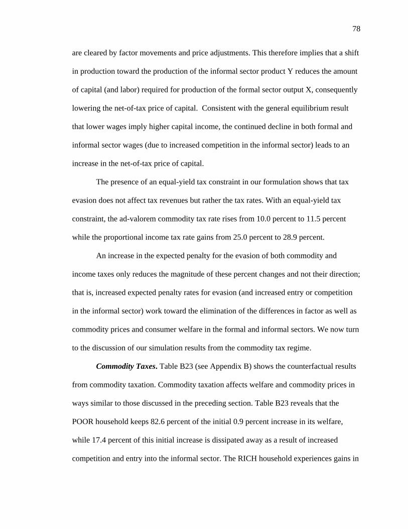
78

are cleared by factor movements and price adjustments. This therefore implies that a shift

in production toward the production of the informal sector product Y reduces the amount

of capital (and labor) required for production of the formal sector output X, consequently

lowering the net-of-tax price of capital. Consistent with the general equilibrium result

that lower wages imply higher capital income, the continued decline in both formal and

informal sector wages (due to increased competition in the informal sector) leads to an

increase in the net-of-tax price of capital.

The presence of an equal-yield tax constraint in our formulation shows that tax

evasion does not affect tax revenues but rather the tax rates. With an equal-yield tax

constraint, the ad-valorem commodity tax rate rises from 10.0 percent to 11.5 percent

while the proportional income tax rate gains from 25.0 percent to 28.9 percent.

An increase in the expected penalty for the evasion of both commodity and

income taxes only reduces the magnitude of these percent changes and not their direction;

that is, increased expected penalty rates for evasion (and increased entry or competition

in the informal sector) work toward the elimination of the differences in factor as well as

commodity prices and consumer welfare in the formal and informal sectors. We now turn

to the discussion of our simulation results from the commodity tax regime.

Commodity Taxes. Table B23 (see Appendix B) shows the counterfactual results

from commodity taxation. Commodity taxation affects welfare and commodity prices in

ways similar to those discussed in the preceding section. Table B23 reveals that the

POOR household keeps 82.6 percent of the initial 0.9 percent increase in its welfare,

while 17.4 percent of this initial increase is dissipated away as a result of increased

competition and entry into the informal sector. The RICH household experiences gains in

79

consumer welfare especially since the initial 0.3 percent fall in welfare reduces to -0.2

percent, representing a 36 percent increase in welfare for the RICH household. These

gains in welfare for the RICH household are due to increased competition and entry in

the informal sector.

Consistent with the findings in Table B22, Table B23 shows that the net-of-tax

wage for labor supplied by the POOR household declines constantly as the elasticity of

substitution between leisure and consumption (our measure of competition in the

informal sector) increases. As mentioned above, this results from the fact that an

increased tax rate in the formal sector increases the supply of evading labor, which

lowers wages in the informal sector. Stated differently, the higher tax rate makes evasion

more profitable to the POOR household at the margin, thereby leading to an increase in

the supply of informal sector labor, a fact that depress the net-of-tax wage for labor

supplied by the POOR household. However, Table B23 reveals that the net-of-tax wage

for labor supplied by the RICH household increases, albeit at a decreasing rate, with an

increase in the level of competition in the informal sector. These positive gains in the net-

of-tax wage for RICH household labor are possible if the direct effect of the higher tax

rate in the formal sector is to encourage formal sector workers to consume more leisure.

This reduces the supply of formal sector labor, and consequently leads to an increase in

the net-of-tax wage for the RICH household.40 A discussion of our simulation results

from the income tax regime follows.

40 Analogously, if the average remuneration of informal sector labor increases, the RICH household will have higher income by simply re-allocating some of her labor from the formal to the informal sector; if leisure is a normal good, then these two effects will combine to reduce the amount of formal sector labor supplied leading to an increase in the net-of-tax wage for RICH household labor. Section IV.2 discusses findings from our simulations that allow the RICH household to allocate some of her labor to the informal sector.

80

Income Taxes. Table B24 (see Appendix B) shows the counterfactual results

from income taxation. The effects of income taxation on commodity prices, factor

returns, and welfare for both POOR and RICH households are comparable to those

discussed in Tables B22 and B23. Table B24 reveals that the POOR household retains

81.5 percent of the initial 2.0 percent increase in its welfare, while 18.5 percent of this

initial gain in welfare is wiped away due to increased competition and entry into the

informal sector. The RICH consumers’ welfare initially falls by 0.5 percent, but increased

competition in the informal sector reduces this loss in the RICH households’ welfare to -

0.2 percent, which represents a 54.4 percent increase in welfare for the RICH household.

Consistent with our earlier findings, these results indicate that the POOR household

benefits only slightly and this benefit falls with increased entry into the informal sector.

Table B24 also indicates that the net-of-tax wage for labor supplied by the POOR

household declines continuously as more evaders set up shop in the informal sector (as

entry or competition increases in the informal sector). Additionally and also consistent

with the earlier findings, the net-of-tax wages for labor supplied by the RICH household

increase but at a decreasing rate. The initial increase in the net-of-tax wage accruing to

the RICH household can be explained by the fall in the amount of labor supplied by the

RICH household. RICH household labor responds to the increased tax rate by consuming

more leisure, consequently leading to a fall in the amount of labor supplied, a feature that

leads to an increase in the net-of-tax wage for RICH household labor. However, the

higher income tax rates (and increased entry into the informal sector) eventually lead to

an increase in the amount of labor supplied by the RICH household, consequently

reducing the initial gains in the net-of-tax wages to RICH household labor. As argued

81

earlier, the RICH household responds to higher income tax rates by supplying more labor

so as to mitigate the drop in income or purchasing power, which eventually lowers the

initial growth in the net-of- tax wage for RICH household labor.

To summarize, Tables B21-B24 show that the net-of-tax wage to informal sector

labor falls continuously in response to increased competition and increased expected

penalty rates in this sector. Formal sector net-of-tax wages increase initially, due to

increased consumption of leisure, but decline eventually as the level of competition and

entry increases in the informal sector. The ultimate decline in the formal sector net-of-tax

wages is attributed to an increased supply of labor in the formal sector. This is especially

true since formal sector labor responds to the increasing tax rates (due to the equal-yield

constraint) by supplying more labor to offset declining incomes or purchasing power.

Tables B21-B24 indicate that the POOR households’ post-evasion welfare is only 0.68-

2.43 percent higher than the post-tax welfare if it had fully complied with taxes. The

simulation results shown in Tables B21-B24 further reveal that the POOR household

keeps between 78.6-82.6 percent of this initial increase in welfare, while 17.4-21.4

percent of this initial gain is dissipated away as a result of increased competition and

entry in the informal sector. The RICH households’ welfare falls initially due to an

increase in the tax-inclusive price of the formal sector good X. However, the increased

supply of formal sector labor and the subsequent increase in the production of commodity

X lead to an increase in the commodity X-intensive RICH households’ welfare by 36.0-

96.9 percent. Thus, if changes in consumer welfare are interpreted as an overall measure

of the gains and/or losses from tax evasion, then the POOR household only benefits

82

slightly from tax evasion and this gain lessens with increased entry and competition in the

informal sector.

Partial Compliance in the Formal Sector and Tax Evasion in the Informal Sector

We also allow for the possibility of evasion in the formal sector. The RICH

household allocates her labor between the formal and informal sectors by comparing the

statutory tax rate with the expected penalty for evasion, respectively (or the relative

wages in these two sectors). All counterfactual results presented here incorporate an

equal-yield tax constraint in the formal sector and a labor-leisure choice in both formal

and informal sectors.

Commodity and income taxes. The counterfactual results are presented in Table

B25 in Appendix B. The effects on commodity prices, price of capital, and welfare for

both the POOR and RICH household mimic those shown in Table B22. However, Table

B25 reveals that, unlike in Table B22, the net-of-tax wage for RICH household labor falls

continually with increased entry into the informal sector. One possible explanation for

this finding is the shift of RICH household labor from the informal sector back to the

formal sector. Declining wages (due to increased supply of evading labor to the informal

sector) reduce the incentive to RICH household labor from working in the informal

sector, which feeds back positively on labor supply (and negatively on net-of-tax wages)

in the formal sector. The increase in formal sector labor supply leads to a reduction in

formal sector wages. Lower formal sector wages could also result from the income effect

of higher taxes due to the equal-yield tax constraint. The RICH household will supply

more labor (and enjoy less leisure) in the formal sector to lessen the effects of reduced

83

incomes, consequently leading to a drop in formal sector wages. Our simulation results

from the commodity tax regime reveal similar trends as discussed in the next section.

Commodity taxes. Unlike in Table B23, Table B26 (see Appendix B) indicates

that the net-of-tax wage for RICH household labor drops repeatedly with increased entry

into the informal sector. This therefore indicates that the increase in formal sector labor

(to provide a cushion against falling purchasing power of income) resulting from a

reduction in net-of-tax wages for RICH household labor more than offsets any other

effects such as increased consumption of leisure (due to a reduced relative price of

leisure, a result of higher equal-yield tax rates) that would reduce formal sector labor

supply. Other commodity and factor prices as well as welfare for both the POOR and

RICH households depict trends similar to those in Table B23. These findings are also

consistent with our simulations results from an income tax regime as the next section

reveals.

Income Taxes. Tables B24 and B27 (see Appendix B) indicate that allocation of

some of the RICH households’ labor to the informal sector does not alter the general

equilibrium effects on commodity and factor prices plus the POOR and RICH

households’ welfare in any significant way. In particular, the net-of-tax wage for POOR

household labor declines continuously with increased competition in the informal sector,

while the net-of-tax wage for the RICH household labor increases but at a decreasing

rate. The former is due to the increase in the supply of evading labor as entry and/or

competition increase in the informal sector, while the latter results from relocation of

RICH household labor from the informal sector back to the formal sector. This leads to

an increase in formal sector labor supply, consequently resulting in an eventual reduction

84

in the initial gains in the net-of-tax wage to RICH household labor. Additionally, Table

B27 reveals that the RICH household labor allocated to the informal sector starts

relocating back to the formal sector when the amount of labor supplied to the informal

sector is 5.3 percent over and above the pre-evasion levels.

Sensitivity Analysis

Since the choice of our parameters could have a significant influence on our

simulation results, we verify the consistency of our results by performing several

sensitivity analyses. The sensitivity analyses are based on SAMs shown in Tables B16-

B19 and the results are presented in Tables B28-B41 (see Appendix B). Overall, the

sensitivity results show that variations in the proportion of the POOR households’

endowment to that of the RICH household does not affect our simulation results in any

significant way. For instance, Table B28 reveals that the POOR households’ post-evasion

welfare is only 3.01 percent higher than the post-tax welfare if it had fully complied with

taxes. The simulation results further reveal that the POOR household keeps 77.1 percent

of this initial increase in welfare, while 22.9 percent of this initial gain is competed away

as a result of increased competition and entry into the informal sector. The RICH

households’ welfare initially falls by 0.5 percent, but increased competition in the

informal sector results in a 0.1 percent increase in the RICH households’ welfare,

representing a gain of 101.7 percent. The increase in the RICH households’ commodity

X-intensive welfare is attributed to a reduction in the tax-inclusive price of commodity X

as competition in the informal sector increases. Table B28 shows that the tax-inclusive

price of commodity X falls by 8.5 percent with increased competition in the informal

sector, while the commodity price of good Y increases by 10.3 percent. The POOR

85

households’ welfare is intensive in commodity Y, and as such, an increase in the

commodity price of good Y leads to a reduction in the POOR households’ welfare.

Further, increased competition in the informal sector leads to an increase in the amount of

labor supplied in the informal and formal sectors by 61.8 percent and 159.6 percent,

respectively, leading to a reduction in the net-of-tax wages by 15.1 percent and 140.7

percent, respectively. Therefore, if changes in consumer welfare are taken to represent an

overall measure of the gains and/or losses from tax evasion, then the POOR household

only benefits marginally from tax evasion and this advantage diminishes with increased

entry and competition in the informal sector.

Increasing the expected penalty rate for evasion only alters the size of these

changes and not their trend. Table B28 (see Appendix B) shows that with increased

expected penalty rates for evading consumption and income taxes, the initial increase in

the POOR households’ welfare is only 1.31 percent. Table B28 also reveals that the

POOR household keeps merely 75.6 percent of this initial increase in welfare, while 24.4

percent is competed away as the informal sector becomes increasingly competitive. The

RICH household experiences a 121.7 percent increase in welfare due to increased

competitiveness in the informal sector. Table B29 (see Appendix B) presents these

counterfactual results in detail. We now turn to a comprehensive discussion of the

counterfactual results.

Table B29 shows that with an elasticity of substitution equal to 2, and when ad-

valorem commodity tax is 0.1, the proportional income tax rate is 0.25, the expected

penalty rate on commodity taxes is 0.07, and when the expected penalty rate on income

taxes is 0.2, evasion of commodity and income taxes in the informal sector raises the

86

welfare of the POOR household by 3.01 percent but lowers the RICH household’s

welfare by 0.58 percent. This arises because an increase in the tax-inclusive price of

sector X output and a fall in the commodity price of sector Y output lowers the RICH

household’s X-intensive welfare and increases the POOR household’s Y-intensive

welfare, respectively. However, with increased entry or competition in the informal

sector (as measured by an increase in the elasticity of substitution between consumption

and leisure), the welfare of the POOR household increases only at an decreasing rate,

while the RICH household’s welfare posts reduced declines and eventually turns positive.

This is due to the declining rates at which sector X and sector Y commodity prices are

increasing and decreasing, respectively. The declining rate of increase in the net-of-tax

price of commodity X eventually leads to an increase in the commodity X-intensive-

RICH household welfare. On the other hand, a reduction in the rate at which the net-of-

tax price of commodity Y is falling consequently lowers the gains in the commodity-Y-

intensive-POOR household welfare.

Table B29 reveals that evasion of both commodity and income taxes in the

informal sector leads to an increase in the tax-inclusive price of commodity X and a

reduction in the commodity price of sector Y output. Particularly, the tax- inclusive price

of sector X output increases by 4.10 percent while the commodity price of sector Y

output by falls by 6.89 percent. These changes in commodity or consumer prices are due

to a shift toward sector Y production. The commodity price of sector Y output continues

to decline with increased entry and/or competition in the informal sector while the tax-

inclusive price of sector X output increases, albeit at a declining rate. Lower wages imply

higher capital income, which reduces the total supply of labor by the RICH household

87

causing a shift to the less labor-intensive production in the formal sector. This leads to an

increase in the production of sector X output, slightly offsetting the initial gain in the tax-

inclusive price of formal sector output X. Additionally, the net-of-tax wage rates for labor

supplied by the POOR and RICH households decline by 3.89 and 0.20 percent,

respectively.

These results arise from the fact that increased tax rates in the formal sector (as a

result of the equal-yield tax constraint) increase the supply of evading labor, which

lowers wages in the informal sector. Higher tax rates induce the RICH household to

supply more labor to mitigate the reduction in purchasing power of income, subsequently

reducing the net-of-tax wages to the RICH household. Further, as in the case of

commodity prices, the net-of-tax wages for both the POOR and RICH household labor

decline continuously with increased entry or competition in the informal sector. This

indicates therefore that tax evasion reduces the net-of-tax return to labor supplied by both

POOR and RICH households. The net-of-tax returns to capital for both POOR and RICH

households fall by 0.41 percent. The reduction in the net-of-tax price of capital follows

from the assumption that the supply of capital is fixed (and fixed production

technologies), while all markets are cleared by factor movements and price adjustments.

This therefore implies that a shift in production toward the production of the

informal sector product Y reduces the amount of capital (and labor) required for

production of the formal sector output X, consequently lowering the net-of-tax price of

capital. However, consistent with the general equilibrium result that lower wages imply

higher capital income, the continued decline in both formal and informal sector wages

due to increased competition in the informal sector, leads to an increase in the net-of-tax

88

price of capital. With an equal-yield tax constraint, the ad-valorem commodity tax rate

rises from 10.0 percent to 11.1 percent while the proportional income tax rate gains from

25.0 percent to 27.8 percent. An increase in the expected penalty for the evasion of both

commodity and income taxes only reduces the magnitude of these percent changes and

not their direction. In other words, an increase in the expected penalty for evasion and

increased entry or competition in the informal sector work toward the elimination of the

differences in factor as well as commodity prices and consumer welfare in the formal and

informal sectors.

To summarize, the sensitivity results shown in Tables B28-B34, where the POOR

households’ endowment is 25 percent of the RICH households’ endowment, are

consistent with the simulation results presented in Table B21-B27 where the POOR

households’ endowment is 33 percent of the RICH households’ endowment. Further, our

sensitivity results in Tables B35-B41, where the rectangular SAMs are constructed under

the assumption that the POOR households’ endowment is 50 percent of the RICH

households’ endowment, are also consistent with simulation results in Tables B21-B27

and in Tables B28-B34.

Conclusions, Policy Implications, and Suggestions for Further Research

The portfolio approach to tax evasion postulates that individuals weigh the probability of

getting caught and paying a penalty against the probability of being able to keep the

evaded income, subsequently leading to the conclusion that the individual evader benefits

by keeping the evaded income in its entirety. However, conclusions drawn from the

conventional portfolio approach regarding the incidence of tax evasion are quite

unsatisfactory because the portfolio approach ignores the fact that in numerous situations,

89

especially those in which the expected value is positive, tax evasion is comparable to a

tax advantage in the law. Consequently, it would be rational to expect replication and

competition, when possible, to work toward the elimination of this direct advantage. This

process of adjustment generally should take place through changes in the relative prices

of both commodities and factors of production. The portfolio approach affords tax

evasion incidence analysis only a partial equilibrium treatment and does not capture this

general equilibrium effect.

Our novel approach counters this drawback by utilizing a Computable General

Equilibrium (CGE) model to analyze the incidence of tax evasion in two broadly defined

sectors of the economy; the formal and informal sectors. This essay incorporates the

element of uncertainty in an individual’s decision to evade so as account for the

uncertainty of returns to the tax evader. We also allow for varying degrees of competition

or entry across sectors in the economy to examine how much of the tax advantage is

retained by the initial evaders and how much is shifted via factor and commodity price

changes.

The counterfactual experiments reveal that, though the post-evasion welfare of the

POOR or evading household is positive, it falls with increased competition in the

informal sector. The RICH (or compliant) household’s post-evasion welfare, while

negative, increases and eventually turns positive with increased competition in the

informal sector. The shift in production toward the informal sector output subsequently

leads to a fall in the consumer price of the informal sector output and to an increase in the

tax-inclusive price of formal sector output, while the increase in the supply of evading

labor reduces the net-of-tax wage for labor supplied by the POOR household.

90

Higher tax rates due to the equal-yield tax constraint have two distinct effects on

the net-of-tax wage for labor supplied by the RICH household. Higher tax rates change

the relative price of leisure, leading to increased consumption of leisure and subsequently

a reduction in the amount of labor supplied in the formal sector. This raises the net-of-tax

wage for the RICH household, albeit at a decreasing rate as the informal sector becomes

increasingly competitive. On the other hand, if the direct effect of the higher tax rates is

increased supply of formal sector labor (to offset the reduction in income due to the

higher taxes), the net-of-tax wage for RICH household labor declines. However, the

decline in the net-of-tax wage for RICH household labor in this latter scenario is just a

fraction of the decline in the net-of-tax wage for the POOR household labor. Consistent

with the general equilibrium result that lower wages imply higher capital income, the

continued decline in both formal and informal sector wages (as competition in the

informal sector increases) leads to an increase in the net-of-tax price of capital. Further,

our results verify the notion that tax evasion does not affect government revenues but

rather tax rates, particularly in the presence of an equal-yield tax constraint.

Our results indicate that the tax evader does not benefit exclusively and that this

advantage diminishes with an increase in both the expected penalty associated with tax

evasion and degree of competition or entry in the informal sector. In particular, our

simulation results reveal that the POOR households’ post-evasion welfare is only 0.6-3.4

percent higher than the post-tax welfare if it had fully complied with taxes. The

simulation results further show that the POOR household retains between 77.1-83.2

percent of this initial increase in welfare, while 16.8-22.9 percent of this initial gain is

competed away as a result of increased competition and entry into the informal sector.

91

The RICH households’ welfare increases by 58.8-101.7 percent with increased

competition and entry in the informal sector. Therefore, if we construe the changes in

consumer welfare as an overall indicator of the gains and/or losses from tax evasion, then

the POOR household only benefits marginally from tax evasion and this advantage

shrinks with increased entry and competition in the informal sector. Additionally, both

the net-of-tax wage for informal sector labor and the consumer price of the informal

sector output decline continually.

This consequently indicates that the gains from evasion are shifted from the

evaders to the consumers of their output via lower prices. This essay therefore

demonstrates that the general equilibrium effects work to eliminate the incentive for

workers to enter the underground or informal sector beyond some margin, via relative

price and productivity changes. As more workers set up shop in the underground sector,

their production pushes down the relative price of the informal sector output and

consequently the per-unit or hourly returns of working in the informal sector. The

movement of workers between the sectors may also change the relative productivity of

workers in each sector. In equilibrium, therefore, the marginal entrant to the informal

sector has his/her gains from evading taxes offset by the relative price and productivity

effects plus his real (and any “psychic”) costs of operating in the underground sector.

Our findings have several implications for tax policy in particular and government

policy in general. For instance, government redistribution programs that ignore informal

market participants may worsen actual income distribution especially if such programs

are implemented with the belief that the informal sector is already benefiting

(exclusively) from not paying taxes. A case in point here is the federal earned income tax

92

credit (EITC) in the United States, whose original intent was to offset the FICA (social

security) payroll tax for low-income workers. Since its introduction in 1975, the EITC

has expanded beyond the purpose of offsetting the FICA tax and now provides actual

cash assistance to low-income working families. The EITC provides a tax credit equal to

a certain percentage of earned income (wages, salaries, tips, and self-employment) up to a

limit41. Further, the EITC is a fully refundable tax credit, implying that if a taxpayer is

eligible for the EITC and has no taxable income, the government gives a tax refund for

the credit nevertheless. In cases where the credit exceeds the taxpayer’s tax liability, he

or she receives the amount of the credit that exceeds the tax liability as a refund. To the

extent that informal sector workers (tax evaders) do not file tax returns, the otherwise

eligible informal sector workers are thus not accounted for in this government

redistribution program. Our findings therefore indicate that any effective government

redistribution program ought to account for the fact that evaded taxes are capitalized in

the relative prices of both commodities and factors of production, in which case the tax

evader does not benefit exclusively.

Another tax policy implication concerns tax administration and enforcement.

Given that the beneficiaries from tax evasion are not the tax evaders themselves but

rather the consumers of the goods and services sold by the tax evaders, tax authorities

could find it more feasible and even desirable to tax those services more heavily to

compensate for the evaded taxes.

Finally, it is noteworthy to point out that the strength of static CGE models lies in

their ability to emphasize the interaction among different industries and/or sectors of the

41 For instance, a taxpayer with two children gets a tax credit of 40 cents on every $1 of earned income up to a limit of $9,540 in 1999, (Bruce, 2001).

93

economy. Since they stress the impact of reallocation of resources across sectors of an

economy, these models are excellent tools for identifying both winners and losers under a

policy change. However, these models fail to capture the effect of a policy change on the

dynamic facets of an economy. Such a drawback could be remedied in part via the

incorporation of a steady-state formulation as discussed below.

Our static CGE model can be extended in several directions. First, precise

amounts of informal sector labor together with service sectors that operate only in the

informal sector need to be identified and included in the production processes. The social

accounting matrices used in this essay are constructed based on the assumptions we make

about the structure and size of the both the formal and informal sectors as well as the

RICH and POOR households. Traditionally, informal sector economic activity includes

small-scale farming, street marketing plus other small-volume activities. A typical

modeling exercise therefore is to identify this portion of the economy as the “informal

sector” (Light, 2004). This represents a portion of employment and output that is not

subject to taxation, either legally or illegally. However, identification of the nature and

size of these activities requires a survey of both individuals and firms.

Unfortunately, to the best of our knowledge, such survey data or even indicators

related to the scope of informal sector activities are not readily available. If such

information was available, the precise amounts of informal labor would be included in

the production process, enabling us to identify the extent to which changes in labor taxes

encourage workers to substitute informal for formal sector activities. Additionally, the

precise magnitude of service sectors that operate exclusively in informal economy would

also be included.

94

The second extension of our static CGE model would entail the modeling of

dynamic phenomena in the economy. As mentioned above, our static model fails to

capture the intertemporal aspects of an economy, something that can be remedied by

incorporating steady-state aspects in the CGE model presented earlier. One way of

modeling these steady-state features is via the introduction of endogenous supply of

capital. Given that intertemporal models focus on capital-stock accumulation, the labor-

leisure choice is not relevant in such models and may not be considered here. The steady-

state model allows capital and investment to adjust to changes in policy directives,

consistent with a long-run analysis. The long-run equilibrium condition links the cost of

capital with the return to capital in the following way:

kinv rp = k⊥

The capital scale factor k equilibrates this investment arbitrage condition to ensure that

the cost of capital always equals the return to capital. When the return to capital rises

relative to the price or cost of investment: invk pr f , k increases to scale up investment to

reflect this arbitrage condition. Therefore, in the steady-state equilibrium, k adjusts

investment so that the cost of capital is consistent with the return to capital (Light, 2004).

It is important to note however that, since we choose the model parameters for the steady

state, this formulation is a little less flexible than allowing a full dynamic model.

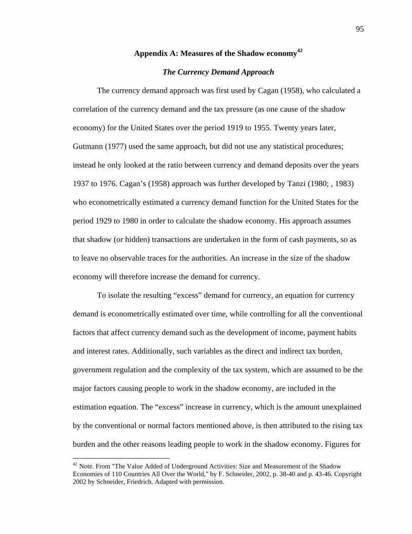
95

Appendix A: Measures of the Shadow economy42

The Currency Demand Approach

The currency demand approach was first used by Cagan (1958), who calculated a

correlation of the currency demand and the tax pressure (as one cause of the shadow

economy) for the United States over the period 1919 to 1955. Twenty years later,

Gutmann (1977) used the same approach, but did not use any statistical procedures;

instead he only looked at the ratio between currency and demand deposits over the years

1937 to 1976. Cagan’s (1958) approach was further developed by Tanzi (1980; , 1983)

who econometrically estimated a currency demand function for the United States for the

period 1929 to 1980 in order to calculate the shadow economy. His approach assumes

that shadow (or hidden) transactions are undertaken in the form of cash payments, so as

to leave no observable traces for the authorities. An increase in the size of the shadow

economy will therefore increase the demand for currency.

To isolate the resulting “excess” demand for currency, an equation for currency

demand is econometrically estimated over time, while controlling for all the conventional

factors that affect currency demand such as the development of income, payment habits

and interest rates. Additionally, such variables as the direct and indirect tax burden,

government regulation and the complexity of the tax system, which are assumed to be the

major factors causing people to work in the shadow economy, are included in the

estimation equation. The “excess” increase in currency, which is the amount unexplained

by the conventional or normal factors mentioned above, is then attributed to the rising tax

burden and the other reasons leading people to work in the shadow economy. Figures for

42 Note. From "The Value Added of Underground Activities: Size and Measurement of the Shadow Economies of 110 Countries All Over the World," by F. Schneider, 2002, p. 38-40 and p. 43-46. Copyright 2002 by Schneider, Friedrich. Adapted with permission.

96

the size and development of the shadow economy can be calculated in a first step by

comparing the difference between the development of currency when the direct and

indirect tax burden (and government regulations) are held at their lowest value, and the

development of currency with the current (much higher) burden of taxation and

government regulations. Assuming in a second step the same income velocity for

currency used in the shadow economy as for legal M1 in the official economy, the size of

the shadow can be computed and compared to the official GDP.

The currency demand approach is one of the most commonly used approaches. It

has been applied to many OECD countries, but has nevertheless been criticized on

various grounds. First, not all transactions in the shadow economy are paid in cash.

Isachsen and Strom (1985) used the survey method to find out that in Norway, in 1980,

roughly 80 percent of all transactions in the hidden sector were paid in cash. The size of

the total shadow economy (including barter) may thus be even larger than previously

estimated. Second, most studies consider only one particular factor, the tax burden, as a

cause of the shadow economy. But others (such as the impact of regulation, taxpayers’

attitudes toward the state, “tax morality” and so on) are not considered, because reliable

data for most countries is not available. If, as seems likely, these other factors also have

an impact on the extent of the hidden economy, its size might again be bigger than

reported in most studies. Third, a further weakness of this approach, at least when applied

to the United States, is discussed by Garcia (1978), Park (1979), and Feige (1996), who

point out that increases in currency demand deposits are due largely to a slowdown in

demand deposits rather than to an increase in currency caused by activities in the shadow

economy. Fourth, Blades (1982) and Feige (1986; , 1996), criticize Tanzi’s studies on the

97

grounds that the U.S. dollar is used as an international currency. They argue that Tanzi

should have considered (and even controlled for) the US dollars, which are used as an

international currency and held in cash abroad. Moreover, Frey and Pommerehne (1984)

and Thomas (1986; , 1999; , 1992) claim that Tanzi’s parameter estimates are not very

stable. Fifth, another weakness of this procedure, in most studies, is the assumption of the

same velocity of money in both types of economies. As Hill and Kabir (1996) for Canada

and Klovland (1984) for the Scandinavian countries argue, there is already considerable

uncertainty about the velocity of money in the official economy; the velocity of money in

the hidden sector is even more difficult to estimate. Without knowledge about the

velocity of currency in the shadow economy, one has to accept the assumption of “equal”

money velocity in both sectors. Finally, the assumption of no shadow economy in a base

year is open to criticism. Relaxing this assumption would again imply an upward

adjustment of the figures attained in the bulk of the studies already undertaken.

The Model Approach

The currency demand approach is designed to estimate the size and development

of the shadow economy but considers just one indicator that “must” capture all effects of

the shadow economy. However, it is obvious that its effects show up simultaneously in

the production, labor, and money markets. An even more important critique is that the

causes which determine the size of the hidden economy are taken into account only in

some of the monetary approach studies which usually consider one cause, the burden of

taxation. The model approach explicitly considers multiple causes leading to the

existence and growth as well as the multiple effects of the shadow economy over time.

The empirical method used is quite different. It is based on the statistical theory of

98

unobserved variables, which considers multiple causes and multiple indicators of the

phenomenon to be measured.

For the estimation, a factor-analytic approach is used to measure the hidden

economy as an unobserved variable over time. The unknown coefficients are estimated in

a set of structural equations within which the “unobserved” variable cannot be measured

directly. The DYMIMIC (dynamic multiple-indicators multiple-causes) model consists in

general of two parts; the measurement model links the unobserved variables to observed

indicators while the structural equations model specifies causal relationships among the

unobserved variables. In this case, there is one unobserved variable, the size of the

shadow economy. It is assumed to be influenced by a set of indicators, thus capturing the

structural dependence of the shadow economy on variables that may be useful in

predicting its movement and size in the future. The interaction over time between the

causes Zit (i = 1, 2, ..., k), the size of the shadow economy Xt, and the indicators Yjt (j = 1,

2, ..., p) is shown in the Figure A1 below.43

Figure A1: Development of the Shadow Economy

Causes Xt-1 Indicators

Z1t Development of the Shadow Y1t . Economy over time . . Xt . . . Zkt Ypt

43 Note. From "The Value Added of Underground Activities: Size and Measurement of the Shadow Economies of 110 Countries All Over the World," by F. Schneider, 2002, p. 44. Copyright 2002 by Schneider, Friedrich. Reprinted with permission.

99

There is a large body of literature on the possible causes and indicators of the

shadow economy, in which the following three types of causes are distinguished. First,

the burden of direct and indirect taxation, both actual and perceived: a rising burden of

taxation provides a strong incentive to work in the shadow economy. Second, the burden

of regulation as proxy for all other state activities: it is assumed that increases in the

burden of regulation gives a strong incentive to enter the shadow economy. Finally, the

“tax morality” (citizens’ attitudes toward the state), which describes the readiness of

individuals (at least partly) to leave their official occupations and enter the shadow

economy: it is assumed that a declining tax morality tends to increase the size of the

shadow economy. A change in the size of the shadow economy may be reflected in the

following indicators. First, development of monetary indicators: if activities in the

shadow economy rise, additional monetary transactions are required. Second,

development of the labor market: increasing participation of workers in the hidden sector

results in a decrease in participation in the official economy. Similarly, increased

activities in the hidden sector may be expected to be reflected in shorter working hours in

the official economy. Finally, development of the production market: an increase in the

shadow economy means that inputs (especially labor) move out of the official economy

(at least partly); this displacement might have a depressing effect on the official growth

rate of the economy.

The most recent use of the model approach has been undertaken by Giles (1999a;

, 1999b) and by Giles, Tedds, and Gupsa (1999), and Giles and Tedds (2002). They

basically estimate a comprehensive (dynamic) MIMIC model to get a time series index of

the hidden/measured output of New Zealand or Canada, and then estimate a separate

100

“cash-demand model” to obtain a benchmark for converting this index into percentage

units. Unlike earlier empirical studies of the hidden economy, they pay proper attention

to the non-stationary, and possible co-integration of time serious data in both models.

Again this DYMIMIC model treats hidden output as a latent variable, and uses several

(measurable) causal variables and indicator variables. The former include measures of the

average and marginal tax rates, inflation, real income and the degree of regulation in the

economy. The latter include changes in the (male) labor force participation rate and in the

cash/money supply ratio. In their cash-demand equation they allow for different

velocities of currency circulation in the hidden and recorded economies.

The cash-demand equation here is used not as an input to determine the variation

in the hidden economy over time, but rather to obtain the long-run average value of

hidden/measured output, so that the index for this ratio predicted by the DYMIMIC

model can be used to calculate level and percentage units of the shadow economy. Giles

latest combination of the currency demand and DYMIMIC approach clearly shows that

some progress in the estimation technique of the shadow economy has been achieved and

a number of critical limitations have been overcome.

101

Appendix B: Tables

Table B1. Descriptive Statistics: East African Countries

Variable Observations Mean Standard Deviation

Minimum Maximum

SDWGDP (Shadow Economy, % of GDP)

33 45.13 10.68 32.00 62.30

CORRUPTION 33 2.22 0.22 1.90 2.70 GDP Per Capita (U.S$) 33 276.09 71.01 176.23 354.82 Agriculture income (% of GDP) 33 38.40 10.40 16.40 51.50 Mining income (% of GDP) 33 0.32 0.12 0.21 0.60 Openness(value of exports & Imports, % of GDP)

33 48.10 14.50 22.20 70.50

Export ratio (value of exports, % of GDP)

33 7.20 2.30 3.80 12.40

Import ratio (value of imports, % of GDP)

33 11.10 3.30 6.60 19.50

Exchange Rate (LCU per US$) 33 547.97 479.63 22.92 1644.48 Real GDP (US$ Billions) 33 21.30 9.60 11.20 37.40 Real GNP (US$ Billions) 33 20.00 9.50 9.60 39.10 POPULATION (Millions) 33 25.30 5.00 16.30 33.70

TAX RATIOS Total Tax ratio (Total taxes, % of GDP)

33 6.2 1.9 2.9 10.9

Income taxes (% of GDP) 33 1.8 1.0 0.4 4.4 Consumption taxes (VAT + Sales + Excises,% of GDP)

33 2.8 1.0 1.0 4.8

International taxes (export and import taxes, % of GDP)

33 1.3 0.6 0.3 2.7

Value Added Taxes (VAT, % of GDP) 33 1.3 1.1 0 3.5 Sales taxes (% of GDP) 33 0.4 0.6 0 1.9 Excise taxes (% of GDP) 33 1.1 0.4 0.3 2.0 Other taxes (% of GDP) 33 0.36 0.34 0 1.4

102

Table B2. Descriptive Statistics: OECD Countries

aIncome taxes refer to the sum of personal income taxes, corporate income taxes, social security

contributions, and taxes on payroll and workforce.

Variable Observations Mean Standard Deviation

Minimum Maximum

SDWGDP (Shadow Economy in %of GDP) 126 15.6 5.5 6.7 29 POPN (Population, millions) 105 39.1 59 3.4 274 CRPT (Corruption Index; higher value indicates lower corruption)

126 7.732 1.627 2.99 10.00

Real GDP ($ Billions) 126 1,120 1,910 50.8 9,010 Real GNP ($ Billions) 126 1,110 1,910 46 9,000 GDPC (GDP per capita, in constant U.S.$)

126 25338.920 9049.661 9710.45 46183.19

Agriculture income (% of GDP) 126 3.6 2.1 1.0 10.7 Openness(value of exports & Imports, % of GDP)

126 70.9 34.4 17.9 186.0

Mining income (% of GDP) 126 4.5 7.7 0.1 30.2 Export ratio (value of exports, % of GDP)

126 36.6 20.9 8.5 95.5

Import ratio (value of imports, % of GDP)

126 35.0 17.7 6.6 96.2

TAX RATIOS Total Tax ratio (Total taxes, % of GDP)

126 25.1 7.1 7.4 45.0

Income taxesa (% of GDP) 126 12.9 4.9 3.5 27.1 Consumption taxes (VAT + Sales + Excises, % of GDP)

126 8.6 3.1 0.0 13.8

Property Taxes (% of GDP) 126 1.8 1.0 0.4 4.7 International taxes (export and import taxes, % of GDP)

126 0.2 0.2 0 1.0

Value Added Taxes (VAT, % of GDP)

126 5.4 2.7 0 10.0

Sales taxes (% of GDP) 126 0.4 0.9 0 3.0 Excise taxes (% of GDP) 126 2.8 1.2 0 5.5 Other taxes (% of GDP) 126 1.6 0.9 0 3.5

103

Table B3. Simple Correlations: East African Countries yg yi yc yn yv ys ye sgdp crpt gdpc agric eratio iratio yi 0.9 yc 0.7 0.6 yn 0.4 0.3 -0.2 yv 0.6 0.6 0.9 -0.2 ys -0.2 -0.3 -0.6 0.5 -0.8 ye 0.3 0.2 0.7 -0.5 0.6 -0.6 sgdp 0.1 -0.1 -0.2 0.4 -0.3 0.5 -0.3 crpt -0.1 -0.3 -0.1 0.0 -0.1 0.2 -0.1 0.3 gdpc -0.1 0.1 0.3 -0.6 0.4 -0.6 0.5 -0.9 -0.3 agric -0.3 -0.5 -0.5 0.3 -0.6 0.6 -0.5 0.7 0.5 -0.7 eratio 0.7 0.8 0.6 0.0 0.7 -0.4 0.3 -0.2 -0.2 0.2 -0.5 iratio 0.4 0.2 0.0 0.4 -0.2 0.5 -0.2 0.8 0.1 -0.7 0.3 0.2 ming -0.5 -0.6 -0.2 -0.4 -0.2 -0.1 0.1 0.2 0.0 0.1 0.2 -0.4 0.1

yg Total Tax ratio yi Income taxes (% of GDP) yc Consumption taxes (VAT + Sales + Excises, % of GDP) yn International taxes (export and import taxes, % of GDP) yv Value Added Taxes (% of GDP) ys Sales taxes (% of GDP) ye Excise taxes (% of GDP) sgdp Shadow Economy, % of GDP crpt Corruption gdpc GDP Per Capita (U.S$) agric Agriculture income (% of GDP) eratio Export ratio (value of exports, % of GDP) iratio Import ratio (value of imports, % of GDP) ming Mining income (% of GDP)

104

Table B4. Simple Correlations: OECD Countries

yg yi yc yw yn yv ys ye sgdp crpt gdpc agric open ming eratio yi 0.9 yc 0.6 0.3 yw 0.3 0.3 -

0.2

yn 0.2 0.2 - 0.1

0.2

yv 0.5 0.2 0.9 - 0.4

- 0.2

ys 0.1 0.2 - 0.4

0.6 0.4 - 0.7

ye 0.6 0.4 0.8 - 0.1

- 0.1

0.6 - 0.3

sgdp 0.2 0.0 0.5 - 0.3

- 0.3

0.4 - 0.3

0.4

crpt 0.5 0.6 0.1 0.2 0.2 0.0 0.2 0.2 - 0.5

gdpc - 0.2

0.1 - 0.4

- 0.1

- 0.3

- 0.3

0.0 - 0.3

- 0.4

0.3

agric 0.1 - 0.1

0.3 - 0.2

0.3 0.3 - 0.1

0.2 0.3 - 0.2

- 0.6

open 0.2 0.1 0.3 - 0.2

- 0.1

0.3 - 0.2

0.2 0.1 0.2 - 0.0

- 0.0

ming 0.0 - 0.1

0.2 - 0.2

0.1 0.1 - 0.1

0.4 0.1 0.0 - 0.3

0.2 0.4

eratio 0.2 0.2 0.2 - 0.2

- 0.2

0.2 - 0.2

0.2 0.1 0.2 0.1 - 0.1

0.9 0.5

iratio 0.2 0.1 0.3 - 0.2

- 0.2

0.3 - 0.2

0.2 0.2 0.1 - 0.1

0.0 0.9 0.5 0.9

yg Total Tax ratio (Total taxes as % of GDP) yi Income taxes (% of GDP) yc Consumption taxes (VAT + Sales + Excises, % of GDP) yw Property taxes (% of GDP) yn International taxes (export and import taxes, % of GDP) yv Value Added Taxes (% of GDP) ys Sales taxes (% of GDP) ye Excise taxes (% of GDP) sgdp Shadow Economy, % of GDP crpt Corruption gdpc GDP Per Capita (U.S$) agric Agriculture income (% of GDP) eratio Export ratio (value of exports, % of GDP) iratio Import ratio (value of imports, % of GDP) ming Mining income (% of GDP)

105

Table B5. Tax Burden and the Size of the Shadow Economy in East African Countries

% of GDP Country

Year

Direct Taxes

Indirect Taxes

Customs & Import duties

Overall Tax burden

Shadow economy

1991/92 0.9 2.4 3 6.3 38.4

1992/93 1.1 2.6 3.4 7.1 38.8

1993/94 1.3 3.3 3.7 8.3 39.2

1994/95 1.6 4.1 3.6 9.3 40.1

1995/96 1.5 7.1 1.3 9.9 40.7

1996/97 1.6 8.1 1.1 10.8 41.2

1997/98 1.8 8.4 1.1 11.3 42.1

1998/99 1.9 8.8 1.0 11.7 42.6

1999/00 2.1 8.4 1.1 11.7 43.1

2000/01 2.1 8.0 1.1 11.3 43.0

Uganda

2001/02 2.3 8.5 1.0 11.8 43.1

1991/92 7 10.4 2.1 19.0 32.1

1992/93 6.7 10 2.4 19.1 33.4

1993/94 10 11 4 25.0 37.3

1994/95 10.1 10.5 4.3 24.9 37.1

1995/96 9.9 10.7 4.4 25.0 37.2

1996/97 8.6 9.6 4 22.2 35.9

1997/98 8.5 9.9 3.7 22.1 35.6

1998/99 7.7 9.7 4 21.3 34.9

1999/00 7.1 9.2 3.7 20.0 34.3

2000/01 6.6 9.4 3.4 19.4 34.0

Kenya

2001/02 6.1 9.1 2.4 17.6 32.0

1991/92 3.3 4.7 3.1 11.1 62.3

1992/93 2.9 3 2 7.9 58.0

1993/94 2.9 3.5 2.5 8.9 58.2

1994/95 3.3 2.7 3.4 10.4 60.5

1995/96 3.3 3.1 3.6 10.0 59.8

1996/97 3.2 3.3 4.1 10.6 60.2

1997/98 3 4.7 1.7 9.4 59.4

1998/99 2.7 4.9 1.5 9.1 58.6

1999/00 3 4.6 1.3 8.9 58.3

2000/01 2.5 5.9 1.2 9.6 58.9

Tanzania

2001/02 2.7 6.2 1 9.9 59.1

106

Table B6. The Size of the Shadow Economy in OECD Countries

Size of the Shadow Economy (in % of GDP) using the Currency Demand Method OECD-Countries Average

1989/90 Average 1991/92

Average 1994/95

Average 1997/98

Average 1999/2000

Average 2001/20021)

1. Australia 10.1 13.0 13.5 14.0 14.3 14.1 2. Belgium 19.3 20.8 21.5 22.5 22.2 22.0 3. Canada 12.8 13.5 14.8 16.2 16.0 15.8 4. Denmark 10.8 15.0 17.8 18.3 18.0 17.9 5. Germany 11.8 12.5 13.5 14.9 16.0 16.3 6. Finland 13.4 16.1 18.2 18.9 18.1 18.0 7. France 9.0 13.8 14.5 14.9 15.2 15.0 8. Greece 22.6 24.9 28.6 29.0 28.7 28.5 9. Great Britain 9.6 11.2 12.5 13.0 12.7 12.5 10. Ireland 11.0 14.2 15.4 16.2 15.9 15.7 11. Italy 22.8 24.0 26.0 27.3 27.1 27.0 12. Japan 8.8 9.5 10.6 11.1 11.2 11.1 13. Netherlands 11.9 12.7 13.7 13.5 13.1 13.0 14. New Zealand2) 9.2 9.0 11.3 11.9 12.8 12.6 15. Norway 14.8 16.7 18.2 19.6 19.1 19.0 16. Austria 6.9 7.1 8.6 9.0 9.8 10.6 17. Portugal 15.9 17.2 22.1 23.1 22.7 22.5 18. Sweden 15.8 17.0 19.5 19.9 19.2 19.1 19. Switzerland 6.7 6.9 7.8 8.1 8.6 9.4 20. Spain 3) 16.1 17.3 22.4 23.1 22.7 22.5 21. USA 6.7 8.2 8.8 8.9 8.7 8.7 Unweighted Average over 21 OECD countries

13.2 14.3 15.7 16.7 16.8 16.7

Note. From "The Value Added of Underground Activities: Size and Measurement of the Shadow

Economies of 110 Countries All Over the World," by F. Schneider, 2002, p. 21. Copyright 2002 by

Schneider, Friedrich. Reprinted with permission.

The DYMIMIC and Currency demand approaches were used to calculate the Shares of the Shadow

economy for the East African and OECD countries, respectively (Schneider, 2002; Schneider & Enste,

2000):

1) Preliminary values.

2) The figures are calculated using the MIMIC-method and Currency demand approach. Source: Giles

(1999b).

3) The figures have been calculated for 1989/90, 1990/93 and 1994/95 from Mauleon (1998) and for

1997/98 and 1999 figures are from Schneider (2002).

107

Table B7. First Stage Least Squares Estimates (OECD and East African Countries)

OECD East Africa Dependent variable: Tax evasion Constant 12.902 18.690 Agriculture(% of GDP)

0.747*** (0.001)

0.689*** (0.000)

Corruption -1.634*** (0.000)

2.253 (0.401)

Mining 0.348** (0.022)

3.646*** (0.000)

GDPC -0.214*** (0.000)

-1.751*** (0.000)

Export ratio 0.045** (0.017)

0.778*** (0.007)

Trend 0.983*** (0.000)

-0.019 (0.933)

R-squared 0.497 0.448 Durbin-Watson 1.909 2.218 Observations 126 33

Note. P-values in parenthesis.

*,**,*** denote significance at 10%, 5% and 1%, respectively.

108

Table B8. OLS and GMM Estimates with no Fixed Effects (OECD Countries)

OLS OLS GMM OLS GMM OLS GMM OLS GMM Tax ratio Income Consumption Property International trade

Constant 51.059

38.068

38.068

4.447

4.447

5.527

5.527

0.169

0.169

Tax evasion

-1.351*** (0.008)

-1.320*** (0.000)

-1.320*** (0.000)

0.216 (0.278)

0.216 (0.264)

-0.243*** (0.000)

-0.243*** (0.000)

0.010 (0.410)

0.010 (0.396)

Corruption

1.144*** (0.008)

0.654** (0.038)

0.654** (0.032)

0.380** (0.025)

0.380** (0.021)

0.194*** (0.001)

0.194*** (0.000)

0.043*** (0.000)

0.043*** (0.000)

Mining

0.128 (0.611)

-0.110 (0.553)

-0.110 (0.541)

0.178* (0.075)

0.178* (0.067)

0.006 (0.859)

0.006 (0.854)

0.012** (0.048)

0.012** (0.042)

GDP per capita -0.293*** (0.002)

-0.067 (0.314)

-0.067 (0.300)

-0.137*** (0.000)

-0.137*** (0.000)

-0.046*** (0.000)

-0.046*** (0.000)

-0.007*** (0.001)

-0.007*** 0.000)

Export ratio

0.075** (0.017)

0.044* (0.054)

0.044* (0.047)

0.029** (0.018)

0.029** (0.015)

-0.013*** (0.001)

-0.013*** (0.000)

-0.001 (0.203)

-0.001 (0.189)

Trend

-0.109 (0.771)

-0.178 (0.517)

-0.178 (0.504)

-0.004 (0.981)

-0.004 (0.980)

0.065 (0.186)

0.065 (0.174)

-0.060*** (0.000)

-0.060*** (0.000)

R-squared 0.185

0.190

0.190

0.282

0.282

0.225

0.225

0.484 0.484

Observations 126 126 126 126 126 126 126 126 126 Note. P-values in parenthesis.

*,**,*** denote significance at 10%, 5% and 1%, respectively.

109

Table B9. OLS and GMM Estimates with no Fixed Effects (East African Countries)

OLS OLS GMM OLS GMM OLS GMM Tax ratio Income Consumption International trade

Constant 13.951

6.462

6.462

0.039

0.039

5.088

5.088

Tax evasion

-0.159** (0.032)

-0.094*** (0.002)

-0.094*** (0.000)

-0.034 (0.530)

-0.034 (0.497)

-0.004 (0.887)

-0.004 (0.872)

Corruption

0.607 (0.565)

0.075 (0.857)

0.075 (0.839)

0.960 (0.241)

0.960 (0.188)

-0.583 (0.179)

-0.583 (0.132)

GDP per capita -1.641*** (0.002)

-0.606*** (0.004)

-0.606*** (0.001)

0.034 (0.927)

0.034 (0.918)

-0.534** (0.012)

-0.534*** (0.005)

Mining

-0.016 (0.995)

-0.214 (0.825)

-0.214 (0.803)

0.350 (0.852)

0.350 (0.833)

-1.574 (0.120)

-1.574* (0.081)

Export ratio

0.508*** (0.000)

0.249*** (0.000)

0.249*** (0.000)

0.253*** (0.004)

0.253*** (0.001)

-0.008 (0.854)

-0.008 (0.835)

Trend

-0.180** (0.052)

-0.110*** (0.004)

-0.110*** (0.001)

0.022 (0.748)

0.022 (0.717)

-0.054 (0.143)

-0.054* (0.100)

R-squared 0.750

0.852

0.852

0.480

0.480

0.609

0.609

Observations 33 33 33 33 33 33 33

Note. P-values in parenthesis.

*,**,*** denote significance at 10%, 5% and 1%, respectively.

110

Table B10. OLS and GMM Estimates with Fixed Effects (OECD Countries)

OLS OLS GMM OLS GMM OLS GMM OLS GMM Tax ratio Income Consumption Property International trade

Constant -0.034

-0.081

-0.081

-0.004

-0.004

0.056

0.056

-0.006

-0.006

Tax evasion

-1.692*** (0.003)

-1.597*** (0.000)

-1.597*** (0.000)

0.129 (0.561)

0.129 (0.549)

-0.247*** (0.001)

-0.247*** (0.001)

0.022 (0.195)

0.022 (0.182)

Corruption

1.034** (0.015)

0.464 (0.148)

0.464 (0.136)

0.304* (0.071)

0.304** (0.063)

0.223*** (0.000)

0.223*** (0.000)

0.042*** (0.000)

0.042*** (0.000)

Mining

0.137 (0.568)

-0.102 (0.577)

-0.102 (0.566)

0.208** (0.032)

0.208** (0.027)

0.023 (0.484)

0.023 (0.470)

0.008 (0.146)

0.008 (0.134)

GDP per capita -0.228*** (0.009)

-0.043 (0.515)

-0.043 (0.502)

-0.128*** (0.000)

-0.128*** (0.000)

-0.050*** (0.000)

-0.050*** (0.000)

-0.006*** (0.002)

-0.006*** (0.001)

Export ratio

0.065** (0.027)

0.047** (0.036)

0.047** (0.031)

0.033*** (0.005)

0.033*** (0.004)

-0.013*** (0.001)

-0.013*** (0.000)

-0.001** (0.050)

-0.001** (0.043)

Trend

0.010 (0.976)

0.023 (0.924)

0.023 (0.921)

0.001 (0.994)

0.001 (0.993)

-0.016 (0.709)

-0.016 (0.700)

0.002 (0.829)

0.002 (0.824)

R-squared 0.175

0.202

0.202

0.267

0.267

0.236

0.236

0.288

0.288

Observations 126 126 126 126 126 126 126 126 126 Note. P-values in parenthesis.

*,**,*** denote significance at 10%, 5% and 1%, respectively.

111

Table B11. OLS and GMM Estimates with Fixed Effects (East African Countries)

OLS OLS GMM OLS GMM OLS GMM Tax ratio Income Consumption International trade

Constant 0.267

0.117

0.117

0.061

0.061

0.063

0.063

Tax evasion

-0.052 (0.483)

-0.035 (0.220)

-0.035 (0.168)

-0.005 (0.928)

-0.005 (0.918)

0.006 (0.816)

0.006 (0.793)

Corruption

0.593 (0.610)

0.057 (0.897)

0.057 (0.884)

1.058 (0.223)

1.058 (0.171)

-0.645 (0.141)

-0.645* (0.099)

GDP per capita -0.174*** (0.004)

-0.067*** (0.004)

-0.067*** (0.001)

-0.004 (0.919)

-0.004 (0.909)

-0.049** (0.024)

-0.049*** (0.011)

Mining

0.306 (0.908)

0.115 (0.909)

0.115 (0.897)

0.785 (0.688)

0.785 (0.650)

-1.880* (0.063)

-1.880** (0.037)

Export ratio

0.180*** (0.001)

0.095*** (0.000)

0.095*** (0.000)

0.079** (0.027)

0.079*** (0.013)

0.002 (0.901)

0.002 (0.883)

Trend

-0.045** (0.498)

-0.019 (0.439)

-0.019 (0.383)

-0.010 (0.832)

-0.010 (0.811)

-0.010 (0.666)

-0.010 (0.627)

R-squared 0.691

0.829

0.829

0.384

0.384

0.542

0.542

Observations 33 33 33 33 33 33 33 Note. P-values in parenthesis.

*,**,*** denote significance at 10%, 5% and 1%, respectively.

112

Table B12. List of Variable Definitions

X Activity level for sector X Y Activity level for sector Y TX Ad-valorem tax rate for X sector inputs TY Ad-valorem tax rate for Y sector inputs TXI Proportional tax rate on X sector inputs TYI Proportional tax rate on Y sector inputs POOR Evading (informal) household RICH Conforming (formal) household WP Hicksian welfare function for Informal (POOR) household WR Hicksian welfare function for Formal (RICH) household G Government activity level (zero in benchmark) TCONSR Labor supply for Formal (RICH) household TCONSP Labor supply for Informal (POOR) household PX Price index for commodity X PY Price index for commodity Y PL Price index for primary factor L PK Price index for primary factor K PWP Price index for POOR household welfare PWR Price index for RICH household welfare PG Price index for the government good (cost of administration)PLSP Price index for POOR household labor supply PLSR Price index for RICH household labor supply GOVT Government - tax collector esub Elasticity of substitution between leisure and consumption

113

Table B13. Social Accounting Matrix: Summary of Salient Features

Production Sectors Consumers’ Endowment Markets Sector X Sector Y POOR RICH Good X o X is more capital-intensive o POOR has 25 percent of o Y is more labor-intensive RICHs’ endowment Good Y o X uses only inputs of capital and labor

o Y uses K and L inputs plus intermediate

inputs from sector X o POOR has 33 percent of Capital (K) o POORs’ welfare is commodity Y-intensive RICHs’ endowment o RICHs’ welfare is commodity X-intensive Labor (L) o POOR enjoys more leisure compared to o POOR has 50 percent of RICH RICHs’ endowment

Note. The actual values in the Social Accounting Matrix reflect three internal consistence

conditions: zero profit, market clearing, and income balance.

114

Table B14. Social Accounting Matrix: Labor-leisure choice and intermediate inputs in

production with full compliance in the formal sector and full evasion in the informal

sector (the POOR households’ endowment is 33 percent of the RICH households’ endowment)

Production Sectors Consumers Markets X Y WP WR TCONSP TCONSR POOR RICH PX 110 -30 -5 -75 PY 100 -35 -65 PWP 50 -50 PWR 150 -150 PLSP -30 30 PLSR -50 50 PL -10 -10 -30 -50 40 60 PK -60 -40 10 90

115

Table B15. Social Accounting Matrix: Labor-leisure choice and intermediate inputs in

production with partial compliance in the formal sector and tax evasion in the informal

sector (the POOR households’ endowment is 33 percent of the RICH households’

endowment)

Production Sectors Consumers Markets X Y WP WR TCONSP TCONSR POOR RICH PX 110 -30 -5 -75 PY 100 -35 -65 PWP 50 -50 PWR 150 -150 PLSP -30 30 PLSR -40 -10 50 PL -10 -10 -30 -50 40 60 PK -70 -30 10 90

116

Table B16. Social Accounting Matrix: Labor-leisure choice and intermediate inputs in

production with full compliance in the formal sector and full evasion in the informal

sector (the POOR households’ endowment is 25 percent of the RICH households’

endowment)

Production Sectors Consumers Markets X Y WP WR TCONSP TCONSR POOR RICH PX 155 -30 -5 -120 PY 100 -35 -65 PWP 50 -50 PWR 200 -200 PLSP -30 30 PLSR -70 70 PL -10 -15 -30 -70 40 85 PK -85 -40 10 115

117

Table B17. Social Accounting Matrix: Labor-leisure choice and intermediate inputs in

production with partial compliance in the formal sector and full evasion in the informal

sector (the POOR households’ endowment is 25 percent of the RICH households’

endowment)

Production Sectors Consumers Markets X Y WP WR TCONSP TCONSR POOR RICH PX 155 -30 -5 -120 PY 100 -35 -65 PWP 50 -50 PWR 200 -200 PLSP -30 30 PLSR -56 -14 70 PL -10 -15 -30 -70 40 85 PK -99 -26 10 115

118

Table B18. Social Accounting Matrix: Labor-leisure choice and intermediate inputs in

production with full compliance in the formal sector and full evasion in the informal

sector (the POOR households’ endowment is 50 percent of the RICH households’

endowment)

Production Sectors Consumers Markets X Y WP WR TCONSP TCONSR POOR RICH PX 110 -10 -25 -75 PY 100 -35 -65 PWP 50 -75 PWR 150 -150 PLSP -45 45 PLSR -50 50 PL -15 -10 -45 -50 60 60 PK -60 -45 15 90

119

Table B19. Social Accounting Matrix: Labor-leisure choice and intermediate inputs in

production with partial compliance in the formal sector and full evasion in the informal

sector (the POOR households’ endowment is 50 percent of the RICH households’

endowment)

Production Sectors Consumers Markets X Y WP WR TCONSP TCONSR POOR RICH PX 110 -10 -25 -75 PY 100 -35 -65 PWP 75 -75 PWR 150 -150 PLSP -45 45 PLSR -40 10 50 PL -15 -10 -45 -50 60 60 PK -70 -35 15 90

120

Table B20. Elasticity Choices

Labor/Capital elasticity in value-added 1

Elasticity of substitution between intermediate inputs 0

Elasticity of substitution between goods X and Y in final demand 1

Labor-leisure elasticity 1

Elasticity of substitution between leisure and consumption (esub) 2

121

Table B21. Summary of the General Equilibrium Effects from the Evasion of Consumption and

Income Taxes in the Informal Sector (POOR households’ endowment is 33 percent of the RICH

households’ endowment)

Statutory ad-valorem commodity tax = 0.1, Statutory proportional income tax rate = 0.25 Expected penalty rate (commodity taxes) = 0.07, Expected penalty rate (income taxes) = 0.2

POOR Household RICH Household Magnitude (%) Percent

change (%) Magnitude (%) Percent

change (%) Initial Post-Evasion Welfare 2.43 -0.64 Final Post-Evasion Welfare 1.90

-21.8 -0.02

96.9

Initial Price of good X 5.99 5.99 Final Price of good X 5.47

-8.6 5.47

-8.6

Initial Price of good Y -6.30 -6.30 Final Price of good Y -5.68

9.8 -5.68

9.8

Initial Post-Evasion Rental rate -0.49 -0.49 Final Post-Evasion Rental rate 2.36

131.2 2.36

131.2

Initial Post-Evasion Net-Wage -4.02 0.05 Final Post-Evasion Net-Wage -4.56

-12.6 -0.87

-178.2

Initial Post-Evasion Labor supply 6.43 -2.74 Final Post-Evasion Labor supply 10.28

59.8 0.62

122.6

Statutory ad-valorem commodity tax = 0.1, Statutory proportional income tax rate = 0.25 Expected penalty rate (commodity taxes) = 0.095, Expected penalty rate (income taxes) = 0.225

Initial Post-Evasion Welfare 1.08 -0.25 Final Post-Evasion Welfare 0.83

-23.2 0.03

112

Initial Price of good X 2.56 2.56 Final Price of good X 2.32

-9.4 2.32

-9.4

Initial Price of good Y -2.79 -2.79 Final Price of good Y -2.49

-10.8 -2.49

-10.8

Initial Post-Evasion Rental rate -0.17 -0.17 Final Post-Evasion Rental rate 1.13

147.6 1.13

147.6

Initial Post-Evasion Net-Wage -0.99 0.06 Final Post-Evasion Net-Wage -1.24

-24.2 -0.36

-142.8

Initial Post-Evasion Labor supply 2.80 -1.18 Final Post-Evasion Labor supply 4.47

59.6 0.36

130.5

Note. “Initial” refers outcome with limited competition and/or entry in the informal sector. “Final” refers

outcome with increased competition and/or entry in the informal sector. “Magnitude” refers to percentage

difference between the post-evasion and post-tax outcome if both POOR and RICH households complied

with taxes. “Percent change” refers to the percentage change between the magnitude for the “initial” and

“final” outcome.

122

Table B22. Percentage Changes in Product and Factor Prices with Full Compliance in the

Formal Sector and Full Evasion in the Informal Sector: Commodity and Income Taxes (the

POOR households’ endowment is 33 percent of the RICH households’ endowment)

Statutory ad-valorem commodity tax = 0.1, Statutory proportional income tax rate = 0.25 Expected penalty rate (commodity taxes) = 0.07, Expected penalty rate (income taxes) = 0.2

esub = 2 esub = 4 esub = 6 esub = 8 Price of X 5.99 5.79 5.62 5.47 Price of Y -6.30 -6.06 -5.86 -5.68 Price of capital -0.49 0.56 1.53 2.36 Labor Supply_Poor 6.43 7.84 9.15 10.28 Labor Supply_Rich -2.74 -1.49 -0.35 0.62 Price of labor_Poor -4.02 -4.22 -4.40 -4.56 Price of labor_Rich 0.05 -0.28 -0.60 -0.87 Welfare_Poor 2.43 2.22 2.05 1.91 Welfare_Rich -0.64 -0.40 -0.19 -0.02 Equal-yield commodity tax rate 0.115 0.114 0.113 0.111 Equal-yield income tax rate 0.289 0.285 0.282 0.279

Statutory ad-valorem commodity tax = 0.1, Statutory proportional income tax rate = 0.25 Expected penalty rate (commodity taxes) = 0.085, Expected penalty rate (income taxes) = 0.215Price of X 3.92 3.79 3.67 3.56 Price of Y -4.21 -4.05 -3.90 -3.78 Price of capital -0.28 0.44 1.09 1.66 Labor Supply_Poor 4.26 5.20 6.06 6.81 Labor Supply_Rich -1.81 -0.95 -0.17 0.49 Price of labor_Poor -2.19 -2.33 -2.46 -2.57 Price of labor_Rich 0.07 -0.16 -0.37 -0.56 Welfare_Poor 1.63 1.48 1.36 1.27 Welfare_Rich -0.39 -0.23 -0.09 0.02 Equal-yield commodity tax rate 0.110 0.109 0.108 0.107 Equal-yield income tax rate 0.276 0.273 0.271 0.269

Statutory ad-valorem commodity tax = 0.1, Statutory proportional income tax rate = 0.25 Expected penalty rate (commodity taxes) = 0.095, Expected penalty rate (income taxes) = 0.225Price of X 2.56 2.47 2.39 2.32 Price of Y -2.79 -2.68 -2.58 -2.49 Price of capital -0.17 0.32 0.76 1.13 Labor Supply_Poor 2.80 3.42 3.98 4.47 Labor Supply_Rich -1.18 -0.60 -0.08 0.36 Price of labor_Poor -0.99 -1.08 -1.17 -1.24 Price of labor_Rich 0.06 -0.09 -0.23 -0.36 Welfare_Poor 1.08 0.98 0.90 0.83 Welfare_Rich -0.25 -0.14 -0.04 0.03 Equal-yield commodity tax rate 0.107 0.106 0.105 0.105 Equal-yield income tax rate 0.267 0.265 0.263 0.262

123

Table B23. Percentage Changes in Product and Factor Prices with Full Compliance in the

Formal Sector and Full Evasion in the Informal Sector: Commodity Taxes (the POOR

households’ endowment is 33 percent of the RICH households’ endowment)

Statutory ad-valorem commodity tax = 0.25 Expected penalty rate (commodity taxes) = 0.2

esub = 2 esub = 4 esub = 6 esub = 8 Price of X 2.20 2.17 2.15 2.14 Price of Y -2.40 -2.35 -2.32 -2.29 Price of capital -0.30 -0.09 0.08 0.23 Labor Supply_Poor 2.24 2.59 2.89 3.15 Labor Supply_Rich -1.11 -0.83 -0.58 -0.36 Price of labor_Poor -4.52 -4.61 -4.69 -4.77 Price of labor_Rich 2.06 1.87 1.70 1.55 Welfare_Poor 0.98 0.91 0.86 0.81 Welfare_Rich -0.33 -0.29 -0.24 -0.21 Equal-yield commodity tax rate 0.283 0.282 0.281 0.280

Statutory ad-valorem commodity tax = 0.25 Expected penalty rate (commodity taxes) = 0.215

Price of X 1.53 1.51 1.49 1.48 Price of Y -1.68 -1.65 -1.62 -1.60 Price of capital -0.20 -0.06 0.06 0.17 Labor Supply_Poor 1.56 1.81 2.02 2.20 Labor Supply_Rich -0.77 -0.57 -0.40 -0.24 Price of labor_Poor -3.16 -3.23 -3.29 -3.34 Price of labor_Rich 1.43 1.30 1.18 1.07 Welfare_Poor 0.69 0.64 0.60 0.57 Welfare_Rich -0.23 -0.19 -0.17 -0.14 Equal-yield commodity tax rate 0.273 0.272 0.271 0.271

Statutory ad-valorem commodity tax = 0.25 Expected penalty rate (commodity taxes) = 0.225

Price of X 1.09 1.08 1.07 1.06 Price of Y -1.20 -1.18 -1.16 -1.14 Price of capital -0.14 -0.04 0.05 0.13 Labor Supply_Poor 1.11 1.29 1.44 1.57 Labor Supply_Rich -0.55 -0.40 -0.28 -0.17 Price of labor_Poor -2.26 -2.30 -2.35 -2.38 Price of labor_Rich 1.02 0.92 0.83 0.76 Welfare_Poor 0.49 0.46 0.43 0.41 Welfare_Rich -0.16 -0.14 -0.12 0.10 Equal-yield commodity tax rate 0.266 0.266 0.265 0.265

124

Table B24. Percentage Changes in Product and Factor Prices with Full Compliance in the

Formal Sector and Full Evasion in the Informal Sector: Income Taxes (the POOR households’

endowment is 33 percent of the RICH households’ endowment)

Statutory proportional income tax rate = 0.20 Expected penalty rate (income taxes) = 0.15

esub = 2 esub = 4 esub = 6 esub = 8 Price of X 4.51 4.45 4.39 4.34 Price of Y -4.82 -4.72 -4.63 -4.55 Price of capital -0.48 0.02 0.47 0.86 Labor Supply_Poor 4.76 5.58 6.33 6.97 Labor Supply_Rich -2.20 -1.53 -0.93 -0.42 Price of labor_Poor -6.78 -7.07 -7.25 -8.32 Price of labor_Rich 4.26 3.67 3.32 1.87 Welfare_Poor 2.00 1.85 1.73 1.63 Welfare_Rich -0.57 -0.45 -0.35 -0.26 Equal-yield income tax rate 0.240 0.238 0.237 0.235

Statutory proportional income tax rate = 0.20 Expected penalty rate (income taxes) = 0.165

Price of X 3.16 3.11 3.07 3.03 Price of Y -3.42 -3.35 -3.28 -3.22 Price of capital -0.31 0.05 0.37 0.65 Labor Supply_Poor 3.36 3.94 4.47 4.92 Labor Supply_Rich -1.54 -1.06 -0.63 -0.26 Price of labor_Poor -4.80 -5.00 -5.19 -5.28 Price of labor_Rich 2.97 2.63 2.28 2.16 Welfare_Poor 1.42 1.31 1.22 1.15 Welfare_Rich -0.39 -0.30 -0.23 -0.16 Equal-yield income tax rate 0.228 0.227 0.226 0.225

Statutory proportional income tax rate = 0.20 Expected penalty rate (income taxes) = 0.175

Price of X 2.26 2.22 2.19 2.17 Price of Y -2.47 -2.42 -2.37 -2.33 Price of capital -0.14 0.05 0.29 0.49 Labor Supply_Poor 2.41 2.83 3.21 3.54 Labor Supply_Rich -1.10 -0.75 -0.44 -0.17 Price of labor_Poor -3.44 -3.64 -3.74 -3.83 Price of labor_Rich 2.13 1.79 1.56 1.46 Welfare_Poor 1.02 0.95 0.88 0.83 Welfare_Rich -0.27 -0.21 -0.15 -0.11 Equal-yield income tax rate 0.220 0.219 0.218 0.218

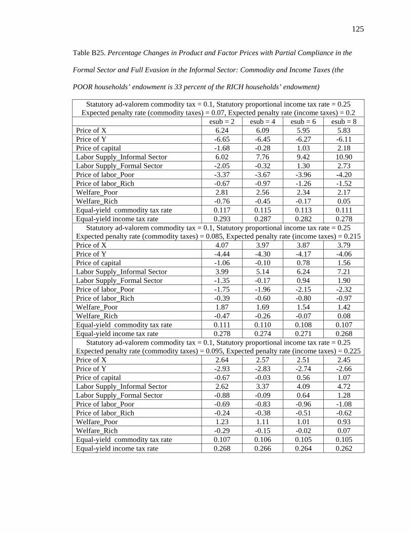
125

Table B25. Percentage Changes in Product and Factor Prices with Partial Compliance in the

Formal Sector and Full Evasion in the Informal Sector: Commodity and Income Taxes (the

POOR households’ endowment is 33 percent of the RICH households’ endowment)

Statutory ad-valorem commodity tax = 0.1, Statutory proportional income tax rate = 0.25 Expected penalty rate (commodity taxes) = 0.07, Expected penalty rate (income taxes) = 0.2

esub = 2 esub = 4 esub = 6 esub = 8 Price of X 6.24 6.09 5.95 5.83 Price of Y -6.65 -6.45 -6.27 -6.11 Price of capital -1.68 -0.28 1.03 2.18 Labor Supply_Informal Sector 6.02 7.76 9.42 10.90 Labor Supply_Formal Sector -2.05 -0.32 1.30 2.73 Price of labor_Poor -3.37 -3.67 -3.96 -4.20 Price of labor_Rich -0.67 -0.97 -1.26 -1.52 Welfare_Poor 2.81 2.56 2.34 2.17 Welfare_Rich -0.76 -0.45 -0.17 0.05 Equal-yield commodity tax rate 0.117 0.115 0.113 0.111 Equal-yield income tax rate 0.293 0.287 0.282 0.278

Statutory ad-valorem commodity tax = 0.1, Statutory proportional income tax rate = 0.25 Expected penalty rate (commodity taxes) = 0.085, Expected penalty rate (income taxes) = 0.215Price of X 4.07 3.97 3.87 3.79 Price of Y -4.44 -4.30 -4.17 -4.06 Price of capital -1.06 -0.10 0.78 1.56 Labor Supply_Informal Sector 3.99 5.14 6.24 7.21 Labor Supply_Formal Sector -1.35 -0.17 0.94 1.90 Price of labor_Poor -1.75 -1.96 -2.15 -2.32 Price of labor_Rich -0.39 -0.60 -0.80 -0.97 Welfare_Poor 1.87 1.69 1.54 1.42 Welfare_Rich -0.47 -0.26 -0.07 0.08 Equal-yield commodity tax rate 0.111 0.110 0.108 0.107 Equal-yield income tax rate 0.278 0.274 0.271 0.268

Statutory ad-valorem commodity tax = 0.1, Statutory proportional income tax rate = 0.25 Expected penalty rate (commodity taxes) = 0.095, Expected penalty rate (income taxes) = 0.225Price of X 2.64 2.57 2.51 2.45 Price of Y -2.93 -2.83 -2.74 -2.66 Price of capital -0.67 -0.03 0.56 1.07 Labor Supply_Informal Sector 2.62 3.37 4.09 4.72 Labor Supply_Formal Sector -0.88 -0.09 0.64 1.28 Price of labor_Poor -0.69 -0.83 -0.96 -1.08 Price of labor_Rich -0.24 -0.38 -0.51 -0.62 Welfare_Poor 1.23 1.11 1.01 0.93 Welfare_Rich -0.29 -0.15 -0.02 0.07 Equal-yield commodity tax rate 0.107 0.106 0.105 0.105 Equal-yield income tax rate 0.268 0.266 0.264 0.262

126

Table B26. Percentage Changes in Product and Factor Prices with Partial Compliance in the

Formal Sector and Full Evasion in the Informal Sector: Commodity Taxes (the POOR

households’ endowment is 33 percent of the RICH households’ endowment)

Statutory ad-valorem commodity tax = 0.25 Expected penalty rate (commodity taxes) = 0.2

esub = 2 esub = 4 esub = 6 esub = 8 Price of X 2.25 2.26 2.26 2.26 Price of Y -2.50 -2.48 -2.46 -2.44 Price of capital -0.69 -0.42 -0.18 0.02 Labor Supply_Informal Sector 2.07 2.51 2.91 3.26 Labor Supply_Formal Sector -0.83 -0.42 -0.06 0.25 Price of labor_Poor -4.23 -4.36 -4.48 -4.58 Price of labor_Rich -0.24 -0.38 -0.50 -0.61 Welfare_Poor 1.15 1.07 1.01 0.95 Welfare_Rich -0.38 -0.32 -0.27 -0.22 Equal-yield commodity tax rate 0.285 0.283 0.282 0.28

Statutory ad-valorem commodity tax = 0.25 Expected penalty rate (commodity taxes) = 0.215

Price of X 1.56 1.57 1.57 1.57 Price of Y -1.75 -1.74 -1.72 -1.71 Price of capital -0.48 -0.29 -0.11 0.03 Labor Supply_Informal Sector 1.45 1.75 2.03 2.28 Labor Supply_Formal Sector -0.58 -0.29 -0.03 0.19 Price of labor_Poor -2.96 -3.05 -3.13 -3.21 Price of labor_Rich -0.16 -0.26 -0.34 -0.42 Welfare_Poor 0.80 0.75 0.70 0.66 Welfare_Rich -0.26 -0.22 -0.18 -0.15 Equal-yield commodity tax rate 0.274 0.273 0.272 0.271

Statutory ad-valorem commodity tax = 0.25 Expected penalty rate (commodity taxes) = 0.225

Price of X 1.12 1.12 1.11 1.11 Price of Y -1.25 -1.24 -1.23 -1.22 Price of capital -0.34 -0.20 -0.07 0.03 Labor Supply_Informal Sector 1.03 1.25 1.45 1.62 Labor Supply_Formal Sector -0.41 -0.20 -0.02 0.14 Price of labor_Poor -2.11 -2.18 -2.24 -2.29 Price of labor_Rich -0.11 -0.18 -0.24 -0.30 Welfare_Poor 0.57 0.53 0.50 0.47 Welfare_Rich -0.18 -0.15 -0.12 -0.10 Equal-yield commodity tax rate 0.267 0.266 0.266 0.265

127

Table B27. Percentage Changes in Product and Factor Prices with Partial Compliance in the

Formal Sector and Full Evasion in the Informal Sector: Income Taxes (the POOR households’

endowment is 33 percent of the RICH households’ endowment)

Statutory proportional income tax rate = 0.20 Expected penalty rate (income taxes) = 0.15

esub = 2 esub = 4 esub = 6 esub = 8 Price of X 4.55 4.53 4.51 4.49 Price of Y -4.94 -4.88 -4.82 -4.77 Price of capital -1.27 -0.63 -0.03 0.48 Labor Supply_Informal Sector 4.33 5.34 6.27 7.11 Labor Supply_Formal Sector -1.62 -0.70 0.15 0.90 Price of labor_Poor -6.28 -6.47 -6.76 -6.94 Price of labor_Rich 5.10 4.61 3.88 3.40 Welfare_Poor 2.28 2.11 1.96 1.84 Welfare_Rich -0.66 -0.51 -0.38 -0.26 Equal-yield income tax rate 0.242 0.240 0.237 0.235

Statutory proportional income tax rate = 0.20 Expected penalty rate (income taxes) = 0.165

Price of X 3.18 3.17 3.15 3.14 Price of Y -3.51 -3.46 -3.42 -3.38 Price of capital -0.87 -0.40 0.02 0.39 Labor Supply_Informal Sector 3.06 3.77 4.44 5.03 Labor Supply_Formal Sector -1.14 -0.47 0.13 0.67 Price of labor_Poor -4.39 -4.59 -4.88 -4.98 Price of labor_Rich 3.68 3.20 2.61 2.38 Welfare_Poor 1.62 1.49 1.38 1.30 Welfare_Rich 0.45 -0.34 -0.24 -0.16 Equal-yield income tax rate 0.230 0.228 0.226 0.225

Statutory proportional income tax rate = 0.20 Expected penalty rate (income taxes) = 0.175

Price of X 2.27 2.26 2.25 2.24 Price of Y -2.53 -2.50 -2.46 -2.44 Price of capital -0.61 -0.27 0.03 0.31 Labor Supply_Informal Sector 2.20 2.71 3.19 3.62 Labor Supply_Formal Sector -0.81 -0.33 0.11 0.50 Price of labor_Poor -3.13 -3.33 -3.53 -3.63 Price of labor_Rich 2.59 2.24 1.90 1.67 Welfare_Poor 1.16 1.07 0.99 0.93 Welfare_Rich -0.31 -0.23 -0.16 -0.10 Equal-yield income tax rate 0.221 0.220 0.219 0.218

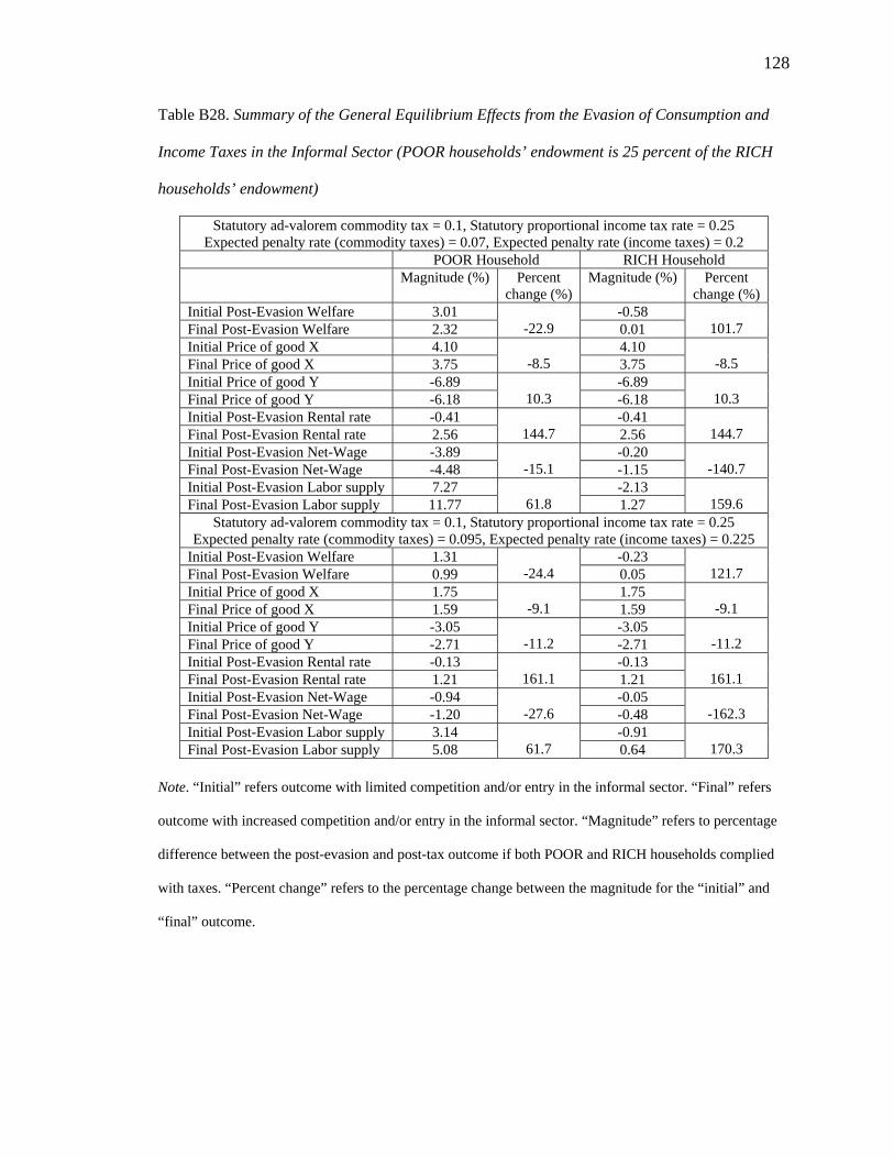
128

Table B28. Summary of the General Equilibrium Effects from the Evasion of Consumption and

Income Taxes in the Informal Sector (POOR households’ endowment is 25 percent of the RICH

households’ endowment)

Statutory ad-valorem commodity tax = 0.1, Statutory proportional income tax rate = 0.25 Expected penalty rate (commodity taxes) = 0.07, Expected penalty rate (income taxes) = 0.2

POOR Household RICH Household Magnitude (%) Percent

change (%) Magnitude (%) Percent

change (%) Initial Post-Evasion Welfare 3.01 -0.58 Final Post-Evasion Welfare 2.32

-22.9 0.01

101.7

Initial Price of good X 4.10 4.10 Final Price of good X 3.75

-8.5 3.75

-8.5

Initial Price of good Y -6.89 -6.89 Final Price of good Y -6.18

10.3 -6.18

10.3

Initial Post-Evasion Rental rate -0.41 -0.41 Final Post-Evasion Rental rate 2.56

144.7 2.56

144.7

Initial Post-Evasion Net-Wage -3.89 -0.20 Final Post-Evasion Net-Wage -4.48

-15.1 -1.15

-140.7

Initial Post-Evasion Labor supply 7.27 -2.13 Final Post-Evasion Labor supply 11.77

61.8 1.27

159.6

Statutory ad-valorem commodity tax = 0.1, Statutory proportional income tax rate = 0.25 Expected penalty rate (commodity taxes) = 0.095, Expected penalty rate (income taxes) = 0.225

Initial Post-Evasion Welfare 1.31 -0.23 Final Post-Evasion Welfare 0.99

-24.4 0.05

121.7

Initial Price of good X 1.75 1.75 Final Price of good X 1.59

-9.1 1.59

-9.1

Initial Price of good Y -3.05 -3.05 Final Price of good Y -2.71

-11.2 -2.71

-11.2

Initial Post-Evasion Rental rate -0.13 -0.13 Final Post-Evasion Rental rate 1.21

161.1 1.21

161.1

Initial Post-Evasion Net-Wage -0.94 -0.05 Final Post-Evasion Net-Wage -1.20

-27.6 -0.48

-162.3

Initial Post-Evasion Labor supply 3.14 -0.91 Final Post-Evasion Labor supply 5.08

61.7 0.64

170.3

Note. “Initial” refers outcome with limited competition and/or entry in the informal sector. “Final” refers

outcome with increased competition and/or entry in the informal sector. “Magnitude” refers to percentage

difference between the post-evasion and post-tax outcome if both POOR and RICH households complied

with taxes. “Percent change” refers to the percentage change between the magnitude for the “initial” and

“final” outcome.

129

Table B29. Percentage Changes in Product and Factor Prices with Full Compliance in the

Formal Sector and Full Evasion in the Informal Sector: Commodity and Income Taxes (the

POOR households’ endowment is 25 percent of the RICH households’ endowment)

Statutory ad-valorem commodity tax = 0.1, Statutory proportional income tax rate = 0.25 Expected penalty rate (commodity taxes) = 0.07, Expected penalty rate (income taxes) = 0.2

esub = 2 esub = 4 esub = 6 esub = 8 Price of X 4.10 3.97 3.85 3.75 Price of Y -6.89 -6.63 -6.40 -6.18 Price of capital -0.41 0.65 1.66 2.56 Labor Supply_Poor 7.27 8.86 10.39 11.77 Labor Supply_Rich -2.13 -0.90 0.25 1.27 Price of labor_Poor -3.89 -4.10 -4.30 -4.48 Price of labor_Rich -0.20 -0.54 -0.86 -1.15 Welfare_Poor 3.01 2.74 2.51 2.32 Welfare_Rich -0.58 -0.36 -0.15 0.01 Equal-yield commodity tax rate 0.111 0.110 0.108 0.107 Equal-yield income tax rate 0.278 0.274 0.271 0.268

Statutory ad-valorem commodity tax = 0.1, Statutory proportional income tax rate = 0.25 Expected penalty rate (commodity taxes) = 0.085, Expected penalty rate (income taxes) = 0.215Price of X 2.69 2.60 2.52 2.45 Price of Y -4.61 -4.43 -4.26 -4.11 Price of capital -0.23 0.49 1.17 1.78 Labor Supply_Poor 4.80 5.84 6.85 7.76 Labor Supply_Rich -1.40 -0.56 0.22 0.92 Price of labor_Poor -2.11 -2.26 -2.39 -2.51 Price of labor_Rich -0.10 -0.33 -0.55 -0.75 Welfare_Poor 2.00 1.81 1.65 1.52 Welfare_Rich -0.36 -0.21 -0.07 0.04 Equal-yield commodity tax rate 0.107 0.106 0.105 0.105 Equal-yield income tax rate 0.268 0.266 0.264 0.262

Statutory ad-valorem commodity tax = 0.1, Statutory proportional income tax rate = 0.25 Expected penalty rate (commodity taxes) = 0.095, Expected penalty rate (income taxes) = 0.225Price of X 1.75 1.70 1.64 1.59 Price of Y -3.05 -2.93 -2.81 -2.71 Price of capital -0.13 0.34 0.80 1.21 Labor Supply_Poor 3.14 3.83 4.49 5.08 Labor Supply_Rich -0.91 -0.35 0.17 0.64 Price of labor_Poor -0.94 -1.03 -0.67 -1.20 Price of labor_Rich -0.05 -0.21 -0.35 -0.48 Welfare_Poor 1.31 1.19 1.08 0.99 Welfare_Rich -0.23 -0.12 -0.03 0.05 Equal-yield commodity tax rate 0.105 0.104 0.104 0.103 Equal-yield income tax rate 0.262 0.260 0.259 0.257

130

Table B30. Percentage Changes in Product and Factor Prices with Full Compliance in the

Formal Sector and Full Evasion in the Informal Sector: Commodity Taxes (the POOR

households’ endowment is 25 percent of the RICH households’ endowment)

Statutory ad-valorem commodity tax = 0.25 Expected penalty rate (commodity taxes) = 0.2

esub = 2 esub = 4 esub = 6 esub = 8 Price of X 1.49 1.47 1.46 1.45 Price of Y -2.58 -2.53 -2.49 -2.45 Price of capital -0.26 -0.05 0.13 0.30 Labor Supply_Poor 2.50 2.89 3.24 3.56 Labor Supply_Rich -0.87 -0.59 -0.34 -0.12 Price of labor_Poor -4.46 -4.56 -4.65 -4.72 Price of labor_Rich 1.36 1.18 1.01 0.86 Welfare_Poor 1.20 1.12 1.06 1.00 Welfare_Rich -0.30 -0.25 -0.22 -0.18 Equal-yield commodity tax rate 0.273 0.272 0.271 0.270

Statutory ad-valorem commodity tax = 0.25 Expected penalty rate (commodity taxes) = 0.215

Price of X 1.03 1.02 1.01 1.01 Price of Y -1.81 -1.77 -1.74 -1.72 Price of capital -0.17 -0.03 0.10 0.21 Labor Supply_Poor 1.74 2.01 2.264 2.48 Labor Supply_Rich -0.60 -0.40 -0.23 -0.07 Price of labor_Poor -3.12 -3.19 -3.25 -3.31 Price of labor_Rich 0.95 0.82 0.70 0.59 Welfare_Poor 0.84 0.78 0.74 0.70 Welfare_Rich -0.20 -0.17 -0.15 -0.12 Equal-yield commodity tax rate 0.266 0.265 0.265 0.26

Statutory ad-valorem commodity tax = 0.25 Expected penalty rate (commodity taxes) = 0.225

Price of X 0.73 0.73 0.72 0.71 Price of Y -1.29 -1.26 -1.24 -1.22 Price of capital -0.12 -0.02 0.07 0.16 Labor Supply_Poor 1.24 1.43 1.61 1.77 Labor Supply_Rich -0.43 -0.29 -0.16 -0.05 Price of labor_Poor -2.23 -2.28 -2.32 -2.36 Price of labor_Rich 0.67 0.58 0.49 0.42 Welfare_Poor 0.59 0.56 0.52 0.50 Welfare_Rich -0.14 -0.12 -0.10 -0.08 Equal-yield commodity tax rate 0.261 0.261 0.260 0.260

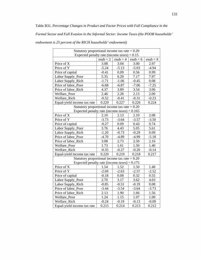
131

Table B31. Percentage Changes in Product and Factor Prices with Full Compliance in the

Formal Sector and Full Evasion in the Informal Sector: Income Taxes (the POOR households’

endowment is 25 percent of the RICH households’ endowment)

Statutory proportional income tax rate = 0.20 Expected penalty rate (income taxes) = 0.15

esub = 2 esub = 4 esub = 6 esub = 8 Price of X 3.08 3.04 3.00 2.97 Price of Y -5.24 -5.13 -5.03 -4.94 Price of capital -0.41 0.09 0.56 0.99 Labor Supply_Poor 5.35 6.29 7.17 7.97 Labor Supply_Rich -1.71 -1.06 -0.45 0.08 Price of labor_Poor -6.68 -6.87 -7.06 -7.25 Price of labor_Rich 4.37 3.89 3.54 3.06 Welfare_Poor 2.46 2.28 2.13 2.00 Welfare_Rich -0.52 -0.41 -0.31 -0.23 Equal-yield income tax rate 0.229 0.227 0.226 0.224

Statutory proportional income tax rate = 0.20 Expected penalty rate (income taxes) = 0.165

Price of X 2.10 2.13 2.10 2.08 Price of Y -3.73 -3.64 -3.57 -3.50 Price of capital -0.27 0.09 0.43 0.74 Labor Supply_Poor 3.76 4.43 5.05 5.61 Labor Supply_Rich -1.20 -0.73 -0.29 0.09 Price of labor_Poor -4.70 -4.89 -4.99 -5.18 Price of labor_Rich 3.08 2.73 2.50 2.16 Welfare_Poor 1.73 1.61 1.50 1.40 Welfare_Rich -0.35 -0.27 -0.20 -0.14 Equal-yield income tax rate 0.220 0.219 0.218 0.217

Statutory proportional income tax rate = 0.20 Expected penalty rate (income taxes) = 0.175

Price of X 1.54 1.52 1.50 1.48 Price of Y -2.69 -2.63 -2.57 -2.52 Price of capital -0.18 0.08 0.32 0.55 Labor Supply_Poor 2.70 3.17 3.62 4.03 Labor Supply_Rich -0.85 -0.51 -0.19 0.08 Price of labor_Poor -3.44 -3.54 -3.64 -3.73 Price of labor_Rich 2.13 1.90 1.66 1.56 Welfare_Poor 1.24 1.15 1.07 1.00 Welfare_Rich -0.24 -0.19 -0.13 -0.09 Equal-yield income tax rate 0.215 0.214 0.213 0.212

132

Table B32. Percentage Changes in Product and Factor Prices with Partial Compliance in the

Formal Sector and Full Evasion in the Informal Sector: Commodity and Income Taxes (the

POOR households’ endowment is 25 percent of the RICH households’ endowment)

Statutory ad-valorem commodity tax = 0.1, Statutory proportional income tax rate = 0.25 Expected penalty rate (commodity taxes) = 0.07, Expected penalty rate (income taxes) = 0.2

esub = 2 esub = 4 esub = 6 esub = 8 Price of X 4.19 4.136 4.08 4.03 Price of Y -7.23 -7.07 -6.91 -6.76 Price of capital -1.91 -0.45 1.00 2.32 Labor Supply_Informal Sector 6.84 8.84 0.93 12.89 Labor Supply_Formal Sector -1.44 0.34 2.14 3.79 Price of labor_Poor -3.03 -0.34 -3.66 -3.95 Price of labor_Rich -0.31 -0.63 -0.96 -1.25 Welfare_Poor 3.40 3.08 2.80 2.56 Welfare_Rich -0.69 -0.38 -0.09 0.15 Equal-yield commodity tax rate 0.113 0.111 0.109 0.107 Equal-yield income tax rate 0.282 0.277 0.272 0.267

Statutory ad-valorem commodity tax = 0.1, Statutory proportional income tax rate = 0.25 Expected penalty rate (commodity taxes) = 0.085, Expected penalty rate (income taxes) = 0.215Price of X 2.73 2.69 2.66 2.62 Price of Y -4.82 -4.71 -4.59 -4.49 Price of capital -1.21 -0.22 0.76 1.65 Labor Supply_Informal Sector 4.51 5.83 7.19 8.46 Labor Supply_Formal Sector -0.94 0.27 1.49 2.59 Price of labor_Poor -1.53 -1.74 -1.96 -2.15 Price of labor_Rich -0.17 -0.39 -0.61 -0.80 Welfare_Poor 2.24 2.02 -1.82 1.66 Welfare_Rich -0.43 -0.22 -0.02 0.14 Equal-yield commodity tax rate 0.108 0.107 0.106 0.104 Equal-yield income tax rate 0.271 0.267 0.264 0.261

Statutory ad-valorem commodity tax = 0.1, Statutory proportional income tax rate = 0.25 Expected penalty rate (commodity taxes) = 0.095, Expected penalty rate (income taxes) = 0.225Price of X 1.77 1.75 1.72 1.70 Price of Y -3.18 -3.10 -3.02 -2.94 Price of capital -0.77 -0.11 0.54 1.13 Labor Supply_Informal Sector 2.94 3.80 4.69 5.51 Labor Supply_Formal Sector -0.61 0.19 1.00 1.73 Price of labor_Poor -0.55 -0.69 -0.84 -0.96 Price of labor_Rich -0.09 -0.24 -0.38 -0.51 Welfare_Poor 1.46 1.31 1.18 1.07 Welfare_Rich -0.26 -0.12 0.00 0.11 Equal-yield commodity tax rate 0.105 0.104 0.104 0.103 Equal-yield income tax rate 0.263 0.261 0.259 0.257

133

Table B33. Percentage Changes in Product and Factor Prices with Partial Compliance in the

Formal Sector and Full Evasion in the Informal Sector: Commodity Taxes (the POOR

households’ endowment is 25 percent of the RICH households’ endowment)

Statutory ad-valorem commodity tax = 0.25 Expected penalty rate (commodity taxes) = 0.2

esub = 2 esub = 4 esub = 6 esub = 8 Price of X 1.55 1.56 1.56 1.56 Price of Y -2.74 -2.72 -2.71 -2.69 Price of capital -0.68 -0.46 -0.27 -0.10 Labor Supply_Informal Sector 2.41 2.79 3.13 3.43 Labor Supply_Formal Sector -0.60 -0.30 -0.03 0.19 Price of labor_Poor -4.26 -4.35 -4.42 -4.48 Price of labor_Rich -0.28 -0.36 -0.44 -0.50 Welfare_Poor 1.41 1.37 1.34 1.32 Welfare_Rich -0.36 -0.32 -0.29 -0.26 Equal-yield commodity tax rate 0.276 0.275 0.274 0.273

Statutory ad-valorem commodity tax = 0.25 Expected penalty rate (commodity taxes) = 0.215

Price of X 1.08 1.08 1.08 1.08 Price of Y -1.92 -1.90 -1.89 -1.88 Price of capital -0.46 -0.31 -0.17 -0.05 Labor Supply_Informal Sector 1.68 1.95 2.19 2.40 Labor Supply_Formal Sector -0.41 -0.20 -0.01 0.14 Price of labor_Poor -2.98 -3.04 -3.09 -3.14 Price of labor_Rich -0.19 -0.25 -0.30 -0.35 Welfare_Poor 0.98 0.96 0.93 0.92 Welfare_Rich -0.24 -0.22 -0.19 -0.17 Equal-yield commodity tax rate 0.268 0.267 0.267 0.266

Statutory ad-valorem commodity tax = 0.25 Expected penalty rate (commodity taxes) = 0.225

Price of X 0.76 0.76 0.76 0.77 Price of Y -1.37 -1.36 -1.35 -1.34 Price of capital -0.33 -0.22 -0.12 -0.03 Labor Supply_Informal Sector 1.19 1.39 1.56 1.71 Labor Supply_Formal Sector -0.29 -0.14 -0.01 0.11 Price of labor_Poor -2.13 2.17 -2.21 -2.24 Price of labor_Rich -0.13 -0.17 -0.21 -0.25 Welfare_Poor 0.70 0.68 0.66 0.65 Welfare_Rich -0.17 -0.15 -0.13 -0.12 Equal-yield commodity tax rate 0.263 0.262 0.262 0.261

134

Table B34. Percentage Changes in Product and Factor Prices with Partial Compliance in the

Formal Sector and Full Evasion in the Informal Sector: Income Taxes (the POOR households’

endowment is 25 percent of the RICH households’ endowment)

Statutory proportional income tax rate = 0.20 Expected penalty rate (income taxes) = 0.15

esub = 2 esub = 4 esub = 6 esub = 8 Price of X 3.02 3.04 3.05 3.07 Price of Y -5.32 -5.29 -5.25 -5.22 Price of capital -1.40 -0.75 0.11 0.48 Labor Supply_Informal Sector 4.88 6.03 7.19 8.30 Labor Supply_Formal Sector -1.15 -0.22 0.70 1.56 Price of labor_Poor -5.98 -6.27 -6.46 -6.75 Price of labor_Rich 5.43 4.83 4.20 3.61 Welfare_Poor 2.74 2.55 2.38 2.23 Welfare_Rich -0.60 -0.46 -0.32 -0.20 Equal-yield income tax rate 0.231 0.226 0.226 0.224

Statutory proportional income tax rate = 0.20 Expected penalty rate (income taxes) = 0.165

Price of X 2.12 2.13 2.14 2.15 Price of Y -3.78 -3.75 -3.73 -3.70 Price of capital -0.96 -0.49 -0.03 0.39 Labor Supply_Informal Sector 3.44 4.25 5.07 5.85 Labor Supply_Formal Sector -0.81 -0.14 0.52 1.15 Price of labor_Poor -4.19 -4.49 -0.59 -4.78 Price of labor_Rich 3.90 3.30 2.93 2.59 Welfare_Poor 1.93 1.79 1.67 1.56 Welfare_Rich -0.40 -0.30 -0.21 -0.12 Equal-yield income tax rate 0.222 0.220 0.218 0.217

Statutory proportional income tax rate = 0.20 Expected penalty rate (income taxes) = 0.175

Price of X 1.51 1.52 1.53 1.53 Price of Y -2.73 -2.710 -2.69 -2.67 Price of capital -0.68 -0.34 -0.00 0.314 Labor Supply_Informal Sector 2.46 3.05 3.64 4.20 Labor Supply_Formal Sector -0.58 -0.09 0.39 0.84 Price of labor_Poor -3.03 -3.23 -3.33 -3.53 Price of labor_Rich 2.70 2.35 2.12 1.78 Welfare_Poor 1.39 1.28 1.19 1.11 Welfare_Rich -0.28 -0.21 -0.14 -0.07 Equal-yield income tax rate 0.216 0.214 0.213 0.212

135

Table B35. Summary of the General Equilibrium Effects from the Evasion of Consumption and

Income Taxes in the Informal Sector (POOR households’ endowment is 50 percent of the RICH

households’ endowment)

Statutory ad-valorem commodity tax = 0.1, Statutory proportional income tax rate = 0.25 Expected penalty rate (commodity taxes) = 0.07, Expected penalty rate (income taxes) = 0.2

POOR Household RICH Household Magnitude (%) Percent

change (%) Magnitude (%) Percent

change (%) Initial Post-Evasion Welfare 0.77 -0.51 Final Post-Evasion Welfare 0.64

-16.8 -0.21

58.8

Initial Price of good X 7.75 7.75 Final Price of good X 7.43

-4.1 7.43

-4.1

Initial Price of good Y -8.17 -8.17 Final Price of good Y -7.81

4.4 -7.81

4.4

Initial Post-Evasion Rental rate -0.93 -0.93 Final Post-Evasion Rental rate 0.32

134.4 0.32

134.4

Initial Post-Evasion Net-Wage -3.31 1.11 Final Post-Evasion Net-Wage -3.55

-7.2 0.68

-38.7

Initial Post-Evasion Labor supply 8.06 -6.55 Final Post-Evasion Labor supply 9.42

16.8 -4.85

25.9

Statutory ad-valorem commodity tax = 0.1, Statutory proportional income tax rate = 0.25 Expected penalty rate (commodity taxes) = 0.095, Expected penalty rate (income taxes) = 0.225

Initial Post-Evasion Welfare 0.36 -0.15 Final Post-Evasion Welfare 0.29

-19.4 -0.02

86.6

Initial Price of good X 3.09 3.09 Final Price of good X 2.95

-4.5 2.95

-4.5

Initial Price of good Y -3.43 -3.43 Final Price of good Y -3.26

4.9 -3.26

4.9

Initial Post-Evasion Rental rate -0.29 -0.29 Final Post-Evasion Rental rate 0.27

193.1 0.27

193.1

Initial Post-Evasion Net-Wage -0.63 0.52 Final Post-Evasion Net-Wage -0.75

-19.0 0.31

-40.3

Initial Post-Evasion Labor supply 3.31 -2.67 Final Post-Evasion Labor supply 3.91

18.1 -1.86

81.0

Note. “Initial” refers outcome with limited competition and/or entry in the informal sector. “Final” refers

outcome with increased competition and/or entry in the informal sector. “Magnitude” refers to percentage

difference between the post-evasion and post-tax outcome if both POOR and RICH households complied

with taxes. “Percent change” refers to the percentage change between the magnitude for the “initial” and

“final” outcome.

136

Table B36. Percentage Changes in Product and Factor Prices with Full Compliance in the

Formal Sector and Full Evasion in the Informal Sector: Commodity and Income Taxes (the

POOR households’ endowment is 50 percent of the RICH households’ endowment)

Statutory ad-valorem commodity tax = 0.1, Statutory proportional income tax rate = 0.25 Expected penalty rate (commodity taxes) = 0.07, Expected penalty rate (income taxes) = 0.2

esub = 2 esub = 4 esub = 6 esub = 8 Price of X 7.75 7.63 7.52 7.43 Price of Y -8.17 -8.04 -7.92 -7.81 Price of capital -0.93 -0.47 -0.04 0.32 Labor Supply_Poor 8.06 8.55 9.02 9.42 Labor Supply_Rich -6.55 -5.93 -5.35 -4.85 Price of labor_Poor -3.31 -3.40 -3.48 -3.55 Price of labor_Rich 1.11 0.95 0.80 0.68 Welfare_Poor 0.77 0.72 0.68 0.64 Welfare_Rich -0.51 -0.39 -0.29 -0.21 Equal-yield commodity tax rate 0.119 0.118 0.118 0.117 Equal-yield income tax rate 0.298 0.296 0.294 0.293

Statutory ad-valorem commodity tax = 0.1, Statutory proportional income tax rate = 0.25 Expected penalty rate (commodity taxes) = 0.085, Expected penalty rate (income taxes) = 0.215Price of X 4.92 4.84 4.77 4.70 Price of Y -5.34 -5.25 -5.17 -5.09 Price of capital -0.52 -0.20 0.09 0.34 Labor Supply_Poor 5.21 5.55 5.86 6.12 Labor Supply_Rich -4.21 -3.77 -3.36 -3.01 Price of labor_Poor -1.68 -1.74 -1.81 -1.86 Price of labor_Rich 0.77 0.66 0.56 0.46 Welfare_Poor 0.54 0.50 0.47 0.45 Welfare_Rich -0.28 -0.20 -0.13 0.08 Equal-yield commodity tax rate 0.112 0.112 0.111 0.111 Equal-yield income tax rate 0.280 0.279 0.278 0.277

Statutory ad-valorem commodity tax = 0.1, Statutory proportional income tax rate = 0.25 Expected penalty rate (commodity taxes) = 0.095, Expected penalty rate (income taxes) = 0.225Price of X 3.09 3.04 2.99 2.95 Price of Y -3.43 -3.36 -3.31 -3.26 Price of capital -0.29 -0.08 0.11 0.27 Labor Supply_Poor 3.31 3.53 3.73 3.91 Labor Supply_Rich -2.67 -2.37 -2.09 -1.86 Price of labor_Poor -0.63 -0.67 -0.72 -0.75 Price of labor_Rich 0.52 0.44 0.37 0.31 Welfare_Poor 0.36 0.33 0.31 0.29 Welfare_Rich -0.15 -0.10 -0.06 -0.02 Equal-yield commodity tax rate 0.108 1.07 0.107 0.107 Equal-yield income tax rate 0.269 0.268 0.268 0.267

137

Table B37. Percentage Changes in Product and Factor Prices with Full Compliance in the

Formal Sector and Full Evasion in the Informal Sector: Commodity Taxes (the POOR

households’ endowment is 50 percent of the RICH households’ endowment)

Statutory ad-valorem commodity tax = 0.25 Expected penalty rate (commodity taxes) = 0.2

esub = 2 esub = 4 esub = 6 esub = 8 Price of X 3.20 3.18 3.17 3.15 Price of Y -3.54 -3.51 -3.49 -3.47 Price of capital -0.37 -0.25 -0.14 -0.05 Labor Supply_Poor 3.34 3.51 3.66 3.78 Labor Supply_Rich -2.82 -2.63 -2.46 -2.32 Price of labor_Poor -4.20 -0.26 -4.30 -4.34 Price of labor_Rich 3.29 -4.25 3.07 2.98 Welfare_Poor 0.38 0.35 0.33 0.31 Welfare_Rich -0.23 -0.20 -0.17 -0.15 Equal-yield commodity tax rate 0.294 0.293 0.292 0.292

Statutory ad-valorem commodity tax = 0.25 Expected penalty rate (commodity taxes) = 0.215

Price of X 2.21 2.20 2.18 2.17 Price of Y -2.47 -2.45 -2.43 -2.42 Price of capital -0.24 -0.16 -0.08 -0.01 Labor Supply_Poor 2.32 2.44 2.55 2.63 Labor Supply_Rich -1.95 -1.82 -1.70 -1.59 Price of labor_Poor -2.93 -2.97 -3.00 -3.03 Price of labor_Rich 2.27 2.19 2.11 2.05 Welfare_Poor 0.27 0.25 0.23 0.22 Welfare_Rich -0.15 -0.13 -0.11 -0.09 Equal-yield commodity tax rate 0.280 0.280 0.279 0.279

Statutory ad-valorem commodity tax = 0.25 Expected penalty rate (commodity taxes) = 0.225

Price of X 1.56 1.55 1.54 1.54 Price of Y -1.76 -1.74 -1.73 -1.72 Price of capital -0.17 -0.10 -0.05 0.00 Labor Supply_Poor 1.65 1.73 1.81 1.87 Labor Supply_Rich -1.38 -1.29 -1.20 -1.12 Price of labor_Poor -2.09 -2.11 -2.14 -2.16 Price of labor_Rich 1.61 1.54 1.49 1.45 Welfare_Poor 0.19 0.18 0.17 0.16 Welfare_Rich -0.10 -0.09 -0.07 -0.06 Equal-yield commodity tax rate 0.271 0.271 0.271 0.270

138

Table B38. Percentage Changes in Product and Factor Prices with Full Compliance in the

Formal Sector and Full Evasion in the Informal Sector: Income Taxes (the POOR households’

endowment is 50 percent of the RICH households’ endowment)

Statutory proportional income tax rate = 0.20 Expected penalty rate (income taxes) = 0.15

esub = 2 esub = 4 esub = 6 esub = 8 Price of X 5.24 5.21 5.18 5.15 Price of Y -5.67 -5.63 -5.58 -5.55 Price of capital -0.59 -0.38 -0.20 -0.04 Labor Supply_Poor 5.49 5.77 6.03 6.24 Labor Supply_Rich -4.51 -4.20 -3.92 -3.69 Price of labor_Poor -6.19 -6.28 -6.38 -6.48 Price of labor_Rich 4.92 4.54 4.29 3.92 Welfare_Poor 0.62 0.57 0.54 0.51 Welfare_Rich -0.37 -0.32 -0.27 -0.23 Equal-yield income tax rate 0.244 0.243 0.242 0.241

Statutory proportional income tax rate = 0.20 Expected penalty rate (income taxes) = 0.165

Price of X 3.65 3.62 3.60 3.59 Price of Y -4.02 -3.98 -3.95 -3.93 Price of capital -0.38 -0.23 -0.09 0.01 Labor Supply_Poor 3.86 4.07 4.25 4.40 Labor Supply_Rich -3.17 -2.93 -2.73 -2.55 Price of labor_Poor -4.40 -4.40 -4.60 -4.59 Price of labor_Rich 3.40 3.27 2.92 2.79 Welfare_Poor 0.45 0.42 0.39 0.37 Welfare_Rich -0.24 -0.20 -0.16 -0.13 Equal-yield income tax rate 0.231 0.230 0.229 0.229

Statutory proportional income tax rate = 0.20 Expected penalty rate (income taxes) = 0.175

Price of X 2.60 2.58 2.56 2.55 Price of Y -2.89 -2.87 -2.84 -2.82 Price of capital -0.26 -0.14 -0.04 0.03 Labor Supply_Poor 2.77 2.92 3.05 3.16 Labor Supply_Rich -2.26 -2.09 -1.94 -1.81 Price of labor_Poor -3.13 -3.13 -3.34 -3.34 Price of labor_Rich 2.45 2.32 1.98 1.98 Welfare_Poor 0.33 0.31 0.29 0.27 Welfare_Rich -0.16 -0.13 -0.10 -0.08 Equal-yield income tax rate 0.222 0.221 0.221 0.221

139

Table B39. Percentage Changes in Product and Factor Prices with Partial Compliance in the

Formal Sector and Full Evasion in the Informal Sector: Commodity and Income Taxes (the

POOR households’ endowment is 50 percent of the RICH households’ endowment)

Statutory ad-valorem commodity tax = 0.1, Statutory proportional income tax rate = 0.25 Expected penalty rate (commodity taxes) = 0.07, Expected penalty rate (income taxes) = 0.2

esub = 2 esub = 4 esub = 6 esub = 8 Price of X 7.71 7.59 7.49 7.40 Price of Y -8.27 -8.12 -7.99 -7.88 Price of capital -2.53 -1.66 -0.87 -0.19 Labor Supply_Informal Sector 7.34 8.25 9.08 9.79 Labor Supply_Formal Sector -5.00 -3.87 -2.85 -1.97 Price of labor_Poor -2.32 -2.54 -2.74 -2.90 Price of labor_Rich 0.40 0.18 -0.01 -0.18 Welfare_Poor 1.19 1.08 1.00 0.93 Welfare_Rich -0.66 -0.45 -0.27 -0.13 Equal-yield commodity tax rate 0.120 0.119 0.118 0.117 Equal-yield income tax rate 0.301 0.298 0.295 0.292

Statutory ad-valorem commodity tax = 0.1, Statutory proportional income tax rate = 0.25 Expected penalty rate (commodity taxes) = 0.085, Expected penalty rate (income taxes) = 0.215Price of X 4.88 4.81 4.74 4.68 Price of Y -5.40 -5.30 -5.21 -5.13 Price of capital -1.54 -0.95 -0.42 0.02 Labor Supply_Informal Sector 4.75 5.35 5.90 6.36 Labor Supply_Formal Sector -3.21 -2.44 -1.74 -1.14 Price of labor_Poor -1.03 -1.18 -1.32 -1.44 Price of labor_Rich 0.33 0.18 0.04 -0.07 Welfare_Poor 0.81 0.74 0.68 0.63 Welfare_Rich -0.37 -0.23 -0.11 -0.02 Equal-yield commodity tax rate 0.113 0.112 0.111 0.111 Equal-yield income tax rate 0.283 0.280 0.278 0.277

Statutory ad-valorem commodity tax = 0.1, Statutory proportional income tax rate = 0.25 Expected penalty rate (commodity taxes) = 0.095, Expected penalty rate (income taxes) = 0.225Price of X 3.06 3.01 2.97 2.94 Price of Y -3.46 -3.39 -3.33 -3.28 Price of capital -0.94 -0.56 -0.21 0.08 Labor Supply_Informal Sector 3.02 3.41 3.76 4.05 Labor Supply_Formal Sector -2.03 -1.52 -1.06 -0.67 Price of labor_Poor -0.21 -0.31 -0.41 -0.48 Price of labor_Rich 0.24 0.13 0.04 -0.03 Welfare_Poor 0.53 0.48 0.44 0.41 Welfare_Rich -0.21 -0.12 -0.04 0.01 Equal-yield commodity tax rate 0.108 0.108 0.107 0.107 Equal-yield income tax rate 0.271 0.269 0.268 0.267

140

Table B40. Percentage Changes in Product and Factor Prices with Partial Compliance in the

Formal Sector and Full Evasion in the Informal Sector: Commodity Taxes (the POOR

households’ endowment is 50 percent of the RICH households’ endowment)

Statutory ad-valorem commodity tax = 0.25 Expected penalty rate (commodity taxes) = 0.2

esub = 2 esub = 4 esub = 6 esub = 8 Price of X 3.12 3.12 3.12 3.12 Price of Y -3.52 -3.51 -3.49 -3.48 Price of capital -0.99 -0.76 -0.55 -0.38 Labor Supply_Informal Sector 3.00 3.31 3.58 3.82 Labor Supply_Formal Sector -2.12 -1.77 -1.46 -1.20 Price of labor_Poor -3.74 -3.85 -3.94 -4.02 Price of labor_Rich 0.26 0.15 0.05 -0.02 Welfare_Poor 0.58 0.53 0.49 0.45 Welfare_Rich -0.32 -0.26 -0.20 -0.16 Equal-yield commodity tax rate 0.296 0.295 0.293 0.292

Statutory ad-valorem commodity tax = 0.25 Expected penalty rate (commodity taxes) = 0.215

Price of X 2.15 2.15 2.15 2.15 Price of Y -2.46 -2.44 -2.43 -2.42 Price of capital -0.67 -0.51 -0.36 -0.24 Labor Supply_Informal Sector 2.08 2.30 2.49 2.66 Labor Supply_Formal Sector -1.47 -1.22 -1.00 -0.82 Price of labor_Poor -2.60 -2.68 -2.75 -2.80 Price of labor_Rich 0.19 0.11 0.04 -0.01 Welfare_Poor 0.41 0.37 0.34 0.32 Welfare_Rich -0.21 -0.17 -0.13 -0.10 Equal-yield commodity tax rate 0.282 0.281 0.280 0.279

Statutory ad-valorem commodity tax = 0.25 Expected penalty rate (commodity taxes) = 0.225

Price of X 1.52 1.52 1.52 1.52 Price of Y -1.75 -1.74 -1.73 -1.73 Price of capital -0.47 -0.35 -0.25 -0.16 Labor Supply_Informal Sector 1.48 1.64 1.77 1.89 Labor Supply_Formal Sector -1.04 -0.86 -0.71 -0.57 Price of labor_Poor -1.85 -1.91 -1.96 -2.00 Price of labor_Rich 0.14 0.08 0.03 -0.00 Welfare_Poor 0.29 0.27 0.24 0.23 Welfare_Rich -0.14 -0.11 -0.09 -0.06 Equal-yield commodity tax rate 0.272 0.272 0.271 0.270

141

Table B41. Percentage Changes in Product and Factor Prices with Partial Compliance in the

Formal Sector and Full Evasion in the Informal Sector: Income Taxes (the POOR households’

endowment is 50 percent of the RICH households’ endowment)

Statutory proportional income tax rate = 0.20 Expected penalty rate (income taxes) = 0.15

esub = 2 esub = 4 esub = 6 esub = 8 Price of X 5.09 5.09 5.08 5.07 Price of Y -5.63 -5.60 -5.57 -5.55 Price of capital -1.60 -1.21 -0.86 -0.57 Labor Supply_Informal Sector 4.90 5.42 5.88 6.27 Labor Supply_Formal Sector -3.41 -2.83 -2.32 -1.89 Price of labor_Poor -5.48 -5.68 -5.78 -5.88 Price of labor_Rich 5.99 5.49 4.96 4.58 Welfare_Poor 0.93 0.85 0.78 0.73 Welfare_Rich -0.50 -0.40 -0.31 -0.24 Equal-yield income tax rate 0.245 0.244 0.243 0.242

Statutory proportional income tax rate = 0.20 Expected penalty rate (income taxes) = 0.165

Price of X 3.55 3.54 3.54 3.53 Price of Y -3.99 -3.96 -3.94 -3.93 Price of capital -1.09 -0.80 -0.56 -0.35 Labor Supply_Informal Sector 3.45 3.82 4.15 4.43 Labor Supply_Formal Sector -2.39 -1.97 -1.60 -1.29 Price of labor_Poor -3.88 -3.99 -4.09 -4.19 Price of labor_Rich 4.23 3.85 3.47 3.23 Welfare_Poor 0.67 0.61 0.57 0.53 Welfare_Rich -0.33 -0.25 -0.19 -0.14 Equal-yield income tax rate 0.232 0.231 0.230 0.229

Statutory proportional income tax rate = 0.20 Expected penalty rate (income taxes) = 0.175

Price of X 2.52 2.52 2.52 2.51 Price of Y -2.87 -2.85 -2.84 -2.82 Price of capital -0.76 -0.56 -0.37 -0.22 Labor Supply_Informal Sector 2.47 2.74 2.98 3.18 Labor Supply_Formal Sector -1.71 -1.40 -1.13 -0.90 Price of labor_Poor -2.82 -2.82 -3.03 -3.03 Price of labor_Rich 2.92 2.78 2.43 2.30 Welfare_Poor 0.49 0.45 0.41 0.38 Welfare_Rich -0.22 -0.17 -0.12 -0.09 Equal-yield income tax rate 0.223 0.222 0.221 0.221

142

References Allingham, M. G., & Sandmo, A. (1972). Income Tax Evasion: A Theoretical Analysis.

Journal of Public Economics, 1, 323-338.

Alm, J. (1985). The Welfare Cost of the Underground Economy. Economic Inquiry,

23(2), 243-263.

Alm, J., Martinez-Vazquez, J., & Wallace, S. (Eds.). (2004). Sizing the Problem of the

Hard-to-Tax: An International Perspective. Amsterdam: Elsevier.

Bahl, R. (1971). A Regression Approach to Tax Effort and Tax Ratio Analysis (pp. 570-

612): IMF.

Baldes, D. (1982). The Hidden Economy and the National Accounts (pp. 28-44): OECD

Occassional Studies.

Bolnick, B., & Haughton, J. (1998). Tax Policy in Sub-Saharan African: Examining the

Role of Excise Taxation. Journal of African Finance and Economic Development,

4(1), 31-64.

Bruce, N. (2001). Public Finance and the American Economy: Addison-Wesley

Longman, Inc.

Cagan, P. (1958). The Demand for Currency Relative to the Total Money Supply.

Journal of Political Economy, 66(3), 302-328.

Davidson, R., & MacKinnon, J. G. (2004). Econometric Theory and Methods. New York:

Oxford University Press.

Erickson, T., & Whited, T. M. (2002). Two-Step GMM Estimation of the Errors-in-

Variables Model using High-Order Moments. Econometric Theory, 18, 776-799.

143

Feige, E. L. (1986). A Re-examination of the Underground Economy in the United States

(pp. 768-781): IMF Staff Papers.

Feige, E. L. (Ed.). (1996). Overseas Holdings of U.S. Currency and the Underground

Economy. : Kalamazoo.

Frey, B. S., & Pommerehne, W. (1984). The Hidden Economy: State and Prospect for

Measurement Review of Income and Wealth, 30(1), 1-23.

Friedman, J. E., Kaufmann, S. D., & Zoido-Lobaton, P. (2000). Dodging the Grabbing

Hand: Determinants of Unofficial Activity in 69 Countries. Journal of Public

Economics, 76, 459-496.

Garcia, G. (1978). The Currency Ratio and the Subterranean Economy. Financial

Analysts Journal, 69(1), 64-66.

Giles, D. E. A. (1999a). Measuring the Hidden Economy: Implications for Econometric

Modeling. The Economic Journal, 109(456), 370-380.

Giles, D. E. A. (1999b). Modelling the hidden economy in the Tax-Gap in New Zealand:

Department of Economics, University of Victoria, Canada.

Giles, D. E. A., & Tedds, L. M. (2002). Taxes and the Canadian Underground Economy:

Canadian Tax Foundation, Toronto/Ontario.

Giles, D. E. A., Tedds, L. M., & Gupsa, W. (1999). The Canadian Underground and

Measured Economies: Department of Economics, University of Victoria, Canada.

Gordon, R. H., & Nielsen, S. B. (1997). Tax Evasion in an Open Economy: Value-added

Versus Income Taxation. Journal of Public Economics, 66, 173-197.

Gutmann, P. M. (1977). The Subterranean Economy. Financial Analysts Journal, 34(1),

24-27.

144

Hettich, W., & Winer, S. (1984). A Positive Model of Tax Structure. Journal of Public

Economics, 24, 67-87.

Hettich, W., & Winer, S. (1988). Economic and Political Foundations of Tax Structure.

American Economic Review, 78(4), 701-712.

Hill, R., & Kabir, M. (1996). Tax rates, the Tax Mix, and the Growth of the Underground

Economy in Canada: What can we infer? Canadian Tax Journal, 44(6), 1552-

1583.

Hsiao, C. (1986). Analysis of Panel Data. New York: Cambridge University Press.

Isachsen, A. J., & Strom, S. (1985). The Size and Growth of the Hidden Economy in

Norway. Review of Income and Wealth, 31(1), 21-28.

Kehoe, P. J., & Kehoe, T. J. (1994). A Primer on Static Applied General Equilibrium

Models. Journal of Public Economics, 22, 1-26.

Kehoe, T., & Serra-Puche, J. (1983). A Computational General Equilibrium Model with

Endogenous Unemployment. Journal of Public Economics, 38, 137-182.

Kesselman, J. R. (1989). Income Tax Evasion: An Intersectoral Analysis. Journal of

Public Economics, 38, 137-182.

Klovland, J. (1984). Tax Evasion and the Demand for Currency in Norway and Sweden:

Is there a Hidden Relationship? . Scandinavian Journal of Economics, 86(4), 423-

439.

Lai, C.-C., & Chang, W.-Y. (1988). Tax Evasion and Tax Collections: An Aggregate

Demand-Aggregate Supply Analysis. Public Finance 43, 138-146.

145

Light, M. (2004). Taxation and Economic Efficiency in Jamaica: International Studies

Program Working Paper, Andrew Young School of Policy Studies, Georgia State

University.

Martinez-Vazquez, J. (1996). Who Benefits from Tax Evasion? The Incidence of Tax

Evasion. Public Economics Review 1(2), 105-135.

Mathiesen, L. (1985). Computation of Economic Equilibria by a Sequence of Linear

Complementarity Problems. Mathematical Programming Study, 23, 144-162.

Mauleon, I. (1998). Quantitative Estimation of the Spanish Underground Economy:

Discussion Paper, Department of Economics and History, University of

Salamanka, Salamanka, Spain.

Nielsen, S., Schou, P., & Sobygaard, J. (2002). Elements of Income Tax Evasion and

Avoidance in Denmark. Swedish Economic Policy Review 9, 139-164.

Park, T. (1979). Reconciliation between Personal Income and Taxable Income: Mimeo,

Washington D.C., Bureau of Economic Analysis.

Peacock, A., & Shaw, G. K. (1982). Tax Evasion and Tax Revenue Loss. Public Finance,

37, 269-278.

Persson, M., & Wissen, P. (1984). Redistributional Aspects of Tax Evasion.

Scandinavian Journal of Economics, 86(2), 131-149.

Ricketts, M. (1984). On the Simple Macroeconomics of Tax Evasion: An Elaboration of

the Peacock-Shaw Approach. public Finance, 93, 420-424.

Sandmo, A. (2004). Theory of Tax Evasion: A Retrospective View: Research Forum on

Taxation, Rosendal, Norway.

146

Schneider, F. (2002). The Value Added of Underground Activities: Size and

Measurement of the Shadow Economies of 110 Countries All over the World,

mimeo: Department of Economics, Johannes Kepler University of Linz, Austria.

Schneider, F., & Enste, D. H. (2000). Shadow Economies: Size, Causes, and

Consequences. Journal of Economic Literature, 38(1), 77-114.

Shah, A., & Whalley, J. (1990). An Alternative View of Tax Incidence Analysis for

Developing Countries: NBER Working Paper.

Skinner, J., & Selmrod, J. (1986). An Economic Perspective on Tax Evasion. National

Tax Journal, 38(1), 345-353.

Slemrod, J., & Yitzhaki, S. (1996). The Cost of Taxation and the Marginal Efficiency

Cost of Funds (pp. 172-198): IMF Staff Papers.

Tanzi, V. (1980). The Underground Economy in the United States: Estimates and

Implications (pp. 427-453): Banca Nazionale del Lavoro 135:4.

Tanzi, V. (1983). The Underground Economy in the United States: Annual Estimates,

1930-1980 (pp. 283-305): IMF Staff Papers, 30:2.

Teera, J. (2002). Tax Performance: A Comparative Study: Centre for Public Economics,

University of Bath.

Thalmann, P. (1992). Factor Taxes and Evasion in General Equilibrium. Regional

Science and Urban Economics, 22, 259-283.

Thomas, J. J. (1986). The Underground Economy in the United States: A comment on

Tanzi (pp. 782-789): IMF Staff Papers 33:4.

Thomas, J. J. (1999). Quantifying the Black Economy: ‘Measurement without Theory’

Yet Again? Economic Journal 109(456), 381-389.

147

Thomas, J. J. (Ed.). (1992). Informal Economic Activity. London: Harvester Wheatsheaf.

UN. (2005). National Accounts Statistics 2002-2003: Main Aggregates and Detailed

Tables (Vol. I&II): United Nations.

Von Zameck, W. (1989). Tax Evasion and Tax Revenue Loss: Another Elaboration of the

Peacock-Shaw Approach. Public Finance 44, 308-315.

Watson, H. (1985). Tax Evasion and Labor Markets. Journal of Public Economics 27,

231-246.

Wooldridge, M. J. (2001). Econometric Analysis of Cross Section and Panel Data.

Cambridge: MIT Press, Massachusetts.

Yitzhaki, S. (1974). A Note on Income Tax Evasion: A Theoretical Analysis. Journal of

Public Economics, 3, 201-202.

148

Curriculum Vita

Edward Batte Sennoga was born in 1975 in Uganda, and grew up in Kampala,

Uganda. He received a Bachelor of Science degree in Economics from Makerere

Univerity, Kampala in 1999, and was awarded a graduate scholarship by the University

of North Texas during the same year. He earned a Master of Science degree in Economic

Research from the University of North Texas in August 2001, and was accepted into the

doctoral program at Georgia State University in the fall of 2001. He completed all the

requirements for the Doctor of Philosophy in Economics degree at the Andrew Young

School of Policy Studies of Georgia State University in February, 2006.

While at Georgia State University, he worked as graduate research assistant for

Professor James Alm, as a research associate in the Economic Forecasting Center, and as

an instructor in the Department of Economics. He has served as president of the

Department of Economics graduate students association and as the Andrew Young

School of Policy Studies representative on the Electronic Theses and Dissertations

Committee. He has received numerous awards for both academic and teaching

excellence.

He is currently a research associate at the Andrew Young School of Policy

Studies Fiscal Research Center, also at Georgia State University. His primary research

interest is in the field of public economics, particularly in the areas of taxation and state

and local public finance.