Error Rate Bounds and Iterative Weighted Majority Voting for Crowdsourcing
52
Error Rate Bounds and Iterative Weighted Majority Voting for Crowdsourcing Hongwei Li [email protected] Department of Statistics University of California Berkeley, CA 94720-1776, USA Bin Yu [email protected] Department of Statistics & EECS University of California Berkeley, CA 94720-1776, USA Abstract Crowdsourcing has become an effective and popular tool for human-powered computa- tion to label large datasets. Since the workers can be unreliable, it is common in crowd- sourcing to assign multiple workers to one task, and to aggregate the labels in order to obtain results of high quality. In this paper, we provide finite-sample exponential bounds on the error rate (in probability and in expectation) of general aggregation rules under the Dawid-Skene crowdsourcing model. The bounds are derived for multi-class labeling, and can be used to analyze many aggregation methods, including majority voting, weighted majority voting and the oracle Maximum A Posteriori (MAP) rule. We show that the oracle MAP rule approximately optimizes our upper bound on the mean error rate of weighted majority voting in certain setting. We propose an iterative weighted majority voting (IWMV) method that optimizes the error rate bound and approximates the oracle MAP rule. Its one step version has a provable theoretical guarantee on the error rate. The IWMV method is intuitive and computationally simple. Experimental results on simulated and real data show that IWMV performs at least on par with the state-of-the-art methods, and it has a much lower computational cost (around one hundred times faster) than the state-of-the-art methods. Keywords: Crowdsourcing, Error rate bound, Mean error rate, Expectation-Maximization, Weighted majority voting 1. Introduction There are many tasks which can be easily carried out by people but that tend to be hard for computers, e.g., image annotation, visual design and video event classification. When these tasks are extensive, outsourcing them to experts or well-trained people may be too expensive. Crowdsourcing has recently emerged as a powerful alternative. It outsources tasks to a distributed group of people (called workers) who might be inexperienced in these tasks. However, if we can appropriately aggregate the outputs from a crowd, the yielded results could be as good as the ones by experts (Smyth et al., 1995; Snow et al., 2008; 1 arXiv:1411.4086v1 [stat.ML] 15 Nov 2014
Transcript of Error Rate Bounds and Iterative Weighted Majority Voting for Crowdsourcing
Error Rate Bounds and Iterative Weighted Majority Votingfor Crowdsourcing
Hongwei Li [email protected] of StatisticsUniversity of CaliforniaBerkeley, CA 94720-1776, USA
Bin Yu [email protected]
Department of Statistics & EECS
University of California
Berkeley, CA 94720-1776, USA
Abstract
Crowdsourcing has become an effective and popular tool for human-powered computa-tion to label large datasets. Since the workers can be unreliable, it is common in crowd-sourcing to assign multiple workers to one task, and to aggregate the labels in order toobtain results of high quality. In this paper, we provide finite-sample exponential boundson the error rate (in probability and in expectation) of general aggregation rules under theDawid-Skene crowdsourcing model. The bounds are derived for multi-class labeling, andcan be used to analyze many aggregation methods, including majority voting, weightedmajority voting and the oracle Maximum A Posteriori (MAP) rule. We show that theoracle MAP rule approximately optimizes our upper bound on the mean error rate ofweighted majority voting in certain setting. We propose an iterative weighted majorityvoting (IWMV) method that optimizes the error rate bound and approximates the oracleMAP rule. Its one step version has a provable theoretical guarantee on the error rate. TheIWMV method is intuitive and computationally simple. Experimental results on simulatedand real data show that IWMV performs at least on par with the state-of-the-art methods,and it has a much lower computational cost (around one hundred times faster) than thestate-of-the-art methods.
Keywords: Crowdsourcing, Error rate bound, Mean error rate, Expectation-Maximization,Weighted majority voting
1. Introduction
There are many tasks which can be easily carried out by people but that tend to be hardfor computers, e.g., image annotation, visual design and video event classification. Whenthese tasks are extensive, outsourcing them to experts or well-trained people may be tooexpensive. Crowdsourcing has recently emerged as a powerful alternative. It outsourcestasks to a distributed group of people (called workers) who might be inexperienced in thesetasks. However, if we can appropriately aggregate the outputs from a crowd, the yieldedresults could be as good as the ones by experts (Smyth et al., 1995; Snow et al., 2008;
1
arX
iv:1
411.
4086
v1 [
stat
.ML
] 1
5 N
ov 2
014
Whitehill et al., 2009; Raykar et al., 2010; Welinder et al., 2010; Yan et al., 2010; Liu et al.,2012; Zhou et al., 2012).
The flaws of crowdsourcing are apparent. Each worker is paid purely based on howmany tasks that he/she has completed (for example, one cent for labeling one image). Noground truth is available to evaluate how well he/she has performed on the tasks. So someworkers may randomly submit answers independent of the questions when the tasks assignedto them are beyond their expertise. Moreover, workers are usually not persistent. Someworkers may complete many tasks, while the others may finish only very few tasks.
In spite of these drawbacks, is it still possible to get reliable answers in a crowdsourcingsystem? The answer is yes. In fact, majority voting (MV) has been able to generate fairlyreasonable results (Snow et al., 2008). However, majority voting treats each worker’s resultas equal in quality. It does not distinguish a spammer from a diligent worker. Thus majorityvoting can be significantly improved upon (Karger et al., 2011).
The first improvement over majority voting dates back at least to (Dawid and Skene,1979). They assumed that each worker is associated with an unknown confusion matrix,whose rows are discrete conditional distributions of input from workers given ground truth.Each off-diagonal element represents misclassification rate from one class to the other, whilethe diagonal elements represent the accuracy in each class. Based on the observed labelsby the workers, the maximum likelihood principle is applied to jointly estimate unobservedtrue labels and worker confusion matrices. Although the likelihood function is non-convex,a local optimum can be obtained by using the Expectation-Maximization (EM) algorithm,which can be initialized by majority voting.
Dawid and Skene’s model (Dawid and Skene, 1979) can be extended by assuming truelabels are generated from a logistic model (Raykar et al., 2010), or putting a prior overworker confusion matrices (Liu et al., 2012), or taking the task difficulties into account(Bachrach et al., 2012). One may simplify the assumption made by Dawid and Skene(1979) to consider a confusion matrix with only a single parameter (Karger et al., 2011; Liuet al., 2012), which we call the Homogenous Dawid-Skene model (Section 2).
Recently, significant progress has been made for inferring the true labels of the items.Raykar et al. (2010) presented a maximum likelihood estimator (via EM algorithm) thatinfers worker reliabilities and true labels. Welinder et al. (2010) endowed each item (i.e.,image data in their work) with features, which could represent concepts or topics, and work-ers have different areas of expertise of matching these topics. Liu et al. (2012) transformedlabel inference in crowdsourcing into a standard inference problem in graphical models, andapplied approximate variational methods. Zhou et al. (2012) inferred the true labels byapplying a minimax entropy principle to the distribution which jointly model the workers,items and labels. Some work also considers the problem of adaptively assigning the tasksto workers for budget efficiency (Ho et al., 2013; Chen et al., 2013).
All the previous work we mentioned above focused on applying or extending Dawid-Skene model, and inferring the true labels based on that. However, to understand thebehavior and consequences of the crowdsourcing system, it is of great intension to investigatethe error rate of various aggregation rules. To theoretically analyze specific algorithm,Karger et al. (2011) provided asymptotic error bounds for their iterative algorithm andalso majority voting. It seems difficult to generalize their results to other aggregation rulesin crowdsourcing or apply to finite sample scenario. Very recently, Gao and Zhou (2014)
2
studied the minimax convergence rate of the global maximizer of a lower bound of themarginal-likelihood function under a simplified Dawid-Skene model (i.e., one coin modelin binary labeling). Their results are on clustering error rate, which is different from theordinary error rate, i.e., proportion of mistakes in final labeling. They focused on themathematical properties of the global optimizer of a specific function for sufficiently largenumber of workers and items, and not on the behavior of rules/algorithms which find theoptimizer or aggregate the results.
In this paper, we focus on providing finite sample bounds on the error rate of somegeneral aggregation rules under crowdsourcing models of which the effectiveness on realdata has been evaluated in (Dawid and Skene, 1979; Raykar et al., 2010; Liu et al., 2012;Zhou et al., 2012), and motivate efficient algorithms. Our main contributions are as follows:
1. We derived error rate bounds (in probability and in expectation) of a general type ofaggregation rules with any finite number of workers and items under the Dawid-Skenemodel (with the Class-Conditional Dawid-Skene model and Homogenous Dawid-Skenemodel (Section 2) as special cases).
2. By applying the general error rate bounds to some special cases such as weightedmajority voting and majority voting under specific models, we gain insights and in-tuitions. These lead to the oracle bound-optimal rule for designing optimal weightedmajority voting, and also the consistency property of majority voting.
3. We show that the oracle Maximum A Posteriori (MAP) rule approximately optimizesthe upper bound on the mean error rate of weighted majority voting. The EM algo-rithm approximates the oracle MAP rule, thus the error rate bounds can help us tounderstand the EM algorithm in the context of crowdsourcing.
4. We proposed a data-driven iterative weighted majority voting (IWMV) algorithmwith performance guarantee on its one-step version (Section 4.2). It is intuitive, easyto implement and performs as well as the state-of-the-art methods on simulated andreal data but with much lower computational cost.
To the best of our knowledge, this is the first work which focuses on the finite sampleerror rate analysis on general aggregation rules under the practical Dawid-Skene model forcrowdsourcing. The results we obtained can be used for analyzing error rate and samplecomplexity of algorithms. It is also worth mentioning that most of the previous workdone only focused on binary crowdsourcing labeling, while our results are based on multi-class labeling, which naturally apply to the binary case. Meanwhile, we did not make anyassumptions on the number of workers and items in the crowdsourcing, thus the results canbe directly applied to the setting of real crowdsourcing data.
2. Background and formulation
As an example of crowdsourcing, we assume that a set of workers are assigned to performlabeling tasks, such as judging whether an image of an animal is that of a cat, a dog or asheep, or evaluating if a video event is abnormal or not.
3
Throughout this paper, we assume there are M workers and N items for a labelingtask with L label classes. We denote the set of workers [M ] = 1, 2, · · · ,M, the set ofitems [N ] = 1, 2, · · · , N, and the set of labels [L] = 1, 2, · · · , L (called label set). Theextended label set is defined as [L] = [L] ∪ 0 = 0, 1, 2, · · · , L, where 0 represents thelabel is missing. However, in the case of L = 2, we use the common convention of label setas −1,+1 and extended label set as 0,−1,+1.
In what follows, we use yj as the true label for the j-th item, and yj as the predictedlabel for the j-th item by an algorithm.1 Let πk = P(yj = k) denotes the prevalence of label“k” in the true labels of the items for any j ∈ [N ] and k ∈ [L].
The observed data matrix is denoted by Z ∈ [L]M×N
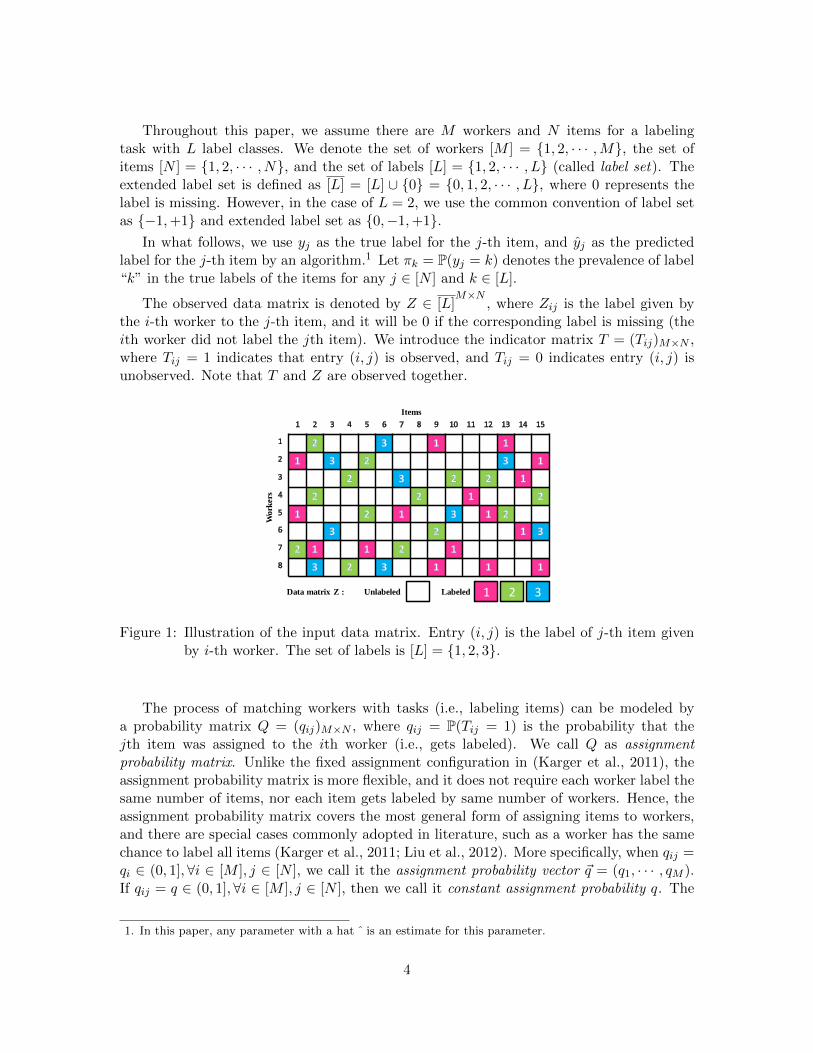
, where Zij is the label given bythe i-th worker to the j-th item, and it will be 0 if the corresponding label is missing (theith worker did not label the jth item). We introduce the indicator matrix T = (Tij)M×N ,where Tij = 1 indicates that entry (i, j) is observed, and Tij = 0 indicates entry (i, j) isunobserved. Note that T and Z are observed together.
Work
ers
Items
Data matrix Z : 1 Unlabeled Labeled 2 3
Figure 1: Illustration of the input data matrix. Entry (i, j) is the label of j-th item givenby i-th worker. The set of labels is [L] = 1, 2, 3.
The process of matching workers with tasks (i.e., labeling items) can be modeled bya probability matrix Q = (qij)M×N , where qij = P(Tij = 1) is the probability that thejth item was assigned to the ith worker (i.e., gets labeled). We call Q as assignmentprobability matrix. Unlike the fixed assignment configuration in (Karger et al., 2011), theassignment probability matrix is more flexible, and it does not require each worker label thesame number of items, nor each item gets labeled by same number of workers. Hence, theassignment probability matrix covers the most general form of assigning items to workers,and there are special cases commonly adopted in literature, such as a worker has the samechance to label all items (Karger et al., 2011; Liu et al., 2012). More specifically, when qij =qi ∈ (0, 1],∀i ∈ [M ], j ∈ [N ], we call it the assignment probability vector ~q = (q1, · · · , qM ).If qij = q ∈ (0, 1],∀i ∈ [M ], j ∈ [N ], then we call it constant assignment probability q. The
1. In this paper, any parameter with a hat ˆ is an estimate for this parameter.
4
three assignment configurations above are referred to as the task assignment 2 is based onprobability matrix Q, probability vector ~q and constant probability q , respectively.
Generally, we use π, p, q as probabilities, and they might have indices according to thecontext. We denote A and C as constants which depend on other given variables, anda as either a general constant or a vector depending on context. η denotes likelihoodprobabilities in the context. Θ denotes a set of parameters. ε and δ are constants in(0, 1), where ε is used for bounding the error rate, and δ is used for denoting a positiveprobability. He(ε) denotes the natural entropy of Bernoulli random variable with parameterε, i.e., He(ε) = −ε ln ε− (1− ε) ln(1− ε). Operators ∧ and ∨ denote the min operator andthe max operator between two numbers, respectively. Meanwhile, throughout the paper,we will locally define each notation in the context before using them.
2.1 Dawid-Skene models
We discuss three models covering all the cases that are widely used for modeling the qualityof the workers (Dawid and Skene, 1979; Raykar et al., 2010; Karger et al., 2011; Liu et al.,2012; Zhou et al., 2012). The first one, which is also the most general one, was originallyproposed by Dawid and Skene (1979):
General Dawid-Skene model. In this model, the reliability of worker i is modeled as
a confusion matrix P (i) =(p
(i)kl
)L×L∈ [0, 1]L×L , which is in a matrix form and represents
a conditional probability table such that
p(i)kl
.= P (Zij = l|yj = k, Tij = 1) , ∀k, l ∈ [L], ∀i ∈ [M ]. (1)
Note that p(i)kk denotes the accuracy of worker i on labeling an item with true label k
correctly, and p(i)kl , k 6= l represents the error probability of labeling an item with true label
k as l mistakenly. The number of free parameters of modeling the reliability of a workerare L(L− 1) under the General Dawid-Skene model.
Since the General Dawid-Skene model has L(L − 1) degree of freedom to model eachworker, it is flexible, but often leads to overfitting on small datasets. As a further regu-larization of the worker models, we consider another two models which are special cases ofGeneral Dawid-Skene model via imposing constraints on the worker confusion matrices.
• Class-Conditional Dawid-Skene model. In this model, the error probabilities of la-beling an item with true label k as label l mistakenly for each worker are the same
2. The term task assignment seems to imply that workers are passive of labeling items — they will surelylabel an item whenever they are assigned to. This might not match the reality in the crowdsourcingplatform. When a task owner distributed tasks to the crowd, it is likely that most of the workers willlabel a set of items and they can stop whenever they want to (Snow et al., 2008), unless they are required(by the owner) to complete a specific set of tasks for getting paid. Thus the process of matching taskswith workers might be determined by either workers (subjectively) or task owners (by enforcement),which depends on how the owners design and distribute tasks. If the workers have choice to select whichitem to label, it might be more proper to call the task-worker matching as task selection, instead of taskassignment. However, both of the cases can be modeled by the probability matrix Q (or probabilityvector ~q, or constant probability q). In what follows, we use the term task assignment to represent thetask-worker matching without introducing ambiguity.
5
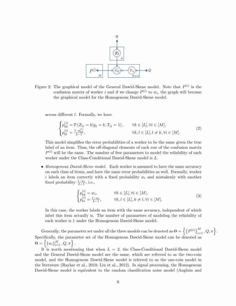
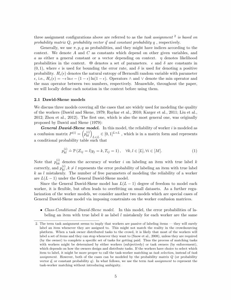
Figure 2: The graphical model of the General Dawid-Skene model. Note that P (i) is theconfusion matrix of worker i and if we change P (i) to wi, the graph will becomethe graphical model for the Homogenous Dawid-Skene model.
across different l. Formally, we havep(i)kk = P (Zij = k|yj = k, Tij = 1) , ∀k ∈ [L],∀i ∈ [M ],
p(i)kl =
1−p(i)kkL−1 , ∀k, l ∈ [L], l 6= k, ∀i ∈ [M ].
(2)
This model simplifies the error probabilities of a worker to be the same given the truelabel of an item. Thus, the off-diagonal elements of each row of the confusion matrixP (i) will be the same. The number of free parameters to model the reliability of eachworker under the Class-Conditional Dawid-Skene model is L.
• Homogenous Dawid-Skene model. Each worker is assumed to have the same accuracyon each class of items, and have the same error probabilities as well. Formally, workeri labels an item correctly with a fixed probability wi and mistakenly with anotherfixed probability 1−wi
L−1 , i.e.,p
(i)kk = wi, ∀k ∈ [L], ∀i ∈ [M ],
p(i)kl = 1−wi
L−1 , ∀k, l ∈ [L], k 6= l,∀i ∈ [M ].(3)
In this case, the worker labels an item with the same accuracy, independent of whichlabel this item actually is. The number of parameters of modeling the reliability ofeach worker is 1 under the Homogenous Dawid-Skene model.
Generally, the parameter set under all the three models can be denoted as Θ =P (i)
Mi=1
, Q, π
.
Specifically, the parameter set of the Homogenous Dawid-Skene model can be denoted as
Θ =wiMi=1 , Q, π
.
It is worth mentioning that when L = 2, the Class-Conditional Dawid-Skene modeland the General Dawid-Skene model are the same, which are referred to as the two-coinmodel, and the Homogenous Dawid-Skene model is referred to as the one-coin model inthe literature (Raykar et al., 2010; Liu et al., 2012). In signal processing, the HomogenousDawid-Skene model is equivalent to the random classification noise model (Angluin and
6
0.8 0.1 0.1
0.1 0.8 0.1
0.1 0.1 0.8
0.7 0.15 0.15
0.05 0.9 0.05
0.1 0.1 0.8
0.7 0.2 0.1
0.03 0.9 0.07
0.05 0.15 0.8
(a) (b) (c) T
ru
e l
ab
el
Predicted label
Figure 3: Toy examples of confusion matrices of different worker reliability models. Weassume L = 3 thus confusion matrices ∈ [0, 1]3×3. (a) General Dawid-Skenemodel. (b) Class-Conditional Dawid-Skene model. (c) Homogenous Dawid-Skenemodel. Vertical axis is actual classes, and horizontal axis is predicted classes.Different color corresponds to different conditional probability, and the diagonalelements are the accuracy of labeling the corresponding class of items correctly.
Laird, 1988), and the Class-Conditional Dawid-Skene model is also referred to as the class-conditional noise model (Natarajan et al., 2013). We do not adopt the original term becausethe error comes from the limitations of workers’ ability to label items correctly, not fromnoise which is in the context of signal processing.
Binary labeling is the special case (L = 2), and it is the major focus of the previousresearch in crowdsourcing (Raykar et al., 2010; Karger et al., 2011; Liu et al., 2012). Asa convention, we assume the set of labels is ±1 instead of 1, 2 when L = 2. Fornotation convenience, we defined the worker confusion matrix in a different way as follows:for i = 1, 2, · · · ,M
p(i)+ = P(Zij = 1|yj = 1, Tij = 1),
p(i)− = P(Zij = −1|yj = −1, Tij = 1).
(4)
Then the parameter set will be Θ =
p
(i)+ , p
(i)−
Mi=1
, Q, π
under this model. When we
present the result of binary labeling, we will use p(i)+ and p
(i)− without introducing any
ambiguity.Under the models above, the posterior probability of the true label of item j to be k is
defined as:
ρ(j)k = P(yj = k|Z, T,Θ), ∀j ∈ [N ]. (5)
For binary labeling, the posterior probability of the true label of item j to be k is definedas:
ρ(j)+ = P(yj = 1|Z, T,Θ), ∀j ∈ [N ]. (6)
2.2 Aggregation rules
After collecting the crowdsourced labels, the task owner could use an arbitrary rule toaggregate the multiple noisy labels of an item to a “refined” label for that item. The
7
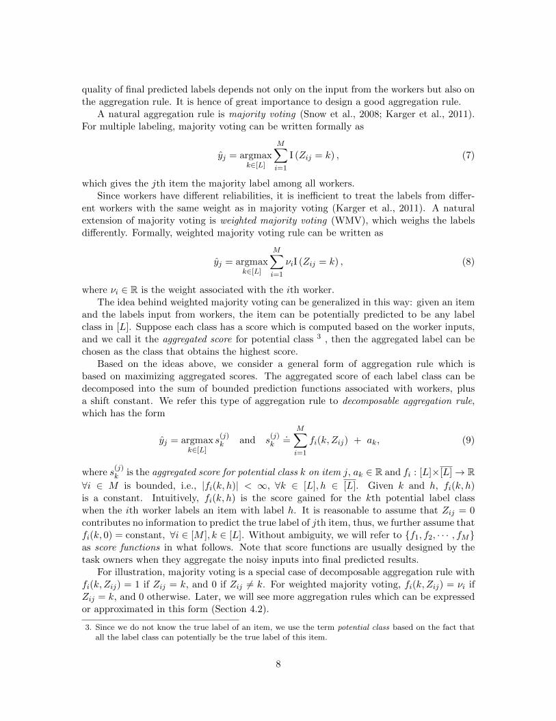
quality of final predicted labels depends not only on the input from the workers but also onthe aggregation rule. It is hence of great importance to design a good aggregation rule.
A natural aggregation rule is majority voting (Snow et al., 2008; Karger et al., 2011).For multiple labeling, majority voting can be written formally as
yj = argmaxk∈[L]
M∑i=1
I (Zij = k) , (7)
which gives the jth item the majority label among all workers.Since workers have different reliabilities, it is inefficient to treat the labels from differ-
ent workers with the same weight as in majority voting (Karger et al., 2011). A naturalextension of majority voting is weighted majority voting (WMV), which weighs the labelsdifferently. Formally, weighted majority voting rule can be written as
yj = argmaxk∈[L]
M∑i=1
νiI (Zij = k) , (8)
where νi ∈ R is the weight associated with the ith worker.The idea behind weighted majority voting can be generalized in this way: given an item
and the labels input from workers, the item can be potentially predicted to be any labelclass in [L]. Suppose each class has a score which is computed based on the worker inputs,and we call it the aggregated score for potential class 3 , then the aggregated label can bechosen as the class that obtains the highest score.
Based on the ideas above, we consider a general form of aggregation rule which isbased on maximizing aggregated scores. The aggregated score of each label class can bedecomposed into the sum of bounded prediction functions associated with workers, plusa shift constant. We refer this type of aggregation rule to decomposable aggregation rule,which has the form
yj = argmaxk∈[L]
s(j)k and s
(j)k
.=
M∑i=1
fi(k, Zij) + ak, (9)
where s(j)k is the aggregated score for potential class k on item j, ak ∈ R and fi : [L]×[L]→ R
∀i ∈ M is bounded, i.e., |fi(k, h)| < ∞, ∀k ∈ [L], h ∈ [L]. Given k and h, fi(k, h)is a constant. Intuitively, fi(k, h) is the score gained for the kth potential label classwhen the ith worker labels an item with label h. It is reasonable to assume that Zij = 0contributes no information to predict the true label of jth item, thus, we further assume thatfi(k, 0) = constant, ∀i ∈ [M ], k ∈ [L]. Without ambiguity, we will refer to f1, f2, · · · , fMas score functions in what follows. Note that score functions are usually designed by thetask owners when they aggregate the noisy inputs into final predicted results.
For illustration, majority voting is a special case of decomposable aggregation rule withfi(k, Zij) = 1 if Zij = k, and 0 if Zij 6= k. For weighted majority voting, fi(k, Zij) = νi ifZij = k, and 0 otherwise. Later, we will see more aggregation rules which can be expressedor approximated in this form (Section 4.2).
3. Since we do not know the true label of an item, we use the term potential class based on the fact thatall the label class can potentially be the true label of this item.
8
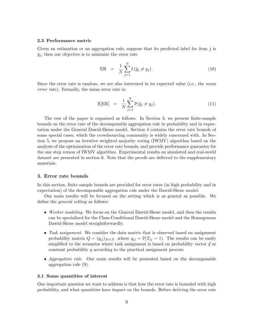
2.3 Performance metric
Given an estimation or an aggregation rule, suppose that its predicted label for item j isyj , then our objective is to minimize the error rate
ER =1
N
N∑j=1
I (yj 6= yj) . (10)
Since the error rate is random, we are also interested in its expected value (i.e., the meanerror rate). Formally, the mean error rate is:
E[ER] =1
N
N∑j=1
P(yj 6= yj). (11)
The rest of the paper is organized as follows. In Section 3, we present finite-samplebounds on the error rate of the decomposable aggregation rule in probability and in expec-tation under the General Dawid-Skene model. Section 4 contains the error rate bounds ofsome special cases, which the crowdsourcing community is widely concerned with. In Sec-tion 5, we propose an iterative weighted majority voting (IWMV) algorithm based on theanalysis of the optimization of the error rate bounds, and provide performance guarantee forthe one step verson of IWMV algorithm. Experimental results on simulated and real-worlddataset are presented in section 6. Note that the proofs are deferred to the supplementarymaterials.
3. Error rate bounds
In this section, finite sample bounds are provided for error rates (in high probability and inexpectation) of the decomposable aggregation rule under the Dawid-Skene model.
Our main results will be focused on the setting which is as general as possible. Wedefine the general setting as follows:
• Worker modeling. We focus on the General Dawid-Skene model, and then the resultscan be specialized for the Class-Conditional Dawid-Skene model and the HomogenousDawid-Skene model straightforwardly.
• Task assignment. We consider the data matrix that is observed based on assignmentprobability matrix Q = (qij)M×N ,where qij = P(Tij = 1). The results can be easilysimplified to the scenarios where task assignment is based on probability vector ~q orconstant probability q according to the practical assignment process.
• Aggregation rule. Our main results will be presented based on the decomposableaggregation rule (9).
3.1 Some quantities of interest
One important question we want to address is that how the error rate is bounded with highprobability, and what quantities have impact on the bounds. Before deriving the error rate
9
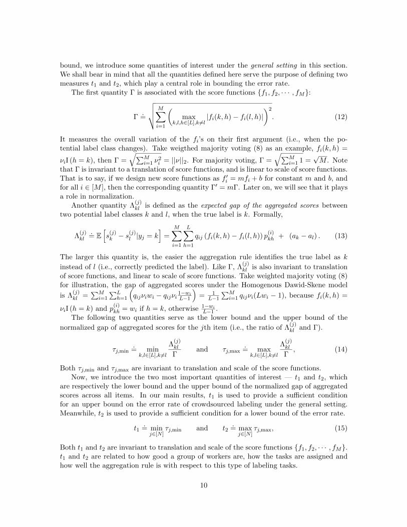
bound, we introduce some quantities of interest under the general setting in this section.We shall bear in mind that all the quantities defined here serve the purpose of defining twomeasures t1 and t2, which play a central role in bounding the error rate.
The first quantity Γ is associated with the score functions f1, f2, · · · , fM:
Γ.=
√√√√ M∑i=1
(max
k,l,h∈[L],k 6=l|fi(k, h)− fi(l, h)|
)2
. (12)
It measures the overall variation of the fi’s on their first argument (i.e., when the po-tential label class changes). Take weigthed majority voting (8) as an example, fi(k, h) =
νiI (h = k), then Γ =√∑M
i=1 ν2i = ||ν||2. For majority voting, Γ =
√∑Mi=1 1 =
√M . Note
that Γ is invariant to a translation of score functions, and is linear to scale of score functions.That is to say, if we design new score functions as f ′i = mfi + b for constant m and b, andfor all i ∈ [M ], then the corresponding quantity Γ′ = mΓ. Later on, we will see that it playsa role in normalization.
Another quantity Λ(j)kl is defined as the expected gap of the aggregated scores between
two potential label classes k and l, when the true label is k. Formally,
Λ(j)kl
.= E
[s
(j)k − s
(j)l |yj = k
]=
M∑i=1
L∑h=1
qij (fi(k, h)− fi(l, h)) p(i)kh + (ak − al) . (13)
The larger this quantity is, the easier the aggregation rule identifies the true label as k
instead of l (i.e., correctly predicted the label). Like Γ, Λ(j)kl is also invariant to translation
of score functions, and linear to scale of score functions. Take weighted majority voting (8)for illustration, the gap of aggregated scores under the Homogenous Dawid-Skene model
is Λ(j)kl =
∑Mi=1
∑Lh=1
(qijνiwi − qijνi 1−wi
L−1
)= 1
L−1
∑Mi=1 qijνi(Lwi − 1), because fi(k, h) =
νiI (h = k) and p(i)kh = wi if h = k, otherwise 1−wi
L−1 .The following two quantities serve as the lower bound and the upper bound of the
normalized gap of aggregated scores for the jth item (i.e., the ratio of Λ(j)kl and Γ).
τj,min.= min
k,l∈[L],k 6=l
Λ(j)kl
Γand τj,max
.= max
k,l∈[L],k 6=l
Λ(j)kl
Γ, (14)
Both τj,min and τj,max are invariant to translation and scale of the score functions.Now, we introduce the two most important quantities of interest — t1 and t2, which
are respectively the lower bound and the upper bound of the normalized gap of aggregatedscores across all items. In our main results, t1 is used to provide a sufficient conditionfor an upper bound on the error rate of crowdsourced labeling under the general setting.Meanwhile, t2 is used to provide a sufficient condition for a lower bound of the error rate.
t1.= min
j∈[N ]τj,min and t2
.= max
j∈[N ]τj,max, (15)
Both t1 and t2 are invariant to translation and scale of the score functions f1, f2, · · · , fM.t1 and t2 are related to how good a group of workers are, how the tasks are assigned andhow well the aggregation rule is with respect to this type of labeling tasks.
10
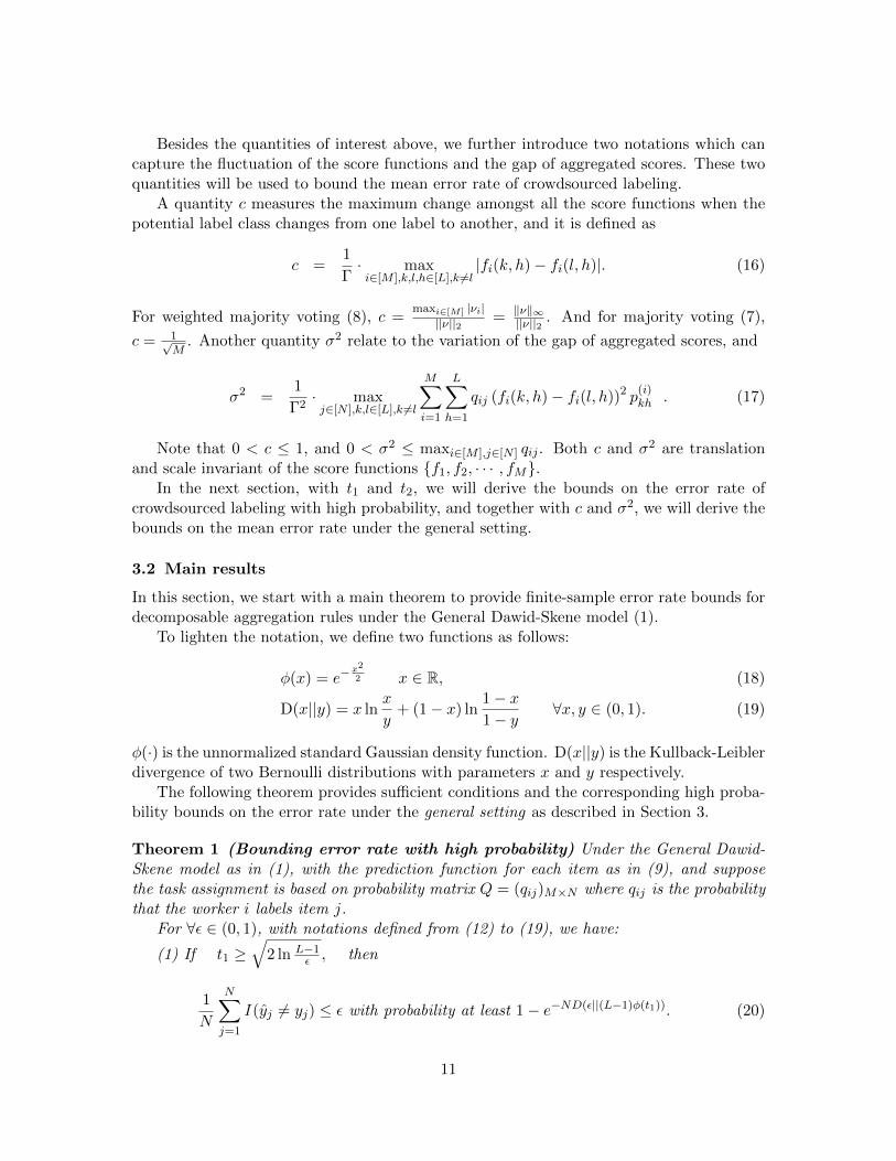
Besides the quantities of interest above, we further introduce two notations which cancapture the fluctuation of the score functions and the gap of aggregated scores. These twoquantities will be used to bound the mean error rate of crowdsourced labeling.
A quantity c measures the maximum change amongst all the score functions when thepotential label class changes from one label to another, and it is defined as
c =1
Γ· maxi∈[M ],k,l,h∈[L],k 6=l
|fi(k, h)− fi(l, h)|. (16)
For weighted majority voting (8), c =maxi∈[M ] |νi|||ν||2 = ‖ν‖∞
||ν||2 . And for majority voting (7),
c = 1√M
. Another quantity σ2 relate to the variation of the gap of aggregated scores, and
σ2 =1
Γ2· maxj∈[N ],k,l∈[L],k 6=l
M∑i=1
L∑h=1
qij (fi(k, h)− fi(l, h))2 p(i)kh . (17)
Note that 0 < c ≤ 1, and 0 < σ2 ≤ maxi∈[M ],j∈[N ] qij . Both c and σ2 are translationand scale invariant of the score functions f1, f2, · · · , fM.
In the next section, with t1 and t2, we will derive the bounds on the error rate ofcrowdsourced labeling with high probability, and together with c and σ2, we will derive thebounds on the mean error rate under the general setting.
3.2 Main results
In this section, we start with a main theorem to provide finite-sample error rate bounds fordecomposable aggregation rules under the General Dawid-Skene model (1).
To lighten the notation, we define two functions as follows:
φ(x) = e−x2
2 x ∈ R, (18)
D(x||y) = x lnx
y+ (1− x) ln
1− x1− y
∀x, y ∈ (0, 1). (19)
φ(·) is the unnormalized standard Gaussian density function. D(x||y) is the Kullback-Leiblerdivergence of two Bernoulli distributions with parameters x and y respectively.
The following theorem provides sufficient conditions and the corresponding high proba-bility bounds on the error rate under the general setting as described in Section 3.
Theorem 1 (Bounding error rate with high probability) Under the General Dawid-Skene model as in (1), with the prediction function for each item as in (9), and supposethe task assignment is based on probability matrix Q = (qij)M×N where qij is the probabilitythat the worker i labels item j.
For ∀ε ∈ (0, 1), with notations defined from (12) to (19), we have:
(1) If t1 ≥√
2 ln L−1ε , then
1
N
N∑j=1
I (yj 6= yj) ≤ ε with probability at least 1− e−ND(ε||(L−1)φ(t1)). (20)
11
(2) If t2 ≤ −√
2 ln 11−ε , then
1
N
N∑j=1
I (yj 6= yj) ≥ ε with probability at least 1− e−ND(ε||1−φ(t2)). (21)
Remark: The high probability bounds on error rate require conditions on t1 and t2,which are related to the normalized gap of aggregated scores (Section 3.1). Basically, if thescores of predicting an item as its true label (predicted correctly) are larger than the scoresof predicting as a wrong label, then it is more likely that the error rate will be small, thusit is bounded from above with high probability. The interpretation of the lower bound andits condition is similar to the upper bound.
To ensure the probability of bounding the error rate to be at least 1 − δ, we have tosolve the equation D(ε||(L− 1)φ(t1)) = 1
N ln 1δ , which cannot be solved analytically. Thus,
we need to figure out the minimum t1 for bounding the error rate with probability at least1 − δ. The following theorem serves this purpose by slightly relaxing the conditions on t1and t2 in Theorem 1.
Before presenting the next theorem, we define a notation C , which depends on param-eters ε, δ ∈ (0, 1), for lightening notations in the theorem.
C(ε, δ) = 1 + exp
(1
ε
[He(ε) +
1
Nln
1
δ
]), (22)
where He(ε) = −ε ln ε− (1− ε) ln(1− ε), which is the natural entropy of a Bernoulli randomvariable with parameter ε.
Theorem 2 With the same notation as in Theorem 1, for ∀ε, δ ∈ (0, 1), we have:(1) if t1 ≥
√2 ln [(L− 1)C(ε, δ)], then 1
N
∑Nj=1 I (yj 6= yj) ≤ ε with probability at least
1− δ,(2) if t2 ≤ −
√2 lnC(1− ε, δ), then 1
N
∑Nj=1 I (yj 6= yj) ≥ ε with probability at least
1− δ.
Remark: For any scenarios that can be formulated into the general setting as in 3,with t1 and t2 computed as in Section 3.1, both Theorem 1 and Theorem 2 can be applied.Therefore, in the rest of the paper, for any special case (Section 4) of the general setting ,we will only present one of Theorem 1 and Theorem 2, and omit the other for clarity.
In practice, the mean error rate might be a better measure of performance because ofits non-random nature. The method of evaluating the accuracy of a certain algorithm isoften conducted by taking an empirical average of its performance in each trial, which is aconsistent estimator of the mean error rate. Thus it will be of general interest to bound themean error rate.
For the next theorem, we present the mean error rate bound under the general settingused in Theorem 1.
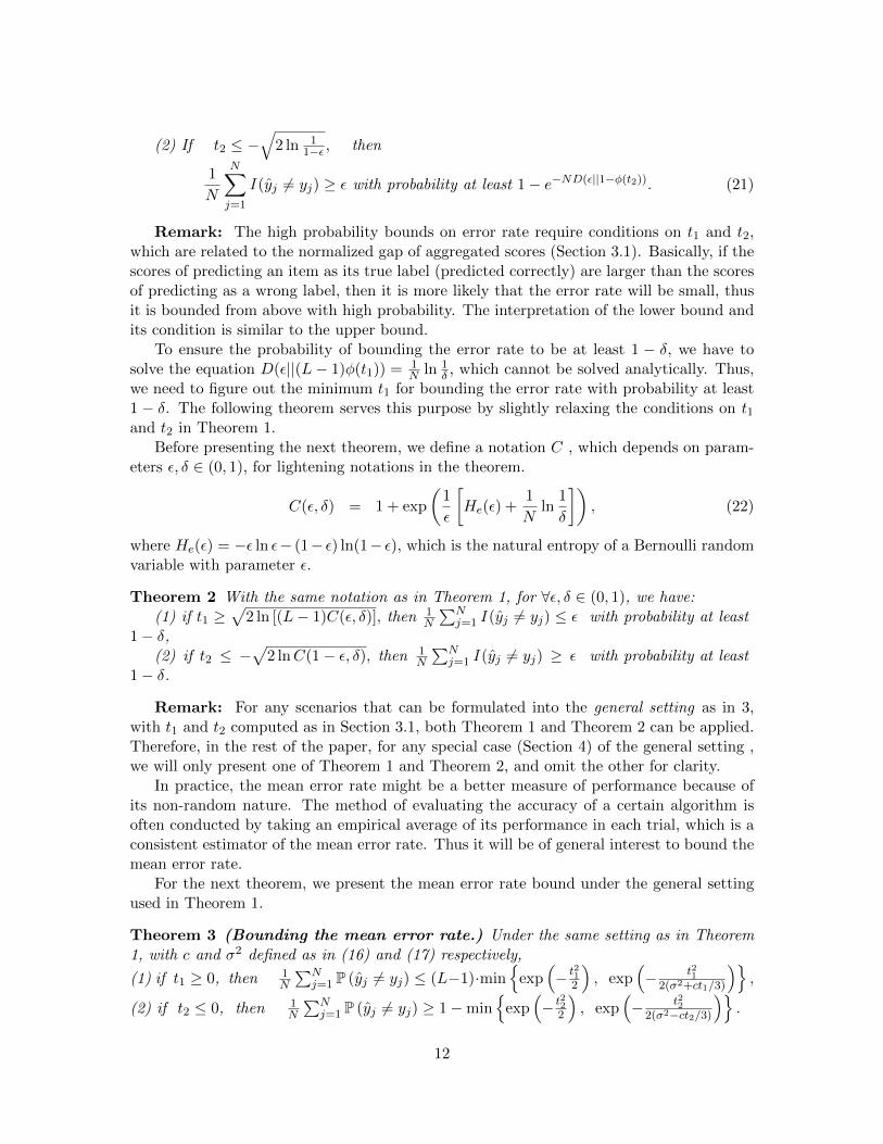
Theorem 3 (Bounding the mean error rate.) Under the same setting as in Theorem1, with c and σ2 defined as in (16) and (17) respectively,
(1) if t1 ≥ 0, then 1N
∑Nj=1 P (yj 6= yj) ≤ (L−1)·min
exp
(− t21
2
), exp
(− t21
2(σ2+ct1/3)
),
(2) if t2 ≤ 0, then 1N
∑Nj=1 P (yj 6= yj) ≥ 1−min
exp
(− t22
2
), exp
(− t22
2(σ2−ct2/3)
).
12
Remark: The results above are composed of two exponential bounds, and neither isgenerally dominant over the other. Thus each component inside the min operator can beserved as an individual bound for the mean error rate. Take the upper bound in (1) as anexample, when t1 is small (recall that both σ2 and c are bounded above by 1), the secondcomponent will be tighter than the first one. Thus the error rate bound behaves like e−t1 .Otherwise, the first component will be tighter, and the mean error rate behaves like e−t
21 .
All the proofs of the results in this section are deferred to Appendix A. In the followingsection, we demonstrate how the main results here can be applied to various settings oflabeling by crowdsourcing, and provide theoretical bounds for the error rate correspondingly.
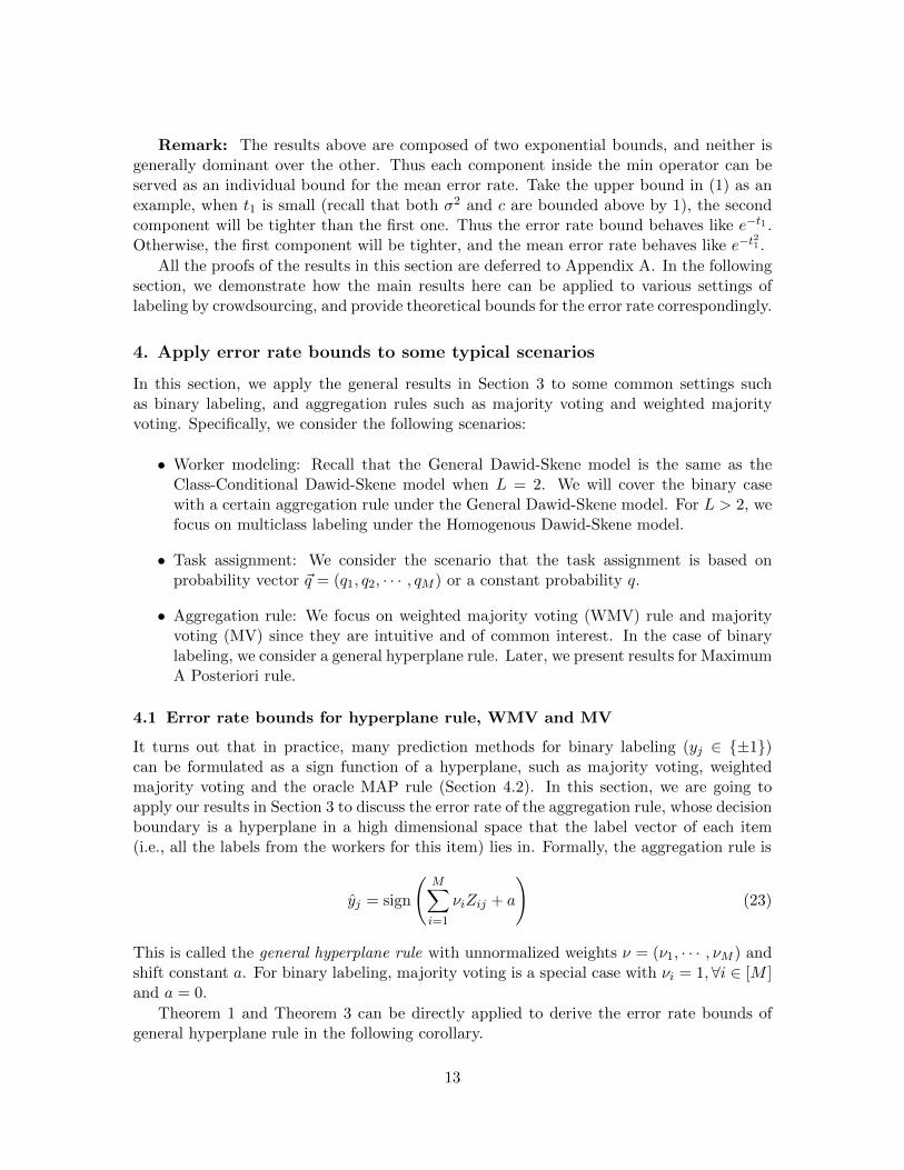
4. Apply error rate bounds to some typical scenarios
In this section, we apply the general results in Section 3 to some common settings suchas binary labeling, and aggregation rules such as majority voting and weighted majorityvoting. Specifically, we consider the following scenarios:
• Worker modeling: Recall that the General Dawid-Skene model is the same as theClass-Conditional Dawid-Skene model when L = 2. We will cover the binary casewith a certain aggregation rule under the General Dawid-Skene model. For L > 2, wefocus on multiclass labeling under the Homogenous Dawid-Skene model.
• Task assignment: We consider the scenario that the task assignment is based onprobability vector ~q = (q1, q2, · · · , qM ) or a constant probability q.
• Aggregation rule: We focus on weighted majority voting (WMV) rule and majorityvoting (MV) since they are intuitive and of common interest. In the case of binarylabeling, we consider a general hyperplane rule. Later, we present results for MaximumA Posteriori rule.
4.1 Error rate bounds for hyperplane rule, WMV and MV
It turns out that in practice, many prediction methods for binary labeling (yj ∈ ±1)can be formulated as a sign function of a hyperplane, such as majority voting, weightedmajority voting and the oracle MAP rule (Section 4.2). In this section, we are going toapply our results in Section 3 to discuss the error rate of the aggregation rule, whose decisionboundary is a hyperplane in a high dimensional space that the label vector of each item(i.e., all the labels from the workers for this item) lies in. Formally, the aggregation rule is
yj = sign
(M∑i=1
νiZij + a
)(23)
This is called the general hyperplane rule with unnormalized weights ν = (ν1, · · · , νM ) andshift constant a. For binary labeling, majority voting is a special case with νi = 1, ∀i ∈ [M ]and a = 0.
Theorem 1 and Theorem 3 can be directly applied to derive the error rate bounds ofgeneral hyperplane rule in the following corollary.
13

When task assignment is based on probability vector ~q, the corresponding quantities ofinterest for the hyperplane rule (as in Section 3.1) are defined as follows:
t1 =1
||ν||2
[(M∑i=1
qiνi(2p(i)+ − 1) + a
)∧
(M∑i=1
qiνi(2p(i)− − 1)− a
)](24)
t2 =1
||ν||2
[(M∑i=1
qiνi(2p(i)+ − 1) + a
)∨
(M∑i=1
qiνi(2p(i)− − 1)− a
)](25)
c =||ν||∞||ν||2
and σ2 =1
||ν||22
M∑i=1
qiν2i , (26)
where ∧ and ∨ are min and max operators respectively, ||ν||∞.= maxi∈[M ] |νi|, and functions
φ(x) and D(x||y) are defined in (18) and (19).
Corollary 4 (Hyperplane rule in binary labeling) Consider binary labeling under the Gen-
eral Dawid-Skene model, i.e., yj ∈ ±1, p(i)+ and p
(i)− are defined as in (4). Suppose the
task assignment is based on probability vector ~q = (q1, q2, · · · , qM ) where qi is the probabilitythat worker i labels an item, aggregation rule is general hyperplane rule as in (23), and thequantities of interest are defined in (24)-(26), for ∀ε ∈ (0, 1):
(1) If t1 ≥ 0, then 1N
∑Nj=1 P (yj 6= yj) ≤ min
exp
(− t21
2
), exp
(− t21
2(σ2+ct1/3)
).
Furthermore, if t1 ≥√
2 ln 1ε , then P
(1N
∑Nj=1 I (yj 6= yj) ≤ ε
)≥ 1−e−ND(ε||φ(t1)).
(2) If t2 ≤ 0, then 1N
∑Nj=1 P (yj 6= yj) ≥ 1−min
exp
(− t22
2
), exp
(− t22
2(σ2−ct2/3)
).
Furthermore, if t2 ≤ −√
2 ln 11−ε , then P
(1N
∑Nj=1 I (yj 6= yj) ≥ ε
)≥ 1−e−ND(ε||1−φ(t2)).
Proof The aggregation rule can be expressed as yj = argmaxk∈±1∑M
i=1 νiI (Zij = k)+ak,where a+ = a and a− = 0. Directly apply Theorem 1 and Theorem 3, with fi(k, k) = νi for
k ∈ ±1, fi(k, l) = 0 for k 6= l, and denote p(i)kl in terms of p
(i)+ and p
(i)− , qij = qi,∀j ∈ [N ],
we can obtain the desired result immediately.
Remark: From this corollary, we know that if t1 is big enough, then the error rate willbe upper bounded by ε with high probability. This means when the workers’ reliabilitiesare generally good, it is very likely that we will have high quality aggregated results. Notethat usually we can freely choose q, ν and a, so the most important factors are worker
reliabilities on positive samples (p(i)+ ) and negative samples (p
(i)− ).
If one needs to know, given ε and δ, what are the results under the setting abovecorresponding to Theorem 2, we can simply compute t1 and t2 as listed in Corollary 4, thenthe conditions and bounds in Theorem 2 hold.
As mentioned in the beginning of this section, weighted majority voting (WMV) is animportant special case covered by our results in Section 3. For the next several results,we focus on the mean error rate bound of WMV and MV under Homogenous Dawid-Skenemodel.
14
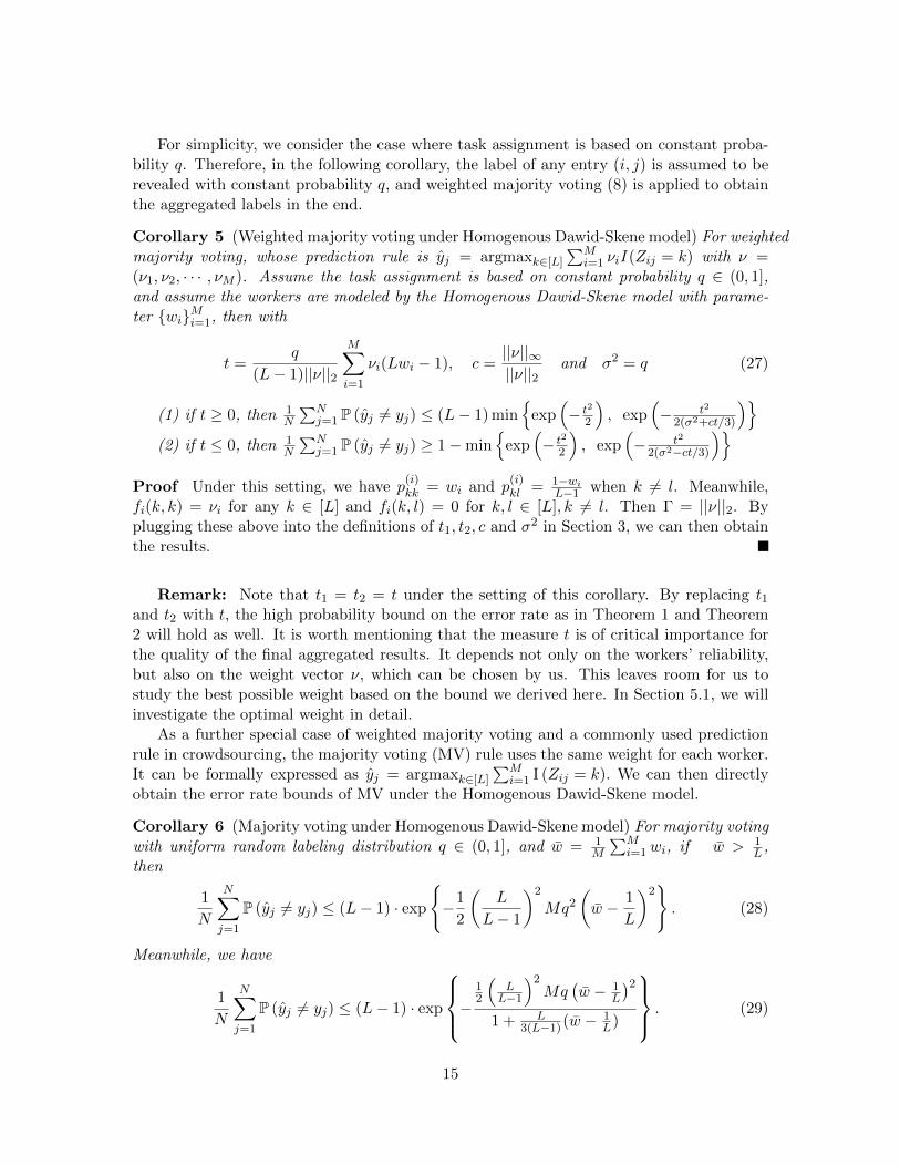
For simplicity, we consider the case where task assignment is based on constant proba-bility q. Therefore, in the following corollary, the label of any entry (i, j) is assumed to berevealed with constant probability q, and weighted majority voting (8) is applied to obtainthe aggregated labels in the end.
Corollary 5 (Weighted majority voting under Homogenous Dawid-Skene model) For weightedmajority voting, whose prediction rule is yj = argmaxk∈[L]
∑Mi=1 νiI (Zij = k) with ν =
(ν1, ν2, · · · , νM ). Assume the task assignment is based on constant probability q ∈ (0, 1],and assume the workers are modeled by the Homogenous Dawid-Skene model with parame-ter wiMi=1, then with
t =q
(L− 1)||ν||2
M∑i=1
νi(Lwi − 1), c =||ν||∞||ν||2
and σ2 = q (27)
(1) if t ≥ 0, then 1N
∑Nj=1 P (yj 6= yj) ≤ (L− 1) min
exp
(− t2
2
), exp
(− t2
2(σ2+ct/3)
)(2) if t ≤ 0, then 1
N
∑Nj=1 P (yj 6= yj) ≥ 1−min
exp
(− t2
2
), exp
(− t2
2(σ2−ct/3)
)Proof Under this setting, we have p
(i)kk = wi and p
(i)kl = 1−wi
L−1 when k 6= l. Meanwhile,fi(k, k) = νi for any k ∈ [L] and fi(k, l) = 0 for k, l ∈ [L], k 6= l. Then Γ = ||ν||2. Byplugging these above into the definitions of t1, t2, c and σ2 in Section 3, we can then obtainthe results.
Remark: Note that t1 = t2 = t under the setting of this corollary. By replacing t1and t2 with t, the high probability bound on the error rate as in Theorem 1 and Theorem2 will hold as well. It is worth mentioning that the measure t is of critical importance forthe quality of the final aggregated results. It depends not only on the workers’ reliability,but also on the weight vector ν, which can be chosen by us. This leaves room for us tostudy the best possible weight based on the bound we derived here. In Section 5.1, we willinvestigate the optimal weight in detail.
As a further special case of weighted majority voting and a commonly used predictionrule in crowdsourcing, the majority voting (MV) rule uses the same weight for each worker.It can be formally expressed as yj = argmaxk∈[L]
∑Mi=1 I (Zij = k). We can then directly
obtain the error rate bounds of MV under the Homogenous Dawid-Skene model.
Corollary 6 (Majority voting under Homogenous Dawid-Skene model) For majority votingwith uniform random labeling distribution q ∈ (0, 1], and w = 1
M
∑Mi=1wi, if w > 1
L ,then
1
N
N∑j=1
P (yj 6= yj) ≤ (L− 1) · exp
−1
2
(L
L− 1
)2
Mq2
(w − 1
L
)2. (28)
Meanwhile, we have
1
N
N∑j=1
P (yj 6= yj) ≤ (L− 1) · exp
−12
(LL−1
)2Mq
(w − 1
L
)21 + L
3(L−1)(w − 1L)
. (29)
15
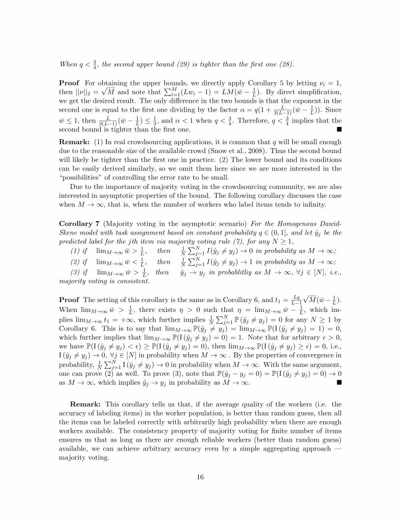
When q < 34 , the second upper bound (29) is tighter than the first one (28).
Proof For obtaining the upper bounds, we directly apply Corollary 5 by letting νi = 1,then ||ν||2 =
√M and note that
∑Mi=1(Lwi − 1) = LM(w − 1
L). By direct simplification,we get the desired result. The only difference in the two bounds is that the exponent in thesecond one is equal to the first one dividing by the factor α = q(1 + L
3(L−1)(w − 1L)). Since
w ≤ 1, then L3(L−1)(w − 1
L) ≤ 13 , and α < 1 when q < 3
4 . Therefore, q < 34 implies that the
second bound is tighter than the first one.
Remark: (1) In real crowdsourcing applications, it is common that q will be small enoughdue to the reasonable size of the available crowd (Snow et al., 2008). Thus the second boundwill likely be tighter than the first one in practice. (2) The lower bound and its conditionscan be easily derived similarly, so we omit them here since we are more interested in the“possibilities” of controlling the error rate to be small.
Due to the importance of majority voting in the crowdsourcing community, we are alsointerested in asymptotic properties of the bound. The following corollary discusses the casewhen M →∞, that is, when the number of workers who label items tends to infinity.
Corollary 7 (Majority voting in the asymptotic scenario) For the Homogenous Dawid-Skene model with task assignment based on constant probability q ∈ (0, 1], and let yj be thepredicted label for the jth item via majority voting rule (7), for any N ≥ 1,
(1) if limM→∞ w > 1L , then 1
N
∑Nj=1 I (yj 6= yj)→ 0 in probability as M →∞;
(2) if limM→∞ w < 1L , then 1
N
∑Nj=1 I (yj 6= yj)→ 1 in probability as M →∞;
(3) if limM→∞ w > 1L , then yj → yj in probablitliy as M → ∞, ∀j ∈ [N ], i.e.,
majority voting is consistent.
Proof The setting of this corollary is the same as in Corollary 6, and t1 = LqL−1
√M(w− 1
L).
When limM→∞ w > 1L , there exists η > 0 such that η = limM→∞ w − 1
L , which im-
plies limM→∞ t1 = +∞, which further implies 1N
∑Nj=1 P (yj 6= yj) = 0 for any N ≥ 1 by
Corollary 6. This is to say that limM→∞ P(yj 6= yj) = limM→∞ P(I (yj 6= yj) = 1) = 0,which further implies that limM→∞ P(I (yj 6= yj) = 0) = 1. Note that for arbitrary ε > 0,we have P(I (yj 6= yj) < ε) ≥ P(I (yj 6= yj) = 0), then limM→∞ P(I (yj 6= yj) ≥ ε) = 0, i.e.,I (yj 6= yj)→ 0, ∀j ∈ [N ] in probability when M →∞ . By the properties of convergence in
probability, 1N
∑Nj=1 I (yj 6= yj)→ 0 in probability when M →∞. With the same argument,
one can prove (2) as well. To prove (3), note that P(yj − yj = 0) = P(I (yj 6= yj) = 0)→ 0as M →∞, which implies yj → yj in probability as M →∞.
Remark: This corollary tells us that, if the average quality of the workers (i.e. theaccuracy of labeling items) in the worker population, is better than random guess, then allthe items can be labeled correctly with arbitrarily high probability when there are enoughworkers available. The consistency property of majority voting for finite number of itemsensures us that as long as there are enough reliable workers (better than random guess)available, we can achieve arbitrary accuracy even by a simple aggregating approach —majority voting.
16
The examples we covered in this section do not require the estimation of parameters suchas worker reliabilities. In the next section, we discuss the maximizing likelihood methods forinferring the parameters in crowdsourcing models, such as the celebrated EM (Expectation-Maximization) algorithm. Then we illustrate how our main results can be applied to analyzean underlining method that the ML methods approximate.
4.2 Error rate bounds for the Maximum A Posteriori rule
If we know the label posterior distribution of each item defined in (5), then the Bayesclassifier is
yj = argmaxk∈[L]
ρ(j)k , (30)
which is well known to be the optimal classifier (Duda et al., 2012).
In reality, we do not know the true parameters of the model, thus the true posteriorremains unknown. One natural way is to estimate the parameters of the model by MaximumLikelihood methods, further estimate the posterior of each label class for each item, andthen build a classifier based on that. This is usually called the Maximum A Posteriori(MAP) approach (Duda et al., 2012). After the EM algorithm estimating parameters, theMaximum A Posteriori (MAP) rule, which predicts the label of an item as the one that hasthe largest estimated posterior, can be applied. The prediction function of such a rule is
yj = argmaxk∈[L]
ρ(j)k , (31)
where ρ(j)k is the estimated posterior. If the MAP rule is applied after the parameters are
learned by the EM algorithm, then we call this method the EM-MAP rule, and sometimessimply refer it to EM without introducing any ambiguity in the context.
However, the EM algorithm cannot guarantee convergence to the global optimum. Thus,the estimated parameters might be biased from the true parameters and the estimatedposterior might be far away from the true one if it starts from a “bad” initialization.Moreover, it is generally hard to study the solution of the EM algorithm, and thus it isrelatively difficult for us to obtain the error rate for the EM-MAP rule.
We consider the oracle MAP rule, which assumes there is an oracle who knows the trueparameters and uses the true posterior to predict labels. Hence the oracle MAP rule is the
Bayes classifier (30), and recall that its prediction function is yj = argmaxk∈[L] ρ(j)k , where
ρ(j)k is the true posterior of yj = k. Based on our empirical observations (Section 6), the
EM-MAP rule approximates the oracle MAP rule well in performance when most of theworkers are good (better than random guess). In the next, we provide an error rate boundfor the oracle MAP rule, which hopefully will help us understand the EM-MAP rule better.
The following result is about the error rate bounds on the oracle MAP rule, and it canbe straightforwardly derived from the main results in Section 3 since the oracle MAP ruleis a decomposable rule as in (9).
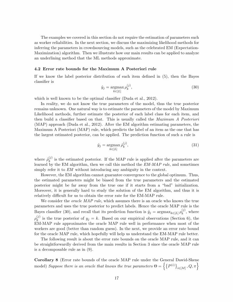
Corollary 8 (Error rate bounds of the oracle MAP rule under the General Dawid-Skene
model) Suppose there is an oracle that knows the true parameters Θ =P (i)
i∈[M ]
, Q, π
17
where P (i) =(p
(i)kh
)k,h∈[L]
∈ (0, 1]L×L. The prediction function of the oracle MAP rule is
yj = argmaxk∈[L] ρ(j)k , where ρ
(j)k is the true posterior. All the error rate bounds in Theorem
1, 2 and 3 hold for the oracle MAP rule with fi(k, h).= log p
(i)kh, ∀k, h ∈ [L].
As a special case of General Dawid-Skene model, the Homogenous Dawid-Skene modelis relatively easy to visualize and simulate. Therefore, the results under this model willbe useful in simulation. The next corollary shows that the oracle MAP rule under theHomogenous Dawid-Skene model is weighted majority voting with class dependent shiftsakk∈[L] where ak = log πk. For simplicity, we assume that the true labels of the items are
drawn from uniform distribution (i.e., πk = 1L , balanced classes).
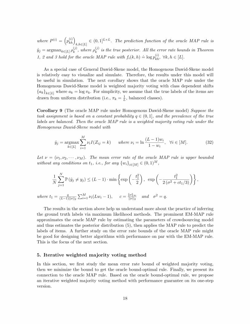
Corollary 9 (The oracle MAP rule under Homogenous Dawid-Skene model) Suppose thetask assignment is based on a constant probability q ∈ (0, 1], and the prevalence of the truelabels are balanced. Then the oracle MAP rule is a weighted majority voting rule under theHomogenous Dawid-Skene model with
yj = argmaxk∈[L]
M∑i=1
νiI (Zij = k) where νi = ln(L− 1)wi
1− wi, ∀i ∈ [M ]. (32)
Let ν = (ν1, ν2, · · · , νM ). The mean error rate of the oracle MAP rule is upper boundedwithout any conditions on t1, i.e., for any wii∈[M ] ∈ (0, 1)M ,
1
N
N∑j=1
P (yj 6= yj) ≤ (L− 1) ·min
exp
(− t
21
2
), exp
(− t21
2 (σ2 + ct1/3)
),
where t1 = q(L−1)||ν||2
∑Mi=1 νi(Lwi − 1), c = ‖ν‖∞
||ν||2 and σ2 = q.
The results in the section above help us understand more about the practice of inferringthe ground truth labels via maximum likelihood methods. The prominent EM-MAP ruleapproximates the oracle MAP rule by estimating the parameters of crowdsourcing modeland thus estimates the posterior distribution (5), then applies the MAP rule to predict thelabels of items. A further study on the error rate bounds of the oracle MAP rule mightbe good for designing better algorithms with performance on par with the EM-MAP rule.This is the focus of the next section.
5. Iterative weighted majority voting method
In this section, we first study the mean error rate bound of weighted majority voting,then we minimize the bound to get the oracle bound-optimal rule. Finally, we present itsconnection to the oracle MAP rule. Based on the oracle bound-optimal rule, we proposean iterative weighted majority voting method with performance guarantee on its one-stepversion.
18
5.1 The oracle bound-optimal rule and the oracle MAP rule
Here we explore the relationship between the oracle MAP rule and the mean error rate boundof WMV under the Homogenous Dawid-Skene model. We assume the task assignmentis based on a constant probability q for simplicity, and ignore the shift terms ak inthe aggregation rules (this is the case for the oracle MAP rule when the label classes arebalanced, Corollary 9).
The mean error rate bound of weighted majority voting (WMV) in Corollary 5 implies
that if t1 ≥ 0, then 1N
∑Nj=1 P (yj 6= yj) ≤ (L− 1) ·min
exp
(− t21
2
), exp
(− t21
2(σ2+ct1/3)
),
where σ2 = q and 1√M≤ c ≤ 1. Note that the impact of c on the bound is marginal
compared to that of t1 since c can be replaced by 1 to relax the bound slightly. At the same
time, both functions exp(− t21
2
)and exp
(− t21
2(σ2+ct1/3)
)are monotonely decreasing w.r.t.
t1 ∈ [0,∞). Thus the upper bound (L− 1) ·min
exp(− t21
2
), exp
(− t21
2(σ2+ct1/3)
)is also
monotonely decreasing w.r.t. t1 ∈ [0,∞). The mean error rate is bounded from above withthe condition t1 ≥ 0. Therefore, maximizing t1 will increase the chance of t1 ≥ 0 beingsatisfied and reduce the bound to some extent. Recall that
t1 =q
L− 1
M∑i=1
νi||ν||2
(Lwi − 1).
Since q is fixed now and we assume t1 ≥ 0, so optimizing the upper bound is equivalent tomaximizing t1:
ν? = argmaxν∈RM
t1 = argmaxν∈RM
q
L− 1
M∑i=1
νi||ν||2
(Lwi − 1)
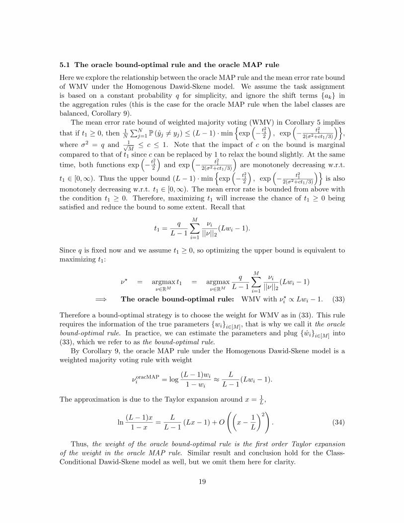
=⇒ The oracle bound-optimal rule: WMV with ν?i ∝ Lwi − 1. (33)
Therefore a bound-optimal strategy is to choose the weight for WMV as in (33). This rulerequires the information of the true parameters wii∈[M ], that is why we call it the oraclebound-optimal rule. In practice, we can estimate the parameters and plug wii∈[M ] into(33), which we refer to as the bound-optimal rule.
By Corollary 9, the oracle MAP rule under the Homogenous Dawid-Skene model is aweighted majority voting rule with weight
νoracMAPi = log
(L− 1)wi1− wi
≈ L
L− 1(Lwi − 1).
The approximation is due to the Taylor expansion around x = 1L ,
ln(L− 1)x
1− x=
L
L− 1(Lx− 1) +O
((x− 1
L
)2). (34)
Thus, the weight of the oracle bound-optimal rule is the first order Taylor expansionof the weight in the oracle MAP rule. Similar result and conclusion hold for the Class-Conditional Dawid-Skene model as well, but we omit them here for clarity.
19
By observing that the oracle MAP rule is very close to the oracle bound-optimal rule,the oracle MAP rule approximately optimizes the upper bound of the mean error rate. Thisfact also indicates that our bound is meaningful since the oracle MAP rule is the oracleBayes classifier.
5.2 Iterative weighted majority voting with performance guarantee
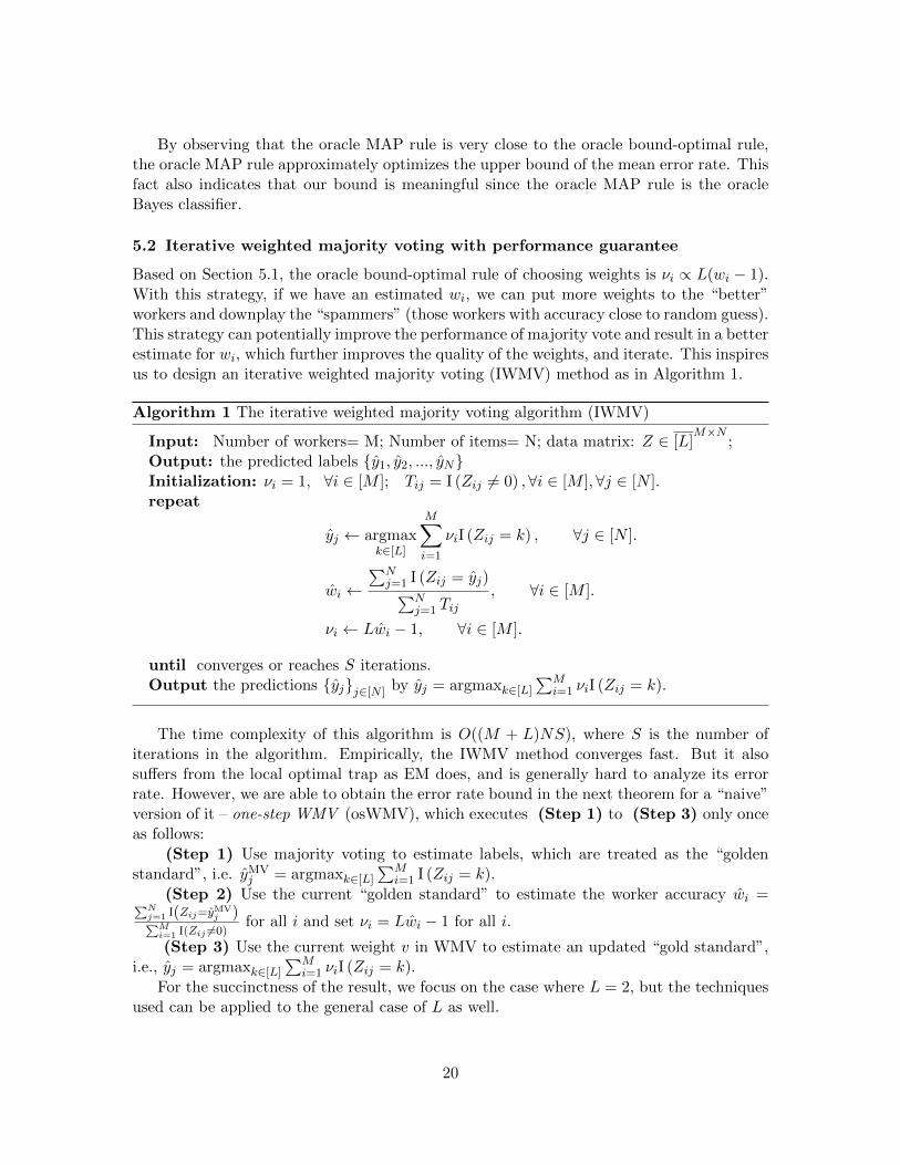
Based on Section 5.1, the oracle bound-optimal rule of choosing weights is νi ∝ L(wi − 1).With this strategy, if we have an estimated wi, we can put more weights to the “better”workers and downplay the “spammers” (those workers with accuracy close to random guess).This strategy can potentially improve the performance of majority vote and result in a betterestimate for wi, which further improves the quality of the weights, and iterate. This inspiresus to design an iterative weighted majority voting (IWMV) method as in Algorithm 1.
Algorithm 1 The iterative weighted majority voting algorithm (IWMV)
Input: Number of workers= M; Number of items= N; data matrix: Z ∈ [L]M×N
;Output: the predicted labels y1, y2, ..., yNInitialization: νi = 1, ∀i ∈ [M ]; Tij = I (Zij 6= 0) ,∀i ∈ [M ],∀j ∈ [N ].repeat
yj ← argmaxk∈[L]
M∑i=1
νiI (Zij = k) , ∀j ∈ [N ].
wi ←∑N
j=1 I (Zij = yj)∑Nj=1 Tij
, ∀i ∈ [M ].
νi ← Lwi − 1, ∀i ∈ [M ].
until converges or reaches S iterations.Output the predictions yjj∈[N ] by yj = argmaxk∈[L]
∑Mi=1 νiI (Zij = k).
The time complexity of this algorithm is O((M + L)NS), where S is the number ofiterations in the algorithm. Empirically, the IWMV method converges fast. But it alsosuffers from the local optimal trap as EM does, and is generally hard to analyze its errorrate. However, we are able to obtain the error rate bound in the next theorem for a “naive”version of it – one-step WMV (osWMV), which executes (Step 1) to (Step 3) only onceas follows:
(Step 1) Use majority voting to estimate labels, which are treated as the “goldenstandard”, i.e. yMV
j = argmaxk∈[L]
∑Mi=1 I (Zij = k).
(Step 2) Use the current “golden standard” to estimate the worker accuracy wi =∑Nj=1 I(Zij=yMV
j )∑Mi=1 I(Zij 6=0)
for all i and set νi = Lwi − 1 for all i.
(Step 3) Use the current weight v in WMV to estimate an updated “gold standard”,i.e., yj = argmaxk∈[L]
∑Mi=1 νiI (Zij = k).
For the succinctness of the result, we focus on the case where L = 2, but the techniquesused can be applied to the general case of L as well.
20
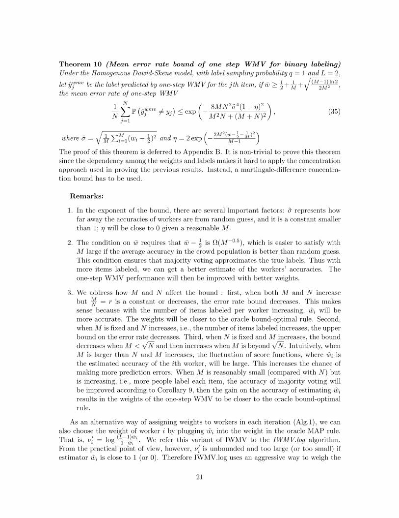
Theorem 10 (Mean error rate bound of one step WMV for binary labeling)Under the Homogenous Dawid-Skene model, with label sampling probability q = 1 and L = 2,
let ywmvj be the label predicted by one-step WMV for the jth item, if w ≥ 12 + 1
M +√
(M−1) ln 22M2 ,
the mean error rate of one-step WMV
1
N
N∑j=1
P(ywmvj 6= yj
)≤ exp
(− 8MN2σ4(1− η)2
M2N + (M +N)2
), (35)
where σ =√
1M
∑Mi=1(wi − 1
2)2 and η = 2 exp(−2M2(w− 1
2− 1M
)2
M−1
)The proof of this theorem is deferred to Appendix B. It is non-trivial to prove this theoremsince the dependency among the weights and labels makes it hard to apply the concentrationapproach used in proving the previous results. Instead, a martingale-difference concentra-tion bound has to be used.
Remarks:
1. In the exponent of the bound, there are several important factors: σ represents howfar away the accuracies of workers are from random guess, and it is a constant smallerthan 1; η will be close to 0 given a reasonable M .
2. The condition on w requires that w − 12 is Ω(M−0.5), which is easier to satisfy with
M large if the average accuracy in the crowd population is better than random guess.This condition ensures that majority voting approximates the true labels. Thus withmore items labeled, we can get a better estimate of the workers’ accuracies. Theone-step WMV performance will then be improved with better weights.
3. We address how M and N affect the bound : first, when both M and N increasebut M
N = r is a constant or decreases, the error rate bound decreases. This makessense because with the number of items labeled per worker increasing, wi will bemore accurate. The weights will be closer to the oracle bound-optimal rule. Second,when M is fixed and N increases, i.e., the number of items labeled increases, the upperbound on the error rate decreases. Third, when N is fixed and M increases, the bounddecreases when M <
√N and then increases when M is beyond
√N . Intuitively, when
M is larger than N and M increases, the fluctuation of score functions, where wi isthe estimated accuracy of the ith worker, will be large. This increases the chance ofmaking more prediction errors. When M is reasonably small (compared with N) butis increasing, i.e., more people label each item, the accuracy of majority voting willbe improved according to Corollary 9, then the gain on the accuracy of estimating wiresults in the weights of the one-step WMV to be closer to the oracle bound-optimalrule.
As an alternative way of assigning weights to workers in each iteration (Alg.1), we canalso choose the weight of worker i by plugging wi into the weight in the oracle MAP rule.That is, ν ′i = log (L−1)wi
1−wi . We refer this variant of IWMV to the IWMV.log algorithm.From the practical point of view, however, ν ′i is unbounded and too large (or too small) ifestimator wi is close to 1 (or 0). Therefore IWMV.log uses an aggressive way to weigh the
21
workers, and it might be too risky when the estimates wii∈[M ] are noisy. Recall that givenan estimate wi of the reliability of worker i, the way that the IWMV algorithm chooses theweight is νi = Lwi − 1. As a linearized version of ν ′i (34), νi is more stable to the noise inthe estimate wi. Furthermore, IWMV is more convenient for theoretical analysis than theIWMV.log algorithm. In the next section, we will show some comparisons between IWMVand IWMV.log by experiments.
6. Experiments
In this section, we first compare the theoretical error rate bound with the error rate oforacle MAP rule via simulation. Meanwhile, we compare IWMV with EM and IWMV.logon synthetic data. We then experimentally test IWMV and compare it with the state-of-art algorithms on real-world data. We implement majority voting, EM algorithm (Raykaret al., 2010) with MAP rule (also referred as the EM-MAP rule in the experiments), anduse public available code 4 — the iterative algorithm in (Karger et al., 2011) is referred toas KOS, and the variational inference algorithm from (Liu et al., 2012) is referred to as LPI.All results are averaged over 100 random trials. All our experiments are implemented inMatlab 2012a, and run on a PC with Windows 7 operation system, Intel Core i7-3740QM(2.70GHz) CPU and 8GB memory.
6.1 Simulation
The error rate of a crowdsourcing system is affected by variations of different parameterssuch as number of workers M , number of items N and worker reliabilities wii∈[M ] etc. Tostudy how the error rate bound reflects the change of error rate when a parameter of thesystem changes, we conduct numerical experiments on simulated data for comparing theoracle MAP rule with its error rate bound (Corollary 9). We also measure the performanceof the IWMV algorithm and compare it with the performance of oracle MAP rule.
The simulations are run under the Homogenous Dawid-Skene model. Each worker hasq =30% chance to label any item which belongs to one of three classes (L = 3). Theground truth labels of items are uniformly generated. The accuracies of workers (i.e., wi)are sampled from a beta distribution Beta(a, b) with b = 2. Given an expected averageworker accuracy w, we choose the paramater a = 2w
1−w so that the expected value forworker accuracies under distribution Beta(a, 2) matches with w. In each random trial inthe simulation, we keep sampling M workers from this Beta distribution until the averageworker accuracy is within ±0.01 range from the expected w. This is to maintain the averageworker accuracy at the same level for each trial.
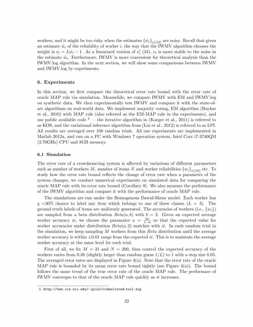
First of all, we fix M = 31 and N = 200, then control the expected accuracy of theworkers varies from 0.38 (slightly larger than random guess 1/L) to 1 with a step size 0.05.The averaged error rates are displayed in Figure 4(a). Note that the error rate of the oracleMAP rule is bounded by its mean error rate bound tightly (see Figure 4(a)). The boundfollows the same trend of the true error rate of the oracle MAP rule. The performace ofIWMV converges to that of the oracle MAP rule quickly as w increases.
4. http://www.ics.uci.edu/∼qliu1/codes/crowd tool.zip
22
0.4 0.5 0.6 0.7 0.8 0.9 1−5
−4.5
−4
−3.5
−3
−2.5
−2
−1.5
−1
−0.5
0
Average accuracy of workers
log
10(M
ea
n e
rro
r ra
te)
Oracle MAP ruleOracle MAP boundIWMV
0 20 40 60 80 100 120−3
−2.5
−2
−1.5
−1
−0.5
0
M: number of workers
log
10(M
ean e
rror
rate
)
Oracle MAP ruleOracle MAP boundIWMV
0 200 400 600 800 1000
−2
−1.8
−1.6
−1.4
−1.2
−1
−0.8
−0.6
−0.4
−0.2
0
N: number of tasks
log
10(M
ean e
rror
rate
)
Oracle MAP ruleOracle MAP boundIWMV
(a) (b) (c)
Figure 4: Comparing the oracle MAP rule with its theoretical error rate bound by simula-tion. The performance of the IWMV algorithm is also imposed. These simulationsare done under the Homogenous Dawid-Skene model with L = 3 and q = 0.3.(a) Vary the average accuracy of workers and fix M = 31 and N = 200.(b) VaryM and fix N = 200. (c) Vary N and fix M = 31. The reliabilities of workersare sampled based on wi ∼Beta(2.3, 2), ∀i ∈ [M ] in (b) and (c). Note that all ofthem are in log scale and all the results are averaged across 100 repetitions.
By fixing a = 2.3 and q = 0.3, we then vary one of the two parameters— numberof items N (default as 200) and number of workers M (default as 31) — with the otherparameter maintained as the default. The corresponding results are presented in Figure 4(b) and (c), respectively. According to the results of simulation, the error rate bound of theoracle MAP rule and its upper bound do not change when the number of tasks N increases(Figure 4(c)), but they change log linearly when the number of workers M increases (Figure4(b)). Nevertheless, the performance of IWMV changes whenever we increase M or N . Itbehaves closely to the oracle MAP rule when M varies, but differently from the oracle MAPrule when N increases. This is because with more and more tasks done by the workers,the estimation of the reliability of the workers will be more accurate, and this can boostthe performance of IWMV. However, the oracle MAP rule knows the true worker reliabilityinitially, so its performance will be independent with N .
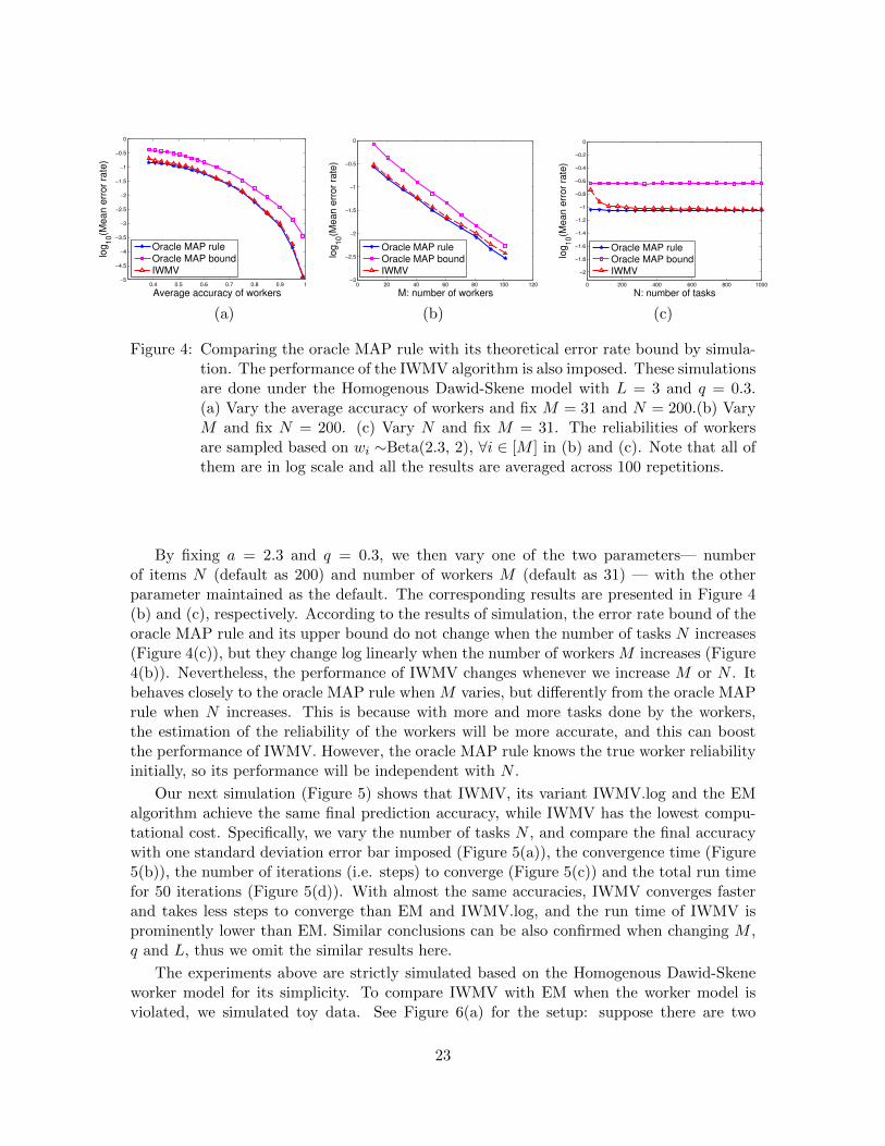
Our next simulation (Figure 5) shows that IWMV, its variant IWMV.log and the EMalgorithm achieve the same final prediction accuracy, while IWMV has the lowest compu-tational cost. Specifically, we vary the number of tasks N , and compare the final accuracywith one standard deviation error bar imposed (Figure 5(a)), the convergence time (Figure5(b)), the number of iterations (i.e. steps) to converge (Figure 5(c)) and the total run timefor 50 iterations (Figure 5(d)). With almost the same accuracies, IWMV converges fasterand takes less steps to converge than EM and IWMV.log, and the run time of IWMV isprominently lower than EM. Similar conclusions can be also confirmed when changing M ,q and L, thus we omit the similar results here.
The experiments above are strictly simulated based on the Homogenous Dawid-Skeneworker model for its simplicity. To compare IWMV with EM when the worker model isviolated, we simulated toy data. See Figure 6(a) for the setup: suppose there are two
23
0 2000 4000 6000 8000 10000 12000
0.75
0.8
0.85
0.9
0.95
1
N: number of tasks(a)
Accu
racy
IWMV
IWMV.log
EM
0 2000 4000 6000 8000 10000 120000
50
100
150
200
N: number of tasks(b)
Co
nve
rg.
tim
e (
ms)
0 2000 4000 6000 8000 10000 120003.5
4
4.5
5
5.5
6
6.5
N: number of tasks(c)
Ste
ps t
o c
on
ve
rge
0 2000 4000 6000 8000 10000 120000
200
400
600
800
1000
1200
1400
N: number of tasks(d)
To
tal ru
n t
ime
(m
s)
IWMV
IWMV.log
EM
Figure 5: Comparison between IWMV, IWMV.log and the EM-MAP rule, with the num-ber of items varying from 1000 to 11000. Simulation was performed withL = 3,M = 31, q = 0.3 under the Homogenous Dawid-Skene model. The re-liabilities of workers are sampled based on wi ∼Beta(2.3, 2), i ∈ [M ]. All theresults are averaged across 100 repetitions. (a) Final accuracy with error bar im-posed. (b) The time until convergence, and we need to know the ground truth formeasuring it. (c) Number of steps to converge. (d) Total run time is computedbased on finishing 50 iterations.
0.9
0.5
0.6
0.7
𝑮𝟏: 20
workers
𝑺𝟏: 60 items 𝑺𝟐: 40 items
𝑮𝟐: 30
workers
0
0.02
0.04
0.06
0.08
0.1
0.12
0.14
MV EM IWMV.log IWMV
Err
or
rate
(10.3 +/− 0.1)%
(12.9 +/− 0.1)%
(9.7 +/− 0.1)%(9.4 +/− 0.1)%
(a) (b)
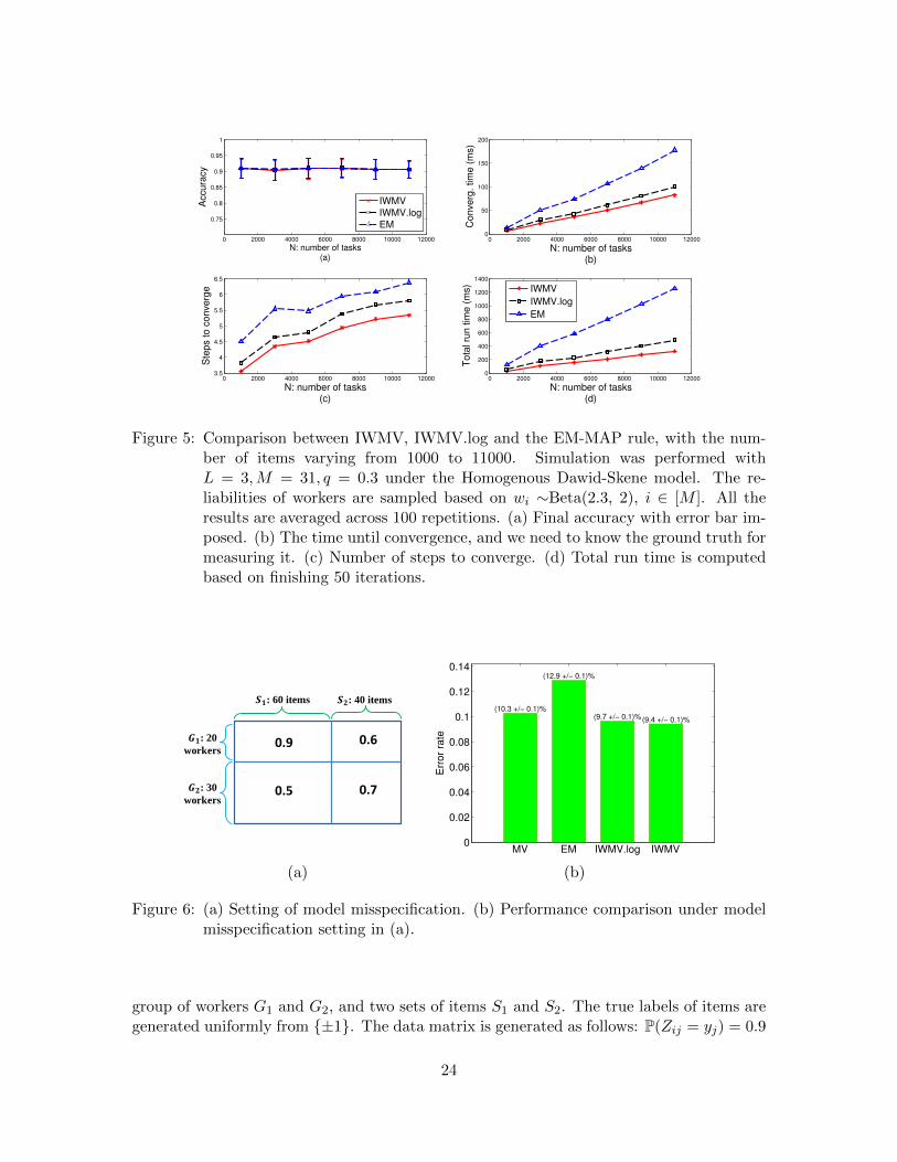
Figure 6: (a) Setting of model misspecification. (b) Performance comparison under modelmisspecification setting in (a).
group of workers G1 and G2, and two sets of items S1 and S2. The true labels of items aregenerated uniformly from ±1. The data matrix is generated as follows: P(Zij = yj) = 0.9
24
if i ∈ G1, j ∈ S1; P(Zij = yj) = 0.6 if i ∈ G1, j ∈ S2; P(Zij = yj) = 0.5 if i ∈ G2, j ∈ S1;P(Zij = yj) = 0.7 if i ∈ G2, j ∈ S2. We use q = 0.3. The error rate (with one standarddeviation) of MV, EM, IWMV.log and IWMV are shown in Figure 6 (b), which shows thatIWMV achieves lower error rate than EM and IWMV.log do in this model misspecificationexample. The results in Figure 6 shows that IWMV are more robust than EM undermodel misspecification to some extent. Similar results can be obtained under other differentconfiguations (as in Figure 6), and we omit them here.
6.2 Real data
To compare our proposed iterative weighted majority voting with the state-of-the-art meth-ods (Raykar et al., 2010; Karger et al., 2011; Liu et al., 2012), we conducted several experi-ments on real data (most of them are publicly available). We sampled the collected labels inthe real data independently with probability q which varies from 0.1 to 1, and see how theerror rate and run time change accordingly. For clarity of the figures produced in this sec-tion, we omit the results of IWMV.log since its performance is usually worse than IWMV interms of both accuracy and computational time. Our focus will be the comparisons amongIWMV, EM, KOS and LPI.
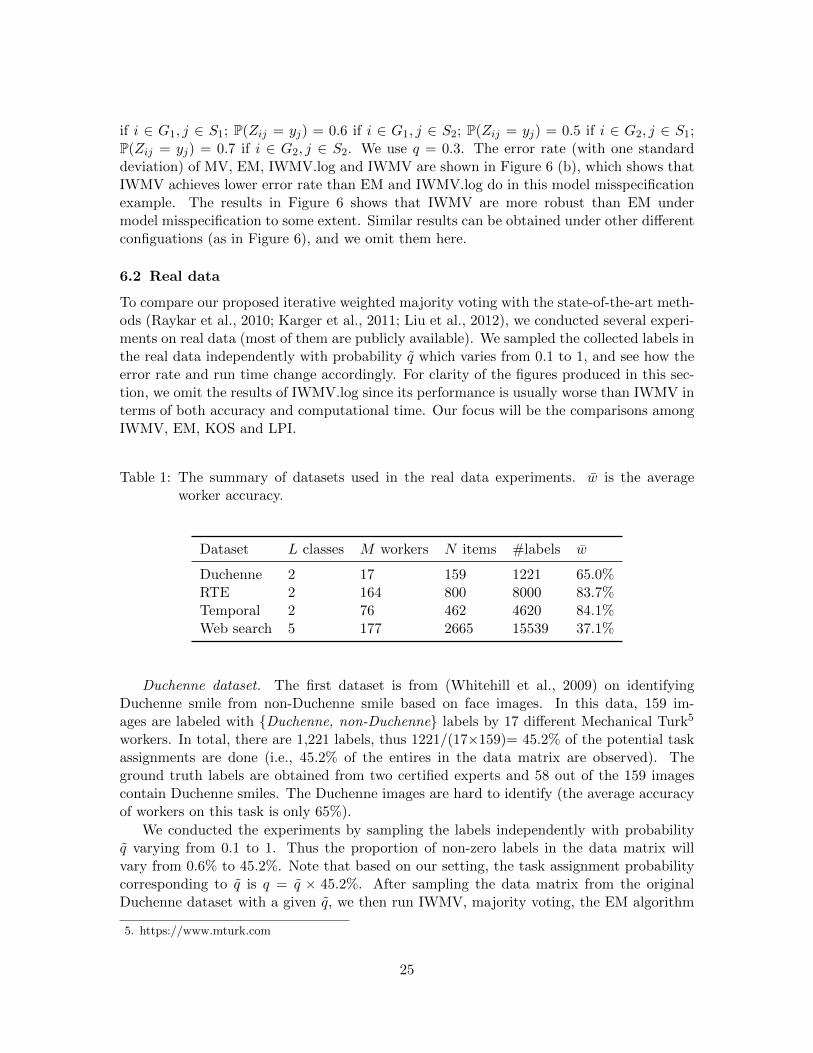
Table 1: The summary of datasets used in the real data experiments. w is the averageworker accuracy.
Dataset L classes M workers N items #labels w
Duchenne 2 17 159 1221 65.0%RTE 2 164 800 8000 83.7%Temporal 2 76 462 4620 84.1%Web search 5 177 2665 15539 37.1%
Duchenne dataset. The first dataset is from (Whitehill et al., 2009) on identifyingDuchenne smile from non-Duchenne smile based on face images. In this data, 159 im-ages are labeled with Duchenne, non-Duchenne labels by 17 different Mechanical Turk5
workers. In total, there are 1,221 labels, thus 1221/(17×159)= 45.2% of the potential taskassignments are done (i.e., 45.2% of the entires in the data matrix are observed). Theground truth labels are obtained from two certified experts and 58 out of the 159 imagescontain Duchenne smiles. The Duchenne images are hard to identify (the average accuracyof workers on this task is only 65%).
We conducted the experiments by sampling the labels independently with probabilityq varying from 0.1 to 1. Thus the proportion of non-zero labels in the data matrix willvary from 0.6% to 45.2%. Note that based on our setting, the task assignment probabilitycorresponding to q is q = q × 45.2%. After sampling the data matrix from the originalDuchenne dataset with a given q, we then run IWMV, majority voting, the EM algorithm
5. https://www.mturk.com
25

4.5% 9.0% 13.6% 18.1% 22.6% 27.1% 31.6% 36.1% 40.7% 45.2%0.25
0.3
0.35
0.4
0.45
0.5
Duchenne Dataset (Whitehill et al., 2009)
Percentage of task assignments done
Err
or
rate
EM−MAP
Majority Voting
KOS
LPI
IWMV
4.5% 9.0% 13.6% 18.1% 22.6% 27.1% 31.6% 36.1% 40.7% 45.2%0
500
1000
1500
2000
2500
Duchenne Dataset (Whitehill et al., 2009)
Percentage of task assignments done
Ru
n t
ime
(m
s)
EM−MAPMajority Voting
KOS
LPIIWMV
0
200
400
600
800
1000
1200
1400
1600
IWMV EM KOS LPI
Duchenne Dataset (Whitehill et al., 2009)
Run tim
e (
ms)
ER=25.8% ER=36.4%
ER=29.2%
ER=27.7%
(a) (b) (c)
Figure 7: Duchenne smile dataset (Whitehill et al., 2009). (a) Error rate of different algo-rithms when the number of labels available increases. (b) Run time comparison.(c) A visualization with both run time and error rate when 40.7% of the taskassignments are done.
(Raykar et al., 2010) , KOS (the iterative algorithm in (Karger et al., 2011)), and LPI (thevariational inference algorithm from (Liu et al., 2012)). The entire process will be repeated100 times, and the results will be averaged. The comparison is shown in Figure 7(a).
From Figure 7(a), We can see that when the available labels are very few, the perfor-mance of IWMV is as good as LPI, and these two generally dominate the other algorithms.With more labels available, the error rate of IWMV is around 2% lower than LPI (Figure7(a)). At the same time, we compared the run time of each algorithm (Figure 7(b)). Withmore labels, the run time of LPI increases fast (non-linearly), while the IWMV maintainsa lower run time than EM, KOS and LPI. For a better visualization of comparing run timeand error rate, we compared the run time of IWMV, EM, KOS and LPI by a bar plot withtheir error rates imposed on top. Figure 7(c) shows the comparison when 40.7% of thelabels are available (q = 0.9). IWMV is more than 100 times faster than LPI, and achievesthe lowest error rate among these algorithms.
An interesting phonomenon in Figure 7(a) is that EM performs poorly — it is evenworse than MV. The major reason for this is that the workers reliabilities form a patternsimilar to our model misspecification example in Figure 6(a): some workers are good ata set of images but bad at the complementary set of images, while the other workers arereversed. This is a real-data example of model misspecificatioin, and IWMV is more robustto the model misspecification on this data than EM.
RTE dataset. The RTE data is a language processing dataset from (Snow et al., 2008).The dataset is collected by asking workers to perform recognizing textual entailment (RTE)tasks, i.e., for each question the worker is presented with two sentences and given a binarychoice of whether the second sentence can be inferred from the first.
Temporal event dataset. This dataset is also a natural language processing dataset from(Snow et al., 2008). The task is to provide a label from strictly before, strictly after forevent-pairs that represents the temporal relation between them.
26
0.6% 1.2% 1.8% 2.4% 3.0% 3.7% 4.3% 4.9% 5.5% 6.1%0.05
0.1
0.15
0.2
0.25
0.3
0.35
0.4
0.45
0.5
0.55
RTE dataset (Snow et al., 2008)
Percentage of task assignments done
Err
or
rate
EM−MAP
Majority Voting
KOS
LPI
IWMV
0.6% 1.2% 1.8% 2.4% 3.0% 3.7% 4.3% 4.9% 5.5% 6.1%0
1000
2000
3000
4000
5000
6000
7000
8000
RTE dataset (Snow et al., 2008)
Percentage of task assignments done
Run tim
e (
ms)
EM−MAPMajority Voting
KOS
LPIIWMV
0
1000
2000
3000
4000
5000
6000
IWMV EM KOS LPI
RTE dataset (Snow et al., 2008)
Run tim
e (
ms)
ER=8.2% ER=8.4%
ER=49.6%
ER=8.3%
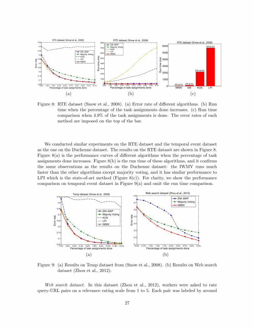
(a) (b) (c)
Figure 8: RTE dataset (Snow et al., 2008). (a) Error rate of different algorithms. (b) Runtime when the percentage of the task assignments done increases. (c) Run timecomparison when 4.9% of the task assignments is done. The error rates of eachmethod are imposed on the top of the bar.
We conducted similar experiments on the RTE dataset and the temporal event datasetas the one on the Duchenne dataset. The results on the RTE dataset are shown in Figure 8.Figure 8(a) is the performance curves of different algorithms when the percentage of taskassignments done increases. Figure 8(b) is the run time of these algorithms, and it confirmsthe same observations as the results on the Duchenne dataset: the IWMV runs muchfaster than the other algorithms except majority voting, and it has similar performance toLPI which is the state-of-art method (Figure 8(c)). For clarity, we show the performancecomparison on temporal event dataset in Figure 9(a) and omit the run time comparison.
1.3% 2.6% 3.9% 5.3% 6.6% 7.9% 9.2% 10.5% 11.8% 13.2%0.05
0.1
0.15
0.2
0.25
0.3
0.35
0.4
0.45
Temp dataset (Snow et al., 2008)
Percentage of task assignments done
Err
or
rate
EM−MAP
Majority Voting
KOS
LPI
IWMV
0.3% 0.7% 1.0% 1.3% 1.7% 2.0% 2.3% 2.7% 3.0% 3.3%0.1
0.2
0.3
0.4
0.5
0.6
0.7
0.8
Web search dataset (Zhou et al., 2012)
Percentage of task assignments done
Err
or
rate
EM−MAP
Majority Voting
IWMV
(a) (b)
Figure 9: (a) Results on Temp dataset from (Snow et al., 2008). (b) Results on Web searchdataset (Zhou et al., 2012).
Web search dataset. In this dataset (Zhou et al., 2012), workers were asked to ratequery-URL pairs on a relevance rating scale from 1 to 5. Each pair was labeled by around
27
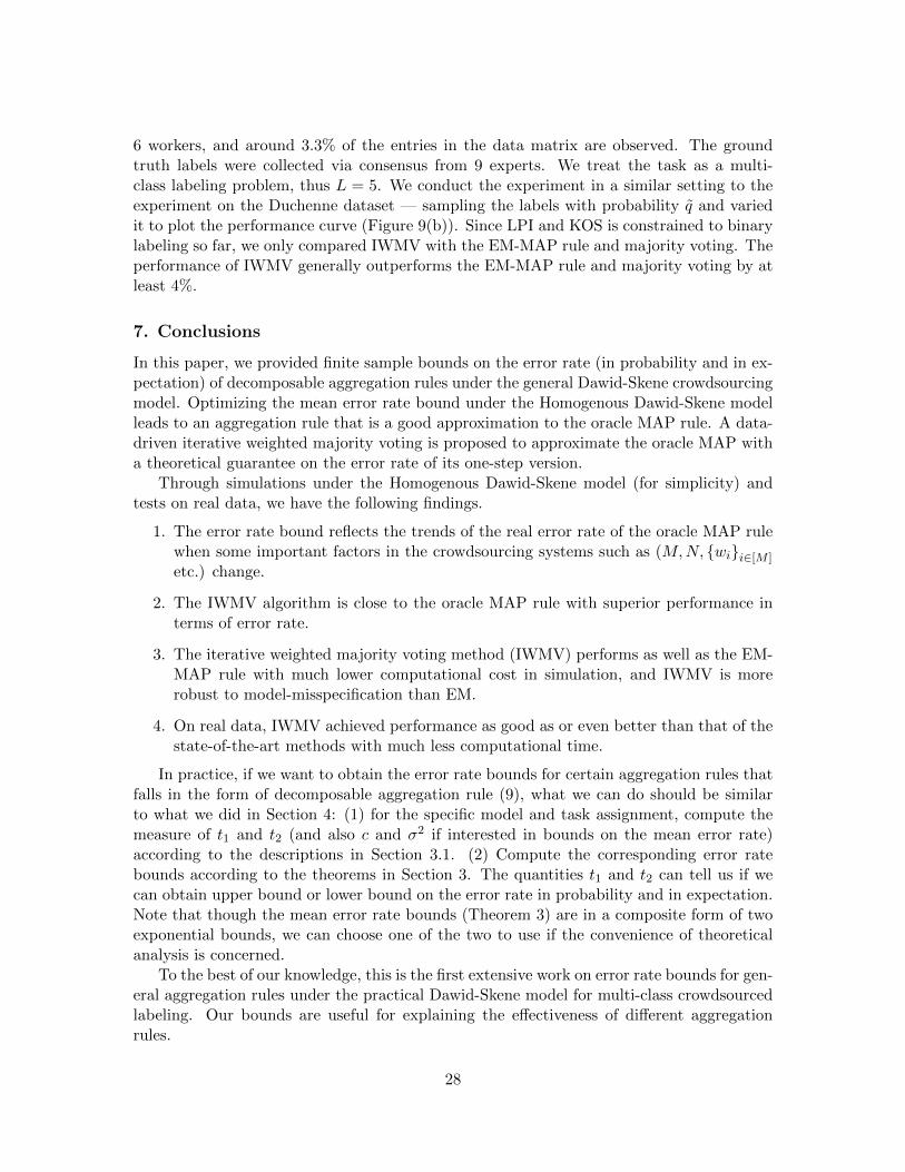
6 workers, and around 3.3% of the entries in the data matrix are observed. The groundtruth labels were collected via consensus from 9 experts. We treat the task as a multi-class labeling problem, thus L = 5. We conduct the experiment in a similar setting to theexperiment on the Duchenne dataset — sampling the labels with probability q and variedit to plot the performance curve (Figure 9(b)). Since LPI and KOS is constrained to binarylabeling so far, we only compared IWMV with the EM-MAP rule and majority voting. Theperformance of IWMV generally outperforms the EM-MAP rule and majority voting by atleast 4%.
7. Conclusions
In this paper, we provided finite sample bounds on the error rate (in probability and in ex-pectation) of decomposable aggregation rules under the general Dawid-Skene crowdsourcingmodel. Optimizing the mean error rate bound under the Homogenous Dawid-Skene modelleads to an aggregation rule that is a good approximation to the oracle MAP rule. A data-driven iterative weighted majority voting is proposed to approximate the oracle MAP witha theoretical guarantee on the error rate of its one-step version.
Through simulations under the Homogenous Dawid-Skene model (for simplicity) andtests on real data, we have the following findings.
1. The error rate bound reflects the trends of the real error rate of the oracle MAP rulewhen some important factors in the crowdsourcing systems such as (M,N, wii∈[M ]
etc.) change.
2. The IWMV algorithm is close to the oracle MAP rule with superior performance interms of error rate.
3. The iterative weighted majority voting method (IWMV) performs as well as the EM-MAP rule with much lower computational cost in simulation, and IWMV is morerobust to model-misspecification than EM.
4. On real data, IWMV achieved performance as good as or even better than that of thestate-of-the-art methods with much less computational time.
In practice, if we want to obtain the error rate bounds for certain aggregation rules thatfalls in the form of decomposable aggregation rule (9), what we can do should be similarto what we did in Section 4: (1) for the specific model and task assignment, compute themeasure of t1 and t2 (and also c and σ2 if interested in bounds on the mean error rate)according to the descriptions in Section 3.1. (2) Compute the corresponding error ratebounds according to the theorems in Section 3. The quantities t1 and t2 can tell us if wecan obtain upper bound or lower bound on the error rate in probability and in expectation.Note that though the mean error rate bounds (Theorem 3) are in a composite form of twoexponential bounds, we can choose one of the two to use if the convenience of theoreticalanalysis is concerned.
To the best of our knowledge, this is the first extensive work on error rate bounds for gen-eral aggregation rules under the practical Dawid-Skene model for multi-class crowdsourcedlabeling. Our bounds are useful for explaining the effectiveness of different aggregationrules.
28
As a further direction for research, it would be interesting to obtain finite sample errorbounds for the aggregation rules with random score functions, which depend on the datain a complicated manner. For example, the EM-MAP rule can be formulated as a weightedmajority voting under the Homogenous Dawid-Skene model. However, the weights areestimated by EM algorithm (Raykar et al., 2010) and depend on the data complicatedly.Hence the analysis of the EM algorithm is rather difficult. The IWMV and the EM algorithmshare the similar iterative nature, and IWMV is simpler than EM. An error rate analysisof the final prediction of the IWMV will be helpful to understand the behavior of EMalgorithm in the crowdsourcing context.
8. Acknowledgement
We thank Dengyong Zhou for his valuable suggestions and enlightening comments whichlead to many improvements of this paper. We would like to thank Riddhipratim Basu andQiang Liu for the valuable discussions. We would also like to thank Terry Speed for hishelpful comments and suggestions.
References
D. Angluin and P. Laird. Learning from noisy examples. Machine Learning, 2(4):343–370,1988.
Y. Bachrach, T. Graepel, T. Minka, and J. Guiver. How to grade a test without knowing theanswers — a bayesian graphical model for adaptive crowdsourcing and aptitude testing.In ICML, pages 1183–1190, New York, NY, USA, 2012.
J. A. Bilmes. A Gentle Tutorial of the EM Algorithm and its Application to ParameterEstimation for Gaussian Mixture and Hidden Markov Models. Technique Report, 1198(510), 1998.
X. Chen, Q. Lin, and D. Zhou. Optimistic Knowledge Gradient Policy for Optimal BudgetAllocation in Crowdsourcing. In ICML, 2013.
F. Chung and L. Liu. Old and new concentration inequalities, Chapter 2 in Complex Graphsand Networks. AMS, 2010. ISBN ISBN-10:0-8218-3657-9.
N. Dalvi, A. Dasgupta, R. Kumar, and V. Rastogi. Aggregating crowdsourced binaryratings. In WWW, 2013.
A. P. Dawid and A. M. Skene. Maximum Likelihood Estimation of Observer Error-RatesUsing the EM Algorithm. Journal of the Royal Statistical Society., 28(1):20–28, 1979.
Marie Jean Antoine Nicolas de Caritat et al. Essai sur l’application de l’analyse a laprobabilite des decisions rendues a la pluralite des voix. L’imprimerie royale, 1785.
O. Dekel and O. Shamir. Good learners for evil teachers. Proceedings of the26th Annual International Conference on Machine Learning, pages 1–8, 2009. doi:10.1145/1553374.1553404.
29
A. P. Dempster, N. M. Laird, and D. B. Rubin. Maximum likelihood from incomplete datavia the em algorithm. Journal of the Royal Statistical Society. Series B (Methodological),pages 1–38, 1977.
R. O. Duda, P. E. Hart, and D. G. Stork. Pattern classification. John Wiley & Sons, 2012.
S. Ertekin, H. Hirsh, and C. Rudin. Approximating the Wisdom of the Crowd. In NIPSWorkshop on Computational Social Science and the Wisdom of Crowds, pages 1–5, 2011.
C. Gao and D. Zhou. Minimax optimal convergence rates for estimating ground truth fromcrowdsourced labels. arXiv:1310.5764, 2014.
C. Ho, S. Jabbari, and J. W. Vaughan. Adaptive Task Assignment for CrowdsourcedClassification. In ICML, 2013.
W. Hoeffding. On the distribution of the number of successes in independent trials. TheAnnals of Mathematical Statistics, pages 713–721, 1956.
R. Jin and Z. Ghahramani. Learning with Multiple Labels. In NIPS, 2002.
D. R. Karger, S. Oh, and D. Shah. Iterative learning for reliable crowdsourcing systems. InNIPS, 2011.
Q. Liu, J. Peng, and A. Ihler. Variational Inference for Crowdsourcing. In NIPS, 2012.
C. McDiarmid. Concentration. Technique Report, 1998. URLhttp://cgm.cs.mcgill.ca/ breed/conc/colin.pdf.
N. Natarajan, I. Dhillon, P. Ravikumar, and A. Tewari. Learning with noisy labels. InNIPS, pages 1196–1204, 2013.
H. Q. Ngo. Tail and Concentration Inequalities. Lecture Notes, pages 1–6, 2011. URLhttp://www.cse.buffalo.edu/ hungngo/classes/2011/Spring-694/lectures/l4.pdf.
V. C. Raykar, S. Yu, L. H. Zhao, C. Florin, L. Bogoni, and L. Moy. Learning From Crowds.Journal of Machine Learning Research, 11:1297–1322, 2010.
C. S. Sheng and F. Provost. Get Another Label? Improving Data Quality and Data MiningUsing Multiple, Noisy Labelers Categories and Subject Descriptors. SIGKDD, pages614–622, 2008.
P. Smyth, U. Fayyad, M. Burl, P. Perona, and P. Baldi. Inferring Ground Truth fromSubjective Labelling of Venus Images. In NIPS, 1995.
R. Snow, B. O. Connor, D. Jurafsky, and A. Y. Ng. Cheap and Fast - But is it Good ?Evaluating Non-Expert Annotations for Natural Language Tasks. EMNLP, 2008.
P. Welinder, S. Branson, S. Belongie, and P. Perona. The Multidimensional Wisdom ofCrowds. In NIPS, 2010.
30

J. Whitehill, P. Ruvolo, T. Wu, J. Bergsma, and J. Movellan. Whose Vote Should CountMore : Optimal Integration of Labels from Labelers of Unknown Expertise. In NIPS,2009.
Y. Yan, R. Rosales, G. Fung, M. Schmidt, G. Hermosillo, L. Bogoni, L. Moy, and J. G. Dy.Modeling annotator expertise : Learning when everybody knows a bit of something. InICML, volume 9, pages 932–939, 2010.
Y. Yan, R. Rosales, G. Fung, and J. G. Dy. Active Learning from Crowds. In ICML, 2011.
D. Zhou, J. Platt, S. Basu, and Y. Mao. Learning from the Wisdom of Crowds by MinimaxEntropy. In NIPS, 2012.
Appendix A. Proofs of the main theorems
Since the proof of Theorem 1 requires other theorems in this paper, we will not present theproofs in the same order as in the paper. The order of our proofs will be: Proposition 11,Theorem 3, Theorem 1 and then Theorem 2. After proving the first four main results, wealso prove Corollary 8 and Corollary 9. Since the proof of Theorem 10 requires differenttechniques and more efforts than the proofs in this section, we put its proof in a seperatesection — Appendix B.
Before presenting the proofs, we would like to propose some notations for simplicity andclarity.
We simplify fi(k, h) to
µ(i)kh
.= fi(k, h), ∀k ∈ [L], h ∈ [L], (36)
then each worker is associated with a vote matrix µ(i) = (µ(i)kh), k ∈ [L], h ∈ [L], where µ
(i)kh
is the voting score when worker i labels item j whose true label is k, as class h if h 6= 0.Then the aggregation rule (9) is equivalent to
yj = argmaxk∈[L]
(M∑i=1
L∑h=1
µ(i)khI (Zij = h) + ak
), (37)
Note that
s(j)k =
M∑i=1
L∑h=1
µ(i)khI (Zij = h) + ak, ∀k ∈ [L], j ∈ [N ] (38)
is the aggregated score of label class k on the jth item, and the general aggregation rule is
yj = argmaxk∈[L]
s(j)k . (39)
We will frequently discuss conditional probability, expectation and variance conditionedon the event yj = k. For simplicity of notations, we define:
Pk ( · ).= P( · |yj = k) (40)
Ek [ · ].= E[ · |yj = k] (41)
Vark ( · ).= Var( · |yj = k). (42)
31
Note that
Ek[s
(j)l
]=
M∑i=1
L∑h=1
qijµ(i)lh p
(i)kh + al, ∀l, k ∈ [L]. (43)
A.1 Proof of Proposition 11: bounding the mean error rate of labeling eachitem
Proposition 11 (Bounding the mean error rate of labeling each item) Followingthe setting of Theorem 1, and with τj,min and τj,max defined as in (14) , we have ∀j ∈ [N ],
(1) if τj,min ≥ 0, then P(yj 6= yj) ≤ (L−1)·min
exp
(− τ2j,min
2
), exp
(− τ2j,min
2(σ2+cτj,min/3)
);
(2) if τj,max ≤ 0, then P(yj 6= yj) ≥ 1−min
exp
(− τ2j,max
2
), exp
(− τ2j,max
2(σ2−cτj,max/3)
).
Remark: Proposition 11 provides the mean error rate bounds of labeling any specific
item, and the bounds depend on the minimum and maximum values of
Λ(j)kl
k,l∈[L]
. Note
that the subscript j only comes from the assignment distribution qij . If a specific worker hasthe same assignment probability to label all items, say qi, then we can drop the subscriptj from τj,min and τj,max, which means the error rate bounds of each item are eventually thesame under that task assignment.
Proof First of all, we expand the error probability of labeling the j-th item wrong in termsof the conditional probabilities:
P(yj 6= yj) =∑k∈[L]
P(yj = k)P(yj 6= k|yj = k) =∑k∈[L]
πkPk (yj 6= k) . (44)
Our major focus in this proof is to bound the term Pk (yj 6= k). Our approach will bebased on the following events relations:⋃
l∈[L],l 6=k
s
(j)l > s
(j)k
⊆ yj 6= k ⊆
⋃l∈[L],l 6=k
s
(j)l ≥ s
(j)k
. (45)
(1). Assuming τj,min ≥ 0, we want to show the lower bound for P(yj 6= yj). Note that
Pk (yj 6= k) ≤ Pk
⋃l∈[L],l 6=k
s
(j)l ≥ s
(j)k
≤ ∑l∈[L],l 6=k
Pk(s
(j)l ≥ s
(j)k
). (46)
With s(j)l defined as in (38), Λ
(j)kl defined as in (13) and
ξ(i)kl
.=
L∑h=1
(µ(i)lh − µ
(i)kh)I (Zij = h) , (47)
Ek[ξ
(i)kl
]=
L∑h=1
qij
(µ
(i)lh − µ
(i)kh
)p
(i)kh, (48)
32
we have
Pk(s
(j)l ≥ s
(j)k
)= Pk
(M∑i=1
L∑h=1
(µ
(i)lh − µ
(i)kh
)I (Zij = h) ≥ ak − al
)
= Pk
(M∑i=1
ξ(i)kl ≥ ak − al
)
= Pk
(M∑i=1
ξ(i)kl −
M∑i=1
Ek[ξ
(i)kl
]≥ (ak − al)−
M∑i=1
Ek[ξ
(i)kl
]),
= Pk
(M∑i=1
ξ(i)kl −
M∑i=1
Ek[ξ
(i)kl
]≥ Λ
(j)kl
)(49)
Note thatξ
(i)kl
i∈[M ]
are conditionally independent when given yj = k, and they
are bounded given the voting weightsµ
(i)kh
are bounded. Therefore, we can apply the
Hoeffding concentration inequality (Hoeffding, 1956) to further bound Pk(s
(j)l ≥ s
(j)k
).
We have that minl,k,h∈[L],k 6=l
µ
(i)lh − µ
(i)kh
≤ ξ(i)
kl ≤ maxl,k,h∈[L],k 6=l
µ
(i)lh − µ
(i)kh
, and
M∑i=1
[max
l,k,h∈[L],k 6=l
µ
(i)lh − µ
(i)kh
− minl,k,h∈[L],k 6=l
µ
(i)lh − µ
(i)kh
]2
≤M∑i=1
(2 maxl,k,h∈[L],k 6=l
|µ(i)lh − µ
(i)kh|)2
= 4Γ2
When Λ(j)kl ≥ τj,min · Γ ≥ 0, by applying the Hoeffding inequality to (49), we have
Pk(s
(j)l ≥ s
(j)k
)≤ Pk
(M∑i=1
ξ(i)kl −
M∑i=1
Ek[ξ
(i)kl
]≥ Λ
(j)kl
)
≤ exp
− 2Λ(j)kl
2
∑Mi=1
[maxl,k,h∈[L],k 6=l
µ
(i)lh − µ
(i)kh
−minl,k,h∈[L],k 6=l
µ
(i)lh − µ
(i)kh
]2
≤ exp
−Λ(j)kl
2
2Γ2
(because of (50))
≤ exp
(−τ2j,min
2
). (based on the definition of τj,min))
The right hand side of the last inequality does not depend on k, l or i, then
Pk (yj 6= k) ≤∑
l∈[L],l 6=k
Pk(s
(j)l ≥ s
(j)k
)≤ (L− 1) exp
(−τ2j,min
2
). (50)
33
Because the RHS does not depend on k, we have
P(yj 6= yj) =∑k∈[L]
πkPk (yj 6= k)
≤ (L− 1) exp
(−τ2j,min
2
)∑k∈[L]
πk
= (L− 1) exp
(−τ2j,min
2
)(51)
The Hoeffding inequality does not take the variance information of the independent randomvariables into account, thus a “stronger” concentration inequality can be applied when the
fluctuation of ξ(i)kl is available.
Note the definition of c and σ2 are defined as
c =1
Γ· maxi∈[M ],k,l,h∈[L],k 6=l
|µ(i)kh − µ
(i)lh |,
σ2 =1
Γ2· maxj∈[N ]
maxk,l∈[L],k 6=l
M∑i=1
L∑h=1
qij
(µ
(i)kh − µ
(i)lh
)2p
(i)kh.
The sum of the second moment of ξ(i)kl can be bounded as
M∑i=1
Ek[(ξ
(i)kl
)2]
=
M∑i=1
Ek
( L∑h=1
(µ(i)lh − µ
(i)kh)I (Zij = h)
)2 =
M∑i=1
L∑h=1
qij
(µ
(i)kh − µ
(i)lh
)2p
(i)kh ≤ σ
2Γ2.
ξ(i)kl can be bounded as |ξ(i)
kl | ≤ maxi∈[M ],h∈[L] |µ(i)lh − µ
(i)kh| = cΓ.
By applying the Bernstein-type concentration inequality ((Chung and Liu, 2010), The-
orem 2.8) with that Λ(j)kl ≥ τj,minΓ ≥ 0,
Pk(s
(j)l ≥ s
(j)k
)≤ Pk
(M∑i=1
ξ(i)kl −
M∑i=1
Ek[ξ
(i)kl
]≥ Λ
(j)kl
)
≤ exp
− Λ(j)kl
2
2(σ2 + cΓΛ
(j)kl /3
) ,
≤ exp
(−
τ2j,min
2 (σ2 + cτj,min/3)
)(because
Λ(j)kl
Γ≥ τj,min ≥ 0), (52)
where the RHS does not depend on k, l. Then, we have
Pk (yj 6= k) ≤ (L− 1) exp
(−
τ2j,min
2 (σ2 + cτj,min/3)
).
34
Furthermore,
P(yj 6= yj) =∑k∈[L]
πkPk (yj 6= k) ≤ (L− 1) exp
(−
τ2j,min
2 (σ2 + cτj,min/3)
). (53)
Combining inequalities (51) and (53) together, we can get the desired result in Theorem11.(1).
(2). Assuming that τj,max ≤ 0, we want to show the upper bound for P(yj 6= yj).Using the same argument as in (1), we provide a lower bound for Pk (yj 6= k).
Pk (yj 6= k) ≥ Pk
⋃l∈[L],l 6=k
s
(j)l > s
(j)k
≥ maxl∈[L],l 6=k
Pk(s
(j)l > s
(j)k
)= 1− min
l∈[L],l 6=kPk(s
(j)l ≤ s
(j)k
)Given Λ
(j)kl ≤ τj,max ·Γ ≤ 0, by applying the Hoeffding and the Bernstein inequality as in
(1), we can obtain Pk(s
(j)l ≤ s
(j)k
)≤ exp
(−Λ
(j)kl
2
2Γ2
)≤ exp
(− τ2j,max
2
), and Pk
(s
(j)l ≤ s
(j)k
)≤
exp
(− Λ
(j)kl
2
2(σ2Γ2−cΓΛ(j)kl )
)≤ exp
(− τ2j,max
2(σ2−cτj,max)
). Since the RHS of the two inequalities do
not depend on k or l, Pk (yj 6= k) ≥ 1−min
exp
(− τ2j,max
2
), exp
(− τ2j,max
2(σ2−cτj,max)
).
With (44), we have P (yj 6= yj) ≥ 1−min
exp
(− τ2j,max
2
), exp
(− τ2j,max
2(σ2−cτj,max)
).
A.2 Proof of Theorem 3
Proof Given σ2 ≥ 0 and c > 0, both functions exp(− t2
2
)and exp
(− t2
2(σ2+ct/3)
)are
monotonely increasing on t ∈ [0,∞). On the other hand, both functions exp(− t2
2
)and
exp(− t2
2(σ2−ct/3)
)are monotonely decreasing on t ∈ (−∞, 0].
Given t1 ≥ 0, then τj,min ≥ t1 ≥ 0. By Proposition 11,
1
N
N∑j=1
P (yj 6= yj) ≤1
N
N∑j=1
(L− 1) min
exp
(−τ2j,min
2
), exp
(−
τ2j,min
2 (σ2 + cτj,min/3)
)
≤ L− 1
N
N∑j=1
min
exp
(− t
21
2
), exp
(− t21
2 (σ2 + t1/3)
)
= (L− 1) min
exp
(− t
21
2
), exp
(− t21
2 (σ2 + t1/3)
).
Thus, we have proved Theorem 3.(1).
35
With the same argument, we can straightforwardly prove Theorem 3.(2).
A.3 Proof of Theorem 1
So far, we have bounded the mean error rate, but we still need more tools for bounding theerror rate in the practical case with high probability. The following lemma is another formof the Bernstein-Chernoff-Hoeffding theorem (Ngo, 2011).
Lemma 12 (Bernstein-Chernoff-Hoeffding) Let ξi ∈ [0, 1] be independent randomvariables where Eξi = pi, i ∈ [n]. Let ξ = 1
n
∑ni=1 ξi and p = 1
n
∑ni=1 pi. Then,
(1) for any m such that p ≤ mn < 1, P
(ξ > m/n
)≤ e−nD(m/n||p),
(2) for any m such that 0 < mn ≤ p, P
(ξ < m/n
)≤ e−nD(m/n||p).
The proof of Theorem 1 is as follows:Proof (Theorem 1)
Proof of Theorem 1 (1) Let µ = 1N
∑Nj=1 P (yj 6= yj). By Theorem 3.(1), we have
that µ ≤ (L − 1)e−t21/2 = (L − 1)φ(t1). Assume t1 ≥
√2 ln L−1
ε , then we can get (L −1)φ(t1) ≤ ε, which gives us 0 ≤ µ ≤ (L − 1)φ(t1) ≤ ε. Then by the Bernstein-Chernoff-
Hoeffding Theorem, i.e. Lemma 12, we get P(
1N
∑Nj=1 I (yj 6= yj) > ε
)≤ e−ND(ε||µ) ≤
e−ND(ε||(L−1)φ(t1)). Therefore, we have
P
1
N
N∑j=1
I (yj 6= yj) ≤ ε
≥ 1− e−ND(ε||(L−1)φ(t1)).
Proof of Theorem 1 (2) With the same argument as above, assuming t2 ≤ −√
2 ln 11−ε ,
then 1 ≥ µ ≥ 1− φ(t2) ≥ ε, which gives us
P
1
N
N∑j=1
I (yj 6= yj) ≥ ε
≥ 1− e−ND(ε||1−φ(t2)).
Thus, we have proved Theorem 1.
A.4 Proof of Theorem 2
Before proving Theorem 2, we are going to prove an important lemma for bounding theaverage of a group of independent Bernoulli random variables. The proof of this lemmarelies on Hoeffding bounds and the Bernstein-Chernoff-Hoeffding theorem (Ngo, 2011).
Lemma 13 Suppose ∀j ∈ [N ], ξj ∼ Bernoulli(pj) with pj ∈ (0, 1), and ξj’s are independent
of each other. Let ξ = 1N
∑Nj=1 ξj and p = Eξ = 1
N
∑Nj=1 pj Given any ε, δ ∈ (0, 1):
36
(1) If 0 < p ≤ 11+exp( 1
ε [He(ε)+1N
ln 1δ ]), then P(ξ ≤ ε) ≥ 1− δ.
(2) If 11+exp(− 1
1−ε(He(ε)+1N
ln 1δ ))≤ p < 1, then P(ξ ≤ ε) < δ.
Proof For simplicity let’s define A =(He(ε) + 1
N ln 1δ
)The proof of Lemma 13.(1): We will finish the proof in several steps:
Assume 0 < p ≤ 11+exp( 1
ε [He(ε)+1N
ln 1δ ])
.
Step 1. we want to show p < ε :
exp
(A
ε
)= exp
(ε ln 1
ε + (1− ε) ln 11−ε + 1
N ln 1δ
ε
)
= exp
(ln
1
ε+
1− εε
ln1
1− ε+
1
Nεln
1
δ
)> exp
(ln
1
ε
)(∵ ε, δ ∈ (0, 1), N > 0)
=1
ε
=⇒ 1 + exp(Aε
)> 1
ε =⇒ 11+exp(Aε )
< ε
Since 0 < p ≤ 11+exp(A/ε) , then we have p < ε
Step 2. We want to show P(ξ ≤ ε
)≥ 1− e−N ·D(ε||p) :
This is obtained by the Bernstein-Chernoff-Hoeffding Theorem ((Ngo, 2011; McDiarmid,1998)), which leads to:
If 0 < p ≤ ε, then P(ξ ≤ ε) ≤ 1− e−ND(ε||p) (54)
If ε ≤ p < 1, then P(ξ ≤ ε) ≤ e−ND(ε||p) (55)
Since we have shown in step 1 that p < ε, then we can get the desired result in this stepeasily.
Step 3. We want to show e−ND(ε||p) ≤ δ :Note:
e−ND(ε||p) ≤ δ
⇐⇒ D(ε||p) ≥ 1
Nln
1
δ
⇐⇒ lnεε(1− ε)1−ε
pε(1− p)1−ε ≥ ln
(1
δ
) 1N
⇐⇒ pε(1− p)1−ε ≤ exp
(−(He(ε) +
1
Nln
1
δ
))= e−A (56)
37
From the condition we have,
p ≤ 1
1 + exp(A/ε)=⇒
(p
1− p
)ε≤ e−A
Note that pε(1− p)1−ε =(
p1−p
)ε(1− p) <
(p
1−p
)ε(∵ 1− p < 1)
=⇒ Inequality (56) holds: pε(1− p)1−ε ≤ e−A =⇒ e−ND(ε||p) ≤ δBy step 2 and step 3, we can easily get that if p ≤ 1
1+eA/ε, then P(ξ ≤ ε) ≥ 1− δ, which
is the results we want.
The proof of Lemma 13.(2): We will also finish the proof in several steps:
Assume
1
1 + exp(− 1
1−ε(He(ε) + 1
N ln 1δ
)) ≤ p < 1
Step 1. We want to show p > ε
We show it by proving as follows:
1
1 + exp(− 1
1−ε(He(ε) + 1
N ln 1δ
)) > ε
⇐⇒ 1 + exp
(− 1
1− ε
(He(ε) +
1
Nln
1
δ
))<
1
ε
⇐⇒(He(ε) +
1
Nln
1
δ
)> (1− ε) ln
ε
1− ε
⇐⇒ ε ln1
ε+ (1− ε) ln
1
1− ε+
1
Nln
1
δ> (1− ε) ln
1
1− ε− (1− ε) ln
1
ε
⇐⇒ ln1
ε+
1
Nln
1
δ> 0
which is of course true since ε, δ ∈ (0, 1). Therefore, we have proved p > ε.
Step 2. We want to show P(ξ ≤ ε) ≤ e−ND(ε||p)
By the Bernstein-Chernoff-Hoeffding Theorem, since ε < p = Eξ and ξj ∼ Bernoulli(pj)independently, we can directly prove this step.
Step 3. we want to show e−ND(ε||p) < δ
Note that
e−ND(ε||p) < δ ⇐⇒ D(ε||p) > 1
Nln
1
δ
⇐⇒ pε(1− p)1−ε < exp
(−(He(ε) +
1
Nln
1
δ
))= e−A (57)
38
From the condition we have
p ≥ 1
1 + exp− A1−ε
=⇒ 1− pp≤ e−
A1−ε
=⇒(
1− pp
)1−ε≤ exp
(−(He(ε) +
1
Nln
1
δ
))(58)
And note that
pε(1− p)1−ε =
(1− pp
)1−ε· p <
(1− pp
)1−ε(∵ p < 1) (59)
By combining inequalities (58) and (59), we can prove inequality (57). Thus we obtainede−ND(ε||p) < δ Finally, by step 2 and 3, we get : if p ≥ 1
1+exp(− 11−ε(He(ε)+
1N
ln 1δ ))
, then
P(ξ ≤ ε
)< δ
Now, we are going to prove Theorem 2 with the results we obtained in Lemma 13Proof of Theorem 2
Let ζj = I (yj 6= yj) ∼ Bernoulli(1− θj) and let p = Eζ = 1N
∑Nj=1 Eζj = 1− θ.
The proof of Theorem 2.(1):Assume that t1 ≥
√2 ln [(L− 1)C(ε, δ)], where C(ε, δ) = 1 + exp
(1ε
[He(ε) + 1
N ln 1δ
]),
then t1 ≥ 0.By Theorem 3, we have
θ = 1− 1
N
N∑j=1
P (yj 6= yj) ≥ 1− (L− 1)e−t212 (60)
Let A =(He(ε) + 1
N ln 1δ
), then
t1 ≥√
2 ln [(L− 1)C(ε, δ)] =√
2 ln [(L− 1)(1 + exp(A/ε))]
=⇒ (L− 1) exp
(− t
21
2
)≤ 1
1 + exp(Aε
)=⇒ θ ≥ 1− (L− 1) exp
(− t
21
2
)≥ 1− 1
1 + exp(Aε
) (∵ (60))
=⇒ 1− θ ≤ 1
1 + exp(Aε
) . (61)
By inequality (61) and by Lemma 13, we have
P(ζ ≤ ε) ≥ 1− δ
which is to say,
P
1
N
N∑j=1
I (yj 6= yj) ≤ ε
≥ 1− δ
39
Therefore, we have proved (1).
The proof of Theorem 2.(2):
Assume t2 ≤ −√
2 lnC(1− ε, δ) ≤ 0 , where C(1− ε, δ) = 1+exp(
11−ε(He(ε) + 1
N ln 1δ
)).
Then by Theorem 3.(2), we have
θ =1
N
N∑j=1
P(yj = yj) ≤ exp
(− t
22
2
)(62)
From the conditions in (2)
t2 ≤ −
√2 ln
(1 + exp
(1
1− ε
[He(ε) +
1
Nln
1
δ
]))=⇒ exp
(− t
22
2
)≤ 1
1 + exp(
A1−ε
)=⇒ 1− θ ≥ 1− exp
(− t
22
2
)≥ 1− 1
1 + exp(
A1−ε
) =1
1 + exp(− A
1−ε
)By Lemma 13.(2), we have P(ζ ≤ ε) < δ which implies the desired result.
A.5 Proof of Corollary 8 (Error rate bounds of the oracle MAP rule)
Proof The posterior distribution is
ρ(j)k =
πkη(j)k∑L
l=1 πlη(j)l
, ∀j ∈ [N ], k ∈ [L],
where
η(j)k =
M∏i=1
L∏h=1
(p
(i)kh
)I(Zij=h).
For the oracle MAP classifier,
yoraclej = argmax
k∈[L]ρ
(j)k = argmax
k∈[L]πkη
(j)k = argmax
k∈[L]log(η
(j)k ) + log πk
=
M∑i=1
L∑h=1
(log p
(i)kh
)I (Zij = h) + log πk =
M∑i=1
L∑h=1
µ(i)khI (Zij = h) + ak,
where µ(i)kh = log p
(i)kh and ak = log πk. Therefore the oracle MAP rule is a form of the general
aggregation rule (37). Thus all the results of error rate bounds in Section 3 holds for theoracle MAP rule.
40
A.6 Proof of Corollary 9 (The oracle MAP rule under HomogenousDawid-Skene model)
Proof The Homogenous Dawid-Skene model is the special case of the General Dawid-
Skene model, in which case we have p(i)kk = wi and p
(i)kh = 1−wi
L−1 for all k, h ∈ [L], k 6= h. By
Corollary 8, we can replace µ(i)kk with logwi, and µ
(i)kh, k 6= h with log 1−wi
L−1 , and so we have
yj = argmaxk∈[L]
M∑i=1
L∑h=1
µ(i)khI (Zij = h) + log
1
L
= argmaxk∈[L]
M∑i=1
(I (Zij = k) logwi + I (Zij 6= k, 0) log
1− wiL− 1
)
= argmaxk∈[L]
M∑i=1
(I (Zij = k) logwi + (I (Zij 6= 0)− I (Zij = k)) log
1− wiL− 1
)
= argmaxk∈[L]
[M∑i=1
I (Zij = k) log(L− 1)wi
1− wi+
M∑i=1
I (Zij 6= 0) log1− wiL− 1
]
= argmaxk∈[L]
M∑i=1
(log
(L− 1)wi1− wi
)I (Zij = k)
= argmaxk∈[L]
M∑i=1
νiI (Zij = k) ,
where νi = log (L−1)wi1−wi . Therefore the oracle MAP rule under the Homogenous Dawid-Skene
model is a MWV rule. Thus the results from Corollary 5 can be directly applied here. i.e.,
t1 =q
(L− 1)||ν||2
M∑i=1
νi(Lwi − 1), c =‖ν‖∞||ν||2
and σ2 = q.
And if t1 ≥ 0, then
1
N
N∑j=1
P (yj 6= yj) ≤ (L− 1) ·min
exp
(− t
21
2
), exp
(− t21
2 (σ2 + ct1/3)
).
Now all we need to show is that t1 is always non-negative. We can see that if wi ≥ 1L ,
then (Lwi − 1) ≥ 0 and νi = (L−1)wi1−wi ≥ 0 for all i ∈ [M ], then t1 ≥ 0 in this case.
wi <1L , then (Lwi − 1) < 0 and (L−1)wi
1−wi < 0, thus t1 > 0 in this case as well. All in all,t1 ≥ 0 is always true for the oracle MAP rule under the Homogenous Dawid-Skene model.
Appendix B. Proof of Theorem 10 : error rate bounds of one-stepWeighted Majority Voting
In the proof of this result, we focus on P(Tij = 1) = q = 1,∀i ∈ [M ], j ∈ [N ], i.e., everyworker labels any item with probability q. Meanwhile, we assume L = 2, and the label set
41
[L].= ±1. It’s not hard to generalize our results to q ∈ (0, 1] and general L case, which is
more practical, but the bound will be much more complicated. We omit it here for clarity.The prediction of the one-step Weighted Majority Voting for the jth item is
ywmvj = sign
(M∑i=1
(2wi − 1)Zij
), (63)
where wi is the estimated worker accuracy by taking the output from majority voting as“true” labels. That is to say,
wi =1
N
N∑j=1
I(Zij = ymvj
), where ymvj = sign
(M∑i=1
Zij
). (64)
Note that the average accuracy of workers is w = 1M
∑Mi=1wi.
In fact, Theorem 10 is a direct implication by the following result.
Proposition 14 If w ≥ 12 + 1
M +√
(M−1) ln 22M2 , then the mean error rate of one-step Weighted
Majority Voting for the jth item will be:
P(ywmvj 6= yj
)≤ exp
(− 8MN2σ4(1− η)2
M2N + (M +N)2
), (65)
where σ and η is as defined in Theorem 10 .
In the next section, we will focus on proving this result first, then Theorem 10 can beobtained directly.
B.1 The preparation for the proofs
Before we prove Proposition 14, we need to prove several useful results for our final proofof Proposition 14.
With the same notations as we have used for proving Theorem 1, we simplified somenotations as follows for convenience and clearance:
P(j)+ ( · )
.= P( · |yj = +1) and P(j)
− ( · ).= P( · |yj = −1), (66)
E(j)+ [ · ]
.= E[ · |yj = +1] and E(j)
− [ · ].= E[ · |yj = −1], (67)
where “ · ” denotes any event belonging to the σ-algebra generated by Z.The following lemma enable us to bound the probability of where the majority vote of
the jth item agrees with the label given by the ith worker given the true label and Zij .
Lemma 15 ∀j ∈ [N ] and ∀i ∈ [M ], we have(1) if w > 1
2 , then
P(ymvj = +1|yj = +1, Zij = +1
)≥ 1− exp
(−
2M2(w − 12 + 1−wi
M )2
M − 1
), (68)
42

and the same bound holds for P(ymvj = −1|yj = −1, Zij = −1
).
(2) if w ≥ 12 + 1
M , then
P(ymvj = −1|yj = +1, Zij = −1
)≤ exp
(−
2M2(w − 12 −
wiM )2
M − 1
), (69)
and the same bound holds for P(ymvj = +1|yj = −1, Zij = +1
).
Proof (1) Notice that for any i ∈ [M ] and j ∈ [N ], given yj , Zij is independent of Zljl 6=i,E(j)
+ Zlj = 2wl − 1 and E(j)− Zlj = −(2wl − 1), then∑
l 6=iE(j)
+ Zlj + 1 =∑l 6=i
(2wl − 1) + 1 = 2M
(w − 1
2+
1− wiM
)> 0, (70)
since w − 12 + 1−wi
M > w − 12 > 0. Therefore, we can apply the Hoeffding inequality to get:
P(ymvj = +1|yj = +1, Zij = +1
)= P(j)
+
(ymvj = +1|Zij = +1
)= P(j)
+
(M∑l=1
Zlj > 0
∣∣∣∣Zij = +1
)
= P(j)+
∑l 6=i
Zlj −∑l 6=i
E(j)+ Zlj > −(
∑l 6=i
E(j)+ Zlj + 1)
≥ 1− exp
(−
[∑
l 6=i E(j)+ Zlj + 1]2
2(M − 1)
)(by Hoeffding)
= 1− exp
(−
2M2(w − 12 + 1−wi
M )2
M − 1
)(by (70))
Note that with the same argument,
P(ymvj = −1|yj = −1, Zij = −1) = P(j)−
(M∑l=1
Zlj < 0|Zij = −1
)
= P(j)−
∑l 6=i
Zlj −∑l 6=i
E(j)− Zlj < −
∑l 6=i
E(j)− Zlj + 1
≥ 1− exp
(−
2M2(w − 12 + 1−wi
M )2
M − 1
),
provided that −∑
l 6=i E(j)− Zlj + 1 = 2M
(w − 1
2 + 1−wiM
)> 0, which is satisfied by the
assumption w > 12 .
(2) With the same argument as above, notice that∑
l 6=i E(j)+ Zlj−1 = 2M
(w − 1
2 −wiM
)≥
0 because w ≥ 12 + 1
M .
43
By applying the Hoeffding inequality:
P(ymvj = −1|yj = +1, Zij = −1
)= P(j)
+ (∑l 6=i
Zlj < 0|Zij = −1)
= P(j)+
∑l 6=i
Zlj −∑l 6=i
E(j)+ Zlj < −(
∑l 6=i
E(j)+ Zlj − 1)
≤ exp
(−
[∑
l 6=i E(j)+ Zlj − 1]2
2(M − 1)
)
= exp
(−
2M2(w − 12 −
wiM )2
M − 1
)Following the same argument, we can show that the same bound holds for
P(ymvj = +1|yj = −1, Zij = +1
).
Our next lemma will bound the probability that the label of item j given by worker iagrees with Majority Voting.
Lemma 16 Given w ≥ 12 + 1
M , then ∀j ∈ [N ], we have
wi − ξ(1)i ≤ P(Zij = ymvj | yj) ≤ wi + ξ
(2)i , (71)
where ξ(1)i = wi exp
(−2M2(w− 1
2+
1−wiM
)2
M−1
)and ξ
(2)i = (1 − wi) exp
(−2M2(w− 1
2−wiM
)2
M−1
)Fur-
thermore, we have
wi − ξ(1)i ≤ P(Zij = ymvj ) ≤ wi + ξ
(2)i , (72)
Remark: This result implies that under mild conditions, the probability that the labelof the jth item given by the ith worker matches the majority vote will be close to wi, i.e.,the accuracy of this worker. As the number of workers increase, it will be closer and closer.Intuitively, this makes sense since if M is large, majority voting will be close to the truelabel if w > 0.5.Proof
P(Zij = ymvj ) = πP(j)+ (Zij = ymvj ) + (1− π)P(j)
− (Zij = ymvj ). (73)
P(j)+ (Zij = ymvj ) = wiP
(j)+ (ymvj = +1|Zij = +1) + (1− wi)P(j)
+ (ymvj = +1|Zij = −1).
Applying P(j)+ (ymvj = +1|Zij = +1) ≥ 1−exp
(−2M2(w− 1
2+
1−wiM
)2
M−1
)from Lemma 15.(1) and
(1− π)P(j)− (Zij = ymvj ) ≥ 0 we can get
P(j)+ (Zij = ymvj ) ≥ wi − wi exp
(−
2M2(w − 12 + 1−wi
M )2
M − 1
). (74)
44

By applying P(j)+ (ymvj = +1|Zij = +1) ≤ 1 and P(j)
− (Zij = ymvj ) ≤ exp(−2M2(w− 1
2−wiM
)2
M−1
)from Lemma 15.(2), we can get
P(j)+ (Zij = ymvj ) ≤ wi + (1− wi) exp
(−
2M2(w − 12 −
wiM )2
M − 1
). (75)
Similarly, we can obtain the same bounds for P(j)− (Zij = ymvj ), i.e.,
P(j)− (Zij = ymvj ) ≥ wi − wi exp
(−
2M2(w − 12 + 1−wi
M )2
M − 1
), (76)
P(j)− (Zij = ymvj ) ≤ wi + (1− wi) exp
(−
2M2(w − 12 −
wiM )2
M − 1
)(77)
Since P(j)+ (Zij = ymvj ) and P(j)
− (Zij = ymvj ) have the same bounds, and
P(Zij = ymvj | yj) = I (yj = 1)P(j)+ (Zij = ymvj ) + I (yj = −1)P(j)
− (Zij = ymvj ),
then (71) holds. Furthermore, since
P(Zij = ymvj ) = πP(j)+ (Zij = ymvj ) + (1− π)P(j)
− (Zij = ymvj ),
then (74) to (77) implies (72) .
The next lemma will be crucial for applying concentration measure results to boundP(ywmvj 6= yj | ykNk=1).
For measuring the fluctuation of a function gj : 0,±1M×N → R if we change one entryof the data matrix, we define a quantity as follows:
d(j)i?j?
.= inf
d : |gj(Z)− gj(Z ′)| ≤ d,where Z and Z ′ only differ on (i?, j?)
. (78)
The constraints Z and Z ′ only differ on (i?, j?), which means that Z ′i?j? is a independentcopy of Zi?j? , and Zij = Z ′ij for (i, j) 6= (i?, j?).
Lemma 17 Let gj(Z).=∑M
i=1(2wi − 1)Zij , ∀j ∈ [N ], where Z is the data matrix and wi
is as defined in (64), with d(j)i?j? defined in (78), we have
(1)if j? 6= j, then d(j)i?j? ≤
2(M−1)N ;
(2)if j? = j, then d(j)i?j? ≤
2(M−1)N + 2 .
Proof Since Z ′i?j? is an independent copy of Zi?j? , Z′i?j? = Zi?j? or Z ′i?j? = −Zi?j? . When
Z ′i?j? = Zi?j? , Z′ = Z, then of course |gj(Z) − gj(Z ′)| = 0, which satisfies the inequality
trivially.Next, we focus on the non-trivial case Z ′i?j? = −Zi?j? .
45
Note that Zij = Z ′ij when (i, j) 6= (i?, j?). Let ymvj be the majority vote of the jth
column of Z, and ymv′
j be the majority vote by the jth column of Z ′.
Recall that |gj(Z)− gj(Z ′)| = |∑M
i=1(2wi − 1)Zij −∑M
i=1(2w′i − 1)Z ′ij |.If j? 6= j, then Zij = Z ′ij , ∀i ∈ [M ], so,
|gj(Z)− gj(Z ′)| = |M∑i=1
(2wi − 2w′i)Zij | ≤ 2M∑i=1
|(wi − w′i)Zij | = 2M∑i=1
|wi − w′i|. (79)
If j? = j, we have Zij? = Z ′ij? for i 6= i?, and Zi?j? = −Z ′i?j? , then,
|gj(Z)− gj(Z ′)| = |∑i 6=i?
2(wi − w′i)Zij + 2(pi? + p′i? − 1)Zi?j? |
≤ 2∑i 6=i?|wi − w′i|+ 2|pi? + p′i? − 1| (80)
We can see that the difference gj(Z) − gj(Z′) depends heavily on the two quantities
|wi − w′i| and |pi? + p′i? − 1|.Next we bound |wi − w′i|:
|wi − w′i| = | 1N
M∑i=1
(I (Zik = ymvk )− I
(Z ′ik = ymv
′k
))| = 1
N|I(Zij? = ymvj?
)− I(Z ′ij? = ymv
′j?
)|,
because Zik = Z ′ik and ymvk = ymv′
k if k 6= j?.
(a). If ymvj? = ymv′
j? , then by (81)
|wi − w′i| =
0 if i 6= i?,1N if i = i?.
In this case,
M∑i=1
|wi − w′i| =1
N, and
∑i 6=i?|wi − w′i| = 0. (81)
(b). If If ymvj? 6= ymv′
j? , then by (81)
|wi − w′i| =
1N if i 6= i?,
0 if i = i?.
In this case,
M∑i=1
|wi − w′i| =M − 1
N, and
∑i 6=i?|wi − w′i| =
M − 1
N. (82)
46
Now, we are going to bound |pi? + p′i? − 1|:
|pi? + p′i? − 1| =1
N|N∑k=1
(I (Zi?k = ymvk ) + I
(Z ′i?k = ymv
′k
)− 1)|
≤ 1
N
N∑k=1
|I (Zi?k = ymvk ) + I(Z ′i?k = ymv
′k
)− 1|. (83)
(c). If ymvj? = ymv′
j? , then
|I (Zi?k = ymvk ) + I(Z ′i?k = ymv
′k
)− 1| =
1 if k 6= j?,
0 if k = j?.
So in this case, |pi? + p′i? − 1| = N−1N .
(d). If ymvj? 6= ymv′
j? , then
|I (Zi?k = ymvk ) + I(Z ′i?k = ymv
′k
)− 1| =
1 if k 6= j?,
1 if k = j?.
So in this case, |pi? + p′i?−1| = 1. Putting together all the results above, if Zi?j? 6= Z ′i?j? ,then we have,
(1’) If ymvj? = ymv′
j? ,
|gj(Z)− gj(Z ′)| ≤
2N if j? 6= j,2(N−1)N if j? = j.
(2’) If ymvj? 6= ymv′
j? ,
|gj(Z)− gj(Z ′)| ≤
2(M−1)
N if j? 6= j,2(N−1)N + 2 if j? = j.
The upper bound in the case when ymvj 6= ymv′
j is also an upper bound for the case when
ymvj = ymv′
j . By the definition of d(j)i?j? and noting that Z can only take a finite number of
values, we have
d(j)i?j? ≤
2(M−1)
N if j? 6= j,2(N−1)N + 2 if j? = j.
Remark: d(j)i?j? is the smallest upper bound on the difference between gj(Z) and gj(Z
′).From the proof, we can see that the bound we get is achievable, thus the bounds are tight.This result basically says that if we change only one entry of the data matrix, the fluctuationof the prediction score function of one-step Weighted Majority Voting, i.e., gj(Z), will belarge if M increases and will decrease if N increases.
47
B.2 The proof of Proposition 14 and Theorem 10
In this section, we will use the lemmas we obtained in the last section to prove Proposition14 and then easily derive the bounds on the expected error rate of one-step WMV from it.
Proof of Proposition 14
P(ywmvj 6= yj) =∑
y1,··· ,yN
P(ywmvj 6= yj | y1, · · · , yN
)· P(y1, · · · , yN )
If we can get an unified upper bound on P(ywmvj = yj | y1, · · · , yN
), say B, which is
independent of ykNk=1, then this bound will also be an upper bound of P(ywmvj 6= yj) since∑y1,··· ,yN
P(ywmvj 6= yj | y1, · · · , yN
)· P(y1, · · · , yN ) ≤
∑y1,··· ,yN
B · P(y1, · · · , yN ) = B.
Note that the Zij ’s are not independent of each other unless conditioned on all the truelabels of y1, · · · , yN . For convenience of notation, we define the conditional probability andconditional expectation as follows:
P(j)+ ( · )
.= P
(· | yj = +1, ykk 6=j
), (84)
P(j)− ( · )
.= P
(· | yj = −1, ykk 6=j
), (85)
E(j)+ [ · ]
.= E
[· | yj = +1, ykk 6=j
], (86)
E(j)− [ · ]
.= E
[· | yj = −1, ykk 6=j
], (87)
where “·” denotes any event with respect to the σ-algebra generated by Z and yjNj=1.Note that in these conditional notations, all true labels of item k, k 6= j remain unknown
but are conditioned on, e.g., E(j)+ [yk] = yk for k 6= j.
Notice that
P(ywmvj = yj | y1, · · · , yN
)= I (yj = +1) · P
(ywmvj = −1 | yj = +1, ykk 6=j
)+I (yj = −1) · P
(ywmvj = +1 | yj = −1, ykk 6=j
)= I (yj = +1) · P(j)
+
(ywmvj = −1
)+I (yj = −1) · P(j)
−(ywmvj = +1
)= I (yj = +1) · P(j)
+ (gj(Z) < 0)
+I (yj = −1) · P(j)− (gj(Z) > 0) ,
where gj(Z) =∑M
i=1(2wi − 1)Zij and wi is defined as (64).
We want to provide the upper bound on both P(j)+
(ywmvj = −1
)= P(j)
+ (gj(Z) < 0) and
P(j)−
(ywmvj = +1
)= P(j)
+ (gj(Z) > 0).
48
We complete our proof in several steps.
Step 1. Providing an upper bound on P(j)+ (gj(Z) < 0)
Once we condition on ykNk=1, all the entries in Z will be independent of each other, and
then we can apply McDiarmid Inequality (McDiarmid, 1998) to the probability P(j)+ (gj(Z) < 0).
From Lemma 17, we get that if Z and Z ′ only differ on entry (i?, j?), Z ′i?j? is anindependent copy of Zi?j? , and so
|gj(Z)− gj(Z ′)| ≤ d(j)i?j? .
Combining this with the results from Lemma 17 we have
M∑i?=1
N∑j?=1
(d
(j)i?j?
)2≤ M(N − 1)
(2(M − 1)
N
)2
+M
(2 +
2(M − 1)
N
)2
≤ MN
(2M
N
)2
+M
(2 +
2M
N
)2
≤ 4M
N2
[M2N + (M +N)2
](88)
Applying the McDiamid Inequality, we get
P(j)+ (gj(Z) < 0) = P(j)
+
(gj(Z)− E(j)
+ [gj(Z)] < −E(j)+ [gj(Z)]
)≤ exp
− 2(E(j)
+ [gj(Z)])2
∑Mi?=1
∑Nj?=1
(d
(j)i?j?
)2
≤ exp
− N2(E(j)
+ [gj(Z)])2
2M [M2N + (M +N)2]
, (89)
provided E(j)+ gj(Z) ≤ 0.
Now, if we can provide a lower bound of E(j)+ [gj(Z)], then by replacing E(j)
+ [gj(Z)] with
that lower bound in the last inequality, we can further bound P(j)+ (gj(Z) < 0) from above.
Next, we aim at deriving a good lower bound of E(j)+ [gj(Z)].
We can expand gj(Z) so that
E(j)+ [gj(Z)] = E(j)
+
[M∑i=1
(2wi − 1)Zij
]= 2
M∑i=1
E(j)+ [wiZij ]−
M∑i=1
E(j)+ Zij
= 2M∑i=1
E(j)+ [wiZij ]−
M∑i=1
(2wi − 1),
since E(j)+ Zij = E
[Zij | yj = +1, ykk 6=j
]= E[Zij |yj = +1] = 2wi − 1.
49
Note that for any i ∈ [M ] and j ∈ [N ], given yj , ZijMi=1 will be independent of Zlkk 6=jand ykk 6=j . We will use this property for dropping all the irrelevant conditioned yk’s.
E(j)+ [wiZij ] = E(j)
+
[Zij ·
1
N
N∑k=1
I (Zik = ymvk )
]=
1
N
N∑k=1
E(j)+ [ZijI (Zik = ymvk )]
=1
N
∑k 6=j
E(j)+ [ZijI (Zik = ymvk )] + E(j)
+
[ZijI
(Zij = ymvj
)] (90)
When k 6= j, Zik and ymvk are independent of Zij given yj .
E(j)+ [ZijI (Zik = ymvk )] = E(j)
+ Zij · E(j)+ I (Zik = ymvk )
= (2wi − 1)P(Zik = ymvk | yk)
≥ I (2wi − 1 ≥ 0) · (2wi − 1)wi
[1− exp
(−
2M2(w − 12 + 1−wi
M )2
M − 1
)]
+I (2wi − 1 < 0) · (2wi − 1)wi
[1 +
1− wiwi
exp
(−
2M2(w − 12 −
wiM )2
M − 1
)](By Lemma 16)
≥ (2wi − 1)wi
[I
(wi ≥
1
2
)− I
(wi ≥
1
2
)exp
(−
2M2(w − 12 + 1−wi
M )2
M − 1
)]
+(2wi − 1)wi
[I
(wi <
1
2
)+ I
(wi <
1
2
)(1− wiwi
)exp
(−
2M2(w − 12 −
wiM )2
M − 1
)]
= (2wi − 1)wi
[1 +
1− 2wiwi
exp
(−
2M2(w − 12 −
wiM )2
M − 1
)](Because w >
1
2+
1
M)
= (2wi − 1)wi
[1 +
1− 2wi2wi
ηi
],
where ηi = 2 exp(−2M2(w− 1
2−wiM
)2
M−1
).
Furthermore,
E(j)+
[ZijI
(Zij = ymvj
)]= E(j)
+
[ZijE
(j)+
[I(Zij = ymvj | Zij
)]]= wiP(ymvj = +1 | yj = +1, Zij = +1)− (1− wi)P(ymvj = −1 | yj = +1, Zij = −1)
= wi
[1− exp
(−
2M2(w − 12 + 1−wi
M )2
M − 1
)]− (1− wi) exp
(−
2M2(w − 12 −
wiM )2
M − 1
)(By Lemma 15)
≥ wi
[1− exp
(−
2M2(w − 12 −
wiM )2
M − 1
)]− (1− wi) exp
(−
2M2(w − 12 −
wiM )2
M − 1
)(As w >
1
2+
1
M)
= wi − exp
(−
2M2(w − 12 −
wiM )2
M − 1
)≥ wi − ηi/2
50
Combining the two bounds above, we obtained
E(j)+ [wiZij ] =
1
N
∑k 6=j
E(j)+ [ZijI (Zik = ymvk )] + E(j)
+
[ZijI
(Zij = ymvj
)]≥ 1
N
[(N − 1)(2wi − 1)wi(1 +
1− 2wi2wi
ηi) + wi −ηi2
]=
1
2N
[((N − 1)(2wi − 1)2 + 1
)(1− ηi) +N(2wi − 1)
]≥ 1
2N
[N(2wi − 1)2(1− ηi) +N(2wi − 1)
](Because 1 ≥ (2wi − 1)2)
=1
2(2wi − 1)2(1− ηi) +
1
2(2wi − 1)
Let η = 2 exp(−2M2(w− 1
2− 1M
)2
M−1
), so η ≤ ηi ∀i ∈ [M ]
E(j)+ gj(Z) = 2
M∑i=1
E(j)+ [wiZij ]−
M∑i=1
(2wi − 1)
≥M∑i=1
(2wi − 1)2(1− ηi) +M∑i=1
(2wi − 1)−M∑i=1
(2wi − 1)
≥ (1− η)
M∑i=1
(2wi − 1)2
= 4Mσ2(1− η), (91)
where σ =√
1M
∑Mi=1(2wi − 1)2.
Since w ≥ 12 + 1
M +√
(M−1) ln 22M2 , so η ≤ 1, which implies E(j)
+ gj(Z) ≥ 0.
Then by (89) and (91) we have
P(j)+ gj(Z) < 0 ≤ exp
− N2(E(j)
+ [gj(Z)])2
2M [M2N + (M +N)2]
≤ exp
(− 8MN2σ4(1− η)2
M2N + (M +N)2
). (92)
Step 2. With the same argument and following the same logic, we can obtain the
same upper bound for P(j)− gj(Z) > 0.
Step 3. Combining the results we obtained from Step 1 and Step 2.Since
P(ywmvj = yj | y1, · · · , yN
)= I (yj = +1) · P(j)
+ (gj(Z) < 0) + I (yj = −1) · P(j)− (gj(Z) > 0)
and both P(j)+ (gj(Z) < 0) and P(j)
− (gj(Z) > 0) have the same upper bound, we have that
P(ywmvj = yj | y1, · · · , yN
)≤ exp
(− 8MN2σ4(1− η)2
M2N + (M +N)2
).
51
The upper bound above does not depend on the value of ykNk=1. By what we have discussedin the very beginning of the proof,
P(ymvj 6= yj) ≤ exp
(− 8MN2σ4(1− η)2
M2N + (M +N)2
).
Now, we can directly prove Theorem 10 as follows:Proof (Proof of Theorem 10 )Since the upper bound of P(ymvj 6= yj) doesn’t depend on j, it can directly imply that
1
N
N∑j=1
P(ymvj 6= yj) ≤ exp
(− 8MN2σ4(1− η)2
M2N + (M +N)2
),
which is the desired result in Theorem 10 .
52