Erratum: Doppler factors, Lorentz factors, and viewing angles for quasars, BL Lacertae objects and...

arX

iv:0

811.

4278

v1 [

astr

o-ph

] 26

Nov

200

8Astronomy & Astrophysicsmanuscript no. 1150 c© ESO 2013February 19, 2013

Doppler factors, Lorentz factors and viewing angles for quasars,BL Lacertae objects and radio galaxies

T. Hovatta1, E. Valtaoja2,3, M. Tornikoski1, and A. Lahteenmaki1

1 Metsahovi Radio Observatory, TKK, Helsinki University ofTechnology, Metsahovintie 114, 02540 Kylmala, Finlande-mail:[email protected]

2 Tuorla Observatory, University of Turku, Vaisalantie 20, 21500 Piikkio, Finland3 Department of Physics and Astronomy, University of Turku, Vesilinnantie 5, 20100 Turku, Finland

Received/ Accepted

ABSTRACT

Aims. We have calculated variability Doppler boosting factors, Lorentz factors, and viewing angles for a large sample of sources byusing total flux density observations at 22 and 37 GHz and VLBIdata.Methods. We decomposed the flux curves into exponential flares and determined the variability brightness temperatures of the fastestflares. By assuming the same intrinsic brightness temperature for each source, we calculated the Doppler boosting factors for 87sources. In addition we used new apparent jet speed data to calculate the Lorentz factors and viewing angles for 67 sources.Results. We find that all quasars in our sample are Doppler-boosted andthat the Doppler boosting factors of BL Lacertae objects arelower than of quasars. The new Lorentz factors are about twice as high as in earlier studies, which is mainly due to higher apparentspeeds in our analyses. The jets of BL Lacertae objects are slower than of quasars. There are some extreme sources with very highderived Lorentz factors of the order of a hundred. These highLorentz factors could be real. It is also possible that the sources exhibitsuch rapid flares that the fast variations have remained undetected in monitoring programmes, or else the sources have a complicatedjet structure that is not amenable to our simple analysis. Almost all the sources are seen in a small viewing angle of less than 20degrees. Our results follow the predictions of basic unification schemes for AGN.

Key words. galaxies: active – galaxies: jets – radio continuum: galaxies – radiation mechanisms: non-thermal – quasars: general

1. Introduction

All radio-bright active galactic nuclei (AGN) have relativisticjets emitting synchrotron radiation. The jets can at the sim-plest level be modelled by using two intrinsic parameters, theLorentz factor (Γ), which describes the speed of the jet flow,and the viewing angle (θ), which is the angle between the jetaxis and the line of sight to the observer. These parameters canbe calculated if the Doppler boosting factor (D) and the appar-ent speedβapp = v/c are known. We can find out theβapp fromVery Long Baseline Interferometry (VLBI) observations, and inthe past few years major progress has been made in this area(e.g. Jorstad et al. 2001; Homan et al. 2001; Kellermann et al.2004; Jorstad et al. 2005; Piner et al. 2007; Britzen et al. 2008).The Doppler boosting factors can be calculated in various ways,and different methods are compared in Lahteenmaki & Valtaoja(1999) (hereafter LV99).

A common way to calculate the Doppler boosting fac-tors is to combine X-ray observations with VLBI compo-nent fluxes (e.g. Ghisellini et al. 1993; Guijosa & Daly 1996;Guerra & Daly 1997; Britzen et al. 2007). This method assumesinverse Compton (IC) origin of the X-ray emission, and that thesame synchrotron photons forming the lower frequency radia-tion are responsible also for the IC emission. Assuming thattheVLBI observations are done at the spectral turnover frequency, apredicted X-ray flux can be calculated. By comparing this to theobserved X-ray flux, and by interpreting the excess flux as dueto Doppler boosting, the Doppler boosting factors can be calcu-lated. If the VLBI frequency is not at the turnover, large errorsare induced in the Doppler boosting factors. This method also

suffers greatly from non-simultaneous X-ray and VLBI data, andas was argued in LV99, gives much less accurate estimates forthe Doppler boosting factors.

Using VLBI it is possible to directly observe the bright-ness temperature of the source (Tb,obs). This can be comparedto the intrinsic brightness temperature of the source (Tb,int),which is often assumed to be the equipartition temperature(Teq) (Readhead 1994; Lahteenmaki et al. 1999). The excessof Tb,obs is interpreted as caused by Doppler boosting. Thismethod also requires the values to be obtained at the turnoverfrequency, which enhances the errors in the Doppler boostingfactors (LV99).

Another way to use VLBI observations is shown inJorstad et al. (2005) who estimated the variability Dopplerboosting factors of 15 AGN using Very Long Baseline Array(VLBA) data at 43 GHz. They calculated the flux decline time(τobs ∝ τintD) of a component in the jet and compared it tothe measured size of the VLBI component (which does not de-pend onD). Assuming the intrinsic variability timescale corre-sponds to the light-travel time across the knot, they estimated theDoppler boosting factors. They also estimated the Lorentz fac-tors and the viewing angles for these sources by using apparentspeed data.

Variability timescales can also be obtained from total fluxdensity (TFD) observations. This is the method used in LV99and we use the same method in our analyses. We decomposeeach flux curve into exponential flares and calculate the vari-ability timescale of each flare. From this we gain the observedbrightness temperature, which is boosted byD3 in comparison

http://arxiv.org/abs/0811.4278v1

2 Hovatta et al.: Doppler factors, Lorentz factors and viewing angles for a sample of AGN

with Tb,int. This makes possible the extraction of the variabil-ity Doppler factorDvar if Tb,int is known. In Lahteenmaki et al.(1999) it was argued, based on observations, that in every largeflareTb,int reaches the equipartition temperatureTeq = 5×1010K.

In LV99 a sample of 81 sources was studied at 22 and37 GHz frequencies. They calculated the Doppler boosting fac-tors based on observations from a period of over 15 years. Foreach source they combined the results of the two frequencybands and chose the fastest flare for the analysis. In addition theydetermined the Lorentz factors and the viewing angles for 45sources. We have done similar calculations for a larger sampleof sources and using data from almost 30 years of monitoring.We will also compare our results with the results of LV99 to seeif the values have changed during the past 10 years.

The paper is organised as follows: in Sect. 2 we describethe source sample and the method used. In Sect. 3 we calculatethe variability Doppler boosting factors and compare our resultswith LV99 and other related studies. The Lorentz factors andthe viewing angles are presented in Sect. 4 and the discussionfollows in Sect. 5. Finally conclusions are drawn in Sect. 6.

2. Data and the method

Our sample consists of 87 bright, well-monitored AGN fromthe Metsahovi Radio Observatory monitoring list. This is arather good approximation of a complete flux limited sample ofthe brightest compact northern sources. (Missing are a handfulof sources for which we had insufficient data to calculate theDoppler factors.) The sources have been observed regularlyforalmost 30 years at 22 and 37 GHz with the Metsahovi 14m tele-scope (Salonen et al. 1987; Terasranta et al. 1992, 1998, 2004,2005). Details of the observation method and data reductionpro-cess are described in Terasranta et al. (1998). Our study also in-cludes unpublished data at 37 GHz from December 2001 untilthe end of 2006. Data of BL Lacertae objects at 37 GHz fromDecember 2001 until April 2005 are published in Nieppola et al.(2007). In our sample we have 30 high polarisation quasars(HPQs), which have optical polarisation exceeding 3 percent atsome point in the past. In addition we have 22 low polarisa-tion quasars (LPQs), 8 quasars (QSOs) for which no polarisationdata were available, 22 BL Lacertae objects (BLOs), and 5 ra-dio galaxies (GALs). We have used the classification used in theMOJAVE1 programme whenever possible. All the quasars in oursample can be classified as flat spectrum radio quasars (FSRQs),which show blazar-like properties. Our sample does not containordinary quasars that have larger viewing angles and which donot show the rapid variability common for FSRQs. In our anal-yses we have usually combined QSOs with LPQs, following thechoice of LV99.

We decomposed the flux curves into exponential flares of theform

∆S (t) =

∆S maxe(t−tmax)/τ, t < tmax,

∆S maxe(t−tmax)/1.3τ, t > tmax,(1)

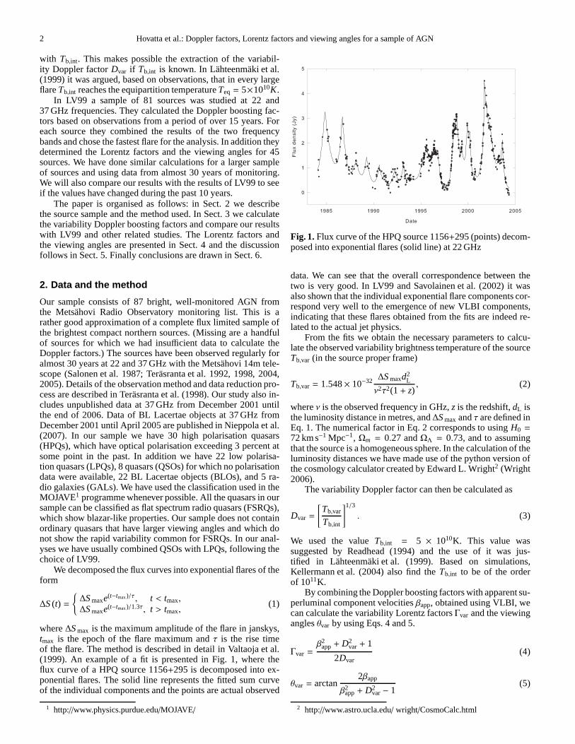
where∆S max is the maximum amplitude of the flare in janskys,tmax is the epoch of the flare maximum andτ is the rise timeof the flare. The method is described in detail in Valtaoja et al.(1999). An example of a fit is presented in Fig. 1, where theflux curve of a HPQ source 1156+295 is decomposed into ex-ponential flares. The solid line represents the fitted sum curveof the individual components and the points are actual observed

1 http://www.physics.purdue.edu/MOJAVE/

Fig. 1. Flux curve of the HPQ source 1156+295 (points) decom-posed into exponential flares (solid line) at 22 GHz

data. We can see that the overall correspondence between thetwo is very good. In LV99 and Savolainen et al. (2002) it wasalso shown that the individual exponential flare componentscor-respond very well to the emergence of new VLBI components,indicating that these flares obtained from the fits are indeedre-lated to the actual jet physics.

From the fits we obtain the necessary parameters to calcu-late the observed variability brightness temperature of the sourceTb,var (in the source proper frame)

Tb,var = 1.548× 10−32 ∆S maxd2L

ν2τ2(1+ z), (2)

whereν is the observed frequency in GHz,z is the redshift,dL isthe luminosity distance in metres, and∆S max andτ are defined inEq. 1. The numerical factor in Eq. 2 corresponds to usingH0 =

72 km s−1 Mpc−1, Ωm = 0.27 andΩΛ = 0.73, and to assumingthat the source is a homogeneous sphere. In the calculation of theluminosity distances we have made use of the python version ofthe cosmology calculator created by Edward L. Wright2 (Wright2006).

The variability Doppler factor can then be calculated as

Dvar =

[

Tb,var

Tb,int

]1/3

. (3)

We used the valueTb,int = 5 × 1010K. This value wassuggested by Readhead (1994) and the use of it was jus-tified in Lahteenmaki et al. (1999). Based on simulations,Kellermann et al. (2004) also find theTb,int to be of the orderof 1011K.

By combining the Doppler boosting factors with apparent su-perluminal component velocitiesβapp, obtained using VLBI, wecan calculate the variability Lorentz factorsΓvar and the viewinganglesθvar by using Eqs. 4 and 5.

Γvar =β2

app+ D2var+ 1

2Dvar(4)

θvar = arctan2βapp

β2app+ D2

var− 1(5)

2 http://www.astro.ucla.edu/ wright/CosmoCalc.html

Hovatta et al.: Doppler factors, Lorentz factors and viewing angles for a sample of AGN 3

We obtained 67βapp values from the MOJAVE sample, ob-served with the VLBA at 15 GHz. The values are taken fromthe website on September 9, 2008 and some of them may stillbe preliminary and change slightly in the final results (Lister etal. in preparation). This is the most homogeneous and largestsample ofβapp available at higher radio frequencies. These val-ues represent the fastest reliable speed in each jet as measured bythe MOJAVE programme at 15 GHz, using VLBA data spanningbetween 5 to 13 years, depending on the individual source.

3. The variability Doppler boosting factors

3.1. Estimation of the Doppler boosting factors

We were able to calculate the Doppler boosting factor (Dvar) for86 sources at 22 GHz, and for 72 sources at 37 GHz. For manysources we were able to determine theDvar for more than oneflare. The medians ofDvar are slightly larger at 22 GHz than at37 GHz, which could be due to different intrinsic brightness tem-peratures at the two frequency bands. In our analysis we chosethe fastest flare of each source (either at 22 or 37 GHz, whicheverhad the fastest flare) to calculate theDvar, as was done in LV99.The argument for using the fastest flare to determineDvar is thatthey are most likely to reach the limiting brightness temperatureand least likely to suffer from blending of flares which tends toincrease the fitted timescale. This way we were able to calculatetheDvar for all the 87 sources in our sample. By visual examina-tion, we divided the fits into three categories based on the good-ness of the fit. No single numerical value, such as theχ2 test, isalone suitable for describing the goodness, because these usuallycharacterise the entire flux curve, while we have only used one,fastest flare, to determine theDvar. In addition, relatively largeerror bars in some fainter sources cause theχ2 value to be small,while we consider a fit to be better when the scatter among thedatapoints is small.

We classified theDvar as excellent (E, 21 sources), good (G,24 sources) or acceptable (A, 42 sources). In the fits classified asexcellent, the exponential decomposition follows the datapointsquite precisely, as in the flares after the year 1997 in Fig. 1.Thefit is also unambiguous and other functions do not describe thebehaviour as well. Larger flares in Fig. 1 before 1995 wouldmainly be defined as good, because in these flares the fit followsthe flux curve well, but there is also some scatter, and in somecases there are not as many datapoints to define the fit as in theones defined as excellent. In the fits classified as acceptable, thescatter around the fit is still larger. This is often the case when theflux level of the source is modest and the errorbars consequentlylarge. However, none of our results change significantly if weexclude the acceptable sources. All Doppler boosting factors areshown in Table 1 where the B1950-name, other commonly usedname, type of the object, frequency of theDvar determination,redshift, quality of theDvar, logTb,var, Dvar, βapp, Γvar, θvar, coredominance parameterR, and maximum optical polarisationPmaxand its reference are listed.

It is difficult to determine exact error estimates for theDvarof each source. Some indications can be obtained from the stan-dard deviation ofDvar calculated from the various flares in onesource. We calculated the deviations for all the sources classi-fied as excellent, which had more than one flare to determinethe Dvar, including also flares determined as good. There were45 such cases (including all the fits at both 22 and 37 GHz) and,on average, each source had 5.7 well-defined flares. The medianstandard deviation for these is∼ 27%, which can be thought ofas an indication of the upper limit for the error estimate since in

Table 2. Median values of log(Tb,var) andDvar.

Type N log(Tb,var)[K] Dvar

HPQ 30 14.31 15.98LPQ 30 13.92 11.90FSRQ 60 14.19 14.61BLO 22 13.09 6.25GAL 5 11.65 2.07ALL 87 13.94 12.02

many cases the change in theDvar of individual flares can also bedue to differences in the source behaviour. It is also more likelyto see a very fast flare in each source the longer they are moni-tored. More insight into the errors can be obtained when our newDvar are compared to other studies (cf. Chapt. 3.2).

In Table 2 we show the median values of log(Tb,var) andDvarfor each source class separately and for HPQs and LPQs com-bined together (FSRQ). The distributions are shown in Figs.2and 3 and we can see that the distributions of quasars and BLOshave considerable overlap. HPQs have a tail extending to higherDvar and LPQs seem to be in between the HPQs and BLOs. Also,it is interesting to note that all the quasars are clearly Doppler-boosted, the smallest estimatedTb,var being 3.5 × 1011 K for1928+738. We ran the Kruskal-Wallis analysis to examine thedifferences between source classes. (All Kruskal-Wallis analy-ses in this paper have been performed with the Unistat statisticalpackage for Windows3 (version 5.0).) The results confirm thatall the source classes differ from the other classes significantlywith a 95% confidence limit.

3.2. Comparison with previous analyses

Our sample has 71 sources in common with the sample of LV99.We have re-calculated the Doppler boosting factors of LV99,us-ing the current cosmological model. Figure 4 shows the corre-lation between the Doppler boosting factors of LV99 and thenew values. The results are very similar and the values correlatewith a coefficient r= 0.77 (p=0.0000). Kruskal-Wallis analysisalso shows that the values come from the same population. Thisconfirms that the method is reliable because the results havenotchanged even though we have now ten more years of data. Thedifferences are mainly due to poor fits in LV99 which are dueto poor sampling or low flux density (large scatter) in the data.The scatter between the old and the new values is consistent withthe error analysis in Sect. 3.1. In some cases (e.g. 0430+052 and1156+295) the source has clearly changed its behaviour and ex-hibits a much faster flare in our new dataset. The new estimateswhich are calculated using almost 30 years of data should there-fore be more representative of the source behaviour.

We also compared ourDvar values with the Jorstad et al.(2005) values for 15 AGN, obtained at 43 GHz. Figure 5 showsthe correlation between the two values, and a Spearman rank cor-relation gives a coefficient r=0.56 (p=0.0123). We can see thatthe values in Jorstad et al. (2005) are in general somewhat higherthan ours. This can be due to their higher observing frequency(cf. Discussion). Also, their analysis method gives only anup-per limit to some sources. The distribution of source classes issimilar to ours, with quasars having the highest Doppler boost-ing factors, GALs the lowest and BLOs being in between them.

3 http://www.unistat.com/


Fig. 2. Distribution ofTb,var of the fastest flare in each source

Therefore we conclude that the Doppler boosting factors of thesetwo analyses correspond well with each other.

Homan et al. (2006) argued that during the most active stateTb,int should be closer to 2× 1011K and therefore theDvar of theLV99 are overestimated. This would make ourDvar values evensmaller, and the correspondence to Jorstad et al. (2005) would beworse. HigherTb,int would also increase our Lorentz factors forthe fastest sources, and as is shown later (cf. Chapters 4 and5),our new values are already twice as high as in LV99 and in somesources even extremely high. We also note that a different valuefor Tb,int does not change the distributions themselves, only thenumerical values.

We also compared our Doppler boosting factors to a re-cent study at a lower frequency of 5 GHz (Britzen et al. 2007).They calculated the IC Doppler boosting factors by using VLBIdata from the Caltech-Jodrell Bank Flat-Spectrum source sample(Taylor et al. 1996) and non-simultaneous ROSAT X-ray data.The Spearman rank correlation between our 24 common sources(excluding one outlier, 0836+710, with DIC = 88) is still quitegood (r=0.63, p=0.0004), and the slope of the linear fit betweenDIC andDvar is almost exactly one. We believe that most of thescatter is due to the errors in the IC Doppler boosting factors,since LV99 showed that for several reasons these are likely to bemuch less accurate than the variability Doppler boosting factors.

Fig. 3. Distribution ofDvar of the fastest flare in each source

3.3. Core dominance

Standard beaming models expect that more core-dominated ob-jects should be more beamed and thus have higher Doppler

Fig. 4. Correlation between theDvar from LV99 and our newDvarvalues


Fig. 5. Correlation between theDvar andδvar from Jorstad et al.(2005).

boosting factors. We studied this by calculating the core-dominance parameter R from VLBA data of Kovalev et al.(2005) at 15 GHz. The core-dominance is calculated by relat-ing the flux density of the coreS core to the total single-dish fluxdensity observed at 15 GHzS tot. In Kovalev et al. (2005) theseare given for 250 sources observed with the VLBA at 15 GHzat different epochs. Their sample includes 80 sources for whichwe have determinedDvar. We calculated the median R for eachsource from the separate epochs. Figure 6 shows the correla-tion between log R and logDvar, excluding an outlier source0923+392 with a very small core dominance (logR = −1.76).Spearman rank correlation between the parameters isr = 0.37(p = 0.0004). When the outlier source is included, the cor-relation is still significant with a coefficient r = 0.39 (p =0.0002). This shows that there is indeed some indication thatsources which are more core-dominated are also more boosted.In Kovalev et al. (2005) the core-dominance is defined to be therelation ofS core to the total VLBA flux densityS VLBA . We testedthe correlation using also this parameter but the results did notchange becauseS tot andS VLBA are so similar. Using the core-dominance defined withS VLBA , Kovalev et al. (2005) show thatquasars and BLOs are significantly different from GALs withlower core-dominance.

Similar calculations were made in Britzen et al. (2007) fortheir sample. They used the core flux density and total single-dish flux density at 5 GHz to calculate the core-dominance pa-rameter. They found no significant correlation between theircore-dominance parameter and the IC Doppler boosting factor.We have only 25 sources in common with their sample, andwhen we compared ourDvar with their core-dominance parame-ter, we found no correlation.

4. The Lorentz factors and viewing angles

We were able to calculate Lorentz factorsΓvar and viewing an-glesθvar for 67 sources. The median values of different sourceclasses are shown in Table 3. These are affected by two outlierswith exceptionally largeΓvar. The source 0923+392 hasΓvar =

216.1 and 1730-130 hasΓvar = 64.6. Both of these show highsuperluminal motion ofβapp> 35c, which increases the Lorentzfactors. The distributions of the source classes are shown in Figs.7 and 8. InΓvar the distributions of quasars and BLOs over-

Fig. 6. Correlation between log(R) using data from Kovalev et al.(2005) and log(Dvar), excluding the outlier source 0923+392with log(R) = −1.76 and log(Dvar) = 0.63.

Table 3. Median values ofΓvar andθvar.

Type N Γvar θvar

HPQ 26 17.41 3.28LPQ 23 13.96 3.90

21a 12.65 3.96FSRQ 49 16.24 3.37BLO 13 10.29 5.24GAL 5 1.82 15.52ALL 67 13.96 3.81

a = excluding outliers 0923+392 and 1730-130

lap, but BLOs and GALs have slower jet speeds than quasars.Kruskal-Wallis analysis shows that whenΓvar are studied with-out the outlier sources, HPQs differ from other classes withhigher Lorentz factors, and GALs differ with smaller Lorentzfactors. BLOs and LPQs come from the same population witha 13% confidence. There is one BLO (1823+568) for whichΓvar = 37.8. This source has also been classified as a HPQ(e.g. Veron-Cetty & Veron 2006) and therefore we ran the KW-analysis again by moving this source into the HPQ class. In thiscase also BLOs and LPQs differ significantly from each otherwith a 96% confidence. We must note that in our samples of 13to 26 objects the significance of differences can depend on theclassification of a single extreme source. However, a clear re-sult is that the BLOs and the quasars differ from each other withBLOs having slower jets (FSRQs and BLOs differ significantlywith a 99% confidence if 1823+568 is classified as a BLO andwith a 99.9% confidence if 1823+568 is classified as a HPQ).This result is in accordance with several earlier but more indirectestimates of jet speeds. Similar results have also been obtainedwith simulations (Hughes et al. 2002).

When θvar is studied, the distributions overlap even moreand KW-analysis shows that GALs and BLOs differ from othersource classes with a 95% confidence. Also, if the differences be-tween FSRQs and BLOs are studied, they differ from each othersignificantly with a 99% confidence with BLOs having largerviewing angles.


Fig. 7. Distribution ofΓvar of the fastest flare in each source (ex-cluding the outlier LPQs 0923+392 and 1730-130)

We compared our new Lorentz factors with the ones fromLV99. There are 38 sources in common in our samples, and inFig. 9 we can see that the newΓvar are about twice as large asin LV99. This is mainly because also the apparent speeds usedin our analysis are about twice as large as in LV99, where theywere collected from the literature. We should now have betterand more homogeneous estimates ofβapp which should makeour new estimates more accurate. The correlation between ourΓvar and those from LV99 is onlyr = 0.37 (p = 0.0113) whenthe outlier (0923+392) is not included (the other outlier 1730-130 is not included in the sample of LV99). When we compareour Γvar with Lorentz factors estimated in Jorstad et al. (2005)we find a good correlation ofr = 0.50 (p = 0.0281) which givescredibility to our new estimates. Also the distribution is similarwith quasars having the highest Lorentz factors, BLOs beinginbetween and GALs having the smallest Lorentz factors. We haveonly 12 sources in common with the sample of Britzen et al.(2007) and we find no correlation between our Lorentz factorseven if we leave out their outlier source 0016+731 for which theydetermine a Lorentz factor of 860. The differences are probablydue to their much lower values ofβapp and differences in theDoppler boosting factors.

When studying the viewing angles, the difference betweenour new and LV99 values is not as large and the correlation isgood (r = 0.51 p = 0.0005). The correlation between our valuesand Jorstad et al. (2005) values is also very good withr = 0.59

Fig. 8. Distribution ofθvar of the fastest flare in each source

(p = 0.0105). Again there are no significant correlations be-tweenθvar and values from Britzen et al. (2007).

5. Discussion

Although the Doppler boosting factors have remained on theaverage almost identical (cf. Fig. 4) even though we now haveten more years of data, there is a factor of two difference in theLorentz factors when comparing our new results to LV99. Thisismainly due to twice as fast apparent speeds in our new analysis.In LV99 the βapp values are mainly from Vermeulen & Cohen(1994), in which the values were gathered from the literature.This means that the speeds were obtained in the 1980s and early1990s from a variety of observing programmes and frequen-cies, mainly at 5 GHz. We use 15 GHz MOJAVE data from 1994up to September 2008, giving a far more uniform dataset. Wealso note that higher frequency VLBI observations often tend togive higher apparent speeds as can be seen by comparing, e.g.,data from Vermeulen & Cohen (1994); Kellermann et al. (2004);Jorstad et al. (2005) and Britzen et al. (2007), although therea-son for this is not clear. The use of a single frequency thereforediminishes the internal scatter.

Long-term observations, both TFD monitoring and VLBI,are essential in understanding source behaviour. We have al-ready shown this in our earlier studies of long-term variabilitybehaviour of these sources (Hovatta et al. 2007; Hovatta et al.2008a,b). Some sources have changed their behaviour in our


Fig. 9. Correlation between Lorentz factors from LV99 andthe new values (excluding the outlier source 0923+392 with aLorentz factor of 216 in the new analysis).

TFD observations during the past 10 years. Similar changes canbe seen in VLBI sources over a long time, such as the positionswings seen, for example, in 3C 273 (Savolainen et al. 2006) andNRAO 150 (Agudo et al. 2007). We emphasise that our way toestimate the Lorentz factors and viewing angles is as good ascanbe, when we are characterising a complex, changing jet with justtwo parameters, both assumed to be constant.

In addition to having twice as high apparent speeds in gen-eral, there are also some extreme sources showing very high ap-parent motion. While in LV99 the highest apparent speed was14.9, we now have two sources (0923+392 and 1730-130) withβapp > 35c. As a consequence, the Lorentz factors of thesesources are also extremely high,Γvar = 216 for 0923+392 andΓvar = 65 for 1730-130. We also note that if theβapp = 45.9 forthe source 1510-089 from Jorstad et al. (2005) is accepted, ourlog(Tb,var) = 14.4 would indicate aΓvar = 71. Thus, the existenceof a class of very fast jets should perhaps at least be consideredas a possibility.

However, at least theΓvar = 216 seems rather unlikely inview of our current knowledge of the jets in AGN. One alterna-tive explanation is that 0923+392 has a higher observed bright-ness temperature than what we have obtained (log(Tb,var) = 12.6)from our monitoring. If we saw changes of about 1 Jy within atime period of a week, the brightness temperature would be ofthe order of 1015K, which would change the Lorentz factor to amore acceptable value of under 50. Our sampling, like in othermonitoring programmes, is too sparse to detect such rapid flaresreliably, and therefore we have initiated a denser monitoringschedule for the source. Another possibility is that the source hasa complicated internal structure or geometry, such that theTFDvariations and the apparent speeds do not refer to the same com-ponent (e.g. Alberdi et al. 1993; Fey et al. 1997; Alberdi et al.2000). However, independent of ourTb,var estimates, 0923+392must have a Lorentz factor of at least 43 asΓ ≥ βapp.

In Fig. 10 we have plotted the observable quantitiesβappand log(Tb,var). We have included curves to mark areas of dif-ferent Γvar and θvar. The outlier sources are clearly visible inthis plot but otherwise the sources are within rather well-definedlimits. Almost all the sources haveΓvar < 40 andθvar < 20.The differences between the source classes are also seen in this

Fig. 10. Observable quantitiesβapp and log(Tb,var) together withintrinsic parametersΓvar andθvar.

plot, with GALs having slow speeds and low brightness tem-peratures. Using Monte-Carlo simulations, Cohen et al. (2007)find an upper limit for the Lorentz factor to beΓ ≈ 32. Thisagrees quite well with our results, although in our sample wehave five sources withΓvar between 30 and 50 and two quasarswith Γvar > 50.

A common assumption is that sources are viewed close tothe critical angleθc = 1/Γ. Figure 11 shows theΓ sinθ distribu-tion for our sources, which indeed does peak around 1. However,a number of sources haveΓ sinθ significantly larger or smaller,so that the assumption ofΓ sinθ = 1 will in many cases leadto false conclusions both for individual sources and for samples.Cohen et al. (2007) have calculated a Monte Carlo simulationfor a flux density limited survey (similar to ours), (Fig. 1c inCohen et al. (2007), in which the sources withΓ = 15 are plot-ted), finding a distribution rather similar to our empiricalone.

The simplest unification scheme for AGN (e.g. Barthel 1989;Urry & Padovani 1995) predicts that in all radio quasars (includ-ing ordinary quasars and FSRQs) theΓ distributions should besimilar. Ordinary quasars, on the other hand, should have largerviewing angles than blazars (FSRQs and BLOs). BLOs couldalso have a differentΓ distribution because their parent popula-tion is different than in quasars. In Fig. 12 we show the Lorentzfactors and viewing angles in a polar plot. It is easy to see that al-most all the sources are seen at a small viewing angle. What mustbe kept in mind is that our sample essentially includes the∼ 100brightest northern compact radio sources, so this is as expected


Fig. 11. Distribution ofΓ sinθ, excluding the source 0923+392with Γvar sinθvar = 10.

for Doppler boosting dominated sources. Although we have di-vided our quasars into HPQs and LPQs, they all are FSRQs (orblazars), and we do not see ordinary quasars withθvar > 20.Similarly, all our BLOs are radio selected BLOs (RBLs) whichshould have small viewing angles (Barthel 1989). In addition,the five GALs in our sample are the most compact and variablesources of their type. Figure 13 also shows how the sources atdifferent redshifts are selected due to their Doppler boosting sothat small Doppler boosting factors are not seen at high redshifts.These caveats must be kept in mind when comparing our differ-ent classes of sources with each other.

The distribution ofΓvar agrees well with unification schemesfor AGN. Padovani & Urry (1992) and Urry et al. (1991) calcu-lated beamed luminosity functions for FSRQs and BLOs, andcompared them with observed luminosity functions, which wereassumed to have the same shape as the intrinsic luminosity func-tion of radio-loud quasars. The validity of this assumptionwasrecently confirmed by using the maximum likelihood method tocalculate the intrinsic luminosity functions (Liu & Zhang 2007;Cara & Lister 2008). In Padovani & Urry (1992) the FSRQswere best described with a distribution of 5. Γ . 40 with anaverage of∼ 11 (using a cosmology withH0 = 50 km s−1 Mpc−1

andq0 = 0). In our sample all the FSRQs haveΓvar > 5 and threehaveΓvar > 40. The medianΓvar is somewhat bigger than theaverage from the luminosity functions. In Urry et al. (1991)theBLOs were best described with a distribution of 5. Γ . 35 withan average of∼ 7. Again we have only three BLOs withΓvar < 5and one BLO (1823+568, also classified as HPQ) withΓvar > 35.Our median is also only slightly bigger. In addition they madeanother fit for the BLOs with a distribution of 2. Γ . 20 whichalso fit the data well. In this case only one BLO (1807+698 withΓvar = 1.0) would be below the lower limit and there would betwo BLOs with Γvar > 20. Their calculations also set a valuefor the critical viewing angle in which all the FSRQs and BLOsshould be seen. For FSRQs the angle is 14, and all our quasarsare within this limit. For BLOs the critical angle is either 11

or 19 depending on the model. In both cases only one BLO(1807+698 withθvar = 57, which is also the nearest BLO in oursample) would have a viewing angle outside the limit.

As expected with sources with small viewing angles, distri-butions of LPQs and HPQs overlap and one should not iden-

Fig. 12. Polar plot of Lorentz factors against the viewing an-gles, excluding the outlier sources 0923+392 and 1730-130.The lower panel shows only the 0 to 20 portion of the view-ing angles, additionally excluding the galaxies 0007+106 and0316+413, and the BLO 1807+698.

tify LPQs as ordinary quasars. In Fig. 14 we show the maxi-mum optical polarisation against the viewing angle for all thesources for which we could find polarisation information in theliterature (Pmax and its reference for all the sources are shownin Table 1). Most of the sources seem to be within an enve-lope with Pmax decreasing asθvar increases. The situation maybe similar as in Seyfert galaxies with an obscuring torus (e.g.Schmitt et al. 2001). When the viewing angle is small, we can


Fig. 13. Dvar against the redshift.

Fig. 14. Maximum optical polarisation against the viewing an-gle.

see deeper into the jet and are more likely to see the sourceas more optically polarised. Also, it has been shown that boththe optical and the radio polarisation originate from transverseshocks located very close to the base of the jet (Lister & Smith2000). Therefore the range of polarisation variability is muchhigher for sources with a viewing angle of a few degrees thanfor sources withθvar = 10 − 20. In Fig. 14 it is also pos-sible to see that the definitionPmax = 3% for an object to beclassified as highly polarised is somewhat artificial. We believethat with a larger number of polarisation observations, a con-siderable fraction of the LPQ population could, at times, showpolarisation exceeding 3%, as expected from blazar-type AGN.Since there usually is only a small number of polarisation obser-vations, the likelihood of observing high polarisation increaseswith decreasing viewing angle. However, as has been pointedoutby Lister & Smith (2000), there is a physical difference betweenat least some HPQs and LPQs, especially in the magnetic fieldstructure of their inner jets.

Figure 14 hints that the transition from blazar-type AGN toordinary quasars may occur around a viewing angle of 15 to20, presumably corresponding to the half opening angle of an

AGN obscuring torus, and in agreement with, e.g., estimatesfrom luminosity functions and source counts. As our sampledoes not contain any ordinary quasars, no definite conclusionscan be drawn.

6. Conclusions

We have decomposed flux curves of 87 sources into exponentialflares and using the fits calculated the variability brightness tem-perature and Doppler boosting factor for each source. In addi-tion we used new MOJAVE observations of apparent jet speedsto calculate the variability Lorentz factors and viewing angles.We have compared our results with LV99, in which the param-eters were determined in a similar way. In our new analyses wehave used almost 15 years more data and the estimates shouldbe more accurate. Our main conclusions can be summarised asfollows.

1. The variability Doppler boosting factors have remained onthe average almost identical compared to LV99. All thequasars are Doppler-boosted and they are in general moreboosted than the BLOs or GALs.

2. The Lorentz factors of our new analyses are about twice aslarge as in LV99. The difference can be explained with twiceas large apparent VLBI speeds in our new analyses. TheBLOs have slower jets compared to quasars (ΓBLO = 10.3,ΓFSRQ= 16.2 andΓGAL = 1.8).

3. A few sources, 0923+392 and 1730-130, have extremeLorentz factors (216 and 65, respectively). Either theseLorentz factors are real, or the sources exhibit so rapid flaresthat the fast variations have remained undetected in the mon-itoring programmes. We are studying the second possibilitywith dense observations of 0923+392. A third possibility isthat the sources have a structure too complex for our method.

4. Almost all the sources in our sample are seen in a small view-ing angle of less than 20 degrees (θBLO = 5.2, θFSRQ= 3.4

andθGAL = 15.5).5. The viewing angle distribution peaks aroundΓ sinθ = 1,

with a distribution similar to that found in simulations.6. Our results generally follow the predictions of basic unifi-

cation models for AGN. Based on our results, we cannotseparate HPQs and LPQs from each other, and therefore itis well-grounded to treat them as a single group of FSRQswhen the jet parameters are considered.

Acknowledgements. We thank M. Lister and the members of the MOJAVE teamfor providing data in advance of publication. We acknowledge the support of theAcademy of Finland (project numbers 212656 and 210338). This research hasmade use of data from the MOJAVE (Lister and Homan, 2005, AJ, 130, 1389)and 2cm Survey (Kellermann et al., 2004, ApJ, 609, 539) programs.

ReferencesAgudo, I., Bach, U., Krichbaum, T. P., et al. 2007, A&A, 476, L17Alberdi, A., Gomez, J. L., Marcaide, J. M., Marscher, A. P.,& Perez-Torres,

M. A. 2000, A&A, 361, 529Alberdi, A., Marcaide, J. M., Marscher, A. P., et al. 1993, ApJ, 402, 160Angel, J. R. P. & Stockman, H. S. 1980, ARA&A, 18, 321Barthel, P. D. 1989, ApJ, 336, 606Britzen, S., Brinkmann, W., Campbell, R. M., et al. 2007, A&A, 476, 759Britzen, S., Vermeulen, R. C., Campbell, R. M., et al. 2008, A&A, 484, 119Cara, M. & Lister, M. L. 2008, ApJ, 674, 111Cohen, M. H., Lister, M. L., Homan, D. C., et al. 2007, ApJ, 658, 232Fey, A. L., Eubanks, M., & Kingham, K. A. 1997, AJ, 114, 2284Ghisellini, G., Padovani, P., Celotti, A., & Maraschi, L. 1993, ApJ, 407, 65Guerra, E. J. & Daly, R. A. 1997, ApJ, 491, 483Guijosa, A. & Daly, R. A. 1996, ApJ, 461, 600


Homan, D. C., Kovalev, Y. Y., Lister, M. L., et al. 2006, ApJ, 642, L115Homan, D. C., Ojha, R., Wardle, J. F. C., et al. 2001, ApJ, 549,840Hovatta, T., Lehto, H. J., & Tornikoski, M. 2008a, A&A, 488, 897Hovatta, T., Nieppola, E., Tornikoski, M., et al. 2008b, A&A, 485, 51Hovatta, T., Tornikoski, M., Lainela, M., et al. 2007, A&A, 469, 899Hughes, P. A., Miller, M. A., & Duncan, G. C. 2002, ApJ, 572, 713Impey, C. D., Bychkov, V., Tapia, S., Gnedin, Y., & Pustilnik, S. 2000, AJ, 119,

1542Impey, C. D., Lawrence, C. R., & Tapia, S. 1991, ApJ, 375, 46Impey, C. D. & Tapia, S. 1990, ApJ, 354, 124Jorstad, S. G., Marscher, A. P., Lister, M. L., et al. 2005, AJ, 130, 1418Jorstad, S. G., Marscher, A. P., Mattox, J. R., et al. 2001, ApJS, 134, 181Jorstad, S. G., Marscher, A. P., Stevens, J. A., et al. 2007, AJ, 134, 799Kellermann, K. I., Lister, M. L., Homan, D. C., et al. 2004, ApJ, 609, 539Kovalev, Y. Y., Kellermann, K. I., Lister, M. L., et al. 2005,AJ, 130, 2473Lahteenmaki, A. & Valtaoja, E. 1999, ApJ, 521, 493, LV99Lahteenmaki, A., Valtaoja, E., & Wiik, K. 1999, ApJ, 511, 112Lister, M. L. & Smith, P. S. 2000, ApJ, 541, 66Liu, Y. & Zhang, S. N. 2007, ApJ, 667, 724Moore, R. L. & Stockman, H. S. 1984, ApJ, 279, 465Nieppola, E., Tornikoski, M., Lahteenmaki, A., et al. 2007, AJ, 133, 1947Padovani, P. & Urry, C. M. 1992, ApJ, 387, 449Piner, B. G., Mahmud, M., Fey, A. L., & Gospodinova, K. 2007, AJ, 133, 2357Punsly, B. 1996, ApJ, 473, 152Readhead, A. C. S. 1994, ApJ, 426, 51Salonen, E., Terasranta, H., Urpo, S., et al. 1987, A&AS, 70, 409Savolainen, T., Wiik, K., Valtaoja, E., Jorstad, S. G., & Marscher, A. P. 2002,

A&A, 394, 851Savolainen, T., Wiik, K., Valtaoja, E., & Tornikoski, M. 2006, A&A, 446, 71Schmitt, H. R., Antonucci, R. R. J., Ulvestad, J. S., et al. 2001, ApJ, 555, 663Sluse, D., Hutsemekers, D., Lamy, H., Cabanac, R., & Quintana, H. 2005, A&A,

433, 757Smith, P. S., Balonek, T. J., Heckert, P. A., Elston, R., & Schmidt, G. D. 1985,

AJ, 90, 1184Stickel, M. & Kuehr, H. 1994, A&AS, 105, 67Taylor, G. B., Vermeulen, R. C., Readhead, A. C. S., et al. 1996, ApJS, 107, 37Terasranta, H., Achren, J., Hanski, M., et al. 2004, A&A, 427, 769Terasranta, H., Tornikoski, M., Mujunen, A., et al. 1998, A&AS, 132, 305Terasranta, H., Tornikoski, M., Valtaoja, E., et al. 1992,A&AS, 94, 121Terasranta, H., Wiren, S., Koivisto, P., Saarinen, V., & Hovatta, T. 2005, A&A,

440, 409Urry, C. M. & Padovani, P. 1995, PASP, 107, 803Urry, C. M., Padovani, P., & Stickel, M. 1991, ApJ, 382, 501Valtaoja, E., Lahteenmaki, A., Terasranta, H., & Lainela, M. 1999, ApJS, 120,

95Vermeulen, R. C. & Cohen, M. H. 1994, ApJ, 430, 467Veron-Cetty, M.-P. & Veron, P. 2006, A&A, 455, 773Wills, B. J., Wills, D., Breger, M., Antonucci, R. R. J., & Barvainis, R. 1992,

ApJ, 398, 454Wright, E. L. 2006, PASP, 118, 1711


Table 1. Doppler boosting factors, Lorentz factor and viewing angles for all sources.

B1950-name Other name Type ν z Quality log(Tb) Dvar βapp Γvar θvar logR Pmax ref.0003−066 NRAO 5 BLO 22 0.347 A 12.82 5.1 2.660 3.3 9.5 -0.133 3.4 110007+106 III ZW 2 GAL 37 0.089 E 11.37 1.7 0.98 1.4 35.4 0.004 0.2 120016+731 LPQ 37 1.781 A 13.40 7.9 6.67 6.8 7.1 -0.104 0.6 110048−097 PKS 0048-097 BLO 22 0.300 A 13.65 9.6 ... ... ... -0.082 27.1 20059+581 QSO 22 0.644 G 14.15 14.1 11.1 11.5 4.0 0.018 ... ...0106+013 OC 012 HPQ 22 2.099 E 14.50 18.4 26.16 27.8 2.9 -0.172 7.1 110133+476 DA 55 HPQ 22 0.859 G 14.65 20.7 12.95 14.4 2.5 -0.068 20.8 30149+218 LPQ 37 1.320 A 12.83 5.1 ... ... ... -0.024 ... ...0202+149 4C 15.05 HPQ 22 0.405 G 14.24 15.1 8.31 9.9 3.2 -0.216 4.0 20212+735 HPQ 22 2.367 A 13.48 8.5 7.35 7.5 6.7 -0.268 7.8 20219+428 3C 66A BLO 37 0.444 A 11.92 2.6 ... ... ... ... 29.7 50224+671 QSO 22 0.523 A 13.43 8.2 11.67 12.5 6.6 -0.308 ... ...0234+285 4C 28.07 HPQ 37 1.213 G 14.32 16.1 12.23 12.7 3.4 -0.090 11.3 20235+164 BLO 22 0.940 G 14.84 24.0 2.000 12.1 0.4 -0.092 44.7 20306+102 PKS 0306+102 BLO 22 0.863 A 13.97 12.3 ... ... ... ... ... ...0316+413 3C 84 GAL 37 0.018 G 9.26 0.3 0.32 1.8 39.1 -0.654 6.0 110333+321 NRAO 140 LPQ 22 1.263 G 14.74 22.2 12.7 14.7 2.2 -0.140 0.7 120336−019 CTA 026 HPQ 22 0.852 A 14.42 17.4 22.32 23.0 3.2 -0.133 19.420355+508 NRAO 150 QSO 37 1.510 G 14.05 13.1 ... ... ... -0.015 ... ...0415+379 3C 111 GAL 37 0.049 G 12.09 2.9 5.94 7.7 15.5 -0.432 3.1 50420−014 OA 129 HPQ 37 0.915 E 14.59 19.9 7.52 11.4 1.9 -0.097 26.2 110430+052 3C 120 GAL 22 0.033 G 13.01 5.9 5.42 5.5 9.7 -0.488 0.5 50440−003 NRAO 190 HPQ 22 0.844 A 14.03 12.9 ... ... ... -0.291 12.5 110458−020 PKS 0458-020 HPQ 37 2.286 G 14.29 15.8 16.2 16.2 3.6 -0.13417.3 20528+134 PKS 0528+134 HPQ 22 2.070 E 15.18 31.2 18.73 21.2 1.6 -0.059 4.1 50552+398 DA 193 LPQ 37 2.363 A 14.91 25.2 0.45 12.6 0.1 -0.157 1.9 120605−085 PKS 0605-085 HPQ 37 0.872 A 13.34 7.6 19.98 30.2 5.0 -0.1919.8 110642+449 OH 471 LPQ 22 3.396 G 13.78 10.7 0.53 5.4 0.5 -0.192 1.7 70716+714 BLO 22 0.310 E 13.81 10.9 10.22 10.3 5.2 -0.219 17.3 40735+178 PKS 0735+17 BLO 37 0.424 G 12.43 3.8 ... ... ... -0.378 36.0 20736+017 HPQ 22 0.191 E 13.50 8.6 14.73 17.0 5.8 -0.157 8.4 110754+100 OI 090.4 BLO 37 0.266 A 12.95 5.6 14.530 21.7 6.9 -0.168 26.0 10804+499 HPQ 22 1.436 E 15.35 35.5 1.81 17.8 0.2 -0.096 8.6 20814+425 BLO 22 0.245 G 12.69 4.6 1.720 2.7 8.4 -0.139 8.7 20827+243 OJ 248 LPQ 37 0.941 A 14.05 13.1 21.3 23.9 3.9 -0.037 1.5 70836+710 4C 71.07 LPQ 37 2.218 A 14.33 16.3 25.39 28.0 3.2 -0.119 1.1110847−120 J 0850-1213 QSO 37 0.566 G 14.35 16.5 ... ... ... ... ... ...0851+202 OJ 287 BLO 22 0.306 E 14.39 17.0 15.31 15.4 3.3 -0.181 15.6 50923+392 4C 39.25 LPQ 37 0.695 G 12.60 4.3 42.94 216.1 2.6 -1.757 0.520945+408 4C 40.24 HPQ 37 1.249 A 13.13 6.4 18.47 29.8 5.5 -0.274 6.5 30953+254 LPQ 37 0.712 A 12.61 4.3 ... ... ... -0.268 2.2 20954+658 S4 0954+65 BLO 37 0.367 A 13.07 6.2 ... ... ... -0.054 33.7 111055+018 OL 093 HPQ 37 0.888 G 13.96 12.2 10.96 11.1 4.7 -0.159 5.0 21156+295 4C 29.45 HPQ 22 0.729 E 15.06 28.5 24.85 25.1 2.0 -0.080 9.2121219+285 ON 231 BLO 22 0.102 A 10.96 1.2 ... ... ... -0.363 10.0 11222+216 PKS 1222+216 LPQ 37 0.432 A 12.85 5.2 21.12 45.5 5.1 -0.210 1.5 91226+023 3C 273 LPQ 22 0.158 E 14.39 17.0 13.59 14.0 3.3 -0.809 0.5 21253−055 3C 279 HPQ 37 0.536 E 14.84 24.0 20.64 20.9 2.4 -0.242 39.2 51308+326 AU CV n HPQ 22 0.997 G 14.26 15.4 27.500 32.2 3.2 -0.096 25.021324+224 QSO 22 1.400 A 14.68 21.2 3.04 10.9 0.8 -0.075 ... ...1413+135 BLO 22 0.247 G 13.96 12.2 1.860 6.3 1.4 -0.112 13.0 81418+546 OQ 530 BLO 22 0.151 A 12.83 5.1 ... ... ... -0.175 19.0 11502+106 OR 103 HPQ 37 1.839 E 13.94 12.0 14.6 14.9 4.7 -0.202 3.0 21510−089 PKS 1510-089 HPQ 37 0.360 E 14.37 16.7 20.29 20.7 3.4 -0.167 7.8 111538+149 4C 14.60 BLO 37 0.605 A 12.60 4.3 8.750 11.2 10.5 -0.296 17.4 21606+106 4C 10.45 LPQ 22 1.226 G 14.89 25.0 18.78 19.6 2.2 -0.081 1.9111611+343 DA 406 LPQ 37 1.401 A 14.11 13.7 14.17 14.2 4.2 -0.179 2.3 61633+382 4C 38.41 HPQ 22 1.814 E 14.70 21.5 29.13 30.5 2.5 -0.256 7.061637+574 OS 562 LPQ 22 0.751 A 14.13 14.0 10.61 11.0 4.0 -0.093 1.5 121641+399 3C 345 HPQ 37 0.593 E 13.38 7.8 19.27 27.7 5.1 -0.412 38.3 51725+044 PKS 1725+044 QSO 22 0.293 A 12.44 3.8 ... ... ... ... ... ...1730−130 NRAO 530 QSO 37 0.902 G 13.79 10.7 35.6 64.6 3.0 -0.291 ... ...1739+522 S4 1739+52 HPQ 22 1.375 E 14.97 26.5 ... ... ... -0.040 3.7 111741−038 PKS 1741-038 HPQ 22 1.054 E 14.58 19.7 ... ... ... -0.055 9.2 21749+096 PKS 1749+096 BLO 37 0.322 E 13.93 12.0 5.880 7.5 3.8 -0.030 31.3 21803+784 S5 1803+784 BLO 22 0.684 A 13.96 12.2 8.980 9.5 4.5 -0.250 7.0 31807+698 3C 371.0 BLO 37 0.051 A 10.78 1.1 0.120 1.0 57.3 -0.328 8.0 3


Table 1. continued.

B1950-name Other name Type ν z Quality log(Tb) Dvar βapp Γvar θvar logR Pmax ref.1823+568 4C 56.27 BLO 22 0.663 A 13.11 6.4 20.950 37.8 5.0 -0.154 29.8 51828+487 3C 380 LPQ 37 0.692 A 12.97 5.7 13.66 19.3 7.1 -0.391 0.4 21928+738 4C 73.18 LPQ 22 0.302 A 11.55 1.9 8.48 19.9 12.8 -0.402 0.8 21954+513 LPQ 22 1.223 A 13.30 7.4 ... ... ... -0.181 1.4 112005+403 QSO 37 1.736 A 14.07 13.3 19.48 21.0 4.0 -0.257 ... ...2007+776 S5 2007+77 BLO 22 0.342 A 13.39 7.9 ... ... ... -0.304 15.1 112021+614 OW 637 GAL 22 0.227 A 11.65 2.1 0.41 1.3 13.3 ... 0.3 32022+171 LPQ 22 1.050 A 12.99 5.8 ... ... ... ... ... ...2121+053 HPQ 22 1.941 A 14.25 15.3 13.05 13.2 3.7 -0.061 10.7 72134+004 OX 057 LPQ 22 1.932 A 14.32 16.1 5.62 9.0 2.2 -0.405 2.8 122136+141 LPQ 22 2.427 A 13.46 8.3 5.08 5.8 6.2 -0.175 1.6 112145+067 LPQ 37 0.990 G 14.28 15.6 2.49 8.0 1.1 -0.171 0.6 22200+420 BL LAC BLO 37 0.069 E 13.28 7.3 10.700 11.6 7.3 -0.264 23.0 12201+315 4C 31.63 LPQ 22 0.295 G 13.17 6.7 7.88 8.1 8.5 -0.096 0.2 22223−052 3C 446 HPQ 22 1.404 G 14.31 16.0 16.470 16.5 3.6 -0.203 17.3102227−088 HPQ 22 1.562 A 14.31 15.9 4.95 8.8 2.0 -0.137 6.9 122230+114 CTA 102 HPQ 37 1.037 E 14.28 15.6 15.51 15.5 3.7 -0.269 10.972234+282 HPQ 22 0.795 A 13.03 6.0 ... ... ... -0.464 4.4 112251+158 3C 454.3 HPQ 37 0.859 E 15.26 33.2 14.86 19.9 1.3 -0.564 16.0 12254+074 PKS 2254+074 BLO 22 0.190 A 11.91 2.5 ... ... ... ... 21.0 1

References: (1) Angel & Stockman (1980); (2) Impey & Tapia (1990); (3) Impey et al. (1991); (4) Impey et al. (2000); (5) Jorstad et al. (2007);(6) Lister & Smith (2000); (7) Moore & Stockman (1984); (8) Punsly (1996); (9) Sluse et al. (2005); (10) Smith et al. (1985); (11) Stickel & Kuehr(1994); (12) Wills et al. (1992).


List of Objects

‘1156+295’ on page 2‘1156+295’ on page 2‘1928+738’ on page 3‘0430+052’ on page 3‘1156+295’ on page 3‘0836+710’ on page 4‘0923+392’ on page 5‘0923+392’ on page 5‘1730-130’ on page 5‘0923+392’ on page 5‘1823+568’ on page 5‘1823+568’ on page 5‘1823+568’ on page 5‘0923+392’ on page 6‘1730-130’ on page 6‘0016+731’ on page 6‘3C 273’ on page 7‘NRAO 150’ on page 7‘0923+392’ on page 7‘1730-130’ on page 7‘0923+392’ on page 7‘1730-130’ on page 7‘1510-089’ on page 7‘0923+392’ on page 7‘0923+392’ on page 7‘0923+392’ on page 8‘1823+568’ on page 8‘1807+698’ on page 8‘1807+698’ on page 8‘0923+392’ on page 9‘1730-130’ on page 9‘0923+392’ on page 9‘0003−066’ on page 11‘0007+106’ on page 11‘0016+731’ on page 11‘0048−097’ on page 11‘0059+581’ on page 11‘0106+013’ on page 11‘0133+476’ on page 11‘0149+218’ on page 11‘0202+149’ on page 11‘0212+735’ on page 11‘0219+428’ on page 11‘0224+671’ on page 11‘0234+285’ on page 11‘0235+164’ on page 11‘0306+102’ on page 11‘0316+413’ on page 11‘0333+321’ on page 11‘0336−019’ on page 11‘0355+508’ on page 11‘0415+379’ on page 11‘0420−014’ on page 11‘0430+052’ on page 11‘0440−003’ on page 11‘0458−020’ on page 11‘0528+134’ on page 11‘0552+398’ on page 11‘0605−085’ on page 11‘0642+449’ on page 11‘0716+714’ on page 11‘0735+178’ on page 11‘0736+017’ on page 11‘0754+100’ on page 11‘0804+499’ on page 11‘0814+425’ on page 11‘0827+243’ on page 11‘0836+710’ on page 11

‘0847−120’ on page 11‘0851+202’ on page 11‘0923+392’ on page 11‘0945+408’ on page 11‘0953+254’ on page 11‘0954+658’ on page 11‘1055+018’ on page 11‘1156+295’ on page 11‘1219+285’ on page 11‘1222+216’ on page 11‘1226+023’ on page 11‘1253−055’ on page 11‘1308+326’ on page 11‘1324+224’ on page 11‘1413+135’ on page 11‘1418+546’ on page 11‘1502+106’ on page 11‘1510−089’ on page 11‘1538+149’ on page 11‘1606+106’ on page 11‘1611+343’ on page 11‘1633+382’ on page 11‘1637+574’ on page 11‘1641+399’ on page 11‘1725+044’ on page 11‘1730−130’ on page 11‘1739+522’ on page 11‘1741−038’ on page 11‘1749+096’ on page 11‘1803+784’ on page 11‘1807+698’ on page 11‘1823+568’ on page 12‘1828+487’ on page 12‘1928+738’ on page 12‘1954+513’ on page 12‘2005+403’ on page 12‘2007+776’ on page 12‘2021+614’ on page 12‘2022+171’ on page 12‘2121+053’ on page 12‘2134+004’ on page 12‘2136+141’ on page 12‘2145+067’ on page 12‘2200+420’ on page 12‘2201+315’ on page 12‘2223−052’ on page 12‘2227−088’ on page 12‘2230+114’ on page 12‘2234+282’ on page 12‘2251+158’ on page 12‘2254+074’ on page 12

Erratum: Doppler factors, Lorentz factors, and viewing angles for quasars, BL Lacertae objects and...

Documents

Transcript of Erratum: Doppler factors, Lorentz factors, and viewing angles for quasars, BL Lacertae objects and...