Ernest Shult · David Surowski A Teaching and Source Book
551
Ernest Shult · David Surowski Algebra A Teaching and Source Book
-
Upload
khangminh22 -
Category
Documents
-
view
0 -
download
0
Transcript of Ernest Shult · David Surowski A Teaching and Source Book

Ernest Shult · David Surowski
AlgebraA Teaching and Source Book

Algebra

Ernest Shult • David Surowski
AlgebraA Teaching and Source Book
123

Ernest ShultDepartment of MathematicsKansas State UniversityManhattan, KSUSA
David SurowskiManhattan, KSUSA
David Surowski is deceased.
ISBN 978-3-319-19733-3 ISBN 978-3-319-19734-0 (eBook)DOI 10.1007/978-3-319-19734-0
Library of Congress Control Number: 2015941161
Springer Cham Heidelberg New York Dordrecht London© Springer International Publishing Switzerland 2015This work is subject to copyright. All rights are reserved by the Publisher, whether the whole or partof the material is concerned, specifically the rights of translation, reprinting, reuse of illustrations,recitation, broadcasting, reproduction on microfilms or in any other physical way, and transmissionor information storage and retrieval, electronic adaptation, computer software, or by similar or dissimilarmethodology now known or hereafter developed.The use of general descriptive names, registered names, trademarks, service marks, etc. in thispublication does not imply, even in the absence of a specific statement, that such names are exempt fromthe relevant protective laws and regulations and therefore free for general use.The publisher, the authors and the editors are safe to assume that the advice and information in thisbook are believed to be true and accurate at the date of publication. Neither the publisher nor theauthors or the editors give a warranty, express or implied, with respect to the material contained herein orfor any errors or omissions that may have been made.
Printed on acid-free paper
Springer International Publishing AG Switzerland is part of Springer Science+Business Media(www.springer.com)

Preface
This book is based on the notes of both authors for a course called “HigherAlgebra,” a graduate level course. Its purpose was to offer the basic abstract algebrathat any student of mathematics seeking an advanced degree might require.Students may have been previously exposed to some of the basic algebraic objects(groups, rings, vector spaces, etc.) in an introductory abstract algebra course such asthat offered in the classic book of Herstein. But that exposure should not be a hardrequirement as this book proceeds from first principles. Aside from the far greatertheoretical depth, perhaps the main difference between an introductory algebracourse, and a course in “higher algebra” (as exemplified by classics such asJacobson’s Basic algebra [1, 2] and Van der Waerden’s Modern Algebra [3]) is anemphasis on the student understanding how to construct a mathematical proof, andthat is where the exercises come in.
The authors rotated teaching this one-year course called “Higher Algebra” atKansas State University for 15 years—each of us generating his own set of notesfor the course. This book is a blend of these notes.
Listed below are some special features of these notes.
1. (Combinatorial Background) Often the underlying combinatorial contexts—partially ordered sets etc.—seem almost invisible in a course on modern algebra.In fact they are often developed far from home in the middle of some specificalgebraic context. Partially ordered sets are the natural context in which todiscuss the following:
(a) Zorn’s Lemma and the ascending and descending chain conditions,(b) Galois connections,(c) The modular law,(d) The Jordan Hölder Theorem,(e) Dependence Theories (needed for defining various notions of
“dimension”).
The Jordan Hölder Theorem asserts that in a lower semimodular semilattice, anysemimodular function from the set of covers (unrefinable chains of length one)
v

to a commutative monoid extends to an interval measure on all algebraicintervals (those intervals containing a finite unrefinable chain from the bottom tothe top). The extension exists because the multiset of values of the function onthe covers in any two unrefinable chains connecting a and b must be the same.The proof is quite easy, and the applications are everywhere. For example, whenG is a finite group and P is the poset of subnormal subgroups, one notes that P isa semimodular lower semilattice and the reading of the simple group A=B of acover A\B, is a semimodular function on covers by a fundamental theorem ofhomomorphisms of groups. By the theorem being described, this functionextends to an interval measure with values in the additive monoid of multisetson the isomorphism classes of simple groups. The conclusion of the combina-torial Jordan-Hölder version in this context becomes the classical Jordan-HölderTheorem for finite groups. One needs no “Butterfly Lemma” or anything else.
2. (Free Groups) Often a free group on generators X is presented in an awkwardway—bydefining a “multiplication”on ‘reducedwords’rðwÞ, wherew is aword inthe free monoid MðX [X�1Þ. ‘Reduced’ means all factors of the form xx�1 havebeen removed. Here are the complications: First the reductions, which can often beperformed in many ways, must lead to a common reduced word. Then one mustshow rðw1 � w2Þ ¼ rðrðw1Þ � rðw2ÞÞ to get “multiplication” defined on reducedwords. Then one needs to verify the associative law and the other group axioms.In this book the free group is defined to be the automorphism group of a certainlabelled graph, and the universal mapping properties of the free group are easilyderived from the graph. Since full sets of automorphisms of an object alwaysform a group, one will not be wasting time showing that an akwardly-definedmultiplication obeys the axioms of a group.
3. (Universal Mapping Properties) These are always instances of the existence ofan initial or terminal object in an appropriate category.
4. (Avoiding Determinants of Matrices) Of course one needs matrices to describelinear transformations of vector spaces, or to record data about bilinear forms(the Grammian). It is important to know when the rows or columns of a matrixare linearly dependant. One can calculate what is normally called the determi-nant by finding the invariant factors. For an n� n matrix, that process involvesroughly n3 steps, while the usual procedure for evaluating the determinant usingLagrange’s rule, involves exponentially many steps.One of the standard proofs that the trace mapping tr : K ! F of a finite sepa-rable field extension F�K is nonzero proceeds as follows: First, one forms thenormal closure L of the field K. One then invokes the theorem that L ¼ FðθÞ, asimple extension, with the algebraic conjugates of θ as an F-basis of L. And thenone reaches the conclusion by observing that a van der Monde determinant isnon-zero. Perhaps it is an aesthetic quibble, but one does not like to see a nice“soft” algebraic proof about “soft” algebraic objects reduced to a matrix cal-culation. In Sect. 11.7 the proof that the trace is non-trivial is accomplishedusing only the Dedekind Independence Lemma and an elementary fact aboutbilinear forms.
vi Preface

In general, in this book, the determinant of a transformation T acting on ann-dimension vector space V is defined to be the scalar multiplication it induceson the n-th exterior product ^nðVÞ. Of course there are historical reasons formaking a few exceptions to any decree to ban the usual formulaic definition ofdeterminants altogether. Our historical discussion of the discriminant on page395 is such an exception.
In addition, we have shaped the text with several pedagogical objectives in mind.
1. (Catch-up opportunities) Not infrequently, the teacher of a graduate course isexpected to accommodate incoming transfer students whose mathematicalpreparation is not quite the same as that of current students of the program, or iseven unknown. At the same time, this accommodation should not sacrificecourse content for the other students. For this this reason we have written eachchapter at a gradient—with simplest explanations and examples first, beforecontinuing at the level the curriculum requires. This way, a student may “catchup” by studying the introductory material more intensely, while a more briefreview of it is presented in class. Students already familiar with the introductorymaterial have merely to turn the page.
2. (Curiosity-driven Appendices) The view of both authors has always been that acourse in Algebra is not an exercise in cramming information, but is instead away of inspiring mathematical curiosity. Real learning is basicallycuriosity-driven self-learning. Discussing what is is already known is simplythere to guide the student to the real questions. For that reason we have inserteda number of appendices which are largely centered around incites connectedwith proofs in the text. Similarly, in the exercises, we have occasionally wan-dered into open problems or offered avenues for exploration. Mathematicseducation is not a catechism.
3. (Planned Redundancy) Beside its role as a course guide, a textbook often livesanother life as a source book. There is always the need of a student or colleaguein a nearby mathematical field to check on some algebraic fact—say, to makesure of the hypotheses that accompany that fact. He or she does not need to readthe whole book. But occasionally one wanders into the following scenario: onelooks up topic A in the index, and finds, at the indicated page, that A is definedby further words B and C whose definition can be deciphered by a further visitto the index, which obligingly invites one to further pages at which the frus-tration may be enjoyed once again. It becomes a tree search. In order to interceptthis process, we have tried to do the following: when an earlier-defined keyconcept re-inserts itself in a later discussion, we simply recall the definition forthe reader at that point, while offering a page number where the concept wasoriginally defined.1 Nevertheless we are introducing a redundancy. But in the
1If we carried out this process for the most common concepts, pages would be filled with re-definitions of rings, natural numbers, and what the containment relation is. Of course one has tolimit these reminders of definitions to new key terms.
Preface vii

view of the authors’ experience in Kansas, redundancy is a valuable tool inteaching. Inspiration is useless if the student cannot first understand the words—and no teacher should apologize for redundancy. Judiciously applied, it does notwaste class time; it actually saves it.
Of course there are many topics—direct offshoots of the material of thiscourse—that cannot be included here. One cannot do justice to such topics in a briefsurvey like this. Thus one will not find in this book material about(i) Representation Theory and Character Theory of Groups, (ii) Commutative Ringsand the world of Ext and Tor, (iii) Group Cohomology or other HomologicalAlgebra, (iv) Algebraic Geometry, (v) Really Deep Algebraic Number Theory and(vi) many other topics. The student is better off receiving a full exposition of thesecourses elsewhere rather than being deceived by the belief that the chapters of thisbook provide such an expertise. Of course, we try to indicate some of these pointsof departure as we meet them in the text, at times suggesting exterior references.
A few words are inserted here about how the book can be used.As mentioned above, the book is a blend of the notes of both authors who
alternately taught the course for many years. Of course there is much more in thisbook than can reasonably be covered in a two-semester course. In practice a courseincludes enough material from each chapter to reach the principle theorems. That is,portions of chapters can be left out. Of course the authors did not always present thecourse in exactly the same way, but the differences were mainly in the way focusand depth were distributed over the various topics. We did not “teach” theappendices to the chapters. They were there for the students to explore on theirown.
The syllabus presented here would be fairly typical. The numbers in parenthesisrepresent the number of class-hours the lectures usually consume. A two-semestercourse entails 72 class-hours. Beyond the lectures we normally allowed ourselves10–12 h for examinations and review of exercises.
1. Chapter 1: (1 or 2) [This goes quickly since it involves only two easy proofs.]2. Chapter 2: (6, at most) [This also goes quickly since, except for three easy
proofs, it is descriptive. The breakdown would be: (a) 2.2.1–2.2.9 (skip 2.2.10),2.2.10–2.2.15 (3 h), (b) 2.3 and 2.5 (2 h) and (c) 2.6 (1 h).]
3. Chapter 3: (3)4. Chapter 4: (3) [Sometimes omitting 4.2.3.]5. Chapter 5: (3 or 4) [Sometimes omitting 5.5.]6. Chapter 6: (3) [Omitting the Brauer-Ree Theorem [6.4] but reserving 15
minutes for Sect. 6.6.]7. Chapter 7: (3) Mostly examples and few proofs. Section 7.3.6 is often omitted.]8. Chapter 8: (7 or 8) [Usually (a) 8.1 (2 or 3 h), and (b) 8.2–8.4 (4 h). We
sometimes omitted Sect. 8.3 if behind schedule.]9. Chapter 9: (4) [One of us taught only 9.1–9.8 (sometimes omitting the local
characterization of UFDs in 9.6.3) while the other would teach all of 9.9–9.12(Dedekind’s Theorem and the ideal class group.]
viii Preface

10. Chapter 10: (6) [It takes 3 days for 10.1–10.5. The student is asked to read 10.6,and 3 days remain for Sect. 10.7 and autopsies on some of the exercises.]
11. Chapter 11: (11) [The content is rationed as follows: (a) 11.1–11.4 (2 h),sometimes omitting 11.4.2 if one is short a day, (b) 11.5–11.6 (3 h) (c) 11.7[One need only mention this.] (d) 11.8–11.9 (3 h) (e) [One of us would oftenomit 11.10 (algebraic field extensions are often simple extensions). Many insistthis be part of the Algebra Catechism. Although the result is vaguely inter-esting, it is not needed for a single proof in this book.] (f) 11.11 (1 h) (g) [Thena day or two would be spent going through sampled exercises.]]
12. Chapter 12: (5 or 6) [Content divided as (a) 12.1–12.3 (2 h) and (b) 12.4–12.5(2 h) with an extra hour wherever needed.]
13. Chapter 13: (9 or 10) [Approximate time allotment: (a) 13.1–13.2 (1 h) (onlyelementary proofs here), (b) 13.3.1–13.3.2 (1 h), (c) 13.3.3–13.3.4 (adjunctfunctors) (1 h), (d) 13.4–13.5 (1 h), (e) 13.6–13.8 (1 or 2 h), (f) 13.9 (1 h), 13.10 (2 h) and 13.8 (3 h).]
The list above is only offered as an example. The book provides ample “wiggleroom” for composing alternative paths through this course, perhaps evenre-arranging the order of topics. The one invariant is that Chap. 2 feeds all sub-sequent chapters.
Beyond this, certain groups of chapters may serve as one semester courses ontheir own. Here are some suggestions:
GROUP THEORY: Chaps. 3–6 (invoking only the Jordan Holder Theorem fromChap. 2).
THEORY OF FIELDS: After an elementary preparation about UFD’s (their maximalideals, and homomorphisms of polynomial rings in Chap. 6), and Groups (theiractions, homomorphisms and facts about subgroup indices from Sects. 3.2, 3.3 and4.2) one could easily compose a semester course on Fields from Chap. 11.
ARITHMETIC: UFD’s, including PID’s with applications to Linear Algebra usingChaps. 7–10.
BASIC RING THEORY: leading to Wedderburn’s Theorem. Chapters 7, 8 and 12.RINGS AND MODULES, TENSOR PRODUCTS AND MULTILINEAR ALGEBRA: Chaps. 7, 8
and 13.
References
1. Jacobson N (1985) Basic algebra I, 2nd edn. W. H. Freeingsman and Co., New York2. Jacobson N (1989) Basic algebra II, 2nd edn. W. H. Freeman and Co., New York3. van der Waerden BL (1991) Algebra, vols I–II. Springer, New York Inc., New York
September 2014
Preface ix

In Memory
My colleague and co-author David D. Surowski expired in a Shanghai hospital onMarch 2, 2011. He had recently recovered from surgery for pancreatic cancer,although this was not the direct cause of his death.
David was a great teacher of incite and curiosity about the mathematics that heloved. He was loved by his graduate students and his colleagues. But most of all heloved and was deeply loved by his family.
He was my best friend in life.Eight years ago (2004), David and I agreed that this book should be lovingly
dedicated to our wives:Jiang Tan Shult and Susan (Yuehua) Zhang.
Ernest Shult
xi

Contents
1 Basics. . . . . . . . . . . . . . . . . . . . . . . . . . . . . . . . . . . . . . . . . . . . . 11.1 Presumed Results and Conventions . . . . . . . . . . . . . . . . . . . 1
1.1.1 Presumed Jargon . . . . . . . . . . . . . . . . . . . . . . . . . 11.1.2 Basic Arithmetic . . . . . . . . . . . . . . . . . . . . . . . . . 21.1.3 Sets and Maps . . . . . . . . . . . . . . . . . . . . . . . . . . 41.1.4 Notation for Compositions of Mappings. . . . . . . . . 10
1.2 Binary Operations and Monoids . . . . . . . . . . . . . . . . . . . . . 121.3 Notation for Special Structures . . . . . . . . . . . . . . . . . . . . . . 141.4 The Axiom of Choice and Cardinal Numbers . . . . . . . . . . . . 15
1.4.1 The Axiom of Choice . . . . . . . . . . . . . . . . . . . . . 151.4.2 Cardinal Numbers . . . . . . . . . . . . . . . . . . . . . . . . 15
References. . . . . . . . . . . . . . . . . . . . . . . . . . . . . . . . . . . . . . . . . . 19
2 Basic Combinatorial Principles of Algebra . . . . . . . . . . . . . . . . . . 212.1 Introduction . . . . . . . . . . . . . . . . . . . . . . . . . . . . . . . . . . . 212.2 Basic Definitions . . . . . . . . . . . . . . . . . . . . . . . . . . . . . . . 22
2.2.1 Definition of a Partially Ordered Set . . . . . . . . . . . 222.2.2 Subposets and Induced Subposets . . . . . . . . . . . . . 232.2.3 Dual Posets and Dual Concepts . . . . . . . . . . . . . . 242.2.4 Maximal and Minimal Elements
of Induced Posets . . . . . . . . . . . . . . . . . . . . . . . . 242.2.5 Global Maxima and Minima. . . . . . . . . . . . . . . . . 252.2.6 Total Orderings and Chains . . . . . . . . . . . . . . . . . 252.2.7 Zornification. . . . . . . . . . . . . . . . . . . . . . . . . . . . 262.2.8 Well-Ordered Sets . . . . . . . . . . . . . . . . . . . . . . . . 262.2.9 Order Ideals and Filters . . . . . . . . . . . . . . . . . . . . 302.2.10 Antichains . . . . . . . . . . . . . . . . . . . . . . . . . . . . . 322.2.11 Products of Posets . . . . . . . . . . . . . . . . . . . . . . . . 322.2.12 Morphisms of Posets . . . . . . . . . . . . . . . . . . . . . . 33
xiii

2.2.13 Examples . . . . . . . . . . . . . . . . . . . . . . . . . . . . . . 342.2.14 Closure Operators . . . . . . . . . . . . . . . . . . . . . . . . 372.2.15 Closure Operators and Galois Connections . . . . . . . 38
2.3 Chain Conditions . . . . . . . . . . . . . . . . . . . . . . . . . . . . . . . 412.3.1 Saturated Chains . . . . . . . . . . . . . . . . . . . . . . . . . 412.3.2 Algebraic Intervals and the Height Function . . . . . . 412.3.3 The Ascending and Descending Chain
Conditions in Arbitrary Posets . . . . . . . . . . . . . . . 422.4 Posets with Meets and/or Joins . . . . . . . . . . . . . . . . . . . . . . 45
2.4.1 Meets and Joins . . . . . . . . . . . . . . . . . . . . . . . . . 452.4.2 Lower Semilattices with the Descending
Chain Condition . . . . . . . . . . . . . . . . . . . . . . . . . 472.4.3 Lower Semilattices with both Chain Conditions . . . 48
2.5 The Jordan-Hölder Theory . . . . . . . . . . . . . . . . . . . . . . . . . 492.5.1 Lower Semi-lattices and Semimodularity . . . . . . . . 502.5.2 Interval Measures on Posets . . . . . . . . . . . . . . . . . 512.5.3 The Jordan-Hölder Theorem . . . . . . . . . . . . . . . . . 522.5.4 Modular Lattices . . . . . . . . . . . . . . . . . . . . . . . . . 53
2.6 Dependence Theories . . . . . . . . . . . . . . . . . . . . . . . . . . . . 592.6.1 Introduction . . . . . . . . . . . . . . . . . . . . . . . . . . . . 592.6.2 Dependence . . . . . . . . . . . . . . . . . . . . . . . . . . . . 592.6.3 Extending the Definition to S� PðSÞ . . . . . . . . . . 602.6.4 Independence and Spanning . . . . . . . . . . . . . . . . . 612.6.5 Dimension . . . . . . . . . . . . . . . . . . . . . . . . . . . . . 622.6.6 Other Formulations of Dependence Theory. . . . . . . 63
2.7 Exercises . . . . . . . . . . . . . . . . . . . . . . . . . . . . . . . . . . . . . 662.7.1 Exercises for Sect. 2.2 . . . . . . . . . . . . . . . . . . . . . 662.7.2 Exercises for Sects. 2.3 and 2.4 . . . . . . . . . . . . . . 682.7.3 Exercises for Sect. 2.5 . . . . . . . . . . . . . . . . . . . . . 702.7.4 Exercises for Sect. 2.6 . . . . . . . . . . . . . . . . . . . . . 71
References. . . . . . . . . . . . . . . . . . . . . . . . . . . . . . . . . . . . . . . . . . 71
3 Review of Elementary Group Properties . . . . . . . . . . . . . . . . . . . 733.1 Introduction . . . . . . . . . . . . . . . . . . . . . . . . . . . . . . . . . . . 733.2 Definition and Examples . . . . . . . . . . . . . . . . . . . . . . . . . . 74
3.2.1 Orders of Elements and Groups . . . . . . . . . . . . . . 773.2.2 Subgroups . . . . . . . . . . . . . . . . . . . . . . . . . . . . . 773.2.3 Cosets, and Lagrange’s Theorem in Finite
Groups . . . . . . . . . . . . . . . . . . . . . . . . . . . . . . . 793.3 Homomorphisms of Groups . . . . . . . . . . . . . . . . . . . . . . . . 80
3.3.1 Definitions and Basic Properties . . . . . . . . . . . . . . 803.3.2 Automorphisms as Right Operators . . . . . . . . . . . . 813.3.3 Examples of Homomorphisms . . . . . . . . . . . . . . . 82
xiv Contents

3.4 Factor Groups and the Fundamental Theoremsof Homomorphisms. . . . . . . . . . . . . . . . . . . . . . . . . . . . . . 893.4.1 Introduction . . . . . . . . . . . . . . . . . . . . . . . . . . . . 893.4.2 Normal Subgroups . . . . . . . . . . . . . . . . . . . . . . . 893.4.3 Factor Groups. . . . . . . . . . . . . . . . . . . . . . . . . . . 913.4.4 Normalizers and Centralizers . . . . . . . . . . . . . . . . 93
3.5 Direct Products . . . . . . . . . . . . . . . . . . . . . . . . . . . . . . . . . 943.6 Other Variations: Semidirect Products and Subdirect
Products . . . . . . . . . . . . . . . . . . . . . . . . . . . . . . . . . . . . . 963.6.1 Semidirect Products . . . . . . . . . . . . . . . . . . . . . . . 963.6.2 Subdirect Products . . . . . . . . . . . . . . . . . . . . . . . 99
3.7 Exercises . . . . . . . . . . . . . . . . . . . . . . . . . . . . . . . . . . . . . 1013.7.1 Exercises for Sects. 3.1–3.3 . . . . . . . . . . . . . . . . . 1013.7.2 Exercises for Sect. 3.4 . . . . . . . . . . . . . . . . . . . . . 1013.7.3 Exercises for Sects. 3.5–3.7 . . . . . . . . . . . . . . . . . 102
4 Permutation Groups and Group Actions . . . . . . . . . . . . . . . . . . . 1054.1 Group Actions and Orbits . . . . . . . . . . . . . . . . . . . . . . . . . 105
4.1.1 Examples of Group Actions . . . . . . . . . . . . . . . . . 1064.2 Permutations . . . . . . . . . . . . . . . . . . . . . . . . . . . . . . . . . . 107
4.2.1 Cycle Notation . . . . . . . . . . . . . . . . . . . . . . . . . . 1084.2.2 Even and Odd Permutations . . . . . . . . . . . . . . . . . 1094.2.3 Transpositions and Cycles: The Theorem
of Feit, Lyndon and Scott . . . . . . . . . . . . . . . . . . 1114.2.4 Action on Right Cosets . . . . . . . . . . . . . . . . . . . . 1134.2.5 Equivalent Actions . . . . . . . . . . . . . . . . . . . . . . . 1144.2.6 The Fundamental Theorem of Transitive
Actions . . . . . . . . . . . . . . . . . . . . . . . . . . . . . . . 1144.2.7 Normal Subgroups of Transitive Groups . . . . . . . . 1154.2.8 Double Cosets . . . . . . . . . . . . . . . . . . . . . . . . . . 116
4.3 Applications of Transitive Group Actions. . . . . . . . . . . . . . . 1164.3.1 Cardinalities of Conjugacy Classes of Subsets . . . . 1164.3.2 Finite p-groups . . . . . . . . . . . . . . . . . . . . . . . . . . 1174.3.3 The Sylow Theorems. . . . . . . . . . . . . . . . . . . . . . 1174.3.4 Fusion and Transfer. . . . . . . . . . . . . . . . . . . . . . . 1194.3.5 Calculations of Group Orders . . . . . . . . . . . . . . . . 121
4.4 Primitive and Multiply Transitive Actions . . . . . . . . . . . . . . 1234.4.1 Primitivity . . . . . . . . . . . . . . . . . . . . . . . . . . . . . 1234.4.2 The Rank of a Group Action . . . . . . . . . . . . . . . . 1244.4.3 Multiply Transitive Group Actions . . . . . . . . . . . . 1274.4.4 Permutation Characters . . . . . . . . . . . . . . . . . . . . 130
Contents xv

4.5 Exercises . . . . . . . . . . . . . . . . . . . . . . . . . . . . . . . . . . . . . 1314.5.1 Exercises for Sects. 4.1–4.2 . . . . . . . . . . . . . . . . . 1314.5.2 Exercises Involving Sects. 4.3 and 4.4 . . . . . . . . . . 133
5 Normal Structure of Groups . . . . . . . . . . . . . . . . . . . . . . . . . . . . 1375.1 The Jordan-Hölder Theorem for Artinian Groups . . . . . . . . . 137
5.1.1 Subnormality . . . . . . . . . . . . . . . . . . . . . . . . . . . 1375.2 Commutators . . . . . . . . . . . . . . . . . . . . . . . . . . . . . . . . . . 1405.3 The Derived Series and Solvability . . . . . . . . . . . . . . . . . . . 1425.4 Central Series and Nilpotent Groups . . . . . . . . . . . . . . . . . . 146
5.4.1 The Upper and Lower Central Series . . . . . . . . . . . 1465.4.2 Finite Nilpotent Groups . . . . . . . . . . . . . . . . . . . . 149
5.5 Coprime Action . . . . . . . . . . . . . . . . . . . . . . . . . . . . . . . . 1525.6 Exercises . . . . . . . . . . . . . . . . . . . . . . . . . . . . . . . . . . . . . 156
5.6.1 Elementary Exercises. . . . . . . . . . . . . . . . . . . . . . 1565.6.2 The Baer-Suzuki Theorem . . . . . . . . . . . . . . . . . . 159
6 Generation in Groups . . . . . . . . . . . . . . . . . . . . . . . . . . . . . . . . . 1636.1 Introduction . . . . . . . . . . . . . . . . . . . . . . . . . . . . . . . . . . . 1636.2 The Cayley Graph. . . . . . . . . . . . . . . . . . . . . . . . . . . . . . . 164
6.2.1 Definition. . . . . . . . . . . . . . . . . . . . . . . . . . . . . . 1646.2.2 Morphisms of Various Sorts of Graphs . . . . . . . . . 1646.2.3 Group Morphisms Induce Morphisms
of Cayley Graphs . . . . . . . . . . . . . . . . . . . . . . . . 1656.3 Free Groups . . . . . . . . . . . . . . . . . . . . . . . . . . . . . . . . . . . 165
6.3.1 Construction of Free Groups. . . . . . . . . . . . . . . . . 1656.3.2 The Universal Property . . . . . . . . . . . . . . . . . . . . 1716.3.3 Generators and Relations . . . . . . . . . . . . . . . . . . . 171
6.4 The Brauer-Ree Theorem. . . . . . . . . . . . . . . . . . . . . . . . . . 1786.5 Exercises . . . . . . . . . . . . . . . . . . . . . . . . . . . . . . . . . . . . . 180
6.5.1 Exercises for Sect. 6.3 . . . . . . . . . . . . . . . . . . . . . 1806.5.2 Exercises for Sect. 6.4 . . . . . . . . . . . . . . . . . . . . . 182
6.6 A Word to the Student . . . . . . . . . . . . . . . . . . . . . . . . . . . 1826.6.1 The Classification of Finite Simple Groups. . . . . . . 182
References. . . . . . . . . . . . . . . . . . . . . . . . . . . . . . . . . . . . . . . . . . 183
7 Elementary Properties of Rings . . . . . . . . . . . . . . . . . . . . . . . . . 1857.1 Elementary Facts About Rings . . . . . . . . . . . . . . . . . . . . . . 185
7.1.1 Introduction . . . . . . . . . . . . . . . . . . . . . . . . . . . . 1857.1.2 Definitions . . . . . . . . . . . . . . . . . . . . . . . . . . . . . 1857.1.3 Units in Rings . . . . . . . . . . . . . . . . . . . . . . . . . . 188
xvi Contents

7.2 Homomorphisms. . . . . . . . . . . . . . . . . . . . . . . . . . . . . . . . 1897.2.1 Ideals and Factor Rings . . . . . . . . . . . . . . . . . . . . 1917.2.2 The Fundamental Theorems of Ring
Homomorphisms . . . . . . . . . . . . . . . . . . . . . . . . . 1927.2.3 The Poset of Ideals . . . . . . . . . . . . . . . . . . . . . . . 193
7.3 Monoid Rings and Polynomial Rings . . . . . . . . . . . . . . . . . 1987.3.1 Some Classic Monoids. . . . . . . . . . . . . . . . . . . . . 1987.3.2 General Monoid Rings. . . . . . . . . . . . . . . . . . . . . 1997.3.3 Group Rings. . . . . . . . . . . . . . . . . . . . . . . . . . . . 2027.3.4 Möbius Algebras. . . . . . . . . . . . . . . . . . . . . . . . . 2027.3.5 Polynomial Rings . . . . . . . . . . . . . . . . . . . . . . . . 2027.3.6 Algebraic Varieties: An Application
of the Polynomial Rings F½X� . . . . . . . . . . . . . . . . 2087.4 Other Examples and Constructions of Rings . . . . . . . . . . . . . 210
7.4.1 Examples . . . . . . . . . . . . . . . . . . . . . . . . . . . . . . 2107.4.2 Integral Domains. . . . . . . . . . . . . . . . . . . . . . . . . 218
7.5 Exercises . . . . . . . . . . . . . . . . . . . . . . . . . . . . . . . . . . . . . 2227.5.1 Warmup Exercises for Sect. 7.1 . . . . . . . . . . . . . . 2227.5.2 Exercises for Sect. 7.2 . . . . . . . . . . . . . . . . . . . . . 2237.5.3 Exercises for Sect. 7.3 . . . . . . . . . . . . . . . . . . . . . 2257.5.4 Exercises for Sect. 7.4 . . . . . . . . . . . . . . . . . . . . . 229
References. . . . . . . . . . . . . . . . . . . . . . . . . . . . . . . . . . . . . . . . . . 230
8 Elementary Properties of Modules . . . . . . . . . . . . . . . . . . . . . . . . 2318.1 Basic Theory . . . . . . . . . . . . . . . . . . . . . . . . . . . . . . . . . . 231
8.1.1 Modules over Rings . . . . . . . . . . . . . . . . . . . . . . 2318.1.2 The Connection Between R-Modules
and Endomorphism Rings of Additive Groups . . . . 2328.1.3 Bimodules . . . . . . . . . . . . . . . . . . . . . . . . . . . . . 2348.1.4 Submodules . . . . . . . . . . . . . . . . . . . . . . . . . . . . 2358.1.5 Factor Modules. . . . . . . . . . . . . . . . . . . . . . . . . . 2368.1.6 The Fundamental Homomorphism Theorems
for R-Modules . . . . . . . . . . . . . . . . . . . . . . . . . . 2378.1.7 The Jordan-Hölder Theorem for R-Modules . . . . . . 2398.1.8 Direct Sums and Products of Modules . . . . . . . . . . 2418.1.9 Free Modules . . . . . . . . . . . . . . . . . . . . . . . . . . . 2438.1.10 Vector Spaces. . . . . . . . . . . . . . . . . . . . . . . . . . . 245
8.2 Consequences of Chain Conditions on Modules . . . . . . . . . . 2468.2.1 Noetherian and Artinian Modules . . . . . . . . . . . . . 2468.2.2 Effects of the Chain Conditions
on Endomorphisms . . . . . . . . . . . . . . . . . . . . . . . 2488.2.3 Noetherian Modules and Finite Generation . . . . . . . 2538.2.4 E. Noether’s Theorem . . . . . . . . . . . . . . . . . . . . . 2538.2.5 Algebraic Integers and Integral Elements . . . . . . . . 254
Contents xvii

8.3 The Hilbert Basis Theorem . . . . . . . . . . . . . . . . . . . . . . . . 2568.4 Mapping Properties of Modules . . . . . . . . . . . . . . . . . . . . . 258
8.4.1 The Universal Mapping Propertiesof the Direct Sum and Direct Product . . . . . . . . . . 258
8.4.2 HomRðM;NÞ. . . . . . . . . . . . . . . . . . . . . . . . . . . . 2618.4.3 Exact Sequences . . . . . . . . . . . . . . . . . . . . . . . . . 2638.4.4 Projective and Injective Modules. . . . . . . . . . . . . . 265
8.5 Exercises . . . . . . . . . . . . . . . . . . . . . . . . . . . . . . . . . . . . . 2718.5.1 Exercises for Sect. 8.1 . . . . . . . . . . . . . . . . . . . . . 2718.5.2 Exercises for Sects. 8.2 and 8.3 . . . . . . . . . . . . . . 2738.5.3 Exercises for Sect. 8.4 . . . . . . . . . . . . . . . . . . . . . 274
Reference . . . . . . . . . . . . . . . . . . . . . . . . . . . . . . . . . . . . . . . . . . 277
9 The Arithmetic of Integral Domains . . . . . . . . . . . . . . . . . . . . . . 2799.1 Introduction . . . . . . . . . . . . . . . . . . . . . . . . . . . . . . . . . . . 2799.2 Divisibility and Factorization . . . . . . . . . . . . . . . . . . . . . . . 280
9.2.1 Divisibility . . . . . . . . . . . . . . . . . . . . . . . . . . . . . 2809.2.2 Factorization and Irreducible Elements . . . . . . . . . . 2839.2.3 Prime Elements. . . . . . . . . . . . . . . . . . . . . . . . . . 284
9.3 Euclidean Domains . . . . . . . . . . . . . . . . . . . . . . . . . . . . . . 2859.3.1 Examples of Euclidean Domains . . . . . . . . . . . . . . 287
9.4 Unique Factorization . . . . . . . . . . . . . . . . . . . . . . . . . . . . . 2899.4.1 Factorization into Prime Elements . . . . . . . . . . . . . 2899.4.2 Principal Ideal Domains Are Unique
Factorization Domains . . . . . . . . . . . . . . . . . . . . . 2929.5 If D Is a UFD, Then so Is D½x�. . . . . . . . . . . . . . . . . . . . . . 2929.6 Localization in Commutative Rings. . . . . . . . . . . . . . . . . . . 296
9.6.1 Localization by a Multiplicative Set. . . . . . . . . . . . 2969.6.2 Special Features of Localization in Domains. . . . . . 2979.6.3 A Local Characterization of UFD’s . . . . . . . . . . . . 2989.6.4 Localization at a Prime Ideal . . . . . . . . . . . . . . . . 300
9.7 Integral Elements in a Domain . . . . . . . . . . . . . . . . . . . . . . 3009.7.1 Introduction . . . . . . . . . . . . . . . . . . . . . . . . . . . . 300
9.8 Rings of Integral Elements . . . . . . . . . . . . . . . . . . . . . . . . . 3029.9 Factorization Theory in Dedekind Domains
and the Fundamental Theorem of AlgebraicNumber Theory . . . . . . . . . . . . . . . . . . . . . . . . . . . . . . . . 305
9.10 The Ideal Class Group of a Dedekind Domain . . . . . . . . . . . 3099.11 A Characterization of Dedekind Domains. . . . . . . . . . . . . . . 3109.12 When Are Rings of Integers Dedekind? . . . . . . . . . . . . . . . . 3149.13 Exercises . . . . . . . . . . . . . . . . . . . . . . . . . . . . . . . . . . . . . 317
9.13.1 Exercises for Sects. 9.2, 9.3, 9.4 and 9.5 . . . . . . . . 3179.13.2 Exercises on Localization . . . . . . . . . . . . . . . . . . . 3209.13.3 Exercises for Sect. 9.9 . . . . . . . . . . . . . . . . . . . . . 321
xviii Contents

9.13.4 Exercises for Sect. 9.10 . . . . . . . . . . . . . . . . . . . . 3229.13.5 Exercises for Sect. 9.11 . . . . . . . . . . . . . . . . . . . . 3239.13.6 Exercises for Sect. 9.12 . . . . . . . . . . . . . . . . . . . . 324
Appendix: The Arithmetic of Quadratic Domains . . . . . . . . . . . . . . . 325
10 Principal Ideal Domains and Their Modules . . . . . . . . . . . . . . . . 33310.1 Introduction . . . . . . . . . . . . . . . . . . . . . . . . . . . . . . . . . . . 33310.2 Quick Review of PID’s . . . . . . . . . . . . . . . . . . . . . . . . . . . 33410.3 Free Modules over a PID. . . . . . . . . . . . . . . . . . . . . . . . . . 33510.4 A Technical Result . . . . . . . . . . . . . . . . . . . . . . . . . . . . . . 33510.5 Finitely Generated Modules over a PID . . . . . . . . . . . . . . . . 33810.6 The Uniqueness of the Invariant Factors . . . . . . . . . . . . . . . 34210.7 Applications of the Theorem on PID Modules . . . . . . . . . . . 343
10.7.1 Classification of Finite Abelian Groups . . . . . . . . . 34310.7.2 The Rational Canonical Form of a Linear
Transformation . . . . . . . . . . . . . . . . . . . . . . . . . . 34410.7.3 The Jordan Form. . . . . . . . . . . . . . . . . . . . . . . . . 34810.7.4 Information Carried by the Invariant Factors. . . . . . 350
10.8 Exercises . . . . . . . . . . . . . . . . . . . . . . . . . . . . . . . . . . . . . 35110.8.1 Miscellaneous Exercises. . . . . . . . . . . . . . . . . . . . 35110.8.2 Structure Theory of Modules over Z
and Polynomial Rings . . . . . . . . . . . . . . . . . . . . . 353
11 Theory of Fields . . . . . . . . . . . . . . . . . . . . . . . . . . . . . . . . . . . . . 35511.1 Introduction . . . . . . . . . . . . . . . . . . . . . . . . . . . . . . . . . . . 35511.2 Elementary Properties of Field Extensions . . . . . . . . . . . . . . 356
11.2.1 Algebraic and Transcendental Extensions . . . . . . . . 35711.2.2 Indices Multiply: Ruler and Compass Problems . . . 35811.2.3 The Number of Zeros of a Polynomial. . . . . . . . . . 360
11.3 Splitting Fields and Their Automorphisms . . . . . . . . . . . . . . 36311.3.1 Extending Isomorphisms Between Fields . . . . . . . . 36311.3.2 Splitting Fields . . . . . . . . . . . . . . . . . . . . . . . . . . 36411.3.3 Normal Extensions . . . . . . . . . . . . . . . . . . . . . . . 368
11.4 Some Applications to Finite Fields . . . . . . . . . . . . . . . . . . . 37011.4.1 Automorphisms of Finite Fields . . . . . . . . . . . . . . 37011.4.2 Polynomial Equations Over Finite Fields:
The Chevalley-Warning Theorem . . . . . . . . . . . . . 37211.5 Separable Elements and Field Extensions . . . . . . . . . . . . . . . 374
11.5.1 Separability . . . . . . . . . . . . . . . . . . . . . . . . . . . . 37411.5.2 Separable and Inseparable Extensions . . . . . . . . . . 377
11.6 Galois Theory . . . . . . . . . . . . . . . . . . . . . . . . . . . . . . . . . 38011.6.1 Galois Field Extensions . . . . . . . . . . . . . . . . . . . . 380
Contents xix

11.6.2 The Dedekind Independence Lemma . . . . . . . . . . . 38111.6.3 Galois Extensions and the Fundamental
Theorem of Galois Theory . . . . . . . . . . . . . . . . . . 38411.7 Traces and Norms and Their Applications . . . . . . . . . . . . . . 387
11.7.1 Introduction . . . . . . . . . . . . . . . . . . . . . . . . . . . . 38711.7.2 Elementary Properties of the Trace and Norm. . . . . 38811.7.3 The Trace Map for a Separable Extension
Is Not Zero . . . . . . . . . . . . . . . . . . . . . . . . . . . . 38911.7.4 An Application to Rings of Integral Elements . . . . . 390
11.8 The Galois Group of a Polynomial . . . . . . . . . . . . . . . . . . . 39111.8.1 The Cyclotomic Polynomials . . . . . . . . . . . . . . . . 39111.8.2 The Galois Group as a Permutation Group . . . . . . . 392
11.9 Solvability of Equations by Radicals . . . . . . . . . . . . . . . . . . 39811.9.1 Introduction . . . . . . . . . . . . . . . . . . . . . . . . . . . . 39811.9.2 Roots of Unity . . . . . . . . . . . . . . . . . . . . . . . . . . 40111.9.3 Radical Extensions . . . . . . . . . . . . . . . . . . . . . . . 40211.9.4 Galois’ Criterion for Solvability by Radicals. . . . . . 403
11.10 The Primitive Element Theorem . . . . . . . . . . . . . . . . . . . . . 40611.11 Transcendental Extensions . . . . . . . . . . . . . . . . . . . . . . . . . 407
11.11.1 Simple Transcendental Extensions . . . . . . . . . . . . . 40711.12 Exercises . . . . . . . . . . . . . . . . . . . . . . . . . . . . . . . . . . . . . 414
11.12.1 Exercises for Sect. 11.2 . . . . . . . . . . . . . . . . . . . . 41411.12.2 Exercises for Sect. 11.3 . . . . . . . . . . . . . . . . . . . . 41611.12.3 Exercises for Sect. 11.4 . . . . . . . . . . . . . . . . . . . . 41611.12.4 Exercises for Sect. 11.5 . . . . . . . . . . . . . . . . . . . . 41811.12.5 Exercises for Sect. 11.6 . . . . . . . . . . . . . . . . . . . . 41811.12.6 Exercises for Sect. 11.8 . . . . . . . . . . . . . . . . . . . . 41911.12.7 Exercises for Sects. 11.9 and 11.10 . . . . . . . . . . . . 42111.12.8 Exercises for Sect. 11.11 . . . . . . . . . . . . . . . . . . . 42311.12.9 Exercises Associated with Appendix 1
of Chap. 10 . . . . . . . . . . . . . . . . . . . . . . . . . . . . 424Appendix 1: Fields with a Valuation. . . . . . . . . . . . . . . . . . . . . . . . 424Reference . . . . . . . . . . . . . . . . . . . . . . . . . . . . . . . . . . . . . . . . . . 441
12 Semiprime Rings . . . . . . . . . . . . . . . . . . . . . . . . . . . . . . . . . . . . 44312.1 Introduction . . . . . . . . . . . . . . . . . . . . . . . . . . . . . . . . . . . 44312.2 Complete Reducibility . . . . . . . . . . . . . . . . . . . . . . . . . . . . 44412.3 Homogeneous Components . . . . . . . . . . . . . . . . . . . . . . . . 447
12.3.1 The Action of the R-Endomorphism Ring . . . . . . . 44712.3.2 The Socle of a Module Is a Direct Sum
of the Homogeneous Components . . . . . . . . . . . . . 44812.4 Semiprime Rings . . . . . . . . . . . . . . . . . . . . . . . . . . . . . . . 449
12.4.1 Introduction . . . . . . . . . . . . . . . . . . . . . . . . . . . . 44912.4.2 The Semiprime Condition . . . . . . . . . . . . . . . . . . 450
xx Contents

12.4.3 Completely Reducible and Semiprimitive RingsAre Species of Semiprime Rings. . . . . . . . . . . . . . 451
12.4.4 Idempotents and Minimal Right Idealsof Semiprime Rings. . . . . . . . . . . . . . . . . . . . . . . 452
12.5 Completely Reducible Rings . . . . . . . . . . . . . . . . . . . . . . . 45512.6 Exercises . . . . . . . . . . . . . . . . . . . . . . . . . . . . . . . . . . . . . 461
12.6.1 General Exercises . . . . . . . . . . . . . . . . . . . . . . . . 46112.6.2 Warm Up Exercises for Sects. 12.1 and 12.2 . . . . . 46312.6.3 Exercises Concerning the Jacobson Radical . . . . . . 46412.6.4 The Jacobson Radical of Artinian Rings. . . . . . . . . 46512.6.5 Quasiregularity and the Radical. . . . . . . . . . . . . . . 46612.6.6 Exercises Involving Nil One-Sided Ideals
in Noetherian Rings. . . . . . . . . . . . . . . . . . . . . . . 467References. . . . . . . . . . . . . . . . . . . . . . . . . . . . . . . . . . . . . . . . . . 469
13 Tensor Products . . . . . . . . . . . . . . . . . . . . . . . . . . . . . . . . . . . . . 47113.1 Introduction . . . . . . . . . . . . . . . . . . . . . . . . . . . . . . . . . . . 47113.2 Categories and Universal Constructions . . . . . . . . . . . . . . . . 472
13.2.1 Examples of Universal Constructions. . . . . . . . . . . 47213.2.2 Definition of a Category . . . . . . . . . . . . . . . . . . . 47313.2.3 Initial and Terminal Objects, and Universal
Mapping Properties . . . . . . . . . . . . . . . . . . . . . . . 47613.2.4 Opposite Categories. . . . . . . . . . . . . . . . . . . . . . . 47713.2.5 Functors. . . . . . . . . . . . . . . . . . . . . . . . . . . . . . . 478
13.3 The Tensor Product as an Abelian Group. . . . . . . . . . . . . . . 47913.3.1 The Defining Mapping Property . . . . . . . . . . . . . . 47913.3.2 Existence of the Tensor Product . . . . . . . . . . . . . . 48113.3.3 Mapping Properties of the Tensor Product . . . . . . . 48213.3.4 The Adjointness Relationship of the Hom
and Tensor Functors . . . . . . . . . . . . . . . . . . . . . . 48713.4 The Tensor Product as a Right S-Module. . . . . . . . . . . . . . . 48813.5 Multiple Tensor Products and R-Multilinear Maps. . . . . . . . . 49113.6 Interlude: Algebras . . . . . . . . . . . . . . . . . . . . . . . . . . . . . . 49313.7 The Tensor Product of R-Algebras . . . . . . . . . . . . . . . . . . . 49613.8 Graded Algebras . . . . . . . . . . . . . . . . . . . . . . . . . . . . . . . . 49713.9 The Tensor Algebras . . . . . . . . . . . . . . . . . . . . . . . . . . . . . 501
13.9.1 Introduction . . . . . . . . . . . . . . . . . . . . . . . . . . . . 50113.9.2 The Tensor Algebra: As a Universal
Mapping Property . . . . . . . . . . . . . . . . . . . . . . . . 50113.9.3 The Tensor Algebra: The Standard Construction . . . 502
13.10 The Symmetric and Exterior Algebras . . . . . . . . . . . . . . . . . 50413.10.1 Definitions of the Algebras. . . . . . . . . . . . . . . . . . 50413.10.2 Applications of Theorem 13.10.1 . . . . . . . . . . . . . 506
13.11 Basic Multilinear Algebra . . . . . . . . . . . . . . . . . . . . . . . . . 512
Contents xxi

13.12 Last Words . . . . . . . . . . . . . . . . . . . . . . . . . . . . . . . . . . . 51413.13 Exercises . . . . . . . . . . . . . . . . . . . . . . . . . . . . . . . . . . . . . 515
13.13.1 Exercises for Sect. 13.2 . . . . . . . . . . . . . . . . . . . . 51513.13.2 Exercises for Sect. 13.3 . . . . . . . . . . . . . . . . . . . . 51613.13.3 Exercises for Sect. 13.3.4 . . . . . . . . . . . . . . . . . . . 51713.13.4 Exercises for Sect. 13.4 . . . . . . . . . . . . . . . . . . . . 51813.13.5 Exercises for Sects. 13.6 and 13.7 . . . . . . . . . . . . . 52113.13.6 Exercises for Sect. 13.8 . . . . . . . . . . . . . . . . . . . . 52213.13.7 Exercises for Sect. 13.10 . . . . . . . . . . . . . . . . . . . 52213.13.8 Exercise for Sect. 13.11 . . . . . . . . . . . . . . . . . . . . 527
References. . . . . . . . . . . . . . . . . . . . . . . . . . . . . . . . . . . . . . . . . . 527
Bibliography . . . . . . . . . . . . . . . . . . . . . . . . . . . . . . . . . . . . . . . . . . . 529
Index . . . . . . . . . . . . . . . . . . . . . . . . . . . . . . . . . . . . . . . . . . . . . . . . 531
xxii Contents

Chapter 1Basics
Abstract The basic notational conventions used in this book are described. Compo-sition of mappings is defined the standard left-handed way: f g means mapping g wasapplied first. But things are a little more complicated than that since we must also dealwith both left and right operators, binary operations and monoids. For example, rightoperators are sometimes indicated exponentially—that is by right superscripts (asin group conjugation)—or by right multiplication (as in right R-modules). Despitethis, the “◦”-notation for composition will always have its left-handed interpreta-tion. Of course a basic discussion of sets, maps, and equivalence relations shouldbe expected in a beginning chapter. Finally the basic arithmetic of the natural andcardinal numbers is set forth so that it can be used throughout the book withoutfurther development. (Proofs of the Schröder-Bernstein Theorem and the fact thatℵ0 · ℵ0 = ℵ0 appear in this discussion.) Clearly this chapter is only about everyonebeing on the same page at the start.
1.1 Presumed Results and Conventions
1.1.1 Presumed Jargon
Most abstract algebraic structures in these notes are treated from first principles. Evenso, the reader is assumed to have already acquired some familiarity with groups,cosets, group homomorphisms, ring homomorphisms and vector spaces from anundergraduate abstract algebra course or linear algebra course. We rely on thesetopics mostly as a source of familiar examples which can aid the intuition as well aspoints of reference that will indicate the direction various generalizations are taking.
The Abstraction of Isomorphism Classes
What do we mean by saying that object A is isomorphic to object B? In general, inalgebra, we want objects A and B to be isomorphic if and only if one can obtaina complete description of object B simply by changing the names of the operating
© Springer International Publishing Switzerland 2015E. Shult and D. Surowski, Algebra, DOI 10.1007/978-3-319-19734-0_1
1

2 1 Basics
parts of object A and the names of the relations among them that must hold—andvice versa. From this point of view we are merely dealing with the same situation, butunder a new management which has renamed everything. This is the “alias” point ofview; the two structures are really the same thing with some name changes imposed.
The other way—the “alibi” point of view—is to form a one-to-one correspondence(a bijection) of the relevant parts of object A with object B such that a relation holdsamong parts in the domain (A) if and only if the corresponding relation holds amongtheir images (parts of set B).1
There is no logical distinction between the two approaches, only a psychologi-cal one.
Unfortunately “renaming” is a subjective human conceptualization that is awk-ward to define precisely. That is why, at the beginning, there is a preference fordescribing an isomorphism in terms of bijections rather than “re-namings”, eventhough many of us secretly think of it as little more than a re-baptism.
It is a standing habit in abstract mathematics for one to assert that mathematicalobjects are “the same” or even “equal” when one only means that the two objectsare isomorphic. It is an abuse of language when we say that “two manifolds are thesame”, “two groups are the same”, or that “A and B are really the same ring”. Weshall meet this over and over again; for this is at the heart of the “abstractness” ofAbstract Algebra.2
1.1.2 Basic Arithmetic
The integers are normally employed in analyzing any finite structure. Thus for ref-erence purposes, it will be useful to establish a few basic arithmetic properties ofthe integers. The integers enjoy the two associative and commutative operations ofaddition and multiplication, connected by the distributive law, that every student isfamiliar with.
There is a natural (transitive) order relation among the integers: thus
· · · − 4 < −3 < −2 < −1 < 0 < 1 < 2 < 3 < · · · .
If a < b, in this ordering, we say “integer a is less than integer b”. (This can alsobe rendered by saying “b is greater than a”.) In the set Z of integers, those integersgreater than or equal to zero form a set
1We are deliberately vague in talking about parts rather than “elements” for the sake of generality.2There is a common misunderstanding of this word “abstract” that mathematicians seem condemnedto suffer. To many, “abstract” seems to mean “having no relation to the world—no applications”.Unfortunately, this is the overwhelming view of politicians, pundits of Education, and even manyUniversity Administrators throughout the United States. One hears words like “Ivory Tower”, “Intel-lectuals on welfare”, etc. On the contrary, these people have it just backwards. A concept is “abstract”precisely because it has more than one application—not that it hasn’t any application. It is veryimportant to realize that two things introduced in distant contexts are in fact the same structure andsubject to the same abstract theorems.

1.1 Presumed Results and Conventions 3
N = {0, 1, 2, . . .}
called the natural numbers. Obviously, for every integer a that is not zero, exactlyone of the integers a or −a is positive, and this one is denoted |a|, and is called theabsolute value of a. We also define 0 to be the absolute value of itself, and write0 = |0|.
Of course this subset N inherits a total ordering from Z, but it also possesses avery important property not shared by Z:
(The well-ordering property) Every non-empty subset of N possesses a leastmember.
This property is used in the Lemma below.
Lemma 1.1.1 (The Division Algorithm) Let a, b be integers with a �= 0. Then thereexist unique integers q (quotient) and r (remainder) such that
b = qa + r, where 0 ≤ r < | a|.
Proof Define the set R := {b − qa | q ∈ Z, b − qa ≥ 0}; clearly R �= ∅. Sincethe set of non-negative integers N is well ordered (See p. 34, Example 1), the set Rmust have a least element, call it r . Therefore, it follows already that b = qa + rfor suitable integers q, r and where r ≥ 0. If it were the case that r ≥ |a|, thensetting r ′ := r − | a|, one has r ′ < r and r ′ ≥ 0, and yet b = qa + r =qa + (r ′ + |a|) = (q ± 1)a + r ′ (depending on whether a is positive or negative).Therefore, r ′ = b − (q ± 1)a ∈ R, contrary to the minimality of r . Therefore, weconclude the existence of integers q, r with
b = qa + r, where 0 ≤ r < | a|,
as required.The uniqueness of q, r turns out to be unimportant for our purposes; therefore we
shall leave that verification to the reader. �
If n and m are integers, and if n �= 0, we say that n divides m, and write n| m, ifm = qn for some integer (possibly 0) q . If a, b are integers, not both 0, we call d agreatest common divisor of a and b if
(i) d > 0,(ii) d| a and d| b,
(iii) for any integer c satisfying the properties of d in (i), (ii), above, we must havec| d.
Lemma 1.1.2 Let a, b be integers, not both 0. Then a greatest common divisor of aand b exists and is unique. Moreover, if d is the greatest common divisor of a and b,then there exist integers s and t such that
d = sa + tb (The Euclidean Trick).

4 1 Basics
Proof Here, we form the set D := {xa + yb | x, y ∈ Z, xa + yb > 0}. Again, it isroutine to verify that D �= ∅. We let d be the smallest element of D, and let s andt be integers with d = sa + tb. We shall show that d| a and that d| b. Apply thedivision algorithm to write
a = qd + r, 0 ≤ r < d.
If r > 0, then we have
r = a − qd = a − q(sa + tb) = (1 − qs)a − qtb ∈ D,
contrary to the minimality of d ∈ D. Therefore, it must happen that r = 0, i.e., thatd| a. In an entirely similar fashion, one proves that d| b. Finally, if c| a and c| b, thencertainly c| (sa + tb), which says that c| d . �
As a result of Lemma 1.1.2, when the integers a and b are not both 0, we mayspeak unambiguously of their greatest common divisor d and write d = GCD(a, b).When GCD(a, b) = 1, we say that a and b are relatively prime.
One final simple, but useful, number-theoretic result:
Corollary 1.1.3 Let a and b be relatively prime integers with a �= 0. If for someinteger c, a| bc, then a| c.
Proof By the Euclidean Trick, there exist integers s and t with sa + tb = 1. Mul-tiplying both sides by c, we get sac + tbc = c. Since a divides bc, we infer that adivides sac + tbc, which is to say that a| c. �
1.1.3 Sets and Maps
1. Sets: Intuitively, a set A is a collection of objects. If x is one of the objects ofthe collection we write x ∈ A and say that “x is a member of set A”.The reader should have a comfortable rapport with the following set-theoreticconcepts: the notions of membership, containment and the operations of inter-section and union over arbitrary collections of subsets of a set. In order to makeour notation clear we define these concepts:
(a) If A and B are sets, the notation A ⊆ B represents the assertion that everymember of set A is necessarily a member of set B. Two sets A and B areconsidered to be the same set if and only if every member of A is a memberof B and every member of B is a member of A—that is, A ⊆ B and B ⊆ A.In this case we write A = B.3
3Of course the sets A and B might have entirely different descriptions, and yet possess the samecollection of members.

1.1 Presumed Results and Conventions 5
(b) There is a set called the empty set which has no members. It is denotedby the universal symbol ∅. The empty set is contained in any other setA. To prove this assertion one must show that x ∈ ∅ implies x ∈ A. Bydefinition, the hypothesis (the part preceding the word “implies”) is false.A false statement implies any statement, in particular our conclusion thatx ∈ A. (This recitation reveals the close relation between sets and logic.)In particular, since any empty set is contained in any other, they are allconsidered to be “equal” as sets, thus justifying the use of one single symbol“∅”.
(c) Similarly, if A and B are sets, the symbol A − B denotes the set {x ∈ A|x �∈B}, that is, the set of elements of A which are not members of B. (The readeris warned that in the literature one often encounters other notation for thisset—for example “A\B”. We will stick with “A − B”.)
(d) If {Aσ}σ∈I is a collection of sets indexed by the set I , then either of thesymbols
∩σ∈I Aσ or ∩ {Aσ|σ ∈ I }
denotes the set of elements which are members of each Aσ and this set iscalled the intersection of the sets {Aσ|σ ∈ I }.Similarly, either one of the symbols
∪σ∈I Aσ or ∪ {Aσ|σ ∈ I }
denotes the union of the sets {Aσ|σ ∈ I }—namely the set of elements whichare members of at least one of the Aσ .Beyond this, there is the special case of a union which we call a partition.We say that a collection π := {Aσ|σ ∈ I } of subsets of a set X is a partitionof set X if and only if
i. each Aσ is a non-empty subset of X (called a component of the partition),and
ii. Each element of X lies in a unique component Aσ—that is, X =∪{Aσ|σ ∈ I } and distinct components have an empty intersection.
2. The Cartesian product construction, A × B: That would be the collectionof all ordered pairs (a, b) (“ordered” in that we care which element appearson the left in the notation) such that the element a belongs to set A and theelement b is a member of set B. Similarly for positive integer n we understandthe n-fold Cartesian product of the sets B1, . . . , Bn to be the collection of allordered sequences (sometimes called “n-tuples”), (b1, . . . , bn) where, for i =1, 2, . . . , n, the element bi is a member of the set Bi . This collection of n-tuplesis denoted
B1 × · · · × Bn .
3. Binary Relations: The student should be familiar with the device of viewingrelations between objects as subsets of a Cartesian product of sets of these

6 1 Basics
objects. Here is how this works: Suppose R is a subset of the Cartesian productA× B. One uses this theoretical device to provide a setting for saying that object“a” in set A is related to object “b” in set B: one just says “element a is relatedto element “b” if and only if the pair (a, b) belongs to the subset R of A × B.4
(This device seems adequate to handle any relation that is understood in someother sense. For example: the relation of being “first cousins” among membersof the set P of living U.S. citizens, can be described as the set C of all pairs(x, y) in the Cartesian product P × P , where x is the first cousin of y.)The phrase “a relation on a set A” is intended to refer to a subset R of A × A.There are several useful species of such relations, such as equivalence relations,posets, simple graphs etc.
4. Equivalence relations: Equivalence relations behave like the equal sign in ele-mentary mathematics. No one should imagine that any assertion that x is equalto y (an assertion denoted by an “equation x = y”) is saying that x really is y.Of course that is impossible since one symbol is one side of the equation andthe other is on the other side. One only means that in some respect (which maybe limited by an observer’s ability to make distinctions) the objects x and y donot appear to differ. It may be two students in class with the same amount ofmoney on their person, or it may be two presidential candidates with equallyfruitless goals. What we need to know is how this notion that things “are thesame” operates. We say that the relation R (remember it is a subset of A × A) isan equivalence relation if an only if it obeys these three rules:
(a) (Reflexive Property) For each a ∈ A, (a, a) ∈ R—that is, every element ofA is R-related to itself.
(b) (Symmetric Property) If (a, b) ∈ R, then (b, a) ∈ R—that is, if element ais related to b, then also element b is related to a.
(c) (Transitive property) If a is related to b and b is related to c then one musthave a related to c by the specified relation R.
Suppose R is an equivalence relation on the set A. Then, for any element a ∈ A,the set [a] of all elements related to a by the equivalence relation R, is called theequivalence class containing a, and such classes possess the following properties:
(a) For each a ∈ A, one has a ∈ [a].(b) For each b ∈ [a], one has [a] = [b].(c) No element of A − [a] is R-related to an element of [a].
4This is not just a matter of silly grammatical style. How many American Calculus books muststudents endure which assert that a “function” (for example from the set of real numbers to itself)is a “rule that assigns to each element of the domain set, a unique element of the “codomain” set?The “rules” referred to in that definition are presumably instructions in some language (for examplein American English) and so these instructions are strings of symbols in some finite alphabet,syllabary, ideogramic system or secret code. The point is that such a set is at best only countablyinfinite whereas the collection of subsets R of A × B may well be uncountably infinite. So there isa very good logical reason for viewing relations as subsets of a Cartesian product.

1.1 Presumed Results and Conventions 7
It follows that for an equivalence relation R on the non-empty set A, the equiva-lence classes form the components of a partition of the set A in the sense definedabove. Conversely, if π := {Aσ|σ ∈ I } is a partition of a set A, then we obtain acorresponding equivalence relation Rπ defined as follows: the pair (x, y) belongsto the subset Rπ ⊆ A × A—that is, x and y are Rπ-related—if and only if theybelong to the same component of the partition π. Thus there is a one-to-onecorrespondence between equivalence classes on a set A and the partitions of theset A.
5. Partially ordered sets: Suppose a relation R on a set A, satisfies the followingthree properties:
(a) (Reflexive Property) For each element a of A, (a, a) ∈ R.(b) (Transitive property) If a is related to b and b is related to c then one must
have a related to c by the specified relation R.(c) (Antisymmetric property) If (a, b) and (b, a) are both members of R, then
a = b.
A set A together with such a relation R is called a partially-ordered set or poset,for short. Partially ordered sets are endemic throughout mathematics, and arethe natural home for many basic concepts of abstract algebra, such as chainconditions, dependence relations or the statement of “Zorn’s Lemma”. Even thefamous Jordan-Hölder Theorem is simply a theorem on the existence of intervalmeasures in meet-closed semi-modular posets.One often denotes the poset relation by writing a ≤ b, instead of (a, b) ∈ R.Then the three axioms of a partially ordered set (A,≤) read as follows:
(a) x ≤ x for all x ∈ A.(b) If x ≤ y and y ≤ z, then x ≤ z.(c) If x ≤ y and y ≤ x , then x = y.
Note that the third axiom shows that the relations x1 ≤ x2 ≤ · · · ≤ xn ≤ x1imply that all the xi are equal.A simple example is the relation of “being contained in” among a collectionof sets. Note that our definition of equality of sets, realizes the anti-symmetricproperty. Thus, if set A is contained in set B, and set B is contained in set A thenthe two sets are the same collection of objects—that is, they are equal as sets.
6. Power sets: Given a set X , there is a set 2X of all subsets of X , called the powerset of X . In many books, for example, Keith Devlin’s The Joy of Sets [16], thenotation P(X) is used in place of 2X . In Example 2 on p. 35, we introducethis notation when we regard 2X as a partially ordered set with respect to thecontainment relation between subsets—at which point it is called the “powerposet”. But in fact, virtually every time one considers the set 2X , one is aware ofthe pervasive presence of the containment relation, and so might as well regardit as a poset. Thus in practice, the two notations 2X and P(X) are virtuallyinterchangeable. Most of the time we will use P(X), unless there is some reasonnot to be distracted by the containment relation or for the reason of a previouscommitment of the symbol “P”.

8 1 Basics
7. Mappings: The word “mapping” is intended to be indistinguishable from theword “function” as it is used in most literature. We may define a mapping R :X → Y as a subset R ⊆ X×Y with the property that for every x ∈ X , there existsexactly one y ∈ Y such that the pair (x, y) is in R.5 Then the notation y = R(x)simply means (x, y) ∈ R and we metaphorically express this fact by saying“the function R sends element x to y”—as if the function was actively doingsomething. The suggestive metaphors continue when we also render this samefact—that y = R(x)—by saying that y is the image of element x or equivalentlythat x is a preimage of y.
8. Images and range: If f : X → Y is a mapping, the collection of all “images”f (x), as x ranges over X , is clearly a subset of Y which we call the image orrange of the function f and it is denoted f (X).
9. Equality of mappings: Two mappings are considered equal if they “do the samethings”. Thus if f and g are both mappings (or functions) from X to Y we saythat mapping f is equal to mapping g if and only if f (x) = g(x) for all x in X .(Of course this does not mean that f and g are described or defined in the sameway. Asserting that two mappings are equal is often a non-obvious Theorem.)
10. Identity mappings: A very special example is the following: The mapping1X : X → X which takes each element x of X to itself—i.e. f (x) = x—iscalled the identity mapping on set X. This mapping is very special and is uniquelydefined just by specifying the set X .
11. Domains, codomains, restrictions and extensions of mappings: In defininga mapping f : X → Y , the sets X and Y are a vital part of the definition of amapping or function. The set X is called the domain of the function; the set Y iscalled the codomain of the mapping or function.A simple manipulation of both sets allows us to define new functions from oldones. For example, if A is a subset of the domain set X , and f : X → Y is amapping, then we obtain a mapping
f |A : A → Y
which sends every element a ∈ A to f (a) (which is defined a fortiori). This newfunction is called the restriction of the function f to the subset A. If g = f |A,we say that f extends function g.Similarly, if the codomain Y of the function f : X → Y is a subset of a set B(that is, Y ⊆ B), then we automatically inherit a function f |B : X → B justfrom the definition of “function”. When f : X → Y is the identity mapping1X : X → X , the replacement of the codomain X by a larger set B yields amapping 1X |B : X → B called the containment mapping.6
A mapping f : X → Y is said to be one-to-one or injective if any two dis-tinct elements of the domain are not permitted to yield the same image element.
5Note that there is no grammatical room here for a “multivalued function”.6Unlike the notion of “restriction”, this construction does not seem to enjoy a uniform name.

1.1 Presumed Results and Conventions 9
This is another way of saying, that the fibre f −1(y) of each element y of Y ispermitted to have at most one element.The reader should be familiar with the fact that the composition of two injec-tive mappings is injective and that the composition of two surjective mappings(performed in that chronological order) is surjective. She or he should be ableto prove that the restriction f |A : A → Y of any injective mapping f : X → Y(here A is a subset of X ) is an injective mapping.
12. One-to-one mappings (injections) and onto mappings (surjections):A mapping f : X → Y is called onto or surjective if and only if Y = f (X) assets. That means that every element of set Y is the image of some element of setX , or, put another way, the fibre f −1(y) of each element y of Y is nonempty.A mapping f : X → Y is said to be one-to-one or injective if any two distinctelements of the domain are not permitted to yield the same image element. Thisis another way of saying, that the fibre f −1(y) of each element y of Y is permit-ted to have at most one element.The reader should be familiar with the fact that the composition of two injec-tive mappings is injective and that the composition of two surjective mappings(performed in that chronological order) is surjective. She or he should be ableto prove that the restriction f |A : A → Y of any injective mapping f : X → Y(here A is a subset of X ) is an injective mapping.
13. Bijections:A mapping f : X → Y is a bijection if and only if it is both injective andsurjective—that is, both one-to-one and onto.When this occurs, the fibre f −1(y) of every element y ∈ Y contains a uniqueelement which can unambiguously be denoted f −1(y). This notation allows usto define the unique function f −1 : Y → X which we call the inverse of thebijection f. Note that the inverse mapping possesses these properties,
f −1 ◦ f = 1X , and f ◦ f −1 = 1Y ,
where 1X and 1Y are the identity mappings on sets X and Y , respectively.14. Examples using mappings:
(a) Indexing families of subsets of a set X with the notation {Xα}I (or {Xα}α∈I )should be understood in its guise as a mapping I −→ 2X .7
(b) The construction hom(A, B) as the set of all mappings A −→ B. (This isdenoted B A in some parts of mathematics.) The reader should see that if A isa finite set, say with n elements, then hom(A, B) is just the n-fold Cartesianproduct of B with itself
B × B × · · · × B (with exactly n factors).
7Note that in the notation, the “α” is ranging completely over I and so does not itself affect thecollection being described; it is what logicians call a “bound” variable.

10 1 Basics
Also ifN denotes the collection of all natural numbers (including zero), thenhom(N, B) is the set of all sequences of elements of B.
(c) Recall from an earlier item (p. 5) that a partition of a set X is a collection{Xα}I of non-empty subsets Xα of X such that (i) ∪α∈I Xα = X , and (ii)the sets Xα are pairwise disjoint—that is, Xα ∩ Xβ = ∅ whenever α �= β.The sets Xα of the union are called the components of the partition.A partition may be described in another way: as a surjection π : X −→ I .Then the collection of fibers—that is, the sets π−1(α) := {x ∈ X |π(x) = α}as α ranges over I —form the components of a partition. Conversely, if {Xα}I
is a partition of X , then there is a well-defined surjection π : X −→ I whichtakes each element of X to the index of the unique component of the partitionwhich contains it.
15. A notational convention on partitions: In these lecture notes if A and B aresets, we shall write X = A + B (rather than X = A∪B or X = A � B) toexpress the fact that {A, B} is a partition of X with just two components A andB. Similarly we write
X = X1 + X2 + · · · + Xn
when X possesses a partition with n components Xi , i = 1, 2, . . . , n. Thisnotation goes back to Galois’ rendering of a partition of a group by cosets ofa subgroup. The notation is very convenient since one doesn’t have to “doctorup” a “cup” (or “union”) symbol. Unfortunately similar notation is also used inmore algebraic contexts with a different meaning—for example as a set of sumsin some additive group. We resolve the possible ambiguity in this way:When a partition (rather than, say, a set of sums) is intended, the partition willsimply be introduced by the words “partition” or “decomposition”.
1.1.4 Notation for Compositions of Mappings
There is a perennial awkwardness cast over common mathematical notation for thecomposition of two maps. Mappings are sometimes written as left operators andsometimes as right operators, and the awkwardness is not the same for both choicesdue to the asymmetric fact that English is read from left to right. Because of this,right operators work much better for representing the action of sets with a binaryoperation as mappings with compositions.
Then why are left operators used at all? There are two answers: Suppose there isa division of the operators on X into two sets—say A and B. Suppose also that ifan operator a ∈ A is applied first in chronological order and the operator b ∈ B isapplied afterwards; that the result is always the same had we applied b first and thenapplied a later. Then we say that the two operations “commute” (at least in the timescale of their application, if not the temporal order in which the operators are readfrom left to right). This property can often be more conveniently rendered by having

1.1 Presumed Results and Conventions 11
one set, say A, be the left operators, and the other set B be the “right” operators,and then expressing the “commutativity“as something that looks like an “associativelaw”. So one needs both kinds of operators to do that.
The second reason for using left operators is more anthropological than mathe-matical. The answer comes from the sociological accident of English usage. In theEnglish phrase “function of x”, the word “function” comes first, and then its argu-ment. This is reflected in the left-to-right notation “ f (x)” so familiar from calculus.
Then if the composition α ◦ β were to mean “α is applied first and then β isapplied”, one would be obligated to write (α ◦ β)(x) = β(α(x)). That is, we mustreverse their “reading” order.
On the other hand, if we say α ◦ β means β is applied first and α is appliedsecond—so (α ◦ β)(x) = α(β(x))—then things are nice as far as the treatmentof parentheses are concerned, but we still seem to be reading things in the reversechronological order (unless we compensate by reading from right to left). Either waythere is an inconvenience.
In the vast majority of cases, the Mathematical Literature has already chosen thelatter as the least of the two evils. Accordingly, we adopt this convention:
Notation for Composition of Mappings: If α : X → Y and β : Y → Z , thenβ ◦ α denotes the result of first applying mapping α to obtain an element y of Y ,and then applying mapping β to y. Thus if the mappings α and β are regarded asleft operators of X , and Y , respectively, we have, for each x ∈ X ,
(β ◦ α)(x) := β(α(x)).
But if α and β are right operators on X and Y , respectively, we have, for eachx ∈ X ,
x(β ◦ α) = (xα)β.
But right operators are also very useful. A common instance is when (i) the setF consists of functions mapping a set X into itself, and (ii) F itself possesses anassociative binary operation “∗” (see Sect. 1.4) and (iii) composition of two suchfunctions is the function representing the binary operation of them—that is f ∗ gacts as g◦ f . In this case, it is really handier to think of the functions as right operators,so that we can write
(x f )g = x f ∗g,
for all x ∈ X and f and g in F . For this reason we tend to view the action of groupsor rings as induced mappings which are right operators.
Finally, there are times when one needs to discuss “morphisms” which commutewith all right operators in F . It is then easier to think of these morphisms as leftoperators, for if the function α commutes with the right operator g, we can expressthis by the simple equation
α(xg) = (α(x))g, for all x ∈ X and g in F.

12 1 Basics
So there are cases where both types of operators must be used.The convention of these notes is to indicate right operators by exponential notation
or with explicit apologies (as in the case of right R-modules), as right multiplications.Thus in general we adopt these rules:
Rule #1: The symbol α ◦ β denotes the composition resulting from first applyingβ and then α in chronological order. Thus
(α ◦ β)(x) = α(β(x)).
Rule #2: Exponential notation indicates right operators. Thus compositions havethese images:
xα◦β = (xβ)α.
Exception to Rule #2: For right R-modules we indicate the right operators by right“multiplication”, that is right juxtaposition. Ring multiplication still gets repre-sented the right way since we have (mr)s = m(rs) for module element m andring elements r and s (it looks like an associative law). (The reason for eschewingthe exponential notation in this case is that the law mr+s = mr + ms for rightR-modules would then not look like a right distributive law.)
1.2 Binary Operations and Monoids
It is not our intention to venture into various algebraic structures at such an earlystage in this book. But we are forced to make an exception for monoids, since theyare always lurking around so many of the most basic definitions (for example, thedefinition of interval measures on posets).
Suppose X is a set and let X (n) be the n-fold Cartesian product of X with itself.For n > 0, a mapping
X (n) → X
is called an n-ary operation on X. If n = 1 such an operation is just a mapping ofX into itself. There are certain concepts that are brought to bear at the level of 2-ary(or binary) operations that fade away for larger n.
We say that set X admits a binary operation if there exists a 2-ary functionf : X × X → X . In this case, it is possible to indicate the operation by a constantsymbol (say “∗”) inserted between the elements of an ordered pair—thus one mightwrite “x ∗ y” to indicate f ((x, y)) (which we shall write as f (x, y) to rid ourselvesof one set of superfluous parentheses).

1.2 Binary Operations and Monoids 13
Indeed one might even use the empty symbol in this role—that is f (x, y) isrepresented by “juxtaposition” of symbols: that is we write “xy” for f (x, y). Thejuxtaposition convention seems the simplest way to describe properties of a generalbut otherwise unspecified binary operation.
The binary operation on X is said to be commutative if and only if
xy = yx, for all x and y in X.
The operation is associative if and only if
x(yz) = (xy)z for all x, y, z ∈ X .
Again let us consider an arbitrary binary operation on X . Do not assume that itis associative or commutative. The operation admits a left identity element if thereexists an element—say eL in X such that eL x = x for all x ∈ X . Similarly, we saythe operation admits a right identity element if there exists an element eR such thatxeR = x for all x ∈ X . However, if X admits both a left identity element and a rightidentity element, say eL and eR , respectively, then the two are equal for
eR = eL eR = eL .
(The first equality is from eL being a left identity, and the second is from eR being aright identity.) We thus have
Proposition 1.2.1 Suppose X is a set admitting a (not necessarily associative)binary operation indicated by juxtaposition. Suppose this operation on X admitsat least one left identity element and at least one right identity element (they need notbe distinct elements). Then all right identity elements and all left identity elementsare equal to a unique element e for which ex = xe = x for all x ∈ X. (Such anelement e is called an identity element or a two-sided identity for the given binaryoperation on X .)
A set admitting an associative binary operation is called a semigroup. For exampleif X contains more than two elements and the binary operation is defined by xy = yfor all x, y ∈ X , then with respect to this binary operation, X is a semigroup withmany left identity elements and no right identity elements.
A semigroup with a two-sided identity is called a monoid. A semigroup (ormonoid) with respect to a commutative binary operation is simply called a com-mutative semigroup (or commutative monoid).
We list several commonly encountered monoids.
1. The set N of non-negative integers (natural numbers) under the operation ofordinary addition.
2. Let X be any set. We let M(X) be the set of all finite strings (including the emptystring) of the elements of X . A string is simply a sequence of elements of X . Itbecomes a monoid under the binary operation of concatenation of strings. The

14 1 Basics
concatenation of strings is the string obtained by extending the first sequence byadjoining the second one as a “suffix”. Thus if s1 = (x1, x2, x3) and s2 = (y1, y2),then the concatenation would be s1 ∗ s2 = (x1, x2, x3, y1, y2). (Note that con-catenation is an associative operation, and that the empty string is the two sidedidentity of this monoid.) For reasons that will be made clear in Chaps. 6 and 7,it is called the free monoid on the set X.
3. A multiset of the set X is a function f : X → N that assigns to each element ofX a non-negative integer. In this sense a multiset represents a sort of inventory ofobjects of various types drawn from a set of types X . The collection of all multisetson set X , denoted M(X), admits a commutative binary operation which we call“addition”. If f, g : X → N are two multisets, their sum f +g is defined to be thefunction that sends x to f (x) + g(x). In the language of inventories, addition oftwo multisets is just the merging of inventories. Since this addition is associativeand the empty multiset (the function with all values zero) is a two-sided identity,the multisets on X form a monoid (M(X),+), with respect to addition. Thismonoid is also called the free commutative monoid on set X , an appellation fullyjustified in Chap. 7.A multiset f is finite if the set of elements x at which the function f assumesa positive value (called the support of the function) is a finite set. By settingf (i) = ai , i ∈ N, we can write any finite multiset as a countable sequence(a0, a1, . . .) of natural numbers which has only finitely many non-zero entries.Addition of two multisets (a0, . . .) and (b0, . . .) is then performed coordinate-wise. We denote this submonoid of finite multisets of elements chosen from Xby the symbol, (M<∞(X),+). If the set X is itself finite, then, of course, allelements of M(X) are finite multisets.
1.3 Notation for Special Structures
There are certain sets and structures which are encountered over and over, and thesewill have a special fixed notation throughout this book.
Standard Sets
1. N. The system of natural numbers, {0, 1, 2, . . .}. It is important for the studentto realize that this term is understood here to include the integer zero. It is awell-ordered poset with the descending chain condition (see Chap. 2).
2. Z. This is the collection of all integers, {. . . ,−2,−1, 0, 1, 2, . . .}. It forms anintegral domain under the operations of addition and multiplication (Chap. 7).
3. Q. The field of rational numbers.4. R. The field of real numbers.5. C. The field of complex numbers.

1.4 The Axiom of Choice and Cardinal Numbers 15
1.4 The Axiom of Choice and Cardinal Numbers
1.4.1 The Axiom of Choice
The student ought to be acquainted with and to be able to useThe Axiom of Choice: Suppose {Xα}I is a family of pairwise disjoint non-
empty sets. Then there exists a subset R of the union of the Xα, which meets eachcomponent Xα in exactly a one-element set.
This assertion is about the existence of systems of representatives. If only finitelymany of the Xα are infinite sets this can be proved from ordinary set theory. But thereader should be aware that in its full generality it is independant of set theory, andyet, is consistent with it. The reader is thus encouraged to think of it as an adjunctaxiom to set theory, to make a note of each time it is used, and to quietly produce theappropriate guilt feelings when using it.
The Axiom of Choice has many uses. For example it guarantees the existence of asystem of coset representatives for any subgroup of any group. In fact we shall see anapplication of the axiom of choice in the very next subsection on cardinal numbers.
In the presence of set theory (which is actually ever-present for the purposes ofthese notes) the Axiom of Choice is equivalent to another assertion called Zorn’sLemma, which should also be familiar to the reader. Since it appears in the settingof partially ordered sets, a full discussion of Zorn’s Lemma is deferred to a sectionof the next chapter.
The reader is not required to know a proof of the equivalence of the Axiom ofChoice and Zorn’s Lemma, or a proof of their consistency with set theory. At thisstage, all that is required to read these notes is the psychological assurance that onecannot “get into trouble” by using these principles. For a good development of themany surprising equivalent versions of the Axiom of Choice the curious student isencouraged to peruse Sect. 2.2.7 of the book by Keith Devlin entitled The Joy ofSets [16].
1.4.2 Cardinal Numbers
Not all collections of things are actually amenable to the axioms of set theory, asRussell’s paradox illustrates. Nonetheless certain operations and constructions onsuch collections can still exist. It is still possible that they may possess equivalencerelations and that is true of the collection of all sets.
We have mentioned that a mapping f : A −→ B which is both an injection anda surjection is called a bijection or a one-to-one correspondence in a slightly olderlanguage.8 In that case the partition of A defined by the surjection f (see above) isthe trivial partition of A into its one-element subsets. This means the fibering f −1
8A “one-to-one correspondence” is not to be confused with the weaker notion of a “one-to-onemapping” introduced on p. 9. The latter is just an injective mapping which may or may not be abijection.

16 1 Basics
defines an inverse mapping f −1 : B −→ A which is also a bijection satisfyingf ◦ f −1 = 1A and f −1 ◦ f = 1B as described in item 15 on p. 9. It is clear,using obvious facts about compositions of bijections and identity mappings, that therelation of two sets having a bijection connecting them is an equivalence relation.The resulting equivalence classes are called cardinal numbers and the equivalenceclass containing set X is denoted |X | and is called the cardinality of X .
Cardinal numbers possess an inherent partial ordering. One writes |X | ≤ |Y | ifand only there exists an injection f : X −→ Y .9 We are obligated to show threethings:
1. The relation “≤” is well-defined—that is, if, for sets X , Y and Z , we have that|X | ≤ |Y | and |Y | = |Z |, then |X | ≤ |Y |.
2. The relation “≤” is transitive.3. The relation “≤” is anti-symmetric.
First we observe that our definitions force the transitive law (item 2). Suppose,for sets X , Y and Z , one has |X | ≤ |Y | and |Y | ≤ |Z |. Then from our definition of“≤”, there exist injective mappings f : X → Y , and g : Y → Z . Then g ◦ f is aninjective mapping from X to Z , and so by definition, |X | ≤ |Y |.
Next the student may observe that |Y | = |Z | implies |Y | ≤ |Z |, for the formerstatement implies a bijection g : Y → Z , and as any bijection is injective, |Y | ≤ |Z |by definition. This observation together with the transitive law implies the statementof item 2.
For the anti-symmetric law we appeal to a famous Theorem:
Theorem 1.4.1 (The Schröder-Bernstein Theorem) If, for two sets X and Y , onehas
|X | ≤ |Y | and |Y | ≤ |X |,
then |X | = |Y |.Proof By hypothesis there are two injective (one-to-one) mappings f : X → Yand g : Y → X . Our task is to use this data to devise a bijective (one-to-one onto)mapping h : X → Y .
We may assume that neither of the injective mappings f or g is surjective (onto),for otherwise either f or g−1 will serve as our desired mapping h.
As a result, f (X) is a proper subset of Y and, as g is injective, g( f (Y ) = (g ◦f )(Y ) is a proper subset of g(Y ). In this way, one obtains a properly descendingchain of subsets:
X ⊃ g(Y ) ⊃ (g ◦ f )(X) ⊃ (g ◦ f ◦ g)(Y ) ⊃ · · · . (1.1)
Transposing the roles of f and g presents a second properly descending chain:
9It should be clear to the student that this partial ordering is on the collection of cardinal numbers.It is not a relation between the sets themselves.

1.4 The Axiom of Choice and Cardinal Numbers 17
Y ⊃ f (X) ⊃ ( f ◦ g)(Y ) ⊃ ( f ◦ g ◦ f )(X) ⊃ · · · . (1.2)
An element a ∈ X ∪Y is said to be an ancestor of element b ∈ Y ∪Y if and only ifthere is a finite string of alternate applications of the mappings f and g which, whenapplied to a, yields b. For example, if a, b ∈ X , and (g◦· · ·◦ f )(a) = b, for some finitestring g ◦ · · · ◦ f , then a is an ancestor of b. Thus, the non-empty set X0 := X −g(Y )
are the members of X which have no ancestors; the set X1 := g(Y ) − (g ◦ f )(X)
comprise the members of X with exactly one ancestor. We let Xk be denote the setof elements of X with exactly k ancestors—namely, the non-empty set
Xk = g ◦ ( f ◦ g)(k−1)/2(Y ) − (g ◦ f )(k+1)/2(X), if k is odd, or
Xk = (g ◦ f )k/2(X) − g ◦ ( f ◦ g)k/2(Y ), if k is even.
The symbol X∞ will denote the set of elements of X which possess infinitelymany ancestors. If the intersection of the sets in the tower of Eq. (1.1) is empty, thenthere are no elements with infinitely many ancestors. Thus, unlike the Xk , the setX∞ could be empty.
Next we similarly define the non-empty sets Yk , as members of Y with exactlyk ancestors, and let Y∞ denote the set of those members of Y with infinitely manyancestors. Now if an element z of X (or Y ) possesses infinitely many ancestors, thenso does g−1z and f (z) (or f −1(z) and g(z) when z ∈ Y ). Thus f restricted to X∞induces a bijection h∞ : X∞ → Y∞ whether the sets are empty or not. It remainsonly to devise a bijection X − X∞ → Y − Y∞.
We now have two partitions (into non-empty sets):
X − X∞ = X0 + X1 + X2 + · · ·Y − Y∞ = Y0 + Y1 + Y2 + · · ·
If k is even, define hk : Xk → Yk+1 as the restriction of the mapping f to thesubset Xk . Note that hk is surjective, and so is a bijection. If k is odd, then Xk liesin g(Y ) and so the inverse mapping g−1 may be applied to it, to produce a mappinghk : Xk → Yk−1, that is surjective and injective since g was a mapping. Thus hk isa bijection in this case as well.
Now h : X → Y is defined by h : x �→ hk(x) if x ∈ Xk , and x �→ h∞(x) ifx ∈ X∞. Since the hk are all bijections and the codomains of the hk reproduce thepartition of Y − Y∞ given above, h is our desired bijection. �
Remark This elementary proof due to J. König may be found in the book of P.M.Cohn entitled Algebra, vol. 2 [10, p. 11] and in the book of Birkhoff and McLane [8].
These lecture notes presume and use two further results concerning cardinalitiesof sets:
Theorem 1.4.2 If there exists a surjection f : X −→ Y then |Y | ≤ |X |.

18 1 Basics
Proof With the axiom of choice one gets a subset X ′ containing exactly one elementxy from each fiber f −1(y) as y ranges over Y . One then has an injection Y → X ′taking y to xy . We can then compose this with the inclusion mapping i : X ′ → X toobtain the desired injection from Y into X . �
As usual, let N denote the set of natural numbers, that is, the set {0, 1, 2, . . .} ofall integers which are positive or zero (non-negative).
A cardinal number is defined to be the name of a cardinality equivalence class.For a finite set F , the cardinality |F | is simply a natural number. Thus, the cardinalityof the empty set ∅ is 0, and for non-empty finite sets, this association with naturalnumbers seems perfectly natural since any finite set is bijective with some finite initialsegment—say (1, 2, . . . n)—of the positive integers listed in their natural ordering.Indeed, producing that bijection is what we usually refer to as “counting”.
One can define a product of two cardinal numbers, in the following way: If a =|A| and b = |B| are two cardinal numbers, (A and B chosen representatives fromthe equivalence classes of sets denoted by a and b, respectively), then one writesab = |A × B|, the cardinality of the Cartesian product of A and B. This productis well-defined, for if one selected other representatives A′ and B ′ of these classes,there are then bijections α : A → A′ and β : B → B ′ which can be used to define abijection A × B → A′ × B ′ defined by
(a, b) �→ (α(a),β(b)), for all (a, b) ∈ A × B.
Similarly, the mapping
((a, b), c) �→ (a, (b, c)), for all (a, b, c) ∈ A × B × C
defines a bijection (A× B)×C → A×(B ×C). Thus we see that taking the productamong cardinal numbers is an associative operation.
The reader will appreciate that this definition of product is completely compatiblewith the definition of multiplication of positive integers familiar to most children. IfA contains three elements, and B contains seven, then the Cartesian product A × Bcontains twenty-one distinct pairs. However now, our definition can be applied tocardinalities of infinite sets, as well.
The simplest infinite set familiar to the young student is the set of natural numbersitself. Custom has assigned the rather unique symbol ℵ0 for the cardinality of N. Anyset is said to be countably infinite, if its cardinality is ℵ0—or equivalently, there is abijection taking such a set to N.
Now a property which distinguishes infinite sets from finite sets is that an infiniteset can be bijective with a proper subset of itself. For example, N is bijective withthe non-negative even integers. It is also bijective with all of the natural numbers thatare perfect squares. Similarly, the integers Z are bijective with N by the mappingdefined by

1.4 The Axiom of Choice and Cardinal Numbers 19
n �→ 2n for n ∈ N
−n �→ 2n − 1 for n ∈ N, n > 0.
It is also easy to see this:
Theorem 1.4.3 If k is a positive integer, then the cardinality of the union of k disjointcopies of N is |N| = ℵ0.
Proof This is left as an exercise.
Now something peculiar happens:
Theorem 1.4.4 ℵ0 · ℵ0 = ℵ0
Proof We must produce a bijection f : N → N × N. First we assign the pair(a, b) ∈ N×N to the point in the real (Cartesian) plane with those coordinates. All theintegral coordinates in and on the boundary of the first quadrant now represent pointsof N×N. Now partition the points into non-empty finite sets according to the sum oftheir coordinates. First comes (0, 0), then {(0, 1), (1, 0)}, then {(0, 2), (1, 1), (2, 0)},and so on. Having ordered the points within each component of the partition by thenatural ordering of its first coordinate, we obtain in this way, a sequence S indexedby N. Mapping the n-th member of this sequence to n − 1 produces a bijectiong : N × N → N. �
Corollary 1.4.5 |N| = |Z × Z|.It is left as an exercise, to prove that |N| = |Q|, where, as usual, Q is the set of
rational numbers—the fractions formed from the integers.In the next chapter, we shall generalize Theorem 1.4.4 by showing that for any
infinite cardinal number a, one has ℵ0 · a = a.
References
1. Cohn PM (1977) Algebra, vol 2. Wiley, London2. Devlin K (1997) The joy of slets. Springer, New York

Chapter 2Basic Combinatorial Principles of Algebra
Abstract Many basic concepts used throughout Algebra have a natural home inPartially Ordered Sets (hereafter called “posets”). Aside from obvious poset resi-dents such as Zorn’s Lemma and the well-ordered sets, some concepts are morewider roaming. Among these are the ascending and descending chain conditions,the general Jordan-Hölder Theorem (seen here as a theorem on interval measuresof certain lower semillattices), Galois connections, the modular laws in lattices, andgeneral independence notions that lead to the concepts of dimension and transcen-dence degree.
2.1 Introduction
The reader is certainly familiar with examples of sets X possessing a transitiverelation “≤” which is antisymmetric. Such a pair (X,≤) is called a partially orderedset—often abbreviated as poset. For any subset Y of the poset X there is an inducedpartial ordering (Y,≤) imposed on Y by the partially ordered set (X,≤) whichsurrounds it: one merely restricts the relation “≤” to the pairs of Y × Y . We then call(Y,≤) an induced poset of (X,≤).
Certainly one example of a partially ordered set familiar tomost readers is the posetP(X) := (2X ,⊆) called the power poset of all subsets of X under the containmentrelation.
Throughout this algebra course one will encounter sets X which are closed undervarious n-ary operations subject to certain axioms—that is, some species of “alge-braic object”. Each such object X naturally produces a partially ordered set whosemembers are the subsets of X closed under these operations—that is, the poset ofalgebraic subobjects of the same species. For example, If X is a group, then the posetof algebraic subobjects is the poset of all subgroups of X . If R is a ring and M is aright R-module, then we obtain the poset of submodules of M . Special cases are theposets of vector subspaces of a right vector space V and the poset of right ideals ofa ring R.
In turn these posets have special induced posets: Thus the poset L<∞(V ) of allfinite-dimensional vector subspaces of a (possibly infinite-dimensional) vector space
© Springer International Publishing Switzerland 2015E. Shult and D. Surowski, Algebra, DOI 10.1007/978-3-319-19734-0_2
21

22 2 Basic Combinatorial Principles of Algebra
V is transparently a subposet of the poset of all vector subspaces of V . For examplefrom a group G one obtains the poset of normal subgroups of G, or more generally,the poset of subgroups invariant under any fixed subgroup A of the automorphismgroup of G. Similarly there are posets of invariant subrings of polynomial rings, andinvariant submodules for an R-module admitting operators. Finally, there are inducedposets of algebraic objects which are closed with respect to a closure operator on aposet (perhaps defined by a Galois connection).
All of these examples will be made precise later. The important thing to note atthis stage is that
1. Partially ordered sets underly all of the algebraic structures discussed in this book.2. Many of the crucial conditions which make arguments work are basically proper-
ties of the underlying posets alone and do not depend on the particular algebraicspecies within which one is working: Here are the main examples:
(a) Zorn’s Lemma,(b) the ascending and descending chain conditions,(c) Galois connections and closure operators,(d) interval measures on semimodular semilattices (The General Jordan-Hölder
Theorem), and(e) dependence theory (providing the notion of “dimension”).
The purpose of this chapter is to introduce those basic arguments that arise strictlyfrom the framework of partially ordered sets, ready to be used for the rest of thisbook.
2.2 Basic Definitions
2.2.1 Definition of a Partially Ordered Set
A partially ordered set, (P,≤), hereafter called a poset, is a set P with a transitiveantireflexive binary relation ≤. This means that for all elements x, y and z of P ,
1. (transitivity) x ≤ y and y ≤ z together imply x ≤ z, and2. (antireflexivity or antisymmetry)1 the assertions x ≤ y and y ≤ x together imply
x = y.
It is often useful to view elements of a poset pictorially, as if they were verticesplaced in vertical plane. Thus we say “x is below y” or “y is above x” if x ≤ y insome poset.2
1In the literature on binary relations, the term “antisymmetric” often replaces its equivalent “antire-flexive”.2This is just metaphorical language, nothing more.

2.2 Basic Definitions 23
We write y ≥ x if x ≤ y and write x < y if x ≤ y and x �= y. In the latter casewe say that x is properly below y, or, equivalently, that y is properly above x .
2.2.2 Subposets and Induced Subposets
Now let (P,≤) be a poset, and suppose X is a subset of P with a relation ≤X forwhich (X,≤X ) is a partially ordered set. In general, there may be no relation between(X,≤X ) and the order relation ≤ that the elements of X inherit from (P,≤). But ifit is true that for any x and y in X ,
x ≤X y implies x ≤ y, (2.1)
then we say that (X,≤X ) is a subposet of (P,≤). Thus in a general subposet itmight happen that two elements x1 and x2 of (X,≤X ) are incomparable with respectto the ordering ≤X even though one is bounded by the other (say, x1 ≤ x2) in theambient poset (P,≤).
However, if the converse implication in Eq. (2.1) holds for a subposet, we say thatposet is an induced subposet. Formally, (X,≤X ) is defined to be an induced subposetof (P,≤), if and only if X ⊆ P and for any x and y in X ,
x ≤X y if and only if x ≤ y. (2.2)
Suppose (P,≤) is a poset, and X is a subset of P . Then we can agree to induce therelation≤ on the subset X—that is, for any two elements x and y of the subset X , weagree to say that x ≤X y if and only if x ≤ y in the poset (P,≤). Thus an inducedsubposet of (P,≤) is entirely determined once its set of elements is specified.
The empty set is considered to be an induced subposet of any poset.Let X and Y be two subsets of P where (P,≤) is a poset. We make these obser-
vations:
1. If (X,≤X ) is a partial ordering on X and if (Y,≤Y ) is a partial ordering on Ysuch that (X,≤X ) is an induced subposet of (Y,≤Y ) and (Y,≤Y ) is an inducedsubposet of (P,≤), then (X,≤X ) is also an induced subposet of (P,≤). This factmeans that if X is any subset of P , and (P,≤) is a poset, we don’t need thoselittle subscripts attached to the relation “≤” any more: we can unambiguouslywrite (X,≤) to indicate the subposet induced by (P,≤) on X . In fact, when it isclear that we are speaking of induced subposets, we may write X for (X,≤) andspeak of “the induced poset X”.

24 2 Basic Combinatorial Principles of Algebra
2. If (X,≤) and (Y,≤) are induced subposets of (P,≤) then we can form theintersection of induced posets (X ∩ Y,≤). In fact, since this notion depends onlyon the underlying sets, one may form the intersection of induced posets
(⋂σ∈I
Xσ,≤)
,
from any family {(Xσ,≤)|σ ∈ I } of induced posets of a poset (P,≤).
Perhaps the most important example of an induced poset is the interval. Suppose(P,≤) is a poset and that x ≤ y for elements x, y ∈ P . Consider the induced poset
[x, y]P := {z ∈ P|x ≤ z ≤ y}.
This is called the interval in (P,≤) from x to y. If (P,≤) is understood, we wouldwrite [x, y] in place of [x, y]P . But we must be very careful: there are occasions inwhich one wishes to discuss intervals within an induced poset (X,≤), in which caseone would write [x, y]X for the elements z of X between x and y. Clearly one couldmix the notations and write [x, y]X := [x, y] ∩ X , the intersection of two inducedposets.
2.2.3 Dual Posets and Dual Concepts
Suppose now that (P,≤) is given. One may obtain a new poset, (P∗,≤∗) whoseelements are exactly those of P , but in which the partial ordering has been reversed!Thus a ≤ b in (P,≤) if and only if b ≤∗ a in (P∗,≤∗). In this case, (P∗,≤∗) iscalled the dual poset of (P,≤).
We might as well get used to the idea that for every definition regarding (P,≤),there is a “dual notion”—that is, the generically-defined property or set in (P,≤)
resulting from defining the same property or set in (P∗,≤∗). Examples will follow.
2.2.4 Maximal and Minimal Elements of Induced Posets
An element x is said to be maximal in (X,≤) if and only if there is no element in X ,which is strictly larger than x—that is x ≤ y for y ∈ X implies x = y.
Note that this is quite different than the more specialized notion of a globalmaximum (over X ) which would be an element x in X for which x ′ ≤ x for allelements x ′ of X . Of course defining something does not posit its existence; (X,≤)
may not even possess maximal elements, or if it does, it may not contain a globalmaximum.

2.2 Basic Definitions 25
We let max X denote the full (but possibly empty) collection of all maximalelements of (X,≤).
By replacing the symbol “≤” by “≥” in the preceding definitions, we obtain thedual notions of a minimal element and a global minimum of an induced poset (X,≤).
Of course some posets may contain no minimal elements whatsoever.
2.2.5 Global Maxima and Minima
If a poset (P,≤) possesses a global minimum, then, by the antisymmetric property,that element is the unique global minimum, and so deserves a special name. We callit the zero-element of the poset.
Dually, there may exist a global maximum (a “one-element”, denoted 1P , orsomething similar) which is an element in (P,≤) with the property that all otherelements are less than or equal to it. Obviously this 1P is the zero-element of thedual poset, (P∗,≤∗).
Some posets have a “zero”, some have a “one”, some have both, and some haveneither.
But whether or not a “zero” is present in P , one can always adjoin a new elementdeclared to be properly below all elements of P to obtain a new poset 0(P). Forexample, if P contains just one element p, then 0(P) consists of just two elements{01, p} with 01 < p—called a chain of length one. Iterating this construction withthe same meaning of P , we see that 02(P) introduces a “new zero element”, 02, toproduce a 3-element poset with 02 < 01 < p—that is, a chain of length two. Clearly0k(P) would be a poset with elements (up to a renaming of the elements) arrangedas
0k < 0k−1 < · · · < 01 < p,
which we call a chain of length k. Of course this construction can also be performedon any poset P so that 0k(P) in general becomes the poset P with a tail of lengthk − 1 adjoined to it from below—a sort of attached “kite-tail”.
Also, by dually defining 1k(P) one can attach a “stalk” of length k − 1 above anarbitrary poset P .
2.2.6 Total Orderings and Chains
A poset (P,≤) is said to be totally ordered if {c, d} ⊆ C implies c ≤ d or d ≤ c.Sometimes this notion is referred to as “simply ordered”. Obviously any inducedposet of a totally ordered set is also totally ordered. Any maximal (or minimal ele-ment) of a totally ordered set is in fact a global maximum (or global minimum).Familiar examples of totally ordered sets are obtained as induced posets of thereal numbers under its usual ordering, for example (1) the rational numbers, (2)

26 2 Basic Combinatorial Principles of Algebra
the integers, (3) the positive integers (4) the open, half-closed or closed intervals(a, b), [a, b), (a, b], or [a, b] of the real number system, or (5) the intersections ofsets in (4) with those in (1)–(3).
A chain of poset (P,≤) is an induced subposet (C,≤)which happens to be totallyordered.
2.2.7 Zornification
Although an induced poset (X,≤) of a poset (P,≤) may not have a maximum, itmight have an upper bound—that is, an elementm in P which is larger than anythingin the subset X (precisely rendered by “m ≥ x for all elements x of X”). (Of courseif it happened that such an element m were already in X then it would be a globalmaximum of X ).
The dual notion of “lower bound” should be easy to formulate.The existence upper bounds on a class of induced posets of (P,≤) is connected
with a criterion for asserting that maximal elements exist in P .
Zorn’s Lemma: Suppose (P,≤) is a poset for which any chain has an upper bound.Then any element of (P,≤) lies below a maximal element.
However, Zorn’s Lemma is not a Lemma or even a Theorem. It does not followfrom the axioms of set theory (Zermelo-Fraenkel), nor does it contradict them. Thatis why we called it “a criterion for an assertion”. Using it can never produce acontradiction with formal set theory. But since its denial also cannot produce such acontradiction, one can apparently have it either way. The experiencedmathematician,though not always eschewing its use, at least prudently reports each appeal to “Zorn’sLemma”.3
Zorn’s Lemma is used in the next subsection. After that, it is used only verysparingly in this book.
2.2.8 Well-Ordered Sets
A well-ordered set is a special kind of totally ordered set. A poset (X,≤) is said topossess the well-ordered property (or is said to be well-ordered) if and only if
(a) (X ≤) is totally ordered.(b) every non-empty subset of X possesses a (necessarily unique) minimal member.
3 Even an appropriate feeling of guilt is not discouraged. Who knows? Each indulgence in Zorni-fication might revisit some of you in another life.

2.2 Basic Definitions 27
It should be clear from this definition that every induced subposet of awell-orderedset is also well-ordered.4
Any subset X of a well-ordered set A is called an initial segment if it possessesthe property that if x ∈ X and y ≤ x , then y ∈ X . (In the next subsection, we shallmeet sets with this property in the context of general posets. There they are calledorder ideals.) An example of an initial segment of a well-ordered set would be theset L(a) := {x ∈ A|x < a}. (Note that x < a means x ≤ a while x �= a.)
Lemma 2.2.1 Suppose X is an initial segment of the well-ordered set (A,≤). Sup-pose X �= A. Then X has the form L(a), for some element a ∈ A.
Proof By hypothesis, the set A − X , being non-empty, possesses a minimal elementa. All elements of L(a) belong to X by the minimality of a. Conversely, all elementsof X are properly less than a by the definition of a. Thus X = L(a). �
Theorem 2.2.2 Any set A possesses a total ordering ≤ with respect to which it iswell-ordered.
Proof This proof is a classic application of Zorn’s lemma. Let W denote the fullcollection of possible well-ordered posets (W,≤W ), where W is a subset of A. (Notethat the same subset W may possess many possible well-orderings (W,≤), eachrepresenting a distinct element of W .) If (W1,≤1) and (W2,≤2) are two elementsof W , we write
(W1,≤1) � (W2,≤2)
if and only if (W1,≤1) is an initial segment of the well-ordered poset (W2,≤2).(Specifically, this means that there is an element x ∈ W2 such that W1 = {z ∈W2|z ≤2 x} and the relation ≤1 is just ≤2 restricted to W1 × W1.) Since an initialsegment of an initial segment is an initial segment, the relation � is transitive andreflexive. It is clearly antisymmetric. In this way the collection of well-ordered setsW itself becomes a partially-ordered set with respect to the relation �.
Now consider a chain C = {wλ = (Wλ,≤λ)|λ ∈ I }, in the poset (W,�).Form the set-theoretic union WC := ∪λ∈I Wλ. WC inherits a natural total ordering≤ derived from the ≤λ. If x and y are elements of WC , then x ∈ Wλ and y ∈ Wμ
for some indices λ,μ ∈ I . Since C is a chain, one of these W ’s is contained inthe other, so we may assume (Wλ,≤λ) � (Wμ,≤μ). Since both x and y lie in thetotally ordered set Wμ, we write x ≤ y or y ≤ x according as x ≤μ y or y ≤μ x .In other words, in comparing two elements of WC , we utilize the comparison thatworks in any of the posets (Wλ,≤λ) or (Wμ,≤μ) that may contain both of them.The comparisons will always be consistent since each poset is an initial segment ofany poset above it in the chain.
Next, we must show that the poset (WC ,≤) is well-ordered. For that purpose,consider a non-empty subset S of WC . Choose any x ∈ S. Then x ∈ Wλ, for some
4We shall see very soon that a well-ordered poset is simply a chain with the descending chaincondition (see p. 44 and Corollary 2.3.6).

28 2 Basic Combinatorial Principles of Algebra
λ ∈ I . Now, (Wλ,≤λ) is a well ordered set, and ≤λ is the global relation ≤ ofWC restricted to Wλ. Since S ∩ Wλ is non-empty, it contains a minimal elementm. We claim that m is a minimal element of the induced poset (S,≤). If this werefalse, one could find a second element m0 ∈ S, with m0 ≤ m but m0 �= m. But asm0 ∈ S ⊂ WC , m0 lies in some Wμ. Now if Wμ ⊆ Wλ, then m0 ∈ S ∩ Wλ, againstthe minimality of m. Thus, as C is a chain, we must have that (Wλ,≤λ) � (Wμ,≤μ).But in that case, Wλ is an initial segment of Wμ so that m0 < m implies that m0 isin Wλ. We have just seen that this is impossible as that contradicts the minimality ofm in S ∩ Wλ. Thus no such m0 exists, and m is the unique minimal element of S.
At this point, (WC ,≤) is a member of (W,�) that is an upper bound of all mem-bers of the chain C . Since the chain C is arbitrary, we have achieved the conditionsnecessary for applying Zorn’s Lemma. Thus we may assume there exists a maximalelement (Wm,≤m) in the poset (W,�).
If x were a point of A − Wm , one could extend the relation ≤m to ({x} ∪ Wm) ×({x} ∪ Wm) by declaring w ≤m x for all w ∈ {x} ∪ Wm . Then Wm would become aninitial segment of ({x} ∪ Wm,≤m), and the latter is again a well-ordered set. Thusone obtains (Wm,≤m) ≺ ({x} ∪ Wm,≤m), against the maximality of (Wm,≤m)
in (W,�). So no such x exists, Wm = A, and we have obtained a well-ordering,(A,≤m). �
It is time to examine the actual structure of a well-ordered set. First, any well-ordered set (A,≤) inherits a simple partition into equivalence classes. Let us say thattwo elements of x and y of A are near, if and only if there are only a finite numberof elements between x and y—that is, if x ≤ y, the set {z ∈ A|x ≤ z ≤ y} is finite,and if y ≤ x then {z ∈ A|y ≤ z ≤ x} is finite.
Now, using only the fact that A is a totally-ordered set, we can conclude thatthe nearness relation between points, is transitive. For, given any three points,{a, b, c}, they possess some order—say a ≤ b ≤ c. Now if two of the intervals[a, b], [b, c], [a, c] are finite, then so is the third interval. It follows that the relationof nearness is transitive. It is obviously symmetric and reflexive, and so the “near-ness” relation is an equivalence relation on the elements of A. We let {Aλ} denotethe collection of nearness-equivalence classes of the well-ordered set A.
Awell-ordered set Amayormaynot contain amaximal element. For example, anywell-ordered finite set contains a maximal element, while the infinite set of naturalnumbersN, under its natural ordering, is awell-ordered set with nomaximalmember.If A contains a maximal element m A, let Amax denote the near-ness equivalenceclass containing m A. In that case, there are only finitely many elements between theminimal element of the set Amax and the maximal element m A, forcing Amax to bea finite set in this case. Otherwise, if there is no maximal element, let Amax be theempty set. Whether or not a maximal element exists in A, let A∗ denote the set ofnon-maximal members of A.
The well-ordered property produces an injective mapping
σ : A∗ → A

2.2 Basic Definitions 29
which takes each non-maximal element a to the least member σ(a) of the set {x ∈A|x > a}.We call a the predecessor ofσ(a). Note that a < σ(a) and that no elementsproperly lie between them. Similarly, for any n ∈ N, if σn(a) is not maximal, thereare exactly n − 1 elements lying properly between a and σn(a). Thus the elementsof {σn(a)|σn−1(a) ∈ A∗} all belong to the same nearness class.
Lemma 2.2.3 Let Aλ be any nearness equivalence class of the well-ordered set A.
1. There is a least member aλ, of the set Aλ. It has no predecessors.2. Conversely, is x is an element of A that has no predecessor, then x is the least
member of the near-ness equivalence class that contains it.3. If Aλ = Amax —that is, it contains an element that is maximal in A—then it is a
finite set.4. If Aλ �= Amax , then Aλ = {σn(aλ)|n ∈ N}, where aλ is the least member of the
set Aλ. In this case Aλ is an infinite countable set.
Proof Part 1. If aλ = σ(x), then by the definition of σ, x is near aλ, while beingproperly less than it. In that case, aλ could not be the least member of its nearnessclass.
Part 2. If x has no predecessor and lies in Aλ, then x is near aλ, forcing x = σn(aλ)
for some natural number n. But since x has no predecessor, n = 0, and so x = aλ.Part 3. If m A were a maximal element of (A,≤), then m A would be near the least
member amax of its nearness equivalence class Amax , forcing m A = σn(amax ), for anatural number n. Since m A is maximal in Amax , |Amax | = n.
Part 4. Suppose Aλ �= Amax . Then each element x of Aλ is non-maximal, and sohas a successor σ(x) that is distinct from it. Thus if aλ is the least member of Aλ,{σn(aλ)|n ∈ N} is an infinite set. Clearly, A ⊆ {σn(aλ)|n ∈ N} ⊆ A. �
This analysis ofwell-ordered sets has implications for cardinal numbers in general.
Corollary 2.2.4 Let A be any infinite set. Then A is bijective with a set of the formN × B. In other words, any infinite cardinal number a has the form a = ℵ0b, forsome cardinal number b.5
Proof By Theorem 2.2.2 one may impose a total ordering on the set A to produce awell-ordered set (A,≤). By Lemma 2.2.3 the set Amax of elements near a maximalelement, is either finite or empty. Since A is infinite, the set A − Amax is non-emptyand has a partition
A − Amax =⋃
{Aλ|λ ∈ I }.
where I indexes the nearness classes distinct from Amax . Each class Aλ contains aunique minimal element aλ which has no predecessor, and each element of Aλ can
5The definition of cardinal number appears on p. 18, and ℵ0 is defined to be the cardinality of thenatural numbers in the paragraphs that follow.

30 2 Basic Combinatorial Principles of Algebra
be written as σn(aλ) for a unique natural number N. Thus we have a bijection
A − Amax → N × P−
where P− = {aλ|λ ∈ I } is the set of all elements of A which have no predecessorand are not near a maximal element.. The mapping takes an arbitrary element x ofA − Amax to the pair (n, aλ) ∈ N× P− where aλ is the unique minimal element ofthe nearness-class containing x and x = σn(aλ).
Now one can adjoin the finite set Amax to just one of the classes Aλ withoutchanging the cardinality of that class. This produces an adjusted bijection A →N × P−, as desired. �
Corollary 2.2.5 Suppose A is an infinite set. Then A is bijective with N × A. Forcardinal numbers, if a is any infinite cardinal number, then a = ℵ0 · a.
Proof It suffices to prove the statement in the language of cardinal numbers. ByCorollary 2.2.4, we may write a = ℵ0 · b, for come cardinal number b. Now
ℵ0 · a = ℵ0 · (ℵ0 · b) = (ℵ0 · ℵ0) · b = ℵ0 · b = a,
by Theorem 1.4.4 and the associative law for multiplying cardinal numbers.�
The above Corollary is necessary for showing that any two bases of an inde-pendence theory (or matroid) have the same cardinality when they are infinite (seeSect. 2.6). That result in turn is ultimately utilized for further dimensional concepts,such as dimensions of vector spaces and transcendence degrees of field extensions.
2.2.9 Order Ideals and Filters
For this subsection fix a poset (P,≤). An order ideal of P is an induced subposet(J,≤), with this property:
If y ∈ J and x is an element of P with x ≤ y, then x ∈ J .
In other words, an order ideal is a subset J of P with the property that once someelement belongs to J , then all elements of P below that element are also in J . Notethat the empty subposet is an order ideal.
The reader may check that the intersection of any family of order ideals is an orderideal. (Since order ideals are a species of induced posets, we are using “intersection”here in the sense of the previous Sect. 2.1.2 on induced subposets.) Similarly, anyset-theoretic union of order ideals is an order ideal.
Then there is the dual notion. Suppose (F,≤∗) were an order ideal of the dualposet (P,≤∗). Then what sort of induced poset of (P,≤) is F? It is characterizedby being a subset of (P,≤) with this property:

2.2 Basic Definitions 31
If x ∈ F and y is any element of P with x ≤ y, then y ∈ F .
Any subset of P with this property is called a filter.There is an easy way to construct order ideals. Take any subset X of P . Then
definePX := {y ∈ P|y ≤ x for some elementx ∈ X}.
Note that always X ⊆ PX . In fact the order ideal PX is “generated” by X in thesense that it is the intersection of all order ideals that contain X . Also, we understandthat P∅ = ∅.
In the particular case that X = {x} we write Px for P{x}, and call Px the principalorder ideal generated by x (or just a principal order ideal if x is left unspecified).
Of course any order ideal has the form PX (all we have to do is set X = PX ) but ingeneral, we do not need all of the elements of X . For example if x1 < x2 for xi ∈ X ,and if we set X ′ := X − {x1}, then PX = PX ′ . Thus if we throw out elements of Xeach of which is below an element left behind, the new set defines the same orderideal that X did. At first the student might get the idea that we could keep throwingout elements until we are left with an antichain. That is indeed true when X is a finiteset, or more generally if every element of X is below some member of max(X,≤).But otherwise it is generally false.
There is another kind of order ideal defined by a subset X of poset P . We set
∧PX :=
⋂x∈X
Px = {y ∈ P|y ≤ x for every x ∈ X}.
Of course this order ideal may be empty. If it is non-empty we say that the set X hasa lower bound in P—that is, there exists an element y ∈ P which is below everyelement of the set X .
The dual notion of the filter generated by X should be transparent. It is the setP X of elements of P which bound from above at least one element of X . It could bedescribed as
P X := {y ∈ P|Py ∩ X �= ∅}.
If X = {x}, then P X is called a principal filter. By duality, the intersection and unionof any collection of filters is a filter.
Then there is also the filter∧P X := {y ∈ P|x ≤ y for all x ∈ X},
which may be thought of as the set of all “upper bounds” of the set X . Of course itmay very well be the empty set.
An induced subposet (X,≤) of (P,≤) is said to be convex if, whenever x1 andx2 are elements of X with x1 ≤ x2 in (P,≤), then in fact the entire interval [x, y]P
is contained in X . Any intersection of convex induced subposets is convex. All orderideals, all filters, and all intersections and unions thereof are convex.

32 2 Basic Combinatorial Principles of Algebra
2.2.10 Antichains
The reader is certainly familiar with many posets which are not totally ordered, suchas the set P(X) of all subsets of a set X of cardinality at least two. Here the relation“≤” is containment of sets. Again there are many structures that can be viewed as acollection of sets, and thus become a poset under this same containment relation: forexample, subspaces of a vector space, subspaces of a point-line geometry, subgroupsof a group, ideals in a ring and R-submodules of a given R-module and in generalnearly any admissible subobject of an object admitting some specified set of algebraicproperties.
Two elements x and y are said to be incomparable if both of the statements x ≤ yand y ≤ x are false. A set of pairwise incomparable elements in a poset is called anantichain.6
The set max(X,≤) where (X,≤) is an induced subposet of (P,≤), is always anantichain.
2.2.11 Products of Posets
Suppose (P1,≤) and (P2,≤) are two posets.7 The product poset (P1 × P2,≤) isthe poset whose elements are the elements of the Cartesian product P1 × P2, whereelement (a1, a2) is declared to be less-than-or-equal to (b1, b2) if and only if
a1 ≤ b1 and also a2 ≤ b2.
It should be clear that this notion can be extended to any collection of posets{(Pσ,≤)|σ ∈ I } to form a direct product of posets.. Its elements are the elements ofthe Cartesian product �σ∈I Pσ—that is, the functions f : I → U , where U is thedisjoint union of the sets Pσ with the property that at any σ in I, f always assumes a
6In a great deal of the literature, sets of pairwise incomparable elements are called independent.Despite this convention, the term “independent” has such a wide usage in mathematics that little isserved by employing it to indicate the property of belonging to what we have called an antichain.However, some coherent sense of the term “independence” is exposed in Sect. 2.6 later in thischapter.7Usually authors feel that the two poset relations should always have distinguished notation—thatis, one should write (P1,≤1) and (P2,≤2) instead of what we wrote. At times this can produceintimidating notation that would certainly finish off any sleepy students. Of course that precautioncertainly seems to be necessary if the two underlying sets P1 and P2 are identical. But sometimesthis is a little over-done. Since we already have posets denoted by pairs consisting of the set Pi and asymbol “≤”, the relation “≤” is assumed to be the one operating on set Pi and we have no ambiguityexcept possibly when the ground sets Pi are equal. Of course in the case the two “ground-sets”are equal we do not hesitate for a moment to adorn the symbol “≤” with further distinguishingemblems. This is exactly what we did in defining the dual poset. But even in the case that P1 = P2one could say that in the notation, the relation “≤” is determined by the name Pi of the set, ratherthen the actual set, so even then the “ordered pair” notation makes everything clear.

2.2 Basic Definitions 33
value in Pσ . Then for functions f and g we have f ≤ g if and only if f (σ) ≤ g(σ)
for each σ ∈ I .Suppose now, each poset Pσ contains its own “zero element”, 0σ less than or equal
to all other elements of Pσ . We can define a direct sum of posets {(Pσ,≤)} as theinduced subposet of the direct product consisting only of the functions f ∈
∏σ∈I
Pσ
for which f (σ) differs from 0σ for only finitelymany σ. This poset is denoted∐σ∈I
Pσ .
2.2.12 Morphisms of Posets
Let (P,≤P ) and (Q,≤Q) be two posets. A mapping f : P → Q is said to be orderpreserving (or is said to be a poset morphism) if and only if
x ≤P y implies f (x) ≤Q f (y).
Evidently, the composition g ◦ f of two poset morphisms f : (P,≤P ) → (Q,≤Q)
and g : (Q,≤Q) → (R,≤R) is also a poset morphism (P,≤P ) → (R,≤R). Clearlythe identity mapping 1P : P → P is a morphism. If f : P → Q is a poset morphismas above, then f ◦ 1P = 1Q ◦ f = f . The student should be aware that if x andy are incomparable elements of P , it is still quite possible that f (x) ≤Q f (y) orf (y) ≤Q f (x) in the poset (Q,≤Q).To clarify this point a bit further, using the morphism f : (P. ≤P ) → (Q,≤Q),
let us form the image poset f (P) := ( f (P),≤ f ) whose elements are the imagesf (p), p ∈ P , and we write f (x) ≤ f (y) if and only if there is a pair of elements(x ′, y′) ∈ f −1( f (x)) × f −1( f (y)), the Cartesian product of the fibers above f (x)
and f (y), such that x ′ ≤P y′. Then the image poset ( f (P),≤ f ) is a subposet of(Q,≤Q).
We say that the morphism f is full if and only if the image poset ( f (P),≤) is aninduced poset of (Q,≤Q). Thus for a full morphism, we have a ≤Q b in the image,if and only if there exist elements x and y in P such that x ≤P y and f (x) = a andf (y) = b.A bijection f : P → Q is an isomorphism of posets if and only if it is also a full
poset morphism. Thus if f is an isomorphism, we have f (x) ≤Q f (y) if and onlyif x ≤P y. In this case the inverse mapping f −1 : Q → P is also an isomorphism.Thus an isomorphism really amounts to changing the names of the elements and thename of the relation but otherwise does not change anything. Isomorphism of posetsis clearly an equivalence relation and we call the corresponding equivalence classesisomorphism classes of posets.
If the order preserving mapping f : P → Q is injective then the posets (P,≤)
and ( f (P),≤ f ) are isomorphic, and we say that f is an embedding of poset (P,≤)
into (Q,≤). The following result, although not used anywhere in this book, at least

34 2 Basic Combinatorial Principles of Algebra
displays the fact that one is interested in cases in which the image poset of anembedding is not an induced subposet of the co-domain.
Any poset (P,≤) can be embedded in a totally ordered set.8
2.2.13 Examples
Example 1 (Examples of totally ordered sets) Isomorphism classes of these sets arecalled ordinal numbers. The most familiar examples are these:
1. The natural numbers This is the set of non-negative integers,
N := {0, 1, 2, 3, 4, 5, 6, . . .},
with the usual ordering
0 < 1 < 2 < 3 < 4 < 5 · · · .
Rather obviously, as an ordered set, it is isomorphic to the chain
1 < 2 < 3 < · · ·
or evenk < k + 1 < k + 2 < k + 3 < · · · ,
k any integer, under the shift mapping n → n + k − 1.9
Recall that a poset (X,≤) is said to possess the well-ordered property (or is saidto be well-ordered) if and only if (i) (X,≤) is totally ordered, and (ii) every non-empty subset of X possesses a (necessarily unique) minimal member. It shouldbe clear from this definition that every induced subposet of a well-ordered posetis also well-ordered. The point here is that the natural numbers is a well-orderedposet under the usual ordering. This fundamental principle is responsible for someof the basic properties concerning greatest common divisors (see Chap.3, p. 2).
2. The system of integers
Z := {. . . < −2 < −1 < 0 < 1 < 2 < . . .}.
8 Many books present an equivalent assertion “any poset has a linear extension”. The proof is anelementary induction for finite posets. For infinite posets it requires some grappling with Zorn’sLemma and ordinal numbers.9This isomorphism explains why it is commonplace to do an induction proof with respect to thesecond of these examples beginning with 1 rather than the first, which begins with 0.
In enumerative combinatorics, for example, the “natural numbers” N are defined to be all non-negative integers, not just the positive integers (see Enumerative Combinatorics, vol 1, p. 1. by R.Stanley) [1].

2.2 Basic Definitions 35
One notes that any subset of Z which possesses a lower bound, forms a well-ordered induced subposet of Z.
3. The systemQ of the rational numbers with respect to the usual ordering—that isa/b > c/d if and only if ad > bd, an inequality of integers.
4. The real number system R.5. Any induced subposet of a totally ordered set. We have already mentioned inter-
vals of the real line. (Remark: the word “interval” here is used for themoment as itis used in Freshman College Algebra, open, closed, and half-open intervals suchas (a, b] or [a,∞). In this context, the intervals of posets that we have definedearlier, become the closed intervals, [a, b], of the real line, with a consistency ofnotation.Here is an example: Consider the induced poset of the rational numbers (Q,≤)
consisting of those positive fractions less than or equal to 1/2 which (in lowestterms) have a denominator not exceeding the positive integer d in absolute value.For d = 7 this is the chain
1
7<
1
6<
1
5<
1
4<
2
7<
1
3<
2
5<
3
7<
1
2.
This is called a Farey series. A curiosity is that if ab and c
d are adjacent membersfrom left to right in such a series, then bc − ad = 1!
Example 2 (Examples of the classical locally finite (or finite) posets which are notchains) A poset (P,≤) is said to be a finite poset if and only if it contains only finitelymany elements—that is, |P| < ∞. It is said to be locally finite if and only if everyone of its intervals [x, y] is a finite poset.1. The Boolean poset B(X) of all finite subsets of a set X , with the containment
relation (⊆) between subsets as the partial-ordering. (There is, of course, thepower poset P(X), the collection of all subsets of X , as well as the cofiniteposet which is the collection B∗(X) of all subsets of X whose complement inX is finite—both collections being partially ordered by the inclusion relation.Of course, these two posets P(X), and B∗(X) are not locally finite unless X isfinite.)
2. The divisor poset D of all positive integers N+ under the divisor relation:—thatis, we say a|b if and only if integer a divides integer b evenly—i.e. b/a is aninteger.10
10There are variations on this theme: In an integral domain a non-unit a is said to be irreducibleif and only if a = bc implies one of b or c is a unit. Let D be an integral domain in which eachnon-unit is a product of finitely many irreducible elements, and let U be its group of units. LetD∗/U be the collection of all non-zero multiplicative cosets U x . Then for any two such cosets, U xand U y, either every element of U x divides every element of U y or else no element of U x dividesany element of U y. In the former case writeU x ≤ U y. Then (D∗/U,≤) is a poset. If D is a uniquefactorization domain, then, as above, (D∗/U,≤) is locally finite for it is again a product of chains(one factor in the product for each association class U p of irreducible elements).
One might ask what this poset looks like when D is not a unique factorization domain. Must itbe locally finite? It’s something to think about.

36 2 Basic Combinatorial Principles of Algebra
3. Posets of vector subspaces. The partially ordered set L<∞(V ; q) of all finite-dimensional vector subspaces of a vector space V over a finite field of q elementsis a locally finite poset. (There is a generalization of this: the poset L<∞(M)
of all finitely generated submodules of a right R-module M and in particularthe poset L<∞(V ) of all finite-dimensional subspaces of a right-vector space Vover some division ring. But of course these are not locally finite in general.)11
4. The partition set: �n . Suppose X is a set of just n elements. Recall that a partitionof X is a collection π := {Y1, . . . , Yk} of non-empty subsets Y j whose join isX but which pairwise intersect at the empty set. The subsets Y j are called thecomponents of the partition π.Suppose π1 := {Yi |i ∈ I } is a partition of X and π′ = {Zk |k ∈ K } is a secondpartition. We say that partition π′ refines partition π if and only if there exists apartition I = J1 + · · · Jk of the index set, such that
Yi :=⋃�∈ Ji
Z�.
[We can state this another way: A partition π can be associated with a surjectivefunction fπ : X → I where the preimages of the points are the fibers partitioningX : the same being true of π′ and an surjective function fπ′ : X → K .We say thatpartition π′ refines a partition π if and only if there exists a surjectivemappingφ :K → I , such that fπ = φ ◦ fπ′—that is, for each x ∈ X, fπ(x) = φ( fπ′(x)).]For example {6}{4, 9}{2, 3, 8}{1, 5, 10}{9, 10}, with five components refines{1, 5, 6, 9, 10}, {2, 3, 4, 8, 9} with just two components.Then �n is the partially ordered set of all partitions of the n-set X under therefinement relation.12
5. The Poset of Finite Multisets: Suppose X is any non-empty set. A multiset isessentially a sort of inventory whose elements are drawn from X . For example:if X = {oranges, apples, and bananas} then m = {three oranges, two apples} isan inventory whose elements are multiple instances of elements from X . LettingO = oranges, A = apples, and B = bananas, one may represent the multiset mby the symbol 3 · O + 2 · A + 0 · B or even the sequence (3, 2, 0) (where theorder of the coordinates corresponds to a total ordering of X ). But both of thesenotations can become inadequate when X is an infinite set. The best way is tothink of a multiset as a mapping. Precisely, a multiset is a mapping
f : X → N,
from X into the set N of non-negative integers.
11InAigner’s book (see references),L<∞(V, q) is denotedL(∞, q) in the case that V has countabledimension over the finite field of q elements. This makes sense when one’s plan is to relate thestructure to certain types of generating functions (the q-series). But of course, it is a well-definedlocally finite poset whatever the dimension of V .12Its cardinality |�n | is called the nth Bell number and will reappear in Chap. 4 in the context ofpermutation characters.

2.2 Basic Definitions 37
A multiset f is dominated by a multiset g (written f ≤ g) if and only if
f (x) ≤ g(x) for all x ∈ X
(where the “≤” in the presented assertion reflects the standard total ordering ofthe integers).The collection hom(X,N) of all multisets of a set X forms a partially ordered setunder the dominance relation. Since the multisets are actually mappings fromX to N the dominance relation is exactly that used in comparing mappings inproducts. We are saying that the definition of the poset of multisets shows usthat
(hom(X,N),≤) =∏x∈X
N, (2.3)
—that is a product in which each “factor” Pσ in the definition of product ofposets is the constant poset (N,≤) of non-negative integers.The multiset f is said to be a finite multiset of magnitude | f | if and only if
f (x) > 0 for only finitely many values of x, and (2.4)
| f | =∑
x∈X, f (x)>0
f (x), (2.5)
where the sum in the second equation is understood to be the integer 0 when therange of summation is empty (i.e. f (x) = 0 for all x ∈ X ).Thus in the example concerning apples, bananas, and oranges above, themultisetm is finite of magnitude 3 + 2 = 5.In this way the collectionM<∞(X) of all finite multisets forms an induced posetof (hom(X,N),≤). Next one observes that a mapping f : X → N is a finitemultiset if and only if f (x) = 0 for all but a finite number of instances of x ∈ X .This means Eq. (2.3) has a companion with the product replaced by a sum:
M<∞(X) =∐x∈X
N. (2.6)
The above list of examples shall continue in the subsequent sections.
2.2.14 Closure Operators
We need a few other definitions related to poset mappings.An order preserving mapping f : P → P is said to be monotone non-decreasing
if p ≤ f (p) for all elements p of P .

38 2 Basic Combinatorial Principles of Algebra
A closure operator is a monotone non-decreasing poset homomorphism τ : P →P which is idempotent. In other words, τ possesses the following three properties:
(i) (Monotonicity) If x ∈ P , then x ≤ τ (x)
(ii) (Homomorphism) If x ≤ y, then τ (x) ≤ τ (y).(ii) (Idempotence) τ (x) = τ (τ (x)) for all x ∈ P .
We call the images of τ the closed elements of P .There are many contexts in which closure operators arise, and we list a few.
1. The ordinary topological closure in the poset of subsets of a topological space.2. The mapping which takes a subset of a group (ring or R-module) to the subgroup
(subring or submodule, resp.) generated by that set in the poset of all subsets ofa group (ring or R-module).
3. The mapping which takes a set of points to the subspace which they generate ina point-line geometry (P,L).13
2.2.15 Closure Operators and Galois Connections
One interesting context in which closure operators arise are Galois connections. Let(P,≤) and (Q,≤) be posets. A mapping f : P → Q is said to be order reversingif and only x ≤ y implies f (x) ≥ f (y).
Example 3 This example displays a common context that produces order reversingmappings between posets. Suppose X = ∪σ∈I Aσ , a union of non-empty sets indexedby I . Now there is a natural mapping among power posets:
α : P(X) → P(I ),
which takes each subset Y of X , to
α(Y ) := {σ ∈ I |Y ⊆ Aσ}.
For example, if Y is contained in no Aσ , then α(Y ) = ∅. Now if Y1 ⊆ Y2 ⊆ X wesee that α(Y2) ⊆ α(Y1)—that is, as the Yi get larger, there are generally fewer Aσ
that contain them. Thus the mapping α is order-reversing.
Let (P,≤) and (Q,≤) be posets. A Galois connection (P, Q,α,β) is a pairof order-reversing mappings α : P → Q and β : Q → P , such that the twocompositions β ◦ α : P → P and α ◦ β : Q → Q are both monotone non-decreasing.
13Here, the set of lines, L, is simply a family of subsets of the set of points, P . A subspace is a setS of points, with the property that if a line L ∈ L contains at least two points of S, then L ⊆ S.Thus the empty set and the set P are subspaces. From the definition, the intersection over anyfamily of subspaces, is a subspace. The subspace generated by a set of points X is defined to be theintersection of all subspaces which contain X .

2.2 Basic Definitions 39
Galois connections arise in several contexts, especially when some algebraicobject acts on something.
Example 4 (Groups acting on sets) Suppose that G is a group of bijections of a set Xinto itself. The group operation is composition of bijections and the identity elementis the identity mapping 1X : X → X defined by x �→ x for all x ∈ X . For g ∈ G,the corresponding bijection or permutation is described as an exponential operatorby x �→ xg for all x ∈ X .
Consider the two posets P(X) and P(G), the power posets of X and G. Define
CG : P(X) → P(G)
by setting CG(U ) := {g ∈ G | g(u) = ug = u for all u ∈ U }, for each subset U ofX . This mapping is order reversing: if U ⊆ V , then CG(U ) ⊇ CG(V ). Conversely,if H is a subset of G, set Fix(H) := {x ∈ X | x = xh for all h ∈ H}.
Then Fix is an order-reversing mapping P(G) → P(X). Therefore, (P(X),
P(G),CG ,Fix) becomes a Galois connection upon verifying that the compositionsCG ◦ Fix : P(G) → P(G) and Fix ◦ CG : P(X) → P(X) are monotone non-decreasing.
Example 5 In the above example, the set X might have extra structure that is pre-served by G. For example X might itself be a group, ring, field, or a vector space, andG is a group of automorphisms of X . This situation arises in the classical Galois the-ory studied in Chap. 11, where X is a field, and where G is a group of automorphismsfixing a subfield Y of X .
Example 6 A ring R may act as a ring of endomorphisms of an abelian group Awith the (multiplicative) identity element inducing the identity mapping on A. Onecan then form a Galois connection (P(A),P(R),CR,Fix) with
CR := {r ∈ R | ur = u for all u ∈ U },
Fix(S) := {a ∈ A | as = a for all s ∈ S}
for all U ∈ P(A) and for all S ∈ P(R).
Example 7 Another example arises in algebraic geometry. We say that a polynomialp(x1, . . . , xn) vanishes at a vector v = (a1, . . . , an) in the vector space F (n) ofn-tuples over the field F if and only if p(v) := p(a1, . . . , an) = 0 ∈ F . Let(P,≤) be the poset of ideals in the polynomial ring F[x1, . . . , xn] with respect tothe containment relation and for each ideal I let α(I ) be the set of vectors in F (n)
at which each polynomial of I vanishes. Let (Q,≤) be the poset of all subsets ofF (n) with respect to containment. For any subset X of F (n), let β(X) be the set of allpolynomials which vanish simultaneously at every vector in X . Then (P, Q,α,β)
is a Galois connection.

40 2 Basic Combinatorial Principles of Algebra
The Corollary following the Lemma below shows how closure operators can arisefrom Galois connections.
Lemma 2.2.6 Suppose (P, Q,α,β) is a Galois connection. Then for any elementsp and q of P and Q respectively
α(β(α(p))) = α(p) and β(α(β(q))) = β(q)
Proof For p ∈ P , p ≤ β(α(p)) since β ◦ α is monotone non-decreasing. Thusα(β(α(p))) ≤ α(p) since α is order reversing.
On the other hand
α(p) ≤ α(β(α(p))) = (α ◦ β)(α(p))
since (α◦β) ismonotonenon-decreasing.By antisymmetry,wehave thefirst equationof the statement of the Lemma.
The second statement then follows from the symmetry of the definition of Galoisconnection—that is (P, Q,α,β) is a Galois connection if and only if (Q, P,β,α)
is. �
Corollary 2.2.7 If (P, Q,α,β) is a Galois connection, then τ := β ◦α is a closureoperator on (P,≤).
Proof Immediate upon taking the β-image of both sides of the first equation of thepreceding Lemma. �
Example 8 Once again consider the order reversing mapping α : P(X) → P(I ) ofExample3, where X was a union of non-empty sets Aσ indexed by a parameter σranging over a set I . For every subset Y of X , α(Y ) was the set of those σ for whichY ⊆ Aσ .
There is another mapping β : P(I ) → P(X) defined as follows: If J ⊆ I setβ(J ) := ∩σ∈J Aσ , with the understanding that if J = ∅, then β(J ) = X . Then β iseasily seen to be an order-reversing mapping between the indicated power posets.
Now the mapping τ = β ◦ α : P(X) → P(X) takes each subset Y of X to theintersection of all of the Aσ which contain it (with the convention that an intersectionsover an empty family of sets denotes the set X itself). Thus τ is a nice closure operator.
Similarly, ρ = α ◦ β : P(I ) → P(I ) takes each subset J to the set
ρ(J ) = {σ ∈ I |Aσ ⊇ ∩ j∈J A j }.

2.3 Chain Conditions 41
2.3 Chain Conditions
2.3.1 Saturated Chains
Recall that a chain C of poset (P,≤) is simply a (necessarily induced) subposet(C,≤) which is totally ordered. In case C is a finite set, |C | − 1 is called the lengthof the chain.
We say that a chain C2 refines a chain C1 if and only if C1 ⊆ C2. The chains ofa poset (P,≤) themselves form a partially ordered set under the inclusion relation(the dual of the refinement relation) which we denote (ch(P,≤),⊆).
Suppose now thatC0 ⊆ C1 ⊆ · · ·
is an ascending chain in the poset (ch(P,≤),⊆). Then the set-theoretic union⋃
Ci
is easily seen to be totally ordered and so is an upper bound in (ch(P,≤),⊆) of thischain. An easy application of Zorn’s Lemma then shows that every element of theposet (ch(P,≤),⊆) lies below amaximal member. These maximal chains are calledunrefinable chains. Thus
Theorem 2.3.1 If C is a chain in any poset (P,≤), then C is contained in anunrefinable chain of (P,≤).
Of course we can restrict this in special ways to an interval. In a poset (P,≤), achain from x to y is a chain (C,≤) with x as its unique minimal element and y as itunique maximal element. Thus x ≤ y and {x, y} ⊆ C ⊆ [x, y].
The collection of all chains of (P,≤) from x to y itself becomes a poset(ch[x, y],⊆) under the containment (or “corefinement”) relation. A chain from x toy is said to be saturated if it is a maximal element of (ch[x, y],⊆).14
We can apply Theorem 2.3.1 for P = [x, y] and the chains C in it that do contain{x, y} to obtain:Corollary 2.3.2 If C is a chain from x to y in a poset (P,≤), then there exists asaturated chain C ′ from x to y which refines C. In particular, given an interval [x, y]of a poset (P,≤), there exists an unrefinable chain in P from x to y.
2.3.2 Algebraic Intervals and the Height Function
Let (P,≤) be any poset. An interval [x, y] of (P,≤) is said to be algebraic (orof finite height) if and only if there exists a saturated chain from x to y of finite
14 Note that (ch[x, y],⊆) is not quite the same as (ch([x, y],≤) since the latter may contain chainswhich, although lying in the interval [x, y], do not contain x or y.

42 2 Basic Combinatorial Principles of Algebra
length.15 Note that to assert that [a, b] is an algebraic interval, does not precludethe simultaneous existence of infinite chains from a to b. The height of an algebraicinterval [x, y] is then defined to be the minimal length of a saturated chain from x toy.16
If [a, b] is an algebraic interval, its height is denoted h(a, b), and is always anon-negative integer. We denote the collection of all algebraic intervals of (P,≤) bythe symbol AP .
Proposition 2.3.3 The following hold:
(i) If [a, b] and [b, c] are algebraic intervals of poset (P,≤), then [a, c] is also analgebraic interval.
(ii) The height function h : AP → N from the non-empty algebraic intervals of(P,≤) to the non-negative integers, satisfies this property: If [a, b] and [b, c]are algebraic intervals, then
h(a, c) ≤ h(a, b) + h(b.c)
2.3.3 The Ascending and Descending Chain Conditionsin Arbitrary Posets
Let (P,≤) be any partially ordered set. We say that P satisfies the ascending chaincondition or ACC if and only if every ascending chain of elements of P stabilizesafter a finite number of steps—that is, for any chain
p1 ≤ p2 ≤ p3 ≤ · · · ,
there exists a positive integer N , such that
pN = pN+1 = · · · = pk, for all integers k greater than N .
Put another way, (P,≤) has the ACC if and only if every properly ascending chain
p1 < p2 < · · ·
15This adjective “algebraic” does not enjoy uniform usage. In Universal Algebras, elements whichare the join of finitelymany atoms are called algebraic elements (perhaps by analogywith the theoryof field extensions). Here we are applying the adjective to an interval, rather than an element of aposet.16Since the adjective “algebraic” entails the existence of a finite unrefinable chain, the height of aalgebraic interval is always a natural number. The term “height” is used here instead of “length”which is appropriate when all unrefineable chains have the same length, as in the semimodularlower semilattices that appear in the Jordan-Hölder Theorem.

2.3 Chain Conditions 43
terminates after some finite number of steps. Finally, it could even be put a third way:(P,≤) satisfies the ascending chain condition if and only if there is no countablesequence {pn}∞n=1 with pn < pn+1 for all natural numbers n.
Lemma 2.3.4 For any poset P = (P,≤) the following assertions are equivalent:
(i) (P,≤) satisfies the ascending chain condition (ACC).(ii) (The Maximum Condition) Every non-empty subset X of P the induced subposet
(X,≤) contains a maximal member.(iii) (The Second form of the Maximum Condition) In particular, for every induced
poset X of (P,≤), and every element x ∈ X, there exists an element y ∈ Xsuch that x is bounded by y and y is maximal in (X,≤). (To just make sure thatwe understand this: for every x ∈ X there exists an element y ∈ X such that
(a) x ≤ y.(b) If u ∈ X and y ≤ u then u = y.)
Remark The student is reminded: to say that “x is a maximal member of a subset Xof a poset P” simply means x is an element of X which is not properly less than anyother member of X .
Proof of Lemma 2.3.4:1. (The ACC implies the Maximum Condition). Let X be any nonempty subset of
P . By way of contradiction, assume that X contains no maximal member. Choosex1 ∈ X . Since x1 is not maximal in X , there exists an element x2 ∈ X with x1 < x2.Suppose now, that we have been able to extend the chain x1 < x2 to x1 < · · · < xn .Since xn is not maximal in X , there exists an element xn+1 ∈ X , such that xn < xn+1.Thus, by mathematical induction, for every positive integer n, the chain x1 < · · · <
xn , can be extended to x1 < · · · < xn < xn+1. Taking the union of these extensionsone obtains an infinite properly ascending chain
x1 < x1 < x3 < · · · ,
contrary to the assumption of ACC.17
2. (The first version of the Maximum Principle implies the second.) Now assumeonly the first version of the maximum condition. Take a subset X and an elementx ∈ X . Then set X ′ = X ∩ Px where Px := {z ∈ P|x ≤ z} is the principal filter
17 The graduate student has probably encountered arguments like this many times, where a sequencewith certain properties is said to exist because after the first n members of the sequence are con-structed, it is always possible to choose a suitable n + 1-st member. This has an uncomfortable feelto it, for the sequence alleged to exist must exemplify infinitely many of these choices—at leastinvoking the Axiom of Choice in choosing the xi . But in a sense it appears worse. The sets are notjust sitting there as if we had prescribed non-empty sets of socks in closets lined up in an infinitehallway (the traditional folk-way model for the Axiom of Choice). Here, it as if each new closetwas being defined by our choice of sock in a previous closet, so that it is really a statement aboutthe existence of infinite paths in trees having no vertex of degree one. All we can feebly tell you isthat it is basically equivalent to the Axiom of Choice.
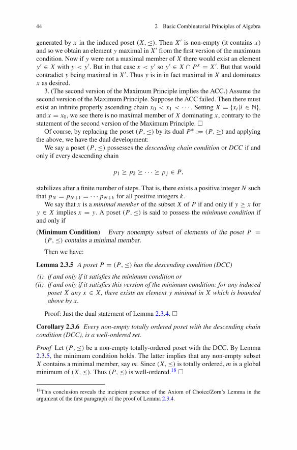
44 2 Basic Combinatorial Principles of Algebra
generated by x in the induced poset (X,≤). Then X ′ is non-empty (it contains x)and so we obtain an element y maximal in X ′ from the first version of the maximumcondition. Now if y were not a maximal member of X there would exist an elementy′ ∈ X with y < y′. But in that case x < y′ so y′ ∈ X ∩ Px = X ′. But that wouldcontradict y being maximal in X ′. Thus y is in in fact maximal in X and dominatesx as desired.
3. (The second version of the Maximum Principle implies the ACC.) Assume thesecond version of theMaximum Principle. Suppose the ACC failed. Then there mustexist an infinite properly ascending chain x0 < x1 < · · · . Setting X = {xi |i ∈ N},and x = x0, we see there is no maximal member of X dominating x , contrary to thestatement of the second version of the Maximum Principle. �
Of course, by replacing the poset (P,≤) by its dual P∗ := (P,≥) and applyingthe above, we have the dual development:
We say a poset (P,≤) possesses the descending chain condition or DCC if andonly if every descending chain
p1 ≥ p2 ≥ · · · ≥ p j ∈ P,
stabilizes after a finite number of steps. That is, there exists a positive integer N suchthat pN = pN+1 = · · · pN+k for all positive integers k.
We say that x is a minimal member of the subset X of P if and only if y ≥ x fory ∈ X implies x = y. A poset (P,≤) is said to possess the minimum condition ifand only if
(Minimum Condition) Every nonempty subset of elements of the poset P =(P,≤) contains a minimal member.
Then we have:
Lemma 2.3.5 A poset P = (P,≤) has the descending condition (DCC)
(i) if and only if it satisfies the minimum condition or(ii) if and only if it satisfies this version of the minimum condition: for any induced
poset X any x ∈ X, there exists an element y minimal in X which is boundedabove by x.
Proof: Just the dual statement of Lemma 2.3.4. �
Corollary 2.3.6 Every non-empty totally ordered poset with the descending chaincondition (DCC), is a well-ordered set.
Proof Let (P,≤) be a non-empty totally-ordered poset with the DCC. By Lemma2.3.5, the minimum condition holds. The latter implies that any non-empty subsetX contains a minimal member, say m. Since (X,≤) is totally ordered, m is a globalminimum of (X,≤). Thus (P,≤) is well-ordered.18 �
18This conclusion reveals the incipient presence of the Axiom of Choice/Zorn’s Lemma in theargument of the first paragraph of the proof of Lemma 2.3.4.

2.3 Chain Conditions 45
Corollary 2.3.7 (The chain conditions are hereditary) If X is any induced poset of(P,≤), and P satisfies the ACC (or DCC), then X also satisfies the ACC (or DCC,respectively).
Proof This is not really a Corollary at all. It follows from the definition of “inducedposet” and the chain-definitions directly. Any chain in the induced poset is a fortiori achain of its ambient parent.Wemention it only to have a signpost for future reference.
In the next section, Theorem 2.4.2 will have a surprising consequence for lowersemilattices with the DCC.
Any poset satisfying both the ACC and the DCC also satisfies
(FC) Any unrefinable chain of P has finite length.
This is because patently one of the two chain conditions is violated by an infiniteunrefinable chain. Conversely, if a poset P satisfies condition (FC) then there can beno properly ascending or descending chain of infinite length since by Theorem 2.3.1it would then lie in a saturated chain which was also infinite against (FC). Thus
Lemma 2.3.8 The condition (FC) is equivalent to the assumption of both DCC andACC.
2.4 Posets with Meets and/or Joins
2.4.1 Meets and Joins
Let W be any subset of a poset (P,≤). The join of the elements of W is an elementv in (P,≤) with these properties:
1. w ≤ v for all w ∈ W .2. If v′ is an element of (P,≤) such that w ≤ v′ for all w ∈ W , then v ≤ v′.
Similarly there is the dual notion: the meet of the elements of W in P would bean element m in P such that
1. m ≤ w for all w ∈ W .2. If m′ is an element of (P,≤) such that m′ ≤ w for all w ∈ W , then m′ ≤ m.
Of course, P may or may not possess a meet or a join of the elements of W . Butone thing is certain: if the meet exists it is unique; if the join exists, it is unique.Because of this uniqueness we can give these elements names. We write
∧P (W ) (or
just∧
(W ) if the ambient poset P is understood) for the meet of the elements of Win P (if it exists). Similarly, we write
∨P (W ) (or
∨(W )) for the join in P of all of
the elements of W (if that exists).

46 2 Basic Combinatorial Principles of Algebra
In the case that W is the set {a, b}, we render the meet and join of a and b by a ∧band a ∨ b, respectively. The reader may verify
a ∧ b = b ∧ a (2.7)
a ∧ (b ∧ c) = (a ∧ b) ∧ c (2.8)
(a ∧ b) ∨ (a ∧ c) ≤ a ∧ (b ∨ c) (2.9)
and the three dual statements when the indicated meets and joins exist.We say that (P,≤) is a lower semilattice if it is “meet-closed”—that is, the meet
of any two of its elements exists. In this case it follows that the meet of any finitesubset {a1, a2, . . . , an} exists (see Exercise (9) in Sect. 2.7.2). We denote this meetby a1 ∧ a2 ∧ · · · ∧ an . We then have
Lemma 2.4.1 Suppose P is a lower semilattice, containing elements x, a1, a2, . . . ,an ∈ P such that x ≤ ai for i = 1, 2, . . . , n. Then
x ≤ a1 ∧ a2 ∧ · · · ∧ an .
Dually we can define an upper semilattice (it is “join closed”).A lattice is a poset (P,≤) that is both a lower semilattice and an upper
semilattice—that is, the meet and join of any two of its elements both exist in P .Thus, a lattice is a self-dual concept: If P = (P,≤) is a lattice, then so is its dualposet P∗ = (P,≤∗).
If every non-empty subset U of P has a meet (join) we say that arbitrary meets(joins) exists. If both arbitrary meets and joins exist we say that P is a completelattice.
Example 9 Here are some familiar lattices:
1. Any totally ordered poset is a lattice. The meet of a finite set is its minimalmember; its join is its maximal member. Considering the open real interval (0, 1)with its induced total ordering from the real number system, it is easy to see
(a) that there are lattices with no “zero” or “one”,(b) that there can be (infinite) subsets of a lattice with no lower bound or no
upper bound.
2. The power set P(X) is the poset of all subsets of a set X under the containmentrelation. It is a lattice with the intersection of two sets being their meet, and theunion of two sets being their join. This lattice is self dual and is a completelattice, meaning that any subset of elements of P(X), whether infinite or not, hasa least upper bound and greatest lower bound—i.e. a meet and a join. Of coursethe lattice has X as its “one” and the empty set as its “zero”.

2.4 Posets with Meets and/or Joins 47
2.4.2 Lower Semilattices with the Descending Chain Condition
The proof of the following theorem is really due to Richard Stanley, who presentedit for the case that P is finite [36, Proposition 3.3.1, p. 103].
Theorem 2.4.2 Suppose P is a meet-closed poset (that is, a lower semilattice) withthe DCC condition.
Then the following assertions hold:
(i) If X is a meet-closed induced poset of P, then X contains a unique minimalmember.
(ii) Suppose, for some subset X of P, the filter of upper bounds
∧P X := {y ∈ P|x ≤ y for all x ∈ X}
is non-empty. Then the join∨
(X) exists in P.In particular, if (P,≤) possesses a one-element 1, then for any arbitrary subsetX of P, there exists a join
∨(X). Put more succinctly, if 1 exists, unrestricted
joins exist.(iii) For any non-empty subset X of P, the universal meet
∧(X) exists and is
expressible as a meet of a finite number of elements of X.(iv) The poset P contains a 0.(v) If P contains a 1, then P is a complete lattice.
Proof (i) The set ofminimal elements of X is non-empty (Lemma 2.3.5 of the sectionon chain conditions.) Suppose there were at least two distinct minimal members ofX , say x1 and x2. Then x1 ∧ x2 is also a member of X by the meet-closed hypothesis.But by minimality of each xi , one has
x1 = x1 ∧ x2 = x2.
Since any two minimal members of the set X are now equal (and the set of them isnon-empty) there exists a unique minimal member. The proof of Part (i) is complete.
(ii) Let X be any subset of P for which the filter∧
P X is non-empty. One observesthat
∧P X is ameet-closed induced poset and so by part 1, contains a uniqueminimal
member j (X). Then, by definition, j (X) is the join∨
(X). If 1 ∈ P then of couse∧P X is non-empty for all subsets X and the result follows.(iii) Let W (X) be the collection of all elements of P which can be expressed as
a meet of finitely many elements of X , viewed as an induced poset. Then W (X) ismeet-closed, and so has a unique minimal member x0 by (i). In particular x0 ≤ x forall x ∈ X . Now suppose z ≤ x for all x ∈ X . Then by Lemma2.4.1, z is less thanor equal to any finite meet of elements of X , and so is less than or equal to x0. Thusx0 = ∧
(X), by definition of a global meet.(iv) By (i), P containsminimal non-zero elements (often called “atoms”). Suppose
m is such an atom. If m ≤ x for all x ∈ P then x would be the element 0, against our

48 2 Basic Combinatorial Principles of Algebra
definition of “minimal element”. Thus there exists an element y ∈ P such that y isnot greater than or equal to m. Then y ∧ m (which exists by meet-closure) is strictlyless than m. Since m is an atom, we have y ∧ m = 0 ∈ P .
(v) If 1 exists, P enjoys both unrestricted joins by (ii). But by (iii), unrestrictedmeets exist, and so now P is a complete lattice.
The proof is complete. �
Example 10 The following posets are all lower semilattices with the DCC:
1. N+ = {1 < 2 < · · · } of all positive integers with the usual ordering. This is a
chain.2. D, the positive integers under the partial ordering of “dividing”—that is, a ≤ b
if and only if integer a divides the integer b.3. B(X), the poset of all finite subsets of a set X .4. L<∞(V ), the poset of finite-dimensional subspaces of a vector space V .5. M<∞(I ), the finite multisets over a set I .
It follows that arbitrary meets exist and a 0 exists.
Remark Of course, we could also adjoin a global maximum 1 to each of theseexamples and obtain complete lattices in each case.
2.4.3 Lower Semilattices with both Chain Conditions
Recall from Sect. 2.4.3, Lemma 2.3.8, that a poset has both the ACC and the DCC ifand only if it possesses condition
(FC) Every proper chain in P has finite length.
An observation is that if P satisfies (FC), then so does its dual P∗. Similarly, ifP has finite height, then so does its dual. This is trivial. It depends only on the factthat rewriting a finite saturated chain in descending order produces a saturated chainof P∗.
We obtain at once
Lemma 2.4.3 Suppose P is a lower semilattice satisfying (FC).
(i) P contains a 0. If P contains a 1 then P is a complete lattice.(ii) Every element of P − {1} is bounded by a maximal member of P − {1} (that is,
an element of max(P)).(iii) Every element of P − {0} is above a minimal element of P − 0 (that is, an
element of min(P)).(iv) The meet of all maximal elements of P—that is
∧(max(P)) (called the Frattini
element or radical of (P,≤)) exists and is the meet of just finitely many elementsof max(P).

2.4 Posets with Meets and/or Joins 49
(v) If 1 ∈ P, the join of all atoms,∨
(min(P)) (called the socle of P and denotedsoc(P)) exists and is the join of just finitely many atoms.
Proof Parts (i) and (iv) follow from Theorem 2.4.2. Parts (ii) and (iii) are imme-diate consequences of the hypothesis (FC), and Part (v) follows from Parts (i) and(iii). �
Remark Hopefully the reader will notice that the hypothesis that P contained theelement 1 played a role—even took a bow—in Parts (i) and (v) of the above Lemma.Is this necessary? After all, we have both the DCC and the ACC. Well, there is anasymmetry in the hypotheses. P is a lower semilattice, but not an upper semilattice(though this symmetry is completely restored once 1 exists in P , because then wehave arbitrary joins).
Example 11 Consider any one of the posets D, B(X), L<∞(V ). These are rankedposets, with the rank of an element being (1) the number of prime factors, (2) thecardinality of a set, or (3) the vector-space dimension of a subspace, respectively.Select a positive integer r and consider the induced poset trr (P) of all elements ofrank at most r in P where P = D, B(X), L<∞(V ). Then trr (P) is still a lowersemilattice with both the DCC and the ACC. But it has no 1.
2.5 The Jordan-Hölder Theory
In the previous two sections we defined the notions of “algebraic interval”, “heightof an algebraic interval” and the meet-closed posets which we called “lower semi-lattices”. They shall be used with their previous meanings without further comment.
This section concerns a basic theorem that emergeswhen a certain property, that ofsemimodularity, is imposed on lower semilattices. Many important algebraic objectsgive rise to lower semilattices which are semimodular (for example the posets ofsubnormal subgroups of a finite group, or the submodule poset of an R-module) andeach enjoys its own “Jordan-Holder Theorem”—it always being understood there isa general form of this theorem. It is in fact a very simple theorem about extending“semimodular functions”19 on the set of covers of a semimodular lower semilatticeto an interval measure on that semilattice. It sounds like a mouthful, but it is reallyquite simple.
Fix a poset (P,≤). An unrefinable chain of length one is called a cover and isdenoted by (a, b) (which is almost the name of its interval [a, b]—altered to indicatethat we are talking about a cover). Thus (a, b) is a cover if and only if a < b and thereis no element c in P with a < c < b—i.e. a is a maximal element in the induced
19The prefix “semi-” is justified for several reasons. The term “modular function” has quite anothermeaning as a certain type of meromorphic function of a complex variable. Secondly the function inquestion is defined in the context of a semimodular lower semilattice. So why not put in the “semi”?We do not guarantee that every term coined in this book has been used before.

50 2 Basic Combinatorial Principles of Algebra
poset of all elements properly below b (the principal order ideal Pb minus {b}). Thecollection of all covers of (P,≤) is denoted CovP . Note that CovP is a subset ofAP ,the collection of all algebraic intervals of (P,≤).
2.5.1 Lower Semi-lattices and Semimodularity
A lower semilattice (P,≤) is said to be semimodular if, whenever (x1, b) and (x2, b)
are both covers with x2 �= x2, then both (x1∧x2, x1) and (x1∧x2, x2) are also covers.
Lemma 2.5.1 Suppose (P,≤) is a semimodular lower semilattice. Suppose [x, a]is algebraic and (b, a) is a cover, where x ≤ b. Then [x, b] is algebraic.
Proof Since [x, a] is algebraic, there exists a finite unrefinable chain from x to a,say A = (x = a0, a1, . . . , an = a). Clearly each interval [x, a j ] is algebraic. SeeFig. 2.1.
By hypothesis, x ≤ b and so there is a largest subscript i such that ai ≤ b. Clearlyi < n. If i = n − 1 then an−1 = b so [x, b] is algebraic by the previous paragraph.Thus we may assume that b �= an−1. (See Fig. 2.1.) Since both (an−1, a) and (b, a)
are covers, then by semimodularity, both (an−1 ∧ b, an−1) and (an−1 ∧ b, b) arecovers. Continuing in this way we obtain that (ak ∧ b, ak) and (ak ∧ b, ak−1 ∧ b)
are covers for all k larger than i . Finally, as ai ≤ b, this previous statement yieldsai+1 ∧ b = ai and (by semimodularity) (ai , ai+2 ∧ b) must be a cover). Note that
(x = a0, . . . , ai , ai+2 ∧ b, ai+3 ∧ b, . . . , an−1 ∧ b, b)
is an finite unrefinable chain since its successive pairs are covers. This makes [x, b]algebraic, completing the proof. �
Fig. 2.1 The poset showing[x, b] is algebraic. Thesymbol “cov” on a depictedinterval indicates that it is acover

2.5 The Jordan-Hölder Theory 51
2.5.2 Interval Measures on Posets
Let M be a commutative monoid. This means M possesses a binary operation, say“∗,” which is commutative and associative, and that M contains an identity element,say “e”, such that m = e ∗ m = m ∗ e for all m ∈ M .
There is one commutative monoid that plays an important role in the applicationsof our main theorem and that is the monoidM(X) of all finite multisets over a set X .We have met this object before in the guise of a locally finite poset M<∞(X) (seethe last item under Example2 of this chapter). We have seen that any finite multisetover X can be represented as a function f : X → N from X to the non-negativeintegers N whose “support” is finite—i.e. the function achieves a non-zero valuein only finitely many instances as x wanders over X . Now, if f and g are two suchfunctions,wemay let “ f +g” denote the function that takes x ∈ X to the non-negativeinteger f (x)+g(x), the sum of two integers. Clearly f +g has finite support, and so(M<∞(X),+) (under this definition of “plus”) becomes a commutative semigroup.But as the constant function 0X : X → {0} is an identity element with respect to thisoperation,M(X) := (M<∞(X),+) is actually a commutative monoid. We call thisthe commutative monoid of finite multisets over X .
An interval measure μ of a poset (P,≤) is a mapping μ : AP → M from the setof algebraic intervals of P into a commutative monoid (M, ∗) with identity elemente such that
μ(a, a) = e for all a ∈ P. (2.10)
μ(a, b) ∗ μ(b, c) = μ(a, c) whenever [a, b] and [b, c] are in AP (2.11)
[Notice that we have found it convenient to write μ(a, b) for μ([a, b]).]Here are some examples of interval measures on posets:
Example 12 Let M be the multiplicative monoid of positive integers. Let (P,≤) bethe set of positive integers and write x ≤ y if x divides y evenly. Then every intervalof (P,≤) is algebraic. Define μ by setting μ(a, b) := b/a for every interval (a, b).
Example 13 Let (P,≤) be as in Example 14, but now let M be the additive monoidof all non-negative integers. Now if we set μ(a, b);= the total number of primedivisors of b/a, then μ is a measure.
Example 14 Let (P,≤) be the poset of all finite-dimensional subspaces of some(possibly infinite dimensional) vector space V , where “≤” is the relation of “con-tained in”.
(i) Let M be the additive monoid of all non-negative integers. If we defineμ(A, B) := dim(B/A), then μ is a measure on (P,≤).
(ii) If M is the multiplicative group {1,−1}, then setting μ(A, B) := (−1)dim(A/B)
for every algebraic interval (A, B) also defines a measure.

52 2 Basic Combinatorial Principles of Algebra
2.5.3 The Jordan-Hölder Theorem
Now we can prove
Theorem 2.5.2 (The Jordan-Hölder Theorem) Let (P,≤) be a semimodular lowersemilattice. Suppose μ : CovP −→ (M,+) is a mapping from the set of covers of Pto a commutative monoid (M,+), and suppose this mapping is “semimodular” inthe sense that
μ(b, y) = μ(a ∧ b, a) whenever (a, y) and (b, y) are distinct covers. (2.12)
Then for any two finite unrefinable chains U = (u = u0, . . . , un = v) and V =(u = v0, . . . , vm = v) from u to v, we have
n−1∑i=0
μ(ui , ui+1) =m−1∑i=0
μ(vi , vi+1) (2.13)
and n = m (the finite summation is taking place in the additive monoid (M.+)). Inparticular, μ extends to a well-defined interval measure μ : AP −→ M.
Proof If n = 0 or 1, then U = V , and the conclusion holds. We therefore pro-ceed by induction on the minimal length h(u, v) of an unrefinable chain fromu to v for any algebraic interval [u, v]—that is, the height of [u, v]. It sufficesto assume U = (u = u0, u1, . . . , un = v) is such a minimal chain (so thatn = h(u, v)) and prove Eq. (2.13), and n = m for any other unrefinable chainV = (u = v0, v1, . . . , vm = v).
If un−1 = vm−1, h(u, vn−1) = n − 1, so by induction,∑n−2
i=0 μ(ui , ui+1) =∑m−2i=0 μ(vi , vi+1) and m − 1 = n − 1 and the conclusion follows.So assume un−1 �= vm−1. Set z = un−1∧vm−1. Since (un−1, v) and (vm−1, v) are
both covers, by semi-modularity, so also are (z, un−1) and (z, vm−1) (see Fig. 2.2).
Fig. 2.2 The main figure forthe Jordan Hölder Theorem

2.5 The Jordan-Hölder Theory 53
Since u ≤ z, (z, vn−1) is a cover, and [u, vn−1] is algebraic, we see that Lemma2.5.1 implies that [u, z] is also algebraic. So a finite unrefinable chain
Z = (u = z0, z1, . . . , zr = z)
from u to z exists. Since h(u, un−1) = n − 1 < n, by induction
(r−1∑i=0
μ(zi , zi+1)
)+ μ(z, un−1) =
n−1∑i=0
μ(ui , ui+1) (2.14)
and r +1 = n −1. But h(u, vm−1) ≤ r +1 = n −1 so induction can also be appliedto the algebraic interval [u, vm−1] to yield
(r−1∑i=0
μ(zi , zi+1)
)+ μ(z, vm−1) =
m−1∑i=0
μ(vi , vi+1). (2.15)
and the fact that r + 1 = m − 1. Thus n = m.But by (2.12), μ(z, un−1) = μ(vm−1, v) and μ(z, vm−1) = μ(un−1, v). The
result (2.13) now follows from (2.14) and the commutativity of (M,+). The proofis complete. �
To see how this theorem works in a semimodular lattice in which not all intervalsare algebraic, the reader is referred to Example 15 on p. 53 and the remark following.
There are many applications of this theorem. In the case of finite groups(R-modules) we let (M,+) be the commutative monoid of multisets of all iso-morphism classes of finite simple groups (or all isomorphism classes of irreducibleR-modules, resp.). These are the classical citations of the Jordan-Hölder Theoremfor Groups and R-modules.20
2.5.4 Modular Lattices
Consider for the moment the following example:
Example 15 The poset (P,≤) contains as elements P = {a, b, c} ∪ Z, where Z isthe set of integers, with ordering defined by these rules:
20We beg the reader to notice that in the case of groups there is no need for Zassenhaus’ famous“butterfly lemma”, nor the need to prove that subnormal subgroups of a finite group form a lattice.A lower semilattice will do. One of the classic homomorphism theorems, provides the semimodularfunction from CovP to finite simple groups. The result is then immediate from Theorem 2.4.2,Eq. (2.13), where the interval measure displays the multiset of “chief factors” common to all satu-rated chains in P .

54 2 Basic Combinatorial Principles of Algebra
1. a ≤ p for all p ∈ P—i.e. a is the poset “zero”,2. c ≥ p for all p ∈ P , so c is the poset “one”,3. b is not comparable to any integer in Z, and4. the integers Z are totally ordered in the natural way.
Notice that the meet or join of b and any integer are a and c respectively. Thus (P,≤)
is a lattice with its “zero” and “one” connected by an unrefinable proper chain oflength 2 and at the same time by an infinite unrefinable chain. The lattice is evenlower semimodular since the only covers are (a, b), (b, c) and (n, n + 1), for allintegers n.
Remark For the purposes of the Jordan-Hölder theory, such examples did not botherus, for the J-H theory was phrased as an assertion about measures which take valueson algebraic intervals—that is to say, non-algebraic intervals could be ignored—and the calculation of the measure used only finite unrefinable chains. In Example15, the only intervals of the semimodular lattice (P,≤) which are not algebraicare those of the form [n, c], n ∈ Z. The Jordan-Hölder Theorem is valid here: Infact if f is any function from the set of covers, into a commutative monoid M ,then by Theorem 2.5.2, f extends to an interval measure μ : AP → M . Note thatμ(a, c) = f (a, b) + f (b, c).
However, unlike Example 15, many of the most important posets in Algebra areactually lattices with a property called “the modular law”, which prevents elementsx and y from being connected by both a finite unrefinable chain and an infinitechain. This modular law always occurs in posets of congruence subalgebras whichare subject to one of the so-called “Fundamental Theorems of Homomorphisms”.
Recall the definition of lattice (p. 46). A lattice L is called a modular lattice or Lis said to be modular if and only if
(M) for all elements a, b, c of L with a ≥ b,
a ∧ (b ∨ c) = b ∨ (a ∧ c).
The dual condition is
(M∗) for all elements a, b, c of L with a ≤ b,
a ∨ (b ∧ c) = b ∧ (a ∨ c).
But by transposing the roles of a and b it is easy to see that the two conditions areequivalent. Thus
Lemma 2.5.3 A lattice satisfies (M) if and only if it satisfies (M∗). Put another way:a lattice L is modular if and only if its dual lattice L∗ is.
An immediate consequence of the modular law is the following

2.5 The Jordan-Hölder Theory 55
Lemma 2.5.4 (Identification Principle) Let x, y and n be elements of the modularlattice L. Suppose
x ∨ n = y ∨ n, and (2.16)
x ∧ n = y ∧ n. (2.17)
Then either x = y or else x and y are incomparable. Equivalently, either x ≤ yor y ≤ x implies x = y.
Proof Assume the hypotheses and assume x and y are comparable. Because x andy play symmetric roles in the hypothesis, we may assume that x ≤ y. Now by themodular law (M):
y ∧ (x ∨ n) = x ∨ (y ∧ n). (2.18)
But by Eq. (2.16), the left side of (2.18) is y. On the other hand, by Eq. (2.17), theright side of (2.18) is x . Thus x = y. �
The most important property of a modular lattice is given in the following:
Theorem 2.5.5 (The Correspondence Theorem for Modular Lattices) Suppose Lis a modular lattice. Then for any two elements a and b of L, there is a posetisomorphism
μ : [a, a ∨ b] → [a ∧ b, b],
taking each element x of the domain to x ∧ b.
Proof As μ is defined, μ(a) = a ∧ b, μ(a ∨ b) = (a ∨ b) ∧ b = b, and if a ≤ x ≤y ≤ b, then μ(x) = x ∧ b ≤ y ∧ b = μ(y). Thus μ is poset homomorphism andtakes values in [a ∧ b, b].
Suppose now that x, y ∈ [a, a ∨ b] and μ(x) = μ(y). Then x ∧ b = y ∧ b andso a ∨ (x ∧ b) = a ∨ (y ∧ b). Since a ≤ x and a ≤ y we may apply the law (M) toeach side of the last equation. This yields x = x ∧ (a ∨ b) = y ∧ (a ∨ b) = y, sincea ∨ b dominates both x and y. Thus μ is injective.
Now suppose x is an arbitrary element of the interval [a ∧ b, b], that is, a ∧ b ≤x ≤ b. Then by the first inequality, x = x ∨ (b ∧ a). Since x ≤ b, applying (M∗)(with x and a in the role of a and c in (M∗)), x = b ∧ (x ∨ a) = μ(x ∨ a). Thus μis onto.
Finally, we must show that for any x, y ∈ [a, a ∨ b], one has μ(x) ≤ μ(y) if andonly if x ≤ y.
Obviously if x ≤ y, then clearly x ∧ b ≤ y ∧ b, so μ(x) ≤ μ(y).Conversely, suppose μ(x) ≤ μ(y). Then x ∧ b ≤ y ∧ b, giving us
a ∨ (x ∧ b) ≤ a ∨ (y ∧ b). (2.19)

56 2 Basic Combinatorial Principles of Algebra
Since a ≤ x and a ≤ y, applying (M∗) to each side of (2.19) yields
x ∧ (a ∨ b) ≤ y ∧ (a ∨ b)
which gives us x ≤ y, since x and y are in [a, a ∨ b].Thus μ is a poset isomorphism. �
Recognizing the Chain Conditions in Modular Lattices
Lemma 2.5.6 Assume a ≤ b ≤ c is a chain in a modular lattice L. Then the interval[a, c] has the ACC (DCC) if and only if both intervals [a, b] and [b, c] have the ACC(DCC).
Proof Recall fromCorollary 2.3.7 that if [a, c] has either of the two chain conditions,then its subintervals [a, b] and [b, c] also possess the same condition.
So we assume that the two intervals [a, b] and [b, c] possess the ascending chaincondition (ACC). We must show that [a, c] has the ascending chain condition. Byway of contradiction, suppose
a = c0 < c1 < c2 < · · ·
is an infinite properly ascending chain in the poset [a, c]. Then we have ascendingchains
c0 ∨ b ≤ c1 ∨ b ≤ · · · and c0 ∧ b ≤ c1 ∧ b ≤ · · ·
in posets [b, c] and [a, b], respectively. Since these two posets are assumed to possessthe ACC, there exists a natural number k such that for every integer m exceeding kwe have
ck ∨ b = cm ∨ b, (2.20)
ck ∧ b = cm ∧ b. (2.21)
Since ck ≤ cm , the Identification Principle, Lemma 2.5.4, forces ck = cm . But thatis impossible since these are distinct entries in a properly ascending chain.
The argument that the presence of the descending chain condition for both [a, b]and [b, c] implies the same condition for [a, c] now follows by duality from our resultfor the ACC. (It can also be proved by considering an infinite properly descendingchain c0 > c1 > · · · , and again obtaining a natural number k such that Eqs. (2.20)and (2.21) hold and again invoking the Identification Principle.) �
Lemma 2.5.7 Assume L is a modular lattice and {a1, . . . , an} is a finite subset ofL.
(i) Suppose c ≤ ai for all i = 1, 2, . . . , n. Then [c, a1 ∨ · · · ∨ an] has the ACC(DCC) if and only if each interval [c, ai ] possesses the ACC (DCC).

2.5 The Jordan-Hölder Theory 57
(ii) Suppose ai ≤ c for all i = 1, 2, . . . , n. Then [a1 ∧ · · · ∧ an, c] has the ACC(DCC) if and only if each interval [ai , c] has the ACC (DCC).
Proof Part (i). We assume c ≤ ai for all i . Of course, by Corollary 2.3.7, if [c, a1 ∨a2 ∨ · · · ∨ an] has the ACC (DCC) then so does any of its intervals [c, ai ]. So weneed only prove the reverse implication.
Assume each interval [c, ai ], i = 1, 2, . . . , n, possesses theACC (DCC).A simpleinduction on n reduces us to the case that n = 2. By Theorem 2.5.5, [a2, a1 ∨ a2] �[a1∧a2, a1]which has the ACC since it is an interval of [c, a1]which is hypothesizedto have this chain condition. But the interval [a1 ∧ a2, a2] is a subinterval of [c, a2]which has theACC (DCC). Sowe see that both intervals [a1∧a2, a2] and [a2, a1∨a2]have the ACC (DCC) and so by Lemma 2.5.6, the interval [a1 ∧ a2, a1 ∨ a2] alsopossesses the ACC (DCC). Finally, noting that [c, a1 ∧ a2] has the ACC (DCC)because it is an interval of [c, a1] hypothesized to have this chain condition, onemore application of Lemma 2.5.6 now yields the fact that [c, a1 ∨ a2] also enjoysthis condition.
Part (ii) follows from Part (i) by duality. �
Corollary 2.5.8 Any modular lattice is a semi-modular lower semilattice and sois subject to the Jordan-Hölder theory (See Theorem 2.5.2.). In particular, any twofinite unrefinable chains that may happen to connect two elements x and y of thelattice, must have the same length, a length which depends only on the pair (x, y).
Proof Apply the previous Lemma for the case [a, a ∨ b] and [b, a ∨ b] are bothcovers. �
The preceeding Corollary only compared two finite unrefinable chains from x toy. Could one still have both a finite unrefinable chain from x to y as well as an infiniteone as in Example 15 at the beginning of this subsection? The next result shows thatsuch examples are banned from the realm of modular lattices.
Theorem 2.5.9 Suppose L is a modular lattice and suppose a = a0 < a1 < · · · <
an = b is an unrefinable proper chain of length n preceding from a to b. Then everyother proper chain proceeding from a to b has length at most n.
Proof Ofcourse, byZorn’s lemma, anyproper chain is refinedby aproper unrefinablechain. So, if we can prove that all proper chains connecting a and b are finite, such achain possesses a well-defined measure by the Jordan-Hölder Theory. In particularall such chains possess the same fixed length n. So it suffices to show that any properchain connecting a and b must be finite.
We propose to accomplish this by induction on the parameter n given in thestatement of the theorem. But this means that we shall have to keep track of thebound on length asserted by the induction hypothesis, in order to obtain new intervals[a′, b′] to which induction may be applied.
So we begin by considering a (possibly infinite) totally ordered subposet X of(P,≤) having a as its minimal member and b as its maximal member. We must
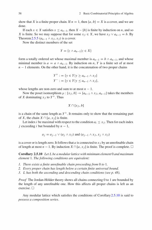
58 2 Basic Combinatorial Principles of Algebra
show that X is a finite proper chain. If n = 1, then {a, b} = X is a cover, and we aredone.
If each x ∈ X satisfies x ≤ an−1, then X − {b} is finite by induction on n, and soX is finite. So we may suppose that for some xβ ∈ X , we have xβ ∨ an−1 = b. ByTheorem2.5.5 (an−1 ∧ xβ, xβ) is a cover.
Now the distinct members of the set
Y = {z ∧ an−1|z ∈ X}
form a totally ordered set whose maximal member is an−1 = b ∧ an−1, and whoseminimal member is a = a ∧ an−1. By induction on n, Y is a finite set of at mostn − 1 elements. On the other hand, it is the concatenation of two proper chains
Y + : = {y ∈ Y |y ≥ an−1 ∧ xβ}Y − : = {y ∈ Y |y ≤ an−1 ∧ xβ},
whose lengths are non-zero and sum to at most n − 1.Now the poset isomorphism μ : [xβ, b] → [an−1 ∧ xβ, an−1] takes the members
of X dominating xβ to Y +. Thus
X ∩ [xβ, b]
is a chain of the same length as Y +. It remains only to show that the remaining partof X , the chain X ∩ [a, xβ] is finite.
Let index i be maximal with respect to the condition ai ≤ xβ . Then for each indexj exceeding i but bounded by n − 1,
a j = a j−1 ∨ (a j ∧ xβ) and (a j−1 ∧ xβ, x j ∧ xβ)
is a cover or is length zero. It follows that a is connected to xβ by an unrefinable chainof length at most n − 1. By induction X ∩ [a, xβ] is finite. The proof is complete. �
Corollary 2.5.10 Let L be a modular lattice with minimum element 0 and maximumelement 1. The following conditions are equivalent:
1. There exists a finite unrefinable chain proceeding from 0 to 1.2. Every proper chain has length below a certain finite universal bound.3. L has both the ascending and descending chain conditions (see p. 48).
Proof The Jordan-Hölder theory shows all chains connecting 0 to 1 are bounded bythe length of any unrefinable one. How this affects all proper chains is left as anexercise. �
Any modular lattice which satisfies the conditions of Corollary2.5.10 is said topossess a composition series.

2.5 The Jordan-Hölder Theory 59
Example 16 Let L be the latticeD of all positive integers where a ≤ b if and only ifa divides b. Then D is a modular lattice which possesses the DCC but not the ACC.There is a “zero” (the integer 1), but no lattice “one”. However, every interval [a, b]possesses a composition series.
2.6 Dependence Theories
2.6.1 Introduction
If we say A “depends” on B, what does this mean? In ordinary language one mightintend several things: “A depends entirely on B” or that “A depends just a little onB”—a statement so mild that it might suggest only that B has a “slight influence” onA. But some syntax seems to be applied all the same: thus if we say that A dependson B and that B in turn depends on C , then A (we suppose to some small degree)depends on C .
In mathematics we also usually use the word “depends” in both senses. When oneasserts that f (x, y) depends (to some degree) upon the variable x , one means onlythat f might be influenced by x . After all, it could be that f is a “constant” functionas far as x is concerned. But on the other hand the mathematician also intends that fis entirely determined by the pair (x, y). Thus we may consider the phrase “ f (x, y)
depends on x” as one borrowed from ordinary everyday speech. In its various guises,the stronger idea of total and entire dependence appears throughout mathematicswith such a common strain of syntactical features as to deserve codification.
But as you will see, the theory here is highly special.
2.6.2 Dependence
Fix a set S, and let F(S) be the set of all finite subsets of the set S. A dependencerelation on S is a relationD from S to F(S)—that is, a subset of S ×F(S)—subjectto the axioms (D1)–(D3) listed below. We shall say that the element s in S dependson the subset A ∈ F(S) if and only if (s, A) ∈ D. The dependence relation mustsatisfy these conditions:
(D1) (The Reflexive Condition) If s ∈ S and if s ∈ A ∈ F(S), then s depends onA—that is, s depends on any finite subset of S that contains it.
(D2) (The Transitivity Condition) If the element s depends on the finite set A, andif every member of A depends on the finite set B, then s depends on B.

60 2 Basic Combinatorial Principles of Algebra
(D3) (TheExchangeCondition) If s, a1, . . . , an are elements of S such that s dependson the set {a1, . . . , an} but does not depend on the set {a1, . . . .an−1}, then an
depends on the set {a1, . . . , an−1, s}.Before concluding anything from this, let us consider some examples.
Example 17 (Linear dependence) Suppose V is a left vector space over some fieldor division ring D. Let us say that a vector v depends on a finite set of vectors{v1, . . . , vn} if and only if v can be expressed as a linear combination of thosevectors,—that is,
∑ni=1δivi = v for some choice of δi in D. One checks that this
defines a dependence relation on V .
Example 18 (Algebraic dependence) Let K be a field containing k as a subfield. (Forexample, one might let K and k respectively be the complex and rational numberfields.) We say that an element b of K depends on a finite subset X = {a1, . . . .an−1}of K if and only if b is the root of a polymonial equation whose coefficients areexpressible as a k-polynomial expressions in X . This means that there exists a poly-nomial p(x, x1, . . . , xn) in the polynomial ring k[x, x1, . . . , xn] when evaluated atx = b, xi = ai , 1 ≤ i ≤ n yields 0. We shall see in Chap. 11 that all three axioms ofa dependence theory hold for this definition of dependence among elements of thefield K .
2.6.3 Extending the Definition to S ×P(S)
Our first task will be to extend the definition of a dependence relationD ⊆ S ×F(S)
to a relation D ⊆ S × P(S), where P(S) is the collection of all subsets of S (thepower set). Thus, it will be possible to speak of element x depending on a (possiblyinfinite) subset A of S. Namely, for any subset A of S, we say that the element xdepends on A if and only there exists a finite subset A1 of A such that x dependson A1 (in the original sense). We leave it as an exercise to the reader to prove thefollowing:
Lemma 2.6.1 In the following, the sets A and B may be infinite sets:
(i) Element x of S depends on any set A which contains it.(ii) If A and B are subsets of S, if x depends on A and every element of A depends
on set B, then x depends on B.(iii) If a ∈ A, a subset of S, and x is an element of S which depends on A but does
not depend on A − {a}, then a depends on (A − {a}) ∪ {x}(See Exercise (1) in Sect. 2.7.4.)

2.6 Dependence Theories 61
2.6.4 Independence and Spanning
Let S be a set with dependence relation D ⊆ S × F(S), and let D ⊆ S × P(S) bethe extension of this relation to infinite subsets as in Lemma2.6.1 above. Now let Abe any subset of S. The flat generated by A is the set 〈A〉 := {y|y depends on A}.A subset X of S is called a spanning set if and only if 〈X〉 = S.
Next, we say that a subset Y of S is independent if and only if for each elementx of Y , x does not depend on Y − {x}.
Now the collections of all spanning sets form a partially ordered set under thecontainment relation. A similar statement holds for the collection of all independentsets. Thus it makes perfect sense to speak of a minimal spanning set and a maximalindependent set (should such sets exist). We wish to show that these two conceptscoincide.
Theorem 2.6.2 Let S be a set with dependence relation D ⊆ S × P(S) as above.
(i) Every minimal spanning set is a maximal independent set.(ii) Every maximal independent set is a minimal spanning set.
Proof We prove (i). Suppose U is a minimal spanning set. If U is not independentthen there exists an element u in U such that u depends on a finite subset U1 ofU − {u}. Thus every element of S depends on U and by Lemma 2.6.1, part 1, andwhat we know of u, every element of U depends on U −{u}. Thus by Lemma 2.6.1,part (ii), every element of S depends on U − {u}. Thus U − {u} is a spanning set,against the minimality of U . Thus U must be independent.
If U were not a maximal independent set there would exist an element z in S −Uwhich did not depend on U . But that is impossible as U spans S.
Next we show (ii). If X is a maximal independent set, then bymaximality, X spansS. If a proper subset X1 of X also spanned S, then any element x of X − X1 woulddepend on X1 and so would depend on X − {x} by the definition of dependence.But this contradicts the fact that X is independent. Thus X is actually minimal as aspanning set. The proof is complete. �
Next, we have the following important result.
Theorem 2.6.3 Maximal independent subsets of S exist.
Proof This is a straightforward application of Zorn’s Lemma. As remarked above,the collection J of all independent subsets of S form a partially ordered set (J ,≤)
under the inclusion relation. Now consider any chain C = {Jα} of independent setsand form their union C := ⋃
α Jα. Then if C were not an independent set, therewould exist an element x in C and a finite subset F of C − {x} such that x dependson F . But since the chain C is totally ordered and F ∪ {x} is finite, there exists anindex σ such that F ∪ x ⊆ Jσ . But this contradicts Jσ independent. Thus we seethat C must be an independent set.
Thus every chain C in J possesses an upper bound C in (J ,≤). By the ZornPrinciple, J contains maximal elements. The proof is complete. �

62 2 Basic Combinatorial Principles of Algebra
2.6.5 Dimension
The purpose of this section is to establish
Theorem 2.6.4 If X and Y are two maximal independent sets, then |X | = |Y |.Proof By the Schröder-Bernstein Theorem (Theorem1.4.1, p. 16), it suffices to showonly that |X | ≥ |Y | for any two maximal independent sets X and Y .
The proof has a natural division into two cases: the case X is a finite set and thecase that X is infinite.
First assume X is finite. We proceed by induction on the parameter k := |X | −|X ∩ Y |. If k = 0, then X = X ∩ Y ⊆ Y . But as Y is independent and each of itselements depends on its subset X , we must have X = Y , whence |X | = |Y | and weare done. Thus we may assume k > 0.
Suppose X = {x1, . . . , xn} where the xi are pairwise distinct elements of Sand the indexing is chosen so {x1, . . . , xr } = X ∩ Y , thereby making k = n − r .From maximality of the independent set X , every element of Y − X depends on X .Similarly, every element of X depends onY . If every element ofY depended on X0 :={x1, . . . , xn−1}, then xn , which depends on Y , would depend on X0 by Lemma2.6.1(i) above, against the independence of X . Thus there is someelement y ∈ Y −X whichdepends on X but does not depend on X0. By the exchange condition, xn dependson X1 := {x1, . . . , xn−1, y}. Moreover, if X1 were not independent, then either ydepends on X1−{y} = {x1, . . . , xn−1} or some xi depends on (X0−{xi })∪{y}. Theformer alternative is ruled out by our choice of y. If the latter dependence held, thenas the independence of X prevents xi from depending on X0 − {xi }, the exchangecondition would force y to depend on X0, again contrary to the choice of y. Thus X1is an independent set of n distinct elements. But as xn depends on X1, each elementof X depends on X1. Thus as all elements of S depend on X , they all depend on X1as well. Thus X1 is a maximal independent set. But since |X1 ∩ Y | = 1 + |X ∩ Y |,induction on k yields |X1| ≥ |Y |. The result now follows from |X | = |X1|.
Now assume X is an infinite set. Since Y is a maximal independent set, it is aspanning set. Thus for each element x in X there is at least one finite non-emptysubset Yx of Y on which it depends. Choose, if possible y ∈ (Y − ⋃
X Yx ). Since ydepends on X and by construction every element of X depends on
⋃X Yx , we see
that y depends on⋃
X Yx ⊆ Y , contradicting the independence of Y . Thus we seethat no such y can exist and so Y = ⋃
X Yx .Our goal is to produce an injective mapping
φ : Y → X × N,
where, as usual, N denotes the natural numbers. Since, for each x ∈ X , the set Yx
is finite, there exists an injective mapping φx : Yx → N. The problem is that thesets Yx may intersect non-trivially, so that merely combining the φx does not yield awell-defined φ.
We get around this problem as follows: First, by Theorem 2.2.2, the set X can bewell-ordered. Next given y ∈ Y , let S(y) := {x ∈ X |y ∈ Yx }, and let �(x) be the

2.6 Dependence Theories 63
least element of the set S(y). Now define φ : Y → X × N, by setting
φ(y) := (�(y),φ�(y)(y)) ∈ X × N (2.22)
for each y ∈ Y . If φ(y1) = φ(y2), then �(y1) = �(y2) and then y1 = y2 followsfrom the injectivity of φ�(y). Thus the mapping φ defined in (2.22) is injective.
It follows that|Y | ≤ |X × N|.
Now by Corollary 2.2.5 near the beginning of this chapter, |X | = |X × N|, since Xis infinite.
Thus |Y | ≤ |X | as required. The proof is complete. �
This common cardinality of maximal independent sets is called the dimension ofthe dependence system (S,D).
2.6.6 Other Formulations of Dependence Theory
For the sake of completeness, this subsection surveys a number other views of depen-dence theory. Since this subsection is not essential for anything further in the book,many results are not proved. Most of the missing proofs can be found in the book byOxley [1].
Fix a set X and let I be a family of subsets of X . The pair (X, I) is called amatroid if and only if the following axioms hold:
(M1) The family I is closed under taking subsets.(M2) (Exchange axiom) If A, B ∈ I with |A| > |B|, then there exists an element
a ∈ A − B, such that {a} ∪ B ∈ I.(M3) If every finite subset of a set A belongs to I, then A belongs to I.
Note that if A and B are maximal elements of (I,⊆), then |A| = |B| is animmediate consequence of axiom (M2).However, fromaxioms (M1) and (M2) alone,it does not follow that maximal elements even exist. One needs (M3) for that.
Lemma 2.6.5 If (X, I) is a matroid, then every element of I lies in a maximalelement of I.
Proof This proof utilizes Zorn’s lemma. Let A0 be an arbitrary member of I. Weexamine the poset of all subsets in I which contain A0. Let A1 ⊆ A2 ⊆ · · · be achain in this poset and let B be the union of all the sets Ai . Consider any finite subsetF of B. Then each element f ∈ F lies in some member Ai( f ) of the chain. Settingm to be the maximal index in the finite set {i( f )| f ∈ F}, we see that F ⊆ Am .Since Am ∈ I, (M1) implies F ∈ I. But since F was an arbitrary finite subset ofB, (M3) shows that B ∈ I. Thus every finite chain in the poset of elements of Iwhich contain A0 has an upper bound in that poset, so, by Zorn’s lemma, that poset

64 2 Basic Combinatorial Principles of Algebra
contains a maximal element M . Clearly M is a maximal member of I, since anymember of I which contains M also contains A0, and so lies in the poset of whichM is a maximal member. Thus A0 lies in a maximal member of I, as required. �Example 19 Let D ⊆ X × F(S) be a dependence theory. Let I be the set of inde-pendent sets of the dependence theory D. Then (X, I) is a matroid.
Example 20 Suppose (V, E) is a simple graph with vertex set V and edge set E .(The adjective “simple” just means that edges are just certain unordered pairs ofdistinct vertices.) A cycle is a sequence of edges (e0, e1, . . . , en) such that ei sharesjust one vertex with ei+1, and another vertex with ei−1, indices i taken modulo n.Thus en−1 shares a vertex with en = e0, and the “length” of the cycle, n, cannot beone or two. A graph with no cycles is called a forest—its connected components arecalled trees. Now let I be the collection of all subsets A of E such that the graph(V, A) is a forest. Then (E, I) is a matroid.
Example 21 Let F be a fixed family of subsets of a set X . A finite subset{x1, x2, . . . , xn} of X is said to be a partial transversal of F if and only if thereare pairwise distinct subsets A1, . . . An of F such that xi ∈ Ai , i = 1, . . . , n—that is, the set {x1, . . . , xn} is a “system of distinct representatives” of the sets {Ai }.Now let I be the collection of all subsets of X all of whose finite subsets are partialtransversals. Then (X, I) is a matroid.
Example 22 Suppose (X, I) is any given matroid, and Y is any subset of X . LetI(Y ) be all members of I which happen to be contained in the subset Y . Then itis straightforward that the axioms (M1), M(2) and (M3) all hold for (Y, I(Y )). Thematroid (Y, I(Y )) is called the induced matroid on Y .
Here is another approach to matroids, using a so-called rank function.
Theorem 2.6.6 Suppose r is a map from the set of all subsets of a set X, into thecardinal numbers, satisfying these three rules:
(R1) For each subset Y of X, 0 ≤ ρ(Y ) ≤ |Y |.(R2) (Monotonicity) If Y1 ⊆ Y2 ⊆ X, then ρ(Y1) ≤ ρ(Y2).(R3) (The submodular inequality) If A and B are subsets of X, then
ρ(A ∪ B) + ρ(A ∩ B) ≤ ρ(A) + ρ(B).
Let I be the collection of a subsets Y of X with the following property:
(*) For every finite subset FY of Y we have |FY | = r(FY ).
Then (X, I) is a matroid.
Now suppose we are given a matroid (X, I). Can we recover a dependence theoryfrom this matroid? Clearly we need to have a definition of “dependence” constructedexclusively from matroid notions. Consider this definition:

2.6 Dependence Theories 65
Definition: Let x be an element of X and let A be a finite subset of X . We say thatx depends on A if and only if there exists a subset A0 of A which lies in I, suchthat either (i) x ∈ A0, or (ii) {x} ∪ A0 is not in I.
Theorem 2.6.7 Given a matroid (X, I), let the relation of “dependence” betweenelements of X and finite subsets of X be given as in the preceding definition. Thenthis notion satisfies the axioms of a dependence theory.
It now follows fromExample19, and the assertion of Theorem2.6.7, that matroidsand dependence theories are basically the same thing.
There are purely combinatorial ways to express the gist of a dependence theory,and these are the various formulations of the notion of a matroid in terms of circles,in terms of flats, or in terms of closure operators.
Let us consider flats, for a moment. We have already defined them from the pointof view a dependence theory. From a matroid point of view, the flat 〈A〉 spanned bysubset A in matroid (X, I), is the set of all elements x for which {x} ∪ Ax /∈ I forsome finite subset Ax of A. It is an easy exercise (Exercise (6) in Sect. 2.7.4) to showthat 〈〈A〉〉 = 〈A〉, for all subsets A of X . In fact the reader should be able to provethe following:
Theorem 2.6.8 The mapping τ which sends each subset A of X to the flat 〈A〉spanned by A, is a closure operator on the lattice of all subsets of X. The imagesets—or “closed” sets—form a lattice:
1. The intersection of two closed sets is closed, and is the meet in this lattice.2. The closure of the set-theoretic union of two sets is a join, that is, a global minimum
in the poset of all flats above the two sets.
The characterization of matroids by closure operators is the following:
Proposition 2.6.9 Suppose P = P(X) is the poset of all subsets of a set X andτ : P → P satisfies
(Increasing) For each subset A, A ⊆ τ (A).(Closure) The mapping τ is a closure operator—that is, it is an idempotent
monotone mapping of a poset into itself.(The Steinitz-MacLane Exchange Property) If X ⊆ P and y, z ∈ P − τ (X) then
y ∈ τ (X ∪ {z}) implies z ∈ τ (X ∪ {y}).Then, setting
I = {A ⊆ X |x /∈ τ (A − {x}) for all x ∈ A},
we have that M := (X, I) is a matroid.Conversely, if (X, I) is a matroid, then the mapping τ which takes each subset of
A to the flat 〈A〉 which it spans, is a monotone increasing closure operator P → Ppossessing the Steinitz-MacLane Exchange Property.
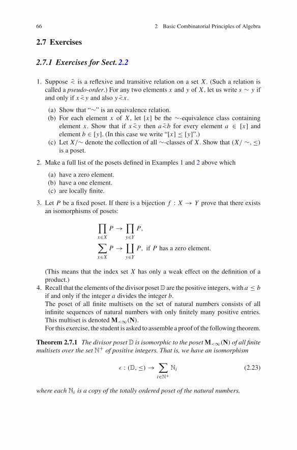
66 2 Basic Combinatorial Principles of Algebra
2.7 Exercises
2.7.1 Exercises for Sect. 2.2
1. Suppose < is a reflexive and transitive relation on a set X . (Such a relation iscalled a pseudo-order.) For any two elements x and y of X , let us write s ∼ y ifand only if x<y and also y<x .
(a) Show that “∼” is an equivalence relation.(b) For each element x of X , let [x] be the ∼-equivalence class containing
element x . Show that if x<y then a<b for every element a ∈ [x] andelement b ∈ [y]. (In this case we write “[x] ≤ [y]”.)
(c) Let X/∼ denote the collection of all ∼-classes of X . Show that (X/ ∼,≤)
is a poset.
2. Make a full list of the posets defined in Examples 1 and 2 above which
(a) have a zero element.(b) have a one element.(c) are locally finite.
3. Let P be a fixed poset. If there is a bijection f : X → Y prove that there existsan isomorphisms of posets:
∏x∈X
P →∏y∈Y
P,
∑x∈X
P →∐y∈Y
P, if P has a zero element.
(This means that the index set X has only a weak effect on the definition of aproduct.)
4. Recall that the elements of the divisor posetD are the positive integers, with a ≤ bif and only if the integer a divides the integer b.The poset of all finite multisets on the set of natural numbers consists of allinfinite sequences of natural numbers with only finitely many positive entries.This multiset is denoted M<∞(N).For this exercise, the student is asked to assemble a proof of the following theorem.
Theorem 2.7.1 The divisor poset D is isomorphic to the poset M<∞(N) of all finitemultisets over the set N+ of positive integers. That is, we have an isomorphism
ε : (D,≤) →∑
i∈N+Ni (2.23)
where each Ni is a copy of the totally ordered poset of the natural numbers.

2.7 Exercises 67
[Hint: We sketch the argument: Notice that the right side of (2.23) consists ofall sequences of non-negative integers of which only finitely many are positive(equivalently, all finite sequences of positive integers). The mapping ε is easyto define. First place the positive prime numbers in ascending (natural) order2 = p1 < p2 < · · · . For example p6 = 13. Now any integer d ∈ D greater thanone has a unique factorization into positive prime powers, with the primes placedfrom left to right in ascending order:
d =∏σ∈Jd
paσσ ,
for some (possibly empty) ascending sequence of positive integers Jσ . If onedeclares ε(d) to be the function f : N+ → N0 such that
f (σ) ={
aσ if σ ∈ Jd ,
0 if σ �∈ Jd ,
and declares ε(1) := 0, the constant function with all values 0, then one sees thatf (c) ≤ f (d) in the sum on the right side of Eq. (2.23) if and only if c divides devenly—i.e. c ≤ d in (D,≤). Clearly ε is a bijection.]
5. Recall that if (P,≤) and X ⊆ P , then the symbol PX denoted the order ideal
PX := {z ∈ P|z ≤ x for some x ∈ X}.
Show that PX = ⋃{Px |x ∈ X}.6. For the filters P X and PY generated by these sets, show that
(∧P X
) ⋂ (∧PY
)=
∧P(X∪Y ).
7. Let X be a subset of a poset (P,≤), and let PX be the order ideal of all elementsbounded aboveby at least one element of X (see p. 31 orExercise (5) inSect. 2.7.1in this section). Prove that PX is the intersection of all order ideals of P whichcontain X .
8. Give an example of a poset P and subset X for which the order ideal PX is notgenerated by an antichain.
9. Give an example of a poset (P,≤) and an order ideal J of P such that J doesnot have the form PX for any antichain X .
10. Let X be an infinite set. Recall that a partition of X is a decomposition π = {Xσ}of X into pairwise disjoint non-empty subsets Xσ called the components of thepartition. (The word “decomposition” is there to indicate that the union of theXσ is X .) A component Xσ is said to be trivial if it contains exactly one elementof X . Such a partition π is said to be a finitary partition if and only if finitelymany of the components are non-trivial and each of these is a finite set.

68 2 Basic Combinatorial Principles of Algebra
Let F P(X) be the full collection of finitary partitions of X . Show that withrespect to the refinement relation, F P(X) is a locally finite poset.
11. Let F := {Aσ | σ ∈ I } ⊆ P(X). Let α : P(X) → P(I ) be the mapping ofposets which sends each subsetU of X to the set α(U ) := {σ ∈ I | U ⊆ Aσ}. (Ifno such subset Aσ contains U , then α(U ) is the empty set.) Similarly, for eachsubset K of I , set β(K ) :=
⋂σ∈K
Aσ so that β : P(I ) → P(X) is a mapping of
posets.
(a) Show that α and β are both order reversing and that (P(X),P(I ),α,β)
is a Galois connection.(b) Show that the closed elements of X are those subsets expressible as inter-
sections of Aσ’s.(c) Show that a subset J of I is closed if and only if it has the property: If
Aτ ⊇⋂σ∈J
Aσ , then τ ∈ J .
2.7.2 Exercises for Sects. 2.3 and 2.4
1. We let [n] be the chain {1 < 2 < · · · < n} in the usual total ordering of thepositive integers. Show that the infinite union of disjoint chains,
[1] ∪ [2] ∪ [3] ∪ · · · ,
satisfies (FC) but does not possess finite height, and possesses neither a 1 nor a0.
2. If we adjoin 0 to the poset presented in the previous Exercise, show that theFrattini element exists, and is 0.
3. Show that the product of posets.
[1] × [2] × [3] × · · · ,
does not satisfy (FC).4. Let P be a lower semilattice with 0 and 1 satisfying (FC). Set B := max(P) and
let P be the induced subposet generated by B—that is, the set of elements of Pexpressible as a finite meet of elements of B. We understand the empty meet tobe the element 1, so the latter is an element of P .
(a) Show that P has the Frattini element φ(P) as its zero element, 0 P .(b) For each x ∈ P − {1}, show that the induced poset Px ∩ P has a unique
minimal member (which we shall call σ(x)).(c) Defining σ(1) = 1 show the following:
i. For all x ∈ P , x ≤ σ(x). (This is built into the definition of σ.)ii. The mapping σ : P → P is a surjective morphism of posets.

2.7 Exercises 69
iii. For each x ∈ P , one has σ(σ(x)) = σ(x).(Recall that any morphism onto an induced subposet which satisfies thesethree conditions is called a closure operator.)
5. Suppose P = N × {0, 1}. We totally order P (lexicographically) as follows:
(a) (a, 0) ≤ (b, 1) for any a, b ∈ N.(b) (a, 0) ≤ (b, 0) if and only if a ≤ b, a, b ∈ N.(c) (a, 1) ≤ (b, 1) if and only if a ≤ b, a, b ∈ N.
Show that (P,≤) has the Descending Chain Condition (DCC), but that thereexist intervals (x, y) with no finite unrefinable chain from x to y.
6. Suppose (P,≤) is a poset with a zero element 0. Recall from Sect. 2.4.2 that inthis case an atom of (P,≤) is an element a distinct from 0 with the propertythat there is no element x ∈ P such that 0 < x < a,—that is, (0, a) is a cover.Let A be the set of atoms of P . Assume now that (P,≤) has the property thatevery interval [0, b] possesses the DCC. Show that either P = {0} or that the setA of atoms is non-empty.
7. Give an example of a locally finite poset which does not possess the descendingchain condition.
8. Suppose (P,≤) is a locally finite poset which possesses a zero element 0. Showbymeans of an example, that such a poset need not possess the descending chaincondition.
9. Suppose L is a lattice. Give an induction proof showing that for any finite col-lection {a1, . . . , an} of elements of L , the elements
a1 ∨ · · · ∨ an and a1 ∧ · · · ∧ an,
exist and are respectively the greatest lower bound and greatest upper bound inL of the set {a1, . . . , an}.
10. Suppose (P,≤) is a lower semilattice with the descending chain condition(DCC). Show that any principle order ideal is a lattice. Conclude that for anynon-empty subset X ⊆ P , the order ideal
Px := {z ∈ P|z ≤ x for all x ∈ X}
is always a lattice.11. Suppose (P,≤) is a locally finite poset.
(a) Suppose (P,≤) possesses a zero element 0 and at least one other element.Show that the set A of atoms of (P,≤) is not empty. (Note that we are notassuming the Descending Condition, so this is a little different than Problem(6) in Sect. 2.7.2.)
(b) Now assume that (P,≤) is a lower semilattice. Show that any principleorder ideal is a finite lattice.

70 2 Basic Combinatorial Principles of Algebra
12. A lattice L := (L ,≤) is said to be distributive if and only if, for any elementsa and b in L , one always has:
a ∧ (b ∨ c) = (a ∧ b) ∨ (a ∧ c). (2.24)
An example of a distributive lattice is the power poset P(X) of all subsets of aset X .
(a) Prove that if L is a distributive lattice and (M,≤) is an induced subposetclosed under taking pair-wise meets and joins, then M is also a distributivelattice.
(b) Use the result of item (a) to prove the following:i. The Boolean poset B(X)—of all finite subsets of X is a distributive
lattice.ii. Let J (P) be the poset of all order ideals of a poset (P,≤) under the
containment relation. Use item (a) to prove that J (P) is a distributivelattice. [One must define “meet” and “‘join” of order ideals and setL = P(P) in item (a) of this exercise.]
2.7.3 Exercises for Sect. 2.5
1. (The Jordan-Hölder Theorem implies the Fundamental Theorem of Arithmetic.)Let (P,≤) be the poset of positive integers where a ≤ b if and only if integer adivides integer b evenly (Example 1, of this chapter).
(a) Show that (P,≤) is a lower semimodular semilattice with all intervals alge-braic. Let μ : CovP → N
+ be the function which records the prime numberb/a at every cover (a, b) of (P,≤). Indicate why μ is a semimodular func-tion in the sense given in Eq. (2.12) of the Jordan-Hölder Theorem.
(b) Suppose integer a properly divides integer b. For every factorization b/a =p1 p2 · · · pr of b/a into primes show that there exists a finite unrefineablechain (a = a0, a1, a2, . . . ar = b) such that ai/ai−1 = pi for i = 1, . . . r .
(c) Conclude from the Jordan-Hölder Theorem that every positive integer pos-sesses a factorization into prime numbers, and that the multiset of positiveprime numbers involved in the factorization is unique.
2. Show that the following lattices are modular:
(i) The poset of subspaces of a vector space.(ii) The poset of subgroups of an abelian group.
In both cases, the order relationship is that of containment.

2.7 Exercises 71
3. Show that the product L1 × L2 of two modular lattices is modular. If the latticesLσ, σ ∈ I are modular and possess a “zero”, does the modularity extend to thedirect sum
∐σ∈I
Lσ?
4. Is the lattice of partitions of a finite set, modular? (Here the order relationship isrefinement of one partition by another.)
5. Write out an explicit proof of Corollary 2.5.10.
2.7.4 Exercises for Sect. 2.6
1. Prove the three parts of Lemma2.6.1 for the extended definition of dependenceallowing infinite subsets of S.
2. Verify the axioms of a matroid for Example 22, on the edge-set of a graph.3. Verify the axioms of a matroid for Example 23, on finite partial transversals.4. Let� = (V, E) be a simple graph. Let M = (E, I) be thematroid of Example20.
For any subset F of the edge set E , let
(V, F) =⋃σ∈K
(Vσ, Fσ)
be a decomposition of � into connected components. For each connected com-ponent (Vσ, Fσ), let Eσ be the collection of edges connecting two vertices in Vσ .Thus (Vσ, Eσ) is the subgraph induced on the vertex set Vσ . Prove that in thematroid, the flat spanned by F is the union ∪σ∈K Eσ .
5. Let M = (X, I) be a matroid. A set which is minimal with respect to not lyingin I is called a circuit. Show that any circuit is finite. (Remark: There is also acharacterization of matroids by circuits. See Matroid Theory, by James G. Oxley[1], Proposition 1.3.10.)
6. Let M = (X, I) be a matroid. For each subset A of X , let 〈A〉 be defined as theset of all elements x ∈ X for which there exists a finite subset Ax ⊆ A such that{x} ∪ Ax �∈ I (this is the matroid version of “the flat generated by A” defined onp. 65. Show that 〈A〉 = 〈〈A〉〉.
References
1. Oxley J (2011) Matroid theory, Oxford graduate texts. vol 21, Oxford University Press, Oxford2. Stanley RP (1997) Enumerative Combinatorics, vol 1, Cambridge studies in advanced mathe-
matics, vol 49, Cambridge University Press, Cambridge

Chapter 3Review of Elementary Group Properties
Abstract Basic properties of groups are collected in this chapter. Here are exposedthe concepts of order of a group (any cardinal number) or of a group element (finiteor countable order), subgroup, coset, the three fundamental theorems of homomor-phisms, semi-direct products and so forth.
3.1 Introduction
Groups are systems of symmetries of objects, in particular mathematical objects.Understanding groups can be useful in classifying objects in a particular class. Oneuses a group of symmetries to transfer any object of the class to a representativeobject which is an easily-studied canonical form. For example, the groupGL(n, F)×GL(n, F), generated by elementary row and column operations on the class Mn(F)
of n × n matrices is used to transport an arbitrary matrix to a more easily studiedcanonical form.
This is just one of the reasons that group theory is needed, whatever field ofmathematics you might choose to enter. There are of course many other reasonshaving to dowith special uses of groups (such as “Polya counting”,1 quantumphysics,invariant theory etc.). But overall, the need to classify things seems the broadestreason that group theory is pertinent to all of mathematics.
Groups are defined by a hallowed set of axioms which are useful only for thepurpose of banishing all ambiguities from the subject. Somehow, staring at the axiomsof a group mesmerizes one away from their basic and natural habitat. Every groupthat ever exists in the world is in fact the full group of symmetries of something. Thatis what the theory of groups is: the study of symmetries. But it is useful to know thisonly on a philosophical plane. Knowing that there is a set of objects such that everygroup—or even every finite group—is the full group of automorphisms of at leastone of these objects, is not very helpful for classifying the groups themselves.
1This has a long pre-Polya history.
© Springer International Publishing Switzerland 2015E. Shult and D. Surowski, Algebra, DOI 10.1007/978-3-319-19734-0_3
73

74 3 Review of Elementary Group Properties
3.2 Definition and Examples
This is probably a good place to explain a convention. A group is a set G with a binaryoperationwith certain properties—ofwhich there are a goodmany examples. In someof these examples the binary operation is written as “+”; in others, it is written as “◦”or “×”. (If one uses “+”, one might think the operation is commutative. If one uses“◦”, the elements seem to be mappings, and if one uses “×”, Cartesian products canconfuse the issue). How then does one speak generally about all possible groups? Thestandard solution is this: The group operation of an arbitrary group, will be indicatedby simple juxtaposition, the act of writing one symbol directly after the other—thus,the group operation, applied to the ordered pair (x, y) will be denoted xy.
A group is a set G equipped with a binary operation G × G → G (denoted hereby juxtaposition) such that the following axioms hold:
1. (TheAssociative Law) The binary operation is associative—that is (ab)c = a(bc)for all elements a, b, c ofG. (The parentheses indicate the temporal order inwhichoperations were performed. This axiommore-or-less says that the temporal orderof applying the group operations doesn’t matter, while, of course, the left-rightorder of the elements being operated on does matter.)
2. (Identity Element) There exists an element, say e, such that eg = g = ge for allelements g in G.
3. (The Existence of Inverses) For each element x in G, there exists an element x ′such that x ′x = xx′ = e where e is the element referred to in Axiom 2.2
One immediately deduces the following:
Lemma 3.2.1 For any group G one has:
1. The identity element e is the unique element of G possessing the property of Axiom2.
2. Given element g in G, there is at most one element g′ such that gg′ = g′g = e.3. In light of the preceding item 2, we may denote the unique inverse of g by the
symbol g−1. Then note that
(i) (ab)−1 = (b−1)(a−1) for all elements a, b ∈ G.(ii) (a−1)−1 = a, for each element a ∈ G.
(iii) For any element x and natural number k, the product xx . . . x (with k factors)is a unique element which we denote as xk . We have (xk)−1 = (x−1)k . (Asa notational convention, this element is also written as x−k .).
2People have figured out how to “improve” these axioms, by hypothesizing only right identitiesand left inverses and so on. There is no attempt here to make these axioms independent or logicallyneat. Of course, the axioms indeed over-state their case; but a little redundancy won’t hurt at thisbeginning stage.

3.2 Definition and Examples 75
Example 23 Familiar Examples of Groups:
(a) The group (Z,+) of integers under the operation of addition.(b) The group of non-zero rational numbers under multiplication.(c) The group of non-zero complex numbers under multiplication.(d) The cyclic groupZn of order n. This can be thought of as the group of rotations of
a regular n-gon. This group consists of the elements {1, x, x2 . . . , xn−1} wherex is a clockwise rotation of 2π/n radians and “1” is the identity transformation.All multiplications of the powers of x can be deduced solely from the algebraicidentity xn = 1.
(e) The dihedral group D2n , of order 2n. This is the group of all rigid symmetries ofthe regular n-gon. In addition to the group of n rotations just considered, it alsocontains n reflections which are symmetries of the n-gon. If n is an odd number,these reflections are about an axis through a corner or vertex of the polygon andbisecting an opposite side. If n is even, the axes of the reflections are of twosorts: those which go from a vertex through its opposite vertex, and those whichbisect a pair of opposite sides. There are then n/2 of each type. The elements ofthe group all have the form t i x j , where t is any reflection, x is the clockwiserotation by 2π/n radians and 0 ≤ i ≤ 1 and 0 ≤ j ≤ n − 1. The results ofall multiplications of such elements can be deduced entirely from the relationsxn = 1, t2 = 1, t x = x−1t (and its consequence, t x−1 = xt).The isomorphism type of the dihedral group of order 2n is denoted D2n . In thespecial case that n = 2, each group in the resulting class D4 is called a foursgroup. It is distinguished from the cyclic group of order four by the fact that thesquare of any of its elements is the identity element.
(f) The symmetric groups Sym(X). Let X be a set. A permutation of the elementsof X is a bijective mapping X → X . This class of mappings is closed undercomposition of mappings, inverses exists, and it is easy to verify that they forma group with the identity mapping 1X which takes each element to itself, asthe group identity element. This group is called the symmetric group on X andis denoted Sym(X). If |X | = n it is well known from elementary countingprinciples that there are exactly n! permutations of X . In this case one writesSym(n) for Sym(X), since the names or identities of the elements of X do notreally affect the nature of the group of all permutations.
(g) The group of rigid motions of a (regular) cube. Just imagine a wooden cube onthe desk before you. We consider the ways that cube can be rotated so that itachieves a position congruent to the original one. The result of doing one rotationafter another is still some sort of rotation. It should be clear that these rotationscan have axes which are situated in three different ways with respect to the cube.The axis of rotation may pass through the centers of opposite faces, it may passthough the midpoints of opposite edges, or it could be passing through oppositevertices.
(h) Let G = (V, E) be a simple graph. This means the edges E are pairwise distinct2-subsets of the vertex set V . Two (distinct) vertices are said to be adjacent ifand only if they are the elements of an edge. Now the group of automorphisms

76 3 Review of Elementary Group Properties
of the graph G is the set of permutations of the set of vertices V which preservethe adjacency relation. The group operation is composition of the permutations.
(i) Let R be any ring with identity element e.3 An element u of R is said to be aunit if and only there exists a two-sided multiplicative inverse in R—that is, anelement u′ such that u′u = e = uu′. (Observe in this case, that u′ itself must bea unit.) Then the set U (R) of all units of the ring R forms a group under ringmultiplication. Some specific cases:
(i) The group U (Z) of units of the ring of integers Z, is the set of numbers{+1,−1} undermultiplication.Clearly this group behaves just like the cyclicgroup of order 2, one of those introduced in part (d) above.
(ii) Let D = Z ⊕ Zi , where i2 = −1, the ring of Gaussian integers {a +bi |a, b ∈ Z} as a multiplicatively and additively closed subset (that is a sub-ring) of the ring of all complex numbers. Then the reader may check thatU (D) is the set {±1,±i} under multiplication. This is virtually identicalwith the cyclic group of order four as defined in part (d) of this series ofexamples.
(iii) Let V be a left vector space over a division ring D. Let hom(V, V ) be the col-lection of all linear transformations f : V → V (viewed as right operatorson the set of vectors V ). This is an additive group under the operation “+”where, for all f, g ∈ hom(V, V ), ( f + g) is the linear transformation whichtakes each vector v to v f + vg. With composition of such transformationsas “multiplication” the set hom(V, V ) becomes a ring.4
Now the group of units of hom(V, V ) would be the set GL(V ) of all lineartransformations t : V → V where t is bijective on the set of vectors (i.e.a permutation of the set of vectors. (V is not assumed to be finite or evenfinite-dimensional in this example.) The group GL(V ) is called the generallinear group of V .
(iv) The group GL(n, F). Let F be a field, and let G = GL(n, F) be the setof all invertible n × n matrices with entries in F .5 This set is closed undermultiplication and forms a group. In fact it is the group of units of the ring ofall n × n matrices with respect to ordinary matrix multiplication and matrixaddition.
3It is presumed that the reader has met rings before. Not much beyond the usual definitions arepresumed here.4Actually it is more, for hom(V, V ) can be made to have the structure of a vector space, and hencean algebra if D possesses an anti-automorphism—e.g. when D is a field. But we can get into thislater.5Recall from your favorite undergraduate linear algebra or matrix theory course that if n is a positiveinteger, then an n-by-n matrix M has a right inverse if and only if it has a left inverse (this is aconsequence of the equality of row and column ranks).

3.2 Definition and Examples 77
3.2.1 Orders of Elements and Groups
Suppose x is an element of a group G. We set x0 := e, x1 := x, x2 := xx, andfor each natural number n, inductively define xn := xxn−1. If there exists a naturalnumber n such that xn = e, then x is said to have finite order. If n is the smallestpositive integer such that xn = e then we write o(x) = n, calling n the order of theelement x . Otherwise, we say that x has infinite order and write o(x) = ∞. In thelatter case, the powers e, x, x2, . . . of x are all distinct, for if xn = xm for n < m,then e = xn x−n = xm x−n = x (m−n), and so x would have finite order.
Lemma 3.2.2 Let G be a group, and let x ∈ G be an element of finite order n.
(i) If xm = e, then n| m.(ii) If n and m are relatively prime, then o(xm) = n.
Proof We apply the Division Algorithm (Lemma 1.1.1 of Chap.1) and write m =qn + r with 0 ≤ r < n. From this, one has r = m − qn and so xr = xm−qn =xm x−qn = e. By definition of o(x) = n together with 0 ≤ r < n, we must haver = 0, i.e., that n| m, proving part (i).
Next, let o(xm) = k, and so xkm = e. By part (i), we infer that n| km. ByLemma 1.1.3 we have n| k. Since it is clear that (xm)n = e, we conclude that, k|n aswell, forcing n = k = o(xm). �
Elements of order 2 play a special role in finite group theory, and so are given aspecial name: any element of order two is called an involution.
The order of a group G is the number |G| of elements within it.
3.2.2 Subgroups
Let G be a group. For any two subsets X and Y of G, the symbol XY denotes theset of all group products xy where x ranges over X and y ranges independently overY . (It is not immediately clear just how many group elements are produced in thisway, since a single element g might be expressible as such a product in more thanone way. At least we have |XY | ≤ |X | · |Y |.)
A second convention is to write X−1 for the set of all inverses of elements ofthe subset X . Thus X−1 := {x−1|x ∈ X}. This time |X−1| = |X |, since the corre-spondence x → x−1 defines a bijection X → X−1 (using Lemma 3.2.1, part 3(ii)here).
A subset H of G is said to be a subgroup of G if and only if
1. HH ⊆ H , so that by restriction H admits the group operation of G, and2. with respect to this operation, H is itself a group.
One easily obtains the useful result:

78 3 Review of Elementary Group Properties
Lemma 3.2.3 (Subgroup Criterion) For any subset X of G, the following are equiv-alent:
1. X is a subgroup of G.2. X = X−1 and XX ⊂ X.3. XX−1 ⊆ X.
A remark on notation Whenever subset X is a subgroup of G, we write X ≤ Ginstead of X ⊆ G. This is in keeping with the general practice in abstract algebra ofwriting A ≤ B whenever A is a subobject of the same algebraic species as B. Forexample we write this if A is an R-submodule of the R-module B, and its specialcase: when A is a vector subspace of a vector space B. Usually the context shouldmake it clear what species of algebraic object we are talking about. Here it is groups.
Corollary 3.2.4 1. The set-intersection over any family of subgroups of G is asubgroup of G.
2. If A and B are subgroups of G, then AB is a subgroup of G if and only ifAB = B A (an equality of sets).
3. For any subset X of G, the set 〈X〉G of all finite products y1y2 . . . yn, n ∈ Nwherethe yi range independently over X ∪ X−1, is a subgroup of G, which is containedin any subgroup of G which contains subset X.Thus we can also write
〈X〉G = ∩X⊆H≤G H
where the intersection on the right is taken over all subgroups of G which containset X.
The proof is left to the reader (see Exercise (2) in Sect. 3.7.1). The subgroup 〈X〉G
(which is often written 〈X〉 when the “parent” group G is understood) is called thesubgroup generated by X . As is evident from theCorollary, it is the smallest subgroupin the poset of all subgroups of G which contains set X .
Example 24 Examples of Subgroups.
(a) Let �(V, E) be a graph with vertex set V and edge set E , and set H := Aut(�),the group of automorphisms of the graph �, as in Example 23, part (h) in theprevious subsection. Then H is a subgroup of Sym(V ), the symmetric group onthe vertex set.
(b) Cyclic Subgroups Let x be an element of the group G. The set 〈x〉 := {xn|n ∈ Z}(where, for negative integers n, we adopt the convention of Lemma 3.2.1 3(iii)that x−n = (x−1)n) is clearly a subgroup of G (Corollary 3.2.4). Now one seesthat the order of the element x is the (group) order of the subgroup 〈x〉.
(c) Let Y be a subset of X . The set of all permutations of X which map the subsetY onto itself forms a subgroup of Sym(X) called the stabilizer of Y . If G is anysubgroup of Sym(X), then the intersection of the stabilizer of Y with G is calledthe stabilizer of Y in G and is denoted StabG(Y ). This is clearly a subgroupof G. Thus it makes sense to speak of the stabilizer of a specified vertex in

3.2 Definition and Examples 79
the automorphism group Aut(�) of a graph �. (For sets with a single member,the convention is to write Stab(y) instead of Stab({y}). Note also that all thesedefinitions apply when G = Sym(X), as well.
(d) Let us return once more to the example of the group of rotations of a regular cube(Example (g) of the previous subsection).Weasserted that each non-identity rigidmotionwas a rotation in ordinary Euclidean 3-space about an axis symmetricallyplaced on the cube.One can see that the group of rotations about an axis through the center of a squareface and through the center of its opposite face, is a cyclic group generated by arotation y of order four. There are 6/2 = 3 such axes: in fact, they can be taken tobe the three pair-wise orthogonal coordinate axes of the surrounding Euclideanspace. This contributes 6 elements y of order four and 3 elements of order two(such as y2).Another type of axis extends from the midpoint of one edge to the midpoint ofan opposite edge. Rotations about such an axis form a subgroup of order two.The generating rotation t of order two does not stabilize any face of the cube,and so is not any of the involutions (elements of order two) stabilizing any of theprevious “face-to-face” axes. Since there are twelve edges in six opposite pairs,these “edge-to-edge” axes contribute 6 new involutions to the group.Finally there are 8/2 = 4 “vertex-to-vertex” axes, the rotations about which formcyclic subgroups generated by a rotation of order three. Thus each of these fourgroups contribute two elements of order three.Thus the group of rotations of the cube contains 1 identity element, 6 elementsof order four, 3 involutions stabilizing a face, 6 involutions not stabilizing a face,and 8 elements of order three—a total of 24 elements.
3.2.3 Cosets, and Lagrange’s Theorem in Finite Groups
Suppose H is a subgroup of a group G. If x is any element of G, we write H x forthe product set H{x} introduced in the last subsection. Such a set Hx is a right cosetof H in G. If x and y are elements of G and H ≤ G, then y is an element of Hx ifand only if H y = Hx. This is any easy exercise. It follows that all the elements of Gare partitioned into right cosets as
G = ∪x∈T Hx a disjoint union of right cosets, for appropriate T .
Here T is merely a set consisting of one element from each right coset. Such a setis called a system of right coset representatives of H in G, or sometimes a (right)transversal of H in G.
The components of this partition—that is the sets {H x |x ∈ T } for any transversalT—is denoted G/H . It is just the collection of all right cosets themselves. Thecardinality of this set is called the index of H in G and is denoted [G : H ].

80 3 Review of Elementary Group Properties
One notes that right multiplication by element x induces a bijection H → H x .Thus all right cosets have the same cardinality. Since they partition all the elementsof G we have the following:
Lemma 3.2.5 (Lagrange’s Theorem)
1. If H ≤ G, then |G| = [G : H ] · |H |.2. The order of any subgroup divides the order of the group.3. The order of any element of G divides the order of G.
We conclude with a useful result.
Lemma 3.2.6 Suppose A and B are subgroups of the finite group G. Then |AB| ·|A ∩ B| = |A| · |B|.Proof Consider the mapping f : A × B → AB, which maps every element (a, b)
of the Cartesian product to the group product ab. This map is surjective, and the fibref −1(ab) contains all pairs {(ax, x−1b)|x ∈ A∩ B}. (Note that in order for (ax, x−1b)
to be in the designated fibre, one must have ax ∈ A, and x−1b ∈ B, forcing x ∈ Aand x−1 ∈ B–that is, x ∈ A∩ B.) Thus |A× B| ≥ |A∩ B| · |AB|. On the other hand,if ab = a′b′ for (a, b) and (a′, b′) in A × B, then a−1a′ = b(b′)−1 = x ∈ A ∩ B.But then ax = a′, x−1b = b′. So the fibers are no larger than |A ∩ B|. This gives theinequality in the other direction. �
3.3 Homomorphisms of Groups
3.3.1 Definitions and Basic Properties
Let G and H be groups. Amapping f : G → H is called a homomorphism of groupsif and only if
f (xy) = f (x) f (y) for all elements x, y ∈ G. (3.1)
Here, aswas our convention,we have represented the group operation of both abstractgroups G and H by juxtaposition. Of course in actual practice, the operations mayalready possess some other notation customary for familiar examples.
For any subset X , we set f (X) := { f (x)|x ∈ X}. In particular, the set f (G) iscalled the homomorphic image of G.
We have the usual glossary for special properties of homomorphisms. Supposef : G → H is a homomorphism of groups. Then
1. f is an epimorphism if f is onto—that is, f is a surjection of the underlying setsof group elements. Equivalently, f is an epimorphism if and only if f (G) = H .
2. f is an embedding of groups whenever f is an injection of the underlying set ofgroup elements. (It need not be surjective).
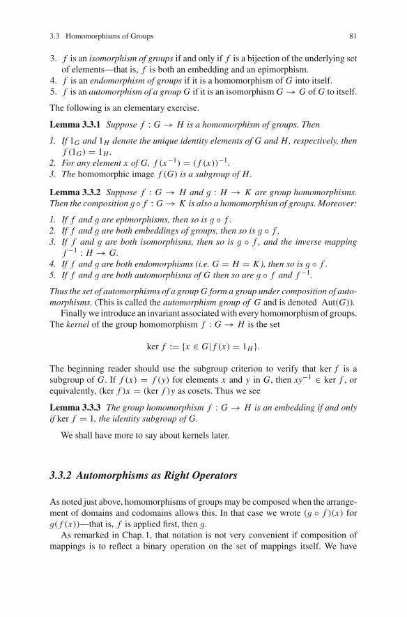
3.3 Homomorphisms of Groups 81
3. f is an isomorphism of groups if and only if f is a bijection of the underlying setof elements—that is, f is both an embedding and an epimorphism.
4. f is an endomorphism of groups if it is a homomorphism of G into itself.5. f is an automorphism of a group G if it is an isomorphism G → G of G to itself.
The following is an elementary exercise.
Lemma 3.3.1 Suppose f : G → H is a homomorphism of groups. Then
1. If 1G and 1H denote the unique identity elements of G and H, respectively, thenf (1G) = 1H .
2. For any element x of G, f (x−1) = ( f (x))−1.3. The homomorphic image f (G) is a subgroup of H.
Lemma 3.3.2 Suppose f : G → H and g : H → K are group homomorphisms.Then the composition g ◦ f : G → K is also a homomorphism of groups. Moreover:
1. If f and g are epimorphisms, then so is g ◦ f .2. If f and g are both embeddings of groups, then so is g ◦ f ,3. If f and g are both isomorphisms, then so is g ◦ f , and the inverse mapping
f −1 : H → G.4. If f and g are both endomorphisms (i.e. G = H = K ), then so is g ◦ f .5. If f and g are both automorphisms of G then so are g ◦ f and f −1.
Thus the set of automorphisms of a group G form a group under composition of auto-morphisms. (This is called the automorphism group of G and is denoted Aut(G)).
Finallywe introduce an invariant associatedwith every homomorphism of groups.The kernel of the group homomorphism f : G → H is the set
ker f := {x ∈ G| f (x) = 1H }.
The beginning reader should use the subgroup criterion to verify that ker f is asubgroup of G. If f (x) = f (y) for elements x and y in G, then xy−1 ∈ ker f , orequivalently, (ker f )x = (ker f )y as cosets. Thus we see
Lemma 3.3.3 The group homomorphism f : G → H is an embedding if and onlyif ker f = 1, the identity subgroup of G.
We shall have more to say about kernels later.
3.3.2 Automorphisms as Right Operators
As noted just above, homomorphisms of groups may be composed when the arrange-ment of domains and codomains allows this. In that case we wrote (g ◦ f )(x) forg( f (x))—that is, f is applied first, then g.
As remarked in Chap.1, that notation is not very convenient if composition ofmappings is to reflect a binary operation on the set of mappings itself. We have

82 3 Review of Elementary Group Properties
finally reached such a case. The automorphisms of a group G themselves form agroup Aut(G). To represent how the group operation is realized by composition ofthe induced mappings, it is notationally convenient to represent then in “exponentialnotation” and view the composition as a composition of right operators.
(The exponential convention) If σ is an automorphism of a group G, and g ∈ G,we rewrite σ(g) as gσ . This way, passing from the group operation (in Aut(G))to composition of the automorphisms does not entail a reversal in the order of thegroup arguments.6
Thus for automorphisms σ and τ of G and any x ∈ G we then have,
xστ = (xσ)τ .
3.3.3 Examples of Homomorphisms
Symmetries that are induced by group elements on some object X are a great sourceof examples of group homomorphisms. Where possible in these examples we writethese as left operators with ordinary composition “◦”—but we will begin to renderthese things in exponential notation here and there, to get used to it. In the nextchapter on group actions, we will be using the exponential notation uniformly whena group acts on anything.
Example 25 Examples of homomorphisms.
(a) Suppose there is a bijection between sets X and Y . Then there is an isomorphismSym(X) → Sym(Y ). This just amounts to changing the names of the objectsbeing permuted.
(b) Let R∗ be the multiplicative group of all nonzero real numbers, and let R+∗be the multiplicative group of the positive real numbers. Then the “squaring”mapping, which sends each element to its square, defines a homomorphism ofgroups
σ : R∗ → R+∗,
and, by restriction, an embedding
σ|R+∗ : R∗ → R∗.
The kernel of σ is the multiplicative group consisting of the real numbers ±1.
6This is part of a general scheme in which elements of some ‘abstract group’ G (with its ownmultiplication) induce a group of symmetries Aut(X) of some object X so that group multiplicationis represented by composition of the automorphisms. These are called “group actions” and arestudied carefully in the next chapter.

3.3 Homomorphisms of Groups 83
(c) In any intermediate algebra course (cf. books of Dean or Herstein, for exam-ple), one learns that complex conjugation (which sends any complex numberz = a + bi to z := a − bi , a and b real) is an automorphism of the field of com-plex numbers. The norm mapping N : C∗ → R
+∗ from the multiplicative groupof non-zero complexnumbers to themultiplicative groupof positive real numbersis defined by setting N (z) := z · z for each complex number z. Since complexconjugation is an automorphism of the commutative multiplicative group C∗, itfollows that the norm mapping N satisfies N (z1z2) = N (z1)N (z2) and hence isa homomorphism of groups. The kernel of the homomorphism is the group C1of complex numbers of norm 1—the so-called circle group.(When one considers that N (a + bi) = a2 + b2, a, b ∈ R, it is not mysteriousthat the set of integers which are the sum of two perfect squares is closed undermultiplication.)
(d) (Part 1.) Now consider the group of rigid rotations of the (regular) cube. Thereare four diagonal axes intersecting the cube from a vertex to its opposite vertex.These four axes intersect at the center of the cube, which we take to be the originof Euclidean 3-space. The angle α formed at the origin by the intersection of anyof these two axes, satisfies cos(α) = ±1/3. Let us label these four axes 1, 2, 3, 4in any manner. As we rotate the cube to a new congruent position, the four axesare permuted among themselves. Thus we have a mapping
rotations of the cube → permutations of the labeled axes
which defines a group homomorphism
rigid rotations of the cube → Sym(4),
the symmetric group on the four labels of the axes. The kernelwould be a group ofrigid motions which stabilizes each of the four axes. Of course it is conceivablethat some axes are reversed (sent end-to-end) by such a motion while othersare fixed point-wise by the same motion. In fact if we had used the three face-centered axes, it would be possible to reverse two of the axes while rigidly fixingthe third. But with these four vertex-centered axes, that is not possible. (Can youshow why? It has to do with the angle and the rigidity of the motion.) So thekernel here is the identity rotation of the cube. Thus we have an embedding of therotations of the cube into Sym(4). But we have seen in the previous subsectionthat both of these groups have order 24. Thus by the “pigeon-hole principle”,the homomorphism we have defined is an isomorphism.
(d) (Part 2.) Again G is the group of rigid rotations of the cube. There are exactlythree face-centered axes which are at right angles to one another. A 90◦ rotationabout one of these three axes fixes it, but transposes the other two. Thus if welabel the three face-centered axes by the letters {1, 2, 3}, and send each rotationin the group G to the permutation of the labels of the three face-centered axes

84 3 Review of Elementary Group Properties
which it induces, we obtain an epimorphism of groups G → Sym(3), or, in viewof part 1 of (d), a homomorphism Sym(4) → Sym(3). The kernel is the groupK which stabilizes each of the three face-centered axes. This group consists ofthe identity element, together with three involutions, each being a 180◦ rotationabout one of the three face-centered axes. Multiplication in K is commutative.
(e) Linear groups to matrix groups. Now let V be a vector space over a field F offinite dimension n. We have seen in the previous subsection that the bijectivelinear transformations from V into itself form a group which we called GL(V ),the general linear group on V . Now fix a basis A = {v1, . . . , vn} of V . Anylinear transformation T : V → V , viewed as a right operator of V can berepresented as a matrix
ATA := (pi j )
where
(vi )T = pi1v1 + pi2v2 + · · · + pinvn
(so that the rows of the matrix depict the fate of the vector vi under T ).7 Forcomposition of the right operators S and T on V let us write
v(T ∗ S) = ((v)T )S, v ∈ V,
so that T ∗ S is simply S ◦ T in the standard notation for composition. Then wesee that
A(T ∗ S)A = A(T )A · A(S)A
(where chronologically, the notation intends that T is applied first, then S, beingright operators and “·” denotes ordinarymultiplication ofmatrices.) This way thesymbolism does not transpose the order of the arguments, so in fact the mapping
T →A TA
defines a group homomorphism
fA : GL(V ) → GL(n, F)
7Thanks to the analysts’ notation for functions, combined with our habit of reading from left toright, many linear algebra books make linear transformations left operators of their vector spaces,so that their matrices are then the transpose of those you see here. That is, the columns of theirmatrices record the fates of their basis vectors. However as algebraists are aware, this is actually avery awkward procedure when one wants to regard the composition of these transformations as abinary operations on any set of such transformations.
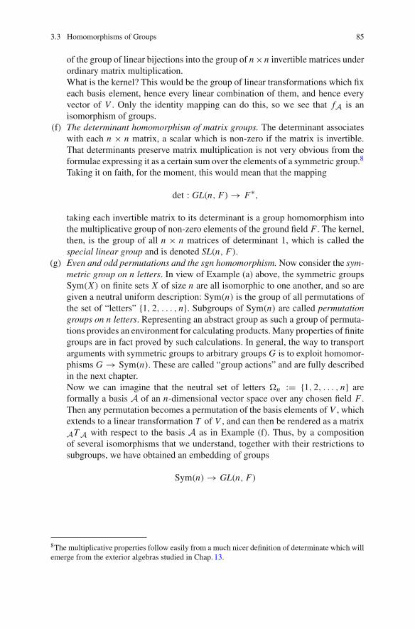
3.3 Homomorphisms of Groups 85
of the group of linear bijections into the group of n ×n invertible matrices underordinary matrix multiplication.What is the kernel? This would be the group of linear transformations which fixeach basis element, hence every linear combination of them, and hence everyvector of V . Only the identity mapping can do this, so we see that fA is anisomorphism of groups.
(f) The determinant homomorphism of matrix groups. The determinant associateswith each n × n matrix, a scalar which is non-zero if the matrix is invertible.That determinants preserve matrix multiplication is not very obvious from theformulae expressing it as a certain sum over the elements of a symmetric group.8
Taking it on faith, for the moment, this would mean that the mapping
det : GL(n, F) → F∗,
taking each invertible matrix to its determinant is a group homomorphism intothe multiplicative group of non-zero elements of the ground field F . The kernel,then, is the group of all n × n matrices of determinant 1, which is called thespecial linear group and is denoted SL(n, F).
(g) Even and odd permutations and the sgn homomorphism. Now consider the sym-metric group on n letters. In view of Example (a) above, the symmetric groupsSym(X) on finite sets X of size n are all isomorphic to one another, and so aregiven a neutral uniform description: Sym(n) is the group of all permutations ofthe set of “letters” {1, 2, . . . , n}. Subgroups of Sym(n) are called permutationgroups on n letters. Representing an abstract group as such a group of permuta-tions provides an environment for calculating products. Many properties of finitegroups are in fact proved by such calculations. In general, the way to transportarguments with symmetric groups to arbitrary groups G is to exploit homomor-phisms G → Sym(n). These are called “group actions” and are fully describedin the next chapter.Now we can imagine that the neutral set of letters �n := {1, 2, . . . , n} areformally a basis A of an n-dimensional vector space over any chosen field F .Then any permutation becomes a permutation of the basis elements of V , whichextends to a linear transformation T of V , and can then be rendered as a matrixATA with respect to the basis A as in Example (f). Thus, by a compositionof several isomorphisms that we understand, together with their restrictions tosubgroups, we have obtained an embedding of groups
Sym(n) → GL(n, F)
8The multiplicative properties follow easily from a much nicer definition of determinate which willemerge from the exterior algebras studied in Chap. 13.

86 3 Review of Elementary Group Properties
which represents each permutation by a matrix possessing exactly one 1 in eachrow and in each column, all other entries being zero. Such a matrix is calleda a permutation matrix.Now even the usual sum formula for the determinant shows that the determinantof a permutation matrix is ±1. Now if we accept the thesis of Example (f) justabove, that the determinant function is in fact multiplicative, we obtain a usefulgroup homomorphism:
sgn : Sym(n) → {±1}
into the multiplicative group Z2 of numbers ±1, which records the determinantof each permutation matrix representing a permutation. The kernel of sgn iscalled the alternating group, denoted Alt(n), and its elements are called evenpermutations. All other permutations are called odd permutations. Since sgn isa group homomorphism, we see that
An even permutation times an even permutation is even.An odd permutation times an odd permutation is even.An even permutation times an odd permutation (in any order) is odd.
Since the argument developed for this example assumed the thesis of part (f)(of this same Example 25)—that the determinant of a product of matrices is theproduct of their determinants—and since that thesis may not be known from firstprinciples by some students, we shall give an elementary proof of the existenceof the sgn homomorphism in Sect. 4.2.2 of the next chapter, without any appealto determinants.
(h) The automorphism group of a cyclic group of order n. Finally, perhaps,we shouldconsider an example of an automorphism group of a group. We consider here,the group Aut(Zn), the group of automorphisms of the cyclic group of order n,where n is any natural number. Suppose, then, that C is the additive group ofintegers mod n—that is, the additive group of residue classes modulo n. Thus{[ j] := j + nZ}, j = 1, 2, . . . , n − 1, n. The addition rule becomes
[i] + [ j] = [i + j] or [i + j − n], whichever does not exceed n,
where 1 ≤ i ≤ j ≤ n. Then element [1] generates this group. Indeed so does[m] if and only if gcd(m, n) = 1. Thus, if f : C → C is an automorphismof C it follows than f ([1]) = [m] where gcd(m, n) = 1. Moreover, since fis a homomorphism, f [k] = [mk]. Thus the automorphism f is completelydetermined by the natural number m coprime to and less than n. The number ofsuch numbers is called the Euler φ-function, and it’s value at n is denoted φ(n).Thus φ(n) = |Aut(Zn)|.
It now follows that Aut(C) is isomorphic to the multiplicative group �(n) of allresidues mod n which consist only of numbers which are relatively prime to n.9
9 We will obtain a more exact structure of this group when we encounter the Sylow theorems.

3.3 Homomorphisms of Groups 87
(i) The inner automorphism group. Let G be a general abstract group and let x bea fixed element of G. We define a mapping
ψx : G → G,
called conjugation by x , by the rule ψx (g) := x−1gx , for all g ∈ G. One caneasily verify that ψx (gh) = ψx (g)ψx (h), and as ψx is a bijection, it is an auto-morphism of G. Any automorphism of G which is of the form ψx for some x inG, is called an inner automorphism of G.Now if {x, y, g} ⊆ G, one always has
y−1(x−1gx)y = (y−1x−1)g(xy) = (xy)−1g(xy) (3.2)
which means
ψy ◦ ψx = ψxy (3.3)
for all x, y. Thus the set of inner automorphisms is closed under composition ofmorphisms. Setting y = x−1 in Eq. (3.3) we have
ψx−1 = ψ−1x , (3.4)
and so the set of inner automorphisms is also closed under taking inverses. Itnow follows that the set of inner automorphisms of a group G forms a subgroupof the full automorphism group Aut(G). We call this subgroup the inner auto-morphism group of G, denoted by Inn(G).Now Eq. (3.3) would suggest that there is a homomorphism from G to Aut(G)
except for one thing: the arguments of the ψ-morphisms come out in the wrongorder in the right side of the equation. That is because the operation “◦” isdenoting composition of left operators.This reveals the efficacy of using the exponential notation for denoting automor-phisms as right operators. We employ the following:
(Convention of writing conjugates in groups) If a and b are elements of agroup G, we write
a−1ba in the exponential form ba .
In this notation Eq. (3.2) reads as follows:
(gx )y = gxy (3.5)
for all {g, x, y} ⊆ G. What could be simpler?

88 3 Review of Elementary Group Properties
Then we understand Eq. (3.3) to read
ψxy = ψxψy, (3.6)
where the juxtaposition on the right hand side of the equation indicates compo-sition of right operators—that is the chronological order in which the mappingsare performed reads from left to right, ψx first and then ψy .Now Eq. (3.6) provides us with a group homomorphism:
ψ : G → Aut(G)
taking element x to the inner automorphism ψx , the automorphisms of Aut(G)
being composed as right operators (as in the exponential convention for isomor-phisms on p. 81).What is the kernel of the homomorphismψ? This would be the set of all elementsz ∈ G such that ψz = 1G , the identity map on G. Thus this is the set Z(G) ofelements z of G satisfying any one of the following equivalent conditions:
(a) ψz = 1G , the identity map on G,(b) z−1gz = g for all elements g of G,(c) zg = gz for all elements g of G.
The subgroup Z(G) is called the center of G. The identity element is alwaysin the center. If Z(G) = G, then multiplication in G is “commutative”—that isxy = yx for all (x, y) ∈ G × G. Such a group is said to be commutative, and isaffixed with the adjective abelian. Thus G is abelian if and only if G = Z(G).
A Glossary of Terms Expected to be Understood from the Examples
1. Homomorphism of groups.2. Epimorphism of groups.3. Embedding of groups.4. Isomorphism of groups.5. Endomorphism of a group.6. Automorphism of a group.7. The kernel of a homomorphism, ker f .8. The automorphism group, Aut(G), of a group G.9. The inner automorphism group, Inn(G), of a group, G.10. An inner automorphism.11. The center of a group, Z(G).12. Abelian groups.

3.4 Factor Groups and the Fundamental Theorems of Homomorphisms 89
3.4 Factor Groups and the Fundamental Theoremsof Homomorphisms
3.4.1 Introduction
A teacher is sometimes obliged to present to a class a Theorem labeled as somesort of “Fundamental Theorem”. More often than not, such a theorem is not quite asfundamental as it must have seemed at an earlier time in our history.10
At a minimum it would seem that a proposition should be labelled “a fundamentaltheorem” if it has these properties:
1. It should be used so constantly in the daily life of a scholar of the field, thatquoting it becomes repetitive.
2. It’s logical distance from the “first principles” of the field should be short enoughto bear a short explanation to a puzzled student (that is, the alleged “fundamentaltheorem” should be “teachable”).
We are lucky today! The fundamental theorems of homomorphisms of groupsactually meets both of these criteria. They tell us that the homomorphic images ofgroups, their compositions, and their effects on subgroups, can all be derived froman internal study of the groups themselves.
The custom has been to name these three theorems as the “First-”, “Second-”, and“Third Fundamental Theorems of Homomorphisms”. However a perusal of eightwell-known textbooks in algebra shows this nomenclature to be far from uniform.11
Sowe have tried to sidestep the ambiguity by naming these three very basic Theoremsin a way related to what these theorems are telling us.
3.4.2 Normal Subgroups
The set of all subgroups of a group are permuted among themselves by automor-phisms of a group. Explicitly: if σ ∈ Aut(G), and K is a subgroup of G, thenK σ := {kσ|k ∈ K } is again a subgroup of G.12 Moreover, if H is a subgroup ofAut(G), then any subgroup of G left invariant by the elements of H is said to be
10 Who on earth decided that the Fundamental Theorem of Algebra should be the fact that theComplex Numbers form an algebraically closed field? Who on earth decided that the FundamentalTheorem of Geometry should be the fact that an isomorphism between two Desarguesian ProjectiveSpaces of sufficient dimension is always induced by a semilinear transformation of the underlyingvector spaces?11One author’s “First” theorem is another’s “Second”, all three ordinal labels are used by one author(Hall) for what another calls the “First” Theorem, and some authors (Michael Artin, for example),seeing the problem, wisely declined to assign ordinal numbers beyond the “First”.12Note the convention of regarding automorphisms as right operators whose action is denotedexponentially (see p. 81).

90 3 Review of Elementary Group Properties
H-invariant. Naturally we have special cases for special choices of H . A subgroup Kwhich is invariant under the full group Aut(G) is said to be a characteristic subgroupof G. We write this as K char G. (The center which we previously encountered iscertainly one of these).
But let us drop down to a larger class of H -invariant subgroups by lettingH descend from the full automorphism group of G to the case that H is sim-ply the inner automorphism group, Inn(G), encountered in the previous Section,Example 25, part (i). A subgroup which is invariant under Inn(G) is said to benormal in G or to be a normal subgroup of G.
Just putting definitions together one has
Lemma 3.4.1 The following are equivalent conditions for a subgroup K of G:
1. ψx (K ) = K , for all x ∈ G,2. x−1K x = K for every x ∈ G,3. x K = K x, for each x ∈ G.
(In this Lemma, ψx is the inner automorphism induced by the element x : seeExample 25, part (i) preceding.)
As a notational convenience, the symbol K �G will always stand for the assertion:“K is a normal subgroup of G” or, equivalently, “K is normal in G”. This is alwaysa relation between a subgroup K and some subgroup G which contains it. It is nota transitive relation. It is quite possible for a group G to possess subgroups L andK , with L � K and K � G, for which L is not normal in G.13 Two immediateconsequences of normality are the following:
Corollary 3.4.2 Suppose N is a normal subgroup of the group G and suppose H isany subgroup of G. Then the following statements hold:
1. N is normal in any subgroup of G which contains it.2. N ∩ H is a normal subgroup of H. (As a special case, if H contains N, then N
is normal in H).3. NH = HN is a subgroup of G.4. If H is also normal in G, then so is HN.
The proof is left for the beginning student in Exercise (4) in Sect. 3.7.1 at the endof this chapter.
One should not leave a basic section on normal subgroups without touching on therelationship between the normal subgroups and characteristic subgroups. As notedabove, a normal subgroup of G is simply a subgroup N of G which is invariant underall the inner automorphisms of G, while a characteristic subgroup is a subgroup
13 In the group G of rigid rotations of a cube (Example 23, part (g) of Sect. 3.2), the 180◦ rotationabout one of the three face-centered axes, generates a subgroup L which point-wise fixes its axisof rotation, but inverts the other two face-centered axes. This a normal subgroup of the abeliansubgroup K of all rotations of the cube which leave each of the three face-centered axes invariant.Then K is normal in G, being the kernel of the homomorphism of Example 25, Part (d) of Sect. 3.3.But clearly L is not normal in G, since otherwise its unique point-wise fixed face-centered axis,would also be fixed. But it is not fixed as G/K induces all permutations of Sym(3) on these axes.

3.4 Factor Groups and the Fundamental Theorems of Homomorphisms 91
K of G that is invariant under all automorphisms of G. Thus every characteristicsubgroup of G is already normal, but, in general, being characteristic is a muchstronger condition.
Theorem 3.4.3 Assume N is a normal subgroup of G. If K is a characteristicsubgroup of N (i.e. K is invariant under Aut(N )), then K is normal in G.
One more result:
Theorem 3.4.4 For any group G, Inn(G) � Aut(G).
The proofs of these two theorems are left as Exercises 3 and 4 of Sect. 3.7.3 at theend of this chapter.
Almost any subgroup of G that is unique in some respect is a characteristicsubgroup of G. For example the identity group 1, the whole group G and the center,Z(G), are all characteristic subgroups of G.
3.4.3 Factor Groups
Let N be a normal subgroup if G. By Part 3. of the above Lemma 3.4.1, one seesthat the subset xN is in fact the set Nx, for each x ∈ G. But it also asserts thatNx · Ny = N (xN)y = NNxy = Nxy as subsets of G. Thus there is actually amultiplicative group G/N whose elements are the right cosets of N in G, wheremultiplication is unambiguously given by the rule
(Nx) · (Ny) = Nxy. (3.7)
We have a name for this multiplicative group of cosets of a normal subgroup N . It iscalled the factor group, G/N . Its identity element is the subgroup N itself (certainlya right coset N · n, for any n ∈ N ) since Nx · N = NNx = Nx. The inverse in G/N ofthe element Nx is the element Nx−1. In fact it is now easy to verify that the mappingG → G/N that sends element x to coset Nx is a group homomorphism (see Theorem3.4.5, part (i) below).
Now let f : G → H be a homomorphism of groups. Two special groups asso-ciated with a group homomorphism f have been introduced earlier in this chapter:the range or image, f (G), and the kernel, ker f . Now if y ∈ ker f , and x ∈ G, wesee that
f (x−1yx) = ( f (x))−1 f (y) f (x) = ( f (x))−1 · 1 · f (x) = 1 ∈ H,
since f (y) = 1. Thus for all y ∈ ker f , and x ∈ G, x−1yx ∈ ker f so ker f is alwaysa normal subgroup. What about the corresponding factor group?

92 3 Review of Elementary Group Properties
Theorem 3.4.5 (The Fundamental Theorem of Homomorphisms)
(i) If N is a normal subgroup of a group G, the mapping G → G/N which mapseach element x of G to the right coset Nx which contains it, is an epimorphismof groups. Its kernel is N .
(ii) If f : G → H is a homomorphism of groups, there is an isomorphism η :f (G) → G/(ker f ) taking each element f (x), x ∈ G, to (ker f )x. Thus everyhomomorphic image f (G) is isomorphic to a factor group of G.
(iii) In particular, the kernel of the homomorphism is trivial—i.e. ker f = 1—if andonly if the homomorphism itself is injective.
Proof (i) That the mapping π : G → G/N defined by π(x) := Nx, is a homomor-phism follows from NxNy = Nxy, for all (x, y) ∈ G × G. By definition of G/Nthis map is onto. (The epimorphism π : G → G/N is usually called the projec-tion homomorphism or sometimes the natural homomorphism onto the factor groupG/N .) Since the coset N = N · 1 is the identity element of G/N , the kernel of ν isprecisely the subset {x ∈ G|N x = N } = {x ∈ G|x ∈ N } = N . Thus ker π = N .
(ii) Now set ker f := N We propose a mapping η : f (G) → G/N which takesan image element f (x) to the coset Nx. Since this recipe is formulated in termsof a single element x , we must show that the proposed mapping is well-defined.Suppose f (x) = f (y). We wish to show Nx = Ny. But the hypothesis shows thatf (x−1y) = f (x−1) f (y) = ( f (x))−1 f (x) = 1 ∈ G, so x−1y ∈ ker f = N ,whence Nx = Ny, as desired.
Now
η( f (x) f (y)) = η( f (xy)) = Nxy (3.8)
= NxNy = η( f (x)) · η( f (y)). (3.9)
Thus η is a homomorphism. If f (x)were in the kernel of η, then η( f (x)) = Nx = N ,the identity element of G/N . Thus x ∈ N , so f (x) = f (1), the identity element off (G). Finally, η is onto, since, for any g ∈ G, the coset Ng = η( f (g)). Thus η is abijective homomorphism and so is an isomorphism.
(iii) This is obvious from first principles since xy−1 ∈ ker f if and only if f (x) =f (y). It also follows from (ii). The proof is complete. �
Remark (a) The main idea about (i) is that when you spot a homomorphism shootingoff somewhere, you do not have to search all over the Universe to study it. Instead,you can realize the homomorphic image right inside the structure of the group Gitself, as one of its factor groups.
(b) We have included statement (iii) in the Fundamental Theorem of Homomor-phisms since it is so often implicitly used without any particular reference. Since itis an immediate consequence of part (ii) we have given it a home here.
There are two further consequences of Theorem 3.4.5 which are contained in thefollowing Corollary.

3.4 Factor Groups and the Fundamental Theorems of Homomorphisms 93
Corollary 3.4.6 (The classical isomorphism theorems)
(i) (The Composition Theorem for Groups) Suppose K and N are both normalsubgroups of G, with K contained in N. Then N/K is a normal subgroup ofG/K , and G/N is isomorphic to the factor group (G/K )/(N/K ).
(ii) (The Modularity Theorem for Groups) If N is a normal subgroup of G, and His any subgroup of G, HN/N is isomorphic to H/(H ∩ N ).
Proof (i) By Corollary 3.4.2, part 1, K is normal in N , so N /K is the multiplicativegroup of cosets {K n|n ∈ N }. For any coset K x of G/K , and coset K n of N /K ,(K x)−1K nK x = K (x−1nx), which is in N /K . Thus N /K � G/K . Thus there is anatural epimorphism f2 : G/K → (G/K )/(N /K ) onto the factor group as describedin the Fundamental Theorem (Theorem 3.4.5, part (i)). By the same token, thereis a canonical epimorphism f1 : G → G/K . By Lemma 3.3.2 of Sect. 3.2. Thecomposition of these epimorphisms is again an epimorphism:
f2 ◦ f1 : G → (G/K )/(N/K ).
An element x of G is first mapped to the coset K x and then to the coset (K x){K n|n ∈N } (which, viewed as a set of elements of G is just N x). Thus x maps to the identityelement (N /K )/(N /K ) of (G/K )/(N /K ) if and only if x ∈ N . Thus the kernel ofepimorphism f2 ◦ f1 is N . The result now follows from the Fundamental Theoremof Homomorphisms (Theorem 3.4.5 Part (ii)).
(ii) Clearly N � HN and N ∩ H � H by Corollary 3.4.2, part1. We proposeto define a morphism f : H → HN/N by sending element h of H to coset Nh ∈HN/N . Clearly hh′ is sent to Nhh′ = (Nh)(Nh′), so f is a group homomorphism.Since every coset of N in HN = NH has the form Nh for some h ∈ H , f is anepimorphism of groups. Now if h ∈ H , then Nh = N , the identity of HN/N , if andonly if h ∈ H ∩ N . Thus ker f = H ∩ N and now the conclusion follows from theFundamental Theorem of Homomorphisms (Theorem 3.4.5 Part (ii)). �
3.4.4 Normalizers and Centralizers
Let X be some non-empty subset of a group G. For each x ∈ G, the set ψx (X) :=x−1X x is called a conjugate (in G) of the set X . Given X , consider the set
NG(X) := {x ∈ G|x−1X x = X}.
The reader may verify that the set on the right side of the presented equation indeedsatisfies any one of the equivalent conditions listed in the SubgroupCriterion (Lemma3.2.3). The subgroup described by this equation is called the normalizer (in G) ofthe set X and is denoted NG(X). Also, if H is any subgroup of G, we say that Hnormalizes the set X if and only if H is a subgroup of the normalizer NG(X).
In practice, X is often itself a subgroup.

94 3 Review of Elementary Group Properties
Lemma 3.4.7 The following statements about a group G are true.
1. The subgroup H is a normal subgroup of G, i.e. H � G, if and only if NG(H) = G.More generally, H is normal in the subgroup K —i.e. H � K —if and only ifH ≤ K ≤ NG(H).
2. If H and K are subgroups of G, then NK (H) = NG(H) ∩ K .3. If H and K are subgroups of G, and K normalizes H, then HK = KH, and KH
is a subgroup of G.4. Suppose the subgroup K normalizes the subset X of G. Then K also normalizes
the subgroup 〈X〉G generated by X.
The statements are immediate consequences of the definitions. The beginningstudent is urged to warm up some nice fall afternoon by devising formal proofs ofthese statements.
There is another kind of subgroup determined by a subset X of a group G, namelythe subgroup
CG(X) := {g ∈ G|g−1xg = x, for all x ∈ X},
called the centralizer (in G) of X . It consists precisely of those elements in G whichcommute with every element of X . We say that subgroup H centralizes the set X ifand only if H ⊆ CG(X).
At this point it might be useful to compare the centralizer and the normalizer. Thenormalizer NG(X) is the set of elements g ∈ G whose associated inner automorphismψg leaves the subset X invariant as a whole. The centralizer CG(X) consists of thoseelements g ∈ G whose associated inner automorphism ψg fixes set X element-wise.Now, as with the normalizer, we possess a number of elementary observations.
Lemma 3.4.8 Suppose G is some fixed group with a designated subset X. Thefollowing statements hold.
1. We have CG(X) � NG(X).2. If H is a subgroup of G, then CH (X) = CG(X) ∩ H.3. If subgroup H centralizes X, then it also centralizes the subgroup 〈X〉G generated
by X.
Once again the beginning student is invited to spend a few moments some nicefall afternoon assembling formal proofs of the statements in Lemma 3.4.8 This time,in view of part 1, the student is permitted to order a drink.
3.5 Direct Products
A direct product is a formal construction for getting new groups in a rather easy way.First let G = {Gσ|σ ∈ I } be a family of groups indexed by the index set I . We canwrite elements of the Cartesian product of the Gσ as functions

3.5 Direct Products 95
f : I →⋃
σ∈IGσ such that f (σ) ∈ Gσ.
Of course, when I is countable, we can represent elements f in the usual way, assequences ( f (1), f (2), . . .). Define a binary operation on the Cartesian product bydeclaring the “product” f1 f2 of f1 and f2 to be the functionwhose value ( f1 f2)(σ) atσ ∈ I is f1(σ) f2(σ)—that is, the values fi (σ) at the “coordinate” σ are multiplied inthe group Gσ) to yield the σ-coordinate of the “product”. This is termed “coordinate-wisemultiplication”, since for sequences, the product of (a1, a2, . . .) and (b1, b2, . . .)is (a1b1, a2b2, . . .), by this definition. The Cartesian product with this coordinate-wise multiplication clearly forms a group, which we call the direct product over Gand is denoted by ∏
σ∈I(Gσ) or
∏GGσ
or, when I = {1, 2, . . . , n}, simply by
G1 × G2 × · · · × Gn .
It contains a subgroup consisting of all maps f in the definition of direct product,for which f (σ) fails to be the identity element of the group Gσ only finitely manytimes. This subgroup is called the weak direct product or direct sum over G and isdenoted ⊕
σ∈I(Gσ) or
⊕G(Gσ).
When I is finite, there is no distinction between the direct product and direct sum.Consider the group G = {±1} under ordinary multiplication of integers. Thus
G is a group of order 2, with involution −1. Then G × G is the group of pairs(u, v), u, v ∈ {±1}, with coordinate-wisemultiplication. For example, one calculatesthat (−1, 1) ·(1,−1) = (−1,−1). In this case G ×G is a group of order four with anidentity element and three involutions. The product of any two distinct involutionsis the third involution. Any group in the isomorphism class of this group is called afours group.
For every index τ in I , there is clearly a homomorphism πτ : ⊕G(Gσ) → Gτ
which takes f to f (τ ), for all f in the direct product. Such an epimorphism is calleda projection onto the coordinate indexed by τ . This epimorphism retains this nameeven when it is restricted to the direct sum.
Any permutation of the index set induces an obvious isomorphism of direct prod-ucts and direct sums. Thus G1 × G2 is isomorphic to G2 × G1 even though they arenot formally the same group.
Similarly, any (legitimate) rearrangement of parentheses involved in constructingdirect products yields isomorphisms; specifically
G1 × G2 × G3 � (G1 × G2) × G3 � G1 × (G2 × G3).

96 3 Review of Elementary Group Properties
Now suppose A and B are two subgroups of a group G with A ∩ B = 1, and Bnormalizing A (that is, B ≤ NG(A)). Then together they generate a subgroup ABwith order |A| · |B| (Lemma 3.2.6). Now suppose in addition that A normalizes B.Then for any element a ∈ A and element b ∈ B, the factorizations (aba−1)b−1 =a(ba−1b−1) show that aba−1b−1 ∈ A ∩ B = {1} and so ab = ba. Thus all elementsof A commute with all elements of B. In that case the mapping A × B → ABwhich takes (a, b) ∈ A × B to ab, is a group homomorphism whose kernel is{(x, x−1)|x ∈ A ∩ B}. Since A ∩ B = {1}, this map is an isomorphism.
These remarks are summarized in the next Lemma.
Lemma 3.5.1
(i) For any permutation π in Sym(n), There is an isomorphism
G1 × G2 × · · · × Gn → Gπ(1) × Gπ(2) × · · · × Gπ(n)
although neither of the groups are necessarily formally the same.(ii) Any two well-formed groupings of the factors of a direct product into paren-
theses yields groups which are isomorphic to the original direct product andhence are isomorphic to each other.
(iii) (Internal Direct Products) Suppose A1, A2, . . . is a countable sequence ofsubgroups of a group G.
(a) Suppose A j normalizes Ai whenever i �= j , and(b) A1A2 · · · Ak−1 ∩ Ak = 1, for all k ≥ 2.
Then A1A2 · · · An is isomorphic to the direct product A1 × · · · × An for anyfinite initial segment {A1, . . . , An} of the sequence of subgroups.
3.6 Other Variations: Semidirect Products and SubdirectProducts
3.6.1 Semidirect Products
Suppose we are given a homomorphism
f : H → Aut(N ),
for two abstract groups N and H . Then f defines a formal construction of a groupN :H , which is called a semidirect product of N by H .14 The elements of N :H are
14In some older books there is other notation for the semidirect product—some sort of decorationadded to the “�” symbol. The notation N :H is the notation for a “split extension of groups” usedin the Atlas of Finite Groups [12].

3.6 Other Variations: Semidirect Products and Subdirect Products 97
the elements of the Cartesian product N × H . Multiplication proceeds according tothis rule: For any two elements (n1, h1) and (n2, h2) in N × H :
(n1, h1)(n2, h2) := (n1(n2)f (h−1
1 ), h1h2).
Verification of the associative law for a triple product (n1, h1)(n2, h2)(n3, h3) comesdown to the calculation
n f ((h1h2)−1)3 = (n
f (h−12 )
3 ) f (h−11 ).
Example 26 1. If f : H → Aut(N ) is the trivial homomorphism—that is, f mapsevery element of H to the identity automorphism of N—then N :H is just theordinary direct product N × H of the previous section.
2. If A and B are subgroups of a group G for which A normalizes B and A∩ B = 1,then the subgroup AB of G, is isomorphic to the semidirect product B:A withrespect to the morphism f : A → Aut(B) which takes each element a of A tothe automorphism of B induced by conjugating the elements of B by a—that isψa |B .
3. Let N be the additive group of integers mod n, and let H be any subgroup ofthe multiplicative group of residues coprime to n (for example, the quadraticresidues coprime to n). Let G be the group of all permutations of N of the form
μ(m, h) : x → hx + m, for all x ∈ N .
Then G is the semidirect product N :H .4. Let F be any field, let F∗ be the multiplicative group of all nonzero elements of
F , and let H be any subgroup of F∗. Then the set of all transformations of F ofthe form
x → hx + a, a ∈ F, h ∈ H,
forms a group under the composition of such transformations. This group isisomorphic to the semidirect product (F,+):H , where (F,+) denotes the groupon F whose operation is addition in the field F .
5. (The Frobenius group of order 21.) The group is generated by elements x and ysubject only to the relations
x3 = 1, y7 = 1, x−1yx = y2.
It is a semidirect product Z7 : Z3. (This is an example of a “presented group”,which we shall meet in Chap.6.) Here, the presentation reveals the homomor-phism H = 〈x〉 → Aut(〈y〉. This group is isomorphic to a group constructedby the recipe in part 4, where N is the additive group of the field Z/(7) and His the multiplicative group of quadratic residues mod 7.

98 3 Review of Elementary Group Properties
6. Suppose A is an abelian group of order n which is not a direct product of Z2’s.Then the mapping σ : A → A defined by aσ = a−1 for all a ∈ A, is anautomorphism of order 2. Using the inclusion 〈σ〉 ⊆ Aut(A) for f , one canform the semidirect product A〈σ〉 as above. Some authors refer to A〈σ〉 as ageneralized dihedral group.
7. A group is said to be a normal extension of a group N by H (written G = H.N )if and only if
N � G and G/N � H.
The extension is said to be split if and only if there is a subgroup H1 of G suchthat
G = NH1, N ∩ H1 = 1.
In this case, H1 � H . One can see that
G is a split extension of G by H if and only if G is a semidirect product of Nby H .
First, if the extension is split, every element of G has the form g = nh, (n, h) ∈N × H . Because N ∩ H1 = 1, the expression g = nh is unique for a givenelement g. We thus have a bijection
σ : G → N × H1
which takes g = nh to (n, τ (h)), where τ is the isomorphism H1 → H = G/N(from Corollary 3.4.6, part (ii)). Now if we multiply two elements of G, wetypically obtain
(n1h1)(n2h2) = n1(h1n2h−11 )h1h2 = n1(n2)
(h−11 ) · h1h2,
where, by our convention on inner automorphisms, gx := x−1gx. The σ-valueof this element is the pair
((n1)(n2)(h−1
1 ), τ (h1)τ (h2)).
Thus σ is an isomorphism of G with the semidirect product of N by H , definedby composing τ−1 with the homomorphism
H1 → Aut(N )
induced by conjugation. (The latter is just the restriction to H1 of the homomor-phism ψ of Example 3, part (i).)Conversely, if G is the semidirect product of N by H defined by some homo-morphism ρ : H → Aut(N ), then, setting

3.6 Other Variations: Semidirect Products and Subdirect Products 99
N0 := {(n, 1)|n ∈ M}H0 := {(1, h)|h ∈ H}
then
N0 � G = N0H0 and N0 ∩ H0 = 1,
so G is the split extension N0 by H0 and conjugation in G by element h0 of H0induces automorphism ρ(h0) on N0. (Clearly, N0 � N and H0 � H .)
3.6.2 Subdirect Products
Something a little less precise is the notion of a subdirect product. We say that agroup H is a subdirect product of the groups {Gσ|σ ∈ I } if and only if (i) H is asubgroup of the direct product
∏I Gσ and (ii) for each index τ , the restriction of
the projection map πτ to H is onto—i.e. πτ (H) = Gτ . There may be many suchsubgroups, so the isomorphism type of H is not uniquely determined by (i) and (ii)above.
Subdirect products naturally arise in the following situation: Suppose M and Nare normal subgroups of a group G. Then G/(M ∩ N ) is a subdirect product ofG/N and G/M . This is because G/(M ∩ N ) can be embedded as a subgroup of(G/M) × (G/N ) by mapping each coset (N ∩ M)x to the ordered pair (Mx, Nx).
In fact something very general happens:If {Nσ|σ ∈ I } is a family of normal subgroups of a group G, then
• G/(∩I Nσ) is the subdirect product of the groups {G/Nσ|σ ∈ I }.• SupposeF is a family of groups “closed under taking subdirect products”—that is,any subdirect product of members of F is in F . (For example the class of abeliangroups is closed under subdirect products.) Then for any arbitrary group G, thereis a “smallest” normal subgroup GF whose associated factor group G/GF lies inF . Precisely, G/GF ∈ F and if N is normal in G with G/N ∈ F , then GF ≤ N .
A simple group is a group G whose only proper normal subgroup is the identitysubgroup. (Note that by this definition, the group of order one is not a simple group.)
A maximal normal subgroup of a group G is a maximal element in the partiallyordered set of proper normal subgroups of G (ordered by inclusion, of course).
In Exercise (1) in Sect. 3.7.2 the following is proved:
Lemma 3.6.1 A factor group G/N of G is a simple group if and only if N is amaximal normal subgroup of G.
We begin with an elementary Lemma.

100 3 Review of Elementary Group Properties
Lemma 3.6.2 Suppose {Mi |i ∈ I } is a finite collection of maximal normal sub-groups of a group G. Then for some subset J of I ,
G/(∩i∈I Mi ) = G/(∩ j∈J M j ) �∏
j∈J(G/M j ),
a direct product of simple groups.
Proof The result is true for |I | = 1, as G/M1 is simple. We use induction on|I |. Renumbering the subscripts if necessary, the induction hypothesis allows us toassume that for some subset J = {1, . . . , d} ⊆ I ′ = {1, . . . , k − 1},
N : = ∩i∈I ′ Mi = ∩ j∈J M j . (3.10)
G/N � (G/M1) × · · · × (G/Md). (3.11)
We set I := {1, . . . , k} = I ′ + {k} and assume, without any loss of generality,that Mk is not contained in N . Then since N Mk is a normal subgroup of G properlycontaining Mk , we must have G = NMk . Also, since Mk is a simple group, N ∩ M =1. Then
G/(N ∩ Mk) � (G/N ) × (G/Mk),
and the result for |I | = k follows upon substitution for G/N in the right-hand side.�
One may conclude.
Corollary 3.6.3
(i) Suppose G is a finite group with no non-trivial proper characteristic subgroups.Then G is a direct product of pairwise isomorphic simple groups.
(ii) If N is a minimal normal subgroup of a finite group G, then N is a direct productof isomorphic simple groups.
Proof Part (i) Let M be a maximal normal subgroup of the finite group G. Then Ghas a finite automorphism group, and so {Mσ|σ ∈ Aut(G)} is a finite collection ofmaximal normal subgroups of G whose intersection N is a characteristic subgroup ofG properly contained in G. By hypothesis, N = 1. Then by the above Lemma 3.6.2,G = G/N is the direct product of simple groups. If G = 1, we have an empty directproduct and there is nothing to prove. Otherwise, the product of those direct factorsisomorphic to the first direct factor clearly form a non-trivial characteristic subgroup,which, by hypothesis must be the whole group.
Part (ii) Since N is a minimal normal subgroup of the finite group G, N is anon-trivial finite group with only the identity subgroup as a proper characteristicsubgroup, so the conclusion of Part (i) holds for N . �

3.7 Exercises 101
3.7 Exercises
3.7.1 Exercises for Sects. 3.1–3.3
1. Write out formal proofs of Lemmas 3.3.1 and 3.3.2 (all parts).2. Prove Corollary 3.2.4.3. Prove that G/Z(G) can never be a cyclic group. [Hint: If false, cosets of the form
Z(G)x±k partition G, and elements on one of these cosets commute with thosein any other such coset. So G can be shown to be abelian.]
4. Prove Corollary 3.4.2. [Hint: Use the subgroup criterion (Lemma 3.2.3) for part3.]
5. Suppose a group G has exponent 2—-that is, g2 = 1 for every g ∈ G. Show thatG is abelian.
6. Suppose p is a (positive) prime number and k is a positive integer.
(i) If p > 2, show that Aut(Z pk ) � Z p−1 × Z pk−1 .(ii) If p = 2 show that Aut(Z2k ) � Z2 × Z2k−2 .
3.7.2 Exercises for Sect. 3.4
1. Suppose N is a normal subgroup of the group G.
(a) Show that there is an isomorphism between the poset of all subgroups Hof G which contain N , and the poset of all subgroups of G/N (both posetspartially ordered by the containment relation).[Hint: The isomorphism takes H in the first poset to H /N in the second.]
(b) Show that H is normal in G if and only if H /N is normal in G/N . Thus theisomorphism of part (a) and its inverse both preserve the normality relation.(Note that they need not preserve the property of being characteristic ineither direction. The group H containing N is called the inverse image ofH /N .)
(c) Using the fundamental theorem of homomorphisms conclude that if
f : G → L
is an epimorphism of groups, then there is a 1-1 correspondence of thesubgroups of L with the subgroups of G containing ker f preserving con-tainment and normality. The correspondence takes a subgroup L1 of L tothe subset {g ∈ G| f (g) ∈ L1}, also called the inverse image of L1.
2. If X is a subset of the group G (that is, the subset X is not necessarily a subgroupof G), define the centralizer in G of X to be the set of all group elements g ofG such that gx = xg for all x ∈ X . This set is denoted CG(X). Similarly, the

102 3 Review of Elementary Group Properties
normalizer in G of X is the set of elements {g ∈ G|g−1Xg = X}. Such elementsmay permute the elements of X by conjugation, but they stabilize X as a set. Asubgroup H is said to normalize X if and only if H ≤ NG(X). If NG(X) = G,then X is called a normal set in G.
(a) Show that CG(X) and NG(X) are subgroups of G.(b) Show that if X is a normal set in G, then CG(X) is also normal in G.(c) Show that if N is a normal subgroup of G, then the inner automorphism
ψg : x → g−1xg induces an automorphism of N .
3. (a) Conclude that a characteristic subgroup of a normal subgroup of G is normalin G, that is, K char N � G implies K � G.
(b) Conclude that a characteristic subgroup of a characteristic subgroup of G ischaracteristic in G, that is, L char K char G implies L char G.
(c) Suppose N is a normal subgroup of G. Show that the mapping which sendselement g to ψg|N , the restriction of the inner automorphism conjugation-by-g to N , defines a group homomorphism
ψN : G → Aut(N )
whose kernel is CG(N ). Conclude that the group of automorphisms inducedon N by the inner automorphisms of G is isomorphic to G/CG(N ).
4. Show that for any group G, Inn(G) � Aut(G). (The factor group Out(G) :=Aut(G)/Inn(G) is called the outer automorphism group of G.)
5. Prove the assertions of Corollary 3.4.2.6. Recall from p. 99 that a group is said to be a simple group if and only if its only
proper normal subgroup is the identity subgroup. (Note that the definition forbidsthe identity group to be a simple group.)
(a) Prove that any group of prime order is a simple group.(b) Suppose G is a group. A subgroup M is a maximal subgroup of G if and
only if it is maximal in the poset of all proper subgroups of G. A subgroupM is a maximal normal subgroup of G if and only if it is maximal in theposet of all proper normal subgroups of G. (Note that it does not mean thatit is a maximal subgroup which is normal. Amaximal normal subgroup mayvery well not be a maximal subgroup.) Prove that a factor group G/N of Gis a simple group if and only if N is a maximal normal subgroup.[Hint: Use the result of Exercise (1)b in Sect. 3.7.2 just above.]
3.7.3 Exercises for Sects. 3.5–3.7
1. Let V be any vector space, and form the group GL(V ) of all invertible lineartransformations of V . Let G be any group and let f : G → GL(V ) be a homo-morphism of groups. [Such a homomorphism is said to be a representation of thegroup G.] Define multiplication on V × G by the rule

3.7 Exercises 103
(v1, g1) · (v2, g2) := (v1 + vf (g1)2 , g1g2).
(a) Show that this group is isomorphic to the semidirect product (V,+):G uponnoting that GL(V ) ≤ Aut(V,+).
(b) Show that the center of (V,+):G is the direct product CG(V ) × ker f .
2. A popular textbook in intermediate algebra (after presenting the Sylow theoremswhich will appear in the next chapter) offers an exercise requesting that the readerprove that every group of order 75 is abelian. Using the semidirect product con-struction, show that there exists a non-abelian group of order 75.[Hint: Let V := Z5 × Z5. One can regard V as a vector space over the fieldZ/(5) of integers mod 5. Let t : V → V be a linear transformation acting withminimal polynomial x2 + x + 1. This means V has a basis {v1, v2} with vt
1 = v2,and vt
2 = −v1 − v2. Then t3 induces the identity transformation 1V . Thus 〈t〉,as a subgroup of GL(V ), has order 3. One can then form the semidirect product(V,+)〈t〉 as described in the previous exercise.]
3. Suppose K is a characteristic subgroup of N and N is a normal subgroup of G.Show that K is a normal subgroup of G.[Hint: Conjugation by any element of G induces an automorphism of N and soleaves K invariant, since K is characteristic in N .]
4. Show that the group of inner automorphism of G is a normal subgroup of thegroup of all automorphisms of G.[Hint: Let ψ(g) be conjugation by g. show that
σ−1 · ψ(g) · σ
is conjugation by σ−1(g) and so is an inner automorphism.]

Chapter 4Permutation Groups and Group Actions
Abstract A useful paradigm for discussing a group is to regard it as acting as a groupof permutations of some set. The power of this point of view derives from the flexi-bility one has in choosing the set being acted on. Odd and even finitary permutations,the cycle notation, orbits, the basic relation between transitive actions and actionson cosets of a subgroup are first reviewed. For finite groups, the paradigm producesSylow’s theorem, the Burnside transfer and fusion theorems, and the calculations ofthe order of any group of automorphisms of a finite object. Of more special interestare primitive and multiply transitive groups.
4.1 Group Actions and Orbits
As defined earlier, a permutation of a set X is a bijective mapping X → X . Becausewe will be dealing with groups of permutations it will be convenient to use the“exponential” notation which casts permutations in the role of right operators. Thus ifπ is a permutation of X , we write xπ for the image of element x under the permutationπ. Recall that composition of bijections and inverses of bijections are bijections, sothat the set of all bijections of set X into itself form a group under composition whichwe have called the symmetric group on X and have denoted Sym(X). Recall alsothat any bijection ν : X → Y induces a group isomorphism ν : Sym(X) → Sym(Y )
by the rule:ν(xπ) = (ν(x))ν(π) .
In order to emphasize the distinction between the elements of Sym(X) and theelements of the set X which are being permuted, we often refer to the elementsof X by the neutral name “letters”. In view of the isomorphism just recorded, thesymmetric group on any finite set of n elements can be thought of as permuting theset of symbols (or ‘letters’) �n := {1, 2, . . . , n}. This group is denoted Sym(n) andhas order n!.
Now suppose H is any subgroup of Sym(X). Say for the moment that two elementsof X are H -related if and only if there exists an element of H which takes one tothe other. It is easy to see that “H -relatedness” is an equivalence relation on theelements of X . The equivalence classes with respect to this relation are called the
© Springer International Publishing Switzerland 2015E. Shult and D. Surowski, Algebra, DOI 10.1007/978-3-319-19734-0_4
105

106 4 Permutation Groups and Group Actions
H-orbits of X . Within an H -orbit, it is possible to move from any one letter to anyother, by means of an element of H . Thus X is partitioned into H -orbits. We say His transitive on X if and only if X comprises a single H -orbit.
We now extend these notions in a very useful way. We say that a group G acts onset X if and only if there is a group homomorphism
f : G → Sym(X).
We refer to both f and the image f (G) as the action of G, and we shall borrowalmost any adjective of a subgroup f (G) of Sym(X), and apply it to G. Thus wecall an f (G)-orbit, a G-orbit, we say “G acts in k orbits on X” if X partitions intoexactly k such f (G)-orbits, and we say “G is transitive on X”, or “acts transitivelyon X” if and only if f (G) is transitive on X .
If the action f is understood, we write xg instead of x f (g). Also the unique G-orbitcontaining letter x is the set {xg|g ∈ G}, and is denoted xG . Its cardinality is calledthe length of the orbit. The group action is said to be faithful if and only if the kernelof the homomorphism f : G → Sym(X) is the identity subgroup of G—that is,f is an embedding of G as a subgroup of the symmetric group.
The power of group actions derives from the fact that the same group can haveseveral actions, each of which can yield new information about a group. We havealready met several examples of group actions, although not in this current language.We list a few.
4.1.1 Examples of Group Actions
1. Recall that each rigid rotation of a regular cube induces a permutation on thefollowing sets:
(a) the four vertex-centered axes.(b) the three face-centered axes.(c) the six edge-centered axes.(d) the six faces.(e) the eight vertices.(f) the twelve edges.
If Y is any one of the six sets just listed, and G is the full group of rigid rotationsof the cube, then we obtain a transitive action fY : G → Sym(Y ). Except forthe case Y is the three perpendicular face-centered axes (Case (b)), the action isfaithful. The action is an epimorphism onto the symmetric group only in Cases(a) and (b).

4.1 Group Actions and Orbits 107
2. If N is a normal subgroup of G, then G acts on the elements of N by innerautomorphisms of G. Thus ng := g−1ng for each element g of G and eachelement n of N , to give the group action: f : G → Sym(N ). Clearly the identityelement of G forms one of the G-orbits and has length one.If N = G, the G-orbits xG := {g−1xg|g ∈ G}, x ∈ G are called conjugacyclasses of G. Now one may consider the transitive action G → Sym(xG) on asingle conjugacy class xG .
3. The image Hσ of any subgroup H of G under an automorphism σ is again asubgroup of G, and this is certainly true of inner automorphisms. Thus H g :=g−1 Hg is a subgroup of G called a G-conjugate of H or just conjugate of H . Thusthere is an action G → Sym(S(G)) where S(G) is the collection of all subgroupsof G. As in the previous case, this restricts to the transitive action G → Sym(H G)
on the set H G := {H g|g ∈ G} of all conjugates of the subgroup H .4. Finally we can take any fixed subset X of elements of G and watch the action
G → Sym(X G) on the collection X G := {g−1 Xg|g ∈ G} of all G-conjugates ofset X .
5. Let Pk = Pk(V ) be the collection of all k-dimensional subspaces of the vectorspace V , where k is a natural number. We assume dim V ≥ k to avoid the pos-sibility that Pk is empty. Since an invertible linear transformation must preservethe dimension of any finite dimensional subspace, we obtain an action
f : GL(V ) → Sym(Pk).
It is necessarily transitive.6. Similarly, if we have an action f : G → Sym(X), where |X | ≥ k, we also inherit
an action fY : G → Sym(Y ) on the following sets Y :
(a) The set X (k) of ordered k-tuples of elements of X .(b) the set X (k)∗ of ordered k-tuples with pairwise distinct entries.(c) the set X (k) of all (unordered) subsets of X of size k.
4.2 Permutations
A permutation π ∈ Sym(X) is said to displace letter x ∈ X if and only if xπ �= x .A permutation is said to be finitary if and only if it displaces only a finite numberof letters. The products among, and inverses and conjugates of finitary permutationsare always finitary, and so the set of all finitary permutations always form a normalsubgroup FinSym(X) of the symmetric group Sym(X). Any finitary permutationobviously has finite order.
In this subsection we shall study certain arithmetic properties of group actionswhich are mostly useful for finite groups.

108 4 Permutation Groups and Group Actions
4.2.1 Cycle Notation
Now suppose π is a finitary permutation in Sym(X). Letting H be the cyclic subgroupof Sym(X) generated by π, we may partition X into H -orbits. By our self-imposedfinitary hypothesis, there are only finitely many H -orbits of length greater than one.Let O be one of these, say of length n. Then for any letter x in O , we see thatO = x H must consist of the set {x, xπ, xπ2
, . . . xπn−1}. Now xπnmust be a letter in
this sequence which, by the injectivity of π, can only be x itself. We represent thispermutation of O by the symbol:
(x xπ xπ2. . . xπn−1
)
called a cycle. Stated in this generality, the notation is not very impressive. But inspecific instances it is quite useful. For example the notation (1 2 4 7 6 3) denotes apermutation which takes 1 to 2, takes 2 to 4, takes 4 to 7, takes 7 to 6, takes 6 to 3, andtakes 3 back to 1. Thus everyone is moved forward one position along a circular trailindicated by the cycle. In particular the cycle notation is not unique since you canbegin anywhere in the cycle: thus (7 6 3 1 2 4) represents the same permutation justgiven. Moreover, writing the cycle with the reverse orientation of the circuit yieldsthe inverse permutation, (4 2 1 3 6 7) in this example.
Now the generator π of the cyclic group H = 〈π〉 acts on each H -orbit as a cycle.This can be restated as the assertion that any finitary permutation can be representedas a product of disjoint cycles, that is, cycles which pairwise displace no commonletter. Such cycles commute with one another so it doesn’t matter in which orderthe cycles are written. Also, if the set X is known, the permutation is determinedonly by its list of disjoint cycles of length greater than one—the cycles of lengthone (indicating letters that are fixed) need not be mentioned. Thus in Sym(9), thefollowing permutations are the same:
(14597)(26) = (62)(14597)(8).
Now to multiply two such permutations we simply compose the two permuta-tions—and here the order of the factors does matter. (It is absolutely necessary thatthe student learn to compute these compositions.) Suppose
π = (7 6 1)(3 4 8)(2 5 9) (4.1)
σ = (7, 10, 11)(9 2 4). (4.2)
Then, applying π first and σ second, the composition σ ◦π of these right operators is
πσ = (1, 10, 11, 7 6)(2 5)(3 9 4 8).

4.2 Permutations 109
We simply compute 〈πσ〉-orbits.1 The computation begins with an involved letter–say “1”—and asks what πσ did to it? 1π = 7 and 7σ = 10, so 1πσ = 10. Then itasks what πσ did to 10 in turn? One gets 10πσ = 11, 11πσ = 7, and so on, until the〈πσ〉-orbit is completed upon returning to 1. One then looks for a new letter displacedby at least one of the two permutations, but which is not involved in the orbit justcalculated—say, “2”—and one then repeats the process.
We make this observation:
Lemma 4.2.1 The order of a finitary permutation expressed as a product of disjointcycles is the least common multiple of the lengths of those cycles.
Proof Suppose x and y are disjoint cycles of lengths a and b respectively, Since xand y commute, we have (xy)k = xk yk for any positive integer k. Thus if m is anycommon multiple of a and b, then (xy)m = 1. On the other hand, if (xy)d = 1, thefact that the cycles are disjoint yields xd = 1 = yd . this forces d to be a multiple ofboth a and b. Thus the order of xy is the least common multiple of a and b.�
4.2.2 Even and Odd Permutations
We begin with a technical result:
Lemma 4.2.2 If k and l are non-negative integers, then
(i) (a b)(a x1 . . . xk b y1 . . . yl) = (a y1 . . . yl)(b x1 . . . xk), and(ii) (a b)(a y1 . . . yl)(b x1 . . . xk) = (a x1 . . . xk b y1 . . . yl).
Proof The permutation on the left side of the first equation sends a to y1, sends yi
to yi+1 for i < l, and yl to a. Similarly it sends b to x1, sends x j to x j+1 for j < k,and sends xk to b. Thus the left side has been expressed as the product of the twodisjoint cycles on the right side of the first equation.
The second equation follows from the first my multiplying both sides of the firstequation by the 2-cycle (a b).�
Let FinSym(X) denote the group of all finitary permutations of the set of ‘letters’X . Each element π of FinSym(X) is expressible as a finite product of disjoint cyclesof lengths d1, . . . dk greater than one, together with arbitrarily many cycles of lengthone. These numbers {d j } are uniquely determined by π since they are the orbit-lengthsgreater than one, of the group 〈π〉. Define the sign of π to be the number
∏ j=k
j=1(−1)d j −1.
Then the function sgn : FinSym(X) → {±1} is well-defined.
1We will follow Burnside in explaining that commas are introduced into the cycle notation only forthe specific purpose of distinguishing a 2-or-more-digit entry from other entries.

110 4 Permutation Groups and Group Actions
A permutation of Sym(X) which displaces exactly two letters is called a transpo-sition. Thus every transposition can be expressed in cycle notation by (a b), for thetwo displaced letters, a and b. Clearly, the sign of a transposition is (−1)2−1 = −1.
We now can state
Lemma 4.2.3 If g is a permutation in FinSym(X), and if t is a transposition, then
sgn(tg) = −sgn(g) = sgn(gt).
Proof The permutation g is a product of disjoint cycles c j of length d j . Thussgn(g) = ∏
j (−1)d j −1. Suppose t is the transposition (a b). If the letters a andb are not involved in any of the cycles gi , then the result follows from the formulafor the sign of gt = tg since we have simply tacked on the disjoint cycle (a b) informing gt .
Suppose on the other hand, that a and b appear in the same 〈g〉-orbit, say the onerepresented by the cycle g j . Then g j has the form (a x1 . . . xk b y1 . . . yl), where kand l are non-negative. By Lemma 4.2.2,
tg j = (a y1 . . . yl)(b x1 . . . xk).
Thus d j = k + l + 2 so sgn(g j ) = (−1)k+l+1 while sgn(tg j ) = (−1)k(−1)l , sosgn(tg j ) = −sgn(g j ). Since tg = g1 · · · (tg j ) · · · gi · · · , the result follows from theformula.
Now suppose a occurs in one cycle, say g1 = (a x1, . . . xk) and b occurs in anothercycle, which we can take to be g2 = (b y1 . . . yl). Then by Lemma 4.2.2,
tg = (tg1g2)g3 · · · gm
= (a y1 . . . yl b x1 . . . xk)g3 · · · gm .
Thus
sgn(tg) = sgn(tg1g2)∏
i>2(−1)(di −1)
= (−1)sgn(g1)sgn(g2)∏
i>2(−1)(di −1)
= −sgn(g).
So the result follows in this case. The proof is complete.�
Now any cycle (x1 . . . xm) is a product of transpositions
(x1 xk)(xk xk−1) · · · (x3 x2).
Since each element of FinSym(X) is the product of disjoint cycles we see thatFinSym(X) is generated by its transpositions.

4.2 Permutations 111
It now follows from Lemma 4.2.3 that no element can be both a product of an evennumber of transpositions as well as a product of an odd number of transpositions.Thus we have a partition
FinSym(X) = A+ + A−
of all the elements of FinSym(X) into the set A+ of all finitary permutations whichare a product of an even number of transpositions, and A−, all finitary permutationswhich are a product of an odd number of transpositions. Right multiplication by anyfinitary permutation at best permutes the two sets A+ and A−, and multiplication bya transposition clearly transposes them. Thus we have a transitive permutation action
sgn : FinSym(X) → Sym({A+, A−}).
The right side is Sym(2) Z2, isomorphic to the multiplicative group {±1}.The kernel of this action is the normal subgroup FinAlt(X) := A+, the finitary
alternating group. Its elements are called the even permutations. The elements in theother coset A−, are called odd permutations. These terms are used only for finitarypermutations. If X is a finite set, there is no distinction gained by singling out thefinitary permutations, and the prefix “Fin” is dropped throughout. So in that case thealternating group is denoted Alt(X) or Alt(n) when |X | = n.
The factorization of a cycle of length n given above shows that any cycle of evenlength is an odd permutation and any cycle of odd length is an even permutation. Itonly “sounds” confusing; by the formula, the sign of an n-cycle is (−1)n−1.
4.2.3 Transpositions and Cycles: The Theorem of Feit, Lyndonand Scott
Recall that a transposition of a symmetric group Sym(X) is an element which dis-places exactly two of the letters of the set X . These two letters must clearly exchangeplaces, otherwise we are dealing with the identity permutation.
Let T be any collection of transpositions of Sym(X). We can then construct asimple2 graph G(T ) := (X, T ) with vertex set X and edge set consisting of thetransposed 2-subsets determined by each involution in T .
2In the context of graphs (as opposed to groups) “simple” actually means something rather simple.A simple graph is one which is undirected, without loops or multiple edges. That is, edges connectonly distinct vertices, there is at most one edge connecting two distinct vertices, and no orientationto any edge. In other words, edges are 2-subsets of the vertex set.

112 4 Permutation Groups and Group Actions
Lemma 4.2.4 Let T be a set of transpositions of Sym(X). Suppose G(T ), the sub-group generated by the transpositions of T , acts on X with orbits Xσ of finite length.Then G(T ) can be expressed as a direct sum:
G(T ) ⊕
σ∈ISym(Xσ)
where Xσ are the G(T )-orbits on X.
Proof First of all, since transpositions displace just two letters, G(T ) is a finitarypermutation group on X . Let Xσ be a connected component of the graph G(T ) andsuppose x and y are two of its vertices.. Since there is a sequence of transpositionsdefining the edges of a path in Xσ , connecting x and y, the product of these transpo-sitions in the order they occur in the path is an element of G(T ) taking x to y. On theother hand, there is no such path connecting a vertex in one connected componentof G(T ) with a vertex in another connected component, and so no element of thegroup G(T ) can move one of these vertices to the other. Thus the connected com-ponents Xσ are actually the G(T )-orbits. Let Tσ be the set of transpositions whichform an edge of the connected component Xσ of G(T ), and let Gσ be the subgroupthey generate. Then Gσ is transitive on Xσ but fixes each other orbit point-wise. Itfollows that any conjugate g−1Gσg in G(T ), displaces only vertices in Xσ , and so isa subgroup Gσ since it is generated by transpositions in Tσ . Thus each Gσ is normalin G(T ) and if Xτ and Xσ are distinct orbits, we have Gσ ∩ Gτ = 1. Since G(T )
is finitary, each element of the group is uniquely determined by its action on eachorbit Xσ . Conversely, if Gσ Sym(Xσ), we see that any product of permutationsdisplacing only finitely many letters, is a product of involutions, and so is an elementof G(T ). It then follows that G(T ) is the direct sum of the groups
Gσ := 〈Tσ〉.
So all that remains is to show that Gσ acts on Xσ as the full symmetric groupon the finite orbit Xσ . Thus, without loss of generality, we assume that G(T ) istransitive on the finite set X of cardinality n and that the transpositions T define aconnected graph on X . If |T | = 1, then |X | = 2 and there is nothing to prove. Wemay now proceed by induction on |T | and conclude that G(T ) is a tree. Now weare free to choose the transposition t ∈ T so that as an edge of the graph G(T ),t connects an “end point” a of valence one, and a vertex b. Thus G(T − {t}) is a treeon the vertices X − {a}, and so by induction the stabilizer in G(T ) of the vertex ahas order (n − 1)!, and so as G(T ) is clearly transitive, it has order n!. Since it isfaithful, (for its elements fix every single letter of every other orbit), we have herethe full symmetric group.�
Theorem 4.2.5 (Feit, Lyndon and Scott) Let T be a minimal set of transpositionsgenerating Sym(n). Then their product in any order is an n-cycle.

4.2 Permutations 113
Proof We have seen from above that the minimality of T implies that the graphG(T ) is a tree.
Let a = t1t2 · · · tn−1 be the product of these transpositions in any particular order.Consider t1 and remove the edge t1 from the graph G(T ) to obtain a new graph G′which is not connected, but has two connected component trees G1 and G2, connectedin G by the “bridging” edge t1. Now by an obvious induction any order of multiplyingthe transpositions of
Ti := {s ∈ T |sis an edge inGi },
i = 1, 2, . . ., yields an n -cycle. Thus
a = t (x1, . . . xk)(y1, . . . yl),
where the second cycle b is the product of the transpositions of T1 as they areencountered in the factorization a = t1 · · · tn , and the third cycle c above is the productof the transpositions of T2 in the order in which they are encountered in the productgiven for a. (Recall that every transposition in T1 commutes with every transpositionin T2.) Now these two cycles involve two separate orbits bridged by the transpositiont1. That the product t1bc is an n-cycle follows directly from Lemma 4.2.2 Part (ii)above. The proof is complete.�
This strange theorem will bear fruit in the proof of the Brauer-Ree Theorem,which takes a bow in the chapter on generation of groups (Chap. 6).
4.2.4 Action on Right Cosets
Let H be any subgroup of the group G, and let G/H be the collection{Hg|g ∈ G} ofall right cosets of H in G. Note that we have extended our previous notation. G/Hused to mean a group of right cosets of a normal subgroup H of G. It is still the sameset (of right cosets of H in G) even when H is not normal in G. But it no longer hasthe structure of a group. Nonetheless, as we shall see, it still admits a right G-action.
For any element g of G and coset H x in G/H , H xg is also a right coset of H inG. Moreover, H xg = H yg implies H x = H y, while H x = (H xg−1)g. Thus rightmultiplication of all the right cosets of H in G by the element g induces a bijection πg :G/H → G/H . Moreover for elements g, h ∈ G, the identity H x(gh) = ((H x)g)h,forced by the associative law, implies πgπh = πgh as right operators on G/H . Thuswe have a group action
πH : G → Sym(G/H)
which takes g to the permutation πg , induced by right multiplication of right cosetsby g. This action is always transitive, for coset H x is mapped to coset H y by πx−1 y .

114 4 Permutation Groups and Group Actions
4.2.5 Equivalent Actions
Suppose a group G acts on sets X and Y —that is, there are group homomorphismsfX : G → Sym(X) and fY : G → Sym(Y ). The two actions are said to beequivalent actions if and only if there is a bijection e : X → Y such that for eachletter x ∈ X , and element g ∈ G,
e(x fX (g)) = (e(x)) fY (g).
That is, the action is the same except that we have used the bijection e to “changethe names of the elements of X to those of Y ”.
4.2.6 The Fundamental Theorem of Transitive Actions
First we make an observation:
Lemma 4.2.6 Let f : G → Sym(X) be a transitive action of the group G on the setX. For each letter x ∈ X, let Gx be the subgroup of all elements of G which leavethe letter x fixed—i.e. Gx := {g ∈ G|xg = x}.(i) If x, y ∈ X, then Gx and G y are conjugate subgroups of G. Precisely, G y =
g−1Gxg whenever xg = y.(ii) The set {g ∈ G|xg = y} of all elements of G taking x to y, is a right coset of
Gx .
Proof (i) If xg = y, yg−1Gx g = xgg−1Gx g = xGx g = xg = y, so g−1Gxg ⊆ G y ..
But since x = yg−1, we have G y ⊆ gGxg
−1, by the same token. Thus the firstcontainment is reversible and g−1Gxg = G y .
(ii) If xg = y then clearly, xh = y for all h ∈ Gxg. Conversely, if xg = xh = y,then gh−1 ∈ Gx , so Gxg = Gx h.�
Theorem 4.2.7 (The Fundamental Theorem of Transitive Group Actions) Supposef : G → Sym(X) is a transitive group action. Then for any letter x in X, f isequivalent to the action
πGx : G → Sym(G/Gx ),
of G on the right cosets of Gx by right multiplication.
Proof In order to show the equivalence, we must construct the bijection e : X →G/Gx compatible with both actions. For each letter y ∈ X set e(y) := {g ∈ G|xg =y}. Lemma 4.2.6 informs us that the latter is a right coset Gx h of Gx . Now for anyelement g in G, e(yg) is the set of all elements of G which take x to yg . This clearlycontains Gx hg; yet by Lemma 4.2.6, it must itself be a right coset of Gx . Thus e(yg)
is the right multiple e(y)g, establishing the compatibility of the actions.�

4.2 Permutations 115
Corollary 4.2.8
(i) If G acts on the set X, then every G-orbit has length dividing the order of G.(ii) If G acts transitively on X, then for any subgroup H of G which also acts
transitively on X, one has G = Gx H, for any x ∈ X.
Proof (i) The action of G on any G-orbit O is transitive. Applying the fundamentalTheorem 4.2.7, we see that the action on O is equivalent to the action of G on G/Gx ,the set of right cosets of Gx , where x is any fixed element of O . Thus |O| = |G/Gx |for any letter x in O .
(ii) To say that subgroup H is transitive on O , says that right multiplication of onesuch coset by the elements of H yields all such cosets. Since these cosets partitionall the elements of G, one obtains Gx H = G.�
4.2.7 Normal Subgroups of Transitive Groups
If G acts transitively on a set X , we say that G acts regularly on X if and only if forsome x ∈ X , Gx = 1.
Lemma 4.2.9 Suppose G acts transitively on X.
(i) If N is a normal subgroup of G, then all N-orbits on X have the same length.(ii) In particular, if N is a non-identity normal subgroup of G lying in a subgroup
Gx , for some x in X, then N acts trivially on X, and the action is not faithful.(iii) The faithful transitive action of an abelian group is always a regular action.(iv) Suppose N is a normal subgroup of G which acts regularly on X. Then for
any x ∈ X, G = Gx N, with Gx ∩ N = 1, and the action of Gx on X − {x}(by restriction) is equivalent to that action of Gx on N − {1}, the set of allnon-identity elements of N , induced by conjugation by the elements of Gx .
Proof (i) For any g ∈ G and x ∈ X , the mapping
x N → (x N )g = x Ng = xgN = (xg)N
is a bijection of N -orbits. Since G is transitive, all N -orbits can be gotten this way.(ii) This is immediate from (i), since N has an orbit of length 1.(iii) If A is an abelian subgroup acting transitively on X , for any x ∈ X , Ax acts
trivially on X by part (ii) Since A acts faithfully, Ax = 1, so A has the regular action.(iv) That G = Gx N and Gx ∩ N = 1 follows from Lemma 4.2.8, part (ii), and
the fact that N is regular.Since the normal subgroup N is regular, there is a bijection, ex : N → X = x N
which sends element n ∈ N to xn . For each element h ∈ Gx ,
e(h−1nh) = xh−1nh = xnh = (xn)h = e(n)h .

116 4 Permutation Groups and Group Actions
So e defines an equivalence of the action of Gx on N by conjugation and the actionof Gx on X obtained by restriction of the action of G. Throwing away the Gx -orbit{x} of length 1 yields the last statements of (iv).�
4.2.8 Double Cosets
Let H and K be subgroups of a group G. Any subset of the form HgK is called an(H, K )-double coset. Such a set is, on the one hand, a disjoint union of right cosetsof H , and on the other, a disjoint union of left cosets of K . So it’s cardinality must bea common multiple of |H | and |K |. The precise cardinality is given in the following:
Lemma 4.2.10 Let H and K be subgroups of G.
(i) |HgK | = |H | · [K : K ∩ g−1 Hg] = |H ||K |/|gKg−1 ∩ H | = [H : H ∩gKg−1]|K |.
(ii) The (H, K )-double cosets partition the elements of G.
Proof In the actionπH of G on G/H by right multiplication, the K -orbits are preciselythe right cosets of H within an (H, K )-double coset. Since G/K is partitioned bysuch orbits, and the right cosets of H partition G, part (ii) follows.
The length of a K -orbit on G/H , is the index of its subgroup fixing one of its“letters”, say Hg. This subgroup would be {k ∈ K |Hgk = Hg} = K ∩ gHg−1.Since each, right coset of H has |H | elements of G, the second and third terms ofthe equations in Part (i) give |HgK |. The last term appears from the symmetry of Hand K .�
4.3 Applications of Transitive Group Actions
4.3.1 Cardinalities of Conjugacy Classes of Subsets
For any subset X of a group G, the normalizer of X in G is the set of all elementsNG(X) := {g ∈ G|g−1 Xg = X}. Now G acts transitively by conjugation onX G = {g−1 Xg|g ∈ G}, the set of distinct conjugates of X , and the normalizerNG(X) is just the subgroup fixing one of the “letters” of X G . Thus
Lemma 4.3.1
(i) Let X be a subset of G. The cardinal number |X G | of distinct conjugates of Xin G is the index [G : NG(X)] of the normalizer of X in G. This holds when Xis a subgroup, as well.
(ii) The cardinality of a conjugacy class xG in G is the index of the centralizer CG(x)
in G.

4.3 Applications of Transitive Group Actions 117
4.3.2 Finite p-groups
A finite p-group is a group whose order is a power of a prime number p. The trivialgroup of order 1 is always a p-group.
Lemma 4.3.2
(i) If a finite p-group acts on a finite set X of cardinality not divisible by the primep, then it fixes a letter.
(ii) A non-trivial finite p-group has a nontrivial center.(iii) If H is a proper subgroup of a finite p-group P, then H is properly contained
in its normalizer in P, that is H < NP (H).
Proof (i) Let P be a finite p-group, say of order pn . Then any P-orbit on X haslength a power of p. Thus if no orbit had length 1, p would divide |X |, since Xpartitions into such orbits. But as p does not divide |X |, some P-orbit must havelength 1, implying the conclusion.
(ii) Let P be as in part (i), but of order pn > 1. Now P acts by conjugation on theset P − {1} of pn − 1 non-identity elements. Since p does not divide the cardinalityof this set, part (i) implies there is a non-identity element z left fixed by this action.That is, g−1zg = z, for all g ∈ P . Clearly z is a non-identity element of the centerZ(P), our conclusion.
(iii) Suppose H is a proper subgroup of a p-group P . By way of contradictionassume that H = NP (H). Then certainly, Z(P) ≤ H . By Part (ii), Z(P) �= 1. IfH = Z(P), then H � P , so P = NP (H) = H , a contradiction to H being a propersubgroup. Thus, under the homomorphism
f : P → P := P/Z(P),
H maps to a non-trivial proper subgroup f (H) := H of the p-group P . By induc-tion on |P|, NP (H) properly contains H . Thus the preimage of NP (H), which isf −1(NP (H)), properly contains H = f −1(H). But this preimage is
f −1(NP (H)) = {x ∈ P|x−1(H/Z(P)x = H/Z(P)} = Np(H) ≤ H,
and this contradicts its proper containment of H . The proof is complete.�
4.3.3 The Sylow Theorems
Theorem 4.3.3 (Sylow’s Theorem) Let G be a group of finite order n and let k bethe highest power of the prime p such that pk divides the group order n. Then thefollowing three statements hold:
(i) (Existence) G contains a subgroup P of order pk.

118 4 Permutation Groups and Group Actions
(ii) (Covering and Conjugacy) Every p-subgroup R of G is contained in someconjugate of P. In particular, any subgroup of order pk is conjugate in G to P.
(iii) (Arithmetic) The number of subgroups of order pk is congruent to 1 mod p.
Proof (i) Let � denote the collection of all subsets of G of cardinality pk . The number
of such subsets is |�| =(
npk
). Since, for any natural number r ≤ pk , the numbers
n − r and pk − r are both divisible by the same highest power of p, the number|�| is not divisible by the prime p. Now G acts on � by right multiplication—that is, if X ∈ � then Xg ∈ �, for any group element g. Thus � partitions intoG-orbits under this action, and not all of these orbits can have length divisible byp, since p doesn’t divide |�|. Let �1 be such a G-orbit of length not divisible byp. By the Fundamental Theorem of Transitive Group Actions (Theorem 4.2.7), thenumber of sets in �1 is the index of the subgroup G X fixing the “letter” X in �1.Since n = |G| = [G : G X ]|G X | = |�1||G X |, we see that pk divides |G X |. Butby definition, XG X = X , so X is a union of left cosets of G X ; so |G X | divides|X | = pk . It follows that G X has order pk exactly. So G X is the desired subgroup Pof statement (i).
(ii) Let R be any p-subgroup of G. Then R also acts on �1 by right multiplication.Since p does not divide |�1|, Lemma 4.3.2, part (i), shows that R must fix a letter Yin �1. Thus R ≤ GY . But as G is transitive on �1, Lemma 4.2.6 shows that GY isconjugate to P = G X . Thus R lies in a conjugate of P as required.
(iii) Now letS denote the collection of all subgroups of G having order pk exactly.By parts (i) and (iii), already proved, S is non-empty, and G acts transitively on Sby conjugation. Thus by Lemma 4.3.1 part (i), |S| = [G : N ], where N := NG(P),the normalizer in G of a subgroup P in S. Now P itself acts on S by conjugation,fixing itself, and acting on S − {P} in orbits of p-power length. Suppose {R} weresuch a P-orbit in S − {P} of length one. Then P normalizes R so P R is a subgroupof G. Then |P R| = |P| · [R : P ∩ R], (Theorem 3.4.5, part (ii)) a product of pk
and [R : P ∩ R], another power of p. Since |P R| divides n and pk is the largestp-power dividing n, one must conclude that [R : P ∩ R] = 1, which forces P = R,contrary to the choice of R in S − {P}. Thus P acts on S − {P} in orbits of lengthsdivisible by p. This yields |S| ≡ 1 mod p. Thus all parts of Sylow’s theorem havebeen proved.�
The subgroups of G of maximal p-power order are called the p-Sylow subgroupsof G, and the single conjugacy class which they form is denoted Sylp(G).
Corollary 4.3.4 (The Frattini Argument) Suppose N is a normal subgroup of thefinite group G, and select P ∈ Sylp(N ). Then G = NG(P)N.
Proof We know that conjugation by elements of G induces automorphisms ofthe normal subgroup N . Since Sylp(N ) is the full collection of subgroups ofN of their order, G acts on Sylp(N ) by conjugation. But by Sylow’s Theorem(Theorem 4.3.3) the subgroup N is already transitive on Sylp(N ). The result nowfollows from Lemma 4.2.8, part 2.�

4.3 Applications of Transitive Group Actions 119
Corollary 4.3.5
(i) Any normal p-Sylow subgroup of a finite group is in fact characteristic in it.(ii) Any finite abelian group is the direct product of its p-sylow subgroups, that is,
A S1 × S2 · · ·× Sn, where Si is the pi -Sylow subgoup of A, and {p1, . . . , pn}lists all the distinct prime divisors of |A| exactly once each. Moreover, we have:
Aut(A) Aut(S1) × Aut(S2) × · · · , Aut(Sn).
(iii) The Euler phi-function is multiplicative, that is,
φ(n) = φ(a)φ(b)
whenever n = ab and gcd(a, b) = 1.
Proof (i) Any normal p-sylow subgroup is the unique subgroup of its order, andhence is characteristic.
(ii) Since, in a finite abelian group, each p-Sylow subgoup is normal, and hasorder prime to the direct product of the remaining r -Sylow subgroups (r �= p), Ais the internal direct product (see Lemma 3.5.1, part (iii)) Since by part (i) above,each Si is characteristic in A, each automorphism σ of A induces an automorphismσi of Si . But conversely, if we apply all possible automorphisms σi to the directfactor Si and the identity automorphism to all other p-sylow subgroups S j , j �= i ,we obtain a subgroup Bi of Aut(A). Now the internal direct product characterizationof Lemma 3.5.1 applies to the Bi to yield the conclusion.
(iii) Applying part (ii) of this Corollary when A is the cyclic group of order n, thegroup Zn , one obtains
φ(n) =∏i=n
i=1φ(pai
i )
when n has prime factorization n = pa11 pa2
2 · · · pann , upon equating group orders. �
4.3.4 Fusion and Transfer
Lemma 4.3.6 (The Tail-Wags-the-Dog Lemma) Suppose � = (V, E) is a bipartitegraph with vertices in two parts V1 and V2, and each edge of E involving one vertexfrom V1 and one vertex from V2. Suppose G is a group of automorphism of the graph� acting on the vertex set V with V1 and V2 as its two orbits. Then the followingconditions are equivalent.
(i) G acts transitively on the edges of �.(ii) For each vertex v1 ∈ V1, the subgroup G1 of G fixing v1 acts transitively on
the edges on v1

120 4 Permutation Groups and Group Actions
(iii) For each vertex v2 in V2, the subgroup G2 of G fixing v2 acts transitively onthe edges of � on vertex v2.
Proof By the symmetry of the Vi , is suffices to prove the equivalence of (i) and(ii) If G transitively permutes the edges (as in (i)), any edge on v1 must be movedto any other edge on v1 by some element g. But since v1 is the only vertex of theG-orbit V1 incident with these edges, such an element g fixes v1. So (ii) holds.Conversely, suppose (ii), so that the subgroup G1 transitively permutes the edges onv1. Since G is transitive V1, any edge meeting V1 at a single vertex can be taken toany other. But by hypothesis, all edges have this property and (i) follows. The proof iscomplete. �Theorem 4.3.7 (The Burnside Fusion Theorem) Let G be a finite group, and letX1 and X2 be two normal subsets of a p-sylow subgroup P of G. Then X1 and X2are conjugate in G if and only if they are conjugate in the normalizer in G of P. Inparticular, any two elements of the center of P are conjugate if and only if they areconjugate in NG(P).
Proof Obviously, if the Xi are conjugate in NG(P), they are conjugate in G. Soassume the Xi belong to X := X G
1 . We now form a graph whose vertex set is X ∪ SwhereS := Sylp(G). An edge will be any pair (Y, R) ∈ X ×S for which the subset Yis a normal subset of the p-sylow group R. Then G acts by conjugation on the vertexset V with just two orbits, X and S (the first by construction, the second by Sylow’sTheorem). Moreover the conjugation action preserves the normal-subset relationshipon X ×S, and so G acts as a group of automorphisms of our graph, which is clearlybipartite. Now by Sylow’s theorem, the subgroup G1 := NG(X1) acts transitivelyby conjugation on Sylp(G1). But since X1 is normal in some p-sylow subgroup(namely P),
Sylp(G1) ⊆ Sylp(G)
Thus Sylp(G1) are theS-vertices of all the edges of our graph which lie on vertex X1.We now have the hypothesis (ii) of the Tail-Wags-the-Dog Lemma. So the assertion(iii) of that lemma must hold. In this context, it asserts that the stabilizer G2 of avertex of S—for example, NG(P)—is transitive on the members of X which arenormal in P . But that is exactly the desired conclusion.�Theorem 4.3.8 (The Thompson Transfer Theorem) Suppose N is a subgroup ofindex 2 in a 2-sylow subgroup S of a finite group G. Suppose t is an involution inS − N, which is not conjugate to any element of N . Then G contains a normalsubgoup M of index 2.
Proof Let G act on G/N , the set of right cosets of N in G, by right multiplication.In this action, the involution t cannot fix a letter, for if N xt = N x , then xtx−1 ∈ N ,contrary to assumption. Thus t acts as [G : S] 2-cycles on G/N . Since this makes tthe product of an odd number of transpositions in Sym(G/N ), we see that the imageof G in the action f : G → Sym(G/N ) intersects the alternating group Alt(G/N )
at a subgroup of index 2. Its preimage M is the desired normal subgroup of G.�

4.3 Applications of Transitive Group Actions 121
4.3.5 Calculations of Group Orders
The Fundamental Theorem of Transitive Group Actions is quite useful in calculatingthe orders of the automorphism groups of various objects. We peruse a few examples.
(Petersen’s Graph) The reader is invited to verify that the two graphs which appearin Fig. 4.1 are indeed isomorphic (vertices with corresponding numerical labels arematched under the isomorphism). Presenting them in these two ways reveals theexistence of certain automorphisms.
In the left hand figure, vertex 1 is adjacent to vertices 2, 3, and 4. The remainingvertices form a hexagon, with three antipodal pairs, (5, 8), (6, 9) and (7, 10), whichare connected to 2, 4 and 3, respectively. Any symmetry of the hexagon induces apermutation of these antipodal pairs, and hence induces a corresponding permutationof {2, 3, 4}. Thus, if we rotate the hexagon clockwise 60 degrees, we obtain anautomorphism of the graph which permutes the vertices as:
y = (1)(2 3 4)(5 10 9 8 7 6).
But if we reflect the hexagon about its vertical axis we obtain
t = (1)(4)(2 3)(7 5)(8 10)(6)(9).
Now any automorphism of the graph which fixes vertex 1 must induce some sym-metry of the hexagon on the six vertices not adjacent to vertex 1. The automorphisminducing the identity, preserves the three antipodal pairs, and so fixes vertices 2,3and 4, as well as vertex 1—i.e. it is the identity element. Thus if G is the full auto-morphism group of the Petersen graph, G1 is the dihedral group 〈y, t〉 of order 12,acting in orbits, {1}, {2, 3, 4}, {5, 6, 7, 8, 9, 10}.
Fig. 4.1 Two views of Petersen’s graph. The positions labeled 1–10 are the vertices, and arcsconnecting two vertices represent the edges. (Note that since the graph is non-planar, it is drawnwith apparent intersections of arcs, which, if unlabeled, do not represent vertices)

122 4 Permutation Groups and Group Actions
On the other hand, the right hand figure in Fig. 4.1 reveals an obvious automor-phism of order five, namely
u = (1 2 5 6 4)(3 8 10 7 9).
That G is transitive comes from overlaying the three orbits of G1, and the two orbitsof 〈u〉 of length five. Together, one can travel from any vertex to any other, by hoppinga ride on each orbit, and changing orbits where they overlap. This forces [G : G1] =10, the number of vertices. Since we have already determined |G1| = 12, we seethat the full automorphism group of this graph has order |G| = [G : G1]|G1| =10 · 12 = 120.(The Projective Plane of Order 2.) Now consider a system P of seven points, whichwe shall name by the integers {0, 1, 2, 3, 4, 5, 6}. We introduce a system L of seventriplets of points, which we call lines:
L1 : = [1, 2, 4]L2 : = [2, 3, 5]L3 : = [3, 4, 6]L4 : = [4, 5, 0]L5 : = [5, 6, 1]L6 : = [6, 0, 2]L0 : = [0, 1, 3]
Notice that the first line L1 is the set of quadratic residues mod 7, and that theremaining lines are translates, mod 7, of L1—that is, each Li has the form L1+(i−1),with entries in the integers mod 7.
This system is also depicted by the six straight lines and the unique circle inFig. 4.2. (The reader need only check that the lines in each system are labeled iden-tically.) Automorphisms of the system (P,L) are those permutations of the sevenpoints which take lines to lines—i.e. preserve the system L. We shall determine theorder of the group G of all automorphisms. First, from the way lines were definedabove, as translates mod 7 of L1, we have an automorphism
u = (0 1 2 3 4 5 6) : (L1 l2 L3 L4 L5 L6 L0).
Fig. 4.2 The configurationof the projective plane oforder 2

4.3 Applications of Transitive Group Actions 123
Thus G is certainly transitive on points. Thus the subgroup G1 fixing point 1 hasindex 7. There are three lines on point 1, namely, L0, L1 and L5. There is an obviousreflection of the configuration of Fig. 4.2 about the axis formed by line L5 = [1, 6, 5],giving the automorphism
s = (1)(6)(5)(0 4)(3 2) : (L0 L1)(L3 L6)(L2)(L4)(L5).
But not quite so obvious is the fact that t = (0)(1)(3)(2 6)(4 5) induces the per-mutation (L0)(L1 L5)(L2 L3)(L4)(L6) and so is an automorphism fixing 1 and L5and transposing L0 and L1. Thus G1 acts as the full symmetric group on the set{L0, L1, L5} of three lines on point 1. Consequently the kernel of this action is anormal subgroup K of G1, at index 6. Now K stabilizes all three lines {L0, L1, L5},and contains
r = (0 3)(1)(2 4)(5)(6) : (L0)(L1)(L2 L4)(L3 L6)(L5).
So K acts as a transposition on the remaining points of L0 beyond point 1. Thus Kin turn has a subgroup K1 fixing L0 pointwise, and stabilizing L1 and L5. K1, inturn, contains
v = (0)(1)(2 4)(3)(5 6) : (L0)(L1)(L5)(L2 L3)(L4 L6).
It in turn contains a subgroup of index 2 whose elements now fix 0, 1, 3, 5 and 6.One can see that any such element stabilizes every line (for every pair of fixed pointsdetermines a fixed line), and hence stabilizes all intersections of such lines, and hencefixes all points. Thus K1 has order only 2. We now have
|G| = [G : G1][G1 : K ][K : K1]|K1| = 7 · 6 · 2 · 2 = 168.
4.4 Primitive and Multiply Transitive Actions
4.4.1 Primitivity
Suppose G acts on a set X . A system of imprimitivity for the action of G is a non-trivial partition of X which is stabilized by G. Thus X is a disjoint union of two ormore proper subsets Xi , not all of cardinality one, such that for each g ∈ G, Xg
i = X j
for some—that is, G permutes the components of the partition among themselves.Of course, if G is transitive in its action on X , the components Xi all have thesame cardinality (evidently one dividing the cardinality of X ), and are transitivelypermuted among themselves.
As an example, the symmetric group Sym(n) acts on all of its elements by rightmultiplication (the regular representation). But these elements were partitioned as

124 4 Permutation Groups and Group Actions
Sym(n) = A+ ∪ A−, into those elements which were a product of an even numberof transpositions (A+) and those which were a product of an odd number of trans-positions (A−). Right multiplication permutes these sets, and they form a system ofimprimitivity when n > 2.
We have seen that when N is a non-trivial normal intransitive subgroup of agroup G acting faithfully on X , then the N -orbits form a system of imprimitivity.(Lemma 4.2.9 considers the case of N -orbits when G acts transitively on X .)
If a transitive group action preserves no system of imprimitivity, it is said to be aprimitive group action. (Often one renders this by saying that G acts primitively.) Weunderstand this to mean that primitive groups are always transitive. The immediatecharacterization is this:
Theorem 4.4.1 Suppose G acts transitively on X, where |X | > 1. Then G actsprimitively if and only Gx is a maximal subgroup of G for some x in X.
Proof Since G is transitive, all the subgroups Gx , x ∈ X are conjugate in G (seeLemma 4.2.6, part 1). By the fundamental theorem of group actions (Theorem 4.2.7),we may regard this action as that of right multiplication of the right cosets of Gx .Now if Gx < H < G, then each right coset of H is a union of right cosets of Gx .In this way the rights cosets of H partition G/Gx to form a system of imprimitivity.Thus in the imprimitive case, no such H exists, so Gx is G or is maximal in G. Theformer case is ruled out by |X | > 1.
Conversely, if X = X1 + X2 + · · · is a system of imprimitivity, then all the Xi
have the same cardinality and for x ∈ X1, Gx stabilizes the set X1. But by transitivityof G, if L = StabG(X1) is the stabilizer in G of the component X1, then L must acttransitively on X1. Since |X1| �= 1, Gx is a proper subgroup of L . Since X1 �= X , Lis a proper subgroup of G. Thus transitive but imprimitive action, forces Gx not tobe maximal. That is, Gx maximal implies primitive action of G on G/Gx and henceX . The proof is complete.�
We immediately have:
Corollary 4.4.2 If G has primitive action on X, then for any normal subgroup Nof G either (i) N acts trivially on X (so either N = 1 or the action is not faithful),or (ii) N is transitive on X.
Proof From Lemma 4.2.9, p. 99, the N -orbits either form a system of imprimitivityor form a trivial partition of X . The former alternative is excluded by our hypothesis.Therefore the partition into N -orbits is trivial—that is, (i) or (ii) holds.�
4.4.2 The Rank of a Group Action
Suppose G acts transitively on a set X . The rank of the group action is the number oforbits which the group G induces on the cartesian product X × X . Here an element

4.4 Primitive and Multiply Transitive Actions 125
g of G takes the ordered pair (x, y) of X × X to (xg, yg). Since G is transitive, onesuch orbit is always the diagonal orbital D = {(x, x)|x ∈ X}. The total number ofsuch “orbitals” —as the orbits on X × X are called—is the rank of the group action.
Basically, the non-diagonal orbitals mark the possible binary relations on the setX which could be preserved by G. Such a relation is defined by asserting that letterx has relation Ri to letter y (which we write as x Ri y) if and only if the ordered pair(x, y) is a member of the non-diagonal orbital Oi (G-orbit on X × X .) We couldthen represent this relation by a directed graph, �i = (X, Ei ), where the orderedpair (x, y) is a directed edge of Ei if and only if x Ri y holds. In that case G acts asa group of automorphisms of the graph Gi —that is, G ≤ Aut(�i ).
If Oi is an orbital, there is also an orbital O∗i consisting of all pairs (y, x) for
which (x, y) belongs to Oi . Clearly O∗i has the same cardinality as Oi .
The orbital Oi is symmetric if and only if (x, y) ∈ Oi implies (y, x) ∈ Oi , that isOi = O∗
i . In this case, the relation Ri is actually a symmetric relation and if Oi �= D,then the graph �i is a simple undirected graph.3 Thus representing groups as groupsof automorphisms of graphs, has a natural setting in permutation groups of rank 3 ormore.
Now fix a letter x in X . If (u, v) is in the orbital Oi , there exists, by transitivity,an element g such that ug = x . Thus the orbital Oi possesses a representative(x, vg), with first coordinate equal to x . Moreover, if (x, v) and (x, w) are two suchelements of Oi with first coordinate x , the fact that Oi is a G-orbit, shows thatthere is an element h in Gx taking (x, u) to (x, w). That is, u and w must belongto the same Gx -orbit on X . Thus there is a one-to-one correspondence between theorbitals of the action of G on X and Gx -orbits on X . The lengths of these orbitsare called the subdegrees of the permutation action of G on X . By the FundamentalTheorem of Group Actions (Theorem 4.2.7), these Gx -orbits on X (or equivalently,G/Gx ) correspond to (Gx , Gx )-double cosets of G, and the length of GxgGx is[Gx : Gx ∩ g−1Gxg].
We summarize most of this in the following;
Theorem 4.4.3 Suppose G acts transitively on X.
(i) Then the rank of this action is the number of Gx -orbits on X.(ii) The lengths of these Gx -orbits are called subdegrees and are the numbers
[Gx : Gx ∩ g−1Gxg]
as g ranges over a full system of (Gx , Gx )-double coset representatives.(iii) The correspondence of an orbital Oi and a (Gx , Gx )-double coset is that
(Gx , Gx h) ∈ Oi if and only coset Gx h is in the corresponding (Gx , Gx )-double coset, namely Gx hGx . Then
|Oi | = |X |[Gx : Gx ∩ g−1Gxg].
3For graphs, the word “simple” means is has no multiple edges (of the same orientation) or loops.

126 4 Permutation Groups and Group Actions
Clearly Oi and O∗i correspond to Gx -orbits of the same size. In particular, if
an orbital is not symmetric, then there must be two subdegrees of the same size.(iv) If a double coset GxgGx contains an involution t, then the corresponding orbital
must be symmetric.
Remark All but item (iv) was developed in the discussion preceding. If t is aninvolution in GxgGx , then t inverts the edge (Gx , Gx t) in the graph �i .
Let’s look at a few simple examples.
Example 27 (i) (Grassmannian Action) Suppose V is a finite-dimensional vectorspace of dimension at least 2. As we have done before, let Pk(V ) be the col-lection of all k-dimensional subspaces, where k ≤ (dim V )/2. Then the groupGL(V ) acts transitively on Pk(V ), as noted earlier. But because of the inequal-ity on dimensions, a given k-subspace W may intersect other k-subspaces at anydimension from 0 to k. Moreover, the stabilizer H in GL(V ) of the subspace Wis transitive on all further k-subspaces which meet W at a specific dimension.Thus we see that GL(V ) acts on Pk(V ) with an action which is rank k + 1.
(ii) (Symmetric Groups) If k ≤ n/2, the group G = Sym(n), transitively permutesA(k), the k-subsets of A = {1, 2, . . . , n}. Again, the stabilizer H of a fixedk-subset U , is transitive on the set of all k-subsets which meet U in a subset offixed cardinality. Thus G = Sym(n) has rank k +1 in its action on all k-subsets.For example, G = Sym(7), acts faithfully on the 35 points of A(3), as a rankfour group with subdegrees 1, 12, 18, 4.G = Sym(6), acts as a rank 4 group on the 20 letters of A(3), with subdegrees1, 9, 9, 1.Similarly, G = Sym(5), acts as a rank 3 group on the 10 letters of A(2), withsubdegrees 1, 3, 6. If Oi is the orbital of 30 ordered pairs corresponding to thesubdegree 3, then, as this orbital is symmetric, it contributes 15 undirected edgeson the 10 vertices, yielding a graph �i = (A(2), Ei ) isomorphic to Petersen’sgraph, whose automorphism group of order 120 we met in the last section.
(iii) We have mentioned that G turns out to be a subgroup of the automorphismgroup of the graph �i . It need not be the full automorphism group, and whetherit is or not depends on which orbital Oi one uses. For example, we have justseen above that the group G = Sym(7), has a rank 4 action on the 35 3-subsetschosen from the set A of 7 letters, with subdegrees 1, 12, 18, 4. Now it happensthat the graph �3 corresponding to the subdegree 18 has diameter 2, and its fullautomorphism group is Sym(8).
(iv) This might be a good time to introduce an example of a rank 3 permutationgroup with two non-symmetric orbitals. Consider the group G = AQ of allaffine transformations,

4.4 Primitive and Multiply Transitive Actions 127
x → sx + y where x ∈ Zp, s a square,
where Zp denotes the additive group of integer residue classes modulo a primep ≡ 3 mod 4. Here A denotes the additive group of translations {ty : x →x + y, x ∈ Zp}, and Q denotes the multiplications by quadratic residue classesmodulo p. Then G acts faithfully on G/Q, with A as a normal regular abeliansubgroup. Now the group G has order p(p − 1)/2 which is odd. G is rankthree with subdegrees 1, (p − 1)/2, (p − 1)/2, and the non-diagonal orbitalsare not symmetric. By Lemma 4.2.9, the graph � can be described as follows:The vertices are the residue classes [m] mod p. Two of them are adjacent ifand only if they differ by a quadratic residue class. Since −1 is not a quadraticresidue here, this adjacency relation is not symmetric.
A rank 1 permutation group is so special that it is trivial, for the diagonal orbitalD is the only orbital, forcing |X | = 1.
A rank 2 group action has just two orbitals, the diagonal and one other. These arethe doubly transitive group actions which are considered in the next subsection. Infact
Corollary 4.4.4 The following are equivalent:
(i) G acts as a rank 2 permutation group.(ii) G transitively permutes the ordered pairs of distinct letters of X.
(iii) G acts transitively on X and for some letter x ∈ X, Gx acts with two orbits:{x} and X − {x}.
4.4.3 Multiply Transitive Group Actions
Suppose G acts transitively on a set X . We have remarked in Sect. 3.1 that in thatcase, for every positive integer k ≤ |X |, that G also acts on any of the following sets:
1. X (k), the set of ordered k-tuples of elements from X ,2. X (k)∗, the set of ordered k-tuples of elements of X with entries pairwise distinct.3. X (k), the set of (unordered) subsets of X of size k.
For k > 1, the first set is of little interest to us; for the group can never acttransitively here, and what orbits that exist tend to be equivalent to orbits on the othertwo sets. A group G is said to act k-fold transitively on X if and only if it inducesa transitive action on the set X (k)∗ of k-tuples of distinct letters. It is said to have ak-homogeneous action if and only if G induces a transitive action of the set of allk-sets of letters.
Lemma 4.4.5 (i) If G acts k-transitively on X, then it acts k-homogeneously onX. That is, k-transitivity implies k-homogeneity.
(ii) For 1 < k ≤ |X |, a group which acts k-transitively on X acts (k−1)-transitivelyon X.

128 4 Permutation Groups and Group Actions
(iii) For 1 < k < |X | − 1,a group G which acts transitively on X, acts k-fold tran-sitively on X if and only if the subgroup fixing any (k − 1)-tuple (x1, . . . , xk−1)
transitively permutes the remaining letters, X − {x1, . . . , xk−1}.Proof The first two parts are immediate from the definitions. The third part followsfrom Corollary 4.4.4 when k = 2. So we assume 2 < k < |X | − 1, and will applyinduction.
Assume X = {1, 2, 3, . . .} (the notation is not intended to suggest that X iscountable; only that a countable few elements have been listed first), and suppose Gacts transitively on X and that for any finite ordered (k −1)-tuple (1, 2, . . . , (k −1)),the subgroup G1,...(k−1) that fixes the (k − 1)-tuple point-wise, is transitive on theremaining letters, X − {1, 2, . . . , (k − 1)}. Clearly, the result will follow if we canfirst show that G is (k − 1)-fold transitive on X . Now set U = X −{1, . . . , (k − 2)}.The subgroup H := G1,...,k−2, of all elements of G fixing {1, . . . , k −2} point-wise,properly contains the group G1,...,k−1 just discussed, and has this property:
(4.43) For every letter u in U , Hu fixes {u} and is transitive on U − {u}.Since k < |X | − 1 causes |U | ≥ 3, the presented property implies H acts
transitively on U . Thus we have the hypotheses of part (iii) for k − 1, and so we canconclude by induction, that G has (k − 1)-fold action on X . Then the hypothesis onG1,...,k−1 implies the k-fold transitive action.
The converse implication in part (iii), that k-fold transitive action causes G1,...,k−1to be transitive on all remaining letters, is straightforward from the definitions.�
Remark The condition that k < |X | − 1 is necessary. The group Alt(5) acts tran-sitively on five letters, and any subgroup fixing four of these letters, is certainlytransitive on the remaining letters (or more accurately “letter”, in this case). Yet thegroup is not 4-transitive on the five letters: it is only 3-fold transitive.
Lemma 4.4.6 Suppose f : G → Sym(X) is a 2-transitive group action. Then thefollowing statements hold:
(i) G is primitive in its action on X.(ii) If x ∈ X, G = Gx + Gx tGx where t is congruent to an involution mod ker f .
(iii) Suppose N is a finite regular normal subgroup of G. Then N has no propercharacteristic subgroups and is a direct product of cyclic groups of prime orderp. (Such a group is called an elementary abelian p-group). It follows that|N | = |X | = pa is a prime power.
Proof (i) Suppose X1 is a non-trivial component of a system of imprimitivity, sothat 1 �= |X1| and X1 �= X . For any x ∈ X1, the subgroup Gx stabilizes X1. But Gx
acts transitively on X − {x}, forcing X1 = X , a contradiction. So there is no suchsystem of imprimitivity, as was to be shown.
(ii) Since n(n − 1) = |X (2)∗| divides |G/ker f |, the latter number is even. Soby Sylow’s theorem applied to G/ker f , there must exist an element z of G whichacts as an involution on X . Then z must induce at least one 2-cycle, say (a, b) on X .
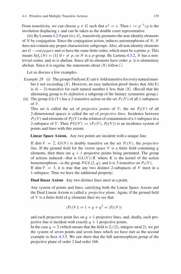
4.4 Primitive and Multiply Transitive Actions 129
From transitivity, we can choose g ∈ G such that ag = x . Then t := g−1zg is theinvolution displacing x and can be taken as the double coset representative.
(iii) By Lemma 4.2.9 part (iv), Gx transitively permutes the non-identity elementsof N by conjugation. Since the conjugation action, induces automorphisms of N , Ndoes not contain any proper characteristic subgroups. Also, all non-identity elementsare G − conjugate and so have the same finite order, which must be a prime p. Thismeans Sylr (N ) = {1} if r �= p, so N is a p-group. By Lemma 4.3.2, N has a non-trivial center, and so is abelian. Since all its elements have order p, it is elementaryabelian. Since it is regular, the statements about |X | follow.�
Let us discuss a few examples.
Example 28 (i) The groups FinSym(X) are k-fold transitive for every natural num-ber k not exceeding |X |. However, an easy induction proof shows that Alt(X)
is (k − 2)-transitive for each natural number k less than |X |. (Recall that thealternating group is by definition a subgroup of the finitary symmetric group.)
(ii) The group GL(V ) has a 2-transitive action on the set P1(V ) of all 1-subspacesof V .This set is called the set of projective points of V ; the set P2(V ) of all2-dimensional spaces is called the set of projective lines. Incidence betweenP1(V ) and elements of P2(V ) is the relation of containment of a 1-subspace in a2-subspace of V . Then PG(V ) := (P1(V ), P2(V )) is an incidence system ofpoints and lines with this axiom:
Linear Space Axiom. Any two points are incident with a unique line.
If dim V = 2, Gl(V ) is doubly transitive on the set P1(V ), the projectiveline. If the ground field for the vector space V is a finite field containing qelements, then there are q + 1 projective points being permuted. The groupof actions induced—that is GL(V )/K where K is the kernel of the actionhomomorphism—is the group PGL(2, q), and it is 3-transitive on P1(V ).If dim V = 3, it is true that any two distinct 2-subspaces of V meet in a1-subspace. Thus we have the additional property:
Dual linear Axiom Any two distinct lines meet at a point.
Any system of points and lines, satisfying both the Linear Space Axiom andthe Dual Linear Axiom is called a projective plane. Again, if the ground fieldof V is a finite field of q elements then we see that
|P1(V )| = 1 + q + q2 = |P2(V )|
and each projective point lies on q + 1 projective lines, and, dually, each pro-jective line is incident with exactly q + 1 projective points.In the case q = 2 (which means that the field is Z/(2), integers mod 2), we getthe system of seven points and seven lines which we have met as the secondexample in Sect. 4.3.5. We saw there that the full automorphism group of theprojective plane of order 2 had order 168.

130 4 Permutation Groups and Group Actions
4.4.4 Permutation Characters
The results in this section only make sense for actions on a finite set X .Suppose f : G → Sym(X) is a group action on a finite set X . Then f (G) is a
finite group of permutations of X . Without loss of generality we assume G itself isfinite. (We do this, so that some sums taken over the elements of G are finite. Butthis is no drawback, for the assertions we wish to obtain can in general be applied tof (G) as a faithfully acting finite permutation group.)
Associated with the finite action of G is the function
π : G → Z
which maps each element g of G to the number π(g) of fixed points of g—that is,the number of letters that g leaves fixed. This function is called the permutationcharacter of the (finite) action f , and, of course, is completely determined by f . Theusefulness of this function is displayed in the following:
Theorem 4.4.7 (Burnside’s Lemma)
(i) The number of orbits with which G acts on X is the average number of lettersfixed by the group elements:
(1/|G|)∑
g∈Gπ(g).
In particular, G is transitive, if and only if the average value of π over the groupis 1.
(ii) The number of orbits of G on X (k)∗ is
(1/|G|)∑
g∈Gπ(g)(π(g) − 1) · · · (π(g) − k + 1).
(iii) In particular, if G acts 2-transitively, then
(1/|G|)∑
π(g)2 = 2.
Also, if G is 3-transitive,
(1/|G|)∑
g∈G(π(g))3 = 5.
Proof (i) Count pairs (x, g) ∈ X × G with xg = x . One way is to first choose x ∈ Xand then find g ∈ Gx . This count yields
∑x∈X
|Gx | =∑
orbits|Gx ||Ox | =
∑orbits
|G| = |G| · no. of orbits.
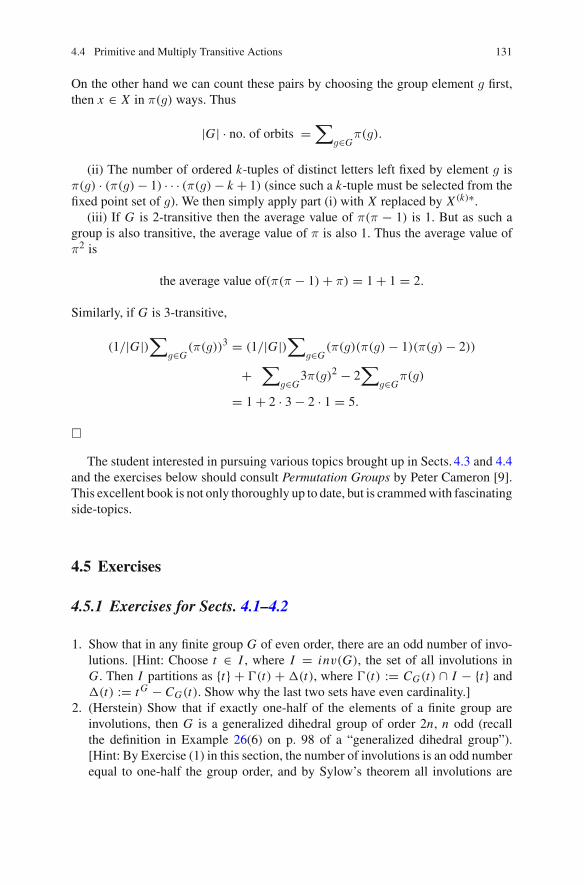
4.4 Primitive and Multiply Transitive Actions 131
On the other hand we can count these pairs by choosing the group element g first,then x ∈ X in π(g) ways. Thus
|G| · no. of orbits =∑
g∈Gπ(g).
(ii) The number of ordered k-tuples of distinct letters left fixed by element g isπ(g) · (π(g) − 1) · · · (π(g) − k + 1) (since such a k-tuple must be selected from thefixed point set of g). We then simply apply part (i) with X replaced by X (k)∗.
(iii) If G is 2-transitive then the average value of π(π − 1) is 1. But as such agroup is also transitive, the average value of π is also 1. Thus the average value ofπ2 is
the average value of(π(π − 1) + π) = 1 + 1 = 2.
Similarly, if G is 3-transitive,
(1/|G|)∑
g∈G(π(g))3 = (1/|G|)
∑g∈G
(π(g)(π(g) − 1)(π(g) − 2))
+∑
g∈G3π(g)2 − 2
∑g∈G
π(g)
= 1 + 2 · 3 − 2 · 1 = 5.
�
The student interested in pursuing various topics brought up in Sects. 4.3 and 4.4and the exercises below should consult Permutation Groups by Peter Cameron [9].This excellent book is not only thoroughly up to date, but is crammed with fascinatingside-topics.
4.5 Exercises
4.5.1 Exercises for Sects. 4.1–4.2
1. Show that in any finite group G of even order, there are an odd number of invo-lutions. [Hint: Choose t ∈ I , where I = inv(G), the set of all involutions inG. Then I partitions as {t} + �(t) + �(t), where �(t) := CG(t) ∩ I − {t} and�(t) := tG − CG(t). Show why the last two sets have even cardinality.]
2. (Herstein) Show that if exactly one-half of the elements of a finite group areinvolutions, then G is a generalized dihedral group of order 2n, n odd (recallthe definition in Example 26(6) on p. 98 of a “generalized dihedral group”).[Hint: By Exercise (1) in this section, the number of involutions is an odd numberequal to one-half the group order, and by Sylow’s theorem all involutions are

132 4 Permutation Groups and Group Actions
conjugate, forcing CG(t) = 〈t〉. The result follows from any Transfer Theoremsuch as Thompson’s.4]
3. This has several parts:
(a) Show that if p is a prime, then any group of order p2 is abelian. [Hint: Itmust have a non-trivial center, and the group mod its center cannot be anon-trivial cyclic group.]
(b) Let G be a finite group of order divisible by the prime p. Show that thenumber of subgroups of G or order p is congruent to one modulo p. [Hint:Make the same sort of decomposition of the class of groups of order p aswas done for groups of order 2 in Exercise (1) in this section. You need toknow something about the number of subgroups of order p in a group oforder p2.]
(c) If prime number p divides |G| < ∞, show that the number of elements oforder p in G is congruent to −1 modulo p.
(d) (McKay’s proof of parts (b) and (c) of this exercise.) Let G be a finite groupof order divisible by the prime p. LetS be the set of p-tuples (g1, g2, . . . , gp)
of elements of G such that∏
gi = 1.i. Show that S is invariant under the action of σ, a cyclic shift which takes
(g1, g2, . . . , gp) to (gp, g1, . . . , gp−1).ii. As H = 〈σ〉 Z p acts on S, suppose there are a H -orbits of length 1
and b H -orbits of length p. Show that |G|p−1 = |S| = a + bp. As pdivides the order of G conclude that p divides a.
iii. Show that a �= 0. Conclude that a is the number of elements of orderone or order p in G, and is a non-zero multiple of p.
iv. Let P1, . . . , Pk be a full listing of the subgroups of order p in G. Showthat | ∪ Pj | = a ≡ 0modp, and deduce that k ≡ 1mod p.
(e) Suppose pk divides the order of G and P is a subgroup of order pk−1. Showthat p divides the index [NG(P) : P]. [Hint: Set N := NG(P) and suppose,by way of contradiction, that p does not divide [N : P]. Then P is theunique subgroup of N of order pk−1 and so is characteristic in N . As pk
divides |G|, we see that p divides the index [G : N ]. Now P acts on theleft cosets of N in G by left multiplication, with N comprising a P-orbitof length one. Show that there are at least p such orbits of length one sothat there is a left coset bN �= N , with PbN = bN . Then b−1 Pb ≤ Nforcing b−1 Pb = P from the uniqueness of its order. But then b ∈ N , acontradiction.]
(f) Suppose the prime power pk divides the order of the finite group G. Definea p-chain of length k to be a chain of subgroups of G,
P1 < P2 < · · · < Pk,
4Almost certainly this is the elementary proof that Herstein had in mind rather than the proofs inseveral longer papers on this subject which have appeared in the AMA monthly.

4.5 Exercises 133
where Pj is a subgroup of G of order p j , j = 1, . . . , k. Show that thenumber of p-chains of G of length k is congruent to one modulo p. [Hint:Proceed by induction on k. The case k = 1 is part 4 (d) of this Exercise. Onecan assume the number m of p-chains of length k − 1 is congruent to 1 modp. and these chains of length k − 1 partition the chains of length k. If c is achain of length k − 1 with terminal member Pk−1, then any extension of cto a chain of length k is obtained by adjoining a group Pk of order pk in thenormalizer NG(Pk−1). The number of such candidates is thus the numberof subgroups of order p in NG(Pk−1)/Pk−1. Part 5 of this Exercise showsthat p divides this group order, and so by part 4 (d), the number of Z p’s inthe factor N/P is congruent to one mod p. Show that the conclusion is nowforced.]
(g) From the previous result show that if pk divides |G|, for k > 0, then thenumber of subgroups of order pk is congruent to 1 mod p.
[Remark: Note that parts 3–7 of this Exercise did not require either the Sylowtheorems of even the weaker Cauchy’s Theorem that asserts that G contains anelement of prime order p if p divides |G|. Indeed, these exercises essentiallyreprove them. Exercise (1) in this section and part 2 of this Exercise, on the otherhand, required Cauchy’s theorem in order to have Z p’s to discuss.]
4. Let G be a group of order pnq , where p and q are primes and n > 1. Showthat G is not a simple group. [Hint: We may assume that there are at least twop-sylow subgroups. Select a pair (P1, P2) of distinct p-Sylow subgroups so thattheir intersection N = P1 ∩ P2 is as large as possible. Invoke Lemma 4.3.2, part(iii), to conclude that NG(N ) contains distinct p-Sylow subgroups, and hence hasorder divisible by q . Choose Q1 ∈ Sylp(NG(N )). Then G = P1 Q, and so
〈MG〉 = 〈M P1〉.
The left side of this equation is a normal subgroup of G. But the right side ofthe presented equation is properly contained in P1. Thus G is not simple unlessM = 1. In the latter case, the q elements of Sylp(G) pairwise intersect at theidentity. Now count the number of elements of order dividing q.]
4.5.2 Exercises Involving Sects. 4.3 and 4.4
1. Show that any group of order fifteen is cyclic. [Hint: Use Sylow’s Theorem toshow that the group is the direct product of two cyclic p-sylow subgroups.]
2. Show that any group of order 30 has a characteristic cyclic subgroup of order15.
3. Show that any group N which admits a group of automorphisms which is2-transitive on its non-identity elements is an elementary abelian 2-group or a

134 4 Permutation Groups and Group Actions
cyclic group of order 3.Extend this result by showing that if there is a group of automorphisms of Nwhich is 3-transitive on the non-identity elements of N , then |N | ≤ 4.
4. Show that if G faithfully acts as a k-fold transitive group on a set X , and Gx
is a simple group, then (as k is at least 1) any proper normal subgroup of G isregular on X .Using a basic lemma of this chapter, show that if 1 �= N is a normal subgroupof G, then G is the semidirect product N Gx (here Gx ∩ N = 1 so Gx is acomplement to N in G). Moreover, Gx acts (k − 1)-fold transitively on the non-identity elements of N .Conclude that under these circumstances, G can be at most 4-fold transitive onX , and then only in the case that |X | = 4 and G = Sym(4).
5. Show that the group Alt(5) acts doubly transitively on its six 5-sylow subgroups.6. Show that if N is a non-trivial normal subgroup of G = Alt(5), then either (i) N
has order divisible by 30 or (ii) N normalizes and hence centralizes each 5-sylowsubgroup. [Hint: Use the fact that G acts primitively on both 5 and 6 letters.]
7. Conclude that possibility (ii) of the previous exercise is impossible, by showingthat a 5-sylow subgroup of Alt(5) is its own centralizer.
8. Using Exercises (5–7) in this section (the three preceding exercises), show injust a few steps, that Alt(5) is a simple group.
9. If G is a k-transitive group, and Gx1,...xk−1 is simple, then, provided k ≥ 3, and|X | > 4 , G must be a simple group. So in this case, the property of simplicity isconferred from the simplicity of a subgroup. (This often happens for primitivegroups of higher permutation rank, but the situation is not easy to generalize.)[Hint: Use Exercises (4–8) above.]
10. Provide a proof of the following result:
Lemma 4.5.1 Suppose G is a group acting faithfully and primitively on a set X.Assume further that:
(i) A is a normal subgroup of Gx , and(ii) G is generated by the set of conjugates AG = {Ag|g ∈ G}.Then for any non-trivial normal subgroup N of G, we have G = AN.
[Hint: Use Corollary 4.4.2 and get G = Gx N and then use (i) and (ii)].
11. Organize the last few exercises into a proof that all alternating groups Alt(n) aresimple for n ≥ 5.
12. (Witt’s Trick) Suppose K is a k-transitive group acting faithfully on the set X ,where k ≥ 2.
(a) Show that if H := Kα, for some letter α in X , then K = H + Ht H forsome involution t in K .
(b) Suppose ∞ is not a letter in X , set X ′ := X ∪ {∞}, and set S := Sym(X ′).Suppose now that S contains an involution s such that
i. s transposes ∞ and α,

4.5 Exercises 135
ii. s normalizes H—i.e. s Hs = H , andiii. o(st) = 3, that is, (st)3 = 1, while st �= 1.
Then show that the subset Y = K ∪ K sK is a subgroup of S. [Hint: One need onlyshow that Y is closed under multiplication, and this is equivalent to the assertionthat sK s ⊂ Y . Decompose K ; use the fact that s H = Hs and that sts = tst .]
13. Show that in the previous Exercise Y is triply transitive on X ′.14. Suppose G is a simple group with an involution t such that the centralizer CG(t)
is a dihedral group of order 8. Show the following:
(a) The involution t is a central involution—that is, t is in the center of at leastone 2-Sylow subgroup of G, or, equivalently, |tG | is an odd number. Thusany 2-Sylow subgroup of G is just D8.
(b) There are exactly two conjugacy classes of fours groups—say V G1 and V G
2 ,where V1 and V2 are the unique two fours subgroups of a 2-Sylow subgroupD of G.
(c) There is just one conjugacy class of involutions in G.(d) Each fours group Vi is a TI-group—that is, a subgroup that intersects its
distinct conjugates only at the identity group.
[Hints: This is basically an exercise in the use of Sylow’s Theorem (Theorem4.3.3), the Burnside Fusion Theorem (Theorem 4.3.7) and the Thompson TransferTheorem (Theorem 4.3.8).
Part (a): Take D = CG(t) D8. Then its center is just 〈t〉, so NG(D) ≤CG(t) = D.
Part (b): Let Vi , i = 1, 2, be the two unique fours subgroups of D ∈ Syl(G). Sinceeach Vi is normal in D, the Burnside Fusion theorem tells us that they could beconjugate in G only if they were already conjugate in NG(D) = D, where it ispatently untrue.
Part (c): Let D = V1V2 = Cg(t) where V1 ∩ V2 = 〈t〉. Since D D8, it alsocontains a normal cyclic group C of order 4. If no non-central involution of D isconjugate to the central involution t , then a contradiction to the simplicity of G isobtained from the Thompson Transfer Theorem, using C as the subgroup of index2 in D. If tG ∩ D ⊆ V1, the same argument, using V1 in place of C , again yieldsa contradiction. Thus all involutions in D are conjugate to t .
Part (d): Clearly two conjugates of Vi could at best meet at a central involution,of which, by Part (c) there is only one class, tG . In that case they would com-prise two fours subgroups of the same 2-Sylow subgroup (the centralizer of theirintersection), and hence could not be conjugate by Part (b).]
Remark A nice little geometry lurks in the above exercise. The pointsP are one classof fours groups—say V G
1 , and the lines L are the other class V G2 . A line is declared
to be incident with a point, if and only if the corresponding fours groups normalizeeach other—i.e. they lie in a common 2-Sylow subgroup. With the information above,

136 4 Permutation Groups and Group Actions
the reader can easily prove that NG(Vi ) Sym(4), which tells us that each line isincident with just three points and each point lies on exactly three lines. Here are twoexamples:
(a) |G| = 168, (P,L) is the projective plane of order 2; 7 points, 7 lines.(b) |G| = 360, (P,L) is the generalized quadrangle of order (2, 2); 15 points, 15
lines.Are these the only possibilities?
15. This exercise is really an optional student project. First show that if G if a 4-foldtransitive group of permutations of the finite set X , then
(1/|G|)∑
g∈Gπ(g)4 = 15.
The object of the project would be to show that in general, if G is k-fold transitiveon X then
(1/|G|)∑
g∈Gπ(g)k = Bk,
where Bk is the total number of partitions of a k-set (also known as the k-th Bellnumber). An analysis of the formulae involves one in expressing the numberof sequences (with possible repetitions) of k elements from a set X in termsof ordered sequences with pair-wise distinct entries. The latter are expressed interms of the so-called “falling factorials” x(x − 1)(x − 2) · · · (x − � + 1) in thevariable x = |X |. The coefficients involve Stirling numbers and the Bell numbercan be reached by known identities. But a more direct argument can be made bysorting the general k-tuples over X into those having various sorts of repetitions;this is where the partitions of k come in.

Chapter 5Normal Structure of Groups
Abstract The Jordan-Hölder Theorem for Artinian Groups is a simple applicationof the poset-theoretic Jordan-Hölder Theorem expounded in Chap.2. A discussionof commutator identities is exploited in defining the derived series and solvabilityas well as in defining the upper and lower central series and nilpotence. The Schur-Zassenhaus Theorem for finite groups ends the chapter. In the exercises, one willencounter the concept of normally-closed families of subgroups of a group G, whichgives rise to several well-known characteristic subgroups, such asOp(G), the torsionsubgroup, and (whenG is finite) theFitting subgroup. Some further challenges appearin the exercises.
5.1 The Jordan-Hölder Theorem for Artinian Groups
5.1.1 Subnormality
As defined in Chap.4, p. 99, a group is simple if and only if its only proper normalsubgroup is the identity subgroup. (In particular, the identity group is not consideredto be a simple group.)
A subgroup H is said to be subnormal in G if and only if there exists a finite chainof subgroups
H = N0 � N1 � · · · � Nk = G.
(Recall that this means each group Ni is normal in its successor Ni+1, but is notnecessarily normal in the groups further up the chain.) We express the assertion thatH is subnormal in G by writing
H � �G.
LetSN (G) be the collection of all subnormal subgroups of G. This can be viewedas a poset in two different ways: (1) First we can say that A is “less than or equalto B” if and only if A is a subgroup of B, that is, SN has the inherited structure
© Springer International Publishing Switzerland 2015E. Shult and D. Surowski, Algebra, DOI 10.1007/978-3-319-19734-0_5
137

138 5 Normal Structure of Groups
of an induced poset of S(G), the poset of all subgroups of G with respect to thecontainment relation. (2) We also have the option of saying that A “is less than B”if and only if A is subnormal in B. The second way of defining a poset on SNwould seem to be more conservative than the former. But actually the two notionsare exactly the same, as can be concluded from the following Lemma.
Lemma 5.1.1 (Basic Lemma on Subnormality) The following hold:
(i) If A � �B and B � �G, then A � �G.(ii) If A � �G and H is any subgroup of G, then A ∩ H � �H.
(iii) If A is a subnormal subgroup of G, then A is subnormal in any subgroup thatcontains it.
(iv) If A and B are subnormal subgroups of G, then so is A ∩ B.
Proof (i) This is immediate from the definition of subnormality: By assumptionthere are two finite ascending chains of subgroups, one running from A to B, andone running from B to G, each member of the chain is normal in its successor in thechain. Clearly concatenating the two chains produces a chain of subgroups from Ato G, each member of the chain normal in the member immediately above it. So bydefinition, A is subnormal in G.
(ii) If A � �G one has a finite subnormal chain A = A0 � A1 � · · · � A j := G.Suppose H is any subgroup of G. It is then no trouble to see that A ∩ H � A1 ∩ H �A2 ∩ H � · · · A j ∩ H = G ∩ H = H , is a subnormal series from A ∩ H to H .
(iii) This assertion follows from Part (ii) where H contains A.(iv)ByPart (ii), A∩B is subnormal in B. Since B is subnormal inG, the conclusion
follows by an application of Part (i). �
At this point the student should be able to provide a proof that the two methods(1) and (2) of imposing a partial order on the subnormal subgroups lead to the sameposet. We simply denote it (SN (G),≤) (or simply SN if G is understood) since itis an induced poset of the poset of all subgroups of G. From Lemma 5.1.1, Part (iv),we see that
SN (G) is a lower semilattice.
Finally it follows from the second or third isomorphism theorem, that if
If A and B are distinct maximal normal subgroups of G = 〈A, B〉 = AB = B A,then G/A � B/(A ∩ B). Thus SN (G) is a semimodular lower semilattice andthe mapping
μ : Cov(SN ) → simple groups
(which records for every cover X � Y where X a maximal normal subgroup of Y ,the isomorphism type of the simple group Y/X ) is “semimodular” in the sense ofTheorem2.5.2,Sect. 2.5.3.

5.1 The Jordan-Hölder Theorem for Artinian Groups 139
According to the general Jordan-Holder theory (advanced in Sect. 2.5.3, Theorem2.5.2), μ can be extended to an interval measure
ASN → M.
from all algebraic intervals of SN into the additive monoid M of all multisetsof isomorphism classes of simple groups—that is, the free additive semigroup ofall formal non-negative integer linear combinations of isomorphism classes [G] ofsimple groups: ∑
simpa[G][G], of finite support.
If there is a finite unrefinable ascending chain in SN from 1 to G, then such achain of subnormal subgroups is called a composition series of G. The multiset ofthe isomorphism classes of the simple groups Ai+1/Ai appearing in such a compo-sition series 1 � A1 � · · · � An = G is called the multiset of composition factors.The Theorem2.5.2 states that these are the same multisets for any two compositionseries—the “measure” μ([1, G]).
If you have been alert, you will notice that no assumption that the involved groupsare finite has been made. The composition factors may be infinite simple groups.
But of course, in applying the Jordan-Hölder theorem, one is interested in pinningdown a class of algebraic intervals. This is easy in the case of a finite group, forthere, all intervals of SN (G) are algebraic. How does one approach this for infinitegroups? The problem is that one can have an infinitely descending chain of subnormalsubgroups, and also one can have an infinitely ascending chain of proper normalsubgroups (just think of an abelian group with such an ascending chain).
However one can select certain subposets of SN which will provide us with manyof these algebraic intervals: Suppose from any SN (G) we extract the set SN ∗ of allsubnormal subgroups for which any downward chain of subgroups each normallycontaining its successor, must terminate in a finite number of steps. There are threeother descriptions of this subcollection SN ∗, of subnormal subgroups: (i) they arethe subnormal subgroups of G which belong to a finite unrefinable subnormal chainextended downward to the identity. (ii) They are the elements M of SN for which[1, M] is an algebraic interval of SN—see Chap.2, Sect. 2.3.2. (iii) This is thespecial class of subgroups amenable to the Jordan-Holder Theorem—the subnormalsubgroups of G which themselves possess a finite composition series. We call theelements of SN ∗ the Artinian subgroups. They are closed under the operation oftaking pairwise meets in SN and so SN ∗ is clearly a lower semilattice, all of whoseintervals are algebraic.
As a special case, we have:
Theorem 5.1.2 (The Jordan-Holder Theorem for general groups) Let SN ∗ be theclass of all Artinian subnormal subgroups of a group G. Then for any H in SN ∗, thelist (with multiplicities) of all isomorphism classes of simple groups which appear

140 5 Normal Structure of Groups
as a cheif factor in any finite unrefinable subnormal chain of H is independent ofthe particular choice of that chain.
Corollary 5.1.3 Any two composition series (unrefinable subnormal series) of afinite group recreates through its chief factors the same list of isomorphism classesof finite simple groups, with mutiplicities respected.
5.2 Commutators
Let G be a group. A commutator in G is an element of the form x−1y−1xy (calleda commutator) and is denoted [x, y]. A triple commutator [x, y, z] is an element ofshape [[x, y], z], which the student may happily work out to be
[x, y]−1z−1[x, y]z = y−1x−1yxz−1x−1y−1xyz.
If we write ux := x−1ux , the result of conjugation of u by x , then it is an exerciseto verify the following identities, for elements x, y, and z in any group G:
[x, y] = [y, x]−1. (5.1)
[xy, z] = [x, z]y[y, z] = [x, z][x, z, y][y, z]. (5.2)
[x, yz] = [x, z][x, y]z = [x, z][x, y][x, y, z]. (5.3)
1 = [x, y−1, z]y[y, z−1, x]z[z, x−1, y]x . (5.4)
[x, y, z][y, z, x][z, x, y] = [y, x][z, x][z, y]x ×[x, y][x, z]y[y, z]x [x, z][z, x]y . (5.5)
A commutator need not be a very typical element in a group. For example, in anabelian group, all commutators are equal to the identity.
If A, B and C are subgroups of a group G, then [A, B] is the subgroup of Ggenerated by all commutators of the form a−1b−1ab = [a, b] as (a, b) ranges overA × B. Similarly we write [A, B, C] := [[A, B], C].Theorem 5.2.1 (Basic Identities on Commutators of Subgroups) Suppose A, B andC are subgroups of a group G.
(i) A centralizes B if and only if [A, B] = 1.(ii) [A, B] = [B, A].
(iii) B always normalizes [A, B].(iv) A normalizes B if and only if [A, B] ≤ B. In that case, [A, B] is a normal
subgroup of B.

5.2 Commutators 141
(v) If f : G → H is a group homomorphism, then [ f (A), f (B)] = f ([A, B]).(vi) (The Three Subgroups Lemma of Phillip Hall) If at least two of the three sub-
groups [A, B, C], [B, C, A] and [C, A, B] are trivial, then so is the third.
Proof Part (i) A centralizes B if andonly if every commutator of shape [a, b], (a, b) ∈A × B, is the identity. The result follows from this.
Part (ii) A subgroup generated by set X is also the subgroup generated by X−1.Apply (5.1).
Part (iii) If (a, b, b1) ∈ A × B × B, then it follows from (5.3) that
[a, b]b1 = [a, b1]−1[a, bb1] ∈ [A, B].
Part (iv) The following statements are clearly equivalent:
1. A normalizes B2. [a, b] ∈ B for all (a, b) ∈ A × B3. [A, B] ≤ B.
The normality assertion follows from part (iii).Part (v) This is obvious.Part (vi) Without loss of generality assume that [A, B, C] and [B, C, A] are the
identity subgroup. Then all commutators [a, b, c] and [b, c, a] are the identity, nomatter how the triplet (a, b, c) is chosen in A × B × C . Now by Eq. (5.4), anycommutator [c, a, b] is the identity, for any (a, b, c) ∈ A × B × C . This proves that[C, A, B] has only the identity element for a generator. �
Corollary 5.2.2 Suppose again that A and B are subgroups of a group G.
(i) If A normalizes B and centralizes [A, B], then A/CA(B) is abelian.In particular, if A ≤ Aut(B) and A centralizes [A, B] := 〈a−1ab|(a, b) ∈A × B〉, then A is an abelian group.
(ii) If A is a group of linear transformations of the vector space V , centralizing asubspace W as well as its factor space V/W , then A is an abelian group.1
Proof All these results are versions of the following: By the Three SubgroupsLemma, [A, B, A] = 1 implies [A, A, B] = 1. That is the proof. �
Of course anytime someone has some machinery, some mathematician wants toiterate it. We have defined the commutator of two subgroups in such manner that theresult is also a subgroup. Thus inductively we may define a multiple commutatorof subgroups in this way: Suppose (A1, A2, . . .) is a (possibly infinite) sequence ofsubgroups of a group G. Then for any natural number k, we define
[A1, . . . Ak+1] := [[A1, . . . Ak], Ak+1].
1This seems to be a frequently rediscovered result.

142 5 Normal Structure of Groups
5.3 The Derived Series and Solvability
From the previous section, we see that the subgroup [G, G] is a subgroup which
(i) is mapped into itself by any endomorphism f : G → G (a consequence of The-orem5.2.1(V)). (This condition is called fully invariant. Since inner automor-phisms are automorphisms which are in turn endomorphisms, “fully invariant”implies “characteristic” implies “normal”.)
(ii) yields an abelian factor, G/[G, G] (let f : G → G/[G, G] and apply parts (i)and (iii) of Theorem 5.2.1). Moreover, if G/N is abelian, then [G, G] ≤ N , so[G, G] is the smallest normal subgroup of G, which possesses an abelian factor(see Chap.3).
The group [G, G] is called the commutator subgroup or derived subgroup of Gand is often denoted G ′.
Since we have formed the group G ′ := [G, G], we may iterate this definition toobtain the second derived group,
G′′ := [[G, G], [G, G]].
Once on to a good thing, why not set G ′ = G(1) and G ′′ = G(2) and define
G(k+1) := [G(k), G(k)]
for all natural numbers k? The resulting sequence
G ≥ G(1) ≥ G(2) ≥, · · · .
is called the derived series of G. Since each G(k) is characteristic in its successorwhich in turn is characteristic in its successor, etc., we see the following:
Every G(k) is characteristic in G.
Note also that
G(k+l) = (G(k))(l). (5.6)
A group G is said to be solvable if and only if the derived series
G ≥ G(1) ≥ G(2), . . . ,
eventually becomes the identity subgroup after a finite number of steps.2 The smallestpositive integer k such that G(k) = 1 is called the derived length of G. Thus a groupis abelian if and only if it has derived length 1.
2In this case, for once, the name “solvable” is not accidental. The reason will be explained in theChap.11 on Galois Theory.

5.3 The Derived Series and Solvability 143
Theorem 5.3.1 (i) If H ≤ G and A ≤ G, then [A, H ] ≤ [A, G]. In particular
[H, H ] ≤ [G, H ] ≤ [G, G].
(ii) If H ≤ G, then H (k) ≤ G(k). Thus, if G is solvable, so is H.(iii) If f : G → H is a group homomorphism, then
f (G(k)) = ( f (G))(k) ≤ H (k).
(iv) If N � G, then G is solvable if and only if both N and G/N are solvable.(v) For a direct product,
(A × B)(k) = A(k) × B(k).
(vi) The class of all solvable groups is closed under taking finite direct products andtaking subgroups and hence is closed under taking finite subdirect products. Inparticular, if G is a finite group, there is a normal subgroup N of G minimalamong normal subgroups with respect to the property that G/N is solvable.(Clearly this normal subgroup is characteristic; it is called the solvable resid-ual.)
Proof Part (i) follows from the containment,
{[a, h]|(a, h) ∈ A × H} ⊆ {[a, g]|(a, g) ∈ A × G}.
Part (ii) By Part (i), H ′ ≤ G ′. If we have H (k−1) ≤ G(k−1), then
H (k) = [H (k−1), H (k−1)] ≤ [G(k−1)), G(k−1)] = G(k),
utilizing H (k−1) and G(k−1) in the roles of H and G in the last sentence of Part (i).The result now follows by induction.
Part (iii) The equal sign is from Theorem 5.2.1, Part (v); the subgroup relation isfrom Part (i) above of this Theorem.
Part (iv) Suppose G is solvable. Then so are N and G/N by Parts (i) and (iii).Now assume, G/N and N are solvable. Then there exists natural numbers k and l,such that (G/N )(k) = 1 and N (l) = 1. Then by Part (iii), the former equation yields
G(k)N/N = 1 or G(k) ≤ N .
Then
G(k+l) = (G(k))(l) ≤ N (l) ≤ 1,
by Part (ii), so G is solvable.Part (v) If the subgroups A and B of G centralize each other, it follows from
Eqs. (5.2) or (5.3) that [ab, a′b′] = [a, a′][b, b′] for all (a, b), (a′, b′) ∈ A× B. This

144 5 Normal Structure of Groups
shows (A × B)′ ≤ A
′ × B′. The reverse containment follows from Part (i). Thus the
conclusion holds for k = 1. One need only iterate this result sufficiently many timesto get the stated result for all k.
Part (vi) This is a simple application of the other parts. A subgroup of a solvablegroup is solvable because of the inequality of Part (ii). A finite direct product ofsolvable groups is solvable by Part (v). Thus, from the definition of subdirect product,a finite subdirect product of solvable groups is solvable. The last part follows fromthe remarks in Sect. 3.6.2. �
Remark Suppose G1, G2, . . . is a countably infinite sequence of finite groups forwhich Gk has derived length k (It is a fact that a group of derived length k existsfor every positive integer k: perhaps one of those very rare applications of wreathedproducts.) Then the direct sum
∑k∈NGk = G1 ⊕ · · · does not have a finite derived
length and so is not solvable. Thus solvable groups are not closed under infinite directproducts.
Recall that a finite subnormal series for G is a chain
G = N0 � N1 � N − 1 · · · � Nk = 1,
where each N j+1 is a normal subgroup of its predecessor, N j , j = 0, . . . k − 1,k is a natural number. (Of course what we have written is actually a descendingsubnormal series. We could just as well have written it backwards as an ascendingseries.) Recall also that a unrefinable subnormal series of finite length is called acomposition series, and when such a thing exists, the factors N j/N j+1 are simplegroups called the composition factors of G. That the list of composition factors thatappears is the same for all composition series, was the substance of the Jordan-HölderTheorem for groups.
These notions make their reappearance in the following:
Corollary 5.3.2 (i) A group G is solvable of derived length at most k if and onlyif it possesses a subnormal series
G = N0 � N1 � N1 � · · · � Nk = 1.
such that each factor N j/N j+1, j = 0, . . . k − 1, is abelian.(ii) A finite group is solvable if and only if it possesses a composition series with all
composition factors cyclic of prime order (of course, the prime may depend onthe particular factor taken).
Proof Part (i) If G is solvable, the derived series is a subnormal series for which allfactor groups formed by successive members of the series are abelian. Conversely,if the subnormal series is as given, then N0/N1 abelian implies [G, G] = G
′ ≤ N1.Inductively, if G( j) ≤ N j , then N j/N j+1 abelian implies G( j+1) ≤ [N j .N j ] ≤N j+1. So by induction, G( j+1) ≤ N j+1 for all j = 0, 1, . . . k − 1. Thus G(k) ≤Nk = 1, and G is solvable.

5.3 The Derived Series and Solvability 145
Part (ii) If G possesses a composition series with all composition factors cyclic ofprime order, G is solvable by Part (i). On the other hand, if G is finite and solvableit possesses a subnormal series
G = N0 � N1 � · · · � Nk = 1,
with each factor N j/N j+1 a finite abelian group. But in any finite abelian group(where all subgroups are normal) we can form a composition series by choosinga maximal subgroup M1 of A, a maximal subgroup M2 of M1, and so forth. Eachfactor will then be cyclic of prime order. Thus each interval N j � N j+1 can be refinedto a chain with successive factors of prime order. The result is a refinement of theoriginal subnormal series to a composition series with all composition factors cyclicof prime order. �
There aremany very interesting facts about solvable groups, especially finite ones,which unfortunately we do not have space to reveal. Two very interesting topics arethese:
• Phillip Hall’s theory of Sylow Systems. In a finite solvable group there is a repre-sentative Si of Sylpi (G), the pi -Sylow subgroups of G such that G = S1S2 · · · Sm ,and the Si are permutable in pairs—that is Si S j = S j Si where p1, . . . pm is the listof all primes dividing the order of G. Thus in any solvable group of order 120, forexample, there must exist a subgroup of order 15. (This is not true, for example, ofthe non-solvable subgroup Sym(5) of that order.) A full account of Hall systemscan be found in [22].
• The theory of formations. Basically, a formation is an isomorphism-closed classof finite solvable groups closed under finite subdirect products. Then each finitegroup G contains a characteristic subgroup GF which is unique in being minimalamong all normal subgroups N of G which yield a factor G/N belonging to F .(GF is called theF-residual of G.) Whenever G is a finite group, let D(G) be theintersection of all the maximal subgroups of G. This is a characteristic subgroupwhich we shall meet shortly, called the Frattini subgroup of G. A formation is saidto be saturated, if for every solvable finite group G, G/D(G) ∈ F implies G ∈ F .If F is saturated, then there exists a special class of subgroups, the F-subgroups,subgroups in F described only by their embedding in G, which form a conjugacyclass. Finite abelian groups comprise a formation but are not a saturated formation.A class of groups considered in the next section are the nilpotent groups and theydo form a saturated formation. As a result one gets a theorem like this: “SupposeX and Y are two nilpotent subgroups of a finite solvable group G, each of whichis its own normalizer in G. Then X and Y are conjugate subgroups. Moreover,G must contain such groups.”3 A bit surprising. (The term ‘nilpotent group’ isdefined in the following section.)
3This conjugacy class of subgroups was first announced in a paper by Roger Carter; they are calledthe class of “Carter subgroups” of G.

146 5 Normal Structure of Groups
5.4 Central Series and Nilpotent Groups
5.4.1 The Upper and Lower Central Series
Let G be a fixed group. Set γ0(G) = G, γ1(G) = [G, G], and inductively define
γk+1(G) := [γk(G), G],
for all positive integers k. Then the descending sequence of subgroups
G = γ0(G) ≥ γ1(G) ≥ γ2(G) ≥ · · · ,
is called the lower central series of the group G. Note that
γk(G) = [G, G, . . . G] (with k arguments).
Since any endomorphism f : G → G, maps the arguments of the above multiplecommutator into themselves, the endomorphism f maps each member of the lowercentral series into itself. A similar argument for homomorphisms allows us to statethe following elementary result:
Lemma 5.4.1 (i) Each member γk(G) of the lower central series is a fully invariantsubgroup of G.
(ii) If f : G → H is a homomorphism of groups then
f (γk(G)) = γk( f (G)).
(iii) If H is a subgroup of G, then γk(H) ≤ γk(G).
Proof The proof is an easy exercise. �
A group G is said to be nilpotent if and only if its lower central series terminatesat the identity subgroup in a finite number of steps. In this case G is said to belong tonilpotence class k if and only if k is the smallest positive integer such that γk(G) = 1.Thus abelian groups are the groups of nilpotence class 1.
The following is immediate from Lemma 5.4.1, and the definition of nilpotence.
Corollary 5.4.2 (i) Every homomorphic image of a group of nilpotence class atmost k is a group of nilpotence class at most k.
(ii) Every subgroup of a group of nilpotence class at most k is also nilpotent ofnilpotence class at most k.
(iii) Every finite direct product of nilpotent groups of nilpotence class at most k isitself nilpotent of nilpotence class at most k.

5.4 Central Series and Nilpotent Groups 147
The beginning student should be able to supply immaculate proofs of these asser-tions by this time. [Follow the lead of the similar result for solvable groups in theprevious section; do not hesitate to utilize the commutator identities in proving part(iii) of this theorem.]
Clearly, the definitions show that
[γk(G), γk(G)] ≤ [γk(G), G] = γk+1(G),
so the factor groups (γk(G))/(γk+1(G)) are abelian. As a consequence,
Corollary 5.4.3 Any nilpotent group is solvable.
The converse fails drastically: Sym(3) is a solvable group of derived length 2.But is not nilpotent since its lower central series drops from Sym(3) to its subgroupN � Z3, and stabilizes at N for the rest of the series.
Now again fix G. Set Z0(G) := 1, the identity subgroup; set Z1(G) = Z(G), thecenter of G (the characteristic subgroup of those elements of G which commute withevery element of G); and inductively define Zk(G) to be that subgroup satisfying
Zk(G)/Zk−1(G) = Z(G/Zk−1(G)).
That is, Zk(G) is the inverse image of the center of G/Zk−1(G) under the naturalhomomorphism G → G/Zk−1(G). For example:
Z2(G) = {z ∈ G|[z, g] ∈ Z(G), for all g ∈ G}.
By definition Zk(G) ≤ Zk+1(G), so we obtain an ascending series of character-istic subgroups
1 = Z0(G) ≤ Z1(G) ≤ Z2(G) ≤ · · · ,
called the upper central series of G. Of course if G has a trivial center, this seriesdoes not even get off the ground. But, as we shall see below, it proceeds all the wayto the top precisely when G is nilpotent.
Suppose now that G has nilpotence class k. This means γk(G) = 1while γk−1(G)
is non-trivial. Then as
[γk−1(G), G] = γk(G) = 1,
G centralizes γk−1(G), that is
γk−1(G) ≤ Z1(G).
Now assume for the purposes of induction, that
γk− j (G) ≤ Z j (G).
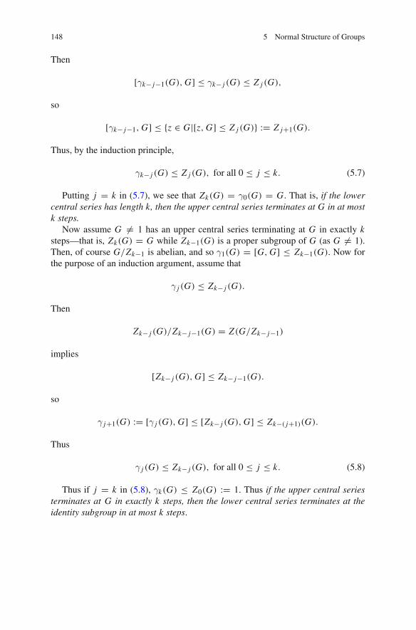
148 5 Normal Structure of Groups
Then
[γk− j−1(G), G] ≤ γk− j (G) ≤ Z j (G),
so
[γk− j−1, G] ≤ {z ∈ G|[z, G] ≤ Z j (G)} := Z j+1(G).
Thus, by the induction principle,
γk− j (G) ≤ Z j (G), for all 0 ≤ j ≤ k. (5.7)
Putting j = k in (5.7), we see that Zk(G) = γ0(G) = G. That is, if the lowercentral series has length k, then the upper central series terminates at G in at mostk steps.
Now assume G �= 1 has an upper central series terminating at G in exactly ksteps—that is, Zk(G) = G while Zk−1(G) is a proper subgroup of G (as G �= 1).Then, of course G/Zk−1 is abelian, and so γ1(G) = [G, G] ≤ Zk−1(G). Now forthe purpose of an induction argument, assume that
γ j (G) ≤ Zk− j (G).
Then
Zk− j (G)/Zk− j−1(G) = Z(G/Zk− j−1)
implies
[Zk− j (G), G] ≤ Zk− j−1(G).
so
γ j+1(G) := [γ j (G), G] ≤ [Zk− j (G), G] ≤ Zk−( j+1)(G).
Thus
γ j (G) ≤ Zk− j (G), for all 0 ≤ j ≤ k. (5.8)
Thus if j = k in (5.8), γk(G) ≤ Z0(G) := 1. Thus if the upper central seriesterminates at G in exactly k steps, then the lower central series terminates at theidentity subgroup in at most k steps.

5.4 Central Series and Nilpotent Groups 149
We can assemble these observations as follows:
Theorem 5.4.4 The following assertions are equivalent:
1. G belongs to nilpotence class k. (By definition, its lower central series terminatesat the identity in exactly k steps.)
2. The upper central series of G terminates at G in exactly k steps.
There is an interesting local property of nilpotent groups:
Theorem 5.4.5 If G is a nilpotent group, then any proper subgroup H of G isproperly contained in its normalizer NG(H).
Proof If G = 1, there is nothing to prove. Suppose H is a proper subgroup of G.Then there is a minimal positive integer j such that Z j (G) is not contained in H .Then there is an element z in Z j (G) − H . Then [z, H ] ≤ [z, G] ≤ Z j−1(G) ≤ H .Thus z normalizes H , but does not lie in it. �
Corollary 5.4.6 Every maximal subgroup of a nilpotent group is normal.
Remark There are many groups with nomaximal subgroups at all. Some of these arenot even nilpotent. Thus one should not expect a converse to the aboveCorollary. Thisraises the question, though, whether the property of the conclusion of Theorem 5.4.5characterizes nilpotent groups. Again one might expect that this is false for infinitegroups. However, in the next subsection we shall learn that among finite groups it isindeed a characterizing property.
Here is a classical example of a nilpotent group: Suppose V is an n-dimensionalvector space over a field F . A chamber is an ascending sequence of subspaces S =(V1, V2, . . . Vn−1)whereVj has vector spacedimension j . (This chain is unrefinable.)Now consider the group B(S) of all linear transformations T ∈ GL(V ) such that Tfixes each Vj and induces the identity transformation on each 1-dimensional factor-space Vj/Vj−1. Rendered as a group of matrices these are upper triangular matriceswith “1’s” on the diagonal. The reader may verify that the k-th member of the lowercentral series of this group consists of upper triangular matrices still having 1’s onthe diagonal, but having more and more upper subdiagonals all zero as k increases.Eventually one sees that B(S)(n−1) contains only the identity matrix.
5.4.2 Finite Nilpotent Groups
Let p be a prime number. As originally defined, a p-group is a group in whicheach element has p-power order. Suppose P is a finite p-group. Then by the SylowTheorem, the order of G cannot be divisible by a prime distinct from p. Thus weobserve
A finite group is a p-group if and only if the group has p-power order.

150 5 Normal Structure of Groups
Now we have seen before (Lemma 4.3.2, part (ii)), that a non-trivial finitep-group must possess a non-trivial center. Thus if P �= 1 is a finite p-group, wesee that Z(P) �= 1. Now if Z(P) = P , then P is abelian. Otherwise, P/Z(P) has anontrivial center. Similarly, in general, if P is a finite p-group:
Either Zk(P) = P or Zk(P) properly lies in Zk+1(P).
As a result, a finite p-group possesses an upper central series of finite length,and hence is a nilpotent group. Obviously, a finite direct product of finite p-groups(where the prime p is allowed to depend upon the direct factor) is a finite nilpotentgroup.
Now consider this
Lemma 5.4.7 If G is a finite group and S is a p-Sylow subgroup of G, thenany subgroup H which contains the normalizer of S is itself self-normalizing—i.e.NG(H) = H In particular NG(S) is self-normalizing.
Proof Suppose x is an element of NG(H). Since P is a p-Sylow subgroup of G, itis also a p-Sylow subgroup of NG(H) and H . Since Px ∈ Sylp(H), by Sylow’stheorem there exists an element h ∈ H such that Px = Ph . Then xh−1 ∈ NG(P) ≤H whence x ∈ H . (Actually this could be done in one line, by exploiting the “FrattiniArgument” (Chap.4; Corollary4.3.4)). �
Now we have
Theorem 5.4.8 Let G be a finite group. Then the following statements are equiva-lent.
(i) G is nilpotent.(ii) G is isomorphic to the direct product of its various Sylow subgroups.
(iii) Every Sylow subgroup of G is a normal subgroup.
Proof ((ii) implies (i)) Finite p-groups are nilpotent, as we have seen, and so too aretheir finite direct products. Thus any finite group which is the direct product of itsSylow subgroups is certainly nilpotent.
((ii) if and only (iii))Now it is easy to see that a group is isomorphic to a direct prod-uct of its various p-Sylow subgroups, (p ranging over the prime divisors of the orderof G) if and only if each Sylow subgroup of G is normal. Being direct factors Sylowsubgroups of such a direct product are certainly normal. Conversely, if all p-Sylowsubgroups are normal, the direct product criterion of Chap.3 (Lemma3.5.1, Part (iii),p. 96) is satisfied, upon considering the orders of the intersections S1S2 · · · Sk ∩Sk+1,where {Si } is the full (one-element) collection of Sylow subgroups of G (one for eachprime).
((i) implies (iii)) So it suffices to show that in a finite nilpotent group, each p-sylowsubgroup P is a normal subgroup of G. If NG(P) = G, there is nothing to prove. Butif NG(P) is a proper subgroup of G, then it is a proper self-normalizing subgroup byLemma 5.4.7. This completely contradicts Theorem 5.4.5 which asserts that everyproper subgroup of a nilpotent group is properly contained in its normalizer. �

5.4 Central Series and Nilpotent Groups 151
Fix a group G. A non-generator of G is an element x of G such that whenever x isa member of a generating set X—that is, when x ∈ X , and 〈X〉 = G, then X −{x} isalso a generating set: 〈X −{x}〉 = G. Thus x is just one of those superfluous elementsthat you never need. Now it is not easy to see from “first principles”—that is, fromthe defining property alone—that in a finite group, the product of a non-generatorand a non-generator is again a non-generator. But we have this characterization of anon-generator:
Lemma 5.4.9 Suppose G is a finite group. Let D(G) be the intersection of allmaximal subgroups of G. Then D(G) is the set of all nongenerators of G.
Proof Two statements are to be proven: (i) every non-generator lies in D(G), and(ii) every element of D(G) is a non-generator.
(i) Suppose x is a non-generator, and let M be any maximal subgroup of G. Thenif x is not in M wemust have 〈{x}∪ M〉 = G, while 〈M〉 = M , against the definitionof “non-generator”. Thus x lies in every maximal subgroup M and so x ∈ D(G).
(ii) On the other hand assume that x is an arbitrary element of D(G), and that Xis a set of generators of G which counts x among its active participants. If X − {x}does not generate G, then, as G is finite, there is a maximal subgroup M containingH := 〈X − {x}〉. But by assumption x ∈ D(G) ≤ M , whence 〈X〉 ≤ M , acontradiction. Thus always it is the case that if x ∈ X , where X generates G, thenalso X − {x} generates G. Thus x is a non-generator. �
Remark This theorem really belongs to posets. Clearly finiteness can be replaced bythe only distinctive property used in the proof: that for every subset X of this poset,there is an upper bound—that is, an element of the filter P X , which is either the1-element of the poset or lies in a maximal member of the poset with the 1-elementremoved. Its natural habitat is therefore lattices with the ascending chain condition.(We need upper semi-lattices so that we can take suprema; we need something likea lower-semilattice in order to define the Frattini element of the poset as the meetof all maximal elements. Finally the ascending chain condition makes sure that themaximal elements fully cover all subsets whose supremum is not “1”. So at leastlattices with the ascending chain condition (ACC) are more than sufficient for thisresult.)
Theorem 5.4.10 (Global non-generators) If X ∪ D(G) generates a finite group G,then X generates G.
Proof The argument is the same and has a similar poset-generalization. Suppose 〈X〉is not G. Then it lies below a maximal subgroup M . By definition D(G) must liein M , and so X ∪ D(G) lies in M , which contradicts the hypothesis that X ∪ D(G)
generates G. Thus we must abandon the foregoing supposition and conclude that〈X〉 = G. �

152 5 Normal Structure of Groups
The subgroup D(G) is called the Frattini subgroup of G.4 It is clearly a charac-teristic subgroup of G. In the case of finite groups, something special occurs whichcould be imitated only artificially in the context of posets:
Theorem 5.4.11 In a finite group, the Frattini subgroup D(G) is a characteristicnilpotent subgroup of G.
Proof The “characteristic” part is clear, and has been remarked on earlier. SupposeP ∈ Sylp(D(G)). By the Frattini Argument, G = NG(P)D(G). It now followsfrom Theorem 5.4.10 that NG(P) = G and so in particular P is normal in D(G).Thus every p-sylow subgroup of D(G) is normal in it. Since it is finite, it is a directproduct of its Sylow subgroups and so is nilpotent. �Corollary 5.4.12 (Wielandt) For a finite group G the following are equivalent:
(i) G is nilpotent.(ii) Every maximal subgroup of G is normal.
(iii) G ′ ≤ D(G).
Proof If M is a maximal subgroup of the finite group G which also happens to benormal, then G/M is a simple group with no proper subgroups, and so must be acyclic group of order p, for some prime p. Thus if all maximal subgroups are normal,the commutator subgroup lies in each maximal subgroup and so lies in the Frattinisubgroup D(G). On the other hand, if G/D(G) is abelian, every subgroup aboveD(G) is normal; so in particular, all maximal subgroups are normal. Thus Parts (ii)and (iii) are equivalent.
But if M is a maximal subgroup of a nilpotent group, M properly lies in itsnormalizer in G, and so NG(M) = G. Thus the assertion of Part (i) implies Parts (ii)and (iii).
So it remains only to show that if every maximal subgroup is normal, then G isnilpotent. Since G is finite, we need only show that every Sylow subgroup is normal,under these hypotheses. Suppose P is a p-Sylow subgroup of G. Suppose NG(P) �=G. Then NG(P) lies in some maximal subgroup M of G. By Lemma 5.4.7, M isself-normalizing. But that contradicts our assumption that every maximal subgroupis normal. Thus NG(P) = G for every Sylow subgroup P . Now G is nilpotent byTheorem 5.4.8. �
5.5 Coprime Action
Suppose G is a finite group possessing a normal abelian subgroup A, and let F =G/A be the associated factor group. Any transversal of A—that is, a system of cosetrepresentatives of A in G can be indexed by the elements of the factor group F . Anytransversal T := {t f | f ∈ F} determines a function
4 In some of the earlier literature one finds D(G) written as “�(G)”. We do not understand fullythe reason for the change.

5.5 Coprime Action 153
αT : F × F → A
(called a factor system) by the rule that for all ( f, g) ∈ F ,
t f · tg = t f gαT ( f, g).
In some sense, the factor system measures how far off the transversal is from beinga group. Because of the associative law, one has
αT ( f g, h)αT ( f, g)h = αT ( f, gh)αT (g, h), (5.9)
for all f, g, h ∈ F . (Notice that since A is abelian, conjugation by any element h ofthe coset Ax gives the same result ax = x−1ax = h−1ah which we have denotedby ah .)
Now, given a transversal T = {t f | f ∈ F}, any other transversal S = {s f | f ∈ F}is uniquely determined by a function β : F → A, by the rule that
s f = t f β( f ), f ∈ F.
Then the new factor system αS for transversal S can be determined from the old oneαT by the equations
αS( f, g) = αT ( f, g)[(β( f g))−1β( f )gβ(g)] for all f, g ∈ F. (5.10)
The group G is said to split over A if and only if there is a subgroup H of Gsuch that G = H A, H ∩ A = 1—that is, if and only if some transversal H formsa subgroup. Such a subgroup H is called a complement of A in G. In that case, thefactor system αH for H is just the constant function at the identity element of A.Then, given G, A and transversal T = {t f | f ∈ F}, we can conclude from Eq. (5.10)that G splits over A if and only if there exists a function β : F → A such that
αT ( f, g) = β( f g)β( f )−gβ(g)−1, for all f, g ∈ F. (5.11)
Now suppose A is a normal abelian p-subgroup of the finite group G and supposeP is a Sylow p-subgroup of G with the property that “P splits over A”. That meansthat P (which necessarily contains A) contains a subgroup B such that P = AB andB ∩ A = 1. Let X be a transversal of P in G. Then T := B X := {bx |b ∈ B, x ∈ X}is a transversal of A in G whose factor system αT satisfies
αT (b, t) = 1 for all (b, t) ∈ B × T .
Now let m be the p-Sylow index [G : P] = |X | in G. Since m is prime to |A|,there exists an integer k such that mk ≡ 1 mod |A|. Since A is abelian, the factors of

154 5 Normal Structure of Groups
any finite product of elements of A can be written in any order. So there is a functionγ : F → A defined by
γ( f ) :=∏
x∈XαT (x, f ).
Now, multiplying each side of Eq. (5.9) as f ranges over F , one obtains
γ(h)γ(g)h = γ(gh)αT (gh)m .
Then, setting β(g) := γ(g)−k for all g ∈ F , we obtain Eq. (5.11). Thus G splits overA.
Noting that conversely, if G splits over A, so does P , we have in fact proved,
Theorem 5.5.1 (Gaschütz) Suppose G is a finite group with a normal abelianp-subgroup A. Then G splits over A if and only if some p-Sylow subgroup of Gsplits over A.
Next suppose A is a normal abelian subgroup of the finite group G and thatH is a complement of A in G, so G = H A and H ∩ A = 1. Now suppose somesecond subgroup K was also a complement to A. Then there is a natural isomorphismμ : H → K factoring through G/A, and a function β : H → A so that
μ(h) = hβ(h) for all h ∈ H.
Expressed slightly differently, K is a transversal {kh |h ∈ H} whose elements can beindexed by H , and kh = hβ(h) for all h ∈ H . Since K is a group, it is easy to seethat for h, g ∈ H ,
kg · kh = hgh = (gh)β(gh)
= gβ(g) · hβ(h)
= ghβ(g)hβ(h).
So
β(gh) = β(g)hβ(h), for all g, h ∈ H. (5.12)
Now assume m = [G : A] is relatively prime to |A|, and select an integer n suchthat mn ≡ 1 mod |A|. Then as A is abelian, the product
∏H β(g), taken as g ranges
over H , is a well-defined constant b, an element of A. Forming a similar product ofthe terms on both sides of Eq. (5.12) as g ranges over H , one now has
b = bh · β(h)m,

5.5 Coprime Action 155
so
β(h) = a · a−h, where a = bn, h ∈ H.
Then for every h ∈ H ,
kh = hβ(h) = h · a−h · a = a−1ha.
Thus K = a−1Ha is a conjugate of H . So we have shown the following:
Lemma 5.5.2 If A is a normal abelian subgroup of a group G of finite order, andthe order of A is relatively prime to its index [G : A], then any two complements ofA in G are conjugate.
The reader should be able to use Gaschütz’ Theorem and the preceeding Lemmato devise an induction proof of the following
Theorem 5.5.3 (The lower Schur-Zassenhaus Theorem) Suppose N is a solvablenormal subgroup of the finite group G whose order is relatively prime to its index[G : N ]. Then the following statements are true:
1. There exists a complement H of N in G.2. Any two complements of N in G are conjugate by an element of N .
On the other hand, using little more than Sylow’s theorem, a Frattini argument,and induction on group orders one can easily prove the following:
Theorem 5.5.4 (The upper Schur-Zassenhaus Theorem) Suppose N is a normalsubgroup of the finite group G, such that |N | and its index [G : N ] are coprime. IfG/N is solvable, then the following holds:
1. There exists a complement H of N in G.2. Any two complements of N in G are conjugate by an element of N .
Remark Both the lower and upper Schur-Zassenhaus theorems contain an assump-tion of solvability, either on N or G/N . However this condition can be droppedaltogether, because of the famous Feit-Thompson theorem [18] which says that anyfinite group of odd order must be solvable. The hypothesis that |N | and [G : N ] arecoprime forces one of N or G/N to have odd order and so at least one is solvable. Ofcourse the Feit-Thompson theorem is far beyond the sophistication of this relativelyelementary course.
A somewhat over-looked application of the Schur-Zassenhaus theorem is thefollowing:
Theorem 5.5.5 (Glauberman) Let A be a group of automorphisms acting on a groupG leaving invariant some coset H x of a subgroup H. Then the following hold:

156 5 Normal Structure of Groups
1. H is itself A-invariant.2. If A and H have coprime orders (so that at least one is solvable), then A fixes an
element of the coset H x.
Proof This is Exercise (10) in Sect. 5.6.1.
5.6 Exercises
5.6.1 Elementary Exercises
1. We say that a subgroup A of G is subnormal in G if and only if there is a finiteascending chain of subgroups:
A = N0 < N1 · · · < Nm = G
from A to G, with each member of the chain normal in its successor—i. e.Ni � Ni+1, i = 0, . . . , m − 1.
(a) Using the Corollary to the Fundamental Theorem of Homomorphisms(Corollary 3.4.6), show that SN (G) is a semi-modular lower semi-lattice.
(b) Use Theorem 2.4.2, part (ii), to conclude that in a group for which SN (G)
has the descending condition—for example a finite group—the join of anycollection of subnormal subgroups of a group is subnormal.
2. Suppose N is a family of normal subgroups of G. Let �N be defined to be theset of elements of G which are expressible as a finite product of elements eachof which belongs to a subgroup in N .
(a) Show that �N is the subgroup of G generated by the subgroups inN—i.e.�N = 〈N 〉 := 〈{N |N ∈ N }〉.
(b) We say thatN is a normally closed family, if and only if for any non-emptysubset M ⊆ N , 〈M〉 ∈ N . A group is said to be a torsion group if andonly if every element of G has finite order. (This does not mean that thegroup is finite: far from it: there are many infinite torsion groups.) Showthat the family T (G) of all normal torsion subgroups of G, is a normallyclosed family. [hint: When any element x is expressed as a finite productx = a1 · · · ak with ai ∈ Ni ∈ N , only a finite number of groups Ni areinvolved. So the proof comes down to the case k = 2.] Then the group
Tor(G) := 〈T (G)〉 ∈ T (G)
is a characteristic subgroup of G.

5.6 Exercises 157
3. Fix a prime number p. A group H is said to be a p-group if and only if eveyelement of H has order a power of the prime p. Show that the collection of allnormal p-subgroups of a (not necessarily finite) group G is normally closed. (Inthis case the unique maximal member of the collection of all normally closedp-subgroups of G is denoted Op(G).)
4. Let G be any group, finite or infinite.
(a) Show that any subnormal torsion subgroup of G lies in T (G).(b) Show that any subnormal p-subgroup of G lies in Op(G).
5. Let Q denote the additive group of the rational numbers. The group Zp∞ isdefined to be the subgroup of Q/Z generated by the infinite set {1/p, 1/p2, . . .}.Show that this is an infinite p-group. Also show that it is indecomposable—thatis, it is not the direct product of two of its proper subgroups.
6. Let F be a family of abstract groups which is closed under taking unrestrictedsubdirect products—that is, if H is a subgroup of the direct product
∏σ∈I Xσ ,
with each Xσ ∈ F , and the restriction of each canonical projection
πτ :∏
σ∈IXσ → Xτ
to H is an epimorphism, then H ∈ F .
(a) Show that there exists a uniquenormal subgroup NF such that NF isminimalwith respect to being a normal subgroup which yields a factor G/NF ∈ F5
(b) Show that there is always a subgroup G ′ of G minimal with respect to theseproperties:(i) G ′ � G,(ii) G/G ′ is abelian.
(c) Explain why there is not always a subgroup N of G minimal with respect tobeing normal and having G/N a torsion group (or even a p-group). [Hint:Although torsion groups are closed under taking direct sums, they are notclosed under taking direct products. This contrasts with Exercise (6) in thissection where the family of groups was closed under unrestricted subdirectproducts.]
(d) If G is finite, and F is closed under finite subdirect products—that is, theset of possibilities for F is enlarged because of the weaker requirement thatit is enough that any subgroup H of a finite direct product of members of Fwhich remains surjectve under the restrictions of the canonical projections,is still in F—then there does exist a subgroup NF which is minimal withrespect to the two requirements: (i) NF � G, and (ii) G/NF ∈ F . (If π isany set of (non-negative) prime numbers, a group G is said to be a π-group
5Note that as a class of abstract groups F can either be viewed as either (i) a collection of groupsclosed under isomorphisms, or (ii) a disjoint union of isomorphism classes of groups. Under theformer interpretation, the “membership sign”, ∈, as in “G/NF ∈ F” is appropriate. But in thesecond case, “∈” need only be replaced by “an isomorphism with a member of F”. One must getused to this.

158 5 Normal Structure of Groups
if and only every element of G has finite order divisible only by the primesin π. In particular, a π-group is a species of torsion group, and a p-group isa species of π-group.Show that all π-groups are closed under finite subdirect products. [In thiscase we write
NF = Oπ(G), Op(G), or Op′(G)
where π = {p} or all primes except p, in the last two cases.]
7. Suppose F is a family of groups closed under normal products. Suppose Gpossesses a subgroup N that is maximal with respect to being both normal andbeing a member ofF (this occurs when G is finite). Is it true that any subnormalsubgroup of G which belongs to the family F lies in N? Prove it, or give acounterexample.
8. Suppose A and B are normal subgroups of a group G. Prove the following:
(a) If A and B normalize subgroup C , then
[AB, C] = [A, C][B, C].
[Hint: Use the commutator identity (5.2) and the fact that B normalizes[A, C] to show the containment of the left side in the right side.]
(b) Show that the k-fold commutator [AB, . . . , AB] is a normal product
∏[X1, X2, . . . , Xk],
where the Xi = A or B, and the product extends over all 2k possibilities forthe k-tuples (X1, . . . , Xk). (Of course each factor in the normal product isa normal subgroup of G. But some of them occur more than once since thecases with X1 = A and X2 = B, are duplicated in the cases with X1 = Band X2 = A.)
(c) Show that if A and B are nilpotent of class k and �, respectively, then ABis nilpotent of class at most k + �. [Hint: Consider γk+�+1(AB) and use theprevious step.]
(d) Prove that in a finite group, there exists a normal nilpotent subgroup whichcontains all other normal nilpotent subgroups of G. (This characteristicsubgroup is called the Fitting subgroup of G and is denoted F(G).)
9. Let G be a finite group. Show that if A and B are solvable normal subgroupsof a group G, then their normal product AB is also solvable. [Hint: Use thecommutator identities.] Conclude from this that if G is finite, then there exists aunique subgroup that is maximal with respect to being both normal and solvable.Clearly, it contains all other solvable normal subgroups of G.6
6This group is sometimes called the “solvable radical”, but this usage, which intrudes on similarterminology from non-associative algebras, is far from uniform.

5.6 Exercises 159
10. Prove Theorem 5.5.5. The finite group G contains a subgroup H , and A is agroup of automorphisms of G which leaves the coset H x invariant.
(a) (i) Show that A leaves H invariant.(b) (ii) If A and H have coprime orders show that some element of H x is fixed
by the automorphism group A.
[Hint: For the first part, note that for every a ∈ A xa = ha x for some elementha ∈ H . Compute (hx)a for arbitrary h ∈ H .For the second part, note that in the semidirect product G A, A normalizes H bypart (i) so H A = AH is a subgroup of G A. Show that one can define a transitiveaction of H A on the elements of the coset H x in which the elements of A actas they do as automorphisms, but the elements of H act by left multiplication.(One must show that the left-multiplication action of ha is the composition of theactions of a−1, of h and of a, in that order.) Let X be the subgroup of H A fixinga “letter”—say x—in H x . Since H is transitive, H A = H X . Now X and A aretwo complements of H in the group. Apply the Schur Zassenhaus theorem.]
11. Here is an interesting simplicity criterion. Let G be a group acting faithfullyand primitively on the set X , and let H be the stabilizer of some element of X .Assume
(a) G = G ′,(b) H contains a non-identity normal solvable subgroup A whose conjugates
generate G.
Prove that G is simple.[Hint: First note that G = 1 is not possible since A �= 1 . The imprimitivefaithful action of G on X makes G and any non-trivial normal subgroup N ofG transitive on X so G = H N . Then show AN is normal, and so contains allconjugates of A. The final contradiction that is around the corner must exploitthe solvability of A.]
5.6.2 The Baer-Suzuki Theorem
The next few exercises spell out a subtle but well-known theorem known as theBaer-Suzuki theorem.7 The proof considered here is actually due to Alperin andLyons [2].
In the following, G is a finite group. There is some new but totally natural notationdue to Aschbacher. Suppose� is a collection of subgroups of G and H is a subgroupof G. Then the symbol � ∩ H denotes the collection of all subgroups in � whichhappened to be contained in the subgroup H . (Of course this collection could verywell be empty.) If γ is any collection of subgroups of G, the symbol NG(γ) denotes
7Not to be confused with “Brauer-Suzuki Theorem”.

160 5 Normal Structure of Groups
the subgroup of G of all elements which under conjugation of subgroups leaves thecollection γ invariant.
1. Suppose � is a G-invariant collection of p-subgroups of G. Let Q be anyp-subgroup of G and let γ be any subset of � ∩ Q for which γ ⊆ NG(γ).Show that either
(a) γ = � ∩ Q or(b) Then there is an element X ∈ � ∩ Q which also lies in NG(γ).
[Hint: Without loss of generality, one may assume that γ = �∩ Q ∩ NG(γ). Thenevery element of NQ(NQ(γ)) leaves γ = � ∩ NQ(γ) invariant, so NQ(NQ(γ) =NQ(γ). Since Q is a nilpotent group, γ is a Q-invariant collection of subgroupsof Q and the conclusion follows easily.]
2. Prove the following:
Theorem 5.6.1 (The Baer-Suzuki Theorem) Suppose X is some p-subgroup of thefinite group G. Either X ≤ Op(G) or 〈X, Xg〉 is not a p-subgroup for some conjugateXg ∈ X G.
[Hint: Set � = X G , choose P a p-sylow subgroup of G which contains X , andset � := � ∩ P . Since � = � implies 〈�〉 is a normal p-group, forcing theconclusion X ∈ Op(G), we may assume � − � �= ∅.Now show that for any subgroup Y ∈ � − �, 〈Y,�〉 cannot be a p-group. [ If Ris a p-Sylow subgroup containing 〈R,�〉, compare |� ∩ R| and |� ∩ P|.]Next consider the set S of all pairs (Y, γ) where Y ∈ X G − �, γ ⊆ � and 〈Y, γ〉is a p-group. (We have just seen that this collection is non-empty.) Among thesepairs, choose one, say (Y, γ) ∈ S, so that |γ| is maximal. Now if γ = ∅, 〈X〉 isnot a p-group and we are done. Thus we may assume γ is non-empty.Now set Q := 〈Y, γ〉, a p-group. Then, noting that 〈Y,� ∩ Q〉 is a p-group, themaximality of γ forces γ = �∩ Q. Now γ := ∪X∈γ X ⊆ P ⊆ NG(�) and γ ⊆ Qtogether imply
γ ⊆ NC (Q) ∩ NG(�) ⊆ NG(Q ∩ �) = NG(γ).
By the previous exercise, either γ = �∩ Q or there is a subgroup Y ′ ∈ �∩ Q −γwith Y ′ ⊆ NG(γ). The former alternative is dead from the outset because of theexistence of Y . Now Y ′ belongs to X G − �, and 〈Y ′, γ〉 is a p-subgroup, as it isa subgroup of Q. Thus (Y ′, γ) is also one of the extreme pairs in S.Similarly, since 〈Y ′,�〉 is not a p-group, γ �= � and so, applying the previousexercise once more with P in place of Q, there must exist a subgroup Z ∈ � − γ,with Z ∈ NP (γ). Thus
{Y ′, Z} ∪ γ ⊆ � ∩ NG(γ).

5.6 Exercises 161
Now NG(γ) is a proper subgroup of G (otherwise some element of X G lies in thenormal p-subgroup 〈γ〉). Now for the first time, we exploit induction on the grouporder to conclude that
〈Y ′, γ ∪ {Z}〉
is a p-group. Clearly this contradicts the maximality of |γ|, completing the proof.]
3. The proof just sketched is very suggestive of other generalizations, but there arelimits. We say that a finite group is p-nilpotent if and only if G/Op′(G) is ap-group.Show that the collection of finite p-nilpotent subgroups is closed under finitenormal products. (In a finite group, there is then a unique maximal normalp-nilpotent subgroup, usually denoted Op′ p(G).)
4. Is the following statement true? Suppose X is a p-subgroup of the finite groupG. Then either X ∈ Op′ p(G) or else there exists a conjugate Xg ∈ X G suchthat 〈X, Xg〉 is not p -nilpotent. [Hint: Think about the fact that in any group, thegroup generated by two involutions is a dihedral group, and so is 2-nilpotent.]

Chapter 6Generation in Groups
Abstract Here, the free group on set X is defined to be the automorphism group ofa certain tree with labeled edge-directions. This approach evades some awkwardnessin dealing with reduced words. The universal property that any group generated bya set of elements X is a homomorphic image of the free group on X , as well asthe fact that a subgroup of a free group is free (possibly on many more generators)are easy consequences of this definition. The chapter concludes with a discussion of(k, l, m)-groups and the Brauer-Ree theorem.
6.1 Introduction
One may recall that for any subset X of a given group G, the subgroup generated byX , denoted 〈X〉, always has two descriptions:
1. It is the intersection of all subgroups of G which contain X ;2. It is the subset of all elements of G with are expressible as a finite product of
elements which are either in X or are the inverse (in G) of an element of X .
The two notions are certainly equivalent, for the set of elements described in item2, is closed under group multiplication and taking inverses and so, by the SubgroupCriterion (Lemma 3.2.3) is a subgroup of G containing X . On the other hand it mustbe a subset of every subgroup containing X . So this set is the same subgroup whichwas denoted 〈X〉.
But there is certainly a difference in the way the two notions feel. Our point ofview in this chapter will certainly be in the spirit of the second of these two notions.
© Springer International Publishing Switzerland 2015E. Shult and D. Surowski, Algebra, DOI 10.1007/978-3-319-19734-0_6
163

164 6 Generation in Groups
6.2 The Cayley Graph
6.2.1 Definition
Suppose we are given a group G and a subset X of G. X is said to be a set ofgenerators of G if and only if 〈X〉 = G. For any such set of generators X , we canobtain a directed graph C(G, X) without multiple edges as follows:
1. The vertex set of C := C(G, X) is the set of elements of G.2. The directed edges are the ordered pairs of vertices: (g, gx), where g ∈ G and
x ∈ X . (It is our option to label such an edge by the symbol “x”. Note that if xand y are distinct elements of X , then gx �= gy so each directed edge receives aunique label by this rule.)
The directed edge-labelled graph C(G, X) is called the Cayley graph of the gen-erating set X of the group G. Note that if the identity element 1 is a member of X ,loops are possible. But of course 1, being a non-generator, can always be removedfrom X without disturbing any of our assumptions about X and G. If we do this, noloops will appear.
One now notices that left multiplication of all the vertices of C (that is, the elementsof G) by a given element h of G induces an automorphism πh of C (in fact onepreserving the labels) since (hg, hgx) is also an edge labelled by “x”.
Let us look at a very simple example. The set X = {a = (12), b = (23)} is a setof generators of the group G = Sym(3), the symmetric group on the set of letters{1, 2, 3}. The Cayley graph then has six vertices, and each vertex has two out-goingedges labeled “a” and “b”, respectively, and two in-going edges labeled “a” and “b”as well. Indeed, we could coalesce an outgoing and ingoing edge with the same label,as one undirected edge of that label. This only happens when the label indicates aninvolution of the group. In this case we get a hexagon with sides labelled “a” and “b”alternately.
6.2.2 Morphisms of Various Sorts of Graphs
Since we are talking about graphs, this may be a good time to discuss homomorphismsof graphs. But there are various sorts of graphs to discuss. The broad categories are
1. Simple graphs � = (V, E) where V is the vertex set, and edges are just cer-tain subsets of V of size two. (These graphs record all non-reflexive symmetricrelations on a set V , for example the acquaintanceship relation among personsattending a large party.)
2. Undirected graphs with multiple edges. (This occurs when the edges themselveslive an important life of their own—for example when they are the bridges con-necting islands, airplane flights connecting cities, or doors connecting rooms.)

6.2 The Cayley Graph 165
3. Simple graphs with directed edges. Here the edge set is a collection of orderedpairs of vertices. (This occurs when one is recording asymmetric relations, forexample, which football team beat which in a football league, assuming eachpair of teams plays each other at most once. Or the the comparison relation ofelements in a poset. We even allow two relations between points, for example(a, b) and (b, a) may both be directed edges. This occurs in some cities wheresites are connected by a network of both one-way and two-way streets.)
4. We could have any of the above, with labels attached to the edges. Cayley graphs,for example, can be viewed as directed labeled graphs.
A graph homomorphism f : (V1, E1) → (V2, E2) is a mapping, f : V1 → V2such that if (a, b) ∈ E1 then either f (a) = f (b) or ( f (a), f (b)) ∈ E2. If the twographs are labeled, there are labelling mappings λi : Ei → Li assigning to each(directed) edge, a label from a set of labels Li , i = 1, 2. Then we require an auxilliarymapping f ′ : L1 → L2, so that if (a, b) ∈ E1 carries label x and if ( f (a), f (b)) isan edge, then it too carries label f ′(x).
6.2.3 Group Morphisms Induce Morphisms of Cayley Graphs
Now suppose f : G → H is a surjective homomorphism of groups. Then it is easyto see that if X is a set of generators of G, then also f (X) is a set of generatorsof f (G) = H . Now f is a fortiori a map from the vertex set of the Cayley graphC(G, X) to the vertex set of the Cayley graph C(H, f (X)). For (g, x) ∈ G × X ,(g, gx) is a directed edge labelled x . Then clearly either f (g) = f (gx) or else,( f (g), f (gx)) = ( f (g), f (g) f (x)) is a directed edge of C(H, f (X)), labelled f (x).Thus
Lemma 6.2.1 If X is a set of generators of a group G and f : G → H is asurjective morphism of groups, then f (X) is a set of generators of H and f inducesa homomorphism of the Cayley graphs, f : C(G, X) → C(H, f (X)) as labeleddirected graphs.1
6.3 Free Groups
6.3.1 Construction of Free Groups
The Cayley graphs of the previous section were defined by the existence of a groupG (among other things). Now we would like to reverse this; we should like to startwith a set X and obtain out of it a certain group which we shall denote F(X).
1Note that the graph morphism has also denoted by the symbol f . This slight abuse of notation ismotivated by the fact that f is indeed the mapping being applied to both vertices and labels of thedomain Cayley graph.

166 6 Generation in Groups
We do this in stages.First we give ourselves a fixed abstract set X . The free monoid on X is the collection
M(X), of “words” xi x2 · · · xk spelled with “letters” xi chosen from the alphabet X .2
The number k is allowed to be zero—that is, there is a unique “word” spelled withno letters at all—which we denote by the symbol φ and call the empty word. Thenumber k is called the length of the word which, as we have just seen, can be zero.
The concatenation of two words u = x1 · · · xk and w = y1 y2 · · · y� , xi , y j ∈ X ,is the word,
u ∗ w := x1 · · · xk y1 · · · y�.
The word “bookkeeper” is the concatenation of “book” and “keeper”; 12345 is theconcatenation 123∗45 or 12∗345, and so forth. Clearly the concatenation operation“∗” is a binary operation on the set W (X) of all words over the alphabet X , and itis associative (though very non-commutative). Moreover, for any word w ∈ W (X),φ ∗ w = w ∗ φ = w. So the empty word φ is a two-sided identity with respectto the operation “∗”. Thus M(X) = (W (X), ∗) is an associative semigroup withidentity—that is, a monoid. Indeed, since it is completely determined by the abstractset X alone, it is called the free monoid on (alphabet) X .3
Now let σ : X → X be an involutory fixed-point-free permutation of X . Thismeans σ is a bijection from X to itself such that
1. σ2 = 1X , the identity mapping on X , and2. σ(x) �= x for all elements x in X .
We are going to construct a directed labelled graph � = F(X,σ), called a framewhich is completely determined by X and the involution σ.
Let W ∗(X) be the subset of W (X) of those words y1 y2 · · · yr , r any non-negativeinteger, for which yi �= σ(yi+1), for any i = 1, . . . , r − 1. These are the wordswhich never have a “factor” of the form yσ(y). (Notice that these words contain nofactors of the form σ(y)y as well since, σ(y)y = uσ(u) where u = σ(y).) We callsuch words reduced words.
We now construct a labelled directed graph � whose vertices are these reducedwords in W ∗(X). The set E of oriented labelled edges are of two types:
1. Ordered pairs (w,wy) ∈ W ∗(X)× W ∗(X) are to be directed edges labelled “y”.(Note that the nature of the domain forces the reduced word w not to end in theletter σ(y)—otherwise wy would not be reduced.)
2. Similarly those ordered pairs of the form (wy, w) (under the same hypothesisthat w not end in σ(y)) are directed edges labeled by “σ(y)”.
The two types of directed edges are distinguished this way: for an edge of the firstkind, the “head” of the directed edge is a word of length one more than it’s “tail”,while the reverse is the case for an edge of the second kind.
2Of course, to be formal about it, one can regard these as finite sequences (x1, . . . , xk), but theanalogy with linguistic devices is helpful because the binary operation we use here is not naturalfor sequences.3Monoids were introduced in Chap. 1.

6.3 Free Groups 167
Then the directed graph � = (W ∗(X), E) which we have defined and have calleda frame, has these properties:
1. Let Vk be the set of words of W ∗(X) of length k. Then V0 = {φ}, and the vertexset partitions as W ∗(X) = V0 + V1 + V2 + . . ..
2. Each vertex has all its outgoing edges labeled by X ; it also has all its ingoingedges labeled by X . Each directed edge (a, b) that is labeled by y ∈ X , has its“transpose” (b, a) labelled by σ(y).
3. For k > 0, each vertex in Vk receives just one ingoing edge from Vk−1 and givesone outgoing edge to the same vertex in Vk−1. All further edges leaving or arrivingat this vertex, are to or from vertices of Vk+1.
4. Given any ordered pair of vertices (w1, w2) (recall the wi are reduced words)there is a unique directed path in � from vertex w1 to vertex w2. It follows thatthere are no circuits other than “backtracks”—that is circular directed walks ofthe form
(v1, v2, . . . vm, . . . v2m+1)
where v j = v2m+1− j , (v j , v j+1) and (v j+1, v j ) are all directed edges, j =1, . . . m.
As usual, the symbol Aut(�) denotes the automorphism group of the directedlabeled graph �. At this point we define a monoid homomorphism
μ : M(X) → Aut(�).
For each y ∈ X , and vertex w in W ∗(X) define
μ(y)(w) :={
yw if w does not begin with letter σ(y)
w′ if w has the form σ(y)w′.
It is then quite clear that μ(y) is a label-preserving automorphism of � (this needsonly be checked at vertices w of very short length where “cancellation” affects theterminal vertices).
Notice that by definition
μ(σ(y)) = (μ(y))−1,
the inverse of the automorphism induced by σ(y).Next, for any word m = y1 y2 · · · yk in the monoid M(X) we set
wμ(m) := μ(m)(w) := μ(yk)(μ(yk−1)(· · · (μ(y1)(w)) · · · ) = wμ(y1)···μ(yk );

168 6 Generation in Groups
that is, μ(m) is the composition
μ(yk) ◦ · · · ◦ μ(y1)
of automorphisms of �. Of course, since the automorphism group Aut(�) is assumedto act as right operators, we can express this composition as μ(y1) · · ·μ(yk) wherejuxtaposition in this expression denotes multiplication in the group Aut(�).
Then, μ(m1m2) = μ(m1)μ(m2) for all (m1, m2) ∈ M(X) × M(X) and μ(φ) =1W ∗(X). So μ is a monoid homomorphism
μ : W (X) → Aut(�).
Note that μ is far from being 1-to-1. For each y ∈ X , μ(yσ(y)) = 1� ,the identity automorphism on �. Thus all compound expressions derived fromthe empty word by successively inserting factors of the form yσ(y)—such asabσ(c)deσ(e)σ(d)c f gσ(g)σ( f )σ(b)σ(a)–also induce the identity automorphismof �.
We now have
Lemma 6.3.1 Let G = Aut (�), the group of all label preserving automorphismsof the directed graph �.
(i) The monoid homomorphism μ : M(X) → G is onto.(ii) G acts regularly on the vertices of �.
(iii) The group G is generated by the set μ(Y ), where Y is any system of represen-tatives of the σ-orbits on X.
(iv) Identities of the form μ(m) = 1� occur if and only if the word m ∈ M(X) isformed by a sequence of insertions of factors yiσ(yi ) starting with the emptyword.
(v) � is the Cayley graph of G with respect to the set of generators X.
Proof Suppose g is an element of G fixing a vertex w in �. Then, as each (in- orout-) edge on w bears a unique label, every vertex next to w is fixed. Since everyvertex u is connected to the vertex φ, the empty word in W ∗(X), by an “undirectedpath” of length equal to the length �(u), the undirected version of � is connected.This forces the elements g in the first sentence of this paragraph to fix all verticesW ∗(X) of �.
But now it is clear that for any word w ∈ W ∗(X), regarded as a monoid element,μ(w) is an element of G taking vertex φ to w. Thus μ(M(X)) = G, and 1. and 2.are proved. So is the statement that μ(X) is a set of generators of G in part (iii).
Suppose now, that w = y1 y2 · · · yk ∈ M(X), satisfies μ(w) = 1� . Then succes-sive premultiplications by yk , then yk−1, and so on, take the vertex φ on a journeyalong a directed path with successive arrows labelled yk, yk−1, . . .; eventually return-ing to φ via a directed edge (y1,φ). At each stage of this journey, the current imageof φ is either taken to a vertex that is one length further or else one length closer toits original “home”, vertex φ. So there is a position
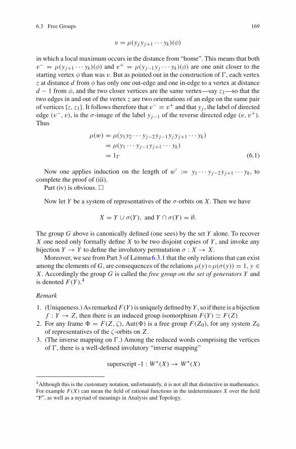
6.3 Free Groups 169
v = μ(y j y j+1 · · · yk)(φ)
in which a local maximum occurs in the distance from “home”. This means that bothv− = μ(y j+1 · · · yk)(φ) and v+ = μ(y j−1 y j · · · yk)(φ) are one unit closer to thestarting vertex φ than was v. But as pointed out in the construction of �, each vertexz at distance d from φ has only one out-edge and one in-edge to a vertex at distanced − 1 from φ, and the two closer vertices are the same vertex—say z1—so that thetwo edges in and out of the vertex z are two orientations of an edge on the same pairof vertices {z, z1}. It follows therefore that v− = v+ and that y j , the label of directededge (v−, v), is the σ-image of the label y j−1 of the reverse directed edge (v, v+).Thus
μ(w) = μ(y1 y2 · · · y j−2 y j−1 y j y j+1 · · · yk)
= μ(y1 · · · y j−1 y j+1 · · · yk)
= 1� (6.1)
Now one applies induction on the length of w′ := y1 · · · y j−2 y j+1 · · · yk , tocomplete the proof of (iii).
Part (iv) is obvious. �
Now let Y be a system of representatives of the σ-orbits on X . Then we have
X = Y ∪ σ(Y ), and Y ∩ σ(Y ) = ∅.
The group G above is canonically defined (one sees) by the set Y alone. To recoverX one need only formally define X to be two disjoint copies of Y , and invoke anybijection Y → Y to define the involutory permutation σ : X → X .
Moreover, we see from Part 3 of Lemma 6.3.1 that the only relations that can existamong the elements of G, are consequences of the relations μ(y)◦μ(σ(y)) = 1, y ∈X . Accordingly the group G is called the free group on the set of generators Y andis denoted F(Y ).4
Remark
1. (Uniqueness.) As remarked F(Y ) is uniquely defined by Y , so if there is a bijectionf : Y → Z , then there is an induced group isomorphism F(Y ) F(Z)
2. For any frame � = F(Z , ζ), Aut(�) is a free group F(Z0), for any system Z0of representatives of the ζ-orbits on Z .
3. (The inverse mapping on �.) Among the reduced words comprising the verticesof �, there is a well-defined involutory “inverse mapping”
superscript -1 : W ∗(X) → W ∗(X)
4Although this is the customary notation, unfortunately, it is not all that distinctive in mathematics.For example F(X) can mean the field of rational functions in the indeterminates X over the field“F”, as well as a myriad of meanings in Analysis and Topology.

170 6 Generation in Groups
which fixes only the empty word φ and takes the reduced word w = y1 y2 · · · yk
to the reduced word w−1 := σ(yk)σ(yk−1) · · · σ(y1).Thus the group-theoretic inverse mapping μw → (μw)−1 is extended to thevertices of � by the rule that (μw)−1 := μw−1 : that is, the inverse mapping ofgroup elements induces a similar mapping on W ∗(X) via the bijection μ from theregular action of G = Aut(�) on the vertices of �.Thus without ambiguity, we may write y−1 for σ(y) and Y −1 for σ(Y ), so Y ∩Y −1 = ∅.(It is this mapping on X which defines the graph �; there is no mention of aspecial system of representatives of σ-orbits. Thus if Y ′ is any other such system,then F(Y ) = F(Y ′) with “equals”, rather than the weaker isomorphism sign.)
Corollary 6.3.2 Any subgroup of a free group is also a free group.
Proof Let F(Y ) be the free group on the set Y , let X = Y ∪ Y −1, and let � be theCayley graph of F(Y ) with respect to the set of generators X . We used � to defineF(Y ), for by the preceding lemma F(Y ) is the group of all label-and-direction-preserving automorphisms of �.
Let H be a non-trivial subgroup of F(Y ) and let �H be the H -orbit on verticesof � which contains the vertex φ, the empty word. Now each vertex in �H is areduced word w and there is a unique directed path from φ to that vertex; moreoverthe sequence of labels from Y encountered along this directed path, are in fact theletters which in their order “spell” the reduced word w comprising this vertex. AnH -neighbor of φ, is a vertex w of �H such that along the unique directed path in� from φ to w, no intermediate vertex of �H is encountered. Let Y H denote thecollection of all H -neighbors of φ. Note from the remarks above, and the fact thatH is a subgroup of F(X), that if the reduced word w is an H -neighbor of φ, then sois w−1.
Now we construct a new labelled graph on the vertex set �H . There is a directededge (x, y) ∈ �H × �H if and only if x = yw where yw is reduced and w ∈ Y H .(This means x = μ(y)(w).) In a sense this graph can be extracted from the originalgraph � in the following way: If we think of �H as embedded in the graph �, weare drawing a directed edge from x to y labelled w if an only if the reduced wordformed by juxtaposing the labels of the successive edges along the unique directedpath in � from x to y is w and w is in Y H .
Now the graph �H has as its vertices elements of W ∗(Y H ). There is a uniquedirected path in �H connecting any two vertices. Also for every two vertices thereare no directed edges or exactly two directed edges, (x, y) and (y, x) respectivelylabelled w and w−1 for a unique w ∈ Y H . Thus the graph �H has all of the propertiesthat � had except that X has been replaced by Y H . Thus as H is a regularly actingorientation- and label-preserving group of automorphisms of �H , H F(Y H+ )
where Y H = Y H− + Y H+ is any partition of Y H such that for each w ∈ Y H , exactlyone representative of {w,w−1} lies in Y H+ . (Notice that we have used the inverse mapon vertices of � in describing �H .) Thus the graph �H is a frame F = F(Y H , E),and H , being transitive, is by Lemma 6.3.1 the free group on Y H+ . �

6.3 Free Groups 171
Remark If X is finite with at least two elements, it is possible that the subgroup His a free group on infinitely many generators (see Exercise (1) in Sect. 6.5.1).
6.3.2 The Universal Property
We begin with a fundamental theorem.
Theorem 6.3.3 Suppose G is any group, and suppose X is a set of generators of G.Then there is a group epimorphism F(X) → G, from the free group on the set Xonto our given group G, taking X to X identically.
Proof Here X is simply a set of generators of the group G, and so a subset of G. Buta free group F(X) can be constructed on any set, despite whatever previous roles theset X had in the context of G. One constructs the formal set Y = X + X−1 = twodisjoint copies of X , with the notational convention that the exponential operator −1denotes both a bijection X → X−1 and its inverse X−1 → X so that (x−1)−1 = x .Recall that any arbitrary element of the free group F(X) was a reduced word in thealphabet Y—that is, an element of W ∗(Y ), consisting of those words which do nothave the form w1 yy−1w2 for any y ∈ Y . (Recall that these were the vertices of theCayley graph � = �(Y ) which we constructed in the previous subsection.)
Now there is a mapping f which we may think of as our “amnesia-recoveringmorphism”. For each word w = u1 · · · yk ∈ W ∗(Y ), f (w) is the element of G weobtain when we “remember” that each yi is one of the generators of G or the inverseof one. Clearly f (w1w2) = f (w1) f (w2), since this is how elements multiply whenwe remember that they are group elements. Then f is onto because every elementof G can be expressed as a finite product of elements of X and their inverses. Thereis really nothing more to prove. �
One should bear in mind that the epimorphism of the theorem completely dependson the pair (G, X). If we replace X by another set of generators, Y —possibly ofsmaller cardinality—one gets an entirely different epimorphism: F(Y ) → G.
6.3.3 Generators and Relations
Now consider the same situation as in the previous subsection: A group G containsa set of generators X , and there is an epimorphism f := fG,X : F(X) → G, taking

172 6 Generation in Groups
X to X “identically”. But there was on the one hand, a directed labelled graph �
(the “frame”) that came from the construction in Lemma 6.3.1. This was seen tobe the Cayley graph C(F(X), X). Since X ∪ X−1 is also a set of generators of G,one may form the Cayley graph C(G, X ∪ X−1). Then by Lemma 6.2.1, there is alabel-preserving vertex-surjective homomorphism of directed labelled graphs
f : � → C(G, X ∪ X−1),
from the frame � = F(X ∪ X−1,−1) to the Cayley graph.Where � had no circuitous directed walks other than backtracks, the Cayley graph
C(G, X ∪ X−1) may now have directed circuits. In fact it must have them if f is notan isomorphism. For suppose f (w1) = f (w2). If w1 �= w2, there is in � a uniquedirected walk from w1 to w2. Its image is then a directed circuit in C(G, X ∪ X−1).
Since G acts regularly on its Cayley graph by left multiplication, every directedcircular walk in C(G, XU X−1) can be translated to one that begins and ends at theidentity element 1 of G. Ignoring the peripheral attached backtracks, we can takesuch a walk to be a circuit
(1, x1, x1x2, x1x2x3, ..., x1x2 · · · xk = 1), xi ∈ X ∪ X−1,
where x1x2 · · · xk is reduced in the sense that for i = 1, . . . , k − 1, xi �= x−1i+1. The
equationx1 · · · xk = 1
where a reduced word in the generators is asserted to be 1, is called a relation. Ina set of relations, the words that are being asserted to be the identity are calledrelators. Obviously, the distinction is only of grammatical significance since therelators determine the relations and vice versa.
Let R be a set of relators in the set of generators X ; precisely, this means that Ris a set of reduced words in W ∗(X ∪ X−1). Then the normal closure of R in the freegroup F(X), is the subgroup 〈RF(X)〉F(X), generated by the set of all conjugates inF(X) of all relators in R. Clearly, this is the intersection of all normal subgroups ofF(X) which contain R. A group G is said to be presented by the generators X andrelations R, if and only if
G F(X)/〈RF(X)〉F(X).
This is expressed by writingG = 〈X |R〉.
This is the “free-est” group which is generated by a set X and satisfying therelations R in the very real sense that any other group which satisfies these relationsis a homomorphic image of the presented group. Stated more precisely we have

6.3 Free Groups 173
Theorem 6.3.4 Let 〈X |R〉 be a presented group, and let φ : X → H be a function,where H is a group with identity element e. Then φ extends uniquely to a homomor-phism 〈X |R〉 → H if and only if
φ(x1)φ(x1) · · ·φ(xr ) = e
whenever x1x2 · · · xr ∈ R.
In writing out a presentation, the collection R of words declared to be equalto the identity element can be replaced by equations that are equivalent to suchdeclarations. For example, if R = {xyx, x2 yx} one can replace R by equations{yx2 = 1, x2 y = x−1}, or {xy = x−1, x3 y = x−1}. Let us look at some examples:
Example 29 (The infinite dihedral group D∞) G = 〈x, y|x2 = y2 = 1〉. As you cansee we allow some latitude in the notation. The set of generators here is X = {x, y};but we ignore the extra wavy brackets in displaying the presentation. The set ofrelators is R = {x2, y2}, but we have actually written out the explicit relations.
This is a group generated by two involutions x and y. Nothing is hypothesizedat all about the order of the product xy, so it generates an infinite cyclic subgroupN = 〈xy〉. Now setting u := xy, the generator of N , we see that yx = u−1 andthat x(xy)x = yx so xux = u−1. Similarly yuy = u−1. Moreover, uy = x showsN y = N x . Thus
x N = N x = N y = yN
and so N is a normal cyclic subgroup of index 2 in G. One of the standard modelsof this group is given by its action on the integers.
Example 30 (The dihedral group of order 2n, denoted D2n) Here G = 〈x, y|x2 =y2 = (xy)n = 1〉. Everything is just as above except that the element u = xy nowhas order n. This means the subgroup N = 〈u〉 (which is still normal) is cyclic oforder n, so G = N + x N has order 2n. Note that this group is a homomorphic imageof the group of Example 29. When n = 2, the group is an elementary abelian groupof order 4—the so-called Klein fours group.
Example 31 Consider the following fairly simple presentation: G = 〈x, y|xy =y2x, yx = x2 y〉. It follows that
y−1xy = y−1 y2x = yx = x2 y = xxy,
so that y−1 = x (after right multiplying the extreme members of the above equationby (xy)−1). But then
e = xy = y2x = y(yx) = y,
so y = e, implying x = e. In other words, the relations imposed on the generatingelements of G are so destructive that the group defined is actually the trivial group.

174 6 Generation in Groups
The general question of calculating the order of a group presented by generatorsand relations, is not only difficult, but in certain instances can be shown to be animpossible task. (This is a consequence of Boone’s theorem on the the so-calledword problem in group theory.)
Example 32 (Polyhedral or (k, l, m)-groups) Here k, l, and m are integers greaterthan one. The presentation is
G := 〈x, y|xk = yl = (xy)m = 1〉.
The case that k = l = 2 is the dihedral group of order 2m of Example 30, above. Weconsider a few more cases:
(1) the case (k = 2, m = 2): Here u = xy has order 2. But then x and u areinvolutions, and the product xu = y has order l. So G is a homomorphic imageof the dihedral group of order 2l, namely:
〈x, u|x2 = u2 = (xu)l〉 D2l .
It is not difficult to see that this homomorphism is an isomorphism.(2) the case (k = 2, l = 3, m = 3): Here the relations are
x2 = y3 = (xy)3 = 1.
There is a group satisfying the relations. The alternating group on four letterscontains a permutation x = (12)(34) of order 2, an element y = (123) oforder 3 for which the product u = (12)(34)(123) = (134) has order three, andthese elements generate Alt(4). Thus there is an epimorphism of the presented(2, 3, 3)-group onto Alt(4). But the reader can check that the relations imply
x(yxy2) = y2xy.
The left side is the product of two involutions, while the right side is an involution.It follows that the involutions x and x1 = yxy2 commute. But now the equationsjust presented show that
x y2 = x1, and x y = xx1.
Thus the abelian fours group K := 〈x, x1〉 is normalized by y, so the presented(2, 3, 3)-group G has coset decomposition
G = K + yK + y2 K ,
and so has order 12.It follows that G is isomorphic to Alt(4).

6.3 Free Groups 175
(3) the case (k = 2, l = 3, m = 4): Here x2 = y3 = (xy)4 = 1, so xyxy =y−1xy−1x and yxyx = xy−1xy−1. Now conjugation by x inverts y−1 yx since
(y−1 yx ) = (y−1)x · y = [y−1 · ((y−1)x )−1]−1 = (y−1 yx )−1.
But
y−1 yx = y2 · xyx = y(yxyx) = y(xy−1xy−1) = (xy−1)−1 · y−1 · (xy−1)
and is a conjugate of y−1 and so has order 3. But yx is conjugate to xy, so yxhas order four. Summarizing,
(i) y has order 3,(ii) yxyx has order 2, and
(iii) y · yxyx = y2xyx has order 3.
Thus,H := 〈y, yxyx〉
is a (2, 3, 3)-group, and so by the previous case, has order at most 12. Butobviously
G = 〈x, y〉 = 〈x, H〉 = H + H x,
so |G| = 24. But in the case of Sym(4), setting x = (12) and y := (134), wesee that there is an epimorphism
G → Sym(4).
The orders force5 this to be an isomorphism, whence
any (2, 3, 4)-group is Sym(4). (6.2)
(4) the case (k, l, m) = (2, 3, 5) : So here goes. We certainly have
G = 〈x, y|x2 = y3 = (xy)5 = 1〉.
Again set z := xy. Then y = xz has order three.Then for x and z, we have the relations
x2 = z5 = 1. (6.3)
(xz)3 = 1. (6.4)
5Of course this could also be worked out by showing that the Cayley graph must complete itself ina finite number of vertices. But the reasons seem equally ad hoc when done this way.

176 6 Generation in Groups
But the latter implies
xzx = z−1xz−1 (6.5)
xz−1x = zxz. (6.6)
Now set t = zxz−1, an involution. Then
(t y)3 = (zxz−1 · xz)3 = (z(zxz)z)3 = (z2xz2)3 (6.7)
= z2xz4xz4xz2 = z2x(xzx)xz2 = z5 = 1. (6.8)
Thus H = 〈t, y〉 is a (2, 3, 3)-subgroup of order divisible by 6, and so is Alt(4).It contains a normal subgroup K with involutions t , r := t y and t y2
, and settingY = 〈y〉, one has H = Y + YrY .Next let s be the involution z−1(t y)z, which, upon writing t and y in terms of xand z becomes
s = z−1xz3xz.
Now
sy = z−1xz3xz · xz = (xz)−1(z3xz2)(xz)
= (xz)−1z−1(z−1xz)z · xz
is a conjugate of x and so has order 2. Thus s inverts y.Also
sr = st y = (z−1xz3xz)(xz3xz)
= (xz)−1z3xzxz3(xz)
= (xz)−1z3(z−1xz−1)z3(xz)
= (xz)−1(z2xz2)(xz)
is conjugate to z2xz2 which has order 3 by Eq. 6.7. Consider now the collection
M = K H K = H + Hs H = H + Hs + Hst + Hst y + Hst y2,
a set of 60 elements closed under taking inverses. We show that M is closedunder multiplication. Using the three results
M = H + Hs H
H = Y + YrY
sY = Y s

6.3 Free Groups 177
we have M M ⊆ M if and only if
srs ∈ M.
But this is true since (sr)3 = 1 implies
srs = rsr ∈ Hs H ⊆ M.
Finally, to get G = M we must show that at least two of the three generatorsx, y or z lies in M . Now M already contains y, and
s = z−1xz3xz = (xz)−1z3(xz) = y−1z3 y,
and so M contains z3 and z = (z3)2. Now, as |G| = 60 and G contains asubgroup of index 5, there is a homomorphism ρ : G → Sym(5) whose imagehas order at least 30 = lcm{2, 3, 5}. Because of the known normal strucureof Sym(5) obtained in the previous chapter, the only possibility is that ρ is amonomorphism and that G Alt(5).Again, this could have been proved using the Cayley graph. Neither proof isparticularly enlightening.6
Example 33 (Coxeter Groups) This class covers all groups generated by involutionswhose only further relations are the declared orders of the pairwise products of theseinvolutions. First we fix abstract set X . A Coxeter Matrix M over X is a functionM : X × X → N ∪ {∞} which associates with each ordered pair (x, y) ∈ X × X ,a natural number m(x, y) or the symbol “∞” so that (1) m(x, x) = 1 and (2) thatm(x, y) = m(y, x)—that is, the matrix is “symmetric”.7
The coxeter group W (M) is then defined to be the presented group
W (M) := 〈X |R〉.
where R = {(xy)m(x,y)|(x, y) ∈ X × X}. Thus W (M) is generated by involutions(because of the 1’s on the ‘diagonal’ of M). If X is non-empty, the group is alwaysnon-trivial. In 1934, H M. S. Coxeter [6] classified the M for which W (M) is a finitegroup. These finite Coxeter groups have an uncanny way of appearing all over alarge part of important mathematics: Lie Groups, Algebraic Groups, and Buildings,to name a few areas.
6 The real situation is basically topological. It is a fact that a (k, l, m)-group is finite if and only if
1/k + 1/ l + 1/ l > 1.
The natural proof of this is in terms of manifolds and curvature. Far from discouraging anyone,such a connection shows the great and mysterious “interconnectedness” of mathematics!7 Of course if X is finite, it can be totally ordered so that the data provided by M can be encodedin an ordinary matrix. We just continue to say “matrix” in the infinite case—perhaps out of love ofanalogy.

178 6 Generation in Groups
Remark As remarked on p. 174, there are many instances in which the choice ofrelations, R may very well imply that the presented group has order only 1. Forexample if G := 〈x |x3 = x232 = 1〉 then G has order 1. In fact, if we were to selectat random an arbitrary set of relations on a set X of generators, the odds are thatthe presented group has order 1. From this point of view, it seems improbable thata presented group is not the trivial group. But this is illusory, since any non-trivialgroup bears some set of relations, and so the presented group with these relations isalso non-trivial in these cases. So most of the time, the non-trivial-ness of a presentedgroup is proved by finding an object on which the presented group can act in a non-trivial way.8 Thus a Coxeter group W (M) is known not to be trivial for the reason thatit can be faithfully represented as an orthogonal group over the real field, preservinga bilinear form B := BM : V × V → R defined by M . Thus Coxeter Groups arenon-trivially acting groups, in which each generating involution acts as a reflectionon some real vector space with some sort of inner product. That is the trivial part ofthe result. The real result is that the group acts faithfully in this way. This means thatthere is no product of these reflections equal to the identity transformation unlessit is already a consequence of the relations given in M itself. This is a remarkabletheorem.
6.4 The Brauer-Ree Theorem
If G acts on a finite set �, and X is any subset of G, we let ν(X) be defined by theequation
ν(X) :=∑
�i =〈X〉-orbit(|�i | − 1),
where the sum ranges over the 〈X〉-orbits �i induced on �. Thus if 1 is the identityelement, ν(1) = 0, and if t is an involution with exactly k orbits of length 2, thenν(t) = k.
Theorem 6.4.1 (Brauer-Ree) Suppose G = 〈x1, . . . , xm〉 acts on � and x1 · · · xm =1. Then ∑m
i=1ν(xi ) ≥ 2ν(G).
Proof Let � = �1 + · · · + �k be a decomposition of � into G-orbits, and for anysubset X of G, set
νi (X) =∑
�i j =〈X〉-orbits in �i(|�i j | − 1),
8It is the perfect analogue of Locke’s notion of “substance”: something on which to hang properties.

6.4 The Brauer-Ree Theorem 179
so ν(X) = ∑νi (X). By induction, if k > 1,
∑νi (x j ) ≥ 2(|�i | − 1), so
∑jν(x j ) =
∑i, j
νi (x j ) ≥∑
i2(|�i | − 1) = 2ν(G).
Thus we may assume k = 1, so G is transitive.Now each xi induces a collection of disjoint cycles on �. We propose to replace
each such cycle of length d , by the product of d − 1 transpositions t1 · · · td−1. Thenthe contribution of that particular cycle of xi to ν(xi ) is
∑ν(ti ) = d − 1 and xi
itself is the product of the transpositions which were used to make up each of itsconstituent cycles. We denote this collection of transpositions T (xi ) so
ν(xi ) =∑
t∈T (xi )ν(t) and xi =
∏t∈T (xi )
t,
in an appropriate order. Since x1 · · · xm = 1, we have
∏i
∏t∈T (xi )
t = 1,
or, letting T be the union of the T (xi ), we may say∏
t∈T t = 1, with the transpositionsin an appropriate order. But as i ranges over 1, . . . m, the cycles cover all pointsof �, since G is transitive. It follows that the graph G(T );= (�, T ), where thetranspositions are regarded as edges, is connected. It follows that
〈T 〉 = Sym(�).
But Sym(�) is transitive and so ν(Sym(�)) = ν(G). Since∏
T t = 1, 〈T 〉 =Sym(�), and
∑T ν(t) = ∑
iν(xi ), it suffices to prove the asserted inequality for thecase that G = Sym(�) and the xi are transpositions.
So now, G = Sym(�), x1 · · · xm = 1, where the xi are a generating set oftranspositions. Among the xi we can select a minimal generating set {s1, . . . , sk}taken in the order in which they are encountered in the product x1 · · · xm . We canmove these si to the left in the product
∏xi at the expense of conjugating the elements
they pass over, to obtain
s1s2 · · · sk y1 y2 · · · yl = 1, k + l = m,
where the y j ’s are conjugates of the xi ’s. Now by the Feit-Lyndon-Scott Theorem(Theorem 4.2.5, p. 112), the product s1 · · · sk is an n-cycle (where n = |�|). Thusk ≥ n − 1. But then y1 · · · yl is the inverse n-cycle, and so l ≥ n − 1, also. Butk + l = m = ∑
ν(xi ) and n − 1 = ν(G), so the theorem is proved. �

180 6 Generation in Groups
6.5 Exercises
6.5.1 Exercises for Sect. 6.3
1. Show that if |X | > 1, then it is possible to have |X | finite, while |Y H | is infinite.That is, a free group on a finite number of generators can have a subgroup whichis a free group on an infinite number of generators. [Hint: Show that one mayselect members of Y H first, and choose them with unbounded length.
2. This is a project. Is it possible for a group to be a free group on more than onecardinality of generator? The question comes down to asking whether F(X) F(Z) implies there is a bijection X → Z . Clearly the graph-automorphismdefinition of a free group is the way to go.
3. Another project: What can one say about the automorphism group of the freegroup F(X)? Use the remarks above to show that it is larger than Sym(X). [Hint:Consider the free group on one generator].
4. Suppose G = 〈x, y|R〉. Show that G = {e}, the identity group, if R implieseither of the following relations:
(a) yx = y2x, xy3 = y2x ,(b) xy2 = y3x, x2 y = yx3.
5. Prove that
〈x, y|x4 = e, y2 = x2, yxy−1 = yx3〉 〈r, s, t |r2 = s2 = t2 = rst〉.
6. Prove that the group
G = 〈x, y|x2 = y3 = (xy)3 = e〉
has order at most 12. Conclude that G Alt (4).7. Prove that
(a) |〈x, y|x2 = y3 = (xy)4 = e〉| = 24(b) |〈x, y|x2 = y3 = (xy)5 = e〉| = 60
8. Let Q2a+1 := 〈x, y|x2a = e, y2 = x2a−1, yxy−1 = x−1〉. Show that |Q2a+1 | =
2a+1. When a > 1, the group Q2a+1 is called the generalized quaternion group.It contains a unique involution. Can you prove this?
9. Suppose G is a (k, l, m)-group. Using only the directed Cayley graph C(G, X)
where X is the set of two elements {x, y} of orders 2 and 4, Show that
(a) any (2, 4, 4)-group has order 24 and so is Sym(4).(b) any (2, 3, 5)-group has order 60.
10. The following chain of exercises was inspired by a problem in a recent bookon Group Theory. That book asks the student to show that any simple group oforder 360 is the alternating group on six letters. As a “Hint”, it asks the reader

6.5 Exercises 181
to consider the index of a 5-Sylow normalizer. This would be a useful hint ifthere were just six 5-Sylow subgroups. Unfortunately, there are 36 of them, andthe proof does not appear to be a simple consequence of group actions and theSylow theorems. However the statement can be proved as a useful applicationof (k, l, m)-groups.
In the following G is a simple group of order 360. The reader is asked to provethat G is isomorphic to the alternating group on six letters. It will suffice to provethat it has a subgroup of index 6. In this series of exercises, the student is askedto assume
(H) There is no subgroup of index 6 in G.
and show that this leads to a contradiction.
(1) Show that G contains 36 5-Sylow subgroups, and so contains 144 elementsof order 5. [Hint: Use Sylow’s theorem, the simplicity of G, and (H).]
(2) The 3-Sylow subgroups are abelian, and each intersects its other conjugatesonly at the identity element. [Hint: If x were an element of order threecontained in two distinct 3-Sylow subgroups, then the number d of 3-Sylowsubgroups contained in CG(x) is 4 or 40 and the latter choice makes |CG(x)|large enough to conflict with (H). So T = Syl3(CG(x)) has 4 elements actedon transitively by conjugation, with one of the 3-Sylows inducing a 3-cycle.If F is the kernel of the action of CG(x) on T , then CG(x)/F is isomorphicto Alt (4) or Sym(4). The latter choice forces CG(x) to have index 5. Showthat CG(x) now contains a normal fours group K . Since K is normalized bya 2-Sylow subgroup containing it, NG(K ) now has index at most 5 against(H) and simplicity.]
(3) The collection � = Syl3(G) has 10 members, G acts doubly transitivelyon � and G contains 80 elements of order 3 or 9. [Hint: If |�| = 40, thereare 320 non-identity elements of 3-power order and this conflicts with (1).]
(4) Prove the following:i. Every involution t fixes exactly two letters of �.
ii. If t normalizes 3-Sylow subgroup P , then t centralizes only the identityelement of P .
iii. The 2-Sylow subgroup of NG(P) is cyclic of order 4.iv. P is elementary abelian.
[Hint: Since t must act on the elements of � − {P} exactly as it doeson the elements of P , t must fix 2 or 4 letters of �. But it must also fixan odd number of letters (why?). Now that t−1at = a−1 for all a ∈ P ,t is the unique involution in a 2-Sylow subgroup of NG(P) (explain).The other parts follow.]
(5) There are no elements of orders 6, 10 or 15.(6) Fix an involution t and let A be the full collection of 40 subgroups of order 3
in G. (Of course these are partitioned in 10 sets of four each, by the 3-Sylowsubgroups.) By Step (5), we know that if y is an element of order 3, then the

182 6 Generation in Groups
product t y has order 2, 3, 4 or 5. From our results on (k, l, m)-groups, wehave a corresponding partition of A with these components:
A2 := {A ∈ A|〈t, A〉 = Sym(3)} (6.9)
A3 := {A ∈ A|〈t, A〉 = Alt(4)} (6.10)
A4 := {A ∈ A|〈t, A〉 = Sym(4)} (6.11)
A5 := {A ∈ A|〈t, A〉 = Alt(5)}, (6.12)
Prove the following:(i) |A2| = 8
(ii) |A3| = 8 :(iii) |A4| = 8
[Hint: For (i), count Z3’s inverted by t . For (ii), let K(t) be the set ofKlein fours groups K which contain t . (There are just two.) Each suchmember is normalized by four members ofA, and, of course, these fourbelong to A3. Similarly for (iii), let K′(t) be the fours groups which arenormalized by t but do not contain t . There is a bijection between K′(t)and the set of involutions of CG(t)−{t}. If K ∈ K′(t), then t normalizestwo of the elements of A in NG(K ) Sym(4), but generates the wholeNG(K ) with the other two.]
(7) Conclude that A5 is not empty.
6.5.2 Exercises for Sect. 6.4
1. Use the Brauer-Ree Theorem to show that Alt(7) is not a (2, 3, 7)-group. [Hint:Use the action of G = Alt(7) on the 35 3-subsets of the seven letters. (We will callthese 3-subsets “triplets”.) With respect to this action show that an involution fixesexactly seven triplets, and so has ν-value 14. Any element of order 3 contributesν = 22, and that an element of order 7 fixes no triplet, acts in five 7-cycles andcontributes ν = 30.]
6.6 A Word to the Student
6.6.1 The Classification of Finite Simple Groups
The Jordan-Holder theorem associates with each finite group, a multiset of finitesimple groups—the so-called chief factors. What are these groups? Many many the-orems are known which, under the induction hypothesis reduce to the case that aminimal counter-example to the theorem, say G, is a finite simple group. If one had

6.6 A Word to the Student 183
a list of these groups, then one need only run through the list, verifying that eachof these groups either satisfies the conjectured conclusion or belongs to some otherclass of groups forbidden by the hypothesis.This is how the classification of maximalsubgroups of the finite classical groups and the classification of flag-transitive linearspaces proceeded [13].
After decades of intensive effort, the classification of finite simple groups wasfinally realized in 2004 when the last steps, classifying the so-called “quasi-thingroups” was published (M. Aschbacher and S. Smith) [2–4].
Here is the over-all conclusion:
Theorem 6.6.1 Suppose G is a finite simple group. Then G belongs to one of thefollowing categories:
1. G is cyclic of prime order.2. G is an alternating group on at leas five letters3. G belongs to one of 16 families of groups defined as automorphism groups of
objects defined by buildings.4. G is one of a strange list of 26 so-called “sporadic groups”.
The sporadic groups have no apparent algebraic reason for existing, yet they doexist. If anything should spur the sense of mystery about our logical universe it isthis! (The student may consult a complete listing of these groups in the books ofAschbacher [1], Gorenstein [9] or Greiss [10].)
There have been many estimates of the number of pages that a convincing proofof this grand theorem would require. For some authors it is 10,000 for others 30,000.
Like similar endeavors in other branches of mathematics, a great deal of thedifficulty is encountered when the degrees of freedom are small. For finite groups,this occurs for groups with “small” 2-rank; that is, groups of odd order and groupswhose 2-Sylow subgroup has a cyclic subgroup of index 2. Here, the theory of groupcharacters, both ordinary, exceptional and modular, plays a central role.
Group characters are certain complex-valued functions on a finite group whichare indicators of ways to represent a finite group as a multiplicative group of matrices(a “representation” of the group). This beautiful subject involves a vast interplay ofring theory, linear algebra and algebraic number theory. No book on general algebracould begin to do justice to this topic. Accordingly, the interested student is advisedto seek out books that are entirely devoted to representation theory and/or charactertheory. The classic text for representation theory is Representation Theory of FiniteGroups and Associative Algebras by Curtis and I. Reiner [7]. Excellent books on thetheory of group characters are by M. Isaacs [12], W. Feit [8], M. J. Collins [5] andL. C. Grove [11], but there are many others.
References
1. Aschacher M (1993) Finite group theory. Cambridge studies in advanced mathematics, vol 10.Cambridge University Press, Cambridge
2. Aschbacher M, Stephen S (2004) The structure of strong quasithin K -groups. Mathematicalsurveys and monographs, vol 112. American Mathematical Society, Providence

184 6 Generation in Groups
3. Aschbacher M, Smith S (2004) The classication of quasithin groups II, main theorems: the clas-sication of QTKE-groups. Mathematical surveys and monographs, vol 172. American Mathe-matical Society, Providence
4. Aschbacher M, Lyons R, Smith S, Solomon R (2004) The classication of nite simple groups ofcharaceristic 2 type. Mathematical surveys and monographs, vol 112. American MathematicalSociety, Providence
5. Collins MJ (1990) Representations and characters of finite groups. Cambridge studies inadvanced mathematics, vol 22. Cambridge University Press, Cambridge
6. Coxeter HMS (1934) Discrete groups generated by reections. Ann Math 35:588–6217. Curtis CW, Reiner I (1962) Representation theory of finite groups and associative algebras.
Pure and applied mathematics, vol IX. Interscience Publishers, New York, pp xiv+6858. Feit W (1967) Characters of finite groups. W. A. Benjamin Inc., New York9. Gorenstein D (1968) Finite groups. Harper & Row, New York
10. Griess R (1998) Twelve sporadic groups. Springer monographs in mathematics. Springer,Berlin
11. Grove LC (1997) Groups and characters. Pure and applied mathematics interscience series.Wiley, New York
12. Isaacs IM (1994) Character theory of finite groups. Dover Publications Inc., New York13. Kleidman P, Liebeck M (1990) The subgroup structure of the finite classical groups. London
mathematical society lecture note series, vol 129. Cambridge University Press, Cambridge

Chapter 7Elementary Properties of Rings
Abstract Among the most basic concepts concerning rings are the poset of ideals(left, right and 2-sided), possible ring homomorphisms, and the group of units of thering. Many examples of rings are presented—for example the monoid rings (whichinclude group rings and polynomial rings of various kinds), matrix rings, quaternions,algebraic integers etc. This menagerie of rings provides a playground in which thestudent can explore the basic concepts (ideals, units, etc.) in vivo.
7.1 Elementary Facts About Rings
7.1.1 Introduction
In the next several parts of this course we shall take up the following topics and theirapplications:
1. The Galois Theory.2. The Arithmetic of Integral Domains.3. Semisimple Rings.4. Multilinear Algebra.
All of these topics require some basic facility in the language of rings and modules.For the purposes of this survey course, all rings possess a multiplicative identity.
This is not true of all treatments of the theory of rings. But virtually every majorapplication of rings is one which uses the presence of the identity element (forexample, this is always part of the axiomatics of Integral Domains, and Field Theory).So in order to even have a language to discuss these topics, we must touch base ona few elementary definitions and constructions.
7.1.2 Definitions
Recall from Sect. 1.2 that a monoid is a set M with an associative binary operationwhich admits a two-sided identity element. Thus if (M, ·) is a monoid, there exists
© Springer International Publishing Switzerland 2015E. Shult and D. Surowski, Algebra, DOI 10.1007/978-3-319-19734-0_7
185

186 7 Elementary Properties of Rings
an element “1” with the property, that 1 · m = m · 1 = m for all m ∈ M . Notice thatProposition 1.2.1 tells us that such a two-sided identity is unique in a monoid. Indeedthe “1” is also the unique left identity element as well as the unique right identityelement.
A ring is a set R endowed with two distinct binary operations, called (ring)addition and (ring) multiplication—which we denote by “+” and by juxtapositionor “·”, respectively—such that
Addition laws: (R,+) is an abelian group.Multiplicative Rules: (R, ·) is a monoid.Distributive Laws: For all a, b, c ∈ R,
a(b + c) = ab + ac (7.1)
(a + b)c = ac + bc (7.2)
Just to make sure we know what is being asserted here, for any elements a, b andc of R:
1. a + (b + c) = (a + b) + c2. a + b = b + a3. There exists a “zero element” (which we denote by 0R , or when the context is
clear, simply by 0) with the property that 0R + a = a for all ring elements a.4. Given a ∈ R, there exists a unique element (−a) in R such that a + (−a) = 0R .5. a(bc) = (ab)c.6. There exists a multiplicative “identity element” (which we denote by 1R or just
by 1 when no confusion is likely to arise) with the property that 1Ra = a1R = a,for all ring elements a ∈ R.
7. Then there are the distributive laws which we have just stated—that is, if a, b, c ∈R, then a(b + c) = ab + ac and (a + b)c = ac + bc.
As we know from the group theory, the zero element 0R is unique in R. Alsogiven element x in R, there is exactly one additive inverse −x , and that −(−x) = x .The reader should be warned that in the axioms for a ring, the zero element may notbe distinct from the multiplicative identity 1R (although this is required for integraldomains as seen below). If they are the same, it is easy to see that the ring containsjust one element, the zero element.
Lemma 7.1.1 For any elements a, b in R:
1. (−a)b = −(ab) = a(−b), and2. 0 · b = b · 0 = 0.
Some notation: Suppose X and Y are subsets of the set R of elements of a ring.We write
X + Y := {x + y|x ∈ X, y ∈ Y } (7.3)

7.1 Elementary Facts About Rings 187
XY := {xy|x ∈ X, y ∈ Y }, (7.4)
−X := {−x |x ∈ X} (7.5)
Species of Rings
• A ring is said to be commutative if and only multiplication of ring elements iscommutative. A consequence of the distributive laws in a commutative ring is thefamous “binomial theorem” familiar to every student of algebra:
Theorem 7.1.2 (The Binomial Theorem) If a and b are elements of a commutativering R, then for every positive integer n,
(a + b)n =n∑
k=0
[n!/(n − k)!k!]akbn−k .
• A division ring is a ring in which (R∗ := R − {0}, ·) is a group.• A commutative division ring is called a field.• A commutative ring in which (R∗, ·) is a monoid—i.e. the non-zero elements
are closed under multiplication and possesses an identity—is called an integraldomain.
There are many other species of rings—Artinian, Noetherian, Semiprime, Primi-tive, etc. which we shall meet later, but there is no immediate need for them at thispoint.
There are many examples of rings that should be familiar to the reader fromprevious courses. The most common examples are the following:
Z, the integers, an integral domain,Q, the field of rational numbers,R, the field of real numbers,C, the field of complex numbers,Z/(n), the ring of integral residue classes mod n,K [x], the ring of polynomials with coefficients from the field K .Mn(R), the ring of n-by-n matrices with entries in a commutative ring R, underordinary matrix addition and matrix multiplication.
More examples are developed in Sects. 7.3 and 7.4. In particular the reader willrevisit polynomial rings as part of a general construction.
Finally, if R is a ring with multiplicative identity element 1, then a subring of Ris a subset S of R such that is itself is a ring under the addition and multiplicationoperations of R. Thus

188 7 Elementary Properties of Rings
1. S is a subgroup of (R,+)—i.e. S = −S and S + S = S. In particular 0R ∈ S.2. SS ⊆ S—i.e. S is closed under multiplication.3. S contains a multplicative identity element eS (which may or may not be the
identity element of R).
Thus the ring of integers, Z, is a subring of any of the three fields Q,R and C, ofrational, real and complex numbers, respectively. But the set of even numbers is nota subring of the ring of integers.
If R is an arbitrary ring and B is any subset of R, the centralizer of B in R willdenote the set
CR(B) := {r ∈ R|rb = br for all b ∈ B}.
We leave the reader to verify that the centralizer CR(B) is a subring of R (Exercise(6) in Sect. 7.5.1). In the case that B = R, the centralizer of B is called the centerof R.1
7.1.3 Units in Rings
Suppose R is a ring with multiplicative identity element 1R . We say that an elementx in R has a right inverse if and only if there exists an element x ′ in R such thatxx ′ = 1R . Similarly, x has a left inverse if and only if there exists an element x ′′ inR such that x ′′x = 1R . (If R is not an integral domain these right and left inversesmight not be unique.) An element x in R is called a unit if and only if it possesses atwo-sided inverse, that is, an element that is both a right and a left inverse in R. Theelement 1R , of course, is a unit, so we always have at least one of these. We observe
Lemma 7.1.3 1. An element x has a right inverse if and only if x R = R. Similarly,x has a left inverse if and only if Rx = R.
2. If both a right inverse and a left inverse of an element x exist, then these inversesare equal, and represent the unique (two-sided) inverse of x.
3. The set of units of any ring form a group under multiplication.
Proof Part 1. If x has a right inverse x R contains xx ′ = 1R , so x R contains R.The converse, that x R = R implies that xx ′ = 1R , for some element x ′ in R, istransparent. The left inverse story follows upon looking at this argument through amirror.
Part 2. Suppose xl and xr are respectively left and right inverses of an element x .Then
xr = (1R)xr = (xl x)xr = xl(xxr ) = xl(1R) = xl .
Thus x−1 := xl is a two sided inverse of x and is unique, since it is equal to any rightinverse of x .
1Sometimes the literature calls this the centrum of R.

7.1 Elementary Facts About Rings 189
Part 3. Suppose x and y are units of the ring R with inverses equal to x−1 andy−1, respectively. Then xy has y−1x−1 as both a left and a right inverse. Thus xy is aunit. Thus the set U (R) of all units of R is closed under an associative multiplication,has an identity element with respect to which every one of its elements has a 2-sidedinverse. Thus it is a group. �
A ring in which every non-zero element is a unit must be a division ring andconversely.
Example 34 Some examples of groups of units:
1. In the ring of integers, the group of units is {±1}, forming a cyclic group of order2.
2. The integral domain Z ⊕ Zi of all complex numbers of the form a + bi with a, bintegers and i = √−1, is called the ring of Gaussian integers. The units of thisring are {±1,±i} forming the cyclic group of order four under multiplication.
3. The complex numbers of the form a+b(e2iπ/3), a and b integers, form an integraldomain called the Eisenstein numbers. The units of this ring are {1, z, z2, z3 =−1, z4, z5}, where z = −e2iπ/3, forming a cyclic group of order 6.
4. The number λ := 2 +√5 is a unit in the domain D := {a + b
√5|a, b ∈ Z} since
(2 + √5)(−2 + √
5) = 1. Now λ is a real number, and since 1 < λ, we see thatthe successive powers of λ form a monotone increasing sequence, and so we mayconclude that the group U (D) of units for this domain is an infinite group.
5. In the ring R := Z/Zn of residue classes of integers mod n, under addition andmultiplication of these residue classes, the units are the residue classes of theform w+Zn where w is relatively prime to n (of course, if we wish, we may take0 ≤ w ≤ n−1.) They thus form a group of order φ(n), where φ denotes the Eulerphi-function. Thus the units of R = Z/8Z are {1 + 8Z, 3 + 8Z, 5 + 8Z, 7 + 8Z},and form a group isomorphic to the Klein fours group rather than the cyclic groupof order four.2
6. In the ring of n-by-n matrices with entries from a field F , the units are the invertiblematrices and they form the general linear group, GL(n, F), under multiplication.
7.2 Homomorphisms
Let R and S be rings. A mapping f : R → S is called a ring homomorphism if andonly if
1. For all elements a and b of R, f (a + b) = f (a) + f (b).2. For all elements a and b of R, f (ab) = f (a) f (b).
2See p. 75 for the general definition of “fours group”.

190 7 Elementary Properties of Rings
A basic consequence of Part 1 of this definition is that f induces a homomorphismof the underlying additive group, so, from our group theory, we know that f (−a) =− f (a), and f (0R) = 0S . In fact any polynomial expression formed from a finiteset of elements using only the operations of addition, multiplication and additiveinverses gets mapped by f to a similar expression with all the original elementsreplaced by their f -images. Thus:
f ([(a + b)c2 + (−c)bc]a) = [( f (a) + f (b))( f (c))2 + (− f (c))( f (b) f (c))] f (a).
As was the case with groups, the composition g ◦ f : R → T of two ringhomomorphisms f : R → S and g : S → T , must also be a ring homomorphism.The homomorphism is onto or is an epimorphism or a surjection, is injective, oris an isomorphism, if and only if these descriptions apply to the induced grouphomomorphism of the underlying additive groups.
An automorphism of a ring R is an isomorphism α : R → R. The composi-tion β ◦ α of automorphisms is itself an automorphism, and the collection of allautomorphisms of R form a group Aut(R) under the operation of composition ofautomorphisms.
An antiautomorphism of a ring R is an automorphism α of the additive group(R,+) such that for any elements a and b of R,
α(ab) = α(b)α(a).
Note that since the multiplicative identity element of a ring R is unique (see thefirst paragraph of Sect. 7.1.2, p. 186), both automorphisms and antiautomorphismsmust leave the identity element fixed. If α is an automorphism, the set CR(α) ofelements left fixed by α form a subring of R containing its multiplicative identityelement. However, if α is an antiautomorphism, the fixed point set, while closed underaddition, need not be closed under multiplication. But, if by chance a subring S of R isfixed elementwise by the antiautomorphism α then S must be a commutative ring. Infact, for any commutative ring R, the identity mapping on R is an antiautomorphism(as well as an automorphism).
Antiautomorphisms and automorphisms of a ring R can be composed with theseresults:
antiautomorphism ◦ antiautomorphism = automorphism
antiautomorphism ◦ automorphism = antiautomorphism
automorphism ◦ antiautomorphism = antiautomorphism
Example 35 The complex conjugation mapping that sends α = a + bi to α =a − bi , where a and b are real numbers, is certainly a familiar example of a fieldautomorphism. Now let F be any field, let n be a positive integer, and let σ be anyautomorphism of the field F , and let Mn(F) be the ring of all n × n matrices havingentries in the field F . The operations are entry-wise addition of matrices, and ordinary

7.2 Homomorphisms 191
matrix multiplication. IF X ∈ Mn(F), the expression X = (xi j ) means that xi j isthe entry in the i th row and j th column of X .
(a) The mapping m(σ) : S : Mn(F) → Mn(F) which replaces each matrix entryby its σ-image, is transparently an automorphism of the ring Mn(F).
(b) The transpose mapping, T : Mn(F) → Mn(F) replaces each entry ai j by a ji
for any matrix A = (ai j ) ∈ Mn(F). Suppose A = (ai j ) and B = (bi j ) areelements of Mn(F). Then the (i, j)-entry of the matrix AB is the “dot” productof the i th row of A with the j th column of B—that is,
∑k aikbk, j . On the other
hand, the ( j i)th entry of BT AT is the dot product of the j th row of BT (whichis j-column of B) and the i th column of AT (which is the i th row of A—the(i, j)th entry of AB. Thus this product is the transpose of the matrix AB, andwe may write
BT AT = (AB)T .
Since T respects addition, we see that the transpose mapping is an antiautomor-phism of the ring Mn(F).
(c) One can then compose the two mappings to obtain the antiautomorphism
S ◦ T = T ◦ S : Mn(F) → Mn(F),
which we call the σ-transpose mapping.
7.2.1 Ideals and Factor Rings
Again let R be a ring. A left ideal is a subgroup (I,+) of the additive group (R,+),such that RI ⊆ I . Similarly, a subgroup J ≤ (R,+) is a right ideal if J R ⊆ J .Finally, a (two-sided) ideal is a left ideal which is also a right ideal. The parenthesesare to indicate that if we use the word “ideal” without adornment, a two-sided idealis intended. A subset X of R is a two sided ideal if and only if
X + X = X (7.6)
−X = X (7.7)
R X + X R ⊆ X. (7.8)
Note that while a 2-sided ideal I ⊆ R is closed under both addition and multiplica-tion, it cannot be regarded as a subring of R unless it possesses its own multiplicativeidentity element.
If I is a two sided ideal in R, then, under addition, it is a (normal) subgroupof the commutative additive group (R,+). Thus we may form the factor groupR/I := (R,+)/(I,+) whose elements are the additive cosets x + I in R.

192 7 Elementary Properties of Rings
Not only is R/I an additive group, but there is a natural multiplication on this set,induced from that fact that all products formed from two such additive cosets, x + Iand y + I , lie in a unique further additive coset. This is evident from
(x + I )(y + I ) ⊆ xy + x I + I y + I I ⊆ xy + I + I + I = xy + I. (7.9)
With respect to addition and multiplication, R/I forms a ring which we call the factorring. Moreover, by Eq. (7.9), the homomorphism of additive groups R → R/I is aring epimorphism.
7.2.2 The Fundamental Theorems of Ring Homomorphisms
Suppose f : R → S is a homomorphism of rings. Then the kernel of the homomor-phism f is the set
ker f := {x ∈ R| f (x) = 0S}.
We have
Theorem 7.2.1 (The Fundamental Theorem of Ring Homomorphisms)
1. The kernel of any ring homomorphism is a two-sided ideal.2. If f : R → S is a homomorphism of rings, then there is a natural isomorphism
between the factor ring R/ ker f and the image ring f (R), which takes each cosetx + ker f to f (x).
Proof Part 1. Suppose f : R → S is a ring homomorphism and that x is an elementof ker f . Then as ker f is the kernel of the group homomorphism of the underlyingadditive groups of the two rings, ker f is a subgroup of the additive group of R.Moreover, for any element r in R, f (r x) = f (r) f (x) = f (r))0S = 0S . ThusR(ker f ) + (ker f )R ⊆ ker f , and so ker f is a two-sided ideal.
Part 2. The image ring f (R) is a subring of S formed from all elements of S whichare of the form f (x) for at least one element x in R. We wish to define a mappingφ : R/(ker f ) → f (R) which will take the additive coset x + ker f to the imageelement f (x). We must show that this mapping is well-defined. Now if x + ker f =y +ker f , then x +(−y) ∈ ker f , so 0S = f (x +(−y)) = f (x)+(− f (y)), whencef (x) = f (y). So changing the coset representative does not change the image, andso the mapping is well-defined. (In fact the φ-image of x + ker f is found simply byapplying f to the entire coset, that is, f (x + ker f ) = f (x).)
The mapping φ is easily seen to be a ring homomorphism since
φ((x + ker f ) + (y + ker f )) = φ(x + y + ker f ) = f (x + y)
= f (x) + f (y) = φ(x + ker f ) + φ(y + ker f )

7.2 Homomorphisms 193
and
φ((x + ker f )(y + ker f )) = φ(xy + ker f ) = f (xy)
= f (x) f (y) = φ(x + ker f ) · φ(y + ker f ).
Clearly φ is onto since by definition, f (x) = φ(x +ker f ) for any image elementf (x). If φ(x + ker f ) = φ(y + ker f ) then f (x) = f (y) so f (x + (−y)) = 0S , andthis gives x + ker f = y + ker f . Thus φ is an injective mapping.
We have assembled all the requirements for φ to be an isomorphism. �Before leaving this subsection, there is an important class of ring homomorphisms
which play a role in the theory of R-algebras.3
Let A and B be two rings that contain a common subring R lying in the center ofboth A and B. A ring homomorphism f : A → B for which f (ra) = r f (a) = f (a)rfor all ring elements a ∈ A and r ∈ R is called an R-homomorphism. (We shallgeneralize this notion to R-modules in the next chapter.)
7.2.3 The Poset of Ideals
We wish to make certain statements that hold for the set of all left ideals of R aswell as for the set of all right ideals and all (two-sided) ideals of R. We do this byasserting “X holds for (left, right) ideals with property Y”. This means the statementis asserted three times: once about ideals with property Y, again about left idealswith property Y, and again about right ideals with property Y. It does save a littlespace, and helps point out a uniformity among the theorems. But on the other hand itmakes statements difficult to scan, and sometimes renders the statement a little lessindelible in the student’s memory. So we will keep this practice at a minimum.
Lemma 7.2.2 Suppose A and B are (left, right) ideals in the ring R. Then
1. A + B := {a + b|(a, b) ∈ a × B} is itself a (left, right) ideal and is the uniquesuch ideal minimal with respect to containing both A and B.
2. A ∩ B is a (left, right) ideal which is the maximal such ideal contained in both Aand B.
3. The set of all (left, right) ideals of R form a partially ordered set—that is a poset—with respect to the containment relation. In view of the preceding two conclusions,this poset is a lattice.
Theorem 7.2.3 (The Correspondence Theorem for Rings) Suppose f : R → S is anepimorphism of rings—that is, S = f (R). Then there is a one-to-one correspondence
3 R-algebras are certain rings that are also R-modules in a way that is compatible with ring multi-plication. Since we have not yet defined R-modules, we cannot introduce R-algebras at this point.Nor do we need to do so. R-homomorphisms between rings can still be defined at this point and wedo require this concept for describing a universal property of polynomial rings on p. 207.

194 7 Elementary Properties of Rings
between the left (right) ideals of S and the left (right) ideals of R which contain ker f .4
Under this correspondence, 2-sided ideals are matched only with 2-sided ideals.
Proof The statement of the theorem is to be read as two statements, one aboutisomorphic posets of left ideals and one about isomorphic posets of right ideals. Weprove the theorem only for left ideals. The proof for right ideals is virtually a mirrorreflection of the proof we give here.
If J is a left ideal of the ring S, set f −1(J ) := {r ∈ R| f (r) ∈ J }. Clearly if aand b are elements of f −1(J ), and r is an arbitrary element of R, then
f (ra) = f (r) f (a) ∈ J
f (−a) = − f (a) ∈ J
f (a + b) = f (a) + f (b) ∈ J
So ra,−a, and a + b all belong to f −1(J ). Thus f −1(J ) is a left ideal of Rcontaining f −1(0S) = ker f . If also J is a right ideal of S, we have J S ⊆ J . Thenf ( f −1(J )R) ⊆ J f (R) = J R ⊆ J , whence f −1(J )R ⊆ f −1(J ). Thus f −1(J ) isa right ideal if and only if J is.
Now if I is a left ideal of R, then so is f (I ) a left ideal of f (R) = S. But ifI contains ker f , then f −1( f (I )) = I , because, for any element x ∈ f −1( f (I )),there is an element i ∈ I such that f (x) = f (i). But then x + (−i) ∈ ker f ⊆ I ,whence x ∈ I .
We thus see that the operator f −1 induces a mapping of the poset of left ideals ofS onto the set of left ideals of R containing ker f . It remains only to show that this(containment-preserving) operator is one-to-one. Suppose I = f −1(J1) = f −1(J2).We claim J1 ⊆ J2. If not, there is an element y ∈ J1− J2. Since f is an epimorphism,y has the form y = f (x), for some element x in R. Then x is in f −1(J1) but notf −1(J2), a contradiction. Thus we have J1 ⊆ J2. By symmetry, J2 ⊆ J1 and soJ1 = J2. This completes the proof. �a second proof We can take advantage of the fact that the kernel of the surjectivering homomorphism f : R → S is also the kernel of the homomorphism f + :(R,+) → (S,+) of the underlying additive groups and exploit the fact that theCorrespondence Theorem for Groups already presents us with a poset isomorphism
A(R : ker f ) → A(S : 0),
whereA(M : N ) denotes the poset of all subgroups of M which contain the subgroupN . The isomorphism is given by sending subgroup A ofA(R : ker f ) to the subgroupf (A) of S.
We need only show that if X is a subgroup of A(R : S). then
1. R X ⊆ X if and only if S f (X) ⊆ f (X).2. X R ⊆ X if and only if f (X)S ⊆ f (X).
4The latter poset is the principle filter generated by ker f in the poset of left (right) ideals of R.

7.2 Homomorphisms 195
Both of these are immediate consequences of the fact that f is a ring homomorphism,and S = f (R). �
As in the case of groups, when we say maximal (left, right) ideal, we mean amaximal member in the poset of all proper (left, right) ideals. Thus the ring R itself,though an ideal, is not a maximal ideal.
Lemma 7.2.4 Every (left, right) ideal lies in a maximal (left, right) ideal.
Proof Let P be the full poset of all proper ideals, all proper left ideals or all properright ideals of the ring R. The proof is essentially the same for these three cases. Let
C := Jσ|σ ∈ I }
be an a totally ordered subset (that is, an ascending chain) in the poset P . Let U bethe set-theoretic union of the Jσ . Then, from the total ordering, any ring element inU belongs to some Jσ . Thus any (left, right) multiple of that element by an elementof R belongs to U . Thus it is easy to see that RU R, RU , or U R is a subset of Uin the three respective cases of P . Similarly, −U = U and using the total orderingof the chain, U + U ⊆ U . Thus U is an (left, right) ideal in R. If U = R, then 1R
would belong to some Jσ , whence R Jσ , Jσ R and R Jσ R would all coincide with R,against Jσ ∈ P . Thus U , being a proper ideal, is a member of P and so is an upperbound in P to the ascending chain C .
Since any ascending chain in P has an upper bound in P , it follows from Zorn’sLemma (see p. 26) that any element of P is contained in a maximal memberof P . �
A simple ring is a ring with exactly two (two-sided) ideals: 0 := {0R} and R. (Notethat the “zero-ring” in which 1R = 0R is not considered a simple ring here. Simplerings are non-trivial). Since every non-zero element of a division ring D is a unit, 0is a maximal ideal of D. Thus any division ring is a simple ring. The really classicalexample of a simple ring, however, is the full matrix ring over a division ring, which(when the division ring is a field) appears among the examples in Sect. 7.4.
Lemma 7.2.5 1. An ideal A of R is maximal in the poset of two-sided ideals if andonly if R/A is a simple ring.
2. An ideal A of a commutative ring R is maximal if and only if R/A is a field.
Proof Part 1, is a direct consequence of the Correspondence Theorem 7.2.3 of theprevious subsection.
Part 2. Set R := R/A. If R is a field, it is a simple ring, and A is maximal byPart 1. If A is a maximal ideal, the commutative ring R has only 0 for a proper ideal.Thus for any non-zero element x of R, x R = Rx = R. Thus any non-zero elementof R is a unit. Thus R is a commutative division ring, and hence is a field. The proofis complete. �
Suppose now that A and B are ideals in a ring R. In a once-only departurefrom our standard notational convention—special for (two-sided) ideals—we let the

196 7 Elementary Properties of Rings
symbol AB denote the additive subgroup of (R,+) generated by the set of elements{ab | (a, b) ∈ A × B} (the latter would ordinarily have been written as “AB” in ourstandard notation). That is, for ideals A and B, AB is the set of all finite sums of theform ∑
a j b j , a j ∈ A, b j ∈ B.
If we multiply such an expression on the left by a ring element r , then by the leftdistributive laws, each a j is replaced by ra j which is in A since A is a left ideal,yielding thus another such expression. Similarly, right multiplication of such anelement by any element of R yields another such element. Thus AB is an ideal.5
Such an ideal AB clearly lies in A ∩ B, but it might be even smaller. Indeed, if Blies in the right annihilator of A, that is the set of elements x of R such that Ax = 0,then AB = 0, while possibly A ∩ B is a non-zero ideal (with multiplication table allzeroes, of course).
This leads us to still another construction of new ideals from old: Suppose A andB are right ideals in the ring R with B ≤ A. The right residual quotient is the set
(B : A) := {r ∈ R|Ar ⊆ B}.
Similarly, if B and A are left ideals of R, with B ≤ A, the same symbol (B : A)will denote the left residual quotient, the set of ring elements r such that r A ⊆ B.6
Lemma 7.2.6 If B ≤ A is a chain of right (left) ideals of the ring R, then the right(left) residual quotient (B : A) is a two-sided ideal of R.
Proof We prove here only the right-hand version. Set W := (B : A). Clearly W +W ⊆ W , W = −W , and W R ⊆ W , since B is a right ideal. It remains to showRW ⊆ W . Since A is also a right ideal,
A(RW ) = (AR)W ⊆ AW ⊆ B,
so by definition, RW ⊆ W . �
A prime ideal of the ring R is an ideal—say P–such that whenever two idealsA and B have the property that AB ⊆ P , then either A ⊆ P , or B ⊆ P . (Note:here AB is the product of two ideals as defined above. But of course, since P is anadditive group, AB (as a product of two ideals) lies in P if and only if AB (the oldset product) lies in P—so the multiple notation is not critical here.)
5Indeed, one can see that it would be a two-sided ideal even if A were only a left ideal and Bwere a right ideal. It is unfortunate to risk this duplication of notation: AB as ideal product, orset product, but one feels bound to hold to the standard notation of the literature—when there is astandard—even if there are small overlaps in that standard.6The common notation (B : A) should not cause confusion. One knows which concept is intended,from the fact that one is either talking about right ideals A and B or left ideals, or, in the case that theideals are two-sided, by the explicit use of the word “right” or “left” in front of “residual quotient”.

7.2 Homomorphisms 197
A rather familiar example of a prime ideal would be the set of all multiples of aprime number—say 137, to be specific—in the ring of integers. This set is both aprime ideal and a maximal ideal. The ideal {0} in the ring of integers would be anexample of a prime ideal which is not a maximal ideal.
We have the following analog of Lemma 7.2.5 for prime ideals in a commutativering:
Lemma 7.2.7 Let R be a commutative ring, and let P be an ideal of R. Then thefollowing conditions are equivalent:
(i) P is a prime ideal;(ii) R/P is an integral domain—a commutative ring whose non-zero elements are
closed under multiplication.
Proof (i) implies (ii). Suppose P is a prime ideal. Suppose x + P and y + P aretwo cosets of P (that is, elements of R/P) for which (x + P)(y + P) ⊆ P . Thenxy ∈ P and so (x R)(y R) ⊆ P . But since R is commutative, x R and y R are idealsof R whose product lies in the prime ideal P . It follows that one of these ideals isalready in P forcing one of the cosets x + P or y + P to be the zero coset 0+ P = P ,contrary to assumption. Thus the non-zero elements of the factor ring (the non-zeroadditive cosets of P) are closed under multiplication. That makes R/P and integraldomain.
(ii) implies (i). Now suppose P is an ideal of the commutative ring R for whichR/P is an integral domain. We must show that P is a prime ideal. Suppose A and Bare ideals of R with the property that AB ⊆ P . Then (A + P)/P and (B + P)/Pare two ideals of A/P whose product ideal (A + P)(B + P)/P = (AB + P)/Pis the zero element of R/P . Since R/P is an integral domain, it is not possible thatboth ideals, (A + P)/P and (B + P)/P contain non-zero cosets. Thus, one of theseideals of R/P is already the zero coset. That forces A ⊆ P or B ⊆ P . Since, forany two ideals, A and B, AB ⊆ P implies A ⊆ P or B ⊆ P , P must be a primeideal. �
Theorem 7.2.8 In any ring, a maximal ideal is a prime ideal.
Proof Suppose M is a maximal ideal in R and A and B are ideals such that AB ⊆ M .Assume A is not contained in M . Then A + M = R, by the maximality of M , butRB = AB + M B ⊆ M , so B belongs to the two-sided ideal (M : R). Since M is aleft ideal, M also belongs to this right residual quotient. Thus we see that M + B liesin this right residual quotient (M : R). But the latter cannot be R since 1R does notbelong to this residual quotient. Thus M + B is a proper ideal of R and maximalityof M as a two-sided ideal forces B ⊆ M .
Thus either A ⊆ M or (as just argued) or B ⊆ M . Thus M is a prime ideal.

198 7 Elementary Properties of Rings
7.3 Monoid Rings and Polynomial Rings
7.3.1 Some Classic Monoids
Recall that a monoid is a set with an associative operation (say, multiplication) andan identity element with respect to that operation.
Example 36 (Frequently Encountered Monoids)
1. Of course any group is a monoid.2. The positive integers Z
+ under multiplication. The integer 1 is the multiplicativeidentity.
3. The set N of natural numbers (non-negative integers) under addition. Of course,0 is the identity relative to this operation.
4. M(X), the multisets over a set X . The elements of this monoid consist of allmappings f : X → N which achieve a non-zero value at only finitely manyelements of X . The addition of functions f and g yields the function f +g whosevalue at x is defined to be f (x) + g(x), the sum of two natural numbers (see p.xiii).When X = {x1, . . . , xn} is finite, there are three common ways to represent themonoid of multisets.
(a) We can think of a multiset as a sequence of n natural numbers. In this way,the mapping f : X → N is represented by the sequence
( f (x1), f (x2), . . . , f (xn)).
Addition is performed entry-wise, that is, if {ai } and {b1} are two sequencesof natural numbers of length n, then
(a1, a2, . . . , an) + (b1, b2, . . . , bn) = (a1 + b1, a2 + b2, . . . , an + bn).
(b) We can regard a multiset f as an inventory of the number of objects ofeach type from a list of types, X . We can then represent this inventory forf as a linear combination
∑i f (xi )xi , where two such linear combinations
are regarded as distinct if they differ at any coefficient. Addition is thenperformed by simply merging the two inventories—in effect adding togetherthe linear combinations coefficient-wise. For example if X = {a, b, o},where a = apples, b = bananas, and o = oranges, then (a+2b)+(b+2o) =a + 3b + 2o—that is, an apple and two bananas added to a banana and twooranges is one apple, three bananas and two oranges. Thus one can addapples and oranges in this system!7
7See p. 51 to realize that the positive-integer linear combinations simply encode the mappingsof finite support that are elements of the monoid of multisets defined there. We used just such a

7.3 Monoid Rings and Polynomial Rings 199
(c) Finally one can represent a multiset over X = {x1, . . . , xn} as a monomial incommuting indeterminates. Thus the mutiset f is represented as a product∏
x f (xi )i , a monomial in the commuting indeterminates {xi }. (Terms with a
zero exponent are represented by 1 or are omitted.) For example, if n = 4,then x2
1 x23 x3
4 = x34 x2
3 x02 x2
1 . Multiplication here, is the usual multiplicationof monoids one learns in freshman algebra, where exponents of a common“variable” can be added. We denote this monoid by the symbol M∗(X), toemphasize that the operation is multiplication. Of course we have a monoidisomorphism M(X) → M∗(X) in this case.8 This isomorphism takes asequence (a1, . . . , an) of natural numbers to the monomial xa1
1 · · · xann .
5. The Free Monoid over X . This was the monoid whose elements are the wordsof finite length over the alphabet X . These are sequences (possibly empty) ofjuxtaposed elements of X , x1x2 · · · xm where m ∈ N and the “letters” xi areelements of X , as well as the empty word which we denote by φ. The associativeoperation is concatenation of words, the act of writing one word right after another.The empty word is an identity element. We utilized this monoid in constructingfree groups in Chap. 6, p. 166.In particular, the free monoid over the single letter alphabet X = {x}, consists ofφ, x, xx, xxx, . . . which we denote as 1, x, x2, x3, . . ., etc. Clearly this monoid isisomorphic to the monoid N of non-negative integers under addition (the seconditem in this list).
6. Let L be a lower semillatice with a “one” element 1. Thus, L is a partially orderedset (P,≤) with the property that the poset ideal generated by any finite subset ofP possesses a unique maximal element. Thus if X = {x1, . . . , xn} ⊆ P , then theposet ideal I := {y ∈ P|y ≤ xi , for i = 1, . . . , n} contains a unique maximalelement called the “meet” of X and denoted
∧X = x1 ∧ · · · ∧ xn . When applied
to pairs of elements, “∧” becomes an associative binary operation on P . In thisway (P,∧) forms a monoid M(L), whose multiplicative identity is the element 1.Similarly one derives a monoid M(P,∨) from an upper semilattice P with azero element, using the “join” operation. One just applies the construction of theprevious paragraph to its dual semilattice.
7.3.2 General Monoid Rings
Let R be any ring, and let M be a monoid. The monoid ring RM is the set of allfunctions f : M → R such that f (m) �= 0 for only finitely many elements m ∈ M .
(Footnote 7 continued)multiset monoid over the set of isomorphism classes of simple groups in proving the Jordan-HölderTheorem for groups.8The need for a multiplicative representation (like M∗(X)) rather than an additive one (like M(X))occurs when a monoid is to be embedded into the multiplicative semigroup of elements of a ring.Without it there would be a confusion of the two additive operations.

200 7 Elementary Properties of Rings
We make RM into a ring as follows. First of all, addition is defined by “pointwiseaddition” of functions, i.e., if f, g ∈ RM , then we define
( f + g)(m) = f (m) + g(m) ∈ R, m ∈ M.
Clearly, this operation gives RM the structure of an additive abelian group. Next,multiplication is defined by what is called convolution of functions. That is, if f, g ∈RM , then we define
( f ∗ g)(m) =∑
m′m′′=m
f (m′)g(m′′) ∈ R, m ∈ M. (7.10)
The summation on the right hand side of Eq. (7.10) is taken over all pairs (m′,m′′) ∈M × M such that m′m′′ = m. Note that since f and g are non-zero at only finitelymany elements of the domain M , the sum on the right side is a sum of finitely manynon-zero terms, and so is a well-defined element of R.
If 1M is the identity of the monoid M and if 1 is the identity of R, then the functione : M → R defined by setting
e(m) ={
1 if m = 1M ,
0 if m �= 1M
is the multiplicative identity in RM . Indeed, if f ∈ RM , and if m ∈ M , then
(e ∗ f )(m) =∑
m′m′′=m
e(m′) f (m′′)
= f (m)
and so e ∗ f = f . Similarly, f ∗ e = f , proving that e is the multiplicative identityof RM .
Next, we establish the associative law for multiplication. Thus, let f, g, h ∈ RM ,and let m ∈ M . Then, through repeated use of the distributive law among elementsof R, we have:
( f ∗ (g ∗ h))(m) =∑
m′m′′=m
f (m′)(g ∗ h)(m′′)
=∑
m′m′′=m
f (m′)( ∑
n′n′′=m′′g(n′)h(n′′)
)
=∑
m′m′′=m
( ∑n′n′′=m′′
f (m′)g(n′)h(n′′))
=∑
m′n′n′′=m
f (m′)g(n′)h(n′′)

7.3 Monoid Rings and Polynomial Rings 201
=∑
k′m′′=m
( ∑m′n′=k′
f (m′)g(n′))
h(n′′)
=∑
k′m′′=m
( f ∗ g)(k′)h(m′′)
= (( f ∗ g) ∗ h)(m).
The distributive laws in RM are much easier to verify, and so we conclude that(RM,+, ∗) is indeed a ring.
One might ask: “Why all this business about mappings M → R? Why not justsay the elements of RM are just R-linear combinations of elements of M such as
∑m∈M
amm
with only finitely many of the am non-zero?” The answer is that we can—but onlywith the following:
Proviso: linear combinations of elements of M which display different coefficientsare to be regarded as distinct elements of RM.9
The correspondence between R-valued functions on the monoid M and finiteR-linear sums as above is given by the mapping
f →∑
m∈M
f (m)m ∈ RM.
Since the “Proviso” given above is in force, this correspondence is bijective and iseasily seen to be a ring isomorphism.
Writing the elements of RM as R-linear combinations of elements of M some-times makes calculation easier. Thus if α = ∑
amm, and β = ∑bnn are elements
of RM (so only finitely many of the am and bm are non-zero), then
αβ =∑
m∈M
( ∑kn=m
akbn
)m.
9In mathematics the phrase “linear combinations of a set of objects X” is used, even when thoseobjects themselves satisfy linear relations among themselves. So we can’t just say a monoid ringRM is the collection of R-linear combinations of the elements of M until there is some insurancethat the elements of M do not already satisfy some R-linear dependence relation. That is why oneuses the formalism of mappings M → R. Two mappings differ if and only if they differ in value atsome argument in M .

202 7 Elementary Properties of Rings
Note that since R may not be a commutative ring, the ak’s must always appear to theleft in the products akbn in the formula presented above.
7.3.3 Group Rings
A first example is the so-called group ring. Namely, let G be a multiplicative group(regarded, of course, as a monoid), let R be a ring, and call the resulting monoid ringRG the R-group ring of G. Thus, elements of RG are the finite sums
∑g∈G
agg where
each ag ∈ R. (The sums are finite because only finitely many of the coefficients ag arenon-zero.) Note that the group ring is commutative if and only if R is a commutativering and G is an abelian group.10
7.3.4 Möbius Algebras
Let M be the monoid M(P,∨) of part 6 of Example 36. Here (P,≤) is an uppersemilatice, with a “zero” element. Thus for any two elements a and b of P , there is anelement a∨b which is the unique minimal element in the filter {y ∈ P|y ≥ a, y ≥ b}generated by a and b. Then for any ring R, we may form the monoid ring RM . SinceM is commutative in this case, the monoid ring is commutative if the ring R iscommutative.
In the case that P is finite, Theorem 2.4.2 forces the semilattice P to be a lattice.In that particular case, if R is a field F , then the monoid ring F M is called a MöbiusAlgebra of P over F and is denoted AV (P). There are many interesting features ofthis algebra, that can be used to give short proofs for the many identities involvingthe Möbius function of a poset. The reader is referred to the classic paper of CurtisGreene [1].
7.3.5 Polynomial Rings
The Ring R[x]
If M is the free monoid on the singleton set {x}, then we write R[x] := RM andcall this the polynomial ring over R in the indeterminate x . At this point the reader,who almost certainly has had previous experience with abstract algebra, will have
10Modules over group rings are the source of the vast and important subject known as “Represen-tation Theory”. Unfortunately it is beyond the capacity of a book such as this one on basic higheralgebra to do justice to this beautiful subject.

7.3 Monoid Rings and Polynomial Rings 203
encountered polynomials, but might not recognize them in the present guise. Indeed,polynomials are most typically represented as elements (sometimes referred to as“formal sums”) of the form
a0 + a1x + a2x2 + · · · + an xn,
where the “coefficients” a0, a1, . . . , an come from the ring R, and polynomials withdifferent coefficients are regarded as different polynomials (the Proviso). If f iswritten as above, and if an �= 0, then we say that f has degree n.
We mention in passing that polynomials are frequently written in “functionalform:”
f (x) =n∑
i=0
ai xi .
This is arguably misleading, as such a notation suggests that x is a “variable,” rangingover some set. This is not the case, of course, as x is the fixed generator of the freemonoid on a singleton set and therefore does not vary at all. Yet, we shall retainthis traditional notation as we shall show below—through the so-called “evaluationhomomorphism”—that the functional notation above is not unreasonable.
Note that if R is a ring, and if we regard R ⊆ R[x] as above, then we see that Rand the element x commute. Suppose now that R and S are rings, that R ⊆ S andthat s ∈ S is an element of S that commutes with every element of R. The subring ofS generated by R and s is denoted by R[s]. A moment’s thought reveals that everyelement of R[s] can be written as a polynomial in s with coefficients in R; that is, ifα ∈ R[s], then we can write α as
α =n∑
i=0
ai si ,
for some nonnegative integer n, and where the coefficients ai ∈ R. In this situation,we can define the evaluation homomorphism Es : R[x] → R[s] ⊆ S by setting
Es( f (x)) = f (s) :=n∑
i=0
ai si ,
where f (x) =n∑
i=0ai xi . That is to say, the evaluation homomorphism (at s) simply
“plugs in” the ring element s for the indeterminate x .The evaluation homomorphism is, as asserted, a homomorphism of rings. To
prove this we need only show that Es preserves addition and multiplication. Letf (x), g(x) ∈ R[x], let f (x) have degree k and let g(x) have degree m. Setting
n = max{k,m} we may write f (x) =n∑
i=0ai xi , g(x) =
n∑i=0
bi xi ∈ R[x]. Then

204 7 Elementary Properties of Rings
Es( f (x) + g(x)) =n∑
i=0
(ai + bi )si
=n∑
i=0
ai si +
n∑i=0
bi si
= f (s) + g(s) = Es( f (x)) + Es(g(x)).
Next, since
f (x)g(x) =k+m∑l=0
l∑i=0
ai bl−i xl ,
we conclude that
Es( f (x)g(x)) =k+m∑l=0
l∑i=0
ai bl−i sl
=(
k∑i=0
ai si
) ⎛⎝ m∑
j=0
b j sj
⎞⎠
= f (s)g(s) = Es( f (x))Es(g(x)).
Therefore, Es : R[x] → S is a ring homomorphism whose image is obviously thesubring R[s] ⊆ S.
The Polynomial Ring R{X} in Non-commuting Indeterminates
Let X be a set and let R be a fixed ring. The free monoid on X was defined on p.166 and denoted M(X). It consists of sequences (x1, . . . , xn), n ∈ N, of elements xi
of X which are symbolically codified as “words” x1x2 · · · xn . (When n is the naturalnumber zero, then we obtain the empty word which is denoted φ.) The monoidoperation is concatenation (the act of writing one word w2 right after another w1 toobtain the word w1w2).
The resulting monoid ring RM(X) consists of all mappings f : M(X) → Rwhich assume a value different from 0 ∈ R at only finitely many words of M(X).Addition is pointwise and multiplication is the convolution defined on p. 200. Then,as described there, RM(X) is a ring with respect to addition and multiplication. Thisring is called the polynomial ring in non-commuting indeterminates X and is denotedR{X}.11
Suppose S is a ring containing the ring R as a subring, and let B be a subsetof the centralizer in S of R—i.e. B ⊆ CS(R). Suppose α : X → B is somemapping of sets. We can then extend α to a function α : M(X) → CS(R), by setting
11This notation is not completely standard.

7.3 Monoid Rings and Polynomial Rings 205
α(w) = α(x1)α(x2) · · ·α(xn) exactly when w is the word x1x2 · · · xn , and settingα(φ) = 1R , the multiplicative identity element of the ring R as well as CS(R).
For each function f : M(X) → R which is an element of the monoid ringRM(X), define
E∗α( f ) :=
∑w∈M(X)
f (w)α(w). (7.11)
Since f (w) can be non-zero for only finitely many words w of the free monoidM(X), the quantity on the right side of Eq. (7.11) is a well-defined element of S.[Of course we can rewrite all this in a way that more closely resembles conventionalpolynomial notation. Following the discussion on p. 202 we can represent the functionf ∈ RM(X) in polynomial notation as
p f :=∑
w∈ Supp ff (w) · w
where Supp f is the “support” of f —the finite set of words w for which f (w) �=0 ∈ R. Then
E∗α( f ) = E∗
α(p f ) :=∑
w∈ Supp ff (w)α(w),
a finite sum of elements of RCS(R) ⊆ S. ]In Exercise (6) in Sect. 7.5.3 the student is asked to verify that E∗
α : RM(X) =R{X} → S is a ring homomorphism, and is the unique ring homomorphism fromRM(X) to S that extends the mapping α : X → B.
The Polynomial Ring R[X] over a Set of Commuting Indeterminates
We have defined a multiplicative version of the monoid of multisets over X , namelyM∗(X) (see Example 36, part 4(c)). The elements of this monoid are the mul-tiplicative identity element 1 and all finite monomials products
∏ni=1 xai
i , where{x1, . . . , xn} may range over any finite subset of X . There is a natural monoid homo-morphism
deg : M∗(X) → (N,+)
which is defined byn∏
i=1
xaii �→
n∑i=1
ai .
The image deg m is called the degree of m, for m ∈ M∗(X).The monoid ring RM∗(X)), is denoted R[X ] in this case. As remarked, its ele-
ments can be uniquely described as formal sums∑
amm where m ∈ M∗(X),am ∈ R, and only finitely many of the coefficients am are non-zero. The adjec-tive “formal” is understood to mean that two such sums are distinct if and only theyexhibit some difference in their coefficients (our Proviso from p. 201). These sums

206 7 Elementary Properties of Rings
are called polynomials. Since M∗(X) is a commutative monoid, the polynomial ringR[X ] is a commutative ring if and only if R is commutative.
A polynomial is said to be homogeneous if and only if all of its non-zero monomialsummands possess the same degree, or if it is the zero polynomial. This commondegree of non-zero summands of a homogeneous polynomial h is called the degreeof that polynomial, and is again denoted deg h.
Any polynomial p = ∑amm can be expressed as a sum of homogeneous poly-
nomials p = ∑i hi where hi has degree i ∈ N, simply by grouping the mono-
mial summands according to their degree. Clearly, the uniqueness of the coeffi-cients am which define p tells us that decomposition of an arbitrary polynomial asa sum of homogeneous polynomials is unique. The degree of a non-zero polyno-mial p = ∑d
i=0 hi ∈ R[X ] is defined to be the highest value d = deg hi achievedfor a non-zero homogeneous summand in p. By a further extension of notation, itis denoted deg p. The convention is that the zero polynomial (where all am = 0)possesses every possible degree in N.
Recall from p. 187 that an integral domain is a commutative ring in which thenon-zero elements are closed under multiplication.
Lemma 7.3.1 If D is an integral domain, then so is the polynomial ring D[X ].Proof The proof proceeds in three steps.
(Step 1) If D is an integral domain and X = {x}, then D[x] is an integral domain.
For any non-zero polynomial p = ∑ai xi (a finite sum), the lead coefficient is
the coefficient of the highest power of x appearing among the non-zero terms ofthe sum. The distributive law alone informs us that the lead coefficient of a productof two non-zero polynomials is in fact the product of the lead coefficients of eachpolynomial, and this is non-zero since D is an integral domain. Thus the product oftwo non-zero polynomials cannot be zero, and so D[x] is an integral domain.
(Step 2) If X is a finite set, and D is an integral domain, then D[X ] is also anintegral domain.
We may suppose X = {x1, . . . , xn} and proceed by induction on n. The casen = 1 is Step 1. Suppose the assertion of Step 2 were true for n − 1. Then D′ :=D[x1, . . . , xn−1] is an integral domain. Then D[X ] = D′[xn] is an integral domainby applying Step 1 with D′ in the role of D.
(Step 3) If X is an infinite set and D is an integral domain, then D[X ] is an integraldomain.
Consider any two non-zero polynomials p and q in D[X ]. Each is a finite D-linearcombination of monomials and so both p and q lie in a subring D[X ′] where X ′ isa finite subset of X . But D[X ′] is itself an integral domain by Step 2, and so theproduct pq cannot be zero.
The proof is complete. �

7.3 Monoid Rings and Polynomial Rings 207
Theorem 7.3.2 (Degrees in polynomial domains) If D is an integral domain, thenD[X ] possesses the following properties:
1. Let Di denote the set of homogeneous polynomials of degree i . (Note that thisset includes the zero polynomial and is closed under addition) The degree of theproduct of two non-zero homogeneous polynomials is the sum of their degrees. Ingeneral, the domain D[X ] possesses a direct decomposition as additive groups(actually D-modules)
D[X ] = D0 ⊕ D1 ⊕ D2 ⊕ · · · ⊕ Dn ⊕ · · ·
where Di D j ⊆ Di+ j .2. For arbitrary non-zero polynomials p and q (whether homogeneous or not) the
degree of their product is the sum of their degrees. The group of units consists ofthe units of D (embedded as polynomials of degree zero in D[X ]).
3. An element of D[X ] is said to be irreducible if and only if it cannot be expressedas a product of two non-units. (Notice that this definition does not permit anirreducible element to be a unit.) If D = F is a field, then every non-zero non-unit of F[X ] is a product of finitely many irreducible polynomials.12
Proof Part 1. Let h1 and h2 be non-zero homogeneous polynomials of degrees d1 andd2, respectively. Then all formal monomial terms delivered to the product h1h2 byuse of the distributive law, possess the same degree d1+d2. But can all the coefficientsof these monomials be zero? Such an event is impossible since, by Lemma 7.3.1,D[X ] is an integral domain. The decomposition of D[X ] as a direct sum of the Di
follows from the uniqueness of writing any polynomial as a sum of homogeneouspolynomials.
Part 2. The degree of any polynomial is the highest degree of one of its homoge-neous summands. That the degrees add for products of homogeneous polynomials,now implies the same for arbitrary polynomials. It follows that no polynomial ofpositive degree can be a unit of D[X ], and so all units are found in D � D0, and arethus units of D itself.
Part 3. Let D = F be a field. Suppose p ∈ D[X ] were not a finite product ofirreducible elements. Then p is itself not irreducible, and so can be written as aproduct p1 p2 of two non-units. Suppose one of these factors—say p1, had degreezero. Then p1 would be a non-zero element of F . But in that case, p1 would be aunit of F[X ] contrary to its being irreducible. Thus p1 and p2 have positive degrees,and by Part 2, these degrees must be less than the degree of p. An easy induction ondegrees reveals that both of the pi are finite products of irreducible elements, andtherefore p = p1 p2 is also such a product. �
Clearly the polynomial ring R[x] studied in an earlier part of this section is justthe special case of R[X ] where X = {x}. For R[X ] there is also a version of theevaluation homomorphism Es of R[x]. The reader is asked to recall the definition ofR-homomorphism which was introduced on p. 193.
12A much stronger statement about factorization in D[X ] is investigated in Chap. 10.

208 7 Elementary Properties of Rings
Theorem 7.3.3 (The Universal Property of Polynomial Rings) Suppose B is a com-mutative ring containing R as a subring. Let X = {x1, . . . , xn}, and let φ : X → Bbe any function. Then there exists an R-homomorphism
φ : R[X ] → B
which extends φ.
Proof For each monomial m = ∏ni=1 xai
i set φ(m) = ∏ni=1 φ(xi )
ai , which is aunique element of B. For each polynomial p = ∑
amm, where m is a monomial inM∗(X), we set
φ(p);=∑
m
am φ(m). (7.12)
In other words, to effect φ, one merely substitutes φ(xi ) for xi , leaving all coefficientsthe same. Note that when m is the unique monomial in the xi of degree zero (i.e. allthe exponents ai are zero) them m = 1, the multiplicative identity element of R[X ].Then by definition
φ(1) = φ(x01 x0
2 · · · x0n ) =
n∏i=1
φ(xi )0 = 1B,
the multiplicative identity element of the ring B.For all polynomials p, p1, p2 ∈ R[X ], and ring elements r ∈ R, one has
φ(r p) = r φ(p)
φ(p1 + p2) = φ(p1) + φ(p2)
φ(p1 p2) = φ(p1)φ(p2).
The first equation follows from the definition of φ given in Eq. (7.12). The next twoequations are natural consequences of φ being a substitution transformation.
Since B is commutative, it follows that φ : R → B is an R-homomorphism asdefined on p. 193. �
7.3.6 Algebraic Varieties: An Application of the PolynomialRings F[X]
This brief section is a side issue. Its purpose is to illustrate the interplay betweenpolynomials in many commuting indeterminates and other parts of Algebra. Theevaluation homomorphism plays a key role in this interplay.

7.3 Monoid Rings and Polynomial Rings 209
Let n be a positive integer and let V be the familiar n-dimensional vector spaceF (n) of all n-tuples over a field F . Since the field F is commutative, the ring F[X ] :=F[x1, x2, . . . , xn] of all polynomials in n (commuting) indeterminates {x1, . . . , xn}having coefficients in the field F , is a commutative ring.
Recall from Theorem 7.3.3 that if f is a mapping taking xi to ai ∈ F , i = 1, . . . , n,we obtain an F-homomorphism
f : F[X ] → F.
Since f is defined by substituting ai for xi , it makes sense to denote the image ofpolynomial p under this mapping by the symbol p(a1, . . . , an).
Notice that for every vector v = (a1, . . . , an) ∈ V , there exists a unique map-ping α(v) : X → F taking xi to ai and so, by Theorem 7.3.3, there exists anF-homomorphism of rings: α(v) : F[X ] → F . Thus each polynomial p definesa polynomial function e(p) : V → F taking v to α(v)(p)—that is, it maps vectorv = (ai , . . . , an) to the field element p(a1, . . . , an). (Harking back to our discussionin one variable, p is a polynomial, not a function, but with the aid of the evaluationmappings, it now determines a polynomial function e(p) : V → F .)
The vectors v such that e(p)(v) = 0 ∈ F are called the zeroes of polynomial p.Collections of vectors in V that are the common zeroes of some set of polynomialsis called an affine variety.
Suppose we begin with an ideal J in F[X ]. Then the variety of zeroes of J isdefined to be the subset
V(J ) := {(a1, . . . , an) ∈ V | p(a1, . . . , an) = 0 for all p ∈ J }.
In other words, V(J ) is the set of vectors which are zeroes of each polynomialp(x1, . . . , xn) in J . Clearly, if we have ideals I ⊆ J ⊆ F[X ], then V(I ) ⊇ V(J ),and so we have an order-reversing mapping
V : the poset of ideals of F[X ] → the poset of subsets of V .
Conversely, for every subset X ⊆ V , we may consider the collection
I(X) := {p(x1, . . . , xn) ∈ F[X ] | p(a1, . . . , an) = 0 for all (a1, . . . , an) ∈ X}.
Clearly I(X) is an ideal of F[X ] for any subset X ⊆ V and that if Y ⊆ X ⊆ V ,then I(Y ) ⊇ I(X). Therefore we have an order-reversing mapping of these posetsin the opposite direction:
I : poset of subsets of V → poset of ideals of F[X ].

210 7 Elementary Properties of Rings
Moreover, one has the monotone relations
J := I(V(J )) ≥ J
X := V(I(X)) ≤ X
for every ideal J ⊆ F[X ] and every subset X ⊆ V . Thus the pair of mappings forms aGalois connection in the sense of Chap. 2, and the two “bar” operations, ideal J → J ,and subset X → X , are closure operators (idempotent order preserving maps on aposet). Their images—the “closed” objects—are a special subposet which definesa topology on the respective ambient sets. If we start with an ideal J , its closure Jturns out to be the ideal
√J := {x ∈ F[X ]|xn ∈ J, for some natural number n}.
This is the content of the famous “zeroes Theorem” of David Hilbert.13 An analoguefor varieties would be a description of the closure X of X in terms of the originalsubset X . These image sets X are called (affine) algebraic varieties. That there isnot a uniform description of affine varieties in terms of V alone should be expected.The world of “V ” allows only such a primitive language to describe things that wecannot say words like “nilpotent”, “ideal”, etc. That is why the Galois connection isuseful. The mystery of these “topology-inducing” closed sets can be pulled back toa better understood algebraic world, the poset of ideals.
Is the new topology on V really new? Of course, it is not ordained in heaven thatany vector space actually has a topology which is more interesting than the discreteone. In the case of finite vectors spaces, one cannot expect anything better, and indeedevery subset of a finite vector space is an affine algebraic variety. Also, if F is the fieldof complex numbers, the two topologies coincide, although that takes a non-trivialargument. But there are cases where this topology on algebraic varieties differs fromother standard topologies on V .
Every time this happens, one has a new opportunity to do analysis another way,and to deduce new theorems.
7.4 Other Examples and Constructions of Rings
7.4.1 Examples
Example 37 Constructions of Fields Perhaps the three most familiar fields arethe rational numbers Q, the real numbers R, and the complex numbers C. In addition
13Note that√
J , as defined, is not necessarily an ideal when F is replaced by a non-commutativedivision ring.

7.4 Other Examples and Constructions of Rings 211
we have the field of integers modulo a prime. Later, when we begin the Galois theoryand the theory of fields, we shall meet the following ways to construct a field:
1. Forming the factor ring D/M where M is a maximal ideal in an integral domainD.
2. Forming the ring of quotients of an integral domain.3. Forming the topological completion of a field.
The first of these methods is already validated in Theorem 7.2.5. However, makinguse of this theorem requires that we have sufficient machinery to determine thata given ideal is maximal. Using the Division Algorithm and the Euclidean Trick(Lemmas 1.1.1 and 1.1.2, respectively), we can flesh this out in the ring Z of integers,as follows.
First of all, let I be an ideal in Z. We shall show that I is a principal ideal, thatis, I = Zn := {mn | m ∈ Z} for some integer n. If I = 0, then it is already clear thatI = Z0. Thus, we assume that I �= 0. Since x ∈ I implies that −x ∈ I , we mayconclude that I ∩ Z
+ �= ∅..Thus, we let n be the least positive integer in I ; we claim that I = Zn. Suppose
x ∈ I . By the Division Algorithm there are integers q and r with x = qn + r, 0 ≤r < n. Since r = x − qn ∈ I , we infer that r = 0, by our minimal choice of n. Thusx = qn is a multiple of n. Since x was an arbitrary member of I , one has I = Zn.
Next, we shall show that the ideal I = Zp is a maximal ideal if and only if pis prime. To this end, let p be prime and let I be an ideal of Z containing Zp. IfZp � I , then there exists an element x in the set I − Zp. Thus, we see that p � |x .We can then apply the Euclidean Trick to obtain integers s and t with sp + t x = 1.But as p, x ∈ I , we find that 1 ∈ I , forcing I = Z. Therefore, when p is prime, theideal Zp is maximal. The converse is even easier; we leave the details to the reader.
The complex numbers C is also an example of this sort. The integral domainR[x] also possesses an analogue of the Euclidean algorithm utilizing the degree of apolynomial to compare the remainder r with a in the standard equation a = qb + rproduced by the algorithm. As a result, an argument similar to that of the previousparagraph employing the Euclidean trick shows that the principal ideal R[x]p(x)of all multiples of the polynomial p(x), is a maximal ideal whenever p(x) is apolynomial that is prime in the sense that it cannot be factored into two non-unitsin R[x]—that is, p(x) is an irreducible polynomial in R[x]. Now the polynomialx2 + 1 cannot factor into two polynomials of R[x] of degree one, so it is irreducibleand the ideal ((x2 + 1)) := R[x](x2 + 1) is therefore maximal. The factor ringF = R[x]/((x2 + 1)) is therefore a field. Each element of the field is a coset withthe unique form a + bx + ((x2 + 1)), a, b ∈ R . Setting i := x + ((x2 + 1)) and1 = 1 + ((x2 + 1)) we see that
(i) 1 is the multiplicative identity of F ,(ii) i2 = −1, and that
(iii) every element of the field F has a unique expression as a1+bi for real numbersa and b.

212 7 Elementary Properties of Rings
One now sees that F conforms to the usual presentation of the field C of complexnumbers.
The field Q on the other hand is the ring of quotients of the ring of integersZ, while R is the topological completion of the order topology on Q (its elementsare the familiar Dedekind cuts). Thus each of the most commonly used fields ofmathematics, Q,R, and C, exemplify one of the three methods of forming a fieldlisted at the beginning of this example.
Example 38 Rings of Functions. Let X be a set and let R be a ring. Set RX :={functions X → R}. For f, g ∈ RX , we define their point-wise sum and product bysetting
( f + g)(x) := f (x) + g(x), ( f g)(x) := f (x)g(x),
where the sum and product on the right-hand sides of the equations above are com-puted in the ring R. The additive identity is the function mapping X identically to0 ∈ R; the multiplicative identity maps X identically to 1 ∈ R. One easily checksthe remaining ring properties in RX .
Example 39 Direct Product of Rings. Suppose {Rσ}σ∈I is a family of ringsindexed by I . Let 1σ be the multiplicative identity element of Rσ . Now we can canform the direct product of the additive groups (Rσ,+), σ ∈ I :
P :=∏σ∈I
(Rσ,+).
Recall that the elements of the product are functions f : I → ⋃σ∈I Mσ (disjoint
union), with the property that f (σ) ∈ Rσ for each σ ∈ I . We can then convert thisadditive group into a ring by defining the multiplication of two elements f and g ofP by the rule that f g is the function I → ⋃
σ∈I Rσ defined by
( f g)(σ) := f (σ)g(σ), σ ∈ I,
where the juxtaposition on the right indicates multiplication in the ring Rσ . (Thissort of multiplication is often called “coordinate-wise multiplication.” Note also thatthis example generalizes Example 38 above.) It is an easy exercise to show that thismultiplication is associative and is both left and right distributive with respect toaddition in P . Finally, one notes that the function 1P whose value at σ is 1σ , themultiplicative identity of the ring Rσ, σ ∈ I , is the multiplicative identity in P; soP is indeed a ring.
Now that we understand a direct product of rings, is there a corresponding directsum of rings? The additive group (S,+) of such a ring should be a direct sum⊕I (Rσ,+) of additive groups of ring. But in that case, the multiplicative identityelement 1S of the ring S must be uniquely expressible as a function which vanisheson all but a finite subset F of indices in I . But if multiplication is the “coordinate-wise multiplication” of its ambient direct product, we have a problem when I isinfinite. For in that case, there is an indexing element σ ∈ I − F , and there exists

7.4 Other Examples and Constructions of Rings 213
a function pσ which vanishes at all indices distinct from σ, but assumes the value1σ at σ. Then we should have 1S · pσ = 0 �= pσ contradicting the assumption that1S was the identity element. Since our definition of ring requires the existence of amultiplicative identity we see that any infinite direct sum of rings,
⊕I Rσ = ⊕F Rσ,
although possessing most of the properties of a ring, is not actually a ring itself. Thisis an expense one pays in maintaining a multiplicative identity.
Example 40 Opposite rings. Suppose we have a ring R with a given multiplicationtable. We can define a new multiplication (let’s call it “◦”) by transposing this mul-tiplication table. That is, a ◦ b := ba for all a and b in R. The new operation is stilldistributive with respect to addition with both distributive laws simply transposed,and it is easy for the student to verify that (R,+, ◦) is a ring. (Remember, we need amultiplicative identity, and the associative law should at least be checked.) We callthis ring the opposite ring of R and denote it by the symbol Opp(R).
One may now observe that any antiautomorhism of R is essentially an isormor-phism R → Opp(R).
Example 41 Endomorphism rings. Let (A,+) be an additive abelian group andlet End(A) := Hom(A, A) denote the set of all group homomorphisms A → A.We give End(A) the structure of a ring as follows. First of all, addition is definedpoint-wise, i.e., ( f + g)(a) := f (a) + g(a), f, g ∈ End(A), a ∈ A. The readershould have no difficulty in showing that End(A) is an abelian group relative to theabove addition, with identity being the mapping that sends every element of A to theadditive identity 0 ∈ A.
The multiplication in End(A) is just function composition f g := f ◦g : A → A,which is always associative. The identity function 1A which takes every element a ∈A to itself is clearly the multiplicative identity. Next, note that if f, g, h ∈ End(A),and if a ∈ A, then
f (g + h)(a) = f (g(a) + h(a)) = f g(a) + f h(a) = ( f g + f h)(a),
Similarly, one has the right distributive law, and so it follows that End(A) is a ringrelative to the above-defined addition and multiplication.
In case A is a right vector space over the field F , we may not only consider End(A)as above (emphasizing only the structure of A as an additive abelian group), but wemay also consider the set
EndF (A) := {F-linear transformations f : A → A}.
Since the point-wise sum of F-linear transformations is again a F-linear transfor-mation, as is the composition of two F-linear transformations, we conclude thatEndF (A) is, in fact, a subring of End(A).

214 7 Elementary Properties of Rings
When the F-vector space A has finite dimension n, then by choosing a basis, everylinear transformation of A into itself can be rendered uniquely as an n × n matrixwith coefficients in F . Then addition and composition of linear transformations isduplicated as matrix addition and multiplication. In this guise, EndF (A) is seen tobe isomorphic to the full matrix ring over F—the ring Mn(F) of all n × n matricesover F , with respect to matrix addition and multiplication.
Now suppose σ ∈ Aut(F), the groups of automorphisms of F . Then σ determinesa bijection m(σ) : Mn(F) → Mn(F)which takes each matrix A = (ai j ) to Am(σ) :=((ai j )
σ). Recall that for matrices A = (ai j ) and B = (bi j ), the (i, j)-entry of AB isthe sum
∑kaikbk j . Observing that applying the field automorphism σ to this sum is
the same as applying it to each aik and bkj one sees that
(AB)m(σ) = Am(σ)Bm(σ).
Similarly m(σ) preserves sums of matrices and so m(σ) is an automorphism of thematrix ring Mn(F).
Next define the transpose mapping T : Mn(F) → Mn(F) which takes eachmatrix A = (ai j ) to its transpose AT := (a ji )—in other words, the entries of thematrix are reflected across its main diagonal. Now if A = (ai j ) and B = (bi j ) arematrices of Mn(F) it is straightforward to check that both (AB)T and BT AT possessthe same (i, j)th entry, namely
∑ka jkbki (see Example 35, p. 190). Since it is clear
from the definition of T that it preserves addition, one now sees that the transposemapping is an antiautomorphism of the ring Mn(F).
We finally ask the reader to observe that the antiautomorphism T and the auto-morphism m(σ) are commuting mappings on Mn(F). Thus (from the data given atthe beginning of Sect. 7.2) the composition of these two mappings in any order isone and the same antiautomorphism of the ring Mn(F).
The ring Mn(F) is a simple ring for every positive integer n and field F . We willnot prove this until much later; it is only offered here as a “sociological” statementabout the population of mathematical objects which are known to exist. It would besadistic to propose definitions to students which turn out to be inhabited by nothing—providing yet one more description of the empty set. So there is some value in pointingout (without proof) that certain things exist.
Example 42 Quaternions. As in the previous Example 37, we consider the fieldC of complex numbers with each complex number uniquely represented in the forma + bi , a, b ∈ R, where i2 = −1 ∈ R. Complex conjugation is the bijection C → C
which maps each complex number α = a + bi , a, b ∈ R to its complex conjugateα = a − bi . One can easily check that for any complex numbers α and β
α + β = α + β (7.13)
αβ = αβ (7.14)
so that complex conjugation is an automorphism of the field C.

7.4 Other Examples and Constructions of Rings 215
It is useful to define the “norm” N (α) of a complex number as the real numberαα. Thus, if α = a + bi , then N (α) = a2 + b2, which is always a non-negative realnumber, and is zero only if a = b = 0 = α. Moreover, since complex conjugationis an automorphism of the complex number field, we have
N (αβ) = N (α)N (β) for all α,β ∈ R.
Next let H be the collection of all 2-by-2 matrices of the form
h(α,β) :=(
α β
−β α
).
where α and β are complex numbers. Clearly by Eq. (7.13), H is an additive subgroupof the full group M2(C) of all 2-by-2 matrices with entries in C under matrix addition.But H is actually a subring of the matrix ring M2(C), since
(α β
−β α
) (γ δ
−δ γ
)=
(αγ − βδ αδ + βγ
−βγ − αδ −βδ + αγ
)
by ordinary matrix mutiplication. Thus, using Eq. (7.14), we have
h(α,β)h(γ, δ) = h(αγ − βδ,αδ + βγ). (7.15)
Clearly the 2-by-2 identity matrix I2 is the multiplicative identity of the ring H.Notice that the complex-transpose mapping defined by
(α β
−β α
)τ
=(
α −β
−β α
)
induces an antiautomorphism τ : H → H (see Example 35, p. 190). Thus h(α,β)τ =h(α,−β).
Next one may notice that
D(h(α,β)) := h(α,β)h(α,β)τ = (N (α) + N (β))I2, (7.16)
the sums of the norms of two complex numbers times the 2×2 identity matrix. Sincesuch norms are non-negative real numbers, the sum can be zero only if each summandnorm is zero, and this forces α = β = 0 ∈ C so that h(α,β) is the 2-by-2 zeromatrix, the zero element of the ring H. Thus if h(α,β) �= 0 ∈ H, it is an invertiblematrix of M2(C), whose inverse is given by
h(α,β)−1 = h(d−1α, d−1(−β)), where d = (N (α) + N (β)),

216 7 Elementary Properties of Rings
and this inverse clearly belongs to H. Thus we see that every non-zero element ofH is a unit in H. Thus H is a division ring. The reader may check that it is not acommutative ring, and so the ring H—called “the division ring of real quaternions”—is our first example of a division ring which is not a field. (The student is encouragedto peruse Exercise (7) in Sect. 7.5.4.)
Example 43 The Dirichlet Algebra and Möbius Inversion. This examplecomes from Number Theory. Let P = (Z+, |) denote the divisor poset on the set ofpositive integers. Thus one writes a|b if integer a divides integer b, a, b,∈ Z
+.Let A := Hom(Z+,C) denote the set of all functions from the positive integers
into the complex numbers, viewed as a vector space over C. A binary operation “∗”is defined on A in the following way: if f and g are functions, then f ∗ g is definedby the formula
( f ∗ g)(n) :=∑
d1,d2;d1d2=n
f (d1)g(d2).
It is easily seen that “∗” is distributive with respect to vector addition and that
[( f ∗ g) ∗ h](n) =∑
d1,d2,d3;d1d2d3=n
f (d1g(d2)h(d3)
= [ f ∗ (g ∗ h)]
so the associative law holds. Define the function ε by
ε(1) = 1 and ε(n) = 0, if n > 1.
Then ε ∗ f = f ∗ ε = f for all f ∈ A. Thus A = (A,+.∗) is a commutative ring(actually a C-algebra) whose multiplication ∗ is called “Dirichlet multiplication”(see [23], p. 23).
The zeta function is the constant function ζ such that
ζ(n) = 1, for all n ∈ Z+.
The zeta function is a unit in the ring A, and its inverse, μ is called the Möbiusfunction. The definition of the Möbius function depends on the fact that every positiveinteger n is uniquely expressible (up to the order of the factors) as a product of positiveprime numbers, n = pa1
1 · · · parr .14 (In the case n = 1 all exponents ai are zero and
the product is empty.) Then μ(n) is given by:
μ(n) = 1, if n = 1
μ(n) = 0 if some ai ≥ 2,
μ(n) = (−1)r ( when each ai = 1).
14A consequence of the Jordan-Hölder Theorem.

7.4 Other Examples and Constructions of Rings 217
Lemma 7.4.1 If n > 1 ∑d|n
μ(d) = 0,
where the sum is over all positive integer divisors of n.
Proof Suppose n = pa11 · · · par
r , where the pi are positive primes. Then
∑d|n
μ(d) =∑
(e1,...,er )
μ(pe11 · · · per
r ) where the ei are 0 or 1
= 1 − r +(
r2
)+ · · · + (−1)r
= (1 − 1)r = 0.
�Lemma 7.4.2 μ ∗ ζ = ζ ∗ μ = ε.
Proof By the definition of Dirichlet multiplication, (μ ∗ ζ)(1) = ζ(1) · μ(1) = 1. Ifn > 1,
(μ ∗ ζ)(n) =∑d|n
μ(d) = 0
by Lemma 7.4.1. �Theorem 7.4.3 (Möbius Inversion) If the functlons f and g are related by theequation
g(n) =∑d|n
f (d) for all n, (7.17)
thenf (n) =
∑d|n
g(d)μ(n/d) =∑d|n
μ(d)g(n/d) (7.18)
for all positive integers n.
Proof Equation (7.17) asserts the g = ζ ∗ f . Since ζ is a unit, f = ζ−1 ∗g = μ∗g. �Remark In the 1930s the group-theorist Phillip Hall recognized that the theory ofthe Dirichlet Algebra and its Mobius function could be generalized to more generalpartially ordered sets. This idea was fully expounded by Gian-Carlo Rota using anarbitrary locally finite poset to replace the integer divisor poset P = (Z+, |) (see[2]). Here the analogue of the Dirichlet Algebra is defined over an arbitrary commu-tative ring and is call the Incidence Algebra in this context.15 The zeta function and
15The incidence algebra in general is not commutative. The commutativity of the Dirichlet algebrawas a consequence of the fact that the poset of divisors of any integer n is self-dual.

218 7 Elementary Properties of Rings
its inverse, the Mobius function, are still defined for the incidence algebras. Beyondthis, Rota’s theory exposed a labyrinth of unexpected identities involving the Möbiusfunction. More on this interesting subject can be harvested from [1] and [2].
7.4.2 Integral Domains
Let D be any integral domain. Recall from p. 187 that this term asserts that D is acommutative non-zero ring such that if a, b ∈ D are both nonzero elements, thenab �= 0. In other words, D∗ := D\{0} is closed under multiplication (and hence,from the other ring axioms, D∗ is a multiplicative monoid).
The Cancellation Law
A very useful consequence of the definition of integral domain is the following:
Lemma 7.4.4 (The cancellation law) Let D be an integral domain. Suppose forelements a, b, c in D, one has ab = ac. If a is non-zero, then b = c.
Proof Indeed, ab = ac implies that a(b − c) = 0. Since a is non-zero, and non-zeroelements are closed under multiplication, one must conclude that b − c = 0, forcingb = c. �
Domains Which Are Not Like the Integers
Obviously, the example par excellence of an integral domain is the ring of integers.But perhaps that is also why it may be the least representative example.
The integers certainly enjoy every property that defines an integral domain.But there are many further properties of the integers which are not shared by many
integral domains. For example, we already showed in Example 37 above that everyideal I of the ring of integers is a principal ideal. Such an integral domain is calleda principal ideal domain. Other elementary examples of principal ideal domainsinclude
Z[i] = {a + bi ∈ C | a, b ∈ Z} (the Gaussian integers);Z[ω] := {a + bω ∈ C | a, b ∈ Z} (the Eisenstein numbers)(Here, ω = (−1 + √−3)/2, a root of x2 + x = 1.)Z[√−2] := {a + b
√−2 ∈ C | a, b ∈ Z}.F[x], where F is any field.
We shall postpone till Chap. 9 the proofs that the above integral domains are actuallyprincipal ideal domains.
One the other hand, we shall give an example of a perfectly respectable integraldomain which is not a principal ideal domain. This is the domain

7.4 Other Examples and Constructions of Rings 219
D := {a + b√−5 | a, b ∈ Z}.
Now consider the ideal I = 3D + (2 + √−5)D. We shall show that D is not aprincipal ideal. We start by showing that I �= D. Were I equal to D, then we wouldhave 1 ∈ I , forcing the existence of elements x = a + b
√−5, y = c + d√−5 ∈ D,
a, b, c, d ∈ Z with
1 = 3x + (2 +√−5)y = (3a + 2c − 5d) + (3b + 2d + c)√−5. (7.19)
Thus
3b + c + 2d = 0 (7.20)
3a + 2c − 5d = 1. (7.21)
Then c = −3b − 2d , and substitution for c in Eq. (7.21) yields
3a − 6b − 9d = 1.
But this is impossible, as 1 is not an integer multiple of 3. Therefore, I is a properideal in D.
Now, by way if contradiction, assume I is a principle ideal, so that I = ζ D, forsome element ζ ∈ D. Notice that complex conjugation induces an automorphism ofD taking any element z = a + b
√−5D with a, b ∈ Z to z := a − b√−5. Then the
norm of z, which is defined by N (z) := zz = a + 5b2 is a mapping N : D → Z
which preserves multiplication. Precisely,
N (yz) = yz yz = yz yz = (y y)(zz) = N (y)N (z).
Thus if I = ζ D, then the norm of every element of the ideal I must be a multiple ofN (ζ). Now I = 3D + (2 +√−5)D contains these two elements:
3 − (2 +√−5) = 1 −√−5
3 − 2(2 +√−5) = −1 − 2√−5
of norms 6 and 21, respectively. It follows that ζ = e + f√−5 (e, f ∈ Z), must
have norm 1, or 3. If N (ζ) = e2 + 5 f 2 = 1, then ζ = ±1. But that would forceI = D which we have already shown is impossible. Thus, N (ζ) = 3, which is alsoimpossible, since 3 is not of the form n2 +5m2 for any integers m and n. We concludethat I cannot be a principle ideal.
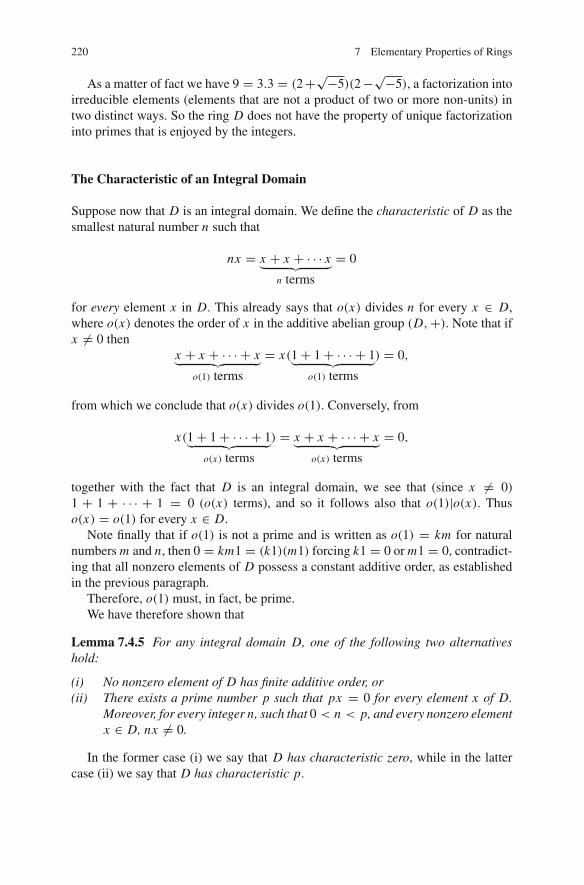
220 7 Elementary Properties of Rings
As a matter of fact we have 9 = 3.3 = (2 +√−5)(2 −√−5), a factorization intoirreducible elements (elements that are not a product of two or more non-units) intwo distinct ways. So the ring D does not have the property of unique factorizationinto primes that is enjoyed by the integers.
The Characteristic of an Integral Domain
Suppose now that D is an integral domain. We define the characteristic of D as thesmallest natural number n such that
nx = x + x + · · · x︸ ︷︷ ︸n terms
= 0
for every element x in D. This already says that o(x) divides n for every x ∈ D,where o(x) denotes the order of x in the additive abelian group (D,+). Note that ifx �= 0 then
x + x + · · · + x︸ ︷︷ ︸o(1) terms
= x(1 + 1 + · · · + 1︸ ︷︷ ︸o(1) terms
) = 0,
from which we conclude that o(x) divides o(1). Conversely, from
x(1 + 1 + · · · + 1︸ ︷︷ ︸o(x) terms
) = x + x + · · · + x︸ ︷︷ ︸o(x) terms
= 0,
together with the fact that D is an integral domain, we see that (since x �= 0)1 + 1 + · · · + 1 = 0 (o(x) terms), and so it follows also that o(1)|o(x). Thuso(x) = o(1) for every x ∈ D.
Note finally that if o(1) is not a prime and is written as o(1) = km for naturalnumbers m and n, then 0 = km1 = (k1)(m1) forcing k1 = 0 or m1 = 0, contradict-ing that all nonzero elements of D possess a constant additive order, as establishedin the previous paragraph.
Therefore, o(1) must, in fact, be prime.We have therefore shown that
Lemma 7.4.5 For any integral domain D, one of the following two alternativeshold:
(i) No nonzero element of D has finite additive order, or(ii) There exists a prime number p such that px = 0 for every element x of D.
Moreover, for every integer n, such that 0 < n < p, and every nonzero elementx ∈ D, nx �= 0.
In the former case (i) we say that D has characteristic zero, while in the lattercase (ii) we say that D has characteristic p.

7.4 Other Examples and Constructions of Rings 221
It should be clear that all subrings of an integral domain of characteristic c (c = 0or c = p, for some prime p) are integral domains of the same characteristic c. Inparticular, if D is any subring of the complex numbers C, then it is an integral domainof characteristic 0. Thus, the Gaussian Integers, the Eisenstein numbers, or any othersubring of the reals or complex numbers, must be an integral domain of characteristic0. The field Z/pZ, where p is a prime number, clearly has positive characteristic p.
The following lemma shows that integral domains of non-zero characteristic pmay possess certain endomorphisms. It will be crucial for our analysis of finite fieldsand inseparable extensions in Chap. 11.
Lemma 7.4.6 Suppose D is an integral domain of positive characteristic p, a primenumber. The pth power mapping D → D, which maps each element r ∈ D to itspth power r p, is an endomorphism of D.
Proof Since any integral domain D is commutative, one has (xy)p = x p y p for anyx, y ∈ D—that is the pth power mapping preserves multiplication. It remains toshow that for any x, y ∈ D,
(x + y)p = x p + y p. (7.22)
Since we are in a commutative ring, the “binomial theorem” (Theorem 7.1.2) holds:thus:
(x + y)p =∑k=p
k=0xk y p−k
(pk
).
Using the fact that p is a prime number, one can show that each combinatorialnumber (
pk
)= p!/(k!(p − k)!
is a multiple of p whenever 0 < k < p.16 The result then follows. �
Finite Integral Domains
We shall conclude this subsection with a result that is not only interesting in its ownright, but whose proof involves one of the most important “counting arguments” inall of mathematics. This is the so-called “Pigeon Hole Principle,” which says simplythat any injective mapping of a finite set into itself must also be surjective.
Theorem 7.4.7 Let D be a finite integral domain. Then D is a field.
Proof Let d be a nonzero element of D; we shall show that d has a multiplicativeinverse. Note that right multiplication by d defines an injective mapping D → D.
16In fact this argument is a special case of the same argument used in Wielandt’s proof of the SylowTheorems (Theorem 4.3.3, p. 117).

222 7 Elementary Properties of Rings
For if ad = bd then a = b by the Cancellation Law (see Lemma 7.4.4). By thePigeon Hole Principle, this mapping must be surjective and so there must exist anelement c ∈ D such that cd = 1. This says that c is the multiplicative inverse of dand the proof is complete. �
7.5 Exercises
7.5.1 Warmup Exercises for Sect. 7.1
1. Give a formal proof of Lemma 7.1.1 using only the axioms of a ring and knownconsequences (e.g. relevant Lemmata in Chap. 3) of the fact that (R,+) is acommutative group.
2. Do the even integers form a ring? Explain your answer.3. Let K be one of the familiar fields, Q,R, or C, or let K be the ring of integers
Z. Let M2(K ) be the collection of all 2-by-2 matrices with entries in K . Defineaddition and multiplication by the standard formulae
(a1 b1c1 d1
)+
(a2 b2c2 d2
)=
(a1 + a2 b1 + b2c1 + c2 d1 + d2
)
(a1 b1c1 d1
)·(
a2 b2c2 d2
)=
(a1a2 + b1c2 a1b2 + b1d2c1a2 + d1c2 c1b2 + d1d2
).
(a) Show that M2(K ) is a ring with respect to matrix addition and multiplication.(b) Explicitly demonstrate that M2(K ) is not a commutative ring.(c) Show that the subset
T2(K ) ={(
a b0 d
)|a, b, d ∈ K
}
is a subring.(d) Is the set
T2(K ) ={(
0 b0 0
)|d ∈ K
}
a subring of M2(K )?(e) In the three cases where K is a field, is M2(K ) a division ring?(f) Now suppose K = Z, the ring of integers.
(i) Let
A ={(
a bc d
)|a, b, c, d ∈ Z, c is even
}.

7.5 Exercises 223
Is A a subring of M2(Z)?(ii) Let
A ={(
a b−b a
)|a, b ∈ Z,
}.
Is B a subring of M2(Z)?
4. Consider the subset S of the field Q of rational numbers consisting of all fractionsa/b, where the non-zero integer b is not divisible by 5. Is S a subring of Q?Explain your answer.
5. Let R be the ring Z/(12) of integer residues classes modulo 12. List the units ofR and write out a multiplication table for the multiplicative group that they form.Can you identify this multiplicative group as one that you have met before?
6. Let B be any non-empty subset of a ring R. Show explicitly that the centralizerCR(B) is a subring of R. [Hint: Use the three-point criterion of p. 193.]
7. (The Binomial Theorem for Commutative Rings) Let R be any commutative ring,let x and y be two elements of R, and let n be a positive integer. Show that
(x + y)n =∑k=p
k=0xk yn−k
(nk
),
where as usual (nk
):= n!/(k!(n − k)!),
denotes the combinatorial number. [Hint: Use induction on n and the usual recur-sion identities for the combinatorial numbers.]
7.5.2 Exercises for Sect. 7.2
1. Suppose α : R → S is a surjective homomorphism of rings. Suppose T is asubring of S. Is the set
α−1(T ) := {r ∈ R|α(r) ∈ T }
a subring of R? (Be aware that subrings must contain their own multiplicativeidentity element.)
2. Let R be a commutative ring and let P be an ideal of R. Prove that P is a primeideal if and only if whenever a, b ∈ R with ab ∈ P then a ∈ P or b ∈ P .
3. Prove Lemma 7.2.7.4. In a commutative ring, a non-zero element a is said to be a zero divisor if and
only if there exists a non-zero element b such that ab = 0. Thus an integral

224 7 Elementary Properties of Rings
domain could be characterized as a non-zero commutative ring with no zerodivisors.Show that if R is a commutative non-zero ring with only finitely many zerodivisors, then R is either an integral domain or is a finite ring. [Hint: For anyzero divisor a, consider the surjective homomorphism φ : (R,+) → (a R,+)
of additive abelian groups, defined by r �→ ar , for all r ∈ R. Then note thatevery non-zero element of a R and every non-zero element of ker φ is a zerodivisor. Apply the group isomorphism R/kerφ � (a R,+) to deduce that ker φhas finite index as a subgroup of (R,+). (Explain why the homomorphism φneed not be a ring homomorphism. )]
5. Let R be a ring and let I, J be ideals of R. We say that I, J are relatively prime(or are comaximal) if I + J = R. Prove that if I, J are relatively prime idealsof R, then I J + J I = I ∩ J .
6. (a) Prove the Chinese Remainder Theorem: Let R be a ring and let I, J berelatively prime ideals of R. Then the ring homomorphism R → R/I ×R/Jgiven by r �→ (r + I, r + J ) determines an isomorphism
R/(I ∩ J ) ∼= R/I × R/J.
(b) More generally, if I1, I2, . . . , Ik ⊆ R are pairwise relatively prime, then thering homomorphism R → R/I1 × R/I2 × · · · × R/Ir , r �→ (r + I1, r +I2, . . . , r + Ir ) determines an isomorphism
R/(I1 ∩ I2 ∩ · · · ∩ Ik) ∼= R/I1 × R/I2 × · · · × R/Ik .
[Hint: For the homomorphism in part (a), the kernel is easy to identify. Theissue is showing its surjectivity. For this use I+J = R to show that 0×(R/J )and (R/I ) × 0 are both contained in the image of the homomorphism. Part(b), cries out for an induction proof.]
7. Let R be a ring and let I ⊆ R be an ideal. Show that if I ⊆ P1 ∪ P2 ∪ · · · ∪ Pr ,where P1, P2, . . . Pr are prime ideals, then I ⊆ Pj for some index j . [Hint: foreach i = 1, 2, . . . , r , let xi ∈ I − (P1 ∪ P2 ∪ · · · ∪ Pi−1 ∪ Pi+1 ∪ · · · ∪ Pr ).Show that x1 + x2x3 · · · xr �∈ P1 ∪ · · · ∪ Pr .]
8. Recall the definition of residual quotient, (B : A) := {r ∈ R|Ar ⊆ B}. Let Rbe a ring and let I, J and K be right ideals of R. Prove that ((I : J ) : K ) = (I :J K ). (Here, following the custom of the ring-theorists, the symbol J K denotesthe additive group generated by the set product J K . Of course it is a right idealof R.)
9. Let R be a commutative ring and let I be an ideal of R. Define the radical of Ito be the set
√I = {r ∈ R| rm ∈ I for some positive integer m}.
Show that√
I is an ideal of R containing I .

7.5 Exercises 225
10. Let R be a commutative ring, and let Q ⊆ R be an ideal. We say that Q isprimary if ab ∈ Q and a �∈ Q implies that bn ∈ Q for some positive integer n.Prove the following for the primary ideal Q ⊆ R:
(a) P := √Q is a prime ideal containing Q. In fact P is the smallest prime
ideal containing Q. (In this case we call Q a P-primary ideal.)(b) If Q is a P-primary ideal, ab ∈ Q, and a �∈ P , then b ∈ Q.(c) If Q is a P-primary ideal and I, J are ideals of R with I J ⊆ Q, I �⊆ P ,
then J ⊆ Q.(d) If Q is a P-primary ideal and if I is an ideal I �⊆ P , then (Q : I ) = Q.
11. Suppose that P and Q are ideals of the commutative ring R satisfying the fol-lowing:
(a) P ⊇ Q.(b) If x ∈ P then for some positive integer n, xn ∈ Q.(c) If ab ∈ Q and a �∈ P , then b ∈ Q.
Prove that Q is a P-primary ideal.12. Assume that Q1, Q2, . . . , Qr are all P-primary ideals of the commutative ring
R. Show that Q1 ∩ Q2 ∩ . . . ∩ Qr is a P-primary ideal.13. Let R be a commutative ring and let Q ⊆ R be an ideal. Prove that Q is a primary
ideal if and only if the only zero divisors of R/Q are nilpotent elements. (Anelement r of a ring is called nilpotent if rn = 0 for some positive integer n.)
14. Consider the ideal I = nZ[x] + xZ[x] ⊆ Z[x], where n ∈ Z is a fixed integer.Prove that I is a maximal ideal of Z[x] if and only if n is a prime.
15. If R is a commutative ring and x ∈ ⋂{M | M is a maximal ideal}, show that1 + x ∈ U(R), the group of units of R.
7.5.3 Exercises for Sect. 7.3
1. Let R be a ring and let M be a monoid with the following property:
(F) Each element m possesses only finitely many distinct factorizations m1m2in M .
Define the completion, (RM)∗ of the monoid ring RM to be the set of allfunctions f : M → R with point-wise addition and convolution multiplication.(The point is that we are no longer limited to functions of finite support.) Showthat one still obtains a ring and that the usual monoid ring RM occurs as a subringof (RM)∗.
2. The completion of the polynomial ring R[x] is usually denoted R[[x]]. Note thatR[[x]] can be viewed as the ring of “power series” in the indeterminate x . Showthat while the only units of R[x] are in fact the units of R, R[[x]] has far moreunits. In particular, note that

226 7 Elementary Properties of Rings
(1 − x)−1 = 1 + x + x2 + · · · =∞∑
i=0
xi .
Show that, in fact, f (x) =∞∑
i=0ai xi is a unit of R[[x]] if and only if a0 is a unit of
R. [Hint: Show that if f (x) · g(x) = 1, where f (x) = ∑ai xi , g(x) = ∑
bi xi ,ai , bi ∈ R, then a0b0 = 1 so a0 is a unit.On the other hand if a0 is a unit in R, one can set b0 = a−1
0 , and show inductivelythat there exist solutions bi to
∑n
i=0an−i bi = 0
in which each bi is a Z-linear combination of monomial words in a−10 and
{a1, a2, . . . , an}.]3. Let R be a ring, and let M be the free commutative monoid on the two-element set
{x, y}. Thus M = {xi y j | i, j ∈ N}, where, as usual, we employ the conventionthat when the natural number zero appears as an exponent, one reads this as themonoid identity element. (Note that M can also be identified with the monoid ofmultisets over {x, y}) The monoid algebra RM is usually denoted by R[x, y] :=RM and is called a polynomial ring in two commuting indeterminates. Elementscan be written as finite sums of the form
f (x, y) =∑
i, j≥0
ai j xi y j , ai j ∈ R.
On the other hand, the polynomial ring construction can clearly be iterated,giving the polynomial ring R[x][y] := (R[x]) [y]. Show that these rings areisomorphic.
4. (a) Suppose M and N are monoids with identity elements 1M and 1N (themonoid operation in both cases is multiplication and is denoted by juxta-position of its arguments). A monoid homomorphism from M to N is amapping φ : M → N with the property that φ(1M ) = 1N and φ(m1m2) =φ(m1)φ(m2) for all elements m1,m2 ∈ M . Fix a ring R and form themonoid rings RM and RN . Consider the mapping ρ(φ) : RM → RNwhich is defined by
∑m∈M
rm · m �→∑
m∈Mrmφ(m),
where rm ∈ R and as usual, the elements rm are non-zero for only finitelymany m’s. Show that ρ(φ) is a ring homomorphism. Show that ρ(φ) is one-to-one (onto) if and only if φ is one-to-one (onto). In particular, if φ is anautomorphism of M , then ρ(φ) is an automorphism of RM .

7.5 Exercises 227
(b) Similarly we may define an antiautomorphism of the monoid M to be abijection τ : M → M such that τ (m1m2) = τ (m2)τ (m1). Prove that τmust fix the identity element 1M . In addition, let α be an antiautomorphismof the ring R. Let the mapping ρ(α, τ ) : RM → RM be defined by
∑m∈Supp f
f (m)m �→∑
m∈Supp ff (m)σmτ .
Show that ρ(σ, τ ) is an antiautomorphism of the monoid ring RM .(c) Let rev : M(X) → M(X) be the antiautomorphism of the free monoid on
X which rewrites each word with the letters appearing in reverse order. Thusrev(x1x2 · · · xn) = xn xn−1 · · · x2x1. Show that if R is a commutative ring,
then the mapping β : R{X} → R{X} defined by
∑w∈M(X)
rww →∑
w∈Wrw rev(w),
is an antiautomorphism of the ring R{X}. (Here as usual, the rw are ringelements which are non-zero for only finitely many words w.)
(d) Let β be the antiautomorphism of the preceding part of this exercise. Showthat the subset CR{X}(β) of polynomials left fixed by β are the R-linearcombinations of the palindromic words, and, if |X | > 1, that this set is notclosed under multiplication.
5. Suppose X is a finite set, and R[X ] is the ring of polynomials whose commutingindeterminates are the elements of X . We suppose B is a ring which is eitherthe zero ring or contains R in its center. Suppose φ : X → B is any mappinginto the commutative ring B. As in Theorem 7.3.3, we define the mapping φ :R[X ] → B which maps every polynomial
∑m∈M amm (with only finitely many
of the coefficients am in R nonzero) to the element∑
m amφ(m). This mappingsimply substitutes φ(xi ) for xi in each polynomial in R[X ] and xi ∈ X Showthat φ possesses the following properties:
φ(b1 + b2) = φ(b1) + φ(b2)
φ(b1b2) = φ(b1)φ(b2)
φ(rb) = r φ(b)
for any b.b1, b2 in B and any r in R.6. Let α : X → B ⊆ CS(R) be a mapping from a set X into a set B which is
contained in the centralizer, in ring S, of a subring R.
(a) Show that the corresponding evaluation mapping
E∗α : R{X} → S
is a ring homomorphism. (See p. 204 for definitions.)

228 7 Elementary Properties of Rings
(b) (Uniqueness) If we regard X as the set of words of length one in the freemonoid on X , show that E∗
α is the unique ring homomorphism h : R{X} →S which extends the given mapping α : X → B. [Show that h(p) = E∗
α(p)for each polynomial p.]
7. Let X = {x1, . . . , xn} be any non-empty finite set. Recall that M(X) denotes thefree monoid on the set X—that is, the set of all “words” of finite length in thealphabet X with the concatenation operation. Also one may recall that M(X) isthe additive monoid of multisets of X—that is, sequences (a1, . . . , an) of non-negative integers. Define the “letter inventory mapping” κ : M(X) → M(X)
where, for a word w,κ(w) = (a1, . . . , an)
if and only if, for each i , the letter xi occurs exactly ai times in the word w. Showthat κ is a monoid homomorphism (as defined in the first part of Exercise 4).From the same exercise, conclude that for any commutative ring R, the mappingκ extends to an R-homomorphism of rings R{X} → R[X ].
8. Let R be a subring of ring S and let B be a set of pairwise commuting elementsof CS(R). Suppose α : X → B is a mapping of set X into B.
(a) Show that the mapping Eα : R[X ] → S defined on p. 204 is a homomor-phism of rings.
(b) (Uniqueness) Show that if X is regarded as a subset of R[X ] (namely as theset of those monomials which are words of length one), then for any ringhomomorphism ν : R[X ] → S which extends α : X → B, one must haveν = Eα.
9. Again let α : X → B be a mapping of set X into B, a collection of pairwisecommuting elements of the centralizer in ring S of its subring R. Let κ be themonoid homomorphism of Exercise 7 and let
ρ(κ) : R{X} = RM(X) → RM(X) = R[X ]
be its extension to the monoid rings as in Exercise 4. Show that
E∗α = Eα ◦ ρ(κ).
[Hint: Use the uniqueness of E∗α.]
10. Let n be a positive integer. Suppose A = (ai j ) is an n × n matrix with entriesdrawn from the ring R. For j ∈ {1, . . . , n}, let e j be the n-tuple of R(n) whosej th entry is 1 ∈ R, the multiplicative identity of R, and all of whose remainingentries are equal to 0 ∈ R. The matrix A is said to be R-invertible if and only ifeach e j is an R-linear combination of the rows of A. Let X = {x1, . . . , xn}, andlet
σ(A) : R[X ] → R[X ]

7.5 Exercises 229
which replaces each polynomial p(x1, . . . , xn) by the polynomial
p(∑
a1i xi ,∑
a2i xi , . . . ,∑
ani xi
),
the parameter i in each sum ranging from 1 to n. Show that if A is R-invertible,then σ(A) is an automorphism of R[X ]. [Hint: Use the evaluation homomor-phism Eα for an appropriate triplet (α, B, S). Then show that it is onto.]
11. Let G be a finite group, let F be a field, and let χ : G → F× be a homomorphismof G into the multiplicative group F× := F\{0}. Define the element εχ =∑g∈G
χ(g−1)g ∈ FG and show that ε2χ = |G|εχ.
12. Same assumptions as the above exercise. Show that the element εχ, commuteswith every element of FG by showing that for all g ∈ G, gεχ = χ(g)εχ.
7.5.4 Exercises for Sect. 7.4
1. Let {Rσ}σ∈I be a family of rings and let P = ∏σ∈I Rσ be the direct product of
these rings. If K is any subset of the index set I , set PK := { f ∈ P | f (σ) =0 for all σ �∈ K }. Show that PK forms a (two-sided) ideal of P .
2. Let X be a set and let R be a ring. In Example 38 we defined the ring of functionsRX . Prove that
RX ∼=∏x∈X
Rx ,
where Rx � R for each x ∈ X .3. Prove that any non-zero subring of an integral domain contains the multiplicative
identity element of the domain. [Hint: use Lemma 7.4.4.]4. Prove that the polynomial ring Z[x] is not a principal ideal domain by showing
that the ideal I := 2Z[x] + xZ[x] is not a principal ideal.5. Let d be a positive integer congruent to −1 modulo 4 and consider the integral
domainD := {a + b
√−d| a, b ∈ Z}
whose operations are inherited as a subring of the complex number field C. Showthat the ideal I := 2D + (1 +√−d)D is not a principal ideal.
6. Suppose ω = e2iπ/3 = (−1 − √−3)/2, so ω is a complex number satisfyingthe identity: ω2 = −ω − 1. On p. 189 and again on p. 218 we introduced theEisenstein numbers, the integral domain Z[ω]. Show that the mapping Z[ω] →Z[ω] defined by
a + bω �→ a + bω2, a, b ∈ Z
is an automorphism of this ring.

230 7 Elementary Properties of Rings
7. Let τ : M2(C) → M2(C)be the composition of the transpose antiautomorphism,T , and the automorphism m(c) induced by complex conjugation (c : C → C)of the matrix entries. (See Example 41 for notation and the fact that τ = c ◦ T =T ◦c.) Let H = {h(α,β)|(α,β) ∈ C×C} be the ring of real quaternions viewedas a subring of M2). (See p. 215.)
(a) Show that as an antiautomorphism of M2(C), that τ2 is the identityautomorphism—that is, τ is an involution.
(b) Show that H is invariant under this antiautomorphism.(c) Establish that h(α,β)τ = h(αc,−β) and conclude that the centralizer in H
of the antiautomorphism τ (that is, its fixed points) is the center of H, theset RI2 = {h(r, 0)|r ∈ R}, the real multiples of the 2-by-2 identity matrix.
(d) Show that for any h ∈ H, D(h) := hhτ is a “real” element—that is anelement of the center Z(H). [Hint: Show that hhτ is fixed by τ .]
(e) Compute that D(h(α,β)) = N (α) + N (β) = det (h(α,β)).(f) Show that D(h1h2) = D(h1)Dh2), for all h1, h2 ∈ H. [Hint: Use the fact
that τ is an antiautomorphism of H and that D(H) is in the center of H.](g) Let
H|Z := {h(α,β)|α,β Gaussian integers}.
Show that H|Z is a subring of H which is also invariant under the antiauto-morphism τ . [Hint: Just check the rules for multiplying and applying τ forthe quaternionic numbers h(α,β).]
(h) Using the previous two steps, prove that the set of integers which are thesum of four perfect squares, is closed under multiplication. (This set turnsout to include all natural numbers.)
References
1. Greene C (1982) The Möbius function of a partially ordered set. In: Rival I (ed) Appeared inordered sets. D. Reidel Publishing Company, Dordrecht, pp 555–581
2. Rota G-C (1964) On the foundations of combinatorial theory I. Theory of Mobius functionsZeitschrift für Wahrscheinlichkeitstheorie, Band 2, Heft 4. Springer, Berlin, pp 340–368

Chapter 8Elementary Properties of Modules
Abstract One way to study rings is through R-modules, which (in some possi-bly non-faithful way) serve to “represent” the ring. But such a view is restrictive.With R-modules one enjoys an increased generality. Any property possessed by anR-module can conceivably apply to the ring R itself, as a module over itself. Also,any universal property gains a greater strength, when one enlarges the ambient realmin which the property is stated—in this case from rings R, to their R-modules. Thischapter still sticks to basics: homomorphisms, submodules, direct sums and productsand free R-modules. Beyond that, chain conditions on the poset of submodules canbe seen to have important consequences in two areas: endomorphisms of modules,and their generation. The former yields the Krull-Remak-Schmidt Theorem con-cerning the uniqueness of direct decompositions into indecomposable submodules,while, for the latter, the ascending chain condition is connected with finite generationvia Noether’s Theorem. (The existence of rings of integral elements is derived fromthis theorem.) The last sections of the chapter introduce exact sequences, projec-tive and injective modules, and mapping properties of Hom(M, N )—a hint of thecategory-theoretic point of view to be unfolded at the beginning of Chap.13.
8.1 Basic Theory
8.1.1 Modules over Rings
Fix a ring R. A left module over R or left R-module is an additive group M = (M,+),which admits a composition (or scalar multiplication)
R × M → M
(which we denote as a juxtaposition of arguments, as we do for multiplication in R)such that for all elements a, b ∈ R, m, n ∈ M ,
a(m + n) = am + an (8.1)
(a + b)m = am + bm (8.2)
© Springer International Publishing Switzerland 2015E. Shult and D. Surowski, Algebra, DOI 10.1007/978-3-319-19734-0_8
231

232 8 Elementary Properties of Modules
(ab)m = a(bm) (8.3)
1 · m = m, (8.4)
where 1 denotes the multiplicative identity element of R. It follows from 0R + 0R =0R that for any element m of M , 0Rm + 0Rm = 0Rm. Thus 0Rm = 0M for anym ∈ M . Here, of course, 0R denotes the additive identity of the additive group (R,+)
while 0M denotes the additive identity of the additive group (M,+).A right R-module is an additive group M = (M,+) admitting a right composition
M×R → M , such that, subject to the same conventions of denoting this compositionby juxtaposition, we have for all a, b ∈ R, m, n ∈ M ,
(m + n)a = ma + na (8.5)
m(a + b) = ma + mb (8.6)
m(ab) = (ma)b (8.7)
m1 = m. (8.8)
Again we can easily deduce the identities
m0R = 0M (8.9)
m(−a) = −(ma) (8.10)
where 0R and 0M are the additive identity elements of the groups (R,+) and (M,+),and where m is an arbitrary element of M .
Notice that for a left R-module, M , the set {r ∈ R|r M = 0} is a 2-sided idealof R. It is called the left annihilator of M . Similarly, for a right R-module M theset {r ∈ R|Mr = 0} is also a 2-sided ideal, called the right annihilator of M. Ineither case (left module or right), the module is said to be faithful if and only if thecorresponding annihilating ideal is the 0-ideal. (See Exercise (3) in Sect. 8.5.1.)
8.1.2 The Connection Between R-Modules andEndomorphism Rings of Additive Groups
Consider first a left R-module M . For each element r ∈ R, the mapping ρ(r) :(M,+) → (M,+) defined by m �→ rm, is an endomorphism of the additive group(M,+). (This is a consequence of Eq. (8.1).) As remarked in Example 41 of Chap. 7,the set End(M) of all endomorphisms of the additive group (M,+) forms a ringunder point-wise addition of endomorphisms and composition of endomorphisms.Now for any elements r, s in the ring R and m ∈ M , Eq. (8.3) yields

8.1 Basic Theory 233
ρ(rs)m = (rs)m = r(sm) = ρ(r)[ρ(s)(m)] = (ρ(r) ◦ ρ(s))(m).
Thusρ(rs) = ρ(r) ◦ ρ(s). (8.11)
Similarly, Eq. (8.2) yieldsρ(r + s) = ρ(r) + ρ(s). (8.12)
These equations tell us that ρ : R → End(M) is a homomorphism of rings.Notice that ker ρ = {r ∈ R|r M = 0}, is the left annihilator of M as defined in
the previous subsection.Conversely, if we are given such a ring homomorphism ρ : R → End(M), where
M is an additive group, then M acquires the structure of a left R-module by settingrm := ρ(r)(m), for all r ∈ R, m ∈ M .
In the same vein, a right R-module structure on the abelian group (M,+) is equiv-alent to specifying a ring homomorphism R → Opp(R)(End(M)) Here Opp(R) isthe additive group of all endomorphisms of M endowed with a multiplication ◦o
where, for any endomorphisms α and β,
α ◦o β = β ◦ α,
the endomorphism obtained by first applying α and then applying β in that chrono-logical order. (See Example 40.)
Remark At times one might wish to convert a left R-module to a right S-module, orthe reverse. We have the following constructions:
Suppose R and S are rings whose multiplicative identity elements are denoted eR
and eS , respectively.
1. Let M be a left R-module. Suppose ψ : S → Opp(R) is a ring homomorphismfor which ψ(eS) = eR . For each m ∈ M , and s ∈ S define
ms := ψ(s)m.
Sinceψ(s) ∈ R, and M is a left R-module, the right side is a well-defined elementof M . With multiplication M × S → M in this way, it is easy to show that Mbecomes a right S module.
2. Similarly if M is a right S module, then, from a ring homomorphism φ : R →Opp(S) for which φ(eR) = eS , one may convert M into a left R-module.
Proof of the appropriate module axioms is requested in Exercises in Sect. 8.5.2.
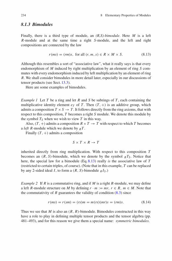
234 8 Elementary Properties of Modules
8.1.3 Bimodules
Finally, there is a third type of module, an (R,S)-bimodule. Here M is a leftR-module and at the same time a right S-module, and the left and rightcompositions are connected by the law
r(ms) = (rm)s, for all (r, m, s) ∈ R × M × S. (8.13)
Although this resembles a sort of “associative law”, what it really says is that everyendomorphism of M induced by right multiplication by an element of ring S com-mutes with every endomorphism induced by left multiplication by an element of ringR. We shall consider bimodules in more detail later, especially in our discussions oftensor products (see Sect. 13.3).
Here are some examples of bimodules.
Example 1 Let T be a ring and let R and S be subrings of T , each containing themultiplicative identity element eT of T . Then (T,+) is an additive group, whichadmits a composition T × S → T . It follows directly from the ring axioms, that withrespect to this composition, T becomes a right S module. We denote this module bythe symbol TS when we wish to view T in this way.
Also, (T,+) admits a composition R × T → T with respect to which T becomesa left R-module which we denote by R T .
Finally (T,+) admits a composition
S × T × R → T
inherited directly from ring multiplication. With respect to this composition Tbecomes an (R, S)-bimodule, which we denote by the symbol R TS . Notice thathere, the special law for a bimodule (Eq.8.13) really is the associative law of T(restricted to certain triples, of course). (Note that in this example, T can be replacedby any 2-sided ideal I , to form a (R, S)-bimodule R IS .)
Example 2 If R is a commutative ring, and if M is a right R-module, we may definea left R-module structure on M by defining r · m := mr, r ∈ R, m ∈ M . Note thatthe commutativity of R guarantees the validity of condition (8.3) since
r(ms) = r(sm) = (rs)m = m(rs)(mr)s = (rm)s. (8.14)
Thus we see that M is also an (R, R)-bimodule. Bimodules constructed in this wayhave a role to play in defining multiple tensor products and the tensor algebra (pp.481–493), and for this reason we give them a special name: symmetric bimodules.

8.1 Basic Theory 235
Example 3 Here is a simple variation on the preceding example. Let σ be an auto-morphism of the commutative ring R. Then a right R-module M can be convertedinto an (R, R)-bimodule by declaring that mr = rσm for all (m, r) ∈ M × R.(One simply emulates the sequence of Eq. (8.14) applying σ or its inverse when ringelements pass to the left or right over module elements.)
Remark In these two examples, the commutativity of R is more or less forced. Forsuppose M is an arbitrary right R-module andσ is automorphismof the additive group(R,+). If we attempt to convert M into an (R, R)-bimodule by the rule mr = rσmfor all (m, r) ∈ M × R, three conclusions are immediate: (i) σ is easily seen to bean antiautomorphism of R (that is, (rs)σ = sσrσ), (ii) σ takes the right annihilatorof MR , that is, the two-sided ideal I = AnnR(MR) := {r ∈ R|Mr = 0}, to the leftannihilator I σ = AnnR(RM), and (iii) that the factor ring R/I is commutative. Thusif I = I σ , we have recovered Example 3 above with R replaced by R′ := R/I .
8.1.4 Submodules
Fix a (right) R-module M . A submodule is an additive subgroup of (M,+) that isclosed under all scalar multiplications by elements of R.
It is easy to see that a subset N is a submodule of the right R-module M , if andonly if
(i) N + N = N(ii) −N = N , and(iii) NR ⊆ N .
It should be remarked that the last containment is actually the equalityNR = N , sinceright multiplication by the identity element 1R induces the identity endomorphismof N .
Suppose now N = {Nσ|σ ∈ I } is a family of submodules of the right R-moduleM . The intersection ⋂
σ∈I
Nσ
of all these submodules is clearly a submodule of M . This is the unique supremumof the poset of all submodules contained in all of the submodules inN .
Now let X be an arbitrary subset of the right R-module M . The submodulegenerated by X is defined to be the intersection of all submodules of M which containthe subset X and is denoted 〈X〉R . From the previous paragraph, this intersection isthe unique smallest submodule in the poset of all submodules of M which contain X .
This object has another description. Let X be the set of all elements of M whichare finite (right) R-linear combinations of elements from X—that is elements of theform x1r1 + · · · + xnrn where n is any natural number, the xi belong to X and the r j
belong to the ring R. Then X is a subgroup (recall that x(−1R) = −x) and X R = X ,

236 8 Elementary Properties of Modules
so X is a submodule. On the other hand, it must lie in any submodule which containsX and so must coincide with 〈X〉R .
In the case that X = {x1, . . . , xn} is a finite set,
X = x1R + · · · + xn R.
A right R-module is said to be finitely generated if and only if it is generated by afinite set. Thus right R-module N is finitely generated if and only if
N = x1R + · · · + xn R
for some finite subset {x1, . . . xn} of its elements.Now once again let N = {Nσ|σ ∈ I } be a family of submodules of the right
R-module M . The sum over N is the submodule of M generated by the set-theoreticunion ∪{N |N ∈ N } of all the submodules in the familyN and is denoted
∑σ∈I Nσ .
It is therefore the set of all finite R-linear combinations of elements which lie inat least one of the submodules in N . But of course, as each submodule is invariantunder right multiplication by elements of R, this simply consists of all finite sums ofelements lying in at least one module of the family. In any event, this is the uniquemember of the set of all submodules of M which contain every member of N .
We summarize this information in
Lemma 8.1.1 Let R be a ring, and let M be a left R-module. The poset of all submod-ules of M (with containment as the partial order) is a lattice with unrestricted meetsand joins, given respectively by the intersection and sum operations on arbitraryfamilies of submodules.
Obviously, a corresponding lemma holds for the poset of submodules of a givenleft module over some ring R.
8.1.5 Factor Modules
Now suppose N is a submodule of the right R-module M . Since N is a subgroupof the additive group (M,+), we may form the factor group M /N whose elementsare the additive cosets x + N , x ∈ M of N . Next, define an R-scalar multiplicationM /N × R → M /N by setting (x + N )r := xr + N . That this is well defined isan immediate consequence of the fact that Nr ⊆ N for each r ∈ R. Showing theremaining requisite properties (8.5)–(8.8) is equally routine, completing the defini-tion of the quotient right R-module M /N . Again, this construction can be duplicatedfor left R-modules: For each submodule N of a left R-module M , we obtain a leftR-module M /N .

8.1 Basic Theory 237
8.1.6 The Fundamental Homomorphism Theoremsfor R-Modules
Suppose M and N are right R-modules (for the same ring R). An R-module homo-morphism M → N is a homomorphism f : (M,+) → (N ,+) between the under-lying additive groups, such that
f (m)r = f (mr), (8.15)
for all m ∈ M and all r ∈ R. In other words, these are group homomorphisms whichcommute with the right multiplications by each of the elements of the ring R.
It follows from the definition that the composition β ◦ α of two module homo-morphisms α : A → B and β : B → C , is an R-homomorphism A → C .
Before going further, we will find it convenient to adopt a common visual-linguistic device for discussing compositions of homomorphisms. Suppose α : A →B, β : B → C and γ : A → C are homomorphisms. This data is assembled in thefollowing diagram:
B
A C
�
�
��
��
���
βα
γ
We say that the “diagram commutes” if and only if γ = β ◦ α, the compositionof α and β.
We use similar language for square diagrams:
Aγ−−−−→ C
α⏐⏐� ⏐⏐�δ
Cβ−−−−→ D
Again, such a diagram “commutes” if and only if δ ◦ γ = β ◦ α.The adjectives which accrue to an R-homomorphism are exactly those which are
applicable to it as a homomorphism of additive groups: Thus the R-homomorphismf is
• an R-epimorphism• an R-monomorphism• an R-isomorphism
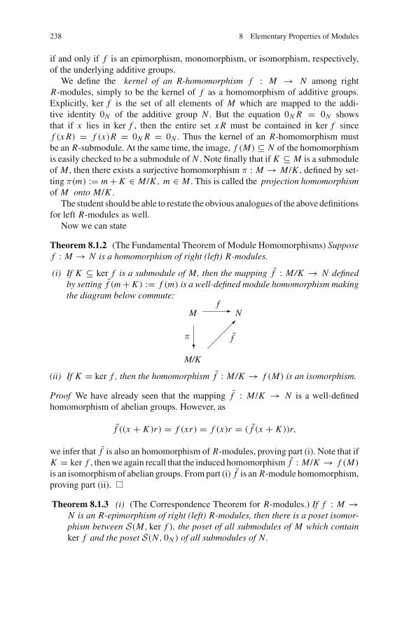
238 8 Elementary Properties of Modules
if and only if f is an epimorphism, monomorphism, or isomorphism, respectively,of the underlying additive groups.
We define the kernel of an R-homomorphism f : M → N among rightR-modules, simply to be the kernel of f as a homomorphism of additive groups.Explicitly, ker f is the set of all elements of M which are mapped to the addi-tive identity 0N of the additive group N . But the equation 0N R = 0N showsthat if x lies in ker f , then the entire set x R must be contained in ker f sincef (x R) = f (x)R = 0N R = 0N . Thus the kernel of an R-homomorphism mustbe an R-submodule. At the same time, the image, f (M) ⊆ N of the homomorphismis easily checked to be a submodule of N . Note finally that if K ⊆ M is a submoduleof M , then there exists a surjective homomorphism π : M → M /K , defined by set-ting π(m) := m + K ∈ M /K , m ∈ M . This is called the projection homomorphismof M onto M /K .
The student should be able to restate the obvious analogues of the above definitionsfor left R-modules as well.
Now we can state
Theorem 8.1.2 (The Fundamental Theorem of Module Homomorphisms) Supposef : M → N is a homomorphism of right (left) R-modules.
(i) If K ⊆ ker f is a submodule of M, then the mapping f : M/K → N definedby setting f (m + K ) := f (m) is a well-defined module homomorphism makingthe diagram below commute:
M/K
M N
�
�
��
��π f
f
(ii) If K = ker f , then the homomorphism f : M/K → f (M) is an isomorphism.
Proof We have already seen that the mapping f : M /K → N is a well-definedhomomorphism of abelian groups. However, as
f ((x + K )r) = f (xr) = f (x)r = ( f (x + K ))r,
we infer that f is also an homomorphism of R-modules, proving part (i). Note that ifK = ker f , thenwe again recall that the induced homomorphism f : M /K → f (M)
is an isomorphism of abelian groups. Frompart (i) f is an R-module homomorphism,proving part (ii). �
Theorem 8.1.3 (i) (The Correspondence Theorem for R-modules.) If f : M →N is an R-epimorphism of right (left) R-modules, then there is a poset isomor-phism between S(M, ker f ), the poset of all submodules of M which containker f and the poset S(N , 0N ) of all submodules of N .

8.1 Basic Theory 239
(ii) (The Composition Theorem for R-modules.) Suppose A ≤ B ≤ M is a chainin the poset of submodules of a right (left) R-module M. Then there is anR-isomorphism
M/A → (M/B)/(B/A)
Proof If N ′ ∈ S(N , 0N ), then f −1(N ′) ∈ S(M, ker f ) and f f −1(N ′) = N ′. On theother hand, if M ′ ∈ S(M, ker f ) and if M ′′ = f −1 f (M ′′), then f −1 f (M ′′) ⊇ M ′′.However, if there exists an element m ∈ f −1 f (M ′′)\M ′′, then f (m) = f (m′′)for some m′′ ∈ M ′′. But then, m − m′′ ∈ ker f , forcing m − m′′ ∈ M ′′ and som ∈ M ′′, a contradiction. Therefore the homomorphism f establishes a bijectionS(M, ker f ) → S(N , 0N ), proving part (i).
For part (ii), note that the projection homomorphism p : M → M /A contains
the submodule B in its kernel. Therefore, the induced mapping M /Bp−→ M /A is
a well-defined surjective R-module homomorphism. However, since it is clear thatker p = A/B, we may apply Theorem 8.1.2 to infer that (M /B)/(A/B) ∼= M /A,proving part (ii). �
Theorem 8.1.4 (The Modularity Theorem for R-modules.) Suppose A and B aresubmodules of the right (left) R-module M. Then there is an R-isomorphism
(A + B)/A → B/(B ∩ A).
Proof We have the composite homomorphism
B ↪→ A + Bπ−→ (A + B)/A,
whose kernel is obviously B ∩ A. Since every element of (A + B)/A is of the form(a + b) + A = b + A, a ∈ A, b ∈ B, we infer that the above homomorphism isalso surjective. Now apply Theorem 8.1.3, part (ii). �
8.1.7 The Jordan-Hölder Theorem for R-Modules
An R-module is said to be irreducible if and only if its only submodules are itselfand the zero submodule—that is, it has no proper submodules.
Let Irr(R) denote the collection of all isomorphism classes of non-zero irreducibleR modules. Suppose M is a given R-module, and let P(M) be the lattice of all itssubmodules. Recall that an interval [A,B] in P(M) is the set {C ∈ P(M)|A ≤ C ≤B} (this is considered to be undefined if A is not a submodule of B). Therefore, inthis context, a cover is an interval [A, B] such that A is a maximal proper submoduleof B. Finally, recall that a non-empty interval [A, B] is said to be algebraic if andonly if there exists a finite unrefinable chain of submodules from A to B.

240 8 Elementary Properties of Modules
Because of the Correspondence Theorem for R-modules (Theorem 8.1.3), we seethat (A, B) is a cover if and only if B/A is a non-trivial irreducible R-module. Thuswe have a well-defined mapping
μ : Cov(P(M)) → Irr(R),
from the set of all covers in the lattice P(M) to the collection of all non-zero irre-ducible R-modules. If A1 and A2 are distinct proper submodules of a submodule B,with each Ai maximal in B, then A1 + A2 = B, and by the Modularity Theoremfor R-modules (Theorem 8.1.4), A2/(A1 ∩ A2) (being isomorphic to B/A1) is anirreducible R-module. Thus if {[A1, B], [A2, B]} ∈ Cov(P(M)) and A1 �= A2, then[A1 ∩ A2, Ai ], i = 1, 2 are also covers. This is the statement that
• The poset P(M) of all submodules of the R-module M , is a semi-modular lattice.
At this point the Jordan-Hölder Theorem (Theorem 2.5.2 of Chap.2) for semi-modular lower semilattices, implies the following:
Theorem 8.1.5 (Jordan-Hölder Theorem for R-modules.) Let M be an arbitraryR-module, and let P(M) be its poset of submodules.
(i) Then the mappingμ : Cov(P(M)) → Irr(R),
extends to an interval measure
μ : Alg(P(M)) → M(Irr(R)),
from the set of all algebraic intervals of P(M) to the monoid of multisets overthe collection of all isomorphism classes of non-trivial irreducible R-modules.Specifically, the value of this measure μ at any algebraic interval [A, B], isthe multiset which inventories the collection of irreducible modules Ai+1/Ai
which appear for any finite unrefinable chain A = A0 < A1 < · · · < Ak = Baccording to their isomorphism classes. The multiset of isomorphism classes ofirreducible modules is the same for any such chain.
(ii) Suppose M itself possesses a composition series—that is, there exists a finiteunrefinable properly ascending chain of submodules beginning at the zero sub-module and terminating at M. The composition factors are the finitely manynon-trivial irreducible submodules formed from the factors between successivemembers of the chain. Then the collection of irreducible modules so obtainedis the same (up to isomorphism) with the same multiplicities, no matter whatcomposition series is used. In particular all composition series of M have thesame length.

8.1 Basic Theory 241
8.1.8 Direct Sums and Products of Modules
Let I be any index set, and let {Mσ|σ ∈ I } be a family of right R-modules indexedby I . Recall that the direct product of the additive groups (Mσ,+) is the collectionof all functions
f : I →⋃σ∈I
Mσ (disjoint union)
subject to the condition that f (σ) ∈ Mσ for each σ ∈ I . This had the structure of anadditive group
∏σ∈I
Mσ with addition defined “coordinatewise,” i.e., ( f + g)(σ′) =f (σ′) + g(σ′), f, g ∈ ∏
Mσ, σ′ ∈ I . Here, since each Mσ is an R-module,∏
Mσ
can be endowed with the structure of a right R-module, as follows. If f ∈ ∏Mσ, and
r ∈ R, we define f r ∈ ∏Mσ to be the function defined by f r(σ) := f (σ)r. The
right R-module so defined is called the direct product over the family {Mσ | σ ∈ I }of R-modules.
The direct sum of the family {Mσ | σ ∈ I } of R-modules is the submodule of∏Mσ consisting of all functions f ∈ ∏
Mσ such that f (σ) �= 0Mσ for only finitelymany σ ∈ I . (This is easily verified to be a submodule of
∏Mσ .)
The direct product∏
Mσ comes equipped with a family of projection homomor-phisms πσ′ : ∏
Mσ → Mσ′ , σ′ ∈ I , defined by setting πσ′( f ) = f (σ′) ∈ Mσ′ .Likewise the direct sum comes equipped with a family of coordinate injectionsμσ′ : Mσ′ → ∏
Mσ , defined by the rule μσ′(mσ′) := fσ′ ∈ ∏Mσ , where
fσ′(σ) ={
mσ′ if σ = σ′
0 if σ �= σ′.
The direct sum of the R-modules Mσ, σ ∈ I is denoted⊕σ∈I
Mσ; again, note that this
is a submodule of the direct product∏σ∈I
Mσ . These projection and injection homo-
morphisms satisfy certain “universal conditions;”which are expounded in Sect. 8.4.1.We note that each μσ′(Mσ′) ∼= Mσ′ ; furthermore it is routine to verify that⊕Mσ = ∑
μσ(Mσ) ⊆ ∏Mσ .
As was the case for abelian groups, when I is a finite set, say, I = {1, . . . , n}, thenotions of direct product and direct sum coincide, and we write
n∏i=1
Mi =n⊕
i=1
Mi = M1 ⊕ M2 ⊕ · · · ⊕ Mn .
Let M be a right R-module and assume that {Mσ |σ ∈ I } is a family of submoduleswith M = ∑
σ∈I Mσ . We have a natural surjective homomorphism p : ⊕Mσ →∑
Mσ via

242 8 Elementary Properties of Modules
p( f ) :=∑σ∈I
f (σ) ∈∑σ∈I
Mσ. (8.16)
Since f ∈ ⊕Mσ implies that f (σ) �= 0 for only finitely many σ ∈ I , we see that
the sum in Eq. (8.16) makes sense (being a finite sum). Again, the verification thatp is a surjective R-module homomorphism is entirely routine. When p is injective(and hence is an isomorphism), we say that M = ∑
Mσ is an internal direct sumof the submodules Mσ, σ ∈ I ; when there is no danger of confusion, we shall write∑
Mσ = ⊕Mσ .
Theorem 8.1.6 (How To Recognize Direct Sums Internally) Let M be a rightR-module and let {Mσ | σ ∈ I } be a family of submodules. Then M = ⊕
Mσ if andonly if
(i) M =∑σ∈I
Mσ , and
(ii) for each σ ∈ I, Mσ ∩∑ν �=σ
Mν = 0.
Proof Assuming conditions (i) and (ii) above, it suffices to show that the homomor-phism p : ⊕
Mσ → M = ∑Mσ defined above is injective. Thus, let f ∈ ⊕
Mσ ,and assume that p( f ) = ∑
f (σ) = 0. But then, for any σ ∈ I ,
f (σ) = −∑ν �=σ
f (ν) ∈ Mσ ∩∑ν �=σ
Mν = 0;
since σ ∈ I was arbitrary, we conclude that f = 0, proving that p : ⊕Mσ → M is
injective.Conversely, assume that p : ⊕
Mσ → M is an isomorphism. Then, asp(
⊕Mσ) = ∑
Mσ , we conclude already that M = ∑Mσ . Next, if m ∈
Mσ ∩∑ν �=σ
Mν , we have elements mσ′ ∈ Mσ′ , σ′ ∈ I satisfying mσ = −∑ν �=σ
mν . But
then, if we define f ∈ ⊕Mσ by f (σ′) := mσ′ , σ′ ∈ I , we conclude that f ∈ ker p,
a contradiction. �
Hypothesis (ii) of the preceding Theorem 8.1.6 can be relaxed when the collectionof potential summands is finite.
Corollary 8.1.7 (Recognizing finite internal direct sums) Suppose {M1, . . . , Mn}is a collection of submodules of the right R-module M and suppose they “span”M—that is, M = ∑n
i=1Mi . Then M � M1 ⊕ · · · ⊕ Mn if and only if, for each i ,1 ≤ i ≤ n − 1, one has
Mi+1 ∩∑i
j=1M j = 0.
The proof is left as Exercise (4) in Sect. 8.5.1.

8.1 Basic Theory 243
8.1.9 Free Modules
Let M be a right R-module, and let B be a subset of M . An R- linear combinationof elements of B is any expression of the form
∑b∈B
brb ∈ M , where each rb ∈ R and
where only finitely many terms brb �= 0. We say that B spans M if each element ofM can be expressed as an R-linearly combination of elements in B. In this case, it isclear that M =
∑b∈B
bR.
The subset B ⊆ M is said to be R- linearly independent if the linear combination∑brb = 0 if and only if each “scalar” rb = 0. Finally, we say that B is a basis of
M if and only if B is R-linearly independent and spans M .
Lemma 8.1.8 The following statements about a right R-module are equivalent:
(i) M has a basis.(ii) There exists a subsetB of M such that each element of M is uniquely expressible
as an R-linear combination of elements of B.(iii) M is a direct sum of submodules isomorphic to RR.
Proof (i) implies (ii). By (i) M contains a basis B, an R-linearly independent span-ning set. If
∑Bbiri and
∑Bbi si were two R-linear combinations for the same ele-
ment m ∈ M , then their difference∑
Bbi (ri − si )would be an R-linear combinationrepresenting the module element 0. By the R-linear independence of B, one hasri = si for all i , so the R-linear combinations for m are the same. Thus (ii) holds.
(ii) implies (i) Since we can always write 0 = ∑Bbi · 0 the uniqueness of the
R-linear combinations of elements of B representing 0, establishes that B is anR-linearly independent. Since B is presented as a spanning set, it is in fact a basis.
(iii) implies (ii). Suppose M is a direct sumofmodules isomorphic to RR . Then forsome set B, we can regard M as themodule of all functions f : B → R where f (b) �=0 for only finitely many b ∈ B, under point-wise addition and right multiplicationsby elements of R. For each such f let supp( f ) = {b ∈ B| f (b) �= 0}, a finite set.Let B be the collection of functions {εb|b ∈ B} where εb(y) = 1R if y = b and is0R otherwise (here 0R and 1R are the additive and multiplicative identity elementsof the ring R). Then for any function f we may write f = ∑
b∈supp( f )ε(b) f (b).
In case f = 0 ∈ M , each f (b) = 0. It follows that every element of the direct sumhas a unique expression as an R-linear combination of the functions in B. Thus (ii)holds.
(i) Implies (iii) Now suppose the R-module M has a basis B. Suppose b ∈ B. Thenthe uniqueness of expression means that for any r, s ∈ R, br = bs implies r = s.Thus the map which sends br to r is a well-defined isomorphism bR → RR of rightR-modules. The directness of the sum M = ⊕b∈BbR follows from the uniquenessof expression. Thus (iii) holds.
The proof is complete. �

244 8 Elementary Properties of Modules
We hasten to warn the reader that a given R-module need not have a basis (oreven a nontrivial linearly independent set). One need only consider the case that M isnot a faithful module. At the other extreme, if R is any ring, the corresponding rightR-module M = RR has the basis {1}, where 1 is the multiplicative identity elementof R. (Note that, in fact, if u ∈ R is any unit (=invertible element) of R, then {u} isa basis of R.)
A free (left) right R-module is simply an R-module having a basis—or equiva-lently the other two properties of Lemma 8.1.8.
The fundamental universal property of free modules is the following.
Theorem 8.1.9 (TheUniversal Property of FreeModules) Let F be a free R-modulewith basis B ⊆ F. Let M be an arbitrary R-module, and let mb, b ∈ B be arbitraryelements of M. Then there exists a unique R-module homomorphism φ : F → Msuch that φ(b) = mb, b ∈ B.
Proof The desired homomorphism φ : F → M will be defined in stages. First setφ(b) = mb, for all b ∈ B. Next we set
φ
(∑b∈B
brb
)=
∑b∈B
mbrb ∈ M. (8.17)
Note that Eq.8.17 produces a well-defined mapping F → M , since any element ofF has a unique representation as an R-linear combination of the basis elements in B.
Next, it must be shown that this mapping obeys the fundamental properties of anR-homomorphism. Consider elements x, x ′ ∈ F , and if r, r ′ ∈ R. Since B is a basisof F , there are unique representations
x =∑b∈B
brb, x ′ =∑b∈B
br ′b
for suitable scalars rb, r ′b ∈ R. Therefore,
φ(xr + x ′r ′) = φ
(∑b∈B
brbr +∑b∈B
br ′br ′
)
= φ
(∑b∈B
b(rbr + r ′br ′)
)
=∑b∈B
mb(rbr + r ′br ′)
=∑b∈B
mbrbr +∑b∈B
mbr ′br ′
= φ(x)r + φ(x ′)r ′,

8.1 Basic Theory 245
proving that φ is, indeed, a homomorphism of right R-modules. This proves theresult. �
The following result is very nearly obvious, but important nonetheless.
Theorem 8.1.10 Let M be an R-module. Then there exists a free R-module F anda surjective homomorphism ε : F → M.
Proof Form the direct sum F =⊕m∈M
Rm , where each Rm � RR . From the above,
F is a free R-module having basis {em | m ∈ M} where the elements em are defined,as usual, by requiring that
em′(m) ={1 if m′ = m
0 if m′ �= m.
Also, using Theorem 8.1.9, we see that there is a (unique) R-module homomorphismε : F → M with ε(em) = m, m ∈ M . Obviously, ε is surjective, completing theproof. �
8.1.10 Vector Spaces
Let D be a division ring. A right D-module M is called a right vector space overD. Similarly, a left D-module is a left vector space over D.
The student should be able to convert everything that we define for a right vectorspace to the analogous notion for a left vector space. There is thus no need to gothrough the discussion twice, once for left vector spaces and once again for rightvector spaces—so we will stick to right vector spaces for this discussion.
The elements of the vector space are called vectors.We say that a vector v linearlydepends on a set {x1, . . . , xn} of vectors if there exist elements α1, . . . ,αn ∈ D,such that
v = x1α1 + · · · + xnαn .
Equivalently, v linearly depends on {x1, . . . , xn} if and only if v is contained in the(right) submodule generated by x1, . . . , xn . Clearly from this definition, the followingproperties hold:
Reflexive Property. x1 linearly depends on {x1, . . . , xn}.Transitivity. If v linearly depends on {x1, . . . , xn} and each xi linearly depends
on {y1, . . . , ym}, then v linearly depends on {y1, . . . , ym}.The Exchange Condition. If vector v linearly depends on {x1, . . . , xn} but not on
{x1, . . . , xn−1}, then xn linearly depends on {x1, . . . , xn−1, v}.Thus linear dependence is a dependence relation as defined in Sect. 2.6.2. It fol-
lows from Theorems 2.6.2 and 2.6.3 that maximal linearly independent sets exist and

246 8 Elementary Properties of Modules
span V . Such a set is then a basis of V , and so it follows immediately that a vectorspace over a division ring D is a free D-module. Next, by Theorem 2.6.4, any twomaximal linearly independent sets in the vector space V have the same cardinality.Therefore this cardinality is an invariant of V and is called the dimension of V overD and is denoted dimD(V ). Thus in particular, if V is a finitely generated D-module,then it is finite dimensional.
The above discussion motivates the following general question. If M is a freeR-module over the arbitrary ring R, must it be true that any two bases of M have thesame cardinality? The answer is no, in general, but is known to be true, for example, ifthe right R-module RR is Noetherian. (See Sect. 8.2 for the definition of Noetherian.For the proof of a basis in this case, see [1], An Introduction to Homological Algebra,Academic Press, 1979, Theorem 4.9, p. 111 [33].) If the ring R is commutative, thenwe have the following affirmative result:
Theorem 8.1.11 If M is a free module over the commutative ring R, then any twobases of M have the same cardinality.
Proof Wemay, using Zorn’s lemma, extract a maximal ideal J ⊆ R; thus F := R/Jis a field. Furthermore, one has that M /M J is an R/J -module, i.e., is an F-vectorspace. Let B ⊆ M be an R-basis of M ; as we have just seen that the dimension of avector space is well defined, it suffices to show that the set B := {b + M J | b ∈ B}is an F-basis of M /MJ. First, it is obvious that B spans M /MJ. Next, an F-lineardependence relation
∑bi ∈B(bi + M J )(ri + J ) = 0 translates into a relation of the
form∑
biri ∈ M J . Therefore, there exist elements si ∈ J such that∑
biri =∑bi si ; but as the elements bi are R-linearly independent, we infer that each ri = si ,
i.e., that each ri ∈ J . Therefore, each ri + J = 0 ∈ F , proving that B is F-linearlyindependent.
This shows that the cardinality of any basis of the free-module M is equal to thedimension of the F-vector space M /MJ. �
As a result of Theorem 8.1.11, we see that we may unambiguously define therank of a free module over a commutative ring to be the cardinality of any basis.
8.2 Consequences of Chain Conditions on Modules
8.2.1 Noetherian and Artinian Modules
Let M be a right R-module. We are interested in the poset P(M) := (P,≤), of allsubmodules of M , partially ordered by inclusion.We alreadymentioned in Sect. 8.1.7that P(M) is a semimodular lower semi-lattice for the express purpose of activatingthe general Jordan-Hölder theory. Actually, the fundamental homomorphism theo-rems of Sect. 8.1.6 imply a much stronger property:

8.2 Consequences of Chain Conditions on Modules 247
Theorem 8.2.1 The poset P(M) = (P,≤) of all submodules of a right R-module isa modular lattice with a minimal element 0 (the lattice “zero”) and a unique maximalelement, M (the lattice “one”).
Recall from Sect. 2.5.4 that a lattice L is modular if and only if
(M) a ≥ b implies a ∧ (b ∨ c) = b ∨ (a ∧ c) for all a, b, c in L .
This condition is manifestly equivalent to its dual:
(M∗) a ≤ b implies a ∨ (b ∧ c) = b ∧ (a ∨ c) for all a, b, c in L .
In the poset P(M) the condition (M) reads:
If A, B, and C are submodules with B contained in A, then
A ∩ (B + C) = B + (A ∩ C).
This is an easy argument, achieved by showing that an arbitrary element of one sideis an element of the set described by the other side.
We say that the right R-module M is right Noetherian if and only if the posetP(M) satisfies the ascending chain condition (ACC) (See Sect. 2.3.3). Recall fromLemma 2.3.4 that this is equivalent to saying that any nonempty collection C ofsubmodules of M has a maximal member—that is, a module not properly containedin any other module in C. This formulation will be extremely useful in the sequel.Similarly, we say that a right R-module M is Artinian if and only if the poset P(M)
satisfies the descending chain condition (DCC). By Lemma 2.3.5 this is equivalentto the assertion that any nonempty collection of submodules of M must contain aminimal member.
Of course, there are left-module versions of these concepts: leading to “left-Noetherian”, and “left-Artinian” modules. When it is clear that one is speaking in thecontext of (left) right-R-modules, to say that a module is Noetherian is understoodto mean that it is (left) right Noetherian. Similarly, “Artinian” means “(left) rightArtinian” when speaking of (left) right R-modules.
Finally, the chain conditions enjoy certain hereditary properties:
Lemma 8.2.2 (i) Suppose N is a submodule of the right R-module M. Then Mis Noetherian (or Artinian), if and only if both M/N and N are Noetherian(Artinian).
(ii) Suppose M = ∑ni=1Ni , a finite sum of its submodules. Then M is Noetherian
(Artinian) if and only if each Ni is Noetherian (Artinian).(iii) Let {Ai |i = 1, . . . , n} be a finite family of submodules of M. Then M/(A1 ∩
. . . ∩ An) is Noetherian (Artinian) if and only if each factor module M/Ai isNoetherian (Artinian).
Proof These results are consequences of three facts:
1. The poset P(M) = (P,≤) of all submodules of a right R-module M is a modularlatticewith aminimal element 0 (the lattice “zero”) and auniquemaximal element,M (the lattice “one”) (Theorem 8.2.1).

248 8 Elementary Properties of Modules
2. Purely lattice-theoretic results concerning chain conditions in a modular latticegiven in Sect. 2.5.4—in particular, Lemmas 2.5.6 and 2.5.7.
3. The Correspondence Theorem for Modules (Theorem 8.1.3, part (i)) which pro-duces a isomorphism between the principle filter P(M)N and the poset P(M /N )
of submodules of the factor module M /N .
In Exercises (2–4) in Sect. 8.5.2, respectively, the reader is asked to supply formalproofs of the three parts of the Lemma using the facts listed above. �
We say that the module M has a finite composition series if and only if there is afinite unrefinable chain of submodules in P(M) proceeding from 0 to M . Now sinceP(M) is a modular lattice, so are each of the intervals [A, B] := {X ∈ P(M)| A ≤X ≤ B}. Moreover, from the modular property, we have that any interval [A, A+ B]is poset isomorphic to [A ∩ B, B]. We then have:
Lemma 8.2.3 The following three conditions for an R-module M are equivalent:
(i) M has a finite composition series.(ii) M is both Noetherian and Artinian.
(iii) Every unrefinable chain of submodules if finite.
Proof Note first that (i) implies (iii) by Theorem 2.5.5. Next, as any chain of submod-ules is contained in an unrefinable chain by Theorem 2.3.1, we see immediately that(iii) implies (ii). Finally, assume condition (ii). Then as M is Artinian, M contains aminimal submodule, say M1. Again, as M is Artinian, the set of submodules of Mproperly containing M1 has a minimal member, say M2. We continue in this fashionto obtain an unrefinable chain 0 � M1 � M2 � . . . . Finally, since M is Noetherian,this unrefinable chain must stabilize, necessarily at M , which therefore produces afinite composition series for M . �
8.2.2 Effects of the Chain Conditions on Endomorphisms
The Basic Results
Let f : M → M be an endomorphism of the right R-module M . As usual, we regardf as operating from the left. Set f 0 to be the identity mapping on M , f 1 := f andinductively define f n := f ◦ f n−1, for all positive integers n. Then f n is alwaysan R-endomorphism, and so its image Mn := f n(M) and its kernel Kn := ker( f n)
are submodules. We then have two series of submodules, one ascending and onedescending:
0 = K0 ≤ K1 ≤ K2 ≤ . . .
M = M0 ≥ M1 ≥ M2 ≥ . . .

8.2 Consequences of Chain Conditions on Modules 249
Lemma 8.2.4 Let f be an endomorphism of the right R-module M and let Kn :=ker( f n) and Mn := f n(M) as above. The following statements hold:
(i) Mn = Mn+1 implies M = Mn + Kn.(ii) Kn = Kn+1 implies Mn ∩ Kn = 0.
(iii) If M is Noetherian, then for all sufficiently large n, Mn ∩ Kn = 0.(iv) If M is Artinian, then M = Mn + Kn for all sufficiently large n.(v) If M is Noetherian and f is surjective, then f is an automorphism of M.
(vi) If M is Artinian and f is injective, then again f is an automorphism of M.
Proof (i) Since Mn = f (Mn) we have Mn = M2n . Suppose x is an arbitraryelement of M . Then f n(x) = f 2n(y), for some element y. But we can write x =f n(y)+ (x − f n(y)). Now the latter summand is an element of Kn while the formersummand belongs to Mn . Thus x ∈ Mn + Kn , proving (i).
For (ii), suppose Kn = Kn+1, so that Kn = K2n . Choose x ∈ Kn ∩ Mn . Thenx = f n(y) for some element y, and so
0 = f n(x) = f 2n(y).
But as K2n = Kn , f 2n(y) = 0 implies f n(y) = 0 = x . Thus Kn ∩ Mn = 0.(iii) If M is Noetherian, the ascending series K0 ≤ K1 ≤ . . . must stabilize at
some point, so there exists a natural number n such that Kn = Kn+1. By part (ii),Mn ∩ Kn = 0, and so (iii) holds.
(iv) If M is Artinian, the descending series M0 ≥ M1 ≥ M2 . . . eventuallystabilizes and so we have Mn = Mn+1 for sufficiently large n. Now apply part (i).
(v) Note that if f is surjective, M = M0 = Mn for all n. But M is Noetherian, soby part (iii), Mn ∩ Kn = 0 for some n. Thus Kn = 0. But since the Ki are ascending,K1 ≤ Kn = 0, which makes f injective. Hence f is a bijective endomorphism, thatis, an automorphism, whence (v).
(vi) Finally, if f is injective, 0 = Kn for all n; since M is Artinian, Mn = Mn+1for sufficiently large n. Apply part (iv) to conclude that M = Mn + Kn , i.e., thatM = Mn . Since M1 ≥ Mn we have, a fortiori, that M = M1 proving that f issurjective. Hence f is a bijection once more, proving (vi). �
Corollary 8.2.5 Suppose M is both Artinian and Noetherian and f : M → M isan endomorphism. Then for some natural number n,
M = Mn ⊕ Kn .
Schur’s and Fitting’s Lemmas
Schur’s Lemma and Fitting’s lemma both address the structure of the endomor-phism ring EndR(M) of an R-module M . First of all, recall from Sect. 8.1.7 that anR-module M �= 0 is said to be irreducible if M has no nontrivial properR-submodules.

250 8 Elementary Properties of Modules
Lemma 8.2.6 (Schur’s Lemma.) If M is an irreducible R-module, then EndR(M)
is a division ring.
Proof If 0 �= φ ∈ EndR(M), then as ker φ and im φ are both submodules of M , weconclude that φ : M → M must be bijective, and hence possesses an inverse, i.e.,EndR(M) is a division ring. �
Next, a module M is said to be indecomposable if and only if it is not the directsum of two non-trivial submodules. Fitting’s Lemma generalizes Schur’s lemma, asbelow:
Theorem 8.2.7 (Fitting’s Lemma.) Suppose M �= 0 is an indecomposable rightR-module having a finite composition series. Then the following hold:
(i) For any R-endomorphism f : M → M, f is either invertible (that is, f is aunit in the endomorphism ring S := EndR(M)) or f is nilpotent (which meansthat f n = 0, the trivial endomorphism, for some natural number n).
(ii) The endomorphism ring S = EndR(M) possesses a unique maximal right idealwhich is also the unique maximal left ideal, and which consists of all nilpotentelements of S.
Proof (i) First of all, by Lemma 8.2.3, M has a finite composition series if and only ifit is both Artinian andNoetherian. It follows fromCorollary 8.2.5 that for sufficientlylarge n, M = Mn ⊕ Kn . Since M is indecomposable, either Mn = 0 or Kn = 0. Inthe former case f is nilpotent. In the latter case f is injective, and it is also surjectivesince M = Mn . Thus f is an automorphism of M and so possesses a two-sidedinverse in S.
(ii) It remains to show that the nilpotent elements of S form a two-sided ideal,and to prove the uniqueness assertions about this ideal.
Suppose f is nilpotent. Since M �= 0, K1 = ker f �= 0, and so for any endomor-phism s ∈ S, neither s f nor f s is injective. So, by the dichotomy imposed by Part(i), both s f and f s must be nilpotent.
Next, assume that f and g are nilpotent endomorphisms while h := f + g is not.Then by the dichotomy, h possesses a 2-sided inverse h−1. Then
idM = hh−1 = fh−1 + gh−1,
where idM denotes the identity mapping M → M . Since s = idM − t , it follows thatthe two endomorphisms, s := f h−1 and t := gh−1, commute and, by the previousparagraph, are nilpotent. Then there is a natural number m large enough to forcesm = tm = 0. Then
idM = (idM )2m = (s + t)2m =2m∑j=0
(2mj
)s2m− j t j .
Each monomial s2m− j t j = 0 since at least one of the two exponents exceeds m − 1.Therefore, idM = 0, an absurdity as M �= 0. Thus h must also be nilpotent, and

8.2 Consequences of Chain Conditions on Modules 251
so the set nil(S) of all nilpotent elements of S is closed under addition. From theconclusion of the previous paragraph this set of nilpotent elements nil(S) forms atwo-sided ideal.
That this ideal is the unique maximal member of the poset of right ideals of Sfollows from the fact that S − nil(S) consists entirely of units. A similar statementholds for the poset of left ideals of S. The proof is complete. �
The Krull-Remak-Schmidt Theorem
The Krull-Remak-Schmidt Theorem asserts that any Artinian right R-module can beexpressed as a direct sum of indecomposable submodules, and that thisdecomposition is unique up to the isomorphism type and order of the summands. Webegin with a lemma that will be used in the uniqueness aspect.
Lemma 8.2.8 Let f : A = A1 ⊕ A2 → B = B1 ⊕ B2 be an isomorphism ofArtinian modules, and define homomorphisms α : A1 → B1 and β : A1 → B2 bythe equation
f (a1, 0) = (α(a1),β(a1))
for all a1 ∈ A1. If α is an isomorphism, then there exists an isomorphism
g : A2 → B2.
Proof Clearly α = π1 ◦ f ◦ μ1 and β = π2 ◦ f ◦ μ1, where π j is the canonicalcoordinate projection B → B j , j = 1, 2, and μ1 is the canonical embeddingA1 → A1 ⊕ A2 sending a1 to (a1, 0).
Suppose first that β = 0. In this case, the composition π2 ◦ f : A → B2 issurjective and has kernel precisely A1 ⊕ 0 ≤ A and hence induces an isomorphism
π2 ◦ f : A2 ∼= A/(A1 ⊕ 0)∼=→ B2.
So our proof will be complete if we can construct from f another isomorphismh : A → B such that h(a1, 0) = (α(a1), 0) for all a1 ∈ A1. We define h in thefollowing way: if f (a1, a2) = (b1, b2), set
h(a1, a2) := (b1, b2 − βα−1(b1)).
Clearly h is an R-homomorphism, and is easily checked to be injective. Now h◦ f −1 :B → B is an endomorphism of anArtinianmodule. Since h is injective, so is h◦ f −1.Then by Lemma 8.2.4, part (vi), h ◦ f −1 is surjective which clearly implies that h issurjective. Since h(a1, 0) = (α(a1), 0), the proof is complete. �
The next lemma addresses the existence aspect of the Remak-Krull-SchmidtTheorem:
Lemma 8.2.9 Suppose A is an Artinian right R-module. Then A is a direct sum offinitely many indecomposable modules.

252 8 Elementary Properties of Modules
Proof Let C be the family of submodules C ⊆ A for which the statement of thelemma is false. We shall assume, by way of contradiction, that C �= ∅. Since A isArtinian,C has aminimalmember, sayC ∈ C. Clearly,C is not itself indecomposable,and so must itself decompose: C = C ′ ⊕ C ′′, for proper nontrivial submodules 0 <
C ′, C ′′ < C . By minimality of C ∈ C, we infer that both C ′ and C ′′ must decomposeinto direct sums of indecomposable submodules. But then so does C = C ′ ⊕ C ′′, acontradiction. Thus, C = ∅ and the proof is complete. �
The above preparations now lead to:
Theorem 8.2.10 (The Krull-Remak-Schmidt Theorem) If A is an Artinian andNoetherian right R-module, then A decomposes into a direct sum of finitely manyindecomposable right R-modules. This decomposition is unique up to the isomor-phism type and order of the summands.1
Proof By Lemma 8.2.9 we know that A admits such a decomposition. As forthe uniqueness, assume that A, A′ are isomorphic right R-modules admittingdecompositions
A = A1 ⊕ A2 ⊕ · · · ⊕ Am, A′ = A′1 ⊕ A′
2 ⊕ · · · ⊕ A′n,
where the submodules Ai ⊆ A, A′j ⊆ A′ are indecomposable submodules. We may
assume that m ≤ n and shall argue by induction on m that m = n and that (possiblyafter rearrangement) Ai ∼=R A′
i , i = 1, 2, . . . , n.Assume that f : A → A′ is the hypothesized isomorphism, and denote by
πi : A → Ai , π′j : A′ → A′
j ,μi : Ai → A, μ′j : A′
j → A′ the canonicalprojection and coordinate injection homomorphisms. We now define the R-modulehomomorphisms
αi : = π′1 ◦ f ◦ μi : Ai → A′
1,
α′i : = πi ◦ f −1 ◦ μ′
1 : A′1 → Ai ,
i = 1, 2, . . . , m. One then checks that
m∑i=1
αi ◦ α′i
is the identity mapping on the indecomposable module B1. By Fitting’s Lemma(Theorem 8.2.7) not all the αi ◦ α′
i can be nilpotent. Reindexing if necessary, wemay assume α1 ◦ α′
1 is not nilpotent. Then it is in fact an automorphism of A′1, and
so α1 : A1 → A′1 is an isomorphism. Furthermore, we have
1Here is a precise rendering of the uniqueness statement: Let A = A1 ⊕ · · · ⊕ Am be isomorphicto B = B1 ⊕ · · · ⊕ Bn where the Ai and B j are indecomposable. Then m = n and there is apermutation ρ of the index set I = {1, . . . , n} such that Ai is isomorphic to Bρ(i) for all i ∈ I .
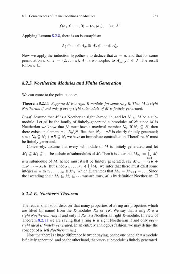
8.2 Consequences of Chain Conditions on Modules 253
f (a1, 0, . . . , 0) = (α1(a1), . . .) ∈ A′.
Applying Lemma 8.2.8, there is an isomorphism
A2 ⊕ · · · ⊕ Am ∼= A′2 ⊕ · · · ⊕ A′
n .
Now we apply the induction hypothesis to deduce that m = n, and that for somepermutation σ of J = {2, . . . , n}, Ai is isomorphic to A′
σ(i), i ∈ J . The resultfollows. �
8.2.3 Noetherian Modules and Finite Generation
We can come to the point at once:
Theorem 8.2.11 Suppose M is a right R-module, for some ring R. Then M is rightNoetherian if and only if every right submodule of M is finitely generated.
Proof Assume that M is a Noetherian right R-module, and let N ⊆ M be a sub-module. Let N be the family of finitely-generated submodules of N ; since M isNoetherian we know that N must have a maximal member N0. If N0 � N , thenthere exists an element n ∈ N0\N . But then N0 + n R is clearly finitely generated;since N0 � N0 + n R ⊆ N , we have an immediate contradiction. Therefore, N mustbe finitely generated.
Conversely, assume that every submodule of M is finitely generated, and let
M1 ⊆ M2 ⊆ · · · be a chain of submodules of M . Then it is clear that M∞ :=∞⋃
i=1Mi
is a submodule of M , hence must itself be finitely generated, say M∞ = x1R +x2R · · · + xn R. But since x1, . . . , xn ∈ ⋃
Mi , we infer that there must exist someinteger m with x1, . . . , xn ∈ Mm , which guarantees that Mm = Mm+1 = . . .. Sincethe ascending chain M1 ⊆ M2 ⊆ · · · was arbitrary, M is by definitionNoetherian. �
8.2.4 E. Noether’s Theorem
The reader shall soon discover that many properties of a ring are properties whichare lifted (in name) from the R-modules RR or R R. We say that a ring R is aright Noetherian ring if and only if RR is a Noetherian right R-module. In view ofTheorem 8.2.11 we are saying that a ring R is right Noetherian if and only everyright ideal is finitely generated. In an entirely analogous fashion, we may define theconcept of a left Noetherian ring.
Note that there is a huge difference between saying, on the one hand, that amoduleis finitely generated, and on the other hand, that every submodule is finitely generated.

254 8 Elementary Properties of Modules
Indeed if R is a ring, then the right R-module RR is certainly finitely generated (viz.,by the identity 1 ∈ R). However, if RR is not right Noetherian, then there will existright ideals of R that are not finitely generated.
However, if the ring R is right Noetherian, then this difference evaporates: this isthe content of Noether’s Theorem.
Theorem 8.2.12 (E. Noether’s Theorem) Let R be a right Noetherian ring, andlet M be a right R-module. Then M is finitely generated if and only if M is rightNoetherian.
Proof Obviously, if M is Noetherian, it is finitely generated. Conversely, we maywrite M = x1R + x2R +· · ·+ xn R and each submodule xi R, being a homomorphicimage of RR , is a Noetherian module. Therefore, M is Noetherian by virtue ofExercise (2) in Sect. 8.5.2. �
Although the above theorem reveals a nice consequence of Noetherian rings,the applicability of the theorem appears limited until we know that such rings arerather abundant. One very important class of Noetherian rings are the principal idealdomains. These are the integral domains such that every ideal is generated by a singleelement, and in Chap.10, we shall have quite a bit more to say about modules oversuch rings. The basic prototype here is the ring Z of integers. That this is a principalideal domain can be shown very easily, as follows. Let 0 �= I ⊆ Z be an ideal andlet d be the least positive integer contained in I . If x ∈ I , then by the “divisionalgorithm” (Lemma 1.1.1) there exist integers q and r with x = qd + r and where0 ≤ r < d. Since r = x − qd ∈ I , we conclude that by the minimality of d, r = 0,i.e., x must be a multiple of d . Therefore,
Lemma 8.2.13 The ring of integers Z is a principal ideal domain.
Note that since an integral domain is by definition commutative, it does not matterwhether we are speaking of right ideals or left ideals here.
This argument used only certain properties shared by all Euclidean Domains(see Sect. 9.3). All of them are principal ideal domains by a proof almost identicalto the above. But principal ideal domains are a larger class of rings, and most ofthe important theorems (about their modules and the unique factorization of theirelements into primes) encompass basically the analysis of finite-dimensional lineartransformations and the elementary arithmetic of the integers. So this subject shallbe taken up in much greater detail in a separate chapter (see Chap.10). Nonetheless,as we shall see in the next subsection, just knowing thatZ is a Noetherian ring, yieldsthe important fact that “algebraic integers” form a ring.
8.2.5 Algebraic Integers and Integral Elements
Let D be a Noetherian integral domain and let K be a field containing D. An elementα ∈ K is said to be integral over D if and only if α is the zero of a polynomial in

8.2 Consequences of Chain Conditions on Modules 255
D[x] having lead coefficient 1. In this case, of course, some power of α is a D-linearcombination of lower powers, say
αn = an−1αn−1 + · · · + a2α
2 + a1α + a0,
where n is a positive integer and the coefficients ai lie in D.In the particular case that D = Z and K is a subfield of the complex numbers,
then any element α ∈ K that is integral over Z is called an algebraic integer. Thus√3 is an algebraic integer (as it is a zero of the polynomial x2 − 3 ∈ Z[x]), but one
can show, however, that 12
√3 is not. The complex number ω = (1 − √−3)/2 is an
algebraic integer because w2 + w + 1 = 0.Their is a simple criterion for an element of K to be integral over D.
Lemma 8.2.14 Let K be a field containing the Noetherian integral domain D. Thenan element α of K is integral over D if and only if the subring D[α] is a finitelygenerated D-module.
Proof First suppose α is integral over D. We must show that D[α] is a finitelygenerated D-module. By definition, there exists a positive integer n such that αn is aD-linear combination of the elements of X := {1,α,α2, . . . ,αn−1}. Let M = 〈X〉D
be the submodule of D[α] generated by X . Now αX contains αn together with lowerpowers of α all of which are D-linear combinations of elements of X . Put moresuccinctly, Mα ⊆ M . It now follows that all positive integer powers of α lie in M ,and so M = D[α]. Since M is generated by the finite set X , D[α] is indeed finitelygenerated.
Now suppose D[α] is a finitely generated D-module. We must show that α isintegral over D—that is, α is a zero of a monic polynomial in D[x]. We now applyNoether’s Theorem (Theorem 8.2.12) to infer that, in fact, D[α] is a NoetherianD-module. But it contains the following chain of submodules:
D ≤ D + αD ≤ D + αD + α2D ≤ . . .
and the Noetherian condition forces this chain to terminate, say at
D + αD + · · · + αn−1D. (8.18)
Then αn D must lie in the module presented in (8.18) and so the element αn isa D-linear combination of lower powers of α. Of course that makes α integralover D. �
The main thrust of this subsection is the following:
Theorem 8.2.15 Let K be a field containing the Noetherian integral domain D andlet O denote the collection of all elements of K that are integral over D. Then O isa subring of K .

256 8 Elementary Properties of Modules
Proof Using the identity (−α) j = (−1) jα j , it is easy to see that if α is the zero ofa monic polynomial in D[x], then so is −α. Thus −O = O.
It remains to show that the set O is closed under the addition and multiplicationoperations of K . Let α and β be any elements ofO. Then there exist positive integersn andm such that the subring D[α] is generated (as a D-module) by powersαi , i < nand similarly the D-module D[β] is generated by powers β j , j < m. Thus everymonomial expression αkβ� in the subring D[α,β] is a D-linear combination of thefinite set of monomial elements {αiβ j |i < n, j < m}. It follows that the D-moduleD[α,β] is finitely generated. Now since D is a Noetherian ring, Theorem 8.2.12implies that D[α,β] is Noetherian.
Now D[α+β] and D[αβ] are submodules of the Noetherian moduleD[α,β] andso are themselves Noetherian by Theorem 8.2.11. But then, invoking once again thefact that D is a Noetherian ring, we see that D[α + β] and D[αβ] are both finitelygenerated D-modules, and so are inO by Lemma 8.2.14. ThusO is indeed a subsetof the field K which is closed under addition and multiplication in K . �
Since the algebraic integers are simply the elements of the complex number fieldC
which are integral over the subringZ of integers, we immediately have the following:
Corollary 8.2.16 The algebraic integers form a ring.
In the opinion of the authors, the spirit of abstract algebra is immortalized in thismaxim:
• a good definition is better than many lines of proof.
Perhaps nothing illustrates this principle better than the proof of Theorem 8.2.15 justgiven. In the straightforward way of proving this theorem one is obligated to producemonic polynomials with coefficients in D for which α + β and αβ are roots; not aneasy task. Yet the above proof was not hard. That was because we had exactly theright definitions!
8.3 The Hilbert Basis Theorem
This section gives us a second important application of Theorem 8.2.12.In this section we consider polynomial rings of the form R[x1, x2, . . . , xn], where
x1, x2, . . . , xn are commuting indeterminates. In the language of Sect. 7.3, theseare the monoid rings RM where M is the free commutative monoid on the set{x1, x2, . . . , xn}. However, and in contrast tomost textbooks, we shall not require thatthe coefficient ring R be commutative. We recall that by Exercise (3) in Sect. 7.5.3,the iterated polynomial ring R[x][y] can be identified with R[x, y]. Since R is notassumed to be commutative, we see a fortiori that the polynomial ring R[x] may notbe commutative. However, we hasten to remind the reader that the indeterminate xcommutes with every element of R. As a result of this, we infer immediately thatR[x] inherits a natural right R-module structure.

8.3 The Hilbert Basis Theorem 257
Theorem 8.3.1 (The Hilbert Basis Theorem) If R is right Noetherian, then R[x] isalso right Noetherian.
Proof It suffices to show that if A is a right ideal of R[x], then A is finitely generatedas a right R[x]-module. Let A+ be the collection of all leading coefficients of allpolynomials lying in A; that is
A+ :=⎧⎨⎩cm | there exists f (x) =
m∑j=0
c j x j ∈ A, deg f (x) = m
⎫⎬⎭ ⊆ R.
Since A is a right ideal in the polynomial ring R[x], A+ is a right ideal in R. Since Ris right Noetherian, we know that A+ must be finitely generated as a right R-module,so we may write
A+ = a1R + a2R + · · · + an R
for suitable elements a1, a2 . . . , an ∈ A+. From the definition of A+, there existpolynomials pi (x) in A having lead coefficients ai , i = 1, 2, . . . , n. Let ni :=deg pi (x) and set m := max{ni }. Now let Rm[x] be the polynomials of degree atmost m in R[x] and set
Am = A ∩ Rm[x].
We claim that
A = Am + p1(x)R[x] + p2(x)R[x] + · · · + pn(x)R[x]. (8.19)
Let f (x) be a polynomial in A of degree N > m and write
f (x) = αx N + terms involving lower powers of x .
Then, as α is the leading coefficient of f (x) we have α ∈ A+, and so
α = a1r1 + a2r2 + · · · anrn
for suitable r1, r2, . . . , rn ∈ R. Then
f1(x) := f (x) − x N−n1 p1(x)r1 − x N−n2 p2(x)r2 − · · · − x N−nn pn(x)rn
is a polynomial in A which has degree less than N . In turn, if the degree of f1(x)
exceeds m this procedure can be repeated. By so doing, we eventually obtain apolynomial h(x) in A of degree at most m, which is equal to the original f (x) minusan R[x]-linear combination of {p1(x), p2(x), . . . , pn(x)}. But since each pi (x) andf (x) all lie in A, we see that h(x) ∈ Am . Thus
f (x) ∈ Am + p1(x)R[x] + · · · pn(x)R[x].

258 8 Elementary Properties of Modules
Since f (x) was an arbitrary member of A, Eq. (8.19) holds.In view of Eq. (8.19), it remains only to show that Am R[x] is a finitely generated
R[x]-module, and this is true if Am is a finitely generated R-module. But Am isan R-submodule of Rm[x] which is certainly a finitely generated R-module (for{1, x, . . . xm} is a set of generators). By Noether’s Theorem (Theorem 8.2.12) Rm[x]is Noetherian and hence so is Am . Thus, Am is a finitely-generated right R-module,and the proof is complete. �
Corollary 8.3.2 If R is right Noetherian, then so is R[x1, . . . , xn].Remark As expected, there is an obvious left version of the above result. Thus, if Ris left Noetherian, than R[x] is also a left Noetherian ring.
8.4 Mapping Properties of Modules
In this section we shall consider the “calculus of homomorphisms” of modules—the idea that constructions can be characterized by mapping properties. Such anapproach, leads to the important notions of exact sequences, projective and injectivemodules, and other notions which feed the rich lore of homological algebra.
8.4.1 The Universal Mapping Properties of the Direct Sumand Direct Product
Characterizing the Direct Sum by a Universal Mapping Property
Recall that the formal direct sum over a family {Mσ|σ ∈ I } of right R-modules is theset of all mappings f : I → ∪σ Mσ, with f (σ) ∈ Mσ , and f (σ) non-zero for onlyfinitely many indices σ. We think of the indices as indicators of coordinates, and thevalue f (σ) as the σ-coordinate of the element f . This is an R-module ⊕σ Mσ underthe usual coordinate-wise addition and application of right operators from R.
There is at hand a canonical collection of injective R-homomorphisms: κσ :Mσ → ⊕σ Mσ defined by setting
(κσ(aσ))(τ ) ={
aσ if σ = τ0 if σ �= τ
where aσ is an arbitrary element of Mσ . That is, κσ takes an element a of Mσ tothe unique element of the direct sum whose coordinate at σ is a, and whose othercoordinates are all zero.
Theorem 8.4.1 Suppose M = ⊕σ∈I Mσ is the direct sum of modules {Mσ|σ ∈ I }with canonical homomorphisms κσ : Mσ → M. Then, for every module B, and

8.4 Mapping Properties of Modules 259
family of homomorphisms φσ : Mσ → B, there exists a unique homomorphismφ : M → B such that φ ◦ κσ = φσ for all σ ∈ I . In fact, this property characterizesthe direct sum up to isomorphism.
Proof We define φ : M → B by the equation
φ(a) :=∑
σφσ(a(σ)).
Since a(σ) ∈ Mσ , by definition, and only finitely many of these summands are non-zero, the sum describes a unique element of B. It is elementary to verify that φ, aswe have defined it, is an R-homomorphism. Moreover, if aτ is an arbitrary elementof Mτ , then
φ ◦ κτ (aτ ) = φ(κτ (aτ )) =∑
σ∈Iφσ(κτ (aτ (σ))) = φτ aτ .
Thus we have φ ◦ κτ = φτ , for all τ .Now suppose there were a second homomorphism λ : M → B, with the property
that λ ◦ κτ = φτ , for all τ ∈ I . Then
λ(a) =∑
σ∈Iλ(κσ(a(σ))) =
∑σ∈I
φσ(a(σ)) = φ(a).
Thus λ = φ. So the homomorphism φ which we have produced is unique.Nowassume that the R-module N , and the collection ofmorphismsλσ : Mσ → N
satisfy the universal mapping conditions of the last part of the theorem.First apply this property to M when B = N and φσ = λσ . Then there is a
homomorphism λ : M → N with λ ◦ κσ = λσ .Similarly, there is a homomorphism κ : N → M for which κ ◦ λσ = κσ . It
follows thatκ ◦ κσ = κ ◦ λσ = κσ = 1M ◦ κσ,
where 1M is the identity morphism on M . So by the uniqueness of the homomor-phism, one may conclude that κ◦λ = 1M . Similarly, reversing the roles, λ◦κ = 1N .Therefore κ is an isomorphism. The proof is complete. �
We have seen from our earlier definition of the direct sum M = ⊕σ∈I Mσ thatthere are projection mappings πσ : M → Mσ which, for any element m ∈ M , readsoff its σ-coordinate, m(σ). One can see that these projection mappings are related tothe canonical mappings κσ by the equations
πi ◦ κi = 1 (the identity mapping on Mi ) (8.20)
πi ◦ κ j = 0 if i �= j. (8.21)
We remark that the existence of the projection mappings πi with the compositionsjust listed could have been deduced directly from the universal mapping property

260 8 Elementary Properties of Modules
which characterizes the direct sum. Let δi j be the morphism M j → Mi which isthe zero map if i �= j , but is the identity mapping on Mi if i = j . If we apply theuniversal property with Mi and δi j in the respective roles of B and φi , we obtain thedesired morphism φ = πi : M → Mi with πi ◦ κ j = δi j .
Characterizing the Direct Product by a Universal Mapping Property
We can now characterize the direct product of modules by a universal property whichis the complete dual of that for the direct sum.
Theorem 8.4.2 Suppose M = ∏σ∈I Mσ is the direct product of the modules
{Mσ|σ ∈ I } with canonical projections πσ : M → Mσ . Then, for every moduleB, and family of homomorphisms φi : B → Mi there exists a unique homomor-phism φ : B → M such that πi ◦φ = φi , for each i ∈ I . This property characterizesthe direct product up to isomorphism.
Proof The canonical projection mapping πi , recall, reads off the i-th coordinate ofeach element of M . Thus, if m ∈ M , m is a mapping I → ∪Mσ with m(i) ∈ Mi ,and πi (m) := m(i).
Now define the mapping φ : B → M by the rule:
φ(b)(i) := φi (b),
for all (i, b) ∈ I × B. Then certainly φ is an R-homomorphism. Moreover, onechecks that
(πi ◦ φ)(b) = πi (φ(b)) = (φ(b))(i) = φi (b).
Thus πi ◦ φ = φi .Now if ψ : B → M were an R-homomorphism which also satisfied πi ◦ ψ = φi ,
for all i ∈ I , then we should have
(ψ(b))(i) = πi (ψ(b)) = (πi ◦ ψ)(b) = φi (b) = (φ(b))(i),
at each i , so ψ(b) = φ(b) at each b ∈ B—i.e. ψ = φ as mappings.Now suppose N were some R-module equipped with morphisms π′
i : N → Mi ,i ∈ I satisfying thismapping property:whenever there is amodule B withmorphismsφi : B → Mi , then there is a morphism φB : B → N such that π′
i ◦ φB = φi .First we use the property for M . Setting B = N and φi = π′
i , we obtain (in therole of φ) a morphism π′ : N → M such that πi ◦ π′ = π′
i .Similarly, using the same property for N (with M and πi in the roles of B and the
φi ), we obtain a homomorphism π : M → N such that π′i ◦ π′ = πi . It follows that
πi ◦ π′ ◦ π = π′i ◦ π = πi = πi ◦ 1M .

8.4 Mapping Properties of Modules 261
By the uniqueness, one has π′ ◦ π = 1M . Similarly π ◦ π′ = 1N . Therefore π is anisomorphism.
As afinal remark, the universalmappingproperty canbeused to show the existenceof mappings κi : Mi → ∏
i∈I Mi such that πi ◦κ j is the identity map on Mi if i = j ,and is the zero mapping Mi → M j if i �= j . �
8.4.2 HomR(M, N)
The Basic Definition
We shall continue to assume that R is an arbitrary ring with identity element 1R . IfM, N are right R-modules, then we may form the abelian group HomR(M, N ) con-sisting of R-module homomorphisms M → N . Indeed, the abelian group structureon HomR(M, N ) is simply given by pointwise addition: if φ, θ ∈ HomR(M, N ),then (φ + θ)(m) := φ(m) + θ(m) ∈ N .
HomR(M, N) Is a Left R-Module
We remark here that HomR(M, N ) possesses a natural structure of a left R-module:For each ring element r ∈ R and homomorphism φ ∈ HomR(M, N ), the mappingr · φ is defined by
(r · φ)(m) := φ(mr) = φ(m)r
Notice, by this definition, that for r, s ∈ R, and m ∈ M ,
(r · (s · φ))(m) = (s · φ)(mr) = (φ(mr))s (8.22)
= (φ(m)r)s = φ(m)(rs) = ((rs) · φ)(m). (8.23)
In the preceding equations left multiplication of maps by ring elements was indi-cated by a “dot”. The sole purpose of this device was to clearly distinguish thenewly-defined left ring multiplications of maps from right ring multiplication ofthe module elements in the equations. However, from this point onward, the “dot”operation will be denoted by juxtaposition as we have been doing for left modulesgenerally.
Clearly rφ ∈ HomR(M, N ), and the reader can easily check that the requiredequations of mappings hold:
r(φ1 + φ2) = rφ1 + rφ2,
(r + s)φ1 = rφ1 + sφ1, and
(rs)φ1 = r(sφ1),

262 8 Elementary Properties of Modules
where r, s ∈ R and φi ∈ HomR(M, N ), i = 1, 2. In particular, when R is acommutative ring, one may regard HomR(M, N ) as a right R-module simply bypassing scalars from one side to another. (For more about making HomR(M, N ) intoa module, see the Exercise Sect. 8.5.3.)
In the special case that N = RR , and M is any right R-module, we obtain a leftR-module M∗ := HomR(M, RR) called the dual module of M. We shall have usefor this latter, especially when R is a field.
Basic Mapping Properties of HomR(M, N)
We note that HomR has the following mapping properties. If α : M1 → M2 andβ : N1 → N2 are homomorphisms of right R-modules, then we have an inducedhomomorphism of abelian groups,
Hom(α,β) : HomR(M2, N1) → HomR(M1, N2), φ �→ β ◦ φ ◦ α. (8.24)
Let idM denote the identity mapping M → M .2
The reader should have no difficulty in verifying that Hom(idM ,α) really is ahomomorphism of abelian groups. In particular, if we fix a right R-module M , thenthe induced homomorphism of abelian groups are:
Hom(idM ,β) : HomR(M, N1) → HomR(M, N2), φ �→ β ◦ φ. (8.25)
In a language that will be developed later in this book, this says that the assignmentHomR(M, •) is a “functor” from the “category” of right R-modules to the “category”of abelian groups. (See Sect. 13.2 for a full exposition.) Likewise, if N is a fixed rightR-module, and if α : M2 → M1 is an R-module homomorphism, then we have aninduced homomorphism of abelian groups
Hom(α, idN ) : HomR(M1, N ) → HomR(M2, N ), φ �→ φ ◦ α.
This gives rise to another “functor,” HomR(•, N ), from the category of rightR-modules to the category of abelian groups, but is “contravariant” in the sensethat the directions of the homomorphisms get reversed:
M1φ← M2 gets mapped to HomR(M1, N )
β→ HomR(M2, N ).
2The notation “idM” serves to distinguish the identity mapping on the set M from the multiplicativeidentity element 1M of any ring or monoid which unfortunately happens to be named “M”.

8.4 Mapping Properties of Modules 263
8.4.3 Exact Sequences
Definition
Let φ : M → N be a homomorphism of right R-modules, and set M ′′ :=φ(M), M ′ = ker φ. Then we may build a sequence of homomorphisms
M ′ μ−→ Mε−→ M ′′,
where μ : M ′ ↪→ M is just the inclusion homomorphism and where ε(m) = φ(m) ∈M" for all m ∈ M . Furthermore, by definition, we notice the seemingly innocuousfact that ker ε = im μ.
More generally, suppose that we have a sequence of right R-modules andR-module homomorphisms:
· · · → Mi−1φi−1−→ Mi
φi−→ Mi+1 → · · · .
We say that the above sequence exact at Mi if im φi−1 = ker φi . The sequenceabove is said to be exact if it is exact at every Mi . Note that the homomorphism
μ : M → N is injective if and only if the sequence 0 → Mμ→ N is exact. Likewise
ε : M → N is surjective if and only if the sequence Mε→ N → 0 is exact.
Of particular interest are the short exact sequences. These are exact sequences ofthe form
0 → M ′ μ→ Mε→ M ′′ → 0.
Note that in this case Theorem 8.1.2 simply says that M ′′ ∼= M /μ(M ′).
The Left-Exactness of Hom
The “hom functors” come very close to preserving short exact sequences, as follows.
Theorem 8.4.3 Let 0 → N ′ μ−→ Nε−→ N ′′ be an exact sequence of right
R-modules, and let M be a fixed R-module. Then the following sequence of abeliangroups is also exact:
0 → HomR(M, N ′) Hom(1M ,μ)−→ HomR(M, N )Hom(1M ,ε)−→ HomR(M, N ′′).
Likewise, if M ′ μ−→ Mε−→ M ′′ → 0 is an exact sequence of right R-modules, and
if N is a fixed R-module, then the following sequence of abelian groups is exact:
0 → HomR(M ′′, N )Hom(μ,1N )−→ HomR(M, N )
Hom(ε,1N )−→ HomR(M ′, N ).

264 8 Elementary Properties of Modules
Proof Assume that 0 → N ′ μ−→ Nε−→ N ′′ is exact and that M is a fixed
R-module. First of all, note that if φ′ ∈ HomR(M, N ′), then since μ is injec-tive, we see that 0 = Hom(M,μ)(φ′) = μ ◦ φ′ clearly implies that φ′ = 0,and so Hom(M,μ) : HomR(M, N ′) → HomR(M, N ) is injective. Next, sinceHom(M, ε) ◦ Hom(M,μ) = Hom(M,μ ◦ ε) = Hom(M, 0) = 0, we haveimHom(M,μ) ⊆ ker Hom(M, ε). Finally, suppose that φ ∈ ker Hom(M, ε). Thenε ◦ φ = 0 : N → M ′′ which says that for each n ∈ N , φ(n) ∈ ker ε = im μ,i.e. φ(n) ∈ im μ for each n ∈ N . But since μ : M ′ → M is injective, we maywrite φ(n) = μ ◦ φ′(n) for some uniquely defined element φ′(n) ∈ M ′. Finally,since φ′ : N → M ′ is clearly a homomorphism, we are finished as we have provedthat Hom(M,μ)(φ′) = φ. The second statement in the above theorem is provedsimilarly. �
If the sequences in Theorem 8.4.3 were completed to short exact sequences, itwould be natural to wonder whether the resulting sequences would be exact. This isnot the case as the following simple counterexample shows. Consider the short exactsequence of Z-modules (i.e., abelian groups):
0 → Zμ2−→ Z
ε−→ Z/Z2 → 0,
where μ2 : Z → Z is multiplication by 2: μ2(m) = 2m, and where ε is the canonicalquotient mapping. The sequence below
0 → HomZ(Z/Z2,Z)Hom(1,μ2)−→ HomZ(Z/Z2,Z)
Hom(1,ε)−→ HomZ(Z/Z2,Z/Z2) → 0
is not exact as HomZ(Z/Z2, Z) = 0, whereas HomZ(Z/Z2, Z/Z2) ∼= Z/Z2, andso Hom(Z/Z2, ε) : HomZ(Z/Z2, Z) → HomZ(Z/Z2, Z/Z2) certainly cannot besurjective.
Thus, we see that the “hom functors” do not quite preserve exactness. The extentto which short exact sequences fail to map to short exact sequences—and the remedyfor this deficiency is the subject of homological algebra. (In a subsequent chapter,we shall encounter another “functor” (namely that derived from the tensor product)from right R-modules to abelian groups which also fails to preserve short exactsequences).
Split Exact Sequences
Note that given any right R-modules M ′, M ′′, we can always build the followingrather trivial short exact sequence:
0 → M ′ μ1−→ M ′ ⊕ M ′′ π2−→ M ′′ → 0,
where μ1 is inclusion into the first summand and π2 is projection onto the secondsummand. Such a short exact sequence is called a split short exact sequence. More

8.4 Mapping Properties of Modules 265
generally, we say that the short exact sequence 0 → M ′ μ−→ Mε−→ M ′′ → 0 splits
if and only if there is an isomorphism α : M → M ′ ⊕ M ′′ making the followingladder diagram commute3:
0 −−−−→ M ′ μ−−−−→ Mε−−−−→ M ′′ −−−−→ 0⏐⏐�1M ′
⏐⏐�α
⏐⏐�1M ′′
0 −−−−→ M ′ μ1−−−−→ M ′ ⊕ M ′′ π2−−−−→ M ′′ −−−−→ 0
In turn, the following lemma provides simple conditions for a short exact sequenceto split:
Lemma 8.4.4 Let0 → M ′ μ−→ M
ε−→ M ′′ → 0 (∗)
be a short exact sequence of right R-modules. Then the following conditions areequivalent:
(i) There exists an R-module homomorphism σ : M ′′ → M such that ε ◦ σ = 1M ′′ .(ii) There exists an R-module homomorphism ρ : M → M ′ such that ρ ◦ μ = 1M ′ .
The short exact sequence (*) splits.
Proof Clearly condition (iii) implies both (i) and (ii); we shall be content to provethat (i) implies (iii), leaving the remaining implication to the reader. Note first thatsince ε ◦ σ = 1M ′′ , it follows immediately that σ : M ′′ → M is injective. Inparticular, σ : M ′′ → σ(M ′′) is an isomorphism. Clearly it suffices to show thatM = μ(M ′) ⊕ σ(M ′′) (internal direct sum). If m ∈ M then ε(m − σ(ε(m))) =ε(m) − (ε ◦ σ)(ε(m)) = ε(m) − ε(m) = 0, which says that m − σ(ε(m)) ∈ ker ε =im μ. Therefore, there exists m ′ ∈ M ′ with m − σ(ε(m)) = μ(m′), forcing m =μ(m′) + σ(ε(m)) ∈ μ(M ′) + σ(M ′′). Finally, if for some m′ ∈ M ′, m′′ ∈ M ′′, sothat μ(m′) = σ(m′′), then m′′ = ε(σ(m′′)) = ε(μ(m′)) = 0, which implies thatμ(M ′) ∩ σ(M ′′) = 0, proving that M = μ(M ′) ⊕ σ(M ′′), as required. �
8.4.4 Projective and Injective Modules
Let R be a ring and let P be an R-module. We say that P is projective if everydiagram of the form
P⏐⏐�φ′′
Mε−−−−→ M ′′ −−−−→ 0 (exact row)
3Recall the definition of “commutative diagram” on p. 237.

266 8 Elementary Properties of Modules
can be embedded in a commutative diagram of the form
P
M”M 0 (exact row)
�
��
��� �
ε
φ φ′′′
Note first that any free right R-module is projective. Indeed, assume that F is afree right R-module with basis { fα | α ∈ A} and that we have a diagram of the form
F⏐⏐�φ′′
Mε−−−−→ M ′′ −−−−→ 0 (exact row)
For each m′′α := φ′′( fα) ∈ M ′′, α ∈ A, select an element mα ∈ M with
ε(mα) = m′′α, α ∈ A. As F is free with basis { fα | α ∈ A}, there exists a (unique)
homomorphism φ : F → M with φ( fα) = mα, α ∈ A. This gives the desired“lifting” of the homomorphism φ′′ :
F
M”M 0 (exact row)
�
��
��� �
ε
φ φ′′
We have the following simple characterization of projective modules.
Theorem 8.4.5 The following conditions are equivalent for the R-module P.
(i) P is projective.(ii) Every short exact sequence 0 → M ′ → M → P → 0 splits.
(iii) P is a direct summand of a free R-module.
Proof That (i) implies (ii) follows immediately from Lemma 8.4.4. Now assumecondition (ii) and let ε : F → P be a surjective R-module homomorphism, whereF is a free right R-module. Let K = ker ε and consider the commutative diagram
P
0 K PF 0�
��
��� � � �
μ ε
σ 1P

8.4 Mapping Properties of Modules 267
where μ : K ↪→ F , and where the homomorphism σ : P → F exists by the projec-tivity of P. Apply Lemma 8.4.4 to infer that F ∼= μ(K ) ⊕ σ(P); since σ(P) ∼= P .Thus (iii) holds.
Finally, we prove that (iii) implies (i). Thus, let F be a free right R-module whichadmits a direct sum decomposition F = N ⊕ P , where N ⊆ F is a submodule.From the diagram
P⏐⏐�φ′
M −−−−→ε
M ′′ −−−−→ 0
we obtain the following diagram.
F = N ⊕ P P
M M ′′ 0�ε
�� �
��μ
π
θ φ
Here π : N ⊕ P → P is the projection of the sum onto the right coordinate, andμ : P → N ⊕ P is the injection onto 0⊕ P so that π ◦μ = 1P . The homomorphismθ : F → M satisfying ε ◦ θ = φ ◦ π2 exists since, as already observed above, freemodules are projective. However, setting φ := θ ◦ μ gives the desired lifting of φ,and so it follows that P is projective. �
Dual to the notion of a projective module is that of an injective module. A rightR-module I is said to be injective if every diagram of the form
I
θ′�⏐⏐
0 −−−−→ M ′ μ−−−−→ M (exact row)
can be embedded in a commutative diagram of the form
0 M’
I
M
��
��
� �
μ
θ′ θ
In order to obtain a characterization of injective modules we need a concept dualto that of a free module. In preparation for this, however, we first need the concept of

268 8 Elementary Properties of Modules
a divisible abelian group. Such a group D satisfies the property that for every d ∈ Dand for every 0 �= n ∈ Z, there is some c ∈ D such that nc = d.
Example 44 1. The most obvious example of a divisible group is probably theadditive group (Q,+) of rational numbers.
2. A moment’s thought should reveal that if F is any field of characteristic 0, then(F,+) is a divisible group.
3. Note that any homomorphic image of a divisible group is divisible. Of paramountimportance is the divisible group Q/Z.
4. Let p be a prime, and let Z(p∞) be the subgroup of Q/Z consisting of elementsof p-power order. ThenZ(p∞) is a divisible group. (You should check this. Notethat there is a direct sum decomposition Q/Z = ⊕
Z(p∞), where the directsum is over all primes p).
5. Note that the direct product of any number of divisible groups is also divisible.
The importance of divisible groups is displayed by the following.
Theorem 8.4.6 Let D be an abelian group. Then D is divisible if and only if D isinjective.
Proof Assume first that D is injective. Let d ∈ D, and let 0 �= n ∈ Z. We form thediagram
0 Z
D
Z
��
��
� �
μn
θ′ θ
where μn : Z → Z is multiplication by n, θ′(m) = md, m ∈ Z, and where θ is theextension of θ′ guaranteed by the injectivity of D. If θ(1) = c then nc = nθ(1) =θ(n) = θ(μn(1)) = θ′(1) = d , proving that D is divisible.
Conversely, assume that D is divisible and that we are given a diagram of theform
D
θ′�⏐⏐
0 −−−−→ A′ μ−−−−→ A
where μ : A′ → A is an injective homomorphism of abelian groups. We shall, forthe sake of convenience, assume that A′ ≤ A via the injective homomorphism μ. LetP = {(A′′, θ′′)} where A′ ≤ A′′ ≤ A and where θ′′ : A′′ → D is a homomorphismwith θ′′|A′ = θ′. We make P into a poset via the relation (A′′
1, θ′′1) � (A′′
2, θ′′2) if
and only if A′′1 ≤ A′′
2 and θ′′2 |A′′
1= θ′′
1 . Since (A′, θ′) ∈ P , it follows that P �= ∅. If{(A′′
α, θ′′α)}α∈A is a chain inP , wemay set A′′ = ⋃
α∈A A′′α, and define θ′′ : A′′ → D
by setting θ′′(a′′) = θ′′α(a′′) where a′′ ∈ A′′
α. Since {(A′′α, θ′′
α)}α∈A is a chain, it

8.4 Mapping Properties of Modules 269
follows that θ′′(a′′) doesn’t depend upon the particular choice of index α ∈ A witha′′ ∈ A′′
α. Therefore, we see that the chain {(A′′α, θ′′
α)}α∈A has (A′′, θ′′) as an upperbound. This allows us to apply Zorn’s lemma and infer the existence of a maximalelement (A′′
0, θ′′0) ∈ P . Clearly the proof is complete once we show that A′′
0 = A.Assume, by way of contradiction, that there exists an element a ∈ A\A′′
0, and letm be the order of the element a + A′′
0 in the additive group A/A′′0. We divide the
argument into the two cases according to m = ∞ and m < ∞.
m = ∞. In this case it follows easily that Z〈a〉 is an infinite cyclic group and thatZ〈a〉 ∩ A′′
0 = 0. As a result, A′′ := Z〈a〉 + A′′0 = Z〈a〉 ⊕ A′′
0 and an extension ofθ′′0 can be obtained simply by setting θ′′(ka + a′′
0 ) = θ′′0 , k ∈ Z, a′′
0 ∈ A′′0. This
is a well-defined homomorphism A′′ → D extending θ′′0 . But that contradicts the
maximality of (A′′0, θ
′′0) in the poset P .
m < ∞. Here, we have that ma ∈ A′′0 and so θ′′
0(ma) ∈ D. Since D is divisible,there exists an element c ∈ D with mc = θ′′
0(ma). Now define θ′′ : A′′ :=Z〈a〉 + A′′
0 → D by setting θ′′(ka + a′′0 ) = kc + θ′′
0(a′′0 ) ∈ D. We need to show
that θ′′ is well defined. Thus, assume that k, l are integers and that a′′0 , b′′
0 ∈ A′′0
are such that ka +a′′0 = la +b′′
0 . Then (k −l)a = b′′0 −a′′
0 ∈ A′′0 and so k −l = rm
for some integer r . Therefore
kc − lc = rmc
= rθ′′0(ma)
= θ′′0(rma)
= θ′′0(b
′′0 − a′′
0 )
= θ′′0(b
′′0) − θ′′
0(a′′0 ),
which says thatkc + θ′′
0(a′′0 ) = lc + θ′′
0(b′′0)
and so θ′′ : A′′ → D is well defined. As clearly θ′′ is a homomorphism extendingθ′′0 , we have once again violated the maximality of (A′′
0, θ′′0) ∈ P , and the proof
is complete. �
Let R be a ring, and let A be an abelian group. Define M := HomZ(R, A); thusM is certainly an abelian group under point-wise operations. Give M the structureof a right R-module via
( f · r)(s) = f (rs), r, s ∈ R, f ∈ M.
It is easy to check that the above recipe gives HomZ(R, A) the structure of a rightR-module. (See Exercise (1) in Sect. 8.5.3.)
The importance of the above construction is found in the following.
Proposition 8.4.7 Let R be a ring and let D be a divisible abelian group. Then theright R-module HomZ(R, D) is an injective R-module.

270 8 Elementary Properties of Modules
Proof Suppose that we are given the usual diagram
HomZ(R, D)
θ′�⏐⏐
0 −−−−→ M ′ μ−−−−→ M (exact row)
The homomorphism θ′ : M ′ → HomZ(R, D) induces the homomorphism φ′ :M ′ → D by setting φ′(m′) = θ′(m′)(1), for all m′ ∈ M ′. Since D is divisible, it isinjective and so we may form the commutative diagram:
0 M’
D
M
��
��
� �
μ
φ′ φ
In turn, we now define θ : M → HomZ(R, D) by setting θ(m)(r) := φ(mr) ∈ D.It is routine to check that θ is a homomorphism of right R-modules and that thefollowing diagram commutes:
0 M’
HomZ(R, D)
M (exact row)
��
�
� �
μ
θ′θ
Thus HomZ is an injective R-module. �
Recall that any free right R-module is the direct sum of a number of copies of RR ,and that any R-module is a homomorphic image of a free module. We now define acofree R-module to be the direct product (not sum!) of any number of copies of theinjective module HomZ(R, Q/Z). Note that by Exercise (12) in Sect. 8.5.3, a cofreemodule is injective. We now have
Proposition 8.4.8 Let M be an R-module. Then M can be embedded in a cofreeR-module.
Proof Let 0 �= m ∈ M and pick a nonzero element α(m) ∈ Q/Z whose ordero(m) in the additive group Q/Z is equal to that of m in the additive group M . (For,example, one could choose α(M) = (1/o(m)) + Z.) This gives an additive grouphomomorphism α : Z〈m〉 → Q/Z given by α(km) = kα(m), for each integer k.As Q/Z is a divisible abelian group, there exists a homomorphism of abelian groupsαm : M → Q/Z extending α : Z〈m〉 → Q/Z. In turn, this homomorphism gives

8.4 Mapping Properties of Modules 271
a homomorphism βm : M → HomZ(R, Q/Z) defined by setting βm(m′)(r) =αm(m′r) ∈ Q/Z. It is routine to verify that βm is indeed, a homomorphism of rightR-modules.
Next, we form the cofree module C := ∏0 �=m∈M HomZ(R, Q/Z)m , where each
HomZ(R, Q/Z)m = HomZ(R, Q/Z). Collectively, the homomorphisms βm, 0 �=m ∈ M , give a homomorphism μ : M → C via
μ(m′)(m) = βm(m′) ∈ HomZ(R, Q/Z).
It remains only to show that μ is injective. Suppose m were a non-zero element inker μ. Then μ(m)(m′) = 0 for all 0 �= m′ ∈ M . But this says in particular that0 = βm(m) ∈ HomZ(R, Q/Z), forcing αm(m) = βm(m)(1) = 0. That assertion,however, produces a contradiction since αm(m) = α(m) was always chosen to havethe same additive order o(m) of the non-zero element m in (M,+). �
Finally we have the analogue of Theorem 8.4.5, above; the proof is entirely dualto that of Theorem 8.4.5.
Theorem 8.4.9 The following conditions are equivalent for the R-module I .
(i) I is injective.(ii) Every short exact sequence 0 → I → M → M ′′ → 0 splits.
(iii) I is a direct summand of a cofree R-module.
8.5 Exercises
8.5.1 Exercises for Sect. 8.1
1. Show that any abelian group is a Z-module. [Hint: Write the group operation asaddition, and define the multiplication by integers.]
2. (Right modules from left modules). In the remark on p. 233, a recipe is given forconverting a left R module into a right S-module, by the formula ms := ψ(s)m,where m ∈ M , a left R-module, s ∈ S and where ψ : S → Opp(R) is a ringhomomorphism mapping the multiplicative identity element of S to that of R.Show that all the axioms of a right S-module are satisfied by this rule.
3. (Annihilators of modules as two-sided ideals.) Suppose that M is a rightR-module.
(a) Show that Ann(M) := {r ∈ R|Mr = 0M } is a two-sided ideal in R. (It iscalled the annihilator of M.)
(b) Suppose A ≤ B ≤ M is a chain of submodules of the right R-module M .Show that
(A : B) := {r ∈ R|Br ⊆ A}

272 8 Elementary Properties of Modules
is a 2-sided ideal of R. [Hint: (A : B) is the annihilator of the submoduleB/A. Use the previous step. Note that if A and B are right ideals of R (thatis, submodules of RR), then Ann(B/A) is just the residual quotient (A : B)
defined on p. 196.]
4. Prove Corollary 8.1.7. [Hint: Establish the criterion of Lemma 8.1.6.]5. (Finite generation)
(a) Let (Q,+) be the additive group of the field of rational numbers. Being anabelian group, this group is a Z-module by Exercise (1) in Sect. 8.5.1. Showthat (Q,+) is not finitely generated as a Z-module. [Hint: Pay attention todenominators.]
(b) Suppose M is a finitely generated right R-module. Show that for any gen-erating set X for M , there is a finite subset X0 of X which also generatesM . [Hint: By assumption there exists a finite generating set F . Write eachmember of F as a finite R-linear combination of elements of X .]
6. Let Mα, M ′α, α ∈ A be right R-modules, and let φα : Mα → M ′
α, α ∈ A beR-module homomorphisms. Prove that there is a unique homomorphism
∏φα :∏
Mα → ∏M ′
α making each diagram below commute:
∏α∈A Mα
∏φα−−−−→ ∏
α∈A M ′α
πβ
⏐⏐� π′β
⏐⏐�Mβ
φβ−−−−→ M ′β
7. Let Mα, M ′α, α ∈ A be right R-modules, and let φα : Mα → M ′
α, α ∈ A beR-module homomorphisms. Prove that there is a unique homomorphism ⊕φα :⊕
Mα → ⊕M ′
α making each diagram below commute:
Mβπβ−−−−→ M ′
β
μβ
⏐⏐� μ′β
⏐⏐�⊕α∈A Mα
⊕φα−−−−→ ⊕α∈A M ′
α
8. Prove, or provide a counterexample to the following statement. Any submoduleof a free module must be free.
9. Prove that the direct sum of free R-modules is also free.

8.5 Exercises 273
8.5.2 Exercises for Sects. 8.2 and 8.3
1. Show that any submodule or factor module of a Noetheriean (Artinian) moduleis Noetherian (Artinian). [Hint: This is Sect. 2.3, Corollary 2.3.7.]
2. Suppose M = N1 + · · · + Nk , a sum of finitely many submodules Ni . Show thatif each submodule Ni is Noetherian (Artinian) then M is Noetherian (Artinian).[Hint: This is Sect. 2.5.4, Lemma 2.5.7, part (i).]
3. Show that if N is a submodule of M then M is Noetherian (Artinian) if and onlyif both N and M /N are Noetherian (Artinian). [Hint: Isn’t this just the content ofLemma 2.5.6 of Sect. 2.5.4?]
4. Show that if M /Ai is a Noetherian (Artinian) right module for a finite collection ofsubmodules A1, . . . An , then so is M /(A1 ∩ · · · ∩ An). [Hint: Refer to Sect. 2.5.4,Lemma 2.5.7, part (ii).]
5. Let R be a ring. Suppose the R-module RR is Noetherian (Artinian)—that is,the ring R is right Noetherian (right Artinian). Show that any finitely generatedright R-module is Noetherian (Artinian). [Hint: Such a right module M is ahomomorphic image of a free module F = x1R ⊕· · ·⊕ xk R over a finite numberof generators. Then apply other parts of this exercise.]
6. Suppose the right R-module M satisfies the ascending chain condition onsubmodules. Then every generating set X of M contains a finite subset thatgenerates M .
7. Let F be a field and let V = F (n), the vector space of n-tuples of elementsof F , where n is a positive integer. Recall that an n-tuple α := (a1, . . . , an) isa zero of the polynomial p(x1, . . . , xn) if and only p(a1, . . . , an) = 0 (moreprecisely, the polynomial p is in the kernel of the evaluation homomorphismeα : F[x1, . . . , xn] → F (see p. 209)).
(a) Show that if {p1, p2, . . .} is an infinite set of polynomials in the polynomialring F[x1, . . . , xn], and Vi is the full set of zeros of the polynomial pi , thenthe set of common zeros of the pi—that is the intersection ∩Vi—is actuallythe intersection of finitely many of the Vi .
(b) Show that for any subset X of V there exists a finite set SX := {p1, . . . pk}polynomials such that any polynomial which vanishes on X is an F-linearcombination of those in the finite set F .
(c) Recall that a variety is the set of common zeros in V of some collectionof polynomials in F[x1, . . . , xn]. The varieties in V form a poset under theinclusion relation (see p. 209). Show that the poset of varieties of V possessesthe descending chain condition. [Hint: All three parts exploit theHilbert BasisTheorem.]

274 8 Elementary Properties of Modules
8.5.3 Exercises for Sect. 8.4
1. Let M be a left R-module and let A be an abelian group. Show that theright R-scalar multiplication on HomZ(M, A) defined by setting ( f r)(m) =f (rm) ∈ A, gives HomZ(M, A) the structure of a right R-module. If Ais also a left R-module is the subgroup HomR(M, A) an R-submodule ofHomZ(M, A)?
2. Let R, S be rings. Recall from p. 234 that an (R, S)-bimodule is an abeliangroup M having the structure of a left R-module and the structure of a rightS-module such that these scalar multiplications commute, i.e., r(ms) = (rm)sfor all m ∈ M, r ∈ R and s ∈ S.4 Now assume that M is an (R, S)-bimoduleand that N is a right S-module. Show that one may give HomS(M, N ) thestructure of a right R-module by setting ( f r)(m) = f (rm), r ∈ R, m ∈M, f ∈ HomS(M, N ).
3. Let M be a right R-module. Interpret and prove:
HomR(R, M) ∼=R M.
4. Show that the “functorially induced mapping” of Eq. (8.24) is a homomorphismas left R-modules. [Hint: the only real point is to verify the equation
β ◦ (rφ) ◦ α = r(β ◦ φ ◦ α)
using the left R-action defined for these modules on p. 261 preceding theequation.]
5. Let R be a ring, let M be a right R-module, and let A be an abelian group.Interpret and prove:
HomR(M,HomZ(R, A)) ∼=Z HomZ(M, A).
6. Let R be an integral domain in which every ideal is a free R-module. Prove thatR is a principal ideal domain.
7. (a) Let M, N1 and N2 be right R-modules. Show that
Hom(M, N1 ⊕ N2) ∼=Z Hom(M, N1) ⊕ Hom(M, N2).
More generally, show that if {Nα, α ∈ A} is a family of right R-modules,then
Hom
(M,
⊕α∈A
Nα
)∼=Z
⊕α∈A
Hom(M, Nα).
4Perhaps the most important example of bimodules occur as follows: if R is a ring and if S ⊆ R isa subring, then R is an (R, S)-bimodule.

8.5 Exercises 275
(b) Let N , M1 and M2 be right R-modules and show that
Hom(M1 × M2, N ) ∼=Z Hom(M1, N ) × Hom(M2, N ).
More generally, show that if {Mα, α ∈ A} is a family of R-modules, then
Hom
( ∏α∈A
Mα, N
)∼=Z
∏α∈A
Hom(Mα, N ).
(c) Show that if0 → N ′ μ→ N
ε→ N ′′ → 0
is a split short exact sequence of R-modules, and if M is a fixed rightR-module, then the sequences
0 → Hom(M, N ′) Hom(1M ,μ)−→ Hom(M, N )Hom(1M ,ε)−→ Hom(M, N ′′) → 0,
and
0 → Hom(N ′′, M)Hom(μ,1M )−→ Hom(N , M)
Hom(ε,1M )−→ Hom(N ′, M) → 0,
are both exact (and also split).8. Show that the sequences which appear in Theorem 8.4.3 exhibiting the left or
right exactness of the “hom’ functors” are morphisms as left R-modules, notjust abelian groups.
9. Let 0 → M ′ → M → M ′′ → 0 be a short exact sequence of right R-modules.Prove that M is Noetherian (resp. Artinian) if and only if both M ′, M ′′ are. [Ofcourse, this is just a restatement of Exercise (3) in Sect. 8.5.2]
10. Prove that if Aα, α ∈ A, is a family of abelian groups, then
HomZ
(R,
∏α∈A
Aα
)∼=R
∏α∈A
HomZ(R, Aα).
11. Let Pα ,α ∈ A be a family of right R-modules. Show that⊕
α∈APα is projective
if and only if each Pα is projective.12. Let Iα ,α ∈ A be a family of right R-modules. Show that
∏α∈A
Iα is injective if
and only if each Iα is injective.13. Let P be an R-module. Prove that P is projective if and only if given any exact
sequence 0 → M ′ μ→ Mε→ M ′′ → 0, the induced sequence
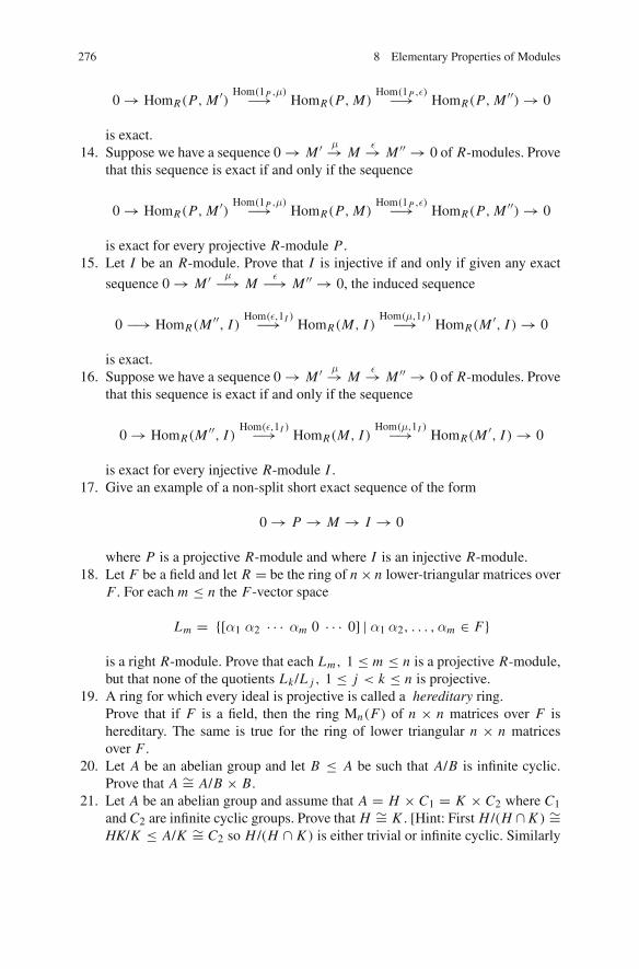
276 8 Elementary Properties of Modules
0 → HomR(P, M ′) Hom(1P ,μ)−→ HomR(P, M)Hom(1P ,ε)−→ HomR(P, M ′′) → 0
is exact.14. Suppose we have a sequence 0 → M ′ μ→ M
ε→ M ′′ → 0 of R-modules. Provethat this sequence is exact if and only if the sequence
0 → HomR(P, M ′) Hom(1P ,μ)−→ HomR(P, M)Hom(1P ,ε)−→ HomR(P, M ′′) → 0
is exact for every projective R-module P .15. Let I be an R-module. Prove that I is injective if and only if given any exact
sequence 0 → M ′ μ−→ Mε−→ M ′′ → 0, the induced sequence
0 −→ HomR(M ′′, I )Hom(ε,1I )−→ HomR(M, I )
Hom(μ,1I )−→ HomR(M ′, I ) → 0
is exact.16. Suppose we have a sequence 0 → M ′ μ→ M
ε→ M ′′ → 0 of R-modules. Provethat this sequence is exact if and only if the sequence
0 → HomR(M ′′, I )Hom(ε,1I )−→ HomR(M, I )
Hom(μ,1I )−→ HomR(M ′, I ) → 0
is exact for every injective R-module I .17. Give an example of a non-split short exact sequence of the form
0 → P → M → I → 0
where P is a projective R-module and where I is an injective R-module.18. Let F be a field and let R = be the ring of n × n lower-triangular matrices over
F . For each m ≤ n the F-vector space
Lm = {[α1 α2 · · · αm 0 · · · 0] | α1 α2, . . . ,αm ∈ F}
is a right R-module. Prove that each Lm, 1 ≤ m ≤ n is a projective R-module,but that none of the quotients Lk /L j , 1 ≤ j < k ≤ n is projective.
19. A ring for which every ideal is projective is called a hereditary ring.Prove that if F is a field, then the ring Mn(F) of n × n matrices over F ishereditary. The same is true for the ring of lower triangular n × n matricesover F .
20. Let A be an abelian group and let B ≤ A be such that A/B is infinite cyclic.Prove that A ∼= A/B × B.
21. Let A be an abelian group and assume that A = H × C1 = K × C2 where C1and C2 are infinite cyclic groups. Prove that H ∼= K . [Hint: First H /(H ∩ K ) ∼=HK/K ≤ A/K ∼= C2 so H /(H ∩ K ) is either trivial or infinite cyclic. Similarly

8.5 Exercises 277
for K /(H ∩ K ). Next A/(H ∩ K ) ∼= H /(H ∩ K ) × C1 and A/(H ∩ K ) ∼=K /(H ∩ K )×C2 so H /(H ∩ K ) and K /(H ∩ K ) are either both trivial (in whichcase H = K ) or both infinite cyclic. Thus, from the preceding Exercise (20) inSect. 8.5.3 obtain H ∼= H /(H ∩ K ) × H ∩ K ∼= K /(H ∩ K ) × H ∩ K ∼= K ,done.]
22. Prove Baer’s Criterion: Let I be a left R-module and assume that for any leftideal J ⊆ R and any R-module homomorphismαJ : J → I ,α extends to an R-module homomorphism α : R → I . Show that I is an injective module. [Hint:Let M ′ ⊆ M be R-modules and assume that there is an R-module homomor-phism α : M ′ → I . Consider the poset of pairs (N ,αN ), where M ′ ⊆ N ⊆ Mand where αN extends α. Apply Zorn’s Lemma to obtain a maximal element(N0,α0). If N0 �= M , let m ∈ M − N0 and let J = {r ∈ R| rm ∈ N0}; notethat J is a left ideal of R. Now what?]
Reference
1. Rotman J (1979) An introduction to homological algebra. Academic Press, Boston
Chapter 9The Arithmetic of Integral Domains
Abstract Integral domains are commutative rings whose non-zero elements areclosed under multiplication. If each nonzero element is a unit, the domain is calleda field and is shipped off to Chap. 11. For the domains D which remain, divisibilityis a central question. A prime ideal has the property that elements outside the idealare closed under multiplication. A non-zero element a ∈ D is said to be prime if theprinciple ideal Da which it generates is a prime ideal. D is a unique factorizationdomain (or UFD) if any expression of an element as a product of prime elementsis unique up to the order of the factors and the replacement of any prime factor bya unit multiple. If D is a UFD, so is the polynomial ring D[X ] where X is a finiteset of commuting indeterminates. In some cases, the unique factorization propertycan be determined by the localizations of a domain. Euclidean domains (like theintegers, Gaussian and Eisenstein numbers) are UFD’s, but many domains are not.One enormous class of domains (which includes the algebraic integers) is obtainedthe following way: Suppose K a field which is finite-dimensional over a subfield Fwhich, in turn, is the field of fractions of an integral domain D. One can then definethe ringOD(K ) of elements of K which are integral with respect to D. Under modestconditions, the integral domainOD(K ), will become a Noetherian domain in whichevery prime ideal is maximal—a so-called Dedekind domain. Although not UFD’s,Dedekind domains offer a door prize: every ideal can be uniquely expressed as aproduct of prime ideals (up to the order of the factors, of course).
9.1 Introduction
Let us recall that an integral domain is a species of commutative ring with thefollowing simple property:
(ID) If D is an integral domain then there are no zero divisors—that is, there is nopair of non-zero elements whose product is the zero element of D.
Of course this is equivalent (in the realm of commutative rings) to the proposition
(ID’) The set D∗ of non-zero elements of D, is closed under multiplication, andthus (D∗, ·) is a commutative monoid under ring multiplication.
© Springer International Publishing Switzerland 2015E. Shult and D. Surowski, Algebra, DOI 10.1007/978-3-319-19734-0_9
279

280 9 The Arithmetic of Integral Domains
As an immediate consequence one has the following:
Lemma 9.1.1 The collection of all non-zero ideals of an integral domain are closedunder intersection, and so form a lattice under either the containment relation or itsdual. Under the containment relation, the ‘meets’ are intersections and the ‘joins’are sums of two ideals.
Proof The submodules of DD form a lattice under the containment relation with‘sum’ and ‘intersection’ playing the roles of and “join” and “meet”. Since suchsubmodules are precisely the ideals of D, it remains only to show that two nonzeroideals cannot intersect at the zero ideal in an integral domain. But if A and B areideals carrying non-zero elements a and b, respectively, then ab is a non-zero elementof A ∩ B. �
We had earlier introduced integral domains as a class of examples in Chap.6 onbasic properties of rings. One of the unique and identifying properties of integraldomains presented there was:
(The Cancellation Law) If (a, b, c) ∈ D∗ × D × D, then ab = ac implies b = c.
It is this law alonewhich defines themost interesting aspects of integral domains—their arithmetic—which concerns who divides who among the elements of D. (Itdoes not seem to be an interesting question in general rings with zero divisors—suchas full matrix algebras.)
9.2 Divisibility and Factorization
9.2.1 Divisibility
Onemay recall from Sect. 7.1.3 that the units of a ring R form amultiplicative group,denoted U (R). Two elements a and b of a ring are called associates if a = bu forsome unit u ∈ U (R). Since U (R) is a group, the relation of being an associate, is anequivalence relation. This can be seen in the followingway: the group of units acts byright multiplication on the elements of the ring R. Two elements are associates if andonly if they belong to the same U (R)-orbit under this action. Since the U (R)-orbitspartition the elements of R, the property of belonging to a common orbit is clearlyan equivalence relation on the set of ordered pairs R × R. We call these equivalenceclasses association classes.
Equivalence relations arefine, but howcanweconnect these upwith “divisibility”?To make the notion precise, we shall say that element a divides element b if and onlyif b = ca for some element c in R. Notice that this concept is very sensitive to theambient ring R which contains elements a and b, for that is the “well” from whicha potential element c is to be drawn. By this definition,

9.2 Divisibility and Factorization 281
• Every element divides itself.• Zero divides only zero, while every element divides zero.• If element a divides b and element b divides c, then a divides c.
Thus the divisibility relationship is transitive and so we automatically inherit apre-order which is trying to tell us as much as possible about the question of whodivides whom.
As one may recall from the very first exercise for Chap.2 (Sect. 2.7.1), for everypre-order, there is an equivalence relation (that of being less-than-or-equal in bothdirections) whose equivalence classes become the elements of a partially orderedset. Under the divisibility pre-order for an integral domain, D, equivalent elementsa and b should satisfy
a = sb, and b = ta.
for certain elements s and t in D. If either one of a or b is zero, then so is the other,so zero can only be equivalent to zero. Otherwise, a and b are both non-zero and so,by the Cancellation Law,
a = s(ta) = (st)a and st = 1.
In this case, both s and t are units. That means a and b are associates.Conversely, if a and b are associates, they divide one another.Thus in an integral domain D, the equivalence classes defined by the divisibility
preorder, are precisely the association classes of D—that is, the multiplicative cosetsxU(D) of the group of units in the multiplicative monoid D∗ := (D − {0}, ·).
The resulting poset of association classes of the integral domain D is called thedivisibility poset and is denoted Div(D). Moreover:
Lemma 9.2.1 (Properties of the divisibility poset)
1. The additive identity element 0D, is an association class that is a global maximumof the poset Div(D).
2. The group of units U (D) is an associate-class comprising the global minimumof the poset Div(D).
One can also render this poset in another way. We have met above the lattice ofall ideals of D under inclusion—which we will denote here by the symbol L(D). Itsdual lattice (ideals under reverse containment) is denoted L(D)∗. We are interestedin a certain induced sub-poset of L(D)∗. Ideals of the form xD which are generatedby a single element x are called principal ideals. Let P(D) be the subposet ofL(D) induced on the collection of all principal ideals of D, including the zero ideal,0 = 0D. We call this the principal ideal poset. To obtain a comparison with theposet Div(D), we must pass to the dual. Thus P(D)∗ is defined to be the subposetof L∗ induced on all principal ideals—that is, the poset of principal ideals orderedby reverse inclusion.
We know the following:
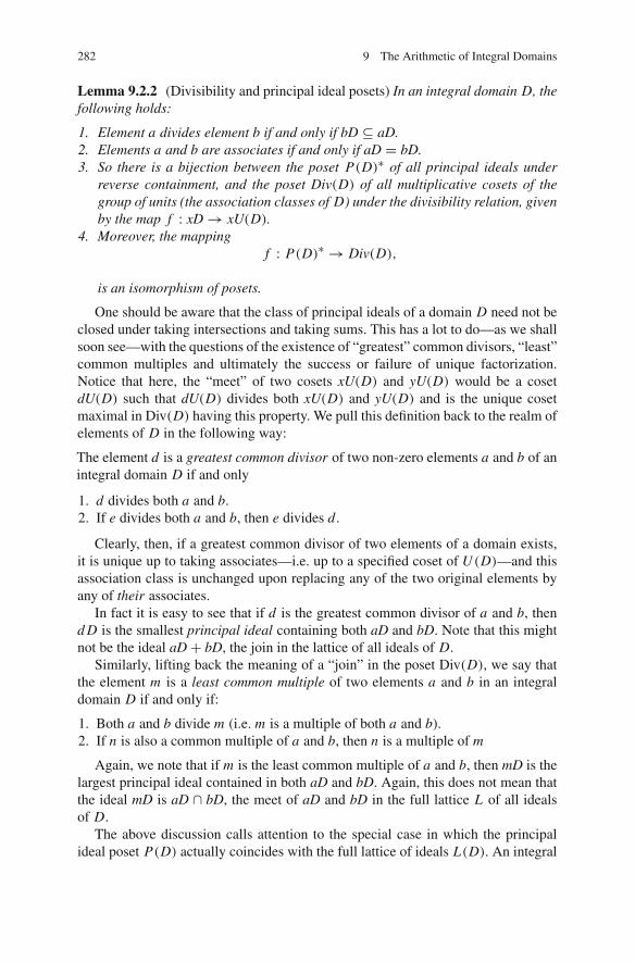
282 9 The Arithmetic of Integral Domains
Lemma 9.2.2 (Divisibility and principal ideal posets) In an integral domain D, thefollowing holds:
1. Element a divides element b if and only if bD ⊆ aD.2. Elements a and b are associates if and only if aD = bD.3. So there is a bijection between the poset P(D)∗ of all principal ideals under
reverse containment, and the poset Div(D) of all multiplicative cosets of thegroup of units (the association classes of D) under the divisibility relation, givenby the map f : xD → xU(D).
4. Moreover, the mappingf : P(D)∗ → Div(D),
is an isomorphism of posets.
One should be aware that the class of principal ideals of a domain D need not beclosed under taking intersections and taking sums. This has a lot to do—as we shallsoon see—with the questions of the existence of “greatest” common divisors, “least”common multiples and ultimately the success or failure of unique factorization.Notice that here, the “meet” of two cosets xU(D) and yU(D) would be a cosetdU(D) such that dU(D) divides both xU(D) and yU(D) and is the unique cosetmaximal in Div(D) having this property. We pull this definition back to the realm ofelements of D in the following way:
The element d is a greatest common divisor of two non-zero elements a and b of anintegral domain D if and only
1. d divides both a and b.2. If e divides both a and b, then e divides d .
Clearly, then, if a greatest common divisor of two elements of a domain exists,it is unique up to taking associates—i.e. up to a specified coset of U (D)—and thisassociation class is unchanged upon replacing any of the two original elements byany of their associates.
In fact it is easy to see that if d is the greatest common divisor of a and b, thend D is the smallest principal ideal containing both aD and bD. Note that this mightnot be the ideal aD + bD, the join in the lattice of all ideals of D.
Similarly, lifting back the meaning of a “join” in the poset Div(D), we say thatthe element m is a least common multiple of two elements a and b in an integraldomain D if and only if:
1. Both a and b divide m (i.e. m is a multiple of both a and b).2. If n is also a common multiple of a and b, then n is a multiple of m
Again, we note that if m is the least common multiple of a and b, then mD is thelargest principal ideal contained in both aD and bD. Again, this does not mean thatthe ideal mD is aD ∩ bD, the meet of aD and bD in the full lattice L of all idealsof D.
The above discussion calls attention to the special case in which the principalideal poset P(D) actually coincides with the full lattice of ideals L(D). An integral

9.2 Divisibility and Factorization 283
domain D for which P(D) = L(D) is called a principle ideal domain, or PID forshort. From our discussion in the preceding paragraphs we have:
Lemma 9.2.3 For any two elements a and b of a principal ideal domain D, a greatestcommon divisor d = gcd(a, b) and a least common multiple m = lcm(a, b) exist.For the least common multiple m, one has Dm = Da ∩ Db, the meet of Da and Dbin the lattice L(D). Similarly the greatest common divisor d generates the join ofthe ideals spanned by a and b. That is,
Da + Db = Dd.
Thus there exist elements s and t in D, such that d = sa + tb.
9.2.2 Factorization and Irreducible Elements
The next two lemmas display further instances in which a question on divisibility inan integral domain, refers back to properties of the poset of principal ideals.
A factorization of an element of the integral domain D is simply a way of repre-senting it as a product of other elements of D. Of course one can write an elementas a product of a unit and another associate in as many ways as there are elementsin U (D). The more interesting factorizations are those in which none of the factorsare units. These are called proper factorizations.
Suppose we begin with an element x of D. If it is a unit, it has no proper factor-ization. Suppose element x is not a unit, and has a proper factorization x = x1y1 intotwo non-zero non-units. We attempt, then, to factor each of these factors into twofurther factors. If such a proper factorization is not possible for one factor, one pro-ceeds with the other proper factor. In this way one may imagine an infinite scheduleof such factorizations. This schedule would correspond to a downwardly growingbinary tree in the graph of the divisibility poset Div(D), An end-node to this tree(that is, a vertex of degree one) results if and only if one obtains a factor y whichpossesses no proper factorization. We call such an element “irreducible”.
Precisely, an element y of D∗ is irreducible if and only if it is a non-zero non-unitwith the property that if y = ab is a factorization, one of the factors a or b, is aunit. Applying the poset isomorphism f : Div(D) → P(D)∗ given in Lemma 9.2.2above, these comments force the following:
Lemma 9.2.4 If D is an integral domain, an element y of D is an irreducibleelement if and only if the principal ideal yD is non-zero and does not properly lie inany other principal ideal except D itelf (that is, it is maximal in the induced posetP(D) − {D, 0} of proper principal ideals of D under containment).
Here is another important central result of this type which holds for a large classof integral domains.

284 9 The Arithmetic of Integral Domains
Lemma 9.2.5 Let D be an integral domain possessing the ascending chain conditionon its poset P(D) of principal ideals. Then every non-zero non-unit is the productof a unit and a finite number of irreducible elements.
Proof Suppose there were a non-zero element x ∈ D − U (D) which was not theproduct of a finite number of irreducible elements. Then the collection T of principalideals xD where x is not a product of finitely many irreducible elements is non-empty. We can thus choose an ideal y D which is maximal in T because T inheritsthe ascending chain condition from the poset of principal ideals. Since y itself is notirreducible, there is a factorization y = ab where neither a nor b is a unit. Then aDproperly contains yD, since otherwise aD = yD and y is an associate ua of a whereu is a unit. Instantly, the cancellation law yields b = u contrary to hypothesis. Thuscertainly the principal ideal aD does not belong to T . Then a is a product of finitelymany irreducible elements of D. Similarly, b is a product of finitely many irreducibleelements of D. Hence their product y must also be so, contrary to the choice of y.The proof is complete. �
9.2.3 Prime Elements
So far, we have been discussing irreducible elements. A similar, but distinct notionis that of a prime element. A non-zero non-unit r in D is said to be a prime, if andonly if, whenever r divides a product ab, then either r divides a or r divides b.
One of the very first observations to be made from this definition is that the notionof being prime is stronger than the notion of being irreducible, Thus:
Lemma 9.2.6 In any integral domain, any prime element is irreducible.
Proof Let r be a prime element of the integral domain D. Suppose, by way ofcontradiction that r is not irreducible, so that r = ab, where a and b are non-units.Then r divides ab, and so, as r is prime, r divides one of the two factors a or b—saya. Then r = rvb for some v ∈ D. But then, by the Cancellation laws, 1 = vb,whence b is a unit, contrary to our assumption.
Thus r is irreducible. �
In general, among integral domains, an irreducible element may not be prime.1
However it is true for principle ideal domains.
Lemma 9.2.7 In a principle ideal domain, every irreducible element is a primeelement.
Proof Let x be an irreducible element in the principle ideal domain D. By definitionx is a non-unit. Assume, by way of contradiction that x is not a prime. Then thereexists elements a and b in D, such that x divides ab, but x does not divide either
1An example is given under the title “a special case” on p. 290.

9.2 Divisibility and Factorization 285
a of b. Notice that if a were a unit, then x would divide b, against our hypothesis.Thus it follows that neither a nor b are units. Thus Da is a proper ideal that does notlie in Dx . Since x is irreducible, Dx is a maximal ideal in D (Lemma 9.2.4), and isproperly contained in the ideal Dx + Da. Thus Dx + Da = D, and so 1 = d1a + d2xfor some elements d1, d2 of D. But since x divides ab, we may write ab = d3x ford3 ∈ D. Now
b = b · 1 = b(d1a + d2x) = d1ab + d2xb
= d1(d3x) + d2xb = (d1d3 + d2b)x .
Thus b is amultiple of x , which is impossible, since x does not divide b by hypothesis.This contradiction tells us that x is indeed a prime element. �
Thus, in a principal ideal domain, the set of irreducible elements and the set ofprime elements coincide.
The reader will observe, the following:
Corollary 9.2.8 In a principle ideal domain D, the element a is prime, if and onlyif the factor ring D/Da is an integral domain.
9.3 Euclidean Domains
An integral domain D is said to be a Euclidean Domain if and only if there is afunction g : D∗ → N into the natural numbers (non-negative integers)2 satisfyingthe following:
(ED1) For a, b ∈ D∗ := D − {0}, g(ab) ≥ g(a).(ED2) If (a, b) ∈ D × D∗, then there exist elements q and r such that a = bq + r ,
where either r = 0 or else g(r) < g(b).
The notation in (ED2) is intentionally suggestive: q stands for “quotient” and rstands for “remainder”. The function g is sometimes called the “grading function”of the domain D.
Recall that in a ring R, an ideal I of the form x R is called a principal ideal. Anintegral domain in which every left ideal is a principal ideal is called a principal idealdomain or PID. We have
Theorem 9.3.1 Every Euclidean domain is a principal ideal domain.
Proof Let D be a Euclidean domain with grading function g : D∗ → N. Let J beany ideal in D. Among the non-zero elements of J we can find an element x withg(x) minimal. Let a be any other element of J . Then a = qx + r as in (ED2) wherer = 0 or g(r) < g(x). Since r = a − qx ∈ J , minimality of g(x) shows that the
2As remarked several times, in this book, the term “natural numbers” includes zero.

286 9 The Arithmetic of Integral Domains
second alternative cannot occur, so r = 0 and a = qx. Thus J ⊆ xD. But x ∈ J ,an ideal, already implies xD ⊆ J so J = xD is a principal ideal. Since J was anarbitrary ideal, D is a PID. �
There are, however, principle ideal domains which are not Euclidean domains.Clearly any Euclidean domain D possesses the algebraic property that it is a PID,
so that greatest common divisors d = gcd(a, b) always exist along with elements sand t such that d = sa + bt (Lemmas 9.2.3 and 9.3.1). What is really new here isthe computional-logical property that the greatest common divisor d = gcd(a, b) aswell as the elements s and t can actually be computed! Behold!
euclidean algorithm. Given a and b in D and D∗, respectively, by (ED2) wehave
a = bq1 + r1,
and if r1 �= 0,b = r1q2 + r2,
and if r2 �= 0,r1 = r2q3 + r3,
etc., until we finally obtain a remainder rk = 0 in
rk−2 = rk−1qk + rk .
Such a termination of this process is inevitable for g(r1), g(r2), . . . is a strictlydecreasing sequence of non-negative integers which can only terminate at g(rk−1)
when rk = 0.We claim the number rk−1 (the last non-zero remainder) is a greatest common
divisor of a and b. First rk−2 = rk−1qk and also rr−3 = rk−2qk−1+rk−1 aremultiplesof rk−1. Inductively, if rk−2 divides both r j and r j+1, it divides r j−1. Thus all of theright hand sides of the equations above are multiples of rk−1; in particular, a and bare multiples of rk−1. On the other hand if d ′ is a common divisor of a and b, d ′divides r1 = a − bq1 and in general divides r j = r j−2 − r j−1q j and so d ′ dividesrk−1, eventually. Thus d := rk−1 is a greatest common divisor of a and b.
Also an explicit expression of d = rk−1 as a D-linear combination sa + tb can beobtained from the same sequence of equations. For
d = rk−1 = rk−3 − rk2qk−1,
and each r j similarly is a D-linear combination of r j−2 and r j−1, j = 1, 2, . . .Successive substitutions for the r j ultimately produces an expression d = sa + tb.All quite computable.

9.3 Euclidean Domains 287
9.3.1 Examples of Euclidean Domains
Example 45 The Gaussian integers and the Eisenstein integers.These are respectively the domains D1 := Z ⊕ Zi (where i2 = −1 �= −i)
and D2 = Z ⊕ Zω (where ω = e2iπ/3). The complex number ω is a zero of theirreducible polynomial x2 + x + 1, and so is a cube root of unity distinct from 1.
Both of these domains are subrings of C, the complex number field, and each isinvariant under complex conjugation. Thus both of them admit a multiplicative normfunction N : C → Rwhere N (z) := z · z records the square of the Euclidean distanceof z from zero in the complex plane. (As usual, z denotes the complex conjugate ofthe complex number z.)
We shall demonstrate that these rings are Euclidean domains with the norm func-tion in the role of g. That its values are taken in the non-negative integers followsfrom the formulae
N (a + bi) = a2 + b2
N (a + bω) = a2 − ab + b2.
As already remarked, the norm function is multiplicative so (ED1) holds. To demon-strate (ED2) we choose elements a and b of D = D1 or D2 with b �= 0. Now theelements of D1 form a square tessellation of the complex plane with {0, 1, i, i + 1}as a fundamental square. Similarly, the elements of D2 form the equilateral triangletessellation of the complex plane with {0, 1,−ω2} or {0, 1,−ω} at the corners of thefundamental triangles. We call the points where three or more tiles of the tessellationmeet lattice points.
When we superimpose the ideal bD on either one of these tessellations of theplane, we are depicting a tessellation of the same type on a subset of the latticepoints with a possibly larger fundamental tile. Thus for the Gaussian integers, bDis a tessellation whose fundamental square is defined by the four “corner” points{0, b, ib, (1+ i)b}. The resulting lattice points are a subset of the Gaussian integersclosed under addition (vector addition in the geometric picture). Similarly for theEisenstein numbers, a fundamental triangle of the tessellation defined by the idealbD is the one whose “corners” are in {0, b,−bω2} or {(0, b,−bω)}. In either casethe tiles of the tessellation bD cover the plane, and so the element a must fall in sometile T—either a square or an equilateral triangle—of the superimposed tessellationbD. Now let qb be a corner point of T which is nearest a. Since T is a square or anequilateral quadrangle, we have
(Nearest Corner Principle) The distance from a point of T to its nearest corner isless than the length of a side of T
Thus the distance |a − qb| = √N (a − qb) is less than |b| = √
N (b). Using thefact that the square function is monotone increasing on non-negative real numbers,we have
g(a − bq) = N (a − bq) < N (b) = g(b).

288 9 The Arithmetic of Integral Domains
Thus setting r = a − qb, we have r = 0 or g(r) < g(b). Thus (with respect to thefunction g), r serves to realize the condition (ED2).3
Before passing to the next example, this may be a good place to illustrate howembedding one domain into another sometimes may provide new results for theoriginal domain: in this case we are embedding the integers Z into the Gaussianintegers Z[i]. When we select a prime integer (called a rational prime), the questionis raisedwhether it is still a prime element in the ring ofGaussian integers (aGaussianprime). The Theorem 9.3.3 below gives a complete answer.
Lemma 9.3.2 Let p be any rational prime. If p is not a Gaussian prime then p isthe sum of two integer squares.
Proof Suppose that rational prime p is the product of two non-units in Z[i], sayp = ζη. Taking norms, we have p2 = N (ζ)N (η). Since a Gaussian integer is aunit if and only if its norm is ±1, it follows that the last two norms of the previousequation are both positive integers dividing p2. Since p is a rational prime, each ofthese norms is equal to p. Thus, writing ζ = a+bi one has p = N (ζ) = a2+b2. �Theorem 9.3.3 Let p be a rational prime. Then p is a Gaussian prime if and onlyif it leaves a remainder of 3, when divided by 4.
Proof First, the prime integer 2 is not a Gaussian prime since 2 = (1 + i)(1 − i),so we may assume that the rational prime p is odd. Since the square of every oddinteger leaves a remainder of 1, when divided by 4, the sum of two integer squarescan only be congruent to 0, 1, or 2 modulo 4. Thus if p ≡ 3 mod 4, it is not thesum of two integer squares and so must be a Gaussian prime, by the previous Lemma9.3.2.
That leaves the case that p ≡ 1 mod 4. In this case Z/(p) is a field whosemultiplicative group of non-zero elements contains a unique cyclic subgroup of order4 whose generator has a square equal to −1, that is, there exists an integer b suchthat b2 ≡ −1 mod p. Let P be the principle ideal generated by p in the domainof Gaussian integers. Since Z[i] is Euclidean, it is a principle ideal domain, and so,by Corollary 9.2.8, the factor ring Z[i]/P is an integral domain if and only if p is aprime in Z[i]. But since b �≡ 0 mod p, the numbers 1 ± bi cannot be multiples ofp in Z[i]. Thus the equation
(1 + bi + P)(1 − bi + P) = (1 + bi)(1 − bi) + P = (1 + b2) + P = P,
reveals that the factor ring Z[i]/P possesses zero divisors, and so cannot be anintegral domain. Accordingly p is not a prime element of Z[i]. �
3Usually boxing matches are held (oxymoronically) in square “boxing rings”. Even if (as well)they were held in equilateral triangles, it is a fact that when the referee commands a boxer to “goto a neutral corner”, the fighter really does not have far to go (even subject to the requirement of“neutrality” of the corner). But woe the fighter who achieves a knock-down near the center, of amore ring-like N -gon for large N . After the mandatory hike to a neutral corner, the fighter can onlyreturn to the boxing match totally exhausted from the long trip. No Euclidean algorithm for theseboxers.

9.3 Euclidean Domains 289
Corollary 9.3.4 If p is a rational prime of the form 4n + 1, then p is a sum of twointeger squares.
Proof By Theorem 9.3.3 p is not a Gaussian prime. Now apply Lemma 9.3.2. �
This result does not seem easy to prove within the realm of integers alone.
Example 46 Polynomial domains over a field. Let F be a field and let F[x] be thering of polynomials in indeterminate x and with coefficients from F . We let deg bethe degree function, F[x] → N.4 Then if f (x) and g(x) are non-zero polynomials,
deg( f g) = deg f + deg g,
so (ED1) holds. The condition (ED2) is the familiar long division algorithm ofCollege Algebra and grade school.
9.4 Unique Factorization
9.4.1 Factorization into Prime Elements
Let D be any integral domain. Recall that a non-zero non-unit of D is said to beirreducible if it cannot be written as the product of two other non-units. This meansthat if r = ab is irreducible, then either a or b is a unit.
Recall also that a non-zero non-unit r in D is said to be a prime element, if andonly if, whenever r divides a product ab, then either r divides a or r divides b.
In the case of the familiar ring of integers (indeed for all PID’s), the two notionscoincide, and indeed they are forced to coincide in an even larger collection ofdomains.
An integral domain D is said to be a unique factorization domain (or UFD) if andonly if
(UFD1) Every non-zero non-unit is a product of a unit and a finite number ofirreducible elements.
(UFD2) Every irreducible element is prime.
We shall eventually show that a large class of domains—the principal idealdomains—are UFD’s. (See Theorem 9.4.3.) One of the very first observations tobe made from these definitions is that the notion of being prime is stronger than thenotion of being irreducible. Thus:
4The student will recall the familiar degree function, that records the highest exponent of x thatappears when a polynomial is expressed as a linear combination of powers of x with non-zerocoefficients.

290 9 The Arithmetic of Integral Domains
Lemma 9.4.1 The following are equivalent:
(i) D is a UFD.(ii) In D every non-zero non-unit is a product of a unit and a finite number of primes.
Proof (i) ⇒ (ii) is obvious since (i) implies each irreducible element is a prime.(ii) ⇒ (i). First we show that every irreducible element is prime. Let r be irre-
ducible. Then by (ii), r is a product of a unit and a finite number of primes. But sincer is irreducible, r = up where u is a unit and p is a prime.
Now every non-zero non-unit is a product of a unit and finitely many irreducibleelements, since each prime is irreducible by Lemma 9.2.6. Thus the two definingproperties of a UFD follow from (ii) and the proof is complete. �
Theorem 9.4.2 (The Basic Unique Factorization Theorem) Let D be an integraldomain which is a UFD. Then every non-zero non-unit can be written as a productof finitely many primes. Such an expression is unique up to the order in which of theprime factors appear, and the replacement of any prime by an associate—that is, amultiple of that prime by a unit.
Proof Let r be a non-zero non-unit of the UFD D. Then by Lemma 9.4.1, r can bewritten as a unit times a product of finitely many primes. Suppose this could be donein more than one way, say,
r = up1 p2 · · · ps = vq1q2 · · · qt
where u and v are units and the pi and qi are primes. If s = 0 or t = 0, then ris a unit, contrary to the choice of r . So without loss of generality we may assume0 < s ≤ t . Now as p1 is a prime, it divides one of the right hand factors, and thisfactor cannot be v. Rearranging the indexing if necessary, we may assume p1 dividesq1. Since q1 is irreducible, p1 and q1 are associates, so q1 = u1 p1. Then
r = up1 · · · ps = (vu1)p1q2 · · · qt
so, by the cancellation law
up2 · · · ps = (vu1)q2 · · · qt ,
with t − 1 factors on the right side. By induction on t , we have s = t and qi =ui pπ(i) for some unit ui , i = 2, . . . t and permutation π of these indices. Thus thetwo factorizations involve the same number of primes with the primes in one of thefactorizations being associates of the primes in the other, written in some possiblydifferent order. �

9.4 Unique Factorization 291
A Special Case
Of course we are accustomed to the domain of the integers, which is a UFD. So itmight be instructive to look at a more pathological case.
Consider the ring D = {a + b√−5|a, b ∈ Z}. Being a subring of the field of
complex numbers C, it is an integral domain.The mapping z → z, where z is the complex conjugate of z, is an automorphism
of C which leaves D invariant (as a set) and so induces an automorphism of D. Wedefine the norm of a complex number ζ to be N (ζ) := ζζ. Then N : C → R
+,the positive real numbers, and N (ζψ) = N (ζ)N (ψ) for all ζ,ψ ∈ C. Clearly,N (a + b
√−5) = a2 + 5b2 so the restriction of N to D has non-negative integervalues. (Moreover, we obtain for free the fact that the integers of the form a2 + 5b2
are closed under multiplication.)Let us determine the units of D. Clearly if ν ∈ D is a unit, then there is a μ in D
so that νμ = 1 = 1 + 0√−5, the identity of D. Then
N (ν)N (μ) = N (νμ) = N (1) = 12 + 5 · 02 = 1.
But how can the integer 1 be expressed as the product of two non-negative integers?Obviously, only if N (ν) = 1 = N (μ). But if a2 + 5b2 = 1, it is clear that b = 0 anda = ±1. Thus
U (D) = {±1} = {d ∈ D|N (d) = 1}.
We can also use norms to locate irreducible elements of D. For example, if ζ is anelement of D of norm 9, then ζ is irreducible. For otherwise, one would have ζ = ψηwhere ψ and η are non-units. But that means N (ψ) and N (η) are both integers largerthan one. Yet 9 = N (ψ)N (η) so N (ψ) = N (η) = 3, which is impossible since 3 isnot of the form a2 + 5b2.
But now note that
9 = 3 · 3 = (2 + √−5)(2 − √−5)
are two factorizations of 9 into irreducible factors (irreducible, because they havenorm 9) and, as U (D) = {±1}, 3 is not an associate of either factor on the righthand side.
Thus unique factorization fails in the domain D = Z ⊕ Z√−5. The reason is
that 3 is an irreducible element which is not a prime. It is not a prime because 3divides (2 + √−5)(2 − √−5), but does not divide either factor.
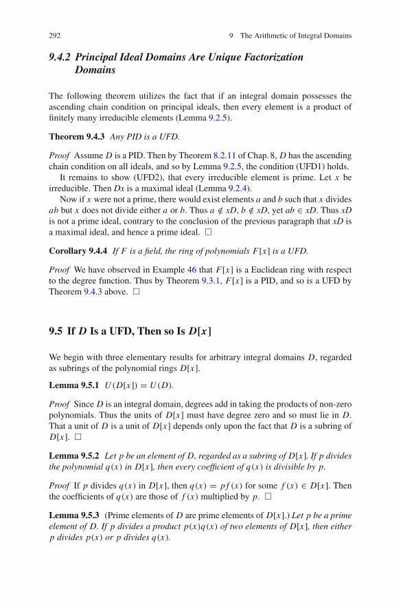
292 9 The Arithmetic of Integral Domains
9.4.2 Principal Ideal Domains Are Unique FactorizationDomains
The following theorem utilizes the fact that if an integral domain possesses theascending chain condition on principal ideals, then every element is a product offinitely many irreducible elements (Lemma 9.2.5).
Theorem 9.4.3 Any PID is a UFD.
Proof Assume D is a PID. Then by Theorem 8.2.11 of Chap. 8, D has the ascendingchain condition on all ideals, and so by Lemma 9.2.5, the condition (UFD1) holds.
It remains to show (UFD2), that every irreducible element is prime. Let x beirreducible. Then Dx is a maximal ideal (Lemma 9.2.4).
Now if x were not a prime, there would exist elements a and b such that x dividesab but x does not divide either a or b. Thus a /∈ xD, b /∈ xD, yet ab ∈ xD. Thus xDis not a prime ideal, contrary to the conclusion of the previous paragraph that xD isa maximal ideal, and hence a prime ideal. �
Corollary 9.4.4 If F is a field, the ring of polynomials F[x] is a UFD.
Proof We have observed in Example 46 that F[x] is a Euclidean ring with respectto the degree function. Thus by Theorem 9.3.1, F[x] is a PID, and so is a UFD byTheorem 9.4.3 above. �
9.5 If D Is a UFD, Then so Is D[x]
We begin with three elementary results for arbitrary integral domains D, regardedas subrings of the polynomial rings D[x].Lemma 9.5.1 U (D[x]) = U (D).
Proof Since D is an integral domain, degrees add in taking the products of non-zeropolynomials. Thus the units of D[x] must have degree zero and so must lie in D.That a unit of D is a unit of D[x] depends only upon the fact that D is a subring ofD[x]. �
Lemma 9.5.2 Let p be an element of D, regarded as a subring of D[x]. If p dividesthe polynomial q(x) in D[x], then every coefficient of q(x) is divisible by p.
Proof If p divides q(x) in D[x], then q(x) = p f (x) for some f (x) ∈ D[x]. Thenthe coefficients of q(x) are those of f (x) multiplied by p. �
Lemma 9.5.3 (Prime elements of D are prime elements of D[x].) Let p be a primeelement of D. If p divides a product p(x)q(x) of two elements of D[x], then eitherp divides p(x) or p divides q(x).

9.5 If D Is a UFD, Then so Is D[x] 293
Proof Suppose the irreducible element p divides p(x)q(x) as hypothesized. Write
p(x) =∑n
i=0ai xi , and q(x) =
∑m
j=0b j x j ,
where ai , b j ∈ D. Suppose byway of contradiction that p does not divide either p(x)
or q(x). Then by the previous Lemma 9.5.2, p divides each coefficient of p(x)q(x)
while there is a first coefficient ar of p(x) not divisible by p, and a first coefficientbs of q(x) not divisible by p. Then the coefficient of xr+s in p(x)q(x) is
cr+s =∑
i+ j=r+sai b j , subject to 0 ≤ i ≤ n and 0 ≤ j ≤ m (9.1)
Now if (i, j) �= (r, s), and i + j = r + s, then either i < r or j < s, and in eithercase ai b j is divisible by p. Thus all summands ai b j in the right side of Eq. (9.1)except possibly ar bs are divisible by p. But p is a prime element in D that does notdivide either ar or bs . It follows that p does not divide ar bs which would mean thatp does not divide cr+s , against Lemma 9.5.2 and the fact that p divides p(x)q(x).
Thus p must divide one of p(x) or q(x), completing the proof. �
We are all familiar with the way that the rational number field Q is obtained as asystemof fractions of integers. In an identicalmanner, one can formafield of fractionsF of any integral domain D. Its elements are “fractions”—that is, equivalence classesof pairs in D× D∗ with the equivalence class [n, d] containing the pair (n, d) definedto be the set of pairs (bn, bd) as b ranges over all nonzero elements b ∈ D∗. Additionand multiplication of classes are as they are for rational numbers:
[a, b] + [c, d] = [ad + bc, bd] and [a, b] · [c, d] = [ac, bd].
(This an example of a localization F = DS , of the sort studied in the next section,with S = D∗ = D − {0}.) Since D is a subdomain of the field F , D[x], the domainof polynomials with coefficients from D, can be regarded as a subring of F[x] bythe device of regarding coefficients d of D as fractions d/1. We wish to compare thefactorization of elements in D[x] with those in F[x].
We say that a polynomial p(x) ∈ D[x] is primitive if and only if, whenever d ∈ Ddivides p(x), then d is a unit.
From this point onward, we assume that D is a UFD, so all irreducible elementsare prime and every non-zero element is a unit or a product of prime elements.
We now approach two lemmas that involve F[x] where F is the field of fractionsof D.
Lemma 9.5.4 If p(x) = αq(x), where p(x) and q(x) are primitive polynomials inD[x], and α ∈ F, then α is a unit in D.
Proof Since D is a UFD, greatest common divisors and least common multiplesexist, and so there is a “lowest terms” representation of α as a fraction t/s where anygreatest common divisor of s and t is a unit. If s is itself a unit, then t divides each

294 9 The Arithmetic of Integral Domains
coefficient of p(x), and since p(x) is primitive, t must also be a unit. In that caseα = s/t − st−1 is a unit of D, as claimed. Otherwise, there is a prime divisor p of s.Then p does not divide t , and so from sp(x) = tq(x), we see that every coefficientof q(x) is divisible by p, against q(x) being primitive. �
Lemma 9.5.5 If f (x) ∈ F[x], then f (x) has a factorization
f (x) = rp(x)
where r ∈ F and p(x) is a primitive polynomial in D[x]. This factorization is uniqueup to replacement of each factor by an associate.
Proof We prove this in two steps. First we establish
Step 1. There exists a scalar γ such that f (x) = γ p(x) , where p(x) is primitivein D[x].
Each non-zero coefficient of xi in f (x) has the form ai/bi with bi ∈ D − {0}.Multiplying through by a least common multiple m of the bi (recall that lcm’s existin UFD’s), we obtain a factorization
f (x) = (1
m)∑
ai (m/bi )xi ,
whose second factor is clearly primitive in D[x].Step 2. The factorization in Step 1 is unique up to associates.
Suppose f (x) = γ1 p1(x) = γ2 p2(x) with γi ∈ F , and pi (x) primitive in D[x].Then p1(x) and p2(x) are associates in F[x] so
p1(x) = γ p2(x), for γ ∈ F.
Then by Lemma 9.5.4, γ is a unit in D. But as γ = γ2γ−11 , the result follows. �
A non-zero element of an integral domain D′ is said to be reducible simply if itis not irreducible—i.e. it has a factorization into two non-units of D′.
Lemma 9.5.6 (Gauss’ Lemma) Suppose p(x) ∈ D[x] is reducible in the ring F[x].Then p(x) is reducible in D[x].Proof By hypothesis p(x) = f (x)g(x), where f (x) and g(x) are polynomials ofpositive degree in F[x]. Then by Step 1 of the proof of Lemma 9.5.5 above, we maywrite
f (x) = μ f1(x)
g(x) = γg1(x).

9.5 If D Is a UFD, Then so Is D[x] 295
where μ, γ ∈ F and f1(x) and g1(x) are primitive polynomials in D[x]. Now byLemma 9.5.3, f1(x)g1(x) is a primitive polynomial in D[x] so
p(x) = (μγ)( f1(x)g1(x)),
and Lemma 9.5.4 shows that μγ is a unit in D. Then
p(x) = ((μγ) f1(x)) · g1(x)
is a factorization of p(x) in D[x], with factors of positive degree. The conclusionthus follows. �
Theorem 9.5.7 If D is a UFD, then so is D[x].Proof Let p(x) be any element of D[x]. We must show that p(x) has a factorizationinto irreducible elements which is unique up to the replacement of factors by asso-ciates. Since D is a unique factorization domain, a consideration of degrees showsthat it is sufficient to do this for the case that p(x) is primitive of positive degree.
Let S = D − {0} and form the field of fractions F = DS , regarding D[x]as a subring of F[x] in the usual way. Now by Corollary 9.4.4, F[x] is a uniquefactorization domain. Thus we have a factorization
p(x) = p1(x)p2(x) · · · pn(x)
where each pi (x) is irreducible in F[x]. Then by Lemma 9.5.5, there exist scalarsγi , i = 1, . . . , n, such that pi (x) = γi qi (x), where qi (x) is a primitive polynomialin D[x]. Then
p(x) = (γ1γ2 · · · γn)q1(x) · · · qn(x).
Since theqi (x) are primitive, so is their product (Lemma9.5.3). Then byLemma9.5.4the product of the γi is a unit u of D. Thus
p(x) = uq1(x) · · · qn(x)
is a factorization in D[x] into irreducible elements.If
p(x) = vr1(x) · · · rm(x)
were another such factorization, the fact that F[x] is a PID and hence a UFD showsthat m = n and the indexing can be chosen so that ri (x) is an associate of qi (x) inF[x]—i.e. there exist scalars ρi in F such that ri (x) = ρi qi (x), for all i . Then asri (x) and qi (x) are irreducible in D[x], they are primitive, and so by Lemma 9.5.4,each γi is a unit in D. Thus the two factorizations of p(x) are alike up to replacementof the factors by associates in D[x]. The proof is complete. �

296 9 The Arithmetic of Integral Domains
Corollary 9.5.8 If D is a UFD, then so is the ring
D[x1, . . . , xn].
Proof Repeated application of Theorem 9.5.7 to
D[x1, . . . , x j+1] � (D[x1, . . . , x j ])[x j+1]. �
9.6 Localization in Commutative Rings
9.6.1 Localization by a Multiplicative Set
Section9.2 revealed that the divisibility structure of D, as displayed by the divisibilityposet Div(D), is in part controlled by the group of units. It is then interesting to knowthat the group of units can be enlarged by a process described in this section.5
We say that a subset S of a ring ismultiplicatively closed if and only if SS ⊆ S andS does not contain the zero element of the ring. If S is a non-empty multiplicativelyclosed subset of the ring R, we can define an equivalence relation “∼” on R × S bythe rule that (a, s) = (b, t) if and only if, for some element u in S, u(at − bs) = 0.
Let us first show that the relation “∼” is truly an equivalence relation. Obviouslythe relation “∼” is symmetric and reflexive. Suppose now
(a, s) ∼ (b, t) ∼ (c, r) for {r, s, t} ⊆ S.
Then there exists elements u and v in S such that
u(at − bs) = 0 and v(br − tc) = 0.
Multiplying the first equation by vr we get vr(uat) = vr(ubs). But vr(ubs) =us(vbr) = us(vtc), by the second equation. Hence
vut (ar) = vut (sc),
so (a, s) ∼ (c, r), since vut ∈ S. Thus ∼ is a transitive relation.For any element s ∈ S, we now let the symbol a/s (sometimes written a
s ) denotethe∼—equivalence class containing theorderedpair (a, s).Wecall these equivalenceclasses fractions.
Next we show that these equivalence classes enjoy a ring structure. First observethat if there is an element u in S such that u(as′ −sa′) = 0 (i.e. (a, s) ∼ (a′, s′)) then
5When this happens, the student may wish to verify that the new divisibility poset so obtained is ahomomorphic image of the former poset.

9.6 Localization in Commutative Rings 297
u(abs′t −sta′b) = 0, so (ab, st) ∼ (a′b, s′t). Thus we can unambiguously define theproduct of two equivalence classes—or ‘fractions’—by setting (a/s)·(b/t) = ab/st .
Similarly, if (a, s) ∼ (a′, s′), so that for some u ∈ S, u(as′ − sa′) = 0 , we seethat
u(at + sb)s′t − u(a′t + s′b)st = 0,
so(at + bs)/s = (a′t + s′b)/s′t.
Thus ‘addition’, defined by setting
a
s+ b
t:= at + bs
st,
is well defined, since this is also (a′t + s′b)/s′t .The set of all ∼—classes on R × S is denoted RS . Now that multiplication and
addition are defined on RS , we need only verify that
1. (RS,+) is an abelian group with identity element 0/s—that is, the ∼—classcontaining (0, s) for any s ∈ S.
2. (RS, ·) is a commutative monoid with multiplicative identity s/s, for any s ∈ S.3. Multiplication is distributive with respect to addition in RS .
All of these are left as Exercises in Sects. 9.13.1–9.13.2. The conclusion, then, isthat
(Rs,+, ·) is a ring.
This ring Rs is called the localization of R by S.
9.6.2 Special Features of Localization in Domains
For each element s in the multiplicatively closed set S, there is a homomorphism ofadditive groups
ψs : (R,+) → (RS,+)
given byψs(r) = r/s. This need not be an injectivemorphism. If a/s = b/s, it meansthat there is an element u ∈ S such that us(a − b) = 0. Now if the right annihilatorof us is nontrivial, such an a − b exists with a �= b, and ψs is not one-to-one.
Conversely, we can say, however,
Lemma 9.6.1 If s is an element of S such that no element of sS is a “zero divisor”—an element with a non-trivial annihilator—then ψs : R → RS is an embedding ofadditive groups. The converse is also true. In particular, we see that in an integraldomain, where every non-zero element has only a trivial annihilator, the map ψs isinjective for each s ∈ S.

298 9 The Arithmetic of Integral Domains
Lemma 9.6.2 Suppose S is a multiplicatively closed subset of non-zero elements ofthe commutative ring R and suppose no element of S is a zero divisor in R.
(i) Suppose ac �= 0 and b, d are elements of S. Then in the localized ring RS
(a
b)(
c
d) is non-zero in RS.
(ii) If a is not a zero divisor in R, then for any b ∈ S, a/b is not a zero divisor inRS.
(iii) If R is an integral domain, then so is RS.(iv) If R is an integral domain, the mapping ψ1 : R → RS is an injective homo-
morphism of rings (that is an embedding of rings).
Proof Part (i). Suppose ac �= 0, but that for some {b, d, s} ⊆ S,
(a
b)(
c
d) = 0
s. (9.2)
Then(ac, bD) ∼ (0, s).
Then by the definition of the relation “∼”, there is an element u ∈ S such thatu(acs − ab · 0) = 0 which implies uacs = 0. But since u and s are elements ofS, they are not zero divisors, and so we obtain ac = 0, a contradiction. Thus theassumption ac �= 0 forces Eq. (9.2) to be false. This proves Part (i).
Parts (ii) and (iii) follow immediately from Part (i).Part (iv). Assume R is an integral domain. From the second statement of Lemma
9.6.1, the mapping ψs : R → RS which takes element r to element r/s is an injec-tive homomorphism of additive groups for each s ∈ S. Now put s = 1. We seethat ψ1(ab) = ψ1(a)ψ1(b) for all a, b ∈ R. Thus ψ1 is an injective ring homomor-phism. �
9.6.3 A Local Characterization of UFD’s
Theorem 9.6.3 (Local Characterization of UFD’s) Let D be an integral domain.Let S be the collection of all elements of D which can be written as a product ofa unit and a finite number of prime elements. Then S is multiplicatively closed anddoes not contain zero; so the localization DS can be formed.
The domain D is a UFD if and only if DS is a field.
Proof (⇒) If D is a UFD, then, by Lemma 9.4.1, S comprises all non-zero non-unitsof D. One also notes that DS = DS′ where S′ is S with the setU (D) of all units of Dadjoined. (By Exercise (2) in Sect. 9.13.1 of this chapter, this holds for all domains.)Thus S′ = S − {0}. Then DS′ is the field of fractions of D.

9.6 Localization in Commutative Rings 299
(⇐) Let D∗ := D − {0}, the non-zero elements of D. It suffices to prove that Sis all non-zero non-units of D (Lemma 9.4.1). In fact, as S ⊆ D − U (D), it sufficesto show that D∗ − U (D) ⊆ S. Let r be any non-zero non-unit—i.e. an element ofD∗ − U (D), and suppose by way of contradiction that r /∈ S.
Since r is a non-unit, Dr is a proper ideal of D. Then
(Dr)S;= {a/s|a ∈ Dr, s ∈ S}
is clearly a non-zero ideal of DS . Since DS is a field, it must be all of DS . But thismeans that 1/1 is an element of (Dr)S—i.e. one can find (b, s) ∈ D × S, such that
br/s = 1/1.
This means br = s soDr ∩ S �= ∅.
Now from the definition of S, we see that there must be multiples of r which can beexpressed as a unit times a non-zero number s of primes. Let us choose the multipleso that the number of primes that can appear in such a factorization attains aminimumm. Thus there exists an element r ′ of D such that
rr ′ = up1 · · · pm
where u is a unit and the pi are primes. We may suppose the indexing of the primesto be such that p1, . . . , pd do not divide r ′, while pd+1, . . . , do divide r ′. Then ifd < m, pd+1 divides r ′ so r ′ = bpd+1. Then we have
rbpd+1 = up1 · · · pd pd+1 · · · pm
sorb = up1 · · · pd pd+2 · · · pm (m − 1 prime factors)
against the minimal choice of m. Thus d = m, and each pi does not divide r ′. Theneach pi divides r . Thus r = a1 p1 so a1r ′ = up2 · · · pd , upon canceling p1. Butagain, as p2 does not divide r ′, p2 divides a1. Thus a1 = a2 p2 so a2r ′ = up3 · · · pd .As each pi does not divide r ′, this argument can be repeated, until finally one obtainsadr ′ = u when the primes run out. But then r ′ is a unit. Then
r = ((r ′)−1u)p1 · · · pm ∈ S.
Thus as r was arbitrarily chosen in D∗ − U (D) ⊆ S, we are done. �

300 9 The Arithmetic of Integral Domains
9.6.4 Localization at a Prime Ideal
Now let P be a prime ideal of the commutative ring R—that means P has thisproperty: If, for two ideals A and B of R, one has AB ⊆ P , then at least one of Aand B lie in P . For commutative rings, this is equivalent to asserting either of thefollowing (see the Exercise (2) in Sect. 7.5.2 at the end of Chap. 7):
(1) For elements a and b in R, ab ∈ P implies a ∈ P or b ∈ P .(2) The set R − P is a multiplicatively closed set.
It should be clear that a prime ideal contains the annihilator of every element outside it.Now let P be a prime ideal of the integral domain D, and set S := D − P , which,
as noted, is multiplicatively closed. Then the localization of D by S is called thelocalization of D at the prime ideal P . In the literature the prepositions are important:The localization by S = D − P is the localization of D at the prime ideal P .
Now we may form the ideal M := {p/s|(p, s) ∈ P × S} in DS for which eachelement of DS − M , being of the form s′/s, (s, s′) ∈ S × S, is a unit of DS . Thisforces M to be a maximal ideal of DS , and in fact, every proper ideal B of DS mustlie in it. Thus we see
DS has a unique maximal ideal M. (9.3)
Any ring having a unique maximal ideal is called a local ring.This discussion together with Part (iv) of Lemma 9.6.2 yields
Theorem 9.6.4 Suppose P is a prime ideal of the integral domain D. Then thelocalization at P (that is, the ring DS where S = D − P) is a local ring that is alsoan integral domain.
Example 47 The zero ideal {0} of any integral domain is a prime ideal. Formingthe localization at the zero ideal of an integral domain D thus produces an integraldomain with the zero ideal as the unique maximal ideal and every non-zero elementa unit. This localized domain is called the field of fractions of the domain D.6 (Thisstandard construction was used in Sect. 9.5 in studying D[x] as a subring of DS[x].)
9.7 Integral Elements in a Domain
9.7.1 Introduction
In Sect. 8.2.5 the notion of an algebraic integer was introduced as a special instance ofsets of field elements that are integral over a subdomain. Using elementary properties
6One finds “field of quotients” or even “quotient field” used in place of “field of fractions” here andthere. Such usage is discouraged because the literature also abounds with instances in which theterm “quotient ring” is used to mean “factor ring”.

9.7 Integral Elements in a Domain 301
of finitely-generated modules and Noetherian rings, it was a fairly simple matterto demonstrate that sums and products of algebraic integers were again algebraicintegers. At the beginning of the Appendix to this chapter (which the student shouldnow be able to read without further preparation) these discussions are carried abit further, wherein the algebraic integers contained in any quadratic extension ofthe rational field are determined. Furthermore, the factorization properties of thesequadratic domains are addressed, with the result that these rings enjoyed varyingdegrees of good factorization properties, ranging from being Euclidean (as with theGaussian integers Z[i]) through not even satisfying unique factorization (as withZ[√−5]).
A little historical perspective is in order. The subject of Arithmetic is probablyone of the first subjects that a student of Mathematics encounters. Its fundamentalscan be taught to anyone. But its mysteries are soon apparent to even the youngeststudent. Why is any positive prime number that is one more than a multiple of four,the sum of the squares of two integers? Why is every positive integer expressible asthe sum of four squares of integers? These problems have been solved. But there aremany more unsolved problems. In fact, there is no other field of Mathematics whichpresents so many unsolved problems that could be easily stated to the man on thestreet. For example, the famous Goldbach Conjecture that asserts that
Every even integer greater than two is the sum of two prime numbers.
One of these questions concerns an assertion known as “Fermat’s Last Theorem”.According to tradition, Fermat had jotted in the margin of a book that he had a proofof the following theorem7
Suppose x, y, z is a triplet of (not-necessarily distinct) integers. If n is a positiveinteger greater than 2 , then there exists no such triplet such that
xn + yn = zn . (9.4)
That is, in the realm of integers, no nth power can be the sum of two other nthpowers for n > 2. Perhaps the problem became more intriguing because there aresolutions when n = 2. At any rate this problem attracted the attention of manygreat mathematicians of the 19th century. Here is a case where the solution was farless important than the theory that was developed to solve the problem. Our earliestmathematical ancestors might not have approached the problem with a full-fledgedGalois Theory of field extensions at hand, for they knew that they were dealing with
7The book in which he wrote this marginal note has never been found. All that we actually have isa third party who initiated the anecdote. So there are two schools of thought: (1) Fermat thoughtthat he had a proof but must have made a mistake. Skeptics believe his proof could not only not fitin a margin, but that his proof (in order to be less than a thousand pages) must have been in error.Then there is the other view: (2) He really did prove the theorem in a relatively simple way—wejust haven’t discovered how he did it. The authors are personally acquainted with at least one greatliving research mathematician who does not rule out the second view. That man is not willing todismiss a mind (like Fermat’s) of such proven brilliance. That respect says something.

302 9 The Arithmetic of Integral Domains
some “subring” of “integers”in these fields. (Complex numbers had been explicitlydeveloped by Gauss and the idea of Gaussian integers may be seen as an anticipationof the general idea guiding others to this point.) So this was the foil that producedthe concept of Algebraic Integers.
It came as quite a revelation to early nineteenth century mathematicians that evenin the algebraic integer domains, unique factorization of elements into prime elementscould fail. Perhaps our intellectual history (as opposed to the political one) is simplythe gradual divestment of unanalyzed assumptions.
Themain objects of study for the rest of this chapterwill be the ringsOE consistingof the elements in the field E which are integral with respect to a subdomain D whereE is a finite extension of F := F(D), the field of fractions of D. (The phrase “finiteextension” means that the field E contains F and is finite dimensional as a vectorspace over its subfield F .) In the special case that D = Z, the ring of integers (sothat F = Q, the field of the rational numbers), the ringsOE are the algebraic integerdomains of the previous paragraph.
Such algebraic integer domains OE include the above-mentioned quadraticdomains (such as Z + Z
√−5). Thus, while microscopically (i.e., element-wise),these rings may not enjoy unique factorization, they all satisfy a macroscopic ver-sion of unique factorization inasmuch as their ideals will always factor uniquely asa product of prime ideals. This can be thought of as a partial remedy to the fact thatthe rings OK tend not to be UFDs.
9.8 Rings of Integral Elements
Suppose K is a field, and D is a subring of F . Then, of course, D is an integraldomain. Recall from Sect. 8.2.5. that an element α of K is integral over D if an onlyif α is a zero of a polynomial in D[x] whose lead coefficient is 1 (the multiplicativeidentity of D and K ). Say that an integral domain D is integrally closed if, wheneverα ∈ F(D) and α is integral over D, then α ∈ D. Here F(D) is the field of fractionsof the integral domain D.
The following is a sufficient, but not a necessary condition, for an integraldomain to be integrally closed.
Lemma 9.8.1 If D is a UFD, then D is integrally closed.
Proof Graduate students who have taught basic-level courses such as “college alge-bra” will recognize the following argument. Indeed, given that D is a UFD, with fieldof fractions F , then elements of F may be expressed in the form α = a/b, wherea and b have no common prime factors in D. If such an element α were integral
over D, then we would have a monic polynomial f (x) =r∑
i=0ai xi ∈ D[x] with
f (α) = 0: thus

9.8 Rings of Integral Elements 303
(a
b
)r + ar−1
(a
b
)r−1 + · · · + a1(a
b
)+ a0 = 0.
Upon multiplying both sides of the above equation by br one obtains
ar + ar−1bar−1 + · · · + a1br−1a + a0br = 0.
Therefore, any prime divisor p of b will divider−1∑i=0
ai br−i ai and so would divide ar .
Since D is a UFD, that would imply that this prime divisor p divides a, as well.8
This is a contradiction since a and b possess no common prime factors. We are leftwith the case that b is not divisible by any prime whatsoever. In that case b is a unit,in which case α = a/b ∈ D. �
Remark The above lemma provides us with a very large class of integral domainsthat are not UFDs. Indeed, Appendixwill show that the quadratic domainsO = A(d)
consisting of algebraic integers in the quadratic extension Q(√
d) ⊇ Q, where d isa square-free integer, d ≡ 1mod 4, have the description
A(d) ={
a + b√
d
2| a, b ∈ Z, a, b are both even or are both odd
}.
This implies immediately that the proper subring Z[√d] � A(d) is not integrallyclosed and therefore cannot enjoy unique factorization. A more direct way of seeingthis is that in the domain D = Z[√d], where d is square-free and congruent to 1modulo 4, the element 2 is irreducible in D (easy to show directly) but not prime, as2|(1 +√
d)(1 −√d) but 2 doesn’t divide either 1 +√
d or 1 −√d.
The following lemmas essentially recapitulate much of the discussion ofSect. 8.2.5.
Lemma 9.8.2 Let R ⊆ S be integral domains.
1. If R is Noetherian and S is a finitely-generated R-module, then every element ofS is integral over R.
2. If R ⊆ S ⊆ T are integral domains with T a finitely-generated S-module and Sa finitely-generated R-module, then T is a finitely-generated R-module.
Proof The first statement is immediate from Theorem 8.2.12 and Lemma 8.2.14.From the hypothesis of the second statement, T = ∑
ti S and S = ∑s j R,
where the summing parameters i and j have finite domains. Thus T = ∑i, j ti s j R
is generated as an R module by the finite set {ti s j }. �
Note that R need not be Noetherian in part 2 of the above Lemma.
8A word of caution is in order here. If D is not a UFD, it’s quite possible for an element—evenan irreducible element—to divide a power of an element without dividing the element itself. SeeExercise (5) in Sect. 9.12, below.

304 9 The Arithmetic of Integral Domains
Lemma 9.8.3 Suppose K is a field containing the Noetherian integral domain D.Then we have the following:
1. An element α ∈ K is integral over D if and only if D[α] is a finitely generatedD-module (Theorem 8.2.14).
2. If O is the collection of all elements of K which are integral over D, then O is asubring of K (Theorem 8.2.15).
Let K be a field containing the integral domain D and letO be the ring of integralelements (with respect to D) as in the above Lemma.
Theorem 9.8.4 LetO be the ring of integral elements with respect to the Noetheriansubdomain D of field K . Then O, contains all elements of K that are integral withrespect to O. Since the field of fractions F(O) lies in K , we see that O is integrallyclosed.
Proof Assume that α ∈ K is integral over O. Thus there exist coefficientsa0, a1, . . . , an−1 ∈ O with αn + an−1α
n−1 + · · · + a0 = 0. Therefore, we seethat α is integral over the domain D[a0, a1, . . . , an−1]. In turn each ai is integralover D, so by repeated application of Lemma 9.8.2 (using both parts), we concludethat D[a0, a1, . . . , an−1,α] is a finitely generated D-module. Since D is Noetherian,the submodule D[α] is also finitely generated. This means α is integral over D, i.e.,α ∈ O. That O is integrally closed follows immediately. �
The field K is said to be algebraic over a subfield L if and only if every elementof K is a zero of a polynomial in L[x]—equivalently, the set of all powers of anysingle element of K are L-linearly dependent. Clearly if K has finite dimension asa vector space over L , then K is algebraic over L .
Corollary 9.8.5 Suppose K is algebraic over the field of fractions F = F(D) ofits subdomain D and let O denote the ring of elements of K that are integral withrespect to D. Then for each element α ∈ K , there exists an element dα ∈ D, suchthat dαα ∈ O. It follows that K = FO = F(O).
Proof Supposeα ∈ K . Then thepowers of K are linearly dependent over F . Thus, forsome positive integer m, there are fractions f0, f1, . . . fm−1 inF(D) = F , such that
αm = fm−1αm−1 + · · · + f1α + f0. (9.5)
Let d be the product of all the denominators of the fi . Then d and each d fi lies inO. Multiplying both sides of Eq. (9.5) by dm we obtain
(dα)m = d fm−1(dα)m−1 + · · · + dm−1 f1(dα) + dm f0.
Since all coefficients di fm−i lie in O, we see from the statement of Theorem 9.8.4that dα must lie in O. Since d ∈ D ⊆ O, and d �= 0, by its definition, we see thatα ∈ FO ⊆ F(O). Since α was arbitrarily chosen in K , the equations K = FO =F(O) follow. �
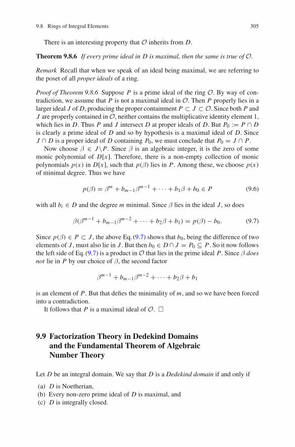
9.8 Rings of Integral Elements 305
There is an interesting property that O inherits from D.
Theorem 9.8.6 If every prime ideal in D is maximal, then the same is true of O.
Remark Recall that when we speak of an ideal being maximal, we are referring tothe poset of all proper ideals of a ring.
Proof of Theorem 9.8.6 Suppose P is a prime ideal of the ring O. By way of con-tradiction, we assume that P is not a maximal ideal in O. Then P properly lies in alarger ideal J of D, producing the proper containment P ⊂ J ⊂ O. Since both P andJ are properly contained inO, neither contains the multiplicative identity element 1,which lies in D. Thus P and J intersect D at proper ideals of D. But P0 := P ∩ Dis clearly a prime ideal of D and so by hypothesis is a maximal ideal of D. SinceJ ∩ D is a proper ideal of D containing P0, we must conclude that P0 = J ∩ P .
Now choose β ∈ J\P . Since β is an algebraic integer, it is the zero of somemonic polynomial of D[x]. Therefore, there is a non-empty collection of monicpolynomials p(x) in D[x], such that p(β) lies in P . Among these, we choose p(x)
of minimal degree. Thus we have
p(β) = βm + bm−1βm−1 + · · · + b1β + b0 ∈ P (9.6)
with all bi ∈ D and the degree m minimal. Since β lies in the ideal J , so does
β(βm−1 + bm−1βm−2 + · · · + b2β + b1) = p(β) − b0. (9.7)
Since p(β) ∈ P ⊂ J , the above Eq. (9.7) shows that b0, being the difference of twoelements of J , must also lie in J . But then b0 ∈ D ∩ J = P0 ⊆ P . So it now followsthe left side of Eq. (9.7) is a product inO that lies in the prime ideal P . Since β doesnot lie in P by our choice of β, the second factor
βm−1 + bm−1βm−2 + · · · + b2β + b1
is an element of P . But that defies the minimality of m, and so we have been forcedinto a contradiction.
It follows that P is a maximal ideal of O. �
9.9 Factorization Theory in Dedekind Domainsand the Fundamental Theorem of AlgebraicNumber Theory
Let D be an integral domain. We say that D is a Dedekind domain if and only if
(a) D is Noetherian,(b) Every non-zero prime ideal of D is maximal, and(c) D is integrally closed.

306 9 The Arithmetic of Integral Domains
The reader will notice that if the integral domain D is a field, then D possessesonly one proper ideal {0}, which is both prime and maximal. Such a D is its own fieldof fractions, and any element α ∈ D is a zero of the monic polynomial x − α and sois integral over D. Thus, in a trivial way, fields are Dedekind domains. However, theinteresting features of a Dedekind domain involve its nonzero ideals. For the rest ofthis section, we begin our examination of the ideal structure of an arbitrary Dedekinddomain, D.
The reader is reminded of the following notation that is customary in ring theory: IfA and B are ideals in a commutative ring R, one writes AB for the set {∑n
1 ai bi |ai ∈A, bi ∈ B, n ∈ N}, the ideal generated by all products of an element of A with anelement of B. The ideal AB is called a product of ideals A and B.
Lemma 9.9.1 Assume that P1, P2, . . . , Pr are maximal ideals of the integral domainD, and that P is a prime ideal satisfying
P1P2 · · · Pr ⊆ P.
Then P = Pi for some i.
Proof If P �= Pi , i = 1, 2, . . . , r , then, since each Pi is a maximal ideal distinctfrom P we may find elements ai ∈ Pi\P, i = 1, 2, . . . , r . Thus, a1a2 · · · ar ∈P1P2 · · · Pr ⊆ P . Since P is a prime ideal, we must have ai ∈ P for some i , whichis a contradiction. �
Lemma 9.9.2 Any non-zero ideal of D contains a finite product of non-zero primeideals.
Proof We let A be the family of all non-zero ideals of D for which the desiredconclusion is false. Assume A is non-empty. As D is Noetherian, A must contain amaximal member I0. Clearly, I0 cannot be a prime ideal, since it is a member of A.Accordingly, there must exist a pair of elements α, β ∈ D\I0 with αβ ∈ I0. Next,form the ideals I ′
0 = I0 + αD and I ′′0 = I0 + βD. By maximality of I0, neither
of the ideals I ′0 and, I ′′
0 can lie in A. Therefore, both I ′0 and I ′′
0 respectively containproducts P1 · · · Pm and Pm+1 · · · Pn of non-zero prime ideals. Since I ′
0 I ′′0 ⊆ I0, and
I ′0 I ′′
0 contains P1 · · · Pn , we have arrived at a contradiction. Thus A = ∅ and theconclusion follows. �
At this point it is convenient to introduce some notation. Let D be a Dedekinddomain with field of fractions E . If I ⊆ D is an ideal, set
I −1 = {α ∈ E | α · I ⊆ D}.
Note that D−1 = D, for if α · D ⊆ D, then α = α · 1 ∈ D. Next note that I ⊆ Jimplies that I −1 ⊇ J−1.

9.9 Factorization Theory in Dedekind Domains and the Fundamental Theorem … 307
Lemma 9.9.3 If I is a proper ideal of D, then I −1 properly contains D.
Proof Clearly D ⊆ I −1. Let 0 �= α ∈ I ; by Lemma 9.9.2, we have prime idealsP1, P2, . . . , Pr with P1P2 · · · Pr ⊆ αD ⊆ I . We may assume, furthermore, thatthe index r above is minimal. Since D is Noetherian, there is a maximal ideal Mcontaining I ; thus we have P1P2 · · · Pr ⊆ M . Applying Lemma 9.9.1 we concludethat P1 = M for some index i . Re-index if necessary so that P1 = M . This says that
(i) M P2P3 · · · Pr ⊆ αD ⊆ M , and(ii) P2P3 · · · Pr �⊆ αD,
by the minimality of r . Let β ∈ P2P3 · · · Pr\αD and set λ = β/α. Then λ ∈ E\D;yet, by (i) and (ii),
λI = βα−1 I ⊆ βα−1M ⊆ α−1MP2 · · · Pr ⊆ α−1(αD) ⊆ D,
which puts λ ∈ I −1\D. �
Lemma 9.9.4 If I ⊆ D is an ideal then I −1 is a finitely generated D-module.
Proof If 0 �= α ∈ I , then I −1 ⊆ (αD)−1 = D[α−1], which is a finitely-generatedD-module. Since D is Noetherian, D[α−1] is Noetherian (Theorem 8.2.12), and soI −1 is finitely generated (Theorem 8.2.11). �
Theorem 9.9.5 If I ⊆ D is an ideal, then I −1 I = D.
Proof Set B = I −1 I ⊆ D, so B is an ideal of D. Thus, I −1IB−1 = BB−1 ⊆ D;which says that I −1B−1 ⊆ I −1. But then for any β ∈ B−1, I −1β ⊆ I −1, forcingI −1[β] ⊆ I −1. Since, by Lemma 9.9.4, I −1 is a Noetherian D-module, so is itsD-submodule I −1D[β]I −1[β], From D[β] ⊆ I −1[β] ⊆ I −1 we infer that D[β] isa finitely-generated D module and so β ∈ E is integral over D. As D is integrallyclosed, it follows that β ∈ D. Therefore, B−1 ⊆ D ⊆ B−1 and so D = B−1. Anapplication of Lemma 9.9.3 completes the proof. �
Corollary 9.9.6 If I, J ⊆ D are ideals, then (I J )−1 = I −1 J−1.
Proof D = D2 = I −1 I · J−1 J = I −1 J−1 I J . Therefore, (I J )−1 = D(I J )−1 =I −1 J−1(I J )(I J )−1 = I −1 J−1D = I −1 J−1. �
The following theorem gives us basic factorization theory in a Dedekind domain.
Theorem 9.9.7 Let D be a Dedekind domain and let I ⊆ D be an ideal. Then thereexist prime ideals P1, P2, · · · , Pr ⊆ D such that
I = P1P2 · · · Pr .
The above factorization is unique in that if also
I = Q1Q2 · · · Qs,

308 9 The Arithmetic of Integral Domains
where the Qi ’s are prime ideals, then r = s and Qi = Pπ(i), for some permutationπ of 1, 2, · · · , r .
Proof By Lemma 9.9.2 we know that the ideal I ⊆ D contains a product of primeideals: P1P2 · · · Pr ⊆ I . We shall argue by induction that if P1P2 · · · Pr ⊆ I , andif r is minimal in this respect, then, in fact, P1P2 · · · Pr = I . Since prime ideals aremaximal, the result is certainly true when r = 1. Next, as D is Noetherian, we mayselect a maximal ideal M containing I ; thus we have
P1P2 · · · Pr ⊆ I ⊆ M.
Applying Lemma 9.9.1 we conclude that (say) M = P1. But then
M−1MP2 · · · Pr ⊆ M−1 I ⊆ M−1M = D.
That is to say, M−1 I is an ideal of D and that
P2P3 · · · Pr = M−1M1P2 · · · Pr ⊆ M−1 I.
We apply induction to infer that P2P3 · · · Pr = M−1 I . If one multiplies both sidesby M , then, noting again that MM−1 = D, one obtains P1P2 · · · Pr = I . This provesthe existence of a factorization of I into a product of prime ideals.
Next we prove uniqueness. Thus, assume that there exist prime ideals P1, P2, . . . ,
Pr , Q1, Q2, . . . , Qs with
P1P2 · · · Pr = Q1Q2 · · · Qs . (9.8)
We argue by induction on the minimum of r and s. If, say, r = 1, then we setP = P1 and we have a factorization of the form P = Q1Q2 · · · Qs . By Lemma9.9.1 we may assume that P = Q1 and so P = P Q2 · · · Qs . Multiply both sidesby P−1 and infer that D = Q2 · · · Qs . If s > 2 this is an easy contradiction as thenD = Q2 · · · Qs ⊆ Q2.
Thus we may assume that both s and r are at least 2. Since D is Noetherian, wemay find a maximal ideal M containing the common ideal in (9.8) above, so
P1P2 · · · Pr = Q1Q2 · · · Qs ⊆ M.
AnapplicationofLemma9.9.1 allowsus to infer that (again possibly after reindexing)that M = P1 = Q1. Upon multiplying both sides by M−1 one obtains P2 · · · Pr =Q2 · · · Qs . Induction takes care of the rest. �
We close by mentioning the following result; a proof is outlined in Exercise (8) inSect. 9.9. It can be viewed as saying that Dedekind domains are “almost” principalideal domains.

9.9 Factorization Theory in Dedekind Domains and the Fundamental Theorem … 309
Theorem 9.9.8 Let E ⊇ Q be a finite field extension and let D = OE . Then anyideal I ⊆ D can be expressed as I = Dα + Dβ for suitable elements α,β ∈ I .
9.10 The Ideal Class Group of a Dedekind Domain
We continue to assume that D is a Dedekind domain, with fraction field E . A D-submodule B ⊆ E is called a fractional ideal if it is a finitely generated D-module.
Lemma 9.10.1 Let B be a fractional ideal. Then there exist prime idealsP1, P2, . . . , Pr , Q1, Q2, . . . , Qs such that B = P1P2 · · · Pr Q−1
1 Q−12 · · · Q−1
s . (Itis possible that either r = 0 or s = 0.)
Proof Since B is finitely generated, there exist elements α1,α2, . . . ,αk ∈ E withB = D[α1, . . . ,αk]. Since E is the fraction field of D, we may choose an elementβ ∈ D with βαi ∈ D, i = 1, 2, . . . , k. Therefore, it follows immediately that βB ⊆D, i.e.,βB is an ideal of D. Therefore, applyTheorem9.9.7 to obtain the factorizationβB = P1P2 · · · Pr into prime ideals of D. Next, factor βD as βD = Q1Q2 · · · Qs ,prime ideals, and so (βD)−1 = Q−1
1 Q−12 · · · Q−1
s . Thus, B = β−1P1P2 · · · Pr =D[β−1]P1P2 · · · Pr = (βD)−1P1P2 · · · Pr = P1P2 · · · Pr Q−1
1 Q−12 · · · Q−1
s . �Corollary 9.10.2 The set of fractional ideals in E forms an abelian group undermultiplication.
Proof It suffices to prove that for any collection P1, · · · , Pr , Q1, . . . , Qs of primeideals of D, the D-module P1 · · · Pr Q−1
1 · · · Q−1s is finitely generatedover D. Letα ∈
Q1Q2 · · · Qs , and so αD ⊆ Q1Q2 . . . Qs . In turn, it follows that Q−11 · · · Q−1
s ⊆(αD)−1 = α−1D = D[α−1]. But then
P1 · · · Pr Q−11 · · · Q−1
s ⊆ Q−11 · · · Q−1
s ⊆ D[α−1].
That is to say, P1 · · · Pr Q−11 · · · Q−1
s is contained in a finitely-generated module overthe Noetherian domain D and hence must be finitely generated. �
A fractional ideal B ⊆ E is called a principal fractional ideal if it is of the formαD, for some α ∈ E . Note that in this case, B−1 = α−1D. It is easy to show that ifD is a principal ideal domain, then every fractional ideal is principal (Exercise (1)in Sect. 9.10).
If F is the set of fractional ideals in E we have seen that F is an abelian groupundermultiplication, with identity D. If we denote byP the set of principal fractionalideals, then it is easy to see that P is a subgroup of F ; the quotient group C = F/Pis called the ideal class group of D; it is trivial precisely when D is a principalideal domain. If D = OE for a finite extension E ⊇ Q, then it is known that C is afinite group. The order h = |C| is called the class number of D (or of E) and is afundamental (though somewhat subtle) invariant of E .

310 9 The Arithmetic of Integral Domains
9.11 A Characterization of Dedekind Domains
In this section we’ll prove the converse of Theorem 9.9.7, thereby giving a charac-terization of Dedekind domains.
To begin with, let D be an arbitrary integral domain, with fraction field E . Inanalogy with the preceding section, if I ⊆ D is an ideal, we set
I −1 = {α ∈ E | αI ⊆ D},
and say that I is invertible if I −1 I = D.
Lemma 9.11.1 Assume that an ideal I of D admits factorizations into invertibleprime ideals:
P1P2 · · · Pr = I = Q1Q2 · · · Qs .
Then r = s, and (possibly after re-indexing) Pi = Qi , i = 1, 2, . . . , r .
Proof We shall apply induction on the total number of ideals r + s. Among thefinitely many ideals in {Pi } ∪ {Q j } chose one that is minimal with respect to thesubset relationship. By reindexing the ideals and transposing the symbols “P” and“Q”, if necessary, we may assume this minimal prime ideal is P1. Since P1 is primeand contains
∏Q j , we must have Q j ⊆ P1 for some index j . After a further
reindexing, we may assume j = 1. Now, since P1 was chosen minimal in the finiteposet ({Pi } ∪ {Q j },⊆), one has P1 = Q1. Then by invertibility of the ideals, we seethat
P−11 I = Q−1
1 I = P2 · · · Pr = Q2 · · · Qs . (9.9)
Applying induction to Eq. (9.9) forces r = s and (with further reindexing) Pi = Qi ,i = 2, . . . , s. This completes the proof. �Lemma 9.11.2 Let D be an integral domain.
(i) Any non-zero principal ideal is invertible.(ii) If 0 �= x ∈ D, and if the principal ideal xD factors into prime ideals as
xD = P1P2 · · · Pr , then each Pi is invertible.
Proof Clearly if x ∈ D, then (xD)−1 = x−1D and (xD)(x−1D) = D, so xD isinvertible, proving (i). For (ii), simply note that for any i = 1, 2, . . . , r , that
D = P1P2 · · · Pr · (x−1D) = Pi (P1 · · · Pi−1Pi+1 · · · Pr )(x−1D),
forcing Pi to be invertible. �Now assume that D is an integral domain satisfying the following condition:
(*) If I ⊆ D is an ideal of D, then there exist prime ideals P1, P2, . . . , Pr ⊆ Dsuch that
I = P1P2 · · · Pr .

9.11 A Characterization of Dedekind Domains 311
Note that no assumption is made regarding the uniqueness of the above factoriza-tion. We shall show not only that uniqueness automatically follows (See Corol-lary 9.11.6, below), but that D is actually a Dedekind domain, giving us the desiredcharacterization.
Theorem 9.11.3 Any invertible prime ideal of D is maximal.
Proof Let P be an invertible prime ideal and let a ∈ D\P . Define the ideals I =P + aD, J = P + a2D, and factor into prime ideals:
I = P1P2 · · · Pr , J = Q1Q2 · · · Qs .
Note that each Pi , Q j ⊇ P . We now pass to the quotient ring D = D/P and setPi = Pi/P, i = 1, 2, . . . , r, Q j = Q j/P, j = 1, 2, . . . , s. Clearly the idealsPi , Q j , i = 1, 2, . . . , r, j = 1, 2, . . . , s are prime ideals of D. Note that wherea = a + P , we have I = aD, J = a2D, principal ideals of D.
Note thataD = I = P1 · · · Pr , a2D = J = Q1 · · · Qs,
which, by Lemma 9.11.2 part (ii), imply that the prime ideals P1, · · · , Pr and
Q1, · · · Qs , are invertible ideals of D. However, as J = I2, then
Q1 · · · Qs = P21 · · · P
2r ,
by Lemma 9.11.1 we conclude that s = 2r and (possibly after reindexing) Pi =Q2 j−1 = Q2 j , j = 1, 2, . . . , r . This implies that Pi = Q2 j−1 = Q2 j , j =1, 2, . . . , r , and so J = I 2. Therefore, P ⊆ J = I 2 = (P + aD)2 ⊆ P2 + aD.If x ∈ P we can write x = y + az, where y ∈ P2, z ∈ D. Thus, az = x − y ∈P . As a �∈ P , and P is prime, we infer that z ∈ P . Therefore, in fact, we haveP ⊆ P2 + a P ⊆ P , and so it follows that P = P2 + a P . As P is invertible byhypothesis, we may multiply through by P−1 and get D = P + aD = I , and so Pis maximal. �
Theorem 9.11.4 Any prime ideal is invertible, hence maximal.
Proof Let P be a prime ideal of D and let x ∈ P .Wemay factor the principal ideal xDas xD = P1P2 · · · Pr . By Lemma 9.11.2 (ii) the prime ideals Pi , i = 1, 2, . . . , r areinvertible, and hence, by Theorem 9.11.3, they aremaximal. Now apply Lemma 9.9.1to infer that P = Pi , for some i and hence is invertible. Theorem 9.11.3 now forcesP to be maximal. �
The following two corollaries are now immediate:
Corollary 9.11.5 Any ideal of D is invertible.
Corollary 9.11.6 Any ideal of D factors uniquely into prime ideals.

312 9 The Arithmetic of Integral Domains
Theorem 9.11.7 D is Noetherian.
Proof Let I ⊆ D be an ideal. Being invertible by Corollary 9.11.5, there existelements a1, a2, . . . , ar ∈ I, b1, b2, . . . , br ∈ I −1 such that
∑ai bi = 1. If x ∈ I,
then bi x ∈ D, i = 1, 2, . . . , r and x = ∑(xbi )ai , i.e., I = D[a1, a2, . . . , ar ],
proving that I is finitely generated, and hence D is Noetherian. �
Our task of showing that D is a Dedekind domain will be complete as soon as wecan show that D is integrally closed. To do this it is convenient to introduce certain“overrings” of D, described below.
Let D be an arbitrary integral domain and let E = F(D), the field of fractions ofD. If P ⊆ D is a prime ideal of D, we set
DP = {α/β ∈ E | α,β ∈ D, β �∈ P}.
It should be clear (using the fact that P is a prime ideal) that DP is a subring ofE containing D. (The reader will recall from Sect. 9.6.4 that DP is the localizationof D at the prime ideal P .) It should also be clear that the same field of fractionsemerges: F(DP) = E .
Lemma 9.11.8 Let I be an ideal of D, and let P be a prime ideal of D.
(i) If I �⊆ P then DP I = DP .(ii) DP P−1 properly contains DP .
Proof Note that DP I is an ideal of DP . Since I �⊆ P , any element α ∈ I\P is a unitin DP . It follows that DP I = DP , proving (i). If DP P−1 = DP , then multiplyingthrough by P , and using the fact that P−1P = D, we obtain DP = DP P . Therefore,there is an equation of the form
1 =k∑
i=1
ri
sixi , where each ri ∈ D, si ∈ D\P, xi ∈ P.
Multiply the above through by s1s2 · · · sk , and set s′i = s1 · · · si−1si+1 · · · sk, i =
1, 2, . . . , k. Then
s1 · · · sk =k∑
i=1
ri s′i xi ∈ P,
which is an obvious contradiction as each si �∈ P and P is prime. �
Lemma 9.11.9 If α ∈ E then either α ∈ DP or α−1 ∈ DP .
Proof Write α = ab−1, a, b ∈ D, and factor the principal ideals aD and bD asaD = Pe I, bD = P f J , where I, J �⊆ P . Thus, DPa = DP Pe, DP b = DP P f .Assuming that e ≥ f , we have ab−1 ∈ DP Pe P− f = DP Pe− f ∈ DP . Similarly, ife ≤ f one obtains that ba−1 ∈ DP . �

9.11 A Characterization of Dedekind Domains 313
Lemma 9.11.10 DP is integrally closed.
Proof Let α ∈ E\DP be integral over DP . Then there is an equation of the form
αm + am−1αm−1 + · · · + a1α + a0 = 0,
where a0, a1, . . . , am−1 ∈ DP . Since α �∈ DP , we have, by Lemma 9.11.9 thatα−1 ∈ DP ; therefore,
α = 1
αm−1αm = − 1
αm−1
(am−1α
m−1 + · · · + a0)
= am−1 + am−21
α· · · a0
1
αm−1 ∈ DP ,
a contradiction. �
Theorem 9.11.11 D = ∩DP , the intersection taken over all prime ideals P ⊆ D.
Proof Let ab−1 ∈ ∩DP , where a, b ∈ D. Factor the principal ideals aD and bD asaD = Pe1
1 Pe22 · · · Per
r , bD = P f11 P f2
2 · · · P frr ; here all exponents are ≥ 0. It suffices
to show that ei ≥ fi , i = 1, 2, . . . , r . Fix an index i and set P = Pi , e = ei , f = fi .Therefore, aDP = DP Pe, bDP = DP P f , which gives ab−1DP = DP Pe− f .Since ab−1 ∈ DP , and since DP P−1 properly contains DP by Lemma 9.11.8, wehave ab−1DP ⊆ DP � P−c for all integers c > 0. Thus, it follows that e− f ≥ 0. �
As an immediate result, we get
Corollary 9.11.12 D is integrally closed.
Proof Indeed, if α ∈ E and is integral over D, then it is, a fortiori, integral over DP .Since DP is integrally closed by Lemma 9.11.10 we have that α ∈ DP . Now applyTheorem 9.11.11. �
Combining all of the above we get the desired characterization of Dedekinddomains:
Corollary 9.11.13 D is a Dedekind domain if and only if every ideal of D can befactored into prime ideals.
We conclude this section with a final remark.
Corollary 9.11.14 Any Dedekind domain (in particular, any algebraic integerdomain) is a PID if and only if it is a UFD.
Proof ByTheorem9.4.3 any principle ideal domain is a unique factorization domain.So it only remains to show that any Dedekind domain that is a UFD, is also a PID.
Assume that the Dedekind domain D is a UFD. We begin by showing that allprime ideals of D are principal. Thus, let 0 �= P ⊂ D be a prime ideal and let0 �= x ∈ P . As D is a UFD, we may factor x into primes: x = p1 p2 · · · pk ∈ P;

314 9 The Arithmetic of Integral Domains
this easily implies that pi ∈ P for some index i . Set p = pi . The principal ideal pDgenerated by p is a prime ideal and hence is maximal (as D is Dedekind), forcingP = pD.
Next let I ⊆ D be an arbitrary ideal of D. Since D is aUFD, each nonzero non-unitof D can be factored into a unique number of primes in D; we shall denote this numberby l(x) (the “length” of x). Now select an element x ∈ I such that l(x) is a minimum.If also y ∈ I , and x does not divide y, we take z to be the greatest common divisor ofx and y; clearly l(z) < l(x). We set x = za, y = zb, where a, b are relatively prime.If the ideal D(a, b) of D generated by both a and b is not all of D, then since D isNoetherian, the non-empty collection {proper ideals J | J ⊇ D(a, b)} must containa maximal ideal M . Since maximal ideals are prime, the assumption guarantees thatthere is a prime p with M = pD ⊇ D(a, b). But this says that p divides both aand b, which is impossible. Therefore, the ideal D(a, b) must be all of D and so1 ∈ D(a, b). Therefore, there exist elements x0, y0 ∈ D with 1 = x0a + y0b, whichleads to z = x0az + y0bz = x0x + y0y ∈ I . Since l(z) < l(x), this contradictionimplies that the ideal I was principal in the first place. �
9.12 When Are Rings of Integers Dedekind?
The tour de force of the theory of Dedekind Domains given in the preceding sectionwould lead one to suspect that this theory should apply as well to the rings of integralelements of Sect. 9.8—that is, rings OK where K is a field and integrality is withrespect to an integrally closed sub-domain D in which every prime ideal is maximal.9
In order to make such a dream a reality, the definition of Dedekind domain wouldalso demand that OK be Noetherian, and that seems to ask that the dimension of Kover the subfield F(D) be finite. Even given that, is it really Noetherian? So, let ussay that a ring O is a classical ring of integral elements if and only O = OK is thering of elements of K that are integral with respect to a subdomain D, having thefollowing properties:
(CRI1) The domain D is integrally closed in its field of fractions F = F(D). (F isregarded as a subfield of K .)
(CRI2) Every prime ideal of the domain D is a maximal ideal of D.(CRI3) K has finite dimension as an F-vector space.
Lemma 9.12.1 If OK is a classical ring of integral elements, then
1. It is integrally closed.2. Every prime ideal of OK is maximal.
Proof Conclusion 1 is immediate from Theorem 9.8.4. Theorem 9.8.6 implies con-clusion 2. �
9Somehow this historical notationOK seems to glorify K at the expense of the subdomain D, whichis hardly mentioned.

9.12 When Are Rings of Integers Dedekind? 315
Remark Notice that the proof did not utilize (CRI3).
The goal of this section is to present a condition sufficient to force a classical ringof integers to be Dedekind. By Lemma 9.12.1 all that is needed is a proof that OK
is Noetherian.Since the proof involves bilinear forms and dual bases, it might be useful to review
these concepts from linear algebra in the next two paragraphs enclosed in brackets.[Let V be a finite-dimensional vector space over a field F . In general, a mapping
B : V × V → F is a symmetric bilinear form if and only if:
(i) B(x, ay + bz) = aB(x, y) + bB(x, z)(ii) B(ax + by, z) = aB(x, z) + bB(y, z)(iii) B(x, y) = B(y, x)
for each (x, y, z, a, b) ∈ V ×V × K × F × F . Thus for each vector x ∈ V , statement(i) asserts that the mapping λx : K → F defined by y �→ B(x, y) is a functional,that is, a vector of the dual space V ∗ := HomF (V, F). The bilinear form B is said tobe non-degenerate if and only if the linear transformation λ : V → V ∗ defined by
x �→ λx , for all x ∈ K
is an injection, and so, as V is finite-dimensional over F , a bijection. Thus the bilinearform B is non-degenerate if and only if ker λ = 0—that is, the only element x , suchthat B(x, y) = 0 for every element y ∈ K , is x = 0.
For any finite F-basis {xi } of K , there exists a functional fi , such that fi (xi ) = 1,while fi (x j ) = 0 for j �= i . If the bilinear form B is non-degenerate, the previousparagraph tells us that the associated mapping λ : V → V ∗ := HomF (K , F) issurjective. Thus for each functional fi described just above, there exists a vector yi
such that λ(yi ) = fi . Thus, for each index i , one has
B(yi , x j ) = δi j , where δi j = 1 if i = j and is zero otherwise.
Wecall {yi } adual basis of {xi } with respect to the form B. Note that a dual basis existsonly if the vector space V is finite dimensional, and the form B is non-degenerate.]
Now, as above, consider D, F = F(D), K a field containing F as a subfield sothat dim(K F ) is finite, and considerOK , the subring of elements of K that are integralwith respect to D. Let T be the collection of F-linear transformations K → F . Thiscollection contains the “zero” mapping K → {0}, and of course many others. Wesay that a transformation T ∈ T is tracelike if and only if
T (OK ) ⊆ D.
We now offer the following:
Theorem 9.12.2 Let OK be a classical ring of integral elements of a field K , withrespect to the subdomain D so that conditions (CID1) (CID2) and (CID3) hold for

316 9 The Arithmetic of Integral Domains
D. Suppose a non-zero tracelike transformation T : K → F exists. Then OK is aNoetherian domain, and so (by Lemma 9.12.1) is a Dedekind domain.
Proof Let T : K → F be the tracelike transformationwhose existencewas assumed.From T we define a symmetric bilinear form BT : K × K → F , by the followingrecipe:
BT (x, y) := T (xy), for all x, y ∈ K .
Next we show that the form BT is non-degenerate. If this form were degeneratethere would exist a non-zero element x in the field K such that T (xy) = 0 for allelements y ∈ K . Since xy wanders over all of K as y wanders over K , we see thatthis means T (K ) = 0. But that is impossible as T was assumed to be non-zero.
Now by (CID3) K has finite dimension over F and so we may choose an F-basisof K , say X := {x1, . . . , xn}. By Corollary 9.8.5, we may assume that each basiselement xi lies in OK . Since K is finite-dimensional, and BT is a non-degenerateform, there exists a so-called dual basis {yi } of K , such that BT (yi , x j ) is 0 if i �= j ,and is 1, if i = j .
Now consider an arbitrary integral element β ∈ OK . We may write β = ∑ai yi ,
since {yi } is a basis for K . Then for any fixed index j , we see that T (β · x j ) = a j ,where a j ∈ F . Since both x j and β belong toOK , so does the product βx j . Since Tis tracelike, we must conclude that T (β · x j ) = a j belongs to D. Thus β is a D-linearcombination of the yi . Since β was an arbitrary element of OK , we must concludethat
OK ⊆ Dy1 ⊕ Dy2 ⊕ · · · ⊕ Dyn := M
a finitely generated D-module. Now D is Noetherian, and so, by Noether’s Theorem(Theorem8.2.12), M is alsoNoetherian.ByLemma8.2.2, part (i), each D-submoduleof M is also Noetherian. Thus OK is also Noetherian, and the proof is complete. �
Where does this leave us? Chap. 11 provides a detailed study of fields and fieldextensions. Among field extensions, F ⊆ K , there is a class called separable exten-sions. Itwill emerge that for any separable extension F ⊆ K with dimF K finite, theredoes exist a non-zero tracelike linear transformation K → F (see Corollary11.7.6in Sect. 11.7.4). Moreover, the extension F ⊆ K is always separable if the field F(and hence K ) has characteristic zero (Lemma 11.5.4).
Of course, historically, the prize integral domain motivating all of this, is the ringof algebraic integers. That would be the ring of integral elementsOK where D = Z,the ring of integers, and the extension field K has finite-dimension as a vector spaceover thefield of rational numbersQ. The result of the previous paragraph (anticipatingresults from Chap.11, to be sure) together with Theorem 9.12.2 yields the following.
Corollary 9.12.3 Any ring of algebraic integers is a Dedekind domain.

9.13 Exercises 317
9.13 Exercises
9.13.1 Exercises for Sects. 9.2, 9.3, 9.4 and 9.5
1. Earlier, in Theorem 7.4.7, we learned that every finite integral domain is a field.Prove the following theorem which replaces finiteness by finite dimension.
Theorem 9.13.1 Suppose an integral domain D is finite-dimensional over a subfieldF. Then D is a field.
[Hint: If F = D their is nothing to prove, so wemay assume dimF D = n > 1 andproceed by induction on n. Choose an element α ∈ D − F , consider a minimalsubmodule M for the subring F[α] (Why does it exist?) Prove that it has theform m F[α] (i.e. it is cyclic,) and that there is a right F[α]-module isomorphismφ : M → F[x]/I , where φ(α) = x + I , and I is the ideal in F[x] consisting allpolynomials r(x) ∈ F[x] such that mr(α) = 0. Cite the theorems that force I tobe a maximal principal ideal F[x]p(x), and explain why p(x) is an irreduciblepolynomial. Noting that D is a domain, conclude that p(α) is the zero element ofD and so K := F[α] � F[x]/F[x]p(x) as rings, and so K is a field. Finish theinduction proof.]
2. Let D be a fixed unique-factorization-domain (UFD), and let p be a prime elementin D. Then the principal ideal (p) := pD is a maximal ideal and D/(p) is afield. The next few exercises concern the following surjection between integraldomains:
m p : D[x] → (D/(p))[x],
which reduces mod p the coefficients of any polynomial of D[x].Show that m p is a ring homomorphism. Conclude that the principal ideal in D[x]generated by p is a prime ideal and from this, that p is a prime element in thering D[x].
3. This exercise has two parts. In each of them D is a UFD and is embedded in thepolynomial ring D[x] as the polynomials of degree zero together with the zeropolynomial. For every prime element p in D we let Fp := D/(p), a field, and letF := F(D) be the field of fractions of D. We fix a maximal ideal M in D[x] andset K = D[x]/M , another field. Our over-riding assumption in this exercise isthat M ∩ D = (0)—that is, M contains no non-zero polynomials of degree zero.Prove the following statements:
(a) For any prime p ∈ D, show that m p(M) = Fp[x].[Hint: If m p(M) �= Fp[x], then ker(m p)+ M is a proper ideal of D[x]. SinceM ∩ D = (0), we see that p ∈ ker(m p) − M , contradicting the maximalityof M .]
(b) Let n be the minimal degree of a non-zero polynomial in M . (Since M ∩ D =(0), n is positive.) Then there exists a prime element b(x) in D[x] of degreen such that M = D[x]b(x), a principle ideal of D[x].

318 9 The Arithmetic of Integral Domains
[Hint: Choose a polynomial b′(x) ∈ M such that deg b′(x) = n. Since D[x]is a UFD, b′(x) is a product of prime elements of D[x], and so one of theseprime factors b(x), must belong to the prime ideal M . Since M ∩ D = (0),deg b(x) = n.Now consider any non-zero polynomial a(x) ∈ M . Using the fact that F[x]is a Euclidean domain as well as the minimality of n, show that there existsan element d ∈ D such that da(x) is divisible by b(x). Since b(x) is a primeelement of D[x]which does not divide a (because of its degree), b(x) dividesa(x), because it is a prime element.]
4. Prove the following result:
Theorem 9.13.2 Assume D is a UFD with infinitely many association classes ofprimes. Then, if M is a maximal ideal of D[x], M ∩ D �= 0—that is, M contains anon-zero polynomial of degree zero.
[Hint: By way of contradiction assume M ∩ D = (0). Let p be any prime ele-ment in D. By Exercise 3, part (a), there exists a polynomial a(x) ∈ M , suchthat m p((a(x)) = 1, the multiplicative identity element of Fp[x]. By part (ii) ofExercise 3, a(x) = b(x) · e(x), for some e(x) ∈ D[x]. Apply the morphism m p
to this factorization to conclude that m p(b(x) has degree zero in the polynomialring Fp[x]. Thus, writing b(x) = ∑
i bi xi , bi ∈ D, we see that if i > 0, then bi isdivisible by p. But this is true for any prime, and since there are infinitely manyassociation classes of primes, this can be true only if bi = 0, for i > 0. But thenb(x) ∈ D ∩ M , a contradiction. Why?]
5. Let D be a UFD with infinitely many association classes of primes. Show thatany maximal ideal of D[x] is generated by a prime p ∈ D and a polynomialp(x) such that m p(p(x)) is irreducible in Fp[x].
6. Let D be a UFDwith finitely many association classes of primes with representa-tives {p1, . . . , pn}. Setπ = ∏
pi and form theprinciple ideal M = D[x](1+πx).Then M ∩ D = (0). Show that M is a maximal ideal. [Hint: Show that each non-zero element of D[x]/M is a unit of that factor ring, using the unique factorizationin D and the identity xπ = −1 mod M .]
7. (Another proof of Gauss’ Lemma.) Let D be a UFD. A polynomial h(x) in D[x]is said to be primitive if and only there is no prime element p of D dividing eachof the D-coefficients of h(x). Using the morphism m p of the first exercise, showthat if f and g are primitive polynomials in D[x], then the product f g is alsoprimitive. [Hint: by assumption, there is no prime in D dividing f or g in D[x].If a prime p of D divides f g in D[x] then m p( f g) = 0 = m p( f ) · m p(g). Thenuse the fact that (D/(p))[x] is an integral domain.]
8. (Eisenstein’s Criterion) Let D be a UFD. Suppose p is a prime in D and
f (x) = an xn + · · · a1x + a0
is a polynomial in D[x] with n > 1 and an �= 0. Further, assume that

9.13 Exercises 319
(E1) p does not divide the lead coefficient an ;(E2) p divides each remaining coefficient ai for i = 0, . . . , n − 1; and(E3) p2 does not divide a0.
Show that f cannot factor in D[x] into polynomial factors of positive degree. Inparticular f is irreducible in F[x], where F is the field of fractions of D. [Hint:Suppose by way of contradiction that there was a factorization f = gh in D[x]with f and g of degree at least one. Then apply the ring morphism m p to get
m p( f ) = m p(g) · m p(h) = m p(an)xn �= 0.
Now by hypothesis (E1) the polynomials f and m p( f ) have the same degree,while the degrees of g and h are at least as large as the respective degrees oftheir m p images. Since f = gh, and degm p( f ) = degm p(g) + degm p(h), wemust have the last two summands of positive degree. Since (D/(p)[x] is a UFD,x must divide both m p(g) and m p(h). This means the constant coefficients of gand h are both divisible p. This contradicts hypothesis (E3).]
9 Show that under the hypotheses of the previous Exercise 8, one cannot concludethat f is an irreducible element of D[x]. [Hint: In Z[x], the polynomial 2x + 6satisfies the Eisenstein hypotheses with respect to the prime 3. Yet it has a properfactorization in Z[x].]
10 Let p be a prime element of D. Using the morphism m p show that the subset
B := {p(x) = a0 + a1x + · · · + an xn|ai ≡ 0 mod p, for i > 0}
of D[x] is a subdomain.11 Let E be an arbitrary integral domain. For each non-zero polynomial p(x) ∈ E[x]
let �(p) be its leading coefficient—that is the coefficient of the highest powerof x possessing a non-zero coefficient. Thus p(x) is a monic polynomial if andonly if �(p(x)) = 1, and for non-zero polynomials p(x) and q(x), one has�(p(x)q(x)) = �(p(x)) · �(q(x)). Prove the following theorem:
Theorem 9.13.3 Let D1 is an integral domain and suppose D is a subring of D1.Then, of course, D is also an integral domain and we have a containment of polyno-mial rings: D[x] ⊆ D1[x]. Suppose a(x), b(x), and c(x) are polynomials in D1[x]such that c(x) = a(x)b(x). Assume the following:
(i) a(x) and c(x) lie in D[x].(ii) a(x) is monic.
(iii) �(b(x)) ∈ D.
Then b(x) ∈ D[x].In particular, if a(x), b(x), and c(x) are monic polynomials in D1[x] such thatc(x) = a(x)b(x), then two of the polynomials lie in D[x] if and only if the thirddoes.

320 9 The Arithmetic of Integral Domains
[Hint: By hypothesis �(a(x))�(b(x)) = �(c(x)) ∈ D. Write out the three polyno-mials a(x), b(x), and c(x) as linear combinations of powers of x with coefficientsai , bi and ci , with �(a(x)), �(b(x)), and �(c(x)) represented as as, bt and cn ,respectively (of course n = s + t , as = 1 and bt = cn ∈ D). By induction on k,show that bt−k ∈ D for all k for which 0 ≤ k ≤ t .]
12 Let F be a subfield of the field K . Consider the set
L F (K [x]) = {p(x) ∈ K [x]|�(p(x) ∈ F} ∪ {0}
consisting of the zero polynomial and all non-zero polynomials whose leadcoefficient lies in the subfield F .
(a) Show that L F (K [x]) is a subring of K [x].(b) Show that L F (K [x]) is a Euclidean Domain. [Hint: Use the Euclidean algo-
rithm for F[x] and the properties of the lead-coefficient function describedin the preamble of the preceding exercise.]
9.13.2 Exercises on Localization
1. Using the definitions of multiplication and addition for fractions, fill in all thesteps in the proof of the following assertions:
(a) (DS,+) is an abelian group,(b) Multiplication of fractions DS is a monoid.(c) In DS multiplication is distributive with respect to addition.
2. Let D be an integral domain with group of units U (D). Show that if S is amultiplicatively closed subset and S′ is either U (D)S or U (D) ∪ U (D)S, thenthe localizations DS and DS′ are isomorphic.
3. Below are given examples of a domain D and a multiplicatively closed subset ofnon-zero elements of D. Describe as best you can the local ring DS .
(a) D = Z; S is all powers of 3. Is DS a local ring?(b) D = Z; S consists of all numbers of the form 3a5b where a and b are natural
numbers and a + b > 0. Is the condition a + b > 0 necessary?(c) D = Z; S is all positive integers which are the sum of two squares.(d) D = Z; S is all integers of the form a2 + 5b2.(e) D = Z; S is all integers which are congruent to one modulo five.(f) D = Z[x]; S is all primitive polynomials of D.
4. A valuation ring is an integral domain D such that if I and J are ideals of D,then either I ⊆ J or J ⊆ I . Prove that for an integral domain D, the followingthree conditions are equivalent:
(i) D is a valuation ring.

9.13 Exercises 321
(ii) if a, b ∈ R, then either Da ⊆ Db or Db ⊆ Da.(iii) If α ∈ E := F(D), then either α ∈ D or α−1 ∈ D.
Thus, we see that the localizations DP defined at the prime ideal P (which weredefined on p. 312) are valuation rings.
5. Let D be a Noetherian valuation ring.
(i) Prove that D is a PID.(ii) Prove that D contains a unique maximal ideal. (This is true even if D isn’t
Noetherian.)(iii) Conclude that, up to associates, D contains a unique prime element.
(A ring satisfying the above is often called a discrete valuation ring.)6. Let D be a discrete valuation ring, as in Exercise 5, above, and let π be the prime,
unique up to associates. Define ν(a) = r , where a = πr b, π � | b.Prove that ν is an algorithm for D, giving D the structure of a Euclidean domain.
7. Let D be a Noetherian domain and let P be a prime ideal. Show that the local-ization DP is Noetherian.
9.13.3 Exercises for Sect. 9.9
1. Let D be a Dedekind domain and let I ⊆ D be an ideal. Show that I ⊆ P forthe prime ideal P if and only if P is a factor in the prime factorization of I . Moregenerally, show that I ⊆ Pe if and only if Pe is a factor in the prime factorizationof I . Conclude that I = Pe1
1 Pe22 · · · Per
r is the prime factorization of the ideal I
if and only if for each i = 1, 2, . . . , r , I ⊆ Peii , but that I �⊆ Pei +1
i .2. Let P and Q be distinct prime ideals of the Dedekind domain D. Show that
P Q = P ∩ Q. (Note that P Q ⊆ P ∩ Q in any ring.)3. Assume that D is a Dedekind domain and that I = Pe1
1 Pe22 · · · Per
r ,
J = P f11 P f2
2 · · · P frr . Show that
I + J = Pmin{e1, f1}1 · · · Pmin{er , fr }
r , I ∩ J = Pmax{e1, f1}1 · · · Pmax{er , fr }
r .
Conclude that AB = (A+B)(A∩B). (Use Exercise 1. Note that this generalizesExercise 2.)
4. (Chinese Remainder Theorem) Let R be an arbitrary ring and let I, J ⊆ R beideals. Say that I and J are coprime if I + J = R. Prove that if I, J are coprimeideals in R, then R/(I ∩ J ) ∼= R/I × R/J . [Hint: map R/(I ∩ J ) → R/I × R/Jby r + (I ∩ J ) �→ (r + I, r + J ). Map R/I × R/J → R(I ∩ J ), as follows. Fixx ∈ I, y ∈ J with x + y = 1, and let (a + I, b + J ) �→ (xb + ya) + (I ∩ J ).]
5. Let R be a commutative ring and let I ⊆ R be an ideal. Assume that for someprime ideals P1, P2, . . . , Pr one has I ⊆ P1 ∪ P2 ∪ · · · ∪ Pr . Show that I ⊆ Pi
for some i

322 9 The Arithmetic of Integral Domains
6. Let D be a Dedekind domain and let I, J ⊆ D be ideals. Show that I and J arecoprime (see Exercise 4) if and only if they do not have a common prime idealin their factorizations into prime ideals.
7. Let D be a Dedekind domain and let I ⊆ D be an ideal. If I = Pe11 Pe2
2 · · · Perr
is the factorization of I into a product of prime ideals (where Pi �= Pj if i �= j)in the Dedekind domain D, show that
D/I ∼= D/Pe11 × D/Pe2
2 × · · · × D/Perr .
8. Let D be a Dedekind domain with ideal I ⊆ D. Factor I as I = Pe11 Pe2
2 · · · Perr
into distinct prime-power factors.
(i) For each i = 1, 2, . . . , r select αi ∈ Peii \Pei +1
i+1 , i = 1, 2 . . . , r . Use Exer-
cise 7 to infer that there exists an element α ∈ D with α ≡ αi mod Pei +1i+1 ,
i = 1, 2, . . . , r .(ii) Show that α ∈ I , and so the principal ideal αD ⊆ I .(iii) Assuming r > 1 if necessary, show that the principal ideal αD factors as
αD = I J , where I and J are coprime.(iv) Factor J = Q f1
1 Q f22 · · · Q fs
s , a product of distinct prime powers. Show thatthere exists an element β ∈ I\(Q1 ∪ Q2 ∪ · · · ∪ Qs). (See Exercise 5.)
(v) Show that the ideal (α,β)D = I .
The above shows that every ideal in a Dedekind domain is “almost principal”inasmuch as no ideal requiresmore than two elements in a generating set, provingTheorem 9.9.8.
9. In the Dedekind domain D = Z[√−5] show that (3) = (3, 4 +√−5)(3, 4 −√−5) is the factorization of the principal ideal (3) into a product of prime ideals.10. Let E be a finite extension of the rational field Q, and set R = OE . Let P be
a prime ideal of R. Then P ∩ Z is a prime ideal of Z so that P ∩ Z = pZ, forsome prime number p. Show that we may regard Z/pZ as a subfield of R/P ,and that dimensions satisfy the inequality
dim(Z/pZ)(R/P) ≤ dimQ E,
with equality if and only if p remains prime in OE . [Hint: Don’t forget to firstconsider why R/P is a field.]
9.13.4 Exercises for Sect. 9.10
1. If D is a PID prove that every fractional ideal of E is principal.2. Let D be a Dedekind domain with fraction field E . Prove that E itself is not a
fractional ideal (except in the trivial case in which D is a field to be begin with).

9.13 Exercises 323
[Hint: If E properly contains D, one must prove that E is not a finitely generatedD-module.]
3. Let D be aDedekind domainwith ideal class group C. Let P ⊆ D be a prime idealand assume that the order of the element [P] ∈ C is k > 1. If Pk = (π) := Dπ,for some π ∈ D, show that π is irreducible but not prime.
4. An integral domain D such that every non-unit a ∈ D can be factored intofinitely many irreducible non-units is called an atomic domain. Prove that everyNoetherian domain is atomic. (Note that uniqueness of factorizationwill typicallyfail.)
5. Let D be a Dedekind domain with ideal class group of order at most 2. Provethat the number of irreducible factors in a factorization of an element a ∈ Ddepends only on a.10 [Hint: Note first that by Exercise 4, any non-unit of D canbe factored into finitely many irreducible elements. By induction on the minimallength of a factorization of a ∈ D into irreducible elements, we may assumethat a has no prime factors. Next assume that π ∈ D is a non-prime irreducibleelement. If we factor the principal ideal into prime ideals: (π) = Q1Q2 · · · Qr
then the assumption guarantees that Q1Q2 = (α), for some α ∈ D. If r > 2,then (π) is properly contained in Q1Q2 = (α) and so α is a proper divisor of π, acontradiction. Therefore, it follows that a principal ideal generated by a non-primeirreducible element factors into the product of two prime ideals. Nowwhat?]2593
6. Let D be as above, i.e., a Dedekind domain with ideal class group of order atmost 2. Let π1,π2 ∈ D be irreducible elements. As seen in Exercise 5 above,any factorization of π1π2 will involve exactly two irreducible elements. Showthat, up to associates, there can be at most three distinct factorizations of π1π2into irreducible elements. (As a simple illustration, it turns out that the Dedekinddomain Z[√−5] has class group of order 2; correspondingly we have distinctfactorizations: 21 = 3 · 7 = (1+ 2
√−5)(1− 2√−5) = (4+√−5)(4−√−5).)
9.13.5 Exercises for Sect. 9.11
1. Let D be a ring in which every ideal I ⊆ D is invertible. Prove that D is aDedekind domain. [Hint: First, as in the Proof of Theorem 9.11.7, show that D isNoetherian. Now let C be the set of all ideals that are not products of prime ideals.Since D is Noetherian,C �= ∅ implies that C has amaximalmember J . Let J ⊆ P ,where P is a maximal ideal. Clearly J �= P . Then JP−1 ⊆ PP−1 = D and soJP−1 is an ideal of D; clearly J ⊆ JP−1. If J = JP−1, then JP−1 = P1P2 · · · Pr
so J = PP1P2 · · · Pr . Thus J = JP−1 so JP = J . This is a contradiction. Why?]2. Here is an example of a non-invertible ideal in an integral domain D. Let
10See L. Carlitz, A characterization of algebraic number fields with class number two, Proc. Amer.Math. Soc. 11 (1960), 391–392. In case R is the ring of integers in a finite extension of the rationalfield, Carlitz also proves the converse.

324 9 The Arithmetic of Integral Domains
D = {a + 3b√−5| a, b ∈ Z},
and let I = (3, 3√−5), i.e., I is the ideal generated by 3 and 3
√−5. Show thatI is not invertible. (An easy way to do this is to let J = (3), the principal idealgenerated by 3, and observe that despite the fact that I �= J , we have I 2 = IJ.)
3. This exercise gives a very important class of projective R-modules; see Sect. 8.4.4.Let R be an integral domain with field of fractions F and let I be an ideal ofR. Prove that if I is invertible, then I is a projective R-module. Conversely,prove that if the ideal I is finitely generated and projective as an R-module,then I is an invertible ideal. [Hint: Assuming that I is invertible, there mustexist elements α1,α2, . . . ,αn ∈ I, β1,β2, . . . ,βn ∈ I −1 with
∑αiβi = 1.
Let F be the free R-module with basis { f1, f2, . . . , fn} and define σ : I → Fby σ(α) = ∑
αβi fi ∈ F . Show that σ(I ) ∼=R I and that σ(I ) is a directsummand of F . ApplyTheorem8.4.5 to infer that I is projective. For the converse,assume that I = R[α1,α2, . . . ,αn] and let F be the free R-module with basis{ f1, f2, . . . , fn}. Let ε : F → I be the homomorphism given by ε( fi ) = αi , i =1, 2, . . . , n. Show that since I is projective, there is a homomorphism σ : I → Fsuch that ε ◦ σ = 1I . For each α ∈ I , write σ(α) = ∑
ai (α) fi and show thatfor each i = 1, 2, . . . , n the elements βi := ai (α)/α ∈ F are independent of0 �= α ∈ I . Next, show that each βi ∈ I −1 and finally that
∑αβi = 1, proving
that I is invertible. Note, incidentally, that this exercise shows that Dedekind ringsare hereditary in the sense of Exercise (19) in Sect. 8.5.3. Also, by Exercise 1 ofthis subsection we see that a Noetherian domain is a Dedekind domain if and onlyif every ideal is projective.]
4. Let R be a Dedekind domain with field of fractions E . If I, J ⊆ E are fractionalideals, and if 0 �= φ ∈ HomR(I, J ), prove that φ is injective. [Hint: Argue thatif J0 = im φ, then J0 is a projective R-module. Therefore one obtains I =ker φ ⊕ J ′, where J ∼=R J0. Why is such a decomposition a contradiction?]
5. Let R be a Dedekind domain with field of fractions E , and let I, J ⊆ E befractional ideals representing classes [I ], [J ] ∈ CR , the ideal class group of R.If [I ] = [J ], prove that I ∼=R J . (The converse is also true; see Exercise (9) inSect. 13.13.4 of Chap. 13.)
9.13.6 Exercises for Sect. 9.12
1. Let F be a field and let x be an indeterminate. Prove that the ring R = F[x2, x3]is not integrally closed, hence is not a UFD.
2. Prove the assertion that if a is an algebraic integer, so is√
a.3. Let E be a finite field extension of the rational numbers. Suppose τ is an auto-
morphism of E . Show that τ leaves the algebraic integer ringOE invariant. [Hint:Since themultiplicative identity element 1 is unique, show that any automorphismof E fixes Z and Q element-wise. The rest of the argument examines the effectof such an automorphism on the definition of an algebraic integer.]

9.13 Exercises 325
4. Show that A(−6) := Z[√−6] is not a UFD.5. As we have seen, the ring A(−5) = Z[√−5] is not a UFD. Many odd things
happen in this ring. For instance, find an example of an irreducible element π ∈Z[√−5] and an element a ∈ Z[√−5] such that π doesn’t divide a, but π dividesa2. [Hint: look at factorizations of 9 = 32.]
6. The following result is well-known to virtually every college student. Let f (x) ∈Z[x], and let a
b be a rational root of f (x). If the fraction ab is in lowest terms, then
a divides the constant term of f (x) and b divides the leading coefficient of f (x).If we ask the same question in the context of the ring Z[√−5], then the answeris negative. Indeed, if we consider the polynomial f (x) = 3x2 − 2
√−5 x − 3 ∈Z[√−5][x], then the zeroes are 2+√−5
3 and −2+√−53 . Since both 3 and±2+√−5
are non-associated irreducible elements, then the fractions can be considered tobe in lowest terms. Yet neither of the numerators divide the constant term of f (x).
7. We continue on the theme set in Exercise 6, above. Let D be an integral domainwith field of fractions F(D). Assume the following condition on the domain D:
For every polynomial f (x) = an xn + · · · + a0 ∈ D[x], with a0, an �= 0, and azero a
b ∈ F(D)which is a fraction in lowest terms—i.e., a and b have no commonnon-unit factors and f (a/b) = 0— then a divides a0 and b divides an .
Now prove that for such a ring every irreducible element is actually prime. [Hint:Let π ∈ D be an irreducible element and assume that π|uv, but that π doesn’tdivide either u or v. Let uv = rπ, r ∈ D, and consider the polynomial ux2 −(π + r)x + v ∈ R[x].]
8. Let K be a field such that K is the field of fractions of both subrings R1, R2 ⊆ K .Must it be true that K is the field of fractions of R1∩R2? [Hint: A counter-examplecan be found in the rational function field K = F(x).]
9. Let Q ⊆ K be a finite-degree extension of fields. Prove that if K is the field offractions of subrings R1, R2 ⊆ K , then K is also the field of fractions of R1∩ R2.
10. Again, letQ ⊆ K be a finite-degree extension of fields. This time, let {Rα|α ∈ A}consist of all the subrings of K having K as field of fractions. Show that K is notthe field of fractions of ∩α∈ARα. (In fact, ∩α∈ARα = Z.)
Appendix: The Arithmetic of Quadratic Domains
Introduction
We understand the term quadratic domain to indicate the ring of algebraic integersof a field K of degree two over the rational number fieldQ. The arithmetic propertiesof interest are those which tend to isolate Euclidean domains: Are these principalideal domains (or PID’s)? Are they unique factorization domains (or UFD’s, alsocalled “factorial domains” in the literature)?

326 9 The Arithmetic of Integral Domains
Quadratic Fields
Throughout Q will denote the field of rational numbers. Suppose K is a subfield ofthe complex numbers. Then it must contain 1, 2 = 1+1, all integers and all fractionsof such integers. Thus K contains Q as a subfield and so is a vector space over Q.Then K is a quadratic field if and only of dimQ(K ) = 2.
Suppose now that K is a quadratic field, so as a Q-space,
K = Q ⊕ ωQ, for any chosen ω ∈ K − Q.
Then ω2 = −bω − c for rational numbers b and c, so ω is a root of the monicpolynomial
p(x) = x2 + bx + c
in Q[x]. Evidently, p(x) is irreducible, for otherwise, it would factor into two linearfactors, one of which would have ω for a rational root, against our choice of ω. Thusp(x) has two roots ω and ω given by
(−1 ±√
b2 − 4c)/2.
We see that K is a field generated by Q and either ω or ω—a fact which can beexpressed by writing
K = Q(ω) = Q(ω).
Evidently
K = Q(√
d), where d = b2 − 4c.
Observe that substitution of ω for the indeterminate x in each polynomial of Q[x]produces an onto ring homomorphism,
vω : Q[x] → K ,
whose kernel is the principal ideal p(x)Q[x].11 But as vω : Q[x] → K has the samekernel, we see that the Q-linear transformation
σ : Q ⊕ ωQ → Q ⊕ ωQ,
which takes each vector a + bω to a + bω, a, b ∈ Q, is an automorphism of the fieldK . Thus σ(ω) = ω, and σ2 = 1K (why?).
Associated with the group 〈σ〉 = {1K ,σ} of automorphisms of K are two furthermappings.
11This was the “evaluation homomorphism” of Theorem 7.3.3, p. 207.

Appendix: The Arithmetic of Quadratic Domains 327
First is the trace mapping,Tr : K → Q,
which takes each element ζ of K to ζ + ζσ . Clearly this mapping is Q-linear.The second mapping is the norm mapping,
N : K → Q,
which takes each element ζ of K to ζζσ . This mapping is not Q-linear, but it followsfrom its definition (and the fact that multiplication in K is commutative) that it ismultiplicative—that is
N (ζψ) = N (ζ)N (ψ),
for all ζ, ψ in K .Just to make sure everything is in place, consider the roots ω and ω of the irre-
ducible polynomial p(x) = x2 + bx + c. Since p(x) factors as (x − ω)(x − ω) inK [x], we see that the trace is
T (ω) = T (ω) = −b ∈ Q,
and that the norm is
N (ω) = N (ω) = c, also in Q.
Quadratic Domains
We wish to identify the ring A of algebraic integers of K . These are the elementsω ∈ K which are roots of at least one monic irreducible polynomial in Z [x]. At thisstage the reader should be able to prove:
Lemma 9.A.1 An element ζ ∈ K − Q is an algebraic integer if and only if its traceT (ζ) and its norm N (ζ) are both rational integers.
Now putting ζ = √d , where d is square-free and K = Q(
√d), the lemma
implies:
Lemma 9.A.2 If d is a square-free integer, then the ring of algebraic integers ofK = Q(
√d) is the Z-module spanned by
{1,√d} if d ≡ 2, 3 mod 4,
{1, (1 + √d)/2} if d ≡ 1 mod 4.
Thus the ring of integers for Q(√7) is the set {a +b
√7|a, b ∈ Z}. But if d = −3,
then (1+√−3)/2 is a cube root of unity, and the ring of integers for Q(√−3) is the
domain of Eisenstein numbers.

328 9 The Arithmetic of Integral Domains
Which Quadratic Domains Are Euclidean, Principal Idealor Factorial Domains?
Fix a square free integer d and let A(d) denote the full ring of algebraic integers ofK = Q(
√d). A great deal of effort has been devoted to the following questions:
1. When is A(d) a Euclidean domain?2. More generally, when is A(d) a principal ideal domain?
In this chapter we showed that the Gaussian integers, A(−1) and the Eisensteinnumbers, A(−3) were Euclidean by showing that the norm function could act as thefunction g : A(d) → Z with respect to which the Euclidean algorithm is defined. Inthe case that the norm can act in this role, we say that the norm is algorithmic.
The two questions have been completely answered when d is negative.
Proposition 9.A.1 The norm is algorithmic for A(d) when d = −1,−2,−3,−7and −11. For all remaining negative values of d, the ring A(d) is not even Euclidean.However, A(d) is a principal ideal domain for
d = −1,−2,−3,−7,−11,−19,−43,−67,−163,
and for no further negative values of d.
There are ways of showing that A(d) is a principal ideal domain, even when thenorm function is not algorithmic. For example:
Lemma 9.A.3 Suppose d is a negative square-free integer and the (positively val-ued) norm function of A(d) has this property:
• If N (x) ≥ N (y) then either y divides x or else there exist elements u and v
(depending on x and y) such that
0 < N (ux − yv) < N (y).
Then A(d) is a principal ideal domain.
This lemma is used, for example, to show that A(−19) is a PID.12
For positive d (where Q(√
d) is a real field) the status of these questions is not soclear. We can only report the following:
Proposition 9.A.2 Suppose d is a positive square-free integer. Then the norm func-tion is algorithmic precisely for
d = 2, 3, 5, 6, 7, 11, 13, 17, 19, 21, 29, 33, 37, 41, 57, 73.
12See an account of this in Pollard’s The Theory of Algebraic Numbers, Carus Monograph no. 9,Math. Assoc. America, p. 100, and in Wilson, J.C., A principal ideal domain that is not Euclidean,Mathematics Magazine, vol. 46 (1973), pp. 34–48.

Appendix: The Arithmetic of Quadratic Domains 329
The domain A(d) is known to be a principal ideal domain for many further valuesof d. But we dont even know if this can occur for infinitely many values of d!Moreover, among these PID’s, how many are actually Euclidean by some functiong other than the norm function? Are there infinitely many?
Non-Factorial Subdomains of Euclidean Domains
Here it is shown that standard Euclidean domains such as the Gaussian integerscontain subdomains for which unique factorization fails. These nice examples aredue to P. J. Arpaia (“A note on quadratic Euclidean Domains”, Amer.Math.Monthly,vol. 75(1968), pp 864–865).
Let A0(d) be the subdomain of A(d) consisting of all integral linear combinationsof 1 and
√d, where d is a square-free integer. Thus A0(d) = A(d) if d ≡ 2, 3 mod 4,
and is a proper subdomain of A(d) only if d ≡ 1 mod 4.Let p be a rational prime. Let A0/(p) be the ring whose elements belong to the
vector space(Z/(p))1 ⊕ (Z/(p))
√d,
where multiplication is defined by setting (√
d)2 to be the residue class modulo pcontaining d. Precisely, A0/(p) is the ring Z[x]/I where I is the ideal generated bythe prime p and the polynomial x2−d . It should be clear that A0/(p) is a field if d isnot zero or is not a quadratic residue mod p, and is the direct (ring) sum of two fieldsif d is a quadratic residue mod p. If p divides d , it has a 1-dimensional nilpotentideal. But in all cases, it contains Z/(p) as a subfield containing the multiplicativeidentity element.
There is a straightforward ring homomorphism
n p : A0 → A0/(p),
which takes a + b√
d to a + b√
d where “bar” denotes the taking of residue classesof integers mod p. Now set
B(d, p) := n−1p (Z/(p)).
Then B(d, p) is a ring, since it is the preimage under n p of a subfield of the imageA0/(p). In fact, as a set,
B(d, p) := {a + b√
d ∈ A0|b ≡ 0 mod p}.
Clearly it contains the ring of integers and so is a subdomain of A(p). Note that thedomains A0 and B(d, p) are both σ-invariant.

330 9 The Arithmetic of Integral Domains
In the subdomain B(d, p), we will show that under a mild condition, there areelements which can be factored both as a product of two irreducible elements andas a product of three irreducible elements. Since d and p are fixed, we write B forB(d, p) henceforward.
Lemma 9.A.4 An element of B of norm one is a unit in B.
Proof Since B = Bσ , N (ζ) = ζζσ = 1 for ζ ∈ B implies ζσ is an inverse in B forζ.
Lemma 9.A.5 Suppose ζ is an element A0 whose norm N (ζ) is the rational primep. The ζ does not belong to B.
Proof By hypothesis, N (ζ) = a2 − b2d = p. If p divided integer b, it would divideinteger a, so p2 would in fact divide N (ζ), an absurdity. Thus p does not divide band so ζ is not an element of B.
Corollary 9.A.1 If an element of B has norm p2, then it is irreducible in B.
Proof By Lemma 9.A.4, elements of norm one in B are units in B. So if an elementof norm p2 in B were to have a proper factorization, it must factor into two elementsof norm p. But the preceding lemma shows that B contains no such factors.
Theorem 9.A.1 Suppose there exist integers a and b such that a2 − db2 = p(that is, A0 contains an element of norm p). Then the number p3 admits these twofactorizations into irreducible elements of B:
p3 = p · p · p
p3 = (pa + pb√
d) · (pa − pb√
d).
Proof The factors are clearly irreducible by Corollary 9.A.1.
We reproduce Arpaia’s table displaying p = a2 − db2 for all d for which thenorm function on A(d) is algorithmic.
d p = a2 − db2 d p = a2 − db2 d p = a2 − db2
−11 47 = 62 − (−11)12 5 11 = 42 − 5 · 12 21 −17 = 22 − 21 · 12−7 11 = 22 − (−3)12 6 −5 = 12 − (6)12 29 −13 = 42 − (26)12
−3 7 = 22 − (−3)12 7 −3 = 22 − 3 · 12 33 −29 = 22 − 33 · 12−2 3 = 12 − (−2)12 11 −7 = 22 − 11 · 12 37 107 = 122 − 37 · 12−1 2 = 1 − (−1)12 13 3 = 42 − 13 · 12 41 −37 = 22 − 41 · 122 −7 = 12 − 2 · 22 17 −13 = 22 − 17 · 12 57 −53 = 22 − 57 · 123 −2 = 12 − 3 · 12 19 −3 = 42 − 19 · 12 73 −37 = 62 − 73 · 12

Appendix: The Arithmetic of Quadratic Domains 331
A Student Project
In the preceding subsection, a non-factorial subdomain B was produced for eachcase that the domain A(d) = alg. int.(Q(
√d)) was Euclidean. But there are only
finitely many of these domains A(d). This raises the question whether one can findsuch a subdomain B in more standard generic Euclidean domains? We know thatno such subdomain can exist in the domain of integers Z due to the paucity of itsubdomains. But are there non-factorial subdomains B of the classical Euclideandomain of polynomials over a field?
This might be done by duplicating the development of the previous section replac-ing the ring of integers Z , by an arbitrary unique factorization domain D which isdistinct from its field of fractions k. Suppose further that K is a field of degree twoover k generated by a root ω of an irreducible quadratic polynomial x2 − bx − c inD[x] which has distinct roots {ω, ω}. (One must assume that the characteristic of Dis not 2.) Then the student can show that, as before, K = k ⊕ ωk as a vector spaceover k and that the mapping σ defined by
σ(u + ωv) = u + ωv, for all u, v ∈ k,
is a field automorphism of K of order two so that the trace and norm mappings Tand N can be defined as before.
Now let A be the set of elements in K whose norm and trace are in D. Thestudent should be able to prove that if D is Noetherian, A is a ring. In any event,A0 := {a + ωb|a, b ∈ D} is a subring.
Now since D is a UFD not equal to its quotient field, there is certainly a prime pin D. It is easy to see that
Bp = {a + ωb|a, b ∈ D, b ∈ pD} = D ⊕ ω pD
is a σ-invariant integral domain. Then the proofs of Lemmas 9.A.4 and 9.A.5 andCorollary 9.A.1 go through as before (note that the fact that D is a UFD is used here).The analogue of the Theorem will follow:
If A0 contains an element of norm p, B is not factorial.
Can we do this so that between A and B lies the Euclidean ring F[x]? The answeris “yes”, if the characteristic of the field F is not 2.
In fact we can pass directly from F[x] to the subdomain B and fill in the roles ofD, k, K , A, and A0 later.
Let p(x) be an irreducible polynomial in F[x] where the characteristic of F isnot 2. Then (using an obvious ring isomorphism) p(x2) is an irreducible element ofthe subdomain F[x2]. Now the student may show that the set
Bp : F[x2] ⊕ xp(x2)F[x2]
is a subdomain of F[x].

332 9 The Arithmetic of Integral Domains
Now D = F[x2] is a UFD with quotient field k = F(x2)—the so called “fieldof rational functions” over F . The quotient field K = F(x) of F[x], is degree twoover k, with the indeterminate x playing the role of ω. Thus
F(x) = F(x2) ⊕ xF(x2)
since ω = x is a zero of the polynomial y2 − x2 which is irreducible in F[x2][y] =D[y]. Since the characteristic is not 2, the roots x and−x are distinct. Thus we obtainour field automorphism σ which takes any element ζ = r(x2) + xs(x2) of F(x), tor(x2)− xs(x2) (r and s are quotients of polynomials in F[x2]). (Note that this is justthe substitution of −x for x in F(x).) Now the student can write out the norm andtrace of such a generic ζ. For example
N (ζ) = r2 − x2s2. (9.10)
At this point the ring Bp given above is not factorial if there exists a polynomialζ = a(x2) + xb(x2) in F[x] of norm p(x2). That is,
a(x2)2 − x2b(x2)2 = p(x2)
is irreducible in F[x2].Here is an example: Take a(x2) = 1 = b(x2), so ζ = x + 1. Then N (1 + x) =
x2 − 1 is irreducible in F[x2]. Then in Bp = F[x2] ⊕ x(x2 − 1)F[x2], we have thefactorizations
(1 − x2)3 = (1 + x − x2 − x3)(1 − x − x2 + x3)
into irreducible elements.

Chapter 10Principal Ideal Domains and Their Modules
Abstract An integral domain in which every ideal is generated by a single elementis called a principle ideal domain or PID. Finitely generated modules over a PID arecompletely classified in this chapter. They are uniquely determined by a collectionof ring elements called the elementary divisors. This theory is applied to two of themost prominent PIDs in mathematics: the ring of integers, Z, and the polynomialrings F[x], where F is a field. In the case of the integers, the theory yields a completeclassification of finitely generated abelian groups. In the case of the polynomial ringone obtains a complete analysis of a linear transformation of a finite-dimensionalvector space. The rational canonical form, and, by enlarging the field, the Jordanform, emerge from these invariants.
10.1 Introduction
Throughout this chapter, the integral domain D (and sometimes R) will be a principalideal domain (PID). Thus it is a commutative ring forwhich a product of two elementsis zero only if one of the factors is already zero—that is, the set of non-zero elements isclosed under multiplication.Moreover every ideal is generated by a single element—and so has the form Dg for some element g in the ideal.
Of course, as rings go, principal ideal domains are hardly typical. But two of theirexamples, the ring of integers Z, and the ring F[x], of all polynomials in a singleindeterminate x over a field F , are so pervasive throughout mathematics that theiratypical properties deserve special attention.
In the previous chapter we observed that principal ideal domains were in factunique factorization domains. In this chapter, the focus is no longer on the internalarithmetic of such rings, but rather on the structure of all finitely-generated submod-ules over these domains. As one will soon see, the structure is rather precise.
© Springer International Publishing Switzerland 2015E. Shult and D. Surowski, Algebra, DOI 10.1007/978-3-319-19734-0_10
333

334 10 Principal Ideal Domains and Their Modules
10.2 Quick Review of PID’s
Principal Ideal Domains (PID’s) are integral domains D for which each ideal I hasthe form I = aD for some element a of D. One may then employ Theorem 8.2.11to infer from the fact that every ideal is finitely generated, that the Ascending ChainCondition (ACC) holds for the poset of all ideals.
Recall that a non-zero element a divides element b if and only if
aD ⊇ bD.
It follows—as we have seen in the arguments that a principal ideal domain (PID)is a unique factorization domain (UFD)—that a is irreducible if and only if aD is amaximal ideal, and that this happens if and only if a is a prime element (see Lemma9.2.4).
We also recall that for ideals,xD = yD
if and only if x and y are associates. For this means x = yr and y = xs for somer and s in D, so x = xrs, so sr = 1 by the cancellation law. Thus r and s, beingelements of D, are both units.
The least common multiple of two elements a, b ∈ D is a generator m of theideal
aD ∩ bD = mD
where m is unique up to associates.The greatest common divisor of two non-zero elements a and b is a generator d of
aD + bD = dD,
again up to the replacement of d by an associate. Two elements a and b are relativelyprime if and only if
aD + bD = D.
Our aim in this chapter will be to find the structure of finitely-generated modulesover a PID. Basically, our main theorem will say that if M is a finitely-generatedmodule over a principal ideal domain D, then
M � (D/De1) ⊕ (D/De2) ⊕ · · · ⊕ (D/Dek)
as right D-modules, where k is a natural number and for 1 ≤ i ≤ k − 1, ei dividesei+1.

10.2 Quick Review of PID’s 335
This is a very useful theorem. Its applications are (1) the classification of finiteabelian groups, and (2) the complete analysis of a single linear transformation T :V → V of a finite-dimensional vector space into itself. It will turn out that the setof elements ei which are not units is uniquely determined up to associates. But all ofthat still lies ahead of us.
10.3 Free Modules over a PID
We say that an R-module M has a basis if and only if there is a subset B of M (calledan R-basis or simply a basis, if R is understood) such that every element m of Mhas a unique expression ∑
biri , bi ∈ B, ri ∈ R,
as a finite R-linear combination of elements of B. The uniqueness is the key itemhere.
Recall that in Chap. 8, p. 243, we have defined a free (right) module over thering R to be a (right) R module M satisfying any of the following three equivalentconditions:
• M possesses an R-basis, as defined just above.• M is generated by an R-linearly independent set B. (In this case, B is indeed abasis).
• M is a direct sum of submodules Mσ each of which is isomorphic to RR as rightR-modules.
The equivalence of these conditions was the content of Lemma 8.1.8.In general, there is no result asserting that two bases of a free R-module have the
same cardinality. However, the result is true when R is commutative (see Theorem8.1.11), and so it is true for an integral domain D. We call the unique cardinality ofa basis for a free D-module F , the D-rank of F and denote it rkD(F) or just rk(F)
if D is understood.
10.4 A Technical Result
Theorem 10.4.1 Let n and m be natural numbers and let A be an n ×m matrix withcoefficients from a principal ideal domain D. Then there exists an n × n matrix Pinvertible in (D)n×n, and an m × m matrix Q, invertible in (D)m×m, such that
P AQ =
⎛⎜⎜⎝
d1 0 . . . 00 d2 . . . 0. . . . . .
. . . . . .
⎞⎟⎟⎠ where di divides di+1.

336 10 Principal Ideal Domains and Their Modules
The elements {d1, d2, . . . , dk}, where k = min(n, m), are uniquely determined up toassociates by the matrix A.
Proof For each non-zero element d of D let ρ(d) be the number of prime divisorsoccurring in a factorization of d into primes. (Recalling that a PID is always a UFD,the function ρ is seen to be well-defined.) We call ρ(d), the factorization length ofthe element d.
Our goal is to convert A into a diagonalmatrixwith successively dividing diagonalelements by a series of right and left multiplications by invertible matrices. Thesewill allow us to perform several so-called elementary row and column operationsnamely:
(I) Add b times the i th row (column) to the j th row (column), i = j . This isleft (right) multiplication by a suitably sized matrix having b in the (i, j)th(or ( j, i)th) position while having all diagonal elements equal to 1D , and allfurther entries equal to zero.
(II) Multiply a row (or column) throughout by a unit u of D. This is left (right)multiplication by a diagonal matrix diag(1, . . . , 1u, 1, . . . , 1) of suitable size.
(III) Permute rows (columns). This is left (right) multiplication by a suitable per-mutation matrix.
First observe that there is nothing to do if A is the n × m matrix with all entrieszero. In this case each di = 0D , and they are unique.
Thus for A = 0, we consider the entire collection of matrices
S = {PAQ|P, Q units in D(n×n) and D(m×m), respectively}.
Among the non-zero entries of the matrices in S, there can be found a matrix elementbij (in some B ∈ S) with factorization length ρ(bij) minimal. Then by rearrangingthe rows and columns of B if necessary, we may assume that this bij is in the (1, 1)-position of B—that is, (i, j) = (1, 1).
We now claim
b11 divides b1k for k = 2, . . . , m. (10.1)
To prove the claim, assume b11 does not divide b1k . Permuting a few columns ifnecessary, we may assume k = 2. Since D is a principal ideal domain, we may write
b11D + b12D = Dd.
Then as d divides b11 and b12, we see that
b12 = ds and − b11 = dt, with s, t ∈ D.
Then, as d = b11x + b12y, for some x, y ∈ D, we see that
d = (−dt)x + (ds)y so 1 = sy − tx,

10.4 A Technical Result 337
by the cancellation law. Thus
(−t sy −x
)(x sy t
)=
(1 00 1
).
So, after multiplying B on the right by the invertible
Q1 =
⎛⎜⎜⎜⎜⎝
x s 0 . . . 0y t 0 . . . 00 0 1 0 . . .
. . . . . . .
0 0 . . . 0 1
,
⎞⎟⎟⎟⎟⎠
the first row of BQ1 is (d, 0, b13, . . . , b1m). Thus, as d now occurs as a non-zeroelement of D in a matrix in S, we see that ρ(b11) ≤ ρ(d) ≤ ρ(b11) so that b11 is anassociate of d. Thus b11 divides b12 as claimed.
Similarly, we see that b11 divides each entry bk1 in the first column of B. Thus,subtracting suitable multiples of the first row from the remaining rows of B, weobtain a matrix in S with first column, (b11, 0, . . . , 0)T . Then subtracting suitablemultiples of the first column from the remaining columns of this matrix, we arriveat a matrix
B0 :=
⎛⎜⎜⎜⎜⎝
b11 0 0 . . . 00·· B10
,
⎞⎟⎟⎟⎟⎠ ,
where B0 ∈ S. We set B1 = (cij), where 1 ≤ i ≤ n − 1 and 1 ≤ j ≤ m − 1.We now expand on this: we even claim that
b11 divides each entry cij of matrix B1.
This is simply because addition of the j th row to the first row of the matrix B0 justlisted above, yields a matrix B ′ in S whose first row is (b11, c j2, c j3, . . . cjm). But wehave just seen that in any matrix B0 in S containing an element of minimal possiblefactorization length in the (1, 1)-position, that this element divides every element ofthe first row and column. Since B ′ is such a matrix, b11 divides cij.
Now by induction on n + m, there exist invertible matrices P1 and Q1 such thatP1B1Q1 = diag(d2, d3, . . . , ) with d2 dividing d3 dividing . . . dk .1 AugmentingP1 and Q1 by adding a row of zeros above, and then a column to the left whose
1We apologize for the notation here: diag(d2, d3, . . . ,) should not be presumed to be a squarematrix.Of course it is still an (n − 1) × (m − 1)-matrix, with all entries zero except possibly those thatbear a di at the (i, i)-position. If n < m the main diagonal hits the “floor” before it hits the “eastwall”, and the other way round if n > m.

338 10 Principal Ideal Domains and Their Modules
top entry is 1, the remaining entries 0, one obtains matrices P ′1 and Q′
1 such thatP ′1B0Q′
1 = diag(d1, d2, . . .) where we have written d1 for b11.Let us address the uniqueness. Now the element d1 = b11 with minimal prime
length among the entries in B was completely determined by B. Moreover, the pair(b11, B) determined B0 and as well as its submatrix B1. Finally, by induction, onn +m, the numbers d2, . . . dk , are uniquely determined up to associates by the matrixB1. Thus all of the di are uniquely determined by the initial matrix B. �
10.5 Finitely Generated Modules over a PID
Theorem 10.5.1 (The Invariant Factor Theorem) Let D be a principal ideal domainand let M be a finitely generated D-module. Then as right D-modules, we have
M � (D/Dd1) ⊕ (D/Dd2) ⊕ · · · ⊕ (D/Ddn),
where di divides di+1, i = 1, . . . , n − 1.
Proof Let M be a finitely generated D-module. Then by Theorem 8.1.9, there is afinitely generated free module F and a D-epimorphism
f : F → M.
Then F has a D-basis {x1, . . . , xn}, and, as D is Noetherian, its submodule ker f isfinitely generated. Thus we have
M = x1D ⊕ x2D ⊕ · · · ⊕ xn D (10.2)
ker f = y1D + y2D + · · · + ym D. (10.3)
We then have m unique expressions
yi = x1ai1 + x2ai2 + · · · + xnain, i = 1, . . . , m,
and an m × n matrix A = (aij) with entries in D. By the technical result of theprevious subsection, there exist matrices P = (pij) and Q = (qij) invertible inDm×m and Dn×n , respectively, such that
PAQ =⎛⎝ d1 0 . . . 00 d2 . . . 0
..
⎞⎠ (where di |di+1),
an m × n matrix whose only non-zero entries are on the principal diagonal and pro-ceed until they cant go any further (that is, they are defined up to subscriptmin(m, n)).

10.5 Finitely Generated Modules over a PID 339
If we set
Q−1 = (q∗ij), and
y′i =
∑y j pij and
x ′i =
∑x j q
∗ij
then PAQ expresses the y′i in terms of the x ′
i , which now comprise a new D-basis forF . Thus we have
y′1 = x ′
1d1, y′2 = x ′
2d2, . . . etc.,
(where, by convention the expression dk is taken to be zero for min(m, n) < k ≤ m).Also, since P and Q−1 are invertible, the y′
i also span ker f . So, bearing in mindthat some of the y′
i = x ′i di may be zero, and extending the definition of the dk by
setting dk := 0 if m < k ≤ n, we may write
F = x ′1D ⊕ x ′
2D ⊕ · · · ⊕ x ′n D
ker f = x ′1d1D ⊕ x ′
2d2D ⊕ · · · ⊕ x ′ndn D.
Then
M = f (F) � F/ ker f � (D/d1D) ⊕ (D/d2D) ⊕ · · · ⊕ (D/dm D)
and the proof of the theorem is complete. �
Remark The essential uniqueness of the elements {di } appearing in the above the-orem will soon emerge in Sect. 9.6 below. These elements are called the invariantfactors (or sometimes the elementary divisors) of the finitely generated D-module M .
At this stage their uniqueness does not immediately follow from the fact that theyare uniquely determined by the matrix A since this matrix itself depended on thechoice of a finite spanning set for ker f and it is not clear that all such finite spanningsets can be moved to one another by the action of an invertible transformation Q inhomD{ker f, ker f }.
An element m of a D-module M is called a torsion element if and only if thereexists a non-zero element d ∈ D such that md = 0. Recall from Exercise (3) inSect. 8.5.1 that the annihilator Ann(m) = {d ∈ D|md = 0} is an ideal and that wehave just said that m is a torsion element if and only if Ann(m) = 0. In an integraldomain, the intersection of two non-zero ideals is a non-zero ideal; it follows fromthis that the sum of two torsion elements of an R-module is a torsion element. Infact the set of all torsion elements of M forms a submodule of M called the torsionsubmodule and denoted torM .
Corollary 10.5.2 A finitely generated D-module over a principal ideal domain D,is a direct sum of its torsion submodule torM and a free module.

340 10 Principal Ideal Domains and Their Modules
Proof By the Invariant Factor Theorem (Theorem 10.5.1),
M = (D/d1D) ⊕ · · · ⊕ (D/dn D)
where di divides di+1. Choose index t so that i ≤ t implies di = 0, and, for i > twe have di = 0. Then
torM = (D/d1D) ⊕ · · · ⊕ (D/dt D)
and so
M = torM ⊕ DD ⊕ DD ⊕ · · · ⊕ DD,
with n − t copies of DD . �
If M = torM , we say that M is a torsion module.Let M be a module over a principal ideal domain, D. Let p be a prime element
in D. We define the p-primary part of M as the set of elements of M annihilated bysome power of p, that is
Mp = {m ∈ M |mpk = 0 for some natural number k = k(m)}.
It is easy to check that Mp is a submodule of M . We now have
Theorem 10.5.3 (Primary Decomposition Theorem) If M is a finitely generatedtorsion D-module, where D is a principal ideal domain, then there exists a finitenumber of primes p1, p2, . . . , pN such that
M � Mp1 ⊕ · · · ⊕ MpN .
Proof Since M is finitely generated, we have M = x1D + · · · xm D for some finitegenerating set {xi }. Since M is a torsion module, each of the xi is a torsion element,and so all of the ideals Ai := Ann(xi ) are non-zero; and since D is a principal idealdomain,
Ai = Ann(xi ) = di D, where di = 0, i = 1, . . . , m.
Also, as D is a unique factorization domain aswell, each di is expressible as a productof primes:
di = pai1i1 pai2
i2 · · · paif(i)
if(i) ,
for some function f of the index i . We let {p1, . . . , pN } be a complete re-listing ofall the primes pij which appear in these factorizations. If f (i) = 1, then di is a primepower and so xi D ⊆ Mp j for some j . If, on the other hand, f (i) = 1, then, forming

10.5 Finitely Generated Modules over a PID 341
the elements vij = di/paijij , we see that the greatest common divisor of the elements
{vi1, . . . , vif(i)} is 1, and this means
vi1D + vi2D + · · · + vif(i) D = D.
Thus there exist elements b1, . . . , b f (i) such that
vi1b1 + vi2b2 + · · · + vif(i)b f (i) = 1.
Note that
b jvijxi ∈ Mpij since paijij vijb j xi = 0,
so
xi = xi · 1 =∑
b jvijxi ∈ Mpi1 + · · · + Mpif(i) .
Thus in all cases
xi D ⊆ Mp1 + · · · + MpN
for i = 1, . . . , m, and the sum on right side is M . Now it remains only to show thatthis sum is direct and we do this by the criterion for direct sums of D-modules (seeTheorem 8.1.6). Consider an element
a ∈ (Mp1 + · · · + Mpk ) ∩ Mpk+1 .
Then the ideal Ann(a) contains an element m which on the one hand is a product ofprimes in {p1, . . . , pk}, and on the other hand is a power of the prime pk+1. Sincegcd(m, pk+1) = 1, we have
Ann(a) ⊇ m D + pρk+1D = D,
so 1 · a = a = 0. Thus we have shown that
(Mp1 + · · · + Mpk ) ∩ Mpk+1 = (0).
This proves that
M = Mp1 ⊕ Mp2 ⊕ · · · ⊕ MpN ,
and the proof is complete. �

342 10 Principal Ideal Domains and Their Modules
10.6 The Uniqueness of the Invariant Factors
We have seen that a finitely generated module M over a principal ideal domain hasa direct decomposition as a torsion module and a finitely generated free module(corresponding to the number of invariant factors which are zero). This free moduleis isomorphic to M/torM and so its rank is the unique rank of M/torM (Theorem8.1.11), and consequently is an invariant of M . The torsion submodule, in turn,has a unique decomposition into primary parts whose invariant factors determinethose of tor(M). Thus, in order to show that the so-called invariant factors earn theirname as genuine invariants of M , we need only show this for a module M which isprimary—i.e. M = Mp for some prime p in D.
In this case, applying the invariant factor theorem, we have
M � D/ps1 D ⊕ · · · ⊕ D/pst D (10.4)
where s1 ≤ s2 ≤ · · · ≤ st , and we must show that the sequence S = (s1, . . . , st ) isuniquely determined by M . We shall accomplish this by producing another sequence� = {ωi }, whose terms are manifestly invariants determined by the isomorphismtype of M , and then show that S is determined by �.
For any p-primary D-module A, set
�1(A) := {a ∈ A|ap = 0}.
Then �1(A) is a D-submodule of A which can be regarded as a vector space overthe field F := D/pD. We denote the dimension of this vector space by the symbolrk(�1(A)). Clearly,�1(A) and its rank are uniquely determined by the isomorphismtype of A.
Now let us apply these notions to the module M with invariants S = (s1, . . . , st )
as in Eq. (10.4). First we set ω1 := rk(�1(M)), and K1 := �1(M). In general weset
Ki+1/Ki := �1(M/Ki ), and ωi+1 := rk(Ki+1/Ki ).
The Ki form an ascending chain of submodules of M which ascends properly untilit stabilizes at i = st , the maximal element of S (Note that Ann(M) = Dpst , so thatpst can be thought of as the “exponent” of M). Moreover, each of the D-modules Ki ,is completely determined by the isomorphism type of M/Ki−1, which is determinedby Ki−1, and ultimately by M alone. Thus we obtain a sequence of numbers
� = (ω1,ω2, . . . ,ωst ),
which are completely determined by the isomorphism type of M . One can easily see
(*) ω j is the number of elements in the sequence S which are at least as large as j .

10.6 The Uniqueness of the Invariant Factors 343
Now the sequence S can be recovered from � as follows:
(**) For j = 0, 1, . . . , t − 1, st− j is the number of elements ωr of � of cardinalityat least j + 1.
Example 48 Suppose p is a prime in the principal ideal domain D and A is a primaryD-module with invariant factors:
p, p, p2, p3, p3, p4, p7, p7, p10,
so S = (1, 1, 2, 3, 3, 4, 7, 7, 10). Then, setting F = D/pD, K1 is an F-module ofrank 9, K2/K1 is an F-module of rank 7, and in general� = (9, 7, 6, 4, 3, 3, 3, 1, 1,1). Then S = (1, 1, 2, 3, 3, 4, 7, 7, 10) is recovered by the recipe in (**).
We conclude:
Theorem 10.6.1 The non-unit invariant factors of a finitely-generated module overa principal ideal domain are completely determined by the isomorphism type of themodule—i.e., they are really invariants.
10.7 Applications of the Theorem on PID Modules
10.7.1 Classification of Finite Abelian Groups
As remarked before, an abelian group is simply a Z-module. Since Z is a PID, anyfinitely generated Z-module A has the form
A � Zd1 × Zd2 × · · · × Zdm
—that is, A is uniquely expressible as the direct product of cyclic groups, the orderof each dividing the next. The numbers (d1, . . . dn) are thus invariants of A and thedecomposition just presented is called the Jordan decomposition of A. The numberof distinct isomorphism types of abelian groups of order n is thus the number ofordered sets (d1, . . . , dm) such that di divides di+1 and d1d2 · · · dm = n.
Example 49 The number of abelian groups of order 36 is 4. The four possible orderedsets are: (36), (2, 18), (3, 12), (6, 6).
This number is usually much easier to compute if we first perform the primarydecomposition. If we assume A is a finite abelian group of order n, and if p is aprime dividing n, then Ap = {a ∈ A|apk = 0, k ≥ 0} is just the set of elements of Aof p-power order. Thus Ap is the unique p-Sylow subgroup of A. Then the primarydecomposition
A = Ap1 ⊕ · · · ⊕ Apt

344 10 Principal Ideal Domains and Their Modules
is simply the additive version of writing A as a direct product of its Sylow subgroups.Since the Api are unique, the isomorphism type of A is uniquely determined by theisomorphism types of the Api . Thus if Api is an abelian group of order ps , we canask for its Jordan decomposition:
Z ps1 × Z ps2 × · · · × Z psm
where psi divides psi+1 and ps1 ps2 · · · psm = ps . But we can write this condition as:si ≤ si+1 and s1 + s2 + · · · + sm = s. Thus each unordered set renders s as a sum ofnatural numbers without regard to the order of the summands—called an unorderedpartition of the integer s. The number of these is usually denoted p(s), and p(s) iscalled the partition function. For example p(2) = 2, p(3) = 3, p(4) = 5, p(5) = 7,etc. Here, we see that the number of abelian groups of order ps is just p(s), and that:
Corollary 10.7.1 The number of isomorphism classes of abelian groups of ordern = pt1
1 · · · ptrr is
p(t1)p(t2) · · · p(tr ).
Again, we can compute the number of abelian groups of order 36 = 2232 asp(2)p(2) = 22 = 4.
10.7.2 The Rational Canonical Form of a LinearTransformation
Let F be any field and let V be an n-dimensional vector space over F so V = F ⊕· · · ⊕ F (n copies) as an F-module. Suppose T : V → V is a linear transformationon V , which we regard as a right operator on V . Now in homF (V, V ), the ring oflinear transformations of V into V , multiplication is composition of transformations.Thus for any such transformation T , the transformations T , T 2 := T ◦ T and in factany polynomial in T are well-defined linear transformations of V .
As is customary, F[x] will denote the ordinary ring of polynomials in an indeter-minate x . We wish to convert V into an F[x]-module by defining
v · p(x) := vp(T ) for any v ∈ V and p(x) ∈ F[x].
This module is finitely generated since an F-basis of V will certainly serve as a setof generators of V as an F[x]-module.
It now follows fromourmain theorem (Theorem10.5.1) that there are polynomialsp1(x), p2(x), . . . , pm(x) with pi (x) dividing pi+1(x) in F[x] such that
VF[x] � F[x]/(p1(x)) ⊕ · · · ⊕ F[x]/(pm(x)),

10.7 Applications of the Theorem on PID Modules 345
where as usual (pi (x)) denotes the principal ideal pi (x)F[x]. Note that none of thepi (x) is zero since otherwise VF[x] would have a (free) direct summand F[x]F[x]which is infinite dimensional over F . Also, as usual, those pi (x) which are units—that is, of degree zero—contribute nothing to the direct decomposition of V . In factwe may assume that the polynomials pi (x) are monic polynomials of degree at leastone. Since they are now uniquely determined polynomials, they have a special name:the invariant factors of the transformation T .
Now since each pi (x) divides pm(x), we must have that V pm(x) = 0 and so
pm(x)F[x] = AnnF[x](V ).
For this reason, pm(x), being a polynomial of smallest degree such that pm(T ) : V →0, is called the minimal polynomial of T and denoted mT (x). Such a polynomial isdetermined up to associates, but bearing in mind that we are taking pm(x) to bemonic, the word “the” preceeding “minimal polynomial” is justified.
The product p1(x)p2(x) · · · pm(x) is called the characteristic polynomial of T(denoted χT (x)) and we shall soon see that the product of the constant terms ofthese polynomials is, up to sign, the determinant detT , familiar from linear algebracourses.
How do we compute the polynomials pi (x)? To begin with, we must imaginethe transformation T : V → V given to us in such a way that it can be explicitlydetermined, that is, by a matrix A describing the action of T on V with respect to abasis B = (v1, . . . , vn). Specifically, as T is regarded as a right operator,2
[T ]B = A = (aij) so T (vi ) =∑n
j=1v j aij.
Then in forming the F[x]-module VF[x], we see that application of the transformationT to V corresponds to rightmultiplication of every element of V by the indeterminatex . Thus, for any fixed row index i :
vi x =∑
v j aij
so
0 = v1ai1 + · · · + vi−1ai,i−1 + vi (aii − x) + vi+1ai,i+1 · · · vnain.
Now as in the proof of the Invariant Factor Theorem, we form the free module
Fr = x1F[x] ⊕ · · · ⊕ xn F[x]
2Note that the rows of A record the fate of each basis vector under T . Similarly, if T had been a leftoperator rather than a right one, the columns of A would have been recording the fate of each basisvector. The difference is needed only for the purpose of making matrix multiplication representcomposition of transformations. It has no real effect upon the invariant factors.
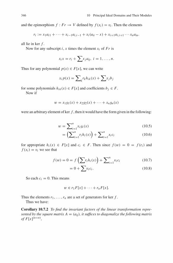
346 10 Principal Ideal Domains and Their Modules
and the epimorphism f : Fr → V defined by f (xi ) = vi . Then the elements
ri := x1ai1 + · · · + xi−1ai,i−1 + xi (aii − x) + xi+1ai,i+1 · · · xnain.
all lie in ker f .Now for any subscript i , x times the element xi of Fr is
xi x = ri +∑
x j aij, i = 1, . . . , n.
Thus for any polynomial p(x) ∈ F[x], we can write
xi p(x) =∑
krkhik(x) +
∑x j b j
for some polynomials hik(x) ∈ F[x] and coefficients b j ∈ F .Now if
w = x1g1(x) + x2g2(x) + · · · + xngn(x)
were an arbitrary element of ker f , then it would have the formgiven in the following:
w =∑n
i=1xigi (x) (10.5)
=(∑n
i=1ri hi (x)
)+
∑n
i=1xi ci (10.6)
for appropriate hi (x) ∈ F[x] and ci ∈ F . Then since f (w) = 0 = f (ri ) andf (xi ) = vi we see that
f (w) = 0 = f(∑
ri hi (x))
+∑n
i=1vi ci (10.7)
= 0 +∑
vi ci . (10.8)
So each ci = 0. This means
w ∈ r1F[x] + · · · + rn F[x].
Thus the elements r1, . . . , rn are a set of generators for ker f .Thus we have:
Corollary 10.7.2 To find the invariant factors of the linear transformation repre-sented by the square matrix A = (aij), it suffices to diagonalize the following matrixof F[x](n×n),

10.7 Applications of the Theorem on PID Modules 347
A − I x =
⎛⎜⎜⎜⎜⎝
a11 − x a12 a13 . . . a1n
a21 a22 − x a23 . . . a2n
a31 a32 a33 − x . . . a3n
.. .. .. .. ..
an1 . . . . . . . . . ann − x
⎞⎟⎟⎟⎟⎠
by the elementary row and column operations to obtain the matrix
diag(p1(x), p2(x), . . . , pn(x))
with each pi (x) monic, and with pi (x) dividing pi+1(x). Then the pi (x) which arenot units are the invariant factors of A.
Now, re-listing the non-unit invariant factors of T as p1(x), . . . , pr (x), r ≤ n,the invariant factor theorem says that T acts on V exactly as right multiplication byx acts on
V ′ := F[x]/(p1(x)) ⊕ · · · ⊕ F[x]/(pr (x)).
The space V ′ has a very nice basis. Each pi (x) is a monic polynomial of degreedi > 0, say
pi (x) = b0i + b1i x + b2i x2 + · · · + bdi −1,i xdi −1 + xdi .
Then the summand F[x]/(p1(x)) of V ′ is non-trivial, and has the F-basis
1 + (pi (x)), x + ((pi (x)), x2 + (pi (x)), . . . , xdi −1 + (pi (x)),
and right multiplication by x effects the action:
x j + (pi (x)) → x j+1 + (pi (x)), 1 ≤ j < di − 1 (10.9)
xdi −1 + (pi (x)) → −b0i (1 + (pi (x))) − b1i (x + (pi (x))) − · · · . (10.10)
Thus, with respect to this basis, right multiplication of F[x]/(pi (x)) by x isrepresented by the matrix
C pi (x) :=
⎛⎜⎜⎜⎜⎝
0 1 0 . . . 00 0 1 0 . . . 0.. .. .. . . . ..
0 0 . . . 0 1−b0i −b1i −b2i . . . −b(di −1)i
⎞⎟⎟⎟⎟⎠ (10.11)
called the companion matrix of pi (x). If pi (x) is a unit in F[x]—that is, it is justa nonzero scalar—then our convention is to regard the companion matrix as the“empty” (0 × 0) matrix. That convention is incorporated in the following

348 10 Principal Ideal Domains and Their Modules
Corollary 10.7.3 If p1(x), . . . , pn(x) are the invariant factors of the square matrixA, then A is conjugate to the matrix
P−1AP =
⎛⎜⎜⎝
C p1(x) 0 . . . 00 C p2(x) 0 . . . 0.. .. . . . ..
0 . . . 0 C pn(x)
⎞⎟⎟⎠ .
This is called the rational canonical form of A.
Remark Note that each companion matrix C pi (x) is square with di := deg(pi (x))
rows. Using decomposition along the first column, one calculates that C pi (x) inEq. (10.11) has determinant (−1)di −1(−b0i ) = (−1)di b0i . Thus the determinant ofA is completely determined by the invariant factors. The determinant is just theproduct
detA =∏r
i=1(−1)d
i b0i = (−1)n∏r
i=1b0i ,
which is the product of the constant terms of the invariant factors times the parity ofn = ∑
di , the dimension of the original vector space V .It may be of interest to know that the calculation of the determinant of matrix A
by ordinary means (that is, iterated column expansions) uses on the order of n! steps.Calculating the determinant by finding the invariant factors (diagonalizing A − xI)uses on the order of n3 steps. The “abstract” way is ultimately faster.
10.7.3 The Jordan Form
This section involves a special form that is available when the ground field of thevector space V contains all the roots of the minimal polynomial of transformation T .
Suppose now F is a field containing all roots of the minimal polynomial of alinear transformation T : V → V . Then the minimal polynomial, as well as all ofthe invariant factors, completely factors into prime powers (x − λi )
ai . Applying theprimary decomposition to the right F[x]-module V , we see that a “primary part”V(x−λ) of V is a direct sum of modules, each isomorphic to F[x] modulo a principalideal I generated by a power of x − λ. This means that any matrix representingthe linear transformation T is equivalent to a matrix which is a diagonal matrix ofsubmatrices which are companion matrices of powers of linear factors. So one isreduced to considering F[x]-modules of the form F[x]/I = F[x]/((x − λ)m), forsome root λ. Now F[x]/I has this F-basis:
1 + I, (x − λ) + I, (x − λ)2 I, . . . (x − λ)m−1 + I.

10.7 Applications of the Theorem on PID Modules 349
Now right multiplying F[x]/I by x = λ + (x − λ) takes each basis element toλ times itself plus its successor basis element—except for the last basis element,which is merely multiplied by λ. That basis element, (x − λ)m−1 + I , and its scalarmultiples comprise a 1-space of all “eigenvectors” of F[x]/I—that is, vectors v suchthat vT = λv. The resulting matrix, with respect to this basis has the form:
⎛⎜⎜⎜⎜⎝
λ 1 0 . . . 0 00 λ 1 0 . . . 0.. .. .. . . . .. ..
0 0 0 . . . λ 10 0 0 . . . 0 λ
⎞⎟⎟⎟⎟⎠ .
It is called a Jordan block and is denoted Jm(λ).The matrix which results from assembling blocks according to the primary de-
composition, and rewriting the resulting companion matrices in the above form, iscalled the Jordan form of the transformation T .
Example 50 Suppose the invariant factors of a matrix A were given as follows:
x, x(x − 1), x(x − 1)3(x − 2)2.
Here, F is any field in which the numbers 0, 1 and 2 are distinct. What is the Jordanform?
First we separate the invariant factors into their elementary divisors:
prime x : {x , x , x}.prime x − 2: {(x − 2)2}.prime x − 1: {x − 1, (x − 1)3}.Next we write out each Jordan block as above: the result being⎛
⎜⎜⎜⎜⎜⎜⎜⎜⎜⎜⎜⎜⎝
0002 1211 11 11
⎞⎟⎟⎟⎟⎟⎟⎟⎟⎟⎟⎟⎟⎠
.
(All unmarked entries in the above matrix are zero).

350 10 Principal Ideal Domains and Their Modules
10.7.4 Information Carried by the Invariant Factors
What are some things one would like to know about a linear transformation T : V →V , and how can the invariant factors provide this information?
1. We have already seen that the last invariant factor pr (x) is theminimal polynomialof T , that is—the smallest degree monic polynomial p(x) such that p(T ) is thezero transformation V → 0V . (We recall that the ideal generated by p(x) isAnn(VF[x]) when V is converted to an F[x]-module via T .)
2. Sometimes it is of interest to know the characteristic polynomial of T , which isdefined to be the product p1(x) · · · pr (x) of the invariant factors of T . One mustbear in mind that by definition the invariant factors of T are monic polynomialsof positive degree. The characteristic polynomial must have degree n, the F-dimension of V . This is because the latter is the sum of the dimensions of theF[x]/(pi (x)), that is, the sum of the numbers deg pi (x) = di .
3. Since V has finite dimension, T is onto if and only if it is one-to-one.3 Thedimension of ker T is called the nullity of T , and is given by the number ofinvariant factors pi (x) which are divisible by x .
4. The rank of T is the F-dimension of T (V ). It is just n minus the nullity of T (seethe footnote just above).
5. V is said to be a cyclic F[x]-module if and only if there exists a module elementv such that the set vF[x] spans V—i.e. v generates V as an F[x]-module. Thisis true if and only if the only non-unit invariant factor is pr (x) the minimalpolynomial (equivalently: the minimal polynomial is equal to the characteristicpolynomial).
6. Recall that an R-module is said to be irreducible if and only if there are no propersubmodules. (We met these in the Jordan-Hölder theorem for R-modules.) Here,we say that T acts irreducibly on V if and only if the associated F[x]-module isirreducible. This means there exists no proper sub-vector space W of V whichis T -invariant in the sense that T (W ) ⊆ W . One can then easily see that T actsirreducibly on V if and only the characteristic polynomial is irreducible in F[x].4
7. An eigenvector of T associated with the root λ or λ-eigenvector is a vector v
of V such that vT = λv. A scalar is called an eigen-root of T if and only ifthere exists a non-zero eigenvector associated with this scalar. Now one can seethat the eigenvectors associated with λ for right multiplication of VF[x] by x , areprecisely the module elements killed by the ideal (x −λ)F[x]. Clearly they forma T -invariant subspace of V whose dimension is the number of invariant factorsof T which are divisible by (x − λ).
3This is a well-known consequence of the so-called “nullity-rank” theorem for transformations butfollows easily from the fundamental theorems of homomorphisms for R-modules applied whenR = F is a field. Specifically, there is an isomorphism between the poset of subspaces of T (V ) andthe poset of subspaces of V which contain ker T . Since dimension is the length of an unrefinablechain in such a poset one obtains codimV (ker T ) = dim(T (V )).4This condition forces the minimal polynomial to equal the characteristic polynomial (so that themodule is cyclic) and both are irreducible polynomials.

10.7 Applications of the Theorem on PID Modules 351
8. A matrix is said to be nilpotent if and only some power of it is the zero matrix.Similarly a linear transformation T : V → V is called a nilpotent transforma-tion if and only if some power (number of iterations) of T annihilates V . Quiteobviously the following are equivalent:
• T is a nilpotent transformation.• T can be represented by a nilpotent matrix with respect to some basis of V .• The characteristic polynomial of T is a power of x .• The minimal polynomial of T is a power of x .
10.8 Exercises
10.8.1 Miscellaneous Exercises
Bezout Domains
1. An integral domain is said to be a Bezout domain if and only if all of its finitely-generated ideals are principal ideals. Give a proof that an integral domain is aBezout domain if and only if every ideal generated by two elements is a principalideal.
2. Of course the class of Bezout domains includes all principal ideal domains, soit would be interesting to have an example of a Bezout domain which was not aprincipal ideal domain. This and the subsequent four exercises are designed toproduce examples of Bezout domains which are not principal ideal domains. Ourcandidate will be the integral domain D described in the next paragraph.Let E be a PID and let F be the field of fractions of E . Let D be the set ofall polynomials of F[x] whose constant coefficient belongs to the domain E .The first elementary result is to verify that D is a subdomain of F[x]. [Thewarmup result is elementary. But the reader might in general like to prove it usingExercise (1) in Sect. 7.5.2 on p. 223, as applied to the evaluation homomorphisme0 : F[x] → F .]
3. Let g(x) and h(x) be two non-zero polynomials lying in D. The greatest commondivisors of these two polynomials are unique up to scalar multiplication.
(i) Show that if x divides both g(x) and h(x) then
g(x)D + h(x)D = Dd(x)
where d(x) is any greatest common divisor of g(x) and h(x).(ii) Suppose at least one of the two polynomials is not divisible by x . Then
any greatest common divisor of g(x) and h(x) has a non-zero constantcoefficient. We let d(x) be the appropriate scalar multiple of a greatestcommon divisor such that the constant term d(0) is a greatest common

352 10 Principal Ideal Domains and Their Modules
divisor of g(0) and h(0) in the PID E . (The latter exists since not both of g(0)and h(0) are zero). Thus d(x) ∈ D. Moreover, we have g(x) = d(x)p(x)
and h(x) = d(x)q(x). Then p(0) = (g(0)/d(0)) is an element of E byour choice of d(0) so p(x) ∈ D. Similarly q(x) ∈ D. Moreover thesepolynomials p(x) and q(x) are relatively prime in F[x]. Show that
Dg(x) + Dh(x) = Dd(x)
if and only ifDp(x) + Dq(x) = Dd(0).
4. From now on we assume p(x) and q(x) elements of D which are relatively primepolynomials in F[x]. As above, d will denote a greatest common divisor of p(0)and q(0) in the PID E . We set I = Dp(x) + Dq(x). Show that there existsa non-zero element e ∈ E such that ed ∈ I [Hint: Since p(x) and q(x) arerelatively prime in F[x], there exists polynomials A(x) and B(x) in F[x] suchthat d = A(x)p(x) + B(x)q(x). Then, since F is the field of fractions of thedomain E , there exists a non-zero element e ∈ E such that eA(0) and eB(0) areboth elements of E . Then, observe that eA(x) and eB(x) are elements of D andthe result follows].
5. Show that d ∈ I [Hint: Since d is a greatest common divisor of elements p(0)and q(0) in the domain E , there exist elements A and B of E such that d =Ap(0) + Bq(0). Write p(x) = p(0) + p′(x) where p′(x) is a multiple of x .Noting that p′(x)/ed lies in D and ed lies in I we see that
p′(x) = ed · (p′(x)/ed)
lies in I , and so p(0) is the difference of two elements of I . Similarly argue thatq(0) lies in I so that d = Ap(0) + Bq(0) is also in I ].
6. Show that I ⊆ Dd [Hint: We have p′(x)/d ∈ D (since its constant term is zero)and p0/d ∈ E ⊆ D (since d is a divisor of p0 in E by its definition). It followsthat
p(x) = d · ((p(0)/d) + p′(x)/d) ∈ I.
Similarly argue that q(x) ∈ I . Thus I ⊆ Dd].7. Assemble the preceding problems into steps that show that D is a Bezout domain.8. Suppose the domain E is not equal to its field of fractions F . Then it contains a
prime element p. Show that the ideal J of D generated by the set
X := {x, x/p, x/p2, x/p3, . . .}
is not a principle ideal [Hint: Let Jk be the ideal of D generated by the first kelements listed in the set X . Show that J1 ⊂ J2 ⊂ · · · is an infinite properlyascending chain of ideals of D].

10.8 Exercises 353
9. Consider the following two integral domains:
(a) The domain D1 of all polynomials inQ[x]whose constant term is an integer.(b) Let K be a field and let S be the set of non-zero polynomials in K [x], the
latter being regarded as a subring of K [x, y]. Let K [x, y]S be the localizationof K [x, y] relative to the multiplicative set S. Observe that K [x, y]S =K (x)[y] where K (x) is the so-called “field of rational functions” in theindeterminate x . Let D2 be the subdomain of those polynomials p(x, y) ∈K [x, y]S for which p(x, 0) is a polynomial.
Show that both domains D1 and D2 are Bezout domains which are not principalideal domains.
10.8.2 Structure Theory of Modules over Z and PolynomialRings
1. Suppose A is an additive abelian group generated by three elements a, b, and c.Find the order of A when A is presented by the following relations
2a + b + c = 0
a + b + c = 0
a + b + 2c = 0
2. Answer the same question when
2a + 2b + c = 0
2a + 3b + c = 0
2a + 4b + c = 0
3. Suppose A is presented by the following relations
2a + 2b + 2c = 0
3b + 2c = 0
2a + c = 0.
Write A as a direct product of cyclic groups.4. Find the invariant factors of the linear transformation which is represented by the
following matrix over the field of rational numbers:
⎛⎜⎜⎝2 1 1 11 1 1 10 0 0 01 0 1 0
⎞⎟⎟⎠

354 10 Principal Ideal Domains and Their Modules
5. Let V be a vector space over the rational field Q and suppose T : V → V is alinear transformation. We are presented with three possibilities for the non-trivialinvariant factors of T :
(i) x, x4, x4(x + 1).(ii) x + 1, x3 + 1.(iii) 1 + x + x2 + x3 = (1 + x)(1 + x2),
(a) What is the dimension of V in each of the three cases (i)–(iii)?(b) In which cases is the module V a cyclic module?(c) In which cases is the module V irreducible?(d) In case (ii) write the rational canonical form of the matrix representing T .(e) Write out the full Jordan form of a matrix representing T is case (i).
6. Suppose t : V → V is a linear transformation of a vector space over the fieldZ/(3) represented by the matrix:
⎛⎜⎜⎝1 1 0 00 1 1 00 0 1 10 0 0 1
⎞⎟⎟⎠
Find the order of t as an element of the group GL(4, 3).

Chapter 11Theory of Fields
Abstract If F is a subfield of a field K , then K is said to be an extension of thefield F . For α ∈ K , F(α) denotes the subfield generated by F ∪ {α}, and theextension F ⊆ F(α) is called a simple extension of F . The element α is algebraicover F if dimF F(α) is finite. Field theory is largely a study of field extensions. Acentral theme of this chapter is the exposition of Galois theory, which concerns acorrespondence between the poset of intermediate fields of a finite normal separableextension F ⊆ K and the poset of subgroups of GalF (K ), the group of automorphisms of K which leave the subfield F fixed element-wise. A pinnacle of this theory isthe famous Galois criterion for the solvability of a polynomial equation by radicals.Important side issues include the existence of normal and separable closures, thefact that trace maps for separable extensions are non-zero (needed to show that ringsof integral elements are Noetherian in Chap.9), the structure of finite fields, theChevalley-Warning theorem, as well as Luroth’s theorem and transcendence degree.Attached are two appendices that may be of interest. One gives an account of fieldswith valuations, while the other gives several proofs that finite division rings arefields. There are abundant exercises.
11.1 Introduction
In this chapter we are about to enter one of the most fascinating and historicallyinteresting regions of abstract algebra. There are at least three reasons why this is so:
1. Fields underlie nearly every part of mathematics. Of course we could not havevector spaces without fields (if only as the center of the coefficient division ring).In addition to vector spaces, fields figure in the theory of sesquilinear and mul-tilinear forms, algebraic varieties, projective spaces and the theory of buildings,Lie algebras and Lie incidence geometry, representation theory, number theory,algebraic coding theory as well as many other aspects of combinatorial theoryand finite geometry, just to name a few areas.
2. There are presently many open problems involving fields—some motivated bysome application of fields to another part of mathematics, and some entirelyintrinsic.
© Springer International Publishing Switzerland 2015E. Shult and D. Surowski, Algebra, DOI 10.1007/978-3-319-19734-0_11
355

356 11 Theory of Fields
3. Third, there is the strange drama that so many field-theoretic questions bear onold historic questions, and indeed, its own history has a dramatic story of itsown. These questions for fields involve some of the oldest and longest-standingproblems inmathematics—they all involve the existence or non-existence of rootsof polynomial equations in one indeterminate.
11.2 Elementary Properties of Field Extensions
Recall that a field is an integral domain in which every non-zero element is a unit.Examples are:
1. The field of rational numbers—in fact, the “field of fractions” of an arbitraryintegral domain D (that is, the localization DS where S = D − {0}). A specialcase is the field of fractions of the polynomial domain F[x]. This field is calledthe field of rational functions over F in the indeterminate x (even though they arenot functions at all).
2. The familiar fields R and C of real and complex numbers, respectively.3. The field of integers modulo a prime—more generally, the field D/M where M
is a maximal ideal of an integral domain D.
Of course there are many further examples.Let K be a field. A subfield is a subset F of K which contains a non-zero element,
and is closed under addition, multiplication, and the taking of multiplicative inversesof the non-zero elements. It follows at once that F is a field with respect to theseoperations inherited from K , and that F contains the multiplicative identity of Kas its own multiplicative identity. Obviously, the intersection of any collection ofsubfields of K is a subfield, and so one may speak of the subfield generated by asubset X of K as the intersection of all subfields of K containing set X . The subfieldof K generated by a subfield F and a subset X is denoted F(X).1
The subfield generated by themultiplicative identity element, 1, is called the primesubfield of K . (By definition, it contains the multiplicative identity as well as zero.)Since a field is a species of integral domain, it has a characteristic. If themultiplicativeidentity element 1, as an element of the additive group (K ,+), has finite order, then itsorder is a prime number p which we designate as the characteristic of F . Otherwise1 has infinite order as an element of (K ,+) and we say that K has characteristiczero. We write char(F) = p or 0 in the respective cases. In the former case, it isclear that the prime subfield of F is just Z/pZ; in the latter case the prime subfield isisomorphic to the field Q of rational numbers. One last observation is the following:
Any subfield F of K contains the prime subfield and possesses the same charac-teristic as K .
1Of course this notation suffers the defect of leaving K out of the picture. Accordingly we shalltypically be using it when the ambient overfield K of F is clearly understood from the context.

11.2 Elementary Properties of Field Extensions 357
Since we shall often be dealing in this chapter with cases in which the subfield isknown but the over-field is not, it is handy to reverse the point of view of the previousparagraph. We say that K is an extension of F if and only if F is a subfield of K . Achain of fields F1 ≤ F2 ≤ · · · ≤ Fn , where each Fi+1 is a field extension of Fi , iscalled a tower of fields.
If the field K is an extension of the field F , then K is a right module over F ,that is, a vector space over F . As such, it possesses a dimension (which might be aninfinite cardinal) as an F-vector space. We call this dimension the degree (or index)of the extension F ≤ K , and denote it by the symbol [K : F].
11.2.1 Algebraic and Transcendental Extensions
Let K be a field extension of the field F , and let p(x) be a polynomial in F[x]. Wesay that an element α of K is a zero of p(x) (or a root of the equation p(x) = 0)if and only it p(x) �= 0 and yet p(α) = 0.2 If α is a zero in K of a polynomial inF[x], then α is said to be algebraic over F . Otherwise α is said to be transcendentalover F .
If K is an extension of F , and if α is an element of K , then the symbol F[α]denotes the subring of K generated by F ∪{α}. This would be the set of all elementsof K which are F-linear combinations of powers of α. Note that as this subringcontains the field F , it is a vector space over F whose dimension is again denoted[F[α] : F].
There is then a ring homomorphism
ψ : F[x] → F[α] ⊆ K
which takes the polynomial p(x) to the field element p(α) in K . Clearly ψ(F[x]) =F[α].
Suppose now ker ψ = 0. Then F[x] � F[α] and α is transcendental since anynon-trivial polynomial of which it is a zero would be a polynomial of positive degreein ker ψ.
2Two remarks are appropriate at this point. First note that the definition makes it “un-grammatic”to speak of a zero of the zero polynomial. Had the non-zero-ness of p(x) not been inserted in thedefinition of root, we should be saying that every element of the field is a zero of the zero polynomial.That is such a bizarre difference from the situation with non-zero polynomials over infinite fieldsthat we should otherwise always be apologizing for that exceptional case in the statements of manytheorems. It thus seems better to utilize the definition to weed out this awkwardness in advance.
Second, there are natural objections to speaking of a “root” of a polynomial. Some have askedwhether it might not be better to follow the German example and write “zero” (Nullstelle) for “root”(Wurzel), despite usage of the latter term in some English versions of Galois Theory. However weshall follow tradition by speaking of a “root” of an equation, p(x) = 0, while we speak of a “zero”of a polynomial, p(x).

358 11 Theory of Fields
On the other hand, if ker ψ �= 0, then, as F[x] is a principal ideal domain, wehave ker ψ = F[x]p(x) = (p(x)), for some polynomial p(x). Then
F[α] = ψ(F[x]) � F[x]/ker ψ = F[x]/(p(x)).
Now, as F[α] is an integral domain, the principal ideal (p(x)) is a prime ideal,and so p(x) is a prime element of F[x]. Therefore, since F[x] is a PID, we inferimmediately that the ideal (p(x)) = ker ψ is actually a maximal ideal of F[x], andso the subring F[α] is a field, which is to say, F[α] = F(α).
The irreducible polynomial p(x)determined byα is unique up tomultiplication bya non-zero scalar. The unique associate of p(x)which is monic is denoted IrrF (α). Itis the the uniquemonic polynomial of smallest possible degreewhich hasα for a zero.
Note that in this case, the F-dimensionof F[α] is the F-dimensionof F[x]/(p(x)),which, by the previous chapter can be recognized to be the degree of the polyno-mial p(x).
Now conversely, assume that [F[α] : F] is finite. Then there exists a non-trivialfinite F-linear combination of elements in the infinite list
{1,α,α2,α3, . . .}
which is zero. It follows that α is algebraic in this case.Summarizing, we have the following:
Theorem 11.2.1 Let K be an extension of the field F and let α be an element of K .
1. If α is transcendental over F, then the subring F[α] which it generates is isomor-phic to the integral domain F[x]. Moreover, the subfield F(α) which it generatesis isomorphic to the field of fractions F(x) of F[x].
2. If α is algebraic over F, then the subring F[α] is a subfield intermediate betweenK and F. As an extension of F its degree is
[F(α) : F] = [F[α] : F] = deg IrrF (α).
3. Thus dimF F[α] is finite or infinite according as α is algebraic or transcendentalover F.
11.2.2 Indices Multiply: Ruler and Compass Problems
Lemma 11.2.2 If F ≤ K ≤ L is a tower of fields, then the indices “multiply” inthe sense that
[L : F] = [L : K ][K : F].

11.2 Elementary Properties of Field Extensions 359
Proof Let A be basis of L as a vector space over K , and let B be a basis of K as avector space over F . Let AB be the set of all products {ab|a ∈ A, b ∈ B}. We shallshow that AB is an F-basis of L .
If α ∈ L , then α is a finite K -linear combination of elements of A, say
α = a1α1 + · · · + amαm .
Now each coefficient αi , being an element of K , is a finite linear combination
α j = b j1β j1 + · · · + b jm j β jm j
of elements b ji of B (with the β j i in F). Substituting these expressions for α j inthe L-linear combination for α, we have expressed α as an F-linear combination ofelements of AB. Thus AB is an F-spanning set for L .
It remains to show that AB is an F-linearly independent set. So suppose for somefinite subset S of A × B, that ∑
(a,b)∈Sabβa,b = 0.
Then as each βa,b is in F , and each b is in K , the left side of the presented formulamay be regarded as a K -linear combination of a’s equal to zero, and so, by theK -linear independence of A, each coefficient
∑bbβa,b
of each a is equal to zero. Hence each βa,b = 0, since B is F-linearly independent.Thus AB is F-linearly independent and hence is an F-basis for L . Since this entailsthat all the products in AB are pairwise distinct elements, we see that
|AB| = |A||B|,
which proves the lemma. �
Corollary 11.2.3 If F1 ≤ F2 ≤ · · · ≤ Fn is a finite tower of fields, then
[Fn : F1] = [Fn : Fn−1] · [Fn−1 : Fn−2] · · · [F2 : F1].
We can use this observation to sketch a proof of the impossibility of certain rulerand compass constructions. Given a unit length 1, using only a ruler and compass wecan replicate it m times, or divide it into n equal parts, and so can form all lengthswhich are rational numbers. We can also form right-angled triangles inscribed in acircle and so with ruler and compass, we can extract the square root of the differencesof squares, and hence any square root because of the formula

360 11 Theory of Fields
c =(
c + 1
2
)2
−(
c − 1
2
)2
.
If α is such a square root, where c is a rational length, then by ruler and compasswe can form all the lengths in the ring Q[α], which (since α is a zero of x2 − c) isa field extension of Q of degree 1 or 2. Iterating these constructions a finite numberof times, the possible lengths that we could encounter all lie in the uppermost fieldof a tower of fields
Q = F1 < F2 < · · · < Fn = K
with each Fi+1 an extension of degree two over Fi . By the Corollary above, the index[K : Q] is a power of 2.
Now we come to the arm-waving part of the proof: One needs to know that oncea field L of constructible distances has been achieved, the only new number notin K constructed entirely from old numbers already in K is in fact obtained byproducing a missing side of a right triangle, two of whose sides have lengths in K .(A really severe proof of that fact would require a formalization of exactly what“ruler and compass” constructions are—a logical problem beyond the field-theoreticapplications whose interests are being advanced here.) In this sketch, we assume thatthat has been worked out.
This means, for example, that we cannot find by ruler and compass alone, a lengthα which is a zero of an irreducible polynomial of degree n where n contains an oddprime factor. For if so, Q[α] would be a subfield of a field K of degree 2m over Q.On the other hand, the index n = [F[α] : F] must divide [K : Q] = 2m , by theTheorem11.2.1. But the odd prime in n cannot divide 2m . That’s it! That’s the wholeamazingly simple argument!
Thus one cannot solve the problem posed by the oracle of Delos, to “duplicate”(in volume) a cubic altar—i.e., find a length α such that α3 − 2 = 0—at least notwith ruler and compass.
Similarly, given angle α, trisect it with ruler and compass. If one could, then onecould construct the length cosβ where 3β = α. But cos(3β) = 4cos3β − 3 cosβ =λ = cosα. This means we could always find a zero of 4x3 − 3x − λ and whenα = 60o, so λ = 1/2, setting y = 2x yields a constructed zero of y3−3y −1, whichis irreducible over Q. As observed above, this is impossible.
11.2.3 The Number of Zeros of a Polynomial
Lemma 11.2.4 Let K be an extension of the field F and suppose the element α ofK is a zero of the polynomial p(x) in F[x]. Then in the polynomial ring F[α][x],x − α divides p(x).

11.2 Elementary Properties of Field Extensions 361
Proof Since p(α) = 0 we may write
p(x) = a0 + a1x + · · · + an xn
= p(x) − p(α)
= a1(x − α) + a2(x2 − α2) + · · · + an(xn − αn)
= (x − α)[a1 + a2(x + α) + a3(x2 + αx + α2) + · · ·· · · + an(xn−1 + · · · αn−1)].
�Theorem 11.2.5 Let K be an extension of the field F and let p(x) be a polynomialin F[x]. Then p(x) possesses at most deg p(x) zeros in K .
Proof We may assume p(x) is a monic polynomial. If p(x) has no zeroes in K ,we are done. So assume α is a zero of p(x). Then by Lemma11.2.4 we obtain afactorization p(x) = (x − α)p1(x) in K [x], where deg p1(x) is one less than thedegree of p(x). Suppose β is any zero of p(x) in K which is distinct from α. Then
0 = p(β) = (β − α)p1(α).
Since the first factor on the right is not zero, and F is a domain, β is forced to be azero of the polynomial p1(x). By induction on the degree of p(x), we may concludethat the number of distinct possibilities for β does not exceed the degree of p1(x).Thus, as any zero of p(x) is either α or one of the zeroes β of p1(x), we see that thetotal number of zeroes of p(x) cannot exceed 1 + deg p1(x), that is, the degree ofp(x). �
Of course, when we write p(x) = (x − α)p1(x), it may happen that α is alsoa zero of p1(x), as well. In that case, we can again write p1(x) = (x − α)p2(x),and ask whether α is a zero of p2(x). Pushing this procedure as far as we can, weeventually obtain a factorization p(x) = (x − α)k pk(x) where pk(x) does not haveα for a zero. Repeating this for the finitely many zeroes αi of p(x), one obtains afactorization
p(x) = (x − α1)n1(x − α2)
n2 · · · (x − αm)nm r(x) (11.1)
in K[x] where r(x) possesses no “linear factors”—that is, factors of degree one.The number ni is called themultiplicity of the zeroαi , and clearly fromEq. (11.1),∑ni ≤ deg p(x). Thus the following slight improvement of Theorem11.2.5
emerges:
Corollary 11.2.6 If K is an extension of the field F and p(x) is a non-zero poly-nomial in F[x], then the number of zeroes—counting multiplicities—is at most thedegree of p(x).3
3The student should notice that when we count zeroes with their multiplicities we are not doinganything mysterious. We are simply forming a multiset of zeroes. The Corollary just says that thedegree of the polynomial bounds the weight of this multiset.

362 11 Theory of Fields
There are a number of other elementary but important corollaries of Theorem11.2.5.
Corollary 11.2.7 (Polynomial Identities) Suppose a(x), b(x), are polynomials inF[x]. Suppose a(α) = b(α) for all α ∈ F. If F contains infinitely many elements,then
a(x) = b(x)
is a polynomial identity—that is, both sides are the same element of F[x].Proof We need only show that the polynomial J (x) := a(x) − b(x) has degreezero. If it has positive degree, then by Theorem11.2.5 it possesses only finitely manyzeros. But then by hypothesis, the infinitely many elements of F would all be zerosof J (x), a contradiction. �
Corollary 11.2.8 (Invertibility of the Vandermonde matrix) Let n be a positive inte-ger. Suppose z1, z2, . . . , zn are pairwise distinct elements of a field F. Then the n ×nmatrix
M =
⎡⎢⎢⎢⎢⎣1 z1 z21 · · · zn−1
1
1 z2 z22 · · · zn−12
......
... · · · ...
1 zn z2n · · · zn−1n
⎤⎥⎥⎥⎥⎦
is invertible.
Proof Thematrix M is invertible if and only if its columnsC1, . . . , Cn are F-linearlyindependent. So, if M were not invertible, therewould exist coefficients a0, . . . , an−1in F such that
n−1∑i=0
ai Ci+1 = [0], the n × 1 zero column vector. (11.2)
But each entry on the left side of Eq. (11.2) is p(zi ) where p(x) is the polynomiala0 + a1x + · · · , an−1xn−1 ∈ F[x]. This conflicts with Theorem11.2.5, since thepolynomial p(x) has degree at most n−1, but yet possesses n distinct zeroes—the zi .
Thus the columns of M are F-linearly independent and so M is invertible. �
Remark Notice that the proof of Corollary11.2.8 was determinant-free. Matrices ofthe form displayed in Corollary11.2.8 are called Vandermonde matrices.
For the next result, we require the following definition: a group G is said to belocally cyclic if and only if every finitely-generated subgroup of G is cyclic. Clearlysuch a group is abelian. Recall from Exercise (2) in Sect. 5.6.1 that a group is atorsion group if and only each of its elements has finite order. In any abelian groupA, the set of elements of finite order are closed under multiplication and the takingof inverses, and so form a subgroup which we call the torsion subgroup of A.

11.2 Elementary Properties of Field Extensions 363
Corollary 11.2.9 Let F be any field and let F∗ be its multiplicative group of non-zero elements. Then the torsion subgroup of F∗ is locally cyclic.
Proof Any finitely-generated subgroup of the torsion subgroup of F∗ is a finiteabelian group A. If A were not cyclic, it would contain a subgroup isomorphic toZ p × Z p, for some prime p. In that case, the polynomial x p − 1 would have at leastp2 zeros in F , contrary to Theorem11.2.5. �
11.3 Splitting Fields and Their Automorphisms
11.3.1 Extending Isomorphisms Between Fields
Suppose E is a field extension of F and that α is an element of E which is algebraicover F . Then the development in the previous section (p. 395) showed that there isa unique irreducible monic polynomial,
g(x) = IrrF (α) ∈ F[x],
having α as a zero. The subfield F(α) of E generated by F ∪ {α}, is the subringF[α], which we have seen is isomorphic to the factor ring F[x]/(g(x)).
We remind the reader of a second principle. Suppose f : F1 → F2 is an isomor-phism of fields. Then f can be extended to a ring isomorphism
f ∗ : F1[x] → F2[x],
which takes the polynomial
p := a0 + a1x + · · · + an xn
tof ∗(p) := f (a0) + f (a1)x + · · · + f (an)xn .
It is obvious that f ∗ takes irreducible polynomials of F1[x] to irreducible poly-nomials of F2[x].
With these two principles in mind we record the following:
Lemma 11.3.1 (Fundamental Lemma on Extending Isomorphisms) Let E be a fieldextension of F, and suppose f : F → E is an embedding of F as a subfield F of thefield E. Let f1 be the induced isomorphism f1 : F → F obtained by resetting thecodomain of f . Next let f ∗
1 be the extension of this field isomorphism f1 to a ringisomorphism F[x] → F[x], as described above.
Finally, let α be an element of E which is algebraic over F, and let g be its monicirreducible polynomial in F[x].

364 11 Theory of Fields
Then the following assertions hold:
(i) The embedding (injective morphism) f : F → E can be extended to an embed-ding
f : F(α) → E,
if and only if the polynomial f ∗1 (g) := g has a zero in E.
(ii) Moreover, for each zero α of g in E , there is a unique embedding f :F(α) → E , taking α to α and extending f .
(iii) The number of extensions f : F(α) → E of the embedding f is equal to thenumber of distinct zeros of g to be found in E.
Proof (i) If there is an embedding f : F(α) → E extending the embedding f , thenf (α) is a zero of g in E .Conversely, if α in E , then F(α) is a subfield of E isomorphic to F[x]/(g(x)).
Similarly, F(α) is isomorphic to F[x]/(g(x)). But the ring isomorphism f ∗1 :
F[x] → F[x] takes the maximal ideal (g(x)) of F[x] to the maximal ideal (g(x))
of F[x], and so induces an isomorphism of the corresponding factor rings:
f ′ : F[x]/(g(x)) → F[x]/(g(x)).
Linking up these three isomorphisms
F(α) → F[x]/(g(x))f ′
→ F[x]/(g(x)) → F(α) ⊆ E,
yields the desired embedding.(ii) If therewere two embeddings h1, h2 : F(α) → E , takingα to α and extending
f , then the composition of the inverse of one with the other would fix α, would fixF element-wise, and so would be the identity mapping on F(α). Thus, for anyβ ∈ F(α),
h1(β) = (h2 ◦ h−11 )(h1(β) = h2(β).
Thus h1 and h2 would be identical mappings.(iii) This part follows from parts (i) and (ii). �
11.3.2 Splitting Fields
Suppose E is an extension field of F . Then, of course, any polynomial in F[x] can beregarded as a polynomial in E[x], and any factorization of it in F[x] is a factorizationin E[x]. Put another way, F[x] is a subdomain of E[x].
A non-zero polynomial p(x) in F[x] of positive degree is said to split over E ifand only if p(x) factors completely into linear factors (that is, factors of degree 1)in E[x]. Such a factorization has the form

11.3 Splitting Fields and Their Automorphisms 365
p(x) = a(x − a1)n1(x − a2)
n2 · · · (x − ar )nr (11.3)
where a is a nonzero element of F , the exponents ni are positive integers and thecollection {a1, . . . , ar } of zeros of p(x) in E is contained in E .
Obviously, if E ′ is a field containing E and the polynomial p(x) splits over E ,then it splits over E ′. Also, if E0 were a subfield of E containing F together with allof the zeros {a1, . . . , ar }, then p(x) would split over over E0, since the factorizationin Eq. (11.3) can take place in E0[x]. In particular, this is true if E0 = F(a1, . . . , ar ),the subfield of E generated by F and the zeros ai , i = 1, . . . , r .
An extension field E of F is called a splitting field of the polynomial p(x) ∈ F[x]over F if and only if
(S1) F ⊆ E .(S2) f (x) factors completely into linear factors in E[x] as
f (x) = a(x − a1)(x − a2) · · · (x − an).
(S3) E = F(a1, . . . , an), that is, E is generated by F and the zeros ai .
The following observations follow directly from the definition just given and theproofs are left as an exercise.
Lemma 11.3.2 The following hold:
(i) If E is a splitting field for p(x) ∈ F[x] over F, and L is a subfield of Econtaining F, then E is a splitting field for p(x) over L.
(ii) Suppose p(x) and q(x) are polynomials in F[x]. Suppose E is a splitting fieldfor p(x) over F and K is a splitting field for q(x) over E. Then K is a splittingfield for p(x)q(x) over F.
Our immediate goals are to show that splitting fields for a fixed polynomial exist,to show that they are unique up to isomorphism, and to show that between any twosuch splitting fields, the number of isomorphisms is bounded by a function of thenumber of distinct zeros of f (x).
Theorem 11.3.3 (Existence of Splitting Fields) If f (x) ∈ F[x], then a splittingfield for f (x) over F exists. Its degree over F is at most the factorial number d!,where d is the sum of the degrees of the non-linear irreducible polynomial factors off (x) in F[x].Proof Let f (x) = f1(x) f2(x) · · · fm(x) be a factorization of f (x) into irreduciblefactors in F[x]. (This is possible by Theorem7.3.2, Part 3.) Set n = deg f (x), andproceed by induction on k = n − m. If k = 0, then n = m, so each factor fi (x)
is linear and clearly E = F satisfies all the conclusions of the theorem. So assumek > 0. Then some factor, say f1(x), has degree greater than 1. Form the field
L = F[x]/( f1(x)),

366 11 Theory of Fields
(this is a field since f1(x) is irreducible and it is an extension of F since it is avector-space over F). Observe that the coset a := x + F[x] f1(x) is a zero of f1(x)
(and hence f (x)) in the field L . Thus in L[x], we have the factorizations:
f1(x) = (x − a)h1(x),
andf (x) = (x − a)h1(x) f2(x) · · · fm(x),
with � > m irreducible factors. Thus n − � < n − m and so by induction, there is asplitting field E of f (x) over L . Moreover, this degree is at most (d − 1)! since thesum of the degrees of the non-linear irreducible factors of f (x) over L[x] has beenreduced by at least one because of the appearance of the new linear factor x − a.
Now we claim that E is a splitting field of f (x) over F . We must verify thethree defining properties of a splitting field given at the beginning of this subsec-tion (p. 365).
Property (S1) holds since L ⊆ E implies F ⊆ E . We already have (S2) from thedefinition of E . It remains to see that E is generated by the zeros of f . Since (x − a)
is one of the factors of f (x) in the factorization
f (x) = (x − a1)(x − a2) · · · (x − an)
in E[x], we may assume without loss of generality that a = a1. We have E =L(a2, . . . , an) from the definition of E . But L = F(a1), so
E = L(a2, . . . , am) = F(a1)(a2, . . . , an) = F(a1, . . . , an),
and so (S3) holds. Thus E is indeed a splitting field for f (x) over F .Finally, since [L : F] = deg f1(x) ≤ d , and [E : L] ≤ (d − 1)! we obtain
[E : F] = [E : L][L : F] ≤ (d − 1)! · d = d! as required. �
Theorem 11.3.4 Let η : F → F be an isomorphism of fields, which we extend to aring isomorphism η∗ : F[x] → F[x], and let us write f (x) for η∗( f (x)) for eachf (x) ∈ F[x]. Suppose E and E are splitting fields of f (x) over F, and f (x) overF, respectively. Then η can be extended to an isomorphism η of E onto E, and thenumber of ways of doing this is at most the index [E : F]. If the irreducible factors off (x) have no multiple zeros in E, then there are exactly [E : F] such isomorphisms.
Proof We use induction on [E : F]. If [E : F] = 1, f (x) factors into linear factors,and there is precisely one isomorphism extending η, namely η itself.
Assume [E : F] > 1. Then f (x) contains an irreducible factor g(x) of degreegreater than 1. Since η∗ is an isomorphism of polynomial rings, g(x) is an irreduciblefactor of f (x) with the same degree as g(x). Let α ∈ E be a zero of g(x), andset K = F(α). Since the irreducible polynomial g(x) splits completely in E , we

11.3 Splitting Fields and Their Automorphisms 367
may apply the Fundamental Lemma on Extensions (Lemma11.3.1), to infer that theisomorphism η has k extensions ζ1, . . . , ζk : F(α) → E , where k is the number ofdistinct zeros of g(x) in E .
Note that if m = deg g(x), then [K : F] = m and k ≤ m. If the zeros of g(x) aredistinct, k = m.
Now clearly E is a splitting field of f (x) over K , and E is a splitting field off (x) over each ζi (K ). Since [E : K ] < [E : F], induction implies that each ζi canbe extended to an isomorphism E → E in at most [E : K ] ways, and in exactly[E : K ] ways if the irreducible factors of f (x) ∈ K [x] have distinct zeros in E .However if the irreducible factors of f (x) ∈ F[x] have distinct zeros in E , the sameis obviously true for the irreducible factors of g(x) ∈ K [x]. This yields at mostk[E : K ] = [K : F][E : K ] = [E : F] isomorphisms in general, and exactly[E : F] isomorphisms if the irreducible factors of f (x) have distinct zeros in E .
This proves the theorem. �
Corollary 11.3.5 If E1 and E2 are two splitting fields for f (x) ∈ F[x] over F,there exists an F-linear field isomorphism:
σ : E1 → E2.
Proof This follows immediately from Theorem11.3.4 for the case σ = 1F , theidentity mapping on F = F1 = F2. �
Example 51 Suppose F = Q, the rational field, and p(x) = x4 − 5, irre-ducible by Eisenstein’s criterion. One easily has that the complex zeros of p(x)
are ± 4√5,±i 4
√5 ∈ C, where, of course, i is the imaginary complex unit (i2 = −1),
and 4√5 is the real fourth root of 5. This easily implies that the splitting field E ⊆ C
can be described by setting E = Q(i, 4√5). Since p(x) ∈ Q[x] is irreducible by
Eisenstein, we conclude that [Q(4√5) : Q] = 4. Since E is the complex splitting
field over Q(4√5) of the polynomial x2 + 1 ∈ Q(
4√5)[x], and since Q(
4√5) � E , we
infer that [E : Q(4√5)] = 2, giving the splitting field extension degree:
[E : Q] = [E : Q(4√5)] · [Q(
4√5) : Q] = 2 · 4 = 8.
This shows that the bound [E : F] ≤ d! need not be obtained. Note, finally, byTheorem11.3.4, that there are exactly 8 = [E : Q] distinct Q-automorphisms of E .
We close this subsection with a useful observation:
Lemma 11.3.6 Suppose K is an extension of a field F, and that K contains asubfield E which is a splitting field for a polynomial p(x) ∈ F[x] over F. Then anyautomorphism of K fixing F point-wise must stabilize E.
Remark The Lemma just says that the splitting field E is “characteristic” amongfields in K which contain F—that is, E is invariant under all F-linear automorphismsof K .

368 11 Theory of Fields
Proof It suffices to note that if σ is an F-linear automorphism of K , then for anyzero α of p(x) in K , σ(α) is also a zero of p(x) in K . Since E is generated by Fand the zeroes of f (x) in K , we have E = Eσ , for all F-automorphisms σ of K . �
11.3.3 Normal Extensions
So far the notion of splitting field is geared to a particular polynomial. The purposeof this section is to show that the polynomial-splitting property can be seen as aproperty of a field extension itself, independent of any particular polynomial.
Before proceeding further, let us streamline our language concerning field auto-morphisms.
Definition Let K and L be fields containing a common subfield F . An isomorphismK → L of K onto L is called an F-isomorphism if and only if it fixes the subfieldF element-wise. (Heretofore, we have been calling these F-linear isomorphisms.)Of course, if K = L , an F-isomorphism, K → L , is called an F-automorphism.Finally, an F-isomorphism of K onto a subfield of L is called an F-embedding.
We say that a finite extension E of F is normal over F if and only if E is thesplitting field over F of some polynomial of F[x]. Just as a reminder, recall that thismeans that there is a polynomial p(x) which splits completely into linear factors inE[x] and that E is generated by F and all the zeros of p(x) that lie in E .
Note that if E is a normal extension and K is an intermediate field,—that is,F ≤ K ≤ E—then E is a normal extension of K .
We have a criterion for normality.
Theorem 11.3.7 (A characterization of normal field extensions4) The following areequivalent for the finite extension F ⊆ E:
(i) E is normal over F;(ii) every irreducible polynomial g(x) ∈ F[x] having a zero in E must split com-
pletely into linear factors in E[x].Proof Suppose E is normal over F , so that E is the splitting field of a polynomialf (x) ∈ F[x]. Let g(x) be an irreducible polynomial in F[x] with a zero a in E . LetK ⊇ E be a splitting field over E for g(x) and let b be an arbitrary zero of g(x) in K .Since g(x) is irreducible in F[x], there is an isomorphism σ : F(a) → F(b)which isthe identity mapping when restricted to F . Furthermore, E is clearly a splitting fieldfor f (x) over F(a); likewise E(b) is a splitting field for f (x) over F(b). Therefore,we may apply Theorem11.3.4, to obtain an isomorphism τ : E → E(b) extendingσ : F(a) → F(b). In particular, this implies that [E : F(a)] = [E(b) : F(b)].
4In many books, the characterizing property (ii) given in this theorem is taken to be the definitionof “normal extension”. This does not alter the fact that the equivalence of the two distinct notionsmust be proved.

11.3 Splitting Fields and Their Automorphisms 369
Since [F(a) : F] = [F(b) : F], it follows that [E : F] = [E(b) : F], and so b ∈ E ,forcing E to be a normal extension of F .
Next, suppose that the extension F ⊆ E satisfies condition (ii). Since E is a finiteextension of F , it has an F-basis, say {u1, . . . , un}. Set gi (x) = IrrF (ui ), and letp(x) be the product of g1(x), g2(x), . . . , gn(x). Then by hypothesis, every zero ofp(x) is in E and p(x) splits into linear factors in E[x]. Since the {ui } are among thesezeros and generate E over F , we see a fortiori that the zeros of p(x) will generateE over F . That is, E is a splitting field for p(x) over F . �
Corollary 11.3.8 If E is a (finite) normal extension of F and K is any intermediatefield, then any F-embedding
σ : K → E .
can be extended to an automorphism of E fixing F element-wise.
Proof E is a splitting field over F for a polynomial f (x) ∈ F[x]. Thus E is asplitting field for f (x) over K as well as over σ(K ). The result then follows fromTheorem11.3.4. �
Suppose K/F is a finite extension. Then K = F(a1, . . . , an) for some finite set ofelements {ai } of K (for example, an F-basis of K ). As in the proof of Theorem11.3.7we let p(x) be the product of the polynomials gi (x) := IrrF (ai ), i = 1, 2, . . . , n.Now any normal extension E ⊇ F capturing K as an intermediate field must containevery zero of gi (x) and hence every zero of p(x). Thus, between E and K there existsa splitting field L of p(x) over F . The splitting field L is the “smallest” normalextension of F containing K in the sense that any other finite normal extensionE ′ ⊇ F which contains K also contains an isomorphic copy of L—that is, there isan embedding L → E ′ whose image contains K . Since this global description ofthe field L is independent of the polynomial p(x), we have the following:
Corollary 11.3.9 (Normal Closure) If K is a finite extension of F, then there is anormal extension L of F, unique up to F-isomorphism, containing K and havingthe property that for every normal extension E ⊇ F containing K , there is anF-isomorphism of L onto a subfield of E which is normal over F and contains K .
The extension L of F so defined is called the normal closure of K over F . Thereader should bear in mind that this notion depends critically on F . For example itmay happen that K is not normal over F , but is normal over some intermediate fieldN . Then the normal closure of K over N is just K itself while the normal closure ofK over F could be larger than K .
Another consequence of Corollary11.3.8 is this:
Corollary 11.3.10 (Normality of invariant subfields) Let K be a normal extensionof the field F of finite degree, and let G be the full group of F-automorphisms ofK . If L is a subfield of K containing F, then L is normal over F if and only if it isG-invariant.

370 11 Theory of Fields
Proof If L is normal over F , then L is the splitting field for some polynomialf (x) ∈ F[x]. But the zeroes of f (x) in K are permuted among themselves byG, and so the subfield over F that they generate, namely L , is G-invariant.
On the other hand, assume L is G-invariant. Suppose p(x) is an irreducible poly-nomial in F[x] with at least one zero, α in L . Suppose β were another zero of p(x)
in K . Then there is an F-isomorphism F[α] → F[β] of subfields of K , which, byCorollary11.3.8, can be extended to an element of G. Since L is G invariant, β ∈ L .Thus p(x) has all its zeros in L and so splits completely over L . By Theorem11.3.7,L is normal over F . �
11.4 Some Applications to Finite Fields
Suppose now that F is a finite field—that is, one which contains finitely manyelements. Then, of course, its prime subfield P is the fieldZ/pZ, where p is a prime.Furthermore, F is a finite-dimensional vector space over P—say, of dimension n.This forces |F | = pn = q , a prime power.
It now follows from Corollary11.2.9 that the finite multiplicative group F∗ ofnon-zero elements of F is a cyclic group of order q − 1. This means that F containsall the q − 1 zeroes of the polynomial xq−1 − 1 in P[x]. Since 0 is also a root of theequation xq − x = 0, the following is immediate:
Lemma 11.4.1 F is a splitting field of the polynomial xq − x ∈ P[x].It follows immediately, that F is uniquely determined up to P-isomorphism by
the prime-power q alone.
Corollary 11.4.2 For any given prime-power q, there is, up to isomorphism, exactlyone field with q elements.
One denotes any member of this isomorphism class by the symbol GF(q).
11.4.1 Automorphisms of Finite Fields
Suppose F is a finite field with exactly q elements, that is, F � GF(q). We have seenthat char (F) = p, a prime number, where, for some positive integer n, q = pn .We know from Lemma7.4.6 of Sect. 7.4.2, p. 221 that the “pth power mapping”σ : F → F is a ring endomorphism. Its kernel is trivial since F contains no non-zero nilpotent elements. Thus σ is injective, and so, by the pigeon-hole principle,is bijective—that is, it is an automorphism of F . Finally, since the multiplicative

11.4 Some Applications to Finite Fields 371
subgroup P∗ of the prime subfield P ∼= Z/pZ has order p−1, it follows immediatelythat a p−1 = 1 for all 0 �= a ∈ P . This implies that a p = a for all a ∈ P , and hencethe above p-power automorphism of F is a P-automorphism.5
Now suppose pth power mapping, σ, had order k. Then, αpk = α for all elementsα of F . But as there are at most pk roots of x pk − x = 0, we see that k ≥ n. On theother hand, we have already seen above that σn is the identity on F , forcing k ≤ n.Thus k = n and σ generates a cyclic subgroup of Aut(F) of order n.
We proceed now to show that, in fact, 〈σ〉 = Aut(F). Let τ be an arbitraryautomorphism of F , and fix a generator θ of the multiplicative group F∗. Then thereexists an integer t , 0 < t < q−1, such that τ (θ) = θt . Then, as τ is an automorphism,τ (θi ) = (θi )t . Since also 0t = 0 = τ (0), it follows that the automorphism τ is apowermappingα → αt on F . Next, since τ must fix 1 and preserve addition, one has
αt + 1 = (α + 1)t = αt + tαt−1 +(
t2
)tk−2 + · · · + 1t .
Thus, if t > 1, all of the q − 1 elements α in C are roots of the equation
∑t−1
k=1
(tk
)xk = 0. (11.4)
If the polynomial on the left were not identically zero, its degree t − 1 would be atleast as large as the number of its distinct zeros which is at least q −1. That is outsidethe range of t . Thus each of the binomial coefficients in the equation is zero. Thuseither p divides t or t = 1.
Now if t = pk · s, where s is not divisible by p, we could apply the argument ofthe previous paragraph to ρ := τ pk
, to conclude that s = 1. Thus t is a prime powerand so τ is a power σ.
We have shown the following:
Corollary 11.4.3 If F is the finite field GF(q), q = pn, then the full automorphismgroup of F is cyclic of order n and is generated by the pth power mapping.
Remark The argument above, that Aut(F) = 〈σ〉, could be achieved in one strokeby the “Dedekind Independence Lemma;” see Sect. 11.6.2. However, the above argu-ment uses only the most elementary properties introduced so far.
We see at this point that [F : P] = |Aut(F)|. In the language of a later section, wewould say that F is a “Galois extension” of P . It will have very strong consequencesfor us. For one thing, itwill eventuallymean that no irreducible polynomial of positivedegree in GF(q)[x] can have repeated zeros in some extension field.
5Actually, it’s pretty easy to see directly that if E is any field and P is its prime subfield, then anyautomorphism of E is a P-automorphism.
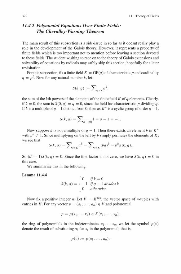
372 11 Theory of Fields
11.4.2 Polynomial Equations Over Finite Fields:The Chevalley-Warning Theorem
The main result of this subsection is a side-issue in so far as it doesnt really play arole in the development of the Galois theory. However, it represents a property offinite fields which is too important not to mention before leaving a section devotedto these fields. The student wishing to race on to the theory of Galois extensions andsolvability of equations by radicals may safely skip this section, hopefully for a laterrevisitation.
For this subsection, fix a finite field K = GF(q) of characteristic p and cardinalityq = p�. Now for any natural number k, let
S(k, q) :=∑
a∈Kak .
the sum of the kth powers of the elements of the finite field K of q elements. Clearly,if k = 0, the sum is S(0, q) = q = 0, since the field has characteristic p dividing q.If k is a multiple of q −1 distinct from 0, then as K ∗ is a cyclic group of order q −1,
S(k, q) =∑
K−{0}1 = q − 1 = −1.
Now suppose k is not a multiple of q − 1. Then there exists an element b in K ∗with bk �= 1. Since multiplying on the left by b simply permutes the elements of K ,we see that
S(k, q) =∑
a∈Kak =
∑a∈K
(ba)k = bk S(k, q).
So (bk − 1)S(k, q) = 0. Since the first factor is not zero, we have S(k, q) = 0 inthis case.
We summarize this in the following
Lemma 11.4.4
S(k, q) =⎧⎨⎩0 if k = 0−1 if q − 1 divides k0 otherwise
Now fix a positive integer n. Let V = K (n), the vector space of n-tuples withentries in K . For any vector v = (a1, . . . , an) ∈ V and polynomial
p = p(x1, . . . xn) ∈ K [x1, . . . , xn],
the ring of polynomials in the indeterminates x1, . . . xn , we let the symbol p(v)
denote the result of substituting ai for xi in the polynomial, that is,
p(v) := p(a1, . . . , an).

11.4 Some Applications to Finite Fields 373
If p(v) = 0 for a vector v ∈ V , we say that v is a zero of the polynomial p.Now suppose p = xk1
1 xk22 · · · xkn
n is a monomial of degree∑
ki < n(q − 1). Then
∑v∈V
p(v) =∏n
i=1S(ki , q) = 0,
since at least one of the exponents ki is less than q − 1 and so by Lemma11.4.4introduces a factor of zero in the product. Since every polynomial p in K [x1, . . . , xn]is a sum of such monomials of degree less than n(q − 1), we have
Lemma 11.4.5 If p ∈ K [x1, . . . , xn] has degree less than n(q − 1), then
S(p) :=∑
v∈Vp(v) = 0.
Now we can prove the following:
Theorem 11.4.6 (Chevalley-Warning) Let K be a finite field of characteristic p withexactly q elements. Suppose p1, . . . , pm is a family of polynomials of K [x1, . . . , xn],the sum of whose degrees is less than n, the number of variables. Let X be thecollection
{v ∈ K (n)|pi (v) = 0, i = 1, . . . , m}
of common zeroes of these polynomials. Then
|X | ≡ 0 mod p.
Proof Let R := ∏mi=1(1 − pq−1
i ). Then R is a polynomial whose degree (q − 1)∑deg pi is less than n(q − 1). Now if v ∈ X , then v is a common zero of the
polynomials pi , so R(v) = 1. But if v /∈ X , then for some i , pi (v) �= 0, sopi (v)q−1 = 1, introducing a zero factor in the definition of R(v). Thus we see thatthe polynomial R induces the characteristic function of X—that is, it has value 1 onelements of X and value 0 outside of X . It follows that
S(R) :=∑
v∈VR(v) ≡ |X | mod p. (11.5)
But since deg R < n(q − 1), Lemma11.4.5 forces S(R) = 0, which converts(11.5) into the conclusion. �
Corollary 11.4.7 Suppose p1, . . . pm is a collection of polynomials over K =GF(q) in the indeterminates x1, . . . , xn, each with a zero constant term. Then thereexists a common non-trivial zero for these polynomials. (Non-trivial means one thatis not the zero vector of V .)
In particular, if p is a homogeneous polynomial over K in more indeterminatesthan its degree, then it must have a non-trivial zero.

374 11 Theory of Fields
11.5 Separable Elements and Field Extensions
11.5.1 Separability
Apolynomial p(x) ∈ F[x] is said to be separable if and only if its irreducible factorsin F[x] each have no repeated zeros in any splitting field.
Our discussion on separability of polynomials will be greatly facilitated by thefollowing concept. Let F be a field and define the formal derivative
∂ : F[x] → F[x], f (x) �→ f ′(x)
by setting
f ′(x) =n∑
k=0
kak xk−1, whenever f (x) =n∑
k=0
ak xk .
The formal derivative satisfies the familiar “product rule:” ∂( f (x)g(x)) =(∂ f (x))g(x) + f (x)∂g(x), and hence, its generalization, the “Leibniz rule”:
∂( f1(x) f2(x) · · · fr (x)) =r∑
i=1
f1(x) · · · fi−1(x)(∂ fi (x)) fi+1(x) · · · fr (x).
Furthermore, the formal derivative is “independent of its domain” inasmuch as ifF ⊆ E is an extension of fields, then the following diagram commutes:
E[x] ∂−−−−→ E[x]�⏐⏐ �⏐⏐F[x] ∂−−−−→ F[x]
where the vertical arrows are obvious inclusions.The following simple result will be useful in the sequel.
Lemma 11.5.1 Let f (x), g(x) ∈ F[x], and let F ⊆ E be a field extension. Thenf (x) and g(x) are relatively prime in F[x] if and only if they are relatively prime inE[x].Proof If f (x), g(x) are relatively prime in F[x], then there exist polynomialss(x), t (x) ∈ F[x] with s(x) f (x) + t (x)g(x) = 1. Since this equation is obviouslyvalid in E[x] we infer that f (x), g(x) are relatively prime in E[x], as well.
If f (x) and and g(x) are not relatively prime in F[x], their greatest commondivisor in F[x] has positive degree, and so this is also true in E[x]. Thus not beingrelatively prime in F[x] implies not being relatively prime in E[x]. �
There is a simple way to tell whether a polynomial f (x) in F[x] is separable.
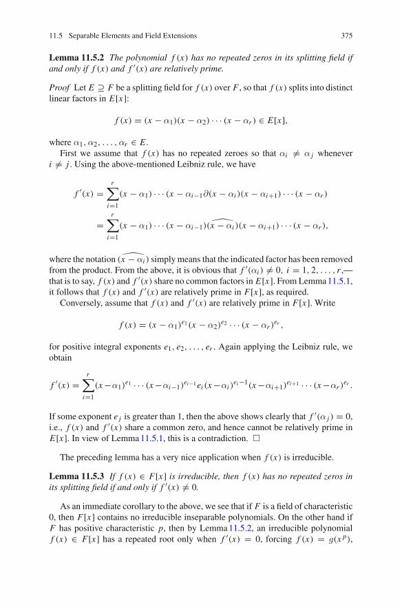
11.5 Separable Elements and Field Extensions 375
Lemma 11.5.2 The polynomial f (x) has no repeated zeros in its splitting field ifand only if f (x) and f ′(x) are relatively prime.
Proof Let E ⊇ F be a splitting field for f (x) over F , so that f (x) splits into distinctlinear factors in E[x]:
f (x) = (x − α1)(x − α2) · · · (x − αr ) ∈ E[x],
where α1,α2, . . . ,αr ∈ E .First we assume that f (x) has no repeated zeroes so that αi �= α j whenever
i �= j . Using the above-mentioned Leibniz rule, we have
f ′(x) =r∑
i=1
(x − α1) · · · (x − αi−1∂(x − αi )(x − αi+1) · · · (x − αr )
=r∑
i=1
(x − α1) · · · (x − αi−1) (x − αi )(x − αi+1) · · · (x − αr ),
where the notation (x − αi ) simplymeans that the indicated factor has been removedfrom the product. From the above, it is obvious that f ′(αi ) �= 0, i = 1, 2, . . . , r ,—that is to say, f (x) and f ′(x) share no common factors in E[x]. From Lemma11.5.1,it follows that f (x) and f ′(x) are relatively prime in F[x], as required.
Conversely, assume that f (x) and f ′(x) are relatively prime in F[x]. Write
f (x) = (x − α1)e1(x − α2)
e2 · · · (x − αr )er ,
for positive integral exponents e1, e2, . . . , er . Again applying the Leibniz rule, weobtain
f ′(x) =r∑
i=1
(x −α1)e1 · · · (x −αi−1)
ei−1ei (x −αi )ei −1(x −αi+1)
ei+1 · · · (x −αr )er .
If some exponent e j is greater than 1, then the above shows clearly that f ′(α j ) = 0,i.e., f (x) and f ′(x) share a common zero, and hence cannot be relatively prime inE[x]. In view of Lemma11.5.1, this is a contradiction. �
The preceding lemma has a very nice application when f (x) is irreducible.
Lemma 11.5.3 If f (x) ∈ F[x] is irreducible, then f (x) has no repeated zeros inits splitting field if and only if f ′(x) �= 0.
As an immediate corollary to the above, we see that if F is a field of characteristic0, then F[x] contains no irreducible inseparable polynomials. On the other hand ifF has positive characteristic p, then by Lemma11.5.2, an irreducible polynomialf (x) ∈ F[x] has a repeated root only when f ′(x) = 0, forcing f (x) = g(x p),

376 11 Theory of Fields
for some polynomial g(x) ∈ F[x]. In fact, a moment’s thought reveals that, in fact,if f (x) ∈ F[x] is irreducible and inseparable, then we may write f (x) = g(x pe
),where e is a positive integral exponent and where g(x) ∈ F[x] is an irreducibleseparable polynomial.
Let F ⊆ E be an extension and let α ∈ E . We say that α is separable over F ifit is algebraic over F and if IrrF (α) is a separable polynomial. The extension E ofF is said to be separable if and only if every element of E which is algebraic overF is separable. We may already infer the following:
Lemma 11.5.4 The algebraic extension F ⊆ E is separable whenever F has char-acteristic 0 or is a finite field.
Proof If F has characteristic 0, the result is obvious by the above remarks. If F isa finite field, the p-power mapping σ : F → F is an automorphism, and hence issurjective. Now let f (x) ∈ F[x] be irreducible and assume that f (x) is inseparable.
Write f (x) = g(x p), where g(x) =m∑
i=0ai xi . For each i = 0, 1, . . . , m, let bi ∈ F
satisfy bpi = ai ; thus,
f (x) = g(x p) =m∑
i=0
bpi xip =
(m∑
i=0
bi xi
)p
,
contrary to the irreducibility of f (x). Thus, any finite extension of a finite field isalso separable. �
We see, therefore, that if F ⊆ E is an inseparable algebraic extension, then Fmust be an infinite field of positive characteristic p. We shall take up this situationin the section to follow. Before doing this, it shall be helpful to consider two rathertypical examples.
Example 52 Let P = GF(2) be the field of two elements, let x be an indeterminateover P , and set F = P(x), the field of “rational functions” over P . Obviously, F isan infinite field of characteristic 2. Note also that F is the field of fractions of the PIDP[x]. Now set f (y) = y2 + x ∈ F[y]; note that since x is prime in P[x], we mayapply Eisenstein’s criterion (see Exercise (8) in Sect. 9.13.1, p. 318) to infer that f (y)
is irreducible in F[y]. Thus, if α is a zero of f (y) in a splitting field over F for f (y),then [F(α) : F] = 2. Furthermore, since f ′(y) = 2y +0 = 0 ∈ F[x], we see that αis inseparable over F . Therefore F(α) ⊇ F is an inseparable extension (that is to say,not a separable extension). However, we can argue that every element of F(α)\F isinseparable over F , as follows. Since {1,α} is an F-basis of F(α), we see that everyelement of F(α)\F can be written in the form β = a +bα, a, b ∈ F, b �= 0. We set
g(y) = (y − (a + bα))2 = y2 + (a + bα)2 = y2 + a2 + b2x ∈ F[y];

11.5 Separable Elements and Field Extensions 377
since a+bα is a zero of g(y), and since a+bα �∈ F , we see that g(y) = IrrF (a+bα).But as g′(y) = 0 we see that β is an inseparable element over F . Thus proves thatevery element of F(α)\F is inseparable over F ;we shall come to call such extensionspurely inseparable.
Example 53 As a hybrid example, we take P = GF(3), the 3-element field, anddefine F = P(x). Set f (y) = y6 + x2y3 + x ∈ F[y]. Again, an application ofEisenstein reveals that f (y) is irreducible in F[y]. Since f ′(y) = 0 we infer thatf (y) is inseparable over F . We take α to be a zero (in a splitting field) of f (y),from which we infer that [F(α) : F] = 6. Furthermore, we know that this is nota separable extension since α is not separable over F . We note that f (y) = g(y3),where g(y) is the irreducible separable polynomial g(y) = y2 + x2y + x ∈ F[y].This says that α3, being a root of g(y), is separable over F (note that α3 �∈ F).Therefore, we see that F(α)\F contains both separable and inseparable elementsover F . In fact, we have a tower F ⊆ F(α3) ⊆ F(α), where [F(α3) : F] = 2and so [F(α) : F(α3)] = 3. Our work in the next section will show that, in fact,F(α3) contains all of the separable elements of F(α) over F , and that the extensionF(α3) ⊆ F(α) is purely inseparable.
11.5.2 Separable and Inseparable Extensions
The primary objective of this subsection is to show that a finite-degree extensionF ⊆ E can be factored as F ⊆ Esep ⊆ E , where Esep consists precisely of thoseelements of E separable over F , and where Esep ⊆ E is a purely inseparableextension (i.e., no elements of E − Esep are separable).
Suppose that F is a field of positive characteristic p, and that K ⊇ F is anextension of finite degree. We have the pth power mapping K → K , a �→ a p, a ∈K . Note that if F is not finite, K is not finite, and we cannot infer that this mappingis an automorphism of K—we can only infer that it gives an embedding of K intoitself (as explained in Lemma7.4.6 of Sect. 7.4.2, p. 221). We denote the image byK p, and denote by F K p the subfield of K generated by the subfields F and K p.
We shall have need of the following technical result:
Theorem 11.5.5 Let F be a field of positive characteristic p, and let K ⊇ F be anextension of finite degree. If K = F K p, then the pth power mapping on K preservesF-linear independence of subsets.
Proof Since any F-linearly independent subset of K can be completed to an F-basis for K , it suffices to prove that the pth power mapping preserves the linearindependence of any F-basis for K . Suppose, then, that {a1, . . . , an} is a F-basis ofK , and that c is an element of K . Then c can be written as an F-linear combinationof the basis elements:
c = α1a1 + · · · + αnan, all αi ∈ F,

378 11 Theory of Fields
from which we conclude that
cp = αp1 a p
1 + · · · + αpn a p
n .
Therefore,K p = F pa p
1 + · · · + F pa pn ,
and so, by hypothesis,
K = F K p = Fa p1 + · · · + Fa p
n .
Thus the pth powers of the basis elements ai form a F-spanning set of K of size n.Since n = dimF K , these n spanning elements must be F-linearly independent. �Theorem 11.5.6 (Separability criterion for fields of prime characteristic) Let K beany algebraic field extension of the field F, where F (and hence K ) have primecharacteristic p.
(i) If K is a separable extension of F, then K = FKp. (Note that the degree [K : F]need not be finite here.)
(ii) If K is a finite extension of F such that K = FKp, then K is separable over F.
Proof Assume, as in Part (i), that K ⊇ F is a separable extension. Then it is clearthat every element of K is also separable over the intermediate subfield L := FKp. Ifa ∈ K , then b = a p ∈ L and so a is a zero of the polynomial x p − b ∈ L[x]. Thus,if p(x) = IrrL(a) ∈ L[x], we have that p(x) divides x p − b in L[x]. However, inK [x], x p − b = x p − a p = (x − a)p and so p(x) cannot be separable unless it hasdegree 1. This forces p(x) = x − a ∈ L[x], i.e., that a ∈ L , proving that K = FKp.
For Part (ii), assume that [K : F] is finite, and that K = FKp. Suppose, by wayof contradiction that a is an element of K which is not separable over F . Then iff (x) := IrrF (a), we have that f (x) = g(x p), where g(x) ∈ F[x] is irreducible.Write g(x) =
m∑j=0
a j x j and conclude that
0 = f (a) = g(a p) = a0 + a1a p + · · · + ama pm,
which says that {1, a p, a2p, . . . , amp} is an F-linearly dependent subset of K On theother hand, if {1, a, a2. . . . , am}were F-linearly dependent, then there would exist apolynomial p(x) in F[x] of degree at mostm having element a for a zero, contrary tothe fact that f (x) = IrrF (a) has degree pm > m, which is a contradiction. Therefore,the pth power mapping has taken the F-linearly independent set {1, a, a2, . . . , am}to the F-linearly dependent set {1, a p, a2p, . . . , amp}, a violation of Theorem11.5.5.Therefore, a ∈ K must have been separable over F in the first place. �Corollary 11.5.7 (Separability of simple extensions) Fix a field F of prime charac-teristic p, let F ⊆ K be a field extension, and let a ∈ K be algebraic over F. Thefollowing are equivalent:

11.5 Separable Elements and Field Extensions 379
(i) F(a) ⊇ F is a separable extension;(ii) a is separable over F;
(iii) F(a) = F(a p).
Proof (i)⇒(ii) is, of course, obvious.Assume (ii). Since a is a zero of the polynomial x p − a p ∈ F(a p)[x], we see
that IrrF(a p)(a) divides x p − a p. But x p − a p = (x − a)p ∈ F(a)[x]. Since a isseparable over F , it is separable over F(a p) and so it follows that a ∈ F(a p), forcingF(a) = F(a p), which proves (ii)⇒(iii).
Finally, if F(a) = F(a p), then F · F(a)p = F · F p(a p) = F(a p) = F(a), byhypothesis. Apply Theorem11.5.6 part (ii) to infer that F(a) is separable over F ,which proves that (iii)⇒(i). �
Corollary 11.5.8 (Transitivity of separability among finite extensions) Suppose Kis a finite separable extension of L and that L is a finite separable extension of F.Then K is a finite separable extension of F.
Proof That [K : F] is finite is known by Lemma11.2.2, so we only need to prove theseparability of K over F .Wemay assume that F has prime characteristic p, otherwiseK is separable by Lemma11.5.4. By Part (ii) of Theorem11.5.6, it suffices to provethat K = FKp. But, since K is separable over L , and since L is separable over F ,we have
K = LKp = (FLp)K p = F(LK)p = FKp.
That K is separable over F now follows from Theorem11.5.6, part (ii). �
Corollary 11.5.9 Let K be an arbitrary extension of F. Then
Ksep = {a ∈ K |a is separable over F}
is a subfield of K containing F.
Proof It clearly suffices to show that Ksep is a subfield of K . However, if a, b ∈ Ksep,then by Corollary11.5.7 we have that F(a) is separable over F and that F(a, b) isseparable over F(a). Apply Corollary11.5.8. �
The field Ksep is called the separable closure of F in K .Finally, recall that we have called an algebraic extension F ⊆ K purely insepa-
rable if every element of K\F is inseparable over F . Therefore, we see already thatif F ⊆ K is an algebraic extension, then Ksep is a separable extension of F , and, byCorollary11.5.8, K is a purely inseparable extension of Ksep.
We conclude this section with a characterization of purely inseparable extensions.
Theorem 11.5.10 Let F ⊆ K be an algebraic extension. The following propositionsare equivalent:

380 11 Theory of Fields
(1) K is a purely inseparable extension of F;(2) For all a ∈ K\F, a pe ∈ F, for some positive exponent e of the positive charac-
teristic p;(3) For all a ∈ K\F, IrrF (a) = x pe − b, for some b ∈ F and some positive
exponent e.
As a corollary to Theorem11.5.10 we extract the following useful corollary forsimple extensions.
Corollary 11.5.11 Let F be a field of characteristic p, contained in some field K .Assume that a ∈ K satisfies a pe ∈ F. Then the subfield F(a) ⊆ K is a purelyinseparable extension of F.
Proof If [F(a) : F] = r , then any element b ∈ F(a) can be expressed as a polyno-
mial in a: b =r−1∑j=0
a j a j , where the coefficients a0, a1, . . . , ar−1 ∈ F . But then
bpe =⎛⎝r−1∑
j=0
a j aj
⎞⎠
pe
=r−1∑j=0
a pe
j a jpe ∈ F.
Now apply Theorem11.5.10. �
11.6 Galois Theory
11.6.1 Galois Field Extensions
Let K be any field, and let k be a subfield of K . The k-isomorphisms of K with itselfare called k-automorphisms of K . Under composition they form a group which wedenote by Gal(K/k). The group of all automorphisms of K is denoted Aut(K ), asusual. It is obvious that Gal(K/k) is a subgroup of Aut(K ).
Suppose now that G is any group of automorphisms of the field K . The elementsfixed by every automorphism of G form a subfield called the fixed subfield of G(and sometimes the field of invariants of G), accordingly denoted invG(K ). If G ≤Gal(G/k) then clearly k is a subfield of invG(K ).
Now let �G be the poset of all subgroups of G, and let �K/k be the poset ofall subfields of K which contain k; in both cases we take the partial order to becontainment. To each subfield L with k ≤ L ≤ K , there corresponds a subroupGal(K/L). Similarly, for each subgroup H of Gal(K/k), there corresponds thesubfield invH (K ) containing k. These correspondences are realized as twomappings:
Gal(K/•) : �K/k −→ �G, inv•(K ) : �G −→ �K/k,

11.6 Galois Theory 381
which are obviously inclusion reversing. Furthermore, for all E ∈ �K/k and for allH ∈ �G , one has that
inv•(K ) ◦ Gal(K/•)(E) = invGal(K/E)(K ) ⊇ E, and
Gal(K/•) ◦ inv•(E)(H) = Gal(E/invH (E)) ≥ H.
In plain language, the composition of the two poset morphisms in either order, ismonotone on its defined poset. Therefore, we see that the quadruple (�K/k,�G ,
Gal(K/•), inv•(K )) is a Galois connection in the sense of Sect. 2.2.15.Next, if we assume, as we typically shall, that [K : k] < ∞, then every interval
in �K/k is algebraic in the sense of Sect. 2.3.2.6 In fact, the mapping which takesthe algebraic interval [E1, E2] of �K/k to the index [E2 : E1] is a Z-valued intervalmeasure in the sense of Sect. 2.5.2. We shall show presently that when [K : k] ≤ ∞,|Gal(K/k)| ≤ ∞, and so similar comments apply to the poset�G , where, if H2 ≤ H1are subgroups of G = Gal(K/k), then themappingwhich takes the interval [H2, H1]to the index [H1 : H2] is the appropriate Z-valued interval measure.
11.6.2 The Dedekind Independence Lemma
We begin with the following observation. Let K be a field; let S be a set; and let K S
be the set of mappings S → K .Wemay give K S a K -vector space structure by point-wise operations. Thus, if f1, f2 ∈ K S , and if α ∈ K , then we set α( f1 + f2)(s) :=α f1(s) + α f2(s).
In terms of the above, we state the following important result.
Lemma 11.6.1 (Dedekind Independence Lemma)
1. Let E, K be fields, and let σ1,σ2, . . . ,σr be distinct monomorphisms E → K .Then σ1,σ2, . . . ,σr are K -linearly independent in K E , the K -vector space ofall functions from E to K .
2. Let E be a field, and let G be a group of automorphisms of E. We may regard eachα ∈ E as an element of EG via σ �→ σ(α) ∈ E, σ ∈ G. Now set K = invG(E)
and assume that we are given K -linearly independent elements α1,α2, . . . ,αr ∈E. Then α1,α2, . . . ,αr are E-linearly independent elements of EG.
Proof For Part 1, suppose, byway of contradiction, that there exists a nontrivial lineardependence relation of the form a1σ1 + · · · + arσr = 0 ∈ K E , a1, . . . , ar ∈ K .Among all such relations we may assume that we have chosen one in which thenumber of summands r is as small as possible.
We have, for all α ∈ E , that
a1σ1(α) + a2σ2(α) + · · · + arσr (α) = 0, (11.6)
6Recall that a poset is algebraic if its “zero” and “one” are connected by a finite unrefinable chain.

382 11 Theory of Fields
where each coefficient ai is non-zero by the minimality of r . Since σ1 �= σ2, we maychoose α′ ∈ E such that σ1(α
′) �= σ2(α′). If we replace the argument α in Eq. (11.6)
by α′α and use the fact that each σi , i = 1, 2, . . . , r is a homomorphism, we obtainthe following:
a1σ1(α′)σ1(α) + a2σ2(α
′)σ2(α) + · · · + arσr (α′)σr (α) = 0. (11.7)
Next, multiply both sides of Eq. (11.6) by the scalar σ1(α′):
a1σ1(α′)σ1(α) + a2σ1(α
′)σ2(α) + · · · + arσ1(α′)σr (α) = 0. (11.8)
Subtracting Eq. (11.8) from Eq. (11.7) yields
a2(σ2(α′) − σ1(α
′))σ2(α) + · · · + ar (σr (α′) − σ1(α
′))σr (α) = 0.
Since a2(σ2(α′)−σ1(α
′)) �= 0, and α was arbitrary, we have produced a non-trivialdependence relation among the σi , i �= 1, against the minimal choice of r . Thus nosuch dependence relation among the maps {σi } exists and Part 1 is proved.
For part 2, we again argue by considering an E-linear dependence relation amongthe functions αi : G → E with a minimal number of terms r . Thus one obtains arelation
a1σ(α1) + a2σ(α2) + · · · + arσ(αr ) = 0, (11.9)
valid for all σ ∈ G, and where we may assume that the elements a1, a2, . . . , ar ∈ Eare all nonzero. We may as well assume that a1 = 1. Then setting σ = 1 ∈ G inEq. (11.9) yields
α1 + a2α2 + · · · arαr = 0.
Sinceα1,α2, . . . ,αr are linearly independent over K , the preceding equation impliesthat at least one of the elements a2, . . . , ar is not in K . Re-indexing the ai if necessarywe may assume that a2 �∈ K . Therefore, there exists an element σ′ ∈ G such thatσ′(a2) �= a2. Equation (11.9) with σ replaced by σ′σ then reads as:
σ′σ(α1) + a2σ′σ(α2) + · · · + arσ
′σ(αr ) = 0, (11.10)
still valid for all σ ∈ G. Applying σ′ to both sides of Eq. (11.9) yields
σ′σ(α1) + σ′(a2)σ′σ(α2) + · · · + σ′(ar )σ′σ(αr ) = 0, (11.11)
and subtracting Eq. (11.11) from Eq. (11.10) yields
(a2 − σ′(a2))σ′σ(α2) + · · · + (ar − σ′(ar ))σ′σ(ar ) = 0.

11.6 Galois Theory 383
Since this is true for all σ ∈ G, and since a2 − σ′(a2) �= 0, we have produceda dependence relation on a smaller set of functions {σ �→ σ(αi )|i > 1}, whichcontradicts the minimality of r . Thus no dependence relation as described can existand Part 2 must hold. �
From theDedekind IndependenceLemma,we extract the following lemma,whichsummarizes the relationships between field extension degrees and group indices.
Theorem 11.6.2 Let k ⊆ K be a field extension, with Galois group G = Gal(K/k).
1. Assume that k ⊆ E1 ⊆ E2 ⊆ K is a tower of fields, and set Hi = Gal(K/Ei ), i =1, 2. If [E2 : E1] < ∞, then [H1 : H2] ≤ [E2 : E1].
2. Assume that H2 ≤ H1 ≤ G are subgroups, and set Ei = invHi (K ), i = 1, 2. If[H1 : H2] < ∞, then [E2 : E1] ≤ [H1 : H2].
Proof For part 1, we shall assume, by way of contradiction, that [H1 : H2] > [E2 :E1]. Set r = [E2 : E1], and let {α1, . . . ,αr } be an E1-basis of E2. Assume that{σ1,σ2, . . . ,σs}, s > r , is a set of distinct left H2-coset representatives in H1. Sinces > r , we may find elements a1, a2, . . . , as ∈ K , not all zero, such that
s∑i=1
aiσi (α j ) = 0, j = 1, 2, . . . , r.
Since any element of E2 can be written as an E1-linear combination of α1, . . . ,αr ,
we conclude thats∑
i=1aiσi : E2 → K is the 0-mapping. Since σ1, . . . ,σs are distinct
coset representatives, they are distinct mappings E2 → K . This contradicts part 1of the Dedekind Independence Lemma.
For part 2 of the Theorem, we shall assume, by way of contradiction, that [E2 :E1] > [H1 : H2]. Let {σ1, . . . ,σr } be a complete set of H2-coset representatives inH1, and assume that {α1, . . . ,αs} is an E1-linearly independent subset of E2, where,by assumption, s > r . Again, we may find elements a1, a2, . . . , as ∈ K , not all zero,such that
s∑i=1
aiσ j (αi ) = 0, j = 1, 2, . . . , r.
If σ ∈ H1, then σ = σ jτ , for some index j, 1 ≤ j ≤ r and for some τ ∈ H2.Therefore, as E2 is fixed point-wise by H2, we have
s∑i=1
aiσ(αi ) =s∑
i=1
aiσ jτ (αi ) =s∑
i=1
aiσ j (αi ) = 0.
Since not all ai are zero in the first term of the equation just presented, the mappingsσ �→ σ(αi ) ∈ K are not K -linearly independent, against part (ii) of the DedekindIndependence Lemma. �

384 11 Theory of Fields
Corollary 11.6.3 Let k ⊆ K be a finite degree extension, and set G = Gal(K/k).If k0 = invG(K ), then
|G| = [K : k0].
Proof Note first that G = Gal(K/k0). We have
[K : k0] ≥ |G| ≥ [K : k0],
where the first inequality is Theorem11.6.2, part (1), and the second inequality isTheorem11.6.2, part (2). The result follows. �
11.6.3 Galois Extensions and the Fundamental Theoremof Galois Theory
Onemay recall fromSect. 2.2.15 thatwith anyGalois connection between two posets,there is a closure operator for each poset. That notion of closure holds for the twoposets that we have been considering here: the poset of subgroups of Gal(K/k) andthe poset of subfields of K that contain k. Accordingly, we say that a subfield k ofK is Galois closed in K if and only if
k = invGal(K/k)(K ).
We define an algebraic extension k ⊆ K to be a Galois extension if k is Galoisclosed in K . Note that from the property that K/k is a Galois extension, we caninfer immediately that every subfield E ∈ �K/k of finite degree over k is also Galoisclosed in K . Indeed, we can set G = Gal(K/k), E = invGal(K/E)(K ) (the Galoisclosure of E in K ), and use Theorem11.6.2 to infer that
[E : k] ≥ [G : Gal(K/E)] ≥ [E : k].
Since we already have E ⊆ E , the result that E = E follows immediately.We characterize the Galois extensions as follows.
Theorem 11.6.4 Let k ⊆ K be a finite extension. The following are equivalent:
(i) k ⊆ K is a Galois extension;(ii) k ⊆ K is a separable, normal extension.
Proof Assume that k ⊆ K is a Galois extension. Assume that f (x) ∈ k[x] is anirreducible polynomial having a zero α ∈ K . Let {α1 = α,α2, . . . ,αr } be theG-orbit of α in K , where G = Gal(K/k). Set
g(x) =r∏
i=1
(x − αr ) ∈ K [x].

11.6 Galois Theory 385
Note that since each σ ∈ G simply permutes the elements α1, . . . ,αr , we inferimmediately that for each σ ∈ G, σ∗g(x) = g(x). (Here σ∗ is the ring automorphismof K [x] that applies σ to the coefficients of the polynomials. See Sect. 11.3.1, p. 363.)Therefore the coefficients of g(x) are all in invG(K ) = k, as k is closed in K .Therefore g(x) ∈ k[x]; since g(α) = 0, f (x) must divide g(x), which impliesthat f (x) splits completely in K [x]. Since f (x) was arbitrarily chosen in k[x], weconclude that K is a normal extension of k.
Note that the above also proves that the arbitrarily-chosen irreducible polynomialf (x) ∈ k[x] is separable. Applying this to f (x) = Irrk(α), α ∈ K , we see that Kis a separable extension of k, as well.
Conversely, assume that the finite extension k ⊆ K is a separable normal exten-sion. Let α ∈ K\k and set f (x) = Irrk(x). Then f (x) is of degree at least twoand splits into distinct linear factors in K [x]. Thus, if β ∈ K is another zero off (x), then by Lemma11.3.1 there exists a k-isomorphism k(α) → k(β) taking αto β. Next, by Theorem11.3.4 this isomorphism can be extended to one defined onall of K . Therefore, we have shown that for all α ∈ K\k, there is an element ofσ ∈ G = Gal(K/k) such that σ(α) �= α. It follows that k = invG(K ), proving theresult. �
Theorem 11.6.5 (The Fundamental Theorem of Galois Theory) Suppose K is afinite separable normal extension of the the field k. Let G := Gal(K/k), let S(G) bethe dual of the poset of subgroups of G, and let �K/k be the poset of subfields of Kwhich contain k. Then the following hold:
(i) (the Galois Connection) The mappings of the Galois correspondence
S(G)Gal(K/•)
�inv•(K )
�K/k
are inverse to each other, and hence are bijections.(ii) (The connection between upper field indices and group orders) For each inter-
mediate field L ∈ �K/k
[K : L] = |Gal(K/L)|.
(iii) (The connection between group indices and lower field indices) If H ≤ G, then[invH (K ) : k] = [G : H ].
(iv) (The correspondence of normal fields and normal subgroups).
1. L ∈ �K/k is normal over k if and only if Gal(K/L) is a normal subgroupof G = Gal(K/k).
2. N � G if and only if invN (K ) is a normal extension of k.
(v) (Induced groups and normal factors) Suppose L is a normal extension of kcontained in K . Then Gal(L/k) is isomorphic to the factor group Gal(K/k)/
Gal(K/L).

386 11 Theory of Fields
Proof Thanks to our preparation, the statement of this Theorem is almost longerthan its proof. Part (i) follows by the discussion at the beginning of this subsection.By part (i) together with Theorem11.6.2, one has, for any subfield L ∈ �K/k , that
[K : L] ≥ [Gal(K/L) : 1] = |Gal(K/L)| ≥ [K : invGal(K/L)(K )] = [K : L].
Likewise, for any subgroup H ≤ G, one has
[G : H ] ≥ [invH (K ) : k] ≥ [G : Gal(K/invH (K ))] = [G : H ],
proving both parts (ii) and (iii).We prove part (iv) part 1: If L ∈ �K/k is normal over k, then by Corollary11.3.8
K is G-invariant. This gives a homomorphism G → Gal(L/k), σ �→ σ|L ; and thekernel of this homomorphism is obviously Gal(K/L) � G.
For (iv), part 2, suppose N � G, and choose α ∈ invN (K ). Then for any σ ∈ Gand n ∈ N we have nσ(α) = σ(σ−1nσ)(α) = σ(α), where we have used the factthat σ−1nσ ∈ N and N fixes point-wise the elements of invN (K ). This proves thatσ(α) ∈ invN (K ). Now apply Corollary11.3.8 to conclude that invN (K ) is a normalextension of k.
Finally, we prove part (v): Now we have observed above that when L ∈ �K/k
is a normal extension of k, there a homomorphism G → Gal(L/k) having kernelGal(K/L).
This homomorphism can be seen to be surjective by two distinct arguments.(1) First a direct application of Corollary11.3.8 (with (K , L , k) playing the roleof (E, K , F) of that Corollary) shows that any automorphism in Gal(L/k) lifts toan automorphism of Gal(K/k). (2) A second argument achieves the surjectivity byshowing that the order of the image of the homomorphism is at least as large as thecodomain Gal(L/k). First, by the fundamental theorem of group homomorphisms,the order of the image is [G : Gal(K/L)]. By (iii),
[G : Gal(K/L)] = [invGal(K/L)(K ) : k].
But by definition, invGal(K/L)(K ) contains L , and so the field index on the right sideis at least [L : k]. But since L/k is also a Galois extension, one has [L : k] =|Gal(L/k)|, by (ii) applied to L/k. Putting these equations and inequalities togetherone obtains
|G/Gal(K/L)| ≥ |Gal(L/k)|
and so the homomorphism G → Gal(L/k) is again onto.Now, since the homomorphism is onto, the fundamental theorem of group homo-
morphisms shows that the factor group G/Gal(K/L) is isomorphic to the homomor-phic image Gal(L/k). �

11.7 Traces and Norms and Their Applications 387
11.7 Traces and Norms and Their Applications
11.7.1 Introduction
Throughout this section, F is a separable extension of a field k, of finite degreedimk(F) = [F : k].
Let E be the normal closure of F over k. Then E is a finite normal separableextension of k—that is, it is aGalois extension.Accordingly, ifG = Gal(E/k) and His the subgroup of G fixing the subfield F element-wise, we have [G : H ] = [F : k].Let σ1 = 1,σ2, . . . ,σn be any right transversal of H in G.7 We regard each σi as anisomorphism F → E .
The trace and norm are two functions TF/k and NF/k from F into k, which aredefined as follows: for each α ∈ F ,
TF/k(α) =n∑
i=1
ασi , (11.12)
NF/k(α) =n∏
i=1
ασi . (11.13)
The elements {ασi } list the full orbit αG of α under the (right) action of G, andso does not depend on the particular choice of coset representatives {σi }. Since theorbit sum TF/k(α) and orbit product NF/k(α) are both fixed by G, and E/K is aGalois extension, these elements must lie in k = invG(E).
When the extension k ⊆ F is understood, one often writes T (α) for TF/k(α) andN (α) for NF/k(α).
The formulae (11.12) and (11.13) imply the following:
T (α + β) = T (α) + T (β),α,β ∈ F (11.14)
T (αc) = T (α)c,α ∈ F, c ∈ k, (11.15)
so that T is a k-linear transformation F → k.Similarly, for the norm (11.12) and (11.13) yield
N (αβ) = N (α)N (β),α,β ∈ F (11.16)
N (αc) = N (α)cn,α ∈ F, c ∈ k. (11.17)
7Recall from Chap.3 that a right transversal of a subgroup is simply a complete system of rightcoset representatives of the subgroup in its parent group. In this case {Hσi } lists all right cosets ofH in G.

388 11 Theory of Fields
11.7.2 Elementary Properties of the Trace and Norm
Theorem 11.7.1 (The Transitivity Formulae) Suppose k ⊆ F ⊆ L is a tower offields with both extension L/F and F/k finite separable extensions. Then for anyelement α ∈ L,
TL/k(α) = TF/k(TL/F (α)) (11.18)
NL/k(α) = NF/k(NL/F (α)). (11.19)
Proof Let E be the normal closure of L so that E/k is a Galois extension. SetG = Gal(E/k), H = Gal(E/F) and U = Gal(E/L). Then U ≤ H ≤ G, and
n = [G : H ] = [K : k]m = [H : U ] = [L : F] and
nm = [G : U ] = [L : k].
If X is a right transversal of H in G, and Y is right transversal of U in H , then
TL/k(α) =∑
σ∈XY
ασ =∑σ∈X
(∑τ∈Y
ατ
)σ
(11.20)
=∑σ∈X
(TL/F (α))σ = TF/k(TL/F (α)). (11.21)
The anagolous formula for norms is obtained upon replacing sums by productsin the preceding Eq. (11.21). �
Corollary 11.7.2 If k ⊂ F is a separable extension of degree n = [F : k], and ifα ∈ F has monic irreducible polynomial
irr(α) = xd + ad−1xd−1 + · · · + a1x + a0 ∈ k[x],
thenTF/k(α) = −(n/d)ad−1. (11.22)
Similarly,NF/k(α) = ((−1)da0)
n/d . (11.23)
Proof Let E be the normal closure of F , so that we have the factorization
irr(α) = (x − θ1) · · · (x − θd)

11.7 Traces and Norms and Their Applications 389
in E[x]. Then −ad−1 = ∑θi and
∏θi = (−1)da0. But
∑θi = Tk(α)/k(α) and∏
θi = Nk(α)/k(α). Now applying the transitivity formulae (11.18) and (11.19) forthe extension tower k ⊆ k(α) ⊆ F one obtains
TE/k(α)(α) = Tk(α)/k(TF/k(α)(α) = Tk(α)/k(α) · [F : k(α)]
since α ∈ k(α). Similarly
NF/k(α) = Nk(α/k(α))[F :k(α)].
�
11.7.3 The Trace Map for a Separable Extension Is Not Zero
Theorem 11.7.3 Suppose k ⊆ F is a finite separable extension. Then the tracefunction TF/k : F → k is not the zero function.
Proof Let E be the normal closure of F ; it then follows that k ⊆ E is a Galoisextension. Let G = Gal(E/k), and let {σ1, . . . ,σn} be a complete listing of its ele-ments. By the Dedekind Independence Lemma (Lemma11.6.1), part 1, the functionsσi : E → E are k-linearly independent. In, particular, the mapping
∑σi defined by
α �→ ∑ni=1 ασi cannot be the zero function. So there is an element β ∈ E such that
0 �=∑
i
βσi = TE/k(β). (11.24)
Set β′ = TE/F (β). Then β′ lies in F since F ⊆ E is also a Galois extension. Nowif TF/k(β
′) = 0, then
TE/k(β) = TF/k(TE/F (β) = TF/k(β′) = 0,
against Eq. (11.24). Thus we have found β′ ∈ F such that TF/k(β′) �= 0 showing
that the trace mapping TF/k is not the zero mapping. �
Associated with the trace function TF/k : F → k is a symmetric bilinear formBT : F × F → k called the trace form defined by
BT (α,β) = TF/k(αβ),α,β ∈ F.
This form is said to be non-degenerate if BT (α,β) = 0 for all β ∈ F impliesα = 0.8
8The reader is referred to Sect. 9.12 where these concepts were applied to all k-linear maps T :F → k.

390 11 Theory of Fields
Corollary 11.7.4 Let F be a finite separable extension of the field k. Then the traceform is non-degenerate.
Proof If BT (α,β) = 0 for all β ∈ F , then TF/k(αβ) = 0 for all β ∈ F . Ifα �= 0, this would imply TF/k(F) = 0, contrary to the conclusion of the precedingTheorem11.7.3. �
11.7.4 An Application to Rings of Integral Elements
Suppose D is an integral domain, which is integrally closed in its field of fractionsk. (Recall that this means that any fraction formed from elements of D that is alsoa zero of a monic polynomial in D[x], is already an element of D.) Suppose F isa finite separable extension of k, and let OF be the ring of integral elements of Fwith respect to D—that is, the elements of D which are a zero of at least one monicpolynomial in D[x].
In Sect. 9.12 of Chap. 9, a k-linear transformation t : F → k was said to betracelike if and only t (OF ) ⊆ D. Theorem9.12.2 then asserted the following:
If there exists a non-zero tracelike transformation t : F → k, then the ring OF isa Noetherian D-module.
But now we have
Lemma 11.7.5 Let F be a finite separable extension of k, the field of fractions ofthe integrally closed domain D, and let OF be the ring of integral elements as in theintroductory paragraph of this subsection. Then the trace function TF/k : F → k isa tracelike k-linear transformation.
Proof It is sufficient to show that if α ∈ OF , then TF/k(α) ∈ OF , for in that caseTF/k(α) ∈ OF ∩k = D, since D is integrally closed. Let E be the normal closure ofF and setG := Gal(E/k). For eachσ ∈ G, andα ∈ OF ,ασ is also a zero of the samemonic polynomial in D[x] that α is; so it follows that σ(Ok) ⊆ OE . Now TF/k(α)
is the sum of the elements in the orbit αG and so, being a finite sum of elements ofOE , must lie in OE as well as k. Thus TF/k(α) ∈ OE ∩ k ⊆ OE ∩ F = OF . �
Corollary 11.7.6 Let D be an integral domain that is integrally closed in its fieldof fractions k. Let k ⊆ F be a finite separable extension, and let OF be the ringof integral elements (with respect to D) in the field F. Then OF is a NoetherianD-module.
Proof By Theorem9.12.2 it is sufficient to observe that the trace function TF/k isa non-zero tracelike transformation F → k. But as F is a separable extension ofk, these two features of the trace function are established in Theorem11.7.3 andLemma11.7.5. �

11.8 The Galois Group of a Polynomial 391
11.8 The Galois Group of a Polynomial
11.8.1 The Cyclotomic Polynomials
Let n be a positive integer, and let ζ be the complex number ζ = e2πi/n . Set
�n(x) =∏
d
(x − ζd),
where 1 ≤ d ≤ n, and gcd(d, n) = 1. We call�n(x) the nth cyclotomic polynomial.Thus, we see that the zeros of�n(x) are precisely the generators of the unique cyclicsubgroup of order n in the multiplicative group C
∗ of the complex numbers, alsocalled the primitive nth roots of unity. It follows that the degree of �n(x) is thenumber φ(n) of residue classes mod n which are relatively prime to n.9 Note inparticular that
xn − 1 =∏d|n
�d(x). (11.25)
Since each nth root of unity is a power of the primitive root ζ we see that the fieldK = Q(ζ) is the splitting field over Q for xn − 1. If we set G = Gal(K/Q), thenG clearly acts on the zeros of �n(x) (though we don’t know yet that this action istransitive!), and so the coefficients of �n(s) are in invG(K ) = Q. In fact, however,
Lemma 11.8.1 For each positive integer n, �n(x) ∈ Z[x].Proof We shall argue by induction on n. First one has �1(x) = x −1 ∈ Z[x], so theassertion holds for n = 1. Assume n > 1. In Eq. (11.25), c(x) := xn − 1 is writtenas a product of cyclotomic polynomials,�d(x), all of which are monic by definition.By induction
a(x) :=∏d|m
1 ≤ d < m
�d(x) ∈ Z[x],
(where d ranges over proper divisors of n) is a product of monic polynomials inZ[x],and so itself is such a polynomial. Setting b(x) := �n(x), we see that a(x), b(x) andc(x) are monic polynomials with c(x) = a(x)b(x), with a(x) and c(x) in Z[x] andwith b(x) monic in Q[x]. Now we apply Theorem9.13.3 (with Z and Q in the rolesof the domains D and D1, respectively—see Exercise (11) in Sect. 9.13.1, Chap. 9),to conclude that b(x) = �n(x) is also in Z[x]. The induction proof is complete. �
Theorem 11.8.2 For each positive integer n, the nth cyclotomic polynomial �n(x)
is irreducible in Q[x].
9The function: φ : Z → Z is called Euler’s totient function or simply the Euler phi-function.

392 11 Theory of Fields
Proof Since �n(x) ∈ Z[x], we may invoke Gauss’s lemma and be satisfied withproving that �n[x] is irreducible in Z[x]. Thus, assume that �n(x) = h(x)k(x),where h(x), k(x) ∈ Z[x] and h(x) is monic and irreducible. Let p be a prime notdividing n, and let ζ be a zero of h(x) in a splitting field F for �n(x) over Q. Weshall show that ζ p is also a zero of h(x). Note that since p and n are relatively prime,ζ p is another zero of�n(x). Assuming that ζ p is not a zero of h(x), it must be a zeroof k(x), forcing ζ to be a zero of the polynomial of k(x p). This implies that h(x)
divides k(x p), and so we may now write
k(x p) = h(x)l(x) (11.26)
for some monic polynomial l(x) ∈ Z[x].At this point, we may invoke the ring homomorphism
m p : Z[x] → (Z/(p))[x],
which preserves degrees but reads the integral coefficients of all polynomials modulop. For each polynomial p(x) ∈ Z[x], we write p(x) for m p(p(x)).
Since n is relatively prime to p, there exists an integer b such that bn ≡ 1mod p. Since (bx)∂(xn − 1) − (xn − 1) = 1 in Z/(p))[x], by Lemma11.5.3,the polynomial xn − 1 must have distinct zeroes in its splitting field K over Z/p.So this also must be true of any factor of the polynomial xn − 1. We now havexn − 1 = �n(x) f (x) = h(x)k(x) f (x), so �n(x) is such a factor.
Now, applying m p to each side of Eq. (11.26), one obtains
h(x)l(x) = k(x p) = k(x)p ∈ (Z/p)[x].
Thus the zeroes of h in K can be found among those of k(x). Since �n(x) =h(x) ¯k(x), we see that �n(x) has repeated zeroes in K , contrary to the observationin the previous paragraph.
What the above has shown is that if ζ is a zero of h(x) in the splitting field F ,then so is ζ p, for every prime p not dividing n. Finally, let η be any primitive n-rootof unity (i.e., a zero of �n(x) in F). Therefore, η = ζr for some integer r relativelyprime to n. We factor r as r = pe1
1 pe22 · · · pes
s ; then as each pi is relatively prime ton, and since the pi th power of a zero of h(x) is another zero of h(x), we concludethat η = ζr is also a zero of h(x). It follows that all zeros of �n(x) are zeroes of itsirreducible monic factor h(x), whence h(x) = �(x), completing the proof. �
11.8.2 The Galois Group as a Permutation Group
Let F be a field and let f (x) ∈ F[x] be a polynomial. If K ⊆ F is a splittingfield over F for f (x), and if G = Gal(K/F), we call G the Galois group of thepolynomial f (x). If α1,α2, . . . ,αk are the distinct zeros of f (x) in K , then, since

11.8 The Galois Group of a Polynomial 393
K = F(α1,α2, . . . ,αk), we see that the automorphisms in G are determined bytheir effects on the elements α1, . . . ,αk . Furthermore, as the elements of G clearlypermute these zeros, we have an injective homomorphism G → Sk (where Sk isidentified with the symmetric group on the k zeros of f (x)) thereby embedding G asa subgroup of Sk . Note finally that if f (x) is irreducible, then the above embeddingrepresents the Galois group G as a transitive subgroup of Sk .
For example, in the previous subsectionwe saw that thenth cyclotomic polynomial�n(x) ∈ Z[x] is irreducible and of degreeφ(n), whereφ is Euler’s “totient” function.Setting k = φ(n), ζ = e2πi/n , and G = Gal(Q(ζ)/Q), we have an embedding of Ginto Sk . However, as G must act as a group of automorphisms of K = Q(ı), we seein particular that it must restrict to a group of automorphisms of the cyclic group 〈ζ〉of order n. Therefore, we have a (faithful) homomorphism G → Aut(〈ζ〉), the latterbeing abelian of order φ(n) (see p. 392). Since |G| = φ(n) = deg�n(x), and sincethe splitting field of �n(x) is the same as that of xn − 1, we conclude that:
Theorem 11.8.3 The Galois group of the polynomial xn − 1 is isomorphic with theautomorphism group of a cyclic group of order n and is therefore abelian of orderφ(n), where φ is Euler’s totient function.
The following is a useful summary of what has been obtained thus far.
Theorem 11.8.4 Let f (x) ∈ F[x] and let G be the corresponding Galois group.Assume that f (x) factors into irreducibles as
f (x) =∏
fi (x)ei ∈ F[x].
Let E be a splitting field over E of f (x), and let �i be the set of zeros of fi (x) in E.Then G acts transitively on each �i .
Proof Ifα,α′ are distinct zeros of fi (x) in E the byLemma11.3.1 there is an isomor-phism F(α) → F(α′); by Theorem11.3.4, this can be extended to an automorphismof E . �
From the above, we see that if � is the set of zeros of a polynomial f (x) in asplitting field E , we have an embedding G → Sym(�) of the Galois group intothe symmetric group on �. Identifying G with its image in Sym(�), an interestingquestion that naturally occurs is whether G ≤ Alt(�), the alternating group on�. Toanswer this, we introduce the discriminant of the separable polynomial f (x). Thuslet f (x) ∈ F[x], where char F �= 2, and let E be a splitting field over F for f (x).Let {α1,α1, . . . ,αk} be the set of distinct roots of f (x) in E . Set
δ =∏
1≤ j<i≤k
(αi − α j ) = det
⎡⎢⎢⎢⎢⎢⎢⎢⎢⎣
1 α1 α21 · · αk−1
1
1 α2 α22 · · αk−1
2
· · · · · ·· · · · · ·· · · · · ·1 αk α2
k · · αk−1k
⎤⎥⎥⎥⎥⎥⎥⎥⎥⎦
,

394 11 Theory of Fields
and let D f = δ2. We call D f the discriminant of the polynomial f (x), sometimesdenoted disc f (x). Note that D f ∈ invG(E); when f (x) is separable, this impliesthat D f ∈ F .
Example 54 (Discriminant of a quadratic) Suppose that f (x) ∈ F[x] is a monicseparable quadratic; thus f (x) = x2 + bx + c = (x − α1)(x − α2) in a splittingfield over F for f (x). Therefore, we have
(i) α1 + α2 = −b, and(ii) α1α2 = c.
It follows that
disc f (x) = (α2 − α1)2
= α21 + α2
2 − 2α1α2
= (α1 + α2)2 − 4α1α2
= b2 − 4c ∈ F[x],
a formula for the discriminant familiar to every high school student.
Before tackling the n = 3 case, we make a few observations of general interest.Relative to α1,α2, . . . ,αk , we define the i th power sum, i = 0, 1, 2, . . .:
si = αi1 + αi
2 · · · + αik .
Since the determinant of a matrix is the same as the determinant of its transpose, wemay express the discriminant of the polynomial f (x) thus:
disc f (x) = det
⎡⎢⎢⎢⎢⎢⎢⎣
1 1 1 · · · 1
α1 α2 α3 · · · αk
α21 α2
2 α23 · · · α2
k...
...... · · · ...
αk−11 αk−1
2 αk−13 · · · αk−1
k
⎤⎥⎥⎥⎥⎥⎥⎦
⎡⎢⎢⎢⎢⎢⎢⎢⎣
1 α1 α21 · · · αk−1
1
1 α2 α22 · · · αk−1
2
1 α3 α23 · · · αk−1
3...
...... · · · ...
1 αk α2k · · · αk−1
k
⎤⎥⎥⎥⎥⎥⎥⎥⎦
,
from which one concludes that
disc f (x) = det
⎡⎢⎢⎢⎢⎢⎢⎢⎣
1 s1 s2 · · · sk−1
s1 s2 s3 · · · sk
s2 s3 s4 · · · sk+1
......
... · · · ...
sk−1 sk sk+1 · · · s2k−2
⎤⎥⎥⎥⎥⎥⎥⎥⎦
. (11.27)

11.8 The Galois Group of a Polynomial 395
Example 55 (Discriminant of a cubic) Suppose that f (x) = x3+a2x2+a1x +a0 ∈F[x] is a monic separable cubic, with zeros α1,α2,α3 in a splitting field. In thiscase, using Eq.11.27 one obtains
disc f (x) = det
⎡⎣ 1 s1 s2
s1 s2 s3s2 s3 s4
⎤⎦ .
Next, note that the coefficients of f (x) are given by
−σ1 : = −(α1 + α2 + α3) = a2,
σ2 : = α1α2 + α1α3 + α2α3 = a1,
−σ3 : = −α1α2α3 = a0.
Furthermore, one has s1 = σ1 = −a2; furthermore,
s2 = α21 + α2
2 + α23
= (α1 + α2 + α3)2 − 2(α1α2 + α1α3 + α2α3)
= σ21 − 2σ2
= a22 − 2a1.
s3 = α31 + α3
2 + α33
= (α1 + α2 + α3)(α21 + α2
2 + α23)
−(α1 + α2 + α3)(α1α2 + α1α3 + α2α3) + 3α1α2α3
= σ1(σ21 − 2σ2) − σ1σ2 − 3σ3
= σ31 − 3σ1σ2 + 3σ3
= −a32 + 3a1a2 − 3a0.
s4 = = α41 + α4
2 + α43
= (α1 + α2 + α3)(α31 + α3
2 + α33)
−(α1α2 + α1α3 + α2α3)(α21 + α2
2 + α23)
+α1α2α3(α1 + α2 + α3)
= −σ1(σ31 − 3σ1σ2 + 3σ3)
−σ2(σ21 − 2σ2) + σ1σ3
= a42 − 4a1a2
2 + 4a0a2 + 2a21 .

396 11 Theory of Fields
From all of the above, one obtains, therefore, that
disc f (x) = det
⎡⎢⎣
3 −a2 a22 − 2a1
−a2 a22 − 2a1 −a3
2 + 3a1a2 − 3a0
a22 − 2a1 −a3
2 + 3a1a2 − 3a0 a42 − 4a1a2
2 + 4a0a2 + 2a21
⎤⎥⎦
= a21a2
2 − 4a31 − 4a0a3
2 − 27a30 + 18a0a1a2,
after admittedly odious calculations!
The above examples reveal a general trend, viz., that the discriminant of a poly-nomial can always be expressed in terms of the coefficients of the polynomial. To seewhy this is the case, we assume, for the moment that x1, x2, . . . , xn are commutingindeterminates, and define the elementary symmetric polynomials σ1,σ2, . . . ,σn ,and the power sum polynomials s1, s2, . . . , sn by setting
σk =∑
i1<i2<···<ik
xi1xi2 · · · xik , sl =n∑
i=1
xl , k = 1, 2, . . . , n, l = 1, 2, . . .
Therefore,
σ1 = s1 = x1 + x2 + . . . xn,
σ2 = ∑i< j
xi x j = x1x2 + x1x3 + · · · xn−1xn ,
s2 = x21 + x22 + . . . + x2n ,
and so on.Next, note that
n∏i=1
(x − xi ) = xn − σ1xn−1 + σ2xn−2 + · · · + (−1)nσn .
From this, it follows immediately that if the power sum polynomials s1, s2, . . . canbe written as polynomials in the elementary symmetric polynomials σ1,σ2, . . . ,σn ,then from Eq. (11.27) we infer immediately that the discriminant of a polynomialcan be expressed as a polynomial in its coefficients. Our detailed calculations of thediscriminant of quadratics and cubics hint that this might be possible. We turn nowto a demonstration that this can always be done.
First, suppose that g(x) = g(x1, x2, . . . , xn) ∈ F[x1, x2, . . . , xn]. We say thatg(x) is a symmetric polynomial if it remains unchanged upon any permutation of theindices 1, 2, . . . , n. Therefore, we see immediately that the elementary symmetricpolynomials as well as the power sum polynomials are symmetric polynomials.
Theorem 11.8.5 (Fundamental Theorem on Symmetric Polynomials) Any symmet-ric polynomial g(x) ∈ F[x1, x2, . . . , xn] can be expressed as a polynomial in theelementary symmetric polynomials.

11.8 The Galois Group of a Polynomial 397
Proof We clearly may assume that g = g(x) is homogeneous, i.e., that it is com-posed of monomials each of the same degree, say k. Next, we introduce into the setof monomials of the form xi1
1 xi22 · · · xin
n , where i1 + i2 + · · · + in = k, the so-called
lexicographic ordering. Thus we say that xi11 · · · xin
n < x j11 · · · x jn
n if i1 = j1, i2 =j2, . . . , il = jl , il+1 < jl+1. Thus, if n = 3 we have x21 x2x33 < x21 x22 x23 < x31 x2x23 .Next, let xm1
1 xm22 · · · xmn
n be the highest monomial occurring in g with nonzero coef-ficient. Since g is symmetric, it must also contain all monomials obtained fromxm11 xm2
2 · · · xmnn by permuting the indices. It follows, therefore, that we must have
m1 ≥ m2 ≥ · · · ≥ mn .Next, let d1, d2, . . . , dn be exponents; wewish to identify the highest monomial in
the symmetric polynomial σd11 σd2
2 · · ·σdnn . Here it is useful to observe that if M1, M2
are monomials of the same degree with M1 < M2, and if M is any monomial, thenM1M < M2M . Having observed this, we note next that the highest monomial inσi is clearly x1x2 · · · xi . Therefore, the highest monomial in σdi
i is xdi1 xdi
2 · · · xdin . In
turn, the highest monomial in σd11 σd2
2 · · ·σdnn is therefore
xd1+d2+···dn1 xd2+d3+···+dn
2 · · · xdnn .
From this, we see that the highest degree monomial in both g and and the polynomialσm1−m21 σm2−m3
2 · · · σmnn is xm1
1 xm22 · · · xmn
n . This implies that if
g = axm11 xm2
2 · · · xmnn + lower monomials ,
then the symmetric polynomial g−aσm1−m21 σm2−m3
2 · · ·σmnn will only involvemono-
mials lower than xm11 xm2
2 · · · xmnn . A simple induction finishes the proof. �
Corollary 11.8.6 The discriminant of the separable polynomial f (x) ∈ F[x] canbe expressed as a polynomial (with coefficients in F) in the coefficients of f (x).
The permutation-group theoretic importance of the discriminant is the following.
Theorem 11.8.7 Let f (x) ∈ F[x], where char F �= 2 be a polynomial with discrim-inant D f = δ2 = disc f (x) defined as above. Let G be the Galois group of f (x),regarded as a subgroup of Sym(n), acting on the zeros {α1, · · · ,αn} in a splittingfield E over F for f (x). If A := G ∩ Alt(n), then invA(E) = F(δ).
Proof Note that any odd permutation of the zeros α1, . . . ,αk will transform δ into−δ and even permutations will fix δ. �
The following is immediate.
Corollary 11.8.8 Let G be the Galois group of f (x) ∈ F[x], where char F �= 2. Ifthe discriminant D f is the square of an element in F, then G ≤ Alt(n).
The following is occasionally useful in establishing that the Galois group of apolynomial is the full symmetric group.

398 11 Theory of Fields
Theorem 11.8.9 Let f (x) ∈ Q[x] be irreducible, of prime degree p, and assumethat f (x) has exactly 2 non-real roots. Then G f = Sym(p).
We close by mentioning that for a general “trinomial,” there is a formula for thediscriminant, due to R.G. Swan,10 given as follows.
Theorem 11.8.10 Let f (x) = xn +axk +b, and let d = g.c.d.(n, k), N = nd , K =
kd . Then
D f = (−1)12 n(n−1)bk−1[nN bN−k − (−1)N (n − k)N−K kK aN ]d .
11.9 Solvability of Equations by Radicals
11.9.1 Introduction
Certainly one remembers that point in one’s education that one first encountered thequadratic equation. If we are given the polynomial equation
ax2 + bx + c = 0,
where a �= 0 (to ensure that the polynomial is indeed “quadratic”), then the roots ofthis equation are given by the formula
(−b ±√
b2 − 4ac)/2a.
Later, perhaps, the formula is justified by the procedure known as “completing thesquare”. One adds some constant to both sides of the equation so that the left side isthe square of a linear polynomial, and then one takes square roots. It is fascinating torealize that this idea of completing the square goes back at least two thousand yearsto the Near East and India. It means that at this early stage, there is the suggestion thatthere could be a realm where square roots could always be taken, and the subtletythat there are cases in which square roots can never be taken because the radican isnegative.
A second method of solving the equation involves renaming the variable x ina suitable way. One first divides the equation through by a so that it has the formx2 + b′x + c′ = 0. Then setting y := x − b′/2, the equation becomes
y2 + c′ − (b′)2/4 = 0,
10R.G. Swan, Factorization of polynomials over finite fields, Pacific Journal, vol 12, pp. 1099–1106, MR 26 #2432. (1962); see also Gary Greenfield and Daniel Drucker, On the discriminant ofa trinomial, Linear Algebra Appl. 62 (1984), 105-112.

11.9 Solvability of Equations by Radicals 399
from which extraction of the square root (if that can be done) yieldsy = √
(4c′ − (b′)2)/2. The original zero named by x , is obtained by x = y + b′/2,and the equations b′ = b/a and c′ = c/a.
Certainly the polynomials in these equations were seen as generic expressionsrepresenting relations between some sort of possible numbers. But these numberswere known not to be rational numbers in many cases. One could say that solutionsdon’t exist in those cases, or that there is a larger realm of numbers (for examplefields like Q(
√2) or the reals), and the latter view only began to emerge in the last
three centuries.Of course the quadratic formula is not valid over fields of characteristic 2 since
dividing by 2 was used in deriving and expressing the formula. The same occurs forthe solutions of the cubic and quartic equations: fields of characteristic 2 and 3 mustbe excluded.
Dividing through by the coefficient of u3, the general cubic equation has the formu3 +bu2 + cu +d = 0, where u is the generic unkown root. Replacing u by x −b/3yields the simpler equation,
x3 + qx + r = 0.
Next, one puts x = y + z to obtain
y3 + z3 + (3yz + q)x + r = 0. (11.28)
There is still a degree of freedom allowing one to demand that yz = −q/3, thuseliminating the coefficient of x in (11.28). Then z3 and y3 are connected by whatamounts to the norm and trace of a quadratic equation:
z3 + y3 = −r,
andz3y3 = −q3/27.
One can then solve for z3 and y3 by the quadratic formula. Taking cube roots (assum-ing that is possible) one gets a value for z and y. The possible zeroes of x3 + qx + rare:
y + z, ωy + ω2z, ω2y + ωz,
where ω is a complex primitive cube root of unity. The formula seems to have beendiscovered in 1515 by Scipio del Ferro and independently by Tartaglia.
Just thirty years later, when a manuscript of Cardan published the cubic formula,Ferrari discovered the formula for solving the general quartic equation. Here oneseeks the roots of a monic fourth-degree polynomial, whose cubic term can be elim-inated by a linear substitution to yield an equation
x4 + qbx2 + r x + s = 0.

400 11 Theory of Fields
We would like to re-express the left side as
(x2 − kx + u)(x2 + kx + v),
for suitable numbers k, u and v. From the three equations arising from equating coef-ficients, the first two allow u and v to be expressed in terms of rk, and a substitutionof these expressions for u and v into the third equation produces a cubic in k2, whichcan be solved by the cubic formula. Then u and v are determined and so the rootscan be obtained from two applications of the quadratic formula.
It is hardly surprising, with all of this success concentrated in the early sixteenthcentury, that the race would be on to solve the general quintic equation. But thiseffort met with complete frustration for the next 270 years.
Looking back we can make a little better sense of this. First of all, where are wefinding these square roots and cube roots that appear in these formulae? That can beanswered easily from the concepts of this chapter. If we wish to find the nth root ofa number w in a field F , we are seeking a root of the polynomial xn − w ∈ F[x].And of course we need only form the field F[α] � F[x]/p(x)F[x] where p(x) isany irreducible factor of xn − w. But in that explanation, why should we start witha general field F? Why not the rational numbers? The answer is that in the formulafor the general quartic equation, one has to take square roots of numbers whichthemselves are roots of a cubic equation. So in general, if one wishes to consider thepossibility of having a formula for an nth degree equation, he or shemust be preparedto extract pth roots of numbers which are already in an uncontrollably large class offield extensions of the rational numbers, or whatever field we wish to begin with.
Then there is this question of actually having an explicit formula that is goodfor every nth degree equation. To be sure, the sort of formula one has in mindwould involve only the operations of root extraction, multiplication and addition andtaking multiplicative inverses. But is it not possible that although there is not oneformula good for all equations, it might still be possible that roots of a polynomialf (x) ∈ F[x] can be found in a splitting field K which is obtained by a series ofroot extractions—put more precisely, K lies in some field Fr which is the terminalmember of a tower of fields
F = F0 < F1 < · · · < Fr ,
where Fi+1 = Fi (αi ) andαnii ∈ Fi , for positive integers ni , i = 0, . . . , r −1? In this
case we call Fr a radical extension of F . Certainly, if there is a formula for the rootsof the general nth degree equation, there must be a radical extension Fr/F whichcontains a copy of the the splitting field K f (x) for every polynomial f (x) of degreen. Yet something more general might happen: Conceivably, for each polynomialf (x), there is a radical extension F f /F , containing a copy of the splitting field off (x), which is special for that polynomial, without there being one universal radicalextension which does the job for everybody. Thus we say that f (x) is solvable byradicals if and only if its splitting field lies in some radical extension. Then, if there

11.9 Solvability of Equations by Radicals 401
is a polynomial not solvable by radicals, there can be no universal formula. Indeedthat turned out to be the case for polynomials of degree at least five.
This field-theoretic view-point was basically the invention of a French teenager,Evariste Galois. His account of it appears in a final letter frantically written the nightbefore he died in a duel, just before his twenty first birthday, we are told.11 Thediscovery of his theory might have been delayed for many decades had this letter notcome to light some years after his death.12 For further reading on Galois, the authorsrecommend the following references:
Livio, Mario, The Equation That Couldn’t Be Solved: How Mathematical GeniusDiscovered the Language of Symmetry, Simon and Schuster, New York, 2005
Rothman T., “The short life of Evariste Galois”, Scientific American, 246, no.4,(1982), p. 136.
Rothman, Tony, “Genius and biographers: the fictionalization of Evariste Galois,”Amercan Math. Monthly, 84 (1982), p. 89
The next sections will attempt to describe this theory.
11.9.2 Roots of Unity
Any zero of xn − 1 ∈ F[x] lying in some extension field of F is called an nth rootof unity. If F has characteristic p, a prime, we may write n = m · pa where p doesnot divide m and observe that
xn − 1 = (xm − 1)pa. (11.29)
Thus all nth roots of unity are in fact mth roots of unity in this case.Of course if α and β are nth roots of unity lying in some extension field of K
of F , then (αβ)n = αnβn = 1 so αβ is also an nth root of unity. Thus the nthroots of unity lying in K always form a finite multiplicative subgroup of K ∗, which,by Corollary11.2.9, is necessarily cyclic (of order m, if n = mpe as above). Anygenerator of this cyclic group is called a primitive nthroot of unity.
Suppose now that n is relatively prime to the characteristic p of F , or that F hascharacteristic zero. Let K be the splitting field of xn − 1 over F . Then xn − 1 isrelative prime to its formal derivative, as nxn−1 �= 0. Therefore, in this case xn − 1splits completely in K [x]. But even if F had positive characteristic p and if n = mpe
where p does not divide m, the nth roots of unity are, by Eq. (11.29), just the mthroots of unity, and so the splitting field of xn − 1 is just the splitting field of the
11There is some doubt about this, but his birthday nonetheless seems to be near this date.12What appears to be an early hand-written copyof this letter (in French) nowexists as a photocopy insomeAmerican University libraries, for example, theMorris Library at Southern Illinois University.

402 11 Theory of Fields
separable polynomial xm −1. Thus in either case, the splitting field K of xn −1 overthe field F is separable (and, of course normal), and hence is Galois over F .
We denote the splitting field over F of xn − 1 by K , and set G = Gal(K/F).Since K is generated over F by the nth roots of unity, and since G clearly acts onthese roots of unity, this action is necessarily faithful. Finally, it is clear that G actsas a group of automorphisms of the (cyclic) group of nth roots of unity; since thefull automorphism group of a cyclic group is abelian, G is abelian, as well.
We summarize these observations in the following way:
Lemma 11.9.1 Let n be any positive integer and let F be any field. Let K be thesplitting field of xn − 1 over F. Then the following hold:
(i) K is separable over F and is a simple extension K = F[ζ], where ζ is aprimitive nth root of unity.
(ii) Gal(K/F) is an abelian group.
11.9.3 Radical Extensions
Suppose n is a positive integer. We say that a field F contains all nth roots of unityif and only if the polynomial xn − 1 splits completely into linear factors in F[x].Lemma 11.9.2 Let F be a field, let n be a positive integer, and suppose F containsall nth roots of unity. Suppose α is an element of some extension field of F, whereαn ∈ F. Then
(i) the simple extension F[α] is normal over F, and(ii) the Galois group Gal(F[α]/F) is cyclic of order equal to a divisor of n.
Proof Note that if K is a splitting field over F for f (x) = xn − αn ∈ F[x],then for any zero α′ ∈ K of f (x), we have (α′/α)n = 1, and so, by hypothesis,η = α′/α ∈ F , and so α′ = ηα ∈ F(α), proving that K = F(α), and so F(α) is asplitting field over F for xn − αn , hence is normal.
Next, the multiplicative group of the nth roots of unity in F is a cyclic group;let ζ be a generator of this group. Where G = Gal(F(α)/F) is the Galois groupof F(α) over F , we define a mapping φ : G → 〈ζ〉 as follows. We know thatif σ ∈ G, then σ(α) = ζ iσα, for some index iσ; we set φ(σ) = ζ iσ . Next, ifσ,σ′ ∈ G, then σσ′(α) = σ(ζ iσ′ α) = ζ iσ′ σ(α) = ζ iσ′ ζ iσα, and so it follows thatφ(σσ′) = ζ iσ′ ζ iσ = ζ iσ ζ iσ′ = φ(σ)φ(σ′), i.e., φ is a homomorphism of groups. Ifσ ∈ ker φ, then σ(α) = α. But then, σ(ζ jα) = ζ jσ(α) = ζ jα, forcing σ = 1.Therefore, φ embeds G as a subgroup of the cyclic group 〈ζ〉, proving the result. �
Recall from p. 401 that a polynomial p(x) ∈ F[x] is said to be solvable byradicals if and only its splitting field lies in a radical extension of F .
Theorem 11.9.3 Suppose p(x) is a polynomial in F[x] which is solvable by radi-cals. Then if E is a splitting field for p(x) over F, Gal(E/F) is a solvable group.

11.9 Solvability of Equations by Radicals 403
Proof By hypothesis, there is a radical extension F = F0 ⊆ F1 ⊆ · · · ⊆ Fr suchthat E ⊆ Fr . Assume that Fs = Fs−1(αs), s = 1, 2, . . . , r , where each α
jss ∈ Fs−1.
Let m be the least common multiple of j1, j2, . . . , jr , and let K be a splitting fieldover Fr of xm − 1. It suffices to show that Gal(K/F) is solvable, for then Gal(E/F)
would be a quotient of Gal(K/F), and hence would also be solvable.We argue by induction that Gal(K/F) is solvable. Let η be a generator for the
cyclic group of mth roots of unity in K . We have the tower
F ⊆ F(η) ⊆ F1(η) ⊆ · · · ⊆ Fr−1(η) ⊆ Fr (η) = K ⊇ E .
By Lemma11.9.2 part (i) each of the intermediate subfields Fl(η) is normal over F .We get a short exact sequence
1 → Gal(Fr (η)/Fr−1(η)) → Gal(K/F) → Gal(Fr−1(η)/F) → 1.
By Lemma11.9.2 part (ii) Gal(Fr (η)/Fr−1(η)) is solvable, and by inductionGal(Fr−1(η)/F) is solvable. It follows that Gal(K/F), is solvable. The proof iscomplete. �
11.9.4 Galois’ Criterion for Solvability by Radicals
In this subsection we will prove a converse to Theorem11.9.3 for polynomials over aground field in characteristic zero. (In characteristic p the converse statement is noteven true.) In order to do this, we first require a partial converse to Lemma11.9.2.
Lemma 11.9.4 Let F ⊆ K be a Galois extension of prime degree q, and assumethat the characteristic of F is distinct from q. Assume further that xq − 1 splitscompletely in F[x]. Then K is a simple radical extension of F—that is K = F[ζ]where ζq ∈ F.
Proof Our assumption about the characteristic guarantees that the polynomial xq −1splits completely into q distinct linear factors in F[x]. Let z1, z2, . . . , zq be thedistinct qth roots of unity in F . We know that the Galois group G = Gal(K/F)
has order dividing the prime q , and so it is cyclic. Fix a generator σ ∈ G, so thatG = 〈σ〉 where σq = 1 ∈ G. (Note that σ may be the identity automorphism.) Now,for each element θ ∈ K\F we set θi = σi−1(θ), i = 1, 2, . . . , q and define thecorresponding Lagrange resolvents:
(zi , θ) = θ1 + θ2zi + θ3z2i + · · · + θq zq−1i (11.30)
=q∑
j=1
σ j−1(θ)z j−1i (11.31)

404 11 Theory of Fields
=q−1∑j=0
σ j (θ)z ji . (11.32)
Note that σ(zi , θ) = θ2 + θ3zi + · · · + θ1zq−1i = z−1
i (zi , θ), and so it follows thatσ(zi , θ)
q = (zi , θ)q , which says, of course, that (zi , θ)
q ∈ F . Thus, we’ll be finishedas soon as we can show that one of the resolvents (zi , θ) �∈ F . We display Eq. (11.30)in matrix form: ⎡
⎢⎢⎢⎢⎣1 z1 z21 · · · zq−1
1
1 z2 z22 · · · zq−12
......
... · · · ...
1 zq z2q · · · zq−1q
⎤⎥⎥⎥⎥⎦
⎡⎢⎢⎢⎣
θ1θ2...
θq
⎤⎥⎥⎥⎦ =
⎡⎢⎢⎢⎣
(z1, θ)(z2, θ)
...
(zq , θ)
⎤⎥⎥⎥⎦
As we have already observed, the qth roots of unity are all distinct (by our assump-tion that the characteristic of F does not divide q), and so by Corollary11.2.8, thisVandermonde matrix on the left can be inverted to solve for each of the coefficientsθ1, θ2, . . . , θq as F-linear combinations of the resolvents (z1, θ), i = 1, 2, . . . , q.Since θ1 = θ �∈ F , we conclude immediately that at least one of the resolvents(zi , θ) �∈ F , and we are finished. �
We are now ready for the main result of this section.
Theorem 11.9.5 Suppose F is a field of characteristic zero and that f (x) is apolynomial in F[x]. Let K be the splitting field of f (x) over F. If G = Gal(K/F)
is a solvable group then the equation f (x) = 0 is solvable in radicals.
Proof Let E be a splitting field over K for the polynomial xn − 1, where n = |G|,and let ζ be a primitive nth root of unity so that E = K (ζ). Now both K and andF(ζ) are splitting fields and so E is a normal extension of each of the subfields.These extensions are Galois extensions since they are also separable for the reasonthat all fields in sight have characteristic zero.
Since K is invariant under Gal(E/F), there is a restriction homomorphismφ : Gal(E/F) → G, σ �→ σ|K , with kernel Gal(E/K ), mapping each F-automorphism of E to the automorphism it induces on K . Let H = Gal(E/F(ζ)), anormal subgroup of Gal(E/F). The restriction of the homomorphismφ to H is injec-tive since any element τ ∈ H fixing K point-wise fixes ζ and hence fixes E = K (ζ)
point-wise. Thus φ embeds H into the solvable group G = Gal(K/F), and so Hitself is solvable.
Next, form the subnormal series
H = H0 � H1 � · · · � Hm = 1,
where each quotient Hi/Hi+1, i = 0, 1, . . . , m − 1, is cyclic of prime order. Nextset Ei = invHi (E); then Ei+1 is Galois over Ei and Gal(Ei+1/Ei ) ∼= Hi/Hi+1,

11.9 Solvability of Equations by Radicals 405
which is cyclic of prime order. Apply Lemma11.9.4 to infer that Ei+1 is a radicalextension of Ei , i = 0, 1, . . . , m − 1. Since the field at the bottom of this chain,E0 = invH (E) = F(ζ) is patently a radical extension of F , we see that E is a radicalextension of F . The result now follows. �
Corollary 11.9.6 (Galois’ solvability criterion) Assume f (x) ∈ F[x] where F hascharacteristic zero. Then the polynomial f (x) is solvable by radicals if and only ifthe Galois group Gal(K/F) of the splitting field K for f (x) is a solvable group.
Proof This is just a combination of Theorems11.9.3 and 11.9.5. �
Example 56 Let E = GF(2) and let F = E(x) be the field of rational functionsin the indeterminate x . Let f (y) = y2 + xy + x ∈ F[y], irreducible by Eisenstein(see Exercise (8) in Sect. 9.13.1, p. 318) and separable as ∂ f (y) = x �= 0. Thus, thesplitting field K over F for f (y) is a Galois extension of degree 2, and therefore hasGalois group G = Gal(K/F) cyclic of order 2. We shall argue, however, that f (y)
is not solvable by radicals. Thus, assume that F = F0 ⊆ F1 ⊆ · · · ⊆ Fr ⊇ K is aroot tower over F , say Fi = Fi−1(ai ), where an1
i ∈ Fi−1. Next let m be the leastcommon multiples of the exponents n1, n2, . . . , nr , and let L ⊇ Fr be the splittingfield over Fr for the polynomial xn − 1. Let ζ be a generator of the cyclic group ofzeros of xn − 1 in L .
Note that F(ζ) = E(ζ)(x) and—again using Eisenstein— f (y) continues to beseparable and irreducible over F(ζ). ThereforeGal(F(ζ)(α)/F(ζ)) is cyclic of order2. We set E ′ = E(ζ), a finite field of characteristic 2 over which the polynomialxn − 1 splits completely. At the same time, we set F ′
i = Fi (ζ), i = 0, 1, . . . , r , sothat F ′
0 = F(ζ) = E ′(ζ).Next, note that if nr = m2e, where m is odd, then set br = a2e
r and obtain thesubextension:
F ′r−1 ⊆ F ′
r−1(br ) ⊆ F ′r−1(ar ) = F ′
r .
By Corollaries11.5.7 and 11.5.11 we may conclude that F ′r−1(br ) is precisely the
subfield (F ′r )sep of Fr . If α ∈ K is a zero of f (y), then α is separable over F ′, and
hence is separable over every subfield of F ′r . This puts α ∈ (F ′
r )sep = F ′r−1(br ).
Next, as F ′r−1 contains all nth roots of unity, we may apply Lemma11.9.2 to infer
that Gal(F ′r−1(br )/F ′
r−1) is not only cyclic but is of order a divisor of m, which isodd. But, since α is separable over F ′, it is separable over F ′
r−1. As α satisfies apolynomial of degree 2, and since
F ′r−1 ⊆ F ′
r−1(α) ⊆ F ′r−1(br ),
we conclude immediately that α ∈ F ′r−1. Continuing this argument, we eventually
reach the conclusion that α ∈ F ′0 = F ′, which is false. Therefore the polynomial
f (y) = y2 + xy + x ∈ F[x] is not solvable by radicals despite having a Galoisgroup which is cyclic of order 2.

406 11 Theory of Fields
11.10 The Primitive Element Theorem
It seems to be a tradition that a course in higher algebra must include the “primitiveelement theorem” (Theorem11.10.2 below). Of course it is of interest, but its use-fulness seems vastly over-rated. It is not used to prove any further theorem in thisbook and the reader who has better things to do is invited to skip this subsection.
Inmany of our concrete discussions of splitting fields of polynomials, we obtainedsuch fields over the base field by adjoining several field elements. For example, anoft-quoted example is that of the splitting field K over the rational field Q of theirreducible polynomial x4 −2 ∈ Q[x]. Since the (complex) zeros of this polynomialare ±ω,±iω, where ω = 4
√2, the definition of splitting field might compel us to
describe K by listing all of the zeros, adjoined to Q: K = Q(ω,−ω, iω,−iω).However, it’s obvious that the second and fourth roots listed above are superfluous,and so we can write K more simply as K = Q(ω, iω). Of course, there are variantsof this representation, as a moment’s thought reveals that also K = Q(i,ω). At thisstage, onemight inquire as towhether one canwrite K as a simple extension ofQ, thatis, as K = Q(α), for some judiciously chosen element α ∈ K . In this case, we shalltake a somewhat random stab at this question and ask whether K = Q(i +ω). In thissituation,we can argue in the affirmative, as follows. IfG = Gal(K/Q), and ifσ ∈ G,then clearly σ(i + ω) = ±i ± ω, or σ(i + ω) = ±i ± iω. However, one concludesvery easily that the elements i,ω and iω are Q-linearly independent. Therefore,σ(i +ω) = i +ω if and only if σ = 1. That is to say, Gal(K/Q(i + ω)) = 1, forcingQ(i +ω) = K , and we have succeeded in representing K as a simple extension ofQ.
Henceforth, if F ⊆ K is a simple field extension, then any element α ∈ K withK = F(α) is called a primitive element of K over F .
The theorem below gives a somewhat surprising litmus test for a finite extensionto be a simple field extension.
Theorem 11.10.1 Let F ⊆ K be a field extension of finite degree. Then K has aprimitive element over F if and only if there are only a finite number of subfieldsbetween F and K .
Proof Assume first that K = F(α) for some α ∈ K . Set f (x) = IrrF (α), andassume that E is an intermediate subfield: F ⊆ E ⊆ K . Let g(x) = IrrE (α);clearly g(x)| f (x). Furthermore, if E ′ ⊆ K is the subfield generated over F by thecoefficients of g(x), then it is clear that E ′ ⊆ E . Furthermore, we also have thatg(x) = IrrE ′(α), and so
[K : E] = deg g(x) = [K : E ′],
forcing E = E ′. Therefore, we see that subfields of K containing F are generated bycoefficients of factors of f (x) in K [x]. There are clearly finitely many such factors,so we are finished with this case.
Conversely, assume that there are only finitely many subfields of K containingF . As [K : F] < ∞, we clearly have K = F(α1,α2, . . . ,αr ) for suitable elements
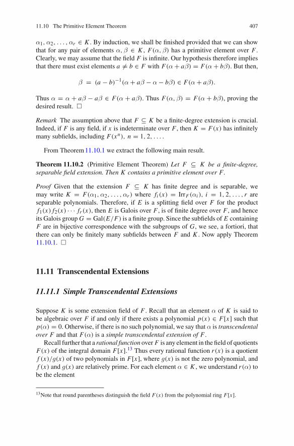
11.10 The Primitive Element Theorem 407
α1,α2, . . . ,αr ∈ K . By induction, we shall be finished provided that we can showthat for any pair of elements α,β ∈ K , F(α,β) has a primitive element over F .Clearly, we may assume that the field F is infinite. Our hypothesis therefore impliesthat there must exist elements a �= b ∈ F with F(α + aβ) = F(α + bβ). But then,
β = (a − b)−1(α + aβ − α − bβ) ∈ F(α + aβ).
Thus α = α + aβ − aβ ∈ F(α + aβ). Thus F(α,β) = F(α + bβ), proving thedesired result. �
Remark The assumption above that F ⊆ K be a finite-degree extension is crucial.Indeed, if F is any field, if x is indeterminate over F , then K = F(x) has infinitelymany subfields, including F(xn), n = 1, 2, . . . .
From Theorem11.10.1 we extract the following main result.
Theorem 11.10.2 (Primitive Element Theorem) Let F ⊆ K be a finite-degree,separable field extension. Then K contains a primitive element over F.
Proof Given that the extension F ⊆ K has finite degree and is separable, wemay write K = F(α1,α2, . . . ,αr ) where fi (x) = IrrF (αi ), i = 1, 2, . . . , r areseparable polynomials. Therefore, if E is a splitting field over F for the productf1(x) f2(x) · · · fr (x), then E is Galois over F , is of finite degree over F , and henceits Galois group G = Gal(E/F) is a finite group. Since the subfields of E containingF are in bijective correspondence with the subgroups of G, we see, a fortiori, thatthere can only be finitely many subfields between F and K . Now apply Theorem11.10.1. �
11.11 Transcendental Extensions
11.11.1 Simple Transcendental Extensions
Suppose K is some extension field of F . Recall that an element α of K is said tobe algebraic over F if and only if there exists a polynomial p(x) ∈ F[x] such thatp(α) = 0. Otherwise, if there is no such polynomial, we say that α is transcendentalover F and that F(α) is a simple transcendental extension of F .
Recall further that a rational function over F is any element in the field of quotientsF(x) of the integral domain F[x].13 Thus every rational function r(x) is a quotientf (x)/g(x) of two polynomials in F[x], where g(x) is not the zero polynomial, andf (x) and g(x) are relatively prime. For each element α ∈ K , we understand r(α) tobe the element
13Note that round parentheses distinguish the field F(x) from the polynomial ring F[x].

408 11 Theory of Fields
r(α) := f (α) · (g(α))−1,
provided α is not a zero of g(x). If α is transcendental over F , then r(α) is alwaysdefined.
Lemma 11.11.1 If F(α) is a transcendental extension of F, then there is an iso-morphism F(α) → F(x) taking α to x.
Proof Define the mapping ε : F(x) → F(α) by setting ε(r(x)) := r(α), for everyr(x) ∈ F(x). Clearly ε is a ring homomorphism. Suppose
r1(x) = a(x)
b(x), r2(x) = c(x)
d(x),
are rational functions with r1(α) = r2(α). Wemay assume a(x), b(x), c(x) and d(x)
are all polynomials with b(x)d(x) �= 0. Then
a(α)d(α) − b(α)c(α) = 0.
Sinceα is transcendental, a(x)d(x) = b(x)c(x) so r1(x) = r2(x). Thus ε is injective.But its image is a subfield of F(α) containing F and the element ε(x) = α and so itis also surjective. Thus ε is bijective, and so ε−1 is the desired isomorphism. �
Now suppose F(α) is a simple transcendental extension of F , and let β be anyelement of F(α). By Lemma11.11.1, there exist a coprime pair of polynomials( f (x), g(x)), with g(x) �= 0 ∈ F[x], such that
β = f (α)(g(α))−1.
Suppose
f (x) = a0 + a1x + · · · + an xn
g(x) = bo + b1x + · · · + bn xn
where n is the maximum of the degrees of f (x) and g(x), so at least one of an or bn
is non-zero. Then f (α) − βg(α) = 0, so
(a0 − βb0) + (a1 − βb1)α + · · · + (an − βbn)αn = 0.
Thus α is a zero of the polynomial
hβ(x) := (a0 − βb0) + (a1 − βb1)x + · · · + (an − βbn)xn
in F(β)[x].

11.11 Transcendental Extensions 409
Claim The polynomial hβ(x) is the zero polynomial if and only if β ∈ F.
First, if β ∈ F , then hβ(x) = f (x) − βg(x) is in F[x]. If hβ(x) were a non-zeropolynomial, then its zero, α, would be algebraic over F , which it is not. Thus hβ(x)
is the zero polynomial.On the other hand, if hβ(x) is the zero polynomial, each coefficient ai − βbi is
zero. Now, since g(x) is not the zero polynomial, for some index j , b j �= 0. Thenβ = a j · b−1
j , an element of F .The claim is proved.
Now suppose β is not in F . Then the coefficient (ai − βbi ) is zero if and onlyif ai = 0 = bi , and this cannot happen for i = n as n was chosen. Thus hβ(x)
has degree n. So certainly α is algebraic over the intermediate field F(β). Since[F(α) : F] is infinite, and [F(α) : F(β)] is finite, [F(β) : F] is infinite, and so β istranscendental over F .
We shall now show that hβ(x) is irreducible in F(β)[x].Let D := F[y] be the domain of polynomials in the indeterminate y, with coef-
ficients from F . (This statement is here only to explain the appearance of the newsymbol y.) Then F(y) is the quotient field of D. Since β is transcendental over F ,Lemma11.11.1 yields an F-isomorphism
ε : F(β) → F(y)
of fields which can be extended to a ring isomorphism
ε∗ : F(β)[x] → F(y)[x].
Then h(x) := ε∗(hβ(x)) = f (x) − yg(x) is a polynomial in D[x] = F[x, y].Moreover, hβ(x) is irreducible in F(β)[x] if andonly if h(x) is irreducible in F(y)[x].Now since D = F[y] is a UFD, by Gauss’ Lemma, h(x) ∈ D[x] is irreducible inF(y)[x] if and only if it is irreducible in D[x]. Now, D[x] = F[y, x] is a UFD andh(x) is degree one in y. So, if h(x) had a non-trivial factorization in D[x], one of thefactors k(x) would be of degree zero in y and hence a polynomial of positive degreein F[x]. The factorization is then
h(x) = f (x) − yg(x) = k(x)(a(x) + yb(x)),
where k(x), a(x) and b(x) all lie in F[x]. Then f (x) and g(x) possess the commonfactor k(x) of positive degree, against the fact that f (x) and g(x) were coprime inF[x]. We conclude that h(x) is irreducible in F(y)[x], and so hβ(x) is irreducibleof degree n in F(β)[x] as promised.
We now have the following
Theorem 11.11.2 (Lüroth’s Theorem) Suppose F(α) is a transcendental extensionof F. Let β be an element of F(α) − F. Then we can write β = f (α)/g(α) wheref (x) and g(x) are a pair of coprime polynomials in F[x], unique up to multiplying

410 11 Theory of Fields
the pair through by a scalar from F. Let n be the maximum of the degrees of f (x)
and g(x). Then [F(α) : F(β)] = n. In particular, α is algebraic over F(β).
Remark Ageneral consequence is that if E is an intermediate field distinct from F—that is, F < E ≤ F(α)—then [E : F] is infinite. In particular, F(α)—F containsno elements which are algebraic over F (a fact that has an obvious direct proof fromfirst principles).
Lüroth’s theorem gives us a handle on the Galois group Gal(F(α)/F) of a tran-scendental extension. Suppose now that σ is an F-automorphism F(α) → F(α).Then σ is determined by what it does to the generator α. Thus, setting β = σ(α),for any rational function t (x) of F , we have σ(t (α)) = t (β). Now in particularβ = r(α) for a particular rational function r(x) = f (x)/g(x) where ( f (x), g(x)) isa coprime pair of polynomials in F[x]. Since σ is onto, F(α) = F(β). On the otherhand, by Lüroth’s Theorem, [F(α) : F(β)] is the maximum of the degrees of f (x)
and g(x). Thus we can write
β = aα + b
cα + d, (11.33)
where a, b, c and d are in F , a and c are not both zero, and ad − bd �= 0 to keep thepolynomials ax + b and cx + d coprime. Actually the latter condition implies theformer, that a and c are not both zero.
Now let G = Gal(F(α)/F) and set O := αG , the orbit of α under G. Ourobservations so far are that there exists a bijection between any two of the followingthree sets:
1. the elements of the group Gal(F(α)/F),2. the orbit O , and3. the set LF(F) of so-called “linear fractional” transformations,
ω → aω + b
cω + d, a, b, c, d ∈ F, ad − cb non-zero,
viewed as a set of permutations of the elements of O .
A perusal of how these linear factional transformations compose shows thatLF(F)
is a group, and that in fact, there is a surjective group homomorphism
GL(2, F) → LF(2, F),
defined by
(a bc d
)→
[the transformation z → az + b
cz + don set O
],
where the matrix has non-zero determinant—i.e. is invertible. The kernel of thishomomorphism is the subgroup of two-by-two scalar matrices γ I , comprising the

11.11 Transcendental Extensions 411
center ofGL(2, F).As the readerwill recall, the factor group,GL(2, F)/Z(GL(2, F))
is called the “one-dimensional projective group over F” and is denoted PGL(2, F).Our observation, then, is that
Gal(F(α)/F) � LF(F) � PGL(2, F).
Notice how the fundamental theorem of Galois Theory falls to pieces in the caseof transcendental extensions. Suppose F is the field Z/pZ, the ring of integersmod p, a prime number. If α is transcendental over F , then [F(α) : F] is infinite,while Gal(F(α)/F) is PGL(2, p), a group of order p(p2 − 1) which, when p ≥ 5,contains at index two, a simple subgroup.
Let K be an extension of the field F . We define a notion of algebraic dependenceover F on the elements of K as follows:We say that elementα algebraically depends(over F) on the finite subset {β1, . . . ,βn} if and only if
• α is algebraic over the subfield F(β1, . . . ,βn).
Theorem 11.11.3 Algebraic dependence over F is an abstract dependence relationon K in the sense of Chap.2, Sect. 2.6.
Proof We must show that the relation of algebraic dependence over F satisfies thethree required properties of a dependence relation: reflexivity, transitivity and theexchange condition.
Clearly if β ∈ {β1, . . . ,βn}, then β lies in F(β1, . . . ,βn) and so is algebraic overit. So the relation is reflexive.
Now suppose γ is algebraic over F(α1, . . . ,αm), and each αi is algebraic overF(β1, . . . ,βn). Then certainly, αi is algebraic over the field
F(β1, . . . ,βn,α1, . . . ,αi−1).
So, setting B := {β1, . . . ,βn}, we obtain a tower of fields,
F(B) ≤ F(B,α1) ≤ F(B,α1,α2) ≤ · · ·≤ F(B,α1, . . . ,αn) ≤ F(β1, . . . ,βm,α1, . . . ,αn, γ)
with each field in the tower of finite degree over its predecessor. Thus the top field inthe tower is a finite extension of the bottom field, and so γ is algebraic over F(B).
We now address the exchange condition: we are to show that if γ is algebraic overF(β1, . . . ,βn} but is not algebraic over F(β1, . . . ,βn−1}, then βn is algebraic overthe field F(β1, . . . ,βn−1, γ}.14
14It is interesting to observe that in this context the Exchange Condition is essentially an “implicitfunction theorem”. The hypothesis of the condition, transferred to the context of algebraic geom-etry, says that the “function” γ is expressible locally in terms of {β1, . . . , βn} but not in terms of{β1, . . . , βn−1}. Intuitively, this means ∂γ
∂βn�= 0 , from which we anticipate the desired conclusion.

412 11 Theory of Fields
By hypothesis, there is a polynomial relation
0 = akγk + ak−1γ
k−1 + · · · + a1γ + a0 (11.34)
where ak is non-zero, and each a j is in F(β1, . . . ,βn), and so, at the very least, can beexpressed as a rational function, n j/d j , where the numerators n j and denominatorsd j are polynomials in F[β1, . . . ,βn]. We can then multiply Eq. (11.34) through bythe product of the di , from which we see that without loss of generality, we mayassume the coefficients ai are polynomials—explicitly:
ai =∑
jbi jβ
jn , bi j ∈ F[β1, . . . ,βn−1], ak �= 0. (11.35)
Then substituting the formulae of Eq. (11.35) into Eq. (11.34), and collecting thepowers of βn , we obtain the polynomial relation
0 = pmβmn + pm−1β
m−1n + · · · p1βn + p0, (11.36)
with each coefficientpt =
∑k
s=0bstγ
s, (11.37)
a polynomial in the ring F[β1, . . . ,βn−1, γ].Now we get the required algebraic dependence of βn on {β1, . . . ,βn−1, γ} from
Eq. (11.36), provided not all of the coefficients pt are zero. Suppose, by way ofcontradiction, that they were all zero. Then as γ does not depend on {β1, . . . ,βn−1},having each of the expressions in Eq. (11.37) equal to zero forces each coefficient bst
to be zero, so by Eq. (11.35), each ai is zero. But that is impossible since certainlyak is non-zero.
Thus the Exchange Condition holds and the proof is complete. �
So, as we have just seen, if K is an extension of the field F , then the relation ofbeing algebraically dependent over F is an abstract dependence relation, and we callany subset X of K which is independent with respect to this relation algebraicallyindependent (over F). By the basic development of Chap. 1, Sect. 1.3, maximal alge-braically independent sets exist, they “span” K , and any two such sets have the samecardinality. We call such subsets of K transcendence bases of K over F , and theircommon cardinality is called the transcendence degree of K over F , and is denoted
tr.deg(K/F).
If X is a transcendence basis for K over F , then the “spanning” property meansthat every element of K is algebraic over the subfield F(X) generated by X . Onecalls K (X) a “purely transcendental” extension of F , although this notion conveyslittle since it is completely relative to X . For example, if x is a real number that is

11.11 Transcendental Extensions 413
transcendental over Q, the field of rational numbers, then both Q(x) and Q(x2) arepurely transcendental extensions ofQ, while the former is algebraic over the latter.15
Nextwe observe that transcendence degrees add (in the sense of cardinal numbers)under iterated field extension just as ordinary degrees multiply. Specifically:
Corollary 11.11.4 Suppose we have a tower of fields
F ≤ K ≤ L .
Thentr.deg[K : F] + tr.deg[L : K ] = tr.deq[L : F].
Proof Let X be a transcendence basis of K over F and let Y similarly be a transcen-dence basis of L over K . Clearly then, X ∩ Y = ∅, every element of K is algebraicover F(X), and every element of L is algebraic over K (Y ).
The corollary will be proved if we can show that X ∪ Y is a transcendence basisof L over F .
First, we claim that X ∪ Y spans L—that is, every element of L is algebraic overF(X ∪ Y ). Let λ be an arbitrary element of L . Then there is an algebraic relation
λm + amλm−1 + · · · + a1λ + a0 = 0,
where m ≥ 1, and the coefficients ai are elements of K (Y ). This means that each ofthem can be expressed as a quotient of two polynomials in K [Y ]. Let B be the set ofall coefficients of the monomials in Y appearing in the numerators and denominatorsof these quotients representing ai , as i ranges over 0, 1, . . . , m. Then B is a finitesubset of K , and λ is now algebraic over F(X ∪ Y ∪ B). Since each element of B isalgebraic over F(X), F(X ∪ B) is a finite extension of F(X), and so F(X ∪ Y ∪ B)
is a finite extension of F(X ∪ Y ). It then follows that F(X ∪ Y ∪ B,λ) is a finiteextension of F(X ∪ Y ), and so λ is algebraic over F(X ∪ Y ) as desired.
It remains to show that X ∪ Y is algebraically independent over Y . But if not,there is a polynomial p ∈ F[z1, . . . , zn+m] and finite subsets {x1, . . . , xm} and{y1, . . . , yn} of X and Y , respectively, such that upon substitution of the m xi for thefirst m zi ’s, and the yi for the remaining n zi ’s, one obtains
0 = p(x1, . . . , xm, y1, . . . ym).
Now this can be rewritten as a polynomial whose monomial terms are monomialsin the yi , with coefficients which are polynomials ck in F[z1, . . . , zn] evaluatedat x1, . . . , xn . Since the yi are algebraically independent over K , the coefficientpolynomials ck are each equal to zero when evaluated at x1, . . . , xn . But again,
15In this connection, there is a notion that is very useful in looking at the subject of RiemannSurfaces from an algebraic point of view: A field extension K of F of finite transcendence degreeover F is called an algebraic function field if and only if, for any transcendence basis X , K is afinite extension of F(X).

414 11 Theory of Fields
since the x j are algebraically independent over F , we see that each polynomial ck
is identically 0. This means that the original polynomial p was the zero polynomialof F[z1, . . . , zm+n], establishing the algebraic independence of X ∪ Y . The proof iscomplete. �.
Corollary 11.11.5 An algebraic extension of an algebraic extension is algebraic.Precisely, if F ≤ K ≤ L is a tower of fields with K an algebraic extension of F andL an algebraic extension of K , then L is an algebraic extension of F.
Proof This follows from the previous theorem and the fact that zero plus zero iszero.
Remark Before, we knew this corollary anyway, but with the word “finite degree”replacing the word “algebraic” in the statement.
11.12 Exercises
11.12.1 Exercises for Sect. 11.2
1. Compute the minimal polynomials in Q[x] of each of the following complexnumbers. (Recall that if a is a positive real number and n is a positive integer,the symbol n
√a refers to the positive nth root of a.)
(a)√2 +√
3.(b)
√2 + ζ, where ζ = e2πi/3.
(c)√2 +√
2(d) ζ + ζ−1, where ζ = e2πi/16
(e) ζ + ζ−1, where ζ = e2πi/7
2. Let F ⊆ K be a field extension with [K : F] odd. If α ∈ K , prove thatF(α2) = F(α).
3. Assume that α = a + bi ∈ C is algebraic over Q, where a is rational and b isreal. Prove that IrrQ(α) has even degree.
4. Let K = Q(3√2,
√2) ⊆ C. Compute [K : Q].
5. Let f (x) = x5 − 9x3 + 3x + 3 ∈ Q[x].(i) Show that f (x) is irreducible over Q.(ii) Show that f (x) is irreducible over Q(i).
6. Let K = Q(4√2, i) ⊆ C. Show that
(a) K contains all roots of x4 − 2 ∈ Q[x].(b) Compute [K : Q].

11.12 Exercises 415
7. Compute ⎡⎣Q
⎛⎝√2 +
√2 +√
2
⎞⎠ : Q
⎤⎦
8. Let F ⊆ E ⊆ K be fields, let α ∈ K , and let f (x) = IrrF (α). Assume that[E : F] and deg f (x) are relatively prime. Prove that f (x) = IrrE (α).
9. Let F be any field, and prove that there are infinitely many irreducible polyno-mials in F[x]. [Hint: Euclid’s proof of the corresponding result for the ring Z
works here, too.]10. Let F = C(x), where C is the complex number field and x is an indeterminate.
Assume that F ⊆ K and that K contains an element y such that y2 = x(x − 1).Prove that there exists an element z ∈ F(y) such that F(y) = C(z), i.e., F(y)
is a “simple transcendental extension” of C.11. Let F ⊆ K be a field extension. If the subfields of K containing F are totally
ordered by inclusion, prove that K is a simple extension of F . (Is the conversetrue?)
12. Let Q ⊆ K be a field extension. Assume that K is closed under taking squareroots, i.e., if α ∈ K , then
√α ∈ K . Prove that [K : Q] = ∞.
13. Suppose the field F is a subring of the integral domain R. If every element of Ris algebraic over F , show that R is actually a field. Give an example of a non-integral domain R containing a field F such that every element of R is algebraicover F . Obviously, R cannot be a field.
14. Let F ⊆ K be fields and let f (x), g(x) ∈ F[x] with f (x)|g(x) in K [x]. Provethat f (x)|g(x) in F[x].
15. Let F ⊆ K be fields and let f (x), g(x) ∈ F[x]. If d(x) is the greatest commondenominator of f (x) and g(x) in F[x], prove that d(x) is the greatest commondenominator of f (x) and g(x) in K [x].
16. Let F ⊆ E1, E2 ⊆ E be fields. Define E1E2 ⊆ E to be the smallest fieldcontaining both E1 and E2. E1E2 is called the composite (or compositum) ofthe fields E1 and E2. Prove that if [E : F] < ∞, then [E1E2 : F] ≤ [E1 :F] · [E2 : F].
17. Given a complex number α it can be quite difficult to determine whether α isalgebraic or transcendental. It was known already in the nineteenth century thatπ and e are transcendental, but the fact that such numbers as eπ and 2
√2 are
transcendental is more recent, and follows from the following deep theorem ofGelfond and Schneider: Let α and β be algebraic numbers. If
η = logα
logβ
is irrational, then η is transcendental. (See E. Hille, American MathematicalMonthly, vol. 49 (1942), pp. 654–661.) Using this result, prove that 2
√2 and eπ
are both transcendental. [Hint: For 2√2, set α = 2
√2, β = 2.]

416 11 Theory of Fields
11.12.2 Exercises for Sect. 11.3
1. Let f (x) = xn − 1 ∈ Q[x]. In each case below, construct a splitting field Kover Q for f (x), and compute [K : Q].(i) n = p, a prime.(ii) n = 2p, where p is prime.(iii) n = 6.(iv) n = 12.
2. Let f (x) = xn − 2 ∈ Q[x]. Construct a splitting field for f (x) over Q.3. Let f (x) = x3 + x2 − 2x − 1 ∈ Q[x].
(a) Prove that f (x) is irreducible.(b) Prove that if α ∈ C is a root of f (x), so is α2 − 2.(c) Let K ⊇ Q be a splitting field over Q for f (x). Using part (b), compute
[K : Q].4. Let ζ = e2πi/7 ∈ C, and let α = ζ +ζ−1. Show that IrrQ(α) = x3+ x2−2x −1
(as in Exercise 3 above), and that α2 − 2 = ζ2 + ζ−2.5. Write the complex splitting field for x3 − 2 ∈ Q[x] in the form Q(α), for some
α ∈ C.
6. Let ζ = e2πi/n ∈ C and set ω = ζ + ζ−1. Show that Q(ω) is a normal extensionof Q.
7. Give an example of a normal extension Q ⊆ K such that [K : Q] = 3.8. Let F = C(x) be the field of rational functions over the complex field C and let
f (y) = y3 − x ∈ F[y]. Let α be a zero of f (y) in some splitting field over Fand show that F(α) is a normal extension of F .
9. Let E = Q(5√2), and let K be a normal closure of E over Q. Compute [K : Q].
10. Which of the following simple extensions of the rational field are normal?
(a) Q(√2 +√
3),
(b) Q
(√2 +√
2),
(c) Q
(√2 +
√2 +√
2
),
(d) Q(ζ 4√2), where ζ = e2πi/8.
11.12.3 Exercises for Sect. 11.4
1. Let q be a prime power, set F = GF(q) and let E ⊇ F be a field extensionof degree n. Let σ be the qth power automorphism of E (sometimes called theFrobenius map of E), given by F(α) = αq . Define the norm map
N = NE/F : E −→ F

11.12 Exercises 417
by settingN (α) = α · σ(α) · σ2(α) · · ·σn−1(α).
Note that N restricts to a mapping
N : E∗ −→ F∗,
where E∗ and F∗ are the multiplicative groups of no-zero elements of E and F .
(a) Show that N : E∗ → F∗ is a group homomorphism.(b) Show that |ker N | = qn−1
q−1 .
2. Let p be a prime and let r be a positive integer. Prove that there exists an irreduciblepolynomial of degree r over F = GF(p). [Hint: Isn’t this equivalent to theexistence of an extension field K ⊇ F of degree r?]
3. Let p be prime, n a positive integer and set q = pn . Let F = GF(p) and showthat if f (x) ∈ F[x] is irreducible of degree n, then f (x)|xq − x . More generally,show that if f (x) is irreducible of degree m, where m|n, then again, f (x)|xq − x .
4. Show that if F = GF(q), then the polynomial x2 + x + 1 ∈ F[x] is irreducibleif and only if 3 � | q − 1.
5. For any integer n, let Dn be the number of irreducible polynomials of degree nin F[x], where F = GF(q). Prove that
Dn = 1
n
∑k|n
μ(n
k
)qk .
[Hint: Note that, by Exercise 3, qn = ∑k|n k · Dk ; now use theMöbuis Inversion
Theorem (see Example43, Theorem7.4.3, p. 217).]6. Here’s another application of Möbius inversion. Let F be a field and let C be a
finitemultiplicative subgroup of themultiplicative group F∗ of non-zero elementsof F . We know C to be cyclic. Assume that |C | = n, and d|n, and let Nd be thesum in F of the elements of order d in C . Thus Nn is the sum in F of the φ(n)
generators of C . Prove that, in fact,
Nn = μ(n).
[Hint: Study f (n) = ∑d|n
Nd ; how does this relate to the polynomial xn − 1 ∈F[x]?)]
7. Let F = GF(q), where q = pn and p is an odd prime.
(i) Show that for any α ∈ F , and any prime power r = pk , one has
(x − α)r−1 = xr−1 + αxr−2 + · · · + αr−2x + αr−1.

418 11 Theory of Fields
(ii) Suppose m is an integer between 1 and p − 1, inclusive. Prove that if α isa zero of a polynomial f (x) ∈ F[x] with multiplicity exactly m, then α isa zero of the formal derivative f ′(x) of multiplicity exactly m − 1. [Hint:Write f (x) = (x − α)mg(x) where g(α) �= 0, then apply the product rulefor the formal derivative.]
(iii) Suppose m is as it is in part (ii) of this problem. For fixed non-zero α ∈ F ,define the polynomial
fm,α(x) :=∑p−1
i=1im xiαp−i .
(Whenα = 1andm = (p−1)/2 these are knownas theFekete polynomials.)Show that α is a root of fm,α(x) with multiplicity exactly m. [Hint: Use (i)to observe that
f0,α(x) + αp−1 = (xα)p−1.
Then observe that for m ≥ 1, fm+1,α(x) = x f ′m,α(x) and apply part (ii) of
this problem.]
11.12.4 Exercises for Sect. 11.5
1. Let k = GF(3), and set F = k(x), the field of rational functions over k in x . Letf (y) = y6 + x2y3 + x ∈ F[y].(a) Show that f (y) is irreducible over F .(b) Let α be a root of f (y) in some splitting field over F . Is F(α) separable
over F?(c) If K = F(α) as above, determine [K : F] and [Ksep : F].
2. Let F be a field of characteristic p. Determine the number of roots of the polyno-mial xn − 1 ∈ F[x] in some splitting field. [Hint: write n = mpe, where p doesnot divide m.]
11.12.5 Exercises for Sect. 11.6
1. Let F ⊆ K be a finite extension of fields, and let E1, E2 be two intermediatesubfields. Assume that F ⊆ E1 is a Galois extension and that K is generated overF by E1 and E2. Prove that
(a) E2 ⊆ K is a Galois extension, and that(b) Gal(K/E2) ∼= Gal(E1/E1 ∩ E2).

11.12 Exercises 419
2. Assume that F ⊆ K is a field extension of finite degree, and let E1, E2 beintermediate subfields, both Galois over over F , and generating K . Prove that Kis Galois over E2 and that Gal(K/E2) is isomorphic to a subgroup of Gal(E1/F).(This is the so-called Lemma on Accessory Irrationalities.)
11.12.6 Exercises for Sect. 11.8
1. Using Möbius inversion, prove that
�n(x) =∏d|n
(xd − 1)μ(n/d).
2. Consider the polynomial x4 + 3 ∈ Q[x], and let K ⊆ C be its splitting field.
(a) Show that K = Q(i,ω), where ω = ζ 4√3, and where ζ = e2πi/8.
(b) Compute [K : Q].(c) If we write the zeros of f (x) as a1 = ω, a2 = −ω, a3 = iω, a4 = −iω,
calculate the stabilizer in G of a1, with its elements written in cycle notation.(So for instance, an element σ = (2 3 4) would fix a1 and do this:
a2σ�→ a3
σ�→ a4σ�→ a2.
Incidentally, does such an element exist in G? Why or why not?)(d) Is G abelian? Why or why not?(e) Assuming that you determined that G is, in fact, non-abelian, give a non-
normal subfield E , with Q ⊆ E ⊆ K .(f) List all the elements of G, using cycle notation.
3. Let α =√2+√
3, and set p(x) = IrrQ(α). Compute the Galois group of p(x).
4. Let α =√2 +
√2 +√
2, let q(x) = IrrQ(), and compute the Galois group ofq(x).
5. Are the Galois groups of the polynomials x8 − 2, x8 − 3, and x8 − 5 in Q[x] allisomorphic? Investigate.
6. Let ζ = e2πi/32, and set K = Q(ζ).
(a) Show that K is a separable normal extension of Q.(b) Let α be as in Problem 4, above. Show that Q(α) ⊆ K and compute [K :
Q(α)]. [Hint: Look at ζ + ζ−1.](c) Compute IrrQ(ζ) ∈ Q[x].
7. Let f (x) = x6 − 4x3 + 1 ∈ Q[x].(a) Show that if ω = 3
√2 + √
3 is real and ζ = e2πi/3 ∈ C, then the complexsplitting field K of f (x) is Q(ζ,ω).

420 11 Theory of Fields
(b) Show that f (x) is irreducible. [Hint: If it’s not, it has a linear, quadratic, orcubic factor. Use the factorization of f (x) ∈ K [x] into linear factors andshow that the product of at most three of these factors cannot be in Q[x].]
(c) Label the zeros of f (x) as a1 = ω, a2 = ζω, a3 = ζ2ω, a4 =ω−1, a5ζω−1, a6 = ζ2ω−1. Showi. With the above correspondence, show that the following elements are
in G:γ = (2 3)(5 6) (complex conjugation),
σ = (1 2 3)(4 6 5), τ = (1 4)(2 5)(3 6).
ii. Show that
Gal(K/Q(ζ)) = 〈τ ,σ〉, Gal(K/Q(ω + ω−1)) = 〈γ, τ 〉,
G = 〈γ, σ, τ 〉 ∼= D12, Z(G) = 〈γτ 〉,
where D12 is the dihedral group of order 12.iii. Show that Q ⊆ Q(
√3) ⊆ K and that Gal(K/Q(
√3)) = 〈γ,σ〉.
iv. Show that Q ⊆ Q(i) ⊆ K and that Gal(K/Q(i)) = 〈σγτ 〉.8. Let f (x) = x6 − 2x3 − 2 ∈ Q[x].
(a) Let α = 3√1 + √
3, β = 3√1 − √
3 ∈ R, and let ζ = e2πi/3 ∈ C. Show thatthe zeros of f (x) are ζ jα, ζ jβ, j = 0, 1, 2.
(b) Show that the complex splitting field K of f (x) over Q contains the fieldL = Q(i, 3
√2,
√3).
(c) Show that [L : Q] = 12.(d) Show that [K : Q] = 12 or 36.(e) Let ω = 3
√2 +√
3, exactly as in Exercise 7. Show that ω +ω−1 ∈ K . (Takethe quotient of the two real zeros of f (x).)
(f) Show that L ⊇ Q is a Galois extension and that Gal(L/Q) ∼= D12, thedihedral group of order 12. (Arguments similar to those given for Exercise7 will do.) Note that D12 has three 2-Sylow subgroups.
(g) Show that if K = L , then there are exactly three intermediate subfields ofextension degree 3 over Q, viz., Q(
3√2), Q(ζ 3
√2), and Q(ζ2 3
√2).
(h) Show that Q(ω + ω−1) �= Q(3√2), Q(ζ 3
√2), Q(ζ2 3
√2).
(i) Conclude that [K : Q] = 36 and that Gal(K/Q) ∼= S3 × S3.
9. Let K = Q(√2,
√3, u), where u =
√(9 − 5
√3)(2 − 2
√2).
(a) Show that K ⊇ Q is a Galois extension.(b) Find an irreducible polynomial f (x) ∈ Q[x] for which K is the splitting
field over Q.(c) Show that Gal(K/Q) is nonabelian but is not dihedral.

11.12 Exercises 421
(d) Conclude that Gal(K/Q)must be isomorphic with Q8, the quaternion groupof order 8.
10. Let F be a field of characteristic �= 2, and let x1, x2, . . . , xn be commut-ing indeterminates over F . Let K = F(x1, x2, . . . , xn), the field of fractionsof the polynomial ring F[x1, x2, . . . , xn] (or the field of rational functions inx1, x2, . . . , xn).
(a) Let σ1,σ2, . . . ,σn be the elementary symmetric polynomials in x1, x2, . . . ,xn , and set E = F(σ1,σ2, . . . ,σn). Show that K is a splitting field over Efor the polynomial xn − σ1xn−1 + · · · + (−1)nσn ∈ E[x].
(b) Show that [K : E] ≤ n!.(c) Noting that G = Sn acts as a group of automorphisms of K in the obvious
way, show that E = invG(K ) and thereby conclude that [K : E] = n!.(d) Show that K is a Galois extension of E .(e) Set δ = ∏
i< j (x j − xi ) ∈ K and show that E(δ) = invAn (K ).
11. Let f (x) ∈ Q[x] be an irreducible polynomial and assume that the discriminantof f (x) is a perfect square in Q.
(a) Show that if deg f (x) = 3, then f (x) must have three real zeros in thecomplex field C.
(b) Show that if deg f (x) = 3, and if α ∈ R is a fixed zero of f (x), show thatthe other two zeros of f (x) are polynomials in α with rational coefficients.
(c) If deg f (x) = 4, how many real zeros can f (x) have?(d) If deg f (x) = 4, can the Galois group have an element that acts as a 4-cycle
on the four zeros of f (x)?
12. Suppose that F is a field and that f (x) ∈ F[x]. Suppose, moreover, that in somesplitting field, f (x) factors as
f (x) = (x − α1)2(x − α2) · · · (x − αn−1),
where α1,α2, . . . ,αn−1 are distinct. Show that α1 ∈ F .13. Let f (x) = x3−9x−9 ∈ Q[x] and compute theGalois group of this polynomial.14. Using Swan’s formula, compute the discriminants of x7 − 7x + 3, x5 − 14x2 −
42 ∈ Q[x].
11.12.7 Exercises for Sects. 11.9 and 11.10
1. (Euler) Show that if F is a field possessing a primitive eight root of unity, then2 = 1 + 1 is a square in F . [Hint: Let ζ be a primitive eighth root. Consider thesquare of ζ + ζ−1.]

422 11 Theory of Fields
2. Let F be a field with a primitive twelfth root of unity. Show that the number 3 isa square in this field. [Hint: Consider the cube of ζ + ζ−1 where ζ is a primitive12th root.]16
3. Suppose K is the splitting field for an irreducible polynomial p(x) ∈ F[x].Suppose L is an intermediate field—that is F ⊆ L ⊆ K . Show that if p(x)
is solvable by radicals relative to the field F , then p(x) is solvable by radicalsrelative to the intermediate field L . (Remark: At first sight it seems a triviality. Ifsolvability by radicals over F is seen as the ability to express the roots of p(x)
in terms of some compound formula involving successive field operations and(multiple) root-extractions whose input variables belong to F , then the result is atriviality, for any such formula with input variables from F is a formula with inputvariables from the intermediate field L . But that is not exactly howwe defined theproperty that “p(x) is solvable by radicals”. Our criterion was that the splittingfield K was a radical extension of F , that is, there is a tower of fields
F0 ⊆ F1 ⊆ · · · ⊆ Fk = K ,
such that Fi+1 was obtained for Fi by adjoining the ri th root of an element inthe latter field. Since L may not be one of the Fi , some work is needed to showthat K is a radical extension of L . The point of this remark is to motivate thefollowing hint.) [Hint: Quoting the correct Theorems and Lemmas, observe thatp(x) is solvable by radicals if and only the Galois group G(K/F) is solvable.Note that G(K/L) is a subgroup of the former, and apply Galois’ criterion.]
4. Suppose p(x) and r(x) are two irreducible polynomials in F[x], and let K be thesplitting field of p(x) over F . Suppose the field K contains a root of r(x).
(a) Show that K contains a copy of the splitting field L of r(x).(b) By the “Primitive Element Theorem” (Theorem11.10.2, p. 407), L = F(θ)
for some element θ whose irreducible polynomial is s(x) := Irr(θ) ∈ F[x].Using the theorems of the sections cited above for this exercise set, showthe following:
p(x) is solvable by radicals over F if and only if (i) p(x) is solvable byradicals over L and (ii) s(x) is solvable by radicals over F .
[Hint: Use the fact that L is a normal extension of F , Galois’ criterion, and anelementary fact about solvable groups.]
5. The final exercise of this section is due to Prof. Michael Artin, and uses such acombination of facts that it cannot easily be assigned to any one subsection ofthis chapter. On the other hand, it is not difficult if one uses the full symphony offacts available. A perfect test question!
16In the case that F is Z/(p), where p is a rational prime, the conclusions of these two exercisesfollow from the more extensive theory of quadratic reciprocity. A beautiful account of this, usingGauss sums, can be found in the book Elements of Number Theory by Ireland, K. and Rosen, M.I.Bogden & Quigley, New York, 1972.

11.12 Exercises 423
Suppose F is a finite field of characteristic 2 and suppose K is an extension of Fof degree 2.
(a) Show K = F(α) for some element α whose irreducible monic polynomialp(x) ∈ F[x] has the specific form
x2 + x + a, where, of course a belongs to the subfield F .
(b) Show that necessarily α + 1 is also a root of the irreducible quadratic poly-nomial p(x) ∈ F[x].
(c) Find an explicit formula for an automorphism of K that takes α to α + 1.
11.12.8 Exercises for Sect. 11.11
1. Let G be a finite subgroup of the general linear group GL(n, F). We supposeeach element g ∈ G to be an invertible matrix (α
(g)i j ). Let K be the field of quo-
tients of the polynomial ring F[x1, . . . xn]. (In other words, K = F(x1, . . . , xn)
is a transcendental extension of F by algebraically independent transcendentalelements xi .)
(a) For each (transcendental) element xi , and g ∈ G, let
xgi := α
(g)i1 x1 + · · · + α
(g)in xn .
For each rational function f (x1, . . . , xn), define
f g(x1, . . . xn) := f (xg1 , . . . , xg
n ).
i. Show that the permutation f �→ f g , for all f ∈ K is a field automor-phism φ(g) of K .
ii. Show that φ : G → Aut(K ) is an embedding of groups.(b) Assume G to be embedded (that is, with a little abuse of notation we write
G for φ(G)). Let KG be the subfield of elements of K which are fixed byall elements of G. (In this particular context, the elements of KG are calledinvariants of G.) Show that G = Gal(K/KG).
(c) Show that any n+1 rational functions f1, . . . , fn+1 ∈ K are connected by analgebraic equation—precisely, there is a polynomial p ∈ F[y1, . . . , yn+1]such that
p( f1, . . . , fn+1) = 0 ∈ K .
[Hint: Consider the transcendence degree of the subfield generated byf1, . . . fn+1.]

424 11 Theory of Fields
(d) Is it true that there exists a set X of n algebraically independent invariantsin the subfield KG such that every element of KG is a rational function inthe elements of X?
11.12.9 Exercises Associated with Appendix 1 of Chap. 10
1. Prove Lemma11.A.1.2. Prove the uniqueness of the limit of a a convergent sequence with respect to a
valuation φ of a field F . (See the paragraph following Eq.11.38.).3. Prove that every convergent sequence is a Cauchy sequence.
Appendix 1: Fields with a Valuation
Introduction
Let R denote the field of real numbers and let F be any field. A mapping φ : F → R
from F into the field of real numbers is a valuation on F if and only if, for each αand β in F :
1. φ(α) ≥ 0, and φ(α) = 0 if and only if α = 0.2. φ(αβ) = φ(α)φ(β), and3. φ(α + β) ≤ φ(α) + φ(β).
This concept is a generalization of certain “distance” notions which are familiarto us in the case that F is the real or complex field. For example, in the case of thereal field R, the absolute value function
|r | ={
r if r ≥ 0−r if r < 0
is easily seen to be a valuation. Similarly, for the complex numbers, the function“‖ ‖”, defined by
‖a + bi‖ =√
a2 + b2,
where a, b ∈ R and the square root is non-negative, is also a valuation. In this case,upon representing complex numbers by points in the complex plane, ‖z‖ measuresthe distance of z from 0. The “subadditive property” (3.) then becomes the triangleinequality.
A valuation φ : F → R is said to be archimedean if and only if there is a naturalnumber n such that if

Appendix 1: Fields with a Valuation 425
s(n) := 1 + 1 + · · · + 1 { with exactly n summands},
in F , then φ(s(n)) > 1.These valuations of the real and complex numbers are clearly archimedean.An example of a non-archimedian valuation is the trivial valuation for which
φ(0) = 0, and φ(α) = 1 for all non-zero elements α in F .Here is another important example. Let F be the field of quotients of some unique
factorization domain D which contains a prime element p. Evidently, F �= D. Thenany nonzero element α of F can be written in the form
α = a
b· pk,
where a, b ∈ D, p does not divide either a or b, and k is an integer. The integer kand the element a/b ∈ F are uniquely determined by the element α. Then, if α �= 0,set
φ(α) = e−k,
where e is anyfixednumber larger than1, such as 2.71 . . ..Otherwisewe setφ(0) = 0.The student may verify that φ is a genuine valuation of F . (Only the subadditiveproperty really needs to be verified.) From this construction, it is clear that φ isnon-archimedean—that is, it is not archimedean.
Lemma 11.A.1 If φ is a valuation of F, then the following statements hold:
1. φ(1) = 1.2. If ζ is a root of unity in F, then φ(ζ) = 1. In particular, φ(−1) = 1 and so
φ(−α) = φ(α), for all α in F.3. The only valuation possible on a finite field is the trivial valuation4. For any α,β ∈ F,
|φ(α) − φ(β)| ≤ φ(α − β).
The proof of this lemma is left as an exercise for the student on p. 424.
Lemma 11.A.2 If φ is a non-archimedean valuation of F, then for any α,β ∈ F,
φ(α + β) ≤ max(φ(α),φ(β)).
Proof From the subadditivity, and that fact that for any number of summands, φ(1+1 + · · · + 1) ≤ 1, we have
φ((α + β)n) = φ
(∑n
j=0
(nj
)αn− jβ j
)
≤∑n
j=0φ(α)n− jφ(β) j
≤ (n + 1)max (φ(α)n,φ(β)n).

426 11 Theory of Fields
Since the taking of positive nth roots in the reals is monotone, we have
φ(α + β) ≤ (n + 1)1/nmax (φ(α),φ(β)).
Now since n is an arbitrary positive integer, and (n + 1)1/n can be made arbitrarilyclose to 1, the result follows. �
The Language of Convergence
We require a few definitions. Throughout them, φ is a valuation of the field F .First of all, a sequence is a mapping N → F , from the natural numbers to the
field F , but as usual it can be denoted by a displayed indexed set, for example
{α0,α1, . . .} = {αk} or {β0,β1, . . .} = {βk}, etc..
A sequence {αk} is said to be a Cauchy sequence if and only if, for every positivereal number ε, there exists a natural number N (ε), such that
φ(αm − αn) < ε,
for all natural numbers n and m larger than N (ε).A sequence {αk} is said to converge relative to φ if and only if there exists an
element α ∈ F such that for any real ε > 0, there exists a natural number N (ε), suchthat
φ(α − αk) < ε, (11.38)
for all natural numbers k exceeding N (ε).It is an easy exercise to show that an element α satisfying (11.38) for each ε > 0
is unique. [Note that in proving uniqueness, the choice function N : R+ → N taking
ε to N (ε) is posited for the assertion that α is a limit. To assert that β is a limit, anentirely different choice function M : ε → M(ε) may be posited. That α = β is thethrust of Exercise 2 in Sect. 11.12.9.] In that case we say that α is the limit of theconvergent sequence {αk} or that the sequence {αk} converges to α.
A third easy exercise is to prove that every convergent sequence is a Cauchysequence. (See Exercise 3 in Sect. 11.12.9.)
A sequence which converges to 0 is called a null sequence. Thus {αk} is a nullsequence if and only if, for every real ε > 0, however small, there exists a naturalnumber N (ε), such that φ(αk) < ε, for all k > N (ε).
A field F with a valuation φ is said to be complete with respect to φ if and onlyif every Cauchy sequence converges (with respect to φ) to an element of F .
Now, finally, a completion of F (with respect to φ) is a field F with a valuationφ having these three properties:

Appendix 1: Fields with a Valuation 427
1. The field F is an extension of the field F .2. F is complete with respect to φ.3. Every element of F is the limit of a φ-convergent sequence of elements of F .
(We capture this condition with the phrase “F is dense in F”.
So far our glossary entails
• Convergent sequence• Limit• Null sequence• Cauchy sequence• Completeness with respect to a valuation φ• A completion of a field with a valuation
Completions Exist
The stage is set. In this subsection our goal is to prove that a completion (F, φ) of afield with a valuation (F,φ) always exists.
In retrospect, onemaynow realize that thefield of real numbersR is the completionof the field of rational numbers Q with respect to the “absolute” valuation, | |. Theconstruction of such a completion should not be construed as a “construction” of thereal numbers. That would be entirely circular since we used the existence of the realnumbers just to define a valuation and to deduce some of the elementary propertiesof it.
One may observe that the set of all sequences over F possesses the structure of aring, namely the direct product of countably many copies of the field F . Thus
S := FN =∏
k∈NFk where each Fk = F .
Using our conventional sequence notation, addition and multiplication in S aredefined by the equations
{αk} + {βk} = {αk + βk}{αk} · {βk} = {αkβk}.
For each element α ∈ F , the sequence {αk} for which αk = α, for every naturalnumber k is called a constant sequence and is denoted α. The zero element of thering S is clearly the constant sequence 0. The multiplicative identity of the ring S isthe constant sequence 1 (where “1” denotes the multiplicative identity of F).
Obviously, the constant sequences form a subring of S which is isomorphic tothe field F . It should also be clear that every constant sequence is also a Cauchysequence. We shall show that the collection Ch of all Cauchy sequences also formsa subring of S.

428 11 Theory of Fields
In order to do this, we first make a simple observation. A sequence {αk} is saidto be bounded if and only if there exists a real number b such that φ(αk) < b for allnatural numbers k. Such a real number b is called an upper bound of the sequence{αk}. The observation is
Lemma 11.A.3 Every Cauchy sequence is bounded.
Proof Suppose {αk} is a Cauchy sequence. Then there is a natural number N = N (1)such that φ(αN − αm) < 1, for all natural numbers m exceeding N . Now set
b := 1 + max {φ(α0),φ(α1), . . . , φ(αN }).
If k ≤ N , φ(αk) < b, by the definition of b. If k > N then φ(αk) < b by thedefinition of N and the fact that φ(αN ) ≤ b − 1. So b is an upper bound. �
Lemma 11.A.4 The collection Ch of all Cauchy sequences of S is closed underaddition and multiplication of sequences. Thus Ch is a subring of S, the ring of allsequences over F.
Proof Recall that if {αk} is a Cauchy sequence, there must exist an auxiliary functionN : R
+ → N such that if ε ∈ R+, then φ(αn − αm) < ε for all numbers n and
m larger than N (ε). This auxiliary function N is not unique; it is just that at leastone such function is available for each Cauchy sequence. If we wish to indicate anavailable auxiliary function N , we simply write ({αk}, N ) instead of {αk}.
Now suppose ({αk}, N ) and ({βk}, M) are two Cauchy sequences. For each posi-tive real number ε set K (ε) := max(N (ε/2), M(ε/2)). Then for any natural numbersn and m exceeding K (ε), we have
φ(αn + βn − αm − βm) ≤ φ(αn − αm) + φ(βn − βm) ≤ ε/2 + ε/2 = ε.
Thus ({αk + βk}, K ) is a Cauchy sequence.Again suppose ({αk}, N ) and ({βk}, M) are two Cauchy sequences. By the pre-
ceding Lemma11.A.3, we may assume that these sequences possess positive upperbounds b and c, respectively. For each positive real number ε set
K (ε) := max (N (ε/2c), M(ε/2b)).
Now suppose n and m are natural numbers exceeding K (ε). Then
φ(αmβm − αnβn) = φ(αmβm − αmβn + αmβn − αnβn)
≤ φ(αm)(φ(βm − βn) + φ(βn)φ(αn − αm)
< b(ε/2b) + c(ε/2c) = ε.
Thus ({αkβk}, K ) is a Cauchy sequence.Finally, it should be obvious that {−αk} is the additive inverse in S of {αk} and,
from an elementary property of φ, that the former is Cauchy if and only if the latter

Appendix 1: Fields with a Valuation 429
is. Finally one notices that the constant sequence 1 is a Cauchy sequence that is themultiplicative identity element of Ch.
It follows that the Cauchy sequences form a subring of S. �The null sequences of S are simply the sequences that converge to zero. We have
already remarked that every convergent sequence is a Cauchy sequence. Thus theset Z of all null sequences lies in Ch. Note that any sequence whose coordinates arenonzero at only finitely many places (that is, the direct sum
⊕N F) form a subset
Z0 of Z .Clearly the sum or difference of two null sequences is null. Suppose {αk} is a
null sequence so that for every positive real ε, there is a natural number N (ε) suchthat φ(αm) ≤ ε for all m > N (ε) Next let {γk} be any Cauchy sequence with upperbound b. Then, for every real ε > 0, and n > N (ε/b), we see that
φ(αnγn) ≤ b · (ε/2) = ε.
Thus the product {αk}{γk} is a null sequence. So we have shown the following:
Lemma 11.A.5 Z is an ideal of the ring Ch.
A sequence {αk} is said to possess a lower bound � if and only if for some real� > 0, one has φ(αn) > � for every natural number n. The next lemma, thoughmildly technical, is important.
Lemma 11.A.6 The following assertions hold:
(i) Suppose a sequence {γk} in S has the property that for every real ε > 0,φ(γk) > ε for only finitely many natural numbers k. Then {γk} is a null sequence.
(ii) Suppose {βk} is a Cauchy sequence which is not a null sequence. Then thereexists a real number λ > 0, and a natural number N such that φ(βk) > λ forall k > N.
(iii) If {αk} is a Cauchy sequence having a non-zero lower bound �, then it is a unitin the ring Ch.
Proof (i). The reader may want to do this as an exercise. The hint is that the hypothe-ses allow us to define a mapping K : R
+ → N where
K (ε) := max {k ∈ N|φ(γk) > ε}.
Then K serves the desired role in the definition of a null sequence.(ii). Using the contrapositive of the statement in part (i), we see that if {βk} is a
Cauchy sequence which is not null, there must exist some ε > 0 such that φ(βk) > εinfinitely often. Also, since the sequence is Cauchy, there exists a natural numberN (ε/2) such that
φ(βn − βm) ≤ ε/2,
for all natural numbers n and m exceeding N (ε/2). So there is an natural number Nexceeding N (ε/2) such that φ(βM ) > ε. Then for m > N ,

430 11 Theory of Fields
φ(βm) = φ(βM − (βM − βm)
≥ φ(βM ) − φ(βM − βn)
> ε − (ε/2) = ε/2.
Thus λ := ε/2 and N satisfy the conclusion of part (ii).(iii). For each ε > 0, let K (ε) := N (ε · �2). Then for any natural numbers n and
m exceeding K (ε), we have
φ
(1
αn− 1
αm
)= φ
(1
αnαm
)φ(αm − αn)
≤ �−2 · (ε�2) = ε.
Thus the sequence of reciprocals {αk−1} is a Cauchy sequence and is a multiplicative
inverse to {αk} in Ch. The proof is complete. �
Corollary 11.A.1 The factor ring F := Ch/Z is a field.
Proof It suffices to show that every element of Ch\Z is congruent to a unit modulothe ideal Z . Suppose {βk} is a non-null Cauchy sequence. Then by Lemma11.A.6,there is a positive real number λ and a natural number N such that φ(βn) > λ for allnatural numbers n greater than N . Now let {ζk} be a sequence for which
ζk ={1 if k ≤ N0 if k > N .
Then {ζk + βk} is bounded below by � := min (1,λ) and so by Lemma11.A.6,part 3., is a unit. Since {ζk} belongs to Z , we have shown the sufficient conditionannounced at the beginning of this proof. �
Note that we have a natural embedding F → F taking each element α to theconstant sequence α, all of whose terms are equal to α.
Nowwe need to extend the valuationφ on (the embedded copy of) F to a valuationφ of F . The key observation is that whenever we consider a Cauchy sequence {αk},then {φ(αk)} is itself a Cauchy sequence of real numbers with respect to the absolutevalue. For, given real ε > 0, there is a number N (ε) such that φ(αn − αm) < ε forall n and m exceeding N (ε). But
|φ(αm) − φ(αm)| ≤ φ(αn − αm) < ε
with the same conditions on n and m.Now Cauchy sequences {rn} of real numbers tend to a real limit which we denote
by the symbollim
k→∞ rk .

Appendix 1: Fields with a Valuation 431
Thus, for any Cauchy sequence {αk} in Ch, we may define
φ({αk}) := limk→∞ φ(αk).
Now note that if {αk} happens to be a sequence that already converges to αin F , then, by the definition of convergence, limk→∞ φ(αk) = φ(α). In short, onconvergent sequences, φ can be evaluated simply by taking φ of the existing limit.In particular this works for constant sequences, whereby we we have arrived at thefact that φ extends the mapping φ defined on the embedded subfield F .
Now observe
Lemma 11.A.7 If {αk} and {βk} are two Cauchy sequences with the property that
φ(αk) ≤ φ(βk),
for all natural numbers k larger than some number N, then
φ({αk}) ≤ φ({βk}).
Proof The student should be able to prove this, either by assuming the result for realCauchy sequences, or from first principles by examining what it would mean for theconclusion to be false. �
Corollary 11.A.2 If {αk} and {βk} are two Cauchy sequences,
φ({αk + βk}) ≤ φ({αk}) + φ({βk}).
Proof Immediate from Lemma11.A.7. �
Corollary 11.A.3 The following statements are true.
(i) {αk} is a null sequence if and only if φ({αk}) = 0 ∈ R.(ii) φ assumes a constant value on each coset of Z in Ch.
Proof Another exercise in the meaning of the definitions. �
Now for any coset γ := {βk}+ Z of Z in Ch we can let φ(γ) be the constant valueof φ on all Cauchy sequences in this coset. In effect φ is now defined on the factorring F = Ch/Z , which, as we have noted, is a field. Moreover, from the precedingCorollary φ assumes the value 0 only on the zero element 0 = 0 + Z = Z of F .
At this stage—and with a certain abuse of notation—φ is a non-negative-real-valued function defined on two distinct domains, Ch and F . However the ring epi-morphism f : Ch → F preserves the φ-values. That is important for three reasons.
First it means that if φ is multiplicative on Ch, then it is on F . But it is indeed thecase that φ is multiplicative on Ch, since, for {αk} and {βk} in Ch,
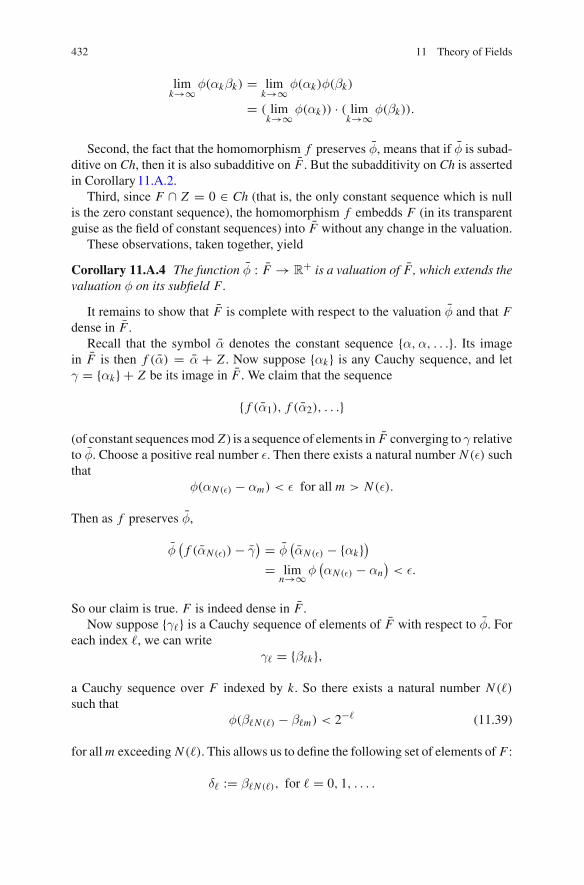
432 11 Theory of Fields
limk→∞ φ(αkβk) = lim
k→∞ φ(αk)φ(βk)
= ( limk→∞ φ(αk)) · ( lim
k→∞ φ(βk)).
Second, the fact that the homomorphism f preserves φ, means that if φ is subad-ditive on Ch, then it is also subadditive on F . But the subadditivity on Ch is assertedin Corollary11.A.2.
Third, since F ∩ Z = 0 ∈ Ch (that is, the only constant sequence which is nullis the zero constant sequence), the homomorphism f embedds F (in its transparentguise as the field of constant sequences) into F without any change in the valuation.
These observations, taken together, yield
Corollary 11.A.4 The function φ : F → R+ is a valuation of F , which extends the
valuation φ on its subfield F.
It remains to show that F is complete with respect to the valuation φ and that Fdense in F .
Recall that the symbol α denotes the constant sequence {α,α, . . .}. Its imagein F is then f (α) = α + Z . Now suppose {αk} is any Cauchy sequence, and letγ = {αk} + Z be its image in F . We claim that the sequence
{ f (α1), f (α2), . . .}
(of constant sequencesmod Z ) is a sequence of elements in F converging to γ relativeto φ. Choose a positive real number ε. Then there exists a natural number N (ε) suchthat
φ(αN (ε) − αm) < ε for all m > N (ε).
Then as f preserves φ,
φ(
f (αN (ε)) − γ) = φ
(αN (ε) − {αk}
)= lim
n→∞ φ(αN (ε) − αn
)< ε.
So our claim is true. F is indeed dense in F .Now suppose {γ�} is a Cauchy sequence of elements of F with respect to φ. For
each index �, we can writeγ� = {β�k},
a Cauchy sequence over F indexed by k. So there exists a natural number N (�)
such thatφ(β�N (�) − β�m) < 2−� (11.39)
for all m exceeding N (�). This allows us to define the following set of elements of F :
δ� := β�N (�), for � = 0, 1, . . . .

Appendix 1: Fields with a Valuation 433
Then taking limits in Eq. (11.39), we have
φ( f (δ�) − γ�) < 2−�,
where, as usual, f (δk) is the image of a constant sequence, namely the coset
{δk, δk, δk, . . .} + Z .
Now for any natural numbers n and m, we have
φ(δn − δm) = φ(
f (δm) − f (δn))
= φ(
f (δn) − γm + γm − γn + γn − f (δm))
≤ φ( f (δn − γm) + φ(γn − γm) + φ(γm − f (δm))
≤ φ(γn − γm) + 2−m + 2−n
But since {γ�} is a Cauchy sequence, the above equations tell us that δ := {δk} is aCauchy sequence in Ch. It is now clear that
φ(δ − γ�) = limk→∞(δk − β�k) < 2−�.
Thus {γ�} converges to δ with respect to φ. It follows that F is a complete field.Summarizing all of the results of this subsection, one has the following
Theorem 11.A.1 The field F = Ch/Z with valuation φ is a completion of (F,φ).
The Non-archimedean p-Adic Valuations
Our classical example of a non-archimedean valuation was derived from the choiceof a prime p in a unique factorization domain D. The valuation φ is defined on thefield F of quotients of D by the rule that φ(r) = e−k , whenever we write r ∈ F\{0}in the canonical form r = (a/b)pk where a and b are elements of D which are notdivisible by p, and k is an integer. Of course to make this function subadditive, wemust take e to be a fixed real number greater than 1. (Many authors choose p itself.That way, the values never overlap from one prime to another.)
Now notice that from Lemma11.A.2, the collection of all elements α of F forwhich φ(α) ≤ 1 is closed under addition as well as multiplication, and so form asubring O of F called the valuation ring of (F,φ). From the multiplicative prop-erties of φ, it is clear that every non-zero element of F either lies in O , or has itsmultiplicative inverse in O .
A somewhat smaller set is P := {α ∈ F |φ(α) < 1}. It is easy to see that this isan ideal in O . In fact the set O − P = {u ∈ F |φ(u) = 1} is closed under takingmultiplicative inverses in F and so consists entirely of units of O . Conversely, since

434 11 Theory of Fields
φ(1) = 1, every unit of O must have φ-value 1, so in fact
O\P = U (O), (11.40)
the (multiplicative) group of units of O . Thus P is the unique maximal ideal of Oand so O is a local ring.
Note that O and P have been completely determined by F and φ. The factorring O/P is a field called the residue field of F with respect to φ. The same sortof argument used to show (11.40) can be used to show that there exists an elementπ ∈ P , such that for any natural number k,
Pk\Pk+1 = πkU (O).
Taking the disjoint union of these set differences, one concludes that P is the principalideal P = Oπ.
Suppose p is a prime integer, D = Z, so F = Q, the field of rational numbers.Then O is the ring of all fractions a
b where a and b are integers and p does not divideb. Terribly odd things happen! For example {1, p, p2, . . .} is a null sequence (sinceφ(pk) = e−k , for all positive integers k), and
1 + p + p2 + · · ·
is a “convergent series”—that is its sequence of partial sums is a Cauchy sequence.Let us return to our classic example. There F is the field of fractions of a unique
factorization domain D, p is a prime element of D and φ(r) = e−k when r ∈ F iswritten in the form (a/b)pk , a, b ∈ D, k an integer. Let O be the valuation ring andlet P be its unique prime ideal. Similarly, let F , φ, O and P be the completion of F ,its extended valuation, valuation ring and uniqe maximal ideal, respectively.
Theorem 11.A.2 The following statements hold:
(i) D ⊆ O, and D ∩ P = pD.(ii) D + P = O.
(iii) F ∩ O = O, O ∩ P = P.(iv) O + P = O.(v) The residue class fields of F and F are both D/pD.
Proof (i) Clearly every element of D has valuation at most 1 so the first statementholds. Those elements of D of value less than 1 are divisible by p, and vice versa.So the second statement holds.
(ii) Suppose r ∈ O\P . Then r has the form a/b where a and b are elements ofD which are not divisible by p. Since p is a prime and D is a UFD, this means thereare elements c and d of D such that cp + db = a.
Then
r = a
b=( c
b
)· p + d. (11.41)

Appendix 1: Fields with a Valuation 435
Now p does not divide d , otherwise it would divide a = cp + db, against ourassumption about r . Thus d is an element of D also in O − P , and by Eq. (11.41),r ≡ (a/b) modulo P . This proves (ii).
(iii) Both statements here just follow from that fact the φ extends φ.(iv) Now let α be any element in O − P so φ(α) = 1. Since F is dense in F ,
there is an element r ∈ F such that φ(α − r) < 1. This means r − α is an elementof P . Since O is an additive subgroup of F containing P , r belongs to O ∩ F = O ,and we can say r ≡ α mod P . This proves (iv).
(v) First using (iii) and (iv), and then (i) and (ii),
O/P = (O + P)/P
� O/(O ∩ P) = O/P, while
O/P = (D + P)/P
� D/(D ∩ P) = D/pD.
The proof is complete. �
Now fix a system Y of coset representatives of pD in the additive group (D,+)
and suppose 0 ∈ Y . For example, if D = Z, then p is a rational prime, the residueclass field is Z/pZ, and we may take Y to be the set of integers,
{0, 1, 2, . . . , p − 1}.
For another example, suppose D = K [x] where K is some field, and p = x + a is amonic polynomial of degree one. Then the residue class field is K [x]/(x + a) � K .But as K is a subring of D, it makes perfect sense to take Y = K (the polynomialsof degree zero).
Now in the notation of Theorem11.A.2, D + P = (D + P) + P = O + P = O .So, for a fixed α ∈ O , there is a unique element a0 ∈ Y such that α − a0 ∈ P . (If αis already in P , this element is 0.) Now P = pO , so
α1 = 1
p(α − a0) ∈ O.
Then we repeat this procedure to obtain a unique element a1 ∈ Y such that α1−a1 ∈pO . Then
α ≡ a0 + pa1 mod p2 O.
Again, one can find a2 ∈ Y such that if α2 := (1/p)(α1−a1), then α2−a2 ∈ pO . So,after k repetitions of this procedure, we obtain a sequence of k + 1 unique elementsof Y , (a0, a1, . . . , ak) such that
α ≡ a0 + a1 p + a2 p2 + · · · + ak pk mod Pk+1.

436 11 Theory of Fields
Thus we can write any α ∈ F in the “power series” form,
α = pk[a0 + a1 p + a2 p2 + · · · ],
where the ai are uniquely determined elements of Y , and a0 �= 0, so that k isdetermined by e−k = φ(α).
For example, if p = x ∈ K [x] = D, then, taking Y = K , we see that F is thefield of Laurent series over K—that is, the ring of power series of the form
b−k x−k + · · · + b−1x−1 + b0 + b1x + b2x2 + · · · , k ∈ N
where the bi are in K and one follows the usual rules of adding and multiplyingpower series.
The ring of Laurent series is very important in the study of power series generatingfunctions. Be aware that the field K here is still arbitrary. It can even be a finite field.
Note that if D = Z and p is a rational prime, the system of coset representativesY is not closed under either addition or multiplication and so, in order to restore thecoefficients of the powers of p to their proper location in Y , some local adjustmentsare needed after addition or multiplication. For example if p = 5, then we mustrewrite
(1 + 3(5))(1 + 4(5)) = 1 + 7(5) + 12(52)
as1 + 2(5) + 3(52) + 2(53).
Appendix 2: Finite Division Rings
In 1905 J.H.M. Wedderburn proved that every finite division ring is in fact a field.On pp. 104–105 of van Der Waerden’s classic book (1930–31), (cited at at the
end of this appendix) one finds a seemingly short proof that depends only on theeasy exercise which proves that no finite group can be the union of the conjugates ofa proper subgroup. But the proof is short only in the sense that the number of wordsrequired to render it is not large. Measured from actual elementary first principles,the proof spans a considerable “logical distance”. It uses the notion of a splittingfield for a division ring, and a certain structure theorem involving a tensor productof algebras. Both of these notions are beyond what has been developed in this andthe preceding chapters.
Several other more elementary proofs are available. The first proof given belowis due to T.J. Kaczynski (cited at the end of this appendix) and has several points ofinterest.
We begin with a small lemma.

Appendix 2: Finite Division Rings 437
Lemma 11.A.8 Every element in a finite field GF(q) is the sum of two squares. Asa consequence, when p is a prime number, there exist numbers t and r such thatt2 + r2 ≡ −1, mod p, with t �≡ 0.
Proof If q is even, all elements are squares and hence is the sum of 02 and a square.So suppose q is odd and let S be the set of non-zero squares. Then, for any non-square g ∈ GF(q), we have a partition GF(q)∗ = S + Sg. Now using 0 as one of thesummand squares, we see that every element of {0}∪S is the sum of two squares, andif (S + S)∩gS �= ∅ (where now “S + S” indicates all possible sums of two squares),then this is true of gS as well and the result is proved. Otherwise S + S ⊆ {0} ∪ Sand so {0}∪ S is a subfield of GF(q). That is impossible since |{0}∪ S| = (q + 1)/2is not a prime power dividing q .
In particular, −1 can be represented as the sum of two squares in Z/(p), and oneof them at least (say t) is non-zero. �
Theorem 11.A.3 (Wedderburn) Every finite division ring is a field.
Proof ([1]) Let D be a finite division ring and let P be the prime subfield in itscenter. Also let D∗ be the multiplicative group of non-zero elements of D. For someprime r let S be an r -Sylow subgroup of D∗, of order ra , say. Now S cannot containan abelian subgroup A of type Zr × Zr otherwise the subfield generated by P ∪ Awould have too many roots of xr − 1 = 0. Thus S is either cyclic or else r = 2and S is a generalized quaternion group. We shall show that the latter case is alsoforbidden.
Suppose S is generalized quaternion. Then the characteristic p is not 2 and Scontains a subgroup S0 which is quaternion of order 8, generated by two elementsa and b or order 4 for which bab = a−1 and z = a2 = b2 is its central involution.Then the extension P(z) is a subfield containing the two roots of x2−1 = 0, namely1 and −1. It follows that
a2 = −1 = z = b2
so a3 = −a. Thusba = a−1b = −ab.
Now let p = |P|, the characteristic of D. Then by the lemmawe can find elementst and r in P (and hence central in D) such that t2 + r2 = z = −1. Then
((ta + b) + r) ((ta + b) − r) = (ta + b)2 − r2
= t2a2 + r(ab + ba) + b2 − r2
= −t2 + b2 − r2 = 0.
So one of the factors on the left is zero. But then b = −ta ± r and so as t �= 0, bcommutes with a, a contradiction.
Thus, regardless of the parity of p, every r -Sylow subgroup of D∗ must be cyclic.If follows that D∗ must be solvable. Now let Z∗ = Z(D∗) be the center of the group

438 11 Theory of Fields
D∗ and suppose Z∗ �= D∗. Then we can find a normal subgroup A of D∗ containingZ∗ such that A/Z∗ is a minimal normal subgroup of D∗/Z∗. Since the latter issolvable with all Sylow subgroups cyclic, A/Z∗ is cyclic. Now Z∗ is in the centerof A, and since no group has a non-trivial cyclic factor over its center, A is abelian.
Now we shall show that in general, D∗ cannot contain a normal abelian subgroupA which is not in the center Z∗. Without loss of generality we can take (as above)Z∗ < A � D∗. Choose y ∈ A − Z∗. Then there exists an element x in D∗ whichfails to commute with y. Then also x + 1 is not in A as it fails to commute with y aswell. Then, as A is normal,
(1 + x)y = a(1 + x),
for some element a ∈ A. Then
y − a = ax − xy = (a − xyx−1)x . (11.42)
Now if y − a = 0, then a = y and a = xyx−1 by (11.42), so y = xyx−1 againstthe fact that x and y do not commute. Thus (a − xyx−1) is invertible, and from(11.42),
x = (a − xyx−1)−1(y − a). (11.43)
But a, y and xyx−1 all belong to A and so commute with y. Thus every factoron the right side of (11.43) commutes with y, and so x commutes with y, the samecontradiction as before. �
Remark As noted, the last part of Kaczynski’s proof did not use finiteness at all. Asa result, one can infer
Corollary 11.A.5 (Kaczynski) Suppose D is any division ring with center Z. Thenany abelian normal subgroup of D∗ lies in Z.
One might prefer a proof that did not use the fact that a finite group with all Sylowsubgroups cyclic is solvable. This is fairly elementary to a finite group theorist (oneuses a transfer argument on the smallest prime and applies induction) but it wouldnot be as transparent to the average man or woman on the street.
Another line of argument due to I.N. Herstein (cited below) develops some trulybeautiful arguments from first principles. Consider:
Lemma 11.A.9 Suppose D is a division ring of characteristic p, a prime, and letP be its prime subfield, which, of course, is contained in the center Z. Suppose a isany element of D − Z which is algebraic over P. Then there exists an element y ∈ Dsuch that
yay−1 = ai �= a
for some integer i .

Appendix 2: Finite Division Rings 439
Proof Fix element a as described. The commutator mapping δ : D → D, whichtakes an arbitrary element x to xa − ax , is clearly an endomorphism of the additivegroup (D,+). Also, for any element λ of the finite subfield P(a) obtained by adjoin-ing a to P , the fact that λ commutes with a yields
δ(λx) = λxa − aλx = λ(xa − ax) = λδ(x).
Thus, regarding D as a left vector space over the field P(a), we see that δ is a lineartransformation of V .
Now, for any x ∈ D, and positive integer k, an easy computation reveals
δk(x) =∑k
j=0(−1) j
(kj
)a j xak− j . (11.44)
Now P(a) is a finite field of order pm , say. Then a pm = a. Since D has characteristicp, putting k = pm in (11.44) gives
δ pm(x) = xa pm − a pm
x = xa − ax = δ(x).
Thus the linear transformation δ of V satisfies
δ pm = δ.
Thus, in the commutative subalgebra of Hom (V, V ) generated by δ, we have
0 = δ pm − δ =∏
λ∈P(a)(δ − λI ),
where the λI are the scalar transformations V → V , λ ∈ P(a).Now ker δ is the subalgebra CD(a) of all elements of D which commute with
a. (This is a proper subspace of V since a is not in the center Z .) Thus δ acts as anon-singular transformation of W := V/CD(a)while
∏(δ −λI ) (the product taken
over all non-zero λ ∈ P(a)) vanishes on it. It follows that for some λ ∈ P(a) − {0},δ −λI is singular on W . This means there is a coset b0 + CD(a) �= CD(a) such that
δ(b0) = λb0 + c, c ∈ CD(a).
Setting y = b0 + λ−1c, we have δ(y) = λy �= 0. This means
yay−1 = a + λ ∈ P(a).
Now if m is the order of a in the multiplicative group P(a)∗, then yay−1 is one ofthe roots of Xm − 1 = 0 lying in P(a). But since these roots are just the powers ofa, we have yay−1 = ai �= a, for some i , 1 < m ≤ m − 1, as desired. �

440 11 Theory of Fields
Now we proceed with a proof of Wedderburn’s theorem. We may assume that Dis a non-commutative finite division ring in which all proper subalgebras are fields.In particular, for any element v ∈ D − Z , the centralizing subalgebra CD(v) is afield. It follows that the commuting relation on D − Z is an equivalence relation. Foreach commuting equivalence class Ai , and element ai ∈ Ai , we have
Fi := Z ∪ Ai = CD(ai ). (11.45)
Let D∗ be the multiplicative group of non-zero elements of D, so Z∗ := Z − {0}is its center. Choose a coset aZ∗ so that its order in D∗/Z∗ is the smallest prime sdividing the order of D∗/Z∗. The actual representative element a can then be chosento have s-power order.
Now by Herstein’s lemma, there is an element y ∈ D such that
yay−1 = at �= a.
From (11.45) it follows that conjugation by y leaves the subfield F := CD(a)
invariant, and induces on it an automorphism whose fixed subfield is
CD(y) ∩ CD(a) = Z .
But the same conclusion must hold when y is replaced by a power yk which is not inZ . It follows that Gal(F/Z) is cyclic of prime order r and conjugation by y inducesan automorphism of order r . Thus yr ∈ CD(a) ∩ CD(a) = Z , so r is the orderof y Z∗ in the group D∗/Z∗. We can then choose the representative y to be in ther -Sylow subgroup of Z(y)∗, so that it has r -power order.
Now, by the “(very) little Fermat Theorem” i s−1 ≡ 1 mod s. Thus
y(s−1)ay−(s−1) = ais−1
≡ a mod Z∗.
So, setting b := ys−1, we havebab−1 = az,
for some element z in Z which is also a power of a. Now from this equation, z = 1if and only if b ∈ CD(y) ∩ CD(a) = Z .
Case 1: z = 1 and b is in the center. Then ys−1 ∈ Z , so r , the order of y Z∗ inD∗/Z∗, divides s −1. That is impossible since s was chosen to be the smallest primedivisor of |D∗/Z∗|.
Case 2: z �= 1 and b has order r mod Z∗. Then br a−r = a = azr . But since zis an element of s-power order, we now have that r = s and is the order of z. Nowat this stage, the multiplicative subgroup H := 〈a, b〉 of D∗ generated by a andb is a nilpotent group generated by two elements of r -power order, and so is an rgroup. Since it is non-abelian without a subgroup of type Zr × Zr , it is generalized

Appendix 2: Finite Division Rings 441
quaternion and so contains the quaternion subgroup of order 8. Herstein goes on toeliminate the presence of Q8 by an argument that essentially anticipates by threeyears the argument given in the first part of Kaczynski’s proof above.17 �
There is another fairly standard proof which comes closer to being a proof fromelementary principles. It uses an argument due to Witt (cited below) concerningcyclotomic polynomials and the partition of the group D∗ into conjugacy classes.One may consult Jacobson’s book (cited below), pp. 431–2, for a presentation of thisproof.
Reference
1. Kaczynski TJ (1964) Another proof of Wedderburn’s theorem. Am Math Mon 71:652–653
17ActuallyHerstein inadvertently omittedCase 1 by taking s = r from amisreading of the definitionof s. As we see, this presents no real problem since his lemma applies when s is the smallest possibleprime.

Chapter 12Semiprime Rings
Abstract As was the case with groups, a ring is said to be simple if it has no properhomomorphic images (equivalently, it has no proper 2-sided ideals). On the otherhand, a right (or left) R-module without proper homomorphic images is said to beirreducible. A right (or left) module is said to be completely reducible is it is a directsum of irreducible modules. Similarly, a ring R is said to be completely reducible ifand only if the rightmodule RR is completely reducible. A ring is semiprimitive if andonly if the intersection of its maximal ideals is zero, and is semiprime if and only ifthe intersection of all its prime ideals is the zero ideal. Written in the presented order,each of these three properties of rings implies its successor—that is, the propertiesbecome weaker. The goal here is to prove the Artin-Wedderburn theorem, basicallythe following two statements: (1) A ring is completely reducible if and only if it isa direct sum of finitely many full matrix algebras, each summand defined over itsown division ring. (2) If R is semiprimitive and Artinian (i.e. it has the descendingchain condition on right ideals) then the same conclusion holds. A corollary is thatany completely reducible simple ring is a full matrix algebra.
12.1 Introduction
In this chapter we develop the material necessary to reach the famous Artin-Wedderburn theorem which—in the version given here—classifies the Socle of aprime ring. The reader should probably be reminded here that all rings in this chapterhave a multiplicative identity element.
We begin with the important concept of complete reducibility of modules. Whentransferred to rings, this notion and its equivalent incarnations give us quick accessto the Socle of a ring and its homogeneous components. Most of the remainingdevelopment takes place in a general class of rings called the semiprime rings. It hasseveral important subspecies, the prime, primitive, and completely reducible rings,where the important role of idempotents unfolds.
We remind the reader that R-module homomorphisms are applied on the left.Thus if M and M ′ are right R-modules and if φ : M → M ′ is an R-modulehomomorphism, then one has
© Springer International Publishing Switzerland 2015E. Shult and D. Surowski, Algebra, DOI 10.1007/978-3-319-19734-0_12
443

444 12 Semiprime Rings
φ(mr) = (φm)r, for all m ∈ M and all r ∈ R. (12.1)
Next, if we set E = EndR(M) = HomR(M, M), the endomorphism ring of M , then(12.1) shows that M has the structure of an (E, R)-bimodule, a formalism that willbe useful in the sequel.
12.2 Complete Reducibility
Given a right R-module M , the concept of minimal or submodule refers to minimalor maximal elements in the poset of all proper submodules of M . Thus 0 is not aminimal submodule and M itself is not a maximal submodule of M .
One defines the radical rad(M) of a right R-module M as the intersection of allmaximal submodules of M . If there are nomaximal submodules—as in theZ-module
Z(p∞) = 〈1/p, 1/p2, . . .〉
—then rad(M) = M , by definition.There is a dual notion: One defines the socle Soc(M) as the submodule generated
by all minimal submodules (that is, all irreducible submodules) of M . Similarly, ifthere are no irreducible submodules—as in the case of the free Z-module ZZ—thenby convention one sets Soc(M) = 0, the zero submodule.
Examples If D is any principle ideal domain (PID), and if p is a prime element in D,then the D module D/p2D has radical rad(M) = Soc(M) = pD/p2D � D/pD.(See Exercise (1) in Sect. 12.6.1.) In a similar vein, if F is a field, and if R is thematrix ring
R ={[
x 0y z
]| x, y, z ∈ F
},
consisting of lower-triangular matrices over F , and if V is the right R-module con-sisting of 1 × 2 row vectors with entries in F :
V = {[x y
] | x, y ∈ F},
it also follows thatrad V = Soc(V ) = {[
x 0] | x ∈ F
}.
(See Exercise (4) in Sect. 12.6.1.)
Theorem 12.2.1 Let M be a right R-module having at least one irreducible sub-module, so that Soc(M) = 0. Then
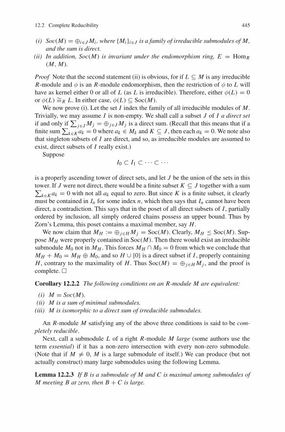
12.2 Complete Reducibility 445
(i) Soc(M) = ⊕i∈J Mi , where {Mi }i∈J is a family of irreducible submodules of M,and the sum is direct.
(ii) In addition, Soc(M) is invariant under the endomorphism ring, E = HomR
(M, M).
Proof Note that the second statement (ii) is obvious, for if L ⊆ M is any irreducibleR-module and φ is an R-module endomorphism, then the restriction of φ to L willhave as kernel either 0 or all of L (as L is irreducible). Therefore, either φ(L) = 0or φ(L) ∼=R L . In either case, φ(L) ⊆ Soc(M).
We now prove (i). Let the set I index the family of all irreducible modules of M .Trivially, we may assume I is non-empty. We shall call a subset J of I a direct setif and only if
∑j∈J M j = ⊕ j∈J M j is a direct sum. (Recall that this means that if a
finite sum∑
k∈K ak = 0 where ak ∈ Mk and K ⊆ J , then each ak = 0. We note alsothat singleton subsets of I are direct, and so, as irreducible modules are assumed toexist, direct subsets of I really exist.)
SupposeI0 ⊂ I1 ⊂ · · · ⊂ · · ·
is a properly ascending tower of direct sets, and let J be the union of the sets in thistower. If J were not direct, there would be a finite subset K ⊆ J together with a sum∑
k∈K ak = 0 with not all ak equal to zero. But since K is a finite subset, it clearlymust be contained in In for some index n, which then says that In cannot have beendirect, a contradiction. This says that in the poset of all direct subsets of I , partiallyordered by inclusion, all simply ordered chains possess an upper bound. Thus byZorn’s Lemma, this poset contains a maximal member, say H .
We now claim that MH := ⊕ j∈H M j = Soc(M). Clearly, MH ≤ Soc(M). Sup-pose MH were properly contained in Soc(M). Then there would exist an irreduciblesubmodule M0 not in MH . This forces MH ∩ M0 = 0 from which we conclude thatMH + M0 = MH ⊕ M0, and so H ∪ {0} is a direct subset if I , properly containingH , contrary to the maximality of H . Thus Soc(M) = ⊕ j∈H M j , and the proof iscomplete. �
Corollary 12.2.2 The following conditions on an R-module M are equivalent:
(i) M = Soc(M).(ii) M is a sum of minimal submodules.
(iii) M is isomorphic to a direct sum of irreducible submodules.
An R-module M satisfying any of the above three conditions is said to be com-pletely reducible.
Next, call a submodule L of a right R-module M large (some authors use theterm essential) if it has a non-zero intersection with every non-zero submodule.(Note that if M = 0, M is a large submodule of itself.) We can produce (but notactually construct) many large submodules using the following Lemma.
Lemma 12.2.3 If B is a submodule of M and C is maximal among submodules ofM meeting B at zero, then B + C is large.

446 12 Semiprime Rings
Proof Assume B andC chosen as above and let D = 0 be any non-trivial submoduleof M . Suppose (B + C) ∩ D = 0. If b, c, and d are elements of B, C and D,respectively, and b = c +d , then d = b − c and this is zero by our supposition. Thusb = c ∈ B ∩ C = 0, so b = c = 0. Thus B ∩ (C + D) = 0. By maximality of C ,D ⊆ C . Then D = (B + C) ∩ D = 0, a contradiction. Thus always (B + C) ∩ D isnon-zero, and so B + C is large. �
That such a submodule C exists which is maximal with respect to meeting Btrivially, as in Lemma12.2.3, is an easy application of Zorn’s Lemma.
If M is a right R-module, let L(M) be the lattice of all submodules of M (sum isthe lattice “join”, intersection is the lattice “meet”). We say L(M) is complemented(or that M is semisimple) if every submodule B of M has a complement in L(M)—i.e. there exists a submodule B′ such that B ∩ B ′ = 0 and B + B ′ = M (this meansM = B ⊕ B ′).
Lemma 12.2.4 If L(M) is complemented, then so is L(N ) for any submoduleN of M.
Proof Let C be a submodule of N . By hypothesis there is a complement C ′ to C inL(M). Then setting C ′′ := C ′ ∩ N , we see
C ∩ C ′′ ⊆ C ∩ C ′ = 0, and
C + C ′′ = C + (C ′ ∩ N ) = (C + C ′) ∩ N , (the modular law)
= M ∩ N = N .
Thus C ′′ is a complement of C in N . �
Remark Of course the above is actually a lemma about any modular lattice: if it iscomplemented, then so are any of its intervals above zero.
Lemma 12.2.5 If M is a right R-module for which L(M) is complemented, thenrad(M) = 0.
Proof Letm be a non-zero element of M and let A bemaximal among the submoduleswhich do not contain m. (A exists by Zorn’s Lemma.) Suppose now A < B < Mso A is not maximal in L(M). Let B ′ be a complement to B in L(M). Then by themodular law (Dedekind’s Lemma)
A = (B ∩ B ′) + A = B ∩ (B ′ + A).
Now as B < M implies B ′ = 0 and A < B implies B′ ∩ A = 0, we see that A isproperly contained in B ′ + A. Then the maximality of A implies m ∈ B′ + A andalso m ∈ B. Thus m lies in B ∩ (B ′ + A) = A, contrary to the choice of A.
Thus no such B exists and A is in fact a maximal submodule of M . Then we seethat every non-zero module element is avoided by some maximal submodule of M ,and hence is outside rad(M). It follows that rad(M) = 0. �

12.2 Complete Reducibility 447
Theorem 12.2.6 The following conditions on an R-module M are equivalent:
(i) M is completely reducible.(ii) M contains no proper large submodule.
(iii) M is semisimple.
Proof Assume condition (i), i.e., that M = Soc(M) and that A � M is a proper sub-module of M . If A contained every irreducible submodule of M , then it would clearlycontain Soc(M) = M . But then A couldn’t be proper, contrary to our assumption onA. Thus there is an irreducible submodule U not in A, and so A ∩ U = 0, since Uis minimal. Thus A is not large, proving condition (ii).
Next, assume that (ii) holds, i.e., M contains no proper large submodules, and letA ⊆ M be a submodule. Using Zorn’s lemma, there exists a submodule B ⊆ Mwhich is maximal with respect to the condition A ∩ B = 0. But then Lemma12.2.3asserts that A+B is large and so by part (ii), A+B = M . Thismeans that M = A⊕B,i.e., that B is a complement to A in M , proving that M is semisimple.
Finally, assume condition (iii). Since M is semisimple, Soc(M) has a comple-ment C in L(M). Next, by Lemma12.2.5, we know that rad(C) = 0 and so theset of maximal submodules of C must be nonempty (else C = rad(C) would bethe intersection of the empty collection of maximal submodules). Letting L ⊆ Cbe a maximal submodule, we now apply Lemma12.2.4 to infer the existence of asubmodule A ⊆ C with C = A ⊕ L . But then, A ∼= C/L and so A is an irreducibleR-module with A ∩ Soc(M) = 0. This is clearly impossible unless C = 0, in whichcase Soc(M) = M , proving (i). �
12.3 Homogeneous Components
12.3.1 The Action of the R-Endomorphism Ring
Let M be a right R-module and let E = HomR(M, M) be its R-endomorphism ring.As remarked earlier, we may regard M as a left E-module, giving M the structureof an (E, R)-bimodule.
Let M be any right R-module, and let F be a family of irreducible R-modules.We set M[F ] = ∑
A, where the sum is taken over all irreducible submodulesA ⊆ M such that A is R-isomorphic to at least one module in F . Note that if Mcontains no submodules isomorphic with any member of F , then M[F ] = 0. IfF = {N }, the set consisting of a single irreducible right R-module N , then we writeM[N ] := M[{N }], and call it the N-homogeneous component of M ; again, it isentirely possible that M[N ] = 0. Note that by Corollary12.2.2, M[F ] is completelyreducible for any family F of irreducible submodules of M that we may choose.Next, suppose that F is a family of irreducible submodules of M , and that B ⊆ Mis a submodule of M isomorphic with some irreducible submodule A ∈ F . Then forany e ∈ E = HomR(M, M) we have that eB = 0 or eB ∼=R∼=R A, proving that also

448 12 Semiprime Rings
eB ⊆ M[A] ⊆ M[F ]. This proves already that M[A] (as well as M[F ]) is invariantunder the left action of every element of E .
We can internalize this discussion to the ring R itself. In particular, if M = RR , theregular right R-module R, and if A ⊆ R is a minimal right ideal, then R[A] = M[A]is obviously also a right ideal of R. But it’s also a left ideal since left multiplicationby an element r ∈ R gives, by the associative multiplication in R, an R-moduleendomorphism R → R. By what was noted above, this proves that r R[A] ⊆ R[A],and so R[A] is a left ideal, as well. We shall capitalize on this simple observationshortly.
Lemma 12.3.1 Assume that M is a completely reducible R-module and set E =HomR(M, M). If A ⊆ M is any irreducible submodule of M, then EA = M[A].Proof Wehave already observed above that M[A] is invariant under every R-moduleendomorphism of M , so EA ⊆ EM[A] ⊆ M[A]. Conversely, assume that A′ ⊆ Mis a submodule with A ∼=R A′. Since rad(M) = 0 we may find an irreducible R-submodule L ⊆ M with A ∩ L = 0. Therefore it follows that M = A ⊕ L . If
π : M = A ⊕ L → A is the projection onto the first coordinate, and if φ : A∼=→ A′
is an R-module isomorphism, then the composite
Mπ−→ A
φ−→ A′ ↪→ M
defines an R-module endomorphism carrying A to A′. �
12.3.2 The Socle of a Module Is a Direct Sumof the Homogeneous Components
Our first lemma below informs us that inside the modules M[F ]we won’t encounterany unexpected submodules.
Lemma 12.3.2 If M is an R-module and if F is a family of irreducible R-modules,then any irreducible submodule of M[F ] is isomorphic with some member of F .
Proof Set N = M[F ] ⊆ M , and let A ⊆ N be an irreducible submodule. ByLemma12.2.5 we have rad(N ) = 0 from which we infer the existence of a maximalsubmodule L ⊆ N with A ∩ L = 0. Since N is generated by submodules eachof which is isomorphic with a member of F , we may choose one, call it B, whereB ∩ L = 0. Since L is maximal, we have N = A ⊕ L = B ⊕ L . Therefore,
A ∼= (A ⊕ L)/L = N/L = (B ⊕ L)/L ∼= B,
proving the result. �

12.3 Homogeneous Components 449
As a consequence of the above, we may exhibit the socle of a module as the directsum of its homogeneous components, that is, the direct sum of its A-homogeneouscomponents M[A] as A ranges over a set of representatives of the R-isomorphismsclasses of irreducible submodules of M .
Corollary 12.3.3 Soc(M) is the direct sum of the homogeneous components of M.
Proof Let F be a family of pairwise non-isomorphic irreducible R-submodulesof M such that each irreducible submodule of M is isomorphic with a memberof F . Obviously Soc(M) = M[F ] = ∑
A∈FM[A]. By Lemma12.3.2 we see that
for all A ∈ F , one has M[A] ∩ ∑B∈FA
M[B] = 0, where FA = F\{A}. Now by
Theorem8.1.6 on internal direct sums, it follows immediately that
Soc(M) =∑A∈F
M[A] =⊕A∈F
M[A]
as claimed. �
The next several sections concern rings rather than modules. But we can alreadyapply a few of the results of this section to the module RR . Of course, the firststatement below has already been observed above.
Corollary 12.3.4 Every homogeneous component of Soc(RR) is a 2-sided ideal ofR. Also Soc(RR) is itself a 2-sided ideal of R (which we write as Soc(R)).
12.4 Semiprime Rings
12.4.1 Introduction
Wenowpass to rings. The basic class of rings thatwe shall dealwith are the semiprimerings and certain subspecies of these. In order to state the defining properties, a fewreminders about 2-sided ideals are in order.
If A and B are 2-sided ideals of the ring R, the product AB of ideals is the additivegroup generated by the set of all products {ab |(a, b) ∈ A × B}. This additive groupis itself already a 2-sided ideal which the ring-theorists denote by the symbol AB. Ofcourse it lies in the ideal A ∩ B. (From this definition, taking products among idealsis associative.)
We say that a (2-sided) ideal A is nilpotent if and only if there exists some positiveinteger n such that
An := A · A · · · A (n factors) = 0 := {0R},
the zero ideal.

450 12 Semiprime Rings
An ideal P is said to be a prime ideal if and only if, whenever A and B are idealssuch that AB ⊆ P , then either A ⊆ P or B ⊆ P . The intersection of all prime idealsof the ring R is called the prime radical of R and is denoted Prad(R). We say that thering R is semiprime if the intersection of its prime ideals is 0, i.e., if Prad(R) = 0.Clearly Prad(R) is an ideal of R. A moment’s thought should be enough to revealthat R/Prad(R) is semiprime. If the 0-ideal of R is itself a prime ideal, the ring R iscalled a prime ring.
12.4.2 The Semiprime Condition
Theorem 12.4.1 The following conditions on a ring R are equivalent:
(i) R is semiprime.(ii) For any ideals A and B of R, AB = 0 implies A ∩ B = 0.
(iii) 0 is the only nilpotent ideal.(iv) For each non-zero x ∈ R, x Rx = 0.
Proof (i)=⇒(ii) Assume A and B are ideals for which AB = 0. Then AB ⊆ P forany prime ideal P so either A lies in P or B lies in P . In any event A ∩ B ⊆ P foreach prime ideal P . Thus A ∩ B is contained in the intersection of all prime ideals,and so, since R is semiprime, is zero.
(ii)=⇒(iii) Suppose, by way of contradiction, that A is a non-zero nilpotent idealof R. Let k be the least positive integer for which Ak = 0. Then Ak−1 · A = 0,which implies by condition (ii) that Ak−1 ⊆ Ak−1 ∩ A = 0, contrary to the choiceof exponent k.
(iii)=⇒(iv) If, for some 0 = x ∈ R we had x Rx = 0, then as x ∈ Rx R, weconclude that Rx R is a non-zero ideal of R. But then
Rx R · Rx R = Rx Rx R = R · 0 · R = 0,
forcing Rx R to be a non-zero nilpotent ideal, against (iii).(iv)=⇒(i) Let a = 0; we shall prove that there exists a prime ideal P ⊆ R with
a ∈ P , proving that R is semiprime. Seta0 := a; by (iv),a0Ra0 = 0. Therefore, thereexists a non-zero element a1 ∈ a0Ra0. We may continue this process to generate asequence of non-zero elements a0, a1, . . ., such that ai+1 ∈ ai Rai . Set T = {an|n ∈N. Before proceeding further, we note an important property of this sequence:
(S) If the element ai is in some ideal J ⊆ R, then so are all of its successors in T .
Let P be an ideal maximal with respect to not containing any element of T . (Itexists by Zorn’s Lemma.) Now suppose A and B are ideals of R neither of which iscontained in P but withAB ⊆ P . By themaximality of P the ideals A+ P and B + Pboth meet T non-trivially. So there are subscripts i and j such that ai ∈ A + P , anda j ∈ B + P . Set m = max(i, j). Then by the property (S), am lies in both P + Aand P + B, so

12.4 Semiprime Rings 451
am+1 ∈ am Ram ⊆ (A + P)(B + P) ⊆ AB + P ⊆ P
against P ∩ T = ∅. Thus no such ideals A and B exist, so P is a prime ideal. SinceP doesn’t contain a = a0, the proof that R is semiprime is complete. �
12.4.3 Completely Reducible and Semiprimitive RingsAre Species of Semiprime Rings
At the beginning of this chapter we defined the radical of a right R-module M tobe the intersection of all maximal submodules of M , or, if there are no maximalsubmodules, to be M itself. Similarly, we define the radical, rad(R), of the ringR to be rad(RR)—the radical of the right module RR . Accordingly, rad(R) is theintersection of all maximal right ideals of R and is called the Jacobson radical of R.
While rad(R) is, a priori, a right ideal of R, the reader may be surprised to learnthat it is also a left ideal. As this is relatively easy to show, we shall pause long enoughto address this issue. Assume first that M is a non-zero irreducible right R-module.Then for each 0 = m ∈ M , we have that (by irreducibility) M = m R. Furthermore,the mapping R → M, r �→ mr is easily verified to be a surjective R-modulehomomorphism. This implies immediately that if J = AnnR(m) := {r ∈ R | mr =0}, then J is the kernel of the above R-module homomorphism: M ∼=R R/J . ClearlyJ is a maximal right ideal of R. Next, recall that any R-module M determines a ringhomomorphism R → EndZ(M), the ring of abelian group homomorphisms of M .Furthermore, it is clear that AnnR(M) := {r ∈ R | Mr = 0} is the kernel of theabove ring homomorphism, and hence AnnR(M) is a 2-sided ideal of M . Finally,note that
AnnR(M) =⋂
0 =m∈M
AnnR(m), (12.2)
i.e., AnnR(M) is the intersection of the maximal right ideals AnnR(m), m ∈ M . Ourproof will be complete as soon as we can show that
rad(R) =⋂
J∈M(R)
AnnR(R/J ),
whereM(R) denotes the collection of all maximal right ideals of R. By Eq. (12.2) wesee that each AnnR(R/J ) is an intersection of maximal right ideals of R; therefore ifx ∈ rad(R) then x is contained in AnnR(R/J ) for every maximal right ideal J ⊆ R.This proves that
rad(R) ⊆⋂
J∈M(R)
AnnR(R/J ).

452 12 Semiprime Rings
Conversely, if x ∈ AnnR(R/J ), then Eq. (12.2) implies that x ∈ J = AnnR(1+ J ),and so it is now clear that
rad(R) ⊇⋂
J∈M(R)
AnnR(R/J ),
proving that, as claimed rad(R) is a 2-sided ideal of R.We note in passing that the Jacobson radical annihilates every irreducible right
R-module.A ring is said to be semiprimitive if and only its Jacobson radical is trivial. A
ring is primitive if and only if there exists an irreducible right R-module M withAnn(M) = 0, i.e., if and only if R has a faithful irreducible module. It follows, ofcourse, that every primitive ring is semiprimitive as is R/rad(M) for any ring R.Finally we say that a ring R is completely reducible if and only if the right moduleRR is a completely reducible module. A hierarchy of these concepts is displayed inthe following Theorem:
Theorem 12.4.2 The following implications hold among properties of a ring:
completely reducible ⇒ semiprimitive ⇒ semiprime
Proof The first implication is just Lemma12.2.5, together with Theorem12.2.6applied to the module M = RR .
For the second implication, suppose R is a ring which is semiprimitive but notsemiprime. Then rad(R) = 0 and there exists a non-zero nilpotent ideal N . Byreplacing N by an appropriate power if necessary, we may assume N 2 = 0 = N .Since rad(R) = 0, there exists a maximal right ideal M not containing N . ThenR = N + M by maximality of M . Thus we may write 1 = n + m, where n ∈ N andm ∈ M . Then
n = 1 · n = n2 + mn = 0 + mn ∈ M.
Thus 1 = n + m ∈ M , which is impossible. Thus we see that N must lie in everymaximal right ideal, so N ⊆ Rad(R) = 0. This contradicts N = 0. Thus no suchring R exists, and so the implication holds. �
12.4.4 Idempotents and Minimal Right Idealsof Semiprime Rings
The importance of semiprimness for us is that it affects the structure of the minimalright ideals of R.
We pause, however, to define an idempotent in a ring R to be a non-zero element esatisfying e2 = e. Such elements play a central role in this and the following subsec-tion. Furthermore, the role that they play is analogous to that played by projectionsin linear algebra.

12.4 Semiprime Rings 453
Lemma 12.4.3 (Brauer’s lemma) Let K be a minimal right ideal of a ring R. Theneither
(i) K 2 = 0, or(ii) K = eR, for some idempotent e ∈ R.
Proof If K 2 = 0, then by the minimality of K , K = K 2 = kK for some elementk ∈ K . From this we infer the existence of an element e such that ke = k. Next,since the right annihilator, AnnK (k) = {x ∈ K | kx = 0}, is a right ideal of R lyingproperly in K , we have AnnK (k) = 0. But as ke = k,
k(e2 − e) = (ke)e − ke = ke − ke = 0,
so e2 − e ∈ AnnK (k) = 0, forcing e2 = e. Finally, 0 = eR ⊆ K , so eR = K as Kwas minimal. �
Corollary 12.4.4 If R is semiprime, then every minimal right ideal of R has theform eR for some idempotent e ∈ R.
Proof Let K be a minimal right ideal of R. Then by Brauer’s Lemma, the conclusionholds or else K 2 = 0. But in the latter case, RK is a nilpotent 2-sided ideal containingK , as
(RK)2 = R(KR)K ⊆ RK2 = 0.
This contradicts the fact that R is semiprime. �
Lemma 12.4.5 Suppose e and f are non-zero idempotent elements of a ring R.Then there is an additive group isomorphism HomR(eR, f R) � f Re. Moreover, iff = e, then this isomorphism can be chosen to be a ring isomorphism.
Proof Consider the mapping ψ : f Re → HomR(eR, f R) defined by
ψ( f re) : es �→ ( f re)es = f res,where r, s ∈ R
In other words, for each r ∈ R, ψ(fre) is left multiplication of eR by fre. This isclearly a homomorphism of right R-modules e R → f R. Note that ψ(f re)(e) = f re,so the image of ψ(fre) can be the zero homomorphism if and only if fre = 0. So themapping ψ is injective.
The mapping is also surjective, for if λ is a right module homomorphism e R →f R, then λ(e) = fs, for some s ∈ R. Then, for any r ∈ R,
λ(er) = λ(e2r) = λ(e) · er = ( f se)er = ψ( f se)(er),
so the R-homomorphism λ is an image of the mapping ψ.Of course for elements r1, r2 in R, f (r1 + r2)e = f (r1 + r2)e has a ψ-image that
is the sum of the R-morphisms ψ( f r1e) + ψ( f r2e), so ψ preserves addition. Thusψ is an isomorphism f Re → HomR(eR, f R) of additive groups.

454 12 Semiprime Rings
Now suppose e = f . Then eRe inherits a ring multiplication from R that isdistributive with respect to addition. We must show that ψ preserves multiplicationin this case. For two arbitrary elements er1e, er2e of eRe, the ψ-image of theirproduct is left multiplication of eR by er1eer2, which by the associative law, is thecomposition ψ(er1e) ◦ ψ(er2e) in HomR(eR, f R) = EndR(eR). �
Lemma 12.4.6 If R is a semiprime ring, and e2 = e ∈ R, then eR is a minimalright ideal if and only if eRe is a division ring.
Proof (=⇒) If eR is a minimal ideal, then EndR(eR) is a division ring by Schur’sLemma (Lemma8.2.6). By the preceding Lemma12.4.5, eRe is isomorphic to thisdivision ring.
(⇐=) Assume eRe is a division ring. Let us assume, by way of contradiction, thateR is not a minimal ideal. Then there is a right ideal N , such that 0 < N < eR. ThenNe ⊆ eRe ∩ N . Since a division ring has no proper right ideals, eRe ∩ N is either 0or eRe.
Suppose Ne = 0. Then there exists an element n ∈ N such that ne = 0. Thenne, being a non-zero element of a division ring, possesses a multiplicative inverse ineRe, say ese. Then
ne(ese) = nese = e.
Since N is a right ideal in R, it follows that e lies in N . Thus eR ⊆ N , contrary toour choice of N . Thus we must have Ne = 0.
Now eN is a right ideal of R such that (eN)2 = e(Ne)N = 0. Since R is semiprime,it possesses no non-trivial nilpotent right ideals (Theorem12.4.1). Thus eN = 0. Butleft multiplication by e is the identity endomorphism eR → eR, yet it annihilates thesubmodule N of eR. It follows that N = 0, also against our choice of N .
Thus no such N , as hypothesized exists, and so eR is an irreducible R-module—i.e. a minimal right ideal. �
Corollary 12.4.7 Let e be an idempotent element of the semiprime ring R. Then eRis a minimal right ideal if and only if Re is a minimal left ideal.
Proof In Lemma12.4.6 a fact about a right ideal is equivalent with a fact about a ringeRe which possesses a complete left-right symmetry. Thus, applying this symmetry,eRe is a division ring if and only if the principal left ideal Re is minimal—that is, anirreducible R-module. �
Lemma 12.4.8 Let e and f be idempotent elements of the ring R. Then the rightideals eR and f R are isomorphic as R-modules if and only if there exist elements uand v in R such that vu = e and uv = f .
Proof (=⇒) Assume there exists an isomorphism α : eR → f R. Here we exploitthe isomorphism ψ−1 : HomR(eR, f R) → eRf of Lemma12.4.5, to see that α isachieved by left multiplication by an element u = fae ∈ f Re. Note that u = fue,since e and f are idempotent elements. Similarly, α−1 is achieved by left multipli-cation by v = ebf ∈ eRf. Clearly v = evf, since e and f are idempotents. The left

12.4 Semiprime Rings 455
multiplications compose asα◦α−1 = 1eR, which is represented as left-multiplicationby e. Thus vu = e. Similarly, α−1 ◦ α = 1 f R is left multiplication of f R by uv andby f . Thus uv = f .
(⇐=) Now assume that there exist elements u and v in R such that vu = eand uv = mf. Then ue = uvu = fu, so left multiplication by u effects anR-homomorphism eR → f R as right R modules. Similarly, left multiplication by v
effects another R-homomorphism of right R-modules f R → eR. Now since vu = eand vu = f , these morphisms are inverses of each other, and so are R-isomorphismsof R-modules. Hence eR � f R. �
Now consider a homogeneous component A of the semiprime ring R. We havealready observed that left multiplication of a minimal right ideal eR by an elementr ∈ R produces a module reR which, being a homomorphic image of an irreduciblemodule, is either 0 or is an irreducible right module isomorphic to eR. It follows thatRA ⊆ A, so A is a 2-sided ideal. But there is more.
First, A, being the sum of irreducible right R-modules, is a completely reduciblemodule. By Lemma12.3.2 every irreducible right submodule in A is of the sameisomorphism type. Because of this, Lemma12.4.8 tells us that we can pass fromone irreducible right submodule of A to any other by multiplying on the left by anappropriate element of R. Thus A is a completely reducible left R-module spannedby irreducible left R-modules of the same isomorphism type. These observationsimply the following:
Corollary 12.4.9 Let R be a semiprime ring, and let A be any homogeneous com-ponent of RR. Then A is an irreducible left R-module, and so is a minimal 2-sidedideal of R. We also see from Lemma12.4.6, that A is also a homogeneous componentof R R.
12.5 Completely Reducible Rings
The left-right symmetry that has emerged in the previous section can be applied tothe characterization of completely reducible rings.
Theorem 12.5.1 The following four statements are equivalent for any ring R.
(i) Every right R-module is completely reducible.(ii) RR is completely reducible.
(iii) Every left R-module is completely reducible.(iv) R R is completely reducible.
Proof That (i) implies (ii) is true a fortiori. Now assume (ii), and let M be a rightR-module. We may write R = ∑
i∈I Ai where the Ai are minimal right ideals in R.We clearly have

456 12 Semiprime Rings
M =∑
m∈M
m R =∑
m∈M
∑i∈I
m Ai .
Note that the mapping Ai → m Ai , a �→ ma is a surjective R-module homomor-phism; therefore, it follows that either m Ai = 0 or m Ai is an irreducible submoduleof M . By Corollary12.2.2, we see that M is completely reducible. This proves that(i) and (ii) are equivalent. In an entirely similar fashion (iii) and (iv) are equivalent.Finally, by Corollary12.4.7, (ii)⇐⇒(iv), which clearly finishes the proof. �
There is an immediate application:
Corollary 12.5.2 Let D be a division ring. Then any right vector space V over Dis completely reducible. In particular V is a direct sum of copies of DD.
Proof Since D is a division ring, DD is an irreduciblemodule, so any right D moduleV (for that is what a right vector space is!) is completely reducible. �
Before stating the following, recall that R is a prime ring if and only if 0 is aprime ideal.
Lemma 12.5.3 Let R be a prime ring, and assume that S = Soc(RR) = 0. If eR isa minimal right ideal of R (where e is an idempotent element), then EndR(S) :=HomR(S, S) is isomorphic to the ring of all linear transformations EndeRe(Re) :=HomeRe(Re, Re). (Note that Re is a right eRe-vector space.)
Proof Since S = Soc(RR) is a 2-sided ideal and is the direct sum of its homogeneouscomponents, each of which is a 2-sided ideal, the prime hypothesis implies that S isitself a homogeneous component. Let S be written as a direct sum
∑ei R of minimal
right ideals with e2i = ei , and fix one of these, say e = e1. Then each eiR � eR so,by Lemma12.4.8, there exist elements ui and vi such that vi ui = e and uivi = ei .
Thenui evi = uivi uivi = e2i = ei .
Now let φ ∈ HomR(S, S). We define
τ (φ) : Re → Re
by the ruleτ (φ)(re) = φ(re) = φ(re)e, for all r ∈ R.
Note that τ (φ) is right eRe-linear, for if r1e, r2e ∈ Re, and if es1e, es2e ∈ eRe, then,
τ (φ)(r1e · es1e + r2e · es2e) = φ(r1e · es1e + r2e · es2e)
= φ(r1e · es1e) + φ(r2e · es2e)
= φ(r1e)es1e + φ(r2e)es2e
= τ (φ)(r1e)es1e + τ (φ)(r2e)es2e.

12.5 Completely Reducible Rings 457
Also, if φ1,φ2 ∈ HomR(S, S), it is clear that
τ (φ1 + φ2) = τ (φ1) + τ (φ2)
and that τ (φ1 ◦ φ2) = (τ (φ1)) ◦ (τ (φ2)), proving that τ is a ring homomorphism.Clearly, τ (φ) = 0 if and only if φ(re) = 0 for all r ∈ R. So
φ(ei ) = φ(ui evi ) = φ(ui e)vi = 0 · vi = 0.
for all indices i . Thus φ(S) = 0, and hence is the zero mapping. It follows that τ isinjective.
We shall now show that τ : HomR(S, S) → HomeRe(Re, Re)) is surjective. Letψ ∈ HomeRe(Re, Re), and define φ ∈ HomR(S, S) as follows. If s ∈ S, then sinceS = ∑
ei R is a direct sum, we may write s as s = ∑eiri , with unique summands
eiri , for suitable elements ri ∈ R. Here we warn the reader that the elements ri arenot necessarily unique, as the idempotents ei do not necessarily comprise a basis ofS (that is, S need not be a free R-module). We set
φ(s) =∑
ψ(ui e)vi ri .
To show thatφ is well defined,we need only show that if eiri =0, thenψ(ui e)vi ri =0.However, as ψ ∈ HomeRe(Re, Re), and since e ∈ eRe, we have that
ψ(ui e)vi ri = ψ(ui e · e)vi ri = ψ(ui e)evi ri
= ψ(ui e)vi uivi ri
= ψ(ui e)vi ei ri
= ψ(ui e) · 0 = 0,
and so φ is well defined. Checking that φ is R-linear is entirely routine.The proof will be complete as soon as we show that τ (φ) = ψ. Thus, let re ∈ Re
and write re = ∑eiri ∈ S. Then
τ (φ)(re) = φ(re) = φ(re)e
=∑
ψ(ui e)vi ri e
=∑
ψ(ui e2)vi ri e
=∑
ψ(ui e)evi ri e
=∑
ψ(ui e · evi ri e)
=∑
ψ(ui evi ri e)
=∑
ψ(uivi uivi ri e)

458 12 Semiprime Rings
=∑
ψ(e2i ri e)
=∑
ψ(eiri e)
= ψ(∑
eiri e)
= ψ(re · e) = ψ(re),
Where all sums on the right are over the parameter i . Comparing first and last terms,we see that τ (φ) = ψ, proving that τ is a surjective mapping. �
Before passing to our main result, we pause long enough to observe that for anyring R, we have R ∼= EndR(RR). This isomorphism is given via r �→ λr , where, asusual, λr (s) = rs, for all r, s ∈ R. Furthermore, the associative and distributive lawsin R guarantee not only that each λr is a homomorphism of the right R-module R butalso that the mapping r �→ λr defines a ring homomorphism R → EndR(RR). Thishomomorphism is injective since λr = 0 implies 0 = λr (1) = r · 1 = r . Finally, ifφ ∈ EndR(R), set r = φ(1); then for all s ∈ R,
λr (s) = rs = φ(1)s = φ(1 · s) = φ(s).
Theorem 12.5.4 (Wedderburn-Artin)
(i) A ring R is completely reducible if and only if it is isomorphic to a finite directproduct of completely reducible simple rings.
(ii) A ring R is completely reducible and simple if and only if it is the ring of alllinear transformations of a finite dimensional vector space.
Proof First we prove part (i). Let R be completely reducible, so R is a direct sumR = ⊕
i∈I Ai , where the Ai are minimal right ideals. Now write 1 = ∑ei , where
each ei ∈ Ai . Note that for each j ∈ I , we have
e j = 1 · e j =(∑
i∈I
ei
)· e j =
∑i∈I
ei e j .
Since ei e j ∈ Ai e j ⊆ Ai , we conclude that e2j = e j and that when i = j , ei e j = 0.Next, since 1 = ∑
ei is necessarily a finite sum, we may as well write this as
1 =n∑
i=1
ei ,
for some n. Therefore, it follows that
R = 1 · R =n∑
i=1
ei R. (12.3)

12.5 Completely Reducible Rings 459
Since ei R ⊆ Ai , we infer that the sum in Eq. (12.3) is necessarily finite. Furthermore,since each Ai is a minimal right ideal, we must have ei R = Ai , and so conclude thatR is a finite direct sum of minimal right ideals:
R = e1R ⊕ e2R ⊕ · · · ⊕ en R. (12.4)
Next, we gather the above minimal right ideals into their constitutent homoge-neous components, giving rise to the direct sum
R = C1 ⊕ C2 ⊕ · · · ⊕ Cm,
where the C1, . . . , Cm are the distinct homogeneous components of R. If we writethe identity element of R according to the above sum:
1 =m∑
j=1
c j ,
we easily infer that c2j = c j , and that c j ck = 0 whenever j = k. Furthermore, ifx j ∈ C j , and if k ∈ {1, 2, . . . , m}, we see that x j ck and ck x j are both elements ofC j ∩ Ck . If j = k, then C j ∩ Ck = 0 so x j ck = ck x j = 0. From this it follows that
x j = x j · 1 = x j c j = 1 · x j = c j x j .
This proves that each of the 2-sided ideals C j has a multiplicative identity, viz.,c j . That C j is a simple ring is already contained in Corollary12.4.9. That C j iscompletely reducible follows from the definition of homogeneous component.
Conversely, if R is a finite direct product of completely reducible rings, this finitedirect product can be regarded as a finite direct sum, which already implies that RR
is completely reducible.We turn now to part (ii). Let R be a completely reducible and simple ring. Let eR
be a minimal right ideal of R. By Lemma12.5.3 together with the discussion above,we have
R � EndR(R) � EndeRe(Re).
Our proof will be complete as soon as we show that Re is a finite-dimensionalvector space over the division ring eRe. Note first of all that the right R-module RR ,being a direct sum of finitely many irreducible modules as in Eq. (12.4) is certainly aNoetherian module. Therefore, any collection of right ideals has a maximal member.To show that Re is finite dimensional over eRe, it suffices to show that any collectionof subspaces of Re has amaximal member (i.e., thatRe is a Noetherian eRe-module).Thus, let {Lμ} be a collection of eRe-subspaces ofRe, and note that {Lμ R} is a family

460 12 Semiprime Rings
of right ideals of R. Since RR is Noetherian, it has a maximal member, say Lσ R.Suppose Lν is a subspace with Lν ⊇ Lσ . Then we have Lν R = Lσ R. Furthermore,as LeRe = L for any subspace L ⊆ Re, we have
Lν = LνeRe = Lν Re = Lσ Re = LσeRe = Lσ,
and so Lσ is a maximal subspace.Finally, we must prove that the ring of endomorphisms of a finite-dimensional
vector space forms a simple ring. Assume that R ∼= EndD(V ) the ring of lineartransformations of a finite-dimensional vector spaceV over a division ring D. In ordertomake the argumentsmore transparent,we shall showfirst that EndD(V ) ∼= Mn(D),the ring of n × n matrices over D, where n is the dimension of V over D. Fix anordered basis (v1, v2, . . . , vn) and let φ ∈ EndD(V ). Write
φ(v j ) =n∑
i=1
vi aij, j = 1, 2, . . . , n,
where aij ∈ D. It is entirely routine to check that the mapping φ �→ A = [aij] ∈Mn(D) is a ring isomorphism. Next, one argues that for i = 1, 2, . . . , n, the sets
Li =
⎧⎪⎪⎪⎪⎪⎪⎨⎪⎪⎪⎪⎪⎪⎩
⎡⎢⎢⎢⎢⎢⎢⎣
0 0 · · · 0...
... · · · ...
ai1 ai2 · · · ain...
... · · · ...
0 0 · · · 0
⎤⎥⎥⎥⎥⎥⎥⎦
| ai1, ai2, . . . , ain ∈ D
⎫⎪⎪⎪⎪⎪⎪⎬⎪⎪⎪⎪⎪⎪⎭
⊆ Mn(D)
are isomorphic minimal right ideals in Mn(D). This makes all of Mn(D) a homoge-neous component and so is a simple ring. �
We turn, finally, to an alternative formulation of the Wedderburn-Artin theorem.In this version, we assume the ring R to be semiprimitive (so rad(R) = 0), as well asbeing (right) Artinian. The object shall be to prove that RR is completely reducible.
Theorem 12.5.5 Let R be a semiprimitive Artinian ring. Then R can be representedas a finite direct product of matrix rings over division rings.
Proof It clearly suffices to prove that RR is completely reducible. Since R is rightArtinian, we may find a minimal right ideal I1 ⊆ R. Also, since rad(R) = 0 we mayfind a maximal right ideal, say, M1 with I1 ⊆ M1. Clearly
R = I1 + M1.

12.5 Completely Reducible Rings 461
Next, using again the fact that R is right Artinian, we may extract a minimal rightideal I2 ⊆ M1. Since rad(R) = 0 there is a maximal right ideal, say M2 such thatI2 ⊆ M2. Since M1 = R ∩ M1, and since R = I2 + M2, we may use the modularlaw to obtain
M1 = R ∩ M1
= (I2 + M2) ∩ M1
= I2 + (M2 ∩ M1),
from which we conclude that
R = I1 + M1 = I1 + I2 + (M1 ∩ M2).
Wemay continue in this fashion to produce a sequence M1, M2, . . . of maximal rightideals and a sequence I1, I2, . . . of minimal right ideals such that
R = I1 + I2 + · · · Ik + (M1 ∩ M2 ∩ · · · ∩ Mk).
Since R is right Artinian, the strictly decreasing sequence
M1 � M1 ∩ M2 � · · · �
t⋂i=1
Mi � · · ·
must terminate. Since R is semiprime, it must terminate at 0. This means that fora suitable positive integer s, we will have found finitely many minimal right idealsI1, I2, . . . , Is such that
R = I1 + I2 + · · · + Is .
The proof is complete. �
12.6 Exercises
12.6.1 General Exercises
1. Let D be a PID and let 0 = a ∈ D be a non-unit. Compute the radical and thesocle of the cyclic D-module D/aD.
2. Let D be a PID.
(a) Show that every nonzero submodule of the free right D-module DD is large.(b) Let p ∈ D be a prime. Show that for every integer n ≥ 1, every nonzero
submodule of the cyclic D-module D/pn D is large.

462 12 Semiprime Rings
3. Show that every nonzero Z-submodule of Z(p∞) is large.4. Let F be a field and let A ⊆ Mn(F) be the ring of lower triangular n×n matrices
over F . Let V be the A-module of 1 × n matrices
V = {[x1 x2 . . . xn
] | x1, x2, . . . , xn ∈ F}.
Compute Soc(V ) and rad(V ) and show that they are both large submodules.5. Let M be a right R-module. Show that the socle of M is the intersection of the
large submodules of M .6. Let R = M2(F), where F is a field. Show that
L ={[
x y0 0
]| x, y ∈ F
},
is a minimal right ideal in R and hence is an irreducible R-module. Show thatany other minimal right ideal of R is isomorphic to L as a right R-module. [Hint:If
L ′ ={[
0 0x y
]| x, y ∈ F
},
then L ′ ∼=R L .) Conclude that RR = R[L].]7. Let F be a field and let x be indeterminate over F . Let A be the 2 × 2 matrix
A =[1 01 1
].
Make V = F2 = {[a b] | a, b ∈ F} into an F[x]-module in the usual way andcompute Soc(V ) and rad(V ).
8. Let F be a field, and let A ∈ Mn(F). Let M be the set of 1 × n matrices overF regarded as a right F[x]-module in the usual way. If A is diagonalizable overF , show that M is a completely reducible F[x]-module. (This strong hypothesisisn’t necessary. In fact all one really requires is that the minimal polynomial ofA factor into distinct irreducible factors in F[x].)
9. A right R-module M is called a prime module if for any submodule N ⊆ M ,and any ideal I ⊆ R we have that NI = 0 implies that either N = 0 or thatMI = 0. Show that the annihilator in R of a prime module is a prime ideal.
10. Define a primitive ideal in the ring R to be the annihilator of an irreducibleright R-module. Now show that we have the following hierarchy for ideals inthe ring R:
maximal ideal =⇒ primitive ideal =⇒ prime ideal.
11. Let R and S be rings, and let ρ and σ be antiautomorphisms of R and S, respec-tively. Given an (R, S)-bimodule M , define new multiplications
S × M × R → M

12.6 Exercises 463
by the rules thatsm = m(sσ) and mr = (rρ)m,
for all (s, m, r) ∈ S × M × R.
(a) Show that with respect to these new multiplications, the additive group(M,+) is endowed with the structure of an (S, R)-bimodule, which wedenote as σ Mρ.
(b) Show that if Z is the ring of integers, any abelian additive group (M,+) isa (Z, Z)-bimodule where the action of an integer n on module element m(from the right or left) is to add m or−m to itself |n| times, according as n ispositive or negative, and to set 0m = m0 = 0. With this interpretation, anyleft R-module is an (R, Z)-bimodule, and any right S-module is already a(Z, S)-bimodule.
(c) By applying part 1 with one of (R, ρ) or (S,σ) set equal (Z, 1Z), the ring ofintegers with the identity antiautomorphism, show that any left R-module Mcan be converted into a right R-module Mρ. Similarly, any right S-moduleN can be converted into a left S-module, σ N , by the recipe of part 1.
(d) Suppose N is a monoid with anti-automorphism μ. Let K be a field and letKN denote the monoid ring—that is, a K -vector space with the elementsof N as a basis, and all multiplications of K -linear combinations of thesebases elements determined (via the distributive laws) by the multiplicationtable of N . Define μ : KN → KN by applying μ to each basis element of Nin each K -linear combination, while leaving the scalars from K unaffected.Show that μ is an anti-automorphism of KN.
(e) Suppose now N = G, a group. Show that every anti-automorphism σ of Ghas the form g → (g−1)α, where α is a fixed automorphism of G.
12.6.2 Warm Up Exercises for Sects. 12.1 and 12.2
1. An element x of a ring R is nilpotent if and only if, for some positive integer n,xn = 0. Show that no nilpotent element is right or left invertible.
2. Show that if x is a nilpotent element, then 1 − x is a unit of R.3. A right ideal A of R is said to be nilpotent if and only if, for some positive integer
n (depending on A) An = 0. Show that if A and B are nilpotent right ideals ofR, then so is A + B.
4. (An interesting example) Let F be any field. Let F〈x, y〉 denote the ring of allpolynomials in two “non-commuting” variables x and y. Precisely F〈x, y〉 is themonoid-ringFMwhere M is the freemonoid generated by the two-letter alphabet{x, y}. (We shall see later on that this ring is the tensor algebra T (V ) where V isa two-dimensional vector space over F .) Let I be the 2-sided ideal generated by{x2, y2}, and form the factor ring R := F〈x, y〉/I .

464 12 Semiprime Rings
(a) For each positive integer k, let
(x)k := xyx · · · (k factors ) + I,
(y)k := yxy · · · (k factors ) + I.
Show that the set {1, (x)k, (y)k |0 < k ∈ Z} is a basis for R as a vector spaceover F . Thus each element of R is a finite sum
r = α0 · 1 +∑
i∈Jαi (x)i + βi (y)i ,
where J is a finite set of positive integers.(b) Show that the sum (x + I )R + (y + I )R of two right ideals is direct, and is
a maximal two-sided ideal of R.(c) An element (x)k is said to be x-palindromic if it begins and ends in x—i.e.,
if k is odd. Similarly (y)k is y-palindromic if and only if k is odd: Show thatany linear combination of x-palindromic elements is nilpotent.
(d) Let Px ( Py) denote the vector subspace spanned by all x-palindromic (y-palindromic) elements. Then the group of units of R contains (1 + Px ) ∪(1 + Py) and hence all possible products of these elements.
(e) Show that for any positive integer k, (x + y)k = (x)k + (y)k . (Here is a sumof two nilpotent elements which is certainly not nilpotent.)
5. A right ideal is said to be a nil right ideal if and only all of its elements arenilpotent. (If the nil right ideal is 2-sided, we simply call it a nil ideal.)
(a) For any family F of nilpotent right ideals, show that the sum∑
F of allideals in F is a nil ideal.
(b) Show that if A is a nilpotent right ideal, then so is r A.(c) Define N (R) to be the sum of all nilpotent right ideals of R. (This invariant
of R can be thought of as a certain kind of “radical” of R.) Show that N (R)
is a 2-sided nil ideal.
12.6.3 Exercises Concerning the Jacobson Radical
Recall that Jacobson radical of a ring R (with identity) was defined to be the inter-section of all the maximal right ideals of R, and was denoted by the symbol rad(R).
1. Show that an element r of the ring R is right invertible if and only if it belongsto no maximal right ideal.
2. Let “1” denote the multiplicative identity element of R. Show that the followingfour conditions on an element r ∈ R are equivalent:
(a) r belongs to the Jacobson radical of R.(b) For each maximal right ideal M , 1 does not belong to M + r R.

12.6 Exercises 465
(c) For every element s in R, 1 − rs belongs to no maximal right ideal of M .(d) For every element s in R, 1 − rs is right invertible.
3. Show that if an element 1 − rt is right invertible in R, then so is 1 − tr. [Hint:By hypothesis there exists an element u such that (1 − rt)u = 1. So we have :u = 1 + rtu. Use this to show that the product
(1 − tr)(1 + tur) = 1 + tur − t (1 + rtu)r,
is just 1.] Prove that Rad(R) is a 2-sided ideal. [Hint: Show that if t ∈ rad(R),then so is rt.]
4. Show that Rad(R) contains every nilpotent 2-sided ideal. [Hint: If false, thereis a nilpotent 2-sided ideal A and a maximal ideal M such that A2 ⊆ M whileR = A + M . Then 1 = a + m where a ∈ A and m ∈ M . Thus 1 − a is on theone hand an element of M , and on the other hand it is a unit by Exercise (2) inSect. 12.6.2.]
12.6.4 The Jacobson Radical of Artinian Rings
A ring whose poset of right ideals satisfies the descending chain condition is calledan Artinian ring. The next group of exercises will lead the student to a proof that forany Artinian ring, the Jacobson radical is a nilpotent ideal.
1. We begin with something very elementary. Suppose b is a non-zero element ofthe ring R. If b = ba, then there is a maximal right ideal not containing a—inparticular a is not in the Jacobson radical. [Hint: Just show that 1−a has no rightinverse.]
2. Suppose R is an Artinian ring, and A is a non-zero ideal for which A2 = A. Showthat there exists a non-zero element b and an element a ∈ A such that ba = b.[Hint: ConsiderF , the collection of all non-zero right ideals C such that CA = 0.A ∈ F , so this family is non-empty. By the DCC there is a minimal element B inF . Then for some b ∈ B, bA = 0. Then as bA = bA2, bA ∈ F . But minimalityof B shows bA = B, and the result follows.]
3. Show that if R isArtinian, then rad(R) is a nilpotent ideal. [Hint: J := rad(R) is anideal (Exercise (3) in Sect. 12.6.3). Suppose by way of contradiction that J is notnilpotent. Use theDCC to show that for some positive integer k, A := J k = J k+1,so A2 = A = 0. Use Exercise (2) in Sect. 12.6.3 to obtain a non-zero element bwith ba = b for some a ∈ A. Use Exercise (1) in Sect. 12.6.3 to argue that a isnot in J . It is apparent that the last assertion is a contradiction.]
4. Show that an Artinian ring with no zero divisors is a division ring. [No hints thistime. Instead a challenge.]

466 12 Semiprime Rings
12.6.5 Quasiregularity and the Radical
Given a ring R, we define a new binary operation “◦” on R, by declaring
a ◦ b := a + b − ab, for all a, b ∈ R.
The next few exercises investigate invertibility properties of elements with respect tothis operation, and use these facts to describe a new poset of right ideals for which theJacobson radical is a supremum. One reward for this will be a dramatic improvementof the elementary result in Exercise (4) in Sect. 12.6.3: the Jacobson radical actuallycontains every nil right ideal.
1. Show that (R, ◦) is amonoidwithmonoid identity element being the zero element,0, of the ring R.
2. An element x of R is said to be right quasiregular if it has a right inverse in(R, ◦)—that is, there exists an element r such that x ◦ r = 0. Similarly, x isleft quasiregular if � ◦ x = 0 for some � ∈ R. The elements r and � are calledright and left quasi-inverses of x , respectively. (They need not be unique.) If x isboth left and right quasiregular, then x is simply said to be quasiregular. You areasked here to verify again a fundamental property of all monoids: Show that if xis quasiregular, then any left quasi-inverse is equal to any right quasi-inverse, sothere is a unique element x◦ such that
x◦ ◦ x = x ◦ x◦ = 0.
Show also that (x◦)◦ = x , for any x ∈ R.3. This exercise has four parts, all elementary.
(a) Show that for any elements a, b ∈ R,
a ◦ b = 1 − (1 − a)(1 − b).
(b) Show that x is right (left) quasiregular if and only if 1 − x is right (left)invertible in R. From this, show that if x is quasiregular, then 1 − x has1 − x◦ for a two-sided multiplicative inverse.
(c) Conclude that x is quasiregular if and only if 1 − x is a unit.(d) Prove that any nilpotent element a of R is quasiregular. [Hint: Think about
the geometric series in powers of a.]
4. Now we apply these notions to right ideals. Say that a right ideal is quasiregularif and only if each of its elements is quasiregular. Prove the following
Lemma 12.6.1 If every element of a right ideal K is right quasiregular, then eachof its elements is also quasiregular—that is, K is a quasiregular right ideal.

12.6 Exercises 467
[Hint: First observe that if x ∈ K and y is a right quasi-inverse of x , then y ∈ Kas well. So now y has both left and right quasi-inverses which must be x (why?).Why does this make x quasiregular?]
5. Next prove the following:
Lemma 12.6.2 Suppose K is a quasiregular right ideal and M is a maximal rightideal. Then K ⊆ M. (Thus every quasiregular right ideal lies in the Jacobsonradical.)
[Hint: If K does not lie in M , R = M + K so 1 = m + k where m ∈ M andk ∈ K , Now k has a right quasi-inverse z. As above, z ∈ K . Then
0 = 1 · z − z = (m + k)z − z = mz + (kz − z) = mz − k,
to force k ∈ M , an absurdity.]
6. Show that the Jacobson radical is itself a right quasiregular ideal. [Hint: Showeach element y ∈ rad(R) is right quasiregular. If not, (1 − y)R lies in somemaximal right ideal M.] We have now reached the following result:
Lemma 12.6.3 The radical rad(R) is the unique supremum in the poset of rightquasiregular ideals of R.
7. Prove that every nil right ideal lies in the Jacobson radical Rad(R). [Hint: Itsuffices to show that every nil right ideal is quasiregular. There are previousexercises that imply this.]
8. Are there rings R (with identity) in which some nilpotent elements do not lie inthe Jacobson radical? Try to find a real example.)
12.6.6 Exercises Involving Nil One-Sided Ideals in NoetherianRings
1. Show that if B is a nil right ideal, then for any element b ∈ B, Rb is a nil leftideal.
2. For any subset X of ring R, let X⊥ := {r ∈ R|Xr = 0}, the right annihilator ofX .
(a) Show that always X⊥ R ⊆ X⊥.(b) Show that X⊥ ⊆ (R X)⊥.(c) Show that X⊥ is a right ideal.(d) Show that if X is a left ideal of R, then X⊥ is a 2-sided ideal.
3. Now suppose L is a left ideal, and P is the poset of right ideals of the form y⊥ asy ranges over the non-zero elements of L (partially ordered by the containmentrelation).

468 12 Semiprime Rings
(a) Show that R cannot be a member of P .(b) Show that if y⊥ is a maximal member of P , then (ry)⊥ = y⊥ for all r ∈ R.
4. Suppose R is Noetherian—that is, it has the ascending chain condition on rightideals.
(a) Show that if L is a left ideal, then there exists an element u ∈ L − {0} suchthat u⊥ = (ru)⊥, for all r ∈ L .
(b) Suppose L is a nil left ideal and that u is chosen as in Part (a) of this exercise.Show that uRu = 0. Conclude from this that (RuR)2 = 0, so u generates anilpotent 2-sided ideal. [Hint: Note that if k is the least positive integer suchthat uk = 0, then u ∈ (uk−1)⊥ = u⊥, so Ru ⊆ u⊥.]
(c) Because R is Noetherian, there exists an ideal M which is maximal amongall nilpotent 2-sided ideals. Show that M contains every nil left ideal. [Hint:If L is a nil left ideal, so is L + M , and so (L + M)/M is a nil left ideal ofthe Noetherian ring R/M . Now if L + M is not contained in M , Part (b) ofthis exercise applied to R/M will yield a non-zero nilpotent 2-sided idealin R/M . Why is this absurd?]
(d) Show that every nil right ideal lies in a nilpotent 2-sided ideal. [Hint: LetN be a nil right ideal and let M be the maximal nilpotent 2-sided ideal ofpart (c) of this exercise. (M exists by the Noetherian condition.) By wayof contradiction assume n ∈ N − M . Select an element r ∈ R. Since Nis a right nil ideal there exists an integer k ≥ 2 such that (nr)k = 0. Then(rn)k+1 = r · (nr)k · n = 0. Thus Rn is a left nil ideal, and so, by part (c) ofthis exercise, lies in M against our choice of n,]
(e) In a Noetherian ring, the sum of all nilpotent right ideals, N (R),is a nil2-sided ideal (Exercise (5) in Sect. 12.6.2). Prove the following:
Theorem 12.6.4 (Levitsky) In a Noetherian ring, N (R) is a nilpotent ideal and itcontains all left and right nil ideals.
Remarks The reader is advised thatmost of the theory exposed in these exercises alsoexist in “general ring theory” where (unlike this limited text) rings are not requiredto possess a multiplicative identity element. The proofs of the results without theassumption of an identity element—especially the results about radicals—require abit of ingenuity. There are three basic ways to handle this theory without a multi-plicative identity. (1) Embed the general ring in a ring with identity (there is a rather‘minimal’ way to do this) and apply the theory for these rings.. Only certain sortsof statements about general rings can extracted in this way. For example, quasireg-ularity can be defined in any general ring. But to establish the relation connectingquasiregularity of x with 1− x being a unit, the embedding is necessary. (2) Anotherpractice is to exploit the plentitude of right ideals by paying attention only to rightideals possessing properties they would have had if R had an identity element. Thusa regular right ideal in a general ring, is an ideal I for which there is an elemente, such that e − er ∈ I for all R in the ring. The Jacobson radical is then definedto be the intersection of all such regular right ideals. With this modified definition,

12.6 Exercises 469
nearly all of the previous exercises regarding the Jacobson radical can be emulated inthis more general context. But even this is just “scratching the surface”. There is anextensive literature on all kinds of radicals of general rings. (3) In Artinian generalrings, one can often find sub-(general)-rings containing an idempotent serving as amultiplicative identity for that subring. Then one can apply any relevant theoremabout rings with identity to such subrings.
Two particularly good sources extending the material in this chapter are the clas-sic Rings and Modules by J. Lambeck [2] and the excellent and thorough book ofJ. Dauns, Modules and Rings [1].1
References
1. Dauns J (1994) Modules and rings. Cambridge University Press, Cambridge2. Lambek J (1966) Rings and modules. Blaisdell Publishing Co., Toronto
1As indicated by the titles of these two books, they have this subject covered “coming and going”.

Chapter 13Tensor Products
Abstract No algebra course would be complete without introducing the student tothe language of category theory. Some properties of the objects of algebra are definedby their internal structure, while other properties describe how the object sits in amorphism-closed environment. Universal mapping properties are of the latter sort.Their relation to initial and terminal objects of another suitably-chosen category isemphasized. The tensor product in the category of right R-modules is defined intwo ways: as a constructed object, and as a unique solution to a universal mappingproblem. From the tensor product one derives functorswhich are adjoint to the “Hom”functors. Another feature is that tensor products can also be defined for F-algebras.The key facts that tensor products “distribute” over direct sums and that there isa uniform way to define multiple tensor products, allows one to define the tensoralgebra. In the category of F-algebras generated by n elements, this algebra becomesan initial object. This graded algebra, T (V ), is uniquely determined by an F-vectorspace V and has two important homomorphic offspring: the symmetric algebra,S(V ) (modeled by polynomial rings), and the exterior algebra, E(V ), (modeledby an algebra on poset chains). In the category of vector spaces, T, S and E , andtheir restrictions to the homogenous summands, are all functors—that is, morphismsamong vector spaces induce morphisms among the algebras and their componentsof fixed degree. Herein lie the basic theorems concerning multilinear forms.
13.1 Introduction
In this chapter we shall present the notion of tensor product. The exposition willemphasize many of its “categorical” properties (including its definition), as well asits ubiquity in multilinear algebra (and algebra in general!). In so doing, we shallfind it convenient to weave some rather general discussions of “category theory”into this chapter, which will also help to explain the universal nature of many of theconstructions that we’ve given thus far.
© Springer International Publishing Switzerland 2015E. Shult and D. Surowski, Algebra, DOI 10.1007/978-3-319-19734-0_13
471

472 13 Tensor Products
13.2 Categories and Universal Constructions
13.2.1 Examples of Universal Constructions
In past chapters, we have encountered “universal mapping properties”. They alwaysseem to say that given a certain situation, there exists a special collection ofmaps suchthat for every similar collection of maps, there is a unique collection of morphismsto or from that special collection. So, far we have discussed such “universal mappingproperties” for special realms such as rings, or R-modules. But it is time to givethis notion a concrete setting. The natural home for describing “universal mappingproperties” in a general way is a “category”. In this section, we shall define the notionof a category, which will not only unify some of the concepts that we’ve consideredthus far, but also give meaning to the concept of a “universal construction”—that is,the construction of an object satisfying a “universal mapping property”. Examplesof universal constructions given so far include
1. the kernel of a group (or ring or module) homomorphism;2. the commutator subgroup [G, G] of a group G;3. the direct product of groups (rings, modules, . . .);4. the direct sum of modules;5. the free group on a set;6. the free module on a set.
We shall encounter more examples. The reader is likely to wonder what the aboveexamples have in common. The objective of this discussion is to make that clear.
Before turning to the formal definitions, let us indicate here the “universality”of kernels. Indeed, let φ : G → H be a homomorphism of groups, with kernelμ : K ↪→ G where μ is the inclusion mapping.1 From this, it is a trivial fact that thecomposition φ ◦ μ : K → H is the trivial homomorphism. With φ : G → H fixed,the “universal” property of the pair (K ,μ) is as follows: Suppose that (K ′,μ′) isanother pair consisting of a group K ′ and a homomorphism μ′ : K ′ → G such thatφ◦μ′ : K ′ → H is also the trivial homomorphism. It follows fromTheorem3.4.5 thatthere exists a unique homomorphism θ : K ′ → K such that μ ◦ θ = μ′ : K ′ → G.In other words, the homomorphism μ′ : K ′ → G satisfying the given property (viz.,that φ ◦ μ′ is the trivial homomorphism) must occur through the “courtesy” of thehomomorphism μ : K → G. Perhaps a commutative diagram depicting the abovewould be helpful:
1The student may be more accustomed to saying that K = {g ∈ G|φ(g) = 1H } is a subgroup ofG. But these “category people” like to think in terms of morphisms and their compositions.
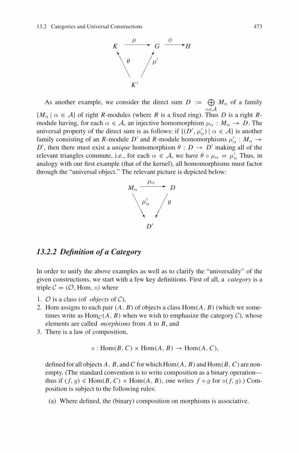
13.2 Categories and Universal Constructions 473
GK H
K ′
μ φ
θ μ′
��
���
�����
� �
As another example, we consider the direct sum D := ⊕α∈A
Mα of a family
{Mα | α ∈ A} of right R-modules (where R is a fixed ring). Thus D is a right R-module having, for each α ∈ A, an injective homomorphism μα : Mα → D. Theuniversal property of the direct sum is as follows: if {(D′,μ′
α) | α ∈ A} is anotherfamily consisting of an R-module D′ and R-module homomorphisms μ′
α : Mα →D′, then there must exist a unique homomorphism θ : D → D′ making all of therelevant triangles commute, i.e., for each α ∈ A, we have θ ◦ μα = μ′
α Thus, inanalogy with our first example (that of the kernel), all homomorphisms must factorthrough the “universal object.” The relevant picture is depicted below:
DMα
D′
μα
μ′α θ
�����
��
���
�
13.2.2 Definition of a Category
In order to unify the above examples as well as to clarify the “universality” of thegiven constructions, we start with a few key definitions. First of all, a category is atriple C = (O,Hom, ◦) where
1. O is a class (of objects of C),2. Hom assigns to each pair (A, B) of objects a class Hom(A, B) (which we some-
times write as HomC(A, B) when we wish to emphasize the category C), whoseelements are called morphisms from A to B, and
3. There is a law of composition,
◦ : Hom(B, C) × Hom(A, B) → Hom(A, C),
defined for all objects A, B, andC forwhichHom(A, B) andHom(B, C) are non-empty. (The standard convention is to write composition as a binary operation—thus if ( f, g) ∈ Hom(B, C) × Hom(A, B), one writes f ◦ g for ◦( f, g).) Com-position is subject to the following rules:
(a) Where defined, the (binary) composition on morphisms is associative.

474 13 Tensor Products
(b) For each object A, Hom(A, A) contains a special morphism, 1A, calledthe identity morphism at A, such that for all objects B, and for all f ∈Hom(A,B), g ∈ Hom(B, A),
f ◦ 1A = f, 1B ◦ g = g.
NOTE:When object A is a set, we often write idA for 1A, since the identity mappingidA : A → A, taking each element of A to itself, is the categorical morphism 1A inthat case.
Occasionally one must speak of subcategories. If C = (O,Hom, ◦) is a category,then any subcollection of objects, O0 ⊆ O, determines an induced subcategoryC0 := (O0,Hom0, ◦), where Hom0 denotes those morphisms in Homwhich connecttwo objects inO0. There is also another kind of subcategory in which the collectionof morphisms is restricted. Let C = (O,Hom, ◦), as before, and let Hom1 be asubcollection of Hom containing 1A, for all A ∈ O, with the property that if acomposition of two morphisms in Hom1 exists in Hom, then that composition liesin Hom1. Then (O,Hom1, ◦) is a morphism restricted subcategory. In general asubcategory of C is any category obtained from C by a sequence of these processes:forming induced subcategories and restricting morphisms.
There are some rather obvious categories, as follows.
1. The category Set, whose objects are all sets and whose morphisms are justmappings of sets.
2. The categories Group, Ab, Ring, Field, ModR of groups, abelian groups,rings, fields, and (right) R-modules and their relevant homomorphisms. Note thatAb is an induced subcategory of Group.
3. The category Top of all topological spaces and continuous mappings.Here are a few slightly less obvious examples.
4. Fix a group G and define the category (O,Hom, ◦) where O = G, and where,for x, y ∈ G, Hom(x, y) = {g ∈ G | gx = y}. (Thus Hom(x, y) is a singletonset, viz., {yx−1}). Here, ◦ is defined in the obvious way and is associative by theassociativity of multiplication in G.
5. Let M be a fixed monoid. We form a category with {M} as its sole object. Homwill be the set of monoid elements of M , and composition of any two of these isdefined to be their product under the binary monoid operation. (Conversely, notethat in any category with object A, Hom(A, A) is always a monoid with respectto morphism composition.)
6. Let G be a simple graph (V, E). Thus, V is a set (of vertices) and E (the set ofedges) is a subset of the set of all 2-element subsets of V . If x and y are vertices ofG,wedefine a walk from x to y to be afinite sequencew = (x = x0, x1, . . . , xn =y) where each successive pair {xi , xi+1} ∈ E for i = 0, . . . , n − 1. The graph issaid to be connected if, for any two vertices, there is a walk beginning at one ofthe vertices and terminating at the other. For a connected graph (V, E), we definea category as follows:
(a) The objects are the vertices of V .

13.2 Categories and Universal Constructions 475
(b) If x and y are vertices, then Hom(x, y) is the collection of all walks thatbegin at x and end at y. (This is often an infinite set.)
Suppose now u = (x = x0, x1, . . . , xn = y) is a walk in Hom(x, y), andv = (y = y0, y1, . . . , ym = z) is a walk in Hom(y, z). Then the compositionof the two morphisms is defined to be their concatenation, that is, the walkv ◦ u := (x = x0, . . . , xn = y0, . . . , ym = z) from x to z in Hom(x, z).
7. If G1 := (V1, E1) and G2 = (V2, E2) are two simple graphs, a graph homo-morphism φ : G1 → G2 is a set-mapping f : V1 → V2 such that if {x, y} is anedge in E1, then either f (x) = f (y) ∈ V2, or else { f (x), f (y)} is an edge in E2.The category of simple graphs, denoted Graphs, has all simple graphs and theirgraph homomorphisms as objects and morphisms. [By restricting morphisms orobjects, this category has all sorts of subcategories for which each object pos-sesses a unique “universal cover”. ]We conclude with two examples of categories that are especially relevant to theconstructions of kernel and direct sum given above.
8. Letφ : G → H be a homomorphismof groups.Define the categorywhose objectsare the pairs (L , η), where L is a group andwhere η : L → G is a homomorphismsuch that φ ◦ η : L → H is the trivial homomorphism. If (L , η), (L ′, η′) are twosuch pairs, a morphism from (L , η) to (L ′, η′) is simply a group homomorphismθ : L → L ′ such that the diagram below commutes:
L
L ′
G
θ η′
η�
�
It should be clear that the axioms of a category are satisfied for this example.9. Let {Mα | α ∈ A} be a family of right R-modules and form the category whose
objects are of the form (M, {φα | α ∈ A}), where M is a right R-module andwhere each φα is an R-module homomorphism from Mα to M . In this case amorphism from (M, {φα | α ∈ A}) to (M ′, {φ′
α | α ∈ A}) is simply an R-modulehomomorphism θ : M → M ′ such that for all α ∈ A, the following trianglecommutes:
M M ′
Mα
φαφ′
α
θ �
��
��

476 13 Tensor Products
13.2.3 Initial and Terminal Objects, and Universal MappingProperties
We continue with a few more definitions. Let C = (O,Hom, ◦) be a category andlet A and B be objects of C. As usual, let 1A and 1B be the identity morphisms ofHom(A, A) andHom(B, B). Amorphism f ∈ Hom(A, B) is called an isomorphismif there exists a morphism g ∈ Hom(B, A) such that g ◦ f = 1A and f ◦ g = 1B . Inthis case, we write f = g−1 and g = f −1. An initial object in C is an object I of Csuch that for all objects A, Hom(I, A) is a singleton set. That is to say, I is an initialobject of C if and only if, for each object A of C, there exists a unique morphismfrom I to A. Likewise, a terminal object is an object T such that for all objects A,Hom(A, T ) is a singleton set.
The following should be clear, but we’ll pause to give a proof anyway.
Lemma 13.2.1 (“Abstract Nonsense”) If the category C contains an initial object,then it is unique up to isomorphism in C. Similarly, if C contains a terminal object,it is unique up to isomorphism in C.
Proof Let I and I ′ be initial objects of C. Let f ∈ Hom(I, I ′), f ′ ∈ Hom(I ′, I ) bethe unique morphisms. Then
f ′ ◦ f ∈ Hom(I, I ) = {1I }, f ◦ f ′ ∈ Hom(I ′, I ′) = {1I ′ }.
Thus, if C has a terminal object, then it is unique. Essentially the same proof showsthat if C has a terminal object, it is unique. �
At first blush, it might seem that the notion of an initial object in a categorycannot be very interesting. Indeed, the category Group of groups and group homo-morphisms contains an initial object, viz., the trivial group {e}, which is arguably notvery interesting. At the same time the trivial group is also a terminal object in Group.Similarly, {0} is both an initial and a terminal object in ModR . As a less trivial exam-ple, note that if K is the kernel of the group homomorphism φ : G → H , then by ourdiscussions above, (K ,μ) is a terminal object in the category of example 8 above.Likewise, (
⊕α∈A
Mα, {μα | α ∈ A}) is an initial object in the category of example
9, above. In light of these examples, we shall say that an object has a universalmapping property if it is an initial (or terminal) object (in a suitable category).
In general, we cannot expect a given category to have either initial or terminalobjects. When they do, we typically shall demonstrate this via a direct construction.This is certainly the case with the kernel and direct sum; once the constructions weregiven, one then proves that they satisfy the appropriate universal mapping properties,i.e., that they are terminal (resp. initial) objects in an appropriate category.

13.2 Categories and Universal Constructions 477
13.2.4 Opposite Categories
For each category C = (O,HomC, ◦), there is an opposite category Copp =(O,Homopp, ◦′), having the same set of objects O; but we now turn the arrowsthat depict morphisms around. More precisely, f ∈ Hom(A, B), if and only iff opp ∈ Homopp(B, A). In category C, if f ∈ Hom(A, B), g ∈ Hom(B, C), so thath := g ◦ f ∈ Hom(A, C), then in category Copp we have hopp = f opp ◦′ gopp ∈Homopp(C, A). One notices that an identity mapping 1A in C becomes an identitymapping in Copp and that an initial (terminal) object in C becomes a terminal (initial)object in Copp.
A universal mapping property in one category corresponds to an “opposite” map-ping property in its opposite category. Let us illustrate this principle with the notionof the kernel. Earlier we discussed the universalmapping property of the kernel in thecategory of right R-modules. Let us do it again in a much more general categoricalcontext.
Suppose C = (O,Hom, ◦) is a category in which a terminal object T exists andthat T is also the initial object I—that is T = I . Now for any two objects A andB in O, consider the class Hom(A, B), in category C . This class always containsa unique morphism which factors through I = T . Thus there is a unique mappingτA : A → T , since T is a terminal object, and a unique mapping ιB : T = I → B,since T is also the initial object. Then 0AB := ιB ◦ τA is the unique mapping inHom(A, B) which factors though I = T . This notation, 0AB is exploited in the nextparagraphs.
Now, suppose φ : A → B is a fixed given morphism. Then the kernel of φ, is amorphism κ : (ker φ) → A such that φ ◦ κ = 0(ker φ)B , with this universal property:
If γ : X → A is a morphism of C such that φ ◦γ = 0X B , then there is a morphismθX : X → ker φ such that κ ◦ θX = γ.
Now in the opposite category this property becomes the defining property of thecokernel. Again suppose C = (O,Hom, ◦) is a category in which a terminal objectT exists and that T is also the initial object I . Fix a morphism φ : A → B. Then thecokernel (if it exists) is a morphism ε : B → C := cokerφ such that ε ◦ φ = 0AC,with the following universal property:
If ε′ : B → X is a morphism of C such that γ ◦φ = 0AX, then there exists a uniquemorphism θX : C → X such that θx ◦ ε = ε′. That is, the following diagramcommutes:
A B C
X
φ ε
ε′ θX
� �
�

478 13 Tensor Products
Again, it is easy to describe the cokernel as an initial object in a suitable categoryof diagrams that depend on the morphism φ.
13.2.5 Functors
Let C1 = (O1,Hom1, ◦1) and C2 = (O2,Hom2, ◦2) be two categories. We maywrite Homi = ∪{Homi (A, B), |A, B ∈ Oi }, the full collection of morphisms ofcategory Ci , i = 1, 2.
A covariant functor F : C1 → C2 is a pair of mappings,
FO : O1 → O2,FH : Hom1 → Hom2,
such that
(*) If f ∈ Hom1(A, B) and g ∈ Hom1(B, C), then
1. FH( f ) ∈ Hom2(F(A), F(B)), FH(g) ∈ Hom2(F(B), F(C)), and2. FH(g ◦1 f ) = FH(g) ◦2 FH( f ) ∈ Hom2(F(A), F(C)).
In other words: (1) FH is compatible with FO in the sense that if f : A → B isa morphism of C1, then FH ( f ) is a morphism in Hom2(F(A), F(B)), and (2) FH
preserves composition of mappings.Here is an example : Let C be the category of example 4 of p. 597, whose objects
were the elements of a group G and whose morphisms were the maps induced by leftmultiplication by elements of G. Then any endomorphism G → G is a a covariantfunctor of this category into itself. The reader can easily devise a similar functorusing a monoid endomorphism for example 5 of p. 597.
Here is a classic example we have met before (see p. 494). Let M be a fixedright R-module. Now for any right R-module A, the set HomR(M, A) is an abeliangroup. If f : A → B is a morphism, composing all the elements of Hom(M, A)
with f yields amapping F( f ) : Hom(M, A) → Hom(M, B) preserving the additivestructure. Thus (Hom,−) : ModR → Ab is a covariant functor from the categoryof right R-modules to the category of abelian groups.
Similarly, HomR(M,−) is a covariant functor ModR →R Mod, from the cate-gory of right R-modules to the category of left R-modules (again see p. 494).
Now suppose F is a covariant functor from category C1 = (O1,Hom1, ◦1) toC2 = (O2,Hom2, ◦2) such that FO : O1 → O2 and FH : Hom1 → Hom2 arebijections. Let F−1
O and F−1H be the corresponding inverse mappings. Then F−1 =
(F−1O , F−1
H ) preserves composition and so is a functor F−1 : C2 → C1. In this casethe covariant functor F is called an isomorphism of categories.
There is another kind of functor—a contravariant functor—which reverses thedirection and order of compositions. Again it consists of two maps: FO : O1 →O2, FH : Hom1 → Hom2, except now we have:
(1*) If f : A → B is in Hom1, then FH ( f ) ∈ Hom2(B, A).

13.2 Categories and Universal Constructions 479
(2*) If f : A → B and g : B → C are inHom1, then FH (g◦ f ) = FH ( f )◦FH (g) ∈Hom2(C, A).
Now, fixing the right R-module M , the functor Hom(−, M) : MR → Ab is acontravariant functor from the category of right R-modules to the category of abeliangroups.
There are further versions of functors of this sort, where M is a bimodule. Aclassical example is the functor which, in the category of vector spaces, takes a vectorspace to it’s dual space. Specifically, let F be a field and let Vect be the categorywhose objects are the (F, F)-bimodules—that is, F-vector spaces where αv = vαfor any vector v and scalar α. The morphisms are the linear transformations betweenvector spaces. The dual space functor HomF (−, F) : Vect → Vect takes a lineartransformation T : V → W , to the mapping HomF (W, F) → HomF (V, F) whichtakes the functional f ∈ HomF (W, F) to the functional f ◦ T ∈ HomF (V, F).
One final issue is that functors between categories can be composed: If F : C1 →C2 and G : C2 → C3 are functors, then, by composing the maps on objects and on themorphism classes: GO ◦ FO and G H ◦ FH , one obtains a functor G ◦ F : C1 → C3.Obviously
If F : C1 → C2 and G : C2 → C3 are functors, then the composite functor G ◦ F iscovariant if and only if F and G are either both covariant or both contravariant.
Of course you know where this is leading: to a “category of all categories”. Let’scall it Cat . It’s objects would be all categories (if this is even conceivable), and itsmorphisms would be the covariant functors between categories. This is a dangerousneighborhood, for as you see, Cat is also one of the objects of Cat . Clearly, we haveleft the realm of sets far behind. The point of this meditation is that actually we haveleft sets behind long ago: the collection of objects in many of our favorite categoriesAb, Ring, ModR, etc. are not sets. Of course this does not preclude them from beingcollections that possessmorphisms. These things are still amazingly useful since theyprovide us with a language in which we can describe universal mapping properties.We just have to be very careful not to inadvertently insert inappropriate axioms ofset-theory to the collections of objects of these categories.2
13.3 The Tensor Product as an Abelian Group
13.3.1 The Defining Mapping Property
Let M be a right R-module, let N be a left R-module, and let A be an abelian group.By a balanced mapping (or R-balanced mapping if we wish to specify R), we mean
2For a lucid superbly-written account of the difference between sets and classes, the authors rec-ommend the early chapters of Set Theory and the Continuum Hypothesis by Raymond Smullyanand Melvin Fitting [3].

480 13 Tensor Products
a functionf : M × N −→ A,
such that
(i) f (m1 + m2, n) = f (m1, n) + f (m2, n),(ii) f (m, n1 + n2) = f (m, n1) + f (m, n2),(iii) f (mr, n) = f (m, rn)
where m, m1, m2 ∈ M, n, n1, n2 ∈ N , r ∈ R.Define a tensor product of M and N to mean an abelian group T , together with
a balanced map t : M × N → T such that given any abelian group A, and anybalanced map f : M × N → A there exists a unique abelian group homomorphismφ : T → A, making the diagram below commute.
M × N A
T
�
� ��
��
� f
φt
Notice that a tensor product has been defined in terms of a universal mappingproperty. Thus, by our discussions in the previous section, we should be able toexpress a tensor product of M and N as an initial object of some category. Indeed,define the category having as objects ordered pairs (A, f ) where A is an abeliangroup and f : M × N → A is a balanced mapping. A morphism from (A, f ) to(A′, f ′) is an abelian group homomorphism θ : A → A′ such that the followingdiagram commutes:
M × N
A A′
f f ′
θ
��
�� �
Then the preceding diagram defining the tensor product T displays its role as aninitial object in this category. The following corollary is an immediate consequenceof “abstract nonsense” (see Lemma13.2.1).
Corollary 13.3.1 The tensor product of the right R-module M and the left R-moduleN (if it exists) is unique up to abelian group isomorphism.

13.3 The Tensor Product as an Abelian Group 481
13.3.2 Existence of the Tensor Product
Thus, there remains only the question of existence of the tensor product of the respec-tive right and left R-modules M and N . To this end, let F be the free Z-module withbasis M × N (often called “the free abelian group on the set M × N”). Let B be thesubgroup of F generated by the set of elements of the form
(m1 + m2, n) − (m1, n) − (m2, n),
(m, n1 + n2) − (m, n1) − (m, n2),
(mr, n) − (m, rn),
where m, m1, m2 ∈ M, n, n1, n2 ∈ N , r ∈ R. Write M ⊗R N := F/B and setm ⊗ n := (m, n) + B ∈ M ⊗R N . Therefore, the defining relations in M ⊗R N areprecisely
(m1 + m2) ⊗ n = m1 ⊗ n + m2 ⊗ n,
m ⊗ (n1 + n2) = m ⊗ n1 + m ⊗ n2,
mr ⊗ n = m ⊗ rn.
for all m, m1, m2 ∈ M, n, n1, n2 ∈ N , r ∈ R.The elements of the form m ⊗ n where m ∈ M and n ∈ N are called pure
tensors (or sometimes “ simple tensors”). Furthermore, from its definition, M ⊗R Nis generated by all of its pure tensors m ⊗ n, m ∈ M, n ∈ N .
Finally, define the mapping t : M × N → M ⊗R N by setting t (m, n) =m ⊗ n, m ∈ M, n ∈ N . Then, by construction, t is a balanced map. In fact:
Theorem 13.3.2 The abelian group M ⊗R N, together with the balanced map t :M × N → M ⊗R N, is a tensor product of M and N.
Proof Let A be an abelian group and let f : M × N → A be a balanced mapping. Ifthe abelian group homomorphism θ : M ⊗R N → A is to exist, then it must satisfythe condition that for allm ∈ M and for all n ∈ N , θ(m⊗n) = θ◦t (m, n) = f (m, n).Since M ⊗R N is generated by the simple tensors m ⊗ n, m ∈ M, n ∈ N , it followsthat θ : M ⊗R N → A is already uniquely determined. It remains, therefore, to showthat θ is an abelian group homomorphism. To do this, we need only verify that thedefining relations are satisfied. We have, since t and f are balanced,
θ((m1 + m2) ⊗ n) = f ((m1 + m2), n)
= f (m1, n) + f (m2, n)
= θ(m1 ⊗ n) + θ(m2 ⊗ n),
for all m1, m2 ∈ M, n ∈ N . The remaining relations are similarly verified, provingthat θ is, indeed, a group homomorphism M ⊗R M → A, satisfying θ ◦ t = f . We

482 13 Tensor Products
have already noted that θ is uniquely determined by this condition, and so the proofis complete. �
A few very simple applications are in order here. The first is cast as a Lemma.
Lemma 13.3.3 If M is a right R-module, then M ⊗R R ∼= M as abelian groups.
To show this, one first easily verifies that the mapping t : M × R → M defined bysetting t (m, r) = mr, m ∈ M, r ∈ R is balanced. Next, let A be an arbitrary abeliangroup and let f : M × R → A be a balanced mapping. Define θ : M → A bysetting θ(m) := f (m, 1R), m ∈ M . (Here 1R is the multiplicative identity elementof the ring R.) Using the fact that f is balanced, we have that θ(m1 + m2) =f (m1 + m2, 1R) = f (m1, 1R) + f (m2, 1R) = θ(m1) + θ(m2), m1, m2 ∈ M , andso θ is a homomorphism. Finally, let m ∈ M, r ∈ R; then θ ◦ t (m, r) = θ(mr) =f (mr, 1R) = f (m, r), and so θ ◦ t = f , proving that (M, t) satisfies the defininguniversal mapping property for tensor products. By Corollary13.3.1, the proof iscomplete. �Remark Of course in the preceding proof one could define e : M → M ⊗ R bysetting e(m) := m ⊗1R and then observe that the mappings t ◦e and e◦ t are identitymappings of M and M ⊗ R respectively—but that proof would not illustrate the useof the uniqueness of of the tensor product. Later in this chapter we shall encounterother proofs of an isomorphism relation which also exploit the uniqueness of anobject defined by a universal mapping property.
As a second application of our definitions the consider the following:If A is any torsion abelian group and if D is any divisible abelian group, then
D ⊗Z A = 0. If a ∈ A, let 0 = n ∈ Z be such that na = 0. Then for any d ∈ D thereexists d ′ ∈ D such that d ′n = d. Therefore d ⊗a = d ′n⊗a = d ′⊗na = d ′⊗0 = 0.Therefore every simple tensor in D⊗Z A is zero; since D⊗Z A is generated by simpletensors, we conclude that D ⊗Z A = 0.
Using the simple observation in the preceding paragraph, the reader should haveno difficulty in proving that if m and n are positive integers with greatest commondivisor d, then
Z/mZ ⊗Z Z/nZ ∼= Z/dZ
(see Exercise (2) in Sect. 13.13.2).
13.3.3 Mapping Properties of the Tensor Product
The following is an important mapping property of the tensor product.
Theorem 13.3.4 Let R be a ring, let φ : M → M ′ be a right R-module homomor-phism and let ψ : N → N ′ be a left R-module homomorphism. Then there exists aunique abelian group homomorphism φ ⊗ ψ : M ⊗R N → M ′ ⊗R N ′ such that forall m ∈ M, n ∈ N , (φ ⊗ ψ)(m ⊗ n) = φ(m) ⊗ ψ(n).

13.3 The Tensor Product as an Abelian Group 483
Proof We start by defining the mapping φ × ψ : M × N → M ′ ⊗R N ’, by the rule
(φ × ψ)(m, n) := φ(m) ⊗ ψ(n) for all m ∈ M, n ∈ N .
Using the fact that φ, ψ are both module homomorphisms, φ×ψ is easily checked tobe balanced. By the universality of M ⊗R N , there exists a unique mapping—whichwe shall denote φ ⊗ ψ—from M ⊗R N to M ′ ⊗R N ′ such that (φ ⊗ ψ) ◦ t = φ × φ,where, as usual t : M×N → M⊗R N is the balancedmapping t (m, n) = m⊗n, m ∈M, n ∈ N . Therefore, (φ ⊗ ψ)(m ⊗ n) = (φ ⊗ ψ) ◦ t (m, n) = (φ × ψ)(m, n) =φ(m) ⊗ ψ(n), and we are done. �
The following is immediate from Theorem13.3.4:
Corollary 13.3.5 (Composition of tensored maps) Let R be a ring, let Mφ→ M ′ φ′
→M ′′ be a sequence of right R-module homomorphisms, and let N
ψ→ N ′ ψ′→ N ′′ be
a sequence of left R-module homomorphisms. Then
(φ′ ⊗ ψ′) ◦ (φ ⊗ ψ) = (φ′ ◦ φ) ⊗ (ψ′ ◦ ψ) : M ⊗R N → M ′′ ⊗R N ′′.
Corollary 13.3.6 (The Distributive Law of Tensor Products) Let∑
σ∈I Aσ be adirect sum of right R-modules {Aσ|σ ∈ I }, and let N be a fixed left R-module. Then(∑
σ∈I Aσ) ⊗ N is a direct sum of its submodules {Aσ ⊗ N }.Proof ByTheorem8.1.6 on identifying internal direct sums, it is sufficient to demon-strate two things: (i) that (
∑σ∈I Aσ)⊗ N is spanned by its submodules Aσ ⊗ N and
(ii) that for any index τ ∈ I , that
(Aτ ⊗ N ) ∩∑σ =τ
Aσ ⊗ N = 0. (13.1)
We begin with (i). Any element a ∈ ∑Aσ , has the form a = ∑
τ∈S aτ where S isa finite subset of I , and aτ ∈ Aτ . From the elementary properties of “⊗” presentedat the beginning of Sect. 13.3.2, for any n ∈ N , we have a ⊗ n = ∑
S aτ ⊗ n, thesummands of which lie in submodules Aτ ⊗ N . Since (
∑σ∈I Aσ) ⊗ N is spanned
by such elements a ⊗n, it is also spanned by its submodules Aσ ⊗ N . Thus (i) holds.Since the sum
∑σ∈I Aσ is direct, there exists a family of projection mappings
{πτ : ∑σ∈I Aσ → Aτ } with the property that the restriction of πτ to the submodule
Aσ is the identity mapping if σ = τ , while it is the zero mapping Aσ → 0, wheneverσ = τ (see Sect. 8.1.8).
Now, letting 1N denote the identitymapping on the submodule N , Theorem13.3.4gives us mappings πτ ⊗1N : (
∑Aσ)⊗ N → Aτ ⊗ N whose value at a pure element
a⊗n isπτ (a)⊗n, for (a, n) ∈ (∑
Aσ)×N . Thusπτ ⊗1N restricted to the submoduleAτ ⊗ N is the identity mapping 1Aτ ⊗ 1N on that submodule. In contrast, for σ = τ ,the mapping πτ ⊗ 1N restricted to Aσ ⊗ N has image 0 ⊗ N = 0.

484 13 Tensor Products
Nowconsider an elementb ∈ (Aτ ⊗N )∩∑σ =τ (Aσ⊗N ). Then (πτ ⊗1N )(b) = b,
as b ∈ Aτ ⊗ N , while on the other hand this value is 0, since, b ∈ ∑σ =τ (Aσ ⊗ N ).
Thus b = 0 and so Eq. (13.1) holds. Thus (ii) has been established. �
Of course, a “mirror image” of this proof will produce the following:
Corollary 13.3.7 If N is a right R-module and∑
σ∈I Aσ is a direct sum of a familyof left R-modules {Aσ|σ ∈ I }, then N ⊗(
∑σ∈I Aσ) is a direct sum of its submodules
{N ⊗ Aσ|σ ∈ I }. Thus one can write
N ⊗ (⊕σ∈I
Aσ) �⊕σ∈I
(N ⊗ Aσ).
From Corollary13.3.5, we see that for any ring R and for each left R-module N ,F : ModR → Ab given by
F(M) := M ⊗R N , F(φ) := φ ⊗ idN : M ⊗R N → M′ ⊗R N
(where φ′ : M → M ′ is a right R-module homomorphism and as usual idN is theidentity mapping on N ) defines a functor.
Similarly,Theorem13.3.4 andCorollary13.3.5 tell us that for each right R-moduleM the assignment G : ModR → Ab given by
G(N ) := M ⊗R N , F(φ) := idM⊗ φ : M ⊗R N → M ⊗R N ′
(where φ : N → N ′ is a left R-module homomorphism) also defines a functor.These two functors are often denoted − ⊗R N and M ⊗R −, respectively.
We shall continue our discussion of mapping properties of the tensor product,with the existence of these functors in mind.
The next theorem shows how the tensor product behaves with respect to exactsequences. (In the language just introduced, this result describes the right exactnessof the tensor functors just introduced.)
Theorem 13.3.8 (i) Let M ′ μ→ Mε→ M ′′ → 0 be an exact sequence of right
R-modules, and let N be a left R-module. Then the sequence
M ′ ⊗R Nμ⊗idN−→ M ⊗R N
ε⊗idN−→ M ′′ ⊗R N → 0
is exact.(ii) Let N ′ μ→ N
ε→ N ′′ → 0 be an exact sequence of left R-modules, and let M bea right R-module. Then
M ⊗R N ′ idM⊗μ−→ M ⊗R NidM⊗ε−→ M ⊗R N ′′ → 0
is exact.

13.3 The Tensor Product as an Abelian Group 485
Proof We shall be content to prove (i) as (ii) is entirely similar. First of all, ifm′′ ∈ M ′′, then there exists an element m ∈ M with ε(m) = m′′. Therefore, itfollows that for any n ∈ N , (ε ⊗ idN)(m ⊗ n) = (m) ⊗ idN(n) = m′′ ⊗ n. SinceM ′′ ⊗R N is generated by the simple tensors of the form m′′ ⊗ n, we infer thatε ⊗ idN : M ⊗R N → M′′ ⊗R N is surjective.
Next, since (ε⊗ idN)(¯ ⊗ idN) = ¯ ⊗ idN = 0 : M′ ⊗R N → M′′ ⊗R N, we inferthat im (μ⊗ idN) ⊆ ker (ε⊗ idN). Next, let A be the subgroup of M ⊗R N generatedby simple tensors of the form m ⊗ n, where m ∈ ker ε. Note that it is clear thatA ⊆ ker (ε ⊗ idN). As a result, ε ⊗ idN factors through a homomorphism
ε ⊗ idN : (M ⊗R N )/A → M ′′ ⊗R N
satisfying
ε ⊗ idN(m ⊗ n + A) = ε(m) ⊗ n ∈ M ′′ ⊗R N , m ∈ M, n ∈ N .
If we can show that ε ⊗ idN is an isomorphism, we will have succeeded in showingthat A = ker ε ⊗ idN. To do this we show that ε ⊗ idN has an inverse. Indeed. definethe mapping
f : M ′′ × N → (M ⊗R N )/A, f (m′′, n) := m ⊗ n + A,
where m ∈ M is any element satisfying ε(m) = m′′. Note that if m1 ∈ M is anyother element satisfying ε(m1) = m′′, then m ⊗ n − m1 ⊗ n = (m − m1) ⊗ n ∈ A,which proves that f : M ′′ × N → (M ⊗R N )/A is well defined. As it is clearlybalanced, we obtain an abelian group homomorphism θ : M ′′⊗R N → (M ⊗R N )/Asatisfying θ(m′′ ⊗ n) = (m ⊗ n) + A, where ε(m) = m′′. As it is clear that θ isinverse to ε ⊗ idN, we conclude that A = ker (ε ⊗ idN).
Finally, note that since ker ε = im μ we have that A ⊆ im (μ ⊗ idN). Sincewe have already shown that im (μ ⊗ idN) ⊆ ker (ε ⊗ idN) = A, it follows thatim (μ ⊗ idN) = ker (ε ⊗ idN), and the proof is complete. �
We hasten to warn the reader that in Theorem13.3.8 (i) above, even if M ′ μ→ M
is injective, it need not follow that M ′ ⊗R Nμ⊗idN−→ M ⊗R N is injective. (A similar
comment holds for part (ii).) Put succinctly, the tensor product does not take shortexact sequences to short exact sequences. In fact a large portion of “homologicalalgebra” is devoted to the study of functors that do not preserve exactness. As aneasy example, consider the short exact sequence of abelian groups (i.e. Z-modules):
Zμ2→ Z → Z/2Z → 0,

486 13 Tensor Products
where μ2(a) = 2a. If we tensor the above short exact sequence on the right byZ/2Z,we get the sequence
Z/2Z0→ Z/2Z
∼=→ Z/2Z.
Thus the exactness breaks down.Motivated by Theorem13.3.8 and the above example, we call a left R-module N
flat if for any short exact sequence of the form
0 → M ′ μ→ Mε→ M ′′ → 0,
the following sequence is also exact:
0 → M ′ ⊗R Nμ⊗idN−→ M ⊗R N
ε⊗idN−→ M ′′ ⊗R N → 0.
Note that by Theorem13.3.8, one has that the left R-module is flat if and only iffor every injective right R-module homomorphism μ : M ′ → M , the inducedhomomorphism μ ⊗ idN : M′ ⊗R N → M ⊗R N is also injective.
The following lemma will prove useful in the discussion of flatness.
Lemma 13.3.9 Let R be a ring, and let F be a free left R-module with basis { fβ |β ∈B}. Let M be a right R-module. Then every element of M ⊗R F can be uniquelyexpressed as
∑β∈B
mβ ⊗ fβ , where only finitely many of the elements mβ, β ∈ B are
nonzero.
Proof First of all, it is obvious that each element of M ⊗R F admits such an expres-sion. Now assume that the element
∑β∈B
mβ ⊗ fβ = 0. We need to show that each of
the elements mβ, β ∈ B are 0. Since F is free with basis { fβ | β ∈ B}, there exist,for each β ∈ B, a so-called projection homomorphism πβ : F →R R such that
πβ( fγ) ={0 if γ = β
1 if γ = β.
Next, we recall that M ⊗R R ∼= M via the isomorphism σ : M ⊗R R → M, m⊗r →mr ∈ M (see Lemma13.3.3). Combining all of this, we have the following
0 = σ(1M ⊗ πβ)∑
mβ ⊗ fβ
= σ(mβ ⊗ 1)
= mβ .
The result follows. �

13.3 The Tensor Product as an Abelian Group 487
Remark Of course one could easily devise a proof of Lemma13.3.9 based on rightdistributive properties (see Corollary13.3.6). However here we are interested inretrieving a “flatness” result.
Theorem 13.3.10 Let R be a ring. If F is a free left R-module, then it is flat.
Proof Let { fβ | β ∈ B} be a basis of F and let μ : M ′ → M be an injectivehomomorphism of right R-modules. We shall show that the induced homomorphismμ ⊗ 1F : M ′ ⊗R F → M ⊗R F is also injective. Using Lemma13.3.9 we mayexpress a typical element of M ′ ⊗R F as
∑m′
β ⊗ fβ , where only finitely many ofthe elements m′
β, β ∈ B are nonzero. Thus, if (μ ⊗ 1F )(∑
m′β ⊗ fβ) = 0, then∑
μ(m′β)⊗ fβ = 0 ∈ M ⊗R F . But then the uniqueness statement of Lemma13.3.9
guarantees that each μ(m′β) = 0. Since μ : M ′ → M is injective, we infer that each
m′β = 0, and so the original element
∑m′
β ⊗ fβ = 0, proving the result. �
13.3.4 The Adjointness Relationship of the Hom and TensorFunctors
In this section, we use some of the elementary language of category theory intro-duced in Sect. 13.2. Let R be a ring and let RMod, Ab denote the categories of leftR-modules and abelian groups, respectively. Thus, if M is a fixed right R-module,then we have a functor
M ⊗R − :R Mod −→ Ab.
In an entirely similar way, for any fixed left R-module N , there is a functor
− ⊗R N : ModR → Ab,
where ModR is the category of right R-modules. Next we consider a functor Ab →R
Mod, alluded to in Sect. 8.4.2, Chap. 8. Indeed, if M is a fixed right R-module, wemay define
HomZ(M,−) : Ab →R Mod.
Indeed, note that if A is an abelian group, then HomZ(M, A) is a left R-module via(r · f )(m) = f (mr). For the fixed right R-module M , the functors M ⊗R − andHomZ(M,−) satisfy the following important adjointness relationship:
Theorem 13.3.11 (Adjointness Relationship) If M is a right R-module, N is a leftR-module, and if A is an abelian group, there is a natural equivalence of sets:
HomZ(M ⊗R N , A) ∼=Set HomR(N , HomZ(M, A)). (13.2)

488 13 Tensor Products
Proof One defines a mapping θ from the left side of (13.2) to the right side in thefollowing way. For each f ∈ HomZ(M ⊗R N , A) let
θ( f ) : N → HomZ(M, A)
be defined by
θ( f )(n) : M → A, where [θ(n)](m) = f (m ⊗ n)
for all n ∈ N and m ∈ M .For the inverse consider an arbitrary abelian group morphism ψ : N →
HomZ(M, A). Observe that θ∗(ψ) : M × N → A defined by θ∗(ψ)(m, n) =[ψ(m)](n) is a balancedmapping, and so factors through M ⊗R N to yield a mappingθ−1(ψ) : MR ⊗ N → A. The fact that θ−1 really is an inverse (that is, θ−1 ◦ θ andθ ◦ θ−1 are respectively the identity mappings on the left and right sides of (13.2)) iseasily verified. �
In general if C,D are categories, and if F : C → D, G : D → C are functors, wesay that F is left adjoint to G (and that G is right adjoint to F) if there is a naturalequivalence of sets
HomD(F(X), Y ) ∼=Set HomC(X, G(Y )),
where X is an object of C and Y is an object of D. Thus, we see that the functorM ⊗R − is left adjoint to the functor HomZ(M,−).
13.4 The Tensor Product as a Right S-Module
In the last section we started with a right R-module M and a left R-module N andconstructed the abelian group M ⊗R N satisfying the universal mapping propertiesrelative to balanced mappings. In this section, we shall discuss conditions that willenable M ⊗R N to carry a module structure.
To this end let S, R be rings, assume that M is a right R-module, and assume thatN is an (R, S)-bimodule. In order to give M ⊗R N the structure of a right S-module,it suffices to construct a ring homomorphism
φ : S → EndZ(M ⊗R N )∗;
where the “*” is there to indicate that the endomorphisms are to act on the right, inthis abselian group. This will allow for the definition of an S-scalar multiplication:a · s := aφ(s), a ∈ M ⊗R N . For each s ∈ S define fs : M × N → M ⊗R N bysetting fs(m, n) := m ⊗ ns, s ∈ S, m ∈ M, n ∈ N . Then fs is easily checked tobe a balanced map. By the universal mapping property of the tensor product, there

13.4 The Tensor Product as a Right S-Module 489
exists a uniqsue abelian group homomorphism φs : M ⊗R N → M ⊗R N satisfyingφs(m ⊗ n) = m ⊗ ns. Note that if m ∈ M and n ∈ N , then
φs1+s2(m ⊗ n) = m ⊗ n(s1 + s2)
= m ⊗ (ns1 + ns2)
= m ⊗ ns1 + m ⊗ ns2= φs1(m ⊗ n) + φs2(m ⊗ n)
= (φs1 + φs2)(m ⊗ n).
It follows, therefore, that φs1+s2 = φs1 + φs2 . Similarly, one verifies that φs1s2 =(φs1) · (φs2), where, for composition of right operators, the “dot” indicates that s1is applied first and s2 second. In turn, this immediately implies that the mappingφ : S → EndZ(M ⊗R N ), φ(s) := φs is the desired ring homomorphism. In otherwords, we have succeeded in giving M ⊗R N the structure of a right S-module.
The relevant universal property giving rise to a module homomorphism is thefollowing:
Theorem 13.4.1 Let R and S be rings, let M be a right R-module, and let N be an(R, S)-bimodule. If K is a right S-module and if f : M × N → K is a balancedmapping which also satisfies
f (m, ns) = f (m, n)s, s ∈ S, m ∈ M, n ∈ N ,
then the uniquely induced abelian group homomorphism θ : M ⊗R N → K is alsoa right S-module homomorphism.
Proof Let m ∈ M, n ∈ N , and let s ∈ S. Then
θ((m ⊗ n)s) = θ(m ⊗ (ns))
= θ ◦ t (m, ns)
= f (m, ns)
= f (m, n)s
= (θ ◦ t (m, n))s
= θ(m ⊗ n)s.
Since M⊗R N is generated by the simple tensorsm⊗n, m ∈ M, n ∈ N , we concludethat θ preserves S-scalar multiplication, and hence is an S-module homomorphismM ⊗R N → K . �
Corollary 13.4.2 (Exchange of Rings) Let R be a subring of S. If M is a rightR-module, then M ⊗R S is a right S-module.
Proof Since S is an (R, S)-bimodule, it can replace the module N in Theo-rem13.4.1. �

490 13 Tensor Products
A frequent example of such an exchange is the enlargement of the ground field ofa vector space: here an F-vector space V becomes V ⊗F E , where E is an extensionfield of F .3 In fact one has the following:
Corollary 13.4.3 Suppose E is a field containing F as a subfield. Let 1E denote themultiplicative identity element of E. If V is an F-vector space, then V ⊗F E is aright vector space over E. If X = {xσ} is a basis for V then X ⊗ 1E := {xσ ⊗ 1E }is an E-basis for V ⊗ E. Hence
dimF V = dimE (V ⊗ E).
The proof is left as Exercise (1) in Sect. 13.13.4.Of particular importance is the following special case. Assume that R is a com-
mutative ring. In this case, any right R-module M can also be regarded as a leftR-module by declaring that rm := mr, m ∈ M, r ∈ R. Furthermore, this specifi-cation also gives M the structure of an (R, R)-bimodule. On p. 234 we called sucha module M a symmetric bimodule. For example, vector spaces over a field arenormally treated as symmetric bimodules.
suppose M and N are such symmetric (R, R)-bimodules. Then for allm ∈ M, n ∈N , and r ∈ R, we can define left and right scalar multiplication of pure tensors bythe first and last entries in the following equations:
(m ⊗ n)r = m ⊗ (nr) = m ⊗ (rn) = (mr) ⊗ n = (rm) ⊗ n = r(m ⊗ n).
Of course, this endows M ⊗R N with the structure of a symmetric (R, R)-bimodule.Note that Theorem13.4.1 says in particular that if F is a field and if V and W are
vector spaces over F , then V ⊗F W is automatically a vector space over F . In fact,we can say more:
Theorem 13.4.4 Let F be a field, and let V and W be F-vector spaces with bases{vσ|σ ∈ I }, and {wτ |τ ∈ J }, respectively. Then V ⊗F W has basis {vσ⊗wτ | (σ, τ ) ∈I × J }. In particular,
dim F (V ⊗F W ) = dimF V · dimF W,
as a product of cardinal numbers.
Proof Since F-vector spaces are free (F, F)-bimodules, wemaywrite them as directsums of their 1-dimension subspaces. Thus
V =⊕σ∈I
vσ F , W =⊕τ∈J
Fwτ .
3Of course for over a century mathematicians (perhaps in pursuit of eigenvalues of transformations)have been replacing F-linear combinations of a basis with E-linear combinations without feelingthe need of a tensor product.

13.4 The Tensor Product as a Right S-Module 491
Now by the “distributive laws” (Corollaries13.3.6 and 13.3.7) we have
V ⊗F W =⊕
(σ,τ )∈I×J
vσ F ⊗ Fwτ .
Since each summand is an (F, F)-bimodule, we may write vσ ⊗ wτ F in place ofvσ F ⊗ Fwτ , and the direct sum of these summands is also an (F, F)-bimodule. ThusV ⊗F W is an F-vector space with basis {vσ ⊗ wτ |(σ, τ ) ∈ I × J }. �
13.5 Multiple Tensor Products and R-Multilinear Maps
Everything that we did in defining a tensor product can also be done in definingmultiple tensor products. This important topic is the basis ofwhat is calledmultilinearalgebra. There are two reasons that it should be introduced at this stage: (1) it isneeded in Sect. 13.7 to define the tensor product of algebras, and (2) it is neededagain in a construction of the tensor algebra in Sect. 13.9, and in our discussions ofthe symmetric and exterior algebras. The main idea here is to avoid having to justifyany kind of associative law of the tensor product.
Throughout this section, R is a commutative ring and all modules considered are(not neccessarily symmetric) (R, R)-bimodules.
Let {Mi |i = 1, . . . , n} be a sequence of (R, R)-bimodules, and let A be anyabelian group (with its operation denoted by addition). A homomorphism of additivegroups
α : M1 ⊕ . . . ⊕ Mn → A
is said to be balanced if, for each index i = 1, . . . , n, for each n-tuple (a1, . . . , an) ∈⊕Mi , and for any r ∈ R, one has
α((a1, . . . , air, ai+1, . . . , an)) = α(a1, . . . , ai , rai+1, ai+2, . . . , an). (13.3)
This simply extends our previous definition of balancedmappingwhere the parametern was 2.
Generalizing the recipe for the usual tensor product, we form the free Z-moduleF with basis consisting of the set of all n-tuples in M1 × . . . Mn ,4 and let B be thesubgroup of F generated by all elements of the form:
(a1, . . . , ai + a′i , . . . , an) − (a1, . . . , an) − (a1, . . . , a′
i , . . . , an)
(a1, . . . , air, ai+1, . . . , an) − (a1, . . . , ai , rai+1, . . . , an),
where i = 1, 2, . . . , n, ai , a′i ∈ Mi and r ∈ R.
4Again, the reader is warned that addition in F is not addition in⊕
Mi when the elements beingadded lie in the latter sum.

492 13 Tensor Products
Let a1 ⊗ · · · ⊗ an := (a1, . . . , an) + B, the image of (a1, . . . , an) under thecanonical projection π : F → F/B (such an element is called a pure multitensor)and we write
F/B := M1 ⊗ M2 ⊗ · · · ⊗ Mn .
Then for each i ,
a1 ⊗ · · · ⊗ (ai + a′i ) ⊗ · · · ⊗ an = (a1 ⊗ · · · ⊗ an) + (a1 ⊗ · · · ⊗ a′
i ⊗ · · · ⊗ an)
a1 ⊗ · · · ⊗ air ⊗ ai+1 ⊗ · · · ⊗ an = a1 ⊗ · · · ⊗ ai ⊗ rai+1 ⊗ · · · ⊗ an
for all a j ∈ M j , a′i ∈ Mi and r ∈ R. Thus the mapping
θ : M1 × · · · × Mn → F/B
(a restriction of π) is balanced.Conversely, suppose β is a balanced mapping
M1 × · · · × Mn → A
for some abelian group A. Using the universal property of free Z -modules, β deter-mines a unique group homomorphism β : F → A, and, since β is balanced, ker βcontains B. Thus by the Composition Theorem of homomorphisms and the twoapplications of the Fundamental Theorems of homomorphisms we have the follow-ing sequence of homomorphisms:
π : F → F/B = M1 ⊗ · · · ⊗ Mn, (13.4)
πβ : F/B → (F/B)/(ker β/B), (13.5)
iso1 : (F/B)/(ker β/B) → F/(ker β), (13.6)
iso2 : F/(ker β) → β(F), (13.7)
inc : β(F) → A (13.8)
Here, (13.4) is the afore-mentioned projection, (13.5) is a projection using B ⊆ ker β,(13.6) is a classical isomorphism, (13.7) is another classical isomorphism, and (13.8)is the inclusion mapping.
Thenβ = inc ◦ iso2 ◦ iso1 ◦ πβ ◦ π,
which is a detailed way of saying that β factors through the tensor product:
F → M1 ⊗ · · · ⊗ Mn → A.
Recalling that β is a restriction of β one concludes the following:

13.5 Multiple Tensor Products and R-Multilinear Maps 493
Theorem 13.5.1 Suppose M1, . . . , Mn, A are (R, R)-bimodules Then there is aunique balanced map t : M1 × · · · × Mn → M1 ⊗ · · · ⊗ Mn such that for anybalanced mapping
β : M1 × · · · × Mn → A,
There exists a balanced mapping
θ(β) : M1 ⊗ · · · ⊗ Mn → A
such that β = θ(β) ◦ t—that is, “β factors through the tensor product”.
The theorem is only about R-balanced mappings—certain morphisms of additivegroups. If the component Mi ’s are symmetric (R, R) bimodules, one naturally real-izes that such a theorem can hold so that the mappings involved, t , β and θ(β) areall morphisms of symmetric (R, R)-bimodules.
Theorem 13.5.2 Suppose M1, . . . , Mn, A are (R, R)-bimodules where R is a com-mutative ring and rmi = mirand ra = ar for all (r, , mi ) ∈ R × Mi × A, i ∈{1, 2, . . . , n}. Then there is a unique balanced map t : M1 × · · · × Mn →M1 ⊗ · · · ⊗ Mn such that for any balanced mapping
β : M1 × · · · × Mn → A,
There exists an (R, R)-bimodule homomorphism
θ(β) : M1 ⊗ · · · ⊗ Mn → A
such that β = θ(β) ◦ t—that is, “β factors through the tensor product”.
Remark It is important for the student to realize that in this development, themultipletensor product is not approached by a series of iterations of the binary tensor product.Rather, it is directly defined as a factor group F/B—a definition completely free ofparentheses.
13.6 Interlude: Algebras
Let A be a right R-module, where, for the moment, R is an arbitrary ring (withidentity 1R). We say that A is an R- algebra if and only if A is both a ring and thatthe R-scalar multiplication satisfies the condition
(ab)r = a(br) = (ar)b, for all a, b ∈ A, r ∈ R. (13.9)

494 13 Tensor Products
Note that as a consequence of the above requirement, we have, for all a, b ∈ A, r, s ∈R, that
(ab)(rs) = (a(br))s = ((as(br) = ((as)rb = ((a(sr))b.
Moreover if we set b = 1A, the multiplicative identity of A, in the above equation,then we obtain the fact that a(rs) = a(sr) for all a ∈ A and all r, s R. Therefore theannihilator I := AnnR(A) contains all commutators rs − sr ∈ R, from which weconclude that A is an R/I -module. Noting that R/I is a commutative ring, we seethat in our definition of R-algebra, we may as well assume—and we shall—that R iscommutative from the outset. Note that with this convention in force, the R-algebraA is a symmetric (R, R)-bimodule via the definition ra := ar, a ∈ A, r ∈ R.
We consider some familiar examples:
Example 57 Let F be a field and let Mn(F) be the ring of n × n matrices over F .Then the usual F-scalar multiplication with matrices is easily checked to provideMn(F) the structure of an F-algebra.
Example 58 Let F-be a field, let V be an F-vector space and let EndF (V ) be theset of linear transformations V → V . This is already an F-vector space by thedefinitions
(T + S)(v) := T (v) + S(v), (T α)(v) := T (vα),
T, S ∈ EndF (V ), v ∈ V, α ∈ F. Multiplication of linear transformations is justcomposition: (TS)(v) := T (S(v)), T, S ∈ EndF (V ), v ∈ V , which is again a lineartransformation. This gives EndF (V ) a ring structure. Finally, one checks that forall T, S ∈ EndF (V ) and for all α ∈ F, (TS)α = T (Sα) = (T α)S by showingthat these three linear transformations have the same effect at all v ∈ V . Therefore,EndF (V ) is an F-algebra.
Example 59 Let R be a commutative ring, let X be a set and let RX be the set offunctions X → R with ring structure given by point-wise multiplication:
( f + g)(x) := f (x) + g(x), (fg)(x) := f (x)g(x), for all f, g ∈ RX , x ∈ X.
An R-scalar multiplication can again be given point-wise:
( f · α)(x) := f (x)α, f ∈ R X , x ∈ X, α ∈ R.
The reader should have no difficulty in verifying that the above definition endowsRX with the structure of an R-algebra.
Example 60 The Dirichlet Algebra was defined as a certain collection ofcomplex-valued functions on the set of positive integers. Multiplication was a sortof convolution (see Example43 on p. 216 for details). Of course one can replace thecomplex numbers by any commutative ring R in the definition of “Dirichlet multi-plication” on the R-valued functions on the positive integers, to obtain an R-algebra.

13.6 Interlude: Algebras 495
Example 61 Let F be afield, and M be amonoid.Then the F-monoid ringFM admitsan F-scalar multiplication via pointwise scalar multiplication: if f ∈ FM, α ∈ F,
and m ∈ M , set ( f α)(m) := f (m)α. Perhaps this is made more transparent bywriting elements of M in the form f : ∑
m∈Mαmm, where the usual convention that
αm = 0 for only finitely many m ∈ M , and defining
f α :=∑
m∈M
ααmm.
This givesFM the structure of an F-algebra.We hasten to emphasize two very impor-tant special cases of this construction: the polynomial rings and group rings (over afinite group). Thus, we can—and often shall—refer to such objects as polynomialalgebras and group algebras. Note that the F-group algebra FG over the finitegroup G is finite dimensional over F .
Note that if R is a commutative ring and A is an R-algebra, then any ideal I ⊆ Aof the ring A must also be an R-submodule of A. Indeed, we realize that if 1A isthe identity of A, and if α ∈ R, then we have, for all x ∈ I , that xα = (x1A)α =x(1Aα) ∈ I , as I is an ideal. From this it follows immediately that quotients of Aby right ideals are also R-modules. Furthermore, a trivial verification reveals thatquotients of A by two-sided ideals of A are also R-algebras.
We shall conclude this short section with a tensor product formulation of R-algebras. Thus, we continue to assume that R is a commutative ring and that A isan R-module. First of all, notice that if A is an R-algebra, then by Eq. (13.9) themultiplication A × A → A in A is R-balanced, and hence factors through the tensorproduct, giving an R-module homomorphism μ : A⊗R A → A. The associativity ofthe multiplication in A translates into the commutativity of the diagram of Fig. 13.1.
At the same time, the identity element 1 ∈ A determines an R-linear homomor-phism η : R → A, defined by η(α) := 1A · α ∈ A. The fact that 1 is the identity ofA translates into the commutativity of the diagrams of the following figure, whereε : R ⊗ A → A and ε′ : A ⊗ R → A are the isomorphisms given by
ε(α ⊗ a) = αa, ε′(a ⊗ α) = aα,
a ∈ A, α ∈ R.
Fig. 13.1 Diagram forassociativity

496 13 Tensor Products
Fig. 13.2 Diagrams for atwo-sided identity
Note that the distributive laws are already contained in the above. Indeed, ifa, b, c ∈ A, then using the fact that μ : A ⊗R A → A is an abelian group homomor-phism, we have
a(b + c) = μ(a ⊗ (b + c)) = μ(a ⊗ b + a ⊗ c) = μ(a ⊗ b) + μ(a ⊗ c) = ab + ac.
Conversely, if A is an algebra over the commutative ring R, and if a multiplicationμ : A⊗R A → A is givenwhichmakes the diagrams of Figs. 13.1 and 13.2 commute,then μ gives A the structure of an R-algebra (Exercise (1) in Sect. 13.13.5).
13.7 The Tensor Product of R-Algebras
Throughout this section, we continue to assume that R is a commutative ring. IfA, B are both R-algebras, we shall give a natural R-algebra structure on the tensorproduct A ⊗R B. Recall from Sect. 13.4 that A ⊗R B is already an R-module withscalar multiplication satisfying
(a ⊗ b)α = a ⊗ bα = aα ⊗ b,
a ∈ A, b ∈ B, α ∈ R.To obtain an R-algebra structure on A ⊗R B, we map
f : A × B × A × B −→ A ⊗R B,
by setting f (a1, b1, a2, b2) = a1a2 ⊗ b1b2, a1, a2 ∈ A, b1, b2 ∈ B. Then, as f isclearly multilinear, Theorem13.5.2 gives a mapping
μ : (A ⊗R B) ⊗R (A ⊗R B) −→ A ⊗R B
such that f = μ ◦ t , where t is the standard mapping
t : A × B × A × B → A ⊗ B ⊗ A ⊗ B.
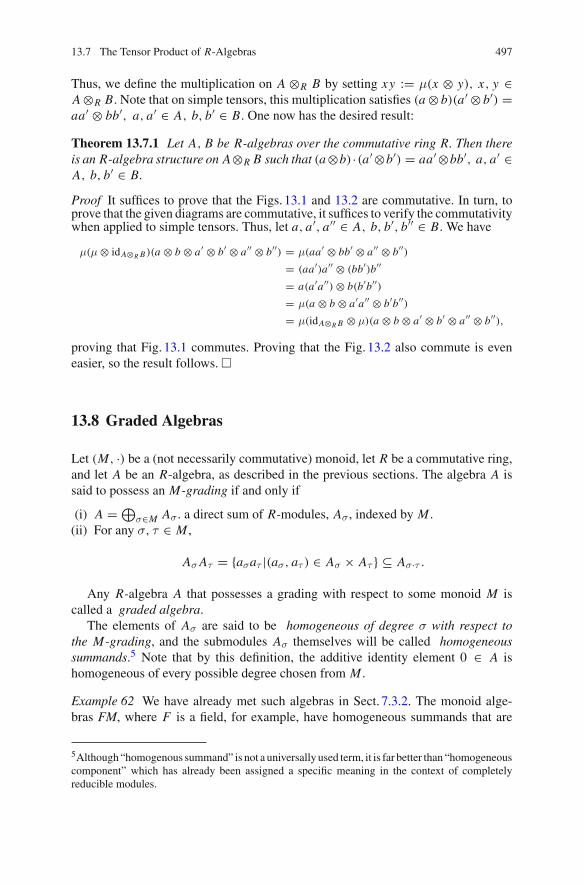
13.7 The Tensor Product of R-Algebras 497
Thus, we define the multiplication on A ⊗R B by setting xy := μ(x ⊗ y), x, y ∈A ⊗R B. Note that on simple tensors, this multiplication satisfies (a ⊗ b)(a′ ⊗ b′) =aa′ ⊗ bb′, a, a′ ∈ A, b, b′ ∈ B. One now has the desired result:
Theorem 13.7.1 Let A, B be R-algebras over the commutative ring R. Then thereis an R-algebra structure on A⊗R B such that (a⊗b) ·(a′⊗b′) = aa′⊗bb′, a, a′ ∈A, b, b′ ∈ B.
Proof It suffices to prove that the Figs. 13.1 and 13.2 are commutative. In turn, toprove that the given diagrams are commutative, it suffices to verify the commutativitywhen applied to simple tensors. Thus, let a, a′, a′′ ∈ A, b, b′, b′′ ∈ B. We have
μ(μ ⊗ idA⊗R B)(a ⊗ b ⊗ a′ ⊗ b′ ⊗ a′′ ⊗ b′′) = μ(aa′ ⊗ bb′ ⊗ a′′ ⊗ b′′)= (aa′)a′′ ⊗ (bb′)b′′
= a(a′a′′) ⊗ b(b′b′′)= μ(a ⊗ b ⊗ a′a′′ ⊗ b′b′′)= μ(idA⊗R B ⊗ μ)(a ⊗ b ⊗ a′ ⊗ b′ ⊗ a′′ ⊗ b′′),
proving that Fig. 13.1 commutes. Proving that the Fig. 13.2 also commute is eveneasier, so the result follows. �
13.8 Graded Algebras
Let (M, ·) be a (not necessarily commutative) monoid, let R be a commutative ring,and let A be an R-algebra, as described in the previous sections. The algebra A issaid to possess an M-grading if and only if
(i) A = ⊕σ∈M Aσ . a direct sum of R-modules, Aσ , indexed by M .
(ii) For any σ, τ ∈ M ,
Aσ Aτ = {aσaτ |(aσ, aτ ) ∈ Aσ × Aτ } ⊆ Aσ·τ .
Any R-algebra A that possesses a grading with respect to some monoid M iscalled a graded algebra.
The elements of Aσ are said to be homogeneous of degree σ with respect tothe M-grading, and the submodules Aσ themselves will be called homogeneoussummands.5 Note that by this definition, the additive identity element 0 ∈ A ishomogeneous of every possible degree chosen from M .
Example 62 We have already met such algebras in Sect. 7.3.2. The monoid alge-bras FM, where F is a field, for example, have homogeneous summands that are
5Although “homogenous summand” is not a universally used term, it is far better than “homogeneouscomponent” which has already been assigned a specific meaning in the context of completelyreducible modules.

498 13 Tensor Products
1-dimensional over the field F . (The converse is not true. There are M-gradedF-algebras with 1-dimensional summands, which are not monoid rings.)
We also should include in this generic example the polynomial rings D[x] andD[X ] where D is an integral domain and the respective multiplicative monoidsare respectively the powers of x , or all monomials xa1
1 xa22 · · · xan
n , ai , n ∈ N, incommuting indeterminates xi ∈ X6 Note that we must use an integral domain inorder to maintain property (i), that Aσ Aτ ⊆ Aσ·τ .
But this genus of examples also includes examples where the monoid (M, ·) isnot commutative:
1. The polynomial ring D{X} in non-commuting indeterminates, where the relevantgrading is provided by the free monoid on X (consisting of two or more symbols)whose elements are words in the alphabet X .
2. The group ring DG where G is a non-commutative group.
In these examples, which were discussed in Sects. 7.3.2 and 7.3.5, the homoge-neous summands are of the form Dm (one-dimensional if D is a field).
The following observation provides examples of graded D-algebras whose homo-geneous summands are not of this form.
Lemma 13.8.1 Let A be an D-algebra graded with respect to a monoid (M, ·).Suppose φ : (M, ·) → (M ′, ·) is a surjective homomorphism of monoids. For eachelement m′ of the image monoid M ′, define
Am′ :=∑
φ(σ)=m′Aσ.
Then the direct decomposition A = ⊕m′∈M ′ Am′ , defines a grading of A with respect
to the image monoid M ′.
Proof We need only show that if m′1 and m′
2 are elements of M ′, then Am′1Am′
1⊆
Am′1·m′
2. But if φ(mi ) = m′
i , i = 1, 2, then φ(m1 · m2) = m′1m′
2, since φ is a monoidmorphism. Thus Am1 Am2 ⊆ Am′
1·m′2for all mi such that φ(mi ) = m′
i , i = 1, 2. SinceAm′
i= ∑
φ(m)=m′i
Am , the result follows. �
In effect, the monoid homomorphism φ produces a grading that is more “course”than the original M-grading.
Example 63 The (commutative) polynomial ring R[X ], where R is any commutativering, is graded by themultiplicativemonoidM∗(X) of finitemonomials chosen fromX . As noted in Sect. 7.3.5, p. 205, there is a monoid morphism
deg : M∗(X) → (N,+)
6Recall that these monoids are respectively isomorphic to (N,+) and the additive monoid of allfinite multisets chosen from X . (Once again, we remind the beginning reader that the set of naturalnumbers, N, includes 0.).

13.8 Graded Algebras 499
which is defined by
deg :n∏
i=1
xaii →
n∑i=1
ai
for any finite subset {x1, . . . , xn} of X . The image degm is called the degree of m,for monomial m ∈ M∗(X).
Assume that A, A′ are both M-graded algebras over the commutative ring R. Analgebra homomorphism φ : A → A′ is said to be a graded algebra homomorphismif for each m ∈ M, φ(Am) ⊆ A′
m . When A is an M-graded algebra over R, we shallbe interested in ideals I ⊆ A for which R/I is also M-graded and such that theprojection homomorphism A → A/I is a homomorphism of M-graded algebras.
For example, suppose A = D[x], the usual polynomial ring, and the ideal I isAxn , n > 1. Then is one writes Ai := xi D, 0 ≤ i ≤ n − 1, then
A/I = (A0 + I )/I ⊕ (A1 + I )/I ⊕ · · · ⊕ (An−1 + I )/I
is a grading on A/I by the monoid Z/nZ.On the other hand assume that D = F is a field, and let I be the ideal of A = F[x]
generated by the inhomogeneous polynomial x + x2. By the division algorithm, wesee that the quotient algebra A/I has dimension 2 over the field F .
Assume, however, that A/I is graded by the nonnegative integers, and that A →A/I is a homomorphism of graded algebras. This would yield
A/I =∞∑
m=0
(Am + I )/I.
Since, for each nonnegative integer m, Am = F · xm , we would have (Am + I )/I =F(xm + I ) = 0, since xm cannot be a multiple of x + x2. In turn, this would clearlyimply that A/I is infinite dimensional, contradicting our prior inference that A/Ihas F-dimension 2. Thus A/I is not a graded algebra in this case.
Motivated by the above, we call the ideal I of the M-graded R-algebra A homo-geneous if
A/I =⊕m∈M
(Am + I )/I.
Note that this implies both that A/I is M-graded via (A/I )m = (Am + I )/I andthat the projection homomorphism A → A/I is a homomorphism of M-gradedR-algebras.
Theorem 13.8.2 Let A be an M-graded R-algebra, and let I be an ideal of A. Then,the following are equivalent:
(i) I is homogeneous,(ii) I = ⊕
m∈M(Am ∩ I ),

500 13 Tensor Products
(iii) I is generated by homogeneous elements.
Proof Assume (i), i.e., that I is homogeneous; thus
A/I =⊕m∈M
(Am + I )/I.
Let x ∈ I and write x as x = ∑m∈M
xm , where each xm ∈ Am . We shall show that, in
fact, each xm ∈ I . For otherwise, we would have
0 + I = x + I =∑
m∈M
xm + I =∑
m∈M
(xm + I ).
Since the last sum is direct, we conclude that each xm + I = 0 + I , i.e., that eachxm ∈ I . This implies that I = ∑
m∈M(Am ∩ I ). Since this sum is obviously direct, we
infer (ii).If we assume (ii), and if elements am ∈ Am are given with
∑m∈M
(am + I ) = 0 + I ∈ A/I,
then ∑m∈M
am ∈ I =∑
m∈M
(Am ∩ I ).
This clearly forces each am ∈ (Am ∩ I ) ⊆ I , and so the sum∑
m∈M(Am + I )/I is
direct. As it clearly equals A/I , we infer condition (i). Thus, conditions (i) and (ii)are equivalent.
If we assume condition (ii), then it is clear that I is generated by homogeneouselements, as each Am ∩ I, m ∈ M consists wholly of homogeneous elements, so(iii) holds.
Finally, assume condition (iii). The homogeneous elements that lie in the ideal Iform a set S = ∪σ∈M (I ∩ Aσ), which, by hypothesis, generates I as a 2-sided ideal.Let
H :=⊕σ∈M
Hσ where Hσ = I ∩ Aσ, (13.10)
so that H is the additive group generated by S. Clearly H ⊆ I . Since part (ii) ofthe definition of an M-grading requires that homogeneous elements be closed undermultiplication, we see that if h is an arbitrary homogeneous element of A, then
hS ∪ Sh ⊆ S,

13.8 Graded Algebras 501
since the products to the left of the containment symbol are homogeneous elementsof A lying in the ideal I . It follows that hH andHh both lie in H for any homogeneouselement h chosen from A. Since the additive span of these homogeneous elements isA itself, the distributive law of the ring yields AHA ⊆ H , so H is itself a two-sidedideal of A. Since H contains S the ideal-generators of I , we have I ⊆ H . SinceH ⊆ I we also have H = I and now Eq. (13.10) produces
I =⊕σ∈M
(I ∩ Aσ),
proving (ii).Thus all three conditions (i), (ii), and (iii) are equivalent. �
13.9 The Tensor Algebras
13.9.1 Introduction
In this section and the nextwe hope to introduce several basic algebraswith importantuniversal properties. There are two ways to do this: (1) first define the object by aconstruction, and then show it possesses the desired universal property, or (2) firstbase the definition upon a universalmapping property, and then utilize our categoricalarguments for uniqueness to show that it is something we know or can construct.We think that the second strategy is particularly illustrative in the case of the tensoralgebra.
13.9.2 The Tensor Algebra: As a Universal Mapping Property
Fix a vector space V over a field F . The tensor algebra of V is defined to bea pair (ι, T (V )) where ι : V → T (V ) is an injection of V into an F-algebra,T (V ) such that every F-linear transformation t : V → A into an F-algebra Auniquely factors through ι—that is, there exists a unique F-algebra homomorphismθ(t) : T (V ) → A, such that θ(t) extends t . In other words t = θ(T ) ◦ ι and we havethe commutative triangle below:
V T (V )
A
�
��
�
�
ι
t θ
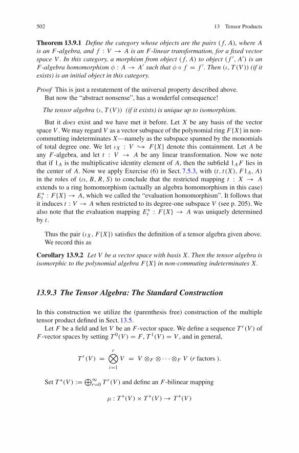
502 13 Tensor Products
Theorem 13.9.1 Define the category whose objects are the pairs ( f, A), where Ais an F-algebra, and f : V → A is an F-linear transformation, for a fixed vectorspace V . In this category, a morphism from object ( f, A) to object ( f ′, A′) is anF-algebra homomorphism φ : A → A′ such that φ ◦ f = f ′. Then (ι, T (V )) (if itexists) is an initial object in this category.
Proof This is just a restatement of the universal property described above.But now the “abstract nonsense”, has a wonderful consequence!
The tensor algebra (ι, T (V )) (if it exists) is unique up to isomorphism.
But it does exist and we have met it before. Let X be any basis of the vectorspace V . We may regard V as a vector subspace of the polynomial ring F{X} in non-commutting indeterminates X—namely as the subspace spanned by the monomialsof total degree one. We let ιX : V ↪→ F{X} denote this containment. Let A beany F-algebra, and let t : V → A be any linear transformation. Now we notethat if 1A is the multiplicative identity element of A, then the subfield 1A F lies inthe center of A. Now we apply Exercise (6) in Sect. 7.5.3, with (t, t (X), F1A, A)
in the roles of (α, B, R, S) to conclude that the restricted mapping t : X → Aextends to a ring homomorphism (actually an algebra homomorphism in this case)E∗
t : F{X} → A, which we called the “evaluation homomorphism”. It follows thatit induces t : V → A when restricted to its degree-one subspace V (see p. 205). Wealso note that the evaluation mapping E∗
t : F{X} → A was uniquely determinedby t .
Thus the pair (ιX , F{X}) satisfies the definition of a tensor algebra given above.We record this as
Corollary 13.9.2 Let V be a vector space with basis X. Then the tensor algebra isisomorphic to the polynomial algebra F{X} in non-commuting indeterminates X.
13.9.3 The Tensor Algebra: The Standard Construction
In this construction we utilize the (parenthesis free) construction of the multipletensor product defined in Sect. 13.5.
Let F be a field and let V be an F-vector space. We define a sequence T r (V ) ofF-vector spaces by setting T 0(V ) = F , T 1(V ) = V , and in general,
T r (V ) =r⊗
i=1
V = V ⊗F ⊗ · · · ⊗F V (r factors ).
Set T ∗(V ) := ⊕∞r=0 T r (V ) and define an F-bilinear mapping
μ : T ∗(V ) × T ∗(V ) → T ∗(V )

13.9 The Tensor Algebras 503
by setting
μ
( ∞∑r=0
τr ,
∞∑s=0
τ ′s
):=
∞∑k=0
∑r+s=k
τr ⊗ τ ′s ∈ T r+s(V ) ⊆ T ∗(V ).
This is easily verified to endow T ∗(V ) with the structure of an F-algebra, called thetensor algebra over F . When V has a basis X , then T ∗(V ) has an F-basis consistingall pure tensors of the form x1 ⊗· · ·⊗ xd , where d ∈ N, the xi are in X and an emptyproduct is taken to be the identity element e of T ∗(V ). In terms of this basis of puretensors the multiplication follows this rule:
μ(v1 ⊗ · · · ⊕ vn, vn+1 ⊗ · · · ⊗ vn+m) = v1 ⊗ · · · ⊗ vn+m . (13.11)
Since this is simply a concatenation of pure multitensors, the operation is asso-ciative.
Let ι : V = T 1(V ) → T ∗(V ), be the (injective) containment mapping. We shallshow that the pair (ι, T ∗(V )) satisfies the universal mapping property of our previousdefinition of a tensor algebra T (V ).
Theorem 13.9.3 Fix an F-vector space V . Define the category whose objects arethe pairs (A, f ), where A is any F-algebra, and f : V → A is any F-lineartransformation. A morphism from (A, f ) to (A′, f ′) in this category is an F-algebrahomomorphism φ : A → A′ such that φ ◦ f = f ′. Then (ι, T ∗(V )) (the embeddingof V into it’s tensor algebra) is an initial object in this category.
Proof Let (A, f ) be an object in this category. Note that if φ : T (V ) → A is anF-algebra homomorphism such that φ ◦ ι = f , then for all nonnegative integers r ,we must have φ(v1 ⊗ v2 ⊗ · · · ⊗ vr ) = f (v1) f (v2) · · · f (vr ). Since any elementof T (V ) is a sum of such simple tensors, we must have that φ : T (V ) → A mustbe unique. It remains to prove the existence of such a mapping φ. First define, φ0 :T 0(V ) = Fe → F1A, to be the F-linear mapping which takes the identity elemente of T ∗(V ) to 1A, the identity element of the algebra A. Now, by Theorem13.5.2,for each positive integer r > 0, the F-balanced mapping
fr : V × V × · · · × V → A, where fr (v1, v2, . . . , vr ) = f (v1) f (v2) · · · f (vr ).
induces a unique F-linear mapping
φr : T r (V ) = V ⊗F V ⊗F ⊗F · · · ⊗F V → A,

504 13 Tensor Products
where φr (v1 ⊗ v2 ⊗ · · · ⊗ vr ) = f (v1) f (v2) · · · f (vr ). In turn, by the universality
of the direct sum T ∗(V ) =∞⊕
r=0T r (V ), we then get a unique F-linear mapping
φ : T ∗(V ) =∞⊕
r=0
T r (V ) → A
which is an F-algebra homomorphism. This proves the existence of φ, and the resultfollows. �
At this point, we know from the uniqueness of initial objects that the three objectsT (V ), F{X} (where X is a basis of V ) and T ∗(V ) are all three the same object.7
In fact, the isomorphism T ∗(V ) → F{X} is induced by the following mappingconnecting their basis elements:
e → 1, the monic polynomial of degree zero
x1 ⊗ · · · ⊗ xn → x1x2 · · · xn , a monomial of degree n
(Here n is any positive integer and the xi lie in X , a basis for V .)From now on we will write T (V ) for T ∗(V ).
13.10 The Symmetric and Exterior Algebras
13.10.1 Definitions of the Algebras
Inside the tensor algebra T (V )over the field F , we define the following homogeneousideals (cf. Theorem13.8.2):
(i) I ⊆ T (V ), generated by all elements of the form v ⊗ w − w ⊗ v, v,w ∈ V ;(ii) J ⊆ T (V ), generated by all simple tensors of the form v ⊗ v, v ∈ V .
In terms of the above ideals, we now define the symmetric algebra over V tobe S(V ) := T (V )/I . Likewise, we define the exterior algebra by setting E(V ) :=T (V )/J . By Theorem13.8.2, these are both graded algebras. Thus,
S(V ) =∞⊕
r=0
Sr (V ), where each Sr (V ) = (T r (V ) + I )/I,
7Up to isomorphism, of course.

13.10 The Symmetric and Exterior Algebras 505
and
E(V ) =∞⊕
r=0
Er (V ), where each Er (V ) = (T r (V ) + J )/J.
(Many authors write∧
V for E(V ) and then write∧r V for Er (V ).)
We denote by ιS : V → S(V ) and by ιE : V → E(V ) the F-linear mappings
ιS(v) := v + I ∈ S(V ), ιE (v) := v + J ∈ E(V ), v ∈ V .
Since it is clear that V ∩ I = V ∩ J = 0, we see that ιS and ιE are both injec-tive F-linear transformations. We shall often identify V with their respective imagesubspaces ιS(V ) ⊆ S(V ) and ιE (V ) ⊆ E(V ) and write V ⊆ S(V ) and V ⊆ E(V ).
Multiplication in S(V ) is typicallywritten simply as juxtaposition: if a, b ∈ S(V ),then the product of a and b is denoted ab ∈ S(V ).We note that S(V ) is a commutativealgebra. Indeed, any element of S(V ) is an F-linear combination of elements of theform v1v2 · · · vr (that is, the product v1⊗v2⊗· · ·⊗vr + I ), where v1, v2, . . . , vr ∈ V .Now write
a := v1v2 · · · vr , b := w1w2 · · ·ws,
where v1, . . . , vr , w1, . . . , ws ∈ V . Since for any vectors v,w ∈ V we havevw = wv, it follows immediately that ab = ba and so it follows easily that S(V ) iscommutative, as claimed.
In the exterior algebra, products are written as “wedge products”: if c, d ∈ E(V ),their product is denoted c ∧ d . It follows immediately that for all vectors v,w ∈ V ,one has v ∧ v = 0, and from (v + w) ∧ (v + w) = 0 one obtains v ∧ w = −w ∧ v.
Like the tensor algebra, the universal properties satisfied by the symmetric andexterior algebras involve an F-linear mapping V → A into an F-algebra A. Such anF-linear mapping is said to be commuting if and only if f (u) f (v) = f (v) f (u) forall u, v ∈ V—that is, the image f (V ) generates a commutative subring. Similarlysuch a mapping is said to be alternating if and only if f (v)2 = 0, for all v ∈ V .
Theorem 13.10.1 Let F be a field, let V be a vector space over F, and letS(V ), E(V ) be the symmetric and exterior algebras over V , respectively.
(i) Consider the category of pairs (A, f ) of F-algebras and commuting F-linearmappings f : V → A. A morphism from the pair (A, f ) to the pair (A′, f ′) is anF-algebra homomorphism φ : A → A′ such that φ ◦ f = f ′. Then (S(V ), ιS)
is an initial object in this category.(ii) Consider the category of pairs (A, f ) of F-algebras and alternating F-linear
mappings f : V → A. A morphism from the pair (A, f ) to the pair (A′, f ′) is anF-algebra homomorphism φ : A → A′ such that φ ◦ f = f ′. Then (E(V ), ιE )
is an initial object in this category.
We shall leave the proof to the motivated reader in Exercise (2) in Sect. 13.13.7.The uniqueness of these algebras follows. Whenever one hears the word “unique-
ness” in a categorical setting, one knows that isomorphisms are being implied, and so

506 13 Tensor Products
a number of corollaries can be expected to result from the precedingTheorem13.10.1.We produce some of them in the next subsection.
13.10.2 Applications of Theorem 13.10.1
A Model for S(V )
We begin with this example: From the uniqueness assertion in Theorem13.10.1,one can easily exploit the evaluation morphism of polynomial rings (in commutingindeterminates) to prove the following:
Corollary 13.10.2 Let X be an F-basis for the vector space V . Then S(V ) ∼= F[X ]as F-algebras.
The proof is simply that the universal property of the evaluation mapping Eα
for polynomial rings in commuting indeterminates proves that the pair (ιX , F[X ])satisfies the universal mapping property of the tensor algebra. (See Sect. 7.3 forbackground and Exercise (8) in Sect. 7.5.3 for the universal property. A formal proofis requested in Exercise (3) in Sect. 13.13.7.)
A Model for E(V )
Let (X,≤) denote a totally ordered poset bijective with a basis X of the vector spaceV . Let C be the collection of all finite ascending subchains (including the emptychain, φ) of (X,≤). (Clearly this collection is in one-to-one-correspondence withthe finite subsets of X . It forms a boolean lattice (C,≤) under the refinement relationamong chains. Thus the “join” c1 ∨ c2, is the smallest chain refining both c1 and c2.)For every non-empty ascending chain c = {x1 < · · · < xr } ∈ C , let wc be theword x1x2 · · · xr (viewed either as a word in the free monoid over X or simply as asequence of elements of X ). For the empty chain φ we denote wφ by the symbol e.(For convenience, we shall refer to these wc as “chain-words”.)
Let A be the F-vector space defined as the formal direct sum
E =⊕c∈C
Fwc.
Weconvert A into an F-algebra by definingmultiplication between basis elementsand extending this to a definition ofmultiplication ( “∗”) on A by the usual distributivelaws. In order to accomplish this we consider two chains a = {x1 < · · · < xr } andb = {y1 < · · · < ys}.We letm(a, b)be the number of pairs (xk, yl) such that xk > yl .Then if the two chains a and b possess a common element, we set a∗b := 0. But if thechains a and b possess no common element, their disjoint union can be reassembled

13.10 The Symmetric and Exterior Algebras 507
into a properly ascending chain c = a ∨ b, the smallest common refinement of thechains a and b. In that case we set
a ∗ b := (−1)m(a,b)wc.
(Note that (−1)m(a,b) is simply the sign of the permutation π(a, b) of indices thatpermutes the concatenated sequence wa · wb to wa∨b.)
Two make sure that the student gets the sense of this, note that when (X,≤) ={1 < 2 < · · · < 9}, we have
(1 < 2 < 4 < 7) ∗ (3 < 6 < 7) = 0 while
(1 < 2 < 4 < 7) ∗ (3 < 6 < 8) = −(1 < 2 < 3 < 4 < 6 < 7 < 8).
To show that “∗” is an associative binary operation for A it is enough to checkit on the basis elements—the chains. Thus we wish to compare two products (a ∗b) ∗ c and a ∗ (b ∗ c) where wa, wb, wc are the respective ascending sequences(a1, . . . , ar ), (b1 . . . , bs), (c1, . . . , ct ).Wemay assume r, s, t are all positive integersand that a, b and c pairwise share no common element (otherwise (a ∗ b) ∗ c = 0 =a ∗ (b ∗ c)). Form the concatenation of sequences
wa · wb · wc = (a1, . . . , ar , b1, . . . , bs, c1, . . . , ct ) = (y1, . . . , yr+s+t ) := y,
and let π be the permutation of indices so that {yπ(i)}r+s+ti=1 is in ascending order,
thus realizing the chain a ∨ b ∨ c. (We view the group of permutations of sequencesas acting on sequences from the right, so that a factorization of permutations π1π2means π1 is applied first.) Now the permutation π has two factorizations: (i) π =π(a, b) · π(a ∨ b, c) and (ii) π = π(b, c)π(a, b ∨ c). Here π(a, b) fixes the last tindices to effectwa ·wb ·wc → wa∨b ·wc, while π(a ∨b, c) rearranges the entries ofthe latter sequence to produce wa∨b∨c. So (i) holds. Similarly, we could also applyπ(b, c) to the last s + t entries in y = wa · wb · wc while fixing the first r entries toget wa ∗ wb∨c and then apply π(a, b ∨ c) to obtain the ascending sequence wa∨b∨c.Thus the factorization (ii) holds.
Now (a ∗ b) ∗ c = a ∗ (b ∗ c) = sgn(π)(a ∨ b ∨ c) follows from the associativityof the “join” operation in (C,≤), the definition of “∗”, and
sgn(π) = sgn(π(a, b))sgn(π(a ∨ b, c)) = sgn(π(b, c))sgn(π(a, b ∨ c)),
given to us by the factorizations (i) and (ii).Now, extending the binary operation ∗ to all of A by linearity from its definition
on the basis C , we obtain an F-vector space A with an associative binary operation“∗” which distributes with respect to addition and respects scalar multiplication fromF on either side. One easily checks that e ∗ a = a ∗ e = a for each a ∈ A, so e is amultiplicative identity. Thus (A, ∗) is an algebra.

508 13 Tensor Products
Notice that the lengths of the chains produce a grading A = ⊕Ad where, for
every natural number d , Ad is the subspace spanned by all wc as c ranges over thechains of length d. Thus A0 = Fe and Ar ∗ As ⊆ Ar+s .
At this stage we see that (A, ∗) is a genuine graded F-algebra which we call thealgebra of ascending chains. Its dimension is clearly the number of finite subchainsof (X,≤), and if V has finite dimension n then A has dimension 2n .
There is a natural injection ιA : V → A mapping linear combinations of basiselements xi of V to the corresponding linear combination of chain-wordswi := w{xi }of length one.
If xσ < xτ is a chain, and wσ = ιA(xσ) and wτ = ιA(xτ ) are the length-onechain words {xσ} and {xτ }, we have
w2σ = w2
τ = 0 (writing a2 for a ∗ a ) and
wσ ∗ xτ = −wτ ∗ xσ.
This gives usw2v = 0 for every vector v ∈ V , and so ιA : V → A is an alternating
mapping as defined above. Thus the universal property of E(V ) requires that there is aunique algebra epimorphism ε : E(V ) → A extending ιA. If V had finite dimension,we would know at once that ε is an isomorphism. Instead we obtain the isomorphismby showing that (A, ιA) possesses the desired universal mapping property.
Suppose f : V → (B, ◦) is an alternating mapping into an F-algebra B havingidentity element 1B . Then of course
f (v)2 = 0, and (13.12)
f (u) ◦ f (v) = − f (v) ◦ f (u) (13.13)
for all vectors u, v ∈ V .We then define an F-linear mapping α f : A → B by describing its values on a
basis for A. Firstwe setα f (e) = 1B . For eachfinite ascending chain c = (x1, . . . , xn)
in (X,≤) we setα f (wc) = f (x1) · · · f (xn).
This can be extended to linear combinations of the xi to yield
α f (ιA(v)) = f (v), for all v ∈ V .
We also note that for any two finite ascending chains a and b in (X,≤), we have
α f (wa ∗ wb) = f (wa) ◦ f (wb).
So once again extending by linearity, we see that
α f : A → B

13.10 The Symmetric and Exterior Algebras 509
is an algebra homomorphism and that α f ◦ ιA = f . Thus A possesses the uni-versal property which defines the exterior algebra. By the uniqueness asserted inTheorem13.10.1, we have a companion to Corollary13.10.2:
Corollary 13.10.3 Suppose V is any F-vector space. Then the exterior algebraE(V ) is isomorphic to the algebra (A, ∗) of finite ascending chains of a total orderingof a basis X of V .
In particular, if V is an F-vector space of finite dimension n, then the exterioralgebra E(V ) is isomorphic to the algebra of ascending chains, (A, ∗) based on thechain N = {1 < · · · < n}. It is a graded algebra of dimension 2n.
Morphisms Induced on S(V ) and E(V )
Suppose t : V → V is any F-linear transformation of V . Then, ιS ◦ t is a commutingmapping V → S(V ) and so, by the universal mapping property of S(V ) (placing(ιS ◦ t, S(V )) in the role of (t, A)), we obtain an algebra homomorphism
S(t) : S(V ) → S(V )
which forces the commutativity of the following diagram:
S(V )S(t)−−−−→ S(V )
ιS
�⏐⏐ �⏐⏐ιS
Vt−−−−→ V
The algebra homomorphism S(t) : S(V ) → S(V ) preserves the grading and soinduces morphisms
Sr (t) : Sr (V ) → Sr (V )
taking any product of elements of V , v1v2 · · · vn , to vt1 · · · vt
n where vt denotes theimage of the vector v ∈ V under the linear transformation t .
It is apparent that if s, t ∈ homF (V, V ), then
Sr (s ◦ t) = Sr (s) ◦ Sr (t).
The same journey can be emulated for the exterior algebra E(V ) using its par-ticular universal mapping property. Given F-linear t : V → V one obtains thealternating mapping ιE ◦ t → E(V ) and so by the universal mapping property, acommutative diagram

510 13 Tensor Products
E(V )E(t)−−−−→ E(V )
ιE
�⏐⏐ �⏐⏐ιE
Vt−−−−→ V
where the algebra homomorphism E(t) at the top of the diagram preserves degreesand so induces mappings
Er (t) : Sr (V ) → Er (V )
taking a product of vectors in V , v1 ∧ v2 ∧ · · ·∧ vn to vt1 ∧ · · ·∧ vt
n where vt denotesthe image of an arbitrary vector v under the linear transformation t . Again
Er (s ◦ t) = Er (s) ◦ Er (t).
We collect these observations in this way:
Corollary 13.10.4 Suppose t ∈ homF (V, V ). Let
ιS : V → S(V ), and
ιE : V → E(V )
be the canonical embeddings of V into the symmetric and exterior algebras, respec-tively.
Then there exist F-algebra homomorphisms
S(t) : S(V ) → S(V ) and
E(t) : E(V ) → E(V )
such that one has
S(t) ◦ ιS = ιS ◦ t, and
E(t) ◦ ιE = ιE ◦ t,
respectively. Both S(t) and E(t) preserve the algebra grading and so induce map-pings
Sr (t) : Sr (V ) → Sr (V ) and
Er (t) : Er (V ) → Er (V ).
For any r-tuple (v1, . . . , vr ) ∈ V (r) one has
Sr (t)(v1 · · · vn) = vt1v
t2 · · · vt
r , and
Er (t)((v1 ∧ · · · ∧ vr ) = at1 ∧ · · · ∧ vt
r .

13.10 The Symmetric and Exterior Algebras 511
Finally if the symbol � denotes either T, T r , S, Sr , E, or Er , one has
�(s ◦ t) = �(s) ◦ �(t). (13.14)
Remark Of course by now even the beginning student has noticed that T, T r ,S, Sr , E, and Er—all of them—are functors V → V where V is an appropriatesub-category of Vect, the category of all F-vector spaces.
There are other consequences of Corollary13.10.4. For example, if t : V → V isan invertible linear transformation, then so are S(t), Sr (t), E(t) and Er (t). Thus
Corollary 13.10.5 If t : V → V is invertible, then S(t)and E(t)are automorphismsof the F-algebras S(V ) and E(V ), respectively.
In particular, there are injective homomorphisms
ρS : GL(V ) → Aut(S(V ))
ρE : GL(V ) → Aut(E(V ))
whose images elements preserve the grading.As a result, for any subgroup G of GL(V ) one obtains group representations
ρrS : G → GL(Sr (V ))
ρrE : G → GL(Er (V ))
Remark All of the results above were consequences of just one result: Theo-rem13.10.1. There is a lesson here for the student.8 It is that universal mappingproperties—as abstract as they may seem—possess a real punch! Suppose you are ina situation where something is defined in the heavenly sunlight of a universal map-ping property. Of course that does not mean it exists. But it does mean, that any twoconstructions performed in the shade which satisfy this universal property (whetherknown or new) are isomorphic (a consequence of the “nonsense” about initial andterminal objects in a category). So we prove existence. What more is there to do,one might ask? The answer is that one does not so easily depart from a gold minethey are standing on. Here are three ways the universal characterizations produceresults: (1) It is a technique by which one can prove that two constructed algebraicobjects are isomorphic—simply show that they satisfy the same universal mappingproperty within the same category. (2) One can prove that an object defined in onecontext has a specific property by recasting it in the context of another “solution”of the same universal mapping property. (3) One can prove the existence of derivedendomorphisms and automorphisms of the universal object.
8Of course such a phrase should be a signal that the teacher is about to become engulfed by theurge to present a sermon and that perhaps the listener should surreptitiously head for an exit! Buthow else can a teacher portray a horizon beyond a mere list of specific theorems?.

512 13 Tensor Products
13.11 Basic Multilinear Algebra
In Sect. 13.5 we proved that R-multibalanced mappings from a finite direct sum ofsymmetric (R, R)-bimodules to a target (R, R)-bimodule factored through the mul-tiple tensor product (see Theorem13.5.2). In this brief subsection we wish to extendthis theorem to alternating and symmetric forms (the key theorems of multilinearalgebra), but we shall do this in the case that R is a field so that we can exploituniversal properties of the symmetric and exterior algebras developed in the pre-vious section. As the student shall observe, the device for transferring statementsabout algebras to statements about multilinear mappings depends critically upon ourdiscussion of graded algebras and homogeneous ideals.
First the context: Let V and W be vector spaces over a field F . We regard both Vand W as symmetric (F, F)-bimodules—that is αv = vα for all (α, v) ∈ F × V orF × W .
A mappingf : V × · · · × V (n factors) → W
is F-multilinear if and only if (1) it is an F-linear mapping of the n-fold directproduct (and so preserves addition in the direct product) and (2) that for any n-tupleof vectors of V , (v1, . . . , vn), for any field element α ∈ F , and for any index j < n,one has
f (v1, . . . , v jα, v j+1, . . . , vn) = f (v1, . . . , v j ,αv j+1, . . . , vn) (13.15)
= ( f (v1, . . . , vn))α. (13.16)
Such an F-multilinear mapping is said to be alternating if and only iff (v1, . . . , vn) = 0 if at least two distinct entries among the vi are equal. By consid-ering a sequence whose i th and (i + 1)st entries are both vi + vi+1, one sees that foran alternating F-multilinear mapping f , the sign of f (v1, . . . , vn) is changed by thetransposition of entries in the i th and (i + 1)st positions. It follows that the sign is infact changed by any odd permutation of the entries, but the value of f is preservedby any even permutation of the entries.
An F-multilinear mapping f : V × · · · × V (n factors) → W is said to be sym-metric if f (v1, . . . , . . . , vn) is unchanged under the transposition (vi , vi+1) inter-changing the two entries in the i th and i +1st positions. It then follows that the valueof f is unchanged by any permutation of its arguments.
Theorem 13.11.1 (Fundamental Theorem of Multilinear Mappings) Let V be avector space over a field F, viewed as an (F, F)-bimodule so that αv = vα for all(α, v) ∈ F × V . Throughout, we assume that f is an F-multilinear mapping
f : V × · · · × V (n factors) → W
into another (F, F)-bimodule W . The following three statements hold:

13.11 Basic Multilinear Algebra 513
1. f = f ◦ ι where f is a homomorphism
f : T n(V ) = V ⊗ . . . ⊗ V → W,
uniquely determined by f . Specifically, the mapping f “factors through f ” sothat
f (v1, . . . , . . . , vn) = f (v1 ⊗ · · · ⊗ vn).,
for all n-tuples of vectors vi ∈ V .2. Now suppose the mapping f is alternating. Then the mapping f factors through
a unique mapping
fE : En(V ) = V∧
· · ·∧
V (n factors) → W
so thatf (v1, . . . , . . . , vn) = fE (v1 ∧ v2 ∧ · · · ∧ vn),
for all n-tuples of vectors vi ∈ V .3. Finally suppose the multilinear mapping f is symmetric. Then f factors
through a unique fS : Sn(V ) → W where Sn(V ) is the space of all homo-geneous elements of degree n in the graded symmetric algebra S(V ). Thusf (v1, . . . , vn) = fS(v1 · · · vn).
Proof Part 1 is just Theorem13.5.2 with the commutative ring R replaced by a field.Part 2. By definition E(V ) = T (V )/J where J is the homogeneous ideal given
at the beginning of Sect. 13.10. We have these direct decompositions:
T (V ) = F ⊕ V ⊕ T 2(V ) ⊕ · · · ⊕ T r (V ) ⊕ · · · (13.17)
J (V ) = F ∩ J ⊕ (V ∩ J ) ⊕ · · · ⊕ (T r (V ) ∩ J ) ⊕ · · · (13.18)
E(V ) = F ⊕ V ⊕⊕∞
r=2(T r (V )/(T r (V ) ∩ J )) (13.19)
= F ⊕ V ⊕ V ∧ V ⊕ · · ·r∧
(V ) ⊕ · · · (13.20)
The first two summands in Eq. (13.18) are of course zero. Comparing degreecomponents in the last two equations yields
n∧(V ) ∼= T n(V )/(T n(V ) ∩ J ). (13.21)
Now, since f is multilinear, it factors through f : T n(V ) → W as in part 1. Butsince f is alternating, we see that ker f contains (T n(V ) ∩ J ). Thus it follows that

514 13 Tensor Products
f factors through this chain:
T n(V ) → T n(V )/(T n(V ) ∩ J ) → [T n(V )/(T n(V ) ∩ J )]/(ker f /(T n(V ) ∩ J ))
∼= T n(V )/ ker f ∼= f (T n(V ) ↪→ W.
(The first two morphisms are natural projections, the next two isomorphisms arefrom the classical homomorphisms theorems, and the last mapping is the inclusionrelation into W .) Folding in the isomorphism of Eq. (13.21) at the second term andcomposing with the remaining mappings we obtain the desired morphism
f nE :
n∧(V ) → W
through which f (and hence f ) factors. That
f (v1, . . . , vn) = f (v1 ⊗ · · · ⊗ vn) = f nE (v1 ∧ · · · ∧ vn)
follows upon applying the mappings.Part 3 follows the samepattern except thatweuse the ideal I , given at the beginning
of Sect. 13.10, in place of J . Again one exploits the fact that I is a homogeneousideal to deduce that Sn(V ) ∼= T n(V )/(T n(V ) ∩ I ). We leave the student to fill inthe details in Exercise (1) in Sect. 13.13.8. �
13.12 Last Words
From here the subject of multilinear algebra begins to blend with another subjectcalled Geometric Algebra. Although space does not allow us to pursue the lattersubject, a hint of its flavor may be suggested by the following.
Suppose V is both a left vector space, as well as a right vector space over a divisionring D. Do not assume that V is an (D, D)-bimodule. (This would virtually makeD a field.) A 2-form is a bi-additive mapping f : V × V → D such that
f (αu, vβ) = α f (u, v)β for all α,β ∈ D,u, v,∈ V .
If g = α f for a fixed scalar α in D, then g is said to be proportional to f . Such a2-form f is said to be reflexive if and only if f (u, v) = 0 implies f (v,u) = 0, andis non-degenerate if and only if f (v, V ) = 0, implies v = 0, u, v ∈ V .
Theorem 13.12.1 Suppose dim V ≥ 2 and f : V × V → F is a reflexive non-degenerate 2-form, where F is a field. Then f is proportional to a 2-form g such thatfor all u, v ∈ V exactly one of the following holds:
(i) g(u, v) = g(v,u), (symmetric form)

13.12 Last Words 515
(ii) g(u,u) = 0, (alternating of symplectic form)(iii) g(u, v) = g(v,u)σ , where σ is a field automorphism of order 2 (Hermitian
form).
The first case can be derived from quadratic forms (see Exercise (9) inSect. 13.13.7). All three cases are the children of a description of 2-forms over divi-sion rings—the so-called (σ, ε)-Hermitian forms (see [2], pp. 199–200 for versionsof J. Tits’ proof that reflexive forms must take this shape).
There are many beautiful results intertwining 2-forms and multilinear forms aswell as widespread geometric applications of such forms. The interested student isreferred to the classic book Geometric Algebra by E. Artin [1], which, after morethan fifty years, now begs for an update.
13.13 Exercises
13.13.1 Exercises for Sect. 13.2
1. Letφ : M → N be a homomorphismof right R-modules. Recall that the cokernelof φ was defined by a universal mapping property on p. 477, in any category forwhich an initial object exists and is also a terminal object. (i) In the categoryof right R-modules, show that the projection π : N → N/im φ satisfies thismapping property. (ii) In the category of groups and their homomorphisms, docokernels of homomorphisms exist? If so define it. [Hint: Examine the universalmapping property of a cokernel in this category.]
2. Given the morphism Mφ→ N in the category of right R-modules, define a
category within which the cokernel of φ appears as an initial object.3. Let {Mα | α ∈ A} be a family of right R-modules. Recall from p. 260 that if
P := ∏α∈A
Mα, then P satisfies the following universal mapping property: First of
all, there are projection homomorphisms πα : P → Mα, α ∈ A; if P ′ is anotherright R-module with homomorphisms π′
α : P ′ → Mα, α ∈ A, then there existsa unique R-module homomorphism θ : P ′ → P , making the following diagramcommute for every α ∈ A.
P ′
P Mα
θ πα
π′α
�
��
� �
Now define a category within which the direct product P appears as a terminalobject.

516 13 Tensor Products
4. Let X be a fixed set and define the following category. The objects are the pairs(G,μ), where G is a group and μ : X → G is a mapping of the set X intoG. A morphism from the (G,μ) to the pair (G ′,μ′) is a group homomorphismφ : G → G ′ such that μ′ = φ ◦ μ. Show how the free group F(X) on the set Xaffords an initial object in this category.
5. Rephrase and repeat the above exercise with “groups” replaced with “right R-modules”. [Hint: The free module with basis X replaces the free group F(X).]
6. Suppose F : C1 → C2 is a contravariant functor. Show that there are also covariantfunctors F ′ : Copp
1 → C2 and F ′′ : C1 → Copp2 .
7. Show that there exists an isomorphism C → (Copp)opp which induces the identitymapping on objects. (It may move maps, however.)
13.13.2 Exercises for Sect. 13.3
1. Let A be an abelian group. If n is a positive integer, prove that
Z/nZ ⊗Z A ∼= A/n A.
2. Let m, n be positive integers and let d = g.c.d(m, n). Prove that
Z/mZ ⊗Z Z/nZ ∼= Z/dZ.
3. Let0 → M ′ μ→ M
ε→ M ′′ → 0
be a split exact sequence of right R-modules, and let N be a left R-module. Showthat the induced sequence
0 → M ′ ⊗R Nμ⊗1N−→ M ⊗R N
ε⊗1N−→ M ′′ ⊗R N → 0
is also split exact. Prove the corresponding statement if the split exact sequenceoccurs as the right hand factor of the tensor product sequence.
4. Prove that if P is a projective left R-module, then P is flat. [Hint: Letμ : M ′ → Mbe an injective homomorphism of right R-modules. We know that P is the directsummand of a free left R-module F , and so there must be a split exact sequenceof the form
0 → Pi→ F
j→ N → 0,
for some left R-module N . ByExercise 3we know that both 1M ′ ⊗i : M ′⊗R P →M ′⊗R F and 1M ⊗i : M⊗R P → M⊗R F are injective.Wehave the commutativesquare

13.13 Exercises 517
M ′ ⊗R Pμ⊗1P−−−−→ M ⊗R P
1M ′⊗l
⏐⏐� ⏐⏐�iM ⊗l
M ′ ⊗R Fμ⊗1F−−−−→ M ⊗R F
Now what?]5. Generalize the proof of Theorem13.3.8 so as to prove the following. Let R be a
ring, let M, M ′ be right R-modules, and let N , N ′ be left R-modules. Let φ :M → M ′ and letψ : N → N ′ bemodule homomorphisms. Define K ⊆ M ⊗R Nto be the subgroup generated by simple tensors m ⊗ n where either m ∈ ker φ orn ∈ ker ψ. Show that, in fact, K = ker (φ ⊗ ψ : M ⊗R N → M ′ ⊗R N ′).
13.13.3 Exercises for Sect. 13.3.4
1. Let C be a category and let μ : A → B be a morphism. We say that μ is amonomorphism if whenever A′ is an object with morphisms f : A′ → A, g :A′ → A such that μ ◦ f = μ ◦ g : A′ → B, then f = g : A′ → A. In otherwords, monomorphisms are those morphisms that have “left inverses.” Similarly,epimorphisms are those morphisms that have right inverses. Now assume thatC,D are categories, and that F : C → D, G : D → C are functors, with Fleft adjoint to G. Prove that F preserves epimorphisms and that G preservesmonomorphisms.
2. Let i : Z ↪→ Q be the inclusion homomorphism. Prove that in the category ofrings, i is an epimorphism. Thus an epimorphism need not be surjective.
3. Let V, W be F-vector spaces and let V ∗ be the F-dual of V . Prove that there is avector space isomorphism V ∗ ⊗F W ∼= HomF(V, W ).
4. Let G be a group. Exactly as in Sect. 7.3.2, we may define the integral group ringZG. (These are formal Z-linear combinations of group elements in G.) In thisway a group gives rise to a ring. Correspondingly, given a ring R we may form itsgroup of units U (R). This time, a ring is giving rise to a group. Show that thesecorrespondences define functors
Z : Groups −→ Rings, U : Rings −→ Groups.
Prove that Z is left adjoint to U .5. Below are some further examples of adjoint functors. In each case you are to
prove that F is left adjoint to G.
(a)
GroupsF−→ Abelian Groups
G↪→ Groups;
F is the commutator quotient map.

518 13 Tensor Products
(b)
SetsF−→ Groups
G−→ Sets,
where F(X) = free group on X and G(H) is the underlying set of the groupH .
(c)
Integral DomainsF−→ Fields
G↪→ Integral Domains;
F(D) is the field of fractions of D. (Note: for this example we considerthe morphisms of the category Integral Domains to be restricted only toinjective homomorphisms.)
(d) Fix a field K .
K − Vector SpacesF−→ K − Algebras
G−→ K − Vector Spaces;
F(V ) = T (V ), the tensor algebra of V and G(A) is simply the underlyingvector space structure of algebra A.
(e)
Abelian GroupsF−→Torsion Free Abelian Groups
G↪→ Abelian Groups;
F(A) = A/T (A), where T (A) is the torsion subgroup of A.(f)
Left R-modulesF−→ Abelian Groups
G−→ Left R-modules.
F is the forgetful functor, G = HomZ(R,−).
(g) If G is a group, denote by G Set the category of all sets X acted on by G.If X1, X2 are objects in G Set then the morphisms from X1 to X2 are themappings in HomG(X1, X2). Let H be a subgroup of G. Then an adjointfunctor pair is given by
G SetF→ H Set
I G→ G Set
where, for G-set X , and H -set Y , F(X) = ResGH (X), I G(Y ) = IndG
H (Y ).[The induced action of G on Y × G/H , denoted by the symbol IndG
H (Y ), isdefined in Exercise 7 of the following Sect. 13.13.4 on p. 519.]
13.13.4 Exercises for Sect. 13.4
1. Give a formal proof of Corollary13.4.3, which asserts that if F ⊆ E is an exten-sion of fields, and V is an F-vector space with basis {xi }, then as an E-vector

13.13 Exercises 519
space, V ⊗F E has basis {xi ⊗ 1E }. [Hint: Write V = ∑xi F and use Corol-
lary13.3.6.]2. Let T : V → V be a linear transformation of the finite-dimensional F-vector
space V . Let mT,F (x) denote the minimal polynomial of T with respect to thefield F . If F ⊆ E is a field extension, prove that mT,F (x) = mT ⊗1V ,E (x). [Hint:Apply the previous Exercise 1, above.]
3. LetW be an F-vector space and let T : V1 → V2 be an injective linear transforma-tion of F-vector spaces. Prove that the sequence T ⊗1W : V1⊗F W → V2⊗F W isinjective. (Note that by Theorem13.3.8, we’re really just saying that every objectin the category of F-vector spaces is flat.)
4. Let F be a field and let A ∈ Mn, B ∈ Mm be square matrices. Define theKronecker (or tensor) product A ⊗ B as follows. If A = [aij], B = [bkl ], thenA ⊗ B is the block matrix [Dpq], where each entry Dpq (in row p and column qof D) is the m × m matrix Dpq = apq B. Thus, for instance, if
A =[
a11 a12a21 a22
], B =
[b11 b12b21 b22
].
then
A ⊗ B =
⎡⎢⎢⎣
a11b11 a11b12 a12b11 a12b12a11b21 a11b22 a12b21 a12b22a21b11 a21b12 a22b11 a22b12a21b21 a21b22 a22b21 a22b22
⎤⎥⎥⎦ .
Now Let V, W be F-vector spaces with ordered bases A = (v1, v2, . . . , vn),
B = (w1, w2, . . . , wm), respectively. Let T : V → V, S : W → W be lineartransformations with matrix representations TA = A, SB = B. Assume thatA ⊗ B is the ordered basis of V ⊗F W given by A ⊗ B = (v1 ⊗ w1, v1 ⊗w2, . . . , v1 ⊗ wm; v2 ⊗ w1, . . . , v2 ⊗ wm; . . . , vn ⊗ wm). Show that the matrixrepresentation of T ⊗ S relative toA⊗ B is given by (T ⊗ S)A⊗TB = TA ⊗ TB(the Kronecker product of matrices given earlier in this exercise) .
5. Let V be a two-dimensional vector space over the field F , and let T, S : V → Vbe linear transformations. Assume the minimal polynomials of S and T are givenby:mT (x) = (x −a)2, mS(x) = (x −b)2. (Therefore T and S can be representedby 2×2 Jordan blocks, J2(a), J2(b), respectively.) Compute the invariant factorsof T ⊗ S : V ⊗V → V ⊗V . (See Sect. 10.7.2, p. 349, for notation and definitionsconcerning minimal polynomials and Jordan blocks.)
6. Let M be a right R-module, and let I ⊆ R be a 2-sided ideal in R. Prove that, asright R-modules,
M ⊗R (R/I ) ∼= M/MI.
7. (Induced representations) Here is an important application of the tensor prod-uct. Let G be a finite group, let F be a field, and let FG be the F-group ring

520 13 Tensor Products
(see Sect. 7.3). Note that FG is clearly an F-vector space via scalar multiplication
α∑g∈G
αgg :=∑g∈G
(ααg)g, α ∈ F.
Likewise, if M is any right FG-module, then M naturally carries the structure ofan F-vector space by setting α · m := m(αe), α ∈ F, m ∈ M , where e is theidentity of the group G. Now let H be a subgroup of G and regard FH as a subringof FG in the obvious way. Let V be a right FH-module, finite dimensional overF , and form the induced module
IndGH (V ) := V ⊗FH FG.
Since FG is an (FH, FG)-bimodule, we infer that, in fact, IndGH (V ) is actually a
right FG-module. Now show that
dimF IndGH (V ) = [G : H ] · dim V .
8. Let A be an abelian group. Prove that a ring structure on A is equivalent to anabelian group homomorphism μ : A ⊗Z A → A, together with an element e ∈ Asuch that μ(e ⊗ a) = μ(a ⊗ e) = a, for all a ∈ A, and such that
A ⊗Z A ⊗Z A
A ⊗Z A
A ⊗Z A
A�
�
μ
1 ⊗ μ
μ ⊗ 1 μ
commutes. (The above diagram, of course, stipulates that multiplication is asso-ciative.)
9. The following theorem is an application of the tensor product to ideal classes inthe field of fractions of a Dedekind Domain.
Theorem 13.13.1 Let I and J be fractional ideals in the field of fractions E of aDedekind domain R. If [I ] = [J ] (that is, I and J belong to the same ideal class inE) then I and J are isomorphic as right R-modules.
Provide a proof of this theorem. (The converse is easy: see Exercise (5) inSect. 9.13.5.) [Hint: First, since I has the form αI ′ for some α ∈ E and idealI ′ in R, we have [I ] = [I ′]. Thus, without loss of generality, we may assume thatI is an ideal of R. Note that since R is an integral domain, themultiplicative identityof R is the multiplicative identity 1E of E . Define the injections i I : I → I ⊗R Eand i J : J → J ⊗R E by

13.13 Exercises 521
i I (r) → r ⊗ 1E , and
i J (s) → s ⊗ 1E
for all (r, s) ∈ I × J .Now consider the commutative diagram below:
I J
I ⊗R E J ⊗R E E
�
�
� �
��
����
�
φ
φ ⊗ 1E
iI i J
ε
i
where i I , i J are the injections, given above, ε : J ⊗R E → E is given byε(b ⊗ λ) = bλ, and where i : J ↪→ E is the containment mapping. Note also thatφ ⊗ 1E : I ⊗R E → J ⊗R E is an E-linear transformation.Next, note that if 0 = a0 ∈ I , then (a0 ⊗ a−1
0 )a = (a0 ⊗ 1)a−10 a = (a0 ⊗
a)a−10 = (aa0 ⊗ 1)a−1
0 = (a ⊗ a0)a−10 = (a ⊗ 1)a−1
0 a0 = a ⊗ 1. Therefore,set α0 := ε(φ ⊗ 1)(a0 ⊗ a−1
0 ) ∈ E and obtain φ(a) = ε(φ ⊗ 1)(a ⊗ 1) =ε(φ ⊗ 1)((a0 ⊗ a−1
0 )a) = ε(φ ⊗ 1)(a0 ⊗ a−10 )a = α0a ∈ J . Since φ : I → J is
an isomorphism, the result follows.]
13.13.5 Exercises for Sects. 13.6 and 13.7
1. Show that if R is a commutative ring, and if A is an R-module, then a multipli-cation μ : A ⊗R A → A gives A the structure of an R-algebra if and only if thediagrams in Figs. 13.1 and 13.2 (see p. 495) are commutative.
2. Let A1, A2 be commutative R-algebras. Prove that A1 ⊗R A2 satisfies a univer-sal condition reminiscent of that for direct sums of R-modules. Namely, thereexist R-algebra homomorphisms μi : Ai → A1 ⊗R A2, i = 1, 2 satisfying thefollowing. If B is any commutative R-algebra such that there exist R-algebrahomomorphisms φi : Ai → B, then there exists a unique R-algebra homomor-phism θ : A1 ⊗R A2 → B such that for i = 1, 2, the diagram
Ai B
A1 ⊗R A2
�
� �
��
�� φi
θμi
commutes.

522 13 Tensor Products
3. Prove that R[x] ⊗R R[y] ∼= R[x, y] as R-algebras.4. Let F be a field and form F-group algebras for the finite groups G1, G2 as in
Sect. 7.3. Prove that F[G1 × G2] ∼= FG1 ⊗F FG2 as F-algebras.
13.13.6 Exercises for Sect. 13.8
1. Let A be an R-algebra graded over the nonnegative integers. We say that A isgraded-commutative if whenever ar ∈ Ar , as ∈ As we have ar as = (−1)rsasar .
Now let A =∞⊕
r=0Ar , B =
∞⊕s=0
Bs be graded-commutative R-algebras. Prove that
there is a graded-commutative algebra structure on A ⊗R B satisfying
(ar ⊗ bs) · (ap ⊗ bq) = (−1)sp(ar ap ⊗ bsbq),
ar ∈ Ar , ap ∈ Ap, bs ∈ Bs, bq ∈ Bq . (This is usually the intended meaning of“tensor product” in the category of graded-commutative R-algebras.)
13.13.7 Exercises for Sect. 13.10
1. Assume that the F-vector space V has dimension n. For each r ≥ 0, computethe F-dimension of Sr (V ).
2. Prove Theorem13.10.1.3. Prove Corollary13.10.2.4. (Determinants) Let T : V → V be a linear transformation, and assume that
dim V = n. Show that there exists a scalar det(T ), such that
En(T ) = det T · idEn(V ) : En(V ) → En(V ).
Cite the results in Sect. 13.9 that show, for S, T ∈ Hom(V, V ), that
det(S) · det(T ) = det(S ◦ T ) = det(T ◦ S).
5. Let G → GLF (V ) be a group representation on the F-vector space V . Showthat the mapping G → GLF (Er (V )) given by g → Er (g) defines a grouprepresentation on Er (V ), r ≥ 0.
6. Let V be a vector space and let v ∈ V . Define the linear map · ∧ v : Er (V ) →Er+1(V ) by ω → ω ∧ v. If dim V = n, compute the dimension of the kernel of· ∧ v.
7. (Boundary operators) Let V be n-dimensional over the field F , and having basis{v1, v2, . . . , vn}. For each integer r, 1 ≤ r ≤ n, define the linear transformation∂r : Er (V ) → Er−1(V ), from its value on basis elements by setting

13.13 Exercises 523
∂r (vi1 ∧ vi2 ∧ · · · ∧ vir ) =r∑
j=1
(−1) j−1vi1 ∧ vi2 ∧ · · · ∧ vi j ∧ · · · ∧ vir ,
where (·) means delete the factor (·). The mapping ∂0 : E1(V ) = V →E0(V ) = F is the mapping determined by ∂0(vi ) = 1, i = 1, 2, . . . , n.
(a) Show that if r ≥ 1, then ∂r−1∂r = 0 : Er (V ) → Er−2(V ).(b) Define a mapping hr : Er (V ) → Er+1(V ), 0 ≤ r ≤ n − 1 by setting
hr (η) = v1 ∧ η, where η ∈ Er (V ).Show that if 1 ≤ r ≤ n − 1, then ∂r+1hr + hr−1∂r = idEr (V ), and thathn−1∂n = idEn(V ), ∂1h0 = idE0(V ).
(c) Conclude that the sequence
0 → En(V )∂n→ En−1 ∂n−1→ En−2 → · · · ∂2→ E1(V )
∂1→ E0(V ) → 0
is exact.
8. Let V be an F-vector space. An F-linear mapping δ : E(V ) → E(V ) is calledan antiderivation if for all ω ∈ Er (V ), η ∈ Es(V ) we have
δ(ω ∧ η) = δ(ω) ∧ η + (−1)rω ∧ δ(η).
Now let f : V → F be a linear functional, and show that f can be extendeduniquely to an antiderivation δ : E(V ) → E(V ) satisfying δ(v) = f (v) ·1E(V ),for all v ∈ V . In addition, show that δ satisfies
(a) δ : Er (V ) → Er−1(V ), r ≥ 1, δ : E0(V ) → {0}.(b) δ2 = 0 : E(V ) → E(V ).
9. (The Clifford Algebra) Let V be an F-vector space and let Q : V → F be afunction. We call Q a quadratic form if Q satisfies
(a) Q(αv) = α2Q(v), for all α ∈ F, v ∈ V , and(b) the mapping B : V × V → F given by
(v,w) → Q(v + w) − Q(v) − Q(w)
defines a (clearly symmetric) bilinear form on V .
Given the quadratic form Q on V , we define a new algebra, C(Q), the Cliffordalgebra, as follows. Inside the tensor algebra T (V ) define the ideal I to begenerated by elements of the form v ⊗ v − Q(v) · 1F , v ∈ V . (Note that I isnot a homogeneous ideal of T (V ).) The Clifford algebra is the quotient algebraC(Q) = T (V )/I .Show that C(Q) satisfies the following universal criterion. Assume that C ′ isan F-algebra and that there exists a linear mapping f : V → C ′ such that for

524 13 Tensor Products
all v ∈ V , ( f (v))2 = Q(v) · 1C ′ . Prove that there exists a unique F-algebrahomomorphism γ : C(Q) → C ′ making the following triangle commute:
V C ′
C(Q)
�
� ��
��
� f
γι
(In the above diagram, ι : V → C(Q) is just the natural homomorphism v →v + I .)
10. Let V be an n-dimensional F-vector space. If d ≤ n, define the (n, d)-Grassmann space, Gd(V ) as the set of all d-dimensional subspaces of V . Inparticular, if d = 1, the set G1(V ) is more frequently called the projective spaceon V , and is denoted by P(V ).9 We define a mapping
φ : Gd(V ) −→ P(Ed(V )),
as follows. IfU ∈ Gd(V ), let {u1, . . . ,ud} be a basis ofU , and let φ(U ) be the 1-space in P(Ed(V )) spanned by u1∧· · ·∧ud . Prove thatφ : Gd(V ) → P(Ed(V ))
is a well-defined injection of Gd(V ) into P(Ed(V )). (This mapping is called thePlücker embedding.)
11. Let V be an n-dimensional vector space over the field F .
(a) Show that if 1 < d < n − 1, then the Plücker embedding φ : Gn−1(V ) −→P(En−1(V )) is never surjective. [Hint: Why is it sufficient to consider only(d, n) = (2, 4)?]
(b) If F is a finite field Fq , show that the Plücker embedding φ : Gn−1(V ) −→P(En−1(V )) is surjective. This implies that every element of z ∈ En−1(V )
can be written as a “decomposable element” of the form z = v1 ∧ v2 ∧· · · ∧ vn−1 for suitable vectors v1, v2, . . . , vn−1 ∈ V . [An obvious countingargument.] .
12. Let V, W be F-vector spaces. Prove that there is an isomorphism
⊕i+ j=r
Ei (V ) ⊕ E j (W ) −→ Er (V ⊕ W ).
9 In geometry, the terms “Grassmann space”, and “Projective space” not only include the “points”,Gd (V ) and G1(V ), respectively, but also include collections of “lines” as well. In the case of theprojective space, the lines are G2(V ), while, for the Grassmann space Gd (V ), 1 < d < n, the linesare all pairs (X, Y ) ∈ Gd−1(V ) × Gd+1(V ) such that X ⊂ Y . The “points” belonging to (X, Y ) arethose Z ∈ Gd (V ) such that X ⊂ Z ⊂ Y . These lines correspond to 2-dimensional subspaces ofEd (V ).

13.13 Exercises 525
13. Let V be an F-vector space, where char F = 2. Define the linear transformationS : V ⊗ V → V ⊗ V by setting S(v ⊗ w) = w ⊗ v.
(a) Prove that S has minimal polynomial mS(x) = (x − 1)(x + 1).(b) If V1 = ker(S − I ), V−1 = ker(S + I ), conclude that V ⊗ V = V1 ⊕ V−1.(c) Prove that V1 ∼= S2(V ), V−1 ∼= E2(V ).
(d) If T : V → V is any linear transformation, prove that V1 and V−1 areT ⊗ T -invariant subspaces of V ⊗ V .
14. Let V be an n-dimensional F-vector space.
(a) Prove that E(V ) is graded-commutative in the sense of Exercise (1) inSect. 13.13.6.
(b) If {Li }, i = 1, . . . , n, is a collection of one-dimensional subspaces of Vwhich span V , prove that as graded-commutative algebras,
E(V ) ∼= E(L1) ⊗ E(L2) ⊗ · · · ⊗ E(Ln)
15. Let G = GL(V ) act naturally on the n-dimensional F-vector space V so that Vbecomes a right FG-module..
(a) Show that the recipe g( f ) = det g · f ◦g−1, g ∈ G, f ∈ V ∗ = Hom(V, F),defines a representation of G on V ∗, the dual space of V .
(b) Show that in the above action, G acts transitively on the non-zero vectors ofV ∗.
(c) Fix any isomorphism En V ∼= F ; show that the map En−1(V ) → V ∗ givenby ω → ω ∧ · is a morphism of right FG-modules, i.e., the map commuteswith the action of G.
(d) A vector z ∈ Ed(V ) is said to be decomposable or pure if and only if ithas the form z = v1 ∧ · · · ∧ vd for suitable vectors vi ∈ V . Since G clearlyacts on the set of decomposable vectors in En−1(V ), conclude from (b) thatevery vector in En−1 is decomposable.
16. (Veronesean action)Againfixavector spaceV withfinite basis X = {x1, . . . , xn}with respect to the field F .
(a) Lef f : V → F be a functional (that is, a vector of the dual space V ∗).Show that Sd( f ) is a linear mapping Sd(V ) → F , and so is a functional ofSd(V ), 1 ≤ d ≤ n.
(b) Set G = GL(V ). First let us view V as a left G-module. Thus for allS, T ∈ G and v ∈ V , we have (ST )v = S(T (v)). If f ∈ Hom(V, F) andT ∈ G, then f ◦ T is also a functional. Show that for all ( f, T ) ∈ V ∗ × G,the mapping
f → f ◦ T
defines a right action of G on V ∗ ( i.e. V ∗ becomes a right FG-module).[Hint: One must show that f ◦ (ST ) = f ◦ S ◦ T . One can check these mapsat arbitrary v ∈ V recalling that the operators T, S and f operate on V from

526 13 Tensor Products
the left.] (By way of comparison with part (a) of the previous exercise, notethat we have defined a representation of G on the dual space V ∗, withoutemploying the determinant.)
(c) For each f ∈ Hom(V, F), and integer d ≥ 1, Sd( f ) : Sd(V ) → F is afunctional of Sd(V ) called a Veronesean vector. With respect to the basisX = {xi }, we may regard Sd(V ) as the space of homogeneous polynomi-als of degree d in F[x1, . . . , xn]. If f (xi ) = εi ∈ F , show that at eachhomogeneous polynomial p ∈ Sd(V ),
f (p(x1, . . . , xn)) = p(ε1, . . . , εn) ∈ F.
conclude from this, that if (α, f ) ∈ F × V ∗, then
Sd(α f ) = αd Sd( f ). (13.22)
Describe how this produces a bijection between the 1-dimensional sub-spaces of V ∗ (the points of the projective space P(V ∗)) and the 1-spaces ofSd(V )∗ spanned by the individual Veronesean vectors. (The latter collectionof 1-dimensional subspaces is called the (projective) Veronesean variety ofdegree d.) [Hint: Use Eq. (13.22).]
(d) Prove that the (right) action of G = GL(V ) on V ∗ described in part (b) ofthis exercise transfers to an action on G on Sd(V )∗ which is transitive onthe non-zero Veronesean vectors it contains. It also induces a permutationisomorphism between the action of G on the projective points of P(V ∗)and the action of G on the projective Veronesean variety of degree d. [Hint:Citing relevant theorems, show that if ( f, T ) ∈ V ∗ × G then Sd( f ◦ T ) =Sd( f ) ◦ Sd(T ), so that
ρd(T ) : Sd( f ) → Sd( f ) ◦ Sd(T )
defines a mappingρd : G → EndF (Sd(V )∗)
which describes this action.]
17. Attempt to emulate the development of the previous exercise with E(V ) replac-ing S(V ) everywhere. Thus for 1 ≤ d ≤ n, one desires an injective mapping
φ : P(V ∗) → P(Ed(V ∗))
by transferring functional f of V ∗ to Ed( f ) : Ed(V ) → F . Explain in detailwhat goes wrong.

13.13 Exercises 527
13.13.8 Exercise for Sect. 13.11
1. Write out a proof of part 3 of Theorem13.11.1
References
1. Artin E (1957) Geometric algebra. Interscience Publishers, Inc., New York2. Shult E (2011) Points and lines. Universitex series. Springer, New York3. Smullyan R, Fitting M (2010) Set theory and the continuum problem. Dover Publications,
Mineola

Bibliography
1. Aigner M (1997) Combinatorial theory. Springer, Berlin2. Alperin J, Lyons R (1971) On conjugacy classes of p-elements. J Algebra 19:536–5373. Artin E (1957) Geometric algebra. Interscience Publishers, Inc., New York4. Aschacher M (1993) Finite group theory. Cambridge studies in advanced mathematics, vol 10.
Cambridge University Press, Cambridge5. Aschbacher M, Smith S (2004) The structure of strong quasithin K -groups. Mathematical
surveys and monographs, vol 112. American Mathematical Society, Providence6. Aschbacher M, Smith S (2004) The classification of quasithin groups II, main theorems: the
classification of QTKE-groups. Mathematical surveys and monographs, vol 172. AmericanMathematical Society, Providence
7. Aschbacher M, Lyons R, Smith S, Solomon R (2004) The classification of finite simple groupsof characeristic 2 type. Mathematical surveys and monographs, vol 112. American Mathemat-ical Society, Providence
8. Birkhoff G, MacLane S (1965) A survey of modern algebra, 3rd edn. Macmillan, New York9. Cameron P (1999) Permutation groups. London mathematical society student texts, vol 45.
Cambridge University Press, Cambridge10. Cohn PM (1977) Algebra, vol 2. Wiley, London11. Collins MJ (1990) Representations and characters of finite groups. Cambridge studies in ad-
vanced mathematics, vol 22. Cambridge University Press, Cambridge12. Conway JH, Curtis RT, Norton SP, Parker RA,Wilson RA (1985) Atlas of finite groups. Oxford
University Press, Eynsham13. Coxeter HMS (1934) Discrete groups generated by reflections. Ann Math 35:588–62114. Curtis CW, Reiner I (1962) Representation theory of finite groups and associative algebras.
Pure and applied mathematics, vol IX. Interscience Publishers, New York, pp xiv+68515. Dauns J (1994) Modules and rings. Cambridge University Press, Cambridge16. Devlin K (1997) The joy of sets. Springer, New York17. Feit W (1967) Characters of finite groups. W. A. Benjamin Inc., New York18. Feit W, Thompson J (1963) Solvability of groups of odd order. Pac J Math 13:775–102919. Gorenstein D (1968) Finite groups. Harper & Row, New York20. Greene C (1982) The Möbius function of a partially ordered set. In: Rival I (ed) Appeared in
ordered sets. D. Reidel Publishing Company. Dordrecht, pp 555–58121. Griess R (1998) Twelve sporadic groups. Springer monographs in mathematics. Springer,
Berlin22. Grove LC (1997) Groups and characters. Pure and applied mathematics interscience series.
Wiley, New York
© Springer International Publishing Switzerland 2015E. Shult and D. Surowski, Algebra, DOI 10.1007/978-3-319-19734-0
529

530 Bibliography
23. Ireland K, Rosen M (1972) Elements of number theory. Bogden and Quigley Inc., New York24. Isaacs IM (1994) Character theory of finite groups. Dover Publications Inc., New York25. Jacobson N (1985) Basic algebra I, 2nd edn. W. H. Freeman and Co., New York26. Jacobson N (1989) Basic algebra II, 2nd edn. W. H. Freeman and Co., New York27. Kleidman P, Liebeck M (1990) The subgroup structure of the finite classical groups. London
mathematical society lecture note series, vol 129. Cambridge University Press, Cambridge28. Kung JP (ed) (1995) Gian-Carlo Rota on combinatorics. Birkhaüser, Boston29. Lambek J (1966) Rings and modules. Blaisdell Publishing Co., Toronto30. Oxley J (2011) Matroid theory. Oxford graduate texts, vol 21. Oxford University Press, Oxford31. Passman D (1968) Permutation groups. W. A. Benjamin Inc., New York32. Rota G-C (1964) On the foundations of combinatorial theory I. Theory of Mobius functions
Zeitschrift für Wahrscheinlichkeitstheorie, Band 2, Heft 4. Springer, Berlin, pp 340–36833. Rotman J (1979) An introduction to homological algebra. Academic Press, Boston34. Smullyan R, Fitting M (2010) Set theory and the continuum problem. Dover Publications,
Mineola35. Shult E (2011) Points and lines. Universitex series. Springer, New York36. Stanley RP (1997) Enumerative combinatorics, vol 1, Cambridge studies in advanced mathe-
matics, vol 49. Cambridge University Press, Cambridge37. van der Waerden BL (1991) Algebra, vols I–II. Springer, New York38. Wielandt H (1964) Finite permutation groups. Academic Press, New York

Index
AAbelian group, 88
divisible, 268torsion subgroup, 362
Absolute value, 424ACC, see ascending chain conditionAdjoint
left, 488right, 488
Algebra, 493Clifford, 523exterior, 504graded commutative, 522monoid ring, 199of ascending chains, 508symmetric, 504tensor, 503
Algebraic independence, 412Algebraic integer, 255, 316Algebraic interval, 239Alternating group, 111Annihilator
of a module, 271right, 196
Antiautomorphismof a ring, 190
Antichain, 32Antiderivation, 523Ascending chain condition, 42Association class, 281Associative law, 74Atom
in a poset, 47, 69Automorphism
of a group G, 81
of a graph, 76of a ring, 190
Automorphism group, of a group, 81
BBaer’s criterion, 277Balanced map
multiple arguments, 491Balanced mapping, 479Basis
of a free module, 335of a module, 243
Bell numbers, 36, 136Bilinear form
symmetric, 315Bimodule, 234
symmetric, 234
CCanonical form, rational, 348Cardinal number, 16, 18Cartesian product
of n sets, 5of two sets, 5
Category, 473initial object, 476isomorphism, 476, 478morphism, 473object, 473opposite, 477subcategory, 474terminal object, 476
Cauchy sequence, 426convergence of, 426
Cayley graph, 164
© Springer International Publishing Switzerland 2015E. Shult and D. Surowski, Algebra, DOI 10.1007/978-3-319-19734-0
531
532 Index
Centerof a ring, 188
Centralizerin rings, 188
Centralizer in a group, 101Centrum, see centerCharacteristic, 220
positive, 220Characteristic polynomial, 345, 350Characteristic subgroup, 90Characteristic zero, 220Chinese Remainder theorem, 224Clifford algebra, 523Closure operator, 38Cofree R-module, 270Cokernel, 515Comaximal ideals, 224Commutator
in a group, 140in groups, 140triple, 140
Commutator subgroup, 142Companion matrix, 347Complement
of a subgroup, 153Completion, 225, 426Complex numbers, 211Composition factors, 139Composition series, 58, 139
finite, 248Compositum, 415Concatenation, 199, 475Conjugacy class, 107Conjugate
of a group element, 107of a group subset, 107of a subgroup, 107
Conjugationby a group element, 87
Convolution, 200Countably infinite, 18Cover, 239Cycle
in a graph, 64Cyclic group, 75
DDedekind
Independence Lemma, 381Dedekind domain, 305Degree
of a polynomial, 206
Dependence, 60algebraic, 411
Dependence relation, 59, 60dimension, 63flat, 61independent set, 61spanning set, 61
Derivative, formal, 374Derived length, 142Derived series, 142Descending chain condition, 44Dihedral group, 75Dimension
in a dependence relation, 63of a vector space, 246
Direct productof groups, 95
Direct sumof groups, 95
Dirichlet algebra, 216, 494Discrete valuation ring, 321Discriminant, 393, 394Divides, 3Divisibility, 280
associates, 280Divisibility poset, 281Divisible abelian group, 268Division ring, 187Domain
Bezout, 351principal ideal, 351
Dual basis, 315
EEigenroot
of a linear transformation, 350Eigenvector, 350Eisenstein integers, 287Eisenstein irreducibility criterion, 318Eisenstein numbers, 189, 218, 327Elementary column operations, 336Elementary divisors, 339Elementary row operations, 336Embedding of groups, 80Endomorphism
of an additive group, 232of groups, 81
Endomorphism ring, 213, 444Epimorphism
of modules, 237Equation
root of, 357
Index 533
Equivalence relation, 6Euclidean domain, 285Euler phi-function, 189Euler totient function, 391Evaluation homomorphism, 203Exterior algebra, 504
pure vectors of, 525
FFactor module, 236Factor ring, 192Factor system, 153Factorization, 283
proper, 283Factorization length, 336Farey series, 35Field
characteristic of, 356composite of, 415definition, 356generated subfield, 356of fractions, 300of Laurent series, 436prime subfield of, 356quadratic, 326splitting, 365subfield, 356
Field extension, 357algebraic element of, 357algebraic independence in, 412degree of, 357Galois, 384normal, 368purely inseparable, 377radical, 400separable, 376separable closure, 379transcendental, 357, 407
Filter, 31principal, 31
Flat, 486generated by a set, 61in a matroid, 61
Forestin a graph, 64
Formal derivative, 374Formation of groups, 145Fours group, 75Fractional ideal, 309
principal fractional ideal, 309Frame, 167Frattini element, 48
Frattini subgroup, 145Free group, 169Free R-module, 274Free module, 244
rank, 246, 335Free monoid, 166Function
rational, 407Functor
covariant, 478isomorphism, 478
GGalois connection, 38, 210Galois E., 401Galois group
of a polynomial, 392Gaussian integers, 189, 218, 287Generators and relations, 172Graded algebra
homomorphism of, 499Graded commutative, 522Graded-commutative algebra, 522Grading of an algebra, 497Graph
automorphism of, 76Cayley, 164connected, 474edges, 474homomorphism, 165simple, 164, 474vertices, 474walk, 474
Grassmann space, 524Greatest common divisor, 4, 282, 334Group
abelian, 88alternating, 111automorphism of, 81commutator subgroup, 140cyclic, 75definition of, 74dihedral, 75embedding of, 80endomorphism of, 81epimorphism, 80fours group, 75, 95generalized dihedral, 98generators of, 164homomorphism, 80
kernel of, 81inner automorphism of, 87

534 Index
isomorphism of, 81locally cyclic, 362nilpotent, 146order of, 77p-nilpotent, 161presentation of, 172simple, 137solvable, 142symmetric, 75, 105
Group action, 106equivalence of, 114faithful, 106k-fold transitivity, 127k-homogeneous, 127multiply transitive, 127primitive, 124rank of, 124regular, 115subdegrees, 125transitive, 106
Group algebra, 495Group extension, 98
split, 98Group of units, 517Group representation, 102Group ring, 202Groups
direct product of, 95direct sums of, 95
HHereditary, 276Hom
as a functor, 262definition for modules, 261
Homogeneouselement, 497summand, 497
Homogeneous component, 447, 449Homogeneous ideal, 499Homomorphism
of graphs, 165of rings, 189of R-modules, 237
IIdeal
two-sided, 191homogeneous, 499left, 191nilpotent, 449
P-primary, 225primary, 225prime, 196, 450primitive, 462principal, 211, 285products of, 306radical, 224right, 191
Ideal class group, 309Ideals
comaximal, 224product of, 449
Idempotent, 452Identity morphism, 474Image
of module homomorphism, 238Image poset, 33Imprimitivity
system of, 123Independent set
in dependence theory, 61Indeterminate, 202Induced matroid, 64Induced module, 520Initial object, 476Injective module, 267Inner automorphism
of a group, 87Integral domain, 187, 218
characteristic of, 220Euclidean, 285field of fractions, 300PID, 289principal ideal, 283, 285, 334quadratic, 325UFD, 289unique factorization, 289
Integral elementsring of, 314
Integral group ring, 517Integral over a domain, 255Integrally closed, 302Interval
algebraic, 41height of, 42
Invariant factors, 339of a linear transformation, 345
Invariant subgroups, 90Inverse image, 101Invertible ideal, 310Involution, 77Irreducible
element in a domain, 283

Index 535
Irreducible actionof a linear transformation, 350
Irreducible element, 289Isomorphism, 476
of groups, 81of modules, 237
JJoin
in a poset, 45Jordan block, 349Jordan canonical form, of a matrix, 349Jordan decomposition, 343
KKernel, 477
of a group homomorphism, 81of a module homomorphism, 238
Kronecker product, 519Krull-Remak-Schmidt theorem, 252
LLattice, 46
complete, 46modular, 54, 247
Laurent series, 436Least common divisor, 3Least common multiple, 282, 334Left adjoint, 488Leibniz rule, 374Limit
of a convergent sequence, 426Linear combination, 243Linear dependence
right, 245Linear independence, 243Linear transformation
characteristic polynomial of, 345invariant factors of, 345minimal polynomial of, 345nullity of, 350rank of, 350
Local ring, 300, 434residue field of, 434
Localizationat a prime ideal, 300, 312by S, 297
Lower central series, 146Lower semilattice, 46
semimodular, 50
MMappings
bijection, 9codomain of, 8containment mapping, 8domain of, 8equality of, 8extension of, 8identity mapping, 8injective, 9inverse of a bijection, 9one-to-one, 9onto, 9restriction of, 8surjective, 9
Matrixnilpotent, 351R-invertible, 228
Matroid, 63induced, 64
Maximum condition, 43Measure
of a poset interval, 51Meet
in a poset, 45Minimal polynomial, 345Minimum condition, 44Möbius function, 216Möbius inversion, 216Modular lattice, 54Modular law, 54Module
Artinian, 247basis, 243bimodule, 234cofree, 270completely reducible, 445cyclic, 350direct product, 241direct sum, 241
internal, 242dual of, 262factor module of, 236faithful, 232finitely generated submodule, 236flat, 486free, 244, 274homomorphism, 237
epimorphism, 237isomorphism, 237kernel of, 238monomorphism, 237
indecomposable, 250

536 Index
injective, 267internal direct sum, 242irreducible, 239, 350left, 231Noetherian, 247p-primary part of, 340prime, 462projective, 265right, 232submodule, 235submodule generated by, 235sum of submodules in, 236torsion, 340torsion submodule, 339
Module homomorphismcokernel, 515
Monoid, 13, 198commutative, 51free, 166free commutative, 199monoid ring, 199
Monomorphism, 517of modules, 237
Morphism, 473Multilinear mapping, 512
alternating, 512symmetric, 512
Multiplicityof zeros, 361
Multiset, 36as a monoid, 51finite, 37
poset of, 37poset of, 37
Multitensorpure, 492
NNatural numbers, 18Nilpotent
matrix, 351Nilpotent element, 225Non-generator, 151Norm
of a complex number, 215, 291Norm map, 416Norm mapping
in quadratic field, 327Normal set, 102Normal subgroup, 90Normalizer
of a group subset, 116
Normalizer in a group, 102Nullity
of a linear transformation, 350Number
cardinal, 18natural, 18
OObject, 473Opposite rings, 213Orbit, 106
length, 106Orbital, 125
diagonal, 125symmetric, 125
Orderof a group element, 77
Order ideal, 30principal, 31
Order of a group, 77Overring, 312
PPartial transversal, 64Partition, 5, 67
component of, 36, 67finitary, 67refinement of, 36
Partition function, 344Partition of a number, 344Permutation, 105
cycle, 108even and odd, 111finitary, 107transposition, 110
Phi-function, 189PID, 283, 285Plücker embedding, 524p-nilpotent, 161Polynomial
cyclotomic, 391degree, 203leading coefficient of, 319multiplicity of zero, 361separable over a field, 374symmetric, 396zero of, 209, 357
Polynomial algebra, 495Polynomial ring, 202, 226
over a field, 289Polynomials

Index 537
elementary symmetric, 396power sum, 396
Poset, 22antichain, 32chain, 26, 41direct sum, 33dual, 24filter, 31image, 33interval, 24isomorphism classes, 33lattice, 46order ideal, 30product, 32totally ordered, 25well-ordered, 26, 34
Poset mappingsclosure operator, 38embedding, 33Galois connection, 38isomorphism, 33monotone non-decreasing, 37order-reversing, 38
Power set, 7P-primary ideal, 225Primary ideal, 225Prime element, 284, 289Prime ideal, 300Prime ring, 450Primitive
group action, 124Primitive ideal, 462Primitive polynomial, 293Primitive roots of unity, 391Principal fractional ideal, 309Principal ideal, 211Principal ideal domain, 218, 283, 285Product
point-wise, 212Projection homomorphism, 238Projection morphism
in a direct sum, 95Projective module, 265Projective space, 524p-Sylow subgroups, 118Pure tensors, 481
QQuadratic domain, 325Quadratic field, 326Quadratic form, 523Quasi-inverse, 466
Quasiregular element, 466Quasiregular ideal, 466Quaternions, 214
RRadical, 48
of a module, 444prime, 450
Rank, 246of a free module, 335
Rational canonical form, of a matrix, 348Reduced word
in a free group, 166, 172Refines
a chain, 41a partition, 36
Relatively prime, 4, 334Relatively prime ideals, 224Residual quotient
left , 196right, 196
Right adjoint, 488Ring
commutative, 187completely reducible, 452definition, 186division, 187factor ring of, 192field, 187group ring, 202hereditary, 276homomorphism of, 189ideal of, 191integral domain, 187left Noetherian, 253local, 300, 434
residue field of, 434monoid ring, 199of integral elements
classical, 314of matrices, 214opposite of, 213polynomial ring, 202prime, 450primitive, 452right Artinian, 273right ideal of, 191right Noetherian, 253, 273semiprime, 450semiprimitive, 452simple, 195subring of, 187

538 Index
Ring homomorphismkernel of, 192
Ring left ideal of, 191
SScalar multiplication, 231Schröder-Bernstein theorem, 62Semidirect product, 96Semigroup, 13Semilattice
Frattini element, 48lower, 46radical, 48socle, 49upper, 46
Semimodular, 50Semiprime ring, 450Separable
closure of a set, 379field element, 376field extension, 376polynomial, 374
Sequencebounded, 428convergent, 426exact, 263lower bound of, 429null, 426short exact, 263upperbound of, 428
Setscardinality of, 16intersection of, 5power sets of, 7union of, 5
Short exact sequence, 263split, 264
Simple group, 99, 102Socle, 49Solvable group, 142Spanning set, 61Spans in modules, 243Split extension
of groups, 153Split extension of groups, 98Subgroup
centralizer, 101commutator, 142definition of, 77derived, 142Frattini, 152maximal, 102
maximal normal, 99, 102normal, 90normalizer, 102p-Sylow, 118second derived, 142subnormal, 137
Subgroup criterion, 78Submodule
finitely generated, 236Subposet
induced, 23Subring, 187Sum
point-wise, 212Sylow subgroup, 118Symmetric algebra, 504Symmetric groups, 75
TTensor algebra, 503Tensor product, 480Terminal object, 476Three subgroups lemma, 141Torsion element, 339Torsion submodule, 339Tower of fields, 357Trace mapping
in a quadratic field, 327Tracelike linear forms, 315Transcendence basis, 412Transcendence degree, 412Transcendental element, 407Transitive, 106Transpose, 191
σ -transpose, 191Transposition, 110Transversal
in groups, 152Trees
in a graph, 64
UUFD, 289Unit of a ring, 188Universal mapping property, 476Upper central series, 147Upper semilattice, 46
VValuation, 424
archimedean, 424

Index 539
non-archimedean, 425trivial, 425
Valuation ring, 320, 433Vandermonde matrices, 362Vector, 245Vector space
dimension, 246right, left, 245
Veroneseanas projective variety, 526vector, 526
WWalk, 474Well-ordered property, 26, 34
ZZeroes
of a polynomial, 209Zeta function, 216Zorn’s Lemma, 26


![Pierre-Ernest de Mansfeld: l’homme de guerre [2007]](https://static.fdokumen.com/doc/165x107/6332561c83bb92fe98045d0d/pierre-ernest-de-mansfeld-lhomme-de-guerre-2007.jpg)