Working Paper 94-14 Departamento de Economia Economics Series 06 Universidad Carlos In de Madrid May 1994 Calle Madrid, 126

28903 Getafe, Madrid (Spain) Fax (91) 624-9875

EQUILIBRIUM DYNAMICS IN TWO-SECTOR MODELS OF ENDOGENOUS GROWTH

Antonio Ladr6n-de-Guevara1�

Salvador Ortigueira1�

and� Manuel S. Santos 1�

Abstract _

This paper presents an account of the dynamics of endogenous growth models with physical capital and human capital. We consider some important ex­tensions of the basic framework of Lucas (1988) and Uzawa (1964), including physical capital in the human capital technology and leisure activities as an additional argument of agents' welfare.

Key words:� Endogenous growth, physical capital, human capital, long-term growth, tran­�sitional dynamics.�

1 Departamento de Economia, Universidad Carlos III de Madrid.

1. Introduction

Recent research has focused on the dynamics of the Lucas- Uzawa model of endogenous

growth [e.g., CabalIe-Santos (1993), Chamley (1993) and Faig (1993)]. This model allows

for permanent growth of both consumption and investment, propelled by a human capital

technology. In contrast to the standard neoclassical growth model, the level of technological

progress or education is determined by the decision process of economic agents, and thus

the dynamics of growth is not driven by an exogenous force external to the economy. The

model then yields certain specific predictions on the determinants of long-term growth, and

on the interaction of physical and human capital in the transition off steady states. Also,

this framework provides a useful setting to assess the effects of economic policies on the

process of physical and human capital accumulation.

Regarding long-term growth in the Lucas-Uzawa framework, it is well known that if

externalities are absent in the production process, then under standard conditions there is a

unique ray of steady states (or balanced paths) that yield the same rate of growth. (Thus, in

this setting there are economies that may grow at the same rate although their long-run levels

of physical and human capital never converge.) Moreover, the rate of growth is determined

by the productivity of the human capital technology and consumers' preferences, and it

remains invariant to the technology for producing the physical good. This rate increases

with population growth and the elasticity of intertemporal substitution for consumption and

decreases with the rate of discount. Further results are obtained if technological externalities

are present, or if taxes and other economic policies are introduced [cf. Jones, Manuelli and

Rossi (1993) and Chamley (1992)].

Regarding transitional dynamics, a higher proportion of physical (or human) capital may

affect the time devoted to education, and thus may induce changes in the accumulation of

human capital. Since the level of human capital varies the value of the marginal productiv­

ities, a change in physical capital may move the economy to a different steady-state path.

Indeed, making an appropriate renormalization of the variables, an increment in physical

capital from a given steady-state solution can lead to the following three situations: (a)

The normal case, the level of human capital goes up and the economy converges to a higher

steady state; (b) The exogenous growth case, the level of human capital remains constant

and the economy converges back to the initial steady state; (c) The paradoxical case, the

level of human capital goes down and the economy converges to a lower steady state.

2

I

A sudden increase in physical capital makes labor more productive, raising thereby the

opportunity cost of going to school, and discouraging thus the accumulation of human capital.

This negative effect is determined by the elasticity of the marginal productivity of labor with

respect to capital. Also, a sudden increase in physical capital raises future wages and lowers

the rate of growth in consumption, fostering thus human capital accumulation. This positive

effect is inversely related to the intertemporal elasticity of substitution: Human capital

investment will be less attractive if agents are more willing to intertemporally substitute

consumption.

Solely these two key parameter values -the elasticity of intertemporal substitution for

consumption (EISC) and the elasticity of the marginal productivity of labor with respect

to capital (EMPLK)- determine the sign of the evolution of human capital near a steady

state. Thus, the normal case is obtained if the inverse of EISC is greater than EMPLK, the

paradoxical case if the inverse of ElSe is less than EMPLK, and the exogenous growth case

only if there is equality of these values. Surprisingly, other parameters of the model such as

the productivity of the human capital technology, the discount factor and population growth

are irrelevant to determine the sign of the evolution of human capital near a steady-state

solution. These latter parameters may change, though, the speed of convergence or the

quantitative response of human capital. For an account of these results, see Caballe and

Santos (1993), Chamley (1993) and Faig (1993).

This paper reviews two extensions of the aboye simplified framework. Our first model

considers the case in which physical capital is also included as an input of the human capital

technology. In our second model, leisure appears as an argument of the utility function.

Our purpose is to provide a systematic account of the dynamics of these two models, and

examine how the above results on the qualitative evolution of human capital hold in light of

these two substantive extensions.

Several authors [see Hall (1992) and references therein] have documented that expendi­

tures in materials goods and physical investment account for a significant fraction of the

educational sector. Models with physical capital in the educational technology are analyzed

in Bond et al. (1992), Mino (1992), Mulligan and Sala-i-Martin (1993), and Rebelo and

Stokey (1992). Besides proving global convergence to the ray of steady states, this paper

presents a detailed characterization of the qualitative evolution of the state and control

variables. Furthermore, it is shown that the productivity of the human capital technology,

3

r-­

population growth and the discount rate are relevant parameters to determine the normal,

exogenous and paradoxical cases. Thus, there does not seem to exist a simple rule to single

out these three growth cases, although the paradoxical case is less likely if physical capital

acts as an input of the educational sector.

Our second extension includes leisure as an additional argument of the utility function.

The choice between leisure and work has played a central role in the recent literature on

real business cycles developed in a stochastic growth framework [e.g., see King, Plosser and

Rebelo (1988) and Kydland and Prescott (1982)]. [It is unknown in this context, however,

if the extra consideration of educational activities may help to explain the "worked hours

puzzle" as documented, for example, in Hansen and Wright (1992).] Much less attention has

being devoted to the effects of leisure on long-term growth, and this is the primary focus of

the present study.

There are several alternative ways to model leisure depending on how it is assumed that

the level of education may affect its productivity. Our analysis will be confined here to two

polar cases. In the first case -the so called case of "Beckerian preferences"- human capital

will enter symmetrically along with leisure as an argument of the utility function. This case

has been recently studied by Ortigueira (1994). It is shown that this class of models contains

under general conditions a unique globally stable steady-state ray, and hence the equilibrium

dynamics are qualitatively similar to those obtained in our previously studied framework.

There is the other extreme case, analyzed in Ladron-de-Guevara et al. (1994), in which

the level of education has no effect on the marginal utility of leisure l . In this case it is

possible to obtain a multiplicity of steady-state rays, and consequently global convergence

is lost. We would like to emphasize thq.t these results hold in the absence of any type of

technological externalities, and so our findings are of a different nature from those reported

in Chamley (1993) and Benhabib and Perli (1993), where a multiplicity of steady states also

1Paradoxically, we interpret that this case is in accordance with certain observations from Gary Becker's

Nobel Lecture. In the introductory section, Becker (1993) states: "Different constraints are decisive for

different situations, but the most fundamental contraint is limited time. Economic and medical progress

have greately increased length of life, but not the physical flow of time itself, which always restricts everyone

to 24 hours per day. So while goods and services have expanded enormously in rich countries, the total time

available to consume has not... time becomes more valuable as goods become more abundant." Some of the

literature, however, has referred to the case of "Beckerian preferences" as that where the level of education

affects the productivity of leisure [e.g., Rebelo (1991)].

4

anses. In our model economy, all steady states are optimal and the rate of growth varies

across them. Consequently, without resorting to externality-type arguments our model can

account for a disparity of long-term growth rates depending on the initial composition of

physical and human capital.

In all of our models with leisure, it is also true that the productivity of the educational

sector, population growth and the discount rate are relevant parameters to single out the

normal, exogenous and paradoxical growth cases. (Hence, EISC and EMPLK are sufficient

parameters to determine these growth cases only if physical capital is not an input of the

educational sector and if leisure considerations are absent.) It is also found that leisure has

a noticeable effect on the transitional dynamics to a given balanced path. If leisure activities

are present, an increment in physical capital in the economy from a certain steady state

induces an increase in both consumption and leisure. Agents find now more costly to spend

time in the educational sector. As a consequence, the paradoxical case gains here more

plausibility. Several numerical computations will illustrate these results.

The outline of the paper is as follows. Our framework of analysis is explained in Section

2. A model with physical capital in the educational sector is studied in Section 3, whereas

Section 4 includes leisure as an additional argument of the utility function. We end the

paper with a summary of our main findings.

2. The Benchmark Model

In this section we present a general model economy of endogenous growth. In absence of

externalities and other distortions, a competitive equilibrium may be found through the

planner's optimal solution. Thus, without loss of generality we shall limit our analysis to

the planner's problem. The economy is populated by a continuum of identical infinitely

lived households or dynasties that grow at an exogenously given rate, n. Each household

derives utility from the consumption of an aggregate good and a measure of the efficiency

units of leisure. If l(t) is the fraction of time devoted to household activities, then effective

leisure units are l(t) times an index h(t)·\ of the level of education, h(t), where 0 :5 .x :5 1. The instantaneous utility function, U[c(t), l(t)h(t)~], is a C2 mapping, strictly concave

and increasing in both consumption, c(t), and effective leisure units, l(t)h(t)~. Each agent

discounts future utility at a constant rate, p.

5

r�

I

ll-----�

Agents may devote their available time either to produce the single aggregate good, to

accumulate human capital, or to engage in leisure activities. In the consumption sector,

the technology is represented by a C2 concave production function, F( j(, i), increasing and

linearly homogeneous in physical capital, k, and labor, i. This function exhibits unbounded

partial derivatives at the boundary, and capital as well as labor are essential factors in the

production process. More precisely,

limFL(K,i) = 00, limFK(I?,L)=oo, and F(O,L)=F(K,O)=O, (I)L-o k-o

where the subindex denotes the variable with respect to which the partial derivative is

taken, and K > 0 and L > 0 remain fixed. Also, FKI\(k,i) < 0 and FLL(k,i) < o. If a

representative agent devotes the fraction u(t) of his available time to produce the physical

good and the efficiency per unit of Jabor supplied is h(t), then aggregate labor is i(t) = N(t)u(t)h(t). In a competitive economy real wages equal the marginal productivity of labor,

FL' times the supplied units, u(t)h(t).

Production of the aggregate good may be accumulated as physical capital or sold for

consumption. Physical capital depreciates at a constant rate, 7l' ~ O. The resource constraint

for the physical good may then be expressed as:

c(t) + k(t) + (7l' + 71)1·(t) ~ F[v(t)k(t),u(t)h(t)], (2)

where k(t) is the average amount of physical capital, k(t) is the time derivative, and v(t) is

the proportion of physical capital devoted to the output sector.

In the education sector the technology is also given by a C2 concave production function,

G(k, L). Such function is increasing and linearly homogeneous in physical capital and labor.

As in the output sector, we postulate unbounded partial derivatives at the boundary and

that both inputs are essential in the production process. We shall follow Lucas (1988) to

assume that educational capital accrues at no cost to newly-born individuals. The resource

constraint for the educational sector is then written as:

h(t) +6h(t) ~ G((l - v(t))k(t), (1 - u(t) - l(t))h(t)] (3)

where 6 ~ 0 represents the depreciation rate of the average human capital stock, h(t), and

h(t) is the time derivative.

6

In this economy, the optimization problem is to choose at each moment in time the

amount of consumption, the amounts of physical capital allocated to production and ed­

ucation, and fractions of time allocated to production, education and leisure activities, so

as to maximize the infinite stream of discounted instantaneous utilities, given the resource

constraints (2) and (3), and initial per capita stocks, ko and ho. For every such optimal

solution, constraints (2) and (3) must always be binding.

DEFINITION 2.1: An optimal solution for this economy is a set of paths {c(t),l(t), k(t),

h(t), u(t), v(t)}~o which solve the following optimization problem:

• max roe e-ptU[c(t), l(t)h(t).\]N(t)dt c(t),/(t),u(t),t/(t) lo subject to (P)

k(t) = F[v(t)k(t), u(t)h(t)]- (7i + n)X~(t) - c(t)

h(t) = G[(l - v(t))k(t), (1 - u(t) - l(t))h(t)]- eh(t)

c(t) ~ 0, k(t) ~ 0, h(t) ~ 0

l(t) ~ 0, u(t) ~ 0, 0 ~ u(t) + l(t) ~ 1, 0 ~ v(t) ~ 1

k(O), h(O) given, N(t) = Noe"t, n > 0, p > o.

DEFII\'ITION 2.2: A balanced path (or steady-state equilibrium) for this economy is a set of

paths {c(t), l(t), k(t), h(t), u(t), v(t)} that solve the optl:mization problem (P), for some initial

conditions k(O) = ko and h(O) = ho, such that c(t), k(t) and h(t) grow at constant rates,

l(t), u(t) and v(t) remain constant, and the output-capital ratio is constant.

It is readily shown that at a steady-state equilibrium the levels c(t), k(t) and h(t) must all

grow at the same rate, say 11. Following Caballe and Santos (1993), and for purely analytical

purposes, we shall redefine these variables, using the rate of growth 11 of a given steady state

as the discounting parameter. That is,

~·(t) = k(t)e-vt

h(t) = h(t)e-vt

c( t) = c(t)e- vt

Observe that the values c(t), k(t) and h(t) remain fixed at such steady state with growth

7

I

rate v. The law of motion for physical capital accumulation now becomes,

k(t) = F[v(t)k(t), u(t)h(t)] - (71" + V +n)k(t) - c(t)

And the law of motion for human capital accumulation is now rewritten as

k(t) =G[(l - v(t))k(t), (1 - v(t) -l(t))h(t)] - (6 +v)h(t)

It is shown in King, Plosser and Rebelo (1988) that the existence of a balanced path

imposes certain restrictions on the functional form of the utility function. In addition to

joint concavity, the utility function must exhibit a constant elasticity of intertemporal sub­

stitution in consumption. Moreover, substitution effects associated with sustained growth

in consumption and labor productivity must not alter the labor supply.

Making use of some additional regularity conditions spelt out in CabalIe and Santos

(1993) we could prove the existence of a balanced path. Once the existence of a balanced

path is guaranteed, one can focus on the equilibrium behavior of the transition to a steady­

state ray. In order-to simplify our analysis. we shall consider separately the effects of physical

capital in the educational sector and of leisure in the utility function. Thus, in Section 3 we

review a model with physical capital in the human capital technology and no leisure. And in

Section 4 we study a model with leisure in the utility function and a simpler human capital

accumulation technology.

3. Physical Capital in the Human Capital Technology

Our goal in this section is to analyze the equilibrium dynamics of a model with physical

capital in the human capital technology. Similar settings have been recently put forth in

Bond et al. (1992), Mino (1992) and Mulligan and Sala-i-Martin (1993). It is shown in the

Appendix that under standard conditions there is a unique ray of steady states. Moreover,

we shall provide here a detailed analysis of the dynamic evolution of the state and control

variables to such a steady-state ray. Also, several numerical computations will be reported as

to illustrate the behavior of human capital near a steady-state solution, pointing out certain

differences with respect to the Lucas-Uzawa framework.

We begin with the following optimization problem

8

00 (t)l-eTV(ko, ho) = max f e-(p-n-(l-eT)lI)t c dt

c:(t),u(t),v(t) lo 1 - q .

subject to

k(t) =F[v(t)k(t), u(t)h(t)] - (11" +n +v)k(t) - c(t) (4)

h(t) = G[(1 - v(t))k(t), (1 - u(t))h(t)] - (v +8)h(t) (5)

c(t) ~ 0, k(t) ~ 0, h(t) ~ 0

o$ u(t) $ 1, 0 $ v(t) $ 1

ko, ho given, p - n - (1 - q)v > 0

Observe that the concavity and linear homogeneity of the functions F and G imply that

the value function V, defined above, is concave and homogeneous of degre 1 - q. Also,

under the above assumptions the optimal policy (k, h) = g( k, h) is well defined and linearly

homogeneous.

It follows from the Maximum Principle that for every interior optimal solution {c(t), k(t),

h(t), u(t), v(t)} there is a path of co-state variables {1'1 (t), 1'2(t)} such that the following set

of first-order conditions must be satisfied at all times

c(tt eT = 1'1 (t) (6)

1'1 (t)FK[v(t)k(t), u(t)h(t)] = '""2(t)G/\'[(1 - v(t))k(t), (1 - u(t))h(t)] (7)

'}1 (t)Fdv(t)k(t), u(t)h(t)] = l'2(t)Gd(1 - v(t))/'·(t), (1 - u(t))h(t)] (8) 1'1 (t)

= P+uv + 11" - Fh'[V(t)k(t), u(t)h(t)] (9)1'l(t)� 'Y2(t)�

- p - n +qV +8 - Gd(1 - v(t))k(t), (1 - u(t))h(t)] (10)"Y2 (t)

Equation (6) determines the optimal allocation of output, at the point where the marginal

utility of consumption equals the shadow price of physical capital. Equations (7) and (8)

yield the optimal allocations of physical and human capital in each sector at each moment

in time. The weights u(t) and v(t) specify such allocations, and depend on the shadow price

ratio, ~~g, and the capital stocks, k(t) and h(t). According to the Rybczynski theorem

an increment in a given capital stock, say k(t), will result in an increase in production of

the sector using intensively such factor, and a decrease in prod uction of the other sector.

9

Also, by the Stolper-Samuelson theorem, a change in relative prices, say an increase in ~{:~,

will result in an increase of the marginal productivities of that factor used intensively in

the production of the physical sector. Finally, equations (9) and (10) are the intertemporal

arbitrage conditions governing the law of motion of the co-state variables. To complete the

characterization of an optimal path the following "transversality conditions at infinity" are

needed.

Hm e-(p-n-(I-cr)lI)t"YI(t)k(t) =0 (11) t-oo

lim e-(p-n-<t-cr)lI)t"Y2(t)h(t) = 0 (12) t-oo

Equations (4)-(12) fully specify the equilibrium allocations for this economy. A steady

state equilibrium or balanced path is a solution to (4)-(12) such that for some JI the time

derivatives of the state and control variables are always equal to zero, Le., c(t) = k(t) = h(t) = u(t) = v(t) = 0, for all t ~ O. As already pointed out, under certain standard

conditions there is always a unique ray of steady-state solutions. Our purpose now is to

study the stability properties of the ray of steady states.

3.1 Global Stability of the Steady State Solution

To prove global stability we follow an approach developed by Caballe and Santos (1993)

for a model without physical capital in the education sector. This methodology combines

techniques from Dynamic Programming and the :Maximum Principle. It exploits the fact

that the derivative of the value function, DV( k, h), is equal to the vector of co-state variables,

("Y1, "Y2), a result established in Benveniste and Scheinkman (1982). The method of proof is

to consider that the economy is at an arbitrary (non-sta tionary) point, say with a larger ratio

of physical capital, and then from the laws of motion of the co-state variables, as defined in

(9) and (10), and the concavity and homogeneity of the value function, we show convergence

to the ray of steady states.

For simplicity the proof is divided into two cases. We first assume that the educational

sector is physical capital intensive, and then we consider the case in which the output sector

is physical capital intensive. We therefore leave aside cases of intensity reversals, although

such cases could be covered under our approach using more elaborate arguments. In what r 11 I ()!i!lli!l d (t) (l-\l(t))k(t) 2 10 ows, et Xl t = u(t)h(t) an X2 = (l-u(t))h(t)'

2Following standard terminology, we say that the education sector is physical capital intensive if whenever

10

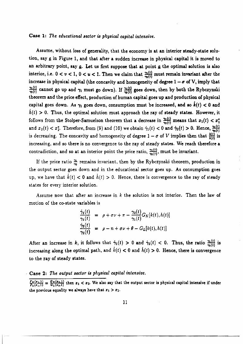
Case 1: The educational ,ector is physical capital intensive.

Assume, without loss of generality, that the economy is at an interior steady-state solu­

tion, say , in Figure 1, and that after a sudden increase in physical capital it is moved to

an arbitrary point, say 4. Let us first suppose that at point 4 the optimal solution is also

interior, i.e. 0 < v < 1, 0 < u < 1. Then we claim that ~{:I must remain invariant after the

increase in physical capital (the concavity and homogeneity of degree 1 - t1 of V, imply that

~(:I cannot go up and "Yl must go down). If ~(a goes down, then by both the Rybczynski

theorem and the price effect, production of human capital goes up and production of physical

capital goes down. As "Yl goes down, consumption must be increased, and 10 k(t) < 0 and

h(t) > O. Thus, the optimal solution must approach the ray of steady states. However, it

follows from the Stolper-Samuelson theorem that a decrease in ~(:Imeans that ZI(t) < zi and X2(t) < xi. Therefore, from (9) and (10) we obtain 'h (t) < 0 and "Y2(t) > O. Hence, ;;{:}

is decreasing. The concavity and homogeneity of degree 1 - u of V implies then that ~ is

increasing, and so there is no convergence to the ray of steady states. We reach therefore a

contradiction, and so at an interior point the price ratio, :;;ia, must be invariant.

If the price ratio ~ remains invariant, then by the Rybczynski theorem, production in

the output sector goes down and in the educational sector goes up. As consumption goes

up, we have that k(t) < 0 and h(t) > O. Hence, there is convergence to the ray of steady

states for every interior solution.

Assume now that after an increase in k the solution is not interior. Then the law of

motion of the co-state variables is

'h (t) 12(t)- P+ (71) + 11" - -(-)Gl\"[k(t), h(t)]

11 (t) 11 t

"Y2(t) _ P _ n +UII +9 - Gdk(t), h(t)]12(t)

After an increase in k, it follows that ;"1 (t) > 0 and ;"2(t) < O. Thus, the ratio ;$l is

increasing along the optimal path, and k(t) < 0 and h(t) > O. Hence, there is convergence

to the ray of steady states.

. Case 2: The output sector is physical capital intensive.

FK (' : =G (' : then Zl < Z2' We a)so say that the out.put sector is physical capital intensive if under L'l. L'3.�

the previous equality we always have that ZI > Z2·�

11

Assume again that the economy is at an interior stationary solution, (see Figure 1), and

that after an increase in k it moves to an arbitrary point, say A. We then claim that relative

prices go down and there is convergence \0 the ray of steady states. To reach a contradiction

assume first that ~f:} remains invariant. Then by Rybzcynski's theorem, production in the

output sector goes up and in the education sector goes down, and so h(t) < O. Also, for an

interior solution, we must have that %1(t) =%j and %2(t) =%;. Hence, from (9) and (10)

relative prices ~f:} will remain unchanged, and ''h(t) =12(t) =O. Hence, consumption will

remain constant and if there is ~onvergence to the steady state ray we must move along a

(downward sloping) level curve of the value function V with h(t) > O. However, as h(t) < 0,

there must be divergence from the steady-state ray and so the optimal path must be such

that production in the human capital sector becomes zero. In such case, the law of motion

of the co-state variables is given by

'h (t) _ p + (7IJ + 7r - Fr,[J.·(t), h(t)] (13)

11(t)� 12(t)� _ P _ n + (7/1 +() _ 11 ((t)) Fdk(t), h(t)] (14)12(t) 12 t

Hence, the ratio ~{g must go up, with.1'1(t) > 0 and 1'2(t) < O. This is impossible, as

concavity of the value function implies now that there is convergence to the ray of steady

states. Consequently, ~{:~ must go down.

If ~{:~ goes down, it follows from the law of motion of the co-state variables that at an

interior solution, 1'1 (t) > 0 and 1'2(t) < O. The concavity and homogeneity of degree 1 ­ (j

of V imply then that there is convergence to the ray of steady states. If the solution is

not interior, we again obtain from (13) and (14) that after an increase in k, 11(t) > 0 and

1'2(t) < 0 and so the optimal solution converges to the ray of steady states.

These arguments show that in both cases an optimal solution starting at an arbitrary

interior point A, has the property that the ratio f approaches the steady-state ratio ::.

Moreover, in case 1, human capital accumulation is always positive, h(t) > 0, and so point

A must be attracted to some positive point (k-, h-) > 0 of the ray of steady states. In

order to show in case 2 that A is also attracted by some interior stationary point, one may

proceed as in CabalIe an Santos (1993), and linearize the system of equations (4)-(10) at

a given steady-state solution. This system must have a negative eigenvalue with associated

eigenvector transversal to the steady-state ray. Hence, every interior point with a relative

stock f arbitrarily close to that of the ray of steady states must be attracted by some interior

12

point of this ray. Furthermore, point II must also be attracted by some interior point of this

ray, as the optimal solution starting at II has the property that the ratio f converges to the

steady-state ratio Z:.

3.2 Equilibrium Dynamics

The above analysis also gives a very precise description of the dynamic behavior of the state

and control variables along the transition path. If the economy is perturbed by a positive

shock on physical (or human capital), then there is convergence to an interior steady state.

This positive shock, however, may bring permanent effects, leading the economy either to a

higher steady state (the normal case), or to a lower steady state (the paradoxical case), or

back to the same steady state (the exogenous growth case). Whether the economy reaches a

higher or lower steady state depends on whether or not human capital is accumulated along

the transition. CabalIe and Santos (1993), Chamley (1993) and Faig (1993) established

analytically that in the Lucas-Uzawa framework the sign of the evolution of human capital

accumulation around a steady state (k·, h·) depends only on the inverse of the elasticity of

intertemporal substitution for consumption, (1, and the elasticity of marginal productivity of

labor with respect to capital, FLPS}\~~~;W·. In the model of this section, there is also factor

substitution in the production of education, and such result no longer holds. The education

technology must play an additional role. Moreover, we shall see that the discount rate and

population growth are also relevant parameters to single out the above three growth cases.

Our purpose now is to examine the behavior of consumption, physical and human capital

along the transition, with emphasis on the conditions that give rise to the above three growth

cases. Our commentary will be confined to the case in which the economy is perturbed by

a positive shock in physical capital. (Symmetric conclusions may be drawn for a negative

shock in physical capital, or equivalently for a positive shock in human capital.)

Consumption: Consumption jumps up immediately. Then it never goes up along the

transition path and in some situations it goes down. The concavity and homogeneity of

degree 1 - u of V imply that a sudden increase in k lowers the multiplier 1'1' Hence,

consumption must initially jump up. As shown in Caballe and Santos (1993, Th. 5.3),

the elasticity of this increase, f c,lc, depends on the cross-partial derivative Vlrh (k-, he), with

fc.k < 1 if Vkh(k", he) < 0, fc,k = 1 if Vkh(k", he) = 0, and fc,k > 1 if Vlrh(k", he) > O. In case

1, with a physical capital intensity in the production of education, relative prices remain

13

constant. Therefore, if 11 goes down, then ;2 must also go down. Hence, the cross-partial

derivative Vth(k-, h-) ~ 0, and consequently, the elasticity of consumption with respect to

capital, £e,t, is no greater than unity. In case 2, with a physical capital intensity in the

production of the aggregate good, the eiasticity £e.t may be greater or smaller than unity.

However, analogously to case lone can show that for the exogenous and normal cases such

elasticity cannot be greater than unity.

Along the transition, at interior solutions in case 1 consumption remains constant, and

relative prices are also constant. Therefore, the value function displays flat level curves,

and such downward sloping, straight level curves must conform the optimal trajectories

generated by the policy function. In all other cases, 'Yt (t) > 0 along the transition path.

Hence, consumption is decreasing. Interest rates are therefore smaller in the transition

period, encouraging thus human capital investment.

Physical Capital: Physical capital accumulation is always negative along the transition.

This is readily shown for an interior solution in case 1, where the optimal trajectories are

given by the level curves of the value function, and such curves are negatively sloped straight

lines. In all other situations, the level curves of the value function are strictly convex, and

consumption goes down along the transition. Therefore, optimal trajectories must cross the

level curves from above, and such trajectories must then be negatively sloped. This proves

that physical capital always goes down along the transition.

Human Capital: Human capital accumulation is positive in case 1, and it may be positive

or negative in case 2. An increase in ~~ may be decomposed into the following two effects

(a) The factor intensity effect (The Rybczynski theorem): An increase in k stimulates

production in the sector intensive in k and decreases production in the other sector.

(b) The price effect: An increase in k may lower the relative price, ~, shifting production

towards the educational sector.

In case 1, both effects work in the same direction, and therefore human capital accumu­

lation should increase. In case 2, these effects work in opposite directions, and as illustrated

below the sign of the evolution of h depends on the parameters of the model. Therefore,

in case 1 only the normal case is possible, whereas in case 2 the normal, paradoxical and

exogenous growth cases are all possible.

Our purpose now is to analyze the economic conditions that may lead to these three

14

growth cases. In contrast to the simpler Lucas-Uzawa framework, it seems very difficult to

obtain an analytical rule that will single out these three growth cases. Moreover, as already

argued such rule must involve several relevant parameters of the model, and not only the

elasticities (7 and Fz.:lr;;.~;lf·. In the absence of such a rule, we shall confine ourselves

to a more limited model with Cobb-Douglas production functions, and provide numerical

computations for the conditions that give rise to the three growth cases. Let

cl-er U(c) =-1' F(vk,uh) = A(vk)l1(uh)I-I1,

-(7

G((l - v)k, (1 - u)h) = B((l - v)k)cr((l - U)h)l-cr.

where 0 < f3 < 1, 0 < 0' < 1, and A, B > O. In all numerical computations, we shall

impose the transversality condition, p - n - (1 - O')v > 0, that physical capital is intensive

in producing the physical good, that A = 1, B = 0.1, n = 0.015, and the following values

for the depreciation rates 1r =0.01 and 8 = 0.01. All our computations are performed at the

corresponding ray of steady states.

It is shown in Caballe and Santos (1993) that as Q -+ 0, our model converges in the C2

topology to a Lucas-type model with a linear production function, h(t) = B[l - u(t)]h(t),

in the educational sector. All our computations will start with this limit model, where the

condition 0' = f3 determines the boundary of the three growth cases3 . Then we shall increase

Q and see the required changes in 0' and p so as to stay in the exogenous growth case.

In a (Q, O')-plane, Figure 2 depicts the three growth cases for values f3 = 0.8 and p = 0.05.

As expected, an increase in Q makes less likely the paradoxical case. As Q goes up, the factor

intensity effect is weaker, and an increment in physical capital will be less effective in reducing

production in the educational sector. \\le can see from Figure 2 that for small values of 0'

there is an approximately linear relationship between Q and 0': To remain in the exogenous

growth case, a O.OOI-point increment in value in Q requires a O.l5-pointdecrease in (7. Hence,

the above three growth regions are very sensitive to parameter 0'. Moreover, even though we

have chosen a fairly high value, f3 = 0.8, the paradoxical case ceases to exist for 0' > 0.0055.

Similar findings were observed for other calibrations of the model.

In our second exercise we shall illustrate the effects of discounting on human capital

accumulation. (Similar results hold for changes in population growth.) Figure 3 depicts the

3As pointed out in the introductory section, the normal case is obtained if (1 > 13, the paradoxical case if

(1 < p, and the exogenous growth case implies (1 = 13.

1·5

exogenous-growth-case lines for three values of (7 (7 = 0.7, (7 = 0.6, (7= 0.5), and f3 = 0.8.

In all three situations, p moves up with Q. Our explanation for this fact is as follows. In the

Lucas-Uzawa framework with h(t) = B[l - u(t)]h(t), if h(t) = 0 then u is constant at the

steady-state value u·. Hence, in the transition of the exogenous growth case, u .. u· and

12(t) is constant at the steady-state value 12(t) =1; [cf. equation (10)]. Moreover, from the

first-order conditions for u (Le. 11(t)Fdv(t)k(t), u(t)h(t)] = 12(t)G'[1 - u(t)]) we see that

human capital returns, 11(t)FL[V(t)k(t), t.e(t)h(t)], are always constant. We may deduce that

the discount rate has no additional effect on the price 12(t) over· the steady-state value 1i. . In the present formulation, however, with physical capital in the production of education, u

and v are not constant over the transition path of the exogenous growth case. Also, as shown

above, 'h(t) < 0 along the transition. Then it must be that an increment in k increases the

price of human capital, 12(t). Also, ;;{:} goes down after the shock on physical capital, and

so the ratio f~::m~~m goes up, and GL goes up. It follows from equation (8) that 11FL must

then go up. Hence, a smaller discount rate p must have an additional increase in the price

12(t). Consequently, a smaller discount rate, p, must encourage production in the human

capital sector. The same effect is also obtained for a higher population growth rate, n.

4. Leisure in the Utility Function

In this section we shall be concerned with a class of models in which agents value time

allocated to leisure activities. Following -the benchmark model of section 2, we assume that

households can assign their unitary time endowment among three different activities: work,

schooling and leisure. Thus, the total time devoted to production and education becomes an

endogenous variable as there is a new time argument embedded in the utility function. The

existence of a balanced path imposes certain separability restrictions on the feasible class

of utility functions. As mentioned in the introduction, we shall review in our analysis two

families of models compatible with the existence of a balanced path.

Our first model, considered in Ortigueira (1994), features Beckerian-type preferences, in

which the level of education affects the efficiency of leisure. We shall see that in this case

there is a unique globally stable balanced path, and so the model exhibits similar qualitative

behavior to that of the Lucas-Uzawa framework.

In our second model, studied in Ladron-de-Guevara et' al. (1994), the level of education

16

I I

does not matter for the efficiency of leisure. In this case, there could be a multiplicity of

balanced paths, all of which are optimal. This is of course a major qualitative difference with

respect to the Lucas-Uzawa framework. In contrast to Chamley (1993) and Benhabib and

Perli (1993), the multiplicity of balanced paths holds here in the absence of external effects.

Moreover, under the family of utility functions compatible with the existence of a balanced

path the multiplicity of steady states does not arise in either the standard neoclassical model

with production and leisure [cf., Chase (1967)] or our previous family of endogenous growth

models with time allocated between production and educational activities. Therefore, this

is the minimal extension to generate the non uniqueness result.

In the case of multiple steady states, some of them are stable and some are unstable. As a

consequence global stability is lost. An example will be reported to illustrate these findings.

In addition we shall provide a detailed analysis of the behavior of leisure, consumption,

physical and human capital in the transition to a stable steady-state ray.

The multiplicity of steady states implies that a different composition of physical and

human capital across countries not only has temporary effects on growth, but may lead to

increasing differences over time in income per capita. Without resorting to externality-type

arguments we shall show that a country with a higher ratio of human capital may prefer

to consume less, grow faster, and devote less proportion of time to leisure activities. This

observation also agrees with some facts in the labor market where one can find that the

most qualified people accumulate even more human capital over their professional careers,

and devote a smaller fraction of their available time to leisure activities. Our explanation

for this fact is as follows. Since both the growth rate and the supply of labor to non-leisure

activities are chosen endogenously, a higher endowment of human capital could induce the

agent to behave as if he were more patient.

4.1 Education and Leisure in the Utility Function

We now examine a model in which leisure and the level of education enter symmetrically as an

additional argument of the utility function, U(c,lh), and we briefly report on their dynamic

behavior. In our dynamic model, the existence of a steady-state ray is only compatible with

the following functional forms on the utility function

17

(c'(lh)I-') I-er U(c,/h) ­ for (7 > 0 and (7 ::f 1, 0 < 6 ~ 1,

1-(7 U(c,/h) - 610gc + (1 - 6) 10g(1h), for (7 =1, and 0 < 6 ~ 1

The optimization problem to be considered is

V(ko,ho) = max 100 e-(p-n-(I-er)v)f {--.!- [c(t)'(/(t)h(t) )1-'] 1-.} dt (P') c(t),/(t),u(t) 10 1 - (7 .ubject to

k(t) =F(k(t), u(t)h(t)) - (11 +n)k(t) - c(t) (15)

h(t) = h(t)G(1 - u(t) - I(t)) - 'lIh(t) (16)

c(t) ~ 0, k(t) ~ 0, h(t) ~ 0

0$ I(t) $ 1, 0 $ u(t) $ 1, 0 $ u(t) + I(t) $ 1

ko, ho given, p - n - (1 - (7)11 > 0

Observe that the instantaneous utility function, U( c, lh), depends on the level of con­

sumption, c, and the effective units of leisure, lh. In a static context, leisure in the utility

function was originally postulated in Becker (1965) to encompass in his analysis household

production and alternative uses of time.

Under the assumptions stated in Sect. 2, the value function, V(k, h), defined above, takes

on finite values if the following condition is satisfied

(1 - (7)G(l) < p - n

This is the transversality condition originally imposed in Uzawa (1964). Moreover, the value

function V(k, h) is an increasing, concave function, and homogeneous of degree 1- (7. In the

case of interior solutions, this function is also a C2 mapping. The following mild assumptions

guarantee the existence of a unique steady-state ray and its global convergence

PROPOSITION 4.1: Consider the optimization problem given in (P) where

F(·, .) is a C2 linearly homogeneous, strictly increasing and concave function that satisfies

condition (1) and FKKh') < 0, FLLh') < O.

G(·) is a C2, strictly increasing and concave function,

Then there is at most a unique steady-state ray, and such ray is globally stable.

18

1--­

This result is proved in Ortigueira (1994). Consequently, the qualitative dynamic behav­

ior of this model is fairly similar to our previously studied framework.

Using numerical computations, it has been shown in the transitional dynamics [cf., Mul­

ligan and Sala-i-Martin (1993)] of the Lucas-Uzawa framework that for a relevant range of

the parameter space the speed of convergence to the steady-state ray is relatively slow. In

the model of this section, Ortigueira (1994) has found analytically that parameter 8 -which

determines the relative weight of leisure- has no impact on the speed of convergence. As

illustrated in the next result, however, parameter 8 affects the behavior of human capital ac­

cumulation. Indeed, the corresponding rule to single out the three growth cases [cf. footnote

3] is now the following

PROPOSITION 4.2: Consider the optimization problem given in (P) with the same assump­

tions as in Propostion 4.1. Let (3* = FLj;.~((::·,::h·)r ' where (k*, h*) is an interior steady state.

Then

(a) In the normal case, u ~ (3* C~~~~ ). oXlcal· case, u::; ( 1+9~(b) In t he parad (3• 1+13.ef.- ) .

1+9 •(C) In t h (3• (1+0.9&'1:)e exogenous case, U = 11

Here 1* and u· refer to the attained values at the unique steady-state ray. Proposition

4.2 determines thus the sign of the evolution of human capital near a steady-state ray. On

the other hand, the transitional dynamics of the remaining variables -leisure, working time,

education, consumption and physical capital- does not differ in a fundamental way from

those of our next model with leisure in which the level of education does not enter into the

utility function. This analysis of the transition is taken up in Section 4.3. We now proceed

with our next model with leisure.

4.2 Pure Leisure in the Utility Function

We now examine the other polar case in which the level of education has no effect on the

efficiency of leisure. In contrast to our previous models, we shall find that there are economies

with a multiplicity of steady-state rays, all of which may be optimal.

19

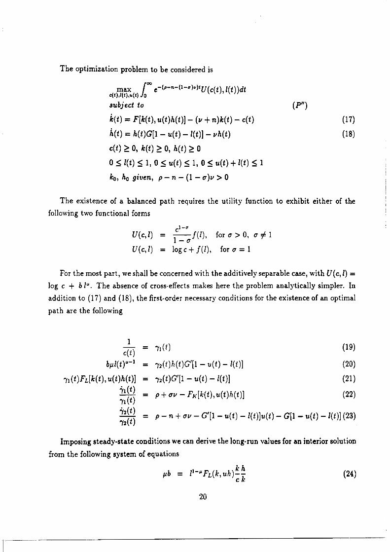
The optimization problem to be considered is

max /00 e-(P-n-(l-C7)iI)tU(c(t), I(t))dtc(t),/(t),u(t) 10�

subject to (P")�

k(t) = F[k(t), u(t)h(t)] - (11 +n)k(t) - c(t) (17)�

h(t) =h(t)G[1 - u(t) -/(t)] - IIh(t) (18)�

c(t) ~ 0, k(t) ~ 0, h(t) ~ °� o~ I(t) =::; 1, 0 ~ u(t) =::; 1, 0 =::; u(t) +I(t) =::; 1�

ko, ho given, p - n - (1 - 0')11 > 0

The existence of a balanced path requires the utility function to exhibit either of the

following two functional forms

1-(1

U(c, I) - l c _ O'f(1), for 0' > 0, O':f 1

U(c,l) - log c + f(1), for 0' = 1

For the most part, we shall be concerned with the additively separable case, with U(c, I) =

log c + b IIJ • The absence of cross-effects makes here the problem analytically simpler. In

addition to (17) and (18), the first-order necessary conditions for the existence of an optimal

path are the following

1 c(t)

(19)

blll(t)IJ-1 _ 12(t)h(t)G'[1 - u(t) ­ l(t)] (20)

11 (t)Fdk(t), u(t)h(t)] ­ 12(t)G'[1 ­ u(t) -1(t)] (21) 1'l(t) 11(t)

_ p + 0'11 - Fl\"[k(t) ,u(t)h(t)] (22)

1'2(t) 12(t)

- p - n + 0'11 - G/[1 - u(t) - l(t)]u(t) ­ G[1 - u(t) ­ I(t)] (23)

Imposing steady-state conditions we can derive the long-run values for an interior solution

from the following system of equations

(24)

20

P+II - Fh:(k, uh) (25)

p-n - G'(l - u -l)u (26) c

k - F(k, uh) k

- (11 +n) (27)

11 - G(l - u-1) (28)

In order to show that the system of equations (24)-(28) may contain multiple interior

solutions, we first show that for a given equilibrium value for 1·, equation system (25)-(28) determines the remaining equilibrium values,u·, 11, ~ and ~. That is, all these values may

be written as a function of 1·. Hence, the problem is reduced to the study of the existence

and uniqueness of 1· in (24), provided that the other values fall within the feasible range.

For 1· given, we obtain from equation (26) an equation on u,

p - n = G' (1 - u - r) 1l

The concavity of G implies then the existence of a unique solution 0 < u· ~ 1, where the

boundary solution l·+u· = 1 is only true for p-n ~ G'(O)u·. Moreover, iflimk_oo FK(k, uh) < p +G(O), then there exists a unique value Z: that satisfies (25). The existence of ~ and 11

follows directly from (27) and (28), respectively. Hence, we can now express the right-hand

side of (24) as a function of 1. Let us represent such an expression by '1J(1). The existence of

an interior steady-state then boils down to the existence of a solution to equation (24), for

btL = '1J(1).

These facts are formally summarized in the following proposition.

PROPOSITION 4.3: Consider the optimization problem (Pll), where

F(·, .) is a C2 increasing, concave, linearly homogenous function that satisfies (1) and

(2)

U(·,·) is an additively separable, increasing, concave function, of the form, U(c,l) = log c +bIll, with 0 < p. < 1, b > O.

G(·) is C2 increasing, concave function.

Let

21

(a) 0 < p - n,

Then the following conditions are necessary and sufficient for the existence of a steady state

equiZibrium,

(c) bp. E (minO<I<l \II(Z),maxO<I<l \11(1)),

(d) p - n < G'(O)(l -Z-), for Z- such that bp. = \II(r),

where

Zl-~ F [p-1[p +G(l _ p-n -i)]] G'(l-uo- ll F-;l[p +G(l _ p-n -Z)]iIt(1) = L K G'(l-uO-1) p-n 1\ G'(l-uO-l)�

F [FK1[P +G(l - G,d:un.-1j -1)] - G(l - G,(C:'-l) - Z) - n�

Moreover, the number of interior steady-state rays is equaZ to the number of soZutions Z-,

bp. = iIt(r), that satisfy condition (d).

The assumptions imposed so far are not sufficient to guarantee a unique solution to

bp = iIt(r). As a result, there may be multiple steady-state rays. As shown below, if

the ratio f is high, then optimizing agents may want to achieve a steady state with a

high proportion of consumption, and de\'ote more time to leisure activities and less time

to education and growth. Indeed, as illustrated subsequently it is possible to have steady

states with a high ratio f in which the economy reaches a boundary solution with time

devoted to both leisure and working acti\'ities, and no time to human capital accumulation

and growth. We now provide a simple example with multiple steady states and study their

stability properties. Then we shall study some properties of our economic variables across

steady states. Our example uses an additively separable utility function, and the following

technologies, F(k,uh) = k13 (uh)l-l3, 0 < (3 < 1, and G(·) =6(1- u -Z), 6> O.

Example 1: AdditiveZy separable utility function, U( c, Z) = log c +bZ~.

In this example, we consider the following parameter values

p. =0.95, p =0.05, n =0.005, 6 = 0.08, (3 =0.5, b =1.

In this case, equation bp. = \11(1) has two solutions, Zl =0.0202 and Z2 = 0.3332. Both

solutions satisfy condition (d) of Prop. 4.3 , and hence the economy has two interior steady

22

states. Moreover, there is also a non-interior steady state with time devoted only to leisure

and working activities, and no time devoted to education.

Steady State 1:

(i), =2.5966, /, =0.0202, (~), =20.2257, U, =0.5625, and v =0.0334.

Steady State 2:

(i), =4.2693, /, =0.3332, (~), =41.3115, U, =0.5625, and v =0.0083

Steady State 3:

(i) J =5.0664, I, =0.4667, (~) J =53.330, UJ =0.5333, and v =0

These three steady states4 feature the following qualitative properties: steady state 1 is

stable, steady state 2 is unstable, and steady state 3 is stable; moreover, orbits to the left of

steady state 2 are attracted by steady state 1 and orbits to the right of steady state 2 are

attracted by steady state 3.

One way to show these qualitative results is, as pointed out in Caballe and Santos (1993),

footnote 3, to reduce the problem to the one-dimensional state variable, x = f, exploiting

the homogeneity on k and h of the technologies and the CES utility function. As is usual in

one dimensional problems, under Inada-type conditions one easily shows that there are an

odd number of steady states, x· > O. Those placed at odd positions are stable and those

placed at even positions are unstable. In our case, these arguments will prove that every

x = f > 0 will be attracted by some x· = ~: > 0, even though there is the possibility

that both k and h converge to zero. However, one may rule out this latter fact, following

arguments sketched in Caballe and Santos (1993).

4Rustichini and Schmitz (1991) present a somewhat related model with also three pOllible uses of time,

and with two steady states. However, in their model the competitive solution may differ from the optimal

allocation, and they claim that one steady state may be non-optimal. As shown in Ladr6n-de-Guevara et al. (1994), in our case all three steady-state rays are optimal.

23

In the context of our simple model, we now provide further results on the behavior of

the variables across steady states. Roughly, economies with a higher proportion of physical

capital will grow less, consume more and enjoy more leisure time. ·The time devoted to

work remains invariant as the elasticity of intertemporal substitution for consumption is

here unity.

PROPOSITION 4.4: Let F(k, uh) = klJ(uh)l-1J and G(1 - u - I) = 6(1 - u - I). Let

U( c, I) =log c+ bl". Assume that there are two interior steady states {ci, 'i, ui, ki, hi =1, VI}

and {c;, li, ui, ki, hi =1, V2} with k; > ki. Then

(a) ui =ui

(b) I; > 'i

(d) c; > ci

Proof: It follows from equation (26) and the fact that G'(·) - 6 that there is a unique

steady-state value for u, _ p - n

u =-6­

Plugging (28) into (26) we obtain that p + v = 6(1 - la) + n, and hence (25) can be

rewritten as 6(1 - la) + n = {3 (~: r~-l .Then

d 1- _ {3(1 - {3) ka~-2 _I-~ 0 dk- 6 u >

Hence, I; > li, and thus the second equilibrium attains a higher level of leisure.

As both equilibria show the same fraction of time devoted to work, the per capita growth

rate is negatively related to the leyel of leisure [equation (28)]. Thus, V2 < VI.

Finally, from equation (24), the steady-state level of consumption can be expressed as a

function of the physical capital stock, ka, and the level of leisure, la. That is,

Therefore, c; > ci.

24

Finally, we present a numerical exercise with a calibrated version of the model. We again

consider a utility function of the form U(c, I) = log c + bl~ and technologies F(k, uh) =

k13 (uhP-1J and G(1 - u -I) = 0(1 - u -I), with the following parameter values,

b = -3.5, p. =-0.5, p =0.05, n =0.015, 6' =0.14, r; =0.3

Parameter values band p. have been chosen in order to obtain a steady-state value for leisure

equal to 2/3, and an intertemporal substitution elasticity for leisure, ~ =h. Parameter 6' has been chosen to obtain a per capita steady-state growth rate of 1%. For an initial stock of

human capital h· =1 the steady-state values are c· = 0.4676, I· = 0.667, k· = 2.6835, u· = 0.2672 and v = 0.01. Such steady state is unique. Moreover, the economy belongs to

the normal case. Nevertheless, the transitional dynamics ressemble those of the exogenous

growth case, as near the steady state the dynamics are such that the ratio (h/h)/(k/k) is about -0.0661. A similar result was obtained for the basic model without leisure [see

CabalJe and Santos (1993)] where the computed ratio was -0.1467. For lower values of the

intertemporal substitution elasticity for leisure (higher values of J.I), the economy falls into

the paradoxical case. This latter property will be analyzed in the next section, where it is

seen that parameter J.I affects negatively the permanent effects of physical capital on the

steady-state level of output.

4.3 Equilibrium Dynamics: The Case of Additively Separable Utility Functions

Our goal now is to examine the behavior of the economic variables along the transition to

an interior, locally stable steady state with an instantaneous utility function of the form

U(c, I) = log c +bllJ • As in Section 3, our commentary will be confined to the case in which

the economy is perturbed by a positive shock in physical capital from a given steady-state

solution. (Symmetric conclusions may be drawn for a negative shock on physical capital,

or equivalently for a positive shock on human capital.) The transitional dynamics for hu­

man capital are still undetermined and w.ithout further restrictions it is possible to obtain

the normal, exogenous and paradoxical cases. We shall illustrate that (in constrast to the

Lucas-Uzawa model) these three growth cases are not solely detemined by the elasticity

of intertemporal substitution for consumption (EISC) and the elasticity of the marginal

productivity of labor with respect to capital (EMPLK). Moreover, we shall show that the

paradoxical case may arise even if the elasticity of intertemporal substitution for consumption

is unity.

25

In order to proceed with our analysis we recall the first-order conditions and feasible

constraints that an interior optimal solution must satisfy

c(tt1 - "'(1 (t) (29)

bJlI(t)~-l - "'(2(t)h(t)G'[1 - u(t) -/(t)] (30)

"'(1 (t)Fdk(t), u(t )h(t)] - "'(2(t)G'[I- u(t) -/(t)] (31) i'l(t) "'(1 (t) - P+ 0'11 - FK[k(t), u(t)h(t)] (32)

i'2(t) "'(2(t) - P- n + 0'11 - G'[I- u(t) -/(t)]u(t) ­ G[I ­ u(t) -/(t)] (33)

k(t) - F[l.-(t), u(t)h(t)] ­ (11 +n)k(t) ­ c(t) (34)

h(t) - h(t)G[l - u(t) ­ l(t)] ­ IIh(t) (35)

\Ve now assume that the economy is at a stable interior steady state {p., I·, ::, u·, II} and

examine the behavior of our economic variables after a small positive shock on physical

capital. As shown in Ladr6n-de-Guevara et al. (1994), in this case the value function

V(k,h) is C2 , and the derivative DV(I.·,h) is homogeneous of degree -1. For convenience,

we suppose that F(k,uh) = k13 (uh)1-13 and G(l - u -1) =6(1 - u -1).

Leisure, working time, and education: After and increase in k, 1 cannot decrease, and in

the normal and exogenous growth cases u goes down. The time devoted to education is

undetermined.

v..re shall show by a contradictor)' argument that 1 cannot decrease. Assume that 1

decreases. It follows from (30) that "2 must increase. By the homogeneity of degree -1 of

DV(k, h) = hI, "'2)' we have that

Vu(k, h)l.~ +Vu(k, h)h = -"'(1 (36)

Hence, ~~ + ~ ~1 = -1. Therefore, if ~ ~ 0 then the elasticity of ~ with respect to

k is no less than unity in absolute value. Observe that the elasticity of FL with respect to

k is 0 < /3 < 1. Hence, (31) implies that u must go down, and this is impossible in the

paradoxical and exogenous growth cases. Moreover, in the normal case, if 1goes down and

u goes down, we have from (33) that i'2(t) > O. Hence, ~1t) < 0 as in the normal case "'(2(t)

converges to a steady state with a lower value for "'(2. But ~ < 0 implies that I cannot

decrease.

26

Consumption: Consumption jumps up immediately and then it goes down along the transi­

tion. Observe that 1'1 goes down as k goes up. Hence, c must increase. Notice, however,

that from the above arguments we can show that 1'2 also goes down, as I goes up after an

increase in k. Hence, from (36) we have that -~~ :5 1; and thus, the elasticity ~~ :5 1.

Along the transition, c(t) < 0, since one can show that -h (t) > O.

Physical Capital: Physical capital accumulation is negative along the transition. To find a

contradiction, assume that physical capital accumulation is non-negative along the transition;

for example that the economy goes from point 4 to b, in Figure 4. Observe that as shown

previously Vhk(k, h) = ~ :5 0, and hence Vkh(k, h) = W:5 O. However, along the transition

-h (t) > 0, and if the economy goes from point g to h, this implies, by the concavity of V,

that ~ > O. This contradiction shows that physical capital accumulation must be negative.

Human Capital: Human capital may go up or down depending upon parameter values. Even

if (J ~ 1, it is possible to obtain the exogenous and paradoxical growth cases. In the

exogenous growth case ~ = - :~. Hence, taking logs in equations (29)-(31), and after some

simple arrangements, we obtain the following equation for the exogenous growth case

(1 + _f3_!) 8"Y2!5- _ 8"Y1! - t3 =0 (37)

1 - 11 u- 8k 1'2 8k 1'1

Observe that 0 < f3 < 1, 0 :5 -~ ~ :5 1, ~~ :5 0, and without further restrictions,

(37) may hold with equality. Hence, it is possible to obtain the exogenous growth case

with a logarithmic utility function on consumption. \"le shall now report some numerical

computations in order to illustrate some sets of parameters values that separate the three

growth cases.

Figures (5)-(8) show the effect of each parameter on the direction of convergence. The

lines represent the set of values for which the exogenous case is obtained. A higher discount

factor affects negatively the permanent effects of physical capital growth. A lower population

growth rate causes the same effect (see Figures 5 and 6). In both cases the result is explained

by a lower present value of future wages (or lower present value of the productivity of

education ).

For reasons already explained, one can see in all the figures that increases in {3 have a

negative effect on the accumulation of human capital. The relative participation of leisure

on the utilty function depends on p.. A higher value of p. generates a greater instantaneous

substituitability of consumption and leisure. This reduces the time devoted to learn, with a

27

negative effect on the direction of convergence (see Figure 7). Finally, Figure 8 illustrates the

influence of the productivity of the educational sector, 6, on human capital accumulation.

5. Concluding Remarks

This paper has reviewed two extensions of the Lucas-Uzawa framework. In our first ex­

tension, physical capital was included as an input of the educational sector. In our second

extension, leisure considerations were assumed to play a positive ·role in agents' welfare.

The case with physical capital in the production of education features (under standard

conditions) a unique steady-state ray, and thus the dynamics are qualitatively similar to those

of the original Lucas-Uzawa framework. 'Ye have illustrated, however, that the paradoxical

case is less likely, and such case ceases to exist for a relatively small participation of physical

capital in the production of education.

In our second family of models with leisure, the paradoxical case gained more plausability,

and such case is possible for a logarithmic utility function. More importantly, we have shown

that if the level of education does not affect the productivity of leisure, then there could be a

multiplicity of steady states. (The multiplicity of steady states holds for relatively standard

parameter values.) Countries with a relatively high endowment of human capital may want

to choose paths of high growth, and vice versa; countries with a low endowment of human

capital may want to choose paths of low growth. 'What determines here the chosen rate of

growth is the initial ratio of physical over human capital.

Our results therefore illustrate that in a world without externalities there could coexist

different long-term growth rates, and that low-educated countries have less incentives to

invest in education and growth. Hence, policies that tend to encourage human capital

accumulation may change the long-term growth rate of an economy.

28

l-­

ArPENDIX

The purpose in this appendix is to show that the model in Section 3 (with physical capital in the

educational sector) has under the stated assumptions at most a unique (interior) ray of steady states.

Imposing steady state conditions (Le., e(t) = k(t) = het) = ti(t) =ti(t) ='het) = ;'2(t) =0) on equations

(4)-(10), and writing Zl(t) = :m~m, Z2(t) =t:::~m~t~~, we obtain the following equations system:

u·hF(zi,l) c k - =1r+n+lI- k (A.1)

(1 - u·)G(z2,l) = 11 + 9 (A.2) FK(zi,l) _ GK(Z;, 1)

(A.3)FL(zi ,1) - GL(Z;, 10)

p + (7'11 + '" = FK(zj, 1) (AA) .

P- n + (7'V +9 = Gdz;, 1) (A.S)

From our previous assumptions on technologies it follows that ~~t:::U is a strictly decreasing function . hI' FK(~l 1~ 0 d I' Fb'(~l 1) S"I I h Id r G ~ 1 H fof zl, Wit nn~l-OC FL(~l'\ = an Im:-1-o Fd:rl:l) =00. lml ar resu ts 0 lor GL(:r2,1' ence, rom

equations (A.3), (AA) and (A.S) we obtain an unique value for zj, z2 and v. Then from equation (A.2)

and the concavity of GC') we find a unique value for u·. Moreover, from equation (A.1) and given that

t = UZl + (1- U)Z2' we can solve for f and t. Finally, from ZI = ~ we obtain the steady state value for v.

29

t-­

References

[1]� Becker, G.S. (1965) "A Theory of the Allocation of Time," Economic Journal,

Vol. 75, pp. 493-517.

[2]� Becker, G.S. (1993) "Nobel Lecture: The Economic Way of Looking at Behav­

ior," Journal of Political Economy, Vol. 101, pp. 385-409.

[3]� Benhabib, J. and R. Perli (1993) "Uniqueness and Indeterminacy: Transitional

Dynamics in a Model of Endogenous Growth," manuscript, New York Univer­

sity.

[4]� Benveniste, J. and J.A. Scheinkman (1982) "Duality Theory for Dynamic Op­

timization Models of Economics: The Continuous Time Case," Journal of Eco­

nomic Theory, Vol. 27, pp. 1-19.

[5]� Bond, E., P. Wang and C. Vip (1992) "A General Two Sector Model of En­

dogenous Growth with Human and Physical Capital," manuscript, Penn State

University.

[6]� Caballe, J. and M.S. Santos (1993) "On Endogenous Growth with Physical

and Human Capital," Journal of Political Economy, Vol. 101, pp. 1042-1068.

[7]� Chase, E.S. (1967) "Leisure and Consumption," in Essays on the Theory of

Optimal Economic Growth, ed. I\arl Shell, MIT Press.

[8]� Cass, D. (1965) "Optimum Growth in an Aggregative Model of Capital Accu­

mulation," Review of Economics Studies, Vol. 3, pp. 223-40.

[9]� Chamley, C. (1992) "The Vvelfare Cost of Taxation and Endogenous Growth,"

Working Paper no. 92-46, Universidad Carlos III de Madrid.

[10]� Chamley, C. (1993) "Externalities and Dynamics in Models of "Learning or

Doing,"" International Economic Review, Vol. 34, pp. 583-609.

[11]� Faig, M. (1993) "A Simple Economy with Human Capital: Transitional Dy­

namics, Technology Shocks, and Fiscal Policies," forthcoming in Journal of

Economic Dynamics and Control.

30

[12] Hall, B. H. (1992) "R&D Tax Policy During the Eighties: Success or Failure?,"

Working Paper no. 4240, National Bureau of Economic Research.

[13] Hansen, G.D. and R. Wright (1992) "The Labor Market in Real Business Cycle

Theory," Federal Reserve Bank of Minneapolis, Quarterly Review.

[14] Jones, L.E., R.E. Manuelli and P.E. Rossi, P. (1993) "Optimal Taxation in

Models of Endogenous Growth," Journal of Political Economy, Vol. 101, pp.

485-518.

. [15] King, R., C.I. Plosser and S. Rebelo (1988) "Production, Growth and Business

Cycles: 1. The Basic Neoclassical Model," Journal of Monetary Economics,

Vol. 21, pp. 309-341.

[16] Kydland, F. and E.C. Prescott (1982) "Time to Build and Aggregate Fluctu­

ations," Econometrica, Vol. 50, pp. 1345-1370.

[17] Ladr6n-de-Guevara, A., S. Ortigueira and M.S. Santos (1994) "A Two-Sector

Model of Endogenous Growth with Leisure," mimeo, Universidad Carlos III de

Madrid.

[18] Lucas, R. Jr. (1988) "On the Mechanics of Economic Development," Journal

of Afonetary Economics, Vol. 22, pp. 3-42.

[19] Mino, K. (1992) "Analysis of a Two-Sector Model of Endogenous Growth with

Capital Income Taxation," manuscript, Tohoku University.

[20] Mulligan, C.B. and X. Sala-i-Martin (1993) "Transitional Dynamics in Two­

Sector Models of Endogenous Growth," Quarterly Journal of Economics, Vol.

CVIlI, pp. 739-775.

[21] Ortigueira, S. (1994) "A Dynamic Analysis of an Endogenous Growth Model

with Leisure," mimeo, Universidad Carlos III de Madrid.

[22] Rebelo, S. (1991) "Long-Run Policy Analysis and Long-Run Growth," Journal

of Political Economy, Vol. 99, pp. 500-521.

[23] Rebelo, S. and N. Stokey (1992)

manuscript, University of Chicago.

"Growth Effects of Flat-Rate Taxes,"

I' 31

I

1"·'.~-----';·r--'"

I

[24] Rustichini, A. and J. A. Jr. Schmitz (1991) "Research and Imitation in Long­

Run Growth," Journal of Monetary Economics, Vol. 27, pp. 271-292.

32�

I-­

I

Figure 1

h

a

o k

FIGURE 2

GROWTH REGIONS IN A (a,(1)-PLANE 0.8 T'"'::::---~-----,r-----"""'----.....,..----r-----(1

0.78

Normal reaion

0.76

0.74

I Paradoxical I

I

0.72 11=0.8 region ~A=1

B=O.1 I

I 0.7 p=0.05

n=0.015 6=0.01 'll'=O.Ol

I

I i

0. 68 1

I

0 O.OCll 0.002 0.003 0.004 0.005 0.006

a

FIGURE 3 EXOGENOUS GROWTH LINES IN A(a.p)-PLAr\E FOR SOME VALUES OF (1

~oo:: '------.-----,....------.----,....-------.-----j� 0.07

0.065 J

0.06

0.055

13=0.8

0.05 A=l B=O.I

.J

i

0.045

D=O.OIS 6=0.01 11'=0.01

I 1 I

0.04 L.­ ---'-­ "--­ ---'-­ "--­ --'­ ! o 0.005 0.01 0.015 0.02 0.025 0.03

Figure 4

h

b

a

o k

FIGURE 5

THE EXOGENOUS GROWTH CASE IN A (P, ~)-PLANE

(3

095 JL=0.2 6=0.1 n=0.0150.9

085

08

075

0.7

06:' L...---..J----'-----"­__-.l. L­__..l..-__....I-__-J

0.01 0.02 0.03 0.04 0.05 0.06 0.07 0.08 0.09 p

FIGURE 6

THE EXOGENOUS GROWTH CASE IN A (n. B)·PLANE

;98 096-1

I 09~ ~

I I

oe2~ I

0)'! j,

I 086~ ..2

1"=0.2 ,o86~ 0=0.1 ,

p=o.OS

064- i

I, I

0.62~ I

•

08~1__--..l..' 'L-__...L-'__--..l.'----:-:~-_:_, 1 0.01 0.015 0.02 0.025 0.03 0.035 0.04

n

FIGURE 7 THE EXOGENOUS GROWTH CASE IN A (p., P)-PLANE

0.9

1 (3 \

\

0.88­

0.86

i 08~ ~

I I I

082 -

Co ­

G7£.­0:. 0.1 p:0.05

I n=0.015 on ,­

L­ ...L­ ---'-I ---''---__----'-, --'

001 0.02 0.03 0.04 0.05 0.06 IJ.

0.07

FIGURE 8

THE EXOGENOUS GROWTH CASE IN A (6. ~)·PLANE

~95l 09

OB5;l 0,8-�

1 075� J

i

07 / !065� !

I /�

I /� I!=O.2

06!1 //� p=O.OSn=O.015

I'

..j

O::L-__l...' ~_...I!__..J.I_----:..J.'_----:....LI-=-----:....LI-=---::-,",::-~I__l...'__

0,02 0.04 006 OOS 0.' 0.'2 0.14 0.'6 O.'S 0.2 6 0.22