Università degli Studi di Padova

Dipartimento di Ingegneria Civile, Edile e Ambientale

Corso di Laurea Magistrale in

ENVIRONMENTAL ENGINEERING

-Thesis work-

CLOSED-LOOP HEAT-EXCHANGING SYSTEMS IN GEOTHERMAL ANOMALY

AREAS: THE CASE OF THE EUGANEAN THERMAL BASIN, ITALY

Relatore: Prof. Antonio Galgaro

Laureando: Zeno Farina

N° matricola: 1015874

ANNO ACCADEMICO: 2012/2013

i

Abstract

The Euganean Thermal Basin is the most important thermal field in northern Italy. It is located in the

Veneto alluvial plain, south-west of Padua, close to the north-eastern edge of the Euganean Hills.

Abano Terme is the largest town of the Basin (which includes a few other smaller towns) and is one

of the most important thermal and mud-therapeutic resorts and in the world. Its very well structured

hotels’ system offers hospitality to more than 250000 tourists every year. Almost every hotel and spa

owns a well to extract thermal water at a temperature in the range 60-87°C from the fractured

carbonatic bedrock found at a depth of about 150-200 m. To preserve this fundamental resource, the

local legislation does not allow extracted thermal water to be used for purposes other than

therapeutic ones. For this reason, this thesis work wants to analyse the feasibility and sustainability

of a technique which does not require the extraction (and re-injection) of thermal water: closed-loop

heat-exchangers, also known as Borehole Heat Exchangers (BHE). By circulating a refrigerant liquid in

a closed loop of pipes installed vertically in a 400 m deep well, there is no fluid exchange between

refrigerant and groundwater, but only heat transfer. The refrigerant accumulates heat when in

contact with the hot groundwater, and releases it to a receiving body on the surface. An actual

application of such technique to provide heat to the “Kursaal” building of Abano Terme is analysed in

terms of its thermal impact on underground and groundwater temperature. Several hotels are

present in the Kursaal’s surroundings and it must be verified that heat extraction by the BHE does

not hinder the temperature of groundwater extracted by their wells. The analysis is carried out using

the software FEFlow 6.1, using input data from another software called EED. It will be shown how

according to the model there is absolutely no impact caused by the BHE on the extracted thermal

water. Finally, it is estimated that such application may reduce CO2 production by 95% and paid back

in 5.5 years.

Acknowledgments

I would first like to thank my family, especially mum and dad, for the continuous support they have

given me throughout my time at University and entire life, for their faith in me and for allowing me

to be able to think only to my work during these last few months, I could not have done it without

them. I would like to thank my sisters and brother for allowing me to be their “big bro”, and my

grandparents for giving me inspiration through delicious Wednesday lunches and constant interest in

my work. Uncle Peter also deserves a special mention for teaching me everything that he knows and

for keeping me up-to-date with what goes on in the World. I would like to extend my sincerest

thanks and appreciation to my supervisor Prof. Galgaro, for his background knowledge, unfailing

guidance and for being always available to discuss any kind of matter. The other members of “the

corridor” also deserve thanks for their patience and understanding, for their company and support

especially in the last stressful days: thank you Eloisa, Giorgia, Elisa and Laura. I am also very grateful

to Matteo Cultrera for his advice and suggestions on the use of FEFlow. I would like to extend my

gratitude to Julia Mayer and Bastian Rau of DHI-WASY for the fundamental suggestions on how to

improve my FEFlow model. I would like to thank my friends for their friendship and unconditional

assistance when needed, with a particular mention to the “boys”, for making me smile whenever I

receive your texts, pictures and videos. I thank my father for introducing three cute donkeys in our

family, who taught me patience, wisdom and wellness. Last but not least I would like to thank Laura,

for her love, encouragement and final editing assistance.

ii

Table of Contents

Abstract .................................................................................................................................................... i

Acknowledgments .................................................................................................................................... i

1 Introduction ..................................................................................................................................... 1

2 Aims and objectives ......................................................................................................................... 2

3 Background ...................................................................................................................................... 3

3.1 Abano Terme and the Euganean Thermal Basin ..................................................................... 3

3.1.1 The town of Abano Terme and origins of “Spas” ............................................................ 3

3.1.2 Hydrogeology ................................................................................................................... 5

3.1.3 Geology ............................................................................................................................ 8

3.1.4 Land subsidence ............................................................................................................ 11

3.2 Geothermal Energy ................................................................................................................ 12

3.2.1 Geothermal anomalies .................................................................................................. 12

3.2.2 Types of geothermal systems ........................................................................................ 13

3.2.3 Geothermal direct use - Space and district heating ...................................................... 14

3.2.4 Closed-loop heat-exchanging systems .......................................................................... 15

3.2.5 Convection cells ............................................................................................................. 18

3.3 Choice of the equipment ....................................................................................................... 20

3.4 Basic Mechanisms of Heat Transfer ...................................................................................... 23

3.4.1 Conduction .................................................................................................................... 23

3.4.2 Convection ..................................................................................................................... 24

3.4.3 Combination of convection and conduction ................................................................. 25

3.4.4 Energy transfer in modelling ......................................................................................... 27

3.4.5 Heat required................................................................................................................. 28

4 Legislative issues ............................................................................................................................ 30

4.1 National legislation ................................................................................................................ 30

4.2 Regional legislation ................................................................................................................ 31

5 Information on the site .................................................................................................................. 34

5.1 The “Kursaal” building complex ............................................................................................ 34

5.2 Climatic conditions ................................................................................................................ 36

5.3 Site geology, hydrogeology and temperature profile ........................................................... 37

6 Groundwater modelling ................................................................................................................ 41

6.1 EED 3.0 ................................................................................................................................... 41

6.2 Description of input data - FEFlow ........................................................................................ 43

iii

6.2.1 Supermesh and Finite-Element Mesh creation .............................................................. 43

6.2.2 Problem settings ............................................................................................................ 44

6.2.3 Parameters assignment .................................................................................................. 45

6.3 Creation of the model domain ............................................................................................... 46

6.4 Assignment of initial parameters ........................................................................................... 48

6.4.1 Initial conditions ............................................................................................................. 49

6.4.2 Boundary conditions ...................................................................................................... 49

6.4.3 Material properties ........................................................................................................ 54

6.5 Simulation .............................................................................................................................. 56

7 Results ............................................................................................................................................ 57

7.1 CO2 production ....................................................................................................................... 61

7.2 Costs’ analysis ........................................................................................................................ 62

8 Comparison with the CaRM code ................................................................................................... 64

9 Conclusion and future developments ............................................................................................ 66

10 References ...................................................................................................................................... 67

11 Appendix ........................................................................................................................................ 70

1

1 Introduction

Low-temperature geothermal energy has recently gained more attention for its possible use in

geographic areas that are not typically associated with it. The attractive features of low-temperature

geothermal utilisation (known as “low-enthalpy” use) include, but are not limited to, its stable, base-

load energy output, low environmental impact, and the renewability of the resource (Xiaoning and

Anderson, 2012). The city of Abano Terme presents itself as a possible attractive location for the

expansion of geothermal resource utilisation within the Italian territory due to the elevated

temperatures found in the Euganean Thermal Basin, north-east Italy, in which it is found.

This thesis work will discuss an application for the exploitation of low-enthalpy geothermal energy. A

feasibility analysis of a Borehole Heat Exchanger (BHE) to be installed in Abano Terme is carried out

by evaluating its thermal impact on underground temperature.

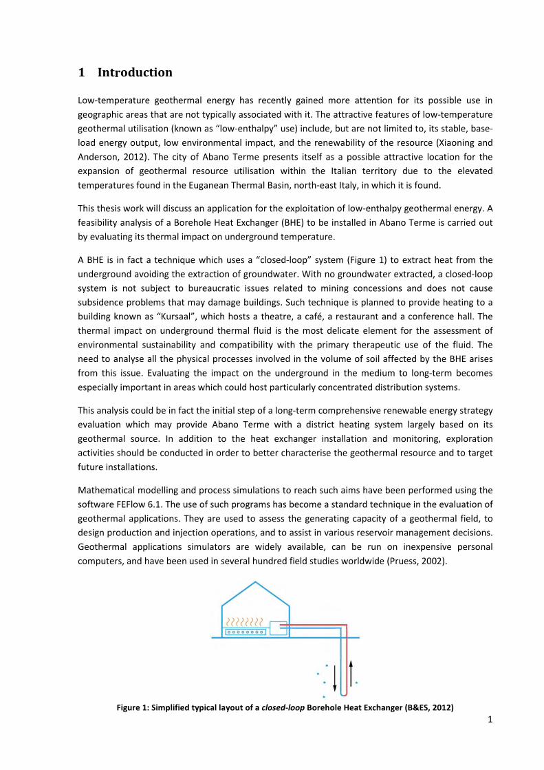
A BHE is in fact a technique which uses a “closed-loop” system (Figure 1) to extract heat from the

underground avoiding the extraction of groundwater. With no groundwater extracted, a closed-loop

system is not subject to bureaucratic issues related to mining concessions and does not cause

subsidence problems that may damage buildings. Such technique is planned to provide heating to a

building known as “Kursaal”, which hosts a theatre, a café, a restaurant and a conference hall. The

thermal impact on underground thermal fluid is the most delicate element for the assessment of

environmental sustainability and compatibility with the primary therapeutic use of the fluid. The

need to analyse all the physical processes involved in the volume of soil affected by the BHE arises

from this issue. Evaluating the impact on the underground in the medium to long-term becomes

especially important in areas which could host particularly concentrated distribution systems.

This analysis could be in fact the initial step of a long-term comprehensive renewable energy strategy

evaluation which may provide Abano Terme with a district heating system largely based on its

geothermal source. In addition to the heat exchanger installation and monitoring, exploration

activities should be conducted in order to better characterise the geothermal resource and to target

future installations.

Mathematical modelling and process simulations to reach such aims have been performed using the

software FEFlow 6.1. The use of such programs has become a standard technique in the evaluation of

geothermal applications. They are used to assess the generating capacity of a geothermal field, to

design production and injection operations, and to assist in various reservoir management decisions.

Geothermal applications simulators are widely available, can be run on inexpensive personal

computers, and have been used in several hundred field studies worldwide (Pruess, 2002).

Figure 1: Simplified typical layout of a closed-loop Borehole Heat Exchanger (B&ES, 2012)

2

2 Aims and objectives

The main objectives of this work are the calibration of a high-resolution model to simulate a BHE and

the determination of model sensitivity with respect to its length and configuration. A full-scale pilot

project is analysed by developing a high-resolution numerical BHE model, to analyse an actual BHE

designed to be installed at a specific location in a situation of thermal anomaly. The analysis is carried

out on the thermal impact caused by this BHE, which by extracting heat from underground thermal

water will cause it to decrease in temperatures. The extent of this cooling effect will be the objective

of this study.

The main reason behind the simulation analysis is that thermal groundwater cannot decrease in

temperature below certain thresholds, as otherwise it could not be extracted for its primary use, that

of sanitary and health-healing effects. A second aim of this project is therefore to design a BHE which

avoids this situation from occurring.

3

3 Background

3.1 Abano Terme and the Euganean Thermal Basin

3.1.1 The town of Abano Terme and origins of “Spas”

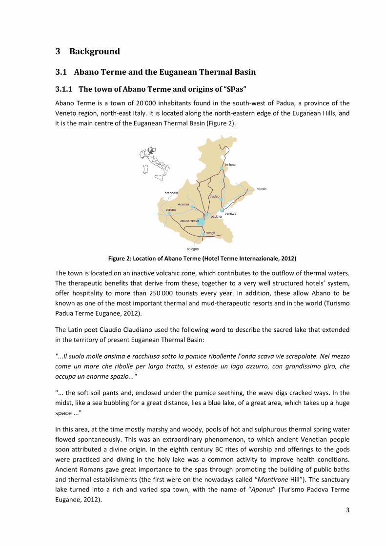
Abano Terme is a town of 20˙000 inhabitants found in the south-west of Padua, a province of the

Veneto region, north-east Italy. It is located along the north-eastern edge of the Euganean Hills, and

it is the main centre of the Euganean Thermal Basin (Figure 2).

Figure 2: Location of Abano Terme (Hotel Terme Internazionale, 2012)

The town is located on an inactive volcanic zone, which contributes to the outflow of thermal waters.

The therapeutic benefits that derive from these, together to a very well structured hotels’ system,

offer hospitality to more than 250˙000 tourists every year. In addition, these allow Abano to be

known as one of the most important thermal and mud-therapeutic resorts and in the world (Turismo

Padua Terme Euganee, 2012).

The Latin poet Claudio Claudiano used the following word to describe the sacred lake that extended

in the territory of present Euganean Thermal Basin:

"...Il suolo molle ansima e racchiusa sotto la pomice ribollente l'onda scava vie screpolate. Nel mezzo

come un mare che ribolle per largo tratto, si estende un lago azzurro, con grandissimo giro, che

occupa un enorme spazio..."

"... the soft soil pants and, enclosed under the pumice seething, the wave digs cracked ways. In the

midst, like a sea bubbling for a great distance, lies a blue lake, of a great area, which takes up a huge

space ..."

In this area, at the time mostly marshy and woody, pools of hot and sulphurous thermal spring water

flowed spontaneously. This was an extraordinary phenomenon, to which ancient Venetian people

soon attributed a divine origin. In the eighth century BC rites of worship and offerings to the gods

were practiced and diving in the holy lake was a common activity to improve health conditions.

Ancient Romans gave great importance to the spas through promoting the building of public baths

and thermal establishments (the first were on the nowadays called “Montirone Hill”). The sanctuary

lake turned into a rich and varied spa town, with the name of “Aponus” (Turismo Padova Terme

Euganee, 2012).

4

Figure 3: Old representation of Abano Terme’s spa activity (Piccoli et al., 1976)

Figure 4: Abano Terme in the Middle Ages, with the Euganean Hills in the background (Piccoli et al., 1976)

Today the Euganean Thermal Field (Bacino Termale Euganeo) is the area where this thermal resource

is exploited for its multiple benefits. This area, which includes the town of Abano Terme and other

smaller towns in the surrounding, covers in total an area of about 23 km2 and includes more than 130

establishments, 220 thermal pools, and has a capacity of over 13˙000 beds. This creates an important

economic social and sanitary reality around which gravitate over 5˙000 direct employees with a total

number of operators estimated to be over 11˙000 (Cosentino, 2010, and Parco Regionale dei Colli

Euganei, 2012). The towns which are found in the Euganean Thermal Field are Abano Terme,

Montegrotto Terme, Battaglia Terme, Galzignano Terme and Teolo. “Terme” is the Italian word for

“Spa” (Fabbri and Trevisani, 2005).

Figure 5: Location of the Euganean Thermal Basin (hatched area) (Gottardi et al., 1995)

5

3.1.2 Hydrogeology

The Euganean Thermal Basin can be classified as a hydrothermal convection system, where the water

represents the dominant phase (Antonelli et al., 1995). At present about 250 wells are active and the

total average extraction flow rate of thermal fluids is about 17 million m3/year. These fluids are

exclusively used for sanitary purposes, as imposed by the current legislation (see Chapter 4). Physical

and chemical parameters of the Euganean thermal waters have been extensively analyzed mainly

with statistical methods: temperature ranges from 60°C to 87°C (80°C to 87°C where the heat flux is

more pronounced), and this temperature remains practically constant up to the bottom holes,

confirming the presence of a system "with a high up flow rate". The total dissolved solids is 6 g/l with

a primary presence of Cl and Na (70%) and secondary of SO4, Ca, Mg, HCO3, SiO2. 3H and 14C

measurements suggest a residence time greater than 60 years, probably a few thousand years. The

analyses of the oxygen isotopes show that the thermal waters are of meteoric origin and fall in an

area up to 1500 m a.s.l. in the Fore – Alps (Pola, 2011). The work of Piccoli et. al. (1976) proposed a

good example of the hydrothermal circuit able to explain the genesis and dynamics of Euganean

fluids (Figure 6 and Figure 7): the rainwater infiltrates in the Fore – Alps and reaches depths of 3000-

4000 meters, warms up by the normal geothermal gradient and circulates towards the SE, flowing

through the hills’ complex formed by the Lessini, Berici and Euganean Hills. The lower limit of the

water circulation system is represented by the Permian crystalline-schist bed and is conditioned by

the regional structural shape (Gestione Unica del BIOCE, n.d.).

Figure 6: Diagram of probable Euganean hydrothermal circuit (Piccoli et al., 1976)

Figure 7: Key to the diagram of the probable Euganean hydrothermal circuit (Piccoli et al., 1976)

Key

miocene clastic complex

oligocene calcareous complex

paleogene igneous rocks

eocene Flysch

eocene limestones and marls

mesozoic carbonate complex

permo-werfenian sandstone-limestone-evaporitic complex

pre-permian stand-crystalline schist water at 0-20°C

water at 20-30°C

water at 30-50°C

water at >50°C

Fore - Alps

Lessini Mountains Berici Hills Euganean Hills

Venetian Plain

Euganean Thermal Basin

6

Special structural conditions of fractures and faults in the Euganean Thermal Basin lead to a rapid

ascent of the fluids and to a phenomenon of temperature homogenization, linked to the presence of

convective motions. Other factors facilitate the up-wards movement, such as, for example, the side

closure of the system by sediments at low permeability and the hydraulic load generated by cold

groundwater seepage from the surface of the Euganean Hills (Gestione Unica del BIOCE, n.d.). When

the shallow zone of the reservoir is achieved by thermal water, a lateral expansion of the water is

allowed. The thermal fluids are partly stored inside the fractures or they can move sideways, partly

go up again to the alluvial cover until some ten meters from the surface, mixing with the overhanging

cold waters (Antonelli et al., 1995).

The main aquifer is formed by red scaglia-Jurassic limestone complex, whereas the other aquifers,

which are localized in the alluvial quaternary sequence, are formed by sands with interbedded layers

of clays and silts. In this sequence the deep waters mix with the surface waters, thus reaching minor

salinities and temperatures. Till the end of the last century, waters used for thermal baths in Abano

Terme originated from springs or lakes. Later they were produced by wells draining the quaternary

aquifers, still later sand production problems, along with formation of sinkholes, led to deepening

the wells in order to produce directly from the fractured rock (Dainese, 1988 and Brighenti, 1991).

In the Sixties, production surpassed 500 l/s and caused both a progressive piezometric level lowering

and an actual ground surface lowering, in a subsidence process (see Chapter 3.1.4). The Italian

Department of Industry, in order to protect the basin, decided to impose a united management of

the local geothermal resources and in 1966 created the "Gestione Unica di Abano Terme e Teolo".

However, due to local political reasons, the authority of this body was limited only to the territory of

Abano Terme and Teolo (Brighenti, 1991).

Some temperature logs have been performed in wells outside the thermal area during some

investigations from few years ago. This was in order to attempt giving an unified hydrogeological

interpretation on the surrounding areas using a contourline hydroisothermal map (Figure 8).

Figure 8: Tectonics map and hydroisothermal map (Antonelli et al., 1995)

The temperatures have been measured at the bottom holes, whose depths range from 40 to 120 m.

Hence they are related to aquifers located in the quaternary sediments. The isolines in Figure 8

correspond to the geological interpretation of the bedrock where a degrading extensional tectonics

eastward could favour an expansion of the hydrothermal anomaly in the same direction. On the

7

contrary in the Euganean Hills the presence of a cold continuous aquifer has been ascertained

(Antonelli et al., 1995).

In 1991 a drilling of a borehole called Aponus 2 down to 465 m from ground level in the centre of

Abano allowed some interesting observations to be performed on alluvial cover and bedrock water

bodies (Figure 9). Using some specific geophysical logs, it was found that the quaternary cover

electrically behaves as a very conductible body because of the presence of thermal waters.

Figure 9: Litostratigraphy and geophysics logs of the “Aponus 2" borehole (Antonelli et al., 1995) simplified

by Gottardi et al., 1995

These logs have been particularly important for hydrogeological applications, in fact they permitted

to locate some fractured levels with a very active water movement, in the bed-rock. Difference in

piezometric head between the high exploitation (spring and autumn) and low exploitation regimes

(winter and summer) seems now to be stabilised between 7-10 m. It must be pointed out that both

because of the high concentration of the production wells and of the considerable variation in the

transmissivity values (from 13 to 2230 m2/d) drawdowns of about 30-40 m can be achieved in some

field sectors. The performance of the Aponus 2 well allowed an accurate characterisation of the main

confined sandy aquifers in the alluvial cover, with a permeability coefficient ranging from 1.12x10-5 to

7.7x10-6 m/s. A hydrogeological connection between the alluvial sequences and the deep carbonatic

complex moreover is demonstrated (Antonelli et al., 1995).

Piezometric lines play an important role in creating a study model, as they show the depth and

direction of groundwater movement. These have been imported from the regional hydro-geologic

map included in the Piano Regionale Attività di Cava (Regional Plan Caves’ Activity) (Figure 10).

8

Figure 10: Piezometric lines in the Padua area, showing the hydrologic setting of Abano Terme

It can be seen how the town of Abano Terme, which is found at an altitude of about 14-15 m above

sea level, is located between the piezometric lines of 12 and 10 m. The movement of groundwater is

perpendicular to the piezometric lines, meaning that it flows towards south-east.

3.1.3 Geology

The Euganean Hills were mainly formed during two magmatic cycles (Eocene and Oligocene), which

have given rise both to volcanic (eg M. Venda, M. Vendevolo, M. Ceva, etc..) and sub-volcanic

displays (M. Rua, M. Madonna, M. Grande, etc..) (Gestione Unica del BIOCE, n.d.).

The two eruptive phases have given origin to diversified products: the first phase, which can be

placed in the Upper Eocene (34 – 37 million years ago), gave rise to submarine basaltic flows

arranged on the bottom of the then existing sea, mingling with marly sediments that deposited

during that period. The second more recent phase, during the Oligocene (23 - 34 million years ago),

is characterized by acidic magmas, predominantly rhyolites , trachytes and latites. These lavas have

given rise to veins, domes and laccoliths. Most of these bodies were intruded at different levels in

the sedimentary sequence rising and dislocating the same levels (Gestione Unica del BIOCE, n.d.).

The stratigraphic sequence belongs the typical Euganean series, marked by carbonatic formations

deposited initially as a platform, progressed then to a pelagic environment and who later proceeded

to a slow raising. The sequence begins with the Rosso Ammonitico (upper Jurassic), with a thickness

of about 30 m and represented by nodular limestone, followed by the Biancone (upper Cretaceous -

upper Jurassic) the thickness of which is about 250 m, composed by micritic limestones and which is

the rock formation at highest hydrothermal potential; then the Scaglia Rossa (lower Eocene - upper

Cretaceous) has thickness ranging from 80 to 130 m and is represented too by micritic limestones.

Euganean Marl (lower Oligocene - lower Eocene), is constituted by clayey marl and is the most recent

term in the sedimentary sequence, about 100 m thick, but almost absent in the area of Abano Terme

(Fabbri and Trevisani, 2005). The mentioned rock formations are fractured in the Euganean area

because of tectonic movements, later described; this situation is connected with the activity of the

extentional tectonics controlled by different fault systems of regional importance, being the Schio-

Vicenza line the most significant one. These formations are characterised by a very low permeability,

being separated from each other by mainly vertical fissures which impose a negligible resistance to

fluid flow. Figure 11 shows an example of fissured limestone which may be similar to the carbonatic

9

bedrock of the Euganean Thermal Basin; with reference to this example, it must be considered

however that when limestone reaches the surface it is easily attacked by atmospheric agents and

eroded rapidly. The Euganean bedrock is probably not as fractured as much.

Figure 11: Deeply fissured limestone pavement in the Aran Islands, Ireland (Lori, 2008)

The fractured carbonatic bedrock, from which thermal fluids are extracted, is topped by a blanket of

alluvial material. The area has experienced a paleoenvironmental evolution since the end of the

Mesozoic and has seen a gradual transformation from a typical marine to a coastal environment,

followed by a purely lacustrine habitat which remained until very recently. Upon emerging from the

sea moreover, selective erosion lasted millions of years has produced a varied landscape, removing

the most tender part of sedimentary cover and highlighting the tough volcanic bodies in smooth

forms found among the Euganean hills. Therefore the alluvial cover consists of sediments originated

by the ancient lacustrine habitat followed by eroded material: overall, these have composed a cover

of mainly loose silty-clay, interspersed locally with silty-peaty and sandy compositions, in lenses or

levels more or less continuous, of variable thickness from a few decimetres to more than two

hundred metres (Gestione Unica del BIOCE, n.d.). These lenses of more conductive material were

aquifers confined from the surrounding clay layers which acted as aquitards. When thermal water

extraction began, it was initially from these sandy levels. However, since recharge of the area was

impaired, the layers lost volume and caused ground surface subsidence, as it will be described in

Chapter 3.1.4. Figure 9 previously shown in the last Chapter details the stratigraphy of the well

Aponus 2, In the town of Abano Terme the alluvial material’s thickness varies on average between

100 and 200 metres, and then increases towards Padova (north-east) where it is more than 500

metres thick (Figure 12). Most of the groundwater wells are drilled for several hundred metres into

the bedrock but the cased intervals are restricted to the alluvial material as it is more brittle and

collapses easily when a well is dug into (Antonelli et al., 1995).

Figure 12: Geological cross section of Figure 8, Chapter 3.1.2

10

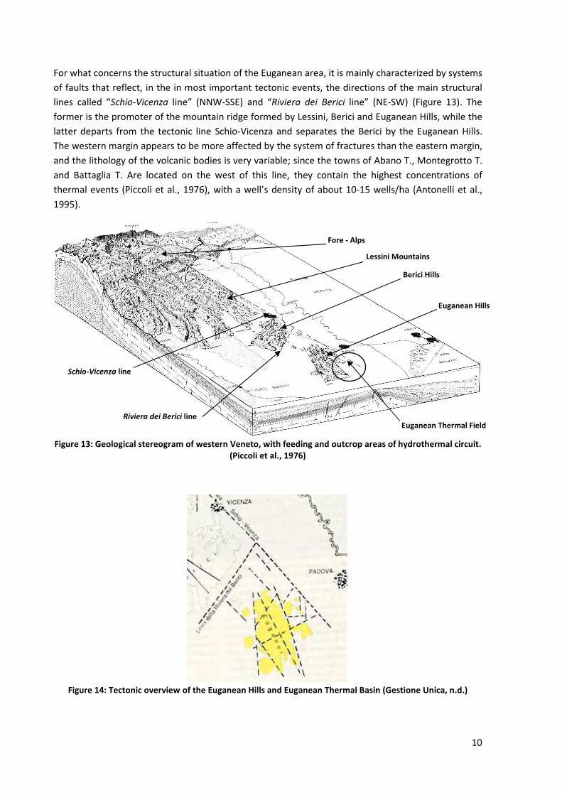
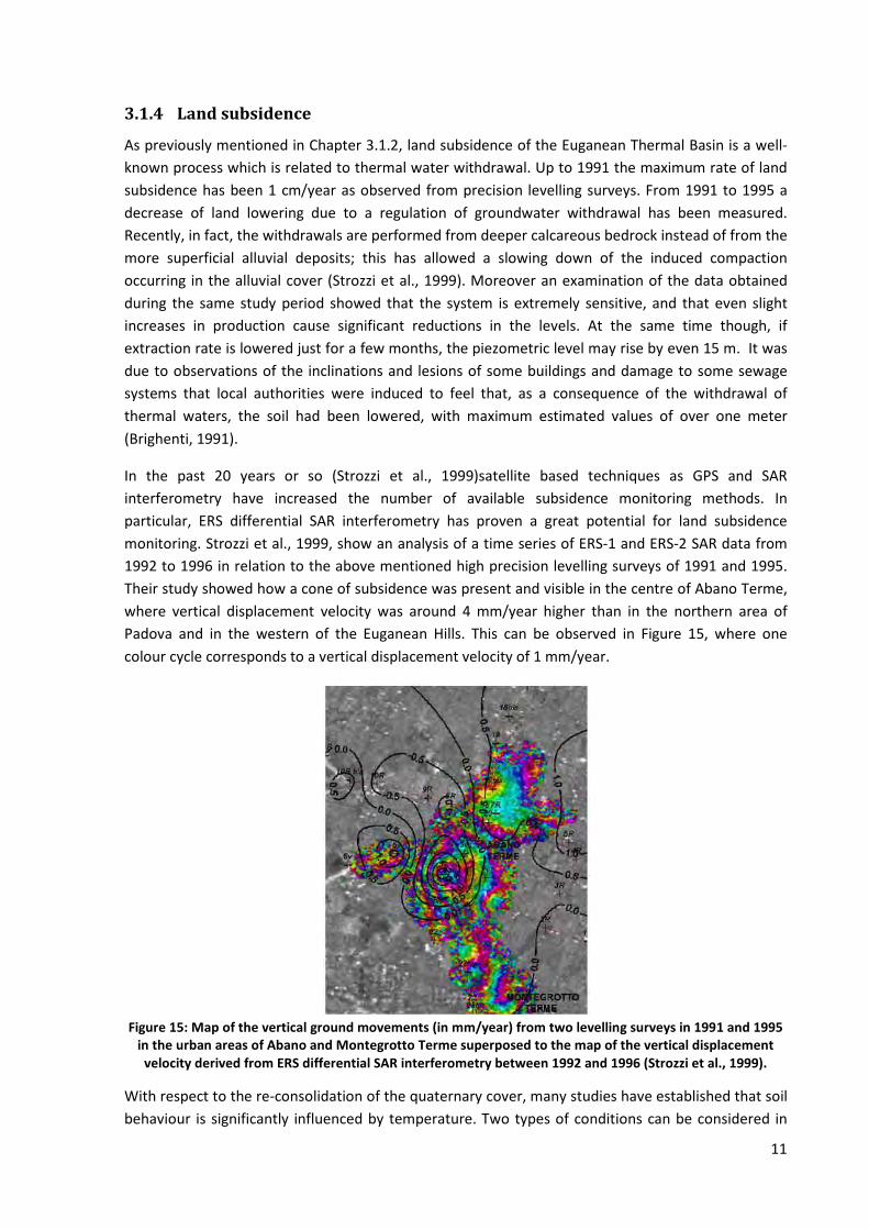
For what concerns the structural situation of the Euganean area, it is mainly characterized by systems

of faults that reflect, in the in most important tectonic events, the directions of the main structural

lines called “Schio-Vicenza line” (NNW-SSE) and “Riviera dei Berici line” (NE-SW) (Figure 13). The

former is the promoter of the mountain ridge formed by Lessini, Berici and Euganean Hills, while the

latter departs from the tectonic line Schio-Vicenza and separates the Berici by the Euganean Hills.

The western margin appears to be more affected by the system of fractures than the eastern margin,

and the lithology of the volcanic bodies is very variable; since the towns of Abano T., Montegrotto T.

and Battaglia T. Are located on the west of this line, they contain the highest concentrations of

thermal events (Piccoli et al., 1976), with a well’s density of about 10-15 wells/ha (Antonelli et al.,

1995).

Figure 13: Geological stereogram of western Veneto, with feeding and outcrop areas of hydrothermal circuit.

(Piccoli et al., 1976)

Figure 14: Tectonic overview of the Euganean Hills and Euganean Thermal Basin (Gestione Unica, n.d.)

Fore - Alps

Lessini Mountains

Berici Hills

Euganean Hills

Schio-Vicenza line

Riviera dei Berici line Euganean Thermal Field

11

3.1.4 Land subsidence

As previously mentioned in Chapter 3.1.2, land subsidence of the Euganean Thermal Basin is a well-

known process which is related to thermal water withdrawal. Up to 1991 the maximum rate of land

subsidence has been 1 cm/year as observed from precision levelling surveys. From 1991 to 1995 a

decrease of land lowering due to a regulation of groundwater withdrawal has been measured.

Recently, in fact, the withdrawals are performed from deeper calcareous bedrock instead of from the

more superficial alluvial deposits; this has allowed a slowing down of the induced compaction

occurring in the alluvial cover (Strozzi et al., 1999). Moreover an examination of the data obtained

during the same study period showed that the system is extremely sensitive, and that even slight

increases in production cause significant reductions in the levels. At the same time though, if

extraction rate is lowered just for a few months, the piezometric level may rise by even 15 m. It was

due to observations of the inclinations and lesions of some buildings and damage to some sewage

systems that local authorities were induced to feel that, as a consequence of the withdrawal of

thermal waters, the soil had been lowered, with maximum estimated values of over one meter

(Brighenti, 1991).

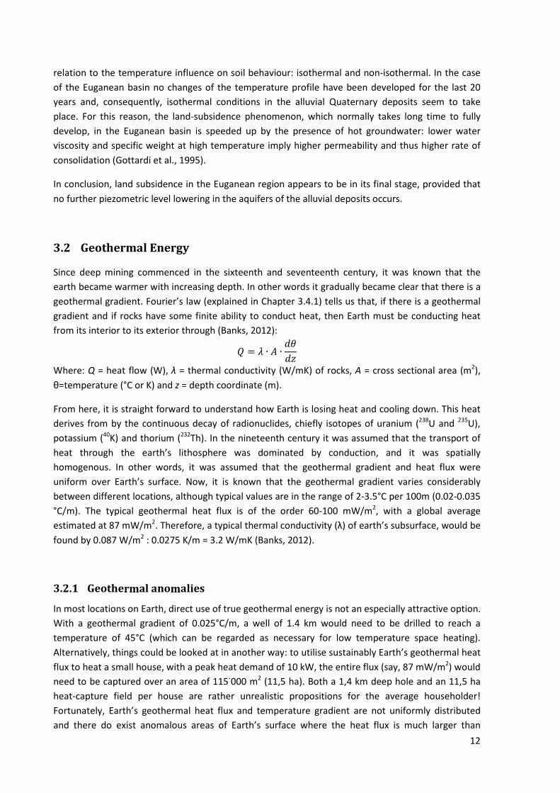
In the past 20 years or so (Strozzi et al., 1999)satellite based techniques as GPS and SAR

interferometry have increased the number of available subsidence monitoring methods. In

particular, ERS differential SAR interferometry has proven a great potential for land subsidence

monitoring. Strozzi et al., 1999, show an analysis of a time series of ERS-1 and ERS-2 SAR data from

1992 to 1996 in relation to the above mentioned high precision levelling surveys of 1991 and 1995.

Their study showed how a cone of subsidence was present and visible in the centre of Abano Terme,

where vertical displacement velocity was around 4 mm/year higher than in the northern area of

Padova and in the western of the Euganean Hills. This can be observed in Figure 15, where one

colour cycle corresponds to a vertical displacement velocity of 1 mm/year.

Figure 15: Map of the vertical ground movements (in mm/year) from two levelling surveys in 1991 and 1995

in the urban areas of Abano and Montegrotto Terme superposed to the map of the vertical displacement

velocity derived from ERS differential SAR interferometry between 1992 and 1996 (Strozzi et al., 1999).

With respect to the re-consolidation of the quaternary cover, many studies have established that soil

behaviour is significantly influenced by temperature. Two types of conditions can be considered in

12

relation to the temperature influence on soil behaviour: isothermal and non-isothermal. In the case

of the Euganean basin no changes of the temperature profile have been developed for the last 20

years and, consequently, isothermal conditions in the alluvial Quaternary deposits seem to take

place. For this reason, the land-subsidence phenomenon, which normally takes long time to fully

develop, in the Euganean basin is speeded up by the presence of hot groundwater: lower water

viscosity and specific weight at high temperature imply higher permeability and thus higher rate of

consolidation (Gottardi et al., 1995).

In conclusion, land subsidence in the Euganean region appears to be in its final stage, provided that

no further piezometric level lowering in the aquifers of the alluvial deposits occurs.

3.2 Geothermal Energy

Since deep mining commenced in the sixteenth and seventeenth century, it was known that the

earth became warmer with increasing depth. In other words it gradually became clear that there is a

geothermal gradient. Fourier’s law (explained in Chapter 3.4.1) tells us that, if there is a geothermal

gradient and if rocks have some finite ability to conduct heat, then Earth must be conducting heat

from its interior to its exterior through (Banks, 2012):

� = � ∙ � ∙����

Where: Q = heat flow (W), λ = thermal conductivity (W/mK) of rocks, A = cross sectional area (m2),

θ=temperature (°C or K) and z = depth coordinate (m).

From here, it is straight forward to understand how Earth is losing heat and cooling down. This heat

derives from by the continuous decay of radionuclides, chiefly isotopes of uranium (238U and 235U),

potassium (40K) and thorium (232Th). In the nineteenth century it was assumed that the transport of

heat through the earth’s lithosphere was dominated by conduction, and it was spatially

homogenous. In other words, it was assumed that the geothermal gradient and heat flux were

uniform over Earth’s surface. Now, it is known that the geothermal gradient varies considerably

between different locations, although typical values are in the range of 2-3.5°C per 100m (0.02-0.035

°C/m). The typical geothermal heat flux is of the order 60-100 mW/m2, with a global average

estimated at 87 mW/m2. Therefore, a typical thermal conductivity (λ) of earth’s subsurface, would be

found by 0.087 W/m2 : 0.0275 K/m = 3.2 W/mK (Banks, 2012).

3.2.1 Geothermal anomalies

In most locations on Earth, direct use of true geothermal energy is not an especially attractive option.

With a geothermal gradient of 0.025°C/m, a well of 1.4 km would need to be drilled to reach a

temperature of 45°C (which can be regarded as necessary for low temperature space heating).

Alternatively, things could be looked at in another way: to utilise sustainably Earth’s geothermal heat

flux to heat a small house, with a peak heat demand of 10 kW, the entire flux (say, 87 mW/m2) would

need to be captured over an area of 115˙000 m2 (11,5 ha). Both a 1,4 km deep hole and an 11,5 ha

heat-capture field per house are rather unrealistic propositions for the average householder!

Fortunately, Earth’s geothermal heat flux and temperature gradient are not uniformly distributed

and there do exist anomalous areas of Earth’s surface where the heat flux is much larger than

13

average and/or high temperatures are encountered at shallow depth. These anomalies can be called

potential geothermal fields, and they can be due to a variety of geological factors. Usually, high-

temperature geothermal fields are usually related to plate tectonic features. They typically occur at

one of three tectonic locations and are often associated with current or historic volcanism (Banks,

2012).

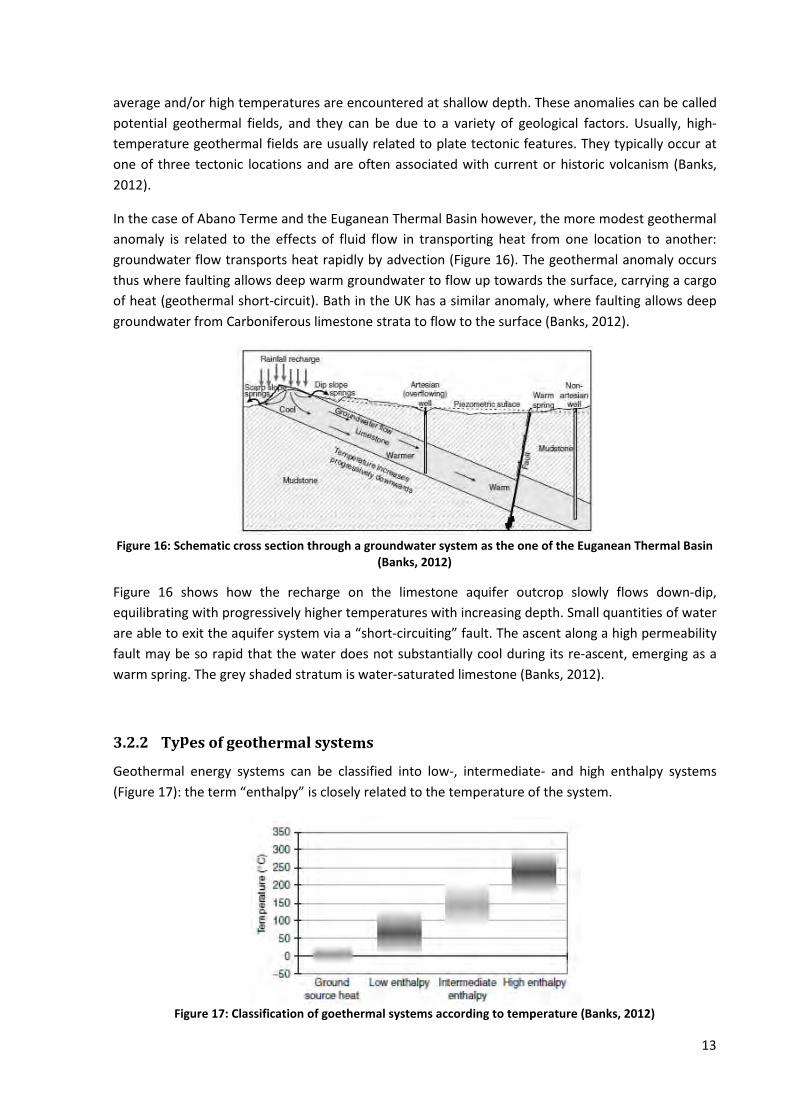
In the case of Abano Terme and the Euganean Thermal Basin however, the more modest geothermal

anomaly is related to the effects of fluid flow in transporting heat from one location to another:

groundwater flow transports heat rapidly by advection (Figure 16). The geothermal anomaly occurs

thus where faulting allows deep warm groundwater to flow up towards the surface, carrying a cargo

of heat (geothermal short-circuit). Bath in the UK has a similar anomaly, where faulting allows deep

groundwater from Carboniferous limestone strata to flow to the surface (Banks, 2012).

Figure 16: Schematic cross section through a groundwater system as the one of the Euganean Thermal Basin

(Banks, 2012)

Figure 16 shows how the recharge on the limestone aquifer outcrop slowly flows down-dip,

equilibrating with progressively higher temperatures with increasing depth. Small quantities of water

are able to exit the aquifer system via a “short-circuiting” fault. The ascent along a high permeability

fault may be so rapid that the water does not substantially cool during its re-ascent, emerging as a

warm spring. The grey shaded stratum is water-saturated limestone (Banks, 2012).

3.2.2 Types of geothermal systems

Geothermal energy systems can be classified into low-, intermediate- and high enthalpy systems

(Figure 17): the term “enthalpy” is closely related to the temperature of the system.

Figure 17: Classification of goethermal systems according to temperature (Banks, 2012)

14

High enthalpy systems are those that started first to use geothermal energy. This type of

development was conventional during the early years of geothermal development and is heavily

biased towards electricity production. The plant output was decided on the basis of an estimated

reservoir volume, average formation temperature, and porosity. Examples are Lardarello, Wairakei,

The Geysers, Tiwi, Cerro Prieto, Ahuachapan, Hatchubaru, and Olkaria. These are found generally on

high-temperature areas, located within active volcanic zones or marginal to them. They are mostly

on high ground. The rocks are geologically very young and permeable. As a result of the topography

and high bedrock permeability, the groundwater table in the high-temperature areas is generally

deep, and surface manifestations are largely steam vents. The system’s heat source is generally

shallow magma intrusions. In the case of high-temperature systems associated with central volcanic

complexes the intrusions often create shallow magma chambers, but where no central volcanoes

have developed only dyke swarms are found. Intrusive rocks appear to be most abundant in

reservoirs associated with central complexes that have developed a caldera (Elíasson, 2001).

It can be observed how the temperatures found in Abano Terme however are located in the low

enthalpy range. As it will be discussed in Chapter 3.2.3, the low temperature geothermal fluids, such

as those found in Abano Terme, are most usually used for direct uses, which include space heating,

industrial heating, swimming pools, horticulture (greenhouses) and aquaculture (fish farming).

3.2.3 Geothermal direct use - Space and district heating

Geothermal reservoirs of hot water, which are found beneath Earth's surface from a few metres to

few kilometres, can be used to provide heat directly for residential, industrial, and commercial uses.

Low-enthalpy geothermal resource is widespread worldwide, and is used in specific to heat homes

and offices, commercial greenhouses, fish farms, food processing facilities and a variety of other

applications. This is called the direct use of geothermal energy (Renewable Energy World, 2012).

Geothermal direct use dates back thousands of years, when people began using hot springs for

bathing, cooking food, and loosening feathers and skin from game. Today, hot springs are still used as

spas. But there are now more sophisticated ways of using this geothermal resource (U.S. Department

of Energy, 2013).

Direct use of geothermal energy in homes and commercial operations is much less expensive than

using traditional fuels. Savings can be as much as 80% over fossil fuels. Direct use is also very clean,

producing only a small percentage (and in many cases none) of the air pollutants emitted by burning

fossil fuels (U.S. Department of Energy, 2013).

A geothermal direct-use project utilises a natural resource: a flow of geothermal fluid at elevated

temperatures, which is capable of providing heat and/or cooling to buildings, greenhouses,

aquaculture ponds, and industrial process. Recommended temperature and flows are suggested for

spas and pools, space and district heating, greenhouse and aquaculture pond heating, and industrial

applications. Guidelines are provided for selecting the necessary equipment for successfully

implementing a direct-use project, including downhole pumps, piping, heat exchangers, and heat

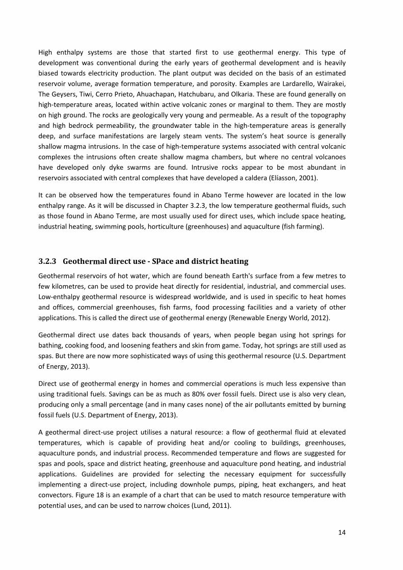
convectors. Figure 18 is an example of a chart that can be used to match resource temperature with

potential uses, and can be used to narrow choices (Lund, 2011).

15

Figure 18: Various geothermal uses, including power generation and direct use, related to their appropriate

temperature range (Lund, 2011)

For the purpose of this project the potential use of space and district heating only is analysed. District

heating involves the distribution of heat (hot water or steam) from a central location through a

network of pipes to individual houses or blocks of buildings. The distinction between district heating

and space heating systems is that space heating usually involves one geothermal well per structure.

An important consideration in district heating projects is the thermal load density, or the heat

demand divided by the ground area of the district. A high heat density, generally above 1.2

gigajoules/hour/hectare (GJ/hr/ha) or a favourability ratio of 2.5 GJ/ha/yr is recommended.

Geothermal district heating systems are capital intensive. The principal costs are initial investment

costs for production and injection wells, downhole and circulation pumps, heat exchangers, pipelines

and distribution networks, flow meters, valves and control equipment, and building retrofitting. The

distribution network may be the largest single capital expense, at approximately 35% to 75% of the

entire project cost. Operating expenses, however, are in comparison lower and consist of pumping

power, system maintenance, control, and management. The typical savings to consumers range from

approximately 30% to 50% per year of the cost of natural gas (Lund, 2011).

3.2.4 Closed-loop heat-exchanging systems

Considering that this project is related to space heating issues rather than district heating, the most

important role is played by the heat exchanger. Closed-loop heat-exchanging systems, also known as

Borehole Heat Exchangers (BHE), are chosen as they work very well with small heating loads, such as

the heating of individual homes, small apartment homes, or businesses, and because they eliminates

the problem of disposal of geothermal fluid since, as previously discussed, only heat is extracted

from the well (Lund, 2003).

In systems with a closed-loop heat-exchange a heat transfer fluid (known as refrigerant, water in this

case) is circulated through one or more pipes which allow this fluid to be heated (or cooled) from the

ground. This is in order for the fluid to be used then on the surface by heat pumps, or alternatively,

as envisaged in this case, in a free-heating system where another simple heat exchanger is used.

Once the fluid has been cooled down on the surface it re-enters the circuit.

16

The free-heating concept is a technique which may only be developed in areas where ground

temperature is much higher than normally, or where thermal anomalies are present. The concept

follows the idea that the temperature of a material, a fluid in this case, decreases as heat is

transported by it. For this reason, if a minimum temperature is required at a destination point, say a

building, the point where it is extracted, its origin, say the ground, must have a temperature high

enough for no other energy-spending units to be required to provide such temperature to the

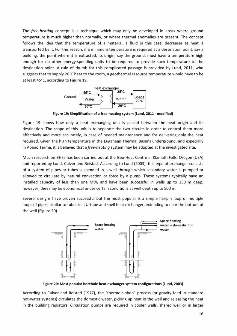
destination point. A rule of thumb for this complicated passage is provided by Lund, 2011, who

suggests that to supply 20°C heat to the room, a geothermal resource temperature would have to be

at least 45°C, according to Figure 19.

Figure 19: Simplification of a free-heating system (Lund, 2011 - modified)

Figure 19 shows how only a heat exchanging unit is placed between the heat origin and its

destination. The scope of this unit is to separate the two circuits in order to control them more

effectively and more accurately, in case of needed maintenance and for delivering only the heat

required. Given the high temperature in the Euganean Thermal Basin’s underground, and especially

in Abano Terme, it is believed that a free-heating system may be adopted at the investigated site.

Much research on BHEs has been carried out at the Geo-Heat Centre in Klamath Falls, Oregon (USA)

and reported by Lund, Culver and Reistad. According to Lund (2003), this type of exchanger consists

of a system of pipes or tubes suspended in a well through which secondary water is pumped or

allowed to circulate by natural convection or force by a pump. These systems typically have an

installed capacity of less than one MWt and have been successful in wells up to 150 m deep;

however, they may be economical under certain conditions at well depth up to 500 m.

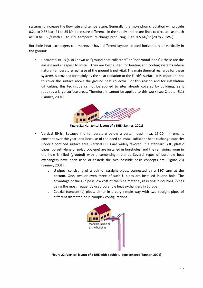
Several designs have proven successful but the most popular is a simple hairpin loop or multiple

loops of pipes, similar to tubes in a U-tube and shell heat exchanger, extending to near the bottom of

the well (Figure 20).

Figure 20: Most popular borehole heat exchanger system configurations (Lund, 2003)

According to Culver and Reistad (1977), the "thermo-siphon" process (or gravity feed in standard

hot-water systems) circulates the domestic water, picking up heat in the well and releasing the heat

in the building radiators. Circulation pumps are required in cooler wells, shared well or in larger

Space heating

water

Space heating

water + domestic hot

water

Heat exchanger

Ground Water Water

17

systems to increase the flow rate and temperature. Generally, thermo-siphon circulation will provide

0.21 to 0.35 bar (21 to 35 kPa) pressure difference in the supply and return lines to circulate as much

as 1.0 to 1.5 l/s with a 5 to 11°C temperature change producing 80 to 265 MJ/hr (20 to 70 kWt).

Borehole heat exchangers can moreover have different layouts, placed horizontally or vertically in

the ground:

• Horizontal BHEs (also known as “ground heat collectors” or “horizontal loops”): these are the

easiest and cheapest to install. They are best suited for heating and cooling systems where

natural temperature recharge of the ground is not vital. The main thermal recharge for these

systems is provided for mainly by the solar radiation to the Earth's surface. It is important not

to cover the surface above the ground heat collector. For this reason and for installation

difficulties, this technique cannot be applied to sites already covered by buildings, as it

requires a large surface areas. Therefore it cannot be applied to this work (see Chapter 5.1)

(Sanner, 2001).

Figure 21: Horizontal layout of a BHE (Sanner, 2001)

• Vertical BHEs: Because the temperature below a certain depth (ca. 15-20 m) remains

constant over the year, and because of the need to install sufficient heat exchange capacity

under a confined surface area, vertical BHEs are widely favored. In a standard BHE, plastic

pipes (polyethylene or polypropylene) are installed in boreholes, and the remaining room in

the hole is filled (grouted) with a cementing material. Several types of borehole heat

exchangers have been used or tested; the two possible basic concepts are (Figure 23)

(Sanner, 2001):

о U-pipes, consisting of a pair of straight pipes, connected by a 180°-turn at the

bottom. One, two or even three of such U-pipes are installed in one hole. The

advantage of the U-pipe is low cost of the pipe material, resulting in double-U-pipes

being the most frequently used borehole heat exchangers in Europe.

о Coaxial (concentric) pipes, either in a very simple way with two straight pipes of

different diameter, or in complex configurations.

Figure 22: Vertical layout of a BHE with double U-pipe concept (Sanner, 2001)

18

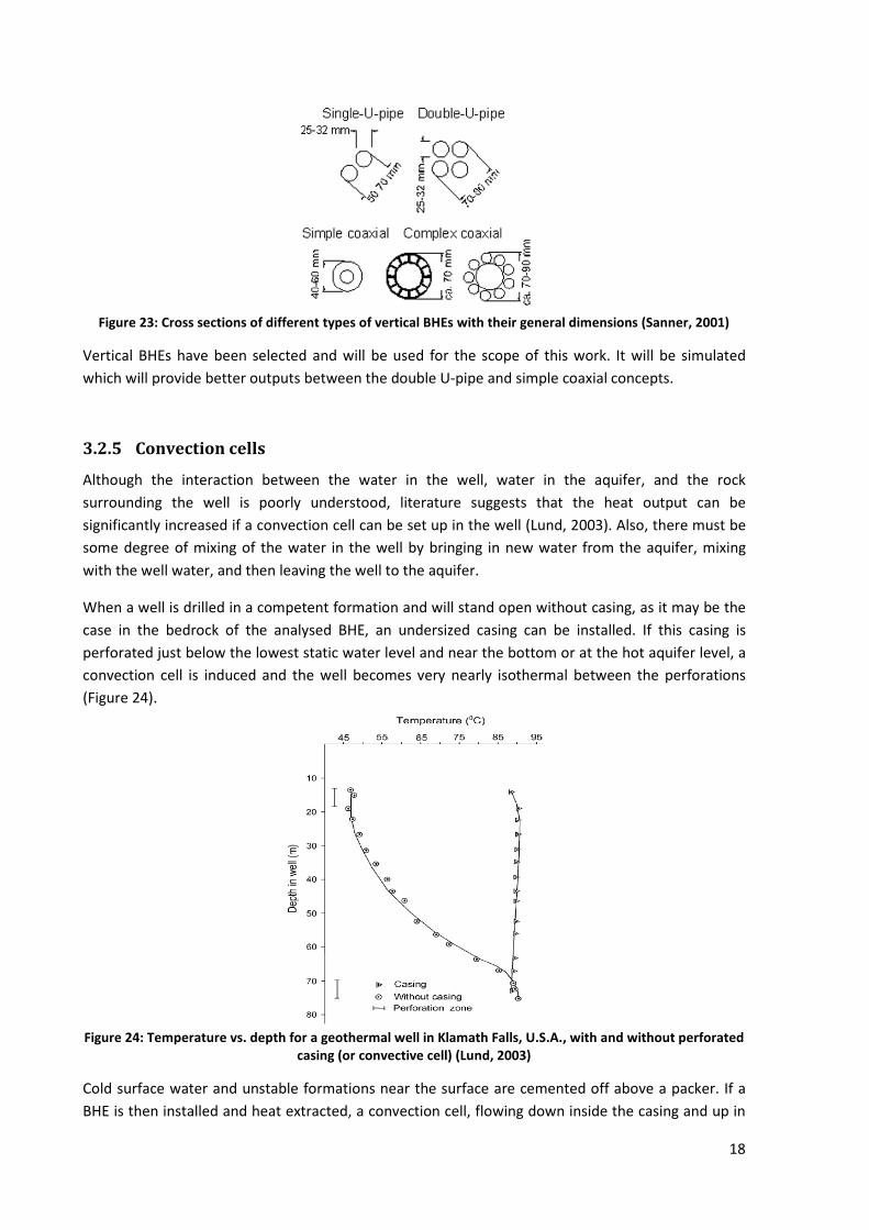
Figure 23: Cross sections of different types of vertical BHEs with their general dimensions (Sanner, 2001)

Vertical BHEs have been selected and will be used for the scope of this work. It will be simulated

which will provide better outputs between the double U-pipe and simple coaxial concepts.

3.2.5 Convection cells

Although the interaction between the water in the well, water in the aquifer, and the rock

surrounding the well is poorly understood, literature suggests that the heat output can be

significantly increased if a convection cell can be set up in the well (Lund, 2003). Also, there must be

some degree of mixing of the water in the well by bringing in new water from the aquifer, mixing

with the well water, and then leaving the well to the aquifer.

When a well is drilled in a competent formation and will stand open without casing, as it may be the

case in the bedrock of the analysed BHE, an undersized casing can be installed. If this casing is

perforated just below the lowest static water level and near the bottom or at the hot aquifer level, a

convection cell is induced and the well becomes very nearly isothermal between the perforations

(Figure 24).

Figure 24: Temperature vs. depth for a geothermal well in Klamath Falls, U.S.A., with and without perforated

casing (or convective cell) (Lund, 2003)

Cold surface water and unstable formations near the surface are cemented off above a packer. If a

BHE is then installed and heat extracted, a convection cell, flowing down inside the casing and up in

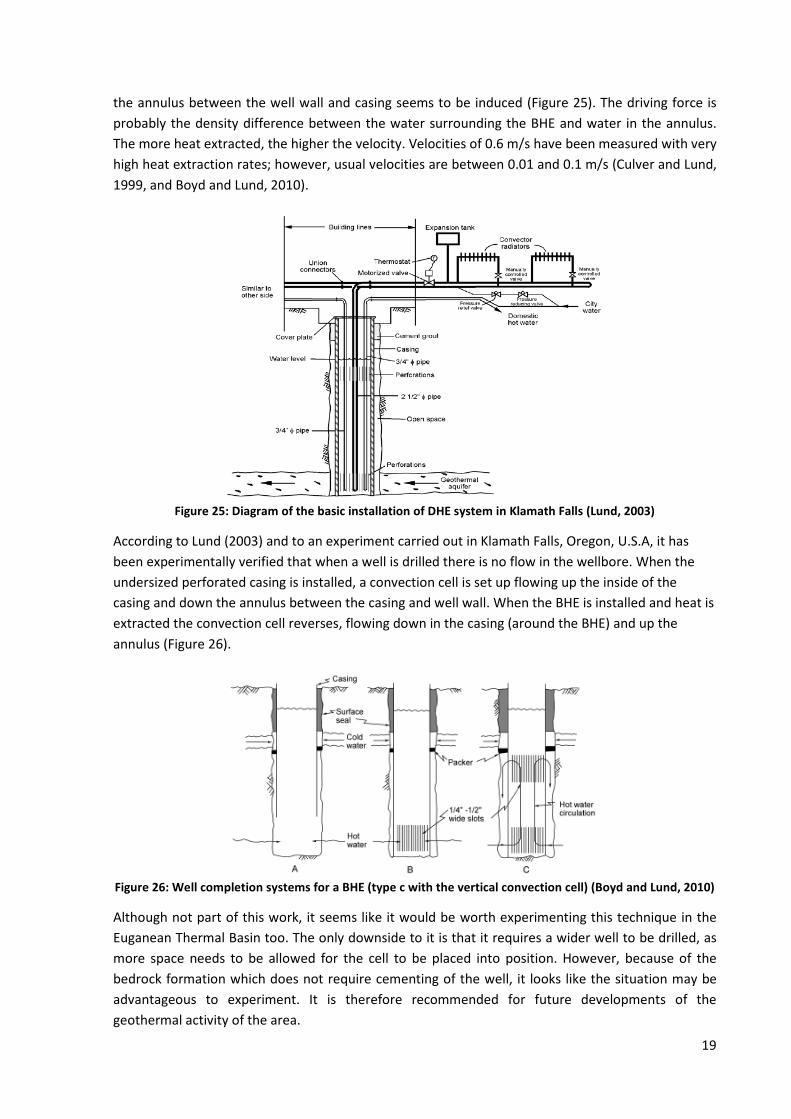
19

the annulus between the well wall and casing seems to be induced (Figure 25). The driving force is

probably the density difference between the water surrounding the BHE and water in the annulus.

The more heat extracted, the higher the velocity. Velocities of 0.6 m/s have been measured with very

high heat extraction rates; however, usual velocities are between 0.01 and 0.1 m/s (Culver and Lund,

1999, and Boyd and Lund, 2010).

Figure 25: Diagram of the basic installation of DHE system in Klamath Falls (Lund, 2003)

According to Lund (2003) and to an experiment carried out in Klamath Falls, Oregon, U.S.A, it has

been experimentally verified that when a well is drilled there is no flow in the wellbore. When the

undersized perforated casing is installed, a convection cell is set up flowing up the inside of the

casing and down the annulus between the casing and well wall. When the BHE is installed and heat is

extracted the convection cell reverses, flowing down in the casing (around the BHE) and up the

annulus (Figure 26).

Figure 26: Well completion systems for a BHE (type c with the vertical convection cell) (Boyd and Lund, 2010)

Although not part of this work, it seems like it would be worth experimenting this technique in the

Euganean Thermal Basin too. The only downside to it is that it requires a wider well to be drilled, as

more space needs to be allowed for the cell to be placed into position. However, because of the

bedrock formation which does not require cementing of the well, it looks like the situation may be

advantageous to experiment. It is therefore recommended for future developments of the

geothermal activity of the area.

20

3.3 Choice of the equipment

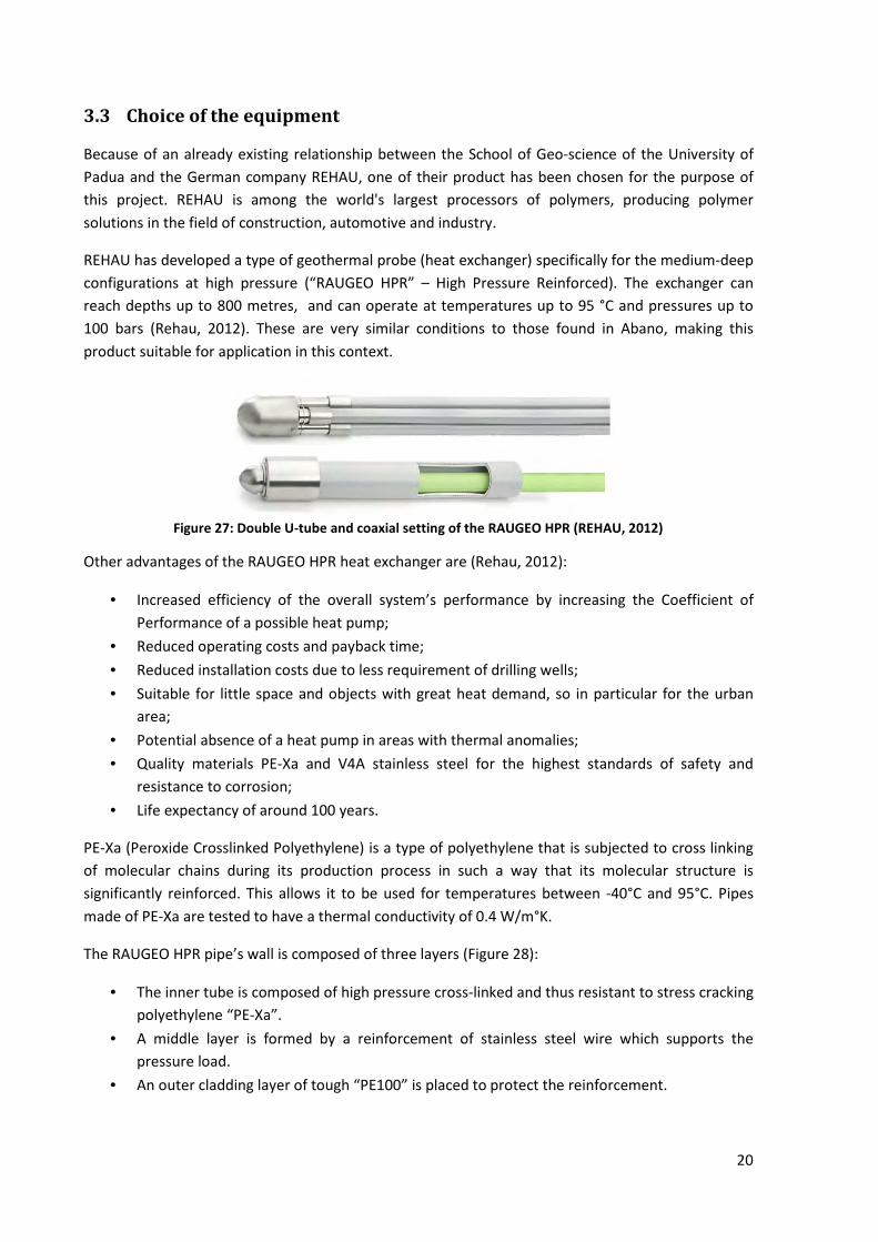
Because of an already existing relationship between the School of Geo-science of the University of

Padua and the German company REHAU, one of their product has been chosen for the purpose of

this project. REHAU is among the world's largest processors of polymers, producing polymer

solutions in the field of construction, automotive and industry.

REHAU has developed a type of geothermal probe (heat exchanger) specifically for the medium-deep

configurations at high pressure (“RAUGEO HPR” – High Pressure Reinforced). The exchanger can

reach depths up to 800 metres, and can operate at temperatures up to 95 °C and pressures up to

100 bars (Rehau, 2012). These are very similar conditions to those found in Abano, making this

product suitable for application in this context.

Figure 27: Double U-tube and coaxial setting of the RAUGEO HPR (REHAU, 2012)

Other advantages of the RAUGEO HPR heat exchanger are (Rehau, 2012):

• Increased efficiency of the overall system’s performance by increasing the Coefficient of

Performance of a possible heat pump;

• Reduced operating costs and payback time;

• Reduced installation costs due to less requirement of drilling wells;

• Suitable for little space and objects with great heat demand, so in particular for the urban

area;

• Potential absence of a heat pump in areas with thermal anomalies;

• Quality materials PE-Xa and V4A stainless steel for the highest standards of safety and

resistance to corrosion;

• Life expectancy of around 100 years.

PE-Xa (Peroxide Crosslinked Polyethylene) is a type of polyethylene that is subjected to cross linking

of molecular chains during its production process in such a way that its molecular structure is

significantly reinforced. This allows it to be used for temperatures between -40°C and 95°C. Pipes

made of PE-Xa are tested to have a thermal conductivity of 0.4 W/m°K.

The RAUGEO HPR pipe’s wall is composed of three layers (Figure 28):

• The inner tube is composed of high pressure cross-linked and thus resistant to stress cracking

polyethylene “PE-Xa”.

• A middle layer is formed by a reinforcement of stainless steel wire which supports the

pressure load.

• An outer cladding layer of tough “PE100” is placed to protect the reinforcement.

21

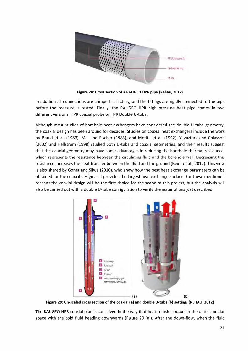
Figure 28: Cross section of a RAUGEO HPR pipe (Rehau, 2012)

In addition all connections are crimped in factory, and the fittings are rigidly connected to the pipe

before the pressure is tested. Finally, the RAUGEO HPR high pressure heat pipe comes in two

different versions: HPR coaxial probe or HPR Double U-tube.

Although most studies of borehole heat exchangers have considered the double U-tube geometry,

the coaxial design has been around for decades. Studies on coaxial heat exchangers include the work

by Braud et al. (1983), Mei and Fischer (1983), and Morita et al. (1992). Yavuzturk and Chiasson

(2002) and Hellström (1998) studied both U-tube and coaxial geometries, and their results suggest

that the coaxial geometry may have some advantages in reducing the borehole thermal resistance,

which represents the resistance between the circulating fluid and the borehole wall. Decreasing this

resistance increases the heat transfer between the fluid and the ground (Beier et al., 2012). This view

is also shared by Gonet and Sliwa (2010), who show how the best heat exchange parameters can be

obtained for the coaxial design as it provides the largest heat exchange surface. For these mentioned

reasons the coaxial design will be the first choice for the scope of this project, but the analysis will

also be carried out with a double U-tube configuration to verify the assumptions just described.

(a) (b)

Figure 29: Un-scaled cross section of the coaxial (a) and double U-tube (b) settings (REHAU, 2012)

The RAUGEO HPR coaxial pipe is conceived in the way that heat transfer occurs in the outer annular

space with the cold fluid heading downwards (Figure 29 [a]). After the down-flow, when the fluid

22

reaches the stainless steel probe, it is diverted in the inner tube to flow back up. The pipe allows the

slow downward flow to provide an optimal extraction rate from the soil through the heat carrier

fluid. The smaller inner tube instead forces a fast return of the heat transfer fluid to the surface at

higher speeds and therefore reducing heat loss. In addition, a further applied thermal insulation, e.g.

RAUISO PE-Xa, reduces thermal wastage. Moreover, the slim design of the coaxial pipe results in a

small drill and a uniform annular space.

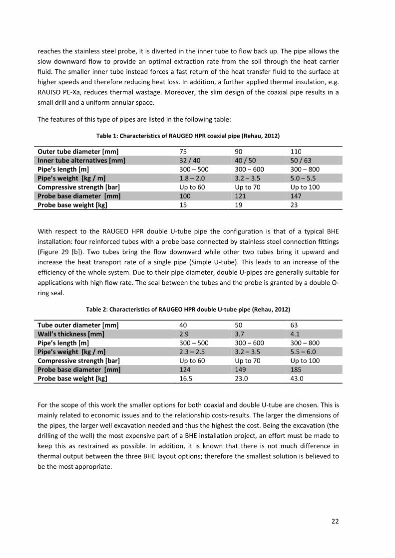
The features of this type of pipes are listed in the following table:

Table 1: Characteristics of RAUGEO HPR coaxial pipe (Rehau, 2012)

Outer tube diameter [mm] 75 90 110 Inner tube alternatives [mm] 32 / 40 40 / 50 50 / 63 Pipe’s length [m] 300 – 500 300 – 600 300 – 800 Pipe’s weight [kg / m] 1.8 – 2.0 3.2 – 3.5 5.0 – 5.5 Compressive strength [bar] Up to 60 Up to 70 Up to 100 Probe base diameter [mm] 100 121 147 Probe base weight [kg] 15 19 23

With respect to the RAUGEO HPR double U-tube pipe the configuration is that of a typical BHE

installation: four reinforced tubes with a probe base connected by stainless steel connection fittings

(Figure 29 [b]). Two tubes bring the flow downward while other two tubes bring it upward and

increase the heat transport rate of a single pipe (Simple U-tube). This leads to an increase of the

efficiency of the whole system. Due to their pipe diameter, double U-pipes are generally suitable for

applications with high flow rate. The seal between the tubes and the probe is granted by a double O-

ring seal.

Table 2: Characteristics of RAUGEO HPR double U-tube pipe (Rehau, 2012)

Tube outer diameter [mm] 40 50 63 Wall’s thickness [mm] 2.9 3.7 4.1 Pipe’s length [m] 300 – 500 300 – 600 300 – 800 Pipe’s weight [kg / m] 2.3 – 2.5 3.2 – 3.5 5.5 – 6.0 Compressive strength [bar] Up to 60 Up to 70 Up to 100 Probe base diameter [mm] 124 149 185 Probe base weight [kg] 16.5 23.0 43.0

For the scope of this work the smaller options for both coaxial and double U-tube are chosen. This is

mainly related to economic issues and to the relationship costs-results. The larger the dimensions of

the pipes, the larger well excavation needed and thus the highest the cost. Being the excavation (the

drilling of the well) the most expensive part of a BHE installation project, an effort must be made to

keep this as restrained as possible. In addition, it is known that there is not much difference in

thermal output between the three BHE layout options; therefore the smallest solution is believed to

be the most appropriate.

23

3.4 Basic Mechanisms of Heat Transfer

As already mentioned, in shallow aquifers a modern geothermal heat extraction technology (geo-

exchange) concerns the use of BHE systems of different construction or configurations (double U-

tubes and coaxial pipe mainly). Such heat exchangers form a vertical borehole system, where a

refrigerant of circulates in closed pipes (hence the name closed-loop system). These pipes are

inserted vertically in a borehole and are fixed by filling the borehole with some sort of grout material.

It is in contact with the surrounding soil where conductive–convective heat transfer processes occur

through the pipe, grout and soil (Diersch et al., 2011).

Transmission of heat takes place spontaneously in fact only from a warm body to a cold body, until

the two bodies reach the same temperature, in a so-called “thermal equilibrium”. The hot body

releases to the cold one part of its energy intensifying thermal molecular agitation. The

propagation of heat can take place by conduction, convection or radiation. Of these, radiation is

usually significant only at temperatures higher than those ordinarily encountered in tubular process

heat transfer equipment; therefore, radiation will not be described in any great detail. The two

others play a vital role in equipment design and would frequently appear in any kind of heat

transfer discussion (Bell and Mueller, 2009).

3.4.1 Conduction

Conduction in a material is largely due to the random movement of electrons through it. The

electrons in the hot part of the material have a higher kinetic energy than those in the cold part and

give up some of this kinetic energy to the cold atoms, thus resulting in a transfer of heat from the

hot surface to the cold. Since the free electrons are also responsible for the conduction of an

electrical current through a metal, there is a qualitative similarity between the ability of a metal

to conduct heat and to conduct electricity. In addition, some heat is transferred by inter-atomic

vibrations (Bell and Mueller, 2009).

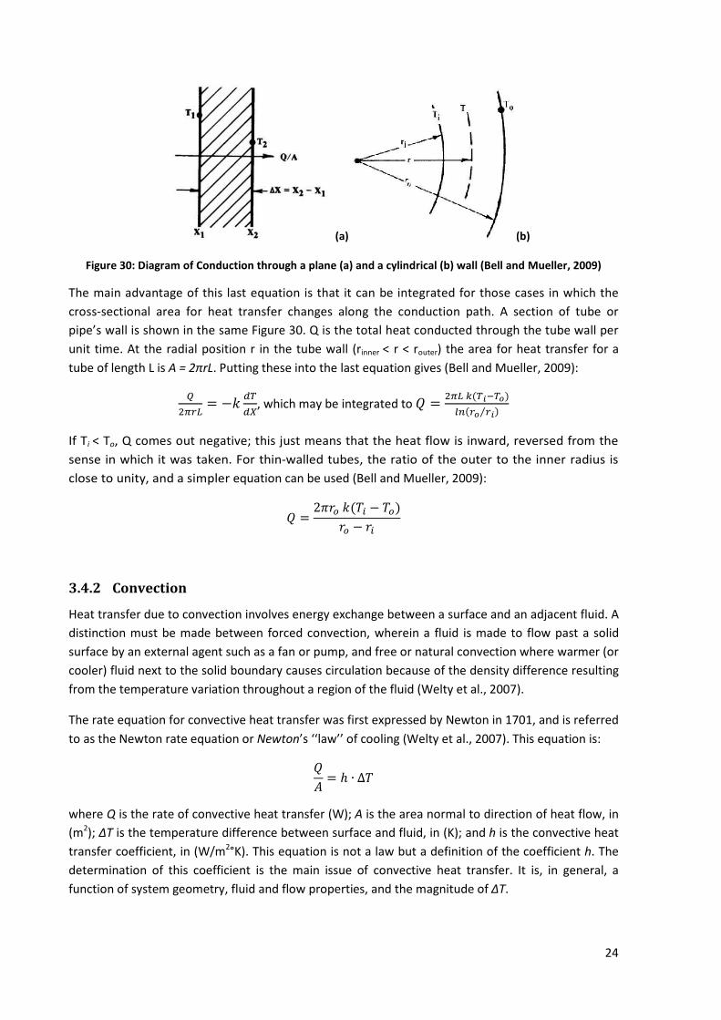
The details of conduction are quite complicated but for engineering purposes may be

handled by a simple equation, known as Fourier's equation. For the steady flow of heat across a

plane wall (Figure 30) with the surfaces at temperatures of T1 and T2, where T1 is greater than T2

the heat flow Q per unit area of surface A (the heat flux) is (Bell and Mueller, 2009):

�

�= � ������

������ = � ∙

Δ�

Δ� or = −� ∙

��

��

Where λ is called the thermal conductivity and is an experimentally measured value for any

material. The negative sign in the equation is introduced to account for the fact that heat is

conducted from a high temperature to a low temperature, making dT/dX inherently negative;

therefore the double negative indicates a positive flow of heat in the direction of decreasing

temperature.

24

(a) (b)

Figure 30: Diagram of Conduction through a plane (a) and a cylindrical (b) wall (Bell and Mueller, 2009)

The main advantage of this last equation is that it can be integrated for those cases in which the

cross-sectional area for heat transfer changes along the conduction path. A section of tube or

pipe’s wall is shown in the same Figure 30. Q is the total heat conducted through the tube wall per

unit time. At the radial position r in the tube wall (rinner < r < router) the area for heat transfer for a

tube of length L is A = 2πrL. Putting these into the last equation gives (Bell and Mueller, 2009):

�

��= −� ��

��, which may be integrated to � =

���(�����)

��� �⁄ �

If Ti < To, Q comes out negative; this just means that the heat flow is inward, reversed from the

sense in which it was taken. For thin-walled tubes, the ratio of the outer to the inner radius is

close to unity, and a simpler equation can be used (Bell and Mueller, 2009):

� =2���(�� − ��)�� − ��

3.4.2 Convection

Heat transfer due to convection involves energy exchange between a surface and an adjacent fluid. A

distinction must be made between forced convection, wherein a fluid is made to flow past a solid

surface by an external agent such as a fan or pump, and free or natural convection where warmer (or

cooler) fluid next to the solid boundary causes circulation because of the density difference resulting

from the temperature variation throughout a region of the fluid (Welty et al., 2007).

The rate equation for convective heat transfer was first expressed by Newton in 1701, and is referred

to as the Newton rate equation or Newton’s ‘‘law’’ of cooling (Welty et al., 2007). This equation is:

�� = ℎ ∙ ∆�

where Q is the rate of convective heat transfer (W); A is the area normal to direction of heat flow, in

(m2); ΔT is the temperature difference between surface and fluid, in (K); and h is the convective heat

transfer coefficient, in (W/m2°K). This equation is not a law but a definition of the coefficient h. The

determination of this coefficient is the main issue of convective heat transfer. It is, in general, a

function of system geometry, fluid and flow properties, and the magnitude of ΔT.

25

It is important to mention that even when a fluid is flowing in a turbulent manner past a surface,

there is still a layer, sometimes extremely thin, close to the surface where flow is laminar; also, the

fluid particles next to the solid boundary are at rest. As this is always true, the mechanism of heat

transfer between a solid surface and a fluid must involve conduction through the fluid layers close to

the surface. This ‘‘film’’ of fluid often presents the controlling resistance to convective heat transfer,

and the coefficient h is often referred to as the film coefficient (Welty et al., 2007).

It is immediate then to understand how convection is closely related to fluid-dynamics, and in

particular to the flow type in ducts. The type of flow in a duct, in fact, can be characterised by the

flow regime; that is, laminar flow, turbulent flow, or some transition state having characteristics of

both of the limiting regimes. Flow in BHE are usually kept in the transient interval, as close as

possible to turbulent.

The flow regime that exists in a given case is ordinarily characterized by the Reynolds number. The

Reynolds number has different definitions for flow in different geometries, but it is defined as

(Welty et al., 2007):

Re =���

�

where ρ is the density of the fluid, V is the average velocity in the tube, D is the inside diameter of

the tube, and μ the viscosity of the fluid. Laminar flow is characterized by Reynolds numbers below

2300, turbulent flow by high Reynolds Numbers above 4000.

For what concerns heat transfer to a flowing fluid, convection heat transfer can be defined as

transport of heat from one point to another in a flowing fluid as a result of macroscopic motions of

the fluid, the heat being carried as internal energy.

3.4.3 Combination of convection and conduction

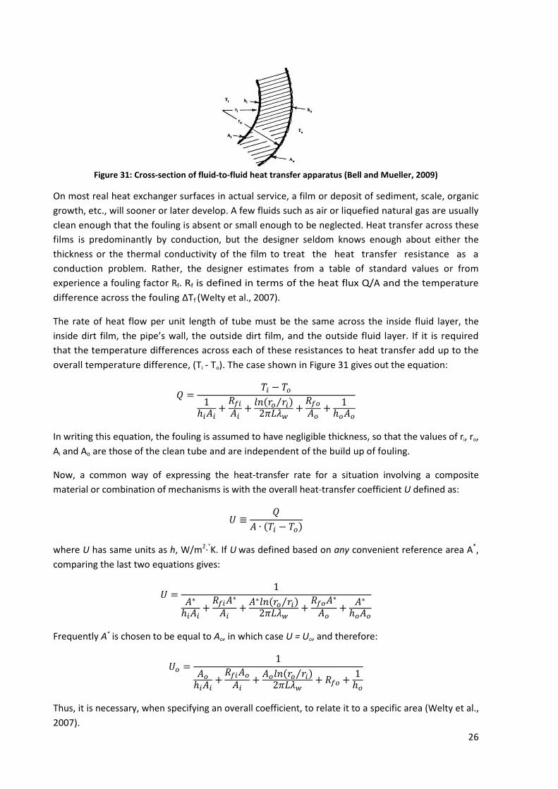
Considering the situation in Figure 31, heat is being transferred from the fluid inside (at a local

bulk or average temperature of Ti), through the above mentioned film layer, through the tube wall,

through another film to the outside fluid at a local bulk temperature of To. Ai and Ao are

respectively inside and outside surface areas for heat transfer for a given length of tube. For a

plain or bare cylindrical tube, ��

��=

�����

�����=

��

��.

The heat transfer rate between the fluid inside the tube and the surface of the inside fouling film is

given by the convection equation in the form Q/A = h(Tf - Ts) where the area is Ai and similarly for

the outside convective process where the area is Ao . The values of hi and ho (Convective heat

transfer coefficients) have to be calculated from appropriate correlations (Welty et al., 2007).

26

Figure 31: Cross-section of fluid-to-fluid heat transfer apparatus (Bell and Mueller, 2009)

On most real heat exchanger surfaces in actual service, a film or deposit of sediment, scale, organic

growth, etc., will sooner or later develop. A few fluids such as air or liquefied natural gas are usually

clean enough that the fouling is absent or small enough to be neglected. Heat transfer across these

films is predominantly by conduction, but the designer seldom knows enough about either the

thickness or the thermal conductivity of the film to treat the heat transfer resistance as a

conduction problem. Rather, the designer estimates from a table of standard values or from

experience a fouling factor Rf. Rf is defined in terms of the heat flux Q/A and the temperature

difference across the fouling ΔTf (Welty et al., 2007).

The rate of heat flow per unit length of tube must be the same across the inside fluid layer, the

inside dirt film, the pipe’s wall, the outside dirt film, and the outside fluid layer. If it is required

that the temperature differences across each of these resistances to heat transfer add up to the

overall temperature difference, (Ti - To). The case shown in Figure 31 gives out the equation:

� =�� − ��

1ℎ��� + ����� + ���� ��⁄ �

2��� +����� +

1ℎ���

In writing this equation, the fouling is assumed to have negligible thickness, so that the values of ri, ro,

Ai and Ao are those of the clean tube and are independent of the build up of fouling.

Now, a common way of expressing the heat-transfer rate for a situation involving a composite

material or combination of mechanisms is with the overall heat-transfer coefficient U defined as:

� ≡�� ∙ ��� − ���

where U has same units as h, W/m2∙°K. If U was defined based on any convenient reference area A*,

comparing the last two equations gives:

� =1�∗

ℎ��� + ����∗

�� +�∗ ���� ��⁄ �2��� +

����∗

�� +�∗

ℎ���

Frequently A* is chosen to be equal to Ao, in which case U = Uo, and therefore:

�� = 1��ℎ��� + ������� +

�� ���� ��⁄ �2��� + ��� + 1

ℎ�

Thus, it is necessary, when specifying an overall coefficient, to relate it to a specific area (Welty et al.,

2007).

27

3.4.4 Energy transfer in modelling

For the analysis of three-dimensional and two-dimensional flow and transport problems a number of

simplifications in the modelling approach are suited, on the one hand, to govern mathematically and

numerically the complex processes and, on the other hand, to attend to intrinsic practical needs

(Diersch and Kolditz,2002).

The use of geothermal energy allows the described conductive-convective heat transfer to cause a

temperature varying trend in the subsurface. Extension and magnitude of such temperature

variations do not only depend on the amount of exchanged energy, but also on the characteristics of

the ground and the installed BHE system itself. In a purely conductive environment, for example,

heat propagation in horizontal direction is uniform and a radial symmetric temperature anomaly

develops. In an advection-dominated system, heat is additionally transported by advection and

enhanced heat transport parallel to the groundwater flow direction causes a more elliptically shaped

plume. The magnitude of the variation is important to the design of a BHE system. Furthermore, the

change in groundwater temperature might adversely affect the quality of the groundwater and

groundwater ecosystem. Under certain conditions, the temperature anomaly can spread significantly

and may reach the range of influence of other BHEs in neighbouring properties (or hotels as in this

case). This can reduce the efficiency of both BHE and extraction well systems. Hence, precise and

reliable models are needed to predict the extension and magnitude of evolving temperature

anomalies (Wagner et al., 2012).

As previously described, heat transport in the soil around the BHE occurs by three different

mechanisms (Casasso and Sethi, 2012):

• conduction, which is driven by the temperature gradient;

• convection, which is the heat transfer between a solid and a moving fluid;

• dispersion, caused by the heterogeneities of the groundwater flow velocity field.

These mechanisms are then described by the heat conservation equation:

��� ������� + �1 − �������+ ���� ����������+���� �λ��

����� = ��

Where:

• ε is the porosity [-];

• ρs and ρf are the density of the solid and liquid phase [M/L3];

• sc and cf are the specific heat of the solid and liquid phase [L2/T2K1];

• qi is the i-th component of the Darcy velocity [L/T];

• λij is the soil effective heat conductivity [ML/T3K1], which is the sum of three components,

representing respectively the conductive transport in the solid phase and in water and the

dispersive transport in water:

��� = �1 − ���!�� + ���!�� + ���� "#�$ �!�� + �#� − #�� ������$ � % = �������� + �

��

�����+ �

��

����

28

Where αL and αT are respectively the longitudinal and the transverse dispersivity [L] and Vq is the

modulus of the Darcy velocity [L/T] (Casasso and Sethi, 2012).

A more detailed explanation of the flow and heat transport modeling in FEFlow is reported in Diersch

and Kolditz (2002).

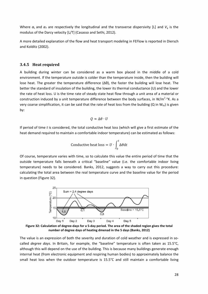
3.4.5 Heat required

A building during winter can be considered as a warm box placed in the middle of a cold

environment. If the temperature outside is colder than the temperature inside, then the building will

lose heat. The greater the temperature difference (Δθ), the faster the building will lose heat. The

better the standard of insulation of the building, the lower its thermal conductance (U) and the lower

the rate of heat loss. U is the time rate of steady state heat flow through a unit area of a material or

construction induced by a unit temperature difference between the body surfaces, in W/m2⋅°K. As a

very coarse simplification, it can be said that the rate of heat loss from the building (Q in Wth) is given

by:

� ≈ ∆� ∙ �

If period of time t is considered, the total conductive heat loss (which will give a first estimate of the

heat demand required to maintain a comfortable indoor temperature) can be estimated as follows:

Conductiveheatloss = � ∙& ∆�d��

�

Of course, temperature varies with time, so to calculate this value the entire period of time that the

outside temperature falls beneath a critical “baseline” value (i.e. the comfortable indoor living

temperature) needs to be considered. Banks, 2012, suggests a way to carry out this procedure:

calculating the total area between the real temperature curve and the baseline value for the period

in question (Figure 32).

Figure 32: Calculation of degree-days for a 5-day period. The area of the shaded region gives the total

number of degree days of heating dmenad in the 5 days (Banks, 2012)

The value is an expression of both the severity and duration of cold weather and is expressed in so-

called degree days. In Britain, for example, the “baseline” temperature is often taken as 15.5°C,

although this will depend on the use of the building. This is because many buildings generate enough

internal heat (from electronic equipment and respiring human bodies) to approximately balance the

small heat loss when the outdoor temperature is 15.5°C and still maintain a comfortable living

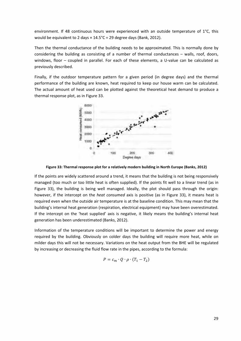
29

environment. If 48 continuous hours were experienced with an outside temperature of 1°C, this

would be equivalent to 2 days × 14.5°C = 29 degree days (Bank, 2012).

Then the thermal conductance of the building needs to be approximated. This is normally done by

considering the building as consisting of a number of thermal conductances – walls, roof, doors,

windows, floor – coupled in parallel. For each of these elements, a U-value can be calculated as

previously described.

Finally, if the outdoor temperature pattern for a given period (in degree days) and the thermal

performance of the building are known, heat required to keep our house warm can be calculated.

The actual amount of heat used can be plotted against the theoretical heat demand to produce a

thermal response plot, as in Figure 33.

Figure 33: Thermal response plot for a relatively modern building in North Europe (Banks, 2012)

If the points are widely scattered around a trend, it means that the building is not being responsively

managed (too much or too little heat is often supplied). If the points fit well to a linear trend (as in

Figure 33), the building is being well managed. Ideally, the plot should pass through the origin:

however, if the intercept on the heat consumed axis is positive (as in Figure 33), it means heat is

required even when the outside air temperature is at the baseline condition. This may mean that the

building’s internal heat generation (respiration, electrical equipment) may have been overestimated.

If the intercept on the ‘heat supplied’ axis is negative, it likely means the building’s internal heat

generation has been underestimated (Banks, 2012).

Information of the temperature conditions will be important to determine the power and energy

required by the building. Obviously on colder days the building will require more heat, while on

milder days this will not be necessary. Variations on the heat output from the BHE will be regulated

by increasing or decreasing the fluid flow rate in the pipes, according to the formula:

' = �� ∙ � ∙ � ∙ ��� − ���

30

4 Legislative issues

4.1 National legislation

In Italy, the law governing the field of geothermal technology is very fragmented, confusing and not

always consistent. Due to the absence of national policies and guidelines, the legislation is very

variable from place to place with a high-diversity situations (BIOCE, 2012).

The main legal reference with regard to thermal water exploitation in the Italian territory is the Royal

Decree of 29th July 1927, n. 1443, which regulates the search and production of minerals and energy

from the ground. This law posed a fundamental division between resources, according to two basic

categories: mines and quarries. The first category includes mineral and thermal waters (Città di

Abano Terme, 2009).

In earlier times, with respect to the legislation prior to the unification of Italy, the mineral and

thermal waters were entirely at the disposal of the owner of the land in which they were found, with

a few exceptions, and these had the right of direct exploitation or grant to third parties (BIOCE,

2012).

The above mentioned Royal Decree formally hands the ownership of the fluids to heritage of the

State. Secondly it forces the creation of special regulation covering thermal and mineral waters by

people owning a mining title who demonstrate adequate technical-economic abilities for the right

exploitation of resources. As a result of these laws and the promising potential of the thermal

activity, the Euganean Thermal Field began to acquire thermal water exploitation licences. By decree

of the Ministry of Industry and Trade dated 6th September 1930, the first two mining licenses were

granted in the area of Abano-Monteortone: the “Montirone”, on an area of over 65 hectares, and the

“Monteortone” (BIOCE, 2012).

The Decree of the President of the Republic no. 616 of 24th July 1977, delegates to Regional Councils

the administrative functions related to the subject of mineral and thermal waters, and to the subject

“quarries and peat bogs”. The Law 59/1997 has ordered that the Legislative Decrees commissioned

by the Government indicate the tasks conferred on regional and local administrations. Finally, with

the Legislative Decree no.112 of 31st March 1998, skills related to Category 1 resources (mines) are

transferred to the Regional Councils with the “transfer of administrative functions and duties of the

State to the Regions and local authorities, in the implementation of Chapter 1 of Law 59/1997”

(BIOCE, 2012).

For what concerns the legislation covering the implementation of geothermal activities, the first law

to be adopted at a National level was Law n. 896 of 9th December 1986, modified only recently by

Law n. 99 of 23rd July 2009, in turn adopted finally by Law n. 22 of 11th February 2010.

31

With respect to Law 896/1986, it is worth mentioning how it established the degree of concern with

respect to the activity’s size:

• National concern is given to those sources which allow the realisation of a geothermal

activity extracting at least 20 MWt.

• Regional concern is given to those sources which allow the realisation of a geothermal

activity extracting less than 20 MWt.

• Local concern is given to those sources which allow the realisation of a geothermal activity

exploiting warm groundwater found at a depth of less than 400 m and allow to extract

maximum 2 MWt.

For this reason the BHE designed in the course of this project will not be deeper than 400 m.

Secondly, the BHE will not require a mining licence, avoiding therefore the long and complex

bureaucratic procedure required to obtain such type of licence.

Law 99/2009 is the law which symbolised the taking over by the Italian Government to establish a

national reference framework in the field of geothermal activities. Relevant to this commitment is

Article 27, sections 28 and 39. Section 28 detailed how the Government committed to enact “one or

more legislative decrees in order to determine a new set of rules in the field of exploration and

production of geothermal resources that ensure, in the context of sustainable development of the

sector and ensuring the protection of the environment, a competitive regime for the use of high-

temperature geothermal resources and simplify administrative procedures for the use of geothermal

resources for low and medium temperature”. In addition, with Section 39 the Government

committed to issue “a decree aimed at defining the requirements for the installation of facilities for

the production of heat from geothermal sources, or rather borehole heat exchangers, for heating

and cooling of buildings, for which it is only necessary a declaration of activity’s beginning”. All these

commitments were subsequently confirmed and adopted by Law 22/2010 (Città di Abano Terme,

2009).

4.2 Regional legislation

For what concerns the geothermal activity in the Veneto Region, the Regional Law no. 40 of 10th

October 1989 regulates the research, cultivation and use of mineral and thermal waters.

In particular, Article. 7 of this Regional Law 40/1989 defines thermal waters as:

• "Mineral waters" are those that are used both for beverages and for curative purposes

thanks to their special properties;

• "Thermal waters" are those that are used solely for therapeutic purposes.

Moreover, Article. 39 of the same Law provides that:

1. “The following is subject to approval of the Regional Council:

a) the creation and operation of bottling establishments of mineral waters;

b) the opening and operation of spas;

c) the use of mineral water for the preparation of soft drinks;

d) the extraction of salts from the mineral waters.

32

2. Spas are defined as thermal establishments if they the following for therapeutic purposes:

a) thermal or mineral waters;

b) both natural and artificially prepared muds, molds and alike;

c) caves, natural and artificial stoves.”

Law 40/1989 furthermore deals with geothermal concessions, considering these as open-loop

systems requiring extraction of thermal fluids. On this matter, it is important to note that, at present,

there are no geothermal concessions in Abano Terme, and new concessions cannot be granted

within the Euganean Thermal Basin or at a distance less than 10 km from it (Article 55). This is in

order to preserve the conditions of the thermal fluids. According to this law, thermal water is

intended as a heat-carrying vector fluid which must necessarily be used for therapeutic and sanitary

uses; in addition, heat cannot be extracted if by doing so its chemical and physical properties are

changed (BIOCE, 2012).

For what concerns the Euganean Thermal Field, this Law is also integrated with the “Piano di

Utilizzazione della Risorsa Termale” – PURT (Plan of Utilisation of Thermal Resources), approved with

the Action of the Regional Council no. 1111 of 23rd April 1980 and subsequent amendments and

additions. This aims at safeguarding the hydrothermal resource and enhancing the value of Euganean

Thermal Field.

The PURT is divided into three main parts including (BIOCE, 2012):

• planning regulations;

• rules for mining;

• health standards.

Planning regulations deal with the intended use of the land, including the subdivision in safeguard

zones for the thermal resource, the size of areas for settlement of the thermal plants and the use and

modification of planning instruments (BIOCE, 2012).

The rules for mining include, for example, the renewal of expiring licenses, the transfer of ownership,

the extension of concessions that do not have space available for new drilling, the closure of

abandoned wells (BIOCE, 2012).

Finally, health standards provide indications for the characteristics of the dressing rooms for mud

therapy, the relationship between the availability of mud beds and between dressing rooms and

beds, the health departments of establishments, etc (Città di Abano Terme, 2009).

Today, the PURT is an old-fashioned instrument, as explicitly expressed by other participants to

Environmental Planning, both because it is no more consistent with the changing social and

economic conditions of the thermal area and because of its inadequate technical standpoint. When it

was approved, the main problems that emerged were to regulate the extraction rate of thermal

waters, to guarantee enough touristic receiving capacity and to protect Euganean Hills from wild

excavations while preserving the undoubted scenic landscape (Città di Abano Terme, 2009).

Secondly, a very strict bond to the exploitation of thermal resource is enforced, blocking a maximum

pumping of hot water set in litres/year, equivalent to the maximum number of beds per thermal

establishment. Areas used for the placement of wells to pump the thermal areas are considered for

public services. In particular, areas for the Protection of Thermal Resource are established that will

33

provide access to the resource, the quality of the thermal settlements and urban functions

connected (Città di Abano Terme, 2009).

More recently, the “Deliberazione della Giunta Regionale” (Decision of the Regional Council) N. 4106

of 29th December 2009 has specified the regional position towards to the extraction of mineral salts

from thermal waters, the management of the temperature parameter and use of exhaust water. For

what concerns the “Management of the temperature parameter”, this Decision describes how

primary thermal fluids cannot be directly used for therapeutic purposes because of their high

temperature (70-80°C). The temperature has to be lowered in advance to acceptable values for the

patient. Nevertheless, after the therapeutic use, temperature in the order of 30-40°C can be

detected if abatement efforts have not been carried out. These temperatures are still too high and

require additional processes of dissipation of the thermal heat before the waters can be discharged.

In conclusion, to protect the prevailing public interests with respect to mineral resource, it must be

established and prescribed that (BIOCE, 2012):

• processes of dissipation / heat recovery for the reduction of the temperature of the fluid are

allowed before and during therapeutic use, and even after such use for the discharge water.

These should occur with processes of thermal recovery, by means of:

o equipment for heat exchange;

o dissipation tanks adjacent to the spa, possibly structured as swimming pools open to

the public, highlighting the inscription: "POOL WITH NON THERAPEUTIC WATER";

o other methods allowed by the Region.

• as these processes deal mainly with the lowering of temperature for environmental reasons

and recovery of thermal energy, they are configured as improvement of the temperature

parameter and of the exhaust water. Moreover they do not require authorizations of

geothermal and/or mining nature, but it is necessary to report such secondary use to the

competent authorities.

Later, with the coming into effect of the Legislative Decree n. 22 of 11th February 2010, rules for

obtaining the necessary permits for the implementation of projects for the enhancement of

geothermal resources for energy purposes are particularly simplified (BIOCE, 2012).

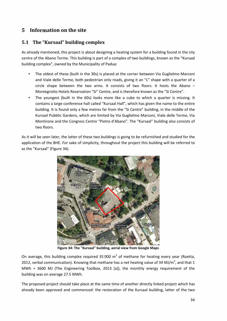
34

5 Information on the site

5.1 The “Kursaal” building complex

As already mentioned, this project is about designing a heating system for a building found in the city

centre of the Abano Terme. This building is part of a complex of two buildings, known as the “Kursaal

building complex”, owned by the Municipality of Padua:

• The oldest of these (built in the 30s) is placed at the corner between Via Guglielmo Marconi

and Viale delle Terme, both pedestrian only roads, giving it an “L” shape with a quarter of a

circle shape between the two arms. It consists of two floors. It hosts the Abano –

Montegrotto Hotels Reservation “Si” Centre, and is therefore known as the “Si Centre”.

• The youngest (built in the 60s) looks more like a cube to which a quarter is missing. It

contains a large conference hall called “Kursaal Hall”, which has given the name to the entire

building. It is found only a few metres far from the “Si Centre” building, in the middle of the

Kursaal Pubblic Gardens, which are limited by Via Guglielmo Marconi, Viale delle Terme, Via

Montirone and the Congress Centre “Pietro d’Abano”. The “Kursaal” building also consists of

two floors.

As it will be seen later, the latter of these two buildings is going to be refurnished and studied for the

application of the BHE. For sake of simplicity, throughout the project this building will be referred to

as the “Kursaal” (Figure 34).

Figure 34: The "Kursaal" building, aerial view from Google Maps

On average, this building complex required 35˙000 m3 of methane for heating every year (Roetta,

2012, verbal communication). Knowing that methane has a net heating value of 34 MJ/m3, and that 1

MWh = 3600 MJ (The Engineering Toolbox, 2013 [a]), the monthly energy requirement of the

building was on average 27.5 MWh.

The proposed project should take place at the same time of another directly linked project which has

already been approved and commenced: the restoration of the Kursaal building, latter of the two

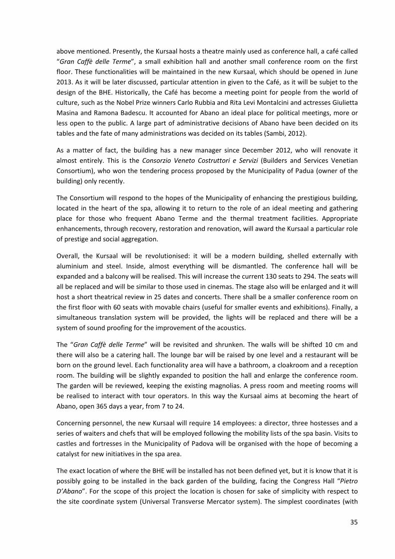
35

above mentioned. Presently, the Kursaal hosts a theatre mainly used as conference hall, a café called

“Gran Caffè delle Terme”, a small exhibition hall and another small conference room on the first

floor. These functionalities will be maintained in the new Kursaal, which should be opened in June

2013. As it will be later discussed, particular attention in given to the Café, as it will be subjet to the

design of the BHE. Historically, the Café has become a meeting point for people from the world of

culture, such as the Nobel Prize winners Carlo Rubbia and Rita Levi Montalcini and actresses Giulietta

Masina and Ramona Badescu. It accounted for Abano an ideal place for political meetings, more or

less open to the public. A large part of administrative decisions of Abano have been decided on its

tables and the fate of many administrations was decided on its tables (Sambi, 2012).

As a matter of fact, the building has a new manager since December 2012, who will renovate it

almost entirely. This is the Consorzio Veneto Costruttori e Servizi (Builders and Services Venetian

Consortium), who won the tendering process proposed by the Municipality of Padua (owner of the

building) only recently.

The Consortium will respond to the hopes of the Municipality of enhancing the prestigious building,

located in the heart of the spa, allowing it to return to the role of an ideal meeting and gathering

place for those who frequent Abano Terme and the thermal treatment facilities. Appropriate

enhancements, through recovery, restoration and renovation, will award the Kursaal a particular role

of prestige and social aggregation.

Overall, the Kursaal will be revolutionised: it will be a modern building, shelled externally with

aluminium and steel. Inside, almost everything will be dismantled. The conference hall will be

expanded and a balcony will be realised. This will increase the current 130 seats to 294. The seats will

all be replaced and will be similar to those used in cinemas. The stage also will be enlarged and it will

host a short theatrical review in 25 dates and concerts. There shall be a smaller conference room on

the first floor with 60 seats with movable chairs (useful for smaller events and exhibitions). Finally, a

simultaneous translation system will be provided, the lights will be replaced and there will be a

system of sound proofing for the improvement of the acoustics.

The “Gran Caffè delle Terme” will be revisited and shrunken. The walls will be shifted 10 cm and

there will also be a catering hall. The lounge bar will be raised by one level and a restaurant will be

born on the ground level. Each functionality area will have a bathroom, a cloakroom and a reception

room. The building will be slightly expanded to position the hall and enlarge the conference room.

The garden will be reviewed, keeping the existing magnolias. A press room and meeting rooms will

be realised to interact with tour operators. In this way the Kursaal aims at becoming the heart of

Abano, open 365 days a year, from 7 to 24.

Concerning personnel, the new Kursaal will require 14 employees: a director, three hostesses and a

series of waiters and chefs that will be employed following the mobility lists of the spa basin. Visits to

castles and fortresses in the Municipality of Padova will be organised with the hope of becoming a

catalyst for new initiatives in the spa area.

The exact location of where the BHE will be installed has not been defined yet, but it is know that it is

possibly going to be installed in the back garden of the building, facing the Congress Hall “Pietro

D’Abano”. For the scope of this project the location is chosen for sake of simplicity with respect to

the site coordinate system (Universal Transverse Mercator system). The simplest coordinates (with

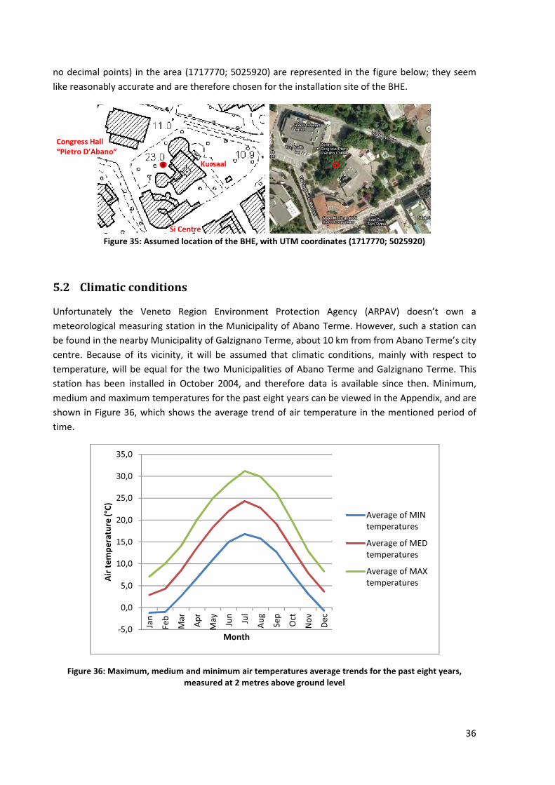
36

no decimal points) in the area (1717770; 5025920) are represented in the figure below; they seem

like reasonably accurate and are therefore chosen for the installation site of the BHE.

Figure 35: Assumed location of the BHE, with UTM coordinates (1717770; 5025920)

5.2 Climatic conditions

Unfortunately the Veneto Region Environment Protection Agency (ARPAV) doesn’t own a

meteorological measuring station in the Municipality of Abano Terme. However, such a station can

be found in the nearby Municipality of Galzignano Terme, about 10 km from from Abano Terme’s city

centre. Because of its vicinity, it will be assumed that climatic conditions, mainly with respect to

temperature, will be equal for the two Municipalities of Abano Terme and Galzignano Terme. This

station has been installed in October 2004, and therefore data is available since then. Minimum,

medium and maximum temperatures for the past eight years can be viewed in the Appendix, and are

shown in Figure 36, which shows the average trend of air temperature in the mentioned period of

time.

Figure 36: Maximum, medium and minimum air temperatures average trends for the past eight years,

measured at 2 metres above ground level

-5,0

0,0

5,0

10,0

15,0

20,0

25,0

30,0

35,0

Jan

Fe

b

Ma

r

Ap

r

Ma

y

Jun

Jul

Au

g

Se

p

Oct

No

v

De

c

Air

te

mp

era

ture

(°C

)

Month

Average of MIN

temperatures

Average of MED

temperatures

Average of MAX

temperatures

Congress Hall

“Pietro D’Abano”

Si Centre

Kursaal

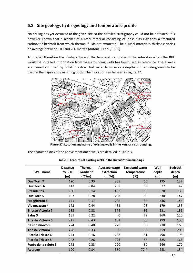
37

5.3 Site geology, hydrogeology and temperature profile

No drilling has yet occurred at the given site so the detailed stratigraphy could not be obtained. It is

however known that a blanket of alluvial material consisting of loose silty-clay tops a fractured

carbonatic bedrock from which thermal fluids are extracted. The alluvial material’s thickness varies

on average between 100 and 200 metres (Antonelli et al., 1995).

To predict therefore the stratigraphy and the temperature profile of the subsoil in which the BHE

would be installed, information from 14 surrounding wells has been used as reference. These wells

are owned and used by hotel to extract hot water from various depths in the underground to be

used in their spas and swimming pools. Their location can be seen in Figure 37.

Figure 37: Location and name of existing wells in the Kursaal’s surroundings

The characteristics of the above mentioned wells are detailed in Table 3.

Table 3: Features of existing wells in the Kursaal’s surroundings

Well name

Distance

to BHE

(m)

Thermal

Gradient

(°C/m)

Average water

extraction

(m3/d)

Extracted water

temperature

(°C)

Well

depth

(m)

Bedrock

depth

(m)

Due Torri 7 120 0.33 288 65 195 137

Due Torri 6 143 0.84 288 65 77 47

President 4 150 0.14 432 86 628 80

Due Torri 5 157 0.28 288 65 230 147

Meggiorato 8 171 0.17 288 58 336 143

Via pozzetto 4 173 0.44 432 78 179 156

Trieste Vittoria 7 183 0.38 576 85 221 185

Salus 3 185 0.22 0 79 360 120

Trieste Vittoria 6 217 0.43 432 86 199 156

Casino nuovo 5 224 0.40 720 85 230 168

Trieste Vittoria 5 228 0.33 0 85 259 205

Piccolo Trieste 6 244 0.16 288 81 498 195

Piccolo Trieste 5 248 0.26 276 85 325 165

Fonte della salute 3 272 0.33 720 80 246 170

Average 190 0.34 360 77.4 283 154

Kursaal’s BHE

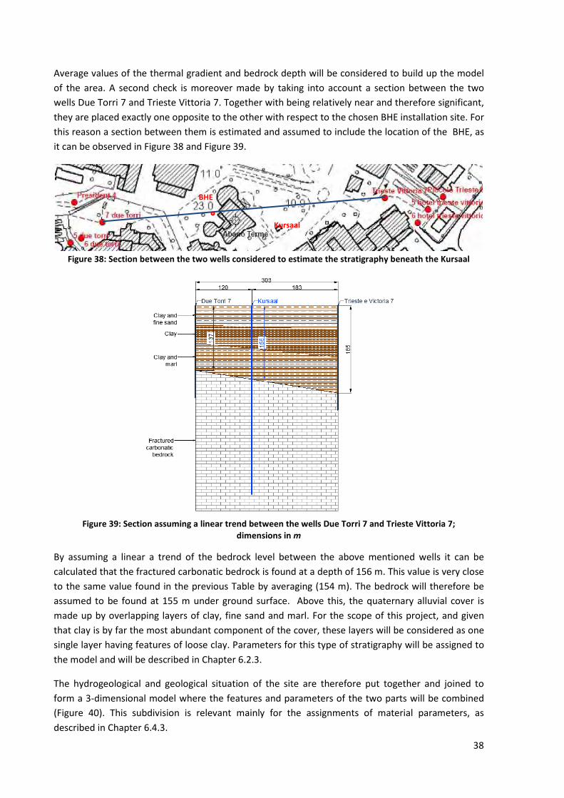
38

Average values of the thermal gradient and bedrock depth will be considered to build up the model

of the area. A second check is moreover made by taking into account a section between the two

wells Due Torri 7 and Trieste Vittoria 7. Together with being relatively near and therefore significant,

they are placed exactly one opposite to the other with respect to the chosen BHE installation site. For

this reason a section between them is estimated and assumed to include the location of the BHE, as

it can be observed in Figure 38 and Figure 39.

Figure 38: Section between the two wells considered to estimate the stratigraphy beneath the Kursaal

Figure 39: Section assuming a linear trend between the wells Due Torri 7 and Trieste Vittoria 7;

dimensions in m

By assuming a linear a trend of the bedrock level between the above mentioned wells it can be

calculated that the fractured carbonatic bedrock is found at a depth of 156 m. This value is very close

to the same value found in the previous Table by averaging (154 m). The bedrock will therefore be

assumed to be found at 155 m under ground surface. Above this, the quaternary alluvial cover is

made up by overlapping layers of clay, fine sand and marl. For the scope of this project, and given

that clay is by far the most abundant component of the cover, these layers will be considered as one

single layer having features of loose clay. Parameters for this type of stratigraphy will be assigned to

the model and will be described in Chapter 6.2.3.

The hydrogeological and geological situation of the site are therefore put together and joined to

form a 3-dimensional model where the features and parameters of the two parts will be combined

(Figure 40). This subdivision is relevant mainly for the assignments of material parameters, as

described in Chapter 6.4.3.

Kursaal

BHE

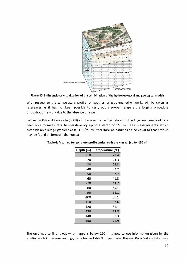
39

Figure 40: 3-dimensional visualization of the combination of the hydrogeological and geological models

With respect to the temperature profile, or geothermal gradient, other works will be taken as

references as it has not been possible to carry out a proper temperature logging procedure

throughout this work due to the absence of a well.

Faldani (2009) and Panazzolo (2009) also have written works related to the Euganean area and have

been able to measure a temperature log up to a depth of 150 m. Their measurements, which

establish an average gradient of 0.34 °C/m, will therefore be assumed to be equal to those which

may be found underneath the Kursaal.

Table 4: Assumed temperature profile underneath the Kursaal (up to -150 m)

Depth (m) Temperature (°C)

-10 21.4

-20 24.3

-30 28.3

-40 33.2

-50 37.7

-60 41.3

-70 44.7

-80 49.1

-90 53.1

-100 56.1

-110 57.6

-120 61.1

-130 64.8

-140 68.3

-150 71.9

The only way to find it out what happens below 150 m is now to use information given by the

existing wells in the surroundings, described in Table 3. In particular, the well President 4 is taken as a

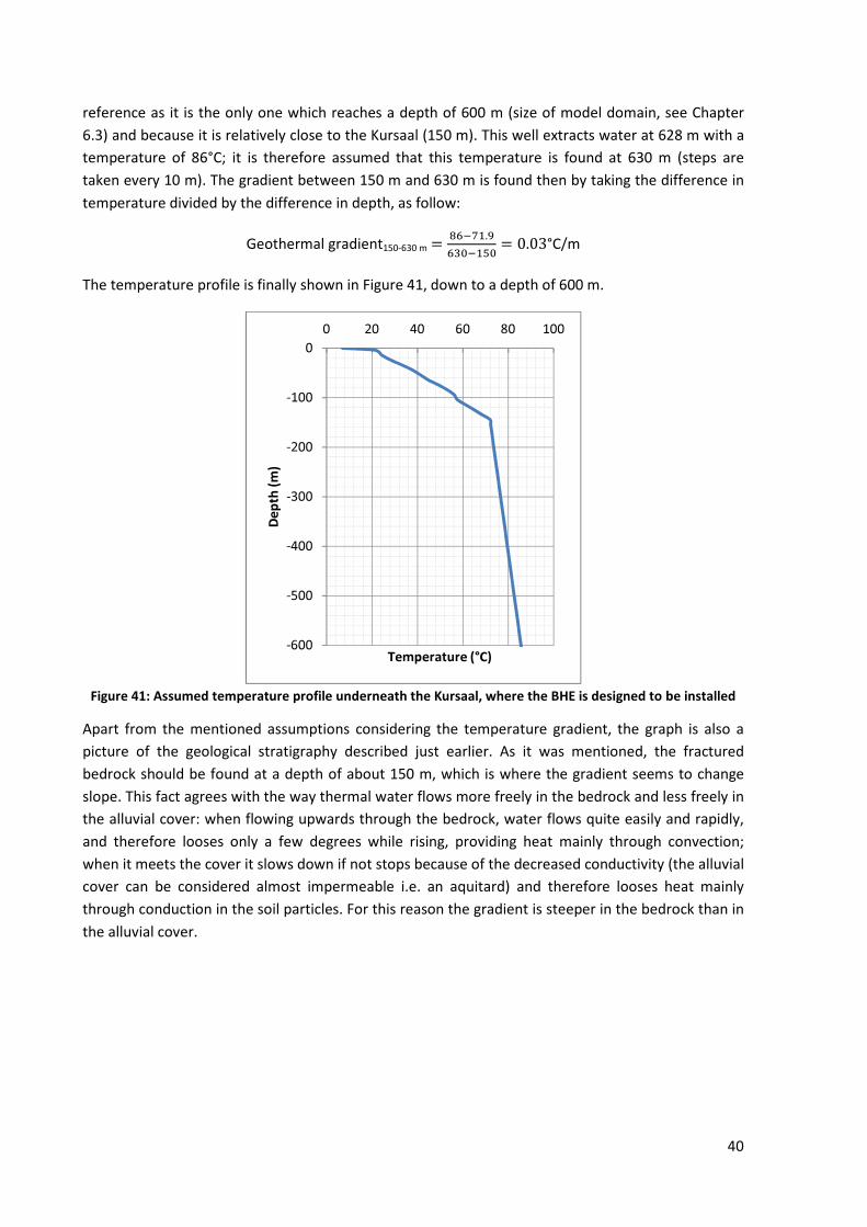
40

reference as it is the only one which reaches a depth of 600 m (size of model domain, see Chapter

6.3) and because it is relatively close to the Kursaal (150 m). This well extracts water at 628 m with a

temperature of 86°C; it is therefore assumed that this temperature is found at 630 m (steps are

taken every 10 m). The gradient between 150 m and 630 m is found then by taking the difference in

temperature divided by the difference in depth, as follow:

Geothermal gradient150-630 m =�����.�

�������= 0.03°C/m

The temperature profile is finally shown in Figure 41, down to a depth of 600 m.

Figure 41: Assumed temperature profile underneath the Kursaal, where the BHE is designed to be installed

Apart from the mentioned assumptions considering the temperature gradient, the graph is also a

picture of the geological stratigraphy described just earlier. As it was mentioned, the fractured

bedrock should be found at a depth of about 150 m, which is where the gradient seems to change

slope. This fact agrees with the way thermal water flows more freely in the bedrock and less freely in

the alluvial cover: when flowing upwards through the bedrock, water flows quite easily and rapidly,

and therefore looses only a few degrees while rising, providing heat mainly through convection;

when it meets the cover it slows down if not stops because of the decreased conductivity (the alluvial

cover can be considered almost impermeable i.e. an aquitard) and therefore looses heat mainly

through conduction in the soil particles. For this reason the gradient is steeper in the bedrock than in

the alluvial cover.

-600

-500

-400

-300

-200

-100

0

0 20 40 60 80 100

De

pth

(m

)

Temperature (°C)

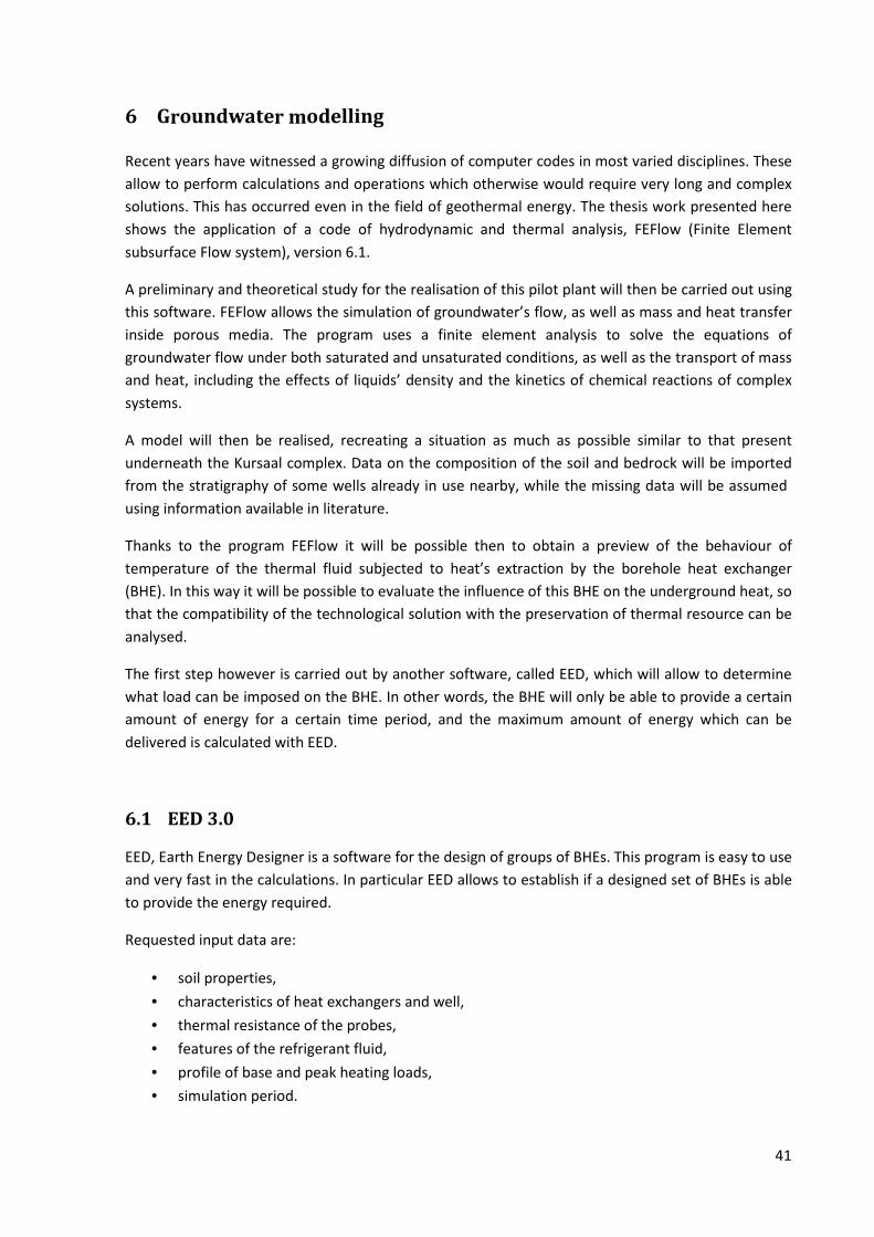
41

6 Groundwater modelling

Recent years have witnessed a growing diffusion of computer codes in most varied disciplines. These

allow to perform calculations and operations which otherwise would require very long and complex

solutions. This has occurred even in the field of geothermal energy. The thesis work presented here

shows the application of a code of hydrodynamic and thermal analysis, FEFlow (Finite Element

subsurface Flow system), version 6.1.

A preliminary and theoretical study for the realisation of this pilot plant will then be carried out using

this software. FEFlow allows the simulation of groundwater’s flow, as well as mass and heat transfer

inside porous media. The program uses a finite element analysis to solve the equations of

groundwater flow under both saturated and unsaturated conditions, as well as the transport of mass

and heat, including the effects of liquids’ density and the kinetics of chemical reactions of complex

systems.

A model will then be realised, recreating a situation as much as possible similar to that present

underneath the Kursaal complex. Data on the composition of the soil and bedrock will be imported

from the stratigraphy of some wells already in use nearby, while the missing data will be assumed

using information available in literature.

Thanks to the program FEFlow it will be possible then to obtain a preview of the behaviour of

temperature of the thermal fluid subjected to heat’s extraction by the borehole heat exchanger

(BHE). In this way it will be possible to evaluate the influence of this BHE on the underground heat, so

that the compatibility of the technological solution with the preservation of thermal resource can be

analysed.

The first step however is carried out by another software, called EED, which will allow to determine

what load can be imposed on the BHE. In other words, the BHE will only be able to provide a certain

amount of energy for a certain time period, and the maximum amount of energy which can be

delivered is calculated with EED.

6.1 EED 3.0

EED, Earth Energy Designer is a software for the design of groups of BHEs. This program is easy to use

and very fast in the calculations. In particular EED allows to establish if a designed set of BHEs is able

to provide the energy required.

Requested input data are:

• soil properties,

• characteristics of heat exchangers and well,

• thermal resistance of the probes,

• features of the refrigerant fluid,

• profile of base and peak heating loads,

• simulation period.

42

The listed data will be later better described throughout the description of the parameters used in

FEFlow, and is therefore not repeated here. The program can work in two ways:

1. by fixing the depth of the BHE and calculating the average temperature of the fluid,

considering its variation over the years;

2. by establishing limit values of temperature and then calculating the depth that the BHE

needs to maintain the average temperature of the fluid always between these limits.

Having already established that the BHE will be only one and 400 m deep, only the average

temperatures of the fluid is evaluated. The calculation of this temperature is basically a check that

the input data is working fine. In fact the thermal loads are written in as inputs, and the average

temperature is checked not to decrease under a certain fixed value.

The BHE will be working with a temperature difference between inlet and outlet which should stay at

about 10°C. This value is used in the previously described formula:

' = �� ∙ � ∙ � ∙ ��� − ��� Where the power is assumed to calculate a flow rate. The assumed power is considered as the

“peak” power, and is also used to calculate energy requirements, assuming the BHE is run 16 hours a

day for the 6 months of winter. Moreover, it is established that the average temperature of the fluid

should not decrease below 35°C, this because the limit at which the BHE system can work is set to

30°C inlet and 40°C (to keep the temperature difference of 10°C mentioned above). The procedure is

finally to input a Power value, and in the end check that this average temperature stays above 35°C

after 10 years of simulated time.

With a trial and error procedure, it is found that the system can work up to a Power of 33 kW. It is

found that:

� =33000

4186 ∙ 10= 0.788 /(

Which is the required flow rate, and that:

Table 5: Thermal load and energy extracted per month by the BHE

Month Peak power load (kW) Daily use (h) Days of fuse (d) Energy extracted (kWh)

Jan 33 16 31 16368

Feb 33 16 28 14784

Mar 33 16 31 16368

Apr 33 16 15 7920

May 0 0 0 0

Jun 0 0 0 0

Jul 0 0 0 0

Aug 0 0 0 0

Sep 0 0 0 0

Oct 33 16 15 7920

Nov 33 16 30 15840

Dec 33 16 31 16368

43

It can finally be observed how these loads allow the minimum peak not to decrease below 35°C.

Figure 42: Maximum and minimum yearly fluid temperature in the BHE

The load of 33 kW will therefore be now applied to the BHE designed for the Kursaal, and its thermal

impact will be assessed with the program FEFlow.

6.2 Description of input data - FEFlow

6.2.1 Supermesh and Finite-Element Mesh creation

The so-called Supermesh in FEFlow forms the framework for the generation of a Finite-Element

Mesh. It contains all the basic geometrical information the mesh generation algorithm needs. While

in the very simplest case the Supermesh only defines the outline of the model area, i.e., consists of

one single polygon, the concept offers many more possibilities: Supermeshes can be composed of an

arbitrary number of polygons, lines and points (DHI-WASY, n.d.). These can be digitised and edited in

the Mesh-Editor toolbar. In addition, instead of digitizing Supermesh features on screen, they can be

imported from background maps. This is done via the Convert to Supermesh tool. All features of the

map (polygons, lines and points) can be converted to Supermesh features using this approach. These

features will provide the boundaries necessary to create the Finite-Element Mesh and will then be

displayed in the Maps panel. It can be said that the Supermesh is practically equivalent to the model

domain.

The Finite-Element Mesh is used to obtain a suitable spatial discretisation of the model domain, or

the Supermesh, by dividing it into a collection of sub-domains (the finite elements). Each sub-domain

is represented by a set of element equations of the original problem; the procedure consists then in

systematically recombining all sets of element equations into a global system of equations for the

final calculation. However, the denser the mesh the better the numerical accuracy, but the higher

the computational effort. Numerical difficulties can arise during the simulation if the mesh contains

too many highly distorted elements.

FEFlow supports either triangular or quadrangular finite-element meshes. The generation is generally

based on the input of an approximate number of finite elements to be generated and the desired

mesh density of each Supermesh polygon can then be edited separately. Mesh generation is typically

a trial-and-error process: the user iteratively optimises element numbers, generator property

settings and the Supermesh until a satisfactory mesh is obtained.

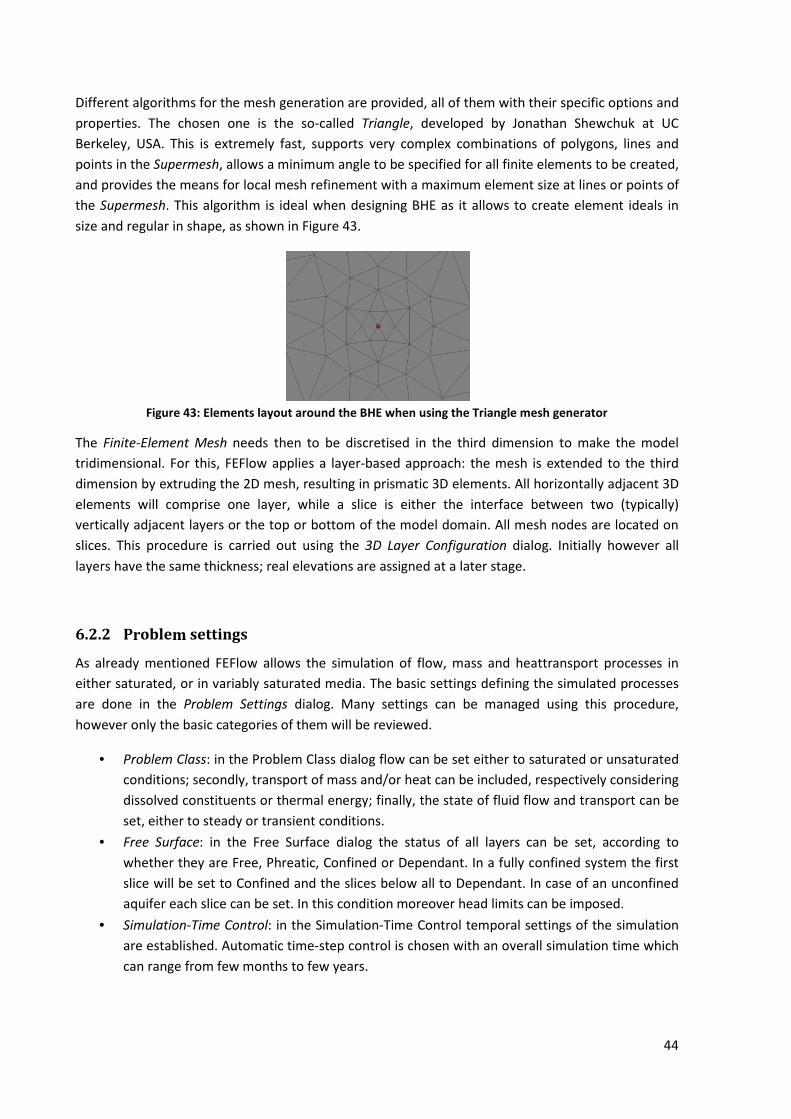
44

Different algorithms for the mesh generation are provided, all of them with their specific options and

properties. The chosen one is the so-called Triangle, developed by Jonathan Shewchuk at UC

Berkeley, USA. This is extremely fast, supports very complex combinations of polygons, lines and

points in the Supermesh, allows a minimum angle to be specified for all finite elements to be created,

and provides the means for local mesh refinement with a maximum element size at lines or points of

the Supermesh. This algorithm is ideal when designing BHE as it allows to create element ideals in

size and regular in shape, as shown in Figure 43.

Figure 43: Elements layout around the BHE when using the Triangle mesh generator

The Finite-Element Mesh needs then to be discretised in the third dimension to make the model

tridimensional. For this, FEFlow applies a layer-based approach: the mesh is extended to the third

dimension by extruding the 2D mesh, resulting in prismatic 3D elements. All horizontally adjacent 3D

elements will comprise one layer, while a slice is either the interface between two (typically)

vertically adjacent layers or the top or bottom of the model domain. All mesh nodes are located on

slices. This procedure is carried out using the 3D Layer Configuration dialog. Initially however all

layers have the same thickness; real elevations are assigned at a later stage.

6.2.2 Problem settings

As already mentioned FEFlow allows the simulation of flow, mass and heattransport processes in

either saturated, or in variably saturated media. The basic settings defining the simulated processes

are done in the Problem Settings dialog. Many settings can be managed using this procedure,

however only the basic categories of them will be reviewed.

• Problem Class: in the Problem Class dialog flow can be set either to saturated or unsaturated

conditions; secondly, transport of mass and/or heat can be included, respectively considering

dissolved constituents or thermal energy; finally, the state of fluid flow and transport can be

set, either to steady or transient conditions.

• Free Surface: in the Free Surface dialog the status of all layers can be set, according to

whether they are Free, Phreatic, Confined or Dependant. In a fully confined system the first

slice will be set to Confined and the slices below all to Dependant. In case of an unconfined

aquifer each slice can be set. In this condition moreover head limits can be imposed.

• Simulation-Time Control: in the Simulation-Time Control temporal settings of the simulation

are established. Automatic time-step control is chosen with an overall simulation time which

can range from few months to few years.

45

6.2.3 Parameters assignment

FEFlow distinguishes between six groups of parameters, all of them visible on the first level of the

tree view in the Data panel. However only the first three groups will be modified, as they are strictly

related to the model configuration.

• Process variables: (or initial conditions) these are defined on the mesh nodes. They include

the primary variables hydraulic head, concentration, and temperature (as applicable). When

setting up the model, they describe the initial conditions. During and after the simulation

these process variables reflect the then-current conditions. Moreover, in 3D models, the

elevation is included in the Process variables section as a nodal parameter. In models with a

fixed mesh, the elevation does not change during the simulation.

• Boundary conditions: by default, all model boundaries in FEFlow are impervious. To allow

flows into or out of the model, boundary conditions have to be defined. FEFlow supports five

basic types of boundary conditions for flow, mass and heat transport:

o Dirilecht type or 1st kind BC: this specifies a time-constant or time-varying value for

the primary variable at a node, i.e. hydraulic head for flow, concentration for mass

transport and temperature for heat transport.

o Neumann type or 2nd kind BC: this specifies a flux, and the boundary condition

describes an in or outflow of water/mass/energy at element edges (2D) or element

faces (3D).

o Cauchy type or 3rd kind BC: this specifies fluid-transfer, and can be used to describe

rivers, lakes, and known hydraulic heads in a distance from the model boundary

(sometimes called “general head” boundaries). The condition is used to apply

transfer properties between a reference value for the primary variable (hydraulic

head, concentration, or temperature) and groundwater.

o Well type or 4th kind BC: their counterparts for mass and heat transport simulation

are nodally applied and represent a time-constant or time-varying local injection or

abstraction of water, mass or energy at a single node or at a group of nodes.

o Multilayer wells and Borehole Heat Exchangers: in 3D models, multilayer-well

boundary conditions can be used to simulate water injection/abstraction via a well

screen. The screen can extend over one or multiple model layers. Borehole heat

exchangers are used to simulate closed-loop geothermal installations. A refrigerant

circulates within closed pipes and heat exchange with the surrounding aquifer

system is solely driven by thermal conductivity. Borehole heat exchangers are

represented as embedded 1D elements and linked to the FEFlow nodes along join

edges in a 3D model.

• Material Properties: material properties describe the relevant characteristics of the porous

medium for the considered flow and transport processes to be simulated. They are defined

on an elemental basis. For the flow simulation, material properties encompass quantities

such as hydraulic conductivity in different directions according to the selected anisotropy

model and specific storage (compressibility). For the heat transport simulation, material

properties can be assigned to both the fluid phase and the solid phase, such as the

volumetric heat capacity and the thermal conductivity.

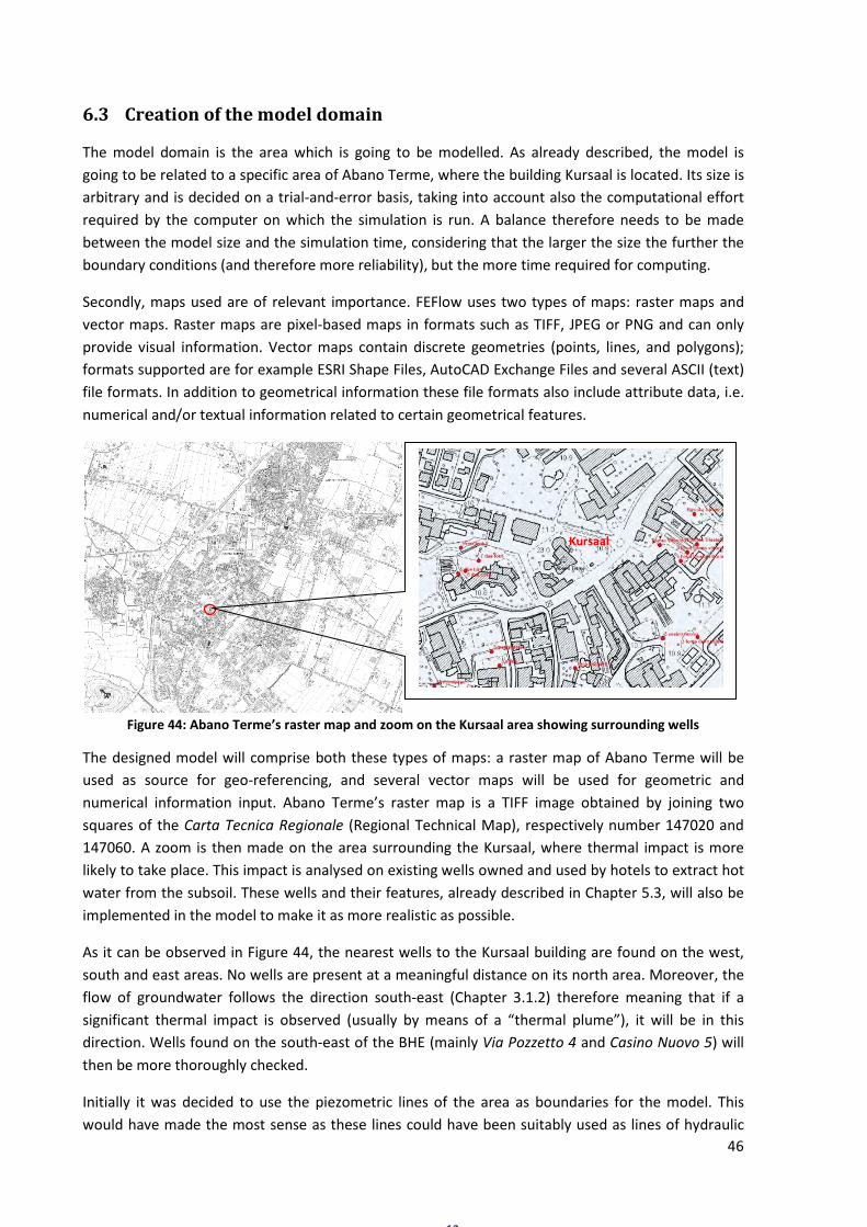
46

6.3 Creation of the model domain

The model domain is the area which is going to be modelled. As already described, the model is

going to be related to a specific area of Abano Terme, where the building Kursaal is located. Its size is

arbitrary and is decided on a trial-and-error basis, taking into account also the computational effort

required by the computer on which the simulation is run. A balance therefore needs to be made

between the model size and the simulation time, considering that the larger the size the further the

boundary conditions (and therefore more reliability), but the more time required for computing.

Secondly, maps used are of relevant importance. FEFlow uses two types of maps: raster maps and

vector maps. Raster maps are pixel-based maps in formats such as TIFF, JPEG or PNG and can only

provide visual information. Vector maps contain discrete geometries (points, lines, and polygons);

formats supported are for example ESRI Shape Files, AutoCAD Exchange Files and several ASCII (text)

file formats. In addition to geometrical information these file formats also include attribute data, i.e.

numerical and/or textual information related to certain geometrical features.

Figure 44: Abano Terme’s raster map and zoom on the Kursaal area showing surrounding wells

The designed model will comprise both these types of maps: a raster map of Abano Terme will be

used as source for geo-referencing, and several vector maps will be used for geometric and

numerical information input. Abano Terme’s raster map is a TIFF image obtained by joining two

squares of the Carta Tecnica Regionale (Regional Technical Map), respectively number 147020 and

147060. A zoom is then made on the area surrounding the Kursaal, where thermal impact is more

likely to take place. This impact is analysed on existing wells owned and used by hotels to extract hot

water from the subsoil. These wells and their features, already described in Chapter 5.3, will also be

implemented in the model to make it as more realistic as possible.

As it can be observed in Figure 44, the nearest wells to the Kursaal building are found on the west,

south and east areas. No wells are present at a meaningful distance on its north area. Moreover, the

flow of groundwater follows the direction south-east (Chapter 3.1.2) therefore meaning that if a

significant thermal impact is observed (usually by means of a “thermal plume”), it will be in this

direction. Wells found on the south-east of the BHE (mainly Via Pozzetto 4 and Casino Nuovo 5) will

then be more thoroughly checked.

Initially it was decided to use the piezometric lines of the area as boundaries for the model. This

would have made the most sense as these lines could have been suitably used as lines of hydraulic

12 m

Kursaal

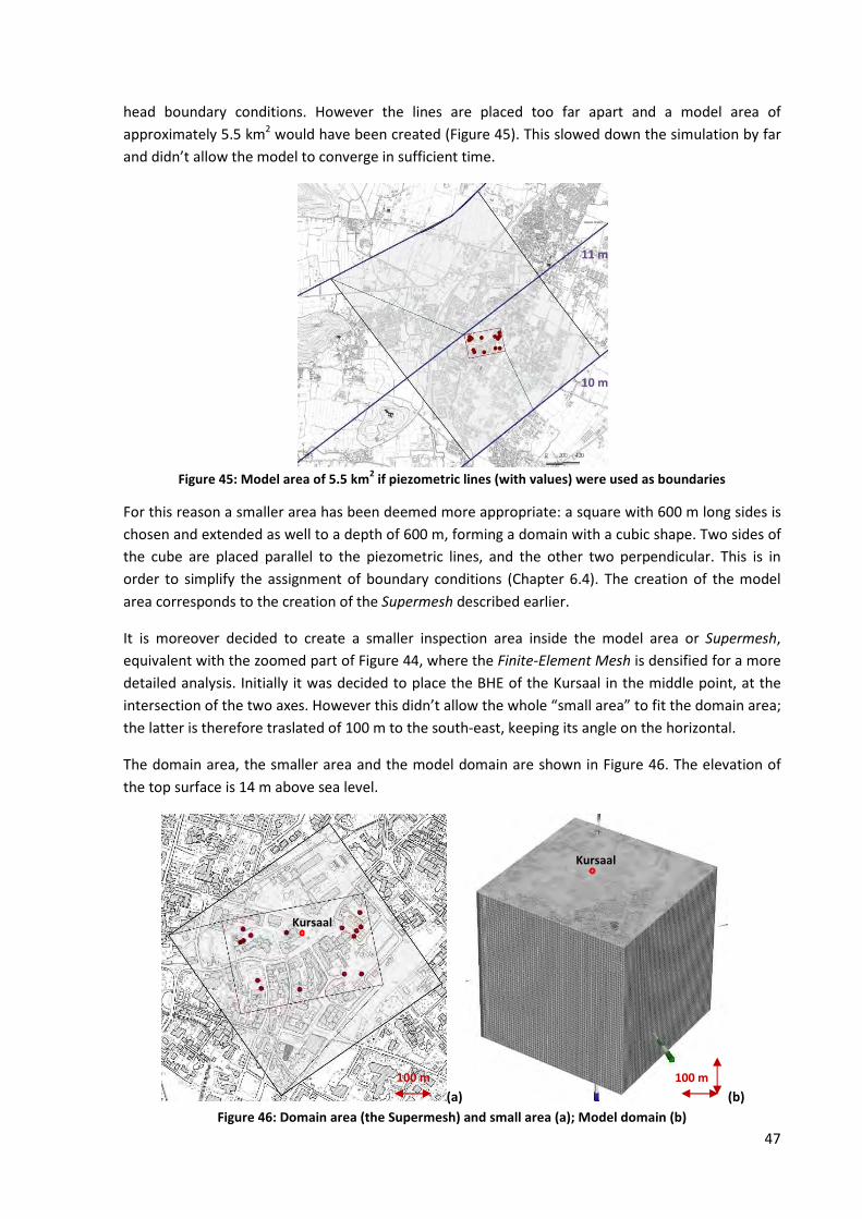
47

head boundary conditions. However the lines are placed too far apart and a model area of

approximately 5.5 km2 would have been created (Figure 45). This slowed down the simulation by far

and didn’t allow the model to converge in sufficient time.

Figure 45: Model area of 5.5 km

2 if piezometric lines (with values) were used as boundaries

For this reason a smaller area has been deemed more appropriate: a square with 600 m long sides is

chosen and extended as well to a depth of 600 m, forming a domain with a cubic shape. Two sides of

the cube are placed parallel to the piezometric lines, and the other two perpendicular. This is in

order to simplify the assignment of boundary conditions (Chapter 6.4). The creation of the model

area corresponds to the creation of the Supermesh described earlier.

It is moreover decided to create a smaller inspection area inside the model area or Supermesh,

equivalent with the zoomed part of Figure 44, where the Finite-Element Mesh is densified for a more

detailed analysis. Initially it was decided to place the BHE of the Kursaal in the middle point, at the

intersection of the two axes. However this didn’t allow the whole “small area” to fit the domain area;

the latter is therefore traslated of 100 m to the south-east, keeping its angle on the horizontal.

The domain area, the smaller area and the model domain are shown in Figure 46. The elevation of

the top surface is 14 m above sea level.

(a) (b)

Figure 46: Domain area (the Supermesh) and small area (a); Model domain (b)

Kursaal

Kursaal

11 m

10 m

100 m 100 m

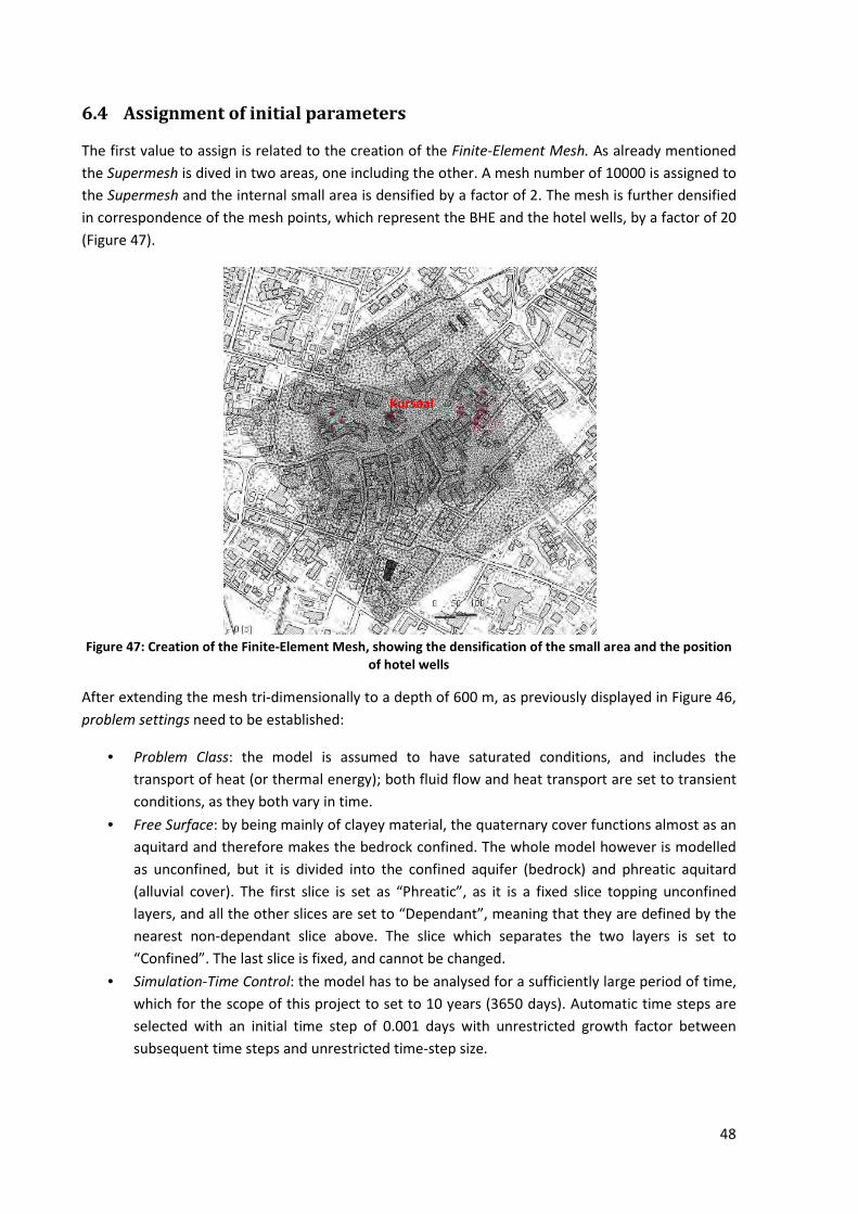
48

6.4 Assignment of initial parameters

The first value to assign is related to the creation of the Finite-Element Mesh. As already mentioned

the Supermesh is dived in two areas, one including the other. A mesh number of 10000 is assigned to

the Supermesh and the internal small area is densified by a factor of 2. The mesh is further densified

in correspondence of the mesh points, which represent the BHE and the hotel wells, by a factor of 20

(Figure 47).

Figure 47: Creation of the Finite-Element Mesh, showing the densification of the small area and the position

of hotel wells

After extending the mesh tri-dimensionally to a depth of 600 m, as previously displayed in Figure 46,

problem settings need to be established:

• Problem Class: the model is assumed to have saturated conditions, and includes the

transport of heat (or thermal energy); both fluid flow and heat transport are set to transient

conditions, as they both vary in time.

• Free Surface: by being mainly of clayey material, the quaternary cover functions almost as an

aquitard and therefore makes the bedrock confined. The whole model however is modelled

as unconfined, but it is divided into the confined aquifer (bedrock) and phreatic aquitard

(alluvial cover). The first slice is set as “Phreatic”, as it is a fixed slice topping unconfined

layers, and all the other slices are set to “Dependant”, meaning that they are defined by the

nearest non-dependant slice above. The slice which separates the two layers is set to

“Confined”. The last slice is fixed, and cannot be changed.

• Simulation-Time Control: the model has to be analysed for a sufficiently large period of time,

which for the scope of this project to set to 10 years (3650 days). Automatic time steps are

selected with an initial time step of 0.001 days with unrestricted growth factor between

subsequent time steps and unrestricted time-step size.

Kursaal

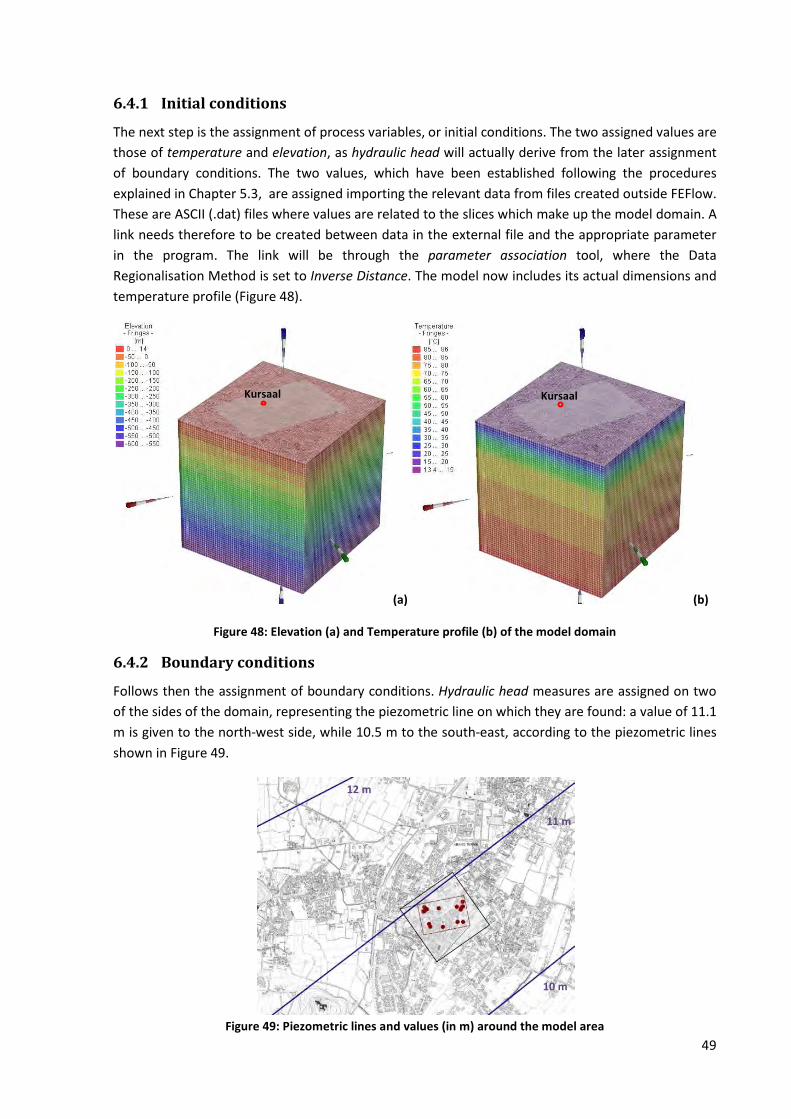
49

6.4.1 Initial conditions

The next step is the assignment of process variables, or initial conditions. The two assigned values are

those of temperature and elevation, as hydraulic head will actually derive from the later assignment

of boundary conditions. The two values, which have been established following the procedures

explained in Chapter 5.3, are assigned importing the relevant data from files created outside FEFlow.

These are ASCII (.dat) files where values are related to the slices which make up the model domain. A

link needs therefore to be created between data in the external file and the appropriate parameter

in the program. The link will be through the parameter association tool, where the Data

Regionalisation Method is set to Inverse Distance. The model now includes its actual dimensions and

temperature profile (Figure 48).

(a) (b)

Figure 48: Elevation (a) and Temperature profile (b) of the model domain

6.4.2 Boundary conditions

Follows then the assignment of boundary conditions. Hydraulic head measures are assigned on two

of the sides of the domain, representing the piezometric line on which they are found: a value of 11.1

m is given to the north-west side, while 10.5 m to the south-east, according to the piezometric lines

shown in Figure 49.

Figure 49: Piezometric lines and values (in m) around the model area

Kursaal Kursaal

12 m

11 m

10 m

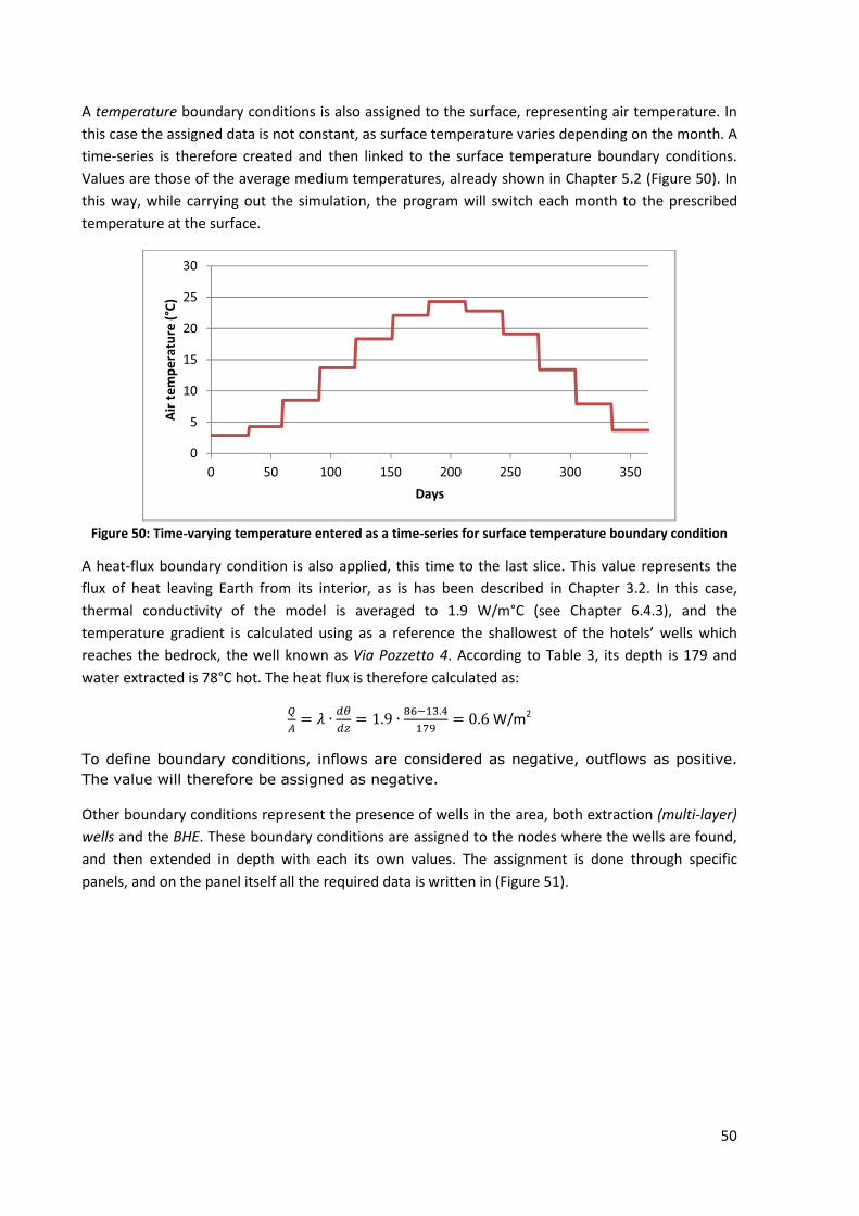
50

A temperature boundary conditions is also assigned to the surface, representing air temperature. In

this case the assigned data is not constant, as surface temperature varies depending on the month. A

time-series is therefore created and then linked to the surface temperature boundary conditions.

Values are those of the average medium temperatures, already shown in Chapter 5.2 (Figure 50). In

this way, while carrying out the simulation, the program will switch each month to the prescribed

temperature at the surface.

Figure 50: Time-varying temperature entered as a time-series for surface temperature boundary condition

A heat-flux boundary condition is also applied, this time to the last slice. This value represents the

flux of heat leaving Earth from its interior, as is has been described in Chapter 3.2. In this case,

thermal conductivity of the model is averaged to 1.9 W/m°C (see Chapter 6.4.3), and the

temperature gradient is calculated using as a reference the shallowest of the hotels’ wells which

reaches the bedrock, the well known as Via Pozzetto 4. According to Table 3, its depth is 179 and

water extracted is 78°C hot. The heat flux is therefore calculated as:

�

�= � ∙ ��

��= 1.9 ∙

�����.

���= 0.6W/m2

To define boundary conditions, inflows are considered as negative, outflows as positive.

The value will therefore be assigned as negative.

Other boundary conditions represent the presence of wells in the area, both extraction (multi-layer)

wells and the BHE. These boundary conditions are assigned to the nodes where the wells are found,

and then extended in depth with each its own values. The assignment is done through specific

panels, and on the panel itself all the required data is written in (Figure 51).

0

5

10

15

20

25

30

0 50 100 150 200 250 300 350

Air

te

mp

era

ture

(°C

)

Days

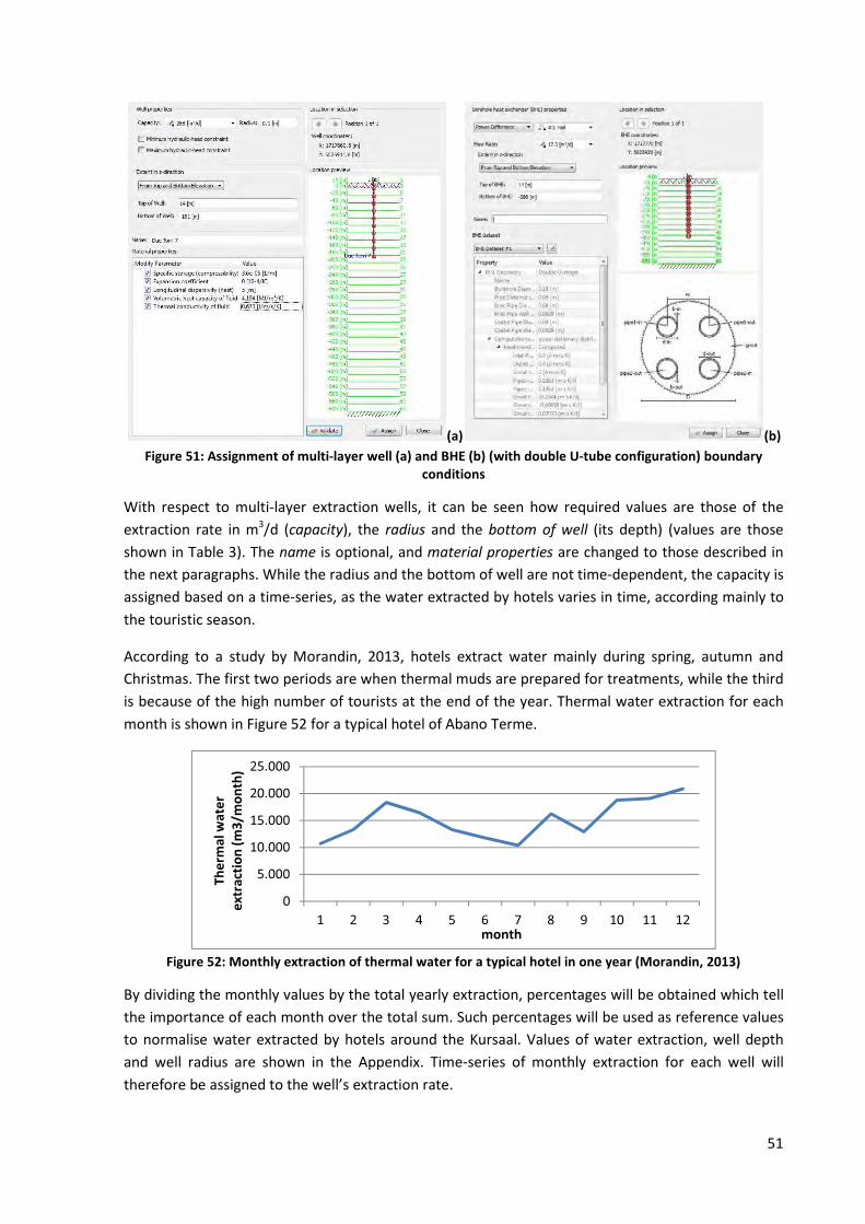
51

(a) (b)

Figure 51: Assignment of multi-layer well (a) and BHE (b) (with double U-tube configuration) boundary

conditions

With respect to multi-layer extraction wells, it can be seen how required values are those of the

extraction rate in m3/d (capacity), the radius and the bottom of well (its depth) (values are those

shown in Table 3). The name is optional, and material properties are changed to those described in

the next paragraphs. While the radius and the bottom of well are not time-dependent, the capacity is

assigned based on a time-series, as the water extracted by hotels varies in time, according mainly to

the touristic season.

According to a study by Morandin, 2013, hotels extract water mainly during spring, autumn and

Christmas. The first two periods are when thermal muds are prepared for treatments, while the third

is because of the high number of tourists at the end of the year. Thermal water extraction for each

month is shown in Figure 52 for a typical hotel of Abano Terme.

Figure 52: Monthly extraction of thermal water for a typical hotel in one year (Morandin, 2013)

By dividing the monthly values by the total yearly extraction, percentages will be obtained which tell

the importance of each month over the total sum. Such percentages will be used as reference values

to normalise water extracted by hotels around the Kursaal. Values of water extraction, well depth

and well radius are shown in the Appendix. Time-series of monthly extraction for each well will

therefore be assigned to the well’s extraction rate.

0

5.000

10.000

15.000

20.000

25.000

1 2 3 4 5 6 7 8 9 10 11 12

Th

erm

al w

ate

r

extr

act

ion

(m

3/m

on

th)

month

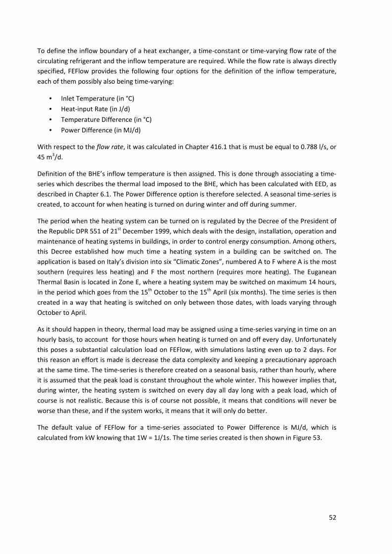
52

To define the inflow boundary of a heat exchanger, a time-constant or time-varying flow rate of the

circulating refrigerant and the inflow temperature are required. While the flow rate is always directly

specified, FEFlow provides the following four options for the definition of the inflow temperature,

each of them possibly also being time-varying:

• Inlet Temperature (in °C)

• Heat-input Rate (in J/d)

• Temperature Difference (in °C)

• Power Difference (in MJ/d)

With respect to the flow rate, it was calculated in Chapter 416.1 that is must be equal to 0.788 l/s, or

45 m3/d.

Definition of the BHE’s inflow temperature is then assigned. This is done through associating a time-

series which describes the thermal load imposed to the BHE, which has been calculated with EED, as

described in Chapter 6.1. The Power Difference option is therefore selected. A seasonal time-series is

created, to account for when heating is turned on during winter and off during summer.

The period when the heating system can be turned on is regulated by the Decree of the President of

the Republic DPR 551 of 21st December 1999, which deals with the design, installation, operation and

maintenance of heating systems in buildings, in order to control energy consumption. Among others,

this Decree established how much time a heating system in a building can be switched on. The

application is based on Italy’s division into six “Climatic Zones”, numbered A to F where A is the most

southern (requires less heating) and F the most northern (requires more heating). The Euganean

Thermal Basin is located in Zone E, where a heating system may be switched on maximum 14 hours,

in the period which goes from the 15th October to the 15th April (six months). The time series is then

created in a way that heating is switched on only between those dates, with loads varying through

October to April.

As it should happen in theory, thermal load may be assigned using a time-series varying in time on an

hourly basis, to account for those hours when heating is turned on and off every day. Unfortunately

this poses a substantial calculation load on FEFlow, with simulations lasting even up to 2 days. For

this reason an effort is made is decrease the data complexity and keeping a precautionary approach

at the same time. The time-series is therefore created on a seasonal basis, rather than hourly, where

it is assumed that the peak load is constant throughout the whole winter. This however implies that,

during winter, the heating system is switched on every day all day long with a peak load, which of

course is not realistic. Because this is of course not possible, it means that conditions will never be

worse than these, and if the system works, it means that it will only do better.

The default value of FEFlow for a time-series associated to Power Difference is MJ/d, which is

calculated from kW knowing that 1W = 1J/1s. The time series created is then shown in Figure 53.

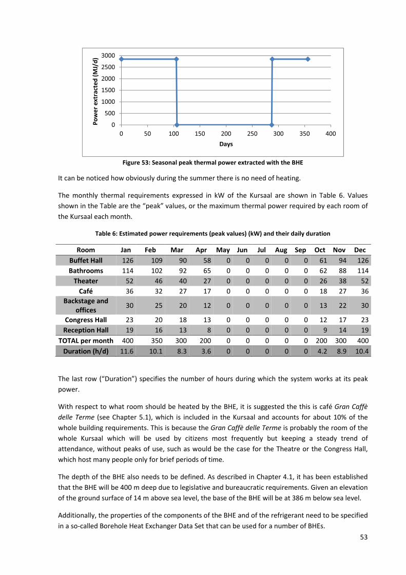
53

Figure 53: Seasonal peak thermal power extracted with the BHE

It can be noticed how obviously during the summer there is no need of heating.

The monthly thermal requirements expressed in kW of the Kursaal are shown in Table 6. Values

shown in the Table are the “peak” values, or the maximum thermal power required by each room of

the Kursaal each month.

Table 6: Estimated power requirements (peak values) (kW) and their daily duration

Room Jan Feb Mar Apr May Jun Jul Aug Sep Oct Nov Dec

Buffet Hall 126 109 90 58 0 0 0 0 0 61 94 126

Bathrooms 114 102 92 65 0 0 0 0 0 62 88 114

Theater 52 46 40 27 0 0 0 0 0 26 38 52

Café 36 32 27 17 0 0 0 0 0 18 27 36

Backstage and

offices 30 25 20 12 0 0 0 0 0 13 22 30

Congress Hall 23 20 18 13 0 0 0 0 0 12 17 23

Reception Hall 19 16 13 8 0 0 0 0 0 9 14 19

TOTAL per month 400 350 300 200 0 0 0 0 0 200 300 400

Duration (h/d) 11.6 10.1 8.3 3.6 0 0 0 0 0 4.2 8.9 10.4

The last row (“Duration”) specifies the number of hours during which the system works at its peak

power.

With respect to what room should be heated by the BHE, it is suggested the this is café Gran Caffè

delle Terme (see Chapter 5.1), which is included in the Kursaal and accounts for about 10% of the

whole building requirements. This is because the Gran Caffè delle Terme is probably the room of the

whole Kursaal which will be used by citizens most frequently but keeping a steady trend of

attendance, without peaks of use, such as would be the case for the Theatre or the Congress Hall,

which host many people only for brief periods of time.

The depth of the BHE also needs to be defined. As described in Chapter 4.1, it has been established

that the BHE will be 400 m deep due to legislative and bureaucratic requirements. Given an elevation

of the ground surface of 14 m above sea level, the base of the BHE will be at 386 m below sea level.

Additionally, the properties of the components of the BHE and of the refrigerant need to be specified

in a so-called Borehole Heat Exchanger Data Set that can be used for a number of BHEs.

0

500

1000

1500

2000

2500

3000

0 50 100 150 200 250 300 350 400

Po

we

r e

xtr

act

ed

(M

J/d

)

Days

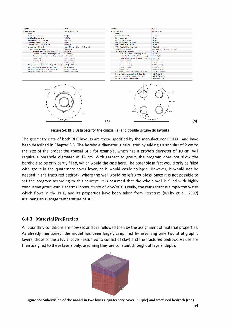
54

(a) (b)

Figure 54: BHE Data Sets for the coaxial (a) and double U-tube (b) layouts

The geometry data of both BHE layouts are those specified by the manufacturer REHAU, and have

been described in Chapter 3.3. The borehole diameter is calculated by adding an annulus of 2 cm to

the size of the probe: the coaxial BHE for example, which has a probe’s diameter of 10 cm, will

require a borehole diameter of 14 cm. With respect to grout, the program does not allow the

borehole to be only partly filled, which would the case here. The borehole in fact would only be filled

with grout in the quaternary cover layer, as it would easily collapse. However, it would not be

needed in the fractured bedrock, where the well would be left grout-less. Since it is not possible to

set the program according to this concept, it is assumed that the whole well is filled with highly

conductive grout with a thermal conductivity of 2 W/m°K. Finally, the refrigerant is simply the water

which flows in the BHE, and its properties have been taken from literature (Welty et al., 2007)

assuming an average temperature of 30°C.

6.4.3 Material properties

All boundary conditions are now set and are followed then by the assignment of material properties.

As already mentioned, the model has been largely simplified by assuming only two stratigraphic

layers, those of the alluvial cover (assumed to consist of clay) and the fractured bedrock. Values are

then assigned to these layers only, assuming they are constant throughout layers’ depth.

Figure 55: Subdivision of the model in two layers, quaternary cover (purple) and fractured bedrock (red)

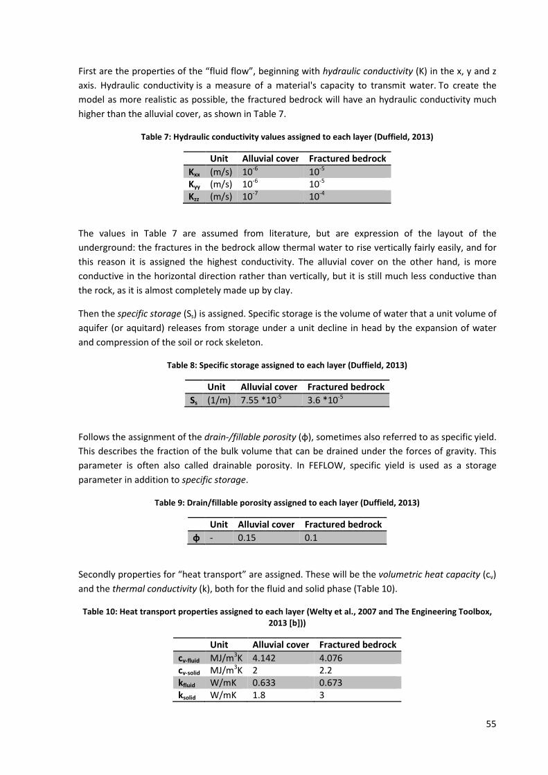
55

First are the properties of the “fluid flow”, beginning with hydraulic conductivity (K) in the x, y and z

axis. Hydraulic conductivity is a measure of a material's capacity to transmit water. To create the

model as more realistic as possible, the fractured bedrock will have an hydraulic conductivity much

higher than the alluvial cover, as shown in Table 7.

Table 7: Hydraulic conductivity values assigned to each layer (Duffield, 2013)

Unit Alluvial cover Fractured bedrock

Kxx (m/s) 10-6 10-5 Kyy (m/s) 10-6 10-5 Kzz (m/s) 10-7 10-4

The values in Table 7 are assumed from literature, but are expression of the layout of the

underground: the fractures in the bedrock allow thermal water to rise vertically fairly easily, and for

this reason it is assigned the highest conductivity. The alluvial cover on the other hand, is more

conductive in the horizontal direction rather than vertically, but it is still much less conductive than

the rock, as it is almost completely made up by clay.

Then the specific storage (Ss) is assigned. Specific storage is the volume of water that a unit volume of

aquifer (or aquitard) releases from storage under a unit decline in head by the expansion of water

and compression of the soil or rock skeleton.

Table 8: Specific storage assigned to each layer (Duffield, 2013)

Unit Alluvial cover Fractured bedrock

Ss (1/m) 7.55 *10-5 3.6 *10-5

Follows the assignment of the drain-/fillable porosity (φ), sometimes also referred to as specific yield.

This describes the fraction of the bulk volume that can be drained under the forces of gravity. This

parameter is often also called drainable porosity. In FEFLOW, specific yield is used as a storage

parameter in addition to specific storage.

Table 9: Drain/fillable porosity assigned to each layer (Duffield, 2013)

Unit Alluvial cover Fractured bedrock

φ - 0.15 0.1

Secondly properties for “heat transport” are assigned. These will be the volumetric heat capacity (cv)

and the thermal conductivity (k), both for the fluid and solid phase (Table 10).

Table 10: Heat transport properties assigned to each layer (Welty et al., 2007 and The Engineering Toolbox,

2013 [b]))

Unit Alluvial cover Fractured bedrock

cv-fluid MJ/m3K 4.142 4.076 cv-solid MJ/m3K 2 2.2 kfluid W/mK 0.633 0.673 ksolid W/mK 1.8 3

56

The volumetric heat capacity (cv) describes the ability of a given volume of a substance to

store internal energy while undergoing a given temperature change, but without undergoing a phase

transition. It is found by multiplicating specific heat capacity (cp) and density (ρ) of the material. The

difference in fact from cp is that cv is a “per unit volume” measure of the relationship between

thermal energy and temperature of a material, while the specific heat is a “per unit mass” measure

(Welty et al., 2007).

Thermal conductivity instead is the quantity of heat transmitted through a unit thickness in a

direction normal to a surface of unit area, due to a unit temperature gradient under steady state

conditions (The Engineering Toolbox, 2013 [b]).

Other important properties are the longitudinal and transverse dispersivity, as they are introduced in

the equations to take into account effects of inhomogeneities not considered in the model

properties. On the one hand, these are microscale inhomogeneities such as pore directions not

parallel to flow direction, on the other hand also macroscale properties such as layer structures and

lenses not considered due to missing knowledge and model discretisation (Welty et al., 2007). For

these values the default values of the program are left, respectively 5 and 0.5 m for both layers.

6.5 Simulation

All the parameters of the model have now been written in and the simulation can be launched. The

analysed time is 10 years.

The FEFlow user interface keeps all visualization options available during the simulation. The

simulation progress can thus be conveniently monitored and problems can be detected early. FEFlow

does not separately store initial conditions of hydraulic head or concentration/temperature during

the simulation. So, for example, the hydraulic-head process variable contains the initial head values

before the simulation, the current hydraulic head results at each time step of a transient simulation,

and the final hydraulic head after the simulation. These final results are also retained when leaving

the simulation mode by stopping it.

The first simulation to be carried out is to check which of the two possible BHE layouts is better

performing. To do this the simulation is carried out for 5 years just to make it last less time and also

because it can is shown how as early as the second year the system becomes stable and no variations

occur in the following years. The comparison is made between the temperature of the fluid entering

the BHE and the fluid exiting the BHE for both layouts.

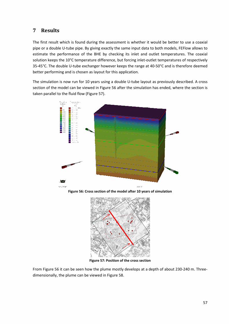
7 Results

The first result which is found during the assessment is whether it would be better to use

pipe or a double U-tube pipe. By giving exactly the same input data to both models, FEFlow allows to

estimate the performance of the BHE by checking its inlet and outlet temperatures. The coaxial

solution keeps the 10°C temperature difference, bu

35-45°C. The double U-tube exchanger however keeps the range at 40

better performing and is chosen as layout for this application.

The simulation is now run for 10 years usin

section of the model can be viewed in

taken parallel to the fluid flow (

Figure 56

From Figure 56 it can be seen how the plume mostly develops at a

dimensionally, the plume can be viewed in

is found during the assessment is whether it would be better to use

tube pipe. By giving exactly the same input data to both models, FEFlow allows to

estimate the performance of the BHE by checking its inlet and outlet temperatures. The coaxial

keeps the 10°C temperature difference, but forcing inlet-outlet temperatures of respectively

tube exchanger however keeps the range at 40-50°C and is therefore deemed

better performing and is chosen as layout for this application.

The simulation is now run for 10 years using a double U-tube layout as previously described. A cross

section of the model can be viewed in Figure 56 after the simulation has ended, where the section is

taken parallel to the fluid flow (Figure 57).

: Cross section of the model after 10 years of simulation

Figure 57: Position of the cross section

it can be seen how the plume mostly develops at a depth of about 230

dimensionally, the plume can be viewed in Figure 58.

57

is found during the assessment is whether it would be better to use a coaxial

tube pipe. By giving exactly the same input data to both models, FEFlow allows to

estimate the performance of the BHE by checking its inlet and outlet temperatures. The coaxial

outlet temperatures of respectively

50°C and is therefore deemed

tube layout as previously described. A cross

after the simulation has ended, where the section is

he model after 10 years of simulation

depth of about 230-240 m. Three-

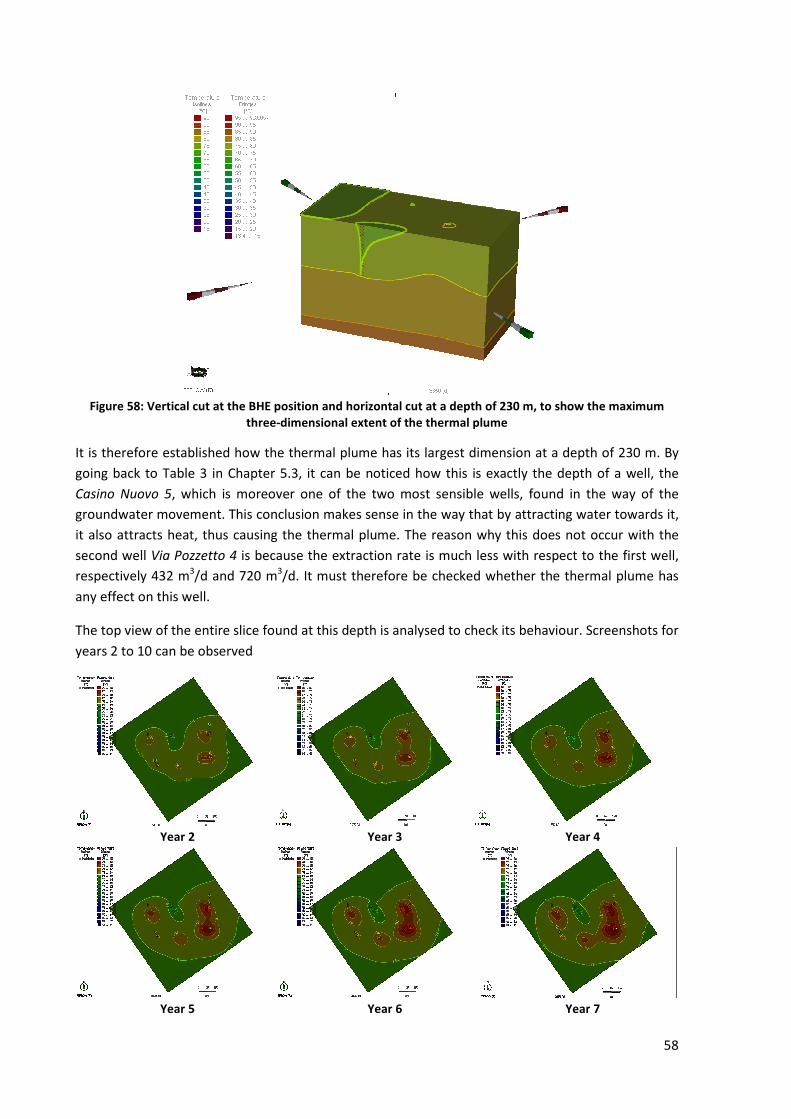
Figure 58: Vertical cut at the BHE position

three-dimens

It is therefore established how the thermal plume has its largest dimension at a depth of 230 m. By

going back to Table 3 in Chapter 5.3

Casino Nuovo 5, which is moreover one of the two most sensible wells, found in the way of the

groundwater movement. This conclusion makes sense in the way that by attracting water towards it,

it also attracts heat, thus causing the thermal plume. The reason why this does not occur with the

second well Via Pozzetto 4 is because the extraction rate is much less with respect to the first well,

respectively 432 m3/d and 720 m3/d.

any effect on this well.

The top view of the entire slice found at this depth is analysed to check

years 2 to 10 can be observed

Year 2

Year 5

cut at the BHE position and horizontal cut at a depth of 230 m, to show the maximum

dimensional extent of the thermal plume

It is therefore established how the thermal plume has its largest dimension at a depth of 230 m. By

5.3, it can be noticed how this is exactly the depth of a well, the

, which is moreover one of the two most sensible wells, found in the way of the

This conclusion makes sense in the way that by attracting water towards it,

using the thermal plume. The reason why this does not occur with the

is because the extraction rate is much less with respect to the first well,

/d. It must therefore be checked whether the thermal

The top view of the entire slice found at this depth is analysed to check its behaviou

Year 3 Year 4

Year 6 Year

58

ut at a depth of 230 m, to show the maximum

It is therefore established how the thermal plume has its largest dimension at a depth of 230 m. By

exactly the depth of a well, the

, which is moreover one of the two most sensible wells, found in the way of the

This conclusion makes sense in the way that by attracting water towards it,

using the thermal plume. The reason why this does not occur with the

is because the extraction rate is much less with respect to the first well,

It must therefore be checked whether the thermal plume has

its behaviour. Screenshots for

Year 4

Year 7

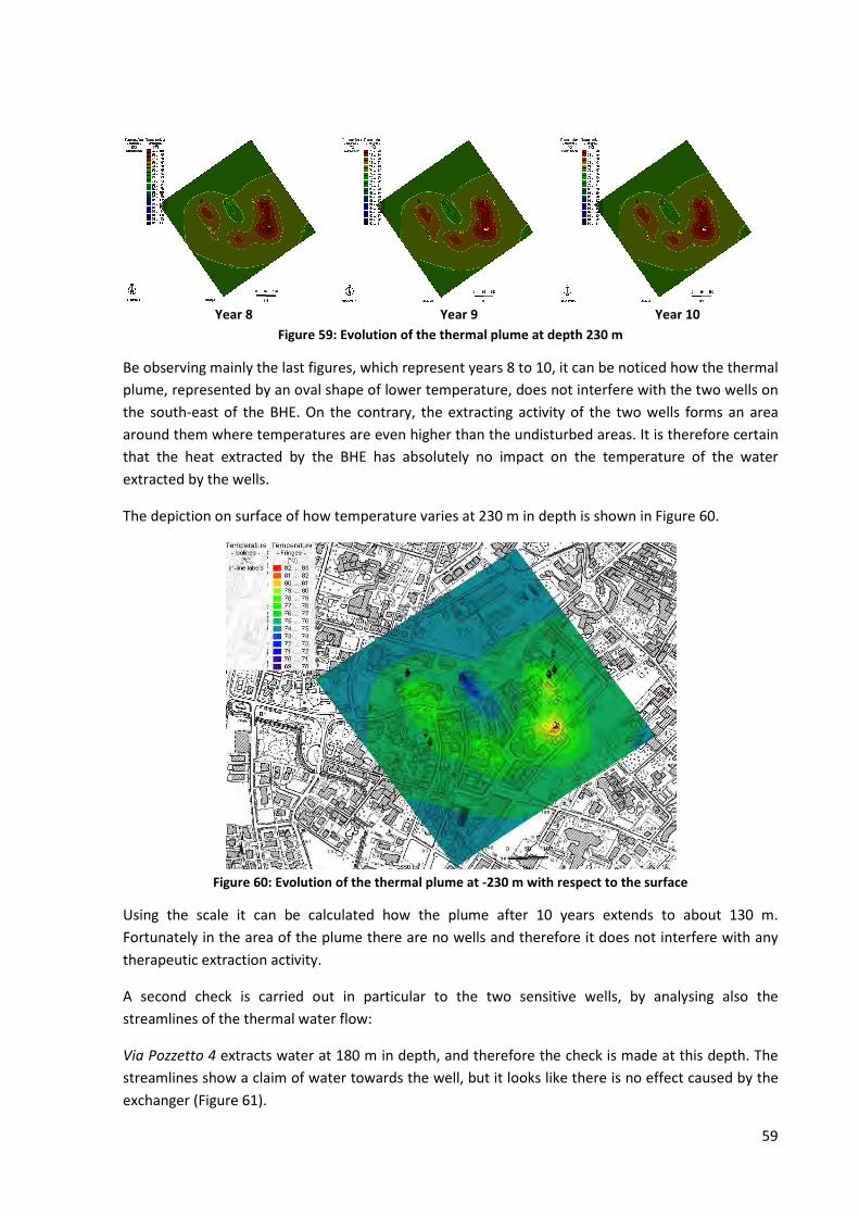
Year 8

Figure

Be observing mainly the last figures, which represent years 8 to 10,

plume, represented by an oval shape of lower temperature, does no

the south-east of the BHE. On the contrary, the extracting activity of the two wells forms an area

around them where temperatures are even higher than the undisturbed areas. It is therefore certain

that the heat extracted by the BHE has absolutely no impact on the temperature of the water

extracted by the wells.

The depiction on surface of how temperature varies at 230 m in depth is shown in

Figure 60: Evoluti

Using the scale it can be calculated how the plume after 10 years extends to about 130 m.

Fortunately in the area of the plume there are no wells and therefore it does not interfere with any

therapeutic extraction activity.

A second check is carried out in particular to the two sensitive wells, by

streamlines of the thermal water flow:

Via Pozzetto 4 extracts water at 180 m in depth

streamlines show a claim of water towards the well, but it looks like there is no effect caused by the

exchanger (Figure 61).

Year 9

Figure 59: Evolution of the thermal plume at depth 230 m

Be observing mainly the last figures, which represent years 8 to 10, it can be noticed how the thermal

plume, represented by an oval shape of lower temperature, does not interfere with the two wells on

On the contrary, the extracting activity of the two wells forms an area

around them where temperatures are even higher than the undisturbed areas. It is therefore certain

by the BHE has absolutely no impact on the temperature of the water

The depiction on surface of how temperature varies at 230 m in depth is shown in

: Evolution of the thermal plume at -230 m with respect to the surface

calculated how the plume after 10 years extends to about 130 m.

Fortunately in the area of the plume there are no wells and therefore it does not interfere with any

rapeutic extraction activity.

A second check is carried out in particular to the two sensitive wells, by

streamlines of the thermal water flow:

extracts water at 180 m in depth, and therefore the check is made at this dep

streamlines show a claim of water towards the well, but it looks like there is no effect caused by the

59

Year 10

hermal plume at depth 230 m

it can be noticed how the thermal

t interfere with the two wells on

On the contrary, the extracting activity of the two wells forms an area

around them where temperatures are even higher than the undisturbed areas. It is therefore certain

by the BHE has absolutely no impact on the temperature of the water

The depiction on surface of how temperature varies at 230 m in depth is shown in Figure 60.

230 m with respect to the surface

calculated how the plume after 10 years extends to about 130 m.

Fortunately in the area of the plume there are no wells and therefore it does not interfere with any

A second check is carried out in particular to the two sensitive wells, by analysing also the

, and therefore the check is made at this depth. The

streamlines show a claim of water towards the well, but it looks like there is no effect caused by the

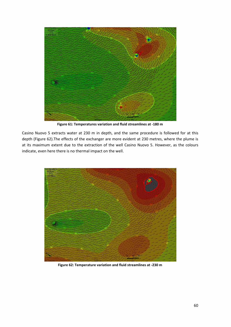
60

Figure 61: Temperatures variation and fluid streamlines at -180 m

Casino Nuovo 5 extracts water at 230 m in depth, and the same procedure is followed for at this

depth (Figure 62).The effects of the exchanger are more evident at 230 metres, where the plume is

at its maximum extent due to the extraction of the well Casino Nuovo 5. However, as the colours

indicate, even here there is no thermal impact on the well.

Figure 62: Temperature variation and fluid streamlines at -230 m

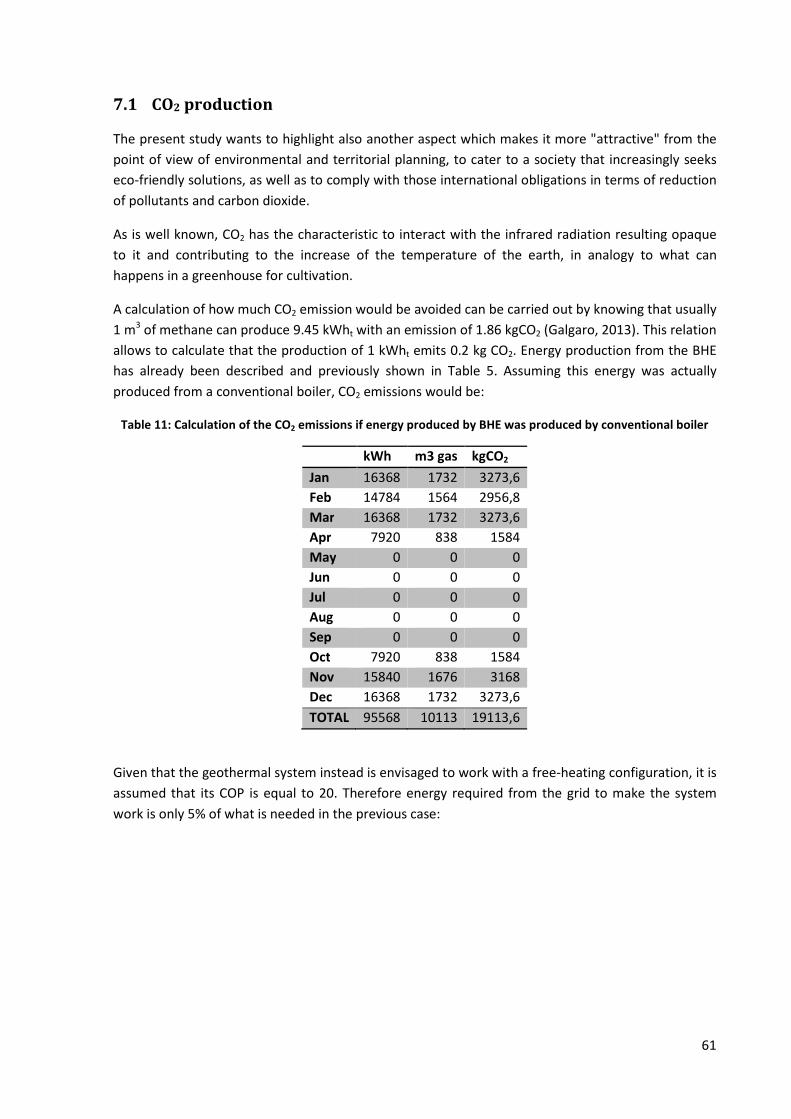
61

7.1 CO2 production

The present study wants to highlight also another aspect which makes it more "attractive" from the

point of view of environmental and territorial planning, to cater to a society that increasingly seeks

eco-friendly solutions, as well as to comply with those international obligations in terms of reduction

of pollutants and carbon dioxide.

As is well known, CO2 has the characteristic to interact with the infrared radiation resulting opaque

to it and contributing to the increase of the temperature of the earth, in analogy to what can

happens in a greenhouse for cultivation.

A calculation of how much CO2 emission would be avoided can be carried out by knowing that usually

1 m3 of methane can produce 9.45 kWht with an emission of 1.86 kgCO2 (Galgaro, 2013). This relation

allows to calculate that the production of 1 kWht emits 0.2 kg CO2. Energy production from the BHE

has already been described and previously shown in Table 5. Assuming this energy was actually

produced from a conventional boiler, CO2 emissions would be:

Table 11: Calculation of the CO2 emissions if energy produced by BHE was produced by conventional boiler

kWh m3 gas kgCO2

Jan 16368 1732 3273,6

Feb 14784 1564 2956,8

Mar 16368 1732 3273,6

Apr 7920 838 1584

May 0 0 0

Jun 0 0 0

Jul 0 0 0

Aug 0 0 0

Sep 0 0 0

Oct 7920 838 1584

Nov 15840 1676 3168

Dec 16368 1732 3273,6

TOTAL 95568 10113 19113,6

Given that the geothermal system instead is envisaged to work with a free-heating configuration, it is

assumed that its COP is equal to 20. Therefore energy required from the grid to make the system

work is only 5% of what is needed in the previous case:

62

Table 12: Calculation of the CO2 emissions caused the geothermal system

kWh kgCO2

Jan 818,4 163,68

Feb 739,2 147,84

Mar 818,4 163,68

Apr 396 79,2

May 0 0

Jun 0 0

Jul 0 0

Aug 0 0

Sep 0 0

Oct 396 79,2

Nov 792 158,4

Dec 818,4 163,68

TOTAL 4778,4 955,68

In conclusion the geothermal system would cause a CO2 emission of 956 kgCO2/year. A traditional

system however would cause a production of 19114 kgCO2/year. A reduction of 95% would therefore

be allowed by the geothermal system.

7.2 Costs’ analysis

With respect to costs evaluation, it is assumed that 1 m3 of gas costs 0.82€, and 1 kWh of electricity

costs 0.30€ (Galgaro, 2013).

The traditional system, consuming gas, has an yearly constant outcome given by the bills which must

be paid for the gas:

Table 13: Calculation of the monthly costs if energy produced by BHE was produced by conventional boiler

kWh m3 gas €/month

Jan 16368 1732 1420

Feb 14784 1564 1283

Mar 16368 1732 1420

Apr 7920 838 687

May 0 0 0

Jun 0 0 0

Jul 0 0 0

Aug 0 0 0

Sep 0 0 0

Oct 7920 838 687

Nov 15840 1676 1374

Dec 16368 1732 1420

TOTAL 95568 10113 8293

63

As already mentioned the geothermal system would only required electricity to run circulating

pumps and control panels, and because it works with free-heating a COP of 20 is assumed.

Table 14: Calculation of the bills generated by the geothermal system

kWh €/month

Jan 818,4 245

Feb 739,2 221

Mar 818,4 245

Apr 396 118

May 0 0

Jun 0 0

Jul 0 0

Aug 0 0

Sep 0 0

Oct 396 118

Nov 792 237

Dec 818,4 245

TOTAL 4778,4 1433

In addition, being the installation of such geothermal system considered as a way to renovate the

Kursaal’s heating system it can access to a tax break of 50% of the whole initial investment in 10

years.

By assuming installation costs of 10000€ for a traditional system and 60000€ for a geothermal

period, the costs trend, considering income and outcomes for both systems, is shown in Figure 63.

Figure 63: Costs evolution with time for traditional and equivalent geothermal systems

The payback period, with respect to the installation of a traditional system, can be observed to be

about 6 years and a half.

0

10000

20000

30000

40000

50000

60000

70000

80000

90000

100000

Year

0

year

1

year

2

year

3

year

4

year

5

year

6

year

7

year

8

year

9

year

10

€

Time (years)

Traditional system

Geothermal system

64

8 Comparison with the CaRM code

CaRM (CApacity Resistance Model) is a geo-exchange simulation tool which considers the heat

transfer within the ground by heat conduction. The BHE is described with a resistance system and the

ground around the BHE is modelled with thermal resistances and capacitances making use of the

electrical analogy. The ground can be modelled into several axial and radial regions (De Carli et al.,

2010).

The model allows to consider different compositions of the soil (defined sub-regions), each of them

with a given undisturbed ground temperature; in this way it is possible to consider a vertical profile

of temperature, which can be relevant for geothermal sites with anomalous gradient of temperature.

These values of undisturbed ground temperatures are assumed independent of time (De Carli et al.,

2010).

Again, ground properties are the same as the ones used in FEFlow. Required data is: thermal

conductivity of the ground, specific heat capacity, density, initial temperature of the ground, BHE

geometry, refrigerant features and distance of undisturbed conditions.

The model is then run to investigate the behaviour of the ground near and far the BHE for 10 years.

The ground around the boreholes has been divided into 35 annular regions until a maximum

diameter of 200 m.

In the following graphs the temperature profile of the annular regions n.5, 10 and 15 compared to

the depth of the ground are shown (respectively, the annular regions have distance 0.5, 1.7 and 4.5

m to the centre of the BHE). The profile temperature of the ground has been plotted at the end of

the 1st, the 6th and the 10th year of operation of the plant.

Figure 64: Temperature profile of the ground after 1 year of operation

-400

-350

-300

-250

-200

-150

-100

-50

0

0 10 20 30 40 50 60 70 80 90 100

De

pth

(m

)

Temperature (°C)

Year 1

radius 0,5 m

radius 1,7 m

radius 4,5 m

Undisturbed ground temp.

65

Figure 65: Temperature profile of the ground after 6 years of operation

Figure 66: Temperature profile of the ground after 10 years of operation

The previous diagrams prove how the temperature profile of the ground as function of the ground

depth undergo changes from the 1st to the 6th year of operation while as for the subsequent years

the behaviour of the soil can be considered constant. The latter consideration is confirmed by the

fact that temperatures of ground and water are not subject to significant changes going from sixth to

tenth year. It can be observed how the flow of water in the BHE brings heat upwards and heats up

the top 120 or so metres, but cools down the ground below that. The extent at which this cooling

occurs can be observed from the graphs.

Focusing on the last graph, which is the more significative, it can be noticed how, below 120°C and at

a distance of 4.5 m, temperature decreases, reaching at the bottom a difference of 10°C. At a larger

radius from the BHE, temperature moves rapidly towards the average ground temperature, meaning

that the thermal impact is confined to a cylinder of a few metres of radius around the BHE.

These results show the limits of the model CaRM, which does not take into consideration for example

the movement of ground water. Heat is transported by conduction only and for this reason it seems

like differences occur almost linearly with depth.

-400

-350

-300

-250

-200

-150

-100

-50

0

0 10 20 30 40 50 60 70 80 90 100

De

pth

(m

)

Temperature (°C)

Year 6

radius 0,5 m

radius 1,7 m

radius 4,5 m

Undisturbed ground temp.

-400

-350

-300

-250

-200

-150

-100

-50

0

0 10 20 30 40 50 60 70 80 90 100

De

pth

(m

)

Temperature (°C)

Year 10

radius 0,5 m

radius 1,7 m

radius 4,5 m

Undisturbed ground temp.

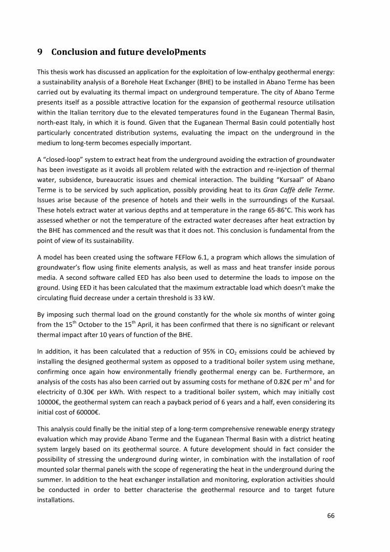
66

9 Conclusion and future developments

This thesis work has discussed an application for the exploitation of low-enthalpy geothermal energy:

a sustainability analysis of a Borehole Heat Exchanger (BHE) to be installed in Abano Terme has been

carried out by evaluating its thermal impact on underground temperature. The city of Abano Terme

presents itself as a possible attractive location for the expansion of geothermal resource utilisation

within the Italian territory due to the elevated temperatures found in the Euganean Thermal Basin,

north-east Italy, in which it is found. Given that the Euganean Thermal Basin could potentially host

particularly concentrated distribution systems, evaluating the impact on the underground in the

medium to long-term becomes especially important.

A “closed-loop” system to extract heat from the underground avoiding the extraction of groundwater

has been investigate as it avoids all problem related with the extraction and re-injection of thermal

water, subsidence, bureaucratic issues and chemical interaction. The building “Kursaal” of Abano

Terme is to be serviced by such application, possibly providing heat to its Gran Caffè delle Terme.

Issues arise because of the presence of hotels and their wells in the surroundings of the Kursaal.

These hotels extract water at various depths and at temperature in the range 65-86°C. This work has

assessed whether or not the temperature of the extracted water decreases after heat extraction by

the BHE has commenced and the result was that it does not. This conclusion is fundamental from the

point of view of its sustainability.

A model has been created using the software FEFlow 6.1, a program which allows the simulation of

groundwater’s flow using finite elements analysis, as well as mass and heat transfer inside porous

media. A second software called EED has also been used to determine the loads to impose on the

ground. Using EED it has been calculated that the maximum extractable load which doesn’t make the

circulating fluid decrease under a certain threshold is 33 kW.

By imposing such thermal load on the ground constantly for the whole six months of winter going

from the 15th October to the 15th April, it has been confirmed that there is no significant or relevant

thermal impact after 10 years of function of the BHE.

In addition, it has been calculated that a reduction of 95% in CO2 emissions could be achieved by

installing the designed geothermal system as opposed to a traditional boiler system using methane,

confirming once again how environmentally friendly geothermal energy can be. Furthermore, an

analysis of the costs has also been carried out by assuming costs for methane of 0.82€ per m3 and for

electricity of 0.30€ per kWh. With respect to a traditional boiler system, which may initially cost

10000€, the geothermal system can reach a payback period of 6 years and a half, even considering its

initial cost of 60000€.

This analysis could finally be the initial step of a long-term comprehensive renewable energy strategy

evaluation which may provide Abano Terme and the Euganean Thermal Basin with a district heating

system largely based on its geothermal source. A future development should in fact consider the

possibility of stressing the underground during winter, in combination with the installation of roof

mounted solar thermal panels with the scope of regenerating the heat in the underground during the

summer. In addition to the heat exchanger installation and monitoring, exploration activities should

be conducted in order to better characterise the geothermal resource and to target future

installations.

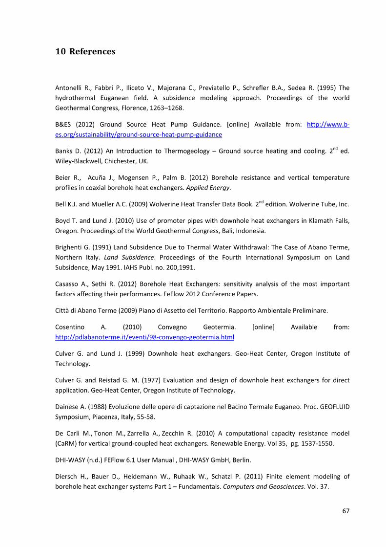
67

10 References

Antonelli R., Fabbri P., Iliceto V., Majorana C., Previatello P., Schrefler B.A., Sedea R. (1995) The

hydrothermal Euganean field. A subsidence modeling approach. Proceedings of the world

Geothermal Congress, Florence, 1263–1268.

B&ES (2012) Ground Source Heat Pump Guidance. [online] Available from: http://www.b-

es.org/sustainability/ground-source-heat-pump-guidance

Banks D. (2012) An Introduction to Thermogeology – Ground source heating and cooling. 2nd ed.

Wiley-Blackwell, Chichester, UK.

Beier R., Acuña J., Mogensen P., Palm B. (2012) Borehole resistance and vertical temperature

profiles in coaxial borehole heat exchangers. Applied Energy.

Bell K.J. and Mueller A.C. (2009) Wolverine Heat Transfer Data Book. 2nd edition. Wolverine Tube, Inc.

Boyd T. and Lund J. (2010) Use of promoter pipes with downhole heat exchangers in Klamath Falls,

Oregon. Proceedings of the World Geothermal Congress, Bali, Indonesia.

Brighenti G. (1991) Land Subsidence Due to Thermal Water Withdrawal: The Case of Abano Terme,

Northern Italy. Land Subsidence. Proceedings of the Fourth International Symposium on Land

Subsidence, May 1991. IAHS Publ. no. 200,1991.

Casasso A., Sethi R. (2012) Borehole Heat Exchangers: sensitivity analysis of the most important

factors affecting their performances. FeFlow 2012 Conference Papers.

Città di Abano Terme (2009) Piano di Assetto del Territorio. Rapporto Ambientale Preliminare.

Cosentino A. (2010) Convegno Geotermia. [online] Available from:

http://pdlabanoterme.it/eventi/98-convengo-geotermia.html

Culver G. and Lund J. (1999) Downhole heat exchangers. Geo-Heat Center, Oregon Institute of

Technology.

Culver G. and Reistad G. M. (1977) Evaluation and design of downhole heat exchangers for direct

application. Geo-Heat Center, Oregon Institute of Technology.

Dainese A. (1988) Evoluzione delle opere di captazione nel Bacino Termale Euganeo. Proc. GEOFLUID

Symposium, Piacenza, Italy, 55-58.

De Carli M., Tonon M., Zarrella A., Zecchin R. (2010) A computational capacity resistance model

(CaRM) for vertical ground-coupled heat exchangers. Renewable Energy. Vol 35, pg. 1537-1550.

DHI-WASY (n.d.) FEFlow 6.1 User Manual , DHI-WASY GmbH, Berlin.

Diersch H., Bauer D., Heidemann W., Ruhaak W., Schatzl P. (2011) Finite element modeling of

borehole heat exchanger systems Part 1 – Fundamentals. Computers and Geosciences. Vol. 37.

68

Diersch H., Kolditz O. (2002) FEFlow Reference Manual, DHI-Wasy, Berlin.

Duffield G. M. (2013) Representative Values of Hydraulic Properties. [online] Available from:

http://www.aqtesolv.com/aquifer-tests/aquifer_properties.htm

Elíasson E.T. (2001) Power generation from high-enthalpy geothermal resources. Geo-heat Centre

Bulletin. June 2001.

Fabbri P. and Trevisani S. (2005) Spatial distribution of temperature in the low-temperature

geothermal Euganean field (NE Italy): a simulated annealing approach. Geothermics. Vol 34, pg. 617-

631.

Faldani M. (2009) Analisi dei processi di interazione tra sottosuolo e sonde geotermiche. Master

Thesis Work. School of Mathematics, Physycs and Natural Sciences. University of Padua.

Franchin F. (2012) Kursaal e Gran Caffè al Cvcs di Padova. Il Mattino di Padova. 19th December 2012.

Galgaro A. (2013) Seminario: Impianti geotermici a bassa entalpia a circuito chiuso. Presentation.

Gestione Unica del bacino idrominerario omogeneo del Colli Euganei (BIOCE) (n.d.) Il bacino

idrominerario omogeneo del Colli Euganei.

Gestione Unica del bacino idrominerario omogeneo del Colli Euganei (BIOCE) (2012) Leggi sul

termalismo in Italia e Leggi Regionali. [online] Avialable from:

http://www.gestioneunica.it/italian/pages/legislatura.php

Gonet A. and Śliwa T. (2010) Modification of Method of Interpreting Thermal Response Test of

Borehole Heat Exchanger. Proceedings World Geothermal Congress 2010, Bali, Indonesia.

Gottardi G., Previatello P., Simonini P., (1995) An extensive investigation of land subsidence in the

Euganean geothermal basin, Italy. Land Subsidence. Proceedings of the Fifth International

Symposium on Land Subsidence, The Hague, October 1995. IAHS Publ. no. 234, 1995.

Hotel Terme Internazionale (2012) Dove siamo. [online] Available from:

http://www.termeinternazionale.it/en/dovesiamo.html

Lund J. (2003) The use of downhole heat exchangers. Geo-Heat Center, Oregon Institute of

Technology.

Lund J. (2011) Development of Direct-use projects. Proceedings of the Thirty-Sixth Workshop on

Geothermal Reservoir Engineering, Stanford University, Stanford, California, SGP-TR-191.

Morandin G. (2013) Valutazione del potenziale termico recuperabile dalle acque termali di risulta nel

comune di Abano Terme. Bachelor Thesis Work. School of Chemical Sciences. University of Padua.

Panazzolo G. (2009) Geoscambio con uso diretto di acqua di falda ed in zona di anomalia termica.

Master Thesis Work. School of Mathematics, Physycs and Natural Sciences. University of Padua.

Parco Regionale dei Colli Euganei (2012) Il Termalismo. [online] Available from:

http://www.parcocollieuganei.com/index.php/ambiente-e-territorio/il-termalismo

69

Piccoli G., Bellati R., Bigotti C., Di Lallo E., Sedea R., Dal Prà A., Cataldi R., Gatto G.O., Ghezzi G.,

Marchetti M., Bulgarelli G., Schiesaro G., Panichi C., Tongiorgi E. Baldi P., Ferrara G.C., Massari F.,

Medizza F.,Iliceto V., Norinelli A., De Vecchi GP., Gregnanin A., Piccirillo E.M., Sbettega G. (1976) Il

sistema idrotermale euganeo-berico e la geologia dei Colli Euganei. Mem. Ist. Geol. Miner. Univ.

Padova, 30, Padova.

Pola M. (2011) Revision of the Euganan Geothermal Field (EGF) using new knowledge in

hydrogeology and structural geology. PhD Thesis.

Pruess K. (2002) Mathematical modelling of fluid flow and heat transfer in geothermal systems – an

introduction in five lectures. Geothermal Training Program, United Nations University.

REHAU (2012) Technical prospectus RAUGEO HPR heat exchangers.

Renewable Energy World (2012) Geothermal Direct Use. [online] Available from:

http://www.renewableenergyworld.com/rea/tech/geodirectuse

Sambi S. (2012) Gran Caffè delle Terme, è calato il sipario. Il Mattino di Padova. 16th January 2012.

Strozzi T., Carbognin L., Galgaro A., Tosi L., Wegmüller U., (1999) Monitoring Land Subsidence in the

Euganean Geothermal Basin with Differential SAR Interferometry

The Engineering Toolbox (2013) [a] Fuel Gases - Heating Values. [online] Available from:

http://www.engineeringtoolbox.com/heating-values-fuel-gases-d_823.html

The Engineering Toolbox (2013) [b] Thermal Conductivity of some common Materials and Gases.

[online] Available from: http://www.engineeringtoolbox.com/thermal-conductivity-d_429.html

Turismo Padova Terme Euganee (2012) Le Terme: la storia di un benessere centenario. [online]

Available from: http://www.abanoterme.net/le-terme-e-i-colli.html

U.S. Department of Energy (2013) Direct use of Geothermal energy. [online] Available from:

http://www1.eere.energy.gov/geothermal/directuse.html

Wagner V., Bayer P., Bisch G., Braun J., Klaas N., Blum P. (2012) Calibrating a High-resolution

Numerical Model of a Borehole Heat Exchanger Using FEFLOW. FeFlow 2012 Conference Papers.

Welty J., Wicks C., Wilson R., Rorrer G. (2007) Fundamentals of Momentum, Heat, and Mass Transfer.

5th edition. John Wiley & Sons, Inc.

Xiaoning H. and Anderson B. (2012) Low-Temperature Geothermal Resources for District Heating: An

Energy-Economic Model of West Virginia University Case Study. Proceedings of the Thirty-Seventh

Workshop on Geothermal Reservoir Engineering, Stanford University, Stanford, California. SGP-TR-

194

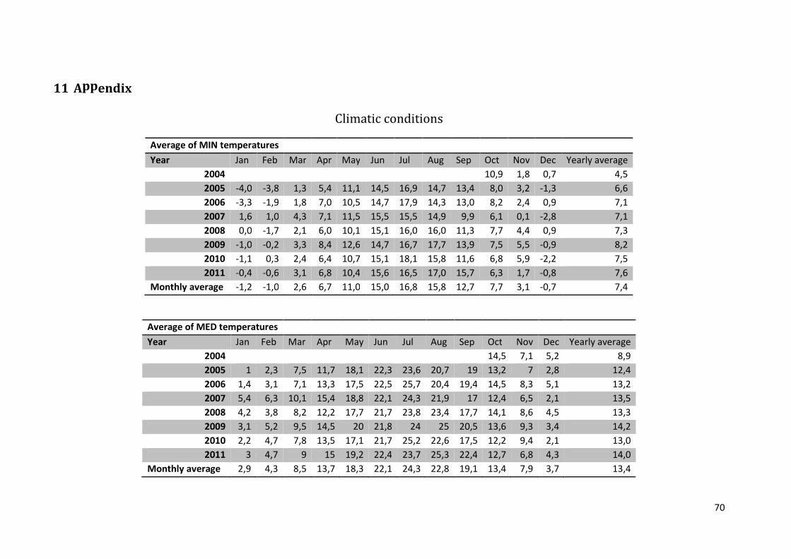
70

11 Appendix

Climatic conditions

Average of MIN temperatures

Year Jan Feb Mar Apr May Jun Jul Aug Sep Oct Nov Dec Yearly average

2004 10,9 1,8 0,7 4,5

2005 -4,0 -3,8 1,3 5,4 11,1 14,5 16,9 14,7 13,4 8,0 3,2 -1,3 6,6

2006 -3,3 -1,9 1,8 7,0 10,5 14,7 17,9 14,3 13,0 8,2 2,4 0,9 7,1

2007 1,6 1,0 4,3 7,1 11,5 15,5 15,5 14,9 9,9 6,1 0,1 -2,8 7,1

2008 0,0 -1,7 2,1 6,0 10,1 15,1 16,0 16,0 11,3 7,7 4,4 0,9 7,3

2009 -1,0 -0,2 3,3 8,4 12,6 14,7 16,7 17,7 13,9 7,5 5,5 -0,9 8,2

2010 -1,1 0,3 2,4 6,4 10,7 15,1 18,1 15,8 11,6 6,8 5,9 -2,2 7,5

2011 -0,4 -0,6 3,1 6,8 10,4 15,6 16,5 17,0 15,7 6,3 1,7 -0,8 7,6

Monthly average -1,2 -1,0 2,6 6,7 11,0 15,0 16,8 15,8 12,7 7,7 3,1 -0,7 7,4

Average of MED temperatures

Year Jan Feb Mar Apr May Jun Jul Aug Sep Oct Nov Dec Yearly average

2004 14,5 7,1 5,2 8,9

2005 1 2,3 7,5 11,7 18,1 22,3 23,6 20,7 19 13,2 7 2,8 12,4

2006 1,4 3,1 7,1 13,3 17,5 22,5 25,7 20,4 19,4 14,5 8,3 5,1 13,2

2007 5,4 6,3 10,1 15,4 18,8 22,1 24,3 21,9 17 12,4 6,5 2,1 13,5

2008 4,2 3,8 8,2 12,2 17,7 21,7 23,8 23,4 17,7 14,1 8,6 4,5 13,3

2009 3,1 5,2 9,5 14,5 20 21,8 24 25 20,5 13,6 9,3 3,4 14,2

2010 2,2 4,7 7,8 13,5 17,1 21,7 25,2 22,6 17,5 12,2 9,4 2,1 13,0

2011 3 4,7 9 15 19,2 22,4 23,7 25,3 22,4 12,7 6,8 4,3 14,0

Monthly average 2,9 4,3 8,5 13,7 18,3 22,1 24,3 22,8 19,1 13,4 7,9 3,7 13,4

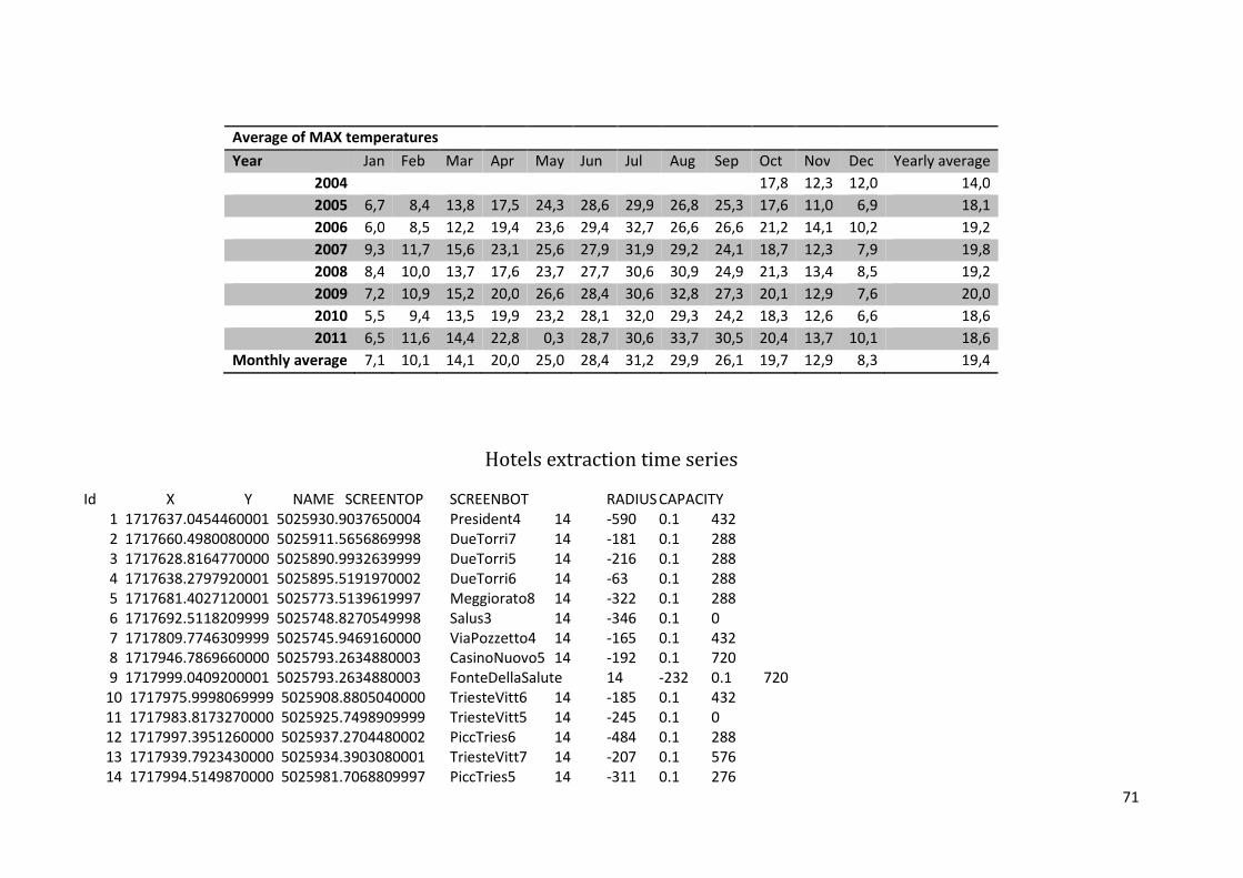
71

Average of MAX temperatures

Year Jan Feb Mar Apr May Jun Jul Aug Sep Oct Nov Dec Yearly average

2004 17,8 12,3 12,0 14,0

2005 6,7 8,4 13,8 17,5 24,3 28,6 29,9 26,8 25,3 17,6 11,0 6,9 18,1

2006 6,0 8,5 12,2 19,4 23,6 29,4 32,7 26,6 26,6 21,2 14,1 10,2 19,2

2007 9,3 11,7 15,6 23,1 25,6 27,9 31,9 29,2 24,1 18,7 12,3 7,9 19,8

2008 8,4 10,0 13,7 17,6 23,7 27,7 30,6 30,9 24,9 21,3 13,4 8,5 19,2

2009 7,2 10,9 15,2 20,0 26,6 28,4 30,6 32,8 27,3 20,1 12,9 7,6 20,0

2010 5,5 9,4 13,5 19,9 23,2 28,1 32,0 29,3 24,2 18,3 12,6 6,6 18,6

2011 6,5 11,6 14,4 22,8 0,3 28,7 30,6 33,7 30,5 20,4 13,7 10,1 18,6

Monthly average 7,1 10,1 14,1 20,0 25,0 28,4 31,2 29,9 26,1 19,7 12,9 8,3 19,4

Hotels extraction time series

Id X Y NAME SCREENTOP SCREENBOT RADIUS CAPACITY

1 1717637.0454460001 5025930.9037650004 President4 14 -590 0.1 432

2 1717660.4980080000 5025911.5656869998 DueTorri7 14 -181 0.1 288

3 1717628.8164770000 5025890.9932639999 DueTorri5 14 -216 0.1 288

4 1717638.2797920001 5025895.5191970002 DueTorri6 14 -63 0.1 288

5 1717681.4027120001 5025773.5139619997 Meggiorato8 14 -322 0.1 288

6 1717692.5118209999 5025748.8270549998 Salus3 14 -346 0.1 0

7 1717809.7746309999 5025745.9469160000 ViaPozzetto4 14 -165 0.1 432

8 1717946.7869660000 5025793.2634880003 CasinoNuovo5 14 -192 0.1 720

9 1717999.0409200001 5025793.2634880003 FonteDellaSalute 14 -232 0.1 720

10 1717975.9998069999 5025908.8805040000 TriesteVitt6 14 -185 0.1 432

11 1717983.8173270000 5025925.7498909999 TriesteVitt5 14 -245 0.1 0

12 1717997.3951260000 5025937.2704480002 PiccTries6 14 -484 0.1 288

13 1717939.7923430000 5025934.3903080001 TriesteVitt7 14 -207 0.1 576

14 1717994.5149870000 5025981.7068809997 PiccTries5 14 -311 0.1 276

References

Antonelli R., Fabbri P., Iliceto V., Majorana C., Previatello P., Schrefler B.A., Sedea R. (1995) The

hydrothermal Euganean field. A subsidence modeling approach. Proceedings of the world Geothermal

Congress, Florence, 1263–1268.

B&ES (2012) Ground Source Heat Pump Guidance. [online] Available from: http://www.b-

es.org/sustainability/ground-source-heat-pump-guidance

Banks D. (2012) An Introduction to Thermogeology – Ground source heating and cooling. 2nd ed. Wiley-

Blackwell, Chichester, UK.

Beier R., Acuña J., Mogensen P., Palm B. (2012) Borehole resistance and vertical temperature profiles in

coaxial borehole heat exchangers. Applied Energy.

Bell K.J. and Mueller A.C. (2009) Wolverine Heat Transfer Data Book. 2nd edition. Wolverine Tube, Inc.

Boyd T. and Lund J. (2010) Use of promoter pipes with downhole heat exchangers in Klamath Falls, Oregon.

Proceedings of the World Geothermal Congress, Bali, Indonesia.

Brighenti G. (1991) Land Subsidence Due to Thermal Water Withdrawal: The Case of Abano Terme,

Northern Italy. Land Subsidence. Proceedings of the Fourth International Symposium on Land Subsidence,

May 1991. IAHS Publ. no. 200,1991.

Casasso A., Sethi R. (2012) Borehole Heat Exchangers: sensitivity analysis of the most important factors

affecting their performances. FeFlow 2012 Conference Papers.

Città di Abano Terme (2009) Piano di Assetto del Territorio. Rapporto Ambientale Preliminare.

Cosentino A. (2010) Convegno Geotermia. [online] Available from: http://pdlabanoterme.it/eventi/98-

convengo-geotermia.html

Culver G. and Lund J. (1999) Downhole heat exchangers. Geo-Heat Center, Oregon Institute of Technology.

Culver G. and Reistad G. M. (1977) Evaluation and design of downhole heat exchangers for direct

application. Geo-Heat Center, Oregon Institute of Technology.

Dainese A. (1988) Evoluzione delle opere di captazione nel Bacino Termale Euganeo. Proc. GEOFLUID

Symposium, Piacenza, Italy, 55-58.

De Carli M., Tonon M., Zarrella A., Zecchin R. (2010) A computational capacity resistance model (CaRM) for

vertical ground-coupled heat exchangers. Renewable Energy. Vol 35, pg. 1537-1550.

DHI-WASY (n.d.) FEFlow 6.1 User Manual , DHI-WASY GmbH, Berlin.

Diersch H., Bauer D., Heidemann W., Ruhaak W., Schatzl P. (2011) Finite element modeling of borehole

heat exchanger systems Part 1 – Fundamentals. Computers and Geosciences. Vol. 37.

Diersch H., Kolditz O. (2002) FEFlow Reference Manual, DHI-Wasy, Berlin.

Duffield G. M. (2013) Representative Values of Hydraulic Properties. [online] Available from:

http://www.aqtesolv.com/aquifer-tests/aquifer_properties.htm

Elíasson E.T. (2001) Power generation from high-enthalpy geothermal resources. Geo-heat Centre Bulletin.

June 2001.

Fabbri P. and Trevisani S. (2005) Spatial distribution of temperature in the low-temperature geothermal

Euganean field (NE Italy): a simulated annealing approach. Geothermics. Vol 34, pg. 617-631.

Faldani M. (2009) Analisi dei processi di interazione tra sottosuolo e sonde geotermiche. Master Thesis

Work. School of Mathematics, Physycs and Natural Sciences. University of Padua.

Franchin F. (2012) Kursaal e Gran Caffè al Cvcs di Padova. Il Mattino di Padova. 19th December 2012.

Galgaro A. (2013) Seminario: Impianti geotermici a bassa entalpia a circuito chiuso. Presentation.

Gestione Unica del bacino idrominerario omogeneo del Colli Euganei (BIOCE) (n.d.) Il bacino idrominerario

omogeneo del Colli Euganei.

Gestione Unica del bacino idrominerario omogeneo del Colli Euganei (BIOCE) (2012) Leggi sul termalismo in Italia e Leggi Regionali. [online] Avialable from: http://www.gestioneunica.it/italian/pages/legislatura.php

Gonet A. and Śliwa T. (2010) Modification of Method of Interpreting Thermal Response Test of Borehole

Heat Exchanger. Proceedings World Geothermal Congress 2010, Bali, Indonesia.

Gottardi G., Previatello P., Simonini P., (1995) An extensive investigation of land subsidence in the

Euganean geothermal basin, Italy. Land Subsidence. Proceedings of the Fifth International Symposium on

Land Subsidence, The Hague, October 1995. IAHS Publ. no. 234, 1995.

Hotel Terme Internazionale (2012) Dove siamo. [online] Available from:

http://www.termeinternazionale.it/en/dovesiamo.html

Lund J. (2003) The use of downhole heat exchangers. Geo-Heat Center, Oregon Institute of Technology.

Lund J. (2011) Development of Direct-use projects. Proceedings of the Thirty-Sixth Workshop on

Geothermal Reservoir Engineering, Stanford University, Stanford, California, SGP-TR-191.

Morandin G. (2013) Valutazione del potenziale termico recuperabile dalle acque termali di risulta nel

comune di Abano Terme. Bachelor Thesis Work. School of Chemical Sciences. University of Padua.

Panazzolo G. (2009) Geoscambio con uso diretto di acqua di falda ed in zona di anomalia termica. Master

Thesis Work. School of Mathematics, Physycs and Natural Sciences. University of Padua.

Parco Regionale dei Colli Euganei (2012) Il Termalismo. [online] Available from:

http://www.parcocollieuganei.com/index.php/ambiente-e-territorio/il-termalismo

Piccoli G., Bellati R., Bigotti C., Di Lallo E., Sedea R., Dal Prà A., Cataldi R., Gatto G.O., Ghezzi G., Marchetti

M., Bulgarelli G., Schiesaro G., Panichi C., Tongiorgi E. Baldi P., Ferrara G.C., Massari F., Medizza F.,Iliceto V.,

Norinelli A., De Vecchi GP., Gregnanin A., Piccirillo E.M., Sbettega G. (1976) Il sistema idrotermale euganeo-

berico e la geologia dei Colli Euganei. Mem. Ist. Geol. Miner. Univ. Padova, 30, Padova.

Pola M. (2011) Revision of the Euganan Geothermal Field (EGF) using new knowledge in hydrogeology and

structural geology. PhD Thesis.

Pruess K. (2002) Mathematical modelling of fluid flow and heat transfer in geothermal systems – an

introduction in five lectures. Geothermal Training Program, United Nations University.

REHAU (2012) Technical prospectus RAUGEO HPR heat exchangers.

Renewable Energy World (2012) Geothermal Direct Use. [online] Available from:

http://www.renewableenergyworld.com/rea/tech/geodirectuse

Sambi S. (2012) Gran Caffè delle Terme, è calato il sipario. Il Mattino di Padova. 16th January 2012.

Strozzi T., Carbognin L., Galgaro A., Tosi L., Wegmüller U., (1999) Monitoring Land Subsidence in the

Euganean Geothermal Basin with Differential SAR Interferometry

The Engineering Toolbox (2013) [a] Fuel Gases - Heating Values. [online] Available from:

http://www.engineeringtoolbox.com/heating-values-fuel-gases-d_823.html

The Engineering Toolbox (2013) [b] Thermal Conductivity of some common Materials and Gases. [online]

Available from: http://www.engineeringtoolbox.com/thermal-conductivity-d_429.html

Turismo Padova Terme Euganee (2012) Le Terme: la storia di un benessere centenario. [online] Available

from: http://www.abanoterme.net/le-terme-e-i-colli.html

U.S. Department of Energy (2013) Direct use of Geothermal energy. [online] Available from:

http://www1.eere.energy.gov/geothermal/directuse.html

Wagner V., Bayer P., Bisch G., Braun J., Klaas N., Blum P. (2012) Calibrating a High-resolution Numerical

Model of a Borehole Heat Exchanger Using FEFLOW. FeFlow 2012 Conference Papers.

Welty J., Wicks C., Wilson R., Rorrer G. (2007) Fundamentals of Momentum, Heat, and Mass Transfer. 5th

edition. John Wiley & Sons, Inc.

Xiaoning H. and Anderson B. (2012) Low-Temperature Geothermal Resources for District Heating: An

Energy-Economic Model of West Virginia University Case Study. Proceedings of the Thirty-Seventh

Workshop on Geothermal Reservoir Engineering, Stanford University, Stanford, California. SGP-TR-194