Engineering Geology 297 (2022) 106484

Available online 4 December 20210013-7952/© 2021 The Authors. Published by Elsevier B.V. This is an open access article under the CC BY license (http://creativecommons.org/licenses/by/4.0/).

Integrated bedrock model combining airborne geophysics and sparse drillings based on an artificial neural network

Asgeir Kydland Lysdahl a, Craig William Christensen a,b,*, Andreas Aspmo Pfaffhuber a,b, Malte Voge a, Lars Andresen a, Guro Huun Skurdal a,b, Martin Panzner b

a Norwegian Geotechnical Institute, Sognsveien 72, 0855 Oslo, Norway b EMerald Geomodelling, Gaustadalleen 21, 0349 Oslo, Norway

A R T I C L E I N F O

Keywords: Artificial neural network Airborne geophysics Depth to bedrock Ground investigations Linear infrastructure Geological risk

A B S T R A C T

Cost overruns caused by unforeseen geological challenges are commonplace for large infrastructure projects. Thorough ground investigations can reduce this risk, but geotechnical drillings and laboratory test are expensive and time consuming. Airborne electromagnetics (AEM) is a low-cost geophysical method being increasingly used for geotechnical ground investigations. However, extracting engineering parameters from these complex data is challenging. We present a novel approach of extracting depth to bedrock from AEM data using artificial neural networks (ANN) and sparse drillings. Using synthetic models, we test its theoretical performance and analyse sources of error. We find that geological complexity is the main limitation on performance. We also test the algorithm on real field data from a complex geological setting. Results show that ANNs produce bedrock models that rival the accuracy of manual interpretations by experts and that are markedly more accurate than existing automated resistivity model interpretation methods. Using ANN based bedrock interpretation, one needs 2 to 3.5 times fewer geotechnical drillings (i.e., a reduction of 50–70%) in the early phases of a project compared to ground investigations using only borehole data. Further improvements may be possible with strategic planning of drilling campaigns and careful data pre-processing.

1. Introduction

Cost overruns and delivery delays are an ever-present challenge for engineers and project owners. Average overruns of between 20 and 50% are typical for linear infrastructure projects (Flyvbjerg et al., 2002). Geological risk is a significant part of planning uncertainties and a key contributor to these cost adjustments (Beckers et al., 2013). The high costs and extensive time of detailed ground investigation and laboratory testing using traditional approaches, consisting primarily of geotech-nical drillings and to some extent ground geophysics, complicate the management of this risk.

Airborne geo-scanning is an emerging application that is increasingly being used to reduce the geological risk in early project phases (Pfaff-huber et al., 2016). In the context of this paper, we define airborne geo- scanning as the technique combining airborne geophysics and ground truth data to produce ground models. It often relies on a method first established for mineral exploration in the 1950s – airborne

electromagnetics (AEM) (Palacky and West, 1991) – that has been adapted for geotechnical purposes. The development of high-resolution time-domain AEM survey equipment (Sørensen and Auken, 2004) and specialized processing and inversion techniques (Viezzoli et al., 2008) were critical for providing the high-resolution, shallow imaging needed for engineering applications. The earth resistivity models derived from this type of survey have since proven valuable for bedrock topography mapping (Christensen et al., 2015, 2020), soil type characterization (He et al., 2014; Christiansen et al., 2014; Anschütz et al., 2017a; Lysdahl et al., 2017; Pfaffhuber et al., 2017b), fracture zone mapping (Okazaki et al., 2011; Pfaffhuber et al., 2016) and rock type delineation (Pfaff-huber et al., 2017a).

However, translating complex geophysical data into parameters and models valuable to engineers is challenging. Traditional techniques, such as qualitative data attribute analysis and geophysical data inver-sion, are time consuming and often produce inadequate and ambiguous results. Manual interpretation of the geophysical data and inverted

* Corresponding author at: Norwegian Geotechnical Institute, Sognsveien 72, 0855 Oslo, Norway. E-mail addresses: aol@ngi.no (A.K. Lysdahl), cch@emrld.no (C.W. Christensen), aap@emrld.no (A.A. Pfaffhuber), mvo@ngi.no (M. Voge), lars.andresen@ngi.no

(L. Andresen), ghs@emrld.no (G.H. Skurdal), mp@emrld.no (M. Panzner).

Contents lists available at ScienceDirect

Engineering Geology

journal homepage: www.elsevier.com/locate/enggeo

https://doi.org/10.1016/j.enggeo.2021.106484 Received 2 October 2020; Received in revised form 25 November 2021; Accepted 30 November 2021

Engineering Geology 297 (2022) 106484

2

parameter models is often very subjective. Machine learning (ML) based techniques offer a promising path forward for complex geophysical and geotechnical data analysis problems. ML algorithms are superior in recognizing patterns in large amounts of multidimensional data, compared to humans. These algorithms are also fast and objective since they are not biased by the skillset or preferences of a human interpreter. That has been demonstrated in multiple examples, including clustering of geophysical data (e.g., Gunnink and Siemon, 2015) as well as finding discrete boundaries such as peat thickness (Dewar et al., 2018) or delineation of hydrogeological units (Korus et al., 2018). Within the realm of geotechnics, a special type of machine learning algorithms, called artificial neural networks (ANNs) have been successfully used in a variety of applications, including modelling of bedrock elevation, pile capacity, foundation settlements, liquefaction, slope stability, and various soil parameters (Zhou and Wu, 1994; Shahin et al., 2001).

In the past, ANNs have occasionally been used interpreting AEM data (e.g., Gunnink et al., 2012). More recently, ANNs are increasingly being employed. Lysdahl et al. (2018) and Pfaffhuber et al. (2019) used AEM- derived resistivity models and sparse geotechnical drilling data as input to ANNs to produce depth to bedrock models. Despite promising results, those works did not address several questions regarding how robust this method can estimate depth to bedrock. This paper aims at advancing the state of the art by addressing the following questions:

1. What are the theoretical performance limits of this ANN-based method?

2. Can this performance be achieved with real field data? 3. Does this method still perform well in very complex geological

environments? 4. Are ANNs quantifiably better compared to earlier traditional data

analysis methods? 5. How does the preparation of non-colocated datasets affect

performance?

By addressing these unknowns, we aim to assess whether ANN based data analysis can enhance the value of AEM data in engineering projects.

First, we use synthetic models of varying complexity to evaluate the theoretical performance of the ANN based bedrock interpretation method and investigate the sources of error. We then revisit a field data example, first considered by Lysdahl et al. (2018), which had a partic-ularly complex geological setting. Extensive drilling data has now become available, which we use to evaluate the performance of this method.

2. Methods

In this section, we briefly introduce the geophysical background and revisit traditional methods for geophysical data analysis to illustrate their shortcomings. Then, we describe the setup and training of the applied artificial neural network (ANN) method and the validation procedure employed.

2.1. Field data and processing and inversion

The geophysical data that form the basis of our analysis are re-sistivity models derived from airborne geo-scanning, more specifically, time-domain airborne electromagnetic (AEM) data. In such airborne surveys, a set of transmitter and receiver coils are carried by a fixed- or rotary-wing aircraft flying at low altitude. The transmitting coil carries a time-varying electric current, which causes a time varying primary magnetic field. This primary magnetic field continues into the subsur-face and induces a time varying electric current in the ground. The strength of these eddy currents is a function of the resistivity distribution in the subsurface. A highly sensitive and accurate receiver coil system measures then a small, secondary magnetic field which correlates with the strength of the eddy currents in the subsurface. Two broad families

of instruments exist: time-domain and frequency-domain systems. Time- domain systems transmit a discrete pulse and record the resultant sec-ondary magnetic field as a function of time. Frequency-domain systems continuously transmit one or several waveforms and record the ampli-tude and phase shift of the secondary magnetic field. For this study, we utilize a time-domain, helicopter-towed AEM system called SkyTEM 304 (Sørensen and Auken, 2004), shown in Fig. 1.

Unlike seismic reflection or ground-penetrating radar (GPR), one cannot acquire a subsurface geometry model (i.e., discrete interfaces, reflectors) by simple processing of raw AEM data. This is due to the diffusive nature of the electromagnetic fields at the frequencies employed. Instead, one must indirectly infer a geophysical parameter model, in this case a resistivity model, that can explain the measured data within the observed data uncertainty. This is a very computation-ally intensive, non-linear process called inverse modelling or inversion. The AEM inverse problem is strongly non-unique, which means that there are many different resistivity models that can explain the measured data equally well. Additional constraints must be employed, to stabilize the inverse problem and to ensure a geologically plausible model.

There are many different approaches for constraining, or regular-izing, a non-linear inverse problem. One possibility is to limit the number of resistivity layers in the subsurface, also referred to as (layered) inversion. The resulting resistivity models have often just a very few layers but often show strong resistivity contrasts between the distinct layers, which can be easily interpreted. With such an approach, one could, for example, produce a simple two-layer model in which the layer boundary can be interpreted directly as the soil-bedrock boundary (e.g., Chouteau et al., 2013). Another alternative to stabilize the AEM inverse problem is to seek for a smooth subsurface resistivity model, also referred to as Occam inversion or multi-layer, smooth inversion. Engineering parameters, like depth to bedrock, are then obtained by integrating ground truth data (e.g., Christensen et al., 2015; Chambers et al., 2014).

Smooth, Occam-type multi-layer inversions are often preferred, for several reasons. First, constrained, layered inversions are usually inad-equate because they cannot account for more complexity than two to three slabs with homogeneous properties (Sengpiel and Siemon, 1998).

Fig. 1. Photo of a helicopter geo-scanning (time domain AEM) system along with illustrative sketch of the fundamental physics: A strong electric current in the carrier frame (white dashed circle) creates a magnetic field (white stippled lines) which in turn induces electric currents in the ground (orange dashed circles). The secondary magnetic field (orange stippled lines) caused by those eddy ground currents is measured by an electromagnetic receiver on the carrier frame as a function of time after the transmitter current is switched off.

A.K. Lysdahl et al.

Engineering Geology 297 (2022) 106484

3

Second, although layered inversions can work well in some more com-plex geological environments, they are dependent on good a priori in-formation (Auken and Christiansen, 2004), something that is not always available in new, poorly understood, or highly heterogeneous geological environments. Third, in some cases, real resistivity changes are gradual rather than sharp at these scales of investigation. This is for instance the case for gradual changes in salt content due to leaching in marine clay deposits common in Scandinavia (Bazin and Pfaffhuber, 2013). Smooth inversions are usually more robust in complex geological settings as they do not require extensive apriori information about the subsurface.

For all the examples discussed in this study we use the processing and inversion software Aarhus Workbench(Auken et al., 2009), which utilizes the inversion kernel AarhusInv (Auken et al., 2015). We use a spatially constrained inversion (SCI) (Viezzoli et al., 2008), which seeks a smooth quasi-3D resistivity model, with a fixed number of model layers (usually 25 to 30) at all AEM sounding locations. The layer thickness is fix and increases from a few meters at the surface to tens of meters at the bottom of the model, reflecting the depth dependent resolution limit and the depth penetration of the AEM method. The layer thicknesses are the

same for any given x-y position of the resistivity model.

2.2. Traditional interpretation of resistivity models from AEM data inversion

To illustrate the resolution that we can expect from a helicopter- derived resistivity model, we built a conceptual 3D geological model illustrating soil and rock layers with geometries and resistivity contrasts typical of projects in Norway (Fig. 2a). The model includes the three most common targets for helicopter geo-scanning in Norway:

1) Multiple bedrock units with varying resistivities (gneiss, shale and limestone)

2) Multiple soil units with varying resistivities, including pockets of quick clay within regular clay

3) A bedrock-sediment interface with varying depth and varying bedrock-sediment resistivity contrasts

Water-saturated weakness zones in bedrock are also a common target

Fig. 2. A.) Cross section of a 3D synthetic geological model with soil and rock layers of varying resistivity, used to compute synthetic AEM data. B) Resistivity model from the AEM data inversion, illustrating resolution and depth penetration of a AEM survey encountering complex geology. Note that the inverted resistivity model is a smooth representation of the synthetic model and would be difficult to interpret without additional subsurface information.

A.K. Lysdahl et al.

Engineering Geology 297 (2022) 106484

4

for geo-scanning. Though not explicitly included in the model, they are dipping structures of lower resistivity than the surrounding host rock. In practice, they may appear essentially identical to the dipping shale unit in Fig. 2a, which has a lower resistivity than the surrounding gneiss and limestone.

From the conceptual model in Fig. 2a, we computed synthetic AEM data for a SkyTEM 304 survey configuration using AarhusInv (Auken et al., 2015). Note that the forward model has a a limited number of layers. The synthetic AEM data were then inverted using a continuously discretized parameter model with a large number of layers, resulting in a smooth resistivity model (Fig. 2b). The resultant model resembles the resolution we could be expected from such a geo-scanning survey.

The inverted resistivity model is smoother than the conceptual model but retains its main features and structures. In some areas, the signal does not penetrate deep enough to resolve the deepest layers because the electromagnetic signal is quickly dissipated by shallow, conductive material (e.g., at 200 to 375 m along the profile in Fig. 2). At this location, there is a strong resistivity contrast at the boundary between clay and gneiss in the conceptual model. However, the inversion is not able to reconstruct this contrast, only a weak increase in resistivity can be observed. Manually interpreting such subtle resistivity variations can be challenging, even for a trained and experienced interpreter. Building a seamless bedrock model can therefore not be based on this geophysical model alone and integration with additional subsurface information is required.

2.3. Artificial neural networks for interpretation of resistivity models from AEM data inversion

Many different automated methods of extracting depth to litholog-ical boundaries, like depth to bedrock, from resistivity models have been tested in the past, but each had a particular weakness. The simplest approach is to select threshold parameters that correspond to mean-ingful isosurfaces like the bedrock-soil interface (Chambers et al., 2013; Anschütz et al., 2014). However, both the smoothness of inverted geophysical models and the spatial variability in bedrock and sediment resistivity limit the effectiveness of this method (Christensen et al., 2015; Anschütz et al., 2017b). Linear statistical methods provided a significant improvement over the threshold approach because ground truth data may be used as training data (Gulbrandsen et al., 2015; Anschütz et al., 2017b). However, linear statistical methods have diffi-culties in handling differing geological environments (Lysdahl et al., 2018). A neural network with non-linear activation functions is a more effective solution to this data analysis problem.

The ultimate goal is to create a depth-surface or, more fundamen-tally, a depth prediction at all xy-surface locations where an AEM measurement was made. This can be done by finding an operator f that maps the AEM-derived subsurface attributes, onto bedrock depth values:

d = f (M) (1)

Here, d is a column vector of bedrock depth predictions at AEM sounding locations and M is a matrix where each row represents a single AEM sounding, with the columns representing AEM sounding attributes. In our case, these attributes include surface terrain elevation and inverted subsurface resistivity values at each AEM sounding location. More precisely, we use the logarithm of the resistivity values to better resemble the sensitivity of the AEM method. We also include the x- and y- coordinates of the sounding location so that the mapping operator f can adapt to different geological environments within a project area, a common practice in geological applications of machine learning-based predictive modelling (e.g. Cracknell and Reading, 2014; Kovacevic et al., 2009).

To construct a suitable operator f, we need training data. This refers to collocated AEM soundings and known depth values dtrain. We generally use known depths to bedrocks from total soundings (TS), a type of geotechnical drilling where drillers continue 3 m after reaching harder

material to confirm that it is bedrock (as opposed to a glacial erratic or blocks). We also limit ourselves to drillings that are within 75 m of a AEM sounding; this is roughly the radius of the footprint of an AEM measurement. Known depth to bedrock values are seldom located exactly at an AEM sounding location and there are several ways of resolving this. In Lysdahl et al. (2018), depth points were simply assigned (projected) to the nearest AEM flightline. However, we choose to interpolate the inverted resistivity model to the depth points' surface location. We use an interpolation method similar to Pryet et al. (2011), where variogram modelling and kriging interpolation are done for each individual layer of the AEM based resistivity model. We suspect that this interpolation step introduces less error than projecting drillings to AEM sounding locations because the resistivity model is smooth in all spatial directions. The resulting pairs of co-located known-depth points and resistivity data are called the training points.

The mapping operator f is derived using a supervised multi-layer perceptron network, a specific type ANN structure from the Python li-brary scikit-learn (Pedregosa et al., 2011). The weighting parameters within the ANN are randomly assigned starting values when initialized, and a stochastic gradient-descent Limited-memory Broyden-Fletcher- Goldfarb-Shanno (L-BFGS) optimization algorithm (Byrd et al., 1995) is used to adjust these weights, thereby fitting the ANN to the training points. The loss function to be minimized is dependent on both the de-viation between true and predicted bedrock depth (at training points) as well as the L2 norm (‖W‖) of the weighting parameters within the neural network:

Loss =dpred − dtrain

2

2 + α‖W‖22 (2)

‖W‖ =

∑m

i=1

∑n

j=1

wij

2

√√√√ (3)

Generally, a high loss value (Eq. 2) indicates that the misfit between predictions and training data are large, whereas small loss values mean a close match with training data. However, a low loss value may also mean overfitting, resulting in an unstable and poorly performing map-ping operator f (in Eq. 1). The regularization parameter α is tuned to reduce the effect of overfitting by constraining the allowed variation among feature weights. This tuning is done manually, with α being set just high enough to avoid noticeable prediction artefacts when inspecting 2D vertical profiles.

Once the network has been trained, resulting in a stable mapping operator f, it can be used to predict the depth to bedrock at all AEM sounding locations. This application of the mapping operator f to the AEM sounding attributes is comparable to a simple forward calculation and is numerically very cheap.

In order to evaluate the ANN based prediction method, the set of available known depths to bedrock is usually divided into two subsets: one training and one validation set. The training set is used to train the network, as described above. The validation set is then used to evaluate the accuracy of the prediction. We refer to the difference between a prediction and a validation data point as the validation error. We increase the number of training data from just a very few to all available depth to bedrock data in steps, and evaluate both the loss and the validation error. In this way, we can also study the effect of training data size on the performance of the algorithm. This evaluation sequence is repeated at least 10 times for every number of training points, with a randomized subset of training and validation points. This is done for two reasons. First, the optimization algorithm used during the training of the ANN may end at a local minimum rather than a global minimum of the loss function. Second, the validation error is somewhat dependent on the choice of training data, especially for small training sets and complex AEM models. The median of the resulting training misfits and validation errors over all sequences is recorded and allows us to evaluate the per-formance and to optimize the construction of the training dataset.

A.K. Lysdahl et al.

Engineering Geology 297 (2022) 106484

5

3. Results

To study the performance of the depth prediction algorithm, we first analyse the theoretically achievable accuracy with simple synthetic 3D models, before testing a complex real field case. The synthetic tests are named ST1 to ST5 and are summarized in Table 1.

3.1. ANN based interpretation of synthetic resistivity models

In test ST1, a simple two-layer resistivity model with a dipping interface was discretized into 900 AEM sounding locations (30 in both x and y directions) with 25 resistivity layers at each location (Fig. 3a). One synthetic borehole was placed at each AEM sounding location, with a depth to bedrock exactly matching the discretized layer interface. Re-sistivity values above and below the interface were constant across the model. The ANN was trained and evaluated with an increasing number of training data points and converged to a median validation error magnitude of below 0.3 m.

To demonstrate the effect of increased complexity in test ST2, we separated the model in two parts: one with decreasing resistivities across the interface and one part with increasing resistivities over the interface, representing a change in the geologic setting (Fig. 3b). The depth to bedrock data were still matching the discretized interface. After training and evaluating the ANN again with an increasing number of training data points, the validation error converged to 1 m with the loss increasing to 1 m.

In synthetic test ST3, the synthetic boreholes were then changed to describe a continuous slope rather than the discretized staircase-like model boundary, to evaluate the performance for a more realistic geologic scenario and the effect of an inversion result with a too coarse model discretization on the ANN prediction (Fig. 3c). This increased the average validation error to 3 m and the loss to 4.5 m.

The discrete models with sharp resistivity contrasts only provide theoretical, best-case scenarios that are unrealistic for processed field data. Often the subsurface consists of more than two layers and realistic AEM data inversion results are often rather smooth due to the limited resolution of the AEM method, like illustrated in Fig. 2. Therefore, we compute synthetic AEM data based on the two-layer models from ST1 and ST2/ST3 and invert these data, resulting in rather smooth resistivity models ST4 and ST5. Again, the ANN was trained and evaluated with these smooth models and an increasing number of training data, converging to a validation error of less than 1 m and 1.5 m, for ST4 and ST5 respectively (Fig. 3d and Fig. 3e).

Finally, after considering these simple synthetic models, we test the ANN based bedrock interpretation with the most complex synthetic model that we might realistically expect, the conceptual model intro-duced in the methods section (Fig. 2). This model includes many chal-lenging features to interpret, including undulating bedrock, dipping rock layers, and a complex mix of clay sand, and moraine soil layers. The strength of our integrated interpretation becomes most evident with this complex model. With only 20 boreholes that are consequently used as training points, a plausible bedrock interface can be reproduced (Fig. 4). The validation error is higher given the high variability along the short profile and converges to around 6 m (Fig. 5).

3.2. Field data example

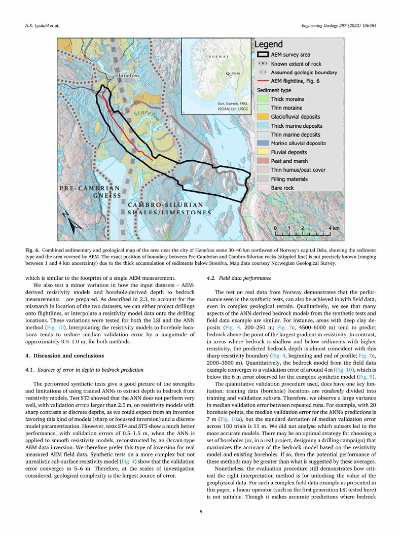
In this section we present the interpretation of a real field dataset using the described artificial neuronal network. The field data were acquired by the Norwegian Geotechnical Institute (NGI) in 2016 near the city of Hønefoss some 30–40 km northwest of Norway's capital Oslo (Fig. 6). The helicopter geo-scanning survey and drilling campaigns were acquired for the design of a new highway and high-speed railway connecting Oslo with these regions and more distant cities such as Bergen. A total of 431 geotechnical drillings were accessible, indicating the sediment stratification and depth to bedrock at the drilling location (NGU, 2019). The drillings were used for training and validation of the ANN based bedrock interface detection. AEM data were acquired with a SkyTEM 304 system (Sørensen and Auken, 2004) and covered 70 km2

with a 100 m line spacing, within one week in June 2016. The data was processed manually removing potential noise and coupling effects and inverted, as described in the methods Section 2.1, resulting in a smooth quasi-3D resistivity model.

3.2.1. Geological setting The survey covers post-glacial geomorphology typical for the low-

lands of southeastern Norway (Fig. 6). In some areas, one finds exposed bedrock, and in others, valleys are filled with massive glaciofluvial de-posits up to tens of meters in thickness. Coarse-grained alluvial deposits (medium resistivity, 100–500 Ωm) are found alongside fine-grained marine clay deposits (which are now above sea level due to post-glacial heave). These marine clay deposits are in parts saline (very low resistivity, <10 Ωm) and in other parts have had their salt content leached and are potentially hazardous quick clay (low resistivity, 10–100 Ωm). Some moraine material is also found and is typically highly compacted and is either coarse-grained or has a mix of grain sizes (very high resistivity, >500 Ωm). The indicated resistivity ranges (after Palacky, 1987) are approximate and may overlap as the formation re-sistivity depends on multiple factors such as porosity, fluid saturation and properties, formation factors and other parameters (Keller, 1987), which make a manual analysis of the resistivity models difficult, even for a trained interpreter.

Northwest of the river Storelva (Fig. 6), the bedrock consists of Precambrian meta-sediments and local intrusions that are very resistive (>4000 Ωm). In the southeast, one finds instead Cambro-Silurian, limestone-rich shales and limestones with medium-high resistivity (200–1000 Ωm). Within this volume of Cambro-Ordovician rocks, near the river Storelva, there are more frequent occurrences of sulphide-rich black shales (as low as 1 Ωm).

3.2.2. Bedrock detection: Qualitative comparison of methods In this subsection, we compare initial manual interpretations and

new automated methods for estimating the depth to bedrock depth. At the time of the airborne survey only a limited number of geotechnical drillings were available.

First, a simple manual triangulation and interpretation between the geotechnical drilling locations is used to find the lateral depth to bedrock distribution, mimicking current state of practice in geotechnical projects that often rely only on drilling and lack geo-scanning data

Table 1 Summary of the tests using synthetic models.

Test name

Features Validation error at convergence (m)

Loss at convergence (m)

Figure

Two layers

Two geological areas

Bedrock fixed to resistivity boundary

Smooth Inversion

Complex geology

ST1 x x 0.3 – 3a ST2 x x x 1 1 3b ST3 x x 3 5 3c ST4 x x 1 4 3d ST5 x x x 1 4 3e

A.K. Lysdahl et al.

Engineering Geology 297 (2022) 106484

6

(Fig. 7a). We also apply a linear statistical Localized Smart Interpreta-tion (LSI) algorithm (Gulbrandsen et al., 2015) to the resistivity models and validated with a subset of the available boreholes (Fig. 7b). Finally, we use a trained ANN to interpret the depth to bedrock utilizing both local information from geotechnical drillings and a AEM based re-sistivity model that covers the entire survey area (Fig. 7c).

To illustrate the differences between the manual, linear and neural network method, we examine one profile that spans over the highly varying geology (Fig. 7). The profile consists of an area with weak contrast between sediments and bedrock the first 2000 m, a central part with shallow bedrock, a transition from conductive to resistive gravel- type sediments (3500 m–4300 m) and finally a deep paleochannel fil-led with both resistive and conductive sediments.

The deep paleochannel between (4300 and 6500 m) is the most difficult location to interpret depth to bedrock. Very conductive sedi-ments (below 4 Ωm, dark blue) lie above a less conductive unit (~10 Ωm, greenish blue), the boundary between these is smooth and indis-tinct. It is known that there is a transition from resistive, pre-Cambrian magmatic bedrock to more conductive Cambro-Silurian shales towards the south, but the position of this transition is uncertain (Fig. 6). It could be that the underlaying bedrock in the paleochannel is more conductive shale which has a weak resistivity contrast with the overlying conduc-tive sediments. However, based on the synthetic modelling and inver-sion study for a complex geological setting (Fig. 2), it is reasonable to assume that the thick conductive sediments are limiting the inversion's ability to accurately reconstruct the absolute resistivity value for the

Fig. 3. Synthetic algorithm training and assessment models along with corresponding validation error and loss curves: a) and b) two-layer models with training points at discrete layer interfaces; c) two-layer models with points at discrete depth values; d) realistic smooth models with homogeneous contrast and e) smooth models with changing contrast.

A.K. Lysdahl et al.

Engineering Geology 297 (2022) 106484

7

underlaying rock which may instead be a resistive, hard magmatic rock unit.

We observe that the linear LSI-algorithm seeks to find a relation between the AEM-derived resistivity models, the topography and the known depth points at drilled locations, but the LSI algorithm is unable to match every known depth point with satisfactory accuracy while keeping a somewhat smooth, consistent surface (Fig. 7b). The linear LSI prediction results are reasonable at homogeneous parts of the survey (e. g., from 2000 to 3500 m in Fig. 7b) but inconsistent when the geological setting and thus the resistivity contrast changes as under the gravel plateau (3500 to 4300 m) or in the deep paleochannel (4300 to 6500 m). It also generally misses the correct bedrock height between 0 and 2000 m, as indicated by the newer drillings from 2019 and 2020, that became available after the data analysis.

In contrast, the ANN based bedrock interpretation algorithm can handle the increased complexity from 2000 m to 6500 m well (Fig. 7c). That is because we used resistivity depth-profiles and depth to bedrock measurements at different drilling locations to teach the ANN these varying resistivity trends, describing the sediment-bedrock interface. Nevertheless, between 0 and 2000 m (Fig. 7c) the ANN algorithm per-forms poorly, due to the lack of training data and significantly different resistivity depth-trends than at locations where we have training data. The human interpreter, however, can interpret the depth to bedrock using the existing contrast in the resistivity model (Fig. 7a).

The ANN algorithm only successfully extrapolates beyond areas covered by geotechnical datasets when there are representative con-trasts, similar to locations with training data, in the resistivity model. For instance, in the section shown in Fig. 8, which is 500 m SW of the main railway alignment where most boreholes are located, the ANN is able to make reasonable depth to bedrock predictions at locations i, ii, iii, and iv. This is because geological conditions and resistivity contrast between the bedrock and overlying marine clays are similar to the lo-cations with training data along the railway alignment. However, if there is no contrast between bedrock and coarser sediments like moraine, glaciofluvial sediments, and beach sands (locations v and vi), the lack of nearby training data leads the ANN to a more uncertain bedrock prediction.

We also compare bedrock models resulting from linear triangulation, LSI, and ANN in map view (Fig. 9). The magnitude of the difference between drilled, ground-truth depth and predicted depth is also plotted alongside these models. Comparing the linear triangulation (Fig. 9a) to the other two methods LSI (Fig. 9b) and ANN (Fig. 9c), the advantage of integrating AEM with borehole data becomes obvious; one obtains a much more nuanced and accurate view of subsurface structures, and the final model covers a larger areal extent. However, in areas where dril-lings are closely spaced, such as the zoomed view shown in the inset map, the simple triangulation performs well. Comparing the LSI and ANN models, it is evident that ANN is much more capable of predicting large variations in bedrock depth, which is most obvious at the deep channels in the zoomed area (Fig. 9a, b, & c).

3.2.3. Bedrock detection: Quantitative performance evaluation In order to quantitatively assess the difference of performance be-

tween the bedrock depth interpretation methods, we tested several randomized sub-sets of training points and validated the results against all remaining drillings. A new ANN was trained and evaluated for each set of training points, which varied in size from 10 to 200 random borehole locations.

Validation errors varied significantly between the three methods and decreased with the number of training points (Fig. 10). The ANN algo-rithm converged to a median magnitude of around 4 m (Fig. 10a) cor-responding to approximately 30% of bedrock depth (Fig. 10b). The LSI algorithm notably fails to achieve a low validation error, even when including large numbers of borehole data. The ANN method offers a significant improvement compared to a simple triangulation when few boreholes are available. However, as borehole density increases, the advantage of AEM data decreases. At around 120 to 140 training points, simple triangulation and the ANN method give similar validation errors. This corresponds to an average inter-borehole distance of 150–200 m,

Fig. 4. ANN based bedrock interpretation of a resistivity model from inversion of synthetic AEM data computed from the resistivity model in Fig. 2a.

0

2

4

6

8

10

12

0 10 20

Med

ian

abso

lute

valid

a�on

erro

r(m

)

Number of training points

Fig. 5. Median magnitude of the validation error of bedrock depth predictions as a function of number of used training points for the resistivity model in Fig. 4.

A.K. Lysdahl et al.

Engineering Geology 297 (2022) 106484

8

which is similar to the footprint of a single AEM measurement. We also test a minor variation in how the input datasets – AEM-

derived resistivity models and borehole-derived depth to bedrock measurements – are prepared. As described in 2.3, to account for the mismatch in location of the two datasets, we can either project drillings onto flightlines, or interpolate a resistivity model data onto the drilling locations. These variations were tested for both the LSI and the ANN method (Fig. 10). Interpolating the resistivity models to borehole loca-tions tends to reduce median validation error by a magnitude of approximately 0.5–1.0 m, for both methods.

4. Discussion and conclusions

4.1. Sources of error in depth to bedrock prediction

The performed synthetic tests give a good picture of the strengths and limitations of using trained ANNs to extract depth to bedrock from resistivity models. Test ST3 showed that the ANN does not perform very well, with validation errors larger than 2.5 m, on resistivity models with sharp contrasts at discrete depths, as we could expect from an inversion favoring this kind of models (sharp or focussed inversion) and a discrete model parametrization. However, tests ST4 and ST5 show a much better performance, with validation errors of 0.5–1.5 m, when the ANN is applied to smooth resistivity models, reconstructed by an Occam-type AEM data inversion. We therefore prefer this type of inversion for real measured AEM field data. Synthetic tests on a more complex but not unrealistic sub-surface resistivity model (Fig. 4) show that the validation error converges to 5–6 m. Therefore, at the scales of investigation considered, geological complexity is the largest source of error.

4.2. Field data performance

The test on real data from Norway demonstrates that the perfor-mance seen in the synthetic tests, can also be achieved in with field data, even in complex geological terrain. Qualitatively, we see that many aspects of the ANN-derived bedrock models from the synthetic tests and field data example are similar. For instance, areas with deep clay de-posits (Fig. 4, 200–250 m; Fig. 7c, 4500–6000 m) tend to predict bedrock above the point of the largest gradient in resistivity. In contrast, in areas where bedrock is shallow and below sediments with higher resistivity, the predicted bedrock depth is almost coincident with this sharp resistivity boundary (Fig. 4, beginning and end of profile; Fig. 7c, 2000–3500 m). Quantitatively, the bedrock model from the field data example converges to a validation error of around 4 m (Fig. 10), which is below the 6 m error observed for the complex synthetic model (Fig. 5).

The quantitative validation procedure used, does have one key lim-itation: training data (borehole) locations are randomly divided into training and validation subsets. Therefore, we observe a large variance in median validation error between repeated runs. For example, with 20 borehole points, the median validation error for the ANN's predictions is 7 m (Fig. 10a), but the standard deviation of median validation error across 100 trials is 11 m. We did not analyse which subsets led to the more accurate models. There may be an optimal strategy for choosing a set of boreholes (or, in a real project, designing a drilling campaign) that maximizes the accuracy of the bedrock model based on the resistivity model and existing boreholes. If so, then the potential performance of these methods may be greater than what is suggested by these averages.

Nonetheless, the evaluation procedure still demonstrates how crit-ical the right interpretation method is for unlocking the value of the geophysical data. For such a complex field data example as presented in this paper, a linear operator (such as the first generation LSI tested here) is not suitable. Though it makes accurate predictions where bedrock

Fig. 6. Combined sedimentary and geological map of the area near the city of Hønefoss some 30–40 km northwest of Norway's capital Oslo, showing the sediment type and the area covered by AEM. The exact position of boundary between Pre-Cambrian and Cambro-Silurian rocks (stippled line) is not precisely known (ranging between 1 and 4 km uncertainty) due to the thick accumulation of sediments below Storelva. Map data courtesy Norwegian Geological Survey.

A.K. Lysdahl et al.

Engineering Geology 297 (2022) 106484

9

depth and bedrock resistivity are mostly uniform (Fig. 7b, 2000–4000 m), it fails to adjust predictions in contrasting geological environments like where the riverbank sediments overlay marine sediments (3800–4500 m) and sediment is very thick and conductive (4500–6000 m). Manual interpretation can overcome this pitfall since a trained expert can integrate geological knowledge, experience with geophysical mapping, knowledge about inversion, measurement uncertainty, etc. However, manual interpretations are subjective and slow, meaning that ground models cannot be as easily updated once new drilling informa-tion becomes available over the duration of a site investigation project. It should be noted that the LSI method tested here has since been updated to include a non-linear operator (Gulbrandsen et al., 2017), but this version was not available at the time of analysis.

The results also show that the way data are prepared does have an effect, regardless of the bedrock prediction method. We found that projecting drilling data onto nearby flightlines leads to less accurate bedrock predictions than interpolating resistivity models onto drilling locations (Fig. 10). The AEM-derived resistivity models are already smoothened, and interpolation to the drilling locations within ~100 m of an AEM measurement point does not seem to introduce significant loss in resolution. Additional data preparation, or integration of other spatial data like geological maps, may provide further, incremental improvements to the automated bedrock depth extraction from AEM data.

Fig. 7. A cross-section of through the 3D resistivity model of the area south of Hønefoss (location indicated by the red line in Fig. 6). The three panels show various generations of bedrock interpretation approaches (black lines) starting with a) manual picking and triangulation, b) a linear statistical approach, and c) the ANN solution presented in this study. Red bars indicate bedrock depth confirmed by geotechnical drillings that were used as training data for LSI and ANN, whereas and grey bars are newer drillings that were not used for either. Only boreholes within 50 m of the plane of the cross-section are shown; boreholes between 20 and 50 m of the plane are shown with 60% transparency. (For interpretation of the references to colour in this figure legend, the reader is referred to the web version of this article.)

A.K. Lysdahl et al.

Engineering Geology 297 (2022) 106484

10

4.3. Limitations of manual resistivity model interpretation

The field data example and the complex synthetic model (Fig. 2) highlight scenarios where the resistivity model is less reliable and where it may not always be possible to interpret a bedrock interface directly from the resistivity model. This can occur where there is a weak re-sistivity contrast between sediment and bedrock. That applies especially for high-resistivity materials because the inductive EM method is less sensitive to changes in resistivity at the high range (>800 Ωm) versus the low range (<100 Ωm). We see two instances of this in the complex synthetic model (Fig. 2), where thin layers of moraine (0–80 m) and sand (375–450 m) lie atop gneiss. In the inverted model, there is little to no increase in resistivity visible at those locations. We see similar in-stances in the field data example where there is no obvious resistivity contrast between bedrock and medium- or high-resistivity sediments like sand, gravel, and moraine (Fig. 8, locations v and vi).

In these cases, the ANN usually provides a reasonable prediction if provided nearby training data. Where there is a lack of contrast, the spatial attributes (i.e., x-, y-, and z-coordinates) have a greater weighting on the predicted depth to bedrock than the resistivity profile. In essence, the predicted bedrock surface reverts to an interpolation between boreholes guided by terrain and fails when making predictions outside the area sampled by the training data. This explains why the ANN suc-ceeds in making reasonable predictions for the complex synthetic example at between 400 and 500 m along in Fig. 4 thanks to the bore-hole at 440 m, but fails in the field data example at locations v and vi in Fig. 8. This finding is similar to Kovacevic et al.'s (2009) conclusion that spatial attributes have little useful information for making predictions outside the domain of training data. Ultimately, the ANN uses the re-sistivity model to improve predictions in most locations except for lo-cations where there is a lack of resistivity contrast outside the spatial domain of the training data.

4.4. Limitations of ANN based resistivity model interpretation

The results do show that ANNs have some weaknesses. To an expe-rienced geophysicist, the shallow, conductive lens at 4300 m in Fig. 7c, is obviously an artefact, or at the very least, a structure that is unrelated to the bedrock. However, for the ANN, which only looks at a single vertical strip of the resistivity model, this is not obvious, and the depth to bedrock predictions are therefore highly erratic here. A convoluted

neural network, which would take into account several side-by-side strips of a model, may put less weight on this feature. In the mean-time, manual quality control of ANN outputs is warranted.

Similarly, ANNs fail to make accurate predictions at locations where the resistivity models are not represented in the training dataset. This is the case for the segment between 0 and 2000 m in the field data example (Fig. 7). While there is a resistivity contrast between sediment and bedrock that the human interpreter was able to detect (Fig. 7a), the ANN lacked training data in this particular geological setting and hence failed to make reasonable predictions (Fig. 7c). Hence, to employ this method effectively, one must ensure that the training datasets contains a representative sample of all the geological settings represented in a geophysical dataset. If this is not possible, additional manual training points provided by an experienced geophysicist are needed to guide the ANN through areas with no actual ground truth.

4.5. Implications for engineering workflows

The field case data also demonstrated that the presented combina-tion of AEM data and geotechnical data using machine learning has potential to provide great value in reducing the risk caused by unknown or poorly understood ground conditions in engineering projects. For a given number of boreholes, the uncertainty in depth to bedrock can be reduced by as much as half, going from a bedrock model based on interpolated sparse boreholes only to a model based on combined interpretation of AEM data and boreholes using ANNs (Fig. 8). Similarly, to get a bedrock model with 40% error, one needs 90 boreholes when using triangulation but only approximately 35 when using AEM and an ANN, a reduction by a factor of 2.5 or a decrease of 60%. This reduction factor is plotted as a function of target bedrock model accuracy in Fig. 11.

This supports the findings of Pfaffhuber et al. (2019), where two cases with simpler geology were studied. Our results also show that the added benefit of using AEM data diminishes once around 140–160 boreholes are used. This corresponds to a density of 10–20 boreholes per km2 or average spacing of 200–300 m between boreholes. This average spacing is slightly more than the measurement footprint of the AEM measurements, which is about 150 m in diameter for the instrument used. Hence, AEM as a ground investigation tool add most value in the early phase of a development project when only a few boreholes are available.

Fig. 8. Oblique view facing NE of the 3D model showing a vertical resistivity section in the south of the study area approximately 500 m SW of the planned railway alignment. Also shown are borehole locations (black cylinders) and sediment cover (as mapped by the Norwegian Geological Survey) draped on a terrain model. At locations where there is a clear resistivity contrast between bedrock and lacustrine (i) or marine clays (ii, iii, iv), the predictions from the ANN (white surface) track closely with this geophysical contrast. At other locations where there are beach sediments, glaciofluvial deposits, or weathered rock (v, vi), neither a clear resistivity contrast nor training boreholes are present to guide the ANN predictions. Vertical exaggeration of the scene is 3×.

A.K. Lysdahl et al.

Engineering Geology 297 (2022) 106484

11

Fig. 9. Integrated bedrock depth model at Ringerike area showing models derived from a) Triangulation or b) LSI projection and c) ANN interpolation. Surface topography are water features shown in the background.

A.K. Lysdahl et al.

Engineering Geology 297 (2022) 106484

12

In Norway, projects with a similar size to our field data example (Section 3.2) may spend millions or tens of millions of USD on geotechnical drillings and sampling over the course of months to years, whereas airborne investigations last days to weeks and cost some hun-dreds of thousands of USD. Hence, when employed early enough, airborne geo-scanning has potential to provide substantial savings in the direct costs of site investigations. The analysis in this article does not consider other indirect cost savings that may arise from optimizing ground investigation and drilling plans, refining design alternatives, or shortening project timelines, meaning that overall cost-savings may be greater than the pure cost savings due to reduced drilling.

4.6. Summary and future directions

In closing, ground models derived from integration of geophysical and geotechnical data via artificial neuronal networks are an enabler for introducing airborne electromagnetic data into engineering project workflows. Our results show that these ground models have clear value for early stages of a development project where limited number of drillings are available. The suggested integration approach reduces

uncertainty and can guide engineers in designing the more cost-effective site investigation programs. The method we present aligns well with current industry trends. The use of 3D models and integrated data management systems like Building Information Modelling (BIM) are widespread in the construction sector (Mehrbod et al., 2019; Tezel et al., 2019). However, the usage of such data management systems in geological and geotechnical engineering is still limited but the obvious benefits have made it an active area of discussion (Svensson, 2019). Being able to acquire a high-resolution bedrock model with good areal coverage early in a project phase with airborne geo-scanning will make such 3D workflows more attractive. Moreover, unlike the manual interpretation of the past, having an automated method to quickly up-date a bedrock model using new borehole information as it becomes available, will maintain the utility of the AEM data throughout a pro-ject's lifetime.

Declaration of Competing Interest

EMerald Geomodelling is a private company and has a potential commercial interest in the technology described in this article. Authors

3456789

10111213141516

0 20 40 60 80 100 120 140 160 180

Med

ian

abso

lute

val

idat

ion

erro

r (m

)

Number of boreholes

a) Validation error, absolute deviation

Triangulation

LSI projected

LSI interpolated

ANN projected

ANN Interpolated

0.2

0.3

0.4

0.5

0.6

0.7

0.8

0.9

1

0 20 40 60 80 100 120 140 160 180

Med

ian

rela

tive

valid

atio

n er

ror (

%)

Number of boreholes

b) Validation error, relative to depth

Triangulation

LSI projected

LSI interpolated

ANN projected

ANN Interpolated

100

90

80

70

60

50

40

30

20

Fig. 10. Accuracy metrics for the field site near Hønefoss comparing various methods: a) median magnitude of validation errors at borehole locations b) median magnitude of validation errors normalized by the borehole depth.

A.K. Lysdahl et al.

Engineering Geology 297 (2022) 106484

13

Christensen, Pfaffhuber, Skurdal, and Panzner are current employees of the company, and Pfaffhuber, Andresen, and Skurdal are members of the board of directors.

Acknowledgements

Parts of the presented work were developed under Research Council of Norway (RCN) FORNY grant “Airborne Geo-Intelligence” (project number 282147). We thank the Norwegian public rail- and road au-thorities (Bane NOR and Statens Vegvesen) for permission to publish the field data results. The presented findings are the cumulative results of a joint effort over many years to establish helicopter geo-scanning within NGI; a big thank you goes to all the colleagues that have been involved.

References

Anschütz, H., Christensen, C., Pfaffhuber, A.A., 2014. Quantitative depth to bedrock extraction from AEM data. In: Extended Abstract: 20th European Meeting of Environmental and Engineering Geophysics - EAGE’s Near Surface, Athens, Greece.

Anschütz, H., Bazin, S., Kåsin, K., Pfaffhuber, A.A., Smaavik, T.F., 2017a. Airborne mapping of sensitive clay – stretching the limits of AEM resolution and accuracy. Near Surf. Geophys. 15, 467–474.

Anschütz, H., Voge, M., Lysdahl, A.K., Bazin, S., Sauvin, G., Pfaffhuber, A., Berggren, A.- L., 2017b. From manual to automatic AEM bedrock mapping. J. Environ. Eng. Geophys. 22 (1), 35–49.

Auken, E., Christiansen, Av, 2004. Layered and laterally constrained 2D inversion of resistivity data. Geophysics 69 (3), 752–761. https://doi.org/10.1190/1.1759461.

Auken, E., Viezzoli, A., Christensen, A., 2009. A single software for processing, inversion, and presentation of AEM data of different systems. In: The Aarhus Workbench, ASEG Extended Abstracts, Vol. 2009, 1, pp. 1–5.

Auken, E., Christiansen, A.V., Kirkegaard, C., Fiandaca, G., Schamper, C., Behroozmand, A., Binley, A., Nielsen, E., Effersø, F., Christensen, N.B., 2015. An overview of a highly versatile forward and stable inverse algorithm for airborne,

ground-based and borehole electromagnetic and electric data. Explorat. Geophys. 46 (3), 223–235. Taylor & Francis.

Bazin, S., Pfaffhuber, A.A., 2013. Mapping of quick clay by electrical resistivity tomography under structural constraint. J. Appl. Geophys. 98, 280–287. https://doi. org/10.1016/j.jappgeo.2013.09.002.

Beckers, F., Chiara, N., Flesch, A., Maly, J., Silva, E., Stegemann, U., 2013. A risk- management approach to a successful infrastructure project. In: McKinsey Working Papers on Risk 52. McKinsey & Company.

Byrd, R.H., Lu, P., Nocedal, J.A., 1995. Limited memory algorithm for bound constrained optimization. SIAM J. Sci. Stat. Comput. 16 (5), 1190–1208.

Chambers, J.E., Wilkinson, P.B., Penn, S., Meldrum, P.I., Kuras, O., Loke, M.H., Gunn, D. A., 2013. River terrace sand and gravel deposit reserve estimation using three- dimensional electrical resistivity tomography for bedrock surface detection. J. Appl. Geophys. 93, 25–32. https://doi.org/10.1016/j.jappgeo.2013.03.002.

Chambers, J.E., Wilkinson, P.B., Uhlemann, S., Sorensen, J.P.R., Roberts, C., Newell, A. J., et al., 2014. Derivation of lowland riparian wetland deposit architecture using geophysical image analysis and interface detection. Water Resour. Res. 50, 5886–5905. https://doi.org/10.1002/2014WR015643.

Chouteau, M., Boudour, Z., Parent, M., Marcotte, D., 2013. Estimation of overburden thickness using airborne time-domain EM data and a few drill hole data. In: 13th SAGA Biennial Conference and Exhibition, Mpumalanga, South Africa. South African Geophysical Association.

Christensen, C., Pfaffhuber, A.A., Anschütz, H., Smaavik, T.F., 2015. Combining airborne electromagnetic and geotechnical data for automated depth to bedrock tracking. J. Appl. Geophys. 119, 178–191.

Christensen, C.W., Skurdal, G.H., Pfaffhuber, A.A., Rønning, S., Lindgard, A., Sellgren, K. C., 2020. Airborne geoscanning and efficient geotechnical ground investigation workflows: a road-building case study from Central Norway. In: 18th Nordic Geotechnical Meeting, 25–27 May 2020, Helsinki, Finland (Delayed to January 2021 due to COVID-19).

Christiansen, A.V., Foged, N., Auken, E., 2014. Inverting for lithology using resistivity models and boreholes. In: 20th European Meeting of Environmental and Engineering Geophysics - EAGE’s Near Surface, Athens, Greece.

Cracknell, M.J., Reading, A.M., 2014. Geological mapping using remote sensing data: a comparison of five machine learning algorithms, their response to variations in the spatial distribution of training data and the use of explicit spatial information. Comput. Geosci. 63, 22–33.

Dewar, N., Gottschalk, I., Knight, R., Smith, R., Silvestri, S., Viezzoli, A., et al., 2018. Estimation of peat thickness in Indonesia from airborne time domain EM data

Fig. 11. A comparison of the triangulation (boreholes only) and the NN interpolated (boreholes and AEM) error curves in Fig. 10. The curves above show that depending on the target accuracy of the output bedrock model, the approach that uses ANN and AEM requires 2 to 3.5 times fewer boreholes than the borehole only approach.

A.K. Lysdahl et al.

Engineering Geology 297 (2022) 106484

14

through machine learning. In: 7th International Workshop on Airborne Electromagnetics. Extended Abstracts.

Flyvbjerg, B., Holm, M.S., Buhl, S., 2002. Underestimating costs in public works projects: error or lie? J. Am. Plan. Assoc. 68 (3), 279–295.

Gulbrandsen, M.L., Bach, T., Cordua, K.S., Hansen, T.M., 2015. Localized Smart Interpretation – a data driven semiautomatic geological modelling method. In: Expanded Abstracts: ASEG-PESA, 24th International Geophysical Conference and Exhibition, Perth, Australia.

Gulbrandsen, M.L., Cordua, K.S., Bach, T., Hansen, T.M., 2017. Smart interpretation – automatic geological interpretations based on supervised statistical models. Comput. Geosci. 21, 427–440. https://doi.org/10.1007/s10596-017-9621-8.

Gunnink, J.L., Siemon, B., 2015. Applying airborne electromagnetics in 3D stochastic geohydrological modelling for determining groundwater protection. Near Surf. Geophys. 13 (2), 46–60.

Gunnink, J.L., Bosch, J.H.A., Siemon, B., Roth, B., Auken, E., 2012. Combining ground- based and airborne EM through Artificial Neural Networks for modelling glacial till under saline groundwater conditions. Hydrol. Earth Syst. Sci. 16, 2031–3074. https://doi.org/10.5194/hess-16-3061-2012.

He, X., Koch, J., Sonnenborg, T.O., Jørgensen, F., Schamper, C., Refsgaard, J.C., 2014. Transition probability-based stochastic geological modeling using airborne geophysical data and borehole data. Water Resour. Res. 50, 3147–3169. https://doi. org/10.1002/2013WR014593.

Keller, G.V., 1987. Rock and mineral properties. In: Nabighian, M.N. (Ed.), Electromagnetic Methods in Applied Geophysics Theory, vol. 1. Society of Exploration Geophysicists, Tulsa, OK, pp. 53–129.

Korus, J.T., Cameron, K., Hobza, C.M., Jensen, N.-P., Rico, D., Munoz-Arriola, F., 2018. Integrating AEM and borehole data for regional hydrogeologic synthesis: tools and examples from Nebraska, USA. In: 7th International Workshop on Airborne Electromagnetics. Extended Abstracts.

Kovacevic, M., Bajat, B., Trivic, B., Pavlovic, R., 2009. Geological units classification of multispectral images by using Support Vector Machines. In: Proceedings of the International Conference on Intelligent Networking and Collaborative Systems. IEEE, pp. 267–272.

Lysdahl, A., Pfaffhuber, A.A., Anschütz, H., Kåsin, K., Bazin, S., 2017. Helicopter electromagnetic scanning as a first step in regional quick clay mapping. In: Thakur, V., et al. (Eds.), Landslides in Sensitive Clays, Advances in Natural and Technological Hazards Research, 46. https://doi.org/10.1007/978-3-319-56487-6_ 39.

Lysdahl, A.K., Andresen, L., Voge, M., 2018. Construction of bedrock topography from airborne-EM data by artificial neural network. In: 9th European Conference on Numerical Methods in Geotechnical Engineering (NMGE 2018), 25–27 June, Porto, Portugal. Extended Abstract.

Mehrbod, S., Staub-French, S., Tory, M., 2019. BIM-based building design coordination: processes, bottlenecks, and considerations. Can. J. Civil Eng. https://doi.org/ 10.1139/cjce-2018-0287 published online 02 May 2019.

NGU, 2019. Geotechnical Methods, Norwegian Geological Survey – NGU. https://www. ngu.no/en/topic/geotechnical-methods.

Okazaki, K., Mogi, T., Utsugi, M., Ito, Y., Kunishima, H., Yamazaki, T., Takahashi, Y., Hashimoto, T., Ymamaya, Y., Ito, H., et al., 2011. Airborne electromagnetic and

magnetic surveys for long tunnel construction design. Phys. Chem. Earth 36, 1237–1246. https://doi.org/10.1016/j.pce.2011.05.008.

Palacky, G.J., 1987. Resistivity characteristics of geologic targets. In: Nabighian, M.N. (Ed.), Electromagnetic Methods in Applied Geophysics Theory, vol. 1. Society of Exploration Geophysicists, Tulsa, OK, pp. 53–129.

Palacky, G.J., West, G.F., 1991. Airborne electromagnetic methods. In: Nabighian, M.N. (Ed.), Electromagnetic Methods in Applied Geophysics, Vol 2.

Pedregosa, F., Varoquaux, G., Gramfort, A., Michel, V., Thirion, B., Grisel, O., Blondel, M., Prettenhofer, P., Weiss, R., Dubourg, V., Vanderplas, J., Passos, A., Cournapeau, D., Brucher, M., Perrot, M., Duchesnay, E., 2011. Scikit-learn: machine learning in Python. J. Mach. Learn. Res. 12, 2825–2830.

Pfaffhuber, A.A., Anschütz, H., Ørbech, T., Bazin, S., Lysdahl, A.O.K., Voge, M., Sauvin, G., Waarum, I.K., Smebye, H.C., Kåsin, K., Grøneng, G., Berggren, A.-L., Pedersen, J.B., Foged, N., 2016. Regional geotechnical railway corridor mapping using airborne electromagnetics. In: 5th International Conference on Geotechnical and Geophysical Site Characterisation, Gold Coast, Australia.

Pfaffhuber, A.A., Lysdahl, A.O.K., Sørmo, E., Bazin, S., Skurdal, G.H., Thomassen, T., Anschütz, H., Scheibz, J., 2017a. Delineating hazardous material without touching - AEM mapping of Norwegian alum shale. First Break 35, 35–39.

Pfaffhuber, A.A., Persson, L., Lysdahl, A.O.K., Kåsin, K., Anschütz, H., Bastani, M., Bazin, S., Lofroth, H., 2017b. Integrated scanning for quick clay with AEM and ground-based investigations. First Break 35, 73–79.

Pfaffhuber, A.A., Lysdahl, A.O., Christensen, C., Voge, M., Kjennbakken, H., Mykland, J., 2019. Large scale, efficient geotechnical soil investigations applying machine learning on airborne geophysical models. In: Proceedings of the XVII European Conference on Soil Mechanics and Geotechnical Engineering, Reykjavik, Iceland.

Pryet, A., Ramm, J., Chiles, J.-P., Auken, E., Deffontaines, B., Violette, S., 2011. 3D resistivity gridding of large AEM datasets: a step toward enhanced geological interpretation. J. Appl. Geophys. 75, 277–283. https://doi.org/10.1016/j. jappgeo.2011.07.006.

Sengpiel, K.-P., Siemon, B., 1998. Examples of 1-D inversion of multifrequency HEM data from 3-D resistivity distributions. Explor. Geophys. 29 (1–2), 133–141. https://doi. org/10.1071/EG998133.

Shahin, M.A., Jaksa, M.B., Maier, H.R., 2001. Artificial neural network applications in geotechnical engineering. Austr. Geotech. J. 36 (1), 49–62.

Sørensen, K.I., Auken, E., 2004. SkyTEM – a new high-resolution helicopter transient electromagnetic system. Explor. Geophys. 35, 191–199.

Svensson, M., 2019. BIM in near surface geosciences. In: 81st EAGE Conference & Exhibition 2019, London, UK.

Tezel, A., Taggart, M., Koskela, L., Tzortzopoulos, H.J., Kelly, M., 2019. Lean construction and BIM in small and medium-sized enterprises (SMEs) in construction: a systematic literature review. Can. J. Civil Eng. https://doi.org/10.1139/cjce-2018- 0408 published online 27 March 2019.

Viezzoli, A., Christiansen, A.V., Auken, E., Sørensen, K., 2008. Quasi-3D modeling of airborne TEM data by spatially constrained inversion. Geophysics 73 (1), F105–F113. https://doi.org/10.1190/1.2895521.

Zhou, Y., Wu, X., 1994. Use of neural networks in the analysis and interpretation of site investigation data. Comput. Geotech. 16, 105–122.

A.K. Lysdahl et al.