Emergence of Inertial Gyres in a Two-Layer Quasigeostrophic Ocean Model
24
MARCH 1998 461 O ¨ ZGO ¨ KMEN AND CHASSIGNET q 1998 American Meteorological Society Emergence of Inertial Gyres in a Two-Layer Quasigeostrophic Ocean Model TAMAY M. O ¨ ZGO ¨ KMEN AND ERIC P. CHASSIGNET RSMAS/MPO, University of Miami, Miami, Florida (Manuscript received 15 October 1996, in final form 23 June 1997) ABSTRACT The emergence of Fofonoff-like flows over a wide range of dissipative parameter regimes is explored in a wind-driven two-layer quasigeostrophic model. Two regimes are found in which Fofonoff-like circulations emerge as a direct consequence of the baroclinic nature of the system, since the wind forcing used in these experiments has been shown to inhibit the formation of Fofonoff flows in the barotropic case. The first regime is one in which the magnitudes of the frictional coefficients (viscosity and bottom dissipation) are extremely small. The experiments clearly illustrate the transition of the numerical solution from a conventional wind-driven circulation to an inertial Fofonoff-like regime. The latter circulation first appears in the lower layer and then spreads throughout the water column via barotropization. The second regime, surprisingly, is obtained with very high bottom friction. This result indicates that entropy can be maximized independently in each layer, depending on the distribution of forcing and dissipation. This sheds a new perspective on the common assumption that forcing and dissipation are disruptive effects that prevent the system from displaying a Fofonoff state. 1. Introduction The investigation of nonlinear processes is of primary importance in developing our understanding of the large-scale general ocean circulation. It is generally ac- cepted that the nonlinear inertial terms are important in regions such as western boundary currents and midlat- itude jets (e.g., Harrison and Holland 1981), and that these terms are responsible for the formation of recir- culating gyres, which enhance the transport of important current systems such as the Gulf Stream and the Ku- roshio many times over the corresponding linear Sver- drup wind-driven transport. The effect of the nonlinear inertial terms is quite different from that of other pro- cesses in the ocean. Unlike wind forcing, heat exchange with the atmosphere, or frictional effects, inertial pro- cesses do not have a net contribution to the energy bud- get. Their major role appears to be in the reorganization of the flow generated by other mechanisms. It is there- fore important to explore and understand the flow char- acteristics to which the inertial terms tend to drive the system. Inertial modes were first sought by Fofonoff (1954), who considered steady solutions of a frictionless, ho- mogeneous fluid in a rectangular ocean basin of constant depth on a beta plane. His solution is characterized by a linear relationship between potential vorticity and Corresponding author address: Dr. Tamay M. O ¨ zgo ¨kmen, RSMAS/MPO,University of Miami, 4600 Rickenbacker Causeway, Miami, FL 33149-1098. E-mail: [email protected] streamfunction and possesses intense inertial boundary layers along the western, eastern, and zonal boundaries of the domain, accompanied by a uniform zonal flow elsewhere. When the total vorticity of the system is zero, the solution consists of two antisymmetric gyres, an anticyclonic gyre in the northern basin and a cyclonic gyre in the southern basin (Fig. 1a). When the total vorticity is positive (negative), the cyclonic (anticy- clonic) gyre then prevails. The significance of Fofon- off’s (1954) solution was not clear until Veronis (1966) pointed to a visual resemblance between his own nu- merical simulations of a barotropic wind-driven ocean consisting of a single gyre and Fofonoff’s solution when nonlinear effects dominated. Theoretically, Salmon et al. (1976, hereafter SHH), using equilibrium statistical mechanics, demonstrated that Fofonoff’s solution corresponds to the mean flow of a stable equilibrium state in which the entropy of the system is maximized. Independently, Bretherton and Haidvogel (1976) showed that Fofonoff’s solution also resulted from the minimum enstrophy states of the sys- tem. That the maximum entropy equilibrium actually coincides with the minimum enstrophy state in the limit of infinite resolution was shown by Carnevale and Fred- ericksen (1987). The derivations by SHH were based on the assump- tion of unforced and undamped quasigeostrophic flows. In an attempt to understand the impact of both forcing and dissipation on the emergence of Fofonoff gyres, Griffa and Salmon (1989, hereafter GS) carried out nu- merical simulations using the barotropic quasigeo- strophic equation in a beta-plane, flat-bottomed basin.
-
Upload
independent -
Category
Documents
-
view
0 -
download
0
Transcript of Emergence of Inertial Gyres in a Two-Layer Quasigeostrophic Ocean Model

MARCH 1998 461O Z G O K M E N A N D C H A S S I G N E T
q 1998 American Meteorological Society
Emergence of Inertial Gyres in a Two-Layer Quasigeostrophic Ocean Model
TAMAY M. OZGOKMEN AND ERIC P. CHASSIGNET
RSMAS/MPO, University of Miami, Miami, Florida
(Manuscript received 15 October 1996, in final form 23 June 1997)
ABSTRACT
The emergence of Fofonoff-like flows over a wide range of dissipative parameter regimes is explored in awind-driven two-layer quasigeostrophic model. Two regimes are found in which Fofonoff-like circulations emergeas a direct consequence of the baroclinic nature of the system, since the wind forcing used in these experimentshas been shown to inhibit the formation of Fofonoff flows in the barotropic case. The first regime is one inwhich the magnitudes of the frictional coefficients (viscosity and bottom dissipation) are extremely small. Theexperiments clearly illustrate the transition of the numerical solution from a conventional wind-driven circulationto an inertial Fofonoff-like regime. The latter circulation first appears in the lower layer and then spreadsthroughout the water column via barotropization. The second regime, surprisingly, is obtained with very highbottom friction. This result indicates that entropy can be maximized independently in each layer, depending onthe distribution of forcing and dissipation. This sheds a new perspective on the common assumption that forcingand dissipation are disruptive effects that prevent the system from displaying a Fofonoff state.
1. Introduction
The investigation of nonlinear processes is of primaryimportance in developing our understanding of thelarge-scale general ocean circulation. It is generally ac-cepted that the nonlinear inertial terms are important inregions such as western boundary currents and midlat-itude jets (e.g., Harrison and Holland 1981), and thatthese terms are responsible for the formation of recir-culating gyres, which enhance the transport of importantcurrent systems such as the Gulf Stream and the Ku-roshio many times over the corresponding linear Sver-drup wind-driven transport. The effect of the nonlinearinertial terms is quite different from that of other pro-cesses in the ocean. Unlike wind forcing, heat exchangewith the atmosphere, or frictional effects, inertial pro-cesses do not have a net contribution to the energy bud-get. Their major role appears to be in the reorganizationof the flow generated by other mechanisms. It is there-fore important to explore and understand the flow char-acteristics to which the inertial terms tend to drive thesystem.
Inertial modes were first sought by Fofonoff (1954),who considered steady solutions of a frictionless, ho-mogeneous fluid in a rectangular ocean basin of constantdepth on a beta plane. His solution is characterized bya linear relationship between potential vorticity and
Corresponding author address: Dr. Tamay M. Ozgokmen,RSMAS/MPO,University of Miami, 4600 Rickenbacker Causeway,Miami, FL 33149-1098.E-mail: [email protected]
streamfunction and possesses intense inertial boundarylayers along the western, eastern, and zonal boundariesof the domain, accompanied by a uniform zonal flowelsewhere. When the total vorticity of the system is zero,the solution consists of two antisymmetric gyres, ananticyclonic gyre in the northern basin and a cyclonicgyre in the southern basin (Fig. 1a). When the totalvorticity is positive (negative), the cyclonic (anticy-clonic) gyre then prevails. The significance of Fofon-off’s (1954) solution was not clear until Veronis (1966)pointed to a visual resemblance between his own nu-merical simulations of a barotropic wind-driven oceanconsisting of a single gyre and Fofonoff’s solution whennonlinear effects dominated.
Theoretically, Salmon et al. (1976, hereafter SHH),using equilibrium statistical mechanics, demonstratedthat Fofonoff’s solution corresponds to the mean flowof a stable equilibrium state in which the entropy of thesystem is maximized. Independently, Bretherton andHaidvogel (1976) showed that Fofonoff’s solution alsoresulted from the minimum enstrophy states of the sys-tem. That the maximum entropy equilibrium actuallycoincides with the minimum enstrophy state in the limitof infinite resolution was shown by Carnevale and Fred-ericksen (1987).
The derivations by SHH were based on the assump-tion of unforced and undamped quasigeostrophic flows.In an attempt to understand the impact of both forcingand dissipation on the emergence of Fofonoff gyres,Griffa and Salmon (1989, hereafter GS) carried out nu-merical simulations using the barotropic quasigeo-strophic equation in a beta-plane, flat-bottomed basin.

462 VOLUME 28J O U R N A L O F P H Y S I C A L O C E A N O G R A P H Y
FIG. 1. (a) Fofonoff solution of a homogeneous fluid in a rectan-gular basin of constant depth on a beta plane. (b) Upper-layer flowbased on the steady solutions of stratified quasigeostrophic dynamicswith weak forcing and dissipation as in Marshall and Nurser (1986).Solid lines indicate anticyclonic circulation and dashed lines cycloniccirculation.
They found that the nonlinear terms still tended to drivethe flow toward the Fofonoff gyres, but that this resultdepended strongly on the geometry of the wind stress.If the prescribed wind stress exerted a torque that actedto balance the bottom-drag torque around every closedstreamline of the Fofonoff flow, then the solutions wereenergetic and Fofonoff-like. If, on the other hand, thewind opposed the Fofonoff flow, the solutions then ex-
hibited small mean flows with much less energy, andthe Fofonoff gyres did not emerge.
The wind stress distribution over the North AtlanticOcean acts to drive a cyclonic (subpolar) gyre in thenorth and an anticyclonic (subtropical) gyre in the south.According to the results of GS, this kind of wind forcingis incompatible with the Fofonoff flows, and one maythen conclude that inertial states are not allowed in thisconfiguration. However, conclusions by GS were basedon the barotropic quasigeostrophic equation, where thewind and bottom torques both act throughout the watercolumn. In the ocean, these two forces are actually sep-arated by the effect of stratification: The wind stresstransfers momentum to the upper ocean, whereas thebottom torque acts mostly on the deeper layers. It istherefore of interest to investigate the possibility for theemergence of Fofonoff gyres in a forced–dissipativesystem when the dividing effect of stratification is in-cluded.
When baroclinicity was introduced by SHH with two-layer quasigeostrophic flows, they demonstrated that,for the unforced inviscid case, the equilibrium flow wasnearly barotropic at scales of motion larger than theradius of deformation, while at smaller scales thestreamfunctions in the two layers were statistically un-correlated. Marshall and Nurser (1986) studied thesteady solutions of a stratified quasigeostrophic flowwith weak forcing and dissipation. Their analytical so-lutions are characterized by a linear relationship be-tween streamfunction and potential vorticity in the upperlayer, as for the Fofonoff solution. However, the signof the proportionality constant is negative, rather thanpositive as in the conventional Fofonoff solution. Theresulting circulation is opposite to that of the conven-tional Fofonoff flow (Fig. 1a), with two gyres dividedby a strong jet (Fig. 1b). In the lower layer, the potentialvorticity is homogenized as in the theory of Rhines andYoung (1982).
The purpose of this paper is to explore the emergenceof inertial gyres in a forced–dissipative baroclinic sys-tem represented by a two-layer quasigeostrophic model.In the two-layer system, the lower layer, while not di-rectly exposed to wind forcing, still receives energy viabarotropic and baroclinic instabilities taking place in thesystem. By analogy to the barotropic case, it is hypoth-esized that the lower-layer flow can take the shape ofFofonoff gyres in the limit of small dissipation. By con-ducting numerical simulations, we demonstrate that in-ertial gyres that are Fofonoff-like (circulation in thesame direction as the conventional barotropic Fofonoffflow) can actually emerge in a two-layer system despitethe fact that the wind torque acts to oppose this flow.
The paper is organized as follows: The numericalmodel is introduced in section 2. In section 3, the con-figuration of the model is described and the main char-acteristics of the numerical experiments are presentedin section 4. The results are discussed in section 5 andsummarized in the concluding section.

MARCH 1998 463O Z G O K M E N A N D C H A S S I G N E T
TABLE 1. List of the numerical experiments. In all experiments, the domain is centered at 408N and shares the same upper-layer depthscale h0 5 1000 m, total fluid depth scale H 5 5000 m, and reduced gravity g9 5 0.02 m s22. The parameters for experiments VI and VIIare the same as those for experiments III and V except for reversed wind forcing.
Parameter
Experiment
I II III IV V VI VII
l (km)Resolutionn (m2 s21)r (s21)Ro 5 Urms/bl2
20001512
50.05 3 1028
2 3 1023
20003012
1.55 3 1028
2 3 1023
20003012
0.05 3 1028
2 3 1023
20003012
0.01 3 1029
3 3 1023
35003012
0.05 3 1024
4.5 3 1023
20003012
0.05 3 1028
6.6 3 1023
35003012
0.05 3 1024
7 3 1023
dL (km)dB (km)dI (km)
14.22.9
31.7
4.42.9
31.7
0.02.9
31.7
0.00.06
41.6
0.02.9 3 104
95.4
0.02.9
70.2
0.02.9 3 104
128.0
2. The numerical model
The quasigeostrophic model used in this study is sim-ilar to the one developed by Holland (1978). The gov-erning equations can be written in nondimensional formas
wE 4q 1 J(c , q ) 5 1 A¹ c (1)1t 1 1 1d
4 2q 1 J(c , q ) 5 A¹ c 2 s¹ c , (2)2t 2 2 2 2
where q1 and q2 are the upper- and lower-layer potentialvorticities given by
F2q 5 y 1 (c 2 c ) 1 R¹ c (3)1 2 1 1d
F2q 5 y 1 (c 2 c ) 1 R¹ c , (4)2 1 2 21 2 d
and c1 and c2 are the upper- and lower-layer stream-functions defined as
bH p bH pc 5 g9h 1 and c 5 . (5)1 22 21 2f Wl r f Wl r0 0 0 0
Here wE(x, y) is the Ekman pumping distribution, W itsamplitude, l the domain length scale, p(x, y, t) the lower-layer pressure, h0 the upper-layer depth scale, h(x, y, t)the interface displacement (positive downward), H thetotal domain depth scale, g9 the reduced gravity, r0 thereference (upper layer) density, f 0 the Coriolis fre-quency at a reference latitude, b the meridional gradientof the Coriolis frequency, n the lateral viscosity coef-ficient, and r the bottom friction coefficient. The non-dimensional parameters are defined as the layer ratio d5 h0/H, the basin Rossby number (based on forcing) R5 f 0W/b2Hl2 5 V/bl2, the Froude number F 5 W/3f 0
g9b2H 2 5 V/bd , the lateral friction parameter A 5 n/2Rd
bl3, the bottom friction parameter s 5 r/bl, where V5 f 0W/bH is the barotropic Sverdrup velocity scale,and Rd 5 (g9h0 )1/2/ f 0 the internal radius of deformation.
The prognostic equations (1) and (2) are advanced intime using a predictor-corrector type leapfrog method(Gazdag 1976). Variable time stepping is employed toobtain high efficiency during the spinup phase and to
reduce the influence of numerical errors. The Jacobianoperator J(a, b) 5 axby 2 aybx is computed using theformulation proposed by Arakawa (1966) that conserveskinetic energy, enstrophy, and the property J(a, b) 52J(b, a). The diagnostic equations (3) and (4) are in-verted using fast Fourier transform techniques.
3. Configuration of the numerical model
The behavior of the two-layer quasigeostrophic modeldescribed in the previous section, when configured withvarious dissipative mechanisms, is investigated in detailin a series of numerical experiments (summarized inTable 1). All experiments are configured in a flat-bottomsquare basin of length equal to 2000 km (except forexpts. V and VII, which have a basin length of 3500km). This domain size is less than that of a typical oceanbasin, but the net result is an increased effective Rossbynumber, which then permits a better resolution of theinertial boundary layers as well as larger inertial gyreswith respect to the basin size (cf. GS; Cummins 1992).The domain is centered on 408N. The upper-layer andtotal depth scales are h0 5 1000 m and H 5 5000 m,respectively. The chosen reduced gravity g9 5 0.02 ms22 yields a radius of deformation of approximately 43km, typical of midlatitude ocean circulation.
In most experiments, the ocean is forced by an Ekmanpumping distribution of the form
y l lw (y) 5 W sin 2p with 2 # y # . (6)E 1 2l 2 2
This forcing generates an anticyclonic (subtropical) gyrein the southern half of the domain and a cyclonic (sub-polar) gyre in the northern half. Therefore, it is ‘‘un-favorable’’ for the emergence of Fofonoff gyres. Thechosen Ekman pumping amplitude (W 5 2.85 3 1026
m s21 for l 5 2000 km and W 5 1.63 3 1026 m s21
for l 5 3500 km) generates a western boundary transportof approximately 30 Sv (Sv [ 106 m3 s21) in the con-ventional Sverdrup (i.e., noninertial) regime. Therefore,it is roughly consistent with the annual mean forcing inthe North Atlantic Ocean.
No slip (zero tangential velocity) or free slip (zero

464 VOLUME 28J O U R N A L O F P H Y S I C A L O C E A N O G R A P H Y
vorticity) are the usual boundary conditions adopted bynumerical modelers. The effect of different boundaryconditions on the development of inertial circulationswas explored by Cummins (1992), who showed thatfree-slip boundary conditions facilitated the develop-ment of Fofonoff gyres when compared to no-slip con-ditions. No-slip boundary conditions actually inhibitedthe formation of Fofonoff gyres at moderately highReynolds number. The influence of different subgrid-scale parameterizations such as Laplacian and bihar-monic operators was investigated by Wang and Vallis(1994), who concluded that the boundary condition wasgenerally more important than the order of the viscosityin determining the emergence of Fofonoff gyres. In thisstudy, we opted to employ free-slip boundary conditionswith the conventional Laplacian dissipation of momen-tum. In the experiments performed with zero viscosity,the viscous dissipation operator had no influence on theoutcome. The boundary condition for the vorticity canstill influence the solution via the nonlinear advectiveterm.
4. Description of the experiments
The focus of this paper is the exploration of the sen-sitivity of inertial gyres to the frictional parameters:eddy viscosity n and bottom friction coefficient r. Theparameters conventionally chosen in most idealized nu-merical ocean simulations are, in general, quite large [nø O(100 m2 s21) and r ø O(1027 s21)], and Fofonoff-like gyres are not favored. For these parameter choices,frictional boundary layers are formed, and the systemis far away from the free state of maximum entropy.
A decrease in eddy viscosity will induce the upperlayer to become more unstable, and more energy willthen be transferred to the lower layer. Similarly, theenergy level in the lower layer will increase as the bot-tom friction coefficient is reduced. Hence, as frictionalparameters are gradually reduced, we expect that moreenergy will become available, nonlinear interactionswill dominate, the entropy of the system will increase,and the system may tend toward a Fofonoff-like meanflow, depending on the influence of the wind forcing(GS).
This trend is first investigated in experiments I–IVby gradually reducing n and r. A final Rossby numberdefined as Ro 5 Urms/bl2, where Urms is the larger rmsvelocity of the two layers, is typically 1023–1022, sothat the QG approximation remains valid. The modelruns are integrated for 10–20 years until the energeticsapproach a statistical steady state. The final statisticsare then performed over the 5 subsequent years. Inte-grations of this length are satisfactory for all experi-ments, except for experiment IV, in which the frictional-damping timescale of about 30 yr causes the model torequire a much longer time to reach equilibrium. Sincethat length of time would create a large computationalload, this integration (expt IV) was not carried out to a
perfect statistical steady state. Experiment V exploresthe development of inertial gyres when the system isinviscid, but damped by a very large bottom frictioncoefficient. Finally, the nature of the gyres developingin experiments with ‘‘unfavorable’’ wind forcing is ex-plored by reversing the direction of the wind forcing(in expts VI and VII) such that it favors Fofonoff gyres.Energy budgets are performed for most experiments inorder to diagnose the various energy pathways.
It is useful to define the thickness of the boundarylayers generated by frictional and inertial processes. Thecorresponding Munk scale for the viscous boundary lay-er thickness dL is given by
1/3n
d 5 . (7)L 1 2b
Similarly, the boundary layer thickness scale dB asso-ciated with bottom friction is
rd 5 , (8)B b
and the scale for the inertial boundary layer dI, estimatedby GS, is given by
dI 5 Ro2/3l. (9)
where Ro is the final Rossby number. The parametersfor the various experiments are listed in Table 1.
a. Experiment I: n 5 50 m2 s21 and r 5 5 3 1028 s21
This reference experiment (expt I) was carried outwith conventional parameter values for the frictionalcoefficients. The eddy viscosity is taken as n 5 50 m2
s21 and the bottom friction coefficient as r 5 5 3 1028
s21. The resulting time-mean flow patterns are depictedin Fig. 2. In the upper layer (Fig. 2a), the flow is char-acterized by two gyres, a cyclonic one in the northernpart of the domain and an anticyclonic one in the south-ern part, separated by a meandering jet with intenserecirculating regions on both sides. The boundary cur-rents result from the westward intensification of the cir-culation, with the western wall acting as a source ofsmall-scale energy. When nonlinear effects become im-portant, the boundary layers are not strong enough todissipate the total input of vorticity to the large-scaleflow by the wind (Pedlosky 1987; Cessi et al. 1990).The recirculating gyres flanking the midlatitude jet thenact as a dissipation mechanism in which potential vor-ticity is modified in the compressed streamlines of thegyres (Boning 1986; Cessi 1991; Chassignet 1995).
Inertial recirculating gyres are also generated in thelower layer into which eddy momentum fluxes are trans-mitted by vortex stretching. A first set of gyres is locatedin the middle of the domain underneath the upper-layerrecirculating gyres, where mesoscale eddies are fre-quently generated via vortex stretching by meanders ofthe upper-layer free jet (Figs. 2b,d). The potential vor-

MARCH 1998 465O Z G O K M E N A N D C H A S S I G N E T
FIG. 2. (a) Upper-layer mean transport streamfunction (CI 5 5 Sv), (b) lower-layer mean transport streamfunction (CI 5 10 Sv), (c) upper-layer mean potential vorticity (nondimensional; CI corresponds to 0.9 3 1026 s21), (d) lower-layer mean potential vorticity (nondimensional;CI corresponds to 2.6 3 1026 s21) for expt I.
ticity is homogenized within these gyres in agreementwith the theory of Rhines and Young (1982). In bothlayers, the maximum transport is achieved via these in-ertial gyres (55 and 73 Sv in the upper and lower layers,respectively). The resulting picture is qualitatively con-sistent with the scenario presented by Marshall andNurser (1986) for relatively weak forcing and dissipa-tion.
One should also note the presence in the lower layerof a second set of gyres along the northern and southernboundaries of the domain (Fig. 2b), as these will playa significant role in the overall circulation when dissi-
pation is reduced. These types of gyres are commonlyobserved in idealized simulations of midlatitude oceancirculation using quasigeostrophic (e.g., Verron and Pro-vost 1991; Barnier et al. 1991) as well as primitiveequation models (e.g., Chassignet and Bleck 1993). Inthe following experiments, it will be shown that, asdissipation is reduced, these gyres will develop into Fo-fonoff-like gyres and that they will eventually occupythe entire domain.
The energy budget of the reference experiment (exptI) is displayed in Fig. 3. For a detailed explanation ofthe energetics, the reader is referred to Holland (1978).
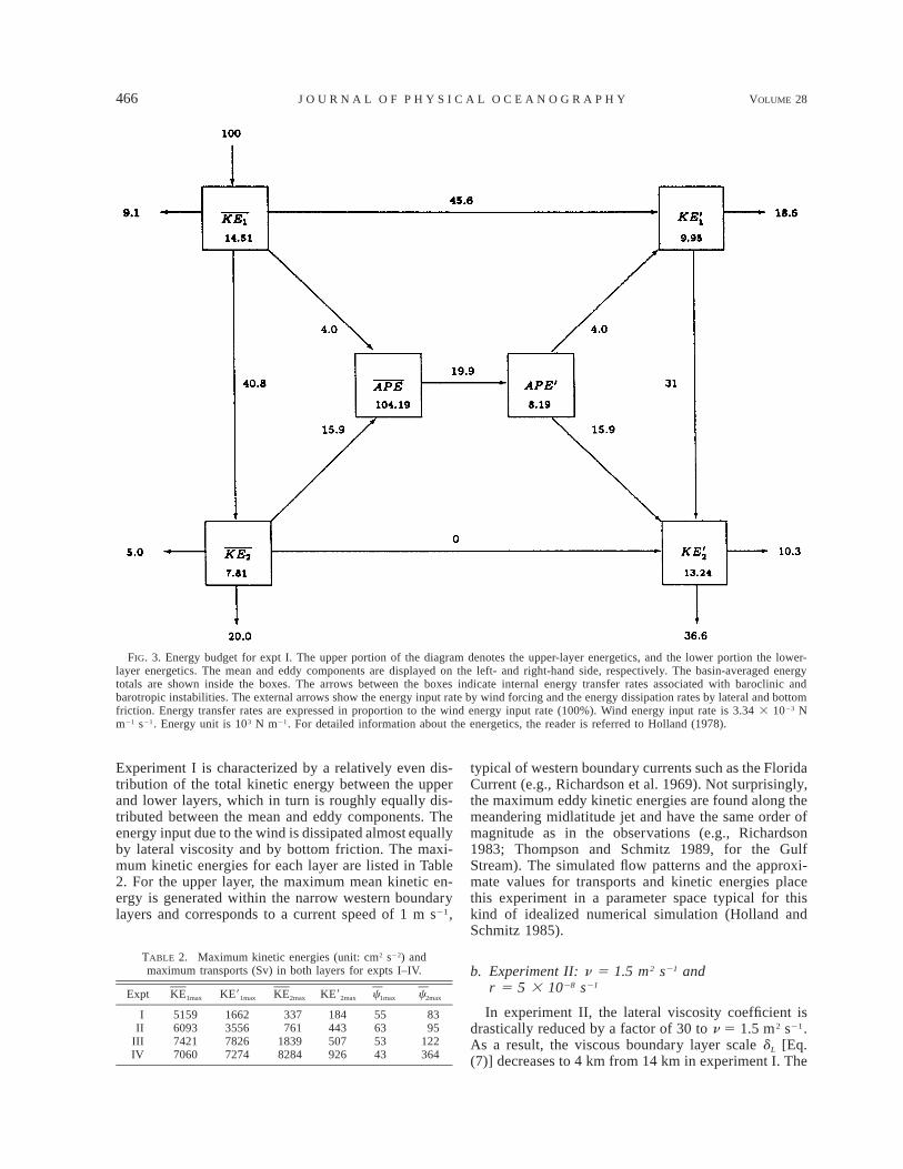
466 VOLUME 28J O U R N A L O F P H Y S I C A L O C E A N O G R A P H Y
FIG. 3. Energy budget for expt I. The upper portion of the diagram denotes the upper-layer energetics, and the lower portion the lower-layer energetics. The mean and eddy components are displayed on the left- and right-hand side, respectively. The basin-averaged energytotals are shown inside the boxes. The arrows between the boxes indicate internal energy transfer rates associated with baroclinic andbarotropic instabilities. The external arrows show the energy input rate by wind forcing and the energy dissipation rates by lateral and bottomfriction. Energy transfer rates are expressed in proportion to the wind energy input rate (100%). Wind energy input rate is 3.34 3 1023 Nm21 s21. Energy unit is 103 N m21. For detailed information about the energetics, the reader is referred to Holland (1978).
TABLE 2. Maximum kinetic energies (unit: cm2 s22) andmaximum transports (Sv) in both layers for expts I–IV.
Expt KE1max KE91max KE2max KE92max c1max c2max
III
IIIIV
5159609374217060
1662355678267274
337761
18398284
184443507926
55635343
8395
122364
Experiment I is characterized by a relatively even dis-tribution of the total kinetic energy between the upperand lower layers, which in turn is roughly equally dis-tributed between the mean and eddy components. Theenergy input due to the wind is dissipated almost equallyby lateral viscosity and by bottom friction. The maxi-mum kinetic energies for each layer are listed in Table2. For the upper layer, the maximum mean kinetic en-ergy is generated within the narrow western boundarylayers and corresponds to a current speed of 1 m s21,
typical of western boundary currents such as the FloridaCurrent (e.g., Richardson et al. 1969). Not surprisingly,the maximum eddy kinetic energies are found along themeandering midlatitude jet and have the same order ofmagnitude as in the observations (e.g., Richardson1983; Thompson and Schmitz 1989, for the GulfStream). The simulated flow patterns and the approxi-mate values for transports and kinetic energies placethis experiment in a parameter space typical for thiskind of idealized numerical simulation (Holland andSchmitz 1985).
b. Experiment II: n 5 1.5 m2 s21 andr 5 5 3 1028 s21
In experiment II, the lateral viscosity coefficient isdrastically reduced by a factor of 30 to n 5 1.5 m2 s21.As a result, the viscous boundary layer scale dL [Eq.(7)] decreases to 4 km from 14 km in experiment I. The

MARCH 1998 467O Z G O K M E N A N D C H A S S I G N E T
FIG. 4. (a) Upper-layer mean transport streamfunction (CI 5 5 Sv), (b) lower-layer mean transport streamfunction (CI 5 10 Sv), (c) upper-layer mean potential vorticity (nondimensional; CI corresponds to 0.9 3 1026 s21), (d) lower-layer mean potential vorticity (nondimensional;CI corresponds to 2.6 3 1026 s21) for expt II.
boundary layer thickness scale dB associated with thebottom friction [Eq. (8)] remains constant and is equalto 3 km. These two boundary layers are not resolvedin experiment II, even though the resolution in that ex-periment was increased to a grid spacing of about 7 km(Table 1). Griffa et al. (1996) showed that actually re-solving the small viscous boundary layer did not affectthe equilibrium flow provided that the inertial boundarylayer is resolved. Hence, it is important to resolve theinertial boundary layer dI ø 32 km of experiment II.This is achieved by the chosen grid spacing (Table 1).
The resulting mean flow is illustrated in Fig. 4. Whilethe upper-layer mean streamfunction remains virtuallyunchanged, the lower layer displays significant modi-fications. Most notable is the strengthening of the gyresalong the southern and northern boundaries of the do-main. These gyres now cover the entire zonal extent ofthe basin (Fig. 4b). The intensity of the inertial recir-culating gyres in the middle of the domain also increas-es, but the gyres themselves do not extend across theentire basin. Their zonal extent is determined by thebalance between the tendency for the highly inertial

468 VOLUME 28J O U R N A L O F P H Y S I C A L O C E A N O G R A P H Y
FIG. 5. Energy budget for expt II. Wind energy input rate is 3.39 3 1023 N m21 s21. Energy unit is 103 N m21.
mid-latitude jet to extend all the way across the basinand its inherent instability, which generates mesoscaleeddies that disrupt the jet, thereby restricting its zonalpenetration (Holland and Schmitz 1985). Both gyre sys-tems exhibit a tendency toward homogenization of po-tential vorticity inside the gyres (Fig. 4d).
The ‘‘original’’ Fofonoff flows (Fig. 1a), obtained fora barotrophic configuration, assume a linear relation be-tween the potential vorticity q and the streamfunctionc, q 5 c1c 1 c2 with c1 . 0. The Fofonoff solutionwas generalized by Marshall and Nurser (1986) to strat-ified flows with weak forcing and dissipation. Theyshowed that solutions satisfying the relationship q 5c1c 1 c2 with c1 , 0 can actually exist in the upperlayer, provided that vortex stretching is strong enough.These solutions have two recirculating gyres, separatedby an inertial jet, that correspond to the prescribed windforcing (cyclonic in the north and anticyclonic in thesouth) (Fig. 1b). These gyres are of opposite sign fromthose in the ‘‘barotropic case.’’ The lower-layer potentialvorticity fields are homogenized.
Both types of gyres are present in experiments I andII and both increased in strength when viscosity was
reduced (Fig. 4b). The question then arises as to whichsystem of gyres will eventually dominate the lower-layercirculation. Marshall and Nurser’s (1986) solution wasderived for weakly forced and dissipative stratifiedflows. Equilibrium statistical mechanics indicates thatFofonoff-like gyres (i.e., circulation in the same direc-tion as the conventional barotropic Fofonoff flow)should be the stable solutions toward which the non-linear terms tend to drive the system (SHH). We there-fore anticipate that those gyres, which tend to becomemore dominant as the nonlinearity in the system in-creases (i.e., as the friction decreases), will be associatedwith Fofonoff flows.
The energy budget of experiment II is shown in Fig.5. There is a significant increase in the eddy kineticenergy levels in both layers, as well as in the meankinetic energy of the lower layer, when compared toexperiment I. This corresponds to a more efficient useof the wind torque in order to reach a higher energylevel and strongly indicates an increase in the nonlin-earity of the system. Finally, most of the energy dis-sipation now takes place in the lower layer via the bot-

MARCH 1998 469O Z G O K M E N A N D C H A S S I G N E T
FIG. 6. (a) Upper-layer mean transport streamfunction (CI 5 5 Sv), (b) lower-layer mean transport streamfunction (CI 5 10 Sv), (c) upper-layer mean potential vorticity (nondimensional; CI corresponds to 0.9 3 1026 s21), (d) lower-layer mean potential vorticity (nondimensional;CI corresponds to 2.6 3 1026 s21) for expt III.
tom friction, shared equally between mean- and eddy-flow activity.
c. Experiment III: n 5 0 and r 5 5 3 1028 s21
In a further deviation from the parameter space usedin typical midlatitude ocean simulations, the lateral vis-cosity coefficient in this experiment is set to zero. Thishas a strong dynamical influence on the solution, asshown by the mean fields displayed in Fig. 6. This sen-sitivity of the solution to a small change in lateral vis-
cosity also indicates that the dissipation associated withthe model’s numerics is minimal.
The primary difference from experiment II is in thedisintegration of the midlatitude jet in the mean fieldand the accompanying recirculation gyres in both layers(Figs. 6a,b). The convergence of the western boundarycurrents still generates a midlatitude jet; however, itsfluctuations are so violent that the resulting mean sig-nature is weak. Consequently, the maximum upper-layereddy kinetic energy is higher than in experiment II andis nearly five times that of experiment I (Table 2). This

470 VOLUME 28J O U R N A L O F P H Y S I C A L O C E A N O G R A P H Y
FIG. 7. Energy budget for expt III. Wind energy input rate is 2.37 3 1023 N m21 s21. Energy unit is 103 N m21.
result illustrates that midocean recirculating gyres arenot stable for very small values of eddy viscosity.
In the lower layer, the northern and southern bound-ary gyres are now dominant and gained strength as thedissipation is reduced, in agreement with the charac-teristics of Fofonoff flows given by the equilibrium me-chanics theory. In experiment III, each of these gyresnow transports more than 120 Sv (Table 2) and displaysthe highest mean kinetic energy. These gyres signifi-cantly influence the upper-layer flow as their signatureis visible in Fig. 6a.
Potential vorticity is mixed and homogenized in thesebottom layer gyres (Fig. 6d). Homogenization of po-tential vorticity is commonly observed in numerical ex-periments, where the dissipation operator and associatedboundary conditions induce deviations from the idealunforced–undamped system, for which the equilibriumstatistical mechanics theory (SHH) predicts a linear re-lationship between the streamfunction and potential vor-ticity. Cummings (1992) found that the boundary con-ditions can have a global influence on the realization ofthe equilibrium state and, in particular, that the free-slipconditions may lead to the homogenization of potential
vorticity within the recirculating flow. Cummings em-ployed the theory of Rhines and Young (1982) to ex-plain how homogenization takes place. This theory as-sumes that the mixing induced by eddies can be param-eterized as u9q9 5 2k=q , where k is a diffusivity co-efficient. When the influence of friction is small incomparison to that of the eddies, Rhines and Young(1982) proved that within the time-averaged closed con-tours of the streamfunction, the potential vorticity isnearly uniform. Wang and Vallis (1994) stated that theviscous dissipation appears to drive the potential vor-ticity field toward homogenization, but they also arguedthat the detailed form of the viscosity operator is lessimportant than the boundary conditions. Griffa et al.(1996) stated that friction tends to flatten the slope ofthe streamfunction–potential vorticity curve. In this ex-periment (expt III), the free-slip boundary condition iseffective via the numerical implementation of the non-linear advective terms.
The energy budget (Fig. 7) remains qualitatively thesame as in experiment II. The significant loss of themean available potential energy is due to the disap-pearance of the midocean recirculating gyres.

MARCH 1998 471O Z G O K M E N A N D C H A S S I G N E T
FIG. 8. (a) Upper-layer mean transport streamfunction (CI 5 5 Sv), (b) lower-layer mean transport streamfunction (CI 5 20 Sv), (c) upper-layer mean potential vorticity (nondimensional; CI corresponds to 1.2 3 1026 s21), (d) lower-layer mean potential vorticity (nondimensional;CI corresponds to 2.6 3 1026 s21) for expt IV.
d. Experiment IV: n 5 0 and r 5 1029 s21
In experiment IV, the bottom friction coefficient isreduced to r 5 1029 s21, which corresponds to a damp-ing timescale of approximately 30 yr. The model is in-tegrated for an additional 27 years starting from thestatistical steady state of experiment III, and the statis-tics are computed over the final 7 years. At the end ofthe integration, the energetics indicate that the systemis fairly close to a statistical steady state but is stillslowly evolving. The trend during the last 7 years of
the integration is small enough for the mean flow patternto be representative.
The mean flow patterns are displayed in Fig. 8. Inthe lower layer, Fofonoff-like inertial gyres now com-pletely dominate the solution and occupy the entire do-main (Fig. 8b). The transport associated with these gyresexceeds 300 Sv and their signature is clearly dominantin the upper layer (Fig. 8a). The configuration in thislayer indicates a tendency for the solution to barotropize,but the upper-layer transports are smaller by almost anorder of magnitude when compared to the lower-layer

472 VOLUME 28J O U R N A L O F P H Y S I C A L O C E A N O G R A P H Y
FIG. 9. Scatterplot of mean streamfunction versus potential vorticity (nondimensional) for expt IV (a) in theupper layer and (b) in the lower layer.
transports (Table 2). A fully barotropic solution wouldexhibit transports in proportion to the upper/lower layerthickness ratio, namely 1/4 for this set of experiments.The resistance of the solution to complete barotropi-zation is the result of the wind forcing acting in theupper layer in opposition to the Fofonoff flows (seesection 4f for a detailed discussion). As discussed byGS, this type of wind forcing can completely prohibitthe emergence of Fofonoff flows in a barotropic model.In this two-layer model, however, Fofonoff-like gyresemerge, by first appearing in the lower layer to even-tually dominate the whole water column. The wind-driven gyres are still apparent in the instantaneous up-
per-layer flow fields, but the mean component is weakdue to a strong fluctuation field (see the eddy kineticenergy values listed in Table 2).
The resemblance of this solution to the Fofonoff so-lution can be further quantified by a scatterplot of themean streamfunction and potential vorticity in both lay-ers (Fig. 9). Despite the large amount of noise due tothe variability, the northern and southern upper-layerinertial gyres are characterized by a linear relationshipbetween the streamfunction and potential vorticity. Thetwo gyres are separated by the wind-driven region inthe middle of the domain, where potential vorticity in-creases with latitude (i.e., the negatively sloped region

MARCH 1998 473O Z G O K M E N A N D C H A S S I G N E T
FIG. 10. Instantaneous streamfunctions of expt IV at the end of theintegration for (a) upper layer (CI 5 10 Sv) and (b) lower layer (CI5 60 Sv).
TABLE 3. Seven-year averaged energy for expt IV (unit: 103 Nm21).
Energy totals
1KE2KE
KE91
KE92
APEAPE9
14129
60100200
12
in Fig. 9a). In the lower layer, instead, the potentialvorticity is strongly homogenized (Fig. 9b).
A sample of experiment IV instantaneous stream-functions is presented in Fig. 10. Even though bothlayers are in general agreement on the large scale, theupper layer exhibits a significant amount of small-scaleactivity (i.e., at scales smaller than the radius of defor-mation), which is absent in the lower-layer flow. Thisfeature is consistent with the conclusions reached bySHH, based on the equilibrium statistical mechanics the-
ory, that the equilibrium flow is nearly barotropic atscales of motion larger than the radius of deformation,while at smaller scales the streamfunctions in the twolayers should be statistically uncorrelated.
The energy budget for this experiment is not in bal-ance since the solution did not reach a statistical steadystate and is therefore not presented. However, for thepurpose of completeness and comparison, the basin-av-eraged kinetic and potential energies over the final 7years of integration are given in Table 3. Both the lower-layer kinetic energy and available potential energy in-creased by a factor of 5 when compared to those ofexperiment III.
e. Experiment V: n 5 0 and r 5 5 3 1024 s21
The four experiments presented in the previous sub-sections appear to indicate the flow tendency toward aFofonoff regime in a two-layer quasigeostrophic model,despite the fact that the wind forcing acted to opposethis regime (see section 4f for a detailed discussion).This result was achieved with very small dissipation inthe system and conforms well with the assumptions oftheoretical models (SHH). Intuitively, one would notexpect a Fofonoff-like solution with high dissipation.This is, however, not necessarily always the case asillustrated by the experiment presented in this section.As before, stratification plays an important role in thebehavior of the system and leads to an unexpected result.
Experiment V was performed with a high bottom fric-tion coefficient, r 5 5 3 1024 s21 (10 000 times greaterthan in expt IV). This coefficient corresponds to a damp-ing timescale of about 33 min and clearly lies outsidethe realistic parameter regime of any oceanic applica-tion. However, the purpose of this study is to explorethe emergence of Fofonoff-like solutions over the fullextent of the parameter space. Due to reasons associatedwith the sequence of the experiments conducted duringthe research phase, the domain size in experiment V is3500 km as opposed to 2000 km in the previous ex-periments. The net effect is a modification of the finalRossby number (see Table 1), which controls the inten-sity and size of the inertial recirculations. It was notdeemed necessary to repeat this experiment in the small-er domain.
In experiment V, the lateral viscosity is gradually re-

474 VOLUME 28J O U R N A L O F P H Y S I C A L O C E A N O G R A P H Y
duced to zero during the time span of the integration.As the lateral viscosity is decreased, the upper layerdissipates less and less energy and becomes very en-ergetic. The lower layer then basically acts as a sink ofenergy and displays only a very weak flow because ofthe high damping. Note that this case is inherently dif-ferent from a reduced gravity model, where the lowerlayer is motionless and hence cannot dissipate energy.
The reduction of the lateral viscosity coefficient hasa significant impact on the separation point of the mid-latitude jet. In the high-viscosity regime, the westernboundary layers are frictional and do not display highvariability. As the viscosity is reduced, the viscousboundary layer thickness becomes smaller than the in-ertial boundary layer thickness, and the boundary layerdynamics becomes controlled by a balance between theinertial terms and the beta effect. The separation point(i.e., where the boundary currents turn eastward) is gov-erned by fully nonlinear dynamics (e.g., Harrison andHolland 1981), in which the eddy component of theadvective term balances its mean component [i.e., J(c ,¹2c) ø J(c9, ¹2c9)]. In the absence of strong dampingin the boundary layer, the separation point becomeshighly variable and boundary eddies are generated. Thisprocess is illustrated by a series of instantaneous upper-layer streamfunction contour diagrams in Fig. 11. Ini-tially (at t 5 t1), the midlatitude jet separates near thezero wind-stress curl line (ZWCL). The separation pointis highly variable, and the northward-flowing boundarycurrent overshoots the ZWCL by approximately 1300km before it sheds a boundary eddy (t 5 t2 and t 5t3) and begins to retract. These eddies tend to accu-mulate along the northern and southern boundaries andtravel eastward with an approximate speed of 10 cm s21
until they interact with other eddies that migrate west-ward with a speed of 1 cm s21, which corresponds tothe typical long Rossby wave speed (t 5 t4 and t 5t5).
As the lateral viscosity becomes smaller, the jet be-comes more energetic and possesses a very weak meanflow. The eddy generation near the separation latitudeincreases, and the migration of eddies along the zonalboundaries tends to mix the potential vorticity. The up-per and lower mean streamfunctions corresponding tothe end result, namely, zero lateral viscosity, are shownin Fig. 12. The lower-layer flow is of course very weak[O(1022) Sv] and does not exhibit a dominant mean flow(although it displays a pattern of waves). In the upperlayer, on the other hand, the wind-forced interior is vis-ible, but its mean component is weak because of thestrong fluctuations. The most prominent features are therecirculating gyres along the southern and northernboundaries, whose sense of direction is consistent withFofonoff flows. Note that these gyres appear exclusivelyin the upper layer despite the fact that the wind forcingacts in opposition to their direction of flow.
In contrast to experiment IV in which the Fofonoff-like gyres were strongly barotropic, the gyres in ex-
periment V are mostly baroclinic. In order to developthe large transports observed in these gyres (which ex-ceed 180 Sv), the density interface must stretch by anamount comparable to its initial thickness, hence vio-lating the quasigeostrophic approximation. However,the tendency toward this flow pattern was clearly ob-served within the quasigeostrophic range while the lat-eral viscosity was gradually reduced during the inte-gration. The flow presented in Fig. 12a is representativeof the equilibrium solution for this parameter regime.
In order to quantify the proximity of this solution toFofonoff flows, the relationship between the stream-function and potential vorticity is investigated. The up-per-layer mean potential vorticity is plotted in Fig. 12c.There is a strong correspondence between the stream-function and the potential vorticity in the upper layer,as illustrated by the scatterplot of Fig. 13, which showsa linear relationship between the streamfunction and thepotential vorticity. This can be explained by consideringthe characteristics of this experiment and the definitionof the upper-layer vorticity [Eq. (3)]. The respectivecontributions of the relative vorticity, of the stretchingterm, and of the beta term are illustrated in Fig. 14.Figure 14a shows the contribution of the stretching termonly. Figure 14b shows the contribution of the stretchingterm and of the beta term combined. The contributionof the relative vorticity is negligible as shown by thenear-identity of Fig. 14b and Fig. 13. This is not sur-prising since F (the Froude number) is much larger thanR (the Rossby number) in this experiment [F/R 5 (l/Rd)2]. While the inclusion of the beta term does modifythe c1–q1 curve in Fig. 14b from that in Fig. 14a, thelinear relationship between the streamfunction and po-tential vorticity in the upper layer is predominantly de-termined by the stretching term. The linear relationshipis then explained by considering that the lower-layermean flow is virtually nonexistent (c1 k c2 ) and thatthe upper-layer potential vorticity equation reduces toq1 ø 2d21Fc1 . The slope of the c1 2 q1 curve in Fig.13 is roughly consistent with this relationship (F 5 8.53 1023, d 5 0.2 for expt V)
In this section, it has been shown that Fofonoff-likeflows are not constrained to unforced–nondissipative re-gimes, but can also emerge in a regime with unfavorableforcing and high damping, as long as stratification isincluded in the dynamics.
f. Experiments VI and VII: Reversed wind forcing
In sections 4d and 4e, it is argued that a flow tendencytoward a Fofonoff regime can be achieved in a two-layer quasigeostrophic model despite the fact that thewind forcing acted to oppose this regime. In order tosubstantiate this hypothesis, experiments III and V wererepeated with a reversed wind forcing (as expts VI andVII, respectively). With such forcing, the emergence ofFofonoff flows should be favored, and the gyres ap-pearing in the previous experiments should strengthen

MARCH 1998 475O Z G O K M E N A N D C H A S S I G N E T
FIG. 11. Time series of instantaneous upper-layer streamfunctions during spinup phase for expt V (CI 510 Sv).

476 VOLUME 28J O U R N A L O F P H Y S I C A L O C E A N O G R A P H Y
FIG. 12. (a) Upper-layer mean transport streamfunction (CI 5 10Sv), (b) lower-layer mean transport streamfunction (CI 5 7 3 1023
Sv) and (c) upper-layer mean potential vorticity (nondimensional; CIcorresponds to 1.5 3 1026 s21) for expt V.
substantially if they are consistent with Fofonoff flows.Griffa and Salmon (1989) demonstrated that in a bar-otropic quasigeostrophic model the emergence of Fo-fonoff flows depends strongly on the geometry of thewind stress. In order to reach an equilibrium state, theparameters of experiment III were chosen for experi-ment VI. The Ekman pumping for both experiments VIand VII is
y l lw (y) 5 2W sin 2p with 2 # y # , (10)E 1 2l 2 2
where the amplitude W remains unchanged from ex-
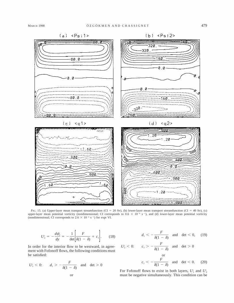
periments III and V. This forcing drives an anticyclonicgyre in the northern half of the domain and a cyclonicgyre in the southern half.
The mean flows for experiment VI are shown in Fig.15. A substantial strengthening of the inertial gyres withrespect to those in experiment III (Fig. 6) is observedand the scatterplots between the streamfunction and po-tential vorticity exhibit quasi-linear relationships forboth layers (Fig. 16). The slopes are negative and pos-itive in the upper and lower layers, respectively. Thisis in apparent contrast with experiment IV (Fig. 9) inwhich the slopes are positive and zero in the upper andlower layers, respectively. The question as to whether

MARCH 1998 477O Z G O K M E N A N D C H A S S I G N E T
FIG. 13. Scatterplot of mean streamfunction versus potential vorticity (nondimensional) in the upper layer for expt V.
or not these slopes correspond to a Fofonoff regime isdiscussed in detail in the next section.
The mean flows for experiment VII are illustrated inFig. 17. Again, the Fofonoff-like gyres strengthen withrespect to those in the experiment with unfavorable windforcing (expt V, Fig. 12), and the gyres occupy the entireupper layer. The lower-layer flow is, as in experimentV, very weak due to high bottom friction. The scatterplotbetween the upper-layer streamfunction and potentialvorticity shows a linear relationship (Fig. 18). As inexperiment V, the slope is negative and its value is pre-dominantly determined by the stretching term.
The results of both experiments show that the inertialgyres intensify substantially when the wind forcing isfavorable. The gyres in experiments III–VII all displaya quasi-linear relationship between the mean stream-function and potential vorticity. However, these rela-tionships exhibit a variety of slopes, which can be neg-ative, zero, or positive in each layer. The consistencyof these slopes with the nature of Fofonoff gyres isdiscussed in the following section.
5. Discussion
Fofonoff flows are defined by a linear relationshipbetween the streamfunction and potential vorticity.Classical Fofonoff gyres (Fofonoff 1954) are definedfor a barotropic flow, and the nature of the relationshipbetween the streamfunction and potential vorticity mayvary in a model that includes stratification. The exper-iments presented in section 4 exhibit inertial gyres thathave visual resemblance to the classic Fofonoff gyres.However, while the quasi-linear relationship betweenthe streamfunction and potential vorticity is retained inthe scatterplots, the corresponding slopes can be posi-
tive, zero, or negative. In this section, we investigateunder which conditions Fofonoff flows can exist in atwo-layer quasigeostrophic model and we examine theconsistency of the gyres discussed in section 4 withFofonoff flows.
In a barotropic model, assuming the existence of Fo-fonoff flows, the relationship between the time-averagedpotential vorticity and streamfunction can be written as(dropping the superscript for simplicity)
q 5 R¹2c 1 y 5 c1c 1 c2, (11)
For a small Rossby number R, the inertial effects areconfined to the boundary layers, and the interior solutionis ci(y) 5 (y 2 c2)/c1. The corresponding interior zonalvelocity is then Ui 5 2dci/dy 5 21/c1. In order forthe interior flow to be westward (Ui , 0), in agreementwith Fofonoff flows, c1 must be positive. Zero or neg-ative slopes are not allowed in a barotropic model.
In a two-layer model, assuming again the existenceof Fofonoff flows, the relationships for the mean flowsin the upper and lower layers can be written as
F2q 5 R¹ c 1 y 1 (c 2 c ) 5 c c 1 c , (12)1 1 2 1 1 1 2d
F2q 5 R¹ c 1 y 1 (c 2 c ) 5 d c 1 d . (13)2 2 1 2 1 2 21 2 d
In the interior, the relative vorticity is small, and thestreamfunctions can be expressed as
1 F Fic (y) 5 2 c 2 c d 2 d1 2 2 1 21det 1 2 d d
F1 y 1 d y , (14)1 2d(1 2 d)

478 VOLUME 28J O U R N A L O F P H Y S I C A L O C E A N O G R A P H Y
FIG. 14. Contributions of the stretching and beta terms to the c1–q1 scatter diagram in the upper layerfor expt V: (a) q1 5 2d21Fc1 and (b) q1 5 y 2 d21Fc1 . In both cases, the slope is approximately equalto 210/240.
1 F Fic (y) 5 2 c 2 c d 2 d2 2 2 2 21det 1 2 d d
F1 y 1 c y , (15)1 2d(1 2 d)
where
d c1 1det 5 F 1 1 c d . (16)1 11 2d 1 2 d
The corresponding interior zonal velocities are
idc 1 F1iU 5 2 5 2 1 d , (17)1 1[ ]dy det d(1 2 d)
MARCH 1998 479O Z G O K M E N A N D C H A S S I G N E T
FIG. 15. (a) Upper-layer mean transport streamfunction (CI 5 20 Sv), (b) lower-layer mean transport streamfunction (CI 5 40 Sv), (c)upper-layer mean potential vorticity (nondimensional; CI corresponds to 0.6 3 1026 s21), and (d) lower-layer mean potential vorticity(nondimensional; CI corresponds to 2.6 3 1026 s21) for expt VI.
idc 1 F2iU 5 2 5 2 1 c . (18)2 1[ ]dy det d(1 2 d)
In order for the interior flow to be westward, in agree-ment with Fofonoff flows, the following conditions mustbe satisfied:
FiU , 0: d . 2 and det . 01 1 d(1 2 d)
or
Fd , 2 and det , 0, (19)1 d(1 2 d)
FiU , 0: c . 2 and det . 02 1 d(1 2 d)
orF
c , 2 and det , 0. (20)1 d(1 2 d)
For Fofonoff flows to exist in both layers, andi iU U1 2
must be negative simultaneously. This condition can be

480 VOLUME 28J O U R N A L O F P H Y S I C A L O C E A N O G R A P H Y
FIG. 16. Scatterplot of mean streamfunction versus potential vorticity (nondimensional) for expt VI (a) inthe upper layer and (b) in the lower layer.
visualized by plotting the zonal interior velocities iU1
and as functions of c1 and d1 in Figs. 19a,b, re-iU 2
spectively. Comparison of Figs. 19a and 19b indicatesthat the zonal velocities are both negative only in theupper-right quadrant. This region is defined by the hy-perbola
F d1c . 2 , (21)1 d [d 1 F /(1 2 d)]1
as displayed in Fig. 19c. The shaded area shows theregion in which Fofonoff flows are allowed in a two-layer quasigeostrophic model. This figure also demon-strates that unlike the barotropic case, the slopes do notnecessarily need to be positive, but that zero (i.e., ho-
mogenized potential vorticity) as well as negative slopesare allowed. The latter is a consequence of the strati-fication (F . 0).
The approximate slopes derived from experiments IVand VI show that they are within the shaded area, andthat the flow patterns in these experiments are thereforeconsistent with Fofonoff flows (Fig. 19c).
For the flow regime generated in experiments V andVII, the lower-layer flow is very weak, and the upper-layer potential vorticity equation can be written as
F2q 5 R¹ c 1 y 2 c 5 c c 1 c . (22)1 1 1 1 1 2d
Again neglecting the relative vorticity, the interior

MARCH 1998 481O Z G O K M E N A N D C H A S S I G N E T
FIG. 17. (a) Upper-layer mean transport streamfunction (CI 5 20Sv), (b) lower-layer mean transport streamfunction (CI 5 0.1 Sv),and (c) upper-layer mean potential vorticity (nondimensional; CI cor-responds to 3 3 1026 s21) for expt VII.
streamfunction can be expressed as (y) 5 (y 2 c2)/ic1
(c1 1 F/d). The interior velocity 5 21/(c1 1 F/d)iU1
will be westward as long as c1 . 2F/d. Note that thisflow regime is a special case of the more general equa-tion [Eq. (21)] when d1 → ` as c2 → 0. In experimentsV and VII, the slope is slightly larger than 2F/d 524.2 3 1022, and the flow patterns in experiments Vand VII are therefore consistent with Fofonoff flows.
For c2 5 0, the symmetric Fofonoff solution is re-covered (Fig. 1a). Other values for c2 result in asym-metric flow patterns, usually associated with nonzerototal vorticity in the initial conditions or forcing (GS).
It is worth noting that Marshall and Nurser (1986) as-sumed c2 5 1 (or bl in dimensional units) for the north-ern half and c2 5 21 for the southern half of the domain,for which case the flow pattern is illustrated in Fig. 1b.In this case, the boundary layers are in the middle ofthe domain in the form of a midlatitude jet. This solutionwas found to be unstable in our experiments (section 4).
6. Summary and conclusions
In this paper, the emergence of Fofonoff-like flowsover a wide range of dissipative parameter regimes has

482 VOLUME 28J O U R N A L O F P H Y S I C A L O C E A N O G R A P H Y
FIG. 18. Scatterplot of mean streamfunction versus potential vorticity (nondimensional) in the upper layerfor expt VII.
been explored in a wind-driven two-layer quasigeo-strophic model. Most of the previous work on this topicwas performed either in the absence of forcing and dis-sipation or with a barotropic model. In a series of ex-periments performed with this two-layer model, two re-gimes were found in which Fofonoff-like circulationsemerged. This is a direct consequence of the baroclinicnature of the system, as the wind forcing used in theseexperiments has been shown to inhibit the formation ofFofonoff flows in the barotropic case.
The ‘‘original’’ Fofonoff flows are defined for a baro-tropic ocean (Fofonoff 1954) and are characterized bya linear relationship between the streamfunction andvorticity, q 5 c1c 1 c2 with c1 . 0. The flow patternof these gyres is exhibited in Fig. 1a. Marshall andNurser (1986) defined ‘‘generalized’’ Fofonoff flows ina baroclinic ocean such that q1 5 c1c1 1 c2 with c1 ,0 in the upper layer, and the lower-layer potential vor-ticity is homogenized. These solutions are characterizedby midlatitude gyres with a sense of direction oppositeto the original Fofonoff flows (Fig. 1b). In this study,the range of the proportionality constants for the exis-tence of Fofonoff-like flows in a two-layer quasigeo-strophic model is derived. Provided that the gyres areconsistent with the sense of direction and location ofthe original Fofonoff flows, it is shown that the pro-portionality constant between the streamfunction andpotential vorticity can be positive, negative, or zero inboth layers. We refer to ‘‘Fofonoff-like’’ gyres in a two-layer ocean as those satisfying the derived criteria.
The first regime in which Fofonoff-like gyres emergeis one in which the magnitudes of the frictional coef-ficients (viscosity and bottom dissipation) are extremelysmall. In this case, Fofonoff-like flows emerge despite
the fact that the wind forcing acts in a direction thatwas shown to prevent the emergence of Fofonoff flowsin the barotropic context (GS). In the two-layer model,the wind forcing acts on the upper layer and does notforce the lower layer directly. Fofonoff-like flows firstappear in the lower layer and then spread throughoutthe water column via barotropization. The series of ex-periments presented in section 4 clearly illustrates thetransition of the numerical solution from a conventionalwind-driven circulation to an inertial Fofonoff-like re-gime. In these experiments, the mean signatures of themidlatitude jet and the associated recirculating gyresdisintegrate as the magnitudes of the frictional param-eters are reduced. The solution proposed by Marshalland Nurser (1986) was found to be unstable in thisparameter regime.
Surprisingly, Fofonoff-like flows are also obtainedwith very high bottom friction. Inertial gyres appearonly in the upper layer, as the lower layer is quasi-motionless and acts as a sink of energy. This case isinherently different from a reduced-gravity model, inwhich the bottom layer is motionless and hence cannotdissipate energy. This result indicates that entropy canbe maximized independently in each layer, dependingon the distribution of forcing and dissipation. Thisbrings a new perspective to the common assumptionthat forcing and dissipation are disruptive effects thatprevent the system from displaying a Fofonoff-likestate. The nature of these gyres in both cases is con-firmed by reversing the wind forcing such that it favorsFofonoff flows. In both cases, the inertial gyres becamemore dominant, as expected for Fofonoff flows accord-ing to GS.
In conclusion, the experiments presented in this paper

MARCH 1998 483O Z G O K M E N A N D C H A S S I G N E T
FIG. 19. (a) Upper-layer zonal velocity U and (b) lower-layer zonali1
velocity plotted as a function of the slopes c1 and d1, and for theiU 2
parameters F 5 1.52 3 1022, d 5 0.2. The shaded areas indicate theregions where the zonal velocities are negative. U1 and U2 are bothnegative (westward flow) only in the upper right quadrant marked bythe hyperbola c1 . 2d21Fd1/[d1 1 F/(1 2 d )], which is plotted in(c). Expts IV and VI fall into the region where Fofonoff flows arepossible.
suggest that Fofonoff-like solutions appear over a muchwider spectrum of forcing and dissipation than was ini-tially implied by the theory based on equilibrium sta-tistical mechanics (SHH) and by previous studies thatsolely relied on barotropic models. The present resultsare obtained in a parameter range that is not realistic,but they indicate the presence of a fundamental mech-anism that might have an impact on the ocean generalcirculation. Therefore, a logical next step would be asystematic investigation of the appearance of these so-
lutions in a realistic configuration under generalizedforcing and dissipation, with special emphasis on theirimpact upon the ocean general circulation.
Acknowledgments. The authors wish to thank A. Grif-fa for lively and constructive discussions and L. Smithfor substantial help in improving the text. Conversationswith P. Cessi and S. Meacham also proved timely andvaluable. We also thank the two anonymous referees fortheir helpful criticism. Support was provided by the Na-

484 VOLUME 28J O U R N A L O F P H Y S I C A L O C E A N O G R A P H Y
tional Science Foundation through Grant OCE-94-06663 and by the Office of Naval Research under Con-tract NOOO14-93-1-0404.
REFERENCES
Arakawa, A., 1966: Computational design for long-term numericalintegration of the equations of fluid motion: Two dimensionalincompressible flow. Part I. J. Comput. Phys., 1, 119–143.
Barnier, B., B. L. Hua, and C. Le Provost, 1991: On the catalyticrole of high baroclinic modes in eddy-driven large-scale circu-lations. J. Phys. Oceanogr., 21, 976–997.
Boning, C. W., 1986: On the influence of frictional parameterizationin wind-driven circulation models. Dyn. Atmos. Oceans, 10, 63–92.
Bretherton, F. P., and D. B. Haidvogel, 1976: Two dimensional tur-bulence above topography. J. Fluid Mech., 78, 129–154.
Carnevale, G. F., and J. D. Fredericksen, 1987: Nonlinear stabilityand statistical mechanics of flow over topography. J. FluidMech., 175, 157–181.
Cessi, P., 1991: Laminar separation of colliding western boundarycurrents. J. Mar. Res., 49, 697–717., R. V. Condie, and W. R. Young, 1990: Dissipative dynamicsof western boundary layers. J. Mar. Res., 48, 677–700.
Chassignet, E. P., 1995: Vorticity dissipation by western boundarycurrents in the presence of outcropping layers. J. Phys. Ocean-ogr., 25, 242–255., and R. Bleck, 1993: The influence of layer outcropping on theseparation of boundary currents. Part I: The wind-driven ex-periments. J. Phys. Oceanogr., 23, 1485–1507.
Cummins, P. F., 1992: Inertial gyres in decaying and forced geo-strophic turbulence. J. Mar. Res., 50, 545–566.
Fofonoff, N. P., 1954: Steady flow in a frictionless homogeneousocean. J. Mar. Res., 13, 254–262.
Gazdag, J., 1976: Time-differencing schemes and transform methods.J. Comput. Phys., 20, 196–207.
Griffa, A., and R. Salmon, 1989: Wind-driven ocean circulation andequilibrium mechanics. J. Mar. Res., 47, 457–492., E. P. Chassignet, V. Coles, and D. B. Olson, 1996: Inertial gyresolutions from a primitive equation ocean model. J. Mar. Res.,54, 653–677.
Harrison, D. E., and W. R. Holland, 1981: Regional eddy vorticitytransport and the equilibrium vorticity budgets of a numericalmodel ocean circulation. J. Phys. Oceanogr., 11, 190–208.
Holland, W. R., 1978: The role of mesoscale eddies in the generalcirculation of the ocean. J. Phys. Oceanogr., 8, 363–392., and W. J. Schmitz, 1985: Zonal penetration scale of modelmidlatitude jets. J. Phys. Oceanogr., 15, 1859–1875.
Marshall, J., and G. Nurser, 1986: Steady, free circulation in a strat-ified quasi-geostrophic ocean. J. Phys. Oceanogr., 16, 1799–1813.
Pedlosky, J., 1987: Geophysical Fluid Dynamics. 2d ed. Springer-Verlag, 624 pp.
Rhines, P. B., and W. Young, 1982: A theory of wind-driven circu-lation I—Mid-ocean gyres. J. Mar. Res., 40, 559–596.
Richardson, P. L., 1983: Eddy kinetic energy in the North Atlanticfrom surface drifters. J. Geophys. Res., 88(C7), 4355–4367.
Richardson, W. S., W. J. Schmitz Jr., and P. P. Niiler, 1969: Thevelocity structure of the Florida Current from the Straits of Flor-ida to Cape Fear. Deep-Sea Res., 16(Suppl.), 225–231.
Salmon, R., G. Holloway, and M. C. Hendershott, 1976: The equi-librium statistical mechanics of simple quasi-geostrophic mod-els. J. Fluid Mech., 75, 691–703.
Thompson, J. D., and W. J. Schmitz Jr., 1989: A limited-area modelof the Gulf Stream: Design, initial experiments, and model-dataintercomparison. J. Phys. Oceanogr., 19, 791–814.
Veronis, G., 1966: Wind driven ocean circulation. Part 2. Numericalsolution of a nonlinear problem. Deep-Sea Res., 13, 31–55.
Verron, J., and C. Le Provost, 1991: Response of eddy-revolved gen-eral circulation numerical models to asymmetrical wind forcing.Dyn. Atmos. Oceans, 15, 505–533.
Wang, J., and G. K. Vallis, 1994: Emergence of Fofonoff states ininviscid and viscous ocean circulation models. J. Mar. Res., 52,83–127.