ES

EA

RC

HR

EP

RO

RT

ID

IA

P

D a l l e M o l l e I n s t i t u t e

fo r Pe rcep tua l A r t i f i c i a l

Intelligence • P.O.Box 592 •

Martigny • Valais •Switzerland

phone +41 − 27 − 721 77 11

fax +41 − 27 − 721 77 12

e-mail secre-

tariat@idiap.ch

internet

http://www.idiap.ch

EMBEDDING MOTION IN

MODEL-BASED STOCHASTIC

TRACKINGJean-Marc Odobez * Daniel Gatica-Perez *

Sileye Ba *

IDIAP–RR 03-72

DECEMBER 10, 2003

SUBMITTED FOR PUBLICATION

* IDIAP, Martigny, Switzerland

IDIAP Research Report 03-72

EMBEDDING MOTION IN MODEL-BASED

STOCHASTIC TRACKING

Jean-Marc Odobez Daniel Gatica-Perez Sileye Ba

DECEMBER 10, 2003

SUBMITTED FOR PUBLICATION

Abstract. Particle filtering is now established as one of the most popular methods forvisual tracking. Within this framework, two assumptions are generally made. The firstis that the data are temporally independent given the sequence of object states. In thispaper, we argue that in general the data are correlated, and that modeling such depen-dency should improve tracking robustness. The second assumption consists of the useof the transition prior as proposal distribution. Thus, the current observation data is nottaken into account, requesting the noise process of this prior to be large enough to handleabrupt trajectory changes. Therefore, many particles are either wasted in low likelihoodarea, resulting in a low efficiency of the sampling, or, more importantly, propagated onnear distractor regions of the image, resulting in tracking failures. In this paper, wepropose to handle both issues using motion. Explicit motion measurements are usedto drive the sampling process towards the new interesting regions of the image, whileimplicit motion measurements are introduced in the likelihood evaluation to model thedata correlation term. The proposed model allows to handle abrupt motion changesand to filter out visual distractors when tracking objects with generic models based onshape or color distribution representations. Experimental results compared against theCONDENSATION algorithm have demonstrated superior tracking performance.

IDIAP–RR 03-72 1

1 Introduction

Visual tracking is an important problem in computer vision, with applications in telecon-ferencing, visual surveillance, gesture recognition, and vision based interfaces [4]. Thoughtracking has been intensively studied in the literature, it is still a challenging task in adversesituations, due to the presence of ambiguities (e.g. when tracking an object in a clutteredscene or when tracking multiple instances of the same object class), the noise in imagemeasurements (e.g. lighting problems), and the variability of the object class (e.g. posevariations).

In the pursuit of robust tracking, Sequential Monte Carlo methods [1, 6, 4] have shown tobe a successful approach. In this temporal Bayesian framework, the probability of the objectconfiguration given the observations is represented by a set of weighted random samples,called particles. This representation allows to simultaneously maintain multiple-hypothesesin the presence of ambiguities, unlike algorithms that keep only one configuration state [5],which are therefore sensitive to single failure in the presence of ambiguities or fast or erraticmotion.

Visual tracking with a particle filter requires the definition of two main elements : a datalikelihood term and a dynamical model. The data likelihood term evaluates the likelihood ofthe current observation given the current object state, and relies on the object representationwe have chosen. The object representation corresponds to all the information that explicitlyor implicitly characterize the object like the target position, geometry, appearance, motionetc. Parametrized shapes like splines [4] or ellipses [18] and color distributions [13, 5, 11, 18]are often used as target representation. One drawback of these generic representations is thatthey are quite unspecific which augment the chances of ambiguities. One way to improvethe robustness of a tracker consists of combining low-level measurements such as shape andcolor [18]. A step further to render the target more discriminative is to use appearence-based models such as templates [15, 16], leading to very robust trackers. However, suchrepresentations do not allow for large changes of appearence, unless adaptation is performedor more complex global appearence models are used (e.g. eigen-space [2] or set of examplars[17]).

The dynamical model characterizes the prior on the state sequence. Examples of suchmodels range from simple constant velocity models to more sophisticated oscillatory ones oreven mixtures of these [8]. A common assumption in particle filtering approaches is to usethe dynamics as proposal distribution (or importance function), that is, as the function thatpredicts the new state hypotheses where the data likelihood will be evaluated. Thus, with thisassumption, the variance of the noise process in the dynamical model implicitly defines somesearch range for the new hypotheses. This assumption raises difficulties in the modeling ofthe dynamics since this term should fulfill two contradictory objectives. On one hand, asprior, dynamics should be tight to avoid the tracker being confused by distractors in thevicinity of the true object configuration, a situation that is likely to happen for unspecificobject representations such as generic shapes or color distributions. On the other hand,as proposal distribution, it should be broad enough to cope with abrupt motion changes.Besides, the proposal distribution does not take into account the most recent observations.

IDIAP–RR 03-72 2

Thus, particles drawn from it will probably have a low likelihood, which results in a lowefficiency of the sampling mechanism. Overall, such a particle filter is likely to be distractedby background clutter.Different approaches have been proposed to address these issues. For instance, auxiliaryinformation, if available, can be used to draw samples from, like color in [7], or audio in thecase of audio-visual tracking [3]. An important advantage of this approach is to allow forautomatic (re)initialization. However, from a filtering point of view, one drawback is that,since these additional samples are not related to the previous samples, the evaluation of thetransition prior term for one new sample involves all past samples, which can become verycostly. To avoid this effect, [12] proposed another auxiliary particle filter. The idea is to usethe likelihood of a first set of predicted samples at time t + 1 to resample the seed samples attime t, and to then apply the standard propagation and evaluation steps on these seed samples.The feedback from the new data acts by increasing or decreasing the number of descendentsof a sample according to its “predicted” likelihood. Such a scheme, however, works wellonly if the variance of the transition prior is small, which is usually not the case in visiontracking. [14] proposed to use the unscented particle filter to generate importance densities.Although attractive, it is still likely to fail in the presence of abrupt motion changes, and themethod needs to convert likelihood evaluations (e.g. color) into state space measurements(e.g. translation, scale). This would be difficult with color distribution likelihoods and forsome state parameters. In [14], only a translation state is considered. .

In this paper we propose a new particle filter tracking method based on visual motion.More precisely, we first argue that a standard hypothesis of this filter, namely the indepen-dence of observations given the state sequence [2, 4, 7, 14, 17, 18], is inaccurate in the caseof visual tracking. In this view, we propose a model that assumes that the current observationdepends on the current and previous object configuration as well as on the past observation.As we will show, the proposed model can be exploited to introduce an implicit object motionlikelihood in the data term. Secondly, we will make a further use of visual motion by exploit-ing explicit motion measurements in the proposal distribution and in the likelihood term. Thebenefits of this new model are two-fold. On one hand, it increases the sampling efficiencyby handling unexpected motion, allowing for a reduced noise variance in the propagationprocess as well as the introduction of non-gaussian prior. On the other hand, the introductionof data-correlation between successive images will turn generic trackers like shape or colorhistogram trackers into more specific ones without resorting to complex appearence basedmodels. As a consequence, it reduces the sensitivity of the algorithm to the difference noisevariances setting in the proposal and prior since, when using a larger values, potential dis-tractors should be filtered out by the introduced correlation and visual motion measurements.

The rest of the paper is organized as follows. In the next Section, we briefly present thestandard particle filter algorithm. Our approach is motivated in Section 3, while Section 4describes the proposed model. Section 5 presents the results and Section 6 provides someconcluding discussions.

IDIAP–RR 03-72 3

2 Particle filtering

Particle filtering is a technique for implementing a recursive Bayesian filter by Monte-Carlosimulations. The key idea is to represent the required density function by a set of randomsamples with associated weights. Let c0:k = {cl, l = 0, . . . , k} (resp. z1:k = {zl, l =1, . . . , k}) represents the sequence of states (resp. of observations) up to time k. Further-more, let {ci

0:k, wik}

Ns

i=1 denote a set of weighted samples that characterizes the posteriorprobability density function (pdf) p(c0:k|z0:k), where {ci

0:k, i = 1, . . . , Ns} is a set of sup-port points with associated weights wi

k. The weights are normalized such that∑

i wik = 1.

Then, a discrete approximation of the true posterior at time k is given by :

p(c0:k|z1:k) ≈Ns∑

i=1

wikδ(c0:k − ci

0:k) . (1)

The weights are chosen using the principle of Importance Sampling (IS). More precisely,suppose that we could draw the samples ci

0:k from an importance (also called proposal) den-sity q(c0:k|z1:k). Then the proper weights in (1) that lead to an approximation of the posteriorare defined by :

wik ∝

p(ci0:k|z1:k)

q(ci0:k|z1:k)

. (2)

The goal of the particle filtering algorithm is the recursive propagation of the samples andestimation of the associated weights as each measurement is received sequentially. Aftersome calculus and using Bayes rule, we obtain the following recursive update equation [1, 6]:

wik ∝ wi

k−1

p(zk|c0:k, z1:k−1)p(ck|c0:k−1, z1:k−1)

q(ck|c0:k−1, z1:k), (3)

= wik−1 p(zk|c

ik) (4)

where Eq. 4 derives from three commonly made hypotheses :

H1 : The observations {zk}, given the sequence of states, are independent. This leads top(z1:k|c0:k) =

∏k

i=1 p(zk|ck), which requires the definition of the individual data-likelihood p(zk|ck) ;

H2 : The state sequence c0:k follows a first-order Markov chain model, characterized by thedefinition of the dynamics p(ck|ck−1).

H3 : The prior distribution p(x0:k) is employed as importance function.In this case, q(ck|c0:k−1, z1:k) = p(ck|ck−1).

It is known that importance sampling is usually inefficient in high-dimensionnal spaces[6], which is the case of the state space c0:k as k increases. To solve this problem, an ad-ditional resampling step is necessary, whose effect is to eliminate the particles with lowimportance weights and to multiply particles having high weights, giving rise to more vari-ety around the modes of the posterior after the next importance sampling step. Altogether,we obtain the particle filter that is displayed in Fig. 2.

IDIAP–RR 03-72 4

(a)

kk-1 k+1

observations

states

(b)

k+1kk-1

states

observations

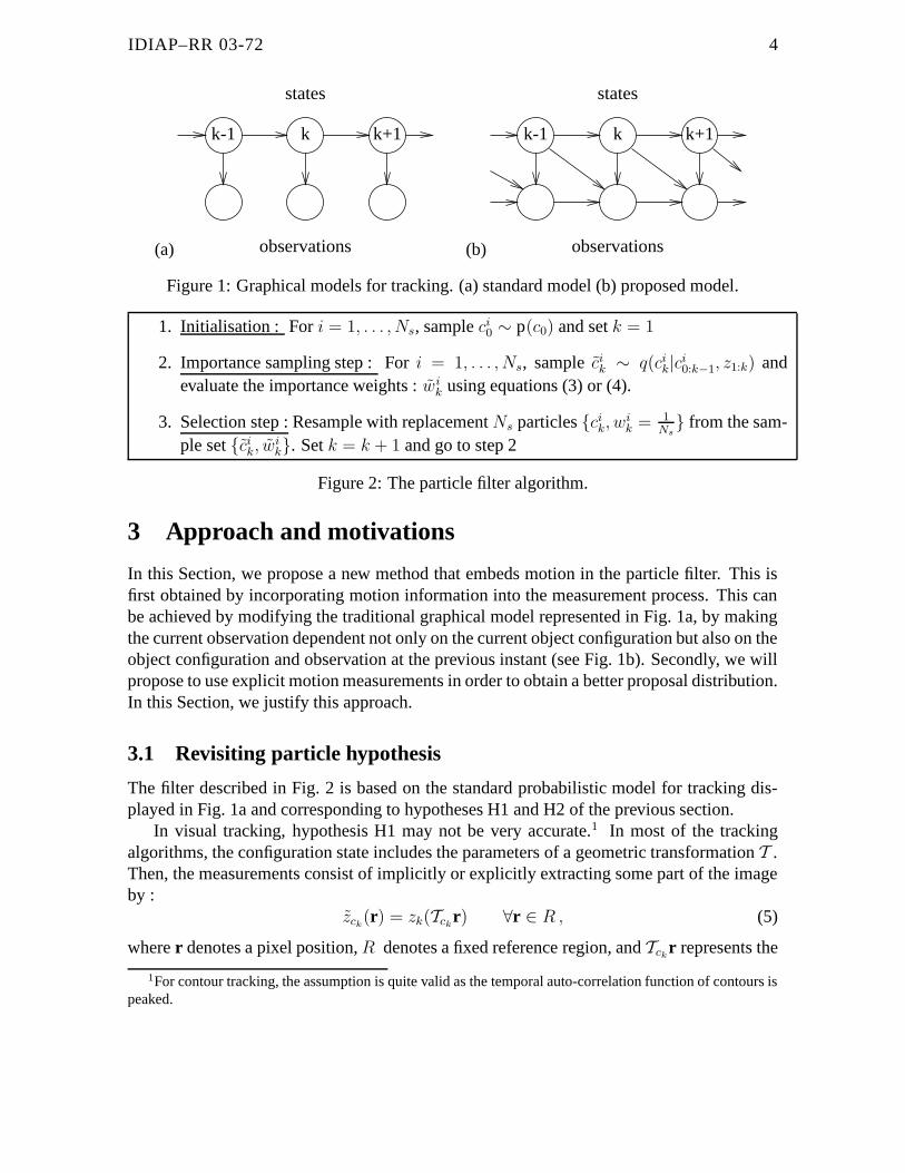
Figure 1: Graphical models for tracking. (a) standard model (b) proposed model.

1. Initialisation : For i = 1, . . . , Ns, sample ci0 ∼ p(c0) and set k = 1

2. Importance sampling step : For i = 1, . . . , Ns, sample cik ∼ q(ci

k|ci0:k−1, z1:k) and

evaluate the importance weights : wik using equations (3) or (4).

3. Selection step : Resample with replacement Ns particles {cik, w

ik = 1

Ns} from the sam-

ple set {cik, w

ik}. Set k = k + 1 and go to step 2

Figure 2: The particle filter algorithm.

3 Approach and motivations

In this Section, we propose a new method that embeds motion in the particle filter. This isfirst obtained by incorporating motion information into the measurement process. This canbe achieved by modifying the traditional graphical model represented in Fig. 1a, by makingthe current observation dependent not only on the current object configuration but also on theobject configuration and observation at the previous instant (see Fig. 1b). Secondly, we willpropose to use explicit motion measurements in order to obtain a better proposal distribution.In this Section, we justify this approach.

3.1 Revisiting particle hypothesis

The filter described in Fig. 2 is based on the standard probabilistic model for tracking dis-played in Fig. 1a and corresponding to hypotheses H1 and H2 of the previous section.

In visual tracking, hypothesis H1 may not be very accurate.1 In most of the trackingalgorithms, the configuration state includes the parameters of a geometric transformation T .Then, the measurements consist of implicitly or explicitly extracting some part of the imageby :

zck(r) = zk(Tck

r) ∀r ∈ R , (5)

where r denotes a pixel position, R denotes a fixed reference region, and Tckr represents the

1For contour tracking, the assumption is quite valid as the temporal auto-correlation function of contours ispeaked.

IDIAP–RR 03-72 5

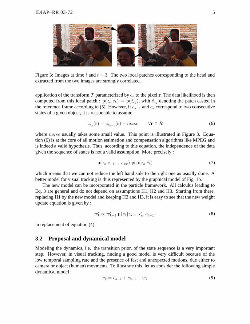
Figure 3: Images at time t and t + 3. The two local patches corresponding to the head andextracted from the two images are strongly correlated.

application of the transform T parameterized by ck to the pixel r. The data likelihood is thencomputed from this local patch : p(zk|ck) = p(zck

), with zckdenoting the patch casted in

the reference frame according to (5). However, if ck−1 and ck correspond to two consecutivestates of a given object, it is reasonable to assume :

zck(r) = zck−1

(r) + noise ∀r ∈ R (6)

where noise usually takes some small value. This point is illustrated in Figure 3. Equa-tion (6) is at the core of all motion estimation and compensation algorithms like MPEG andis indeed a valid hypothesis. Thus, according to this equation, the independence of the datagiven the sequence of states is not a valid assumption. More precisely :

p(zk|z1:k−1, c1:k) 6= p(zk|ck) (7)

which means that we can not reduce the left hand side to the right one as usually done. Abetter model for visual tracking is thus represented by the graphical model of Fig. 1b.

The new model can be incorporated in the particle framework. All calculus leading toEq. 3 are general and do not depend on assumptions H1, H2 and H3. Starting from there,replacing H1 by the new model and keeping H2 and H3, it is easy to see that the new weightupdate equation is given by :

wik ∝ wi

k−1 p(zk|zk−1, cik, c

ik−1) (8)

in replacement of equation (4).

3.2 Proposal and dynamical model

Modeling the dynamics, i.e. the transition prior, of the state sequence is a very importantstep. However, in visual tracking, finding a good model is very difficult because of thelow temporal sampling rate and the presence of fast and unexpected motions, due either tocamera or object (human) movments. To illustrate this, let us consider the following simpledynamical model :

ck = ck−1 + ck−1 + wk (9)

IDIAP–RR 03-72 6

where c denotes the state derivative and models the evolution of the state. As state, considerthe horizontal position of the head of the sequence in Fig. 8. We manually ground-truthed thehead position in 200 images of this sequence. Fig. 4a reports the prediction error w calculatedusing ground-truth data and obtained by estimating c with a simple auto-regressive model :

ck−1 = ck−1 − ck−2 (10)

As can be seen, this prediction is noisy. Furthermore, there are large peak errors (up to30% of the head width). To cope with these peaks, the noise variance in the dynamics,used as proposal distribution, has to be set to a large enough value, with the downside thatmany particles are wasted in low likelihood areas, or spread on local distractors that canultimately lead to tracking failure. On the other hand, exploiting the inter-frame motion toestimate c and predict the new state value (using the coefficient of a robustly estimated affinemotion model, see Section 4.2) can lead to a reduction of both the noise variance and of theerror peaks (Fig. 4b).There is another advantage of using image-based motion estimates. Let us first note thatthe previous state values (here ck−1, ck−2) used to predict the new state value ck are affectedby noise, due to measurement errors and uncertainty. Thus, in the standard AR approach,both the state ck−1 and state derivative ck−1 in Eq. 9 are affected by this noise, resulting inlarge errors (Fig. 4c). When using the inter-frame motion estimates, the estimation of c isalmost not affected by noise (whose effect is to slightly modify the support region used toestimate the motion), as illustrated in Fig. 5, resulting again in a lower noise variance process(Fig. 4d).

Thus, despite needing more computation resources, inter-frame motion estimates areusually more precise than auto-regressive models to predict new state values of geometrictransformation parameters; as a consequence, they are a better choice when designing a pro-posal function. This observation is supported by experiments on other parameters -verticalposition, scale- and on other sequences.

4 The proposed model

In this Section, we describe more precisely the implementation of our method.

4.1 Object representation and state space

We follow an image-based standard approach, where the object is represented by a regionR subject to some valid geometric transformation, and is characterized by a shape. For geo-metric transformations, we have chosen a subspace of the affine transformations comprisinga translation T, a scaling factor s, and an aspect ratio e :

Tαr =

(Tx + xsx

Ty + ysy

), (11)

IDIAP–RR 03-72 7

a) 0 50 100 150 200−15

−10

−5

0

5

10

15prediction error (using AR model)

time

x po

sitio

n

b) 0 50 100 150 200−15

−10

−5

0

5

10

15prediction error (using image−based motion)

time

x po

sitio

nc) 0 50 100 150 200

−15

−10

−5

0

5

10

15prediction error (using AR model)

time

x po

sitio

n

d) 0 50 100 150 200−15

−10

−5

0

5

10

15prediction error (using image−based motion)

timex

posi

tion

Figure 4: a) Prediction error of the x position, when using an AR2 model (σw=2.7). b)Prediction error, but exploiting the inter-frame motion estimation (σw=0.83). c) and d), sameas a) b) but now adding a random gaussian noise (stdev=2 pixels) on the x measurementsused for the prediction. In the AR2 model (Fig. c) both the previous state and state derivativeestimates are affected by noise (σw=5.6), while with visual-motion (Fig. d) the noise onlyaffects the previous measurement (σw=2.3).

where r = (x, y) denotes a point position in the reference frame, α = (T, s, e), and :{

s = sx+sy

2

e = sx

sy

and

{sx = 2es

1+e

sy = 2s1+e

(12)

A state is then defined as ck = (αk, αk−1).

4.2 Proposal distribution

As mentionned in the previous Section, we use inter-frame motion estimates to predict thenew state values. More precisely, an affine displacement model ~dΘ parameterized by Θ =(ai), i = 1..6 is computed using a gradient-based robust estimation method described in[10]2. ~dΘ is defined by:

~dΘ(r) =

(a1 + a2x + a3y

a4 + a5x + a6y

), r = (x, y) , (13)

2We use the code available at http://www.irisa.fr/vista

IDIAP–RR 03-72 8

50 100 150 200 250 300 350

50

100

150

200

250

50 100 150 200 250 300 350

50

100

150

200

250

Figure 5: Example of motion estimates between two images from noisy states. The 3 ellipsescorrespond to different state values. Although the estimation support regions only cover partof the head and enclose textured background, the head motion estimate is still good.

This method takes advantage of a multiresolution framework and an incremental schemebased on the Gauss-Newton method. It minimizes an M-estimator criterion to ensure thegoal of robustness, as follows :

Θ(ck) = argminΘ

∑

r∈R(ck)

ρ (DFDΘ(r))

with DFDΘ(r) = zk+1(r + ~dΘ(r)) − zk(r) , (14)

where zk and zk+1 are the images, and ρ(x) is a robust estimator (bounded for high valuesof x). Owing to the robustness of the estimator, an imprecise region definition R(ck) dueto a noisy state value does not sensibly affect the estimation (see Fig. 5). Moreover, thealgorithm delivers the covariance matrix of the affine parameters. From these estimates, wecan construct an estimate αk of the variation of the coefficients between the two instant,

with their variance Λk. For instance, assuming that coordinates in Eq. 13 are expressed withrespect to the current object center (located at T in the image), we have for the derivativeestimates :

{Tx = a1

Ty = a4and

{sx = a2sx

sy = a6sy

and

{s = s

1+e(a2e + a6)

e = e(a2 − a6)(15)

Denoting the predicted value αk+1 = αk + αk, and assuming the noise on the estimate αk

independent of the noise process w (see Eq. 9), we define the proposal distribution to beused in Equation 3 as :

q(ck+1|c0:k, z1:k+1) ∝ N (αk+1; αk+1, Λk+1) (16)

where N (.; µ, Λ) represents a gaussian distribution with mean µ and Λ variance, and Λk+1 =Λk + Λwp

, Λwpbeing the variance of the process noise wp.

IDIAP–RR 03-72 9

4.3 Dynamics definition

To model the prior, we use a standard second order auto-regressive model (cf Eq. 10) foreach of the components of α. However, to account for outliers (i.e. unexpected and abruptchanges) and reduce the sensitivity of the prior in the tail, we model the noise process with aCauchy distribution ρc(x, σ2) = σ

π(x2+σ2). This leads to :

p(ck+1|ck) =

4∏

j=1

ρc

(αk+1,j − (2αk,j − αk−1,j), σw

2d,j)

). (17)

where σw2d,j denotes the dynamics noise variance of the j th component.

4.4 Data likelihood modeling

To implement the new particle filter, we considered the following data likelihood :

p(zk|zk−1, ck, ck−1) = pc(zk|zk−1, ck, ck−1) × po(zk|ck) (18)

where the first probability pc() models the correlation between the two observations and po()is an object likelihood. This choice decouples the model of the dependency existing betweentwo images, whose implicit goal is to ensure that the object trajectory follows the opticalflow field implied by the sequence of images, from the shape or appearence object model.We assumed that these two terms are independent. When the object is modeled by a shape,this assumption is valid since shape measurement will mainly involve measurements on theborder of the object, while the correlation term will apply to the regions inside the object.

Object shape observation model

The observation model assumes that objects are embedded in clutter. Edge-based measure-ments are computed along L normal lines to a hypothesized contour, resulting for each linel in a vector of candidate positions {ν l

m} relative to a point lying on the contour ν l0. With

some usual assumptions [4], the shape likelihood po(zk|ck) = psh(zk|ck) can be expressed as

psh(zk|ck) ∝L∏

l=1

max

(K, exp(−

‖νlm − νl

0‖2

2σ2)

), (19)

where ν lm is the nearest edge on l, and K is a constant used when no edges are detected.

Image correlation measurement

We model this term in the following way :

pc(zk|zk−1, ck, ck−1) ∝ pc1(αk, αk)pc2(zck, zck−1

) (20)

with :

IDIAP–RR 03-72 10

pc1(αk, αk) ∝ N (αk; αk, Λk) (21)

pc2(zck, zck−1

) ∝ exp−λcdc(zck,zck−1

) (22)

where dc denotes a distance between two image patches. The first probability term in thisexpression compares the parameter values predicted using the estimated motion with thesampled values. This term assumes a Gaussian noise process in parameter space. Thisassumption, however, is only valid around the predicted value. Thus, to introduce a non-Gaussian modeling, we use a second term that compares directly the patches around ck andck−1 using the similarity distance dc. Its purpose can be illustrated using Fig. 5. While allthe three predicted configurations will be weighted equally from pc1 (assuming their esti-mated variance are approximately the same), the second term pc2 will downweight the twopredictions whose corresponding support region is covering part of the background which isundergoing a different motion than the head.

The definition of pc2 requires the specification of a patch distance. Many such distanceshave been defined and used in the literature [15, 17]. The choice of the distance should takeinto account the followings considerations :

1. the distance should still model the underlying motion content, i.e. the distance shouldincrease as the error in the predicted configuration grows;

2. the random nature of the prediction process in the SMC filtering will rarely produceconfigurations corresponding to exact matches(this is particularly true when using asmall number of samples);

3. particles covering both background and object undergoing different motion shouldhave a low likelihood.

For these purposes, we found out that it was preferable not to use robust norms such as L1saturated distance or a Haussdorf distance [17]. Additionnaly, we needed to avoid distanceswhich might a priori favor patches with specific contents. This is the case for instance ofthe L2 distance (which corresponds to an additive Gaussian noise model in Eq.(6)), whichwill generally provide lower scores for patches with large uniform areas. Thus, to avoid thiseffect, we used the normalized-cross correlation coefficient defined as :

dc(z1, z2) =

∑r∈R (z1(r) − ¯z1) · (z2(r) − ¯z2)√

Var(z1)√

Var(z2)(23)

where ¯z1 represents the mean of z1. Regarding the above equation, it is important to againemphasize that the method is not performing template matching, as in [15]. No object tem-plate is learned off-line or defined at the begining of the sequence, and the tracker does notmaintain a single template object representation at each instant of the sequence. Thus, thecorrelation term is not object specific (except through the definition of the reference regionR). A particle “lying” on the background would thus receive a high weight if the predicted

IDIAP–RR 03-72 11

motion is in adequation with background motion. Nevertheless, the methodology could bethe extended to be more object dependent, by allowing the region R to vary over time (usingexamplars for instance).

5 Results

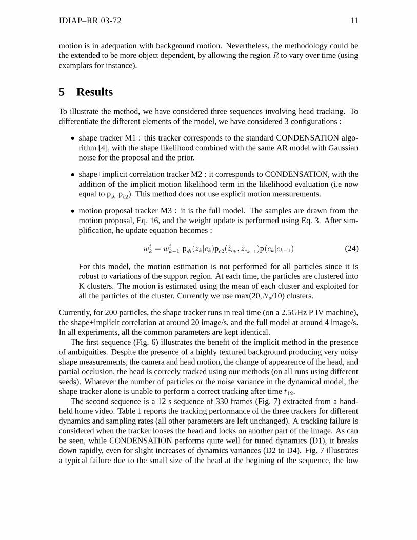
To illustrate the method, we have considered three sequences involving head tracking. Todifferentiate the different elements of the model, we have considered 3 configurations :

• shape tracker M1 : this tracker corresponds to the standard CONDENSATION algo-rithm [4], with the shape likelihood combined with the same AR model with Gaussiannoise for the proposal and the prior.

• shape+implicit correlation tracker M2 : it corresponds to CONDENSATION, with theaddition of the implicit motion likelihood term in the likelihood evaluation (i.e nowequal to psh.pc2). This method does not use explicit motion measurements.

• motion proposal tracker M3 : it is the full model. The samples are drawn from themotion proposal, Eq. 16, and the weight update is performed using Eq. 3. After sim-plification, he update equation becomes :

wik = wi

k−1 psh(zk|ck)pc2(zck, zck−1

)p(ck|ck−1) (24)

For this model, the motion estimation is not performed for all particles since it isrobust to variations of the support region. At each time, the particles are clustered intoK clusters. The motion is estimated using the mean of each cluster and exploited forall the particles of the cluster. Currently we use max(20,Ns/10) clusters.

Currently, for 200 particles, the shape tracker runs in real time (on a 2.5GHz P IV machine),the shape+implicit correlation at around 20 image/s, and the full model at around 4 image/s.In all experiments, all the common parameters are kept identical.

The first sequence (Fig. 6) illustrates the benefit of the implicit method in the presenceof ambiguities. Despite the presence of a highly textured background producing very noisyshape measurements, the camera and head motion, the change of appearence of the head, andpartial occlusion, the head is correcly tracked using our methods (on all runs using differentseeds). Whatever the number of particles or the noise variance in the dynamical model, theshape tracker alone is unable to perform a correct tracking after time t12.

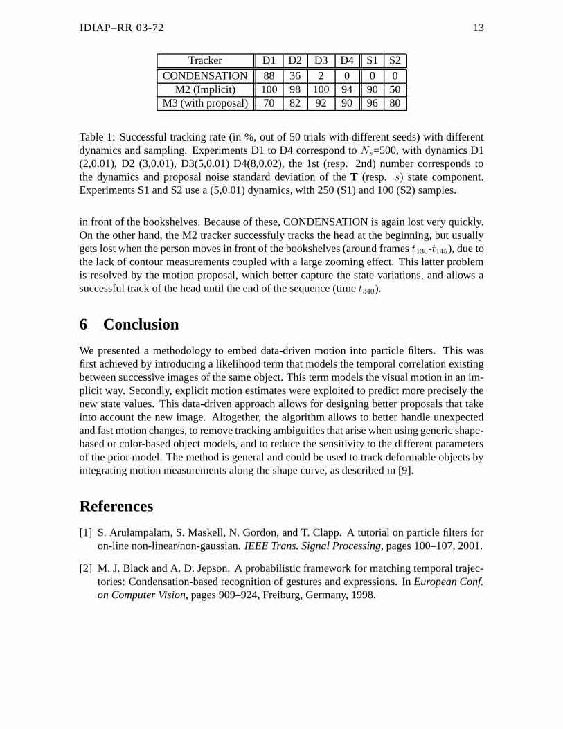
The second sequence is a 12 s sequence of 330 frames (Fig. 7) extracted from a hand-held home video. Table 1 reports the tracking performance of the three trackers for differentdynamics and sampling rates (all other parameters are left unchanged). A tracking failure isconsidered when the tracker looses the head and locks on another part of the image. As canbe seen, while CONDENSATION performs quite well for tuned dynamics (D1), it breaksdown rapidly, even for slight increases of dynamics variances (D2 to D4). Fig. 7 illustratesa typical failure due to the small size of the head at the begining of the sequence, the low

IDIAP–RR 03-72 12

t9 t11

t13 t15

t1 t15

t39 t63

Figure 6: Head tracking 1 : 2 first rows : shape tracker only (CONDENSATION). 2 lastrows : shape+implicit correlation (Ns=100). Same performance with the motion proposaltracker.

contrast at the left of the head, and the clutter. On the other hand, the implicit tracker M2performs well under almost all circumstances, showing its robustness against clutter, partialmeasurements (around time t250 and partial occlusion (end of the sequence). Only when thenumber of samples is low (100 in S2) does the tracker fail. These failures are occuring atdifferent parts of the sequence. Finally, in all experiments, the M3 tracker produces a correcttracking rate equal to 98%, even with a small number of samples, up to the partial occlusion.At this part of the sequence, as the occlusion reaches 50% of the tracked head, the motionestimation sometimes lock onto the woman’s head motion, leading to the reported trackerfailures.

The last sequence (Fig. 8) illustrates more clearly the benefit of using the motion pro-posal. This 24s sequence acquired at 12 frame/s is specially difficult because of the oc-curence of several head turns3 and abrupt motion changes (translations, zooms in and out),the large variations of scale, and importantly, the absence of head contours as the head moves

3The head turn is indeed a difficult case for the new method, as in the extreme case, the motion inside thehead region indicates a right (or left) movement while the head outline remains static.

IDIAP–RR 03-72 13

Tracker D1 D2 D3 D4 S1 S2

CONDENSATION 88 36 2 0 0 0M2 (Implicit) 100 98 100 94 90 50

M3 (with proposal) 70 82 92 90 96 80

Table 1: Successful tracking rate (in %, out of 50 trials with different seeds) with differentdynamics and sampling. Experiments D1 to D4 correspond to Ns=500, with dynamics D1(2,0.01), D2 (3,0.01), D3(5,0.01) D4(8,0.02), the 1st (resp. 2nd) number corresponds tothe dynamics and proposal noise standard deviation of the T (resp. s) state component.Experiments S1 and S2 use a (5,0.01) dynamics, with 250 (S1) and 100 (S2) samples.

in front of the bookshelves. Because of these, CONDENSATION is again lost very quickly.On the other hand, the M2 tracker successfuly tracks the head at the beginning, but usuallygets lost when the person moves in front of the bookshelves (around frames t130-t145), due tothe lack of contour measurements coupled with a large zooming effect. This latter problemis resolved by the motion proposal, which better capture the state variations, and allows asuccessful track of the head until the end of the sequence (time t340).

6 Conclusion

We presented a methodology to embed data-driven motion into particle filters. This wasfirst achieved by introducing a likelihood term that models the temporal correlation existingbetween successive images of the same object. This term models the visual motion in an im-plicit way. Secondly, explicit motion estimates were exploited to predict more precisely thenew state values. This data-driven approach allows for designing better proposals that takeinto account the new image. Altogether, the algorithm allows to better handle unexpectedand fast motion changes, to remove tracking ambiguities that arise when using generic shape-based or color-based object models, and to reduce the sensitivity to the different parametersof the prior model. The method is general and could be used to track deformable objects byintegrating motion measurements along the shape curve, as described in [9].

References

[1] S. Arulampalam, S. Maskell, N. Gordon, and T. Clapp. A tutorial on particle filters foron-line non-linear/non-gaussian. IEEE Trans. Signal Processing, pages 100–107, 2001.

[2] M. J. Black and A. D. Jepson. A probabilistic framework for matching temporal trajec-tories: Condensation-based recognition of gestures and expressions. In European Conf.on Computer Vision, pages 909–924, Freiburg, Germany, 1998.

IDIAP–RR 03-72 14

Figure 7: Head tracking 2 : top row : shape tracker only (CONDENSATION) at initial timet861 and t868 (Ns=500). After a few frame, the tracker diverge. Two last rows : shape+implicitcorrelation (Ns=200) at time t880, t920, t1025, t1110, t1155, t1165. In red, mean shape. In yellow,highly likely particles. Same performance with the motion proposal tracker.

[3] D. Gatica-Perez, G. Lathoud, I. McCowan and J.-M. Odobez A Mixed-State I-ParticleFilter for Multi-Camera Speaker Tracking In IEEE WOMTEC, Nice, France, 2003.

[4] Andrew Blake and Michael Isard. Active Contours. Springer, 1998.

[5] D. Comaniciu, V. Ramesh, and P. Meer. Real-time tracking of non-rigid objects usingmean shift. In CVPR, pp 142–151, 2000.

[6] A. Doucet, N. de Freitas, and N. Gordon. Sequential Monte Carlo Methods in Practice.Springer-Verlag, 2001.

[7] M. Isard and A. Blake. ICONDENSATION : Unifying low-level and high-level trackingin a stochastic framework In 5th ECCV, pp 893-908, 1998.

[8] M. Isard and A. Blake. A mixed-state CONDENSATION tracker with automatic model-switching. In ICCV, pp 107–112, 1998.

[9] C. Kervrann, F. Heitz and P. Pérez Statistical model-based estimation and tracking ofnon-rigid motion In 13th Int. Conf. Pattern Recognition, pp 244-248, 1996.

IDIAP–RR 03-72 15

Figure 8: Tracker with motion proposal (Ns=1000) at time t2, t40, t85, t100, t130, t145, t170,t195, and t210 . In red, mean shape; in green, mode shape; in yellow, likely particles.

[10] J.-M. Odobez and P. Bouthemy Robust multiresolution estimation of parametric mo-tion models In Jl of Visual Com. and Image Representation, vol 6, num. 4, pp 348-365,1995.

[11] P. Pérez, C. Hue, J. Vermaak, and M. Gangnet. Color-based probabilistic tracking. InEur. Conf. on Computer Vision, ECCV’2002, LNCS 2350, pp 661–675, June 2002.

[12] M.K. Pitt and N. Shephard. Filtering via Simulation: Auxiliary Particle Filters InJournal of the American Statistical Association, pp 590–599, vol. 94, num. 446, 1999.

[13] Y. Raja, S. McKenna, and S. Gong. Colour model selection and adaptation in dynamicscenes. In 5th European Conference on Computer Vision, pp 460–474, 1998.

[14] Y. Rui and Y. Chen. Better proposal distribution: object tracking using unscentedparticle filter In CVPR, pp 486–793, dec. 2001.

[15] J. Sullivan and Rittscher J. Guiding random particles by deterministic search. In ICCV,pp 323–330, 2001.

IDIAP–RR 03-72 16

[16] Hai Tao, Harpreet S. Sawhney, and Rakesh Kumar. Object tracking with bayesianestimation of dynamic layer representations. IEEE PAMI, 24(1):75–89, 2001.

[17] K. Toyama and A. Blake. Probabilistic tracking in a metric space. In Proc. 8th Int.Conf. Computer Vision, 2001.

[18] Y. Wu and T. Huang. A co-inference approach for robust visual tracking. In Proc. 8th

Int. Conf. Computer Vision, 2001.