Elementary Statistics - Satya Mandal
277
-
Upload
khangminh22 -
Category
Documents
-
view
1 -
download
0
Transcript of Elementary Statistics - Satya Mandal


Elementary Statistics
Satya MandalUniversity of Kansas, Lawrence, Kansas 66045
28 January 2021

ii

Contents
1 The Language and Terminology 1
1.1 Introduction . . . . . . . . . . . . . . . . . . . . . . . . . . . . . . . . . . . 1
1.2 Basic Definitions and Concepts . . . . . . . . . . . . . . . . . . . . . . . . 3
1.2.1 Population and Sample . . . . . . . . . . . . . . . . . . . . . . . . . 4
1.2.2 Parameters and Statistics . . . . . . . . . . . . . . . . . . . . . . . 5
1.2.3 Frequency Distribution . . . . . . . . . . . . . . . . . . . . . . . . . 5
1.2.4 Ungrouped Data . . . . . . . . . . . . . . . . . . . . . . . . . . . . 6
1.2.5 Grouped Data . . . . . . . . . . . . . . . . . . . . . . . . . . . . . . 7
1.2.6 Use of Calculators . . . . . . . . . . . . . . . . . . . . . . . . . . . 9
1.2.7 Problems on Frequency Distribution . . . . . . . . . . . . . . . . . 10
1.3 Pictorial Representation of Data . . . . . . . . . . . . . . . . . . . . . . . . 13
1.3.1 More Histograms . . . . . . . . . . . . . . . . . . . . . . . . . . . . 14
1.3.2 The Cumulative Frequency Distributions and Ogive . . . . . . . . . 19
2 Measures of Central Tendency and of Dispersion 21
2.1 Measure of Central Tendency: Mean . . . . . . . . . . . . . . . . . . . . . 21
2.1.1 Other Measures of Central Tendency: Median, and Mode . . . . . . 23
2.1.2 Problems on Mean and Median . . . . . . . . . . . . . . . . . . . . 25
2.2 Measures of Dispersion . . . . . . . . . . . . . . . . . . . . . . . . . . . . . 26
2.2.1 Application of Standard deviation . . . . . . . . . . . . . . . . . . . 28
2.2.2 Use of the Frequency Table . . . . . . . . . . . . . . . . . . . . . . 33
2.2.3 Problems on Variance, Standard Deviation . . . . . . . . . . . . . . 36
iii

iv CONTENTS
3 Probability 39
3.1 Introduction . . . . . . . . . . . . . . . . . . . . . . . . . . . . . . . . . . . 39
3.1.1 Basic Concept of Probability . . . . . . . . . . . . . . . . . . . . . . 40
3.1.2 Basic Set theoretic Definitions . . . . . . . . . . . . . . . . . . . . . 43
3.1.3 Statistical Experiments and Sample Space . . . . . . . . . . . . . . 44
3.1.4 The Definition of Probability . . . . . . . . . . . . . . . . . . . . . 47
3.2 Probability Tables and Equally Likely . . . . . . . . . . . . . . . . . . . . . 48
3.2.1 Problems: on Tabular probability . . . . . . . . . . . . . . . . . . . 48
3.2.2 Problems: on Equally Likely model . . . . . . . . . . . . . . . . . . 52
3.3 Laws of Probability . . . . . . . . . . . . . . . . . . . . . . . . . . . . . . . 55
3.3.1 Laws of Probability . . . . . . . . . . . . . . . . . . . . . . . . . . . 56
3.3.2 Problems: on Laws of Probability . . . . . . . . . . . . . . . . . . . 57
3.4 Counting Techniques and Probability . . . . . . . . . . . . . . . . . . . . . 61
3.4.1 Problems: Counting Techniques and Probability . . . . . . . . . . . 66
3.5 Conditional Probability and Independent Events . . . . . . . . . . . . . . . 70
3.5.1 Independent Events . . . . . . . . . . . . . . . . . . . . . . . . . . . 71
3.5.2 Problems: Conditional Probability and Independent Events . . . . . 72
4 Random Variables 79
4.1 Random Variables . . . . . . . . . . . . . . . . . . . . . . . . . . . . . . . . 79
4.2 Probability Distribution . . . . . . . . . . . . . . . . . . . . . . . . . . . . 82
4.2.1 Problems: on Probability Distribution . . . . . . . . . . . . . . . . 84
4.3 The Bernoulli and Binomial Experiments . . . . . . . . . . . . . . . . . . . 87
4.3.1 Binomial Random Variable . . . . . . . . . . . . . . . . . . . . . . . 87
4.3.2 Use TI-84: to compute B(n, p)-probabality . . . . . . . . . . . . . 89
4.3.3 Problems: on Binomial Experiments . . . . . . . . . . . . . . . . . 90
5 Continuous Random Variables 97
5.1 Probability Density Function (pdf) . . . . . . . . . . . . . . . . . . . . . . 97
5.1.1 The Mean, Variance and Standard Deviation . . . . . . . . . . . . . 101
5.1.2 Examples of Continuous random (read only) . . . . . . . . . . . . . 102
5.2 The Normal Random Variable . . . . . . . . . . . . . . . . . . . . . . . . . 108
5.2.1 Problems: on X ∼ N(µ, σ) . . . . . . . . . . . . . . . . . . . . . . . 111

CONTENTS v
5.2.2 Inverse Probability (Cut-Off Values) . . . . . . . . . . . . . . . . . 116
5.2.3 Problems on Cut-off values . . . . . . . . . . . . . . . . . . . . . . . 117
5.3 Normal Approximation to Binomial . . . . . . . . . . . . . . . . . . . . . . 122
5.3.1 Problems: On Normal Approximation of B(n, p) . . . . . . . . . . . 124
6 Elements of Sampling Distribution 129
6.1 Sampling Distribution . . . . . . . . . . . . . . . . . . . . . . . . . . . . . 129
6.1.1 Sampling Types . . . . . . . . . . . . . . . . . . . . . . . . . . . . . 130
6.1.2 Properties . . . . . . . . . . . . . . . . . . . . . . . . . . . . . . . . 131
6.2 Central Limit Theorem . . . . . . . . . . . . . . . . . . . . . . . . . . . . . 132
6.2.1 Problems: on Central Limit Theorem . . . . . . . . . . . . . . . . . 132
6.3 Sampling Distribution of the Sample Proportion . . . . . . . . . . . . . . . 136
6.3.1 Problems: on Sample Proportion . . . . . . . . . . . . . . . . . . . 138
7 Estimation 143
7.1 Point and Interval Estimation . . . . . . . . . . . . . . . . . . . . . . . . . 144
7.1.1 Criterion for Good Estimators (read only) . . . . . . . . . . . . . . . 144
7.1.2 Interval Estimation . . . . . . . . . . . . . . . . . . . . . . . . . . . 145
7.1.3 Procedure to Construct Confidence Interval . . . . . . . . . . . . . 146
7.1.4 Problems: on Z-intervals for µ . . . . . . . . . . . . . . . . . . . . . 148
7.2 Confidence interval for mean µ when σ is Unknown . . . . . . . . . . . . . 155
7.2.1 Student’s t distribution . . . . . . . . . . . . . . . . . . . . . . . . . 155
7.2.2 The T -Interval for µ . . . . . . . . . . . . . . . . . . . . . . . . . . 157
7.2.3 Problems: On T -intervals for mean . . . . . . . . . . . . . . . . . . 159
7.3 Confidence Interval for p . . . . . . . . . . . . . . . . . . . . . . . . . . . . 165
7.3.1 Problems: One proportion Z-interval . . . . . . . . . . . . . . . . . 168
7.4 Confidence Interval of the Variance σ2 . . . . . . . . . . . . . . . . . . . . 174
7.4.1 χ2-random variable . . . . . . . . . . . . . . . . . . . . . . . . . . . 175
7.4.2 The χ2-Interval for σ2 . . . . . . . . . . . . . . . . . . . . . . . . . 177
7.4.3 Problems: On χ2-Interval of σ2 . . . . . . . . . . . . . . . . . . . . 178

vi CONTENTS
8 Comparing Populations 185
8.1 Confidence Interval of µ1 − µ2 . . . . . . . . . . . . . . . . . . . . . . . . . 185
8.1.1 Problems: on Two sample Z-Interval for µ1 − µ2 . . . . . . . . . . . 187
8.2 Two sample T -interval: Unknown σ1, σ2 . . . . . . . . . . . . . . . . . . . 190
8.2.1 Problems: Two sample T -interval . . . . . . . . . . . . . . . . . . . 192
8.3 Comparing Two Population Proportions . . . . . . . . . . . . . . . . . . . 196
8.3.1 Problems: Two proportion Z-interval, for p1 − p2 . . . . . . . . . . 198
9 Significance Test 203
9.1 Introduction and Jargon . . . . . . . . . . . . . . . . . . . . . . . . . . . . 203
9.1.1 Design Decision rules: for µ, when σ is known . . . . . . . . . . . . 205
9.1.2 Problems: Z-Test . . . . . . . . . . . . . . . . . . . . . . . . . . . . 208
9.2 Significance Test for µ: Unknown σ . . . . . . . . . . . . . . . . . . . . . . 217
9.2.1 Problems: T -Test . . . . . . . . . . . . . . . . . . . . . . . . . . . . 219
9.3 Significance Test, for Proportion p . . . . . . . . . . . . . . . . . . . . . . . 226
9.3.1 Problems: One proportion Z-Test . . . . . . . . . . . . . . . . . . . 228
9.4 Testing Hypotheses on Variance σ2 . . . . . . . . . . . . . . . . . . . . . . 233
9.4.1 Problems: on χ2-Test . . . . . . . . . . . . . . . . . . . . . . . . . 234
9.5 Two Populations: Known σ1, σ2 . . . . . . . . . . . . . . . . . . . . . . . . 241
9.5.1 Problems: Two sample Z-Test . . . . . . . . . . . . . . . . . . . . . 243
9.6 Two sample T -Test: Unknown σ1, σ2 . . . . . . . . . . . . . . . . . . . . . 249
9.6.1 Problems: Two sample T -Test . . . . . . . . . . . . . . . . . . . . . 252
9.7 Two Populations: Two Proportions p1, p2 . . . . . . . . . . . . . . . . . . 259
9.7.1 Problems: Two proportion Z-test . . . . . . . . . . . . . . . . . . . 262
9.8 Paired T -test (read only) . . . . . . . . . . . . . . . . . . . . . . . . . . . . 267

Chapter 1
The Language and Terminology
1.1 Introduction
Most people understand that statistics is the study of the numerical features of a sub-ject/population. Understanding of the statisticians would not be much different. A statis-tician would only emphasize on how they do it, in addition. Some statisticians woulddefine statistics as the scientific and mathematical study of the methods of collecting data,summarizing and presenting data, and drawing inferences from data.
American Statistical Association defines statistics follows(https://www.amstat.org/asa/what-is-statistics.aspx): Statistics is the scientific applica-tion of mathematical principles to the collection, analysis, and presentation of numericaldata. Statisticians contribute to scientific enquiry by applying their mathematical and sta-tistical knowledge to the design of surveys and experiments; the collection, processing, andanalysis of data; and the interpretation of the results.
The goal of this course is to learn some commonly used methods to use collectedsample data to draw inferences about a population and the mathematical basis behindsuch methods. The following is an example.
Example. Suppose you want to estimate the mean (average) weight of the fish polulationin the nearest lake. The mean weight is a charecteristic of the whole fish population in thelake. To estimate it, you catch a small sample of fish from the lake. Then compute themean weight of the sample, to be called the sample mean. Then, declair that this samplemean is an estimate of the mean weight of the whole population (also called the populationmean).
Another point about the nature of statistics as a science is that it is not a deter-ministic science. It does not have laws like force is equal to mass times acceleration.Statements in statistics come with a probability (i.e., quantified chance) of being correct.When a weatherman says that it will rain today he means that there is, say, a ninety fivepercent chance that it will rain today. Roughly, this means that if he makes the same
1

2 CHAPTER 1. THE LANGUAGE AND TERMINOLOGY
prediction one hundred times he will be correct 95 times, and it will not rain the other 5days. The problem is that sometimes a weatherman will hide the information that thereis a 95 percent chance only. Such information hiding is sometimes done for simplicity.
Skepticism: Skepticism about statistics is widespread and often justifiably so. It maynot be an overstatement to say that statistics is misused and abused on regular basis.To put it sarcastically, abuse of statistics to generate opinion may already be a brunchof science or sociology based on scientific theory and models. The part that is basedon scientific models may sometimes be ethically wrong, its scientific validity cannot bedenied. Unfortunately, such methods include misleading the public with false data andmisinformation.
On Sunday talk shows pundits and the political opinion makers try to justify opposingpoint of views, sometimes based on data from respectable sources. It would be a fairquestion, how could something be a science when it justifies two opposing point of views?While there is no cure for misleading or incorrect information, sometimes both may bestatistitically correct with emphasis on the different aspects of the statistical inferences.Following is an example.
Example: In December 1998, the House of Representatives impeached President BillClinton. In February 1999, President was acquitted by the Senate. (In impeachment trial,the house works like the prosecutor and the Senate works like the jury. Search internet formore information).
President Clinton was formally charged with perjury and obstruction of justice. In anycase, both stemmed out of allegations of sexual liaison and harassment. During this processof impeachment, there was long political discourse with respect to morality and legalitiesof the whole episode. Following would be typical discussion on TV.
1. Clinton critics would cite data and point out that, according to statistics, the majorityof Americans think that character matters.
2. Clinton sympathizers would cite data and point out, according to statistics, that themajority of Americans think the president is doing a good job.
The implication here is that one of them was "wrong." But the science of statistics says thatboth were correct. Data was collected and analyzed, and it was found that the majorityof Americans think that character matters and that the majority of Americans think thepresident is doing a good job. It does not matter to the science of statistics which one ofthe statistically established facts one would have desired.
Historically, during the early part of development of statistics, skepticism used to be ofdifferent nature. The validity of scientific foundation itself was in question. Statistics wascompared with astrology, because both do predictions regarding unknown. An anecdotefollows. When the proposal to establish the Indian Statistical Institute in Calcutta wasconsidered by the government of India in the early part of the last century, some criticssaid, then why not an institute in astrology?

1.2. BASIC DEFINITIONS AND CONCEPTS 3
At the inception of statistics as a science there was a lot of skepticism about its scientificvalidity. Those days are gone, and statistics is not likened to astrology any more! Statisticsis a well-founded and a precise science. It is a nondeterministic science in nature; it ismade precise by making probabilistic statements only.
Descriptive and Inferential Statistics: In this course we will be talking about twobranches of statistics. The first one is called descriptive statistics which deals with methodsof processing, summarizing, and presenting data. The other part deals with the scientificmethods of drawing inferences and forecasting from the data, and is called inferential orinductive statistics.
Course Organization: The course has nine lessons that can be divided into threeparts:
1. Chapter 1 and 2: Descriptive Statistics. TI-84 (Silver Edition) would be used tosolve problems.
2. Chapter 3, 4, 5, 6: Probability and Mathematical Basis. There is no direct TI-84method for these lessons. However, after explaining the mathematics involved, theDISTR key (menu) of TI-84 (Silver Edition) will be used to compute probability.
3. Chapter 7, 8, 9: Inferential Statistics or Estimation. The goal of this course is todevelop methods to do estimation, which would be accomplished in these lessons.Again, DISTR key (menu) of TI-84 (Silver Edition) will be used heavily.
In the rest of this lesson and the next we deal with descriptive statistics, which include thepresentation of data in the form of tables, graphs, and computations of various averages ofdata.
1.2 Basic Definitions and Concepts
In statistics, we use a small "sample" to make inferences about a "big population". Statis-tics serves a purpose only when we do not have a way to find full or accurate informationabout the whole population. Sometimes, the population is such that it is intrinsically im-possible to find full and accurate information. The same may be the situation because ofthe cost associated with full enumeration. The following are some examples:
1. The mean weight of the fish population in the nearest lake. Realistically, it would beimpossible to catch all the fish in the lake, measure them and find the mean weight.
2. You are a quality control inspector in a lamp factory. To give an idea to the con-sumers, you want to know the mean lifetime (in hours) of the lamps produced. Thereis no way you can measure the mean before you sell.
3. The mean annual expenditure (in year 2011) of the KU student population.

4 CHAPTER 1. THE LANGUAGE AND TERMINOLOGY
4. Remark. In some cases, in spite of existence of full information regarding thewhole population, for cost effectiveness, samples are used to estimate the population.Suppose you want to know the mean GPA of the KU population. Although, KUhas the full information, you may not be able to access the full data and then dothe computations due to the associated cost. So, you may like to be content with asample and the sample mean GPA as an estimate.
5. Remark. Interestingly, advent of computers in abundance caused certain usages ofstatistics obsolete. Thirty years ago, KU used to keep record in papers. Those days,they would have used sample data to avoid dealing with the huge amount of data inpapers.
1.2.1 Population and Sample
Definition 1.2.1. A complete collection of data on the group under study is called thepopulation or the universe. A member of the population is called a sampling unit.Therefore, the population consists of all its sampling units. A Sample is a collection ofsampling units selected from the population.
Most often, we will work with numerical characteristics (like height, weight, and salary)of a group. So usually the population is a large collection of numbers and the sample is asmall subset of the population.
Example. Suppose we are studying the daily rainfall in Lawrence. Since daily rainfallcould be from 0 inches to anything above 0, the population here is all nonnegative numbers(i.e., the interval [0,∞)). A sample from this population would be the observed amountof daily rainfall in Lawrence on some number of days. A sample of size 11 would be theobserved daily rainfall in Lawrence on 11 days.
Definition 1.2.2. A variable is something that varies or changes value. Most often, weconsider numerical variables. Numerical variables are also called quantitative variables.Examples of quantitative variables include height, length, weight, number of typos inbooks, number of credit hours completed by students, number of accidents (or numberof anything) and time. Non-numerical variables are also considered. They are calledqualitative variables. Examples of qualitative variables include blood group and gender.In fact, any genetic property (genotype or phenotype) is a qualitative variable, because theyvary from human to human (or trees to trees).
In Chapter 4, we will have an elaborate discussion on a specific type of variables calledrandom variables, which would be more relevant for our purpose.

1.2. BASIC DEFINITIONS AND CONCEPTS 5
1.2.2 Parameters and Statistics
Definition 1.2.3. 1. Given a set of data, any numerical value computed from the datausing a formula or a rule is called a quantitative measure of the data.
2. A quantitative measure of a population data is called a parameter. In other words,parameters belong to the whole population and are computed (if feasible) from theWHOLE population data. Examples: the average GPA of all KU students, the heightof the tallest student in KU, the average income of the entire KU student population.
One way to study a population is to know some of the parameters of the population.Unfortunately, computing such parameters could be expensive or even impossible. Inpractice, parameters are unknown and the main game of statistics is to try to estimateparameters on the basis of small samples collected from the population.
Definition 1.2.4. A quantitative measure of a sample data is called a statistic. Anyconstant that we compute from a sample is a statistic. We use these statistics to estimatethe parameters of the population. For example, the average height computed from a sampleis a reasonable estimate for the (parameter) average height of the KU student population.Obviously, we do not expect the value of the statistic to be exactly equal to the parametervalue. Hopefully, the error will be small or will exceed our tolerable limit very rarely (sayonce in a 100 trials).
Why do we need a statistic?
Sometimes it will be impossible to know the actual value of a parameter. For example,let µ be the mean length of the life of light bulbs produced by a company. In this case, thecompany cannot test all the bulbs it produces to find a mean length. So, the best that thatwe can do is to we test a few bulbs (the sample), compute the sample mean length x (astatistic) of the life of these bulbs and use x as an estimate for the mean length (parameterµ) of the life for all the bulbs it produces.
1.2.3 Frequency Distribution
In this section we talk about representation of data organized in tabular form. Such arepresentation is called a frequency distribution. We are mostly concerned with numericaldata (i.e., quantitative data), but also consider some non-numerical data (i.e., qualitativedata).

6 CHAPTER 1. THE LANGUAGE AND TERMINOLOGY
Example. The following is data on the blood group of 72 patients in a hospital:
O A O B O A O A A O A O B A O A A OO A O A B B O O AB O A O O A O A O AA A A O A A O AB B O A O B A A A O OO A A B A O O O O A A B O O O A A A
We have four types of blood groups, namely, O,A,B,AB. Each of these blood groups maybe referred to as a "class." The frequency of a class is defined as the number of datamembers that belong to that class. For example, the frequency of the class O is 31; thefrequency of class A is 31. A table that lists the classes and the corresponding frequencyis called the frequency distribution of this qualitative data. Following is the frequencydistribution of this data:
Bloodgroup frequence
O 31A 31B 8AB 2
Total 72
1.2.4 Ungrouped Data
For the quantitative data, we consider two types of frequency table. When we are workingwith a large set of data we group the data set into a few classes and construct a "frequencytable," which we will discuss later.
If the data set contains only a few distinct values then data would not be grouped.We make a list of all the data-values present and give the corresponding frequency foreach data-value in a table. The number of times a data-value appears in the data set iscalled the frequency of the data member. A list that presents the data members andthe corresponding frequency in a tabular form is called a frequency table or frequencydistribution. The relative frequency and percentage frequency of a data memberx are defined as follows:{
relative frequency of x = frequency of xData size
percentage frequency of x = (frequency of x)100Data size
Example 1.1.1 To estimate the mean time taken to complete a three-mile drive by arace car, the race car did several time trials, and the following sample of times taken (inseconds) to complete the laps was collected:
50 48 49 46 54 53 52 51 47 56 52 5151 53 50 49 48 54 53 51 52 54 54 5355 48 51 50 52 49 51 53 55 54 50
Note that there are 35 observations here. So we say that the size of the sample (or data)is 35. Also the values present are 46, 47, 48, 49, 50, 51, 52, 53, 54, 55, 56. Since there

1.2. BASIC DEFINITIONS AND CONCEPTS 7
are only 11 distinct values present we can make a frequency table for the ungrouped data.The following is the frequency distribution of this ungrouped data:
Time relative percentage(in sec) frequency frequency frequency
46 1 1/35 2.8647 1 1/35 2.8648 3 3/35 8.5749 3 3/35 8.5750 4 4/35 11.4351 6 6/35 17.1452 4 4/35 11.4353 5 5/35 14.2954 5 5/35 14.2955 2 2/35 5.7156 1 1/35 2.86
Total 35 1 100
(1.1)
1.2.5 Grouped Data
When we are working with a large set of data that contains too many distinct values,then we group the whole set of data into a few class intervals and give the corresponding"frequency" of the class. When the data is presented in this way, the data is calledgrouped data. The number of data members that fall in a class interval is called theclass frequency and the relative and percentage frequencies are computed by thesame formula as above. A list that gives various class intervals and the correspondingclass frequencies in a tabular form is called a class frequency table or class frequencydistribution of the data. The frequency distribution may also include the relative andpercentage frequencies.
Grouped Data and Loss of Information: Note that when we construct a frequencytable of ungrouped data, there is no loss of information. The original data can be recon-structed from the frequency table of ungrouped data. Only loss would be the order inwhich the original data appeared.
Sometimes it is necessary to group data into class intervals to construct a frequencydistribution. This would be the case when there are too many distinct data-values presentin the data-too many even to fit into a table in a regular size paper for presentation. In suchsituations, we group the data in a few class intervals. While class frequency distributionis very good for presentation and may be convenient for other reasons, we lose a lot ofinformation in this process. There would be no way to recover the original data from theclass frequency distribution.
Steps to Construct Frequency Distribution: To construct a class frequency tableof data-set, the first question would be, how many class intervals should we have? Theanswer is that it should not be too few nor should it be too many. The fewer the number

8 CHAPTER 1. THE LANGUAGE AND TERMINOLOGY
of class intervals, more is the loss of information. In the extreme case, if we use only oneclass interval, all the information would be lost. On the other hand, if we take too many,we will have the problem of having to work with ungrouped data. (In this course we willalways tell you how many classes to take.) Although sometimes it may be necessary totake class intervals of varying width, in this course we only consider classes of equal classwidth. We follow the following steps to construct a class frequency distribution.
1. Range: Pick a suitable number L less than or equal to the smallest value presentin the data. Pick a suitable number H greater than or equal to the highest valuepresent in the data. The range R that we consider is R = H − L.
2. Number of Classes: Decide on a suitable number of classes. (In this course we willtell you the number of classes.)
3. Class Width: We have
class width = w =R
Number of classes
We will pick L,H, and the number of classes so that class width is a "round number."Classes: We divide our interval [L,H] into subintervals, to be called classes, as
[L,L+ w], [L+ w,L+ 2w], [L+ 2w,L+ 3w], · · · , [H − w,H]
4. Frequency: Find the frequency for each of the classes. You can use an advancedcalculator or some software (like Excel) to count frequencies.
An ambiguous situation may arise, when a data-value falls on a class boundary.Depending on the nature of data or otherwise, we would have to follow a consistentconvention whether to count such data members on the left or the right class interval.
A few more important definitions. The above intervals are called class intervals. The wabove is called the class width. The lower end of the class is called lower limit and theupper end of the class is called upper limit. The class mark is the midpoint of the class,defined as follows:
class mark =(lower limit of class) + (upper limit of class)
2
Example 1.2.5. The following is the weight (in ounces), at birth, of a certain number of

1.2. BASIC DEFINITIONS AND CONCEPTS 9
babies.
74 105 124 110 119 137 96 110 120 115 140
65 135 123 129 72 121 117 96 107 80 91
74 123 124 124 134 78 138 106 130 97 145
93 133 128 96 126 124 125 127 62 127 92
95 118 126 94 127 121 117 124 93 135 156
143 125 120 147 138 72 119 89 81 113 91
133 127 138 122 110 113 100 115 110 135 141
97 127 120 110 107 111 126 132 120 108 148
143 103 92 124 150 86 121 98 74 85 99
We construct a class frequency table of this data by dividing the whole range of data intoclass intervals.
Solution: Note that the lowest value is 62 and the highest value is 156. We take L =60, H = 160, so R = H −W = 100. We made such a choice of L and H, precisely so thatR = 100 is a "nice" number. Now we decide to have 5 class intervals and so w = R/5 = 20.According to what I said above, our classes should be :
[60, 80], [80, 100], [100, 120], [120, 140], [140, 160]
But if we do so then there is a risk that some data members (like 80, 100, 120, 140) willfall in two classes. To avoid this we add .5 to all the class boundaries. So, our classes are
[60.5, 80.5], [80.5, 100.5], [100.5, 120.5], [120.5, 140.5], [140.5, 160.5].
So the frequency distribution is as follows:
relative percentageClasses frequency frequency frequency
60.5− 80.5 9 9/99 9.0980.5− 100.5 20 20/99 20.20100.5− 120.5 25 25/99 25.26120.5− 140.5 37 37/99 37.38140.5− 160.5 8 8/99 8.08
Total 99 1 100
(1.2)
1.2.6 Use of Calculators
We would avoid hand computations. We will be using calculators (TI-84) in this course.
1. Entering data in TI-84: let me explain how you enter data in the TI-84.

10 CHAPTER 1. THE LANGUAGE AND TERMINOLOGY
(a) Press the button "stat."(b) Select "Edit" in the Edit menu and enter.(c) You will find a lists named L1, L2, L3, L4, L5, L6.(d) Let’s say you want to enter your data in L1. If L1 has some data, you clear
it by pressing the stat button and selecting ClrList in the Edit menu. ClrListappears then type L1 and hit enter. To type "L1" on your TI-84 simply press2nd then 1.
(e) Once L1 is cleared, you select Edit in the Edit menu and enter.(f) Now type in your data; enter one by one.
2. Sorting and counting frequency: It is not easy to construct a frequency table ofa data set unless you are systematic. Traditionally, we used "tally marks" to countthe frequency. Now you can use some software programs (e.g., Excel). Let me showyou a method, using a calculator (TI-84).
(a) Press "stat."(b) To input data, enter "edit."(c) Enter your data (say in L1).(d) Press "stat."(e) Enter "sortA" L1.(f) Press "stat" and then enter "edit." On L1 you will see that the data is sorted
in an increasing order.(g) Now you can count the frequencies.
1.2.7 Problems on Frequency Distribution
Exercise 1.2.6. Repeat example (1.2.5) with class width 5.
Exercise 1.2.7. The following is the weight (in ounces), at birth, of 96 babies born inLawrence Memorial Hospital in May 2000.
94 105 124 110 119 137 96 110 120 115 119
104 135 123 129 72 121 117 96 107 80 80
96 123 124 124 134 78 138 106 130 97 134
111 133 128 96 126 124 125 127 62 127 96
116 118 126 94 127 121 117 124 93 135 112
120 125 120 147 138 72 119 89 81 113 100
109 127 138 122 110 113 100 115 110 135 120
97 127 120 110 107 111 126 132 120 108 148
133 103 92 124 150 86 121 98
(1.3)

1.2. BASIC DEFINITIONS AND CONCEPTS 11
Construct a class frequency table of this data by dividing the the whole range of data intoclass intervals:
[60.5−70.5], [70.5−80.5], [80.5−90.5], [90.5−100.5], [100.5−110.5], [110.5−120.5], [120.5−130.5], [130.5−140.5], [140.5−150.5]
Exercise 1.2.8. The following are the length (in inches), at birth, of 96 babies born inLawrence Memorial Hospital in May 2000.
18 18.5 19 18.5 19 21 18 19 20 20.5
19 19 21.5 19.5 20 17 20 20 19 20.5
18 18.5 20 19.5 20.75 20 21 18 20.5 20
21 19 20.5 19 20 19.5 17.75 20 19.5 20
20.5 17 21 18.5 20 20 20 18.5 19.5 19
18 20.5 18 20 19 19 19.5 20 20.75 21
17.75 19 18 19 20 18.5 20 19 21 19
19.5 20 20 19 19.5 20 19.5 18.5 20.5 19.5
20.25 20 19.5 19.5 20 20 20 21 20 19
18.5 20.5 21.5 18 19.5 18
Construct a frequency table for this data by dividing the whole range into class intervals:
[16− 17], [17− 18], [18− 19], [19− 20], [20− 21], [21− 22].
Note: If a data member falls on the boundary, count it in the right/upper class-interval.
Exercise 1.2.9. The following data represents the number of typos in a sample of 30books published by some publisher.
156 159 162 160 156 162
159 160 156 156 160 162
156 159 162 156 162 158
160 158 159 162 158 158
162 160 159 162 162 160
Construct a frequency table (by sorting in your calculator).
Exercise 1.2.10. Following is data on the hourly wages (paid only in whole dollars) of 99

12 CHAPTER 1. THE LANGUAGE AND TERMINOLOGY
employees in an industry.
7 11 7 11 10 9 10 10 12 13
7 8 11 11 14 9 7 9 11 7
9 13 12 14 7 8 7 14 15 9
9 7 11 9 12 9 12 11 14 9
12 13 7 9 10 14 11 12 13 7
15 15 16 16 15 16 11 7 18 19
15 16 15 15 16 16 17 16 16 13
15 15 16 15 16 15 15 17 16 12
16 15 15 16 15 15 19 8 16 17
16 16 15 16 16 16 13 12 8
Construct a frequency table (by sorting in your calculator).
Exercise 1.2.11. Following is data on the hourly wages (paid only in whole dollars) in anindustry.
9 11 8 9 10 11 7 10 12 13
7 11 8 11 14 9 10 9 11 7
13 13 14 12 9 8 12 14 15 9
9 7 12 7 12 7 7 11 13 9
11 9 9 9 10 14 11 12 14 7
Construct a frequency table (by sorting in your calculator).

1.3. PICTORIAL REPRESENTATION OF DATA 13
1.3 Pictorial Representation of Data
Another way to represent data is to use pictures and graphs. Such pictorial representa-tions are commonly used in newspapers and other media outlets. Pictorial representationis particularly helpful when you have to represent data to people with limited technicalbackground, like newspaper readers or a governmental or congressional body.
The Pie Chart: The pie chart is a commonly used pictorial representation of data. Whenyou do your tax return every year, you find a few pie charts in the instruction book for form1040. These charts show what proportion/percentage of each tax dollar goes for partic-ular expenses. I reproduced the following pie charts from the 1040 instruction book of 1999.

14 CHAPTER 1. THE LANGUAGE AND TERMINOLOGY
The Histogram Among pictorial representations, the most useful in this course is thehistogram. The histogram of data is the graphical representation of the frequency distri-bution of the data, where we plot the variable on the horizontal axis and above each classinterval, we erect a bar of the height equal to the frequency of the class. Such a histogramis called a frequency histogram.
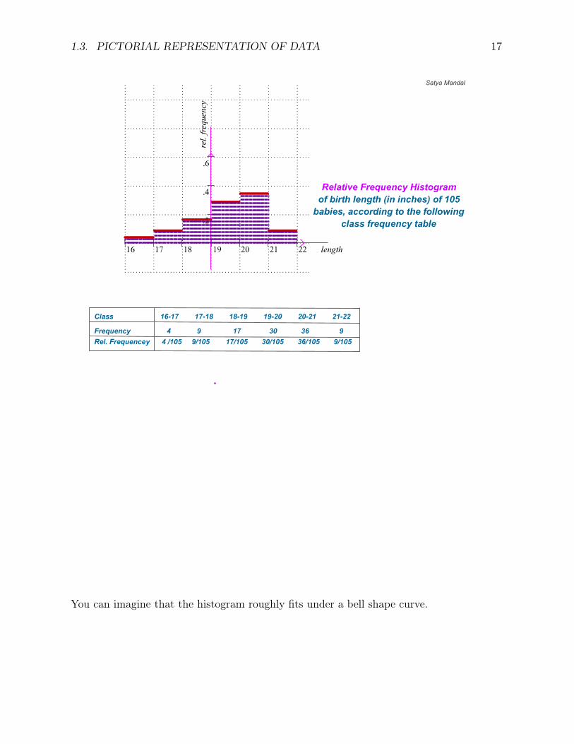
If, instead, we erect bars of height equal to the relative frequency, then the graph iscalled a relative frequency histogram. Similarly, we can construct a percentage frequencyhistogram. The following is a histogram.
We would avoid unequal class lengths, which makes our discussion of the histogram fairlysimple.
1.3.1 More Histograms
In nature, shape of the histograms of almost any kind of numerical data would resemble abell-shaped pattern. A perfect such bell shape is shown in the following diagram:

1.3. PICTORIAL REPRESENTATION OF DATA 15

16 CHAPTER 1. THE LANGUAGE AND TERMINOLOGY
You can imagine that the histogram roughly fits under a bell shape curve. It may or maynot be a great fit, depending upon your expectation.
1.3. PICTORIAL REPRESENTATION OF DATA 17
You can imagine that the histogram roughly fits under a bell shape curve.

18 CHAPTER 1. THE LANGUAGE AND TERMINOLOGY
You can imagine that the histogram roughly fits under a bell shape curve. This one fitsbetter. Normally, it works better when data size is large.

1.3. PICTORIAL REPRESENTATION OF DATA 19
1.3.2 The Cumulative Frequency Distributions and Ogive
We start with this example Example 1.1.3. Following is the frequency table of data onheight (in inches) of some babies at birth. Sketch the histogram of the following data:
Height Frequency
16− 17 317− 18 818− 19 3419− 20 6020− 21 7221− 22 18
For a given value x of a variable, the cumulative frequency of the data, for x, is thenumber of data members that are less than or equal to x.
Definition 1.3.1. Given a frequency distribution of some data, for a class boundary x,the cumulative frequency is the sum of all the class frequencies less or equal to x. Thecumulative frequency distribution is a table that gives the cumulative frequencies againstsome x values (for us the class boundaries). We also define cumulative relative frequencyand cumulative percentage frequency as follows:{
cumulative relative frequency of data , at x = cumulative frequency of xData size
cumulative percent frequency of data , at x = (cumulative frequency of x)100Data size
Example 1.1.4 Once again we consider the data on birth weight of babies in Example1.1.2 that we discussed in the last section. A cumulative frequency distribution can beconstructed from the frequency distribution.Solution: We have seen the frequency distribution before. The following is the cumulativedistributions:
Cumulative Cumulative CumulativeWeight Frequency Relative−Cumulative PercentageFrequency
60.5 0 0 080.5 9 9/99 9.09100.5 29 29/100 29.29120.5 54 54/99 54.55140.5 91 91/99 91.92160.5 99 1 100
Definition. The ogive is a line graph, where we plot the variable on the horizontalaxis and the cumulative frequency on the vertical axis. If we plot the cumulative relative

20 CHAPTER 1. THE LANGUAGE AND TERMINOLOGY
frequency on the vertical axis, then the line graph is called the relative frequency ogive.

Chapter 2
Measures of Central Tendency and ofDispersion
2.1 Measure of Central Tendency: Mean
In this lesson we define various numerical measures (constants) for data sets. These nu-merical measures summarize and describe the data. The average value of the data wouldbe a common example. There are two broad classification such numerical measures thatare computed from the data:
1. measures of central tendency and
2. measures of dispersion.
A measure of central tendency represents an "average value." Mean, median, mode (ifyou already know these) are measures of central tendency. A measure of dispersion is ameasure of how widely the data is scattered around. In the section we discuss (1). Themost common measure of central tendencies is the mean or arithmetic mean.
Definition. Given a data set, by Data size, we mean number of sample units present. Themean x or the arithmetic mean of a set of data x is given by
mean = x =sum of all the data values
Data size
The data size is usually denoted by n. The data variable is usually denoted by x orx1, x2, . . . , xn. So, we can write
x =
∑x
n=
∑ni=1 xin
(2.1)
where the symbol∑
(Sigma) denotes sum, and∑n
i=1 xi = x1 + x2 + · · ·+ xn.
21

22 CHAPTER 2. MEASURES OF CENTRAL TENDENCY AND OF DISPERSION
Weighted Mean: In the formula (2.1), all the values xi have equal weight. Sometimes,different values in data carry different weight. Let us consider the following data and thecorresponding frequency distribution that we computed earlier:
2.1.1 To estimate the mean time taken to complete a three-mile drive by a race car, therace car did several time trials. The following are sample times taken (in seconds) tocomplete the laps (same as in (1.1)) :
50 48 49 46 54 53 52 51 47 56 52 5151 53 50 49 48 54 53 51 52 54 54 5355 48 51 50 52 49 51 53 55 54 50
The following is the frequency distribution of this data, we computed above:
Time xi 46 47 48 49 50 51 52 53 54 55 55Frequency fi 1 1 3 3 4 6 4 5 5 2 1
(Observe, unlike (1.1), we represented the same frequency table, horizontally.) To computethe mean time of the original data (1.1), we obviously, add all the data values and divideby the data size 35. The frequency distribution tells us that, in the data, 46 was present1 time, 47 was present 1 time, 48 was present 3, times and so on. So, using the frequencydistribution, we compute the mean x as follows:
x =(46 · 1 + 47 · 1 + 48 · 3 + 49 · 3 + 50 · 4 + 51 · 6 + 52 · 4 + 53 · 5 + 54 · 5 + 55 · 2 + 56 · 1)
(1 + 1 + 3 + 3 + 4 + 6 + 4 + 5 + 5 + 2 + 1)
=1799
35= 51.4
The mean of the original data is the "weighted mean" of the data values 46, 47, 48, 49,50, 51, 52, 53, 54, 55 and 56 with the corresponding frequencies as the weight. Therefore,when we compute the mean using the frequency table, the formula for the mean would be
x =
∑xifi∑fi
where fi is the weight of xi
The weighted mean is defined in more general context as follows:
Definition. If x1, x2, . . . , xn in a data set have different weights and the values xi hasweight wi, then the weighted is defined as
weighted mean = x =
∑wixi∑wi
Properties of the Mean: Following are some of the obvious properties of means:
1. Combining two means: Suppose we have two sets of data.The mean of the first set is x, and the size of the first set is m;the mean of the second set is y, and size of the second set is n.Then, the mean of the combined data is
Combined mean =mx+ ny
m+ n

2.1. MEASURE OF CENTRAL TENDENCY: MEAN 23
2. Effect of translation: Let x be the mean of x1, x2, . . . , xn. Then the mean ofy1 = x1 + d, y2 = x2 + d, . . . , yn = xn + d is given by
y = x+ d
3. Effect of multiplication by a constant: Let x be the mean of x1, x2, . . . , xn. Thenthe mean of
z1 = cx1, z2 = cx2, . . . , zn = cxn is given by z = cx
Example. (effect of translation): Your teacher tells you that the mean score for themidterm in your class is 73. After you complained and requested a change, he agreed thatall can add 7 points to their score. The new mean score is (old mean + 7) = 73 + 7 = 80.This is what we meant by "effect of translation."
Example. (effect of multiplication by c): Suppose you have some data x1, x2, . . . , xnon salaries in an industry in the United States and the mean is $37000. On a certain day(January 29, 2021), 1 U.S. dollar = 1.28 Canadian dollars (say c = 1.28). So, in Canadiandollars the mean is 37000 ∗ c = 37000 ∗ 1.28 = 47360 Canadian Dollars.
Similarly, any change of units (inches to feet or cm, minutes to seconds) are "multipli-cation by a constant c." (Like inches to centimeters, pounds to kilograms.)
Example 2.1.2. (GPA is an exampled of weighted mean). A student took PHSX115 (College Physics), PSYC 120 (Personality), FREN 110 (Elementary French), BUS 241(Managerial Accounting), and MATH 365 (Elementary Statistics). The number of credithours and the student’s grade is given in the following table:
Course PHSX 115 PSY C120 FREN 110 BUS 241 MATH 365Grade(Points) B(3) A(4) B(3) C(2) B(3)Credit Hours 4 3 5 3 3
What is the student’s GPA?Solution. The GPA is the weighted average of the points (corresponding to the grades),weight being the course-credit hours. So, the
GPA =3 ∗ 4 + 4 ∗ 3 + 3 ∗ 5 + 2 ∗ 3 + 3 ∗ 3
4 + 3 + 5 + 3 + 3=
354
18= 3.
2.1.1 Other Measures of Central Tendency: Median, and Mode
Definition. The median represents the middle value of the data. Half the data will beless than or equal to the median, and half the data will be greater than or equal to themedian. You are above the median American income if half the American population ismaking less than you make. Suppose the data is arranged in an increasing order (i.e., inan array). Then,

24 CHAPTER 2. MEASURES OF CENTRAL TENDENCY AND OF DISPERSION
1. If the size of data is ODD then the median is the middle value.
2. If it is EVEN, then the median is the mean of the middle two values.
Definition. The Percentiles: For a number p with 0 ≤ p ≤ 100, the pth percentile xp ofthe data is a number such that at least p percent of the data members are below xp andat least (100− p) percent of the data members are above xp. Further,
1. The 25th percentile is called the first quartile Q1.
2. The median is the 50th percentile, also called the second quartile Q2.
3. The 75th percentile is called the third quartile Q3.
Definition. (The Mode)The MODE of the data is the value or values that have the highest frequency. For example,the mode of the set {1, 3, 5, 5, 7} is because it has the highest frequency. The mode of{1, 1, 3, 5, 5, 7} is {1, 5} because 1 and 5 both have the highest frequency. Such a set is saidto be bimodal.
Using TI − 84: We already mentioned how to enter data.
1. Sorting data and computing the median:
(a) Enter your data in a list, say L1.
(b) Select SortA in the Edit menu and enter.
(c) The calculator will ask for the list.Type in the list (L1), close the parentheses, and enter.
(d) The calculator will say Done.
(e) Press stat, select edit in the Edit menu, and enter.
(f) You will see that your data in L1 has been sorted in an increasing order.
(g) If the data size is odd, the median is the middle value.
(h) If the data size is even, the median is the average of the middle two values.
2. Computing the mean if only raw data is given:
(a) Enter your data in a list, say L1.
(b) Select "1-Var Stats" in the CALC menu and enter.
(c) The calculator will ask for the list. Type in the list L1 and enter.
(d) The calculator will give a list of numbers; x is the mean .
3. Computing the mean if the frequency table is given:

2.1. MEASURE OF CENTRAL TENDENCY: MEAN 25
(a) Enter the frequency table in the calculator, say,x-values in L1 and frequencies in L2.
(b) Select "1-Var Stats" in the CALC menu and enter.(c) The calculator will ask for the lists. Type in the list L1, L2 and enter.(d) The calculator will give a list of numbers; x is the mean.
4. Computing the median: Do the same as above and scroll down.
2.1.2 Problems on Mean and Median
Exercise 2.1.1. The following is the price (in dollars) of a stock (say, APPL) checked bya trader several times on a particular day.
138 142 127 137 148 130 142 133
Find the median price and mean price observed by the trader. Solution: Use TI-84.
Exercise 2.1.2. The following figures refer to the GPA of six students.
3.0 3.3 3.1 3.0 3.1 3.1
Find the median and mean GPA.
Exercise 2.1.3. The following data give the lifetime (in days) of light bulbs.
138 952 980 967 992 197 215 157
Find the mean and median lifetime of these bulbs. Solution: Use TI-84.
Exercise 2.1.4. An athlete ran an event 32 times. The following frequency table givesthe time taken (in seconds) by the athlete to complete the events.
Time xi (in sec.) frequency fi
26 3
27 6
28 5
29 6
30 9
31 3
Total 32
Compute the mean and median time taken by the athlete. Solution: Use TI-84. Solution:Use TI-84.

26 CHAPTER 2. MEASURES OF CENTRAL TENDENCY AND OF DISPERSION
Exercise 2.1.5. Consider the data, as in (Ex. 1.2.7) on the weight (in ounces), at birth,of 96 babies born in Lawrence Memorial Hospital in May 2000. Compute the mean andmedian weight, at birth, of the babies. Solution: Use TI-84.
Exercise 2.1.6. Consider the data, as in (Ex. 1.2.10) on the hourly wages (paid only inwhole dollars) of 99 employees in an industry. Solution: Use TI-84.
Exercise 2.1.7. Following is the frequency table on the number of typos in a sample of30 books published by a publisher.
No. of Typos 156 158 159 160 162
Frequency 6 4 5 6 9
Find the mean and median number of typos in a book. Solution: Use TI-84.
Exercise 2.1.8. Consider the data, as in (Ex. 1.2.8), on the length (in inches), at birth,of 96 babies born in Lawrence Memorial Hospital in May 2000. Solution: Use TI-84.
2.2 Measures of Dispersion
The measures of central tendencies?mean, median, mode? represent the middle values ofthe data set. The variability of data would also be of our interest, for a better understandingof the distribution of data. Two data sets may have same mean and median, but they maybe spread out differently. Following is an example.
Example 2.2.1. Suppose two sections of the statistics class have the following percentagescore distribution at the end of the semester:
Section A 81 84 83 80 82Section B 72 93 92 82 71
Both these sections have the same mean - 82. Medians of both the sets are same - 82.But the data sets are differently dispersed. In Section A, everybody will get a B grade. Insection B, we will have two C, one B and two A.
The measure of dispersion is a measure of how widely the data is scattered around.In section A, the data has a very small dispersion or variability, whereas section B has alarge dispersion. A very simple (crude) measure of dispersion is the range of the data aswe have defined before:
range = (largest value)− (smallest value).
We will define three more measures of dispersions:Mean Deviation, Variance, and Standard Deviation.

2.2. MEASURES OF DISPERSION 27
Definition: Suppose x1, x2, . . . , xn is a set a of data.
1. Then, the Mean Deviation of the data is defined to be
MeanDeviation =|x1 − x|+ |x2 − x|+ · · ·+ |xn − x|
n
So, the mean deviation is the mean of the absolute deviations |xi − x| from the mean.
2. The the Variance s2 of the data is defined as follows:
s2 =(x1 − x)2 + (x2 − x)2 + · · ·+ (xn − x)2
n− 1(2.2)
Observe:
(a) Note that we denote the sample variance as the square of a number s (and wecan do so).
(b) Also note that we divide by n−1, not by n. For some statistical reason, dividingby n− 1 works better. (We justify this, in the remark, below (7.1).)
(c) We would like our measure of dispersion to have the same units as our data, butour formula involves squares (xi − x)2. Therefore, the unit of the variance, s2,is the unit of the data squared. If the data is in feet, the variance is in squarefeet. To solve this problem we define another measure of dispersion, standarddeviation denoted s.
3. The Standard Deviation is defined as the square root of the variance s2. So, tocompute the sample standard deviation, we have to compute the sample variancefirst.
If the data corresponds to a sample, then we call the above as sample Mean Devia-tion, sample Variance, and sample Standard Deviation. If the data corresponds tothe population, then we call the above as population Mean Deviation, populationVariance, and population Standard Deviation. For now, we work with samples only.(Populations data is actually unknown, which we try to estimate or model.)
If we simplify the definition of the variance we get the following formula:
s2 =(x21 + x22 + · · ·+ x2n)− nx2
n− 1
We do some computations with the above example 2.2.1.
1. The {mean deviation for section A = (1+2+1+2+0)
5= 6
5
mean deviation for section B = (10+11+10+0+11)5
= 425
As expected, mean deviation of Section B is higher, because the variability of sectionB was clearly higher than that of A.

28 CHAPTER 2. MEASURES OF CENTRAL TENDENCY AND OF DISPERSION
2. The variance s2A of section A is:
s2A =(81− 82)2 + (84− 82)2 + (83− 82)2 + (80− 82)2 + (82− 82)2
5− 1= 2.5
The variance s2B of section B is:
s2B =(72− 82)2 + (93− 82)2 + (92− 82)2 + (82− 82)2 + (71− 82)2
5− 1=
442
4
For future discussions, for reasons mentioned above, the standard deviation s would be ourchoice of our (and for practicing statistician’s) measure of dispersions.
2.2.1 Application of Standard deviation
Under normal circumstances, which we will discuss later, the mean and the standarddeviation carries an enormous amount of information regarding the distribution of thedata.
Chebyshev’s Rule. This rule applies for all kinds of data. Suppose x is the mean and sis the standard deviation of a set of data x1, x2, . . . , xn. Then we have the following:
1. At least 0 percent of the observations will fall within 1 standard deviation of themean, i.e, within (x− s, x+ s). This is clearly of not use.
2. At least 75 percent of the observations will fall within 2 standard deviations of themean, i.e., within (x− 2s, x+ 2s).
3. At least 89 percent of the observations will fall within 3 standard deviations of themean, i.e., within (x− 3s, x+ 3s).
4. More generally, at least 100(1− 1
k2
)percent of the data will be within k-standard
deviations from the mean, i.e. within (x− ks, x+ ks).
Note, this applies to any set of data, without any hypotheses. In that respect, it is verystrong. It is mathematically smart, but statistically crude. In fact, in nature, the his-togram of data usually fits nicely, under a nice bell curve, as was shown above and below.

2.2. MEASURES OF DISPERSION 29

30 CHAPTER 2. MEASURES OF CENTRAL TENDENCY AND OF DISPERSION
We incorporate this basic nature of data, in to our statistical modeling, and give aimproved version of Chebyshev’s Rule, which I would call statistically smarter. This iscalled the Empirical Rule, as follows.

2.2. MEASURES OF DISPERSION 31
The Empirical Rule: Suppose the histogram of the data fits under a bell curse as above.So, it is symmetric around the vertical line through the mean x = x: In this case,
1. At least 68.3 percent of the observations will fall within 1 standard deviation of themean, i.e, within (x− s, x+ s). This is clearly of not use.
2. At least 95.4 percent of the observations will fall within 2 standard deviations ofthe mean, i.e., within (x− 2s, x+ 2s).
3. At least 99.7 percent of the observations will fall within 3 standard deviations ofthe mean, i.e., within (x− 3s, x+ 3s).

32 CHAPTER 2. MEASURES OF CENTRAL TENDENCY AND OF DISPERSION

2.2. MEASURES OF DISPERSION 33
Question: What does it mean when the variance or mean deviation of some data iszero? The answer is that all the data members are EQUAL!
Practice Problem. Consider the all the data set given above. For each problem,compute the mean and standard deviation of the data and find what percentage of thedata are within one, two, or three standard deviations from the mean.
2.2.2 Use of the Frequency Table
When a frequency table is given, we can use new formulas to compute the mean andvariance of the data.
Formulas: Suppose frequency table of a data set is given, where the data value xi hasfrequency fi. Let n =
∑fi denote the data size. Then,

34 CHAPTER 2. MEASURES OF CENTRAL TENDENCY AND OF DISPERSION
1. The mean
x =
∑fixi∑fi
=
∑fixin
2. The variance
s2 =
∑fi(x− x)2
n− 1=
(∑fix
2i )− nx2
n− 1
3. If the data is given in a class frequency table of the grouped data, we use the sameformula, with xi as the class mark, which is the average of the class limits. In thiscase, we only get an estimate of the variance of the original data.
Example 2.2.2. The following table expand the frequency table (1.1) of the time takento complete a lap by a race car (example 1.1.1) to compute mean and variance using theabove formulas.
Time xi frequency fi fixi fix2i
46 1 46 211647 1 47 220948 3 144 691249 3 147 720350 4 200 1000051 6 306 1560652 4 208 1081653 5 5265 1404554 5 270 1458055 2 110 605056 1 56 3136
Total∑
35 1799 92673
So, the mean
x =
∑fixin
=1799
35= 51.4
and the variance
s2 =(∑fix
2i )− nx2
n− 1=
92673− 35 ∗ (51.4)2
34= 6.0118
Remark: When computing power was not in abundance (20 or 30 years ago), as it is now,we used to use such tables to do the computations. Such methods are out of date by now.We use TI-84 or other tools now.
Example 2.2.3 Consider the class frequency distribution of the data (1.2) on birth weightof some babies (exercise 1. 2. 5). We expand it, and use the above formula to compute

2.2. MEASURES OF DISPERSION 35
mean and variance.
Classes frequency fi class mark xi fixi fix2i
60.5− 80.5 9 70.5 634.5 44732.2580.5− 100.5 20 90.5 1810 163805100.5− 120.5 25 110.5 2762.5 305256.25120.5− 140.5 37 130.5 4828.5 630119.25140.5− 160.5 8 150.5 1204 181202Total
∑99 11239.5 1325114.75
So, the mean (approximate)
x =
∑fixin
=11239.5
99= 113.53
and the variance (approximate)
s2 =(∑fix
2i )− nx2
n− 1=
1325114.75− 99 ∗ 113.532
99− 1= 500.997
Remarks.
1. Note that we can only get an approximate mean and variance if we use the class markand with the above formula. If you use the original data, you will notice a difference.
2. As mentioned above, because of the availability of computers, the importance of suchapproximations has declined.
Use of calculators: We have had detailed discussions of various formulas for defining themean, variance, and other constants. It is important to understand these concepts andformulas. It is equally important to appreciate the value and necessity of using calcula-tors or other available software (like Excel). It is almost impossible (and unnecessary) tocompute these constants manually and correctly, unless one is specially gifted with numer-ical computations. To compute the variance and standard deviation (with TI-84), do thefollowing:
1. Follow the same steps used for computing the mean (using either raw data or thefrequency table).
2. The calculator will give a list of numbers; SX is the standard deviation.
3. The variance is the square of the standard deviation.

36 CHAPTER 2. MEASURES OF CENTRAL TENDENCY AND OF DISPERSION
2.2.3 Problems on Variance, Standard Deviation
As before (Sec. 2.1.2), we would have problems of raw data and data in frequency tables.We compute measure of dispersions, for all problems in Sec. 2.1.2.
Exercise 2.2.1. Find the variance and standard deviation of the price, for stock price inEx. 2.1.1:
138 142 127 137 148 130 142 133
Solution: Use TI-84.
Exercise 2.2.2. Find the variance and standard deviation of GPA, for the data in Ex.2.1.2:
3.0 3.3 3.1 3.0 3.1 3.1
Find the median and mean GPA.
Exercise 2.2.3. Find the variance and standard deviation of the lifetime of these bulbs,for data in 2.1.3:
138 952 980 967 992 197 215 157
Find the mean and median lifetime of these bulbs. Solution: Use TI-84.
Exercise 2.2.4. Compute the variance and standard deviation of time taken by the athlete,for data in 2.1.4
Time xi (in sec.) frequency fi
26 3
27 6
28 5
29 6
30 9
31 3
Total 32
Solution: Use TI-84.
Exercise 2.2.5. Compute the variance and standard deviation of the weight, at birth, ofthese babies, with data in Ex. 1.2.7, Ex. 2.1.5. Solution: Use TI-84.
Exercise 2.2.6. Compute the variance and standard deviation of the hourly wages, fordata in Ex. 1.2.10, Ex. 2.1.6. Solution: Use TI-84.

2.2. MEASURES OF DISPERSION 37
Exercise 2.2.7. Find the variance, and standard deviation of typos in a book, for date inEx. 2.1.7:
No. of Typos 156 158 159 160 162
Frequency 6 4 5 6 9
Solution: Use TI-84.
Exercise 2.2.8. Compute the variance and standard deviation of the length, at birth, ofthese babies, for data in Ex. 1.2.8, Ex. 2.1.8. Solution: Use TI-84.
Exercise 2.2.9. The following is the frequency table of weight (in pounds) of some salmonin a river.
weight x 31 32 33 34 35 36 37
Frequencyf 3 2 4 5 6 5 9
Find the variance and standard deviation. Solution: Use TI-84.
Exercise 2.2.10. The following data represents the time (in minutes) taken by studentsto drive to campus.
23 17 19 24 42 33 20 22 15 9
26 37 29 19 35 18 30 21 11 23
13 27 32 32 23 35 25 33 24 23
Find the mean, variance, and the standard deviation of the data. Solution: Use TI-84.

38 CHAPTER 2. MEASURES OF CENTRAL TENDENCY AND OF DISPERSION

Chapter 3
Probability
3.1 Introduction
The concept of probability is prevalent at a very basic human intuitive and intellectual level.Other synonyms of probability include likelihood and chances. Probabilistic statements aremade on daily basis without any awareness that there may be some intuitive mathematicalcalculation involved behind such statements.
Most people are aware of different kinds of game of chances and gambling. Examples ofsuch games include tossing coins, any dice rolling game and games of cards. It is universallyaccepted that when you toss a coin, likelihood of head showing up is fifty percent. Whenyou roll a normal die, it is universally accepted that the likelihood of that a particular facewill show up is one in six. There is also awareness of loaded coins and loaded dice, in whichlikelihood of an outcome (say head or the face six) is higher than that of other outcomes.It is a common sense that in a poker game, it is extremely unlikely that one would getthree aces in a particular deal. A lot of people would not buy a lottery ticket becausethey believe, that it is extremely unlikely that he or she would ever win a multi milliondollar or would not make money in the long run. These are intuitive or semi-mathematicalunderstanding of probability of occurrence of certain events.
Statements regarding chances of departure of your flight on time would not be souncommon. Same is true, regarding similar statements on chances of a thunderstorm,rain, snow or other whether related events. Statements regarding the chances of accidentswould be another types probabilistic statements. One would not be surprised to hear afive year old making statements like "I will probably invite Aaron for my birthday". Suchwould mean that the child is aware of uncertainties of parental permission or his/her ownindecisiveness.
When such statement that includes word like "likelihood", "chances" or "probability"are made, one is essentially talking about what they have experienced in the past andtrying to project that the same pattern will continue in future.
39

40 CHAPTER 3. PROBABILITY
Some of the early development of Probability, as a mathematical theory, originatedin gambling. In the last century, this concept received further boost in genetics (moregenerally biosciences) and other branches of science.
3.1.1 Basic Concept of Probability
The concept of Probability attempts to quantify chances (or likelihood) of the occurrenceof an event in a consistent manner. It uses human experience of the past to hypothesizeand formulate a model. The model needs to behave in a manner that makes an overallsense. For example the chances of occurrence (say of raining today) and nonoccurrence ofthe same event should add to 100 percent (or probabilities of the same should add to one).
Our experience with tossing normal coins tells us that if we toss a coin for a largenumber of times, essentially half the time the head shows up. We assume that samepattern will continue in future. Therefore, we hypothesize that the probability that thehead will show up is .50. On the other hand, if through extensive experimentation with acoin, we conclude that the ratio of the number of Heads to the number of tosses remainsclose to and moves around .49 then we would hypothesize that the probability of heads is.49. Such minor difference would be of serious consideration for the gambling houses.
Similarly, our experience with rolling normal dice tells us that when we roll a diea particular face (say face six) would show up, is essentially once is six times. So, wehypothesize that probability that face six will show up is 1/6. Contrary to this, there areloaded dice. You may have a loaded die that you experimented with and determined facesix shows up 40 percent of the times. So, you would hypothesize that probability that facesix will show up for this loaded die is .40.
Similar data may be collected for road accidents and probabilistic hypothesis (model)could be made regarding number of daily accidents on a street.
These examples explain the basic notion of probability. The probability of an eventis hypothesized (modeled), as the "relative frequency", the ratio of occurrences of theEVENT to the total number of times the EXPERIMENT is repeated (or experienced inthe past). Following are some pictures of coin toss experiments:

3.1. INTRODUCTION 41
The first coin is set up to have 1 in 2 chances of Jayhawk
12
5 7

42 CHAPTER 3. PROBABILITY
This second coin is set up to have 3 in 4 chances of Jayhawk
12
11 1

3.1. INTRODUCTION 43
This third coin is set up to have 1 in 10 chances of Jayhawk
12
0 12
3.1.2 Basic Set theoretic Definitions
Definition. By a set S we mean a collection of objects. The objects in this set S are alsocalled elements or members of the set. A set E is said to be a subset of a set S if eachelement of E is also an element of S. We write
E ⊆ S
to mean that E is a subset of S. Obviously, a subset E of S is a smaller collection than orequal to S. The following are some examples. We also explain the usage of braces todescribe a set.
1. Let D = the collection of all 52 cards in a deck. Then D is a set. Let E be thecollection of all the hearts in this deck. Then E is a subset of D. In brace notation
E = {x ∈ D : x is a Heart}

44 CHAPTER 3. PROBABILITY
We read this as "E is equal to the set of all x in D such that x is a heart". We usethe symbol ∈ to abbreviate the word "in" or "is an element of".
2. Let T be the collection of all those who filed a tax return to the IRS for the year2001. Then T is a set. Let L be the collection of those whose Adjusted Gross Incomein the return was less or equal to $30,000. Then L is a subset of T . Let C be thecollection of those who declared capital gains income. Then C is a subset of T . Wewrite
L ⊆ T, C ⊆ T
In brace notation
L = {x ∈ T : the Adjusted Gross Income of x is less or equal to $30, 000}.
3. Let N be the collection of all integers, and let E be the collection of even integers.Then N,E are set and E ⊆ N In brace notation
N = {n : n is an integer} E = {n ∈ N : n is even}.
We also write
N = {· · · ,−2,−1, 0, 1, 2, · · · } E = {· · · ,−4,−2, 0, 2, 4, · · · }
4. Let R be the set of all (real) numbers. Let I be the set of all numbers between 0 and1, not equal to 0,1. Then R, I are sets and I is a subset of R. In brace notation
R = {x : x is a real number}, I = {x ∈ R : 0 < x < 1}.
There are other (interval) notations, likeR = (−∞,∞),I = (0, 1).
5. S = {1, 7, 13, 17, 19} is a set.
6. Let S be the collection of you and your siblings, B be the collection of your brothers,and F be the collection of your sisters. Then S,B, F are sets and we have
F ⊆ S B ⊆ S.
3.1.3 Statistical Experiments and Sample Space
We use the above language of set theory, only in the context of random experiments.
Definition. We introduce three fundamental definitions:
1. A statistical experiment is a procedure that produces exactly one out of manypossible outcomes. All the possible outcomes are known, but which outcome willresult when you perform the experiment is not known. A statistical experiment isalso called a random experiment.

3.1. INTRODUCTION 45
2. Given an experiment, the set of all possible outcomes is called the sample space.The sample space is usually denoted by S.
3. Given an experiment, an outcome of the experiment is also called a sample point.So, the sample space consists of sample points.
Examples. Following are some standard examples of samples spaces.
1. Suppose the experiment is tossing a coin. The outcomes are H (heads) and T (tails).So, the sample space is S = {H,T}.
2. Suppose the experiment is tossing a coin twice. The sample points (or outcomes) areHH,HT, TH, TT and the sample space is S = {HH,HT, TH, TT}.
3. Your experiment is rolling a die. The outcomes are 1, 2, 3, 4, 5, 6 and the sample spaceis S = {1, 2, 3, 4, 5, 6}.
4. Suppose that the experiment is rolling a die twice. Then the sample space is
S =
(1, 1) (1, 2) (1, 3) (1, 4) (1, 5) (1, 6)(2, 1) (2, 2) (2, 3) (2, 4) (2, 5) (2, 6)(3, 1) (3, 2) (3, 3) (3, 4) (3, 5) (3, 6)(4, 1) (4, 2) (4, 3) (4, 4) (4, 5) (4, 6)(5, 1) (5, 2) (5, 3) (5, 4) (5, 5) (5, 6)(6, 1) (6, 2) (6, 3) (6, 4) (6, 5) (6, 6)
(3.1)
In brace notation, we can write the same as
S = {(i, j) : i = 1, 2, 3, 4, 5, 6 and j = 1, 2, 3, 4, 5, 6}.
5. Suppose the experiment is to determine the number of road accidents in Lawrenceon a particular day. So, the sample space is S = {0, 1, 2, 3, . . .}.
6. Suppose the experiment is to determine the sex of an unborn child. Then the samplespace is S = {Female,Male}.
7. Suppose the experiment is to determine the blood group of a patient in a lab. Thenthe sample space is S = {O,A,B,AB}.
8. Suppose the experiment is to observe the annual wheat production in Kansas. Thenthe sample space is
S = {x : x is a nonnegative Number} = {x ∈ R : x ≥ 0} = [0,∞).
9. Suppose that the experiment is rolling a die three times. Then the sample space canbe written as
S = {(i, j, k) : i = 1, 2, 3, 4, 5, 6 and j = 1, 2, 3, 4, 5, 6 and k = 1, 2, 3, 4, 5, 6}.

46 CHAPTER 3. PROBABILITY
A a set can be described or written in many different ways, as was done above, in somecases. There is no hard and fast rules. But some jargons, as above, have become standard.
Definition. The sample space S is called a finite sample space if S has only a finitenumber of outcomes. If S has infinite elements, it is called an infinite sample space. Notethat examples 1, 2, 3, 4, 6, 7, 9 have finite sample spaces, and examples 5, 8 have infinitesample space.
We define Events, in the context of a random experiment.
Definition. Given an experiment and its sample space S, the following are importantdefinitions.
1. A subset E of the sample space S is called an event. So, an event E consists ofoutcomes, and we have
E ⊆ S
We say that E would have occurred, if the outcome of the experiment wouldbe in E, when the experiment is performed.
2. There is a special event called the empty event or impossible event, denotedby φ. It is defined as the event with no outcomes in it. So, the impossible eventconsists of no outcome. Therefore, the impossible event would never occur.
3. Since S is also a subset of itself, S is an event. This event S is called the sure event.Since the outcome of the experiment would always be in S, the sure event S is sureto occur.
4. A simple event consists of a single outcome.
Examples. The following are some examples of events.
1. Consider example 2 above -the experiment on the coin toss. Let E be the event thatat least one of the tosses gave T , and let F be the event that both tosses gave thesame face. Then
E = {HT, TH, TT}, and F = {HH,TT}.
2. Look at example 4 above-the experiment on rolling a die. Let E5 be the event thatfirst die showed 5. Then
E5 = {(5, 1), (5, 2), (5, 3), (5, 4), (5, 5), (5, 6)}.
Let T5 be the event that the sum of the two "rolls" is 5. Then
T5 = {(1, 4), (2, 3), (3, 2), (4, 1)}.
Let T1 be the event that the sum of the two rolls is 1. Because T1 has no outcome,T1 = φ is the impossible event. Likewise, let T13 be the event that the sum of thetwo rolls is 13. Then T13 = φ is also the impossible event.

3.1. INTRODUCTION 47
3. Look at the example 5 above-the experiment on road accidents. Let E be the eventthat there is no accident on that day. Then
E = {0}.
4. Look at example 8 above-the experiment on annual wheat production. Let E be theevent that there will be more than 1000 units of wheat production in 1998. Then
E = (1000,∞).
3.1.4 The Definition of Probability
Given a sample space S, in the MATHEMATICS of probability we have hypotheses andrules for how to compute the probability of an event E. Although the MATHEMATICSof probability was modeled based on our past experiences, we do not derive anything fromour intuitive ideas. We would fully be guided by the precise hypotheses, rules and lawsthat we set up.
For now we would be dealing with finite sample spaces.
Definition. Suppose we have a random experiment, and it has a finite sample space
S = {e1, e2, . . . , eN} with N outcome.
The probability of a simple event {ei} is a number (possibly given) denoted by P ({ei})or loosely written as P (ei), which has the following properties:
1. 0 ≤ P (ei) ≤ 1 for all i = 1, 2, . . . , N
2. The sum of the probabilities of all the simple events is 1:
P (e1) + P (e2) + . . .+ P (eN) = 1.
3. If E is an event, then the probability P (E), of occurrence of E, is defined as the sumof the probabilities of all the simple events ei ∈ E:
P (E) =∑ei∈E
P (ei) (3.2)
So, we also have
P (impossible Event) = P (φ) = 0 P (Sure Event) = P (S) = 1

48 CHAPTER 3. PROBABILITY
3.2 Probability Tables and Equally Likely
Remark. If we know the probabilities P (ei) of all the simple events {ei}, we will be ableto compute the probability of any event E using Formula 3.2. The probabilities of thesimple events would
1. either be given explicitly, say by a table, or
2. OR, a rule or a formula will be given, to compute it.
One of the most frequently used models to compute probabilities of simple events is calledequally likely outcomes, as follows.
Definition. Let S = {e1, e2, , eN} be a finite sample space. We say that all the outcomesare equally likely, if all the outcomes have the same probability. So, in this case, we have
P (e1) = P (e2) = · · · = P (eN) =1
NAlso, in this case, for an event E, from Formula 3.2
P (E) =∑ei∈E
P (ei) =∑ei∈E
1
N=no. of outcomes in E
N
If n(E) denotes the number of outcomes in E then
P (E) =n(E)
n(S)(3.3)
3.2.1 Problems: on Tabular probability
We work out some problems in this section, where probability of simple events is given ina table.
Exercise 3.2.1. The following table gives the blood group distribution of a certain pop-ulation.
Blood Group Distribution
Blood Group O A B AB
percent of population 47 42 8 3
Find the probability that a random sample of blood will be of Blood Group A or B or AB.Solution: Here S = {O,A,B,AB} and we want to compute the probability P (E) of theevent E = {A,B,AB}. From the table
P (O) = .47, P (A) = .42 P (B) = .08 P (AB) = .03
So, P (E) = P ({A,B,AB}) = P (A) + P (B) + P (AB) = .42 + .08 + .03 = .53

3.2. PROBABILITY TABLES AND EQUALLY LIKELY 49
Exercise 3.2.2. A student wants to pick a school based on its grade distribution. Followingis the most recent grade distribution in a school:
Grade Distribution (Unreal Data)
Grades A B C D F
percent of students 19 33 31 14 3
Find the probability that a randomly picked student will have at least a B average.Solution: Here S = {A,B,C,D, F} and we want to compute the probability P (E) of theevent E = {A,B}. From the table
P (A) = .19, P (B) = .33 P (C) = .31 P (D) = .14, P (F ) = .03
So, P (E) = P ({A,B}) = P (A) + P (B) = .19 + .33 = .52
Exercise 3.2.3. The following table gives the probability distribution of a loaded die.
Probability Distribution for the Die
Face 1 2 3 4 5 6
probability 0.20 0.15 .015 0.10 0.05 0.35
Find the probability that the face 2 or 3 or 6 will show up when you roll the die.Solution: Here S = {1, 2, 3, 4, 5, 6} and we want to compute the probability P (E) of theevent E = {2, 3, 6}. From the table
P (1) = 0.20, P (2) = 0.15, P (3) = 0.15, P (4) = 0.10, P (5) = 0.05, P (6) = 0.35
So, P (E) = P ({2, 3, 6}) = P (2) + P (3) + P (6) = 0.15 + 0.15 + 0.35 = .65
Exercise 3.2.4. An arbitrary spot is selected in a swamp. The depth (in feet) of water inthe swamp has the following probability distribution:
Depth Distribution
depth 0+ 1+ 2+ 3+ 4+ 5+ 6+ 7+ 8+
probability .1 .2 .09 .17 .13 .11 .08 .07 .05
1. What is the probability that the depth at an arbitrary spot is less than three feet?
2. What is the probability that the depth at an arbitrary spot is 3 feet or higher?
Solution: Here, the sample space is S = {0+, 1+, 2+, 3+, 4+, 5+, 6+, 7+, 8+}.From the table, probability P (0+) = .1, P (1+) = .2, P (2+) = .09 and so on.

50 CHAPTER 3. PROBABILITY
1. Let E be the event that depth at an arbitrary spot is less than three feet.Then E = {0+, 1+, 2+}. So,P (E) = P (0+) + P (1+) + P (2+) = .1 + .2 + .09 = .39.
2. Let F be the event that the spot is 3 feet or higher.Then F = {3+, 4+, 5+, 6+, 7+, 8+}. So,P (F ) = P (3+) + P (4+) + P (5+) + P (6+) + P (7+) + P (8+)
= .17 + .13 + .11 + .08 + .07 + .05 = .61
Exercise 3.2.5. Van pool can carry 7 people. Following is the distribution of number ofriders in the van on a given day.:
Distribution of number of passengers
number of passengers 1 2 3 4 5 6 7
probability 0 .12 .22 .23 .28 .08 .07
1. What is the probability that there will be at most 4 riders?
2. What is the probability that there will be less than 4 riders?
3. What is the probability that there will be more than 4 riders?
4. What is the probability that the van will not be full on a particular day?
Solution: Here, the sample space is S = {1, 2, 3, 4, 5, 6, 7}.From the table, probability P (1) = 0, p(2) = .12, P (3) = .22 and so on.
1. Let E be the event that there will be at most 4 riders.Then E = {0, 1, 2, 3, 4}.So, P (E) = P (0) + P (1) + P (2) + P (3) + P (4) = 0 + .12 + .22 + .23 = .57.
2. Let F be the event that 3 there will be less than 4 riders.Then F = {0, 1, 2, 3}.So, P (F ) = P (0) + P (1) + P (2) + P (3) = 0 + .12 + .22 = .34.
3. Let G be the event that that there will be more than 4 riders.Then, G = {5, 6, 7}.So, P (G) = P (5) + P (6) + P (7) = .28 + .08 + .07 = .43.

3.2. PROBABILITY TABLES AND EQUALLY LIKELY 51
4. Let H be the event that there the van will not be full.Then, H = {0, 1, 2, 3, 4, 5, 6}.P (H) = P (0) + P (1) + P (2) + P (3) + P (4) + P (5) + P (6)
= 0 + .12 + .22 + .23 + .28 + .08 = .93
Exercise 3.2.6. Following is the distribution of hourly wages (in whole dollars) earned byworkers in an industry:
Wage Distribution
Wage in USD 7 8 9 10 11 12 13 14 15 16 17 18 19 20
probability .04 .06 .07 .09 .11 .12 .14 .11 .09 .08 .04 .03 .01 .01
An employee is selected at random.
1. What is the probability that the randomly selected worker makes less than 10 dollarsan hour?
2. What is the probability that the randomly selected worker makes at least $10 anhour?
3. What is the probability that the randomly selected worker makes between $12-$16an hour?
Solution: Here, the sample space is S = {7, 8, 9, 10, 11, 12, 13, 14, 15, 16, 17, 18, 19, 20}.From the table, probability P (7) = .04, p(8) = .06, P (9) = .07 and so on.
1. Let E be the event that the randomly selected worker makes less than 10 dollars anhour. Then E = {7, 8, 9}.So, P (E) = P (7) + P (8) + P (9) = .04 + .06 + .07 = .17
2. Let F be the event that the randomly selected worker makes at least $10 an hour.So,Then F = {10, 11, 12, 13, 14, 15, 16, 17, 18, 19, 20}.P (F ) = P (10) + P (11) + P (12) + P (13) + P (14) + P (15) + P (16) + P (17) + P18) +
P (19) + P (20)
= .09 + .11 + .12 + .14 + .11 + .09 + .08 + .04 + .03 + .01 + .01 = .83.
3. Let G be the event that that worker makes between $12-$16 an hour. Then, G =
{12, 13, 14, 15, 16}.So, P (G) = P (12)+P (13)+P (14)+P (15)+P (16) = .12+ .14+ .11+ .09+ .08 = .54

52 CHAPTER 3. PROBABILITY
Exercise 3.2.7. In a school district, the distribution of number of students in a class hasthe following probability distribution:
Distribution of number of students
no of students 8 9 10 11 12 13 14 15 16 17 18 19 20 21 22 23
probability .03 .04 .06 .07 .10 .12 .13 .11 .09 .07 .06 .04 .03 .02 .02 .01
A child is selected at random from the school district.
1. What is the probability that the child will be in a class of at least 20?
2. What is the probability that the child will be in a class of at most 10?
3. What is the probability that the child will be in a class of less than 10?
Solution: Here, the sample space isS = {8, 9, 10, 11, 12, 13, 14, 15, 16, 17, 18, 19, 20, 21, 22, 23}. From the table, probabilityP (8) = .03, p(9) = .04, P (10) = .06 and so on.
1. Let E be the event that the the child will be in a class of at least 20.Then E = {20, 21, 22, 23}. So,P (E) = P (20) + P (21) + P (22) + P (23) = .03 + .02 + .02 + .01 = .08
2. Let F be the event that the child will be in a class of at most 10.Then F = {8, 9, 10}. So,P (F ) = P (8) + P (9) + P (10) = .03 + .04 + .06 = .13.
3. Let G be the event that that child will be in a class of less than 10.Then, G = {8, 9}. So,P (G) = P (8) + P (9) = .03 + .04 = .07.
3.2.2 Problems: on Equally Likely model
We work out some problems in this section, where all outcomes are equally likely. Asmentioned above (3.3), we use the formula
P (E) =n(E)
n(S)
Exercise 3.2.8. An urn contains 7 apples and 3 oranges and 5 pears. One piece of fruitis picked at random. Find the probability that

3.2. PROBABILITY TABLES AND EQUALLY LIKELY 53
1. the fruit is an apple,
2. the fruit is either an apple or a pear, and
3. the fruit is an orange.
Solution: Here, the sample space isS = {A1, A2, A3, A4, A5, A6, A7, O1, O2, O3, P1, P2, P3, P4, P5}.So, n(S) = 7 + 3 + 5 = 15
1. Let E be the event that the selected fruit is an apple.Then E = {A1, A2, A3, A4, A5, A6, A7}.So, n(E) = 7
P (E) = n(E)n(S)
= 715
2. Let F be the event that the selected fruit is an apple or a pear.Then F = {A1, A2, A3, A4, A5, A6, A7, P1, P2, P3, P4, P5}.So, n(F ) = 7 + 5 = 12
P (F ) = n(F )n(S)
= 1215
3. Let G be the event that the selected fruit is an orange.Then G = {O1, O2, O3}.So, n(G) = 3
P (G) = n(G)n(S)
= 315
Exercise 3.2.9. A die is rolled twice. Find the probability that
1. the sum is 8,
2. only 2 or 3 showed up in both the rolls, and
3. the first roll produced a bigger number.
4. that the sum of two numbers is 1.
Solution: The sample space S is given above (3.1).So, n(S) = 36.

54 CHAPTER 3. PROBABILITY
1. Let E be the event that the sum is 8.Then E = {(2, 6), (3, 5), (4, 4), (5, 3), (6, 2)} and n(E) = 5.So, P (E) = n(E)
n(S)= 5
36.
2. Let F be the event that only 2 or 3 showed up in both the rolls.Then, F = {(2, 2), (2, 3), (3, 2), (3, 3)} and n(F ) = 4
So, P (F ) = n(F )n(S)
= 436
3. G be the event that the first roll produced a bigger number.Then,
G =
(2, 1)
(3, 1) (3, 2)
(4, 1) (4, 2) (4, 3)
(5, 1) (5, 2) (5, 3) (5, 4)
(6, 1) (6, 2) (6, 3) (6, 4) (6, 5)
So, n(G) = 15.P (G) = n(G)
n(S)= 15
36.
4. Let H be the event that the sum is 1.In fact, sum of the two numbers is never equal to 1.So, H = ϕ is the impossible event .So, n(H) = 0.So, P (H) = n(H)
n(S)= 0
36= 0.
Exercise 3.2.10. A letter is chosen at random from the letters of the English alphabet.Find the probability that
1. the letter is either I or U,
2. the letter is in the word ALWAYS, and
3. the letter is not in the word NEVER.
Solution: Here, the sample space is S = {A,B,C,D,E, . . . , X, Y, Z}.So, n(S) = 26.

3.3. LAWS OF PROBABILITY 55
1. Let E be the event that the selected letter is I or U .Then E = {I, U}.So, n(E) = 2
P (E) = n(E)n(S)
= 226.
2. Let F be the event that letter is in the word ALWAYS.Then F = {A,L,W, Y, S}.So, n(F ) = 5.P (F ) = n(F )
n(S)= 5
26.
3. Let G be the event that the letter is not in the word NEVER.Then G = all letters, except N, E, V, R.So, n(G) = 26− 4 = 22.P (G) = n(G)
n(S)= 22
26.
3.3 Laws of Probability
In the above sections, we defined probability for finite sample spaces. Some of the laws ofprobability will be discussed in this section. In fact, probability laws are similar to that oflaw of area, volume or weight.
Notations from Set Theory Following notations from the set theory will be useful inour context of sample spaces and events.
Notations. Let S be a set and E,F be two subsets of S.
1. The union E ∪ F , of E and F is the set defined as follows:
E ∪ F = {x ∈ S : x ∈ E or x ∈ F}.
So, if you put together the elements of E and F in a single collection, you get theunion E ∪ F .
2. The intersection E ∩ F , of E and F is defined as follows:
E ∩ F = {x ∈ S : both x ∈ E and x ∈ F}.
So, if you take all the elements common to both E and F , you get the intersectionof E and F .
3. The complement Ec, of E is defined as follows:
Ec = {x ∈ S : x /∈ E}.
So, the complement Ec of E is the collection of all the elements in S that are not inE.

56 CHAPTER 3. PROBABILITY
Remark. It would be enough, for our purpose, if we can interpret the above definitionsin our context of sample spaces and events.For us, S will be a fixed sample space and E,F will be events.
1. E∪F is the event that consists of all outcomes that are either in E or in F (or both).So the occurrence of either E or of F is the same as the occurrence of E ∪ F . Thatis why E ∪ F is also denoted by (E or F ).
E ∪ F = (E or F ).
2. E∩F is the event that consists of all the outcomes that are both in E and F . So thesimultaneous occurrence of E and F is the same as the occurrence of E ∩F . That iswhy E ∩ F is also denoted by (E and F ). Notationally,
E ∩ F = (E and F )
3. Similarly, Ec is the event that consists of all the outcomes in S that are not in E.So, the occurrence of Ec is the same as the nonoccurrence of E. Notationally,
Ec = (not E)
3.3.1 Laws of Probability
Following are some of the laws of probability. First, probability behaves like area and thelaws of probability are like that of area.
Some formulas: Let S be sample space and let E and F be two events.
1. Then, {P (E ∪ F ) = P (E) + P (F )− P (E ∩ F ) which is :P (E or F ) = P (E) + P (F )− P (E and F )
(3.4)
We subtract P (E ∩F ) because we counted it twice: once in P (E) and once in P (F ).
2. Definition. We say E and F are mutually exclusive, if E and F cannot occursimultaneously. This is if E and F have no outcome or E ∩ F = φ. Since P (φ) = 0,it follows from (3.4) that if E and F are mutually exclusive then
P (E ∪ F ) = P (E) + P (F )
3. We also haveP (Ec) = P (not E) = 1− P (E). (3.5)
Definition. Let E be an event. We say that the odds of an event E occurringare a to b, if
P (E) =a
a+ b

3.3. LAWS OF PROBABILITY 57
Remark: This concept of ODDS is used often in gambling and horse races. When theodds in favor of a horse are 2 to 3, essentially this means that the probability the horsewill win is 2/5. We say "essentially" because in actual betting, the probability is actuallyslightly less than 2/3, so that in the long run the gambling establishment makes moremoney than it gives. (This instructor is not particularly experienced in such betting orhorse races.)
3.3.2 Problems: on Laws of Probability
Exercise 3.3.1. Let E,F,G be three events. It is given
P (E) = 0.3, P (F ) = 0.7, P (G) = 0.6, P (E ∩ F ) = 0.2, P (E ∪G) = 0.7
Find the probability that
1. E or F occur,
2. both E and G occur, and
3. E does not occur.
Solution:
1. P (E or F ) = P (E) + P (F )− P (E and F ) = 0.3 + 0.7− .02 = 0.8
2. P (E and G) = P (E) + P (G)− P (E or G) = 0.3 + 0.6− 0.7 = 0.2
3. P (not E) = 1− P (E) = 1− 0.3 = 0.7
Exercise 3.3.2. Let E,F,G be events.
1. If the odds in favor of E are 3 to 5, find the probability that E occurs.
2. If the odds against F are 3 to 4, find P (F ).
3. If P (G) = 7/10, what are the odds in favor of G?
Exercise 3.3.3. The probability that a Christmas tree is taller than 6 feet is .30; theprobability that a Christmas tree weighs more than sixty pounds is 0.25; and the probabilitythat a Christmas tree is either taller than 6 feet or more than sixty pounds is .4.
1. Find the probability that a Christmas tree is both taller than 6 feet and weighs morethan sixty pounds.

58 CHAPTER 3. PROBABILITY
2. Find the probability that a Christmas tree is not taller than 6 feet.
3. Find the probability that a Christmas tree is either less than 6 feet tall or less thansixty pounds in weight.
Solution: Let E be the event that the selected tree is taller than 6 feet.Let F be the event that the selected tree is heavier than sixty pounds. We are given
P (E) = 0.30, P (F ) = 0.25, P (E or F ) = 0.4
1. P (E and F ) = P (E) + P (F )− P (E or F ) = 0.30 + 0.25− 0.4 = 0.15
2. P (not E) = 1− P (E) = 1− 0.3 = 0.7
3. In fact not(E and F ) is the event that the selected tree is eitherless than 6 feet tall or less than sixty pounds in weightP (not(E and F )) = 1− P (E and F )1− 0.15 = 0.85.
Exercise 3.3.4. The probability that a student majors in liberal arts is .44; the probabilitythat a student majors in business is .33; and the probability that a student majors in eitherliberal arts or business is .65. Find the probabilities
1. that a student majors in both liberal arts and business.
2. that a student majors in neither liberal arts nor business.
Solution: Let E be the event that the selected student majors in liberal arts.Let F be the event that the selected student majors in business. We are given
P (E) = 0.44, P (F ) = 0.33, P (E or F ) = 0.65
1. P (E and F ) = P (E) + P (F )− P (E or F ) = 0.44 + 0.33− 0.65 = 0.12
2. In fact, not(E or F ) is the event that the selected student majorsneither in liberal arts nor in business.P (not(E or F )) = 1− P (E or F ) = 1− 0.65 = 0.35
Exercise 3.3.5. In a restaurant menu, entrees are served with rice product or potatoproduct or others. Probability that an entree is served with rice product is .35 , probabilitythat an entree is served with potato product is .40, probability that an entree is servedwith both is .15. What is the probability that an entree is served with either rice product

3.3. LAWS OF PROBABILITY 59
or potato product?Solution: Let E be the event that an entree is served with rice productand F be the event that an entree is served with potato product. We are given
P (E) = .35, P (F ) = .40, P (E and F ) = .15.
We need to compute P (E or F ).P (E or F ) = P (E) + P (F )− P (E and F ) = .35 + .40− .15 = .60
Exercise 3.3.6. Usual infections can be bacterial or viral. Probability that a person willget a bacterial infection (next winter) is .35, probability that a person will get a viralinfection is .65, probability that a person will get either a bacterial or a viral infection is.85.
1. What is the probability that a person will get both next winter?
2. What is the probability that a person will not get an infection next winter?
Solution: Let E be the event that a person will get a bacterial infectionand F be the event a person will get a viral infection. We are given
P (E) = .35, P (F ) = .65, P (EorF ) = .85.
1. We need to compute P (E and F ).P (E and F ) = P (E) + P (F )− P (E or F ) = .35 + .65− .85 = .15
2. We need to compute P (not(E or F )).P (not(E or F )) = 1− P (E or F ) = 1− .85 = .15
Exercise 3.3.7. You go for an examination of upper stomach (EGD) and lower stomach(colonoscopy). Probability that some problem in upper stomach would be found is .15,probability that some problem in lower stomach would be found is .20 and probability thatsome problem both in lower and upper stomach would be found is .07.
1. What is the probability that some problem would be found in either upper of lowerstomach?
2. What is the probability that it would found that both upper and lower stomach arehealthy?

60 CHAPTER 3. PROBABILITY
Solution: Let E be the event that some problem would be found in the upper stomachand F be the event that some problem would be found in the lower stomach. We are given
P (E) = .15, P (F ) = .20, P (E and F ) = .07.
1. We need to compute P (E or F ).P (E or F ) = P (E) + P (F )− P (E and F ) = .15 + .20− .07 = .28
2. We need to compute P (not(E or F )).P (not(E or F )) = 1− P (E or F ) = 1− .28 = .72
Exercise 3.3.8. Probability that a person owns a domestic car is .55, probability that aperson owns an import is .55 and the probability that a person owns both is .20.
1. What is the probability that a person owns either a domestic or an import?
2. Also what is the probability that a person owns none?
Solution: Let E be the event that a person owns a domesticand F be the event that a person owns an import. We are given
P (E) = .55, P (F ) = .55, P (EandF ) = .20.
1. We need to compute P (E or F ).P (E or F ) = P (E) + P (F )− P (E and F ) = .55 + .55− .20 = .90
2. We need to compute P (not(EorF )).P (not(E or F )) = 1− P (E or F ) = 1− .90 = .10
Problems on the second formula: (3.5)
Exercise 3.3.9. In a county, 38 percent of the community is a minority. What is theprobability that a randomly selected jury will not be a minority?
Solution: Let E be the event that the jury will be a minority. Then P (E) = .38.Therefore, the answer is P (not E) = 1− P (E) = 1− .38 = .62.
Exercise 3.3.10. In a school district, probability that a student will be in a class of lessthan 10 students is .27. The probability that a student will be in a class of less than 20students is .38. What is the probability that a randomly selected student will be a class10 or more?

3.4. COUNTING TECHNIQUES AND PROBABILITY 61
Solution: Let E be the event that the student will be in a class of less that 10 students.Then, P (E) = .27.So, the answer is P (not E) = 1− P (E) = 1− .27 = .73.
Exercise 3.3.11. In a swamp, probability that the depth at a random spot is higher than4 feet is .17. What is the probability that at a random spot, the depth is four feet or less?
Solution: Let E be the event that at a random spot the depth is higher than 4 feet.So, P (E) = .17. So, the answer isP (not E) = 1− P (E) = 1− .17 = .83.
Exercise 3.3.12. It is known that 43 percent of the work force in a town earns more than$37,000 annually. What is the probability that a randomly selected working person wouldmake at most $37,000 annually?
Solution: Let E be the event that a randomly selected working person would make morethan $37,000 annually.Therefore, P (E) = .43.
So, the answer is P (not E) = 1− P (E) = 1− .43 = .57.
Exercise 3.3.13. It is known that you can get an empty seat in the bus 64 percent of therides. What is the probability that on a particular ride would not get a seat?
Solution: Let E be the event that you get an empty seat in the bus.So, P (E) = .64. Therefore, the answer isP (not E) = 1− P (E) = 1− .64 = .36.
3.4 Counting Techniques and Probability
Counting techniques are important and useful. The following are some interesting exam-ples:
1. the number of English words (formal) of 5 letters, (A formal word is any sequence ofletters from the English alphabet. For example, eefzq is a formal word.)
2. the number of ways you can deal a hand of 13 cards from a deck of 52 cards, or
3. the number of ways you can assign the first row of 11 seats to 231 guests.
Before we go further into counting, let us recall the factorial notation.Notations. Let n be a positive integer. Then the n! (read as n-factorial) is defined as
n! = 1 · 2 · · · (n− 2) · (n− 1) · n 0! = 1.

62 CHAPTER 3. PROBABILITY
n-factorial is the product of all integers from 1 up to n.
One of the main tools for counting is the following principle:
The Basic Counting Principle. Suppose we have an experiment that is a combinationof r sub-experiments, performed one after the other, such that
1. [Exp.1] the first sub-experiment has n1 outcomes;
2. [Exp.2] corresponding to each outcome of the first sub-experiment,the second sub-experiment has n2 outcomes;
3. [Exp.3] corresponding to each outcome of the first and the second sub-experiments,the third sub-experiment has n3 outcomes;
4. · · ·
5. [Exp.r ] corresponding to each outcome of each of the previous r−1 sub-experiments,the rth sub-experiment has nr outcomes.
Then our original (combined) experiment will have
n1n2 · · ·nr outcomes.
This Counting Principle is also referred to as the multiplication rule, for counting.
Remark. Here we have used the word "experiment" in a slightly different sense than thestatistical experiments. The basic counting principle will be used to count the number ofoutcomes in sample spaces and events.

3.4. COUNTING TECHNIQUES AND PROBABILITY 63
Examples. 3.4.1. Count the number of words of length five that can be constructed fromthe English alphabet.Answer:= 26 ∗ 26 ∗ 26 ∗ 26 ∗ 26To see this, use the counting principle by dividing this job of constructing a word of lengthfive into five sub-jobs:
Stage Job to do no. of Ways1. P ick the 1st letter 262. P ick the 2nd letter 263. P ick the 3rd letter 264. P ick the 4th letter 265. P ick the 5th letter 26Answer = Product = 11, 881, 376 words
3.4.2. Count the number of ways you can assign the 11 seats in the first row in a concerthall to 231 guests. The job of assigning 11 seats can be divided into 11 jobs of assigning

64 CHAPTER 3. PROBABILITY
each 11 seats. We use the product rule, as follows:
Stage Job to do no. of Ways1. Assign seat 1 2312. Assign seat 2 2303. Assign seat 3 2294. Assign seat 4 2285. Assign seat 5 2276. Assign seat 6 2267. Assign seat 7 2258. Assign seat 8 2249. Assign seat 9 22310. Assign seat 10 22211. Assign seat 11 221Answer = Product = 221 ∗ 222 ∗ . . . ∗ 230 ∗ 231
Example 3.4.3. Contrast: How many ways can you form a committee of 11 membersfrom a group of 231 people? Unlike assigning seats, here the order of selection of themembers will be ignored. The 11 members, when permuted around, will have differentseat assignments but in the same committee. Forming the committee is a "combination"problem that comes below.
Remark. The difference between assigning 11 seats in a row and forming a committee of11 is that in the first case the order of assignment is important. Assigning the first rowto the same 11 guests in two different ways will count as two different outcomes. When weform a committee, the order in which we pick 11 members does not make any difference.
Definition. Suppose we have n objects. We pick r of them one by one (without everputting them back) and arrange them in a row. Such an ordered arrangement will becalled a permutation of n objects taken r at a time. The number of permutations of nobjects taken r at a time is denoted by nPr. It follows from the basic counting principlethat
nPr = n(n− 1)(n− 2) · · · (n− r + 1) =n!
(n− r)!So, the number of such permutations nPr = product of r integers starting from n down-ward.
Definition. In contrast, we can pick r objects from a collection of n objects one by onebut place the object back in the collection before the next pick, and arrange all of them in arow. Such selection and arrangement is called selection with replacement. Constructinga formal word of length 5 is an experiment of picking with replacement. By the sametoken, permutations are selection without replacement.
Definition. Suppose we have n objects in a container. We pick r of them all at a time. Inthis case the order of selection does not come into consideration. Such a selection is called

3.4. COUNTING TECHNIQUES AND PROBABILITY 65
a combination of n objects taken r at a time. The number of combinations of n objectstaken r at a time is denoted by nCr and is given by
nCr =n!
(n− r)!r!=
nPrr!
Examples.
1. Count the number of ways you can forma committee of 11 from a group of 231 people.Answer:=231 C11
2. Count the number of ways you can deala hand of 13 cards from a deck of 52 cards.Answer:=52 C13
Remarks:
1. Note that n-factorial n! grows very fast. In fact, n! is beggar than 2n−1. Like 2n−1,the computers crashes soon if you try to run a program to commute n!. If and whenyou take a course on programming, one of first program you will be asked to writewould be the computation of n!.
2. Likewise, nPr, nCr can also be very large.
Following chart illustrates different classification of counting:

66 CHAPTER 3. PROBABILITY
Use of Calculators (TI-84): To compute nPr, nCr, using TI-84, do the following:
1. To compute 4! do the following:a) type in 4, b) hit the MATH key and scroll to right to PRB, c) scroll down to !, d)ENTER .
2. To compute 13P4 do the following:a) type in 13, b) hit the MATH key and scroll to right to PRB,c) scroll down to nPr, d) type in 4 and ENTER .
3. To compute 13C4 do the following:a) type in 13, b) hit the MATH key and scroll to right to PRB,c) scroll down to nCr, d) type in 4 and ENTER .
3.4.1 Problems: Counting Techniques and Probability
Exercise 3.4.1. Find 5! Solution: 5! = 1 ∗ 2 ∗ 3 ∗ 4 ∗ 5 = 120

3.4. COUNTING TECHNIQUES AND PROBABILITY 67
Exercise 3.4.2. A homeowner would like to install a new storm door. The local storeoffers 2 brand names; each brand has 4 different styles and 3 colors. How many choicesdoes the homeowner have? Solution: Use of multiplication rule:
Stage To select no. of Ways
1. P ick brand name 2
2. P ick the styles 4
3. P ick the colors 3
Answer = Product = 24
Exercise 3.4.3. Suppose in the World Cup soccer tournament, group A has 8 teams.Each team of group A has to play all the other teams in the group.How many games will be played among the group A teams.Solution: Answer:=8 C2 = 28
Exercise 3.4.4. Suppose there are 14 tennis players are competing is a tournament forthe top three positions. How many outcomes are possible?Solution: Solution: Since, order matters here, this is an ordered selection of 3 from 14.So, Answer:14P3 = 2184
Exercise 3.4.5. Suppose there are 14 applications for three positions in the college office.The positions are all at the same level and pay. How many selection is possible?Solution: Solution: Since all positions are alike, this is an unordered selection of 3 from14. So, So, Answer:14C3 = 364
Exercise 3.4.6. Psychology department has funds for awards, of cash value $2000 each,for best 5 teachers. There are 44 teachers in the math department. How many selectionof five winners is possible?Solution: Since, order of selection is irrelevent, this is an unordered selection of 5 from44. So, Answer:=44 C5 = 1086008
Exercise 3.4.7. Nursing school has funds for awards for the best four teachers this year.Awards have cash values of $5,000, $3000, $2000 and $1000. There are 37 teachers in themath department. How many selection of four winners is possible?Solution: Since, order matters here, this is an ordered selection of 4 from 37. So,Answer:37P4 = 1585080
Exercise 3.4.8. How many ways can you deal a hand of 13 cards from a deck of 52 cards?Solution: Answer:=52 C13.This would be too large, to simplify!Think about this number, in the context of card games.

68 CHAPTER 3. PROBABILITY
Exercise 3.4.9. How many ways can you deal a hand of 4 spades, 3 hearts, 3 diamonds,and 3 clubs? Solution: Use of multiplication rule:
Stage To select no. of Ways
1. P ick 4 spades 13C4 = 715
2. P ick 3 hearts 13C3 = 286
3. P ick 3 diamonds 13C3 = 286
4. P ick 3 clubs 13C3 = 286
Answer = Product = 715 ∗ (286)3
It is too large to simplify.
Exercise 3.4.10. We have 13 students in a class. How many ways can we assign the 4seats in the first row? Solution: This is a ordered assignment of 4 seas to 13.Answer:=13 P4 = 17160.
Alternately, we could use the multiplication rule, and assign the 4 seats, one by one:13 ∗ 12 ∗ 11 ∗ 10 ways.
Exercise 3.4.11. Programming languages sometimes use a hexadecimal system (alsocalled "hex") of numbers. In this system, 16 digits are used and denoted by0,1,2,3,4,5,6,7,8,9,A,B,C,D,E,F. Suppose you form a 6-digit number in a hexadecimal sys-tem.
1. What is the probability that the number will start with a letter digit?
2. What is the probability that the number is divisible by 16 (i.e., ends with 0)?
Solution: Here the sample space is the collection of all the 6-digit hex numbers.Using the counting principle, the number of hex = n(S) = (16)6.
1. Let E be the event that the number starts with a letter digit.Again, by the counting principle, the number of hex in E = n(E) = 6 ∗ (16)5.So, P (E) = n(E)
n(S)= 6∗(16)5
(16)6= 6
16.
2. Let F be the event that the number is divisible by 16.Since a number is divisible by 16 means, in hex, the first digit is 0.So, the number of hex in F = n(F ) = (165) ∗ 1 = 165.So, P (F ) = n(F )
n(S)= 165
166= 1
16.

3.4. COUNTING TECHNIQUES AND PROBABILITY 69
Exercise 3.4.12. You are playing Bridge and you are dealt a hand of 13 cards.
1. What is the probability that you will get a hand of 4 spades, 3 hearts, 3 diamondsand 3 clubs?
2. What is the probability that you will get all 4 aces?
3. What is the probability that you will get all 13 spades?
Solution: Here the sample space S is the set of all possible hands of 13 cards, out of adeck of 52 cards. So, n(S) =52 C13.
1. Let E be the event that you get a hand of4 spades, 3 hearts, 3 diamonds and 3 clubs. In Ex. 3.4.9, we computedn(E) = 715 ∗ (286)3. So,P (E) = n(E)
n(S)= 715∗(286)3
52C13.
2. Let F be the event that you get all 4 aces (and 9 other card).So, n(F ) = (4C4) ∗ (9C39) =9 C39. So,P (F ) = n(F )
n(S)= 9C39
52C13.
3. Let G be the event that you get all 13 spadesThen, n(G) =13 C13 = 1. So,P (G) = n(G)
n(S)= 1
52C13.
These numbers are too large, to simplify.
Exercise 3.4.13. A committee of 9 is selected at random from a group of 11 students, 17mothers and 13 fathers.
1. What is the probability that the committee has 3 students, 3 mothers, and 3 fathers,i. e., is a balanced committee?
2. What is the probability that the committee has 4 mothers and 5 fathers?
3. What is the probability that the committee has all students?
Solution: Here total number of people in n = 11 + 17 + 13 = 41.The sample space S is that set of all possible committees 9 out of these 41.Forming committees are unordered selection.So, n(S) =41 C9 = 350, 343, 565

70 CHAPTER 3. PROBABILITY
1. Let E be the event that the committee consists of 3 students, 3 mothers, and 3fathers.To, count n(E), we make a table for multiplicative principle:
Stage Job to do no. of Ways
1. Select 3 students from 11 11C3 = 165
2. Select 3 mothers from 17 17C3 = 680
3. Select 3 fathers from 13 13C3 = 286
n(E) = Product = 32089200
So, P (E) = n(E)n(S)
= 32089200350,343,565
2. F be the event that the committee has students only. Then,n(F ) = 11C9 = 55. So,P (F ) = n(F )
n(S)= 55
350,343,565
3.5 Conditional Probability and Independent Events
Sometimes when new information becomes available, the probability of an event may haveto be reevaluated in light of this new information. Suppose we have a sample space Sand an event E. Now suppose we have new information that an event C has occurred.We will have to reevaluate the conditional probability of E, given the knowledge that Chas occurred. The conditional probability of E given that C has occurred, is denoted byP (E|C). Clearly, P (E|C) may be different from P (E). In fact, now that C has occurred,our old sample space is no longer relevant. And C assumes the role of the new samplespace. We give the following definition and formulas.
Definition. Let S be a sample space and E,C be two events.
1. The conditional probability of E given that C has occurred is
P (E|C) =P (E ∩ C)
P (C)if P (C) 6= 0.
2. , So, we get the following formula
P (E ∩ C) = P (E|C)P (C). (3.6)

3.5. CONDITIONAL PROBABILITY AND INDEPENDENT EVENTS 71
3.5.1 Independent Events
If the conditional probability P (E|F ) = P (E) the "simple" probability, then we say thatE and F are independent. In this case,
P (E ∩ F ) = P (E)P (F ).
Definition. Two events E and F are defined to be independent if
P (E ∩ F ) = P (E)P (F ).
If two events are not independent, then they are said to be dependent.
Remark. Let us also describe what we mean by independence of 3 or more events. Forevents E1, E2, . . . , En, we say they are independent if the "multiplication rule" applies forany number of them. For example, four events E,F,G,H are defined to be independentif all of the following holds:
1. With two events:
P (E ∩ F ) = P (E)P (F ), P (E ∩G) = P (E)P (G),P (E ∩H) = P (E)P (H), P (F ∩G) = P (F )P (G)P (F ∩H) = P (F )P (H), P (G ∩H) = P (G)P (H)
2. With three events:
P (E ∩ F ∩G) = P (E)P (F )P (G), P (E ∩ F ∩H) = P (E)P (F )P (H),P (E ∩G ∩H) = P (E)P (G)P (H), P (F ∩G ∩H) = P (F )P (G)P (H)
3. With all four events:
P (E ∩ F ∩G ∩H) = P (E)P (F )P (G)P (H)
Example. (Justification). Suppose we pick a KU student at random and let E be theevent that the student is taller than 6 feet.We have the following:
1. The sample space S is the whole KU student population.
2. Since all the outcomes are equally likely, we have
P (E) =number of KU students who are taller than 6 feet
Total number of KU students=n(E)
n(S)

72 CHAPTER 3. PROBABILITY
3. Now suppose we know that the student selected is a male. Let us denote the eventthat the student is a male by C. The probability that the student is taller than 6feet, given that the student is a male, is higher than "simple" P (E). In fact, our newsample space is C, which is the whole KU male student population, not S, which isthe whole KU student population.
4. We now have the probability that the student is taller than 6 feet in height giventhat the student is a male
P (E|C) =number of MALE students who are taller than 6 feet
Total number of male KU students=n(E ∩ C)
n(C)
=n(E ∩ C)/n(S)
n(C)/n(S)=P (E ∩ C)
P (C)
3.5.2 Problems: Conditional Probability and Independent Events
Exercise 3.5.1. Let A, B be two events. It is given
P (A) = .66, P (A ∩B) = .11
Compute P (B|A) Solution: P (B|A) = P (A∩B)P (A)
= .11.66
= 16
Exercise 3.5.2. It is given
P (A|B) = .8, P (B) = .1
Find P (A ∩B).
Solution: By Formula (3.6):
P (A ∩B) = P (A|B)P (B) = .8 ∗ .1 = .08
Exercise 3.5.3. In a certain county, the probability that a person took a flu shot is .45and the probability that a person will get flu, given that he/she took a flu shot is .06.What is the probability that a randomly selected person took a flu shot and will get flu?
Solution: Let E be the event that the person will get a flu. Let C be the event that theperson took a flu shot. We have
P (C) = .45, P (E|C) = .06
We need to find P (C ∩ E). By Formula (3.6):
P (C ∩ E) = P (E|C)P (C) = .06 ∗ .45

3.5. CONDITIONAL PROBABILITY AND INDEPENDENT EVENTS 73
Exercise 3.5.4. Following are data (unreal) from a hospital emergency room:
1. The probability that a patient in the emergency room will have health insurence is0.75.
2. The probability that a patient in the emergency room will survive the treatment 0.85.
3. The probability that a patient in the emergency room will have health insurance andwill also survive is 0.7.
What is the conditional probability that a patient in the emergency room will survive,given that he/she has health insurance.
Solution: Let H = event that that patient has health insurance andS = event that the patient will survive.Given
P (H) = .75, P (S) = .85, P (H and S) = .7
So,
P (S|H) =P (S and H)
P (H)=
.7
.75= .9333
Exercise 3.5.5. Following are some statistics about pneumonia:
1. Probability that an individual will get a pneumonia vaccine shot is .58.
2. Probability that an individual will get a Pneumonia shot and will get pneumonia inwinter is .04.
3. Probability that an individual will get pneumonia is .13.
What is the conditional probability that a randomly selected person will get pneumoniagiven that he/she took pneumonia shot?
Solution: E =event that a randomly selected person ill get a pneumonia vaccine shot,F =event that a randomly selected person will get a pneumonia We are given
P (E) = .58, P (E and F ) = .04, P (F ) = .13
We have
P (F |E) =P (F and E)
P (E)=.04
.58= .0690

74 CHAPTER 3. PROBABILITY
Exercise 3.5.6. Consider the following two circuit diagrams:
For each of the two circuits do the following: As you can see, current flows through twoswitches A and B to the radio and back to the battery. It is given that the probabilitythat the switch A is closed is 0.91 and the probability that the switch B is closed is 0.83.Assume that the two switches function independently. Find the probability that the radiois playing. Solution
Solution: E =the event that Switch A is on (closed) and F= the event that Switch B ison (closed). We are given
P (E) = .91, P (F ) = .83
1. Consider the first circuit: In this case:
P (radio is playing) = P (E and F ) = P (E)P (F ) = .91 ∗ .83 = .7553
2. Consider the second circuit: In this case,
P (radio is playing) = P (E or F ) = P (E) + P (F )− P (E and F )

3.5. CONDITIONAL PROBABILITY AND INDEPENDENT EVENTS 75
= P (E) + P (F )− P (E)P (F ) = .91 + .83− .91 ∗ .83 = .9847
Exercise 3.5.7. An airplane has two engines. The probability that engine 1 fails is 0.023and the probability that engine 2 fails is 0.06. Assume that the engines function indepen-dently.
1. What is the probability that both engines fail?
2. What is the probability that at most one will fail?
3. What is the probability that neither will fail?
Solution:
1. Let E = event that the engine 1 fails and F = event that the engine 2 fails.Then, the event that both fail is (E and F ).We have P (E) = .023 and P (F ) = .06
Assuming independence,P (E and F ) = P (E)P (F ) = .023 ∗ .06 = .00138
2. P (at most one will fail) = P (not(E and F ))
= 1− P (E and F ) = 1− .00138 = .99862
3. P (neither fail) = P [(not E) and (notF )]
= P (not E)P (not F ) = (1− .023)(1− .06) = .91838
Exercise 3.5.8. The probability that you will receive a wrong number call this week is 0.3;the probability that you will receive a sales call this week is 0.8; and that the probabilitythat you will receive a survey call this week is 0.5. What is the probability that you willreceive one of each this week? (Assume that all these calls are independent.)
Solution: Let E = event that you will receive a wrong number call this week,F =event that you will receive a sells number call this week,G = event that you will receive a survey number call this week.
Then, (E and F and G) = the event that you will one of each this week.We have P (E) = .3, P (F ) = 0.8, P (G) = 0.5.
So, P (E and F and G) = P (E)P (F )P (G) = .3 ∗ .8 ∗ .5 = .12
Exercise 3.5.9. Suppose you went for a job interview in Lawrence and another one inKansas City. Probability of that you will get the job in Lawrence is .25 and the probabilityof that you will get the job in Kansas City is .33. It is reasonable to assume independence.

76 CHAPTER 3. PROBABILITY
1. What is the probability that you will get both the jobs?
2. What is the probability that you will get neither?
Solution: Let E = event that you will get the job in Lawrence andF = event that you will get the job in Kansas City.
1. Then, the event that you will get both the jobs is (E and F ).We have P (E) = .25, P (F ) = .33
Assuming independence,P (E and F ) = P (E)P (F ) = .25 ∗ .33 = .0825
2. The event that you will get neither is ((not E)and(not F )).P (not E) = 1− P (E) = 1− .25 = 75, and P (not F ) = 1− .33 = .67
P (Neither) = P ((not E) and (not F )) = P (not E)P (not F ) = .75 ∗ .67 = .5025
Exercise 3.5.10. You are taking the Elementary Statistics course in KU and your brotheris taking the same course in MU. The probability that you will get an A is .18 and theprobability that your brother will get an A is .21.
1. What is the probability that both of you will get an A.
2. What is the probability that none of you will get an A.
Solution: Let E be the event that you will get an A andF be the event that your brother will get an A.
1. Then, the event that both of you will get A is (E and F ).We have P (E) = .18, P (F ) = .21.
Assuming independence,P (Both) = P (E and F ) = P (E) ∗ P (F ) = .18 ∗ .21 = .0378.
2. The event that neither will get A is ((not E) and (not F )).P (notE) = 1− .18 = .82 and P (not F ) = 1− .21 = .79.P (Neither) = P ((not E) and (not F )) = P ((not E) ∗ P (not F )) = .82 ∗ 79 = .6478
Exercise 3.5.11. Probability that you will receive a call from a sibling this week is .35and the that you will receive a call from a parent this week is .43.(Assume independence.)

3.5. CONDITIONAL PROBABILITY AND INDEPENDENT EVENTS 77
1. What is the probability that you receive a call from both, this week.
2. What is the probability that you receive a call from neither, this week.
Solution: Let E be the event that you will receive a call a sibling this week andF be the event that you will receive a call a parent.
1. Then, the event that you will receive a call from both is (E and F ).We have P (E) = .35 and P (F ) = .43.
Assuming independence, P (Both) = P (E and F ) = P (E)∗P (F ) = .35∗ .43 = .1505.
2. The event that neither will call you is ((not E) and (not F )).P (not E) = 1− .35 = .65 and P (not F ) = 1− .43 = .57
P (Neither) = P ((not E) and (not F )) = P (not E) ∗ P (not F )) = .65 ∗ .57 = .3705
Exercise 3.5.12. Probability that it will rain in Lawrence today is .22 and probabilitythat it will rain today at your home town is .40. (Assume independence.)
1. What is the probability that it will rain in both places?
2. What is the probability that it will neither rain in Lawrence nor in your hometown?
Solution: Let E be the event that it will rain in Lawrence todayand F be the event that it will rain at your home town today.
1. Then, the event that it will rain in both places is (E and F ).We have P (E) = .22, P (F ) = .40.
Assuming independence,P (Both) = P (E and F ) = P (E) ∗ P (F ) = .22 ∗ .40 = .088.
2. The event that it will neither rain in Lawrence nor in your hometownis ((not E) and (not F )).P (not E) = 1− .22 = .78 and P (not F ) = 1− .40 = .60
P (Neither) = P ((not E) and (not F )) = P (not E) ∗ P (not F )) = .78 ∗ .60 = .468
Exercise 3.5.13. According to the poll, probability that a person would vote for CandidateA is .43.

78 CHAPTER 3. PROBABILITY
1. What is the probability that both you and I would vote for Candidate A?(We can assume independence because you and I do not influence each other.)
2. What is the probability that neither you nor I would vote for Candidate- A?
Solution: Let E be the event that you will vote for Candidate A andlet F be the event that I will vote for Candidate A.
1. Then, the event that it will rain in both places is (E and F ).We have P (E) = P (F ) = .43.
Assuming independence,P (Both) = P (E and F ) = P (E) ∗ P (F ) = .43 ∗ .43 = .1849
2. The event that neither you nor I will vote for Candidate A is ((not E) and (not F )).P (not E) = 1− .43 = .57 and P (not F ) = 1− .43 = .57.P (Neither) = P ((not E) and (not F ))
= P (not E) ∗ P (not F )) = .57 ∗ .57 = .3249

Chapter 4
Random Variables
4.1 Random Variables
A random variable is a complete description of a numerical characteristic of the population.Among the examples would be (1) Weight of the fish population in a lake, (2) Numberof typos in the textbooks used in KU, (3) GPA of the student population, (4) Delay indeparture time of all the commercial flights originating from US. The following is a formaldefinition.
Definition. A random variable is a rule or a formula or a mechanism that associates anumerical value to each member (outcome) of the the sample space S. So, given a member(outcome) w of S, a variable X assigns a numerical value X(w) to w. For us, X(w) willbe a characteristic (like height, weight, time, salary) of the population.
79

80 CHAPTER 4. RANDOM VARIABLES
Example. Suppose the KU student population is under study. Therefore, the samplespace S is the whole collection of KU students population. A KU student is a sample unit.To this sample space, we can associate multiple random variables, as follows:
1. Let G = the GPA of the students . Then G is a random variable. The GPA is the"characteristic" that G describes. So, given a student, G has a value. For example:
G(Donald Smith) = 3.25, G(Sam Donaldson) = 3.11,G(Karen Currie) = 3.89, G(King Who) = 2.13
2. Define Y as follows:Y (w) = 0 If w is MaleY (w) = 1 If w is Female
Then, Y is a random variable. We have, for example,
G(Donald Smith) = 0, G(Sam Donaldson) = 0,G(Karen Currie) = 1, G(King Who) = 0
3. Let Z = the total expenses of the students this year. Then Z is a random variable.

4.1. RANDOM VARIABLES 81
4. Let H = height of the students. The H is a random variable. Here, H describes theHEIGHT-characteristic of the sample space.
5. Let W = the weight of the students. Then W is a random variable.
6. Let C = the number of course credit hours completed by the student. Then C is arandom variable.
7. Let T = Tuition paid by the students this year. Then T is a random variable.
8. Similarly, given any other characteristic like annual income, distance from KU tothe students’ residence, a random variable can be defined for this sample space orpopulation.
Definition. Random variables are classified to two different types: (1) the continuousrandom variables and (2) discrete random variables.
1. If a random variable X can assume any numerical value over an interval, then itwould be called a continuous random variable. The random variables H and Ware continuous random variable.
2. A random variable X is said to be a discrete random variable, if the possible valuesof X the variable can be written in a (finite or infinite) list:
x1, x2, x3, . . .
In other words, a discrete random variable assumes only finitely many or countably in-finitely many distinct values. In the above example, G, Y , C, T are discrete randomvariables.
Examples of Continuous and Discrete Variables
1. The examples of continuous random variables are weight, length, volume, area, andtime.
2. For this course, most of the examples of discrete random variables would be thenumber of something?number of typos, number of road accidents, number of phonecalls.
You may not need anything more than these examples of continuous and dis-crete random variables.
Two Examples.
1. Let X be the number of wrong number calls you receive in a day. Then X is adiscrete random variable.
2. Let X be the waiting time before you receive the next wrong number call. Then Xis a continuous random variable.

82 CHAPTER 4. RANDOM VARIABLES
4.2 Probability Distribution
A Random variable X represents a numerical feature (say weight) of the whole samplespace (or the population). As far as statistics is concerned, the distribution of X (i.e.distribution of the values of X) is unknown. Goal of this course is to model (or makerealistic hypotheses) and estimate the actual distribution of X.
The probability distribution of a random variable X is a table or a rule or a methodthat answers probability-related questions regarding X. We would first be concerned withthe discrete random variables.
Definition. Suppose X is a discrete random variable that assumes the values
x1, x2, x3, · · ·
The probability distribution of X can be described by giving
p(xi) = P (X = xi) for i = 1, 2, 3, . . .
in a table or by a formula. This function p(xi) is called the probability function of X.
When the probability distribution of X is given in a table, it would look like thefollowing:
Value X x1 x2 x3 · · ·p(xi) p(x1) p(x2) p(x3) · · ·
Properties of Probability function. Suppose X is a discrete random variable thatassumes values
x1, x2, x3, · · ·
and let p(x) be the probability function. Then we have the following:
0 ≤ p(xi) ≤ 1, and∑
p(xi) = 1.
We introduce few more important definitions. Definitions. LetX be a discrete random
variable that assumes the valuesx1, x2, x3, · · ·
and let p(x) be the probability function.
1. The mean µ of X is defined as
µ =∑
xip(xi)
The mean µ of X is also called the expectation E(X) of X.

4.2. PROBABILITY DISTRIBUTION 83
2. The variance σ2 of X is defined as
σ2 = V ar(X) =∑
(xi − µ)2p(xi) =∑
x2i p(xi)− µ2
3. The standard deviation σ of X is defined as the positive square root of the varianceof X. So,
St. Dev. of X = σ =√V ariance(X)
Recall, in chapter 2, we defined mean x (2.1) and variance s2 (2.2) of data. Here the meanµ corresponds to the mean of the whole population, and the mean x would correspond tomean of some sample data from this X-population. Similarly, variance σ2 and s2 defersfrom, and are related, to each other. This is way:
1. the mean x would be referred to as sample mean,s2 would be referred to as sample variance, ands would be referred to as sample st. deviation.These are statistic, as defined in section 1.2.2.
2. And the mean µ of X would be referred to as the population mean,σ2 would be referred to as population variance, andσ would be referred to as population st. deviation.These are parameters, as defined in section 1.2.2.
Remark. As was mentioned above, a random variable X represents numerical charac-teristics of the population. Statistics has a place in life, only because the population isunknown and it needs to be modeled and estimated. In particular,
1. The distribution of the random variable X would be unknown.
2. The mean µ and standard deviation σ of
3. represent the population mean and the population standard deviation of the corre-sponding characteristic. If X represents the weight of the fish population in a lake,then the mean µ of
4. represents the mean weight of the fish population. Similarly, the standard deviationσ of X represents the standard deviation weight of the fish population.
5. The population parameters µ, σ are unknown. Goal of this course would be toestimate them, using the statistics x, s which are computed from collected samples.
6. Under reasonable (Bell curve distribution) assumptions about the population, wewould see in future, mean µ and standard deviation σ would determine the completedistribution of X.

84 CHAPTER 4. RANDOM VARIABLES
Example. Suppose you design a coin toss game . In this game, you give the opponent $3if a head comes and you collect $1 if a tail comes. Let X be the money you receive. ThenX assumes the values -3 and 1. You also have a loaded coin so that
P (H) =1
9, P (T ) =
8
9.
Then the probability distribution of X is given by
Value X −3 1p(xi)
19
89
So, the mean µ of X is given by
µ =∑
xip(xi) = (−3) ∗ 1
9+ 1 ∗ 8
9=
5
9
The variance
σ2 =∑
x2i p(xi)− µ2 =
((9) ∗ 1
9+ 1 ∗ 8
9
)−(
5
9
)2
= 1.5802
The standard deviation is given by
σ =√V ariance(X) =
√1.5802 = 1.2571.
Interpretation of mean µ of X:
1. In this example, the mean µ tells us your average win per game if you play for along time, which is 5
9dollars per game. Similarly, the standard deviation σ = 1.2571
dollars is a measure of variability (or uncertainty) of your win per game.
2. Similarly, if Z represents the height of the KU student population, then the meanµ = E(Z) is the actual mean height of the KU student population. If we take a largesample from the KU student population and compute the sample mean, it shouldapproximate µ.
4.2.1 Problems: on Probability Distribution
Exercise 4.2.1. The number of passengers X in a car on a freeway has the followingprobability distribution.
X = x 1 2 3 4 5
p(x) 0.35 0.30 0.15 0.15 0.05
1. Find the expected number of passengers in a car;

4.2. PROBABILITY DISTRIBUTION 85
2. Find the Variance σ2 of the number of passengers;
3. Find the probability that the number of passengers in a car is at least 3.
Solution:
1. The mean µ of X is given by
µ =∑
xip(xi) = 1 ∗ 0.35 + 2 ∗ 0.30 + 3 ∗ 0.15 + 4 ∗ 0.15 + 5 ∗ 0.05 = 2.25
The variance
σ2 =∑
x2i p(xi)−µ2 = (1∗0.35+4∗0.30+9∗0.15+16∗0.15+25∗0.05)−(2.25)2 = 1.4875
The standard deviation is given by
σ =√V ariance(X) =
√.0475 = 1.2196
Exercise 4.2.2. Karin is a plumber who works for 3 different employers. Employer A paysher $120 a day, employer B pays her $70 dollars a day, and employer C pays her $180 aday. She works for whoever calls her first. The probability that employer A calls her firstis 0.30; the probability that employer B calls first is .20; and the probability that employerC calls her first is 0.40 (the probability that no one calls is .10). What is the expectedincome and variance of Karin per day?Solution: Suppose X =Karin daily earnings.Some days X = 0, the days she has no work. P (X = 0) = 1− (0.30 + 0.20 + 0.40) = .10
So, the probability distribution of X is
X = x 120 70 180 0
p(x) 0.30 0.20 0.40 0.10
1. The mean µ of X is given by
µ =∑
xip(xi) = 120 ∗ .30 + 70 ∗ .20 + 180 ∗ .40 + 0 ∗ .10 = 122
The variance
σ2 =∑
x2i p(xi)− µ2 = (1202 ∗ .30 + 702 ∗ .20 + 1802 ∗ .40 + 02 ∗ .10)− (122)2 = 3376
The standard deviation is given by
σ =√V ariance(X) =
√3376 = 58.1034

86 CHAPTER 4. RANDOM VARIABLES
Exercise 4.2.3. An insurance company sells a flight insurance policy at a flat rate of$500 per flight. If a policyholder dies in flight, the insurance company pays $100,000 tothe survivors. The probability that a policyholder will die in flight is .003. What is theexpected gain and variance of the company per sale?Solution: Let X =gain per policy sellSo, the probability distribution of X is
X = x 500 −99500
p(x) 1− .003 0.003
1. The mean µ of X is given by
µ =∑
xip(xi) = 500 ∗ (1− .003)− 99500 ∗ .003 = 200
The variance
σ2 =∑
x2i p(xi)− µ2 = 5002 ∗ (1− .003) + (−995002) ∗ .003
Exercise 4.2.4. The following table gives the proportion of credit hours that earned gradesF, D, C, B and A in KU:
Grade A B C D F
Proportion .15 .35 .30 .15 .05
Let X represent the points earned for grades A,B,C,D and F. Write down the probabilitydistribution of X and compute the mean (or the ex-pected value E(X) and the standarddeviation. Solution: We have X = 0, 1, 2, 3, 4 respectively, when the grades are F, D, C,B, A. Therefore, the distribution of X is given by
X = x 4 3 2 1 0
p(x) .15 .35 .30 .15 .05
1. The mean µ of X is given by
µ =∑
xip(xi) = 0 ∗ .05 + 1 ∗ .15 + 2 ∗ .30 + 3 ∗ .35 + 4 ∗ .15 = 2.4
The variance
σ2 =∑
x2i p(xi)− µ2 = 02 ∗ .05 + 12. ∗ 15 + 22 ∗ .30 + 32 ∗ .35 + 42 ∗ 2− (2.4)2 = 1.14
2. The standard deviationσ =√σ2 =
√1.14 = 1.0677.

4.3. THE BERNOULLI AND BINOMIAL EXPERIMENTS 87
4.3 The Bernoulli and Binomial Experiments
There are many random variables that we encounter fairly often. The first one that wediscuss is called a Bernoulli random variable.
Definition. There are many statistical experiments that have only two outcomes. In suchcases, the outcomes may be called a success or a failure. So the sample space is
S = {s, f}
Here s means success and f means failure. Such an experiment is called a Bernoulli trial.Given a Bernoulli trial, we can define a random variable as{
X = 1 if successX = 0 if failure
If the probability, P (success) = p, then we have P (failure) = 1− p. So, the probabilitydistribution of a Bernoulli random variable is given by
X = x 0 1p(x) 1− p p
So, the mean µ, variance σ2 and the st. deviation σ of X, is given byµ = 0 ∗ (1− p) + 1 ∗ p = pσ2 = (02 ∗ (1− p) + 12 ∗ p)− µ2 = p− p2 = p(1− p)σ =√σ2 =
√p(1− p)
It is interesting to note that the variance σ2 = p(1− p) = P (success) ∗ P (failure).
Examples. While it a simple random experiment, there are abundance of examplesBernoulli random experiments (or trial) would be. Here are some:
1. Testing an item (a lamp) in a factory for defectiveness. Here, if the item weredefective, the outcome of the experiment would be called a "success".
2. A medical test, like a test for pregnancy. If the woman were pregnant, the outcomeof the experiment would be called a success.
3. Tossing a coin. Head is a "success".
4.3.1 Binomial Random Variable
Bernoulli random variables (experiments) are too simple. But combining certain numberof them leads to something very useful, as follows.
Definition. A combination of n "identical and independent" Bernoulli trials, is calleda Binomial experiment. More formally, given a positive integer n and a number p with0 ≤ p ≤ 1 a Binomial(n, p) experiment (or B(n, p) experiment) is characterized as follows:

88 CHAPTER 4. RANDOM VARIABLES
1. A binomial experiment consists of n identical and independent Bernoulli trials.
2. The probability of success in each trial remains fixed and is equal to p.
Definition. Given a B(n, p)-experiment, let
X = total number of successes in these n trials.
Then X is called a binomial (n, p)−random (or B(n, p)-random) variable.Following are some important facts about a B(n, p)-random variable X. ( We will not tryto prove them in this course.)
1. X assumes values 0, 1, . . . , n.
2. The probability distribution is given by
p(r) = P (X = r) = P (r success) =n Crpr(1− p)n−r where r = 0, 1, 2, . . . , n.
(4.1)
3. The mean µ, variance σ2 and st. deviation σ, of X is given by
µ = E(X) = npσ2 = np(1− p)σ =√σ2 =
√np(1− p)
It is interesting to note, the mean
µ = (number of trial) ∗ (probability of success in each trial).
Following shows the graph of the probability function of a binomial random variable.

4.3. THE BERNOULLI AND BINOMIAL EXPERIMENTS 89
130
0.75
=p(x)Graph of y= p(x).
97.5
4.3.2 Use TI-84: to compute B(n, p)-probabality
We use TI-84, to compute probability, for Binomial variabels.Suppose X is B(12, .6) random variable.
1. he binomialcdf-function:
(a) To compute P (X is at most 8) = P (0 ≤ X ≤ 8) do the following:a) Press 2nd and then Distr (VARS)b) Scroll down to binomialcdf and ENTERc) type in "12, .6, 8)" and ENTER.TI will give the answer.In "binomilacdf" stands for cumulative density function.(It was not proper for them to use the word "density".)
(b) The binomialpdf-function, can also be used.

90 CHAPTER 4. RANDOM VARIABLES
i. To compute P (X = 4):, do the following:a) Press 2nd and then Distr (VARS)b) Scroll down to binomialpdf and ENTERc) type in "12, .6, 4)" and ENTER.TI will give the answer.
ii. To compute P (2 ≤ X ≤ 7), findP (X = 2), P (X = 3), P (X = 4), P (X = 5), P (X = 6), P (X = 7)as above and then add.Use at least four decimal points.
In "binomilapdf", stands for probability density function.(It was not proper for them to use the word "density".) binomilacdf function inTI-84:
4.3.3 Problems: on Binomial Experiments
In a more mathematically demading class, the formula (4.1) would be used to computeprobability. Some of you may try to do so. We use TI-84.
Exercise 4.3.1. Let X be a B(6, .3)-random variable. Find P (X = 2). Also find theprobability that X is at least 2.
Solution by TI-84.Here n = 6, p = .3. We use TI-84:P (X = 2) = binomialpdf(6, .3, 2) = .324135
Alternately. use formula (4.1)
P (X = 2) =n Crpr(1−p)n−r =6 C2(.3)2(1−.3)6−2 =
6!
(6− 2)!2!(.3)2(.7)6−2 =
6 ∗ 5
2 ∗ 1(.3)2(.7)4
Exercise 4.3.2. According to a report entitled "Pediatric Nutrition Surveillance" pub-lished by Centers for Disease Control (CDC), 18 percent of children younger than 2 yearshad anemia in 1997. On a particular day, a pediatrician examined 11 children.
1. What is the probability that none will have anemia?
2. What is the probability that exactly 5 will have anemia?
3. What is the probability that all will have anemia?
4. Compute the expectation and variance of the number of children with anemia.
5. What is the probability that at least 7 will have anemia?

4.3. THE BERNOULLI AND BINOMIAL EXPERIMENTS 91
Solution by TI-84.Here n = 11, p = .18.
X = Number of children with anemia.X is B(11, .18) random variable. We use TI-84 :
1. probability that none will have anemia= P (X = 0) = binomialpdf(11, .18, 0) = .1127
Alternately. use formula (4.1)
P (X = 0) =n Crpr(1− p)n−r =11 C0(.18)0(1− .18)11−0 =
11!
0!11!.8211
2. probability that exactly 5 will have anemia= P (X = 5) = binomialpdf(11, .18, 5) = .0265
Alternately. use formula (4.1)
P (X = 5) =n Crpr(1− p)n−r =11 C5(.18)5(1− .18)11−5 =
11!
(11− 5)!5!.185.827
3. probability that all will have anemia= P (X = 11) = binomialpdf(11, .18, 11) = 0 (approximately)
Alternately. use formula (4.1)
P (X = 11) =n Crpr(1− p)n−r =11 C11(.18)11(1− .18)11−11 =
11!
(0)!11!.1811 = .1811
4. Expected number of children with anemia= E(X) = µ = np = 11 ∗ .18 = 1.98.
V ariance(X) = σ2 = np(1− p) = 11 ∗ .18 ∗ (1− .18) = 1.6236;
5. probability that at least 7 will have anemia = P (X = 7 or more)
= P (X = 7) + P (X = 8) + P (X = 9) + P (X = 10) + P (X = 11)
= binomialpdf(11, .18, 7)+binomialpdf(11, .18, 8)+binomialpdf(11, .18, 9)+binomialpdf(11, .18, 10)+
binomialpdf(11, .18, 11)

92 CHAPTER 4. RANDOM VARIABLES
=.0010213525
Alternately, use the binomialcdf function.probability that at least 7 will have anemia= P (X = 7 or more) = 1− P (0 ≤ X ≤ 6)
= 1− binomialcdf(11, .18, 6) = 1− .9989786475 = .0010213525
Exercise 4.3.3. A gardener planted 15 seeds. The probability that a seed will germinateis 0.1.
1. What is the probability that exactly 3 seeds will germinate?
2. What is the probability that exactly 4 seeds will germinate?
3. What is the probability that exactly 9 seeds will germinate?
4. Compute the expected number of seeds that will germinate.
5. Compute the standard deviation of the number of seeds that will germinate.
6. What is the probability that at most 4 seeds will germinate?
Solution by TI-84.Here n = 15, p = .1.
X = Number of seed that will germinate.X is B(15, .1) random variable. We use TI-84 :
1. probability that exactly 3 seeds will germinate= P (X = 3) = binomialpdf(15, .1, 3) = .1285
2. exactly 4 seeds will germinate= P (X = 4) = binomialpdf(15, .1, 4) = .0428
3. exactly 9 seeds will germinate= P (X = 9) = binomialpdf(15, .1, 9) = 2.6599 ∗ 10−6.
4. Expected number of seeds that will germinate= E(X) = µ = np = 15 ∗ .1 = 1.5
Standard deviation of X = σ =√np(1− p) =
√15 ∗ .1 ∗ (1− .1) = 1.6119
5. probability that at most 4 seeds will germinate = P (X = 4 or less)
= P (X = 0) + P (X = 1) + P (X = 2) + P (X = 3) + P (X = 4)
= binomialpdf(15, .1, 0) + binomialpdf(15, .1, 1) + binomialpdf(15, .1, 2) + binomialpdf(15, .1, 3) +
binomialpdf(15, .1, 4) = .9873

4.3. THE BERNOULLI AND BINOMIAL EXPERIMENTS 93
Alternately, probability that at most 4 seeds will germinate= P (X = 4 or less) = P (0 ≤ X ≤ 4) = binomialcdf(15, .1, 4) = .9873.
Exercise 4.3.4. In a particular county, 60 percent of the population is Hispanic.
1. What is the probability that a jury of 12 will have exactly 6 Hispanic members?
2. What is the probability that a jury of 12 will have more than 6 Hispanic members?
Solution by TI-84.Here n = 12, p = .6.
X =Number of Hispanic juries. X is B(15, .6) random variable. We use TI-84 :
1. probability that will be exactly 6 Hispanic members= P (X = 6) = binomialpdf(12, .6, 6) = .1766
2. probability that a jury of 12 will have more than 6 Hispanic members= P (7 ≤ X ≤ 12) = 1− P (0 ≤ X ≤ 6) = 1− P (0 ≤ X ≤ 6)
= 1− binomialcdf(12, .6, 6) = 1− .3347914423 = .6652085577
Exercise 4.3.5. From the hiring statistics of a corporation (say IBM), it is known thatfor every 4 interviews they give, they make 1 job offer. Suppose that the corporationinterviews 8 candidates each time it comes to campus. What is the mean and standarddeviation of the number of job offers made each time?
Solution:Here n = 8, p = .25.
X = Number of job that will be offered each time.So, X is a B(8..25) random variable.
1. Expected number of jobs offered = E(X) = µ = np = 8 ∗ .25 = 2
2. Standard deviation of X = σ =√np(1− p) =
√8 ∗ .25 ∗ (1− .25) = 1.2247
Remark. In the some of the problems above, sometimes we had to add only less than 10terms with the binomialpdf function. In a real life situation, one may have to add a largenumber of such terms. In those cases, it is better to use binomialcdf function. Followingare some such problems.

94 CHAPTER 4. RANDOM VARIABLES
Exercise 4.3.6. It is believed proportion of voters (in a county) who vote by absenteeballot is p = .18. You sample 725 voters.
1. Compute the mean µ and standard deviation σ of the number of absentee votesamong these 725.
2. What is the probability that at least 160 in this sample will vote by absentee ballot?
3. Compute the probability that the number of absentee votes among these 725 wouldbe at least 120 and at most 150.
Solution by TI-84.Here n = 725, p = .18.
Let X = Number of absentee votes among this sample of 725.So, X is a B(725, .18) random variable. We use TI-84 :
1. Expected number of absentee votes = E(X) = µ = np = 725 ∗ .18 = 130.5
Standard deviation of X = σ =√np(1− p) ==
√725 ∗ .18 ∗ (1− .18) = 10.3446.
2. probability that at least 160 will vote by absentee ballot= P (160 ≤ X) = 1− P (0 ≤ X ≤ 159)
= 1− binomialcdf(725, .18, 159) = 1− .9969 = .0031.
3. probability that the number of absentee votes would be at least 120 and at most 150= P (120 ≤ X ≤ 150) = P (X ≤ 150)− P (X ≤ 119)
= binomialcdf(725, .18, 150)− binomialcdf(725, .18, 119)
= .9718− .1435 = .8283.
Exercise 4.3.7. About 27 percent of the population take flu shots. You are in a class of750 students.
1. Compute the mean µ and standard deviation σ of the number students who took aflu shot.
2. compute the probability that at most 200 would have taken a flu shot.
3. Compute the probability that between 190 and 215 students would have taken a flushot.

4.3. THE BERNOULLI AND BINOMIAL EXPERIMENTS 95
Solution by TI-84.Here n = 750, p = .27.Let X =Number of students in this class who took the flu shot.So, X is a B(750, .27) random variable. We use TI-84 :
1. Expected number = E(X) = µ = np = 750 ∗ .27 = 202.5
Standard deviation of X = σ =√np(1− p) =
√750 ∗ .27 ∗ (1− .27) = 12.1583.
2. probability that at at most 200 would have taken a flu shot= P (X ≤ 200) = binomialcdf(750, .27, 200) = .4371
3. probability that between 190 and 215 students would have taken a flu shot= P (190 ≤ X ≤ 215) = P (X ≤ 215)− P (X ≤ 189)
= binomialcdf(750, .27, 215)− binomialcdf(750, .27, 189)
= .8573− .1423 = .715
Exercise 4.3.8. It is believed that 35 percent of the population in a county shop in healthfood market. If you sample 800 individuals, what is the probability that at least 400 wouldshop in health food market?
1. Compute the mean µ and standard deviation σ of the number those in this samplewho shop in health food market.
2. compute the probability that at least 300 in this sample shop in health food market..
3. Compute the probability that between 270 and 315 shop in in health food market.
Solution by TI-84.Here n = 800, p = .35.
Let X =Number of shop in health food market.Then, X is a B(750, .27) random variable. We use TI-84 :
1. Expected number = E(X) = µ = np = 800 ∗ .35 = 280
Standard deviation of X = σ =√np(1− p) =
√800 ∗ .35 ∗ (1− .35) = 13.4907

96 CHAPTER 4. RANDOM VARIABLES
2. probability that at least 300 in this sample shop in health food market= P (300 ≤ X) = 1− P (X ≤ 299)
= 1− binomialcdf(800, .35, 299) = 1− .9253 = .0747
3. probability that between 270 and 315 shop in in health food market= P (270 ≤ X ≤ 315) = P (X ≤ 315)− P (X ≤ 269)
= binomialcdf(800, .35, 315)− binomialcdf(800, .35, 269)
= .9955− .2186 = .7769
Exercise 4.3.9. It is known that 78 percent of the microwave ovens last more that fiveyears. A SQC inspector sampled 600 microwaves.
1. Compute the mean µ and standard deviation σ of the number of microwave ovens inthis sample that would last more that five years.
2. Compute the probability that at least 470 in this sample microwave ovens would lastmore that five years.
3. Compute the probability that between 460 and 480 of microwaves in this samplewould last more than five years.
Exercise 4.3.10. It is known that a vaccine may cause fever as side effect, after one takesthe shot. The producer of the vaccine claims that only 11 percent of those who take theshot experience such side effects. You sample 1000 individuals who took the shot.
1. Compute the mean µ and standard deviation σ of the number of those this samplewho would get a fever as side effect.
2. Compute the probability that at least 110 in this sample would get a fever as sideeffect.
3. Compute the probability that between 105 and 135 would get a fever as side effect.
Remark. When the number of trials n in a binomial experiment is too large, TI-84 (evencomputers) may fail. Foe example, if we try Ex.4.3.10, with 10,000 individuals, TI-84Binomial(10000, .11, 450) would give erratic answer. We will provide a remedy to thisproblem in chapter 5.

Chapter 5
Continuous Random Variables
5.1 Probability Density Function (pdf)
In chapter 4 a continuous random variable was defined as a random variable X thatcan assume any value on an interval. The probability distribution of a continuous randomvariable defined and behaves in a different manner than a discrete random variable, asfollows.
Definition. Let X be a continuous random variable on a sample space S. The probabilitydistribution of X is defined as follows:
1. There is a function f(x), of real numbers x, associated to X. This function f(x)would be called the probability density function, (abbreviated as pdf) of X. T hepdf f(x) of X must satisfy the following two properties:
(a) f(x) is always non-negative (i.e f(x) ≥ 0 for all x). Geometrically, the graph ofthe function y = f(x) always lies on or above the x-axis.
(b) The total area under the graph of y = f(x) and above the x-axis is one.
2. For any two real numbers a ≤ b (also for a = −∞ and b = ∞) the probability thatX will be between a and b is given by the area under the graph of y = f(x), abovethe x-axis and between the vertical lines x = a and x = b. Notationally, we write
P (a ≤ X ≤ b) = P (a ≤ X < b) = P (a < X ≤ b) = P (a < X < b) =the area of the region under the graph of y = f(x),above x− axis,between the vertical lines x = a and x = b.
3. (A property:) It follows from this that, for any real number a
P (X = a) = P (a ≤ X ≤ a) = 0
97

98 CHAPTER 5. CONTINUOUS RANDOM VARIABLES
This clearly distinguishes continuous random variable, from discrete random variables(like Binimial), where probability is concentrated at certain points.
The following, four diagrams are the graphs of the pdf of four different random variables:

5.1. PROBABILITY DENSITY FUNCTION (PDF) 99

100 CHAPTER 5. CONTINUOUS RANDOM VARIABLES

5.1. PROBABILITY DENSITY FUNCTION (PDF) 101
Remark. Given a continuous random variable X, to get a model for the pdf f(x), we lookat large samples and their relative frequency histograms. We try to encase the histogram,under the graph of a suitable function y = f(x), which is accepted a the model for the pdff(x).
5.1.1 The Mean, Variance and Standard Deviation
Suppose X is a continuous random variable. The mean µ, variance σ2 and standarddeviation σ of continuous random variables X represent the same thing as in the case ofdiscrete random variables. The mean µ of X represents the average value of X. The meanµ is also called the Expected value E(X) of X. The standard deviation? of X is a measureof variability of X.
A formal definition involves some knowledge of Calculus (integration), which is nota prerequisite for this course. For this course, a formal definition will not be necessary.However, we try to give a flavor, which some of you may ignore (if you did not take

102 CHAPTER 5. CONTINUOUS RANDOM VARIABLES
calculus).
Knowledge of of integration (taught in calculus classes), is necessary to formally definevarious concepts for a continuous random variables. Since Calculus is not a prerequisitefor this course, let me comment that integration takes the place of summation incase of continuous random variables. Summation
∑sign was used to define the mean
and variance of discrete random variables. If you replace the summation sign∑
in thosedefinitions, in the case of discrete random variables, by the integration sign
∫, you would
get the corresponding definitions for continuous random variables.
Suppose X is a continuous random variable and f(x) is the pdf of X. Then,
1. The probability
P (a ≤ X ≤ b) =
∫ b
a
f(x)dx
2. The mean µ = E(X) of X is
µ = E(X) =
∫ ∞−∞
xf(x)dx
3. The variance σ2 of X is
σ2 =
∫ ∞−∞
(x− µ)2f(x)dx =
(∫ ∞−∞
x2f(x)dx
)− µ2
5.1.2 Examples of Continuous random (read only)
This subsection is devoted to showcase the graph of the pdfs of some of the well knowncontinuous random variables.
Example. The Normal random variables will be used most extensively, throughoutthe rest of this course. We would pursue detailed discussion on it, in the next section.You will notice, that two unknown parameters the mean µ and the standard deviation σdetermine the pdf of a normal random variable. A goal of this course would be to estimatethese parameters.

5.1. PROBABILITY DENSITY FUNCTION (PDF) 103
0.6
1
The pdf of a normal random variable X with mean µ and st. deviation σ is given by
f(x) =1√2πσ
e−12(x−µσ )
2
−∞ < x <∞ (5.1)
So, the pdf is completely determined by two parameters, µ and σ2. We can prove, theexpectation µ = E(X) and variance of X is:
E(X) =
∫ ∞−∞
xf(x)dx =
∫ ∞−∞
x
(1√2πσ
e−12(x−µσ )
2)dx = µ (5.2)
V ar(X) =
∫ ∞−∞
(x− µ)2f(x)dx =
∫ ∞−∞
(x− µ)2(
1√2πσ
e−12(x−µσ )
2)dx = σ2 (5.3)

104 CHAPTER 5. CONTINUOUS RANDOM VARIABLES
4
The pdf of a T -random variable X with degrees of freedom n ≥ 2 is:
f(x) = A(n)
(1 +
x2
n
)−n+12
−∞ < x <∞ A(n) =
{3·5·····(n−1)
2√n(2·4·····(n−2)) n even2·4·····(n−1)
π√n(3·5·····(n−2)) n odd
(5.4)
So E(X) = µ =
∫ ∞−∞
xf(x)dx =
∫ ∞−∞
x
(A(n)
(1 +
x2
n
)−n+12
)dx = 0 n ≥ 2
V ar(X) = σ2 =
∫ ∞−∞
(x− µ)2f(x)dx =
∫ ∞−∞
x2
(A(n)
(1 +
x2
n
)−n+12
)dx =
n
n− 2n ≥ 3
The pdf of T -random variable look fairly similar to normal, with mean µ = 0. It isevident from (5.4), it has a only one parameter n, known as degrees of freedom. Wewould have some use of T -random variable in Chapter 7, 8, 9.

5.1. PROBABILITY DENSITY FUNCTION (PDF) 105
10
The pdf of a χ2-random variable X with degrees of freedom n ≥ 1 is:
f(x) =1
2Γ(n2
)e− x2
(x2
)n2−1
0 ≤ x <∞, Γ(n
2
)=
{(r − 1)! n = 2r even
0.5 ∗ 1.5 · · · (r − .5)∫∞0
e−y√y dy n = 2r + 1 odd
(5.5)
So E(X) = µ =
∫ ∞−∞
xf(x)dx =
∫ ∞0
x
(1
2Γ(n2
)e−x2 (x2
)n2−1)dx = n
V ar(X) = σ2 =
∫ ∞−∞
(x− µ)2f(x)dx =
∫ ∞0
(x− n)2
(1
2Γ(n2
)e−x2 (x2
)n2−1)dx = 2n
The pdf of χ2-random variable has a bell shape, but it is skewed. It has a only oneparameter n, known as degrees of freedom. Further, a χ2-random variable is alwaysnon negative. We would have some use of χ2-random variable in Chapter 7, 8, 9.

106 CHAPTER 5. CONTINUOUS RANDOM VARIABLES
The pdf of an exponential random variable X with parameter λ > 0 is:
f(x) = λe−λx 0 ≤ x <∞ (5.6)
In this case, we say X is exp(λ)-random variable.
So E(X) = µ =
∫ ∞−∞
xf(x)dx =
∫ ∞0
x(λe−λx
)dx =
1
λ
V ar(X) = σ2 =
∫ ∞−∞
(x− µ)2f(x)dx =
∫ ∞0
(x− 1
λ
)2 (λe−λx
)dx =
1
λ2
We do not have any plan to use exponential random variable, beyond this point.

5.1. PROBABILITY DENSITY FUNCTION (PDF) 107
Uniform random variables are simplest and basic, among the continuous random variables.Give two numbers L < U , the pdf of an uniform random variable X, is defined to be,
f(x) =
{1
U−L if L ≤ x ≤ U
0 otherwise.
In this case, we say X is Uniform(L,U)-random variable.
So E(X) = µ =
∫ ∞−∞
xf(x)dx =
∫ U
L
x
(1
U − L
)dx =
L+ U
2the mid point
V ar(X) = σ2 =
∫ ∞−∞
(x− µ)2f(x)dx =
∫ U
L
(x− L+ U
2
)2(1
U − L
)dx =
L2 − LU + U2
12
Remark. Main point that distinguishes continuous random variables from discrete randomvariables is the following:
1. A continuous random variable X has a probability density function (pdf) f(x).
2. A discrete random variable X has a probability function p(x), also known as proba-bility mass function.

108 CHAPTER 5. CONTINUOUS RANDOM VARIABLES
5.2 The Normal Random Variable
The most commonly encountered random variable in nature and real life is the normalrandom variable.
Definition and Properties:
1. Given real numbers µ, σ > 0, there is a continuous random variable X, to be calledthe normal random variable, whose pdf is given above (5.1).
2. We say X have N(µ, σ)-distribution, or say X is a N(µ, σ)-random variable. We alsowrite X ∼ N(µ, σ), to mean the same thing.
3. Main point it, the graph of the pdf y = f(x) is symmetric around, the vertical linex = µ. As the mean increases or decreases, the graph of the pdf only translates tothe right or left.
4. As the standard deviation σ decreases, the whole probability-area concentrates nearthe mean x = µ. To see this phenomenon, compare the following two diagrams.
5. The standard deviation σ is the distance from the line of symmetry to the pointwhere the concavity of the graph changes from cupped down to cupped up. To seethis compare the following two diagram.
1 0.5 1.5 0.5
Let us keep in mind, that
1. The total area under the graph, above x-axis, is 1.

5.2. THE NORMAL RANDOM VARIABLE 109
2. P (a ≤ X ≤ b) is the area, under the graph, between vertical lines x = a and X = b,above x-axis.
To compute probability, for X ∼ N(µ, σ), we standardize things, as follows.
Definition. The normal random variable Z with mean µ = 0 and standard deviationσ = 1 is called the Standard Normal Random Variable. So, Z ∼ N(0, 1). Thenotation Z is used fairly consistently, to denote a standard normal random variable. Thegraph of its pdf, is as follows:
0.5
1.5
P(0.5 < Z < 1.5) =0.242, accuracy may differ from other software.
Following are some of the properties and usage of Z ∼ N(0, 1):
1. Reinterpreting the above properties of normal random variables, the graph of the pdfy = f(x) of the standard random variable Z is symmetric around the y-axis.
2. Since the total area under the graph and above the x-axis is one, on each side of they-axis the corresponding area is 0.5.
3. Probability tables for the standard normal variable Z are commonly used to computeprobability, in college level statistics courses. Such tables for Z would be available

110 CHAPTER 5. CONTINUOUS RANDOM VARIABLES
in any standard textbook or Internet. Because of the availability of simple andsophisticated tools (like TI-84, Excel, SAS, Minitab) the usage in probability tablesmay have become outdated. In this course, TI-84 will be using compute probability.
4. The distribution of the standard normal random variable Z is the most basic toolused, to deal with problems on any normal random variable X. ( In turn, normalrandom variables are most basic in nature and real life.) Any problem onnormal random variables X ∼ N(µ, σ), is reduced to a problem on standard normalrandom variable Z ∼ N(0, 1). This process of reduction is called standardization.The following theorem makes this precise.
Theorem. Let X N(µ, σ)-random variable.Then Z = X−µ
σ∼ N(0, 1) is a standard normal. So,
P (a ≤ X ≤ b) = P
(a− µσ≤ Z ≤ b− µ
σ
)= normalcdf
(a− µσ
,b− µσ
)(5.7)
where normalcdf(−,−) is the function in TI-84, that comes under "Distr"-key.
Ubiquity of Normal Random Variables: Any random variable that we encounter innature is, almost certainly, either normal or approximately normal. If there is one piece ofinformation that you want to take from this course, it is this: nature’s random variablesare normal or approximately normal. You will hear about normal random variables andthe bell curve in your workplace or anywhere you may have to use statistics.
Problem Solving:There are two steps involved in solving problems in this section:
1. Standardizing the problem to a Z-problem.
2. Use TI-84 to compute the Z-probability.
3. Example: Suppose X ∼ N(2, .5) random variable.What is the probability that P (1 ≤ X ≤ 2.5)?Solution: Here µ = 2, σ = .5.P (1 ≤ X ≤ 2.5)= P
(1−µσ≤ X−µ
σ≤ 2.5−µ
σ
)= P
(1−µσ≤ Z ≤ 2.5−µ
σ
)= P
(1−2.5≤ Z ≤ 2.5−2
.5
)= P (−2 ≤ Z ≤ 1) = normalcdf(−2, 1) = .8186
Use TI-84 to comute Z ∼ N(0, 1) Probability:
1. To computeP (1 ≤ Z ≤ 2.5)do the following.a) Press 2nd and then Distr (VARS)b) Scroll down to normalcdf and ENTERc) type in ”− 2, 1.5)” and ENTER. TI will give the answer.

5.2. THE NORMAL RANDOM VARIABLE 111
2. To compute P (Z ≤ 1.5) do the following.a) Press 2nd and then Distr (VARS)b) Scroll down to normalcdf and ENTERc) type in ”− 5, 1.5)” and ENTER. TI will give the answer.(We used -5 instead of minus infinity.There is no infinity key in TI and this will be precise enough.You can check that P (−5 ≤ Z ≤ 5) = normalcdf(−5, 5) ≈ 1.)
3. To compute P (1.53 ≤ Z) do the following.a) Press 2nd and then Distr (VARS)b) Scroll down to normalcdf and ENTERc) type in ”1.53, 5)” and ENTER. TI will give the answer.(We used 5 instead of infinity.This will be precise enough.)
4. Also note, for continuous random variables, It will not make any difference, if ≤ isreplaced by <, and conversely.
5.2.1 Problems: on X ∼ N(µ, σ)
Exercise 5.2.1. Let Z ∼ N(0, 1) be the standard normal random variable.
1. Find the probability P (−1.1 < Z < 2.5).
2. Find the probability P (Z < −2.1).
3. Find the probability P (−2.1 < Z < −1.5).
4. Find the probability P (1.5 < Z).
Solution:This is already standard normal. Therefore, no standardization is needed. We use TI-84 :
1. P (−1.1 < Z < 2.5) = normalcdf(−1.1, 2.5) = 8581
2. P (Z < −2.1) = normalcdf(−5,−2.1) = .01786
3. P (−2.1 < Z < −1.5) = normalcdf(−2.1,−1.5) = .0489
4. P (1.5 < Z) = normalcdf(1.5, 5) = .0668
Exercise 5.2.2. Let X be a normal random variable with mean µ = 3 and standarddeviation σ = 1.5.

112 CHAPTER 5. CONTINUOUS RANDOM VARIABLES
1. Find the probability P (−1.1 < X < 2.5).
2. Find the probability P (X < −2.1).
3. Find the probability P (−1.2 < X < −0.5).
4. Find the probability P (1.5 < X).
Solution:Here the mean µ = 3 and standard deviation σ = 1.5
X ∼ N(3, 1.5) -random variable. We use TI-84 :
1. P (−1.1 < X < 2.5)
= P(−1.1−µ
σ< X−µ
σ< 2.5−µ
σ
)= P
(1.1−µσ
< Z < 2.5−µσ
)= P
(−1.1−31.5
< Z < 2.5−31.5
)= P (−2.7333 < Z < −.3333) = normalcdf(−2.7333,−.3333) = 0.3663.
2. P (X < −2.1)
= P (X−µσ
< −2.1−µσ
)
= P (Z < −2.1−µσ
)
= P (Z < −2.1−31.5
)
= P (Z < −3.4) = normalcdf(−5,−3.4) = 3.3669 ∗ 10−4
3. P (−1.2 < X < −0.5)
= P (−1.2−µσ
< X−µσ
< −0.5−µσ
)
= P (−1.2−µσ
< Z < −0.5−µσ
)
= P (−1.2−31.5
< Z < −0.5−31.5
)
= P (−2.8 < Z < −2.3333) = normalcdf(−2.8,−2.3333) = 0.0073
4. P (1.5 < X) = P (1.5−µσ
< X−µσ
)
= P (1.5−µσ
< Z)
= P (1.5−31.5
< Z) = P (−1 < Z) = normalcdf(−1, 5) = .8413
Exercise 5.2.3. The length of life of some light bulbs produced in a factory is normallydistributed with mean 8640 hours and standard deviation 1440 hours. Find the probabilitythat a bulb will last

5.2. THE NORMAL RANDOM VARIABLE 113
1. less than 5040 hours;
2. between 5040 hours and 8640 hours.
Solution:Here the mean µ = 8640 and standard deviation σ = 1440.Let X = length of life of light bulbs produced in the factory.Then X ∼ N(8640, 1440)-random variable. We use TI-84 :
1. P (X < 5040)
= P (X−µσ
< 5040−µσ
)
= P (Z < 5040−µσ
)
= P (Z < 5040−86401440
)
= P (Z < −2.5) = normalcdf(−5,−2.5) = .0062
2. P (5040 < X < 8640)
= P (5040−µσ
< X−µσ
< 8640−µσ
)
= P (5040−µσ
< Z < 8640−µσ
)
= P (5040−86401440
< Z < 8640−86401440
)
= P (−2.5 < Z < 0) = normalcdf(−2.5, 0) = 0.4939
Exercise 5.2.4. The length X of a fish in a lake has normal distribution with mean 67cm and standard deviation 21 cm. What proportion (i.e, probability) of fish are between44 cm and 110 cm long?
Solution:Here the mean µ = 67 and standard deviation σ = 21.Let X = length of fish in the lake. Then, X ∼ N(67, 21)-random variable. We use TI-84 :
P (44 < X < 110)
= P (44−µσ
< X−µσ
< 110−µσ
)
= P (44−µσ
< Z < 110−µσ
)
= P (44−6721
< Z < 110−6721
)
= P (−1.0952 < Z < 2.0476) = normalcdf(−1.0952, 2.0476) = 0.8430
If the answer is asked in percent, it would be 84.30 percent.

114 CHAPTER 5. CONTINUOUS RANDOM VARIABLES
Exercise 5.2.5. The diameter of the pumpkins in my patch has normal distribution withmean 13 inches and standard deviation 4.5 inches. What proportion (i.e., probability) ofpumpkins is above 22 inches?
Solution:Here the mean µ = 13 and standard deviation σ = 4.5
Let X = diameter of the pumpkins. Then, X ∼ N(13, 4.5)-random variable. We use TI-84:
P (22 < X)
= P (22−µσ
< X−µσ
)
= P (22−µσ
< Z)
= P (22−134.5
< Z)
= P (2 < Z) = normalcdf(2, 5) = .0227
Since the answer is asked in percent, it would be 2.27 percent.
Exercise 5.2.6. The annual expenditure X of a student is approximately normally dis-tributed with mean µ = 11, 000 dollars and standard deviation σ = 1500 dollars. Whatpercent of students spend less than 10,000 dollars?
Solution:Here the mean µ = 11, 000 and standard deviation σ = 1500. Let X = annual expenditureof students. Then, X ∼ N(11000, 1500)-random variable. We use TI-84 :
P (X < 10000)
= P (X−µσ
< 10000−µσ
)
= P (Z < 10000−µσ
)
= P (Z < 10000−110001500
)
= P (Z < −.6667) = normalcdf(−5,−.6667) = .2525
Since the answer is asked in percent, it would be 25.25 percent.
Exercise 5.2.7. Suppose the annual production X of milk by cows in a farm is normallydistributed with µ = 5500 liters and standard deviation σ = 150 liters. What percent ofcows have annual yield less than 5155 liters?
Solution:Here the mean µ = 5500 and standard deviation σ = 150
Let X = annual production by cows in the farm.Then X ∼ N(5500, 150)-random variable. We use TI-84:

5.2. THE NORMAL RANDOM VARIABLE 115
P (X < 5155)
= P (X−µσ
< 5155−µσ
)
= P (Z < 5155−µσ
)
= P (Z < 5155−5500150
)
= P (Z < −2.3) = normalcdf(−5,−2.3) = .0107
Since the answer is asked in percent, it would be 1.07 percent.
Exercise 5.2.8. The amount of vegetable oil X produced by a machine in a day is nor-mally distributed with µ = 130 liters and standard deviation σ = 25 liters. What is theprobability that a machine will produce between 120 liters and 150 liters on a day?
Solution:Here the mean µ = 130 and standard deviation σ = 25.Let X = vegetable oil produced by the machines.Then X ∼ N(130, 25)-random variable. We use TI-84:
P (120 < X < 150)
= P (120−µσ
< X−µσ
< 150−µσ
)
= P (120−µσ
< Z < 150−µσ
)
= P (120−13025
< Z < 150−13025
)
= P (−.4 < Z < .8) = 0.4436
Since the answer is asked in percent, it would be 44.36 percent.
Exercise 5.2.9. The weightX at birth of babies is normally distributed with mean µ = 114
oz and standard deviation σ = 18 oz. What percent of babies will have birth weight below141 oz?
Solution:Here the mean µ = 114 and standard deviation σ = 18.Let X = vegetable oil produced by the machines.Then X ∼ N(114, 18)-random variable. We use TI-84 :
P (X < 141)
= P (X−µσ
< 114−µσ
)
= P (Z < 141−µσ
)
= P (Z < 141−11418
)
= P (Z < 1.5) = normalcdf(−5, 1.5) = .9332
Since the answer is asked in percent, it would be 93.32 percent.

116 CHAPTER 5. CONTINUOUS RANDOM VARIABLES
5.2.2 Inverse Probability (Cut-Off Values)
In certain situation, the probability is known and the variable values would have to bedetermined. This concept is called inverse probability. These are also called problems ofCut-Off Values. Following is an example of such a situation.
Example. Most common examples of inverse probability or cut-off values would be thepercentiles. Suppose X is the birth weight of babies in a county. When you may want todetermine the 75-percentile of the birth weight (or of weight at any age), it means thatit is given that the probability P (X < u) = .75 and the seventy five percentile u is to bedetermined.
Pediatricians have charts of percentile weights. These charts have age on the horizontalaxis and weight on the vertical axis. Several graphs are given in the chart, representingvarious percentiles (I guess, one for each 5 percent). So, there may be one graph for eachof 5-percentile, 10-percentile and up to 95-percentile.
Other such example would be income percentiles of the US population. This isavailable in Wiki.
Example. The annual income X in a county is normally distributed with mean µ =$37, 000 and standard deviation $15,000. Your annual income is $75,000. Do you thinkthat your annual income is above 90 percentile?Solution.Here the mean µ = 37, 000 and standard deviation σ = 15000Let X = annual income of the members of the county.Then X ∼ N(37000, 15000) -random variable.We would use invNorm function is TI-84, as follws:
Let u = 90 percentile of the annual income. So, P (X < u) = .90P (X−µ
σ< u−µ
σ) = .90{
P (Z < u−µσ
) = .90 Also,P (Z < 1.2816) = .90 Because , invNorm(.90) = 1.2816
By comparing these two equations
u−µσ
= 1.2816 So,u = µ+ 1.2816 ∗ σ = 37000 + 1.2816 ∗ 15000 = 56224.That means that the 95-percentile of the annual income is $56224.We conclude your annual income $75,000 is above 90th percentile.
TI-84: the inNorm functionThis falls under inverse probability. By inverse probability, we mean that the probabilityis given and we want to find certain variable value. For example, suppose Z ∼ N(0, 1),and suppose{
P (Z ≤ u) = .90. what is u? In fact,P (Z ≤ 1.2816) = .90. This information is given by invNorm(.90) = 1.2816

5.2. THE NORMAL RANDOM VARIABLE 117
where invNorm(−) is a function in TI-84, under Distr. key.Following is how we use invNorm(−):to compute the variable value (or Z-value) u such that P (Z < u) = .90 do the following,a) Press 2nd and then Distr (VARS)b) Scroll down to invNorm and ENTERc) type in ".90)" and ENTER. TI will give the answer.
More generally, suppose X ∼ N(µ, σ). For
0 < a < 1 to find u such that P (X ≤ u) = a
do the following:
1. Use the invNorm function from TI-84 and Find invNorm(a) = z.
2. Standardize and reduce the equation P (X ≤ u) = a to P(Z ≤ u−µ
σ
)= a.
So, we have {P(Z ≤ u−µ
σ
)= a
P (Z ≤ z) = a
3. Compare two equations and we have
u− µσ
= z
5.2.3 Problems on Cut-off values
Exercise 5.2.10. Let Z be the standard normal random variable.
1. Given that P (−1.1 < Z < c) = .6881, find c.
2. Given that P (Z < c) = 0.0222, find c.

118 CHAPTER 5. CONTINUOUS RANDOM VARIABLES
3. Given that P (c < Z < 1.5) = 0.0919, find c.
4. Given that P (c < Z) = 0.102, find c.
Solution.This is a problem in standard normal Z. Standardization would not be needed for thisproblem, because Z is already standard normal. We use TI-84 :
1. P (−1.1 < Z < c) = .6881.
P (Z < c)− P (Z < −1.1) = .6881.
P (Z < c)− normalcdf(−5,−1.1) = .6881.
P (Z < c)− .1357 = .6881.{P (Z < c) = .8238. Also,
P (Z < .9299) = .8238. Because invNorm(.8238) = .9299By comparing these two equationsc = .9299.
2.
{P (Z < c) = 0.0222 Also,
P (Z < −2.0103) = 0.0222 Because invNorm(.0222) = −2.0103.by comparing these two equationsc = −2.0103
3. P (c < Z < 1.5) = 0.0919
P (Z < 1.5)− P (Z < c) = .0919.
normalcdf(−5, 1.5)− P (Z < c) = .0919.
.9332− P (Z < c) = .0919.{P (Z < c) = .8413. Also,
P (Z < .9998) = .8413. Because invNorm(.8413) = .9998].By comparing these two equationsc = .9998
4. P (c < Z) = 0.102 So,1− P (Z < c) = 0.102{P (Z < c) = .898. Also,
P (Z < 1.2702) = .898. Because invNorm(.898) = 1.2702.By comparing these two equationsc = 1.2702
Exercise 5.2.11. The length X of a fish in a lake has normal distribution with mean 67cm and standard deviation 21 cm. On a fishing trip to the lake, you are instructed to keep

5.2. THE NORMAL RANDOM VARIABLE 119
only those in the upper 33 percent in length. What is the cut-off length, above which youare permitted keep?
Solution.Here the mean µ = 67 and standard deviation σ = 21.Let X = the length of in the lake.Then X ∼ N(67, 21) random variable. We use TI-84:
Let L = the cut-off length.P (L < X) = .33 So, 1− P (X < L) = .33
P (X < L) = .67
P(X−µσ
< L−µσ
)= .67{
P(Z < L−µ
σ
)= .67 Also,
P (Z < .4399) = .67 Because invNorm(.67) = .4399By comparing the above two equationsL−µσ
= .4399 So,L = µ+ .4399 ∗ σ = 67 + .4399 ∗ 21 = 76.2379 cm.
Exercise 5.2.12. The telephone company’s data shows that lengthX of their internationalcalls has normal distribution with mean 11.5 minutes and standard deviation 4.3 minutes.The company decided to give a special rate for the longest 20 percent calls. What is thecut-off time length?
Solution.Here the mean µ = 11.5 and standard deviation σ = 4.3
Let X = the length of the international calls in minutes.Then X ∼ N(11.5, 4.3) random variable. We use TI-84:
Let L = the cut-off length above which the special rate applies.P (L < X) = .20. So, 1− P (X < L) = .20, and P (X < L) = .80.P(X−µσ
< L−µσ
)= .80{
P(Z < L−µ
σ
)= .80 Also,
P (Z < .8416) = .80 Because invNorm(.80) = .8416By comparing the above two equationsL−µσ
= .8416
So,L = µ+ .8416 ∗ σ = 11.5 + .8416 ∗ 4.3 = 15.1189 minutes.
Exercise 5.2.13. The weight X of babies (of a fixed age) is normally distributed with

120 CHAPTER 5. CONTINUOUS RANDOM VARIABLES
with mean µ = 212 oz and standard deviation σ = 25 oz. Doctors would be concerned(not necessarily alarmed) if a baby is among the lower 5 percent in weight. Find the cut-offweight L below which the doctors will be concerned.
Solution.Here the mean µ = 212 and standard deviation σ = 25.Let X = the weight of the babies of this age group.Then X ∼ N(212, 25) random variable. We use TI-84:
Let U = the cut-off length below which doctors will be concerned.P (X < U) = .05
P(X−µσ
< U−µσ
)= .05
P(Z < U−µ
σ
)= .05{
P(Z < U−µ
σ
)= .05 Also,
P (Z < −1.6449) = .05 Because invNorm(.05) = −1.6449By comparing the above two equationsU−µσ
= −1.6449 So,U = µ+ (−1.6449) ∗ σ = 212 + (−1.6449) ∗ 25 = 170.8775 oz.
Exercise 5.2.14. Let X be a normal random variable with mean µ = 4 and standarddeviation σ = 2.5. Find the values of c from the following equations.
1. Suppose P (L ≤ X ≤ 6.5) = .7787. What is L?
2. Suppose P (2.5 ≤ X ≤ U) = .6000. What is U?
3. Suppose P (X ≤ u) = .0548. What is u
4. Suppose P (l ≤ X) = .7775. What is l?
Solution.Here the mean µ = 4 and standard deviation σ = 2.5.
We use TI-84 :
1. P (L ≤ X ≤ 6.5) = .7787
P (L−µσ≤ X−µ
σ≤ 6.5−µ
σ) = .7787
P (L−µσ≤ Z? ≤ 6.5−µ
σ) = .7787
P (Z ≤ 6.5−µσ
)− P ([Z ≤ L−µσ
) = .7787

5.2. THE NORMAL RANDOM VARIABLE 121
P (Z ≤ 6.5−42.5− P (Z ≤ L−µ
σ) = .7787
P (Z ≤ 1)− P ([Z ≤ L−µσ
) = .7787
normalcdf(−5, 1)− P (Z ≤ L−µσ
) = .7787
.8413− P (Z ≤ L−µσ
) = .7787{P (Z ≤ L−µ
σ) = .0626 Also,
P (Z ≤ −1.5333) = .0626 Because invNorm(.0626) = −1.5333Therefore, comparingL−µσ
= −1.5333
L = µ+ σ ∗ (−1.5333) = 4 + 2.5 ∗ (−1.5333) = 0.1668
2. P (2.5 ≤ X ≤ U) = .6000.
P (2.5−µσ≤ X−µ
σ≤ U−µ
σ) = .6000
P (2.5−µσ≤ Z ≤ U−µ
σ) = .6000
P (Z ≤ U−µσ
)− P (Z ≤ 2.5−µσ
) = .6000
P (Z ≤ U−µσ
)− P (Z ≤ 2.5−42.5
) = .6000
P (Z ≤ U−µσ
)− P ([Z ≤ −.6) = .6000
P (Z ≤ U−µσ
)− normalcdf(−5,−.6) = .6000
P (Z ≤ U−µσ
)− .2743 = .6000{P (Z ≤ U−µ
σ) = .8743 Also,
P (Z ≤ 1.1470) = .8743 Because invNorm(.8743) = 1.1470Therefore, comparingU−µσ
= 1.1470
U = µ+ σ ∗ (1.1470) = 4 + 2.5 ∗ (1.1470) = 6.8675
3. P (X ≤ u) = .0548.
P (X−µσ≤ u−µ
σ) = .0548{
P (Z ≤ u−µσ
) = .0548 Also,
P (Z ≤ −1.6000) = .0548 Because invNorm(.0548) = −1.6000Therefore, comparingu−µσ
= −1.6000
u = µ+ σ ∗ (−1.6000) = 4 + 2.5 ∗ (−1.6000) = 0
4. P (l ≤ X) = .7775, So, 1− P (X ≤ l) = .7775
P (X ≤ l) = .2225
P (X−µσ≤ l−µ
σ) = .2225{
P (Z ≤ l−µσ
) = .2225 Also,
P (Z ≤ −.7638) = .2225 Because invNorm(.2225) = −.7638Therefore, comparing

122 CHAPTER 5. CONTINUOUS RANDOM VARIABLES
l−µσ
= −.7638
l = µ+ σ ∗ (−.7638) = 4 + 2.5 ∗ (−.7638) = 2.0905
Exercise 5.2.15. Monthly water consumptionX per household, in a subdivision in KansasCity, has normal distribution with mean 15000 gallons and standard deviation 3000 gallons.It has been decided that a surcharge will be imposed for those in the top 25 percent. Findthe cut-off consumption u in gallons.
Solution.Here the mean µ = 15000 and standard deviation σ = 3000.u =Cut-offP (u ≤ X) = .25, So, P (X ≤ u) = .75
P (X−µσ≤ u−µ
σ) = .75{
P (Z ≤ u−µσ
) = .75 Also,
P (Z ≤ .6745) = .75 Because invNorm(.75) = .6745Therefore, comparingu−µσ
= .6745
u = µ+ σ ∗ (.6745) = 15000 + 3000 ∗ (.6745) = 17023.5
5.3 Normal Approximation to Binomial
Like most random variables in nature, Binomial(n, p)-random variables also behave ap-proximately like Normal random variables.

5.3. NORMAL APPROXIMATION TO BINOMIAL 123
200
0.616666666666667
=p(x)Graph of y= p(x).
123.
Visually, the graph of the probability function of the B(n, p)-random variables lookssimilar to that the graph has properties similar to that of Normal:
1. The graph maintains a bell-shape.
2. The graph also peaks at (or near) the mean µ = np.
Below Ex. 4.3.10, we indicated the difficulty to deal with Binomial random variableswith large number of trials n. We would approximate Binomial probability, by Normalprobability distribution, as follows.
Theorem. Suppose X ∼ B(n, p) is a Binomial random variable. Assume n is large and pis not too close to 0 or 1. Then X behaves, approximately, like a N(µ, σ) random variable,{
mean µ = np
St. Dev. σ =√np(1− p)
More precise rules to approximate is as follows:

124 CHAPTER 5. CONTINUOUS RANDOM VARIABLES
1. For r = 0, 1, 2, . . . , n, we have
P (X = r) = P (r − .5 ≤ X ≤ r + .5) ≈ P (L ≤ Z ≤ U) with
{L = (r−.5)−µ
σ
U = (r+.5)−µσ
2. More generally (and usefully){P (r ≤ X ≤ s) = P (r − .5 ≤ X ≤ s+ .5)≈ P (L ≤ Z ≤ U)
with
{L = (r−.5)−µ
σ
U = (s+.5)−µσ
(5.8)
3. Remark. This adjustment by .5 on two sides is called continuity correction.Recall P (Y = r) = 0 for any continuous random variable Y . Because of this, wecould not have treated, naively, X as Normal, without this continuity "correction".On the other hand, when n is very large, it would not make any significant difference.In such cases, when the computations are completed, your final answer may not showany difference, whether you do the continuity correction or not.
5.3.1 Problems: On Normal Approximation of B(n, p)
Exercise 5.3.1. A Lawrence bank knows that 35 percent of its customers will visit thedrive-through window. If 400 customers visit the bank, what is the approximate probabilitythat more than 120 will visit the drive-through window?
Solution.Here p = .35 and n = 400.First step is to compute the mean µ and the standard deviation σ :µ = np = 400 ∗ .35 = 140 and σ =
√np(1− p) =
√400 ∗ .35 ∗ (1− .35) = 9.5394
Let X = number of customers who will visit the drive-through window.Then X ∼ B(400, .35) random variable and we will use N(140, 9.5394) to approximate.
Now "X is more than 120" means "X > 120", which is "X ≥ 121".P (121 ≤ X) = P (120.5 ≤ X) (This is continuity correction.)= P (120.5−µ
σ≤ X−µ
σ) ≈ P (120.5−µ
σ≤ Z)
= P (120.5−1409.5394
≤ Z)
= P (−2.0442 < Z) = normalcdf(−2.0442, 5) = .9795
Exercise 5.3.2. It is known that the probability that a household owns a food processoris 0.1. If 190 households are interviewed, find the approximate probability that
1. more than 26 households own a food processor;

5.3. NORMAL APPROXIMATION TO BINOMIAL 125
2. less than 30 households own a food processor.
Solution.Here p = .1 and n = 190.First step is to compute the mean µ and the standard deviation σ :µ = np = 190 ∗ .1 = 19 and σ =
√np(1− p) =
√190 ∗ .1 ∗ (1− .1) = 4.1352
Let X = number of households who own a food processor.Then X ∼ B(190, .1) random variable and we will use N(19, 4.1352) to approximate.
1. Now "X is more than 26" means "X > 26", which is "X ≥ 27".P (27 ≤ X) = P (120.5 ≤ X) (This is continuity correction.)= P (26.5−µ
σ< X−µ
σ) ≈ P (26.5−µ
σ< Z)
= P (26.5−194.1352
< Z) = P (1.8137, < Z) = normalcdf(1.8137, 5) = .0349
2. Again, "X is less than 30" means "X < 30", which is "X ≤ 29".P (X ≤ 29) = P (X ≤ 29.5) (Thisiscontinuitycorrection.)
= P (X−µσ
< 29.5−µσ
) ≈ P (Z < 29.5−µσ
)
= P (Z < 29.5−194.1352
) = P (Z < 2.5392) = normalcdf(−5, 2.5392) = .9944
Exercise 5.3.3. The campaign committee of a candidate claims that sixty percent of thevoters are in favor of the candidate. You interview 150 voters. Assuming that the campaigncommitte’s claim is accurate, what is the approximate probability that less than 77 willfavor the candidate?
Solution.Here p = .6 and n = 150.First step is to compute the mean µ and the standard deviation σ :µ = np = 150 ∗ .6 = 90 and σ =
√np(1− p) =
√150 ∗ .6 ∗ (1− .6) = 6
Let X = number of voters in favor of the candidate.Then X ∼ B(150, .6) random variable and we will use N(90, 6) to approximate.
Now, "X is less than 77" means "X < 77", which is "X ≤ 76".P (X ≤ 76) = P (X ≤ 76.5) (This is continuity correction.)= P
(X−µσ
< 76.5−µσ
)≈ P (Z < 76.5−µ
σ)
= P (Z < 76.5−906
) = P (Z < −2.25) = normalcdf(−5,−2.25) = .0122
Exercise 5.3.4. A technique is used to fertilize eggs in a fertility clinic laboratory. It isknown that the probability that an egg will be fertilized by this technique is 0.1. If 500eggs are treated, what is the probability that at least 60 eggs will be fertilized?

126 CHAPTER 5. CONTINUOUS RANDOM VARIABLES
Solution.Here p = .1 and n = 500.First step is to compute the mean µ and the standard deviation σ :µ = np = 500 ∗ .1 = 50 and σ =
√np(1− p) =
√500 ∗ .1 ∗ (1− .1) = 6.7082.
Let X = number of egg will be fertilize.Then X ∼ B(500, .1) random variable and we will use N(50, 6.7082) to approximate.
Now "X is at least 60" means "X ≥ 60".P (60 ≤ X) = P (59.5 < X) (This is continuity correction.)= P (59.5−µ
σ< X−µ
σ) ≈ P (59.5−µ
σ< Z)
= P (59.5−506.7082
< Z) = P (1.4162, < Z) = normalcdf(1.4162, 5) = .0784
Exercise 5.3.5. The probability that a computer chip produced in a factory is defectiveis .2. If you have a sample of 60 chips, what is the probability that the number of defectivechips will be less than 20?
Solution.Here p = .2 and n = 60.First step is to compute the mean µ and the standard deviation σ :µ = np = 60 ∗ .2 = 12 and σ =
√np(1− p) =
√60 ∗ .2 ∗ (1− .2) = 3.0984
Let X = number of defective chips.Then X ∼ B(60, .2) random variable and we will use N(60, 3.0984) to approximate.
Now, "X is less than 20" means "X < 20", which is "X ≤ 19".P (X ≤ 19) = P (X < 19.5) (This is continuity correction.)= P (X−µ
σ< 19.5−µ
σ) ≈ P (Z < 19.5−µ
σ)
= P (Z < 19.5−123.0984
) = P (Z < 2.4206) = normalcdf(−5, 2.4206) = .9923
Exercise 5.3.6. The probability that a light bulb produced by a machine is defective isp = 0.2. Suppose a quality control inspector takes a sample of 120 bulbs. What is theprobability that more than 30 bulbs will be defective?
Solution.Here p = .2 and n = 120.First step is to compute the mean µ and the standard deviation σ :µ = np = 120 ∗ .2 = 24 and σ =
√np(1− p) =
√120 ∗ .2 ∗ (1− .8) = 4.3818
Let X = number of defective bulbs.Then X ∼ B(120, .2) random variable and we will use N(24, 4.3818) to approximate.

5.3. NORMAL APPROXIMATION TO BINOMIAL 127
Now "X is more than 30" means "X > 30", which is "X ≥ 31".P (31 ≤ X) = P (30.5 < X) (This is continuity correction.)= P (30.5−µ
σ< X−µ
σ) ≈ P (30.5−µ
σ< Z)
= P (30.5−244.3818
< Z) = P (1.4834, < Z) = normalcdf(1.4834, 5) = .0694
Exercise 5.3.7. Suppose the probability that a student has access to the Internet isp = 0.8. Suppose you interview 160 students. What is the probability that less than 120students will have access to the Internet?
Exercise 5.3.8. Suppose that the probability that a person favors medical use of marijuanais p = 0.6. If 780 individuals are interviewed, what is the probability that less than 450will be in favor?
Exercise 5.3.9. Suppose that the probability that a middle-income family invests in thestock market is p = 0.8. If we interview 880 middle-income families, what is the probabilitythat more than 700 have invested in the stock market?
Exercise 5.3.10. Suppose that an insurance company knows from experience that theprobability that a life-insurance policyholder will survive another 10 years is p = 0.9. Thecompany has 2280 policyholders. What is the probability that more than 2025 will surviveanother 10 years.

128 CHAPTER 5. CONTINUOUS RANDOM VARIABLES

Chapter 6
Elements of Sampling Distribution
6.1 Sampling Distribution
The goal of this course has been to develop methods and to use sample statistics t (or T )to estimate the population parameters θ. For example, to estimate the mean weight µ(the parameter) of the fish population in the nearest lake, you may catch a sample of fishand compute the mean weight x (the statistic) of this sample and declare it as an estimatefor population mean µ.
Since t would only be an estimate of θ,
1. there would be an error ε = |t− θ|. We would like this error ε to be small or withinour tolerable (specified) error limit ρ (say).
2. Further, we would like this error ε to be within our tolerable limit ρ, more oftenthan not. For example, we may require that the error ε should be within ourtolerance at least 90 percent times (among all our trials).
In fact, our estimate t is a variable number. It varies each time we take a sample. Wedenote this variable by T . Whenever we have a sample, T has a value T = t. Indeed, T isa random variable on the sample space of all the possible samples. Therefore, T has aprobability distribution. Since T depends on samples, its probability distribution is calleda sampling distribution. When we say that "that error ε should be within our tolerance ρat least 90 percent times", we mean that
P (|T − θ| ≤ ρ) = .90 or higher.
In particular, the sample means x of numerical data that we computed in chapter 2would be the observed values of a random variable X, corresponding to the sample datawe had. Similarly, the sample variances s2 that we computed in chapter 2 would be theobserved values of a random variable S2. Each time you collect a sample (or data), the
129

130 CHAPTER 6. ELEMENTS OF SAMPLING DISTRIBUTION
computed sample mean x (respectively, the variance s2, standard deviation s) would bethe value of the random variable X (respectively, S2, S) for that sample.
Example. Suppose we want to study the height distribution of the U.S. population. LetX represent the height of the whole US population. We collect sample of size n. Thesample would be n numbers
x1, x2, . . . , xn
representing the height of n individuals. We shall consider the height xi of the ith individualas the observed value of a random variable Xi. Here Xi is the notation for the height ofthe ith member of the sample, which could be the height of anybody from population.Therefore, these n measurements
x1, x2, . . . , xn
are, respectively, the observed values of n random variables
X1, X2, . . . , Xn.
We (re)define the sample mean X as a the random variable
X =X1 +X2 + · · ·+Xn
n
We (re)define sample variance S2 as a random variable
S2 =(X1 −X)2 + (X2 −X)2 + · · ·+ (Xn −X)2
n− 1(6.1)
(See the remark, below (7.1), for justification, why the denominator is n− 1, instead of n.)
We (re)define sample standard deviation S as a random variable
S =√Sample V ar(X) =
√S2
So, the sample means x, sample variance s2 and sample st. deviation s that we computedin chapter 2, would be observed values of the radom variables X, S2 and S, respectively.
6.1.1 Sampling Types
There are many ways to do sampling. Most commonly discussed among them are
1. Sampling without replacement,
2. Sampling with replacement.
The Sampling without replacement is the type of sampling where, whenever a samplemember is selected, the member is excluded from the subsequent selections. It is analogousto selecting n balls from a box of N balls. Balls are selected one by one, without replacing

6.1. SAMPLING DISTRIBUTION 131
them back in the box before subsequent selections. This type of sampling is meant torule out the possibility of selecting a member more than once. For small populations,possibility of selecting a member twice may be significant. For such small populations,sampling without replacement would be appropriate.
The Sampling with replacement is the type of sampling where each selection is donewithout any regard to previous selections. In other words, each time a sample member isdrawn, it is placed back to the whole population before the next selection is made. Thisway, each selection is done from the same whole population. A member could, therefore,be selected more than once. This may seem unnatural. But when working with largepopulations this is not likely to happen and is most natural from the statistical pointof view. (How often one receives calls twice for the same poll?) We will only considersampling with replacement.
6.1.2 Properties
LetX (like height) be a random variable with mean µ and variance σ2. LetX1, X2, . . . , , Xn
be a sample from the X-population. We assume that the sampling was done with replace-ment. Such a sample has the following properties.
1. X would be called the parent population or the population random variable. Also µand σ2 are called the population mean and variance.
2. Each of the sample member Xi has the same distribution as X. So, mean of Xi is µand variance of Xi is σ2.
3. The sample members X1, X2, . . . , , Xn are all mutually independent. (In fact, onehad to ensure that they are drawn independently. )
4. The distribution of the sample mean X is called the sampling distribution of X.
Theorem. Let X1, X2, . . . , Xn be a sample from the X population as above. Then,
1. The mean of the sample mean X is the population mean µ, that is
E(X) = E(X) = µ
(For this reason, in future, we would say that X is an unbiased estimator of µ.See section 7.1.1)
2. The variance of the sample mean X is given by
V ar(X) =σ2
n
3. So, the standard deviation of X, denoted by σX , is given by
St. Dev(X) = σX =σ√n
(6.2)
Definition. The standard deviation σX is also called standard error.

132 CHAPTER 6. ELEMENTS OF SAMPLING DISTRIBUTION
6.2 Central Limit Theorem
The following theorem describes the sampling distribution of the Sample Mean. It iscalled the Central Limit Theorem (CLT). It is truly central in terms of applicability ofstatistics.
Theorem (CLT). Suppose X1, X2, · · · , Xn is a sample from a population X, with mean µand variance σ2. Assume n is large. Then the sample meanX is, approximately, distributedas
X ∼ N (µ, σX) where σX =σ√n
So, as in the case of Binomial approximation (5.8), P (a ≤ X ≤ b) = P(a−µσX≤ X−µ
σX≤ b−µ
σX
)≈ P
(a−µσX≤ Z ≤ b−µ
σX
)= P (L ≤ Z ≤ U)
with
σX = σ√
n
L = a−µσX
U = b−µσX
(6.3)
If X ∼ N(µ, σ), then this is exact probability, not just approximate probability.
5
0
1
0.447
0.447
5
8
0
1
0.354
0.354
8
These two diagrams show that, the probability mass p = .6827 is concentrated more closelyto the mean (zero), when the sample size n increases, from n = 5 to n = 8.
6.2.1 Problems: on Central Limit Theorem
Exercise 6.2.1. It is known that the tuition paid per semester by students in a univer-

6.2. CENTRAL LIMIT THEOREM 133
sity has a distribution with mean $2,050 and standard deviation $310. If 64 students areinterviewed, what is the approximate probability that the sample mean tuition paid willbe above $2,060?Solution.Here the population mean µ = 2050 and the population standard deviation σ = 310.The sample size n = 64.First step is to compute the meanµX = µ = 2050
and the standard deviation (error) σX = σ√n
= 310√64
= 38.75
Let X = Tuition paid by the students.Then, the distribution of X is, approximately, X ∼ N(2050, 38.75)
Now " X will be above 2060" means " X > 2060".P (2060 < X) = P
(2060−µσX
< X−µσX
)≈ P
(2060−µσX
< Z)
= P(2060−2050
38.75< Z
)= P (.2580, < Z) = normalcdf(.2580, 5) = .3982
Exercise 6.2.2. The monthly water consumption X per household in a subdivision inKansas City has normal distribution with mean 15000 gallons and standard deviation 3000gallons. What is the probability that the mean consumption of the 44 households in thesubdivision will exceed 16000 gallons?Solution.Here the population mean µ = 15000 and the population standard deviation σ = 3000.The sample size n = 44.First step is to compute the meanµX = µ = 15000.and the standard deviation (error) σX = σ√
n= 3000√
44= 452.2670
Let X = monthly water consumption by the households.Then, the distribution of X is, approximately, X ∼ N(15000, 452.2670)
Now " X will exceed 16000" means " X > 16000".P (16000 < X) = P
(16000−µσX
< X−µσX
)≈ P
(16000−µσX
< Z)
= P (16000−15000452.2670
< Z) = P (2.2111 < Z) = normalcdf(2.2111, 5) = .0135
Exercise 6.2.3. In a class of more than thousand students, the instructor announced aftera test that the mean score was µ = 77 points and standard deviation σ = 24 points. Youtook a sample of 81 students. What would be the approximate probability that the samplemean would be less than 80?

134 CHAPTER 6. ELEMENTS OF SAMPLING DISTRIBUTION
Solution.Here the population mean µ = 77 and the population standard deviation σ = 24.The sample size n = 81.First step is to compute the meanµX = µ = 77,and the standard deviation (error) σX = σ√
n= 24√
81= 2.6667
Let X = Points scored by students.the distribution of X is, approximately, X ∼ N(77, 2.6667).
Now "the sample mean would be less than 80" means "X < 80".P (X < 80) = P
(X−µσX
< 80−µσX
)≈ P
(Z < 80−µ
σX
)= P (Z < 80−77
2.6667) = P (Z < 1.1250) = normalcdf(−5, 1.1250) = .8697
Exercise 6.2.4. The mean salary X of the university professors in a state is µ = $65, 000
and standard deviation σ = $14, 000. You collect a sample of 75 professors. What is theprobability that sample mean salary of these 75 professors would be above $60,000.Solution.Here the population mean µ = 65000 and the population standard deviation σ = 14000.The sample size n = 75.First step is to compute the meanµX = µ = 65000, athe standard deviation (error)σX = σ√
n= 14000√
75= 1616.5808
Let X = monthly water consumption by the households.he distribution of X is, approximately, X ∼ N(65000, 1616.5808).
Now " X would be above 60,000" means " X > 60000".P (16000 < X) = P
(16000−µσX
< X−µσX
)= P
(16000−µσX
< Z)
= P (60000−650001616.5808
< Z) = P (−3.0929, < Z) = normalcdf(−3.0929, 5) = .9990
Exercise 6.2.5. The time X that a child spends watching TV on week- ends has a normaldistribution with mean µ = 330 minutes and standard deviation σ = 95 minutes. Yousample 50 kids in a school. What is the probability that the sample mean time X thatthese kids watch TV on a weekend will be less than 300 minutes.
The Following Problems are Posed in terms of the Total
Exercise 6.2.6. The weight X of fish in a lake has mean µ = 12 pounds and standarddeviation σ = 4.5 pounds. Suppose you catch 150 fish. What is the probability that total

6.2. CENTRAL LIMIT THEOREM 135
weight of fish will be less than 1900 pounds?Solution.Here the population mean µ = 12 and the population standard deviation σ = 4.5.The sample size n = 150.First step is to compute the meanµX = µ = 12,and the standard deviation (error) σX = σ√
n= 4.5√
150= .3674
Let X = weight of fish.Then, the distribution of X is, approximately, X ∼ N(12, .3674).
The problem is posed in terms of Total weight of all the fish.The sample mean X = Total
n.
Now " Total weight will be less than 1900 pounds" means that "Total < 1900".This means " X = Total
n< 1900
n= 1900
150= 12.6667".
P (X < 12.6667) = P(X−µσX
< 12.6667−µσX
)≈ P
(Z < 12.6667−µ
σX
)= P (Z < 12.6667−12
.3674) = P (Z < 1.8146) = normalcdf(−5, 1.8146) = .9652
(Now, you are fairly sure (96 percent sure) that you did not catch 1900 pounds.)
Exercise 6.2.7. The waiting time for the campus bus has a mean µ = 7 minutes and thestandard deviation σ = 2 minutes. A student used the bus 120 times in a month. Whatis the probability that the student would have waited more than 900 minutes during thewhole month?Solution.Here the population mean µ = 7 and the population standard deviation σ = 2.The sample size n = 120.First step is to compute the meanµX = µ = 7,and the standard deviation (error) σX = σ√
n= 2√
120= .1826
Let X = waiting time for the bus.Then, the distribution of X is, approximately, X ∼ N(7, .1826)
The problem is posed in terms of Total weight of a ll the fish.The sample mean X = Total
n.
Now " total of more than 900 minutes will be spent" means that "Total > 900".This means"X = Total
n> 900
120= 7.5".

136 CHAPTER 6. ELEMENTS OF SAMPLING DISTRIBUTION
P (7.5 < X) = P(
7.5−µσX
< X−µσX
)≈= P
(7.5−µσX
< Z)
= P (7.5−7.1826
< Z) = P (2.7382, < Z) = normalcdf(2.7382, 5) = .0031.
(Now you know, the chances are fairly low that you will spend that kind of time waiting forthe bus.)
Exercise 6.2.8. According to some data, the annual Kansas wheat export X has a mean733 million dollars and standard deviation 163 million dollars. What is the probabilitythat over the next 10 years Kansas wheat exports will exceed 8040 million dollars?Solution.Here the population mean µ = 733 and the population standard deviation σ = 163.The sample size n = 10.First step is to compute the meanµX = µ = 733,and the standard deviation (error) σX = σ√
n= 163√
10= 51.5451
Let X = Kansas wheat export annually.Then, the distribution of X is, approximately, X ∼ N(733, 51.5451)
The problem is posed in terms of Total export in 10 years.The sample mean X = Total
n.
Now " Total export will exceed 8040" means that "Total > 8040".This means "X = Total
n> 8040
n= 8040
10= 804".
P (804 < X) = P(
804−µσX
< X−µσX
)≈ P
(804−µσX
< Z)
= P (804−73351.5451
< Z) = P (1.3774, < Z) = normalcdf(1.3774, 5) = .0842
6.3 Sampling Distribution of the Sample Proportion
Suppose you are a statistical quality control (SQC) officer in a lamp factory. Your jobwould include estimating proportion p of the defective lamps. When you test a lamp, itis a Bernoulli(p)-trial. Correspondingly, a Bernoulli(p) random variable X is define asfollows:
X =
{1 if success (i.e. defective)0 if failure (i.e. not defective)
From chapter 4, we know that{mean of X µ = p
st. dev. of X σ =√p(1− p)

6.3. SAMPLING DISTRIBUTION OF THE SAMPLE PROPORTION 137
In subsequent chapters, we would try to estimate p. As usual, we will use a sample meanto estimate the mean µ = p. So, we take a sample X1, X2, . . . , Xn of size n from thisBernoulli(p) population and Xi represents the outcome of testing the i lamp as follows:
Xi =
{1 if ith lamp is a success (i.e. defective)0 if ith lamp is a failure (i.e. not defective)
An estimator of µ = p would be the sample mean
X =X1 +X2 + · · ·+Xn
n=T
nwhere T = X1 +X2 + · · ·+Xn
Since Xi is 1 or 0 according as the ith trial is success or failure (i.e. the ith sample lamp isdefective or not), we have the following:{
T = the total Number of Success in these n trialsX = T
n= Sample proportion success
Theorem. Let p be the proportion of a population with a certain attribute. Out of asample of size n, suppose T have the attribute (or is the number of success). Let X = T
n
be the proportion of success. If n is large and p is not too close to 0 or 1, then by CLT,when n is large, the distribution of X, is approximately,
X ∼ N(p, σX) where σX =
√p(1− p)
n(6.4)
There is obviously nothing special about the testing lamps and estimating propor-tion p of defective lamps produced in the factory. The above applies to any situation ofBernoulli(p)-trials. Other examples would be estimating
1. proportion p of the voter population who favors a particular candidate,
2. proportion p of the population who suffers from asthma
3. proportion p of the grass seeds of a variety that germinates in a particular situation
4. proportion p of the population who benefit from a particular vaccine
5. proportion p of the population who live beyond 70.
Theorem. With notations, as above, the distribution of X ∼ N(p, σX) is normal, as in(6.4). As in (6.3, 5.8), for 0 ≤ a ≤ b ≤ 1, we have P (a ≤ X ≤ b) = P
(a−pσX≤ X−p
σX≤ b−p
σX
)≈ P
(a−pσX≤ Z ≤ b−p
σX
)= P (L ≤ Z ≤ U)
with
σX =
√p(1−p)n
L = a−µσX
U = b−µσX
(6.5)

138 CHAPTER 6. ELEMENTS OF SAMPLING DISTRIBUTION
6.3.1 Problems: on Sample Proportion
Exercise 6.3.1. According to a report entitled "Pediatric Nutrition Surveillance" pub-lished by Centers for Disease Control (CDC) 18 percent of the children younger than twohad anemia in 1997. On a particular day in that year, a pediatrician examined 180 children.What is the probability that the proportion will exceed 0.20? (Equivalently, this would bethe probability that the number T of children with anemia would exceed 180 ∗ .2 = 36.)Solution.Here the population mean p = .18 and the sample size n = 180.Here X = the sample proportion of patients with anemia.First step is to compute the meanµX = p = .18
and the standard deviation of XσX =
√p(1−p)n
=√
.18(1−.18)180
= .028636
(We take unto six decimal points, because we are already working with small numbers.)Approximately, X ∼ N(.18, .028636) has normal distribution.
Now "X will exceed 0.20" means X > .20".P (.20 < X) = P
(.20−pσX
< X−pσX
)≈ P
(.20−pσX
< Z)
= P ( .20−.18.028636
< Z) = P (.6984 < Z) = normalcdf(.6984, 5) = .2625
Exercise 6.3.2. In 1996, the House of Representatives impeached President Clinton. Asa part of the political discourse, numerous polls were conducted and reported. One pollclaimed that 75 percent of eligible voters think the President should not be impeached.Suppose 700 voters were interviewed. Assuming the claim, what would be the probabilitythat less than 72 percent (in this sample of 700) would have thought the President shouldnot be impeached. (Equivalently, this would be the probability that less than .72∗700 = 504
voters would have thought the President should not be impeached.)
Solution. Here the population mean p = .75 and the sample size n = 700.Denote X = the sample proportion of voters who thought that the President should notbe impeached.First step is to compute the meanµX = p = .18,and the standard deviation of XσX =
√p(1−p)n
=√
.75(1−.75)700
= .016366.(We take up to six decimal points, because we are already working with small numbers.)

6.3. SAMPLING DISTRIBUTION OF THE SAMPLE PROPORTION 139
Approximately, X ∼ N(.75, .016366) has normal distribution.
Now " less than 72 percent would have thought the President should not be impeached"means that "X < .72".P (X < .72) = P
(X−pσX
< .72−pσX
)≈= P
(Z < .72−p
σX
)= P
(Z < .72−.75
.016366
)= P (Z < −1.8331) = normalcdf(−5,−1.8331) = .0334
Exercise 6.3.3. It is believed proportion of voters (in a county) who vote by absenteeballot is p=.22. You sample 725 voters. Compute an approximate the probability thesample proportion of absentee votes will exceed 25 percent. (Equivalently, this would bethe probability that the number of absentee votes will exceed 725 ∗ .22 = 159.5.)
Solution.Here the population mean p = .22 and the sample size n = 725.Denote X = the sample proportion of absentee votes.First step is to compute the meanµX = p = .22,
and the standard deviation of XσX =
√p(1−p)n
=√
.22(1−.22)725
= .015385
(We take unto six decimal points, because we are already working with small numbers.)Approximately, X ∼ N(.22, .015385) has normal distribution.
Now "sample proportion of absentee votes will exceed 25 percent"means X will exceed 0.25". That means X > .25".P (.25 < X) = P
(.25−pσX
< X−pσX
)≈= P
(.25−pσX
< Z)
= P ( .25−.22.015385
< Z) = P (1.9500, < Z) = normalcdf(1.9500, 5) = .0256
Exercise 6.3.4. It is believed that 35 percent of the population in a county shop inhealth food market. If you sample 800 individuals, what would be an approximate theprobability the sample proportion of those who shop in health food market exceed 40percent. (Equivalently, this would be the probability that the number T of those who shopin health food market would exceed 800 ∗ .40 = 320.)
Solution.Here the population mean p = .35 and the sample size n = 800. Denote, X = the sampleproportion those who shop in health food market.First step is to compute the meanµX = p = .35,

140 CHAPTER 6. ELEMENTS OF SAMPLING DISTRIBUTION
and the standard deviation of XσX =
√p(1−p)n
=√
.35(1−.35)800
= .016863
(We take unto six decimal points, because we are already working with small numbers.)Approximately, X ∼ N(.35, .016863)has normal distribution.
Now "sample proportion of those who shop in health food market will exceed 40 per-cent"means X will exceed 0.40". That means X > .40".P (.40 < X) = P
(.40−pσX
< X−pσX
)≈ P
(.40−pσX
< Z)
= P ( .40−.35.016863
< Z) = P (2.9651, < Z) = normalcdf(2.9651, 5) = .0015
Exercise 6.3.5. It is known that a vaccine may cause fever as side effect, after one takesthe shot. The producer of the vaccine claims that only 17 percent of those who take theshot experience such side effects. You sample 978 individuals who took the shot. Whatwould be an approximate probability that more than 15 percent would experience sideeffect? (Equivalently, this would be the probability that more than .15 ∗ 978 = 146.7 wouldexperience side effect.)
Solution.Here the population mean p = .11 and the sample size n = 978.Denote X = the sample proportion those who experienced sided effect.First step is to compute the meanµX = p = .17,and the standard deviation of XσX =
√p(1−p)n
=√
.17(1−.17)978
= .012011
(We take up to six decimal points, because we are already working with small numbers.)Approximately, X ∼ N(.17, .012011) has normal distribution.
Now "more than 15 percent would experience side effect "means X will be more than .15". That means X > .15".P (.15 < X) = P
(.15−pσX
< X−pσX
)≈= P
(.15−pσX
< Z)
= P ( .15−.17.012011
< Z) = P (2.9651, < Z) = normalcdf(−1.6651, 5) = .9521
Exercise 6.3.6. About 27 percent of the population take flu shots. You are in a class of750 students. Compute an approximate the probability the sample proportion of those whotook the shot would be less than 25 percent. (Equivalently, this would be the probabilitythat the number T of those who took the shot would be less than .25 ∗ 750 = 167.5.)

6.3. SAMPLING DISTRIBUTION OF THE SAMPLE PROPORTION 141
Exercise 6.3.7. It is known that 78 percent of the microwave ovens last more than fiveyears. A SQC inspector sampled 600 microwaves. What would be the approximate prob-ability that more than 78 percent of this sample would last more than five years? (Equiv-alently, this would be the probability that more than .78 ∗ 600 = 468 of this sample wouldlast more than five years.)

142 CHAPTER 6. ELEMENTS OF SAMPLING DISTRIBUTION

Chapter 7
Estimation
The objective of this course has been to develop methods to use sample statisticsT (e.g. sample mean X, sample standard deviation S, sample proportion of success X)to estimate population parameters θ (e.g. mean µ, standard deviation σ, populationproportion p). Finally, We are ready to do the so, in this chapter. We use the samplingdistributions, from chapter 6, of sample mean X ∼ N(µ, σX), and of sample proportion ofsuccess X ∼ N(p, σX), (and the sampling distributions of other such statistics) to developmethods to estimate the corresponding population parameters.
We consider two methods of estimating parameters.
1. The first one is called point estimation. In point estimation, a number t is givenas an estimate for the parameter θ. Most people are used to the concept of pointestimation. For example, to estimate the mean annual income µ of the US population,one is used to the idea of taking a sample of a certain size, compute the sample meanannual income x, and call it an estimate for µ.
2. The second one is called interval estimation. In interval estimation, an interval(L,U) is given as a range where the parameter θ is estimated to be within. Most ofthe interval estimations we consider would consist of
(a) a point estimate t fot θ and
(b) an estimate e for the error (precision) of this estimation.
Correspondingly, θ would be estimated to be within the interval (t − e, t + e). Forexample, when estimating the mean annual income µ of the US population, a statis-tician may take a sample, compute the sample mean x and say that the populationmean µ is estimated to be within the (x − 1000, x + 1000). Obviously, smaller er-ror (i.e. higher precision) would always be more desirable. Statistical estimationwould always come with information about how often the actual error ε = |θ − T |would remain within a specified error limit e. This is given in terms of probabilityP(ε ≤ e). This probability P (ε ≤ e) would be called the level of confidence, in
143

144 CHAPTER 7. ESTIMATION
the later sections. Ideally, we would like to estimate θ by T , with high precision (i.e,low error) with high level of confidence.
7.1 Point and Interval Estimation
In statistical point estimation, a statistic T is used to estimate a parameter θ. Correspond-ing to a sample, the value t of T would be called a point estimate of θ. The statistic Twould be called an estimator of θ.
For example, the sample mean X would be an estimator of the population mean µ andthe computed value X = x, corresponding to a sample, would be a point estimate of µ.Similarly, the sample variance S2 is an estimator of the population variance σ2 and thecomputed value S2 = s2, corresponding to a sample, is a point estimate of σ2. It wouldbe a common instinct to accept that the sample mean X would be a natural estimator forthe population mean µ and the sample variance S2 would be a natural estimator for thepopulation variance σ2.
7.1.1 Criterion for Good Estimators (read only)
There are some established mathematical criteria, to justify and to decide, why or whenan estimator T would be a good candidate as an estimator for a population parameter θ.The most basic such criterion, is called the unbiasedness as defined below.
Definition. A statistic T is said to be an unbiased estimator of a population parameterθ, if the mean of T is equal to θ, in other words, the expected value E(T ) = θ. In fact, itcan be proved that
E(X) = µ, and E(S2) = σ2 (7.1)
Therefore, the sample mean X is an unbiased estimator of the population mean µ, and thesample variance S2 is an unbiased estimator of the population variance σ2.
Remark. Recall the definition of the sample variance, in (2.2) of s2, and (6.1) of S2. Inthese definitions, justification for having the denominator n−1, instead of n, was to ensureE(S2) = σ2, so that S2 is an unbiased estimator of σ2.
Remark. Other than unbiasedness, there are other criterion, for good estimators.Weoutline one of them. Recall (6.2)
St. Dev(X) = σX =σ√n
decreases to 0 as the sample size n increases.
Because of this, as two diagrams in chapter 6 indicates, the values of X would be closeto the mean µ, more frequently (higher probability), if and when the sample size n islarger. This is another justification why the sample mean X would be a good estimator

7.1. POINT AND INTERVAL ESTIMATION 145
for mean µ. They say X is a consistent estimator of µ, for this reason. It means, theestimator improves, when sample size n is larger. In the next subsection, this property isuse (implicitly), when we consider confidence level.
7.1.2 Interval Estimation
Almost never, a point estimate T = t of a parameter θ would be exactly equal to the actualvalue of θ. This is why, it would be more reasonable to provide an interval (L,U) wherethe parameter θ would estimated to be within. Here L,U would be statistics. The valuesof L = l, U = u would depend on the samples. While θ would be estimated to be within(l, u), for some samples, the true value of θ would sometimes be left outside the interval(l, u). We would be happy as long as the true value of θ falls within the interval(l, u) most often (or often enough), allowing the possibility of being "wrong" afew times.
The next question would be, how often is often enough? The probability P (L ≤ θ ≤ U)is exactly the proportion of times when θ would fall within the interval (l, u). The intervalestimation of θ, formally defined below, provides an interval (L,U) together with theprobability P(L ≤ θ ≤ U) .
Definition. Let θ be a population parameter. An interval estimate for θ provides thefollowing:
1. It gives an interval (L,U) as an estimate for θ. Here L,U are statistics or L = −∞or U = ∞. It also gives the probability P(L ≤ θ ≤ U), to be called the level ofconfidence.
In summary, the confidence interval, with level of significance 1−α is defined by theequation:
P (L ≤ θ ≤ U) = 1− α (7.2)
2. The interval, (L,U) is said to be a (1− α)100 percent confidence interval of θ.
3. In practice, α will be a small number, like, 0.1, 0.01, 0.05. That means, 90, 95 or 99percent confidence intervals of θ are commonly considered.
4. Three different types of confidence intervals are commonly considered.
5. When both L and U are statistics, the confidence interval (L,U) would be called atwo sided confidence interval of θ.
6. When L = −∞ and U is a statistic, the confidence interval (L,U) = (−∞, U) wouldbe called a one sided left confidence interval of θ.
7. When L is a statistic and U =∞, the confidence interval (L,U) = (L,∞) would becalled a one sided right confidence interval of θ.
8. In this course, we only consider two sided confidence intervals.

146 CHAPTER 7. ESTIMATION
7.1.3 Procedure to Construct Confidence Interval
In this subsection, we will construct a two sided confidence interval of the population meanm. As you saw, till chapter 6, we (mostly) computed probability, while the values of theparameters like mean µ were given.
The situation reverses now. As was the goal of this course, at this stage, the value ofthe parameters like mean µ would have to be estimated and the probability will be given(or specified) in terms of the level of confidence. In section 5.2.2, we discussed inverseprobability (or cut-off), which becomes useful now. To construct confidence intervals, thefollowing cut-off numbers for standard normal random variables Z ∼ N(0, 1) would beuseful.
Definition. As usual Z ∼ N(0, 1) would denote the standard normal random variable.Given a number 0 < α < 1, the number zα is defined by the formula
P (zα ≤ Z) = α. Equivalently,
{P (Z ≤ zα) = 1− α, Or,zα = invNorm(1− α)
(7.3)
These numbers zα are also called Critical values. There are many internet sites thatwould give these numbers.

7.1. POINT AND INTERVAL ESTIMATION 147
To explain the procedure to develop a confidence interval (of any parameter θ), we willconstruct a (1 − α)100 percent confidence interval for the mean µ when the standarddeviation σ is known, as follows.
Suppose X is a random variable with mean µ and known standard deviation σ. LetX1, X2, . . . , Xn be a sample from X-population. By CLT, approximately,
Z =(X − µ)
√n
σ∼ N(0, 1) has a st. normal distribution.
So, P(−zα/2 ≤ Z ≤ zα/2
)= 1− α OR, P
(−zα/2 ≤
(X − µ)√n
σ≤ zα/2
)= 1− α
Simplifying,
P
(X −
zα/2σ√n≤ µ ≤ X +
zα/2σ√n
)= 1− α (7.4)
By Equation (7.2), this is exactly what is needed for a confidence interval, with (1−α)100percent confidence interval. We state the same, as in the theorem below.
Theorem. We use the notations as above. Assume that σ is known. A (1 − α)100(approximate) percent confidence interval, for µ, is given by
X − E ≤ µ ≤ X + E where E =zα/2σ√n
If X is normal, then it is an exact confidence interval for µ (not just an approximation).We add few more definitions, to summarize this:
E =zα/2σ√
nis called the Margin of Error (MOE)
LEP = X − E is called the Left end pointREP = X + E is called the Right end pointl = 2E is the total length of the confidence interval.
Informally, this confidence interval is also called a Z-interval.
As was defined above, this will be a two-sided confidence interval of µ. A (1 − α)100percent confidence intervals is interpreted as, if one computes (1−α)100 percent confidenceintervals on a regular basis, the true value of µ will be within the confidence interval(1− α)100 percent times and it outside the interval α100 percent times.
The Required Sample Size: If we want to increase the level of confidence, the Marginof error(MOE) E would increase and conversely. Both can be controlled by increasing the

148 CHAPTER 7. ESTIMATION
sample size n. The required sample size n can be determined by solving the formula forthe MOE above. Given a specified MOE E and a level of confidence (1− α), sample sizen needed is given by
n =(zα/2σ
E
)2always round upward. (7.5)
Note that the formula depends on σ, but on on µ or the sample.
7.1.4 Problems: on Z-intervals for µ
Exercise 7.1.1. Suppose X is a normal population with mean µ and standard deviatioσ = 15. A sample of size 25 and the sample mean X was found to be 81. Compute a 99percent confidence interval fo µ nd give the MOE, LEP, REP.
Solution.Here the population standard deviation σ = 15,the sample size n = 25, the sample mean X = 81,Level of confidence = 99 percent. So1− α = .99, α = .01 and α
2= .005.
Therefore, zα/2 = z.005 = invNorm(.995) = 2.5758
MOE = E =zα/2σ√
n= 2.5758∗15√
25= 7.7274
LEP = X − E = 81− 7.7274 = 73.2726
REP = X + E = 81 + 7.7274 = 88.7274
Exercise 7.1.2. The weight distribution X of a group of students is normal with standarddeviation σ = 9.8. We estimate the mean weight µ, in three situations.
1. A sample of size 14 was collected and the sample mean X was found to be 151.1.Find a 99 percent confidence interval for µ and give the margin of error (MOE), LEP,REP.
2. (Change the Confidence level.) A sample of size 14 was collected and the samplemean X was found to be 151.1. Find a 90 percent confidence interval for µ and givethe margin of error (MOE), LEP, REP.
3. (Change the sample size.) A sample of size 78 was collected and the sample meanX was found to be 151.1. Find a 90 percent confidence interval for µ and give themargin of error (MOE), LEP, REP.

7.1. POINT AND INTERVAL ESTIMATION 149
Solution.
1. We solve (1).Here the population standard deviation σ = 9.8,the sample size n = 14,the sample mean X = 151.1,Level of confidence = 99 percent. So1− α = .99, α = .01, α
2= .005.
Therefore, zα/2 = z.005 = invNorm(.995) = 2.5758
MOE = E =zα/2σ√
n= 2.5758∗9.8√
14= 6.7464
LEP = X − E = 151.1− 6.7464 = 144.3536
REP = X + E = 151.1 + 6.7464 = 157.8464
2. We solve (2).Here the population standard deviation σ = 9.8,the sample size n = 14,the sample mean X = 151.1,Level of confidence = 90 percent. So1− α = .90, α = .10, α
2= .05.
Therefore, zα/2 = z.05 = invNorm(.95) = 1.6449
MOE = E =zα/2σ√
n= 1.6449∗9.8√
14= 4.3083
LEP = X − E = 151.1− 4.3083 = 146.7917
REP = X + E = 151.1 + 4.3083 = 155.4083
Note that the length and/or MOE has decreased, due to the decline in confidencelevel.
3. We solve (3).Here the population standard deviation σ = 9.8,the sample size n = 78,the sample mean X = 151.1,Level of confidence = 90 percent. So1− α = .90, α = .10, α
2= .05.
Therefore, zα/2 = z.05 = invNorm(.95) = 1.6449

150 CHAPTER 7. ESTIMATION
MOE = E =zα/2σ√
n= 1.6449∗9.8√
78= 1.8252
LEP = X − E = 151.1− 1.8252 = 149.2748
REP = X + E = 151.1 + 1.8252 = 152.9252
Note that the length and/or MOE has decreased, due to the increase in sample size.
Exercise 7.1.3. The time taken by an athlete to run an event is normally distributedwith mean µ and known standard deviation σ = 3.5 seconds. To estimate the mean µ,he ran 16 times and the sample mean was found to be X = 33 seconds. Find a 95 percentconfidence interval for true mean time µ and give the margin of error (MOE).
Solution.Here the population standard deviation σ = 3.5,the sample size n = 16,the sample mean X = 33,Level of confidence = 95 percent. So1− α = .95, α = .05, α
2= .025.
Therefore, zα/2 = z.05 = invNorm(1− .025) = 1.9600
MOE = E =zα/2σ√
n= 1.9600∗3.5√
16= 1.715
LEP = X − E = 33− 1.715 = 31.285
REP = X + E = 33 + 1.715 = 34.715
Exercise 7.1.4. Let X represent the monthly consumption of electricity (in KWH , in awinter month) by the households in a county. From past experience, it is known that thestandard deviation is σ == 150 KWH. To estimate the mean monthly consumption µ, asample of size 115 was collected and the sample mean X of the monthly consumption wasfound to be 874. Find a 98 percent confidence interval for µ and give the margin of error(MOE).
Solution.Here the population standard deviation σ = 3.5,the sample size n = 115,the sample mean X = 874,Level of confidence = 98 percent. So1− α = .98, α = .02, and α
2= .01.
Therefore, zα/2 = z.01 = invNorm(1− .01) = 2.3263
MOE = E =zα/2σ√
n= 2.3263∗150√
115= 32.5393

7.1. POINT AND INTERVAL ESTIMATION 151
LEP = X − E = 874− 32.5393 = 841.4607
REP = X + E = 874 + 32.5393 = 906.5393
Exercise 7.1.5. The monthly gas consumption by an individual in a city is normallydistributed with mean µ and known standard deviation σ = 7.5 gallons. To estimate themean µ, a sample of 33 individual collated and their mean consumption X was found tobe 56 gallons. Find a 96 percent confidence interval for true mean consumption µ and givethe margin of error (MOE).
Solution.Here the population standard deviation σ = 7.5,the sample size n = 33,the sample mean X = 56,Level of confidence = 96 percent. So 1− α = .96, α = .04, and α
2= .02.
Therefore, zα/2 = z.02 = invNormal(1− .02) = 2.0537
MOE = E =zα/2σ√
n= 2.0537∗7.5√
33= 2.6813
LEP = X − E = 56− 2.6813 = 53.3187
REP = X + E = 56 + 2.6813 = 58.6813
Exercise 7.1.6. The monthly cell phone minutes used by an individual in a city has amean µ and known standard deviation σ = 350 minutes. To estimate the mean µ, asample of 780 users was collected. The sample mean X was found to be 2222. Find a 97percent confidence interval for true mean cellphone minutes µ and give the margin of error(MOE).
Solution.Here the population standard deviation σ = 350,the sample size n = 780,the sample mean X = 2222 minutes,Level of confidence = 97 percent. So1− α = .97, α = .03, and α
2= .015.
Therefore, zα/2 = z.015 = invNorm(1− .015) = 2.1701
MOE = E =zα/2σ√
n= 2.1701∗350√
780= 27.1957
LEP = X − E = 2222− 27.1957 = 2194.8043
REP = X + E = 2222 + 27.1957 = 2249.1957

152 CHAPTER 7. ESTIMATION
Exercise 7.1.7. The diameter of pumpkins in a farm has a mean µ and known standarddeviation σ = 13 inches. To estimate the mean µ, a sample of 460 pumpkins was collected.The sample mean X was found to be 29 inches. Find a 80 percent confidence interval fortrue mean diameter µ and give the margin of error (MOE).
Solution.Here the population standard deviation σ = 13,the sample size n = 460,the sample mean X = 29
Level of confidence = 80 percent. So,1− α = .80, α = .20, and α
2= .10
Therefore, zα/2 = z.10 = invNorm(1− .1) = 1.2816
MOE = E =zα/2σ√
n= 1.2816∗13√
460= .7768
LEP = X − E = 29− .7768 = 28.2232
REP = X + E = 29 + .7768 = 29.7768
Exercise 7.1.8. The amount of time a student spends doing homework for a three creditmath course has a mean µ and known standard deviation σ = 44 minutes. To estimatethe mean µ, a sample of 178 student homework time was collected. The sample mean Xwas found to be 145 minutes. Find a 92 percent confidence interval for true mean time µand give the margin of error (MOE).
Solution.Here the population standard deviation σ = 44,the sample size n = 178,the sample mean X = 145 minutes,Level of confidence = 92 percent. So,1− α = .92, α = .08, and α
2= .04
Therefore, zα/2 = z.04 = invNorm(1− .04) = 1.7507
MOE = E =zα/2σ√
n= 1.7507∗44√
178= 5.7737
LEP = X − E = 139.2263
REP = X + E = 145 + 5.7737 = 150.7737
Problems: On Required sample size for Z-intervals

7.1. POINT AND INTERVAL ESTIMATION 153
Exercise 7.1.9. The hourly wages in an industry has a standard deviation σ = $17. Themean hourly wages µ has to be estimated within $3 from the true value of µ, with 90percent confidence. What would be the sample size needed?
Solution.Here the population standard deviation σ = 17, and E = 3
Level of confidence = 90 percent. So,1− α = .90, α = .10, and α
2= .05.
Therefore, zα/2 = z.05 = invNorm(1− .05) = 1.6449
The sample size n =( zα/2σ
E
)2=(1.6449∗17
3
)2= 86.8829.
We would round it upward. So, answer = 87
Exercise 7.1.10. The tuition X paid by a student per semester in a university has adistribution with mean µ and σ = $416. How large a sample should you draw so that youare 95 percent sure that the true value of µ will be within $10 of the sample mean x?
Solution.Here the population standard deviation σ = 416, and E = 10.Level of confidence = 95 percent. So,1− α = .95, α = .05, and α
2= .025.
Therefore, zα/2 = z.025 = invNorm(1− .025) = 1.9600.
The sample size n =( zα/2σ
E
)2=(1.9600∗416
10
)2= 6648.1189.
We round it upward. So, answer = 6649 Note that the required sample size is really high,because the required precision within $10 was too low compared to the standard deviationσ = 416.
Exercise 7.1.11. Let X represent the monthly gas consumption (in CCF, in a wintermonth), by the households in a county. From past experience, it is known that the stan-dard deviation is σ = 55 CCF. The county wants to estimate the mean monthly gasconsumption µ within 15 CCF, with 98 percent confidence level. What would be thesample size required?
Solution.Here the population standard deviation σ = 55, and E = 15.Level of confidence = 98 percent. So,1− α = .98, α = .02, and α
2= .01.
Therefore, zα/2 = z.01 = invNorm(1− .01) = 2.3263

154 CHAPTER 7. ESTIMATION
The sample size n =( zα/2σ
E
)2=(2.3263∗55
15
)2= 72.7569.
We round it upward. So, answer = 73
Exercise 7.1.12. The telephone company’s data shows that lengthX of their internationalcalls has a standard deviation 14.5 minutes. The company wants to estimate the meanlength µ of these calls within 2.5 minutes of the mean, with a 96 percent level of confidence.What would be the sample size required?
Solution.Here the population standard deviation σ = 14.5, and the MOE E = 2.5.Level of confidence = 96 percent. So,1− α = .96, α = .04, and α
2= .02.
Therefore, zα/2 = z.02 = invNorm(1− .02) = 2.0537.
The sample size n =( zα/2σ
E
)2=(2.0537∗14.5
2.5
)2= 141.8829.
We round it upward. So, answer = 142
Exercise 7.1.13. The mean birth weight µ of babies have to be estimated within 5 ozfrom the actual mean µ, with a 99 percent confidence level. The standard deviation of thebirth weight is known to be σ = 25 oz. What would be the sample size required?
Solution.Here the population standard deviation σ = 25, and the MOE E = 5.Level of confidence = 99 percent. So,1− α = .99, α = .01, and α
2= .005.
Therefore, zα/2 = z.005 = invNorm(1− .005) = 2.5758.
The sample size n =( zα/2σ
E
)2=(2.5758∗25
5
)2= 165.8686.
We round it upward. So, answer = 166
Exercise 7.1.14. The mean monthly water consumption µ by the households in a subdivi-sion has to be estimated within 500 gallons, with 96 percent confidence level. The standarddeviation of the water consumption is known to be σ = 3000 gallons. What would be thesample size required?
Solution.Here the population standard deviation σ = 3000, and the MOE E = 500.Level of confidence = 96 percent. So,1− α = .96, α = .04, and α
2= .02.
Therefore, zα/2 = z.02 = invNormal(1− .02) = 2.0537

7.2. CONFIDENCE INTERVAL FOR MEAN µ WHEN σ IS UNKNOWN 155
The sample size n =( zα/2σ
E
)2=(2.0537∗3000
500
)2= 151.8366
We round it upward. So, answer = 152
7.2 Confidence interval for mean µ when σ is Unknown
As above, let X be a random variable with mean µ and standard deviation σ. As in thelast section, we want to estimate the mean µ by confidence intervals. In the last section,we assume that the standard deviation σ was known, which would not be the case withpopulations without much familiarity or experience.
In this section, we will deal with such populations where the standard deviation σ isnot known. In the last section, the main tool (or fact) that we used was that, by CLT, thesampling distribution of the statistic Z = (X−µ)
σ/√n∼ N(0, 1) was standard normal. In this
section, we use the distribution of a similar statistic
T =X − µS/√n
=(X − µ)
√n
S(7.6)
In fact, T has a t-distribution, with degrees of freedom n− 1, as described below.
7.2.1 Student’s t distribution
We briefly mentioned T -random variable, in section 5.1.2. We further elaborate propertiesof T -random variables.
Given a positive integer m, there is a random variable, denoted by tm, that is saidto have t-distribution with degrees of freedom m. The distribution is also known asStudent’s t-distribution, because it was discovered by a chemist W. S. Gosset, under thepseudonym "Student". The important properties of t distributions are listed below. A trandom variable with degrees of freedom m would be denoted by T . We also say thatthe random variable T has a tm-distribution, or just write T ∼ tm. Properties of T ∼ tmrandom variables are given as follows:
1. The equation y = f(x) of the pdf of a T ∼ tm random variable was given in section5.1.2, Equation 5.4. The the graph of the pdf y = f(x) of a T ∼ tm was also givenin section 5.1.2, which we reproduce below.
The graph looks very similar to the graph of the pdf of the standard normal randomvariable Z ∼ N(0, 1). Like normal, the graph is also has a bell shape. For an ordinaryreader, it would not be easy to distinguish the graph from that of the standard normalrandom variable.
2. (Normal Approximation:) When m is large (say 30 or above), a T ∼ tm randomvariable can be approximated by the standard normal random variable Z ∼ N(0, 1).

156 CHAPTER 7. ESTIMATION
3. It was stated in section 5.1.2, for T ∼ tm, the mean and standard deviation of T isgiven by {
mean of X µ = E(X) = 0St.Dev. of X σ =
√mm−2 m ≥ 3
4. The distribution T is symmetric around the y-axis (or around the mean zero).
5. When the degrees of freedom m is small, the graph is flatter. For higher degrees offreedom m, the graph is stiffer.
10
Inverse Probability for Student’s t Inverse probability for T ∼ tm random variablesis defined as was done for normal random variables Z ∼ N(0, 1). In particular, like zαdefined above (7.3), we define tm,α as follows:
Definition. Let T ∼ tm. Given a number 0 < α < 1, the number tm,α is defined by theformula
P (tm,α ≤ T ) = α. Equivalently,
{P (T ≤ tm,α) = 1− α, Or,tm,α = invT(1− α,m)
(7.7)
where invT(−,−) is a function in TI-84, under Distr-key. These numbers tm,α are alsocalled Critical values. There are many internet sites that would give these numbers.

7.2. CONFIDENCE INTERVAL FOR MEAN µ WHEN σ IS UNKNOWN 157
1.811.05
10
Area of the shaded region is =0.05
10,0.051.811
7.2.2 The T -Interval for µ
First, we give the sampling distribution of the statistic T = (X−µ)√n
S, mentioned above
(7.6). This can be viewed as a counter part of the CLT, for T .
Theorem. Let X ∼ N(µ, σ) be a normal random variable with mean µ and standarddeviation σ. Let X1, X2, . . . , Xn be a sample of size n, from the X-population. Then
T =X − µS/√n
=(X − µ)
√n
S∼ tn−1 (7.8)
has a T -distribution, with degrees of freedom n− 1.
As in the computations for Z-interval,{P(−tn−1,α/2 ≤ T ≤ tn−1,α/2
)= 1− α OR,
P(−tn−1,α/2 ≤ (X−µ)
√n
S≤ tn−1,α/2
)= 1− α

158 CHAPTER 7. ESTIMATION
Simplifying,
P
(X −
tn−1,α/2S√n
≤ µ ≤ X +tn−1,α/2S√
n
)= 1− α (7.9)
By Equation (7.2), this is exactly what is needed for a confidence interval, with (1−α)100percent confidence interval. We state the same, as in the theorem below.
Theorem. We use the notations as above. Assume that σ is unknown. A (1 − α)100(approximate) percent confidence interval, for µ, is given by
X − E ≤ µ ≤ X + E where E =tn−1,α/2S√
n
We add few more definitions, to summarize this:E =
tn−1,α/2S√n
is called the Margin of Error (MOE)
LEP = X − E is called the Left end pointREP = X + E is called the Right end point
Informally, this confidence interval is also called a T -interval.
As was defined above, this will called be a two-sided confidence interval of µ. We couldcompute one sided confidence intervals, which we avoid.
Remarks.:
1. A common question would be, to estimate µ, when do we use the Z-Interval andwhen do we use the T -Interval? Use the T -Interval only when σ is not known. Notusing σ, when it is known would amount to disregarding some available information,which would not be a good philosophy in estimation.
2. Recall, for large n (say 30 or above), tn−1 would be approximately equal to thestandard normal Z ∼ N(0, 1). That is why, for large sample size n, using zα/2,instead of tn−1,α/2 in the formula for E would not make any noticeable difference.
3. In this course, we avoid probability problems for T . The tcdf function of TI-84,makes it easy to compute probability for T . We would not assign such problems.But we would workout one example.

7.2. CONFIDENCE INTERVAL FOR MEAN µ WHEN σ IS UNKNOWN 159
Example. The mean salaryX of the engineers in a state is µ = $65, 000, andX ∼ N(µ, σ).You collect a sample of 12 engineers. What is the probability that the T statistics (7.8) ofthe sample would be between will be 1.1 and 10.Solution. Here n = 12 andT has degrees of freedom df = n− 1 = 12− 1 = 11.So, P (1.1 ≤ T < 10) = tcdf(1.1, 10, 11) = 0.1474.
7.2.3 Problems: On T -intervals for mean
Exercise 7.2.1. The mean weight µ of a campus population is to be estimated. It wouldbe reasonable to assume that weight X has a normal distribution. A sample of size n = 18
was collected. The sample mean was found to be x = 170.5 and standard deviation wass = 13.3. Compute a 99 percent a confidence interval for µ. State the degrees of freedomdf, compute the margin of error, LEP and REP.
Solution.Since the population standard deviation σ is unknown, we will compute a T -interval.
Here the sample size n = 18, the sample mean X = 170.5,Sample standard deviation s = 13.3.The degrees of freedom df = n− 1 = 18− 1 = 17
Level of confidence = 99 percent. So,1− α = .99, α = .01, and α
2= .005. Therefore,
tn−1,α/2 = t17,.005 = invT (1− .005, 17) = 2.8982
MOE = E =tn−1,α/2S√
n= 2.8982∗13.3√
18= 9.0854
LEP = X − E = 170.5− 9.0854 = 161.4146
REP = X + E = 170.5 + 9.0854 = 179.5854
Exercise 7.2.2. The time taken to complete a problem in a Math 365 test is normallydistributed with mean µ and standard deviation σ. A sample of size 23 was taken, andsample mean and standard deviation were found to be x = 4.7 and s = .47. Estimate themean time µ taken to complete a problem using a 98 percent confidence interval.
Solution.Since the population standard deviation σ is unknown, we will compute a T -interval.

160 CHAPTER 7. ESTIMATION
Here the sample size n = 23,the sample mean X = 4.7,Sample standard deviation s = .47
The degrees of freedom df = n− 1 = 23− 1 = 22
Level of confidence = 98 percent.1− α = .98, α = .02, and α
2= .01. Therefore,
tn−1,α/2 = t22,.01 = invT (1− .01, 22) = 2.5083
MOE = E =tn−1,α/2S√
n= 2.5083∗.47√
23= .2458
LEP = X − E = 4.7− .2458 = 4.4542
REP = X + E = 4.7 + .2458 = 4.9458
Exercise 7.2.3. To estimate the mean length µ of babies at birth a sample of size n = 16
was taken. The sample mean was found to be x = 18.6 and standard deviation wass = 9.486. Construct a 96 percent confidence interval for mean µ. State the degrees offreedom df, compute the margin of error, LEP and REP.
Solution.It is reasonable to assume that the length X is normal. Since the population standarddeviation σ is unknown, we will compute a T -interval.
Here the sample size n = 16,the sample mean X = 18.6,Sample standard deviation s = 9.486
The degrees of freedom df = n− 1 = 16− 1 = 15
Level of confidence = 96 percent. So,1− α = .96, α = .04, and α
2= .02. Therefore,
tn−1,α/2 = t15,.02 = invT (1− .02, 15) = 2.2485
MOE = E =tn−1,α/2S√
n= 2.2485∗9.486√
16= 5.3323
LEP = X − E = 18.6− 5.3323 = 13.2677
REP = X + E = 18.6 + 5.3323 = 23.9323

7.2. CONFIDENCE INTERVAL FOR MEAN µ WHEN σ IS UNKNOWN 161
Exercise 7.2.4. The time taken by an athlete to run an event is normally distributedwith mean µ and unknown standard deviation σ. To estimate the mean µ he ran 9 timesand the sample mean was found to be X = 33 seconds and the sample standard deviations = 3.5 seconds. Construct a 95 percent confidence interval for mean µ. State the degreesof freedom df, compute the margin of error, LEP and REP.
Solution.It is reasonable to assume that the time X is normal. Since the population standard devi-ation σ is unknown, we will compute a T -interval.
Here the sample size n = 9,the sample mean X = 33,Sample standard deviation s = 3.5
The degrees of freedom df = n− 1 = 9− 1 = 8
Level of confidence = 95 percent.1− α = .95, α = .05, and α
2= .025. Therefore,
tn−1,α/2 = t8,.025 = invT (1− .025, 8) = 2.3060
MOE = E =tn−1,α/2S√
n= 2.3060∗3.5√
9= 2.6903
LEP = X − E = 33− 2.6903 = 30.3097
REP = X + E = 33 + 2.6903 = 35.6903
Exercise 7.2.5. The mean length µ of telephone calls would have to be estimated. Insample of 14 calls had a sample mean X = 13 minutes and the sample standard deviationwas s = 5.5 minutes. Construct a 90 percent confidence interval for mean µ. State thedegrees of freedom df compute the margin of error, LEP and REP.
Solution.It is reasonable to assume that the time length X is normal. Since the population standarddeviation σ is unknown, we will compute a T -interval.
Here the sample size n = 14,the sample mean X = 13,

162 CHAPTER 7. ESTIMATION
Sample standard deviation s = 5.5
The degrees of freedom df = n− 1 = 14− 1 = 13
Level of confidence = 90 percent.1− α = .90, α = .10, and α
2= .05. Therefore,
tn−1,α/2 = t13,.05 = invT (1− .05, 13) = 1.7709
MOE = E =tn−1,α/2S√
n= 1.7709∗5.5√
14= 2.6031
LEP = X − E = 13− 2.6031 = 10.3969
REP = X + E = 13 + 2.6031 = 15.6031
Exercise 7.2.6. The mean weight µ of a variety of bananas in a grocery store has tobe estimated. A sample of 20 bananas was collected. The mean weight was found tobe X = 180 grams and the sample standard deviation was s = 27 grams. Construct a85 percent confidence interval for mean µ. State the degrees of freedom df compute themargin of error, LEP and REP.
Solution.It is reasonable to assume that the weight X is normal. Since the population standarddeviation σ is unknown, we will compute a T -interval.
Here the sample size n = 20,the sample mean X = 180,Sample standard deviation s = 27
The degrees of freedom df = n− 1 = 20− 1 = 19
Level of confidence = 85 percent.1− α = .85, α = .15, and α
2= .075. Therefore,
tn−1,α/2 = t19,.075 = invT (1− .075, 19) = 1.5002
MOE = E =tn−1,α/2S√
n= 1.5002∗27√
20= 9.0573
LEP = X − E = 180− 9.0573 = 170.9427
REP = X + E = 180 + 9.0573 = 189.0573
Exercise 7.2.7. It is assumed that the lifetime (in hours) of lightbulbs produced in a

7.2. CONFIDENCE INTERVAL FOR MEAN µ WHEN σ IS UNKNOWN 163
factory is normally distributed with mean µ and standard deviation σ. To estimate µ thefollowing data was collected on the lifetime of bulbs.
5110 4671 6441 3331 5055 5270 5335 4973 1837
7783 4560 6074 4777 4707 5263 4978 5418 5123
Construct a 92 percent confidence interval for mean µ. State the degrees of freedom df,compute the margin of error, LEP and REP.
Solution.It is reasonable to assume that the time X is normal. Since the population standard devi-ation σ is unknown, we will compute a T -interval.
As in chapter 2, enter data in a LIST of your TI-84, andcompute mean X and sample standard deviation S:Here the sample size n = 18,the sample mean X = 5039.2222,Sample standard deviation s = 1203.8025
The degrees of freedom df = n− 1 = 18− 1 = 17
Level of confidence = 92 percent. So,1− α = .92, α = .08, and α
2= .04. Therefore,
tn−1,α/2 = t17,.04 = invT (1− .04, 17) = 1.8619
MOE = E =tn−1,α/2S√
n= 1.8619∗1203.8025√
18= 528.2936
LEP = X − E = 5039.2222− 528.2936 = 4510.9286
REP = X + E = 5039.2222 + 528.2936 = 5567.5158
Exercise 7.2.8. To estimate the mean weight (in pounds) of salmon in a river the followingsample was collected:
34.7 33.8 38.2 20.3 27.8 45.3 43.1 37.3 32.5 32.3
31.8 41.5 44.5 29.2 25.3 29.6 39.5 29.1 37.3
Construct a 97 percent confidence interval for mean µ. State the degrees of freedom df,compute the margin of error, LEP and REP.
Solution.It is reasonable to assume that the weight X is normal. Since the population standard

164 CHAPTER 7. ESTIMATION
deviation σ is unknown, we will compute a T -interval.As in chapter 2, enter data in a LIST of your TI-84, andcompute mean X and sample standard deviation S:
Here the sample size n = 19,the sample mean X = 34.3737,Sample standard deviation s = 6.7608
The degrees of freedom df = n− 1 = 19− 1 = 18
Level of confidence = 92 percent.So,1− α = .97, α = .03, and α
2= .015. Therefore,
tn−1,α/2 = t18,.04 = invT (1− .015, 18) = 2.3562
MOE = E =tn−1,α/2S√
n= 2.3562∗6.7608√
19= 3.6545
LEP = X − E = 34.3737− 3.6545 = 30.7192
REP = X + E = 34.3737 + 3.6545 = 38.0282
Exercise 7.2.9. The following data represents the time (in minutes) taken by students todrive to campus.
5.7 22.4 14.7 16.7 10.6 26.9 17.9 32.5 20.9 9.2
3.4 20.4 17.3 31.9 4.4 23.7
Construct a 98 percent confidence interval for mean µ. State the degrees of freedom dfcompute the margin of error, LEP and REP.
Solution.It is reasonable to assume that the driving time X is normal. Since the population stan-dard deviation σ is unknown, we will compute a T -interval. As in chapter 2, enter data ina LIST of your TI-84, andcompute mean X and sample standard deviation S:
Here the sample size n = 16,the sample mean X = 17.4125,Sample standard deviation s = 9.0843

7.3. CONFIDENCE INTERVAL FOR P 165
The degrees of freedom df = n− 1 = 16− 1 = 15
Level of confidence = 98 percent. So,1− α = .98, α = .02, and α
2= .01. Therefore,
tn−1,α/2 = t15,.01 = invT (1− .01, 15) = 2.6025
MOE = E =tn−1,α/2S√
n= 2.6025∗9.0843√
16= 5.9104
LEP = X − E = 17.4125− 5.9104 = 11.5021
REP = X + E = 17.4125 + 5.9104 = 23.3229
7.3 Confidence Interval for p
In this section, we would estimate the population proportion p of an attribute by a confi-dence interval. Examples would be
1. proportion p of defective lamps produced in a factory,
2. proportion p of a variety of seeds that will germinate in a particular condition,
3. proportion p of voters in favor of a candidate and others.
In fact, this section is about polls and surveys, that you hear about everyday in new media.
To estimate such a proportion p, we would use the sampling distribution of the sampleproportion of success X. The distribution of the sample proportion of success X wasdiscussed in section 6.3. As in section 6.3, let X represent the corresponding Bernoulli(p)random variable. That means
X =
{1 if success0 if failure
To estimate p, we take a sample X1, X2, . . . , Xn of size n from this Bernoulli(p)-populationand Xi represents the outcome of testing the ith-trial as follows:
Xi =
{1 if ith trial is a success0 if ith trial is a failure
Then, T = X1 +X2 + · · ·+Xn is the total number of success, and
X =X1 +X2 + · · ·+Xn
n=T
n= the sample proportion of success

166 CHAPTER 7. ESTIMATION
Also, recall from section 6.3, sample size n is large and p is not very close to 0 or 1, then
X ∼ N(p, σX) where σX =
√p(1− p)
n
So,
Z =X − pσX
=X − p√p(1−p)n
∼ N(0, 1) is st. normal.
We proceed, as we did in the case of the Z-intervals. We have
P(−zα/2 ≤ Z ≤ zα/2
)= 1− α OR, P
−zα/2 ≤ X − p√p(1−p)n
≤ zα/2
= 1− α
Simplifying,
P
(X − zα/2
√p(1− p)
n≤ p ≤ X + zα/2
√p(1− p)
n
)= 1− α (7.10)
By Equation (7.2), roughly, this is exactly what is needed for a confidence interval, with(1− α)100 percent confidence interval, for p. We state the same, as in the theorem below.However, two sides still depend on p, which is the unknown parameter, we are trying toestimate. We use the sample proportion X of success as a point estimate of p to getapproximate equalities
P
X − zα/2√X(1−X)
n≤ p ≤ X + zα/2
√X(1−X)
n
= 1− α (7.11)
Now, by Equation (7.2), this gives a (1− α)100 percent, approximate confidential intervalfor p. We state the same, as in the theorem below.
Theorem. We use the notations as above. A (approximate) (1−α)100 percent confidenceinterval, for p, is given by
X − e ≤ µ ≤ X + e where e = zα/2
√X(1−X)
n

7.3. CONFIDENCE INTERVAL FOR P 167
We add few more definitions, to summarize this:e = zα/2
√X(1−X)
nis called the Margin of Error (MOE)
E = zα/2
√14n
is called the Conservative Margin of Error (MOE)
LEP = X − e is called the Left end pointREP = X + e is called the Right end point
In this list, we introduced the Conservative MOE E = zα/2
√14n, which only depends
on the sample size. Two inequalities, to be noted: The error e = zα/2
√X(1−X)
n≤ E
the actual error, as in (7.10) = zα/2
√p(1−p)n≤ E
The required samples size for estimating p: In the case of Z-intervals, we computedthe required sample size (7.5), when MOE was given. Likewise, given a specified con-servative MOE, E, for a (1 − α)100 percent confidence interval of p, the sample size nrequired is given by
n =(zα/2
2E
)2rounded to the higher integer. (7.12)
Informally, this confidence interval is also called a One proportion Z-interval.
An Example to interpret Conservative MOE: President Clinton was impeached in1998-99 by the House of Representatives and acquitted by the Senate. During the im-peachment trial, a typical news item would read as follows:
President Clinton has 64 percent approval rating.The poll has a margin of error plus or minus 3.1 percentage points.The poll surveyed 972 people.
This meant the following, with p as the proportion of the population who "approved"President Clinton:
1. (A point estimate): that the sample proportion x of people who "approve" PresidentClinton was 0.64. So, a point estimate of p is .64.
2. Such polls usually use 95 percent confidence level.
3. Assuming that they are using a 95 percent confidence interval, they mean that
E = zα/2
√1
4n= z.025
√1
4n= 1.96
√1
4 ∗ 972= 0.031.
Interestingly, they give both the Conservative MOE and sample size, while one can becomputed from the other.

168 CHAPTER 7. ESTIMATION
7.3.1 Problems: One proportion Z-interval
Exercise 7.3.1. In a sample of 197 apples from a lot, 19 were found to be sour. Set a 99percent confidence interval for the proportion p of sour apples in the lot.
Solution.Here the sample size n = 197,The number of success T = 19
So, the sample proportion of success X = Tn
= 19197
= .0964.Level of confidence = 99 percent. So1− α = .99, α = .01, and α/2 = .005. Therefore,zα/2 = z.005 = invNorm(.995) = 2.5758
MOE = e = zα/2
√X(1−X)
n= 2.5758 ∗
√.0964(1−.0964)
197= .054163
In this section, for error terms, we retain at least 6 decimal points.
LEP = X − e = .0964− .054163 = .042237
REP = X + e = .0964 + .054163 = .150563
Conservative MOE E = zα/2
√14n
= 2.5758√
14∗197 = .091759
In this section, for error terms, we retain at least 6 decimal points.
Exercise 7.3.2. A new vaccine was tried on 147 randomly selected individuals, and it wasdetermined that 97 of them developed immunity. Find a 95 percent confidence interval forthe proportion p of individuals in the population for whom the vaccine would help. Givethe MOE, LEP, REP and the conservative MOE.
Solution.Here the sample size n = 147,The number of success T = 97
So, the sample proportion of success X = Tn
= 97147
= .6599
Level of confidence = 95 percent. So1− α = .95, α = .05, and α/2 = .025. Therefore,zα/2 = z.025 = invNorm(.975) = 1.9600
MOE = e = zα/2
√X(1−X)
n= 1.9600 ∗
√.6599(1−.6599)
147= .076584
In this section, for error terms, we retain at least 6 decimal points.

7.3. CONFIDENCE INTERVAL FOR P 169
LEP = X − e = .6599− .076584 = .583316
REP = X + e = .6599 + .076584 = .736484.
Conservative MOE E = zα/2
√14n
= 1.9600√
14∗147 = .080829
In this section, for error terms, we retain at least 6 decimal points.
Exercise 7.3.3. Before a congressional election, a poll was conducted. Out of 887 ran-domly selected voters interviewed, 389 said that they would vote for Candidate A, and 359said that they would vote for Candidate B.
1. Construct a 98 percent confidence interval for the proportion p of voters who wouldvote for A.
2. Construct a 98 percent confidence interval for the proportion p of voters who wouldvote for B.
3. What is the conservative margin of error for both?
Solution.Here the sample size = 887,Level of confidence = 98 percent. So1− α = .98, α = .02, and α/2 = .01. Therefore,zα/2 = z.01 = invNorm(.99) = 2.3263
1. Candidate A:The number of success T = 389
So, the sample proportion of success X = Tn
= 389887
= .4386
MOE = e = zα/2
√X(1−X)
n= 2.3263 ∗
√.4386(1−.4386)
887= .038759
In this section, for error terms, we retain at least 6 decimal points.
LEP = X − e = .4386− .038759 = .399841
REP = X + e = .4386 + .038759 = .477359
Conservative MOE E = zα/2
√14n
= 2.3263√
14∗887 = .039055
In this section, for error terms, we retain at least 6 decimal points.
2. Candidate B:The number of success T = 359

170 CHAPTER 7. ESTIMATION
So, the sample proportion of success X = Tn
= 359887
= .4047
MOE = e = zα/2
√X(1−X)
n= 2.3263 ∗
√.4047(1−.4047)
887= .038339
In this section, for error terms, we retain at least 6 decimal points.
LEP = X − e = .4047− .038339 = .399841
REP = X + e = .4047 + .038339 = .477359
Conservative MOE = same, because the formula only depends on the sample sizeand level of confidence
Exercise 7.3.4. A researcher wants to estimate the proportion p of the children youngerthan two, in a community, who has anemia. He/She examined 180 children and found 42children with anemia? Compute a 97 percent confidence interval for p. Give the MOE,LEP, REP and the conservative MOE.
Solution.Here the sample size n = 180,The number of success T = 42
So, the sample proportion of success X = Tn
= 42180
= .2333
Level of confidence = 97 percent. So1− α = .97, α = .03, and α/2 = .015. Therefore,zα/2 = z.015 = invNorm(.985) = 2.1701
MOE = e = zα/2
√X(1−X)
n= 2.1701 ∗
√.2333(1−.2333)
180= .068409
In this section, for error terms, we retain at least 6 decimal points.
LEP = X − e = .2333− .068409 = .164891
REP = X + e = .2333 + .068409 = .301709
Conservative MOE E = zα/2
√14n
= 2.1701√
14∗180 = .080875
In this section, for error terms, we retain at least 6 decimal points.
Exercise 7.3.5. The proportion p of voters (in a county) who vote by absentee ballot isto be estimated. You sample 683 voters and found that 165 would have voted by absenteeballots. Compute 96 percent confidence interval for p. Give the MOE, LEP, REP and theconservative MOE.
Solution.Here the sample size n = 683,

7.3. CONFIDENCE INTERVAL FOR P 171
The number of success T = 165
So, the sample proportion of success X = Tn
= 165683
= .2416
Level of confidence = 96 percent. So1− α = .96, α = .04, and α/2 = .02. Therefore,zα/2 = z02 = invNorm(.98) = 2.0537
MOE = e = zα/2
√X(1−X)
n= 2.0537 ∗
√.2416(1−.2416)
683= .033638
In this section, for error terms, we retain at least 6 decimal points.
LEP = X − e = .2416− .033638 = .207962
REP = X + e = .2416 + .033638 = .275238
Conservative MOE E = zα/2
√14n
= 2.0537√
14∗683 = .039291
In this section, for error terms, we retain at least 6 decimal points.
Exercise 7.3.6. It is known that a vaccine may cause fever as side effect, after one takesthe shot. The proportion p of those who suffer side effect is to be estimated. A sample of913 individuals were examined and it was found the 153 suffered the side effect. Compute94 percent confidence interval for p. Give the MOE, LEP, REP and the conservative MOE.
Solution.Here the sample size n = 913,The number of success T = 153
So, the sample proportion of success X = Tn
= 153913
= .1676
Level of confidence = 94 percent. So1− α = .94, α = .06, and α/2 = .03. Therefore,zα/2 = z.03 = invNorm(.97) = 1.8808
MOE = e = zα/2
√X(1−X)
n= 1.8808 ∗
√.1676(1−.1676)
913= .023249
In this section, for error terms, we retain at least 6 decimal points.
LEP = X − e = .1676− .023249 = .144351
REP = X + e = .1676 + .023249 = .190849
Conservative MOE E = zα/2
√14n
= 1.8808√
14∗913 = .031123
In this section, for error terms, we retain at least 6 decimal points.
Exercise 7.3.7. The proportion p of those on campus who took a flu shot is to be esti-mated. A sample of 733 individuals were examined and it was found that 220 among them

172 CHAPTER 7. ESTIMATION
took the shot. Compute 93 percent confidence interval for p. Give the MOE, LEP, REPand the conservative MOE.
Required sample size for 1-Proportion Z-intervals:We use formula 7.12.
Exercise 7.3.8. A pollster wants to estimate the proportion p of the US population whowould not support Government shutdown due to budget dispute. What would be thesample size required to estimate p within .02 of the actual value of p, with 99 percentconfidence?
Solution.Here given precision E = .02
Level of confidence = 99 percent. So,1− α = .99, α = .01, and α/2 = .005. Therefore,zα/2 = z.005 = invNorm(.995) = 2.5758
The sample size n =( zα/2
2E
)2=(2.57582∗.02
)2= 4146.7160.
We round it upward. So, answer = 4147
Exercise 7.3.9. The proportion p of defective lightbulbs produced by a machine needsto be estimated within .01 to determine whether the machine needs to be replaced. Howlarge a sample should we take to do this with 90 percent confidence?
Solution.Here given precision E = .01
Level of confidence = 90 percent. So,1− α = .90, α = .10, and α/2 = .05. Therefore,zα/2 = z.05 = invNorm(1− .05) = 1.6449
The sample size n =( zα/2
2E
)2=(1.64492∗.01
)2= 6764.2400.
We would round it upward. So, answer = 6765
Exercise 7.3.10. The proportion p of those who earn more than $50 K, in an industry, isto be estimated within .07 from the actual value of p, with 90 percent confidence. Whatwould be the sample size needed?

7.3. CONFIDENCE INTERVAL FOR P 173
Solution.Here given precision E = .07
Level of confidence = 90 percent. So,1− α = .90, α = .10, and α/2 = .05. Therefore,zα/2 = z.05 = invNorm(1− .05) = 1.6449
The sample size n =( zα/2
2E
)2=(1.64492∗.07
)2= 138.0457.
We would round it upward. So, answer = 139
Exercise 7.3.11. The proportion p of those who paid more than $15 K tuition, in a uni-versity, is to be estimated within .03 from the actual value of p, with 95 percent confidence.What would be the sample size needed?
Solution.Here given precision E = .03
Level of confidence = 95 percent. So1− α = .95, α = .05, and α/2 = .025. Therefore,zα/2 = z.025 = invNorm(.975) = 1.9600
The sample size n =( zα/2
2E
)2=(1.96002∗.03
)2= 1067.1111.
We would round it upward. So, answer = 1068
Exercise 7.3.12. The proportion p of those who consumed more than 200 CCF in Gasin January, in a county, would have to be estimated within .05 from the actual value of p,with 98 percent confidence. What would be the sample size needed?
Solution.Here given precision E = .05
Level of confidence = 98 percent. So1− α = .98, α = .02, and α/2 = .01. Therefore,zα/2 = z.01 = invNorm(.99) = 2.3263
The sample size n =( zα/2
2E
)2=(2.32632∗.05
)2= 541.1672.
We would round it upward. So, answer = 542

174 CHAPTER 7. ESTIMATION
Exercise 7.3.13. A telephone company wants to estimate the proportion p of call thatare longer than 20 minutes. They want to estimated p within .03 from the actual value ofp, with 94 percent confidence. What would be the sample size needed?
Exercise 7.3.14. The proportion p of babies born with weight more than 8 lbs, in ahospital, is to be estimated. It has to be estimated within .08 from the actual value of p,with 99 percent confidence. What would be the sample size required?
Exercise 7.3.15. he proportion p of households, in a county that use more than 5000gallons of water in June, is to be estimated. It has to be estimated within .025 from theactual value of p, with 96 percent confidence. What would be the sample size required?
Interpretation:In a poll released on October 28,1998, it was revealed that 60 percent ofthe US population wanted President Clinton be rebuked but not impeached. The poll wasconducted among 1,013 adults, and it had a margin of error of 3 percentage points.Can you relate the last two numbers?What is the level of confidence used here?
Solution:News media polls use 95 percent confidence intervals. When they say "margin of error,"they mean "conservative margin of error."Here n = 1013Conservative MOE E = .03
Level of confidence = 95 percent. So1− α = .95, α = .05, and α/2 = .025. Therefore,zα/2 = z.025 = invNorm(.975) = 1.9600We have
E = zα/2
√1
4nwe check E = .03 = zα/2
√1
4n= 1.96
√1
4 ∗ 1013
7.4 Confidence Interval of the Variance σ2
Let X ∼ N(µ, σ2) be a normal random variable. In this section, we estimate the varianceσ2, by confidence intervals.
As usual, to estimate σ2, take a sample X1, X2, · · · , Xn of size n from the X-population.As always, S2 would denote the sample variance. To compute confidence intervals of σ2,the distribution of
U =(n− 1)S2
σ2=
∑(Xi −X)2
σ2will be used. (7.13)
In fact, U has a χ2-distribution, which we describe next.

7.4. CONFIDENCE INTERVAL OF THE VARIANCE σ2 175
7.4.1 χ2-random variable
We briefly mentioned χ2-random variable, in section 5.1.2. Given a positive integer n, thereis a random variable Y , that is said to have χ2-distribution with degrees of freedom n,or we simply say Y ∼ χ2
n. The important properties of the distributions, of such a randomvariable Y ∼ χ2
n are listed below. Let Y ∼ χ2n be such a random variable.
1. The equation y = f(x) of the pdf of a Y ∼ χ2n random variable was given in section
5.1.2, Equation 5.5.
2. A Y ∼ χ2n is always non-negative.
3. As stated, Y ∼ χ2n random variables comes, with degrees of freedom df = n.
4. The mean (or expected value) and variance of Y ∼ χ2n, with degrees of freedom
df = n, is given by: {E(Y ) = nV ar(Y ) = 2n
5. The the graph of the pdf y = f(x) of a Y ∼ χ2n was also given in section 5.1.2, which
we reproduce below. The graph is somewhat like a bell. However, unlike normal ort-distribution, the graph does not maintain any symmetry around a vertical line.
10
As the degrees of freedom n increases, the graph starts looking more like that of anormal random variable. So, for large enough n, Y ∼ χ2
n can be approximated by anormal random variable N(n,
√2n).

176 CHAPTER 7. ESTIMATION
6. (Probability computation:) We use the χ2cdf function, under the key "Distr" inTI-84, to compute probability. For example suppose Y ∈ χ2
22-random variable. Then
P (0 ≤ Y ≤ 47.5) = χ2cdf(0, 47.5, 22) = .9987
Inverse Probability for χ2: We defined the inverse probability numbers zα in (7.3) forZ ∼ N(0, 1). Likewise, for T ∼ tm random variables we defined the numbers tm,α in (7.7).Similarly, we define the numbers χ2
n,α for Y ∼ χ2n.
Definition. Let Y ∼ χ2n. Given a number 0 < α < 1, the number χ2
n,α is defined by theformula
P (χ2n,α ≤ Y ) = α. Equivalently,
{P (Y ≤ χ2
n,α) = 1− α, Or,χ2cdf(0, χ2
n,α,n) = 1− α (7.14)
These numbers χ2n,α are also called Critical values. There are many internet sites that
would give these numbers.
Unfortunately (Inconveniently), TI-84 does not have a function invχ2, similar to invNorm(−)or invT(−) (see 7.7). This makes this section, less comfortable than the above sections,in this chapter, on Z-intervals, T -intervals and 1-PropZ-intervals. The above animation

7.4. CONFIDENCE INTERVAL OF THE VARIANCE σ2 177
(in Flash) was created by this author, which is not working any more, because of discon-tinuance of Flash by the browsers. However, there are other such internet sites that wouldcompute such inverse probabilities. We will make use of such websites.
7.4.2 The χ2-Interval for σ2
First, we give the sampling distribution of the statistic U = (n−1)S2
σ2 , mentioned above(7.13).
Theorem. Let X ∼ N(µ, σ) be a normal random variable with mean µ and standarddeviation σ. Let X1, X2, . . . , Xn be a sample of size n, from the X-population. Then
U =(n− 1)S2
σ2=
∑(Xi −X)2
σ2∼ χ2
n−1 (7.15)
has a χ2-distribution, with degrees of freedom n− 1.
Since the pdf of U ∼ χ2n−1 is not symmetric, line Z or T , we have approach a little
more carefully. P(χ2n−1,1−α/2 ≤ U ≤ χ2
n−1,α/2
)= 1− α OR,
P(χ2n−1,1−α/2 ≤
(n−1)S2
σ2 ≤ χ2n−1,α/2
)= 1− α
Simplifying,
P
((n− 1)S2
χ2n−1,α/2
≤ σ2 ≤ (n− 1)S2
χ2n−1,1−α/2
)= 1− α (7.16)
By Equation (7.2), this is exactly what is needed for a confidence interval, with (1−α)100percent confidence interval. We state the same, as in the theorem below.
Theorem. We use the notations as above. In particular X ∼ N(µ, σ2). A (1 − α)100(approximate) percent confidence interval, for σ2, is given by
(n− 1)S2
χ2n−1,α/2
≤ σ2 ≤ (n− 1)S2
χ2n−1,1−α/2
For consistency and convenience, we add the notations: LEP = (n−1)S2
χ2n−1,α/2
is called the Left end point
REP = (n−1)S2
χ2n−1,1−α/2
is called the Right end point

178 CHAPTER 7. ESTIMATION
Note, we did not introduce any Margin of error, which makes more sense when there is asymmetry. This is sometimes informally known as χ2-interval.
7.4.3 Problems: On χ2-Interval of σ2
Before we proceed, we need figure out a way, to deal with the inconvenient situationmentioned above, that TI-84 does not have invχ2-function. So, we need to have an alternateway to compute these numbers χ2
n−1,α/2, and χ2n−1,1−α/2. If you ever use statistics in your
work or higher study, you would have a statistical software, better than TI-84, and thiswould not be an issue. As mentioned above, certain websites would compute these numbersχ2n−1,α/2, and χ2
n−1,1−α/2. Old fashioned way is to use certain tables. We would be usingthe websites, in conjunction with such tables. We would (optionally) double check withthe formula 7.14. The tables are usually limited to α = .01, .05, .1 and few other similarvalues. But the internet websites, and any software, would be able to deal with any valueα.
Exercise 7.4.1. The birth weight of babies has a normal distribution, with variance σ2.Because of the economic and social diversity of the community, there are concerns aboutvariability of the birth weight. A sample of 26 birth-weight was collected and the samplevariance was found to be s2 = 26.7. Compute a 95 percent confidence interval for thevariance σ2 of weight.
Solution.Here sample size n = 26 andthe sample variance s2 = 26.7
Degrees of freedom df = n− 1 = 25
Level of confidence = 95 percent. So1− α = .95, α = .05, and α/2 = .025.
From the websites (or, in this case, directly from the tables):{χ2n−1,α/2 = χ2
25,.025 = 40.646
χ2n−1,1−α/2 = χ2
25,.975 = 13.120Double check by (7.14)
{χ2cdf(0, 40.646, 25) = .975
χ2cdf(0, 13.120, 25) = .025
Therefore, LEP = (n−1)S2
χ2n−1,α/2
= (26−1)∗26.740.646
= 16.4223
REP = (n−1)S2
χ2n−1,1−α/2
= (26−1)∗26.713.120
= 50.8765
Exercise 7.4.2. To estimate the variance length σ2 of babies at birth a sample of size n= 16 was taken. The sample variance was found to be s2 = 90 square-inches. Construct a96 percent confidence interval for σ2. State the degrees of freedom df, LEP and REP.

7.4. CONFIDENCE INTERVAL OF THE VARIANCE σ2 179
Solution.It is reasonable to assume that the length X is normal.Here the sample size n = 16,Sample variance s2 = 90
The degrees of freedom df = n− 1 = 16− 1 = 15
Level of confidence = 96 percent. So1− α = .96, α = .04, and α/2 = .02.
We need to compute, χ2n−1,α/2 = χ2
15,.02 and χ2n−1,1−α/2 = χ2
15,.98
These numbers are not available in the tables. So, we use the websites:{χ215,.02 = 28.2594
χ215,.98 = 5.9849
Double check by (7.14)
{χ2cdf(0, 28.2594, 15) = .98
χ2cdf(0, 5.9849, 15) = .02
Therefore,LEP = (n−1)S2
χ2n−1,α/2
= (16−1)∗9028.2594
= 47.7717
REP = (n−1)S2
χ2n−1,1−α/2
= (16−1)∗905.9849
= 225.5262
Exercise 7.4.3. The variability of the length of the telephone calls would have to beestimated. A sample of 14 calls had a sample variance s2 = 30 minutes-square. Constructa 90 percent confidence interval for σ2 . State the degrees of freedom df, LEP and REP.
Solution.It is reasonable to assume that the length X is normal.Here the sample size n = 14,Sample variance s2 = 30
The degrees of freedom df = n− 1 = 14− 1 = 13
Level of confidence = 90 percent. So,1− α = .90, α = .10, and α/2 = .05.
We need to compute, χ2n−1,α/2 = χ2
13,.05 and χ2n−1,1−α/2 = χ2
13,.95
From the websites (or, in this case, directly from the tables):

180 CHAPTER 7. ESTIMATION
{χ2n−1,α/2 = χ2
13,.05 = 22.362
χ2n−1,1−α/2 = χ2
13,.95 = 5.892Double check by (7.14)
{χ2cdf(0, 22.362, 13) = .95
χ2cdf(0, 5.892, 13) = .05
Therefore,LEP = (n−1)S2
χ2n−1,α/2
= (14−1)∗3022.362
= 17.4403
REP = (n−1)S2
χ2n−1,1−α/2
= (14−1)∗305.892
= 66.1802
Exercise 7.4.4. The variability of weight of a variety of bananas in a grocery store has tobe estimated. A sample of 20 bananas was collected. The sample variance was s2 = 729
grams-square. Construct a 96 percent confidence interval for σ2. State the degrees offreedom df, LEP and REP.
Solution.It is reasonable to assume that the weight X ∼ N(µ, σ) is normal. Here the sample sizen = 20,Sample variance s2 = 729
The degrees of freedom df = n− 1 = 20− 1 = 19.
Level of confidence = 96 percent. So1− α = .96, α = .04, and α/2 = .02.
We need to compute, χ2n−1,α/2 = χ2
19,.02 and χ2n−1,1−α/2 = χ2
19,.98
These numbers are not available in the tables. So, we use the above websites:{χ219,.02 = 33.6874
χ219,.98 = 8.5670
Double check by (7.14)
{χ2cdf(0, 33.6874, 19) = .98
χ2cdf(0, 8.5670, 19) = .02
Therefore,LEP = (n−1)S2
χ2n−1,α/2
= (20−1)∗72933.6874
= 411.1626
REP = (n−1)S2
χ2n−1,1−α/2
= (20−1)∗7298.56702
= 1618.0697
Exercise 7.4.5. The variability of monthly consumption of electricity in a subdivision hasto be estimated. A sample of 9 household had a sample variance was s2 = 22500 KWH-square. Construct a 94 percent confidence interval for σ2. State the degrees of freedom df,LEP and REP.

7.4. CONFIDENCE INTERVAL OF THE VARIANCE σ2 181
Solution.It is reasonable to assume that the monthly consumption X ∼ N(µ, σ) is normal.Here the sample size n = 9,Sample variance s2 = 22500
The degrees of freedom df = n− 1 = 9− 1 = 8
Level of confidence = 94 percent. So1 − α = .94, α = .06, and α/2 = .03. We need to compute, χ2
n−1,α/2 = χ28,.03 and
χ2n−1,1−α/2 = χ2
8,.97
These numbers are not available in the tables. So, we use the websites:{χ28,.03 = 17.0105
χ28,.97 = 2.3101
Double check by (7.14)
{χ2cdf(0, 17.0105, 8) = .97
χ2cdf(0, 2.3101, 8) = .03
Therefore,LEP = (n−1)S2
χ2n−1,α/2
= (9−1)∗2250017.0105
= 10581.6995
REP = (n−1)S2
χ2n−1,1−α/2
= (9−1)∗225002.3101
= 77918.7048
Exercise 7.4.6. The lifetime (in hours) of lightbulbs produced in a factory is normallydistributed. To estimate the variability, the following data was collected on the lifetime ofbulbs.
5110 4671 6441 3331 5055 5270 5335 4973 1837
7783 4560 6074 4777 4707 5263 4978 5418 5123
Construct a 92 percent confidence interval for σ2. State the degrees of freedom df, LEPand REP.
Solution.It is reasonable to assume that the weight X ∼ N(µ, σ) is normal.As in chapter 2, enter data in the TI-84 and compute the variance.Here the sample sizen = 18,Sample variance s2 = (1203.8025)2 = 1449140.459
The degrees of freedom df = n− 1 = 18− 1 = 17
Level of confidence = 92 percent. So,1− α = .92, α = .08, and α
2= .04.

182 CHAPTER 7. ESTIMATION
We need to compute, χ2n−1,α/2 = χ2
17,.04 and χ2n−1,1−α/2 = χ2
17,.96
These numbers are not available in the tables. So, we use the websites:{χ217,.04 = 28.4450
χ217,.96 = 8.2878
Double check by (7.14)
{χ2cdf(0, 28.4450, 17) = .96
χ2cdf(0, 8.2878, 17) = .04
Therefore,LEP = (n−1)S2
χ2n−1,α/2
= (18−1)∗1449140.45928.4450
= 866070.937
REP = (n−1)S2
χ2n−1,1−α/2
= (18−1)∗1449140.4598.2878
= 2972488.183
Exercise 7.4.7. The following data represents the time (in minutes) taken by students todrive to campus. The variance of time σ2 is to be estimated. The following date on timewas collected.
5.7 22.4 14.7 16.7 10.6 26.9 17.9 32.5 20.9 9.2
3.4 20.4 17.3 31.9 4.4 23.7
Construct a 99 percent confidence interval for σ2. State the degrees of freedom df, LEPand REP.
Solution.It is reasonable to assume that the weight X ∼ N(µ, σ) is normal.As in chapter 2, enter data in the TI-84 and compute the variance.
Here the sample size n = 16,Sample variance s2 = (9.0843)2 = 82.5245
The degrees of freedom df = n− 1 = 16− 1 = 15
Level of confidence = 99 percent. So,1− α = .99, α = .01, and α/2 = .005.
We need to compute, χ2n−1,α/2 = χ2
15,.005 and χ2n−1,1−α/2 = χ2
15,.995
These numbers are available in the tables. So, from the table or the websites:{χ215,.005 = 32.8013
χ215,.995 = 4.6009
Double check by (7.14)
{χ2cdf(0, 32.8013, 15) = .995
χ2cdf(0, 4.6009, 15) = .005
Therefore,LEP = (n−1)S2
χ2n−1,α/2
= (16−1)∗82.524532.8013
= 37.7384
REP = (n−1)S2
χ2n−1,1−α/2
= (16−1)∗82.52454.6009
= 269.0490

7.4. CONFIDENCE INTERVAL OF THE VARIANCE σ2 183
Exercise 7.4.8. The following is sample data on the amount (in 1000 bushels) of wheatharvested by Kansas farmers in 2002.
206 300 200 385 280
600 225 933 320 260
Compute a 99 percent confidence interval for the variance σ2 of harvest. State the degreesof freedom df, LEP and REP.
Solution.It is reasonable to assume that the wheat production X ∼ N(µ, σ) is normal. As in chapter2, enter data in the TI-84 and compute the variance.
Here the sample size n = 10,Sample variance s2 = (229.6149)2 = 52723.0023
he degrees of freedom df = n− 1 = 10− 1 = 9
Level of confidence = 99 percent. So,1− α = .99, α = .01, and α/2 = .005.
We need to compute, χ2n−1,α/2 = χ2
9,.005 and χ2n−1,1−α/2 = χ2
9,.995
These numbers are available in the tables. So, from the table or the websites:{χ29,.005 = 23.5894
χ29,.995 = 1.7349
Double check by (7.14)
{χ2cdf(0, 23.5894, 9) = .995
χ2cdf(0, 1.7349, 9) = .005
Therefore,LEP = (n−1)S2
χ2n−1,α/2
= (10−1)∗52723.002323.5894
= 20115.2645
REP = (n−1)S2
χ2n−1,1−α/2
= (10−1)∗52723.00231.7349
= 273506.8423

184 CHAPTER 7. ESTIMATION

Chapter 8
Comparing Populations
In this lesson, two populations will be compared by interval estimation. The following willbe considered:
1. Compute confidence intervals of the difference µ1 − µ2 of the means of two popula-tions. For example, difference µ1 − µ2 between the mean annual income of the malepopulation µ1 and the mean annual income of the female population µ2 could of someinterest.
2. Compute a confidence interval of the difference p1 − p2 of the proportions of anattribute present (or proportions of "success") in two populations. For example,there may be some interest in the difference p1 − p2 between of the proportion p1of the defective items produced by the new machine and the proportion p2 of thedefective items produced by the old machine.
8.1 Confidence Interval of µ1 − µ2
Suppose X, Y are two similar random variables. Let mean and st. deviations of X and Ybe denoted, as follows:
Population X Population Ymean E(X) = µ1 E(Y ) = µ2
St. Dev. σ1 σ2
We proceed as follows.
1. A sample X1, X2, . . . , Xm, of size m, is drawn from the X-population and a sampleY1, Y2, . . . , Yn, of size n, is drawn from the Y population. Let{
X = X1+X2+···+Xmm
Y = Y1+Y2+···+Ymn
be the sample means
185

186 CHAPTER 8. COMPARING POPULATIONS
2. BY CLT, we have, approximately,
X ∼ N
(µ1,
σ1√m
), Y ∼ N
(µ2,
σ2√n
)distributions.
3. Assume that the X-samples and Y -samples are drawn independently. In that case,it follows that, approximately,
X − Y ∼ N (µ1 − µ2, σ) where
{mean(X − Y ) = E(X − Y ) = µ1 − µ2
st. dev(X − Y ) = σ =
√σ21
m+
σ22
n
If X and Y are normal, then this is exact (not just approximate) distribution.
It follows,
Z =(X − Y )− (µ1 − µ2)
σ∼ N(0, 1) has a st. normal distribution. Hence,
P(−zα/2 ≤ Z ≤ zα/2
)= 1−α OR, P
−zα/2 ≤ (X − Y )− (µ1 − µ2)√σ21
m+
σ22
n
≤ zα/2
= 1−α
Simplifying,
P
((X − Y )− zα/2
√σ21
m+σ22
n≤ µ1 − µ2 ≤ (X − Y ) + zα/2
√σ21
m+σ22
n
)= 1− α (8.1)
By Equation (7.2), this is exactly what is needed for a confidence interval, with (1−α)100percent confidence interval, for µ1 − µ2. We state the same, as in the theorem below.
Theorem. We use the notations as above. Assume that σ1 and σ2 are known. A (1−α)100(approximate) percent confidence interval, for µ1 − µ2, is given by
X − E ≤ µ ≤ X + E where E = zα/2
√σ21
m+σ22
n
If X, Y are normal, then it is an exact confidence interval for µ1−µ2 (not just an approx-imation). We add few more definitions, to summarize this:
E = zα/2
√σ21
m+
σ22
nis called the Margin of Error (MOE)
LEP = (X − Y )− E is called the Left end pointREP = (X − Y ) + E is called the Right end point
In formally, this is called the Two sample Z-Interval, for µ1 − µ2.

8.1. CONFIDENCE INTERVAL OF µ1 − µ2 187
8.1.1 Problems: on Two sample Z-Interval for µ1 − µ2
Exercise 8.1.1. Suppose we have two normal populations X ∼ M(µ1, σ1) and X ∼M(µ2, σ2). It is known that σ1 = 8.1 and σ2 = 11.3. A sample of size m = 64 was collectedfrom the first population, and the sample mean was found to be X = 3.7. A sample of sizen = 99 was collected from the second population, and the sample mean was found to beY = 4.1. Compute a 99 percent confidence interval for the difference of mean µ1 − µ2.
Solution. The given data is summarized as follows:
Population I X Population II Y
St. Dev. σ1 = 8.1 σ2 = 11.3
samplemean X = 3.7 Y = 4.1
sample size m = 64 n = 99
Level of confidence = 99 percent. So,1− α = .99, α = .01, and α/2 = .005. Therefore,zα/2 = z.005 = invNorm(.995) = 2.5758
MOE = E = zα/2σ = zα/2
√σ21
m+
σ22
n= 2.5758
√8.12
64+ 11.32
99= 3.9191
LEP = (X − Y )− E = (3.7− 4.1)− 3.9191 = −4.3191
REP = (X − Y ) + E = (3.7− 4.1) + 3.9191 = 3.5191
Exercise 8.1.2. The birth weight of babies in developed and developing countries arenormally distributed with mean µ1, µ2 and standard deviation σ1, σ2, respectively. (Mydata is not real.) Given σ1 = 2.3 pounds and σ2 = 2.9 pounds. A sample of size m = 35
babies from the developed nations were collected and the sample mean birth weight wasfound to be X = 8.9 pounds. A sample of size n = 48 babies from the developing nationswas collected and the sample mean birth weight was found to be Y = 7.1 pounds.
Determine the margin of error of the difference µ1−µ2 and a confidence interval at the95 percent level of confidence.
Solution. The given data is summarized as follows:
Population I X Population II Y
St. Dev. σ1 = 2.3 σ2 = 2.9
sample mean X = 8.9 Y = 7.1
sample size m = 35 n = 48

188 CHAPTER 8. COMPARING POPULATIONS
Level of confidence = 95 percent. So1− α = .95, α = .05, and α/2 = .025. Therefore,zα/2 = z.025 = invNorm(.975) = 1.9600
MOE = E = zα/2σ = zα/2
√σ21
m+
σ22
n= 1.9600
√2.32
35+ 2.92
48= 1.1197
LEP = (X − Y )− E = (8.9− 7.1)− 1.1197 = .6803
REP = (X − Y ) + E = (8.9− 7.1) + 1.1197 = 2.9197
Exercise 8.1.3. African elephants and Indian elephants are different in height, weight,and length of ear and tusk. It is natural to assume that all these are normally distributed.The mean height and standard deviation of African elephants are µ1, σ1 = 1.2 feet, respec-tively. The mean height and standard deviation of Indian elephants are µ2, σ2 = 1.1 feet,respectively. A sample of size 25 African elephants were collected and the sample meanheight was found to be X = 10.9 feet. A sample of size 28 Indian elephants was collectedand the sample mean height was found to be Y = 9.1 feet.
Determine the margin of error and a confidence interval of the difference µ1−µ2 at the98 percent level of confidence.
Solution. The given data is summarized as follows:
Population I X Population II Y
St. Dev. σ1 = 1.2 σ2 = 1.1
sample mean X = 10.9 Y = 9.1
sample size m = 25 n = 28
Level of confidence = 98 percent. So1− α = .98, α = .02, and α/2 = .01. Therefore,zα/2 = z.01 = invNorm(.99) = 2.3263
MOE = E = zα/2σ = zα/2
√σ21
m+
σ22
n= 2.3263
√1.22
25+ 1.12
28= .7386
LEP = (X − Y )− E = (10.9− 9.1)− .7386 = 1.0614
REP = (X − Y ) + E = (10.9− 9.1) + .7386 = 2.5386
Exercise 8.1.4. The mean weight of King salmon in Kenai and Anchor River would haveto be compared. The mean weight of King in Kenai is µ1 and the standard deviationσ1 = 7.7 pounds. The mean weight of King in Anchor is µ2 and the standard deviationσ2 = 9.1 pounds. A sample of 51 King from Kenai had a mean X = 31 pounds. A sampleof 63 King from Anchor had a mean Y = 33 pounds.

8.1. CONFIDENCE INTERVAL OF µ1 − µ2 189
Determine the margin of error and a confidence interval of the difference µ1−µ2 at the97 percent level of confidence.
Solution. The given data is summarized as follows:
Population I X Population II Y
St. Dev. σ1 = 7.7 σ2 = 9.1
sample mean X = 31 Y = 33
sample size m = 51 n = 63
Level of confidence = 97 percent. So1− α = .97, α = .03, and α/2 = .015. Therefore,zα/2 = z.015 = invNorm(.985) = 2.1701
MOE = E = zα/2σ = zα/2
√σ21
m+
σ22
n= 2.1701
√7.72
51+ 9.12
63= 3.4154
LEP = (X − Y )− E = (31− 33)− 3.4154 = −5.4154
REP = (X − Y ) + E = (31− 33) + 3.4154 = 1.4154
Exercise 8.1.5. There is a difference between fall semester grades and spring semestergrades. The mean percentage score in fall is µ1 and the standard deviation σ1 = 27 percent.The mean percentage score in spring is µ2 and the standard deviation σ2 = 23 percent. Asample of 87 students in fall had a sample mean score X = 73 percent. A sample of 77students in spring had a sample mean score Y = 69 percent.
Determine the margin of error and a confidence interval of the difference µ1−µ2 at the96 percent level of confidence.
Solution. The given data is summarized as follows:
Population I X Population II Y
St. Dev. σ1 = 27 σ2 = 23
sample mean X = 73 Y = 69
sample size m = 87 n = 77
Level of confidence = 96 percent. So1− α = .96, α = .04, and α/2 = .02. Therefore,zα/2 = z02 = invNorm(.98) = 2.0537
MOE = E = zα/2σ = zα/2
√σ21
m+
σ22
n= 2.0537
√272
87+ 232
77= 8.0198
LEP = (X − Y )− E = (73− 69)− 8.0198 = −4.0198
REP = (X − Y ) + E = (73− 69) + 8.0198 = 12.0198

190 CHAPTER 8. COMPARING POPULATIONS
Exercise 8.1.6. The difference in mean annual salary of the professors in two state uni-versities have to be estimated. The mean annual salary in the University -I is µ1 and thestandard deviation σ1 = $16, 000. The mean annual salary in the University -II is µ2 andthe standard deviation σ1 = $11, 500. A sample of 47 professors in University-I had amean salary X = $79, 000. A sample of 58 professors in University-II had a mean salaryY = $71, 500.
Determine the margin of error and a confidence interval of the difference µ1−µ2 at the94 percent level of confidence.
Solution. The given data is summarized as follows:
Population I X Population II Y
St. Dev. σ1 = 11500 σ2 = 16000
sample mean X = 79000 Y = 71500
sample size m = 47 n = 58
Level of confidence = 94 percent. So1− α = .94, α = .06, and α/2 = .03. Therefore,zα/2 = z.03 = invNorm(.97) = 1.8808
MOE = E = zα/2σ = zα/2
√σ21
m+
σ22
n= 1.8808
√115002
47+ 160002
58= 85228.1439
LEP = (X − Y )− E = (79000− 71500)− 5228.1439 = 2271.8561
REP = (X − Y ) + E = (79000− 71500) + 5228.1439 = 12728.1439
8.2 Two sample T -interval: Unknown σ1, σ2
As in the last section, X, Y represent two similar populations. In this section also, wewill construct confidence intervals for the difference of means µ1 − µ2, when the standarddeviations σ1, σ2 are unknown.
As a price, we would assume that X ∼ N(µ1, σ1), Y ∼ N(µ2, σ2) have normal distribu-tions, and σ1 = σ2 = σ.
We proceed as follows:
1. As indicated above, X ∼ N(µ1, σ1), Y ∼ N(µ2, σ2) have normal distributions, andassume
σ1 = σ2 = σ

8.2. TWO SAMPLE T -INTERVAL: UNKNOWN σ1, σ2 191
2. A sample X1, X2, . . . , Xm, of size m, is drawn from the X-population and a sampleY1, Y2, . . . , Yn, of size n, is drawn from the Y population. Use the notations for samplemean and sample standard deviations (variance), as follows:{
X = X1+X2+···+Xmm
Y = Y1+Y2+···+Ymn
{S21 = S2
X = (X1−X)2+(X2−X)2+···+(Xm−X)2
m−1
S22 = S2
Y = (Y1−Y )2+(Y2−Y )2+···+(Yn−Y )2
n−1
3. Since σ2 = σ21 = σ2
2, we combined S2X and S2
Y , to obtain a pooled estimate, S2p for
σ2, as follows:
S2p =
(m− 1)S2X + (n− 1)S2
Y
m+ n− 2
This happens to be the weighted mean of S2X with weight (m − 1), and S2
Y withweight (n− 1). So, pooled estimate Sp for σ is
Sp =
√(m− 1)S2
X + (n− 1)S2Y
m+ n− 2
4. As in section 7.2,
T =(X − Y )− (µ1 − µ2)
Sp
√1m
+ 1n
∼ tm+n−2
has a T -distribution, with degrees of freedom df = m+ n− 2.
As in the computations for Z-interval, P(−tm+n−2,α/2 ≤ T ≤ tm+n−2,α/2
)= 1− α OR,
P
(−tm+n−2,α/2 ≤ (X−Y )−(µ1−µ2)
Sp√
1m+ 1n
≤ tm+n−2,α/2
)= 1− α
Simplifying,
P
((X − Y )− tm+n−2,α/2Sp
√1
m+
1
n≤ µ1 − µ2 ≤ (X − Y ) + tm+n−2,α/2Sp
√1
m+
1
n
)= 1− α
(8.2)By Equation (7.2), this is exactly what is needed for a confidence interval, with (1−α)100percent confidence interval, for µ1 − µ2. We state the same, as in the theorem below.

192 CHAPTER 8. COMPARING POPULATIONS
Theorem. We use the notations as above. Assume that σ is unknown. A (1 − α)100(approximate) percent confidence interval, for µ, is given by
X − E ≤ µ1 − µ2 ≤ X + E where E = tm+n−2,α/2Sp
√1
m+
1
n
We add few more definitions, to summarize this:E = tm+n−2,α/2Sp
√1m
+ 1n
is called the Margin of Error (MOE)
LEP = (X − Y )− E is called the Left end pointREP = (X − Y ) + E is called the Right end point
This is referred to as the Two sample T -interval.
8.2.1 Problems: Two sample T -interval
Exercise 8.2.1. Suppose that two "similar" normal populations have means µ1, µ2 respec-tively and same standard deviations σ. A sample of size m = 11 from the first populationthe sample mean was found to be X = 13.2 and the sample standard deviation S1 = 2.33.A sample of size n = 13 was collected from the second population that had a sample meanY = 11.5 and sample standard deviation S2 = 2.73.
Compute the pooled estimate Sp of σ and a confidence interval for µ1 − µ2 at the 96percent level of significance.
Solution. We will use Two Sample T -interval, because σ = σ1 = σ2 are unknown.The given data is summarized as follows:
Population I X Population II Y
sample size m = 11 n = 13
sample mean X = 13.2 Y = 11.5
sample St. Dev. S1 = 2.33 S2 = 2.73
The pooled estimate of σ is given by
Sp =
√(m− 1)S2
1 + (n− 1)S22
m+ n− 2=
√(11− 1)2.332 + (13− 1)2.732
11 + 13− 2= 2.5560
The degrees for freedom df = m+ n− 2 = 11 + 13− 2 = 22
Level of confidence = 96 percent. So1− α = .96, α = .04, and α/2 = .02. Therefore,

8.2. TWO SAMPLE T -INTERVAL: UNKNOWN σ1, σ2 193
tm+n−2,α/2 = invT (.98, 22) = 2.1829
MOE = E = tm+n−2,α/2Sp
√1m
+ 1n
= 2.1829 ∗ 2.5560√
111
+ 113
= 2.2858
LEP = (X − Y )− E = (13.2− 11.5)− 2.2858 = −.5858
REP = (X − Y ) + E = (13.2− 11.5) + 2.2858 = 3.9858
Exercise 8.2.2. Suppose we have two normal populations with means µ1, µ2 and equalstandard deviation σ. A sample of size m = 64 was collected from the first population andthe sample mean and standard deviation were found to be X = 3.7, S1 = 9.2. A sample ofsize n = 99 was collected from the second population and the sample mean and standarddeviation were Y = 4.1, S2 = 8.7.
Compute the pooled estimate Sp of σ and a confidence interval for µ1 − µ2 at the 95percent level of significance.
Solution. We will use Two Sample T -interval, because σ = σ1 = σ2 are unknown.The given data is summarized as follows:
Population I X Population II Y
sample size m = 64 n = 99
sample mean X = 3.7 Y = 9.2
sample St. Dev. S1 = 4.1 S2 = 8.7
The pooled estimate of σ is given by
Sp =
√(m− 1)S2
1 + (n− 1)S22
m+ n− 2=
√(64− 1)4.12 + (99− 1)8.72
64 + 99− 2= 8.8990
The degrees for freedom df = m+ n− 2 = 64 + 99− 2 = 161
Level of confidence = 95 percent. So1− α = .95, α = .05, and α/2 = .025. Therefore,tm+n−2,α/2 = t161,.025 = invT (.975, 161) = 1.9748
MOE = E = tm+n−2,α/2Sp
√1m
+ 1n
= 1.9748 ∗ 8.8990√
164
+ 199
= 2.8187
LEP = (X − Y )− E = (3.7− 4.1)− 2.8187 = −3.2187
REP = (X − Y ) + E = (3.7− 4.1) + 2.8187 = 2.4187
Exercise 8.2.3. The difference in mean monthly water consumption in two adjacent townshas to be estimated estimated. A sample 37 household in the Town-I had a sample mean

194 CHAPTER 8. COMPARING POPULATIONS
6300 gallons and standard deviation 450 gallons. A sample 49 household in the Town-IIhad a sample mean 6800 gallons and standard deviation 650 gallons. Compute a 94 percentconfidence interval for the difference µ1 − µ2.
Solution. We will use Two Sample T -interval, because σ = σ1 = σ2 are unknown.The given data is summarized as follows:
Population I X Population II Y
sample size m = 37 n = 49
sample mean X = 6300 Y = 6800
sample St. Dev. S1 = 450 S2 = 650
The pooled estimate of σ is given by
Sp =
√(m− 1)S2
1 + (n− 1)S22
m+ n− 2=
√(37− 1)4502 + (49− 1)6502
37 + 49− 2= 572.8990
The degrees for freedom df = m+ n− 2 = 37 + 49− 2 = 84
Level of confidence = 94 percent. So1− α = .94, α = .06, and α/2 = .03. Therefore,tm+n−2,α/2 = t84,.03 = invT (.97, 84) = 1.9065
MOE = E = tm+n−2,α/2Sp
√1m
+ 1n
= 1.9065 ∗ 572.8990√
137
+ 149
= 237.8840
LEP = (X − Y )− E = (6300− 6800)− 237.8840 = −737.884
REP = (X − Y ) + E = (6300− 6800) + 237.8840 = −262.116
Exercise 8.2.4. The birth weight of the babies in developed and developing countries arenormally distributed with mean µ1, µ2 and equal standard deviation σ. (My data is notreal.) Suppose the following data about the birth weight from developed and developingnations were collected.
Developed
8.8 8.1 6.3 9.7 6.3
7.1 5.3 7.7 9.1 8.1
8.2 7.9 8.3 8.9 9.0
10.1 9.9 8.8 7.8 5.2
7.2
Developing
6.3 5.2 8.3 5.9 5.5
7.1 8.1 7.9 6.3 6.9
9.1 8.1 7.0 4.9 5.3
6.3 7.1 6.3 6.1 5.8
5.7 6.8 8.3 7.7
Compute the pooled estimate Sp of σ and a confidence interval for µ1−µ2 at the 97 percentlevel of significance.

8.2. TWO SAMPLE T -INTERVAL: UNKNOWN σ1, σ2 195
Solution. We will use Two Sample T -interval, because σ = σ1 = σ2 are unknown.As in chapter 2, enter data in a LIST of your TI-84, andsummarize data, as follows:
Population I X Population II Y
sample size m = 21 n = 24
sample mean X = 7.9905 Y = 6.75
sample St. Dev. S1 = 1.3758 S2 = 1.1417
The pooled estimate of σ is given by
Sp =
√(m− 1)S2
1 + (n− 1)S22
m+ n− 2=
√(21− 1)1.37582 + (24− 1)1.14172
21 + 24− 2= 1.2560
The degrees for freedom df = m+ n− 2 = 21 + 24− 2 = 43
Level of confidence = 97 percent. So1− α = .97, α = .03, and α/2 = .015. Therefore,tm+n−2,α/2 = t43,.015 = invT (.985, 43) = 2.2445
MOE = E = tm+n−2,α/2Sp
√1m
+ 1n
= 2.2445 ∗ 1.2560√
121
+ 124
= .8424
LEP = (X − Y )− E = (7.9905− 6.75)− .8424 = 0.3981
REP = (X − Y ) + E = (7.9905− 6.75) + .8424 = 2.0829
Exercise 8.2.5. African elephants and Indian elephants are different in height, weight,and length of ear and tusk. It is natural to assume that all these are normally distributed.Assume that the height of African and Indian elephants have an equal mean σ. The meanheights of African elephants and Indian elephants are µ1, µ2, respectively. Suppose thefollowing data were collected on the height of elephants from the two continents (these arenot real data).
African
10.9 11.7 9.3 9.9 11.5
8.8 12.9 11.7 9.1 11.1
9.1 8.7 10.5 11.3 12.3
13.1 12.9 9.5 10.7 11.3
Indian
7.1 8.3 8.2 9.1 10.3
9.3 9.7 8.9 8.8 9.1
7.9 9.9 9.2 8.8 8.1
8.7 8.8 9.3 10.1 9.9
9.9
Compute the pooled estimate Sp of σ and a confidence interval for µ1−µ2 at the 99 percentlevel of significance.

196 CHAPTER 8. COMPARING POPULATIONS
Solution. We will use Two Sample T -interval, because σ = σ1 = σ2 are unknown.As in chapter 2, enter data in a LIST of your TI-84, andsummarize data, as follows:
Population I X Population II Y
sample size m = 20 n = 21
sample mean X = 10.815 Y = 9.0190
sample St. Dev. S1 = 1.4162 S2 = 0.8072
The pooled estimate of σ is given by
Sp =
√(m− 1)S2
1 + (n− 1)S22
m+ n− 2=
√(20− 1)1.41622 + (21− 1)0.80722
20 + 21− 2= 1.1451
The degrees for freedom df = m+ n− 2 = 20 + 21− 2 = 39
Level of confidence = 99 percent. So,1− α = .99, α = .01, and α/2 = .005. Therefore,tm+n−2,α/2 = t39,.005 = invT (.995, 39) = 2.7079
MOE = E = tm+n−2,α/2Sp
√1m
+ 1n
= 2.7079 ∗ 1.1451√
120
+ 121
= 0.9688
LEP = (X − Y )− E = (10.815− 9.0190)− 0.9688 = 0.8272
REP = (X − Y ) + E = (10.815− 9.0190) + 0.9688 = 2.7648
8.3 Comparing Two Population Proportions
In this section, estimation of the difference p1 − p2 of the proportions of an attribute intwo populations by confidence interval will be considered. Examples of such differences ofproportions would include
1. the difference between the proportions p1 − p2 of the male and female populationswho earn more than fifty thousand dollars annually;
2. the difference p1−p2 of the proportions of defective items produced by the old machineand the new machine in a factory.
Consider proportions of an attribute A in two populations. Let p1 and p2 represent theproportions of the attribute A, in Population I and Population II, respectively. A confidenceinterval of p1 − p2 will be constructed. We proceed as follows.

8.3. COMPARING TWO POPULATION PROPORTIONS 197
1. A sample of size m from Population I is collected. Let X be the number of samplemembers that have the attribute A and X = X
mbe the sample proportion that has
the attribute A.
2. We take a sample from Population 2 of size n. Let Y be the number of samplemembers that has attribute A and Y = Y
nbe the sample proportion that has the
attribute A.(In other words, X is the number of "success" and X = X
mis the proportion of success
in Population I sample. Similarly, Y and Y = Yn
for the Population II-sample.)Importantly, these two samples are collected independently.
3. BY CLT, we have, approximately,
X ∼ N (p1, σ1) , Y ∼ N (p2, σ2) where
σ1 =√
p1(1−p1)m
σ2 =√
p2(1−p2)n
4. We assumed that the X-samples and Y -samples were drawn independently. In thatcase, it follows that, approximately,
X − Y ∼ N (p1 − p2, σ) where
{mean = E(X − Y ) = p1 − p2st. dev = σ =
√p1(1−p1)
m+ p2(1−p2)
n
It follows,
Z =(X − Y )− (p1 − p2)
σ∼ N(0, 1) has a st. normal distribution. Hence,
P(−zα/2 ≤ Z ≤ zα/2
)= 1− α OR, P
(−zα/2 ≤
(X − Y )− (p1 − p2)σ
≤ zα/2
)= 1− α
Simplifying,
P((X − Y )− zα/2σ ≤ p1 − p2 ≤ (X − Y ) + zα/2σ
)= 1− α (8.3)
By Equation (7.2), this seems what is needed for a confidence interval, with (1−α)100
percent confidence interval, for p1− p2. However, σ =√
p1(1−p1)m
+ p2(1−p2)n
still depends onunknown parameter p1, p2. We use approximate{
p1 ≈ Xp2 ≈ Y
and σ ≈
√X(1−X)
m+Y (1− Y )
n= s

198 CHAPTER 8. COMPARING POPULATIONS
(We use the notation ≈ to abbreviate "approximately equal to".)
So, as in the case of One proportion Z-interval (section 7.3), Equation 8.3, leads to anapproximate confidence interval, as follows:
Theorem. We use the notations as above. A (1−α)100 (approximate) percent confidenceinterval, for p1 − p2, is given by
X − E ≤ p1 − p2 ≤ X + E where E = zα/2s =
√X(1−X)
m+Y (1− Y )
nE = zα/2
√X(1−X)
m+ Y(1−Y)
nis called the Margin of Error (MOE)
LEP = (X − Y )− E is called the Left end pointREP = (X − Y ) + E is called the Right end point
In formally, this is called the Two proportion Z-Interval, for p1 − p2.
Example: Compare proportion of the male and female members in a community who earnmore than $50,000 annually. A sample of m male members are interviewed and X wouldbe the number of those who make more than fifty thousand annually and X = X
mwould
be the sample proportion of those who make more than fifty thousand annually. Similarly,interview n female members and Y = Y
nwould be the sample proportion of female members
who make more than fifty thousand.
8.3.1 Problems: Two proportion Z-interval, for p1 − p2
Exercise 8.3.1. Two independent samples were collected from two populations to comparethe proportions p1, p2 of an attribute A present, respectively, in these two populations. Use95 percent confidence interval to estimate p1−p2. It is given that X = 55 had the attributeA in a sample of size m = 117 from the first population and Y = 37 had the attribute Ain a sample of size n = 79 from the second sample.
Solution. The given data is summarized as follows:
Population I X Population II Y
Number of Success X = 55 Y = 37
Sample size m = 117 n = 79
Sample Proportion of success X = 55117
= 0.4701 Y = 3779
= 0.4684
Level of confidence = 95 percent. So1− α = .95, α = .05, and α/2 = .025. Therefore,zα/2 = z.025 = invNorm(.975) = 1.9600

8.3. COMPARING TWO POPULATION PROPORTIONS 199
MOE = E = zα/2
√X(1−X)
m+ Y (1−Y )
n= 1.9600
√0.4701(1−0.4701)
117+ 0.4684(1−0.4684)
79= .142435
In this section, for the error term, we retain at least 6 decimal points.LEP = (X − Y )− E = (.4701− .4684)− .142435 = .140735
REP = (X − Y ) + E = (.4701− .4684) + .142435 = .114135
Exercise 8.3.2. To compare the proportions p1, p2 of defective lamps produced by newproduction center and old the production center, respectively, samples were collected. Ina sample of 157 lamps from the new center, 26 were found to be defective; and in a sampleof 141 lamps from the old center, 32 were defective. Compute a 99 percent confidenceinterval for p1 − p2.
Solution. The given data is summarized as follows:
Population I X Population II Y
Number of Success X = 26 Y = 32
Sample size m = 157 n = 141
Sample Proportion of success X = 26157
= .1656 Y = 32141
= .2270
Level of confidence = 99 percent. So,1− α = .99, α = .01, and α/2 = .005. Therefore,zα/2 = z.005 = invNorm(.995) = 2.5758
MOE = E = zα/2
√X(1−X)
m+ Y (1−Y )
n= 2.5758
√.1656(1−.1656)
157+ .2270(1−.2270)
141= .118281
In this section, for the error term, we retain at least 6 decimal points.LEP = (X − Y )− E = (.1656− .2270)− .118281 = .179681
REP = (X − Y ) + E = (.1656− .2270) + .118281 = .056881
Exercise 8.3.3. To compare the proportionsp1, p2 of men and women, respectively, whowatch football, data was collected. In a sample of 199 men, 83 said that they watchfootball; and in a sample of 161 women, 51 said they watch football. (These are not realdata.) Construct a 99 percent confidence interval for p1 − p2.
Solution. The given data is summarized as follows:
Population I X Population II Y
Number of Success X = 83 Y = 51
Sample size m = 199 n = 161
Sample Proportion of success X = 83199
= .4171 Y = 51161
= .3168

200 CHAPTER 8. COMPARING POPULATIONS
Level of confidence = 99 percent. So,1− α = .99, α = .01, and α/2 = .005. Therefore,zα/2 = z.005 = invNorm(.995) = 2.5758
MOE = E = zα/2
√X(1−X)
m+ Y (1−Y )
n= 2.5758
√.4171(1−.4171)
199+ .3168(1−.3168)
161= .130804
In this section, for the error term, we retain at least 6 decimal points.LEP = (X − Y )− E = (.4171− .3168)− .130804 = −.030504
REP = (X − Y ) + E = (.4171− .3168) + .130804 = .231104
Exercise 8.3.4. Two varieties of grapes are compared. To compare the proportions p1, p2of acceptable grapes in these two varieties, respectively, samples were drawn. In a sampleof 131 grapes from the variety I, 107 were acceptable. In a sample of 143 grapes fromthe variety II, 113 were acceptable. Construct a 97 percent confidence interval for thedifference p1 − p2.
Solution. The given data is summarized as follows:
Population I X Population II Y
Number of Success X = 107 Y = 113
Sample size m = 131 n = 143
Sample Proportion of success X = 107131
= .8168 Y = 113143
= .7902
Level of confidence = 97 percent. So1− α = .97, α = .03, and α/2 = .015. Therefore,zα/2 = z.015 = invNorm(.985) = 2.1701
MOE = E = zα/2
√X(1−X)
m+ Y (1−Y )
n= 2.1701
√.8168(1−.8168)
131+ .7902(1−.7902)
143= .104111
In this section, for the error term, we retain at least 6 decimal points.LEP = (X − Y )− E = (.8168− .7902)− .104111 = −.077511
REP = (X − Y ) + E = (.8168− .7902) + .104111 = .130711
Exercise 8.3.5. To compare the proportions p1, p2 of students, respectively, in two stateuniversities who pay more than $15 K tuition per year, samples were collected. In a sampleof 217 students in the university I, 129 paid more than $15 K. In a sample of 313 studentsin the university II, 158 paid more than $15 K. Construct a 98 percent confidence intervalfor the difference p1 − p2.

8.3. COMPARING TWO POPULATION PROPORTIONS 201
Solution. The given data is summarized as follows:
Population I X Population II Y
Number of Success X = 129 Y = 158
Sample size m = 217 n = 313
Sample Proportion of success X = 129217
= .5945 Y = 158313
= .5048
Level of confidence = 98 percent. So1− α = .98, α = .02, and α/2 = .01. Therefore,zα/2 = z.01 = invNorm(.99) = 2.3263
MOE = E = zα/2
√X(1−X)
m+ Y (1−Y )
n= 2.3263
√.5945(1−.5945)
217+ .5048(1−.5048)
313= .101656
In this section, for the error term, we retain at least 6 decimal points.LEP = (X − Y )− E = (.5945− .5048)− .101656 = −.011956
REP = (X − Y ) + E = (.5945− .5048) + .101656 = .191356
Exercise 8.3.6. To compare the proportions p1, p2 of college graduates who earn morethan 50 K, in two states, data was collected. In a sample of 444 college graduates in thestate I, 334 earn more than 50 K. In a sample of 546 college graduates in the state II, 414earn more than 50 K. Construct a 96 percent confidence interval for the difference p1− p2.
:
Solution. The given data is summarized as follows:
Population I X Population II Y
Number of Success X = 334 Y = 414
Sample size m = 444 n = 546
Sample Proportion of success X = 334444
= .7523 Y = 414546
= .7582
Level of confidence = 96 percent. So1− α = .96, α = .04, and α/2 = .02. Therefore,zα/2 = z02 = invNorm(.98) = 2.0537
MOE = E = zα/2
√X(1−X)
m+ Y (1−Y )
n= 2.0537
√.7523(1−.7523)
444+ .7582(1−.7582)
546= .056448
In this section, for the error term, we retain at least 6 decimal points.LEP = (X − Y )− E = (.7523− .7582)− .056448 = −.062343
REP = (X − Y ) + E = (.7523− .7582) + .056448 = .050548
Exercise 8.3.7. It is believed that women are safer drivers than men. Let p1, p2 denotethe proportions of women and men drivers, respectively, who were involved in an auto

202 CHAPTER 8. COMPARING POPULATIONS
accident in a year period. In a sample of a size 739 women drivers 39 were involved inauto accident during this period. During the same period, in a sample of size 1215 men79 were involved in auto accident in a year. Construct a 95 percent confidence interval forthe difference p1 − p2.

Chapter 9
Significance Test
9.1 Introduction and Jargon
The Testing of hypotheses is another approach to estimation of parameters. These arealso called Significance Tests. A hypothesis H0, called the Null hypothesis, is testedagainst another hypothesis HA, called the alternative hypothesis. Only one of thesetwo hypotheses is true. Based on the collected sample and established testing criterion,one of them is accepted and the other one rejected. The following two examples wouldprovide further insight.
Example 1. An assertion is made that the disparity between the wages (annual income)of working men and women does not exist any more. To test this assertion, the meanannual incomes µ1, µ2, respectively, of the working male and female populations werecompared. Our Null hypothesis H0 would be that the mean annual income µ1 of theworking male population would be higher than the mean annual income µ2 of the workingfemale population. The Alternative Hypothesis HA would be, as the assertion suggests,that these two means would be equal. We write them formally as:{
H0 : µ1 − µ2 > 0HA : µ1 − µ2 = 0
Example 2. A TV commentator mentioned that, during the last decade, the life ex-pectancy of human being has increased substantially from 75 years. To test this assertion,the mean life expectancy µ was compared with 75. The Null hypothesis H0 would bethat the mean life expectancy µ remains equal to 75, as it was before. The AlternativeHypothesis HA would be that, as the assertion suggests, the mean µ rose above 75 year bynow. We write them formally as: {
H0 : µ = 75HA : µ > 75
203

204 CHAPTER 9. SIGNIFICANCE TEST
Following are some definitions and terminologies.
1. A statistical hypothesis is defined to be a statement, claim, or proposition regard-ing a population. Usually, it would be about the values of the population parameters.The hypotheses H0 and HA in the above two examples would examples of statisticalhypotheses.
2. It would be important to distinguish which one would be the Null hypothesis andwhich one would be the alternative hypothesis in a given context. One of them would,essentially, be the negation of the other.
3. The Null hypothesis H0 represents the status quo or the norm. It would be theconventional wisdom. It represents something that was accepted for a long time, orsome assumption or method that has been working reliably for a long time. Nullhypothesis would remain as the default, unless the collected data provides verystrong evidence against it, in favor of the alternative. There is a clear bias infavor of the Null Hypothesis.The alternative hypothesis represents a new claim or something out of theordinary. It could be a researcher’s new technology or some sales person’s claim.The bar for acceptance of the Alternative Hypothesis is very high. The burden ofproof of its validity belongs to those who asserts the same. There may even beresistance or skepticism about its validity. It would be accepted only if there is verystrong evidence, in the collected data, in its support.There are reasons for such favoritism in favor of Null Hypothesis. This is becausean incorrect decision to reject the Null may have more serious consequences thanrejecting the Alternative incorrectly. For example, in any medical test, erroneouslyconcluding that the patient does not have an ailment would have more grievousconsequences than erroneously concluding that the patient has the same ailment. Inparticular,
(a) For a COVID-19 test, priority would be to minimize the chances (probability)of erroneously concluding that patient does not have the infection, while he/shehas the infection (false negative). While it is less serious, that the test resulterroneously concludes that the patient has been infected, while he/she did not(false positive).
(b) For a pregnancy test, the priority would be to minimize the chances (probability)of erroneously concluding that one is not pregnant when one is indeed pregnant(false negative), than the converse (false positive). Common sense dictatesthat such a test could only allow a maximum of five percent of such erroneousconclusions (false negative).
4. Given a Null hypothesis H0 and an alternative hypothesis HA, a test of hypothesisis a rule or a procedure to decide, based on the collected sample, whether to acceptH0 or HA. The test will be based on the value of a test statistic. The rule is alsocalled the decision rule. A test of hypothesis is also known as a Significance Test.

9.1. INTRODUCTION AND JARGON 205
5. Two Types of errors. In such testing of hypotheses, two types of mistaken con-clusions (errors) are possible as follows.
(a) Rejecting the Null H0 when it is in fact true would be called the type oneerror. The analogy would be a false negative.
(b) Accepting the Null H0 when it is in fact false would be called the type twoerror. The corresponding analogy would be a false positive.
(c) The probability of type one error would be called the level of significance. Itwould be denoted by α. Since the priority would be to minimize the frequencyof false negative, α would be a small number. Most often, α = .1, .05, .01 or asmall number.
The rest of this chapter would be analogous to chapter 7, 8. Corresponding to each intervalestimation we considered, there would consider one Significance Test.
9.1.1 Design Decision rules: for µ, when σ is known
Let X be a random variable with mean µ and standard deviation σ. Some of our hypothesestesting would look like the following.
Two Tail Test Left Tail Test Right Tail Test{H0 : µ = 75HA : µ 6= 75
{H0 : µ = 75HA : µ < 75
{H0 : µ = 75HA : µ > 75
More generally, they would look like one of the following.
Two Tail Test Left Tail Test Right Tail Test{H0 : µ = µ0
HA : µ 6= µ0
{H0 : µ = µ0
HA : µ < µ0
{H0 : µ = µ0
HA : µ > µ0
(9.1)
Analogous to Z-Interval, we develop a significance test, of µ, when σ is known, for all thecases (9.1). We proceed as follows:
1. Draw a sample X1, X2, . . . , Xn from the X-population, of size n. Let
X =X1 +X2 + · · ·+Xn
ndenote the sample mean.
By CLTX ∼ N (µ, σX) where σX =
σ√n
2. By increasing the sample sizem, both type one and type two errors can be controlled.Once the sample size is fixed, it is not possible to control both simultaneously. Asone of them is minimized the other one goes up. As indicated above, priority wouldbe to control the probability P (type one error) = α. Therefore, we proceed todevelop a Test of Significance, at the level of significance α.

206 CHAPTER 9. SIGNIFICANCE TEST
3. Assume H0 : µ = µ0 is true. Then
Z =X − µ0
σX∼ N(0, 1) has st. normal distribution, where σX =
σ√n
(9.2)
Expression Z above would be called a test statistic. We use lower case, to denote
z =x− µ0
σX=
(x− µ0)√n
σthe observed value of Z. (9.3)
For three cases of alternate hypotheses, as in (9.1), we formulate the decision rules:
(a) Two Tail Test: When H0 is true, by (9.2),{P(|Z| ≤ zα/2
)= P
(−zα/2 ≤ Z ≤ zα/2
)= 1− α, OR
P(|Z| > zα/2
)= α
(9.4)
In this case HA : µ 6= µ0. So, it would be reasonable to reject H0, when∣∣X − µ0
∣∣is large.
i. Reject H0, if the observed (absolute) value |Z| = |z| is large.ii. Accept H0, if the observed (absolute) value |Z| = |z| is small and
Before we state the decision rules, we define p-value, for this test, as
p = P (|Z| > |z|) = 1− normalcdf(− |z| , |z|) (9.5)
Because of equation 9.4, at level of significance α, we set our decision rule,as follows:{
Reject H0 if |z| > zα/2Accept H0 if |z| ≤ zα/2
Equivalently,
{Accept HA if |z| > zα/2Reject HA if |z| ≤ zα/2
This translates to the following p-value based decision rule:{Reject H0 if p < αAccept H0 if p ≥ α
(9.6)
(b) Left Tail Test: When H0 is true, by (9.2),
P (Z < −zα) = α (9.7)
In this case HA : µ < µ0. So, it would be reasonable to reject H0, when X ismuch smaller than µ0. So,
i. Reject H0, if the observed (absolute) value Z = z is small (negative)enough.
ii. Accept H0, otherwise.

9.1. INTRODUCTION AND JARGON 207
we define p-value, for this test, as
p = P (Z < z) = normalcdf(−5, z). (9.8)
Because of equation 9.7, at level of significance α, we set our decision rule,as follows:{
Reject H0 if z < −zαAccept H0 Otherwise
Equivalently,
{Accept HA if z < −zαReject HA Otherwise
This translates to the following p-value based decision rule:{Reject H0 if p < αAccept H0 if p ≥ α
(9.9)
(c) Right Tail Test: When H0 is true, by (9.2),
P (zα < Z) = α (9.10)
In this case HA : µ > µ0. So, it would be reasonable to reject H0, when X ismuch higher than µ0. So,
i. Reject H0, if the observed (absolute) value Z = z is large (positive) enough.ii. Accept H0, otherwise.
we define p-value, for this test, as
p = P (Z > z) = normalcdf(z, 5). (9.11)
Because of equation 9.7, at level of significance α, we set our decision rule,as follows:{
Reject H0 if z > zαAccept H0 Otherwise
Equivalently,
{Accept HA ifz > zαReject HA Otherwise
This translates to the following p-value based decision rule:{Reject H0 if p < αAccept H0 if p ≥ α
(9.12)
Universal Decision rule. Consider three significance tests (9.1). In all three cases, thep-value based decision rules (9.6, 9.9, 9.12) looks the same:{
Reject H0 if p < αAccept H0 if p ≥ α
(9.13)
However, p-values p are defined differently (9.5, 9.35, 9.11), are specific to the respectivetests. These three significance tests, for µ, when the value of σ is known, is also calledZ-test.

208 CHAPTER 9. SIGNIFICANCE TEST
9.1.2 Problems: Z-Test
Exercise 9.1.1. It is speculated that the mean life expectancy in a certain community,is not equal to 75 years. It is known that the standard deviation of life expectancy of apopulation is σ = 15 years. A a sample of size 25 had mean life expectancy X = 81 years.Perform a significance test for the null and alternative hypothesis, regarding the mean lifeexpectancy µ: {
H0 : µ = 75
HA : µ 6= 75
1. Compute the value of the test statistic Z.
2. Compute the p-value.
3. At the 5 percent level of significance will you reject or accept the null hypothesis?
4. What would be the lowest level of significance, among .1, .5, 1, 2, 3, 4, 5, 6, 7, 8, 9,10 percent, at which you would REJECT the null hypothesis?
Solution.Here the population standard deviation σ = 15,the sample size n = 25,the sample mean X = 81,Also, µ0 = 75.
1. The test statistic Z = (X−µ0)√n
σ= (81−75)
√25
15= 2.
2. This a a two tail test. So, by (9.5), the p-valuep = P (|Z| > |z|) = 1− normalcdf(− |z| , |z|)= 1− normalcdf(−2, 2) = 1− .9545 = .0455.
3. Five percent level of significance means α = .05. Since,p-value p = .0455 < α = .05,we REJECT the null hypothesis at 5 percent level of significance. That means,at five percent level of significance, we accept that the mean life expectancy µ 6= 75.
4. Since p = .0455, from this possibilities of .1, .5, 1, 2, 3, 4, 5, 6, 7, 8, 9, 10 percent;5 percent (α = .05) would be the lowest level at which we would reject the nullhypothesis.

9.1. INTRODUCTION AND JARGON 209
We change Ex. 9.1.1, and do a right tail test.
Exercise 9.1.2. It is speculated that the mean life expectancy in a certain community, issignificantly higher than 75 years. It is known that the standard deviation of life expectancyof a population is σ = 15 years. A a sample of size 25 had mean life expectancy X = 81
years. Accordingly, perform a significance test for the null and alternative hypothesis,regarding the mean life expectancy µ:{
H0 : µ = 75
HA : µ > 75
1. Compute the value of the test statistic Z.
2. Compute the p-value.
3. At the 5 percent level of significance will you reject or accept the null hypothesis?

210 CHAPTER 9. SIGNIFICANCE TEST
4. What would be the lowest level of significance, among .1, .5, 1, 2, 3, 4, 5, 6, 7, 8, 9,10 percent, at which you would REJECT the null hypothesis?
Solution.Here the population standard deviation σ = 15,the sample size n = 25,the sample mean X = 81,Also, µ0 = 75.
1. The test statistic Z = (X−µ0)√n
σ= (81−75)
√25
15= 2.
2. This a a right tail test. So, by (9.11), the p-valuep = P (Z > z) = normalcdf(z, 5) = .02275
3. Five percent level of significance means α = .05. Since,p-value p = .02275 < α = .05,we REJECT the null hypothesis at 5 percent level of significance. That means,at five percent level of significance, we accept that the mean life expectancy is higher:µ > 75.
4. Since p = .02275, from this possibilities of .1, .5, 1, 2, 3, 4, 5, 6, 7, 8, 9, 10 percent;3 percent (α = .03) would be the lowest level at which we would reject the nullhypothesis (i.e. accept the alternative µ > 75).

9.1. INTRODUCTION AND JARGON 211
Exercise 9.1.3. The time taken by an athlete to run an event is normally distributed withmean µ and known standard deviation σ = 3.5 seconds. The coach believes that his/hermean time µ has improved from last year’s mean 34 seconds. To test, the athlete ran 16times and the sample mean was found to be X = 31 seconds.
1. Formulate the null and alternative hypotheses to perform a significance test forcoach’s belief.
2. Compute the value of the test statistic Z.
3. Compute the p-value.
4. At the 5 percent level of significance will you reject or accept the null hypothesis (orthat his/her time has improved or not)?
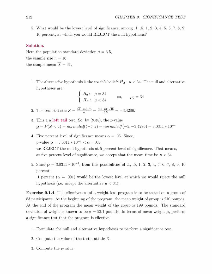
212 CHAPTER 9. SIGNIFICANCE TEST
5. What would be the lowest level of significance, among .1, .5, 1, 2, 3, 4, 5, 6, 7, 8, 9,10 percent, at which you would REJECT the null hypothesis?
Solution.Here the population standard deviation σ = 3.5,the sample size n = 16,the sample mean X = 31,
1. The alternative hypothesis is the coach’s belief: HA : µ < 34. The null and alternativehypotheses are: {
H0 : µ = 34
HA : µ < 34so, µ0 = 34
2. The test statistic Z = (X−µ0)√n
σ= (31−34)
√16
3.5= −3.4286.
3. This a a left tail test. So, by (9.35), the p-valuep = P (Z < z) = normalcdf(−5, z) = normalcdf(−5,−3.4286) = 3.0311 ∗ 10−4
4. Five percent level of significance means α = .05. Since,p-value p = 3.0311 ∗ 10−4 < α = .05,we REJECT the null hypothesis at 5 percent level of significance. That means,at five percent level of significance, we accept that the mean time is: µ < 34.
5. Since p = 3.0311 ∗ 10−4, from this possibilities of .1, .5, 1, 2, 3, 4, 5, 6, 7, 8, 9, 10percent;.1 percent (α = .001) would be the lowest level at which we would reject the nullhypothesis (i.e. accept the alternative µ < 34).
Exercise 9.1.4. The effectiveness of a weight loss program is to be tested on a group of83 participants. At the beginning of the program, the mean weight of group is 210 pounds.At the end of the program the mean weight of the group is 199 pounds. The standarddeviation of weight is known to be σ = 53.1 pounds. In terms of mean weight µ, performa significance test that the program is effective.
1. Formulate the null and alternative hypotheses to perform a significance test.
2. Compute the value of the test statistic Z.
3. Compute the p-value.

9.1. INTRODUCTION AND JARGON 213
4. At the 2 percent level of significance will you reject or accept the null hypothesis (orthat the program is effective or not)?
5. What would be the lowest level of significance, among .1, .5, 1, 2, 3, 4, 5, 6, 7, 8, 9,10 percent, at which you would REJECT the null hypothesis?
Solution.Here the population standard deviation σ = 53.1,the sample size n = 83,the sample mean X = 199,
1. he alternative hypothesis is program was effective to reduce the mean weight from210 pounds:HA : µ < 210. The null and alternative hypotheses are:{
H0 : µ = 210
HA : µ < 210so, µ0 = 210
2. The test statistic Z = (X−µ0)√n
σ= (199−210)
√83
53.1= −1.8872.
3. This a a left tail test. So, by (9.35), the p-valuep = P (Z < z) = normalcdf(−5, z) = normalcdf(−5,−1.8872) = .0296.
4. Two percent level of significance means α = .02. Since,p-value p = .0296 6< α = .02,we ACCEPT the null hypothesis at two percent level of significance.That means, at two percent level of significance, we DO NOT accept that the weightloss program is effective.
5. Since p = .0296, from this possibilities of .1, .5, 1, 2, 3, 4, 5, 6, 7, 8, 9, 10 percent;3 percent (α = .03) would be the lowest level at which we would reject the nullhypothesis (i.e. accept the alternative).
Exercise 9.1.5. A manufacturer of heating furnace is marketing a new model of energyefficient furnace. The mean gas consumption in January by ordinary furnaces is 153 CCF.A sample of 93 new model furnace had a mean consumption of 142 CCF in January. Thestandard deviation of consumption in January is known to be σ = 46 CCF. In termsof mean consumption µ, perform a significance test that the new model is really energyefficient.

214 CHAPTER 9. SIGNIFICANCE TEST
1. Formulate the null and alternative hypotheses to perform a significance test.
2. Compute the value of the test statistic Z.
3. Compute the p-value.
4. At the 1 percent level of significance will you reject or accept the null hypothesis (orthat the new model is energy efficient or not)?
5. What would be the lowest level of significance, among .1, .5, 1, 2, 3, 4, 5, 6, 7, 8, 9,10 percent, at which you would REJECT the null hypothesis?
Solution.Here the population standard deviation σ = 46,the sample size n = 93,the sample mean X = 142,
1. The alternative hypothesis is the claim of the manufacturer: HA : µ < 153. The nulland alternative hypotheses are:{
H0 : µ = 153
HA : µ < 153so, µ0 = 153
2. The test statistic Z = (X−µ0)√n
σ= (142−153)
√93
46= −2.3061.
3. This a a left tail test. So, by (9.35), the p-valuep = P (Z < z) = normalcdf(−5, z) = normalcdf(−5,−2.3061) = .01055.
4. One percent level of significance means α = .01. Since,p-value p = .01055 6< α = .01,we ACCEPT the null hypothesis at two percent level of significance.That means, at one percent level of significance, we do not accept that the this modelis energy efficient.
5. Since p = .01055, from this possibilities of .1, .5, 1, 2, 3, 4, 5, 6, 7, 8, 9, 10 percent;2 percent (α = .02) would be the lowest level at which we would reject the nullhypothesis (i.e. accept the alternative).

9.1. INTRODUCTION AND JARGON 215
Exercise 9.1.6. It is believed that due to favorable weather conditions the mean weightµ of King salmon in Anchor River would be higher than the last year’s mean of 33 pounds. The standard deviation of the weight is known to be σ = 16 pounds. A catch of 53 Kinghad a mean of 39 pounds. In terms of mean weight µ, perform a significance test that theweight would be higher.
1. Formulate the null and alternative hypotheses to perform a significance test.
2. Compute the value of the test statistic Z.
3. Compute the p-value.
4. At the 2 percent level of significance will you reject or accept the null hypothesis (orthat the mean weight has increased or not)?
5. What would be the lowest level of significance, among .1, .5, 1, 2, 3, 4, 5, 6, 7, 8, 9,10 percent, at which you would REJECT the null hypothesis?
Solution.Here the population standard deviation σ = 16,the sample size n = 53,the sample mean X = 39,
1. The alternative hypothesis is that the mean weight has increased: HA : µ > 33. Thenull and alternative hypotheses are:{
H0 : µ = 33
HA : µ > 33so, µ0 = 33
2. The test statistic Z = (X−µ0)√n
σ= (39−33)
√53
16= 2.7300.
3. This a a right tail test. So, by (9.11), the p-valuep = P (Z > z) = normalcdf(z, 5) = normalcdf(2.7300, 5) = .0032.
4. Two percent level of significance means α = .02. Since,p-value p = .0032 < α = .02,we REJECT the null hypothesis at 2 percent level of significance.That means, at two percent level of significance, we accept that the mean weight hasincreased.

216 CHAPTER 9. SIGNIFICANCE TEST
5. Since p = .0032, from this possibilities of .1, .5, 1, 2, 3, 4, 5, 6, 7, 8, 9, 10 percent;.5 percent (α = .005) would be the lowest level at which we would reject the nullhypothesis (i.e. accept the alternative).
Exercise 9.1.7. The instructor of Math 365 claims that due to his updated method ofteaching, the student’s learning has improved. The mean percent score of all his Math 365courses before this semester was 68 percent. This semester in his call of 79 students, themean percent score is 74 percent. The standard deviation of the percent score is known tobe σ = 22 percent. In terms of mean consumption µ, perform a significance test that thepercent score is higher.
1. Formulate the null and alternative hypotheses to perform a significance test.
2. Compute the value of the test statistic Z.
3. Compute the p-value.
4. At the 2 percent level of significance will you reject or accept the null hypothesis (orthat the student’s learning has improved or not)?
5. What would be the lowest level of significance, among .1, .5, 1, 2, 3, 4, 5, 6, 7, 8, 9,10 percent, at which you would REJECT the null hypothesis?
Solution.Here the population standard deviation σ = 22,the sample size n = 79,the sample mean X = 74,
1. The alternative hypothesis is that the mean percent score has increased from 68percent: HA : µ > 68.The null and alternative hypotheses are:{
H0 : µ = 68
HA : µ > 68so, µ0 = 68
2. The test statistic Z = (X−µ0)√n
σ= (74−68)
√79
22= 2.4241.
3. This a a right tail test. So, by (9.11), the p-valuep = P (Z > z) = normalcdf(z, 5) = normalcdf(2.4241, 5) = .0077.

9.2. SIGNIFICANCE TEST FOR µ: UNKNOWN σ 217
4. Two percent level of significance means α = .02. Since,p-value p = .0077 < α = .02,we REJECT the null hypothesis at 2 percent level of significance.That means, at two percent level of significance, we accept that the mean percentscore has increased.
5. Since p = .0032, from this possibilities of .1, .5, 1, 2, 3, 4, 5, 6, 7, 8, 9, 10 percent;1 percent (because .0077 < α = .01) would be the lowest level at which we wouldreject the null hypothesis.
Exercise 9.1.8. It is believed that the annual mean expenditure, including tuition, forstudents has increased from the corresponding mean in year 2000. In year 2000, the meanannual expenditure was $17,000. A sample of 87 students had annual mean expenditure of$19,500. The standard deviation annual expenditure is known to be σ = $7, 500. In termsof mean expenditure µ, perform a significance test that the mean annual expenditure µhas increased.
1. Formulate the null and alternative hypotheses to perform a significance test.
2. Compute the value of the test statistic Z.
3. Compute the p-value.
4. At the 2 percent level of significance will you reject or accept the null hypothesis (orthat the expenditure has or not)?
5. What would be the lowest level of significance, among .1, .5, 1, 2, 3, 4, 5, 6, 7, 8, 9,10 percent, at which you would REJECT the null hypothesis?
9.2 Significance Test for µ: Unknown σ
This section is analogous to section 7.2, on T -intervals. So, the significance tests we developwill be called T -test. As in the case of Z-tests (section 9.1.1), we would do three tests:
Two Tail Test Left Tail Test Right Tail Test{H0 : µ = µ0
HA : µ 6= µ0
{H0 : µ = µ0
HA : µ < µ0
{H0 : µ = µ0
HA : µ > µ0
(9.14)
We design the decision rules, as in the case Z-test (section 9.1.1). We refrain from repeatingsome of the reasoning used above (section 9.1.1) and we only give the decision rules.

218 CHAPTER 9. SIGNIFICANCE TEST
1. Similar to section 7.2, we assume that X ∼ N(µ, σ), and σ is also unknown.
2. Draw a sample X1, X2, . . . , Xn from the X-population, of size n. Let{X = X1+X2+···+Xn
n= the sample mean.
S =√
(X1−X)2+(X2−X)2+···+(Xn−X)2
n−1 = the standard deviation.(9.15)
3. Assume H0 : µ = µ0 is true. Then
T =(X − µ0)
√n
S∼ tn−1 has t distribution, with degrees of freedom n− 1 (9.16)
Expression T above would be called a test statistic. We use lower case, to denote
t =(x− µ0)
√n
sthe observed value of T. (9.17)
For three cases of alternate hypotheses, as in (9.14), we formulate the decision rules:
(a) Two Tail Test: When H0 is true, by (9.16),{P(|T | ≤ tn−1,α/2
)= P
(−tn−1,α/2 ≤ T ≤ tn−1,α/2
)= 1− α, OR
P(|T | > tn−1,α/2
)= α
(9.18)
Before we state the decision rules, we define p-value, for this test, as
p = P (|T | > |t|) = 1− tcdf(− |t| , |t| , n− 1) (9.19)
Because of equation 9.18, at level of significance α, set the decision rule as:{Reject H0 if |t| > tn−1,α/2Accept H0 if |t| ≤ tn−1,α/2
Equivalently,
{Accept HA if |t| > tn−1,α/2Reject HA if |t| ≤ tn−1,α/2
This translates to the following p-value based decision rule:{Reject H0 if p < αAccept H0 if p ≥ α
(9.20)
(b) Left Tail Test: When H0 is true, by (9.16),
P (T < −tn−1,α) = α (9.21)
We define p-value, for this test, as
p = P (T < t) ≈ tcdf(−5, t, n− 1). (9.22)
Because of equation 9.21, at level of significance α, set the decision rule as:{Reject H0 if t < −tn−1,αAccept H0 Otherwise
Equivalently,
{Accept HA if t < −tn−1,αReject HA Otherwise
This translates to the following p-value based decision rule:{Reject H0 if p < αAccept H0 if p ≥ α
(9.23)

9.2. SIGNIFICANCE TEST FOR µ: UNKNOWN σ 219
(c) Right Tail Test: When H0 is true, by (9.16),
P (tn−1,α < T ) = α (9.24)
We define p-value, for this test, as
p = P (T > t) ≈ tcdf(t, 5,m− 1) . (9.25)
Because of equation 9.24, at level of significance α, set the decision rule as:{Reject H0 if t > tn−1,αAccept H0 Otherwise
Equivalently,
{Accept HA if t > tn−1,αReject HA Otherwise
This translates to the following p-value based decision rule:{Reject H0 if p < αAccept H0 if p ≥ α
(9.26)
These three significance tests, for µ, when the value of σ is not known, is also calledT -test.
Universal Decision rule. As in the Z-test, the p-value based decision rules (9.20,9.23, 9.26) looks the same:{
Reject H0 if p < αAccept H0 if p ≥ α
which is even same as (9.13) (9.27)
However, p-values p are defined differently (9.19, 9.22, 9.25), are specific to the respectivetests. This similarity, regarding p-value based decision rule will be repeated for all thesubsequent sections, as well.
9.2.1 Problems: T -Test
Exercise 9.2.1. A supplier of lamps claims that the mean lifetime of his lamps is longerthan that of the lamps in the market. The mean lifetime of the bulbs on the market is3456 hours. To test the claim of the supplier, a sample of 26 bulbs were examined. Thesample mean was found to be 3720 hours and the sample standard deviation was s = 552
hours. In terms of mean lifetime µ, perform a significance test that the supplier’s lampslast longer.
1. Formulate the null and alternative hypotheses to perform a significance test.
2. Compute the value of the test statistic T .
3. Compute the p-value.

220 CHAPTER 9. SIGNIFICANCE TEST
4. At the 5 percent level of significance will you reject or accept the null hypothesis (orthat the mean lifetime of the lamps is higher or not)?
5. What would be the lowest level of significance, among .1, .5, 1, 2, 3, 4, 5, 6, 7, 8, 9,10 percent, at which you would REJECT the null hypothesis?
Solution. The population standard deviation is not known. So, the T -test will be used.We summarize the given data:The sample size n = 26,The sample mean X = 3720,The sample standard deviation S = 552,Degrees of freedom, df = n− 1 = 26− 1 = 25
1. The alternative hypothesis is that mean lifetime µ of the supplier’s lamps is higherthan 3456 hours: HA : µ > 3456.The null and alternative hypotheses are:{
H0 : µ = 3456
HA : µ > 3456so, µ0 = 3456
2. The test statistic T = (X−µ0)√n
s= (3720−3456)
√26
552= 2.4387.
3. This a a right tail test. So, by (9.25), the p-valuep = P (T > t) ≈ tcdf(t, 5, n− 1) = cdf(2.4387, 5, 25) = .0111.
4. Five percent level of significance means α = .05. Since,p-value p = .0111 < α = .05, we REJECT the null hypothesis at 5 percent level ofsignificance.That means, at five percent level of significance, we accept that the supplier’s claim.
5. Since p-value p = .0111, from this possibilities of .1, .5, 1, 2, 3, 4, 5,4, 7,8, 9,10percent; 2 percent (α = .02) would be the lowest level at which we would reject thenull hypothesis.
Exercise 9.2.2. It is believed that the mean length of babies at birth in the United Statesis higher than the mean of 16.7 inches in some other nation. A sample of 33 babies in theUnited States was collected, and the sample mean and standard deviation was found to beX = 19 inches, S = 5.5 inches. Perform a of significance test for this belief as follows.

9.2. SIGNIFICANCE TEST FOR µ: UNKNOWN σ 221
1. Formulate the null and alternative hypotheses to perform a significance test.
2. Compute the value of the test statistic T .
3. Compute the p-value.
4. At the 1 percent level of significance will you reject or accept the null hypothesis (orthat the birth length is higher or not)?
5. What would be the lowest level of significance, among .1, .5, 1, 2, 3, 4, 5, 6, 7, 8, 9,10 percent, at which you would REJECT the null hypothesis?
Solution. The population standard deviation is not known. So, the T -test will be used.Given data summarize, as follows :The sample size n = 33,The sample mean X = 19,The sample standard deviation S = 5.5,Degrees of freedom, df = n− 1 = 33− 1 = 32
1. The alternative hypothesis is that mean birth length µ in US is higher than 16.7inches: HA : µ > 16.7.The null and alternative hypotheses are:{
H0 : µ = 16.7
HA : µ > 16.7so, µ0 = 16.7
2. The test statistic T = (X−µ0)√n
s= (19−16.7)
√33
5.5= 2.4023.
3. This a a right tail test. So, by (9.25), the p-valuep = P (T > t) ≈ tcdf(t, 5, n− 1) = tcdf(2.4023, 5, 32) = .0111.
4. One percent level of significance means α = .01. Since,p-value p = .0111 6< α = .01, we ACCEPT the null hypothesis at 1 percent level ofsignificance.That means, at one percent level of significance, we do NOT accept that the meanbirth length µ is longer than 16.7 .
5. Since p-value p = .0111, from this possibilities of .1, .5, 1, 2, 3, 4, 5,4, 7,8, 9,10percent; 2 percent (α = .02) would be the lowest level at which we would reject thenull hypothesis.

222 CHAPTER 9. SIGNIFICANCE TEST
Exercise 9.2.3. A car manufacturer claims that a new model of car will get more mileageper gallon than the old model. The old model gets a mean mileage of 33 miles per gallon.To test the claim, 19 cars from the new model were tested and the sample mean was foundto be X = 35 miles and standard deviation S = 3.3 miles. Perform a significance test forthis manufacturer’s claim as follows.
1. Formulate the null and alternative hypotheses to perform a significance test.
2. Compute the value of the test statistic T .
3. Compute the p-value.
4. At the 1 percent level of significance will you reject or accept the null hypothesis (orthat the milage is higher or not)?
5. What would be the lowest level of significance, among .1, .5, 1, 2, 3, 4, 5, 6, 7, 8, 9,10 percent, at which you would REJECT the null hypothesis?
Solution. The population standard deviation is not known. So, the T -test will be used.Given data summarize, as follows :The sample size n = 19,The sample mean X = 35,The sample standard deviation S = 3.3,Degrees of freedom, df = n− 1 = 19− 1 = 18
1. The alternative hypothesis is that mean milage µ per gallon for the new model ishigher than 33 miles: HA : µ > 33.The null and alternative hypotheses are:{
H0 : µ = 33
HA : µ > 33so, µ0 = 33
2. The test statistic T = (X−µ0)√n
s= (35−33)
√19
3.3= 2.6218.
3. This a a right tail test. So, by (9.25), the p-valuep = P (T > t) ≈ tcdf(t, 5, n− 1) = tcdf(2.6218, 5, 18) = .0086

9.2. SIGNIFICANCE TEST FOR µ: UNKNOWN σ 223
4. One percent level of significance means α = .01. Since,p-value p = .0086 < α = .01, we REJECT the null hypothesis at 1 percent level ofsignificanc That means, at one percent level of significance, we accept that the meanmilage µ is higher than 33 miles .
5. Since p-value p = .0086, from this possibilities of .1, .5, 1, 2, 3, 4, 5,4, 7,8, 9,10percent; 1 percent (α = .01) would be the lowest level at which we would reject thenull hypothesis.
Exercise 9.2.4. Consider the following data , on life time X of light bulbs produced in afactory.
5110 4671 6441 3331 5055 5270 5335 4973 1837 5487
7783 4560 6074 4777 4707 5263 4978 5418 5123 5017
It is natural to assumed X ∼ N(µ, σ). The mean lifetime for an average light bulb on themarket is 4500 hours. The producer claims that the mean lifetime of the bulbs is morethan the average bulbs on the market. Perform a significance test for this claim.
1. Formulate the null and alternative hypotheses to perform a significance test.
2. Compute the value of the test statistic T .
3. Compute the p-value.
4. At the 2 percent level of significance will you reject or accept the null hypothesis (orthat the lifetime is higher or not)?
5. What would be the lowest level of significance, among .1, .5, 1, 2, 3, 4, 5, 6, 7, 8, 9,10 percent, at which you would REJECT the null hypothesis?
Solution. The population standard deviation is not known. So, the T -test will be used.Use TI-84, as in chapter 2, to summarize the raw data:Here the sample size n = 20,the sample mean X = 5060.5,Sample standard deviation S = 1143.1106
The degrees of freedom df = n− 1 = 20− 1 = 19
1. The alternative hypothesis is that the mean lifetime µ of the lamps is higher than4500 hours: HA : µ > 4500.

224 CHAPTER 9. SIGNIFICANCE TEST
The null and alternative hypotheses are:{H0 : µ = 4500
HA : µ > 4500so, µ0 = 4500
2. The test statistic T = (X−µ0)√n
s= (5060.5−4500)
√20
1143.1106= 2.1928.
3. This a a right tail test. So, by (9.25), the p-valuep = P (T > t) ≈ tcdf(t, 5, n− 1) = tcdf(2.1928, 5, 19) = .0204.
4. Two percent level of significance means α = .02. Since,p-value p = .0204 6< α = .02, we ACCEPT the null hypothesis at 2 percent levelof significance. That means, at two percent level of significance, we do NOT acceptthat the mean lifetime µ is higher than 4500 hours.
5. Since p-value p = .0204, from this possibilities of .1, .5, 1, 2, 3, 4, 5,4, 7,8, 9,10percent; 3 percent (α = .03) would be the lowest level at which we would reject thenull hypothesis.
Exercise 9.2.5. Consider the data, in Ex. 7.2.8, on weight (in pounds) of salmon in ariver. It is suspected that, due to pollution, the mean weight has reduced from last year’sthe mean weight 37 pounds. Perform a significance test as follows.
1. Formulate the null and alternative hypotheses to perform a significance test.
2. Compute the value of the test statistic T .
3. Compute the p-value.
4. At the 10 percent level of significance will you reject or accept the null hypothesis(or that the mean weight has reduced or not)?
5. What would be the lowest level of significance, among .1, .5, 1, 2, 3, 4, 5, 6, 7, 8, 9,10 percent, at which you would REJECT the null hypothesis?
Solution. The population standard deviation is not known. So, the T -test will be used.Use TI-84, as in chapter 2, to summarize the raw data:The sample size n = 19,The sample mean X = 34.3737,The sample standard deviation S = 6.7608,Degrees of freedom, df = n− 1 = 19− 1 = 18

9.2. SIGNIFICANCE TEST FOR µ: UNKNOWN σ 225
1. The alternative hypothesis is that the mean weight µ has reduced from 37 pounds:HA : µ < 37.The null and alternative hypotheses are:{
H0 : µ = 37
HA : µ < 37so, µ0 = 37
2. The test statistic T = (X−µ0)√n
s= (34.3737−37)
√19
6.7608= −1.6933.
3. This a a left tail test. So, by (9.22), the p-valuep = P (T < t) ≈ tcdf(−5, t, n− 1) = tcdf(−5,−1.6933, 18) = .0538
4. Ten percent level of significance means α = .10. Since,p-value p = .0538 < α = .10, we REJECT the null hypothesis at 10 percent level ofsignificance.That means, at ten percent level of significance, we accept that the mean weight µhas reduced from 37 pounds.
5. Since p-value p = .0538, from this possibilities of .1, .5, 1, 2, 3, 4, 5,4, 7,8, 9,10percent; 6 percent (α = .06) would be the lowest level at which we would reject thenull hypothesis.
Exercise 9.2.6. It is speculated that the teenage boys in a certain community are underweight. Under normal circumstances the mean weigh of this age group should be 155pounds. A sample of 27 teenage boys had a mean weight 135 pound and sample standarddeviation 32 pounds. Perform a significance test whether the mean weigh µ of this groupis below 155 pounds, as follows.
1. Formulate the null and alternative hypotheses to perform a significance test.
2. Compute the value of the test statistic T .
3. Compute the p-value.
4. At the 3 percent level of significance will you reject or accept the null hypothesis (orthat the mean weight is lower or not)?
5. What would be the lowest level of significance, among .1, .5, 1, 2, 3, 4, 5, 6, 7, 8, 9,10 percent, at which you would REJECT the null hypothesis?

226 CHAPTER 9. SIGNIFICANCE TEST
Exercise 9.2.7. A guess is that the mean time µ needed for a student to arrive at theclass from his/her residence would be less than 30 minutes. To test his guess, a sample37 was collected. The sample mean time needed was 27 minutes and the sample standarddeviation was 9 minutes. Perform a significance test whether the mean time µ neededwould be below 30 minutes, as follows.
1. Formulate the null and alternative hypotheses to perform a significance test.
2. Compute the value of the test statistic T .
3. Compute the p-value.
4. At the 3 percent level of significance will you reject or accept the null hypothesis (orthat the mean time is lower or not)?
5. What would be the lowest level of significance, among .1, .5, 1, 2, 3, 4, 5, 6, 7, 8, 9,10 percent, at which you would REJECT the null hypothesis?
9.3 Significance Test, for Proportion p
This section is analogous to section 7.3, on confidence intervals for p. So, the significancetests we develop will be called One proportion Z-test, for p. As in the case of Z-tests(section 9.1.1), we would do three tests:
Two Tail Test Left Tail Test Right Tail Test{H0 : p = p0HA : p 6= p0
{H0 : p = p0HA : p < p0
{H0 : p = p0HA : p > p0
(9.28)
We design the decision rules, as in the case Z-test (section 9.1.1). We only give the decisionrules.
1. As in section 7.3, a sample of size n is drawn. Let X be the total number of successand X = X
mdenote the sample proportion of success.
2. Assume H0 : p = p0 is true. From section 6.3, equation 6.4, we have
Z =X − p0√p0(1−p0)
n
=(X − p0)
√n√
p0(1− p0)∼ N(0, 1) has standard normal distribution
(9.29)Expression Z above would be called a test statistic. We use lower case, to denote
z =(x− p0)
√n√
p0(1− p0)the observed value of Z. (9.30)
For three cases of alternate hypotheses, as in (9.28), we formulate the decision rules:

9.3. SIGNIFICANCE TEST, FOR PROPORTION P 227
(a) Two Tail Test: When H0 is true, by (9.29),{P(|Z| ≤ zα/2
)= P
(−zα/2 ≤ Z ≤ zα/2
)= 1− α, OR
P(|Z| > zα/2
)= α
(9.31)
Define p-value, for this test, as
p = P (|Z| > |z|) = 1− normalcdf(− |z| , |z|) (9.32)
Because of (9.31), at level of significance α, set the decision rule:{Reject H0 if |z| > zα/2Accept H0 if |z| ≤ zα/2
Equivalently,
{Accept HA if |z| > zα/2Reject HA if |z| ≤ zα/2
This translates to the following p-value based decision rule:{Reject H0 if p < αAccept H0 if p ≥ α
(9.33)
(b) Left Tail Test: When H0 is true, by (9.29),
P (Z < −zα) = α (9.34)
Define p-value, for this test, as
p = P (Z < z) = normalcdf(−5, z). (9.35)
Because of (9.31), at level of significance α, set the decision rules:{Reject H0 if z < −zαAccept H0 Otherwise
Equivalently,
{Accept HA if z < −zαReject HA Otherwise
This translates to the following p-value based decision rule:{Reject H0 if p < αAccept H0 if p ≥ α
(9.36)
(c) Right Tail Test: When H0 is true, by (9.29),
P (zα < Z) = α (9.37)
Define p-value, for this test, as
p = P (Z > z) = normalcdf(z, 5). (9.38)
Because (9.31), at level of significance α, set the decision rule:{Reject H0 if z > zαAccept H0 Otherwise
Equivalently,
{Accept HA ifz > zαReject HA Otherwise
This translates to the following p-value based decision rule:{Reject H0 if p < αAccept H0 if p ≥ α
(9.39)

228 CHAPTER 9. SIGNIFICANCE TEST
This is known as the One proportion Z-Test.
Universal Decision rule. As before (9.13, 9.27), the p-value based decision rules(9.33,9.36, 9.39) looks the same:{
Reject H0 if p < αAccept H0 if p ≥ α
(9.40)
However, p-values p are defined differently (9.32, 9.35, 9.38), are specific to the respectivetests.
9.3.1 Problems: One proportion Z-Test
Exercise 9.3.1. In a sample of 197 apples from a lot, 26 were found to be sour. Thelot will be rejected if more than 10 percent is sour. Perform a significance test for theacceptability of this lot.
1. Formulate the null and alternative hypotheses to perform a significance test.
2. Compute the value of the test statistic Z.
3. Compute the p-value.
4. At the 3 percent level of significance will you reject or accept the null hypothesis (orwhether the lot is acceptable or not)?
5. What would be the lowest level of significance, among .1, .5, 1, 2, 3, 4, 5, 6, 7, 8, 9,10 percent, at which you would REJECT the null hypothesis?
Solution. The proportion of sour apples will be denoted by p.A one proportion Proportion Z-Test will be performed.Data is summarized as follows:The sample size n = 197,The number of success X = 26,The sample proportion of success X = X
n= 26
197= .1320
1. The alternate hypothesis is that p is more that .1 (ten percent).: HA : p > .1
The null and alternative hypotheses are:{H0 : p = .1
HA : p > .1so, p0 = .1

9.3. SIGNIFICANCE TEST, FOR PROPORTION P 229
2. The test statistic z = (x−p0)√n√
p0(1−p0)= (.1320−.1)
√197√
.1(1−.1)= 1.4971
3. This a a right tail test. So, by (9.38), the p-valuep = P (Z > z) = normalcdf(z, 5) = normalcdf(1.4971, 5) = .0672
4. Three percent level of significance means α = .03. Since,p-value p = .0672 6< α = .03, we accept the null hypothesis at 3 percent level ofsignificance.That means, at three percent level of significance, we conclude that the lot is accept-able.
5. Since p-value p = .0672, from this possibilities of .1, .5, 1, 2, 3, 4, 5,4, 7,8, 9,10percent; 7 percent (α = .07) would be the lowest level at which we would reject thenull hypothesis.
Exercise 9.3.2. A new vaccine was tried on 147 randomly selected individuals, and itwas determined that 61 of them got the virus. It is known that usually fifty percent ofthe population get the virus. Perform a significance test to decide if this vaccine is indeedeffective or not.
1. Formulate the null and alternative hypotheses to perform a significance test.
2. Compute the value of the test statistic Z.
3. Compute the p-value.
4. At the 3 percent level of significance will you reject or accept the null hypothesis (orthat the vaccine is effective or not)?
5. What would be the lowest level of significance, among .1, .5, 1, 2, 3, 4, 5, 6, 7, 8, 9,10 percent, at which you would REJECT the null hypothesis?
Solution. The proportion of the vaccinated population who benefit from it would be de-noted by p.A one proportion Proportion Z-Test will be performed.Data is summarized as follows:The sample size n = 147,The number of success X = 61,The sample proportion of success X = X
n= 61
147= .4150

230 CHAPTER 9. SIGNIFICANCE TEST
1. The alternate hypothesis is that p is less that .5 (better than 50 percent).: HA : p < .5
The null and alternative hypotheses are:{H0 : p = .5
HA : p < .5so, p0 = .5
2. The test statistic z = (x−p0)√n√
p0(1−p0)= (.4150−.5)
√147√
.5(1−.5)= −2.0611
3. This a a left tail test. So, by (9.35), the p-valuep = P (Z < z) = normalcdf(−5, z) = normalcdf(−5,−2.0611) = .0196
4. Three percent level of significance means α = .03. Since,p-value p = .0196 < α = .03, we REJECT the null hypothesis at 3 percent level ofsignificance.That means, at three percent level of significance, we conclude that the vaccine inEFFECTIVE.
5. Since p-value p = .0196, from this possibilities of .1, .5, 1, 2, 3, 4, 5,6, 7, 8, 9,10percent; 2 percent (α = .02) would be the lowest level at which we would reject thenull hypothesis.
Exercise 9.3.3. Before an election for a congressional seat, a poll was conducted. Out of887 randomly selected voters interviewed, 389 said that they would vote for Candidate A.The election strategists have decided that, to win Candidate A needs to get more than 40percent votes. Perform a significance test whether he/she will get more than 40 percent ornot.
1. Formulate the null and alternative hypotheses to perform a significance test.
2. Compute the value of the test statistic Z.
3. Compute the p-value.
4. At the 3 percent level of significance will you reject or accept the null hypothesis (orwhether he/she will get more than 40 percent or not.)?
5. What would be the lowest level of significance, among .1, .5, 1, 2, 3, 4, 5, 6, 7, 8, 9,10 percent, at which you would REJECT the null hypothesis?

9.3. SIGNIFICANCE TEST, FOR PROPORTION P 231
Solution. The proportion of the voter population who would vote for the candidate wouldbe denoted by p.A one proportion Proportion Z-Test will be performed.Data is summarized as follows:The sample size n = 887,The number of success X = 389,The sample proportion of success X = X
n= 389
887= .4386
1. The alternate hypothesis is that p is more that .4 (higher than 40 percent).: HA :
p > .4.The null and alternative hypotheses are:{
H0 : p = .4
HA : p > .4so, p0 = .4
2. The test statistic z = (x−p0)√n√
p0(1−p0)= (.4386−.4)
√887√
.4(1−.4)= 2.3466
3. This a a right tail test. So, by (9.38), the p-valuep = P (Z > z) = normalcdf(z, 5) = normalcdf(2.3466, 5) = .0095
4. Three percent level of significance means α = .03. Since,p-value p = .0095 < α = .03, we REJECT the null hypothesis at 3 percent level ofsignificance.That means, at three percent level of significance, we conclude that the CandidateA will win.
5. Since p-value p = .0095, from this possibilities of .1, .5, 1, 2, 3, 4, 5,4, 7,8, 9,10percent; 1 percent (α = .01) would be the lowest level at which we would reject thenull hypothesis.
Exercise 9.3.4. A pollster was asked to make decision whether the proportion p of theUS population who would support Government shutdown due to budget dispute, wouldbe above 55 percent or not? A sample 898 were polled and 522 of them said they wouldsupport government shutdown. Perform a significance test whether p would be above 55percent?
1. Formulate the null and alternative hypotheses to perform a significance test.

232 CHAPTER 9. SIGNIFICANCE TEST
2. Compute the value of the test statistic Z.
3. Compute the p-value.
4. At the 3 percent level of significance will you reject or accept the null hypothesis?
5. What would be the lowest level of significance, among .1, .5, 1, 2, 3, 4, 5, 6, 7, 8, 9,10 percent, at which you would REJECT the null hypothesis?
Exercise 9.3.5. A telephone company wants to know whether the proportion p of callsthat are longer than 20 minutes, in a town, would exceed 65 percent. A sample of 1123class, 761 were longer than 20 minute. Perform a significance test whether p would beabove 65 percent?
1. Formulate the null and alternative hypotheses to perform a significance test.
2. Compute the value of the test statistic Z.
3. Compute the p-value.
4. At the 3 percent level of significance will you reject or accept the null hypothesis?
5. What would be the lowest level of significance, among .1, .5, 1, 2, 3, 4, 5, 6, 7, 8, 9,10 percent, at which you would REJECT the null hypothesis?
Exercise 9.3.6. It is believed that, this year, proportion p of infected oranges will remainbelow 15 percent. A sample of 1333 class, 175 were were infected. Perform a significancetest whether p would remain below 15 percent?
1. Formulate the null and alternative hypotheses to perform a significance test.
2. Compute the value of the test statistic Z.
3. Compute the p-value.
4. At the 3 percent level of significance will you reject or accept the null hypothesis?
5. What would be the lowest level of significance, among .1, .5, 1, 2, 3, 4, 5, 6, 7, 8, 9,10 percent, at which you would REJECT the null hypothesis?

9.4. TESTING HYPOTHESES ON VARIANCE σ2 233
9.4 Testing Hypotheses on Variance σ2
Let X ∼ N(µ, σ) be a normal random variable.
This section is analogous to section 7.4.2, on χ2-interval for σ2. So, the significancetests we develop will be called χ2-Test. We would do two tests:
Left Tail Test Right Tail Test{H0 : σ2 = σ2
0
HA : σ2 < σ20
{H0 : σ2 = σ2
0
HA : σ2 > σ20
(9.41)
We only give the decision rules.
1. Similar to section 7.4.2, we assume that X ∼ N(µ, σ)
2. Draw a sample X1, X2, . . . , Xn from the X-population, of size n. As always,{X = X1+X2+···+Xn
n= the sample mean.
S2 = (X1−X)2+(X2−X)2+···+(Xn−X)2
n−1 = the sample variance.(9.42)
3. Assume H0 : σ2 = σ20 is true. Then
Y =(n− 1)S2
σ20
∼ χ2n−1 has χ2 distribution, with degrees of freedom n− 1 (9.43)
Expression Y above would be called a test statistic. We use lower case, to denote
y =(n− 1)s2
σ20
the observed value of Y. (9.44)
For two cases of alternate hypotheses, as in (9.41), we formulate the decision rules:
(a) Left Tail Test: When H0 is true, by (9.43),
P(Y < χ2
n−1,1−α)
= α (9.45)
We define p-value, for this test, as
p = P (Y < y) = χ2cdf(0, y, n− 1). (9.46)
Because of (9.45), at level of significance α, set the decision rule as:{Reject H0 if y < χ2
n−1,1−αAccept H0 Otherwise
Equivalently,
{Accept HA if y < χ2
n−1,1−αReject HA Otherwise
This translates to the following p-value based decision rule:{Reject H0 if p < αAccept H0 if p ≥ α
(9.47)

234 CHAPTER 9. SIGNIFICANCE TEST
(b) Right Tail Test: When H0 is true, by (9.43),
P(χ2n−1,α < Y
)= α (9.48)
Define p-value, for this test, as
p = P (y < Y ) = 1− χ2cdf(0, y, n− 1). (9.49)
Because of (9.24), at level of significance α, set the decision rule as:{Reject H0 if y > χ2
n−1,αAccept H0 Otherwise
Equivalently,
{Accept HA if y > χ2
n−1,αReject HA Otherwise
This translates to the following p-value based decision rule:{Reject H0 if p < αAccept H0 if p ≥ α
(9.50)
This is known as the χ2-Test.
Universal Decision rule. As before (9.13, 9.27, 9.40), the p-value based decisionrules (9.47, 9.50) looks the same:{
Reject H0 if p < αAccept H0 if p ≥ α
(9.51)
However, p-values p are defined differently (9.46, 9.49), are specific to the respective tests.
9.4.1 Problems: on χ2-Test
Exercise 9.4.1. Suppose that we have collected a sample of size n = 23 from a normalpopulation X ∼ N(µ, σ). The sample variance was found to be S2 = 46.7. It is believedthat the variance σ2 is higher than 25. Perform a significance test as follows.
1. Formulate the null and alternative hypotheses to perform a significance test.
2. Compute the value of the test statistic.
3. Compute the p-value.
4. At the 3 percent level of significance will you reject or accept the null hypothesis?
5. What would be the lowest level of significance, among .1, .5, 1, 2, 3, 4, 5, 6, 7, 8, 9,10 percent, at which you would REJECT the null hypothesis?

9.4. TESTING HYPOTHESES ON VARIANCE σ2 235
Solution. A χ2-Test will be performed.Given data is summarized: Sample size n = 23
Sample variance S2 = 46.7
Degrees of freedom df = n− 1 = 23− 1 = 22.
1. We are testing the belief, σ2 is higher than 25.The null and alternative hypotheses are:{
H0 : σ2 = 25
HA : σ2 > 25so, σ2
0 = 25
2. The test statistic Y = (n−1)S2
σ20
= (23−1)46.725
= 41.096.
3. This is a right tail test. So, by (9.49), the p-valuep = P (y < Y ) = 1− χ2cdf(0, y, n− 1)
= 1− χ2cdf(0, 41.096, 22) = 1− .9920 = .008
4. Three percent level of significance means α = .03. Since,p-value p = .008 < α = .03, we REJECT the null hypothesis at 3 percent level ofsignificance.That means, we conclude, at 3 percent level of confidence, that the variance σ2 ishigher than 25.
5. Since p-value p = .008, from this possibilities of .1, .5, 1, 2, 3, 4, 5, 6, 7,8, 9,10percent; 1 percent (α = .01) would be the lowest level at which we would reject thenull hypothesis.
Exercise 9.4.2. Following is data on the life expectancies of a group of people older than75.
87 92 81 76 81 87 79 88 88 79 81 89 97 91 82
It is believed that the variance σ2 life expectancy of this group is higher than 16. Performa significance test as follows.
1. Formulate the null and alternative hypotheses to perform a significance test.
2. Compute the value of the test statistic.
3. Compute the p-value.

236 CHAPTER 9. SIGNIFICANCE TEST
4. At the 1 percent level of significance will you reject or accept the null hypothesis?
5. What would be the lowest level of significance, among .1, .5, 1, 2, 3, 4, 5, 6, 7, 8, 9,10 percent, at which you would REJECT the null hypothesis?
Solution. A χ2-Test will be performed.As in chapter 2, given data is processed:Sample size n = 15
Sample variance S2 = (5.8578)2 = 34.3138
Degrees of freedom df = n− 1 = 15− 1 = 14.
1. We are testing the belief, that the variance σ2 is higher than 16.The null and alternative hypotheses are:{
H0 : σ2 = 16
HA : σ2 > 16so, σ2
0 = 16
2. The test statistic Y = (n−1)S2
σ20
= (15−1)34.313816
= 30.0246.
3. This is a right tail test. So, by (9.49), the p-valuep = P (y < Y ) = 1− χ2cdf(0, y, n− 1)
= 1− χ2cdf(0, 30.0246, 14) = 1− .9924 = .0076
4. One percent level of significance means α = .01. Since,p-value p = .0076 < α = .01, we REJECT the null hypothesis at 1 percent level ofsignificance.That means, we conclude, at 1 percent level of confidence, that the variance σ2 ishigher than 16.
5. Since p-value p = .0076, from this possibilities of .1, .5, 1, 2, 3, 4, 5,4, 7, 8, 9,10percent; 1 percent (α = .01) would be the lowest level at which we would reject thenull hypothesis.
Exercise 9.4.3. The following is data on monthly gas consumption (in ccf) by the house-holds in a town during the winter months.
154 222 264 257 127 228 240 393 278 140
It is believed that the variance σ2 is less than 15600 ccf 2 . Perform a significance test asfollows.

9.4. TESTING HYPOTHESES ON VARIANCE σ2 237
1. Formulate the null and alternative hypotheses to perform a significance test.
2. Compute the value of the test statistic.
3. Compute the p-value.
4. At the 5 percent level of significance will you reject or accept the null hypothesis?
5. What would be the lowest level of significance, among .1, .5, 1, 2, 3, 4, 5, 6, 7, 8, 9,10 percent, at which you would REJECT the null hypothesis?
Solution. A χ2-Test will be performed.As in chapter 2, given data is processed:Sample size n = 10
Sample variance S2 = (78.4645)2 = 6156.6778
Degrees of freedom df = n− 1 = 10− 1 = 9.
1. We are testing the belief, σ2 is less than 15600.The null and alternative hypotheses are:{
H0 : σ2 = 15600
HA : σ2 < 15600so, σ2
0 = 15600
2. The test statistic Y = (n−1)S2
σ20
= (10−1)6156.677815600
= 3.5519.
3. This is a left tail test. So, by (9.46), the p-valuep = P (Y < y) = χ2cdf(0, y, n− 1) = χ2cdf(0, 3.5519, 9) = .0616
4. Five percent level of significance means α = .05. Since,p-value p = .0616 6< α = .05, we ACCEPT the null hypothesis at 5 percent level ofsignificance.That means, at the level of significance 5 percent, we do NOT accept that the σ2 islower than 15600
5. Since p-value p = .0616, from this possibilities of .1, .5, 1, 2, 3, 4, 5, 6, 7,8, 9,10percent; 7 percent (α = .07) would be the lowest level at which we would reject thenull hypothesis.

238 CHAPTER 9. SIGNIFICANCE TEST
Exercise 9.4.4. The birth weight of babies has a normal distribution, with variance σ2.Because of the economic and social diversity of the community, there are concerns aboutvariability of the birth weight. It is believed that the variance σ2 may be higher than 17pounds-square. A sample of 26 birth-weight was collected and the sample variance wasfound to be S2 = 26.7 pounds-square. Perform a significance test as follows.
1. Formulate the null and alternative hypotheses to perform a significance test.
2. Compute the value of the test statistic.
3. Compute the p-value.
4. At the 3 percent level of significance will you reject or accept the null hypothesis?
5. What would be the lowest level of significance, among .1, .5, 1, 2, 3, 4, 5, 6, 7, 8, 9,10 percent, at which you would REJECT the null hypothesis?
Solution. A χ2-Test will be performed.Given data is summarized: Sample size n = 26
Sample variance S2 = 26.7
Degrees of freedom df = n− 1 = 26− 1 = 25.
1. We are testing the belief, σ2 is higher than 17.The null and alternative hypotheses are:{
H0 : σ2 = 17
HA : σ2 > 17so, σ2
0 = 17
2. The test statistic Y = (n−1)S2
σ20
= (26−1)26.717
= 39.2647.
3. This is a right tail test. So, by (9.49), the p-valuep = P (y < Y ) = 1− χ2cdf(0, y, n− 1) =
1− χ2(0, 39.2647, 25) = .0346
4. Three percent level of significance means α = .03. Since,p-value p = .0346 6< α = .03, we ACCEPT the null hypothesis at 3 percent level ofsignificance..That means, , at 3 percent level of confidence, we do not accept that the variance σ2
is higher than 17.

9.4. TESTING HYPOTHESES ON VARIANCE σ2 239
5. Since p-value p = .0346, from this possibilities of .1, .5, 1, 2, 3, 4, 5, 6, 7,8, 9,10percent; 4 percent (α = .04) would be the lowest level at which we would reject thenull hypothesis.
Exercise 9.4.5. It is speculated that the variability of length of babies, in a community,at birth may be small. It is speculated that variance length σ2 of babies may be lowerthan 25 square-inches. A sample of size n = 16 on birth-lengths was collected. The samplevariance was found to be S2 = 13 square-inches. Perform a significance test as follows.
1. Formulate the null and alternative hypotheses to perform a significance test.
2. Compute the value of the test statistic.
3. Compute the p-value.
4. At the 5 percent level of significance will you reject or accept the null hypothesis?
5. What would be the lowest level of significance, among .1, .5, 1, 2, 3, 4, 5, 6, 7, 8, 9,10 percent, at which you would REJECT the null hypothesis?
Solution. A χ2-Test will be performed.Given data is summarized:Sample size n = 16
Sample variance S2 = 13
Degrees of freedom df = n− 1 = 16− 1 = 15.
1. We are testing the speculation, σ2 is less than 25.The null and alternative hypotheses are:{
H0 : σ2 = 25
HA : σ2 < 25so, σ2
0 = 25
2. The test statistic Y = (n−1)S2
σ20
= (16−1)1325
= 7.8.
3. This is a left tail test. So, by (9.46), the p-valuep = P (Y < y) = χ2cdf(0, y, n− 1) = χ2cdf(0, 7.8, 15) = .0684
4. Five percent level of significance means α = .05. Since,p-value p = .0684 6< α = .05, we ACCEPT the null hypothesis at 5 percent level of

240 CHAPTER 9. SIGNIFICANCE TEST
significance.That means, at the level of significance 5 percent, we do NOT accept that the σ2 isless than 25.
5. Since p-value p = .0684, from this possibilities of .1, .5, 1,2, 3, 4, 5,4, 7,8, 9,10percent; 7 percent (α = .07) would be the lowest level at which we would reject thenull hypothesis.
Exercise 9.4.6. The variability of the length of the telephone calls is a concern of thetelephone company. It is speculated that the variance σ2 may be higher that 64 minutes-square. A sample of 14 calls had a sample variance S2 = 99 minutes-square. Perform asignificance test as follows.
1. Formulate the null and alternative hypotheses to perform a significance test.
2. Compute the value of the test statistic.
3. Compute the p-value.
4. At the 5 percent level of significance will you reject or accept the null hypothesis?
5. What would be the lowest level of significance, among .1, .5, 1, 2, 3, 4, 5, 6, 7, 8, 9,10 percent, at which you would REJECT the null hypothesis?
Solution. A χ2-Test will be performed.Given data is summarized: Sample size n = 14
Sample variance S2 = 99
Degrees of freedom df = n− 1 = 14− 1 = 13.
1. We are testing the speculation , σ2 is higher than 64.The null and alternative hypotheses are:{
H0 : σ2 = 64
HA : σ2 > 64so, σ2
0 = 64
2. The test statistic Y = (n−1)S2
σ20
= (14−1)9964
= 20.1094.
3. This is a right tail test. So, by (9.49), the p-valuep = P (y < Y ) = 1− χ2cdf(0, y, n− 1)
= 1− χ2cdf(0, 20.1094, 13) = .0925

9.5. TWO POPULATIONS: KNOWN σ1, σ2 241
4. Five percent level of significance means α = .05. Since,p-value p = .0925 6< α = .05, we ACCEPT the null hypothesis at 5 percent level ofsignificance.That means, we conclude, at 5 percent level of confidence, that the variance σ2 is nothigher than 64.
5. Since p-value p = .0925, from this possibilities of .1, .5, 1, 2, 3, 4, 5,4, 7,8, 9,10percent; 10 percent (α = .10) would be the lowest level at which we would reject thenull hypothesis.
9.5 Two Populations: Known σ1, σ2
This section is analogous to section 8.1, on confidence intervals for µ1 − µ2. As in section8.1, suppose X, Y are two similar random variables. Let mean and st. deviations of Xand Y be denoted, as follows:
Population X Population Ymean E(X) = µ1 E(Y ) = µ2
St. Dev. σ1 σ2
We test equality µ1 = µ2, of means. We deal with the case when σ1 and σ2 are known. Wewould do three tests:
Two Tail Test Left Tail Test Right Tail Test{H0 : µ1 − µ2 = 0HA : µ1 − µ2 6= 0
{H0 : µ1 − µ2 = 0HA : µ1 − µ2 < 0
{H0 : µ1 − µ2 = 0HA : µ1 − µ2 > 0
(9.52)
1. A sample X1, X2, . . . , Xm, of size m, is drawn from the X-population and a sampleY1, Y2, . . . , Yn, of size n, is drawn from the Y population. Let{
X = X1+X2+···+Xmm
Y = Y1+Y2+···+Ymn
be the sample means
Assume that the X-samples and Y -samples are drawn independently. As was statedin section 8.1, approximately,
X − Y ∼ N (µ1 − µ2, σ) where
{E(X − Y ) = µ1 − µ2
σ =
√σ21
m+
σ22
n
If X and Y are normal, then this is exact (not just approximate) distribution.

242 CHAPTER 9. SIGNIFICANCE TEST
2. Assume H0 : µ1 − µ2 = 0 is true. Then,
Z =X − Yσ
=X − Y√σ21
m+
σ22
n
∼ N(0, 1) has standard normal distribution (9.53)
Expression Z above would be called a test statistic. We use lower case, to denote
z =x− yσ
=x− y√σ21
m+
σ22
n
the observed value of Z. (9.54)
For three cases of alternate hypotheses, as in (9.52), we formulate the decision rules:
(a) Two Tail Test: When H0 is true, by (9.53),{P(|Z| ≤ zα/2
)= P
(−zα/2 ≤ Z ≤ zα/2
)= 1− α, OR
P(|Z| > zα/2
)= α
(9.55)
Define p-value, for this test, as
p = P (|Z| > |z|) = 1− normalcdf(− |z| , |z|) (9.56)
Because of (9.55), at level of significance α, set the decision rule:{Reject H0 if |z| > zα/2Accept H0 if |z| ≤ zα/2
Equivalently,
{Accept HA if |z| > zα/2Reject HA if |z| ≤ zα/2
This translates to the following p-value based decision rule:{Reject H0 if p < αAccept H0 if p ≥ α
(9.57)
(b) Left Tail Test: When H0 is true, by (9.53),
P (Z < −zα) = α (9.58)
Define p-value, for this test, as
p = P (Z < z) = normalcdf(−5, z). (9.59)
Because of (9.58), at level of significance α, set the decision rules:{Reject H0 if z < −zαAccept H0 Otherwise
Equivalently,
{Accept HA if z < −zαReject HA Otherwise
This translates to the following p-value based decision rule:{Reject H0 if p < αAccept H0 if p ≥ α
(9.60)

9.5. TWO POPULATIONS: KNOWN σ1, σ2 243
(c) Right Tail Test: When H0 is true, by (9.53),
P (zα < Z) = α (9.61)
Define p-value, for this test, as
p = P (Z > z) = normalcdf(z, 5). (9.62)
Because of (9.61), at level of significance α, set the decision rule:{Reject H0 if z > zαAccept H0 Otherwise
Equivalently,
{Accept HA ifz > zαReject HA Otherwise
This translates to the following p-value based decision rule:{Reject H0 if p < αAccept H0 if p ≥ α
(9.63)
These are called Two sample Z-Test.
Universal Decision rule. As before (9.13, 9.27, 9.40, 9.51), the p-value based decisionrules (9.57,9.60, 9.63) looks the same:{
Reject H0 if p < αAccept H0 if p ≥ α
(9.64)
However, p-values p are defined differently (9.56, 9.59, 9.62), are specific to the respectivetests.
9.5.1 Problems: Two sample Z-Test
Exercise 9.5.1. The equality of means µ1, µ2 of two populations is to be compared. Thestandard deviations σ1, σ2, respectively, are known to be σ1 = 8.1 and σ2 = 11.3. A sampleof size m = 64 was collected from the first population, and the sample mean was found tobe X = 3.5. A sample of size n = 99 was collected from the second population, and thesample mean was found to be Y = 7.9.
It is speculated that these two means are unequal: µ1 6= µ2? Perform a significancetest as follows.
1. Formulate the null and alternative hypotheses to perform a significance test.
2. Compute the value of the test statistic.
3. Compute the p-value.

244 CHAPTER 9. SIGNIFICANCE TEST
4. At the 3 percent level of significance will you reject or accept the null hypothesis?
5. What would be the lowest level of significance, among .1, .5, 1, 2, 3, 4, 5, 6, 7, 8, 9,10 percent, at which you would REJECT the null hypothesis?
Solution. The given data is summarized as follows:
Population I X Population II Y
St. Dev. σ1 = 8.1 σ2 = 11.3
samplemean X = 3.7 Y = 7.9
sample size m = 64 n = 99
1. We are testing the speculation, µ1 6= µ2.The null and alternative hypotheses are:{
H0 : µ1 − µ2 = 0
HA : µ1 − µ2 6= 0
2. The test statistic
Z =X − Y√σ21
m+
σ22
n
=3.7− 7.9√8.12
64+ 11.32
99
= −2.8919
3. This is a Two tail test. So, by (9.56), the p-valuep = P (|Z| > |z|) = 1− normalcdf(− |z| , |z|)= 1− normalcdf(−2.8919, 2.8919) = 1− .9962 = .0038
4. Three percent level of significance means α = .03. Since,p-value p = .0038 < α = .03, we REJECT the null hypothesis at 3 percent level ofsignificance.
5. Since p-value p = .0038, from this possibilities of .1, .5, 1, 2, 3, 4, 5,4, 7,8, 9,10percent; .5 percent (α = .005) would be the lowest level at which we would reject thenull hypothesis.
Exercise 9.5.2. The birth weight of babies in two hospitals would have to be compared.The birth-weight distributionsX and Y of these two hospitals are normal with means µ1, µ2
and standard deviations σ1, σ2, respectively. It is known the standard deviations σ1 = 2.3
pounds and σ2 = 2.9 pounds. A sample of size m = 35 babies from the first hospitals was

9.5. TWO POPULATIONS: KNOWN σ1, σ2 245
collected, and the sample mean birth weight was found to be X = 8.9 pounds. A sampleof size n = 48 babies from the second hospital was collected, and the sample mean birthweight was found to be Y = 7.6 pounds.
Due to economic disparities between these two neighborhoods, it is speculated that themean µ1 is higher than the mean µ2. Perform a significance test as follows.
1. Formulate the null and alternative hypotheses to perform a significance test.
2. Compute the value of the test statistic.
3. Compute the p-value.
4. At the 3 percent level of significance would you accept this speculation that µ1 ishigher than µ2?
5. What would be the lowest level of significance, among .1, .5, 1, 2, 3, 4, 5, 6, 7, 8, 9,10 percent, at which you would REJECT the null hypothesis?
Solution. The given data is summarized as follows:
Population I X Population II Y
St. Dev. σ1 = 2.3 σ2 = 2.9
samplemean X = 8.9 Y = 7.6
sample size m = 35 n = 48
1. The alternative hypothesis is that the X-mean µ1 would be higher than the Y -meanµ2: HAµ1 > µ2.The null and alternative hypotheses are:{
H0 : µ1 − µ2 = 0
HA : µ1 − µ2 > 0
2. The test statistic
Z =X − Y√σ21
m+
σ22
n
=8.9− 7.6√2.32
35+ 2.92
48
= 2.2756
3. This is a right tail test. So, by (9.62), the p-valuep = P (Z > z) = normalcdf(z, 5)
= P (2.2756 < Z) = normalcdf(2.2756, 5)) = .0114

246 CHAPTER 9. SIGNIFICANCE TEST
4. Three percent level of significance means α = .03. Since,p-value p = .0114 < α = .03, we REJECT the null hypothesis at 3 percent level ofsignificance.
5. Since p-value p = .0114, from this possibilities of .1, .5, 1, 2, 3, 4, 5,4, 7,8, 9,10percent; 2 percent (α = .02) would be the lowest level at which we would reject thenull hypothesis.
Exercise 9.5.3. Elephants in different parts of the world are different in height, weight,and length of ear and tusk. The mean heights µ1 and µ2 of elephants in two differentregions would be compared. It is assumed that the height distributions X and Y of theelephants in these two regions are normally distributed. The standard deviation of X andY are σ1 = 1.5 feet and σ2 = 1.3 feet, respectively. A sample of size 25 was collected fromregion-I, and the sample mean height was found to be X = 9.9 feet. A sample of size 28was collected from the region-II was collected, and the sample mean height was found to beY = 9.1 feet. It is believed that mean height µ1 is higher than µ2. Perform a significancetest as follows.
1. Formulate the null and alternative hypotheses to perform a significance test.
2. Compute the value of the test statistic.
3. Compute the p-value.
4. At the 3 percent level of significance will you accept µ1 is higher than µ2?
5. What would be the lowest level of significance, among .1, .5, 1, 2, 3, 4, 5, 6, 7, 8, 9,10 percent, at which you would REJECT the null hypothesis?
Solution. The given data is summarized as follows:
Population I X Population II Y
St. Dev. σ1 = 1.5 σ2 = 1.3
samplemean X = 9.9 Y = 9.1
sample size m = 25 n = 28
1. We are testing the speculation, µ1 is higher than µ2.The null and alternative hypotheses are:{
H0 : µ1 − µ2 = 0
HA : µ1 − µ2 > 0

9.5. TWO POPULATIONS: KNOWN σ1, σ2 247
2. The test statistic
Z =X − Y√σ21
m+
σ22
n
=9.9− 9.1√1.52
25+ 1.32
28
= 2.0631
3. This is a right tail test. So, by (9.62), the p-valuep = P (Z > z) = normalcdf(z, 5)
= normalcdf(2.0631, 5)) = .0196
4. Three percent level of significance means α = .03. Since,p-value p = .0196 < α = .03, we REJECT the null hypothesis at 3 percent level ofsignificance; or we accept the alternate that µ1 is higher than µ2.
5. Since p-value p = .0038, from this possibilities of .1, .5, 1, 2, 3, 4, 5,4, 7,8, 9,10percent; 2 percent (α = .02) would be the lowest level at which we would reject thenull hypothesis.
Exercise 9.5.4. It is speculated that the mean weight µ1 of King salmon in Kenai is lowerthan the mean weight µ2 of King salmon in Anchor River. The standard deviation weightof the Kings in Kenai is σ1 = 7.7 pounds. The standard deviation weight of the Kings inAnchor is σ2 = 9.1 pounds. A sample of 51 King from Kenai had a mean X = 30.5 pounds.A sample of 63 King from Anchor had a mean Y = 33 pounds. Perform a significance testas follows.
1. Formulate the null and alternative hypotheses to perform a significance test.
2. Compute the value of the test statistic.
3. Compute the p-value.
4. At the 5 percent level of significance, do you accept that µ1 is lower than µ2?
5. What would be the lowest level of significance, among .1, .5, 1, 2, 3, 4, 5, 6, 7, 8, 9,10 percent, at which you would REJECT the null hypothesis?
Solution. The given data is summarized as follows:
Population I X Population II Y
St. Dev. σ1 = 7.7 σ2 = 9.1
samplemean X = 30.5 Y = 33
sample size m = 51 n = 63

248 CHAPTER 9. SIGNIFICANCE TEST
1. We are testing the speculation, µ1 is lower than µ2.The null and alternative hypotheses are:{
H0 : µ1 − µ2 = 0
HA : µ1 − µ2 < 0
2. The test statistic
Z =X − Y√σ21
m+
σ22
n
=30.5− 33√7.72
51+ 9.12
63
= −1.5885
3. This is a left tail test. So, by (9.59), the p-valuep = P (Z < z) = normalcdf(−5, z)
= normalcdf(−5,−1.5885)) = .0561
4. Five percent level of significance means α = .05. Since,p-value p = .0561 6< α = .05, we ACCEPT the null hypothesis at 5 percent level ofsignificance.That means we do not accept that the mean weight of Kings in Kenai is less thanthat of Anchor, at 3 percent level of significance.
5. Since p-value p = .0561, from this possibilities of .1, .5, 1, 2, 3, 4, 5,4, 7,8, 9,10percent; 6 percent (α = .06) would be the lowest level at which we would reject thenull hypothesis.
Exercise 9.5.5. There is a speculation circulating that the mean percent scores µ1 in fallsemester grades is higher than the mean percent scores µ2 in spring semester grades. Thestandard deviation of fall percent scores is σ1 = 27 percent and the standard deviation ofspring percent scores is σ2 = 23 percent. A sample of 87 students in fall had a samplemean score X = 76 percent. A sample of 77 students in spring had a sample mean scoreY = 69 percent. Perform a significance test as follows.
1. Formulate the null and alternative hypotheses to perform a significance test. ( Thiswould be a Right Tail.)
2. Compute the value of the test statistic.
3. Compute the p-value.
4. At the 3 percent level of significance will you accept µ1 is higher than µ2?

9.6. TWO SAMPLE T -TEST: UNKNOWN σ1, σ2 249
5. What would be the lowest level of significance, among .1, .5, 1, 2, 3, 4, 5, 6, 7, 8, 9,10 percent, at which you would REJECT the null hypothesis?
Exercise 9.5.6. it is speculated that the mean annual salary µ1 of the professors in aState University (I) is higher than the mean annual salary µ2 of the professors in the StateUniversity (II). The standard deviation of the annual salary in the University -I σ1 =
$16, 000 and the standard deviation of the annual salary in the University-II σ2 = $11, 500.A sample of 47 professors in University-I had a mean salary X = $77, 000. A sample of 58professors in University-II had a mean salary Y = $71, 500 Perform a significance test asfollows.
1. Formulate the null and alternative hypotheses to perform a significance test. ( Thiswould be a Right Tail.)
2. Compute the value of the test statistic.
3. Compute the p-value.
4. At the 3 percent level of significance will you accept µ1 is higher than µ2?
5. What would be the lowest level of significance, among .1, .5, 1, 2, 3, 4, 5, 6, 7, 8, 9,10 percent, at which you would REJECT the null hypothesis?
9.6 Two sample T -Test: Unknown σ1, σ2
This section is analogous to section 8.2, on Two sample T -intervals for µ1−µ2. We developa test for H0 : µ1 − µ0 = 0. As in section 8.2, we proceed as follows:
1. As indicated above, X ∼ N(µ1, σ1), Y ∼ N(µ2, σ2) have normal distributions, andassume
σ1 = σ2 = σ
2. A sample X1, X2, . . . , Xm, of size m, is drawn from the X-population and a sampleY1, Y2, . . . , Yn, of size n, is drawn from the Y population. Use the notations for samplemean and sample standard deviations (variance), as follows:{
X = X1+X2+···+Xmm
Y = Y1+Y2+···+Ymn
{S21 = S2
X = (X1−X)2+(X2−X)2+···+(Xm−X)2
m−1
S22 = S2
Y = (Y1−Y )2+(Y2−Y )2+···+(Yn−Y )2
n−1
We obtain the pooled estimate, S2p for σ2, as follows:
S2p =
(m− 1)S2X + (n− 1)S2
Y
m+ n− 2

250 CHAPTER 9. SIGNIFICANCE TEST
This happens to be the weighted mean of S2X with weight (m − 1), and S2
Y withweight (n− 1). So, pooled estimate Sp for σ is
Sp =
√(m− 1)S2
X + (n− 1)S2Y
m+ n− 2
We test equality µ1 = µ2, of means. We deal with the case when σ1 and σ2 are unknown.We would do three tests:
Two Tail Test Left Tail Test Right Tail Test{H0 : µ1 − µ2 = 0HA : µ1 − µ2 6= 0
{H0 : µ1 − µ2 = 0HA : µ1 − µ2 < 0
{H0 : µ1 − µ2 = 0HA : µ1 − µ2 > 0
(9.65)
1. Assume H0 : µ1 − µ2 = 0 is true. Then,
T =X − Y
Sp
√1m
+ 1n
∼ tm+n−2 has t−distribution, (9.66)
with degrees of freedom df = m+ n− 2. Expression T above would be called a teststatistic. We use lower case, to denote
t =x− y
sp
√1m
+ 1n
the observed value of T. (9.67)
As in We formulate the decision rules, analogous to T -test (section 9.2), for threesignificance test, as in (9.65):
(a) Two Tail Test: When H0 is true, by (9.66),{P(|T | ≤ tn−1,α/2
)= P
(−tm+n−2,α/2 ≤ T ≤ tm+n−2,α/2
)= 1− α, OR
P(|T | > tm+n−2,α/2
)= α
(9.68)We define p-value, for this test, as
p = P (|T | > |t|) = 1− tcdf(− |t| , |t| ,m+ n− 2) (9.69)
Because of (9.68), at level of significance α, set the decision rule as:{Reject H0 if |t| > tm+n−2,α/2Accept H0 if |t| ≤ tm+n−2,α/2
Equivalently,
{Accept HA if |t| > tm+n−2,α/2Reject HA if |t| ≤ tm+n−2,α/2
This translates to the following p-value based decision rule:{Reject H0 if p < αAccept H0 if p ≥ α
(9.70)

9.6. TWO SAMPLE T -TEST: UNKNOWN σ1, σ2 251
(b) Left Tail Test: When H0 is true, by (9.66),
P (T < −tm+n−2,α) = α (9.71)
We define p-value, for this test, as
p = P (T < t) ≈ tcdf(−5, t,m+ n− 2). (9.72)
Because of (9.71), at level of significance α, set the decision rule as:{Reject H0 if t < −tm+n−2,αAccept H0 Otherwise
Equivalently,
{Accept HA if t < −tm+n−2,αReject HA Otherwise
This translates to the following p-value based decision rule:{Reject H0 if p < αAccept H0 if p ≥ α
(9.73)
(c) Right Tail Test: When H0 is true, by (9.66),
P (tm+n−2,α < T ) = α (9.74)
We define p-value, for this test, as
p = P (T > t) ≈ tcdf(t, 5,m+ n− 2) . (9.75)
Because of (9.74), at level of significance α, set the decision rule as:{Reject H0 if t > tm+n−2,αAccept H0 Otherwise
Equivalently,
{Accept HA if t > tm+n−2,αReject HA Otherwise
This translates to the following p-value based decision rule:{Reject H0 if p < αAccept H0 if p ≥ α
(9.76)
These are called Two sample T -Test.
Universal Decision rule. As before (9.13, 9.27, 9.40, 9.51, 9.64), the p-value baseddecision rules (9.70,9.73, 9.76) looks the same:{
Reject H0 if p < αAccept H0 if p ≥ α
(9.77)
However, p-values p are defined differently (9.69, 9.72, 9.75), are specific to the respectivetests.

252 CHAPTER 9. SIGNIFICANCE TEST
9.6.1 Problems: Two sample T -Test
Exercise 9.6.1. Suppose that two "similar" normal populations have means µ1, µ2 re-spectively and same standard deviations σ. It is believed that µ1 and µ2 are not equal. Asample of size m = 11 from the first population the sample mean was found to be X = 13.5
and the sample standard deviation S1 = 2.33. A sample of size n = 13 was collected fromthe second population that had a sample mean Y = 11.5 and sample standard deviationS2 = 2.73. Perform a significance test as follows.
1. Formulate the null and alternative hypotheses to perform a significance test.
2. Compute the value of the test statistic.
3. Compute the p-value.
4. At the 3 percent level of significance would you accept this speculation that µ1 is notequal to µ2?
5. What would be the lowest level of significance, among .1, .5, 1, 2, 3, 4, 5, 6, 7, 8, 9,10 percent, at which you would REJECT the null hypothesis?
Solution. Since σ1, σ2 are not known, we perform a two sample T -test.The given data is summarized as follows:
Population I X Population II Y
sample size m = 11 n = 13
samplemean X = 13.5 Y = 11.5
Sample St. Dev. S1 = 2.33 S2 = 2.73
Degrees of freedom = m+ n− 2 = 11 + 13− 2 = 22
The pooled estimate of σ is given by
Sp =
√(m− 1)S2
X + (n− 1)S2Y
m+ n− 2=
√(11− 1)2.332 + (13− 1)2.732
11 + 13− 2= 2.5560
1. The alternative hypothesis is that the µ1 is not equal to µ2: HA : µ1 6= µ2.The null and alternative hypotheses are:{
H0 : µ1 − µ2 = 0
HA : µ1 − µ2 6= 0

9.6. TWO SAMPLE T -TEST: UNKNOWN σ1, σ2 253
2. The test statistic
T =X − Y
Sp
√1m
+ 1n
=13.5− 11.5
2.5560√
111
+ 113
= 1.9100
3. This is a two tail test. So, by (9.69), the p-valuep = P (|T | > |t|) = 1− tcdf(− |t| , |t| ,m+ n− 2)
= 1− tcdf(−1.9100, 1.9100, 22) = 1− .9307 = .0693
4. Three percent level of significance means α = .03. Since,p-value p = .0693 6< α = .03, we ACCEPT the null hypothesis at 3 percent level ofsignificance.
5. Since p-value p = .0693, from this possibilities of .1, .5, 1, 2, 3, 4, 5,4, 7,8, 9,10percent; 7 percent (α = .07) would be the lowest level at which we would reject thenull hypothesis.
Exercise 9.6.2. The means µ1, µ2 of two normal random variables X and Y would haveto be compared. They have equal standard deviation σ. it is believed that µ1 is lower thanµ2. A sample of size m = 64 was collected from the X-population and the sample meanand standard deviation were found to be X = 1.8, S1 = 9.2 . A sample of size n = 99
was collected from the Y -population and the sample mean and standard deviation wereY = 4.4, S2 = 8.7. Perform a significance test as follows.
1. Formulate the null and alternative hypotheses to perform a significance test.
2. Compute the value of the test statistic.
3. Compute the p-value.
4. At the 3 percent level of significance would you accept that µ1 is lower than µ2?
5. What would be the lowest level of significance, among .1, .5, 1, 2, 3, 4, 5, 6, 7, 8, 9,10 percent, at which you would REJECT the null hypothesis?
Solution. Since σ1, σ2 are not known, we perform a two sample T -test.The given data is summarized as follows:

254 CHAPTER 9. SIGNIFICANCE TEST
Population I X Population II Y
sample size m = 64 n = 99
samplemean X = 1.8 Y = 4.4
Sample St. Dev. S1 = 9.2 S2 = 8.7
Degrees of freedom = m+ n− 2 = 64 + 99− 2 = 161
The pooled estimate of σ is given by
Sp =
√(m− 1)S2
X + (n− 1)S2Y
m+ n− 2=
√(64− 1)9.22 + (99− 1)8.72
64 + 99− 2= 8.8990
1. The alternative hypothesis is that µ1 is lower than µ2: HA : µ1 < µ2.The null and alternative hypotheses are:{
H0 : µ1 − µ2 = 0
HA : µ1 − µ2 < 0
2. The test statistic
T =X − Y
Sp
√1m
+ 1n
=1.8− 4.1
8.8990√
164
+ 199
= −1.6114
3. This is a left tail test. So, by (9.72), the p-valuep = P (T < t) ≈ tcdf(−5, t,m+ n− 2)
= tcdf(−5,−1.6114, 161) = .0545
4. Three percent level of significance means α = .03. Since,p-value p = .0545 6< α = .03, we ACCEPT the null hypothesis at 3 percent level ofsignificance.
5. Since p-value p = .0545, from this possibilities of .1, .5, 1, 2, 3, 4, 5,4, 7,8, 9,10percent; 6 percent (α = .06) would be the lowest level at which we would reject thenull hypothesis.
Exercise 9.6.3. The difference in mean monthly water consumption in two adjacent townshas to be compared. It is speculated that the mean monthly consumption µ1 in Town-I islower than the mean monthly consumption µ2 in Town-II. A sample 37 household in theTown-I had a sample mean 6500 gallons and standard deviation 450 gallons. A sample49 household in the Town-II had a sample mean 6800 gallons and standard deviation 650gallons. Assume that the standard deviations are equal. Perform a significance test asfollows.

9.6. TWO SAMPLE T -TEST: UNKNOWN σ1, σ2 255
1. Formulate the null and alternative hypotheses to perform a significance test.
2. Compute the value of the test statistic.
3. Compute the p-value.
4. At the 3 percent level of significance would you accept would you accept that µ1 islower than µ2?
5. What would be the lowest level of significance, among .1, .5, 1, 2, 3, 4, 5, 6, 7, 8, 9,10 percent, at which you would REJECT the null hypothesis?
Solution. Since σ1, σ2 are not known, we perform a two sample T -test.The given data is summarized as follows:
Population I X Population II Y
sample size m = 37 n = 49
samplemean X = 6500 Y = 6800
Sample St. Dev. S1 = 450 S2 = 650
Degrees of freedom = m+ n− 2 = 37 + 49− 2 = 84
The pooled estimate of σ is given by
Sp =
√(m− 1)S2
X + (n− 1)S2Y
m+ n− 2=
√(37− 1)4502 + (49− 1)6502
11 + 13− 2= 572.8990
1. The alternative hypothesis is that the µ1 is lower than µ2: HA : µ1 < µ2.The null and alternative hypotheses are:{
H0 : µ1 − µ2 = 0
HA : µ1 − µ2 < 0
2. The test statistic
T =X − Y
Sp
√1m
+ 1n
=1.8− 4.1
572.8990√
137
+ 149
= −2.4043
3. This is a left tail test. So, by (9.72), the p-valuep = P (T < t) ≈ tcdf(−5, t,m+ n− 2)
= tcdf(−5,−2.4043, 84) = .0092

256 CHAPTER 9. SIGNIFICANCE TEST
4. Three percent level of significance means α = .03. Since,p-value p = .0092 < α = .03, we REJECT the null hypothesis at 3 percent level ofsignificance.That means we ACCEPT that the mean monthly consumption in Town-I is lowerthan that of town-II.
5. Since p-value p = .0092, from this possibilities of .1, .5, 1, 2, 3, 4, 5, 6, 7,8, 9,10percent; 1 percent (α = .01) would be the lowest level at which we would reject thenull hypothesis.
Exercise 9.6.4. The birth weight of the babies in developed and developing countries arenormally distributed with mean µ1, µ2 and equal standard deviation σ. (My data is notreal.) It is believed that µ1 is higher than µ2. The following data about the birth weightfrom developed and developing nations were collected.
Developed
8.8 8.1 6.3 9.7 6.3
7.1 5.3 7.7 9.1 8.1
8.2 7.9 8.3 8.9 9.0
10.1 9.9 8.8 7.8 5.2
7.2
Developing
6.3 5.2 8.3 5.9 5.5
7.1 8.1 7.9 6.3 6.9
9.1 8.1 7.0 4.9 5.3
6.3 7.1 6.3 6.1 5.8
5.7 6.8 8.3 7.7
Perform a significance test as follows.
1. Formulate the null and alternative hypotheses to perform a significance test.
2. Compute the value of the test statistic.
3. Compute the p-value.
4. At the 3 percent level of significance would you accept this that µ1 is higher than µ2?
5. What would be the lowest level of significance, among .1, .5, 1, 2, 3, 4, 5, 6, 7, 8, 9,10 percent, at which you would REJECT the null hypothesis?
Solution. Since σ1, σ2 are not known, we perform a two sample T -test.Use TI-84, as in chapter 2, to summarize the raw data:

9.6. TWO SAMPLE T -TEST: UNKNOWN σ1, σ2 257
Population I X Population II Y
sample size m = 21 n = 24
samplemean X = 7.9905 Y = 6.75
Sample St. Dev. S1 = 1.3758 S2 = 1.1417
Degrees of freedom = m+ n− 2 = 21 + 24− 2 = 43
The pooled estimate of σ is given by
Sp =
√(m− 1)S2
1 + (n− 1)S22
m+ n− 2=
√(21− 1)1.37582 + (24− 1)1.14172
21 + 24− 2= 1.2560
1. The alternative hypothesis is that µ1 is higher than µ2: HA : µ1 > µ2.The null and alternative hypotheses are:{
H0 : µ1 − µ2 = 0
HA : µ1 − µ2 > 0
2. The test statistic
T =X − Y
Sp
√1m
+ 1n
=7.9905− 6.75
1.2560√
121
+ 124
= 3.3053
3. This is a right tail test. So, by (9.75), the p-valuep = P (T > t) ≈ tcdf(t, 5,m+ n− 2)
= tcdf(3.3053, 5, 43) = 9.6030 ∗ 10−4
4. Three percent level of significance means α = .03. Since,p-value p = 9.6030 ∗ 10−4 < α = .03, we REJECT the null hypothesis at 3 percentlevel of significance.That means we ACCEPT that the mean birth weight in Hospital-I is higher thanthat in Hospital-II.
5. Since p-value p = 9.6030 ∗ 10−4, from this possibilities of .1, .5, 1, 2, 3, 4, 5, 6, 7,8,9,10 percent; .1 percent (α = .001) would be the lowest level at which we would rejectthe null hypothesis.
Exercise 9.6.5. Elephants in different parts of the world are different in height, weight,and length of ear and tusk. It is speculated that mean height µ1 of elephants in a region ishigher than the mean height µ2 in another region. It would be reasonable to assume that

258 CHAPTER 9. SIGNIFICANCE TEST
the height distributions X and Y of elephants in these two regions are normally distributedand they have equal standard deviations σ. The following data were collected on the heightof the elephants from these two regions:
Region X
10.9 11.7 9.3 9.9 11.5
8.8 12.9 11.7 9.1 11.1
9.1 8.7 10.5 11.3 12.3
13.1 12.9 9.5 10.7 11.3
Region Y
8.1 9.3 9.2 10.1 10.3
10.3 10.7 9.9 9.8 10.1
8.9 10.9 10.2 9.8 9.1
9.7 9.8 10.3 11.1 10.9
10.9
1. Formulate the null and alternative hypotheses to perform a significance test.
2. Compute the value of the test statistic.
3. Compute the p-value.
4. At the 3 percent level of significance would you accept that µ1 is higher than µ2?
5. What would be the lowest level of significance, among .1, .5, 1, 2, 3, 4, 5, 6, 7, 8, 9,10 percent, at which you would REJECT the null hypothesis?
Solution. Since σ1, σ2 are not known, we perform a two sample T -test.The given data is summarized as follows:
Population I X Population II Y
sample size m = 20 n = 21
samplemean X = 10.815 Y = 10.0190
Sample St. Dev. S1 = 1.4162 S2 = .8072
Degrees of freedom = m+ n− 2 = 20 + 21− 2 = 39
The pooled estimate of σ is given by
Sp =
√(m− 1)S2
X + (n− 1)S2Y
m+ n− 2=
√(20− 1).80722 + (21− 1)2.732
20 + 21− 2= 1.1451
1. The alternative hypothesis is that µ1 is higher than µ2: HA : µ1 > µ2.The null and alternative hypotheses are:{
H0 : µ1 − µ2 = 0
HA : µ1 − µ2 > 0

9.7. TWO POPULATIONS: TWO PROPORTIONS P1, P2 259
2. The test statistic
T =X − Y
Sp
√1m
+ 1n
=0.815− 10.0190
1.1451√
120
+ 121
= 2.2249
3. This is a right tail test. So, by (9.75), the p-valuep = P (T > t) ≈ tcdf(t, 5,m+ n− 2)
= tcdf(2.2249, 5, 39) = .0160
4. Three percent level of significance means α = .03. Since,p-value p = .0160 < α = .03, we REJECT the null hypothesis at 3 percent level ofsignificance.That means we ACCEPT that the mean mean height of elephants in Region-I ishigher than that in Region-II.
5. Since p-value p = .0160, from this possibilities of .1, .5, 1, 2, 3, 4, 5, 6, 7,8, 9,10percent; 2 percent (α = .02) would be the lowest level at which we would reject thenull hypothesis.
9.7 Two Populations: Two Proportions p1, p2
This section is analogous to section 8.3, on confidence intervals for the difference p1 − p2of two population proportions. The test will be called the Two proportion Z-interval. Letp1 and p2 represent the proportions of the attribute A, in Population I and Population II,respectively. As in section 8.3, we draw two independent samples, and the following dateis obtained:
Population I X Population II Ysample size m nNo. of success X Y
Sample proportion of success X = Xm
Y = Yn
As shown in section 8.3, approximately,
Z =(X − Y )− (p1 − p2)
σ∼ N(0, 1) has a st. normal distribution, where (9.78)
st. dev = σ =
√p1(1− p1)
m+
p2(1− p2)
nWe would do three tests:
Two Tail Test Left Tail Test Right Tail Test{H0 : p1 − p2 = 0HA : p1 − p2 6= 0
{H0 : p1 − p2 = 0HA : p1 − p2 < 0
{H0 : p1 − p2 = 0HA : p1 − p2 > 0
(9.79)

260 CHAPTER 9. SIGNIFICANCE TEST
Assume H0 : p1 − p2 = 0 is true. Then,
1. We can combine the estimate X = Xm
for p1, and the estimate Y = Ynfor p2, to obtain
p =X + Y
m+ nas a pooled estimate for p1 = p2
We also say that p is the grand sample proportion of success. So, σ can be estimatedby
σ =
√p1(1− p1)
m+p2(1− p2)
n≈√p(1− p)
m+p(1− p)
n=
√p(1− p)
(1
m+
1
n
)= s (say)
2. By (9.78),
Z =X − Yσ
≈ X − Y√p(1− p)
(1m
+ 1n
) ∼ N(0, 1) has a st. normal distribution.
(9.80)Expression Z above would be called a test statistic. We use lower case, to denote
z =x− y√
p(1− p)(
1m
+ 1n
) the observed value of Z. (9.81)
For three cases of alternate hypotheses, as in (9.79), we formulate the decision rules:
1. Two Tail Test: When H0 is true, by (9.80),{P(|Z| ≤ zα/2
)= P
(−zα/2 ≤ Z ≤ zα/2
)= 1− α, OR
P(|Z| > zα/2
)= α
(9.82)
Define p-value, for this test, as
p = P (|Z| > |z|) = 1− normalcdf(− |z| , |z|) (9.83)
Because of (9.82), at level of significance α, set the decision rule:{Reject H0 if |z| > zα/2Accept H0 if |z| ≤ zα/2
Equivalently,
{Accept HA if |z| > zα/2Reject HA if |z| ≤ zα/2
This translates to the following p-value based decision rule:{Reject H0 if p < αAccept H0 if p ≥ α
(9.84)

9.7. TWO POPULATIONS: TWO PROPORTIONS P1, P2 261
2. Left Tail Test: When H0 is true, by (9.80),
P (Z < −zα) = α (9.85)
Define p-value, for this test, as
p = P (Z < z) = normalcdf(−5, z). (9.86)
Because of (9.85), at level of significance α, set the decision rules:{Reject H0 if z < −zαAccept H0 Otherwise
Equivalently,
{Accept HA if z < −zαReject HA Otherwise
This translates to the following p-value based decision rule:{Reject H0 if p < αAccept H0 if p ≥ α
(9.87)
3. Right Tail Test: When H0 is true, by (9.80),
P (zα < Z) = α (9.88)
Define p-value, for this test, as
p = P (Z > z) = normalcdf(z, 5). (9.89)
Because of (9.88), at level of significance α, set the decision rule:{Reject H0 if z > zαAccept H0 Otherwise
Equivalently,
{Accept HA ifz > zαReject HA Otherwise
This translates to the following p-value based decision rule:{Reject H0 if p < αAccept H0 if p ≥ α
(9.90)
These are called Two proportion Z-Test.
Universal Decision rule. As before (9.13, 9.27, 9.40, 9.51, 9.64, 9.77), the p-valuebased decision rules (9.84,9.87, 9.90) looks the same:{
Reject H0 if p < αAccept H0 if p ≥ α
(9.91)
However, p-values p are defined differently (9.83, 9.86, 9.89) are specific to the respectivetests.

262 CHAPTER 9. SIGNIFICANCE TEST
9.7.1 Problems: Two proportion Z-test
Exercise 9.7.1. The proportions p1, p2 , respectively, of an attribute A present in twopopulations would have to be compared. It is believed that p1 is higher than p2. A sampleof size m = 117 was drawn from the first population and X = 70 had the attribute A.Similarly, a sample of size n = 79 was drawn from the second second population andY = 37 had the attribute A.
Perform a significance test as follows.
1. Formulate the null and alternative hypotheses to perform a significance test.
2. Compute the value of the test statistic.
3. Compute the p-value.
4. At the 3 percent level of significance would you accept this speculation that p1 ishigher than p2?
5. What would be the lowest level of significance, among .1, .5, 1, 2, 3, 4, 5, 6, 7, 8, 9,10 percent, at which you would REJECT the null hypothesis?
Solution. We perform a two proportion Z-test.The given data is summarized as follows:
Population I X Population II Y
No. of success X = 70 Y = 37
sample size m = 117 n = 79
sample proportion X = 70117
= .5983 Y = 3779
= .4684
Grand sample proportion = X+Ym+n
= 70+37117+79
= .5459
1. The alternative hypothesis is that the p1 is higher then p2: HA : p1 > p2.The null and alternative hypotheses are:{
H0 : p1 − p2 = 0
HA : p1 − p2 > 0
2. The test statistic
Z =X − Y√
p(1− p)(
1m
+ 1n
) =.5983− .4684√
.5459(1− .5459)(
1117
+ 179
) = 1.7917

9.7. TWO POPULATIONS: TWO PROPORTIONS P1, P2 263
3. This is a right tail test. So, by (9.89), the p-valuep = P (Z > z) = normalcdf(z, 5)
= normalcdf(z, 5) = normalcdf(1.7917, 5) = .0366
4. Three percent level of significance means α = .03. Since, p-valuep = .0366 6< α = .03, we ACCEPT the null hypothesis at 3 percent level of signifi-cance.That means, at three percent level of significance, we DO NOT accept that p1 ishigher.
5. Since p-value p = .0366, from this possibilities of .1, .5, 1, 2, 3, 4, 5,4, 7,8, 9,10percent; 4 percent (α = .04) would be the lowest level at which we would reject thenull hypothesis.
Exercise 9.7.2. To compare the proportions p1, p2, of defective lamps produced by newproduction center and old the production center, respectively, samples were collected. Ina sample of 157 lamps from the new center, 26 were found to be defective; and in a sampleof 141 lamps from the old center, 32 were defective. Perform a significance test that thenew center is performing better, based on proportion of defective lamps, as follows.
Solution. We perform a two proportion Z-test.The given data is summarized as follows:
Population I X Population II Y
No. of success X = 26 Y = 32
sample size m = 157 n = 141
sample proportion X = 26157
= .1656 Y = 32141
= .2270
Grand sample proportion = X+Ym+n
= 26+32157+141
= .1946
1. The alternative hypothesis the new center is performing better: HA : p1 < p2.The null and alternative hypotheses are:{
H0 : p1 − p2 = 0
HA : p1 − p2 < 0
2. The test statistic
Z =X − Y√
p(1− p)(
1m
+ 1n
) =.1656− .2270√
.1946(1− .1946)(
1157
+ 1141
) = −1.3367

264 CHAPTER 9. SIGNIFICANCE TEST
3. This is a left tail test. So, by (9.86), the p-valuep = P (Z < z) = normalcdf(−5, z)
= normalcdf(z, 5) = normalcdf(−5,−1.3367) = .0907
4. Three percent level of significance means α = .03. Since, p-valuep = .0907 6< α = .03, we ACCEPT the null hypothesis at 3 percent level of signifi-cance.That means, at three percent level of significance, we DO NOT accept that the newcenter is performing better.
5. Since p-value p = .0907, from this possibilities of .1, .5, 1, 2, 3, 4, 5, 6, 7,8, 9,10percent; 10 percent (α = .10) would be the lowest level at which we would reject thenull hypothesis.
Exercise 9.7.3. Data was collected to compare the proportions p1, p2 of men and women,respectively, who watch football. In a sample of 199 men, 83 said that they watch football;and in a sample of 161 women, 51 said they watch football. (These are not real data).
Perform a significance test that the proportion of men who watch football is higher, asfollows.
1. Formulate the null and alternative hypotheses to perform a significance test.
2. Compute the value of the test statistic.
3. Compute the p-value.
4. At the 3 percent level of significance would you accept this speculation that p1 ishigher than p2?
5. What would be the lowest level of significance, among .1, .5, 1, 2, 3, 4, 5, 6, 7, 8, 9,10 percent, at which you would REJECT the null hypothesis?
Solution. We perform a two proportion Z-test.The given data is summarized as follows:
Population I X Population II Y
No. of success X = 83 Y = 51
sample size m = 199 n = 161
sample proportion X = 83199
= .4171 Y = 51161
= .3168
Grand sample proportion = X+Ym+n
= 83+51199+161
= .3722

9.7. TWO POPULATIONS: TWO PROPORTIONS P1, P2 265
1. The alternative hypothesis is that the p1 is higher then p2: HA : p1 > p2.The null and alternative hypotheses are:{
H0 : p1 − p2 = 0
HA : p1 − p2 > 0
2. The test statistic
Z =X − Y√
p(1− p)(
1m
+ 1n
) =.4171− .3168√
.3722(1− .3722)(
1199
+ 1161
) = 1.9574
3. This is a right tail test. So, by (9.89), the p-valuep = P (Z > z) = normalcdf(z, 5)
= normalcdf(z, 5) = normalcdf(1.9574, 5) = .0251
4. Three percent level of significance means α = .03. Since, p-valuep = .0251 < α = .03, we REJECT the null hypothesis at 3 percent level of signifi-cance.That means, at three percent level of significance, we ACCEPT that the proportionof men who watch football is higher than that of women.
5. Since p-value p = .0251, from this possibilities of .1, .5, 1, 2, 3, 4, 5, 6, 7,8, 9,10percent; 3 percent (α = .03) would be the lowest level at which we would reject thenull hypothesis.
Exercise 9.7.4. Two varieties of grapes are compared. To compare the proportions p1, p2of acceptable grapes of these two varieties, respectively, samples were drawn. In a sampleof 131 grapes from the variety I, 112 were acceptable. In a sample of 143 grapes fromthe variety II, 113 were acceptable. Perform a significance test that the proportion p1acceptable grapes of variety-I is higher than that of the variety-II, as follows.
1. Formulate the null and alternative hypotheses to perform a significance test.
2. Compute the value of the test statistic.
3. Compute the p-value.
4. At the 3 percent level of significance would you REJECT the null hypothesis (thatmeans the proportion p1 of acceptable grapes of variety-I is higher)?
5. What would be the lowest level of significance, among .1, .5, 1, 2, 3, 4, 5, 6, 7, 8, 9,10 percent, at which you would REJECT the null hypothesis?

266 CHAPTER 9. SIGNIFICANCE TEST
Exercise 9.7.5. To compare the proportions p1, p2 of students, respectively, in two stateuniversities who pay more than $15 K tuition per year, samples were collected. In a sampleof 217 students in the university I, 129 paid more than $15 K. In a sample of 313 studentsin the university II, 158 paid more than $15 K. It is speculated that the university I is moreexpensive than university-II and p1 is higher than p2. Perform a significance test that theproportion p1 of those in university-I that pay more than $15 K in tuition is higher thatthe proportion p2 of those in university-II, as follows.
1. Formulate the null and alternative hypotheses to perform a significance test.
2. Compute the value of the test statistic.
3. Compute the p-value.
4. At the 3 percent level of significance would you REJECT the null hypothesis (thatmeans that the proportion p1 of acceptable grapes of variety-I is higher)?
5. What would be the lowest level of significance, among .1, .5, 1, 2, 3, 4, 5, 6, 7, 8, 9,10 percent, at which you would REJECT the null hypothesis?
Exercise 9.7.6. To compare the proportions p1, p2 of college graduates who earn morethan $50 K, in two states, data was collected. In a sample of 444 college graduates in thestate I, 354 earn more than $50 K. In a sample of 546 college graduates in the state II,414 earn more than $50 K. It is speculated that higher proportion of graduates in state-Iearn more than $50 K. Perform a significance test that the proportion p1 higher than p2,as follows.
1. Formulate the null and alternative hypotheses to perform a significance test.
2. Compute the value of the test statistic.
3. Compute the p-value.
4. At the 3 percent level of significance would you REJECT the null hypothesis (thatmeans that the proportion p1 is higher)?
5. What would be the lowest level of significance, among .1, .5, 1, 2, 3, 4, 5, 6, 7, 8, 9,10 percent, at which you would REJECT the null hypothesis?

9.8. PAIRED T -TEST (READ ONLY) 267
Exercise 9.7.7. It is believed that women are safer drivers than men. Let p1, p2 denotethe proportions of women and men drivers, respectively, who were involved in an autoaccident in a year period. In a sample of a size 770 women drivers 39 were involved in autoaccident during this period. During the same period, in a sample of size 1215 men 79 wereinvolved in auto accident in a year. It is speculated that proportion p1 of women driverswho were involved in auto accidents last year is lower than that p2 of men. Perform asignificance test that the proportion p1 lower than p2, as follows.
1. Formulate the null and alternative hypotheses to perform a significance test.
2. Compute the value of the test statistic.
3. Compute the p-value.
4. At the 3 percent level of significance would you REJECT the null hypothesis (thatmeans that the proportion p1 is lower)?
5. What would be the lowest level of significance, among .1, .5, 1, 2, 3, 4, 5, 6, 7, 8, 9,10 percent, at which you would REJECT the null hypothesis?
9.8 Paired T -test (read only)
In this section, we deal with a situation, appears similar to Two Sample T -Test (section9.6), while not the same. However, the problem reduces to a T -Test (section 9.2).
We would have two populations, which we continue to denote the first populationrandom variable by X and the second population random variable by Y .
1. It is also assumed that X ∼ N(µ1, σ1) and Y ∼ N(µ2, σ2) have normal distributions.
2. We also assume that X and Y independent.
3. To compare µ1, and µ2, this would be situations, when it is natural to collect samplesin "pairs" (X, Y ) from the two populations and consider the difference D = X − Y .So, mean and standard deviation of D is given by
µD = E(D) = E(X)− E(Y ) = µ1 − µ2, σD =√σ21 + σ2
2
4. Two compare the X and Y population, we test
H0 : µ1 − µ2 = 0 Equivalently, H0 : µD = 0 (9.92)

268 CHAPTER 9. SIGNIFICANCE TEST
5. Samples
(X1, Y1), (X2, Y2), · · · , (Xn, Yn) are collected, in pairs, from (X, Y )−population.
6. WriteD1 = X1 − Y1, D2 = X2 − Y2, · · · , Dn = Xn − Yn
which we call the D-sample.
7. Then the mean of the D-sample
D =D1 +D2 + · · ·+Dn
n= X − Y is the difference of two sample means.
Similar to T -test (section 9.2), the test statistic would be
T =D√n
SDwhere SD =
√∑ni=1(Di −D)2
n− 1is the sample st. deviation.
8. It follows, T ∼ tn−1 has a t-distribution, with degrees of freedom n− 1.
9. Now, decision rules are formulated, as in section 9.2, for three tests:
Two Tail Test Left Tail Test Right Tail Test{H0 : µD = 0HA : µD 6= 0
{H0 : µD = 0HA : µD < 0
{H0 : µD = 0HA : µD > 0
(9.93)
This is known as Paired T -test.
Example. Suppose two models of cars would have to be comapared to see how fast theyaccelerate. In this case, to avoid any variation due to individual drivers, a sample of ndrivers drive one of each model. So, (Xi, Yi) are the accelerations of the first and secondmodel driven by ith-driver. Thus, there would be a sample n pairs of observations
D1 = X1 − Y1, D2 = X2 − Y2, D3 = X3 − Y3, . . . , Dn = Xn − Yn
Now, this can be treated as a T -Test.

Index
T randoma variable, 104T -Test, 219T -interval, 158Z-Test, 207Z-interval, 147χ2 randoma variable, 105χ2-Test, 234χ2-interval, 178p-value, 206, 207, 218, 219, 227, 233, 234,
242, 243, 250, 251, 260, 261t-distribution, 155
Conservative Margin of Error, 167
Alternative hypothesis, 204
Bell curve, 16Bernoulli random variable, 87Bernoulli trial, 87Binomial random variable, 88
Central Limit Theorem, 132Chebyshev’s Rule, 28Class frequency distribution, 8CLT, 132Combination, 65Conditional probability, 70Consistent estimator, 145Continuity correction, 124Continuous random variable, 81, 97Counting principle, 62Counting Techniques, 61Critical value, 146, 156, 176Cumulative frequency, 19Cut-Off values, 116
Decision rule, 204Discrete random variable, 81
Empirical Rule, 31Equally likely, 48Estimate, 144Estimation, 143Estimator, 144Event, 46Exponential randoma variable, 106
False negative, 204False positive, 204Frequency Distribution, 5
Histogram, 14
Impossible event, 46Independent events, 71Interval estimation, 143Inverse probability, 116
Laws of Probability, 56Level of confidence, 144Level of significance, 205
Margin of error, 147, 158, 167Mean, 21, 82, 101Mean Deviation, 27Measure of Dispersion, 26Median, 23Mode, 24
Normal approximation to B(n, p), 123Normal random variable, 103Null hypothesis, 204
Odds, 57
269

270 INDEX
One proportion Z-interval, 167One proportion Z-Test, 228Outcome, 45
Paired T -test, 268Parameter, 5Percentile, 24Permution, 64Pie chart, 13Point estimate, 144Point estimation, 143Pooled estimate for σ, 191, 250Population, 4Population mean, 83Population St. Dev., 83Population variance, 83Probability, 47Probability density function, 97probability distribution, 82Probability function, 82
Quartiles, 24
Random experiment, 44Random variable, 79Required sample size, 148, 167
sample, 4Sample mean, 83Sample point, 45Sample proportion success, 137Sample space, 45Sample St. Dev., 83
Sample variance, 83sampling unit, 4Set, 43Significance Test, 205Simple event, 46Standard Deviation, 27Standard deviation, 83, 101Statistic, 5Statistical experiment, 44Statistical hypothesis, 204Subset, 43Sure event, 46
Test of hypotheses, 205Test statistic, 206, 218, 226, 233, 242,
250, 260Two proportion Z-Interval, 198Two proportion Z-Test, 261Two sample T -interval, 192Two sample T -Test, 251Two sample Z-Interval, 186Two sample Z-Test, 243Type one error, 205Type two error, 205
Unbiased estimator, 144Uniform random variable, 107
Variable, 4Variance, 27, 83
Weighted mean, 22