Electronic structure of bilayer graphene: A real-space Green’s function study
Upload
khangminh22Category
view
0download
0
ELECTRONIC PROPERTIES OF GRAPHENE NANO STRUCTURES
A THESIS
SUBMITTED TO THE GRADUATE SCHOOL
IN PARTIAL FULFILLMENT OF THE REQUIREMENTS
FOR THE DEGREE
MASTER OF SCIENCE
BY
SPENCER JONES
ADVISOR DR MAHFUZA KHATUN
BALL STATE UNIVERSITY
MUNCIE INDIANA
DECEMBER 2016
i
Acknowledgments
First and foremost I would like to express my extreme gratitude to my advisor Dr Khatun Her
help and assistance in accomplishing my research and thesis was immense She truly gave me
hope when I was on the verge of giving up
I would like to thank Dr Cancio for teaching my favorite class computational physics He
organized one of the highlights for me in the Bi-weekly Nanoscience group meetings He could
be counted on corralling the conversation back on topic and provided some very interesting
snacks Next Dr Nelson I would like to thank for his stories and humor He could always be
counted on to keep things interesting in the group meetings
I would also like to thank the Former Chairperson Dr Jordon also known as the man in the
office next to Brenda McCreery for the support he was able to provide and giving me the
opportunity to earn extra money during the summer semesters
Finally last but certainly not least I would like to thank my fellow officemates Albert Nick and
Travis I will always think fondly of the time we spent learning and discussing research
ii
Table of Contents
Chapter 1 Introduction 1
11 Overview 1
12 Thesis Map 3
Chapter 2 Theory and Calculations 4
21 Introduction 4
22 The Tight-Binding Model 4
23 Greenrsquos Function Formalism Conductance and Local Density of States 5
24 The Extended Huckel Method 7
25 Summary 16
Chapter 3 Armchair Graphene Nanoribbons 17
31 Introduction 17
32 Band Structure and Density of States of Armchair Graphene Nanoribbons 17
33 Comparison of Huckel and Extended Huckel Results of Armchair Graphene 31
Nanoribbons
34 Conductance of Armchair Graphene Nanoribbons 34
35 Local Density of States of Armchair Graphene Nanoribbons 36
36 Summary 38
Chapter 4 Zigzag Graphene Nanoribbons 39
41 Introduction 39
42 Band Structure and Density of States of Zigzag Graphene Nanoribbons 39
43 Comparison of Huckel and Extended Huckel Results of Zigzag Graphene 51
Nanoribbons
44 Summary 53
iii
Chapter 5 Summary and Conclusions 55
Appendix
1 Hamiltonian Matrix of an Armchair Graphene Nanoribbon with n = 3 Dimer 58
2 Code for Calculating the Band Structure and Density of States for n= 3 AGNR 59
3 Code for Calculating the Conductance for n=3 AGNR 67
References 73
iv
List of Figures
11 (a) Zig-zag graphene nanoribbon with N= 6 (total number of chains) (b) Armchair
graphene nanoribbon with N= 10 (total number of dimers) [11] 1
21 (a) shows a top down view of the unit cell with orbitals Projections of the Px and Py
orbitals of atom 1 on the S orbital of atom 3 are shown in part (b) 8
22 A single hexogonal armchair graphene ribbon The atoms are marked with numbers
the unit cell I is marked with lines and its neighbors are I+1 and I-1 10
23 Illustration demonstrating the types of sigma and pi bonds between s and p
orbitals [23] 16
31 Armchair graphene nanoribbon width n=9 18
32 (a) The band structure (b) the density of states of n= 3 dimer AGNR (without edge
termination) 19
33 (a) The band structure (b) the density of states near the Fermi energy of n= 3 dimer
AGNR (without edge termination) 21
34 (a) The band structure (b) the density of states of n= 3 dimer AGNR (edge terminated
with hydrogen) 22
35 (a) The band structure (b) the density of states near the Fermi energy of n= 3 dimer
AGNR (edge terminated with hydrogen) 24
v
36 (a) The band structure (b) the density of states of n= 5 dimer AGNR (without edge
termination) 25
37 (a) The band structure (b) the density of states near the Fermi energy of n=5 dimer
AGNR (without edge termination) 27
38 (a) The band structure (b) the density of states of n= 5 dimer AGNR (edge terminated with
hydrogen) 28
39 (a) The band structure (b) the density of states near the Fermi energy of n= 3 dimer
AGNR (edge terminated with hydrogen) 29
310 (a) The band structure (b) the density of states of n= 4 dimer AGNR (edge terminated
with hydrogen) 30
311 (a) The band structure (b) the density of states near the Fermi energy of n= 3 dimer
AGNR (Huckel Method edge terminated with hydrogen) 32
312 (a) The band structure (b) the density of states near the Fermi energy of n= 5 dimer
AGNR (Huckel Method edge terminated with hydrogen) 33
313 Conductance as a function of energy for (a) n = 3 AGNR (b) n = 5 AGNR (edge terminated
with hydrogen) 34
314 Conductance as a function of energy for (a) n = 3 AGNR (b) n = 5 AGNR (without Edge
termination) 35
315 LDOS for a n=3 AGNR (a) for the carbon 1 atom (b) for the carbon 3 atom 36
vi
316 LDOS for a n=3 AGNR (a) for the carbon 1 atom (b) for the carbon 3 atom (c) for the
carbon 5 atom 37
41 Zigzag graphene nanoribbon N=6 chains 39
42 (a) The band structure (b) the density of states of N= 2 chain ZGNR (without edge
termination) 40
43 (a) The band structure (b) the density of states near the Fermi energy of N= 2 chain
ZGNR (without edge terminated) 42
44 (a) The band structure (b) the density of states of N=2 chain ZGNR (edge terminated
with hydrogen) 43
45 (a) The band structure (b) the density of states near the Fermi energy of N= 2 ZGNR
(edge terminated with hydrogen) 45
46 (a) The band structure (b) the density of states of N= 6 chain ZGNR (without edge
termination) 46
47 (a) The band structure (b) the density of state near the Fermi energy of N= 6 chain
ZGNR (without edge terminated) 47
48 Figure 48 The band structure of (a) N=3 (b) N=4 and (c) N=6 chain ZGNRs for a
small energy range about the Fermi enrgy (without ede terminated) 48
49 (a) The band structure (b) the density of state of N=6 chain ZGNR (edge terminated
with hydrogen) 49
vii
410 (a) The band structure (b) the density of state near the Fermi energy of N= 6 chain
ZGNR (edge terminated with hydrogen) 50
411 (a) The band structure (b) the density of states near the Fermi energy of N= 2 ZGNR
(Huckel Method edge terminated with hydrogen) 52
412 (a) The band structure (b) the density of states near the Fermi energy of N= 6 ZGNR
(Huckel Method edge terminated with hydrogen) 53
viii
List of Tables
21 The Hamiltonian matrix for a single graphene hexagon 13
22 Matrix elements H11 H12 and H13 of Table 21 are shown in the blocks (a) (b) and
(c) The phase factors of the corresponding elements are also shown on the top
each block 14
ix
Abstract
Electronic Properties of Graphene Nanoribbons Using Extended Huumlckel Theory
The general objective of the research project is to study the electronic properties of graphene
nanoribbons (GNRs) Graphene nanoribbons are an allotrope of carbon These ribbons can be
viewed as strips of graphene with infinite lengths and finite widths These nanoribbons can be
either metallic or semiconducting depending on their edge structures and widths Based on the
edge structure GNRs are known as zigzag and armchair These are robust materials with
excellent electrical conductivity and the potential for device application
Energy band structure density of states and conductance are calculated using a tight-binding
(TB) model Greenrsquos function method Landauer formula and the Extended Huumlckel theory
(EHT) The band structures and density of states are calculated using the EHT based TB model
and the Greenrsquos function method and the Landauer formula have been implemented for
determining the transmission and conductance Our interest is to compare the EHT results with
the Huumlckel theory results where only Pz orbitals are included in the calculation The EHT
technique not only includes the π orbital interactions but also the stronger sigma orbitals
Therefore one may expect additional insight into the physical properties of the ribbons when
using the EHT compared to the simpler Huckel method It is observed from this investigation
that there is no fundamental difference in the electronic properties near the Fermi energy The
only difference between the two methods is observed at higher energies in the conduction and
valence bands
1
Chapter 1
Introduction
11 Overview
Graphene is a carbon based two-dimensional hexagonal material having a single atomic
thickness first isolated by Novoselov and others in 2004 [1] There has always been interest in
research on graphene [1] this interest was enhanced after the successful isolation
experimentally [1] Graphene has the potential to be shaped into strips These strips are known
as graphene nanoribbons (GNRs) Figure 1 shows an example of a zigzag and an armchair
nanoribbon nanostructure [23] Each ribbon has finite width compared to a semi-infinite
length Since the discovery of graphene lots of research has been done on graphene
nanoribbons (GNRs) [4-12] One of the reasons for the strong interest in studying GNRs is their
unique electrical properties [13] These electronic properties provide GNRs with the potential
to become components for future nano-electronic devises and integrated circuits [491214]
Figure 1 (a) Zig-zag graphene nanoribbon with N= 6 (total number of chains) (b) Armchair graphene
nanoribbon with N= 10 (total number of dimers) [11]
2
GNRs will have semiconducting or metallic properties that depend on the structure of their
edges The edge structure is used to classify the GNRs as either zigzag and armchair It is known
that all zigzag graphene nanoribbons (ZGNRs) are metallic on the other hand one third of the
armchair graphene nanoribbons (AGNRs) are metallic and two thirds are semiconducting [23]
The metallic or semiconducting property of an AGNR depends on its widths Much of the
research done on the electronic properties focuses on the edge structure The edge structure of
the material can be changed by altering a number of factors such as edge defects edge
termination with different elements and compounds and doping with different materials
[121516171819] Being able to control the defects and doping of a material is something
that would be of great value for nano-electronic devices This control would enhance the ability
to ensure the desired semiconducting or metallic property
Today researchers are able to fabricate GNRs from bottom-up synthesis from molecular
precursors [2021] Hydrogen plasma etching is then used to produce high-quality GNRs with
well-defined edges [22]
The science involved in studying GNRs requires an understanding of solid state physics
condensed matter physics quantum physics and chemistry Two of the theories used to study
GNRs and their electrical properties are the tight-binding model and density functional theory
[232425] The model used in this thesis follows the tight-binding approach using extended
Huckel method [2324] The extended Huckel method is an expansion of the Huckel method
The Huckel method uses the weaker π bonds for calculations In the case of GNRs the π bonds
form from the interaction between Pz orbitals The extended Huckel method uses all the outer
3
valence orbitals in the calculations For the GNRs this includes the S Px and Py thus increasing
the number of calculations required by four [2627]
In this project electronic band structure density of states local density of states and
conductance are calculated Two different types of graphene nanoribbons the armchair and
zigzag have been studied The electronic properties are investigated using a tight-binding
model Greenrsquos function methodology Landauer formalism and the extended Huckel method
[232428] The extended Huckel method results are compared with the Huckel method results
The organization of the thesis is described in the next section
12 Thesis Map
In Chapter 2 the theoretical models used for calculation are discussed these models are as
follows the tight-binding model the Greenrsquos function methodology and the Extended Huckel
method The analyses of the Hamiltonian matrix will be shown for the calculation of band
structure density of state and conductance
Chapter 3 will present the results of energy band structure density of states (DOS)
conductance and local density of states (LDOS) for armchair nanoribbons using the extended
Huckel method These band structure results are then compared with the results obtained
using the Huckel method looking only at the Pz orbitals In Chapter 4 results of energy band
structure and the DOS are presented for zigzag nanoribbons As in Chapter 3 the results
obtained by the extended Huckel theory are compared with the simple Huckel method
Chapter 5 will provide the summary and conclusions and include a plan for further
investigation
4
Chapter 2
Theory and Calculations
21 Introduction
The basic theoretical models used in this research project are the extended Huckel- tight-
binding approach Greenrsquos function methodology and the Landauer formalism Electronic
properties such as the band structure density of state (DOS) local density of states (LDOS) and
conductance of the graphene nanoribbons (GNRs) are calculated using these models Briefly
these theories will be discussed in this chapter
22 The Tight-binding Model
The tight-binding approach (TB) is a good approximation method for calculating the electronic
properties of GNRs In a TB model only the nearest-neighbor interactions of the atoms of the
system are taken into account The Hamiltonian matrix of a TB model is given by
119815 = sum єiiaidaggeraii + sum Vijai
daggerajlt119894119895gt (21)
Here 120598119894119894is the on-site energy of the carbon orbital 119886119894 119886119899119889 119886119895dagger represent the creation and
annihilation operators of particles at sites i and j respectively Vij is the overlap interaction
energy between nearest neighbor orbitals and the notation ltijgt representing the restriction to
nearest neighbor interactions The matrix elements of the Hamiltonian are calculated from the
relation [24]
5
119881119894119895119896 = 120578119894119895119896ℏ2
1198981198892 (22)
Here m is the electron mass d is the distance between neighboring nucleuses and 120578119894119895119896 is a
constant used that depends on the type of orbital For a graphene structure the value for d=
142 Adeg and the on-site energy εp = -897 eV and εs = -1752 eV The 119894 119895 notations reflect the
type of orbital and 119896 relates to the type of bond either 120590 119900119903 120587 There are four ɳ values and
these include ppπ ppσ spσ and ssσ matrix elements These are 120578119904119904120590 = minus140 120578119904119901120590 = 184
120578119901119901120590 = 324 and 120578119901119901120587 = minus081 These constants are obtained from the reference [24]
The band structures and the density of states (DOS) of the systems are obtained by
diagonalizing the Hmiltonian matrix as a function wave vector k The density of the ith band is
given by [1011]
119863119874119878119894(119864) =1
2120587int120575 [119864119894(119948) minus 119864]119941119948 (23)
And the total density for all the bands can be calculated by summing each band
119863119874119878 (119864) = sum 1
2120587
119873119894=1 int 120575[119864119894 (119948) minus 119864]119941119948 (24)
where Ei is the ith band the summation over all i = 1 to N bands shows the total DOS [11]
23 Greenrsquos Function Formalism Conductance and Local Density of States
In order to calculate the conductance and local density of states (LDOS) Greenrsquos function
formalism has been used for the GNRs The conductance is obtained from the well-known
Landauer formula [23]
119866(119864) =21198902
ℎ119879(119864) (25)
6
Where G is the conductance of the structure and T is the transmission function The
transmission function is dependent on the total energy of the electron The transmission
function is calculated from the Greenrsquos functions [4 2930]
119879(119864) = 119879119903119886119888119890[1204901 ∙ 119918119898 ∙ 1204902 ∙ 119918119898dagger ] (26)
1204901and 1204902are coupling functions while 119918119898 and 119918119898dagger are the total retarded Greenrsquos function and
total advanced Greenrsquos function respectably The notations 1 and 2 are representing the left
lead and the right lead respectively Next the coupling functions (matrices) are expressed in
terms of self-energy matrices [23]
1204901 = 120154[1205061 minus 1205061dagger]
1204902 = 120154[1205062 minus 1205062dagger] (27)
The self-energy matrices are calculated through the iteration process [429] The molecule and
the leads are divided into sections in the iterating process Therefore there are three specific
segments the molecule the left lead and the right lead The schematic structures of both
zigzag and armchair structures are shown in Figure 11 The middle part marked with red color
boundary is representing the molecule and the leads are extended to the left and right
respectively
The Greenrsquos function (Gm) is calculated in terms of Hamiltonian matrix total energy and the
self-energy matrices [23]
119918119898 = [E119816 minus 119815119950 minus 1205061 minus 1205062]minus1 (28)
7
By finding the Greenrsquos function the local density of states can be calculated and then a
summation of the local density of states leads to the total density of states Therefore the local
density of states of individual atoms is expressed from the Greenrsquos function Gm
LDOS119894(119864) = minus1
120587Im[119814119846(119842 119842)] (29)
It should be noted that the total density of states (DOS) of all the atoms discussed above can
also be obtained by summing the individual LDOS from the Greenrsquos function In this research
project the results are verified by both methods The detailed analyses of the Greenrsquos function
calculations are illustrated in the references [4111229]
24 The Extended Huckel Method
The electronic configuration of the ground state of a single carbon atom is 1s2 2s2 2px1 2py On a
hexagonal graphene structure the 2s 2px and 2py orbitals form sp2 hybridized orbitals These
hybridized orbitals are at 1200 to each other and form σ bonds on the 2-dimensional structures
of graphene Figure 21 illustrates a graphical presentation of the orbitals Figure 21 (a) shows
the S Px and Py orbitals of the atoms The Pz orbitals are perpendicular to the plane and are
not shown here In addition projections of the Px and Py orbitals of atom 1 on the S orbital of atom 3
are shown in part (b) These π bonds are relatively weaker compared to the σ bonds and
electrons can move from one atom to the other
8
Figure 21 (a) shows a top down view of the unit cell with orbitals Projections of the Px and Py orbitals
of atom 1 on the S orbital of atom 3 are shown in part (b)
The electronic properties of these graphene structures are obtained by including only the pz
orbitals for constructing the Hamiltonian of the structures The basic Huckel method deals with
only these 2pz orbitals in finding the electronic properties of structures of interests [2431]
The extended Huckel method expands upon this calculation by not only using the π bonds from
the 2pz orbitals but includes the bonds from the 2s 2px and 2py [26] Like the Huckel the EHM
only takes into account the nearest neighbor interactions between orbitals discussed above in
the TB model
In the case of a GNR the number of orbitals is directly dependent on the width of the ribbon in
the unit cell For an AGNR with n being the number of dimers on the AGNR the number of
orbitals is obtained by taking n multiplied by 2 to get the total number of carbon atoms and
9
then scaling that number by the number of unique orbitals in the case of carbon that is 4
Figure 11 (b) represents an armchair GNR structure with n=10 For example for the n= 10
dimer ribbon the total number of carbon atoms would be 20 and the total number of orbitals
will be 80 Thus the size of the Hamiltonian matrix will be 80 by 80
The next thing to consider is the edge bonds in the unit cell With AGNRs there are two atoms
at each edge of the periodic structure with dangling bonds The zigzag and the armchair
features at the top and bottom edges are clear in Figures (a) and (b) In this calculation a single
hydrogen atom in the ground state is used to terminate each edge bonds The hydrogen orbital
is thus 1s Since the size of the Hamiltonian matrix is determined by the total number of the
orbitals the addition of hydrogen atoms at the edges changes the size of the matrix So instead
of simply being 2n4 orbitals the total number of orbitals becomes 2n4+4 or 8n+4 The
electronic properties such as the band structures and density of states of the system are
obtained by diagonalizing the Hamiltonian matrix as a function of wave number k The charge
densities of individual atoms have been calculated by finding the eigenfunction of Hamiltonian
matrix of each k
Now we discuss the calculation of an armchair graphene nanoribbons of single hexagon in
thickness Figure 22 shows the graphene ribbon structure
10
Figure 22 A single hexogonal armchair graphene ribbon The atoms are marked with numbers the unit
cell I is marked with lines and its neighbors are I+1 and I-1
The unit cell along with its two nearest neighbors are represented by I I-1 I+1 and the sites are
marked 1 through 6 The Schrodinger equation (SE) for the structure is
|120569⟩ = 119864|120569⟩ (210)
and the Hamiltonian operator is given as
=minusℏ2
2119898nabla 2 + 119881(119903 ) (211)
and the wave function |120569 gt is given by
|120569 gt= sum 119890119894119896119877119868119868=119868119868+1119868minus1 |120569119868 gt (212)
where |120569119868 gt is expressed by the four orbitals s px py and pz
|120569119868 gt= sum 119890119894119896∙120591119895[1205721|119904119895⟩ + 1205732|119875119909119895⟩ + 1205743|119875119910119895⟩ + 1205814|119875119911119895⟩]119895=1 (213)
In Eq (212) 119877119868 represents the location of the unit cell I and 120591119895 is the phase factor of the
orbitals Here 120572 120573 120574 120581 are the probability amplitudes To construct the Hamiltonian matrix
11
the following analytical steps are performed First scalar products of the individual orbitals are
taken with Eq (210) Here an example is shown Taking the scalar product of 1199041 orbital one
finds
⟨1199041||sum119890119894119896∙120591119895[120572119895|119904119895⟩ + 120573119895|119875119909119895⟩ + 120574119895|119875119910119895⟩ + 120581119895|119875119911119895⟩]
6
119895=1
=
⟨1199041|119864|sum119890119894119896∙120591[120572119895|119904119895⟩ + 120573119895|119875119909119895⟩ + 120574119895|119875119910119895⟩ + 120581119895|119875119911119895⟩]
6
119895=1
(214)
The left hand side of Equation (214) is expanded as
119890119894119896∙1205911[1205721⟨1199041||1199041⟩ + 1205731⟨1199041||1198751199091⟩ + 1205741⟨1199041||1198751199101⟩ + 1205811⟨1199041||1198751199111⟩]
+119890119894119896∙1205912[1205722⟨1199041||1199042⟩ + 1205732⟨1199041||1198751199092⟩ + 1205742⟨1199041||1198751199102⟩ + 1205812⟨1199041||1198751199112⟩]
+ + 119890119894119896∙1205916[1205726⟨1199041||1199046⟩ + 1205736⟨1199041||1198751199096⟩ + 1205746⟨1199041||1198751199106⟩ + 1205816⟨1199041||1198751199116⟩]
= 119890119894119896∙12059111205721⟨1199041||1199041⟩ + 119890119894119896∙1205912[1205722⟨1199041||1199042⟩ + 1205732⟨1199041||1198751199092⟩] +
119890119894119896∙1205913[1205723⟨1199041||1199043⟩ + 1205733⟨1199041||1198751199093⟩ + 1205743⟨1199041||1198751199103⟩] (215)
In equation (215) all terms are zero except the nearest-neighbors As shown in Figure 22 the
nearest-neighbors for atom 1 are atoms 2 and 3
In a similar way the right hand side is expanded and it appears as
= 119890119894119896∙1205911[1205721⟨1199041|119864|1199041⟩ + 1205731⟨1199041|119864|1198751199091⟩ + 1205741⟨1199041|119864|1198751199101⟩ + 1205811⟨1199041|119864|1198751199111⟩]
+119890119894119896∙1205912[1205722⟨1199041|119864|1199042⟩ + 1205732⟨1199041|119864|1198751199092⟩ + 1205742⟨1199041|119864|1198751199102⟩ + 1205812⟨1199041|119864|1198751199112⟩] + hellip
+119890119894119896∙1205916[1205726⟨1199041|119864|1199046⟩ + 1205736⟨1199041|119864|1198751199096⟩ + 1205746⟨1199041|119864|1198751199106⟩ + 1205816⟨1199041|119864|1198751199116⟩]
= 1205721119890119894119896∙1205911⟨1199041|119864|1199041⟩ = 1205721119864119890119894119896∙1205911 (216)
In equation (216) only a single term is non-zero because the S1 orbital is orthogonal to all the
other orbitals except to itself
12
Combining equations (215) and (216) the following expressions are obtained
1205721⟨1199041||1199041⟩ + 119890119894119896∙1205912minus1205911[1205722⟨1199041||1199042⟩ + 1205732⟨1199041||1198751199092⟩] +
119890119894119896∙1205913minus1205911[1205723⟨1199041||1199043⟩ + 1205733⟨1199041||1198751199093⟩ + 1205743⟨1199041||1198751199103⟩] = 1205721119864 (217)
The matrix elements in Equation (217) are then expressed in a simplified form as
1205721휀119904 + 119890119894119896∙1205912minus1205911[1205722119864119904119904 + 1205732119875119864119904119909] +
119890119894119896∙1205913minus1205911[1205723119864119904119904 + 1205733119864119904119909 + 1205743119864119904119910] = 1205721119864 (218)
The matrix elements between atoms are defined by 휀119904 119864119904119904 119864119904119909 and 119864119904119910 Here 휀119904 is the on-site
energy of the S- orbital and the later three elements are expressed in terms of overlap
integrals 119881119894119895119896 defined in Equation (22) The complete expression of each element is shown in
the Appendix 1 These elements represent the σ and π interactions between orbitals and are
obtained from reference [24] The phase factors are expressed in terms of lattice constant
119886 (= 142Adeg) It should be noted that there are 24 orbitals in a single unit cell Here we have
shown complete analysis for a single orbital Similarly matrix element of the Hamiltonian is
obtained from these scalar products of all the orbitals The analysis is not shown for the rest of
the orbitals here Notice that each equation makes up a single row for the Hamiltonian matrix I
then sorted the Hamiltonian matrix with respect to each carbon atom and the 4 corresponding
orbitals This means every 4 rows are grouped in order by the corresponding S Px Py and Pz I
can then combine each interaction between carbon atoms into their own sub groups
represented by Hij with each group representing a 4 by 4 block Table 21 shows the condensed
Hamiltonian matrix using these Hij Block elements for visualization purposes C1-6 is set outside
the Hamiltonian as a guide to help the reader cross reference terms and identify what each
13
block refers to The phase factors interaction parameters and other terms are all contained in
these sub groups and will be explained below
Table 21 The Hamiltonian matrix for a single graphene hexagon
The Hamiltonian matrix elements in Table 21 are in the form of Hij with i and j terms going
from 1 to 6 for the 6 carbon atoms in this hexagonal periodic structure Note that each element
Hij is a block matrix These notations are used to show the Hamiltonian matrix in a compact
form The size of the Hamiltonian for this narrow n=3 dimer armchair ribbon is 24 by 24 but by
condensing each section into 4 by 4 blocks it reduces the appearance of the Hamiltonian to a 6
by 6 This reduction of size although merely cosmetic in effect makes checking each element in
the matrix much more manageable Instead of checking the entire matrix at once I am able to
check each block at a time for accuracy and feel much more confident in the result Examples of
these block matrices are shown in Table 22
14
Table 22 Matrix elements H11 H12 and H13 of Table 21 are shown in the blocks (a) (b) and (c) The
phase factors of the corresponding elements are also shown on the top of each block
The interaction matrix elements shown in Table 22 are described through schematic diagrams
in Figure 21 and Figure 23 As discussed above Figure 21 (a) shows the S Px and Py orbitals
of the atoms The lobes of the p orbitals are marked with positive and negative signs of atom 5
15
Next part (b) presents the orientations of the Px and Py orbitals toward the S orbital for atom
3 The left two configurations in part (b) represent the σ-bond between the S and Px and Py
orbital requiring 240 and 150 degreesrsquo reorientation of the orbitals respectively While the two
right configurations represent the π-bond between the S and Px and Py orbital Taking the
Cosine of these angles will let you know what portion of the interaction term to take For
instance the σ component for Px1 interacting with S3 will have Cos (240) = -12 and comparing
this with Table 22(c) we see the term should be 12 But there is one major component one
should take into account the positive and negative sides of the lobes and how this effects the
signs of the matrix elements To address this issue Figure 23 is introduced
The matrix elements are illustrated in Figure 23 Six interaction parameters are shown through
the schematic representation of the orientations of the orbitals It should be mentioned that
the interaction terms were defined in Equation (22) by 119881119894119895119896 and for the case at hand 119894 and 119895
are either a s-orbital or p-orbital and 119896 is either be a sigma or pi bond It should be mentioned
that the filled (solid) lobes are positive and the empty ones are negative Combing the results
from Figure 21 (b) and implementing the sign rules of the lobes introduced in Figure 23 we
get (-12)(- Vspσ) = 12( Vspσ) Following the same rules and techniques the other matrix
elements for atom 1 and atom 3 are calculated and shown in Table 22 (c)
The phase factors appeared in Equation (217) can have one of the four possible values plusmn119890119894119896119886
and plusmn119890119894119896119886
2 and two of them appear in parts (b) and (c) in Table 22
16
Figure 23 Illustration demonstrating the types of sigma and pi bonds between s and p orbitals [24]
The full Hamiltonian matrix is shown in the Appendix 1 A list of the matrix elements is also
provided in the Appendix 1
25 Summary
In this chapter we have discussed and shown the theoretical models used in the present
research project First the tight-binding model is discussed for the calculation of band structure
and density of state The associated interaction parameters and their values are presented
Next the Greenrsquos function formalism is discussed for the calculation of conductance and local
density of states In Section 24 the extended Huckel method is explained A detailed analysis
for a single Hamiltonian matrix element is shown Finally some schematic representation of the
orientation of the orbitals is discussed to express the interaction parameters and phase factors
for an AGNR
17
Chapter 3
Armchair Graphene Nanoribbons
31 Introduction
In this chapter we will present the results of electronic band structure density of states (DOS)
local density of states (LDOS) and conductance for armchair graphene nanoribbons (AGNRs)
The band structure and density of states are calculated using the tight binding (TB) model
discussed in chapter 2 Conductance and local density of states (LDOS) are calculated using
Greenrsquos functions methodology and the Landauer formula [4232930] The extended Huckel
method has been implemented in all these calculations [28]
First a brief description of the structure used in this calculation will be presented Next the
Band structure and Density of states will be shown followed by a comparison with results
obtained using the Huckel method Lastly the Conductance and LDOS results will be shown
32 Band Structure and Density of States of Armchair Graphene Nanoribbons
As discussed earlier graphene nanoribbons are strips of graphene with finite widths and semi-
infinite length along the axis of the strip Figure 31 shows a GNR with an armchair shape at the
edges This armchair patterned GNR is known as AGNR The AGNR is separated into unit cells
the Figure bellow shows several unit cells we will focus on the center unit cell I The number of
dimers in Figure 31 is equal to 9 The width of an AGNR is given by 119886radic3
2119899 where 119886 is the the
lattice constant and 119899 is the total number of dimers in the structure Here 119886 = 142A119900 thereby
18
the width of the ribbon is 1107nm For a n= 9 dimer AGNR there are 18 atoms in the unit cell
and these are shown with numbers In Figure 31 it is clear that the carbon atoms in the first
and last dimmer (at the top and bottom edges) are only connected to two other carbon atoms
in the bulk of the structure thus leaving a dangling bond at the edge In order to terminate the
dangling bond an atom can be added to the edge In this study the GNR edges are terminated
with hydrogen Band structures and DOS with and without edge terminated AGNRS are
presented and discussed The distinction between edge terminated bonds and non-terminated
bonds and edges will be a major focus in the chapter
Figure 31 Armchair graphene nanoribbon width n=9
19
Figure 32 (a) The band structure (b) the density of states of n= 3 dimer AGNR (without edge
termination)
In Figure 32 (a) the band structure of an armchair GNR with n = 3 is shown The electronic
band structures are plotted as a function of wave number k were k ranges over the first
Brillouin zone boundary When n = 3 there are 6 atoms in the unit cell There is a total of 24
bands in the figure proportional to the total number of orbitals The Fermi level has been
centered at 0 eV The previous chapter stated that the number of orbitals in the unit cell was
20
obtained by taking the number of dimers (n) and multiplying by 8 (orbitals) The bands located
above the Fermi level are known as the conduction bands while below the Fermi level the
bands are the valence bands An inspection of the bands reveals that not all valence and
conduction bands are perfectly symmetric with respect to the Fermi level One should also note
that there are many flat valence bands below the Fermi energy These flat bands are non-
conducting and the group velocity of the mobile electrons is close to zero [415] That means
the effective mass of the electrons is infinite [15] We predict these flat bands below the Fermi
energy are from the Px Py and S-orbitals of the carbon atoms
There is a distinct gap between highest valence band and the lowest conduction band The gap
in the Fermi level between the valence and conductance points to a material being
semiconducting This is what is expected for n = 3 The dimer rule to follow for AGNRs will be
semiconducting when n=3p or n=3p+1 (with p being an integer) However if n=3p+2 the
AGNRs will be metallic [2315]
In Figure 32 (b) the density of states (DOS) are plotted as a function of electron energy The
DOS value shows the number of k points per energy value Figure 32 (b) reveals that there are
some sharp peaks and gaps in the DOS structure As expected there is a gap around Fermi
energy This gap in DOS corresponds to the band gap observed in Figure 32 (a)
From the theory it is expected to find only the weakly held π bands around the Fermi level
mainly the 6 bands from the Pz interactions In Figure 32 (a) there seems to be 4 extra bands
located on the valence side close to the Fermi energy The current calculation and results
shown above do not account for the edge orbitals along the ribbon as in they could be thought
21
of as dangling or non-bonding orbitals These dangling edge atoms are C1 C2 C5 and C6 shown
in Figure 22 To remedy this situation the edges are terminated by adding hydrogen The
results with edge termination will be shown in Figure 34 Figure 33 shows the close up view
around the Fermi level for n = 3 It is clear from this view that there are many flat bands in the
valence band subsequently there are many peaks observed in the DOS graph The band gap at
k = 0 is about 24 eV This band gap indicates that n =3 AGNR is a semiconducting structure
Figure 33 (a) The band structure (b) the density of states near the Fermi energy of n= 3 dimer AGNR
(without edge termination)
22
Figure 34 (a) The band structure (b) the density of states of n= 3 dimer AGNR (edge terminated with
hydrogen)
Next we introduce the edge terminated results of the band structure and DOS in Figure 34
Due to the addition of the hydrogen at the edges the total number of bands should be 28 It is
clear that due to the edge termination the qualitative features of the bands have changed The
bands are more symmetric about the Fermi energy Also some flat bands observed in Figure 32
(a) moved at lower energy levels in the valence band region We also see that around -20 there
is a large increase in the number of bands compared to Figure 32 (a) From this observation
23
one may suggest that the S-orbital of the hydrogen atom is hybridized with the other orbitals
(Px Py S) of the carbon atoms on the two-dimensional plane From this observation we
conclude the bands at very low energy are tightly bound and are forming σ bonds Those closer
to the Fermi energy are forming π bonds and contribute to conduction Figure 34 (b) also
shows similar changes in DOS around the Fermi level Instead of several distinct peaks below
the Fermi level around -3 eV we see only one peak This relates with the one flat band in Figure
34 (a) at the same energy Also more peaks are observed around -20 eV in the valence band
region A close up view of the bands and DOS are shown around the Fermi energy in Figure 35
As discussed above the width of the band gap at k = 0 remains the same (cong24 eV)
24
Figure 35 (a) The band structure (b) the density of states near the Fermi energy of n= 3 dimer AGNR
(edge terminated with hydrogen)
25
Figure 36 (a) The band structure (b) the density of states of n= 5 dimer AGNR (without edge
termination)
The next thing to study is the case of n=3p+2 dimer AGNR In order to avoid the analytical and
computational cost the lowest number of dimers in the relation n=3p+2 is considered in this
calculation n = 5 Figure 36 shows the band structure and the DOS The electronic bands are
plotted as a function of wave vector k and DOS are plotted as a function of energy It should be
mentioned that these results are without edge termination One of the first things apparent in
26
Figure 36 (a) is the number of bands has increased significantly Remembering that one band
correlates to one orbital there are 10 atoms for n = 5 Hence there are 40 orbitals in total
Some of the bands overlap and appear close together Looking at the highest valence band and
the lowest conduction band it is seen that they meet at the Fermi level at k=0 This point of
degeneracy between bands when k = 0 indicates that the structure is metallic This follows the
theory that the AGNR is metallic when n=3p+2 As discussed above about the flat bands and
peaks in the DOS represent the non-conducting states and indicate infinite mass The bands
around the Fermi energy are linear indicating the group velocity is nonzero and is measured to
be about 106 ms [14] The metallic property of the AGNR with n=5 is confirmed again by
Figure 36 (b) which shows that the DOS is non-zero at the Fermi level In conclusion we see n
= 5 AGNR is indeed metallic Enhanced plots near the Fermi energy for the bands and DOS are
displayed in Figure 37 The detailed characteristics of the bands and DOS are more visible here
27
Figure 37 (a) The band structure (b) the density of states near the Fermi energy of n=5 dimer AGNR
(without edge termination)
28
Figure 38 (a) The band structure (b) the density of states of n= 5 dimer AGNR (edge terminated with
hydrogen)
In Figure 38 the edge terminated results for n=5 AGNR are shown The bands are shown in
Figure 38 (a) and the DOS are in 38 (b) The addition of the hydrogen at the edges results in 44
bands The general behavior of the bands moving away from the Fermi energy is similar as
observed in Figure 34 (a) The weakly bonded π orbitals are near the Fermi energy and the
bands are symmetric about it Due to hybridization of the orbitals on the plane with hydrogen
29
the flat bands near the Fermi energy in Figure 36 (a) moved to very low energy region The
number of peaks observed in the energy range -2 eV to -6 eV in Figure 36 (b) has decreased to
only one This may suggest that they are hybridized with the other orbitals of the hydrogen
atoms on the plane Figure 39 shows the detailed features of the bands and DOS near the
Fermi energy
Figure 39 (a) The band structure (b) the density of states near the Fermi energy of n= 5 dimer AGNR
(edge terminated with hydrogen)
30
For completeness Figure 310 has been included to address the case for n=3p+1 and to confirm that it
is semiconducting as expected Figure 310 shows the band structure and the DOS for an n=4 AGNR with
edge termination The features will not be discussed in detail because they are similar to the n=3 AGNR
case Here the main focus is to confirm the results of a semiconducting nature of the ribbon
Figure 310 (a) The band structure (b) the density of states of n= 4 dimer AGNR (edge terminated with
hydrogen)
31
33 Comparison of Huckel and Extended Huckel Results of Armchair Graphene Nanoribbons
In this section results will be discussed for comparison between the Huckel and extended
Huckel methods different widths of armchair nanoribbons Results from the extended Huckel
method discussed in section 32 will be used for comparison Only the band structure and the
density of states will be compared Since a detailed description for the extended Huckel
method was presented in the previous section only a short explanation will be given for the
comparison
Figures 311 and 35 present the band structure and density of states (DOS) for Huckel and
extended Huckel method for n=3 dimer AGNRs respectively One may notice the bands and
DOS are symmetric about the Fermi level for the Huckel method (Figure 311) On the other
hand both bands and DOS are not symmetric for the extended Huckel method There are a few
bands seen around 80eV in the conduction region Consequently the DOS is non-zero at this
energy As discussed in the previous section the symmetric bands around the Fermi energy are
due to the Pz-orbitals therefore these bands around 80eV are from the other orbitals in the 2-
D plane
32
Figure 311 (a) The band structure (b) the density of states near the Fermi energy of n= 3 dimer AGNR
(Huckel Method edge terminated with hydrogen)
The band structures and DOS are compared for n=5 AGNR in Figures 312 and 39 Here due to
the addition of dimers the number of bands increased As seen above the bonding and anti-
bonding orbitals are symmetric about the Fermi energy The bands must be symmetric since
the energy of all the Pz-orbitals is the same There are some more bands and DOS observed
33
again around E = 80eV In summary the general characteristics of the bands and DOS are
similar around the Fermi energy in both Huckel and extended Huckel method The only
difference observed σ bands in the extended Huckel method and these are farther away from
Fermi level
Figure 312 (a) The band structure (b) the density of states near the Fermi energy of n= 5 dimer AGNR
(Huckel Method edge terminated with hydrogen)
34
34 Conductance of Armchair Graphene Nanoribbons
The conductance results of n = 3 and n = 5 AGNR will be discussed in this section Figure 313
shows the conductance values as a function of energy
Figure 313 Conductance as a function of energy for (a) n = 3 AGNR (b) n = 5 AGNR (edge terminated
with hydrogen)
First we will show and discuss the conductance results for the edge terminated cases In Figure
313 (a) the conductance around the Fermi level is zero the first quantized conductance value
does not show up until -12 eV and 12 eV respectively This zero conductance nature is
expected because n = 3 is a semiconductor type AGNR as seen in Figure 34 From the band
structure as well as DOS analysis discussed above the conductance should be zero within this
energy range (shown in Figure 34(a) amp (b)) This implies there is no propagating mode to
contribute to the transport From Figure 34 it is clear that the number of propagating states is
zero within this range From the Landauer formula conductance is expressed by integer
multiples of (2e2h) Therefore it is expected that the conductance will be quantized by (2e2h)
In Figure 313 (a) the conductance between -32eV to -12 eV and 32 eV to 12 eV is equal to 1
(2e2h) This general behavior of quantization is expected for any semiconductor or metallic
GNRs
35
Next we present the conductance for n = 5 AGNR As stated earlier n = 5 AGNR is metallic The
first quantized conduction band is between -22eV to 22eV and the second quantized
conduction band starts from -22eV and 22eV with conductance value equal to 2 (2e2h) This
corresponds to two possible allowed propagating states for transport
In order to study the effects of edges on transport the conductance results are produced
without the edge termination Figure 314 shows without edge terminated conductance for n=
3 and n=5 dimer AGNRs It is expected from the observations of band structures and DOS
results shown in Figures 33 and 37 that the characteristics of the conductance curves will not
be fully quantized and some different features will appear
Figure 314 Conductance as a function of energy for (a) n = 3 AGNR (b) n = 5 AGNR (without edge termination)
For both n=3 and n= 5 AGNRs in Figure 314 (a) and (b) there is a sharp increment in conductance is
observed in the valence band regions It is predicted that these enhancements are due to the σ -bands
observed in the without edge terminated structures in the valence bands below the Fermi level shown
in Figures 33 and 37 The sharp spikes are at the same location as the energy bands In conclusion the
edge termination is essential for clean quantized features in conductance curves The dangling bonds at
36
the edges destroy the perfect quantized behavior expected from the Landauer formalism for perfect
nanostructures
35 Local Density of States of Armchair Graphene Nanoribbons
The local density of states (LDOS) shows the number of states per energy for each atom in the
unit cell Using the extended Huckel method each atom in the unit cell has four orbitals
contributing to their particular LDOS In this section the LDOS results will be presented for the
edge terminated AGNRs for n=3 and n=5
Figure 315 LDOS for n=3 AGNR (a) for carbon 1 atom (b) for carbon 3 atom Positions of the atoms are
shown in Figure 22
Figure 315(a) and (b) shows the LDOS for 2 of the atoms in the unit cell The Figure shows
carbon atom 1 and carbon atom 3 (refer to Figure 22(a)) Naturally this brings up the question
of why only 2 of the 6 carbon atoms are shown The reason has to do with the symmetry of the
37
unit cell and neighbors because the general symmetric relationship between the matching
atoms they have identical interactions between atoms thus matching LDOS values The general
characteristics of LDOS for the edge atoms 1 and 2 are identical Similarly the features of LDOS
for the middle atoms 3 and 4 are similar It is also expected that the results of atoms 5 and 6
will be similar to atoms 1 and 2 Therefore only the LDOS of two atoms will provide a general
image of the characteristics of the electronic property The graphs tend to show a lot of
similarities It is also noted the difference around the Fermi level between the two LDOS graphs
Figure 315(a) has several distinct peaks at different locations
For the n=5 AGNR there are a total of ten LDOS graphs but like the n=3 case many of the
carbon atoms result in similar LDOS graphs The matching carbon LDOS are as follows 1 2 9
10 make a set 3 4 7 and 8 make a set and 5 6 make the final set The atomic positions are
shown in Figure 31
Figure 316 two LDOS for a n=5 AGNR (a) for the carbon 1 atom (b) for the carbon 3 atom (c) for the
carbon 5 atom
38
Looking at Figure 316 (a) and (b) we can see that these are the carbon atoms where the
electronic transport happens it is shown by the nonzero LDOS at and around the Fermi energy
This becomes interesting when you note these are all the edge atoms It is also noted for Figure
316 (c) there is 0 LDOS around the Fermi energy meaning no electronic transport Being able to
plot the LDOS becomes a very powerful tool when looking at the individual atoms and how they
are affected by changes to the system as a whole A good research topic for the future could
follow an in-depth look at the LDOS and how it changes with respect to anomalies and defects
within the GNRs
36 Summary
In this chapter the electronic properties for several AGNR have been studied using the
extended Huckel method The band structure DOS conductance and LDOS are calculated for
several AGNRs The number of dimers representing the width of the ribbons are chosen based
upon the dimer rule n=3p+2 is metallic and n=3p and n=3p+1 are semiconducting Here p is
an integer For n= 3 4 and 5 AGNR have been investigated As expected n= 3 and 4 AGNR are
semiconducting while n= 5 is metallic From this investigation we find that electron conduction
mostly relies on the Pz orbitals Results with and without edge termination are discussed for
both cases The addition of edge termination was required to successfully explain the results
around the Fermi level
39
Chapter 4
Zigzag Graphene Nanoribbons
41 Introduction
In this chapter zigzag graphene nanoribbon (ZGNR) structure will be discussed and then it will
be compared to the AGNR structures Next the results the band structure and DOS for two
separate ZGNRs will be presented and discussed Finally the chapter will conclude with a
comparison between the Huckel and extended Huckel results obtained for the ZGNR
42 Band Structure and Density of States of Zigzag Graphene Nanoribbons
The name of a GNR comes from the zigzag pattern along the semi-infinite edge of the ribbon In
Figure 310 a ZGNR is displayed with the unit cell marked at the center The unit cell is
represented by I and its neighbors are shown by I +1 and I -1 There are 6 chains in the
structure The width of ZGNRs can determined by the number of chains (N) in the ribbon The
distance between two chains is 3119886
2 Therefore the width of the chain with N=6 will be 1278nm
The numbering scheme for the atoms in the unit cell is top down Results for N=2 and N=6 will
be presented here
Figure 41 Zigzag graphene nanoribbon N= 6 chains
40
Figure 42 (a) The band structure (b) the density of states of N= 2 chain ZGNR (without edge
termination)
Figure 42 displays the electronic band structure and the density of states for a N = 2 chain
ZGNR In Figure 42 (a) the electronic band structures are plotted as a function of wave vector k
where k ranges within the boundary of the first Brillouin zone N = 2 is chosen because it is the
smallest number of chains possible to make up a ZGNR The same relation has been used to find
the number of orbitals in a unit cell for the ZGNR as for the AGNR For the case of N = 2 chain
41
ZGNR the total number of orbitals is thus 16 The Fermi level energy has again been centered
around 0 eV It is observed that the highest valence band and the lowest conduction band meet
at both ends of the Brillouin boundary indicating metallic properties [51011] This feature is
explained by many researchers and these are due to the edge atoms This metallic property is
expected for all ZGNRs It is also seen that the bands flatten out into each other as they meet
on either edge This is in stark contrast to the metallic AGNRs that meet at k = 0 and
approached at a constant slope These flat bandrsquos characteristics indicate the group velocity of
the electrons is zero and the bands are non-conducting It is also noticed like the AGNR that the
bands are not symmetric about the Fermi level in this dangling bond situation
In Figure 42 (b) the density of states (DOS) are plotted as a function of electron energy The
DOS show the number of states per energy value The DOS is non-zero at the Fermi energy
confirms the result of metallic properties Not only is it non-zero but there is a peak at the
Fermi energy which relates to the flattening of the bands as they meet Figure 43 shows the
close up view around the Fermi level the flattening of the bands and the peak at the Fermi
level are much more prominent
42
Figure 43 (a) The band structure (b) the density of states near the Fermi energy of N= 2 chain ZGNR
(without edge terminated)
As discussed in the last section with AGNRs there was a problem with dangling edge-orbitals
This problem persists with the ZGNR The solution is similar to the AGNR but instead of
requiring two hydrogen atoms at each edge of the unit cell ZGNR requires only one at each
edge The results with edge termination are shown in Figure 44 for a ZGNR with N = 2
43
Figure 44 (a) The band structure (b) the density of states of N=2 chain ZGNR (edge terminated with
hydrogen)
Figure 44 displays the bands and DOS for a ZGNR with N = 2 chain where the dangling carbon
orbitals are terminated with hydrogen Due to the addition of the hydrogen at the edges the
total number of bands is 18 It is clear that the edge termination has had an effect on several of
the bands in Figure 44 (a) It is observed that the two bands located slightly below the Fermi
44
energy in Figure 44 (a) have both moved This suggests that these two bands have now moved
to lower energy states with the forming sigma bonds now shared with the hydrogen As
discussed for the AGNR the orbitals that relate to the bands lying on the 2-D plane (S Px Py)
Therefore the four bands about the Fermi energy are the contributions from the Pz orbitals
Recall that the bonding and anti-bonding orbitals are in the valence and conduction band about
the Fermi level respectively The picture around the Fermi level becomes clearer now that two
of the bands have gone It is predicted that these two bands are from the dangling p- orbitals of
the edge atoms Once the edges are terminated the S-orbital of the hydrogen atom form sigma
bonds with the p-orbitals of the carbon atoms and move to the lower energy levels in the
valence band The peak from the touching conduction and valence band at E = 0 eV is easily
discernible in Figure 44 (b) The increase in the DOS is produced by the flattening of the bands
as they approach the Fermi level Figure 45 is used to display this same edge terminated ZGNR
but with the energy ranging from -7 to 7 eV with respect to the Fermi level
45
Figure 45 (a) The band structure (b) the density of states near the Fermi energy of N= 2 ZGNR (edge
terminated with hydrogen)
46
Figure 46 (a) The band structure (b) the density of states of N= 6 chain ZGNR (without edge
termination)
Figure 46 displays the bands and the DOS for an N = 6 chain ZGNR The number of bands in this
case is 48 The edges are not terminated and hence the general characteristics of the bands as
well as the DOS are alike as found in N = 2 ZGNR shown in Figure 42 The valence bands form
the bonding and the conduction bands form anti-bonding orbitals [26] A difference between
the two ZGNRs is shown with the flatter bands at the Fermi energy for the N = 6 As a result the
47
DOS values at the Fermi energy are higher In addition the other Pz orbitals degenerate at the
boundary of the Brillouin zone at two different energy values (around -3 and 3 eV) [11] As
before for clarity the bands in DOS around the Fermi level are displayed in Figure 47
Figure 47 (a) The band structure (b) the density of state near the Fermi energy of N= 6 chain ZGNR
(without edge terminated)
48
It is clear that there are additional bands mixed with the Pz-bands near the Fermi level in the
valence band region For the N=2 chain ZGNR there are two bands observed of this nature
shown in Figure 43 As discussed before we consider that these bands formed from the
dangling P-orbitals of the edge atoms Apparently it appears that there is a single band One
may consider it as a degenerate band In order to avoid this confusion the results for N= 3 4
and 6 ZGNRs are plotted within a small window of energy shown in Figure 48 It is clear that
bands are separated as seen in Figure 43
Figure 48 The band structure of (a) N=3 (b) N=4 and (c) N=6 chain ZGNRs for a small energy range about the Fermi enrgy (without ede terminated)
49
Figure 49 (a) The band structure (b) the density of state of N=6 chain ZGNR (edge terminated with
hydrogen)
Results of edge terminated bands and DOS for N = 6 ZGNR is presented in Figure 49 Because of
the edge termination the bands around the Fermi level are almost symmetric Shifting of the
non Pz orbitals away from the Fermi level in the valence band region is consistent with previous
results This result is compared to the previously calculated result reported by others [11] The
electronic energy bands and DOS values are identical near the Fermi level The only difference
50
appears away from the Fermi level in the conduction band region In order to understand verify
this discrepancy it may require some further investigations in the future For a better view
around the Fermi region Figure 49 is provided
Figure 410 (a) The band structure (b) the density of state near the Fermi energy of N= 6 chain ZGNR
(edge terminated with hydrogen)
51
43 Comparison of Huckel and Extended Huckel Results of Zigzag Graphene Nanoribbons
Here the band structure and DOS will be compared for the two different ZGNRs Figures 411
and 45 show the results for a N=2 chain ZGNR using the Huckel and extended Huckel method
respectively Like the AGNRs the bands and DOS are symmetric about the Fermi level These
bonding and anti-bonding are from the Pz orbitals Therefore one expects the asymmetric
behavior to appear with the extended Huckel method at higher energy Figure 45 reveals the
features in the conduction band
52
Figure 411 (a) The band structure (b) the density of states near the Fermi energy of N= 2 ZGNR (Huckel
Method edge terminated with hydrogen)
Next for N=6 chain ZGNR results are displayed in Figures 412 and 49 Fundamentally there
are not much difference except there are many more bands Overall the general trend of the
bands and DOS around the Fermi energy as well as away are similar for N=2 chain ZGNR
discussed above Therefore with the extended Huckel technique one can extract the details of
the electronic properties of the nanoribbons
53
Figure 412 (a) The band structure (b) the density of states near the Fermi energy of N= 6 ZGNR (Huckel
Method edge terminated with hydrogen)
44 Summary
The band structure and the DOS calculations have been show for ZGNRs of two different
widths The addition of the Hydrogen to work with the dangling edge orbitals was required to
move around some of the bands away from the Fermi level leaving the extended Huckel
method to match the Huckel method As in AGNRs the edges of ZGNRs are terminated with
54
hydrogen The S-orbital of the hydrogen atom form bonds with the S- and P-orbitals of the edge
atoms There are two energy bands observed near the Fermi level in the valence band region
These are mixed with the Pz-bands and are predicted that these are due to the presence of
dangling P-orbitals at the edges of the ribbons Once the edges are terminated with hydrogen
these bands are pushed back at the lower energy levels From this observation we conclude
these dangling P-orbitals are forming σ-bonds with the S-orbital of the hydrogen atom If the
edges are terminated with other element(s) then the investigation will be more interesting and
conclusive
55
Chapter 5
Summary and Conclusions
In this research project two different graphene nanoribbons have been studied These include
the armchair and zigzag nanoribbons Electronic properties are studied by using a tight-binding
model Greenrsquos function methodology Landauer formalism and the extended Huckel method
The electronic properties investigated are the band structures density of states and
conductance The results obtained from the extended Huckel method are compared with the
Huckel method
In Chapter 2 the theoretical methods are presented In addition to the well-known theories
such as the TB model the Greeenrsquos function model examples of analytical and geometrical
techniques used in the calculation of the Hamiltonian matrix elements are illustrated
The electronic properties of AGNRs are presented in Chapter 3 The results of electronic band
structures DOS conductance and LDOS are shown for n= 3 4 and 5 dimer AGNRs The first
two ribbons are semiconducting and the later one is metallic These results are consistent with
theory Then these results are compared with the Huckel method These results are produced
with and without edge terminated structures The edge atoms are terminated with hydrogen
atom The most interesting observation in this study is the effect of the dangling bonds at the
edges of these nanoribbons It is clear from this investigation the edge termination is essential
for quantized conductance as expected in perfect nanostructures
56
Chapter 4 presents only electronic band structures and DOS results for N=2 and N=6 chain
ZGNRs These results are also compared with the results obtained by the Huckel method As in
AGNRs the edge atoms are terminated with hydrogen In the case of non-terminated edges
the most significant observation is the presence of two bands mixed with the Pz bands in the
valence band region near the Fermi level Once the edges are terminated these bands are
pulled into lower energy levels From these analyses we conclude that these bands are due to
the contributions of the hanging P-orbitals of the edge atoms
In summary Extended Huckel method was significantly more challenging than the Huckel
method In the Huckel method only Pz-orbitals are included in the Hamiltonian On the other
hand the extended method uses all four (S Px Py Pz) orbitals in the analyses Specifically the
orientations of the orbitals of each atom have to take into account for calculation Inclusion of
only Pz-orbitals is good enough for a conclusive result near the Fermi energy The detailed
knowledge of the electronic properties at all energy level requires more involved theory such as
the extended Huckel model or density functional theory (DFT) The results will be more exciting
and interesting with the extended Huckel method if the edges are terminated with element(s)
other than hydrogen The addition of hydrogen element at the edges does not show any effect
on the electronic properties in the Huckel theory because the S-orbital of the hydrogen atom is
on the 2-D plane The transport in GNRs near the Fermi energy is only due to pi orbitals formed
by the Pz- orbitals Our observation with the extended Huckel model demonstrates effects far
away from the Fermi energy
57
Therefore I conclude that the research is not complete meaning there are many different
types of nanostructures that can be examined using the extended Huckel method and that
means there is still the possibility for the stronger σ-bonds to have an effect on the electrical
properties This leads to some real interesting possibilities of extension of this work The first
possibility would be to stay with GNRs and start introducing edge defects to the ribbon This
could be accomplished a few ways my initial thought would be to vary one of two things First
vary the types of atoms used in the edge termination Second vary the self-interaction on
certain orbitals or completely remove some orbitals from the unit cell completely As noticed
in Chapters 3 and 4 the results obtained without edge termination have very interesting
changes to the band structure around the Fermi level Another avenue for future research is to
look at different materials that can be isolated into single layer ribbons Whatever avenue is
chosen has the possibility to discover some truly interesting physics and that is always
important and significant from the pedagogical point view as well as in applications
58
Appendix
1 Hamiltonian Matrix of an Armchair Graphene Nanoribbon with n = 3 Dimer
59
The list of the matrix element of the Hamiltonian is defined here
119864119904119904 = 119881119904119904 119864119909119909 =1
4119881119901119901 +
3
4119881119901119901 119875119864119904119901119909 = 119881119904119901
119864119904119901119909 =1
2119881119904119901 119864119910119910 =
3
4119881119901119901 +
1
4119881119901119901 119875119864119909119909 = 119881119901119901
119864119904119901119910 =radic3
2119881119904119901 119864119909119910 =
radic3
4119881119901119901 minus
radic3
4119881119901119901 119875119864119910119910 = 119881119901119901
119864119911119911 = 119881119901119901
The phase factors are defined as
1198921 = 119890119894119896119886 1198922 = 119890119894119896119886
2
1198921lowast = 119890minus119894119896119886 1198922
lowast = 119890minus119894119896119886
2
2 Code for Calculating the Band Structure and Density of States for n= 3 AGNR
Author Spencer Jones
Armchair with n=3 dimer
Band Structure and Density of States Size of the Hamiltonian
matrix is 28x28
Note Edge Terminated by Hydrogen
n=3 Number of dimers
amp=805 Changes Energy Scale of Plots
a=142
V=-081762a^2
ϵ=-897
Overlap Interaction Energy
Vssσ=-140761a^2
Vspσ=184761a^2
Vppσ=324761a^2
Vppπ=-081761a^2
ℰ=-897 a=142
bc=12 (2π)(3a)
60
ℰpx=-897 ℰpy=-897 ℰpz=-897 ℰs=-1752 Phase Factor
g1=Exp[Ika]
gi1=Exp[-Ika]
g2=Exp[Ika2]
gi2=Exp[-Ika2]
Interaction Terms
Ess=Vssσ
Esx=Vspσ2
Esy=VspσSqrt[3]2
Exx=Vppσ4+Vppπ34
Eyy=Vppσ34+Vppπ4
Ezz=Vppπ
Exy=VppσSqrt[3]4-VppπSqrt[3]4
PEsx=Vspσ
PExx=Vppσ
PEyy=Vppπ
Hydrogen-Carbon Interaction Terms
VHssσ=-140761b^2
VHspσ=184761b^2
b=109 Bond legnth between Carbon and Hydrogen
EHss=VHssσ
EHsx=VHspσ2
EHsy=VHspσSqrt[3]2
ℰh=-136
H=Table[0x18n+4y18n+4] Matrix Size
Diagonals ℰs AND ℰp Do[H[[4i-3]][[4i-3]]=ℰsi12n] Do[H[[4i-2]][[4i-2]]=ℰpxi12n] Do[H[[4i-1]][[4i-1]]=ℰpyi12n]
Do[H[[4i]][[4i]]=ℰpzi12n]
C1 on C2
S1-S2Px2
Do[H[[16i-15]][[16i-11]]=g1Essi1(n+1)2]
Do[H[[16i-15]][[16i-10]]=g1PEsxi1(n+1)2]
Px1-S2Px2
Do[H[[16i-14]][[16i-11]]=g1(-PEsx)i1(n+1)2]
Do[H[[16i-14]][[16i-10]]=g1PExxi1(n+1)2]
61
Py1-Py2
Do[H[[16i-13]][[16i-9]]=g1PEyyi1(n+1)2]
Pz1-Pz2
Do[H[[16i-12]][[16i-8]]=g1Ezzi1(n+1)2]
C1 on C3
S1-S3Px3Py3
Do[H[[16i-15]][[16i-7]]=gi2Essi1n2]
Do[H[[16i-15]][[16i-6]]=gi2(-Esx)i1n2]
Do[H[[16i-15]][[16i-5]]=gi2(-Esy)i1n2]
Px1-S3Px3Py3
Do[H[[16i-14]][[16i-7]]=gi2Esxi1n2]
Do[H[[16i-14]][[16i-6]]=gi2Exxi1n2]
Do[H[[16i-14]][[16i-5]]=gi2Exyi1n2]
Py1-S3Px3Py3
Do[H[[16i-13]][[16i-7]]=gi2Esyi1n2]
Do[H[[16i-13]][[16i-6]]=gi2Exyi1n2]
Do[H[[16i-13]][[16i-5]]=gi2Eyyi1n2]
Pz1-Pz3
Do[H[[16i-12]][[16i-4]]=gi2Ezzi1n2]
C2 on C1
S2-S1Px1
Do[H[[16i-11]][[16i-15]]=gi1Essi1(n+1)2]
Do[H[[16i-11]][[16i-14]]=gi1(-PEsx)i1(n+1)2]
Px2-S1Px1
Do[H[[16i-10]][[16i-15]]=gi1PEsxi1(n+1)2]
Do[H[[16i-10]][[16i-14]]=gi1PExxi1(n+1)2]
Py2-Py1
Do[H[[16i-9]][[16i-13]]=gi1PEyyi1(n+1)2]
Pz2-Pz1
Do[H[[16i-8]][[16i-12]]=gi1Ezzi1(n+1)2]
C2 on C4
S2-S4Px4Py4
Do[H[[16i-11]][[16i-3]]=g2Essi1n2]
Do[H[[16i-11]][[16i-2]]=g2Esxi1n2]
Do[H[[16i-11]][[16i-1]]=g2(-Esy)i1n2]
Px2-S4Px4Py4
Do[H[[16i-10]][[16i-3]]=g2(-Esx)i1n2]
Do[H[[16i-10]][[16i-2]]=g2Exxi1n2]
Do[H[[16i-10]][[16i-1]]=g2(-Exy)i1n2]
Py2-S4Px4Py4
Do[H[[16i-9]][[16i-3]]=g2Esyi1n2]
Do[H[[16i-9]][[16i-2]]=g2(-Exy)i1n2]
Do[H[[16i-9]][[16i-1]]=g2Eyyi1n2]
Pz2-Pz4
62
Do[H[[16i-8]][[16i]]=g2Ezzi1n2]
C3 on C4
Do[H[[16i-7]][[16i-3]]=gi1Essi1(n)2]
Do[H[[16i-7]][[16i-2]]=gi1(-PEsx)i1(n)2]
Do[H[[16i-6]][[16i-3]]=gi1PEsxi1(n)2]
Do[H[[16i-6]][[16i-2]]=gi1PExxi1(n)2]
Do[H[[16i-5]][[16i-1]]=gi1PEyyi1(n)2]
Do[H[[16i-4]][[16i]]=gi1Ezzi1(n)2]
C3 on C1
S3-S1Px1Py1
Do[H[[16i-7]][[16i-15]]=g2Essi1n2]
Do[H[[16i-7]][[16i-14]]=g2Esxi1n2]
Do[H[[16i-7]][[16i-13]]=g2Esyi1n2]
Px3-S1Px1Py1
Do[H[[16i-6]][[16i-15]]=g2(-Esx)i1n2]
Do[H[[16i-6]][[16i-14]]=g2Exxi1n2]
Do[H[[16i-6]][[16i-13]]=g2Exyi1n2]
PY3-S1Px1Py1
Do[H[[16i-5]][[16i-15]]=g2(-Esy)i1n2]
Do[H[[16i-5]][[16i-14]]=g2Exyi1n2]
Do[H[[16i-5]][[16i-13]]=g2Eyyi1n2]
Pz3-Pz1
Do[H[[16i-4]][[16i-12]]=g2Ezzi1n2]
C3 on C5
S3-S5Px5Py5
Do[H[[16i-7]][[16(i+1)-15]]=g2Essi1(n-1)2]
Do[H[[16i-7]][[16(i+1)-14]]=g2Esxi1(n-1)2]
Do[H[[16i-7]][[16(i+1)-13]]=g2(-Esy)i1(n-1)2]
Px3-S5Px5Py5
Do[H[[16i-6]][[16(i+1)-15]]=g2(-Esx)i1(n-1)2]
Do[H[[16i-6]][[16(i+1)-14]]=g2Exxi1(n-1)2]
Do[H[[16i-6]][[16(i+1)-13]]=g2(-Exy)i1(n-1)2]
PY3-S5Px5Py5
Do[H[[16i-5]][[16(i+1)-15]]=g2Esyi1(n-1)2]
Do[H[[16i-5]][[16(i+1)-14]]=g2(-Exy)i1(n-1)2]
Do[H[[16i-5]][[16(i+1)-13]]=g2Eyyi1(n-1)2]
Pz3-Pz5
Do[H[[16i-4]][[16(i+1)-12]]=g2Ezzi1(n-1)2]
C4 on C3
S1-S3Px3Py3
Do[H[[16i-3]][[16i-7]]=g1Essi1(n)2]
Do[H[[16i-3]][[16i-6]]=g1PEsxi1(n)2]
Px1-S3Px3Py3
63
Do[H[[16i-2]][[16i-7]]=g1(-PEsx)i1(n)2]
Do[H[[16i-2]][[16i-6]]=g1PExxi1(n)2]
Py1-S3Px3Py3
Do[H[[16i-1]][[16i-5]]=g1PEyyi1(n)2]
Pz1-Pz3
Do[H[[16i]][[16i-4]]=g1Ezzi1(n)2]
C4 on C2
S4-S2Px2Py2
Do[H[[16i-3]][[16i-11]]=gi2Essi1n2]
Do[H[[16i-3]][[16i-10]]=gi2(-Esx)i1n2]
Do[H[[16i-3]][[16i-9]]=gi2Esyi1n2]
Px4-S2Px2Py2
Do[H[[16i-2]][[16i-11]]=gi2Esxi1n2]
Do[H[[16i-2]][[16i-10]]=gi2Exxi1n2]
Do[H[[16i-2]][[16i-9]]=gi2(-Exy)i1n2]
Py4-S2Px2Py2
Do[H[[16i-1]][[16i-11]]=gi2(-Esy)i1n2]
Do[H[[16i-1]][[16i-10]]=gi2(-Exy)i1n2]
Do[H[[16i-1]][[16i-9]]=gi2Eyyi1n2]
Pz4-Py2
Do[H[[16i]][[16i-8]]=gi2Ezzi1n2]
C4 on C6
S4-S6Px6Py6
Do[H[[16i-3]][[16(i+1)-11]]=gi2Essi1(n-1)2]
Do[H[[16i-3]][[16(i+1)-10]]=gi2(-Esx)i1(n-1)2]
Do[H[[16i-3]][[16(i+1)-9]]=gi2(-Esy)i1(n-1)2]
Px4-S6Px6Py6
Do[H[[16i-2]][[16(i+1)-11]]=gi2Esxi1(n-1)2]
Do[H[[16i-2]][[16(i+1)-10]]=gi2Exxi1(n-1)2]
Do[H[[16i-2]][[16(i+1)-9]]=gi2Exyi1(n-1)2]
Py4-S6Px6Py6
Do[H[[16i-1]][[16(i+1)-11]]=gi2Esyi1(n-1)2]
Do[H[[16i-1]][[16(i+1)-10]]=gi2Exyi1(n-1)2]
Do[H[[16i-1]][[16(i+1)-9]]=gi2Eyyi1(n-1)2]
Pz4-Py6
Do[H[[16i]][[16(i+1)-8]]=gi2Ezzi1(n-1)2]
C5 on C3
S5-S3Px3Py3
Do[H[[16(i+1)-15]][[16i-7]]=gi2Essi1(n-1)2]
Do[H[[16(i+1)-15]][[16i-6]]=gi2(-Esx)i1(n-1)2]
Do[H[[16(i+1)-15]][[16i-5]]=gi2Esyi1(n-1)2]
Px5-S3Px3Py3
Do[H[[16(i+1)-14]][[16i-7]]=gi2Esxi1(n-1)2]
Do[H[[16(i+1)-14]][[16i-6]]=gi2Exxi1(n-1)2]
64
Do[H[[16(i+1)-14]][[16i-5]]=gi2(-Exy)i1(n-1)2]
Py5-S3Px3Py3
Do[H[[16(i+1)-13]][[16i-7]]=gi2(-Esy)i1(n-1)2]
Do[H[[16(i+1)-13]][[16i-6]]=gi2(-Exy)i1(n-1)2]
Do[H[[16(i+1)-13]][[16i-5]]=gi2Eyyi1(n-1)2]
Pz5-Py3
Do[H[[16(i+1)-12]][[16i-4]]=gi2Ezzi1(n-1)2]
C6 on C4
S6-S4Px4Py4
Do[H[[16(i+1)-11]][[16i-3]]=g2Essi1(n-1)2]
Do[H[[16(i+1)-11]][[16i-2]]=g2Esxi1(n-1)2]
Do[H[[16(i+1)-11]][[16i-1]]=g2Esyi1(n-1)2]
Px6-S4Px4Py4
Do[H[[16(i+1)-10]][[16i-3]]=g2(-Esx)i1(n-1)2]
Do[H[[16(i+1)-10]][[16i-2]]=g2Exxi1(n-1)2]
Do[H[[16(i+1)-10]][[16i-1]]=g2Exyi1(n-1)2]
Py6-S4Px4Py4
Do[H[[16(i+1)-9]][[16i-3]]=g2(-Esy)i1(n-1)2]
Do[H[[16(i+1)-9]][[16i-2]]=g2Exyi1(n-1)2]
Do[H[[16(i+1)-9]][[16i-1]]=g2Eyyi1(n-1)2]
Pz6-Py4
Do[H[[16(i+1)-8]][[16i]]=g2Ezzi1(n-1)2]
Carbon and Hydrogen Elements
H1 on C1
H[[1]][[8n+1]]=gi2EHss
H[[8n+1]][[1]]=g2EHss
H[[2]][[8n+1]]=gi2EHsx
H[[8n+1]][[2]]=g2EHsx
H[[3]][[8n+1]]=-gi2EHsy
H[[8n+1]][[3]]=-g2EHsy
H2 on C2
H[[5]][[8n+2]]=g2EHss
H[[8n+2]][[5]]=gi2EHss
H[[6]][[8n+2]]=-g2EHsx
H[[8n+2]][[6]]=-gi2EHsx
H[[7]][[8n+2]]=-g2EHsy
H[[8n+2]][[7]]=-gi2EHsy
H3 on C6
If[OddQ[n]==True
H[[8n-3]][[8n+3]]=g2EHss
H[[8n+3]][[8n-3]]=gi2EHss
H[[8n-2]][[8n+3]]=-g2EHsx
65
H[[8n+3]][[8n-2]]=-gi2EHsx
H[[8n-1]][[8n+3]]=g2EHsy
H[[8n+3]][[8n-1]]=gi2EHsy
H4 on C5
H[[8n-7]][[8n+4]]=gi2EHss
H[[8n+4]][[8n-7]]=g2EHss
H[[8n-6]][[8n+4]]=gi2EHsx
H[[8n+4]][[8n-6]]=g2EHsx
H[[8n-5]][[8n+4]]=gi2EHsy
H[[8n+4]][[8n-5]]=g2EHsy]
If[EvenQ[n]==True
H3 on C6
H[[8n-3]][[8n+3]]=gi2EHss
H[[8n+3]][[8n-3]]=g2EHss
H[[8n-2]][[8n+3]]=gi2EHsx
H[[8n+3]][[8n-2]]=g2EHsx
H[[8n-1]][[8n+3]]=gi2EHsy
H[[8n+3]][[8n-1]]=g2EHsy
H4 on C5
H[[8n-7]][[8n+4]]=g2EHss
H[[8n+4]][[8n-7]]=gi2EHss
H[[8n-6]][[8n+4]]=-g2EHsx
H[[8n+4]][[8n-6]]=-gi2EHsx
H[[8n-5]][[8n+4]]=g2EHsy
H[[8n+4]][[8n-5]]=gi2EHsy]
Hydrogen Energy
H[[8n+1]][[8n+1]]=ℰh H[[8n+2]][[8n+2]]=ℰh
H[[8n+3]][[8n+3]]=ℰh
H[[8n+4]][[8n+4]]=ℰh
(Numerical calculation give ks higher value if needed)
ks=500
lh=Length[H]
ke=Table[0i1ks]
ee=Table[Table[0i1ks]j1lh]
ed=Table[0l1ks]
dos=Table[0l1ks]
p=Table[0j1lh]
Do[
ke[[i]]=(2bc)(ks-1) (i-ks)+bc
eig=Sort[Eigenvalues[Hk-gtke[[i]]]Greater]
Do[
66
ee[[j]][[i]]=eig[[j]]
j1lh]
i1ks]
Do[
ed[[l]]=(2ampAbs[V])(ks-1) (l-ks)+ampAbs[V]+ϵ
dos[[l]]=Sum[1ksSum[Exp[-(ee[[j]][[i]]-
ed[[l]])^2001]i1ks]j1lh]
l1ks]
(Do the plots)
Do[
p[[j]]=ListLinePlot[Table[ke[[i]]ee[[j]][[i]]-
ϵi1ks]Axes-gtFalseFrame-gtTruePlotRange-gt-
bcbcampV-ampVFrameStyle-
gtAbsoluteThickness[15]BaseStyle-
gtHelvetica15BoldPlotStyle -
gtBlackAbsoluteThickness[15]FrameLabel-gtk (1Å)E (eV)AspectRatio-gt32ImageSize-gt300FrameTicks-
gtAutomaticNoneAutomaticNone]
j1lh]
pd=ListLinePlot[Table[dos[[l]]ed[[l]]-ϵl1ks]Axes-
gtFalse
Frame-gtTrueFrameTicks-gtAutomaticNoneAutomaticNone
PlotRange-gt01ampVppπ-ampVppπ
FrameStyle-gtAbsoluteThickness[15]BaseStyle-
gtHelvetica14Bold
PlotStyle-gtDirective[BlackAbsoluteThickness[15]]
FrameLabel-gtDOSE (eV)ImageSize-gt305AspectRatio-
gt32]
ped=GraphicsRow[Show[p]pdAlignment-gtTop]
67
3 Code for Calculating the Conductance for n=3 AGNR
GNR ArmchairCondunctance All Orbitals with hydrgen on
edge 6262015 Spencer Jones
n=3 Number Of Diemers
a=142
amp= 105
kB=8617332410-5
Troom=22
η=kBTroom
Vssσ=-140761a^2
Vspσ=184761a^2
Vppσ=324761a^2
Vppπ=-081761a^2
ℰpx=-897 ℰpy=-897 ℰpz=-897 ℰs=-1752 Carbon-Carbon Interaction Terms
Ess=Vssσ
Espx=Vspσ2
Espy=VspσSqrt[3]2
Exx=Vppσ4+Vppπ34
Eyy=Vppσ34+Vppπ4
Ezz=Vppπ
Exy=VppσSqrt[3]4-VppπSqrt[3]4
PEspx=Vspσ
PExx=Vppσ
PEyy=Vppπ
Hydrogen-Carbon Interaction Terms
VHssσ=-140761b^2
VHspσ=184761b^2
b=109
EHss=VHssσ
EHspx=VHspσ2
EHspy=VHspσSqrt[3]2
ℰh=-136
ks=500
ec = Table[0i1ks]
gc= Table[0i1ks]
ldostot = Table[0i1ks]
ldos = Table[Table[0i1ks]j18n+4]
pl = Table[0j18n+4]
HM=H1=H2=HM1=HM2=Table[0x18n+4y18n+4] sets Matrix
Size
68
Sets DiagonalS ℰs AND ℰp Do[
HM[[4i-3]][[4i-3]]=ℰsi12n] S Orbital Do[
HM[[4i-2]][[4i-2]]=ℰpxi12n] Px Orbirtal Do[
HM[[4i-1]][[4i-1]]=ℰpyi12n] Py Orbital Do[
HM[[4i]][[4i]]=ℰpzi12n] Pz Orbital
C1 on C2
S1-S2Px2
Do[HM[[16i-15]][[16i-11]]=HM[[16i-11]][[16i-15]]=Essi1(n+1)2]
Do[HM[[16i-15]][[16i-10]]=HM[[16i-10]][[16i-15]]=PEspxi1(n+1)2]
Px1-S2Px2
Do[HM[[16i-14]][[16i-11]]=HM[[16i-11]][[16i-14]]=(-
PEspx)i1(n+1)2]
Do[HM[[16i-14]][[16i-10]]=HM[[16i-10]][[16i-14]]=PExxi1(n+1)2]
Py1-Py2
Do[HM[[16i-13]][[16i-9]]=HM[[16i-9]][[16i-13]]=PEyyi1(n+1)2]
Pz1-Pz2
Do[HM[[16i-12]][[16i-8]]=HM[[16i-8]][[16i-12]]=Ezzi1(n+1)2]
C1 on C3
S1-S3Px3Py3
Do[HM[[16i-15]][[16i-7]]=HM[[16i-7]][[16i-15]]=Essi1n2]
Do[HM[[16i-15]][[16i-6]]=HM[[16i-6]][[16i-15]]=(-Espx)i1n2]
Do[HM[[16i-15]][[16i-5]]=HM[[16i-5]][[16i-15]]=(-Espy)i1n2]
Px1-S3Px3Py3
Do[HM[[16i-14]][[16i-7]]=HM[[16i-7]][[16i-14]]=Espxi1n2]
Do[HM[[16i-14]][[16i-6]]=HM[[16i-6]][[16i-14]]=Exxi1n2]
Do[HM[[16i-14]][[16i-5]]=HM[[16i-5]][[16i-14]]=Exyi1n2]
Py1-S3Px3Py3
Do[HM[[16i-13]][[16i-7]]=HM[[16i-7]][[16i-13]]=Espyi1n2]
Do[HM[[16i-13]][[16i-6]]=HM[[16i-6]][[16i-13]]=Exyi1n2]
Do[HM[[16i-13]][[16i-5]]=HM[[16i-5]][[16i-13]]=Eyyi1n2]
Pz1-Pz3
Do[HM[[16i-12]][[16i-4]]=HM[[16i-4]][[16i-12]]=Ezzi1n2]
C2 on C4
S2-S4Px4Py4
Do[HM[[16i-11]][[16i-3]]=HM[[16i-3]][[16i-11]]=Essi1n2]
Do[HM[[16i-11]][[16i-2]]=HM[[16i-2]][[16i-11]]=Espxi1n2]
Do[HM[[16i-11]][[16i-1]]=HM[[16i-1]][[16i-11]]=(-Espy)i1n2]
Px2-S4Px4Py4
Do[HM[[16i-10]][[16i-3]]=HM[[16i-3]][[16i-10]]=(-Espx)i1n2]
Do[HM[[16i-10]][[16i-2]]=HM[[16i-2]][[16i-10]]=Exxi1n2]
Do[HM[[16i-10]][[16i-1]]=HM[[16i-1]][[16i-10]]=(-Exy)i1n2]
Py2-S4Px4Py4
Do[HM[[16i-9]][[16i-3]]=HM[[16i-3]][[16i-9]]=Espyi1n2]
69
Do[HM[[16i-9]][[16i-2]]=HM[[16i-2]][[16i-9]]=(-Exy)i1n2]
Do[HM[[16i-9]][[16i-1]]=HM[[16i-1]][[16i-9]]=Eyyi1n2]
Pz2-Pz4
Do[HM[[16i-8]][[16i]]=HM[[16i]][[16i-8]]=Ezzi1n2]
C3 on C5
S3-S5Px5Py5
Do[HM[[16i-7]][[16(i+1)-15]]=HM[[16(i+1)-15]][[16i-7]]=Essi1(n-
1)2]
Do[HM[[16i-7]][[16(i+1)-14]]=HM[[16(i+1)-14]][[16i-
7]]=Espxi1(n-1)2]
Do[HM[[16i-7]][[16(i+1)-13]]=HM[[16(i+1)-13]][[16i-7]]=(-
Espy)i1(n-1)2]
Px3-S5Px5Py5
Do[HM[[16i-6]][[16(i+1)-15]]=HM[[16(i+1)-15]][[16i-6]]=(-
Espx)i1(n-1)2]
Do[HM[[16i-6]][[16(i+1)-14]]=HM[[16(i+1)-14]][[16i-6]]=Exxi1(n-
1)2]
Do[HM[[16i-6]][[16(i+1)-13]]=HM[[16(i+1)-13]][[16i-6]]=(-
Exy)i1(n-1)2]
PY3-S5Px5Py5
Do[HM[[16i-5]][[16(i+1)-15]]=HM[[16(i+1)-15]][[16i-
5]]=Espyi1(n-1)2]
Do[HM[[16i-5]][[16(i+1)-14]]=HM[[16(i+1)-14]][[16i-5]]=(-
Exy)i1(n-1)2]
Do[HM[[16i-5]][[16(i+1)-13]]=HM[[16(i+1)-13]][[16i-5]]=Eyyi1(n-
1)2]
Pz3-Pz5
Do[HM[[16i-4]][[16(i+1)-12]]=HM[[16(i+1)-12]][[16i-4]]=Ezzi1(n-
1)2]
C6 on C4
S6-S4Px4Py4
Do[HM[[16(i+1)-11]][[16i-3]]=HM[[16i-3]][[16(i+1)-11]]=Essi1(n-
1)2]
Do[HM[[16(i+1)-11]][[16i-2]]=HM[[16i-2]][[16(i+1)-
11]]=Espxi1(n-1)2]
Do[HM[[16(i+1)-11]][[16i-1]]=HM[[16i-1]][[16(i+1)-
11]]=Espyi1(n-1)2]
Px6-S4Px4Py4
Do[HM[[16(i+1)-10]][[16i-3]]=HM[[16i-3]][[16(i+1)-10]]=(-
Espx)i1(n-1)2]
Do[HM[[16(i+1)-10]][[16i-2]]=HM[[16i-2]][[16(i+1)-10]]=Exxi1(n-
1)2]
Do[HM[[16(i+1)-10]][[16i-1]]=HM[[16i-1]][[16(i+1)-10]]=Exyi1(n-
1)2]
Py6-S4Px4Py4
Do[HM[[16(i+1)-9]][[16i-3]]=HM[[16i-3]][[16(i+1)-9]]=(-
Espy)i1(n-1)2]
Do[HM[[16(i+1)-9]][[16i-2]]=HM[[16i-2]][[16(i+1)-9]]=Exyi1(n-
1)2]
70
Do[HM[[16(i+1)-9]][[16i-1]]=HM[[16i-1]][[16(i+1)-9]]=Eyyi1(n-
1)2]
Pz6-Py4
Do[HM[[16(i+1)-8]][[16i]]=HM[[16i]][[16(i+1)-8]]=Ezzi1(n-1)2]
Edge Hydrogen In Conductor
Top Left Hydrogen - C1
HM[[1]][[8n+1]]=HM[[8n+1]][[1]]=EHss
HM[[2]][[8n+1]]=HM[[8n+1]][[2]]=EHspx
HM[[3]][[8n+1]]=HM[[8n+1]][[3]]=-EHspy
Top Right Hydrogen - C2
HM[[5]][[8n+2]]=HM[[8n+2]][[5]]=EHss
HM[[6]][[8n+2]]=HM[[8n+2]][[6]]=-EHspx
HM[[7]][[8n+2]]=HM[[8n+2]][[7]]=-EHspy
If[OddQ[n]==True
Bottom Right -C(2n)
HM[[8n-3]][[8n+3]]=HM[[8n+3]][[8n-3]]=EHss
HM[[8n-2]][[8n+3]]=HM[[8n+3]][[8n-2]]=-EHspx
HM[[8n-1]][[8n+3]]=HM[[8n+3]][[8n-1]]=EHspy
Bottom Left - C(2n-1)
HM[[8n-7]][[8n+4]]=HM[[8n+4]][[8n-7]]=EHss
HM[[8n-6]][[8n+4]]=HM[[8n+4]][[8n-6]]=EHspx
HM[[8n-5]][[8n+4]]=HM[[8n+4]][[8n-5]]=EHspy]
If[EvenQ[n]==True
Bottom Right -C(2n)
HM[[8n-3]][[8n+3]]=HM[[8n+3]][[8n-3]]=EHss
HM[[8n-2]][[8n+3]]=HM[[8n+3]][[8n-2]]=EHspx
HM[[8n-1]][[8n+3]]=HM[[8n+3]][[8n-1]]=EHspy
Bottom Left - C(2n-1)
HM[[8n-7]][[8n+4]]=HM[[8n+4]][[8n-7]]=EHss
HM[[8n-6]][[8n+4]]=HM[[8n+4]][[8n-6]]=-EHspx
HM[[8n-5]][[8n+4]]=HM[[8n+4]][[8n-5]]=EHspy]
HM[[8n+1]][[8n+1]]=ℰh HM[[8n+2]][[8n+2]]=ℰh HM[[8n+3]][[8n+3]]=ℰh
HM[[8n+4]][[8n+4]]=ℰh
Coupling Matrix between lead and conductor
C3 on C4
S3-S4Px4
Do[HM1[[16i-7]][[16i-3]]=Essi1(n)2]
Do[HM1[[16i-7]][[16i-2]]=(-PEspx)i1(n)2]
Px3-S4Px4
Do[HM1[[16i-6]][[16i-3]]=PEspxi1(n)2]
Do[HM1[[16i-6]][[16i-2]]=PExxi1(n)2]
71
Py3-Py4
Do[HM1[[16i-5]][[16i-1]]=PEyyi1(n)2]
Pz3-Pz4
Do[HM1[[16i-4]][[16i]]=Ezzi1(n)2]
H1=H2=HM
HCL=HM2=HM1
Iden=IdentityMatrix[8n+4]
Do[
ec[[i]]=2ampAbs[Vppπ](ks-1)(i-ks)+ampAbs[Vppπ]+ℰpz
iteration =20
ta=Table[0k1iteration]
tb=Table[0k1iteration]
ta[[1]]=Inverse[(ec[[i]]+Iη)Iden-H2]ConjugateTranspose[HCL]
tb[[1]]=Inverse[(ec[[i]]+Iη)Iden-H1]HCL
Do[
ta[[k+1]]=Inverse[Iden-ta[[k]]tb[[k]]-
tb[[k]]ta[[k]]]ta[[k]]ta[[k]]
tb[[k+1]]=Inverse[Iden-ta[[k]]tb[[k]]-
tb[[k]]ta[[k]]]tb[[k]]tb[[k]]
k1iteration-1]
Ta=ta[[1]]+Sum[(Apply[DotTable[tb[[k]]k1l]]ta[[l+1]])
l1iteration-1]
Tb=tb[[1]]+Sum[(Apply[DotTable[ta[[k]]k1l]]tb[[l+1]])
l1iteration-1]
Σ1=ConjugateTranspose[HM1]Inverse[(ec[[i]]+Iη)Iden-H1-
ConjugateTranspose[HM1]Tb]HM1
Σ2=HM2Inverse[(ec[[i]]+Iη)Iden-H2-
HM2Tb]ConjugateTranspose[HM2]
GM=Inverse[(ec[[i]]+Iη)Iden-HM-Σ1-Σ2]
Γ1=I(Σ1-ConjugateTranspose[Σ1])
Γ2=I(Σ2-ConjugateTranspose[Σ2])
GRM=GM
GAM=ConjugateTranspose[GM]
gc[[i]]=Tr[Γ1GRMΓ2GAM]
ldostot[[i]]=-1πIm[Tr[GM]]
Do[
ldos[[j]][[i]]=-1πIm[GM[[j]][[j]]]
j18n+4]
i1ks]
pc=ListLinePlot[Table[ec[[i]]-ℰpzRe[gc[[i]]]i1ks]Axes-gtFalse Frame-gtTrueFrameTicks-gtAutomaticNoneAutomaticNone
PlotRange-gtampVppπ-ampVppπ0n2+5
FrameStyle-gtAbsoluteThickness[15]BaseStyle-gtHelvetica14Bold
PlotStyle-gtDirective[BlackAbsoluteThickness[15]]
FrameLabel-gtE (eV)Conductance (2e2h)ImageSize-
gt300PlotLabel-gt(a)]
72
pltot=ListLinePlot[Table[ec[[i]]-ℰpzldostot[[i]]i1ks]Axes-gtFalse
Frame-gtTrueFrameTicks-gtAutomaticNoneAutomaticNone
PlotRange-gtampVppπ-ampVppπ03
FrameStyle-gtAbsoluteThickness[15]BaseStyle-gtHelvetica14Bold
PlotStyle-gtDirective[BlackAbsoluteThickness[15]]
FrameLabel-gtE (eV)DOSImageSize-gt300PlotLabel-gt(b)]
Do[
pl[[j]]=ListLinePlot[Table[ec[[i]]-
ℰpxldos[[j]][[i]]+ldos[[j+1]][[i]]+ldos[[j+2]][[i]]+ldos[[j+3]][[i]]i1ks]Axes-gtFalse
Frame-gtTrueFrameTicks-gtAutomaticNoneAutomaticNone
FrameStyle-gtAbsoluteThickness[15]BaseStyle-
gtHelvetica14Bold
PlotStyle-gtDirective[BlackAbsoluteThickness[15]]
FrameLabel-gtE (eV)LDOS of C ltgt ToString[j]ImageSize-
gt300PlotLabel-gt(c)ltgtToString[j]]
j18n+44]
Do[Print[pl[[j]]]j18n4]
73
References
1 K S Novoselov A K Geim S V Morozov D Jiang Y Zhang S V Dubonos I V Grigorieva and A A Firsov Electric Field Effect in Atonmically Thin Carbon Films Science 306(5696) 666-9 (2004)
2 Yang L Park C-H Son Y-W Cohen M L amp Louie S G Quasiparticle energies and band gaps in graphene nanoribbons Physical Review B Lett 99 186801 (2007)
3 Ezawa M Peculiar width dependence of the electronic properties of carbon Nanoribbons Physical Review B 73 045432 (2006)
4 Li T C amp Lu S Quantum Conductance of Graphene Nanoribbons with Edge Defects Physical Review B 77(8) 1-8 (2008)
5 Nakada K amp Fujita M Edge State in Graphene Ribbons Nanometer Size Effect And
Edge Shape Dependence Physical Review B 54(24) 17954-17961 (1996)
6 M Fujita K Wakabayashi K Nakada and K Kusakabe Peculiar Localized State at Zigzag Graphite Edge JPhys Soc Jpn 65 1920-1923 (1996)
7 Y Niimi T Matsui H Kambara K TagamiM Tsukada and H Fukuyama (2006)
Scanning Tunneling Microscopy and Spectroscopy of the Electronic Local Density of States of graphite Surfaces near Monoatomic Step Edges Phys Rev B 73 085421 (2006)
8 Y Kobayashi K-I Fukui T Enoki and K Kusakabe Edge State on Hydrogen- Terminated
Graphite Edges Investigated by Scanning Tunneling Microscopy Phys Rev B 73 125415 (2006)
9 C Berger Z Song X Li X Wu N Brown C Naud D Mayou T Li J Hass A N
Marchenkov E H Conrad P N First and W A de Heer Electronic Confinement and Coherence in Patterned Epitaxial Graphene Science 312 1191-1196 (2006)
10 A Hinkle Tight-binding Calculation of Electronic Properties of Oligophenyl and
Oligoacene Nanoribbons MS thesis Ball State University (2008)
11 Z Kan Electrical Properties of Carbon Structures Carbon Nanotubes and Graphene Nanoribbons MS Thesis Ball State University (2013)
12 Z Kan C Nelson M Khatun Quantum Conductance of Zigzag Graphene Oxide
Nanoribbons J Appl Phys 115 153704 (2014)
74
13 Jun Nakamura Toshihiro Nitta and Akiko Natori Electronic and magnetic properties of BNC ribbons Physical Review B 72 205429 (2005)
14 M Y Han B Ozyilmaz Y Zhang and P Kim Energy Band-gap Engineering of Graphene
Nanoribbons Phys Rev Lett 98 206805 (2007)
15 M Khatun Z Kan A Cancio C Nelson (2015) EEffects of Band Hybridization on Electronic Properties in Tuning Armchair Graphene Nanoribbons Can J Phys 94(2) 218-225 (2015)
16 D W Boukhvalov M I Katsnelson Chemical Functionalization of Graphene with
Defects Nano Lett 8(12) 4373-9 (2008)
17 F Cervantes-Sodi G Csaacutenyi S Piscanec and A C Ferrari (2008) Edge-functionalized and Substitutionally Doped Graphene Nanoribbons Electronic and Spin Properties Phys Rev B 77 165427 (2008)
18 Simbeck A J Gu D Kharche N Satyam P V Avouris P Nayak S KElectronic
Structure of Oxygen-functionalized Armchair Graphene Nanoribbons Phys Rev B 88 035413(2013)
19 Wagner P Ewels C P Adjizian J Magaud L Pochet P Roche S Lopez-Bezanilla A
Band Gap Engineering via Edge-Functionalization of Graphene Nanoribbons J Phys Chem C 117(50) 26790-6 (2013)
20 Huang H Wei D Sun J Wong SL Feng YP Neto AH Wee AT Spatially resolved electronic
structures of atomically precise armchair graphene nanoribbons Epub (2012)
21 Yen-Chia Chen Dimas G de Oteyza Zahra Pedramrazi Chen Chen Felix R Fischer and Michael F Crommie (2013) Tuning the Band Gap of Graphene Nanoribbons Synthesized from Molecular Precursors ACS Nano 7(7) 6123-8 (2013)
22 Zhang X Yazyev OV Feng J Xie L Tao C Chen YC Jiao L Pedramrazi Z Zettl A Louie SG Dai H Crommie MF Experimentally engineering the edge termination of graphene nanoribbons ACS Nano 7(1) 198-202 (2013)
23 Datta S Electronic transport in mesoscopic systems Cambridge Cambridge University Press (1995)
24 W A Harrison Electronic Structure and the Properties of Solids The Physics of the
Chemical Bond (Dover Publications New York (1989)
75
25 L D Pan L Z Zhang B Q Song S X Du and H J Gao Graphyne- and graphidyne-based nanoribbons Density functional theory calculations of electronic structures Appl Phys Lett 98 173102 (2011)
26 Gil V M Orbitals in chemistry modern guide for students Cambridge Cambridge
University Press (2000)
27 Saito R amp Dresselhaus G Physical properties of carbon nanotubes London Imperial College Press (1998)
28 Kienle D Cerda J-I Ghosh A W Extended Huumlckel theory got Band Structure Chemistry and Transport I Carbon Nanotubes J Appl Phys 100 043714 (2006)
29 Sancho M Sancho J amp Rubio J Quick iterative scheme for the calculation of transfer matrices application to Mo (100) J Phys F Met Phys 14 1205-1215 ((1984)
30 Nardelli M Electronic transport in extended systems application to carbon nanotube Phys Rev B 60 7828 (1999)
31 Kittel C Introduction to Solid State Physics (8th ed) New York Whiley (2005)
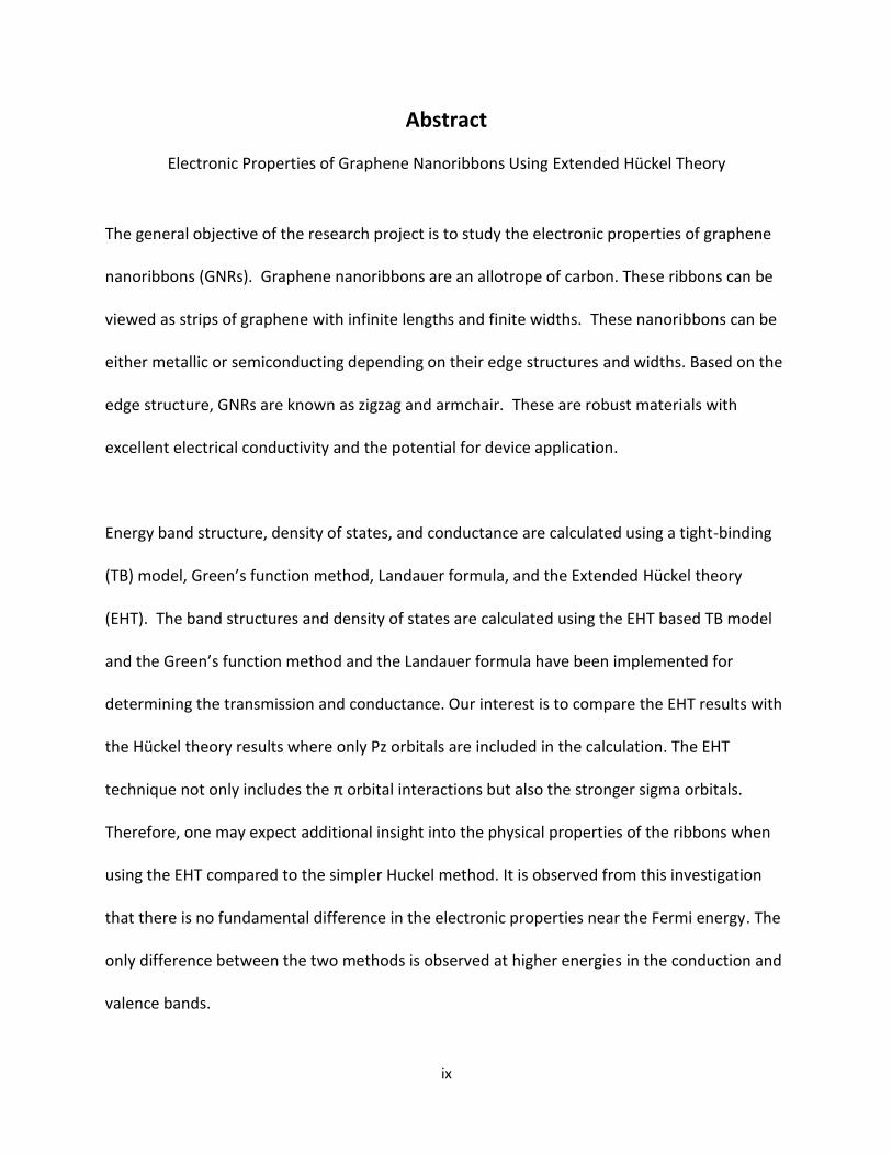
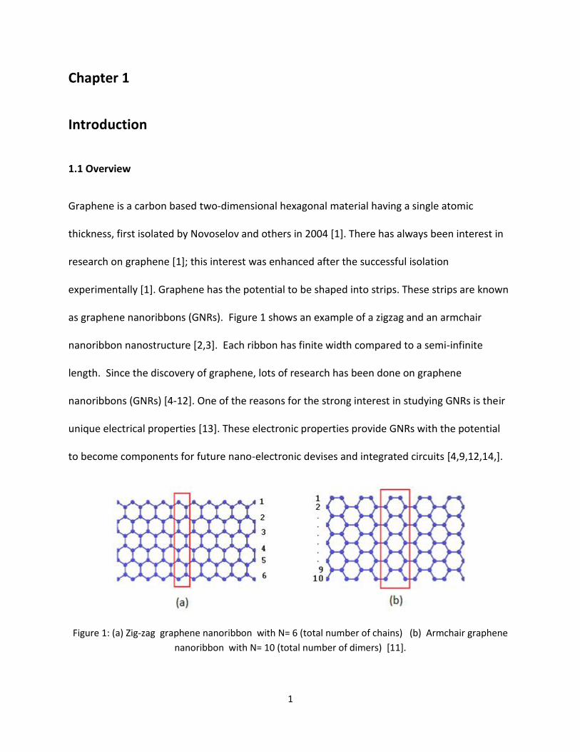
1
Chapter 1
Introduction
11 Overview
Graphene is a carbon based two-dimensional hexagonal material having a single atomic
thickness first isolated by Novoselov and others in 2004 [1] There has always been interest in
research on graphene [1] this interest was enhanced after the successful isolation
experimentally [1] Graphene has the potential to be shaped into strips These strips are known
as graphene nanoribbons (GNRs) Figure 1 shows an example of a zigzag and an armchair
nanoribbon nanostructure [23] Each ribbon has finite width compared to a semi-infinite
length Since the discovery of graphene lots of research has been done on graphene
nanoribbons (GNRs) [4-12] One of the reasons for the strong interest in studying GNRs is their
unique electrical properties [13] These electronic properties provide GNRs with the potential
to become components for future nano-electronic devises and integrated circuits [491214]
Figure 1 (a) Zig-zag graphene nanoribbon with N= 6 (total number of chains) (b) Armchair graphene
nanoribbon with N= 10 (total number of dimers) [11]
2
GNRs will have semiconducting or metallic properties that depend on the structure of their
edges The edge structure is used to classify the GNRs as either zigzag and armchair It is known
that all zigzag graphene nanoribbons (ZGNRs) are metallic on the other hand one third of the
armchair graphene nanoribbons (AGNRs) are metallic and two thirds are semiconducting [23]
The metallic or semiconducting property of an AGNR depends on its widths Much of the
research done on the electronic properties focuses on the edge structure The edge structure of
the material can be changed by altering a number of factors such as edge defects edge
termination with different elements and compounds and doping with different materials
[121516171819] Being able to control the defects and doping of a material is something
that would be of great value for nano-electronic devices This control would enhance the ability
to ensure the desired semiconducting or metallic property
Today researchers are able to fabricate GNRs from bottom-up synthesis from molecular
precursors [2021] Hydrogen plasma etching is then used to produce high-quality GNRs with
well-defined edges [22]
The science involved in studying GNRs requires an understanding of solid state physics
condensed matter physics quantum physics and chemistry Two of the theories used to study
GNRs and their electrical properties are the tight-binding model and density functional theory
[232425] The model used in this thesis follows the tight-binding approach using extended
Huckel method [2324] The extended Huckel method is an expansion of the Huckel method
The Huckel method uses the weaker π bonds for calculations In the case of GNRs the π bonds
form from the interaction between Pz orbitals The extended Huckel method uses all the outer
3
valence orbitals in the calculations For the GNRs this includes the S Px and Py thus increasing
the number of calculations required by four [2627]
In this project electronic band structure density of states local density of states and
conductance are calculated Two different types of graphene nanoribbons the armchair and
zigzag have been studied The electronic properties are investigated using a tight-binding
model Greenrsquos function methodology Landauer formalism and the extended Huckel method
[232428] The extended Huckel method results are compared with the Huckel method results
The organization of the thesis is described in the next section
12 Thesis Map
In Chapter 2 the theoretical models used for calculation are discussed these models are as
follows the tight-binding model the Greenrsquos function methodology and the Extended Huckel
method The analyses of the Hamiltonian matrix will be shown for the calculation of band
structure density of state and conductance
Chapter 3 will present the results of energy band structure density of states (DOS)
conductance and local density of states (LDOS) for armchair nanoribbons using the extended
Huckel method These band structure results are then compared with the results obtained
using the Huckel method looking only at the Pz orbitals In Chapter 4 results of energy band
structure and the DOS are presented for zigzag nanoribbons As in Chapter 3 the results
obtained by the extended Huckel theory are compared with the simple Huckel method
Chapter 5 will provide the summary and conclusions and include a plan for further
investigation
4
Chapter 2
Theory and Calculations
21 Introduction
The basic theoretical models used in this research project are the extended Huckel- tight-
binding approach Greenrsquos function methodology and the Landauer formalism Electronic
properties such as the band structure density of state (DOS) local density of states (LDOS) and
conductance of the graphene nanoribbons (GNRs) are calculated using these models Briefly
these theories will be discussed in this chapter
22 The Tight-binding Model
The tight-binding approach (TB) is a good approximation method for calculating the electronic
properties of GNRs In a TB model only the nearest-neighbor interactions of the atoms of the
system are taken into account The Hamiltonian matrix of a TB model is given by
119815 = sum єiiaidaggeraii + sum Vijai
daggerajlt119894119895gt (21)
Here 120598119894119894is the on-site energy of the carbon orbital 119886119894 119886119899119889 119886119895dagger represent the creation and
annihilation operators of particles at sites i and j respectively Vij is the overlap interaction
energy between nearest neighbor orbitals and the notation ltijgt representing the restriction to
nearest neighbor interactions The matrix elements of the Hamiltonian are calculated from the
relation [24]
5
119881119894119895119896 = 120578119894119895119896ℏ2
1198981198892 (22)
Here m is the electron mass d is the distance between neighboring nucleuses and 120578119894119895119896 is a
constant used that depends on the type of orbital For a graphene structure the value for d=
142 Adeg and the on-site energy εp = -897 eV and εs = -1752 eV The 119894 119895 notations reflect the
type of orbital and 119896 relates to the type of bond either 120590 119900119903 120587 There are four ɳ values and
these include ppπ ppσ spσ and ssσ matrix elements These are 120578119904119904120590 = minus140 120578119904119901120590 = 184
120578119901119901120590 = 324 and 120578119901119901120587 = minus081 These constants are obtained from the reference [24]
The band structures and the density of states (DOS) of the systems are obtained by
diagonalizing the Hmiltonian matrix as a function wave vector k The density of the ith band is
given by [1011]
119863119874119878119894(119864) =1
2120587int120575 [119864119894(119948) minus 119864]119941119948 (23)
And the total density for all the bands can be calculated by summing each band
119863119874119878 (119864) = sum 1
2120587
119873119894=1 int 120575[119864119894 (119948) minus 119864]119941119948 (24)
where Ei is the ith band the summation over all i = 1 to N bands shows the total DOS [11]
23 Greenrsquos Function Formalism Conductance and Local Density of States
In order to calculate the conductance and local density of states (LDOS) Greenrsquos function
formalism has been used for the GNRs The conductance is obtained from the well-known
Landauer formula [23]
119866(119864) =21198902
ℎ119879(119864) (25)
6
Where G is the conductance of the structure and T is the transmission function The
transmission function is dependent on the total energy of the electron The transmission
function is calculated from the Greenrsquos functions [4 2930]
119879(119864) = 119879119903119886119888119890[1204901 ∙ 119918119898 ∙ 1204902 ∙ 119918119898dagger ] (26)
1204901and 1204902are coupling functions while 119918119898 and 119918119898dagger are the total retarded Greenrsquos function and
total advanced Greenrsquos function respectably The notations 1 and 2 are representing the left
lead and the right lead respectively Next the coupling functions (matrices) are expressed in
terms of self-energy matrices [23]
1204901 = 120154[1205061 minus 1205061dagger]
1204902 = 120154[1205062 minus 1205062dagger] (27)
The self-energy matrices are calculated through the iteration process [429] The molecule and
the leads are divided into sections in the iterating process Therefore there are three specific
segments the molecule the left lead and the right lead The schematic structures of both
zigzag and armchair structures are shown in Figure 11 The middle part marked with red color
boundary is representing the molecule and the leads are extended to the left and right
respectively
The Greenrsquos function (Gm) is calculated in terms of Hamiltonian matrix total energy and the
self-energy matrices [23]
119918119898 = [E119816 minus 119815119950 minus 1205061 minus 1205062]minus1 (28)
7
By finding the Greenrsquos function the local density of states can be calculated and then a
summation of the local density of states leads to the total density of states Therefore the local
density of states of individual atoms is expressed from the Greenrsquos function Gm
LDOS119894(119864) = minus1
120587Im[119814119846(119842 119842)] (29)
It should be noted that the total density of states (DOS) of all the atoms discussed above can
also be obtained by summing the individual LDOS from the Greenrsquos function In this research
project the results are verified by both methods The detailed analyses of the Greenrsquos function
calculations are illustrated in the references [4111229]
24 The Extended Huckel Method
The electronic configuration of the ground state of a single carbon atom is 1s2 2s2 2px1 2py On a
hexagonal graphene structure the 2s 2px and 2py orbitals form sp2 hybridized orbitals These
hybridized orbitals are at 1200 to each other and form σ bonds on the 2-dimensional structures
of graphene Figure 21 illustrates a graphical presentation of the orbitals Figure 21 (a) shows
the S Px and Py orbitals of the atoms The Pz orbitals are perpendicular to the plane and are
not shown here In addition projections of the Px and Py orbitals of atom 1 on the S orbital of atom 3
are shown in part (b) These π bonds are relatively weaker compared to the σ bonds and
electrons can move from one atom to the other
8
Figure 21 (a) shows a top down view of the unit cell with orbitals Projections of the Px and Py orbitals
of atom 1 on the S orbital of atom 3 are shown in part (b)
The electronic properties of these graphene structures are obtained by including only the pz
orbitals for constructing the Hamiltonian of the structures The basic Huckel method deals with
only these 2pz orbitals in finding the electronic properties of structures of interests [2431]
The extended Huckel method expands upon this calculation by not only using the π bonds from
the 2pz orbitals but includes the bonds from the 2s 2px and 2py [26] Like the Huckel the EHM
only takes into account the nearest neighbor interactions between orbitals discussed above in
the TB model
In the case of a GNR the number of orbitals is directly dependent on the width of the ribbon in
the unit cell For an AGNR with n being the number of dimers on the AGNR the number of
orbitals is obtained by taking n multiplied by 2 to get the total number of carbon atoms and
9
then scaling that number by the number of unique orbitals in the case of carbon that is 4
Figure 11 (b) represents an armchair GNR structure with n=10 For example for the n= 10
dimer ribbon the total number of carbon atoms would be 20 and the total number of orbitals
will be 80 Thus the size of the Hamiltonian matrix will be 80 by 80
The next thing to consider is the edge bonds in the unit cell With AGNRs there are two atoms
at each edge of the periodic structure with dangling bonds The zigzag and the armchair
features at the top and bottom edges are clear in Figures (a) and (b) In this calculation a single
hydrogen atom in the ground state is used to terminate each edge bonds The hydrogen orbital
is thus 1s Since the size of the Hamiltonian matrix is determined by the total number of the
orbitals the addition of hydrogen atoms at the edges changes the size of the matrix So instead
of simply being 2n4 orbitals the total number of orbitals becomes 2n4+4 or 8n+4 The
electronic properties such as the band structures and density of states of the system are
obtained by diagonalizing the Hamiltonian matrix as a function of wave number k The charge
densities of individual atoms have been calculated by finding the eigenfunction of Hamiltonian
matrix of each k
Now we discuss the calculation of an armchair graphene nanoribbons of single hexagon in
thickness Figure 22 shows the graphene ribbon structure
10
Figure 22 A single hexogonal armchair graphene ribbon The atoms are marked with numbers the unit
cell I is marked with lines and its neighbors are I+1 and I-1
The unit cell along with its two nearest neighbors are represented by I I-1 I+1 and the sites are
marked 1 through 6 The Schrodinger equation (SE) for the structure is
|120569⟩ = 119864|120569⟩ (210)
and the Hamiltonian operator is given as
=minusℏ2
2119898nabla 2 + 119881(119903 ) (211)
and the wave function |120569 gt is given by
|120569 gt= sum 119890119894119896119877119868119868=119868119868+1119868minus1 |120569119868 gt (212)
where |120569119868 gt is expressed by the four orbitals s px py and pz
|120569119868 gt= sum 119890119894119896∙120591119895[1205721|119904119895⟩ + 1205732|119875119909119895⟩ + 1205743|119875119910119895⟩ + 1205814|119875119911119895⟩]119895=1 (213)
In Eq (212) 119877119868 represents the location of the unit cell I and 120591119895 is the phase factor of the
orbitals Here 120572 120573 120574 120581 are the probability amplitudes To construct the Hamiltonian matrix
11
the following analytical steps are performed First scalar products of the individual orbitals are
taken with Eq (210) Here an example is shown Taking the scalar product of 1199041 orbital one
finds
⟨1199041||sum119890119894119896∙120591119895[120572119895|119904119895⟩ + 120573119895|119875119909119895⟩ + 120574119895|119875119910119895⟩ + 120581119895|119875119911119895⟩]
6
119895=1
=
⟨1199041|119864|sum119890119894119896∙120591[120572119895|119904119895⟩ + 120573119895|119875119909119895⟩ + 120574119895|119875119910119895⟩ + 120581119895|119875119911119895⟩]
6
119895=1
(214)
The left hand side of Equation (214) is expanded as
119890119894119896∙1205911[1205721⟨1199041||1199041⟩ + 1205731⟨1199041||1198751199091⟩ + 1205741⟨1199041||1198751199101⟩ + 1205811⟨1199041||1198751199111⟩]
+119890119894119896∙1205912[1205722⟨1199041||1199042⟩ + 1205732⟨1199041||1198751199092⟩ + 1205742⟨1199041||1198751199102⟩ + 1205812⟨1199041||1198751199112⟩]
+ + 119890119894119896∙1205916[1205726⟨1199041||1199046⟩ + 1205736⟨1199041||1198751199096⟩ + 1205746⟨1199041||1198751199106⟩ + 1205816⟨1199041||1198751199116⟩]
= 119890119894119896∙12059111205721⟨1199041||1199041⟩ + 119890119894119896∙1205912[1205722⟨1199041||1199042⟩ + 1205732⟨1199041||1198751199092⟩] +
119890119894119896∙1205913[1205723⟨1199041||1199043⟩ + 1205733⟨1199041||1198751199093⟩ + 1205743⟨1199041||1198751199103⟩] (215)
In equation (215) all terms are zero except the nearest-neighbors As shown in Figure 22 the
nearest-neighbors for atom 1 are atoms 2 and 3
In a similar way the right hand side is expanded and it appears as
= 119890119894119896∙1205911[1205721⟨1199041|119864|1199041⟩ + 1205731⟨1199041|119864|1198751199091⟩ + 1205741⟨1199041|119864|1198751199101⟩ + 1205811⟨1199041|119864|1198751199111⟩]
+119890119894119896∙1205912[1205722⟨1199041|119864|1199042⟩ + 1205732⟨1199041|119864|1198751199092⟩ + 1205742⟨1199041|119864|1198751199102⟩ + 1205812⟨1199041|119864|1198751199112⟩] + hellip
+119890119894119896∙1205916[1205726⟨1199041|119864|1199046⟩ + 1205736⟨1199041|119864|1198751199096⟩ + 1205746⟨1199041|119864|1198751199106⟩ + 1205816⟨1199041|119864|1198751199116⟩]
= 1205721119890119894119896∙1205911⟨1199041|119864|1199041⟩ = 1205721119864119890119894119896∙1205911 (216)
In equation (216) only a single term is non-zero because the S1 orbital is orthogonal to all the
other orbitals except to itself
12
Combining equations (215) and (216) the following expressions are obtained
1205721⟨1199041||1199041⟩ + 119890119894119896∙1205912minus1205911[1205722⟨1199041||1199042⟩ + 1205732⟨1199041||1198751199092⟩] +
119890119894119896∙1205913minus1205911[1205723⟨1199041||1199043⟩ + 1205733⟨1199041||1198751199093⟩ + 1205743⟨1199041||1198751199103⟩] = 1205721119864 (217)
The matrix elements in Equation (217) are then expressed in a simplified form as
1205721휀119904 + 119890119894119896∙1205912minus1205911[1205722119864119904119904 + 1205732119875119864119904119909] +
119890119894119896∙1205913minus1205911[1205723119864119904119904 + 1205733119864119904119909 + 1205743119864119904119910] = 1205721119864 (218)
The matrix elements between atoms are defined by 휀119904 119864119904119904 119864119904119909 and 119864119904119910 Here 휀119904 is the on-site
energy of the S- orbital and the later three elements are expressed in terms of overlap
integrals 119881119894119895119896 defined in Equation (22) The complete expression of each element is shown in
the Appendix 1 These elements represent the σ and π interactions between orbitals and are
obtained from reference [24] The phase factors are expressed in terms of lattice constant
119886 (= 142Adeg) It should be noted that there are 24 orbitals in a single unit cell Here we have
shown complete analysis for a single orbital Similarly matrix element of the Hamiltonian is
obtained from these scalar products of all the orbitals The analysis is not shown for the rest of
the orbitals here Notice that each equation makes up a single row for the Hamiltonian matrix I
then sorted the Hamiltonian matrix with respect to each carbon atom and the 4 corresponding
orbitals This means every 4 rows are grouped in order by the corresponding S Px Py and Pz I
can then combine each interaction between carbon atoms into their own sub groups
represented by Hij with each group representing a 4 by 4 block Table 21 shows the condensed
Hamiltonian matrix using these Hij Block elements for visualization purposes C1-6 is set outside
the Hamiltonian as a guide to help the reader cross reference terms and identify what each
13
block refers to The phase factors interaction parameters and other terms are all contained in
these sub groups and will be explained below
Table 21 The Hamiltonian matrix for a single graphene hexagon
The Hamiltonian matrix elements in Table 21 are in the form of Hij with i and j terms going
from 1 to 6 for the 6 carbon atoms in this hexagonal periodic structure Note that each element
Hij is a block matrix These notations are used to show the Hamiltonian matrix in a compact
form The size of the Hamiltonian for this narrow n=3 dimer armchair ribbon is 24 by 24 but by
condensing each section into 4 by 4 blocks it reduces the appearance of the Hamiltonian to a 6
by 6 This reduction of size although merely cosmetic in effect makes checking each element in
the matrix much more manageable Instead of checking the entire matrix at once I am able to
check each block at a time for accuracy and feel much more confident in the result Examples of
these block matrices are shown in Table 22
14
Table 22 Matrix elements H11 H12 and H13 of Table 21 are shown in the blocks (a) (b) and (c) The
phase factors of the corresponding elements are also shown on the top of each block
The interaction matrix elements shown in Table 22 are described through schematic diagrams
in Figure 21 and Figure 23 As discussed above Figure 21 (a) shows the S Px and Py orbitals
of the atoms The lobes of the p orbitals are marked with positive and negative signs of atom 5
15
Next part (b) presents the orientations of the Px and Py orbitals toward the S orbital for atom
3 The left two configurations in part (b) represent the σ-bond between the S and Px and Py
orbital requiring 240 and 150 degreesrsquo reorientation of the orbitals respectively While the two
right configurations represent the π-bond between the S and Px and Py orbital Taking the
Cosine of these angles will let you know what portion of the interaction term to take For
instance the σ component for Px1 interacting with S3 will have Cos (240) = -12 and comparing
this with Table 22(c) we see the term should be 12 But there is one major component one
should take into account the positive and negative sides of the lobes and how this effects the
signs of the matrix elements To address this issue Figure 23 is introduced
The matrix elements are illustrated in Figure 23 Six interaction parameters are shown through
the schematic representation of the orientations of the orbitals It should be mentioned that
the interaction terms were defined in Equation (22) by 119881119894119895119896 and for the case at hand 119894 and 119895
are either a s-orbital or p-orbital and 119896 is either be a sigma or pi bond It should be mentioned
that the filled (solid) lobes are positive and the empty ones are negative Combing the results
from Figure 21 (b) and implementing the sign rules of the lobes introduced in Figure 23 we
get (-12)(- Vspσ) = 12( Vspσ) Following the same rules and techniques the other matrix
elements for atom 1 and atom 3 are calculated and shown in Table 22 (c)
The phase factors appeared in Equation (217) can have one of the four possible values plusmn119890119894119896119886
and plusmn119890119894119896119886
2 and two of them appear in parts (b) and (c) in Table 22
16
Figure 23 Illustration demonstrating the types of sigma and pi bonds between s and p orbitals [24]
The full Hamiltonian matrix is shown in the Appendix 1 A list of the matrix elements is also
provided in the Appendix 1
25 Summary
In this chapter we have discussed and shown the theoretical models used in the present
research project First the tight-binding model is discussed for the calculation of band structure
and density of state The associated interaction parameters and their values are presented
Next the Greenrsquos function formalism is discussed for the calculation of conductance and local
density of states In Section 24 the extended Huckel method is explained A detailed analysis
for a single Hamiltonian matrix element is shown Finally some schematic representation of the
orientation of the orbitals is discussed to express the interaction parameters and phase factors
for an AGNR
17
Chapter 3
Armchair Graphene Nanoribbons
31 Introduction
In this chapter we will present the results of electronic band structure density of states (DOS)
local density of states (LDOS) and conductance for armchair graphene nanoribbons (AGNRs)
The band structure and density of states are calculated using the tight binding (TB) model
discussed in chapter 2 Conductance and local density of states (LDOS) are calculated using
Greenrsquos functions methodology and the Landauer formula [4232930] The extended Huckel
method has been implemented in all these calculations [28]
First a brief description of the structure used in this calculation will be presented Next the
Band structure and Density of states will be shown followed by a comparison with results
obtained using the Huckel method Lastly the Conductance and LDOS results will be shown
32 Band Structure and Density of States of Armchair Graphene Nanoribbons
As discussed earlier graphene nanoribbons are strips of graphene with finite widths and semi-
infinite length along the axis of the strip Figure 31 shows a GNR with an armchair shape at the
edges This armchair patterned GNR is known as AGNR The AGNR is separated into unit cells
the Figure bellow shows several unit cells we will focus on the center unit cell I The number of
dimers in Figure 31 is equal to 9 The width of an AGNR is given by 119886radic3
2119899 where 119886 is the the
lattice constant and 119899 is the total number of dimers in the structure Here 119886 = 142A119900 thereby
18
the width of the ribbon is 1107nm For a n= 9 dimer AGNR there are 18 atoms in the unit cell
and these are shown with numbers In Figure 31 it is clear that the carbon atoms in the first
and last dimmer (at the top and bottom edges) are only connected to two other carbon atoms
in the bulk of the structure thus leaving a dangling bond at the edge In order to terminate the
dangling bond an atom can be added to the edge In this study the GNR edges are terminated
with hydrogen Band structures and DOS with and without edge terminated AGNRS are
presented and discussed The distinction between edge terminated bonds and non-terminated
bonds and edges will be a major focus in the chapter
Figure 31 Armchair graphene nanoribbon width n=9
19
Figure 32 (a) The band structure (b) the density of states of n= 3 dimer AGNR (without edge
termination)
In Figure 32 (a) the band structure of an armchair GNR with n = 3 is shown The electronic
band structures are plotted as a function of wave number k were k ranges over the first
Brillouin zone boundary When n = 3 there are 6 atoms in the unit cell There is a total of 24
bands in the figure proportional to the total number of orbitals The Fermi level has been
centered at 0 eV The previous chapter stated that the number of orbitals in the unit cell was
20
obtained by taking the number of dimers (n) and multiplying by 8 (orbitals) The bands located
above the Fermi level are known as the conduction bands while below the Fermi level the
bands are the valence bands An inspection of the bands reveals that not all valence and
conduction bands are perfectly symmetric with respect to the Fermi level One should also note
that there are many flat valence bands below the Fermi energy These flat bands are non-
conducting and the group velocity of the mobile electrons is close to zero [415] That means
the effective mass of the electrons is infinite [15] We predict these flat bands below the Fermi
energy are from the Px Py and S-orbitals of the carbon atoms
There is a distinct gap between highest valence band and the lowest conduction band The gap
in the Fermi level between the valence and conductance points to a material being
semiconducting This is what is expected for n = 3 The dimer rule to follow for AGNRs will be
semiconducting when n=3p or n=3p+1 (with p being an integer) However if n=3p+2 the
AGNRs will be metallic [2315]
In Figure 32 (b) the density of states (DOS) are plotted as a function of electron energy The
DOS value shows the number of k points per energy value Figure 32 (b) reveals that there are
some sharp peaks and gaps in the DOS structure As expected there is a gap around Fermi
energy This gap in DOS corresponds to the band gap observed in Figure 32 (a)
From the theory it is expected to find only the weakly held π bands around the Fermi level
mainly the 6 bands from the Pz interactions In Figure 32 (a) there seems to be 4 extra bands
located on the valence side close to the Fermi energy The current calculation and results
shown above do not account for the edge orbitals along the ribbon as in they could be thought
21
of as dangling or non-bonding orbitals These dangling edge atoms are C1 C2 C5 and C6 shown
in Figure 22 To remedy this situation the edges are terminated by adding hydrogen The
results with edge termination will be shown in Figure 34 Figure 33 shows the close up view
around the Fermi level for n = 3 It is clear from this view that there are many flat bands in the
valence band subsequently there are many peaks observed in the DOS graph The band gap at
k = 0 is about 24 eV This band gap indicates that n =3 AGNR is a semiconducting structure
Figure 33 (a) The band structure (b) the density of states near the Fermi energy of n= 3 dimer AGNR
(without edge termination)
22
Figure 34 (a) The band structure (b) the density of states of n= 3 dimer AGNR (edge terminated with
hydrogen)
Next we introduce the edge terminated results of the band structure and DOS in Figure 34
Due to the addition of the hydrogen at the edges the total number of bands should be 28 It is
clear that due to the edge termination the qualitative features of the bands have changed The
bands are more symmetric about the Fermi energy Also some flat bands observed in Figure 32
(a) moved at lower energy levels in the valence band region We also see that around -20 there
is a large increase in the number of bands compared to Figure 32 (a) From this observation
23
one may suggest that the S-orbital of the hydrogen atom is hybridized with the other orbitals
(Px Py S) of the carbon atoms on the two-dimensional plane From this observation we
conclude the bands at very low energy are tightly bound and are forming σ bonds Those closer
to the Fermi energy are forming π bonds and contribute to conduction Figure 34 (b) also
shows similar changes in DOS around the Fermi level Instead of several distinct peaks below
the Fermi level around -3 eV we see only one peak This relates with the one flat band in Figure
34 (a) at the same energy Also more peaks are observed around -20 eV in the valence band
region A close up view of the bands and DOS are shown around the Fermi energy in Figure 35
As discussed above the width of the band gap at k = 0 remains the same (cong24 eV)
24
Figure 35 (a) The band structure (b) the density of states near the Fermi energy of n= 3 dimer AGNR
(edge terminated with hydrogen)
25
Figure 36 (a) The band structure (b) the density of states of n= 5 dimer AGNR (without edge
termination)
The next thing to study is the case of n=3p+2 dimer AGNR In order to avoid the analytical and
computational cost the lowest number of dimers in the relation n=3p+2 is considered in this
calculation n = 5 Figure 36 shows the band structure and the DOS The electronic bands are
plotted as a function of wave vector k and DOS are plotted as a function of energy It should be
mentioned that these results are without edge termination One of the first things apparent in
26
Figure 36 (a) is the number of bands has increased significantly Remembering that one band
correlates to one orbital there are 10 atoms for n = 5 Hence there are 40 orbitals in total
Some of the bands overlap and appear close together Looking at the highest valence band and
the lowest conduction band it is seen that they meet at the Fermi level at k=0 This point of
degeneracy between bands when k = 0 indicates that the structure is metallic This follows the
theory that the AGNR is metallic when n=3p+2 As discussed above about the flat bands and
peaks in the DOS represent the non-conducting states and indicate infinite mass The bands
around the Fermi energy are linear indicating the group velocity is nonzero and is measured to
be about 106 ms [14] The metallic property of the AGNR with n=5 is confirmed again by
Figure 36 (b) which shows that the DOS is non-zero at the Fermi level In conclusion we see n
= 5 AGNR is indeed metallic Enhanced plots near the Fermi energy for the bands and DOS are
displayed in Figure 37 The detailed characteristics of the bands and DOS are more visible here
27
Figure 37 (a) The band structure (b) the density of states near the Fermi energy of n=5 dimer AGNR
(without edge termination)
28
Figure 38 (a) The band structure (b) the density of states of n= 5 dimer AGNR (edge terminated with
hydrogen)
In Figure 38 the edge terminated results for n=5 AGNR are shown The bands are shown in
Figure 38 (a) and the DOS are in 38 (b) The addition of the hydrogen at the edges results in 44
bands The general behavior of the bands moving away from the Fermi energy is similar as
observed in Figure 34 (a) The weakly bonded π orbitals are near the Fermi energy and the
bands are symmetric about it Due to hybridization of the orbitals on the plane with hydrogen
29
the flat bands near the Fermi energy in Figure 36 (a) moved to very low energy region The
number of peaks observed in the energy range -2 eV to -6 eV in Figure 36 (b) has decreased to
only one This may suggest that they are hybridized with the other orbitals of the hydrogen
atoms on the plane Figure 39 shows the detailed features of the bands and DOS near the
Fermi energy
Figure 39 (a) The band structure (b) the density of states near the Fermi energy of n= 5 dimer AGNR
(edge terminated with hydrogen)
30
For completeness Figure 310 has been included to address the case for n=3p+1 and to confirm that it
is semiconducting as expected Figure 310 shows the band structure and the DOS for an n=4 AGNR with
edge termination The features will not be discussed in detail because they are similar to the n=3 AGNR
case Here the main focus is to confirm the results of a semiconducting nature of the ribbon
Figure 310 (a) The band structure (b) the density of states of n= 4 dimer AGNR (edge terminated with
hydrogen)
31
33 Comparison of Huckel and Extended Huckel Results of Armchair Graphene Nanoribbons
In this section results will be discussed for comparison between the Huckel and extended
Huckel methods different widths of armchair nanoribbons Results from the extended Huckel
method discussed in section 32 will be used for comparison Only the band structure and the
density of states will be compared Since a detailed description for the extended Huckel
method was presented in the previous section only a short explanation will be given for the
comparison
Figures 311 and 35 present the band structure and density of states (DOS) for Huckel and
extended Huckel method for n=3 dimer AGNRs respectively One may notice the bands and
DOS are symmetric about the Fermi level for the Huckel method (Figure 311) On the other
hand both bands and DOS are not symmetric for the extended Huckel method There are a few
bands seen around 80eV in the conduction region Consequently the DOS is non-zero at this
energy As discussed in the previous section the symmetric bands around the Fermi energy are
due to the Pz-orbitals therefore these bands around 80eV are from the other orbitals in the 2-
D plane
32
Figure 311 (a) The band structure (b) the density of states near the Fermi energy of n= 3 dimer AGNR
(Huckel Method edge terminated with hydrogen)
The band structures and DOS are compared for n=5 AGNR in Figures 312 and 39 Here due to
the addition of dimers the number of bands increased As seen above the bonding and anti-
bonding orbitals are symmetric about the Fermi energy The bands must be symmetric since
the energy of all the Pz-orbitals is the same There are some more bands and DOS observed
33
again around E = 80eV In summary the general characteristics of the bands and DOS are
similar around the Fermi energy in both Huckel and extended Huckel method The only
difference observed σ bands in the extended Huckel method and these are farther away from
Fermi level
Figure 312 (a) The band structure (b) the density of states near the Fermi energy of n= 5 dimer AGNR
(Huckel Method edge terminated with hydrogen)
34
34 Conductance of Armchair Graphene Nanoribbons
The conductance results of n = 3 and n = 5 AGNR will be discussed in this section Figure 313
shows the conductance values as a function of energy
Figure 313 Conductance as a function of energy for (a) n = 3 AGNR (b) n = 5 AGNR (edge terminated
with hydrogen)
First we will show and discuss the conductance results for the edge terminated cases In Figure
313 (a) the conductance around the Fermi level is zero the first quantized conductance value
does not show up until -12 eV and 12 eV respectively This zero conductance nature is
expected because n = 3 is a semiconductor type AGNR as seen in Figure 34 From the band
structure as well as DOS analysis discussed above the conductance should be zero within this
energy range (shown in Figure 34(a) amp (b)) This implies there is no propagating mode to
contribute to the transport From Figure 34 it is clear that the number of propagating states is
zero within this range From the Landauer formula conductance is expressed by integer
multiples of (2e2h) Therefore it is expected that the conductance will be quantized by (2e2h)
In Figure 313 (a) the conductance between -32eV to -12 eV and 32 eV to 12 eV is equal to 1
(2e2h) This general behavior of quantization is expected for any semiconductor or metallic
GNRs
35
Next we present the conductance for n = 5 AGNR As stated earlier n = 5 AGNR is metallic The
first quantized conduction band is between -22eV to 22eV and the second quantized
conduction band starts from -22eV and 22eV with conductance value equal to 2 (2e2h) This
corresponds to two possible allowed propagating states for transport
In order to study the effects of edges on transport the conductance results are produced
without the edge termination Figure 314 shows without edge terminated conductance for n=
3 and n=5 dimer AGNRs It is expected from the observations of band structures and DOS
results shown in Figures 33 and 37 that the characteristics of the conductance curves will not
be fully quantized and some different features will appear
Figure 314 Conductance as a function of energy for (a) n = 3 AGNR (b) n = 5 AGNR (without edge termination)
For both n=3 and n= 5 AGNRs in Figure 314 (a) and (b) there is a sharp increment in conductance is
observed in the valence band regions It is predicted that these enhancements are due to the σ -bands
observed in the without edge terminated structures in the valence bands below the Fermi level shown
in Figures 33 and 37 The sharp spikes are at the same location as the energy bands In conclusion the
edge termination is essential for clean quantized features in conductance curves The dangling bonds at
36
the edges destroy the perfect quantized behavior expected from the Landauer formalism for perfect
nanostructures
35 Local Density of States of Armchair Graphene Nanoribbons
The local density of states (LDOS) shows the number of states per energy for each atom in the
unit cell Using the extended Huckel method each atom in the unit cell has four orbitals
contributing to their particular LDOS In this section the LDOS results will be presented for the
edge terminated AGNRs for n=3 and n=5
Figure 315 LDOS for n=3 AGNR (a) for carbon 1 atom (b) for carbon 3 atom Positions of the atoms are
shown in Figure 22
Figure 315(a) and (b) shows the LDOS for 2 of the atoms in the unit cell The Figure shows
carbon atom 1 and carbon atom 3 (refer to Figure 22(a)) Naturally this brings up the question
of why only 2 of the 6 carbon atoms are shown The reason has to do with the symmetry of the
37
unit cell and neighbors because the general symmetric relationship between the matching
atoms they have identical interactions between atoms thus matching LDOS values The general
characteristics of LDOS for the edge atoms 1 and 2 are identical Similarly the features of LDOS
for the middle atoms 3 and 4 are similar It is also expected that the results of atoms 5 and 6
will be similar to atoms 1 and 2 Therefore only the LDOS of two atoms will provide a general
image of the characteristics of the electronic property The graphs tend to show a lot of
similarities It is also noted the difference around the Fermi level between the two LDOS graphs
Figure 315(a) has several distinct peaks at different locations
For the n=5 AGNR there are a total of ten LDOS graphs but like the n=3 case many of the
carbon atoms result in similar LDOS graphs The matching carbon LDOS are as follows 1 2 9
10 make a set 3 4 7 and 8 make a set and 5 6 make the final set The atomic positions are
shown in Figure 31
Figure 316 two LDOS for a n=5 AGNR (a) for the carbon 1 atom (b) for the carbon 3 atom (c) for the
carbon 5 atom
38
Looking at Figure 316 (a) and (b) we can see that these are the carbon atoms where the
electronic transport happens it is shown by the nonzero LDOS at and around the Fermi energy
This becomes interesting when you note these are all the edge atoms It is also noted for Figure
316 (c) there is 0 LDOS around the Fermi energy meaning no electronic transport Being able to
plot the LDOS becomes a very powerful tool when looking at the individual atoms and how they
are affected by changes to the system as a whole A good research topic for the future could
follow an in-depth look at the LDOS and how it changes with respect to anomalies and defects
within the GNRs
36 Summary
In this chapter the electronic properties for several AGNR have been studied using the
extended Huckel method The band structure DOS conductance and LDOS are calculated for
several AGNRs The number of dimers representing the width of the ribbons are chosen based
upon the dimer rule n=3p+2 is metallic and n=3p and n=3p+1 are semiconducting Here p is
an integer For n= 3 4 and 5 AGNR have been investigated As expected n= 3 and 4 AGNR are
semiconducting while n= 5 is metallic From this investigation we find that electron conduction
mostly relies on the Pz orbitals Results with and without edge termination are discussed for
both cases The addition of edge termination was required to successfully explain the results
around the Fermi level
39
Chapter 4
Zigzag Graphene Nanoribbons
41 Introduction
In this chapter zigzag graphene nanoribbon (ZGNR) structure will be discussed and then it will
be compared to the AGNR structures Next the results the band structure and DOS for two
separate ZGNRs will be presented and discussed Finally the chapter will conclude with a
comparison between the Huckel and extended Huckel results obtained for the ZGNR
42 Band Structure and Density of States of Zigzag Graphene Nanoribbons
The name of a GNR comes from the zigzag pattern along the semi-infinite edge of the ribbon In
Figure 310 a ZGNR is displayed with the unit cell marked at the center The unit cell is
represented by I and its neighbors are shown by I +1 and I -1 There are 6 chains in the
structure The width of ZGNRs can determined by the number of chains (N) in the ribbon The
distance between two chains is 3119886
2 Therefore the width of the chain with N=6 will be 1278nm
The numbering scheme for the atoms in the unit cell is top down Results for N=2 and N=6 will
be presented here
Figure 41 Zigzag graphene nanoribbon N= 6 chains
40
Figure 42 (a) The band structure (b) the density of states of N= 2 chain ZGNR (without edge
termination)
Figure 42 displays the electronic band structure and the density of states for a N = 2 chain
ZGNR In Figure 42 (a) the electronic band structures are plotted as a function of wave vector k
where k ranges within the boundary of the first Brillouin zone N = 2 is chosen because it is the
smallest number of chains possible to make up a ZGNR The same relation has been used to find
the number of orbitals in a unit cell for the ZGNR as for the AGNR For the case of N = 2 chain
41
ZGNR the total number of orbitals is thus 16 The Fermi level energy has again been centered
around 0 eV It is observed that the highest valence band and the lowest conduction band meet
at both ends of the Brillouin boundary indicating metallic properties [51011] This feature is
explained by many researchers and these are due to the edge atoms This metallic property is
expected for all ZGNRs It is also seen that the bands flatten out into each other as they meet
on either edge This is in stark contrast to the metallic AGNRs that meet at k = 0 and
approached at a constant slope These flat bandrsquos characteristics indicate the group velocity of
the electrons is zero and the bands are non-conducting It is also noticed like the AGNR that the
bands are not symmetric about the Fermi level in this dangling bond situation
In Figure 42 (b) the density of states (DOS) are plotted as a function of electron energy The
DOS show the number of states per energy value The DOS is non-zero at the Fermi energy
confirms the result of metallic properties Not only is it non-zero but there is a peak at the
Fermi energy which relates to the flattening of the bands as they meet Figure 43 shows the
close up view around the Fermi level the flattening of the bands and the peak at the Fermi
level are much more prominent
42
Figure 43 (a) The band structure (b) the density of states near the Fermi energy of N= 2 chain ZGNR
(without edge terminated)
As discussed in the last section with AGNRs there was a problem with dangling edge-orbitals
This problem persists with the ZGNR The solution is similar to the AGNR but instead of
requiring two hydrogen atoms at each edge of the unit cell ZGNR requires only one at each
edge The results with edge termination are shown in Figure 44 for a ZGNR with N = 2
43
Figure 44 (a) The band structure (b) the density of states of N=2 chain ZGNR (edge terminated with
hydrogen)
Figure 44 displays the bands and DOS for a ZGNR with N = 2 chain where the dangling carbon
orbitals are terminated with hydrogen Due to the addition of the hydrogen at the edges the
total number of bands is 18 It is clear that the edge termination has had an effect on several of
the bands in Figure 44 (a) It is observed that the two bands located slightly below the Fermi
44
energy in Figure 44 (a) have both moved This suggests that these two bands have now moved
to lower energy states with the forming sigma bonds now shared with the hydrogen As
discussed for the AGNR the orbitals that relate to the bands lying on the 2-D plane (S Px Py)
Therefore the four bands about the Fermi energy are the contributions from the Pz orbitals
Recall that the bonding and anti-bonding orbitals are in the valence and conduction band about
the Fermi level respectively The picture around the Fermi level becomes clearer now that two
of the bands have gone It is predicted that these two bands are from the dangling p- orbitals of
the edge atoms Once the edges are terminated the S-orbital of the hydrogen atom form sigma
bonds with the p-orbitals of the carbon atoms and move to the lower energy levels in the
valence band The peak from the touching conduction and valence band at E = 0 eV is easily
discernible in Figure 44 (b) The increase in the DOS is produced by the flattening of the bands
as they approach the Fermi level Figure 45 is used to display this same edge terminated ZGNR
but with the energy ranging from -7 to 7 eV with respect to the Fermi level
45
Figure 45 (a) The band structure (b) the density of states near the Fermi energy of N= 2 ZGNR (edge
terminated with hydrogen)
46
Figure 46 (a) The band structure (b) the density of states of N= 6 chain ZGNR (without edge
termination)
Figure 46 displays the bands and the DOS for an N = 6 chain ZGNR The number of bands in this
case is 48 The edges are not terminated and hence the general characteristics of the bands as
well as the DOS are alike as found in N = 2 ZGNR shown in Figure 42 The valence bands form
the bonding and the conduction bands form anti-bonding orbitals [26] A difference between
the two ZGNRs is shown with the flatter bands at the Fermi energy for the N = 6 As a result the
47
DOS values at the Fermi energy are higher In addition the other Pz orbitals degenerate at the
boundary of the Brillouin zone at two different energy values (around -3 and 3 eV) [11] As
before for clarity the bands in DOS around the Fermi level are displayed in Figure 47
Figure 47 (a) The band structure (b) the density of state near the Fermi energy of N= 6 chain ZGNR
(without edge terminated)
48
It is clear that there are additional bands mixed with the Pz-bands near the Fermi level in the
valence band region For the N=2 chain ZGNR there are two bands observed of this nature
shown in Figure 43 As discussed before we consider that these bands formed from the
dangling P-orbitals of the edge atoms Apparently it appears that there is a single band One
may consider it as a degenerate band In order to avoid this confusion the results for N= 3 4
and 6 ZGNRs are plotted within a small window of energy shown in Figure 48 It is clear that
bands are separated as seen in Figure 43
Figure 48 The band structure of (a) N=3 (b) N=4 and (c) N=6 chain ZGNRs for a small energy range about the Fermi enrgy (without ede terminated)
49
Figure 49 (a) The band structure (b) the density of state of N=6 chain ZGNR (edge terminated with
hydrogen)
Results of edge terminated bands and DOS for N = 6 ZGNR is presented in Figure 49 Because of
the edge termination the bands around the Fermi level are almost symmetric Shifting of the
non Pz orbitals away from the Fermi level in the valence band region is consistent with previous
results This result is compared to the previously calculated result reported by others [11] The
electronic energy bands and DOS values are identical near the Fermi level The only difference
50
appears away from the Fermi level in the conduction band region In order to understand verify
this discrepancy it may require some further investigations in the future For a better view
around the Fermi region Figure 49 is provided
Figure 410 (a) The band structure (b) the density of state near the Fermi energy of N= 6 chain ZGNR
(edge terminated with hydrogen)
51
43 Comparison of Huckel and Extended Huckel Results of Zigzag Graphene Nanoribbons
Here the band structure and DOS will be compared for the two different ZGNRs Figures 411
and 45 show the results for a N=2 chain ZGNR using the Huckel and extended Huckel method
respectively Like the AGNRs the bands and DOS are symmetric about the Fermi level These
bonding and anti-bonding are from the Pz orbitals Therefore one expects the asymmetric
behavior to appear with the extended Huckel method at higher energy Figure 45 reveals the
features in the conduction band
52
Figure 411 (a) The band structure (b) the density of states near the Fermi energy of N= 2 ZGNR (Huckel
Method edge terminated with hydrogen)
Next for N=6 chain ZGNR results are displayed in Figures 412 and 49 Fundamentally there
are not much difference except there are many more bands Overall the general trend of the
bands and DOS around the Fermi energy as well as away are similar for N=2 chain ZGNR
discussed above Therefore with the extended Huckel technique one can extract the details of
the electronic properties of the nanoribbons
53
Figure 412 (a) The band structure (b) the density of states near the Fermi energy of N= 6 ZGNR (Huckel
Method edge terminated with hydrogen)
44 Summary
The band structure and the DOS calculations have been show for ZGNRs of two different
widths The addition of the Hydrogen to work with the dangling edge orbitals was required to
move around some of the bands away from the Fermi level leaving the extended Huckel
method to match the Huckel method As in AGNRs the edges of ZGNRs are terminated with
54
hydrogen The S-orbital of the hydrogen atom form bonds with the S- and P-orbitals of the edge
atoms There are two energy bands observed near the Fermi level in the valence band region
These are mixed with the Pz-bands and are predicted that these are due to the presence of
dangling P-orbitals at the edges of the ribbons Once the edges are terminated with hydrogen
these bands are pushed back at the lower energy levels From this observation we conclude
these dangling P-orbitals are forming σ-bonds with the S-orbital of the hydrogen atom If the
edges are terminated with other element(s) then the investigation will be more interesting and
conclusive
55
Chapter 5
Summary and Conclusions
In this research project two different graphene nanoribbons have been studied These include
the armchair and zigzag nanoribbons Electronic properties are studied by using a tight-binding
model Greenrsquos function methodology Landauer formalism and the extended Huckel method
The electronic properties investigated are the band structures density of states and
conductance The results obtained from the extended Huckel method are compared with the
Huckel method
In Chapter 2 the theoretical methods are presented In addition to the well-known theories
such as the TB model the Greeenrsquos function model examples of analytical and geometrical
techniques used in the calculation of the Hamiltonian matrix elements are illustrated
The electronic properties of AGNRs are presented in Chapter 3 The results of electronic band
structures DOS conductance and LDOS are shown for n= 3 4 and 5 dimer AGNRs The first
two ribbons are semiconducting and the later one is metallic These results are consistent with
theory Then these results are compared with the Huckel method These results are produced
with and without edge terminated structures The edge atoms are terminated with hydrogen
atom The most interesting observation in this study is the effect of the dangling bonds at the
edges of these nanoribbons It is clear from this investigation the edge termination is essential
for quantized conductance as expected in perfect nanostructures
56
Chapter 4 presents only electronic band structures and DOS results for N=2 and N=6 chain
ZGNRs These results are also compared with the results obtained by the Huckel method As in
AGNRs the edge atoms are terminated with hydrogen In the case of non-terminated edges
the most significant observation is the presence of two bands mixed with the Pz bands in the
valence band region near the Fermi level Once the edges are terminated these bands are
pulled into lower energy levels From these analyses we conclude that these bands are due to
the contributions of the hanging P-orbitals of the edge atoms
In summary Extended Huckel method was significantly more challenging than the Huckel
method In the Huckel method only Pz-orbitals are included in the Hamiltonian On the other
hand the extended method uses all four (S Px Py Pz) orbitals in the analyses Specifically the
orientations of the orbitals of each atom have to take into account for calculation Inclusion of
only Pz-orbitals is good enough for a conclusive result near the Fermi energy The detailed
knowledge of the electronic properties at all energy level requires more involved theory such as
the extended Huckel model or density functional theory (DFT) The results will be more exciting
and interesting with the extended Huckel method if the edges are terminated with element(s)
other than hydrogen The addition of hydrogen element at the edges does not show any effect
on the electronic properties in the Huckel theory because the S-orbital of the hydrogen atom is
on the 2-D plane The transport in GNRs near the Fermi energy is only due to pi orbitals formed
by the Pz- orbitals Our observation with the extended Huckel model demonstrates effects far
away from the Fermi energy
57
Therefore I conclude that the research is not complete meaning there are many different
types of nanostructures that can be examined using the extended Huckel method and that
means there is still the possibility for the stronger σ-bonds to have an effect on the electrical
properties This leads to some real interesting possibilities of extension of this work The first
possibility would be to stay with GNRs and start introducing edge defects to the ribbon This
could be accomplished a few ways my initial thought would be to vary one of two things First
vary the types of atoms used in the edge termination Second vary the self-interaction on
certain orbitals or completely remove some orbitals from the unit cell completely As noticed
in Chapters 3 and 4 the results obtained without edge termination have very interesting
changes to the band structure around the Fermi level Another avenue for future research is to
look at different materials that can be isolated into single layer ribbons Whatever avenue is
chosen has the possibility to discover some truly interesting physics and that is always
important and significant from the pedagogical point view as well as in applications
58
Appendix
1 Hamiltonian Matrix of an Armchair Graphene Nanoribbon with n = 3 Dimer
59
The list of the matrix element of the Hamiltonian is defined here
119864119904119904 = 119881119904119904 119864119909119909 =1
4119881119901119901 +
3
4119881119901119901 119875119864119904119901119909 = 119881119904119901
119864119904119901119909 =1
2119881119904119901 119864119910119910 =
3
4119881119901119901 +
1
4119881119901119901 119875119864119909119909 = 119881119901119901
119864119904119901119910 =radic3
2119881119904119901 119864119909119910 =
radic3
4119881119901119901 minus
radic3
4119881119901119901 119875119864119910119910 = 119881119901119901
119864119911119911 = 119881119901119901
The phase factors are defined as
1198921 = 119890119894119896119886 1198922 = 119890119894119896119886
2
1198921lowast = 119890minus119894119896119886 1198922
lowast = 119890minus119894119896119886
2
2 Code for Calculating the Band Structure and Density of States for n= 3 AGNR
Author Spencer Jones
Armchair with n=3 dimer
Band Structure and Density of States Size of the Hamiltonian
matrix is 28x28
Note Edge Terminated by Hydrogen
n=3 Number of dimers
amp=805 Changes Energy Scale of Plots
a=142
V=-081762a^2
ϵ=-897
Overlap Interaction Energy
Vssσ=-140761a^2
Vspσ=184761a^2
Vppσ=324761a^2
Vppπ=-081761a^2
ℰ=-897 a=142
bc=12 (2π)(3a)
60
ℰpx=-897 ℰpy=-897 ℰpz=-897 ℰs=-1752 Phase Factor
g1=Exp[Ika]
gi1=Exp[-Ika]
g2=Exp[Ika2]
gi2=Exp[-Ika2]
Interaction Terms
Ess=Vssσ
Esx=Vspσ2
Esy=VspσSqrt[3]2
Exx=Vppσ4+Vppπ34
Eyy=Vppσ34+Vppπ4
Ezz=Vppπ
Exy=VppσSqrt[3]4-VppπSqrt[3]4
PEsx=Vspσ
PExx=Vppσ
PEyy=Vppπ
Hydrogen-Carbon Interaction Terms
VHssσ=-140761b^2
VHspσ=184761b^2
b=109 Bond legnth between Carbon and Hydrogen
EHss=VHssσ
EHsx=VHspσ2
EHsy=VHspσSqrt[3]2
ℰh=-136
H=Table[0x18n+4y18n+4] Matrix Size
Diagonals ℰs AND ℰp Do[H[[4i-3]][[4i-3]]=ℰsi12n] Do[H[[4i-2]][[4i-2]]=ℰpxi12n] Do[H[[4i-1]][[4i-1]]=ℰpyi12n]
Do[H[[4i]][[4i]]=ℰpzi12n]
C1 on C2
S1-S2Px2
Do[H[[16i-15]][[16i-11]]=g1Essi1(n+1)2]
Do[H[[16i-15]][[16i-10]]=g1PEsxi1(n+1)2]
Px1-S2Px2
Do[H[[16i-14]][[16i-11]]=g1(-PEsx)i1(n+1)2]
Do[H[[16i-14]][[16i-10]]=g1PExxi1(n+1)2]
61
Py1-Py2
Do[H[[16i-13]][[16i-9]]=g1PEyyi1(n+1)2]
Pz1-Pz2
Do[H[[16i-12]][[16i-8]]=g1Ezzi1(n+1)2]
C1 on C3
S1-S3Px3Py3
Do[H[[16i-15]][[16i-7]]=gi2Essi1n2]
Do[H[[16i-15]][[16i-6]]=gi2(-Esx)i1n2]
Do[H[[16i-15]][[16i-5]]=gi2(-Esy)i1n2]
Px1-S3Px3Py3
Do[H[[16i-14]][[16i-7]]=gi2Esxi1n2]
Do[H[[16i-14]][[16i-6]]=gi2Exxi1n2]
Do[H[[16i-14]][[16i-5]]=gi2Exyi1n2]
Py1-S3Px3Py3
Do[H[[16i-13]][[16i-7]]=gi2Esyi1n2]
Do[H[[16i-13]][[16i-6]]=gi2Exyi1n2]
Do[H[[16i-13]][[16i-5]]=gi2Eyyi1n2]
Pz1-Pz3
Do[H[[16i-12]][[16i-4]]=gi2Ezzi1n2]
C2 on C1
S2-S1Px1
Do[H[[16i-11]][[16i-15]]=gi1Essi1(n+1)2]
Do[H[[16i-11]][[16i-14]]=gi1(-PEsx)i1(n+1)2]
Px2-S1Px1
Do[H[[16i-10]][[16i-15]]=gi1PEsxi1(n+1)2]
Do[H[[16i-10]][[16i-14]]=gi1PExxi1(n+1)2]
Py2-Py1
Do[H[[16i-9]][[16i-13]]=gi1PEyyi1(n+1)2]
Pz2-Pz1
Do[H[[16i-8]][[16i-12]]=gi1Ezzi1(n+1)2]
C2 on C4
S2-S4Px4Py4
Do[H[[16i-11]][[16i-3]]=g2Essi1n2]
Do[H[[16i-11]][[16i-2]]=g2Esxi1n2]
Do[H[[16i-11]][[16i-1]]=g2(-Esy)i1n2]
Px2-S4Px4Py4
Do[H[[16i-10]][[16i-3]]=g2(-Esx)i1n2]
Do[H[[16i-10]][[16i-2]]=g2Exxi1n2]
Do[H[[16i-10]][[16i-1]]=g2(-Exy)i1n2]
Py2-S4Px4Py4
Do[H[[16i-9]][[16i-3]]=g2Esyi1n2]
Do[H[[16i-9]][[16i-2]]=g2(-Exy)i1n2]
Do[H[[16i-9]][[16i-1]]=g2Eyyi1n2]
Pz2-Pz4
62
Do[H[[16i-8]][[16i]]=g2Ezzi1n2]
C3 on C4
Do[H[[16i-7]][[16i-3]]=gi1Essi1(n)2]
Do[H[[16i-7]][[16i-2]]=gi1(-PEsx)i1(n)2]
Do[H[[16i-6]][[16i-3]]=gi1PEsxi1(n)2]
Do[H[[16i-6]][[16i-2]]=gi1PExxi1(n)2]
Do[H[[16i-5]][[16i-1]]=gi1PEyyi1(n)2]
Do[H[[16i-4]][[16i]]=gi1Ezzi1(n)2]
C3 on C1
S3-S1Px1Py1
Do[H[[16i-7]][[16i-15]]=g2Essi1n2]
Do[H[[16i-7]][[16i-14]]=g2Esxi1n2]
Do[H[[16i-7]][[16i-13]]=g2Esyi1n2]
Px3-S1Px1Py1
Do[H[[16i-6]][[16i-15]]=g2(-Esx)i1n2]
Do[H[[16i-6]][[16i-14]]=g2Exxi1n2]
Do[H[[16i-6]][[16i-13]]=g2Exyi1n2]
PY3-S1Px1Py1
Do[H[[16i-5]][[16i-15]]=g2(-Esy)i1n2]
Do[H[[16i-5]][[16i-14]]=g2Exyi1n2]
Do[H[[16i-5]][[16i-13]]=g2Eyyi1n2]
Pz3-Pz1
Do[H[[16i-4]][[16i-12]]=g2Ezzi1n2]
C3 on C5
S3-S5Px5Py5
Do[H[[16i-7]][[16(i+1)-15]]=g2Essi1(n-1)2]
Do[H[[16i-7]][[16(i+1)-14]]=g2Esxi1(n-1)2]
Do[H[[16i-7]][[16(i+1)-13]]=g2(-Esy)i1(n-1)2]
Px3-S5Px5Py5
Do[H[[16i-6]][[16(i+1)-15]]=g2(-Esx)i1(n-1)2]
Do[H[[16i-6]][[16(i+1)-14]]=g2Exxi1(n-1)2]
Do[H[[16i-6]][[16(i+1)-13]]=g2(-Exy)i1(n-1)2]
PY3-S5Px5Py5
Do[H[[16i-5]][[16(i+1)-15]]=g2Esyi1(n-1)2]
Do[H[[16i-5]][[16(i+1)-14]]=g2(-Exy)i1(n-1)2]
Do[H[[16i-5]][[16(i+1)-13]]=g2Eyyi1(n-1)2]
Pz3-Pz5
Do[H[[16i-4]][[16(i+1)-12]]=g2Ezzi1(n-1)2]
C4 on C3
S1-S3Px3Py3
Do[H[[16i-3]][[16i-7]]=g1Essi1(n)2]
Do[H[[16i-3]][[16i-6]]=g1PEsxi1(n)2]
Px1-S3Px3Py3
63
Do[H[[16i-2]][[16i-7]]=g1(-PEsx)i1(n)2]
Do[H[[16i-2]][[16i-6]]=g1PExxi1(n)2]
Py1-S3Px3Py3
Do[H[[16i-1]][[16i-5]]=g1PEyyi1(n)2]
Pz1-Pz3
Do[H[[16i]][[16i-4]]=g1Ezzi1(n)2]
C4 on C2
S4-S2Px2Py2
Do[H[[16i-3]][[16i-11]]=gi2Essi1n2]
Do[H[[16i-3]][[16i-10]]=gi2(-Esx)i1n2]
Do[H[[16i-3]][[16i-9]]=gi2Esyi1n2]
Px4-S2Px2Py2
Do[H[[16i-2]][[16i-11]]=gi2Esxi1n2]
Do[H[[16i-2]][[16i-10]]=gi2Exxi1n2]
Do[H[[16i-2]][[16i-9]]=gi2(-Exy)i1n2]
Py4-S2Px2Py2
Do[H[[16i-1]][[16i-11]]=gi2(-Esy)i1n2]
Do[H[[16i-1]][[16i-10]]=gi2(-Exy)i1n2]
Do[H[[16i-1]][[16i-9]]=gi2Eyyi1n2]
Pz4-Py2
Do[H[[16i]][[16i-8]]=gi2Ezzi1n2]
C4 on C6
S4-S6Px6Py6
Do[H[[16i-3]][[16(i+1)-11]]=gi2Essi1(n-1)2]
Do[H[[16i-3]][[16(i+1)-10]]=gi2(-Esx)i1(n-1)2]
Do[H[[16i-3]][[16(i+1)-9]]=gi2(-Esy)i1(n-1)2]
Px4-S6Px6Py6
Do[H[[16i-2]][[16(i+1)-11]]=gi2Esxi1(n-1)2]
Do[H[[16i-2]][[16(i+1)-10]]=gi2Exxi1(n-1)2]
Do[H[[16i-2]][[16(i+1)-9]]=gi2Exyi1(n-1)2]
Py4-S6Px6Py6
Do[H[[16i-1]][[16(i+1)-11]]=gi2Esyi1(n-1)2]
Do[H[[16i-1]][[16(i+1)-10]]=gi2Exyi1(n-1)2]
Do[H[[16i-1]][[16(i+1)-9]]=gi2Eyyi1(n-1)2]
Pz4-Py6
Do[H[[16i]][[16(i+1)-8]]=gi2Ezzi1(n-1)2]
C5 on C3
S5-S3Px3Py3
Do[H[[16(i+1)-15]][[16i-7]]=gi2Essi1(n-1)2]
Do[H[[16(i+1)-15]][[16i-6]]=gi2(-Esx)i1(n-1)2]
Do[H[[16(i+1)-15]][[16i-5]]=gi2Esyi1(n-1)2]
Px5-S3Px3Py3
Do[H[[16(i+1)-14]][[16i-7]]=gi2Esxi1(n-1)2]
Do[H[[16(i+1)-14]][[16i-6]]=gi2Exxi1(n-1)2]
64
Do[H[[16(i+1)-14]][[16i-5]]=gi2(-Exy)i1(n-1)2]
Py5-S3Px3Py3
Do[H[[16(i+1)-13]][[16i-7]]=gi2(-Esy)i1(n-1)2]
Do[H[[16(i+1)-13]][[16i-6]]=gi2(-Exy)i1(n-1)2]
Do[H[[16(i+1)-13]][[16i-5]]=gi2Eyyi1(n-1)2]
Pz5-Py3
Do[H[[16(i+1)-12]][[16i-4]]=gi2Ezzi1(n-1)2]
C6 on C4
S6-S4Px4Py4
Do[H[[16(i+1)-11]][[16i-3]]=g2Essi1(n-1)2]
Do[H[[16(i+1)-11]][[16i-2]]=g2Esxi1(n-1)2]
Do[H[[16(i+1)-11]][[16i-1]]=g2Esyi1(n-1)2]
Px6-S4Px4Py4
Do[H[[16(i+1)-10]][[16i-3]]=g2(-Esx)i1(n-1)2]
Do[H[[16(i+1)-10]][[16i-2]]=g2Exxi1(n-1)2]
Do[H[[16(i+1)-10]][[16i-1]]=g2Exyi1(n-1)2]
Py6-S4Px4Py4
Do[H[[16(i+1)-9]][[16i-3]]=g2(-Esy)i1(n-1)2]
Do[H[[16(i+1)-9]][[16i-2]]=g2Exyi1(n-1)2]
Do[H[[16(i+1)-9]][[16i-1]]=g2Eyyi1(n-1)2]
Pz6-Py4
Do[H[[16(i+1)-8]][[16i]]=g2Ezzi1(n-1)2]
Carbon and Hydrogen Elements
H1 on C1
H[[1]][[8n+1]]=gi2EHss
H[[8n+1]][[1]]=g2EHss
H[[2]][[8n+1]]=gi2EHsx
H[[8n+1]][[2]]=g2EHsx
H[[3]][[8n+1]]=-gi2EHsy
H[[8n+1]][[3]]=-g2EHsy
H2 on C2
H[[5]][[8n+2]]=g2EHss
H[[8n+2]][[5]]=gi2EHss
H[[6]][[8n+2]]=-g2EHsx
H[[8n+2]][[6]]=-gi2EHsx
H[[7]][[8n+2]]=-g2EHsy
H[[8n+2]][[7]]=-gi2EHsy
H3 on C6
If[OddQ[n]==True
H[[8n-3]][[8n+3]]=g2EHss
H[[8n+3]][[8n-3]]=gi2EHss
H[[8n-2]][[8n+3]]=-g2EHsx
65
H[[8n+3]][[8n-2]]=-gi2EHsx
H[[8n-1]][[8n+3]]=g2EHsy
H[[8n+3]][[8n-1]]=gi2EHsy
H4 on C5
H[[8n-7]][[8n+4]]=gi2EHss
H[[8n+4]][[8n-7]]=g2EHss
H[[8n-6]][[8n+4]]=gi2EHsx
H[[8n+4]][[8n-6]]=g2EHsx
H[[8n-5]][[8n+4]]=gi2EHsy
H[[8n+4]][[8n-5]]=g2EHsy]
If[EvenQ[n]==True
H3 on C6
H[[8n-3]][[8n+3]]=gi2EHss
H[[8n+3]][[8n-3]]=g2EHss
H[[8n-2]][[8n+3]]=gi2EHsx
H[[8n+3]][[8n-2]]=g2EHsx
H[[8n-1]][[8n+3]]=gi2EHsy
H[[8n+3]][[8n-1]]=g2EHsy
H4 on C5
H[[8n-7]][[8n+4]]=g2EHss
H[[8n+4]][[8n-7]]=gi2EHss
H[[8n-6]][[8n+4]]=-g2EHsx
H[[8n+4]][[8n-6]]=-gi2EHsx
H[[8n-5]][[8n+4]]=g2EHsy
H[[8n+4]][[8n-5]]=gi2EHsy]
Hydrogen Energy
H[[8n+1]][[8n+1]]=ℰh H[[8n+2]][[8n+2]]=ℰh
H[[8n+3]][[8n+3]]=ℰh
H[[8n+4]][[8n+4]]=ℰh
(Numerical calculation give ks higher value if needed)
ks=500
lh=Length[H]
ke=Table[0i1ks]
ee=Table[Table[0i1ks]j1lh]
ed=Table[0l1ks]
dos=Table[0l1ks]
p=Table[0j1lh]
Do[
ke[[i]]=(2bc)(ks-1) (i-ks)+bc
eig=Sort[Eigenvalues[Hk-gtke[[i]]]Greater]
Do[
66
ee[[j]][[i]]=eig[[j]]
j1lh]
i1ks]
Do[
ed[[l]]=(2ampAbs[V])(ks-1) (l-ks)+ampAbs[V]+ϵ
dos[[l]]=Sum[1ksSum[Exp[-(ee[[j]][[i]]-
ed[[l]])^2001]i1ks]j1lh]
l1ks]
(Do the plots)
Do[
p[[j]]=ListLinePlot[Table[ke[[i]]ee[[j]][[i]]-
ϵi1ks]Axes-gtFalseFrame-gtTruePlotRange-gt-
bcbcampV-ampVFrameStyle-
gtAbsoluteThickness[15]BaseStyle-
gtHelvetica15BoldPlotStyle -
gtBlackAbsoluteThickness[15]FrameLabel-gtk (1Å)E (eV)AspectRatio-gt32ImageSize-gt300FrameTicks-
gtAutomaticNoneAutomaticNone]
j1lh]
pd=ListLinePlot[Table[dos[[l]]ed[[l]]-ϵl1ks]Axes-
gtFalse
Frame-gtTrueFrameTicks-gtAutomaticNoneAutomaticNone
PlotRange-gt01ampVppπ-ampVppπ
FrameStyle-gtAbsoluteThickness[15]BaseStyle-
gtHelvetica14Bold
PlotStyle-gtDirective[BlackAbsoluteThickness[15]]
FrameLabel-gtDOSE (eV)ImageSize-gt305AspectRatio-
gt32]
ped=GraphicsRow[Show[p]pdAlignment-gtTop]
67
3 Code for Calculating the Conductance for n=3 AGNR
GNR ArmchairCondunctance All Orbitals with hydrgen on
edge 6262015 Spencer Jones
n=3 Number Of Diemers
a=142
amp= 105
kB=8617332410-5
Troom=22
η=kBTroom
Vssσ=-140761a^2
Vspσ=184761a^2
Vppσ=324761a^2
Vppπ=-081761a^2
ℰpx=-897 ℰpy=-897 ℰpz=-897 ℰs=-1752 Carbon-Carbon Interaction Terms
Ess=Vssσ
Espx=Vspσ2
Espy=VspσSqrt[3]2
Exx=Vppσ4+Vppπ34
Eyy=Vppσ34+Vppπ4
Ezz=Vppπ
Exy=VppσSqrt[3]4-VppπSqrt[3]4
PEspx=Vspσ
PExx=Vppσ
PEyy=Vppπ
Hydrogen-Carbon Interaction Terms
VHssσ=-140761b^2
VHspσ=184761b^2
b=109
EHss=VHssσ
EHspx=VHspσ2
EHspy=VHspσSqrt[3]2
ℰh=-136
ks=500
ec = Table[0i1ks]
gc= Table[0i1ks]
ldostot = Table[0i1ks]
ldos = Table[Table[0i1ks]j18n+4]
pl = Table[0j18n+4]
HM=H1=H2=HM1=HM2=Table[0x18n+4y18n+4] sets Matrix
Size
68
Sets DiagonalS ℰs AND ℰp Do[
HM[[4i-3]][[4i-3]]=ℰsi12n] S Orbital Do[
HM[[4i-2]][[4i-2]]=ℰpxi12n] Px Orbirtal Do[
HM[[4i-1]][[4i-1]]=ℰpyi12n] Py Orbital Do[
HM[[4i]][[4i]]=ℰpzi12n] Pz Orbital
C1 on C2
S1-S2Px2
Do[HM[[16i-15]][[16i-11]]=HM[[16i-11]][[16i-15]]=Essi1(n+1)2]
Do[HM[[16i-15]][[16i-10]]=HM[[16i-10]][[16i-15]]=PEspxi1(n+1)2]
Px1-S2Px2
Do[HM[[16i-14]][[16i-11]]=HM[[16i-11]][[16i-14]]=(-
PEspx)i1(n+1)2]
Do[HM[[16i-14]][[16i-10]]=HM[[16i-10]][[16i-14]]=PExxi1(n+1)2]
Py1-Py2
Do[HM[[16i-13]][[16i-9]]=HM[[16i-9]][[16i-13]]=PEyyi1(n+1)2]
Pz1-Pz2
Do[HM[[16i-12]][[16i-8]]=HM[[16i-8]][[16i-12]]=Ezzi1(n+1)2]
C1 on C3
S1-S3Px3Py3
Do[HM[[16i-15]][[16i-7]]=HM[[16i-7]][[16i-15]]=Essi1n2]
Do[HM[[16i-15]][[16i-6]]=HM[[16i-6]][[16i-15]]=(-Espx)i1n2]
Do[HM[[16i-15]][[16i-5]]=HM[[16i-5]][[16i-15]]=(-Espy)i1n2]
Px1-S3Px3Py3
Do[HM[[16i-14]][[16i-7]]=HM[[16i-7]][[16i-14]]=Espxi1n2]
Do[HM[[16i-14]][[16i-6]]=HM[[16i-6]][[16i-14]]=Exxi1n2]
Do[HM[[16i-14]][[16i-5]]=HM[[16i-5]][[16i-14]]=Exyi1n2]
Py1-S3Px3Py3
Do[HM[[16i-13]][[16i-7]]=HM[[16i-7]][[16i-13]]=Espyi1n2]
Do[HM[[16i-13]][[16i-6]]=HM[[16i-6]][[16i-13]]=Exyi1n2]
Do[HM[[16i-13]][[16i-5]]=HM[[16i-5]][[16i-13]]=Eyyi1n2]
Pz1-Pz3
Do[HM[[16i-12]][[16i-4]]=HM[[16i-4]][[16i-12]]=Ezzi1n2]
C2 on C4
S2-S4Px4Py4
Do[HM[[16i-11]][[16i-3]]=HM[[16i-3]][[16i-11]]=Essi1n2]
Do[HM[[16i-11]][[16i-2]]=HM[[16i-2]][[16i-11]]=Espxi1n2]
Do[HM[[16i-11]][[16i-1]]=HM[[16i-1]][[16i-11]]=(-Espy)i1n2]
Px2-S4Px4Py4
Do[HM[[16i-10]][[16i-3]]=HM[[16i-3]][[16i-10]]=(-Espx)i1n2]
Do[HM[[16i-10]][[16i-2]]=HM[[16i-2]][[16i-10]]=Exxi1n2]
Do[HM[[16i-10]][[16i-1]]=HM[[16i-1]][[16i-10]]=(-Exy)i1n2]
Py2-S4Px4Py4
Do[HM[[16i-9]][[16i-3]]=HM[[16i-3]][[16i-9]]=Espyi1n2]
69
Do[HM[[16i-9]][[16i-2]]=HM[[16i-2]][[16i-9]]=(-Exy)i1n2]
Do[HM[[16i-9]][[16i-1]]=HM[[16i-1]][[16i-9]]=Eyyi1n2]
Pz2-Pz4
Do[HM[[16i-8]][[16i]]=HM[[16i]][[16i-8]]=Ezzi1n2]
C3 on C5
S3-S5Px5Py5
Do[HM[[16i-7]][[16(i+1)-15]]=HM[[16(i+1)-15]][[16i-7]]=Essi1(n-
1)2]
Do[HM[[16i-7]][[16(i+1)-14]]=HM[[16(i+1)-14]][[16i-
7]]=Espxi1(n-1)2]
Do[HM[[16i-7]][[16(i+1)-13]]=HM[[16(i+1)-13]][[16i-7]]=(-
Espy)i1(n-1)2]
Px3-S5Px5Py5
Do[HM[[16i-6]][[16(i+1)-15]]=HM[[16(i+1)-15]][[16i-6]]=(-
Espx)i1(n-1)2]
Do[HM[[16i-6]][[16(i+1)-14]]=HM[[16(i+1)-14]][[16i-6]]=Exxi1(n-
1)2]
Do[HM[[16i-6]][[16(i+1)-13]]=HM[[16(i+1)-13]][[16i-6]]=(-
Exy)i1(n-1)2]
PY3-S5Px5Py5
Do[HM[[16i-5]][[16(i+1)-15]]=HM[[16(i+1)-15]][[16i-
5]]=Espyi1(n-1)2]
Do[HM[[16i-5]][[16(i+1)-14]]=HM[[16(i+1)-14]][[16i-5]]=(-
Exy)i1(n-1)2]
Do[HM[[16i-5]][[16(i+1)-13]]=HM[[16(i+1)-13]][[16i-5]]=Eyyi1(n-
1)2]
Pz3-Pz5
Do[HM[[16i-4]][[16(i+1)-12]]=HM[[16(i+1)-12]][[16i-4]]=Ezzi1(n-
1)2]
C6 on C4
S6-S4Px4Py4
Do[HM[[16(i+1)-11]][[16i-3]]=HM[[16i-3]][[16(i+1)-11]]=Essi1(n-
1)2]
Do[HM[[16(i+1)-11]][[16i-2]]=HM[[16i-2]][[16(i+1)-
11]]=Espxi1(n-1)2]
Do[HM[[16(i+1)-11]][[16i-1]]=HM[[16i-1]][[16(i+1)-
11]]=Espyi1(n-1)2]
Px6-S4Px4Py4
Do[HM[[16(i+1)-10]][[16i-3]]=HM[[16i-3]][[16(i+1)-10]]=(-
Espx)i1(n-1)2]
Do[HM[[16(i+1)-10]][[16i-2]]=HM[[16i-2]][[16(i+1)-10]]=Exxi1(n-
1)2]
Do[HM[[16(i+1)-10]][[16i-1]]=HM[[16i-1]][[16(i+1)-10]]=Exyi1(n-
1)2]
Py6-S4Px4Py4
Do[HM[[16(i+1)-9]][[16i-3]]=HM[[16i-3]][[16(i+1)-9]]=(-
Espy)i1(n-1)2]
Do[HM[[16(i+1)-9]][[16i-2]]=HM[[16i-2]][[16(i+1)-9]]=Exyi1(n-
1)2]
70
Do[HM[[16(i+1)-9]][[16i-1]]=HM[[16i-1]][[16(i+1)-9]]=Eyyi1(n-
1)2]
Pz6-Py4
Do[HM[[16(i+1)-8]][[16i]]=HM[[16i]][[16(i+1)-8]]=Ezzi1(n-1)2]
Edge Hydrogen In Conductor
Top Left Hydrogen - C1
HM[[1]][[8n+1]]=HM[[8n+1]][[1]]=EHss
HM[[2]][[8n+1]]=HM[[8n+1]][[2]]=EHspx
HM[[3]][[8n+1]]=HM[[8n+1]][[3]]=-EHspy
Top Right Hydrogen - C2
HM[[5]][[8n+2]]=HM[[8n+2]][[5]]=EHss
HM[[6]][[8n+2]]=HM[[8n+2]][[6]]=-EHspx
HM[[7]][[8n+2]]=HM[[8n+2]][[7]]=-EHspy
If[OddQ[n]==True
Bottom Right -C(2n)
HM[[8n-3]][[8n+3]]=HM[[8n+3]][[8n-3]]=EHss
HM[[8n-2]][[8n+3]]=HM[[8n+3]][[8n-2]]=-EHspx
HM[[8n-1]][[8n+3]]=HM[[8n+3]][[8n-1]]=EHspy
Bottom Left - C(2n-1)
HM[[8n-7]][[8n+4]]=HM[[8n+4]][[8n-7]]=EHss
HM[[8n-6]][[8n+4]]=HM[[8n+4]][[8n-6]]=EHspx
HM[[8n-5]][[8n+4]]=HM[[8n+4]][[8n-5]]=EHspy]
If[EvenQ[n]==True
Bottom Right -C(2n)
HM[[8n-3]][[8n+3]]=HM[[8n+3]][[8n-3]]=EHss
HM[[8n-2]][[8n+3]]=HM[[8n+3]][[8n-2]]=EHspx
HM[[8n-1]][[8n+3]]=HM[[8n+3]][[8n-1]]=EHspy
Bottom Left - C(2n-1)
HM[[8n-7]][[8n+4]]=HM[[8n+4]][[8n-7]]=EHss
HM[[8n-6]][[8n+4]]=HM[[8n+4]][[8n-6]]=-EHspx
HM[[8n-5]][[8n+4]]=HM[[8n+4]][[8n-5]]=EHspy]
HM[[8n+1]][[8n+1]]=ℰh HM[[8n+2]][[8n+2]]=ℰh HM[[8n+3]][[8n+3]]=ℰh
HM[[8n+4]][[8n+4]]=ℰh
Coupling Matrix between lead and conductor
C3 on C4
S3-S4Px4
Do[HM1[[16i-7]][[16i-3]]=Essi1(n)2]
Do[HM1[[16i-7]][[16i-2]]=(-PEspx)i1(n)2]
Px3-S4Px4
Do[HM1[[16i-6]][[16i-3]]=PEspxi1(n)2]
Do[HM1[[16i-6]][[16i-2]]=PExxi1(n)2]
71
Py3-Py4
Do[HM1[[16i-5]][[16i-1]]=PEyyi1(n)2]
Pz3-Pz4
Do[HM1[[16i-4]][[16i]]=Ezzi1(n)2]
H1=H2=HM
HCL=HM2=HM1
Iden=IdentityMatrix[8n+4]
Do[
ec[[i]]=2ampAbs[Vppπ](ks-1)(i-ks)+ampAbs[Vppπ]+ℰpz
iteration =20
ta=Table[0k1iteration]
tb=Table[0k1iteration]
ta[[1]]=Inverse[(ec[[i]]+Iη)Iden-H2]ConjugateTranspose[HCL]
tb[[1]]=Inverse[(ec[[i]]+Iη)Iden-H1]HCL
Do[
ta[[k+1]]=Inverse[Iden-ta[[k]]tb[[k]]-
tb[[k]]ta[[k]]]ta[[k]]ta[[k]]
tb[[k+1]]=Inverse[Iden-ta[[k]]tb[[k]]-
tb[[k]]ta[[k]]]tb[[k]]tb[[k]]
k1iteration-1]
Ta=ta[[1]]+Sum[(Apply[DotTable[tb[[k]]k1l]]ta[[l+1]])
l1iteration-1]
Tb=tb[[1]]+Sum[(Apply[DotTable[ta[[k]]k1l]]tb[[l+1]])
l1iteration-1]
Σ1=ConjugateTranspose[HM1]Inverse[(ec[[i]]+Iη)Iden-H1-
ConjugateTranspose[HM1]Tb]HM1
Σ2=HM2Inverse[(ec[[i]]+Iη)Iden-H2-
HM2Tb]ConjugateTranspose[HM2]
GM=Inverse[(ec[[i]]+Iη)Iden-HM-Σ1-Σ2]
Γ1=I(Σ1-ConjugateTranspose[Σ1])
Γ2=I(Σ2-ConjugateTranspose[Σ2])
GRM=GM
GAM=ConjugateTranspose[GM]
gc[[i]]=Tr[Γ1GRMΓ2GAM]
ldostot[[i]]=-1πIm[Tr[GM]]
Do[
ldos[[j]][[i]]=-1πIm[GM[[j]][[j]]]
j18n+4]
i1ks]
pc=ListLinePlot[Table[ec[[i]]-ℰpzRe[gc[[i]]]i1ks]Axes-gtFalse Frame-gtTrueFrameTicks-gtAutomaticNoneAutomaticNone
PlotRange-gtampVppπ-ampVppπ0n2+5
FrameStyle-gtAbsoluteThickness[15]BaseStyle-gtHelvetica14Bold
PlotStyle-gtDirective[BlackAbsoluteThickness[15]]
FrameLabel-gtE (eV)Conductance (2e2h)ImageSize-
gt300PlotLabel-gt(a)]
72
pltot=ListLinePlot[Table[ec[[i]]-ℰpzldostot[[i]]i1ks]Axes-gtFalse
Frame-gtTrueFrameTicks-gtAutomaticNoneAutomaticNone
PlotRange-gtampVppπ-ampVppπ03
FrameStyle-gtAbsoluteThickness[15]BaseStyle-gtHelvetica14Bold
PlotStyle-gtDirective[BlackAbsoluteThickness[15]]
FrameLabel-gtE (eV)DOSImageSize-gt300PlotLabel-gt(b)]
Do[
pl[[j]]=ListLinePlot[Table[ec[[i]]-
ℰpxldos[[j]][[i]]+ldos[[j+1]][[i]]+ldos[[j+2]][[i]]+ldos[[j+3]][[i]]i1ks]Axes-gtFalse
Frame-gtTrueFrameTicks-gtAutomaticNoneAutomaticNone
FrameStyle-gtAbsoluteThickness[15]BaseStyle-
gtHelvetica14Bold
PlotStyle-gtDirective[BlackAbsoluteThickness[15]]
FrameLabel-gtE (eV)LDOS of C ltgt ToString[j]ImageSize-
gt300PlotLabel-gt(c)ltgtToString[j]]
j18n+44]
Do[Print[pl[[j]]]j18n4]
73
References
1 K S Novoselov A K Geim S V Morozov D Jiang Y Zhang S V Dubonos I V Grigorieva and A A Firsov Electric Field Effect in Atonmically Thin Carbon Films Science 306(5696) 666-9 (2004)
2 Yang L Park C-H Son Y-W Cohen M L amp Louie S G Quasiparticle energies and band gaps in graphene nanoribbons Physical Review B Lett 99 186801 (2007)
3 Ezawa M Peculiar width dependence of the electronic properties of carbon Nanoribbons Physical Review B 73 045432 (2006)
4 Li T C amp Lu S Quantum Conductance of Graphene Nanoribbons with Edge Defects Physical Review B 77(8) 1-8 (2008)
5 Nakada K amp Fujita M Edge State in Graphene Ribbons Nanometer Size Effect And
Edge Shape Dependence Physical Review B 54(24) 17954-17961 (1996)
6 M Fujita K Wakabayashi K Nakada and K Kusakabe Peculiar Localized State at Zigzag Graphite Edge JPhys Soc Jpn 65 1920-1923 (1996)
7 Y Niimi T Matsui H Kambara K TagamiM Tsukada and H Fukuyama (2006)
Scanning Tunneling Microscopy and Spectroscopy of the Electronic Local Density of States of graphite Surfaces near Monoatomic Step Edges Phys Rev B 73 085421 (2006)
8 Y Kobayashi K-I Fukui T Enoki and K Kusakabe Edge State on Hydrogen- Terminated
Graphite Edges Investigated by Scanning Tunneling Microscopy Phys Rev B 73 125415 (2006)
9 C Berger Z Song X Li X Wu N Brown C Naud D Mayou T Li J Hass A N
Marchenkov E H Conrad P N First and W A de Heer Electronic Confinement and Coherence in Patterned Epitaxial Graphene Science 312 1191-1196 (2006)
10 A Hinkle Tight-binding Calculation of Electronic Properties of Oligophenyl and
Oligoacene Nanoribbons MS thesis Ball State University (2008)
11 Z Kan Electrical Properties of Carbon Structures Carbon Nanotubes and Graphene Nanoribbons MS Thesis Ball State University (2013)
12 Z Kan C Nelson M Khatun Quantum Conductance of Zigzag Graphene Oxide
Nanoribbons J Appl Phys 115 153704 (2014)
74
13 Jun Nakamura Toshihiro Nitta and Akiko Natori Electronic and magnetic properties of BNC ribbons Physical Review B 72 205429 (2005)
14 M Y Han B Ozyilmaz Y Zhang and P Kim Energy Band-gap Engineering of Graphene
Nanoribbons Phys Rev Lett 98 206805 (2007)
15 M Khatun Z Kan A Cancio C Nelson (2015) EEffects of Band Hybridization on Electronic Properties in Tuning Armchair Graphene Nanoribbons Can J Phys 94(2) 218-225 (2015)
16 D W Boukhvalov M I Katsnelson Chemical Functionalization of Graphene with
Defects Nano Lett 8(12) 4373-9 (2008)
17 F Cervantes-Sodi G Csaacutenyi S Piscanec and A C Ferrari (2008) Edge-functionalized and Substitutionally Doped Graphene Nanoribbons Electronic and Spin Properties Phys Rev B 77 165427 (2008)
18 Simbeck A J Gu D Kharche N Satyam P V Avouris P Nayak S KElectronic
Structure of Oxygen-functionalized Armchair Graphene Nanoribbons Phys Rev B 88 035413(2013)
19 Wagner P Ewels C P Adjizian J Magaud L Pochet P Roche S Lopez-Bezanilla A
Band Gap Engineering via Edge-Functionalization of Graphene Nanoribbons J Phys Chem C 117(50) 26790-6 (2013)
20 Huang H Wei D Sun J Wong SL Feng YP Neto AH Wee AT Spatially resolved electronic
structures of atomically precise armchair graphene nanoribbons Epub (2012)
21 Yen-Chia Chen Dimas G de Oteyza Zahra Pedramrazi Chen Chen Felix R Fischer and Michael F Crommie (2013) Tuning the Band Gap of Graphene Nanoribbons Synthesized from Molecular Precursors ACS Nano 7(7) 6123-8 (2013)
22 Zhang X Yazyev OV Feng J Xie L Tao C Chen YC Jiao L Pedramrazi Z Zettl A Louie SG Dai H Crommie MF Experimentally engineering the edge termination of graphene nanoribbons ACS Nano 7(1) 198-202 (2013)
23 Datta S Electronic transport in mesoscopic systems Cambridge Cambridge University Press (1995)
24 W A Harrison Electronic Structure and the Properties of Solids The Physics of the
Chemical Bond (Dover Publications New York (1989)
75
25 L D Pan L Z Zhang B Q Song S X Du and H J Gao Graphyne- and graphidyne-based nanoribbons Density functional theory calculations of electronic structures Appl Phys Lett 98 173102 (2011)
26 Gil V M Orbitals in chemistry modern guide for students Cambridge Cambridge
University Press (2000)
27 Saito R amp Dresselhaus G Physical properties of carbon nanotubes London Imperial College Press (1998)
28 Kienle D Cerda J-I Ghosh A W Extended Huumlckel theory got Band Structure Chemistry and Transport I Carbon Nanotubes J Appl Phys 100 043714 (2006)
29 Sancho M Sancho J amp Rubio J Quick iterative scheme for the calculation of transfer matrices application to Mo (100) J Phys F Met Phys 14 1205-1215 ((1984)
30 Nardelli M Electronic transport in extended systems application to carbon nanotube Phys Rev B 60 7828 (1999)
31 Kittel C Introduction to Solid State Physics (8th ed) New York Whiley (2005)
2
GNRs will have semiconducting or metallic properties that depend on the structure of their
edges The edge structure is used to classify the GNRs as either zigzag and armchair It is known
that all zigzag graphene nanoribbons (ZGNRs) are metallic on the other hand one third of the
armchair graphene nanoribbons (AGNRs) are metallic and two thirds are semiconducting [23]
The metallic or semiconducting property of an AGNR depends on its widths Much of the
research done on the electronic properties focuses on the edge structure The edge structure of
the material can be changed by altering a number of factors such as edge defects edge
termination with different elements and compounds and doping with different materials
[121516171819] Being able to control the defects and doping of a material is something
that would be of great value for nano-electronic devices This control would enhance the ability
to ensure the desired semiconducting or metallic property
Today researchers are able to fabricate GNRs from bottom-up synthesis from molecular
precursors [2021] Hydrogen plasma etching is then used to produce high-quality GNRs with
well-defined edges [22]
The science involved in studying GNRs requires an understanding of solid state physics
condensed matter physics quantum physics and chemistry Two of the theories used to study
GNRs and their electrical properties are the tight-binding model and density functional theory
[232425] The model used in this thesis follows the tight-binding approach using extended
Huckel method [2324] The extended Huckel method is an expansion of the Huckel method
The Huckel method uses the weaker π bonds for calculations In the case of GNRs the π bonds
form from the interaction between Pz orbitals The extended Huckel method uses all the outer
3
valence orbitals in the calculations For the GNRs this includes the S Px and Py thus increasing
the number of calculations required by four [2627]
In this project electronic band structure density of states local density of states and
conductance are calculated Two different types of graphene nanoribbons the armchair and
zigzag have been studied The electronic properties are investigated using a tight-binding
model Greenrsquos function methodology Landauer formalism and the extended Huckel method
[232428] The extended Huckel method results are compared with the Huckel method results
The organization of the thesis is described in the next section
12 Thesis Map
In Chapter 2 the theoretical models used for calculation are discussed these models are as
follows the tight-binding model the Greenrsquos function methodology and the Extended Huckel
method The analyses of the Hamiltonian matrix will be shown for the calculation of band
structure density of state and conductance
Chapter 3 will present the results of energy band structure density of states (DOS)
conductance and local density of states (LDOS) for armchair nanoribbons using the extended
Huckel method These band structure results are then compared with the results obtained
using the Huckel method looking only at the Pz orbitals In Chapter 4 results of energy band
structure and the DOS are presented for zigzag nanoribbons As in Chapter 3 the results
obtained by the extended Huckel theory are compared with the simple Huckel method
Chapter 5 will provide the summary and conclusions and include a plan for further
investigation
4
Chapter 2
Theory and Calculations
21 Introduction
The basic theoretical models used in this research project are the extended Huckel- tight-
binding approach Greenrsquos function methodology and the Landauer formalism Electronic
properties such as the band structure density of state (DOS) local density of states (LDOS) and
conductance of the graphene nanoribbons (GNRs) are calculated using these models Briefly
these theories will be discussed in this chapter
22 The Tight-binding Model
The tight-binding approach (TB) is a good approximation method for calculating the electronic
properties of GNRs In a TB model only the nearest-neighbor interactions of the atoms of the
system are taken into account The Hamiltonian matrix of a TB model is given by
119815 = sum єiiaidaggeraii + sum Vijai
daggerajlt119894119895gt (21)
Here 120598119894119894is the on-site energy of the carbon orbital 119886119894 119886119899119889 119886119895dagger represent the creation and
annihilation operators of particles at sites i and j respectively Vij is the overlap interaction
energy between nearest neighbor orbitals and the notation ltijgt representing the restriction to
nearest neighbor interactions The matrix elements of the Hamiltonian are calculated from the
relation [24]
5
119881119894119895119896 = 120578119894119895119896ℏ2
1198981198892 (22)
Here m is the electron mass d is the distance between neighboring nucleuses and 120578119894119895119896 is a
constant used that depends on the type of orbital For a graphene structure the value for d=
142 Adeg and the on-site energy εp = -897 eV and εs = -1752 eV The 119894 119895 notations reflect the
type of orbital and 119896 relates to the type of bond either 120590 119900119903 120587 There are four ɳ values and
these include ppπ ppσ spσ and ssσ matrix elements These are 120578119904119904120590 = minus140 120578119904119901120590 = 184
120578119901119901120590 = 324 and 120578119901119901120587 = minus081 These constants are obtained from the reference [24]
The band structures and the density of states (DOS) of the systems are obtained by
diagonalizing the Hmiltonian matrix as a function wave vector k The density of the ith band is
given by [1011]
119863119874119878119894(119864) =1
2120587int120575 [119864119894(119948) minus 119864]119941119948 (23)
And the total density for all the bands can be calculated by summing each band
119863119874119878 (119864) = sum 1
2120587
119873119894=1 int 120575[119864119894 (119948) minus 119864]119941119948 (24)
where Ei is the ith band the summation over all i = 1 to N bands shows the total DOS [11]
23 Greenrsquos Function Formalism Conductance and Local Density of States
In order to calculate the conductance and local density of states (LDOS) Greenrsquos function
formalism has been used for the GNRs The conductance is obtained from the well-known
Landauer formula [23]
119866(119864) =21198902
ℎ119879(119864) (25)
6
Where G is the conductance of the structure and T is the transmission function The
transmission function is dependent on the total energy of the electron The transmission
function is calculated from the Greenrsquos functions [4 2930]
119879(119864) = 119879119903119886119888119890[1204901 ∙ 119918119898 ∙ 1204902 ∙ 119918119898dagger ] (26)
1204901and 1204902are coupling functions while 119918119898 and 119918119898dagger are the total retarded Greenrsquos function and
total advanced Greenrsquos function respectably The notations 1 and 2 are representing the left
lead and the right lead respectively Next the coupling functions (matrices) are expressed in
terms of self-energy matrices [23]
1204901 = 120154[1205061 minus 1205061dagger]
1204902 = 120154[1205062 minus 1205062dagger] (27)
The self-energy matrices are calculated through the iteration process [429] The molecule and
the leads are divided into sections in the iterating process Therefore there are three specific
segments the molecule the left lead and the right lead The schematic structures of both
zigzag and armchair structures are shown in Figure 11 The middle part marked with red color
boundary is representing the molecule and the leads are extended to the left and right
respectively
The Greenrsquos function (Gm) is calculated in terms of Hamiltonian matrix total energy and the
self-energy matrices [23]
119918119898 = [E119816 minus 119815119950 minus 1205061 minus 1205062]minus1 (28)
7
By finding the Greenrsquos function the local density of states can be calculated and then a
summation of the local density of states leads to the total density of states Therefore the local
density of states of individual atoms is expressed from the Greenrsquos function Gm
LDOS119894(119864) = minus1
120587Im[119814119846(119842 119842)] (29)
It should be noted that the total density of states (DOS) of all the atoms discussed above can
also be obtained by summing the individual LDOS from the Greenrsquos function In this research
project the results are verified by both methods The detailed analyses of the Greenrsquos function
calculations are illustrated in the references [4111229]
24 The Extended Huckel Method
The electronic configuration of the ground state of a single carbon atom is 1s2 2s2 2px1 2py On a
hexagonal graphene structure the 2s 2px and 2py orbitals form sp2 hybridized orbitals These
hybridized orbitals are at 1200 to each other and form σ bonds on the 2-dimensional structures
of graphene Figure 21 illustrates a graphical presentation of the orbitals Figure 21 (a) shows
the S Px and Py orbitals of the atoms The Pz orbitals are perpendicular to the plane and are
not shown here In addition projections of the Px and Py orbitals of atom 1 on the S orbital of atom 3
are shown in part (b) These π bonds are relatively weaker compared to the σ bonds and
electrons can move from one atom to the other
8
Figure 21 (a) shows a top down view of the unit cell with orbitals Projections of the Px and Py orbitals
of atom 1 on the S orbital of atom 3 are shown in part (b)
The electronic properties of these graphene structures are obtained by including only the pz
orbitals for constructing the Hamiltonian of the structures The basic Huckel method deals with
only these 2pz orbitals in finding the electronic properties of structures of interests [2431]
The extended Huckel method expands upon this calculation by not only using the π bonds from
the 2pz orbitals but includes the bonds from the 2s 2px and 2py [26] Like the Huckel the EHM
only takes into account the nearest neighbor interactions between orbitals discussed above in
the TB model
In the case of a GNR the number of orbitals is directly dependent on the width of the ribbon in
the unit cell For an AGNR with n being the number of dimers on the AGNR the number of
orbitals is obtained by taking n multiplied by 2 to get the total number of carbon atoms and
9
then scaling that number by the number of unique orbitals in the case of carbon that is 4
Figure 11 (b) represents an armchair GNR structure with n=10 For example for the n= 10
dimer ribbon the total number of carbon atoms would be 20 and the total number of orbitals
will be 80 Thus the size of the Hamiltonian matrix will be 80 by 80
The next thing to consider is the edge bonds in the unit cell With AGNRs there are two atoms
at each edge of the periodic structure with dangling bonds The zigzag and the armchair
features at the top and bottom edges are clear in Figures (a) and (b) In this calculation a single
hydrogen atom in the ground state is used to terminate each edge bonds The hydrogen orbital
is thus 1s Since the size of the Hamiltonian matrix is determined by the total number of the
orbitals the addition of hydrogen atoms at the edges changes the size of the matrix So instead
of simply being 2n4 orbitals the total number of orbitals becomes 2n4+4 or 8n+4 The
electronic properties such as the band structures and density of states of the system are
obtained by diagonalizing the Hamiltonian matrix as a function of wave number k The charge
densities of individual atoms have been calculated by finding the eigenfunction of Hamiltonian
matrix of each k
Now we discuss the calculation of an armchair graphene nanoribbons of single hexagon in
thickness Figure 22 shows the graphene ribbon structure
10
Figure 22 A single hexogonal armchair graphene ribbon The atoms are marked with numbers the unit
cell I is marked with lines and its neighbors are I+1 and I-1
The unit cell along with its two nearest neighbors are represented by I I-1 I+1 and the sites are
marked 1 through 6 The Schrodinger equation (SE) for the structure is
|120569⟩ = 119864|120569⟩ (210)
and the Hamiltonian operator is given as
=minusℏ2
2119898nabla 2 + 119881(119903 ) (211)
and the wave function |120569 gt is given by
|120569 gt= sum 119890119894119896119877119868119868=119868119868+1119868minus1 |120569119868 gt (212)
where |120569119868 gt is expressed by the four orbitals s px py and pz
|120569119868 gt= sum 119890119894119896∙120591119895[1205721|119904119895⟩ + 1205732|119875119909119895⟩ + 1205743|119875119910119895⟩ + 1205814|119875119911119895⟩]119895=1 (213)
In Eq (212) 119877119868 represents the location of the unit cell I and 120591119895 is the phase factor of the
orbitals Here 120572 120573 120574 120581 are the probability amplitudes To construct the Hamiltonian matrix
11
the following analytical steps are performed First scalar products of the individual orbitals are
taken with Eq (210) Here an example is shown Taking the scalar product of 1199041 orbital one
finds
⟨1199041||sum119890119894119896∙120591119895[120572119895|119904119895⟩ + 120573119895|119875119909119895⟩ + 120574119895|119875119910119895⟩ + 120581119895|119875119911119895⟩]
6
119895=1
=
⟨1199041|119864|sum119890119894119896∙120591[120572119895|119904119895⟩ + 120573119895|119875119909119895⟩ + 120574119895|119875119910119895⟩ + 120581119895|119875119911119895⟩]
6
119895=1
(214)
The left hand side of Equation (214) is expanded as
119890119894119896∙1205911[1205721⟨1199041||1199041⟩ + 1205731⟨1199041||1198751199091⟩ + 1205741⟨1199041||1198751199101⟩ + 1205811⟨1199041||1198751199111⟩]
+119890119894119896∙1205912[1205722⟨1199041||1199042⟩ + 1205732⟨1199041||1198751199092⟩ + 1205742⟨1199041||1198751199102⟩ + 1205812⟨1199041||1198751199112⟩]
+ + 119890119894119896∙1205916[1205726⟨1199041||1199046⟩ + 1205736⟨1199041||1198751199096⟩ + 1205746⟨1199041||1198751199106⟩ + 1205816⟨1199041||1198751199116⟩]
= 119890119894119896∙12059111205721⟨1199041||1199041⟩ + 119890119894119896∙1205912[1205722⟨1199041||1199042⟩ + 1205732⟨1199041||1198751199092⟩] +
119890119894119896∙1205913[1205723⟨1199041||1199043⟩ + 1205733⟨1199041||1198751199093⟩ + 1205743⟨1199041||1198751199103⟩] (215)
In equation (215) all terms are zero except the nearest-neighbors As shown in Figure 22 the
nearest-neighbors for atom 1 are atoms 2 and 3
In a similar way the right hand side is expanded and it appears as
= 119890119894119896∙1205911[1205721⟨1199041|119864|1199041⟩ + 1205731⟨1199041|119864|1198751199091⟩ + 1205741⟨1199041|119864|1198751199101⟩ + 1205811⟨1199041|119864|1198751199111⟩]
+119890119894119896∙1205912[1205722⟨1199041|119864|1199042⟩ + 1205732⟨1199041|119864|1198751199092⟩ + 1205742⟨1199041|119864|1198751199102⟩ + 1205812⟨1199041|119864|1198751199112⟩] + hellip
+119890119894119896∙1205916[1205726⟨1199041|119864|1199046⟩ + 1205736⟨1199041|119864|1198751199096⟩ + 1205746⟨1199041|119864|1198751199106⟩ + 1205816⟨1199041|119864|1198751199116⟩]
= 1205721119890119894119896∙1205911⟨1199041|119864|1199041⟩ = 1205721119864119890119894119896∙1205911 (216)
In equation (216) only a single term is non-zero because the S1 orbital is orthogonal to all the
other orbitals except to itself
12
Combining equations (215) and (216) the following expressions are obtained
1205721⟨1199041||1199041⟩ + 119890119894119896∙1205912minus1205911[1205722⟨1199041||1199042⟩ + 1205732⟨1199041||1198751199092⟩] +
119890119894119896∙1205913minus1205911[1205723⟨1199041||1199043⟩ + 1205733⟨1199041||1198751199093⟩ + 1205743⟨1199041||1198751199103⟩] = 1205721119864 (217)
The matrix elements in Equation (217) are then expressed in a simplified form as
1205721휀119904 + 119890119894119896∙1205912minus1205911[1205722119864119904119904 + 1205732119875119864119904119909] +
119890119894119896∙1205913minus1205911[1205723119864119904119904 + 1205733119864119904119909 + 1205743119864119904119910] = 1205721119864 (218)
The matrix elements between atoms are defined by 휀119904 119864119904119904 119864119904119909 and 119864119904119910 Here 휀119904 is the on-site
energy of the S- orbital and the later three elements are expressed in terms of overlap
integrals 119881119894119895119896 defined in Equation (22) The complete expression of each element is shown in
the Appendix 1 These elements represent the σ and π interactions between orbitals and are
obtained from reference [24] The phase factors are expressed in terms of lattice constant
119886 (= 142Adeg) It should be noted that there are 24 orbitals in a single unit cell Here we have
shown complete analysis for a single orbital Similarly matrix element of the Hamiltonian is
obtained from these scalar products of all the orbitals The analysis is not shown for the rest of
the orbitals here Notice that each equation makes up a single row for the Hamiltonian matrix I
then sorted the Hamiltonian matrix with respect to each carbon atom and the 4 corresponding
orbitals This means every 4 rows are grouped in order by the corresponding S Px Py and Pz I
can then combine each interaction between carbon atoms into their own sub groups
represented by Hij with each group representing a 4 by 4 block Table 21 shows the condensed
Hamiltonian matrix using these Hij Block elements for visualization purposes C1-6 is set outside
the Hamiltonian as a guide to help the reader cross reference terms and identify what each
13
block refers to The phase factors interaction parameters and other terms are all contained in
these sub groups and will be explained below
Table 21 The Hamiltonian matrix for a single graphene hexagon
The Hamiltonian matrix elements in Table 21 are in the form of Hij with i and j terms going
from 1 to 6 for the 6 carbon atoms in this hexagonal periodic structure Note that each element
Hij is a block matrix These notations are used to show the Hamiltonian matrix in a compact
form The size of the Hamiltonian for this narrow n=3 dimer armchair ribbon is 24 by 24 but by
condensing each section into 4 by 4 blocks it reduces the appearance of the Hamiltonian to a 6
by 6 This reduction of size although merely cosmetic in effect makes checking each element in
the matrix much more manageable Instead of checking the entire matrix at once I am able to
check each block at a time for accuracy and feel much more confident in the result Examples of
these block matrices are shown in Table 22
14
Table 22 Matrix elements H11 H12 and H13 of Table 21 are shown in the blocks (a) (b) and (c) The
phase factors of the corresponding elements are also shown on the top of each block
The interaction matrix elements shown in Table 22 are described through schematic diagrams
in Figure 21 and Figure 23 As discussed above Figure 21 (a) shows the S Px and Py orbitals
of the atoms The lobes of the p orbitals are marked with positive and negative signs of atom 5
15
Next part (b) presents the orientations of the Px and Py orbitals toward the S orbital for atom
3 The left two configurations in part (b) represent the σ-bond between the S and Px and Py
orbital requiring 240 and 150 degreesrsquo reorientation of the orbitals respectively While the two
right configurations represent the π-bond between the S and Px and Py orbital Taking the
Cosine of these angles will let you know what portion of the interaction term to take For
instance the σ component for Px1 interacting with S3 will have Cos (240) = -12 and comparing
this with Table 22(c) we see the term should be 12 But there is one major component one
should take into account the positive and negative sides of the lobes and how this effects the
signs of the matrix elements To address this issue Figure 23 is introduced
The matrix elements are illustrated in Figure 23 Six interaction parameters are shown through
the schematic representation of the orientations of the orbitals It should be mentioned that
the interaction terms were defined in Equation (22) by 119881119894119895119896 and for the case at hand 119894 and 119895
are either a s-orbital or p-orbital and 119896 is either be a sigma or pi bond It should be mentioned
that the filled (solid) lobes are positive and the empty ones are negative Combing the results
from Figure 21 (b) and implementing the sign rules of the lobes introduced in Figure 23 we
get (-12)(- Vspσ) = 12( Vspσ) Following the same rules and techniques the other matrix
elements for atom 1 and atom 3 are calculated and shown in Table 22 (c)
The phase factors appeared in Equation (217) can have one of the four possible values plusmn119890119894119896119886
and plusmn119890119894119896119886
2 and two of them appear in parts (b) and (c) in Table 22
16
Figure 23 Illustration demonstrating the types of sigma and pi bonds between s and p orbitals [24]
The full Hamiltonian matrix is shown in the Appendix 1 A list of the matrix elements is also
provided in the Appendix 1
25 Summary
In this chapter we have discussed and shown the theoretical models used in the present
research project First the tight-binding model is discussed for the calculation of band structure
and density of state The associated interaction parameters and their values are presented
Next the Greenrsquos function formalism is discussed for the calculation of conductance and local
density of states In Section 24 the extended Huckel method is explained A detailed analysis
for a single Hamiltonian matrix element is shown Finally some schematic representation of the
orientation of the orbitals is discussed to express the interaction parameters and phase factors
for an AGNR
17
Chapter 3
Armchair Graphene Nanoribbons
31 Introduction
In this chapter we will present the results of electronic band structure density of states (DOS)
local density of states (LDOS) and conductance for armchair graphene nanoribbons (AGNRs)
The band structure and density of states are calculated using the tight binding (TB) model
discussed in chapter 2 Conductance and local density of states (LDOS) are calculated using
Greenrsquos functions methodology and the Landauer formula [4232930] The extended Huckel
method has been implemented in all these calculations [28]
First a brief description of the structure used in this calculation will be presented Next the
Band structure and Density of states will be shown followed by a comparison with results
obtained using the Huckel method Lastly the Conductance and LDOS results will be shown
32 Band Structure and Density of States of Armchair Graphene Nanoribbons
As discussed earlier graphene nanoribbons are strips of graphene with finite widths and semi-
infinite length along the axis of the strip Figure 31 shows a GNR with an armchair shape at the
edges This armchair patterned GNR is known as AGNR The AGNR is separated into unit cells
the Figure bellow shows several unit cells we will focus on the center unit cell I The number of
dimers in Figure 31 is equal to 9 The width of an AGNR is given by 119886radic3
2119899 where 119886 is the the
lattice constant and 119899 is the total number of dimers in the structure Here 119886 = 142A119900 thereby
18
the width of the ribbon is 1107nm For a n= 9 dimer AGNR there are 18 atoms in the unit cell
and these are shown with numbers In Figure 31 it is clear that the carbon atoms in the first
and last dimmer (at the top and bottom edges) are only connected to two other carbon atoms
in the bulk of the structure thus leaving a dangling bond at the edge In order to terminate the
dangling bond an atom can be added to the edge In this study the GNR edges are terminated
with hydrogen Band structures and DOS with and without edge terminated AGNRS are
presented and discussed The distinction between edge terminated bonds and non-terminated
bonds and edges will be a major focus in the chapter
Figure 31 Armchair graphene nanoribbon width n=9
19
Figure 32 (a) The band structure (b) the density of states of n= 3 dimer AGNR (without edge
termination)
In Figure 32 (a) the band structure of an armchair GNR with n = 3 is shown The electronic
band structures are plotted as a function of wave number k were k ranges over the first
Brillouin zone boundary When n = 3 there are 6 atoms in the unit cell There is a total of 24
bands in the figure proportional to the total number of orbitals The Fermi level has been
centered at 0 eV The previous chapter stated that the number of orbitals in the unit cell was
20
obtained by taking the number of dimers (n) and multiplying by 8 (orbitals) The bands located
above the Fermi level are known as the conduction bands while below the Fermi level the
bands are the valence bands An inspection of the bands reveals that not all valence and
conduction bands are perfectly symmetric with respect to the Fermi level One should also note
that there are many flat valence bands below the Fermi energy These flat bands are non-
conducting and the group velocity of the mobile electrons is close to zero [415] That means
the effective mass of the electrons is infinite [15] We predict these flat bands below the Fermi
energy are from the Px Py and S-orbitals of the carbon atoms
There is a distinct gap between highest valence band and the lowest conduction band The gap
in the Fermi level between the valence and conductance points to a material being
semiconducting This is what is expected for n = 3 The dimer rule to follow for AGNRs will be
semiconducting when n=3p or n=3p+1 (with p being an integer) However if n=3p+2 the
AGNRs will be metallic [2315]
In Figure 32 (b) the density of states (DOS) are plotted as a function of electron energy The
DOS value shows the number of k points per energy value Figure 32 (b) reveals that there are
some sharp peaks and gaps in the DOS structure As expected there is a gap around Fermi
energy This gap in DOS corresponds to the band gap observed in Figure 32 (a)
From the theory it is expected to find only the weakly held π bands around the Fermi level
mainly the 6 bands from the Pz interactions In Figure 32 (a) there seems to be 4 extra bands
located on the valence side close to the Fermi energy The current calculation and results
shown above do not account for the edge orbitals along the ribbon as in they could be thought
21
of as dangling or non-bonding orbitals These dangling edge atoms are C1 C2 C5 and C6 shown
in Figure 22 To remedy this situation the edges are terminated by adding hydrogen The
results with edge termination will be shown in Figure 34 Figure 33 shows the close up view
around the Fermi level for n = 3 It is clear from this view that there are many flat bands in the
valence band subsequently there are many peaks observed in the DOS graph The band gap at
k = 0 is about 24 eV This band gap indicates that n =3 AGNR is a semiconducting structure
Figure 33 (a) The band structure (b) the density of states near the Fermi energy of n= 3 dimer AGNR
(without edge termination)
22
Figure 34 (a) The band structure (b) the density of states of n= 3 dimer AGNR (edge terminated with
hydrogen)
Next we introduce the edge terminated results of the band structure and DOS in Figure 34
Due to the addition of the hydrogen at the edges the total number of bands should be 28 It is
clear that due to the edge termination the qualitative features of the bands have changed The
bands are more symmetric about the Fermi energy Also some flat bands observed in Figure 32
(a) moved at lower energy levels in the valence band region We also see that around -20 there
is a large increase in the number of bands compared to Figure 32 (a) From this observation
23
one may suggest that the S-orbital of the hydrogen atom is hybridized with the other orbitals
(Px Py S) of the carbon atoms on the two-dimensional plane From this observation we
conclude the bands at very low energy are tightly bound and are forming σ bonds Those closer
to the Fermi energy are forming π bonds and contribute to conduction Figure 34 (b) also
shows similar changes in DOS around the Fermi level Instead of several distinct peaks below
the Fermi level around -3 eV we see only one peak This relates with the one flat band in Figure
34 (a) at the same energy Also more peaks are observed around -20 eV in the valence band
region A close up view of the bands and DOS are shown around the Fermi energy in Figure 35
As discussed above the width of the band gap at k = 0 remains the same (cong24 eV)
24
Figure 35 (a) The band structure (b) the density of states near the Fermi energy of n= 3 dimer AGNR
(edge terminated with hydrogen)
25
Figure 36 (a) The band structure (b) the density of states of n= 5 dimer AGNR (without edge
termination)
The next thing to study is the case of n=3p+2 dimer AGNR In order to avoid the analytical and
computational cost the lowest number of dimers in the relation n=3p+2 is considered in this
calculation n = 5 Figure 36 shows the band structure and the DOS The electronic bands are
plotted as a function of wave vector k and DOS are plotted as a function of energy It should be
mentioned that these results are without edge termination One of the first things apparent in
26
Figure 36 (a) is the number of bands has increased significantly Remembering that one band
correlates to one orbital there are 10 atoms for n = 5 Hence there are 40 orbitals in total
Some of the bands overlap and appear close together Looking at the highest valence band and
the lowest conduction band it is seen that they meet at the Fermi level at k=0 This point of
degeneracy between bands when k = 0 indicates that the structure is metallic This follows the
theory that the AGNR is metallic when n=3p+2 As discussed above about the flat bands and
peaks in the DOS represent the non-conducting states and indicate infinite mass The bands
around the Fermi energy are linear indicating the group velocity is nonzero and is measured to
be about 106 ms [14] The metallic property of the AGNR with n=5 is confirmed again by
Figure 36 (b) which shows that the DOS is non-zero at the Fermi level In conclusion we see n
= 5 AGNR is indeed metallic Enhanced plots near the Fermi energy for the bands and DOS are
displayed in Figure 37 The detailed characteristics of the bands and DOS are more visible here
27
Figure 37 (a) The band structure (b) the density of states near the Fermi energy of n=5 dimer AGNR
(without edge termination)
28
Figure 38 (a) The band structure (b) the density of states of n= 5 dimer AGNR (edge terminated with
hydrogen)
In Figure 38 the edge terminated results for n=5 AGNR are shown The bands are shown in
Figure 38 (a) and the DOS are in 38 (b) The addition of the hydrogen at the edges results in 44
bands The general behavior of the bands moving away from the Fermi energy is similar as
observed in Figure 34 (a) The weakly bonded π orbitals are near the Fermi energy and the
bands are symmetric about it Due to hybridization of the orbitals on the plane with hydrogen
29
the flat bands near the Fermi energy in Figure 36 (a) moved to very low energy region The
number of peaks observed in the energy range -2 eV to -6 eV in Figure 36 (b) has decreased to
only one This may suggest that they are hybridized with the other orbitals of the hydrogen
atoms on the plane Figure 39 shows the detailed features of the bands and DOS near the
Fermi energy
Figure 39 (a) The band structure (b) the density of states near the Fermi energy of n= 5 dimer AGNR
(edge terminated with hydrogen)
30
For completeness Figure 310 has been included to address the case for n=3p+1 and to confirm that it
is semiconducting as expected Figure 310 shows the band structure and the DOS for an n=4 AGNR with
edge termination The features will not be discussed in detail because they are similar to the n=3 AGNR
case Here the main focus is to confirm the results of a semiconducting nature of the ribbon
Figure 310 (a) The band structure (b) the density of states of n= 4 dimer AGNR (edge terminated with
hydrogen)
31
33 Comparison of Huckel and Extended Huckel Results of Armchair Graphene Nanoribbons
In this section results will be discussed for comparison between the Huckel and extended
Huckel methods different widths of armchair nanoribbons Results from the extended Huckel
method discussed in section 32 will be used for comparison Only the band structure and the
density of states will be compared Since a detailed description for the extended Huckel
method was presented in the previous section only a short explanation will be given for the
comparison
Figures 311 and 35 present the band structure and density of states (DOS) for Huckel and
extended Huckel method for n=3 dimer AGNRs respectively One may notice the bands and
DOS are symmetric about the Fermi level for the Huckel method (Figure 311) On the other
hand both bands and DOS are not symmetric for the extended Huckel method There are a few
bands seen around 80eV in the conduction region Consequently the DOS is non-zero at this
energy As discussed in the previous section the symmetric bands around the Fermi energy are
due to the Pz-orbitals therefore these bands around 80eV are from the other orbitals in the 2-
D plane
32
Figure 311 (a) The band structure (b) the density of states near the Fermi energy of n= 3 dimer AGNR
(Huckel Method edge terminated with hydrogen)
The band structures and DOS are compared for n=5 AGNR in Figures 312 and 39 Here due to
the addition of dimers the number of bands increased As seen above the bonding and anti-
bonding orbitals are symmetric about the Fermi energy The bands must be symmetric since
the energy of all the Pz-orbitals is the same There are some more bands and DOS observed
33
again around E = 80eV In summary the general characteristics of the bands and DOS are
similar around the Fermi energy in both Huckel and extended Huckel method The only
difference observed σ bands in the extended Huckel method and these are farther away from
Fermi level
Figure 312 (a) The band structure (b) the density of states near the Fermi energy of n= 5 dimer AGNR
(Huckel Method edge terminated with hydrogen)
34
34 Conductance of Armchair Graphene Nanoribbons
The conductance results of n = 3 and n = 5 AGNR will be discussed in this section Figure 313
shows the conductance values as a function of energy
Figure 313 Conductance as a function of energy for (a) n = 3 AGNR (b) n = 5 AGNR (edge terminated
with hydrogen)
First we will show and discuss the conductance results for the edge terminated cases In Figure
313 (a) the conductance around the Fermi level is zero the first quantized conductance value
does not show up until -12 eV and 12 eV respectively This zero conductance nature is
expected because n = 3 is a semiconductor type AGNR as seen in Figure 34 From the band
structure as well as DOS analysis discussed above the conductance should be zero within this
energy range (shown in Figure 34(a) amp (b)) This implies there is no propagating mode to
contribute to the transport From Figure 34 it is clear that the number of propagating states is
zero within this range From the Landauer formula conductance is expressed by integer
multiples of (2e2h) Therefore it is expected that the conductance will be quantized by (2e2h)
In Figure 313 (a) the conductance between -32eV to -12 eV and 32 eV to 12 eV is equal to 1
(2e2h) This general behavior of quantization is expected for any semiconductor or metallic
GNRs
35
Next we present the conductance for n = 5 AGNR As stated earlier n = 5 AGNR is metallic The
first quantized conduction band is between -22eV to 22eV and the second quantized
conduction band starts from -22eV and 22eV with conductance value equal to 2 (2e2h) This
corresponds to two possible allowed propagating states for transport
In order to study the effects of edges on transport the conductance results are produced
without the edge termination Figure 314 shows without edge terminated conductance for n=
3 and n=5 dimer AGNRs It is expected from the observations of band structures and DOS
results shown in Figures 33 and 37 that the characteristics of the conductance curves will not
be fully quantized and some different features will appear
Figure 314 Conductance as a function of energy for (a) n = 3 AGNR (b) n = 5 AGNR (without edge termination)
For both n=3 and n= 5 AGNRs in Figure 314 (a) and (b) there is a sharp increment in conductance is
observed in the valence band regions It is predicted that these enhancements are due to the σ -bands
observed in the without edge terminated structures in the valence bands below the Fermi level shown
in Figures 33 and 37 The sharp spikes are at the same location as the energy bands In conclusion the
edge termination is essential for clean quantized features in conductance curves The dangling bonds at
36
the edges destroy the perfect quantized behavior expected from the Landauer formalism for perfect
nanostructures
35 Local Density of States of Armchair Graphene Nanoribbons
The local density of states (LDOS) shows the number of states per energy for each atom in the
unit cell Using the extended Huckel method each atom in the unit cell has four orbitals
contributing to their particular LDOS In this section the LDOS results will be presented for the
edge terminated AGNRs for n=3 and n=5
Figure 315 LDOS for n=3 AGNR (a) for carbon 1 atom (b) for carbon 3 atom Positions of the atoms are
shown in Figure 22
Figure 315(a) and (b) shows the LDOS for 2 of the atoms in the unit cell The Figure shows
carbon atom 1 and carbon atom 3 (refer to Figure 22(a)) Naturally this brings up the question
of why only 2 of the 6 carbon atoms are shown The reason has to do with the symmetry of the
37
unit cell and neighbors because the general symmetric relationship between the matching
atoms they have identical interactions between atoms thus matching LDOS values The general
characteristics of LDOS for the edge atoms 1 and 2 are identical Similarly the features of LDOS
for the middle atoms 3 and 4 are similar It is also expected that the results of atoms 5 and 6
will be similar to atoms 1 and 2 Therefore only the LDOS of two atoms will provide a general
image of the characteristics of the electronic property The graphs tend to show a lot of
similarities It is also noted the difference around the Fermi level between the two LDOS graphs
Figure 315(a) has several distinct peaks at different locations
For the n=5 AGNR there are a total of ten LDOS graphs but like the n=3 case many of the
carbon atoms result in similar LDOS graphs The matching carbon LDOS are as follows 1 2 9
10 make a set 3 4 7 and 8 make a set and 5 6 make the final set The atomic positions are
shown in Figure 31
Figure 316 two LDOS for a n=5 AGNR (a) for the carbon 1 atom (b) for the carbon 3 atom (c) for the
carbon 5 atom
38
Looking at Figure 316 (a) and (b) we can see that these are the carbon atoms where the
electronic transport happens it is shown by the nonzero LDOS at and around the Fermi energy
This becomes interesting when you note these are all the edge atoms It is also noted for Figure
316 (c) there is 0 LDOS around the Fermi energy meaning no electronic transport Being able to
plot the LDOS becomes a very powerful tool when looking at the individual atoms and how they
are affected by changes to the system as a whole A good research topic for the future could
follow an in-depth look at the LDOS and how it changes with respect to anomalies and defects
within the GNRs
36 Summary
In this chapter the electronic properties for several AGNR have been studied using the
extended Huckel method The band structure DOS conductance and LDOS are calculated for
several AGNRs The number of dimers representing the width of the ribbons are chosen based
upon the dimer rule n=3p+2 is metallic and n=3p and n=3p+1 are semiconducting Here p is
an integer For n= 3 4 and 5 AGNR have been investigated As expected n= 3 and 4 AGNR are
semiconducting while n= 5 is metallic From this investigation we find that electron conduction
mostly relies on the Pz orbitals Results with and without edge termination are discussed for
both cases The addition of edge termination was required to successfully explain the results
around the Fermi level
39
Chapter 4
Zigzag Graphene Nanoribbons
41 Introduction
In this chapter zigzag graphene nanoribbon (ZGNR) structure will be discussed and then it will
be compared to the AGNR structures Next the results the band structure and DOS for two
separate ZGNRs will be presented and discussed Finally the chapter will conclude with a
comparison between the Huckel and extended Huckel results obtained for the ZGNR
42 Band Structure and Density of States of Zigzag Graphene Nanoribbons
The name of a GNR comes from the zigzag pattern along the semi-infinite edge of the ribbon In
Figure 310 a ZGNR is displayed with the unit cell marked at the center The unit cell is
represented by I and its neighbors are shown by I +1 and I -1 There are 6 chains in the
structure The width of ZGNRs can determined by the number of chains (N) in the ribbon The
distance between two chains is 3119886
2 Therefore the width of the chain with N=6 will be 1278nm
The numbering scheme for the atoms in the unit cell is top down Results for N=2 and N=6 will
be presented here
Figure 41 Zigzag graphene nanoribbon N= 6 chains
40
Figure 42 (a) The band structure (b) the density of states of N= 2 chain ZGNR (without edge
termination)
Figure 42 displays the electronic band structure and the density of states for a N = 2 chain
ZGNR In Figure 42 (a) the electronic band structures are plotted as a function of wave vector k
where k ranges within the boundary of the first Brillouin zone N = 2 is chosen because it is the
smallest number of chains possible to make up a ZGNR The same relation has been used to find
the number of orbitals in a unit cell for the ZGNR as for the AGNR For the case of N = 2 chain
41
ZGNR the total number of orbitals is thus 16 The Fermi level energy has again been centered
around 0 eV It is observed that the highest valence band and the lowest conduction band meet
at both ends of the Brillouin boundary indicating metallic properties [51011] This feature is
explained by many researchers and these are due to the edge atoms This metallic property is
expected for all ZGNRs It is also seen that the bands flatten out into each other as they meet
on either edge This is in stark contrast to the metallic AGNRs that meet at k = 0 and
approached at a constant slope These flat bandrsquos characteristics indicate the group velocity of
the electrons is zero and the bands are non-conducting It is also noticed like the AGNR that the
bands are not symmetric about the Fermi level in this dangling bond situation
In Figure 42 (b) the density of states (DOS) are plotted as a function of electron energy The
DOS show the number of states per energy value The DOS is non-zero at the Fermi energy
confirms the result of metallic properties Not only is it non-zero but there is a peak at the
Fermi energy which relates to the flattening of the bands as they meet Figure 43 shows the
close up view around the Fermi level the flattening of the bands and the peak at the Fermi
level are much more prominent
42
Figure 43 (a) The band structure (b) the density of states near the Fermi energy of N= 2 chain ZGNR
(without edge terminated)
As discussed in the last section with AGNRs there was a problem with dangling edge-orbitals
This problem persists with the ZGNR The solution is similar to the AGNR but instead of
requiring two hydrogen atoms at each edge of the unit cell ZGNR requires only one at each
edge The results with edge termination are shown in Figure 44 for a ZGNR with N = 2
43
Figure 44 (a) The band structure (b) the density of states of N=2 chain ZGNR (edge terminated with
hydrogen)
Figure 44 displays the bands and DOS for a ZGNR with N = 2 chain where the dangling carbon
orbitals are terminated with hydrogen Due to the addition of the hydrogen at the edges the
total number of bands is 18 It is clear that the edge termination has had an effect on several of
the bands in Figure 44 (a) It is observed that the two bands located slightly below the Fermi
44
energy in Figure 44 (a) have both moved This suggests that these two bands have now moved
to lower energy states with the forming sigma bonds now shared with the hydrogen As
discussed for the AGNR the orbitals that relate to the bands lying on the 2-D plane (S Px Py)
Therefore the four bands about the Fermi energy are the contributions from the Pz orbitals
Recall that the bonding and anti-bonding orbitals are in the valence and conduction band about
the Fermi level respectively The picture around the Fermi level becomes clearer now that two
of the bands have gone It is predicted that these two bands are from the dangling p- orbitals of
the edge atoms Once the edges are terminated the S-orbital of the hydrogen atom form sigma
bonds with the p-orbitals of the carbon atoms and move to the lower energy levels in the
valence band The peak from the touching conduction and valence band at E = 0 eV is easily
discernible in Figure 44 (b) The increase in the DOS is produced by the flattening of the bands
as they approach the Fermi level Figure 45 is used to display this same edge terminated ZGNR
but with the energy ranging from -7 to 7 eV with respect to the Fermi level
45
Figure 45 (a) The band structure (b) the density of states near the Fermi energy of N= 2 ZGNR (edge
terminated with hydrogen)
46
Figure 46 (a) The band structure (b) the density of states of N= 6 chain ZGNR (without edge
termination)
Figure 46 displays the bands and the DOS for an N = 6 chain ZGNR The number of bands in this
case is 48 The edges are not terminated and hence the general characteristics of the bands as
well as the DOS are alike as found in N = 2 ZGNR shown in Figure 42 The valence bands form
the bonding and the conduction bands form anti-bonding orbitals [26] A difference between
the two ZGNRs is shown with the flatter bands at the Fermi energy for the N = 6 As a result the
47
DOS values at the Fermi energy are higher In addition the other Pz orbitals degenerate at the
boundary of the Brillouin zone at two different energy values (around -3 and 3 eV) [11] As
before for clarity the bands in DOS around the Fermi level are displayed in Figure 47
Figure 47 (a) The band structure (b) the density of state near the Fermi energy of N= 6 chain ZGNR
(without edge terminated)
48
It is clear that there are additional bands mixed with the Pz-bands near the Fermi level in the
valence band region For the N=2 chain ZGNR there are two bands observed of this nature
shown in Figure 43 As discussed before we consider that these bands formed from the
dangling P-orbitals of the edge atoms Apparently it appears that there is a single band One
may consider it as a degenerate band In order to avoid this confusion the results for N= 3 4
and 6 ZGNRs are plotted within a small window of energy shown in Figure 48 It is clear that
bands are separated as seen in Figure 43
Figure 48 The band structure of (a) N=3 (b) N=4 and (c) N=6 chain ZGNRs for a small energy range about the Fermi enrgy (without ede terminated)
49
Figure 49 (a) The band structure (b) the density of state of N=6 chain ZGNR (edge terminated with
hydrogen)
Results of edge terminated bands and DOS for N = 6 ZGNR is presented in Figure 49 Because of
the edge termination the bands around the Fermi level are almost symmetric Shifting of the
non Pz orbitals away from the Fermi level in the valence band region is consistent with previous
results This result is compared to the previously calculated result reported by others [11] The
electronic energy bands and DOS values are identical near the Fermi level The only difference
50
appears away from the Fermi level in the conduction band region In order to understand verify
this discrepancy it may require some further investigations in the future For a better view
around the Fermi region Figure 49 is provided
Figure 410 (a) The band structure (b) the density of state near the Fermi energy of N= 6 chain ZGNR
(edge terminated with hydrogen)
51
43 Comparison of Huckel and Extended Huckel Results of Zigzag Graphene Nanoribbons
Here the band structure and DOS will be compared for the two different ZGNRs Figures 411
and 45 show the results for a N=2 chain ZGNR using the Huckel and extended Huckel method
respectively Like the AGNRs the bands and DOS are symmetric about the Fermi level These
bonding and anti-bonding are from the Pz orbitals Therefore one expects the asymmetric
behavior to appear with the extended Huckel method at higher energy Figure 45 reveals the
features in the conduction band
52
Figure 411 (a) The band structure (b) the density of states near the Fermi energy of N= 2 ZGNR (Huckel
Method edge terminated with hydrogen)
Next for N=6 chain ZGNR results are displayed in Figures 412 and 49 Fundamentally there
are not much difference except there are many more bands Overall the general trend of the
bands and DOS around the Fermi energy as well as away are similar for N=2 chain ZGNR
discussed above Therefore with the extended Huckel technique one can extract the details of
the electronic properties of the nanoribbons
53
Figure 412 (a) The band structure (b) the density of states near the Fermi energy of N= 6 ZGNR (Huckel
Method edge terminated with hydrogen)
44 Summary
The band structure and the DOS calculations have been show for ZGNRs of two different
widths The addition of the Hydrogen to work with the dangling edge orbitals was required to
move around some of the bands away from the Fermi level leaving the extended Huckel
method to match the Huckel method As in AGNRs the edges of ZGNRs are terminated with
54
hydrogen The S-orbital of the hydrogen atom form bonds with the S- and P-orbitals of the edge
atoms There are two energy bands observed near the Fermi level in the valence band region
These are mixed with the Pz-bands and are predicted that these are due to the presence of
dangling P-orbitals at the edges of the ribbons Once the edges are terminated with hydrogen
these bands are pushed back at the lower energy levels From this observation we conclude
these dangling P-orbitals are forming σ-bonds with the S-orbital of the hydrogen atom If the
edges are terminated with other element(s) then the investigation will be more interesting and
conclusive
55
Chapter 5
Summary and Conclusions
In this research project two different graphene nanoribbons have been studied These include
the armchair and zigzag nanoribbons Electronic properties are studied by using a tight-binding
model Greenrsquos function methodology Landauer formalism and the extended Huckel method
The electronic properties investigated are the band structures density of states and
conductance The results obtained from the extended Huckel method are compared with the
Huckel method
In Chapter 2 the theoretical methods are presented In addition to the well-known theories
such as the TB model the Greeenrsquos function model examples of analytical and geometrical
techniques used in the calculation of the Hamiltonian matrix elements are illustrated
The electronic properties of AGNRs are presented in Chapter 3 The results of electronic band
structures DOS conductance and LDOS are shown for n= 3 4 and 5 dimer AGNRs The first
two ribbons are semiconducting and the later one is metallic These results are consistent with
theory Then these results are compared with the Huckel method These results are produced
with and without edge terminated structures The edge atoms are terminated with hydrogen
atom The most interesting observation in this study is the effect of the dangling bonds at the
edges of these nanoribbons It is clear from this investigation the edge termination is essential
for quantized conductance as expected in perfect nanostructures
56
Chapter 4 presents only electronic band structures and DOS results for N=2 and N=6 chain
ZGNRs These results are also compared with the results obtained by the Huckel method As in
AGNRs the edge atoms are terminated with hydrogen In the case of non-terminated edges
the most significant observation is the presence of two bands mixed with the Pz bands in the
valence band region near the Fermi level Once the edges are terminated these bands are
pulled into lower energy levels From these analyses we conclude that these bands are due to
the contributions of the hanging P-orbitals of the edge atoms
In summary Extended Huckel method was significantly more challenging than the Huckel
method In the Huckel method only Pz-orbitals are included in the Hamiltonian On the other
hand the extended method uses all four (S Px Py Pz) orbitals in the analyses Specifically the
orientations of the orbitals of each atom have to take into account for calculation Inclusion of
only Pz-orbitals is good enough for a conclusive result near the Fermi energy The detailed
knowledge of the electronic properties at all energy level requires more involved theory such as
the extended Huckel model or density functional theory (DFT) The results will be more exciting
and interesting with the extended Huckel method if the edges are terminated with element(s)
other than hydrogen The addition of hydrogen element at the edges does not show any effect
on the electronic properties in the Huckel theory because the S-orbital of the hydrogen atom is
on the 2-D plane The transport in GNRs near the Fermi energy is only due to pi orbitals formed
by the Pz- orbitals Our observation with the extended Huckel model demonstrates effects far
away from the Fermi energy
57
Therefore I conclude that the research is not complete meaning there are many different
types of nanostructures that can be examined using the extended Huckel method and that
means there is still the possibility for the stronger σ-bonds to have an effect on the electrical
properties This leads to some real interesting possibilities of extension of this work The first
possibility would be to stay with GNRs and start introducing edge defects to the ribbon This
could be accomplished a few ways my initial thought would be to vary one of two things First
vary the types of atoms used in the edge termination Second vary the self-interaction on
certain orbitals or completely remove some orbitals from the unit cell completely As noticed
in Chapters 3 and 4 the results obtained without edge termination have very interesting
changes to the band structure around the Fermi level Another avenue for future research is to
look at different materials that can be isolated into single layer ribbons Whatever avenue is
chosen has the possibility to discover some truly interesting physics and that is always
important and significant from the pedagogical point view as well as in applications
58
Appendix
1 Hamiltonian Matrix of an Armchair Graphene Nanoribbon with n = 3 Dimer
59
The list of the matrix element of the Hamiltonian is defined here
119864119904119904 = 119881119904119904 119864119909119909 =1
4119881119901119901 +
3
4119881119901119901 119875119864119904119901119909 = 119881119904119901
119864119904119901119909 =1
2119881119904119901 119864119910119910 =
3
4119881119901119901 +
1
4119881119901119901 119875119864119909119909 = 119881119901119901
119864119904119901119910 =radic3
2119881119904119901 119864119909119910 =
radic3
4119881119901119901 minus
radic3
4119881119901119901 119875119864119910119910 = 119881119901119901
119864119911119911 = 119881119901119901
The phase factors are defined as
1198921 = 119890119894119896119886 1198922 = 119890119894119896119886
2
1198921lowast = 119890minus119894119896119886 1198922
lowast = 119890minus119894119896119886
2
2 Code for Calculating the Band Structure and Density of States for n= 3 AGNR
Author Spencer Jones
Armchair with n=3 dimer
Band Structure and Density of States Size of the Hamiltonian
matrix is 28x28
Note Edge Terminated by Hydrogen
n=3 Number of dimers
amp=805 Changes Energy Scale of Plots
a=142
V=-081762a^2
ϵ=-897
Overlap Interaction Energy
Vssσ=-140761a^2
Vspσ=184761a^2
Vppσ=324761a^2
Vppπ=-081761a^2
ℰ=-897 a=142
bc=12 (2π)(3a)
60
ℰpx=-897 ℰpy=-897 ℰpz=-897 ℰs=-1752 Phase Factor
g1=Exp[Ika]
gi1=Exp[-Ika]
g2=Exp[Ika2]
gi2=Exp[-Ika2]
Interaction Terms
Ess=Vssσ
Esx=Vspσ2
Esy=VspσSqrt[3]2
Exx=Vppσ4+Vppπ34
Eyy=Vppσ34+Vppπ4
Ezz=Vppπ
Exy=VppσSqrt[3]4-VppπSqrt[3]4
PEsx=Vspσ
PExx=Vppσ
PEyy=Vppπ
Hydrogen-Carbon Interaction Terms
VHssσ=-140761b^2
VHspσ=184761b^2
b=109 Bond legnth between Carbon and Hydrogen
EHss=VHssσ
EHsx=VHspσ2
EHsy=VHspσSqrt[3]2
ℰh=-136
H=Table[0x18n+4y18n+4] Matrix Size
Diagonals ℰs AND ℰp Do[H[[4i-3]][[4i-3]]=ℰsi12n] Do[H[[4i-2]][[4i-2]]=ℰpxi12n] Do[H[[4i-1]][[4i-1]]=ℰpyi12n]
Do[H[[4i]][[4i]]=ℰpzi12n]
C1 on C2
S1-S2Px2
Do[H[[16i-15]][[16i-11]]=g1Essi1(n+1)2]
Do[H[[16i-15]][[16i-10]]=g1PEsxi1(n+1)2]
Px1-S2Px2
Do[H[[16i-14]][[16i-11]]=g1(-PEsx)i1(n+1)2]
Do[H[[16i-14]][[16i-10]]=g1PExxi1(n+1)2]
61
Py1-Py2
Do[H[[16i-13]][[16i-9]]=g1PEyyi1(n+1)2]
Pz1-Pz2
Do[H[[16i-12]][[16i-8]]=g1Ezzi1(n+1)2]
C1 on C3
S1-S3Px3Py3
Do[H[[16i-15]][[16i-7]]=gi2Essi1n2]
Do[H[[16i-15]][[16i-6]]=gi2(-Esx)i1n2]
Do[H[[16i-15]][[16i-5]]=gi2(-Esy)i1n2]
Px1-S3Px3Py3
Do[H[[16i-14]][[16i-7]]=gi2Esxi1n2]
Do[H[[16i-14]][[16i-6]]=gi2Exxi1n2]
Do[H[[16i-14]][[16i-5]]=gi2Exyi1n2]
Py1-S3Px3Py3
Do[H[[16i-13]][[16i-7]]=gi2Esyi1n2]
Do[H[[16i-13]][[16i-6]]=gi2Exyi1n2]
Do[H[[16i-13]][[16i-5]]=gi2Eyyi1n2]
Pz1-Pz3
Do[H[[16i-12]][[16i-4]]=gi2Ezzi1n2]
C2 on C1
S2-S1Px1
Do[H[[16i-11]][[16i-15]]=gi1Essi1(n+1)2]
Do[H[[16i-11]][[16i-14]]=gi1(-PEsx)i1(n+1)2]
Px2-S1Px1
Do[H[[16i-10]][[16i-15]]=gi1PEsxi1(n+1)2]
Do[H[[16i-10]][[16i-14]]=gi1PExxi1(n+1)2]
Py2-Py1
Do[H[[16i-9]][[16i-13]]=gi1PEyyi1(n+1)2]
Pz2-Pz1
Do[H[[16i-8]][[16i-12]]=gi1Ezzi1(n+1)2]
C2 on C4
S2-S4Px4Py4
Do[H[[16i-11]][[16i-3]]=g2Essi1n2]
Do[H[[16i-11]][[16i-2]]=g2Esxi1n2]
Do[H[[16i-11]][[16i-1]]=g2(-Esy)i1n2]
Px2-S4Px4Py4
Do[H[[16i-10]][[16i-3]]=g2(-Esx)i1n2]
Do[H[[16i-10]][[16i-2]]=g2Exxi1n2]
Do[H[[16i-10]][[16i-1]]=g2(-Exy)i1n2]
Py2-S4Px4Py4
Do[H[[16i-9]][[16i-3]]=g2Esyi1n2]
Do[H[[16i-9]][[16i-2]]=g2(-Exy)i1n2]
Do[H[[16i-9]][[16i-1]]=g2Eyyi1n2]
Pz2-Pz4
62
Do[H[[16i-8]][[16i]]=g2Ezzi1n2]
C3 on C4
Do[H[[16i-7]][[16i-3]]=gi1Essi1(n)2]
Do[H[[16i-7]][[16i-2]]=gi1(-PEsx)i1(n)2]
Do[H[[16i-6]][[16i-3]]=gi1PEsxi1(n)2]
Do[H[[16i-6]][[16i-2]]=gi1PExxi1(n)2]
Do[H[[16i-5]][[16i-1]]=gi1PEyyi1(n)2]
Do[H[[16i-4]][[16i]]=gi1Ezzi1(n)2]
C3 on C1
S3-S1Px1Py1
Do[H[[16i-7]][[16i-15]]=g2Essi1n2]
Do[H[[16i-7]][[16i-14]]=g2Esxi1n2]
Do[H[[16i-7]][[16i-13]]=g2Esyi1n2]
Px3-S1Px1Py1
Do[H[[16i-6]][[16i-15]]=g2(-Esx)i1n2]
Do[H[[16i-6]][[16i-14]]=g2Exxi1n2]
Do[H[[16i-6]][[16i-13]]=g2Exyi1n2]
PY3-S1Px1Py1
Do[H[[16i-5]][[16i-15]]=g2(-Esy)i1n2]
Do[H[[16i-5]][[16i-14]]=g2Exyi1n2]
Do[H[[16i-5]][[16i-13]]=g2Eyyi1n2]
Pz3-Pz1
Do[H[[16i-4]][[16i-12]]=g2Ezzi1n2]
C3 on C5
S3-S5Px5Py5
Do[H[[16i-7]][[16(i+1)-15]]=g2Essi1(n-1)2]
Do[H[[16i-7]][[16(i+1)-14]]=g2Esxi1(n-1)2]
Do[H[[16i-7]][[16(i+1)-13]]=g2(-Esy)i1(n-1)2]
Px3-S5Px5Py5
Do[H[[16i-6]][[16(i+1)-15]]=g2(-Esx)i1(n-1)2]
Do[H[[16i-6]][[16(i+1)-14]]=g2Exxi1(n-1)2]
Do[H[[16i-6]][[16(i+1)-13]]=g2(-Exy)i1(n-1)2]
PY3-S5Px5Py5
Do[H[[16i-5]][[16(i+1)-15]]=g2Esyi1(n-1)2]
Do[H[[16i-5]][[16(i+1)-14]]=g2(-Exy)i1(n-1)2]
Do[H[[16i-5]][[16(i+1)-13]]=g2Eyyi1(n-1)2]
Pz3-Pz5
Do[H[[16i-4]][[16(i+1)-12]]=g2Ezzi1(n-1)2]
C4 on C3
S1-S3Px3Py3
Do[H[[16i-3]][[16i-7]]=g1Essi1(n)2]
Do[H[[16i-3]][[16i-6]]=g1PEsxi1(n)2]
Px1-S3Px3Py3
63
Do[H[[16i-2]][[16i-7]]=g1(-PEsx)i1(n)2]
Do[H[[16i-2]][[16i-6]]=g1PExxi1(n)2]
Py1-S3Px3Py3
Do[H[[16i-1]][[16i-5]]=g1PEyyi1(n)2]
Pz1-Pz3
Do[H[[16i]][[16i-4]]=g1Ezzi1(n)2]
C4 on C2
S4-S2Px2Py2
Do[H[[16i-3]][[16i-11]]=gi2Essi1n2]
Do[H[[16i-3]][[16i-10]]=gi2(-Esx)i1n2]
Do[H[[16i-3]][[16i-9]]=gi2Esyi1n2]
Px4-S2Px2Py2
Do[H[[16i-2]][[16i-11]]=gi2Esxi1n2]
Do[H[[16i-2]][[16i-10]]=gi2Exxi1n2]
Do[H[[16i-2]][[16i-9]]=gi2(-Exy)i1n2]
Py4-S2Px2Py2
Do[H[[16i-1]][[16i-11]]=gi2(-Esy)i1n2]
Do[H[[16i-1]][[16i-10]]=gi2(-Exy)i1n2]
Do[H[[16i-1]][[16i-9]]=gi2Eyyi1n2]
Pz4-Py2
Do[H[[16i]][[16i-8]]=gi2Ezzi1n2]
C4 on C6
S4-S6Px6Py6
Do[H[[16i-3]][[16(i+1)-11]]=gi2Essi1(n-1)2]
Do[H[[16i-3]][[16(i+1)-10]]=gi2(-Esx)i1(n-1)2]
Do[H[[16i-3]][[16(i+1)-9]]=gi2(-Esy)i1(n-1)2]
Px4-S6Px6Py6
Do[H[[16i-2]][[16(i+1)-11]]=gi2Esxi1(n-1)2]
Do[H[[16i-2]][[16(i+1)-10]]=gi2Exxi1(n-1)2]
Do[H[[16i-2]][[16(i+1)-9]]=gi2Exyi1(n-1)2]
Py4-S6Px6Py6
Do[H[[16i-1]][[16(i+1)-11]]=gi2Esyi1(n-1)2]
Do[H[[16i-1]][[16(i+1)-10]]=gi2Exyi1(n-1)2]
Do[H[[16i-1]][[16(i+1)-9]]=gi2Eyyi1(n-1)2]
Pz4-Py6
Do[H[[16i]][[16(i+1)-8]]=gi2Ezzi1(n-1)2]
C5 on C3
S5-S3Px3Py3
Do[H[[16(i+1)-15]][[16i-7]]=gi2Essi1(n-1)2]
Do[H[[16(i+1)-15]][[16i-6]]=gi2(-Esx)i1(n-1)2]
Do[H[[16(i+1)-15]][[16i-5]]=gi2Esyi1(n-1)2]
Px5-S3Px3Py3
Do[H[[16(i+1)-14]][[16i-7]]=gi2Esxi1(n-1)2]
Do[H[[16(i+1)-14]][[16i-6]]=gi2Exxi1(n-1)2]
64
Do[H[[16(i+1)-14]][[16i-5]]=gi2(-Exy)i1(n-1)2]
Py5-S3Px3Py3
Do[H[[16(i+1)-13]][[16i-7]]=gi2(-Esy)i1(n-1)2]
Do[H[[16(i+1)-13]][[16i-6]]=gi2(-Exy)i1(n-1)2]
Do[H[[16(i+1)-13]][[16i-5]]=gi2Eyyi1(n-1)2]
Pz5-Py3
Do[H[[16(i+1)-12]][[16i-4]]=gi2Ezzi1(n-1)2]
C6 on C4
S6-S4Px4Py4
Do[H[[16(i+1)-11]][[16i-3]]=g2Essi1(n-1)2]
Do[H[[16(i+1)-11]][[16i-2]]=g2Esxi1(n-1)2]
Do[H[[16(i+1)-11]][[16i-1]]=g2Esyi1(n-1)2]
Px6-S4Px4Py4
Do[H[[16(i+1)-10]][[16i-3]]=g2(-Esx)i1(n-1)2]
Do[H[[16(i+1)-10]][[16i-2]]=g2Exxi1(n-1)2]
Do[H[[16(i+1)-10]][[16i-1]]=g2Exyi1(n-1)2]
Py6-S4Px4Py4
Do[H[[16(i+1)-9]][[16i-3]]=g2(-Esy)i1(n-1)2]
Do[H[[16(i+1)-9]][[16i-2]]=g2Exyi1(n-1)2]
Do[H[[16(i+1)-9]][[16i-1]]=g2Eyyi1(n-1)2]
Pz6-Py4
Do[H[[16(i+1)-8]][[16i]]=g2Ezzi1(n-1)2]
Carbon and Hydrogen Elements
H1 on C1
H[[1]][[8n+1]]=gi2EHss
H[[8n+1]][[1]]=g2EHss
H[[2]][[8n+1]]=gi2EHsx
H[[8n+1]][[2]]=g2EHsx
H[[3]][[8n+1]]=-gi2EHsy
H[[8n+1]][[3]]=-g2EHsy
H2 on C2
H[[5]][[8n+2]]=g2EHss
H[[8n+2]][[5]]=gi2EHss
H[[6]][[8n+2]]=-g2EHsx
H[[8n+2]][[6]]=-gi2EHsx
H[[7]][[8n+2]]=-g2EHsy
H[[8n+2]][[7]]=-gi2EHsy
H3 on C6
If[OddQ[n]==True
H[[8n-3]][[8n+3]]=g2EHss
H[[8n+3]][[8n-3]]=gi2EHss
H[[8n-2]][[8n+3]]=-g2EHsx
65
H[[8n+3]][[8n-2]]=-gi2EHsx
H[[8n-1]][[8n+3]]=g2EHsy
H[[8n+3]][[8n-1]]=gi2EHsy
H4 on C5
H[[8n-7]][[8n+4]]=gi2EHss
H[[8n+4]][[8n-7]]=g2EHss
H[[8n-6]][[8n+4]]=gi2EHsx
H[[8n+4]][[8n-6]]=g2EHsx
H[[8n-5]][[8n+4]]=gi2EHsy
H[[8n+4]][[8n-5]]=g2EHsy]
If[EvenQ[n]==True
H3 on C6
H[[8n-3]][[8n+3]]=gi2EHss
H[[8n+3]][[8n-3]]=g2EHss
H[[8n-2]][[8n+3]]=gi2EHsx
H[[8n+3]][[8n-2]]=g2EHsx
H[[8n-1]][[8n+3]]=gi2EHsy
H[[8n+3]][[8n-1]]=g2EHsy
H4 on C5
H[[8n-7]][[8n+4]]=g2EHss
H[[8n+4]][[8n-7]]=gi2EHss
H[[8n-6]][[8n+4]]=-g2EHsx
H[[8n+4]][[8n-6]]=-gi2EHsx
H[[8n-5]][[8n+4]]=g2EHsy
H[[8n+4]][[8n-5]]=gi2EHsy]
Hydrogen Energy
H[[8n+1]][[8n+1]]=ℰh H[[8n+2]][[8n+2]]=ℰh
H[[8n+3]][[8n+3]]=ℰh
H[[8n+4]][[8n+4]]=ℰh
(Numerical calculation give ks higher value if needed)
ks=500
lh=Length[H]
ke=Table[0i1ks]
ee=Table[Table[0i1ks]j1lh]
ed=Table[0l1ks]
dos=Table[0l1ks]
p=Table[0j1lh]
Do[
ke[[i]]=(2bc)(ks-1) (i-ks)+bc
eig=Sort[Eigenvalues[Hk-gtke[[i]]]Greater]
Do[
66
ee[[j]][[i]]=eig[[j]]
j1lh]
i1ks]
Do[
ed[[l]]=(2ampAbs[V])(ks-1) (l-ks)+ampAbs[V]+ϵ
dos[[l]]=Sum[1ksSum[Exp[-(ee[[j]][[i]]-
ed[[l]])^2001]i1ks]j1lh]
l1ks]
(Do the plots)
Do[
p[[j]]=ListLinePlot[Table[ke[[i]]ee[[j]][[i]]-
ϵi1ks]Axes-gtFalseFrame-gtTruePlotRange-gt-
bcbcampV-ampVFrameStyle-
gtAbsoluteThickness[15]BaseStyle-
gtHelvetica15BoldPlotStyle -
gtBlackAbsoluteThickness[15]FrameLabel-gtk (1Å)E (eV)AspectRatio-gt32ImageSize-gt300FrameTicks-
gtAutomaticNoneAutomaticNone]
j1lh]
pd=ListLinePlot[Table[dos[[l]]ed[[l]]-ϵl1ks]Axes-
gtFalse
Frame-gtTrueFrameTicks-gtAutomaticNoneAutomaticNone
PlotRange-gt01ampVppπ-ampVppπ
FrameStyle-gtAbsoluteThickness[15]BaseStyle-
gtHelvetica14Bold
PlotStyle-gtDirective[BlackAbsoluteThickness[15]]
FrameLabel-gtDOSE (eV)ImageSize-gt305AspectRatio-
gt32]
ped=GraphicsRow[Show[p]pdAlignment-gtTop]
67
3 Code for Calculating the Conductance for n=3 AGNR
GNR ArmchairCondunctance All Orbitals with hydrgen on
edge 6262015 Spencer Jones
n=3 Number Of Diemers
a=142
amp= 105
kB=8617332410-5
Troom=22
η=kBTroom
Vssσ=-140761a^2
Vspσ=184761a^2
Vppσ=324761a^2
Vppπ=-081761a^2
ℰpx=-897 ℰpy=-897 ℰpz=-897 ℰs=-1752 Carbon-Carbon Interaction Terms
Ess=Vssσ
Espx=Vspσ2
Espy=VspσSqrt[3]2
Exx=Vppσ4+Vppπ34
Eyy=Vppσ34+Vppπ4
Ezz=Vppπ
Exy=VppσSqrt[3]4-VppπSqrt[3]4
PEspx=Vspσ
PExx=Vppσ
PEyy=Vppπ
Hydrogen-Carbon Interaction Terms
VHssσ=-140761b^2
VHspσ=184761b^2
b=109
EHss=VHssσ
EHspx=VHspσ2
EHspy=VHspσSqrt[3]2
ℰh=-136
ks=500
ec = Table[0i1ks]
gc= Table[0i1ks]
ldostot = Table[0i1ks]
ldos = Table[Table[0i1ks]j18n+4]
pl = Table[0j18n+4]
HM=H1=H2=HM1=HM2=Table[0x18n+4y18n+4] sets Matrix
Size
68
Sets DiagonalS ℰs AND ℰp Do[
HM[[4i-3]][[4i-3]]=ℰsi12n] S Orbital Do[
HM[[4i-2]][[4i-2]]=ℰpxi12n] Px Orbirtal Do[
HM[[4i-1]][[4i-1]]=ℰpyi12n] Py Orbital Do[
HM[[4i]][[4i]]=ℰpzi12n] Pz Orbital
C1 on C2
S1-S2Px2
Do[HM[[16i-15]][[16i-11]]=HM[[16i-11]][[16i-15]]=Essi1(n+1)2]
Do[HM[[16i-15]][[16i-10]]=HM[[16i-10]][[16i-15]]=PEspxi1(n+1)2]
Px1-S2Px2
Do[HM[[16i-14]][[16i-11]]=HM[[16i-11]][[16i-14]]=(-
PEspx)i1(n+1)2]
Do[HM[[16i-14]][[16i-10]]=HM[[16i-10]][[16i-14]]=PExxi1(n+1)2]
Py1-Py2
Do[HM[[16i-13]][[16i-9]]=HM[[16i-9]][[16i-13]]=PEyyi1(n+1)2]
Pz1-Pz2
Do[HM[[16i-12]][[16i-8]]=HM[[16i-8]][[16i-12]]=Ezzi1(n+1)2]
C1 on C3
S1-S3Px3Py3
Do[HM[[16i-15]][[16i-7]]=HM[[16i-7]][[16i-15]]=Essi1n2]
Do[HM[[16i-15]][[16i-6]]=HM[[16i-6]][[16i-15]]=(-Espx)i1n2]
Do[HM[[16i-15]][[16i-5]]=HM[[16i-5]][[16i-15]]=(-Espy)i1n2]
Px1-S3Px3Py3
Do[HM[[16i-14]][[16i-7]]=HM[[16i-7]][[16i-14]]=Espxi1n2]
Do[HM[[16i-14]][[16i-6]]=HM[[16i-6]][[16i-14]]=Exxi1n2]
Do[HM[[16i-14]][[16i-5]]=HM[[16i-5]][[16i-14]]=Exyi1n2]
Py1-S3Px3Py3
Do[HM[[16i-13]][[16i-7]]=HM[[16i-7]][[16i-13]]=Espyi1n2]
Do[HM[[16i-13]][[16i-6]]=HM[[16i-6]][[16i-13]]=Exyi1n2]
Do[HM[[16i-13]][[16i-5]]=HM[[16i-5]][[16i-13]]=Eyyi1n2]
Pz1-Pz3
Do[HM[[16i-12]][[16i-4]]=HM[[16i-4]][[16i-12]]=Ezzi1n2]
C2 on C4
S2-S4Px4Py4
Do[HM[[16i-11]][[16i-3]]=HM[[16i-3]][[16i-11]]=Essi1n2]
Do[HM[[16i-11]][[16i-2]]=HM[[16i-2]][[16i-11]]=Espxi1n2]
Do[HM[[16i-11]][[16i-1]]=HM[[16i-1]][[16i-11]]=(-Espy)i1n2]
Px2-S4Px4Py4
Do[HM[[16i-10]][[16i-3]]=HM[[16i-3]][[16i-10]]=(-Espx)i1n2]
Do[HM[[16i-10]][[16i-2]]=HM[[16i-2]][[16i-10]]=Exxi1n2]
Do[HM[[16i-10]][[16i-1]]=HM[[16i-1]][[16i-10]]=(-Exy)i1n2]
Py2-S4Px4Py4
Do[HM[[16i-9]][[16i-3]]=HM[[16i-3]][[16i-9]]=Espyi1n2]
69
Do[HM[[16i-9]][[16i-2]]=HM[[16i-2]][[16i-9]]=(-Exy)i1n2]
Do[HM[[16i-9]][[16i-1]]=HM[[16i-1]][[16i-9]]=Eyyi1n2]
Pz2-Pz4
Do[HM[[16i-8]][[16i]]=HM[[16i]][[16i-8]]=Ezzi1n2]
C3 on C5
S3-S5Px5Py5
Do[HM[[16i-7]][[16(i+1)-15]]=HM[[16(i+1)-15]][[16i-7]]=Essi1(n-
1)2]
Do[HM[[16i-7]][[16(i+1)-14]]=HM[[16(i+1)-14]][[16i-
7]]=Espxi1(n-1)2]
Do[HM[[16i-7]][[16(i+1)-13]]=HM[[16(i+1)-13]][[16i-7]]=(-
Espy)i1(n-1)2]
Px3-S5Px5Py5
Do[HM[[16i-6]][[16(i+1)-15]]=HM[[16(i+1)-15]][[16i-6]]=(-
Espx)i1(n-1)2]
Do[HM[[16i-6]][[16(i+1)-14]]=HM[[16(i+1)-14]][[16i-6]]=Exxi1(n-
1)2]
Do[HM[[16i-6]][[16(i+1)-13]]=HM[[16(i+1)-13]][[16i-6]]=(-
Exy)i1(n-1)2]
PY3-S5Px5Py5
Do[HM[[16i-5]][[16(i+1)-15]]=HM[[16(i+1)-15]][[16i-
5]]=Espyi1(n-1)2]
Do[HM[[16i-5]][[16(i+1)-14]]=HM[[16(i+1)-14]][[16i-5]]=(-
Exy)i1(n-1)2]
Do[HM[[16i-5]][[16(i+1)-13]]=HM[[16(i+1)-13]][[16i-5]]=Eyyi1(n-
1)2]
Pz3-Pz5
Do[HM[[16i-4]][[16(i+1)-12]]=HM[[16(i+1)-12]][[16i-4]]=Ezzi1(n-
1)2]
C6 on C4
S6-S4Px4Py4
Do[HM[[16(i+1)-11]][[16i-3]]=HM[[16i-3]][[16(i+1)-11]]=Essi1(n-
1)2]
Do[HM[[16(i+1)-11]][[16i-2]]=HM[[16i-2]][[16(i+1)-
11]]=Espxi1(n-1)2]
Do[HM[[16(i+1)-11]][[16i-1]]=HM[[16i-1]][[16(i+1)-
11]]=Espyi1(n-1)2]
Px6-S4Px4Py4
Do[HM[[16(i+1)-10]][[16i-3]]=HM[[16i-3]][[16(i+1)-10]]=(-
Espx)i1(n-1)2]
Do[HM[[16(i+1)-10]][[16i-2]]=HM[[16i-2]][[16(i+1)-10]]=Exxi1(n-
1)2]
Do[HM[[16(i+1)-10]][[16i-1]]=HM[[16i-1]][[16(i+1)-10]]=Exyi1(n-
1)2]
Py6-S4Px4Py4
Do[HM[[16(i+1)-9]][[16i-3]]=HM[[16i-3]][[16(i+1)-9]]=(-
Espy)i1(n-1)2]
Do[HM[[16(i+1)-9]][[16i-2]]=HM[[16i-2]][[16(i+1)-9]]=Exyi1(n-
1)2]
70
Do[HM[[16(i+1)-9]][[16i-1]]=HM[[16i-1]][[16(i+1)-9]]=Eyyi1(n-
1)2]
Pz6-Py4
Do[HM[[16(i+1)-8]][[16i]]=HM[[16i]][[16(i+1)-8]]=Ezzi1(n-1)2]
Edge Hydrogen In Conductor
Top Left Hydrogen - C1
HM[[1]][[8n+1]]=HM[[8n+1]][[1]]=EHss
HM[[2]][[8n+1]]=HM[[8n+1]][[2]]=EHspx
HM[[3]][[8n+1]]=HM[[8n+1]][[3]]=-EHspy
Top Right Hydrogen - C2
HM[[5]][[8n+2]]=HM[[8n+2]][[5]]=EHss
HM[[6]][[8n+2]]=HM[[8n+2]][[6]]=-EHspx
HM[[7]][[8n+2]]=HM[[8n+2]][[7]]=-EHspy
If[OddQ[n]==True
Bottom Right -C(2n)
HM[[8n-3]][[8n+3]]=HM[[8n+3]][[8n-3]]=EHss
HM[[8n-2]][[8n+3]]=HM[[8n+3]][[8n-2]]=-EHspx
HM[[8n-1]][[8n+3]]=HM[[8n+3]][[8n-1]]=EHspy
Bottom Left - C(2n-1)
HM[[8n-7]][[8n+4]]=HM[[8n+4]][[8n-7]]=EHss
HM[[8n-6]][[8n+4]]=HM[[8n+4]][[8n-6]]=EHspx
HM[[8n-5]][[8n+4]]=HM[[8n+4]][[8n-5]]=EHspy]
If[EvenQ[n]==True
Bottom Right -C(2n)
HM[[8n-3]][[8n+3]]=HM[[8n+3]][[8n-3]]=EHss
HM[[8n-2]][[8n+3]]=HM[[8n+3]][[8n-2]]=EHspx
HM[[8n-1]][[8n+3]]=HM[[8n+3]][[8n-1]]=EHspy
Bottom Left - C(2n-1)
HM[[8n-7]][[8n+4]]=HM[[8n+4]][[8n-7]]=EHss
HM[[8n-6]][[8n+4]]=HM[[8n+4]][[8n-6]]=-EHspx
HM[[8n-5]][[8n+4]]=HM[[8n+4]][[8n-5]]=EHspy]
HM[[8n+1]][[8n+1]]=ℰh HM[[8n+2]][[8n+2]]=ℰh HM[[8n+3]][[8n+3]]=ℰh
HM[[8n+4]][[8n+4]]=ℰh
Coupling Matrix between lead and conductor
C3 on C4
S3-S4Px4
Do[HM1[[16i-7]][[16i-3]]=Essi1(n)2]
Do[HM1[[16i-7]][[16i-2]]=(-PEspx)i1(n)2]
Px3-S4Px4
Do[HM1[[16i-6]][[16i-3]]=PEspxi1(n)2]
Do[HM1[[16i-6]][[16i-2]]=PExxi1(n)2]
71
Py3-Py4
Do[HM1[[16i-5]][[16i-1]]=PEyyi1(n)2]
Pz3-Pz4
Do[HM1[[16i-4]][[16i]]=Ezzi1(n)2]
H1=H2=HM
HCL=HM2=HM1
Iden=IdentityMatrix[8n+4]
Do[
ec[[i]]=2ampAbs[Vppπ](ks-1)(i-ks)+ampAbs[Vppπ]+ℰpz
iteration =20
ta=Table[0k1iteration]
tb=Table[0k1iteration]
ta[[1]]=Inverse[(ec[[i]]+Iη)Iden-H2]ConjugateTranspose[HCL]
tb[[1]]=Inverse[(ec[[i]]+Iη)Iden-H1]HCL
Do[
ta[[k+1]]=Inverse[Iden-ta[[k]]tb[[k]]-
tb[[k]]ta[[k]]]ta[[k]]ta[[k]]
tb[[k+1]]=Inverse[Iden-ta[[k]]tb[[k]]-
tb[[k]]ta[[k]]]tb[[k]]tb[[k]]
k1iteration-1]
Ta=ta[[1]]+Sum[(Apply[DotTable[tb[[k]]k1l]]ta[[l+1]])
l1iteration-1]
Tb=tb[[1]]+Sum[(Apply[DotTable[ta[[k]]k1l]]tb[[l+1]])
l1iteration-1]
Σ1=ConjugateTranspose[HM1]Inverse[(ec[[i]]+Iη)Iden-H1-
ConjugateTranspose[HM1]Tb]HM1
Σ2=HM2Inverse[(ec[[i]]+Iη)Iden-H2-
HM2Tb]ConjugateTranspose[HM2]
GM=Inverse[(ec[[i]]+Iη)Iden-HM-Σ1-Σ2]
Γ1=I(Σ1-ConjugateTranspose[Σ1])
Γ2=I(Σ2-ConjugateTranspose[Σ2])
GRM=GM
GAM=ConjugateTranspose[GM]
gc[[i]]=Tr[Γ1GRMΓ2GAM]
ldostot[[i]]=-1πIm[Tr[GM]]
Do[
ldos[[j]][[i]]=-1πIm[GM[[j]][[j]]]
j18n+4]
i1ks]
pc=ListLinePlot[Table[ec[[i]]-ℰpzRe[gc[[i]]]i1ks]Axes-gtFalse Frame-gtTrueFrameTicks-gtAutomaticNoneAutomaticNone
PlotRange-gtampVppπ-ampVppπ0n2+5
FrameStyle-gtAbsoluteThickness[15]BaseStyle-gtHelvetica14Bold
PlotStyle-gtDirective[BlackAbsoluteThickness[15]]
FrameLabel-gtE (eV)Conductance (2e2h)ImageSize-
gt300PlotLabel-gt(a)]
72
pltot=ListLinePlot[Table[ec[[i]]-ℰpzldostot[[i]]i1ks]Axes-gtFalse
Frame-gtTrueFrameTicks-gtAutomaticNoneAutomaticNone
PlotRange-gtampVppπ-ampVppπ03
FrameStyle-gtAbsoluteThickness[15]BaseStyle-gtHelvetica14Bold
PlotStyle-gtDirective[BlackAbsoluteThickness[15]]
FrameLabel-gtE (eV)DOSImageSize-gt300PlotLabel-gt(b)]
Do[
pl[[j]]=ListLinePlot[Table[ec[[i]]-
ℰpxldos[[j]][[i]]+ldos[[j+1]][[i]]+ldos[[j+2]][[i]]+ldos[[j+3]][[i]]i1ks]Axes-gtFalse
Frame-gtTrueFrameTicks-gtAutomaticNoneAutomaticNone
FrameStyle-gtAbsoluteThickness[15]BaseStyle-
gtHelvetica14Bold
PlotStyle-gtDirective[BlackAbsoluteThickness[15]]
FrameLabel-gtE (eV)LDOS of C ltgt ToString[j]ImageSize-
gt300PlotLabel-gt(c)ltgtToString[j]]
j18n+44]
Do[Print[pl[[j]]]j18n4]
73
References
1 K S Novoselov A K Geim S V Morozov D Jiang Y Zhang S V Dubonos I V Grigorieva and A A Firsov Electric Field Effect in Atonmically Thin Carbon Films Science 306(5696) 666-9 (2004)
2 Yang L Park C-H Son Y-W Cohen M L amp Louie S G Quasiparticle energies and band gaps in graphene nanoribbons Physical Review B Lett 99 186801 (2007)
3 Ezawa M Peculiar width dependence of the electronic properties of carbon Nanoribbons Physical Review B 73 045432 (2006)
4 Li T C amp Lu S Quantum Conductance of Graphene Nanoribbons with Edge Defects Physical Review B 77(8) 1-8 (2008)
5 Nakada K amp Fujita M Edge State in Graphene Ribbons Nanometer Size Effect And
Edge Shape Dependence Physical Review B 54(24) 17954-17961 (1996)
6 M Fujita K Wakabayashi K Nakada and K Kusakabe Peculiar Localized State at Zigzag Graphite Edge JPhys Soc Jpn 65 1920-1923 (1996)
7 Y Niimi T Matsui H Kambara K TagamiM Tsukada and H Fukuyama (2006)
Scanning Tunneling Microscopy and Spectroscopy of the Electronic Local Density of States of graphite Surfaces near Monoatomic Step Edges Phys Rev B 73 085421 (2006)
8 Y Kobayashi K-I Fukui T Enoki and K Kusakabe Edge State on Hydrogen- Terminated
Graphite Edges Investigated by Scanning Tunneling Microscopy Phys Rev B 73 125415 (2006)
9 C Berger Z Song X Li X Wu N Brown C Naud D Mayou T Li J Hass A N
Marchenkov E H Conrad P N First and W A de Heer Electronic Confinement and Coherence in Patterned Epitaxial Graphene Science 312 1191-1196 (2006)
10 A Hinkle Tight-binding Calculation of Electronic Properties of Oligophenyl and
Oligoacene Nanoribbons MS thesis Ball State University (2008)
11 Z Kan Electrical Properties of Carbon Structures Carbon Nanotubes and Graphene Nanoribbons MS Thesis Ball State University (2013)
12 Z Kan C Nelson M Khatun Quantum Conductance of Zigzag Graphene Oxide
Nanoribbons J Appl Phys 115 153704 (2014)
74
13 Jun Nakamura Toshihiro Nitta and Akiko Natori Electronic and magnetic properties of BNC ribbons Physical Review B 72 205429 (2005)
14 M Y Han B Ozyilmaz Y Zhang and P Kim Energy Band-gap Engineering of Graphene
Nanoribbons Phys Rev Lett 98 206805 (2007)
15 M Khatun Z Kan A Cancio C Nelson (2015) EEffects of Band Hybridization on Electronic Properties in Tuning Armchair Graphene Nanoribbons Can J Phys 94(2) 218-225 (2015)
16 D W Boukhvalov M I Katsnelson Chemical Functionalization of Graphene with
Defects Nano Lett 8(12) 4373-9 (2008)
17 F Cervantes-Sodi G Csaacutenyi S Piscanec and A C Ferrari (2008) Edge-functionalized and Substitutionally Doped Graphene Nanoribbons Electronic and Spin Properties Phys Rev B 77 165427 (2008)
18 Simbeck A J Gu D Kharche N Satyam P V Avouris P Nayak S KElectronic
Structure of Oxygen-functionalized Armchair Graphene Nanoribbons Phys Rev B 88 035413(2013)
19 Wagner P Ewels C P Adjizian J Magaud L Pochet P Roche S Lopez-Bezanilla A
Band Gap Engineering via Edge-Functionalization of Graphene Nanoribbons J Phys Chem C 117(50) 26790-6 (2013)
20 Huang H Wei D Sun J Wong SL Feng YP Neto AH Wee AT Spatially resolved electronic
structures of atomically precise armchair graphene nanoribbons Epub (2012)
21 Yen-Chia Chen Dimas G de Oteyza Zahra Pedramrazi Chen Chen Felix R Fischer and Michael F Crommie (2013) Tuning the Band Gap of Graphene Nanoribbons Synthesized from Molecular Precursors ACS Nano 7(7) 6123-8 (2013)
22 Zhang X Yazyev OV Feng J Xie L Tao C Chen YC Jiao L Pedramrazi Z Zettl A Louie SG Dai H Crommie MF Experimentally engineering the edge termination of graphene nanoribbons ACS Nano 7(1) 198-202 (2013)
23 Datta S Electronic transport in mesoscopic systems Cambridge Cambridge University Press (1995)
24 W A Harrison Electronic Structure and the Properties of Solids The Physics of the
Chemical Bond (Dover Publications New York (1989)
75
25 L D Pan L Z Zhang B Q Song S X Du and H J Gao Graphyne- and graphidyne-based nanoribbons Density functional theory calculations of electronic structures Appl Phys Lett 98 173102 (2011)
26 Gil V M Orbitals in chemistry modern guide for students Cambridge Cambridge
University Press (2000)
27 Saito R amp Dresselhaus G Physical properties of carbon nanotubes London Imperial College Press (1998)
28 Kienle D Cerda J-I Ghosh A W Extended Huumlckel theory got Band Structure Chemistry and Transport I Carbon Nanotubes J Appl Phys 100 043714 (2006)
29 Sancho M Sancho J amp Rubio J Quick iterative scheme for the calculation of transfer matrices application to Mo (100) J Phys F Met Phys 14 1205-1215 ((1984)
30 Nardelli M Electronic transport in extended systems application to carbon nanotube Phys Rev B 60 7828 (1999)
31 Kittel C Introduction to Solid State Physics (8th ed) New York Whiley (2005)

3
valence orbitals in the calculations For the GNRs this includes the S Px and Py thus increasing
the number of calculations required by four [2627]
In this project electronic band structure density of states local density of states and
conductance are calculated Two different types of graphene nanoribbons the armchair and
zigzag have been studied The electronic properties are investigated using a tight-binding
model Greenrsquos function methodology Landauer formalism and the extended Huckel method
[232428] The extended Huckel method results are compared with the Huckel method results
The organization of the thesis is described in the next section
12 Thesis Map
In Chapter 2 the theoretical models used for calculation are discussed these models are as
follows the tight-binding model the Greenrsquos function methodology and the Extended Huckel
method The analyses of the Hamiltonian matrix will be shown for the calculation of band
structure density of state and conductance
Chapter 3 will present the results of energy band structure density of states (DOS)
conductance and local density of states (LDOS) for armchair nanoribbons using the extended
Huckel method These band structure results are then compared with the results obtained
using the Huckel method looking only at the Pz orbitals In Chapter 4 results of energy band
structure and the DOS are presented for zigzag nanoribbons As in Chapter 3 the results
obtained by the extended Huckel theory are compared with the simple Huckel method
Chapter 5 will provide the summary and conclusions and include a plan for further
investigation
4
Chapter 2
Theory and Calculations
21 Introduction
The basic theoretical models used in this research project are the extended Huckel- tight-
binding approach Greenrsquos function methodology and the Landauer formalism Electronic
properties such as the band structure density of state (DOS) local density of states (LDOS) and
conductance of the graphene nanoribbons (GNRs) are calculated using these models Briefly
these theories will be discussed in this chapter
22 The Tight-binding Model
The tight-binding approach (TB) is a good approximation method for calculating the electronic
properties of GNRs In a TB model only the nearest-neighbor interactions of the atoms of the
system are taken into account The Hamiltonian matrix of a TB model is given by
119815 = sum єiiaidaggeraii + sum Vijai
daggerajlt119894119895gt (21)
Here 120598119894119894is the on-site energy of the carbon orbital 119886119894 119886119899119889 119886119895dagger represent the creation and
annihilation operators of particles at sites i and j respectively Vij is the overlap interaction
energy between nearest neighbor orbitals and the notation ltijgt representing the restriction to
nearest neighbor interactions The matrix elements of the Hamiltonian are calculated from the
relation [24]
5
119881119894119895119896 = 120578119894119895119896ℏ2
1198981198892 (22)
Here m is the electron mass d is the distance between neighboring nucleuses and 120578119894119895119896 is a
constant used that depends on the type of orbital For a graphene structure the value for d=
142 Adeg and the on-site energy εp = -897 eV and εs = -1752 eV The 119894 119895 notations reflect the
type of orbital and 119896 relates to the type of bond either 120590 119900119903 120587 There are four ɳ values and
these include ppπ ppσ spσ and ssσ matrix elements These are 120578119904119904120590 = minus140 120578119904119901120590 = 184
120578119901119901120590 = 324 and 120578119901119901120587 = minus081 These constants are obtained from the reference [24]
The band structures and the density of states (DOS) of the systems are obtained by
diagonalizing the Hmiltonian matrix as a function wave vector k The density of the ith band is
given by [1011]
119863119874119878119894(119864) =1
2120587int120575 [119864119894(119948) minus 119864]119941119948 (23)
And the total density for all the bands can be calculated by summing each band
119863119874119878 (119864) = sum 1
2120587
119873119894=1 int 120575[119864119894 (119948) minus 119864]119941119948 (24)
where Ei is the ith band the summation over all i = 1 to N bands shows the total DOS [11]
23 Greenrsquos Function Formalism Conductance and Local Density of States
In order to calculate the conductance and local density of states (LDOS) Greenrsquos function
formalism has been used for the GNRs The conductance is obtained from the well-known
Landauer formula [23]
119866(119864) =21198902
ℎ119879(119864) (25)
6
Where G is the conductance of the structure and T is the transmission function The
transmission function is dependent on the total energy of the electron The transmission
function is calculated from the Greenrsquos functions [4 2930]
119879(119864) = 119879119903119886119888119890[1204901 ∙ 119918119898 ∙ 1204902 ∙ 119918119898dagger ] (26)
1204901and 1204902are coupling functions while 119918119898 and 119918119898dagger are the total retarded Greenrsquos function and
total advanced Greenrsquos function respectably The notations 1 and 2 are representing the left
lead and the right lead respectively Next the coupling functions (matrices) are expressed in
terms of self-energy matrices [23]
1204901 = 120154[1205061 minus 1205061dagger]
1204902 = 120154[1205062 minus 1205062dagger] (27)
The self-energy matrices are calculated through the iteration process [429] The molecule and
the leads are divided into sections in the iterating process Therefore there are three specific
segments the molecule the left lead and the right lead The schematic structures of both
zigzag and armchair structures are shown in Figure 11 The middle part marked with red color
boundary is representing the molecule and the leads are extended to the left and right
respectively
The Greenrsquos function (Gm) is calculated in terms of Hamiltonian matrix total energy and the
self-energy matrices [23]
119918119898 = [E119816 minus 119815119950 minus 1205061 minus 1205062]minus1 (28)
7
By finding the Greenrsquos function the local density of states can be calculated and then a
summation of the local density of states leads to the total density of states Therefore the local
density of states of individual atoms is expressed from the Greenrsquos function Gm
LDOS119894(119864) = minus1
120587Im[119814119846(119842 119842)] (29)
It should be noted that the total density of states (DOS) of all the atoms discussed above can
also be obtained by summing the individual LDOS from the Greenrsquos function In this research
project the results are verified by both methods The detailed analyses of the Greenrsquos function
calculations are illustrated in the references [4111229]
24 The Extended Huckel Method
The electronic configuration of the ground state of a single carbon atom is 1s2 2s2 2px1 2py On a
hexagonal graphene structure the 2s 2px and 2py orbitals form sp2 hybridized orbitals These
hybridized orbitals are at 1200 to each other and form σ bonds on the 2-dimensional structures
of graphene Figure 21 illustrates a graphical presentation of the orbitals Figure 21 (a) shows
the S Px and Py orbitals of the atoms The Pz orbitals are perpendicular to the plane and are
not shown here In addition projections of the Px and Py orbitals of atom 1 on the S orbital of atom 3
are shown in part (b) These π bonds are relatively weaker compared to the σ bonds and
electrons can move from one atom to the other
8
Figure 21 (a) shows a top down view of the unit cell with orbitals Projections of the Px and Py orbitals
of atom 1 on the S orbital of atom 3 are shown in part (b)
The electronic properties of these graphene structures are obtained by including only the pz
orbitals for constructing the Hamiltonian of the structures The basic Huckel method deals with
only these 2pz orbitals in finding the electronic properties of structures of interests [2431]
The extended Huckel method expands upon this calculation by not only using the π bonds from
the 2pz orbitals but includes the bonds from the 2s 2px and 2py [26] Like the Huckel the EHM
only takes into account the nearest neighbor interactions between orbitals discussed above in
the TB model
In the case of a GNR the number of orbitals is directly dependent on the width of the ribbon in
the unit cell For an AGNR with n being the number of dimers on the AGNR the number of
orbitals is obtained by taking n multiplied by 2 to get the total number of carbon atoms and
9
then scaling that number by the number of unique orbitals in the case of carbon that is 4
Figure 11 (b) represents an armchair GNR structure with n=10 For example for the n= 10
dimer ribbon the total number of carbon atoms would be 20 and the total number of orbitals
will be 80 Thus the size of the Hamiltonian matrix will be 80 by 80
The next thing to consider is the edge bonds in the unit cell With AGNRs there are two atoms
at each edge of the periodic structure with dangling bonds The zigzag and the armchair
features at the top and bottom edges are clear in Figures (a) and (b) In this calculation a single
hydrogen atom in the ground state is used to terminate each edge bonds The hydrogen orbital
is thus 1s Since the size of the Hamiltonian matrix is determined by the total number of the
orbitals the addition of hydrogen atoms at the edges changes the size of the matrix So instead
of simply being 2n4 orbitals the total number of orbitals becomes 2n4+4 or 8n+4 The
electronic properties such as the band structures and density of states of the system are
obtained by diagonalizing the Hamiltonian matrix as a function of wave number k The charge
densities of individual atoms have been calculated by finding the eigenfunction of Hamiltonian
matrix of each k
Now we discuss the calculation of an armchair graphene nanoribbons of single hexagon in
thickness Figure 22 shows the graphene ribbon structure
10
Figure 22 A single hexogonal armchair graphene ribbon The atoms are marked with numbers the unit
cell I is marked with lines and its neighbors are I+1 and I-1
The unit cell along with its two nearest neighbors are represented by I I-1 I+1 and the sites are
marked 1 through 6 The Schrodinger equation (SE) for the structure is
|120569⟩ = 119864|120569⟩ (210)
and the Hamiltonian operator is given as
=minusℏ2
2119898nabla 2 + 119881(119903 ) (211)
and the wave function |120569 gt is given by
|120569 gt= sum 119890119894119896119877119868119868=119868119868+1119868minus1 |120569119868 gt (212)
where |120569119868 gt is expressed by the four orbitals s px py and pz
|120569119868 gt= sum 119890119894119896∙120591119895[1205721|119904119895⟩ + 1205732|119875119909119895⟩ + 1205743|119875119910119895⟩ + 1205814|119875119911119895⟩]119895=1 (213)
In Eq (212) 119877119868 represents the location of the unit cell I and 120591119895 is the phase factor of the
orbitals Here 120572 120573 120574 120581 are the probability amplitudes To construct the Hamiltonian matrix
11
the following analytical steps are performed First scalar products of the individual orbitals are
taken with Eq (210) Here an example is shown Taking the scalar product of 1199041 orbital one
finds
⟨1199041||sum119890119894119896∙120591119895[120572119895|119904119895⟩ + 120573119895|119875119909119895⟩ + 120574119895|119875119910119895⟩ + 120581119895|119875119911119895⟩]
6
119895=1
=
⟨1199041|119864|sum119890119894119896∙120591[120572119895|119904119895⟩ + 120573119895|119875119909119895⟩ + 120574119895|119875119910119895⟩ + 120581119895|119875119911119895⟩]
6
119895=1
(214)
The left hand side of Equation (214) is expanded as
119890119894119896∙1205911[1205721⟨1199041||1199041⟩ + 1205731⟨1199041||1198751199091⟩ + 1205741⟨1199041||1198751199101⟩ + 1205811⟨1199041||1198751199111⟩]
+119890119894119896∙1205912[1205722⟨1199041||1199042⟩ + 1205732⟨1199041||1198751199092⟩ + 1205742⟨1199041||1198751199102⟩ + 1205812⟨1199041||1198751199112⟩]
+ + 119890119894119896∙1205916[1205726⟨1199041||1199046⟩ + 1205736⟨1199041||1198751199096⟩ + 1205746⟨1199041||1198751199106⟩ + 1205816⟨1199041||1198751199116⟩]
= 119890119894119896∙12059111205721⟨1199041||1199041⟩ + 119890119894119896∙1205912[1205722⟨1199041||1199042⟩ + 1205732⟨1199041||1198751199092⟩] +
119890119894119896∙1205913[1205723⟨1199041||1199043⟩ + 1205733⟨1199041||1198751199093⟩ + 1205743⟨1199041||1198751199103⟩] (215)
In equation (215) all terms are zero except the nearest-neighbors As shown in Figure 22 the
nearest-neighbors for atom 1 are atoms 2 and 3
In a similar way the right hand side is expanded and it appears as
= 119890119894119896∙1205911[1205721⟨1199041|119864|1199041⟩ + 1205731⟨1199041|119864|1198751199091⟩ + 1205741⟨1199041|119864|1198751199101⟩ + 1205811⟨1199041|119864|1198751199111⟩]
+119890119894119896∙1205912[1205722⟨1199041|119864|1199042⟩ + 1205732⟨1199041|119864|1198751199092⟩ + 1205742⟨1199041|119864|1198751199102⟩ + 1205812⟨1199041|119864|1198751199112⟩] + hellip
+119890119894119896∙1205916[1205726⟨1199041|119864|1199046⟩ + 1205736⟨1199041|119864|1198751199096⟩ + 1205746⟨1199041|119864|1198751199106⟩ + 1205816⟨1199041|119864|1198751199116⟩]
= 1205721119890119894119896∙1205911⟨1199041|119864|1199041⟩ = 1205721119864119890119894119896∙1205911 (216)
In equation (216) only a single term is non-zero because the S1 orbital is orthogonal to all the
other orbitals except to itself
12
Combining equations (215) and (216) the following expressions are obtained
1205721⟨1199041||1199041⟩ + 119890119894119896∙1205912minus1205911[1205722⟨1199041||1199042⟩ + 1205732⟨1199041||1198751199092⟩] +
119890119894119896∙1205913minus1205911[1205723⟨1199041||1199043⟩ + 1205733⟨1199041||1198751199093⟩ + 1205743⟨1199041||1198751199103⟩] = 1205721119864 (217)
The matrix elements in Equation (217) are then expressed in a simplified form as
1205721휀119904 + 119890119894119896∙1205912minus1205911[1205722119864119904119904 + 1205732119875119864119904119909] +
119890119894119896∙1205913minus1205911[1205723119864119904119904 + 1205733119864119904119909 + 1205743119864119904119910] = 1205721119864 (218)
The matrix elements between atoms are defined by 휀119904 119864119904119904 119864119904119909 and 119864119904119910 Here 휀119904 is the on-site
energy of the S- orbital and the later three elements are expressed in terms of overlap
integrals 119881119894119895119896 defined in Equation (22) The complete expression of each element is shown in
the Appendix 1 These elements represent the σ and π interactions between orbitals and are
obtained from reference [24] The phase factors are expressed in terms of lattice constant
119886 (= 142Adeg) It should be noted that there are 24 orbitals in a single unit cell Here we have
shown complete analysis for a single orbital Similarly matrix element of the Hamiltonian is
obtained from these scalar products of all the orbitals The analysis is not shown for the rest of
the orbitals here Notice that each equation makes up a single row for the Hamiltonian matrix I
then sorted the Hamiltonian matrix with respect to each carbon atom and the 4 corresponding
orbitals This means every 4 rows are grouped in order by the corresponding S Px Py and Pz I
can then combine each interaction between carbon atoms into their own sub groups
represented by Hij with each group representing a 4 by 4 block Table 21 shows the condensed
Hamiltonian matrix using these Hij Block elements for visualization purposes C1-6 is set outside
the Hamiltonian as a guide to help the reader cross reference terms and identify what each
13
block refers to The phase factors interaction parameters and other terms are all contained in
these sub groups and will be explained below
Table 21 The Hamiltonian matrix for a single graphene hexagon
The Hamiltonian matrix elements in Table 21 are in the form of Hij with i and j terms going
from 1 to 6 for the 6 carbon atoms in this hexagonal periodic structure Note that each element
Hij is a block matrix These notations are used to show the Hamiltonian matrix in a compact
form The size of the Hamiltonian for this narrow n=3 dimer armchair ribbon is 24 by 24 but by
condensing each section into 4 by 4 blocks it reduces the appearance of the Hamiltonian to a 6
by 6 This reduction of size although merely cosmetic in effect makes checking each element in
the matrix much more manageable Instead of checking the entire matrix at once I am able to
check each block at a time for accuracy and feel much more confident in the result Examples of
these block matrices are shown in Table 22
14
Table 22 Matrix elements H11 H12 and H13 of Table 21 are shown in the blocks (a) (b) and (c) The
phase factors of the corresponding elements are also shown on the top of each block
The interaction matrix elements shown in Table 22 are described through schematic diagrams
in Figure 21 and Figure 23 As discussed above Figure 21 (a) shows the S Px and Py orbitals
of the atoms The lobes of the p orbitals are marked with positive and negative signs of atom 5
15
Next part (b) presents the orientations of the Px and Py orbitals toward the S orbital for atom
3 The left two configurations in part (b) represent the σ-bond between the S and Px and Py
orbital requiring 240 and 150 degreesrsquo reorientation of the orbitals respectively While the two
right configurations represent the π-bond between the S and Px and Py orbital Taking the
Cosine of these angles will let you know what portion of the interaction term to take For
instance the σ component for Px1 interacting with S3 will have Cos (240) = -12 and comparing
this with Table 22(c) we see the term should be 12 But there is one major component one
should take into account the positive and negative sides of the lobes and how this effects the
signs of the matrix elements To address this issue Figure 23 is introduced
The matrix elements are illustrated in Figure 23 Six interaction parameters are shown through
the schematic representation of the orientations of the orbitals It should be mentioned that
the interaction terms were defined in Equation (22) by 119881119894119895119896 and for the case at hand 119894 and 119895
are either a s-orbital or p-orbital and 119896 is either be a sigma or pi bond It should be mentioned
that the filled (solid) lobes are positive and the empty ones are negative Combing the results
from Figure 21 (b) and implementing the sign rules of the lobes introduced in Figure 23 we
get (-12)(- Vspσ) = 12( Vspσ) Following the same rules and techniques the other matrix
elements for atom 1 and atom 3 are calculated and shown in Table 22 (c)
The phase factors appeared in Equation (217) can have one of the four possible values plusmn119890119894119896119886
and plusmn119890119894119896119886
2 and two of them appear in parts (b) and (c) in Table 22
16
Figure 23 Illustration demonstrating the types of sigma and pi bonds between s and p orbitals [24]
The full Hamiltonian matrix is shown in the Appendix 1 A list of the matrix elements is also
provided in the Appendix 1
25 Summary
In this chapter we have discussed and shown the theoretical models used in the present
research project First the tight-binding model is discussed for the calculation of band structure
and density of state The associated interaction parameters and their values are presented
Next the Greenrsquos function formalism is discussed for the calculation of conductance and local
density of states In Section 24 the extended Huckel method is explained A detailed analysis
for a single Hamiltonian matrix element is shown Finally some schematic representation of the
orientation of the orbitals is discussed to express the interaction parameters and phase factors
for an AGNR
17
Chapter 3
Armchair Graphene Nanoribbons
31 Introduction
In this chapter we will present the results of electronic band structure density of states (DOS)
local density of states (LDOS) and conductance for armchair graphene nanoribbons (AGNRs)
The band structure and density of states are calculated using the tight binding (TB) model
discussed in chapter 2 Conductance and local density of states (LDOS) are calculated using
Greenrsquos functions methodology and the Landauer formula [4232930] The extended Huckel
method has been implemented in all these calculations [28]
First a brief description of the structure used in this calculation will be presented Next the
Band structure and Density of states will be shown followed by a comparison with results
obtained using the Huckel method Lastly the Conductance and LDOS results will be shown
32 Band Structure and Density of States of Armchair Graphene Nanoribbons
As discussed earlier graphene nanoribbons are strips of graphene with finite widths and semi-
infinite length along the axis of the strip Figure 31 shows a GNR with an armchair shape at the
edges This armchair patterned GNR is known as AGNR The AGNR is separated into unit cells
the Figure bellow shows several unit cells we will focus on the center unit cell I The number of
dimers in Figure 31 is equal to 9 The width of an AGNR is given by 119886radic3
2119899 where 119886 is the the
lattice constant and 119899 is the total number of dimers in the structure Here 119886 = 142A119900 thereby
18
the width of the ribbon is 1107nm For a n= 9 dimer AGNR there are 18 atoms in the unit cell
and these are shown with numbers In Figure 31 it is clear that the carbon atoms in the first
and last dimmer (at the top and bottom edges) are only connected to two other carbon atoms
in the bulk of the structure thus leaving a dangling bond at the edge In order to terminate the
dangling bond an atom can be added to the edge In this study the GNR edges are terminated
with hydrogen Band structures and DOS with and without edge terminated AGNRS are
presented and discussed The distinction between edge terminated bonds and non-terminated
bonds and edges will be a major focus in the chapter
Figure 31 Armchair graphene nanoribbon width n=9
19
Figure 32 (a) The band structure (b) the density of states of n= 3 dimer AGNR (without edge
termination)
In Figure 32 (a) the band structure of an armchair GNR with n = 3 is shown The electronic
band structures are plotted as a function of wave number k were k ranges over the first
Brillouin zone boundary When n = 3 there are 6 atoms in the unit cell There is a total of 24
bands in the figure proportional to the total number of orbitals The Fermi level has been
centered at 0 eV The previous chapter stated that the number of orbitals in the unit cell was
20
obtained by taking the number of dimers (n) and multiplying by 8 (orbitals) The bands located
above the Fermi level are known as the conduction bands while below the Fermi level the
bands are the valence bands An inspection of the bands reveals that not all valence and
conduction bands are perfectly symmetric with respect to the Fermi level One should also note
that there are many flat valence bands below the Fermi energy These flat bands are non-
conducting and the group velocity of the mobile electrons is close to zero [415] That means
the effective mass of the electrons is infinite [15] We predict these flat bands below the Fermi
energy are from the Px Py and S-orbitals of the carbon atoms
There is a distinct gap between highest valence band and the lowest conduction band The gap
in the Fermi level between the valence and conductance points to a material being
semiconducting This is what is expected for n = 3 The dimer rule to follow for AGNRs will be
semiconducting when n=3p or n=3p+1 (with p being an integer) However if n=3p+2 the
AGNRs will be metallic [2315]
In Figure 32 (b) the density of states (DOS) are plotted as a function of electron energy The
DOS value shows the number of k points per energy value Figure 32 (b) reveals that there are
some sharp peaks and gaps in the DOS structure As expected there is a gap around Fermi
energy This gap in DOS corresponds to the band gap observed in Figure 32 (a)
From the theory it is expected to find only the weakly held π bands around the Fermi level
mainly the 6 bands from the Pz interactions In Figure 32 (a) there seems to be 4 extra bands
located on the valence side close to the Fermi energy The current calculation and results
shown above do not account for the edge orbitals along the ribbon as in they could be thought
21
of as dangling or non-bonding orbitals These dangling edge atoms are C1 C2 C5 and C6 shown
in Figure 22 To remedy this situation the edges are terminated by adding hydrogen The
results with edge termination will be shown in Figure 34 Figure 33 shows the close up view
around the Fermi level for n = 3 It is clear from this view that there are many flat bands in the
valence band subsequently there are many peaks observed in the DOS graph The band gap at
k = 0 is about 24 eV This band gap indicates that n =3 AGNR is a semiconducting structure
Figure 33 (a) The band structure (b) the density of states near the Fermi energy of n= 3 dimer AGNR
(without edge termination)
22
Figure 34 (a) The band structure (b) the density of states of n= 3 dimer AGNR (edge terminated with
hydrogen)
Next we introduce the edge terminated results of the band structure and DOS in Figure 34
Due to the addition of the hydrogen at the edges the total number of bands should be 28 It is
clear that due to the edge termination the qualitative features of the bands have changed The
bands are more symmetric about the Fermi energy Also some flat bands observed in Figure 32
(a) moved at lower energy levels in the valence band region We also see that around -20 there
is a large increase in the number of bands compared to Figure 32 (a) From this observation
23
one may suggest that the S-orbital of the hydrogen atom is hybridized with the other orbitals
(Px Py S) of the carbon atoms on the two-dimensional plane From this observation we
conclude the bands at very low energy are tightly bound and are forming σ bonds Those closer
to the Fermi energy are forming π bonds and contribute to conduction Figure 34 (b) also
shows similar changes in DOS around the Fermi level Instead of several distinct peaks below
the Fermi level around -3 eV we see only one peak This relates with the one flat band in Figure
34 (a) at the same energy Also more peaks are observed around -20 eV in the valence band
region A close up view of the bands and DOS are shown around the Fermi energy in Figure 35
As discussed above the width of the band gap at k = 0 remains the same (cong24 eV)
24
Figure 35 (a) The band structure (b) the density of states near the Fermi energy of n= 3 dimer AGNR
(edge terminated with hydrogen)
25
Figure 36 (a) The band structure (b) the density of states of n= 5 dimer AGNR (without edge
termination)
The next thing to study is the case of n=3p+2 dimer AGNR In order to avoid the analytical and
computational cost the lowest number of dimers in the relation n=3p+2 is considered in this
calculation n = 5 Figure 36 shows the band structure and the DOS The electronic bands are
plotted as a function of wave vector k and DOS are plotted as a function of energy It should be
mentioned that these results are without edge termination One of the first things apparent in
26
Figure 36 (a) is the number of bands has increased significantly Remembering that one band
correlates to one orbital there are 10 atoms for n = 5 Hence there are 40 orbitals in total
Some of the bands overlap and appear close together Looking at the highest valence band and
the lowest conduction band it is seen that they meet at the Fermi level at k=0 This point of
degeneracy between bands when k = 0 indicates that the structure is metallic This follows the
theory that the AGNR is metallic when n=3p+2 As discussed above about the flat bands and
peaks in the DOS represent the non-conducting states and indicate infinite mass The bands
around the Fermi energy are linear indicating the group velocity is nonzero and is measured to
be about 106 ms [14] The metallic property of the AGNR with n=5 is confirmed again by
Figure 36 (b) which shows that the DOS is non-zero at the Fermi level In conclusion we see n
= 5 AGNR is indeed metallic Enhanced plots near the Fermi energy for the bands and DOS are
displayed in Figure 37 The detailed characteristics of the bands and DOS are more visible here
27
Figure 37 (a) The band structure (b) the density of states near the Fermi energy of n=5 dimer AGNR
(without edge termination)
28
Figure 38 (a) The band structure (b) the density of states of n= 5 dimer AGNR (edge terminated with
hydrogen)
In Figure 38 the edge terminated results for n=5 AGNR are shown The bands are shown in
Figure 38 (a) and the DOS are in 38 (b) The addition of the hydrogen at the edges results in 44
bands The general behavior of the bands moving away from the Fermi energy is similar as
observed in Figure 34 (a) The weakly bonded π orbitals are near the Fermi energy and the
bands are symmetric about it Due to hybridization of the orbitals on the plane with hydrogen
29
the flat bands near the Fermi energy in Figure 36 (a) moved to very low energy region The
number of peaks observed in the energy range -2 eV to -6 eV in Figure 36 (b) has decreased to
only one This may suggest that they are hybridized with the other orbitals of the hydrogen
atoms on the plane Figure 39 shows the detailed features of the bands and DOS near the
Fermi energy
Figure 39 (a) The band structure (b) the density of states near the Fermi energy of n= 5 dimer AGNR
(edge terminated with hydrogen)
30
For completeness Figure 310 has been included to address the case for n=3p+1 and to confirm that it
is semiconducting as expected Figure 310 shows the band structure and the DOS for an n=4 AGNR with
edge termination The features will not be discussed in detail because they are similar to the n=3 AGNR
case Here the main focus is to confirm the results of a semiconducting nature of the ribbon
Figure 310 (a) The band structure (b) the density of states of n= 4 dimer AGNR (edge terminated with
hydrogen)
31
33 Comparison of Huckel and Extended Huckel Results of Armchair Graphene Nanoribbons
In this section results will be discussed for comparison between the Huckel and extended
Huckel methods different widths of armchair nanoribbons Results from the extended Huckel
method discussed in section 32 will be used for comparison Only the band structure and the
density of states will be compared Since a detailed description for the extended Huckel
method was presented in the previous section only a short explanation will be given for the
comparison
Figures 311 and 35 present the band structure and density of states (DOS) for Huckel and
extended Huckel method for n=3 dimer AGNRs respectively One may notice the bands and
DOS are symmetric about the Fermi level for the Huckel method (Figure 311) On the other
hand both bands and DOS are not symmetric for the extended Huckel method There are a few
bands seen around 80eV in the conduction region Consequently the DOS is non-zero at this
energy As discussed in the previous section the symmetric bands around the Fermi energy are
due to the Pz-orbitals therefore these bands around 80eV are from the other orbitals in the 2-
D plane
32
Figure 311 (a) The band structure (b) the density of states near the Fermi energy of n= 3 dimer AGNR
(Huckel Method edge terminated with hydrogen)
The band structures and DOS are compared for n=5 AGNR in Figures 312 and 39 Here due to
the addition of dimers the number of bands increased As seen above the bonding and anti-
bonding orbitals are symmetric about the Fermi energy The bands must be symmetric since
the energy of all the Pz-orbitals is the same There are some more bands and DOS observed
33
again around E = 80eV In summary the general characteristics of the bands and DOS are
similar around the Fermi energy in both Huckel and extended Huckel method The only
difference observed σ bands in the extended Huckel method and these are farther away from
Fermi level
Figure 312 (a) The band structure (b) the density of states near the Fermi energy of n= 5 dimer AGNR
(Huckel Method edge terminated with hydrogen)
34
34 Conductance of Armchair Graphene Nanoribbons
The conductance results of n = 3 and n = 5 AGNR will be discussed in this section Figure 313
shows the conductance values as a function of energy
Figure 313 Conductance as a function of energy for (a) n = 3 AGNR (b) n = 5 AGNR (edge terminated
with hydrogen)
First we will show and discuss the conductance results for the edge terminated cases In Figure
313 (a) the conductance around the Fermi level is zero the first quantized conductance value
does not show up until -12 eV and 12 eV respectively This zero conductance nature is
expected because n = 3 is a semiconductor type AGNR as seen in Figure 34 From the band
structure as well as DOS analysis discussed above the conductance should be zero within this
energy range (shown in Figure 34(a) amp (b)) This implies there is no propagating mode to
contribute to the transport From Figure 34 it is clear that the number of propagating states is
zero within this range From the Landauer formula conductance is expressed by integer
multiples of (2e2h) Therefore it is expected that the conductance will be quantized by (2e2h)
In Figure 313 (a) the conductance between -32eV to -12 eV and 32 eV to 12 eV is equal to 1
(2e2h) This general behavior of quantization is expected for any semiconductor or metallic
GNRs
35
Next we present the conductance for n = 5 AGNR As stated earlier n = 5 AGNR is metallic The
first quantized conduction band is between -22eV to 22eV and the second quantized
conduction band starts from -22eV and 22eV with conductance value equal to 2 (2e2h) This
corresponds to two possible allowed propagating states for transport
In order to study the effects of edges on transport the conductance results are produced
without the edge termination Figure 314 shows without edge terminated conductance for n=
3 and n=5 dimer AGNRs It is expected from the observations of band structures and DOS
results shown in Figures 33 and 37 that the characteristics of the conductance curves will not
be fully quantized and some different features will appear
Figure 314 Conductance as a function of energy for (a) n = 3 AGNR (b) n = 5 AGNR (without edge termination)
For both n=3 and n= 5 AGNRs in Figure 314 (a) and (b) there is a sharp increment in conductance is
observed in the valence band regions It is predicted that these enhancements are due to the σ -bands
observed in the without edge terminated structures in the valence bands below the Fermi level shown
in Figures 33 and 37 The sharp spikes are at the same location as the energy bands In conclusion the
edge termination is essential for clean quantized features in conductance curves The dangling bonds at
36
the edges destroy the perfect quantized behavior expected from the Landauer formalism for perfect
nanostructures
35 Local Density of States of Armchair Graphene Nanoribbons
The local density of states (LDOS) shows the number of states per energy for each atom in the
unit cell Using the extended Huckel method each atom in the unit cell has four orbitals
contributing to their particular LDOS In this section the LDOS results will be presented for the
edge terminated AGNRs for n=3 and n=5
Figure 315 LDOS for n=3 AGNR (a) for carbon 1 atom (b) for carbon 3 atom Positions of the atoms are
shown in Figure 22
Figure 315(a) and (b) shows the LDOS for 2 of the atoms in the unit cell The Figure shows
carbon atom 1 and carbon atom 3 (refer to Figure 22(a)) Naturally this brings up the question
of why only 2 of the 6 carbon atoms are shown The reason has to do with the symmetry of the
37
unit cell and neighbors because the general symmetric relationship between the matching
atoms they have identical interactions between atoms thus matching LDOS values The general
characteristics of LDOS for the edge atoms 1 and 2 are identical Similarly the features of LDOS
for the middle atoms 3 and 4 are similar It is also expected that the results of atoms 5 and 6
will be similar to atoms 1 and 2 Therefore only the LDOS of two atoms will provide a general
image of the characteristics of the electronic property The graphs tend to show a lot of
similarities It is also noted the difference around the Fermi level between the two LDOS graphs
Figure 315(a) has several distinct peaks at different locations
For the n=5 AGNR there are a total of ten LDOS graphs but like the n=3 case many of the
carbon atoms result in similar LDOS graphs The matching carbon LDOS are as follows 1 2 9
10 make a set 3 4 7 and 8 make a set and 5 6 make the final set The atomic positions are
shown in Figure 31
Figure 316 two LDOS for a n=5 AGNR (a) for the carbon 1 atom (b) for the carbon 3 atom (c) for the
carbon 5 atom
38
Looking at Figure 316 (a) and (b) we can see that these are the carbon atoms where the
electronic transport happens it is shown by the nonzero LDOS at and around the Fermi energy
This becomes interesting when you note these are all the edge atoms It is also noted for Figure
316 (c) there is 0 LDOS around the Fermi energy meaning no electronic transport Being able to
plot the LDOS becomes a very powerful tool when looking at the individual atoms and how they
are affected by changes to the system as a whole A good research topic for the future could
follow an in-depth look at the LDOS and how it changes with respect to anomalies and defects
within the GNRs
36 Summary
In this chapter the electronic properties for several AGNR have been studied using the
extended Huckel method The band structure DOS conductance and LDOS are calculated for
several AGNRs The number of dimers representing the width of the ribbons are chosen based
upon the dimer rule n=3p+2 is metallic and n=3p and n=3p+1 are semiconducting Here p is
an integer For n= 3 4 and 5 AGNR have been investigated As expected n= 3 and 4 AGNR are
semiconducting while n= 5 is metallic From this investigation we find that electron conduction
mostly relies on the Pz orbitals Results with and without edge termination are discussed for
both cases The addition of edge termination was required to successfully explain the results
around the Fermi level
39
Chapter 4
Zigzag Graphene Nanoribbons
41 Introduction
In this chapter zigzag graphene nanoribbon (ZGNR) structure will be discussed and then it will
be compared to the AGNR structures Next the results the band structure and DOS for two
separate ZGNRs will be presented and discussed Finally the chapter will conclude with a
comparison between the Huckel and extended Huckel results obtained for the ZGNR
42 Band Structure and Density of States of Zigzag Graphene Nanoribbons
The name of a GNR comes from the zigzag pattern along the semi-infinite edge of the ribbon In
Figure 310 a ZGNR is displayed with the unit cell marked at the center The unit cell is
represented by I and its neighbors are shown by I +1 and I -1 There are 6 chains in the
structure The width of ZGNRs can determined by the number of chains (N) in the ribbon The
distance between two chains is 3119886
2 Therefore the width of the chain with N=6 will be 1278nm
The numbering scheme for the atoms in the unit cell is top down Results for N=2 and N=6 will
be presented here
Figure 41 Zigzag graphene nanoribbon N= 6 chains
40
Figure 42 (a) The band structure (b) the density of states of N= 2 chain ZGNR (without edge
termination)
Figure 42 displays the electronic band structure and the density of states for a N = 2 chain
ZGNR In Figure 42 (a) the electronic band structures are plotted as a function of wave vector k
where k ranges within the boundary of the first Brillouin zone N = 2 is chosen because it is the
smallest number of chains possible to make up a ZGNR The same relation has been used to find
the number of orbitals in a unit cell for the ZGNR as for the AGNR For the case of N = 2 chain
41
ZGNR the total number of orbitals is thus 16 The Fermi level energy has again been centered
around 0 eV It is observed that the highest valence band and the lowest conduction band meet
at both ends of the Brillouin boundary indicating metallic properties [51011] This feature is
explained by many researchers and these are due to the edge atoms This metallic property is
expected for all ZGNRs It is also seen that the bands flatten out into each other as they meet
on either edge This is in stark contrast to the metallic AGNRs that meet at k = 0 and
approached at a constant slope These flat bandrsquos characteristics indicate the group velocity of
the electrons is zero and the bands are non-conducting It is also noticed like the AGNR that the
bands are not symmetric about the Fermi level in this dangling bond situation
In Figure 42 (b) the density of states (DOS) are plotted as a function of electron energy The
DOS show the number of states per energy value The DOS is non-zero at the Fermi energy
confirms the result of metallic properties Not only is it non-zero but there is a peak at the
Fermi energy which relates to the flattening of the bands as they meet Figure 43 shows the
close up view around the Fermi level the flattening of the bands and the peak at the Fermi
level are much more prominent
42
Figure 43 (a) The band structure (b) the density of states near the Fermi energy of N= 2 chain ZGNR
(without edge terminated)
As discussed in the last section with AGNRs there was a problem with dangling edge-orbitals
This problem persists with the ZGNR The solution is similar to the AGNR but instead of
requiring two hydrogen atoms at each edge of the unit cell ZGNR requires only one at each
edge The results with edge termination are shown in Figure 44 for a ZGNR with N = 2
43
Figure 44 (a) The band structure (b) the density of states of N=2 chain ZGNR (edge terminated with
hydrogen)
Figure 44 displays the bands and DOS for a ZGNR with N = 2 chain where the dangling carbon
orbitals are terminated with hydrogen Due to the addition of the hydrogen at the edges the
total number of bands is 18 It is clear that the edge termination has had an effect on several of
the bands in Figure 44 (a) It is observed that the two bands located slightly below the Fermi
44
energy in Figure 44 (a) have both moved This suggests that these two bands have now moved
to lower energy states with the forming sigma bonds now shared with the hydrogen As
discussed for the AGNR the orbitals that relate to the bands lying on the 2-D plane (S Px Py)
Therefore the four bands about the Fermi energy are the contributions from the Pz orbitals
Recall that the bonding and anti-bonding orbitals are in the valence and conduction band about
the Fermi level respectively The picture around the Fermi level becomes clearer now that two
of the bands have gone It is predicted that these two bands are from the dangling p- orbitals of
the edge atoms Once the edges are terminated the S-orbital of the hydrogen atom form sigma
bonds with the p-orbitals of the carbon atoms and move to the lower energy levels in the
valence band The peak from the touching conduction and valence band at E = 0 eV is easily
discernible in Figure 44 (b) The increase in the DOS is produced by the flattening of the bands
as they approach the Fermi level Figure 45 is used to display this same edge terminated ZGNR
but with the energy ranging from -7 to 7 eV with respect to the Fermi level
45
Figure 45 (a) The band structure (b) the density of states near the Fermi energy of N= 2 ZGNR (edge
terminated with hydrogen)
46
Figure 46 (a) The band structure (b) the density of states of N= 6 chain ZGNR (without edge
termination)
Figure 46 displays the bands and the DOS for an N = 6 chain ZGNR The number of bands in this
case is 48 The edges are not terminated and hence the general characteristics of the bands as
well as the DOS are alike as found in N = 2 ZGNR shown in Figure 42 The valence bands form
the bonding and the conduction bands form anti-bonding orbitals [26] A difference between
the two ZGNRs is shown with the flatter bands at the Fermi energy for the N = 6 As a result the
47
DOS values at the Fermi energy are higher In addition the other Pz orbitals degenerate at the
boundary of the Brillouin zone at two different energy values (around -3 and 3 eV) [11] As
before for clarity the bands in DOS around the Fermi level are displayed in Figure 47
Figure 47 (a) The band structure (b) the density of state near the Fermi energy of N= 6 chain ZGNR
(without edge terminated)
48
It is clear that there are additional bands mixed with the Pz-bands near the Fermi level in the
valence band region For the N=2 chain ZGNR there are two bands observed of this nature
shown in Figure 43 As discussed before we consider that these bands formed from the
dangling P-orbitals of the edge atoms Apparently it appears that there is a single band One
may consider it as a degenerate band In order to avoid this confusion the results for N= 3 4
and 6 ZGNRs are plotted within a small window of energy shown in Figure 48 It is clear that
bands are separated as seen in Figure 43
Figure 48 The band structure of (a) N=3 (b) N=4 and (c) N=6 chain ZGNRs for a small energy range about the Fermi enrgy (without ede terminated)
49
Figure 49 (a) The band structure (b) the density of state of N=6 chain ZGNR (edge terminated with
hydrogen)
Results of edge terminated bands and DOS for N = 6 ZGNR is presented in Figure 49 Because of
the edge termination the bands around the Fermi level are almost symmetric Shifting of the
non Pz orbitals away from the Fermi level in the valence band region is consistent with previous
results This result is compared to the previously calculated result reported by others [11] The
electronic energy bands and DOS values are identical near the Fermi level The only difference
50
appears away from the Fermi level in the conduction band region In order to understand verify
this discrepancy it may require some further investigations in the future For a better view
around the Fermi region Figure 49 is provided
Figure 410 (a) The band structure (b) the density of state near the Fermi energy of N= 6 chain ZGNR
(edge terminated with hydrogen)
51
43 Comparison of Huckel and Extended Huckel Results of Zigzag Graphene Nanoribbons
Here the band structure and DOS will be compared for the two different ZGNRs Figures 411
and 45 show the results for a N=2 chain ZGNR using the Huckel and extended Huckel method
respectively Like the AGNRs the bands and DOS are symmetric about the Fermi level These
bonding and anti-bonding are from the Pz orbitals Therefore one expects the asymmetric
behavior to appear with the extended Huckel method at higher energy Figure 45 reveals the
features in the conduction band
52
Figure 411 (a) The band structure (b) the density of states near the Fermi energy of N= 2 ZGNR (Huckel
Method edge terminated with hydrogen)
Next for N=6 chain ZGNR results are displayed in Figures 412 and 49 Fundamentally there
are not much difference except there are many more bands Overall the general trend of the
bands and DOS around the Fermi energy as well as away are similar for N=2 chain ZGNR
discussed above Therefore with the extended Huckel technique one can extract the details of
the electronic properties of the nanoribbons
53
Figure 412 (a) The band structure (b) the density of states near the Fermi energy of N= 6 ZGNR (Huckel
Method edge terminated with hydrogen)
44 Summary
The band structure and the DOS calculations have been show for ZGNRs of two different
widths The addition of the Hydrogen to work with the dangling edge orbitals was required to
move around some of the bands away from the Fermi level leaving the extended Huckel
method to match the Huckel method As in AGNRs the edges of ZGNRs are terminated with
54
hydrogen The S-orbital of the hydrogen atom form bonds with the S- and P-orbitals of the edge
atoms There are two energy bands observed near the Fermi level in the valence band region
These are mixed with the Pz-bands and are predicted that these are due to the presence of
dangling P-orbitals at the edges of the ribbons Once the edges are terminated with hydrogen
these bands are pushed back at the lower energy levels From this observation we conclude
these dangling P-orbitals are forming σ-bonds with the S-orbital of the hydrogen atom If the
edges are terminated with other element(s) then the investigation will be more interesting and
conclusive
55
Chapter 5
Summary and Conclusions
In this research project two different graphene nanoribbons have been studied These include
the armchair and zigzag nanoribbons Electronic properties are studied by using a tight-binding
model Greenrsquos function methodology Landauer formalism and the extended Huckel method
The electronic properties investigated are the band structures density of states and
conductance The results obtained from the extended Huckel method are compared with the
Huckel method
In Chapter 2 the theoretical methods are presented In addition to the well-known theories
such as the TB model the Greeenrsquos function model examples of analytical and geometrical
techniques used in the calculation of the Hamiltonian matrix elements are illustrated
The electronic properties of AGNRs are presented in Chapter 3 The results of electronic band
structures DOS conductance and LDOS are shown for n= 3 4 and 5 dimer AGNRs The first
two ribbons are semiconducting and the later one is metallic These results are consistent with
theory Then these results are compared with the Huckel method These results are produced
with and without edge terminated structures The edge atoms are terminated with hydrogen
atom The most interesting observation in this study is the effect of the dangling bonds at the
edges of these nanoribbons It is clear from this investigation the edge termination is essential
for quantized conductance as expected in perfect nanostructures
56
Chapter 4 presents only electronic band structures and DOS results for N=2 and N=6 chain
ZGNRs These results are also compared with the results obtained by the Huckel method As in
AGNRs the edge atoms are terminated with hydrogen In the case of non-terminated edges
the most significant observation is the presence of two bands mixed with the Pz bands in the
valence band region near the Fermi level Once the edges are terminated these bands are
pulled into lower energy levels From these analyses we conclude that these bands are due to
the contributions of the hanging P-orbitals of the edge atoms
In summary Extended Huckel method was significantly more challenging than the Huckel
method In the Huckel method only Pz-orbitals are included in the Hamiltonian On the other
hand the extended method uses all four (S Px Py Pz) orbitals in the analyses Specifically the
orientations of the orbitals of each atom have to take into account for calculation Inclusion of
only Pz-orbitals is good enough for a conclusive result near the Fermi energy The detailed
knowledge of the electronic properties at all energy level requires more involved theory such as
the extended Huckel model or density functional theory (DFT) The results will be more exciting
and interesting with the extended Huckel method if the edges are terminated with element(s)
other than hydrogen The addition of hydrogen element at the edges does not show any effect
on the electronic properties in the Huckel theory because the S-orbital of the hydrogen atom is
on the 2-D plane The transport in GNRs near the Fermi energy is only due to pi orbitals formed
by the Pz- orbitals Our observation with the extended Huckel model demonstrates effects far
away from the Fermi energy
57
Therefore I conclude that the research is not complete meaning there are many different
types of nanostructures that can be examined using the extended Huckel method and that
means there is still the possibility for the stronger σ-bonds to have an effect on the electrical
properties This leads to some real interesting possibilities of extension of this work The first
possibility would be to stay with GNRs and start introducing edge defects to the ribbon This
could be accomplished a few ways my initial thought would be to vary one of two things First
vary the types of atoms used in the edge termination Second vary the self-interaction on
certain orbitals or completely remove some orbitals from the unit cell completely As noticed
in Chapters 3 and 4 the results obtained without edge termination have very interesting
changes to the band structure around the Fermi level Another avenue for future research is to
look at different materials that can be isolated into single layer ribbons Whatever avenue is
chosen has the possibility to discover some truly interesting physics and that is always
important and significant from the pedagogical point view as well as in applications
58
Appendix
1 Hamiltonian Matrix of an Armchair Graphene Nanoribbon with n = 3 Dimer
59
The list of the matrix element of the Hamiltonian is defined here
119864119904119904 = 119881119904119904 119864119909119909 =1
4119881119901119901 +
3
4119881119901119901 119875119864119904119901119909 = 119881119904119901
119864119904119901119909 =1
2119881119904119901 119864119910119910 =
3
4119881119901119901 +
1
4119881119901119901 119875119864119909119909 = 119881119901119901
119864119904119901119910 =radic3
2119881119904119901 119864119909119910 =
radic3
4119881119901119901 minus
radic3
4119881119901119901 119875119864119910119910 = 119881119901119901
119864119911119911 = 119881119901119901
The phase factors are defined as
1198921 = 119890119894119896119886 1198922 = 119890119894119896119886
2
1198921lowast = 119890minus119894119896119886 1198922
lowast = 119890minus119894119896119886
2
2 Code for Calculating the Band Structure and Density of States for n= 3 AGNR
Author Spencer Jones
Armchair with n=3 dimer
Band Structure and Density of States Size of the Hamiltonian
matrix is 28x28
Note Edge Terminated by Hydrogen
n=3 Number of dimers
amp=805 Changes Energy Scale of Plots
a=142
V=-081762a^2
ϵ=-897
Overlap Interaction Energy
Vssσ=-140761a^2
Vspσ=184761a^2
Vppσ=324761a^2
Vppπ=-081761a^2
ℰ=-897 a=142
bc=12 (2π)(3a)
60
ℰpx=-897 ℰpy=-897 ℰpz=-897 ℰs=-1752 Phase Factor
g1=Exp[Ika]
gi1=Exp[-Ika]
g2=Exp[Ika2]
gi2=Exp[-Ika2]
Interaction Terms
Ess=Vssσ
Esx=Vspσ2
Esy=VspσSqrt[3]2
Exx=Vppσ4+Vppπ34
Eyy=Vppσ34+Vppπ4
Ezz=Vppπ
Exy=VppσSqrt[3]4-VppπSqrt[3]4
PEsx=Vspσ
PExx=Vppσ
PEyy=Vppπ
Hydrogen-Carbon Interaction Terms
VHssσ=-140761b^2
VHspσ=184761b^2
b=109 Bond legnth between Carbon and Hydrogen
EHss=VHssσ
EHsx=VHspσ2
EHsy=VHspσSqrt[3]2
ℰh=-136
H=Table[0x18n+4y18n+4] Matrix Size
Diagonals ℰs AND ℰp Do[H[[4i-3]][[4i-3]]=ℰsi12n] Do[H[[4i-2]][[4i-2]]=ℰpxi12n] Do[H[[4i-1]][[4i-1]]=ℰpyi12n]
Do[H[[4i]][[4i]]=ℰpzi12n]
C1 on C2
S1-S2Px2
Do[H[[16i-15]][[16i-11]]=g1Essi1(n+1)2]
Do[H[[16i-15]][[16i-10]]=g1PEsxi1(n+1)2]
Px1-S2Px2
Do[H[[16i-14]][[16i-11]]=g1(-PEsx)i1(n+1)2]
Do[H[[16i-14]][[16i-10]]=g1PExxi1(n+1)2]
61
Py1-Py2
Do[H[[16i-13]][[16i-9]]=g1PEyyi1(n+1)2]
Pz1-Pz2
Do[H[[16i-12]][[16i-8]]=g1Ezzi1(n+1)2]
C1 on C3
S1-S3Px3Py3
Do[H[[16i-15]][[16i-7]]=gi2Essi1n2]
Do[H[[16i-15]][[16i-6]]=gi2(-Esx)i1n2]
Do[H[[16i-15]][[16i-5]]=gi2(-Esy)i1n2]
Px1-S3Px3Py3
Do[H[[16i-14]][[16i-7]]=gi2Esxi1n2]
Do[H[[16i-14]][[16i-6]]=gi2Exxi1n2]
Do[H[[16i-14]][[16i-5]]=gi2Exyi1n2]
Py1-S3Px3Py3
Do[H[[16i-13]][[16i-7]]=gi2Esyi1n2]
Do[H[[16i-13]][[16i-6]]=gi2Exyi1n2]
Do[H[[16i-13]][[16i-5]]=gi2Eyyi1n2]
Pz1-Pz3
Do[H[[16i-12]][[16i-4]]=gi2Ezzi1n2]
C2 on C1
S2-S1Px1
Do[H[[16i-11]][[16i-15]]=gi1Essi1(n+1)2]
Do[H[[16i-11]][[16i-14]]=gi1(-PEsx)i1(n+1)2]
Px2-S1Px1
Do[H[[16i-10]][[16i-15]]=gi1PEsxi1(n+1)2]
Do[H[[16i-10]][[16i-14]]=gi1PExxi1(n+1)2]
Py2-Py1
Do[H[[16i-9]][[16i-13]]=gi1PEyyi1(n+1)2]
Pz2-Pz1
Do[H[[16i-8]][[16i-12]]=gi1Ezzi1(n+1)2]
C2 on C4
S2-S4Px4Py4
Do[H[[16i-11]][[16i-3]]=g2Essi1n2]
Do[H[[16i-11]][[16i-2]]=g2Esxi1n2]
Do[H[[16i-11]][[16i-1]]=g2(-Esy)i1n2]
Px2-S4Px4Py4
Do[H[[16i-10]][[16i-3]]=g2(-Esx)i1n2]
Do[H[[16i-10]][[16i-2]]=g2Exxi1n2]
Do[H[[16i-10]][[16i-1]]=g2(-Exy)i1n2]
Py2-S4Px4Py4
Do[H[[16i-9]][[16i-3]]=g2Esyi1n2]
Do[H[[16i-9]][[16i-2]]=g2(-Exy)i1n2]
Do[H[[16i-9]][[16i-1]]=g2Eyyi1n2]
Pz2-Pz4
62
Do[H[[16i-8]][[16i]]=g2Ezzi1n2]
C3 on C4
Do[H[[16i-7]][[16i-3]]=gi1Essi1(n)2]
Do[H[[16i-7]][[16i-2]]=gi1(-PEsx)i1(n)2]
Do[H[[16i-6]][[16i-3]]=gi1PEsxi1(n)2]
Do[H[[16i-6]][[16i-2]]=gi1PExxi1(n)2]
Do[H[[16i-5]][[16i-1]]=gi1PEyyi1(n)2]
Do[H[[16i-4]][[16i]]=gi1Ezzi1(n)2]
C3 on C1
S3-S1Px1Py1
Do[H[[16i-7]][[16i-15]]=g2Essi1n2]
Do[H[[16i-7]][[16i-14]]=g2Esxi1n2]
Do[H[[16i-7]][[16i-13]]=g2Esyi1n2]
Px3-S1Px1Py1
Do[H[[16i-6]][[16i-15]]=g2(-Esx)i1n2]
Do[H[[16i-6]][[16i-14]]=g2Exxi1n2]
Do[H[[16i-6]][[16i-13]]=g2Exyi1n2]
PY3-S1Px1Py1
Do[H[[16i-5]][[16i-15]]=g2(-Esy)i1n2]
Do[H[[16i-5]][[16i-14]]=g2Exyi1n2]
Do[H[[16i-5]][[16i-13]]=g2Eyyi1n2]
Pz3-Pz1
Do[H[[16i-4]][[16i-12]]=g2Ezzi1n2]
C3 on C5
S3-S5Px5Py5
Do[H[[16i-7]][[16(i+1)-15]]=g2Essi1(n-1)2]
Do[H[[16i-7]][[16(i+1)-14]]=g2Esxi1(n-1)2]
Do[H[[16i-7]][[16(i+1)-13]]=g2(-Esy)i1(n-1)2]
Px3-S5Px5Py5
Do[H[[16i-6]][[16(i+1)-15]]=g2(-Esx)i1(n-1)2]
Do[H[[16i-6]][[16(i+1)-14]]=g2Exxi1(n-1)2]
Do[H[[16i-6]][[16(i+1)-13]]=g2(-Exy)i1(n-1)2]
PY3-S5Px5Py5
Do[H[[16i-5]][[16(i+1)-15]]=g2Esyi1(n-1)2]
Do[H[[16i-5]][[16(i+1)-14]]=g2(-Exy)i1(n-1)2]
Do[H[[16i-5]][[16(i+1)-13]]=g2Eyyi1(n-1)2]
Pz3-Pz5
Do[H[[16i-4]][[16(i+1)-12]]=g2Ezzi1(n-1)2]
C4 on C3
S1-S3Px3Py3
Do[H[[16i-3]][[16i-7]]=g1Essi1(n)2]
Do[H[[16i-3]][[16i-6]]=g1PEsxi1(n)2]
Px1-S3Px3Py3
63
Do[H[[16i-2]][[16i-7]]=g1(-PEsx)i1(n)2]
Do[H[[16i-2]][[16i-6]]=g1PExxi1(n)2]
Py1-S3Px3Py3
Do[H[[16i-1]][[16i-5]]=g1PEyyi1(n)2]
Pz1-Pz3
Do[H[[16i]][[16i-4]]=g1Ezzi1(n)2]
C4 on C2
S4-S2Px2Py2
Do[H[[16i-3]][[16i-11]]=gi2Essi1n2]
Do[H[[16i-3]][[16i-10]]=gi2(-Esx)i1n2]
Do[H[[16i-3]][[16i-9]]=gi2Esyi1n2]
Px4-S2Px2Py2
Do[H[[16i-2]][[16i-11]]=gi2Esxi1n2]
Do[H[[16i-2]][[16i-10]]=gi2Exxi1n2]
Do[H[[16i-2]][[16i-9]]=gi2(-Exy)i1n2]
Py4-S2Px2Py2
Do[H[[16i-1]][[16i-11]]=gi2(-Esy)i1n2]
Do[H[[16i-1]][[16i-10]]=gi2(-Exy)i1n2]
Do[H[[16i-1]][[16i-9]]=gi2Eyyi1n2]
Pz4-Py2
Do[H[[16i]][[16i-8]]=gi2Ezzi1n2]
C4 on C6
S4-S6Px6Py6
Do[H[[16i-3]][[16(i+1)-11]]=gi2Essi1(n-1)2]
Do[H[[16i-3]][[16(i+1)-10]]=gi2(-Esx)i1(n-1)2]
Do[H[[16i-3]][[16(i+1)-9]]=gi2(-Esy)i1(n-1)2]
Px4-S6Px6Py6
Do[H[[16i-2]][[16(i+1)-11]]=gi2Esxi1(n-1)2]
Do[H[[16i-2]][[16(i+1)-10]]=gi2Exxi1(n-1)2]
Do[H[[16i-2]][[16(i+1)-9]]=gi2Exyi1(n-1)2]
Py4-S6Px6Py6
Do[H[[16i-1]][[16(i+1)-11]]=gi2Esyi1(n-1)2]
Do[H[[16i-1]][[16(i+1)-10]]=gi2Exyi1(n-1)2]
Do[H[[16i-1]][[16(i+1)-9]]=gi2Eyyi1(n-1)2]
Pz4-Py6
Do[H[[16i]][[16(i+1)-8]]=gi2Ezzi1(n-1)2]
C5 on C3
S5-S3Px3Py3
Do[H[[16(i+1)-15]][[16i-7]]=gi2Essi1(n-1)2]
Do[H[[16(i+1)-15]][[16i-6]]=gi2(-Esx)i1(n-1)2]
Do[H[[16(i+1)-15]][[16i-5]]=gi2Esyi1(n-1)2]
Px5-S3Px3Py3
Do[H[[16(i+1)-14]][[16i-7]]=gi2Esxi1(n-1)2]
Do[H[[16(i+1)-14]][[16i-6]]=gi2Exxi1(n-1)2]
64
Do[H[[16(i+1)-14]][[16i-5]]=gi2(-Exy)i1(n-1)2]
Py5-S3Px3Py3
Do[H[[16(i+1)-13]][[16i-7]]=gi2(-Esy)i1(n-1)2]
Do[H[[16(i+1)-13]][[16i-6]]=gi2(-Exy)i1(n-1)2]
Do[H[[16(i+1)-13]][[16i-5]]=gi2Eyyi1(n-1)2]
Pz5-Py3
Do[H[[16(i+1)-12]][[16i-4]]=gi2Ezzi1(n-1)2]
C6 on C4
S6-S4Px4Py4
Do[H[[16(i+1)-11]][[16i-3]]=g2Essi1(n-1)2]
Do[H[[16(i+1)-11]][[16i-2]]=g2Esxi1(n-1)2]
Do[H[[16(i+1)-11]][[16i-1]]=g2Esyi1(n-1)2]
Px6-S4Px4Py4
Do[H[[16(i+1)-10]][[16i-3]]=g2(-Esx)i1(n-1)2]
Do[H[[16(i+1)-10]][[16i-2]]=g2Exxi1(n-1)2]
Do[H[[16(i+1)-10]][[16i-1]]=g2Exyi1(n-1)2]
Py6-S4Px4Py4
Do[H[[16(i+1)-9]][[16i-3]]=g2(-Esy)i1(n-1)2]
Do[H[[16(i+1)-9]][[16i-2]]=g2Exyi1(n-1)2]
Do[H[[16(i+1)-9]][[16i-1]]=g2Eyyi1(n-1)2]
Pz6-Py4
Do[H[[16(i+1)-8]][[16i]]=g2Ezzi1(n-1)2]
Carbon and Hydrogen Elements
H1 on C1
H[[1]][[8n+1]]=gi2EHss
H[[8n+1]][[1]]=g2EHss
H[[2]][[8n+1]]=gi2EHsx
H[[8n+1]][[2]]=g2EHsx
H[[3]][[8n+1]]=-gi2EHsy
H[[8n+1]][[3]]=-g2EHsy
H2 on C2
H[[5]][[8n+2]]=g2EHss
H[[8n+2]][[5]]=gi2EHss
H[[6]][[8n+2]]=-g2EHsx
H[[8n+2]][[6]]=-gi2EHsx
H[[7]][[8n+2]]=-g2EHsy
H[[8n+2]][[7]]=-gi2EHsy
H3 on C6
If[OddQ[n]==True
H[[8n-3]][[8n+3]]=g2EHss
H[[8n+3]][[8n-3]]=gi2EHss
H[[8n-2]][[8n+3]]=-g2EHsx
65
H[[8n+3]][[8n-2]]=-gi2EHsx
H[[8n-1]][[8n+3]]=g2EHsy
H[[8n+3]][[8n-1]]=gi2EHsy
H4 on C5
H[[8n-7]][[8n+4]]=gi2EHss
H[[8n+4]][[8n-7]]=g2EHss
H[[8n-6]][[8n+4]]=gi2EHsx
H[[8n+4]][[8n-6]]=g2EHsx
H[[8n-5]][[8n+4]]=gi2EHsy
H[[8n+4]][[8n-5]]=g2EHsy]
If[EvenQ[n]==True
H3 on C6
H[[8n-3]][[8n+3]]=gi2EHss
H[[8n+3]][[8n-3]]=g2EHss
H[[8n-2]][[8n+3]]=gi2EHsx
H[[8n+3]][[8n-2]]=g2EHsx
H[[8n-1]][[8n+3]]=gi2EHsy
H[[8n+3]][[8n-1]]=g2EHsy
H4 on C5
H[[8n-7]][[8n+4]]=g2EHss
H[[8n+4]][[8n-7]]=gi2EHss
H[[8n-6]][[8n+4]]=-g2EHsx
H[[8n+4]][[8n-6]]=-gi2EHsx
H[[8n-5]][[8n+4]]=g2EHsy
H[[8n+4]][[8n-5]]=gi2EHsy]
Hydrogen Energy
H[[8n+1]][[8n+1]]=ℰh H[[8n+2]][[8n+2]]=ℰh
H[[8n+3]][[8n+3]]=ℰh
H[[8n+4]][[8n+4]]=ℰh
(Numerical calculation give ks higher value if needed)
ks=500
lh=Length[H]
ke=Table[0i1ks]
ee=Table[Table[0i1ks]j1lh]
ed=Table[0l1ks]
dos=Table[0l1ks]
p=Table[0j1lh]
Do[
ke[[i]]=(2bc)(ks-1) (i-ks)+bc
eig=Sort[Eigenvalues[Hk-gtke[[i]]]Greater]
Do[
66
ee[[j]][[i]]=eig[[j]]
j1lh]
i1ks]
Do[
ed[[l]]=(2ampAbs[V])(ks-1) (l-ks)+ampAbs[V]+ϵ
dos[[l]]=Sum[1ksSum[Exp[-(ee[[j]][[i]]-
ed[[l]])^2001]i1ks]j1lh]
l1ks]
(Do the plots)
Do[
p[[j]]=ListLinePlot[Table[ke[[i]]ee[[j]][[i]]-
ϵi1ks]Axes-gtFalseFrame-gtTruePlotRange-gt-
bcbcampV-ampVFrameStyle-
gtAbsoluteThickness[15]BaseStyle-
gtHelvetica15BoldPlotStyle -
gtBlackAbsoluteThickness[15]FrameLabel-gtk (1Å)E (eV)AspectRatio-gt32ImageSize-gt300FrameTicks-
gtAutomaticNoneAutomaticNone]
j1lh]
pd=ListLinePlot[Table[dos[[l]]ed[[l]]-ϵl1ks]Axes-
gtFalse
Frame-gtTrueFrameTicks-gtAutomaticNoneAutomaticNone
PlotRange-gt01ampVppπ-ampVppπ
FrameStyle-gtAbsoluteThickness[15]BaseStyle-
gtHelvetica14Bold
PlotStyle-gtDirective[BlackAbsoluteThickness[15]]
FrameLabel-gtDOSE (eV)ImageSize-gt305AspectRatio-
gt32]
ped=GraphicsRow[Show[p]pdAlignment-gtTop]
67
3 Code for Calculating the Conductance for n=3 AGNR
GNR ArmchairCondunctance All Orbitals with hydrgen on
edge 6262015 Spencer Jones
n=3 Number Of Diemers
a=142
amp= 105
kB=8617332410-5
Troom=22
η=kBTroom
Vssσ=-140761a^2
Vspσ=184761a^2
Vppσ=324761a^2
Vppπ=-081761a^2
ℰpx=-897 ℰpy=-897 ℰpz=-897 ℰs=-1752 Carbon-Carbon Interaction Terms
Ess=Vssσ
Espx=Vspσ2
Espy=VspσSqrt[3]2
Exx=Vppσ4+Vppπ34
Eyy=Vppσ34+Vppπ4
Ezz=Vppπ
Exy=VppσSqrt[3]4-VppπSqrt[3]4
PEspx=Vspσ
PExx=Vppσ
PEyy=Vppπ
Hydrogen-Carbon Interaction Terms
VHssσ=-140761b^2
VHspσ=184761b^2
b=109
EHss=VHssσ
EHspx=VHspσ2
EHspy=VHspσSqrt[3]2
ℰh=-136
ks=500
ec = Table[0i1ks]
gc= Table[0i1ks]
ldostot = Table[0i1ks]
ldos = Table[Table[0i1ks]j18n+4]
pl = Table[0j18n+4]
HM=H1=H2=HM1=HM2=Table[0x18n+4y18n+4] sets Matrix
Size
68
Sets DiagonalS ℰs AND ℰp Do[
HM[[4i-3]][[4i-3]]=ℰsi12n] S Orbital Do[
HM[[4i-2]][[4i-2]]=ℰpxi12n] Px Orbirtal Do[
HM[[4i-1]][[4i-1]]=ℰpyi12n] Py Orbital Do[
HM[[4i]][[4i]]=ℰpzi12n] Pz Orbital
C1 on C2
S1-S2Px2
Do[HM[[16i-15]][[16i-11]]=HM[[16i-11]][[16i-15]]=Essi1(n+1)2]
Do[HM[[16i-15]][[16i-10]]=HM[[16i-10]][[16i-15]]=PEspxi1(n+1)2]
Px1-S2Px2
Do[HM[[16i-14]][[16i-11]]=HM[[16i-11]][[16i-14]]=(-
PEspx)i1(n+1)2]
Do[HM[[16i-14]][[16i-10]]=HM[[16i-10]][[16i-14]]=PExxi1(n+1)2]
Py1-Py2
Do[HM[[16i-13]][[16i-9]]=HM[[16i-9]][[16i-13]]=PEyyi1(n+1)2]
Pz1-Pz2
Do[HM[[16i-12]][[16i-8]]=HM[[16i-8]][[16i-12]]=Ezzi1(n+1)2]
C1 on C3
S1-S3Px3Py3
Do[HM[[16i-15]][[16i-7]]=HM[[16i-7]][[16i-15]]=Essi1n2]
Do[HM[[16i-15]][[16i-6]]=HM[[16i-6]][[16i-15]]=(-Espx)i1n2]
Do[HM[[16i-15]][[16i-5]]=HM[[16i-5]][[16i-15]]=(-Espy)i1n2]
Px1-S3Px3Py3
Do[HM[[16i-14]][[16i-7]]=HM[[16i-7]][[16i-14]]=Espxi1n2]
Do[HM[[16i-14]][[16i-6]]=HM[[16i-6]][[16i-14]]=Exxi1n2]
Do[HM[[16i-14]][[16i-5]]=HM[[16i-5]][[16i-14]]=Exyi1n2]
Py1-S3Px3Py3
Do[HM[[16i-13]][[16i-7]]=HM[[16i-7]][[16i-13]]=Espyi1n2]
Do[HM[[16i-13]][[16i-6]]=HM[[16i-6]][[16i-13]]=Exyi1n2]
Do[HM[[16i-13]][[16i-5]]=HM[[16i-5]][[16i-13]]=Eyyi1n2]
Pz1-Pz3
Do[HM[[16i-12]][[16i-4]]=HM[[16i-4]][[16i-12]]=Ezzi1n2]
C2 on C4
S2-S4Px4Py4
Do[HM[[16i-11]][[16i-3]]=HM[[16i-3]][[16i-11]]=Essi1n2]
Do[HM[[16i-11]][[16i-2]]=HM[[16i-2]][[16i-11]]=Espxi1n2]
Do[HM[[16i-11]][[16i-1]]=HM[[16i-1]][[16i-11]]=(-Espy)i1n2]
Px2-S4Px4Py4
Do[HM[[16i-10]][[16i-3]]=HM[[16i-3]][[16i-10]]=(-Espx)i1n2]
Do[HM[[16i-10]][[16i-2]]=HM[[16i-2]][[16i-10]]=Exxi1n2]
Do[HM[[16i-10]][[16i-1]]=HM[[16i-1]][[16i-10]]=(-Exy)i1n2]
Py2-S4Px4Py4
Do[HM[[16i-9]][[16i-3]]=HM[[16i-3]][[16i-9]]=Espyi1n2]
69
Do[HM[[16i-9]][[16i-2]]=HM[[16i-2]][[16i-9]]=(-Exy)i1n2]
Do[HM[[16i-9]][[16i-1]]=HM[[16i-1]][[16i-9]]=Eyyi1n2]
Pz2-Pz4
Do[HM[[16i-8]][[16i]]=HM[[16i]][[16i-8]]=Ezzi1n2]
C3 on C5
S3-S5Px5Py5
Do[HM[[16i-7]][[16(i+1)-15]]=HM[[16(i+1)-15]][[16i-7]]=Essi1(n-
1)2]
Do[HM[[16i-7]][[16(i+1)-14]]=HM[[16(i+1)-14]][[16i-
7]]=Espxi1(n-1)2]
Do[HM[[16i-7]][[16(i+1)-13]]=HM[[16(i+1)-13]][[16i-7]]=(-
Espy)i1(n-1)2]
Px3-S5Px5Py5
Do[HM[[16i-6]][[16(i+1)-15]]=HM[[16(i+1)-15]][[16i-6]]=(-
Espx)i1(n-1)2]
Do[HM[[16i-6]][[16(i+1)-14]]=HM[[16(i+1)-14]][[16i-6]]=Exxi1(n-
1)2]
Do[HM[[16i-6]][[16(i+1)-13]]=HM[[16(i+1)-13]][[16i-6]]=(-
Exy)i1(n-1)2]
PY3-S5Px5Py5
Do[HM[[16i-5]][[16(i+1)-15]]=HM[[16(i+1)-15]][[16i-
5]]=Espyi1(n-1)2]
Do[HM[[16i-5]][[16(i+1)-14]]=HM[[16(i+1)-14]][[16i-5]]=(-
Exy)i1(n-1)2]
Do[HM[[16i-5]][[16(i+1)-13]]=HM[[16(i+1)-13]][[16i-5]]=Eyyi1(n-
1)2]
Pz3-Pz5
Do[HM[[16i-4]][[16(i+1)-12]]=HM[[16(i+1)-12]][[16i-4]]=Ezzi1(n-
1)2]
C6 on C4
S6-S4Px4Py4
Do[HM[[16(i+1)-11]][[16i-3]]=HM[[16i-3]][[16(i+1)-11]]=Essi1(n-
1)2]
Do[HM[[16(i+1)-11]][[16i-2]]=HM[[16i-2]][[16(i+1)-
11]]=Espxi1(n-1)2]
Do[HM[[16(i+1)-11]][[16i-1]]=HM[[16i-1]][[16(i+1)-
11]]=Espyi1(n-1)2]
Px6-S4Px4Py4
Do[HM[[16(i+1)-10]][[16i-3]]=HM[[16i-3]][[16(i+1)-10]]=(-
Espx)i1(n-1)2]
Do[HM[[16(i+1)-10]][[16i-2]]=HM[[16i-2]][[16(i+1)-10]]=Exxi1(n-
1)2]
Do[HM[[16(i+1)-10]][[16i-1]]=HM[[16i-1]][[16(i+1)-10]]=Exyi1(n-
1)2]
Py6-S4Px4Py4
Do[HM[[16(i+1)-9]][[16i-3]]=HM[[16i-3]][[16(i+1)-9]]=(-
Espy)i1(n-1)2]
Do[HM[[16(i+1)-9]][[16i-2]]=HM[[16i-2]][[16(i+1)-9]]=Exyi1(n-
1)2]
70
Do[HM[[16(i+1)-9]][[16i-1]]=HM[[16i-1]][[16(i+1)-9]]=Eyyi1(n-
1)2]
Pz6-Py4
Do[HM[[16(i+1)-8]][[16i]]=HM[[16i]][[16(i+1)-8]]=Ezzi1(n-1)2]
Edge Hydrogen In Conductor
Top Left Hydrogen - C1
HM[[1]][[8n+1]]=HM[[8n+1]][[1]]=EHss
HM[[2]][[8n+1]]=HM[[8n+1]][[2]]=EHspx
HM[[3]][[8n+1]]=HM[[8n+1]][[3]]=-EHspy
Top Right Hydrogen - C2
HM[[5]][[8n+2]]=HM[[8n+2]][[5]]=EHss
HM[[6]][[8n+2]]=HM[[8n+2]][[6]]=-EHspx
HM[[7]][[8n+2]]=HM[[8n+2]][[7]]=-EHspy
If[OddQ[n]==True
Bottom Right -C(2n)
HM[[8n-3]][[8n+3]]=HM[[8n+3]][[8n-3]]=EHss
HM[[8n-2]][[8n+3]]=HM[[8n+3]][[8n-2]]=-EHspx
HM[[8n-1]][[8n+3]]=HM[[8n+3]][[8n-1]]=EHspy
Bottom Left - C(2n-1)
HM[[8n-7]][[8n+4]]=HM[[8n+4]][[8n-7]]=EHss
HM[[8n-6]][[8n+4]]=HM[[8n+4]][[8n-6]]=EHspx
HM[[8n-5]][[8n+4]]=HM[[8n+4]][[8n-5]]=EHspy]
If[EvenQ[n]==True
Bottom Right -C(2n)
HM[[8n-3]][[8n+3]]=HM[[8n+3]][[8n-3]]=EHss
HM[[8n-2]][[8n+3]]=HM[[8n+3]][[8n-2]]=EHspx
HM[[8n-1]][[8n+3]]=HM[[8n+3]][[8n-1]]=EHspy
Bottom Left - C(2n-1)
HM[[8n-7]][[8n+4]]=HM[[8n+4]][[8n-7]]=EHss
HM[[8n-6]][[8n+4]]=HM[[8n+4]][[8n-6]]=-EHspx
HM[[8n-5]][[8n+4]]=HM[[8n+4]][[8n-5]]=EHspy]
HM[[8n+1]][[8n+1]]=ℰh HM[[8n+2]][[8n+2]]=ℰh HM[[8n+3]][[8n+3]]=ℰh
HM[[8n+4]][[8n+4]]=ℰh
Coupling Matrix between lead and conductor
C3 on C4
S3-S4Px4
Do[HM1[[16i-7]][[16i-3]]=Essi1(n)2]
Do[HM1[[16i-7]][[16i-2]]=(-PEspx)i1(n)2]
Px3-S4Px4
Do[HM1[[16i-6]][[16i-3]]=PEspxi1(n)2]
Do[HM1[[16i-6]][[16i-2]]=PExxi1(n)2]
71
Py3-Py4
Do[HM1[[16i-5]][[16i-1]]=PEyyi1(n)2]
Pz3-Pz4
Do[HM1[[16i-4]][[16i]]=Ezzi1(n)2]
H1=H2=HM
HCL=HM2=HM1
Iden=IdentityMatrix[8n+4]
Do[
ec[[i]]=2ampAbs[Vppπ](ks-1)(i-ks)+ampAbs[Vppπ]+ℰpz
iteration =20
ta=Table[0k1iteration]
tb=Table[0k1iteration]
ta[[1]]=Inverse[(ec[[i]]+Iη)Iden-H2]ConjugateTranspose[HCL]
tb[[1]]=Inverse[(ec[[i]]+Iη)Iden-H1]HCL
Do[
ta[[k+1]]=Inverse[Iden-ta[[k]]tb[[k]]-
tb[[k]]ta[[k]]]ta[[k]]ta[[k]]
tb[[k+1]]=Inverse[Iden-ta[[k]]tb[[k]]-
tb[[k]]ta[[k]]]tb[[k]]tb[[k]]
k1iteration-1]
Ta=ta[[1]]+Sum[(Apply[DotTable[tb[[k]]k1l]]ta[[l+1]])
l1iteration-1]
Tb=tb[[1]]+Sum[(Apply[DotTable[ta[[k]]k1l]]tb[[l+1]])
l1iteration-1]
Σ1=ConjugateTranspose[HM1]Inverse[(ec[[i]]+Iη)Iden-H1-
ConjugateTranspose[HM1]Tb]HM1
Σ2=HM2Inverse[(ec[[i]]+Iη)Iden-H2-
HM2Tb]ConjugateTranspose[HM2]
GM=Inverse[(ec[[i]]+Iη)Iden-HM-Σ1-Σ2]
Γ1=I(Σ1-ConjugateTranspose[Σ1])
Γ2=I(Σ2-ConjugateTranspose[Σ2])
GRM=GM
GAM=ConjugateTranspose[GM]
gc[[i]]=Tr[Γ1GRMΓ2GAM]
ldostot[[i]]=-1πIm[Tr[GM]]
Do[
ldos[[j]][[i]]=-1πIm[GM[[j]][[j]]]
j18n+4]
i1ks]
pc=ListLinePlot[Table[ec[[i]]-ℰpzRe[gc[[i]]]i1ks]Axes-gtFalse Frame-gtTrueFrameTicks-gtAutomaticNoneAutomaticNone
PlotRange-gtampVppπ-ampVppπ0n2+5
FrameStyle-gtAbsoluteThickness[15]BaseStyle-gtHelvetica14Bold
PlotStyle-gtDirective[BlackAbsoluteThickness[15]]
FrameLabel-gtE (eV)Conductance (2e2h)ImageSize-
gt300PlotLabel-gt(a)]
72
pltot=ListLinePlot[Table[ec[[i]]-ℰpzldostot[[i]]i1ks]Axes-gtFalse
Frame-gtTrueFrameTicks-gtAutomaticNoneAutomaticNone
PlotRange-gtampVppπ-ampVppπ03
FrameStyle-gtAbsoluteThickness[15]BaseStyle-gtHelvetica14Bold
PlotStyle-gtDirective[BlackAbsoluteThickness[15]]
FrameLabel-gtE (eV)DOSImageSize-gt300PlotLabel-gt(b)]
Do[
pl[[j]]=ListLinePlot[Table[ec[[i]]-
ℰpxldos[[j]][[i]]+ldos[[j+1]][[i]]+ldos[[j+2]][[i]]+ldos[[j+3]][[i]]i1ks]Axes-gtFalse
Frame-gtTrueFrameTicks-gtAutomaticNoneAutomaticNone
FrameStyle-gtAbsoluteThickness[15]BaseStyle-
gtHelvetica14Bold
PlotStyle-gtDirective[BlackAbsoluteThickness[15]]
FrameLabel-gtE (eV)LDOS of C ltgt ToString[j]ImageSize-
gt300PlotLabel-gt(c)ltgtToString[j]]
j18n+44]
Do[Print[pl[[j]]]j18n4]
73
References
1 K S Novoselov A K Geim S V Morozov D Jiang Y Zhang S V Dubonos I V Grigorieva and A A Firsov Electric Field Effect in Atonmically Thin Carbon Films Science 306(5696) 666-9 (2004)
2 Yang L Park C-H Son Y-W Cohen M L amp Louie S G Quasiparticle energies and band gaps in graphene nanoribbons Physical Review B Lett 99 186801 (2007)
3 Ezawa M Peculiar width dependence of the electronic properties of carbon Nanoribbons Physical Review B 73 045432 (2006)
4 Li T C amp Lu S Quantum Conductance of Graphene Nanoribbons with Edge Defects Physical Review B 77(8) 1-8 (2008)
5 Nakada K amp Fujita M Edge State in Graphene Ribbons Nanometer Size Effect And
Edge Shape Dependence Physical Review B 54(24) 17954-17961 (1996)
6 M Fujita K Wakabayashi K Nakada and K Kusakabe Peculiar Localized State at Zigzag Graphite Edge JPhys Soc Jpn 65 1920-1923 (1996)
7 Y Niimi T Matsui H Kambara K TagamiM Tsukada and H Fukuyama (2006)
Scanning Tunneling Microscopy and Spectroscopy of the Electronic Local Density of States of graphite Surfaces near Monoatomic Step Edges Phys Rev B 73 085421 (2006)
8 Y Kobayashi K-I Fukui T Enoki and K Kusakabe Edge State on Hydrogen- Terminated
Graphite Edges Investigated by Scanning Tunneling Microscopy Phys Rev B 73 125415 (2006)
9 C Berger Z Song X Li X Wu N Brown C Naud D Mayou T Li J Hass A N
Marchenkov E H Conrad P N First and W A de Heer Electronic Confinement and Coherence in Patterned Epitaxial Graphene Science 312 1191-1196 (2006)
10 A Hinkle Tight-binding Calculation of Electronic Properties of Oligophenyl and
Oligoacene Nanoribbons MS thesis Ball State University (2008)
11 Z Kan Electrical Properties of Carbon Structures Carbon Nanotubes and Graphene Nanoribbons MS Thesis Ball State University (2013)
12 Z Kan C Nelson M Khatun Quantum Conductance of Zigzag Graphene Oxide
Nanoribbons J Appl Phys 115 153704 (2014)
74
13 Jun Nakamura Toshihiro Nitta and Akiko Natori Electronic and magnetic properties of BNC ribbons Physical Review B 72 205429 (2005)
14 M Y Han B Ozyilmaz Y Zhang and P Kim Energy Band-gap Engineering of Graphene
Nanoribbons Phys Rev Lett 98 206805 (2007)
15 M Khatun Z Kan A Cancio C Nelson (2015) EEffects of Band Hybridization on Electronic Properties in Tuning Armchair Graphene Nanoribbons Can J Phys 94(2) 218-225 (2015)
16 D W Boukhvalov M I Katsnelson Chemical Functionalization of Graphene with
Defects Nano Lett 8(12) 4373-9 (2008)
17 F Cervantes-Sodi G Csaacutenyi S Piscanec and A C Ferrari (2008) Edge-functionalized and Substitutionally Doped Graphene Nanoribbons Electronic and Spin Properties Phys Rev B 77 165427 (2008)
18 Simbeck A J Gu D Kharche N Satyam P V Avouris P Nayak S KElectronic
Structure of Oxygen-functionalized Armchair Graphene Nanoribbons Phys Rev B 88 035413(2013)
19 Wagner P Ewels C P Adjizian J Magaud L Pochet P Roche S Lopez-Bezanilla A
Band Gap Engineering via Edge-Functionalization of Graphene Nanoribbons J Phys Chem C 117(50) 26790-6 (2013)
20 Huang H Wei D Sun J Wong SL Feng YP Neto AH Wee AT Spatially resolved electronic
structures of atomically precise armchair graphene nanoribbons Epub (2012)
21 Yen-Chia Chen Dimas G de Oteyza Zahra Pedramrazi Chen Chen Felix R Fischer and Michael F Crommie (2013) Tuning the Band Gap of Graphene Nanoribbons Synthesized from Molecular Precursors ACS Nano 7(7) 6123-8 (2013)
22 Zhang X Yazyev OV Feng J Xie L Tao C Chen YC Jiao L Pedramrazi Z Zettl A Louie SG Dai H Crommie MF Experimentally engineering the edge termination of graphene nanoribbons ACS Nano 7(1) 198-202 (2013)
23 Datta S Electronic transport in mesoscopic systems Cambridge Cambridge University Press (1995)
24 W A Harrison Electronic Structure and the Properties of Solids The Physics of the
Chemical Bond (Dover Publications New York (1989)
75
25 L D Pan L Z Zhang B Q Song S X Du and H J Gao Graphyne- and graphidyne-based nanoribbons Density functional theory calculations of electronic structures Appl Phys Lett 98 173102 (2011)
26 Gil V M Orbitals in chemistry modern guide for students Cambridge Cambridge
University Press (2000)
27 Saito R amp Dresselhaus G Physical properties of carbon nanotubes London Imperial College Press (1998)
28 Kienle D Cerda J-I Ghosh A W Extended Huumlckel theory got Band Structure Chemistry and Transport I Carbon Nanotubes J Appl Phys 100 043714 (2006)
29 Sancho M Sancho J amp Rubio J Quick iterative scheme for the calculation of transfer matrices application to Mo (100) J Phys F Met Phys 14 1205-1215 ((1984)
30 Nardelli M Electronic transport in extended systems application to carbon nanotube Phys Rev B 60 7828 (1999)
31 Kittel C Introduction to Solid State Physics (8th ed) New York Whiley (2005)
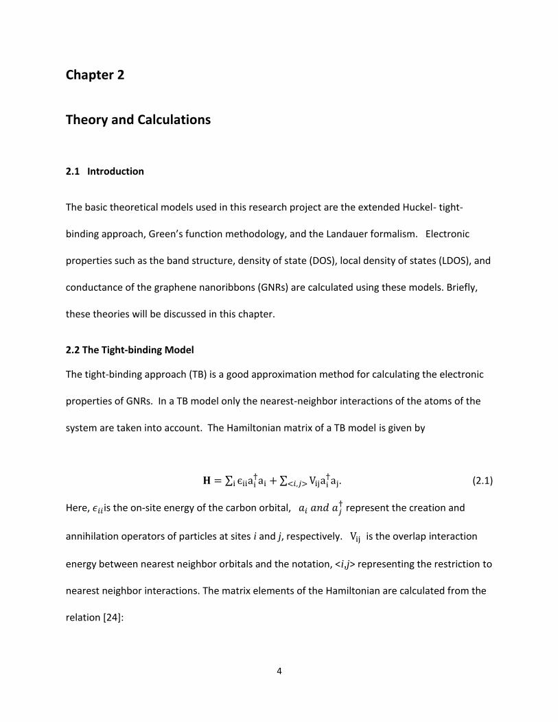
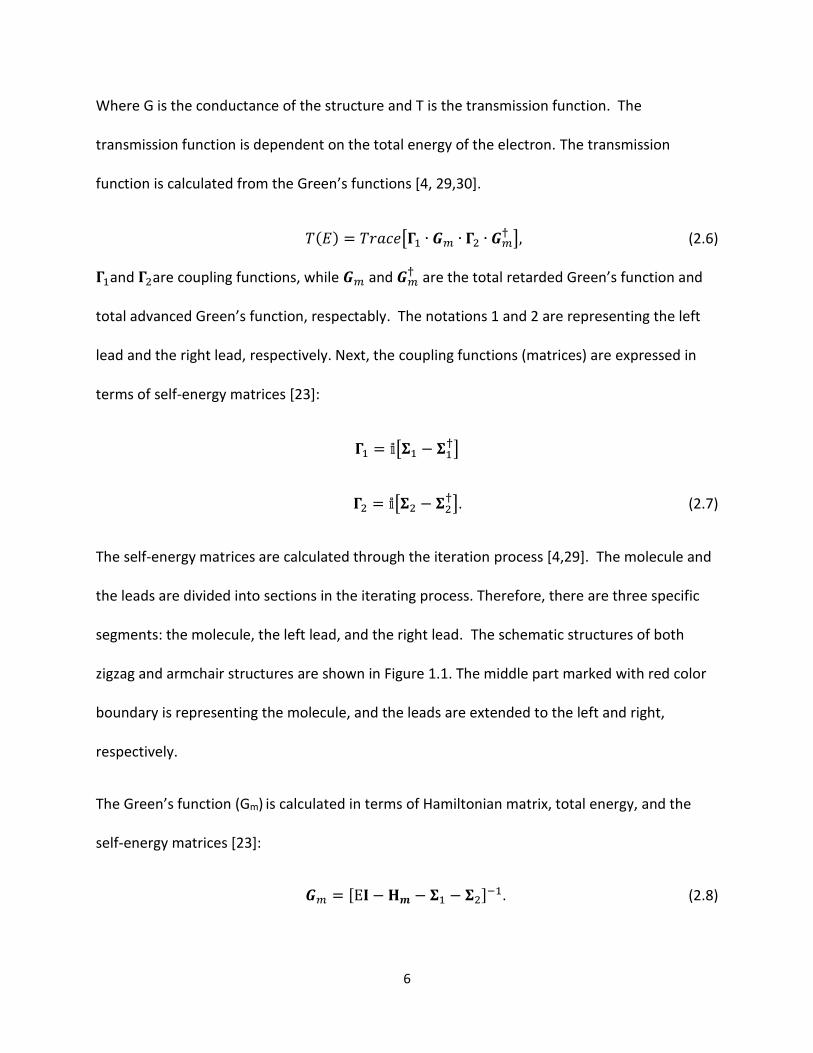
6
Where G is the conductance of the structure and T is the transmission function The
transmission function is dependent on the total energy of the electron The transmission
function is calculated from the Greenrsquos functions [4 2930]
119879(119864) = 119879119903119886119888119890[1204901 ∙ 119918119898 ∙ 1204902 ∙ 119918119898dagger ] (26)
1204901and 1204902are coupling functions while 119918119898 and 119918119898dagger are the total retarded Greenrsquos function and
total advanced Greenrsquos function respectably The notations 1 and 2 are representing the left
lead and the right lead respectively Next the coupling functions (matrices) are expressed in
terms of self-energy matrices [23]
1204901 = 120154[1205061 minus 1205061dagger]
1204902 = 120154[1205062 minus 1205062dagger] (27)
The self-energy matrices are calculated through the iteration process [429] The molecule and
the leads are divided into sections in the iterating process Therefore there are three specific
segments the molecule the left lead and the right lead The schematic structures of both
zigzag and armchair structures are shown in Figure 11 The middle part marked with red color
boundary is representing the molecule and the leads are extended to the left and right
respectively
The Greenrsquos function (Gm) is calculated in terms of Hamiltonian matrix total energy and the
self-energy matrices [23]
119918119898 = [E119816 minus 119815119950 minus 1205061 minus 1205062]minus1 (28)
7
By finding the Greenrsquos function the local density of states can be calculated and then a
summation of the local density of states leads to the total density of states Therefore the local
density of states of individual atoms is expressed from the Greenrsquos function Gm
LDOS119894(119864) = minus1
120587Im[119814119846(119842 119842)] (29)
It should be noted that the total density of states (DOS) of all the atoms discussed above can
also be obtained by summing the individual LDOS from the Greenrsquos function In this research
project the results are verified by both methods The detailed analyses of the Greenrsquos function
calculations are illustrated in the references [4111229]
24 The Extended Huckel Method
The electronic configuration of the ground state of a single carbon atom is 1s2 2s2 2px1 2py On a
hexagonal graphene structure the 2s 2px and 2py orbitals form sp2 hybridized orbitals These
hybridized orbitals are at 1200 to each other and form σ bonds on the 2-dimensional structures
of graphene Figure 21 illustrates a graphical presentation of the orbitals Figure 21 (a) shows
the S Px and Py orbitals of the atoms The Pz orbitals are perpendicular to the plane and are
not shown here In addition projections of the Px and Py orbitals of atom 1 on the S orbital of atom 3
are shown in part (b) These π bonds are relatively weaker compared to the σ bonds and
electrons can move from one atom to the other
8
Figure 21 (a) shows a top down view of the unit cell with orbitals Projections of the Px and Py orbitals
of atom 1 on the S orbital of atom 3 are shown in part (b)
The electronic properties of these graphene structures are obtained by including only the pz
orbitals for constructing the Hamiltonian of the structures The basic Huckel method deals with
only these 2pz orbitals in finding the electronic properties of structures of interests [2431]
The extended Huckel method expands upon this calculation by not only using the π bonds from
the 2pz orbitals but includes the bonds from the 2s 2px and 2py [26] Like the Huckel the EHM
only takes into account the nearest neighbor interactions between orbitals discussed above in
the TB model
In the case of a GNR the number of orbitals is directly dependent on the width of the ribbon in
the unit cell For an AGNR with n being the number of dimers on the AGNR the number of
orbitals is obtained by taking n multiplied by 2 to get the total number of carbon atoms and
9
then scaling that number by the number of unique orbitals in the case of carbon that is 4
Figure 11 (b) represents an armchair GNR structure with n=10 For example for the n= 10
dimer ribbon the total number of carbon atoms would be 20 and the total number of orbitals
will be 80 Thus the size of the Hamiltonian matrix will be 80 by 80
The next thing to consider is the edge bonds in the unit cell With AGNRs there are two atoms
at each edge of the periodic structure with dangling bonds The zigzag and the armchair
features at the top and bottom edges are clear in Figures (a) and (b) In this calculation a single
hydrogen atom in the ground state is used to terminate each edge bonds The hydrogen orbital
is thus 1s Since the size of the Hamiltonian matrix is determined by the total number of the
orbitals the addition of hydrogen atoms at the edges changes the size of the matrix So instead
of simply being 2n4 orbitals the total number of orbitals becomes 2n4+4 or 8n+4 The
electronic properties such as the band structures and density of states of the system are
obtained by diagonalizing the Hamiltonian matrix as a function of wave number k The charge
densities of individual atoms have been calculated by finding the eigenfunction of Hamiltonian
matrix of each k
Now we discuss the calculation of an armchair graphene nanoribbons of single hexagon in
thickness Figure 22 shows the graphene ribbon structure
10
Figure 22 A single hexogonal armchair graphene ribbon The atoms are marked with numbers the unit
cell I is marked with lines and its neighbors are I+1 and I-1
The unit cell along with its two nearest neighbors are represented by I I-1 I+1 and the sites are
marked 1 through 6 The Schrodinger equation (SE) for the structure is
|120569⟩ = 119864|120569⟩ (210)
and the Hamiltonian operator is given as
=minusℏ2
2119898nabla 2 + 119881(119903 ) (211)
and the wave function |120569 gt is given by
|120569 gt= sum 119890119894119896119877119868119868=119868119868+1119868minus1 |120569119868 gt (212)
where |120569119868 gt is expressed by the four orbitals s px py and pz
|120569119868 gt= sum 119890119894119896∙120591119895[1205721|119904119895⟩ + 1205732|119875119909119895⟩ + 1205743|119875119910119895⟩ + 1205814|119875119911119895⟩]119895=1 (213)
In Eq (212) 119877119868 represents the location of the unit cell I and 120591119895 is the phase factor of the
orbitals Here 120572 120573 120574 120581 are the probability amplitudes To construct the Hamiltonian matrix
11
the following analytical steps are performed First scalar products of the individual orbitals are
taken with Eq (210) Here an example is shown Taking the scalar product of 1199041 orbital one
finds
⟨1199041||sum119890119894119896∙120591119895[120572119895|119904119895⟩ + 120573119895|119875119909119895⟩ + 120574119895|119875119910119895⟩ + 120581119895|119875119911119895⟩]
6
119895=1
=
⟨1199041|119864|sum119890119894119896∙120591[120572119895|119904119895⟩ + 120573119895|119875119909119895⟩ + 120574119895|119875119910119895⟩ + 120581119895|119875119911119895⟩]
6
119895=1
(214)
The left hand side of Equation (214) is expanded as
119890119894119896∙1205911[1205721⟨1199041||1199041⟩ + 1205731⟨1199041||1198751199091⟩ + 1205741⟨1199041||1198751199101⟩ + 1205811⟨1199041||1198751199111⟩]
+119890119894119896∙1205912[1205722⟨1199041||1199042⟩ + 1205732⟨1199041||1198751199092⟩ + 1205742⟨1199041||1198751199102⟩ + 1205812⟨1199041||1198751199112⟩]
+ + 119890119894119896∙1205916[1205726⟨1199041||1199046⟩ + 1205736⟨1199041||1198751199096⟩ + 1205746⟨1199041||1198751199106⟩ + 1205816⟨1199041||1198751199116⟩]
= 119890119894119896∙12059111205721⟨1199041||1199041⟩ + 119890119894119896∙1205912[1205722⟨1199041||1199042⟩ + 1205732⟨1199041||1198751199092⟩] +
119890119894119896∙1205913[1205723⟨1199041||1199043⟩ + 1205733⟨1199041||1198751199093⟩ + 1205743⟨1199041||1198751199103⟩] (215)
In equation (215) all terms are zero except the nearest-neighbors As shown in Figure 22 the
nearest-neighbors for atom 1 are atoms 2 and 3
In a similar way the right hand side is expanded and it appears as
= 119890119894119896∙1205911[1205721⟨1199041|119864|1199041⟩ + 1205731⟨1199041|119864|1198751199091⟩ + 1205741⟨1199041|119864|1198751199101⟩ + 1205811⟨1199041|119864|1198751199111⟩]
+119890119894119896∙1205912[1205722⟨1199041|119864|1199042⟩ + 1205732⟨1199041|119864|1198751199092⟩ + 1205742⟨1199041|119864|1198751199102⟩ + 1205812⟨1199041|119864|1198751199112⟩] + hellip
+119890119894119896∙1205916[1205726⟨1199041|119864|1199046⟩ + 1205736⟨1199041|119864|1198751199096⟩ + 1205746⟨1199041|119864|1198751199106⟩ + 1205816⟨1199041|119864|1198751199116⟩]
= 1205721119890119894119896∙1205911⟨1199041|119864|1199041⟩ = 1205721119864119890119894119896∙1205911 (216)
In equation (216) only a single term is non-zero because the S1 orbital is orthogonal to all the
other orbitals except to itself
12
Combining equations (215) and (216) the following expressions are obtained
1205721⟨1199041||1199041⟩ + 119890119894119896∙1205912minus1205911[1205722⟨1199041||1199042⟩ + 1205732⟨1199041||1198751199092⟩] +
119890119894119896∙1205913minus1205911[1205723⟨1199041||1199043⟩ + 1205733⟨1199041||1198751199093⟩ + 1205743⟨1199041||1198751199103⟩] = 1205721119864 (217)
The matrix elements in Equation (217) are then expressed in a simplified form as
1205721휀119904 + 119890119894119896∙1205912minus1205911[1205722119864119904119904 + 1205732119875119864119904119909] +
119890119894119896∙1205913minus1205911[1205723119864119904119904 + 1205733119864119904119909 + 1205743119864119904119910] = 1205721119864 (218)
The matrix elements between atoms are defined by 휀119904 119864119904119904 119864119904119909 and 119864119904119910 Here 휀119904 is the on-site
energy of the S- orbital and the later three elements are expressed in terms of overlap
integrals 119881119894119895119896 defined in Equation (22) The complete expression of each element is shown in
the Appendix 1 These elements represent the σ and π interactions between orbitals and are
obtained from reference [24] The phase factors are expressed in terms of lattice constant
119886 (= 142Adeg) It should be noted that there are 24 orbitals in a single unit cell Here we have
shown complete analysis for a single orbital Similarly matrix element of the Hamiltonian is
obtained from these scalar products of all the orbitals The analysis is not shown for the rest of
the orbitals here Notice that each equation makes up a single row for the Hamiltonian matrix I
then sorted the Hamiltonian matrix with respect to each carbon atom and the 4 corresponding
orbitals This means every 4 rows are grouped in order by the corresponding S Px Py and Pz I
can then combine each interaction between carbon atoms into their own sub groups
represented by Hij with each group representing a 4 by 4 block Table 21 shows the condensed
Hamiltonian matrix using these Hij Block elements for visualization purposes C1-6 is set outside
the Hamiltonian as a guide to help the reader cross reference terms and identify what each
13
block refers to The phase factors interaction parameters and other terms are all contained in
these sub groups and will be explained below
Table 21 The Hamiltonian matrix for a single graphene hexagon
The Hamiltonian matrix elements in Table 21 are in the form of Hij with i and j terms going
from 1 to 6 for the 6 carbon atoms in this hexagonal periodic structure Note that each element
Hij is a block matrix These notations are used to show the Hamiltonian matrix in a compact
form The size of the Hamiltonian for this narrow n=3 dimer armchair ribbon is 24 by 24 but by
condensing each section into 4 by 4 blocks it reduces the appearance of the Hamiltonian to a 6
by 6 This reduction of size although merely cosmetic in effect makes checking each element in
the matrix much more manageable Instead of checking the entire matrix at once I am able to
check each block at a time for accuracy and feel much more confident in the result Examples of
these block matrices are shown in Table 22
14
Table 22 Matrix elements H11 H12 and H13 of Table 21 are shown in the blocks (a) (b) and (c) The
phase factors of the corresponding elements are also shown on the top of each block
The interaction matrix elements shown in Table 22 are described through schematic diagrams
in Figure 21 and Figure 23 As discussed above Figure 21 (a) shows the S Px and Py orbitals
of the atoms The lobes of the p orbitals are marked with positive and negative signs of atom 5
15
Next part (b) presents the orientations of the Px and Py orbitals toward the S orbital for atom
3 The left two configurations in part (b) represent the σ-bond between the S and Px and Py
orbital requiring 240 and 150 degreesrsquo reorientation of the orbitals respectively While the two
right configurations represent the π-bond between the S and Px and Py orbital Taking the
Cosine of these angles will let you know what portion of the interaction term to take For
instance the σ component for Px1 interacting with S3 will have Cos (240) = -12 and comparing
this with Table 22(c) we see the term should be 12 But there is one major component one
should take into account the positive and negative sides of the lobes and how this effects the
signs of the matrix elements To address this issue Figure 23 is introduced
The matrix elements are illustrated in Figure 23 Six interaction parameters are shown through
the schematic representation of the orientations of the orbitals It should be mentioned that
the interaction terms were defined in Equation (22) by 119881119894119895119896 and for the case at hand 119894 and 119895
are either a s-orbital or p-orbital and 119896 is either be a sigma or pi bond It should be mentioned
that the filled (solid) lobes are positive and the empty ones are negative Combing the results
from Figure 21 (b) and implementing the sign rules of the lobes introduced in Figure 23 we
get (-12)(- Vspσ) = 12( Vspσ) Following the same rules and techniques the other matrix
elements for atom 1 and atom 3 are calculated and shown in Table 22 (c)
The phase factors appeared in Equation (217) can have one of the four possible values plusmn119890119894119896119886
and plusmn119890119894119896119886
2 and two of them appear in parts (b) and (c) in Table 22
16
Figure 23 Illustration demonstrating the types of sigma and pi bonds between s and p orbitals [24]
The full Hamiltonian matrix is shown in the Appendix 1 A list of the matrix elements is also
provided in the Appendix 1
25 Summary
In this chapter we have discussed and shown the theoretical models used in the present
research project First the tight-binding model is discussed for the calculation of band structure
and density of state The associated interaction parameters and their values are presented
Next the Greenrsquos function formalism is discussed for the calculation of conductance and local
density of states In Section 24 the extended Huckel method is explained A detailed analysis
for a single Hamiltonian matrix element is shown Finally some schematic representation of the
orientation of the orbitals is discussed to express the interaction parameters and phase factors
for an AGNR
17
Chapter 3
Armchair Graphene Nanoribbons
31 Introduction
In this chapter we will present the results of electronic band structure density of states (DOS)
local density of states (LDOS) and conductance for armchair graphene nanoribbons (AGNRs)
The band structure and density of states are calculated using the tight binding (TB) model
discussed in chapter 2 Conductance and local density of states (LDOS) are calculated using
Greenrsquos functions methodology and the Landauer formula [4232930] The extended Huckel
method has been implemented in all these calculations [28]
First a brief description of the structure used in this calculation will be presented Next the
Band structure and Density of states will be shown followed by a comparison with results
obtained using the Huckel method Lastly the Conductance and LDOS results will be shown
32 Band Structure and Density of States of Armchair Graphene Nanoribbons
As discussed earlier graphene nanoribbons are strips of graphene with finite widths and semi-
infinite length along the axis of the strip Figure 31 shows a GNR with an armchair shape at the
edges This armchair patterned GNR is known as AGNR The AGNR is separated into unit cells
the Figure bellow shows several unit cells we will focus on the center unit cell I The number of
dimers in Figure 31 is equal to 9 The width of an AGNR is given by 119886radic3
2119899 where 119886 is the the
lattice constant and 119899 is the total number of dimers in the structure Here 119886 = 142A119900 thereby
18
the width of the ribbon is 1107nm For a n= 9 dimer AGNR there are 18 atoms in the unit cell
and these are shown with numbers In Figure 31 it is clear that the carbon atoms in the first
and last dimmer (at the top and bottom edges) are only connected to two other carbon atoms
in the bulk of the structure thus leaving a dangling bond at the edge In order to terminate the
dangling bond an atom can be added to the edge In this study the GNR edges are terminated
with hydrogen Band structures and DOS with and without edge terminated AGNRS are
presented and discussed The distinction between edge terminated bonds and non-terminated
bonds and edges will be a major focus in the chapter
Figure 31 Armchair graphene nanoribbon width n=9
19
Figure 32 (a) The band structure (b) the density of states of n= 3 dimer AGNR (without edge
termination)
In Figure 32 (a) the band structure of an armchair GNR with n = 3 is shown The electronic
band structures are plotted as a function of wave number k were k ranges over the first
Brillouin zone boundary When n = 3 there are 6 atoms in the unit cell There is a total of 24
bands in the figure proportional to the total number of orbitals The Fermi level has been
centered at 0 eV The previous chapter stated that the number of orbitals in the unit cell was
20
obtained by taking the number of dimers (n) and multiplying by 8 (orbitals) The bands located
above the Fermi level are known as the conduction bands while below the Fermi level the
bands are the valence bands An inspection of the bands reveals that not all valence and
conduction bands are perfectly symmetric with respect to the Fermi level One should also note
that there are many flat valence bands below the Fermi energy These flat bands are non-
conducting and the group velocity of the mobile electrons is close to zero [415] That means
the effective mass of the electrons is infinite [15] We predict these flat bands below the Fermi
energy are from the Px Py and S-orbitals of the carbon atoms
There is a distinct gap between highest valence band and the lowest conduction band The gap
in the Fermi level between the valence and conductance points to a material being
semiconducting This is what is expected for n = 3 The dimer rule to follow for AGNRs will be
semiconducting when n=3p or n=3p+1 (with p being an integer) However if n=3p+2 the
AGNRs will be metallic [2315]
In Figure 32 (b) the density of states (DOS) are plotted as a function of electron energy The
DOS value shows the number of k points per energy value Figure 32 (b) reveals that there are
some sharp peaks and gaps in the DOS structure As expected there is a gap around Fermi
energy This gap in DOS corresponds to the band gap observed in Figure 32 (a)
From the theory it is expected to find only the weakly held π bands around the Fermi level
mainly the 6 bands from the Pz interactions In Figure 32 (a) there seems to be 4 extra bands
located on the valence side close to the Fermi energy The current calculation and results
shown above do not account for the edge orbitals along the ribbon as in they could be thought
21
of as dangling or non-bonding orbitals These dangling edge atoms are C1 C2 C5 and C6 shown
in Figure 22 To remedy this situation the edges are terminated by adding hydrogen The
results with edge termination will be shown in Figure 34 Figure 33 shows the close up view
around the Fermi level for n = 3 It is clear from this view that there are many flat bands in the
valence band subsequently there are many peaks observed in the DOS graph The band gap at
k = 0 is about 24 eV This band gap indicates that n =3 AGNR is a semiconducting structure
Figure 33 (a) The band structure (b) the density of states near the Fermi energy of n= 3 dimer AGNR
(without edge termination)
22
Figure 34 (a) The band structure (b) the density of states of n= 3 dimer AGNR (edge terminated with
hydrogen)
Next we introduce the edge terminated results of the band structure and DOS in Figure 34
Due to the addition of the hydrogen at the edges the total number of bands should be 28 It is
clear that due to the edge termination the qualitative features of the bands have changed The
bands are more symmetric about the Fermi energy Also some flat bands observed in Figure 32
(a) moved at lower energy levels in the valence band region We also see that around -20 there
is a large increase in the number of bands compared to Figure 32 (a) From this observation
23
one may suggest that the S-orbital of the hydrogen atom is hybridized with the other orbitals
(Px Py S) of the carbon atoms on the two-dimensional plane From this observation we
conclude the bands at very low energy are tightly bound and are forming σ bonds Those closer
to the Fermi energy are forming π bonds and contribute to conduction Figure 34 (b) also
shows similar changes in DOS around the Fermi level Instead of several distinct peaks below
the Fermi level around -3 eV we see only one peak This relates with the one flat band in Figure
34 (a) at the same energy Also more peaks are observed around -20 eV in the valence band
region A close up view of the bands and DOS are shown around the Fermi energy in Figure 35
As discussed above the width of the band gap at k = 0 remains the same (cong24 eV)
24
Figure 35 (a) The band structure (b) the density of states near the Fermi energy of n= 3 dimer AGNR
(edge terminated with hydrogen)
25
Figure 36 (a) The band structure (b) the density of states of n= 5 dimer AGNR (without edge
termination)
The next thing to study is the case of n=3p+2 dimer AGNR In order to avoid the analytical and
computational cost the lowest number of dimers in the relation n=3p+2 is considered in this
calculation n = 5 Figure 36 shows the band structure and the DOS The electronic bands are
plotted as a function of wave vector k and DOS are plotted as a function of energy It should be
mentioned that these results are without edge termination One of the first things apparent in
26
Figure 36 (a) is the number of bands has increased significantly Remembering that one band
correlates to one orbital there are 10 atoms for n = 5 Hence there are 40 orbitals in total
Some of the bands overlap and appear close together Looking at the highest valence band and
the lowest conduction band it is seen that they meet at the Fermi level at k=0 This point of
degeneracy between bands when k = 0 indicates that the structure is metallic This follows the
theory that the AGNR is metallic when n=3p+2 As discussed above about the flat bands and
peaks in the DOS represent the non-conducting states and indicate infinite mass The bands
around the Fermi energy are linear indicating the group velocity is nonzero and is measured to
be about 106 ms [14] The metallic property of the AGNR with n=5 is confirmed again by
Figure 36 (b) which shows that the DOS is non-zero at the Fermi level In conclusion we see n
= 5 AGNR is indeed metallic Enhanced plots near the Fermi energy for the bands and DOS are
displayed in Figure 37 The detailed characteristics of the bands and DOS are more visible here
27
Figure 37 (a) The band structure (b) the density of states near the Fermi energy of n=5 dimer AGNR
(without edge termination)
28
Figure 38 (a) The band structure (b) the density of states of n= 5 dimer AGNR (edge terminated with
hydrogen)
In Figure 38 the edge terminated results for n=5 AGNR are shown The bands are shown in
Figure 38 (a) and the DOS are in 38 (b) The addition of the hydrogen at the edges results in 44
bands The general behavior of the bands moving away from the Fermi energy is similar as
observed in Figure 34 (a) The weakly bonded π orbitals are near the Fermi energy and the
bands are symmetric about it Due to hybridization of the orbitals on the plane with hydrogen
29
the flat bands near the Fermi energy in Figure 36 (a) moved to very low energy region The
number of peaks observed in the energy range -2 eV to -6 eV in Figure 36 (b) has decreased to
only one This may suggest that they are hybridized with the other orbitals of the hydrogen
atoms on the plane Figure 39 shows the detailed features of the bands and DOS near the
Fermi energy
Figure 39 (a) The band structure (b) the density of states near the Fermi energy of n= 5 dimer AGNR
(edge terminated with hydrogen)
30
For completeness Figure 310 has been included to address the case for n=3p+1 and to confirm that it
is semiconducting as expected Figure 310 shows the band structure and the DOS for an n=4 AGNR with
edge termination The features will not be discussed in detail because they are similar to the n=3 AGNR
case Here the main focus is to confirm the results of a semiconducting nature of the ribbon
Figure 310 (a) The band structure (b) the density of states of n= 4 dimer AGNR (edge terminated with
hydrogen)
31
33 Comparison of Huckel and Extended Huckel Results of Armchair Graphene Nanoribbons
In this section results will be discussed for comparison between the Huckel and extended
Huckel methods different widths of armchair nanoribbons Results from the extended Huckel
method discussed in section 32 will be used for comparison Only the band structure and the
density of states will be compared Since a detailed description for the extended Huckel
method was presented in the previous section only a short explanation will be given for the
comparison
Figures 311 and 35 present the band structure and density of states (DOS) for Huckel and
extended Huckel method for n=3 dimer AGNRs respectively One may notice the bands and
DOS are symmetric about the Fermi level for the Huckel method (Figure 311) On the other
hand both bands and DOS are not symmetric for the extended Huckel method There are a few
bands seen around 80eV in the conduction region Consequently the DOS is non-zero at this
energy As discussed in the previous section the symmetric bands around the Fermi energy are
due to the Pz-orbitals therefore these bands around 80eV are from the other orbitals in the 2-
D plane
32
Figure 311 (a) The band structure (b) the density of states near the Fermi energy of n= 3 dimer AGNR
(Huckel Method edge terminated with hydrogen)
The band structures and DOS are compared for n=5 AGNR in Figures 312 and 39 Here due to
the addition of dimers the number of bands increased As seen above the bonding and anti-
bonding orbitals are symmetric about the Fermi energy The bands must be symmetric since
the energy of all the Pz-orbitals is the same There are some more bands and DOS observed
33
again around E = 80eV In summary the general characteristics of the bands and DOS are
similar around the Fermi energy in both Huckel and extended Huckel method The only
difference observed σ bands in the extended Huckel method and these are farther away from
Fermi level
Figure 312 (a) The band structure (b) the density of states near the Fermi energy of n= 5 dimer AGNR
(Huckel Method edge terminated with hydrogen)
34
34 Conductance of Armchair Graphene Nanoribbons
The conductance results of n = 3 and n = 5 AGNR will be discussed in this section Figure 313
shows the conductance values as a function of energy
Figure 313 Conductance as a function of energy for (a) n = 3 AGNR (b) n = 5 AGNR (edge terminated
with hydrogen)
First we will show and discuss the conductance results for the edge terminated cases In Figure
313 (a) the conductance around the Fermi level is zero the first quantized conductance value
does not show up until -12 eV and 12 eV respectively This zero conductance nature is
expected because n = 3 is a semiconductor type AGNR as seen in Figure 34 From the band
structure as well as DOS analysis discussed above the conductance should be zero within this
energy range (shown in Figure 34(a) amp (b)) This implies there is no propagating mode to
contribute to the transport From Figure 34 it is clear that the number of propagating states is
zero within this range From the Landauer formula conductance is expressed by integer
multiples of (2e2h) Therefore it is expected that the conductance will be quantized by (2e2h)
In Figure 313 (a) the conductance between -32eV to -12 eV and 32 eV to 12 eV is equal to 1
(2e2h) This general behavior of quantization is expected for any semiconductor or metallic
GNRs
35
Next we present the conductance for n = 5 AGNR As stated earlier n = 5 AGNR is metallic The
first quantized conduction band is between -22eV to 22eV and the second quantized
conduction band starts from -22eV and 22eV with conductance value equal to 2 (2e2h) This
corresponds to two possible allowed propagating states for transport
In order to study the effects of edges on transport the conductance results are produced
without the edge termination Figure 314 shows without edge terminated conductance for n=
3 and n=5 dimer AGNRs It is expected from the observations of band structures and DOS
results shown in Figures 33 and 37 that the characteristics of the conductance curves will not
be fully quantized and some different features will appear
Figure 314 Conductance as a function of energy for (a) n = 3 AGNR (b) n = 5 AGNR (without edge termination)
For both n=3 and n= 5 AGNRs in Figure 314 (a) and (b) there is a sharp increment in conductance is
observed in the valence band regions It is predicted that these enhancements are due to the σ -bands
observed in the without edge terminated structures in the valence bands below the Fermi level shown
in Figures 33 and 37 The sharp spikes are at the same location as the energy bands In conclusion the
edge termination is essential for clean quantized features in conductance curves The dangling bonds at
36
the edges destroy the perfect quantized behavior expected from the Landauer formalism for perfect
nanostructures
35 Local Density of States of Armchair Graphene Nanoribbons
The local density of states (LDOS) shows the number of states per energy for each atom in the
unit cell Using the extended Huckel method each atom in the unit cell has four orbitals
contributing to their particular LDOS In this section the LDOS results will be presented for the
edge terminated AGNRs for n=3 and n=5
Figure 315 LDOS for n=3 AGNR (a) for carbon 1 atom (b) for carbon 3 atom Positions of the atoms are
shown in Figure 22
Figure 315(a) and (b) shows the LDOS for 2 of the atoms in the unit cell The Figure shows
carbon atom 1 and carbon atom 3 (refer to Figure 22(a)) Naturally this brings up the question
of why only 2 of the 6 carbon atoms are shown The reason has to do with the symmetry of the
37
unit cell and neighbors because the general symmetric relationship between the matching
atoms they have identical interactions between atoms thus matching LDOS values The general
characteristics of LDOS for the edge atoms 1 and 2 are identical Similarly the features of LDOS
for the middle atoms 3 and 4 are similar It is also expected that the results of atoms 5 and 6
will be similar to atoms 1 and 2 Therefore only the LDOS of two atoms will provide a general
image of the characteristics of the electronic property The graphs tend to show a lot of
similarities It is also noted the difference around the Fermi level between the two LDOS graphs
Figure 315(a) has several distinct peaks at different locations
For the n=5 AGNR there are a total of ten LDOS graphs but like the n=3 case many of the
carbon atoms result in similar LDOS graphs The matching carbon LDOS are as follows 1 2 9
10 make a set 3 4 7 and 8 make a set and 5 6 make the final set The atomic positions are
shown in Figure 31
Figure 316 two LDOS for a n=5 AGNR (a) for the carbon 1 atom (b) for the carbon 3 atom (c) for the
carbon 5 atom
38
Looking at Figure 316 (a) and (b) we can see that these are the carbon atoms where the
electronic transport happens it is shown by the nonzero LDOS at and around the Fermi energy
This becomes interesting when you note these are all the edge atoms It is also noted for Figure
316 (c) there is 0 LDOS around the Fermi energy meaning no electronic transport Being able to
plot the LDOS becomes a very powerful tool when looking at the individual atoms and how they
are affected by changes to the system as a whole A good research topic for the future could
follow an in-depth look at the LDOS and how it changes with respect to anomalies and defects
within the GNRs
36 Summary
In this chapter the electronic properties for several AGNR have been studied using the
extended Huckel method The band structure DOS conductance and LDOS are calculated for
several AGNRs The number of dimers representing the width of the ribbons are chosen based
upon the dimer rule n=3p+2 is metallic and n=3p and n=3p+1 are semiconducting Here p is
an integer For n= 3 4 and 5 AGNR have been investigated As expected n= 3 and 4 AGNR are
semiconducting while n= 5 is metallic From this investigation we find that electron conduction
mostly relies on the Pz orbitals Results with and without edge termination are discussed for
both cases The addition of edge termination was required to successfully explain the results
around the Fermi level
39
Chapter 4
Zigzag Graphene Nanoribbons
41 Introduction
In this chapter zigzag graphene nanoribbon (ZGNR) structure will be discussed and then it will
be compared to the AGNR structures Next the results the band structure and DOS for two
separate ZGNRs will be presented and discussed Finally the chapter will conclude with a
comparison between the Huckel and extended Huckel results obtained for the ZGNR
42 Band Structure and Density of States of Zigzag Graphene Nanoribbons
The name of a GNR comes from the zigzag pattern along the semi-infinite edge of the ribbon In
Figure 310 a ZGNR is displayed with the unit cell marked at the center The unit cell is
represented by I and its neighbors are shown by I +1 and I -1 There are 6 chains in the
structure The width of ZGNRs can determined by the number of chains (N) in the ribbon The
distance between two chains is 3119886
2 Therefore the width of the chain with N=6 will be 1278nm
The numbering scheme for the atoms in the unit cell is top down Results for N=2 and N=6 will
be presented here
Figure 41 Zigzag graphene nanoribbon N= 6 chains
40
Figure 42 (a) The band structure (b) the density of states of N= 2 chain ZGNR (without edge
termination)
Figure 42 displays the electronic band structure and the density of states for a N = 2 chain
ZGNR In Figure 42 (a) the electronic band structures are plotted as a function of wave vector k
where k ranges within the boundary of the first Brillouin zone N = 2 is chosen because it is the
smallest number of chains possible to make up a ZGNR The same relation has been used to find
the number of orbitals in a unit cell for the ZGNR as for the AGNR For the case of N = 2 chain
41
ZGNR the total number of orbitals is thus 16 The Fermi level energy has again been centered
around 0 eV It is observed that the highest valence band and the lowest conduction band meet
at both ends of the Brillouin boundary indicating metallic properties [51011] This feature is
explained by many researchers and these are due to the edge atoms This metallic property is
expected for all ZGNRs It is also seen that the bands flatten out into each other as they meet
on either edge This is in stark contrast to the metallic AGNRs that meet at k = 0 and
approached at a constant slope These flat bandrsquos characteristics indicate the group velocity of
the electrons is zero and the bands are non-conducting It is also noticed like the AGNR that the
bands are not symmetric about the Fermi level in this dangling bond situation
In Figure 42 (b) the density of states (DOS) are plotted as a function of electron energy The
DOS show the number of states per energy value The DOS is non-zero at the Fermi energy
confirms the result of metallic properties Not only is it non-zero but there is a peak at the
Fermi energy which relates to the flattening of the bands as they meet Figure 43 shows the
close up view around the Fermi level the flattening of the bands and the peak at the Fermi
level are much more prominent
42
Figure 43 (a) The band structure (b) the density of states near the Fermi energy of N= 2 chain ZGNR
(without edge terminated)
As discussed in the last section with AGNRs there was a problem with dangling edge-orbitals
This problem persists with the ZGNR The solution is similar to the AGNR but instead of
requiring two hydrogen atoms at each edge of the unit cell ZGNR requires only one at each
edge The results with edge termination are shown in Figure 44 for a ZGNR with N = 2
43
Figure 44 (a) The band structure (b) the density of states of N=2 chain ZGNR (edge terminated with
hydrogen)
Figure 44 displays the bands and DOS for a ZGNR with N = 2 chain where the dangling carbon
orbitals are terminated with hydrogen Due to the addition of the hydrogen at the edges the
total number of bands is 18 It is clear that the edge termination has had an effect on several of
the bands in Figure 44 (a) It is observed that the two bands located slightly below the Fermi
44
energy in Figure 44 (a) have both moved This suggests that these two bands have now moved
to lower energy states with the forming sigma bonds now shared with the hydrogen As
discussed for the AGNR the orbitals that relate to the bands lying on the 2-D plane (S Px Py)
Therefore the four bands about the Fermi energy are the contributions from the Pz orbitals
Recall that the bonding and anti-bonding orbitals are in the valence and conduction band about
the Fermi level respectively The picture around the Fermi level becomes clearer now that two
of the bands have gone It is predicted that these two bands are from the dangling p- orbitals of
the edge atoms Once the edges are terminated the S-orbital of the hydrogen atom form sigma
bonds with the p-orbitals of the carbon atoms and move to the lower energy levels in the
valence band The peak from the touching conduction and valence band at E = 0 eV is easily
discernible in Figure 44 (b) The increase in the DOS is produced by the flattening of the bands
as they approach the Fermi level Figure 45 is used to display this same edge terminated ZGNR
but with the energy ranging from -7 to 7 eV with respect to the Fermi level
45
Figure 45 (a) The band structure (b) the density of states near the Fermi energy of N= 2 ZGNR (edge
terminated with hydrogen)
46
Figure 46 (a) The band structure (b) the density of states of N= 6 chain ZGNR (without edge
termination)
Figure 46 displays the bands and the DOS for an N = 6 chain ZGNR The number of bands in this
case is 48 The edges are not terminated and hence the general characteristics of the bands as
well as the DOS are alike as found in N = 2 ZGNR shown in Figure 42 The valence bands form
the bonding and the conduction bands form anti-bonding orbitals [26] A difference between
the two ZGNRs is shown with the flatter bands at the Fermi energy for the N = 6 As a result the
47
DOS values at the Fermi energy are higher In addition the other Pz orbitals degenerate at the
boundary of the Brillouin zone at two different energy values (around -3 and 3 eV) [11] As
before for clarity the bands in DOS around the Fermi level are displayed in Figure 47
Figure 47 (a) The band structure (b) the density of state near the Fermi energy of N= 6 chain ZGNR
(without edge terminated)
48
It is clear that there are additional bands mixed with the Pz-bands near the Fermi level in the
valence band region For the N=2 chain ZGNR there are two bands observed of this nature
shown in Figure 43 As discussed before we consider that these bands formed from the
dangling P-orbitals of the edge atoms Apparently it appears that there is a single band One
may consider it as a degenerate band In order to avoid this confusion the results for N= 3 4
and 6 ZGNRs are plotted within a small window of energy shown in Figure 48 It is clear that
bands are separated as seen in Figure 43
Figure 48 The band structure of (a) N=3 (b) N=4 and (c) N=6 chain ZGNRs for a small energy range about the Fermi enrgy (without ede terminated)
49
Figure 49 (a) The band structure (b) the density of state of N=6 chain ZGNR (edge terminated with
hydrogen)
Results of edge terminated bands and DOS for N = 6 ZGNR is presented in Figure 49 Because of
the edge termination the bands around the Fermi level are almost symmetric Shifting of the
non Pz orbitals away from the Fermi level in the valence band region is consistent with previous
results This result is compared to the previously calculated result reported by others [11] The
electronic energy bands and DOS values are identical near the Fermi level The only difference
50
appears away from the Fermi level in the conduction band region In order to understand verify
this discrepancy it may require some further investigations in the future For a better view
around the Fermi region Figure 49 is provided
Figure 410 (a) The band structure (b) the density of state near the Fermi energy of N= 6 chain ZGNR
(edge terminated with hydrogen)
51
43 Comparison of Huckel and Extended Huckel Results of Zigzag Graphene Nanoribbons
Here the band structure and DOS will be compared for the two different ZGNRs Figures 411
and 45 show the results for a N=2 chain ZGNR using the Huckel and extended Huckel method
respectively Like the AGNRs the bands and DOS are symmetric about the Fermi level These
bonding and anti-bonding are from the Pz orbitals Therefore one expects the asymmetric
behavior to appear with the extended Huckel method at higher energy Figure 45 reveals the
features in the conduction band
52
Figure 411 (a) The band structure (b) the density of states near the Fermi energy of N= 2 ZGNR (Huckel
Method edge terminated with hydrogen)
Next for N=6 chain ZGNR results are displayed in Figures 412 and 49 Fundamentally there
are not much difference except there are many more bands Overall the general trend of the
bands and DOS around the Fermi energy as well as away are similar for N=2 chain ZGNR
discussed above Therefore with the extended Huckel technique one can extract the details of
the electronic properties of the nanoribbons
53
Figure 412 (a) The band structure (b) the density of states near the Fermi energy of N= 6 ZGNR (Huckel
Method edge terminated with hydrogen)
44 Summary
The band structure and the DOS calculations have been show for ZGNRs of two different
widths The addition of the Hydrogen to work with the dangling edge orbitals was required to
move around some of the bands away from the Fermi level leaving the extended Huckel
method to match the Huckel method As in AGNRs the edges of ZGNRs are terminated with
54
hydrogen The S-orbital of the hydrogen atom form bonds with the S- and P-orbitals of the edge
atoms There are two energy bands observed near the Fermi level in the valence band region
These are mixed with the Pz-bands and are predicted that these are due to the presence of
dangling P-orbitals at the edges of the ribbons Once the edges are terminated with hydrogen
these bands are pushed back at the lower energy levels From this observation we conclude
these dangling P-orbitals are forming σ-bonds with the S-orbital of the hydrogen atom If the
edges are terminated with other element(s) then the investigation will be more interesting and
conclusive
55
Chapter 5
Summary and Conclusions
In this research project two different graphene nanoribbons have been studied These include
the armchair and zigzag nanoribbons Electronic properties are studied by using a tight-binding
model Greenrsquos function methodology Landauer formalism and the extended Huckel method
The electronic properties investigated are the band structures density of states and
conductance The results obtained from the extended Huckel method are compared with the
Huckel method
In Chapter 2 the theoretical methods are presented In addition to the well-known theories
such as the TB model the Greeenrsquos function model examples of analytical and geometrical
techniques used in the calculation of the Hamiltonian matrix elements are illustrated
The electronic properties of AGNRs are presented in Chapter 3 The results of electronic band
structures DOS conductance and LDOS are shown for n= 3 4 and 5 dimer AGNRs The first
two ribbons are semiconducting and the later one is metallic These results are consistent with
theory Then these results are compared with the Huckel method These results are produced
with and without edge terminated structures The edge atoms are terminated with hydrogen
atom The most interesting observation in this study is the effect of the dangling bonds at the
edges of these nanoribbons It is clear from this investigation the edge termination is essential
for quantized conductance as expected in perfect nanostructures
56
Chapter 4 presents only electronic band structures and DOS results for N=2 and N=6 chain
ZGNRs These results are also compared with the results obtained by the Huckel method As in
AGNRs the edge atoms are terminated with hydrogen In the case of non-terminated edges
the most significant observation is the presence of two bands mixed with the Pz bands in the
valence band region near the Fermi level Once the edges are terminated these bands are
pulled into lower energy levels From these analyses we conclude that these bands are due to
the contributions of the hanging P-orbitals of the edge atoms
In summary Extended Huckel method was significantly more challenging than the Huckel
method In the Huckel method only Pz-orbitals are included in the Hamiltonian On the other
hand the extended method uses all four (S Px Py Pz) orbitals in the analyses Specifically the
orientations of the orbitals of each atom have to take into account for calculation Inclusion of
only Pz-orbitals is good enough for a conclusive result near the Fermi energy The detailed
knowledge of the electronic properties at all energy level requires more involved theory such as
the extended Huckel model or density functional theory (DFT) The results will be more exciting
and interesting with the extended Huckel method if the edges are terminated with element(s)
other than hydrogen The addition of hydrogen element at the edges does not show any effect
on the electronic properties in the Huckel theory because the S-orbital of the hydrogen atom is
on the 2-D plane The transport in GNRs near the Fermi energy is only due to pi orbitals formed
by the Pz- orbitals Our observation with the extended Huckel model demonstrates effects far
away from the Fermi energy
57
Therefore I conclude that the research is not complete meaning there are many different
types of nanostructures that can be examined using the extended Huckel method and that
means there is still the possibility for the stronger σ-bonds to have an effect on the electrical
properties This leads to some real interesting possibilities of extension of this work The first
possibility would be to stay with GNRs and start introducing edge defects to the ribbon This
could be accomplished a few ways my initial thought would be to vary one of two things First
vary the types of atoms used in the edge termination Second vary the self-interaction on
certain orbitals or completely remove some orbitals from the unit cell completely As noticed
in Chapters 3 and 4 the results obtained without edge termination have very interesting
changes to the band structure around the Fermi level Another avenue for future research is to
look at different materials that can be isolated into single layer ribbons Whatever avenue is
chosen has the possibility to discover some truly interesting physics and that is always
important and significant from the pedagogical point view as well as in applications
58
Appendix
1 Hamiltonian Matrix of an Armchair Graphene Nanoribbon with n = 3 Dimer
59
The list of the matrix element of the Hamiltonian is defined here
119864119904119904 = 119881119904119904 119864119909119909 =1
4119881119901119901 +
3
4119881119901119901 119875119864119904119901119909 = 119881119904119901
119864119904119901119909 =1
2119881119904119901 119864119910119910 =
3
4119881119901119901 +
1
4119881119901119901 119875119864119909119909 = 119881119901119901
119864119904119901119910 =radic3
2119881119904119901 119864119909119910 =
radic3
4119881119901119901 minus
radic3
4119881119901119901 119875119864119910119910 = 119881119901119901
119864119911119911 = 119881119901119901
The phase factors are defined as
1198921 = 119890119894119896119886 1198922 = 119890119894119896119886
2
1198921lowast = 119890minus119894119896119886 1198922
lowast = 119890minus119894119896119886
2
2 Code for Calculating the Band Structure and Density of States for n= 3 AGNR
Author Spencer Jones
Armchair with n=3 dimer
Band Structure and Density of States Size of the Hamiltonian
matrix is 28x28
Note Edge Terminated by Hydrogen
n=3 Number of dimers
amp=805 Changes Energy Scale of Plots
a=142
V=-081762a^2
ϵ=-897
Overlap Interaction Energy
Vssσ=-140761a^2
Vspσ=184761a^2
Vppσ=324761a^2
Vppπ=-081761a^2
ℰ=-897 a=142
bc=12 (2π)(3a)
60
ℰpx=-897 ℰpy=-897 ℰpz=-897 ℰs=-1752 Phase Factor
g1=Exp[Ika]
gi1=Exp[-Ika]
g2=Exp[Ika2]
gi2=Exp[-Ika2]
Interaction Terms
Ess=Vssσ
Esx=Vspσ2
Esy=VspσSqrt[3]2
Exx=Vppσ4+Vppπ34
Eyy=Vppσ34+Vppπ4
Ezz=Vppπ
Exy=VppσSqrt[3]4-VppπSqrt[3]4
PEsx=Vspσ
PExx=Vppσ
PEyy=Vppπ
Hydrogen-Carbon Interaction Terms
VHssσ=-140761b^2
VHspσ=184761b^2
b=109 Bond legnth between Carbon and Hydrogen
EHss=VHssσ
EHsx=VHspσ2
EHsy=VHspσSqrt[3]2
ℰh=-136
H=Table[0x18n+4y18n+4] Matrix Size
Diagonals ℰs AND ℰp Do[H[[4i-3]][[4i-3]]=ℰsi12n] Do[H[[4i-2]][[4i-2]]=ℰpxi12n] Do[H[[4i-1]][[4i-1]]=ℰpyi12n]
Do[H[[4i]][[4i]]=ℰpzi12n]
C1 on C2
S1-S2Px2
Do[H[[16i-15]][[16i-11]]=g1Essi1(n+1)2]
Do[H[[16i-15]][[16i-10]]=g1PEsxi1(n+1)2]
Px1-S2Px2
Do[H[[16i-14]][[16i-11]]=g1(-PEsx)i1(n+1)2]
Do[H[[16i-14]][[16i-10]]=g1PExxi1(n+1)2]
61
Py1-Py2
Do[H[[16i-13]][[16i-9]]=g1PEyyi1(n+1)2]
Pz1-Pz2
Do[H[[16i-12]][[16i-8]]=g1Ezzi1(n+1)2]
C1 on C3
S1-S3Px3Py3
Do[H[[16i-15]][[16i-7]]=gi2Essi1n2]
Do[H[[16i-15]][[16i-6]]=gi2(-Esx)i1n2]
Do[H[[16i-15]][[16i-5]]=gi2(-Esy)i1n2]
Px1-S3Px3Py3
Do[H[[16i-14]][[16i-7]]=gi2Esxi1n2]
Do[H[[16i-14]][[16i-6]]=gi2Exxi1n2]
Do[H[[16i-14]][[16i-5]]=gi2Exyi1n2]
Py1-S3Px3Py3
Do[H[[16i-13]][[16i-7]]=gi2Esyi1n2]
Do[H[[16i-13]][[16i-6]]=gi2Exyi1n2]
Do[H[[16i-13]][[16i-5]]=gi2Eyyi1n2]
Pz1-Pz3
Do[H[[16i-12]][[16i-4]]=gi2Ezzi1n2]
C2 on C1
S2-S1Px1
Do[H[[16i-11]][[16i-15]]=gi1Essi1(n+1)2]
Do[H[[16i-11]][[16i-14]]=gi1(-PEsx)i1(n+1)2]
Px2-S1Px1
Do[H[[16i-10]][[16i-15]]=gi1PEsxi1(n+1)2]
Do[H[[16i-10]][[16i-14]]=gi1PExxi1(n+1)2]
Py2-Py1
Do[H[[16i-9]][[16i-13]]=gi1PEyyi1(n+1)2]
Pz2-Pz1
Do[H[[16i-8]][[16i-12]]=gi1Ezzi1(n+1)2]
C2 on C4
S2-S4Px4Py4
Do[H[[16i-11]][[16i-3]]=g2Essi1n2]
Do[H[[16i-11]][[16i-2]]=g2Esxi1n2]
Do[H[[16i-11]][[16i-1]]=g2(-Esy)i1n2]
Px2-S4Px4Py4
Do[H[[16i-10]][[16i-3]]=g2(-Esx)i1n2]
Do[H[[16i-10]][[16i-2]]=g2Exxi1n2]
Do[H[[16i-10]][[16i-1]]=g2(-Exy)i1n2]
Py2-S4Px4Py4
Do[H[[16i-9]][[16i-3]]=g2Esyi1n2]
Do[H[[16i-9]][[16i-2]]=g2(-Exy)i1n2]
Do[H[[16i-9]][[16i-1]]=g2Eyyi1n2]
Pz2-Pz4
62
Do[H[[16i-8]][[16i]]=g2Ezzi1n2]
C3 on C4
Do[H[[16i-7]][[16i-3]]=gi1Essi1(n)2]
Do[H[[16i-7]][[16i-2]]=gi1(-PEsx)i1(n)2]
Do[H[[16i-6]][[16i-3]]=gi1PEsxi1(n)2]
Do[H[[16i-6]][[16i-2]]=gi1PExxi1(n)2]
Do[H[[16i-5]][[16i-1]]=gi1PEyyi1(n)2]
Do[H[[16i-4]][[16i]]=gi1Ezzi1(n)2]
C3 on C1
S3-S1Px1Py1
Do[H[[16i-7]][[16i-15]]=g2Essi1n2]
Do[H[[16i-7]][[16i-14]]=g2Esxi1n2]
Do[H[[16i-7]][[16i-13]]=g2Esyi1n2]
Px3-S1Px1Py1
Do[H[[16i-6]][[16i-15]]=g2(-Esx)i1n2]
Do[H[[16i-6]][[16i-14]]=g2Exxi1n2]
Do[H[[16i-6]][[16i-13]]=g2Exyi1n2]
PY3-S1Px1Py1
Do[H[[16i-5]][[16i-15]]=g2(-Esy)i1n2]
Do[H[[16i-5]][[16i-14]]=g2Exyi1n2]
Do[H[[16i-5]][[16i-13]]=g2Eyyi1n2]
Pz3-Pz1
Do[H[[16i-4]][[16i-12]]=g2Ezzi1n2]
C3 on C5
S3-S5Px5Py5
Do[H[[16i-7]][[16(i+1)-15]]=g2Essi1(n-1)2]
Do[H[[16i-7]][[16(i+1)-14]]=g2Esxi1(n-1)2]
Do[H[[16i-7]][[16(i+1)-13]]=g2(-Esy)i1(n-1)2]
Px3-S5Px5Py5
Do[H[[16i-6]][[16(i+1)-15]]=g2(-Esx)i1(n-1)2]
Do[H[[16i-6]][[16(i+1)-14]]=g2Exxi1(n-1)2]
Do[H[[16i-6]][[16(i+1)-13]]=g2(-Exy)i1(n-1)2]
PY3-S5Px5Py5
Do[H[[16i-5]][[16(i+1)-15]]=g2Esyi1(n-1)2]
Do[H[[16i-5]][[16(i+1)-14]]=g2(-Exy)i1(n-1)2]
Do[H[[16i-5]][[16(i+1)-13]]=g2Eyyi1(n-1)2]
Pz3-Pz5
Do[H[[16i-4]][[16(i+1)-12]]=g2Ezzi1(n-1)2]
C4 on C3
S1-S3Px3Py3
Do[H[[16i-3]][[16i-7]]=g1Essi1(n)2]
Do[H[[16i-3]][[16i-6]]=g1PEsxi1(n)2]
Px1-S3Px3Py3
63
Do[H[[16i-2]][[16i-7]]=g1(-PEsx)i1(n)2]
Do[H[[16i-2]][[16i-6]]=g1PExxi1(n)2]
Py1-S3Px3Py3
Do[H[[16i-1]][[16i-5]]=g1PEyyi1(n)2]
Pz1-Pz3
Do[H[[16i]][[16i-4]]=g1Ezzi1(n)2]
C4 on C2
S4-S2Px2Py2
Do[H[[16i-3]][[16i-11]]=gi2Essi1n2]
Do[H[[16i-3]][[16i-10]]=gi2(-Esx)i1n2]
Do[H[[16i-3]][[16i-9]]=gi2Esyi1n2]
Px4-S2Px2Py2
Do[H[[16i-2]][[16i-11]]=gi2Esxi1n2]
Do[H[[16i-2]][[16i-10]]=gi2Exxi1n2]
Do[H[[16i-2]][[16i-9]]=gi2(-Exy)i1n2]
Py4-S2Px2Py2
Do[H[[16i-1]][[16i-11]]=gi2(-Esy)i1n2]
Do[H[[16i-1]][[16i-10]]=gi2(-Exy)i1n2]
Do[H[[16i-1]][[16i-9]]=gi2Eyyi1n2]
Pz4-Py2
Do[H[[16i]][[16i-8]]=gi2Ezzi1n2]
C4 on C6
S4-S6Px6Py6
Do[H[[16i-3]][[16(i+1)-11]]=gi2Essi1(n-1)2]
Do[H[[16i-3]][[16(i+1)-10]]=gi2(-Esx)i1(n-1)2]
Do[H[[16i-3]][[16(i+1)-9]]=gi2(-Esy)i1(n-1)2]
Px4-S6Px6Py6
Do[H[[16i-2]][[16(i+1)-11]]=gi2Esxi1(n-1)2]
Do[H[[16i-2]][[16(i+1)-10]]=gi2Exxi1(n-1)2]
Do[H[[16i-2]][[16(i+1)-9]]=gi2Exyi1(n-1)2]
Py4-S6Px6Py6
Do[H[[16i-1]][[16(i+1)-11]]=gi2Esyi1(n-1)2]
Do[H[[16i-1]][[16(i+1)-10]]=gi2Exyi1(n-1)2]
Do[H[[16i-1]][[16(i+1)-9]]=gi2Eyyi1(n-1)2]
Pz4-Py6
Do[H[[16i]][[16(i+1)-8]]=gi2Ezzi1(n-1)2]
C5 on C3
S5-S3Px3Py3
Do[H[[16(i+1)-15]][[16i-7]]=gi2Essi1(n-1)2]
Do[H[[16(i+1)-15]][[16i-6]]=gi2(-Esx)i1(n-1)2]
Do[H[[16(i+1)-15]][[16i-5]]=gi2Esyi1(n-1)2]
Px5-S3Px3Py3
Do[H[[16(i+1)-14]][[16i-7]]=gi2Esxi1(n-1)2]
Do[H[[16(i+1)-14]][[16i-6]]=gi2Exxi1(n-1)2]
64
Do[H[[16(i+1)-14]][[16i-5]]=gi2(-Exy)i1(n-1)2]
Py5-S3Px3Py3
Do[H[[16(i+1)-13]][[16i-7]]=gi2(-Esy)i1(n-1)2]
Do[H[[16(i+1)-13]][[16i-6]]=gi2(-Exy)i1(n-1)2]
Do[H[[16(i+1)-13]][[16i-5]]=gi2Eyyi1(n-1)2]
Pz5-Py3
Do[H[[16(i+1)-12]][[16i-4]]=gi2Ezzi1(n-1)2]
C6 on C4
S6-S4Px4Py4
Do[H[[16(i+1)-11]][[16i-3]]=g2Essi1(n-1)2]
Do[H[[16(i+1)-11]][[16i-2]]=g2Esxi1(n-1)2]
Do[H[[16(i+1)-11]][[16i-1]]=g2Esyi1(n-1)2]
Px6-S4Px4Py4
Do[H[[16(i+1)-10]][[16i-3]]=g2(-Esx)i1(n-1)2]
Do[H[[16(i+1)-10]][[16i-2]]=g2Exxi1(n-1)2]
Do[H[[16(i+1)-10]][[16i-1]]=g2Exyi1(n-1)2]
Py6-S4Px4Py4
Do[H[[16(i+1)-9]][[16i-3]]=g2(-Esy)i1(n-1)2]
Do[H[[16(i+1)-9]][[16i-2]]=g2Exyi1(n-1)2]
Do[H[[16(i+1)-9]][[16i-1]]=g2Eyyi1(n-1)2]
Pz6-Py4
Do[H[[16(i+1)-8]][[16i]]=g2Ezzi1(n-1)2]
Carbon and Hydrogen Elements
H1 on C1
H[[1]][[8n+1]]=gi2EHss
H[[8n+1]][[1]]=g2EHss
H[[2]][[8n+1]]=gi2EHsx
H[[8n+1]][[2]]=g2EHsx
H[[3]][[8n+1]]=-gi2EHsy
H[[8n+1]][[3]]=-g2EHsy
H2 on C2
H[[5]][[8n+2]]=g2EHss
H[[8n+2]][[5]]=gi2EHss
H[[6]][[8n+2]]=-g2EHsx
H[[8n+2]][[6]]=-gi2EHsx
H[[7]][[8n+2]]=-g2EHsy
H[[8n+2]][[7]]=-gi2EHsy
H3 on C6
If[OddQ[n]==True
H[[8n-3]][[8n+3]]=g2EHss
H[[8n+3]][[8n-3]]=gi2EHss
H[[8n-2]][[8n+3]]=-g2EHsx
65
H[[8n+3]][[8n-2]]=-gi2EHsx
H[[8n-1]][[8n+3]]=g2EHsy
H[[8n+3]][[8n-1]]=gi2EHsy
H4 on C5
H[[8n-7]][[8n+4]]=gi2EHss
H[[8n+4]][[8n-7]]=g2EHss
H[[8n-6]][[8n+4]]=gi2EHsx
H[[8n+4]][[8n-6]]=g2EHsx
H[[8n-5]][[8n+4]]=gi2EHsy
H[[8n+4]][[8n-5]]=g2EHsy]
If[EvenQ[n]==True
H3 on C6
H[[8n-3]][[8n+3]]=gi2EHss
H[[8n+3]][[8n-3]]=g2EHss
H[[8n-2]][[8n+3]]=gi2EHsx
H[[8n+3]][[8n-2]]=g2EHsx
H[[8n-1]][[8n+3]]=gi2EHsy
H[[8n+3]][[8n-1]]=g2EHsy
H4 on C5
H[[8n-7]][[8n+4]]=g2EHss
H[[8n+4]][[8n-7]]=gi2EHss
H[[8n-6]][[8n+4]]=-g2EHsx
H[[8n+4]][[8n-6]]=-gi2EHsx
H[[8n-5]][[8n+4]]=g2EHsy
H[[8n+4]][[8n-5]]=gi2EHsy]
Hydrogen Energy
H[[8n+1]][[8n+1]]=ℰh H[[8n+2]][[8n+2]]=ℰh
H[[8n+3]][[8n+3]]=ℰh
H[[8n+4]][[8n+4]]=ℰh
(Numerical calculation give ks higher value if needed)
ks=500
lh=Length[H]
ke=Table[0i1ks]
ee=Table[Table[0i1ks]j1lh]
ed=Table[0l1ks]
dos=Table[0l1ks]
p=Table[0j1lh]
Do[
ke[[i]]=(2bc)(ks-1) (i-ks)+bc
eig=Sort[Eigenvalues[Hk-gtke[[i]]]Greater]
Do[
66
ee[[j]][[i]]=eig[[j]]
j1lh]
i1ks]
Do[
ed[[l]]=(2ampAbs[V])(ks-1) (l-ks)+ampAbs[V]+ϵ
dos[[l]]=Sum[1ksSum[Exp[-(ee[[j]][[i]]-
ed[[l]])^2001]i1ks]j1lh]
l1ks]
(Do the plots)
Do[
p[[j]]=ListLinePlot[Table[ke[[i]]ee[[j]][[i]]-
ϵi1ks]Axes-gtFalseFrame-gtTruePlotRange-gt-
bcbcampV-ampVFrameStyle-
gtAbsoluteThickness[15]BaseStyle-
gtHelvetica15BoldPlotStyle -
gtBlackAbsoluteThickness[15]FrameLabel-gtk (1Å)E (eV)AspectRatio-gt32ImageSize-gt300FrameTicks-
gtAutomaticNoneAutomaticNone]
j1lh]
pd=ListLinePlot[Table[dos[[l]]ed[[l]]-ϵl1ks]Axes-
gtFalse
Frame-gtTrueFrameTicks-gtAutomaticNoneAutomaticNone
PlotRange-gt01ampVppπ-ampVppπ
FrameStyle-gtAbsoluteThickness[15]BaseStyle-
gtHelvetica14Bold
PlotStyle-gtDirective[BlackAbsoluteThickness[15]]
FrameLabel-gtDOSE (eV)ImageSize-gt305AspectRatio-
gt32]
ped=GraphicsRow[Show[p]pdAlignment-gtTop]
67
3 Code for Calculating the Conductance for n=3 AGNR
GNR ArmchairCondunctance All Orbitals with hydrgen on
edge 6262015 Spencer Jones
n=3 Number Of Diemers
a=142
amp= 105
kB=8617332410-5
Troom=22
η=kBTroom
Vssσ=-140761a^2
Vspσ=184761a^2
Vppσ=324761a^2
Vppπ=-081761a^2
ℰpx=-897 ℰpy=-897 ℰpz=-897 ℰs=-1752 Carbon-Carbon Interaction Terms
Ess=Vssσ
Espx=Vspσ2
Espy=VspσSqrt[3]2
Exx=Vppσ4+Vppπ34
Eyy=Vppσ34+Vppπ4
Ezz=Vppπ
Exy=VppσSqrt[3]4-VppπSqrt[3]4
PEspx=Vspσ
PExx=Vppσ
PEyy=Vppπ
Hydrogen-Carbon Interaction Terms
VHssσ=-140761b^2
VHspσ=184761b^2
b=109
EHss=VHssσ
EHspx=VHspσ2
EHspy=VHspσSqrt[3]2
ℰh=-136
ks=500
ec = Table[0i1ks]
gc= Table[0i1ks]
ldostot = Table[0i1ks]
ldos = Table[Table[0i1ks]j18n+4]
pl = Table[0j18n+4]
HM=H1=H2=HM1=HM2=Table[0x18n+4y18n+4] sets Matrix
Size
68
Sets DiagonalS ℰs AND ℰp Do[
HM[[4i-3]][[4i-3]]=ℰsi12n] S Orbital Do[
HM[[4i-2]][[4i-2]]=ℰpxi12n] Px Orbirtal Do[
HM[[4i-1]][[4i-1]]=ℰpyi12n] Py Orbital Do[
HM[[4i]][[4i]]=ℰpzi12n] Pz Orbital
C1 on C2
S1-S2Px2
Do[HM[[16i-15]][[16i-11]]=HM[[16i-11]][[16i-15]]=Essi1(n+1)2]
Do[HM[[16i-15]][[16i-10]]=HM[[16i-10]][[16i-15]]=PEspxi1(n+1)2]
Px1-S2Px2
Do[HM[[16i-14]][[16i-11]]=HM[[16i-11]][[16i-14]]=(-
PEspx)i1(n+1)2]
Do[HM[[16i-14]][[16i-10]]=HM[[16i-10]][[16i-14]]=PExxi1(n+1)2]
Py1-Py2
Do[HM[[16i-13]][[16i-9]]=HM[[16i-9]][[16i-13]]=PEyyi1(n+1)2]
Pz1-Pz2
Do[HM[[16i-12]][[16i-8]]=HM[[16i-8]][[16i-12]]=Ezzi1(n+1)2]
C1 on C3
S1-S3Px3Py3
Do[HM[[16i-15]][[16i-7]]=HM[[16i-7]][[16i-15]]=Essi1n2]
Do[HM[[16i-15]][[16i-6]]=HM[[16i-6]][[16i-15]]=(-Espx)i1n2]
Do[HM[[16i-15]][[16i-5]]=HM[[16i-5]][[16i-15]]=(-Espy)i1n2]
Px1-S3Px3Py3
Do[HM[[16i-14]][[16i-7]]=HM[[16i-7]][[16i-14]]=Espxi1n2]
Do[HM[[16i-14]][[16i-6]]=HM[[16i-6]][[16i-14]]=Exxi1n2]
Do[HM[[16i-14]][[16i-5]]=HM[[16i-5]][[16i-14]]=Exyi1n2]
Py1-S3Px3Py3
Do[HM[[16i-13]][[16i-7]]=HM[[16i-7]][[16i-13]]=Espyi1n2]
Do[HM[[16i-13]][[16i-6]]=HM[[16i-6]][[16i-13]]=Exyi1n2]
Do[HM[[16i-13]][[16i-5]]=HM[[16i-5]][[16i-13]]=Eyyi1n2]
Pz1-Pz3
Do[HM[[16i-12]][[16i-4]]=HM[[16i-4]][[16i-12]]=Ezzi1n2]
C2 on C4
S2-S4Px4Py4
Do[HM[[16i-11]][[16i-3]]=HM[[16i-3]][[16i-11]]=Essi1n2]
Do[HM[[16i-11]][[16i-2]]=HM[[16i-2]][[16i-11]]=Espxi1n2]
Do[HM[[16i-11]][[16i-1]]=HM[[16i-1]][[16i-11]]=(-Espy)i1n2]
Px2-S4Px4Py4
Do[HM[[16i-10]][[16i-3]]=HM[[16i-3]][[16i-10]]=(-Espx)i1n2]
Do[HM[[16i-10]][[16i-2]]=HM[[16i-2]][[16i-10]]=Exxi1n2]
Do[HM[[16i-10]][[16i-1]]=HM[[16i-1]][[16i-10]]=(-Exy)i1n2]
Py2-S4Px4Py4
Do[HM[[16i-9]][[16i-3]]=HM[[16i-3]][[16i-9]]=Espyi1n2]
69
Do[HM[[16i-9]][[16i-2]]=HM[[16i-2]][[16i-9]]=(-Exy)i1n2]
Do[HM[[16i-9]][[16i-1]]=HM[[16i-1]][[16i-9]]=Eyyi1n2]
Pz2-Pz4
Do[HM[[16i-8]][[16i]]=HM[[16i]][[16i-8]]=Ezzi1n2]
C3 on C5
S3-S5Px5Py5
Do[HM[[16i-7]][[16(i+1)-15]]=HM[[16(i+1)-15]][[16i-7]]=Essi1(n-
1)2]
Do[HM[[16i-7]][[16(i+1)-14]]=HM[[16(i+1)-14]][[16i-
7]]=Espxi1(n-1)2]
Do[HM[[16i-7]][[16(i+1)-13]]=HM[[16(i+1)-13]][[16i-7]]=(-
Espy)i1(n-1)2]
Px3-S5Px5Py5
Do[HM[[16i-6]][[16(i+1)-15]]=HM[[16(i+1)-15]][[16i-6]]=(-
Espx)i1(n-1)2]
Do[HM[[16i-6]][[16(i+1)-14]]=HM[[16(i+1)-14]][[16i-6]]=Exxi1(n-
1)2]
Do[HM[[16i-6]][[16(i+1)-13]]=HM[[16(i+1)-13]][[16i-6]]=(-
Exy)i1(n-1)2]
PY3-S5Px5Py5
Do[HM[[16i-5]][[16(i+1)-15]]=HM[[16(i+1)-15]][[16i-
5]]=Espyi1(n-1)2]
Do[HM[[16i-5]][[16(i+1)-14]]=HM[[16(i+1)-14]][[16i-5]]=(-
Exy)i1(n-1)2]
Do[HM[[16i-5]][[16(i+1)-13]]=HM[[16(i+1)-13]][[16i-5]]=Eyyi1(n-
1)2]
Pz3-Pz5
Do[HM[[16i-4]][[16(i+1)-12]]=HM[[16(i+1)-12]][[16i-4]]=Ezzi1(n-
1)2]
C6 on C4
S6-S4Px4Py4
Do[HM[[16(i+1)-11]][[16i-3]]=HM[[16i-3]][[16(i+1)-11]]=Essi1(n-
1)2]
Do[HM[[16(i+1)-11]][[16i-2]]=HM[[16i-2]][[16(i+1)-
11]]=Espxi1(n-1)2]
Do[HM[[16(i+1)-11]][[16i-1]]=HM[[16i-1]][[16(i+1)-
11]]=Espyi1(n-1)2]
Px6-S4Px4Py4
Do[HM[[16(i+1)-10]][[16i-3]]=HM[[16i-3]][[16(i+1)-10]]=(-
Espx)i1(n-1)2]
Do[HM[[16(i+1)-10]][[16i-2]]=HM[[16i-2]][[16(i+1)-10]]=Exxi1(n-
1)2]
Do[HM[[16(i+1)-10]][[16i-1]]=HM[[16i-1]][[16(i+1)-10]]=Exyi1(n-
1)2]
Py6-S4Px4Py4
Do[HM[[16(i+1)-9]][[16i-3]]=HM[[16i-3]][[16(i+1)-9]]=(-
Espy)i1(n-1)2]
Do[HM[[16(i+1)-9]][[16i-2]]=HM[[16i-2]][[16(i+1)-9]]=Exyi1(n-
1)2]
70
Do[HM[[16(i+1)-9]][[16i-1]]=HM[[16i-1]][[16(i+1)-9]]=Eyyi1(n-
1)2]
Pz6-Py4
Do[HM[[16(i+1)-8]][[16i]]=HM[[16i]][[16(i+1)-8]]=Ezzi1(n-1)2]
Edge Hydrogen In Conductor
Top Left Hydrogen - C1
HM[[1]][[8n+1]]=HM[[8n+1]][[1]]=EHss
HM[[2]][[8n+1]]=HM[[8n+1]][[2]]=EHspx
HM[[3]][[8n+1]]=HM[[8n+1]][[3]]=-EHspy
Top Right Hydrogen - C2
HM[[5]][[8n+2]]=HM[[8n+2]][[5]]=EHss
HM[[6]][[8n+2]]=HM[[8n+2]][[6]]=-EHspx
HM[[7]][[8n+2]]=HM[[8n+2]][[7]]=-EHspy
If[OddQ[n]==True
Bottom Right -C(2n)
HM[[8n-3]][[8n+3]]=HM[[8n+3]][[8n-3]]=EHss
HM[[8n-2]][[8n+3]]=HM[[8n+3]][[8n-2]]=-EHspx
HM[[8n-1]][[8n+3]]=HM[[8n+3]][[8n-1]]=EHspy
Bottom Left - C(2n-1)
HM[[8n-7]][[8n+4]]=HM[[8n+4]][[8n-7]]=EHss
HM[[8n-6]][[8n+4]]=HM[[8n+4]][[8n-6]]=EHspx
HM[[8n-5]][[8n+4]]=HM[[8n+4]][[8n-5]]=EHspy]
If[EvenQ[n]==True
Bottom Right -C(2n)
HM[[8n-3]][[8n+3]]=HM[[8n+3]][[8n-3]]=EHss
HM[[8n-2]][[8n+3]]=HM[[8n+3]][[8n-2]]=EHspx
HM[[8n-1]][[8n+3]]=HM[[8n+3]][[8n-1]]=EHspy
Bottom Left - C(2n-1)
HM[[8n-7]][[8n+4]]=HM[[8n+4]][[8n-7]]=EHss
HM[[8n-6]][[8n+4]]=HM[[8n+4]][[8n-6]]=-EHspx
HM[[8n-5]][[8n+4]]=HM[[8n+4]][[8n-5]]=EHspy]
HM[[8n+1]][[8n+1]]=ℰh HM[[8n+2]][[8n+2]]=ℰh HM[[8n+3]][[8n+3]]=ℰh
HM[[8n+4]][[8n+4]]=ℰh
Coupling Matrix between lead and conductor
C3 on C4
S3-S4Px4
Do[HM1[[16i-7]][[16i-3]]=Essi1(n)2]
Do[HM1[[16i-7]][[16i-2]]=(-PEspx)i1(n)2]
Px3-S4Px4
Do[HM1[[16i-6]][[16i-3]]=PEspxi1(n)2]
Do[HM1[[16i-6]][[16i-2]]=PExxi1(n)2]
71
Py3-Py4
Do[HM1[[16i-5]][[16i-1]]=PEyyi1(n)2]
Pz3-Pz4
Do[HM1[[16i-4]][[16i]]=Ezzi1(n)2]
H1=H2=HM
HCL=HM2=HM1
Iden=IdentityMatrix[8n+4]
Do[
ec[[i]]=2ampAbs[Vppπ](ks-1)(i-ks)+ampAbs[Vppπ]+ℰpz
iteration =20
ta=Table[0k1iteration]
tb=Table[0k1iteration]
ta[[1]]=Inverse[(ec[[i]]+Iη)Iden-H2]ConjugateTranspose[HCL]
tb[[1]]=Inverse[(ec[[i]]+Iη)Iden-H1]HCL
Do[
ta[[k+1]]=Inverse[Iden-ta[[k]]tb[[k]]-
tb[[k]]ta[[k]]]ta[[k]]ta[[k]]
tb[[k+1]]=Inverse[Iden-ta[[k]]tb[[k]]-
tb[[k]]ta[[k]]]tb[[k]]tb[[k]]
k1iteration-1]
Ta=ta[[1]]+Sum[(Apply[DotTable[tb[[k]]k1l]]ta[[l+1]])
l1iteration-1]
Tb=tb[[1]]+Sum[(Apply[DotTable[ta[[k]]k1l]]tb[[l+1]])
l1iteration-1]
Σ1=ConjugateTranspose[HM1]Inverse[(ec[[i]]+Iη)Iden-H1-
ConjugateTranspose[HM1]Tb]HM1
Σ2=HM2Inverse[(ec[[i]]+Iη)Iden-H2-
HM2Tb]ConjugateTranspose[HM2]
GM=Inverse[(ec[[i]]+Iη)Iden-HM-Σ1-Σ2]
Γ1=I(Σ1-ConjugateTranspose[Σ1])
Γ2=I(Σ2-ConjugateTranspose[Σ2])
GRM=GM
GAM=ConjugateTranspose[GM]
gc[[i]]=Tr[Γ1GRMΓ2GAM]
ldostot[[i]]=-1πIm[Tr[GM]]
Do[
ldos[[j]][[i]]=-1πIm[GM[[j]][[j]]]
j18n+4]
i1ks]
pc=ListLinePlot[Table[ec[[i]]-ℰpzRe[gc[[i]]]i1ks]Axes-gtFalse Frame-gtTrueFrameTicks-gtAutomaticNoneAutomaticNone
PlotRange-gtampVppπ-ampVppπ0n2+5
FrameStyle-gtAbsoluteThickness[15]BaseStyle-gtHelvetica14Bold
PlotStyle-gtDirective[BlackAbsoluteThickness[15]]
FrameLabel-gtE (eV)Conductance (2e2h)ImageSize-
gt300PlotLabel-gt(a)]
72
pltot=ListLinePlot[Table[ec[[i]]-ℰpzldostot[[i]]i1ks]Axes-gtFalse
Frame-gtTrueFrameTicks-gtAutomaticNoneAutomaticNone
PlotRange-gtampVppπ-ampVppπ03
FrameStyle-gtAbsoluteThickness[15]BaseStyle-gtHelvetica14Bold
PlotStyle-gtDirective[BlackAbsoluteThickness[15]]
FrameLabel-gtE (eV)DOSImageSize-gt300PlotLabel-gt(b)]
Do[
pl[[j]]=ListLinePlot[Table[ec[[i]]-
ℰpxldos[[j]][[i]]+ldos[[j+1]][[i]]+ldos[[j+2]][[i]]+ldos[[j+3]][[i]]i1ks]Axes-gtFalse
Frame-gtTrueFrameTicks-gtAutomaticNoneAutomaticNone
FrameStyle-gtAbsoluteThickness[15]BaseStyle-
gtHelvetica14Bold
PlotStyle-gtDirective[BlackAbsoluteThickness[15]]
FrameLabel-gtE (eV)LDOS of C ltgt ToString[j]ImageSize-
gt300PlotLabel-gt(c)ltgtToString[j]]
j18n+44]
Do[Print[pl[[j]]]j18n4]
73
References
1 K S Novoselov A K Geim S V Morozov D Jiang Y Zhang S V Dubonos I V Grigorieva and A A Firsov Electric Field Effect in Atonmically Thin Carbon Films Science 306(5696) 666-9 (2004)
2 Yang L Park C-H Son Y-W Cohen M L amp Louie S G Quasiparticle energies and band gaps in graphene nanoribbons Physical Review B Lett 99 186801 (2007)
3 Ezawa M Peculiar width dependence of the electronic properties of carbon Nanoribbons Physical Review B 73 045432 (2006)
4 Li T C amp Lu S Quantum Conductance of Graphene Nanoribbons with Edge Defects Physical Review B 77(8) 1-8 (2008)
5 Nakada K amp Fujita M Edge State in Graphene Ribbons Nanometer Size Effect And
Edge Shape Dependence Physical Review B 54(24) 17954-17961 (1996)
6 M Fujita K Wakabayashi K Nakada and K Kusakabe Peculiar Localized State at Zigzag Graphite Edge JPhys Soc Jpn 65 1920-1923 (1996)
7 Y Niimi T Matsui H Kambara K TagamiM Tsukada and H Fukuyama (2006)
Scanning Tunneling Microscopy and Spectroscopy of the Electronic Local Density of States of graphite Surfaces near Monoatomic Step Edges Phys Rev B 73 085421 (2006)
8 Y Kobayashi K-I Fukui T Enoki and K Kusakabe Edge State on Hydrogen- Terminated
Graphite Edges Investigated by Scanning Tunneling Microscopy Phys Rev B 73 125415 (2006)
9 C Berger Z Song X Li X Wu N Brown C Naud D Mayou T Li J Hass A N
Marchenkov E H Conrad P N First and W A de Heer Electronic Confinement and Coherence in Patterned Epitaxial Graphene Science 312 1191-1196 (2006)
10 A Hinkle Tight-binding Calculation of Electronic Properties of Oligophenyl and
Oligoacene Nanoribbons MS thesis Ball State University (2008)
11 Z Kan Electrical Properties of Carbon Structures Carbon Nanotubes and Graphene Nanoribbons MS Thesis Ball State University (2013)
12 Z Kan C Nelson M Khatun Quantum Conductance of Zigzag Graphene Oxide
Nanoribbons J Appl Phys 115 153704 (2014)
74
13 Jun Nakamura Toshihiro Nitta and Akiko Natori Electronic and magnetic properties of BNC ribbons Physical Review B 72 205429 (2005)
14 M Y Han B Ozyilmaz Y Zhang and P Kim Energy Band-gap Engineering of Graphene
Nanoribbons Phys Rev Lett 98 206805 (2007)
15 M Khatun Z Kan A Cancio C Nelson (2015) EEffects of Band Hybridization on Electronic Properties in Tuning Armchair Graphene Nanoribbons Can J Phys 94(2) 218-225 (2015)
16 D W Boukhvalov M I Katsnelson Chemical Functionalization of Graphene with
Defects Nano Lett 8(12) 4373-9 (2008)
17 F Cervantes-Sodi G Csaacutenyi S Piscanec and A C Ferrari (2008) Edge-functionalized and Substitutionally Doped Graphene Nanoribbons Electronic and Spin Properties Phys Rev B 77 165427 (2008)
18 Simbeck A J Gu D Kharche N Satyam P V Avouris P Nayak S KElectronic
Structure of Oxygen-functionalized Armchair Graphene Nanoribbons Phys Rev B 88 035413(2013)
19 Wagner P Ewels C P Adjizian J Magaud L Pochet P Roche S Lopez-Bezanilla A
Band Gap Engineering via Edge-Functionalization of Graphene Nanoribbons J Phys Chem C 117(50) 26790-6 (2013)
20 Huang H Wei D Sun J Wong SL Feng YP Neto AH Wee AT Spatially resolved electronic
structures of atomically precise armchair graphene nanoribbons Epub (2012)
21 Yen-Chia Chen Dimas G de Oteyza Zahra Pedramrazi Chen Chen Felix R Fischer and Michael F Crommie (2013) Tuning the Band Gap of Graphene Nanoribbons Synthesized from Molecular Precursors ACS Nano 7(7) 6123-8 (2013)
22 Zhang X Yazyev OV Feng J Xie L Tao C Chen YC Jiao L Pedramrazi Z Zettl A Louie SG Dai H Crommie MF Experimentally engineering the edge termination of graphene nanoribbons ACS Nano 7(1) 198-202 (2013)
23 Datta S Electronic transport in mesoscopic systems Cambridge Cambridge University Press (1995)
24 W A Harrison Electronic Structure and the Properties of Solids The Physics of the
Chemical Bond (Dover Publications New York (1989)
75
25 L D Pan L Z Zhang B Q Song S X Du and H J Gao Graphyne- and graphidyne-based nanoribbons Density functional theory calculations of electronic structures Appl Phys Lett 98 173102 (2011)
26 Gil V M Orbitals in chemistry modern guide for students Cambridge Cambridge
University Press (2000)
27 Saito R amp Dresselhaus G Physical properties of carbon nanotubes London Imperial College Press (1998)
28 Kienle D Cerda J-I Ghosh A W Extended Huumlckel theory got Band Structure Chemistry and Transport I Carbon Nanotubes J Appl Phys 100 043714 (2006)
29 Sancho M Sancho J amp Rubio J Quick iterative scheme for the calculation of transfer matrices application to Mo (100) J Phys F Met Phys 14 1205-1215 ((1984)
30 Nardelli M Electronic transport in extended systems application to carbon nanotube Phys Rev B 60 7828 (1999)
31 Kittel C Introduction to Solid State Physics (8th ed) New York Whiley (2005)
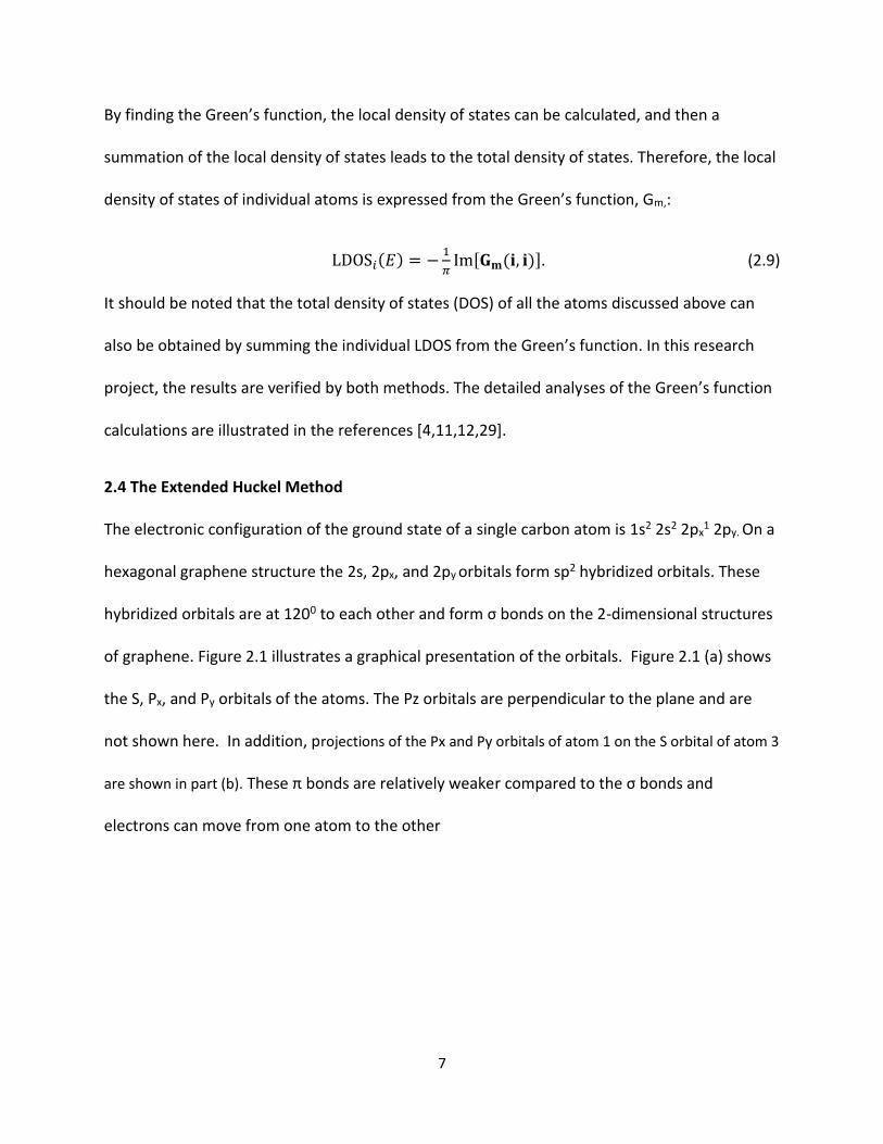
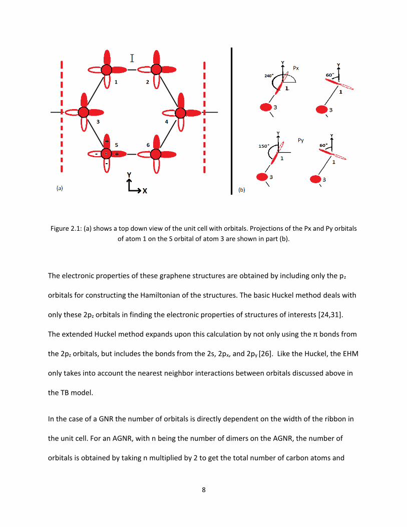
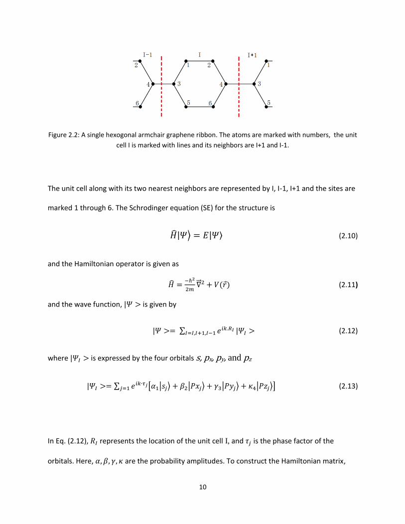
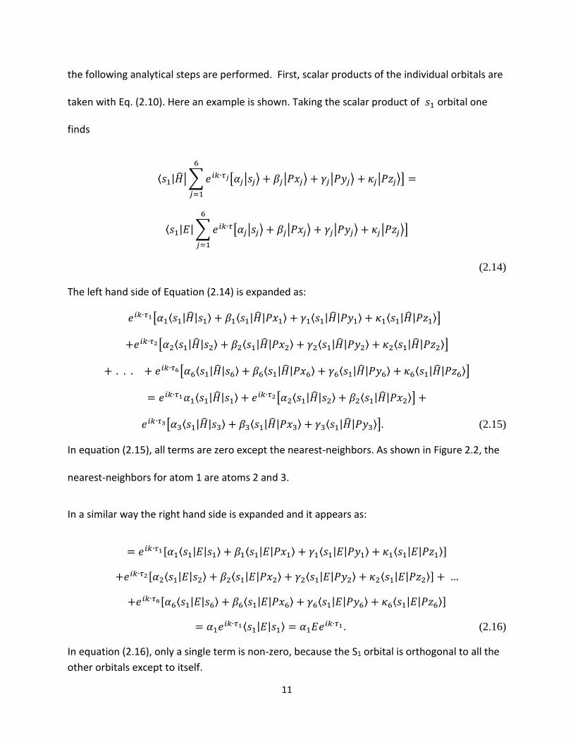
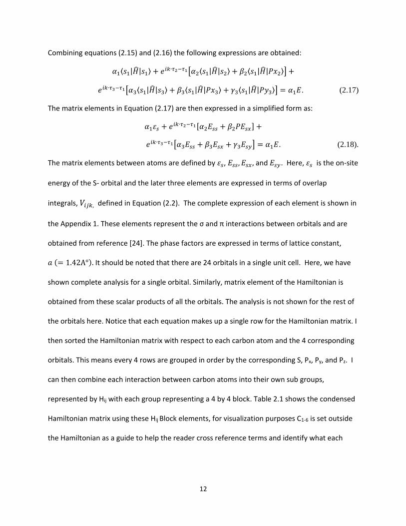
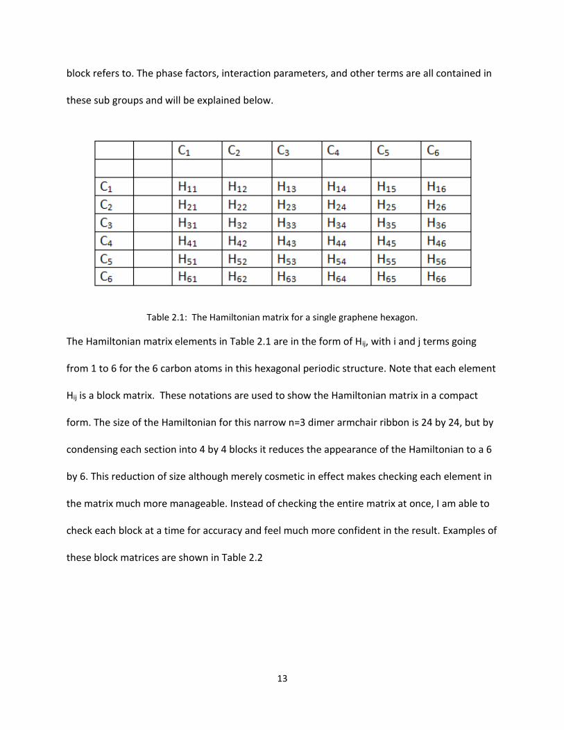
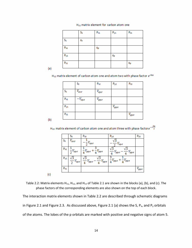
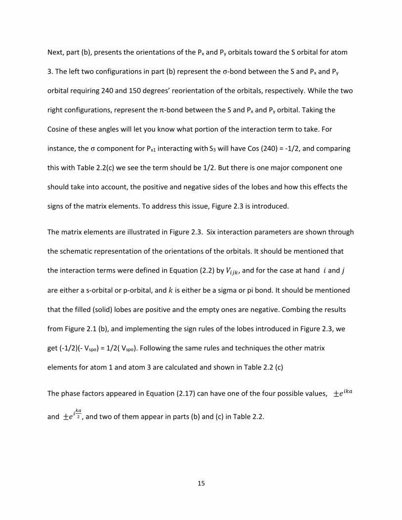
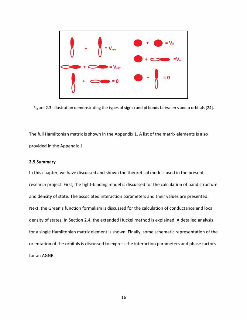
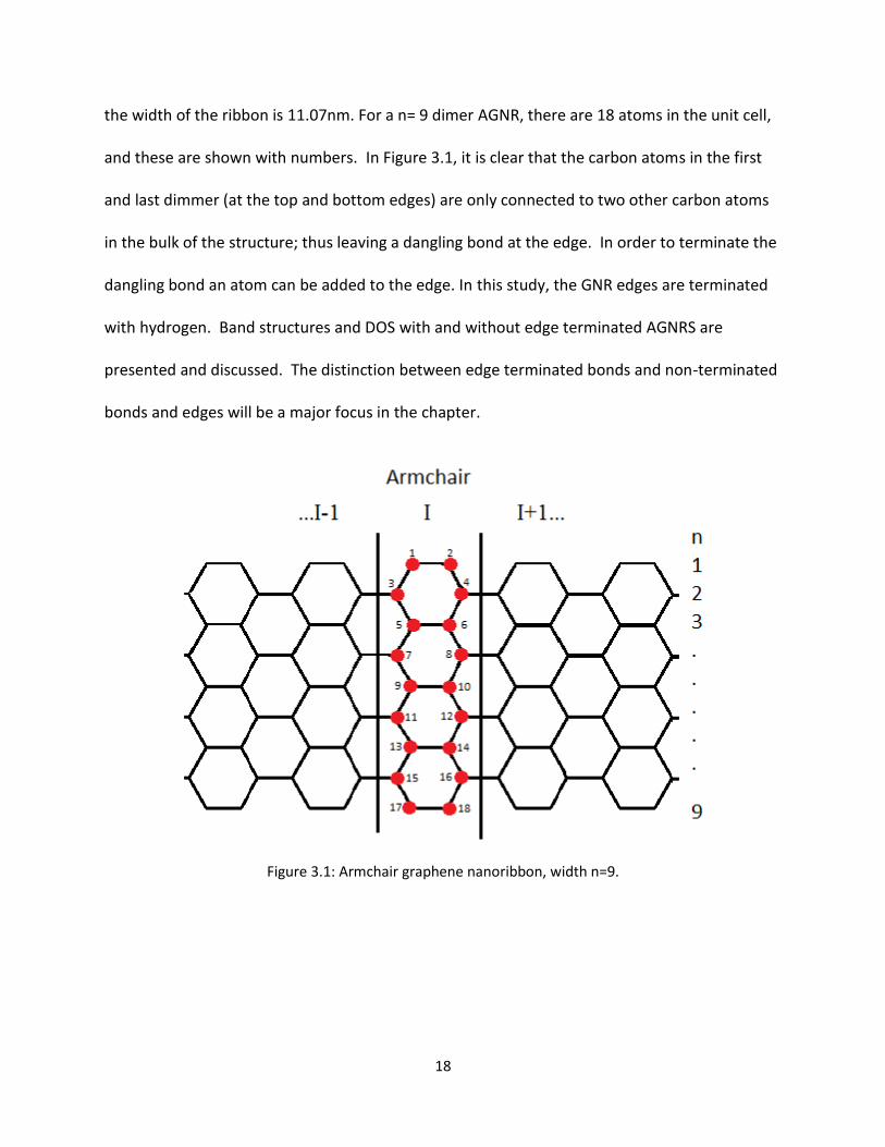
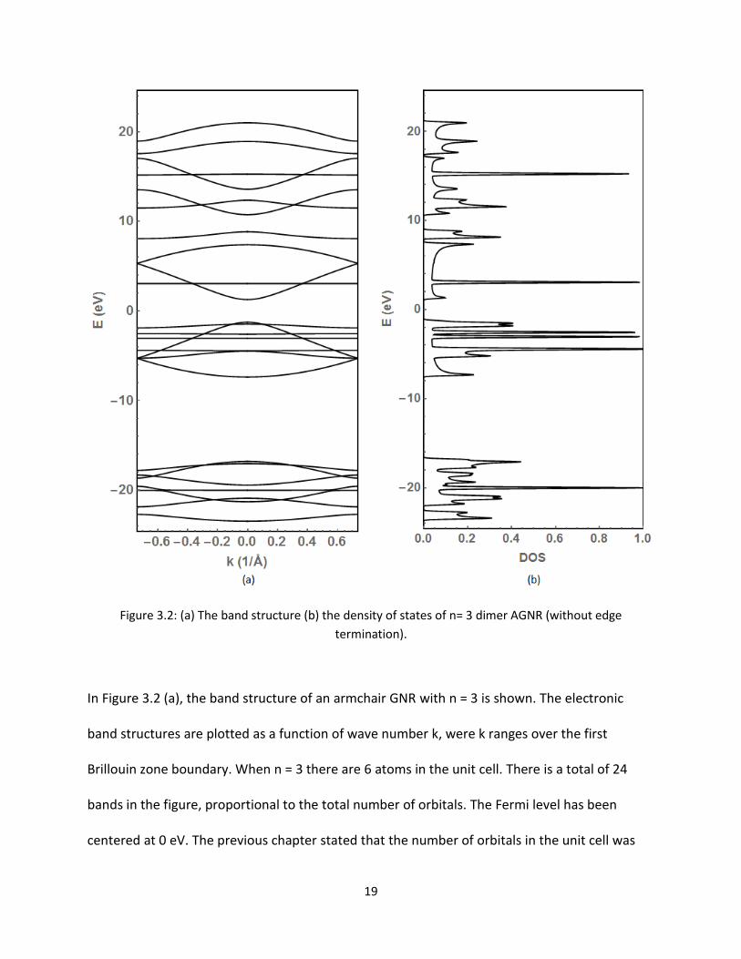
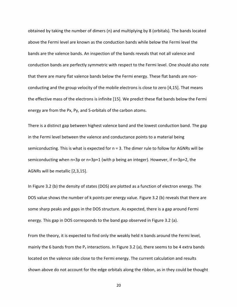
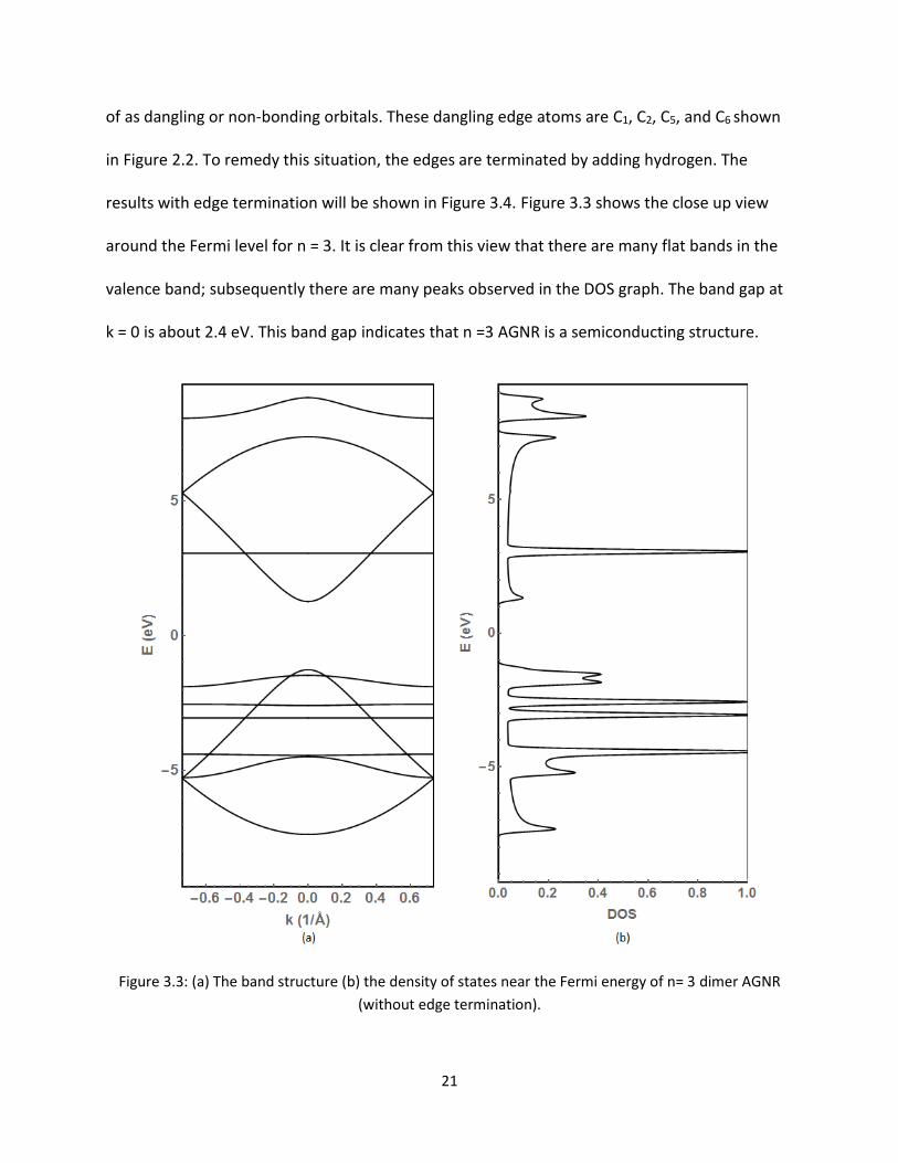
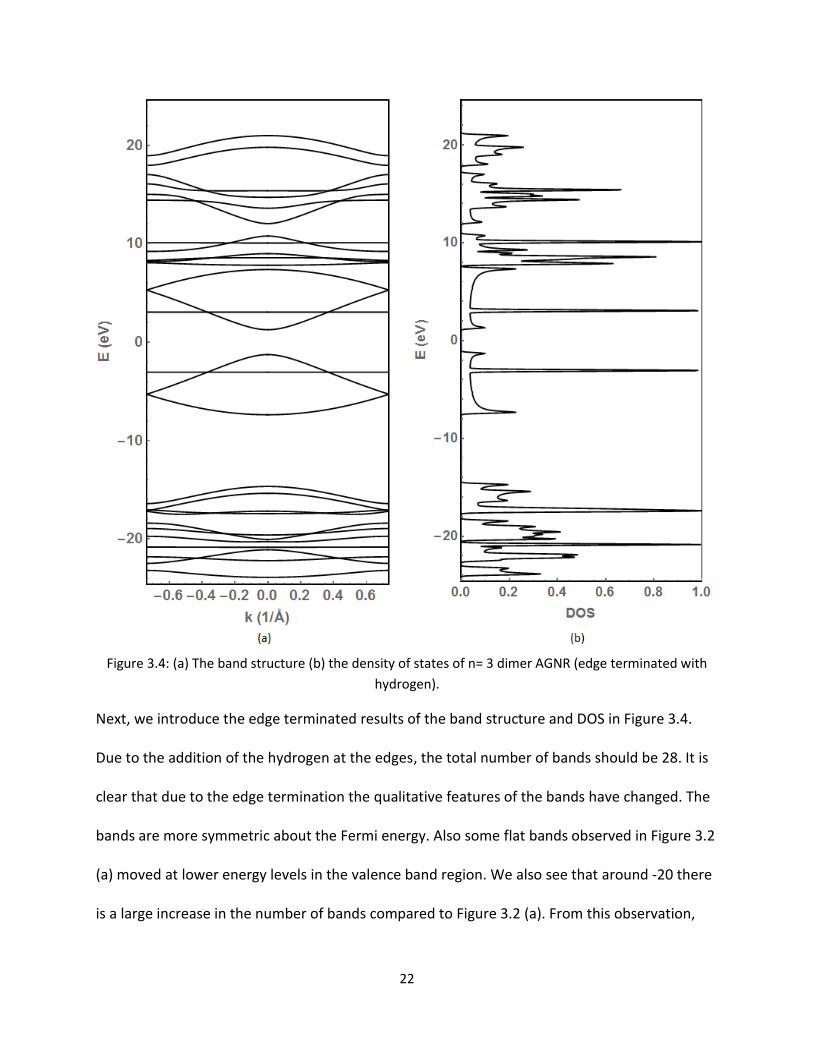
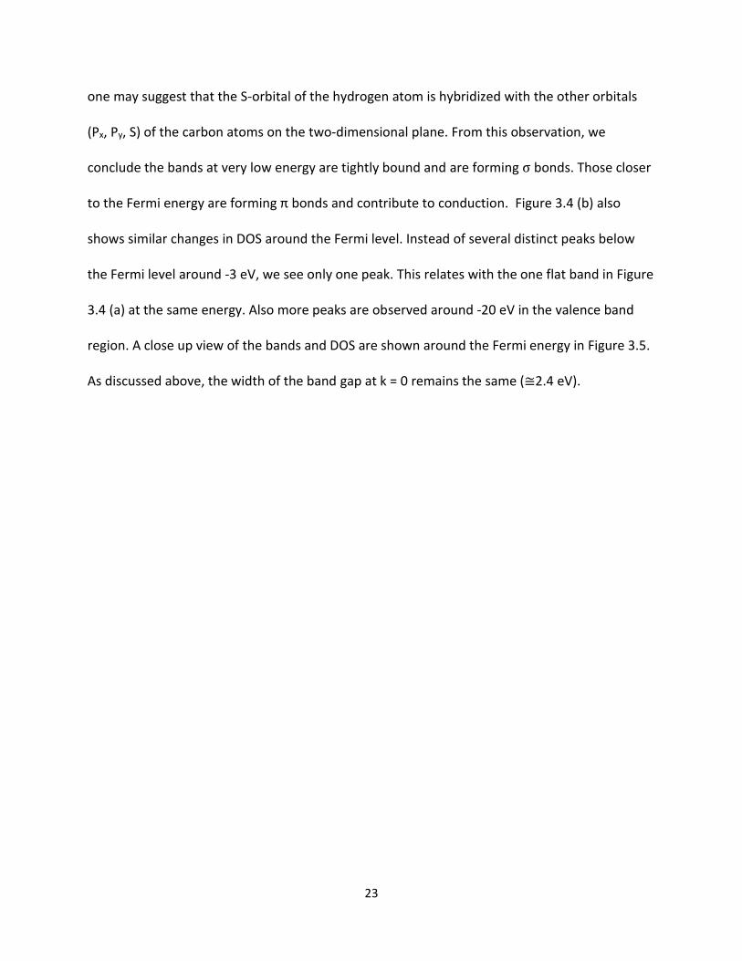
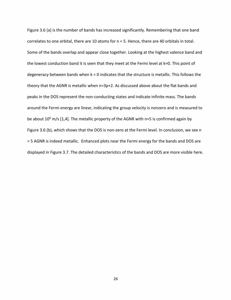
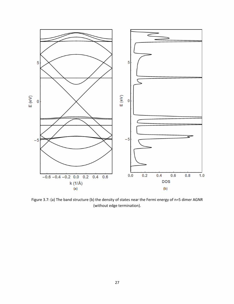
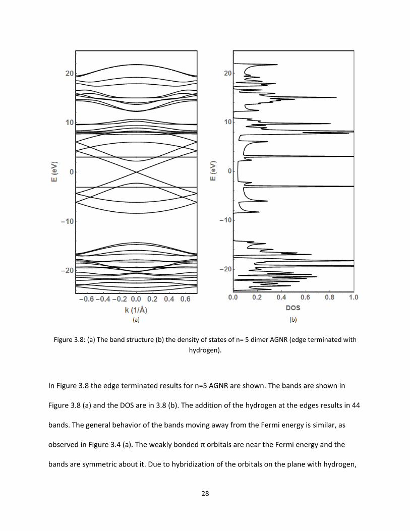
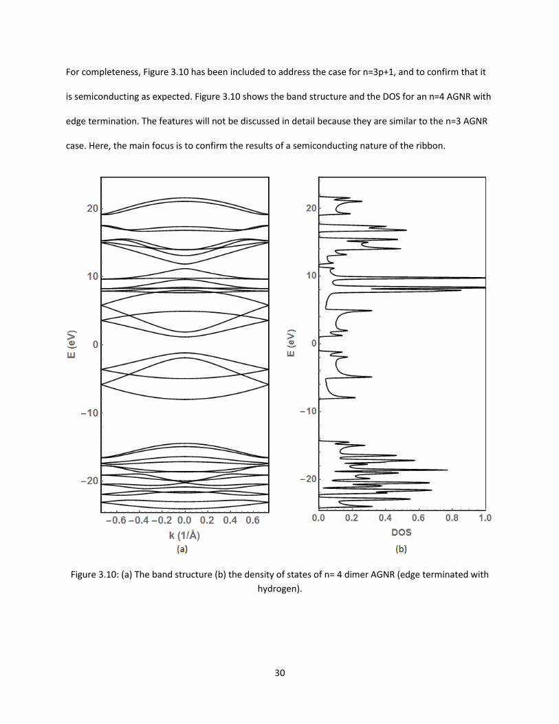
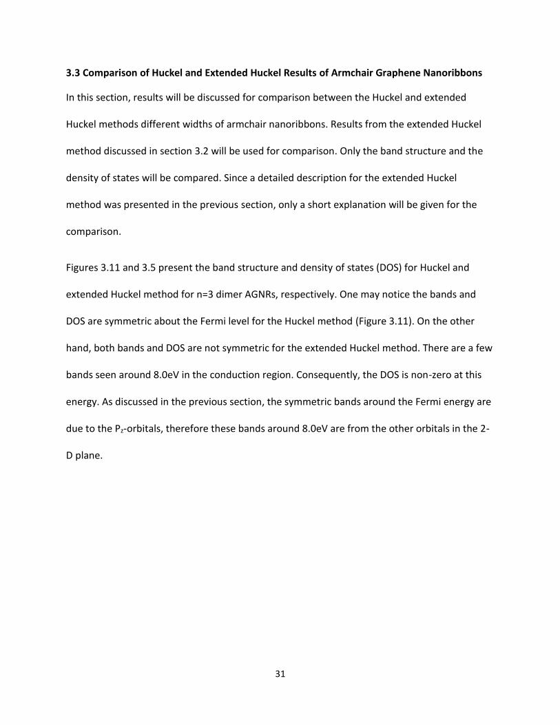
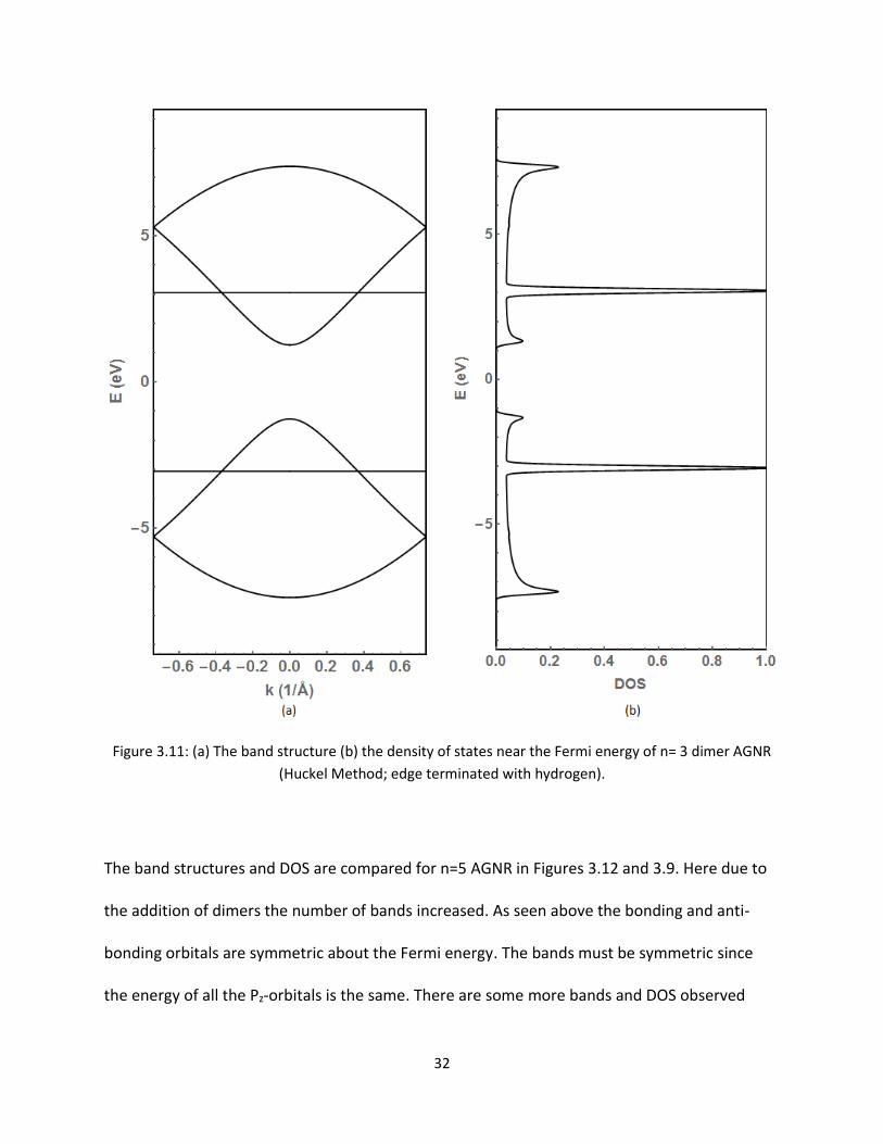
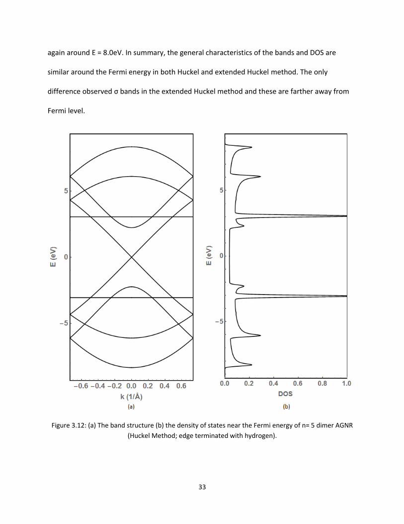
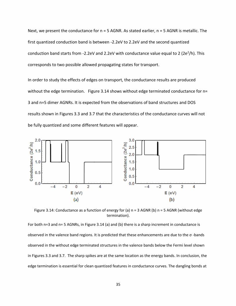
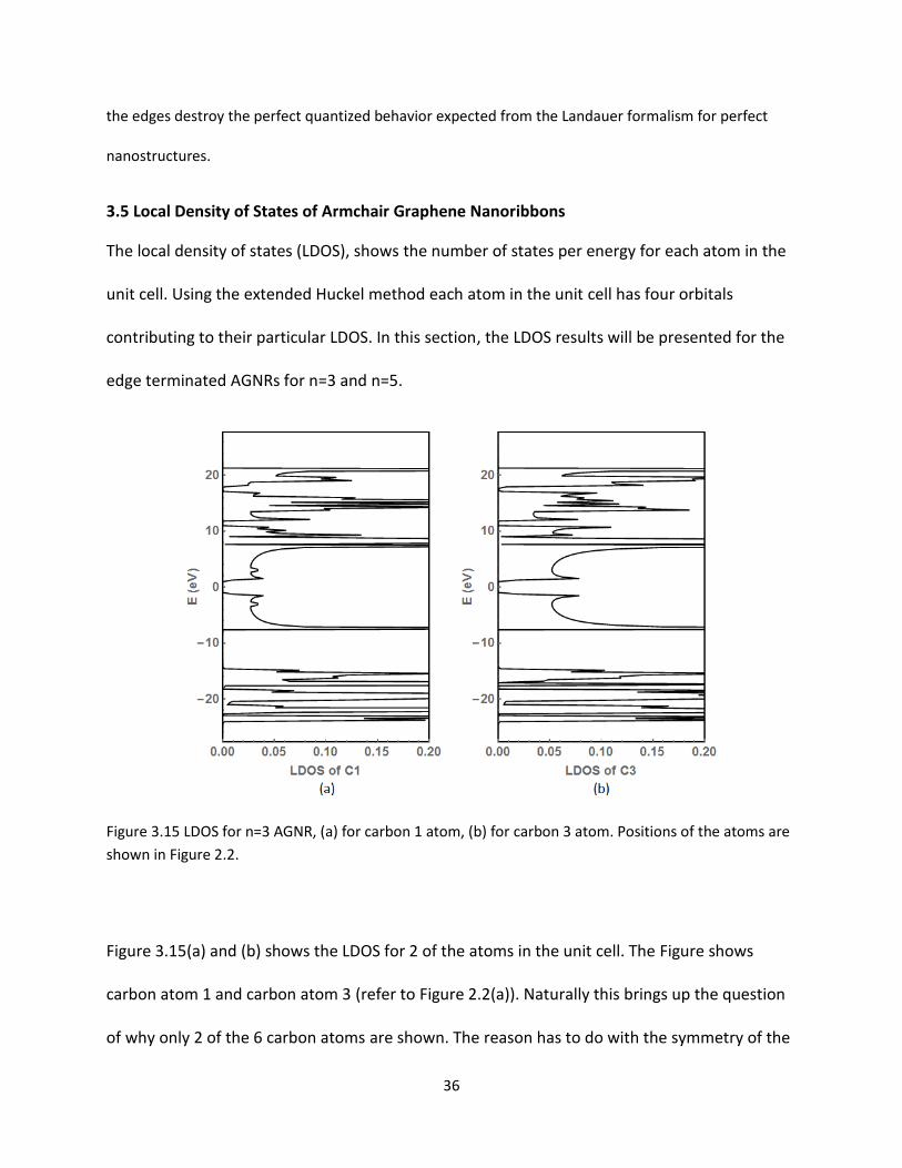
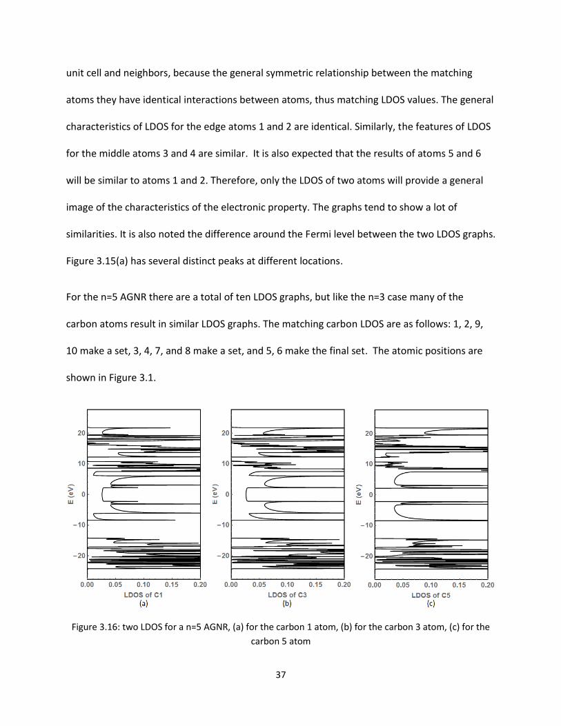
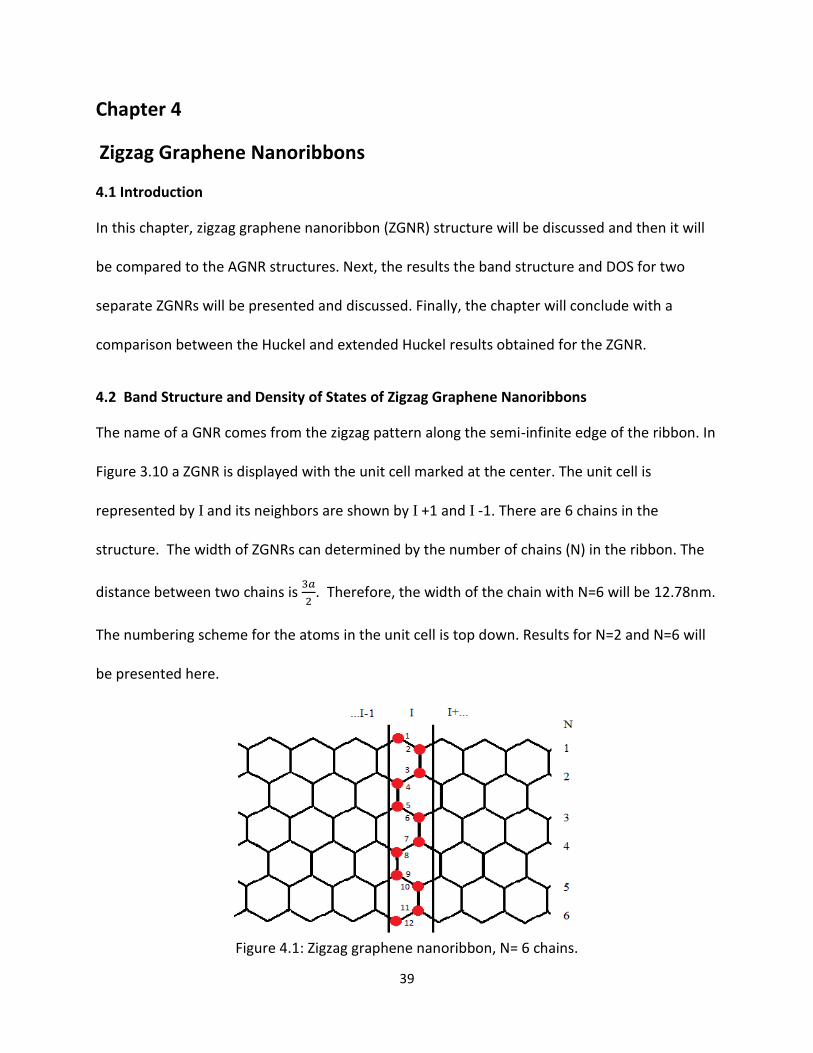
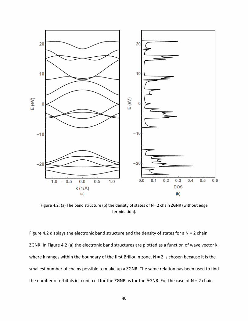
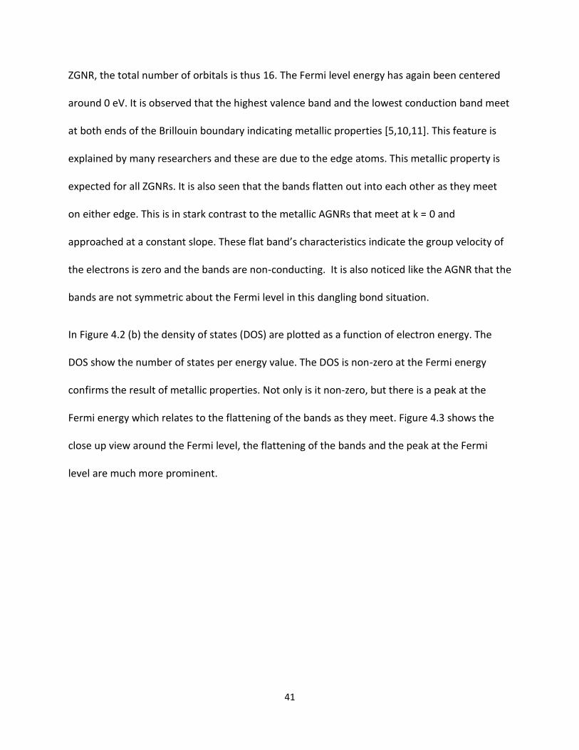
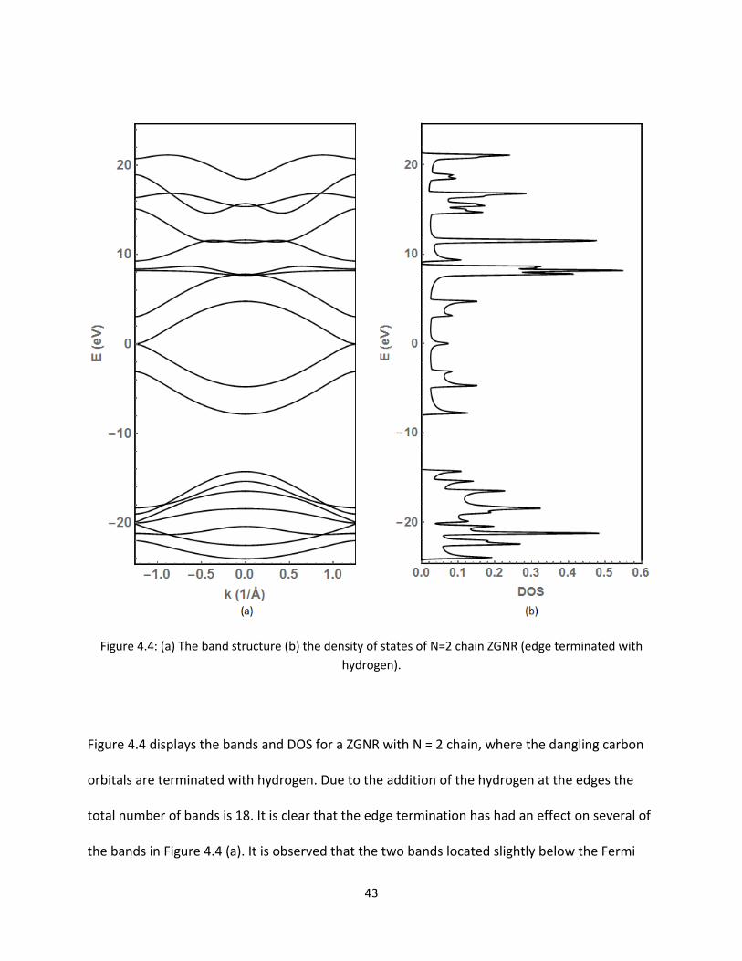
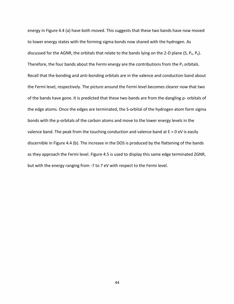
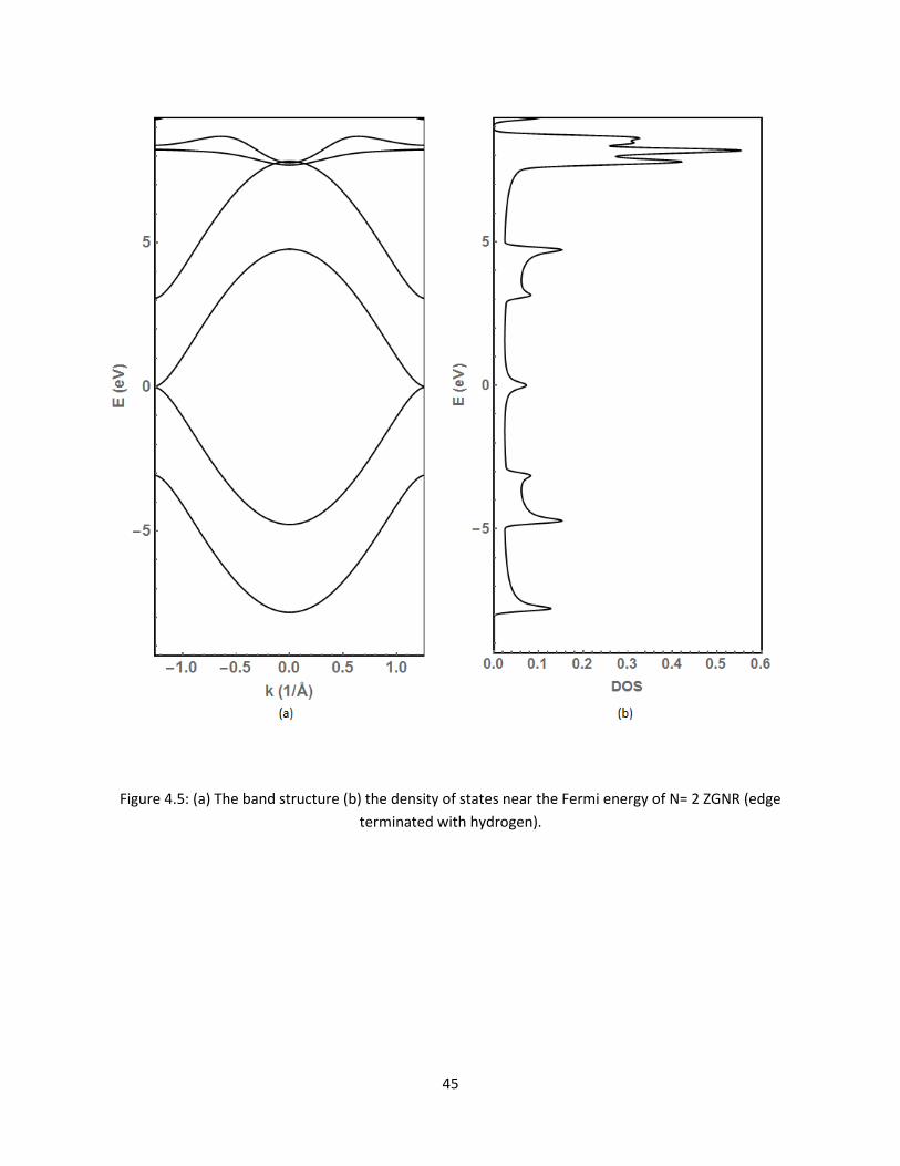
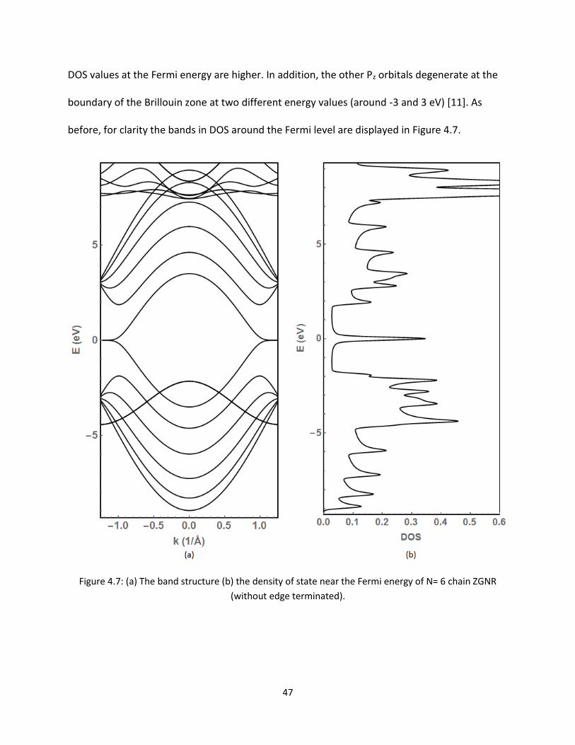
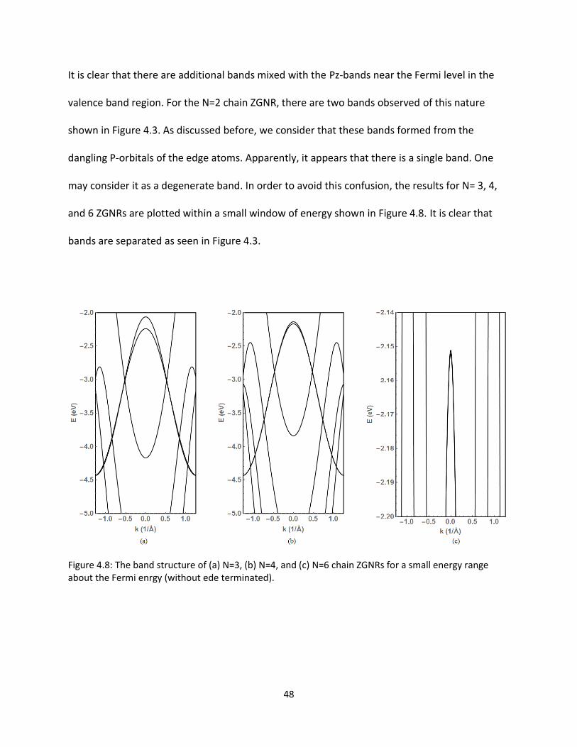
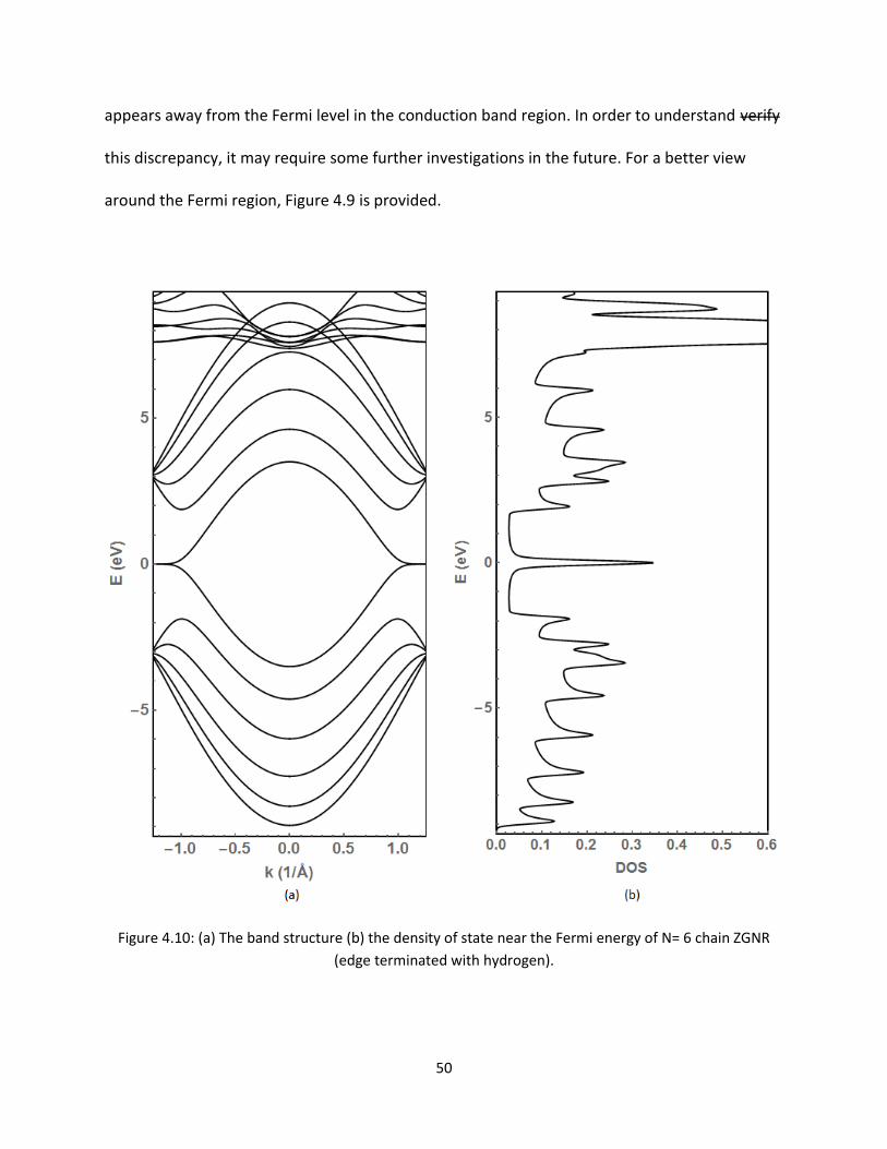
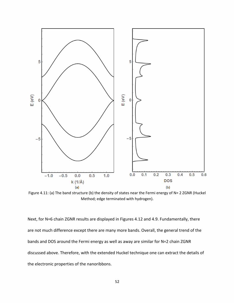
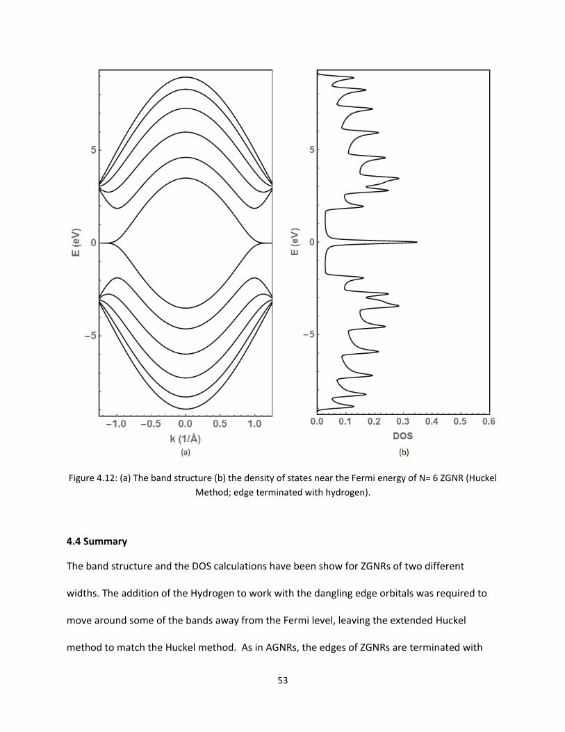
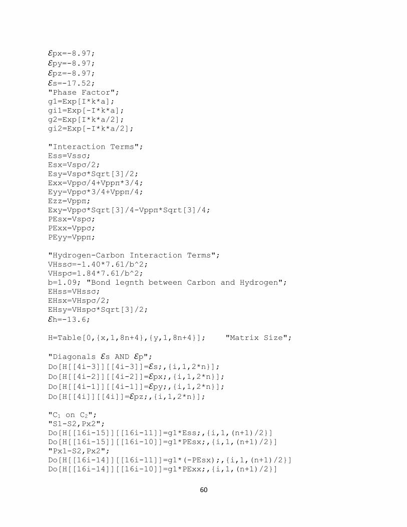
Copyright © 2022 FDOKUMEN