
Electromagnetic Model of a Power Transformer for Low ...
107
Dragan Maletic, BSc Electromagnetic Model of a Power Transformer for Low Frequencies MASTER’S THESIS to achieve the university degree of Diplom-Ingenieur Master’s degree programme: Electrical Engineering and Business submitted to Graz University of Technology Supervisors Ao.Univ.-Prof. Dipl.-Ing. Dr.techn. Herwig Renner Institute of Electrical Power Systems Dennis Albert, M.Sc Institute of Electrical Power Systems Graz, August 2021
-
Upload
khangminh22 -
Category
Documents
-
view
0 -
download
0
Transcript of Electromagnetic Model of a Power Transformer for Low ...
Dragan Maletic, BSc
Electromagnetic Model of a Power Transformer for LowFrequencies
MASTER’S THESIS
to achieve the university degree of
Diplom-Ingenieur
Master’s degree programme: Electrical Engineering and Business
submitted to
Graz University of Technology
Supervisors
Ao.Univ.-Prof. Dipl.-Ing. Dr.techn. Herwig RennerInstitute of Electrical Power Systems
Dennis Albert, M.ScInstitute of Electrical Power Systems
Graz, August 2021


AFFIDAVIT
I declare that I have authored this thesis independently, that I have not used other than
the declared sources/resources, and that I have explicitly indicated all material which
has been quoted either literally or by content from the sources used. The text document
uploaded to TUGRAZonline is identical to the present master’s thesis.
Date, Signature

Abstract
Transmission grid operators are always trying to improve their simulation models since simulations
help to predict the behavior of the electricity grid. Transformers are a particularly important
component of the grid. The usual modeling approach of transformers is the classic T-model. This
model, however, is not able to model unbalanced and transient occurrences accurately. In this thesis,
a topologically correct network model is derived, which is capable of reproducing the behavior
of an actual three-phase power transformer under the influence of low-frequency transients. The
non-linearity of the core material is reproduced with the Jiles-Atherton hysteresis model to represent
this behavior accurately. Another difficulty in transformer modeling is the lack of parameter data. It
is shown in this thesis that the parameters of the network model can be determined from standard
transformer acceptance tests and a simple single-phase hysteresis measurement. The execution of
the hysteresis measurement is possible outside of specialized laboratories. The model was compared
to multiple measurements, including no-load tests and back-to-back tests with superimposed direct
currents. The results show that an accurate transformer model can be derived with reasonable effort.
The simulation model provides transmission grid operators an important and accurate tool for the
simulation of low-frequency transients.
v

Kurzfassung
Netzbetreiber sind stetig daran interessiert ihre Simulationsmodelle zu verbessern, da diese dabei
helfen das Verhalten des Stromnetzes vorauszusagen. Eine besonders wichtige Komponente des
Stromnetzes sind Transformatoren. Die gängige Methode einen Transformator zu modellieren ist
das klassische T-modell. Allerdings ist dieses Modell nicht geeignet, um unsymmetrische und tran-
siente Ereignisse genau zu beschreiben. In dieser Arbeit wird am Beispiel eines realen dreiphasigen
Leistungstransformators ein topologisch-korrektes Netzwerkmodell entwickelt, welches in der Lage
ist das Verhalten des Transformators unter dem Einfluss niederfrequenter transienter Vorgänge
zu simulieren. Um dieses Verhalten genau darzustellen, wird die Nichtlinearität des Transfor-
matorkerns mithilfe des Jiles-Atherton Hysteresemodels modelliert. Eine weitere Schwierigkeit
bei der Modellierung ist das Fehlen von Parameterdaten. In dieser Arbeit wird gezeigt, dass die
Parameter des Netzwerkmodells mithilfe von Abnahmetestdaten und einer einfachen einphasi-
gen Hysteresemessung herleitbar sind. Die Hysteresemessung ist auch außerhalb von speziellen
Laboren durchführbar. Das Modell wurde mit mehreren Messungen verglichen, darunter Messun-
gen in Leerlauf und Back-to-back mit überlagertem Gleichstrom. Die Ergebnisse zeigen, dass mit
überschaubarem Aufwand ein genaues Simulationsmodell erstellt werden kann. Dieses liefert Netz-
betreibern ein wichtiges und genaues Werkzeug in der Simulation von niederfrequenten transienten
Vorgängen.
vii


List of Symbols
α Jiles-Atherton parameter representing interdomain coupling
δ Jiles-Atherton sign function
δm Sign function to prevent non-physical behavior of the Jiles-Atherton model
Θ1, Θ2 Primary and secondary magnetomotive force
µ0 Vacuum permeability
µr Relative permeability
Φm Mutual magnetic flux
Φpeak Peak value of the magnetic flux
ΦU, ΦV, ΦW Magnetic fluxes of phases U, V, and W
ϕU Phase shift between the voltage and current of phase U
ϕV Phase shift between the voltage and current of phase V
ϕW Phase shift between the voltage and current of phase W
Ψm Mutual magnetic flux-linkage
a Jiles-Atherton parameter representing the shape of the anhysteresis
Acore Transformer core area
B Magnetic flux density
Be Effective magnetic flux density
c Jiles-Atherton parameter representing the reversibility
E Energy
E1, E2 Root mean square values electromotive force of the primary and secondary
winding
e1, e2 Instantaneous values electromotive force of the primary and secondary wind-
ing
f , fn Frequency, nominal frequency
ix

i0 Instantaneous magnetizing current
i10 Instantaneous zero-sequence current resulting from magnetic asymmetry
iLV, iHV Instantaneous currents of the low- and high-voltage windings
ILV, IHV Rated root mean square currents of the low- and high-voltage windigs
ISC,U, ISC,V, ISC,W Root mean square values of the short-circuit currents of phases U, V, and W
Izero Root mean square value of the zero-sequence current
J Magnetic polarization
k Jiles-Atherton parameter representing hysteresis loss
keddy Eddy loss parameter
kexc Excess loss parameter
L0 Zero-sequence inductance
L1, L2, L3 Inductances of primary, secondary, and tertiary winding
L12 Short-circuit inductance
LC1 Inductance between core and and first winding
Llimb, Lyoke Limb and yoke inductances
Lm Mutual inductance of the magnetizing branch
llimb, lyoke Lengths of limb and yoke
m Magnetic moment
M Magnetization
Man Anhysteretic magnetization
Mirr, Mrev Irreversible and reversible component of the magnetization
Ms Saturation magnetization
N Number of winding turns
N1, N2 Number of primary and secondary winding turns
NLV, NHV Number of low- and high-voltage winding turns
Pzero Zero-sequence active power
Qzero Zero-sequence reactive power
R1, R2, R3 Primary, secondary, and tertiary winding resistances
RLV, RHV Low- and high-voltage winding resistances
Rm Resistance of the magnetizing branch
Rm12 Reluctance between the two windings
RmC1 Reluctance between the core and first winding
x

Rmlimb, Rmyoke Reluctances of yoke and limb elements
Rm0 Zero-sequence reluctance
R0 Zero-sequence resistance
Szero Zero-sequence complex power
t Time
U Root mean square value of the voltage
U, V, W Phase identifier
U1, U2 Root mean square values of the primary and secondary voltages
u1, u2 Instantaneous values of the primary and secondary voltages
ULV, UHV Rated root mean square voltages of the low- and high-voltage winding
Upeak Peak value of the voltage
USC,U Root mean square value of the short-circuit voltage of phases U
USC,V Root mean square value of the short-circuit voltage of phases V
USC,W Root mean square value of the short-circuit voltage of phases W
Uzero Root mean square value of the zero-sequence voltage
Weddy Eddy component of the energy loss
Wexc Excess component of the energy loss
Whys Hysteresis component of the energy loss
Wtot Total energy loss
X0 Zero-sequence reactance
X12 Short-circuit reactance
Y Admittance
Z0 Zero-sequence impedance
xi


List of Abbreviations
AC alternating current
B2B Back-to-back
DC direct current
GIC Geomagnetically induced current
JA Jiles-Atherton
mmf magnetomotive force
rms root mean square
STC Saturable transformer component
T74 Main transformer under test
T90 Second transformer used for back-to-back
xiii

Contents
Abstract v
1 Introduction 1
1.1 Motivation . . . . . . . . . . . . . . . . . . . . . . . . . . . . . . . . . . . . . . . . . . . . 1
1.2 Objective of the Thesis . . . . . . . . . . . . . . . . . . . . . . . . . . . . . . . . . . . . . 2
1.3 Outline of the Thesis . . . . . . . . . . . . . . . . . . . . . . . . . . . . . . . . . . . . . . 2
2 Essential Transformer Basics 5
2.1 Transformer Theory . . . . . . . . . . . . . . . . . . . . . . . . . . . . . . . . . . . . . . . 5
2.2 Magnetic Fields of the Core Material . . . . . . . . . . . . . . . . . . . . . . . . . . . . . 7
2.3 Magnetic Asymmetry of Three-Phase Transformers . . . . . . . . . . . . . . . . . . . . 10
3 Theory and Methods 15
3.1 Transformer Modeling for Low Frequencies . . . . . . . . . . . . . . . . . . . . . . . . 15
3.1.1 Topology-Based Models . . . . . . . . . . . . . . . . . . . . . . . . . . . . . . . . 16
3.2 Duality-Based Three-Limb Transformer Model . . . . . . . . . . . . . . . . . . . . . . . 17
3.3 Iron Core Modeling . . . . . . . . . . . . . . . . . . . . . . . . . . . . . . . . . . . . . . . 19
3.3.1 Static Hysteresis Modeling – Jiles-Atherton Model . . . . . . . . . . . . . . . . 21
3.3.2 Dynamic Hysteresis Losses . . . . . . . . . . . . . . . . . . . . . . . . . . . . . . 28
3.4 Parameter Derivation . . . . . . . . . . . . . . . . . . . . . . . . . . . . . . . . . . . . . . 29
3.4.1 Linear Parameters . . . . . . . . . . . . . . . . . . . . . . . . . . . . . . . . . . . 30
3.4.2 Non-Linear Core Parameters . . . . . . . . . . . . . . . . . . . . . . . . . . . . . 31
4 Measurements and Fitting 35
4.1 Transformer Under Test (T74) – General Data . . . . . . . . . . . . . . . . . . . . . . . . 35
4.2 T74 - Linear Parameters . . . . . . . . . . . . . . . . . . . . . . . . . . . . . . . . . . . . 36
xv
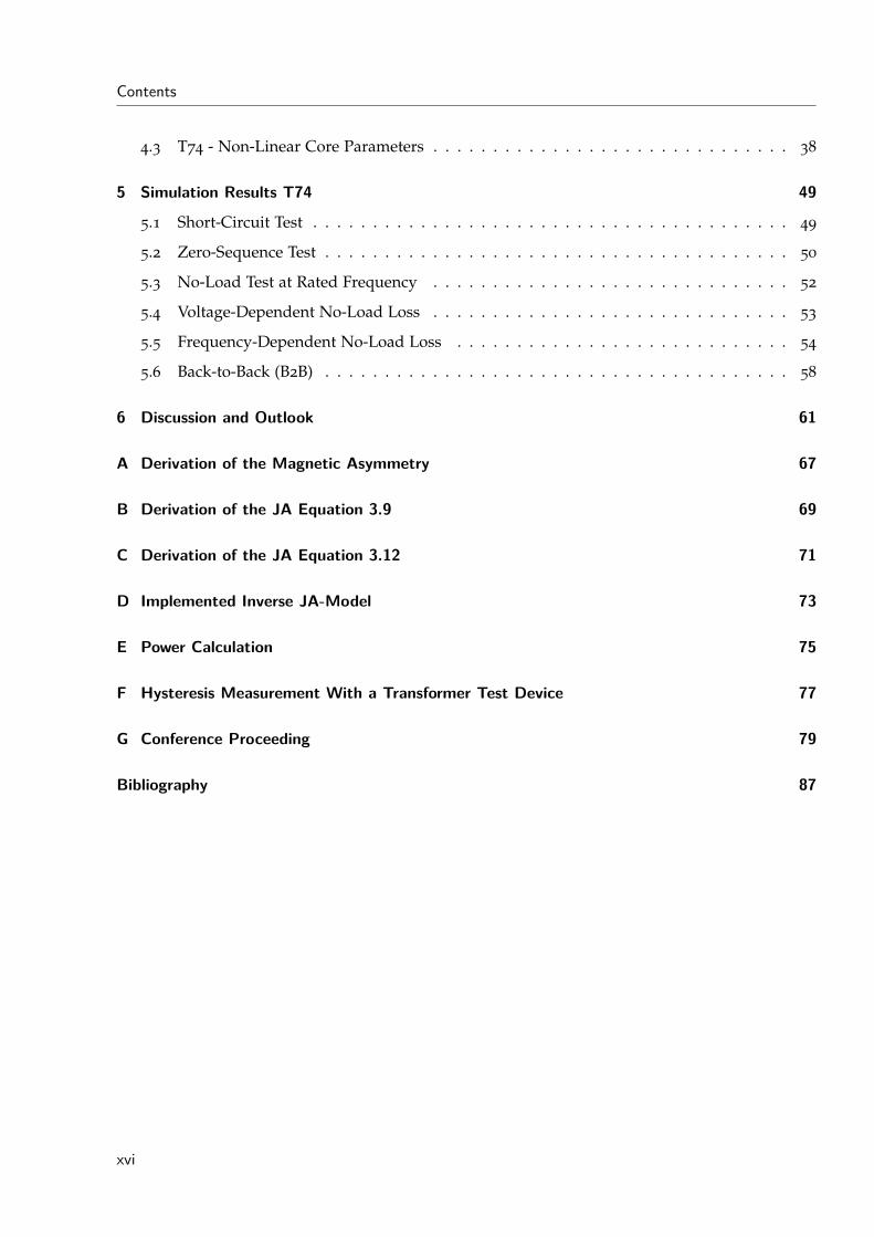
Contents
4.3 T74 - Non-Linear Core Parameters . . . . . . . . . . . . . . . . . . . . . . . . . . . . . . 38
5 Simulation Results T74 49
5.1 Short-Circuit Test . . . . . . . . . . . . . . . . . . . . . . . . . . . . . . . . . . . . . . . . 49
5.2 Zero-Sequence Test . . . . . . . . . . . . . . . . . . . . . . . . . . . . . . . . . . . . . . . 50
5.3 No-Load Test at Rated Frequency . . . . . . . . . . . . . . . . . . . . . . . . . . . . . . 52
5.4 Voltage-Dependent No-Load Loss . . . . . . . . . . . . . . . . . . . . . . . . . . . . . . 53
5.5 Frequency-Dependent No-Load Loss . . . . . . . . . . . . . . . . . . . . . . . . . . . . 54
5.6 Back-to-Back (B2B) . . . . . . . . . . . . . . . . . . . . . . . . . . . . . . . . . . . . . . . 58
6 Discussion and Outlook 61
A Derivation of the Magnetic Asymmetry 67
B Derivation of the JA Equation 3.9 69
C Derivation of the JA Equation 3.12 71
D Implemented Inverse JA-Model 73
E Power Calculation 75
F Hysteresis Measurement With a Transformer Test Device 77
G Conference Proceeding 79
Bibliography 87
xvi
1 Introduction
1.1 Motivation
Transformers, even though they are often taken for granted, are incredibly complicated electromag-
netic devices containing various materials that act differently [1]. This complexity leads to different
behaviors depending on the excitation [2]. Transmission grid operators express a rising demand for
transformer simulation models capable of reproducing various transient behaviors. Such models
can help to increase the understanding of transients in the electricity grid.
The classic T-model can not be used for this scenario because it is only valid for steady-state
studies. The Pi-model is superior to the T-model and should be considered instead [3]. The use of
a Pi-model, however, leads to another problem. The representation of a three-phase transformer
using an equivalent single-phase model disregards the magnetic coupling between the phases.
This limits the single-phase equivalent models to balanced and steady-state studies [4]. While it is
possible to implement extensive models of transformers, a limiting factor is the available data since
manufacturers rarely share their design information [2].
Depending on the study, the use of a hysteresis model can be of considerable importance [5]. The
implementation of such models can be rather simple in theory, however, the parameter identification
of the hysteresis model can be challenging, especially if no data sheet of the core material is
available. Even in the unlikely case that such information is available, it is still necessary to adapt it
to measurements since the losses of an entire transformer are usually higher than the losses of the
pure core material [6].
1
1 Introduction
1.2 Objective of the Thesis
The main objective of this thesis is to develop, implement, and verify a simulation model of a
50 kVA, three-phase, three-limb power transformer. The modeling approach should be applicable
to different transformer core topologies and winding configurations. Only information that can
either be found in the data sheet or can be measured in the field without great effort should be
used. No detailed design data should be used since this information is often not available. Another
objective of the thesis is to measure the hysteresis of the core material and to implement a hysteresis
model. The finalized model has to be verified with multiple measurements to ensure the accurate
representation of various applications. The tests include short-circuit, no-load, and zero-sequence
tests. The behavior under geomagnetically induced currents has to be validated using back-to-back
tests with superimposed direct currents.
1.3 Outline of the Thesis
Chapter 2 introduces basic concepts necessary to understand not just the modeling approach but the
simulation results as well. The chapter consists of explanations of the basic transformer operating
principle, the nonlinear behavior of the ferromagnetic core, and the magnetic asymmetry resulting
from the core design.
Chapter 3 presents a short overview of possible modeling approaches before the simulation model
is developed. The chapter is completed by a description of the parameter identification process of
the developed model.
Chapter 4 presents the parameter identification process of the 50 kVA power transformer used for
this thesis. The single-phase hysteresis measurement which determines the non-linear core behavior
is explained in particular detail.
Chapter 5 compares measurements of various test scenarios to simulations of the developed model.
The conducted experiments are short-circuit tests, zero-sequence tests, no-load tests at various
voltages and frequencies, and back-to-back tests with superimposed direct currents.
2

1.3 Outline of the Thesis
Chapter 6 concludes the most important findings and gives an outlook on possible further research
topics.
A conference proceeding on the topic of this thesis was published in cooperation with Dennis Albert
and Herwig Renner. This publication can be found in the Appendix
3

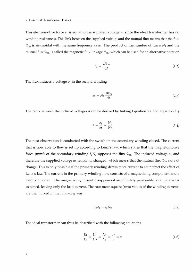
2 Essential Transformer Basics
2.1 Transformer Theory
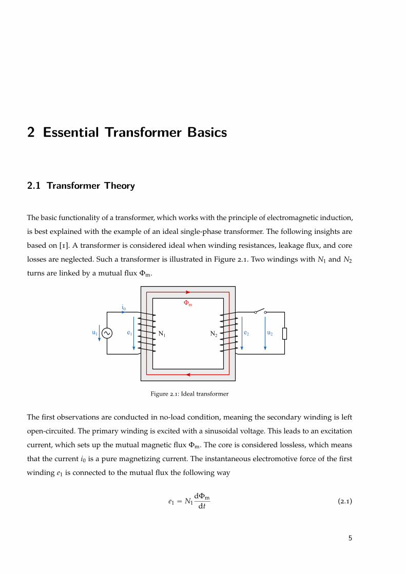
The basic functionality of a transformer, which works with the principle of electromagnetic induction,
is best explained with the example of an ideal single-phase transformer. The following insights are
based on [1]. A transformer is considered ideal when winding resistances, leakage flux, and core
losses are neglected. Such a transformer is illustrated in Figure 2.1. Two windings with N1 and N2
turns are linked by a mutual flux Φm.
Φm
u1 e1 e2 u2
i0
N1 N2
Figure 2.1: Ideal transformer
The first observations are conducted in no-load condition, meaning the secondary winding is left
open-circuited. The primary winding is excited with a sinusoidal voltage. This leads to an excitation
current, which sets up the mutual magnetic flux Φm. The core is considered lossless, which means
that the current i0 is a pure magnetizing current. The instantaneous electromotive force of the first
winding e1 is connected to the mutual flux the following way
e1 “ N1dΦm
dt(2.1)
5
2 Essential Transformer Basics
This electromotive force e1 is equal to the supplied voltage u1 since the ideal transformer has no
winding resistances. This link between the supplied voltage and the mutual flux means that the flux
Φm is sinusoidal with the same frequency as u1. The product of the number of turns N1 and the
mutual flux Φm is called the magnetic flux-linkage Ψm, which can be used for an alternative notation
e1 “dΨm
dt(2.2)
The flux induces a voltage e2 in the second winding
e2 “ N2dΦm
dt(2.3)
The ratio between the induced voltages a can be derived by linking Equation 2.1 and Equation 2.3
a “e1
e2“
N1
N2(2.4)
The next observation is conducted with the switch on the secondary winding closed. The current
that is now able to flow is set up according to Lenz’s law, which states that the magnetomotive
force (mmf) of the secondary winding i2N2 opposes the flux Φm. The induced voltage e1 and
therefore the supplied voltage u1 remain unchanged, which means that the mutual flux Φm can not
change. This is only possible if the primary winding draws more current to counteract the effect of
Lenz’s law. The current in the primary winding now consists of a magnetizing component and a
load component. The magnetizing current disappears if an infinitely permeable core material is
assumed, leaving only the load current. The root mean square (rms) values of the winding currents
are then linked in the following way
I1N1 “ I2N2 (2.5)
The ideal transformer can thus be described with the following equations
E1
E2“
U1
U2“
N1
N2“
I2
I1“ a (2.6)
6

2.2 Magnetic Fields of the Core Material
2.2 Magnetic Fields of the Core Material
The explanations and figures of this section are based on [7]. The phenomenon of magnetic fields
can be described with two field quantities: the magnetic field intensity H in A/m and the magnetic
flux density B in T. The field intensity is associated with the movement of charge carriers, while
the flux density is associated with the force on moving charge carriers. In vacuum the two field
quantities are linked as follows
B “ µ0 ¨ H (2.7)
with µ0 “ 4π ¨ 10´7 being the vacuum permeability. This formulation has to be adapted in the
following way if a material is present
B “ µr ¨ µ0 ¨ H (2.8)
with µr being the relative permeability of the material. This formulation with a constant µr is not
usable for non-linear ferromagnets. In this case a more general formulation can be used which
utilizes the so-called magnetic polarization J
B “ µ0 ¨ H ` J (2.9)
with J having the same unit as B, T. An alternative formulation utilizes the so-called magnetization
M
B “ µ0 ¨ pH `Mq (2.10)
with M having the same unit as H, A/m. As stated previously, the ferromagnetic core material
shows a non-linear relationship between B and H. This behavior can be explained with the structure
of the ferromagnetic material that consists of multiple magnetic domains. A single domain contains
magnetic moments that are aligned in the same direction. The entirety of the domains is formed
in a way that the energy configuration is at its minimum. The magnetization process is shown in
Figure 2.2 in a simplified way. Part a) shows a ferromagnetic material that consists of four magnetic
domains. The domains are aligned in a way which leads the magnetizing moments of the domains
7
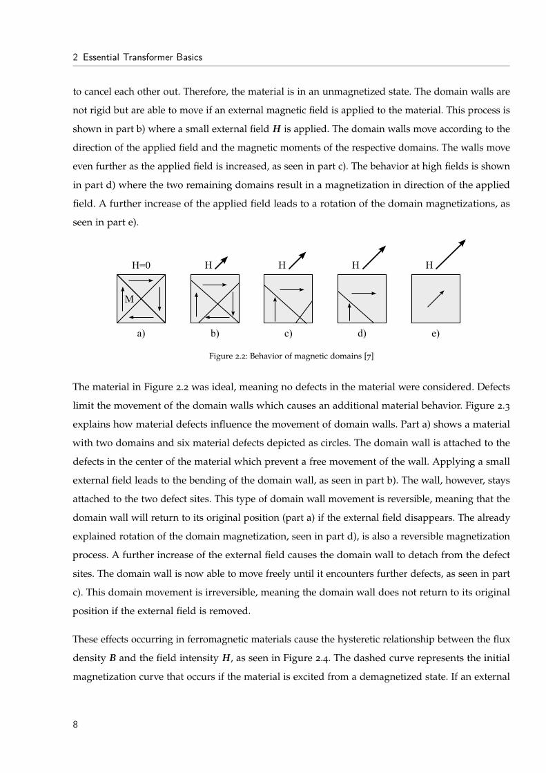
2 Essential Transformer Basics
to cancel each other out. Therefore, the material is in an unmagnetized state. The domain walls are
not rigid but are able to move if an external magnetic field is applied to the material. This process is
shown in part b) where a small external field H is applied. The domain walls move according to the
direction of the applied field and the magnetic moments of the respective domains. The walls move
even further as the applied field is increased, as seen in part c). The behavior at high fields is shown
in part d) where the two remaining domains result in a magnetization in direction of the applied
field. A further increase of the applied field leads to a rotation of the domain magnetizations, as
seen in part e).
M
H=0
a) b) c) d) e)
H H HH
Figure 2.2: Behavior of magnetic domains [7]
The material in Figure 2.2 was ideal, meaning no defects in the material were considered. Defects
limit the movement of the domain walls which causes an additional material behavior. Figure 2.3
explains how material defects influence the movement of domain walls. Part a) shows a material
with two domains and six material defects depicted as circles. The domain wall is attached to the
defects in the center of the material which prevent a free movement of the wall. Applying a small
external field leads to the bending of the domain wall, as seen in part b). The wall, however, stays
attached to the two defect sites. This type of domain wall movement is reversible, meaning that the
domain wall will return to its original position (part a) if the external field disappears. The already
explained rotation of the domain magnetization, seen in part d), is also a reversible magnetization
process. A further increase of the external field causes the domain wall to detach from the defect
sites. The domain wall is now able to move freely until it encounters further defects, as seen in part
c). This domain movement is irreversible, meaning the domain wall does not return to its original
position if the external field is removed.
These effects occurring in ferromagnetic materials cause the hysteretic relationship between the flux
density B and the field intensity H, as seen in Figure 2.4. The dashed curve represents the initial
magnetization curve that occurs if the material is excited from a demagnetized state. If an external
8
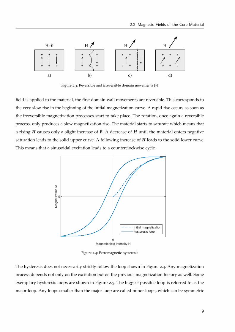
2.2 Magnetic Fields of the Core Material
a) b) c) d)
H=0 H H H
Figure 2.3: Reversible and irreversible domain movements [7]
field is applied to the material, the first domain wall movements are reversible. This corresponds to
the very slow rise in the beginning of the initial magnetization curve. A rapid rise occurs as soon as
the irreversible magnetization processes start to take place. The rotation, once again a reversible
process, only produces a slow magnetization rise. The material starts to saturate which means that
a rising H causes only a slight increase of B. A decrease of H until the material enters negative
saturation leads to the solid upper curve. A following increase of H leads to the solid lower curve.
This means that a sinusoidal excitation leads to a counterclockwise cycle.
0
Magnetic field intensity H
0
Ma
gn
etiza
tio
n M
initial magnetization
hysteresis loop
Figure 2.4: Ferromagnetic hysteresis
The hysteresis does not necessarily strictly follow the loop shown in Figure 2.4. Any magnetization
process depends not only on the excitation but on the previous magnetization history as well. Some
exemplary hysteresis loops are shown in Figure 2.5. The biggest possible loop is referred to as the
major loop. Any loops smaller than the major loop are called minor loops, which can be symmetric
9
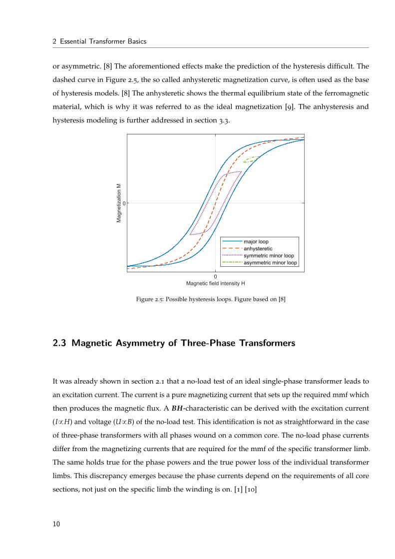
2 Essential Transformer Basics
or asymmetric. [8] The aforementioned effects make the prediction of the hysteresis difficult. The
dashed curve in Figure 2.5, the so called anhysteretic magnetization curve, is often used as the base
of hysteresis models. [8] The anhysteretic shows the thermal equilibrium state of the ferromagnetic
material, which is why it was referred to as the ideal magnetization [9]. The anhysteresis and
hysteresis modeling is further addressed in section 3.3.
0
Magnetic field intensity H
0
Magnetization M
major loop
anhysteretic
symmetric minor loop
asymmetric minor loop
Figure 2.5: Possible hysteresis loops. Figure based on [8]
2.3 Magnetic Asymmetry of Three-Phase Transformers
It was already shown in section 2.1 that a no-load test of an ideal single-phase transformer leads to
an excitation current. The current is a pure magnetizing current that sets up the required mmf which
then produces the magnetic flux. A BH-characteristic can be derived with the excitation current
(I9H) and voltage (U9B) of the no-load test. This identification is not as straightforward in the case
of three-phase transformers with all phases wound on a common core. The no-load phase currents
differ from the magnetizing currents that are required for the mmf of the specific transformer limb.
The same holds true for the phase powers and the true power loss of the individual transformer
limbs. This discrepancy emerges because the phase currents depend on the requirements of all core
sections, not just on the specific limb the winding is on. [1] [10]
10
2.3 Magnetic Asymmetry of Three-Phase Transformers
A
ivv
NN uv
iww
N
u
uu uw
B
iu
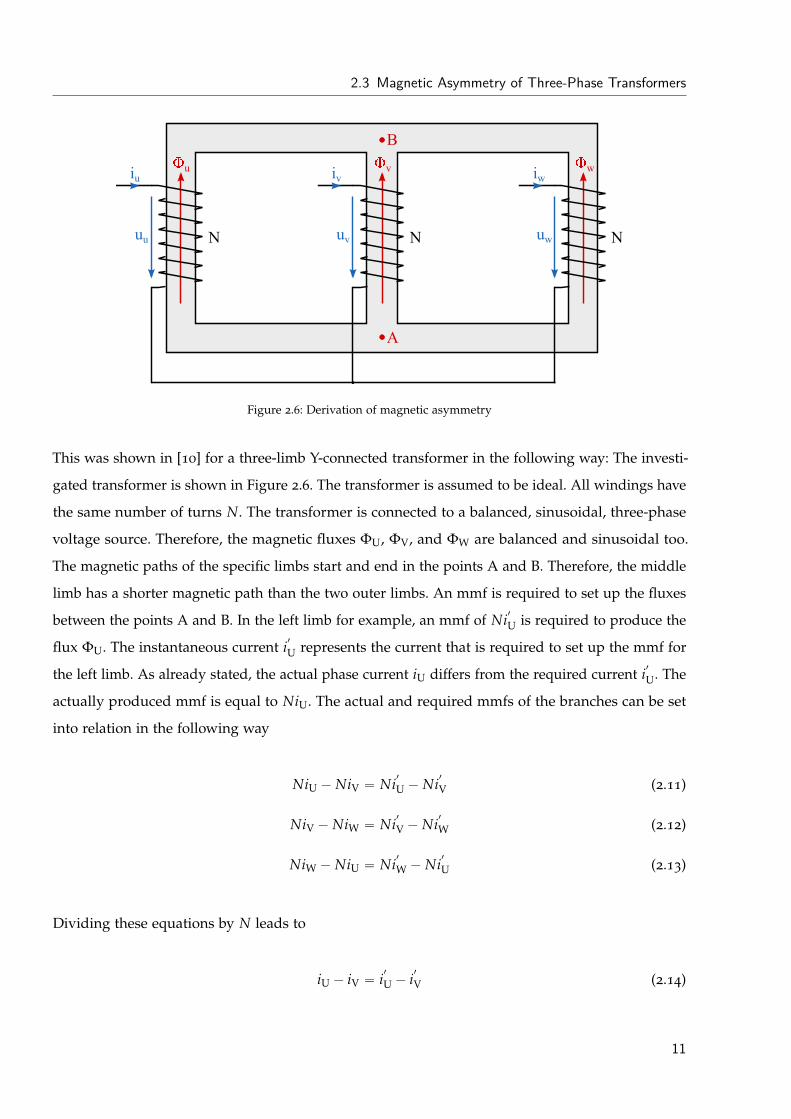
Figure 2.6: Derivation of magnetic asymmetry
This was shown in [10] for a three-limb Y-connected transformer in the following way: The investi-
gated transformer is shown in Figure 2.6. The transformer is assumed to be ideal. All windings have
the same number of turns N. The transformer is connected to a balanced, sinusoidal, three-phase
voltage source. Therefore, the magnetic fluxes ΦU, ΦV, and ΦW are balanced and sinusoidal too.
The magnetic paths of the specific limbs start and end in the points A and B. Therefore, the middle
limb has a shorter magnetic path than the two outer limbs. An mmf is required to set up the fluxes
between the points A and B. In the left limb for example, an mmf of Ni1
U is required to produce the
flux ΦU. The instantaneous current i1
U represents the current that is required to set up the mmf for
the left limb. As already stated, the actual phase current iU differs from the required current i1
U. The
actually produced mmf is equal to NiU. The actual and required mmfs of the branches can be set
into relation in the following way
NiU ´ NiV “ Ni1
U ´ Ni1
V (2.11)
NiV ´ NiW “ Ni1
V ´ Ni1
W (2.12)
NiW ´ NiU “ Ni1
W ´ Ni1
U (2.13)
Dividing these equations by N leads to
iU ´ iV “ i1
U ´ i1
V (2.14)
11
2 Essential Transformer Basics
iV ´ iW “ i1
V ´ i1
W (2.15)
iW ´ iU “ i1
W ´ i1
U (2.16)
One further equation is added due to the Y-connection of the transformer
iU ` iV ` iW “ 0 (2.17)
This set of four equations can be used to derive the following formulations of the phase currents
iU “ i1
U ´13pi
1
U ` i1
V ` i1
Wq (2.18)
iV “ i1
V ´13pi
1
U ` i1
V ` i1
Wq (2.19)
iW “ i1
W ´13pi
1
U ` i1
V ` i1
Wq (2.20)
The derivation is shown in detail for iU in Appendix A. All three currents contain the same expres-
sion which is a zero-sequence component i1
0
i1
0 “13pi
1
U ` i1
V ` i1
Wq (2.21)
This zero-sequence component causes an mmf Ni1
0 which, even at balanced excitation, produces a
zero-sequence flux. This flux leaves the core at point A and closes itself in point B. This proves that
the actual and required currents differ which means that a regular three-phase no-load test can not
be used to derive the magnetization characteristic of the respective transformer limbs.
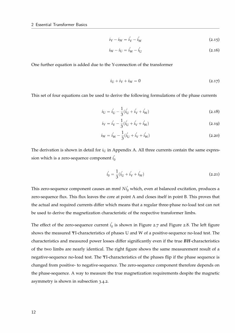
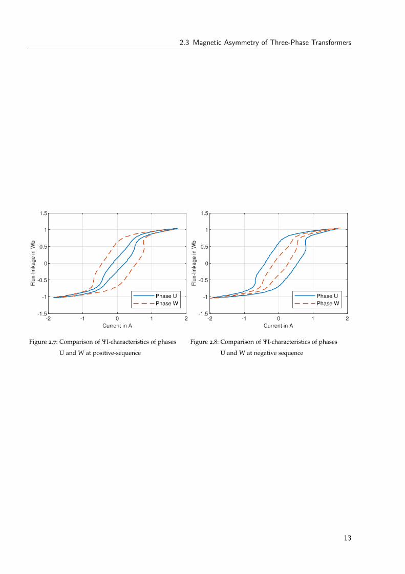
The effect of the zero-sequence current i1
0 is shown in Figure 2.7 and Figure 2.8. The left figure
shows the measured ΨI-characteristics of phases U and W of a positive-sequence no-load test. The
characteristics and measured power losses differ significantly even if the true BH-characteristics
of the two limbs are nearly identical. The right figure shows the same measurement result of a
negative-sequence no-load test. The ΨI-characteristics of the phases flip if the phase sequence is
changed from positive- to negative-sequence. The zero-sequence component therefore depends on
the phase-sequence. A way to measure the true magnetization requirements despite the magnetic
asymmetry is shown in subsection 3.4.2.
12
2.3 Magnetic Asymmetry of Three-Phase Transformers
-2 -1 0 1 2
Current in A
-1.5
-1
-0.5
0
0.5
1
1.5
Flu
x-lin
ka
ge
in
Wb
Phase U
Phase W
Figure 2.7: Comparison of ΨI-characteristics of phases
U and W at positive-sequence
-2 -1 0 1 2
Current in A
-1.5
-1
-0.5
0
0.5
1
1.5
Flu
x-lin
ka
ge
in
Wb
Phase U
Phase W
Figure 2.8: Comparison of ΨI-characteristics of phases
U and W at negative sequence
13

3 Theory and Methods
3.1 Transformer Modeling for Low Frequencies
The complexity of transformers makes their modeling a difficult task. The various materials used in
transformers have different frequency-dependent behaviors. The core effects have to be considered
when the investigated transients have frequencies below a few kHz. The core can, however, be
neglected at higher frequencies, while skin and proximity effects of the windings become dominant.
Therefore, the modeling approach depends on the investigated frequency range. [1]
The frequency ranges of transients can be categorized according to [11] in the following way:
• 0.1 Hz - 3 kHz: low-frequency oscillations
• 50/60 Hz - 20 kHz: slow front surges
• 10 kHz - 3 MHz: fast front surges
• 100 kHz - 50 MHz: very fast front surges
Low-frequency transients in transformers include geomagnetically induced currents (GICs), fer-
roresonance, harmonic currents, and inrush currents [5]. The core and winding representation do
not just depend on the frequency range but on the investigated tests as well. As an example, the
core can be neglected in short-circuit tests, while it is important in the simulation of ferroresonance.
Therefore, the core and winding representation can be viewed separately. [12]
According to [12], low-frequency models can be categorized into three groups:
1. Matrix representation
2. Saturable transformer component (STC)
3. Topology-based models
15
3 Theory and Methods
One approach of the first group is the use of an admittance matrix to represent the transformer
rIs “ rYs ¨ rUs (3.1)
This model does not include the non-linearity of the core since the admittance matrix consists of the
measured short-circuit test results. [12]
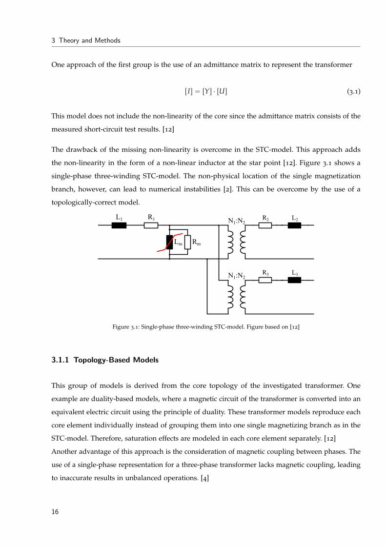
The drawback of the missing non-linearity is overcome in the STC-model. This approach adds
the non-linearity in the form of a non-linear inductor at the star point [12]. Figure 3.1 shows a
single-phase three-winding STC-model. The non-physical location of the single magnetization
branch, however, can lead to numerical instabilities [2]. This can be overcome by the use of a
topologically-correct model.
L1 R1
Lm Rm
L2R2
L3R3
N1:N2
N1:N2
Figure 3.1: Single-phase three-winding STC-model. Figure based on [12]
3.1.1 Topology-Based Models
This group of models is derived from the core topology of the investigated transformer. One
example are duality-based models, where a magnetic circuit of the transformer is converted into an
equivalent electric circuit using the principle of duality. These transformer models reproduce each
core element individually instead of grouping them into one single magnetizing branch as in the
STC-model. Therefore, saturation effects are modeled in each core element separately. [12]
Another advantage of this approach is the consideration of magnetic coupling between phases. The
use of a single-phase representation for a three-phase transformer lacks magnetic coupling, leading
to inaccurate results in unbalanced operations. [4]
16
3.2 Duality-Based Three-Limb Transformer Model
Duality-based models lack a detailed leakage model which lead to the development of hybrid
transformer models. Such models combine the topologically correct core model with a matrix
representation of the leakage inductances [13]. The hybrid model separates core and leakage
representation under the assumption that core inductances are greater than leakage inductances.
This can lead to doubtful results at deep saturation where this assumption does not hold. [14]
The magnetic coupling and the representation of every core element are important in the study of
GICs, therefore, a topology-based model based on the principle of duality is developed in this thesis.
The approach of modeling a three-limb, three-phase transformer is explained in section 3.2.
3.2 Duality-Based Three-Limb Transformer Model
The magnetic circuit of a transformer can be converted into an equivalent electric circuit using
the physically correct duality approach. This allows the transformer to be simulated using only
standard circuit elements. [2] Another advantage in this special case is that power system engineers
are more used to work in the electric rather than the magnetic domain. A duality-based model
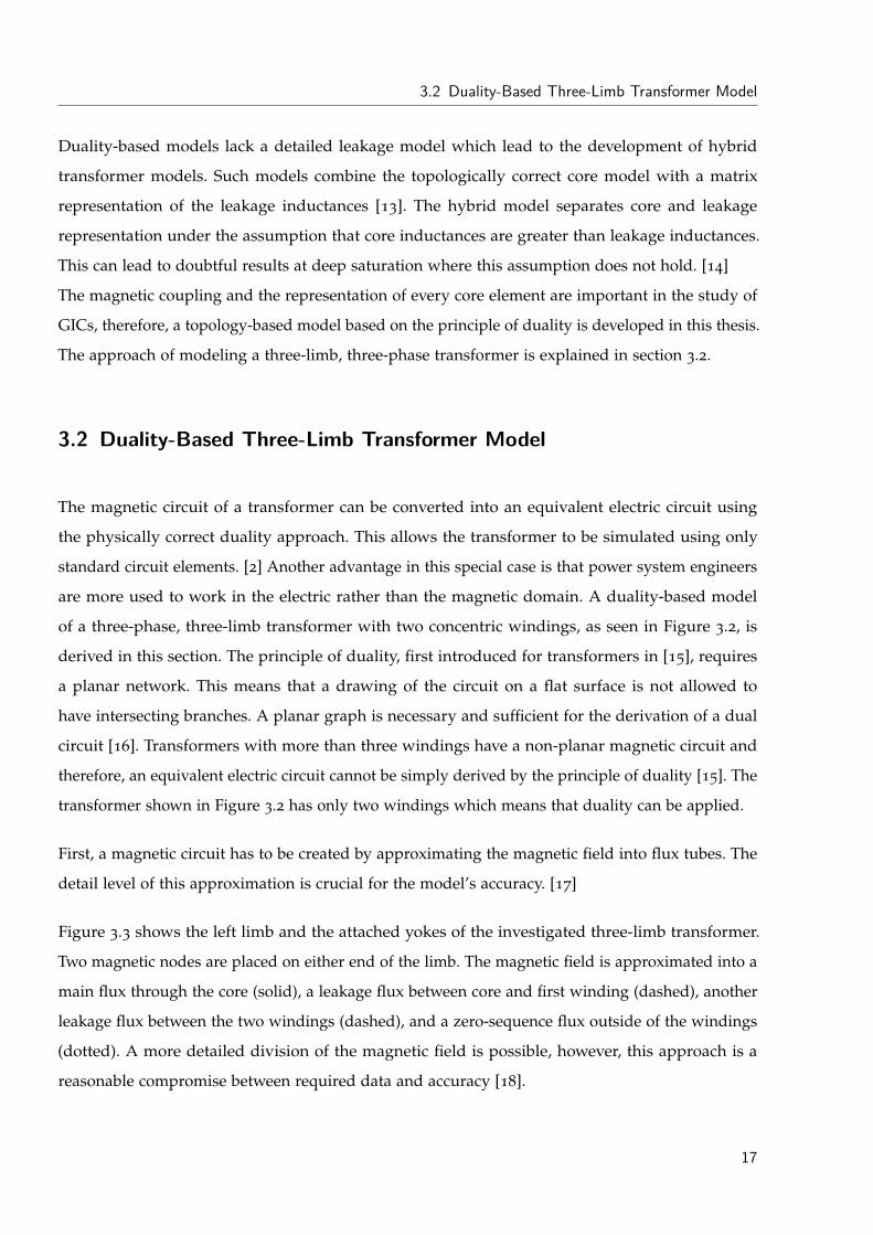
of a three-phase, three-limb transformer with two concentric windings, as seen in Figure 3.2, is
derived in this section. The principle of duality, first introduced for transformers in [15], requires
a planar network. This means that a drawing of the circuit on a flat surface is not allowed to
have intersecting branches. A planar graph is necessary and sufficient for the derivation of a dual
circuit [16]. Transformers with more than three windings have a non-planar magnetic circuit and
therefore, an equivalent electric circuit cannot be simply derived by the principle of duality [15]. The
transformer shown in Figure 3.2 has only two windings which means that duality can be applied.
First, a magnetic circuit has to be created by approximating the magnetic field into flux tubes. The
detail level of this approximation is crucial for the model’s accuracy. [17]
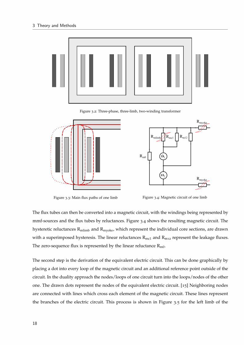
Figure 3.3 shows the left limb and the attached yokes of the investigated three-limb transformer.
Two magnetic nodes are placed on either end of the limb. The magnetic field is approximated into a
main flux through the core (solid), a leakage flux between core and first winding (dashed), another
leakage flux between the two windings (dashed), and a zero-sequence flux outside of the windings
(dotted). A more detailed division of the magnetic field is possible, however, this approach is a
reasonable compromise between required data and accuracy [18].
17
3 Theory and Methods
Figure 3.2: Three-phase, three-limb, two-winding transformer
Figure 3.3: Main flux paths of one limb
Rm0 1
2
Rmc1Rmlimb Rm12
Rmyoke
Rmyoke
Figure 3.4: Magnetic circuit of one limb
The flux tubes can then be converted into a magnetic circuit, with the windings being represented by
mmf-sources and the flux tubes by reluctances. Figure 3.4 shows the resulting magnetic circuit. The
hysteretic reluctances Rmlimb and Rmyoke, which represent the individual core sections, are drawn
with a superimposed hysteresis. The linear reluctances Rmc1 and Rm12 represent the leakage fluxes.
The zero-sequence flux is represented by the linear reluctance Rm0.
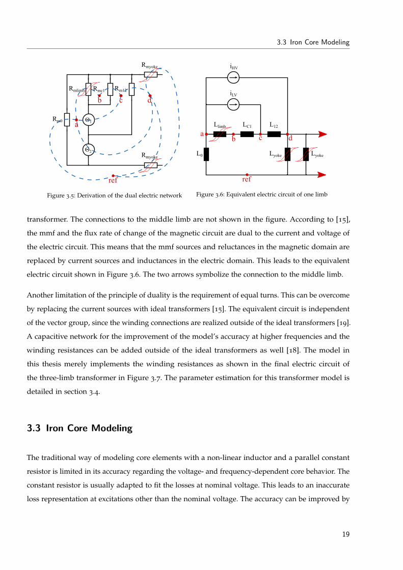
The second step is the derivation of the equivalent electric circuit. This can be done graphically by
placing a dot into every loop of the magnetic circuit and an additional reference point outside of the
circuit. In the duality approach the nodes/loops of one circuit turn into the loops/nodes of the other
one. The drawn dots represent the nodes of the equivalent electric circuit. [15] Neighboring nodes
are connected with lines which cross each element of the magnetic circuit. These lines represent
the branches of the electric circuit. This process is shown in Figure 3.5 for the left limb of the
18
3.3 Iron Core Modeling
Θ1
Θ2
Rmc1 Rm12
Rmyoke
Rmyoke
b c
ref
a
d
Rmlimb
Rm0
Figure 3.5: Derivation of the dual electric network
L12
d
ref
ab c
Llimb LC1
LyokeL0 Lyoke
iHV
iLV
Figure 3.6: Equivalent electric circuit of one limb
transformer. The connections to the middle limb are not shown in the figure. According to [15],
the mmf and the flux rate of change of the magnetic circuit are dual to the current and voltage of
the electric circuit. This means that the mmf sources and reluctances in the magnetic domain are
replaced by current sources and inductances in the electric domain. This leads to the equivalent
electric circuit shown in Figure 3.6. The two arrows symbolize the connection to the middle limb.
Another limitation of the principle of duality is the requirement of equal turns. This can be overcome
by replacing the current sources with ideal transformers [15]. The equivalent circuit is independent
of the vector group, since the winding connections are realized outside of the ideal transformers [19].
A capacitive network for the improvement of the model’s accuracy at higher frequencies and the
winding resistances can be added outside of the ideal transformers as well [18]. The model in
this thesis merely implements the winding resistances as shown in the final electric circuit of
the three-limb transformer in Figure 3.7. The parameter estimation for this transformer model is
detailed in section 3.4.
3.3 Iron Core Modeling
The traditional way of modeling core elements with a non-linear inductor and a parallel constant
resistor is limited in its accuracy regarding the voltage- and frequency-dependent core behavior. The
constant resistor is usually adapted to fit the losses at nominal voltage. This leads to an inaccurate
loss representation at excitations other than the nominal voltage. The accuracy can be improved by
19
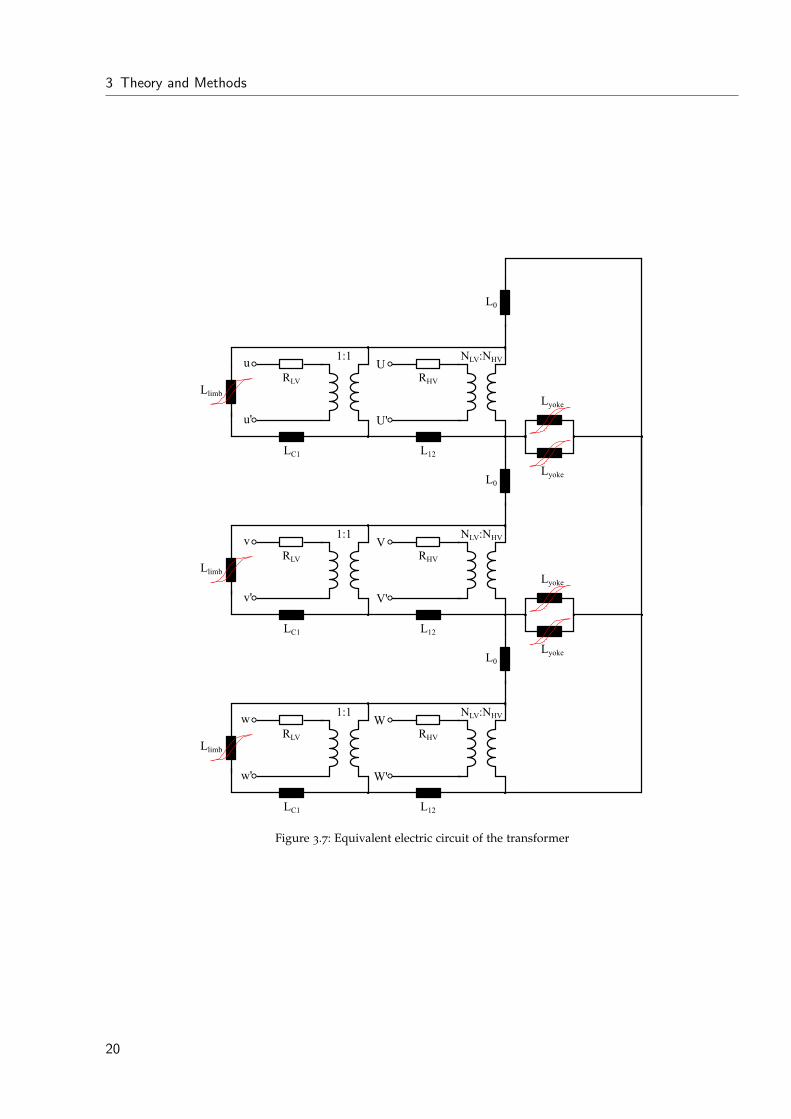
3 Theory and Methods
RLV RHVLlimb
1:1
LC1 L12
NLV:NHV
Lyoke
Lyoke
L0
u
u'
U
U'
RLV RHVLlimb
1:1
LC1 L12
NLV:NHV
Lyoke
Lyoke
L0
v
v'
V
V'
RLV RHVLlimb
1:1
LC1 L12
NLV:NHV
L0
w
w'
W
W'
Figure 3.7: Equivalent electric circuit of the transformer
20
3.3 Iron Core Modeling
replacing the constant resistor with a non-linear one. This does not, however, solve the inaccurate
frequency-dependent representation. A hysteresis model is much better suited to represent the
voltage- and frequency-dependent core losses. [4]
One approach to represent hysteresis is the group of macroscopic models. This group uses mathemat-
ical expressions to describe the hysteresis phenomenon on a macroscopic scale without completely
neglecting material physics [20]. The big advantage over the more detailed models used by physi-
cists is that they are not as computational time-consuming [8]. Therefore, a macroscopic approach
is chosen for this transformer model. The core loss can be divided into static and dynamic loss
components. Thus, hysteresis modeling is separated into a static and dynamic model.
3.3.1 Static Hysteresis Modeling – Jiles-Atherton Model
A static hysteresis model has to replicate the major and symmetrical/asymmetrical minor loops [8].
Two of the best-known static hysteresis models are the Preisach- and the Jiles-Atherton (JA)-
model. A good introduction into the models is given in [8]. A comparison of the two approaches
in [21] concludes that Preisach is more accurate especially at producing minor loops but also more
computationally intensive. It is also stated that Preisach requires extensive measurements but little
fitting while the opposite is true for JA.
Less measurements are a big advantage of the JA-model in the case of power transformers that are
in use. Quicker and simpler measurements lead to shorter downtimes in which the transformer
has to be disconnected from the grid. This is the main reason why the JA-model is used for the
representation of static hysteresis losses in this transformer model.
Multiple mathematical descriptions of the model with slight differences can be found. The main
idea, however, stays the same. The description in this section is based on [22], while the formulas
show a slightly modified version of the model found in [23]. For more detailed explanations see [22]
and [23]. The often-mentioned physical basis of the model has to be viewed critically if a physically
correct representation is important. According to [24] it is in fact non-physical, however, the model
is still useful in circuit simulations.
The JA-model uses the anhysteretic magnetization and combines it with pinning sites that represent
defects in the material. The model creates sigmoid-shaped hysteresis loops by considering the
21
3 Theory and Methods
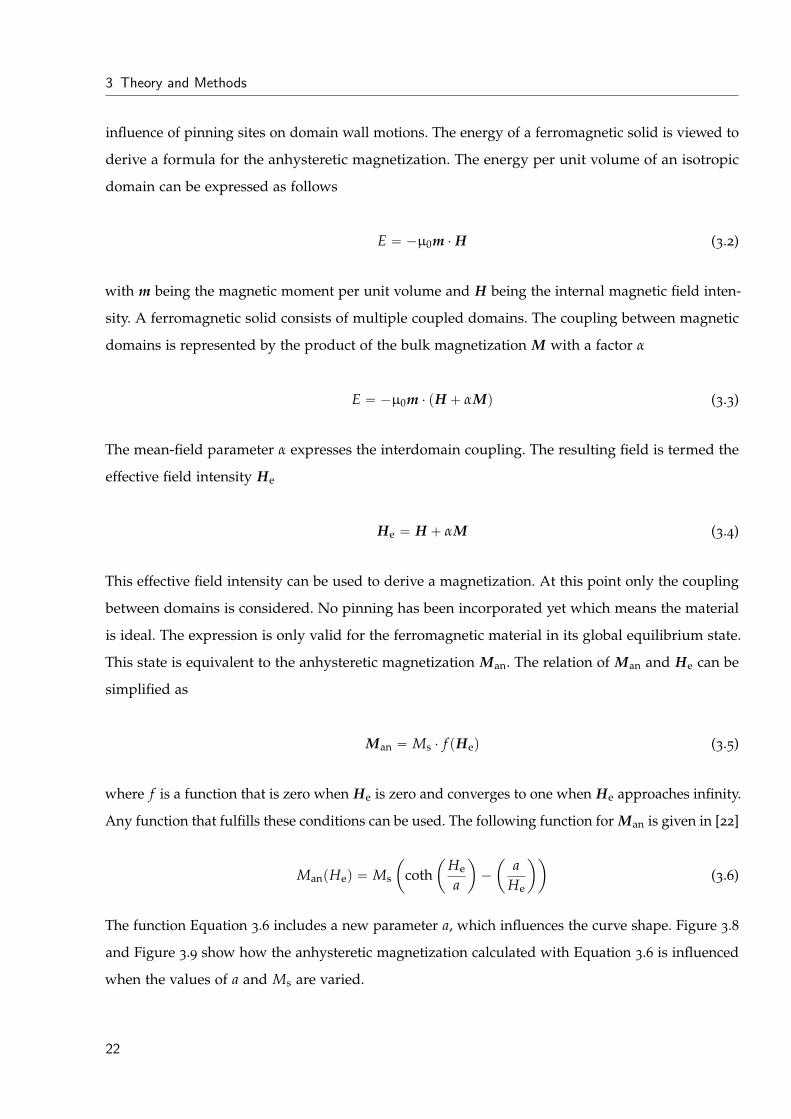
influence of pinning sites on domain wall motions. The energy of a ferromagnetic solid is viewed to
derive a formula for the anhysteretic magnetization. The energy per unit volume of an isotropic
domain can be expressed as follows
E “ ´µ0m ¨ H (3.2)
with m being the magnetic moment per unit volume and H being the internal magnetic field inten-
sity. A ferromagnetic solid consists of multiple coupled domains. The coupling between magnetic
domains is represented by the product of the bulk magnetization M with a factor α
E “ ´µ0m ¨ pH ` αMq (3.3)
The mean-field parameter α expresses the interdomain coupling. The resulting field is termed the
effective field intensity He
He “ H ` αM (3.4)
This effective field intensity can be used to derive a magnetization. At this point only the coupling
between domains is considered. No pinning has been incorporated yet which means the material
is ideal. The expression is only valid for the ferromagnetic material in its global equilibrium state.
This state is equivalent to the anhysteretic magnetization Man. The relation of Man and He can be
simplified as
Man “ Ms ¨ f pHeq (3.5)
where f is a function that is zero when He is zero and converges to one when He approaches infinity.
Any function that fulfills these conditions can be used. The following function for Man is given in [22]
ManpHeq “ Ms
ˆ
cothˆ
He
a
˙
´
ˆ
aHe
˙˙
(3.6)
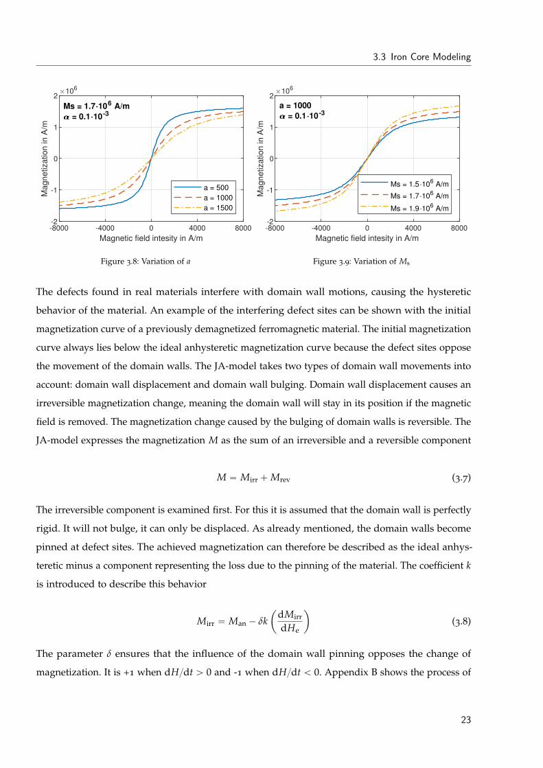
The function Equation 3.6 includes a new parameter a, which influences the curve shape. Figure 3.8
and Figure 3.9 show how the anhysteretic magnetization calculated with Equation 3.6 is influenced
when the values of a and Ms are varied.
22
3.3 Iron Core Modeling
-8000 -4000 0 4000 8000
Magnetic field intesity in A/m
-2
-1
0
1
2
Magnetization in A
/m
106
Ms = 1.7 106 A/m
= 0.1 10-3
a = 500
a = 1000
a = 1500
Figure 3.8: Variation of a
-8000 -4000 0 4000 8000
Magnetic field intesity in A/m
-2
-1
0
1
2
Magnetization in A
/m
106
a = 1000
= 0.1 10-3
Ms = 1.5 106 A/m
Ms = 1.7 106 A/m
Ms = 1.9 106 A/m
Figure 3.9: Variation of Ms
The defects found in real materials interfere with domain wall motions, causing the hysteretic
behavior of the material. An example of the interfering defect sites can be shown with the initial
magnetization curve of a previously demagnetized ferromagnetic material. The initial magnetization
curve always lies below the ideal anhysteretic magnetization curve because the defect sites oppose
the movement of the domain walls. The JA-model takes two types of domain wall movements into
account: domain wall displacement and domain wall bulging. Domain wall displacement causes an
irreversible magnetization change, meaning the domain wall will stay in its position if the magnetic
field is removed. The magnetization change caused by the bulging of domain walls is reversible. The
JA-model expresses the magnetization M as the sum of an irreversible and a reversible component
M “ Mirr `Mrev (3.7)
The irreversible component is examined first. For this it is assumed that the domain wall is perfectly
rigid. It will not bulge, it can only be displaced. As already mentioned, the domain walls become
pinned at defect sites. The achieved magnetization can therefore be described as the ideal anhys-
teretic minus a component representing the loss due to the pinning of the material. The coefficient k
is introduced to describe this behavior
Mirr “ Man ´ δkˆ
dMirr
dHe
˙
(3.8)
The parameter δ ensures that the influence of the domain wall pinning opposes the change of
magnetization. It is +1 when dHdt ą 0 and -1 when dHdt ă 0. Appendix B shows the process of
23
3 Theory and Methods
a) b)
H=0 H
Figure 3.10: Domain wall bulging [7]
how Equation 3.8 is rewritten into its final form
dMirr
dH“
Man ´Mirr
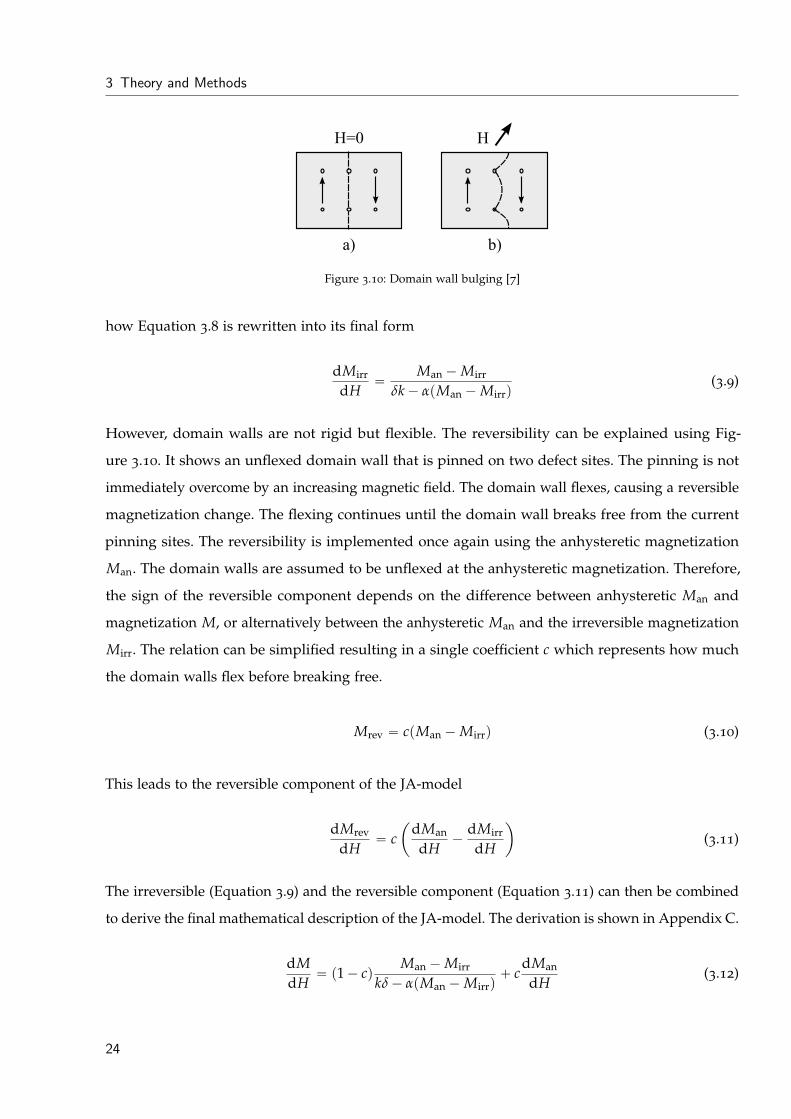
δk´ αpMan ´Mirrq(3.9)
However, domain walls are not rigid but flexible. The reversibility can be explained using Fig-
ure 3.10. It shows an unflexed domain wall that is pinned on two defect sites. The pinning is not
immediately overcome by an increasing magnetic field. The domain wall flexes, causing a reversible
magnetization change. The flexing continues until the domain wall breaks free from the current
pinning sites. The reversibility is implemented once again using the anhysteretic magnetization
Man. The domain walls are assumed to be unflexed at the anhysteretic magnetization. Therefore,
the sign of the reversible component depends on the difference between anhysteretic Man and
magnetization M, or alternatively between the anhysteretic Man and the irreversible magnetization
Mirr. The relation can be simplified resulting in a single coefficient c which represents how much
the domain walls flex before breaking free.
Mrev “ cpMan ´Mirrq (3.10)
This leads to the reversible component of the JA-model
dMrev
dH“ c
ˆ
dMan
dH´
dMirr
dH
˙
(3.11)
The irreversible (Equation 3.9) and the reversible component (Equation 3.11) can then be combined
to derive the final mathematical description of the JA-model. The derivation is shown in Appendix C.
dMdH
“ p1´ cqMan ´Mirr
kδ´ αpMan ´Mirrq` c
dMan
dH(3.12)
24
3.3 Iron Core Modeling
-8000 -4000 0 4000 8000
Magnetic field intensity in A/m
-1.5
-1
-0.5
0
0.5
1
1.5
Ma
gn
etiza
tio
n in
A/m
106
Ms = 1.7 106 A/m
= 0.1 10-3
a = 1000
k = 500
c = 0.15
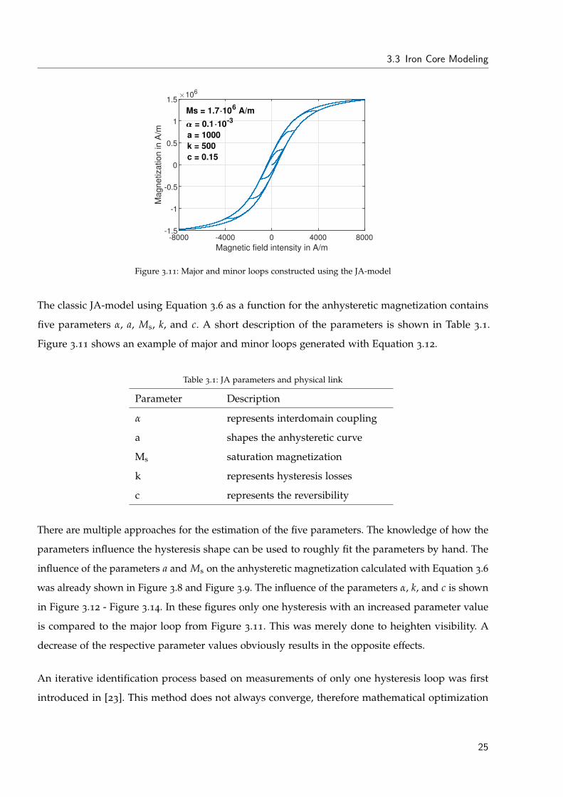
Figure 3.11: Major and minor loops constructed using the JA-model
The classic JA-model using Equation 3.6 as a function for the anhysteretic magnetization contains
five parameters α, a, Ms, k, and c. A short description of the parameters is shown in Table 3.1.
Figure 3.11 shows an example of major and minor loops generated with Equation 3.12.
Table 3.1: JA parameters and physical link
Parameter Description
α represents interdomain coupling
a shapes the anhysteretic curve
Ms saturation magnetization
k represents hysteresis losses
c represents the reversibility
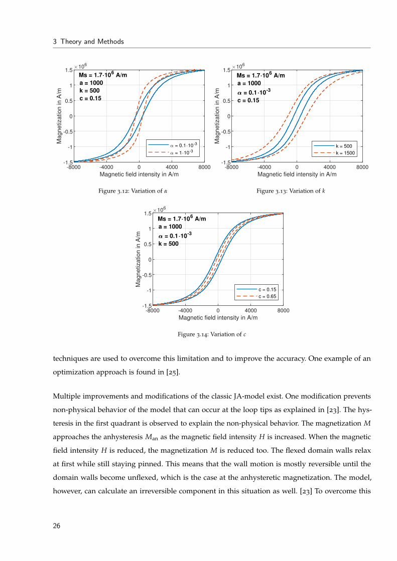
There are multiple approaches for the estimation of the five parameters. The knowledge of how the
parameters influence the hysteresis shape can be used to roughly fit the parameters by hand. The
influence of the parameters a and Ms on the anhysteretic magnetization calculated with Equation 3.6
was already shown in Figure 3.8 and Figure 3.9. The influence of the parameters α, k, and c is shown
in Figure 3.12 - Figure 3.14. In these figures only one hysteresis with an increased parameter value
is compared to the major loop from Figure 3.11. This was merely done to heighten visibility. A
decrease of the respective parameter values obviously results in the opposite effects.
An iterative identification process based on measurements of only one hysteresis loop was first
introduced in [23]. This method does not always converge, therefore mathematical optimization
25
3 Theory and Methods
-8000 -4000 0 4000 8000
Magnetic field intensity in A/m
-1.5
-1
-0.5
0
0.5
1
1.5
Ma
gn
etiza
tio
n in
A/m
106
Ms = 1.7 106 A/m
a = 1000
k = 500
c = 0.15
= 0.1 10-3
= 1 10-3
Figure 3.12: Variation of α
-8000 -4000 0 4000 8000
Magnetic field intensity in A/m
-1.5
-1
-0.5
0
0.5
1
1.5
Ma
gn
etiza
tio
n in
A/m
106
Ms = 1.7 106 A/m
a = 1000
= 0.1 10-3
c = 0.15
k = 500
k = 1500
Figure 3.13: Variation of k
-8000 -4000 0 4000 8000
Magnetic field intensity in A/m
-1.5
-1
-0.5
0
0.5
1
1.5
Ma
gn
etiza
tio
n in
A/m
106
Ms = 1.7 106 A/m
a = 1000
= 0.1 10-3
k = 500
c = 0.15
c = 0.65
Figure 3.14: Variation of c
techniques are used to overcome this limitation and to improve the accuracy. One example of an
optimization approach is found in [25].
Multiple improvements and modifications of the classic JA-model exist. One modification prevents
non-physical behavior of the model that can occur at the loop tips as explained in [23]. The hys-
teresis in the first quadrant is observed to explain the non-physical behavior. The magnetization M
approaches the anhysteresis Man as the magnetic field intensity H is increased. When the magnetic
field intensity H is reduced, the magnetization M is reduced too. The flexed domain walls relax
at first while still staying pinned. This means that the wall motion is mostly reversible until the
domain walls become unflexed, which is the case at the anhysteretic magnetization. The model,
however, can calculate an irreversible component in this situation as well. [23] To overcome this
26
3.3 Iron Core Modeling
problem another parameter δM can be implemented as stated in [26]
δM “
$
’
’
’
’
’
&
’
’
’
’
’
%
0 if H ă 0 and Man ´M ą 0
0 if H ą 0 and Man ´M ă 0
1 otherwise
(3.13)
The multiplication of this parameter with Equation 3.9 ensures that the irreversible component is
set to zero under these circumstances to prevent the non-physical behavior.
A modification that can be useful in some cases is the inverse JA-model. The classic approach uses
the magnetic field intensity H as an input, while the inverse uses the magnetic flux density B. The
approach used in this thesis is based on the inverse time-stepping JA-model found in [27], which
was enhanced by the implementation of Equation 3.13. The implemented JA-model can be found in
Appendix D.
The function for Man given in Equation 3.6 can be exchanged if a higher adjustability is needed.
Equation 3.14, proposed in [28], can give a more accurate model.
Man “ Msa1He ` He
b
a3 ` a2He ` Heb (3.14)
This equation can be used if the following constraints apply
a1 ą 0, a2 ě a1, a3 ą 0, and b ě 1.0 (3.15)
As stated before, the JA-model generates sigmoid-shaped hysteresis loops. Grain-orientated steels
used in transformers, however, have loops that widen at the shoulder and are therefore different
from the uniformly converging sigmoid-shape [29]. The accuracy can be increased by modifying the
constant parameter k to be dependent on the magnetization M, since the width depends on the
parameter k [28].
The accuracy of minor loops can be improved by either introducing scaling factors or by determining
the parameters for different excitations. The use of a scaling factor only requires the measurement
of the major loop. Multiple loops at different excitations are necessary if separate sets of parameters
are used. [25]
27
3 Theory and Methods
3.3.2 Dynamic Hysteresis Losses
The Hysteresis losses can be split into static and dynamic components. In fact, the total energy
loss Wtot can be split into three components: a static hysteresis loss component Whys, an eddy loss
component Weddy, and an excess loss component Wexc [30].
Wtot “ Whys `Weddy `Wexc (3.16)
The total loss can not be described accurately with only a static and an eddy loss component.
The eddy loss component, which is calculated with a Maxwell equation, assumes a homogeneous
magnetic material. This is because the Maxwell equation predates the knowledge of magnetic
domains. The dynamic effect caused by the domains is considered in the excess loss component
Wexc. [29]
The two dynamic components exhibit different frequency-dependent behaviors [30]
Weddy9 f
Wexc9 f 12(3.17)
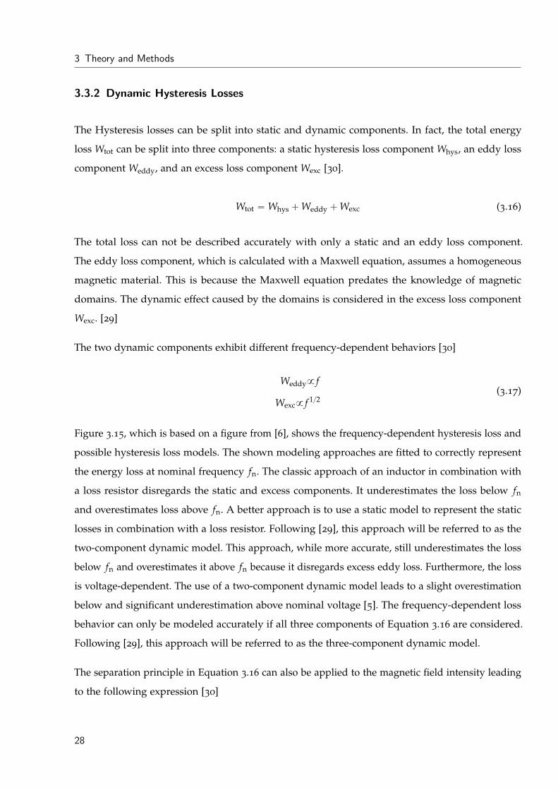
Figure 3.15, which is based on a figure from [6], shows the frequency-dependent hysteresis loss and
possible hysteresis loss models. The shown modeling approaches are fitted to correctly represent
the energy loss at nominal frequency fn. The classic approach of an inductor in combination with
a loss resistor disregards the static and excess components. It underestimates the loss below fn
and overestimates loss above fn. A better approach is to use a static model to represent the static
losses in combination with a loss resistor. Following [29], this approach will be referred to as the
two-component dynamic model. This approach, while more accurate, still underestimates the loss
below fn and overestimates it above fn because it disregards excess eddy loss. Furthermore, the loss
is voltage-dependent. The use of a two-component dynamic model leads to a slight overestimation
below and significant underestimation above nominal voltage [5]. The frequency-dependent loss
behavior can only be modeled accurately if all three components of Equation 3.16 are considered.
Following [29], this approach will be referred to as the three-component dynamic model.
The separation principle in Equation 3.16 can also be applied to the magnetic field intensity leading
to the following expression [30]
28
3.4 Parameter Derivation
fn
Frequency f
W(fn)
Energ
y loss W
three-component model
two-component model
inductor + resistor
Wexc
Whys
Weddy
Figure 3.15: frequency-dependent model accuracy. Figure is modified based on [6]
Htot “ Hhys ` Heddy ` Hexc (3.18)
The dynamic model can be implemented with a two- or three-component approach based on
Equation 3.18. The three-component dynamic model can be implemented as follows [31], [29]
Htot “ Hhys ` keddydBdt` kexcδ
ˇ
ˇ
ˇ
ˇ
dBdt
ˇ
ˇ
ˇ
ˇ
12
(3.19)
with δ being +1 for dBdt ą 0 and -1 for dBdt ă 0. The static component Hhys is calculated by the
inverse JA-model. The complexity of the complete model depends on the required accuracy and the
available data. The static JA hysteresis model can be improved and modified in various ways, as the
examples given in subsection 3.3.1 show. The parameter kexc can be constant [31] or dependent on B
in order to improve the voltage-dependent accuracy [29].
3.4 Parameter Derivation
The parameter derivation process consists of numerous different measurement and fitting proce-
dures. The linear parameters and can either be derived by standard tests or can be found in factory
29
3 Theory and Methods
test protocols. The linear components of the transformer model are:
• Winding resistances RLV and RHV
• Short-circuit inductance L12 between the two windings
• Inductance LC1 between core and first winding
• Zero-sequence impedance L0
The non-linear core parameters require measurements and data beyond the standard tests.
3.4.1 Linear Parameters
The winding resistances can be measured using a direct current (DC) source according to the
standard [32]. The frequency-dependence of the winding resistance, mainly caused by the skin and
proximity effect, can be incorporated [13]. The model in this thesis, however, only includes the DC
winding resistances.
The linear inductance L12 representing the flux between the two windings can be calculated from a
short-circuit test according to the standard [32].
The inductance LC1 can not be measured directly but can be approximated based on L12 [14]
LC1 « K ¨ L12 (3.20)
with K “ 0.5 giving good results [14].
The zero-sequence inductance can be derived from zero-sequence measurements according to
the standard [32]. Depending on the winding connection the zero-sequence flux may flow partly
through the tank which is non-linear. This occurs in transformers with missing winding balancing
ampere-turns, as is the case for Yy-transformers without an additional delta winding [32]. The
non-linearity can safely be neglected according to [14], where a duality-based model is applied
to simulate a 300 kVA Yyn-transformer. This is explained with the linear behavior of the oil gap
between core and tank which outweighs the non-linear behavior of the tank. More detailed models
that include the non-linear tank as well as other structural components are possible, however, the
parameter estimation is not trivial [5].
30
3.4 Parameter Derivation
A
NN
w
N
u
uu uw
B
iu
u
iw
Figure 3.16: Measurement of core properties [10]
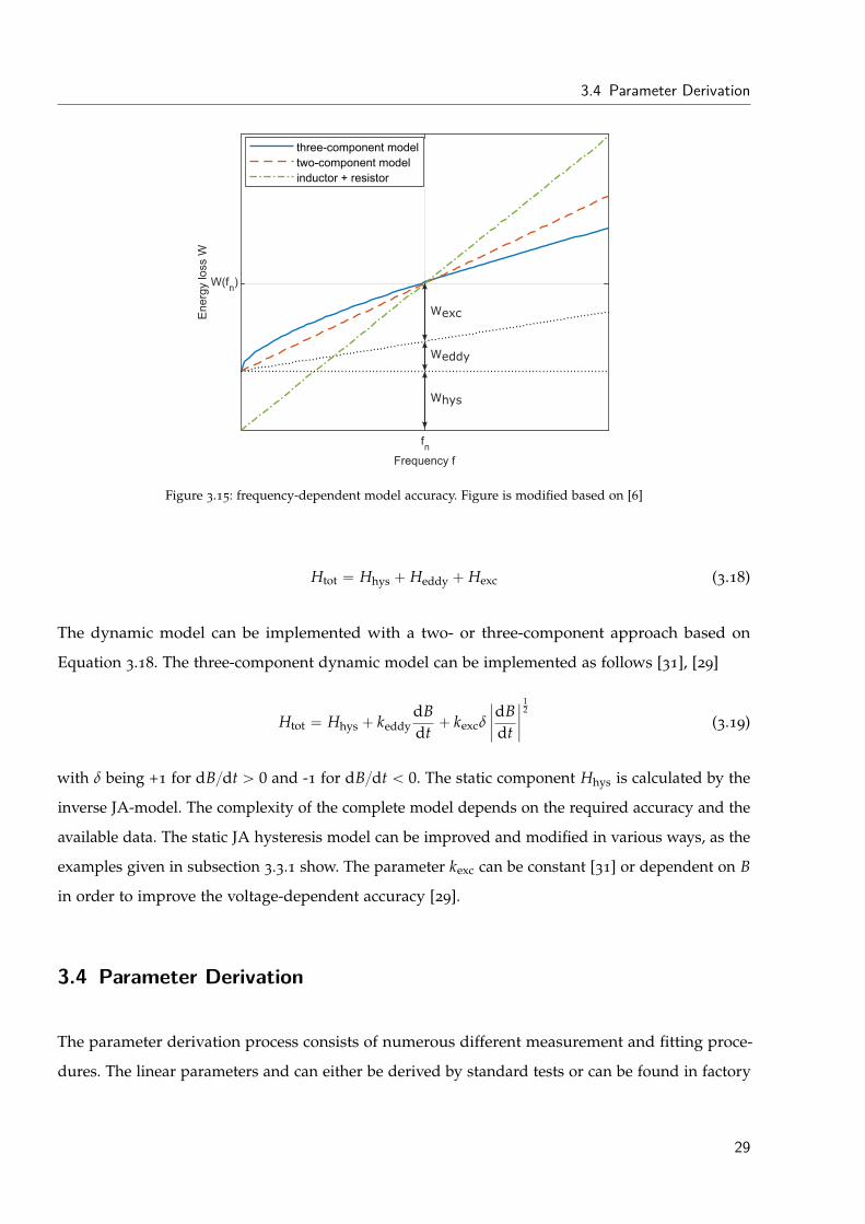
3.4.2 Non-Linear Core Parameters
As stated in chapter 2, the phase currents of a regular three-phase no-load test do not just depend
on the properties of their respective core section but on the other sections as well. Therefore,
the magnetic properties can not be deduced from a three-phase no-load test. Figure 3.16 shows
an approach found in [10] to measure the required excitations of two core sections without the
interference of the third. An ideal transformer without leakage flux and winding resistances is
assumed to explain the method. A sinusoidal voltage is applied to windings U and W. The magnetic
fluxes in the outer limbs will be equal, since the voltage is applied to both windings. This means that
there is no magnetic flux and mmf in the middle limb. The mmf set up in the left limb is consumed
to create the magnetic flux in the same section. Therefore, the drawn current of winding U is the
actual current needed to excite the left limb of the core. The same applies to the right limb and
winding W. In reality a small flux will occur in the middle limb. Nevertheless, this approach allows
to measure the voltage-current and therefore the flux-current properties of the core sections. [10]
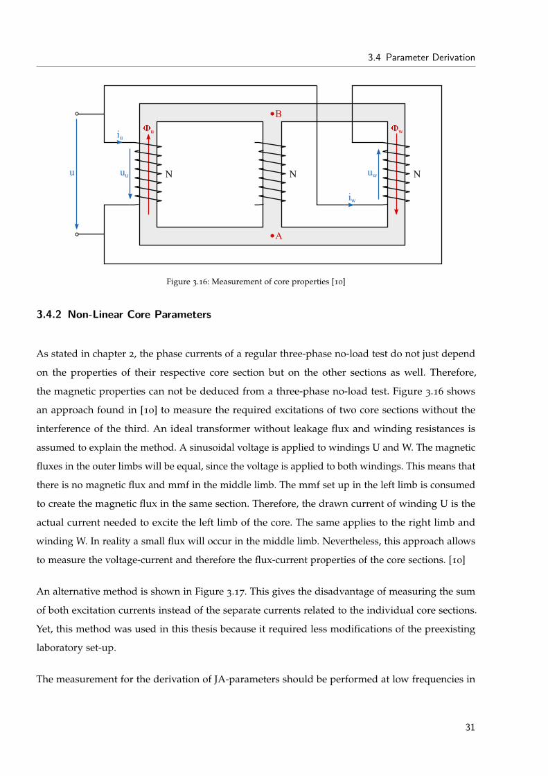
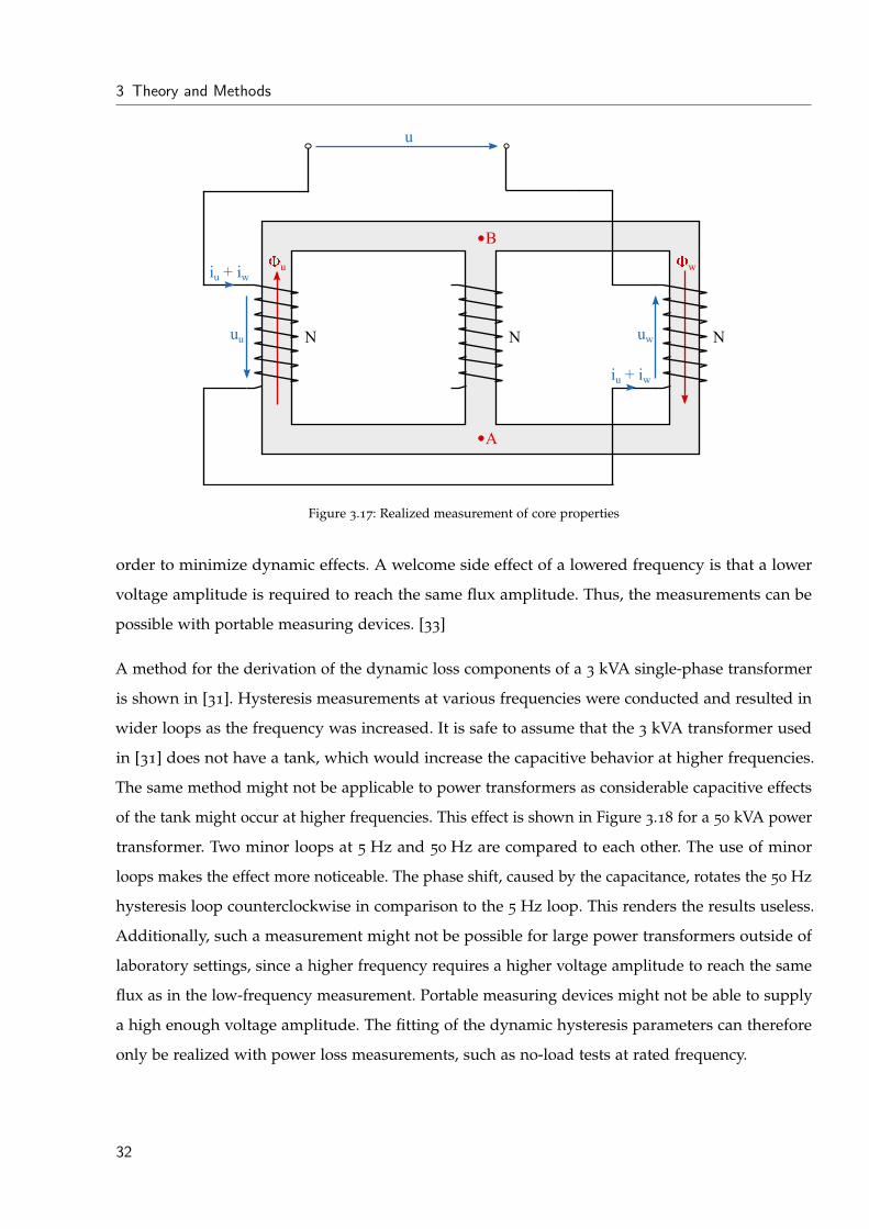
An alternative method is shown in Figure 3.17. This gives the disadvantage of measuring the sum
of both excitation currents instead of the separate currents related to the individual core sections.
Yet, this method was used in this thesis because it required less modifications of the preexisting
laboratory set-up.
The measurement for the derivation of JA-parameters should be performed at low frequencies in
31
3 Theory and Methods
A
NN
w
N
u
uu uw
B
iu + iw
iu + iw
u
Figure 3.17: Realized measurement of core properties
order to minimize dynamic effects. A welcome side effect of a lowered frequency is that a lower
voltage amplitude is required to reach the same flux amplitude. Thus, the measurements can be
possible with portable measuring devices. [33]
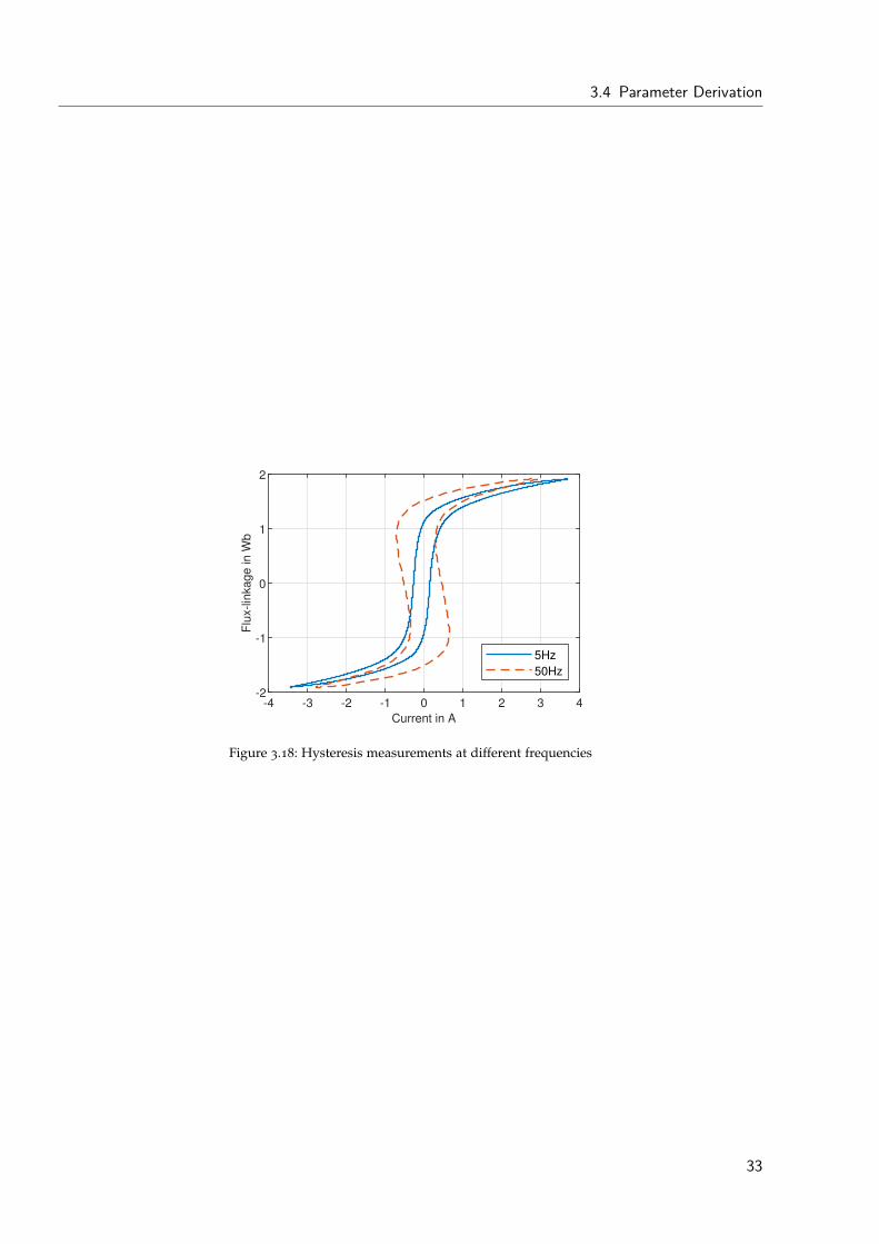
A method for the derivation of the dynamic loss components of a 3 kVA single-phase transformer
is shown in [31]. Hysteresis measurements at various frequencies were conducted and resulted in
wider loops as the frequency was increased. It is safe to assume that the 3 kVA transformer used
in [31] does not have a tank, which would increase the capacitive behavior at higher frequencies.
The same method might not be applicable to power transformers as considerable capacitive effects
of the tank might occur at higher frequencies. This effect is shown in Figure 3.18 for a 50 kVA power
transformer. Two minor loops at 5 Hz and 50 Hz are compared to each other. The use of minor
loops makes the effect more noticeable. The phase shift, caused by the capacitance, rotates the 50 Hz
hysteresis loop counterclockwise in comparison to the 5 Hz loop. This renders the results useless.
Additionally, such a measurement might not be possible for large power transformers outside of
laboratory settings, since a higher frequency requires a higher voltage amplitude to reach the same
flux as in the low-frequency measurement. Portable measuring devices might not be able to supply
a high enough voltage amplitude. The fitting of the dynamic hysteresis parameters can therefore
only be realized with power loss measurements, such as no-load tests at rated frequency.
32
3.4 Parameter Derivation
-4 -3 -2 -1 0 1 2 3 4
Current in A
-2
-1
0
1
2
Flu
x-lin
kage in W
b
5Hz
50Hz
Figure 3.18: Hysteresis measurements at different frequencies
33

4 Measurements and Fitting
4.1 Transformer Under Test (T74) – General Data
The transformer model from chapter 3 is tested on a three-phase, three-limb, two-winding, 50 kVA
power transformer. The topology of the transformer matches the topology of the transformer in
Figure 3.2. Table 4.1 shows the relevant nameplate data. The transformer, built in 1974, will hereafter
be referred to as T74.
The transformer has been modified in a way that allows the low-voltage winding connection to be
chosen at will [34]. All of the following measurements and simulations are based on the transformer
in YNyn0 connection. The deviation of the nameplate winding connection entails a deviation of the
voltage amplitude. If the YNyn0-transformer is excited with 400 V from the low-voltage side, the
voltage on the high-voltage side is less than the rated voltage UHV given in Table 4.1. The number of
low- and high-voltage winding turns are needed to properly represent the voltage ratio independent
of the chosen winding connection. Another requirement are the core dimensions. If the exact core
dimensions are not known, typical ratios for the specific core type can be used instead of the exact
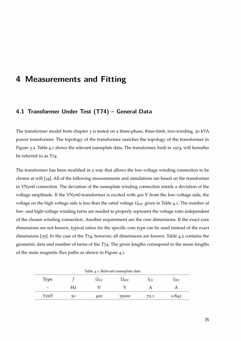
dimensions [35]. In the case of the T74, however, all dimensions are known. Table 4.2 contains the
geometric data and number of turns of the T74. The given lengths correspond to the mean lengths
of the main magnetic flux paths as shown in Figure 4.1.
Table 4.1: Relevant nameplate data
Type f ULV UHV ILV IHV
- Hz V V A A
Yzn5 50 400 35000 72.1 0.842
35
4 Measurements and Fitting
Table 4.2: Geometric transformer data
Acore lyoke llimb NLV NHV
mm2 mm mm - -
6001 237 440 102 7730
llimb
lyoke
Figure 4.1: T74 core dimensions
4.2 T74 - Linear Parameters
The derivation of the linear components is performed as explained in subsection 3.4.1. It is assumed
that there are no differences among the phases. The parameters of the individual phases are
therefore assumed to be equal. All measurements were performed on the low-voltage side of the
transformer.
The first step are the DC winding resistances. The values of the resistances of the low-voltage
winding RLV and the high-voltage winding RHV were measured previously and were provided for
this thesis.
The inductance L12 is calculated using a short-circuit test. Table 4.3 contains the rms values of phase
voltages and currents as well as the power factors of each phase. The mean values of phase voltages,
phase currents and power factors are calculated with Equation 4.1 to Equation 4.3.
ĚUSC “UU,SC ¨UV,SC ¨UW,SC
3“
17.590 V ¨ 18.361 V ¨ 17.557 V3
“ 17.836 V (4.1)
36
4.2 T74 - Linear Parameters
Table 4.3: Short-circuit test data
UU,SC UV,SC UW,SC IU,SC IV,SC IW,SC cospϕUq cospϕVq cospϕWq
V V V A A A - - -
17.590 18.361 17.557 70.352 65.458 70.910 0.482 0.509 0.426
ĎISC “IU,SC ¨ IV,SC ¨ IW,SC
3“
70.352 A ¨ 65.458 A ¨ 70.910 A3
“ 68.901 A (4.2)
Ğcospϕq “cospϕUq ¨ cospϕVq ¨ cospϕWq
3“
0.482 ¨ 0.509 ¨ 0.4263
“ 0.472 (4.3)
The mean values can then be used to calculate the short-circuit impedance L12
X12 “ĚUSCĎISC
¨ Ğsinpϕq “17.836 V68.901 A
¨ sinp61.836˝q “ 0.228 Ω (4.4)
L12 “X12
2 ¨ π ¨ fn“
0.228 Ω2 ¨ π ¨ 50 Hz
“ 726 µH (4.5)
The inductance LC1 can be approximated according to Equation 3.20 with K “ 0.5 [14]
LC1 « K ¨ L12 “ 0.5 ¨ 726 µH “ 363 µH (4.6)
As explained in subsection 3.4.1, the zero-sequence inductance can be assumed to be linear. An
open-circuit zero-sequence test conducted on the T74 transformer confirmed the near linear behavior
at the test current of 23.5 A per phase. A higher test current was not possible due to the current
limitation of the neutral connection. Table 4.4 contains the rms values of the conducted zero-
sequence test. The current Izero is the total current of all three phases combined. The supplied
voltage was adjusted by subtracting the voltage drop across the winding, leading to Uzero. The
zero-sequence impedance X0 per phase is then calculated according to [32].
Z0 “3 ¨Uzero
Izero“
3 ¨ 52.73 V70.50 A
“ 2.244 Ω (4.7)
37
4 Measurements and Fitting
Table 4.4: Main transformer under test (T74) zero-sequence test data
Uzero Izero Szero Pzero Qzero
V A VA W var
52.73 70.50 3784.81 2224.66 3061.97
Table 4.5: T74 linear parameters
RLV RHV L12 LC1 L0 R0
Ω Ω µH µH mH Ω
0.041 332.058 726 363 8.671 3.749
The impedance can be split into an inductance and a parallel resistance which represents the
losses
X0 “3 ¨U2
zeroQzero
“3 ¨ p52.73 Vq2
3061.97 var“ 2.724 Ω (4.8)
L0 “X0
2 ¨ π ¨ fn“
2.724 Ω2 ¨ π ¨ 50 Hz
“ 8.671 mH (4.9)
R0 “3 ¨U2
zeroPzero
“3 ¨ p52.73 Vq2
2224.66 W“ 3.749 Ω (4.10)
The linear parameters of the T74 model are summarized in Table 4.5.
4.3 T74 - Non-Linear Core Parameters
The measurements of the static hysteresis losses were conducted with the measuring setup shown in
Figure 3.17. A power-amplifier capable of supplying near perfect sinusoidal voltages with constant
amplitudes was used for all measurements. The simulations, that use ideal voltage sources, are
therefore comparable to the measurements. All measurements were conducted with a measuring
device that measures the overall power, not just the fundamental power. The simulated powers were
therefore derived in the same way as with the measuring device. The used formulas are shown in
38
4.3 T74 - Non-Linear Core Parameters
Appendix E. A frequency of 5 Hz was used to minimize dynamic effects for the measurement of
the static hysteresis losses. A positive side effect of low frequencies is caused by the proportionality
seen in Equation 4.11. If the frequency is lowered, the voltage amplitude has to be lowered too
for the flux amplitude to remain unchanged. Lower voltage amplitudes make the measurement
possible with portable alternating current (AC) sources. Alternatively, specialized test-devices can
have the ability to output DC-voltages to measure the core characteristics. Appendix F compares
the measurement with the AC power-amplifier to a measurement with a not yet released testing
software of a specialized transformer test-device using DC-excitation.
Φpeak9Upeak
f(4.11)
The supplied voltages are integrated to obtain the flux linkage Ψ. The relation between flux-
linkage Ψ and measured current I can then be used to analyze the core behavior. Figure 4.2
shows a comparison of the ΨI-characteristics measured between the phases UW, UV and VW. The
measurement shows only slight differences between the phases. Therefore, only one characteristic is
used to derive the JA-parameters for all core sections. The parameters of individual core sections
can be adjusted later if necessary.
The measured response between phases U and W was chosen arbitrarily to fit the parameters.
Figure 4.3 shows loops measured between phases U and W at 5 Hz and various excitations.
-30 -20 -10 0 10 20 30
Current in A
-3
-2
-1
0
1
2
3
Flu
x lin
ka
ge
in
Wb
UV
VW
UW
Figure 4.2: Comparison of ΨI-characteristics measured
between different phases
-50 -40 -30 -20 -10 0 10 20 30 40 50
Current in A
-3
-2
-1
0
1
2
3
Flu
x-lin
ka
ge
in
Wb
84V
80V
70V
60V
50V
Figure 4.3: Comparison of ΨI-characteristics measured
between phases U and W at different excitations
39
4 Measurements and Fitting
Only one major loop is needed to implement the JA-model in its original form shown in sub-
section 3.3.1. The parameters are fitted by recreating the measurement setup (Figure 3.17) in the
simulation model. The simulated ΨI-characteristic can then be compared to the measured charac-
teristic. The arbitrary chosen initial JA-parameters were modified by hand using the knowledge
of how the parameters influence the shape of the hysteresis (subsection 3.3.1). Figure 4.4 shows
the measured 80 V ΨI-characteristic that was used to fit the parameters. It can be seen clearly
that the measured loop in Figure 4.4 deviates from the classic sigmoid-shaped hysteresis loop
which the JA-model was developed for. The hysteresis widens noticeably at higher excitation. The
same behavior is observed in the measurement with the specialized transformer test-device seen in
Appendix F. A similar loop shape was measured on 350 MVA transformer built in 1971 [36]. The
similar age of the transformers used in this thesis (1974) and in [36] (1971) suggests that the shape
is caused by the core material of that time period. Therefore, a measuring error can be excluded.
The widening of the loop makes a good fit of the JA-parameters difficult, since a constant k is used.
Adapting the JA-parameters to fit the width at lower excitation leads to poor performance at higher
excitation and vice versa. The performance at nominal and therefore lower excitation was deemed
as more important than the performance at high saturation. A set of parameters fitted to the 84 V
measurement did not deliver satisfactory results at lower excitation voltages. A set of parameters
fitted to the measurement at 80 V lead to a much improved accuracy at lower voltages while
delivering a poor simulation when simulating the 84 V test. Nevertheless, the parameters derived
from the 80 V test were preferred, considering the improved accuracy at nominal excitation.
-30 -20 -10 0 10 20 30
Current in A
-3
-2
-1
0
1
2
3
Flu
x-lin
ka
ge
in
Wb
80V
Figure 4.4: ΨI-characteristic between phases U and W at 80 V
40
4.3 T74 - Non-Linear Core Parameters
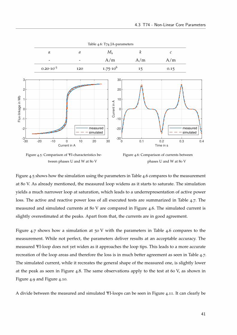
Table 4.6: T74 JA-parameters
α a Ms k c
- - A/m A/m A/m
0.20¨10-3
120 1.75¨106
15 0.15
-30 -20 -10 0 10 20 30
Current in A
-3
-2
-1
0
1
2
3
Flu
x-lin
ka
ge
in
Wb
measured
simulated
Figure 4.5: Comparison of ΨI-characteristics be-
tween phases U and W at 80 V
0 0.1 0.2 0.3 0.4
Time in s
-30
-20
-10
0
10
20
30
Cu
rre
nt
in A
measured
simulated
Figure 4.6: Comparison of currents between
phases U and W at 80 V
Figure 4.5 shows how the simulation using the parameters in Table 4.6 compares to the measurement
at 80 V. As already mentioned, the measured loop widens as it starts to saturate. The simulation
yields a much narrower loop at saturation, which leads to a underrepresentation of active power
loss. The active and reactive power loss of all executed tests are summarized in Table 4.7. The
measured and simulated currents at 80 V are compared in Figure 4.6. The simulated current is
slightly overestimated at the peaks. Apart from that, the currents are in good agreement.
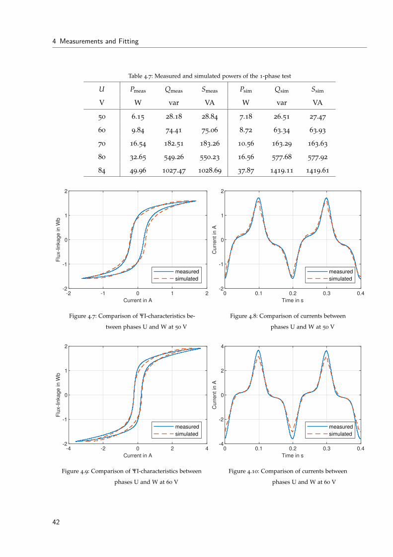
Figure 4.7 shows how a simulation at 50 V with the parameters in Table 4.6 compares to the
measurement. While not perfect, the parameters deliver results at an acceptable accuracy. The
measured ΨI-loop does not yet widen as it approaches the loop tips. This leads to a more accurate
recreation of the loop areas and therefore the loss is in much better agreement as seen in Table 4.7.
The simulated current, while it recreates the general shape of the measured one, is slightly lower
at the peak as seen in Figure 4.8. The same observations apply to the test at 60 V, as shown in
Figure 4.9 and Figure 4.10.
A divide between the measured and simulated ΨI-loops can be seen in Figure 4.11. It can clearly be
41
4 Measurements and Fitting
Table 4.7: Measured and simulated powers of the 1-phase test
U Pmeas Qmeas Smeas Psim Qsim Ssim
V W var VA W var VA
50 6.15 28.18 28.84 7.18 26.51 27.47
60 9.84 74.41 75.06 8.72 63.34 63.93
70 16.54 182.51 183.26 10.56 163.29 163.63
80 32.65 549.26 550.23 16.56 577.68 577.92
84 49.96 1027.47 1028.69 37.87 1419.11 1419.61
-2 -1 0 1 2
Current in A
-2
-1
0
1
2
Flu
x-lin
ka
ge
in
Wb
measured
simulated
Figure 4.7: Comparison of ΨI-characteristics be-
tween phases U and W at 50 V
0 0.1 0.2 0.3 0.4
Time in s
-2
-1
0
1
2
Cu
rre
nt
in A
measured
simulated
Figure 4.8: Comparison of currents between
phases U and W at 50 V
-4 -2 0 2 4
Current in A
-2
-1
0
1
2
Flu
x-lin
ka
ge
in
Wb
measured
simulated
Figure 4.9: Comparison of ΨI-characteristics between
phases U and W at 60 V
0 0.1 0.2 0.3 0.4
Time in s
-4
-2
0
2
4
Cu
rre
nt
in A
measured
simulated
Figure 4.10: Comparison of currents between
phases U and W at 60 V
42
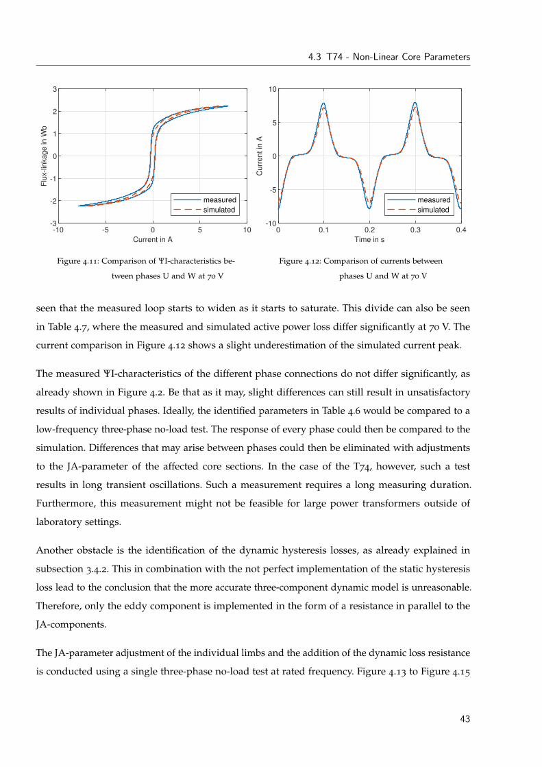
4.3 T74 - Non-Linear Core Parameters
-10 -5 0 5 10
Current in A
-3
-2
-1
0
1
2
3
Flu
x-lin
ka
ge
in
Wb
measured
simulated
Figure 4.11: Comparison of ΨI-characteristics be-
tween phases U and W at 70 V
0 0.1 0.2 0.3 0.4
Time in s
-10
-5
0
5
10
Cu
rre
nt
in A
measured
simulated
Figure 4.12: Comparison of currents between
phases U and W at 70 V
seen that the measured loop starts to widen as it starts to saturate. This divide can also be seen
in Table 4.7, where the measured and simulated active power loss differ significantly at 70 V. The
current comparison in Figure 4.12 shows a slight underestimation of the simulated current peak.
The measured ΨI-characteristics of the different phase connections do not differ significantly, as
already shown in Figure 4.2. Be that as it may, slight differences can still result in unsatisfactory
results of individual phases. Ideally, the identified parameters in Table 4.6 would be compared to a
low-frequency three-phase no-load test. The response of every phase could then be compared to the
simulation. Differences that may arise between phases could then be eliminated with adjustments
to the JA-parameter of the affected core sections. In the case of the T74, however, such a test
results in long transient oscillations. Such a measurement requires a long measuring duration.
Furthermore, this measurement might not be feasible for large power transformers outside of
laboratory settings.
Another obstacle is the identification of the dynamic hysteresis losses, as already explained in
subsection 3.4.2. This in combination with the not perfect implementation of the static hysteresis
loss lead to the conclusion that the more accurate three-component dynamic model is unreasonable.
Therefore, only the eddy component is implemented in the form of a resistance in parallel to the
JA-components.
The JA-parameter adjustment of the individual limbs and the addition of the dynamic loss resistance
is conducted using a single three-phase no-load test at rated frequency. Figure 4.13 to Figure 4.15
43
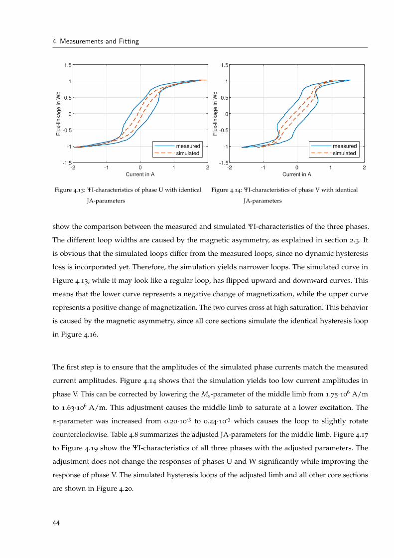
4 Measurements and Fitting
-2 -1 0 1 2
Current in A
-1.5
-1
-0.5
0
0.5
1
1.5
Flu
x-lin
kage in W
b
measured
simulated
Figure 4.13: ΨI-characteristics of phase U with identical
JA-parameters
-2 -1 0 1 2
Current in A
-1.5
-1
-0.5
0
0.5
1
1.5
Flu
x-lin
kage in W
b
measured
simulated
Figure 4.14: ΨI-characteristics of phase V with identical
JA-parameters
show the comparison between the measured and simulated ΨI-characteristics of the three phases.
The different loop widths are caused by the magnetic asymmetry, as explained in section 2.3. It
is obvious that the simulated loops differ from the measured loops, since no dynamic hysteresis
loss is incorporated yet. Therefore, the simulation yields narrower loops. The simulated curve in
Figure 4.13, while it may look like a regular loop, has flipped upward and downward curves. This
means that the lower curve represents a negative change of magnetization, while the upper curve
represents a positive change of magnetization. The two curves cross at high saturation. This behavior
is caused by the magnetic asymmetry, since all core sections simulate the identical hysteresis loop
in Figure 4.16.
The first step is to ensure that the amplitudes of the simulated phase currents match the measured
current amplitudes. Figure 4.14 shows that the simulation yields too low current amplitudes in
phase V. This can be corrected by lowering the Ms-parameter of the middle limb from 1.75¨106 A/m
to 1.63¨106 A/m. This adjustment causes the middle limb to saturate at a lower excitation. The
α-parameter was increased from 0.20¨10-3 to 0.24¨10
-3 which causes the loop to slightly rotate
counterclockwise. Table 4.8 summarizes the adjusted JA-parameters for the middle limb. Figure 4.17
to Figure 4.19 show the ΨI-characteristics of all three phases with the adjusted parameters. The
adjustment does not change the responses of phases U and W significantly while improving the
response of phase V. The simulated hysteresis loops of the adjusted limb and all other core sections
are shown in Figure 4.20.
44
4.3 T74 - Non-Linear Core Parameters
-2 -1 0 1 2
Current in A
-1.5
-1
-0.5
0
0.5
1
1.5
Flu
x-lin
kage in W
b
measured
simulated
Figure 4.15: ΨI-characteristics of phase W with identical
JA-parameters
-300 -200 -100 0 100 200 300
Magnetic field intensity in A/m
-2
-1
0
1
2
Magn
etic flu
x d
ensitiy
in T
Figure 4.16: Identical BH-characteristic of all core
elements
Table 4.8: Adjusted JA-parameters of the middle limb
α a Ms k c
- - A/m A/m A/m
0.24¨10-3
120 1.63¨106
15 0.15
-2 -1 0 1 2
Current in A
-1.5
-1
-0.5
0
0.5
1
1.5
Flu
x-lin
kage in W
b
measured
simulated
Figure 4.17: ΨI-characteristics of phase U with adjusted
JA-parameters
-2 -1 0 1 2
Current in A
-1.5
-1
-0.5
0
0.5
1
1.5
Flu
x-lin
kage in W
b
measured
simulated
Figure 4.18: ΨI-characteristics of phase V with adjusted
JA-parameters
45
4 Measurements and Fitting
-2 -1 0 1 2
Current in A
-1.5
-1
-0.5
0
0.5
1
1.5
Flu
x-lin
kage in W
b
measured
simulated
Figure 4.19: ΨI-characteristics of phase W with adjusted
JA-parameter
-400 -200 0 200 400
Magnetic field intensity in A/m
-2
-1
0
1
2
Magn
etic flu
x d
ensitiy
in T
original
modified
Figure 4.20: Original and modified BH-characteristics of
the middle limb
Table 4.9: Loss resistances of the core elements
Rlimb Ryoke
Ω Ω
2272 4219
The next step is the fitting of the dynamic losses. As already explained, the more simple two-
component dynamic hysteresis model is chosen, which can be derived using a single no-load
measurement at rated frequency and voltage. The dynamic loss is implemented by linear resistors in
parallel to every JA-element. The resistance is then fitted to match the simulated active power loss
to the measurements. The different lengths of limb and yoke elements lead to separate values for
each type of core section. The values of the loss resistances are summarized in Table 4.9. Figure 4.21
to Figure 4.23 show the comparisons of the measurements and the finalized simulation model. The
area of the simulated ΨI-characteristic of phase U is smaller than area of the measurement, while
the opposite is true for phase W. The differences balance each other out, leading to an accurate
reproduction of the total active loss. The results will be shown in more detail in chapter 5.
46
4.3 T74 - Non-Linear Core Parameters
-2 -1 0 1 2
Current in A
-1.5
-1
-0.5
0
0.5
1
1.5
Flu
x-lin
kage in W
b
measured
simulated
Figure 4.21: ΨI-characteristics of phase U with added
dynamic loss
-2 -1 0 1 2
Current in A
-1.5
-1
-0.5
0
0.5
1
1.5
Flu
x-lin
kage in W
bmeasured
simulated
Figure 4.22: ΨI-characteristics of phase V with added
dynamic loss
-2 -1 0 1 2
Current in A
-1.5
-1
-0.5
0
0.5
1
1.5
Flu
x-lin
kage in W
b
measured
simulated
Figure 4.23: ΨI-characteristics of phase W with added dynamic loss
47

5 Simulation Results T74
5.1 Short-Circuit Test
The short-circuit test was conducted on the low-voltage side with the high-voltage windings short-
circuited as seen in Figure 5.1. Figure 5.2 shows the supplied voltages of the measurement (solid
line) and the simulation (dashed line). The power-amplifier was not able to supply a jitter-free
sinusoidal voltage in this measurement setup. The measured voltage waveform, however, does not
deviate significantly from the simulated voltage. Figure 5.3 compares the measured short-circuit
currents (solid line) and the simulated currents (dashed line). The simulation yields slightly delayed
currents. The current in phase V is overestimated slightly by the simulation. This is caused by the
approach described in section 4.2, where the median short-circuit impedance is used for all phases.
The accuracy can be further increased by the implementation of separate short-circuit impedances
for the individual phases.
yn Yn
iu,sc
iv,sc
iw,sc
N N
uw,sc
uu,scuv,sc
LV HVT74
Figure 5.1: Short-circuit measurement setup
49
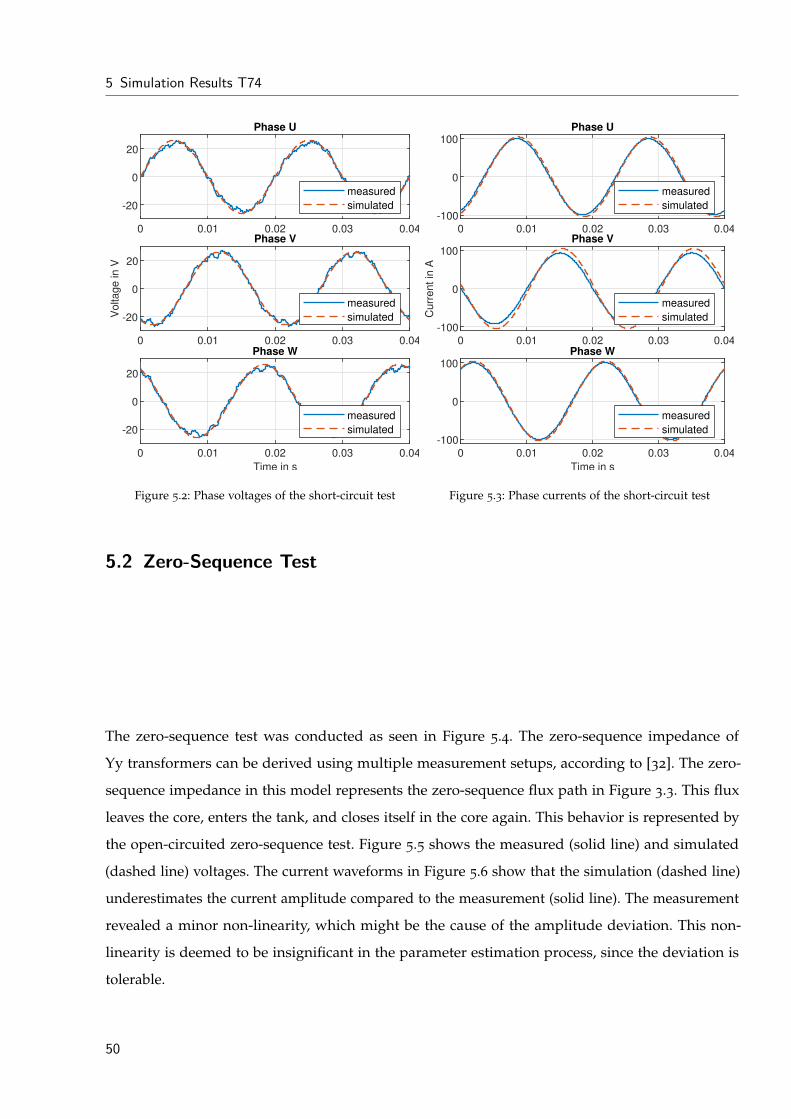
5 Simulation Results T74
0 0.01 0.02 0.03 0.04
-20
0
20
Phase U
measured
simulated
0 0.01 0.02 0.03 0.04
-20
0
20
Voltage in V
Phase V
measured
simulated
0 0.01 0.02 0.03 0.04
Time in s
-20
0
20
Phase W
measured
simulated
Figure 5.2: Phase voltages of the short-circuit test
0 0.01 0.02 0.03 0.04
-100
0
100
Phase U
measured
simulated
0 0.01 0.02 0.03 0.04
-100
0
100
Curr
ent in
A
Phase V
measured
simulated
0 0.01 0.02 0.03 0.04
Time in s
-100
0
100
Phase W
measured
simulated
Figure 5.3: Phase currents of the short-circuit test
5.2 Zero-Sequence Test
The zero-sequence test was conducted as seen in Figure 5.4. The zero-sequence impedance of
Yy transformers can be derived using multiple measurement setups, according to [32]. The zero-
sequence impedance in this model represents the zero-sequence flux path in Figure 3.3. This flux
leaves the core, enters the tank, and closes itself in the core again. This behavior is represented by
the open-circuited zero-sequence test. Figure 5.5 shows the measured (solid line) and simulated
(dashed line) voltages. The current waveforms in Figure 5.6 show that the simulation (dashed line)
underestimates the current amplitude compared to the measurement (solid line). The measurement
revealed a minor non-linearity, which might be the cause of the amplitude deviation. This non-
linearity is deemed to be insignificant in the parameter estimation process, since the deviation is
tolerable.
50
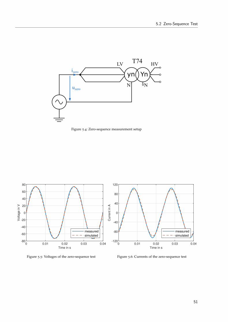
5.2 Zero-Sequence Test
yn Yn
N Nuzero
LV HVT74
izero
Figure 5.4: Zero-sequence measurement setup
0 0.01 0.02 0.03 0.04
Time in s
-80
-60
-40
-20
0
20
40
60
80
Voltage in V
measured
simulated
Figure 5.5: Voltages of the zero-sequence test
0 0.01 0.02 0.03 0.04
Time in s
-120
-80
-40
0
40
80
120
Curr
ent in
A
measured
simulated
Figure 5.6: Currents of the zero-sequence test
51
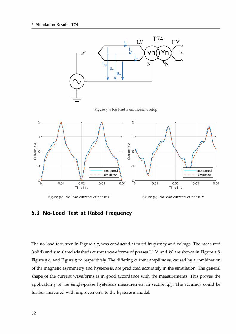
5 Simulation Results T74
yn Yn
iu
iv
iw
N N
uw
uuuv
LV HVT74
Figure 5.7: No-load measurement setup
0 0.01 0.02 0.03 0.04
Time in s
-2
-1
0
1
2
Curr
ent in
A
measured
simulated
Figure 5.8: No-load currents of phase U
0 0.01 0.02 0.03 0.04
Time in s
-2
-1
0
1
2
Curr
ent in
A
measured
simulated
Figure 5.9: No-load currents of phase V
5.3 No-Load Test at Rated Frequency
The no-load test, seen in Figure 5.7, was conducted at rated frequency and voltage. The measured
(solid) and simulated (dashed) current waveforms of phases U, V, and W are shown in Figure 5.8,
Figure 5.9, and Figure 5.10 respectively. The differing current amplitudes, caused by a combination
of the magnetic asymmetry and hysteresis, are predicted accurately in the simulation. The general
shape of the current waveforms is in good accordance with the measurements. This proves the
applicability of the single-phase hysteresis measurement in section 4.3. The accuracy could be
further increased with improvements to the hysteresis model.
52
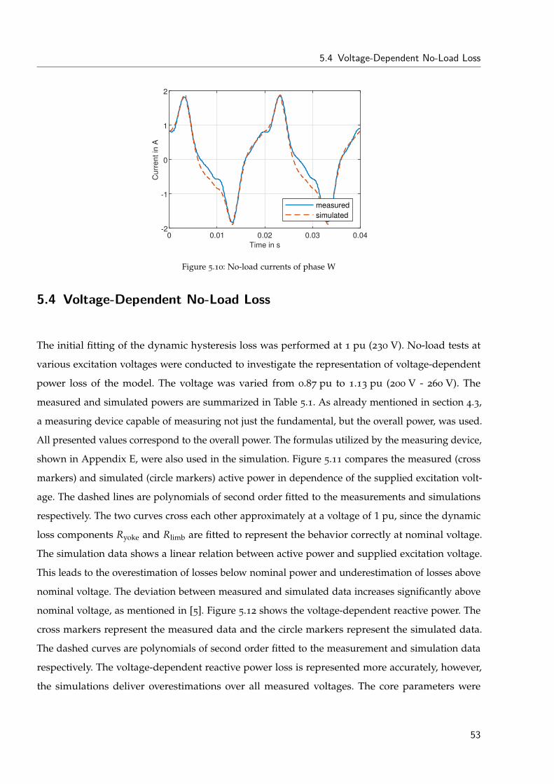
5.4 Voltage-Dependent No-Load Loss
0 0.01 0.02 0.03 0.04
Time in s
-2
-1
0
1
2
Curr
ent in
A
measured
simulated
Figure 5.10: No-load currents of phase W
5.4 Voltage-Dependent No-Load Loss
The initial fitting of the dynamic hysteresis loss was performed at 1 pu (230 V). No-load tests at
various excitation voltages were conducted to investigate the representation of voltage-dependent
power loss of the model. The voltage was varied from 0.87 pu to 1.13 pu (200 V - 260 V). The
measured and simulated powers are summarized in Table 5.1. As already mentioned in section 4.3,
a measuring device capable of measuring not just the fundamental, but the overall power, was used.
All presented values correspond to the overall power. The formulas utilized by the measuring device,
shown in Appendix E, were also used in the simulation. Figure 5.11 compares the measured (cross
markers) and simulated (circle markers) active power in dependence of the supplied excitation volt-
age. The dashed lines are polynomials of second order fitted to the measurements and simulations
respectively. The two curves cross each other approximately at a voltage of 1 pu, since the dynamic
loss components Ryoke and Rlimb are fitted to represent the behavior correctly at nominal voltage.
The simulation data shows a linear relation between active power and supplied excitation voltage.
This leads to the overestimation of losses below nominal power and underestimation of losses above
nominal voltage. The deviation between measured and simulated data increases significantly above
nominal voltage, as mentioned in [5]. Figure 5.12 shows the voltage-dependent reactive power. The
cross markers represent the measured data and the circle markers represent the simulated data.
The dashed curves are polynomials of second order fitted to the measurement and simulation data
respectively. The voltage-dependent reactive power loss is represented more accurately, however,
the simulations deliver overestimations over all measured voltages. The core parameters were
53
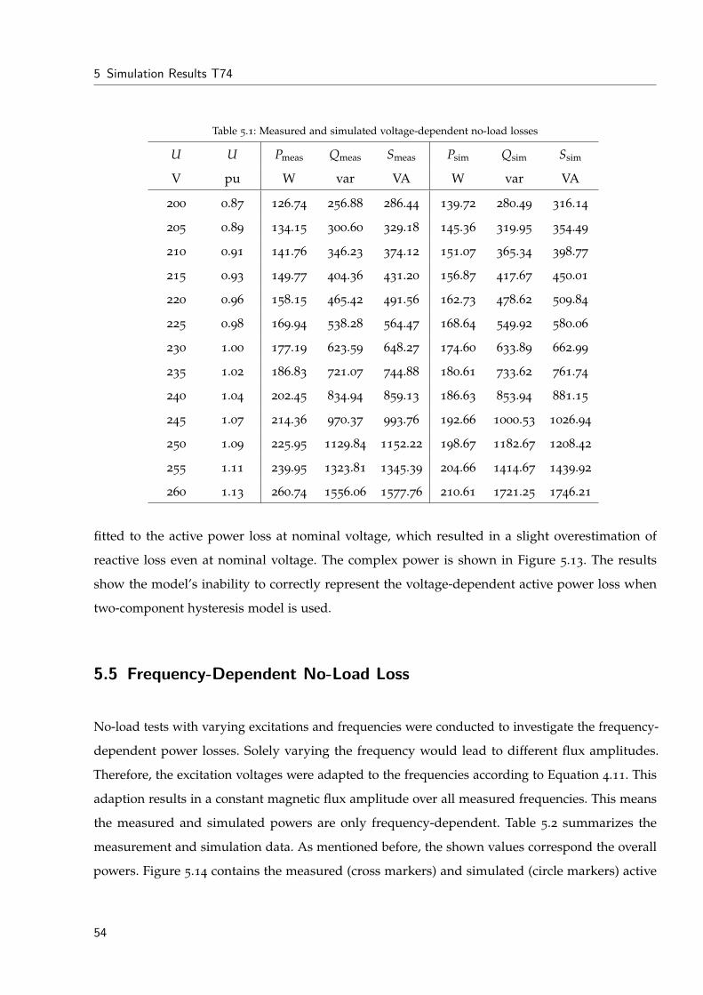
5 Simulation Results T74
Table 5.1: Measured and simulated voltage-dependent no-load losses
U U Pmeas Qmeas Smeas Psim Qsim Ssim
V pu W var VA W var VA
200 0.87 126.74 256.88 286.44 139.72 280.49 316.14
205 0.89 134.15 300.60 329.18 145.36 319.95 354.49
210 0.91 141.76 346.23 374.12 151.07 365.34 398.77
215 0.93 149.77 404.36 431.20 156.87 417.67 450.01
220 0.96 158.15 465.42 491.56 162.73 478.62 509.84
225 0.98 169.94 538.28 564.47 168.64 549.92 580.06
230 1.00 177.19 623.59 648.27 174.60 633.89 662.99
235 1.02 186.83 721.07 744.88 180.61 733.62 761.74
240 1.04 202.45 834.94 859.13 186.63 853.94 881.15
245 1.07 214.36 970.37 993.76 192.66 1000.53 1026.94
250 1.09 225.95 1129.84 1152.22 198.67 1182.67 1208.42
255 1.11 239.95 1323.81 1345.39 204.66 1414.67 1439.92
260 1.13 260.74 1556.06 1577.76 210.61 1721.25 1746.21
fitted to the active power loss at nominal voltage, which resulted in a slight overestimation of
reactive loss even at nominal voltage. The complex power is shown in Figure 5.13. The results
show the model’s inability to correctly represent the voltage-dependent active power loss when
two-component hysteresis model is used.
5.5 Frequency-Dependent No-Load Loss
No-load tests with varying excitations and frequencies were conducted to investigate the frequency-
dependent power losses. Solely varying the frequency would lead to different flux amplitudes.
Therefore, the excitation voltages were adapted to the frequencies according to Equation 4.11. This
adaption results in a constant magnetic flux amplitude over all measured frequencies. This means
the measured and simulated powers are only frequency-dependent. Table 5.2 summarizes the
measurement and simulation data. As mentioned before, the shown values correspond the overall
powers. Figure 5.14 contains the measured (cross markers) and simulated (circle markers) active
54
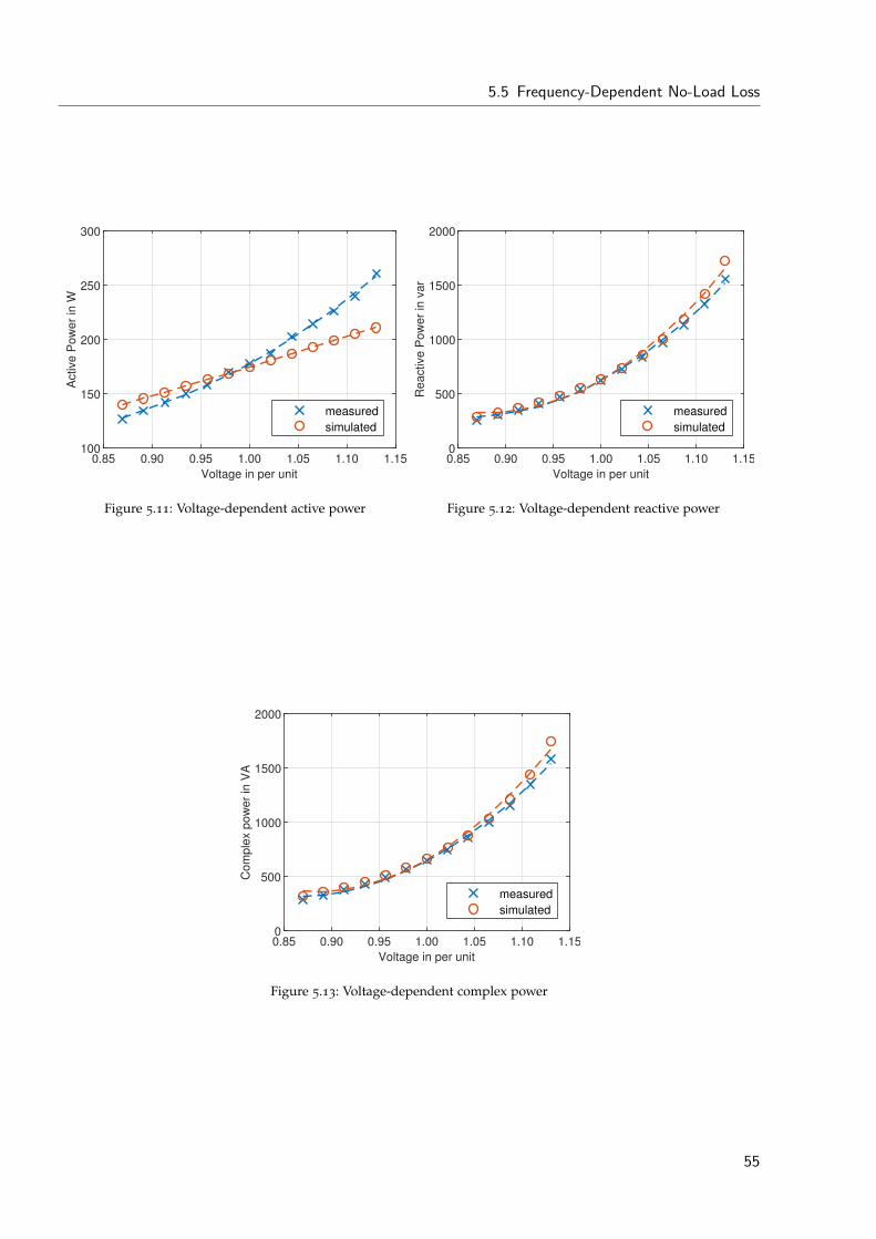
5.5 Frequency-Dependent No-Load Loss
0.85 0.90 0.95 1.00 1.05 1.10 1.15
Voltage in per unit
100
150
200
250
300
Active P
ow
er
in W
measured
simulated
Figure 5.11: Voltage-dependent active power
0.85 0.90 0.95 1.00 1.05 1.10 1.15
Voltage in per unit
0
500
1000
1500
2000
Reactive P
ow
er
in v
ar
measured
simulated
Figure 5.12: Voltage-dependent reactive power
0.85 0.90 0.95 1.00 1.05 1.10 1.15
Voltage in per unit
0
500
1000
1500
2000
Com
ple
x p
ow
er
in V
A
measured
simulated
Figure 5.13: Voltage-dependent complex power
55
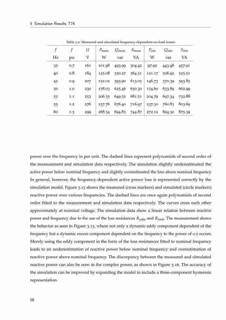
5 Simulation Results T74
Table 5.2: Measured and simulated frequency-dependent no-load losses
f f U Pmeas Qmeas Smeas Psim Qsim Ssim
Hz pu V W var VA W var VA
35 0.7 161 101.98 493.99 504.42 97.92 443.48 457.91
40 0.8 184 125.08 550.27 564.31 121.17 506.92 525.51
45 0.9 207 152.02 593.90 613.05 146.73 570.39 593.85
50 1.0 230 178.03 625.46 650.30 174.60 633.89 662.99
55 1.1 253 206.35 649.52 681.51 204.79 697.34 732.88
55 1.2 276 237.76 676.40 716.97 237.30 760.83 803.69
60 1.3 299 268.34 694.85 744.87 272.12 824.30 875.39
power over the frequency in per unit. The dashed lines represent polynomials of second order of
the measurement and simulation data respectively. The simulation slightly underestimated the
active power below nominal frequency and slightly overestimated the loss above nominal frequency.
In general, however, the frequency-dependent active power loss is represented correctly by the
simulation model. Figure 5.15 shows the measured (cross markers) and simulated (circle markers)
reactive power over various frequencies. The dashed lines are once again polynomials of second
order fitted to the measurement and simulation data respectively. The curves cross each other
approximately at nominal voltage. The simulation data show a linear relation between reactive
power and frequency due to the use of the loss resistances Ryoke and Rlimb. The measurement shows
the behavior as seen in Figure 3.15, where not only a dynamic eddy component dependent of the
frequency but a dynamic excess component dependent on the frequency to the power of 0.5 occurs.
Merely using the eddy component in the form of the loss resistances fitted to nominal frequency
leads to an underestimation of reactive power below nominal frequency and overestimation of
reactive power above nominal frequency. The discrepancy between the measured and simulated
reactive power can also be seen in the complex power, as shown in Figure 5.16. The accuracy of
the simulation can be improved by expanding the model to include a three-component hysteresis
representation.
56
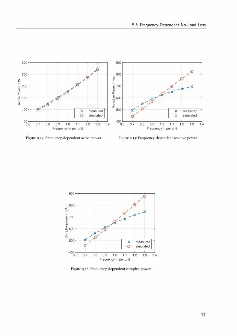
5.5 Frequency-Dependent No-Load Loss
0.6 0.7 0.8 0.9 1.0 1.1 1.2 1.3 1.4
Frequency in per unit
50
100
150
200
250
300
Active
Po
we
r in
W
measured
simulated
Figure 5.14: Frequency-dependent active power
0.6 0.7 0.8 0.9 1.0 1.1 1.2 1.3 1.4
Frequency in per unit
400
500
600
700
800
900
Re
active
Po
we
r in
va
rmeasured
simulated
Figure 5.15: Frequency-dependent reactive power
0.6 0.7 0.8 0.9 1.0 1.1 1.2 1.3 1.4
Frequency in per unit
400
500
600
700
800
900
Co
mp
lex p
ow
er
in V
A
measured
simulated
Figure 5.16: Frequency-dependent complex power
57
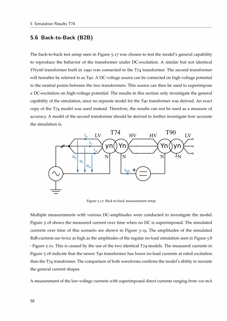
5 Simulation Results T74
5.6 Back-to-Back (B2B)
The back-to-back test setup seen in Figure 5.17 was chosen to test the model’s general capability
to reproduce the behavior of the transformer under DC-excitation. A similar but not identical
YNyn0 transformer built in 1990 was connected to the T74 transformer. The second transformer
will hereafter be referred to as T90. A DC-voltage source can be connected on high-voltage potential
to the neutral points between the two transformers. This source can then be used to superimpose
a DC-excitation on high-voltage potential. The results in this section only investigate the general
capability of the simulation, since no separate model for the T90 transformer was derived. An exact
copy of the T74 model was used instead. Therefore, the results can not be used as a measure of
accuracy. A model of the second transformer should be derived to further investigate how accurate
the simulation is.
yn Yn
iu
iv
iw
N N
uw
uuuv
LV HVT74
ynYn
NN
HVT90
LV
iDC
Figure 5.17: Back-to-back measurement setup
Multiple measurements with various DC-amplitudes were conducted to investigate the model.
Figure 5.18 shows the measured current over time when no DC is superimposed. The simulated
currents over time of this scenario are shown in Figure 5.19. The amplitudes of the simulated
B2B-currents are twice as high as the amplitudes of the regular no-load simulation seen in Figure 5.8
- Figure 5.10. This is caused by the use of the two identical T74-models. The measured currents in
Figure 5.18 indicate that the newer T90 transformer has lower no-load currents at rated excitation
than the T74 transformer. The comparison of both waveforms confirms the model’s ability to recreate
the general current shapes.
A measurement of the low-voltage currents with superimposed direct currents ranging from 100 mA
58
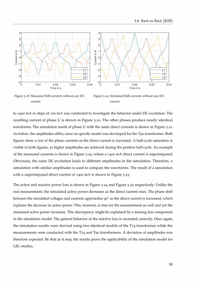
5.6 Back-to-Back (B2B)
0 0.01 0.02 0.03 0.04
Time in s
-4
-3
-2
-1
0
1
2
3
4
Curr
ent in
A
L1
L2
L3
Figure 5.18: Measured B2B-currents without any DC-
current
0 0.01 0.02 0.03 0.04
Time in s
-4
-3
-2
-1
0
1
2
3
4
Curr
ent in
A
L1
L2
L3
Figure 5.19: Simulated B2B-currents without any DC-
current
to 1900 mA in steps of 100 mA was conducted to investigate the behavior under DC-excitation. The
resulting current of phase U is shown in Figure 5.20. The other phases produce nearly identical
waveforms. The simulation result of phase U with the same direct currents is shown in Figure 5.21.
As before, the amplitudes differ, since no specific model was developed for the T90 transformer. Both
figures show a rise of the phase currents as the direct current is increased. A half-cycle saturation is
visible in both figures, as higher amplitudes are achieved during the positive half-cycle. An example
of the measured currents is shown in Figure 5.22, where a 1400 mA direct current is superimposed.
Obviously, the same DC-excitation leads to different amplitudes in the simulation. Therefore, a
simulation with similar amplitudes is used to compare the waveforms. The result of a simulation
with a superimposed direct current of 1900 mA is shown in Figure 5.23.
The active and reactive power loss is shown in Figure 5.24 and Figure 5.25 respectively. Unlike the
real measurement, the simulated active power decreases as the direct current rises. The phase shift
between the simulated voltages and currents approaches 90° as the direct current is increased, which
explains the decrease in active power. This, however, is true for the measurement as well and yet the
measured active power increases. This discrepancy might be explained by a missing loss component
in the simulation model. The general behavior of the reactive loss is recreated correctly. Once again,
the simulation results were derived using two identical models of the T74 transformer while the
measurements were conducted with the T74 and T90 transformers. A deviation of amplitudes was
therefore expected. Be that as it may, the results prove the applicability of the simulation model for
GIC-studies.
59
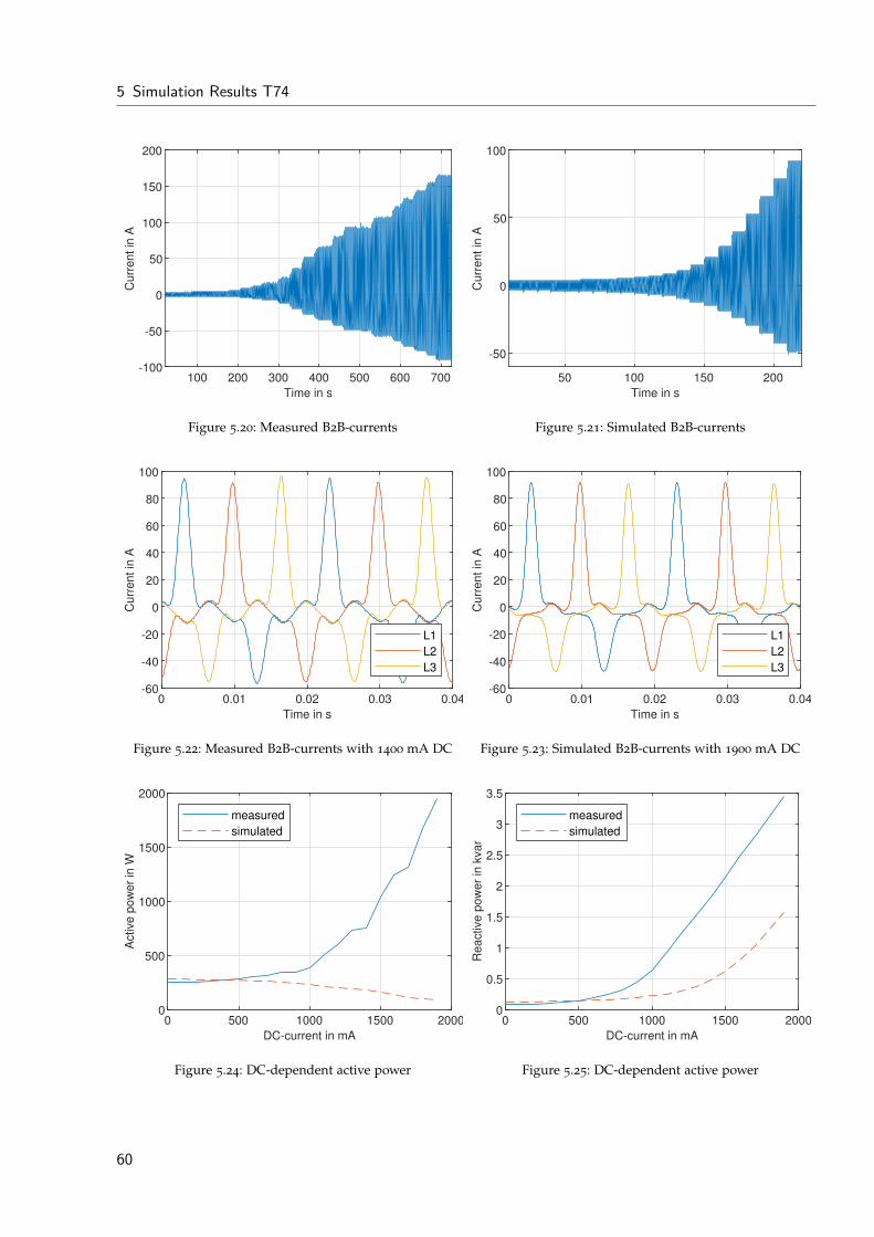
5 Simulation Results T74
100 200 300 400 500 600 700
Time in s
-100
-50
0
50
100
150
200
Curr
ent in
A
Figure 5.20: Measured B2B-currents
50 100 150 200
Time in s
-50
0
50
100
Curr
ent in
A
Figure 5.21: Simulated B2B-currents
0 0.01 0.02 0.03 0.04
Time in s
-60
-40
-20
0
20
40
60
80
100
Curr
ent in
A
L1
L2
L3
Figure 5.22: Measured B2B-currents with 1400 mA DC
0 0.01 0.02 0.03 0.04
Time in s
-60
-40
-20
0
20
40
60
80
100C
urr
ent in
A
L1
L2
L3
Figure 5.23: Simulated B2B-currents with 1900 mA DC
0 500 1000 1500 2000
DC-current in mA
0
500
1000
1500
2000
Active p
ow
er
in W
measured
simulated
Figure 5.24: DC-dependent active power
0 500 1000 1500 2000
DC-current in mA
0
0.5
1
1.5
2
2.5
3
3.5
Reactive p
ow
er
in k
var
measured
simulated
Figure 5.25: DC-dependent active power
60
6 Discussion and Outlook
On the development of the model
The classic way to model a transformer is the well-known single-phase equivalent T-model. This
model, however, lacks magnetic coupling [4] and is only valid in steady-state [3]. A transformer
model capable of reproducing low-frequency transients is derived in section 3.2. This model uses the
topologically correct duality-approach which converts the magnetic circuit of the transformer into
an equivalent electric circuit [15]. A model of a three-phase, three-limb, two-winding transformer is
derived in section 3.2. The same approach can be used to derive a five-limb transformer. A third
winding can be added with the approach shown in [37]. Therefore, the duality approach can be
applied to a multitude of transformer core and winding configurations.
The modeling of the iron core is addressed in section 3.3. The derived model in this thesis implements
a hysteresis model in the form of an inverse JA-model. The JA-model replicates the static hysteresis
loss. The dynamic hysteresis loss can be incorporated with a two- or more accurate three-component
approach, as seen in subsection 3.3.2. The model in this thesis uses the simpler two-component
model which is implemented with constant loss resistances in parallel to every JA core element.
Depending on the investigated low-frequency study, a static hysteresis model might not be necessary.
In such cases a simpler piecewise linear approximation can be used. [5] The importance of a dynamic
hysteresis model can depend on the investigated transient as well. However, the opinions on the
importance of dynamic hysteresis modeling are divided [5]. The lack of definite answers makes this
topic interesting for future research.
On the parameter derivation
The derivation of the linear parameters for the model of the T74 is straightforward, as seen in
section 4.2. The short-circuit and zero-sequence impedance can be derived by standard tests.
The more interesting measurements are associated with the identification of the non-linear core
61
6 Discussion and Outlook
loss. Two possible approaches are shown and explained in subsection 3.4.2. section 4.3 shows
the execution of the measurement and fitting process. It is shown that the behavior of the core
can be measured with a low-frequency sinusoidal voltage source. The measurement is possible
with portable measuring devices, since a lower frequency is accompanied with a lower voltage
amplitude [33]. The measurement returned a rather unusual looking characteristic as seen in
Figure 4.4. The loop widens as it starts to saturate. This makes the fitting of the parameters difficult,
since the JA-model was developed for sigmoid-shaped hysteresis loops [22]. The accuracy could be
improved by making the parameter k, which is responsible for the width of the loop, dependent
on the excitation. Such a modification is shown in [28]. Many modifications of the JA-model exist
that extend the model or improve the accuracy. One main goal of this thesis, however, was to
show the general applicability of the JA-model in the case of a three-limb transformer. A highly
accurate replication of the measurements was not a top priority. Therefore, a very basic version of
the JA-model is used. Nevertheless, the measurements and simulations are in good agreement. For
future research more time should be invested in a optimization procedure of the JA-parameters. A
fitting by hand is possible and can lead to acceptable results as shown in section 4.3, however, an
automated optimization procedure can drastically improve user-friendliness.
The same hysteresis measurement is not repeatable at higher frequencies to derive the dynamic
hysteresis loss components. The capacitive influence of the transformer at higher frequencies
significantly affects the shape of the measured hysteresis, rotating it counterclockwise. Therefore,
the dynamic loss components can not be fitted to the measured shape of the hysteresis. It is possible
to fit the parameters to no-load test data measured at different excitations and frequencies. Results
of these measurements are shown in chapter 5, however, such data might not be available and is
difficult to measure outside of laboratory settings. Therefore, the simpler two-component dynamic
model was used, which can be fitted to standard no-load test data.
On the simulation results
Various simulations and measurements of T74-transformer were compared in chapter 5. All phases
were assumed to be equal in the parameter derivation process. The design of transformers, which
also causes the magnetic asymmetry, leads to unavoidable differences between the phases. This is
seen in the comparison of the measured and simulated short-circuit test. The simulation returns a
slightly too high short-circuit current in phase V. This can easily be corrected by the implementation
of phase-specific short-circuit impedances. The difference between measured and simulated current,
62
however, is not significant enough to make this adjustment necessary.
The zero-sequence test can show a non-linear behavior in Yy-transformers as explained in the
standard [32]. The zero-sequence measurement of the T74-transformer does in fact show a slight
non-linearity. This is, however, insignificant and is therefore ignored in the parameter identification
process. The measurement confirms the assertion in [14], that the non-linearity can safely be
neglected.
The simulation over various voltages shows the inability of the two-component hysteresis model
to accurately represent the active power loss. The parallel loss resistance overestimates the active
loss below nominal voltage and underestimates it above nominal voltage. The reactive power is in
good accordance over a wide voltage range. The accuracy of the active power can be increased if
a three-component hysteresis model with an excitation-dependent excess loss component is used
instead.
The frequency-dependent no-load loss comparison shows that the model is able to reproduce the
active power over a wide frequency range. The reactive power, however, is underestimated below
and overestimated above nominal frequency. Again, a three-component hysteresis model is able to
represent the losses more accurately.
The general ability of the model to represent low-frequency transients was tested with a back-to-back
(B2B) test, which allows to superimpose direct currents. It is important to note that no simulation
model of the second transformer was derived. Instead, a one-to-one copy of the T74 model was
used. This obviously makes an evaluation of the simulation accuracy nonsensical. The results can,
however, show if the general transient response is reproduced correctly. The simulation model is
able to reproduce the general behavior as the results show. The only major discrepancy can be
seen in the measured active power. The simulated power slowly decreases as the direct current is
increased, while the measured active power rises. The cause for this is not known and requires
further research. Furthermore, a model of the second transformer should be derived in order to
assess the simulation accuracy.
On the implementation of the model
The model was implemented in Matlab Simulink 2019a. It was tested with the Simscape Electrical
library as well as the Specialized Power Systems library. Both libraries are suitable and delivered
63
6 Discussion and Outlook
identical results. However, the model implemented in Specialized Power Systems is prone to
instabilities. The use of the Simscape Electrical library is therefore recommended.
On the application in transmission grid simulations
The three-component hysteresis model gives a visible advantage when it comes to voltage- and
frequency-dependent loss representation. Some transient studies such as ferroresonance might even
require a detailed three-component model [5]. However, considering the required effort, such a
model is not feasible for transmission grid operators. It was shown that the hysteresis measurement
is not usable at higher frequencies due to the capacitive influence as the frequency rises. The
dynamic components can theoretically be fitted to loss measurements using various voltages and
frequencies. Such measurements are not technically feasible for large power transformers outside of
specialized laboratory settings. Datasheets usually provide no-load loss data at 90 %, 100 %, and
110 % of nominal voltage. This can be used to fit the excess component. The lack of frequency-
dependent data, however, makes the verification at different frequencies not possible. This means a
three-component dynamic model can hardly be implemented for already installed equipment. This
assessment leads back to the two-component model which can be implemented with considerably
less effort. This approach results in a massive improvement in accuracy over the classic single-phase
equivalent models at a reasonable cost. The only out of ordinary measurement is the hysteresis
measurement which can be measured in mere minutes using modern transformer testing utilities.
The two-component hysteresis model gives the most cost-effective results for transmission grid
operators.
64

Appendix
65

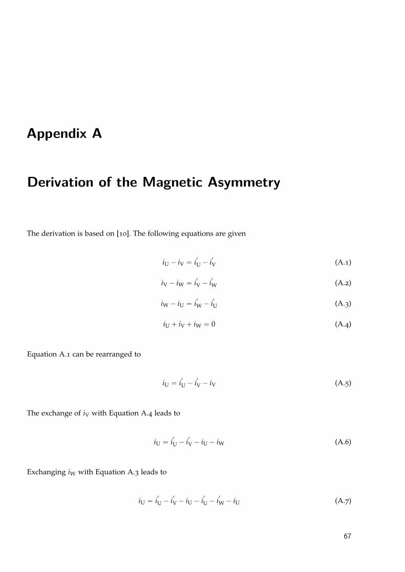
Appendix A
Derivation of the Magnetic Asymmetry
The derivation is based on [10]. The following equations are given
iU ´ iV “ i1
U ´ i1
V (A.1)
iV ´ iW “ i1
V ´ i1
W (A.2)
iW ´ iU “ i1
W ´ i1
U (A.3)
iU ` iV ` iW “ 0 (A.4)
Equation A.1 can be rearranged to
iU “ i1
U ´ i1
V ´ iV (A.5)
The exchange of iV with Equation A.4 leads to
iU “ i1
U ´ i1
V ´ iU ´ iW (A.6)
Exchanging iW with Equation A.3 leads to
iU “ i1
U ´ i1
V ´ iU ´ i1
U ´ i1
W ´ iU (A.7)
67

Appendix A Derivation of the Magnetic Asymmetry
Which can be rearranged to
3iU “ 2i1
U ´ i1
V ´ i1
W (A.8)
Adding and subtracting i1
U on the right side results in
3iU “ 3i1
U ´ i1
U ´ i1
V ´ i1
W (A.9)
Dividing both sides by three delivers the final form of the equation for the first phase
iU “ i1
U ´13pi
1
U ´ i1
V ´ i1
Wq (A.10)
68
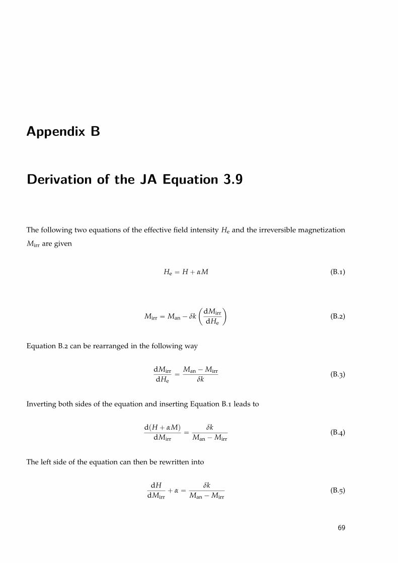
Appendix B
Derivation of the JA Equation 3.9
The following two equations of the effective field intensity He and the irreversible magnetization
Mirr are given
He “ H ` αM (B.1)
Mirr “ Man ´ δkˆ
dMirr
dHe
˙
(B.2)
Equation B.2 can be rearranged in the following way
dMirr
dHe“
Man ´Mirr
δk(B.3)
Inverting both sides of the equation and inserting Equation B.1 leads to
dpH ` αMqdMirr
“δk
Man ´Mirr(B.4)
The left side of the equation can then be rewritten into
dHdMirr
` α “δk
Man ´Mirr(B.5)
69

Appendix B Derivation of the JA Equation 3.9
Subtracting α on both sides and converting the right side of the equation to a common denominator
leads to
dHdMirr
“δk´ αpMan ´Mirrq
Man ´Mirr(B.6)
Inverting both sides leads to the final equation
dMirr
dH“
Man ´Mirr
δk´ αpMan ´Mirrq(B.7)
70
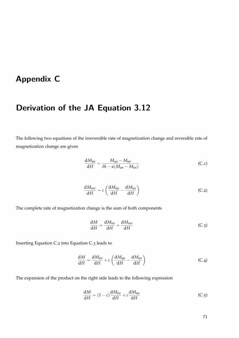
Appendix C
Derivation of the JA Equation 3.12
The following two equations of the irreversible rate of magnetization change and reversible rate of
magnetization change are given
dMirr
dH“
Man ´Mirr
δk´ αpMan ´Mirrq(C.1)
dMrev
dH“ c
ˆ
dMan
dH´
dMirr
dH
˙
(C.2)
The complete rate of magnetization change is the sum of both components
dMdH
“dMirr
dH`
dMrev
dH(C.3)
Inserting Equation C.2 into Equation C.3 leads to
dMdH
“dMirr
dH` c
ˆ
dMan
dH´
dMirr
dH
˙
(C.4)
The expansion of the product on the right side leads to the following expression
dMdH
“ p1´ cqdMirr
dH` c
dMan
dH(C.5)
71
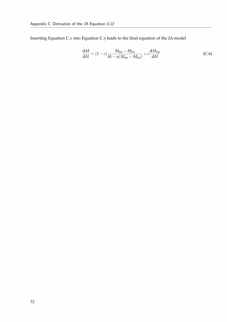
Appendix C Derivation of the JA Equation 3.12
Inserting Equation C.1 into Equation C.5 leads to the final equation of the JA-model
dMdH
“ p1´ cqMan ´Mirr
δk´ αpMan ´Mirrq` c
dMan
dH(C.6)
72
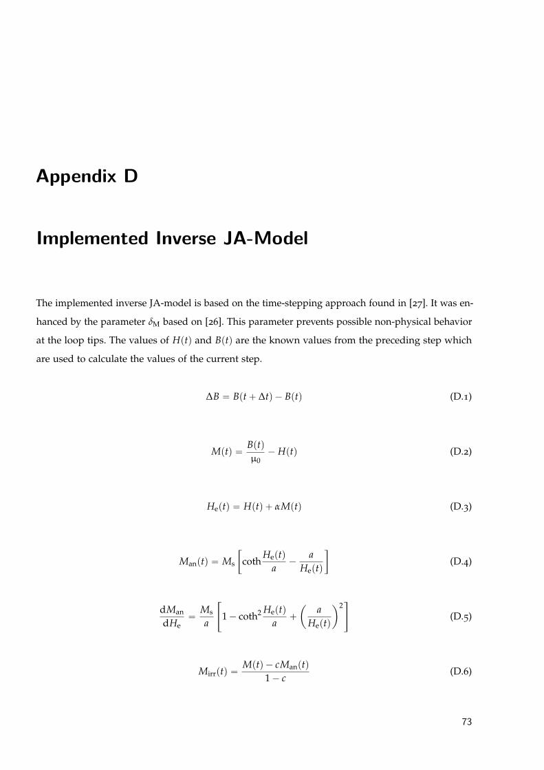
Appendix D
Implemented Inverse JA-Model
The implemented inverse JA-model is based on the time-stepping approach found in [27]. It was en-
hanced by the parameter δM based on [26]. This parameter prevents possible non-physical behavior
at the loop tips. The values of Hptq and Bptq are the known values from the preceding step which
are used to calculate the values of the current step.
∆B “ Bpt` ∆tq ´ Bptq (D.1)
Mptq “Bptqµ0
´ Hptq (D.2)
Heptq “ Hptq ` αMptq (D.3)
Manptq “ Ms
„
cothHeptq
a´
aHeptq
(D.4)
dMan
dHe“
Ms
a
«
1´ coth2 Heptqa
`
ˆ
aHeptq
˙2ff
(D.5)
Mirrptq “Mptq ´ cManptq
1´ c(D.6)
73
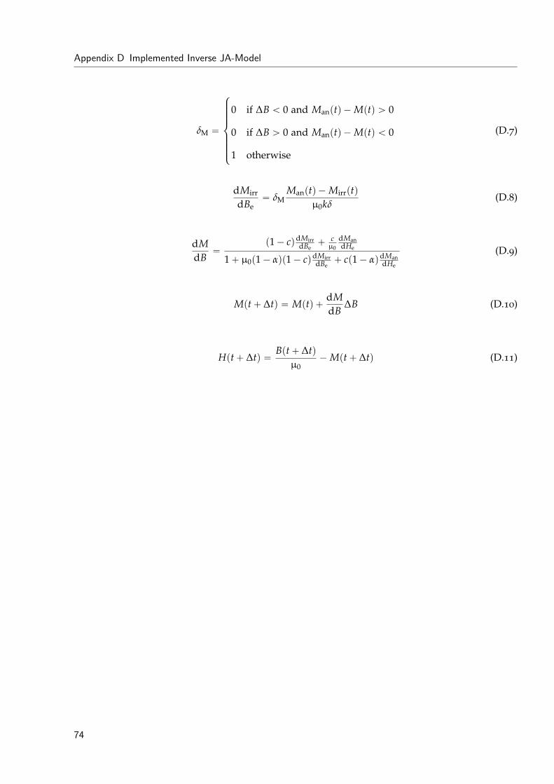
Appendix D Implemented Inverse JA-Model
δM “
$
’
’
’
’
’
&
’
’
’
’
’
%
0 if ∆B ă 0 and Manptq ´Mptq ą 0
0 if ∆B ą 0 and Manptq ´Mptq ă 0
1 otherwise
(D.7)
dMirr
dBe“ δM
Manptq ´Mirrptqµ0kδ
(D.8)
dMdB
“p1´ cqdMirr
dBe` c
µ0
dMandHe
1` µ0p1´ αqp1´ cqdMirrdBe
` cp1´ αqdMandHe
(D.9)
Mpt` ∆tq “ Mptq `dMdB
∆B (D.10)
Hpt` ∆tq “Bpt` ∆tq
µ0´Mpt` ∆tq (D.11)
74
Appendix E
Power Calculation
The following formulas show how the measuring device calculates the AC-power. The same ap-
proach was used to calculate the simulation data. The active power is calculated according to the
next formula
P “1N
Nÿ
n“0
urns ¨ irns (E.1)
The apparent power is calculated according to
S “ URMS ¨ IRMS (E.2)
The reactive power can then be calculated with
Q “a
S2 ´ P2 (E.3)
75

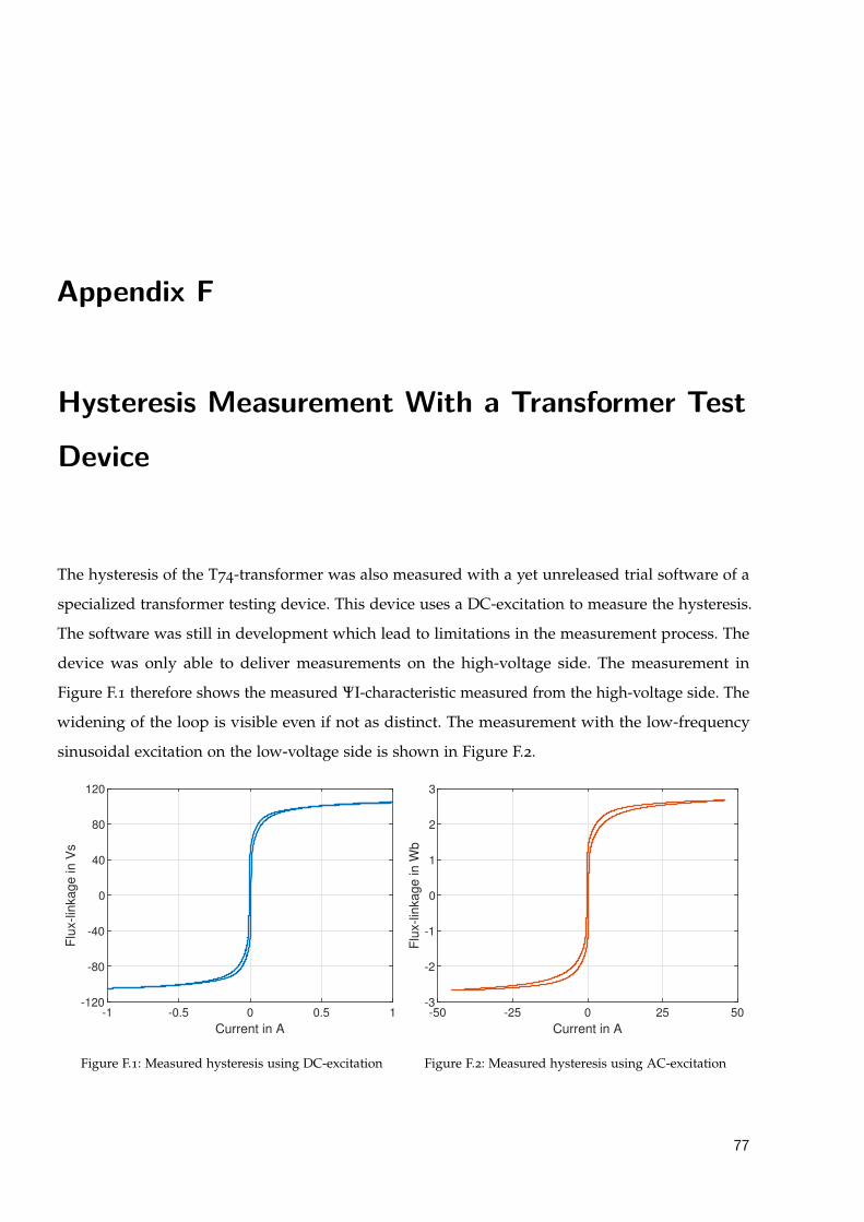
Appendix F
Hysteresis Measurement With a Transformer Test
Device
The hysteresis of the T74-transformer was also measured with a yet unreleased trial software of a
specialized transformer testing device. This device uses a DC-excitation to measure the hysteresis.
The software was still in development which lead to limitations in the measurement process. The
device was only able to deliver measurements on the high-voltage side. The measurement in
Figure F.1 therefore shows the measured ΨI-characteristic measured from the high-voltage side. The
widening of the loop is visible even if not as distinct. The measurement with the low-frequency
sinusoidal excitation on the low-voltage side is shown in Figure F.2.
-1 -0.5 0 0.5 1
Current in A
-120
-80
-40
0
40
80
120
Flu
x-lin
kage in V
s
Figure F.1: Measured hysteresis using DC-excitation
-50 -25 0 25 50
Current in A
-3
-2
-1
0
1
2
3
Flu
x-lin
kage in W
b
Figure F.2: Measured hysteresis using AC-excitation
77
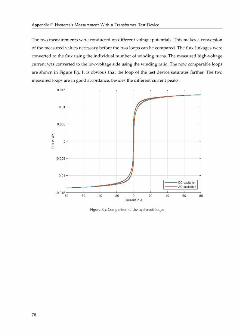
Appendix F Hysteresis Measurement With a Transformer Test Device
The two measurements were conducted on different voltage potentials. This makes a conversion
of the measured values necessary before the two loops can be compared. The flux-linkages were
converted to the flux using the individual number of winding turns. The measured high-voltage
current was converted to the low-voltage side using the winding ratio. The now comparable loops
are shown in Figure F.3. It is obvious that the loop of the test device saturates farther. The two
measured loops are in good accordance, besides the different current peaks.
-80 -60 -40 -20 0 20 40 60 80
Current in A
-0.015
-0.01
-0.005
0
0.005
0.01
0.015
Flu
x in W
b
DC-excitation
AC-excitation
Figure F.3: Comparison of the hysteresis loops
78
Appendix G
Conference Proceeding
Measurement based transformer modellingapproach
Dennis Albert, Dragan Maletic, and Herwig Renner
Internationaler ETG-Kongress 2021
Das Gesamtsystem im Fokus der Energiewende : 18.-19. Mai 2021
79
Messdaten basierte Modellierung von TransformatorenMeasurement based transformer modelling approach
Dennis Albert*, Dragan Maletic*, and Herwig RennerInstitute of Electrical Power Systems, Graz University of Technology, 8010 Graz, Austria, [email protected]
Kurzfassung
Die Modellierung von Transformatoren und deren Interaktion mit dem Stromnetz ist entscheidend für die Aufrechterhal-tung eines zuverlässigen und sicheren Stromnetzes. Allerdings sind die verfügbaren Transformatorendaten oft unvoll-ständig, fehlen oder sind nicht zugänglich. Bisher wurden verschiedene Ansätze zur Modellierung von Transformatorenmit unterschiedlichen Daten und Detaillierungsgraden veröffentlicht. Das Ziel unseres Ansatzes ist es, möglichst schnellund einfach ein Transformatormodell zu erstellen, um das Transformatorverhalten und die Netzinteraktion zu unter-suchen. Die erforderlichen Messungen können einfach im Feld oder im Umspannwerk durchgeführt werden. Die Mes-sungen werden zur Parameteridentifikation des Jiles-Atherton-Hysterese Modells verwendet. Der Modellansatz basiertauf dem Dualitätsprinzip, das den magnetischen Kreis in sein elektrisches Äquivalent transformiert. In dieser Arbeitdemonstrieren wir diesen Ansatz am Beispiel eines 3-phasigen 3-schenkligen 50 kVA Leistungstransformator. Die Sim-ulationen und Messung zeigen eine Übereinstimmung von mindestens 97 %. Daher kann dieser Ansatz in Industrie undForschung verwendet werden, um Transformatoren zu modellieren und deren Verhalten und Netzinteraktion zu unter-suchen.
Abstract
Modelling transformers and the power grid interaction is crucial to maintain a reliable and safe power grid. However,often the available transformer data is incomplete, missing or not accessible. Different approaches have been publishedfor modelling transformers with different amount of data and degree of detail. The aim of this approach is, to easilysetup a fast transformer model to study the transformer behaviour and grid interaction. The required measurements canbe done easily in the field or substation. The measurements are used to setup the Jiles-Atherton hysteretic model. Themodel approach is based on the duality principle, transforming the magnetic circuit into its electric equivalent. In thiswork we demonstrate this approach on a 3-phase 3-limb 2-winding 50 kVA power transformer. The correlation betweensimulation and measurement are at least 97 %. Therefore, this approach can be used in industry and research to modeltransformers and study their behaviour and grid interaction.
1 Introduction
Transformers are a key component in our electrical trans-mission grid. Transformer outages can affect a geograph-ically large area and can have a major economical impact[1]. To ensure a safe, reliable and quiet operation, digitaltransformer models are used to study the transformer be-haviour and the interaction with the power grid. Especiallythe reactive power consumption of the transformer is ofinterest during increased low frequency transformer neu-tral point current (LFC). LFC in the transformer neutralpoint current can be caused by geomagnetically inducedcurrents (GIC) or man-made systems, such as DC trans-portation systems [2, 3]. These LFC can cause transformerhalf-cycle saturation. During the saturation of the trans-former the reactive power demand increases [4]. If the re-active power demand of a large number of transformer inthe power grid take place at the same time, voltage insta-bility or even outages need to be considered. Transformer
*The authors are equally contributing and are mentioned in alphabeticorder
models are used to study the interaction between the in-stalled transformer with the power grid. However, thesemodels often require detailed information about the trans-former under investigation, which are not always available[5]. Also the computational power required for transformermodels increases with the level of detail. Therefore, sim-ulations with many transformer models are time and com-putational power consuming.In this work we describe a new approach to set up an elec-tromagnetic model of a power transformer, which also re-quires low computational power and time. The approachuses measurements and basic information about the trans-former. The model is based on the duality transforma-tion [6] and uses the Jiles-Atherton (JA) model [8] for thehysteresis implementation. The duality principle is usedto transform the magnetic circuit into its equivalent elec-tric circuit, using commonly known electric components.Thus, the magnetic field strength and magnetic flux canbe easily calculated and assessed in the simulation withcurrent and voltage measurements. The JA model is com-monly used in electrical power engineering, because it re-
ETG-Kongress 2021 . ISBN 978-3-8007-5549-3 . ©VDE VERLAG GMBH . Berlin . Offenbach
578
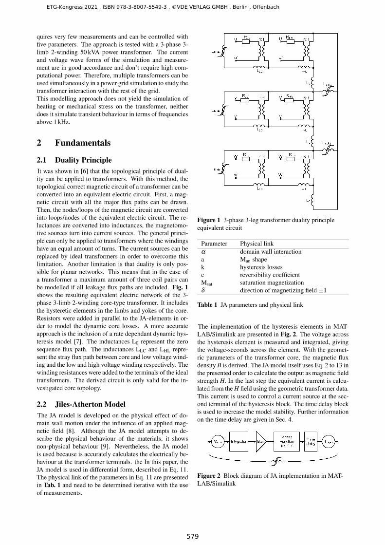
quires very few measurements and can be controlled withfive parameters. The approach is tested with a 3-phase 3-limb 2-winding 50 kVA power transformer. The currentand voltage wave forms of the simulation and measure-ment are in good accordance and don’t require high com-putational power. Therefore, multiple transformers can beused simultaneously in a power grid simulation to study thetransformer interaction with the rest of the grid.This modelling approach does not yield the simulation ofheating or mechanical stress on the transformer, neitherdoes it simulate transient behaviour in terms of frequenciesabove 1 kHz.
2 Fundamentals
2.1 Duality PrincipleIt was shown in [6] that the topological principle of dual-ity can be applied to transformers. With this method, thetopological correct magnetic circuit of a transformer can beconverted into an equivalent electric circuit. First, a mag-netic circuit with all the major flux paths can be drawn.Then, the nodes/loops of the magnetic circuit are convertedinto loops/nodes of the equivalent electric circuit. The re-luctances are converted into inductances, the magnetomo-tive sources turn into current sources. The general princi-ple can only be applied to transformers where the windingshave an equal amount of turns. The current sources can bereplaced by ideal transformers in order to overcome thislimitation. Another limitation is that duality is only pos-sible for planar networks. This means that in the case ofa transformer a maximum amount of three coil pairs canbe modelled if all leakage flux paths are included. Fig. 1shows the resulting equivalent electric network of the 3-phase 3-limb 2-winding core-type transformer. It includesthe hysteretic elements in the limbs and yokes of the core.Resistors were added in parallel to the JA-elements in or-der to model the dynamic core losses. A more accurateapproach is the inclusion of a rate dependant dynamic hys-teresis model [7]. The inductances L0 represent the zerosequence flux path. The inductances LLC and LHL repre-sent the stray flux path between core and low voltage wind-ing and the low and high voltage winding respectively. Thewinding resistances were added to the terminals of the idealtransformers. The derived circuit is only valid for the in-vestigated core topology.
2.2 Jiles-Atherton ModelThe JA model is developed on the physical effect of do-main wall motion under the influence of an applied mag-netic field [8]. Although the JA model attempts to de-scribe the physical behaviour of the materials, it showsnon-physical behaviour [9]. Nevertheless, the JA modelis used because is accurately calculates the electrically be-haviour at the transformer terminals. the In this paper, theJA model is used in differential form, described in Eq. 11.The physical link of the parameters in Eq. 11 are presentedin Tab. 1 and need to be determined iterative with the useof measurements.
Figure 1 3-phase 3-leg transformer duality principleequivalent circuit
Parameter Physical linkα domain wall interactiona Man shapek hysteresis lossesc reversibility coefficientMsat saturation magnetizationδ direction of magnetizing field ±1
Table 1 JA parameters and physical link
The implementation of the hysteresis elements in MAT-LAB/Simulink are presented in Fig. 2. The voltage acrossthe hysteresis element is measured and integrated, givingthe voltage-seconds across the element. With the geomet-ric parameters of the transformer core, the magnetic fluxdensity B is derived. The JA model itself uses Eq. 2 to 13 inthe presented order to calculate the output as magnetic fieldstrength H. In the last step the equivalent current is calcu-lated from the H field using the geometric transformer data.This current is used to control a current source at the sec-ond terminal of the hysteresis block. The time delay blockis used to increase the model stability. Further informationon the time delay are given in Sec. 4.
Figure 2 Block diagram of JA implementation in MAT-LAB/Simulink
ETG-Kongress 2021 . ISBN 978-3-8007-5549-3 . ©VDE VERLAG GMBH . Berlin . Offenbach
579
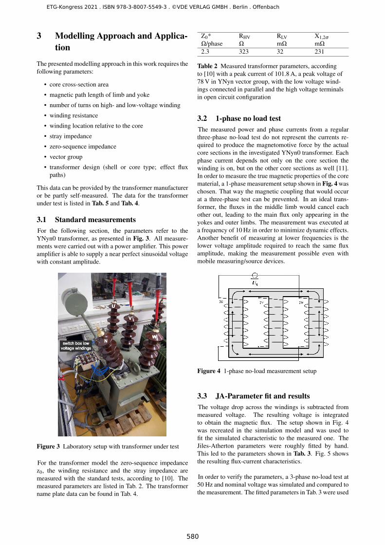
3 Modelling Approach and Applica-tion
The presented modelling approach in this work requires thefollowing parameters:
• core cross-section area
• magnetic path length of limb and yoke
• number of turns on high- and low-voltage winding
• winding resistance
• winding location relative to the core
• stray impedance
• zero-sequence impedance
• vector group
• transformer design (shell or core type; effect fluxpaths)
This data can be provided by the transformer manufactureror be partly self-measured. The data for the transformerunder test is listed in Tab. 5 and Tab. 4.
3.1 Standard measurementsFor the following section, the parameters refer to theYNyn0 transformer, as presented in Fig. 3. All measure-ments were carried out with a power amplifier. This poweramplifier is able to supply a near perfect sinusoidal voltagewith constant amplitude.
switch box lowvoltage windings
W
V
U
N
Figure 3 Laboratory setup with transformer under test
For the transformer model the zero-sequence impedancez0, the winding resistance and the stray impedance aremeasured with the standard tests, according to [10]. Themeasured parameters are listed in Tab. 2. The transformername plate data can be found in Tab. 4.
Z0* RHV RLV X1,2σΩ/phase Ω mΩ mΩ2.3 323 32 231
Table 2 Measured transformer parameters, accordingto [10] with a peak current of 101.8 A, a peak voltage of78 V in YNyn vector group, with the low voltage wind-ings connected in parallel and the high voltage terminalsin open circuit configuration
3.2 1-phase no load testThe measured power and phase currents from a regularthree-phase no-load test do not represent the currents re-quired to produce the magnetomotive force by the actualcore sections in the investigated YNyn0 transformer. Eachphase current depends not only on the core section thewinding is on, but on the other core sections as well [11].In order to measure the true magnetic properties of the corematerial, a 1-phase measurement setup shown in Fig. 4 waschosen. That way the magnetic coupling that would occurat a three-phase test can be prevented. In an ideal trans-former, the fluxes in the middle limb would cancel eachother out, leading to the main flux only appearing in theyokes and outer limbs. The measurement was executed ata frequency of 10 Hz in order to minimize dynamic effects.Another benefit of measuring at lower frequencies is thelower voltage amplitude required to reach the same fluxamplitude, making the measurement possible even withmobile measuring/source devices.
Figure 4 1-phase no-load measurement setup
3.3 JA-Parameter fit and resultsThe voltage drop across the windings is subtracted frommeasured voltage. The resulting voltage is integratedto obtain the magnetic flux. The setup shown in Fig. 4was recreated in the simulation model and was used tofit the simulated characteristic to the measured one. TheJiles-Atherton parameters were roughly fitted by hand.This led to the parameters shown in Tab. 3. Fig. 5 showsthe resulting flux-current characteristics.
In order to verify the parameters, a 3-phase no-load test at50 Hz and nominal voltage was simulated and compared tothe measurement. The fitted parameters in Tab. 3 were used
ETG-Kongress 2021 . ISBN 978-3-8007-5549-3 . ©VDE VERLAG GMBH . Berlin . Offenbach
580
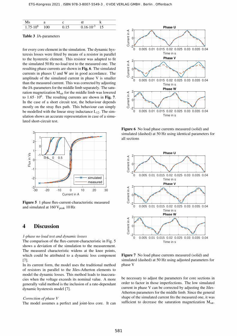
Ms a c α k1.75·106 100 0.15 0.16·10-3 15
Table 3 JA-parameters
for every core element in the simulation. The dynamic hys-teresis losses were fitted by means of a resistor in parallelto the hysteretic element. This resistor was adapted to fitthe simulated 50 Hz no-load test to the measured one. Theresulting phase currents are shown in Fig. 6. The simulatedcurrents in phases U and W are in good accordance. Theamplitude of the simulated current in phase V is smallerthan the measured current. This was corrected by adjustingthe JA-parameters for the middle limb separately. The satu-ration magnetization Msat for the middle limb was loweredto 1.65 · 106. The resulting currents are shown in Fig. 7.In the case of a short circuit test, the behaviour dependsmostly on the stray flux path. This behaviour can simplybe modelled with the linear stray inductance L12. The sim-ulation shows an accurate representation in case of a simu-lated short-circuit test.
-30 -20 -10 0 10 20 30
Current in A
-3
-2
-1
0
1
2
3
Flu
x in V
s
simulated
measured
-0.5 0 0.5-1
0
1
Figure 5 1 phase flux-current-characteristic measuredand simulated at 160 Vpeak 10 Hz
4 Discussion
1-phase no load test and dynamic lossesThe comparison of the flux-current-characteristic in Fig. 5shows a deviation of the simulation to the measurement.The measured characteristic widens at the knee points,which could be attributed to a dynamic loss component[7].In its current form, the model uses the traditional methodof resistors in parallel to the Jiles-Atherton elements tomodel the dynamic losses. This method leads to inaccura-cies when the voltage exceeds its nominal value. A moregenerally valid method is the inclusion of a rate-dependantdynamic hysteresis model [7].
Correction of phase VThe model assumes a perfect and joint-less core. It can
0 0.005 0.01 0.015 0.02 0.025 0.03 0.035 0.04
Time in s
-2
0
2
Curr
ent in
A
Phase U
0 0.005 0.01 0.015 0.02 0.025 0.03 0.035 0.04
Time in s
-2
0
2
Curr
ent in
A
Phase V
0 0.005 0.01 0.015 0.02 0.025 0.03 0.035 0.04
Time in s
-2
0
2
Curr
ent in
A
Phase W
Figure 6 No load phase currents measured (solid) andsimulated (dashed) at 50 Hz using identical parameters forall sections
0 0.005 0.01 0.015 0.02 0.025 0.03 0.035 0.04Time in s
-2
0
2
Cur
rent
in A
Phase U
0 0.005 0.01 0.015 0.02 0.025 0.03 0.035 0.04Time in s
-2
0
2
Cur
rent
in A
Phase V
0 0.005 0.01 0.015 0.02 0.025 0.03 0.035 0.04Time in s
-2
0
2
Cur
rent
in A
Phase W
Figure 7 No load phase currents measured (solid) andsimulated (dashed) at 50 Hz using adjusted parameters forphase V
be necessary to adjust the parameters for core sections inorder to factor in those imperfections. The low simulatedcurrent in phase V can be corrected by adjusting the Jiles-Atherton parameters for the middle limb. Since the generalshape of the simulated current fits the measured one, it wassufficient to decrease the saturation magnetization Msat.
ETG-Kongress 2021 . ISBN 978-3-8007-5549-3 . ©VDE VERLAG GMBH . Berlin . Offenbach
581
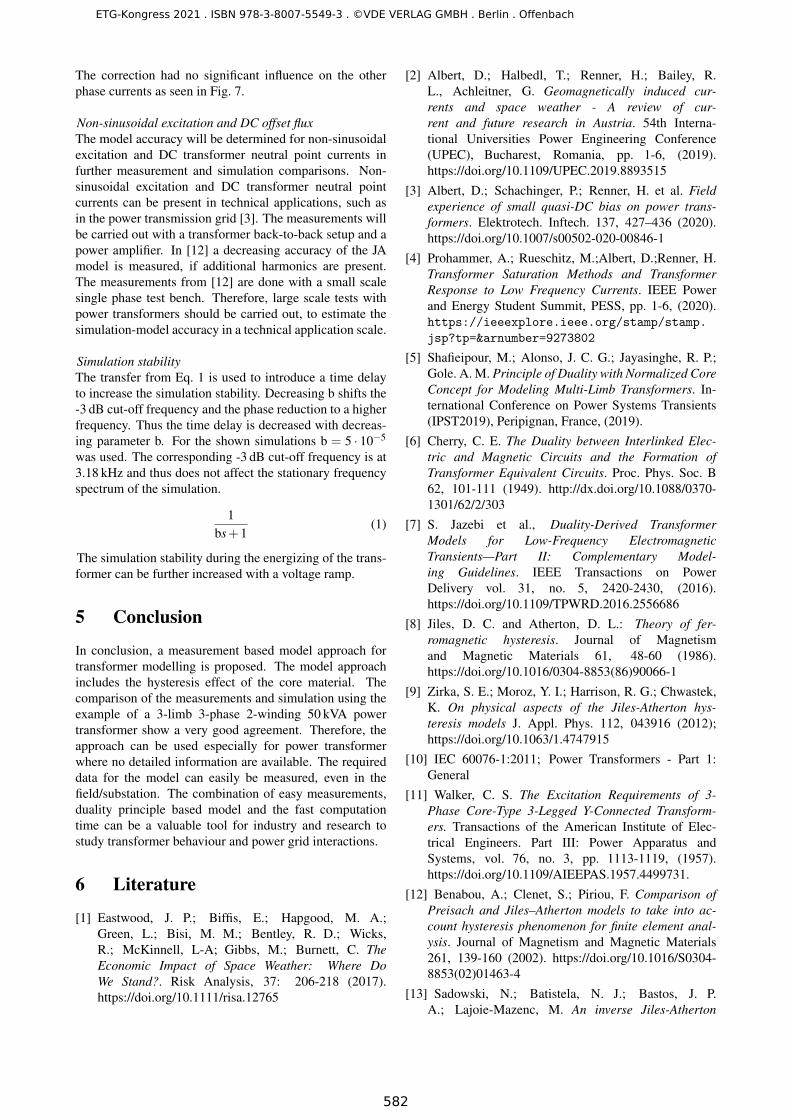
The correction had no significant influence on the otherphase currents as seen in Fig. 7.
Non-sinusoidal excitation and DC offset fluxThe model accuracy will be determined for non-sinusoidalexcitation and DC transformer neutral point currents infurther measurement and simulation comparisons. Non-sinusoidal excitation and DC transformer neutral pointcurrents can be present in technical applications, such asin the power transmission grid [3]. The measurements willbe carried out with a transformer back-to-back setup and apower amplifier. In [12] a decreasing accuracy of the JAmodel is measured, if additional harmonics are present.The measurements from [12] are done with a small scalesingle phase test bench. Therefore, large scale tests withpower transformers should be carried out, to estimate thesimulation-model accuracy in a technical application scale.
Simulation stabilityThe transfer from Eq. 1 is used to introduce a time delayto increase the simulation stability. Decreasing b shifts the-3 dB cut-off frequency and the phase reduction to a higherfrequency. Thus the time delay is decreased with decreas-ing parameter b. For the shown simulations b = 5 · 10−5
was used. The corresponding -3 dB cut-off frequency is at3.18 kHz and thus does not affect the stationary frequencyspectrum of the simulation.
1bs+1
(1)
The simulation stability during the energizing of the trans-former can be further increased with a voltage ramp.
5 Conclusion
In conclusion, a measurement based model approach fortransformer modelling is proposed. The model approachincludes the hysteresis effect of the core material. Thecomparison of the measurements and simulation using theexample of a 3-limb 3-phase 2-winding 50 kVA powertransformer show a very good agreement. Therefore, theapproach can be used especially for power transformerwhere no detailed information are available. The requireddata for the model can easily be measured, even in thefield/substation. The combination of easy measurements,duality principle based model and the fast computationtime can be a valuable tool for industry and research tostudy transformer behaviour and power grid interactions.
6 Literature
[1] Eastwood, J. P.; Biffis, E.; Hapgood, M. A.;Green, L.; Bisi, M. M.; Bentley, R. D.; Wicks,R.; McKinnell, L-A; Gibbs, M.; Burnett, C. TheEconomic Impact of Space Weather: Where DoWe Stand?. Risk Analysis, 37: 206-218 (2017).https://doi.org/10.1111/risa.12765
[2] Albert, D.; Halbedl, T.; Renner, H.; Bailey, R.L., Achleitner, G. Geomagnetically induced cur-rents and space weather - A review of cur-rent and future research in Austria. 54th Interna-tional Universities Power Engineering Conference(UPEC), Bucharest, Romania, pp. 1-6, (2019).https://doi.org/10.1109/UPEC.2019.8893515
[3] Albert, D.; Schachinger, P.; Renner, H. et al. Fieldexperience of small quasi-DC bias on power trans-formers. Elektrotech. Inftech. 137, 427–436 (2020).https://doi.org/10.1007/s00502-020-00846-1
[4] Prohammer, A.; Rueschitz, M.;Albert, D.;Renner, H.Transformer Saturation Methods and TransformerResponse to Low Frequency Currents. IEEE Powerand Energy Student Summit, PESS, pp. 1-6, (2020).https://ieeexplore.ieee.org/stamp/stamp.jsp?tp=&arnumber=9273802
[5] Shafieipour, M.; Alonso, J. C. G.; Jayasinghe, R. P.;Gole. A. M. Principle of Duality with Normalized CoreConcept for Modeling Multi-Limb Transformers. In-ternational Conference on Power Systems Transients(IPST2019), Peripignan, France, (2019).
[6] Cherry, C. E. The Duality between Interlinked Elec-tric and Magnetic Circuits and the Formation ofTransformer Equivalent Circuits. Proc. Phys. Soc. B62, 101-111 (1949). http://dx.doi.org/10.1088/0370-1301/62/2/303
[7] S. Jazebi et al., Duality-Derived TransformerModels for Low-Frequency ElectromagneticTransients—Part II: Complementary Model-ing Guidelines. IEEE Transactions on PowerDelivery vol. 31, no. 5, 2420-2430, (2016).https://doi.org/10.1109/TPWRD.2016.2556686
[8] Jiles, D. C. and Atherton, D. L.: Theory of fer-romagnetic hysteresis. Journal of Magnetismand Magnetic Materials 61, 48-60 (1986).https://doi.org/10.1016/0304-8853(86)90066-1
[9] Zirka, S. E.; Moroz, Y. I.; Harrison, R. G.; Chwastek,K. On physical aspects of the Jiles-Atherton hys-teresis models J. Appl. Phys. 112, 043916 (2012);https://doi.org/10.1063/1.4747915
[10] IEC 60076-1:2011; Power Transformers - Part 1:General
[11] Walker, C. S. The Excitation Requirements of 3-Phase Core-Type 3-Legged Y-Connected Transform-ers. Transactions of the American Institute of Elec-trical Engineers. Part III: Power Apparatus andSystems, vol. 76, no. 3, pp. 1113-1119, (1957).https://doi.org/10.1109/AIEEPAS.1957.4499731.
[12] Benabou, A.; Clenet, S.; Piriou, F. Comparison ofPreisach and Jiles–Atherton models to take into ac-count hysteresis phenomenon for finite element anal-ysis. Journal of Magnetism and Magnetic Materials261, 139-160 (2002). https://doi.org/10.1016/S0304-8853(02)01463-4
[13] Sadowski, N.; Batistela, N. J.; Bastos, J. P.A.; Lajoie-Mazenc, M. An inverse Jiles-Atherton
ETG-Kongress 2021 . ISBN 978-3-8007-5549-3 . ©VDE VERLAG GMBH . Berlin . Offenbach
582
model to take into account hysteresis in time-stepping finite-element calculations IEEE Transac-tions on Magnetics, vol. 38, no. 2, pp. 797-800, (2002).https://doi.org/10.1109/20.996206
[14] Jiles, D. C.; Thoelke, J. B.; Devine, M. K. Nu-merical determination of hysteresis parameters forthe modeling of magnetic properties using the the-ory of ferromagnetic hysteresis IEEE Transactionson Magnetics, vol. 28, no. 1, pp. 27-35, (1992)https://doi.org/10.1109/20.119813
[15] Deane, J. H. B. Modeling the dynamics of non-linear inductor circuits IEEE Transactions on Mag-netics, vol. 30, no. 5, pp. 2795-2801, (1994).https://doi.org/10.1109/20.312521
Appendix
Zref U1 U2 SkΩ kV kV kVA15.7 28 0.4 50
Table 4 Name plate of transformer under test
Tab. 5 lists the geometric data of the transformer under test.The dimensions were measured during the modification ofthe low voltage windings. Acore is the uniform core cross-section area of the yoke and limb. N1 and N2 are the num-ber of turns of the high-voltage and low- voltage winding,respectively. The yoke length lyoke and limb length llimb arethe middle iron path of the yoke and limb.
Acore N1 N2 lyoke llimbmm² mm mm6001 7730 102 237 440
Table 5 Geometric data of transformer
The original Jiles-Atherton model uses the magneticfield H as an input to calculate the magnetization M. Inthis model an inverse Jiles-Atherton model was used,with the magnetic flux density B as an input and themagnetization M as an output. The hysteretic elements usea calculation based on [13]. This method can however leadto unphysical solutions at the loop tips [14]. To overcomethis behaviour the parameter δ M calculated in Eq. 9 wasadded to Eq. 10. This parameter is based on [15] and wasadapted to fit the inverese Jiles-Atherton model.
Eq. 2 to 13 define the calculation in the hysteretic element,presented in fig. 2, according to [13].
H(t) =B(t)µ0
−M(t) (2)
∆B = B(t +∆t)−B(t) (3)
M(t) =B(t)µ0
−H(t) (4)
He(t) = H(t)+αM(t) (5)
Man(t) = Ms
[coth
He(t)a
− aHe(t)
](6)
dMan
dHe=
Ms
a
[1− coth2 He(t)
a+
(a
He(t)
)2]
(7)
Mirr(t) =M(t)− cMan(t)
1− c(8)
δ M =
0 : ∆B < 0 and Man(t)−M(t)> 00 : ∆B > 0 and Man(t)−M(t)< 01 : otherwise
(9)
dMirr
dBe= δ M
Man(t)−Mirr(t)µ0kδ
(10)
dMdB
=(1− c) dMirr
dBe+ c
µ0dMandHe
1+µ0(1−α)(1− c) dMirrdBe
+ c(1−α) dMandHe
(11)
M(t +∆t) = M(t)+dMdB
∆B (12)
H(t +∆t) =B(t +∆t)
µ0−M(t +∆t) (13)
ETG-Kongress 2021 . ISBN 978-3-8007-5549-3 . ©VDE VERLAG GMBH . Berlin . Offenbach
583

Bibliography
[1] S. V. Kulkarni and S. A. Khaparde, Transformer engineering, Design, technology, and diagnostics,
2nd ed. CRC Press, 2017, 750 pp., isbn: 9781351833226 (cit. on pp. 1, 5, 10, 15).
[2] S. Jazebi, S. E. Zirka, M. Lambert, A. Rezaei-Zare, N. Chiesa, Y. Moroz, X. Chen, M. Martinez-
Duro, C. M. Arturi, E. P. Dick, A. Narang, R. A. Walling, J. Mahseredjian, J. A. Martinez,
and F. de Leon, “Duality derived transformer models for low-frequency electromagnetic
transients—part i: Topological models,” IEEE Transactions on Power Delivery, vol. 31, no. 5,
pp. 2410–2419, 2016. doi: 10.1109/TPWRD.2016.2517327 (cit. on pp. 1, 16, 17).
[3] S. Jazebi, F. de Leon, A. Farazmand, and D. Deswal, “Dual reversible transformer model for
the calculation of low-frequency transients,” IEEE Transactions on Power Delivery, vol. 28, no. 4,
pp. 2509–2517, 2013. doi: 10.1109/TPWRD.2013.2268857 (cit. on pp. 1, 61).
[4] N. Chiesa and H. K. Høidalen, “Hysteretic iron-core inductor for transformer inrush current
modelling in emtp,” PSCC 2008-16th Power Systems Computation Conference, 2008 (cit. on pp. 1,
16, 21, 61).
[5] S. Jazebi, A. Rezaei-Zare, M. Lambert, S. E. Zirka, N. Chiesa, Y. I. Moroz, X. Chen, M. Martinez-
Duro, C. M. Arturi, E. P. Dick, A. Narang, R. A. Walling, J. Mahseredjian, J. A. Martinez,
and F. de Leon, “Duality-derived transformer models for low-frequency electromagnetic
transients—part ii: Complementary modeling guidelines,” IEEE Transactions on Power Delivery,
vol. 31, no. 5, pp. 2420–2430, 2016, issn: 0885-8977. doi: 10.1109/TPWRD.2016.2556686 (cit. on
pp. 1, 15, 28, 30, 53, 61, 64).
[6] S. E. Zirka, Y. I. Moroz, N. Chiesa, R. G. Harrison, and H. K. Hoidalen, “Implementation of
inverse hysteresis model into emtp—part ii: Dynamic model,” IEEE Transactions on Power
Delivery, vol. 30, no. 5, pp. 2233–2241, 2015. doi: 10.1109/TPWRD.2015.2416199 (cit. on pp. 1,
28, 29).
87
Bibliography
[7] E. Ivers-Tiffée and W. von Münch, Werkstoffe der Elektrotechnik, Mit 40 Tabellen, ger, 10.,
überarb. und erw. Aufl., ser. Lehrbuch Elektrotechnik. Wiesbaden: Teubner, 2007, 266 pp.,
isbn: 3835100521. [Online]. Available: http://deposit.dnb.de/cgi- bin/dokserv?id=
2657494&prov=M&dok_var=1&dok_ext=htm (cit. on pp. 7–9, 24).
[8] F. Liorzou, B. Phelps, and D. L. Atherton, “Macroscopic models of magnetization,” IEEE
Transactions on Magnetics, vol. 36, no. 2, pp. 418–428, 2000. doi: 10.1109/20.825802 (cit. on
pp. 10, 21).
[9] J. Pearson, P. T. Squire, and D. Atkinson, “Which anhysteretic magnetization curve?” IEEE
Transactions on Magnetics, vol. 33, no. 5, pp. 3970–3972, 1997. doi: 10.1109/20.619632 (cit. on
p. 10).
[10] C. S. Walker, “The excitation requirements of 3-phase core-type 3-legged y-connected trans-
formers,” Transactions of the American Institute of Electrical Engineers. Part III: Power Apparatus
and Systems, vol. 76, no. 3, pp. 1113–1119, 1957. doi: 10.1109/AIEEPAS.1957.4499731 (cit. on
pp. 10, 11, 31, 67).
[11] CIGRE Working Group 02, “Guidelines for representation of network elements when calculat-
ing transients,” CIGRE Brochure 39, 1990 (cit. on p. 15).
[12] J. A. Martinez and B. A. Mork, “Transformer modeling for low- and mid-frequency transients—
a review,” IEEE Transactions on Power Delivery, vol. 20, no. 2, pp. 1625–1632, 2005. doi:
10.1109/TPWRD.2004.833884 (cit. on pp. 15, 16).
[13] B. A. Mork, F. Gonzalez, D. Ishchenko, D. L. Stuehm, and J. Mitra, “Hybrid transformer model
for transient simulation—part i: Development and parameters,” IEEE Transactions on Power
Delivery, vol. 22, no. 1, pp. 248–255, 2007. doi: 10.1109/TPWRD.2006.883000 (cit. on pp. 17,
30).
[14] N. Chiesa and H. K. Høidalen, “Systematic switching study of transformer inrush current:
Simulations and measurements,” IPST’09 - International Conference on Power System Transients,
vol. IPST-139, Kyoto, Japan, Jun. 2009, 2009 (cit. on pp. 17, 30, 37, 63).
[15] E. C. Cherry, “The duality between interlinked electric and magnetic circuits and the formation
of transformer equivalent circuits,” Proceedings of the Physical Society. Section B, vol. 62, no. 2,
pp. 101–111, 1949 (cit. on pp. 17–19, 61).
88
Bibliography
[16] H. Whitney, “Non-separable and planar graphs,” Transactions of the American Mathematical
Society, vol. 34, no. 2, pp. 339–362, 1932, PII: S00029947193215016412. doi: 10.1090/S0002-
9947-1932-1501641-2 (cit. on p. 17).
[17] C. M. Arturi, “Transient simulation and analysis of a three-phase five-limb step-up transformer
following an out-of-phase synchronization,” IEEE Transactions on Power Delivery, vol. 6, no. 1,
pp. 196–207, 1991. doi: 10.1109/61.103738 (cit. on p. 17).
[18] N. Chiesa, B. A. Mork, and H. K. Høidalen, “Transformer model for inrush current calculations:
Simulations, measurements and sensitivity analysis,” IEEE Transactions on Power Delivery,
vol. 25, no. 4, pp. 2599–2608, 2010. doi: 10.1109/TPWRD.2010.2045518 (cit. on pp. 17, 19).
[19] B. A. Mork, “Five-legged wound-core transformer model: Derivation, parameters, implemen-
tation and evaluation,” IEEE Transactions on Power Delivery, vol. 14, no. 4, pp. 1519–1526, 1999.
doi: 10.1109/61.796249 (cit. on p. 19).
[20] F. de Leon and A. Semlyen, “A simple representation of dynamic hysteresis losses in power
transformers,” IEEE Transactions on Power Delivery, vol. 10, no. 1, pp. 315–321, 1995. doi:
10.1109/61.368383 (cit. on p. 21).
[21] D. A. Philips, L. R. Dupre, and J. A. Melkebeek, “Comparison of jiles and preisach hysteresis
models in magnetodynamics,” IEEE Transactions on Magnetics, vol. 31, no. 6, pp. 3551–3553,
1995. doi: 10.1109/20.489566 (cit. on p. 21).
[22] D. C. Jiles and D. L. Atherton, “Theory of ferromagnetic hysteresis,” Journal of Magnetism and
Magnetic Materials, vol. 61, no. 1-2, pp. 48–60, 1986, PII: 0304885386900661, issn: 03048853. doi:
10.1016/0304-8853(86)90066-1 (cit. on pp. 21, 22, 62).
[23] D. C. Jiles, J. B. Thoelke, and M. K. Devine, “Numerical determination of hysteresis parameters
for the modeling of magnetic properties using the theory of ferromagnetic hysteresis,” IEEE
Transactions on Magnetics, vol. 28, no. 1, pp. 27–35, 1992. doi: 10.1109/20.119813 (cit. on
pp. 21, 25, 26).
[24] S. E. Zirka, Y. I. Moroz, C. M. Arturi, N. Chiesa, and H. K. Hoidalen, “Topology-correct
reversible transformer model,” IEEE Transactions on Power Delivery, vol. 27, no. 4, pp. 2037–
2045, 2012. doi: 10.1109/TPWRD.2012.2205275 (cit. on p. 21).
89
Bibliography
[25] D. Lederer, H. Igarashi, A. Kost, and T. Honma, “On the parameter identification and
application of the jiles-atherton hysteresis model for numerical modelling of measured
characteristics,” IEEE Transactions on Magnetics, vol. 35, no. 3, pp. 1211–1214, 1999. doi:
10.1109/20.767167 (cit. on pp. 26, 27).
[26] J. Deane, “Modeling the dynamics of nonlinear inductor circuits,” IEEE Transactions on
Magnetics, vol. 30, no. 5, pp. 2795–2801, 1994. doi: 10.1109/20.312521 (cit. on pp. 27, 73).
[27] N. Sadowski, N. J. Batistela, J. Bastos, and M. Lajoie-Mazenc, “An inverse jiles-atherton model
to take into account hysteresis in time-stepping finite-element calculations,” IEEE Transactions
on Magnetics, vol. 38, no. 2, pp. 797–800, 2002. doi: 10.1109/20.996206 (cit. on pp. 27, 73).
[28] U. D. Annakkage, P. G. McLaren, E. Dirks, R. P. Jayasinghe, and A. D. Parker, “A current
transformer model based on the jiles-atherton theory of ferromagnetic hysteresis,” IEEE
Transactions on Power Delivery, vol. 15, no. 1, pp. 57–61, 2000. doi: 10.1109/61.847229 (cit. on
pp. 27, 62).
[29] S. E. Zirka, Y. I. Moroz, A. J. Moses, and C. M. Arturi, “Static and dynamic hysteresis
models for studying transformer transients,” IEEE Transactions on Power Delivery, vol. 26, no. 4,
pp. 2352–2362, 2011. doi: 10.1109/TPWRD.2011.2140404 (cit. on pp. 27–29).
[30] G. Bertotti, Hysteresis in magnetism, For physicists, materials scientists and engineers, eng, Digitaler
Nachdr, ser. Academic Press series in electromagnetism. San Diego, Calif.: Acad. Press, 2008,
558 pp., isbn: 9780120932702 (cit. on p. 28).
[31] W. Chandrasena, P. G. McLaren, U. D. Annakkage, and R. P. Jayasinghe, “An improved
low-frequency transformer model for use in gic studies,” IEEE Transactions on Power Delivery,
vol. 19, no. 2, pp. 643–651, 2004. doi: 10.1109/TPWRD.2004.824429 (cit. on pp. 29, 32).
[32] Austrian Standards Institute, Ed., Power transformers – part 1: General, Apr. 1, 2012 (cit. on
pp. 30, 37, 50, 63).
[33] D. Albert, D. Maletic, and H. Renner, “Measurement based transformer modelling approach,”
in Internationaler ETG-Kongress 2021, Das Gesamtsystem im Fokus der Energiewende : 18.-19. Mai
2021, Energietechnische Gesellschaft, Ed., ser. ETG-Fachbericht, Berlin and Offenbach: VDE
Verlag GmbH, 2021, pp. 578–583, isbn: 978-3-8007-5549-3 (cit. on pp. 32, 62).
90
Bibliography
[34] B. Taupe, Umbau zweier Leistungstransformatoren zur flexiblen Änderung der Schaltgruppe (BSc
thesis). Institute of Electrical Power Systems, Graz University of Technology, 2020 (cit. on
p. 35).
[35] B. A. Mork, D. Ishchenko, F. Gonzalez, and S. D. Cho, “Parameter estimation methods for
five-limb magnetic core model,” IEEE Transactions on Power Delivery, vol. 23, no. 4, pp. 2025–
2032, 2008. doi: 10.1109/TPWRD.2008.923164 (cit. on p. 35).
[36] C. Kath, J. Velásquez, S. Wenig, S. Beckler, J. Reisbeck, and R. Sapetschnig, “Vor-ort-messung
der hysteresekurve von leistungstransformatoren zur verbesserten modellierung und simula-
tion transienter vorgänge,” in ETG-Fb. 162: VDE Hochspannungstechnik, ETG-Fachtagung, 9.–11.
November 2020, Online-Veranstaltung, ser. ETG-Fachberichte, Berlin: VDE Verlag GmbH, 2020,
isbn: 978-3-8007-5353-6 (cit. on p. 40).
[37] F. de Leon and J. A. Martinez, “Dual three-winding transformer equivalent circuit matching
leakage measurements,” IEEE Transactions on Power Delivery, vol. 24, no. 1, pp. 160–168, 2009.
doi: 10.1109/TPWRD.2008.2007012 (cit. on p. 61).
91