EFFICIENT USE OF SUPPLEMENTARY INFORMATION IN FINITE POPULATION SAMPLING
73
Estimators Values of PRE( ) 0 0 100 1 0 1029.469 1 1 149.686 1 1 115.189 MSE( )min 6.2918 -0.8870 2854.549
-
Upload
independent -
Category
Documents
-
view
1 -
download
0
Transcript of EFFICIENT USE OF SUPPLEMENTARY INFORMATION IN FINITE POPULATION SAMPLING

Estimators Values of 𝜶𝟏 𝑽𝒂𝒍𝒖𝒆𝒔 𝒐𝒇 𝜶𝟐 PRE(�̅�𝒊)
�̅�𝒔𝒕 0 0 100
�̅�𝟏 1 0 1029.469
�̅�𝟓 1 1 149.686
�̅�𝟖 1 1 115.189
MSE(�̅�𝟗)min 6.2918 -0.8870 2854.549

1
THE EFFICIENT USE OF SUPPLEMENTARY INFORMATION IN FINITE POPULATION SAMPLING
Rajesh Singh
Department of Statistics, BHU, Varanasi (U.P.), India
Editor
Florentin Smarandache
Department of Mathematics, University of New Mexico, Gallup, USA
Editor
2014

2
Education Publishing 1313 Chesapeake Avenue Columbus, Ohio 43212 USA Tel. (614) 485-0721
Copyright 2014 by Educational Publisher and the authors for their papers Peer-Reviewers: Dr. A. A. Salama, Faculty of Science, Port Said University, Egypt. Said Broumi, Univ. of Hassan II Mohammedia, Casablanca, Morocco. Pabitra Kumar Maji, Math Department, K. N. University, WB, India. Mumtaz Ali, Department of Mathematics, Quaid-i-Azam University, Islamabad, 44000, Pakistan. EAN: 9781599732756 ISBN: 978-1-59973-275-6
3
Contents
Preface: 4
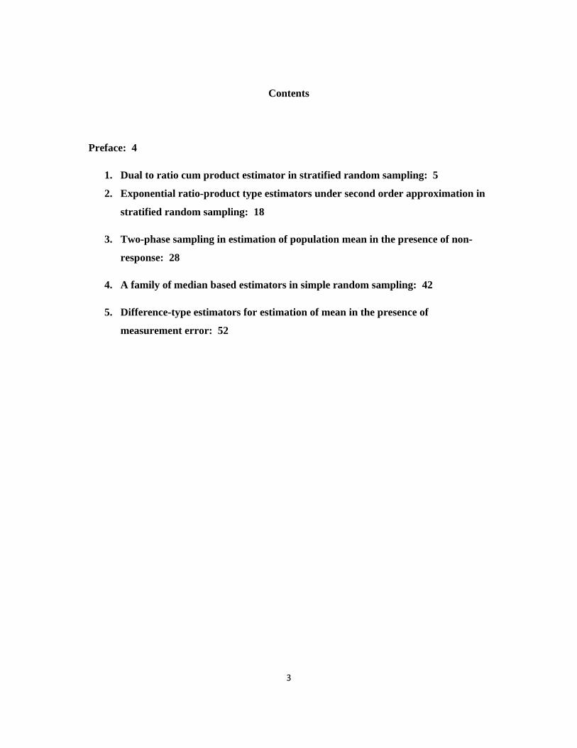
1. Dual to ratio cum product estimator in stratified random sampling: 5
2. Exponential ratio-product type estimators under second order approximation in
stratified random sampling: 18
3. Two-phase sampling in estimation of population mean in the presence of non-
response: 28
4. A family of median based estimators in simple random sampling: 42
5. Difference-type estimators for estimation of mean in the presence of
measurement error: 52

4
Preface
The purpose of writing this book is to suggest some improved estimators using auxiliary information in sampling schemes like simple random sampling, systematic sampling and stratified random sampling.
This volume is a collection of five papers, written by nine co-authors (listed in the order of the papers): Rajesh Singh, Mukesh Kumar, Manoj Kr. Chaudhary, Cem Kadilar, Prayas Sharma, Florentin Smarandache, Anil Prajapati, Hemant Verma, and Viplav Kr. Singh.
In first paper dual to ratio-cum-product estimator is suggested and its properties are studied. In second paper an exponential ratio-product type estimator in stratified random sampling is proposed and its properties are studied under second order approximation. In third paper some estimators are proposed in two-phase sampling and their properties are studied in the presence of non-response.
In fourth chapter a family of median based estimator is proposed in simple random sampling. In fifth paper some difference type estimators are suggested in simple random sampling and stratified random sampling and their properties are studied in presence of measurement error.
The authors hope that book will be helpful for the researchers and students who are working in the field of sampling techniques.

5
Dual To Ratio Cum Product Estimator In Stratified Random Sampling
†Rajesh Singh, Mukesh Kumar and Manoj K. Chaudhary
Department of Statistics, B.H.U., Varanasi (U.P.), India
Cem Kadilar Department of Statistics, Hacettepe University,
Beytepe 06800, Ankara, Turkey † Corresponding author, [email protected]
Abstract
Tracy et al.[8] have introduced a family of estimators using Srivenkataramana and Tracy
([6],[7]) transformation in simple random sampling. In this article, we have proposed a dual
to ratio-cum-product estimator in stratified random sampling. The expressions of the mean
square error of the proposed estimators are derived. Also, the theoretical findings are
supported by a numerical example.
Key words: Auxiliary information, dual, ratio-cum-product estimator, stratified random
sampling, mean square error and efficiency.
1. Introduction
In planning surveys, stratified sampling has often proved as useful in improving the precision
of un-stratified sampling strategies to estimate the finite population mean of the study
variable, = =
=L
1h
N
1ihi
h
yN
1Y . Let y, x and z respectively, be the study and auxiliary variates
on each unit Uh (h=1,2,3, ---, N) of the population U. Here the size of the stratum Uh is Nh,
and the size of simple random sample in stratum Uh is nh, where h=1, 2,---,L. In this study,

6
under stratified random sampling without replacement scheme, we suggest estimators to
estimate Y by considering the estimators in Plikusas [3] and in Tracy et al. [8].
To obtain the bias and MSE of the proposed estimators, we use the following notations in the rest of the article:
where, .N
Nw h
h =
Such that,
where and are the sample and population means of the study variable in the stratum h,
respectively. Similar expressions for X and Z can also be defined.
Using (1), we can write

7
where
The combined ratio and the combined product estimators are, respectively, defined as
And the MSE of and to the first degree of approximation are, respectively, given by
(4)
(5)
Note that Similar expressions for X and Z can also be defined.
2. Classical Estimators

8
Srivenkataramana and Tracy ([6],[7]) considered a simple transformation as
( i=1, 2,…,N)
where A is a scalar to be chosen. This transformation renders the situation suitable for a
product method instead of ratio method. Clearly is unbiased for .
Using this transformation, an estimator in the stratified random sampling is defined as
This is a product type estimator ( alternative to combined ratio type estimator) in stratified
random sampling.
The exact expression for MSE of is given by
(7)
In some survey situations, information on a second auxiliary variable, Z, correlated
negatively with the study variable, Y, is readily available. Let be the known population
mean of Z. To estimate , Singh[4] considered ratio-cum-product estimator as
where Perri[2] used ( )xXxt x −α+= and ( )zZzt z −β+= instead of x and z ,
respectively. Here, α and β are constants that make the MSE minimum.

9
Adapting to the stratified random sampling, the ratio cum product estimator using
two auxiliary variables can be defined as
The approximate MSE of this estimator is
3. Suggested Estimators
Tracy et al. [8] introduced a product estimator using two auxiliary variables in the simple
random sampling given by
Motivated by Tracy et al. [8], we propose the following product estimator for the
stratified random sampling scheme as
Expressing in terms of e’s, we can write (11) as
The MSE to the first order of approximation, is given as
and this MSE equation is minimised for

10
Note that the corresponding A is
By putting the optimum value of in (12), we can obtain the minimum MSE equation
for the first proposed estimator, .
Remark 3.1 : The value of X is known, but the exact values of V110, V011 and V020 are
rarely available in practice. However in repeated surveys or studies based on multiphase
sampling, where information is gathered on several occasions it may be possible to guess the
values of V110, V011 and V020 quite accurately. Even though this approach may reduce the
precision, it may be satisfactory provided the relative decrease in precision is marginal, see
Tracy et al. [8].
Plikusas[3] defined dual to ratio cum product estimator in stratified random sampling
as
where
and .)nN(
ng
hh
hh −
=
Considering the estimator in (13) and motivated by Singh et al. [5], we propose a family of
dual to ratio cum product estimator as –

11
To obtain the MSE of the second proposed estimator, , we write
.
Expressing (14) in terms of e’s, we have
(15)
Expanding the right hand side of (15), to the first order of approximation, we get
Squaring both sides of (16) and then taking expectation, we obtain the MSE of the second
proposed estimator, , to the first order approximation, as
(17)
where
This MSE equation is minimized for the optimum values of and given by

12
Putting these values of and in MSE ( ), given in (17), we obtain the minimum MSE
of the second proposed estimator, .
4. Theoretical Efficiency Comparisons
In this section, we first compare the efficiency between the first proposed estimator, , with
the classical combined estimator, as follows:
.
The estimator is better than the usual estimator if and only if,
,1B2
B
2
1 < (21)
where, 0020202
1 VVB +θ= and .VVVB 0111011102 θ+−θ=
If the condition (21) is satisfied, the first proposed estimator, , performs better than
the classical combined estimator.
We also find the condition under which the second proposed estimator, , performs
better than the classical combined estimator in theory as follows:
,
,

13
The estimator 9y is better than the usual estimator if and only if,
where, and
5. Numerical Example
In this section, we use the data set earlier used in Koyuncu and Kadilar[1] . The population
statistics are given in Table 1. In this data set, the study variable (Y) is the number of
teachers, the first auxiliary variable (X) is the number of students, and the second auxiliary
variable (Z) is the number of classes in both primary and secondary schools for 923 districts
at 6 regions ( as 1: Marmara, 2: Agean, 3: Mediterranean, 4: Central Anatolia, 5: Black Sea,
6: East and South east Anatolia) in Turkey in 2007, see Koyuncu and Kadilar[1]. Koyuncu
and Kadilar[1] have used Neyman allocation for allocating the samples to different strata.
Note that all correlations between the study and auxiliary variables are positive. Therefore,
we decide not to use product estimators for this data set for efficiency comparison. For this
reason, we apply the classical combined estimator, , combined ratio estimator , , the
ratio-cum-product estimator, , Plikusas [3] estimator, , and the second proposed
estimator, , to the data set. For the efficiency comparison, we compute percent relative
efficiencies as

14
Table 1. Data Statistics of Population
N1=127 N2=117 N3=103
N4=170 N5=205 N6=201
n1=31 n2=21 n3=29
n4=38 n5=22 n6=39
= 883.835 = 644 = 1033.467
810.585 = 403.654 =711.723
= 703.74 = 413 573.17
= 424.66 = 267.03 = 393.84
=30486.751 =15180.760 =27549.697
=18218.931 =8997.776 =23094.141
=20804.59 =9211.79 =14309.30
=9478.85 = 5569.95 =12997.59
=25237153.52 =9747942.85 =28294397.04
= 14523885.53 =3393591.75 =15864573.97
= 0.936 = 0.996 =0.994
= 0.983 = 0.989 = 0.965
= 555.5816 = 365.4576 =612.9509281
= 458.0282 = 260.8511 = 397.0481
= 498.28 = 318.33 = 431.36
= 498.28 = 227.20 = 313.71
= 480688.2 = 230092.8 = 623019.3
= 364943.4 = 101539 = 277696.1
= 15914648 = 5379190 = 164900674.56
= 8041254 = 2144057 = 8857729

15
= 0.978914 = 0.9762 = 0.983511
= 0.982958 = 0.964342 = 0.982689
Table 2. Percent Relative Efficiencies (PRE) of estimators
Estimators Values of PRE( )
0 0 100
1 0 1029.469
1 1 149.686
1 1 115.189
MSE( )min 6.2918 -0.8870 2854.549
Table3. The MSE values according to A
Value of Corresponding value of A
<0.8 - >V(yst) 0.8 25779.79 2186.879 0.9 24188.44 1814.999 1.00 22915.37 1492.895 1.10 21873.76 1220.564 1.20 21005.75 998.009 1.30 20271.29 825.227 1.40 19641.74 702.221 1.50 19096.14 628.989
1.5971(opt) 18631.62(opt) 605.511* 1.60 18618.74 605.532 1.70 18197.50 631.849 1.80 17823.06 707.941 1.90 17488.04 833.807 2.00 17186.53 1009.448 2.10 16913.72 1234.864 2.20 16665.72 1510.054 2.30 16439.29 1835.019 2.40 16231.72 2209.758
>2.40 - >V(yst) * MSE (min) at the value A(optimal).

16
6. Conclusion
When we examine Table 2, we observe that the second proposed estimator, , under
optimum condition certainly performs quite better than all other estimators discussed here.
Although the correlations are negative, we also examine the performance of the first proposed
estimator, , according to the classical combined estimator. Therefore, for various values of
A and in Table 3, the MSE values of and are computed. From Table 3, we observe
that the first proposed estimator, , performs better than the estimator, , for a wide range
of as , even in the negative correlations.
References
[1] Koyuncu, N. and Kadilar, C. Family of Estimators of Population Mean Using Two
Auxiliary Variables in Stratified Random Sampling Commun. in Statist.—Theor.
and Meth, 38, 2009, 2398–2417.
[2] Perri, P.F. Improved ratio-cum-product type estimators. Statist. In Trans, 2007, 851-69.
[3] Plikusas, A. Some overview of the ratio type estimators In: Workshop on survey
sampling theory and methodology, Statistics Estonia, 2008.
[4] Singh, M. P. Ratio-cum-product method of estimation. Metrika 12, 1967, 34 -42.
[5] Singh, R., Kumar, M., Chauhan, P., Sawan, N. and Smarandache, F. A general family of
dual to ratio-cum-product estimator in sample surveys. Statist. In Trans- New
series. IJSA, 2012, 1(1), 101-109.
[6] Srivenkataramana, T. and Tracy, D.S. An alternative to ratio method in sample surveys.
Ann. Inst. Statist. Math.32 A, 1980, 111-120.

17
[7] Srivenkataramana, T. and Tracy, D.S. Extending product method of estimation to positive
correlation case in surveys. Austral. J. Statist. 23, 1981, 95-100.
[8] Tracy, D.S., Singh, H.P. and Singh, R. An alternative to the ratio-cum-product estimator
in sample surveys. Jour. of Statist. Plann. and Infere. 53, 1996, 375 -387.

18
Exponential Ratio-Product Type Estimators Under Second Order
Approximation In Stratified Random Sampling
†1Rajesh Singh, 1Prayas Sharma and 2Florentin Smarandache
1Department of Statistics, Banaras Hindu University
Varanasi-221005, India
2Department of Mathematics, University of New Mexico, Gallup, USA
† Corresponding author, [email protected]
Abstract
Singh et al. (20009) introduced a family of exponential ratio and product type
estimators in stratified random sampling. Under stratified random sampling without
replacement scheme, the expressions of bias and mean square error (MSE) of Singh et al.
(2009) and some other estimators, up to the first- and second-order approximations are
derived. Also, the theoretical findings are supported by a numerical example.
Keywords: Stratified Random Sampling, population mean, study variable, auxiliary variable,
exponential ratio type estimator, exponential product estimator, Bias and MSE.
1. INTRODUCTION
In survey sampling, it is well established that the use of auxiliary information results in
substantial gain in efficiency over the estimators which do not use such information.
However, in planning surveys, the stratified sampling has often proved needful in improving
the precision of estimates over simple random sampling. Assume that the population U
consist of L strata as U=U1, U2,…,UL . Here the size of the stratum Uh is Nh, and the size of
simple random sample in stratum Uh is nh, where h=1, 2,---,L.
When the population mean of the auxiliary variable, X , is known, Singh et al. (2009) suggested a combined exponential ratio-type estimator for estimating the population
mean of the study variable ( )Y :

19
+−
=st
stS1 xX
xXexpyt (1.1)
where,
=
=hn
1ihi
hh y
n
1y , ,x
n
1x
hn
1ihi
hh
=
=
hL
1hhst ywy =
=, h
L
1hhst xwx =
=, and .XwX h
L
1hh=
=
The exponential product-type estimator under stratified random sampling is given by
+
−=
Xx
xXexpyt
st
stS2 (1.2)
Following Srivastava (1967) an estimator t3s in stratified random sampling is defined as :
α
+
−=
Xx
xXexpyt
st
stS3 (1.3)
where α is a constant suitably chosen by minimizing MSE of S3t . For α=1 , S3t is same as
conventional exponential ratio-type estimator whereas for α = -1, it becomes conventional
exponential product type estimator.
Singh et al. (2008) introduced an estimator which is linear combination of exponential ratio-
type and exponential product-type estimator for estimating the population mean of the study
variable ( )Y in simple random sampling. Adapting Singh et al. (2008) estimator in stratified random
sampling we propose an estimator t4s as :
+
−θ−+
+
−θ=
Xx
xXexp)1(
Xx
xXexpyt
st
st
st
stS4 (1.4)

20
where θ is the constant and suitably chosen by minimizing mean square error of the
estimator S4t . It is observed that the estimators considered here are equally efficient when
terms up to first order of approximation are taken. Hossain et al. (2006) and Singh and
Smarandache (2013) studied some estimators in SRSWOR under second order approximation.
Koyuncu and Kadilar (2009, 2010) ), have studied some estimators in stratified random sampling
under second order approximation. To have more clear picture about the best estimator, in this
study we have derived the expressions of MSE’s of the estimators considered in this paper
up to second order of approximation in stratified random sampling.
3. Notations used
Let us define, y
yye st
0
−= and
x
xxe st
1
−= ,
such that
( ) ( )[ ]s
hh
r
hh
L
1h
srhrs YyXxEWV −−=
=
+
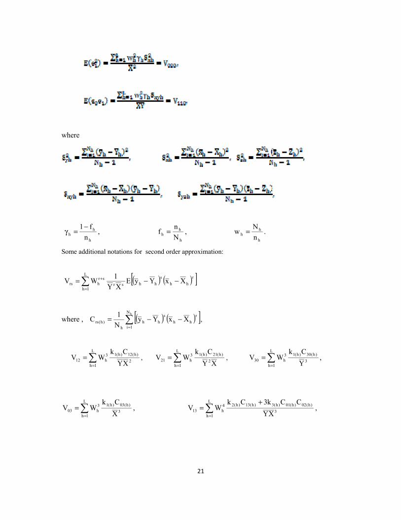
To obtain the bias and MSE of the proposed estimators, we use the following notations in the rest of the article:
where and are the sample and population means of the study variable in the stratum h,
respectively. Similar expressions for X and Z can also be defined.
Also, we have
21
where
h
hh n
f1−=γ ,
h
hh N
nf = ,
h
hh n
Nw = .
Some additional notations for second order approximation:
( ) ( )[ ]r
hh
s
hhsr
L
1h
srhrs XxYyE
XY
1WV −−=
=
+
where , ( ) ( )[ ]=
−−=hN
1i
r
hh
s
hhh
)h(rs XxYyN
1C ,
=
=L
1h2
)h(12)h(13h12 XY
CkWV ,
=
=L
1h2
)h(21)h(13h21 XY
CkWV ,
=
=L
1h3
)h(30)h(13h30 Y
CkWV ,
=
=L
1h3
)h(03)h(13h03 X
CkWV ,
=
+=
L
1h3
)h(02)h(01)h(3)h(13)h(24h13 XY
CCk3CkWV ,

22
=
+=
L
1h4
2)h(02)h(3)h(04)h(24
h04 X
Ck3CkWV ,
( )
=
++=
L
1h22
2)h(11)h(02)h(01)h(3)h(22)h(24
h22 XY
C2CCkCkWV ,
where )2N)(1N(n
)n2N)(nN(k
hh2
hhhh)h(1 −−
−−= ,
)3N)(2N)(1N(n
)nN(n6N)1N)(nN(k
hhh3
hhhhhhh)h(2 −−−
−−+−= ,
)3N)(2N)(1N(n
)1n)(1nN(N)nN(k
hhh3
hhhhhh)h(3 −−−
−−−−= .
4. First Order Biases and Mean Squared Errors under stratified random sampling
The expressions for biases and MSE,s of the estimators t1S, t2S and t3S respectively, are :
−= 1102S1 V
2
1V
8
3Y)t(Bias (4.1)
−+= 110220
2S1 VV
2
1VY)t(MSE (4.2)
−= 0211S2 V
8
1V
2
1Y)t(Bias (4.3)
++= 110220
2S2 VV
4
1VY)t(MSE (4.4)
α−α+α= 1102
202S3 V
2
1V
8
1V
4
1Y)t(Bias (4.5)

23
α−α+= 1102
220
2S3 VV
4
1VY)t(MSE (4.6)
By minimizing )s3t(MSE , the optimum value of α is obtained as 02
11o V
V2=α . By putting this
optimum value of α in equation (4.5) and (4.6), we get the minimum value for bias and MSE of the
estimator t3S.
The expression for the bias and MSE of t4s to the first order of approximation are given respectively,
as
−θ−+
−θ= 02111102)s4 V
8
1V
2
1)1(V
2
1V
8
3Yt(Bias (4.7)
θ−+
θ−+= 1102
2
202
S4 V2
12V
2
1VY)t(MSE (4.8)
By minimizing )S4t(MSE , the optimum value of θ is obtained as 2
1
V
V
02
11o +=θ . By putting this
optimum value of α in equation (4.7) and (4.8) we get the minimum value for bias and MSE of the
estimator t3S. We observe that for the optimum cases the biases of the estimators S3t and S4t are
different but the MSE of S3t and S4t are same. It is also observed that the MSE’s of the
estimators S3t and S4t are always less than the MSE’s of the estimators S1t and S2t . This prompted
us to study the estimators S3t and S4t under second order approximation.
5. Second Order Biases and Mean Squared Errors in stratified random sampling
Expressing estimator ti’s(i=1,2,3,4) in terms of ei’s (i=0,1), we get
( )
+
−+=
1
10s1 e2
eexpe1Yt
Or

24
+−−++−−=− 43
1032
102
1101
0s1 e384
25ee
48
7e
48
7ee
8
3e
8
3ee
2
1
2
eeYYt (5.1)
Taking expectations, we get the bias of the estimator s1t up to the second order of
approximation as
(5.2)
Squaring equation (5.1) and taking expectations and using lemmas we get MSE of s1t up to second
order of approximation as
2
321010
21
10S1 e
48
7ee
8
3ee
2
1e
8
3
2
eeYE)t(MSE
−+−+−=
Or,
++−−−+−+= 4
12
103
103
112
02
12
0102
12
02
s1 e192
55ee
4
5ee
24
25e
8
3eeeeeee
4
1eEY)t(MSE
(5.3)
Or,
(5.4)
Similarly we get the biases and MSE’s of the estimators t2S, t3S and t4S up to second order of
approximation respectively, as
−+−−−= 030413120211s22 V
24
5V
192
1V
24
5V
4
1V
4
1V
2
Y)t(Bias (5.5)
( ) +−+−+++= )VV
24
1V
4
1V
8
1V
192
23VV
4
1VYtMSE 2113120304110220
2S22
(5.6)
+ −−++−== 041303120211s12 V
192
25V
24
7 V
24
7V
4
3V
4
3V
2
Y)t(Bias
( )
+−+−+−+= 0413122122110220
2s12 V
192
55V
24
25V
4
5VVVV
4
1VYtMSE

25
13
32
03
32
1112
2
02
2
S32 V488
V488
V2
V48
V48
Y)t(Bias
α+α−
α+α
α−
α+α+
α+α=
α+α+α+ 04
432
V3843232
(5.7)
( ) 12
2
22
2
2122
2
1102
2
202
S32 V4
3
2V
22VV
22VV
4VYtMSE
α+α+
α+α+α−
α+α+α−α+=
α+α+α+
α+α−
α+α− 04
432
13
32
03
22
V192
7
1616V
24
7
4
3V
84 (5.8)
)Yt(E)t(Bias S4S42 =−= Y { } 04120211 V24
1
16
1VV
4
1
2
1V
2
1
α++
+
α−−
α−
( ){ }++α− 1303 VV52
48
1 (5.9)
( ) ( ) ( )12
2
22
2
02
2
202
S42 V4
14
2
1V
4
14
2
1V
2
1VYtMSE
−θ+
θ−+
−θ+
θ−+
θ−+=
( ) ( ) ( ) 0321042 V14
2
1
4
1V
2
12V52
2
1
24
114
64
1 −θ
θ−+
θ−+
+θ
θ−−−θ+
( ) ( )
−θ
θ−++θ−− 13V14
2
1
2
152
24
1 (5.10)
The optimum value of α we get by minimizing ( )S32 tMSE . But theoretically the determination of
the optimum value of α is very difficult, we have calculated the optimum value by using numerical
techniques. Similarly the optimum value of θ which minimizes the MSE of the estimator t4s is
obtained by using numerical techniques.
6. Numerical Illustration
26
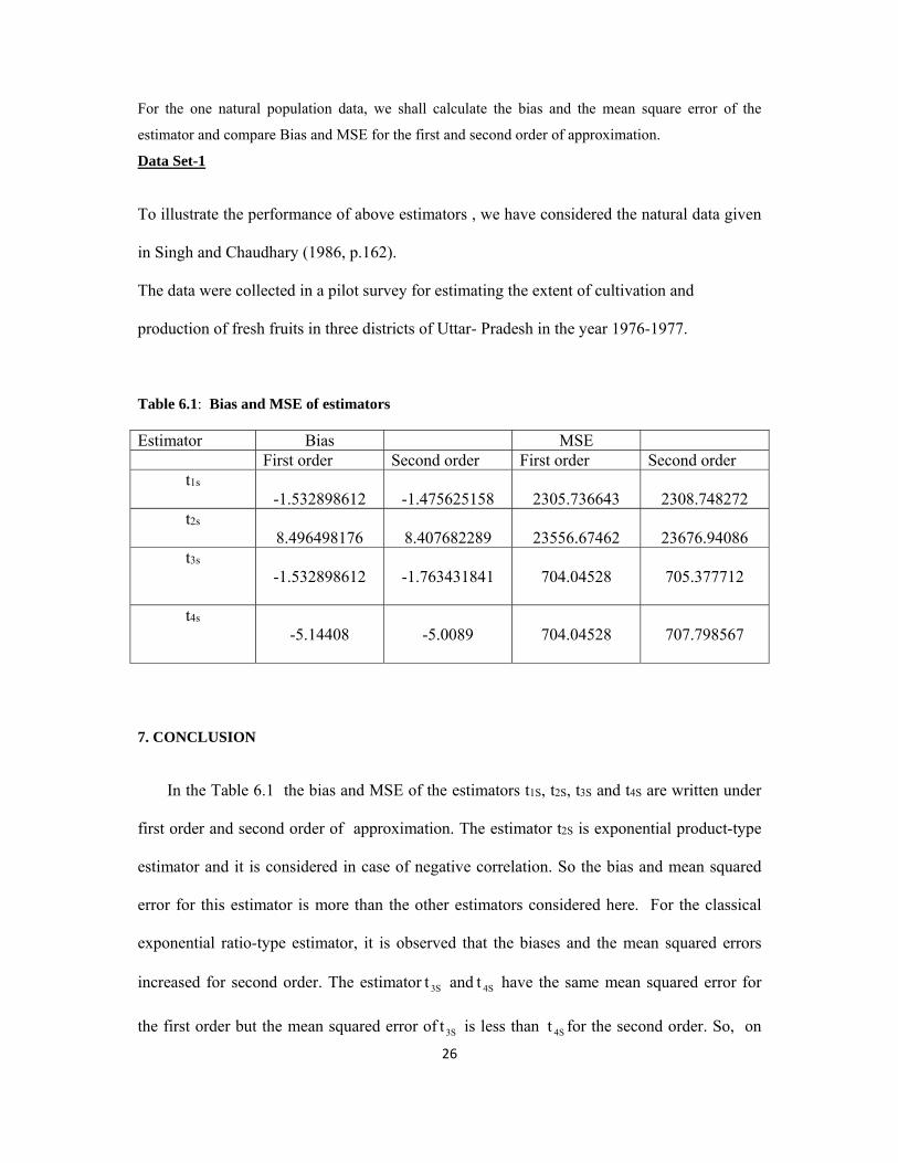
For the one natural population data, we shall calculate the bias and the mean square error of the
estimator and compare Bias and MSE for the first and second order of approximation.
Data Set-1
To illustrate the performance of above estimators , we have considered the natural data given
in Singh and Chaudhary (1986, p.162).
The data were collected in a pilot survey for estimating the extent of cultivation and
production of fresh fruits in three districts of Uttar- Pradesh in the year 1976-1977.
Table 6.1: Bias and MSE of estimators
Estimator Bias MSE First order Second order First order Second order
t1s -1.532898612
-1.475625158
2305.736643
2308.748272
t2s 8.496498176
8.407682289
23556.67462
23676.94086
t3s -1.532898612
-1.763431841
704.04528
705.377712
t4s
-5.14408
-5.0089
704.04528
707.798567
7. CONCLUSION
In the Table 6.1 the bias and MSE of the estimators t1S, t2S, t3S and t4S are written under
first order and second order of approximation. The estimator t2S is exponential product-type
estimator and it is considered in case of negative correlation. So the bias and mean squared
error for this estimator is more than the other estimators considered here. For the classical
exponential ratio-type estimator, it is observed that the biases and the mean squared errors
increased for second order. The estimator S3t and S4t have the same mean squared error for
the first order but the mean squared error of S3t is less than S4t for the second order. So, on

27
the basis of the given data set we conclude that the estimator t3S is best followed by the
estimator t4S among the estimators considered here.
REFERENCES
Koyuncu, N. and Kadilar, C. (2009) : Family of estimators of population mean using two
auxiliary variables in stratified random sampling. Commun. in Statist.—Theor.
and Meth, 38, 2398–2417.
Koyuncu, N. and Kadilar, C. (2010) : On the family of estimators of population mean in
stratified random sampling. Pak. Jour. Stat., 26(2),427-443.
Singh, D. and Chudhary, F.S. (1986): Theory and analysis of sample survey designs. Wiley
Eastern Limited, New Delhi.
Singh, R., Chauhan, P. and Sawan, N.(2008): On linear combination of Ratio-product type
exponential estimator for estimating finite population mean. Statistics in
Transition,9(1),105-115.
Singh, R., Kumar, M., Chaudhary, M. K., Kadilar, C. (2009) : Improved Exponential
Estimator in Stratified Random Sampling. Pak. J. Stat. Oper. Res. 5(2), pp 67-
82.
Singh, R. and Smarandache, F. (2013): On improvement in estimating population
parameter(s) using auxiliary information. Educational Publishing & Journal of
Matter Regularity (Beijing) pg 25-41.

28
TWO-PHASE SAMPLING IN ESTIMATION OF POPULATION MEAN IN THE PRESENCE OF NON-RESPONSE
1Manoj Kr. Chaudhary, 1Anil Prajapati ,†1Rajesh Singh and 2Florentin Smarandache
1Department of Statistics, Banaras Hindu University, Varanasi-221005
2Department of Mathematics, University of New Mexico, Gallup, USA
† Corresponding author, [email protected]
Abstract
The present paper presents the detail discussion on estimation of population mean in simple random sampling in the presence of non-response. Motivated by Gupta and Shabbir (2008), we have suggested the class of estimators of population mean using an auxiliary variable under non-response. A theoretical study is carried out using two-phase sampling scheme when the population mean of auxiliary variable is not known. An empirical study has also been done in the support of theoretical results.
Keywords: Two-phase sampling, class of estimators, optimum estimator, non-response, numerical illustrations.
1. Introduction
The auxiliary information is generally used to improve the efficiency of the
estimators. Cochran (1940) proposed the ratio estimator for estimating the population mean
whenever study variable is positively correlated with auxiliary variable. Contrary to the
situation of ratio estimator, if the study and auxiliary variables are negatively correlated,
Murthy (1964) suggested the product estimator to estimate the population mean. Hansen et al.
(1953) proposed the difference estimator which was subsequently modified to provide the
linear regression estimator for the population mean or total. Mohanty (1967) suggested an
estimator by combining the ratio and regression methods for estimating the population
parameters. In order to estimate the population mean or population total of the study
character utilizing auxiliary information, several other authors including Srivastava ( 1971),
Reddy (1974), Ray and Sahai (1980), Srivenkataramana (1980), Srivastava and Jhajj (1981)

29
and Singh and Kumar (2008, 2011) have proposed estimators which lead improvements over
usual per unit estimator.
It is observed that the non-response is a common problem in any type of survey.
Hansen and Hurwitz (1946) were the first to contract the problem of non-response while
conducting mail surveys. They suggested a technique, known as ‘sub-sampling of non-
respondents’, to deal with the problem of non-response and its adjustments. In fact they
developed an unbiased estimator for population mean in the presence of non-response by
dividing the population into two groups, viz. response group and non-response group. To
avoid bias due to non-response, they suggested for taking a sub-sample of the non-responding
units.
Let us consider a population consists of N units and a sample of size n is selected from
the population using simple random sampling without replacement (SRSWOR) scheme. Let
us assume that Y and X be the study and auxiliary variables with respective population
means Y and X . Let us consider the situation in which study variable is subjected to non-
response and auxiliary variable is free from the non-response. It is observed that there are
1n respondent and 2n non-respondent units in the sample of n units for the study variable.
Using the technique of sub sampling of non-respondents suggested by Hansen and Hurwitz
(1946), we select a sub-sample of 2h non-respondent units from 2n units such
that 1k,knh 22 ≥= and collect the information on sub-sample by personal interview method.
The usual sample mean, ratio and regression estimators for estimating the population mean
Y under non-response are respectively represented by
n
ynyny 2h21n1* +
= (1.1)

30
Xx
yy
**
R = (1.2)
( )xXbyy**
lr −+= (1.3)
where 1ny and 2hy are the means based on 1n respondent and 2h non-respondent units
respectively. x is the sample mean estimator of population mean X , based on sample of size
n and b is the sample regression coefficient of Y on X .
The variance and mean square errors (MSE) of the above estimators*
y , *
Ry and *
lry
are respectively given by
( ) ( ) 22Y2
2Y
*SW
n
1kS
N
1
n
1yV
−+
−= (1.4)
( ) ( ) ( ) 22Y2YX
2X
2Y
2*
R SWn
1kCC2CCY
N
1
n
1yMSE
−+ρ−+
−= (1.5)
( ) ( ) ( ) 22Y2
22Y
2*
lr SWn
1k1CY
N
1
n
1yMSE
−+ρ−
−= (1.6)
where 2YS and 2
XS are respectively the mean squares of Y and X in the population.
( )YSC YY = and ( )XSC XX = are the coefficients of variation of Y and X respectively.
22YS and 2W are respectively the mean square and non-response rate of the non-response
group in the population for the study variable Y . ρ is the population correlation coefficient
between Y and X .
When the information on population mean of auxiliary variable is not available, one
can use the two-phase sampling scheme in obtaining the improved estimator rather than the
previous ones. Neyman (1938) was the first who gave concept of two-phase sampling in
estimating the population parameters. Two-phase sampling is cost effective as well as easier.
This sampling scheme is used to obtain the information about auxiliary variable cheaply from
31
a bigger sample at first phase and relatively small sample at the second stage. Sukhatme
(1962) used two-phase sampling scheme to propose a general ratio-type estimator. Rao
(1973) used two-phase sampling to stratification, non-response problems and investigative
comparisons. Cochran (1977) supplied some basic information for two-phase sampling.
Sahoo et al. (1993) provided regression approach in estimation by using two auxiliary
variables for two-phase sampling. In the sequence of improving the efficiency of the
estimators, Singh and Upadhyaya (1995) suggested a generalized estimator to estimate
population mean using two auxiliary variables in two-phase sampling.
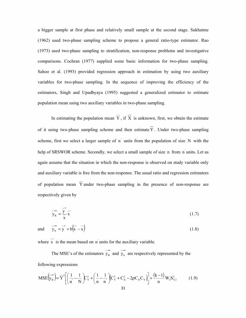
In estimating the population mean Y , if X is unknown, first, we obtain the estimate
of it using two-phase sampling scheme and then estimate Y . Under two-phase sampling
scheme, first we select a larger sample of 'n units from the population of size N with the
help of SRSWOR scheme. Secondly, we select a small sample of size n from 'n units. Let us
again assume that the situation in which the non-response is observed on study variable only
and auxiliary variable is free from the non-response. The usual ratio and regression estimators
of population mean Y under two-phase sampling in the presence of non-response are
respectively given by
'*
**
R xx
yy = (1.7)
and ( )xxbyy'***
lr −+= (1.8)
where '
x is the mean based on 'n units for the auxiliary variable.
The MSE’s of the estimators **
Ry and **
lry are respectively represented by the
following expressions
( ) ( ) ( ) 22Y2YX
2X
2Y'
2Y'
2**
R SWn
1kCC2CC
n
1
n
1C
N
1
n
1YyMSE
−+
ρ−+
−+
−= (1.9)

32
and
( ) ( ) ( ) 22Y2
22Y'
2Y'
2**
lr SWn
1k1C
n
1
n
1C
N
1
n
1YyMSE
−+
ρ−
−+
−= (1.10)
In the present paper, we have discussed the study of non-response of a general class of
estimators using an auxiliary variable. We have suggested the class of estimators in two-
phase sampling when the population mean of auxiliary variable is unknown. The optimum
property of the class is also discussed and it is compared to ratio and regression estimators
under non-response. The theoretical study is also supported with the numerical illustrations.
2. Suggested Class of Estimators
Let us assume that the non-response is observed on the study variable and auxiliary
variable provides complete response on the units. Motivated by Gupta and Shabbir (2008),
we suggest a class of estimators of population mean Y under non-response as
( )[ ]
λ+ηλ+η−α+α=
x
XxXyy 2
*
1
*
t (2.1)
where 1α and 2α are the constants and whose values are to be determined. λ and ( )0≠η are
either constants or functions of the known parameters.
In order to obtain the bias and MSE of*
ty , we use the large sample approximation. Let
us assume that
( )1
*e1Yy += , ( )2e1Xx +=
such that ( ) ( ) 0eEeE 21 == ,
( ) ( ) ( ),
Y
SW
n
1kC
N
1
n
1
Y
yVeE
2
22Y
22Y2
*
21
−+
−==
( ) ( ) 2
222
11XC
NnX
xVeE
−==

33
and ( ) ( )YX
*
21 CCN
1
n
1
XY
x,yCoveeE ρ
−== .
Putting the values of *
y and x form the above assumptions in the equation (2.1), we
get
( ) ( ) ( )2222
22
2212111
*
t eeXeeeeeY1YYy τ−α−τ+τ−τ−α+−α≅− (2.2)
On taking expectation of the equation (2.2), the bias of *
ty to the first order of
approximation is given by
( ) ( ) ( ) ( )[ ]2X2YX
2X
211
*
t
*
t CXCCCYN
1
n
11YYyEyB τα+τρ−τα
−+−α=−= (2.3)
Squaring both the sides of the equation (2.2) and taking expectation, we can obtain the
MSE of *
ty to the first order of approximation as
( ) ( ) ( )[ 2X
222YX
2X
22Y
221
21
2*
t CXCC2CCYN
1
n
11YyMSE α+τρ−τ+α
−+−α=
( )]XYX21 CCCXY2 τ−ραα− ( ) 22Y2
21 SW
n
1k −α+ (2.4)
In the sequence of obtaining the best estimator within the suggested class with respect
to 1α and 2α , we obtain the optimum values of 1α and 2α . On differentiating ( )*
tyMSE
with respect to 1α and 2α and equating the derivatives to zero, we have
( )
0SWn
1k 22Y21 =−α+ (2.5)
( ) ( )[ ] 0CCCYXCXN
1
n
1yMSEXYX1
2X
2
22
*
t =τ−ρα−α
−=
α∂∂
(2.6)
Solving the equations (2.4) and (2.5), we get
( ) ( ) ( ) ( )[ ]XYX2YX2X
22Y1
2
1
2
1
*
t CCCYXCC2CCYN
1
n
11Y
yMSEτ−ρα−τρ−τ+α
−+−α=
α∂∂
34
( )( ) ( )
2
22Y
222
Y
1
Y
SW
n
1k1C
N
1
n
11
1opt
−+ρ−
−+
=α (2.7)
and ( ) ( ) ( )X
XY12
CX
CCYoptopt
τ−ρα=α (2.8)
Substituting the values of ( )opt1α and ( )opt2α from equations (2.7) and (2.8) into the
equation (2.4), the MSE of *
ty is given by the following expression.
( ) ( )( ) ( )
2
22Y
222
Y
*
lrmin
*
t
Y
SW
n
1k1C
N
1
n
11
yMSEyMSE
−+ρ−
−+
= (2.9)
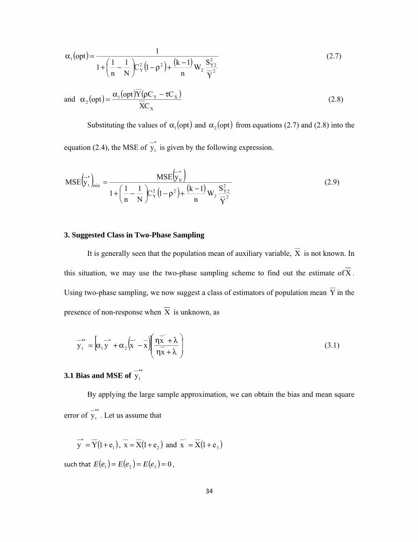
3. Suggested Class in Two-Phase Sampling
It is generally seen that the population mean of auxiliary variable, X is not known. In
this situation, we may use the two-phase sampling scheme to find out the estimate of X .
Using two-phase sampling, we now suggest a class of estimators of population mean Y in the
presence of non-response when X is unknown, as
( )[ ]
λ+ηλ+η−α+α=
x
xxxyy
''
2
*
1
**
t (3.1)
3.1 Bias and MSE of **
ty
By applying the large sample approximation, we can obtain the bias and mean square
error of **
ty . Let us assume that
( )1
*e1Yy += , ( )2e1Xx += and ( )3
'e1Xx +=
such that ( ) ( ) ( ) 0321 === eEeEeE ,

35
( ) ( )2
22
222
1
111
Y
SW
n
kC
NneE Y
Y
−+
−= , ( ) 22
2
11XC
NneE
−= ,
( ) 2'
23
11XC
NneE
−= , ( ) YX21 CC
N
1
n
1eeE ρ
−= ,
( ) YX'31 CCN
1
n
1eeE ρ
−= and ( ) 2
X'32 CN
1
n
1eeE
−= .
Under the above assumption, the equation (3.1) gives
( ) ( )322
31321222
2111
**
t eeeeeeeeeeY1YYy τ−τ+τ+τ−τ−τ+α+−α=−
( )3223
2232232 eeeeeeeeX τ−τ+τ+τ−α+ (3.2)
Taking expectation of both the sides of equation (3.2), we get the bias of **
ty up to the
first order of approximation as
( ) ( ) ( )[ ]2X2YX
2X1'1
**
t CXCCCYn
1
n
11YyB α+ρ−ατ
−+−α= (3.3)
The MSE of **
ty up to the first order of approximation can be obtained by the
following expression
( ) ( ) ( )21
22**
t
**
t 1YYyEyMSE −α=−=
( ) ( )
−+τρ−τ
−+
−α+
2
22Y
2YX2X
2'
2Y
221
Y
SW
n
1kCC2C
n
1
n
1C
N
1
n
1Y
( )[ ]YX2X21
2X
222'
CCCYX2CXn
1
n
1 ρ−ταα+α
−+ (3.4)
3.2 Optimum Values of 1α and 2α
On differentiating ( )**
tyMSE with respect to 1α and 2α and equating the derivatives
to zero, we get the normal equations
36
( ) ( ) ( ) ( )
−+τρ−τ
−+
−α+−α=
α∂∂
2
22Y
2YX2X
2'
2Y
2
11
2
1
**
t
Y
SW
n
1kCC2C
n
1
n
1C
N
1
n
1Y1Y
yMSE
( ) 0CCCYXn
1
n
1YX
2X2'
=ρ−τα
−+ (3.5)
and ( ) ( )[ ] 0CCCYXCX
n
1
n
1yMSEYX
2X1
2X
2
2'2
**
t =ρ−τα+α
−=
α∂∂
(3.6)
From equations (3.5) and (3.6), we get the optimum values of 1α and 2α as
( ) ( )2
22Y
22Y
2'
2Y
1
Y
SW
n
1kC
n
1
n
1C
N
1
n
11
1opt
−+ρ
−−
−+
=α (3.7)
and ( ) ( ) ( )X
XY12
CX
CCYoptopt
τ−ρα=α (3.8)
On substituting the optimum values of 1α and 2α , the equation (3.4) provides
minimum MSE of **
ty
( ) ( )( )
2
22Y
22Y
2'
2Y
**
lrmin
**
t
Y
SW
n
1kC
n
1
n
1C
N
1
n
11
yMSEyMSE
−+ρ
−−
−+
= (3.9)
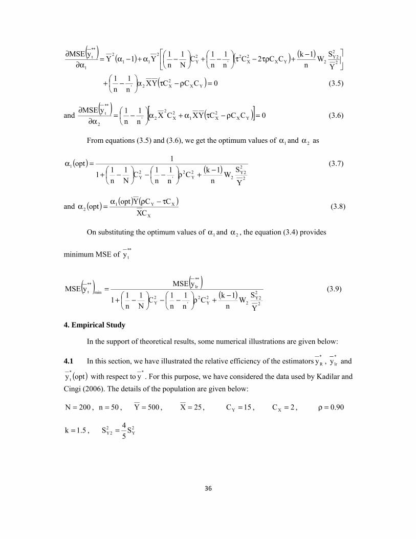
4. Empirical Study
In the support of theoretical results, some numerical illustrations are given below:
4.1 In this section, we have illustrated the relative efficiency of the estimators*
Ry , *
lry and
( )opty*
t with respect to*
y . For this purpose, we have considered the data used by Kadilar and
Cingi (2006). The details of the population are given below:
200N = , 50n = , 500Y = , 25X = , 15CY = , 2CX = , 90.0=ρ
5.1k = , 2Y
22Y S
5
4S =

37
Table 1. Percentage Relative Efficiency (PRE) with respect to *
y
2W Estimator
*
Ry *
lry ( )opty*
t
0.1 126.74 432.88 788.38
0.2 125.13 373.03 746.53
0.3 123.70 331.43 722.93
0.4 122.42 300.83 710.33
0.5 121.28 277.37 704.87
4.2 The present section presents the relative efficiency of the estimators**
Ry , **
lry
and ( )opty**
t with respect to*
y . There are two data sets which have been considered to
illustrate the theoretical results.
Data Set 1:
The population considered by Srivastava (1993) is used to give the numerical interpretation of the present study. The population of seventy villages in a Tehsil of India along with their cultivated area (in acres) in 1981 is considered. The cultivated area (in acres) is taken as study variable and the population is assumed to be auxiliary variable. The population parameters are given below:
70N = , 40n ' = , 25n = , 29.981Y = , 53.1755X = , 66.613SY = ,
13.1406SX = , 11.244S 2Y = , 778.0=ρ , 5.1k =

38
Table 2: Percentage Relative Efficiency with respect to *
y
2W Estimator
*
Ry *
lry ( )opty*
t
0.1 125.48657 153.56020 154.57983
0.2 125.10358 152.57858 153.60848
0.3 124.73193 151.63228 152.67552
0.4 124.37111 150.71945 151.77449
0.5 124.02068 149.83834 150.90579
Data Set 2:
Now, we have used another population considered by Khare and Sinha (2004). The
data are based on the physical growth of upper-socio-economic group of 95 school children
of Varanasi district under an ICMR study, Department of Paediatrics, Banaras Hindu
University, India during 1983-84. The details are given below:
95N = , 70n ' = , 35n = , 4968.19Y = , 8611.55X = , 0435.3SY = , 2735.3SX = ,
3552.2S 2Y = , 8460.0=ρ , 5.1k = .

39
Table 3: Percentage Relative Efficiency with respect to *
y
2W Estimator
*
Ry *
lry ( )opty*
t
0.1 159.61889 217.83004 217.99278
0.2 155.61224 207.27149 207.43596
0.3 152.10325 198.44091 198.58540
0.4 149.01829 190.94488 190.94488
0.5 146.26158 184.51722 184.66554
5. Conclusion
The study of a general class of estimators of population mean under non-response has
been presented. We have also suggested a class of estimators of population mean in the
presence of non-response using two-phase sampling when population mean of auxiliary
variable is not known. The optimum property of the suggested class has been discussed. We
have compared the optimum estimator with some existing estimators through numerical
study. The Tables 1, 2 and 3 represent the percentage relative efficiency of the optimum
estimator of suggested class, linear regression estimator and ratio estimator with respect to
sample mean estimator. In the above tables, we have observed that the percentage relative
efficiency of the optimum estimator is higher than the linear regression and ratio estimators.
It is also observed that the percentage relative efficiency decreases with increase in non-
response.
References
1. Cochran, W. G. (1940) : The estimation of the yields of cereal experiments by

40
sampling for the ratio of grain in total produce, Journal of The Agricultural Sciences,
30, 262-275.
2. Cochran, W. G. (1977) : Sampling Techniques, 3rd ed., John Wiley and Sons,
New York.
3. Gupta, S. and Shabbir, J. (2008) : On improvement in estimating the population mean
in simple random sampling, Journal of Applied Statistics, 35(5), 559-566.
4. Hansen, M. H. and Hurwitz, W. N. (1946) : The problem of non-response in sample
surveys, Journal of The American Statistical Association, 41, 517-529.
5. Hansen, M. H., Hurwitz, W. N. and Madow,, W. G. (1953): Sample Survey Methods
and Theory, Volume I, John Wiley and Sons, Inc., New York.
6. Kadilar, C. and Cingi, H. (2006) : New ratio estimators using correlation coefficient,
Interstat 4, 1–11.
7. Khare, B. B. and Sinha, R. R. (2004) : Estimation of finite population ratio using two
phase sampling scheme in the presence of non-response, Aligarh Journal of
Statistics 24, 43–56.
8. Mohanty, S. (1967) : Combination of regression and ratio estimates, Journal of the
Indian Statistical Association 5, 1–14.
9. Murthy, M. N. (1964) : Product method of estimation, Sankhya, 26A, 69-74.
10. Neyman, J. (1938). Contribution to the theory of sampling human populations,
Journal of American Statistical Association, 33, 101-116.
11. Rao, J.N.K. (1973) : On double sampling for stratification and analytic surveys,
Biometrika, 60, 125-133.
12. Ray, S. K. and Sahai, A. (1980) : Efficient families of ratio and product-type
estimators, Biometrika, 67, 215-217.
13. Reddy, V. N. (1974) : On a transformed ratio method of estimation, Sankhya, 36C,
59-70.
14. Sahoo, J., Sahoo, L. N., Mohanty, S. (1993) : A regression approach to estimation in
two phase sampling using two auxiliary variables. Curr. Sci. 65(1), 73–75.

41
15. Singh, G.N. and Upadhyaya, L.N. (1995) : A class of modified chain-type estimators
using two auxiliary variables in two-phase sampling, Metron, Vol. LIII, No. 3-4, 117-
125.
16. Singh, R., Kumar, M. and Smarandache, F. (2008): Almost Unbiased Estimator for
Estimating Population Mean Using Known Value of Some Population Parameter(s).
Pak. J. Stat. Oper. Res., 4(2) pp63-76.
17. Singh, R. and Kumar, M. (2011): A note on transformations on auxiliary variable in
survey sampling. MASA, 6:1, 17-19. doi 10.3233/MASA-2011-0154
18. Srivastava, S. (1993) Some problems on the estimation of population mean using
auxiliary character in presence of non-response in sample surveys. Ph. D. Thesis,
Banaras Hindu University, Varanasi, India.
19. Srivastava, S.K. (1971) : A generalized estimator for the mean of a finite population
using multi-auxiliary information, Journal of The American Statistical Association,
66 (334), 404-407.
20. Srivastava, S.K. and Jhajj, H. S. (1981) : A class of estimators of the population mean
in survey sampling using auxiliary information, Biometrika, 68 (1), 341-343.
21. Srivenkataramana, T. (1980) : A dual to ratio estimator in sample surveys,
Biometrika, 67 (1), 199-204.
22. Sukhatme, B. V. (1962) : Some ratio-type estimators in two-phase sampling, Journal
of the American Statistical Association, 57, 628–632.

42
A Family of Median Based Estimators in Simple Random Sampling
1Hemant K. Verma, †1Rajesh Singh and 2Florentin Smarandache
Department of Statistics, Banaras Hindu University
Varanasi-221005, India
2Department of Mathematics, University of New Mexico, Gallup, USA
† Corresponding author, [email protected]
Abstract
In this paper we have proposed a median based estimator using known value of some population parameter(s) in simple random sampling. Various existing estimators are shown particular members of the proposed estimator. The bias and mean squared error of the proposed estimator is obtained up to the first order of approximation under simple random sampling without replacement. An empirical study is carried out to judge the superiority of proposed estimator over others.
Keywords: Bias, mean squared error, simple random sampling, median, ratio estimator.
1. Introduction
Consider a finite population }U,...,U,U{U N21= of N distinct and identifiable units. Let Y be
the study variable with value iY measured on N1,2,3...,i ,Ui = . The problem is to estimate the
population mean =
=N
1iiY
N
1Y . The simplest estimator of a finite population mean is the sample mean
obtained from the simple random sampling without replacement, when there is no auxiliary
information available. Sometimes there exists an auxiliary variable X which is positively correlated
with the study variable Y. The information available on the auxiliary variable X may be utilized to
obtain an efficient estimator of the population mean. The sampling theory describes a wide variety of
techniques for using auxiliary information to obtain more efficient estimators. The ratio estimator and
the regression estimator are the two important estimators available in the literature which are using the
auxiliary information. To know more about the ratio and regression estimators and other related
results one may refer to [1-13].

43
When the population parameters of the auxiliary variable X such as population mean, coefficient of variation, kurtosis, skewness and median are known, a number of modified ratio estimators are proposed in the literature, by extending the usual ratio and Exponential- ratio type estimators.
Before discussing further about the modified ratio estimators and the proposed median based modified ratio estimators the notations and formulae to be used in this paper are described below:
• N - Population size
• n - Sample size
• Y - Study variable
• X - Auxiliary variable
• =
−=μμμ=β
N
1i
rir3
2
23
1 ,)Xx(N
1 Where Coefficient of skewness of the auxiliary variable
• ρ - Correlation Co-efficient between X and Y
• Y,X - Population means
• y,x - Sample means
• ,M - Average of sample medians of Y
• m - Sample median of Y
• β - Regression coefficient of Y on X
• B (.) - Bias of the estimator
• V (.) - Variance of the estimator
• MSE (.) - Mean squared error of the estimator
• 100*)e(MSE
)e(MSE)p,e(PRE = - Percentage relative efficiency of the proposed estimator p
with respect to the existing estimator e.
The formulae for computing various measures including the variance and the covariance of the SRSWOR sample mean and sample median are as follows:
===
−=−=−=−=−=n
Nn
Nn
N C
1i
2i
nN
2x
C
1i
2i
nN
2y
C
1i
2i
nN
)Mm(C
1)m(V,S
n
f1)Xx(
C
1)x(V,S
n
f1)Yy(
C
1)y(V
,
==
−−−
−=−−=N
1iii
C
1iii
nN
),Yy)(Xx(1N
1
n
f1)Yy)(Xx(
C
1)x,y(Cov
nN

44
,)Yy)(Mm(C
1)m,y(Cov
nN C
1iii
nN
=
−−= YX
)x,y(CovC,
YM
)m,y(CovC,
M
)m(VC,
X
)x(VC '
yx'ym2
'mm2
'xx ====
==
−−
=−−
==N
1i
2i
2x
N
1i
2i
2y )Xx(
1N
1S ,)Yy(
1N
1S ;
N
nf Where ,
In the case of simple random sampling without replacement (SRSWOR), the sample mean y is used to
estimate the population mean Y . That is the estimator of yYY r == with the variance
2yr S
n
f1)Y(V
−= (1.1)
The classical Ratio estimator for estimating the population mean Y of the study variable Y is defined
as Xx
yYR = . The bias and mean squared error of RY are given as below:
{ }'yx
'xxR CCY)Y(B −= (1.2)
)x,y(CovR2)x(VR)y(V)Y(MSE ''R
2
−+= where X
YR' = (1.3)
2. Proposed estimator
Suppose
if iety,linear var a is set w thedefinitionBy . Ymean population the
estimatingfor estimators typeratio possible all ofset thedenotes w wherew,t ,t ,tSuch that
bamm ,bMaM where mM
)mM(expyt ,
M)1(m
Myt ,yt
210
**
**
**
2
g
**
*
10
∈
+=+=
+−δ=
α−+α==
(2.2) Rw 1wfor
(2.1) W, twtwywt
i
2
0ii
22110
∈=
∈++=
=
where iw (i=0, 1, 2) denotes the statistical constants and R denotes the set of real numbers.
+−δ=
α−+α=
**
**
2
g
**
*
1mM
)mM(expyt ,
M)1(m
Myt ,Also

45
.bamm ,bMaM and **+=+=
To obtain the bias and MSE expressions of the estimator t, we write
)e1(Mm ),e1(Yy 10 +=+=
such that
,0)e(E)e(E 10 ==
( ) ( ) ( )ym10mm2
212
20 C
MY
m,yCov)eE(e ,C
M
mV)E(e ,
Y
yV)e(E =====
Expressing the estimator t in terms of e’s, we have
.bMa
Ma where
(2.3) 2
e1
2
eexpw)e1(ww)e1(Yt
1
112
g1100
+=υ
υ
+
υδ−+υα+++=
−−
Expanding the right hand side of equation(2.3) up to the first order of approximation, we get
(2.8) C2
C84
Y)t(B
(2.7) CC2
)1g(gY)t(B
(2.6) wCCw842
)1g(gwYB(t)
asion approximat oforder first the toup,estimators
theof biases get the wesides,both from Y gsubtractin then and (2.4) of sidesboth of nsexpectatio Taking
(2.5) .w2
gw wwhere
(2.4) eweew842
)1g(gwewe1Yt
ymmm
222
2
ymmm1
ymmm2
22
12
21
10212
22
12
01
δυ−
υδ+δυ=
−+αυαυ=
υ−
δ−δ+α+υ=
δ+α=
υ−
δ−δ+α+υ++υ−≅
From (2.4), we have
(2.9) )wee(YYt 10 υ+≅−
Squaring both sides of (2.9) and then taking expectations, we get the MSE of the estimator t, up to the first order of approximation as
46
( ) ( ) ( ).
M
YR where
(2.10) m,yRwCov2mVwRyV)t(MSE 222
=
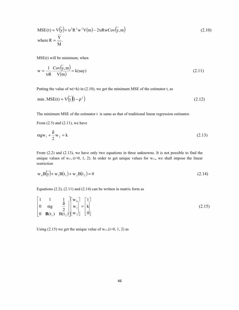
υ−υ+=
MSE(t) will be minimum, when
( )( ) (2.11) )say(kmV
m,yCov
R
1w =
υ=
Putting the value of w(=k) in (2.10), we get the minimum MSE of the estimator t, as
( )( ) (2.12) 1yVMSE(t) .min 2ρ−=
The minimum MSE of the estimator t is same as that of traditional linear regression estimator.
From (2.5) and (2.11), we have
(2.13) kw2
gw 21 =δ+α
From (2.2) and (2.13), we have only two equations in three unknowns. It is not possible to find the unique values of wi’s (i=0, 1, 2). In order to get unique values for wi’s, we shall impose the linear restriction
( ) ( ) ( ) (2.14) 0tBwtBwyBw 22110 =++
Equations (2.2), (2.11) and (2.14) can be written in matrix form as
(2.15)
0
k
1
w
w
w
)t(B)t(02
g0
111
2
1
0
21
=
δα
B
Using (2.15) we get the unique value of wi’s (i=0, 1, 2) as

47
(2.16)
)t(kB
)t(kB2
k)t(B2
1)kg)(t(B
)t(B2
)t(gB
e wher
w
w
w
12
21
120
12r
r
22
r
11
r
00
−=Δ=Δ
δ−+−α=Δ
δ−α=Δ
ΔΔ
=
ΔΔ
=
ΔΔ
=
Table 2.1: Some members of the proposed estimator
w0 w1 w2 a b α g δ Estimators
1 0 0 - - - - - yq1 =
0 1 0 1 0 1 1 - m
Myq2 =
0 1 0 1β ρ 1 1 -
ρ+βρ+β=
m
Myq
1
13
0 1 0 ρ 1β 1 1 -
β+ρβ+ρ=
1
14 m
Myq
0 0 1 1 0 - - 1
+−=
mM
)mM(expyq 5
0 0 1 1β ρ - - 1 ( )
ρ++β
−β=2mM
)mM(expyq
1
16
0 0 1 ρ 1β - - 1 ( )
β++ρ−ρ=
1
72mM
)mM(expyq
0 1 1 1β ρ 1 1 1 ( )
ρ++β
−β+
ρ+βρ+β=
2mM
)mM(expy
m
Myq
1
1
1
18
0 1 1 ρ 1β 1 1 1 ( )
β++ρ
−ρ+
β+ρβ+ρ=
11
19 2mM
)mM(expy
m
Myq
0 1 1 1 0 1 1 1
+−+=
mM
)mM(expy
m
Myq10

48
3. Empirical Study
For numerical illustration we consider: the population 1 and 2 taken from [14] pageno.177, the population 3 is taken from [15] page no.104. The parameter values and constants computed for the above populations are given in the Table 3.1. MSE for the proposed and existing estimators computed for the three populations are given in the Table 3.2 whereas the PRE for the proposed and existing estimators computed for the three populations are given in the Table 3.3.
Table: 3.1 Parameter values and constants for 3 different populations
Parameters For sample size n=3 For sample size n=5
Popln-1 Popln-2 Popln-3 Popln-1 Popln-2 Popln-3
N 34 34 20 34 34 20
n 3 3 3 5 5 5
nN C 5984 5984 1140 278256 278256 15504
Y 856.4118 856.4118 41.5 856.4118 856.4118 41.5
M 747.7223 747.7223 40.2351 736.9811 736.9811 40.0552
X 208.8824 199.4412 441.95 208.8824 199.4412 441.95
1β 0.8732 1.2758 1.0694 0.8732 1.2758 1.0694
R 1.1453 1.1453 1.0314 1.1621 1.1621 1.0361
)y(V 163356.4086 163356.4086 27.1254 91690.3713 91690.3713 14.3605
)x(V 6884.4455 6857.8555 2894.3089 3864.1726 3849.248 1532.2812
)m(V 101127.6164 101127.6164 26.0605 58464.8803 58464.8803 10.6370
)m,y(Cov 90236.2939 90236.2939 21.0918 48074.9542 48074.9542 9.0665
)x,y(Cov 15061.4011 14905.0488 182.7425 8453.8187 8366.0597 96.7461
ρ 0.4491 0.4453 0.6522 0.4491 0.4453 0.6522

49
Table: 3.2. Variance / Mean squared error of the existing and proposed estimators
Estimators For sample size n=3 For sample size n=5
Population-1 Population-2 Population-3 Population-1 Population-2 Population-3
q1 163356.41 163356.41 27.13 91690.37 91690.37 14.36
q2 89314.58 89314.58 11.34 58908.17 58908.17 6.99
q3 89274.35 89287.26 11.17 58876.02 58886.34 6.93
q4 89163.43 89092.75 10.92 58787.24 58730.58 6.85
q5 93169.40 93169.40 12.30 55561.98 55561.98 7.82
q6 93194.86 93186.68 12.42 55573.42 55569.74 7.88
q7 93265.64 93311.19 12.62 55605.24 55625.75 7.97
q8 113764.16 113810.72 21.52 76860.57 76891.47 10.66
q9 151049.79 150701.09 22.00 101236.37 101004.87 10.99
q10 151791.97 151791.97 24.24 101728.97 101728.97 11.87
t(opt) 82838.45 82838.45 10.05 52158.93 52158.93 6.63
Table: 3.3. Percentage Relative Efficiency of estimators with respect to y
Estimators For sample size n=3 For sample size n=5
Population-1 Population-2 Population-3 Population-1 Population-2 Population-3
q1 100 100 100 100 100 100
q2 182.90 182.90 239.191236 155.65 155.65 205.40
q3 182.98 182.96 242.877047 155.73 155.71 207.12
q4 183.21 183.36 248.504702 155.97 156.12 209.64
q5 175.33 175.33 220.500742 165.02 165.02 183.60
q6 175.28 175.30 218.381298 164.99 165.00 182.30
q7 175.15 175.07 214.915968 164.90 164.83 180.16
q8 143.59 143.53 126.034732 119.29 119.25 134.70

50
q9 108.15 108.40 123.254986 90.57 90.78 130.57
q10 107.62 107.62 111.896010 90.13 90.13 120.97
t(opt) 197.20 197.20 269.771157 175.79 175.79 216.51
4. Conclusion
From empirical study we conclude that the proposed estimator under optimum conditions perform better than other estimators considered in this paper. The relative efficiencies and MSE of various estimators are listed in Table 3.2 and 3.3.
References
1. Murthy M.N. (1967). Sampling theory and methods. Statistical Publishing Society, Calcutta,
India.
2. Cochran, W. G. (1977): Sampling Techniques. Wiley Eastern Limited.
3. Khare B.B. and Srivastava S.R. (1981): A general regression ratio estimator for the
population mean using two auxiliary variables. Alig. J. Statist.,1: 43-51.
4. Sisodia, B.V.S. and Dwivedi, V.K. (1981): A modified ratio estimator using co-efficient of
variation of auxiliary variable. Journal of the Indian Society of Agricultural Statistics 33(1),
13-18.
5. Singh G.N. (2003): On the improvement of product method of estimation in sample surveys.
Journal of the Indian Society of Agricultural Statistics 56 (3), 267–265.
6. Singh H.P. and Tailor R. (2003): Use of known correlation co-efficient in estimating the finite
population means. Statistics in Transition 6 (4), 555-560.
7. Singh H.P., Tailor R., Tailor R. and Kakran M.S. (2004): An improved estimator of
population mean using Power transformation. Journal of the Indian Society of Agricultural
Statistics 58(2), 223-230.
8. Singh, H.P. and Tailor, R. (2005): Estimation of finite population mean with known co-
efficient of variation of an auxiliary. STATISTICA, anno LXV, n.3, pp 301-313.
9. Kadilar C. and Cingi H. (2004): Ratio estimators in simple random sampling. Applied
Mathematics and Computation 151, 893-902.
10. Koyuncu N. and Kadilar C. (2009): Efficient Estimators for the Population mean. Hacettepe
Journal of Mathematics and Statistics, Volume 38(2), 217-225.
11. Singh R., Kumar M. and Smarandache F. (2008): Almost unbiased estimator for estimating
population mean using known value of some population parameter(s). Pak.j.stat.oper.res.,
Vol.IV, No.2, pp 63-76.

51
12. Singh, R. and Kumar, M. (2011): A note on transformations on auxiliary variable in survey
sampling. Mod. Assis. Stat. Appl., 6:1, 17-19. doi 10.3233/MAS-2011-0154.
13. Singh R., Malik S., Chaudhary M.K., Verma H.K., and Adewara A.A. (2012): A general
family of ratio-type estimators in systematic sampling. Jour. Reliab. Stat. Ssci., 5(1):73-82.
14. Singh, D. and Chaudhary, F. S. (1986): Theory and analysis of survey designs. Wiley Eastern
Limited.
15. Mukhopadhyay, P. (1998): Theory and methods of survey sampling. Prentice Hall.

52
DIFFRENCE-TYPE ESTIMATORS FOR ESTIMATION OF MEAN IN THE
PRESENCE OF MEASUREMENT ERROR
1Viplav Kr. Singh, †1Rajesh Singh and 2Florentin Smarandache
Department of Statistics, Banaras Hindu University
Varanasi-221005, India
2Department of Mathematics, University of New Mexico, Gallup, USA
† Corresponding author, [email protected]
Abstract
In this paper we have suggested difference-type estimator for estimation of
population mean of the study variable y in the presence of measurement error using auxiliary
information. The optimum estimator in the suggested estimator has been identified along with
its mean square error formula. It has been shown that the suggested estimator performs more
efficient then other existing estimators. An empirical study is also carried out to illustrate the
merits of proposed method over other traditional methods.
Key Words: Study variable, Auxiliary variable, Measurement error, Simple random
Sampling, Bias, Mean Square error.
1. PERFORMANCE OF SUGGESTED METHOD USING SIMPLE RANDOM
SAMPLING
53
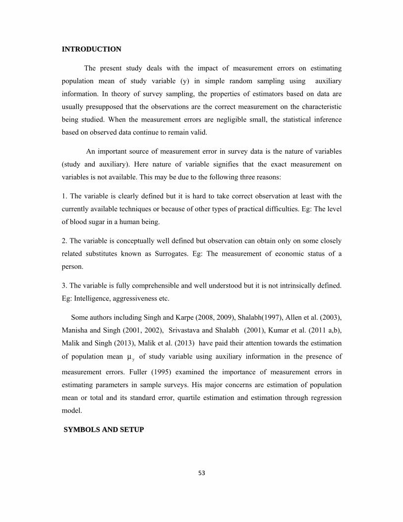
IINNTTRROODDUUCCTTIIOONN
The present study deals with the impact of measurement errors on estimating
population mean of study variable (y) in simple random sampling using auxiliary
information. In theory of survey sampling, the properties of estimators based on data are
usually presupposed that the observations are the correct measurement on the characteristic
being studied. When the measurement errors are negligible small, the statistical inference
based on observed data continue to remain valid.
An important source of measurement error in survey data is the nature of variables
(study and auxiliary). Here nature of variable signifies that the exact measurement on
variables is not available. This may be due to the following three reasons:
1. The variable is clearly defined but it is hard to take correct observation at least with the
currently available techniques or because of other types of practical difficulties. Eg: The level
of blood sugar in a human being.
2. The variable is conceptually well defined but observation can obtain only on some closely
related substitutes known as Surrogates. Eg: The measurement of economic status of a
person.
3. The variable is fully comprehensible and well understood but it is not intrinsically defined.
Eg: Intelligence, aggressiveness etc.
Some authors including Singh and Karpe (2008, 2009), Shalabh(1997), Allen et al. (2003),
Manisha and Singh (2001, 2002), Srivastava and Shalabh (2001), Kumar et al. (2011 a,b),
Malik and Singh (2013), Malik et al. (2013) have paid their attention towards the estimation
of population mean yμ of study variable using auxiliary information in the presence of
measurement errors. Fuller (1995) examined the importance of measurement errors in
estimating parameters in sample surveys. His major concerns are estimation of population
mean or total and its standard error, quartile estimation and estimation through regression
model.
SSYYMMBBOOLLSS AANNDD SSEETTUUPP

54
Let, for a SRS scheme )y,x( ii be the observed values instead of true values
)Y,X( ii on two characteristics (x, y), respectively for all i=(1,2,…n) and the observational or
measurement errors are defined as
)Yy(u iii −= (1)
)Xx(v iii −= (2)
where ui and vi are stochastic in nature with mean 0 and variance 2uσ and 2
vσ respectively.
For the sake of convenience, we assume that s'u i and s'vi are uncorrelated
although s'Xi and s'Yi are correlated .Such a specification can be, however, relaxed at the
cost of some algebraic complexity. Also assume that finite population correction can be
ignored.
Further, let the population means and variances of (x, y) be ),( yx μμ and ),( 2y
2x σσ . xyσ and
ρ be the population covariance and the population correlation coefficient between x and y
respectively. Also let y
yyC
μσ
= and x
xxC
μσ
= are the population coefficient of variation and
yxC is the population coefficients of covariance in y and x.
LLAARRGGEE SSAAMMPPLLEE AAPPPPRROOXXIIMMAATTIIOONN
Define:
y
y0
ye
μμ−
= and x
x1
xe
μμ−
=
where, 0e and 1e are very small numbers and )1,0i(1ei =< .
Also, )1,0i(0)e(E i ==
and, 02y
2u2
y20 1C)e(E δ=
σσ
+θ= ,

55
12x
2v2
x21 1C)e(E δ=
σσ
+θ= , yx10 CC)ee(E θρ= , wheren
1=θ .
22.. EEXXIISSTTIINNGG EESSTTIIMMAATTOORRSS AANNDD TTHHEEIIRR PPRROOPPEERRTTIIEESS
Usual mean estimator is given by
=
=n
1i
i
n
yy (3)
Up to the first order of approximation the variance of y is given by
2y2
y
2u2
y C1)y(Var
σσ
+μθ= (4)
The usual ratio estimator is given by
μ
=x
yy xR (5)
where xμ is known population mean of x.
The bias and MSE ( Ry ), to the first order of approximation, are respectively, given
ρ−
σσ
+μθ= xy2x2
x
2v
yR CCC1)y(B (6)
ρ−
σσ
++
σσ
+μθ= xy2x2
x
2v2
y2y
2u2
yR CC2C1C1)y(MSE (7)
The traditional difference estimator is given by
)x(kyy xd −μ+= (8)
where, k is the constant whose value is to be determined.
Minimum mean square error of dy at optimum value of

56
x2x
2v
x
yy
C1
Ck
σσ
+μ
ρμ= , is given by
σσ
+
σσ
+
ρ−
σσ
+θμ=
2x
2v
2y
2u
22y2
y
2u2
yd
11
1C1)y(MSE (9)
Srivastava (1967) suggested an estimator
1
xyy x
S
μ= (10)
where, 1 is an arbitrary constant.
Up to the first of approximation, the bias and minimum mean square error of Sy at optimum
value of
xx
v
y
C
C
+
=
2
21
1σσ
ρ are respectively, given by
ρθ−
σσ
+θ+
μ= xy12x2
x
2v11
yS CCC12
)1()y(B
(11)
σσ
+
σσ
+
ρ−
σσ
+θμ=
2x
2v
2y
2u
22y2
y
2u2
yS
11
1C1)y(MSE (12)
Walsh (1970) suggested an estimator wy
μ−+
μ=
x22
xw )1(x
yy
(13)
where, 2 is an arbitrary constant.

57
Up to the first order of approximation, the bias and minimum mean square error of wy at
optimum value of
x2x
2v
y2
C1
C
σσ
+
ρ= , are respectively, given by
ρ−
σσ
+θμ= xy22x
2v2
x22yw CC1C)y(B (14)
σσ
+
σσ
+
ρ−
σσ
+θμ=
2x
2v
2y
2u
22y2
y
2u2
yw
11
1C1)y(MSE (15)
Ray and Sahai (1979) suggested the following estimator
μ
+−=x
33RS
xyy)1(y (16)
where, 3 is an arbitrary constant.
Up to the first order of approximation, the bias and mean square of RSy at optimum value of
σσ
+
ρ−=
2x
2v
y3
1
C are respectively, given by
xyy3RS CC)y(B ρμθ= (17)
σσ
+
σσ
+
ρ−
σσ
+θμ=
2x
2v
2y
2u
22y2
y
2u2
yRS
11
1C1)y(MSE (18)
3. SUGGESTED ESTIMATOR
Following Singh and Solanki (2013), we suggest the following difference-type class of
estimators for estimating population mean Y of study variable y as

58
[ ]α
μμα−α−+α+α=
*
*x*
x21*
21p x)1(xyt (19)
where ),( 21 αα are suitably chosen scalars such that MSE of the proposed estimator is
minimum, )x(x * λ+η= , )( x*x λ+ημ=μ with ),n( λ are either constants or function of some
known population parameters. Here it is interesting to note that some existing estimators have
been shown as the members of proposed class of estimators pt for different values of
),,,,( 21 ληααα , which is summarized in Table 1.
Table 1: Members of suggested class of estimators
Values of Constants
Estimators 1α 2α α η λ
y [Usual unbiased] 1 0 0 - -
Ry [Usual ratio] 1 0 1 1 0
dy [Usual difference] 1 2α 0 -1 xμ
Sy [Srivastava (1967)] 1 0 α 1 0
DSy [Dubey and Singh] 1α 2α 0 1 0
The properties of suggested estimator are derived in the following theorems.
Theorem 1.1: Estimator pt in terms of 1,0i;ei = expressed as:
{ }[ 10yy02111
21
*x
*x1
*xp eeAeBCeACeCeBAet μα−μ++α−α+μ+μα−μ=
{ }]211x2 Aee α−ημα+

59
ignoring the terms )ee(E sj
ri for (r+s)>2,where r,s=0,1,2... and 1,0=i ; 1j = (first order of
approximation).
where, λ+μη
μη=
x
xA , 2A2
)1(B
+αα= and .C *xy μ−μ=
Proof
[ ]α
μμα−α−+α+α=
*
*x*
x21*
21p x)1(xyt
Or
[ ][ ] α−+μα−+μηα++α= 1*x11x201p Ae1)1(e)e1(t (20)
We assume 1eA 1 < , so that the term α−+ )Ae1( 1 is expandable. Expanding the right hand
side (20) and neglecting the terms of e’s having power greater than two, we have
{ }10yy02111
21
*x
*x1
*xp eeAeBCeACeCeBAet μα−μ++α−α+μ+μα−μ=
{ }211x2 Aee α−ημα+
Theorem: 1.2 Bias of the estimator pt is given by
{ }[ ]1x201y111*xp AABCB)t(B αδημα−δμα−δα+δμ= (21)
Proof:
)t(E)t(B ypp μ−=
=E { }[ 10yy02111
21
*x
*x1y
*x eeAeBCeACeCeBAe μα−μ++α−α+μ+μα−μ−μ
{ }]211x2 Aee α−ημα+
= { }[ ]1x201y111*x AABCB αδημα−δμα−δα+δμ
where, 0110 and, δδδ are already defined in section 3.

60
Theorem 1.3: MSE of the estimator pt , up to the first order of approximation is
( ){ } 12x
22201y
222210
2y
221p AC4BC2CAC)t(MSE δμηα+δμα−+αδ+δμ+α=
( ){ } ( ) ( ){ }CACABCBCC2BC2AC *xy01
*x
22*x
21
21
*x
2x
221
2 −μμαδ+μα−μ−δ+α−μ−μαδ++
( ) ( )101yx21*x1x2 CA22CA2 δα−δμημαα+−μδαημα− (22)
Proof:
2ypp )t(E)t(MSE μ−=
= { } { }[ 211x210y
21y011 eAeeeABCeeCeACE α−ημα+μα−+μ+α−α
]221
*x
*x1 eBAeC μ−μα+−
Squaring and then taking expectations of both sides, we get the MSE of the suggested
estimator up to the first order of approximation as
( ){ } 12x
22201y
222210
2y
221p AC4BC2CAC)t(MSE δμηα+δμα−+αδ+δμ+α=
( ){ } ( ) ( ){ }CACABCBCC2BC2AC *xy01
*x
22*x
21
21
*x
2x
221
2 −μμαδ+μα−μ−δ+α−μ−μαδ++
( ) ( )101yx21*x1x2 CA22CA2 δα−δμημαα+−μδαημα−
Equation (22) can be written as:
ϕ+ϕαα+ϕα−ϕα−ϕα+ϕα= 52142312221
21p 222)t(MSE (23)
Differentiating (23) with respect to ),( 21 αα and equating them to zero, we get the optimum
values of ),( 21 αα as
2521
5432)opt(1 ϕ−ϕϕ
ϕϕ−ϕϕ=α and
2521
5341)opt(2 ϕ−ϕϕ
ϕϕ−ϕϕ=α
where, ( ) 01y2222
102y
21 AC4BC2CAC δμα−+αδ+δμ+=ϕ
12x
22 δμη=ϕ
61
( ) ( )CACABCBCC *xy01
*x
22*x
21
23 −μμαδ+μα−μ−δ+=ϕ
( )CA *x1x4 −μδαημ=ϕ
( ).CA2 101yx5 δα−δμημ=ϕ
( )*x
2x
221
2 BC2AC μ−μαδ+=ϕ
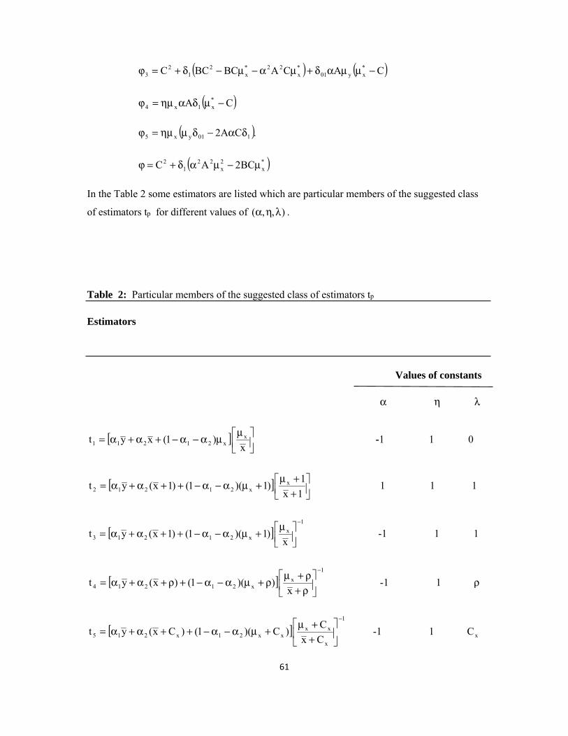
In the Table 2 some estimators are listed which are particular members of the suggested class
of estimators tp for different values of ),,( ληα .
Table 2: Particular members of the suggested class of estimators tp
Estimators
Values of constants
α η λ
[ ]
μ
μα−α−+α+α=x
)1(xyt xx21211 -1 1 0
[ ]
++μ
+μα−α−++α+α=1x
1)1)(1()1x(yt x
x21212 1 1 1
[ ]1
xx21213 x
)1)(1()1x(yt−
μ
+μα−α−++α+α= -1 1 1
[ ]1
xx21214 x
))(1()x(yt−
ρ+ρ+μ
ρ+μα−α−+ρ+α+α= -1 1 ρ
[ ]1
x
xxxx21x215 Cx
C)C)(1()Cx(yt
−
++μ
+μα−α−++α+α= -1 1 xC

62
[ ]
−−μ
−μα−α−+−α+α=x
xxxx21x216 Cx
C)C)(1()Cx(yt -1 1 xC−
[ ]1
x
xxxx21217 Cx
C)C)(1()1x(yt
−
++μ
+μα−α−−+α−α= -1 -1 -1
4. EMPIRICAL STUDY
Data statistics: The data used for empirical study has been taken from Gujarati (2007)
Where, iY =True consumption expenditure,
iX =True income,
iy =Measured consumption expenditure,
ix = Measured income.
n yμ xμ 2yσ 2
xσ ρ 2uσ 2
vσ
10 127 170 1278 3300 0.964 36 36
The percentage relative efficiencies (PRE) of various estimators with respect to the mean per
unit estimator of Y , that is y ,can be obtained as
100*(.)MSE
)y(Var(.)PRE =
Table 3: MSE and PRE of estimators with respect to y
Estimators Mean Square Error Percent Relative Efficiency
y 131.4 100
Ry 21.7906 603.0118
dy 13.916 944.1285

63
Sy 13.916 944.1285
DSy 13.916 944.1285
1t 10.0625 1236.648
2t 9.92677 1323.693
3t 6.82471 1925.356
4t 6.9604 1887.818
5t 9.3338 1407. 774
6t 11.9246 1101.923
7t 7.9917 1644.194
5. PERFORMANCE OF SUGGESTED ESTIMATOR IN STRATIFIED RANDOM
SAMPLING
SSYYMMBBOOLLSS AANNDD SSEETTUUPP
Consider a finite population )u,...,u,u(U N21= of size N and let X and Y respectively
be the auxiliary and study variables associated with each unit )N,......,2,1j(u j == of
population. Let the population of N be stratified in to L strata with the thh stratum containing
hN units, where h=,1,2,3,….,L such that =
=L
1ih NN . A simple random size nh is drown
without replacement from the hth stratum such that nnL
1ih =
=
. Let )X,y( hihi of two
characteristics (Y,X) on ith unit of the hth stratum, where i=,1,2,…,Nh. In addition let
( =
=hn
1ihi
hh y
n
1y ,
=
=hn
1ihi
hh x
n
1x ),
( h
n
1ihsth
n
1ihst xWx,yWy
hh
==
== ),

64
( = =
=μ=μh hN
1i
N
1ihi
hXhhi
hYh x
N
1,y
N
1),
And ( = =
μ=μμ=μL
1h
N
1iXhhXYhhY
h
W,W ) be the samples means and population means of(Y,X)
respectively, where N
NW h
h = is the stratum weight. Let the observational or measurement
errors be
hihihi Yyu −= (24)
hihihi Xxv −= (25)
Where uhi and vhi are stochastic in nature and are uncorrelated with mean zero and variances
2Vhσ and 2
Uhσ respectively. Further let hρ be the population correlation coefficient between Y
and X in the hth stratum. It is also assumed that the finite population correction terms
)f1( h− and )f1( − can be ignored where h
hh N
nf = and
N
nf = .
LLAARRGGEE SSAAMMPPLLEE AAPPPPRROOXXIIMMAATTIIOONN
Let,
)e1(y h0Yst +μ= , and )e1(x h1Xst +μ=
such that, 0)e(E)e(E h1h0 == ,
0Yhh
2Yh
2Yh
2Uh
h
2Yh2
h0 n
C1
n
C)e(E ∇=
θ=
σσ
+= ,
1Xhh
2Xh
2Xh
2Vh
h
2Xh2
h1 n
C1
n
C)e(E ∇=
θ=
σσ
+= ,
01XhYhhh
h1h0 CCn
1)ee(E ∇=ρ= .
where, ,CYh
YhYh μ
σ= ,C
Xh
XhXh μ
σ=
2Yh
2Uh
2Uh
Yh σ+σσ
=θ and .2Xh
2Vh
2Vh
Xh σ+σσ
=θ

65
EEXXIISSTTIINNGG EESSTTIIMMAATTOORRSS AANNDD TTHHEEIIRR PPRROOPPEERRTTIIEESS
sty is usual unbiased estimator in stratified random sampling scheme.
The usual combined ratio estimator in stratified random sampling in the presence of
measurement error is defined as-
st
xstR x
yTμ
= (26)
The usual combined product estimator in the presence of measurement error is
defined as-
x
ststPR
xyT
μ= (27)
Combined difference estimator in stratified random sampling is defined in the
presence of measurement errors for a population mean, as
)x(dyT stxstD −μ+= (28)
The variance and mean square term of above estimators, up to the first order of
approximation, are respectively given by
σσ
+=2Yh
2Uh
h
2Xh
st 1n
C)y(Var (29)
( )XhYXh
L
1h Xh
2Xh
Yh
2Yh
h
2h
R 2RRn
W)T(MSE θβ−
θσ
+θσ
==
(30)
( )XhYXh
L
1h Xh
2Xh
Yh
2Yh
h
2h
P 2RRn
W)T(MSE θβ+
θσ
+θσ
==
(31)
= = =
σβ−
θσ
+
θσ
=L
1h
L
1h
L
1h
2XhXYh
h
2h
Xh
2Xh
h
2h2
Yh
2Yh
h
2h
D n
Wd2
n
Wd
n
W)T(MSE (32)

66
where,
=
=
θσ
σβ=
L
1h Xh
2Xh
h
2h
L
1h
2XhXYh
h
2h
opt
n
W
n
W
d
6. SUUGESTED ESTIMATOR AND ITS PROPERTIES
Let B(.) and M(.) denote the bias and mean square error (M.S.E) of an estimator under
given sampling design. Estimator tp defined in equation (19) can be written in stratified
random sampling as
[ ]β
μμβ−β−+β+β=
*st
*x*
x21*st2st1P
x)1(xyT (33)
where ),( 21 αα are suitably chosen scalars such that MSE of proposed estimator is
minimum, )x(x st*st λ+η= , )( x
*x λ+ημ=μ with ),n( λ are either constants or functions of
some known population parameters. Here it is interesting to note that some existing
estimators have been found particular members of proposed class of estimators Tp for
different values of ),,,,( 21 ληααα , which are summarized in Table 4.
Table 4: Members of proposed class of estimators Tp
Values of Constants
Estimators 1α 2α α η λ
sty [Usual unbiased] 1 0 0 - -
RT [Usual ratio] 1 0 1 1 0
PRT [Usual product] 1 0 -1 1 0
DT [Usual difference] 1 2α 0 -1 xμ

67
Theorem 2.1: Estimator PT in terms of 1,0; =iei by ignoring the terms )( sjh
riheeE for
(r+s)>2,where r,s=0,1,2... and 1,0=i ; 1=j , can be written as
{ }[ h1h0yyh02h1h11
2h1
*x
*xh1
*xP ee'Aee'C'BCe'A'Ce'Be'AT μβ−μ++β−β+μ+μβ−μ=
{ }]2h1h1x2 e'Ae β−ημβ+
where, λ+μη
μη=
x
x'A , 2'A2
)1('B
+ββ= and .'C *xy μ−μ=
Proof
[ ]β
μμβ−β−+β+β=
*st
*x*
x21*
st2st1Px
)1(xyT
= [ ][ ] β−+μβ−+μηβ++β h1*x1h1x2h01 e'A1)1(e)e1( (34)
We assume 1' 1 <heA , so that the term β−+ )'1( 1heA is expandable. Thus by expanding the
right hand side (20) and neglecting the terms of e’s having power greater than two, we have
Tp = { }[ h1h0yyh02h1h11
2h1
*x
*xh1
*x ee'Aee'C'Be'C'A'Ce'Be'A μβ−μ++β−β+μ+μβ−μ
{ }]2h1h1x2 e'Ae β−ημβ+
Theorem: 2.2 Bias of pT is given by
{ }[ ]1x201y111*xP 'A'A'C'B'B)T(B ∇βημβ−∇μβ−∇β+∇μ= (35)
Proof:
)T(E)T(B yPP μ−=
=E { }[ h1h0yyh02h1h11
2h1
*x
*xh1y
*x ee'Aee'C'Be'C'A'Ce'Be'A μβ−μ++β−β+μ+μβ−μ−μ
{ }]2h1h1x2 e'Ae β−ημβ+

68
= { }[ ]1x201y111*x 'A'A'C'B'B ∇βημβ−∇μβ−∇β+∇μ
where, 0110 and, ∇∇∇ are already defined in section 3.
Theorem: 2.3 Mean square error of Tp, up to the first order of approximation is given by
( ){ } 12x
22201y
222210
2y
221P 'C'A4'C'B2'C'A'C)T(MSE ∇μηβ+∇μβ−+β∇+∇μ+β=
( ){ } ( ) ( ){ }'CA'C'A'C'B'C'B'C2'C'B2'A'C *xy01
*x
22*x
21
21
*x
2x
221
2 −μμβ∇+μβ−μ−+∇β−μ−μβ+∇+
( ) ( )101yx21*x1x2 'C'A22'CA2 ∇β−∇μημββ+−μ∇βημβ− (36)
Proof:
2yPP )T(E)T(MSE μ−=
( ){ } 12x
22201y
222210
2y
221P 'C'A4'C'B2'C'A'C)T(MSE ∇μηβ+∇μβ−+β∇+∇μ+β=
( ){ } ( ) ( ){ }'CA'C'A'C'B'C'B'C2'C'B2'A'C *xy01
*x
22*x
21
21
*x
2x
221
2 −μμβ∇+μβ−μ−+∇β−μ−μβ+∇+
( ) ( )101yx21*x1x2 'C'A22'CA2 ∇β−∇μημββ+−μ∇βημβ−
MSE(Tp) can also be written as
χ+χββ+χβ−χβ−χβ+χβ= 52142312221
21P 222)T(MSE (37)
Differentiating equation (37) with respect to ),( 21 ββ and equating it to zero, we get the
optimum values of ),( 21 ββ respectively, as
2521
5432)opt(1 χ−χχ
χχ−χχ=β and
2521
5341)opt(2 χ−χχ
χχ−χχ=β
where, ( ) 01y2222
102y
21 'C'A4'C'B2'C'A'C ∇μβ−+β∇+∇μ+=χ
12x
22 ∇μη=χ
( ) ( )'C'A'C'A'C'BBC'C *xy01
*x
22*x
21
23 −μμβ∇+μβ−μ−+∇=χ
( )'C'A *x1x4 −μ∇βημ=χ

69
( ).'C'A2 101yx5 ∇β−∇μημ=χ
( )*x
2x
221
2 'C'B2'A'C μ−μβ+∇=χ
With the help of these values, we get the minimum MSE of the suggested estimator Tp.
7. DISCUSSION AND CONCLUSION
In the present study, we have proposed difference-type class of estimators of the
population mean of a study variable when information on an auxiliary variable is known in
advance. The asymptotic bias and mean square error formulae of suggested class of
estimators have been obtained. The asymptotic optimum estimator in the suggested class has
been identified with its properties. We have also studied some traditional methods of
estimation of population mean in the presence of measurement error such as usual unbiased,
ratio, usual difference estimators suggested by Srivastava(1967), dubey and singh( 2001),
which are found to be particular members of suggested class of estimators. In addition, some
new members of suggested class of estimators have also been generated in simple random
sampling case. An empirical study is carried to throw light on the performance of suggested
estimators over other existing estimators using simple random sampling scheme. From the
Table 3, we observe that suggested estimator t3 performs better than the other estimators
considered in the present study and which reflects the usefulness of suggested method in
practice.
REFERENCES
Allen, J., Singh, H. P. and Smarandache, F. (2003): A family of estimators of population
mean using mutliauxiliary information in presence of measurement errors.
International Journal of Social Economics 30 (7), 837–849.
A.K. Srivastava and Shalabh (2001). Effect of measurement errors on the regression method
of estimation in survey sampling. Journal of Statistical Research, Vol. 35,
No. 2, pp. 35-44.
Bahl, S. and Tuteja, R. K. (1991): Ratio and product type exponential estimator. Information
and optimization sciences12 (1), 159-163.
Chandhok, P.K., & Han, C.P.(1990):On the efficiency of the ratio estimator under Midzuno
scheme with measurement errors. Journal of the Indian statistical
Association,28,31-39.

70
Dubey, V. and Singh, S.K. (2001). An improved regression estimator for estimating
population mean, J. Ind. Soc. Agri. Statist., 54, p. 179-183.
Gujarati, D. N. and Sangeetha (2007): Basic econometrics. Tata McGraw – Hill.
Koyuncu, N. and Kadilar, C. (2010): On the family of estimators of population mean in
stratified sampling. Pakistan Journal of Statistics. Pak. J. Stat. 2010 vol 26 (2),
427-443.
Kumar, M. , Singh, R., Singh, A.K. and Smarandache, F. (2011 a): Some ratio type
estimators under measurement errors. WASJ 14(2) :272-276.
Kumar, M., Singh, R., Sawan, N. and Chauhan, P. (2011b): Exponential ratio method of
estimators in the presence of measurement errors. Int. J. Agricult. Stat. Sci. 7(2):
457-461.
Malik, S. and Singh, R. (2013) : An improved class of exponential ratio- type estimator in
the presence of measurement errors. OCTOGON Mathematical Magazine, 21,1,
50-58.
Malik, S., Singh, J. and Singh, R. (2013) : A family of estimators for estimating the
population mean in simple random sampling under measurement errors. JRSA,
2(1), 94-101.
Manisha and Singh, R. K. (2001): An estimation of population mean in the presence of
measurement errors. Journal of Indian Society of Agricultural Statistics 54(1),
13–18.
Manisha and Singh, R. K. (2002): Role of regression estimator involving measurement errors.
Brazilian journal of probability Statistics 16, 39- 46.
Shalabh (1997): Ratio method of estimation in the presence of measurement errors. Journal of
Indian Society of Agricultural Statistics 50(2):150– 155.
Singh, H. P. and Karpe, N. (2008): Ratio-product estimator for population mean in presence
of measurement errors. Journal of Applied Statistical Sciences 16, 49–64.
Singh, H. P. and Karpe, N. (2009): On the estimation of ratio and product of two populations
means using supplementary information in presence of measurement errors.
Department of Statistics, University of Bologna, 69(1), 27-47.
Singh, H. P. and Vishwakarma, G. K. (2005): Combined Ratio-Product Estimator of Finite
Population Mean in Stratified Sampling. Metodologia de Encuestas 8: 35- 44.

71
Singh, H. P., Rathour, A., Solanki, R. S.(2013): An improvement over difference method of
estimation of population mean. JRSS, 6(1):35-46.
Singh H. P., Rathour A., Solanki R.S. (2013): an improvement over difference method of
estimation of population mean. JRSS, 6(1): 35-46.
Srivastava, S. K. (1967): An estimator using auxiliary information in the sample surveys.
Calcutta statistical Association Bulletin 16,121-132.
Walsh, J.E.(1970). Generalisation of ratio estimate for population total. Sankhya A.32,
99-106.

The purpose of writing this book is to suggest some improved estimators
using auxiliary information in sampling schemes like simple random sampling,
systematic sampling and stratified random sampling.
This volume is a collection of five papers, written by nine co-authors
(listed in the order of the papers): Rajesh Singh, Mukesh Kumar, Manoj Kr.
Chaudhary, Cem Kadilar, Prayas Sharma, Florentin Smarandache, Anil
Prajapati, Hemant Verma, and Viplav Kr. Singh.
In first paper dual to ratio-cum-product estimator is suggested and its
properties are studied. In second paper an exponential ratio-product type
estimator in stratified random sampling is proposed and its properties are
studied under second order approximation. In third paper some estimators are
proposed in two-phase sampling and their properties are studied in the
presence of non-response.
In fourth chapter a family of median based estimator is proposed in
simple random sampling. In fifth paper some difference type estimators are
suggested in simple random sampling and stratified random sampling and their
properties are studied in presence of measurement error.