Efficient scheme for parametric fitting of data in arbitrary dimensions

Ning-Ning Pang,1,* Wen-Jer Tzeng,2,† and Hisen-Ching Kao1

1Department of Physics, National Taiwan University, Taipei, Taiwan2Department of Physics, Tamkang University, Tamsui, Taipei, Taiwan

�Received 5 December 2007; revised manuscript received 29 April 2008; published 17 July 2008�

We propose an efficient scheme for parametric fitting expressed in terms of the Legendre polynomials. Forcontinuous systems, our scheme is exact and the derived explicit expression is very helpful for further ana-lytical studies. For discrete systems, our scheme is almost as accurate as the method of singular value decom-position. Through a few numerical examples, we show that our algorithm costs much less CPU time andmemory space than the method of singular value decomposition. Thus, our algorithm is very suitable for alarge amount of data fitting. In addition, the proposed scheme can also be used to extract the global structureof fluctuating systems. We then derive the exact relation between the correlation function and the detrendedvariance function of fluctuating systems in arbitrary dimensions and give a general scaling analysis.

DOI: 10.1103/PhysRevE.78.011112 PACS number�s�: 02.50.�r, 05.40.�a, 05.45.Tp, 02.60.�x

I. INTRODUCTION

Various physical systems in Nature, from the scale ofatomic clusters to the scale of oceans, consist of macroscopicstructures. Some examples are molecular-beam-epitaxialgrowth at high temperature �1,2�, pulse-current electrochemi-cal deposition �3�, cultivated tumor growth �4�, and the tem-perature and salinity distribution in the world oceans �5�.Moreover, many time series data also show macroscopictrends, such as the clustering features of seismic sequences�6�, the interfiring time intervals between neural action po-tentials �7�, and the heart-rate fluctuations during sleep �8�.When performing various experiments, people try to con-dense the data and extract the essence by fitting data to ap-propriate parametric models. Without knowledge of the ori-gin of macroscopic structures, the polynomial function iscommonly chosen to be the fitting function. The values ofthe coefficients of the polynomial function are determined bya least-squares fit to the data set.

In the literature, the most commonly used methods for theleast-squares fit are the method of normal equations and themethod of singular value decomposition �SVD� �9–11�.However, each of these two methods has some drawbacks.�1� Although the ideas behind the method of normal equa-tions are very straightforward and natural, the analytical so-lutions of the normal equations are hardly attainable exceptin some simple cases. In addition, the numerical solutions ofthe normal equations suffer seriously from the roundoff er-rors. �2� Among the available methods in the literature, theSVD method is known to be the most accurate method for aleast-squares fit. However, this method takes a relativelylong computation time and large memory space. Thus, to fita large amount of data points to a high-degree polynomial inhigh dimensions, the SVD method is in practice not feasible.Since the need for data fitting to polynomial functions is very

common, we are strongly motivated to construct a fittingalgorithm, which is relatively efficient and accurate for pro-cessing large data sets in arbitrary dimensions.

Notably, fluctuating systems with the formation of macro-scopic structures have drawn much attention in recent years.Some examples are electrochemical deposition, physiologysignals, and the mosaic structure of DNA sequences�3,7,8,12–14�. The common feature of these systems is theexistence of long-range positive �or negative� correlation be-tween the fluctuations. The scaling exponents can then beused to categorize the universality classes of these systems.People usually adopt the polynomial approximation to obtainthe best guess at the global structures of such systems. Sincethese fluctuating systems usually contain large amounts ofdata points, our proposed fitting scheme is very suitable forextracting the global structures of these systems effectively.In addition, in our proposed algorithm, the fitting parametersare explicitly expressed in a systematic way. It will be veryhelpful for further analytical study of the scaling analysis offluctuations.

Interestingly, in the field of computational molecular bi-ology, Peng et al. �12–14� have proposed a “detrended fluc-tuation analysis” �DFA� method to determine the long-rangecorrelation in DNA sequences but exclude the effect causedby the mosaic structure. Its basic algorithm �12–14� is brieflygiven as follows. The first step is to extract the trend �or themacroscopic structure�, which is expressed in terms of aqth-degree polynomial with the coefficients determined by anumerical least-squares fit. The second step is to calculatethe corresponding qth-degree detrended variance functionand analyze its scaling behaviors. Although the DFA methodhas been widely accepted as a standard analysis scheme inthe study of fluctuating systems with the formation of globalstructures, there still exist two unresolved issues in thismethod. �1� The DFA method is based on the following con-jecture. For any fluctuating system in arbitrary dimensions,the detrended variance function can successfully suppress theinfluence of trends �or global structures� and, at the sametime, retain the scaling behaviors originating from the sto-chastic nature of the system. Although this conjecture is in-tuitively correct, it still lacks a rigorous proof. �2� The ex-plicit and exact relations among the correlation functions, the

*Author to whom correspondence should be addressed.nnp@phys.ntu.edu.tw

†Author to whom correspondence should be addressed.wjtzeng@mail.tku.edu.tw

PHYSICAL REVIEW E 78, 011112 �2008�

1539-3755/2008/78�1�/011112�11� ©2008 The American Physical Society011112-1

variance functions, and the detrended variance functions offluctuating systems in arbitrary dimensions have not yet beenderived. We are strongly motivated to address the above twoissues rigorously. Note that, in our proposed fitting scheme,all the fitting parameters of the global structure are explicitlyexpressed in terms of Legendre polynomials. By employingthis expression, we are able to analytically obtain the exactrelation among the correlation functions, the variance func-tions, and the detrended variance functions. If these relationsare obtained, one just needs to know the information aboutthe correlation functions and then the other two quantitiescan be easily derived. Hence, a large amount of computationtime can be saved. Furthermore, by using these obtained ex-act relations, we can then give a rigorous proof of the intui-tive conjecture of the DFA method.

The outline of this paper is as follows. In Sec. II, webriefly review the concept of the general least-squares fit andits two commonly used methods: normal equations and theSVD method. In Sec. III, by employing the Legendre poly-nomials, we propose a scheme for parametric fitting and dis-cuss its merits. In Sec. IV, we use three examples to numeri-cally demonstrate the merits of our proposed scheme overthe old methods. In Sec. V, the exact relation between thecorrelation function and the detrended variance function forfluctuating systems with formation of global structures is de-rived. We then present a scaling analysis applicable for anyfluctuating systems. In Sec. VI, a brief summary is given.

II. GENERAL LEAST-SQUARES FIT AND THE METHODOF SINGULAR VALUE DECOMPOSITION

In this section, we will first briefly review the concept ofgeneral least-squares fit and its two commonly used meth-ods: normal equations and the SVD method. Then, the meritsand the drawbacks of each method will be discussed.

Suppose that one is measuring a variable y as a functionof x, a vector in the d-dimensional space. Given a set of datapoints �y�x��, measured within a d-dimensional observationwindow, one often would like to condense the data and ex-tract the essential information by fitting the data set to aparametric model with adjustable parameters. Without losinggenerality, the polynomial functions are usually chosen to bethe fitting functions and the fit supplies the appropriate coef-ficients. That is, the fitting function is a �q�th-degree ��q���q1 , . . . ,qd�� polynomial with adjustable parameters a�n�,

y�q��x� � ��n�=�0�

�q�

a�n�j=1

d

�xj − xj�nj ,

with the summation running over the set of indices 0�ni�qi for all 1� i�d, and one obtains the appropriate param-eter values by minimizing

�y�x� − y�q��x��2�

with ¯� denoting the average over a d-dimensional obser-vation window centered at x and of size l1� ¯ � ld. Forcontinuous systems, the coefficients �a�n�� satisfy the follow-ing relations:

�y�x�j=1

d

�xj − xj�nj = ��n��=�0�

�q� �a�n��j=1

d � lj

2�nj+nj�

��1 + �− 1�nj+nj��2�nj + nj� + 1� � �1�

for all �n�’s. For discrete systems, the coefficients �a�n�� sat-isfy the relations

�y�x�j=1

d

�xj − xj�nj = �

�n��=�0�

�q� �a�n��j=1

d � 1

lj�xj=1

lj �xj −lj

2�nj+nj��� �2�

for all �n�’s. In the literature, the collection of Eqs. �1� or �2�are called the normal equations of the least-squares problem.To determine �a�n�� in Eqs. �1� or �2�, one needs to deal withthe inverse of a tensor of rank 2d. Since the above line ofthought is very natural and straightforward, one usuallycomes to solving the normal equations. However, the nu-merical solution of �a�n�� directly from Eqs. �2� is very sus-ceptible to roundoff error, and to analytically obtain �a�n��from Eqs. �1� or �2� is barely feasible except for some simplecases. Thus, solving normal equations directly is not a rec-ommended way to deal with the least-squares problem.

For discrete systems, Cuyt et al. �15� have proposed toreformulate the multivariate data fitting problem in terms ofa product of orthogonal polynomial basis, instead of the mul-tinomial basis. For discrete systems with the number of datapoints �which are sampled at optimal locations� equal to thenumber of fitting parameters, these authors have theoreticallyshown that, by employing the fast LU factorization with par-tial pivoting, both computational cost and the degree of illconditioning can be greatly improved when using an or-thogonal polynomial basis. Note that, in linear algebra, theLU factorization with partial pivoting is a matrix decompo-sition which writes a matrix as the product of a lower trian-gular matrix, an upper triangular matrix, and a permutationmatrix.

To numerically solve all kinds of least-squares problems,the most often recommended technique in the literature is theSVD method �9,11� for its general and rigorous treatment ofill-conditioned situations. This method is based on the fol-lowing theorem of linear algebra �9,11�. Any m�n matrix A,with m�n, can be decomposed as

A = U · � · VT.

The matrices U, �, and V are an m�n column-orthogonalmatrix, an n�n diagonal matrix with elements � j beingpositive or zero �the singular value�, and an n�n orthogonalmatrix, respectively. Given an m�n matrix A and an m�1vector �, the n�1 vector � minimizing �A ·�−�� is shownto be

PANG, TZENG, AND KAO PHYSICAL REVIEW E 78, 011112 �2008�

011112-2

� = V · � · UT · �

with the elements of the n�n diagonal matrix � being 1 /� j�if � j�0� or zero �if � j =0�. See Refs. �9,11� for the detailedproof of the above theorem. Subsequently, we give the mainsteps for implementing the SVD method in parametric fittingof data.

�1� Put the measured data set �y�x�� in the m�1 vector �with the elements � j =y�x j� and �x j ; j=1, . . . ,m� denotingthe data points in the x space.

�2� Let �f i�x� ; i=1, . . . ,n� denote the basis functions andthe fitting function is given by �i=1

n �i f i�x�.�3� The n�1 vector � is then constructed by the fitting

parameters ��i� and the m�n matrix A constructed by �f i�x��with the elements Aji= f i�x j�.

�4� Then the appropriate fitting parameters ��i� are ob-tained by the minimization of �A ·�−��. By employing thetheorem we just mentioned, one gets A=U ·� ·VT and �

=V ·� ·UT ·�.In theory, there should not be any column degeneracy in

the matrix A. However, in some cases the matrix A might beill conditioned; namely, some of the � j’s are so small thattheir apparent values are probably an artifact of roundofferror. In such cases, the vector � �of fitting parameters� ob-tained by zeroing the small � j’s is usually much better thanthe solution with the small � j’s left nonzero. Thus, the SVDmethod cannot be applied blindly. One must decide at whatthreshold to zero the small � j’s. If the SVD method is ap-plied correctly, it is the most reliable method in dealing withthe least-squares problem. However, it has one significantdisadvantage: It usually requires a very long computationtime for iteration and a large memory space to store an extraarray of size m�n. Thus, for the fitting with a large amountof data points, the SVD method might be practically infea-sible.

III. AN ALGORITHM WITH GREAT EFFICIENCY

In this section, we would like to propose a differentscheme for parametric fitting. Our proposed scheme is exactfor continuous systems. For discrete systems, this scheme isalmost as accurate as the SVD method, and it takes muchless CPU time and memory space than the SVD method incomputation. In the following, we will first give a detailedderivation of our scheme and then discuss its implicationsand applications.

Recall that, to determine �a�n�� in Eqs. �1� or �2�, oneneeds to deal with the inverse of a tensor of rank 2d. Forcontinuous systems, one can actually avoid the difficulty insolving the inverse of a high-rank tensor by choosing anappropriate set of orthogonal polynomial basis �f i�x��, whichsatisfies the following relation:

f i�x�f j�x�� �1

l�

−l/2

l/2

dx fi�x�f j�x� = 0 for all i � j .

�3�

In the literature �16�, the classical orthogonal polynomialsare categorized into three classes, Jacobi-like, Laguerre-like,

and Hermite-like polynomials, with the intervals of orthogo-nality being �−1,1�, �0,�, and �− ,�, respectively. Obvi-ously, Laguerre-like and Hermite-like polynomials do notmeet the required relation Eq. �3�. In general, Jacobi-likepolynomials �Ji

�,���x�� satisfy the orthogonal relation�−1

1 dx H�,���x�Ji�,���x�Jj

�,���x�=0 for all i� j, with theweight function H�,���x�= �1−x��1+x�� and the parameters ,��−1. An important subclass of Jacobi-like polynomialsis the Gegenbauer polynomials, which correspond to�Ji

�,���x�� with =��−1. Gegenbauer polynomials consistof two important subclasses: Legendre polynomials and twotypes of Chebyshev polynomials, corresponding to �Ji

�,���x��with =�=0 and =�= 1 /2, respectively. Clearly, the setof Legendre polynomials has the weight function simply 1and will satisfy the required relation Eq. �3� under appropri-ate scaling. Hence, the set of Legendre polynomials

Pi�x� = �j=0

�i/2�

�− 1� j �2i − 2j − 1� ! !

�2j� ! ! �i − 2j�!xi−2j for i = 1,2, . . .

�4�

with the orthogonal property �−11 dx Pi�x�Pi��x�=

2�i,i�2i+1 is a per-

fect candidate to be chosen.We express

y�q��x� = ��n�=�0�

�q�

c�n�j=1

d

Pnj�2�xj − xj�

lj� . �5�

The minimization of �y�x�− y�q��x��2� then leads to

c�n� =�y�x�j=1

d

�2nj + 1�Pnj�2�xj − xj�lj

� . �6�

For illustration, we explicitly list some coefficients:

c00 = y�x�� ,

c10 = 6y�x�z1� ,

c11 = 36y�x�z1z2� ,

c20 =5

2y�x��12z1

2 − 1�� ,

c21 = 15y�x��12z12 − 1�z2� ,

c30 = 7y�x��20z13 − 3z1�� ,

with the dimensionless quantity zj ��xj − xj� / lj. Hence, weobtain

y�q��x� = ��n�=�0�

�q� �y�x�j=1

d

�2nj + 1�Pnj�2�xj − xj�lj

� �

i=1

d

Pni�2�xi − xi�li

� .

In the following analysis, the symbol �q� is used to denotethe union of the sets of indices �n���n1 ,n2 , . . . ,nd� with

EFFICIENT SCHEME FOR PARAMETRIC FITTING OF … PHYSICAL REVIEW E 78, 011112 �2008�

011112-3

��n���n1+n2+ ¯ +nd�q and all ni being nonnegative inte-gers. Thus,

y�q��x� = ���n���q

�y�x�j=1

d

�2nj + 1�Pnj�2�xj − xj�lj

� �

i=1

d

Pni�2�xi − xi�li

� . �7�

The above result can be viewed as the original y�x� con-volved by some specific filter, and this result is exact forcontinuous systems in arbitrary dimensions.

In addition, for a fluctuating system with the formation ofglobal structure, the above result y�q��x� can also be used toexpress the global structure. In Sec. V, by employing theexplicit expression of y�q��x�, we will undertake a detailedanalytical study of the correlation function and the detrendedvariance function of fluctuating systems.

Next, for numerical parametric fitting of discrete systems,we need to take a continuum approximation of the originaldata set in order to apply the above scheme. Let�y�j1 , . . . , jd�� denote the original discrete data set within ad-dimensional observation window of grid size l1� ¯ � ld�i.e., ji=1,2 , . . . , li�. This data set is approximated as a con-tinuous step function and rescaled to the range i=1

d �−1,1�,with the continuous step function z�x� given by z�x�=y�j1 , . . . , jd� for

ji−li/2−1li/2

�xi�ji−li/2

li/2and i=1,2 , . . . ,d. Fol-

lowing the scheme for continuous systems, the fitting func-tion is then expressed as

z�q��x� = ��n�=�0�

�q�

c�n�i=1

d

Pni�xi� .

The parametric fitting corresponds to finding the set of coef-ficients c�n� minimizing

�−1

1

¯�−1

1

dx�z�x� − z�q��x��2.

It leads to

c�n� = �−1

1

¯�−1

1

dx z�x�i=1

d2ni + 1

2Pni

�xi� �8�

for discrete systems. If one is interested in the correspon-dence between the coefficients �c�n�� and �a�n��, it can beeasily derived through the relation

��n�=�0�

�q�

c�n�i=1

d

Pni�xi� = �

�n�=�0�

�q�

a�n�i=1

d

xini. �9�

The merit of our scheme in numerical parametric fitting isefficiency, i.e., taking much less CPU time and memoryspace than the SVD method. In the following, we will givean estimation of the complexity of computation time andmemory occupancy for both the SVD method and ourscheme. Let m, n, and d denote the total number of datapoints, the number of fitting parameters, and the dimension-ality of the system, respectively. The main computation timeof the SVD method is spent on the execution of Householderreductions, of which the time span is about O�mn2�. By con-trast, in our scheme, the operation of the inner product be-tween the data and each basis function costs the CPU time ofO�m�. There are n basis functions in total. Hence, the com-putation time complexity of our method is about O�mn�. Thecomplexity of memory occupancy for the SVD method isO(n�m+n�), which can be easily derived from the main stepsof the SVD method given in Sec. II. By contrast, the com-plexity of memory space for our fitting scheme is O�m+m1/dn1/d� �about O�m� for d�2�, which can be obtainedfrom Eq. �8�. We will demonstrate this merit of our methodthrough a few numerical examples in the next section. Inaddition, the SVD method cannot be applied blindly; namely,one needs to deal with the subtlety of ill-conditioned matri-ces with great care. In contrast, our scheme is generally ap-plicable everywhere with straightforward execution. Thus,for a large amount of data fitting, our scheme is obviouslysuperior to the traditional SVD method.

IV. NUMERICAL DEMONSTRATION

In this section, we will use three examples to demonstratethe merits of our proposed algorithm in numerical parametricfitting.

A. Example 1: A polynomial of degree 3 in two dimensions

In this example, we will draw the data set from a knownpolynomial function and compare fitting results from theSVD method and our method. The function we choose is apolynomial of degree 3 in two dimensions,

y�x� = 5 + x1 − 4x2 + 3x12 + x1x2 − 2x2

2 − x13 − 2x1x2

2

� �0�i+j�3

aijx1i x2

j .

Table I gives the result of parametric fitting of example 1

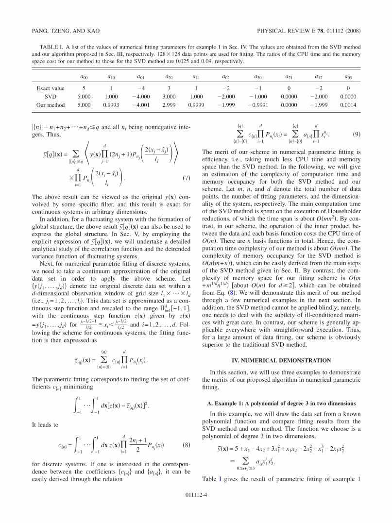
TABLE I. A list of the values of numerical fitting parameters for example 1 in Sec. IV. The values are obtained from the SVD methodand our algorithm proposed in Sec. III, respectively. 128�128 data points are used for fitting. The ratios of the CPU time and the memoryspace cost for our method to those for the SVD method are 0.025 and 0.09, respectively.

a00 a10 a01 a20 a11 a02 a30 a21 a12 a03

Exact value 5 1 �4 3 1 �2 �1 0 �2 0

SVD 5.000 1.000 �4.000 3.000 1.000 �2.000 �1.000 0.0000 �2.000 0.0000

Our method 5.000 0.9993 �4.001 2.999 0.9999 �1.999 �0.9991 0.0000 �1.999 0.0014

PANG, TZENG, AND KAO PHYSICAL REVIEW E 78, 011112 �2008�

011112-4

with the total grids being 128�128 points. The third rowgives the values of �aij� obtained by the SVD method. Thefourth row gives the values of �aij� obtained by our algorithmproposed in Sec. III with the transformation of coefficientsaccording to Eq. �9�. In this example, the ratios of the CPUtime and the memory space cost for our method to those forthe SVD method are 0.025 and 0.09, respectively. Ourmethod is obviously much more efficient than the SVDmethod in computation. The relative deviation between thefitting parameter value obtained by our method and the exactvalue is less than 0.09%. Subsequently, we numerically testhow the fitting results improve as the number of grid pointsfor fitting increases. We find that the relative deviation is lessthan 0.01% if the total grids are more than 1000�1000points.

B. Example 2: Interfacial growth

Next, let us consider an example in interfacial growthphenomena �1,2�. The growth process is described by a sto-chastic partial differential equation in 2+1 dimensions withspatiotemporally correlated noise:

�th�x,t� = − ��4h�x,t� + ��x,t� , �10�

where h�x , t� denotes the interface height at position x andtime t, and ��x , t� represents Gaussian-distributed noise ofzero mean and power-law-decaying correlation

��x,t���x�,t�� = D�x − x��2�−2�t − t��2�−1

with 0���1 /2 and 0���1 /2. Here, the overbar denotesthe ensemble average. In the right-hand side �RHS� of Eq.�10�, the first term accounts for the surface diffusion of de-posits to a nearby position with lower chemical potential andthe second term accounts for the shot noise. The abovegrowth equation with white noise corresponds to the famousHerring-Mullins equation �17�. It is well known that manyexperiments can be well described by the Herring-Mullinsequation; for example, the growth of amorphous Si films bythermal evaporation with a low substrate temperature �18�, Ptsputter deposited on glass at room temperature �19�, and theepitaxial growth of Si on a Si�111� substrate �20�. In contrast,the electrochemical noise is known to be spatiotemporallycorrelated �21,22� and thus the pulse-current electrochemical

deposition process is better described by Eq. �10� with spa-tiotemporally correlated noise.

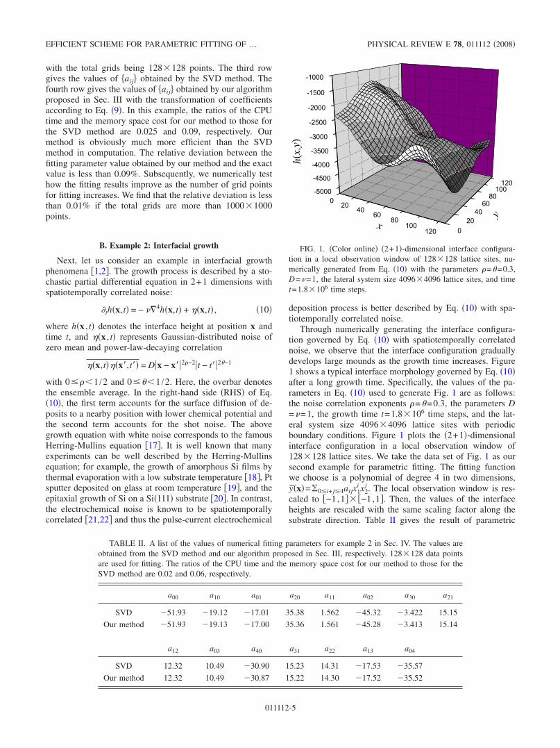
Through numerically generating the interface configura-tion governed by Eq. �10� with spatiotemporally correlatednoise, we observe that the interface configuration graduallydevelops large mounds as the growth time increases. Figure1 shows a typical interface morphology governed by Eq. �10�after a long growth time. Specifically, the values of the pa-rameters in Eq. �10� used to generate Fig. 1 are as follows:the noise correlation exponents �=�=0.3, the parameters D=�=1, the growth time t=1.8�106 time steps, and the lat-eral system size 4096�4096 lattice sites with periodicboundary conditions. Figure 1 plots the �2+1�-dimensionalinterface configuration in a local observation window of128�128 lattice sites. We take the data set of Fig. 1 as oursecond example for parametric fitting. The fitting functionwe choose is a polynomial of degree 4 in two dimensions,y�x�=�0�i+j�4aijx1

i x2j . The local observation window is res-

caled to �−1,1�� �−1,1�. Then, the values of the interfaceheights are rescaled with the same scaling factor along thesubstrate direction. Table II gives the result of parametric

FIG. 1. �Color online� �2+1�-dimensional interface configura-tion in a local observation window of 128�128 lattice sites, nu-merically generated from Eq. �10� with the parameters �=�=0.3,D=�=1, the lateral system size 4096�4096 lattice sites, and timet=1.8�106 time steps.

TABLE II. A list of the values of numerical fitting parameters for example 2 in Sec. IV. The values areobtained from the SVD method and our algorithm proposed in Sec. III, respectively. 128�128 data pointsare used for fitting. The ratios of the CPU time and the memory space cost for our method to those for theSVD method are 0.02 and 0.06, respectively.

a00 a10 a01 a20 a11 a02 a30 a21

SVD �51.93 �19.12 �17.01 35.38 1.562 �45.32 �3.422 15.15

Our method �51.93 �19.13 �17.00 35.36 1.561 �45.28 �3.413 15.14

a12 a03 a40 a31 a22 a13 a04

SVD 12.32 10.49 �30.90 15.23 14.31 �17.53 �35.57

Our method 12.32 10.49 �30.87 15.22 14.30 �17.52 �35.52

EFFICIENT SCHEME FOR PARAMETRIC FITTING OF … PHYSICAL REVIEW E 78, 011112 �2008�

011112-5

fitting of example 2 with the total grids being 128�128sites. The second row in each box of Table II gives the valueof �aij� obtained by the SVD method. The third row gives thevalues of �aij� obtained by our algorithm with the transfor-mation of coefficients according to Eq. �9�. In this example,the ratios of the CPU time and the memory space cost for ourmethod to those for the SVD method are 0.02 and 0.06,respectively. The relative deviation between the fitting pa-rameter value obtained by our method and that by the SVDmethod is less than 0.1% except for the coefficient a30�whose relative deviation is 0.26%�. Again, this discrepancywill diminish as the number of grid points increases. We findthat the relative deviation will be less than 0.01% if the totalgrids are more than 1000�1000 points.

C. Example 3: Annual mean temperature for the world oceanon 0.25° grid

Now let us consider an example in the world ocean tem-perature distribution. It is well known that the world oceanscontain large-scale permanent or semipermanent structures�such as the Pacific Ocean current, the Atlantic Ocean cur-rent, and the Gulf Stream�, which have great influence on theglobal climatology. The data set of annual, seasonal, andmonthly mean temperature and salinity for the world oceanon a 0.25° latitude and longitude grid is given in the WorldOcean Database 2001, which is provided by the NationalOceanographic Data Center under the NOAA Satellite andInformation Service �23�. This data set is obtained by a spe-cial method, the objective analysis technique. �The interestedreader may refer to Ref. �5� for a detailed description.�

It is well known that both increasing temperature and de-creasing salinity can act to decrease local density. The 0.25°grid climatological mean values of temperature and salinityfor the annual, seasonal, and monthly time periods representmean oceanographic characteristics and can be used to testthe validity of various ocean circulation models. Hence,ocean climatologists usually use a polynomial approximationto obtain a best guess at the probable structure of the ocean

climatological mean field. As the third example to demon-strate the merits of our fitting algorithm, we draw from thedata set of the 0.25° latitude and longitude grid annual meantemperature from World Ocean Database 2001 �23�. The areachosen for this example is the central region of the PacificOcean from 179.75°E to 91.5°W longitude and 71.75°S to13.75°N latitude, at the level of 125 m depth from the seasurface. The total grid points are 355�342 points. The riseand fall of the temperature are due to an ocean current pass-ing through this region. The fitting function we choose is apolynomial of degree 5 in two dimensions, y�x�=�0�i+j�5aijx1

i x2j . The latitude and longitude grids for fitting

are rescaled to �−1,1�� �−1,1�. Table III gives the result ofparametric fitting of example 3. The second row in eachcolumn of Table III gives the values of �aij� obtained by theSVD method. The third row gives the values of �aij� obtainedby our algorithm with the transformation of coefficients ac-cording to Eq. �9�. In this example, the ratios of the CPUtime and the memory space cost for our method to those forthe SVD method are 0.014 and 0.043, respectively. We ob-serve that the reduction of the computation time for ourmethod �over the SVD method� becomes more significant asthe number of fitting parameters increases. In this example,the relative deviation between the fitting parameter value ob-tained by our method and that by the SVD method is largerthan in examples 1 and 2, because the total number of fittingparameters in this example is much larger than those in ex-amples 1 and 2. The relative deviation between the valueobtained by our method and that by the SVD method is lessthan 0.6% except for the coefficients a20 and a41 �whoserelative deviations are 1.09% and 1.7%, respectively�.

In words, our algorithm for numerical fitting is muchmore efficient than the traditional SVD method. In addition,the SVD method needs to take a large memory space to storea matrix of size m�n �with m being the total number of datapoints and n being the total number of fitting parameters� andto decompose the matrix into a product of several matrices.Thus, for a large amount of data fitting, the SVD methodmay become infeasible in practice. In contrast, our method

TABLE III. A list of the values of numerical fitting parameters for example 3 in Sec. IV. The values areobtained from the SVD method and our algorithm proposed in Sec. III, respectively. 355�342 data pointsare used for fitting. The ratios of the CPU time and the memory space cost for our method to those for theSVD method are 0.014 and 0.043, respectively.

a00 a10 a01 a20 a11 a02 a30

SVD 18.97 0.1292 25.45 �0.5036 �8.384 �21.49 �1.424

Our method 18.97 0.1300 25.45 �0.4981 �8.385 �21.49 �1.429

a21 a12 a03 a40 a31 a22 a13

SVD �5.004 �15.80 �37.56 �1.223 2.650 5.418 4.684

Our method �4.999 �15.80 �37.54 �1.229 2.651 5.417 4.684

a04 a50 a41 a32 a23 a14 a05

SVD 7.544 0.6889 �0.3428 1.101 8.573 15.56 19.97

Our method 7.541 0.6932 �0.3486 1.101 8.572 15.56 19.95

PANG, TZENG, AND KAO PHYSICAL REVIEW E 78, 011112 �2008�

011112-6

does not take large memory space and can always be handledjust by a desktop PC. The only drawback of our method innumerical fitting is that it is an approximation. However, theprecision of our fitting results can be greatly enhanced as thetotal number of data points increases. Hence, we believe thatour method is the best algorithm for fitting with a large num-ber of data points.

V. THE CORRELATION FUNCTION, THE VARIANCEFUNCTION, AND THE DETRENDED VARIANCE

FUNCTION

Since fluctuating systems with the formation of globalstructures are widely observed in Nature, let us focus on suchsystems in this section. The most important statistical quan-tities in this class of systems are the correlation function, thevariance function, and the detrended variance function. Inthe following, we plan to explicitly obtain the exact relationsamong these statistical quantities. Let y�x� represent a ran-dom function of x, with x being a vector in a d-dimensionalspace. The correlation function is defined as

G�r� � �y�x� − y�x + r��2

with the overbar denoting the ensemble average. The vari-ance function within a d-dimensional observation window isdefined as

w2�l1, . . . ,ld� � Š�y�x� − y�x���2‹ �11�

with ¯� and the overbar denoting the spatial average overan observation window of size i=1

d li and the ensemble aver-

age, respectively. In addition, by using the scheme we pro-posed in Sec. III, one can easily extract the macroscopicstructure of the fluctuating system within the observationwindow. Let the �q�th-degree polynomial y�q��x�, Eq. �7�,represent the �q�th-degree global structure function of thefluctuating system. Then, the �q�th-degree detrended vari-ance function within a d-dimensional observation window isdefined as

w2�q��l1, . . . ,ld� � �y�x� − y�q��x��2� . �12�

With some calculation, we first obtain the relation betweenthe correlation function G�r� and the variance functionw2�l1 , . . . , ld� as

w2�l1, . . . ,ld� = �i=1

d2

li2�

0

li

dri�li − ri��1

2G�r� . �13�

By using Eqs. �5�, �7�, �11�, and �12�, the �q�th-degree de-trended variance function is related to the variance functionas follows:

w2�q��l1, . . . ,ld� = w2�l1, . . . ,ld� − ���n��=1

q

c�n�2 �

j=1

d1

2nj + 1� .

�14�

Subsequently, by employing Eq. �6�, one gets

c�n���0�2 =

j=1

d � �2nj + 1�2

lj2 �

−lj/2

lj/2

dxj�−lj/2

lj/2

dxj�Pnj�2xj

lj�Pnj�2xj�

lj��y�x�y�x��

= −1

2j=1

d � �2nj + 1�2

lj2 �

−lj/2

lj/2

dxj�−lj/2−xj

lj/2−xj

drjPnj�2xj

lj�Pnj�2xj + 2rj

lj��G�r� . �15�

By employing the properties that the Legendre polynomialsare either even or odd functions of their arguments and thecorrelation function G�r� is an even function of all rj, weobtain

c�n���0�2 = −

1

2j=1

d � 2�2nj + 1�2

lj2 �

0

lj

drj��−lj/2

lj/2−rj

dxjPnj�2xj

lj�

�Pnj�2xj + 2rj

lj���G�r� . �16�

Substituting Eqs. �13� and �16� into Eq. �14�, we conse-quently obtain the exact relation between the �q�th-degreedetrended variance function and the correlation function as

w2�q��l1, . . . ,ld� =1

2j=1

d � 1

lj2�

0

lj

drj�G�r�K�q��r� �17�

with the kernel given by

K�q��r� = ���n���q

�j=1

d �2�2nj + 1��−lj/2

lj/2−rj

dxjPnj�2xj

lj�

�Pnj�2xj + 2rj

lj��� . �18�

As an illustration, let us consider the case with d=2. Weexplicitly list out K�0��r� to K�3��r�:

EFFICIENT SCHEME FOR PARAMETRIC FITTING OF … PHYSICAL REVIEW E 78, 011112 �2008�

011112-7

K�0��r� = j=1

2

�2lj − 2rj� ,

K�1��r� = K�0��r� + �j=1

2 �2lj − 6rj + 4rj

3

lj2��2lj� − 2rj�� ,

K�2��r� = K�1��r� + �j=1

2 �2lj − 10rj + 20rj

3

lj2 − 12

rj5

lj4�

��2lj� − 2rj�� + j=1

2 �2lj − 6rj + 4rj

3

lj2� ,

K�3��r� = K�2��r� + �j=1

2 ��2lj − 14rj + 56rj

3

lj2 − 84

rj5

lj4 + 40

rj7

lj6�

��2lj� − 2rj�� + �2lj − 10rj + 20rj

3

lj2 − 12

rj5

lj4�

��2lj� − 6rj� + 4rj�

3

lj�2 �� ,

with j�� j�mod 2�+1.Since many fluctuating systems are modeled by continu-

ous stochastic partial differential equations, the obtained ex-plicit relations among the correlation function, the variancefunction, and the detrended variance function can greatlyhelp the analytical investigation of such systems. In addition,the direct numerical calculation of the high-order detrendedvariance function from its definition, Eq. �12�, is very CPU-time consuming. Now, with the explicit relations among cor-relation function, the variance function, and the detrendedvariance function being derived, one just needs to obtain thecorrelation function first and then the detrended variancefunction can be obtained easily without the cost of large CPUtime.

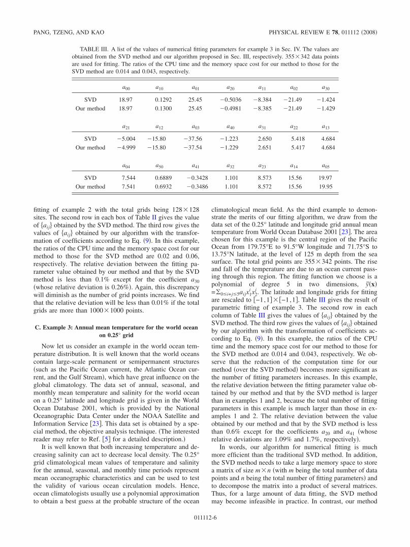
To numerically verify the obtained relations �Eqs. �17�and �18��, we perform some numerical simulation on two-dimensional fractal surfaces as follows. We first numericallygenerate ysto�x1 ,x2�, which is the fractional Brownian fieldcharacterized by the Hurst exponent � �24�. The variancefunction of the two-dimensional fractional Brownian surfacew2�l1 , l2��Š�ysto�x1 ,x2�− ysto�x1 ,x2���2

‹ is expected to scaleas �l1

2+ l22�� with 0���1. Without losing generality, we

choose cases with the Hurst exponent �=0.3, 0.5, and 0.7 inour simulation. To check the accuracy of ysto�x1 ,x2�, we drawa log-log plot �Fig. 2� of w2�l1 , l2� vs l1

2+ l22 for the numeri-

cally generated fractional Brownian surfaces. The wholefractal domain is 4096�4096 lattice sites. The variancefunction is first calculated within an observation window ofsize l1� l2 and then a sliding average is taken over the wholefractal domain. The excellence of the data fitting in Fig. 2confirms the accuracy of ysto�x1 ,x2� representing the frac-tional Brownian field. Subsequently, we numerically imposea global structure function

yglobal�x1,x2� = 4� x1

103� + 3� x1

103�� x2

103� − 2� x1

103�� x2

103�2

− � x1

103�3

�19�

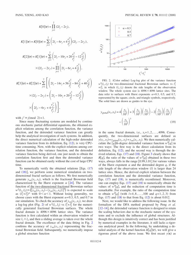
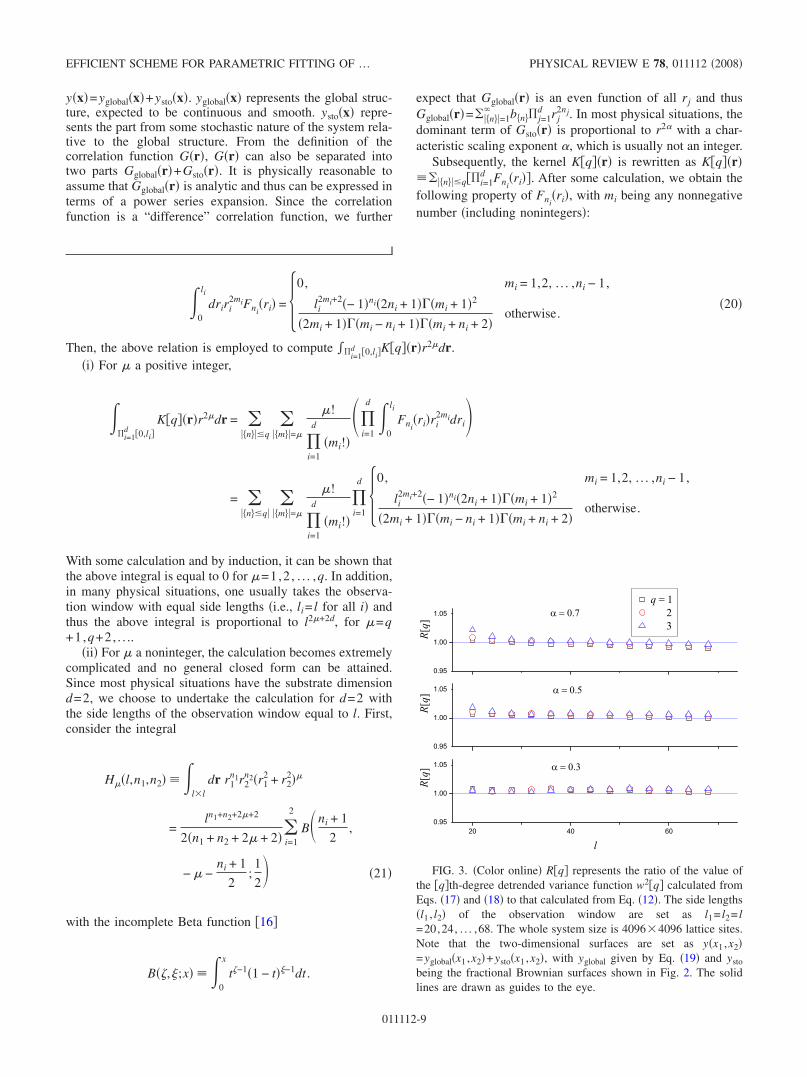
in the same fractal domain, i.e., xi=1,2 , . . . ,4096. Conse-quently, the two-dimensional surfaces are defined asy�x1 ,x2�=yglobal�x1 ,x2�+ysto�x1 ,x2�. We then numerically cal-culate the �q�th-degree detrended variance function w2�q� intwo ways: The first way is the direct calculation from itsdefinition, Eq. �12�, and the second way is through the de-rived relation, Eqs. �17� and �18�. Figure 3 clearly shows thatR�q�, the ratio of the values of w2�q� obtained in these twoways, always falls in the range �0.99,1.01� for various valuesof the Hurst exponent � and the detrended degree q, if theside length of the observation window �l� is larger than 24lattice sites. Hence, the derived explicit relation between thecorrelation function and the detrended variance function,Eqs. �17� and �18�, is numerically reconfirmed. Moreover,one can employ Eqs. �17� and �18� to numerically obtain thevalues of w2�q�, and the reduction of computation time isremarkable. For example, the ratio of the computation timeto obtain w2�q� �with l=4,8 , . . . ,100 and q=1,2 ,3� fromEqs. �17� and �18� to that from Eq. �12� is about 0.012.

Next, we would like to address the following issue. In theformalism of the DFA method proposed by Peng et al.�12–14�, the detrended variance function is designed to retainthe scaling behaviors due to the stochastic nature of the sys-tems and to exclude the influence of global structures. Al-though this design is intuitively correct and has been justifiedby numerical examples in the literature, it still lacks a rigor-ous analytical proof. In the following, by undertaking a de-tailed analysis of the kernel function K�q��r�, we will give arigorous proof of the above issue. We first recast y�x� as

FIG. 2. �Color online� Log-log plot of the variance functionw2�l1 , l2� for two-dimensional fractional Brownian surfaces vs l1

2

+ l22, in which �l1 , l2� denote the side lengths of the observation

window. The whole system size is 4096�4096 lattice sites. Thedata refer to surfaces with Hurst exponents �=0.3, 0.5, and 0.7,represented by the square, circle, and triangle symbols, respectively.The solid lines are drawn as guides to the eye.

PANG, TZENG, AND KAO PHYSICAL REVIEW E 78, 011112 �2008�

011112-8

y�x�=yglobal�x�+ysto�x�. yglobal�x� represents the global struc-ture, expected to be continuous and smooth. ysto�x� repre-sents the part from some stochastic nature of the system rela-tive to the global structure. From the definition of thecorrelation function G�r�, G�r� can also be separated intotwo parts Gglobal�r�+Gsto�r�. It is physically reasonable toassume that Gglobal�r� is analytic and thus can be expressed interms of a power series expansion. Since the correlationfunction is a “difference” correlation function, we further

expect that Gglobal�r� is an even function of all rj and thusGglobal�r�=���n��=1

b�n� j=1d rj

2nj. In most physical situations, thedominant term of Gsto�r� is proportional to r2� with a char-acteristic scaling exponent �, which is usually not an integer.

Subsequently, the kernel K�q��r� is rewritten as K�q��r�����n���q�i=1

d Fni�ri��. After some calculation, we obtain the

following property of Fni�ri�, with mi being any nonnegative

number �including nonintegers�:

�0

li

driri2miFni

�ri� = �0, mi = 1,2, . . . ,ni − 1,

li2mi+2�− 1�ni�2ni + 1���mi + 1�2

�2mi + 1���mi − ni + 1���mi + ni + 2�otherwise. � �20�

Then, the above relation is employed to compute �i=1d �0,li�

K�q��r�r2dr.�i� For a positive integer,

�i=1

d �0,li�K�q��r�r2dr = �

��n���q�

��m��=

!

i=1

d

�mi!��

i=1

d �0

li

Fni�ri�ri

2midri�

= ���n��q�

���m��=

!

i=1

d

�mi!�i=1

d �0, mi = 1,2, . . . ,ni − 1,

li2mi+2�− 1�ni�2ni + 1���mi + 1�2

�2mi + 1���mi − ni + 1���mi + ni + 2�otherwise. �

With some calculation and by induction, it can be shown thatthe above integral is equal to 0 for =1,2 , . . . ,q. In addition,in many physical situations, one usually takes the observa-tion window with equal side lengths �i.e., li= l for all i� andthus the above integral is proportional to l2+2d, for =q+1,q+2, . . ..

�ii� For a noninteger, the calculation becomes extremelycomplicated and no general closed form can be attained.Since most physical situations have the substrate dimensiond=2, we choose to undertake the calculation for d=2 withthe side lengths of the observation window equal to l. First,consider the integral

H�l,n1,n2� � �l�l

dr r1n1r2

n2�r12 + r2

2�

=ln1+n2+2+2

2�n1 + n2 + 2 + 2��i=1

2

B�ni + 1

2,

− −ni + 1

2;1

2� �21�

with the incomplete Beta function �16�

B��,�;x� � �0

x

t�−1�1 − t��−1dt .

FIG. 3. �Color online� R�q� represents the ratio of the value ofthe �q�th-degree detrended variance function w2�q� calculated fromEqs. �17� and �18� to that calculated from Eq. �12�. The side lengths�l1 , l2� of the observation window are set as l1= l2= l=20,24, . . . ,68. The whole system size is 4096�4096 lattice sites.Note that the two-dimensional surfaces are set as y�x1 ,x2�=yglobal�x1 ,x2�+ysto�x1 ,x2�, with yglobal given by Eq. �19� and ysto

being the fractional Brownian surfaces shown in Fig. 2. The solidlines are drawn as guides to the eye.

EFFICIENT SCHEME FOR PARAMETRIC FITTING OF … PHYSICAL REVIEW E 78, 011112 �2008�

011112-9

By employing the above integral and the expansion formulafor the Legendre polynomial, we then derive

�l�l

dr Fn1�r1�Fn2

�r2��r12 + r2

2�

= 4l2H�l,0,0� + 4i=1

2 ��ji=0

ni �2ni + 1��− ni� ji�1 + ni� ji

�2ji + 1��ji!�2l2ji ��H�l,2j1 + 1,2j2 + 1� − 4�2n2 + 1�

��k=0

n2 �− n2�k�1 + n2�k

�2k + 1��k!�2l2k−1

�H�l,0,2k + 1� − 4�2n1 + 1��j=0

n1 �− n1� j�1 + n1� j

�2j + 1��j!�2l2j−1

�H�l,2j + 1,0� �22�

with �n� j �n�n−1�¯ �n− j+1�. Subsequently, by using Eqs.�21� and �22� and the following relations for the incompleteBeta function �16�:

B��,�;x� =����������� + ��

− B��,�;1 − x� , �23�

B��,�;x� =�1 − x��

��j=0

�� + �� j

�� + 1� jxj+�, �24�

we finally obtain

�l�l

K�q��r��r12 + r2

2�dr = �n1+n2�q

�0

l

dr1�0

l

dr2Fn1�r1�Fn2

�r2��r12 + r2

2�

= l2+4�2�q2 + 2q + 2� + 1 �

�=0

�− ��

2��1/2��+1+ 2�

�=0

�− ��

2� �n1+n2�q

�2n1 + 1��2n2 + 1�

��j=0

�k=0

�− n1� j�1 + n1� j�− n2�k�1 + n2�k

�2j + 1��2k + 1��j + k + + 2��j ! k!�2� 1

�k + 1��+1+

1

�j + 1��+1�

− 2+2��=0

�− ��

2� �n=0

q

�2n + 1��q − n + 1��k=0

�− n�k�1 + n�k

�2k + 1��2k + 2 + 3��k!�2� 1

�k + 1��+1+

1

�1/2��+1��

� l2+4. �25�

By substituting the expansion of G�r���Gglobal�r�+Gsto�r��into Eq. �17� and employing the properties of the kernelfunctions we just derived, we rigorously show that, by rais-ing the degree of the detrended variance function, the contri-bution due to the global structure can be successfully sup-pressed. The above result is applicable in any dimensions. Inaddition, at least in two dimensions, we rigorously show thatthe detrended variance functions do retain the scaling expo-nent � �if it is not an integer� originating from the stochasticnature of the fluctuating system.

VI. CONCLUSION

In the physical sciences, data fitting is a very importantstep for researchers to condense the data and extract the es-sential information from experiments. Given a set of datapoints, one usually fits the data set to a parametric model.Without losing generality, polynomial functions are com-monly chosen to be the fitting functions and the fit gives theappropriate parameter values. In addition, many fluctuatingsystems in Nature consist of global structures; examples in-

clude molecular-beam-epitaxial growth, electrochemicaldeposition, the clustering features of seismic sequences, theclimatological temperature and salinity distribution of theworld oceans, physiology signals, and the mosaic structureof DNA sequences. People usually adopt a polynomial ap-proximation to obtain a best guess at the global structures ofsuch systems. In the literature, the method of normal equa-tions and the SVD method are two commonly used methodsfor numerical fitting. However, each of these two methodshas some drawbacks. The method of normal equations israther susceptible to roundoff errors. Although the SVDmethod is very accurate, it requires a relatively long compu-tation time and large memory space. Thus, the SVD methodis not practically feasible for fitting a large amount of data. Inthis work, by employing Legendre polynomials, we proposea different algorithm for parametric fitting. Our proposedscheme is exact for continuous systems. For numerical fit-ting, our proposed schemes takes much less CPU time andmemory space than the traditional SVD method in computa-tion. Although our proposed scheme is an approximation fornumerical fitting of discrete systems, its accuracy can begreatly enhanced as the number of data points increases. We

PANG, TZENG, AND KAO PHYSICAL REVIEW E 78, 011112 �2008�

011112-10

believe that our algorithm is the best method for fitting alarge amount of data points. Furthermore, for fluctuating sys-tems with formation of global structures, we explicitly derivethe exact relations among the correlation function, the vari-ance function, and the detrended variance function in arbi-trary dimensions. The obtained relations can greatly help fur-ther analytical and numerical study of such systems. Inaddition, by undertaking a detailed analysis of the kernelfunctions, we rigorously show that the detrended variancefunctions indeed retain the scaling behaviors due to the sto-chastic nature of the system and exclude the influence ofglobal structures on the scaling behaviors, verifying the in-

tuitive design of the DFA method. All our results are gener-ally applicable in arbitrary dimensions.

ACKNOWLEDGMENTS

The authors are very grateful to Dr. I.-I. Lin for enlight-ening discussions and suggestions. The work of N.-N.P. andW.-J.T. is supported in part by the National Science Councilof the Republic of China �NSCT� under Grants No. NSC-96-2112-M002-003 and No. NSC-96-2112-M032-001, respec-tively, and by the National Center of Theoretical Sciences inTaipei.

�1� J. Krug, Adv. Phys. 46, 139 �1997�.�2� T. Halpin-Healy and Y.-C. Zhang, Phys. Rep. 254, 215 �1995�.�3� M. Saitou, Phys. Rev. B 66, 073416 �2002�.�4� A. Brú, J. M. Pastor, I. Fernaud, I. Brú, S. Melle, and C.

Berenguer, Phys. Rev. Lett. 81, 4008 �1998�.�5� T. Boyer, S. Levitus, H. Garcia, R. A. Locarnini, C. Stephens,

and J. Antonov, Int. J. Climatol. 25, 931 �2005�.�6� L. Telesca, V. Cuomo, V. Lapenna, and M. Macchiato, Geo-

phys. Res. Lett. 28, 4323 �2001�.�7� S. Bahar, J. W. Kantelhardt, A. Neiman, H. H. A. Rego, D. F.

Russell, L. Wilkens, A. Bunde, and F. Moss, Europhys. Lett.56, 454 �2001�.

�8� A. Bunde, S. Havlin, J. W. Kantelhardt, T. Penzel, J.-H. Peter,and K. Voigt, Phys. Rev. Lett. 85, 3736 �2000�.

�9� W. H. Press, S. A. Teukolsky, W. T. Vetterling, and B. P. Flan-nery, Numerical Recipes �Cambridge University Press, NewYork, 1992�.

�10� C. Radhakrishna Rao, Linear Statistical Inference and Its Ap-plications �Wiley, New York, 1973�.

�11� G. E. Forsythe, M. A. Malcolm, and C. B. Moler, ComputerMethods for Mathematical Computations �Prentice-Hall,Englewood Cliffs, NJ, 1977�.

�12� C.-K. Peng, S. V. Buldyrev, S. Havlin, M. Simons, H. E. Stan-ley, and A. L. Goldberger, Phys. Rev. E 49, 1685 �1994�.

�13� S. V. Buldyrev, A. L. Goldberger, S. Havlin, R. N. Mantegna,

M. E. Matsa, C.-K. Peng, M. Simons, and H. E. Stanley, Phys.Rev. E 51, 5084 �1995�.

�14� K. Hu, P. C. Ivanov, Z. Chen, P. Carpena, and H. E. Stanley,Phys. Rev. E 64, 011114 �2001�.

�15� A. Cuyt, R. B. Lenin, S. Becuwe, and B. Verdonk, IEEE Trans.Microwave Theory Tech. 54, 2265 �2006�.

�16� J. Spanier and K. B. Oldham, An Atlas of Functions �Springer-Verlag, Berlin, 1987�; A. P. Prudnikov, Y. A. Brychkov, and O.I. Marichev, Integrals and Series �Gordon and Breach, NewYork, 1986�.

�17� W. W. Mullins, J. Appl. Phys. 28, 333 �1957�.�18� H.-N. Yang, Y.-P. Zhao, G.-C. Wang, and T.-M. Lu, Phys. Rev.

Lett. 76, 3774 �1996�.�19� J.-H. Jeffries, J. K. Zuo, and M. M. Craig, Phys. Rev. Lett. 76,

4931 �1996�.�20� H.-N. Yang, G.-C. Wang, and T.-M. Lu, Phys. Rev. Lett. 73,

2348 �1994�; Phys. Rev. B 50, 7635 �1994�.�21� B. Röseler and C. A. Schiller, Mater. Corros. 52, 413 �2001�.�22� W. Hachem, F. Desbouvries, and P. Loubaton, IEEE Trans.

Signal Process. 50, 651 �2002�.�23� The website for the National Oceanographic Data Center under

the NOAA Satellite and Information Service is http://www.nodc.noaa.gov/

�24� A. Carbone, Phys. Rev. E 76, 056703 �2007�.

EFFICIENT SCHEME FOR PARAMETRIC FITTING OF … PHYSICAL REVIEW E 78, 011112 �2008�

011112-11