Koninklijke Grolsch B.V.

Date: 19/4/2016

[EFFICIENCY ANALYSIS AND IMPROVEMENT AT GROLSCH]

UT Supervisors:

Dr. ir. M.R.K. Mes

Dr. ir. L.L.M. van der Wegen

Grolsch Supervisor:

Ing. W. Vermeulen

Author:

Ing P. Scholten

1

MANAGEMENT SUMMARY

This thesis is executed to improve the efficiency of the canning line at Grolsch.

Problem description

In order to stay competitive, Grolsch needs to continuously improve its operations and keep improving efficiency

of its filling lines. One of the filling lines for which this holds is the canning line, on which beer is canned and

packed. Since we want to improve the actual performance of the line, the focus of this project is to increase

machine efficiency. Currently the 86% machine efficiency of the canning line at Grolsch is far below the target of

95%. The biggest reason for the machine efficiency to lose 14% is because of starvation and blockage of the

bottleneck machine of the line, which is the filler. From preliminary research we found that improving line

dimensioning, buffer strategies and line regulation could probably reduce the starvation and blockage of the filler

and with that improve the machine efficiency. This leads to the following research question:

How can performance of the canning line at Grolsch be improved, by adjusting line regulation?

Approach

To find the bottleneck process that causes the most starvation and blockage on the filler, we evaluate the current

situation. It turns out that in the current situation a large share of the blockage on the filler is caused by the

pasteuriser. This blockage is not particularly caused by a lot of failures on the pasteuriser, but the pasteuriser has a

start-up procedure after a blockage in which a certain amount of buffer needs to be created behind the

pasteuriser before it can start operating again. This start-up procedure takes a lot of time during which the filler is

not operating. Besides the start-up procedure, we also found in the literature that the sensor location for changing

operating speeds of the machines influence machine efficiency.

The two potential causes for blockages at the filler mentioned above are evaluated by means of a simulation

model of the line in which we test 34 different scenarios. These scenarios differ from each other by changing the

sensor locations to change the operating speed and by either using the start-up procedure of the pasteuriser or

not. The sensor locations are changed by means of changing the threshold when different speed levels are

triggered. The start-up procedure is changed in every scenario by either creating a buffer behind the pasteuriser

after a blockage or not.

The performances of these scenarios are compared to the baseline measurement of the current situation in our

simulation model. The performances are measured by the machine efficiency, the number of stops on the

pasteuriser, the amount of cans processed and the number of cans over-pasteurised. Of these performance

measures, machine efficiency is the most important one.

Results

When analysing the performance measures from our simulation study, we found that there are various ways to

improve the current situation. It seems that almost all scenarios in which the start-up procedure of the pasteuriser

is not used score better than the current situation. We also found that scenarios in which the threshold to change

high speed were at a low fill level were performing better than scenarios in which the threshold was very high. The

same holds for the threshold of the sensor to switch to low speed. Eventually we have picked one scenario which

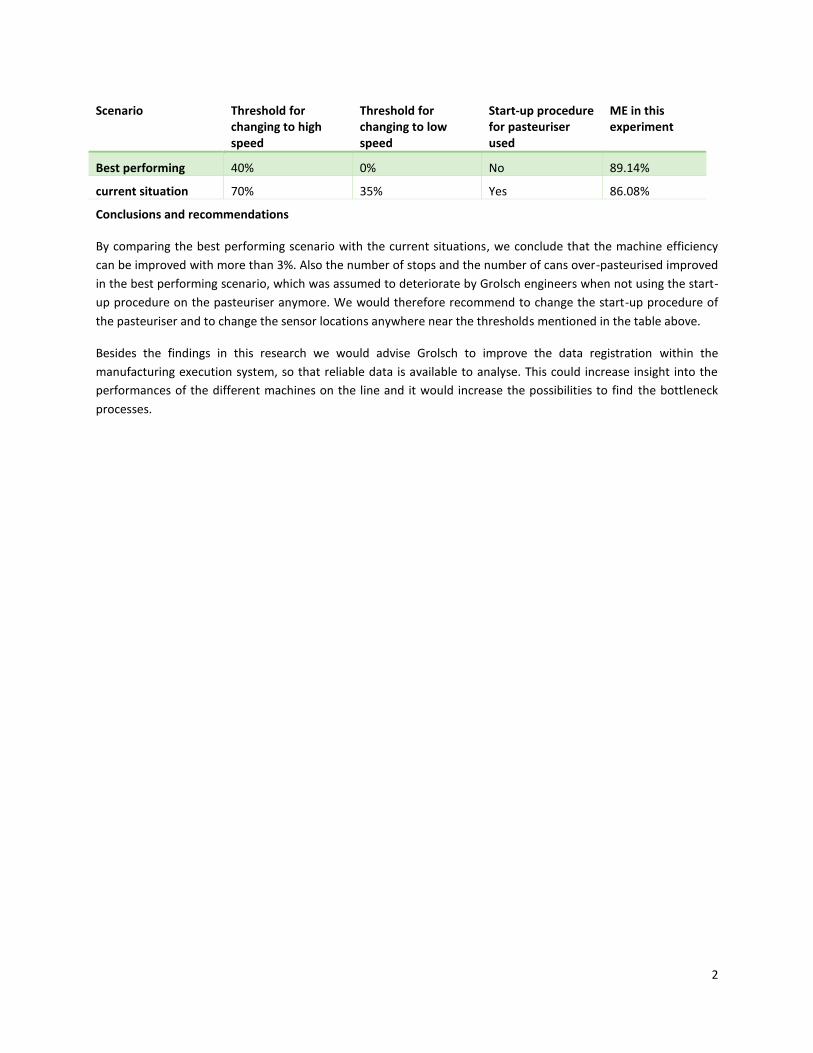
scores best, of which the settings and the performance in machine efficiency are shown in the table below.

2

Scenario Threshold for changing to high speed

Threshold for changing to low speed

Start-up procedure for pasteuriser used

ME in this experiment

Best performing 40% 0% No 89.14%

current situation 70% 35% Yes 86.08%

Conclusions and recommendations

By comparing the best performing scenario with the current situations, we conclude that the machine efficiency

can be improved with more than 3%. Also the number of stops and the number of cans over-pasteurised improved

in the best performing scenario, which was assumed to deteriorate by Grolsch engineers when not using the start-

up procedure on the pasteuriser anymore. We would therefore recommend to change the start-up procedure of

the pasteuriser and to change the sensor locations anywhere near the thresholds mentioned in the table above.

Besides the findings in this research we would advise Grolsch to improve the data registration within the

manufacturing execution system, so that reliable data is available to analyse. This could increase insight into the

performances of the different machines on the line and it would increase the possibilities to find the bottleneck

processes.

3

PREFACE

Although conducting this research was a real challenge, I am proud to present this thesis which concludes my

master Industrial Engineering and Management at the University of Twente. Conducting and completing this

research would have not been possible without the help of others, I would like to take this opportunity to thank

everybody who have directly and indirectly helped me to realise this research.

First of all I would like to thank Grolsch for the opportunity to let me do research at their brewery. Although I have

had several supervisors during my research at Grolsch, special thanks go out to Wim Vermeulen who supervised

and supported me during the last stage of my internship. I would also like to thank, Henk Rensink, Rob Leurink,

Brit Brons and Rene Siegering for supporting me and giving me better insight into the organisation and into the

canning line.

Secondly, I would like to thank Martijn Mes and Leo van der Wegen, my supervisors from the University of Twente.

Your feedback, effort, insights and encouragements helped me to push through till the end and gave me the

inspiration to get this research to a higher level.

Next to that I would like to thank all the people that supported me throughout the master thesis project but also

during my whole study career. A special thanks goes out to my girlfriend Manon who reminded me to take a rest

once in a while and reminded me to enjoy other things. I would also like to thank my parents for making it possible

for me to study in the first place and encourage me to get the most out of myself.

Peter Scholten.

4

MANAGEMENT SUMMARY .................................................................................................................................... 1

PREFACE ................................................................................................................................................................ 3

ABBREVIATIONS AND DEFINITIONS ....................................................................................................................... 7

1 INTRODUCTION ............................................................................................................................................. 8

1.1 COMPANY DESCRIPTION ..................................................................................................................................... 8

1.2 RESEARCH MOTIVATION ................................................................................................................................... 10

1.3 PROBLEM DESCRIPTION .................................................................................................................................... 11

1.4 PRELIMNARY RESEARCH .................................................................................................................................... 12

1.4.1 V-Graph .................................................................................................................................................. 12

1.4.2 Buffers .................................................................................................................................................... 13

1.4.3 Machine speeds ..................................................................................................................................... 14

1.4.4 Breakdowns or speed loss ...................................................................................................................... 14

1.4.5 Conclusion preliminary research ............................................................................................................ 14

1.5 RESEARCH QUESTIONS ..................................................................................................................................... 15

1.6 RESEARCH SCOPE ............................................................................................................................................ 16

2 THE CURRENT SITUATION ............................................................................................................................ 17

2.1 MACHINE PARK .............................................................................................................................................. 17

2.2 CURRENT LINE REGULATION ............................................................................................................................... 19

2.2.1 Sensors ................................................................................................................................................... 19

2.2.2 Line regulation ....................................................................................................................................... 20

2.2.3 machine states ....................................................................................................................................... 23

2.2.4 Machine status Tool ............................................................................................................................... 24

2.3 CURRENT PERFORMANCE .................................................................................................................................. 25

2.3.1 Performance of the canning line ............................................................................................................ 25

2.3.2 Conveyor capacity .................................................................................................................................. 28

2.3.3 Buffer capacity in Can sections .............................................................................................................. 29

2.3.4 Buffer capacities in package sections .................................................................................................... 30

2.3.5 Actual vs theoretical buffer capacity ..................................................................................................... 31

2.3.6 Mttr vs buffer capacity........................................................................................................................... 32

2.3.7 Mttr vs recovery time ............................................................................................................................. 33

2.3.8 Conclusion Section 2.3 ........................................................................................................................... 34

2.4 THE BOTTLENECK PROCESSES ............................................................................................................................. 34

2.4.1 Start up delay after failure ..................................................................................................................... 34

2.4.2 Pasteuriser ............................................................................................................................................. 35

5

2.4.3 conveyor regulation ............................................................................................................................... 37

2.5 SUMMARY AND CONCLUSION ............................................................................................................................. 37

3 LITERATURE REVIEW ................................................................................................................................... 38

3.1 MODELLING TECHNIQUES ................................................................................................................................. 38

3.2 PREVIOUS STUDIES .......................................................................................................................................... 38

3.3 CONCLUSION .................................................................................................................................................. 39

4 CONCEPTUAL MODEL .................................................................................................................................. 40

4.1 LAY-OUT OF THE SYSTEM .................................................................................................................................. 40

4.2 INPUT OF THE MODEL ....................................................................................................................................... 42

4.2.1 batchsize distribution ............................................................................................................................. 42

4.2.2 MTTF and MTTR per machine ................................................................................................................ 43

4.2.3 Buffer sizes ............................................................................................................................................. 44

4.2.4 Sensor locations ..................................................................................................................................... 45

4.3 ASSUMPTIONS IN THE MODEL ............................................................................................................................ 45

4.4 SUMMARY CHAPTER 4 ..................................................................................................................................... 46

5 SIMULATION MODEL ................................................................................................................................... 47

5.1 LAY-OUT........................................................................................................................................................ 47

5.2 PLANT SIMULATION TECHNICAL DETAILS ............................................................................................................... 48

5.2.1 Conveyors ............................................................................................................................................... 48

5.2.2 Processing time of machines .................................................................................................................. 49

5.2.3 Processing time of conveyors ................................................................................................................. 49

5.2.4 Regulation of pasteuriser ....................................................................................................................... 50

5.3 WARM-UP PERIOD .......................................................................................................................................... 51

5.4 RUN-LENGTH AND NUMBER OF REPLICATIONS ....................................................................................................... 51

5.5 VERIFICATION & VALIDATION ............................................................................................................................. 52

5.5.1 Verification ............................................................................................................................................. 52

5.5.2 Validation ............................................................................................................................................... 53

5.6 CONCLUSION .................................................................................................................................................. 53

6 EXPERIMENTAL DESIGN ............................................................................................................................... 55

6.1 EXPERIMENTAL FACTORS ................................................................................................................................... 55

6.2 PERFORMANCE MEASURES ................................................................................................................................ 55

6.3 EXPERIMENTAL SETUP ...................................................................................................................................... 56

6.4 CONCLUSION .................................................................................................................................................. 58

6

7 EXPERIMENTAL RESULTS ............................................................................................................................. 59

7.1 MACHINE EFFICIENCY ....................................................................................................................................... 59

7.2 NUMBER OF CANS OVER PASTEURISED ................................................................................................................. 60

7.3 NUMBER OF STOPS ON THE PASTEURISER ............................................................................................................. 60

7.4 FURTHER ANALYSIS .......................................................................................................................................... 61

7.5 CONCLUSION .................................................................................................................................................. 64

8 CONCLUSIONS & RECOMMENDATIONS ....................................................................................................... 65

8.1 CONCLUSIONS ................................................................................................................................................ 65

8.2 RECOMMENDATIONS ....................................................................................................................................... 66

8.3 FURTHER RESEARCH ......................................................................................................................................... 67

9 BIBLIOGRAPHY ............................................................................................................................................ 68

APPENDICES ...................................................................................................................................................... 70

APPENDIX 1: FACTORY EFFICIENCY & MACHINE EFFICIENCY ................................................................... 70

FACTORY EFFICIENCY ..................................................................................................................................... 70

MACHINE EFFICIENCY .................................................................................................................................... 70

APPENDIX 2: EXPERIMENTAL RESULTS .......................................................................................................... 72

APPENDIX 3: DISTRIBUTION FITTING ............................................................................................................. 73

APPENDIX 4: FLOWCHARTS .............................................................................................................................. 75

APPENDIX 5: MACHINE PARK ........................................................................................................................... 78

APPENDIX 6: DETERMINING THE WARM-UP PERIOD ................................................................................. 83

APPENDIX 7: DETERMINING RUN LENGTH .................................................................................................... 85

7

ABBREVIATIONS AND DEFINITIONS

To prevent the reader from misinterpreting a definition or abbreviation, a list of them with the description can be

found in this chapter.

Buffersize: The size in amount of cans that a buffer can contain.

Conveyor capacity: The amount of cans that a conveyor can contain.

Buffercapacity: The amount of cans that can be used to buffer on a conveyor section.

Buffertime: The amount of time it takes before a buffer is completely used.

Bottleneck process: A process in the line that blocks or starves the core machine. This is not the same as a

bottleneck machine.

Core machine: The machine in the line that has theoretically the lowest speed of the line. This machine therefore

also determines the maximum speed of the whole line, since the line could never operate faster than its slowest

machine.

Bottleneck machine: This is in fact the same machine as the core machine since breakdowns at the line will

eventually cause the core machine to starve or block, which will make the core machine the bottleneck again.

DTR: Down time recording. This is a file that is filled by machine operators everytime that the core machine

interrupted from producing cans of beer.

MES: Management Execution System. The software program that controls the regulation of the line.

Line dimensioning: The way the production line is shaped by means of machine capacities and buffer capacities.

Buffer strategy: The strategy to keep blockages and starvations of machines at a minimum.

Line regulation: The way to regulate the flow of cans by means of sensors at the line, with the corresponding

buffer strategy and line dimensioning.

8

1 INTRODUCTION

This research is performed at Koninklijke Grolsch N.V. The research analyses the production line for canning beer

and the packing process. This chapter will be used to introduce the reader to the company, the problem and the

outline of the project.

1.1 COMPANY DESCRIPTION

Grolsch has been founded in 1615 by Willem Neerfeldt in Grol, currently Groenlo. It has been in the hands of that

family until Theo de Groen bought the brewery in 1895, which in the meantime had grown to the famous brewery

“De Klok”. In that same year, some bankers, traders and textile magnates decided to start “de Enschedese

bierbrouwerij”, which was sold to Theo de Groen as well during the first world war. In 1922 those two breweries

merged into one brewery called “de Klok” which was later renamed to “Grolsche Bierbrouwerij”. In 2004, one big

brewery has been built in Enschede to replace the two old breweries. Since 2008, Grolsch has been part of the SAB

Miller, one of the biggest international brewery concerns. Partly as a result of that, Grolsch is still growing and

currently employs around 650 persons. Grolsch produces around 2,6 million hectoliters of which almost 1,2 million

is exported. An overview of the Grolsch hierarchy can be found in Figure 1.

Figure 1: Hierarchy of Grolsch

In the Supply Chain & Logistics department, the actual production and bottling of beer takes place. In this project,

we focus on this part of the company. The bottling plant is a section of the Supply Chain & Logistics department

and consists out of 7 filling lines. Bottles, cans and kegs are being filled on these different lines. The canning line is

the line which we will research in this project. Although there are only two different sizes of cans, still a lot of

different packaging materials are being used and the cans itself differ in print as well. The canning line fills cans

with a great variety of beer brands, and all these different brands can vary in size of cans, different appearance of

the can, trays to be filled, wrapping material to be used etc, which leads to a complex process to control. To get a

better understanding of the line, see Figure 2 for an overview.

9

Figure 2: Overview of the can line

The line can be split into two sections, a wet part and a dry part. In the wet part, beer is filled into the cans,

pasteurized and coded whereas the dry part is used to pack the cans into the selected packaging material.

1a Central Warehouse (CM3)

1 Can de-palletizer

2 Vacuum transfer device

3 Can inspection

4 Rinser

5 Filler

6 Closer

6.1 Tin lid unpacker

7 Fill height check

8 Can washer

9 Pasteurizer

10 Can dryer

11 Can Coding

12 Fill height check and leak detection

13 KHS shrink-packer

14 Rotate device film packer

15 KHS trayshrink-packer

18 Finished product inspection

19 Tray- and box palletizer

20 Shrink-wrap machine

21 Pallet labeller

22 Pallet destacker

23 Wooden board checker

24 Brush/roll

10

The wet area:

1. De-Palletiser. This machine unpacks the cans from the pallets.

2. The Filler. This machine fills up the clean empty cans with beer, and attaches the tin lids on top.

3. Volume inspection. This machine checks whether the amount of beer in the cans is according to the

norms. Otherwise it will be rejected, and eliminated from the process.

4. Pasteurizer. Depending of the type of beer being bottled, the cans will be pasteurized.

5. Coding. The expiration date and production date are being coded onto the cans.

The dry area:

Cans can be packed in two ways, either being packed onto trays directly or they will be packed in multipacks at the

Shrink packer and after that they will be packed onto trays. After one of those routes, the steps are the same

again:

1. Tray and Box Packer. Boxes or trays are being packed onto pallets.

2. Shrink tunnel. Pallets will be sealed in plastic film.

1.2 RESEARCH MOTIVATION

A goal of every company is to perform better than its competitors and make a profit. This can be done by

continuously improving the performance of the organization. Grolsch also uses this mindset and tries to

continuously improve itself by using the World Class Manufacturing principle. To measure how well the

organization is performing against other organizations, benchmarks are generally conducted. Since Grolsch is part

of SAB Miller, it is possible to benchmark itself internally against other breweries within SAB Miller. The breweries

are measured according to key performance indicators within the following categories: sustainability, productivity,

quality, cost and plant utilization. Since this research will focus on the operational side of the organization,

productivity will be the most important performance measure. Within Grolsch productivity is split up in the KPI’s:

Factory Efficiency (FE) and Machine Efficiency(ME). FE is a measure of how efficiently a line has performed relative

to the time period available for production and/or maintenance work on the line (SAB Miller, 2010). In other words,

what is the time the line has run production compared to the time that personnel was available for production. ME

is a measure of how efficiently the line has performed relative to the time period available once adjustments for

actual maintenance and cleaning time and actual allowed stops/service stops have been made (SAB Miller, 2010).

In other words, what percentage of the available production time, minus adjustments for planned stops, is the line

actually operating. Grolsch is not performing as good as they would like to in the SAB Miller benchmarks, based on

ME and FE measures.

Besides a good score in the benchmarks, the factory efficiency also affects the cost price of the product. And the

cheaper Grolsch can produce, the more competitive they are. Besides that, SAB Miller determines what volume

will be allocated to which brewery based on the cost price of the product, it is thus extra important to have a high

efficiency and score better than the other breweries within SAB Miller Europe.

To stay competitive it is important for Grolsch to continuously improve its performance and have a high efficiency.

This project has been set up to improve the efficiency of the canning line at Grolsch.

11

Total Factory Hours 100%

ME +-80%

FE +-55%

0%

Planned Losses

Unplanned losses

Breakdowns

Maintenance and Cleaning

Quality losses

Changeovers

Reduced speeds

Start up losses

Minor stops and idling

Minor stops and idling

21,46%

56,78%

7,37%

14,39%

Percentage of unplanned ME loss

Unplanned Service Stops

Downtime due to failure ofother machines

Downtime of filler itself

Speed and quality losses

1.3 PROBLEM DESCRIPTION

The process described in the previous sections has become quite complex to control because different sizes of

cans and different packaging types make the process very dynamic, since these specifications changes elements

like the operating speed and machine settings. This makes the process complex to plan therefore as well. Although

the production schedule is almost always fulfilled, performance is not always stable. The planning department

builds extra safety into its schedule in consultation with the unit manager of the canning line, which will assure the

planning department that all orders will be finished in time. Of course if performance was stable, this extra safety

would not be necessary.

The efficiency of a line varies between weeks, since failures of machines are always unexpected. At the canning

line, however, a structural loss on ME is found. Currently Grolsch scores an average

of 86% ME on the canning line, while the global standard is around 95% ME, so

Grolsch has an efficiency loss of 14% on performance when filling cans with beer.

Efficiency loss can be classified into 6 losses of efficiency (Yuniawan, Ito, & E Bin,

2013). These are:

(a) breakdowns;

(b) setups and changeovers;

(c) running at reduced speeds;

(d) minor stops and idling;

(e) quality defects, scraps, yields and reworks and

(f) start-up losses.

A rough distinction between the two efficiency measures, ME and FE, used at

Grolsch are planned and unplanned efficiency losses. In Figure 3 a rough distribution of these two efficiency

measures can be seen. Since planned efficiency losses are already accounted for as a loss,

they will not affect controllability and planning of the line and are not considered

interesting for this project. The losses a, c, d and e, however, are part of unplanned efficiency losses and could

therefore be seen as important factors to influence machine efficiency. To a large extent the unplanned efficiency

losses are caused by the unreliability of the individual processes. This is clearly visible in Figure 4, in which

downtime due to failures cause around 64% of total ME loss. This data is obtained from downtime analysis

conducted by Grolsch throughout the year in a file called the Downtime recording (DTR), this will be discussed in

more detail in Section 2.3.1.

Figure 4: overview of ME

losses from 01-04-2015

until 19-06-2015

according to DTR

Figure 3: Structure of efficiency

12

1.4 PRELIMNARY RESEARCH

To determine in which direction the research will go, we performed a preliminary research for causes of efficiency

losses at Grolsch, that will be described in the following paragraphs.

1.4.1 V-GRAPH

Almost every canning line is designed according to the principle of the V-Graph. The idea is that the “critical

machine” or core machine is at the bottom of the V-graph, and the remaining machines have a potential higher

capacity to absorb small disturbances at the line, to prevent downtime on the core machine. The core machine is

the machine with the lowest pre-set speed (Cooke, Bosma, & Härte, 2005). The core machine is often the machine

that is the most expensive and most difficult to upgrade.

To run the line as efficient as possible, it is important that downtime of the core machine will be as low as possible.

To ensure that the core machine does not stop because of starvation of bottles upstream or blockage downstream,

buffers in front of the machine should always be filled and buffers after the machine should be as empty as

possible. This buffer capacity is achieved with accumulation on the conveyers between the machines.

Accumulation is referred to as the time a machine is allowed to stop without disturbing the operation of the

machines around it (Härte, 1997). When the buffer is build up on the conveyors itself, it is called dynamic

accumulation. This dynamic accumulation is achieved by making the conveyors wider than necessary for

transportation alone, in this way the buffer can be build up in the remaining space of a conveyor belt. In line with

this philosophy it is important that machines upstream and downstream of the core machine have more capacity

in order to fill or empty the buffers (Härte, 1997). Basically, the further downstream or upstream the more

capacity this machine should have in order to drain or fill up conveyors. This results in a V-graph in which

theoretically the core machine should be at the bottom of the V. They call this a v-graph since plotting the machine

speeds in a graph looks like the letter V, with the core machine at the bottom of the V. As can be seen in Figure 5,

the canning line is designed according to this principle. A speed level of 100% means that this machine is running

at 100% of speed at which the line is planned to run. The shown speed levels are the theoretical machine

capacities as pre-set into the machines.

80,00%90,00%

100,00%110,00%120,00%130,00%140,00%150,00%160,00%

Machine speeds as % of line speed

Nominal %

Max %

Figure 5: V-profile of maximum speeds of machines on the canning line in

percentage of the line speed.

13

As can be seen, the filler and the pasteurizer are at the bottom of the V-graph, but Grolsch and SAB Miller decided

that the filler is the core machine of the line. On this machine, performance measures are more easily obtained

than on the pasteurizer, and the speed is more easily adjusted. Another reason is that production quality is much

better when the filler is working at one pace. When the filler would not be the core machine or theoretical slowest

machine, the filler would constantly start and stop or slow down production, this affects fill quality. This would

eventually lead to a bigger efficiency loss than running the filler at the line speed.

Since the core machine has in theory the lowest capacity, it determines the maximum speed of the canning line.

This maximum speed is also reffered to as the line rating. Since the line rating is the theoretical output of the line,

the planning department uses it to calculate the production schedule. When the line produces as fast as the line

rating, it has a machine efficiency of 100%. However, if for some reason the core machine is slowed down, the line

is not able to reach line rating anymore and thus ME will drop. It is therefore important that all other processes are

at least as fast as the core machine and that the core machine itself is reliable in order to reach the highest ME. A

possible cause of efficiency loss could be the fact that there is a bottleneck process, that causes the core machine

to run at a lower pace than line rating.

1.4.2 BUFFERS

Since the core machine is the slowest machine of the line it is automatically the bottleneck of the line. It is

important that this machine is never starved or blocked by cans either up or downstream of this machine. To

ensure that this never happens, a buffer strategy needs to be used, that will ensure that the bottleneck machine

will have a conveyor belt full with cans in front of it and a conveyor belt that is as empty as possible behind it, that

will absorb downtime downstream. Thus buffers upstream of the bottleneck machine should be filled with cans

and buffers downstream of the core machine should be empty. This principle is also used for other machines in the

line to absorb inefficiencies of every machine. For the bottleneck machine, however, this is crucial since it

influences machine efficiency of the whole line directly.

The idea of the V-graph is helpful once actual breakdowns occur and buffers downstream start to fill up and

upstream buffers are starting to drain. The extra capacity of machines either up or downstream can now be used

to fill up buffers or drain buffers respectively. The further a machine is positioned away of the core machine the

more buffer it should be able to drain or fill up. It is therefore important for these machines to have more capacity

than machines closer to the core machine in order to go back to a situation in which breakdowns can be easily

absorbed again.

Sensors on the line are activated once the buffers reach a certain level, these sensors subsequently trigger speeds

of the individual machines and conveyor belts so they can restore buffer sizes to the desirable level. From

interviews with an automation engineer at Grolsch, however, it became clear that these buffer levels are

determined by trial and error and there is no powerfull backing why machine speeds change at certain buffer

levels. There is even only a rough idea at what buffer levels the operating speeds change.

Overall the idea of the V-graph and buffer strategy is to absorb breakdowns or minor stops of certain machines

and with that reduce variability of the line (Battini, Persona, & Regattieri, 2009), in order to have a reasonably

realiable output and thus a fairly constant machine efficiency, so it is less complex to make the production

schedule more accurate. Unfortunately, as can be seen in Figure 4, still 56% of ME losses is caused by failures of

other machines than the filler. Thus the v-graph and buffer strategy as it is currently designed does not reduce

14

efficiency loss and variabillity in the line enough to let the core machine run without blockages or starvation of

cans.

1.4.3 MACHINE SPEEDS

As already mentioned in the previous section, not only buffers are used to absorb breakdowns. Higher capacity of

several machines should help to let the buffers go back to a situation that is desirable to make the bottleneck

machine run with as less blockages or starvations as possible. It is important that the time to go back to a desirable

situation is shorter than the time between the different failures also known as the mean time between failure

(MTBF) (Härte, 1997). It could therefore also be the case that the capacity of the machines are not big enough to

ramp up speed and go back to this desirable situation fast enough and that this causes the high variation in ME of

the complete line.

1.4.4 BREAKDOWNS OR SPEED LOSS

Besides the fact that strategies with respect to buffers/machine speeds/v-graph can be adapted in order to reduce

variability of the line, there are of course also other reasons for the breakdowns to happen in the first place. These

could be for examples the quality of the materials used, the quality of the operators, machine failures or machine

settings etc. If this causes the breakdowns or speed losses to happen more often than what the line is built for, it

could also be a reason why strategies do not match the actual situation and thus causes losses in machine

efficiency.

1.4.5 CONCLUSION PRELIMINARY RESEARCH

In conclusion machine efficiency losses can be caused by:

- Core machine running slower than line rating, this could be cause by:

o Buffer strategy to absorb breakdowns and minor stops.

o Regulation of machine and conveyer speeds to go back to a desirable situation

- Breakdowns itself

o Quality of materials

o Quality of operators

o Machine defects

o Machine settings

o Maintenance of machines

In order to find out where the problem is actually situated and why ME is below target, a full line analysis is

needed that provides insight into the following:

- Buffer capacities and strategies

- Machine capacities

- Recovery capacity, the time it takes for the buffers to return to a desirable situation

- Mean time between failure and mean time to repair (Härte, 1997)

- Number of failures of different machines

- Causes of failures to happen in the first place

- Efficiency losses caused by stoppage or blockage of core machine

- Bottleneck process that causes core machine to slow down.

15

All the issues mentioned in the preliminary research have to do with the way the line is regulated, dimensioned

and what buffer strategies are used. As mentioned in Section 1.4.2 the automation engineer does not have full

insight into the buffer strategy and line regulation, and most of the losses are found in the unreliability of other

processes on the line. Therefore the focus of the project will be on line regulation and dimensioning and buffer

strategies in the first place. What is meant with this paradigms will be explained below.

With line dimensioning we mean changing the capacity of the machines and the buffers. Thus how large should a

buffer be in order to absorb the failures of different machines. On the other hand how high should the machine

capacities be in order to recover the buffer before another failure occurs.

The buffer strategy is a strategy that states at what kind of buffer level a machine or conveyor should change its

operating speed and to what speed level.

How to implement the buffer strategy with its current line dimensioning is meant with line regulation. So it is the

combination of the two things mentioned earlier and how to really translate it onto the line.

1.5 RESEARCH QUESTIONS

Based on the problem description and preliminary research, the main research question for this project will be:

How can performance of the canning line at Grolsch be improved, by adjusting line regulation?

To answer this question we defined several sub questions. Below every sub question, a brief description of how to

obtain the necessary knowledge and the research method is given.

1. How is the canning line currently performing?

a. How is the line currently regulated?

b. How is performance measured, and what are the targets?

c. What is the bottleneck process in the current packaging line?

To answer this question, a line analysis will be done in which all the aspects mentioned in the preliminary research

will be analysed. Most of this information can be obtained from the manufacturing execution system at Grolsch.

However, this data is not used yet for analysis. It is therefore important to check whether this data is accurate. We

will therefore execute some manual measurements on the line itself to check if this data can be used.

Furthermore, handbooks of the line, interviews with line operators and staff will be used to get a better overview

of the current situation. After answering this question, a clear overview of the current situation has been made. In

particular it is now clear why certain choices are made in the line design, what the restrictions are and which

process is the bottleneck.

2. What are the main reasons for unplanned efficiency loss at the canning line?

a. Which factors influence efficiency most?

b. When does efficiency loss occur at the line?

c. Why do these different losses occur?

d. What is the impact of those losses?

Although some conclusions on ME losses has already been made in Section 1.4, we need to do a more detailed

analyses of the causes of efficiency losses. This is done by doing data analysis of information from the

manufacturing execution system. Besides that, the down time recording report, which measures downtime of

every machine separately, will be consulted. We try to find out if certain product types always perform less than

others or that there are certain situations in which the line is always performing less, so that we can focus on those

situations. With this question it should become clear what the reason is that down time has occurred and what

16

causes the efficiency to be below target. Once it is clear which factors influence efficiency most and why certain

machines came to a standstill, we can start to find alternative approaches for reducing this factors.

3. What approaches does literature suggest for improving line efficiency by reducing efficiency losses?

A search for scientific articles in the field of improving efficiency of production lines in general and reducing

efficiency losses will be conducted to find out different suggestions already used for improving machine efficiency.

The focus will be on line dimensioning, line regulation and buffer strategies in the first place since these causes

were found to be influencing performance most during our preliminary research.

4. What approaches (found in literature and by brainstorming) for improving line efficiency are suitable for

implementation at Grolsch?

a. How should the alternative solutions be adapted in order to work for Grolsch?

This question will be mainly answered by alternative suggestions found in the literature in question 3 and by

brainstorming for alternative solutions with employees from Grolsch. Eventually a solution or several solutions will

be specifically made for Grolsch to improve control and efficiency of the canning line. These alternative solutions

can subsequently be experimented within a simulation model to find out which alternative solutions gives the best

result on efficiency loss.

5. What performance can be expected from the proposed solutions for improving control and efficiency of

the line?

A simulation model will be built in order to find out which of the suggested solutions will result in an increase of

the performance of the line. Once all questions have been answered a recommendation to Grolsch will be made.

1.6 RESEARCH SCOPE

The focus of this project will only be on the canning line of the packaging department of Grolsch, this means all

steps from filling the can until it is packed and ready to go to the warehouse. The impact of other steps before or

after this line are not taken into account.

As mentioned earlier, breakdowns can cause efficiency loss and it could be the direction of the research, however,

since finding solutions to breakdowns is a more technical aspect we decided to focus this project more on line

regulation, line dimensioning and buffer strategies. Since buffer capacities are fixed and it is not possible to

increase them, we have to limit our buffer capacity to the current available buffer capacity. Although the machines

also have a maximum capacity in terms of speed as well, which we cannot change, it could be the case that

machines are not running at full speed yet.

Chapter 2 describes the current situation of the canning line, how the line is currently operated and regulated and

where the bottleneck process is located. Chapter 3 discusses the current literature that is found on the topics of

line regulation, line dimensioning and buffer strategies, and which approaches we find most suitable to the

problem. Chapter 4 describes the conceptual model of our solution to the problem. In Chapter 5 we describe how

this conceptual model is translated into a simulation model to simulate different scenarios to optimize the line. In

Chapter 6 we design the experimental setup to analyse the different scenarios. In Chapter 7 these results of these

experiments are shown and analysed. Finally we will write our conclusions and recommendations in Chapter 8.

17

2 THE CURRENT SITUATION

This chapter will be used to find out how the line is currently regulated, how its performance is measured, the

outcome of the line measurement and eventually where the bottleneck process is located that causes the

bottleneck machine/core machine to block or starve. In Section 2.1, the six most important machines will be

described in detail. Section 2.2 will be used to describe the current line regulation and how this is analysed. In

Section 2.3 we will describe the current performance of the canning line, how the performance is measured and

analyses on those performances.

2.1 MACHINE PARK

Although a short overview of the machine park has already been given in Chapter 1, this section will be used to

describe the use of the six most important machines on the line. For a complete description of all machines, see

Appendix 5. For an overview of the line, see Figure 2. The numbers used in this section correspond with the

machines in Figure 2.

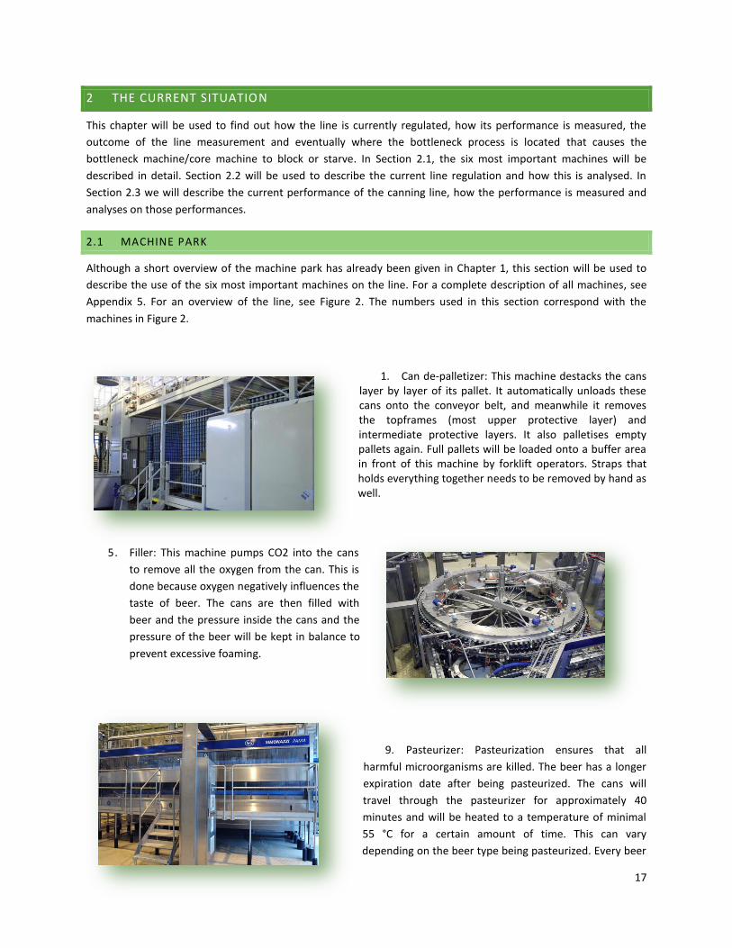
1. Can de-palletizer: This machine destacks the cans layer by layer of its pallet. It automatically unloads these cans onto the conveyor belt, and meanwhile it removes the topframes (most upper protective layer) and intermediate protective layers. It also palletises empty pallets again. Full pallets will be loaded onto a buffer area in front of this machine by forklift operators. Straps that holds everything together needs to be removed by hand as well.

5. Filler: This machine pumps CO2 into the cans

to remove all the oxygen from the can. This is

done because oxygen negatively influences the

taste of beer. The cans are then filled with

beer and the pressure inside the cans and the

pressure of the beer will be kept in balance to

prevent excessive foaming.

9. Pasteurizer: Pasteurization ensures that all

harmful microorganisms are killed. The beer has a longer

expiration date after being pasteurized. The cans will

travel through the pasteurizer for approximately 40

minutes and will be heated to a temperature of minimal

55 °C for a certain amount of time. This can vary

depending on the beer type being pasteurized. Every beer

18

type has a certain target measured in PU (pasteurization units). Depending on this target value the

pasteurization time is calculated. It is very important that the beer is neither too long nor too short in this

pasteurization zone. If it stays too long it will negatively influence the taste, on the other hand a too short

pasteurization means that not all harmful microorganisms have been killed. It is therefore very important

for this machine to have enough space at the backside of the pasteurizer to move cans out of the

pasteurization zone once a breakdown happens behind the pasteurizer. After pasteurization the cans will

be blown dry. This will blow excessive water back into the pasteurizer and prevents the cans from having

deposits on the bottom. The conveyor belts will also split in two directions after the pasteurizer. Cans are

equally distributed to both sides. This is done because one machine cannot handle the complete capacity

of the pasteurizer, thus two machines are placed beside each other.

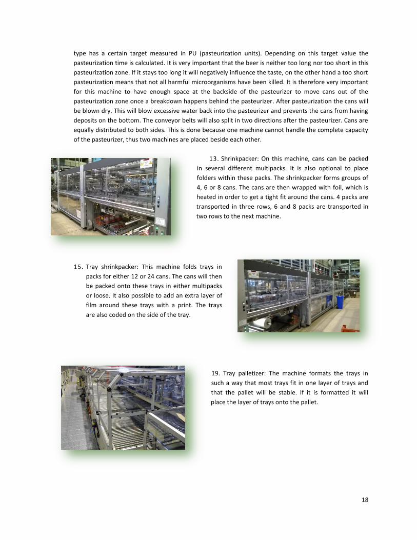
13. Shrinkpacker: On this machine, cans can be packed

in several different multipacks. It is also optional to place

folders within these packs. The shrinkpacker forms groups of

4, 6 or 8 cans. The cans are then wrapped with foil, which is

heated in order to get a tight fit around the cans. 4 packs are

transported in three rows, 6 and 8 packs are transported in

two rows to the next machine.

15. Tray shrinkpacker: This machine folds trays in

packs for either 12 or 24 cans. The cans will then

be packed onto these trays in either multipacks

or loose. It also possible to add an extra layer of

film around these trays with a print. The trays

are also coded on the side of the tray.

19. Tray palletizer: The machine formats the trays in

such a way that most trays fit in one layer of trays and

that the pallet will be stable. If it is formatted it will

place the layer of trays onto the pallet.

19

2.2 CURRENT LINE REGULATION

All the machines described in the previous section are connected with each other by means of conveyors. These

conveyors are used to transport the cans or packages from one machine to another, but also to create buffers to

absorb little breakdowns on the line. The conveyor and machine speeds are all regulated completely automatically

by the use of sensors mounted on the side of the conveyors. These sensors are used to measure the amount of

products on the conveyors. The sensors send this information to PLCs (programmable logic controllers), which are

connected to the motors that drive the conveyors and machines. The PLCs make a decision whether or not a

certain machine or conveyor section should change the operating speed. In this section we will describe which

sensors are used to send information to the PLCs and how these sensors are used to regulate the machine speeds

and how these sensors are used to analyse machine states. Finally we will introduce an extra tool that can be used

to analyse machine states more in detail.

2.2.1 SENSORS

This sections will highlight the different types of sensors used to change operating speed. Two types of sensors are

used to get the information of the fill level of a conveyor section. One is called the proximity switch and the other

one is called a photocell. The use and function of these sensors will be described below.

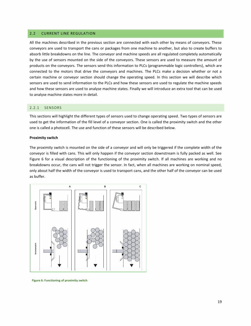
Proximity switch

The proximity switch is mounted on the side of a conveyor and will only be triggered if the complete width of the

conveyor is filled with cans. This will only happen if the conveyor section downstream is fully packed as well. See

Figure 6 for a visual description of the functioning of the proximity switch. If all machines are working and no

breakdowns occur, the cans will not trigger the sensor. In fact, when all machines are working on nominal speed,

only about half the width of the conveyor is used to transport cans, and the other half of the conveyor can be used

as buffer.

Figure 6: Functioning of proximity switch

20

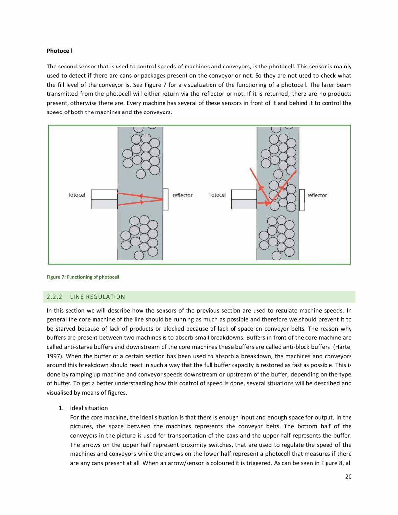
Photocell

The second sensor that is used to control speeds of machines and conveyors, is the photocell. This sensor is mainly

used to detect if there are cans or packages present on the conveyor or not. So they are not used to check what

the fill level of the conveyor is. See Figure 7 for a visualization of the functioning of a photocell. The laser beam

transmitted from the photocell will either return via the reflector or not. If it is returned, there are no products

present, otherwise there are. Every machine has several of these sensors in front of it and behind it to control the

speed of both the machines and the conveyors.

Figure 7: Functioning of photocell

2.2.2 LINE REGULATION

In this section we will describe how the sensors of the previous section are used to regulate machine speeds. In

general the core machine of the line should be running as much as possible and therefore we should prevent it to

be starved because of lack of products or blocked because of lack of space on conveyor belts. The reason why

buffers are present between two machines is to absorb small breakdowns. Buffers in front of the core machine are

called anti-starve buffers and downstream of the core machines these buffers are called anti-block buffers (Härte,

1997). When the buffer of a certain section has been used to absorb a breakdown, the machines and conveyors

around this breakdown should react in such a way that the full buffer capacity is restored as fast as possible. This is

done by ramping up machine and conveyor speeds downstream or upstream of the buffer, depending on the type

of buffer. To get a better understanding how this control of speed is done, several situations will be described and

visualised by means of figures.

1. Ideal situation

For the core machine, the ideal situation is that there is enough input and enough space for output. In the

pictures, the space between the machines represents the conveyor belts. The bottom half of the

conveyors in the picture is used for transportation of the cans and the upper half represents the buffer.

The arrows on the upper half represent proximity switches, that are used to regulate the speed of the

machines and conveyors while the arrows on the lower half represent a photocell that measures if there

are any cans present at all. When an arrow/sensor is coloured it is triggered. As can be seen in Figure 8, all

21

sensors in front of the core machine are triggered, which means full buffer capacity, and none of the

sensors behind the core machine are triggered, which also means full buffer capacity. If such a situation

occurs during production, it means that all machines are running on the nominal speed of 72,000 cans per

hour and thus the line is in balance and full buffer capacities are available.

Figure 8: Ideal situation

2. Buffer capacity has been reduced

When machine B has had downtime either because of its own failure or because of blockage, the buffer

capacity will be used to absorb this downtime. The buffer capacity will slowly reduce and several of the

sensors will be triggered. Once these sensors are triggered, it sends a signal to the PLC, this PLC

subsequently knows to ramp up the machine speed of machine B in order to restore the buffer capacity.

Depending on the occupation (which switch is triggered) of the conveyor, different speed levels are used.

A visual explanation can be found in Figure 9. For anti-starve buffers the exact opposite applies, Machine

A will ramp up once sensors 6,5,4 are not triggered anymore.

Figure 9: Machines need to ramp up speed when buffer capacity has been reduced.

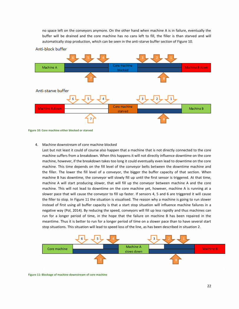
3. Core machine blocked or starved

When buffer capacity is too small to absorb downtime on machine A or B, eventually the core machine

will starve or block. The core machine will then automatically stop producing. See Figure 10 for a visual

explanation of these situations. When machine B fails, the anti-block buffer will start to fill up with cans, if

sensors 1,2 and 3 are triggered, the core machine will be blocked and it will stop production since there is

Machine A Core machine Machine B

12346 5

7 8

22

no space left on the conveyors anymore. On the other hand when machine A is in failure, eventually the

buffer will be drained and the core machine has no cans left to fill, the filler is than starved and will

automatically stop production, which can be seen in the anti-starve buffer section of Figure 10.

Figure 10: Core machine either blocked or starved

4. Machine downstream of core machine blocked

Last but not least it could of course also happen that a machine that is not directly connected to the core

machine suffers from a breakdown. When this happens it will not directly influence downtime on the core

machine, however, if the breakdown takes too long it could eventually even lead to downtime on the core

machine. This time depends on the fill level of the conveyor belts between the downtime machine and

the filler. The lower the fill level of a conveyor, the bigger the buffer capacity of that section. When

machine B has downtime, the conveyor will slowly fill up until the first sensor is triggered. At that time,

machine A will start producing slower, that will fill up the conveyor between machine A and the core

machine. This will not lead to downtime on the core machine yet, however, machine A is running at a

slower pace that will cause the conveyor to fill up faster. If sensors 4, 5 and 6 are triggered it will cause

the filler to stop. In Figure 11 the situation is visualised. The reason why a machine is going to run slower

instead of first using all buffer capacity is that a start stop situation will influence machine failures in a

negative way (Pol, 2014). By reducing the speed, conveyors will fill up less rapidly and thus machines can

run for a longer period of time, in the hope that the failure on machine B has been repaired in the

meantime. Thus it is better to run for a longer period of time on a slower pace than to have several start

stop situations. This situation will lead to speed loss of the line, as has been described in situation 2.

Figure 11: Blockage of machine downstream of core machine

Core machineMachine A

slows downMachine B

12346 5

7 8

23

2.2.3 MACHINE STATES

The sensors described in Section 2.2.1, are also used to describe a state in which a machine is. If all sensors

upstream of the machine are triggered this means that this machine is either blocked or in failure. If the machine

does not send a signal that it is in failure, then it should be blocked, etcetera. In this section we will describe what

states are possible for a machine and when they occur. The manufacturing execution system used at Grolsch

registers these states for the most important machines on the line, these are the de-palletizer, filler, pasteurizer,

shrinkpacker, trayshrinkpacker and palletizer.

- Operating: The most important state of a machine is the operating state. Every company wants it

machines to be operating constantly to get the most money out of it. A machine is in this state when it is

actually producing products.

- Failure: When a machine is down because of a failure on the machine itself it is in failure mode.

- Blocked: When a machine cannot produce any products anymore because the conveyor belt downstream

of the machine is full of cans the machine will be in the blocked state. This could happen for example

when one of the machines downstream of this machine is in failure.

- Starved: When a machine cannot produce products anymore, because there are no products left on the

conveyor upstream of the machine, it will be in the starved state. This could happen for example when

one of the machines upstream of this machine is in failure or when a changeover is being done.

- Starved Secondary: When a machine has two places from which it is fed, for example the closer, that get

cans from the filler and lids from the lid de-stacker. If the closer does not get lids any more than it is

starved by a secondary process.

- Ready: When a machine is not performing any tasks but it is not starved, blocked or in failure either then

the machine is in the ready state. This can happen for example when a can has fallen on its side and the

machine cannot handle it, however, the sensors on the conveyors are triggered, so it is not starved or

blocked either.

- External Failure: When a machine is stopped because of a failure somewhere else in the brewery, for

example when the beer from the beer tank is not able to flow to the filler, than it is in external failure

mode.

- Operator intervention: When a machine is adjusted or a door is opened for example, it is in operator

intervention mode.

These are all the states registered by the manufacturing execution system. However, a machine can run at several

speeds, the operating state only mentions if it is operating or not, and not if it is running slower or faster than

nominal speed. Unfortunately it is not registered in a state at what speed level a machine is running. It could

therefore also not be determined when speed losses occur.

Currently, there is an excel add-in present at Grolsch in which a total overview of machine states for a shift or

order can be generated, see Figure 12Figure 12. However, this add-in only shows the total time of a certain state

during a shift or order and not at what moment of the day a state occured. It is thus not visible how many time a

certain state has occurred and what the duration of a single state is. This tool is not used either by the packaging

department or operators since it is not visible when downtime occurred exactly. Currently all downtime is

recorded at a file called the Down Time Recording (DTR). This file registers all the downtime on the filler and is

recorded by employees working at the production line manually. This is also done, because employees do not fully

trust the data from the information system.

24

Figure 12: Current analysis tool for machine states

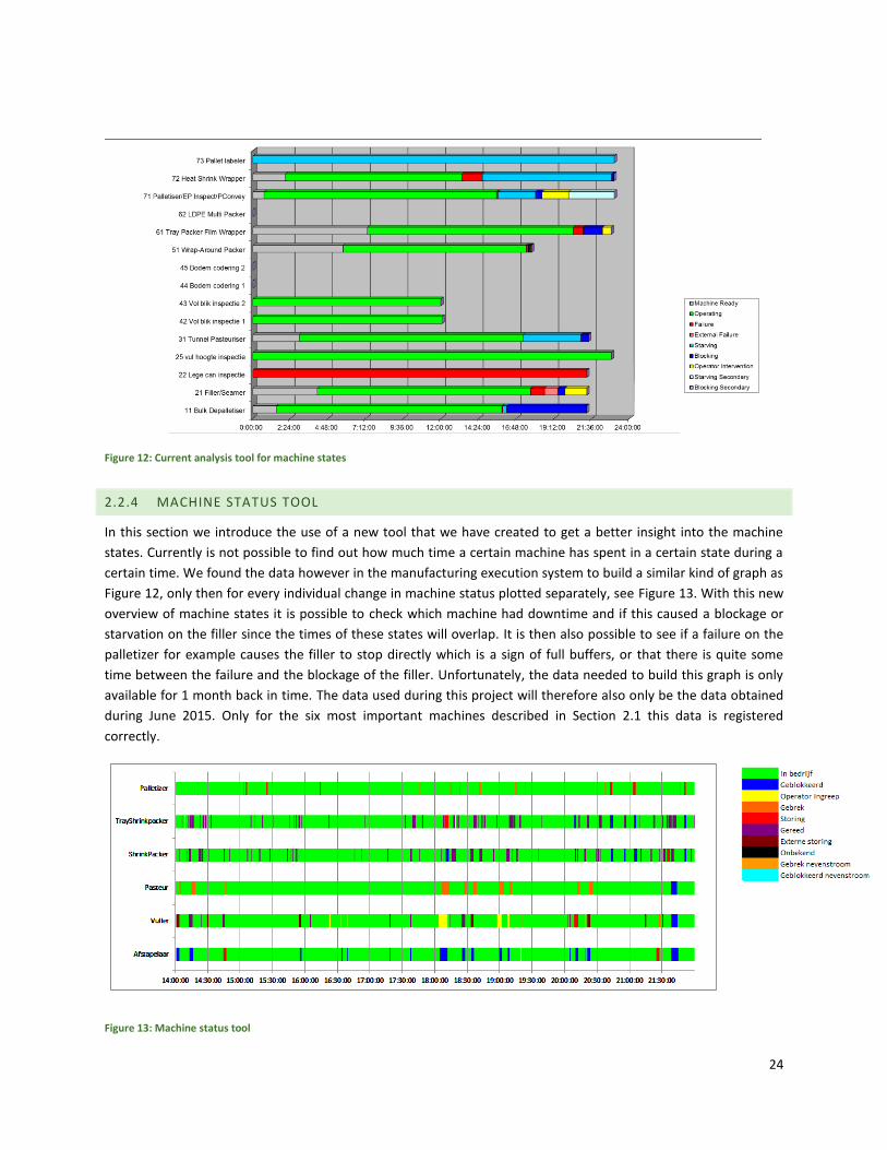
2.2.4 MACHINE STATUS TOOL

In this section we introduce the use of a new tool that we have created to get a better insight into the machine

states. Currently is not possible to find out how much time a certain machine has spent in a certain state during a

certain time. We found the data however in the manufacturing execution system to build a similar kind of graph as

Figure 12, only then for every individual change in machine status plotted separately, see Figure 13. With this new

overview of machine states it is possible to check which machine had downtime and if this caused a blockage or

starvation on the filler since the times of these states will overlap. It is then also possible to see if a failure on the

palletizer for example causes the filler to stop directly which is a sign of full buffers, or that there is quite some

time between the failure and the blockage of the filler. Unfortunately, the data needed to build this graph is only

available for 1 month back in time. The data used during this project will therefore also only be the data obtained

during June 2015. Only for the six most important machines described in Section 2.1 this data is registered

correctly.

Figure 13: Machine status tool

25

To be sure that the data from the information system or also referred as management execution system (MES) is

correct, we have checked the data of the information system with the DTR file recorded by the machine operators

and found this data to be correct most of the time. Sometimes not all times are exactly the same. The reason for

this is the fact that downtime in the DTR file is measured in minutes rather than seconds, or little downtimes are

not registered at all in the DTR. So one can conclude that the data from MES is more detailed than the current DTR

file. Besides comparing MES with the DTR file, we did a measurement on the line and found the times of the MES

to be the same as the times in on the line. One disadvantage of the machine status tool however is, that it is not

visible if a machine is in downtime because of allowed stops, service stops, maintenance & cleaning, no production

planned or because of an actual failure somewhere on the line.

2.3 CURRENT PERFORMANCE

We know now which data is available and how the line is regulated. This section will describe the current

performance of the canning line. In Section 2.3.1 a general description of the ME and FE is given, Section 2.3.2 will

describe the current conveyor capacities, in Sections 2.3.3 and 2.3.4 the buffer capacities in the dry area and the

wet area are given, respectively. Section 2.3.5 will compare the theoretical buffer capacity with the actual buffer

capacity found during production, finally the Mean Time to Repair and Mean Time to Failure will be analysed and

compared with the buffer capacity and the recovery time of certain conveyor sections in Sections 2.3.6 and 2.3.7,

respectively.

For the canning line the performance measures ME and FE are measured on the fill machine, since this machine

determines the speed of the whole line. See Appendix 1 for a complete explanation of the calculations. For our

project, ME is the most important performance measure to improve since this is far below the target of 95%.

2.3.1 PERFORMANCE OF THE CANNING LINE

Although Grolsch is not performing as good as they want to in the benchmarks conducted by SAB Miller, the scores

are not so bad either. As can be seen in Figure 14, both FE and ME have increased slightly during the last 28 weeks

of the last financial year (F15), this can be seen in the linear lines of both the ME and FE since these have increased

slightly. The reason why FE is so much lower than ME is because the line has to be cleaned entirely every time

another brand will be filled. Also 8 hours of maintenance and cleaning is scheduled every week to clean the entire

line, to prevent the beer from getting contaminated with bacteria. Most of the machines need to be changed over

when different brands or packaging materials are used as well. All these actions take a lot of time, that is the

reason why FE is so much lower than ME.

26

Figure 14: Productivity of the canning line

The performance measures ME and FE are based on the downtime recording file (DTR file). This excel sheet is

manually updated every time the filler is stopped either by changeover, maintenance of failures on the line etc.

Within this file all the stoppages of the filler are recorded and the reason why and when applicable the machine

causing the stoppage is noted as well. All the individual parameters from these DTR files are also recorded in a

database for each financial year. A financial year runs from the first of April till the 31st

of March the next year.

If the causes for the filler to stop are analysed, it is quite surprising that machines at the end of the line

(trayshrinkpacker, shrinkpacker, palletizer) cause almost 35% of downtime on the line, see Figure 15 where a

Pareto graph of the downtime in minutes of every machine is shown during June 2015. We found this surprising

since the further a machine is away from the core machine, the more buffer should be available on the conveyor

belts till the filler.

Figure 15: Pareto analysis on causes of downtime on the filler during June.

Measuring downtime only when the filler is interrupted gives enough information for the calculation of ME and FE,

however, for analysis on the downtime of machines it gives a distorted picture. Since only when the filler actually

comes to a standstill the cause is noted. However, upstream or downstream on the line downtime might occur

without disturbing the filler, because of the buffers on the line. The failures that do not disturb the filler are not

0

20

40

60

80

100

35 36 37 39 40 41 43 44 45 47 48 49 50 51 1 2 3 4 6 7 9 10 11 13 14 15 16 17

Pe

rce

nta

ge

Week

Productivity of the canning line

FE

ME

Lineair (FE)

Lineair (ME)

0,00%

20,00%

40,00%

60,00%

80,00%

100,00%

0100200300400500600700

Cu

mu

lati

ve %

Sum

of

do

wn

tim

e

Sum of downtime (in minutes) Cumulative %

27

recorded. From the DTR file it is thus not clear how often other machines than the filler have had downtime. A

situation might have occurred where for example the trayshrinkpacker was in failure for 5 minutes. This did not

cause the filler to stop operating since not all buffer capacity was used. However, if the can coding is in failure for 2

minutes subsequently and this will cause the filler to stop, the cause for downtime in the DTR will be recorded as

the can coding, while the trayshrinkpacker has caused most of the buffers to be used. Since it is not visible in the

DTR how much downtime the machine had that caused the failure during a standstill of the filler, it is also very

difficult to find out if that machine caused the downtime on its own or that conveyors were already too occupied

and that a small failure on the machine causing the failure has already caused downtime on the filler. This is where

the machine status tool, discussed in Section 2.2.4, comes in handy.

With this tool it is better visible how much failures actually happened on the different machines and how much

downtime occurred. See Figure 16 for the failure time and number of failures according to the MES information

system. The reason why the downtime in Figure 16 is bigger than the downtime in Figure 15 is because all failures

are registered in MES, not only failures causing the filler to stop. The reason why the filler has more downtime

than in the DTR file is because also external failures are taken into account. These external failures are recorded as

a failure of a different machine in the DTR file.

Figure 16: Downtime according to information system (MES)

According to MES data, the TSP (trayshrinkpacker) has had 118 failures (see Figure 16), while the DTR file reports

that 31 failures have caused the filler to stop, see Figure 17. This would mean that 87 failures have been absorbed

by the buffers on the line. Based on those facts we can conclude that the buffers are doing their job correctly,

since most of the failures are absorbed by buffers. However, when downtime due to blockage or shortage happens

on the filler, it causes almost the same or sometimes even more downtime on the filler than on the machine with

the failure, what is the complete opposite of what is expected when working with buffers. Table 1 shows the

average difference in downtime between the machine up- or downstream and the filler. A positive number means

that the downtime on the machine causing the failure was that many seconds longer than the downtime on the

filler. Thus although buffers absorb failures, still only a small difference in downtime is eventually measured on the

filler. As can be seen, the average differences are very small, what could mean that buffers are very small

themselves or that buffer capacity is used up most of the time. To find out if the buffers are very small or if the

capacity is used up, we need to find out what the actual buffer capacity is on the line.

35

286

7 20

118 82

0

50

100

150

200

250

300

350

0

200

400

600

800

1000

1200

1400

1600

# o

f fa

ilure

s

Do

wn

tim

e in

min

ute

s

Downtime (in minutes)

Number of failures

28

Figure 17: Downtime according to DTR

Machine causing failure Difference in downtime compared to filler (in seconds)

De-palletiser 29

Pasteuriser 11

Shrinkpacker(SP) 13

Trayshrinkpacker(TSP) 12

Palletiser 90

Table 1: Average difference in downtime compared to downtime on the filler

2.3.2 CONVEYOR CAPACITY

In order to find out how much buffer capacity there is currently available at the line and thus to find out how long

a certain downtime can take before the core machine will stop producing, we did a measurement of the conveyor

capacity. These capacities have been found by measuring the length and width of the conveyors in the technical

drawings of the whole line. The capacities can then be found by using the following formulas defined by (Härte,

1997).

In order to find the total capacity of a conveyor section, it is first calculated how much rows of cans can fit onto the

width of the conveyor. Since certain sections become smaller or larger at the end we measured the start width and

the end width and divided that by two in order to get the average width of that conveyor section. The number of

rows are found by the following formula:

Nb = ROUND[W − d

d ∗ cos(30)+ 1]

where W is the width in millimetres of the conveyor section and d is the diameter of the cans being processed.

The number of cans on every meter of the conveyor can be found by:

31

41

14 17

24

5 051015202530354045

0

100

200

300

400

500

600

700

# o

f fa

ilure

s

Do

wn

tim

e in

min

ute

s

Downtime in minutes

# of failures

29

Nm = [Nb ∗ 1000

d]

The total number of cans on a certain section of the line can subsequently be found by multiplying Nm with the

total length of the section.

Nmsection = Nm ∗ Length conveyor section

These calculations and the corresponding conveyor capacities can be found in Appendix 2.

2.3.3 BUFFER CAPACITY IN CAN SECTIONS

The conveyor capacity itself does not say anything about the buffer capacity of those conveyors yet, since the cans

use some conveyor capacity already by transportation alone. We will therefore calculate the buffer capacity of the

different conveyor sections in this section.

A fundamental rule for the buffer capacity of a conveyor section is, the higher the speed of the transportation line,

the bigger the buffer capacity. When it is known how much time it takes for a can to be transported over a certain

section, it can be calculated how much space the cans use already by just running production and subsequently

how much buffer capacity is left to absorb breakdowns and minor stoppages. From an interview with an

automation engineer at Grolsch it became clear that in general a conveyor section can run twice as fast as the

machine behind it. For example if a machine can produce 72,000 cans per hour, the conveyor upstream of the

machine can transfer 144,000 cans per hour. This speed can be a bit higher or a bit lower, but in general conveyors

can run twice as fast. For the rest of the research we will therefore use this as the maximum conveyor speed.

Dependent on the occupation of the conveyor belt, a can could transfer in either the speed of the conveyor belt or

at the speed of the machine behind it. When the conveyor belt is completely occupied, the speed of the cans is the

same as the amount of cans the machine behind this conveyor can handle, this is called Sb(in meters/minute)

(Härte, 1997). When the conveyor belt is empty, the cans will transfer at the speed of the conveyor belt, of which

the maximum is Sc (Härte, 1997). The speed of the conveyors is not known, but the speed of the machines is

known. With that information Sb is known and thus Sc = 2 × Sb (in meters/minute). With these conveyor speeds

we can calculate the transfer times of a can. The conveyor capacity used by just running production is calculated by

the time it takes to transfer a can over the conveyor sections between two adjacent machines multiplied by the

speed of the machine upstream.

Nominal conveyor occupation = Transfer time ∗ machine speed

If it is known how much space the cans occupy in the nominal situation we can find out how much space is left for

buffer by subtracting that conveyor occupation from the conveyor capacity.

Buffercapacitysection = Nmsection − Nominal conveyor occupation

For all can conveyors, the nominal buffer capacity can be found in Table 2, this is a calculation based on nominal

production speed of 72,000 cans per hour of all machines. It is assumed that the nominal conveyor speed is twice

the speed of the nominal line speed, thus 144,000 cans per hour. This buffer capacity is translated into buffer time.

The buffer time is the time it takes for a buffer to be completely used. In fact this is the time that a machine could

be in failure before it affects the next machine. Off course the buffer times mentioned in this table are based on a

speed of 72,000 cans, however in a real situation a machine will slow down as soon as the conveyor will start filling

30

up, which will make buffer time even longer. To make it easy this has not been taken into account in this buffer

time yet.

Section Transfer

time(sec)

when

Conveyors space Buffer

time

From To Full Empty Conveyor

capacity

Nominal

occupation

Buffer

capacity

Till previous

machine

(seconds)

Till Filler

(seconds)

Depalletiser Filler 295 147 5895 2948 2947 147 147

Filler Pasteurizer 104 52 2765 1384 1381 69 69

Pasteurizer Can coding 208 104 7238 3620 3618 181 250

Can coding Shrinkpacker 375 187 7493 3746 3747 187 437

Can coding Traypacker 387 193 7734 3867 3867 193 443

Table 2: Conveyor capacities when running in a nominal situation in the wet section.

2.3.4 BUFFER CAPACITIES IN PACKAGE SECTIONS

In this section we will describe the conveyor and buffer capacity in the dry area of the line. In the sections where

cans have already been packed into bigger packages like trays or six packs, the conveyor and buffer capacity are

calculated differently. The conveyors for which this is the case are the conveyors between the Shrinkpacker and

the Trayshrinkpacker and between the Trayshrinkpacker and the Palletizer. Special buffer areas are created

between transportation sections, since transportation sections of packages cannot accumulate packages in the

same way as cans. The buffer capacity of these sections is the space between the different packages on the

conveyor. The space between the packages depends on the speed of the conveyor. The faster a conveyor runs the

more space will be in between the packages. Again we suppose that the speed of the conveyors will be twice as

fast as the line speed in a nominal situation. This means that half of the conveyors will be empty to be used for

buffer when operating at nominal speed. In Table 3 an overview of the buffer capacity on all buffer sections can be

found.

31

Section Conveyors space Buffer

time

From To Buffer

section

number

Conveyor

capacity

(cans)

Nominal

occupation

(cans)

Buffer

capacity

Till previous

(sec)

Till Filler

(sec)

SP TSP 1 1188 600 588

SP TSP 2 348 180 168

SP TSP 3 720 360 360

SP TSP 4 552 276 276

SP TSP Total 2808 1416 1392 69 506

TSP Palletizer 1 1824 912 912

TSP Palletizer 2 912 456 456

TSP Palletizer 3 1296 648 648

TSP Palletizer 4 264 132 132

TSP Palletizer Total 4296 2148 2148 107 613

Table 3: Buffer capacity on packaging sections

2.3.5 ACTUAL VS THEORETICAL BUFFER CAPACITY

The theoretical buffer capacity calculated in the previous section is the buffer capacity available in case of nominal

production. However it could be the case that buffer capacity is not completely available all the time. In this

section we will discuss the difference between the actual measured buffer time during June and the theoretical

calculated buffer time.

To calculate the actual buffer time between the failure machine and the filler, we have calculated the difference in

the time of a machine having a failure or blockage and the time when the filler has been blocked. The difference

between these two times is the actual buffer time of the conveyor section. This resulted in the buffer times as can

be found in Table 4. It is clear that the actual buffer time is much smaller than the theoretical buffer time.

Especially, when it is assumed that buffer times should be even larger in real life, because machines will slow down

once conveyors start to fill up. We based our theoretical buffers on completely usable buffers, while in real life

buffers might already have been used partly. Table 4 shows that a relative large amount of the theoretical buffer is

used and thus the buffer strategy is at least working. However, when comparing the average buffer time with the

average difference in downtime of a machine, the difference in downtime is much smaller than the buffer capacity.

It is expected that these numbers would have roughly matched each other, since it takes at least the average

buffer time in Table 4 before the blockage starts on the filler, thus the downtime on the filler is expected to be that

amount shorter.

32

Machine Average buffer time before filler stops (in seconds)

Theoretical buffer till filler (in seconds)

Percentage used of theoretical buffer

Difference in downtime compared to filler (in seconds)

De-palletiser 115 147 78,2% 29

Pasteuriser 50 69 72,5% 11

Shrinkpacker 299 437 68,4% 13

Trayshrinkpacker 298 443 67,3% 12

Palletiser 386 613 63,0% 90

Table 4: Average and theoretical buffer time till filler

2.3.6 MTTR VS BUFFERCAPACITY

Now that the buffer capacities are calculated, this section will describe if the buffer capacities are big enough to

absorb the failures in the system.

To do this, The Mean Time To Repair (MTTR) has been calculated. The MTTR is the time the average failure lasts.

This calculation is done based on all the available production data from June 2015, and thus all failures are taken

into account. Besides the state “failure”, also the states “external failure” and “operator intervention” have been

taken into account as a failure since the machines are in failure during this state most of the times as well. For the

de-palletiser the state “starving” has been taken into account as well since this is the first machine of the line and

thus if this is starving it could be seen as a failure as well. Also for the palletiser the state “blocked” has been taken

into account as a failure, because this is the last machine of the line. Failures longer than 10 minutes have been

filtered out of this analysis. On average only about 15% of the failures is bigger than 10 minutes, but these bigger

failures would make the MTTR increase a lot. The buffers are not able to absorb these longer failures anyway thus

it makes no sense to include these in this analysis. Figure 18 makes clear that the MTTR is bigger than the buffer

capacity in most cases. Thus the buffer is too small to absorb all failures. Only for the shrinkpacker(SP) and the

trayshrinkpacker(TSP) the buffer is bigger than the MTTR, this extra buffer can also be used when the palletiser has

downtime.

Figure 18: MTTR vs buffer capacity

0

50

100

150

200

250

300

350

400

MTT

R in

se

con

ds

Average actual buffertime

Theoretical buffercapacity

MTTR < 10 min

33

As can be seen in Table 5, especially the de-palletiser and palletiser have the most failures bigger than the buffer

capacity allows to be, however, as already explained, the palletiser can use buffer capacity of the sections between

the SP and TSP before it reaches the filler. The reason why not all failures have been absorbed could be because of

the fact that buffers cannot fully restore again because of new failures occurring already again. This will be

discussed in the next section.

Machine MTTR (in sec) Number of failures

Number of failures bigger than theoretical buffer

# failures bigger than actual buffer

De-palletizer 465 35 20 21

Filler 309 286

Pasteuriser 378 7 6 7

Shrinkpacker 212 20 3 4

Trayshrinkpacker 444 118 19 24

Palletizer 274 82 45 82

Total 548 93 138

Table 5: MTTR of all failures, without allowed stops

2.3.7 MTTF VS RECOVERY TIME

In order to have full buffer capacity when another failure happens it is important that the recovery time of a buffer

is larger than Mean Time To Failure (MTTF) of the machine using this buffer, in this section we will compare the

MTTF with the recovery time of a buffer. The recovery time is the time it takes for a machine to create full buffer

again. This is calculated by the overcapacity of a machine compared to the capacity of the line. The MTTF is the

time between two adjacent failures on a machine. Since machines can only breakdown when they are actually

operating, the MTTF is only based on the actual operating time of a machine. As can be found in Figure 19, the

recovery time is short enough to recover the buffer capacity in time to absorb the following failure. Only for the

TSP the MTTF is quite close to the recovery time, thus it might sometimes occur that these buffers are not

completely usable again.

Figure 19: MTTF vs recovery time (only failures)

0

200

400

600

800

1000

1200

1400

Recovery time (min)

Recovery time till filler (min)

MTTF downtime machineoperating

34

2.3.8 CONCLUSION SECTION 2.3

Summarizing Chapter 2, the buffer capacity is a bit too small to absorb all failures, but it is absorbing most of the

failures. Also the recovery time of the buffers is much smaller than the average MTTF, thus full buffer capacity

would be available most of the time. Therefore it makes no sense to adjust machine speeds. However, speeding up

conveyors would increase buffer capacity and could therefore also adjust the difference in downtime of the filler

compared to the machine causing the failure in a positive way. However this is not the core problem of the small

difference in downtime. The most remarkable fact of this chapter is that although significant buffer capacity has

been found between the several machines, the difference in downtime is far less than this buffer capacity.

2.4 THE BOTTLENECK PROCE SSES

As said in the previous section, the time of failure upstream or downstream is eventually almost just as big on the

filler. The causes why this might occur will be explained in this section. We will start with an analysis of our

machine tool in Section 2.4.1. In Section 2.4.2 we research the pasteuriser regulation when in failure. In Section

2.4.3 we describe the conveyor regulation and why this might cause the difference in downtime to be small.

2.4.1 START UP DELAY AFTER FAILURE

When a failure has happened anywhere on the line, and it causes a machine upstream or downstream to stop

working, there is a significant delay between the start of the machine that had the initial failure and the machines

that are blocked. To prove this, see the red rectangle in Figure 20 and Table 6, in which it is clearly visible that the

end of the failure on the TSP (end of the yellow bar) is almost at the same time as when the filler is blocked. And

then it took the filler 525 seconds before it could start producing again. This is probably the reason why the

difference in downtime as mentioned in Table 1 is so small.

Figure 20: An occasion where downtime upstream is bigger than the actual failure (11-06/12-06)

Machine Downtime (in seconds)

TSP 345

SP 450

Pasteuriser 520

Filler 525

Table 6: Downtime of machines in occasion of figure 18

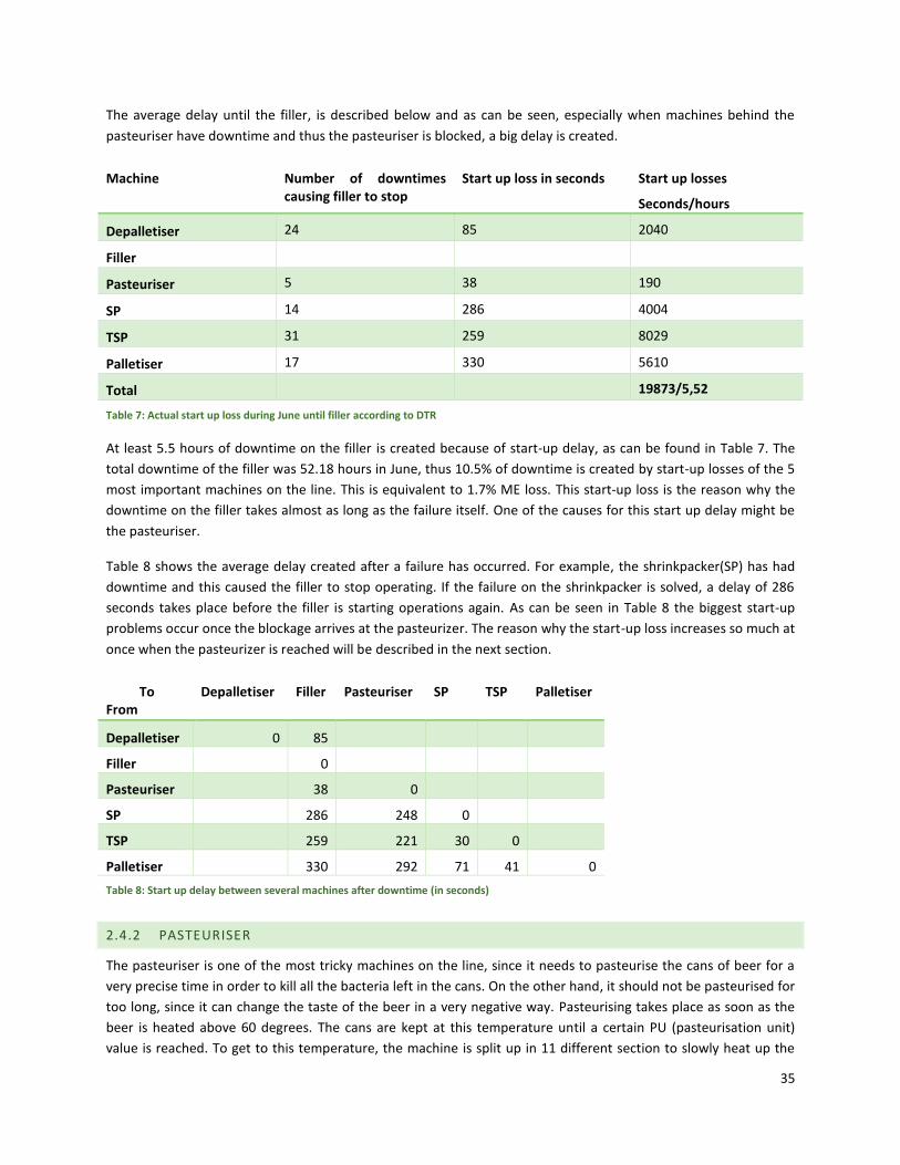
35

The average delay until the filler, is described below and as can be seen, especially when machines behind the

pasteuriser have downtime and thus the pasteuriser is blocked, a big delay is created.

Machine Number of downtimes causing filler to stop

Start up loss in seconds Start up losses

Seconds/hours

Depalletiser 24 85 2040 Filler Pasteuriser 5 38 190 SP 14 286 4004 TSP 31 259 8029 Palletiser 17 330 5610 Total 19873/5,52

Table 7: Actual start up loss during June until filler according to DTR

At least 5.5 hours of downtime on the filler is created because of start-up delay, as can be found in Table 7. The

total downtime of the filler was 52.18 hours in June, thus 10.5% of downtime is created by start-up losses of the 5

most important machines on the line. This is equivalent to 1.7% ME loss. This start-up loss is the reason why the

downtime on the filler takes almost as long as the failure itself. One of the causes for this start up delay might be

the pasteuriser.

Table 8 shows the average delay created after a failure has occurred. For example, the shrinkpacker(SP) has had

downtime and this caused the filler to stop operating. If the failure on the shrinkpacker is solved, a delay of 286

seconds takes place before the filler is starting operations again. As can be seen in Table 8 the biggest start-up

problems occur once the blockage arrives at the pasteurizer. The reason why the start-up loss increases so much at

once when the pasteurizer is reached will be described in the next section.

To From

Depalletiser Filler Pasteuriser SP TSP Palletiser

Depalletiser 0 85

Filler 0

Pasteuriser 38 0

SP 286 248 0

TSP 259 221 30 0

Palletiser 330 292 71 41 0

Table 8: Start up delay between several machines after downtime (in seconds)

2.4.2 PASTEURISER

The pasteuriser is one of the most tricky machines on the line, since it needs to pasteurise the cans of beer for a

very precise time in order to kill all the bacteria left in the cans. On the other hand, it should not be pasteurised for

too long, since it can change the taste of the beer in a very negative way. Pasteurising takes place as soon as the

beer is heated above 60 degrees. The cans are kept at this temperature until a certain PU (pasteurisation unit)

value is reached. To get to this temperature, the machine is split up in 11 different section to slowly heat up the

36

cans and cool it down during different sections. These 11 sections can be found in Figure 21. The first 4 sections

are used to heat up the cans to around 45 degrees. The middle 3 sections are called the pasteurising zone,

however only the last section actually pasteurises the beer, the first 2 sections of the pasteurising zone heat the

cans up till pasteurising temperature. However, for quality reasons, once a can reaches the pasteurising zone it will

never be cooled down before it is completely pasteurised. At last, 4 sections are used to cool beer down again, as

can be seen in Figure 21. In this figure every red bar corresponds to a section in the pasteuriser. The blue line in

this picture corresponds to the temperature of the cans.

All this heating up and cooling down costs a lot of energy and therefore the different heating sections and cooling

sections are connected with each other to save energy. For example heating Section 1 is connected to cooling

Section 4. The heating water from section 1 is cooled down by cold cans in section 1, this cooled water is then used

again to cool cans in cooling section 4. Vice versa, the hot cans heat up the cool water in cooling section 4, this is

used to heat up the cans again in heating section 1. Off course if the temperature of the heating or cooling water is

not correct, extra cooling or heating takes place. To save even more energy, the pumps of the heating up and

cooling down sections will be shut down as soon as the pasteuriser encounters a blockage that is longer than 5

minutes. This is done because after 5 minutes of cooling the cans are below their pasteurisation temperature and

heating for longer than 5 minutes will start pasteurising. The first two sections of the pasteurising zone and the

pasteurisation zone itself are kept at heat until full pasteurisation has been created. This is done to ensure the

quality of the pasteurisation. It was found out in the past that when interrupting the pasteurisation process, the

pasteurisation units are increasing enormously. Also the pressure within the cans increases once a lot of heating

up and cooling down takes place, which could eventually lead to can breakage. This breakage can eventually cause

even bigger failures. This phenomenon already takes place once cans are heating up until 51 degrees, this is the

reason why also the first two pasteurising zones are fully pasteurised once started. Thus once pasteurisation has

started it should be finished. If all the cans in the pasteurisation zone are pasteurised, at last these pumps will cool

down the cans till 51 degrees and also these pumps will shut down.

Figure 21: Overview of pasteurization zones

37

One last thing that is programmed into the software of the plc’s and the pasteuriser software is that at least the

amount of one pasteurisation section of cans should be free on the conveyor section downstream of the

pasteuriser. This is done to have less start and stop situations on the pasteuriser, thus less heating up and cooling

down of the pasteuriser. The reasoning for this is that the complete buffer between can coding and the pasteuriser

is available when you first drain the conveyors and thus shorter stops will not directly influence the pasteuriser. Of

course when the pasteuriser needs to stop, some cans will be pasteurised longer than the target time, since the

cans at the end of a pasteurisation section still need to pasteurise the same amount of time as the cans that just

arrived at the beginning of the section. Also the cans at the beginning of the section will be shortly reheated once

new cans arrive at this section again. However this extra pasteurisation still falls within the boundaries of the PU

value.

Since it is not completely known how large the sections are we roughly calculated it. The first 4 heating zones, the

3 middle pasteurisation zones and the 4 cooling zones are all the same size. The total size of the pasteuriser is

about 57000 cans. This means that the whole pasteurisation zone is: 57000/3 = 19000 cans, and 1 pasteurisation

section is 19000/3 = 6333. When the TSP or SP is running at full speed (92000 cans per hour), this amount can be

drained in 247 seconds. This is already more than 4 minutes of start-up delay. It might be true that by only starting

up the pasteuriser once the buffer downstream is empty enough for one pasteurisation section reduces the

number of stops on the pasteuriser, however, when a blockage actually reaches the pasteuriser it will cause an

extra-large stop on the filler, because the stop will now take at least 247 seconds before the buffer is restored.

Besides that, the overcapacity of the machines downstream of the pasteuriser should be able to restore the buffer

during production by itself. So building extra safety into the regulation of the pasteuriser might be one of the

reasons that so much start-up loss is created once blockage occurs and thus the pasteuriser might be one of the

reasons that efficiency is lost.

2.4.3 CONVEYOR REGULATION

Another cause for start-up delay might be in the way the conveyors are regulated. As said before, the speeds of

the machines and conveyors are regulated by means of sensors mounted on the side of a conveyor. The conveyors

between two adjacent machines are connected by several different conveyor sections, that can all be regulated

differently. These different sections are also switched on and off by these sensors. For example, when all sensors

are triggered because they are blocked by cans, it means that all conveyors are full. The conveyors are then

automatically switched off, however, they will also only start running again when the sensors are not triggered

anymore. This causes quite some delay since it will take a couple of seconds every time when a new sensors is not

triggered anymore, which could eventually lead to a lot of downtime on the filler.

2.5 SUMMARY AND CONCLUSION

In Chapter 2 we found that that if blockages are caused on the filler or the pasteuriser the blockage takes almost

the same time as the failure on the machine with the actual failure. After analysing our machine status tool we

found a significant delay in the start time of the failure and the eventual blockage time of the filler, which is a sign

of buffers being used. On the other hand we also found a significant delay in the end time of the failure and the

end time of the blockage on the filler. This is not good, since this means that extra blockage time is created on the

filler, while the failure that causes the filler to stop has already been solved. The reasons for this could be that

either the pasteuriser is causing an extra delay and/or the conveyors/sensor locations are not properly regulated

once failures have occurred. The possible causes for the start-up delay on the filler are known, however, now we

have to find solutions to solve these causes. In the next chapter we will focus on what literature writes on

improving line regulation and start-up delays in production environments.

38

3 LITERATURE REVIEW

In this chapter we describe which modelling techniques are mostly used in operations research to evaluate

performances and which model is best for us to use. Secondly we describe what kind of studies have already been

done to improve line performance based on line regulation, dimensioning and buffer strategies and how the

prediction of performance is done.

3.1 MODELLING TECHNIQUES

Operations research modelling techniques to evaluate performances can be roughly divided into analytical

modelling and simulation modelling (Kozan, 1997). We consider both techniques below.

Analytical modelling

Analytical models in operations research are often adopted into a form that is easily solvable (Kozan, 1997). The

advantage of analytical models is that they can calculate an exact solution. If an analytical solution is available and

it is computationally efficient, it is usually desirable to study the model in this way (Law, Simulation modeling &

analysis, 2007). However, many systems are complex making it hard to get an analytical solution. In those cases,

simulation models could be more preferable.

Simulation modelling

“Simulation may be defined as a technique that imitates the operation of a real-world system as it evolves over

time” (Winston, 2004). In contrast with exact analytical models, simulation models execute a model through time

to generate samples of the performances. Unlike analytical models, in which one often tries to find an optimal

solution, simulation models are mostly used to test several “what if” scenarios. The fact that simulation models are

able to visualize the system is an advantage since this could help to convince people of a certain solution.

Our system consists of different machines with different failure profiles which need to be incorporated in the

model to mimic a real life situation. Based on the fact that our model needs to handle dynamic events like the

speed of machines and conveyors and because we need to take failures, order sizes and uncertainty into account,

the model would become too complex to make an analytical model of it.

3.2 PREVIOUS STUDIES

This section reviews literature that has already been conducted within the field of performance improvement

based on line regulation, dimensioning and buffer strategies.

A stochastic model has been made by Pourbabai (1993) to calculate the optimal processing rates of both the

machines and the conveyors to increase the throughput of the system and minimizing the time the bottleneck is

blocked. This research is conducted on an automatic assembly line of a manufacturing factory. Although the

solution suggested by Pourbabai (1993) is exactly what we want, he uses fixed operational speeds, while at Grolsch

we have the possibility to change operating speeds by the use of PLCs, making their model less suitable.

Miltenburg & Szendrovits (1989) propose an analytical model that calculates the needed safety stock between

different stages to reach a pre-set efficiency level. Within this model they take down-time of the machine into

account either due to a defective item being produced, breakdown of the machine, or blockage or starvation of

the machine. In this model it is assumed, however, that the line starts production with safety stock already present

39

at the line at start up and that safety stocks are replenished at the end of production. This is not the case in our

problem since machines are able to ramp up speed to replenish safety stocks during production.

Although the above mentioned models present possible ways to analyse and improve the performance, they rely

on analytical models that are not suitable in our system. Pol (2014), Van Leer (2014 ) and Basán, Cóccola, &

Méndez (2014) present simulation models within a beer factory which correspond to our research. These models

will be described below.

Pol (2014) tries to improve performance by changing the moment of changing operating speed of both the

conveyors and the machines. The idea behind the control of different kinds of speed is to have a better continuous

flow of your products and with that all machines will have less start and stop situations. This improves the

reliability of every machine which will consequently improve throughput (Pol, 2014).

Basán, Cóccola, & Méndez (2014) research if line design by changing the theoretical speeds and buffer quantities

can improve the performance of the line. This study also uses a simulation program to simulate different “what if”

scenarios to see if this improves current performance.

The last similar study is done by Van Leer (2014). In this study the author tries to change both the location of

sensors for changing speeds as well as the speed levels themselves. Different locations and speed levels were

tested by means of a simulation model and the author found that these changes would positively influence both

the production balance as well as the output.

From these previous studies, we can learn that changing the buffer strategies and line regulation by means of

sensor locations, buffer quantities and machine speeds can significantly improve the overall performance of the

line and this could therefore be an interesting subject to improve the performance at Grolsch as well.

3.3 CONCLUSION

Based on Section 3.1 and Section 3.2, we conclude that a simulation model is the best option when working with a

complex model. Since different stochastic variables such as failure profiles are needed to mimic real life situations

a simulation model would be the best way to analyse and predict performances for our system. Secondly several

similar studies on the improvement of performance in filling lines also used simulation models to analyse the

performance of different scenarios.

From these previous studies we have also found that significant performance improvements can be generated by

changing the location of sensors for determining machine and conveyors as well as changing the speed levels itself.

Assessing the impact of changing sensor locations and speed levels on the performance will be done by means of a

simulation model. In the next chapter we will therefore describe a conceptual model.

After this literature review we still did not find a way to decrease start-up failures as described in Chapter 2. We

will come back to this issue in Chapter 6 .

40

4 CONCEPTUAL MODEL

In Chapter 3 we decided that a study using a simulation model would be the best way to analyse and predict

performance measures of our system.

The main goal of our project is to find a line regulation and buffer strategy that performs better than the current

situation, we are going to simulate different settings for both the sensor locations to adjust machine speeds as well

as sensor location to start up the pasteuriser after a failure. This chapter will be used to construct a conceptual

model. In Section 4.1 we describe the lay-out of the model. In Section 4.2 we describe the inputs we need to let

the model run. In Section 4.3 we describe the assumptions we have made.

4.1 LAY-OUT OF THE SYSTEM

Albeit Chapter 2 has already given an overview of the system in real life, our simulation model will only simulate

part of the machines, since no reliable data is available for all machines. However, the other machines on the line

cause almost non to very little failures, and will thus not influence performance of the line. Also machines directly

connected to the filler are incorporated in the failure profile of the filler. In Figure 22 an overview is given of which

machines and conveyors (which act as buffers) are used. Although in real life the conveyors are split up into more

conveyors, we have chosen to only split up the conveyors that will actually change the performance of the model.

For example Conveyors 3, 4 and 5 are not modelled as one conveyor because the width and speed of these

conveyors are different. Furthermore, we will describe events that trigger decisions or processes.

Figure 22: Production flow of canning line

Order generation

An order is needed to start up production. This order is made by the planning department and the unit manager.

The order specifies which type of beer, which cans and which packaging materials to use. The production staff will

subsequently make sure that the materials are available on time and at the correct location. In our model we

assume that materials are always available and at the correct location. Within our model it is not necessary to

know which type of beer or which cans are processed since this will not change anything on the behaviour of the

model. The only thing that will change is the packaging method. If multipacks are produced, e.g., 6 packs or 4 packs,

the shrinkpacker is used in the packaging process. If the cans are packed loose (cans are separately packed onto a

tray) the shrinkpacker is not used, as shown in Figure 22. The only things we therefore specify in our “order” are

the number of cans to be produced and the packaging method, either loose or in multipacks. Once the filler has

produced the amount of cans as specified in the order, the model will randomly draw a new order size and

packaging method from a distribution table, this will be described in Section 4.2.1.

41

Change-over packaging

When the packaging method changes, from multipacks to loose or the other way around, the route of the cans

also changes. The shrinkpacker will be used when producing multipacks, otherwise it will not be used. Before the

route can be changed, the current work in progress on the traypacker and/or shrinkpacker should be processed.

On average a changeover of the packaging materials and the set-up of the machines takes 15 minutes. We

therefore decided that once the first can of a new order arrives at the end of conveyor 7, we will stop this

conveyor for 15 minutes. All machines and conveyors behind conveyor 7 keep running until all work in progress on

the shrinkpacker and or traypacker is processed. After 15 minutes conveyor 7 will start up again.

Conveyors

The conveyors used at the canning line are, as has been told in Chapter 2, accumulation lines. This means that a

part of the conveyor could be used as buffer. Since it is difficult to simulate these accumulation lines we decided to

see conveyors as buffers. Every buffer has its own “processing time” which corresponds to the transfer time of a

can on a certain conveyor. Every can entering a buffer has to stay for at least the “processing time” before it can

leave again. During the processing time, part of the buffer will start to fill up, this corresponds to the nominal

occupation of a conveyor. To mimic reality even more, the buffers need to operate according the First in First out

principle and they can only leave the buffer if the machine behind the buffer is ready to process the next can.

When using these principles a buffer will start to fill up even more when a machine behind the buffer is slower

than nominal speed and it will start to drain when the machines speed is higher than nominal. This imitates the

reality of an accumulation line very closely.

Conveyor speed

In real life the conveyor speed and with that the dwell time of a can on a conveyor can change. In our model this

speed is not really changed, but it is set on a fixed “processing time” that corresponds to the maximum speed of a

conveyor. However the can’s dwell time can change, since the cans are not allowed to leave a buffer until the

machine behind it is empty. If the minimum dwell time of a can has elapsed and the machine behind it is not

empty, it should wait as long as all the cans in front it are processed. This is quite similar to changing the

processing time of a buffer.

Sensors

In real life when a sensor on a conveyor is triggered, the system knows the fill level of the conveyors. Based on that

fill level the speed of the adjacent machine is adapted. To mimic this in our model we will monitor the amount of

cans present on a buffer, if the amount of cans surpass a certain level this corresponds to triggering a sensor. This

will subsequently change the speed of the machine connected to this sensor.

Pasteurisation

The last issue that needs to be tackled in our model is the way to imitate the pasteuriser. To do this we have

divided the pasteuriser into 2 servers which can process one can at a time and 5 buffers, as shown in Figure 23.

Figure 23: Flow of cans through the pasteurizer

42

The heating and cooling zone have a capacity of 19,000 cans and a “processing time” of 15 minutes. This is the

time needed to respectively heat up the cans until pasteurization temperature and cool down below

pasteurisation temperature. The 3 pasteurising zones have a capacity of 6333 cans and a processing time of 5

minutes. The reason why we model the cooling-, heating- and pasteurising zones as buffers, is because in real life

the pasteuriser is nothing but a giant conveyor on which hot water is sprayed.

The three pasteurising zones are modelled to control the pasteurisation time of cans inside the pasteuriser. A can

is perfectly pasteurised if it is pasteurised for 15 minutes, which is exactly the processing time of the three

pasteurising zones. As long as a can is pasteurised within 5 minutes of this 15 minutes, quality of the beer will be

more or less the same and still all bacteria will be killed. In real life it impossible to find out how long every can has

been pasteurised, and therefore engineers at Grolsch developed the program to control pasteurisation as

described in Section 2.4.2. In our model we copy this program. Thus if failures longer than 5 minutes take place,

the cooling and heating pumps should stop operating, and the pasteurising pumps should stop operating once

pasteurisation for every can inside the zone has been pasteurised for at least 5 minutes.

Since the pasteuriser is not able to process cans faster than 74,000 cans per hour we modelled a server at both the

start and the end of the pasteuriser to control speed, respectively pasteuriser entry and pasteuriser exit in Figure

23. Cans are not able to flow in or out of the pasteuriser faster than 74,000 cans per hour in this way.

Although the pasteuriser is nothing but a giant conveyor, it is not able to accumulate cans. Thus every time the

pasteuriser exit is blocked, all the buffers and the pasteuriser entry should stop operating as well.

4.2 INPUT OF THE MODEL

In order to mimic the simulation model as close as possible to reality we need input data that corresponds to the

situation in reality. The inputs used for our simulation model are:

- Batchsizes/ Producttype

- MTTR

- MTTF

- Buffer sizes

- Sensor locations

- Processing time of machines and conveyors

The Batchsize, MTTR, MTTF and product type are drawn from distribution functions, and will be discussed in

Sections 4.2.1 and 4.2.2. Buffer sizes will be discussed in Section 4.2.3 and the sensor locations will be discussed in

Section 4.2.4. The processing times are variable based on the fill level of a conveyor, as discussed in the previous

section.

4.2.1 BATCHSIZE DISTRIBUTION

Distribution functions are fitted with the data obtained during the month June 2015. We make use of a theoretical

distribution that properly fits our data. However, when this is not the case we can still use an empirical distribution.

The empirical distribution draws a number from a frequency table of the sample data from June 2015. A short

overview of which distributions will be used can be found in this section.

43

The current batch sizes are measured by the amount of cans produced per batch during June. This data is then

tested with the program Easyfit to find out which distribution fits the data best. The tests done, are the

Kolmogorov-Smirnov test, the Anderson-Darling test and the Chi-squared test. See Appendix 3 for an explanation

on how these tests are performed. If the test statistics are coloured green in the following tables, it means that the

H0 hypothesis that states that the observed data follows the distribution function, will not be rejected. In Table 10

the used distribution with its parameters can be found.

Packtype Used Distribution Parameters

All packs Log normal =0.92847 =12.326

Table 9: Distribution of batch sizes

Packtype K-S test statistic

Critical value

A-D test statistic

Critical value

Chi^2 test statistic

Critical value

Found distribution

All packs 0.11463 0.130 0.39401 2.492 4.7497 11.143 Log normal

Table 10: Distribution used and its parameters

The packaging method of a new batch, is drawn randomly with a 41.30% change to choose multipacks and a

58.70% change to choose loose packaging.

4.2.2 MTTF AND MTTR PER MACHINE

In this section we describe which distribution fits the data best according to the Easyfit tool. If the test statistics are

lower than the critical value it means that the distribution fits the data (marked green). If it is found that 2 or more

of the tests conclude a good fit, we will use the proposed distribution, see Table 11 and Table 12. Although, some

of the distribution functions were found not to be suitable for representing the data from June with the current

value for alpha, if the p-value of the test statistic is reasonable close to the alpha value and the binned data

followed the graph of the distribution function, with small errors, we still chose the distribution suggested by the

Easyfit tool. In that case it is more likely that the future data follows this distribution function than that it would

follow an empirical distribution. If after analysing the graph of the distribution function the conclusion is that the

suggested distribution does not fit our data, we will use an empirical distribution. Table 11 shows the test statistics

and critical values of the distribution best fitted to the data according to Easyfit. Table 12 will give an overview of

the chosen distribution and its parameters. For the pasteuriser we have chosen to use an empirical distribution

since only a very small sample size was available.

Machine MTTR/MTTF K-S test statistic

Critical value

A-D test statistic

Critical value

Chi^2 test statistic

Critical value

Suggested distribution Easyfit

Depalletiser MTTR 0.0904 0.141 1.0485 2.502 4.8212 12.592 Log-normal

Depalletiser MTTF 0.1384 1.444 3.2278 2.518 13.596 12.592 Gamma

Filler MTTR 0.1283 0.055 11.923 2.502 156.45 16.919 Log-normal

Filler MTTF 0.1322 0.056 10.938 2.502 66.453 16.919 Log-normal

Pasteuriser MTTR 0.1241 0.391 0.18 2.502 0.1676 3.841 Exponential

Pasteuriser MTTF 0.2733 0.409 1.042 2.502 N/A Weibull

Shrinkpacker MTTR 0.2022 0.091 15.967 2.502 70.06 14.067 Log-normal

Shrinkpacker MTTF 0.1104 0.130 1.9314 2.502 19.9 11.07 Beta

44

Traypacker MTTR 0.1897 0.057 32.753 2.502 155.19 16.919 Log-normal

Traypacker MTTF 0.0819 0.074 3.5602 2.502 14.819 15.507 Weibull

Palletizer MTTR 0.0957 0.116 1.7997 2.502 28.744 15.507 Log-normal

Palletizer MTTF 0.0534 0.116 0.2678 2.502 5.9524 14.067 Weibull

Table 11: Best distribution fit according to Easyfit

Machine MTTR/MTTF Used Distribution Parameters

Depalletiser MTTR Log-normal =1.6335 =4.9343

Depalletiser MTTF Empirical MTTFofDepalletiser.table

Filler MTTR Empirical MTTRofFiller.table

Filler MTTF Log-normal =2,0415 =5,5351

Pasteuriser MTTR Exponential =0.00292

Pasteuriser MTTF Empirical MTTFofpasteuriser.table

Shrinkpacker MTTR Empirical MTTRofshrinkpacker.table

Shrinkpacker MTTF Beta 1=0,44975 2=2,8368

Traypacker MTTR Empirical MTTRofTraypacker.table

Traypacker MTTF Weibull =0,59241 =2187,2

Palletizer MTTR Log-normal =1,1489 =4,4485

Palletizer MTTF Weibull =0,62711 =4698,2

Table 12: Used distribution with its parameters

4.2.3 BUFFER SIZES

Although buffer sizes are already mentioned in Chapter 2, in our model we will design our buffers differently. We

will use the complete conveyor capacity between two machines, thus the total amount of cans that can fit on a

certain conveyor section. The buffer capacity will subsequently be dynamic, depending on the amount of cans

present on a conveyor section the buffer capacity will change as well. Also the speeds are translated into

“processing times”. Table 13 shows the conveyors sizes with the same name as in Figure 22.

Buffer name Size in amount of cans Processing time (min:sec)

Conveyor 1 5845 2:27.43

Conveyor 2 2765 0:52.16

Conveyor 3 4034 0:50.44

Conveyor 4 1306 0:32.66

Conveyor 5 1050 0:13.13

Conveyor 6 3586 1:29.65

Conveyor 7 3907 1:37.69

Conveyor 8 2809 1:09

Conveyor 9 4148 1:43.7

45

Conveyor 10 9492 3:09.75

Table 13: Overview of buffer sizes in model

4.2.4 SENSOR LOCATIONS

The sensor locations are fixed at the start of every simulation. In our model we mimic these sensors by triggering

an event as soon as the buffer level exceed a certain threshold. In Table 14 an overview of the sensor description,

the location and the threshold, is given. The thresholds are the same as in the current situation. In case multipacks

are produced, the speed of the traypacker is regulated by the sensors located on Conveyor 8, otherwise the

sensors located on Conveyor 9 are used.

Sensor description Machine to trigger Location Fill level of conveyor to trigger sensor

High speed Can coding Conveyor 4 > 50%

Nominal speed Can coding Conveyor 4 < 50%

Low speed Can coding Conveyor 5 < 35%

High speed Traypacker Conveyor 9/Conveyor 8 >70%

Nominal speed Traypacker Conveyor 9/Conveyor 8 <70%, >35%

Low speed Traypacker Conveyor 9/Conveyor 8 < 35%

High speed Shrinkpacker Conveyor 7 >70%

Nominal speed Shrinkpacker Conveyor 7 <70%, >35%

Low speed Shrinkpacker Conveyor 7 < 35%

High speed Palletiser Conveyor 10 >70%

Nominal speed Palletiser Conveyor 10 <70%, >35%

Low speed Palletiser Conveyor 10 < 35%

Table 14: Sensor locations within the model

4.3 ASSUMPTIONS IN THE MODEL

Since it is difficult to mimic all the different situations we make some assumptions in the simulation model. This

section will summarize all assumptions.

- In real life the line can handle 72,000 cans per hour, however, this will cost a lot of calculation time for the

model. We therefore decided to aggregate our cans by a ratio of 1:100. 1 can in the conceptual model

represents 100 cans in real life.

- In real life, the conveyor belts itself experience almost no failures, we therefore decided that the conveyor

belts never fail in the simulation model.

- Failures might occur from outside the model, therefore the blockages of the palletiser and the starvation

of the de-palletiser have been taken into account as failures in our model.

- Since it is not easy to distinguish allowed stops from failures in the machine status tool explained in

Section 2.2.4, we decided to take these allowed stops in as failures as well since they influence the

regulation of the line in the same way. This might influence the ME of the line since these are not taken

into account in ME calculations in real life. This could thus lead to lower ME performances in our model

46

than in real life. However, when comparing different scenarios within our model this will not be an issue

since we will first create a base performance of the current situation. We can thus use this base

performance to see what the difference in performance of the different scenarios will be with the “real

life situation”.

- Although the pasteuriser actually consists of two decks, we have chosen to simulate it as one deck since it

does not change anything. In real life, the pasteuriser will stop both decks even though only one deck is

blocked or failed. This is done because the cooling and heating water sprays both decks simultaneously,

with the same sprinkler. Thus one deck cannot operate individually, and thus it would not matter if we

simulate it as one deck. In real life two decks are used to save space in terms of surface space.

4.4 SUMMARY CHAPTER 4

In this chapter we described how the conceptual model is designed, which inputs are needed and which

assumptions have been made. All these issues will be used to model our simulation model which will be described

in Chapter 5.

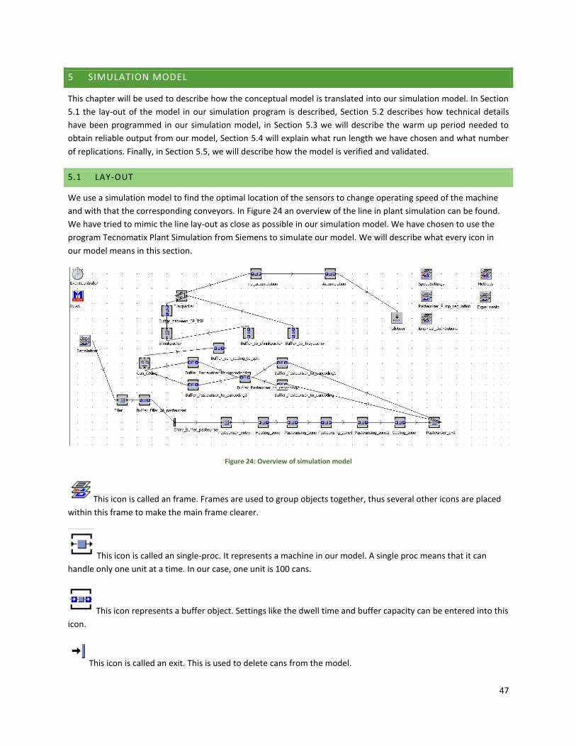
47

5 SIMULATION MODEL

This chapter will be used to describe how the conceptual model is translated into our simulation model. In Section

5.1 the lay-out of the model in our simulation program is described, Section 5.2 describes how technical details

have been programmed in our simulation model, in Section 5.3 we will describe the warm up period needed to

obtain reliable output from our model, Section 5.4 will explain what run length we have chosen and what number

of replications. Finally, in Section 5.5, we will describe how the model is verified and validated.

5.1 LAY-OUT

We use a simulation model to find the optimal location of the sensors to change operating speed of the machine

and with that the corresponding conveyors. In Figure 24 an overview of the line in plant simulation can be found.

We have tried to mimic the line lay-out as close as possible in our simulation model. We have chosen to use the

program Tecnomatix Plant Simulation from Siemens to simulate our model. We will describe what every icon in

our model means in this section.

Figure 24: Overview of simulation model

This icon is called an frame. Frames are used to group objects together, thus several other icons are placed

within this frame to make the main frame clearer.

This icon is called an single-proc. It represents a machine in our model. A single proc means that it can

handle only one unit at a time. In our case, one unit is 100 cans.

This icon represents a buffer object. Settings like the dwell time and buffer capacity can be entered into this

icon.

This icon is called an exit. This is used to delete cans from the model.

48

EventController, the eventcontroller regulates the simulation from initialising till resetting the model. It

controls every event that is needed to perform during our simulation.

This icon is called a method. A method is used to create model specific programming code to make the

model perform actions that are not standard incorporated in the simulation software.

This is a specific method which is only called once the reset button in the event controller is activated.

This icon is called a generator, generators are used to determine when certain methods need to be activated.

For example a generator activates a method to change to another experiment and to save the data of this

experiment.

Besides these icons we have created some model specific frames to make the main frame more clear.

- The frame speedsettings is used to determine the speed of a machine based on the fill level of the

conveyors in front of it. All methods and variables needed to determine this are placed in this frame.

- The methods frame is used to store all the methods, variables and tables needed to regulate the line and

store information of failures.

- The pasteuriser_pump_regulation frame is used to regulate the pasteurisers cooling, heating and

pasteurising program. Within this frame the methods, variables and tables are stored to do this.

- Empirical distributions, within this frame all tables used to determine the empirical distributions are

stored.

5.2 PLANT SIMULATION TECHNICAL DETAILS

In Plant Simulation the modeller can make use of “methods”. Methods contain programming code to make the

model perform actions. The methods worth mentioning will be discussed in this section, in addition we will

describe how we have transferred our conceptual model to Plant Simulation specific solutions.

5.2.1 CONVEYORS

Within Plant Simulation there is a standard object for conveyors called the line objects. For simulating conveyors

this seems to be ideal, however, these line objects can only process one can in the width of the conveyor. This

does not match with the real life situation, since in some cases as many as 20 cans could fit over the width of

conveyor. To simulate one conveyor exactly as in real life, we would have to create as many line objects as the

width of 1 conveyor in real life. For example if a conveyor in real life could process 20 cans in width, it would mean

we have to place 20 line objects beside each other to mimic real life. Since the width of conveyors changes

between machines this would mean we would have to create so much line objects that we decided not to do this.

Within our model we simulate the conveyors by means of buffer objects. Buffer objects can be adjusted with

parameters as the capacity and the dwell time of a can. Since we calculated all the capacities of our conveyors we

can enter these as capacity in the buffer objects. For the dwell time we chose to enter the maximum speed of a

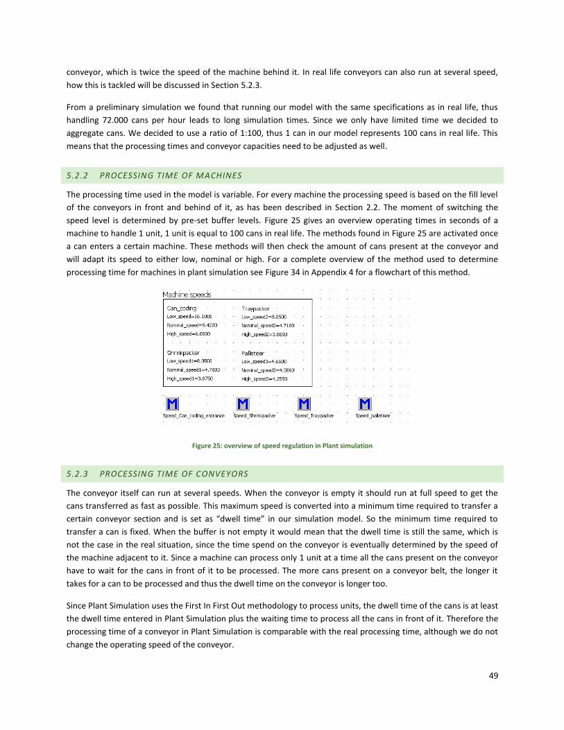
49

conveyor, which is twice the speed of the machine behind it. In real life conveyors can also run at several speed,

how this is tackled will be discussed in Section 5.2.3.

From a preliminary simulation we found that running our model with the same specifications as in real life, thus

handling 72.000 cans per hour leads to long simulation times. Since we only have limited time we decided to

aggregate cans. We decided to use a ratio of 1:100, thus 1 can in our model represents 100 cans in real life. This

means that the processing times and conveyor capacities need to be adjusted as well.

5.2.2 PROCESSING TIME OF MACHINES

The processing time used in the model is variable. For every machine the processing speed is based on the fill level

of the conveyors in front and behind of it, as has been described in Section 2.2. The moment of switching the

speed level is determined by pre-set buffer levels. Figure 25 gives an overview operating times in seconds of a

machine to handle 1 unit, 1 unit is equal to 100 cans in real life. The methods found in Figure 25 are activated once

a can enters a certain machine. These methods will then check the amount of cans present at the conveyor and

will adapt its speed to either low, nominal or high. For a complete overview of the method used to determine

processing time for machines in plant simulation see Figure 34 in Appendix 4 for a flowchart of this method.

Figure 25: overview of speed regulation in Plant simulation

5.2.3 PROCESSING TIME OF CONVEYORS

The conveyor itself can run at several speeds. When the conveyor is empty it should run at full speed to get the

cans transferred as fast as possible. This maximum speed is converted into a minimum time required to transfer a

certain conveyor section and is set as “dwell time” in our simulation model. So the minimum time required to

transfer a can is fixed. When the buffer is not empty it would mean that the dwell time is still the same, which is

not the case in the real situation, since the time spend on the conveyor is eventually determined by the speed of

the machine adjacent to it. Since a machine can process only 1 unit at a time all the cans present on the conveyor

have to wait for the cans in front of it to be processed. The more cans present on a conveyor belt, the longer it

takes for a can to be processed and thus the dwell time on the conveyor is longer too.

Since Plant Simulation uses the First In First Out methodology to process units, the dwell time of the cans is at least

the dwell time entered in Plant Simulation plus the waiting time to process all the cans in front of it. Therefore the

processing time of a conveyor in Plant Simulation is comparable with the real processing time, although we do not

change the operating speed of the conveyor.

50

5.2.4 REGULATION OF PASTEURISER

As said before, the pasteurisation of cans is one of the most important steps in the process. It is important that the

minimum PU value is achieved. However, it is also important not to over pasteurise the beer. To control this we

divide the pasteuriser in 7 separate objects as can be seen in Figure 26.

Figure 26: Overview of the pasteuriser in plant simulation

5.2.4.1 NO ACCUMULATION IN PASTEURISER

Since the pasteuriser is not able to accumulate cans inside, every time a blockage or shortage occurs on this

machine, both the exit and the entry will stop processing cans. Normally a simulation model will accumulate cans

until the capacity is reached, however, since this is not possible for a pasteuriser we created a method which

pauses all buffer objects and the entry and exit object as soon as the entry or the exit fails to process cans. Thus for

example if the exit is blocked this method will directly pause the movement of cans in all the other objects of the

pasteuriser. A separate method is created for both the entrance and the exit, see Figure 35 in Appendix 4.

5.2.4.2 SPEED CONTROL

The pasteuriser entry and exit are single procs used to control the speed by which the cans are going in and out of

the machine. Single procs are objects that can simulate machines. The processing time and failures can be

modelled into these single procs to simulate a machine. The heating_zone, Pasteurising_zone, Pasteurising_zone1,

Pasteurising_zone2 and Cooling_zone are buffer objects that mimic the conveyors inside the pasteuriser. Although

a minimum dwell time has been entered for every buffer object, we still use a single proc at the exit to control the

flow in and out of the pasteuriser, since the maximum number of cans to process is still limited. If we would only

use buffer objects it could happen that all cans leave the pasteuriser at once. This could for example happen when

a blockage occurs on the pasteuriser. The dwell time of a can keeps running while the buffer object is in blockage,

once the blockage is subsequently solved, the minimum dwell time of a can could have been reached and the

buffer object wants to transfer all cans present on it at once, while this could never happen in real life. We

therefore added a single proc with a minimum processing time, a can needs to undergo this process before it can

leave the pasteuriser. This solves the problem that more than one unit can leave the pasteuriser at once.

5.2.4.3 PASTEURISATION TIME

For the heating and cooling zones we have used a user defined attribute to mimic if the pumps for cooling and

heating are operating or not. This is done because these pumps should be shut down when a blockage takes longer

than 5 minutes. The user defined attributes have also been built into the model so that one could see if the actual

number of heating up and cooling down moments change when doing several experiments. These user defined

attributes are changed when a generator is activated. This generator is activated 5 minutes after a failure has

occurred. See Figure 36 in appendix 4 for an overview of how this pumps are activated and shutdown.

For the pasteurising zones these user defined attributes have been used as well, since the pumps of the

pasteuriser should start cooling when the cans inside a section have all finished a minimum pasteurisation time.

These methods work exactly the same as the Figure 36 only the triggering time is different. This minimum

pasteurisation time is different for every pasteurisation zone, because one section has just started pasteurisation

51

and other sections are almost finished with pasteurising. However, the last can entered into a section determines

the minimum time left to pasteurise, since this can still needs to complete the whole section. Since it takes 5

minutes to cover one pasteurisation section, the pumps of zone 2 should start cooling 5 minutes after blockage,

the pumps of zone 1 after 10 and de pumps of zone should start after 15 minutes. These are also the times to

trigger the generator to shut down a pump. Eventually this user defined attribute is used to calculate the

pasteurisation time of every can leaving the pasteuriser. One could then determine at the end of a simulation run

how much cans have been over pasteurised.

A flowchart of the methods used for calculating the pasteurisation time can be found in Figure 37 in Appendix 4. A

side note to this is that a cooling table is recorded for every pasteurising zone in which the starttime, endtime and

the cooling time is registered for every time a pasteurisation zone is cooling. This is necessary to calculate the total

cooling time a can has encountered.

5.2.4.4 START-UP DELAY OF PASTEURISER

The start-up delay of the pasteuriser in case of blockage have been controlled in the same way as the speed of the

machines. A method is triggered when a can exits the conveyor before can coding (conveyor 5), this method

checks the amount of cans left on the conveyors. Since one pasteurisation section of 6333 cans should be able to

run out of the pasteuriser after a blockage the pasteuriser is not allowed to start up before this space is free on the

conveyors. This is achieved once the last conveyor before the can coding is drained half and all other conveyors

between the pasteuriser and the can coding is empty. So every time a can leaves the last conveyor before can

coding it is checked if all conveyors are empty and the last one is half empty. If this is true, then the pasteuriser is

allowed to start processing cans again.

5.3 WARM-UP PERIOD

A simulation of a production system can either be stochastic or deterministic. When random events occur during

production, such as failures, we speak of a stochastic simulation. Since this is also the case in our model, we

simulate a stochastic system. Besides this distinction, a simulation model can also be terminating or non-

terminating. For a terminating simulation there is a natural end point that determines the run length (Robinson,

2004). Non-terminating simulations will run until the user defined run length. At Grolsch the line stops operating

every weekend and will start up again the next week with initial conditions, so there is a natural end point.

However, during this simulation study we try to find out what efficiency improvements could be gained during

production and not during the start-ups every week, we are thus interested in the steady state of the model. We

therefore decided to use a non-terminating simulation, since we only have to get to the steady state once for

every experiment.

The next step is to gain accurate output from our simulation model. Two issues are required to get reliable output

from our model. The first is the removal of initialization bias, the second is ensuring that enough data will be

obtained to measure an accurate estimate of the performances (Robinson, 2004). A good way to remove

initialization bias is to use a warm-up period. The warm-up period is the amount of time needed to run the

simulation model until it reaches realistic conditions and only collecting information after this point. We

determined that a warm up period of 8 hours (1 shift) is sufficient to remove the initialization bias. We determined

this by applying the MSER-5 method. After this warm up period, the model has also reached the desired steady

state. For the exact calculation of the warm up period we refer to Appendix 6.

5.4 RUN-LENGTH AND NUMBER OF REPLICATIONS

52

To ensure that enough output data has been obtained, one could either use one long simulation run or several

replications can be made. Since we are interested in the model’s behaviour during the steady state, we choose to

do one long simulation run, because we only have to get to this steady state once per experiment.

As can be seen in Appendix 7, we found that 200 shifts is enough for our run length to obtain reliable output,

however, to be safe we use 500 shifts. We determined this by creating 3 different replications of the same

experiment, in every experiment we obtained the output of the filler based on a 8 hour interval. Once convergence

of the cumulative mean of these three different experiments drop below 5% we accept the run length. When using

one long single run per experiment it is difficult to create confidence intervals of the output obtained. When

running several replications of an experiment the confidence interval could be created using the results from the

different replications. To obtain reliable, non-correlated output from the model, we make use of the batch means

method.

The batch means method divides the time series of a simulation run in k batches of size b. The number of batches

in 1 single run should be at least 10 (Schmeiser, 1982). We used a spreadsheet (Batchmeans.xls) that uses the

Fishman’s procedure for determining the batch size (Robinson, 2004) and is available on the website

(www.wileyeurope.com/go/robinson). From this spreadsheet we found that our batch size should be 16 shifts to

prevent the data from correlating with each other. This means that 31 batches can be created from one single run.

These batches more or less are the same as different replications.

However, it is always better to perform both long runs and several replications to get even more reliable data

(Robinson, 2004). We therefore decided to run 3 replications per experiment as well. This means that for every

experiment we will generate 93 data points to calculate confidence intervals with.

5.5 VERIFICATION & VALIDATION

This section will be used to validate and verify the model. The model will be verified to make sure that the

conceptual model is transformed into a computer model with sufficient precision (Davis, 1992). Validation will be

done to check if the model output is approximately the same as the output generated in real life.

5.5.1 VERIFICATION

To verify if our simulation model does what we want it to do according to our conceptual model, we “debugged”

the model every time we implemented a new object or new parts of programming code. Within Plant Simulation

this is easy to do, since the program has the option to place “breakpoints” in the code. These breakpoints will

pause the simulation as soon as this line of code is called. At that point it is possible to look at the animation of the

line to see if strange things happen. A useful tool when looking at the animation is to slow down the time of the

simulation, it is even possible to step from event to event, so it is easy to see where problems might occur.

Another verification method is to make sure that the amount of cans going into the model is the same as the

amount of cans going out. To do this we ran our model for 24 hours in simulation time. We then measured the

amount of cans that were entered at the depalletiser and compared this to the amount of cans that left the

palletiser plus all the cans still in the model. This resulted in 1407300 cans entering the model at the depalletiser,

1330200 cans that left the palletiser and still 77100 cans still in the model. The amount of cans still in the model

and the amount of cans that have already left the model is 1330200 + 77100 = 1407300. Thus exactly the same

amount of cans are entering the model as leaving the model.

53

One of the most important steps when verifying the model is to discuss the model with operators and managers at

Grolsch. We have discussed the model with several employees and they agree to the assumptions we have made

and the way we tackled some problems.

5.5.2 VALIDATION

To validate our model we are going to compare several outputs from our model with the data from real life, and

check if this corresponds to each other. If the data does not correspond we describe what the reason for this could

be and if the model could still be valid.

MTTR

To check if the failure profile from our model corresponds to real life we check the MTTR. See Table 15 for the

comparison. The MTTR of both the model and real life correspond reasonably well.

Machine MTTR real life (sec) MTTR model (sec)

Depalletiser 648 533

Filler 221 208

Pasteuriser 342 342

Shrinkpacker 589 552

Traypacker 228 221

Palletiser 202 163

Table 15: Comparison of MTTR

The reason why the Depalletiser and the Palletiser have a lower MTTR in our model is because we have taken

failures from outside the model into account at these two machines as well. These failures might be smaller than

the failures on the Depalletiser itself.

ME

One of the most important performance measures in our model will be the ME. We made a comparison of the ME

in real life and the ME in the model. During June the actual average ME was 82,4%. In our model the average ME is

86,4%. As already mentioned in Section 4.3, the ME in our model could be slightly different from real life

performances. We mentioned that the ME in our model could be lower because we took allowed stops into

consideration as well. The reason why the ME in our model is slightly higher could be because we did not take into

account all machines. Although these machine had almost non to very few failures it could be this difference that

increased ME. Although the ME of our simulation model might not completely match with reality we find it more

important that the results between different experiments could be compared and thus if certain experiments

score better than the current situation.

We decided not to measure more outputs to validate our model since for example the output of the machines is

the same as measuring the ME of a machine. Since ME is the output divided by the potential output.

5.6 CONCLUSION

This chapter was used to describe how our conceptual model will be transferred into a simulation program. The

most important things found in this chapter will be shortly highlighted below.

54

- We are going to use a warm up period of 1 shift of 8 hours.

- The run length of one experiment/replication will be 500 shifts.

- According to the batch means method we will obtain data from our model in batches of 16 shifts.

- Our conceptual model verifies with the simulation model created.

- Although figures found in our validation section do not completely align with reality we assume that our

model is accurate enough for experiments.

55

6 EXPERIMENTAL DESIGN

After our analyses, literature review and discussions with engineers at Grolsch, we conclude that the performance

of the system could be improved by:

- Changing the moment of switching machine speeds based on the fill levels of the conveyors. This could

affect the buffer size of the conveyor, and could improve ME.

- Not emptying conveyor 3 and 4 behind the pasteuriser after a blockage has occurred on the pasteuriser

before starting up the pasteuriser itself. This could decrease the start-up delay on the filler, which would

in turn improve the ME.

To study the effects of the changes above, we design simulation experiments. In this chapter we describe this

experimental design, with in Section 6.1 the experimental factors, in Section 6.2 the performance measures to

measure differences in experiments and in Section 6.3 the setup of our experiments.

6.1 EXPERIMENTAL FACTORS

To see if changing several settings in the simulation model will affect the performance measures and which

settings lead to the best performance, the following experimental factors will be tested:

- The location of the sensor to trigger change in machine speeds.

- Changing the pasteuriser start-up method, it will be tested if the buffer on conveyors 3 and 4 should be

completely empty before starting up the pasteuriser or not.

To check if changing these settings would improve performance, we first need to define the performance

measures we would like to measure. This will be done in the next section.

6.2 PERFORMANCE MEASURES

The main goal of this project is to optimize the machine efficiency. This efficiency is currently measured on the

filler only, since this is the bottleneck machine. We will measure the ME also on the filler. ME is measured by

dividing the actual filled quantity by the theoretical filled quantity. The actual filled quantity is the amount of cans

filled by the filler during a batch of 16 shifts. The theoretical filled quantity is the quantity the filler could have filled

during these 16 shifts. We will subsequently take the average of all the batches in three replications to calculate

the average ME during an experiment.

Secondly it is important to measure how many cans are over pasteurised during the simulation run. A can is over-

pasteurised when it is pasteurised for longer than 20 minutes. We will measure this when a can is leaving the

pasteuriser by subtracting the cooling time from the time a can has spent in the pasteuriser. It is important to

measure this, since instrumental technicians at Grolsch expect that by reducing the buffer capacity the pasteuriser

might cause more over-pasteurisation and more heating up and cooling down of the pasteuriser.

Our third measure is the number of stops of the heating and cooling pumps of the pasteuriser. This is measured by

counting the number of times these pumps are shut down per experiment. Since stopping the cooling and heating

zones will be at the same moment as cooling pasteurising zone 1, we will not separately measure this.

The fourth and fifth measure is the number of times pasteurising zones 2 and 3 have cooled down respectively.

This will be measured the same way as our third measure.

56

The sixth measure is the total amount of cans processed during an experiment. This will be measured by counting

the amount of cans processed on the filler.

Finally we will measure the start-up delay on the filler during an experiment, since this was the main reason for ME

loss.

To summarize we will use the following performance measures:

- Machine Efficiency

- Number of cans over pasteurised.

- Number of stops of the cooling and heating zone

- Number of stops on pasteurising zone 2

- Number of stops on pasteurising zone 3

- Cans processed

6.3 EXPERIMENTAL SETUP

As decided in Section 6.1, we will only experiment with changing 2 settings. Below we will describe the way we

want to experiment this.

Changing the location of the sensor to trigger change in machine speeds.

Since every sensor can be placed on a high number of potential locations, we need to decide which locations/levels

we want to experiment with. Every machine has its own sensors for changing operating speed. However, we

decided that in every experiment, the fill level of changing a machine speed will be the same for every machine,

e.g., if the moment of changing to high speed is 80% for the palletiser, this will also be 80% for the traypacker,

shrinkpacker and can coding. This is done to reduce the number of experiments and because we think that the

moment of changing machine speeds will have the same effect on all machines.

Secondly we decided that the fill level to trigger a sensor should be increased with at least 20% per experiment. In

our eyes smaller steps will not have added value and also the number of experiments would become larger. Every

sensor can therefore be experimented with on 5 different values from 0% till 100%. However, the moment of

switching to high speed could off course never be earlier than the moment of switching to low speed in terms of

fill level. The different ways of experimenting with the sensor location could therefore be as shown in Table 16.

There is no sensor for nominal speed, this speed level is triggered when the amount of cans on the conveyor is

between the low speed sensor and the high speed sensor. In Figure 27 the situation of sensor triggering is

visualised. When none of the sensors is triggered Machine B is running on low speed. A sensors is triggered in the

figure when it is colored. When sensor 1 is triggered, Machine B will operate at nominal speed. When both sensors

are triggered, Machine B will run on high speed.

57

Figure 27: Overview how sensors are triggered in model

Experiment number Conveyor fill level for changing to high speed

Conveyor fill level for changing to low speed

1 0% 0%

2 20% 0%

3 40% 0%

4 60% 0%

5 80% 0%

6 100% 0%

7 40% 20%

8 60% 20%

9 80% 20%

10 100% 20%

11 60% 40%

12 80% 40%

13 100% 40%

14 80% 60%

15 100% 60%

16 100% 80%

17 100% 100%

current situation 70% 35%

Table 16: Experimental setup sensor locations

58

Start-up buffer behind pasteuriser

Since we will not experiment with different buffer sizes of the buffer after the pasteuriser, this setting could either

be used or not at all. Thus there will be a buffer that needs to be completely available again or it should not. These

are the buffers on conveyor 3 and 4. To experiment this setting, we will perform the experiments from Table 16

twice. 17 experiments with the buffer available and thus with empty conveyors 3 and 4, and 17 experiments with

the buffer not needed after start-up of the pasteuriser and thus start-up of the pasteuriser as soon as there is

space available on conveyor 3. From now on will refer to this setting as either using the start-up buffer or not.

Due to small test runs during a failure or blockages to test if the line can start-up again, little space might become

available on conveyor 3. To prevent the pasteuriser to start-up while the failure or blockage is not fixed again, at

least 20% of capacity on conveyor 3 should be emptied. However we still refer to this setting as not using start-up

buffer.

Zoom into best results

The experiments described above will be used to make a first selection of the best performing experiments. In

Chapter 7, we will decide which result are selected to use for further analysis. For these experiments the actual

required number of replications will be calculated to obtain reliable output data.

6.4 CONCLUSION

This chapter was used to make an experimental design. We decided to only perform experiments by only changing

2 different settings, to reduce the number of experiments. The two settings are:

- Changing the combination of sensor location and fill level of the conveyor for changing machine speed.

- Either using the start-up buffer after a failure, or not

These two settings will lead to 34 experiments in which we change our sensor location in steps of 20% fill level for

both the high speed sensor and the low speed sensor, and in which we either make use of the buffer behind the

pasteuriser or not.

Eventually we will make more replications of the best performing experiments, which we describe in Chapter 7.

59

7 EXPERIMENTAL RESULTS

In this chapter we describe the results of the experiments designed in the previous chapter and discuss what the

consequences are of these results. We have decided to first perform all experiments with long runs in combination

with 3 replications. The results obtained from these experiments will be analysed and several experiments with

potential improvements will be further analysed with 20 replications of 31 batches per experiment. A table with all

the results can be found in Appendix 2, the results of the most promising experiments can be found in Section 7.4.

We describe the experimental results with respect to machine efficiency(Section 7.1), over pasteurisation(Section

7.2) and the number of stops on the pasteuriser(Section 7.3). A further analysis on several experiments will be

described in Section 7.4 and finally a description of potential savings is described in Section 7.5

7.1 MACHINE EFFICIENCY

The most important performance measure of the experiments, is the machine efficiency. Based on our

experiments we found that the average machine efficiencies of the different experiments were very close together.

However, all the experiments that are performed without the start-up buffer behind the pasteuriser performed

better than the experiments that emptied the buffer first before starting up the pasteuriser again, as can be seen

in Figure 28. To see how all experiments compare against the current situation we drew a line exactly at 86,08%

since this was the performance of the current situation in our model. To make the graph better readable, we order

the experiments by the moment of switching to high speed. The farther to the right in the graph the higher the

moment of switching to a high speed, thus the more occupied a conveyor needs to be before it triggers the

machine to operate at a high speed. The experiments with a different threshold for switching to high speed are

grouped within the dashed lines, the corresponding threshold is also noted there. The experiments grouped within

these dashed lines are ordered by means of the threshold for switching to low speed in increasing order from 0%

up to the threshold for switching to high speed as noted between the dashed lines. From this graph one could

conclude that it seems to be better to switch to high speed when the buffer is not so full yet, thus with a lower

threshold. This could be explained by the fact that when switching to a higher speed when the conveyor is not so

occupied yet, there is more space to buffer and thus larger failures can be absorbed. Experiment 17 is omitted

from this graph since it scores lower than 80%.

Figure 28: Comparison of ME of all experiments

0,8

0,81

0,82

0,83

0,84

0,85

0,86

0,87

0,88

0,89

0,9

1 2 3 7 4 8 11 5 9 12 14 6 10 13 15 16 17

ME

Experiment number

Current situation

Without start-up buffer

With start-up buffer

0%

20

%

40

%

60

%

80

%

10

0%

60

7.2 NUMBER OF CANS OVER PASTEURISED

An important measure for the quality of the beer is the number of cans over pasteurised. In Figure 29 the over

pasteurisation in number of cans per experiment is shown. The experiments in this graph are ordered by means of

the moment when switching to low speed. The further to the right the higher the threshold of the fill level of the

conveyor to switch to low speed, thus the more occupied the conveyor will be before it switches to low speed.

Within the dashed lines the experiments are ordered by means of the threshold to switch to high speed up till

100%.

Although there is no clear pattern in Figure 29, most of the times the over pasteurisation is higher without the

start-up buffer. This seems to indicate that the expectation of the instrumental technicians and engineers at

Grolsch was correct. Only when the threshold to change to low speed is larger than 20% it is preferable not to use

the start-up buffer. When the threshold is larger it means that on average the conveyors are more occupied, and

thus a smaller buffer is available on the conveyors. A smaller buffer means that a machine is blocked earlier, and

thus that the same failure will block the pasteuriser for a longer amount of time. In those cases it is more

preferable not to use the start-up buffer since this would increase blockage time even more.

Figure 29: Overview of over pasteurisation between different experiments

7.3 NUMBER OF STOPS ON THE PASTEURISER

This performance measure is mainly done to prove to Grolsch that not using the start-up buffer will cause less

stops on the pasteuriser. As shown in Figure 30, most experiments performed without the start-up buffer have less

stops than those with the buffer. The experiments are ordered in the same way as in Section 7.2. From the graph

we can see that the number of stops are always less without the start-up buffer. Secondly we can see that the

number of stops start to increase as soon as the threshold to switch to low speed is higher, and thus while the

conveyors are more occupied. This could be explained by the fact that, when conveyors are more occupied, the

buffers are smaller, thus even the smaller failures cannot be absorbed, this could lead to more stops on the

pasteuriser. We decided not to analyse the number of stops on pasteurisation zone 2 and 3 since this would give

the same picture as can be seen in the table in Appendix 2.

80000

100000

120000

140000

160000

180000

200000

1 2 3 4 5 6 7 8 9 10 11 12 13 14 15 16 17

Nu

mb

er

of

can

s o

ver

pas

teu

rise

d X

10

0

Experiment Number

Current situation

Without start-up buffer

With start-up buffer

0%

20

%

40

%

60

%

80

%

10

0%

61

Figure 30: Number of times that pasteuriser stops cooling and heating

7.4 FURTHER ANALYSIS

From the previous performance measures, we decided to further analyse experiments 2,3,4,7,11 since these

experiments perform better than the current situation on the performance measures ME and number of stops of

the pasteuriser. The settings for threshold when switching to low speed is small (lower than 40% for all

experiments) which increases buffer capacity, which could subsequently lead to higher ME scores. Secondly the

threshold for switching to high speed is below 60% in all experiments, which means that machines start to operate

faster when the conveyor is not so occupied yet. This also results in increased buffer capacity and could thus lead

to a higher ME.

Table 17 shows the performances of the experiments with 20 replications of 31 batches.

Experiment Average ME in percentage

Stops Heating & Cooling zone

Stops pasteurising zone 1

Stops pasteurising zone

# cans overpasteurised

# cans processed

2 yes 0,8789 253,60 79,65 59,60 60834,85 1007466,35

2 no 0,8884 115,80 73,00 53,80 45408,60 1018270,35

3 yes 0,8738 308,75 96,00 65,30 66342,00 1001543,05

3 no 0,8914 125,10 74,20 54,15 46183,30 1021720,70

4 yes 0,8753 275,95 105,40 70,00 60564,75 1003282,05

4 no 0,8762 156,90 87,90 66,85 49730,15 1004344,45

7 yes 0,8787 264,20 97,90 62,65 61122,95 1007210,35

7 no 0,8880 129,15 74,15 54,55 46756,60 1017888,55

11 yes 0,8545 318,95 278,45 79,55 56893,65 979476,60

11 no 0,8710 283,50 87,95 67,20 65005,95 998342,55

Current situation 0,860817 299,2 266,4 65,8 55887 925785

Table 17: Performances of experiment 2,3,4,7,11

0

200

400

600

800

1000

1200

1 2 3 4 5 6 7 8 9 10 11 12 13 14 15 16 17

Nu

mb

er

of

sto

ps

Experiment Number

Current situation

Without start-up buffer

With start-up buffer

20

%

40

%

60

%

80

%

10

0%

0%

62

ME performances

Figure 31 is used to show the performance differences between the experiments more clear. After 20 replications

of the experiments, the performances are more or less the same. As can be seen only experiment 11 with a start-

up buffer performs worse than the current situation. Based on ME, experiment 3 without the start-up buffer

performs best.

Figure 31: ME performances of exp 2,3,4,7 and 11

Over pasteurisation

The difference in over pasteurisation is shown in Figure 32. The over pasteurisation is higher when the start-up

buffer is used except for experiment 11. In experiment 11 the fill level to change to high speed is at 60% and the fill

level to change to low speed is at 40%. The reason why over pasteurisation is higher when the start-up buffer is

not used could be because the average fill level of the buffer between can coding and pasteuriser is higher. This

will lead to more start and stop situations on the pasteuriser.

0,8300

0,8400

0,8500

0,8600

0,8700

0,8800

0,8900

0,9000

2 3 4 7 11

ME

ME with start-up buffer

ME without start-up buffer

Current situation

63

Figure 32: Number of cans over pasteusing per experiment

Number of stops on the pasteuriser

Figure 33 shows the difference in performance of the number of stops on the pasteuriser. As shown, the number

of stops is much lower when the start-up buffer is not used, again experiment 11 scores worst. This has the same

explanation as in the previous performance measure. Experiment 2 and 3 score almost similar and perform the

best. This could be explained because the average buffer level is much higher and machines will speed up to high

speed earlier. This will eventually lead to less stops on the pasteuriser.

Figure 33: Number of stops on the pasteuriser

Overall we can conclude that experiment 2 and 3 perform best, In Table 18 the difference in settings between

experiment 2 and 3 and the current situation is shown, the main difference is that the buffer behind the

pasteuriser is not used in experiment 2 and 3, and that a machine is operated on a high speed for a longer time

40000,00

45000,00

50000,00

55000,00

60000,00

65000,00

70000,00

2 3 4 7 11

Nu

mb

er

of

can

s o

ver

pas

teu

risi

ng

X 1

00

Overpasteurisation with start-up buffer

Overpasteurisation withoutstart-up buffer

Current situation

0,00

50,00

100,00

150,00

200,00

250,00

300,00

350,00

2 3 4 7 11

Nu

mb

er

of

sto

ps Number of stops with start-up

buffer

Number of stops without start-up buffer

Current situation

64

and also it is switched to this speed when the buffer is not so full yet. Although there is almost no difference in

performance we prefer experiment 3 above 2, because the machine is operated on nominal speed for a longer

buffer space. This will lead to less changes in speed on the machines and this could affect the downtime on

machines in a positive way.

Experiment number Conveyor fill level for changing to high speed

Conveyor fill level for changing to low speed

Buffer behind pasteuriser used

ME in this experiment

2 20 0 No 88.84%

3 40% 0% No 89.14%

current situation 70% 35% Yes 86.08%

Table 18: Difference in settings and performance between experiments

To find out if there is a significant difference in ME between experiment 3 and the current situation we perform a

paired t-test of the difference between the current situation and 3 with the H0 hypothesis that the difference is 0.

This results in a p-value of 0,003, with an alpha of 5%. This means that we do reject the H0 hypothesis, and thus

that there is a significant difference between the two experiments.

7.5 CONCLUSION

Based on the previous sections we can conclude that experiment 3, without the start-up buffer used, performs the

best. This experiment scores better than the current situation on all performance measures. Experiment 3 has

2,99% more machine efficiency than the current situation. An increase of 2,99% machine efficiency would mean

that the line has to run 1,8 minutes less per hour to produce the same amount of cans. During June the line has

run 406 hours. This would mean that with this increase in ME the line would have to run 12,18 hours less per

month.

Furthermore, we can conclude that not using the start-up buffer is preferable in most cases, only when as less as

possible over pasteurisation is the goal, in some cases it might be more preferable to use the start-up buffer. Also a

big gap between the thresholds for low speed and high speed

65

8 CONCLUSIONS & RECOMMENDATIONS

This chapter will be used to conclude our research. In Section 8.1, we provide an answer to the research questions

we have made at the beginning of this research. In Section 8.2 we will suggest recommendations to Grolsch based

on our observations. Finally Section 8.3 will be used to describe potential additions for further research.

8.1 CONCLUSIONS

The main research question stated in Section 1.5 was: How can performance of the canning line at Grolsch be

improved, by adjusting line regulation?

To answer this question we first need to answer our sub-questions. We will use this section to answer these sub-

questions.

In Chapter 2 we discussed sub question 1: How is the canning line currently performing? We found that the

machine efficiency of the line, with its performance of 86%, is far below target of 95% This is largely due to

starvation and blockage of the bottleneck machine, which is the filler. In the DTR file we could easily see which

machines cause most blockage or starvation on the filler. We found it quite surprising that the machines at the end

of the line, like the traypacker, shrinkpacker and palletiser, cause around 35% of the stoppages on the filler, while

if the buffer strategies and v-graph principles are used, the blockages and starvation of the filler should be at a

minimum, especially for machines at the end of the line.

Sub question 2: What are the main reasons for unplanned efficiency loss at the canning line? In Chapter 2 we found

that the main reason for unplanned efficiency losses at the canning line are either start-up losses after interference

of the filler or the amount of buffer available on the line. First of all not all failures can be absorbed by the buffers

present on the line, second of all when a failure causes the filler to stop it experiences a big start-up loss after the

failure has been solved. The largest bottleneck process causing the filler to experience a lot of start-up loss is due

to the pasteurisers start-up procedure. The pasteuriser will not start production after a blockage until the

conveyors between can coding and the pasteuriser are almost completely drained. The second largest bottleneck

to cause unplanned efficiency losses at the is caused by the fact that the buffers cannot absorb all failures, and

thus the bottleneck process is the size of the buffers.

Sub question 3: What approaches does literature suggest for improving line efficiency by reducing efficiency losses?

This question is answered in Chapter 3. We found that several different sources in literature used simulation

models to mimic real life situations to experiment with different settings of speed levels, buffer quantities and the

sensor location that triggers different speed levels. The latter is something we found usable for our buffer capacity

problem. The idea is that changing the location of sensors that trigger speed levels at the machines, could make

more buffer capacity available on the conveyor belts. For example if the threshold to trigger the high speed is

lowered, it means that a machine will run on high speed when the conveyor is not so occupied yet. This will

subsequently lead to less occupied conveyors and higher buffer capacity and thus more space is available for

absorbing failures.

Sub question 4: What approaches (found in literature and by brainstorming) for improving line efficiency are

suitable for implementation at Grolsch? The answer to this question is described in Chapter 3 and 6. We found that

the suggestions from literature to experiment with different sensor locations to trigger machine speeds was useful

to the Grolsch case as well. By brainstorming, we found that changing the start-up procedure of the pasteuriser

after a blockage might be worth experimenting with as well. We will experiment to either completely drain the

66

conveyor between can coding and the pasteuriser after a blockage of the pasteuriser, or not. This resulted in 34

experiments.

Sub question 5: What performance can be expected from the proposed solutions for improving control and

efficiency of the line? Although our performances in the model are not completely in line with the real life situation,

we think that the proposed chosen result in similar saving in real life. We will state the performance improvements

in percentages in Table 19.

Experiment Average ME in percentage

Stops Heating & Cooling zone

Stops pasteurising zone 1

Stops pasteurising zone

# cans overpasteurised

# cans processed

3 no 0,8914 125,10 74,20 54,15 46183,30 1021720,70

Current situation 0,8608 299,20 266,40 65,80 55887 925785

Improvement 3,55% 58,19% 72,15% 17,71% 17,36% 10,36%

Table 19: Performance improvements of current situation versus experiment 3 without start-up buffer

Finally we can say that the performance of the canning line at Grolsch can be improved by changing the sensor

location to trigger machine speeds and changing the start-up procedure on the pasteuriser. During our research

we found that the best sensor location to trigger high speed of a machine is at a threshold between 20% and 40%

and the threshold to trigger low speed should be set at a low fill level as well. The change in start-up procedure will

not negatively affect performance measures, such as the number of cans over pasteurised and the amount of

stops on the pasteuriser, as assumed by engineers at Grolsch; it even performs better in our simulation model.

However, even the experiment with the best performances did not get a performance > 95% which is the ultimate

goal of Grolsch for its canning line.

8.2 RECOMMENDATIONS

Based on our research we advise Grolsch to change the sensor locations to trigger machine speeds so that a high

speed is triggered earlier. Secondly we would advise them to change the start-up procedure of the pasteuriser to

improve both ME and over pasteurisation.

Besides the things mentioned in our research we would also recommend Grolsch to improve the data registration

in its MES system in such a way that information from all machines on the line can be analysed. When this is

possible even a better simulation model could be build and overall information about the line is more clear. Also

clear a description of statuses within MES should be implemented to make it better understandable. Currently not

all states for all machines are registered in the same way, which leads to unclear data as well. If this MES system is

upgraded, it would probably be used more and employees would also trust the data better.

When analysing date of the line we also discovered that small failures, like fallen cans are not noticed directly by

operators at the line. This causes the machines to fail unnecessarily long and with that filling up conveyors

unnecessarily, which could cost buffer the next time when a larger failure occurs. We would therefore recommend

to make failure warnings even better so that operators notice the failure directly.

67

8.3 FURTHER RESEARCH

We finish this research by giving some alternatives for further research.

Although the canning line is one of the best performing lines at Grolsch, we still managed to find an improvement

of roughly 3% ME by better regulation. We would therefore recommend to apply a similar kind of simulation study

to other packaging lines, because bigger improvements could probably be found at those lines by improving

regulation.

During this research we have focussed on the buffer strategy and line regulation while taking the current conveyor

capacities and machine capacities for granted. However, we think that this research could be improved when

experimenting with changing the maximum speed of the machines and the conveyors. We would therefore

recommend to research these things as well.

Besides machine and conveyors speeds, maybe even more ME improvement could be achieved by improving

buffer capacities at the line. Larger failures could be absorbed and thus less blockage and starvation would be

caused at the filler. We would advise to research ways to improve buffer capacities at the line.

Lastly we would advise to do more research to reduce the actual number of failures on the machines and check if

the maintenance program of these machines corresponds to the failure pattern. Currently, only failures that cause

the filler to stop operating are registered, which does not give a reliable picture of the actual failure pattern of the

machines. One way to improve this is to use the data from the MES system, however, data registration of the MES

should then be upgraded first.

68

9 BIBLIOGRAPHY

Basán, N. P., Cóccola, M. E., & Méndez, C. A. (2014). OPTIMIZING THE DESIGN AND OPERATION OF A BEER

PACKAGING LINE THROUGH AN ADVANCED SIMIO-BASED DES TOOL. Proceedings of the 2014 Winter

Simulation Conference, (pp. 1989-2000). Argentina.

Battini, D., Persona, A., & Regattieri, A. (2009). Buffer size design linked to reliability performance. Computers &

Industrial Engineering, 1633-1641.

Chan, F. T., & Ng, E. Y. (2002). Comparative Evaluations of Buffer Allocation Strategies in a Serial Production Line.

international journal of advanced manufacturing technology, 789-800.

Cooke, R. M., Bosma, A., & Härte, F. (2005). A practical model of heineken's bottle filling line with dependent

failures. European Journal of Operational Research, 491-504.

Davis, P. K. (1992). Generalizing concepts of verification, validation and accreditation (VV&A) for military simulation.

Santa Monica, CA: RAND.

Goldratt, E. M. (1992). The goal: A process of ongoing improvement. North River Press.

Härte, F. (1997). Efficiency analysis of Packaging Lines. Delft: Delft University press.

Hoad, K., & Robinson, S. (2011). IMPLEMENTING MSER-5 IN COMMERCIAL SIMULATION SOFTWARE AND ITS

WIDER IMPLICATIONS. Proceedings of the 2011 Winter Simulation Conference, 495-503.

Kegg, R. L. (1990). The development of sensors for manufacturing automation. Manufacturing control and

monitoring, 123-129.

King, P. L. (2011). Breaking up logjams can be key for process plant production. Industrial engineer, 41.

Kozan, E. (1997). COMPARISON OF ANALYTICAL AND SIMULATION PLANNING MODELS OF SEAPORT CONTAINER

TERMINALS. Transportation planning and technology, 235-248.

Kuo, C.-T., Lim, J.-T., & Meerkov, S. (1996). Bottlenecks in serial production lines: a system-theoretic approach.

Mathematical Problems in Engineering, 233-276.

Law, A. M. (2007). Simulation modeling & analysis. In A. M. Law, Simulation modeling & analysis. Mc Graw-Hill

International.

Law, A. M. (2007). Simulation Modeling & Analysis. Singapore: McGraw Hill.

Law, A. M., & Kelton, W. D. (2000). Simulation modeling and analysis. McGraw Hill.

Miltenburg, G., & Szendrovits, A. (1989). Determining safety stocks of large transfer lines for a preset efficiency.

Engineering costs and production economics, 137-150.

Pol, M. (2014). Improving the continuous flow .

Pourbabai, B. (1993). An Operational Strategy for Throughput Maximization and Bottleneck Control in an Assembly

Line System: by Selection of the processing rates. The Journal of the Operational Research Society, 1003-

1011.

69

Robinson, S. (2004). Simulation: the practice of model development and use. In S. Robinson. John Wiley & Sons,

Ltd.

SAB Miller. (2010). Packaging procedure: Packaging efficiency and waste collection.

Schmeiser, B. W. (1982). Batch size effects in the analysis of simulation output. Operations Research, 556-568.

Scholl, A., & Becker, C. (2006). State-of-the-art exact and heuristc solution procedures for simple assembly line

balancing. 666-693.

Szendrovits, A., Miltenburg, G., & Goldstein, Z. (1990). Optimizing total safety inventory for large transfer lines. Int.

J. of Mgmt Sci. , 299-313.

van Leer, D. (2014). Improving performance of the star bottle production line.

Winston, W. L. (2004). Operation Research. In W. L. Winston, Operation Research (pp. 1145-1188). Brooks/Cole.

Yuniawan, D., Ito, T., & E Bin, M. (2013). Calculation of overall equipment effectiveness weight by Taguchi method

with simulation. Concurrent Engineering: Research and applications, 296-306.

70

APPENDICES

APPENDIX 1: FACTORY EFFICIENCY & MACHINE EFFICIENCY

The performance of line 7 is measured using several indicators. The indicators used in this project are factory

efficiency and machine efficiency. The definitions used for the calculation of these indicators will be described

below.

FACTORY EFFICIENCY

Factory efficiency is a measure of how effectively a line has performed relative to the time period available for

production and/or maintenance work on the line (SAB Miller, 2010). The definition for factory efficiency is given

below:

Factory Efficiency =Actual saleable volume

Theoretical volume∗ 100

The actual saleable volume is the actual produced amount of beer ready to be shipped to the customer and is

calculated with the following formula:

Actual saleable volume = ∑ produced volume of package type i

n

i=1

The theoretical volume is:

Theoretical volume = ∑ Factory hours of package type i ∗ Line Rating of package type i

n

i=1

Within this formula, factory hours of package type i are:

Factory hours ofpackage type i =

produced volume of package type iline rating of package type i

∗ paid factory hours

standard hours

Within this formula the standard hours is the sum of standard hours per package type i:

Standard hours = ∑saleable produced volume of package type i

line rating of package type i

n

i=1

The line rating of package type i is the capacity of the filler with a specific package type per hour.

MACHINE EFFICIENCY

Machine efficiency is a measure of how effectively the line has performed relative to the time period available

once adjustments for actual maintenance and cleaning time and actual allowed stops/service stops have been

made (SAB Miller, 2010). The definition of the machine efficiency will be given below:

Machine efficiency = Actual saleable volume

Theoretical volume(machine hour based)∗ 100

71

The formula for machine efficiency looks the same as that of the factory efficiency, except that the theoretical

volume is now based on machine hours instead of factory hours. Theoretical volume is therefore:

Theoretical volume = ∑ Machine hours of package type i ∗ Line Rating of package type i

n

i=1

A definition of the machine hours is given below:

Machine hours = Paid factory hours − (paid factory hour adjustments + maintenance & cleaning time

+ allowed stops + service stops)

Paid factory hours are the total amount of operating hours.

Paid factory hour adjustments are time losses, which reduce the plants capability to run or produce but are beyond

the control of the local plant i.e. external occurrences.

Maintenance and cleaning time is the total time scheduled for maintenance and cleaning.

Allowed stops are stops which are necessary to do in order to keep running. Allowed stops can be four different

stops, namely: Start up time of order, pack change time, brand change time and shut down time.

Service stops are stops which cannot be influenced by the operators on the package line, for example due to beer

unavailability.

72

APPENDIX 2: EXPERIMENTAL RESULTS

In this appendix the results of all experiments are presented (see table 20). The first column shows the experiment

number followed by yes or no. Yes means that the start-up buffer is used, no means that this buffer is not used.

Experiment Average ME in percentage

Stops Heating & Cooling zone

Stops pasteurising zone 1

Stops pasteurising zone

# cans overpasteurised

# cans processed

1 yes 0,8568 873 775 185 148328 2462702

1 no 0,8753 844 207 160 179171 2515721

2 yes 0,8781 792 213 148 169192 2523760

2 no 0,8851 329 196 148 112628 2544064

3 yes 0,8804 784 219 140 166445 2530509

3 no 0,8907 343 199 143 116552 2560136

4 yes 0,8670 877 291 177 172497 2491835

4 no 0,8848 405 209 163 122884 2542985

5 yes 0,8724 757 311 179 158237 2507499

5 no 0,8758 449 228 172 123847 2517316

6 yes 0,8511 894 813 257 149189 2446314

6 no 0,8571 585 385 185 131919 2463624

7 yes 0,8753 800 256 150 166561 2515813

7 no 0,8850 349 198 149 119436 2543828

8 yes 0,8733 758 289 161 163679 2510033

8 no 0,8746 408 222 169 123995 2513778

9 yes 0,8589 781 457 203 153447 2468752

9 no 0,8753 467 226 167 129452 2515730

10 yes 0,8512 900 828 250 150732 2446422

10 no 0,8656 627 403 170 138257 2487988

11 yes 0,8543 924 830 187 151008 2455349

11 no 0,8851 696 196 149 158491 2544020

12 yes 0,8542 918 823 192 152105 2455077

12 no 0,8705 871 228 172 176970 2502021

13 yes 0,8543 828 753 240 145409 2455515

13 no 0,8513 721 396 209 147517 2446841

14 yes 0,8401 895 817 242 149196 2414590

14 no 0,8636 841 231 175 173090 2482328

15 yes 0,8317 947 880 768 157079 2390550

15 no 0,8626 884 437 178 163285 2479233

16 yes 0,8214 1021 981 826 162814 2360981

16 no 0,8517 940 503 192 168403 2448014

17 yes 0,5398 5772 5706 1192 456905 1551513

17 no 0,5450 534 232 110 1505133 1566470

Table 20: All 34 experimental results

73

APPENDIX 3: DISTRIBUTION FITTING

To find out which distribution fits best with our data we have tested the distributions that are also available in

Plant Simulation. Other distribution could be tested but it does not make sense since these cannot be used anyway

in Plant Simulation. The distributions available in Plant simulation are:

- Uniform

- Normal

- Lognormal

- Negative exponential

- Geometric

- Hyper Geometric

- Erlang

- Weibull

- Triangle

- Binomial

- Poisson

- Gamma

- Beta

To do the distribution fitting we have used the tool Easyfi,t which fits the data against 60 different distributions

including the ones mentioned above. The tool uses three different tests to do this, namely: the Kolmogorov-

Smirnov test, the Anderson-Darling test and the Chi-squared test. The tool automatically ranks every distribution

from last to best per test. We choose the distribution which is possible in Plant simulation, with the best ranking

overall. If none of the mentioned distributions is found to be a good fit with the data, we use the empirical

distribution. To find out how good the fit is, we use the found test statistic in the Easyfit tool and compare it to the

critical value. The next couple of paragraphs will explain how this is done per test.

9.1.1.1 THE KOLMOGOROV-SMIRNOV TEST

The Kolmogorov-Smirnov tests if the data used does not significantly differ from the distribution it is compared to.

Thus if the outcome of this test is that we should not reject this actually says that there is no significant difference

between the two sets of data. H0 will not be rejected if the following holds:

(√n + 0.12 +0.11

√n) ∗ Dn < C1−α

Equation 1: Equation for rejecting H0. (Law, Simulation modeling & analysis, 2007)

In this equation Dn is the test statistic found in Easyfit. We are going to use an alpha of 0.05 thus our critical value

for all distributions will be 1.358 (Law, Simulation modeling & analysis, 2007)

9.1.1.2 THE ANDERSON-DARLING TEST

The Anderson Darling test is used to reject the H0 hypothesis that a certain distribution fits the data, same as the

Kolmogorov-smirnov test. The test statistic found in Easyfit for this test can be compared to the critical value

directly. H0 will not be rejected if the following equation holds:

An2 < C1−α

74

Equation 2: Equation for rejecting H0. (Law, Simulation modeling & analysis, 2007)

In this case the critical value C1−α for α = 0.05 is 2.492.

9.1.1.3 THE CHI-SQUARED TEST

The difference of this test compared to the other tests is that the data will be binned and then the data will be

compared to a distribution.

The test statistic in this case is:

X2 = ∑(Nj − npj)

2

npj

k

j=1

If this test statistic is bigger than the critical value we should reject H0. With a significance of γ= 0.05 the critical

value can be found in table T.2 on page 717 (Law, Simulation modeling & analysis, 2007). The critical value

depends on the degrees of freedom.

75

APPENDIX 4: FLOWCHARTS

Figure 34: Flowchart of the method to determine machine processing time

76

Figure 35: State change of pasteuriser exit, stops complete pasteurizer

Figure 36: Shut down cooling and heating pumps

77

Figure 37: Calculation of the pasteurisation time after every pasteurisation zone

78

APPENDIX 5: MACHINE PARK

1. Can de-palletizer: This machine destacks the cans layer by layer of its pallet. It automatically unloads these cans onto the conveyor belt, and meanwhile it removes the topframes (most upper protective layer) and intermediate protective layers. It also palletises empty pallets again. Full pallets will be loaded onto a buffer area in front of this machine by forklift operators. Straps which holds everything together needs to be removed by hand as well.

2. Vacuum transfer device: This machine sucks a

vacuum into the cans and puts them on another conveyor

belt. The damaged and fallen cans will be ejected to the

trash container.

3. Can inspection: This machine scans every can

and looks for imperfections and damages on the bottom

and side of the cans. It is also checked if no strange

objects are present in the cans. If a can does not pass

these tests it will be automatically ejected into the trash

container.

4. Rinser: The rinser tilts the cans and washes

them with water. The cans are then turned upside down

with the opening to the bottom to allow the water to

flow away again very easily as well. After rinsing, the cans

will be tilted back again.

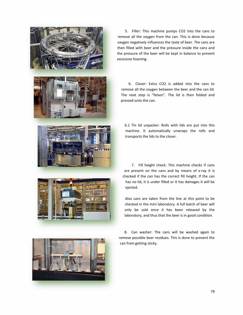
79

5. Filler: This machine pumps CO2 into the cans to

remove all the oxygen from the can. This is done because

oxygen negatively influences the taste of beer. The cans are

then filled with beer and the pressure inside the cans and

the pressure of the beer will be kept in balance to prevent

excessive foaming.

6. Closer: Extra CO2 is added into the cans to

remove all the oxygen between the beer and the can lid.

The next step is “felsen”. The lid is then folded and

pressed onto the can.

6.1 Tin lid unpacker: Rolls with lids are put into this

machine. It automatically unwraps the rolls and

transports the lids to the closer.

7. Fill height check: This machine checks if cans

are present on the cans and by means of x-ray it is

checked if the can has the correct fill height. If the can

has no lid, it is under filled or it has damages it will be

ejected.

Also cans are taken from the line at this point to be

checked in the mini laboratory. A full batch of beer will

only be sold once it has been released by the

laboratory, and thus that the beer is in good condition.

8. Can washer: The cans will be washed again to

remove possible beer residues. This is done to prevent the

can from getting sticky.

80

9. Pasteurizer: Pasteurization ensures that all harmful

microorganisms are killed. The beer has a longer expiration

date after being pasteurized. The cans will travel through

the pasteurizer for approximately 40 minutes and will be

heated to a temperature of minimal 55 °C for a certain

amount of time. This can vary depending on the beer type

being pasteurized. Every beer type has a certain target

measured in PU (pasteurization units). Depending on this

target value the pasteurization time is calculated. It is very

important that the beer is neither too long or too short in this

pasteurization zone. If it stays too long it will negatively influence

the taste, on the other hand a too short pasteurization means that not all harmful microorganisms have

been killed. It is therefore very important for this machine to have enough space at the backside of the

pasteurizer to move cans out of the pasteurization zone once a breakdown happens behind the

pasteurizer. After pasteurization the cans will be blown dry. This will blow excessive water back into the

pasteurizer and prevents the cans from having deposits on the bottom. The conveyor belts will also split

in two directions after the pasteurizer. Cans are equally distributed to both sides. This is done because

one machine cannot handle the complete capacity of the pasteurizer, thus two machines are placed

beside each other.

10. Two different can dryers are placed after the

pasteurizer one will dry both the bottom and sides of the

cans. The other one dries the top of the can. Between these

two dryers the can coding is placed.

11. Can coding: This machine places a code with the

expiration date, production date, production time and

product code on the bottom of the can. After these steps

the can will be transported to the second dryer which will

dry the top of the can.

12. The bulging of the cans is checked in this

machines. During pasteurization pressure inside the cans

is build up and overpressure can arise. Also fill height is

checked again. If cans are too bulged, contain too little

beer or are fallen they will be ejected.

From now on the cans can following a couple of routes.

They can either be packed into sixpacks, four packs etc.

81

and then packed onto trays, or they are directly packed onto trays.

13. Shrinkpacker: On this machine, cans can be packed

in several different multipacks. It is also optional to place

folders within these packs. The shrinkpacker forms groups of

4, 6 or 8 cans. The cans are then wrapped with foil, which is

heated in order to get a tight fit around the cans. 4 packs are

transported in three rows, 6 and 8 packs are transported in

two rows to the next machine.

14. Rotate device film packer: This machine rotates the

multipacks if necessary in the correct direction to be packed

onto trays.

15. Tray shrinkpacker: This machine folds trays in packs

for either 12 or 24 cans. The cans will then be packed onto

these trays in either multipacks or loose. It also possible to

add an extra layer of film around these trays with a print.

The trays are also coded on the side of the tray.

18. Finished product inspection: This machine check of the

total weight of the package is correct. If not it will be

ejected.

82

19. Tray palletizer: The machine formats the trays in such a

way that most trays fit in one layer of trays and that the

pallet will be stable. If it is formatted it will place the layer of

trays onto the pallet.

20. Shrink wrap machine: This machine will make a shrink foil

around the entire pallet. This is done to make the load more

secure but also to prevent to trays and cans to get wet or

dusty.

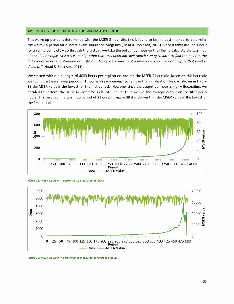
83

APPENDIX 6: DETERMINING THE WARM-UP PERIOD

This warm-up period is determined with the MSER-5 heuristic, this is found to be the best method to determine

the warm-up period for discrete event simulation programs (Hoad & Robinson, 2011). Since it takes around 1 hour

for a can to completely go through the system, we take the output per hour on the filler to calculate the warm up

period. “Put simply, MSER-5 is an algorithm that acts upon batched (batch size of 5) data to find the point in the

data series where the standard error (test statistic) in the data is at a minimum when the data before that point is

deleted. “ (Hoad & Robinson, 2011).

We started with a run length of 4000 hours per replication and ran the MSER-5 heuristic. Based on this heuristic

we found that a warm-up period of 1 hour is already enough to remove the initialisation bias. As shown in Figure

38 the MSER value is the lowest for the first periods. However since the output per hour is highly fluctuating, we

decided to perform the same heuristic for shifts of 8 hours. Thus we use the average output on the filler per 8

hours. This resulted in a warm up period of 8 hours. In Figure 39 it is shown that the MSER value is the lowest at

the first period.

Figure 38: MSER value with performance measured per hour

Figure 39: MSER value with performance measured per shift of 8 hours

0

20

40

60

80

100

0

200

400

600

800

0 250 500 750 1000 1250 1500 1750 2000 2250 2500 2750 3000 3250 3500 3750 4000

MSE

R v

alu

e

Dat

a

Period Data MSER Value

0

5000

10000

15000

20000

0

1000

2000

3000

4000

5000

6000

0 25 50 75 100 125 150 175 200 225 250 275 300 325 350 375 400 425 450 475 500

MSE

R v

alu

e

Dat

a

Period Data MSER Value

84

As an extra prove that one shift is enough warm up time to remove initialization bias we show the average output

of the filler for 5 replications in the first 24 hours in Figure 40. As can be seen in this figure, the output of the

palletiser is stable after 1 hour and thus definitely after 1 shift of 8 hours.

Figure 40: Output of the filler per hour for the first 24 hours.

0

100

200

300

400

500

600

700

800

1 2 3 4 5 6 7 8 9 10 11 12 13 14 15 16 17 18 19 20 21 22 23 24

Nu

mb

er

of

can

s x1

00

Period

Output of cans on filler

Mean (5 replications) Mean (24 hours)

85

APPENDIX 7: DETERMINING RUN LENGTH

To determine the run length of every experiment, we made 3 replications of the same experiment. This is

necessary for the heuristic described below. Every period, in our case a shift of 8 hours, we obtained the output

value of the filler. The cumulative mean of this value for every replication is shown in Figure 41. For every period

we calculated the convergence level, 𝐶𝑖 , of the value for the three different replications, with the following

equation.

𝐶𝑖 = 𝑀𝐴𝑋(𝑌𝑖1, 𝑌𝑖2, 𝑌𝑖3) − 𝑀𝐼𝑁(𝑌𝑖1, 𝑌𝑖2, 𝑌𝑖3)

𝑀𝐼𝑁(𝑌𝑖1 , 𝑌𝑖2, 𝑌𝑖3)

𝐶𝑖 = 𝐶𝑜𝑛𝑣𝑒𝑟𝑔𝑒𝑛𝑐𝑒 𝑙𝑒𝑣𝑒𝑙 𝑓𝑜𝑟 𝑝𝑒𝑟𝑖𝑜𝑑 𝑖

𝑌𝑖𝑗 = 𝑐𝑢𝑚𝑢𝑙𝑎𝑡𝑖𝑣𝑒 𝑚𝑒𝑎𝑛 𝑜𝑓 𝑜𝑢𝑡𝑝𝑢𝑡 𝑑𝑎𝑡𝑎 𝑓𝑜𝑟 𝑝𝑒𝑟𝑖𝑜𝑑 𝑖 𝑓𝑜𝑟 𝑟𝑒𝑝𝑙𝑖𝑐𝑎𝑡𝑖𝑜𝑛 𝑗

As soon as this convergence level goes below 5% and stays below 5%, that number of periods is the run length to

obtain reliable output from our model. As can be seen in Figure 41 this convergence level is reached after around

180 periods. We therefor need to run the model for at least 180 periods. However since 500 periods does not take

very long to perform, we use 500 periods (shifts of 8 hours) as our run length.

Figure 41: Cumulative mean of output of filler per shift

%

0,00%

5,00%

10,00%

15,00%

20,00%

25,00%

30,00%

35,00%

40,00%

0,0

1000,0

2000,0

3000,0

4000,0

5000,0

6000,0

1 41 81 121 161 201 241 281 321 361 401 441 481

Cu

mu

lati

ve m

ean

of

resu

lt

Period

Rep. 1 Rep. 2 Rep. 3 Convergence level