Effects of geomorphology, habitat, and spatial location on fish assemblages in a watershed in Ohio,...

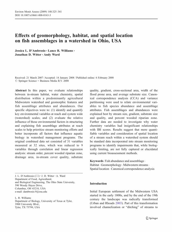
Effects of geomorphology, habitat, and spatial locationon fish assemblages in a watershed in Ohio, USA

Jessica L. D’Ambrosio & Lance R. Williams &

Jonathan D. Witter & Andy Ward

Received: 21 March 2007 /Accepted: 14 January 2008 / Published online: 6 February 2008# Springer Science + Business Media B.V. 2008

Abstract In this paper, we evaluate relationshipsbetween in-stream habitat, water chemistry, spatialdistribution within a predominantly agriculturalMidwestern watershed and geomorphic features andfish assemblage attributes and abundances. Ourspecific objectives were to: (1) identify and quantifykey environmental variables at reach and system wide(watershed) scales; and (2) evaluate the relativeinfluence of those environmental factors in structuringand explaining fish assemblage attributes at reachscales to help prioritize stream monitoring efforts andbetter incorporate all factors that influence aquaticbiology in watershed management programs. Theoriginal combined data set consisted of 31 variablesmeasured at 32 sites, which was reduced to 9variables through correlation and linear regressionanalysis: stream order, percent wooded riparian zone,drainage area, in-stream cover quality, substrate

quality, gradient, cross-sectional area, width of theflood prone area, and average substrate size. Canon-ical correspondence analysis (CCA) and variancepartitioning were used to relate environmental vari-ables to fish species abundance and assemblageattributes. Fish assemblages and abundances wereexplained best by stream size, gradient, substrate sizeand quality, and percent wooded riparian zone.Further data are needed to investigate why waterchemistry variables had insignificant relationshipswith IBI scores. Results suggest that more quanti-fiable variables and consideration of spatial locationof a stream reach within a watershed system shouldbe standard data incorporated into stream monitoringprograms to identify impairments that, while biolog-ically limiting, are not fully captured or elucidatedusing current bioassessment methods.

Keywords Fish abundance and assemblage .

Habitat . Geomorphology .Midwestern streams .

Spatial location . Canonical correspondence analysis

Introduction

Initial European settlement of the Midwestern USAstarted in the early 1800s, and by the end of the 19thcentury the landscape was radically transformed(Urban and Rhoads 2003). Part of this transformationinvolved channelization or “ditching” of streams to

Environ Monit Assess (2009) 148:325–341DOI 10.1007/s10661-008-0163-3

J. L. D’Ambrosio (*) : J. D. Witter :A. WardDepartment of Food, Agricultural,and Biological Engineering, The Ohio State University,590 Woody Hayes Drive,Columbus, OH 43210, USAe-mail: [email protected]

L. R. WilliamsDepartment of Biology, University of Texas at Tyler,3900 University Blvd.,Tyler, TX 75799, USA

provide enhanced capacity for agricultural fielddrainage in the headwaters of many watersheds.Many wetlands were drained, and networks ofagricultural ditches were constructed. The alterationof fluvial systems in the Midwestern USA hasaffected the geomorphological and ecological charac-teristics of these systems over a range of scales.

In 1972, the Clean Water Act was enacted andestablished a process for regulating discharges ofpollutants into the waters of the USA and acceptablelevels of water quality (USEPA 2007). In most states,water chemistry monitoring is conducted to supportestablished water quality criteria and identify prioritypollutants; however, chemical monitoring alone cannotensure that all pollutants and interactions among themare meeting water quality goals (Yagow et al. 2006).Ohio is one of the few states to have aquatic userequirements for lotic systems and to incorporatebiological monitoring, or bioassessment, into its waterquality standards. Bioassessment is important foridentifying problems otherwise missed or underesti-mated by chemical monitoring, and provides responseindicators closest to desired end outcomes related toecological health (Karr and Yoder 2004). Aquaticorganisms serve not only as useful indicators of currentconditions, but also of cumulative effects and changesover time; thus, they provide valuable informationabout the overall integrity of a water body (Plafkin etal. 1989; Barbour et al. 1999).

While monitoring efforts may result in a waterbody being classified as impaired, they do notnecessarily identify the pollutant or stressor causingthe impairment. Developing strategies to improvelotic systems requires knowledge not just of thechemical constituents but also their relationship toaquatic use attainment based on habit and aquaticbiology. In Ohio, each stream is designated an aquaticlife use designation: exceptional warmwater habitat(EWH), warmwater habitat (WWH), modified warm-water habitat (MWH), and limited resource waters(LRW), and each designation has a target value toindicate the healthy level of biotic integrity it cansupport (Ohio EPA 1995). WWH defines healthy fishassemblages and a habitat condition expected in mostwater bodies in Ohio, and is the primary restorationtarget for most water management efforts (Ohio EPA1995). Habitat is monitored using the qualitativehabitat evaluation index (QHEI; Rankin 1995) or

Headwater Habitat Evaluation Index (HHEI; OhioEPA 2002). Fish are monitored using the index ofbiotic integrity (IBI, Karr 1981).

The structure and function of aquatic communitiesis influenced by factors operating across a range ofspatial and temporal scales including geography,geology, climate, richness of regional species pools,stream order and network position, local streamhabitat, water quality, and flow characteristics (Puseyet al. 1995; Richards et al. 1996; Allan et al. 1997;Allan 2004; Angermeier and Winston 1998; Lammertand Allan 1999; Snyder et al. 2003; King et al. 2005;Williams et al. 2005). Gangloff and Faminella (2007)found that relatively minor changes in channelgradient and bankfull depth may have large effectson mussel assemblages in Appalachian streams.Walters et al. (2003) found that geomorphic processessuch as bed mobility and bankfull tractive force werekey predictors of fish species composition in GeorgiaPiedmont streams.

In heavily impacted, channelized streams where allor most of the riparian zone has been removed, onewould expect low QHEI scores to result in low IBIscores and vice versa. An examination of historicalIBI and QHEI data for the entire Olentangy Riverwatershed collected by Ohio EPA from 1979–2004,found that 31% of the sites were either: meeting IBItargets but not meeting QHEI targets or currently notmeeting IBI targets but meeting QHEI targets. WhenIBI and QHEI scores were plotted against each otherand fit with a regression line, the resulting relation-ship was relatively poor (r2=0.22).

These findings, together with an opportunity toconduct a total maximum daily load (TMDL) assess-ment for the Olentangy River, led the authors to askthe following questions about modified systems inOhio and throughout the Midwest: What are the mostimportant environmental factors affecting fish com-munities in Midwestern stream systems beyond in-stream habitat, and can these factors adequatelyexplain variation in fish assemblage structure? Arecurrent bioassessment methods adequate enough toidentify sources of variation affecting fish assem-blages in highly modified stream systems? To answerthese questions the authors identified four categoriesof environmental variables to measure and statisticallyrelate to fish community structure for a major riversystem in Ohio. In this paper, we evaluate relation-

326 Environ Monit Assess (2009) 148:325–341

ships between in-stream habitat, water chemistry,spatial distribution within the watershed, and geomor-phic features and IBI and fish abundances. Theecological focus of the study is on fish, because mostenvironmental management initiatives in this region aredirected toward fish resources (Rhoads and Herricks1996) and over 100 years of comparable, spatiallydistributed data are available on the composition of thefish community (Hauser 1999; Trautman 1981).Additionally, local geomorphic conditions and pro-cesses may contribute to habitat heterogeneity withinthe stream system but have received little attention infish assemblage studies (Frothingham et al. 2001).

Our specific objectives were to: (1) identify andquantify key environmental variables in a predomi-nantly agricultural Midwestern watershed; and (2)evaluate the relative influence of those environmentalfactors in structuring and explaining fish assemblageattributes. An anticipated end-product of workreported in this paper was to obtain knowledge thatwould assist regulatory agencies to revitalize, manageand derive policies for stream ecosystem integrity by:(1) prioritizing monitoring efforts in comprehensivewatershed management programs; and (2) betterincorporating more aspects of the lotic system thathave a major influence on aquatic biology.

Methods

Study site

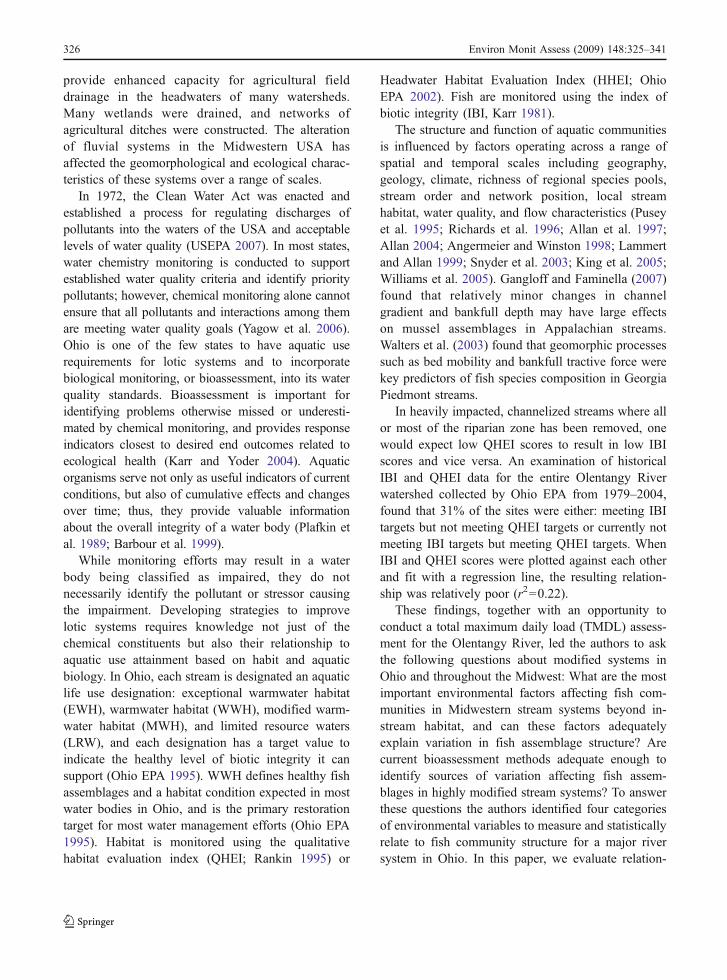
The Olentangy River watershed originates in southernCrawford County, Ohio, and flows south toward itsconfluence with the Scioto River near downtownColumbus, Ohio (Fig. 1). The Olentangy Rivermainstem is 142.4 km long and drains 1,400 km2.Overall, the land use in the Olentangy watershed is56% cropland, 14% urban, 14% forested, 13% pasture(Ohio EPA 2007). However, the watershed exhibitsthree distinctly different areas based on land use andgeology: the Upper Olentangy, Whetstone Creek, andLower Olentangy (Fig. 2). The Lower Olentangywatersheds are predominantly bedrock controlled, lo-cated in ravine-like settings, and dominated by urban/suburban land use (Fig. 2a). Thirty five kilometers ofthe Lower Olentangy River mainstem are designated asa State and National Scenic River.

Row-crop agriculture and sub-surface drainagedominate the Upper Olentangy watersheds, whichtend to be characterized by glaciated tills, lowgradients, and a history of hydrologic and physicalmodifications resulting in little wooded riparian zones(Fig. 2b). Above the City of Delaware is the Delaware

0 10 20

Legend

Sample Sites Streams

Watersheds

Upper Olentangy Whetstone Creek Lower Olentangy

Kilometers

N

Fig. 1 The Olentangy Riverwatershed and the locationof 32 sites with fish abun-dance and IBI, QHEI,geomorphology, spatiallocation, and waterchemistry data

Environ Monit Assess (2009) 148:325–341 327

Dam, which is a regulated flood control system thatlies on the Olentangy River mainstem and is the outletof the Upper Olentangy watershed.

The Whetstone Creek watershed is a majortributary to the Olentangy River and enters the systemnear the inlet of the lake controlled by the DelawareDam. Streams in the Whetstone Creek watershed alsoare dominated by row-crop agriculture, but arecharacterized by terminal moraine shale, slightlyhigher gradients, and a higher percentage of woodedriparian zones than the remainder of the UpperOlentangy watershed (Fig. 2c).

Data collection

The Ohio EPA has developed a 12-step projectmanagement-based process to accomplish TMDLsthat builds on existing monitoring, modeling, permit-ting, and grant programs (1999). The study reportedhere was performed under contract with the Ohio EPAand was constrained by the TMDL process. Thedataset for this study consisted of historical datacollected by Ohio EPA and data collected by theauthors for the entire Olentangy River watershed. TheOhio EPA database included IBI and QualitativeHabitat Evaluation Index (QHEI) metrics and scorescollected at the reach scale at 79 sites within thewatershed from 2003 to 2004 as well as waterchemistry grab samples collected at 32 sites in 2004from specific locations within the watershed. At siteswhere Ohio EPA data were available, the authorscollected geomorphology information at the reach leveland spatial location information at the 11-digit or 14-digit hydrologic unit code (HUC) sub-watershed level(Table 1).

Fish assemblages (IBI Metrics)

Fish sampling was conducted in the Olentangy Riverwatershed by Ohio EPA in 2003–2004 (June toSeptember) based on standardized bioassessmentprotocols (Barbour et al. 1999). Sampled reacheswere a minimum of 150 m in length. Fish collectedwere identified to species, counted, and then classi-fied into trophic, reproductive, and sensitivity guilds.

Fig. 2 Photos of typical streams found in a Lower Olentangywatersheds, b Upper Olentangy watersheds, and c WhetstoneCreek watersheds

R


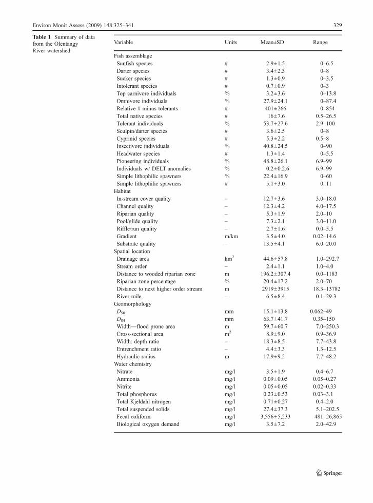
Variable Units Mean±SD Range

Fish assemblageSunfish species # 2.9±1.5 0–6.5Darter species # 3.4±2.3 0–8Sucker species # 1.3±0.9 0–3.5Intolerant species # 0.7±0.9 0–3Top carnivore individuals % 3.2±3.6 0–13.8Omnivore individuals % 27.9±24.1 0–87.4Relative # minus tolerants # 401±266 0–854Total native species # 16±7.6 0.5–26.5Tolerant individuals % 53.7±27.6 2.9–100Sculpin/darter species # 3.6±2.5 0–8Cyprinid species # 5.3±2.2 0.5–8Insectivore individuals % 40.8±24.5 0–90Headwater species # 1.3±1.4 0–5.5Pioneering individuals % 48.8±26.1 6.9–99Individuals w/ DELT anomalies % 0.2±0.2.6 6.9–99Simple lithophilic spawners % 22.4±16.9 0–60Simple lithophilic spawners # 5.1±3.0 0–11HabitatIn-stream cover quality – 12.7±3.6 3.0–18.0Channel quality – 12.3±4.2 4.0–17.5Riparian quality – 5.3±1.9 2.0–10Pool/glide quality – 7.3±2.1 3.0–11.0Riffle/run quality – 2.7±1.6 0.0–5.5Gradient m/km 3.5±4.0 0.02–14.6Substrate quality – 13.5±4.1 6.0–20.0Spatial locationDrainage area km2 44.6±57.8 1.0–292.7Stream order – 2.4±1.1 1.0–4.0Distance to wooded riparian zone m 196.2±307.4 0.0–1183Riparian zone percentage % 20.4±17.2 2.0–70Distance to next higher order stream m 2919±3915 18.3–13782River mile – 6.5±8.4 0.1–29.3GeomorphologyD50 mm 15.1±13.8 0.062–49D84 mm 63.7±41.7 0.35–150Width—flood prone area m 59.7±60.7 7.0–250.3Cross-sectional area m2 8.9±9.0 0.9–36.9Width: depth ratio – 18.3±8.5 7.7–43.8Entrenchment ratio – 4.4±3.3 1.3–12.5Hydraulic radius m 17.9±9.2 7.7–48.2Water chemistryNitrate mg/l 3.5±1.9 0.4–6.7Ammonia mg/l 0.09±0.05 0.05–0.27Nitrite mg/l 0.05±0.05 0.02–0.33Total phosphorus mg/l 0.23±0.53 0.03–3.1Total Kjeldahl nitrogen mg/l 0.71±0.27 0.4–2.0Total suspended solids mg/l 27.4±37.3 5.1–202.5Fecal coliform mg/l 3,556±5,233 481–26,865Biological oxygen demand mg/l 3.5±7.2 2.0–42.9

Table 1 Summary of datafrom the OlentangyRiver watershed


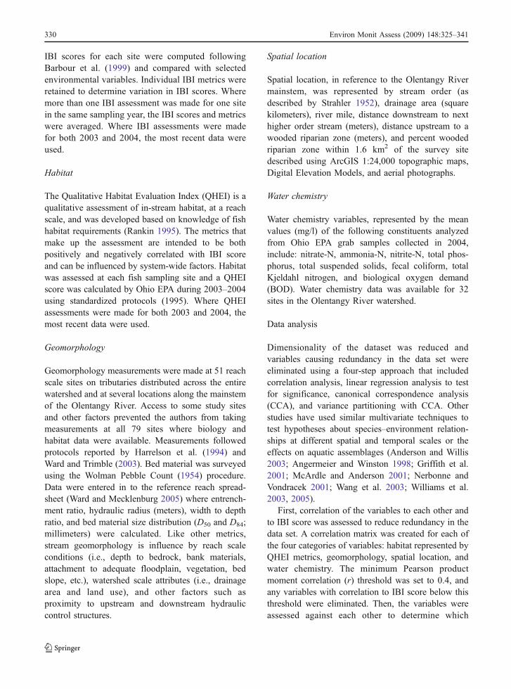
IBI scores for each site were computed followingBarbour et al. (1999) and compared with selectedenvironmental variables. Individual IBI metrics wereretained to determine variation in IBI scores. Wheremore than one IBI assessment was made for one sitein the same sampling year, the IBI scores and metricswere averaged. Where IBI assessments were madefor both 2003 and 2004, the most recent data wereused.

Habitat

The Qualitative Habitat Evaluation Index (QHEI) is aqualitative assessment of in-stream habitat, at a reachscale, and was developed based on knowledge of fishhabitat requirements (Rankin 1995). The metrics thatmake up the assessment are intended to be bothpositively and negatively correlated with IBI scoreand can be influenced by system-wide factors. Habitatwas assessed at each fish sampling site and a QHEIscore was calculated by Ohio EPA during 2003–2004using standardized protocols (1995). Where QHEIassessments were made for both 2003 and 2004, themost recent data were used.

Geomorphology

Geomorphology measurements were made at 51 reachscale sites on tributaries distributed across the entirewatershed and at several locations along the mainstemof the Olentangy River. Access to some study sitesand other factors prevented the authors from takingmeasurements at all 79 sites where biology andhabitat data were available. Measurements followedprotocols reported by Harrelson et al. (1994) andWard and Trimble (2003). Bed material was surveyedusing the Wolman Pebble Count (1954) procedure.Data were entered in to the reference reach spread-sheet (Ward and Mecklenburg 2005) where entrench-ment ratio, hydraulic radius (meters), width to depthratio, and bed material size distribution (D50 and D84;millimeters) were calculated. Like other metrics,stream geomorphology is influence by reach scaleconditions (i.e., depth to bedrock, bank materials,attachment to adequate floodplain, vegetation, bedslope, etc.), watershed scale attributes (i.e., drainagearea and land use), and other factors such asproximity to upstream and downstream hydrauliccontrol structures.

Spatial location

Spatial location, in reference to the Olentangy Rivermainstem, was represented by stream order (asdescribed by Strahler 1952), drainage area (squarekilometers), river mile, distance downstream to nexthigher order stream (meters), distance upstream to awooded riparian zone (meters), and percent woodedriparian zone within 1.6 km2 of the survey sitedescribed using ArcGIS 1:24,000 topographic maps,Digital Elevation Models, and aerial photographs.

Water chemistry

Water chemistry variables, represented by the meanvalues (mg/l) of the following constituents analyzedfrom Ohio EPA grab samples collected in 2004,include: nitrate-N, ammonia-N, nitrite-N, total phos-phorus, total suspended solids, fecal coliform, totalKjeldahl nitrogen, and biological oxygen demand(BOD). Water chemistry data was available for 32sites in the Olentangy River watershed.

Data analysis

Dimensionality of the dataset was reduced andvariables causing redundancy in the data set wereeliminated using a four-step approach that includedcorrelation analysis, linear regression analysis to testfor significance, canonical correspondence analysis(CCA), and variance partitioning with CCA. Otherstudies have used similar multivariate techniques totest hypotheses about species–environment relation-ships at different spatial and temporal scales or theeffects on aquatic assemblages (Anderson and Willis2003; Angermeier and Winston 1998; Griffith et al.2001; McArdle and Anderson 2001; Nerbonne andVondracek 2001; Wang et al. 2003; Williams et al.2003, 2005).

First, correlation of the variables to each other andto IBI score was assessed to reduce redundancy in thedata set. A correlation matrix was created for each ofthe four categories of variables: habitat represented byQHEI metrics, geomorphology, spatial location, andwater chemistry. The minimum Pearson productmoment correlation (r) threshold was set to 0.4, andany variables with correlation to IBI score below thisthreshold were eliminated. Then, the variables wereassessed against each other to determine which


variables grouped together to account for multi-collinearity. Final determinations between redundantvariables were based on our analysis of whichvariable retained more information on fish assem-blage structure based on our knowledge of thewatershed. To illustrate this step, river mile anddistance to the next higher order stream expresssimilar information about spatial location in thewatershed (r=0.99). Distance to the next higher orderstream showed a stronger correlation to IBI score (r=0.52) than river mile (r=0.45) and, therefore, rivermile was eliminated from the list of variablesdescribing spatial location.

Linear regression analyses was then conducted todetermine which of the remaining independent vari-ables were significantly related to IBI score (p<0.05)to further reduce the data set. Linear regressionanalyses using all the variables of the original dataset was also conducted to ensure that significantvariables were not inadvertently eliminated during thecorrelation analysis. Correlation and simple linearregression analyses were performed using the Systatv.11 statistical software package (SSI 2004).

CCA analysis focused on fish assemblage attributes(IBI metrics) and species composition (abundance)using the Canoco v4.5 statistical program (ter Braakand Smilauer 2002) to determine the relationship offish assemblages (dependent variables) to environmen-tal factors (independent variables) in the OlentangyRiver watershed. CCA was used on the full data set ofenvironmental variables as well as the data set ofreduced environmental variables (after correlation andregression analysis) to determine if any explanatoryvariance was lost by eliminating statistically redundantvariables. Significance of canonical axes and variationexplained by environmental variables (α=0.05) werebased on 1,000 Monte Carlo permutations. The natureof the species–environment relationship was theninferred from intraset canonical correlation coefficientsof environmental variables with CCA axes (ter Braakand Smilauer 2002).

In order to improve the overall predictive successof the model, variance partitioning was used toestimate the contribution of each set of variables tocommunity variation after accounting for the othersets (Borcard et al. 1992; ter Braak 1996; Parris 2004;Williams et al. 2005). The technique yielded theproportion of explained variation for the overallmodel, each category of environmental variables,

each two-way interaction among the pairs and theinteraction of all the pairs. In all analyses, proportionswere angular-transformed, and fish abundances wereln-transformed to correct for detected non-constanterror variance.

Results and discussion

The original combined data set consisted of 31variables measured at 32 sites in the Olentangy Riverwatershed: 10 geomorphology variables, 7 habitatvariables, 6 spatial location variables, and 8 waterchemistry variables (Table 1). Sites with missing datavalues were omitted. Sub-watersheds analyzed in thisstudy ranged in size from 1 to 300 km2. IBI scores forthe data set analyzed ranged from 12 to 52 with amedian score of 38. Forty-seven species of fish werecaught among the study sites. The greatest number ofspecies caught at a site was 26 species. The fewestnumber of species caught at a site was one species.The greatest number of fish caught at a site was 1,683individuals. The fewest number of fish caught at a sitewas nine individuals. Whetstone Creek watershedshad greater average diversity and abundance than theUpper and Lower Olentangy watersheds. Redfinshiners (Lythrurus umbratillis) and white crappies(Pomoxis annularis) were unique to the UpperOlentangy watersheds and not found in the LowerOlentangy and Whetstone Creek watersheds. Madtoms(Noturus spp.) and sculpins (Cottus spp.) were foundonly in the Whetstone Creek watersheds. QHEIscores ranged from 29 to 85 with a median score of60. Sites within the Upper Olentangy watershedsexhibited highly variable habitat conditions, havingboth the highest and lowest QHEI scores. LowerOlentangy sites generally had higher gradients andlower riffle and pool quality. Whetstone Creek sitesgenerally had higher in-stream cover, riparian, andsubstrate quality.

Objective 1: analysis of key environmental variables

Within the habitat category, in-stream cover qualitymost highly correlated to IBI score (r=0.60) followedby gradient (r=−0.53) in the correlation analysis.When all habitat variables were regressed against IBIscore (r2=0.60; p=0.001), in-stream cover quality,substrate quality, and gradient were each significant


(p=0.02). Explanatory variance was similar whenonly these three variables were regressed against IBIscore (r2=0.58; p=0.001).

Within the spatial location category, stream order,river mile, and distance to next higher order streamare all descriptors for location of a site within thewatershed and, to a lesser extent, stream size and weredetermined to be strongly correlated to IBI. Streamorder had the highest correlation to IBI score (r=0.68). When all of the spatial location variables wereregressed against IBI score (r2=0.55; p=0.001)stream order (p=0.0001), percent wooded riparianzone (p=0.007), and drainage area (p=0.04) weresignificant. Virtually no explanatory variance was lostwhen only these three variables were regressedagainst IBI score (r2=0.54; p=0.001); therefore, thesethree variables were retained for CCA analysis.

In the geomorphology category cross-sectionalarea, bankfull width, mean depth, max depth, andhydraulic radius are all descriptors of stream channelsize and were all strongly correlated; therefore, cross-sectional area was used to describe stream channelsize as the variable incorporates both width and depthmeasurements. Cross-sectional area (r=0.45), widthof the flood prone area (r=0.42), and averagesubstrate size (r=0.41) were the most highly corre-lated variables to IBI score. When geomorphologyvariables were regressed against IBI score (r2=0.50;p=0.02) cross-sectional area was the only significantvariable (p=0.04). When cross sectional area, averagesubstrate size, and width of the flood prone area wereregressed against IBI score the explained variancedecreased by half, but all the variables were signifi-cant (r2=0.22; p=0.05).

Average total suspended solids was the mosthighly correlated water chemistry variable to IBIscore (r=0.33); however, it did not meet ourminimum correlation threshold (r>0.40). When allof the water chemistry variables were regressedagainst IBI score (r2=0.18; p=0.05) none of thevariables were significant; therefore, no water chem-istry variables were retained for CCA analysis. Thelack of correlation might be due to insufficientvariation in water chemistry between specific sites tosignificantly influence IBI score. For example, therewere no pollution sources that caused very low IBIscores or exceptional water quality areas that resultedin high IBI scores.

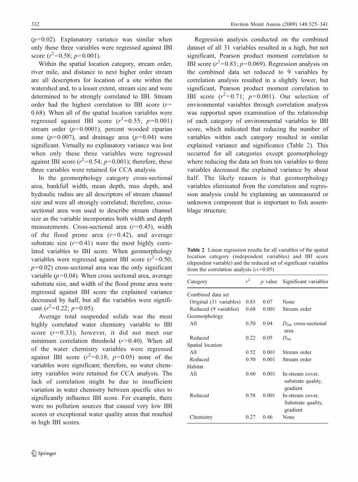
Regression analysis conducted on the combineddataset of all 31 variables resulted in a high, but notsignificant, Pearson product moment correlation toIBI score (r2=0.83; p=0.069). Regression analysis onthe combined data set reduced to 9 variables bycorrelation analysis resulted in a slightly lower, butsignificant, Pearson product moment correlation toIBI score (r2=0.71; p=0.001). Our selection ofenvironmental variables through correlation analysiswas supported upon examination of the relationshipof each category of environmental variables to IBIscore, which indicated that reducing the number ofvariables within each category resulted in similarexplained variance and significance (Table 2). Thisoccurred for all categories except geomorphologywhere reducing the data set from ten variables to threevariables decreased the explained variance by abouthalf. The likely reason is that geomorphologyvariables eliminated from the correlation and regres-sion analysis could be explaining an unmeasured orunknown component that is important to fish assem-blage structure.

Table 2 Linear regression results for all variables of the spatiallocation category (independent variables) and IBI score(dependent variable) and the reduced set of significant variablesfrom the correlation analysis (α=0.05)

Category r2 p value Significant variables

Combined data setOriginal (31 variables) 0.83 0.07 NoneReduced (9 variables) 0.68 0.001 Stream orderGeomorphologyAll 0.50 0.04 D50, cross-sectional

areaReduced 0.22 0.05 D50

Spatial locationAll 0.52 0.001 Stream orderReduced 0.50 0.001 Stream orderHabitatAll 0.60 0.001 In-stream cover,

substrate quality,gradient

Reduced 0.58 0.001 In-stream cover,Substrate quality,gradient

Chemistry 0.27 0.46 None


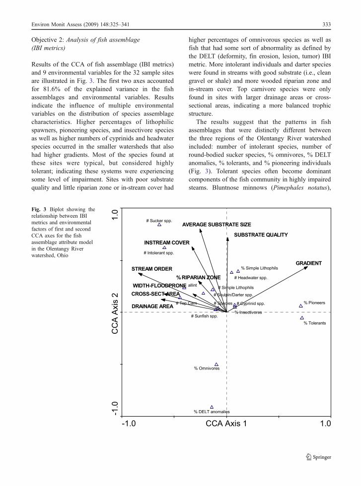
Objective 2: Analysis of fish assemblage(IBI metrics)

Results of the CCA of fish assemblage (IBI metrics)and 9 environmental variables for the 32 sample sitesare illustrated in Fig. 3. The first two axes accountedfor 81.6% of the explained variance in the fishassemblages and environmental variables. Resultsindicate the influence of multiple environmentalvariables on the distribution of species assemblagecharacteristics. Higher percentages of lithophilicspawners, pioneering species, and insectivore speciesas well as higher numbers of cyprinids and headwaterspecies occurred in the smaller watersheds that alsohad higher gradients. Most of the species found atthese sites were typical, but considered highlytolerant; indicating these systems were experiencingsome level of impairment. Sites with poor substratequality and little riparian zone or in-stream cover had

higher percentages of omnivorous species as well asfish that had some sort of abnormality as defined bythe DELT (deformity, fin erosion, lesion, tumor) IBImetric. More intolerant individuals and darter specieswere found in streams with good substrate (i.e., cleangravel or shale) and more wooded riparian zone andin-stream cover. Top carnivore species were onlyfound in sites with larger drainage areas or cross-sectional areas, indicating a more balanced trophicstructure.

The results suggest that the patterns in fishassemblages that were distinctly different betweenthe three regions of the Olentangy River watershedincluded: number of intolerant species, number ofround-bodied sucker species, % omnivores, % DELTanomalies, % tolerants, and % pioneering individuals(Fig. 3). Tolerant species often become dominantcomponents of the fish community in highly impairedsteams. Bluntnose minnows (Pimephales notatus),

-1.0 1.0CCA Axis 1

-1.0

1.0

CC

A A

xis

2

# Sunfish spp.

# Intolerant spp.

% Tolerants

# Top Carn

% Omnivores

# Sucker spp.

% DELT anomalies

# Species

allint

# Sculpin/Darter spp.

# Cyprinid spp.

% Insectivores

# Headwater spp.

% Pioneers

% Simple Lithophils

# Simple Lithophils

INSTREAM COVER

SUBSTRATE QUALITY

GRADIENT

AVERAGE SUBSTRATE SIZE

WIDTH-FLOODPRONE

CROSS-SECT AREA

DRAINAGE AREA

STREAM ORDER

% RIPARIAN ZONE

Fig. 3 Biplot showing therelationship between IBImetrics and environmentalfactors of first and secondCCA axes for the fishassemblage attribute modelin the Olentangy Riverwatershed, Ohio


creek chubs (Semotilus atromaculatus), blacknosedace (Rhinichthys atratulus) are considered highlytolerant and omnivorous. A site with a fish commu-nity dominated by tolerant, omnivorous species mightindicate a disruption of the food base caused byenvironmental degradation (OEPA 1987). However,increased omnivory may be a natural condition offluctuating temperate streams and its impact on fishfood web stability is debatable (Emmerson andYearsley 2004). The species assemblage distinctionwas a function of stream size, gradient and substratequality and size (Table 3).

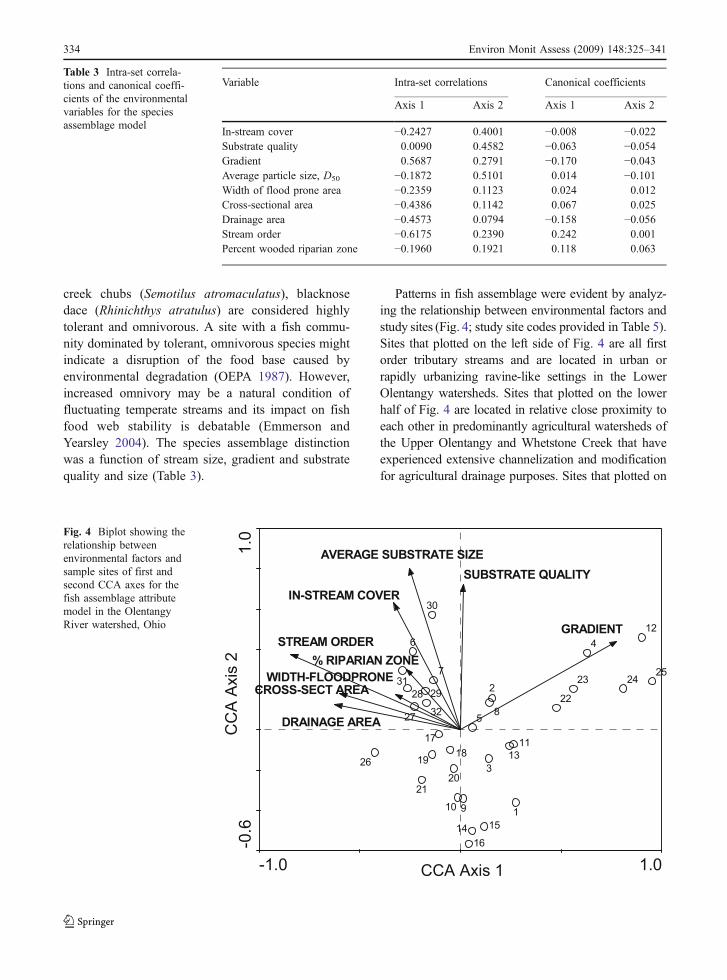
Patterns in fish assemblage were evident by analyz-ing the relationship between environmental factors andstudy sites (Fig. 4; study site codes provided in Table 5).Sites that plotted on the left side of Fig. 4 are all firstorder tributary streams and are located in urban orrapidly urbanizing ravine-like settings in the LowerOlentangy watersheds. Sites that plotted on the lowerhalf of Fig. 4 are located in relative close proximity toeach other in predominantly agricultural watersheds ofthe Upper Olentangy and Whetstone Creek that haveexperienced extensive channelization and modificationfor agricultural drainage purposes. Sites that plotted on

-1.0 1.0

-0.6

1.0

IN-STREAM COVER

SUBSTRATE QUALITY

GRADIENT


WIDTH-FLOODPRONE

CROSS-SECT AREA

DRAINAGE AREA

STREAM ORDER

% RIPARIAN ZONE

1

2

3

4

5

6

7

8

910

11

12

13

14 15

16

17

1819

2021

22

23 2425

26

27

28 29

30

31

32

CC

A A

xis

2

CCA Axis 1

Fig. 4 Biplot showing therelationship betweenenvironmental factors andsample sites of first andsecond CCA axes for thefish assemblage attributemodel in the OlentangyRiver watershed, Ohio

Variable Intra-set correlations Canonical coefficients

Axis 1 Axis 2 Axis 1 Axis 2

In-stream cover −0.2427 0.4001 −0.008 −0.022Substrate quality 0.0090 0.4582 −0.063 −0.054Gradient 0.5687 0.2791 −0.170 −0.043Average particle size, D50 −0.1872 0.5101 0.014 −0.101Width of flood prone area −0.2359 0.1123 0.024 0.012Cross-sectional area −0.4386 0.1142 0.067 0.025Drainage area −0.4573 0.0794 −0.158 −0.056Stream order −0.6175 0.2390 0.242 0.001Percent wooded riparian zone −0.1960 0.1921 0.118 0.063

Table 3 Intra-set correla-tions and canonical coeffi-cients of the environmentalvariables for the speciesassemblage model


the upper half of Fig. 4 also are located in closeproximity to each other in the Upper Olentangy andWhetstone Creek watersheds and, although they arepredominantly agricultural watersheds, they have ahigher degree of recovery resulting in slightly highergradients and more wooded riparian zone comparedto other watersheds in the Upper Olentangy andWhetstone Creek. Overlap of fish assemblage patternsbetween the Upper Olentangy and Whetstone Creekwatersheds might be, in part, because many of thesampling sites were located in close proximity to eachother or near the boundaries of these watershed regions,and may exhibit characteristics of each watershedregion. Fish assemblages in headwater first- andsecond-order streams typically comprise few speciesand low abundances (Robinson and Minshall 1994).Although percent tolerant and pioneering speciesappeared distinct from the other sites, fish sampled atthese sites were typical for disturbed first-order streamsin the Lower Olentangy watersheds. The fish speciesthat comprised this assemblage were found in othersites sampled, but did not constitute the vast majorityof species sampled as they did in the Lower Olentangysites.

Analysis of species abundance (fish species)

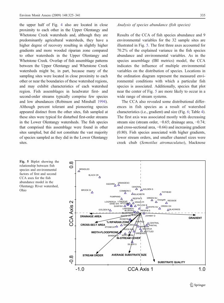
Results of the CCA of fish species abundance and 9environmental variables for the 32 sample sites areillustrated in Fig. 5. The first three axes accounted for70.2% of the explained variance in the fish speciesabundance and environmental variables. As in thespecies assemblage (IBI metrics) model, the CCAindicates the influence of multiple environmentalvariables on the distribution of species. Locations inthe ordination diagram represent the measured envi-ronmental conditions with which a particular fishspecies is associated. Additionally, species that plotnear the center of Fig. 5 are more likely to occur in awide range of stream systems.

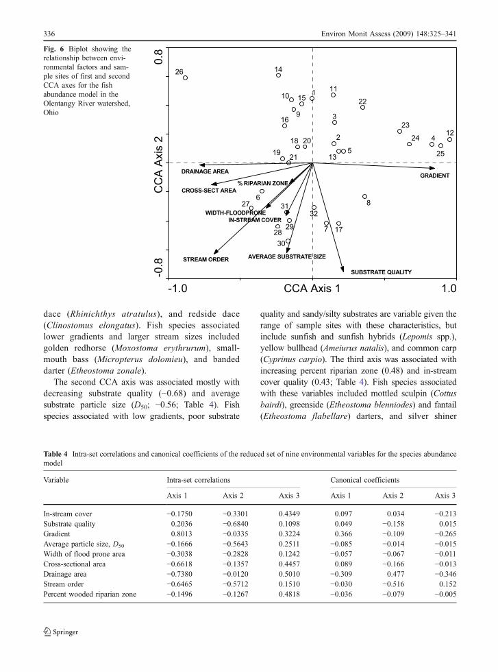
The CCA also revealed some distributional differ-ences in fish species as a result of watershedcharacteristics (i.e., gradient) and size (Fig. 6; Table 4).The first axis was associated mostly with decreasingstream size (stream order, −0.65; drainage area, −0.74;and cross-sectional area, −0.66) and increasing gradient(0.80). Fish species associated with higher gradients,lower stream orders, and smaller channel sizes werecreek chub (Semotilus atromaculatus), blacknose

-1.0 1.0CCA Axis 1

-0.8

0.8

CC

A A

xis

2

BANDED D

BLACK CR

BLACKNOS

BLACKSID

BLACKSTR

BLUEGILL

BLUNTNOS

BRINDLED

BROOK SI

CENTRAL

CENTRAL

COMMON C

CREEK CH

FANTAIL

FATHEAD

GIZZARD

GOLDEN R

GOLDEN S

GRASS PI

SUNFISH

GREEN SU

GREENSID

JOHNNY D

LARGEMOU

LOGPERCH LONGEAR

MOTTLED

NORTHERN

ORANGESO

Orangeth

PUMPKINS

RAINBOW

REDFIN S

REDFIN S

REDSIDE

ROCK BAS

ROSEFIN

SAND SHI

SILVER S

SILVERJA

SMALLMOU

SPOTFIN

STONECAT

STRIPED

WHITE CR

WHITE SUYELLOW B

IN-STREAM COVER

SUBSTRATE QUALITY

GRADIENT


WIDTH-FLOODPRONE

CROSS-SECT AREA

DRAINAGE AREA

STREAM ORDER

% RIPARIAN ZONE

Fig. 5 Biplot showing therelationship between fishspecies and environmentalfactors of first and secondCCA axes for the fishabundance model in theOlentangy River watershed,Ohio


dace (Rhinichthys atratulus), and redside dace(Clinostomus elongatus). Fish species associatedlower gradients and larger stream sizes includedgolden redhorse (Moxostoma erythrurum), small-mouth bass (Micropterus dolomieu), and bandeddarter (Etheostoma zonale).

The second CCA axis was associated mostly withdecreasing substrate quality (−0.68) and averagesubstrate particle size (D50; −0.56; Table 4). Fishspecies associated with low gradients, poor substrate

quality and sandy/silty substrates are variable given therange of sample sites with these characteristics, butinclude sunfish and sunfish hybrids (Lepomis spp.),yellow bullhead (Ameiurus natalis), and common carp(Cyprinus carpio). The third axis was associated withincreasing percent riparian zone (0.48) and in-streamcover quality (0.43; Table 4). Fish species associatedwith these variables included mottled sculpin (Cottusbairdi), greenside (Etheostoma blenniodes) and fantail(Etheostoma flabellare) darters, and silver shiner

Table 4 Intra-set correlations and canonical coefficients of the reduced set of nine environmental variables for the species abundancemodel

Variable Intra-set correlations Canonical coefficients

Axis 1 Axis 2 Axis 3 Axis 1 Axis 2 Axis 3

In-stream cover −0.1750 −0.3301 0.4349 0.097 0.034 −0.213Substrate quality 0.2036 −0.6840 0.1098 0.049 −0.158 0.015Gradient 0.8013 −0.0335 0.3224 0.366 −0.109 −0.265Average particle size, D50 −0.1666 −0.5643 0.2511 −0.085 −0.014 −0.015Width of flood prone area −0.3038 −0.2828 0.1242 −0.057 −0.067 −0.011Cross-sectional area −0.6618 −0.1357 0.4457 0.089 −0.166 −0.013Drainage area −0.7380 −0.0120 0.5010 −0.309 0.477 −0.346Stream order −0.6465 −0.5712 0.1510 −0.030 −0.516 0.152Percent wooded riparian zone −0.1496 −0.1267 0.4818 −0.036 −0.079 −0.005

-1.0 1.0CCA Axis 1

-0.8

0.8

CC

A A

xis

2

IN-STREAM COVER

SUBSTRATE QUALITY

GRADIENT


WIDTH-FLOODPRONE

CROSS-SECT AREA

DRAINAGE AREA

STREAM ORDER

% RIPARIAN ZONE

1

2

3

4

5

6

7

8

9

1011

12

13

14

15

16

17

18

19

20

21

22

23

24

25

26

27

2829

30

3132

Fig. 6 Biplot showing therelationship between envi-ronmental factors and sam-ple sites of first and secondCCA axes for the fishabundance model in theOlentangy River watershed,Ohio


(Notropis photogenis). These species also associatedwith better substrate quality and larger average particlesizes.

Fish species generally did not differ distinctly inthe Olentangy River watershed with the exception ofbrindled madtoms (Noturus miurus), black crappie(Pomoxis nigromaculatus), and brook silverside(Labidesthes sicculus). These species were foundonly at one site in the Whetstone Creek mainstem(site code 26, Table 5) near its confluence with theDelaware Dam Reservoir, and usually are associatedwith lake or slow-moving deep pool environments.

Analysis of variance partitioning

In order to better diagnose the explained variation inthe fish abundance and the species assemblage (IBImetrics) attribute models we performed partial CCAson the reduced data set (Fig. 7). For the speciesassemblage (IBI metrics) model (Fig. 7a), the pureeffects of habitat represented by QHEI metricsexplained more variation (12.9%) than geomorphology(4.1%) and spatial location (7.4%); however, the pure

Table 5 Codes for study sites, and associated sub-watersheds,used in CCA analysis

Site code Site name Sub-watershed

1 Bee Run 0.3 Upper Olentangy2 Big Run 0.1 Lower Olentangy3 Claypool Run 1.2 Whetstone Creek4 Deep Run 1.2 Lower Olentangy5 East Branch Whetstone

Creek 0.4Whetstone Creek

6 Flat Run 0.6 Upper Olentangy7 Flat Run 7.3 Upper Olentangy8 Flat Run 12.6 Upper Olentangy9 Grave Creek 1.4 Upper Olentangy10 Grave Creek 3.2 Upper Olentangy11 Indian Run 0.9 Lower Olentangy12 Mill Run 0.9 Upper Olentangy13 Mitchell Run 0.2 Upper Olentangy14 Mud Run 2.7 Upper Olentangy15 Mud Run 6.7 Upper Olentangy16 QuQua Creek 4.6 Lower Olentangy17 Rocky Fork 2.9 Upper Olentangy18 Sams Creek 1.4 Whetstone Creek19 Shaw Creek 1.6 Whetstone Creek20 Shaw Creek 5.2 Whetstone Creek21 Shaw Creek 10.6 Whetstone Creek22 Shaw Creek 13.2 Whetstone Creek23 Sugar Run 1.3 Upper Olentangy24 Tributary to Whetstone

Creek 0.4Whetstone Creek

25 Turkey Run 0.7 Lower Olentangy26 Walhalla Ravine 0.9 Lower Olentangy27 Whetstone Creek 2.5 Whetstone Creek28 Whetstone Creek 9.2 Whetstone Creek29 Whetstone Creek 18.2 Whetstone Creek30 Whetstone Creek 21.7 Whetstone Creek31 Whetstone Creek 25.5 Whetstone Creek32 Whetstone Creek 29.3 Whetstone Creek

Geomorphology 4.1%

Geomorphology 5.2%

Spatial Location 10.5%

Habitat 13.9%

0%

18.6%

2.2% 3.5%

Total Uncertainty: 46%

Spatial Location 7.4%

Habitat 12.9%

0%

18.6%

3.3% 5.8%

Total Uncertainty: 48%

a

b

Fig. 7 CCA variance partitioning results showing the pureeffects and shared variation of each environmental categorygeomorphology, spatial location, and habitat represented byQHEI for a the species assemblage model (IBI metrics) and bthe species abundance model


effects of each category were not significantly different(α=0.05). Shared variation among all three categorieswas significantly different from the pure effects of eachcategory and explained 18.6%. Total uncertainty, orthat amount of variance that could not be explained,was 48%. This indicates that fish community structurelikely is a function of location within watershed andproximity to a potential source of habitat or fishspecies, stable geomorphology creating diverse in-stream habitats, and the quality of those habitats.Nearly half of the fish community structure is likely aresult of variables that could not be measured such ascompetition and trophic interactions.

For the fish abundance model (Fig. 7b), the pureeffects of habitat represented by QHEI metricsexplained more variation (13.9%) than spatial location(10.5%) and geomorphology (5.2%). The pure effectsof habitat and spatial location were not significantlydifferent from each other, but were significantlydifferent from geomorphology. Shared variationamong all three categories explained 18.6%. Totaluncertainty was 46%. This indicates that individualfish species are more highly influenced by quality ofin-stream habitat and proximity to higher qualityhabitats, and nearly half of the variation in fishspecies abundance is likely a result of variables thatcould not be measured such as species interactionsand behaviors.

A sensitivity analysis was performed on the studysites to determine if interchanging watersheds or thenumber of sample sites within on watershed wouldaffect whether one environmental category becomemore important than another one in the variancepartitioning. For example, the dataset consisted ofseven sites located on the Whetstone Creek mainstem.When the number of Whetstone Creek mainstem siteswas reduced to two, explained variance among thethree categories shifted slightly, but the overalluncertainty was similar. When the overall number ofsites was reduced to include only one site from eachsubwatershed, the explained variance among the threecategories shifted again, but the overall uncertainty wassimilar. This indicates that inclusion of environmentalfactors such as geomorphology and spatial location instream monitoring assessments explains an importantcomponent of variation in fish community structureabove and beyond qualitative habitat metrics alone eventhough the variables within each category will change orbecome more important in different watersheds.

Results of this study suggest that more focusshould be placed on better quantifying in-streamhabitat factors to better understand stream function,which also is recommended by other researchers (Poff1997; Papanicolaou et al. 2003). This type of study,which attempts to determine direct causality of streamfish assemblages using physical environmental vari-ables, necessitates quantifiable data. Studies havedocumented inconsistency between the importanceof habitat metrics measured qualitatively and impor-tance of these factors measured quantitatively or at adifferent scale (Frimpong et al. 2005; Wang et al.1996; Hannaford et al. 1997). Physical integrity todescribe functional attributes of streams is poorlyrepresented in qualitative metrics for a number ofreasons. First, because qualitative metrics are afunction of conditions on the day they are evaluatedand not dependent on flow conditions. Second, localhabitat variables can only infer direct causality whenconsidering fish species that range widely becausetheir optimal habitat will not necessarily reflected atthe exact spot they are captured (Schlosser 1991;Cooper et al. 1998). Third, system impairments thatare limiting to aquatic biology are not necessarilyreflected in the QHEI score itself. For example, thebenefits of a good quality riparian zone and highsinuosity necessary for a stable fish assemblage maybe undermined by thick silty substrate or lack of riffleand pool development. Therefore, the QHEI scoremay exceed a designated target because somecomponents of the habitat are of an excellent qualitybut other poor components are limiting the biologicalcommunity resulting in lower than expected IBIscores. While qualitative multi-metric indices arevaluable for developing extensive databases andidentifying a potential impairment within a reach,they are limited in the ability to diagnose the causesof that impairment.

Quantitative data have advantages over visualassessments in determining stream instability prob-lems. For example, the CCA analyses in this studyshow that substrate size and quality are importantfactors influencing fish assemblages in the OlentangyRiver. Using a Wolman Pebble Count (or othersimilar procedure), we are able to calculate the D50,which then can be used in assessments of sedimenttransport. Comparing measured to predicted values(i.e., via tractive force equations) of average particlesize, one can begin to determine potential instabilities


in shear stresses and stream power that may becausing localized sedimentation or erosion problems.Additionally, other variables such as width to depthratio or connectivity to an active floodplain may helpexplain the instability causing poor substrate conditionsand proper enhancement or restoration activities can beimplemented to ameliorate the impairment. Theauthors recommend that qualitative habitat assess-ments, such as the QHEI, should be retained in streamassessment studies because they describe importanttrends in data over time, and can serve as benchmarksfor success and an important communication tool inlocalized stream enhancement projects.

Conclusions

The analysis associated with Objective 1 identifiedthe following key environmental variables that influ-ence fish assemblages: stream order, percent woodedriparian zone, drainage area, in-stream cover quality,substrate quality, gradient, cross-sectional area, widthof the flood prone area, and average substrate size.Some of these factors, such as drainage area, are afunction of the watershed, while others such as thewidth of the flood prone area and gradient are afunction of reach attributes. No additional predictivepower was gained by using more than two or threeenvironmental variables from each category, and eachcategory will shift in importance as watershedcharacteristics change. Further data are needed toinvestigate why water chemistry variables had insig-nificant relationships with IBI scores. Total suspendedsolids had the strongest relationship to IBI score inboth the correlation and regression analysis. Possiblereasons for water quality not explaining more varia-tion in the fish assemblage structure are numerous. Itis speculated that measured constituents may not haveexhibited wide enough variation between specificsites. It might be necessary to conduct intensive waterquality sampling at a sub-watershed scale (0.5 to2 km2) to really understand its effect on fish. Thoughwater quality signatures were above Ohio EPA targetvalues in some instances, they may not have beenhigh enough to cause an effect on fish assemblages inthe watershed, or to be the largest stressor whencompared to physical parameters such as geomorpho-logical, in-stream habitat, and land use changes.

In the analysis associated with Objective 2, CCAwas used to explore relationships between and amongspecies and environmental factors. The CCA revealeddistributional differences in fish assemblages as aresult of both reach and watershed characteristics. IBImetrics and abundances were explained best bystream size, gradient, substrate size and quality, andpercent wooded riparian zone.

In our study, it was not possible to evaluate theinfluence of hydraulic control structures on the results.There are numerous road crossings through the water-sheds that were studied but few low head weirs. Atseveral locations, however, there are log jams andoccasionally a beaver dam. These natural and artificialstructures probably account for some of the unex-plained variability in the results. Groundwater rechargealso was not quantified because this componentgenerally is small or not evident in most channelizedsystems. It appeared in this study that a few sites likelybenefited from groundwater recharge.

Comprehensive watershed programs, such asTMDL, while effective at identifying impairments atthe watershed scale, are difficult to translate to thereach or site scale where most stream restoration andenhancement projects take place. The importance ofspatial location variables shows some potential fordeveloping a watershed-scale index of stream condi-tion to help managers locate vulnerable sites andprioritize potential restoration projects. Quantitativegeomorphology variables allows examination ofstream integrity on a finer scale than bioassessmentindices that consolidate stream condition into a singlescore, which is especially useful when sites are in themid-range of the indices. Results of this study suggestthat more quantifiable environmental variables of loticsystems and consideration of spatial location of astream reach within a watershed system should bestandard data incorporated into stream monitoringprograms to identify impairments that, while biolog-ically limiting, are not fully captured or elucidatedusing current bioassessment methods.

Acknowledgements The authors thank the Ohio EPA admin-istrative staff, especially Trinka Mount and Maan Osman, forfull funding support of this project. We also thank GreggSablak, Holly Tucker, and Dennis Mischne, of Ohio EPA, foruse of their database and assistance on this project. The authorsare especially grateful to Ohio State University students andemployees Cynthia Yandrich, Trevor Ward, Ahmed Rismani,and Anand Jayakaran for gathering data in the field.


References

Allan, J. D. (2004). Landscapes and riverscapes: The influenceof land use on stream ecosystems. Annual Review ofEcology and Systematics, 35, 257–284.

Allan, J. D., Erickson, D. L., & Fay, J. (1997). The influence ofcatchment land use on stream integrity across multiplespatial scales. Freshwater Biology, 37, 149–161.

Anderson, M. J., & Willis, T. J. (2003). Canonical analysis ofprincipal coordinates: A useful method of constrainedordination for ecology. Ecology, 84(2), 511–525.

Angermeier, P. L., & Winston, M. R. (1998). Local vs. regionalinfluences on local diversity in stream fish communities ofVirginia. Ecology, 79, 911–927.

Barbour,M. T., Gerritsen, J., Snyder, B. D., & Stribling, J. B. (1999).Rapid bioassessment protocols for use in streams andwadeable rivers: Periphyton, benthic macroinvertebratesand fish (2nd ed.). Washington, DC: US EnvironmentalProtection Agency, Office of Water EPA 841-B-99-002.

Borcard, D., Legendre, P., & Drapeau, P. (1992). Partialling outthe spatial component of ecological variation. Ecology, 73,1045–1055.

Cooper, S. D., Diehl, S., Kratz, K., & Sarnelle, O. (1998).Implications of scale for patterns and processes in streamecology. Australian Journal of Ecology, 23, 27–40.

Emmerson, M., & Yearsley, J. M. (2004). Weak interactions,omnivory and emergent food-web properties. Proceedingsof the Royal Society of London B, 271, 397–405.

Frimpong, E. A., Sutton, T. M., Lim, K. J., Hrodey, P. J., Engel,B., Simon, T. P., et al. (2005). Determination of optimalriparian forest buffer dimensions for stream biota-landscapeassociation models using multimetric and multivariateresponses. Canadian Journal of Fisheries and AquaticSciences, 62, 1–6.

Frothingham, K. M., Rhoads, B. L., & Herricks, E. E. (2001).Stream geomorphology and fisheries in channelized andmeandering reaches of an agricultural stream. In J. Dorava,J. F. Fitzpatrick, D. Montgomery, & B. Palscak (Eds.)Geomorphic processes and riverine habitat monograph.Washington, DC: American Geophysical Union.

Gangloff, M. M., & Feminella, J. W. (2007). Stream channelgeomorphology influences mussel abundance in southernAppalachian streams, USA. Freshwater Biology, 52, 64–74.

Griffith, M. B., Kaufman, P. R., Herlihy, A. T., & Hill, B. H.(2001). Analysis of macroinvertebrate assemblages inrelation to environmental gradients in rocky mountainstreams. Ecological Applications, 11(2), 489–505.

Hannaford, M. J., Barbour, M. T., & Resh, V. H. (1997).Training reduces observer variability in visual-basedassessments of stream habitat. Journal of the NorthAmerican Benthological Society, 16, 853–860.

Harrelson, C. C., Rawlins, C. L., & Potyondy, J. P. (1994).Stream channel reference sites an illustrated guide to fieldtechnique. General technical report RM 245, US Dept. ofAgriculture Forest Service Rocky Mountain Forest andRange Experiment Station, Fort Collins, CO.

Hauser, T. A. (1999). Descriptive comparison of resident andtransient fish communities in headwater streams in EastCentral Illinois. MS thesis, University of Illinois, Urbana.

Karr, J. R. (1981). Assessment of biotic integrity using fishcommunities. Fisheries, 6, 21–27.

Karr, J. R., & Yoder, C. O. (2004). Biological assessment andcriteria improve total maximum daily load decisionmaking. Journal of Environmental Engineering, 130(6),594–604.

King, R. S., Baker, M. E., Whigham, D. F., Weller, D. E., Jordan,T. E., Kazyak, P. F., et al. (2005). Spatial considerations forlinking watershed land cover to ecological indicators instreams. Ecological Applications, 15, 137–153.

Lammert, M., & Allan, J. D. (1999). Assessing biotic integrityof streams: Effects of scale in measuring the influence ofland use/cover and habitat structure on fish and macro-invertebrates. Environmental Management, 23, 257–270.

McArdle, B. H., & Anderson, M. J. (2001). Fitting multivariatemodels to community data: A comment on distance-basedredundancy analysis. Ecology, 82(1), 290–297.

Nerbonne, B. A., & Vondracek, B. (2001). Effects of local landuse on physical habitat, benthic macroinvertebrates, andfish in the Whitewater River, Minnesota, USA. Environ-mental Management, 28(1), 87–99.

Ohio EPA. (1987). Biological criteria for the protection ofaquatic life. Vols. I–III. Columbus, OH: Ohio Environ-mental Protection Agency, Division of Water QualityMonitoring and Assessment, Surface Water Section.

Ohio EPA. (1995). The role of biological criteria in water qualitymonitoring, assessment, and regulation. Columbus, OH:Ohio Environmental Protection Agency Technical ReportSeries, Division of Water Quality Monitoring and Assess-ment, Surface Water Section.

Ohio EPA. (2002). Field evaluation manual for Ohio’s primaryheadwater streams. Columbus, OH: Ohio EnvironmentalProtection Agency, Division of Surface Water.

Ohio EPA. (2007). Total maximum daily load for Olentangyriver watershed. Columbus, OH: Division of SurfaceWater.

Papanicolaou, A. N., Bdour, A., Evangelopoulos, N., &Tallebeydokhti, N. (2003). Watershed and instreamimpacts on the fish population in the south fork of theClearwater River, Idaho. Journal of the American WaterResources Association, 39, 191–203.

Parris, K. M. (2004). Environmental and spatial variablesinfluence the composition of frog assemblages in sub-tropical eastern Australia. Ecography, 27, 392–400.

Plafkin, J. L., Barbour, M. T., Porter, K. D., Gross, S. K., &Hughes, R. M. (1989). Rapid bioassessment protocols foruse in streams and rivers. Benthic macroinvertebrates andfish.. Washington, DC: Office of Water Regulations andStandards, US Environmental Protection Agency EPA440-4-89-001.

Poff, N. L. (1997). Landscape filters and species traits: Towardsmechanistic understanding and prediction in stream ecology.Journal of the North American Benthological Society, 16,391–409.

Pusey, B. J., Arthington, A. H., & Read, M. G. (1995).Species richness and spatial variation in fish assemblagestructure in two rivers of the wet tropics of northernQueensland, Australia. Environmental Biology of Fishes,42, 181–199.

Rankin, E. T. (1995). The qualitative habitat evaluation index(QHEI). In W. S. Davis, & T. Simon (Eds.) Biological


assessment and criteria: Tools for risk-based planning anddecision making. Ann Arbor: CRC Press.

Rhoads, B. L., & Herricks, E. E. (1996). Naturalization ofheadwater streams in Illinois. In A. Brookes, & D. F.Shields Jr. (Eds.) River channel restoration (pp. 331–367).UK: Wiley.

Richards, C., Johnson, L. B., & Host, G. E. (1996). Landscape-scale influences on stream habitats and biota. CanadianJournal of Fisheries and Aquatic Science, 53, 295–311.

Robinson, C. T., & Minshall, G. W. (1994). Biological metricsfor regional biomonitoring and assessment of smallstreams in Idaho. Pocatello: Idaho State University,Stream Ecology Center.

Schlosser, I. J. (1991). Stream fish ecology: A landscapeperspective. BioScience, 41, 704–712.

Snyder, C. D., Young, J. A., Villella, R., & Lemarié, D. P. (2003).Influences of upland and riparian land use patterns on streambiotic integrity. Landscape Ecology, 18(7), 647–664.

Strahler, A. N. (1952). Dynamic basis of geomorphology.Geological Society of America Bulletin, 63, 923–938.

Systat Software, Inc. (SSI). (2004). Systat® for Windows®.Richmond, CA.

ter Braak, C. J. F. (1996). Unimodal models to relate species toenvironment. The Netherlands: DLO-Agricultural Mathe-matics Group, Wageningen.

ter Braak, C. J. F., & Smilauer, P. (2002). CANOCO referencemanual and CanoDraw for Window’s user’s guide:Software for canonical community ordination (version4.5). Ithaca, NY: Microcomputer Power.

Trautman, M. B. (1981). The fishes of Ohio. Columbus: OhioState University Press.

Urban, M. A., & Rhoads, B. L. (2003). Catastrophic human-induced change in stream-channel planform and geometryin an agricultural watershed, Illinois, USA. Annals of theAssociation of American Geographers, 93(4), 783–796.

US EPA. (2007). The clean water act. Retrieved March 19,2007, from: http://www.epa.gov/region5/water/cwa.htm.

Walters, D. M., Leigh, D. S., Freeman, M. C., & Pringle, C. M.(2003). Geomorphology and fish assemblages in apiedmont river basin, USA. Freshwater Biology, 48,1950–1970.

Wang, L., Lyons, J., Rasmussen, P., Seelback, P., Simon, T.,Wiley, M., et al. (2003). Watershed, reach, and riparianinfluences on stream fish assemblages in the NorthernLakes and Forest Ecoregion, U.S.A. Canadian Journal ofFisheries And Aquatic Sciences, 60, 491–505.

Wang, L., Simonsen, T. D., & Lyons, J. (1996). Accuracy andprecision of selected stream habitat estimates. NorthAmerican Journal of Fisheries Management, 16, 340–347.

Ward, A. D., & Mecklenburg, D. E. (2005). Design dischargeprocedures in the STREAM spreadsheet tools. ElectronicProceedings, ASCE and EWRI World Water & Environ-mental Resources Congress Anchorage, Alaska, May 15–19. http://www.dnr.state.oh.us/soilandwater/water/streammorphology/

Ward, A. D., & Trimble, S. W. (2003). Environmentalhydrology (2nd ed.). CRC Press: Florida.

Williams, L. R., Bonner, T. H., Hudson III, J. D., Williams, M.G., Leavy, T. R., & Williams, C. S. (2005). Interactiveeffects of environmental variability and military trainingon stream biota of three headwater drainages in westernLouisiana. Transactions of the American Fisheries Society,134, 192–206.

Williams, L. R., Taylor, C. M., Warren Jr., M. L., & Clingenpeel,J. A. (2003). Environmental variability, historical contin-gency, and the structure of regional fish and macroinverte-brate faunas in Ouachita Mountain stream systems.Environmental Biology of Fishes, 67, 203–216.

Wolman, M. G. (1954). A method of sampling coarse riverbedmaterial. Transactions of the American GeophysicalUnion, 35, 951–956.

Yagow,G.,Wilson, B., Srivastava, P., &Obropta, C. C. (2006). Useof biological indicators in TMDL assessment and implemen-tation. Transaction of the ASABE, 49(4), 1023–1032.


http://www.epa.gov/region5/water/cwa.htm

http://www.dnr.state.oh.us/soilandwater/water/streammorphology/

http://www.dnr.state.oh.us/soilandwater/water/streammorphology/

Effects of geomorphology, habitat, and spatial location on fish assemblages in a watershed in Ohio,...

Documents

Transcript of Effects of geomorphology, habitat, and spatial location on fish assemblages in a watershed in Ohio,...