Effects of catastrophic coastal landslides on the Te Angiangi Marine Reserve, Hawke's Bay, New...
210
III Effects of catastrophic coastal landslides on the Te Angiangi Marine Reserve, Hawke's Bay, New Zealand A thesis submitted in partial fulfilment of the requirements for the degree of Master of Science in Earth & Ocean Sciences at The University of Waikato by Diana Julie Macpherson _________ The University of Waikato 2013
Transcript of Effects of catastrophic coastal landslides on the Te Angiangi Marine Reserve, Hawke's Bay, New...
III
Effects of catastrophic coastal
landslides on the Te Angiangi Marine
Reserve, Hawke's Bay, New Zealand
A thesis submitted in partial fulfilment
of the requirements for the degree
of
Master of Science
in Earth & Ocean Sciences
at
The University of Waikato
by
Diana Julie Macpherson
_________
The University of Waikato
2013

IV
III
ABSTRACT
The Te Angiangi Marine Reserve protects 446 hectares of coastline considered to
be representative of the nearshore marine environment of southern Hawke’s Bay.
It was established in 1997, and since then has been an area where human foraging
and fishing has been discouraged through legislation, mindful of the fact that it is
known that poaching does occur. The aim of protection in a general sense is to
facilitate natural ecosystem functioning through protection of species that can
influence habitat character with the desired outcome being a hypothesised return
to a more robust and ecologically natural state. However, the main purpose of a
marine reserve under current law is for scientific study so that the response and
recovery of important marine ecosystems and their component species’ can be
studied and monitored after human predation stress has eased.
The Te Angiangi Marine Reserve was subjected to a large-scale sedimentation
event in April 2011, when 650 mm of intense rain fell over a four day period in
the Hawke's Bay region, which resulted in a significant amount of sediment being
delivered to the coast through catastrophic coastal landslides. An accompanying
trigger was a M4.5 earthquake centred only 10 km offshore from Pourerere at a
depth of 20 km. The bounding hills in which the landslides occurred consist of
soft, jointed, smectite clay-rich mudstone of the late Miocene Mapiri Formation.
The joints enhance water penetration and the swelling (wetting) and shrinkage
(drying) of the expandable smectite clay component. Spheroidal weathering
releases variably sized joint blocks of mudstone which are very easily and
effectively eroded further by the coastal hydrodynamic forces. In particular,
persistent wave action at the coastline and over the intertidal platform releases the
mainly fine and very fine sand, silt and clay sized particles which are readily
dispersed offshore across and beyond the reserve. A subtidal sediment survey
shows that the seabed in the reserve is dominated by fine and very fine sand and
occasional reefs of bedrock mudstone with pronounced mud deposition occurring
seaward of the marine reserve boundary at about 40 m depth.
IV
The debris from the coastal landslides inundated the immediate intertidal platform
adjacent to the hill side, which posed a serious threat to marine life both within
and outside of the reserve. There was evidence of seagrass and marine organism
mortality, especially in the upper intertidal zone. The occurrence of catastrophic
scale landslide sedimentation across the interface of a coastal ecosystem
comprising both protected and non protected habitats has provided a rare
opportunity to examine the response and potential resilience of a marine reserve to
a substantial physical disturbance event.
Internationally, empirical evidence for marine reserve resilience in the face of any
form of disturbance is rare, particularly because most studies lack information
prior to the event. Here, relevant intertidal data is available for the coastal region
of interest, covering a number of years prior to the April 2011 storm events. The
study is important since there are very few investigations which focus on the
resilience of protected organisms to a physical disturbance that is relevant to
examining likely increases in marine ecosystem stress associated with a changing
climate. More extreme storms predicted under Climate Change modelling equate
to more coastal sedimentation events. With the hypothesis that protection offered
by a reserve allows biological interactions within the ecosystem to return to more
balanced and natural states, the expectation is that an area under protection will
have a better chance of recovery than one which may have important ecological
imbalance. Hence the ecosystem within the Te Angiangi Marine Reserve will
have a ‘stronger’ starting point for recovery.
Results from a preliminary intertidal survey of reserve and non-reserve organisms
has indicated that reserve organisms are indeed showing hints of a resilience trend
and reserve effect. This was unexpected given the relatively short time scale for
this study (post sediment inundation) and also because the marine reserve covered
a relatively small coastal area. Intertidal populations of paua (Haliotis spp.), kina
(Evechinus chloroticus) and seagrass (Zostera capricorni) have generally
indicated greater abundance and larger size in protected populations at Te
Angiangi and adjacent areas, and a generally healthier reef platform compared
with the non-reserve locations. The survey results provide an important
contribution to the wider understanding of whether marine reserves increase the

V
resilience of protected populations although the author hastens to add that further
work is needed.
The current study attempts to interrelate both Earth science and Biological science
components of investigation for the purpose of more comprehensively examining
the response of a marine reserve to sedimentation. Ideas and interrelationships
between a large-scale sedimentation event and the observed response of the
intertidal paua, kina and seagrass populations within and outside of a marine
reserve are postulated.

VI
VII
ACKNOWLEDGEMENTS
First and foremost, I would like to thank my supervisors Professor Chris
Battershill and Professor Cam Nelson. Chris has expressed undying enthusiasm
for my project which in turn kept me motivated throughout, and his patience in
explaining marine ecological aspects to me, and in waiting for my drafts (then
reading them in a short amount of time) is gratefully acknowledged. I am
appreciative of the resulting interesting feedback and input. I owe a huge amount
of gratitude to Professor Cam Nelson, who despite retiring in mid 2012, continued
to provide excellent and much needed support, knowledge, advice, and above all,
his time. I am grateful for the time spent reading my rushed drafts, and the
constructive feedback (the many cross-outs and notes made by his infamous red
pen), which greatly improved many sections of this thesis. I'm truly grateful and
honoured to have been counted as one of his students.
Field work was a very challenging aspect of this project and would not have been
completed without assistance from Rod Hansen (DOC), whose knowledge of all
aspects of the Te Angiangi Marine Reserve was paramount to my field work.
Thanks to my many field assistants - Dudley Bell, Warrick Powrie (who is
specifically thanked for finding everything that I had lost and doing the hard yards
while mapping landslides), Courtney Foster, Chris Morcom, Josh de Villiers,
Nicole Hancock (so much driving!), and Daniel (DOC). Many thanks to Wendy
Bradley for providing accommodation at Blackhead, and Blair for providing
accommodation at Aramoana, DOC for the use of their boat, the Tiniwaka, and
Rod for skippering during sediment sampling. DOC are acknowledged for use of
their survey data and providing some support funding, particularly Helen Kettles
and Debbie Freeman. Special thanks to Barry Lynch and the Hawke's Bay
Regional Council for providing landslide mapping information, Vicki Moon and
Phil Ross for reading and providing feedback on some draft chapters, Kim
Battershill for help with data input and organisation, Bernard Hegan (Tonkin &
Taylor) for providing great aerial photographs, and Margaret Nelson for her
company and providing amazing food during one field trip.

VIII
Special thanks to Janine Ryburn, who gave a huge amount of her time, advice and
assistance with laboratory analyses. Also thanks to Annette Rogers for assistance
with laser sizing and XRF, and Renat Radosinsky, Kirsty Vincent, and Ganqing
Xu (XRD) for laboratory training and assistance. Thanks to Chris Morcom for
giving me a crash course in ArcGIS and help with landslide aspects, and Josh de
Villiers for help with statistics.
Last, but not definitely not least, I owe a huge thanks to my family and friends. To
my parents, Karen and John Macpherson, your endless love, support and
encouragement throughout my entire time at university (a long hard road for all of
us!), it has helped me more than you know! Thanks to all the fellow MSc
students, particularly to my office buddies Courtney and Erin, for the crazy
adventures and incredible support over the last couple of years, it has been
amazing. Also thanks to my tolerable flatmates who have listened to many a rant,
donated food when I had none, and were always good at providing distractions.
Lastly, thanks to my boyfriend Lance for taking the risks associated with dating a
crazy Masters student, I am grateful for your support and understanding during
the past year.
Funding for this project was provided by The Department of Conservation, the
University of Waikato Masters Research Scholarship, the Broad Memorial Fund,
and the Geoscience Society of New Zealand Hastie Award, all of which are
gratefully acknowledged.
IX
TABLE OF CONTENTS
ABSTRACT ...................................................................................................... III
ACKNOWLEDGEMENTS ..............................................................................VII
LIST OF FIGURES ........................................................................................ XIII
LIST OF TABLES .......................................................................................... XXI
Chapter 1 INTRODUCTION ......................................................................... 1
1.1 Thesis motivation .................................................................................. 1
1.2 Thesis objectives.................................................................................... 2
1.3 Study area .............................................................................................. 3
1.4 Thesis format ......................................................................................... 7
Chapter 2 GEOLOGICAL SETTING ........................................................... 9
2.1 Tectonic and geological setting of the East Coast, North Island .............. 9
2.1.1 Previous work ............................................................................... 10
2.1.2 Regional structure ......................................................................... 10
2.1.3 Regional stratigraphy and tectonic history..................................... 16
2.1.4 Study area geological setting......................................................... 22
Chapter 3 THE MAPIRI FORMATION MUDSTONE .............................. 25
3.1 Introduction ......................................................................................... 25
3.2 Field methods ...................................................................................... 26
3.3 Laboratory methods ............................................................................. 29
3.3.1 Carbonate content ......................................................................... 30
3.3.2 X-ray diffraction (XRD) ............................................................... 32
3.3.3 X-ray fluorescence (XRF) ............................................................. 41
3.3.4 Grain size analysis ........................................................................ 45
3.4 Discussion ........................................................................................... 49
Chapter 4 SLOPE FAILURES ..................................................................... 55
4.1 Introduction ......................................................................................... 55
4.2 Field work ........................................................................................... 55
4.3 Regional landslide susceptibility .......................................................... 56
4.4 Te Angiangi Marine Reserve landslides ............................................... 59
4.4.1 Triggers ........................................................................................ 59
4.4.2 Type of slope failure ..................................................................... 60
4.5 Volume and area estimates ................................................................... 68
4.5.1 Volume estimate ........................................................................... 68
4.5.2 Area estimates .............................................................................. 70
4.6 Discussion ........................................................................................... 74

X
Chapter 5 OFFSHORE SEDIMENTATION PATTERNS ......................... 75
5.1 Introduction ......................................................................................... 75
5.2 Background information ...................................................................... 76
5.2.1 Sedimentation ............................................................................... 76
5.2.2 Subtidal habitat types and bathymetry ........................................... 79
5.2.3 Oceanography ............................................................................... 81
5.3 Survey design ...................................................................................... 86
5.4 Field methods ...................................................................................... 87
5.5 Laboratory methods ............................................................................. 89
5.5.1 Grain size analysis ........................................................................ 90
5.5.2 Mineralogy ................................................................................... 97
5.5.3 Carbon analysis .......................................................................... 105
5.6 Discussion ......................................................................................... 110
Chapter 6 INTERTIDAL ECOLOGY ....................................................... 113
6.1 Introduction ....................................................................................... 113
6.2 Background information .................................................................... 115
6.2.1 Coastal sedimentation ................................................................. 115
6.2.2 Marine reserves in New Zealand ................................................. 118
6.2.3 Marine reserve effectiveness and resilience ................................. 120
6.2.4 Biology of paua, kina and seagrass.............................................. 122
6.2.5 Te Angiangi Marine Reserve previous survey work .................... 127
6.3 Survey design .................................................................................... 131
6.4 Field methods .................................................................................... 135
6.4.1 Paua and kina .............................................................................. 135
6.4.2 Seagrass ...................................................................................... 136
6.5 Statistical methods ............................................................................. 138
6.6 Results ............................................................................................... 138
6.6.1 Intertidal 2011 survey results ...................................................... 138
6.6.2 Multi-year comparisons .............................................................. 146
6.7 Discussion ......................................................................................... 147
Chapter 7 DISCUSSION AND SUMMARY.............................................. 151
7.1 Mapiri Formation mudstone ............................................................... 151
7.1.1 Important characteristics ............................................................. 151
7.2 Catastrophic landslides ...................................................................... 152
7.3 Extent of significant sedimentation .................................................... 153
7.4 Te Angiangi Marine Reserve response to sedimentation ..................... 154
7.4.1 Sedimentation and subsequent smothering of the intertidal platform .
................................................................................................... 154
XI
7.5 Pre-existing resilience in East Coast populations and a marine reserve
effect .......................................................................................................... 157
REFERENCE LIST ......................................................................................... 159
APPENDICIES ................................................................................................ 169
Appendix 1. Geological timescale ................................................................ 169
Appendix 2. Bulk and clay mineralogy XRD charts ..................................... 170
Appendix 3. XRD Mineralogy ..................................................................... 179
Appendix 4. XRF Geochemistry .................................................................. 181
Appendix 5. Grain size results ...................................................................... 183
Appendix 6. Sediment survey deployment information ................................ 184
Appendix 7. Subtidal sediment grain size data .............................................. 187

XII
XIII
LIST OF FIGURES
Figure 1.1. Locality map showing all place names and regions mentioned in the
text. The red star marks the location of the Te Angiangi Marine Reserve. ............ 3
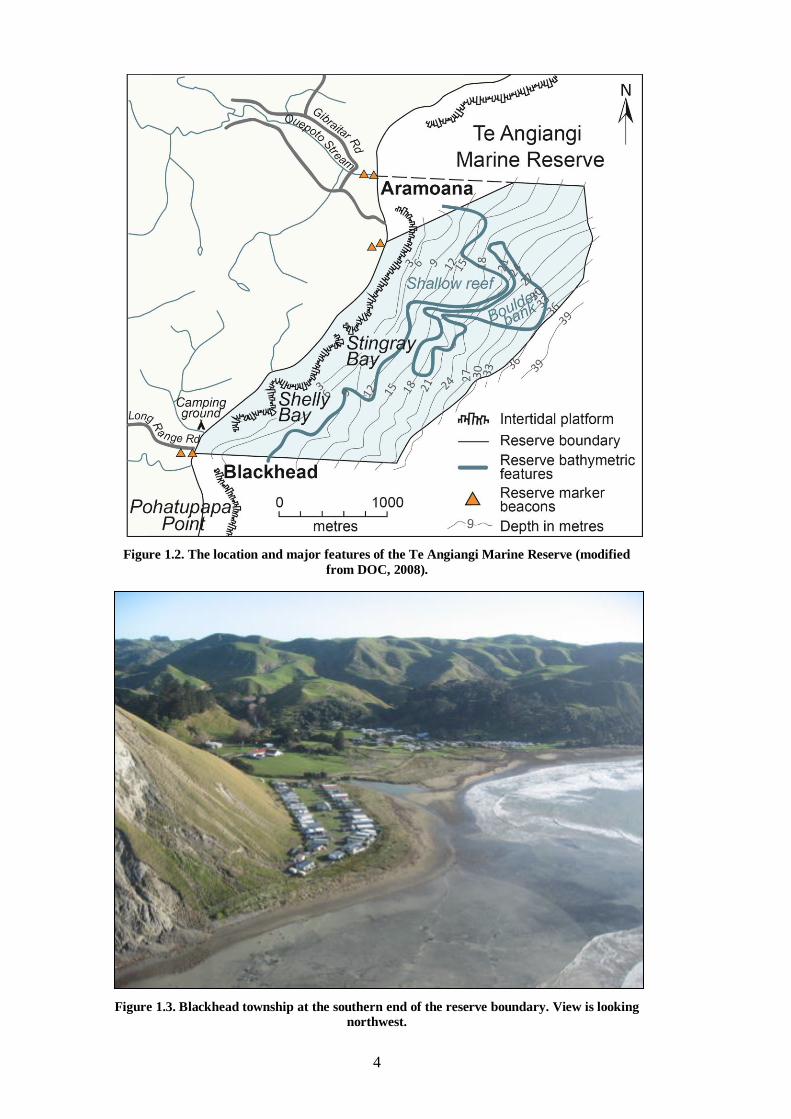
Figure 1.2. The location and major features of the Te Angiangi Marine Reserve
(modified from DOC, 2008). ................................................................................ 4
Figure 1.3. Blackhead township at the southern end of the reserve boundary. View
is looking northwest. ............................................................................................ 4
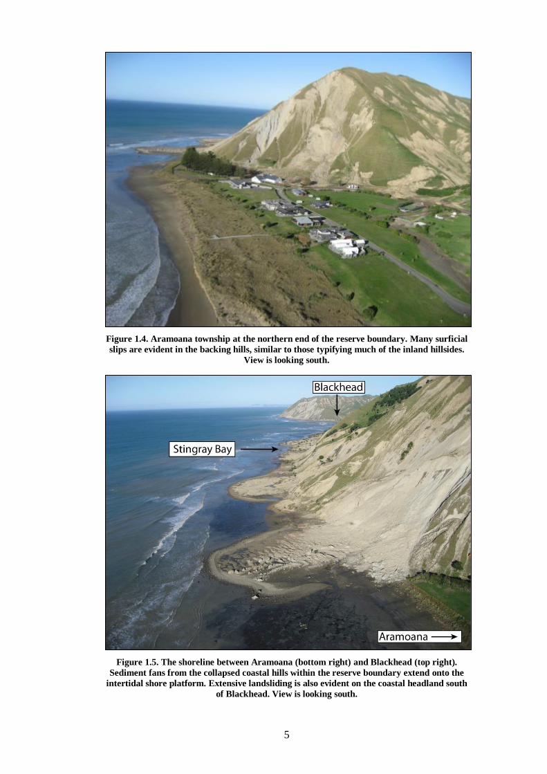
Figure 1.4. Aramoana township at the northern end of the reserve boundary. Many
surficial slips are evident in the backing hills, similar to those typifying much of
the inland hillsides. View is looking south. .......................................................... 5
Figure 1.5. The shoreline between Aramoana (bottom right) and Blackhead (top
right). Sediment fans from the collapsed coastal hills within the reserve boundary
extend onto the intertidal shore platform. Extensive landsliding is also evident on
the coastal headland south of Blackhead. View is looking south. .......................... 5
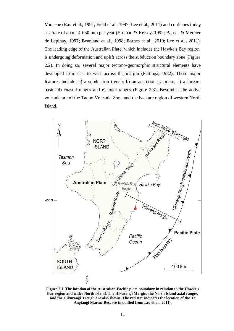
Figure 2.1. The location of the Australian-Pacific plate boundary in relation to the
Hawke's Bay region and wider North Island. The Hikurangi Margin, the North
Island axial ranges, and the Hikurangi Trough are also shown. The red star
indicates the location of the Te Angiangi Marine Reserve (modified from Lee et
al., 2011). ........................................................................................................... 11
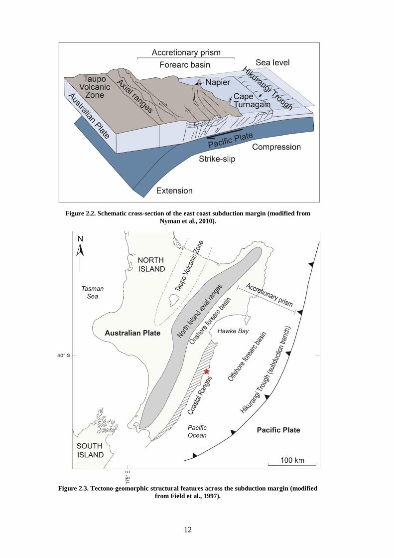
Figure 2.2. Schematic cross-section of the east coast subduction margin (modified
from Nyman et al., 2010). .................................................................................. 12
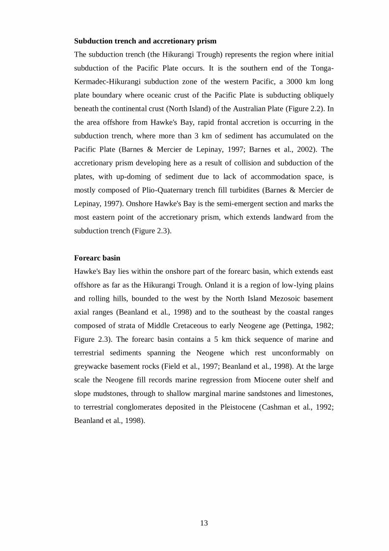
Figure 2.3. Tectono-geomorphic structural features across the subduction margin
(modified from Field et al., 1997). ..................................................................... 12
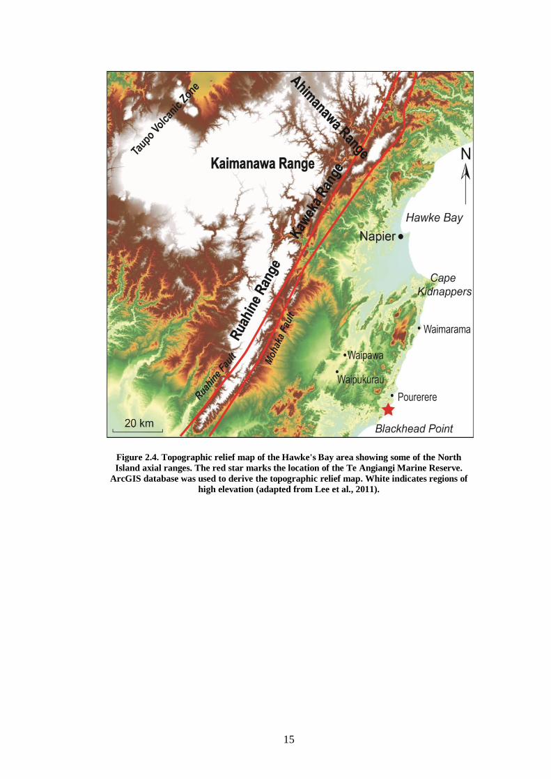
Figure 2.4. Topographic relief map of the Hawke's Bay area showing some of the
North Island axial ranges. The red star marks the location of the Te Angiangi
Marine Reserve. ArcGIS database was used to derive the topographic relief map.
White indicates regions of high elevation (adapted from Lee et al., 2011). ......... 15
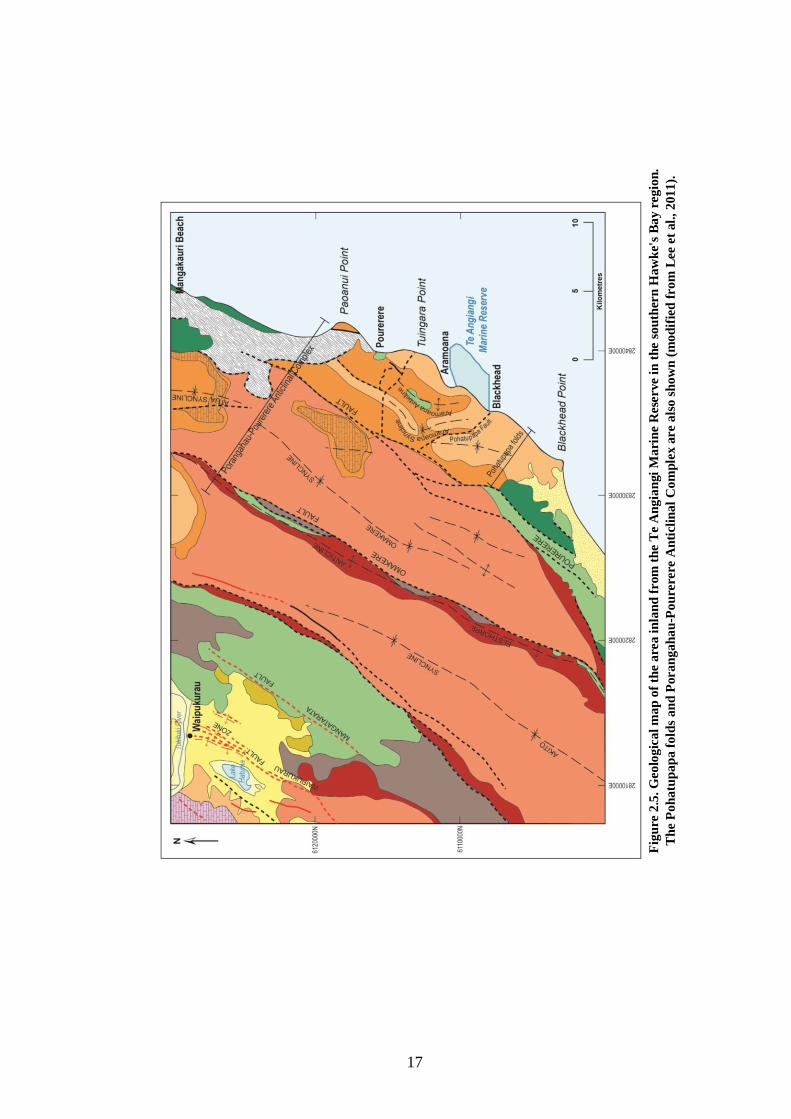
Figure 2.5. Geological map of the area inland from the Te Angiangi Marine
Reserve in the southern Hawke's Bay region. The Pohatupapa folds and
Porangahau-Pourerere Anticlinal Complex are also shown (modified from Lee et
al., 2011). ........................................................................................................... 17
Figure 2.6. Geological legend for Figure 2.5. ..................................................... 18
Figure 2.7 Generalised panel diagram showing the Cretaceous to recent
stratigraphy and depositional environments for the sedimentary rock column in
southern Hawke's Bay. WM is the approximate stratigraphic position of the
Whangaehu Formation mudstone, which contains tubular concretions, and which
has many similar characteristics to the Mapiri Formation mudstone (taken from
Nyman et al., 2010). ........................................................................................... 19
XIV
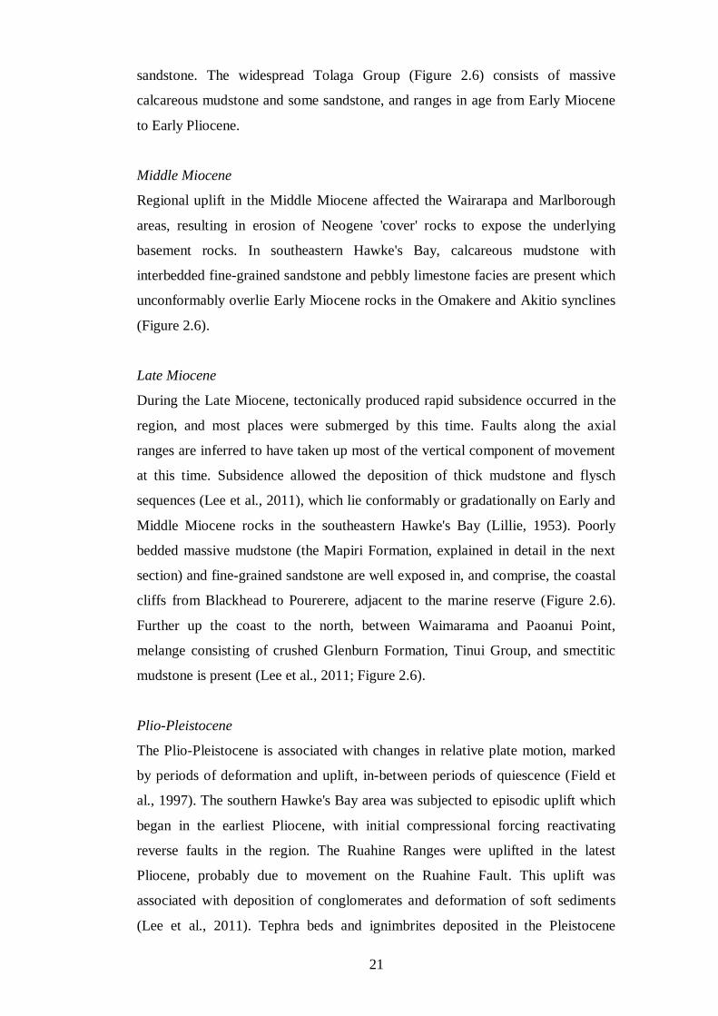
Figure 2.8. In situ carbonate concretions protruding from the intertidal shore
platform as a result of erosion of the surrounding softer host mudstone. ............. 24
Figure 2.9. A section of the intertidal shore platform showing abundant randomly
scattered concretions. Some landslide debris is also evident in the foreground....24
Figure 3.1. Mudstone weathering process. Large jointed block of bedrock (left)
from which clasts of variable sizes were released (middle) and further
disintegrated into smaller rounded "spheroids" of cobble to pebble size (right). .. 25
Figure 3.2. Mudstone and concretion sample locations. A - Sample DM2 was
collected from the shore platform. B - Sample DM7 was collected from blocks of
bedrock in the foreground. C - Sample DM3 came from a near in situ concretion.
D - Sample DM1 was collected from a block of highly jointed bedrock in which
the individual joint blocks exhibit prominent spheroidal weathering. Red arrows
approximate sampling positions. ........................................................................ 27
Figure 3.3. Rock sample locations (red dots) in the Te Angiangi Marine Reserve.
Blue line marks the reserve boundary. Satellite image derived from ArcGIS
database. ............................................................................................................ 27
Figure 3.4. Flow chart of laboratory analyses carried out on samples. ................ 29
Figure 3.5. The set up used to measure carbonate percentage. ............................ 31
Figure 3.6. The expected movement of primary (001) peak positions of the main
clay minerals in untreated, glycolated and heated oriented sample mounts. ........ 34
Figure 3.7. Bulk mineralogical XRD scan for mudstone sample DM1. S =
smectite, C = chlorite, I = illite, K = kaolintie, P = plagioclase, Q = quartz, 001 =
primary clay peak, 002 = secondary clay peak. ................................................... 36
Figure 3.8. The average bulk mineralogical composition (relative abundances
only) of the Mapiri Formation mudstone. A=abundant, C=common, S=some and
N=absent............................................................................................................ 37
Figure 3.9. Bulk mineralogical composition of dolomitic concretion sample DM3.
A=abundant, C=common, S=some and N=absent. .............................................. 37
Figure 3.10. Bulk mineralogical composition of calcitic concretion sample DM4.
A=abundant, C=common, S=some and N=absent. .............................................. 38
Figure 3.11. General clay mineral composition and relative abundances in
samples. ............................................................................................................. 39
Figure 3.12. Sample DM1 mudstone untreated (air dried) oriented mount XRD
scan. S = smectite, C = chlorite, I = illite, K = kaolintie, 001 = primary peak, 002
= secondary peak. .............................................................................................. 40
XV
Figure 3.13. Sample DM1 mudstone ethylene glycolated oriented mount XRD
scan. S = smectite, C = chlorite, I = illite, K = kaolintie, 001 = primary peak, 002
= secondary peak. .............................................................................................. 40
Figure 3.14. Sample DM1 mudstone heated to 550 °C oriented mount XRD scan.
S = smectite, C = chlorite, I = illite, K = kaolintie, 001 = primary peak, 002 =
secondary peak. ................................................................................................. 41
Figure 3.15. The average mudstone major element composition derived from XRF
analysis of the three mudstone samples. ............................................................. 42
Figure 3.16. The element composition of dolomitic concretion derived from XRF
results. ............................................................................................................... 43
Figure 3.17. The element composition of calcitic concretion derived from XRF
results. ............................................................................................................... 43
Figure 3.18. Trace element composition of the average Mapiri Formation
mudstone, the dolomitic concretion and calcitic concretion. ............................... 44
Figure 3.19. Histograms derived from GRADISTAT showing siliciclastic grain
size distribution in all samples. Note the bimodality of samples DM1 and DM7. 47
Figure 3.20. Ternary diagram showing all samples plotted according to their sand-
silt-clay content (derived from GRADISTAT, based on Folk (1954)). ................ 48
Figure 3.21. Spheroidal weathering occurring within a boulder of mudstone. The
boulder consists of many corestones, each one surrounded by concentric sheets or
layers of weathering rock (examples outlined). .................................................. 49
Figure 3.22. Spheroidal shaped pebbles derived from jointed clasts in the
landslide debris litter the beach zone. ................................................................. 50
Figure 3.23. Major element composition comparison of the average Mapiri
Formation mudstone with the global mudstone average derived from Boggs
(2006). ............................................................................................................... 51
Figure 3.24. A Mapiri Formation tubular concretion exhibiting a central conduit
which likely funnelled methane rich fluids upwards in a cold seep system in the
Late Miocene. .................................................................................................... 54
Figure 4.1.Schematic of a landslide showing the aspects that were measured, if
possible, during field work (modified from Selby, 1993). ................................... 56
Figure 4.2. Approximate locations of the Waipoapoa and Ponui landslides, the
Waitawhiti Complex, and the approximate western limit of gravitational collapse
of the Kairakau-Waimarama Regional Slump (modified from Pettinga, 2004 and
Lacoste et al., 2009). .......................................................................................... 57
Figure 4.3. A - Some of the hill side within the reserve pre-April 2011 storm
(photo taken in 2008). Outlined are obvious old landslide scarps. B - The same
hill side post-April 2011 storm (photo taken in 2012). Main scarps of slips 7 to 11
XVI
are outlined. Slip 7 is in the southern part of the reserve and slips 9 to 10 are
directly opposite Stingray Bay. .......................................................................... 61
Figure 4.4. Landslides in the northern half of the reserve. Main scarps of slips 7 to
14 are outlined. View is looking south. .............................................................. 62
Figure 4.5. Slope failures on hills south outside the reserve. ............................... 62
Figure 4.6. Main scarps of slips 1 to 9 are outlined. A - Slips 1 to 3 measure about
20 m in length along the scarps and are closest to Blackhead. Their estimated
depths are ~1 m. B - Slip 4. The scarp length measures about 45 m, with an
estimated depth of ~1 m. C - 'Slip' 5, which is characteristic of a debris flow, has
an estimated depth of ~2 m. D - Slip 6. The scarp length measures about 156 and
is the largest slip to occur heading north from Blackhead, with an estimated depth
of ~4 m. E - Slip 7. The scarp length measures about 167 m, with an estimated
depth of ~3m. F - Slips 8 and 9, both with estimated depths of ~3 m. The scarp
length of slip 8 is about 400 m. .......................................................................... 63
Figure 4.7. Main scarps of slips 10 to 14 are outlined. A - Slips 8, 10 and 11. 'Slip'
11 represents an area of multiple slope failures along ~ 200 m of hill side. B - Slip
10 has an estimated depth of ~3 m. C - Slips 12 (estimated depth of ~4 m), 13
(estimated depth of ~3 m) and 14 (refer to Figures 4.7 to 4.9 for some slip
dimensions). D - Debris from slip 14. The black box outlines the location of E
which shows the northern flank of slip 14 estimated at ~2 - 3 m deep. ................ 64
Figure 4.8. Debris measurements of slip 12, including the length around the debris
frontal lobe, the maximum length (or extent) of the debris, and the width of the
debris at the base of the hill. Also shown is the width near the top of the debris
mass. .................................................................................................................. 65
Figure 4.9. Debris and scarp measurements of slip 13, including the scarp length
at the crown, the length around the debris frontal lobe, the maximum length (or
extent) of the debris, and the width of the debris at the base of the hill. .............. 65
Figure 4.10. Debris measurements of slip 14, including the length around the
debris frontal lobe, the maximum length (or extent) of the debris, and the width of
the debris at the base of the hill. Also shown is the width near the bottom, and the
width at the top, of the debris mass..................................................................... 66
Figure 4.11. Google Earth image showing the distribution of landslides directly
adjacent to the reserve. The main scarp of each landslide is outlined, along with
the length and width of the landslide scars. These measurements were used to
estimate an overall volume of sediment delivered into the reserve from these
landslides. .......................................................................................................... 69
Figure 4.12. Pre-storm mosaic of satellite images from the KiwImage program.
Dates the images were taken range from 2006-2010 (from Jones et al., 2011). The
red line delineates their study area. The image scale is 1:850,000. ...................... 71
Figure 4.13. Post-storm satellite images from the RapidEye system. Images were
taken between 18-19 May 2011 (from Jones et al., 2011). The red line delineates
the study area. .................................................................................................... 72
XVII
Figure 4.14. ArcGIS post-storm (RapidEye) satellite image with pre- and post-
storm bare ground. The general boundary of the three stream catchments is
outlined in black, and the purple represents post-storm bare ground present within
the overall catchment boundary. The image scale is 1:50,000. ............................ 73
Figure.5.1. Schematic showing marine sediments on the continental shelf and
slope off the Te Angiangi Marine Reserve and the general southern Hawke's Bay
and Wairarapa coastline (data from Lewis & Gibb, 1970 and Lewis, 1971). ....... 78
Figure 5.2. Nearshore subtidal biological habitat types in the vicinity of the study
area (modified from Funnell et al., 2005). .......................................................... 80
Figure 5.3. The bathymetry of the nearshore area encompassing the Te Angiangi
Marine Reserve (modified from Funnell et al., 2005). ........................................ 81
Figure 5.4. Wave rose of significant wave height and mean wave direction (waves
primarily travel to the north, as indicated by the bold arrow) offshore from the Te
Angiangi Marine Reserve (from Oldman et al., 2006). ....................................... 82
Figure 5.5. Coastal currents, eddies, water masses and fronts around New
Zealand. The currents are the East Auckland Current (EAUC), West Auckland
Current (WAUC), East Cape Current (ECC), D'Urville Current (DC), Westland
Current (WC), Antarctic Circumpolar Current (ACC), Southland Current (SC)
and the Wairarapa Coastal Current (WCC). The eddies are the North Cape Eddy
(NCE), East Cape Eddy (ECE) and Wairarapa Eddy (WE). The water masses are
Subtropical Water (STW), Subantarctic Water (SAW) and Circumpolar Surface
Water (CSW). The fronts are positioned where the CSW and SAW meet - the
Subantarctic Front (SAF), where the SAW and STW meet - the Subtropical Front
(STF), and the Tasman Front, located in STW to the far north (image modified
from http://www.shiningaspotlight.org.nz/31-the-oceanography-of-the-new-
zealand-marine-ecoregion). ................................................................................ 84
Figure 5.6. Sediment sampling transect locations. .............................................. 86
Figure 5.7. A - The ponar grab sampler. B - The ponar grab sampler being
deployed using a pulley. ..................................................................................... 87
Figure 5.8.A - A ponar grab sample being emptied into a container. B -
Subsample of sediment being taken from the grab sample. ................................. 88
Figure 5.9. Flow chart of laboratory analyses carried out on subtidal sediment
samples. ............................................................................................................. 89
Figure 5.10. Grain size results for Transect 1. Samples are dominated by fine and
very fine sand. ................................................................................................... 91
Figure 5.11. Grain size results for Transect 2. Samples are dominated by fine and
very fine sand. This transect includes a beach sand sample (BH1) taken from
Blackhead Beach....................................................................................................91
XVIII
Figure 5.12. Grain size results for Transect 3. Samples are dominated by fine and
very fine sand. With the exception of sample T3-9, the samples show a steady
increase in mud content with depth, and T3-10 is mainly composed of
silt...........................................................................................................................92
Figure 5.13. Grain size results for Transect 4. Samples are dominated by fine and
very fine sand and increase in mud content with increasing depth. This transect
includes a beach sand sample (SB1) taken from Stingray
Bay.........................................................................................................................92
Figure 5.14. Grain size results for Transect 5. Samples are dominated by fine and
very fine sand and increase in mud content with increasing
depth.......................................................................................................................93
Figure 5.15. Grain size results for Transect 6. Samples are dominated by fine and
very fine sand and increase in mud content with increasing depth. This transect
includes a beach sand sample (ARA1) taken from Aramoana
Beach......................................................................................................................93
Figure 5.16. Grain size results for Transect 7. Samples are dominated by fine and
very fine sand and increase in mud content with increasing
depth.......................................................................................................................94
Figure 5.17. Grain size results for Transect 4. Samples are dominated by fine and
very fine
sand........................................................................................................................94
Figure 5.18. Ternary diagram showing all samples plotted according to their sand-
silt-clay content (derived from GRADISTAT, based on Folk
(1954))....................................................................................................................95
Figure 5.19. Grain size distribution along all transects based on Folk (1954)
classification of all samples. Areas where no samples were taken are assumed to
be hard substrate.....................................................................................................96
Figure 5.20. Photomicrographs of samples BH1 and T6-7. A - Quartz and feldspar
from sample BH1, B - XPL image of A showing quartz interference colours. C -
A bioclast, possibly an echinoderm plate, from sample BH1, D - XPL image of A.
Quartz (E) and feldspar (G and H) from sample T6-7, F - XPL image of
E...........................................................................................................................102
Figure 5.1. Photomicrographs from sample T2-10. A - Calcite fragment, which
could be a piece of a bivalve (i.e. oyster or pectinid), B - Calcite fragment under
XPL. C - Quartz and plagioclase grains (plagioclase in the centre of image). D -
Quartz and plagioclase under XPL. E - A benthic foram bioclast. F - Image
showing the general size of grains in sample T2-10............................................103
Figure 5.22. Photomicrographs of rock fragments. A - Crushed mudstone
fragments from sample DM1. B - rock fragments under XPL. C - An example of a
suspected rock fragment from sample BH1. D - BH1 rock fragment under
XPL......................................................................................................................104
XIX
Figure 5.23. Total carbon results for all samples from the LECO method, with
grain size (black lines) superimposed showing the increase in total carbon with
decreasing grain size
relationship...........................................................................................................106
Figure 5.24. Inorganic carbon (IC) and organic carbon (OC) components of
representative samples from the LOI method, with grain size (black lines)
superimposed showing the increase in organic carbon with decreasing grain size
relationship...........................................................................................................107
Figure 5.25. The organic carbon results derived from the subtraction of inorganic
carbon (from LOI) from total carbon (from LECO), compared to the organic
carbon value derived from
LOI.................................................................................................................. .....109
Figure 6.1. The effects of direct sediment deposition and suspended sediment
concentration on a soft sediment ecosystem. As the disturbance regime increases,
more effects are triggered (modified from Thrush et al., 2004). ........................ 117
Figure 6.2. Marine reserves in New Zealand (from the DOC website). ............. 119
Figure 6.3. The most common species of paua in New Zealand, the black-foot
Haliotis iris (from nabis.govt.nz). .................................................................... 123
Figure 6.4. The New Zealand sea urchin, or kina Evechinus chloroticus (from
forestandbird.org.nz). ....................................................................................... 124
Figure 6.5. Seagrass Zostera capricorni, surrounded by Neptune's necklace
(Hormosira banksii top and bottom right corners of the photo) within a 0.25 m2
quadrat. ............................................................................................................ 126
Figure 6.6. Locations of non-reserve and reserve sites used in the 2011 intertidal
survey. ............................................................................................................. 132
Figure 6.7. Paua on the underside of a rock about to be measured using callipers.
........................................................................................................................ 135
Figure 6.8. A 0.25 m2 quadrat used to measure seagrass parameters. Outlined in
the red circle is a smaller 8 cm2 quadrat used to estimate shoot density. ........... 136
Figure 6.9. Paua abundance and size at each of the low and middle shore heights
for each site. Reserve (C, D, E, F) and non-reserve (A, B, G, H) sites are
delineated by the black vertical lines. Shown is the total paua counted (A) and
their average size (B). This total is divided into adult (>50 mm length) and
juvenile number (<50 mm length; C and E respectively) and average size (D and F
respectively). ................................................................................................... 139
Figure 6.10. Kina abundance and size at each of the low and middle shore heights
for each site. Reserve (C, D, E, F) and non-reserve (A, B, G, H) sites are
delineated by the black vertical lines. Shown is the total paua counted (A) and
their average size (B). This total is divided into adult (>30 mm in size) and
XX
juvenile number (<30 mm in size; C and E respectively) and average size (D and
F respectively). ................................................................................................ 141
Figure 6.11. Seagrass cover and average patch size at each site. ....................... 144
Figure 6.12. Seagrass quadrat results for each site. Shown is the percent of
seagrass cover within the quadrat, and the percent of that seagrass which was
green (A). B shows the average blade length and average shoot density (shoot
density was estimated using small 3 x 8 cm2 quadrats). Reserve (C, D, E, F) and
non-reserve (A, B, G, H) sites are delineated by the black vertical lines. .......... 145
Figure 6.13. An estimate of paua density and average paua size at non-reserve
locations Blackhead (BH) and Aramoana (ARA), and marine reserve location
(MR), in years 1999 to 2003 (pre-event) and 2011 (post-event). ....................... 146
Figure 6.14. An estimate of kina density and average kina size at non-reserve
locations Blackhead (BH) and Aramoana (ARA), and marine reserve location
(MR), in years 1999 to 2003 (pre-event) and 2011 (post-event). ....................... 147
Figure 7.1. Schematic diagrams outlining the response to the 2011 sedimentation
event on marine reserve populations. The blue 'P' (paua) and red 'K' (kina) are
used to demonstrate the relative abundance of paua and kina in the low and mid
shore before, during and after the event. Green patches of grass represent seagrass
abundance before, during and after the event. Before the event (A), the reserve
was functioning well and contained a presumably more robust ecological balance
of interacting biological components. When the sedimentation event happened
(B), landslide debris smothered a significant portion of the intertidal platform
within the reserve and reduced paua and kina populations and seagrass abundance.
The landslide debris began eroding into fine sized particles and being transported
offshore. After the sedimentation event (C), the marine reserve populations began
to recover, and landslide debris on the intertidal platform continues to rapidly
reduce. ............................................................................................................. 155
XXI
LIST OF TABLES
Table 3.1. Description of sample collections. ..................................................... 28
Table 3.2. Carbonate percentage results for mudstone (DM1, DM2 and DM7) and
concretion (DM3 and DM4) samples. ................................................................ 32
Table 3.3. Important peak positions of some common minerals found in the
mudstone and concretion samples. ..................................................................... 35
Table 3.4. Statistical parameters derived from GRADISTAT for the acid insoluble
siliciclastic fraction of all samples based on the Folk & Ward (1957) method.
*Sorting, skewness and kurtosis results for samples DM1 and DM7 are biased due
to their bimodal size distribution. % sand, silt and clay derived from raw data
from Malvern laser sizer. ................................................................................... 46
Table 4.1. Figures associated with each slip. ...................................................... 66
Table 4.2. The estimated volume of sediment derived from each landslide
(excluding slip 4 and 11). The total volume has an error estimate of ±75.02 m2. . 69
Table 5.1. Average sand, silt and clay contents of the sand, silty sand, muddy sand
and sandy silt textural groups (see Figure 5.17). ................................................. 96
Table 5.2. Detrital mineralogy data for Transect 2. Samples BH1 and T2-10
(highlighted) are representative intertidal sand and subtidal sand samples chosen
for further mineralogical
analysis...................................................................................................................98
Table 5.3. Detrital mineralogy data for Transect 4................................................99
Table 5.4. Detrital mineralogy data for Transect 6. Sample T6-7 (highlighted) is a
representative silty sand sample chosen for further mineralogical
analysis...................................................................................................................99
Table 5.5. Key to abbreviations used for petrographic analysis in Tables 5.2 -
5.4...........................................................................................................................99
Table 5.6. Comparison of LECO and LOI carbon results for selected
samples.................................................................................................................108
Table 6.1. Pre-reserve and post-reserve surveys done on the reef platform, paua
and kina, and seagrass, and their associated references. .................................... 128
Table 6.2. A list of sampling undertaken at each site. The number of seagrass
transects sampled varied due landslide debris extending onto the intertidal
platform, which reduced the area available for sampling. Sites E and F were
severely impacted by debris, and therefore any area available was measured out
and sampled. .................................................................................................... 133

XXII
Table 6.3. Human predation and sedimentation stressors acting upon areas to the
south at Blackhead (BH), the marine reserve (MR) and to the north at Aramoana
(ARA). ............................................................................................................. 134
Table 6.4. Main paua and kina results for reserve and non-reserve populations
sampled in the 2011 survey. ............................................................................. 143
Table 6.5. Seagrass transect results. Shown is the total area sampled at each site,
the area and percent of seagrass found within that area, and the mean patch size
for each site. A comparison of the total percent seagrass cover between reserve
and non-reserve sites is also shown. ................................................................. 144
1
Chapter 1
INTRODUCTION
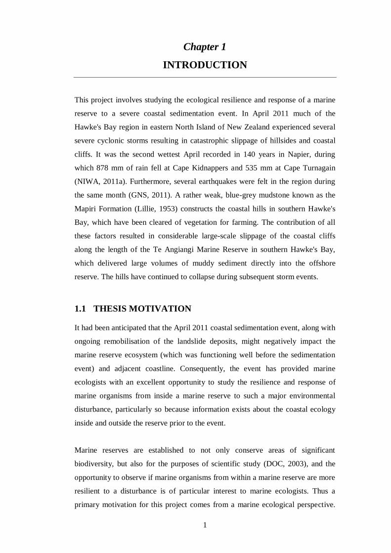
This project involves studying the ecological resilience and response of a marine
reserve to a severe coastal sedimentation event. In April 2011 much of the
Hawke's Bay region in eastern North Island of New Zealand experienced several
severe cyclonic storms resulting in catastrophic slippage of hillsides and coastal
cliffs. It was the second wettest April recorded in 140 years in Napier, during
which 878 mm of rain fell at Cape Kidnappers and 535 mm at Cape Turnagain
(NIWA, 2011a). Furthermore, several earthquakes were felt in the region during
the same month (GNS, 2011). A rather weak, blue-grey mudstone known as the
Mapiri Formation (Lillie, 1953) constructs the coastal hills in southern Hawke's
Bay, which have been cleared of vegetation for farming. The contribution of all
these factors resulted in considerable large-scale slippage of the coastal cliffs
along the length of the Te Angiangi Marine Reserve in southern Hawke's Bay,
which delivered large volumes of muddy sediment directly into the offshore
reserve. The hills have continued to collapse during subsequent storm events.
1.1 THESIS MOTIVATION
It had been anticipated that the April 2011 coastal sedimentation event, along with
ongoing remobilisation of the landslide deposits, might negatively impact the
marine reserve ecosystem (which was functioning well before the sedimentation
event) and adjacent coastline. Consequently, the event has provided marine
ecologists with an excellent opportunity to study the resilience and response of
marine organisms from inside a marine reserve to such a major environmental
disturbance, particularly so because information exists about the coastal ecology
inside and outside the reserve prior to the event.
Marine reserves are established to not only conserve areas of significant
biodiversity, but also for the purposes of scientific study (DOC, 2003), and the
opportunity to observe if marine organisms from within a marine reserve are more
resilient to a disturbance is of particular interest to marine ecologists. Thus a
primary motivation for this project comes from a marine ecological perspective.

2
However, to better interrelate causes and effects, it is pertinent to also investigate
the various physical environmental aspects (geology, geomorphology, engineering
properties, climate, sediment types, ocean wave and current conditions) associated
with the biological elements. Thus an interdisciplinary approach between marine
ecology and Earth sciences is the best way to comprehensively address this topic.
1.2 THESIS OBJECTIVES
There are four main objectives of this project. Three of them address the physical
aspects of the project, and the fourth involves reconnaissance examination of the
response of the marine ecology to sedimentation.
1) Examine the geology of the coastal area immediately adjacent to the Te
Angiangi Marine Reserve, and to determine the structures (bedding, joints, faults,
folds), texture, chemical composition and mineralogy (especially clay mineral
types) of the dominant mudrock lithology.
2) Describe (including gathering estimates of the volume of new sediment
suddenly introduced into the coastal environment) and classify the slope failures
along the coastal hills adjacent to the Te Angiangi Marine Reserve.
3) Investigate the present and likely future erodability of the slip material, and the
ensuing sediment dispersal mechanisms and depositional patterns across and
along the coastal platform and nearshore region encompassing the marine reserve.
This could help explain any spatial and temporal response of the marine
organisms to sedimentation, as it is hypothesised that nearshore currents flowing
to the north could carry and deposit sediment in the coastal zone north of the
reserve.
4) The material derived from the landslides has extended out onto the intertidal
shore platform, posing a serious threat to the intertidal marine organisms living on
the platform, and also beyond into the subtidal zone. A preliminary survey of the
intertidal marine ecology from within and outside the reserve has been made in
order to assess the impact on the marine organisms in response to the high
sedimentation events. There is considerable pre-April 2011 ecological information

3
with which the results of this survey can be compared in order to detect any
changes in the size and abundance of organisms.
1.3 STUDY AREA
The Te Angiangi Marine Reserve is located in the southern Hawke's Bay region
on the east coast of the North Island, about 30 km east of Waipukurau and
Waipawa townships (Figure 1.1). The reserve extends one nautical mile offshore
from the high water mark and in total covers approximately 446 hectares, an area
which is considered representative of the wider southern Hawke's Bay coastal
marine environment (Figure 1.2). It is bordered by the coastal villages of
Blackhead (Figure 1.3) in the south and Aramoana (Figure 1.4) in the north with
about 2.7 km of shoreline between the two villages (Figure 1.5).
Figure 1.1. Locality map showing all place names and regions mentioned in the text. The red
star marks the location of the Te Angiangi Marine Reserve.
4
Figure 1.2. The location and major features of the Te Angiangi Marine Reserve (modified
from DOC, 2008).
Figure 1.3. Blackhead township at the southern end of the reserve boundary. View is looking
northwest.
5
Figure 1.4. Aramoana township at the northern end of the reserve boundary. Many surficial
slips are evident in the backing hills, similar to those typifying much of the inland hillsides.
View is looking south.
Figure 1.5. The shoreline between Aramoana (bottom right) and Blackhead (top right).
Sediment fans from the collapsed coastal hills within the reserve boundary extend onto the
intertidal shore platform. Extensive landsliding is also evident on the coastal headland south
of Blackhead. View is looking south.
6
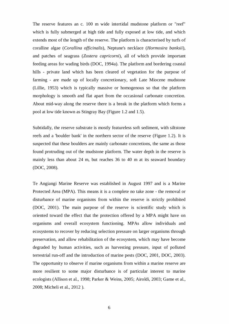
The reserve features an c. 100 m wide intertidal mudstone platform or "reef"
which is fully submerged at high tide and fully exposed at low tide, and which
extends most of the length of the reserve. The platform is characterised by turfs of
coralline algae (Corallina officinalis), Neptune's necklace (Hormosira banksii),
and patches of seagrass (Zostera capricorni), all of which provide important
feeding areas for wading birds (DOC, 1994a). The platform and bordering coastal
hills - private land which has been cleared of vegetation for the purpose of
farming - are made up of locally concretionary, soft Late Miocene mudstone
(Lillie, 1953) which is typically massive or homogenous so that the platform
morphology is smooth and flat apart from the occasional carbonate concretion.
About mid-way along the reserve there is a break in the platform which forms a
pool at low tide known as Stingray Bay (Figure 1.2 and 1.5).
Subtidally, the reserve substrate is mostly featureless soft sediment, with siltstone
reefs and a 'boulder bank' in the northern sector of the reserve (Figure 1.2). It is
suspected that these boulders are mainly carbonate concretions, the same as those
found protruding out of the mudstone platform. The water depth in the reserve is
mainly less than about 24 m, but reaches 36 to 40 m at its seaward boundary
(DOC, 2008).
Te Angiangi Marine Reserve was established in August 1997 and is a Marine
Protected Area (MPA). This means it is a complete no take zone - the removal or
disturbance of marine organisms from within the reserve is strictly prohibited
(DOC, 2001). The main purpose of the reserve is scientific study which is
oriented toward the effect that the protection offered by a MPA might have on
organisms and overall ecosystem functioning. MPAs allow individuals and
ecosystems to recover by reducing selection pressure on larger organisms through
preservation, and allow rehabilitation of the ecosystem, which may have become
degraded by human activities, such as harvesting pressure, input of polluted
terrestrial run-off and the introduction of marine pests (DOC, 2001, DOC, 2003).
The opportunity to observe if marine organisms from within a marine reserve are
more resilient to some major disturbance is of particular interest to marine
ecologists (Allison et al., 1998; Parker & Weins, 2005; Airoldi, 2003; Game et al.,
2008; Micheli et al., 2012 ).
7
1.4 THESIS FORMAT
This thesis is formatted so the physical aspects of the project are addressed first,
which then lead into the biological aspects, before finishing with an overall
synthesis and discussion chapter. Chapters 2 to 5 deals with the geological and
sedimentation aspects of the project. Chapter 2 provides the tectonic and
geological setting and history of the Hawke's Bay region, as well as background
information on the origin, age, structural and geological characteristics of the
dominant lithology present in the study area. Chapter 3 presents in some detail the
geological characteristics of the dominant mudstone lithology which make up the
coastal hills in the study area. Chapter 4 addresses landsliding aspects, in
particular the suspected triggers of slope failures, the distribution and nature of the
landslides, and the estimated volume of sediment released into the marine
environment due to landsliding. Chapter 5 outlines the possible offshore
depositional patterns of the sediment released by the landslides into the marine
environment. It includes a description of the physical oceanography and
bathymetry in the area, along with results from an offshore sediment sampling
exercise. Chapters 6 deals with the biological aspects of the project, and includes
previous marine ecological work carried out in the Te Angiangi Marine Reserve.
It then describes the marine intertidal survey carried out after the 2011 storm
event, the results of this survey, and uses the results to compare and create multi-
year patterns with previous comparable surveys. Chapter 7 attempts to integrate
the results from all previous chapters to gauge any interrelationships between the
catastrophic sedimentation event and the ecological resilience of organisms within
the marine reserve.
To allow the reader to progress through the thesis with ease, and because of the
segmented nature of the thesis, field and laboratory methods will be addressed in
their relevant chapters, so there is no single chapter outlining all the field and
laboratory methods. Most chapters are formatted to include introduction, aims,
background information, field and laboratory methods, results and discussion
sections.

8
9
2 Chapter 2
GEOLOGICAL SETTING
This chapter describes the tectonic and geological setting of the Hawke's Bay
region which aids understanding of the physical aspects of the project.
2.1 TECTONIC AND GEOLOGICAL SETTING OF THE
EAST COAST, NORTH ISLAND
It is relevant to examine the geological setting, including the historical to present
day tectonics, structure and stratigraphy, of the Hawke's Bay region for two
reasons: (1) to know the depositional paleoenvironmental conditions of the
mudstone bedrock underpinning the reserve, and put this into a regional tectonic
context; and (2) to appreciate the historical to present day structural forces
impacting on the region. Such information will allow for further understanding
and characterisation of the mudstone, and assist in proposing likely causes of
slippage, and the effects this slipped mudstone might have on the marine reserve
environment.
The section begins by providing a regional context for the Hawke's Bay
geological structure and stratigraphy, followed by more specific examination of
the lithology and structures in the vicinity of the Te Angiangi Marine Reserve
itself.
10
2.1.1 Previous work
The earliest reference to the geology of the area south of Hawke's Bay was by
Hochstetter (1867), where the Hawke's Bay Series was described as a group of
limestone, sandstone and clay marls. The geology of the Dannevirke Subdivision,
including the study area, was investigated in detail by Lillie (1953). This is one of
the earliest and fundamental texts describing the geology of this region and was
produced as part of a regional geological mapping survey of New Zealand, with
the eventual aim of assisting with oil exploration activities. The most recent and
up-to-date text describing Hawke's Bay geology and structure is by Lee et al.,
(2011), published as part of the new New Zealand 1:250 000 Geological Map
Series (QMAP) produced by GNS Science. Many texts, such as Kamp (1992),
Field et al., (1997), Bland & Kamp (2006), Barnes et al., (2010) and Lee et al.,
(2011), explain the tectonically active geological and structural setting of the
Hawke's Bay region, sitting as it does within the Hikurangi Subduction Margin.
The following section outlines the influence of the subduction margin on the
region.
2.1.2 Regional structure
The Te Angiangi study area is located in the Hawke's Bay of eastern North Island
(Figure 1.1), an area influenced geologically and structurally by the obliquely
convergent Australian-Pacific plate boundary. The boundary runs in a southwest
to northeast direction offshore along the North Island's east coast, almost parallel
to the southern Hawke's Bay coastline where the Te Angiangi Marine Reserve is
located (Figure 2.1). The plate boundary in this area is expressed in seafloor
bathymetry as a subduction zone known as the Hikurangi Margin, where the
dense oceanic crust of the Pacific Plate is obliquely converging and subducting
beneath the more buoyant continental crust of the Australian Plate (Foster &
Carter, 1997; Barnes et al., 2002; Lewis & Pettinga, 1993; Bland & Kamp, 2006).
The Hikurangi Margin encompasses the area from where the plates converge in
the east, to the axial ranges on the North Island landmass to the west (Figure 2.1).
The Hikurangi Trough is part of the margin, otherwise known as the subduction
trench, and is about 3000 m deep. It is where the Pacific Plate dips at an angle of
about 3° for about 100 km before steepening beneath the North Island (Barnes et
al., 2010; Figure 2.2). Subduction in the Hikurangi Margin began in the Early
11
Miocene (Rait et al., 1991; Field et al., 1997; Lee et al., 2011) and continues today
at a rate of about 40-50 mm per year (Erdman & Kelsey, 1992; Barnes & Mercier
de Lepinay, 1997; Beanland et al., 1998; Barnes et al., 2010; Lee et al., 2011).
The leading edge of the Australian Plate, which includes the Hawke's Bay region,
is undergoing deformation and uplift across the subduction boundary zone (Figure
2.2). In doing so, several major tectono-geomorphic structural elements have
developed from east to west across the margin (Pettinga, 1982). These major
features include: a) a subduction trench; b) an accretionary prism; c) a forearc
basin; d) coastal ranges and e) axial ranges (Figure 2.3). Beyond is the active
volcanic arc of the Taupo Volcanic Zone and the backarc region of western North
Island.
Figure 2.1. The location of the Australian-Pacific plate boundary in relation to the Hawke's
Bay region and wider North Island. The Hikurangi Margin, the North Island axial ranges,
and the Hikurangi Trough are also shown. The red star indicates the location of the Te
Angiangi Marine Reserve (modified from Lee et al., 2011).
12
Figure 2.2. Schematic cross-section of the east coast subduction margin (modified from
Nyman et al., 2010).
Figure 2.3. Tectono-geomorphic structural features across the subduction margin (modified
from Field et al., 1997).
13
Subduction trench and accretionary prism
The subduction trench (the Hikurangi Trough) represents the region where initial
subduction of the Pacific Plate occurs. It is the southern end of the Tonga-
Kermadec-Hikurangi subduction zone of the western Pacific, a 3000 km long
plate boundary where oceanic crust of the Pacific Plate is subducting obliquely
beneath the continental crust (North Island) of the Australian Plate (Figure 2.2). In
the area offshore from Hawke's Bay, rapid frontal accretion is occurring in the
subduction trench, where more than 3 km of sediment has accumulated on the
Pacific Plate (Barnes & Mercier de Lepinay, 1997; Barnes et al., 2002). The
accretionary prism developing here as a result of collision and subduction of the
plates, with up-doming of sediment due to lack of accommodation space, is
mostly composed of Plio-Quaternary trench fill turbidites (Barnes & Mercier de
Lepinay, 1997). Onshore Hawke's Bay is the semi-emergent section and marks the
most eastern point of the accretionary prism, which extends landward from the
subduction trench (Figure 2.3).
Forearc basin
Hawke's Bay lies within the onshore part of the forearc basin, which extends east
offshore as far as the Hikurangi Trough. Onland it is a region of low-lying plains
and rolling hills, bounded to the west by the North Island Mezosoic basement
axial ranges (Beanland et al., 1998) and to the southeast by the coastal ranges
composed of strata of Middle Cretaceous to early Neogene age (Pettinga, 1982;
Figure 2.3). The forearc basin contains a 5 km thick sequence of marine and
terrestrial sediments spanning the Neogene which rest unconformably on
greywacke basement rocks (Field et al., 1997; Beanland et al., 1998). At the large
scale the Neogene fill records marine regression from Miocene outer shelf and
slope mudstones, through to shallow marginal marine sandstones and limestones,
to terrestrial conglomerates deposited in the Pleistocene (Cashman et al., 1992;
Beanland et al., 1998).
14
Coastal ranges
The coastal ranges are a structurally complex zone characterised by uplift, which
began in the earliest Pliocene by contraction in the accretionary wedge. This,
along with extensional (in some areas) tectonics produced pronounced northeast-
southwest trending faults and anticlinal and synclinal structures (Pettinga, 1982;
Cashman et al., 1992; Beanland et al., 1998). The study area is located within the
coastal ranges and is influenced structurally by a series of complex folds and
faults (Figure 2.3).
Axial ranges
The North Island axial ranges are a series of north-northeast trending ranges,
including the Ruahine, Kaweka, Kaimanawa, and Ahimanawa ranges (Figure 2.4).
They are composed of weakly metamorphosed Mesozoic sandstone and
mudstone, otherwise known as greywacke basement rocks, all part of the Torlesse
Terrane (Lee et al., 2011). The ranges are fault bounded, where the major Mohaka
and Ruahine oblique-slip faults, part of the North Island Fault System (otherwise
known as the North Island Shear Belt; Bland & Kamp, 2006), allow basement
rocks to lie adjacent to much younger Neogene 'cover' rocks. The North Island
axial ranges act as the western border of the forearc basin and extend continuously
from Cape Palliser in the Wellington region in the south to East Cape in the north.
There is some distinction made between the Tararua and Ruahine ranges in the
south, within the axial ranges, which strike north-northeast, and the Kaimanawa
and Ruakumara ranges in the north, which strike northeast (Field et al., 1997;
Figure 2.1). The uplift history of the axial ranges probably started in the Early
Miocene or early Middle Miocene as a result of the onset of oblique convergence
of the Australian and Pacific plates. The rate of uplift probably picked up during
the Plio-Pliestocene, and remains ongoing as is evident from the elevations of
marine terraces and the depth of incision of rivers in river valleys (Field et al.,
1997).
15
Figure 2.4. Topographic relief map of the Hawke's Bay area showing some of the North
Island axial ranges. The red star marks the location of the Te Angiangi Marine Reserve.
ArcGIS database was used to derive the topographic relief map. White indicates regions of
high elevation (adapted from Lee et al., 2011).
16
2.1.3 Regional stratigraphy and tectonic history
The Late Cretaceous to Neogene tectonic history and stratigraphy are described in
this section (refer to the New Zealand geological timescale in Appendix 1). A
geological map of the inland area from Te Angiangi Marine Reserve in Figure 2.5
and a stratigraphic panel is shown in Figure 2.7.
Early to Middle Cretaceous
Throughout the Cretaceous the East Coast region (including the Hawke's Bay
region) was positioned along the Pacific margin of Gondwana. In the Early
Cretaceous (105 to 95 Ma), sediments of the Torlesse Terrane were accreted along
this margin (Field et al., 1997; Lee et al., 2011). In the Middle Cretaceous
regional convergence ceased or slowed, and was followed by crustal extension in
some areas, which represented the rifting of New Zealand (Zealandia) from the
Australian and Antarctic eastern side of Gondwana (Field et al., 1997).
Middle Cretaceous to Paleocene
In the Late Cretaceous-early Cenozoic, crustal extension in Zealandia was
underway, which led to the isolation of New Zealand from Gondwana with the
opening of, and seafloor spreading in the Tasman Sea (Field et al., 1997; Lee et
al., 2011). Associated with the opening of the Tasman Sea was a change from a
subduction-dominated to a passive margin setting during the early Late
Cretaceous in eastern North Island (Lee et al., 2011). By the Paleocene seafloor
spreading ceased. In the east of the Wairarapa - Hawke's Bay districts, the Late
Cretaceous Glenburn Formation is present east of the Omakere Fault (Figure 2.5)
and is well exposed along the Waimarama coast. The formation consists of well
bedded, carbonaceous, alternating sandstone and mudstone with concretionary
sandstone and conglomerate lenses that has an inferred depositional environment
of outer shelf to upper bathyal (100 - 600 m depth) in a submarine fan setting (Lee
et al., 2011).
17
Fig
ure
2.5
. G
eo
log
ica
l m
ap
of
the
are
a i
nla
nd
from
th
e T
e A
ng
ian
gi
Ma
rin
e R
ese
rve i
n t
he s
ou
ther
n H
aw
ke'
s B
ay r
egio
n.
Th
e P
oh
atu
pa
pa
fo
lds
an
d P
ora
ng
ah
au
-Po
ure
rere
An
ticl
ina
l C
om
ple
x a
re
als
o s
how
n (
mod
ifie
d f
rom
Lee
et
al.
, 2011).

18
Fig
ure
2.6
. G
eo
log
ica
l le
gen
d f
or
Fig
ure
2.5
.

19
The lower contact of the Glenburn Formation is unknown, while the upper contact
is overlain by the widespread Tinui Group, of Late Cretaceous to late Paleocene
age (Figure 2.6), that includes the Whangai and Waipawa Formations (Figure
2.7). The Tinui Group represents a stable to slowly subsiding depositional
environment, as indicated by a decreasing content of terrigenous material,
increasing amounts of glauconite, and an upward fining grain size. The Whangai
Formation is a light and dark banded, well bedded mudstone with intercalated
bands of glauconitic sandstone, and is conformably overlain by the Waipawa
Formation, a dark brown to black carbonaceous mudstone, also with glauconitic
sandstone. Both formations are present inland from the study area, with the
Waipawa Formation well exposed southeast of Waipukurau (Figure 2.5). The
Whangai Formation was deposited in shelf to bathyal depths, as indicated by
microfossil assemblages, and the Waipawa Formation in an outer shelf to upper
slope basin environment (Lee et al., 2011; Figure 2.7).
Figure 2.7 Generalised panel diagram showing the Cretaceous to recent stratigraphy and
depositional environments for the sedimentary rock column in southern Hawke's Bay. WM
is the approximate stratigraphic position of the Whangaehu Formation mudstone, which
contains tubular concretions, and which has many similar characteristics to the Mapiri
Formation mudstone (taken from Nyman et al., 2010).
20
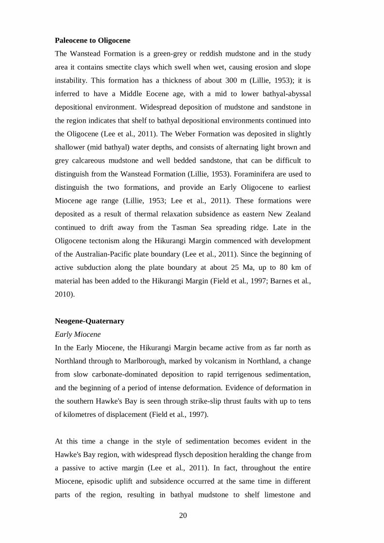
Paleocene to Oligocene
The Wanstead Formation is a green-grey or reddish mudstone and in the study
area it contains smectite clays which swell when wet, causing erosion and slope
instability. This formation has a thickness of about 300 m (Lillie, 1953); it is
inferred to have a Middle Eocene age, with a mid to lower bathyal-abyssal
depositional environment. Widespread deposition of mudstone and sandstone in
the region indicates that shelf to bathyal depositional environments continued into
the Oligocene (Lee et al., 2011). The Weber Formation was deposited in slightly
shallower (mid bathyal) water depths, and consists of alternating light brown and
grey calcareous mudstone and well bedded sandstone, that can be difficult to
distinguish from the Wanstead Formation (Lillie, 1953). Foraminifera are used to
distinguish the two formations, and provide an Early Oligocene to earliest
Miocene age range (Lillie, 1953; Lee et al., 2011). These formations were
deposited as a result of thermal relaxation subsidence as eastern New Zealand
continued to drift away from the Tasman Sea spreading ridge. Late in the
Oligocene tectonism along the Hikurangi Margin commenced with development
of the Australian-Pacific plate boundary (Lee et al., 2011). Since the beginning of
active subduction along the plate boundary at about 25 Ma, up to 80 km of
material has been added to the Hikurangi Margin (Field et al., 1997; Barnes et al.,
2010).
Neogene-Quaternary
Early Miocene
In the Early Miocene, the Hikurangi Margin became active from as far north as
Northland through to Marlborough, marked by volcanism in Northland, a change
from slow carbonate-dominated deposition to rapid terrigenous sedimentation,
and the beginning of a period of intense deformation. Evidence of deformation in
the southern Hawke's Bay is seen through strike-slip thrust faults with up to tens
of kilometres of displacement (Field et al., 1997).
At this time a change in the style of sedimentation becomes evident in the
Hawke's Bay region, with widespread flysch deposition heralding the change from
a passive to active margin (Lee et al., 2011). In fact, throughout the entire
Miocene, episodic uplift and subsidence occurred at the same time in different
parts of the region, resulting in bathyal mudstone to shelf limestone and
21
sandstone. The widespread Tolaga Group (Figure 2.6) consists of massive
calcareous mudstone and some sandstone, and ranges in age from Early Miocene
to Early Pliocene.
Middle Miocene
Regional uplift in the Middle Miocene affected the Wairarapa and Marlborough
areas, resulting in erosion of Neogene 'cover' rocks to expose the underlying
basement rocks. In southeastern Hawke's Bay, calcareous mudstone with
interbedded fine-grained sandstone and pebbly limestone facies are present which
unconformably overlie Early Miocene rocks in the Omakere and Akitio synclines
(Figure 2.6).
Late Miocene
During the Late Miocene, tectonically produced rapid subsidence occurred in the
region, and most places were submerged by this time. Faults along the axial
ranges are inferred to have taken up most of the vertical component of movement
at this time. Subsidence allowed the deposition of thick mudstone and flysch
sequences (Lee et al., 2011), which lie conformably or gradationally on Early and
Middle Miocene rocks in the southeastern Hawke's Bay (Lillie, 1953). Poorly
bedded massive mudstone (the Mapiri Formation, explained in detail in the next
section) and fine-grained sandstone are well exposed in, and comprise, the coastal
cliffs from Blackhead to Pourerere, adjacent to the marine reserve (Figure 2.6).
Further up the coast to the north, between Waimarama and Paoanui Point,
melange consisting of crushed Glenburn Formation, Tinui Group, and smectitic
mudstone is present (Lee et al., 2011; Figure 2.6).
Plio-Pleistocene
The Plio-Pleistocene is associated with changes in relative plate motion, marked
by periods of deformation and uplift, in-between periods of quiescence (Field et
al., 1997). The southern Hawke's Bay area was subjected to episodic uplift which
began in the earliest Pliocene, with initial compressional forcing reactivating
reverse faults in the region. The Ruahine Ranges were uplifted in the latest
Pliocene, probably due to movement on the Ruahine Fault. This uplift was
associated with deposition of conglomerates and deformation of soft sediments
(Lee et al., 2011). Tephra beds and ignimbrites deposited in the Pleistocene
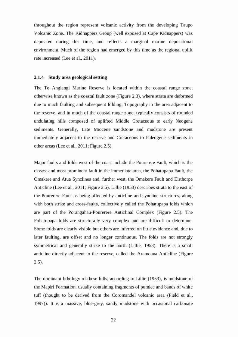
22
throughout the region represent volcanic activity from the developing Taupo
Volcanic Zone. The Kidnappers Group (well exposed at Cape Kidnappers) was
deposited during this time, and reflects a marginal marine depositional
environment. Much of the region had emerged by this time as the regional uplift
rate increased (Lee et al., 2011).
2.1.4 Study area geological setting
The Te Angiangi Marine Reserve is located within the coastal range zone,
otherwise known as the coastal fault zone (Figure 2.3), where strata are deformed
due to much faulting and subsequent folding. Topography in the area adjacent to
the reserve, and in much of the coastal range zone, typically consists of rounded
undulating hills composed of uplifted Middle Cretaceous to early Neogene
sediments. Generally, Late Miocene sandstone and mudstone are present
immediately adjacent to the reserve and Cretaceous to Paleogene sediments in
other areas (Lee et al., 2011; Figure 2.5).
Major faults and folds west of the coast include the Pourerere Fault, which is the
closest and most prominent fault in the immediate area, the Pohatupapa Fault, the
Omakere and Atua Synclines and, further west, the Omakere Fault and Elsthorpe
Anticline (Lee et al., 2011; Figure 2.5). Lillie (1953) describes strata to the east of
the Pourerere Fault as being affected by anticline and syncline structures, along
with both strike and cross-faults, collectively called the Pohatupapa folds which
are part of the Porangahau-Pourerere Anticlinal Complex (Figure 2.5). The
Pohatupapa folds are structurally very complex and are difficult to determine.
Some folds are clearly visible but others are inferred on little evidence and, due to
later faulting, are offset and no longer continuous. The folds are not strongly
symmetrical and generally strike to the north (Lillie, 1953). There is a small
anticline directly adjacent to the reserve, called the Aramoana Anticline (Figure
2.5).
The dominant lithology of these hills, according to Lillie (1953), is mudstone of
the Mapiri Formation, usually containing fragments of pumice and bands of white
tuff (thought to be derived from the Coromandel volcanic area (Field et al.,
1997)). It is a massive, blue-grey, sandy mudstone with occasional carbonate
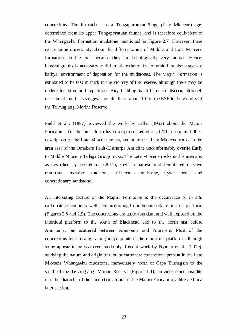
23
concretions. The formation has a Tongaporutuan Stage (Late Miocene) age,
determined from its upper Tongaporutuan faunas, and is therefore equivalent to
the Whangaehu Formation mudstone mentioned in Figure 2.7. However, there
exists some uncertainty about the differentiation of Middle and Late Miocene
formations in the area because they are lithologically very similar. Hence,
biostratigraphy is necessary to differentiate the rocks. Foraminifera also suggest a
bathyal environment of deposition for the mudstones. The Mapiri Formation is
estimated to be 600 m thick in the vicinity of the reserve, although there may be
undetected structural repetition. Any bedding is difficult to discern, although
occasional interbeds suggest a gentle dip of about 10° to the ESE in the vicinity of
the Te Angiangi Marine Reserve.
Field et al., (1997) reviewed the work by Lillie (1953) about the Mapiri
Formation, but did not add to his description. Lee et al., (2011) support Lillie's
description of the Late Miocene rocks, and state that Late Miocene rocks in the
area east of the Omakere Fault-Elsthorpe Anticline unconformably overlie Early
to Middle Miocene Tolaga Group rocks. The Late Miocene rocks in this area are,
as described by Lee et al., (2011), shelf to bathyal undifferentiated massive
mudstone, massive sandstone, tuffaceous mudstone, flysch beds, and
concretionary sandstone.
An interesting feature of the Mapiri Formation is the occurrence of in situ
carbonate concretions, well seen protruding from the intertidal mudstone platform
(Figures 2.8 and 2.9). The concretions are quite abundant and well exposed on the
intertidal platform to the south of Blackhead and to the north just before
Aramoana, but scattered between Aramoana and Pourerere. Most of the
concretions tend to align along major joints in the mudstone platform, although
some appear to be scattered randomly. Recent work by Nyman et al., (2010),
studying the nature and origin of tubular carbonate concretions present in the Late
Miocene Whangaehu mudstone, immediately north of Cape Turnagain to the
south of the Te Angiangi Marine Reserve (Figure 1.1), provides some insights
into the character of the concretions found in the Mapiri Formation, addressed in a
later section.
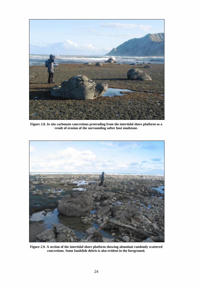
24
Figure 2.8. In situ carbonate concretions protruding from the intertidal shore platform as a
result of erosion of the surrounding softer host mudstone.
Figure 2.9. A section of the intertidal shore platform showing abundant randomly scattered
concretions. Some landslide debris is also evident in the foreground.
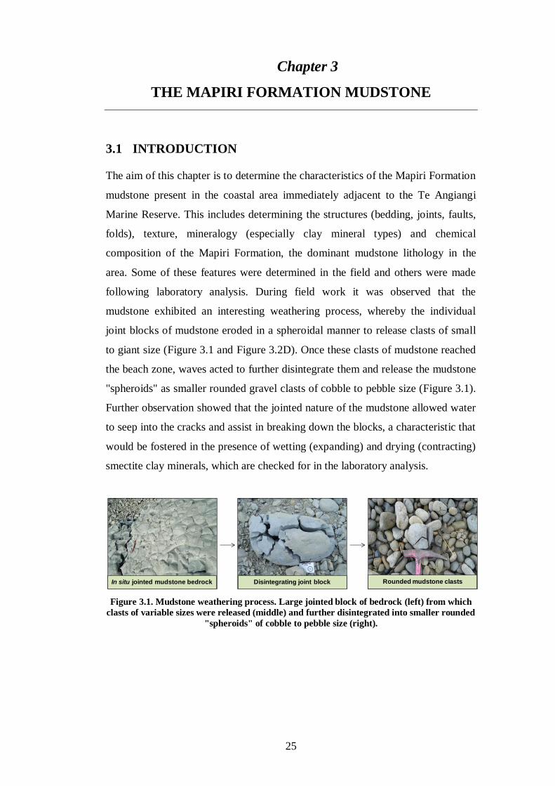
25
3 Chapter 3
THE MAPIRI FORMATION MUDSTONE
3.1 INTRODUCTION
The aim of this chapter is to determine the characteristics of the Mapiri Formation
mudstone present in the coastal area immediately adjacent to the Te Angiangi
Marine Reserve. This includes determining the structures (bedding, joints, faults,
folds), texture, mineralogy (especially clay mineral types) and chemical
composition of the Mapiri Formation, the dominant mudstone lithology in the
area. Some of these features were determined in the field and others were made
following laboratory analysis. During field work it was observed that the
mudstone exhibited an interesting weathering process, whereby the individual
joint blocks of mudstone eroded in a spheroidal manner to release clasts of small
to giant size (Figure 3.1 and Figure 3.2D). Once these clasts of mudstone reached
the beach zone, waves acted to further disintegrate them and release the mudstone
"spheroids" as smaller rounded gravel clasts of cobble to pebble size (Figure 3.1).
Further observation showed that the jointed nature of the mudstone allowed water
to seep into the cracks and assist in breaking down the blocks, a characteristic that
would be fostered in the presence of wetting (expanding) and drying (contracting)
smectite clay minerals, which are checked for in the laboratory analysis.
Figure 3.1. Mudstone weathering process. Large jointed block of bedrock (left) from which
clasts of variable sizes were released (middle) and further disintegrated into smaller rounded
"spheroids" of cobble to pebble size (right).
In situ jointed mudstone bedrock Disintegrating joint block Rounded mudstone clasts
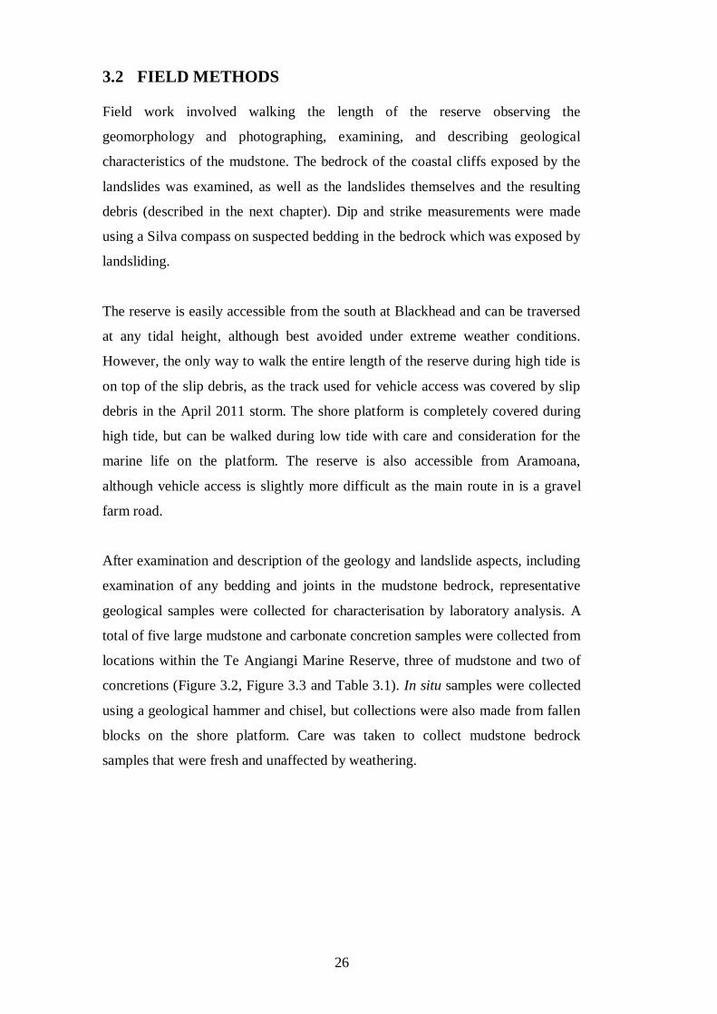
26
3.2 FIELD METHODS
Field work involved walking the length of the reserve observing the
geomorphology and photographing, examining, and describing geological
characteristics of the mudstone. The bedrock of the coastal cliffs exposed by the
landslides was examined, as well as the landslides themselves and the resulting
debris (described in the next chapter). Dip and strike measurements were made
using a Silva compass on suspected bedding in the bedrock which was exposed by
landsliding.
The reserve is easily accessible from the south at Blackhead and can be traversed
at any tidal height, although best avoided under extreme weather conditions.
However, the only way to walk the entire length of the reserve during high tide is
on top of the slip debris, as the track used for vehicle access was covered by slip
debris in the April 2011 storm. The shore platform is completely covered during
high tide, but can be walked during low tide with care and consideration for the
marine life on the platform. The reserve is also accessible from Aramoana,
although vehicle access is slightly more difficult as the main route in is a gravel
farm road.
After examination and description of the geology and landslide aspects, including
examination of any bedding and joints in the mudstone bedrock, representative
geological samples were collected for characterisation by laboratory analysis. A
total of five large mudstone and carbonate concretion samples were collected from
locations within the Te Angiangi Marine Reserve, three of mudstone and two of
concretions (Figure 3.2, Figure 3.3 and Table 3.1). In situ samples were collected
using a geological hammer and chisel, but collections were also made from fallen
blocks on the shore platform. Care was taken to collect mudstone bedrock
samples that were fresh and unaffected by weathering.
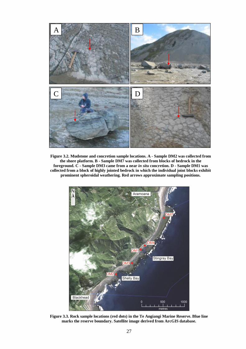
27
Figure 3.3. Rock sample locations (red dots) in the Te Angiangi Marine Reserve. Blue line
marks the reserve boundary. Satellite image derived from ArcGIS database.
Figure 3.2. Mudstone and concretion sample locations. A - Sample DM2 was collected from
the shore platform. B - Sample DM7 was collected from blocks of bedrock in the
foreground. C - Sample DM3 came from a near in situ concretion. D - Sample DM1 was
collected from a block of highly jointed bedrock in which the individual joint blocks exhibit
prominent spheroidal weathering. Red arrows approximate sampling positions.
A B
C D
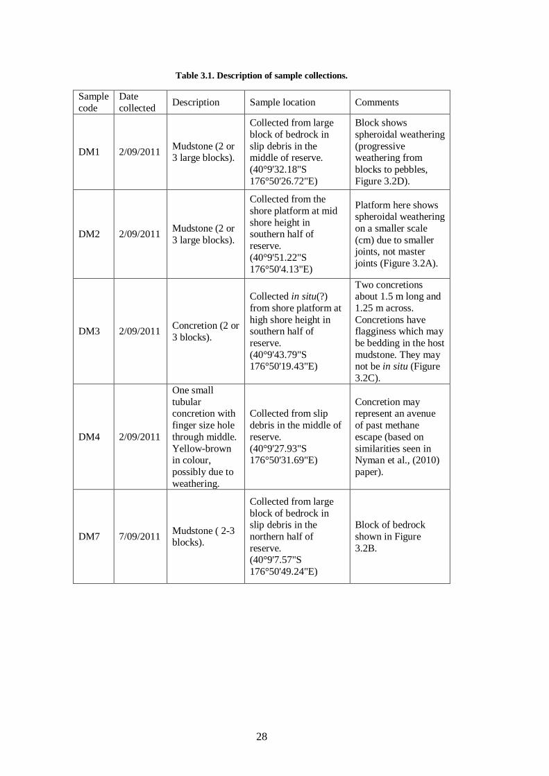
28
Table 3.1. Description of sample collections.
Sample
code Date
collected Description Sample location Comments
DM1 2/09/2011 Mudstone (2 or 3 large blocks).
Collected from large
block of bedrock in
slip debris in the middle of reserve. (40°9'32.18"S
176°50'26.72"E)
Block shows
spheroidal weathering
(progressive weathering from
blocks to pebbles,
Figure 3.2D).
DM2 2/09/2011 Mudstone (2 or
3 large blocks).
Collected from the
shore platform at mid
shore height in southern half of
reserve. (40°9'51.22"S
176°50'4.13"E)
Platform here shows spheroidal weathering
on a smaller scale
(cm) due to smaller joints, not master
joints (Figure 3.2A).
DM3 2/09/2011 Concretion (2 or
3 blocks).
Collected in situ(?)
from shore platform at
high shore height in southern half of
reserve. (40°9'43.79"S 176°50'19.43"E)
Two concretions about 1.5 m long and
1.25 m across.
Concretions have flagginess which may
be bedding in the host
mudstone. They may not be in situ (Figure
3.2C).
DM4 2/09/2011
One small
tubular concretion with
finger size hole
through middle.
Yellow-brown in colour,
possibly due to
weathering.
Collected from slip
debris in the middle of
reserve. (40°9'27.93"S 176°50'31.69"E)
Concretion may represent an avenue
of past methane
escape (based on
similarities seen in Nyman et al., (2010)
paper).
DM7 7/09/2011 Mudstone ( 2-3 blocks).
Collected from large
block of bedrock in slip debris in the
northern half of
reserve. (40°9'7.57"S
176°50'49.24"E)
Block of bedrock
shown in Figure
3.2B.
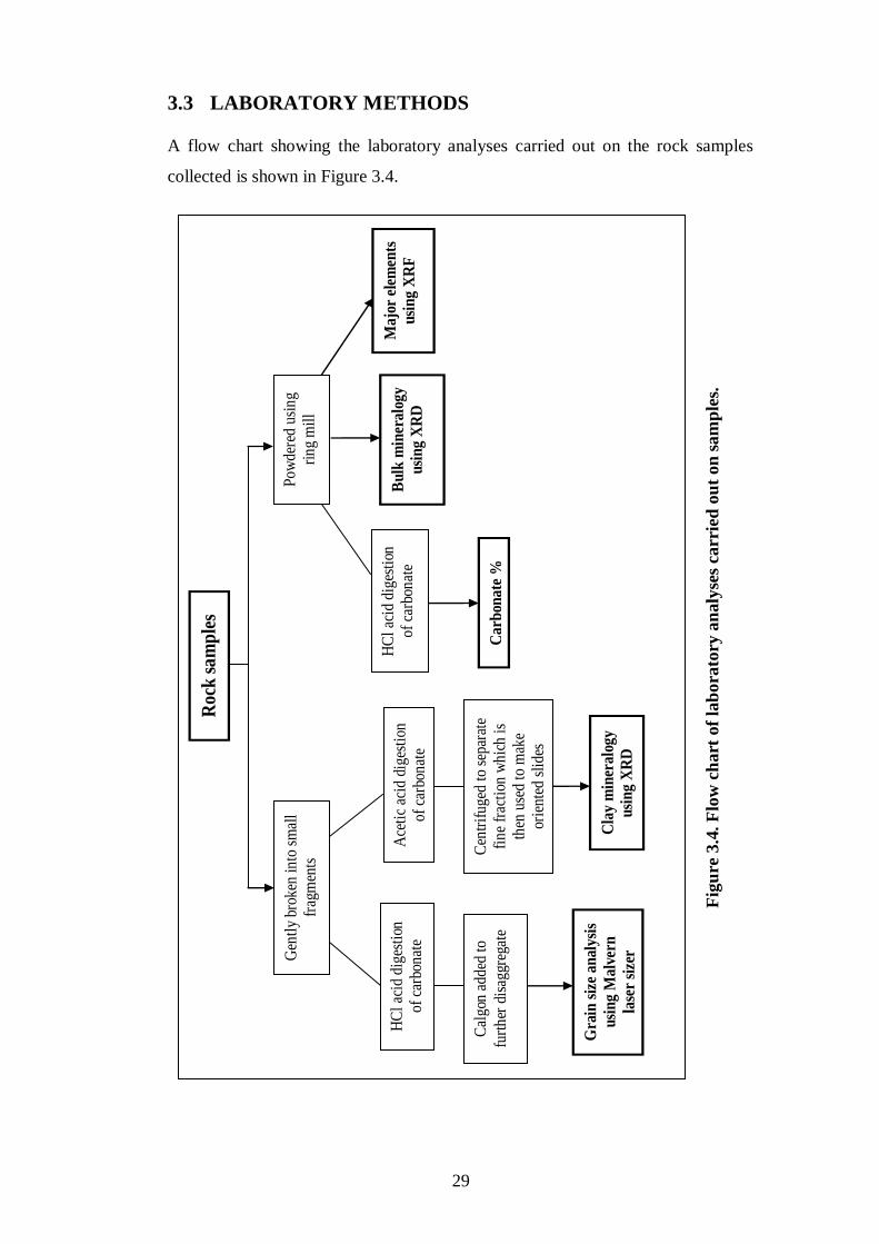
29
3.3 LABORATORY METHODS
A flow chart showing the laboratory analyses carried out on the rock samples
collected is shown in Figure 3.4.
Roc
k s
am
ple
s
Gen
tly
brok
en in
to s
mal
l
frag
men
ts
HC
l ac
id d
iges
tion
of c
arbo
nat
e
Cal
gon
add
ed t
o
furt
her
dis
aggr
egat
e
Gra
in s
ize
anal
ysis
usi
ng
Mal
vern
lase
r si
zer
Ace
tic
acid
dig
esti
on
of c
arbo
nat
e
Cen
trif
uged
to
sepa
rate
fin
e fr
acti
on w
hic
h is
then
use
d to
mak
e
orie
nted
sli
des
Cla
y m
iner
alog
y
usi
ng
XR
D
Pow
dere
d us
ing
rin
g m
ill
HC
l ac
id d
iges
tion
of c
arbo
nat
e
Car
bon
ate
%
Bu
lk m
iner
alog
y
usi
ng
XR
D
Maj
or e
lem
ents
usi
ng
XR
F
Fig
ure
3.4
. F
low
ch
art
of
lab
ora
tory
an
aly
ses
carr
ied
ou
t on
sam
ple
s.
30
3.3.1 Carbonate content
Carbonate percentage was determined for all samples to allow for a fuller
description of the mudstone and further insight into the nature and origin of the
concretions in the host mudstone.
Subsamples were taken of each rock sample and dried overnight in a 40°C oven.
The samples were then powdered, to enable faster acid reaction time, using a
tungsten carbide head in a ring mill at the University of Waikato. After the
samples were powdered, about 5 g of dry powder was measured to four decimal
places into labelled pre-weighed 250 ml beakers and dried overnight in a 40°C
oven. Both the beaker and the powder held within the beaker were then re-
weighed. The beakers were then placed into a fume hood and about 50 ml of 10%
hydrochloric acid (HCl) (or enough to cover the sample in the beaker) was added,
gently swirled and left to dissolve the carbonate overnight, stirring occasionally.
To test if all the carbonate was dissolved, the sample was stirred and observed for
any effervescence; if so, then more HCl was added and left for a further 2 hours.
Five sheets of filter paper (Whatman No. 42 15cm) were folded and placed in a
labelled pre-weighed small glass beaker and dried overnight at 40°C before
weighing. The filter paper and the small beaker were held in a desiccator so the
filter paper did not absorb any moisture while the powdered samples were
digesting. The following day, three stands and five clamps were set up in a fume
hood, with each of the clamps holding a glass funnel (Figure 3.5). A volumetric
flask was placed beneath each of the funnels to collect waste acid. Once the acid
digestion of the powdered samples was complete, one filter paper was placed into
each of the glass funnels, making sure the small labelled glass beakers matched
the filter papers with which they were weighed. The powdered sample was then
diluted with deionised water and filtered through the filter paper using more
deionised water.
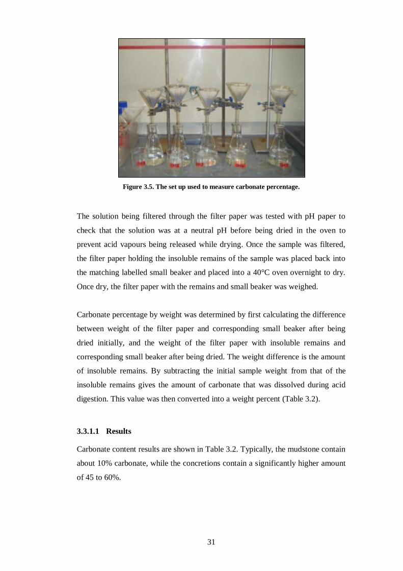
31
Figure 3.5. The set up used to measure carbonate percentage.
The solution being filtered through the filter paper was tested with pH paper to
check that the solution was at a neutral pH before being dried in the oven to
prevent acid vapours being released while drying. Once the sample was filtered,
the filter paper holding the insoluble remains of the sample was placed back into
the matching labelled small beaker and placed into a 40°C oven overnight to dry.
Once dry, the filter paper with the remains and small beaker was weighed.
Carbonate percentage by weight was determined by first calculating the difference
between weight of the filter paper and corresponding small beaker after being
dried initially, and the weight of the filter paper with insoluble remains and
corresponding small beaker after being dried. The weight difference is the amount
of insoluble remains. By subtracting the initial sample weight from that of the
insoluble remains gives the amount of carbonate that was dissolved during acid
digestion. This value was then converted into a weight percent (Table 3.2).
3.3.1.1 Results
Carbonate content results are shown in Table 3.2. Typically, the mudstone contain
about 10% carbonate, while the concretions contain a significantly higher amount
of 45 to 60%.
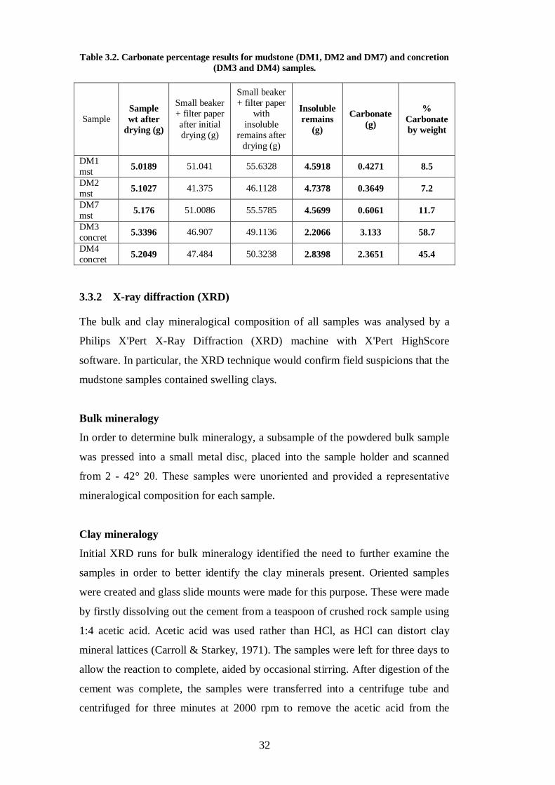
32
Table 3.2. Carbonate percentage results for mudstone (DM1, DM2 and DM7) and concretion
(DM3 and DM4) samples.
Sample Sample
wt after
drying (g)
Small beaker
+ filter paper
after initial
drying (g)
Small beaker
+ filter paper
with
insoluble
remains after
drying (g)
Insoluble
remains
(g)
Carbonate
(g)
%
Carbonate
by weight
DM1
mst 5.0189 51.041 55.6328 4.5918 0.4271 8.5
DM2
mst 5.1027 41.375 46.1128 4.7378 0.3649 7.2
DM7
mst 5.176 51.0086 55.5785 4.5699 0.6061 11.7
DM3
concret 5.3396 46.907 49.1136 2.2066 3.133 58.7
DM4
concret 5.2049 47.484 50.3238 2.8398 2.3651 45.4
3.3.2 X-ray diffraction (XRD)
The bulk and clay mineralogical composition of all samples was analysed by a
Philips X'Pert X-Ray Diffraction (XRD) machine with X'Pert HighScore
software. In particular, the XRD technique would confirm field suspicions that the
mudstone samples contained swelling clays.
Bulk mineralogy
In order to determine bulk mineralogy, a subsample of the powdered bulk sample
was pressed into a small metal disc, placed into the sample holder and scanned
from 2 - 42° 2θ. These samples were unoriented and provided a representative
mineralogical composition for each sample.
Clay mineralogy
Initial XRD runs for bulk mineralogy identified the need to further examine the
samples in order to better identify the clay minerals present. Oriented samples
were created and glass slide mounts were made for this purpose. These were made
by firstly dissolving out the cement from a teaspoon of crushed rock sample using
1:4 acetic acid. Acetic acid was used rather than HCl, as HCl can distort clay
mineral lattices (Carroll & Starkey, 1971). The samples were left for three days to
allow the reaction to complete, aided by occasional stirring. After digestion of the
cement was complete, the samples were transferred into a centrifuge tube and
centrifuged for three minutes at 2000 rpm to remove the acetic acid from the
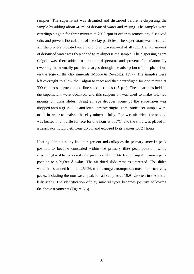
33
samples. The supernatant was decanted and discarded before re-dispersing the
sample by adding about 40 ml of deionised water and mixing. The samples were
centrifuged again for three minutes at 2000 rpm in order to remove any dissolved
salts and prevent flocculation of the clay particles. The supernatant was decanted
and the process repeated once more to ensure removal of all salt. A small amount
of deionised water was then added to re-disperse the sample. The dispersing agent
Calgon was then added to promote dispersion and prevent flocculation by
reversing the normally positive charges through the adsorption of phosphate ions
on the edge of the clay minerals (Moore & Reynolds, 1997). The samples were
left overnight to allow the Calgon to react and then centrifuged for one minute at
300 rpm to separate out the fine sized particles (<5 µm). These particles held in
the supernatant were decanted, and this suspension was used to make oriented
mounts on glass slides. Using an eye dropper, some of the suspension was
dropped onto a glass slide and left to dry overnight. Three slides per sample were
made in order to analyse the clay minerals fully. One was air dried, the second
was heated in a muffle furnace for one hour at 550°C, and the third was placed in
a desiccator holding ethylene glycol and exposed to its vapour for 24 hours.
Heating eliminates any kaolinite present and collapses the primary smectite peak
position to become concealed within the primary illite peak position, while
ethylene glycol helps identify the presence of smectite by shifting its primary peak
position to a higher Å value. The air dried slide remains untreated. The slides
were then scanned from 2 - 25° 2θ, as this range encompasses most important clay
peaks, including the non-basal peak for all samples at 19.9° 2θ seen in the initial
bulk scans. The identification of clay mineral types becomes positive following
the above treatments (Figure 3.6).
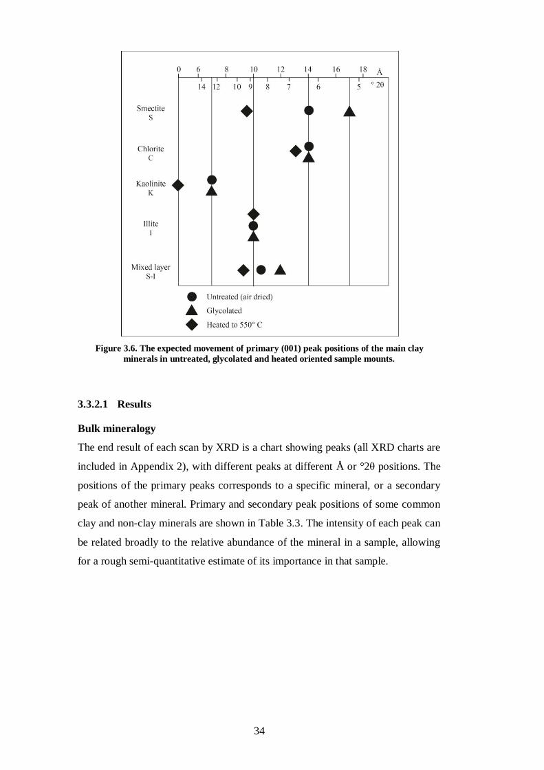
34
Figure 3.6. The expected movement of primary (001) peak positions of the main clay
minerals in untreated, glycolated and heated oriented sample mounts.
3.3.2.1 Results
Bulk mineralogy
The end result of each scan by XRD is a chart showing peaks (all XRD charts are
included in Appendix 2), with different peaks at different Å or °2θ positions. The
positions of the primary peaks corresponds to a specific mineral, or a secondary
peak of another mineral. Primary and secondary peak positions of some common
clay and non-clay minerals are shown in Table 3.3. The intensity of each peak can
be related broadly to the relative abundance of the mineral in a sample, allowing
for a rough semi-quantitative estimate of its importance in that sample.

35
Table 3.3. Important peak positions of some common minerals found in the mudstone and
concretion samples.
Mineral Degrees 2θ Angstroms (Å)
Quartz 26.62 3.35
Plagioclase 27.94 3.19
Low-magnesium calcite 29.42 3.04
High-magnesium calcite 30.0 2.97
Aragonite 26.22 3.40
Dolomite 30.9 2.89
Total clays 19.9 4.46
Illite 001 8.94 9.93
Illite 002 18.9 4.69
Chlorite 001 6.26 14.25
Chlorite 002 12.54 7.08
Kaolinite 001 12.34 7.19
Kaolinite 002 24.9 3.57
Smectite 001 6.0 14.0
Smectite 002 12.02 7.37
Figure 3.7 shows the XRD trace for mudstone sample DM1 as an example of bulk
mineral analysis. The bulk mineralogy results for the mudstone samples were
fairly consistent. All show relatively abundant clay minerals (the peak at about 4.5
Å represents total clays), with common quartz (peak at about 3.34 Å), some to
common plagioclase (peak at about 3.19 Å), with some low-magnesium calcite
(peak at about 3.04 Å; Figure 3.8). Peaks in these bulk mineralogical scans of
unoriented powders suggest the clay minerals are likely illite and some
combination of kaolinite, smectite and chlorite. More specific identification of the
clay minerals present was achieved by creating oriented mounts under the
different treatments mentioned earlier.
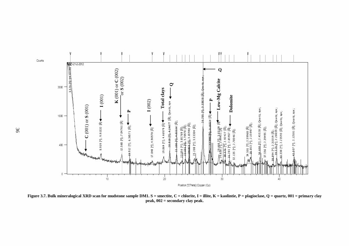
36
Figure 3.7. Bulk mineralogical XRD scan for mudstone sample DM1. S = smectite, C = chlorite, I = illite, K = kaolintie, P = plagioclase, Q = quartz, 001 = primary clay
peak, 002 = secondary clay peak.
C (
001)
or
S (
001) I (0
01)
K (
001)
or
C (
002)
or
S (
002)
P
I (0
02)
Tota
l cl
ays
Q
Q
P
Low
-Mg C
alc
ite
Dolo
mit
e
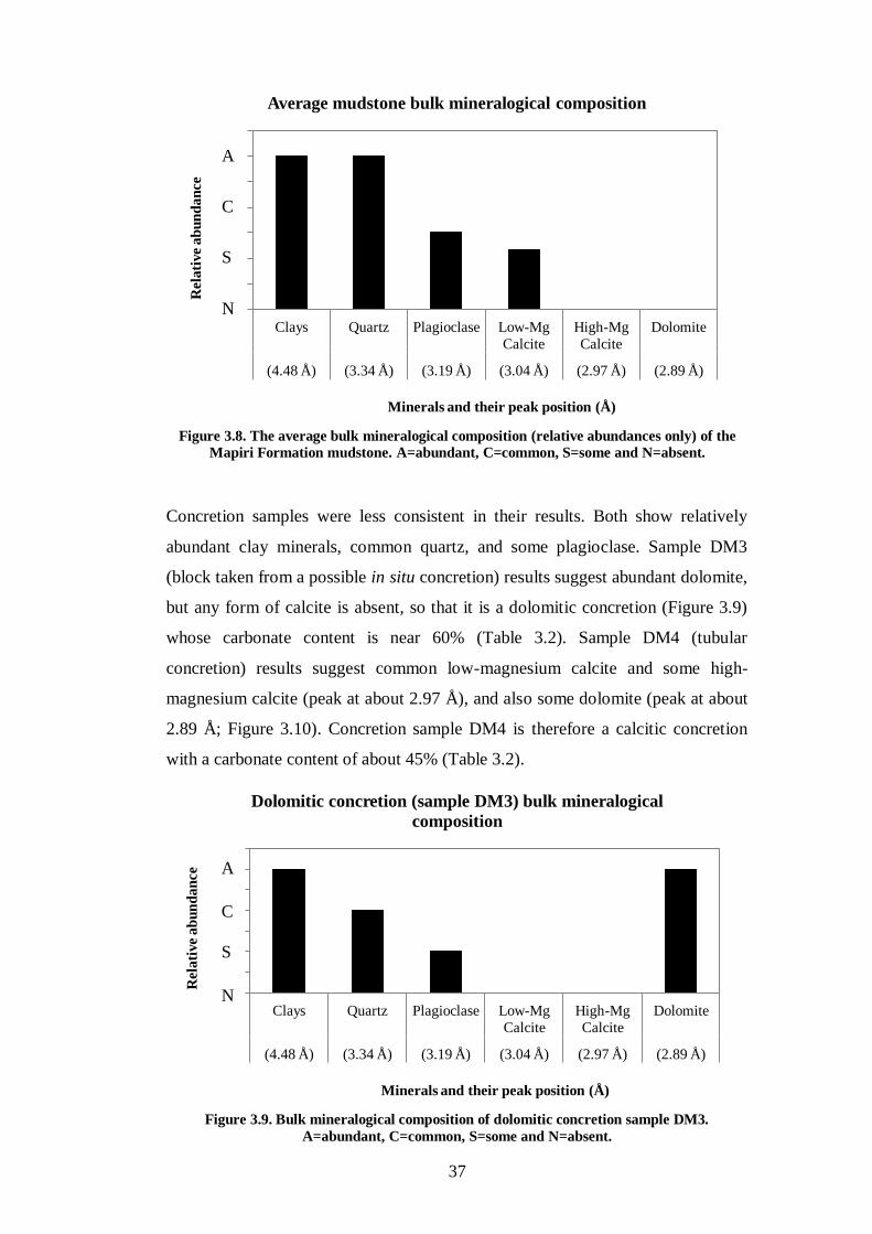
37
Figure 3.8. The average bulk mineralogical composition (relative abundances only) of the
Mapiri Formation mudstone. A=abundant, C=common, S=some and N=absent.
Concretion samples were less consistent in their results. Both show relatively
abundant clay minerals, common quartz, and some plagioclase. Sample DM3
(block taken from a possible in situ concretion) results suggest abundant dolomite,
but any form of calcite is absent, so that it is a dolomitic concretion (Figure 3.9)
whose carbonate content is near 60% (Table 3.2). Sample DM4 (tubular
concretion) results suggest common low-magnesium calcite and some high-
magnesium calcite (peak at about 2.97 Å), and also some dolomite (peak at about
2.89 Å; Figure 3.10). Concretion sample DM4 is therefore a calcitic concretion
with a carbonate content of about 45% (Table 3.2).
Figure 3.9. Bulk mineralogical composition of dolomitic concretion sample DM3.
A=abundant, C=common, S=some and N=absent.
0
0.5
1
1.5
2
2.5
3
3.5
Clays Quartz Plagioclase Low-Mg
Calcite
High-Mg
Calcite
Dolomite
(4.48 Å) (3.34 Å) (3.19 Å) (3.04 Å) (2.97 Å) (2.89 Å)
Rela
tive a
bu
nd
an
ce
Minerals and their peak position (Å)
Average mudstone bulk mineralogical composition
0
0.5
1
1.5
2
2.5
3
3.5
Clays Quartz Plagioclase Low-Mg
Calcite
High-Mg
Calcite
Dolomite
(4.48 Å) (3.34 Å) (3.19 Å) (3.04 Å) (2.97 Å) (2.89 Å)
Rela
tive a
bu
nd
an
ce
Minerals and their peak position (Å)
Dolomitic concretion (sample DM3) bulk mineralogical
composition
A
C
S
N
A
C
S
N

38
Figure 3.10. Bulk mineralogical composition of calcitic concretion sample DM4.
A=abundant, C=common, S=some and N=absent.
Clay mineralogy
Overall, the clay mineral composition based on primary (001) peak positions and
peak intensities for all the samples indicates the presence of abundant illite, and
smectite, some kaolinite, and rare chlorite (Figure 3.11). Appendix 3 contains a
summary of clay mineral results for both oriented and unoriented mounts.
Illite appears persistently in all samples at about 10 Å and, as expected, glycolated
and heated samples show no movement in the illite peak position. The persistence
of a peak at about 14 Å corresponds to smectite in all untreated samples, because
in the glycolated samples the smectite peak position shifts close to 17 Å, while in
the heated samples the peaks shifts to about 9-10 Å to become concealed within
the primary illite peak. A peak at about 7 Å persists in all untreated and glycolated
samples, but disappears in all heated samples, therefore characterising kaolinite.
The presence of chlorite is suspected due to a peak persisting at about 14 Å in all
heated samples. However, curiously, the chlorite peak is not significantly present
in the glycolated scans but appears in the heated ones, a feature needing future
study. Figures 3.12 - 3.14 show sample DM1 as an example of clay mineral
results on untreated and treated oriented mounts.
0
0.5
1
1.5
2
2.5
3
3.5
Clays Quartz Plagioclase Low-Mg
Calcite
High-Mg
Calcite
Dolomite
(4.48 Å) (3.34 Å) (3.19 Å) (3.04 Å) (2.97 Å) (2.89 Å)
Rela
tive a
bu
nd
an
ce
Minerals and their peak position (Å)
Calcitic concretion (sample DM4) bulk mineralogical
composition
A
C
S
N
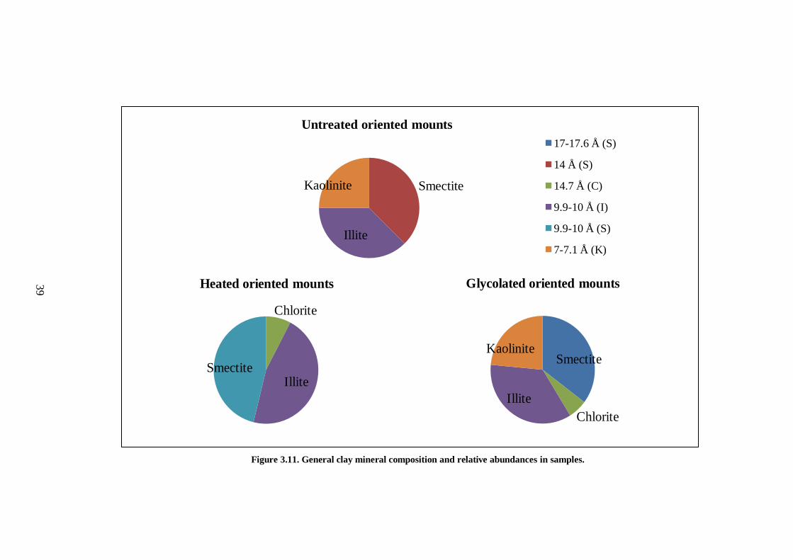
39
Chlorite
IlliteSmectite
Heated oriented mounts
Smectite
Chlorite
Illite
Kaolinite
Glycolated oriented mounts
Chlorite
IlliteSmectite
Heated oriented mounts
Smectite
Chlorite
Illite
Kaolinite
Glycolated oriented mounts
Smectite
Illite
Kaolinite
Untreated oriented mounts
17-17.6 Å (S)
14 Å (S)
14.7 Å (C)
9.9-10 Å (I)
9.9-10 Å (S)
7-7.1 Å (K)
Figure 3.11. General clay mineral composition and relative abundances in samples.
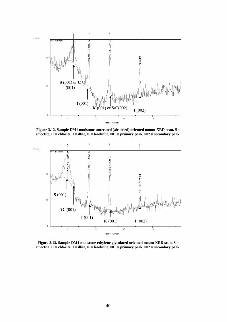
40
Figure 3.12. Sample DM1 mudstone untreated (air dried) oriented mount XRD scan. S =
smectite, C = chlorite, I = illite, K = kaolintie, 001 = primary peak, 002 = secondary peak.
Figure 3.13. Sample DM1 mudstone ethylene glycolated oriented mount XRD scan. S =
smectite, C = chlorite, I = illite, K = kaolintie, 001 = primary peak, 002 = secondary peak.
S (001) or C
(001)
I (001) K (001) or S/C(002)
I (002)
I (002) K (001) I (001)
S (001)
?C (001)
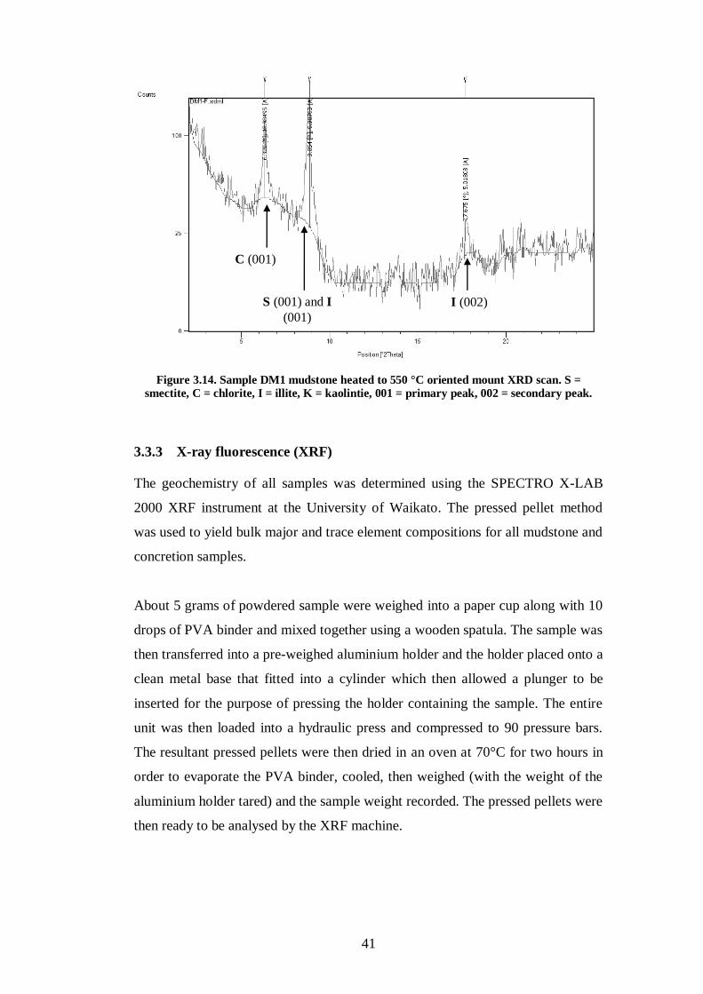
41
Figure 3.14. Sample DM1 mudstone heated to 550 °C oriented mount XRD scan. S =
smectite, C = chlorite, I = illite, K = kaolintie, 001 = primary peak, 002 = secondary peak.
3.3.3 X-ray fluorescence (XRF)
The geochemistry of all samples was determined using the SPECTRO X-LAB
2000 XRF instrument at the University of Waikato. The pressed pellet method
was used to yield bulk major and trace element compositions for all mudstone and
concretion samples.
About 5 grams of powdered sample were weighed into a paper cup along with 10
drops of PVA binder and mixed together using a wooden spatula. The sample was
then transferred into a pre-weighed aluminium holder and the holder placed onto a
clean metal base that fitted into a cylinder which then allowed a plunger to be
inserted for the purpose of pressing the holder containing the sample. The entire
unit was then loaded into a hydraulic press and compressed to 90 pressure bars.
The resultant pressed pellets were then dried in an oven at 70°C for two hours in
order to evaporate the PVA binder, cooled, then weighed (with the weight of the
aluminium holder tared) and the sample weight recorded. The pressed pellets were
then ready to be analysed by the XRF machine.
C (001)
S (001) and I
(001)
I (002)
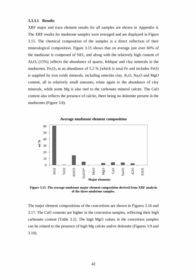
42
3.3.3.1 Results
XRF major and trace element results for all samples are shown in Appendix 4.
The XRF results for mudstone samples were averaged and are displayed in Figure
3.15. The chemical composition of the samples is a direct reflection of their
mineralogical composition. Figure 3.15 shows that on average just over 60% of
the mudstone is composed of SiO2, and along with the relatively high content of
Al2O3 (15%), reflects the abundance of quartz, feldspar and clay minerals in the
mudstones. Fe2O3 at an abundance of 5.2 % (which is total Fe and includes FeO)
is supplied by iron oxide minerals, including smectite clay. K2O, Na2O and MgO
content, all in relatively small amounts, relate again to the abundance of clay
minerals, while some Mg is also tied to the carbonate mineral calcite. The CaO
content also reflects the presence of calcite, there being no dolomite present in the
mudstones (Figure 3.8).
Figure 3.15. The average mudstone major element composition derived from XRF analysis
of the three mudstone samples.
The major element compositions of the concretions are shown in Figures 3.16 and
3.17. The CaO contents are higher in the concretion samples, reflecting their high
carbonate content (Table 3.2). The high MgO values in the concretion samples
can be related to the presence of high Mg calcite and/or dolomite (Figures 3.9 and
3.10).
0
10
20
30
40
50
60
SiO
2
TiO
2
Al2
O3
Fe2
O3
*
Mn
O
Mg
O
CaO
Na2
O
K2
O
P2
O5
wt
%
Major elements
Average mudstone element composition
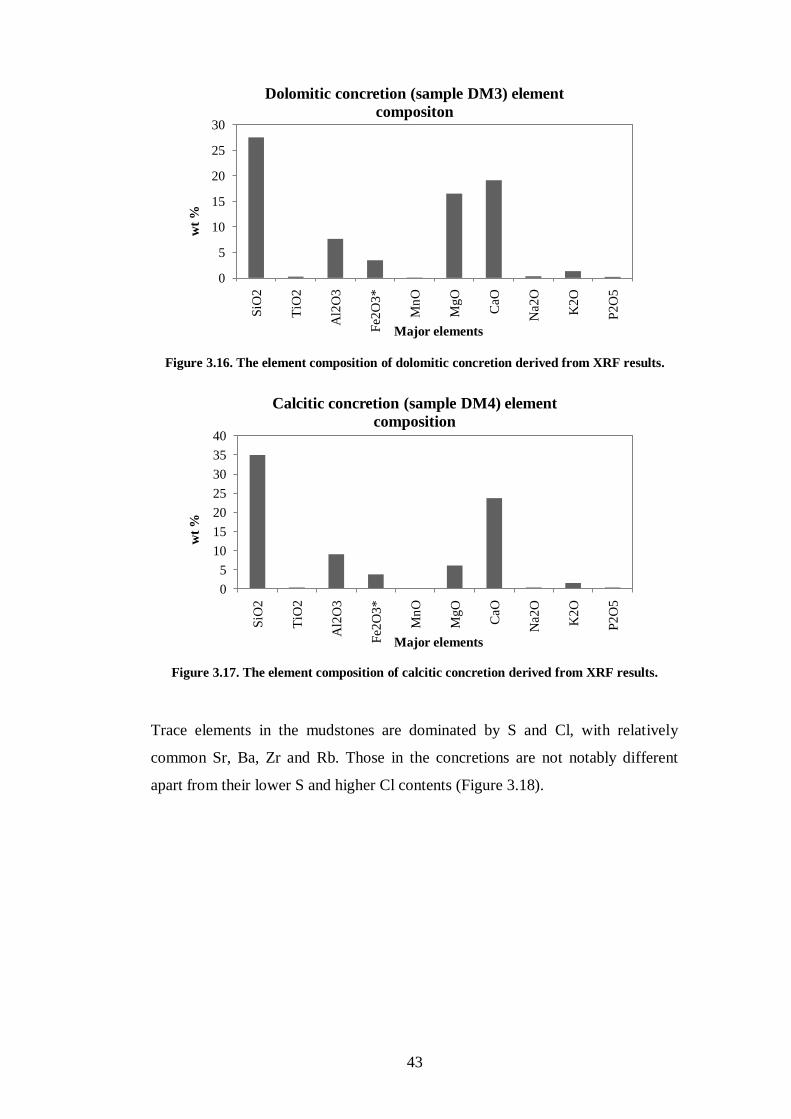
43
Figure 3.16. The element composition of dolomitic concretion derived from XRF results.
Figure 3.17. The element composition of calcitic concretion derived from XRF results.
Trace elements in the mudstones are dominated by S and Cl, with relatively
common Sr, Ba, Zr and Rb. Those in the concretions are not notably different
apart from their lower S and higher Cl contents (Figure 3.18).
0
5
10
15
20
25
30
SiO
2
TiO
2
Al2
O3
Fe2
O3*
Mn
O
MgO
CaO
Na2
O
K2O
P2O
5
wt
%
Major elements
Dolomitic concretion (sample DM3) element
compositon
0
5
10
15
20
25
30
35
40
SiO
2
TiO
2
Al2
O3
Fe2
O3
*
Mn
O
Mg
O
CaO
Na2
O
K2
O
P2
O5
wt
%
Major elements
Calcitic concretion (sample DM4) element
composition
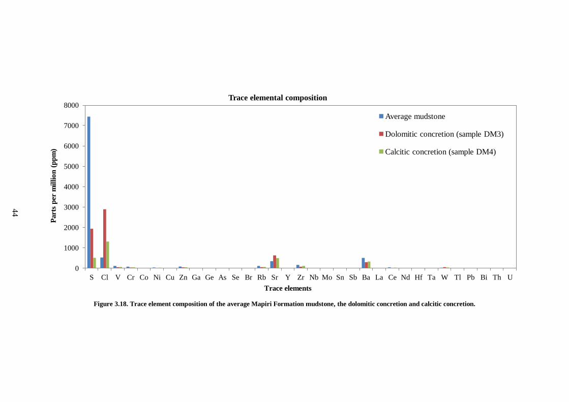
44
Figure 3.18. Trace element composition of the average Mapiri Formation mudstone, the dolomitic concretion and calcitic concretion.
0
1000
2000
3000
4000
5000
6000
7000
8000
S Cl V Cr Co Ni Cu Zn Ga Ge As Se Br Rb Sr Y Zr Nb Mo Sn Sb Ba La Ce Nd Hf Ta W Tl Pb Bi Th U
Part
s p
er m
illi
on
(p
pm
)
Trace elements
Trace elemental composition
Average mudstone
Dolomitic concretion (sample DM3)
Calcitic concretion (sample DM4)
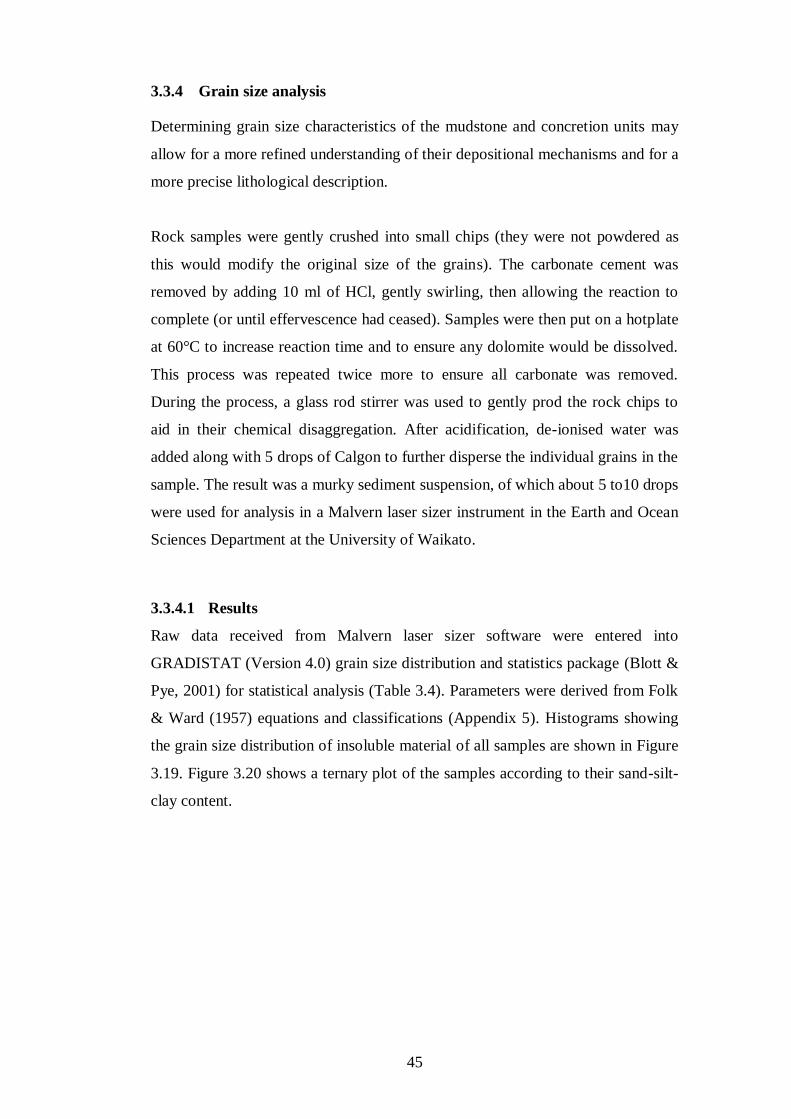
45
3.3.4 Grain size analysis
Determining grain size characteristics of the mudstone and concretion units may
allow for a more refined understanding of their depositional mechanisms and for a
more precise lithological description.
Rock samples were gently crushed into small chips (they were not powdered as
this would modify the original size of the grains). The carbonate cement was
removed by adding 10 ml of HCl, gently swirling, then allowing the reaction to
complete (or until effervescence had ceased). Samples were then put on a hotplate
at 60°C to increase reaction time and to ensure any dolomite would be dissolved.
This process was repeated twice more to ensure all carbonate was removed.
During the process, a glass rod stirrer was used to gently prod the rock chips to
aid in their chemical disaggregation. After acidification, de-ionised water was
added along with 5 drops of Calgon to further disperse the individual grains in the
sample. The result was a murky sediment suspension, of which about 5 to10 drops
were used for analysis in a Malvern laser sizer instrument in the Earth and Ocean
Sciences Department at the University of Waikato.
3.3.4.1 Results
Raw data received from Malvern laser sizer software were entered into
GRADISTAT (Version 4.0) grain size distribution and statistics package (Blott &
Pye, 2001) for statistical analysis (Table 3.4). Parameters were derived from Folk
& Ward (1957) equations and classifications (Appendix 5). Histograms showing
the grain size distribution of insoluble material of all samples are shown in Figure
3.19. Figure 3.20 shows a ternary plot of the samples according to their sand-silt-
clay content.
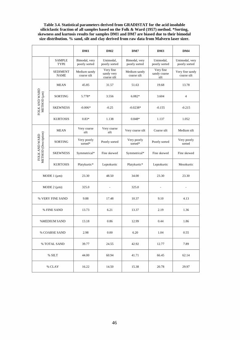
46
Table 3.4. Statistical parameters derived from GRADISTAT for the acid insoluble
siliciclastic fraction of all samples based on the Folk & Ward (1957) method. *Sorting,
skewness and kurtosis results for samples DM1 and DM7 are biased due to their bimodal
size distribution. % sand, silt and clay derived from raw data from Malvern laser sizer.
DM1 DM2 DM7 DM3 DM4
SAMPLE
TYPE
Bimodal, very
poorly sorted
Unimodal,
poorly sorted
Bimodal, very
poorly sorted
Unimodal,
poorly sorted
Unimodal, very
poorly sorted
SEDIMENT
NAME
Medium sandy
coarse silt
Very fine
sandy very
coarse silt
Medium sandy
coarse silt
Very fine
sandy coarse
silt
Very fine sandy
coarse silt
FO
LK
AN
D W
AR
D
ME
TH
OD
(µ
m)
MEAN 45.85 31.57 51.63 19.68 13.78
SORTING 5.778* 3.556 6.082* 3.604 4
SKEWNESS -0.006* -0.25 -0.0238* -0.155 -0.215
KURTOSIS 0.83* 1.138 0.848* 1.137 1.052
FO
LK
AN
D W
AR
D
ME
TH
OD
(D
escr
ipti
on
) MEAN Very coarse
silt
Very coarse
silt Very coarse silt Coarse silt Medium silt
SORTING Very poorly
sorted* Poorly sorted
Very poorly
sorted* Poorly sorted
Very poorly
sorted
SKEWNESS Symmetrical* Fine skewed Symmetrical* Fine skewed Fine skewed
KURTOSIS Platykurtic* Leptokurtic Platykurtic* Leptokurtic Mesokurtic
MODE 1 (µm): 23.30 48.50 34.00 23.30 23.30
MODE 2 (µm): 325.0 - 325.0 - -
% VERY FINE SAND 9.88 17.48 10.37 9.10 4.13
% FINE SAND 13.73 6.21 13.37 2.19 1.36
%MEDIUM SAND 13.18 0.86 12.99 0.44 1.86
% COARSE SAND 2.98 0.00 6.20 1.04 0.55
% TOTAL SAND 39.77 24.55 42.92 12.77 7.89
% SILT 44.00 60.94 41.71 66.45 62.14
% CLAY 16.22 14.50 15.38 20.78 29.97
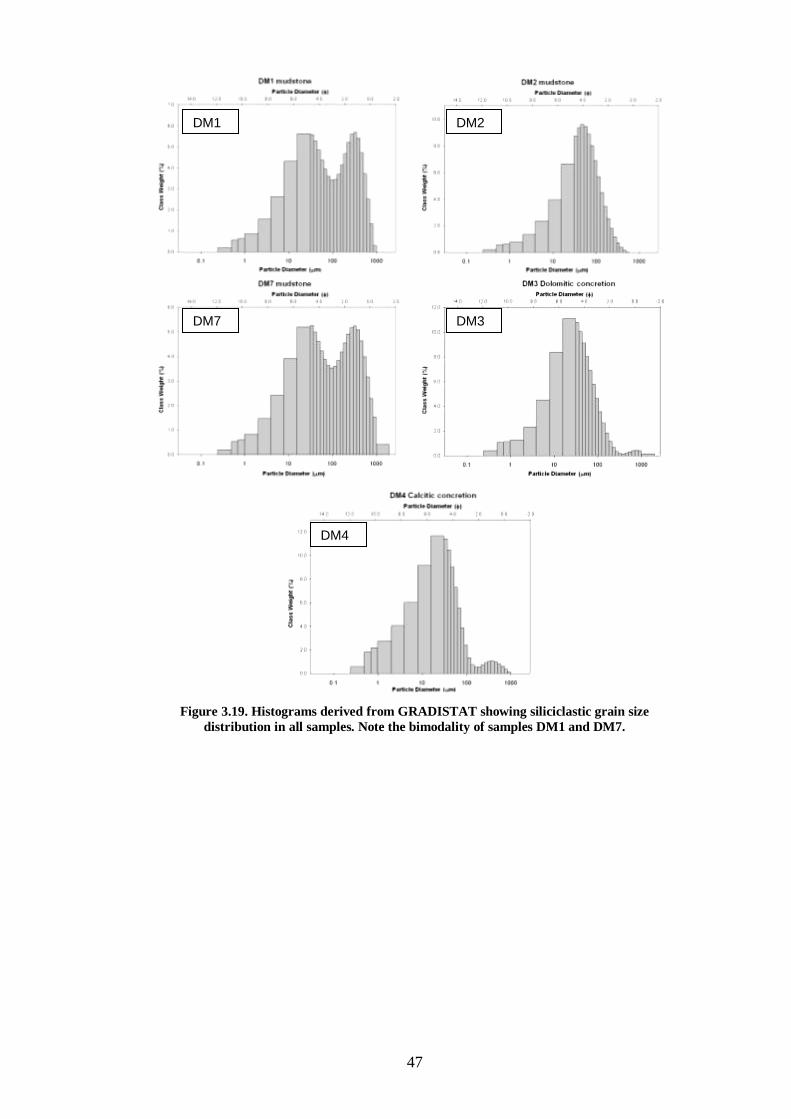
47
Figure 3.19. Histograms derived from GRADISTAT showing siliciclastic grain size
distribution in all samples. Note the bimodality of samples DM1 and DM7.
DM1 DM2
DM7 DM3
DM4
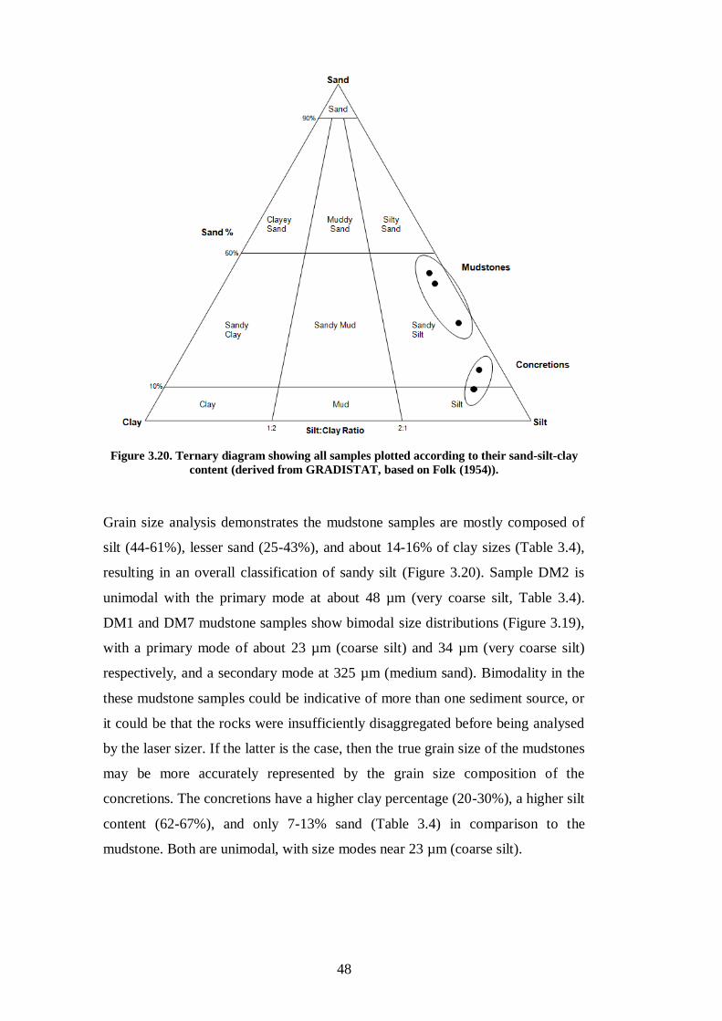
48
Figure 3.20. Ternary diagram showing all samples plotted according to their sand-silt-clay
content (derived from GRADISTAT, based on Folk (1954)).
Grain size analysis demonstrates the mudstone samples are mostly composed of
silt (44-61%), lesser sand (25-43%), and about 14-16% of clay sizes (Table 3.4),
resulting in an overall classification of sandy silt (Figure 3.20). Sample DM2 is
unimodal with the primary mode at about 48 µm (very coarse silt, Table 3.4).
DM1 and DM7 mudstone samples show bimodal size distributions (Figure 3.19),
with a primary mode of about 23 µm (coarse silt) and 34 µm (very coarse silt)
respectively, and a secondary mode at 325 µm (medium sand). Bimodality in the
these mudstone samples could be indicative of more than one sediment source, or
it could be that the rocks were insufficiently disaggregated before being analysed
by the laser sizer. If the latter is the case, then the true grain size of the mudstones
may be more accurately represented by the grain size composition of the
concretions. The concretions have a higher clay percentage (20-30%), a higher silt
content (62-67%), and only 7-13% sand (Table 3.4) in comparison to the
mudstone. Both are unimodal, with size modes near 23 µm (coarse silt).
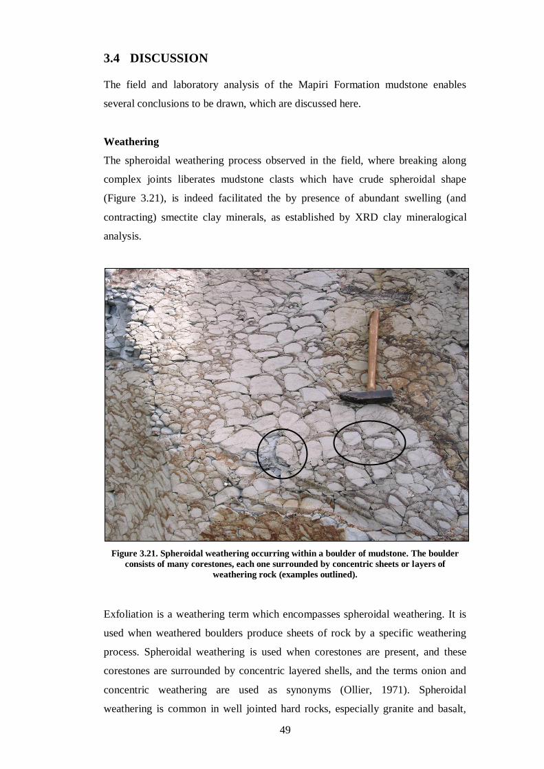
49
3.4 DISCUSSION
The field and laboratory analysis of the Mapiri Formation mudstone enables
several conclusions to be drawn, which are discussed here.
Weathering
The spheroidal weathering process observed in the field, where breaking along
complex joints liberates mudstone clasts which have crude spheroidal shape
(Figure 3.21), is indeed facilitated the by presence of abundant swelling (and
contracting) smectite clay minerals, as established by XRD clay mineralogical
analysis.
Figure 3.21. Spheroidal weathering occurring within a boulder of mudstone. The boulder
consists of many corestones, each one surrounded by concentric sheets or layers of
weathering rock (examples outlined).
Exfoliation is a weathering term which encompasses spheroidal weathering. It is
used when weathered boulders produce sheets of rock by a specific weathering
process. Spheroidal weathering is used when corestones are present, and these
corestones are surrounded by concentric layered shells, and the terms onion and
concentric weathering are used as synonyms (Ollier, 1971). Spheroidal
weathering is common in well jointed hard rocks, especially granite and basalt,
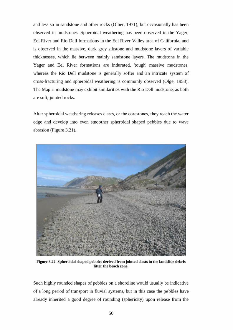
50
and less so in sandstone and other rocks (Ollier, 1971), but occasionally has been
observed in mudstones. Spheroidal weathering has been observed in the Yager,
Eel River and Rio Dell formations in the Eel River Valley area of California, and
is observed in the massive, dark grey siltstone and mudstone layers of variable
thicknesses, which lie between mainly sandstone layers. The mudstone in the
Yager and Eel River formations are indurated, 'tough' massive mudstones,
whereas the Rio Dell mudstone is generally softer and an intricate system of
cross-fracturing and spheroidal weathering is commonly observed (Olge, 1953).
The Mapiri mudstone may exhibit similarities with the Rio Dell mudstone, as both
are soft, jointed rocks.
After spheroidal weathering releases clasts, or the corestones, they reach the water
edge and develop into even smoother spheroidal shaped pebbles due to wave
abrasion (Figure 3.21).
Figure 3.22. Spheroidal shaped pebbles derived from jointed clasts in the landslide debris
litter the beach zone.
Such highly rounded shapes of pebbles on a shoreline would usually be indicative
of a long period of transport in fluvial systems, but in this case the pebbles have
already inherited a good degree of rounding (sphericity) upon release from the
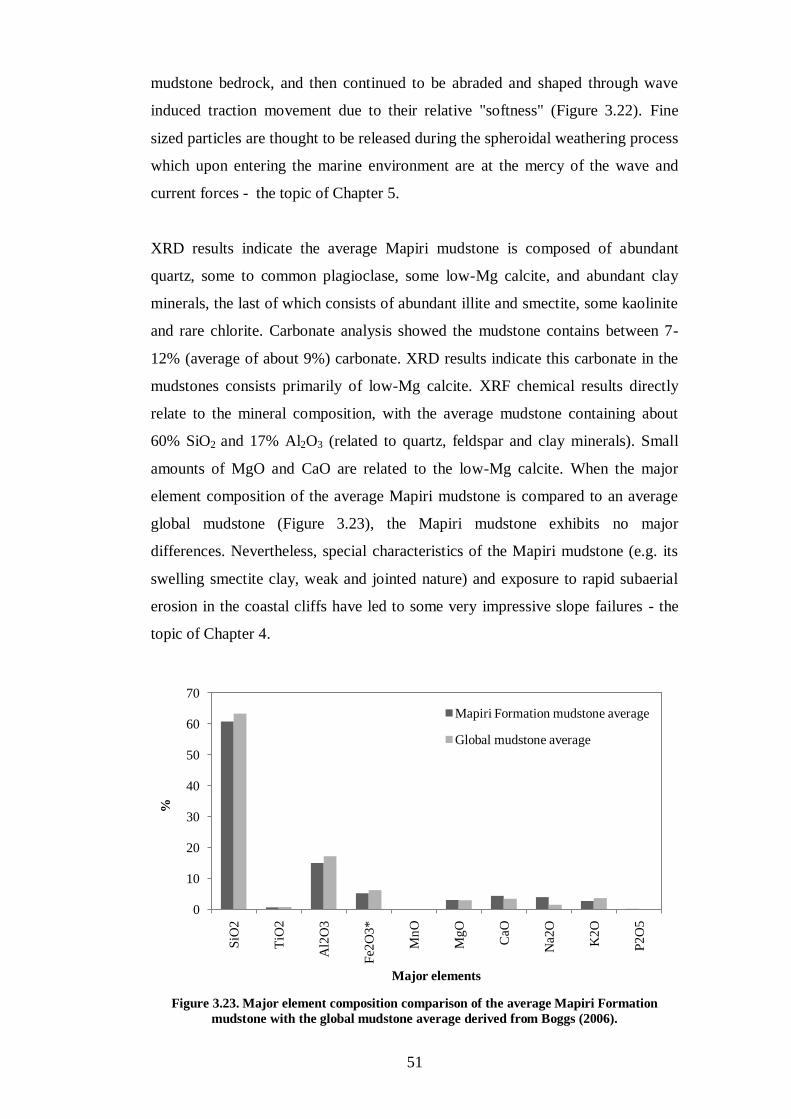
51
mudstone bedrock, and then continued to be abraded and shaped through wave
induced traction movement due to their relative "softness" (Figure 3.22). Fine
sized particles are thought to be released during the spheroidal weathering process
which upon entering the marine environment are at the mercy of the wave and
current forces - the topic of Chapter 5.
XRD results indicate the average Mapiri mudstone is composed of abundant
quartz, some to common plagioclase, some low-Mg calcite, and abundant clay
minerals, the last of which consists of abundant illite and smectite, some kaolinite
and rare chlorite. Carbonate analysis showed the mudstone contains between 7-
12% (average of about 9%) carbonate. XRD results indicate this carbonate in the
mudstones consists primarily of low-Mg calcite. XRF chemical results directly
relate to the mineral composition, with the average mudstone containing about
60% SiO2 and 17% Al2O3 (related to quartz, feldspar and clay minerals). Small
amounts of MgO and CaO are related to the low-Mg calcite. When the major
element composition of the average Mapiri mudstone is compared to an average
global mudstone (Figure 3.23), the Mapiri mudstone exhibits no major
differences. Nevertheless, special characteristics of the Mapiri mudstone (e.g. its
swelling smectite clay, weak and jointed nature) and exposure to rapid subaerial
erosion in the coastal cliffs have led to some very impressive slope failures - the
topic of Chapter 4.
Figure 3.23. Major element composition comparison of the average Mapiri Formation
mudstone with the global mudstone average derived from Boggs (2006).
0
10
20
30
40
50
60
70
SiO
2
TiO
2
Al2
O3
Fe2
O3*
Mn
O
Mg
O
CaO
Na2
O
K2O
P2O
5
%
Major elements
Mapiri Formation mudstone average
Global mudstone average
52
Provenance
There are several factors impacting on and determining the composition of
mudstones in general, which include tectonic setting, sediment source,
depositional environment, grain size and diagenesis (Boggs, 2006). It is also
important to note that mudstones form under environmental conditions in which
fine sediment is abundant and water forces are small enough to allow fine
sediment to settle out of suspension. They are characteristic of marine
environments where the seafloor is deep enough to be out of the influence of
waves and strong ocean currents (Boggs, 2006).
Clay minerals, along with quartz and feldspars are characteristic components of
mudstones, and are mainly detrital, although siliciclastic minerals may also form
or be altered into another mineral type during different stages of diagenesis.
Commonly, clay minerals are derived as a weathering product of pre-existing
rocks which contain feldspars. The Mapiri mudstone was likely deposited in a
bathyal slope basin environment, and its siliciclastic material derived from erosion
of older mudstones from the Paleogene to Neogene, and possibly even Cretaceous
basement rocks. Some of these rocks have high abundance of clay minerals (e.g.
the Wanstead Formation (Figure 2.7) contains smectite which is known to create
slope instability and erosion in this formation), which are thought to have been
released through erosion then transported into a bathyal slope environment,
possibly into a slope basin formed as a result of thrust faulting during
compression along the Hikurangi Margin. The presence of smectite is an
important feature of this mudstone because of its ability to expand and contract,
allowing the indurated mudstone to become weak through wetting and drying
processes after subaerial exposure. The high abundance of illite is also noted.
Illites, a common weathering product of feldspars, is often found in deeply buried
muds in a temperate marine environment, formed by the transformation of
smectite (and also from alteration of kaolinite) at temperatures ranging from 55 to
200°C (Li et al., 1997; Bjorlykke, 1998; Prothero & Schwab, 2003; Boggs, 2006).
Carbonate minerals form in mudstones during burial as cements, and the amount
of carbonate formed relates to the amount of free pore space in the mud during
burial diagenesis. As the degree of diagenesis increases, compaction due to
pressure packs grains together tightly, decreasing the porosity. Carbonate in the
53
Mapiri mudstone, as derived from XRD analysis on the Mapiri concretions, is of
both dolomitic and calcitic types, with contribution from calcitic microfossils.
Concretion formation
It is suspected, based on findings by Nyman et al., (2010), that tectonic setting has
had the most important influence on the formation of concretions within the
Mapiri mudstone. Nyman et al., (2010) found tubular concretions in the host
Whangaehu mudstone (equivalent in age to the Mapiri mudstone) along the
coastline of Whangaehu Beach, just north of Cape Turnagain (Figure 1.1). These
concretions developed as a result of a shallow sub-seafloor plumbing network of a
Late Miocene cold seep system, where methane rich fluid migrated towards the
surface, altering the geochemical composition of the surrounding mudstone as it
travelled. Thrust faults parallel to the coastline likely provided the pathways for
this fluid to travel. Fluid migration due to overpressured sediment at depth occurs
today in the Hikurangi Margin (at about 3000 m depth; Barnes et al., 2010) due to
compaction and compressional tectonics. Nyman et al., (2010) infer that the same
forces resulting in fluid migration occurred in the Late Miocene, resulting in
localised fluid migration through the Whangaehu mudstone. Since this plumbing
system is seen on a regional scale, there is valid reason to believe that the
concretions seen in the Mapiri Formation could have been influenced by, or
formed directly due to, the same cold seep system. Similarities between the
Mapiri and Whangaehu concretions including their moderately high carbonate
contents involving dolomite and calcite, and the presence of central conduits
(Figure 3.24), lend support to this possibility.
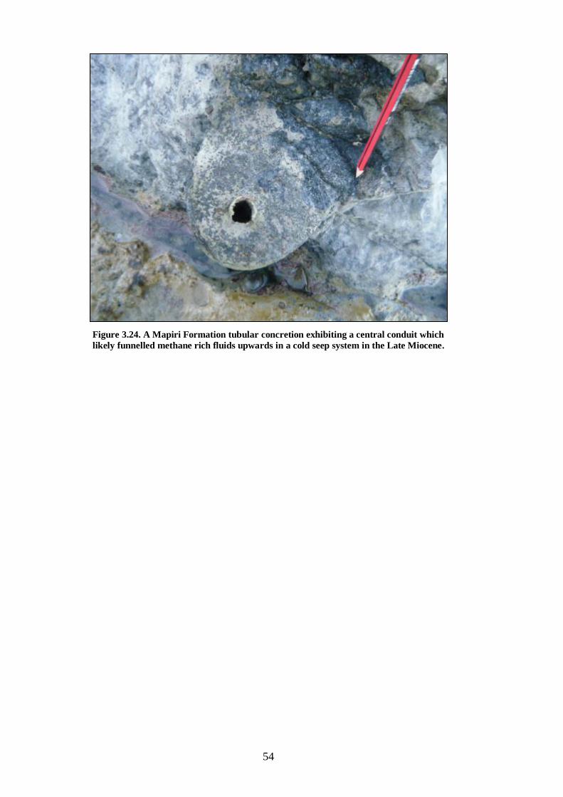
54
Figure 3.24. A Mapiri Formation tubular concretion exhibiting a central conduit which
likely funnelled methane rich fluids upwards in a cold seep system in the Late Miocene.

55
4 Chapter 4
SLOPE FAILURES
4.1 INTRODUCTION
The aim of this chapter is to describe and classify the slope failures along the
coastal hills adjacent to the Te Angiangi Marine Reserve. A brief outline of the
regional landslide susceptibility and occurrence is provided, before describing the
slope failures that occurred sometime between the 25th and 28th April 2011
within and inland from the marine reserve. Intrinsic instabilities within the Mapiri
mudstone, including its jointed and weak nature, and external triggering factors
acting on the hill sides of the study area are outlined, and the slope failures
directly adjacent to the reserve are identified individually and classified into their
general types of failure. Estimates of (1) the volume of sediment produced from
the larger slips directly adjacent to the reserve, and (2) the area of bare ground
generated in the marine reserve stream catchments, are attempted.
4.2 FIELD WORK
Field work involved observing and describing the slope failures while walking the
length of the reserve. The failures were separated from each other as accurately as
possible, described and photographed individually. This involved estimating the
dimensions of each , recording such properties as the depth, length, and width of
the main scarp at the crown, and the length and width of the accumulated debris at
the toe (Figure 4.1), and describing any other features, such as the type of failure,
the presence of vegetation, and the size, sorting and composition of clasts in the
accumulated debris. After the initial descriptions were made approximate
measurements were carried out on the larger landslides using several measuring
tapes and handheld GPS units (except for depth, which was estimated visually due
to the inability in most cases to access the landslide scars for measurements with a
measuring tape). In some cases, a GPS unit (with settings configured to 'track')
was used to trace and measure the length of the main head scarp at the head of the
landslide. The GPS continuously made waypoints as it was carried by a walker
around the perimeter of the landslide. This was only done where it was safe to
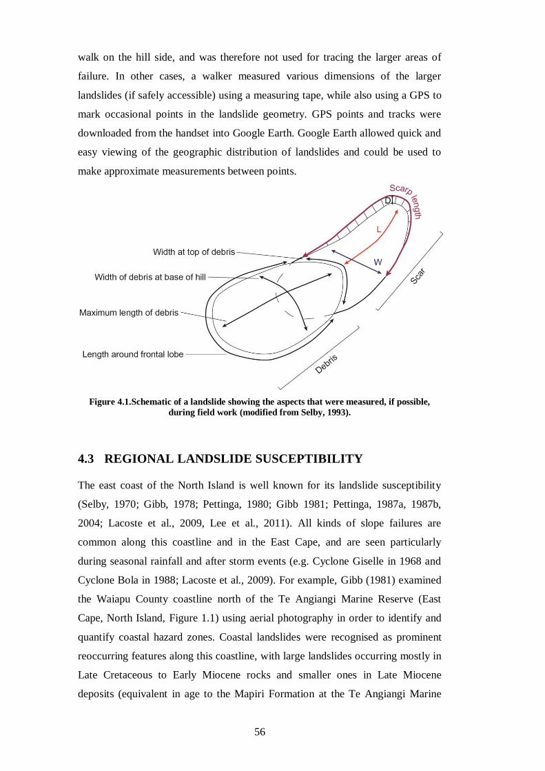
56
walk on the hill side, and was therefore not used for tracing the larger areas of
failure. In other cases, a walker measured various dimensions of the larger
landslides (if safely accessible) using a measuring tape, while also using a GPS to
mark occasional points in the landslide geometry. GPS points and tracks were
downloaded from the handset into Google Earth. Google Earth allowed quick and
easy viewing of the geographic distribution of landslides and could be used to
make approximate measurements between points.
Figure 4.1.Schematic of a landslide showing the aspects that were measured, if possible,
during field work (modified from Selby, 1993).
4.3 REGIONAL LANDSLIDE SUSCEPTIBILITY
The east coast of the North Island is well known for its landslide susceptibility
(Selby, 1970; Gibb, 1978; Pettinga, 1980; Gibb 1981; Pettinga, 1987a, 1987b,
2004; Lacoste et al., 2009, Lee et al., 2011). All kinds of slope failures are
common along this coastline and in the East Cape, and are seen particularly
during seasonal rainfall and after storm events (e.g. Cyclone Giselle in 1968 and
Cyclone Bola in 1988; Lacoste et al., 2009). For example, Gibb (1981) examined
the Waiapu County coastline north of the Te Angiangi Marine Reserve (East
Cape, North Island, Figure 1.1) using aerial photography in order to identify and
quantify coastal hazard zones. Coastal landslides were recognised as prominent
reoccurring features along this coastline, with large landslides occurring mostly in
Late Cretaceous to Early Miocene rocks and smaller ones in Late Miocene
deposits (equivalent in age to the Mapiri Formation at the Te Angiangi Marine
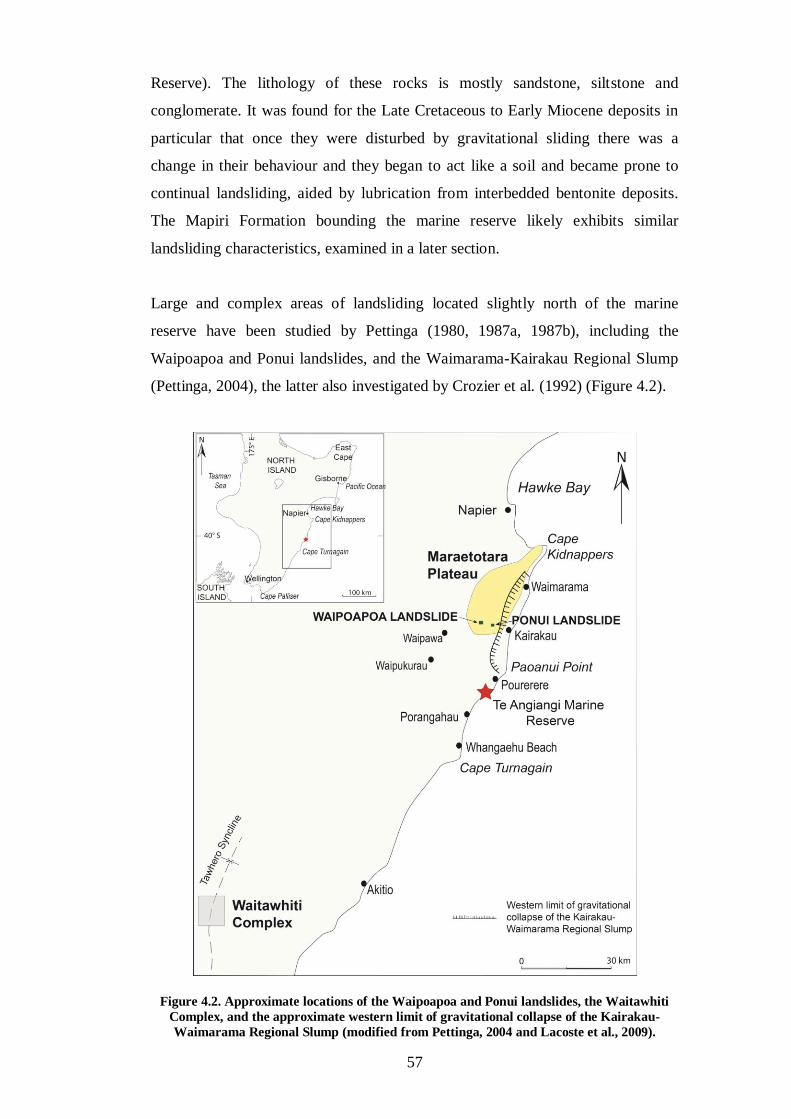
57
Reserve). The lithology of these rocks is mostly sandstone, siltstone and
conglomerate. It was found for the Late Cretaceous to Early Miocene deposits in
particular that once they were disturbed by gravitational sliding there was a
change in their behaviour and they began to act like a soil and became prone to
continual landsliding, aided by lubrication from interbedded bentonite deposits.
The Mapiri Formation bounding the marine reserve likely exhibits similar
landsliding characteristics, examined in a later section.
Large and complex areas of landsliding located slightly north of the marine
reserve have been studied by Pettinga (1980, 1987a, 1987b), including the
Waipoapoa and Ponui landslides, and the Waimarama-Kairakau Regional Slump
(Pettinga, 2004), the latter also investigated by Crozier et al. (1992) (Figure 4.2).
Figure 4.2. Approximate locations of the Waipoapoa and Ponui landslides, the Waitawhiti
Complex, and the approximate western limit of gravitational collapse of the Kairakau-
Waimarama Regional Slump (modified from Pettinga, 2004 and Lacoste et al., 2009).
58
The deep-seated Waipoapoa and Ponui landslides were reactivated on separate
occasions during rainfall events in 1976, and are complex failures in weak, Late
Miocene flysch deposits located in the Maraetotara Plateau in southern Hawke's
Bay (Figure 4.2). The Waimarama-Kairakau Regional Slump is a massive
regional gravitational collapse, stretching along the coast from Waimarama to
Paoanui Point, that occurs within Neogene accretionary slope basin deposits -
mostly undifferentiated mudstones and alternating sandstone and mudstone
successions (Pettinga, 2004; Figure 4.2). A complex landslide area, called the
Waitawhiti landslide complex, located 50 km south of Cape Turnagain (Figure
4.2), was investigated by Lacoste et al. (2009). Their study described possible
factors that triggered landsliding in this area, including river incision at the base of
hills, rainfall, vegetation, earthquakes and tectonic activity, fluid overpressure,
and lithology. The geology of the Waitawhiti complex is Late Miocene
(Tongaporutuan) in age and consists of fine grained sandstones and massive
jointed siltstones, having very similar characteristics to the Mapiri Formation at
the marine reserve.
There are several reasons for the extensive and numerous slope failures on the hill
sides of the Hawke's Bay region. In particular, the coastal ranges in southern
Hawke's Bay from Waimarama to Cape Turnagain consist of rounded undulating
hills composed of fine-grained Miocene or Cretaceous to Paleogene mudstones
and sandstones, with slope angles at the coast ranging from about 20 - 40° (slope
angles ranging from 15 - 25° are described as steep, angles ranging from 25 - 35°
are very steep, and angles ranging from 35 - 55° are precipitous (Moon, 2010)).
The coastal ranges are not only steep, which increases the gravitational forces
already acting on the slopes, but they are also in a tectonically very active region
that is presently subjected to high uplift rates, from 0.5 to 2.3 mm/y-1
(Pettinga,
1987a, 1987b, 1980; Lacoste et al., 2009). Associated earthquakes can contribute
to landsliding by destabilising some slopes (Lacoste et al., 2009). Landsliding is
also attributed to deforestation, which became a serious problem after European
settlement about 170 years ago (Glade, 2003). Since then a considerable area of
coastal land in Hawke's Bay has been converted to pastoral agriculture (Selby,
1970; Dymond et al., 2006; Lacoste et al., 2009). As a consequence, shallow
regolith slides are common in the coastal ranges (Crozier et al., 1980) and
generally result from intense rainfall and lack of vegetation cover (Lacoste et al.,
59
2009). In contrast, deep landsliding is more typically related to structural
weaknesses in the bedrock lithology, and Neogene mudstones in the area are
susceptible and succumb rapidly under weathering processes (Kennedy &
Dickson, 2007).
4.4 TE ANGIANGI MARINE RESERVE LANDSLIDES
4.4.1 Triggers
In April of 2011 the east coast of the North Island was affected by a severe
cyclonic storm, resulting in significant damage to buildings and farm land
primarily due to landsliding (NIWA, 2011b). The storm affected a large section of
the East Coast region, from Mahia in the north to Porangahau in the south, and
included the area about 10 km inland from the coast (Jones et al., 2011). Heavy
rain (up to 650 mm at the coast between Cape Kidnappers and Porangahau) fell
from 25-28 April, with most falling on 26 April when 300 mm was recorded at
Cape Turnagain (NIWA, 2011a), resulting in unusually wet soils for that time of
year (NIWA, 2011b). Widespread shallow landsliding occurred within the
affected area, and some pastoral farmers reported deeper-seated landslides than
ever previously experienced (Jones et al., 2011). Intense rainfall during this storm
is likely the main factor in triggering the extensive landsliding seen in the area, as
the saturated soils led to an increase in pore-fluid pressure which in turn reduced
the shear strength of the mudstone (Selby, 1993; Lacoste et al., 2009). A likely
contributing factor in triggering the slope failures was the occurrence of a small
earthquake Richter magnitude M4.5 on the evening of 26 April that was centred
only 10 km offshore from Pourerere at a depth of 20 km (Jones et al., 2011).
Typically the minimum magnitude for triggering landslides is suggested to be
about M5, with significant landsliding occurring at M6 or greater (Jones et al.,
2011). However, because of the highly saturated soil/rock conditions on the East
Coast at the time of the earthquake, the lower magnitude may have been sufficient
to trigger some landslides (Jones et al., 2011).
In the study area rather weak Miocene mudstone underlies the coastal hills, and
landslides are common in these weakly cemented rocks (Lee et al., 2011).
Although rock hardness was not directly measured in the Mapiri Formation
mudstone, comparable Late Miocene to Early Pliocene mudstone at Cape

60
Turnagain near to the south yielded Schmidt hammer (both L and N type) rebound
('R') values of less than 10 in a study by Kennedy & Dickson (2007), which is
below the detection level of the instruments but indicates that the mudstone is
indeed very 'soft' or 'weak'. For example, Selby (1993) showed that even rebound
values in the 10 to 35 range were characteristic of weathered and weakly
compacted sedimentary rocks. Moreover, Gibb (1978) documented a maximum
cliff retreat rate of 2.25 m/y-1
for mudstone cliffs at Cape Turnagain, one of the
highest coastal cliff erosion rates at the time, supporting that these rocks are
particularly susceptible to erosion, by both subaerial and marine processes.
The Mapiri mudstone includes a significant content of smectite clay minerals (see
section 3.3.2 XRD clay mineral results), and it is also a highly jointed rock
(Figure 3.2A). Jointed rocks are more susceptible to weathering because cracks
provide access for water to enter which, in the presence of smectite minerals
causes swelling of the rock and promotion of chemical decomposition. Swelling
smectite minerals are particularly effective at adsorbing water and generally as
more water becomes present the electrostatic forces between clay minerals and the
surrounding water decreases, since more water separates the clay particles,
resulting in weakening the overall rock cohesion (Selby, 1993). The jointed,
smectite-rich nature of the mudstone means that it has inherent internal
instabilities which combined with exposure to external triggering factors initiate
slope failure. In the case of the Te Angiangi Marine Reserve area, the external
triggering factor was the intense rainfall during the April 2011 storm, with a
possible superimposed contribution from the small 'Pourerere' earthquake.
4.4.2 Type of slope failure
Slope failures are observed on hill sides in the vicinity of the Te Angiangi Marine
Reserve, which between at least 2008 until the April 2011 storm showed little to
no current active erosion (Figure 4.3A). However, there is certainly evidence of
large landslides having occurred on these hill sides in the past, but in the lead up
to April 2011 they supported reasonably continuous vegetation cover (Figure
4.3A).
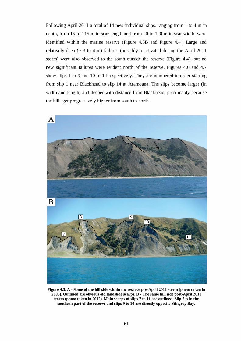
61
Following April 2011 a total of 14 new individual slips, ranging from 1 to 4 m in
depth, from 15 to 115 m in scar length and from 20 to 120 m in scar width, were
identified within the marine reserve (Figure 4.3B and Figure 4.4). Large and
relatively deep (~ 3 to 4 m) failures (possibly reactivated during the April 2011
storm) were also observed to the south outside the reserve (Figure 4.4), but no
new significant failures were evident north of the reserve. Figures 4.6 and 4.7
show slips 1 to 9 and 10 to 14 respectively. They are numbered in order starting
from slip 1 near Blackhead to slip 14 at Aramoana. The slips become larger (in
width and length) and deeper with distance from Blackhead, presumably because
the hills get progressively higher from south to north.
Figure 4.3. A - Some of the hill side within the reserve pre-April 2011 storm (photo taken in
2008). Outlined are obvious old landslide scarps. B - The same hill side post-April 2011
storm (photo taken in 2012). Main scarps of slips 7 to 11 are outlined. Slip 7 is in the
southern part of the reserve and slips 9 to 10 are directly opposite Stingray Bay.

62
Figure 4.4. Landslides in the northern half of the reserve. Main scarps of slips 7 to 14 are
outlined. View is looking south.
Figure 4.5. Slope failures on hills south outside the reserve.
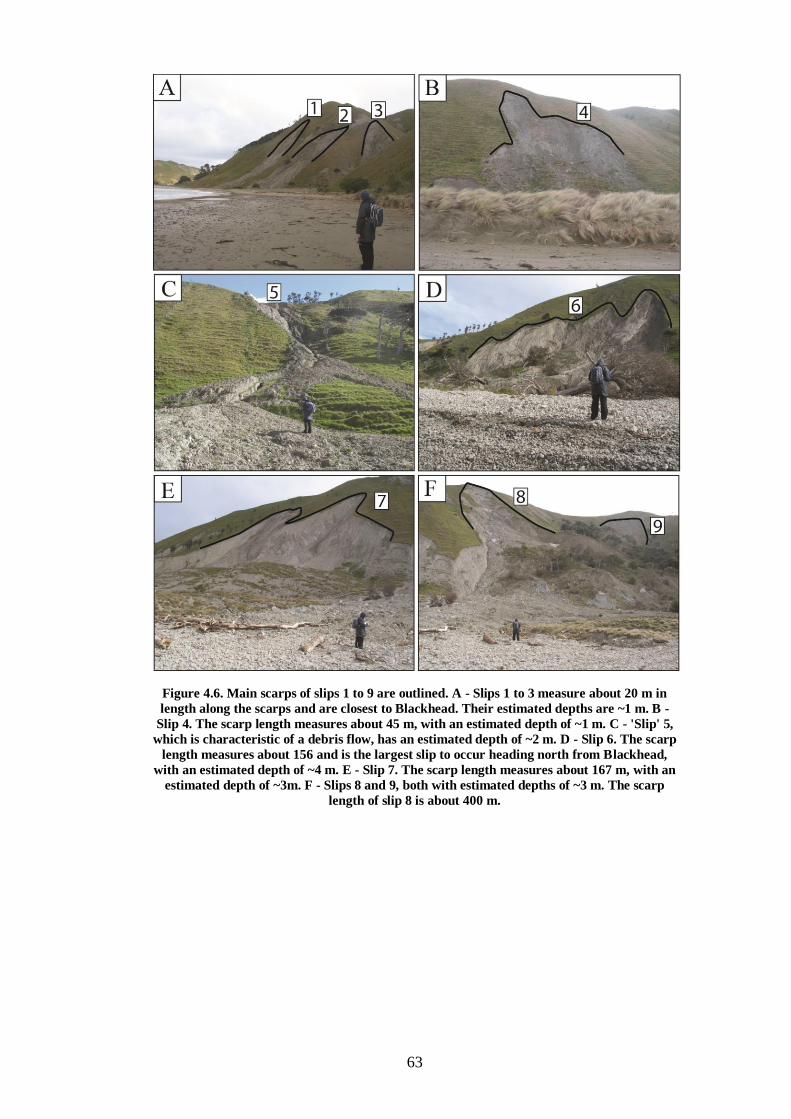
63
Figure 4.6. Main scarps of slips 1 to 9 are outlined. A - Slips 1 to 3 measure about 20 m in
length along the scarps and are closest to Blackhead. Their estimated depths are ~1 m. B -
Slip 4. The scarp length measures about 45 m, with an estimated depth of ~1 m. C - 'Slip' 5,
which is characteristic of a debris flow, has an estimated depth of ~2 m. D - Slip 6. The scarp
length measures about 156 and is the largest slip to occur heading north from Blackhead,
with an estimated depth of ~4 m. E - Slip 7. The scarp length measures about 167 m, with an
estimated depth of ~3m. F - Slips 8 and 9, both with estimated depths of ~3 m. The scarp
length of slip 8 is about 400 m.
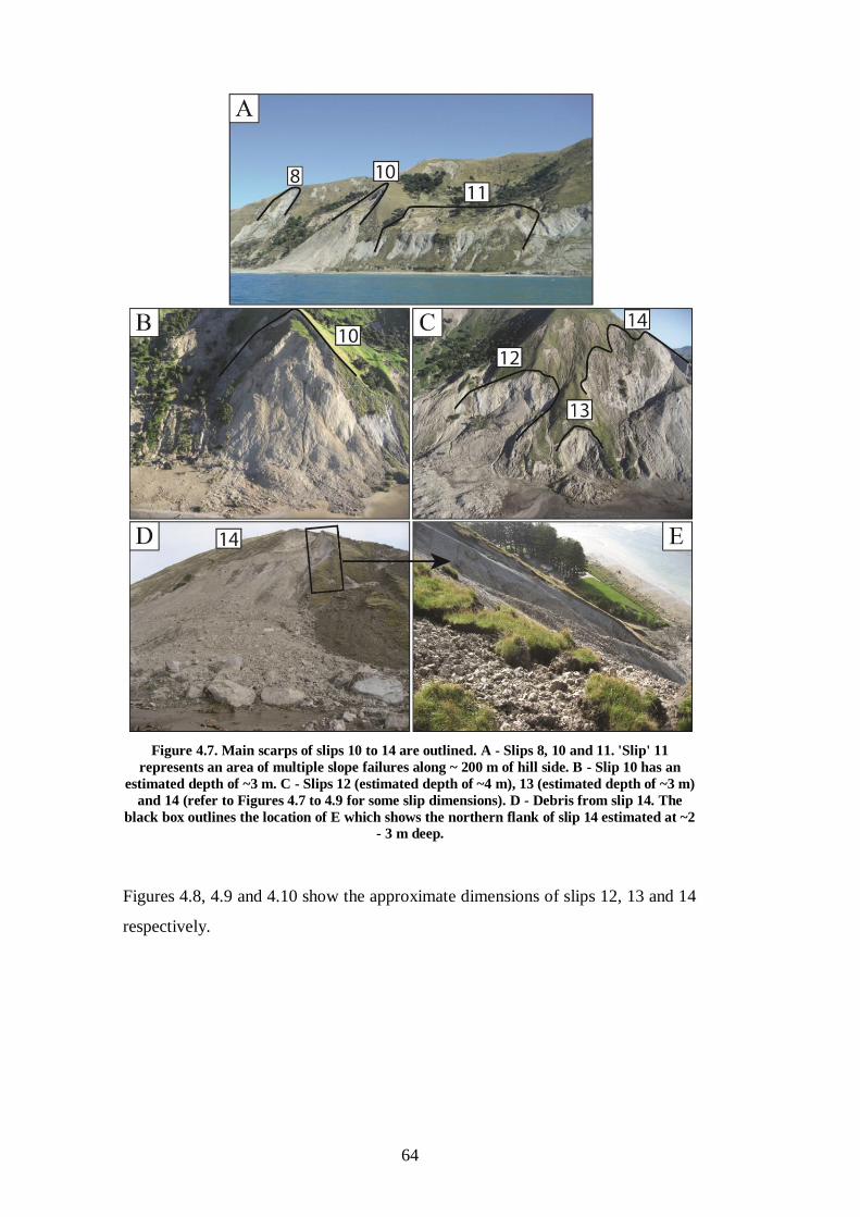
64
Figure 4.7. Main scarps of slips 10 to 14 are outlined. A - Slips 8, 10 and 11. 'Slip' 11
represents an area of multiple slope failures along ~ 200 m of hill side. B - Slip 10 has an
estimated depth of ~3 m. C - Slips 12 (estimated depth of ~4 m), 13 (estimated depth of ~3 m)
and 14 (refer to Figures 4.7 to 4.9 for some slip dimensions). D - Debris from slip 14. The
black box outlines the location of E which shows the northern flank of slip 14 estimated at ~2
- 3 m deep.
Figures 4.8, 4.9 and 4.10 show the approximate dimensions of slips 12, 13 and 14
respectively.

65
Figure 4.8. Debris measurements of slip 12, including the length around the debris frontal
lobe, the maximum length (or extent) of the debris, and the width of the debris at the base of
the hill. Also shown is the width near the top of the debris mass.
Figure 4.9. Debris and scarp measurements of slip 13, including the scarp length at the
crown, the length around the debris frontal lobe, the maximum length (or extent) of the
debris, and the width of the debris at the base of the hill.
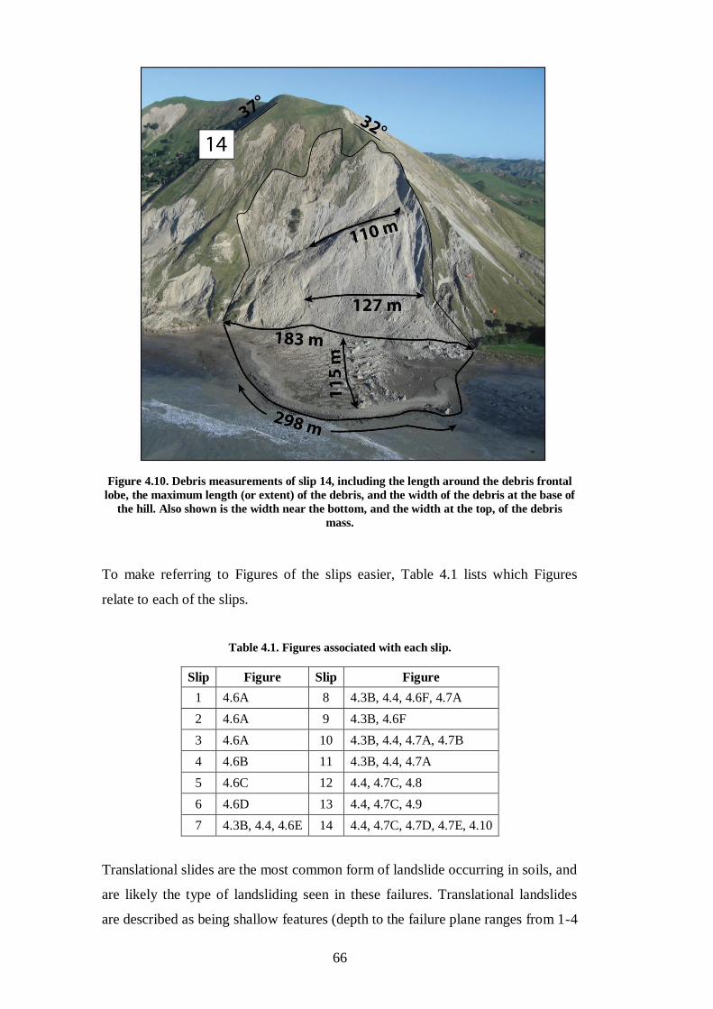
66
Figure 4.10. Debris measurements of slip 14, including the length around the debris frontal
lobe, the maximum length (or extent) of the debris, and the width of the debris at the base of
the hill. Also shown is the width near the bottom, and the width at the top, of the debris
mass.
To make referring to Figures of the slips easier, Table 4.1 lists which Figures
relate to each of the slips.
Table 4.1. Figures associated with each slip.
Slip Figure Slip Figure
1 4.6A 8 4.3B, 4.4, 4.6F, 4.7A
2 4.6A 9 4.3B, 4.6F
3 4.6A 10 4.3B, 4.4, 4.7A, 4.7B
4 4.6B 11 4.3B, 4.4, 4.7A
5 4.6C 12 4.4, 4.7C, 4.8
6 4.6D 13 4.4, 4.7C, 4.9
7 4.3B, 4.4, 4.6E 14 4.4, 4.7C, 4.7D, 4.7E, 4.10
Translational slides are the most common form of landslide occurring in soils, and
are likely the type of landsliding seen in these failures. Translational landslides
are described as being shallow features (depth to the failure plane ranges from 1-4
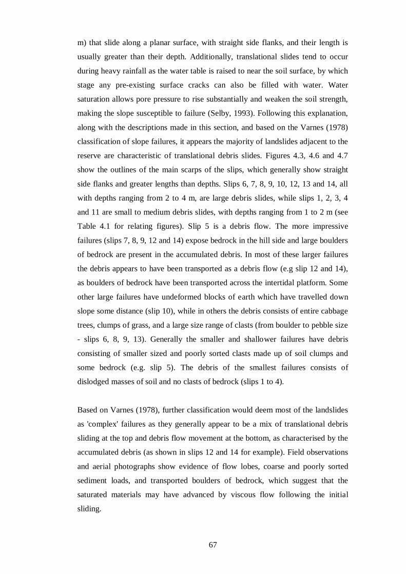
67
m) that slide along a planar surface, with straight side flanks, and their length is
usually greater than their depth. Additionally, translational slides tend to occur
during heavy rainfall as the water table is raised to near the soil surface, by which
stage any pre-existing surface cracks can also be filled with water. Water
saturation allows pore pressure to rise substantially and weaken the soil strength,
making the slope susceptible to failure (Selby, 1993). Following this explanation,
along with the descriptions made in this section, and based on the Varnes (1978)
classification of slope failures, it appears the majority of landslides adjacent to the
reserve are characteristic of translational debris slides. Figures 4.3, 4.6 and 4.7
show the outlines of the main scarps of the slips, which generally show straight
side flanks and greater lengths than depths. Slips 6, 7, 8, 9, 10, 12, 13 and 14, all
with depths ranging from 2 to 4 m, are large debris slides, while slips 1, 2, 3, 4
and 11 are small to medium debris slides, with depths ranging from 1 to 2 m (see
Table 4.1 for relating figures). Slip 5 is a debris flow. The more impressive
failures (slips 7, 8, 9, 12 and 14) expose bedrock in the hill side and large boulders
of bedrock are present in the accumulated debris. In most of these larger failures
the debris appears to have been transported as a debris flow (e.g slip 12 and 14),
as boulders of bedrock have been transported across the intertidal platform. Some
other large failures have undeformed blocks of earth which have travelled down
slope some distance (slip 10), while in others the debris consists of entire cabbage
trees, clumps of grass, and a large size range of clasts (from boulder to pebble size
- slips 6, 8, 9, 13). Generally the smaller and shallower failures have debris
consisting of smaller sized and poorly sorted clasts made up of soil clumps and
some bedrock (e.g. slip 5). The debris of the smallest failures consists of
dislodged masses of soil and no clasts of bedrock (slips 1 to 4).
Based on Varnes (1978), further classification would deem most of the landslides
as 'complex' failures as they generally appear to be a mix of translational debris
sliding at the top and debris flow movement at the bottom, as characterised by the
accumulated debris (as shown in slips 12 and 14 for example). Field observations
and aerial photographs show evidence of flow lobes, coarse and poorly sorted
sediment loads, and transported boulders of bedrock, which suggest that the
saturated materials may have advanced by viscous flow following the initial
sliding.
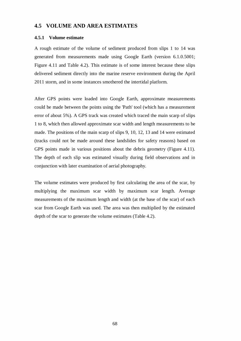
68
4.5 VOLUME AND AREA ESTIMATES
4.5.1 Volume estimate
A rough estimate of the volume of sediment produced from slips 1 to 14 was
generated from measurements made using Google Earth (version 6.1.0.5001;
Figure 4.11 and Table 4.2). This estimate is of some interest because these slips
delivered sediment directly into the marine reserve environment during the April
2011 storm, and in some instances smothered the intertidal platform.
After GPS points were loaded into Google Earth, approximate measurements
could be made between the points using the 'Path' tool (which has a measurement
error of about 5%). A GPS track was created which traced the main scarp of slips
1 to 8, which then allowed approximate scar width and length measurements to be
made. The positions of the main scarp of slips 9, 10, 12, 13 and 14 were estimated
(tracks could not be made around these landslides for safety reasons) based on
GPS points made in various positions about the debris geometry (Figure 4.11).
The depth of each slip was estimated visually during field observations and in
conjunction with later examination of aerial photography.
The volume estimates were produced by first calculating the area of the scar, by
multiplying the maximum scar width by maximum scar length. Average
measurements of the maximum length and width (at the base of the scar) of each
scar from Google Earth was used. The area was then multiplied by the estimated
depth of the scar to generate the volume estimates (Table 4.2).
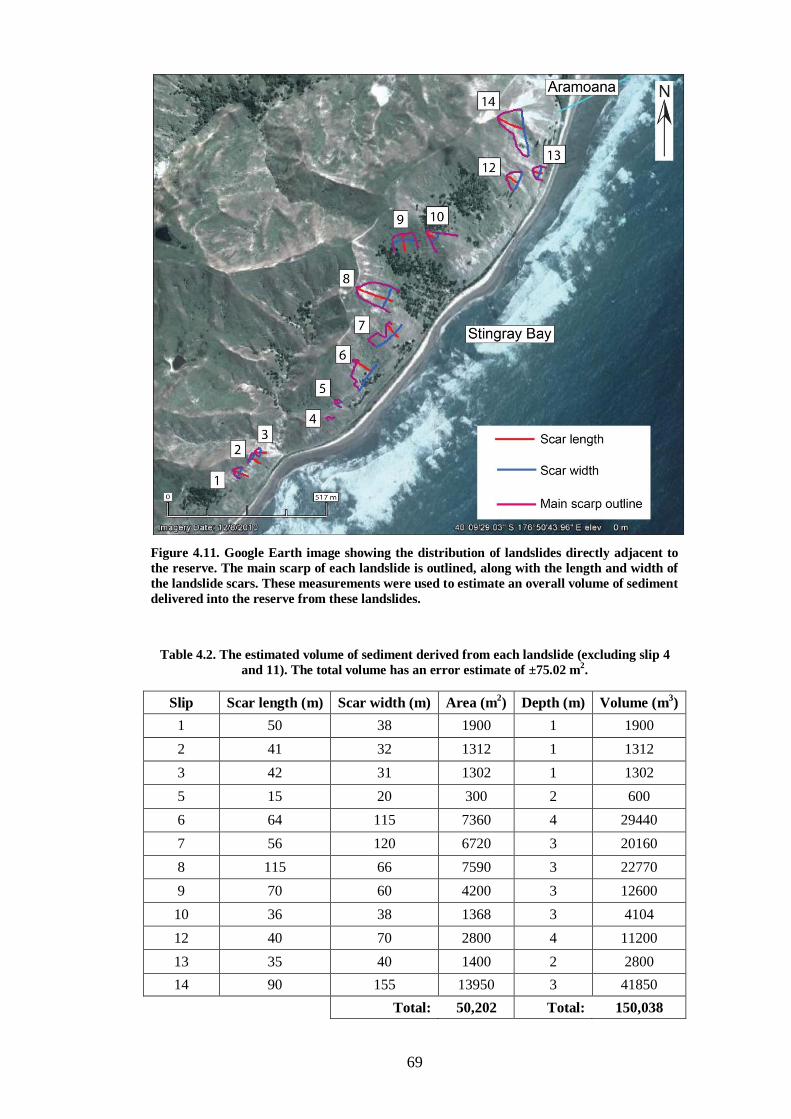
69
Figure 4.11. Google Earth image showing the distribution of landslides directly adjacent to
the reserve. The main scarp of each landslide is outlined, along with the length and width of
the landslide scars. These measurements were used to estimate an overall volume of sediment
delivered into the reserve from these landslides.
Table 4.2. The estimated volume of sediment derived from each landslide (excluding slip 4
and 11). The total volume has an error estimate of ±75.02 m2.
Slip Scar length (m) Scar width (m) Area (m2) Depth (m) Volume (m
3)
1 50 38 1900 1 1900
2 41 32 1312 1 1312
3 42 31 1302 1 1302
5 15 20 300 2 600
6 64 115 7360 4 29440
7 56 120 6720 3 20160
8 115 66 7590 3 22770
9 70 60 4200 3 12600
10 36 38 1368 3 4104
12 40 70 2800 4 11200
13 35 40 1400 2 2800
14 90 155 13950 3 41850
Total: 50,202 Total: 150,038

70
Slip 4 was not included in the volume estimates in Table 4.2 because the debris
from this slip did not reach the beach and was therefore out of influence of the
marine environment. The area of hill side regarded as 'slip' 11 was also not
included since the area was not accessible enough to allow GPS tracks or points to
be made.
The analysis shows that about 150,000 m3 of sediment was produced from slope
failures on the hill sides fronting the Te Angiangi Marine Reserve. The actual
amount of sediment to enter the marine reserve as a result of landslides is likely to
be much larger, because landslides are also locally present throughout the entire
reserve catchment and are also abundant regionally.
4.5.2 Area estimates
Regional area estimate
Geological and Nuclear Science (GNS) were commissioned by the Hawke's Bay
Regional Council to assess the proportion of land affected by landslides on a
regional and individual farm basis along the Hawke's Bay coastal belt. They
achieved this by processing, classifying and analysing satellite imagery from
before and after the storm event by identifying the change in fresh bare ground in
pre- and post-storm images. The study area included the 250 km stretch of
coastline from Mahia to Porangahau and extended 10 km inland.
GNS acquired through the "All of Government" KiwImage program a mosaic of
pre-storm images taken over the period 2006-2010 (Figure 4.12). Post-storm
images were acquired through the RapidEye system which is a constellation of
five satellites that were able to image the Hawke's Bay area on 18-19 May 2011,
shortly after the April 2011 storm (Figure 4.13). The images were then analysed
by GNS using ENVI 4.8 and ArcGIS 10 software for identification of bare ground
(Jones et al., 2011).
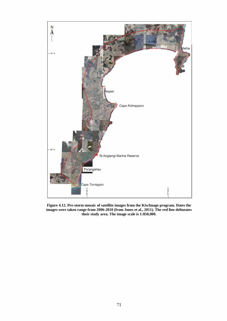
71
Figure 4.12. Pre-storm mosaic of satellite images from the KiwImage program. Dates the
images were taken range from 2006-2010 (from Jones et al., 2011). The red line delineates
their study area. The image scale is 1:850,000.
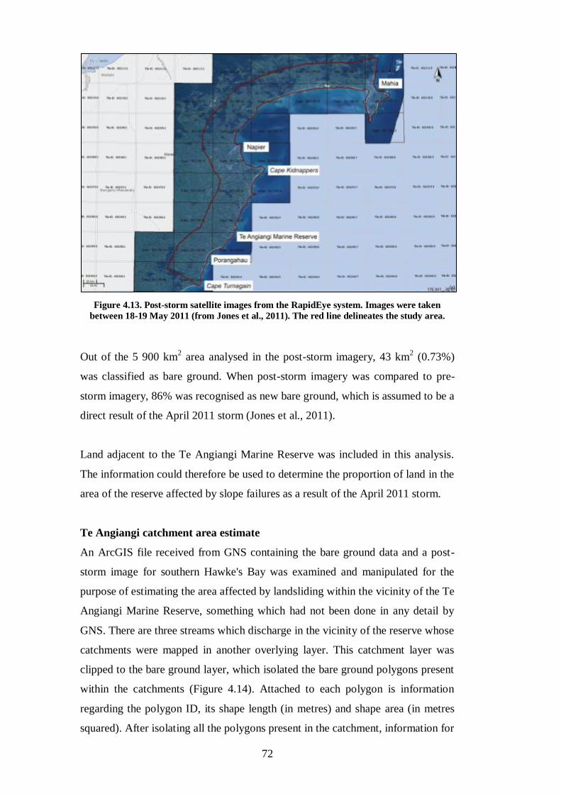
72
Figure 4.13. Post-storm satellite images from the RapidEye system. Images were taken
between 18-19 May 2011 (from Jones et al., 2011). The red line delineates the study area.
Out of the 5 900 km2 area analysed in the post-storm imagery, 43 km
2 (0.73%)
was classified as bare ground. When post-storm imagery was compared to pre-
storm imagery, 86% was recognised as new bare ground, which is assumed to be a
direct result of the April 2011 storm (Jones et al., 2011).
Land adjacent to the Te Angiangi Marine Reserve was included in this analysis.
The information could therefore be used to determine the proportion of land in the
area of the reserve affected by slope failures as a result of the April 2011 storm.
Te Angiangi catchment area estimate
An ArcGIS file received from GNS containing the bare ground data and a post-
storm image for southern Hawke's Bay was examined and manipulated for the
purpose of estimating the area affected by landsliding within the vicinity of the Te
Angiangi Marine Reserve, something which had not been done in any detail by
GNS. There are three streams which discharge in the vicinity of the reserve whose
catchments were mapped in another overlying layer. This catchment layer was
clipped to the bare ground layer, which isolated the bare ground polygons present
within the catchments (Figure 4.14). Attached to each polygon is information
regarding the polygon ID, its shape length (in metres) and shape area (in metres
squared). After isolating all the polygons present in the catchment, information for
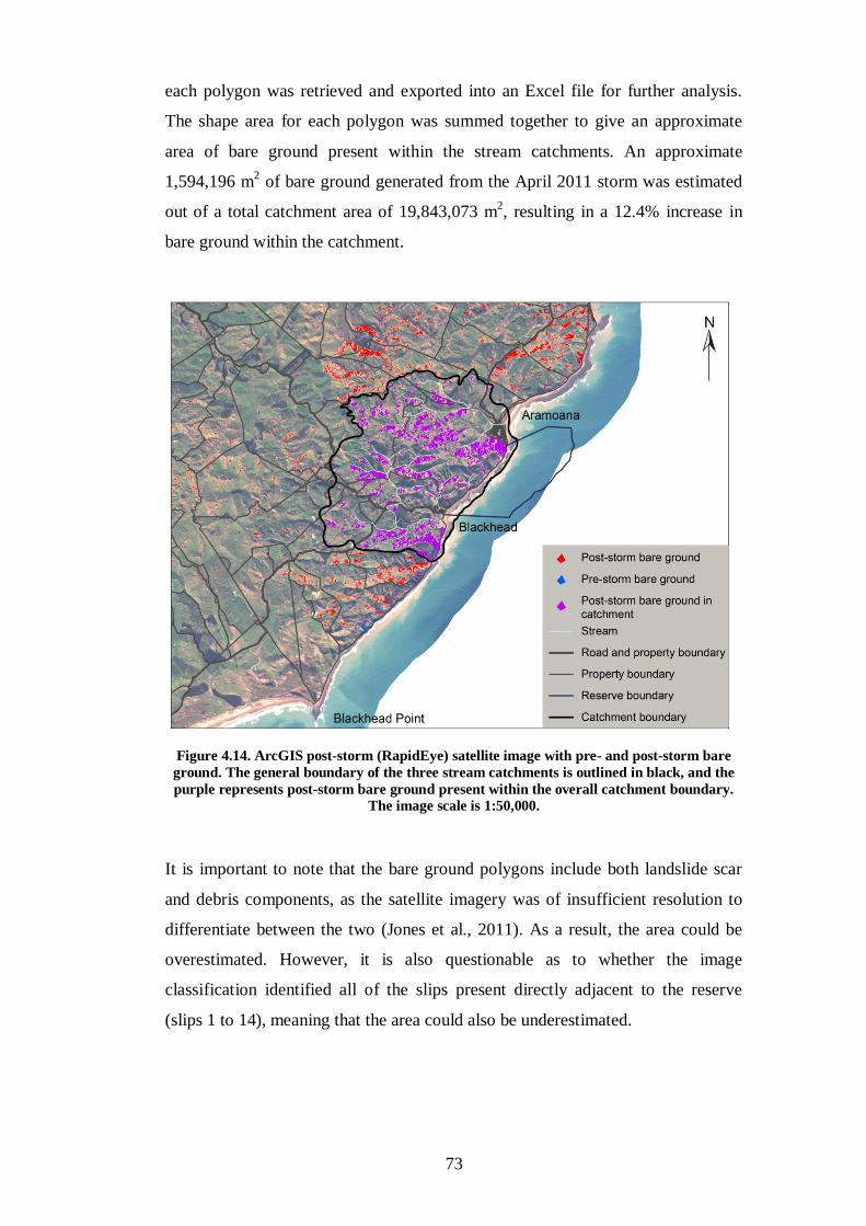
73
each polygon was retrieved and exported into an Excel file for further analysis.
The shape area for each polygon was summed together to give an approximate
area of bare ground present within the stream catchments. An approximate
1,594,196 m2 of bare ground generated from the April 2011 storm was estimated
out of a total catchment area of 19,843,073 m2, resulting in a 12.4% increase in
bare ground within the catchment.
Figure 4.14. ArcGIS post-storm (RapidEye) satellite image with pre- and post-storm bare
ground. The general boundary of the three stream catchments is outlined in black, and the
purple represents post-storm bare ground present within the overall catchment boundary.
The image scale is 1:50,000.
It is important to note that the bare ground polygons include both landslide scar
and debris components, as the satellite imagery was of insufficient resolution to
differentiate between the two (Jones et al., 2011). As a result, the area could be
overestimated. However, it is also questionable as to whether the image
classification identified all of the slips present directly adjacent to the reserve
(slips 1 to 14), meaning that the area could also be underestimated.
74
4.6 DISCUSSION
After describing and classifying the slope failures in the vicinity of the Te
Angiangi Marine Reserve, it is concluded that they are mostly translational debris
slides triggered by intense rainfall during the April 2011 storm, with the possible
contribution from a small earthquake (M4.5) which occurred at the height of the
storm.
An estimated volume of about 150,000 m3 of sediment is thought to have been
produced by the landslides directly adjacent to the marine reserve (Table 4.2). The
figure is approximate because of: (1) small errors in establishing the dimensions
of the landslide scars; (2) the measurement error associated with Google Earth;
and (3) the scar area calculations. The scar area was assumed to be rectangular in
shape when in reality they were more irregular. Also, the volume does not account
for the complex area of landslides named slip 11.
Compared to the volumes of the Ponui and Waipoapoa landslides of 2,500,000 m3
and 8,350,000 m3 respectively the Te Angiangi landslide volume is relatively
small. Moreover, the area of bare ground generated at the immediate coastline, of
about 50,200 m2 (Table 4.2) is tiny area compared with the approximately
1,594,196 m2 of bare ground estimated to have been produced within the
catchment as a result of the April 2011 storm. Such a large area could be more
representative of the amount of sediment to reach the coastline, since it includes
the input from sediment transported in streams. However, this presumes that all
the sediment generated within the catchment was delivered to the coast. The
rainfall which caused the slips very likely provided a medium for much sediment
in the catchment to be transported to the streams and therefore delivered to the
coast.
Sediment produced from landslides within the marine reserve catchment would
have been transported by streams and eventually deposited at the coast, either
within or just outside the reserve, whereas landslides at the coast delivered debris
directly into the marine environment. The landslide sediment from slips 1 to 14
was delivered directly onto the intertidal shore platform, where at high tide it was
exposed to erosion and transported by wave action. The offshore sedimentation
patterns of this landslide sediment is the topic of Chapter 5.
75
5 Chapter 5
OFFSHORE SEDIMENTATION PATTERNS
5.1 INTRODUCTION
The aim of this chapter is to investigate sediment dispersal mechanisms and
depositional patterns over the coastal platform and nearshore region
encompassing the Te Angiangi Marine Reserve. A subtidal sediment survey was
designed in an attempt to detect areas of deposition of the eroded mudstone
detritus. The survey was carried out during field work in March and April 2012,
and the results form the bulk of this chapter. Background information on the
bathymetry and oceanography of the marine reserve are also provided.
Landslides at the coast pose a serious threat to marine organisms and overall
ecological functioning. Landslide plumes of suspended sediment mainly affect
localised offshore areas of the coast. In terms of ecological impacts, direct burial
of sessile communities is a major impact, along with deposition of suspended fine
sediment in plumes. Sediment plumes persist as waves erode away the fine
material, until all that is left of the landslide debris is large boulders (Kiest, 1993).
For the Te Angiangi Marine Reserve project, determining dispersal and
depositional patterns could help explain any spatial and temporal response of the
marine organisms to sedimentation, as it is hypothesised that nearshore currents
might carry and deposit sediment on the reefs north of the reserve, and that
landslide suspended sediment plumes could persist for some time after the initial
landsliding.
After characterising the mudstone through field examination and laboratory work,
and observing its pronounced wetting and drying spheroidal weathering pattern
(Chapter 3), it is considered that fine sized particles are released during this
process. As the eroded particles become finer, they become more easily
transportable by wave action. The large volume landslide debris and long
extension of the debris toes out onto the intertidal platform likely means that it
will take a considerable time for the sediment to be fully dispersed. Sediment is
going to be reworked continuously by wave action during tidal cycles until the
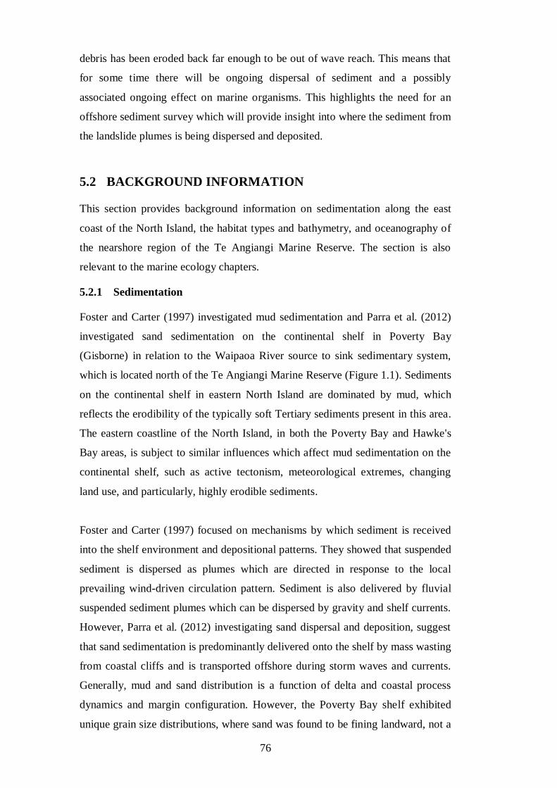
76
debris has been eroded back far enough to be out of wave reach. This means that
for some time there will be ongoing dispersal of sediment and a possibly
associated ongoing effect on marine organisms. This highlights the need for an
offshore sediment survey which will provide insight into where the sediment from
the landslide plumes is being dispersed and deposited.
5.2 BACKGROUND INFORMATION
This section provides background information on sedimentation along the east
coast of the North Island, the habitat types and bathymetry, and oceanography of
the nearshore region of the Te Angiangi Marine Reserve. The section is also
relevant to the marine ecology chapters.
5.2.1 Sedimentation
Foster and Carter (1997) investigated mud sedimentation and Parra et al. (2012)
investigated sand sedimentation on the continental shelf in Poverty Bay
(Gisborne) in relation to the Waipaoa River source to sink sedimentary system,
which is located north of the Te Angiangi Marine Reserve (Figure 1.1). Sediments
on the continental shelf in eastern North Island are dominated by mud, which
reflects the erodibility of the typically soft Tertiary sediments present in this area.
The eastern coastline of the North Island, in both the Poverty Bay and Hawke's
Bay areas, is subject to similar influences which affect mud sedimentation on the
continental shelf, such as active tectonism, meteorological extremes, changing
land use, and particularly, highly erodible sediments.
Foster and Carter (1997) focused on mechanisms by which sediment is received
into the shelf environment and depositional patterns. They showed that suspended
sediment is dispersed as plumes which are directed in response to the local
prevailing wind-driven circulation pattern. Sediment is also delivered by fluvial
suspended sediment plumes which can be dispersed by gravity and shelf currents.
However, Parra et al. (2012) investigating sand dispersal and deposition, suggest
that sand sedimentation is predominantly delivered onto the shelf by mass wasting
from coastal cliffs and is transported offshore during storm waves and currents.
Generally, mud and sand distribution is a function of delta and coastal process
dynamics and margin configuration. However, the Poverty Bay shelf exhibited
unique grain size distributions, where sand was found to be fining landward, not a
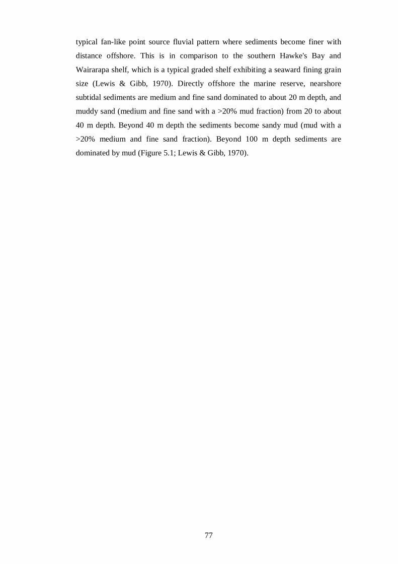
77
typical fan-like point source fluvial pattern where sediments become finer with
distance offshore. This is in comparison to the southern Hawke's Bay and
Wairarapa shelf, which is a typical graded shelf exhibiting a seaward fining grain
size (Lewis & Gibb, 1970). Directly offshore the marine reserve, nearshore
subtidal sediments are medium and fine sand dominated to about 20 m depth, and
muddy sand (medium and fine sand with a >20% mud fraction) from 20 to about
40 m depth. Beyond 40 m depth the sediments become sandy mud (mud with a
>20% medium and fine sand fraction). Beyond 100 m depth sediments are
dominated by mud (Figure 5.1; Lewis & Gibb, 1970).
78
Fig
ure
.5.1
. S
ch
ema
tic s
ho
win
g m
ari
ne
sed
imen
ts o
n t
he
con
tin
en
tal
shel
f a
nd
slo
pe
off
th
e T
e A
ngia
ngi
Mari
ne
Res
erve
an
d t
he g
en
eral
sou
ther
n H
aw
ke'
s B
ay
an
d W
air
ara
pa c
oa
stli
ne
(da
ta f
rom
Lew
is &
Gib
b, 1970 a
nd
Lew
is, 1971).

79
5.2.2 Subtidal habitat types and bathymetry
Funnell et al. (2005) carried out a nearshore subtidal biological habitat and
substrate survey of the area between Blackhead Point in the south to Tuingara
Point in the north, encompassing the Te Angiangi Marine Reserve. This was done
using acoustic mapping and video techniques to collect side-scan sonar,
bathymetry and subtidal video data. The information was collated to create a
habitat map of the study area (Figure 5.2). Side-scan sonar images were analysed
for differences in substrate and the results correlated well with drop camera video
footage. Subtidal reef habitats were classified and mapped for the entire area
based on these data. Based on the video footage it was visually concluded that
most of the study area was soft substrate, composed of well sorted medium sand
covered in medium sized ripples (of 1 to 3 cm high with a wavelength ~10 cm),
with some areas of finer sand and mud. Where there was hard substrate (reef,
boulders and cobbles of rock), the most common habitat in the area was
encrusting invertebrates/sponge flat (15 to 50 m), followed by mixed algae (3 to
20 m) and Ecklonia radiata (kelp) forest (8 to 21 m). Shallow Carpophyllum
maschalocarpum and C. Plumosum (brown algae; 3 to 6 m) is the least common
habitat, but is likely underrepresented due to the inability to systematically
manoeuvre the survey vessel in such shallow water.
80
Figure 5.2. Nearshore subtidal biological habitat types in the vicinity of the study area
(modified from Funnell et al., 2005).
Bathymetry was determined by obtaining survey depths and positions using
differential GPS, single beam echosounder, motion sensor, and hydrographic
software (Figure 5.3).
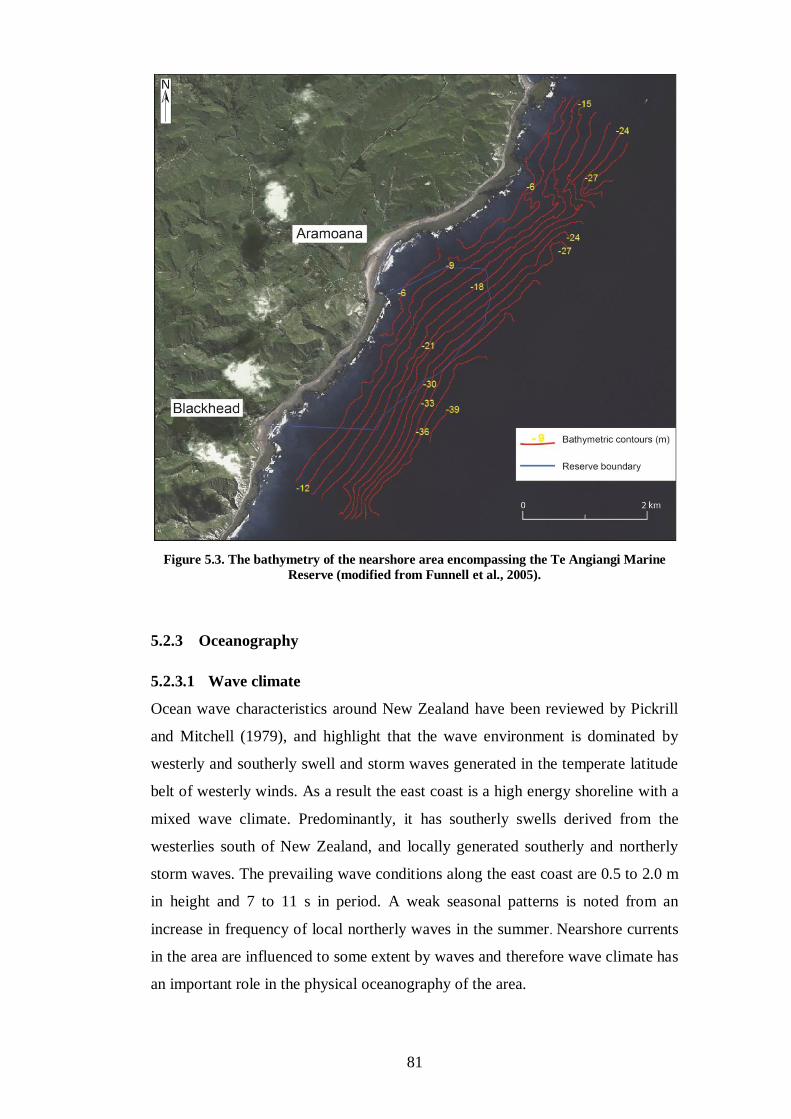
81
Figure 5.3. The bathymetry of the nearshore area encompassing the Te Angiangi Marine
Reserve (modified from Funnell et al., 2005).
5.2.3 Oceanography
5.2.3.1 Wave climate
Ocean wave characteristics around New Zealand have been reviewed by Pickrill
and Mitchell (1979), and highlight that the wave environment is dominated by
westerly and southerly swell and storm waves generated in the temperate latitude
belt of westerly winds. As a result the east coast is a high energy shoreline with a
mixed wave climate. Predominantly, it has southerly swells derived from the
westerlies south of New Zealand, and locally generated southerly and northerly
storm waves. The prevailing wave conditions along the east coast are 0.5 to 2.0 m
in height and 7 to 11 s in period. A weak seasonal patterns is noted from an
increase in frequency of local northerly waves in the summer. Nearshore currents
in the area are influenced to some extent by waves and therefore wave climate has
an important role in the physical oceanography of the area.
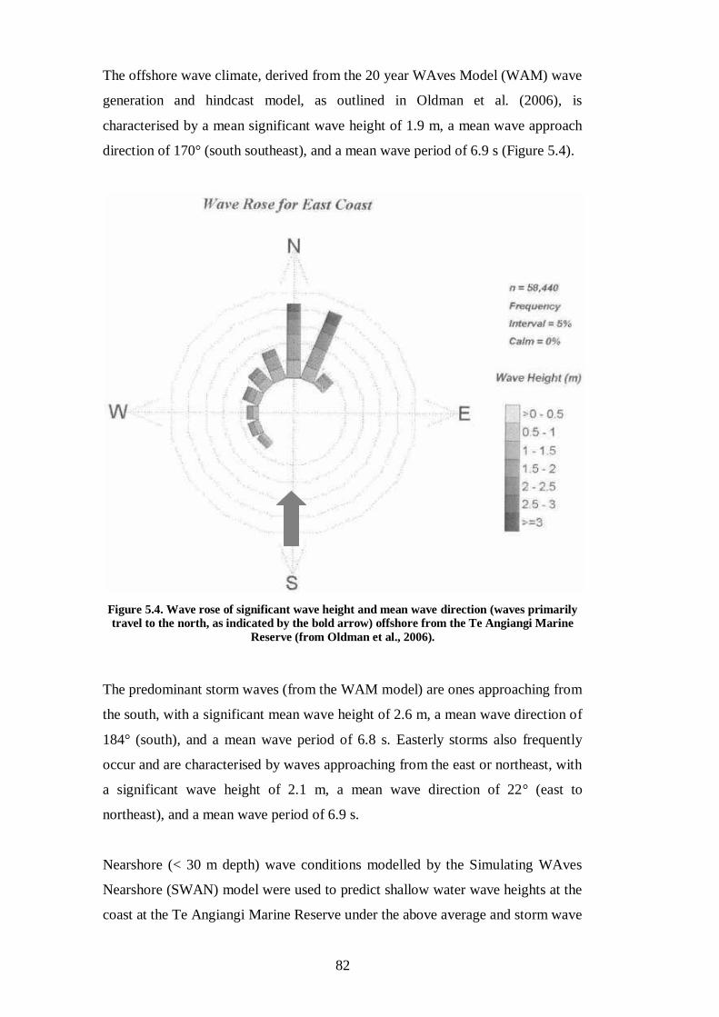
82
The offshore wave climate, derived from the 20 year WAves Model (WAM) wave
generation and hindcast model, as outlined in Oldman et al. (2006), is
characterised by a mean significant wave height of 1.9 m, a mean wave approach
direction of 170° (south southeast), and a mean wave period of 6.9 s (Figure 5.4).
Figure 5.4. Wave rose of significant wave height and mean wave direction (waves primarily
travel to the north, as indicated by the bold arrow) offshore from the Te Angiangi Marine
Reserve (from Oldman et al., 2006).
The predominant storm waves (from the WAM model) are ones approaching from
the south, with a significant mean wave height of 2.6 m, a mean wave direction of
184° (south), and a mean wave period of 6.8 s. Easterly storms also frequently
occur and are characterised by waves approaching from the east or northeast, with
a significant wave height of 2.1 m, a mean wave direction of 22° (east to
northeast), and a mean wave period of 6.9 s.
Nearshore (< 30 m depth) wave conditions modelled by the Simulating WAves
Nearshore (SWAN) model were used to predict shallow water wave heights at the
coast at the Te Angiangi Marine Reserve under the above average and storm wave
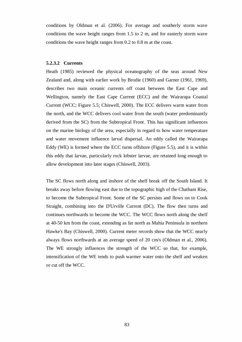
83
conditions by Oldman et al. (2006). For average and southerly storm wave
conditions the wave height ranges from 1.5 to 2 m, and for easterly storm wave
conditions the wave height ranges from 0.2 to 0.8 m at the coast.
5.2.3.2 Currents
Heath (1985) reviewed the physical oceanography of the seas around New
Zealand and, along with earlier work by Brodie (1960) and Garner (1961, 1969),
describes two main oceanic currents off coast between the East Cape and
Wellington, namely the East Cape Current (ECC) and the Wairarapa Coastal
Current (WCC; Figure 5.5; Chiswell, 2000). The ECC delivers warm water from
the north, and the WCC delivers cool water from the south (water predominantly
derived from the SC) from the Subtropical Front. This has significant influences
on the marine biology of the area, especially in regard to how water temperature
and water movement influence larval dispersal. An eddy called the Wairarapa
Eddy (WE) is formed where the ECC turns offshore (Figure 5.5), and it is within
this eddy that larvae, particularly rock lobster larvae, are retained long enough to
allow development into later stages (Chiswell, 2003).
The SC flows north along and inshore of the shelf break off the South Island. It
breaks away before flowing east due to the topographic high of the Chatham Rise,
to become the Subtropical Front. Some of the SC persists and flows on to Cook
Straight, combining into the D'Urville Current (DC). The flow then turns and
continues northwards to become the WCC. The WCC flows north along the shelf
at 40-50 km from the coast, extending as far north as Mahia Peninsula in northern
Hawke's Bay (Chiswell, 2000). Current meter records show that the WCC nearly
always flows northwards at an average speed of 20 cm/s (Oldman et al., 2006).
The WE strongly influences the strength of the WCC so that, for example,
intensification of the WE tends to push warmer water onto the shelf and weaken
or cut off the WCC.
84
Figure 5.5. Coastal currents, eddies, water masses and fronts around New Zealand. The
currents are the East Auckland Current (EAUC), West Auckland Current (WAUC), East
Cape Current (ECC), D'Urville Current (DC), Westland Current (WC), Antarctic
Circumpolar Current (ACC), Southland Current (SC) and the Wairarapa Coastal Current
(WCC). The eddies are the North Cape Eddy (NCE), East Cape Eddy (ECE) and Wairarapa
Eddy (WE). The water masses are Subtropical Water (STW), Subantarctic Water (SAW)
and Circumpolar Surface Water (CSW). The fronts are positioned where the CSW and
SAW meet - the Subantarctic Front (SAF), where the SAW and STW meet - the Subtropical
Front (STF), and the Tasman Front, located in STW to the far north (image modified from
http://www.shiningaspotlight.org.nz/31-the-oceanography-of-the-new-zealand-marine-
ecoregion).
WCC
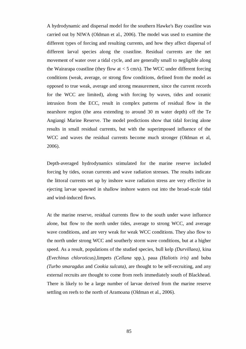
85
A hydrodynamic and dispersal model for the southern Hawke's Bay coastline was
carried out by NIWA (Oldman et al., 2006). The model was used to examine the
different types of forcing and resulting currents, and how they affect dispersal of
different larval species along the coastline. Residual currents are the net
movement of water over a tidal cycle, and are generally small to negligible along
the Wairarapa coastline (they flow at < 5 cm/s). The WCC under different forcing
conditions (weak, average, or strong flow conditions, defined from the model as
opposed to true weak, average and strong measurement, since the current records
for the WCC are limited), along with forcing by waves, tides and oceanic
intrusion from the ECC, result in complex patterns of residual flow in the
nearshore region (the area extending to around 30 m water depth) off the Te
Angiangi Marine Reserve. The model predictions show that tidal forcing alone
results in small residual currents, but with the superimposed influence of the
WCC and waves the residual currents become much stronger (Oldman et al,
2006).
Depth-averaged hydrodynamics stimulated for the marine reserve included
forcing by tides, ocean currents and wave radiation stresses. The results indicate
the littoral currents set up by inshore wave radiation stress are very effective in
ejecting larvae spawned in shallow inshore waters out into the broad-scale tidal
and wind-induced flows.
At the marine reserve, residual currents flow to the south under wave influence
alone, but flow to the north under tides, average to strong WCC, and average
wave conditions, and are very weak for weak WCC conditions. They also flow to
the north under strong WCC and southerly storm wave conditions, but at a higher
speed. As a result, populations of the studied species, bull kelp (Durvillaea), kina
(Evechinus chloroticus),limpets (Cellana spp.), paua (Haliotis iris) and bubu
(Turbo smaragdus and Cookia sulcata), are thought to be self-recruiting, and any
external recruits are thought to come from reefs immediately south of Blackhead.
There is likely to be a large number of larvae derived from the marine reserve
settling on reefs to the north of Aramoana (Oldman et al., 2006).
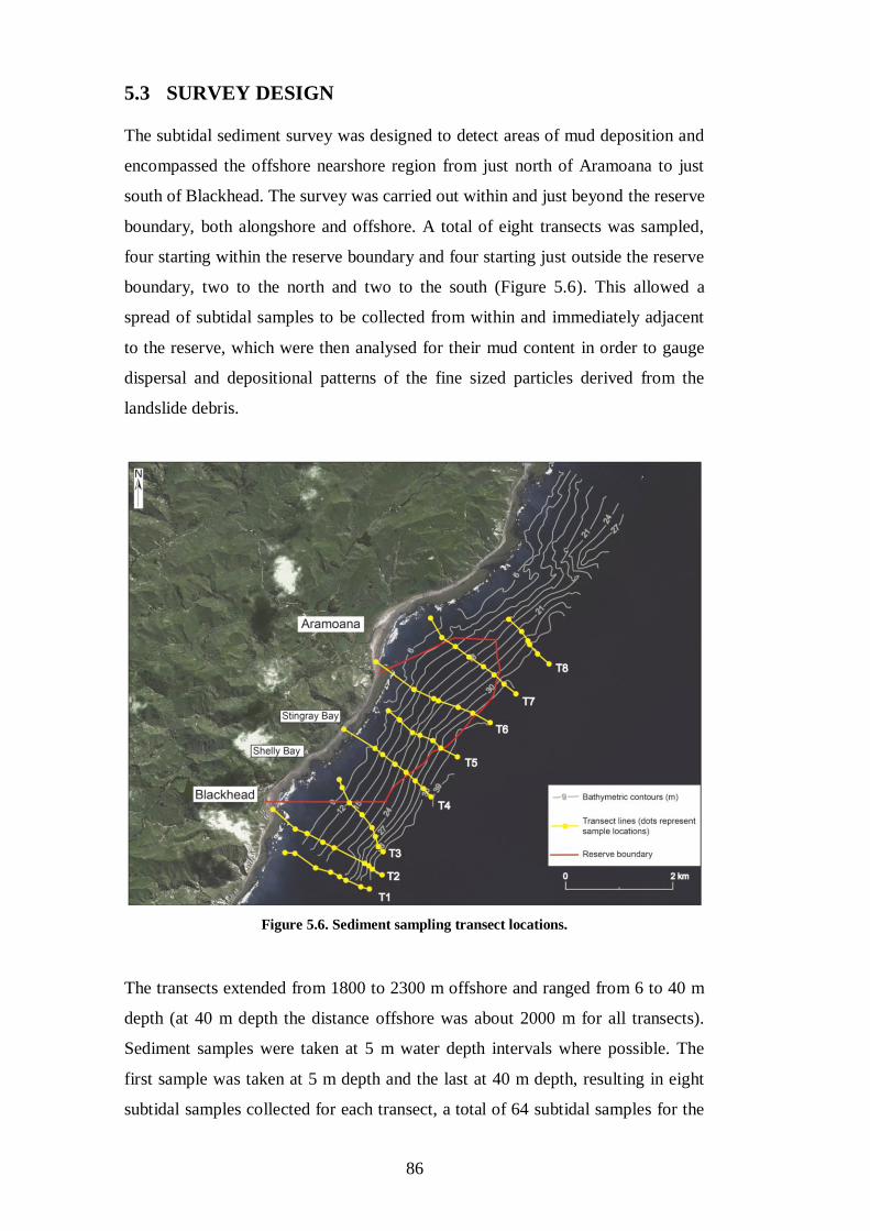
86
5.3 SURVEY DESIGN
The subtidal sediment survey was designed to detect areas of mud deposition and
encompassed the offshore nearshore region from just north of Aramoana to just
south of Blackhead. The survey was carried out within and just beyond the reserve
boundary, both alongshore and offshore. A total of eight transects was sampled,
four starting within the reserve boundary and four starting just outside the reserve
boundary, two to the north and two to the south (Figure 5.6). This allowed a
spread of subtidal samples to be collected from within and immediately adjacent
to the reserve, which were then analysed for their mud content in order to gauge
dispersal and depositional patterns of the fine sized particles derived from the
landslide debris.
Figure 5.6. Sediment sampling transect locations.
The transects extended from 1800 to 2300 m offshore and ranged from 6 to 40 m
depth (at 40 m depth the distance offshore was about 2000 m for all transects).
Sediment samples were taken at 5 m water depth intervals where possible. The
first sample was taken at 5 m depth and the last at 40 m depth, resulting in eight
subtidal samples collected for each transect, a total of 64 subtidal samples for the

87
eight transects. Three intertidal sand samples were collected from Blackhead
Beach, Stingray Bay and Aramoana Beach so that Transect 2 (generally in line
with Blackhead Beach), Transect 4 (generally in line with Stingray Bay) and
Transect 6 (generally in line with Aramoana Beach) could be extended onshore
(Figure 5.6).
5.4 FIELD METHODS
Sediment samples were collected aboard a boat using a petite ponar grab sampler.
Grab samplers are commonly used for quantitative sampling because a volume of
sampled sediment can be calculated based on the dimensions of the sampler
(Morrisey et al., 1998). However, the petite ponar grab was not used for
quantitative purposes in this survey. Primary reasons for its use were: (1) it is easy
to use because it is small and light; (2) it is effective at sampling soft surficial
sediment; and (3) in the case of this survey, due to lack of available SCUBA
divers, it was easier to manage compared to dive core sampling. The petite ponar
grab sampler (Figure 5.7A) is considerably lighter than a standard ponar grab and
allows hand line operation (Figure 5.7B). However, lighter weight grabs
compromise the maximum depths in which it can be deployed because sea
conditions must be calm (mild to moderate current conditions) for adequate use
(Morrisey et al., 1998).
Figure 5.7. A - The ponar grab sampler. B - The ponar grab sampler being deployed using a
pulley.
A B
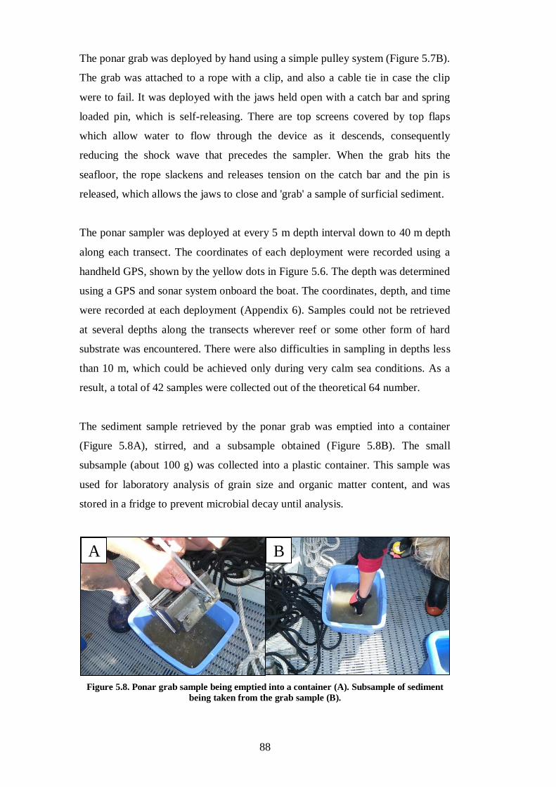
88
The ponar grab was deployed by hand using a simple pulley system (Figure 5.7B).
The grab was attached to a rope with a clip, and also a cable tie in case the clip
were to fail. It was deployed with the jaws held open with a catch bar and spring
loaded pin, which is self-releasing. There are top screens covered by top flaps
which allow water to flow through the device as it descends, consequently
reducing the shock wave that precedes the sampler. When the grab hits the
seafloor, the rope slackens and releases tension on the catch bar and the pin is
released, which allows the jaws to close and 'grab' a sample of surficial sediment.
The ponar sampler was deployed at every 5 m depth interval down to 40 m depth
along each transect. The coordinates of each deployment were recorded using a
handheld GPS, shown by the yellow dots in Figure 5.6. The depth was determined
using a GPS and sonar system onboard the boat. The coordinates, depth, and time
were recorded at each deployment (Appendix 6). Samples could not be retrieved
at several depths along the transects wherever reef or some other form of hard
substrate was encountered. There were also difficulties in sampling in depths less
than 10 m, which could be achieved only during very calm sea conditions. As a
result, a total of 42 samples were collected out of the theoretical 64 number.
The sediment sample retrieved by the ponar grab was emptied into a container
(Figure 5.8A), stirred, and a subsample obtained (Figure 5.8B). The small
subsample (about 100 g) was collected into a plastic container. This sample was
used for laboratory analysis of grain size and organic matter content, and was
stored in a fridge to prevent microbial decay until analysis.
Figure 5.8. Ponar grab sample being emptied into a container (A). Subsample of sediment
being taken from the grab sample (B).
A B
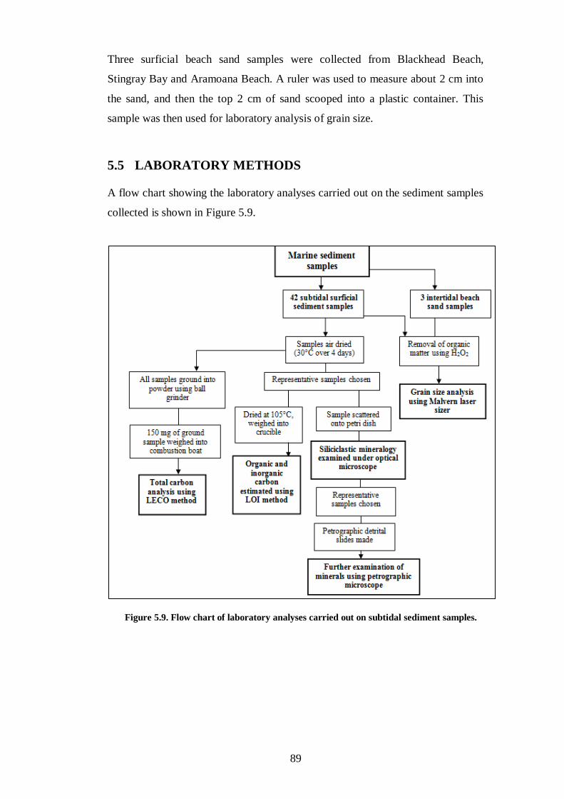
89
Three surficial beach sand samples were collected from Blackhead Beach,
Stingray Bay and Aramoana Beach. A ruler was used to measure about 2 cm into
the sand, and then the top 2 cm of sand scooped into a plastic container. This
sample was then used for laboratory analysis of grain size.
5.5 LABORATORY METHODS
A flow chart showing the laboratory analyses carried out on the sediment samples
collected is shown in Figure 5.9.
Figure 5.9. Flow chart of laboratory analyses carried out on subtidal sediment samples.
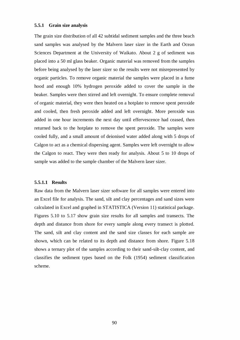
90
5.5.1 Grain size analysis
The grain size distribution of all 42 subtidal sediment samples and the three beach
sand samples was analysed by the Malvern laser sizer in the Earth and Ocean
Sciences Department at the University of Waikato. About 2 g of sediment was
placed into a 50 ml glass beaker. Organic material was removed from the samples
before being analysed by the laser sizer so the results were not misrepresented by
organic particles. To remove organic material the samples were placed in a fume
hood and enough 10% hydrogen peroxide added to cover the sample in the
beaker. Samples were then stirred and left overnight. To ensure complete removal
of organic material, they were then heated on a hotplate to remove spent peroxide
and cooled, then fresh peroxide added and left overnight. More peroxide was
added in one hour increments the next day until effervescence had ceased, then
returned back to the hotplate to remove the spent peroxide. The samples were
cooled fully, and a small amount of deionised water added along with 5 drops of
Calgon to act as a chemical dispersing agent. Samples were left overnight to allow
the Calgon to react. They were then ready for analysis. About 5 to 10 drops of
sample was added to the sample chamber of the Malvern laser sizer.
5.5.1.1 Results
Raw data from the Malvern laser sizer software for all samples were entered into
an Excel file for analysis. The sand, silt and clay percentages and sand sizes were
calculated in Excel and graphed in STATISTICA (Version 11) statistical package.
Figures 5.10 to 5.17 show grain size results for all samples and transects. The
depth and distance from shore for every sample along every transect is plotted.
The sand, silt and clay content and the sand size classes for each sample are
shown, which can be related to its depth and distance from shore. Figure 5.18
shows a ternary plot of the samples according to their sand-silt-clay content, and
classifies the sediment types based on the Folk (1954) sediment classification
scheme.
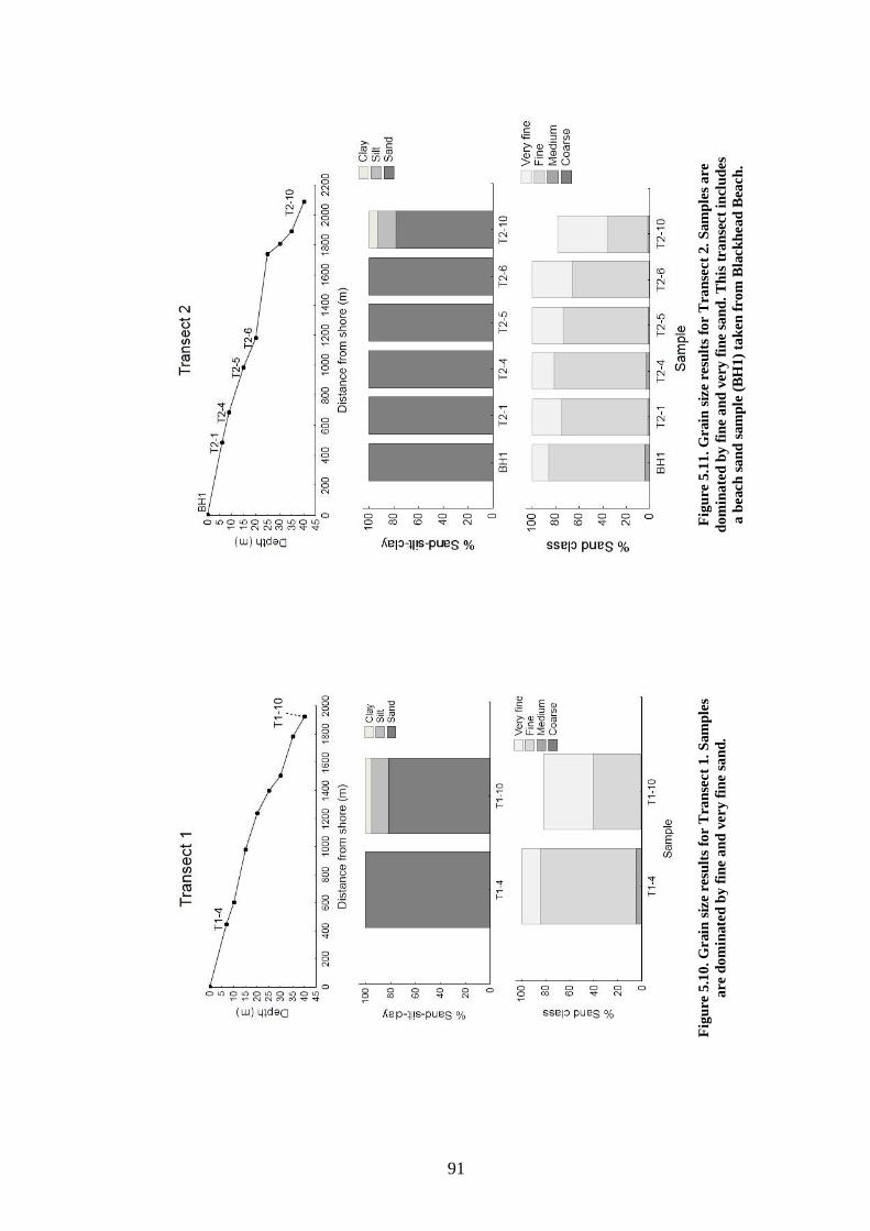
91
Fig
ure
5.1
0. G
rain
siz
e re
sult
s fo
r T
ran
sect
1.
Sam
ple
s
are
dom
inate
d b
y f
ine
an
d v
ery f
ine s
an
d.
Fig
ure
5.1
0. G
rain
siz
e re
sult
s fo
r T
ran
sect
1.
Sam
ple
s
are
dom
inate
d b
y f
ine
an
d v
ery f
ine s
an
d.
Fig
ure
5.1
1.
Grain
siz
e re
sult
s fo
r T
ran
sect
2.
Sam
ple
s are
do
min
ate
d b
y f
ine
an
d v
ery
fin
e sa
nd
. T
his
tran
sect
incl
ud
es
a b
each
san
d s
am
ple
(B
H1)
tak
en
from
Bla
ck
head
Bea
ch
.

92
Fig
ure
5.1
3.
Grain
siz
e re
sult
s fo
r T
ran
sect
4.
Sam
ple
s are
dom
inate
d
by
fin
e an
d v
ery f
ine
san
d a
nd
in
crease
in
mu
d c
on
ten
t w
ith
incre
asi
ng d
ep
th. T
his
tran
sect
inclu
des
a b
each
san
d s
am
ple
(S
B1)
tak
en
from
Sti
ngray B
ay.
Fig
ure
5.1
2. G
rain
siz
e re
sult
s fo
r T
ran
sect
3.
Sam
ple
s a
re d
om
ina
ted
by
fin
e an
d v
ery f
ine
san
d.
Wit
h t
he
exce
pti
on
of
sam
ple
T3
-9, th
e
sam
ple
s sh
ow
a s
tead
y i
ncr
ease
in
mu
d c
on
ten
t w
ith
dep
th,
an
d T
3-1
0
is m
ain
ly c
om
pose
d o
f si
lt.
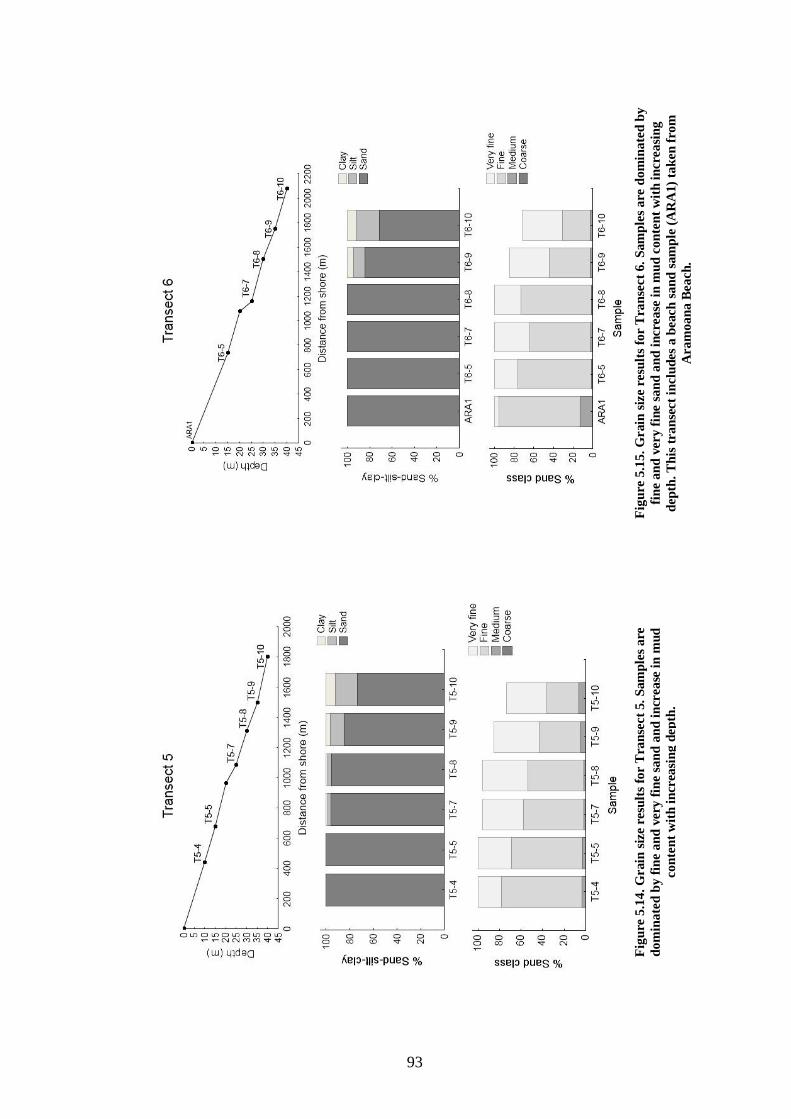
93
Fig
ure
5.1
5.
Grain
siz
e re
sult
s fo
r T
ran
sect
6.
Sam
ple
s are
dom
inate
d b
y
fin
e a
nd
very f
ine s
an
d a
nd
in
cre
ase
in
mu
d c
on
ten
t w
ith
in
cre
asi
ng
dep
th.
Th
is t
ran
sect
inclu
des
a b
each
san
d s
am
ple
(A
RA
1)
tak
en
fro
m
Aram
oan
a B
each
.
Fig
ure
5.1
4.
Grain
siz
e re
sult
s fo
r T
ran
sect
5.
Sam
ple
s a
re
dom
inate
d b
y f
ine
an
d v
ery
fin
e sa
nd
an
d i
ncr
ea
se i
n m
ud
con
ten
t w
ith
in
crea
sin
g d
ep
th.
94
Fig
ure
5.1
7. G
rain
siz
e re
sult
s fo
r T
ran
sect
4.
Sam
ple
s
are
dom
inate
d b
y f
ine
an
d v
ery f
ine s
an
d.
Fig
ure
5.1
6. G
rain
siz
e re
sult
s fo
r T
ran
sect
7.
Sam
ple
s a
re
dom
inate
d b
y f
ine
an
d v
ery
fin
e sa
nd
an
d i
ncr
ea
se i
n m
ud
con
ten
t w
ith
in
crea
sin
g d
ep
th.
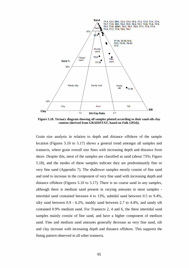
95
Figure 5.18. Ternary diagram showing all samples plotted according to their sand-silt-clay
content (derived from GRADISTAT, based on Folk (1954)).
Grain size analysis in relation to depth and distance offshore of the sample
location (Figures 5.10 to 5.17) shows a general trend amongst all samples and
transects, where grain overall size fines with increasing depth and distance from
shore. Despite this, most of the samples are classified as sand (about 73%; Figure
5.18), and the modes of these samples indicate they are predominantly fine or
very fine sand (Appendix 7). The shallower samples mostly consist of fine sand
and tend to increase in the component of very fine sand with increasing depth and
distance offshore (Figures 5.10 to 5.17). There is no coarse sand in any samples,
although there is medium sand present in varying amounts in most samples -
intertidal sand contained between 4 to 13%, subtidal sand between 0.5 to 9.4%,
silty sand between 0.9 - 6.2%, muddy sand between 2.7 to 4.4%, and sandy silt
contained 0.9% medium sand. For Transects 2, 4 and 6, the three intertidal sand
samples mainly consist of fine sand, and have a higher component of medium
sand. Fine and medium sand amounts generally decrease as very fine sand, silt
and clay increase with increasing depth and distance offshore. This supports the
fining pattern observed in all other transects.
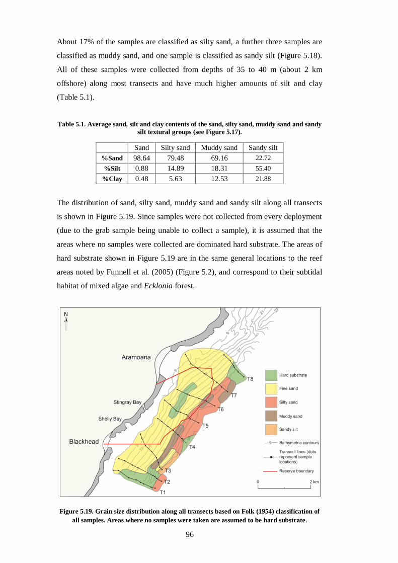
96
About 17% of the samples are classified as silty sand, a further three samples are
classified as muddy sand, and one sample is classified as sandy silt (Figure 5.18).
All of these samples were collected from depths of 35 to 40 m (about 2 km
offshore) along most transects and have much higher amounts of silt and clay
(Table 5.1).
Table 5.1. Average sand, silt and clay contents of the sand, silty sand, muddy sand and sandy
silt textural groups (see Figure 5.17).
Sand Silty sand Muddy sand Sandy silt
%Sand 98.64 79.48 69.16 22.72
%Silt 0.88 14.89 18.31 55.40
%Clay 0.48 5.63 12.53 21.88
The distribution of sand, silty sand, muddy sand and sandy silt along all transects
is shown in Figure 5.19. Since samples were not collected from every deployment
(due to the grab sample being unable to collect a sample), it is assumed that the
areas where no samples were collected are dominated hard substrate. The areas of
hard substrate shown in Figure 5.19 are in the same general locations to the reef
areas noted by Funnell et al. (2005) (Figure 5.2), and correspond to their subtidal
habitat of mixed algae and Ecklonia forest.
Figure 5.19. Grain size distribution along all transects based on Folk (1954) classification of
all samples. Areas where no samples were taken are assumed to be hard substrate.
97
The primary result shown from the grain size distribution analyses is that mud
(silt plus clay) occurs only near or beyond the seaward boundary of the marine
reserve, indicating that the majority of the mud sized sediment has not settled
within the marine reserve itself.
5.5.2 Mineralogy
It is assumed that the origin of the mud found in the nearshore region of the
marine reserve is derived from weathering of the landslide debris material.
However, it may also be derived from alongshore and/or onshore and offshore
transport mechanisms. To aid in identifying the source of mud sized particles,
mineralogical analysis was carried out on representative subtidal samples, the
results of which can be compared with the mineralogical composition of the
onshore mudstone rock samples tested in Chapter 3.
All samples from Transect 2 (BH1, T2-1, T2-4, T2-5, T2-6, T2-10), Transect 4
(SB1, T4-4, T4-5, T4-6, T4-7, T4-8, T4-9) and Transect 6 (ARA1, T6-5, T6-7,
T6-8, T6-9, T6-10; Figure 5.6) were chosen for mineralogical analysis. These
transects were selected to give three complete offshore transects covering both
along and offshore directions.
Detrital mineralogical composition was determined by optical mineralogy
methods. Firstly, the sediment samples were transferred into tin trays and air dried
over four days in a 30°C oven. Once dry, a small amount of sample was scattered
onto a clean petri dish and examined under a binocular microscope to determine
general mineralogical composition. Further examination was then carried out on
representative samples based on the results of the detrital mineralogy.
Petrographic thin-section slides were made for samples BH1, T6-7, T2-10, and
mudstone sample DM1 (refer to Chapter 3), and examined under petrographic
microscope in order to further identify minerals that could not be accurately
identified from the binocular microscope. Sample DM1 was used as a reference to
help in identifying rock fragments. Thin-sections were made by firstly frosting
one side of a glass slide using a Struers diamond Discoplan-TS precision cutting
and grinding machine. Slides were rinsed with water and allowed to dry. For
samples BH1, T6-7 and T2-10, the loose sediment was prepared by sieving
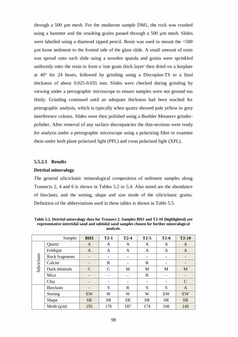
98
through a 500 µm mesh. For the mudstone sample DM1, the rock was crushed
using a hammer and the resulting grains passed through a 500 µm mesh. Slides
were labelled using a diamond tipped pencil. Resin was used to mount the <500
µm loose sediment to the frosted side of the glass slide. A small amount of resin
was spread onto each slide using a wooden spatula and grains were sprinkled
uniformly onto the resin to form a 'one grain thick layer' then dried on a hotplate
at 40° for 24 hours, followed by grinding using a Discoplan-TS to a final
thickness of about 0.025-0.035 mm. Slides were checked during grinding by
viewing under a petrographic microscope to ensure samples were not ground too
thinly. Grinding continued until an adequate thickness had been reached for
petrographic analysis, which is typically when quartz showed pale yellow to grey
interference colours. Slides were then polished using a Buehler Metaserv grinder-
polisher. After removal of any surface discrepancies the thin-sections were ready
for analysis under a petrographic microscope using a polarizing filter to examine
them under both plane polarized light (PPL) and cross polarized light (XPL).
5.5.2.1 Results
Detrital mineralogy
The general siliciclastic mineralogical composition of sediment samples along
Transects 2, 4 and 6 is shown in Tables 5.2 to 5.4. Also noted are the abundance
of bioclasts, and the sorting, shape and size mode of the siliciclastic grains.
Definition of the abbreviations used in these tables is shown in Table 5.5.
Table 5.2. Detrital mineralogy data for Transect 2. Samples BH1 and T2-10 (highlighted) are
representative intertidal sand and subtidal sand samples chosen for further mineralogical
analysis.
Sample: BH1 T2-1 T2-4 T2-5 T2-6 T2-10
Sil
icic
last
s
Quartz A A A A A A
Feldspar A A A A A A
Rock fragments - - - - - -
Calcite - R - R - -
Dark minerals C C M M M M
Mica - - - R - -
Clay - - - - - C
Bioclasts - S R S S A
Sorting EW W W W EW EW
Shape SR SR SR SR SR SR
Mode (µm) 195 176 187 174 166 140
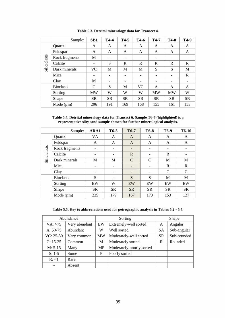
99
Table 5.3. Detrital mineralogy data for Transect 4.
Sample: SB1 T4-4 T4-5 T4-6 T4-7 T4-8 T4-9
Sil
icic
last
s Quartz A A A A A A A
Feldspar A A A A A A A
Rock fragments M - - - - - -
Calcite - S R R R R R
Dark minerals VC M M M S S M
Mica - - - - - - R
Clay M - - - - - -
Bioclasts C S M VC A A A
Sorting MW W W W MW MW W
Shape SR SR SR SR SR SR SR
Mode (µm) 206 191 169 168 155 161 153
Table 5.4. Detrital mineralogy data for Transect 6. Sample T6-7 (highlighted) is a
representative silty sand sample chosen for further mineralogical analysis.
Sample: ARA1 T6-5 T6-7 T6-8 T6-9 T6-10
Sil
icic
last
s
Quartz VA A A A A A
Feldspar A A A A A A
Rock fragments - - - - - -
Calcite - - R - R -
Dark minerals M M C C M M
Mica - - - - R R
Clay - - - - C C
Bioclasts S - S S M M
Sorting EW W EW EW EW EW
Shape SR SR SR SR SR SR
Mode (µm) 225 179 167 173 153 127
Table 5.5. Key to abbreviations used for petrographic analysis in Tables 5.2 - 5.4.
Abundance Sorting Shape
VA: >75 Very abundant EW Extremely-well sorted A Angular
A: 50-75 Abundant W Well sorted SA Sub-angular
VC: 25-50 Very common MW Moderately-well sorted SR Sub-rounded
C: 15-25 Common M Moderately sorted R Rounded
M: 5-15 Many MP Moderately-poorly sorted
S: 1-5 Some P Poorly sorted
R: <1 Rare
- Absent

100
All the sediments consist of abundant quartz and feldspar (50-75%). They also
contain some to common dark minerals, including magnetite (1-25%), some to
abundant bioclasts (1-75%), and rare rock fragments (<1%). Calcite was present
in rare to some amounts (<1 - 5%), mica (muscovite) in rare amounts (<1%), and
clay in many to common amounts (5-25%). Rock fragments were only found in
sample SB1, which was collected at the mid-tide mark directly opposite a large
collection of landslide debris. This sample, along with muddy sand sample T6-9,
and silty sand samples T6-10 and T2-10, contained 5-25% clay. Calcite was found
in rare abundance, while bioclasts were generally more abundant in most samples
from Transect 4. There is no obvious trend in dark mineral abundance along or
offshore.
The samples ranged from moderately to extremely-well sorted and all grains were
sub-rounded. The modal size for intertidal sand ranged from 195 to 225 µm, with
the Blackhead and Aramoana Beach samples being extremely-well sorted and the
Stingray Bay sand being moderately-well sorted. The mode for subtidal sand
ranged from 155 to 191 µm with the sorting ranging from moderately to
extremely-well sorted. The modal size for silty sand ranged from 127 to 153 µm
with the Blackhead and Aramoana Beach samples being extremely-well sorted
and the Stingray Bay sand being well sorted.
A weak alongshore tend in mineralogical composition is observed. Overall,
Transect 4 samples were less well sorted than the other two transects, possibly
because this transect was located directly opposite an area severely affected by
landsliding. Transect 4 also contained rock fragments, generally more calcite, and
a higher abundance of bioclasts. Samples from Transects 2 and 6 were similar, but
Transect 6 contained more clay and mica. No obvious offshore mineral patterns
were observed.
Due to several limitations with simple optical microscopy, mineral identifications
may not be accurate. For example, rock fragments may have been incorrectly
identified as dark minerals, and clay might have been incorrectly identified as
crushed fine rock fragments, dark minerals, or quartz. Calcite may have been
identified as mica, and vice versa. Consequently, some further examination was
needed to better identify the minerals.
101
Thin-section mineralogy
A petrographic microscope was used to further identify minerals that could not be
positively identified from the binocular microscope. Sample BH1 was chosen as a
representative intertidal beach sand sample, sample T6-7 as a representative
subtidal sand sample, and sample T2-10 as a representative silty sand sample.
Samples that classified as sand and silty sand were chosen because they are the
two main sediment types along Transects 2, 4 and 6 (Figure 5.18).
Petrographic analysis allowed better identification of some minerals that were
suspected to be present based on the general mineral results (Tables 5.2 to 5.4).
The intertidal sand sample BH1 mainly contained fractured quartz and feldspar
(Figure 5.20A and B), rock fragments (Figure 5.22C and D) and bioclasts (Figure
5.20C and D). The subtidal sand sample T6-7 mainly contained quartz (Figure
5.20E, F and G), feldspar (mostly plagioclase; Figure 5.20H), and suspected rock
fragments. Silty sand sample T2-10 mainly contained quartz and feldspar (mostly
plagioclase; Figure 5.21C and D), bioclasts (Figure 5.21E) and some calcite
(Figure 5.21A and B). The grains in this sample were notably smaller (10 to 60
µm; Figure 5.21F) compared to the other subtidal sample examined (40 to 100
µm; Figure 5.20E).
To clarify if some grains were rock fragments, thin-section DM1 was examined
and the fragments of mudstone in this sample compared to an example of a
suspected rock fragment from sample BH1 (Figure 5.22).
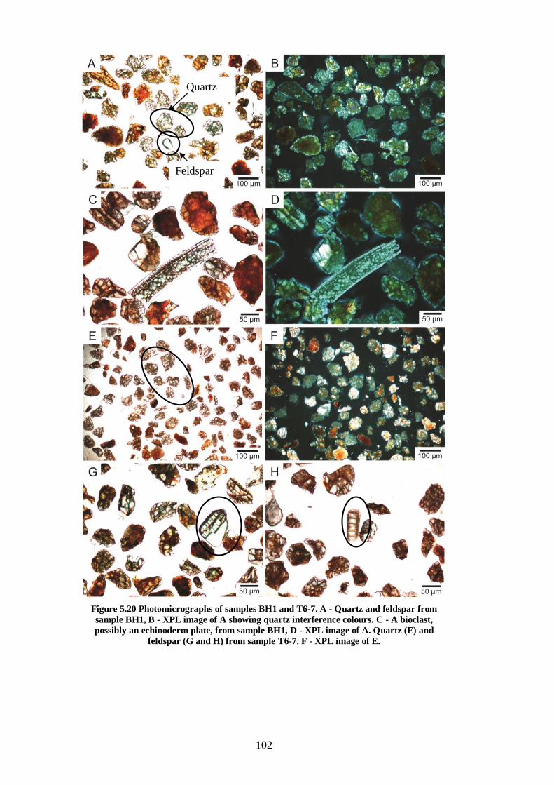
102
Figure 5.20 Photomicrographs of samples BH1 and T6-7. A - Quartz and feldspar from
sample BH1, B - XPL image of A showing quartz interference colours. C - A bioclast,
possibly an echinoderm plate, from sample BH1, D - XPL image of A. Quartz (E) and
feldspar (G and H) from sample T6-7, F - XPL image of E.
Quartz
Feldspar
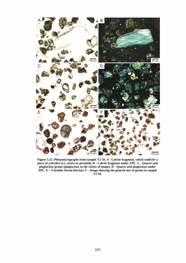
103
Figure 5.21. Photomicrographs from sample T2-10. A - Calcite fragment, which could be a
piece of a bivalve (i.e. oyster or pectinid), B - Calcite fragment under XPL. C - Quartz and
plagioclase grains (plagioclase in the centre of image). D - Quartz and plagioclase under
XPL. E - A benthic foram bioclast. F - Image showing the general size of grains in sample
T2-10.
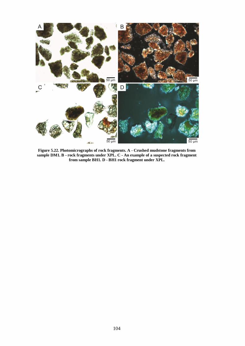
104
Figure 5.22. Photomicrographs of rock fragments. A - Crushed mudstone fragments from
sample DM1. B - rock fragments under XPL. C - An example of a suspected rock fragment
from sample BH1. D - BH1 rock fragment under XPL.
105
5.5.3 Carbon analysis
The organic carbon, or organic matter, content in subtidal surficial sediments can
be used as an indicator of the benthic health for marine ecological purposes. The
amount of carbon in sediments is often used as an indication of the amount of
food available for benthic organisms, or as an indication of the amount and type
of food settling to the sediments through the water column (Byers et al., 1978).
The amount of organic material can also control the oxidation state of silicates in
the sedimentary environment (Velde, 1992). Two methods (LECO and loss on
ignition (LOI)) were trialled in order to determine the carbon content of the
subtidal surficial sediment samples. A combination of LECO and loss on ignition
(LOI) methods are often used to measure carbon in marine sediments (Byers et
al., 1978).
5.5.3.1 LECO carbon analyser total carbon method
The first method used a LECO TruSpec CN Carbon/Nitrogen Determinator to
measure the total carbon (TC = both inorganic and organic carbon components)
within all subtidal sediment samples, which is used to approximate the percentage
of organic carbon. 150 mg of dried, powdered sample was measured into tinfoil
cups before being placed in a loading head. Samples were then combusted at
950°C in a temporary oxygen enriched atmosphere to convert carbon in the solid
sample to gas form (CO2). The combustion gases are passed through a secondary
furnace at 850°C for further oxidation and particulate removal before then being
passed through an additional furnace filter and two stage thermoelectric cooler,
removing moisture, into a collection vessel known as the ballast. Carbon is then
measured in the combustion gases as carbon dioxide by the CO2 infrared detector.
Results
The percentage of total carbon based on weight is very small - from 0.6 to 1.8 %.
However, a trend where total carbon increases with depth and distance offshore is
observed along all the transects, and is particularly evident in Transect 5 (Figure
5.23). This increasing carbon with increasing depth and distance offshore trend is
associated with grain size, and when total carbon is compared to the grain size
mode of each sample (Figure 5.23), a strong relationship where total carbon
increases with a decrease in grain size is evident.
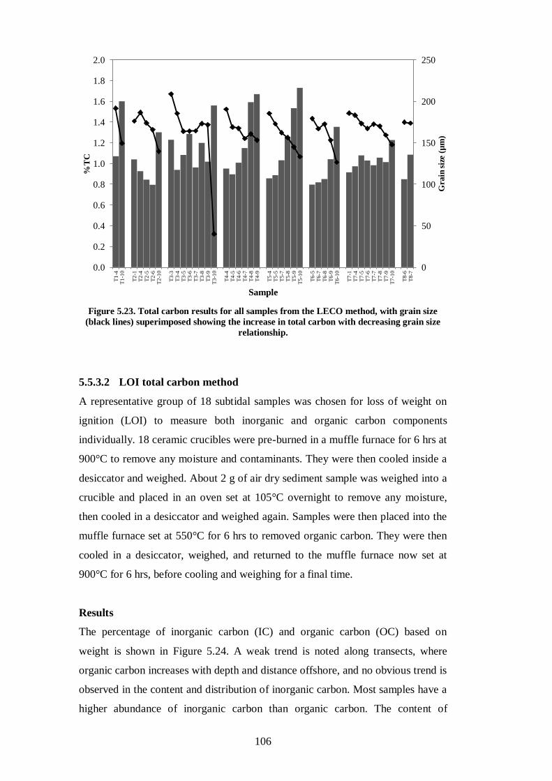
106
Figure 5.23. Total carbon results for all samples from the LECO method, with grain size
(black lines) superimposed showing the increase in total carbon with decreasing grain size
relationship.
5.5.3.2 LOI total carbon method
A representative group of 18 subtidal samples was chosen for loss of weight on
ignition (LOI) to measure both inorganic and organic carbon components
individually. 18 ceramic crucibles were pre-burned in a muffle furnace for 6 hrs at
900°C to remove any moisture and contaminants. They were then cooled inside a
desiccator and weighed. About 2 g of air dry sediment sample was weighed into a
crucible and placed in an oven set at 105°C overnight to remove any moisture,
then cooled in a desiccator and weighed again. Samples were then placed into the
muffle furnace set at 550°C for 6 hrs to removed organic carbon. They were then
cooled in a desiccator, weighed, and returned to the muffle furnace now set at
900°C for 6 hrs, before cooling and weighing for a final time.
Results
The percentage of inorganic carbon (IC) and organic carbon (OC) based on
weight is shown in Figure 5.24. A weak trend is noted along transects, where
organic carbon increases with depth and distance offshore, and no obvious trend is
observed in the content and distribution of inorganic carbon. Most samples have a
higher abundance of inorganic carbon than organic carbon. The content of
0
50
100
150
200
250
0.0
0.2
0.4
0.6
0.8
1.0
1.2
1.4
1.6
1.8
2.0
T1
-4
T1
-10
T2
-1
T2
-4
T2
-5
T2
-6
T2
-10
T3
-3
T3
-4
T3
-5
T3
-6
T3
-7
T3
-8
T3
-9
T3
-10
T4
-4
T4
-5
T4
-6
T4
-7
T4
-8
T4
-9
T5
-4
T5
-5
T5
-7
T5
-8
T5
-9
T5
-10
T6
-5
T6
-7
T6
-8
T6
-9
T6
-10
T7
-1
T7
-4
T7
-5
T7
-6
T7
-7
T7
-8
T7
-9
T7
-10
T8
-6
T8
-7
Gra
in s
ize
(µm
)
%T
C
Sample

107
inorganic and organic carbon is very small, varying from about 0.1 to 0.4%. When
inorganic and organic carbon is compared with grain size, the comparison shows
generally that, with the exception of sample T3-4, organic carbon increases with
decreasing grain size, so the finer grained samples contain a higher amount of
organic carbon compared to coarser grained samples (Figure 5.24).
Figure 5.24. Inorganic carbon (IC) and organic carbon (OC) components of representative
samples from the LOI method, with grain size (black lines) superimposed showing the
increase in organic carbon with decreasing grain size relationship.
Organic carbon is present in higher amounts in finer sediments because during
transport offshore they are sorted together, become bound since organic carbon is
directly associated with mineral grains, and are deposited together in calmer
waters (Chester, 1993). Organic carbon remains present in relatively higher
amounts since the supply of oxidising agents to organic debris are more restricted
to clay-rich deposits (Chester, 1993).
0
50
100
150
200
250
0.00
0.10
0.20
0.30
0.40
0.50
0.60
T1
-4
T1
-10
T2
-4
T2
-5
T2
-6
T2-1
0
T3
-3
T3
-4
T3
-5
T3
-6
T3
-7
T3
-8
T3
-9
T3-1
0
T4
-4
T4
-5
T4
-6
T4
-7
Grain
siz
e (
µm
)
%
Sample
wt% IC
wt% OC
Grain size
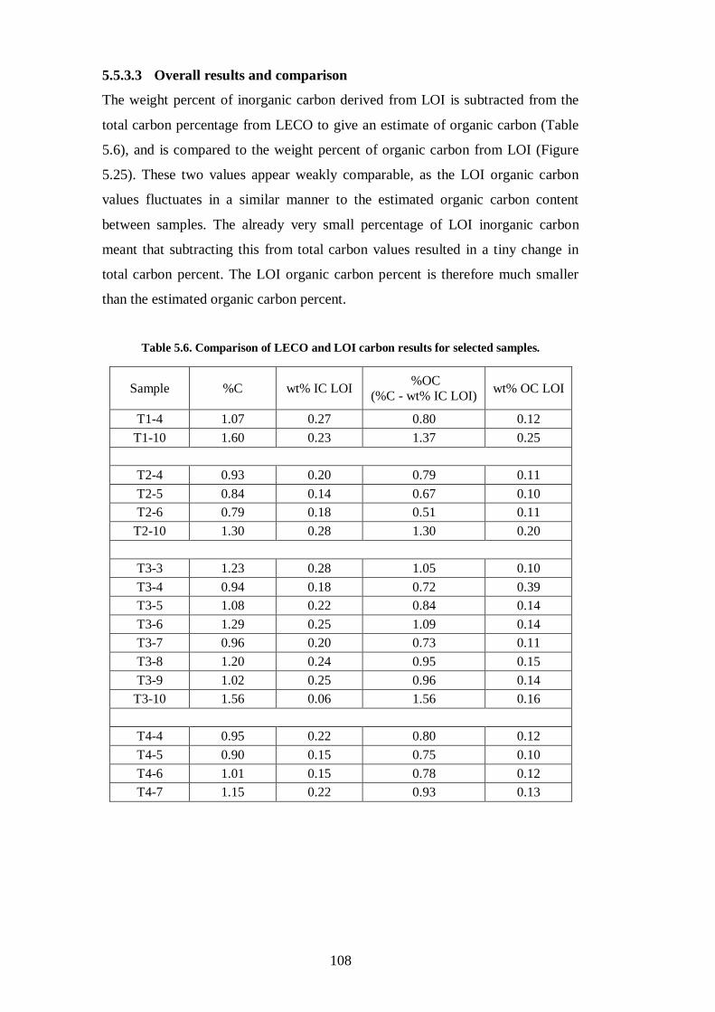
108
5.5.3.3 Overall results and comparison
The weight percent of inorganic carbon derived from LOI is subtracted from the
total carbon percentage from LECO to give an estimate of organic carbon (Table
5.6), and is compared to the weight percent of organic carbon from LOI (Figure
5.25). These two values appear weakly comparable, as the LOI organic carbon
values fluctuates in a similar manner to the estimated organic carbon content
between samples. The already very small percentage of LOI inorganic carbon
meant that subtracting this from total carbon values resulted in a tiny change in
total carbon percent. The LOI organic carbon percent is therefore much smaller
than the estimated organic carbon percent.
Table 5.6. Comparison of LECO and LOI carbon results for selected samples.
Sample %C wt% IC LOI %OC
(%C - wt% IC LOI) wt% OC LOI
T1-4 1.07 0.27 0.80 0.12
T1-10 1.60 0.23 1.37 0.25
T2-4 0.93 0.20 0.79 0.11
T2-5 0.84 0.14 0.67 0.10
T2-6 0.79 0.18 0.51 0.11
T2-10 1.30 0.28 1.30 0.20
T3-3 1.23 0.28 1.05 0.10
T3-4 0.94 0.18 0.72 0.39
T3-5 1.08 0.22 0.84 0.14
T3-6 1.29 0.25 1.09 0.14
T3-7 0.96 0.20 0.73 0.11
T3-8 1.20 0.24 0.95 0.15
T3-9 1.02 0.25 0.96 0.14
T3-10 1.56 0.06 1.56 0.16
T4-4 0.95 0.22 0.80 0.12
T4-5 0.90 0.15 0.75 0.10
T4-6 1.01 0.15 0.78 0.12
T4-7 1.15 0.22 0.93 0.13
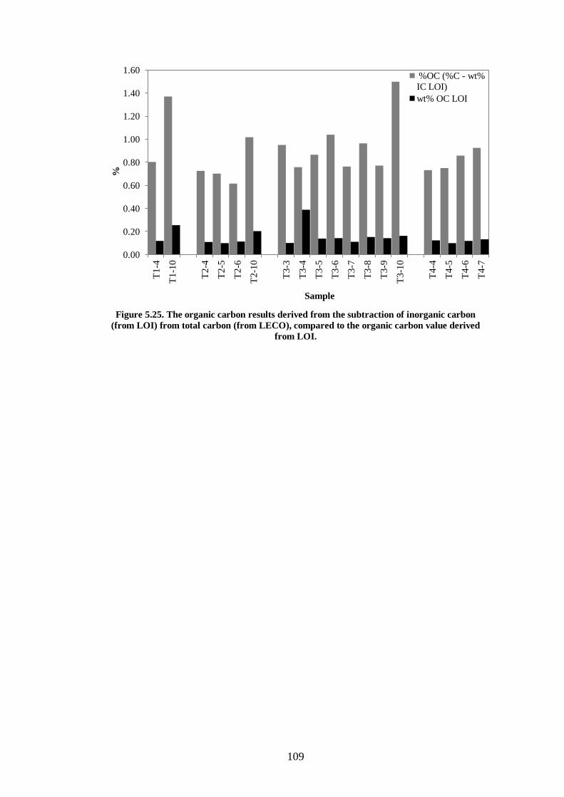
109
Figure 5.25. The organic carbon results derived from the subtraction of inorganic carbon
(from LOI) from total carbon (from LECO), compared to the organic carbon value derived
from LOI.
0.00
0.20
0.40
0.60
0.80
1.00
1.20
1.40
1.60
T1
-4
T1
-10
T2
-4
T2-5
T2
-6
T2
-10
T3
-3
T3
-4
T3
-5
T3
-6
T3
-7
T3
-8
T3
-9
T3-1
0
T4
-4
T4
-5
T4
-6
T4
-7
%
Sample
%OC (%C - wt%
IC LOI)
wt% OC LOI
110
5.6 DISCUSSION
Mud origin
In carrying out this survey which was designed to detect areas of mud (silt plus
clay) deposition, it was assumed that all the mud sized particles in the nearshore
region were derived from the landslide material. A brief mineralogical analysis
revealed that generally the samples contained abundant amounts of quartz and
plagioclase of differing sizes (overall sample grain size modes varied from 127 to
225 µm) and the quartz appeared very fractured under the petrographic
microscope. Also present were calcite and rock fragments. Rock fragments found
in all samples under the petrographic microscope were compared to crushed
mudstone sample DM1. The comparison showed similarities, particularly in the
colour under PPL and the appearance of clumps of smaller grains within the rock
fragment (Figure 5.21). The rock fragments appear to be composed entirely of
finer grains, likely cemented clay minerals. General mudstone XRD results (see
Chapter 3 Figure 3.8) showed abundant clay and quartz, common plagioclase and
some to common calcite, which indicate there are similarities in the presence of
these minerals between the mudstone DM1 and the subtidal sediment samples. It
is also noted that the nearshore subtidal samples did not display any large (i.e. >1
mm) fragments or clumps of material, which might be expected from the landslide
debris immediately offshore . This suggests that weathering and erosion of the
landslide debris is very effective and results in fine grains which have been easily
dispersed offshore. This is not conclusive evidence, but it seems that effective
erosion of the mudstone landslide material results in fine grains and rock
fragments, which may be present in the subtidal samples.
Mud deposition
An earlier survey by Funnell et al. (2005) stated that soft substrate in the marine
reserve nearshore region is dominated by medium sized sand from visual video
footage, with some areas of finer sand and mud. Subtidal sediments collected
during the 2012 Te Angiangi Marine Reserve survey mainly contain fine to very
fine sand, with only up to 10% medium sized sand present in the collected
samples. It could therefore be considered that a layer of finer grained sediment
derived from erosion of the landslide material could have been deposited and
overlie a pre-existing medium sized sand deposit. For this reason, a sediment
coring device for collection of the samples would have been more appropriate for
111
the purpose of this survey, because cores can show changes in grain size with sub-
bottom depth (Morrisey et al., 1998), but for reasons already outlined core
sampling was not possible.
Nearshore currents which predominantly flow to the north (Funnell et al., 2005)
were thought to have a possible influence in transporting and depositing fine
suspended sediment north, but this was not seen in the 2012 survey. Grain size
appears uniformly fine sand distributed alongshore within the reserve boundaries
(Figure 5.18), and no mud was detected in the northern extent of the survey.
However, the survey may have detected mud deposition to the north, had it been
extended further north. The grain size distribution does indicate that offshore
transport mechanisms are important in transporting mud into deeper water, since
mud is detected in increasing amounts with increasing depth and distance
offshore. Suspended mud being transported in landslide plumes is therefore
thought to by-pass the <30 m area altogether, drop out of suspension and settle in
water depths >30 m, where it is assumed the surface wave effects on bottom
sediment transport becomes negligible.
Sand origin
A possible explanation to the origin of the sand present in the study area is that it
has been released from the adjacent mudstone due to erosion, since the Mapiri
mudstone contains a significant amount of sand (about 40% based on mudstone
bedrock samples DM1 and DM7; see Table 3.4). The main sand sizes are medium
and fine sand (about 13% each), with a slightly smaller component of very fine
sand (about 10%). Sand eroded from the mudstone bedrock is a likely source of
fine sized sand present in the subtidal nearshore region, given the recent delivery
of bedrock to the coast due to landsliding.
Carbon
Overall carbon analysis suggests that inorganic carbon is present in higher
abundances than organic carbon, and overall total carbon comprises only a small
portion of each sample (0.6 to 1.8 wt%). In these sediments inorganic carbon is
likely made up of calcium carbonate derived from shell fragments, and perhaps a
lesser amount from foraminifera and carbonate concretions which have eroded out
of the mudstone debris at the coast.
112
Organic carbon is indicative of organic matter, which is an important benthic
health indicator. Organic carbon content in marine sediments can vary
considerably, but generally in nearshore sediments organic carbon accumulates at
relatively fast rates, and usually makes up 1 to 5% percent of the sediment; but
this value can be much higher in nearshore areas under high productivity (for
example up to around 25%; Chester, 1993). The carbon results from the 2012
survey suggest there is little organic carbon settling on the seafloor from the water
column and therefore available to benthic organisms. In relating these results to a
broader continental shelf and margin scale, continental margins are generally
characterised by high levels of organic carbon storage, with an estimated 80 to
85% carbon burial currently occurring, especially off river-dominated coasts.
Brackley et al. (2010) measures changes in organic matter percentage along a
floodplain to shelf to slope transect on the Poverty Bay Shelf on the east coast of
the North Island. Initially, organic matter content decreases from the floodplain to
deeper water (>36 m; this reflects the loss of terrestrial organic carbon as it
becomes buried or transported further offshore), before increasing through
addition of modern marine organic carbon in waters up to 56 m deep, then
increasing again in water depths from 56 to 1428 m as this organic carbon is
accumulated within pre-existing aged marine organic carbon (Brackley et al.,
2010). The percent organic matter within the floodplain to 36 m part of the
transect ranged from 0.2 to 0.8% (compared to Te Angiangi Marine Reserve
subtidal sediments which ranged from 0.1 to 0.4% organic carbon based on LOI
data or up to 1.8% total carbon from LECO). It is possible that the distribution of
organic carbon in the reserve is similar to what is observed along the floodplain to
36 m depth transect, except the organic carbon is assumed to be derived from
landslide plumes rather than river plumes.
The effects that the sedimentation event had on the Te Angiangi Marine Reserve
marine life is investigated in Chapter 6.
113
6 Chapter 6
INTERTIDAL ECOLOGY
6.1 INTRODUCTION
Coastal landslides along the southern Hawke's Bay coastline, which occurred as a
consequence of the April 2011 storm, resulted in a localised sedimentation event
at the Te Angiangi Marine Reserve and adjacent immediate coastline. As
described in Chapter 1, this set the scene for a unique assessment of the short term
ecological response and possible effects along the landslide affected coastline
encompassing the already established marine reserve. Furthermore, there was an
array of information with varying degrees of quantitative detail available, which
permitted some ecological characterisation of the status of the intertidal reefs
inside and outside of the Te Angiangi Marine Reserve.
A preliminary survey of the intertidal marine ecology from within and outside the
reserve was carried out in order to assess the impact on the marine organisms in
response to the high sedimentation event. The context of this study is unique as
(1) it is a natural sedimentation event caused by coastal landsliding within and
adjacent to a marine reserve (this is unprecedented in New Zealand), and (2)
because there is pre- and post-reserve data available (noting surveys are irregular
in occurrence and they have used inconsistent methodologies). Nevertheless, the
data available for the marine ecosystem in this area is valuable in its very
presence. This is because of the reserves remote location, and the reserve is
representative of a less well studied coastal ecosystem of eastern New Zealand
characterised by soft mudstone reefs and highly turbid coastal waters. The
previous surveys provide baseline time series data (which collectively represent
pre-April 2011 storm event data), that can be used with certain limitations, for
comparison with data gathered from the current survey (representing post-event
data), which then allows the ecological consequences of the April 2011 storm
event to be assessed.
An important aspect of this intertidal survey is that it has taken advantage of the
fact that a marine reserve has been influenced by the sedimentation event, which
114
permits an opportunity to examine any resilience that may be afforded to the
reserve ecosystem by virtue of a presumably naturally more robust balance of
interacting biological components. It also takes advantage of the fact that there is
time series information available. However, it is important to note that this work
is not intended to be a comprehensive ecological review of the Te Angiangi
Marine Reserve.
This chapter expands on an otherwise geologically oriented study by examining
the possible consequences of catastrophic landslides on coastal marine
ecosystems. It condenses and summarises the marine ecological aspects of this
project, and is based around the intertidal survey completed after the April 2011
sedimentation event. The results obtained from the post April 2011 intertidal
survey are outlined to highlight any trends in the distribution and abundance of
the representative species selected, and provide a platform for further study which
would extend into the subtidal region of the coast. The results are summarised to
demonstrate ecosystem pattern inside and outside the marine reserve, and a
preliminary analysis is carried out to explore any inconsistencies in the
demographics of the key species.
The aims of the post-event intertidal survey are to (1) examine the effects and
response of coastal marine ecosystems to catastrophic scale sedimentation,
evidenced by changes in intertidal community structure, and (2) detect any
resilience, provided as a result of marine protection, of intertidal communities to
sedimentation.
Along with addressing these aims, this chapter reviews information relating to
coastal sedimentation and effects on marine organisms; it examines the biology of
ecologically and commercially important species present along the Hawke's Bay
coastline - paua, kina and seagrass; it examines the conservation ecology of
marine reserves in New Zealand in general, and Te Angiangi Marine Reserve in
particular; and finally, the chapter examines the potential protection or resilience
marine reserves may afford their included ecosystems in the face of physical
disturbance.
115
6.2 BACKGROUND INFORMATION
6.2.1 Coastal sedimentation
What is coastal sedimentation?
Coastal sedimentation is a process where terrestrial sediment, primarily consisting
of clay, silt, detritus and most commonly sand, is delivered to the coast (Airoldi,
2003). Principle sources of sediment are derived from rivers, erosion of cliffs and
resuspension and transport of sediments. It is important to remember that
sedimentation is a natural process which occurs in all marine environments, from
soft sediment to rocky shores. Sedimentation can be beneficial to normal
ecosystem functioning, for example, organic particulate matter and nutrients (an
important food source to many organisms) can be delivered to the coastal marine
environment through the sedimentation process (Airoldi, 2003).
Although sedimentation is a natural process, it becomes accelerated primarily due
to human activities, for example, through land use change in catchments,
particularly the removal of vegetation for forestry, agriculture the development of
houses and infrastructure. Accelerated or increased sedimentation as a result of
human related activities is now recognised as a significant source of disturbance
in coastal marine environments (e.g. Cummings et al., 2009; Hewitt et al., 2003;
Ellis et al., 2004; Lohrer et al., 2004; Thrush et al., 2004; Lohrer et al., 2006a;
Gillespie, 2007).
Disturbances in the marine environment
Disturbance events in marine ecosystems vary considerably in frequency, scale
and effect (Ellis et al., 2000), but are generally viewed as uncommon, irregular
events that may cause abrupt changes in the structure of natural communities
(Sousa, 1984; Allison et al., 2003). Disturbances can alter the availability of
resources, such as food and space, thereby directly or indirectly influencing the
structure and function of animal assemblages (Ellis et al., 2000). Disturbances can
be either physical or biological in nature (often interacting), with arguably
physical sources having the widest ranging effects on marine ecosystems.
Catastrophic disturbances are relatively large-scale disturbances that involve
significant mortality, habitat loss and overall disruption to ecosystem functioning
116
(Allison et al., 2003). Examples of medium to large-scale disturbances in marine
environments include algal blooms, disease epidemics, coral bleaching events,
hypoxia events, oils spills, increased sedimentation and hurricanes. Frequently the
source of biological anomalies such as algal blooms and coral bleaching events,
are due to abrupt changes in the physical oceanic regime (temperature and nutrient
changes). The nature of catastrophes means they are hard to study because they
are relatively rare, they occur in unpredictable locations and at unpredictable
times, and their extent is often difficult to easily quantify (Allison et al., 2003),
especially if there is no prior information of relevance to the area in question.
A catastrophic sedimentation event could be defined as an event which delivers a
huge volume of sediment directly to the coast (from a source such as landslides),
in a relatively short amount of time. Sediment delivery into the coastal marine
environment through catastrophic cliff failure and erosion of hill sides is already
recognised as an important sediment source (Gorsline, 1985), and is relatively
common along New Zealand coastlines (Airoldi, 2003). However, to the best of
our knowledge, there are no records in New Zealand of a catastrophic
sedimentation as a result of coastal landsliding in a marine reserve.
This is important because phenomena such as landslides can result in catastrophic
deposition of sediments, which profoundly influences the structure and function
of coastal macrobenthic communities (Ellis et al., 2000).
Effects on marine organisms
The ecological consequences of terrestrial sediment in the coastal marine
environment is relatively well studied (Thrush et al., 2003; Cummings & Thrush,
2004; Ellis et al., 2004; Lohrer et al., 2004; Thrush et al., 2004; Lohrer et al.,
2006a; Lohrer et al., 2006b; Cummings et al., 2009). In more recent times studies
are focusing on coral reefs, in light of increased ocean acidification and coral
bleaching events (e.g. Rogers, 1990), and also on investigating in freshwater
environments (e.g. Ryan, 1991). However, relatively few studies have examined
the effects of sediment on coastal rocky reefs (Airoldi & Cinelli, 1997; Airoldi,
2003; Gillespie, 2007). Airoldi (2003) reviews the effects of sedimentation on
rocky coast assemblages, and suggests that rocky coasts are potentially one of the
habitats most sensitive to increased sedimentation.
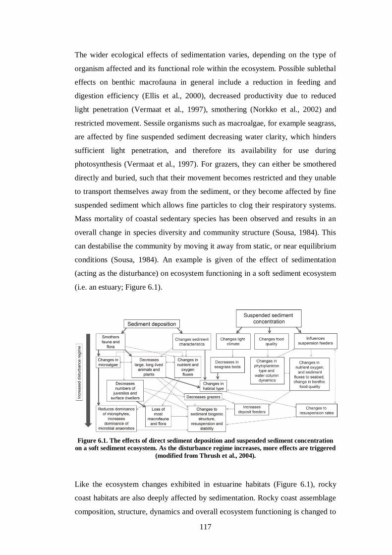
117
The wider ecological effects of sedimentation varies, depending on the type of
organism affected and its functional role within the ecosystem. Possible sublethal
effects on benthic macrofauna in general include a reduction in feeding and
digestion efficiency (Ellis et al., 2000), decreased productivity due to reduced
light penetration (Vermaat et al., 1997), smothering (Norkko et al., 2002) and
restricted movement. Sessile organisms such as macroalgae, for example seagrass,
are affected by fine suspended sediment decreasing water clarity, which hinders
sufficient light penetration, and therefore its availability for use during
photosynthesis (Vermaat et al., 1997). For grazers, they can either be smothered
directly and buried, such that their movement becomes restricted and they unable
to transport themselves away from the sediment, or they become affected by fine
suspended sediment which allows fine particles to clog their respiratory systems.
Mass mortality of coastal sedentary species has been observed and results in an
overall change in species diversity and community structure (Sousa, 1984). This
can destabilise the community by moving it away from static, or near equilibrium
conditions (Sousa, 1984). An example is given of the effect of sedimentation
(acting as the disturbance) on ecosystem functioning in a soft sediment ecosystem
(i.e. an estuary; Figure 6.1).
Figure 6.1. The effects of direct sediment deposition and suspended sediment concentration
on a soft sediment ecosystem. As the disturbance regime increases, more effects are triggered
(modified from Thrush et al., 2004).
Like the ecosystem changes exhibited in estuarine habitats (Figure 6.1), rocky
coast habitats are also deeply affected by sedimentation. Rocky coast assemblage
composition, structure, dynamics and overall ecosystem functioning is changed to
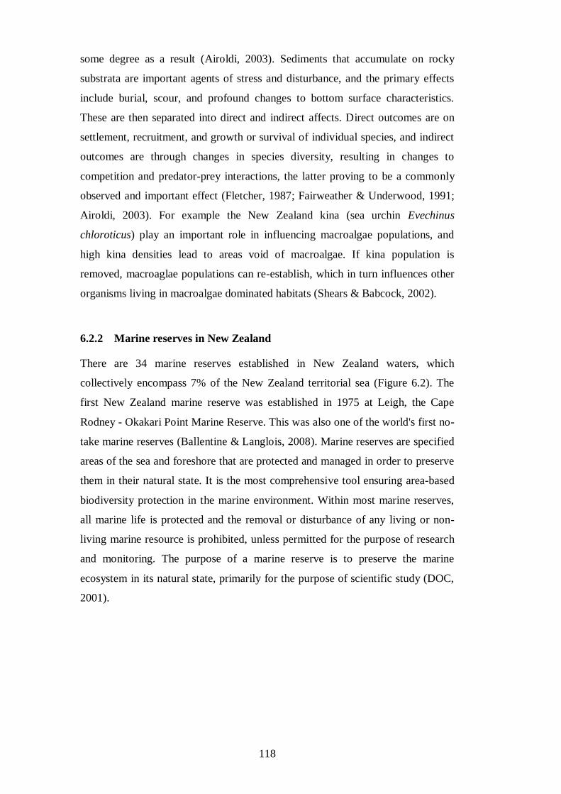
118
some degree as a result (Airoldi, 2003). Sediments that accumulate on rocky
substrata are important agents of stress and disturbance, and the primary effects
include burial, scour, and profound changes to bottom surface characteristics.
These are then separated into direct and indirect affects. Direct outcomes are on
settlement, recruitment, and growth or survival of individual species, and indirect
outcomes are through changes in species diversity, resulting in changes to
competition and predator-prey interactions, the latter proving to be a commonly
observed and important effect (Fletcher, 1987; Fairweather & Underwood, 1991;
Airoldi, 2003). For example the New Zealand kina (sea urchin Evechinus
chloroticus) play an important role in influencing macroalgae populations, and
high kina densities lead to areas void of macroalgae. If kina population is
removed, macroaglae populations can re-establish, which in turn influences other
organisms living in macroalgae dominated habitats (Shears & Babcock, 2002).
6.2.2 Marine reserves in New Zealand
There are 34 marine reserves established in New Zealand waters, which
collectively encompass 7% of the New Zealand territorial sea (Figure 6.2). The
first New Zealand marine reserve was established in 1975 at Leigh, the Cape
Rodney - Okakari Point Marine Reserve. This was also one of the world's first no-
take marine reserves (Ballentine & Langlois, 2008). Marine reserves are specified
areas of the sea and foreshore that are protected and managed in order to preserve
them in their natural state. It is the most comprehensive tool ensuring area-based
biodiversity protection in the marine environment. Within most marine reserves,
all marine life is protected and the removal or disturbance of any living or non-
living marine resource is prohibited, unless permitted for the purpose of research
and monitoring. The purpose of a marine reserve is to preserve the marine
ecosystem in its natural state, primarily for the purpose of scientific study (DOC,
2001).
119
Figure 6.2. Marine reserves in New Zealand (from the DOC website).
Te Angiangi Marine Reserve
The Te Angiangi Marine Reserve (Figure 1.2) encompasses about 446 hectares,
which is considered representative of the southern Hawke's Bay marine
environment. It contains three general habitats - intertidal mudstone reef, subtidal
mudstone reef and a subtidal boulder bank at the northern end of the reserve,
adding complexity to the subtidal region of the reserve (DOC, 2001). Beyond the
subtidal reef, the substrate consists of fine sand. The intertidal reef is characterised
by flora: turfs of coralline algae (Corallina officinalis), Neptune's necklace
(Hormosira banksii) and patches of seagrass (Zostera capricorni); and fauna:
several species of grazing mollusc, including paua (Haliotis spp.) and kina
(Evechinus chloroticus). The immediate subtidal zone consists of shallow mixed
algae, dominated by brown algae (Carpophyllum maschalocarpum and C.
plumosum). The shallow subtidal zone supports stands of kelp forest (Ecklonia
radiata) with a subcanopy of encrusting and turf algae. Below 12 m encrusting
invertebrates become more dominant, with hydroids becoming increasingly
abundant with increasing depth. The boulder bank (extending to 36 m deep) is
characterised by kelp forest, small red algae (e.g. Plocamium costatum), sponges
(e.g. Ancorina alata, Iophon sp., Raspailia sp., Callyspongia sp., Reniera sp.),
hydroids, bryozoans and ascidians (e.g. Hypsistozoa fasmeriana). Subtidal

120
populations of rock lobster (crayfish - Jasus edwardsii), kina, and grazing
gastropods paua and Cookia sulcata are present throughout, along with reef fish:
(blue cod (Parapercis colias), butterfish (Odax pullus), blue moki (Latridopsis
ciliaris) and red moki (Cheilodactylus spectabilis) (DOC, 1994a and 2001, also
see Figure 5.2).
The Te Angiangi Marine Reserve is relatively small compared to most others in
New Zealand. Its 446 hectares is compared to much more generous areas of, for
example, the Poor Nights Marine Reserve, which is 1890 ha, and the Fiordland
marine reserves, which collectively encompass more than 10,000 ha. The Te
Tapuwae o Rongokako Marine Reserve just north of Gisborne encompasses a
relatively large 2450 ha, and at the other end of the spectrum, the Whangarei
Harbour Marine Reserve is 253.7 ha (DOC website). The limited size of the Te
Angiangi Marine Reserve has implications for recruitment of marine organisms
into the reserve given the close proximity of unprotected coastal regions to the
north and south. Nevertheless, the reserve is responding well to protection as
evidenced by increases in those species that are usually predated by humans (this
is discussed in a later section). Its positive response to protection is encouraging,
not only considering its size, but especially so because of illegal poaching
occurring in the area (pers. observ.).
6.2.3 Marine reserve effectiveness and resilience
In New Zealand, the spatially scattered nature of marine reserves, perhaps
excluding Fiordland's marine reserves, is far from adequate. Entire coastlines
protected by a number of marine reserves are ideal for complete conservation and
recovery (Ballentine & Langlois, 2008). However, despite whether or not marine
reserves encompass entire coastlines, or just a small portion of it, it is widely
known that they provide benefits for ecosystem function and health, along with
supporting a platform for marine ecosystem functioning research (Ballentine &
Langlois, 2008). In New Zealand, and increasingly globally, a ‘reserve’ effect can
be evident as a result of protection, and this is commonly reflected and supported
by the increased size and abundance of reserve organisms (particularly those that
were formally sought by humans) and increased species diversity (e.g. Allison et
al., 1998; Babcock et al., 1999; Kelly et al., 2000; Allison et al., 2003; Denny et

121
al., 2004; Shears & Babcock, 2004; Shears, 2007; Ballentine & Langlois, 2008;
Micheli et al., 2012).
Allison et al. (1998, 2003) recognise that reserves do harbour the benefits
mentioned above, and are therefore essential to marine conservation, and their
efficiency can be increased by ensuring their design is scientifically sound and
they are implemented well. However, their potential effectiveness is limited by
large-scale ecological processes occurring within and surrounding reserves.
Processes such as recruitment can occur on a very large spatial and temporal
scale, which means reserve populations may not benefit directly from localised
populations within the reserve. Areas immediately outside of reserves may benefit
greatly from what is called the spill-over effect, where juveniles generated from
within the reserve are added to populations just outside of the reserve boundary.
Integrated protection of organisms within and outside reserves are needed in order
for reserves to function optimally (Allison et al., 1998). Reserves with stable
ecosystem functioning are more likely to withstand disturbance events, and this
benefits non-reserve populations since the reserve populations are able to recover
faster and continue reproducing (Micheli et al., 2012).
Empirical evidence that reserves do increase resilience of reserve populations is
lacking because it is rare for disturbances to be tested within marine reserves
(Allison et al., 1998; Micheli et al., 2012). However, resilience exhibited by
reserve organisms after a disturbance is widely hypothesised (e.g. Ballentine &
Langlois, 2008). Resilience is the ability of populations and ecosystems to adsorb
disturbance while retaining their function and provision of ecosystem services,
which may help combat the impacts of major disturbances (Micheli et al., 2012).
Grafton et al. (2003) demonstrate that the resilience of a population is improved
within a reserve. In the Grafton et al (2003) study, this was achieved by looking at
the recovery time of a population, and improved resilience was defined by the
amount of time taken for the population to reach within one standard deviation of
the population level prior to the disturbance. A shorter period of time represents a
higher level of resilience, and there is indication that resilience improves further
with larger reserve size. Micheli et al. (2012) has recently studied the response of
marine reserves to climate-driven hypoxia, and has shown that marine reserves
increase resilience of marine populations to mass mortality. This is shown by
122
juvenile replenishment, which remained stable despite mass mortality of adult
populations. This benefit was extended as spill over effect to non-reserve
organisms (Micheli et al., 2012).
The sedimentation event which has taken place at the Te Angiangi Marine
Reserve and adjacent coastline has provided a very rare natural experiment
opportunity, which tests the resilience of protected marine organisms to a
disturbance. The results of the current survey will provide valuable insight into
the effectiveness of reserves, and it will broaden our understanding on whether
marine organisms from within a marine reserve are more resilient to disturbances
because of any potential reserve protection effects, of which empirical evidence is
largely lacking (Micheli et al., 2012).
6.2.4 Biology of paua, kina and seagrass
It has been demonstrated that within New Zealand marine reserves, grazers such
as kina and paua are particularly important to monitor because these species
readily undergo changes in distribution and abundance once human predation
pressure has been removed (DOC, 2001). Paua, kina and seagrass are therefore
key species examined in the current intertidal survey, hence it is important to
understand their life cycles, recruitment patterns, and preferred habitats. These
aspects need to be considered when explaining and drawing conclusions on the
findings of the survey.
Paua (Haliotis spp.)
Paua (New Zealand abalone) is a large marine gastropod belonging to the phylum
Mollusca and the family Haliotidae (Costales et al., 2009). There are three species
of paua found in New Zealand's waters, the most common is the black-foot paua
(Haliotis iris; Figure 6.3), the less common is the yellow-foot paua (Haliotis
australis), and the rare white-foot paua (Haliotis virginia). The first two species
are harvested commercially from wild populations and are found at the Te
Angiangi Marine Reserve. All three species are harvested recreationally
(Freeman, 2006).
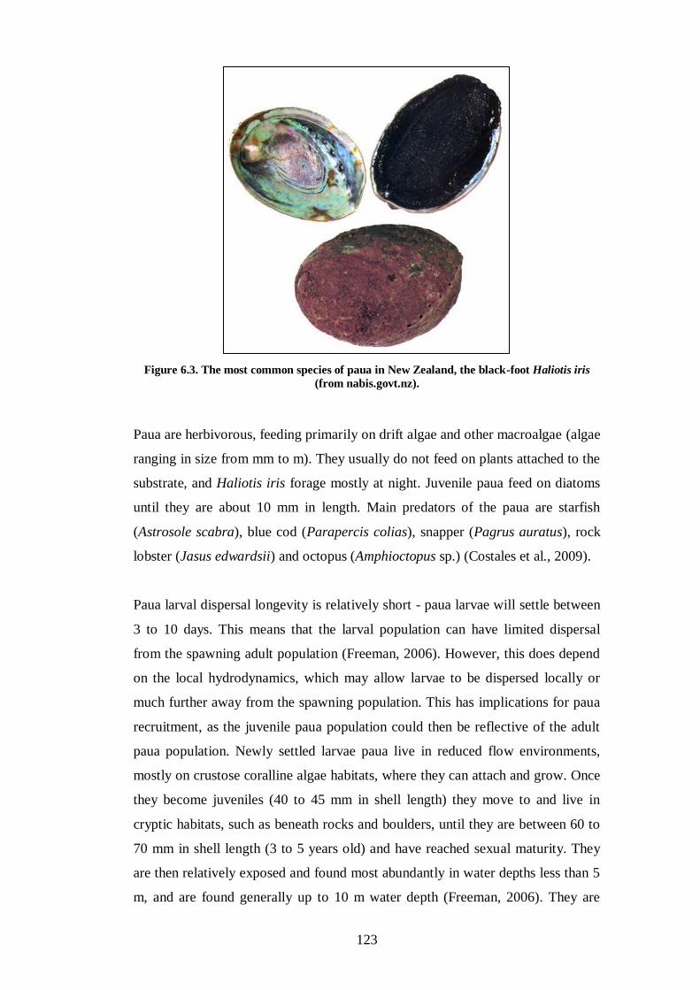
123
Figure 6.3. The most common species of paua in New Zealand, the black-foot Haliotis iris
(from nabis.govt.nz).
Paua are herbivorous, feeding primarily on drift algae and other macroalgae (algae
ranging in size from mm to m). They usually do not feed on plants attached to the
substrate, and Haliotis iris forage mostly at night. Juvenile paua feed on diatoms
until they are about 10 mm in length. Main predators of the paua are starfish
(Astrosole scabra), blue cod (Parapercis colias), snapper (Pagrus auratus), rock
lobster (Jasus edwardsii) and octopus (Amphioctopus sp.) (Costales et al., 2009).
Paua larval dispersal longevity is relatively short - paua larvae will settle between
3 to 10 days. This means that the larval population can have limited dispersal
from the spawning adult population (Freeman, 2006). However, this does depend
on the local hydrodynamics, which may allow larvae to be dispersed locally or
much further away from the spawning population. This has implications for paua
recruitment, as the juvenile paua population could then be reflective of the adult
paua population. Newly settled larvae paua live in reduced flow environments,
mostly on crustose coralline algae habitats, where they can attach and grow. Once
they become juveniles (40 to 45 mm in shell length) they move to and live in
cryptic habitats, such as beneath rocks and boulders, until they are between 60 to
70 mm in shell length (3 to 5 years old) and have reached sexual maturity. They
are then relatively exposed and found most abundantly in water depths less than 5
m, and are found generally up to 10 m water depth (Freeman, 2006). They are
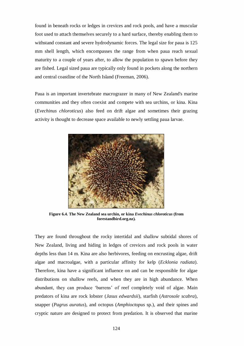
124
found in beneath rocks or ledges in crevices and rock pools, and have a muscular
foot used to attach themselves securely to a hard surface, thereby enabling them to
withstand constant and severe hydrodynamic forces. The legal size for paua is 125
mm shell length, which encompasses the range from when paua reach sexual
maturity to a couple of years after, to allow the population to spawn before they
are fished. Legal sized paua are typically only found in pockets along the northern
and central coastline of the North Island (Freeman, 2006).
Paua is an important invertebrate macrograzer in many of New Zealand's marine
communities and they often coexist and compete with sea urchins, or kina. Kina
(Evechinus chloroticus) also feed on drift algae and sometimes their grazing
activity is thought to decrease space available to newly settling paua larvae.
Figure 6.4. The New Zealand sea urchin, or kina Evechinus chloroticus (from
forestandbird.org.nz).
They are found throughout the rocky intertidal and shallow subtidal shores of
New Zealand, living and hiding in ledges of crevices and rock pools in water
depths less than 14 m. Kina are also herbivores, feeding on encrusting algae, drift
algae and macroalgae, with a particular affinity for kelp (Ecklonia radiata).
Therefore, kina have a significant influence on and can be responsible for algae
distributions on shallow reefs, and when they are in high abundance. When
abundant, they can produce ‘barrens’ of reef completely void of algae. Main
predators of kina are rock lobster (Jasus edwardsii), starfish (Astrosole scabra),
snapper (Pagrus auratus), and octopus (Amphioctopus sp.), and their spines and
cryptic nature are designed to protect from predation. It is observed that marine
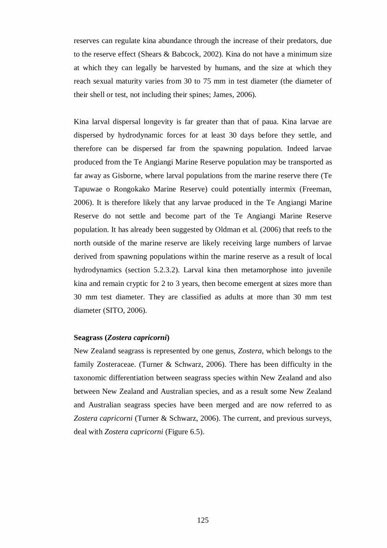
125
reserves can regulate kina abundance through the increase of their predators, due
to the reserve effect (Shears & Babcock, 2002). Kina do not have a minimum size
at which they can legally be harvested by humans, and the size at which they
reach sexual maturity varies from 30 to 75 mm in test diameter (the diameter of
their shell or test, not including their spines; James, 2006).
Kina larval dispersal longevity is far greater than that of paua. Kina larvae are
dispersed by hydrodynamic forces for at least 30 days before they settle, and
therefore can be dispersed far from the spawning population. Indeed larvae
produced from the Te Angiangi Marine Reserve population may be transported as
far away as Gisborne, where larval populations from the marine reserve there (Te
Tapuwae o Rongokako Marine Reserve) could potentially intermix (Freeman,
2006). It is therefore likely that any larvae produced in the Te Angiangi Marine
Reserve do not settle and become part of the Te Angiangi Marine Reserve
population. It has already been suggested by Oldman et al. (2006) that reefs to the
north outside of the marine reserve are likely receiving large numbers of larvae
derived from spawning populations within the marine reserve as a result of local
hydrodynamics (section 5.2.3.2). Larval kina then metamorphose into juvenile
kina and remain cryptic for 2 to 3 years, then become emergent at sizes more than
30 mm test diameter. They are classified as adults at more than 30 mm test
diameter (SITO, 2006).
Seagrass (Zostera capricorni)
New Zealand seagrass is represented by one genus, Zostera, which belongs to the
family Zosteraceae. (Turner & Schwarz, 2006). There has been difficulty in the
taxonomic differentiation between seagrass species within New Zealand and also
between New Zealand and Australian species, and as a result some New Zealand
and Australian seagrass species have been merged and are now referred to as
Zostera capricorni (Turner & Schwarz, 2006). The current, and previous surveys,
deal with Zostera capricorni (Figure 6.5).
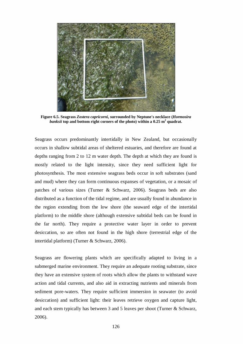
126
Figure 6.5. Seagrass Zostera capricorni, surrounded by Neptune's necklace (Hormosira
banksii top and bottom right corners of the photo) within a 0.25 m2 quadrat.
Seagrass occurs predominantly intertidally in New Zealand, but occasionally
occurs in shallow subtidal areas of sheltered estuaries, and therefore are found at
depths ranging from 2 to 12 m water depth. The depth at which they are found is
mostly related to the light intensity, since they need sufficient light for
photosynthesis. The most extensive seagrass beds occur in soft substrates (sand
and mud) where they can form continuous expanses of vegetation, or a mosaic of
patches of various sizes (Turner & Schwarz, 2006). Seagrass beds are also
distributed as a function of the tidal regime, and are usually found in abundance in
the region extending from the low shore (the seaward edge of the intertidal
platform) to the middle shore (although extensive subtidal beds can be found in
the far north). They require a protective water layer in order to prevent
desiccation, so are often not found in the high shore (terrestrial edge of the
intertidal platform) (Turner & Schwarz, 2006).
Seagrass are flowering plants which are specifically adapted to living in a
submerged marine environment. They require an adequate rooting substrate, since
they have an extensive system of roots which allow the plants to withstand wave
action and tidal currents, and also aid in extracting nutrients and minerals from
sediment pore-waters. They require sufficient immersion in seawater (to avoid
desiccation) and sufficient light: their leaves retrieve oxygen and capture light,
and each stem typically has between 3 and 5 leaves per shoot (Turner & Schwarz,
2006).
127
Seagrass perform a variety of functions within coastal ecosystems, and can
therefore be considered a valuable component in an overall coastal ecosystem
functioning (Turner & Schwarz, 2006). They are representative of areas of high
productivity since they themselves are highly productive, and provide food
sources and habitat for many organisms utilising seagrass beds. The habitat
provided within seagrass beds is low-energy, since seagrass beds increase bottom
friction thereby decreasing current speeds, which facilitates the deposition and
retention of sediment. This in turn stabilises bottom sediments and provides
protection against erosion. This is a very important function of seagrass, mainly
because their ability to trap and retain terrestrially derived sediment then improves
water clarity and quality (Turner & Schwarz, 2006). However, excess or an
increased sedimentation rate (including changes in the proportion of fines) may
have detrimental effects. If the point at which seagrass can retain sediment is
exceeded, excess suspended sediment in the water column decreases light
penetration which may cause harm or death.
6.2.5 Te Angiangi Marine Reserve previous survey work
The Te Angiangi Marine Reserve was established in 1997, and marine surveys
have been carried out in the area since 1990. Data has been gathered on key
intertidal and subtidal species during surveys conducted by the Department of
Conservation and more recently by Victoria University of Wellington students.
Data collected before 1997 act as pre-reserve data or baseline data, and data
collected after 1997 act as post-reserve or monitoring data, all of which is
described in several published and unpublished reports (Table 6.1).
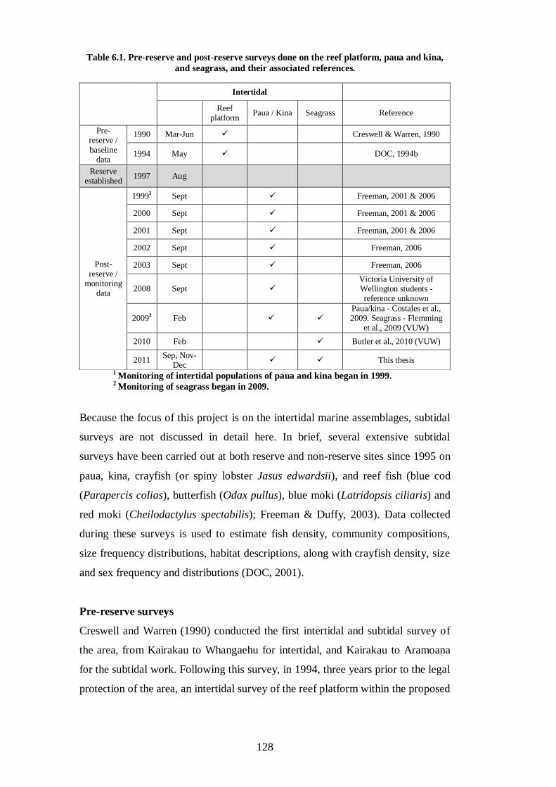
128
Table 6.1. Pre-reserve and post-reserve surveys done on the reef platform, paua and kina,
and seagrass, and their associated references.
1 Monitoring of intertidal populations of paua and kina began in 1999.
2 Monitoring of seagrass began in 2009.
Because the focus of this project is on the intertidal marine assemblages, subtidal
surveys are not discussed in detail here. In brief, several extensive subtidal
surveys have been carried out at both reserve and non-reserve sites since 1995 on
paua, kina, crayfish (or spiny lobster Jasus edwardsii), and reef fish (blue cod
(Parapercis colias), butterfish (Odax pullus), blue moki (Latridopsis ciliaris) and
red moki (Cheilodactylus spectabilis); Freeman & Duffy, 2003). Data collected
during these surveys is used to estimate fish density, community compositions,
size frequency distributions, habitat descriptions, along with crayfish density, size
and sex frequency and distributions (DOC, 2001).
Pre-reserve surveys
Creswell and Warren (1990) conducted the first intertidal and subtidal survey of
the area, from Kairakau to Whangaehu for intertidal, and Kairakau to Aramoana
for the subtidal work. Following this survey, in 1994, three years prior to the legal
protection of the area, an intertidal survey of the reef platform within the proposed
Intertidal
Reef
platform Paua / Kina Seagrass Reference
Pre-reserve / baseline
data
1990 Mar-Jun Creswell & Warren, 1990
1994 May DOC, 1994b
Reserve established
1997 Aug
Post-reserve /
monitoring data
19991 Sept Freeman, 2001 & 2006
2000 Sept Freeman, 2001 & 2006
2001 Sept Freeman, 2001 & 2006
2002 Sept Freeman, 2006
2003 Sept Freeman, 2006
2008 Sept Victoria University of Wellington students - reference unknown
20092 Feb
Paua/kina - Costales et al., 2009. Seagrass - Flemming
et al., 2009 (VUW)
2010 Feb Butler et al., 2010 (VUW)
2011 Sep, Nov-
Dec This thesis
129
reserve area was conducted by DOC (2001). These two studies are the only ones
that have described in detail all species present of the intertidal platform.
Post-reserve surveys
Regular intertidal and subtidal monitoring was carried out since establishment of
the reserve until 2003 to assess the response of organisms to the protection
afforded by the reserve. Between 1999 and 2003, intertidal populations of paua
(Haliotis spp.) and kina (Evechinus chloroticus) were monitored at sites within
and outside of the reserve (Freeman, 2001 and 2006). In September 1999,
populations of paua and kina in intertidal crevices and channels were examined at
three sites: Blackhead, the marine reserve and Aramoana. 10 channels were
sampled at each site. For each channel, all paua and kina were measured, either in
situ or by carefully removing the animal. Kina test diameter and paua shell length
was recorded to the nearest millimetre In September 2000, 2001, 2002 and 2003
this survey was repeated (Freeman, 2006).
Victoria University of Wellington students examined intertidal populations of
paua and kina in 2008 (data was not obtained from this survey), and they were re-
examined again by Victoria University students in 2009 (Costales et al., 2009). In
2009, four sites were established: two within and two outside the reserve (one at
Blackhead and one at Aramoana). These sites roughly matched the sites used in
previous surveys. At each site two intertidal shore heights were sampled - the low
(seaward edge of the platform) and middle shore. At each shore height three 10 m
x 10 m transects were laid out where channels were present, and all channels
searched for all paua and kina which were then measured.
Also in 2009, the first survey focusing solely on seagrass (Zostera capricorni) in
the area was carried out, with the aim of establishing a seagrass monitoring
program (Flemming et al., 2009). This study involved sampling seagrass beds
from four sites: two within and two outside of the reserve (one at Blackhead and
one at Aramoana). Three transects were established at each site, one in each of the
low (seaward edge of the platform), middle, and high (terrestrial edge of the
platform) areas of the platform. Within each of these transects, 10 x 0.25 m2
quadrats were haphazardly placed and used to estimate the percent of seagrass

130
cover, percent of green seagrass, the average blade length, shoot density, any
invertebrates were counted and identified, and the presence of epiphytes noted.
One year after this survey, Butler et al. (2010) re-examined seagrass but using
different methodology. Three sites within the reserve and two outside (one at
Blackhead and one at Aramoana) were established. At each site a 25 m wide by
100 m long area was measured out and all seagrass patches within this area were
measured (maximum width by maximum length). Within the same area for each
site, 10 randomly selected patches were used to estimate shoot density using a
0.25 m2 quadrat for each patch.
Main conclusions made from the 1999 to 2003 intertidal paua and kina survey
data, are (1) densities of kina remained low but stable within the marine reserve,
in contrast with kina density at non-reserve sites which were variable and
occasionally high. In 2001 kina were significantly larger within the marine
reserve, compared to non-reserve sites and marine reserve populations in 1999
and 2000; and (2) densities and mean size of paua was higher within the marine
reserve. The mean size of paua within the reserve increased between 1999 and
2001 and remained stable until 2003 (Freeman, 2006). Conclusions made from the
2009 and 2010 seagrass survey data are: (1) intertidal reef platform elevation
attributes (i.e. low, middle or high shore height on the intertidal platform), was the
main factor influencing seagrass cover, greenness, blade length and density, rather
than any potential reserve effects (Flemming et al., 2009); (2) total seagrass
coverage was significantly higher at non-reserve sites, although this is likely not
related to any potential reserve effects, but rather lack of sufficient sampling size
(Butler et al., 2010); and (3) since there are no pre-reserve seagrass survey data, it
is hard to detect any potential reserve effects in both of these studies.
These data generally indicate the reserve was functioning well, or at least
beginning to take effect before the catastrophic sedimentation event occurred in
April 2011. It then could be hypothesised that since populations within the reserve
are naturally more stable and of greater abundance than the adjacent unprotected
coastline, that the protected populations would exhibit an increased resilience to
the sedimentation and that populations would remain stable (with perhaps a slight
decrease) compared to unprotected populations exposed to the same
131
sedimentation event. This is a major hypothesis of this chapter and will be
examined in a later section.
6.3 SURVEY DESIGN
The sampling design used in the current survey builds on the previous DOC
monitoring design for intertidal paua and kina, and the Costales et al. (2009)
intertidal paua and kina survey. It was designed to encompass the varied designs
of previous seagrass survey designs to permit some across survey comparison.
Firstly, the number of sites used for sampling were increased and balanced, so
there were an equal number of reserve and non-reserve sites. Consequently, four
reserve sites two in the southern half and two in the northern half were
established, along with four non-reserve sites two at Blackhead and two at
Aramoana (Figure 6.6). The sites are labelled from A to H, A being the most
southern site and H being the most northern (Figure 6.6). The placement of the
sites in the current survey generally matched the location of the sites used in all
previous surveys. However, site selection was influenced by the location and the
vertical and horizontal extent on the landslide debris, which in some places,
particularly in the northern half of the reserve, buried a significant portion of the
intertidal platform. It was also nearly impossible to re-sample the exact same
channels sampled during previous paua and kina surveys, but the sites
encompassed the general location of most channels.
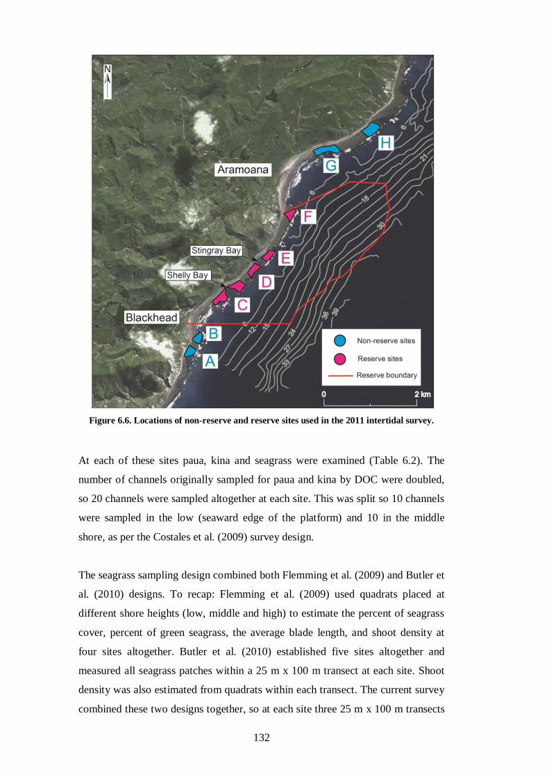
132
Figure 6.6. Locations of non-reserve and reserve sites used in the 2011 intertidal survey.
At each of these sites paua, kina and seagrass were examined (Table 6.2). The
number of channels originally sampled for paua and kina by DOC were doubled,
so 20 channels were sampled altogether at each site. This was split so 10 channels
were sampled in the low (seaward edge of the platform) and 10 in the middle
shore, as per the Costales et al. (2009) survey design.
The seagrass sampling design combined both Flemming et al. (2009) and Butler et
al. (2010) designs. To recap: Flemming et al. (2009) used quadrats placed at
different shore heights (low, middle and high) to estimate the percent of seagrass
cover, percent of green seagrass, the average blade length, and shoot density at
four sites altogether. Butler et al. (2010) established five sites altogether and
measured all seagrass patches within a 25 m x 100 m transect at each site. Shoot
density was also estimated from quadrats within each transect. The current survey
combined these two designs together, so at each site three 25 m x 100 m transects
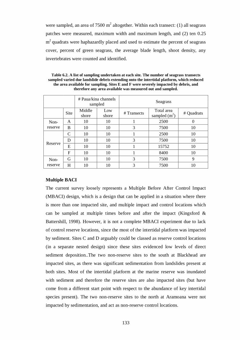
133
were sampled, an area of 7500 m2 altogether. Within each transect: (1) all seagrass
patches were measured, maximum width and maximum length, and (2) ten 0.25
m2
quadrats were haphazardly placed and used to estimate the percent of seagrass
cover, percent of green seagrass, the average blade length, shoot density, any
invertebrates were counted and identified.
Table 6.2. A list of sampling undertaken at each site. The number of seagrass transects
sampled varied due landslide debris extending onto the intertidal platform, which reduced
the area available for sampling. Sites E and F were severely impacted by debris, and
therefore any area available was measured out and sampled.
# Paua/kina channels
sampled Seagrass
Site Middle
shore Low
shore # Transects
Total area
sampled (m2)
# Quadrats
Non-reserve
A 10 10 1 2500 0
B 10 10 3 7500 10
Reserve
C 10 10 1 2500 10
D 10 10 3 7500 10
E 10 10 1 15752 10
F 10 10 1 8400 10
Non-
reserve
G 10 10 3 7500 9
H 10 10 3 7500 10
Multiple BACI
The current survey loosely represents a Multiple Before After Control Impact
(MBACI) design, which is a design that can be applied in a situation where there
is more than one impacted site, and multiple impact and control locations which
can be sampled at multiple times before and after the impact (Kingsford &
Battershill, 1998). However, it is not a complete MBACI experiment due to lack
of control reserve locations, since the most of the intertidal platform was impacted
by sediment. Sites C and D arguably could be classed as reserve control locations
(in a separate nested design) since these sites evidenced low levels of direct
sediment deposition..The two non-reserve sites to the south at Blackhead are
impacted sites, as there was significant sedimentation from landslides present at
both sites. Most of the intertidal platform at the marine reserve was inundated
with sediment and therefore the reserve sites are also impacted sites (but have
come from a different start point with respect to the abundance of key intertidal
species present). The two non-reserve sites to the north at Aramoana were not
impacted by sedimentation, and act as non-reserve control locations.
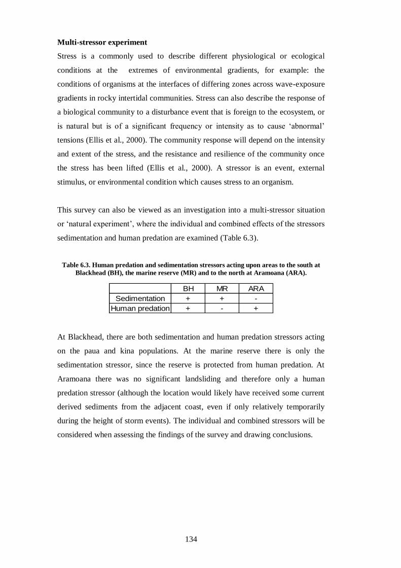
134
Multi-stressor experiment
Stress is a commonly used to describe different physiological or ecological
conditions at the extremes of environmental gradients, for example: the
conditions of organisms at the interfaces of differing zones across wave-exposure
gradients in rocky intertidal communities. Stress can also describe the response of
a biological community to a disturbance event that is foreign to the ecosystem, or
is natural but is of a significant frequency or intensity as to cause ‘abnormal’
tensions (Ellis et al., 2000). The community response will depend on the intensity
and extent of the stress, and the resistance and resilience of the community once
the stress has been lifted (Ellis et al., 2000). A stressor is an event, external
stimulus, or environmental condition which causes stress to an organism.
This survey can also be viewed as an investigation into a multi-stressor situation
or ‘natural experiment’, where the individual and combined effects of the stressors
sedimentation and human predation are examined (Table 6.3).
Table 6.3. Human predation and sedimentation stressors acting upon areas to the south at
Blackhead (BH), the marine reserve (MR) and to the north at Aramoana (ARA).
BH MR ARA
Sedimentation + + -
Human predation + - +
At Blackhead, there are both sedimentation and human predation stressors acting
on the paua and kina populations. At the marine reserve there is only the
sedimentation stressor, since the reserve is protected from human predation. At
Aramoana there was no significant landsliding and therefore only a human
predation stressor (although the location would likely have received some current
derived sediments from the adjacent coast, even if only relatively temporarily
during the height of storm events). The individual and combined stressors will be
considered when assessing the findings of the survey and drawing conclusions.
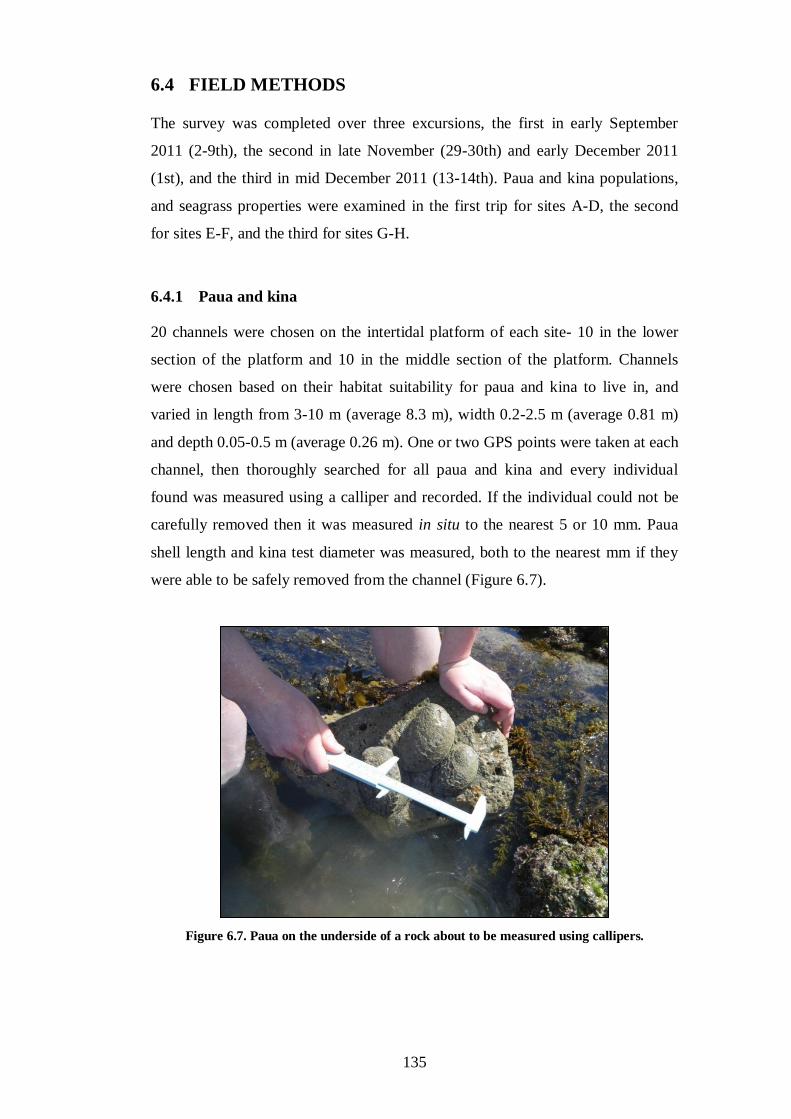
135
6.4 FIELD METHODS
The survey was completed over three excursions, the first in early September
2011 (2-9th), the second in late November (29-30th) and early December 2011
(1st), and the third in mid December 2011 (13-14th). Paua and kina populations,
and seagrass properties were examined in the first trip for sites A-D, the second
for sites E-F, and the third for sites G-H.
6.4.1 Paua and kina
20 channels were chosen on the intertidal platform of each site- 10 in the lower
section of the platform and 10 in the middle section of the platform. Channels
were chosen based on their habitat suitability for paua and kina to live in, and
varied in length from 3-10 m (average 8.3 m), width 0.2-2.5 m (average 0.81 m)
and depth 0.05-0.5 m (average 0.26 m). One or two GPS points were taken at each
channel, then thoroughly searched for all paua and kina and every individual
found was measured using a calliper and recorded. If the individual could not be
carefully removed then it was measured in situ to the nearest 5 or 10 mm. Paua
shell length and kina test diameter was measured, both to the nearest mm if they
were able to be safely removed from the channel (Figure 6.7).
Figure 6.7. Paua on the underside of a rock about to be measured using callipers.
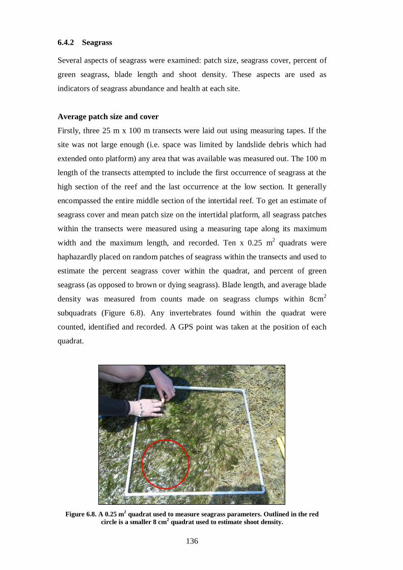
136
6.4.2 Seagrass
Several aspects of seagrass were examined: patch size, seagrass cover, percent of
green seagrass, blade length and shoot density. These aspects are used as
indicators of seagrass abundance and health at each site.
Average patch size and cover
Firstly, three 25 m x 100 m transects were laid out using measuring tapes. If the
site was not large enough (i.e. space was limited by landslide debris which had
extended onto platform) any area that was available was measured out. The 100 m
length of the transects attempted to include the first occurrence of seagrass at the
high section of the reef and the last occurrence at the low section. It generally
encompassed the entire middle section of the intertidal reef. To get an estimate of
seagrass cover and mean patch size on the intertidal platform, all seagrass patches
within the transects were measured using a measuring tape along its maximum
width and the maximum length, and recorded. Ten x 0.25 m2 quadrats were
haphazardly placed on random patches of seagrass within the transects and used to
estimate the percent seagrass cover within the quadrat, and percent of green
seagrass (as opposed to brown or dying seagrass). Blade length, and average blade
density was measured from counts made on seagrass clumps within 8cm2
subquadrats (Figure 6.8). Any invertebrates found within the quadrat were
counted, identified and recorded. A GPS point was taken at the position of each
quadrat.
Figure 6.8. A 0.25 m2 quadrat used to measure seagrass parameters. Outlined in the red
circle is a smaller 8 cm2 quadrat used to estimate shoot density.
137
Percent cover
The percent of total seagrass coverage was visually estimated within the quadrat
to the nearest five percent.
Percent green
The percent of green seagrass was visually estimated by comparing green blades
with total blades within the quadrat to the nearest five percent.
Average shoot density
3 x 8 cm2 quadrats were haphazardly placed within the 0.25 m
2 quadrat and used
to estimate shoot density. Each blade in the small quadrat was counted by
counting one stem and multiplying it by 3 (since each stem typically had 3 blades)
and recorded.
Average blade length
To estimate average blade length, 10 blades were randomly chosen and measured
using a ruler along their vertical axes from the base of the stem to the tip, and
recorded.
138
6.5 STATISTICAL METHODS
Paua, kina and seagrass data from the current survey, along with raw data on the
size of paua and kina counted in the 1999 to 2003 DOC monitoring surveys (for
multi-year comparisons) were analysed and are presented graphically (using
STATISTICA Version 11).
The results focus on paua and kina size and abundance. T-tests were used to
establish the magnitude of differences between reserve and non-reserve paua and
kina from the current survey. The data did not violate the assumptions of the test.
Paua and kina density estimates for the multi-year comparisons were obtained by
dividing the number of paua/kina sampled by the length of the channel they were
sampled from. Standardising numbers of paua/kina to the average number counted
per metre provides a more accurate comparison to be made between the 2011 and
1999-2003 survey results. The current survey sampled 80 channels within the
reserve, 40 at Blackhead, and 40 at Aramoana, compared to the 10 channels
sampled at each of these locations in the DOC surveys. This is taken into
consideration when interpreting the results.
6.6 RESULTS
6.6.1 Intertidal 2011 survey results
The 2011 intertidal paua and kina results are presented for each shore height at
each site. Sites A, B, G and H represent non-reserve populations and sites C, D, E
and F represent reserve populations.
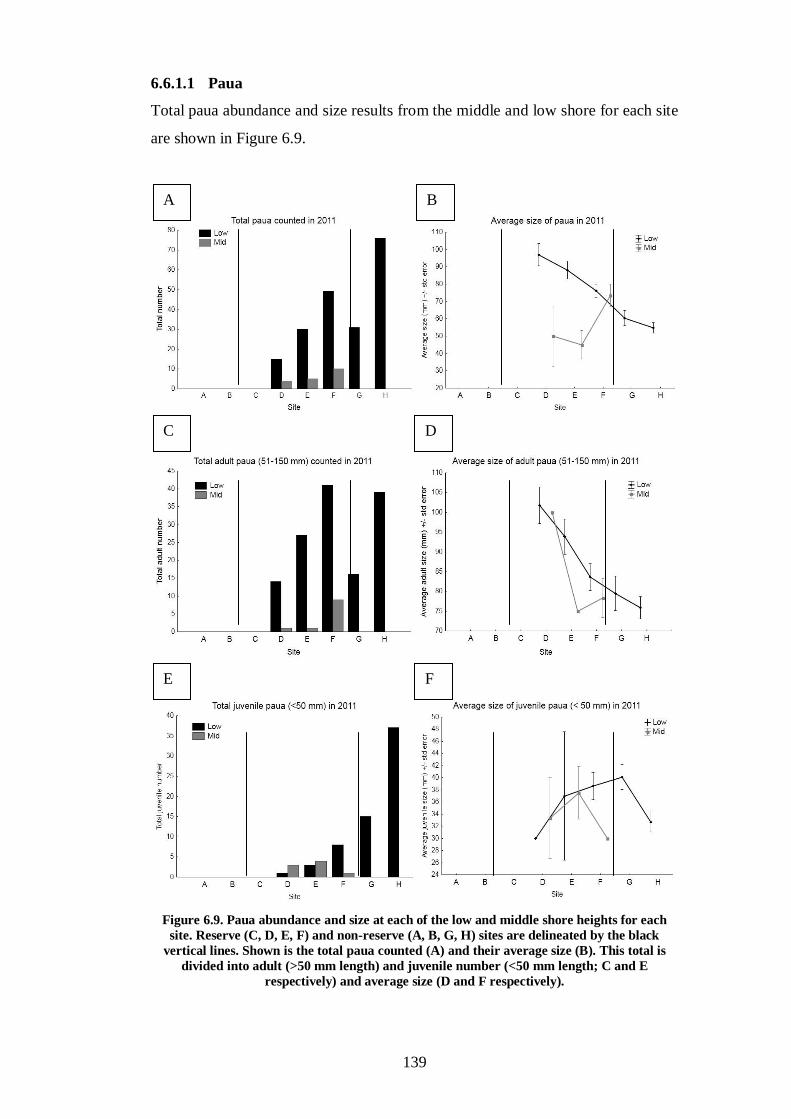
139
6.6.1.1 Paua
Total paua abundance and size results from the middle and low shore for each site
are shown in Figure 6.9.
Figure 6.9. Paua abundance and size at each of the low and middle shore heights for each
site. Reserve (C, D, E, F) and non-reserve (A, B, G, H) sites are delineated by the black
vertical lines. Shown is the total paua counted (A) and their average size (B). This total is
divided into adult (>50 mm length) and juvenile number (<50 mm length; C and E
respectively) and average size (D and F respectively).
A B
C D
E F
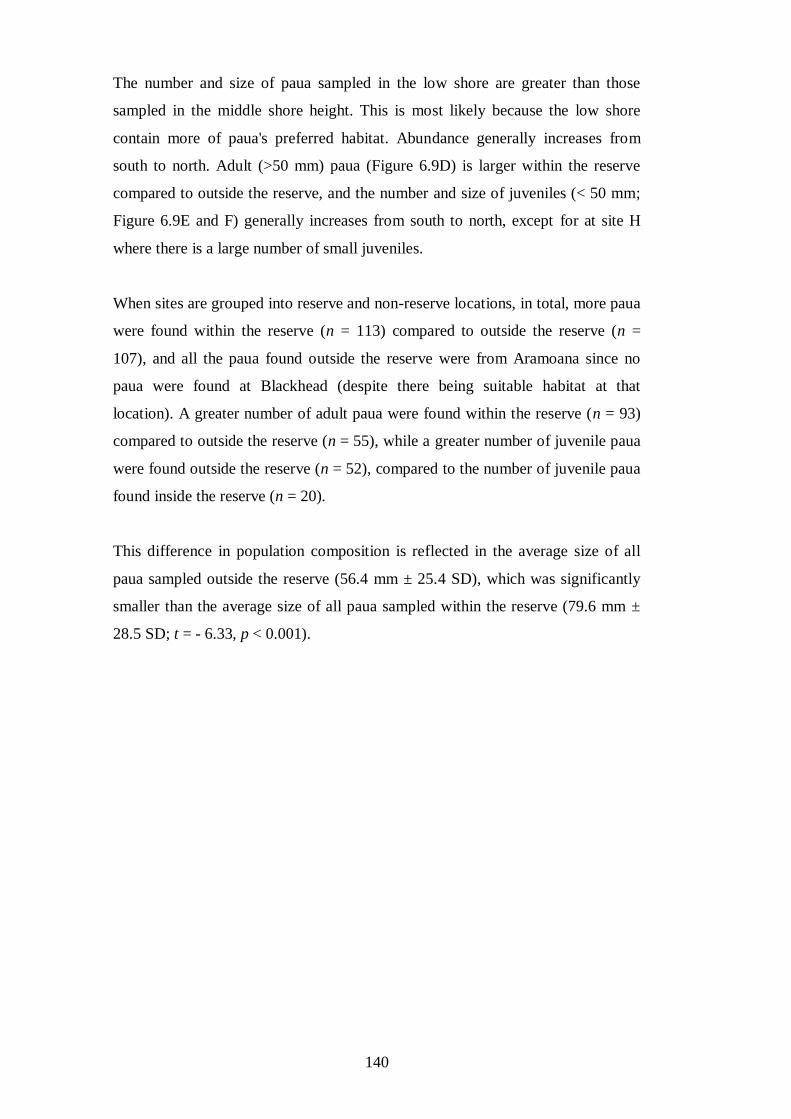
140
The number and size of paua sampled in the low shore are greater than those
sampled in the middle shore height. This is most likely because the low shore
contain more of paua's preferred habitat. Abundance generally increases from
south to north. Adult (>50 mm) paua (Figure 6.9D) is larger within the reserve
compared to outside the reserve, and the number and size of juveniles (< 50 mm;
Figure 6.9E and F) generally increases from south to north, except for at site H
where there is a large number of small juveniles.
When sites are grouped into reserve and non-reserve locations, in total, more paua
were found within the reserve (n = 113) compared to outside the reserve (n =
107), and all the paua found outside the reserve were from Aramoana since no
paua were found at Blackhead (despite there being suitable habitat at that
location). A greater number of adult paua were found within the reserve (n = 93)
compared to outside the reserve (n = 55), while a greater number of juvenile paua
were found outside the reserve (n = 52), compared to the number of juvenile paua
found inside the reserve (n = 20).
This difference in population composition is reflected in the average size of all
paua sampled outside the reserve (56.4 mm ± 25.4 SD), which was significantly
smaller than the average size of all paua sampled within the reserve (79.6 mm ±
28.5 SD; t = - 6.33, p < 0.001).
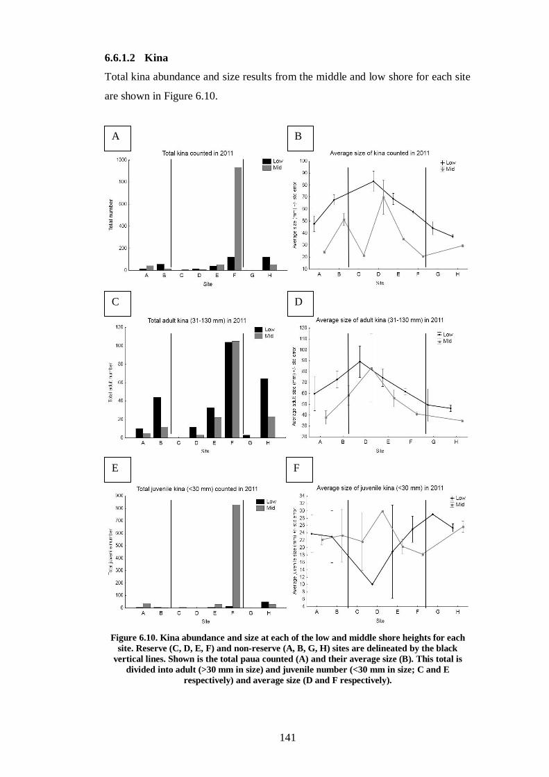
141
6.6.1.2 Kina
Total kina abundance and size results from the middle and low shore for each site
are shown in Figure 6.10.
Figure 6.10. Kina abundance and size at each of the low and middle shore heights for each
site. Reserve (C, D, E, F) and non-reserve (A, B, G, H) sites are delineated by the black
vertical lines. Shown is the total paua counted (A) and their average size (B). This total is
divided into adult (>30 mm in size) and juvenile number (<30 mm in size; C and E
respectively) and average size (D and F respectively).
A B
C D
E F
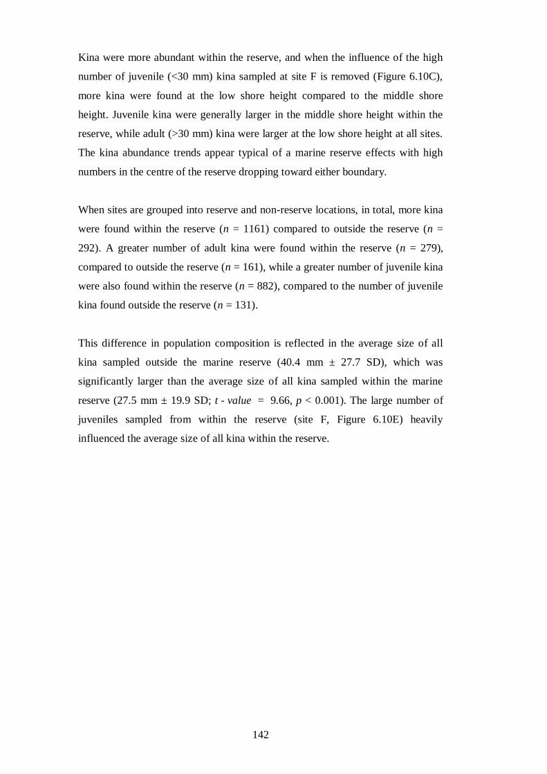
142
Kina were more abundant within the reserve, and when the influence of the high
number of juvenile (<30 mm) kina sampled at site F is removed (Figure 6.10C),
more kina were found at the low shore height compared to the middle shore
height. Juvenile kina were generally larger in the middle shore height within the
reserve, while adult (>30 mm) kina were larger at the low shore height at all sites.
The kina abundance trends appear typical of a marine reserve effects with high
numbers in the centre of the reserve dropping toward either boundary.
When sites are grouped into reserve and non-reserve locations, in total, more kina
were found within the reserve (n = 1161) compared to outside the reserve (n =
292). A greater number of adult kina were found within the reserve (n = 279),
compared to outside the reserve (n = 161), while a greater number of juvenile kina
were also found within the reserve (n = 882), compared to the number of juvenile
kina found outside the reserve (n = 131).
This difference in population composition is reflected in the average size of all
kina sampled outside the marine reserve (40.4 mm ± 27.7 SD), which was
significantly larger than the average size of all kina sampled within the marine
reserve (27.5 mm ± 19.9 SD; t - value = 9.66, p < 0.001). The large number of
juveniles sampled from within the reserve (site F, Figure 6.10E) heavily
influenced the average size of all kina within the reserve.
143
Overall, paua and kina size and abundance of reserve and non-reserve populations
has yielded some interesting results (Table 6.4), the implications of which will be
discussed in a later section
Table 6.4. Main paua and kina results for reserve and non-reserve populations sampled in
the 2011 survey.
Reserve Non-reserve
Paua
Average size (mm) 79.6 56.4
Total number 113 107
Adult number (>50 mm) 93 55
Juvenile number (<50 mm) 20 52
Kina
Average size (mm) 27.5 40.4
Total number 1161 292
Adult number (>30 mm) 279 161
Juvenile number (<30 mm) 882 131
6.6.1.3 Seagrass
Seagrass results are divided into transect and quadrat results. The transect data
provide a percent of seagrass cover over large spatial scales and average patch
size for each site, therefore providing an indication of overall abundance at each
site. The quadrat results show the percent of seagrass cover and greenness, and
average blade length and shoot density at each site, therefore providing an
indication of health at each site.
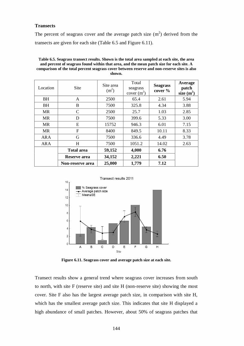
144
Transects
The percent of seagrass cover and the average patch size (m2) derived from the
transects are given for each site (Table 6.5 and Figure 6.11).
Table 6.5. Seagrass transect results. Shown is the total area sampled at each site, the area
and percent of seagrass found within that area, and the mean patch size for each site. A
comparison of the total percent seagrass cover between reserve and non-reserve sites is also
shown.
Location Site Site area
(m2)
Total seagrass
cover (m2)
Seagrass
cover %
Average
patch
size (m2)
BH A 2500 65.4 2.61 5.94
BH B 7500 325.8 4.34 3.88
MR C 2500 25.7 1.03 2.85
MR D 7500 399.6 5.33 3.00
MR E 15752 946.3 6.01 7.15
MR F 8400 849.5 10.11 8.33
ARA G 7500 336.6 4.49 3.78
ARA H 7500 1051.2 14.02 2.63
Total area 59,152 4,000 6.76
Reserve area 34,152 2,221 6.50
Non-reserve area 25,000 1,779 7.12
Figure 6.11. Seagrass cover and average patch size at each site.
Transect results show a general trend where seagrass cover increases from south
to north, with site F (reserve site) and site H (non-reserve site) showing the most
cover. Site F also has the largest average patch size, in comparison with site H,
which has the smallest average patch size. This indicates that site H displayed a
high abundance of small patches. However, about 50% of seagrass patches that

145
were measured at that site were dead, or in poor health. About 20% and 80% of
seagrass at non-reserve sites B and G respectively were also dead or in poor
health.
Seagrass quadrats
The percent of seagrass cover, and the percent of that seagrass which was green
for each site is shown in Figure 6.12A. The average blade length and average
shoot density for each site is shown in Figure 6.12B.
Figure 6.12. Seagrass quadrat results for each site. Shown is the percent of seagrass cover
within the quadrat, and the percent of that seagrass which was green (A). B shows the
average blade length and average shoot density (shoot density was estimated using small 3 x
8 cm2 quadrats). Reserve (C, D, E, F) and non-reserve (A, B, G, H) sites are delineated by the
black vertical lines.
Seagrass quadrat results give an indication of seagrass health at each site.
Generally, seagrass cover within the 0.25 m2 quadrat, and percent of green
seagrass decreased from south to north. The average blade length and shoot
density increased within the reserve sites, and the average shoot density increased
from south to north.
A B
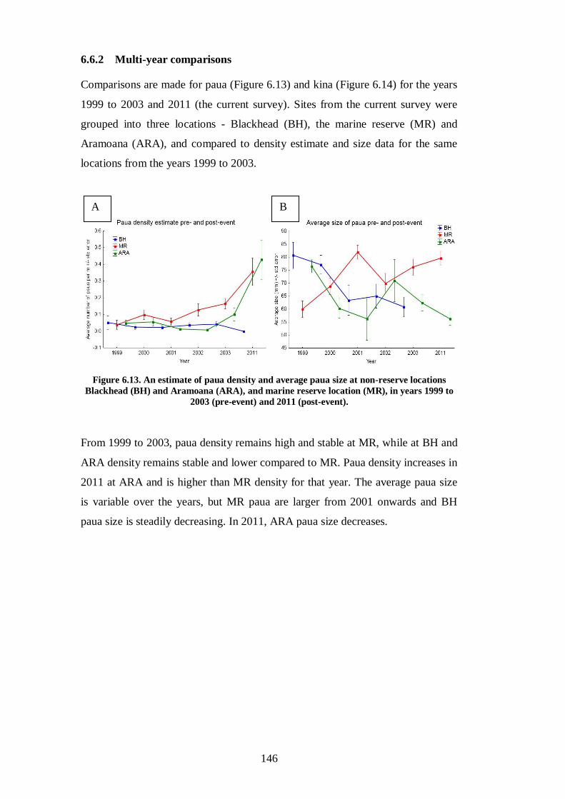
146
6.6.2 Multi-year comparisons
Comparisons are made for paua (Figure 6.13) and kina (Figure 6.14) for the years
1999 to 2003 and 2011 (the current survey). Sites from the current survey were
grouped into three locations - Blackhead (BH), the marine reserve (MR) and
Aramoana (ARA), and compared to density estimate and size data for the same
locations from the years 1999 to 2003.
Figure 6.13. An estimate of paua density and average paua size at non-reserve locations
Blackhead (BH) and Aramoana (ARA), and marine reserve location (MR), in years 1999 to
2003 (pre-event) and 2011 (post-event).
From 1999 to 2003, paua density remains high and stable at MR, while at BH and
ARA density remains stable and lower compared to MR. Paua density increases in
2011 at ARA and is higher than MR density for that year. The average paua size
is variable over the years, but MR paua are larger from 2001 onwards and BH
paua size is steadily decreasing. In 2011, ARA paua size decreases.
A B
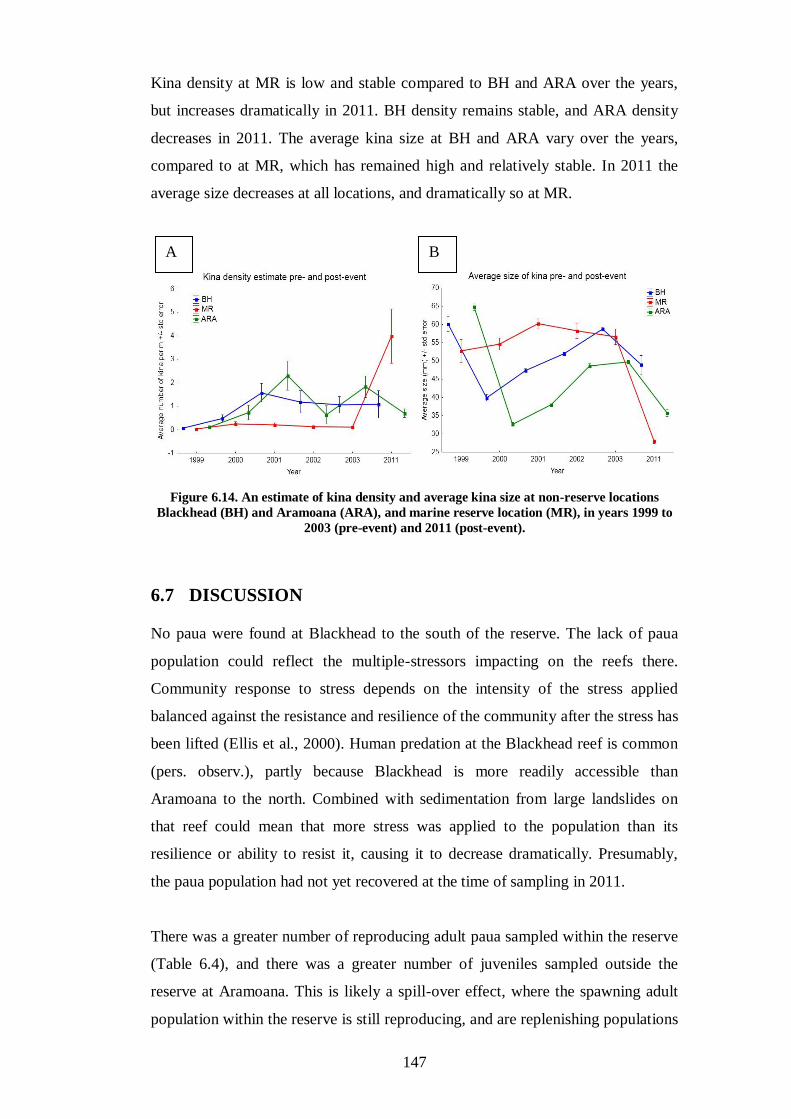
147
Kina density at MR is low and stable compared to BH and ARA over the years,
but increases dramatically in 2011. BH density remains stable, and ARA density
decreases in 2011. The average kina size at BH and ARA vary over the years,
compared to at MR, which has remained high and relatively stable. In 2011 the
average size decreases at all locations, and dramatically so at MR.
Figure 6.14. An estimate of kina density and average kina size at non-reserve locations
Blackhead (BH) and Aramoana (ARA), and marine reserve location (MR), in years 1999 to
2003 (pre-event) and 2011 (post-event).
6.7 DISCUSSION
No paua were found at Blackhead to the south of the reserve. The lack of paua
population could reflect the multiple-stressors impacting on the reefs there.
Community response to stress depends on the intensity of the stress applied
balanced against the resistance and resilience of the community after the stress has
been lifted (Ellis et al., 2000). Human predation at the Blackhead reef is common
(pers. observ.), partly because Blackhead is more readily accessible than
Aramoana to the north. Combined with sedimentation from large landslides on
that reef could mean that more stress was applied to the population than its
resilience or ability to resist it, causing it to decrease dramatically. Presumably,
the paua population had not yet recovered at the time of sampling in 2011.
There was a greater number of reproducing adult paua sampled within the reserve
(Table 6.4), and there was a greater number of juveniles sampled outside the
reserve at Aramoana. This is likely a spill-over effect, where the spawning adult
population within the reserve is still reproducing, and are replenishing populations
A B
148
to the north. This is supported by larval dispersal modelling (Oldman et al., 2006),
which indicates reefs to the north of the reserve are likely to benefit from
spawning populations within the reserve. Population resilience means that
populations of a greater abundance and containing many reproducing adults are
able to maintain larval production and therefore local recruitment (Micheli et al.,
2012). The fact that the number of adult paua within the reserve remained high
after the sedimentation event could represent an increased resilience of the adult
reserve paua population.
For the reserve population to serve as a source of larvae, it must be able to
replenish itself and adjacent areas (Halpern, 2003). If populations to the north of
the reserve are indeed being replenished by spawning reserve populations, this
could indicate the need to extend protection offered by the marine reserve, so
protection encompasses areas to the north where recruitment is likely happening.
This would allow the reserve population to replenish itself and increase
populations even further to the north through spill-over effects, which could lead
to more stabilised populations along a greater length of coastline.
Kina patterns of size and abundance suggest that a large recruitment event
occurred within the reserve (site F) after the sedimentation event. Either the
subtidal spawning population within the reserve generated these recruits, or they
have settled within the reserve and are from a spawning population from another
location. Why the juveniles have settled and are so abundant in the reserve is
difficult to explain. The high juvenile number may only be high because of lack of
kina predators such as crayfish, the populations of which may have been
negatively affected by the sedimentation event. Populations of crayfish are known
to increase in abundance within reserves (Ballentine & Langlois, 2008) and are
thought to have some influence in the abundance of kina (Freeman, 2006). If the
crayfish population decreased after the sedimentation event, it could be possible
that in their absence that kina were able to recover faster due to lack of predation
on the population. A subtidal survey would have provided insight and further
explanation of this aspect.
If the kina juveniles have come from spawning populations within, or from the
immediate area adjacent to the reserve, this could then be an indication of
149
resilience shown by the adult kina population, in that there are still many
reproducing kina present within the reserve. However, the average size of kina
within the reserve was 27.5 mm, which is at the lower end of the range of the
typical spawning size for kina, and the long larval longevity (more than 30 days,
which means factors such as currents can transport larvae over a large and
variable temporal and spatial scale), means that recruitment seen in the reserve
unlikely came from the kina reserve population. Even though the recruitment
event may not be explained by adult kina within the reserve, the adult population
sampled is still greater than the non-reserve adult population (Table 6.5),
indicating there may still be a resilience trend.
The current survey, along with the multi-year results, have demonstrated that the
paua and kina populations within the reserve are likely showing an increased
resilience to the sedimentation event. The populations were high and stable
enough when the sedimentation event occurred, so that after the impact their
numbers were maintained and they were able to continue to reproduce. This is
particularly well seen with the 2011 paua populations within and outside the
reserve, and is also displayed well in the paua multi-year pattern (Figure 6.13).
However, it must be noted that the multi-year density estimates are estimates only
with some earlier sampling designs lacking in adequate replication. The 2011
density estimates are expected to have more accuracy in estimating a true mean
with tighter variance because the numbers of channels sampled in 2011 were
much higher compared to the number DOC channels.
Seagrass are important indicators of coastal primary productivity. They are highly
productive and support numerous detritus and herbivore based food webs (Turner
& Schwarz, 2006). While seagrass habitat may have arguable relevance to paua
and kina population demography, it does indicate a higher general level of healthy
functional intertidal reef inside the reserve compared to locations to the north and
south. It is likely that subtidal algal ecosystems will also reflect this situation, and
hence explain to some extent the more abundant grazing invertebrate communities
(kina and paua) found inside the reserve. Whether this is a consequence of reserve
protection, or other biophysical conditions acting on the various intertidal reef
sites, remains unclear. All sites however, would have been affected more or less to
a similar degree for at least a short period of time by substantial sediment
150
inundation, during the worst periods of storm activity that led to the slope failures.
Subsequent tides have since modified the sedimentary regime in the intertidal area
along this coast.
The current survey has provided a platform for further study relating to resilience
of marine reserve organisms to disturbances. There are little studies providing
conclusive evidence of resilience shown by populations within a marine reserve to
disturbances (Micheli et al., 2012), let alone studies on disturbance events
occurring in marine reserves. Therefore, with further examination, this study can
increase the understanding of whether marine reserves play a role in increasing
resilience of marine reserve populations when exposed to a disturbance.
This study could be repeated in order to gain a better understanding of temporal
influence on the population during recovery of the sedimentation event, and
should be conducted in conjunction with a survey of subtidal paua, kina, crayfish
and reef fish populations, which are likely to be subject to longer periods of
sedimentary input especially in deeper reef areas. This would help explain
recruitment patterns within the reserve and adjacent non-reserve coastline, and
provide further understanding of factors influencing the size and abundance of
reserve organisms.
151
7 Chapter 7
DISCUSSION AND SUMMARY
This chapter provides an overall discussion of work carried out and a summary of
the main conclusions drawn. The chapter integrates the conclusions made through
the previous chapters to examine any interrelationships between the April 2011
catastrophic sedimentation event and possible ecological resilience of Te
Angiangi Marine Reserve habitats, as evidenced by population demographics of
key intertidal species within.
7.1 MAPIRI FORMATION MUDSTONE
7.1.1 Important characteristics
Joints and weakness
The Mapiri mudstone, of late Miocene age, is by nature a highly jointed rock. The
mudstone bedrock exhibits a complex set of joints, ranging in scale from metres to
centimetres apart, the former observed as the master joint cracks across the
intertidal platform (Figure 3.2A). The smaller scale joints facilitate effective in
situ weathering of mudstone boulders in a spheroidal manner (Figure 3.21). Once
the small joint blocks are released they are readily further eroded by wetting and
drying and wave action to produce fine sized particles. The joints are a
particularly important feature in the presence of swelling smectite minerals,
because they allow ready access of percolating water which further weakens the
already relatively weakly indurated rock. The Mapiri mudstone was likely
deposited in a slope basin environment, and was not subjected to especially deep
burial, resulting in a weakly cemented (carbonate content about 10%) rock.
Correlative mudstones at nearby Cape Turnagain have very low Schmidt hammer
values of <10, supportive of the Mapiri mudstone too being an extremely weak
rock (Kennedy & Dickson, 2007). The Mapiri mudstone siliciclastic material,
including its high clay mineral content of illite and smectite, were likely mainly
detritally derived from the erosion of older mudstones.

152
Smectite rich composition
Another important feature of the Mapiri mudstone is that it contains abundant clay
minerals that are dominated by illite and smectite (Figure 3.11). The source of the
common smectite in the Mapiri mudstone was likely mainly from erosion of older
Tertiary mudstones present in the catchment area adjacent to the Te Angiangi
Marine Reserve (Figure 2.5 and 2.6). Of significance are the Wanstead Formation
lithologies which contain smectite clays known to cause slope instability and
erosion (Lee et al., 2011). The ability of smectite minerals to expand and contract
during wetting and drying means that its occurrence in soft rocks can significantly
weaken them. The jointed nature of the Mapiri mudstone means water can
penetrate quite deeply into the deposit, not just within the soil zone, and so the
“active smectite” component becomes an important factor in weakening the rock.
Source of mud and fine sand
Erosion of the Mapiri mudstone through slope failures ultimately led to the
delivery of fine sediment into the nearshore marine environment, including the
area encompassing the Te Angiangi Marine Reserve. The joint controlled
spheroidal weathering of the mudstone tended to release (sub) rounded clasts of
mudstone that were further eroded and broken down under the influence of
shoreline wave action. This process released the fine sized particles occurring in
the offshore area (Figure 5.11). The Mapiri mudstone is rich in clay minerals, but
nevertheless is texturally classified as a ‘sandy silt’ (Figure 3.20). In total and on
average, it contains about 42% sand, about 42% silt, and about 16% clay sizes.
This sand content includes about 10% very fine sand, 13-14% each of fine and
medium sand, and 3-6% coarse sand (Table 3.4). Accordingly, the Mapiri
mudstone is itself a viable source of both the finer sandy and mud sized material
occurring in the subtidal sediments within and about the marine reserve (Chapter
5).
7.2 CATASTROPHIC LANDSLIDES
The landslides, which were the point source of the sediment delivered into the
reserve and adjacent coastline, were catastrophic failures present along a
significant part of the reserve hill side. 14 major landslides are recorded,
generating an estimated total of 150,000 m3 of debris. The Te Angiangi Marine
153
Reserve is located within the much faulted and tectonically active zone of coastal
ranges on the North Island East Coast (Figure 2.3), where relatively young and
soft Neogene rocks are deformed due to extensive folding and fracturing. This is
particularly evident in the reserve catchment, where the Mapiri Formation is
influenced structurally by a series of complex folds and faults (Figure 2.5). The
resulting geomorphology of the study area is mostly steep undulating hill sides, a
significant proportion of which has been cleared of vegetation for the purpose of
pastoral farming (Lacoste et al., 2009).
The external triggering factor initiating the landslides in the reserve and adjacent
coastline was intense rainfall (650 mm) which fell between the 25-28 April 2011.
This coincided also with a M4.5 scale earthquake centred only 10 km offshore
from Pourerere at a depth of 20 km. The Mapiri mudstones location within a
tectonically active subduction margin, along with subaerial erosion and tectonic
influences, resulted in undulating steep hill sides. But most importantly, its soft
and jointed nature and high smectite clay content are intrinsic features which,
along with the above external triggering, caused the landslides which devastated
the Te Angiangi Marine Reserve coastline in April 2011.
7.3 EXTENT OF SIGNIFICANT SEDIMENTATION
The local geology adjacent to the marine reserve, the soft Mapiri Formation
mudstone, has been observed to erode quickly and effectively into fine size
particles (Chapter 3). It is likely that the landslide debris, a large proportion of
which consists of the soft mudstone (the rest being soil), weathers quickly into
fine sediment, which then facilitates its easy dispersal and deposition from
suspension far offshore. Hydrodynamic forces act to transport and disperse the
sediment over large spatial scales, and the subtidal sediment survey undertaken at
the marine reserve and adjacent nearshore area showed that mud sized particles
become increasingly common with depth and distance offshore, with the muddiest
samples found at the offshore limit of the nearshore region at about 40 m depth.
This agrees with the study by Lewis and Gibb (1970) who showed that mud
content increases significantly across the continental shelf, and that completely
mud dominated sediments occur by about 100 m water depth (Figure 5.1).
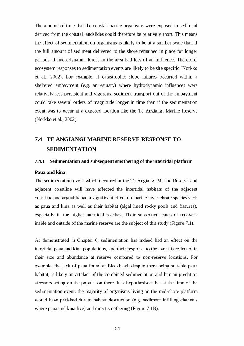
154
The amount of time that the coastal marine organisms were exposed to sediment
derived from the coastal landslides could therefore be relatively short. This means
the effect of sedimentation on organisms is likely to be at a smaller scale than if
the full amount of sediment delivered to the shore remained in place for longer
periods, if hydrodynamic forces in the area had less of an influence. Therefore,
ecosystem responses to sedimentation events are likely to be site specific (Norkko
et al., 2002). For example, if catastrophic slope failures occurred within a
sheltered embayment (e.g. an estuary) where hydrodynamic influences were
relatively less persistent and vigorous, sediment transport out of the embayment
could take several orders of magnitude longer in time than if the sedimentation
event was to occur at a exposed location like the Te Angiangi Marine Reserve
(Norkko et al., 2002).
7.4 TE ANGIANGI MARINE RESERVE RESPONSE TO
SEDIMENTATION
7.4.1 Sedimentation and subsequent smothering of the intertidal platform
Paua and kina
The sedimentation event which occurred at the Te Angiangi Marine Reserve and
adjacent coastline will have affected the intertidal habitats of the adjacent
coastline and arguably had a significant effect on marine invertebrate species such
as paua and kina as well as their habitat (algal lined rocky pools and fissures),
especially in the higher intertidal reaches. Their subsequent rates of recovery
inside and outside of the marine reserve are the subject of this study (Figure 7.1).
As demonstrated in Chapter 6, sedimentation has indeed had an effect on the
intertidal paua and kina populations, and their response to the event is reflected in
their size and abundance at reserve compared to non-reserve locations. For
example, the lack of paua found at Blackhead, despite there being suitable paua
habitat, is likely an artefact of the combined sedimentation and human predation
stressors acting on the population there. It is hypothesised that at the time of the
sedimentation event, the majority of organisms living on the mid-shore platform
would have perished due to habitat destruction (e.g. sediment infilling channels
where paua and kina live) and direct smothering (Figure 7.1B).
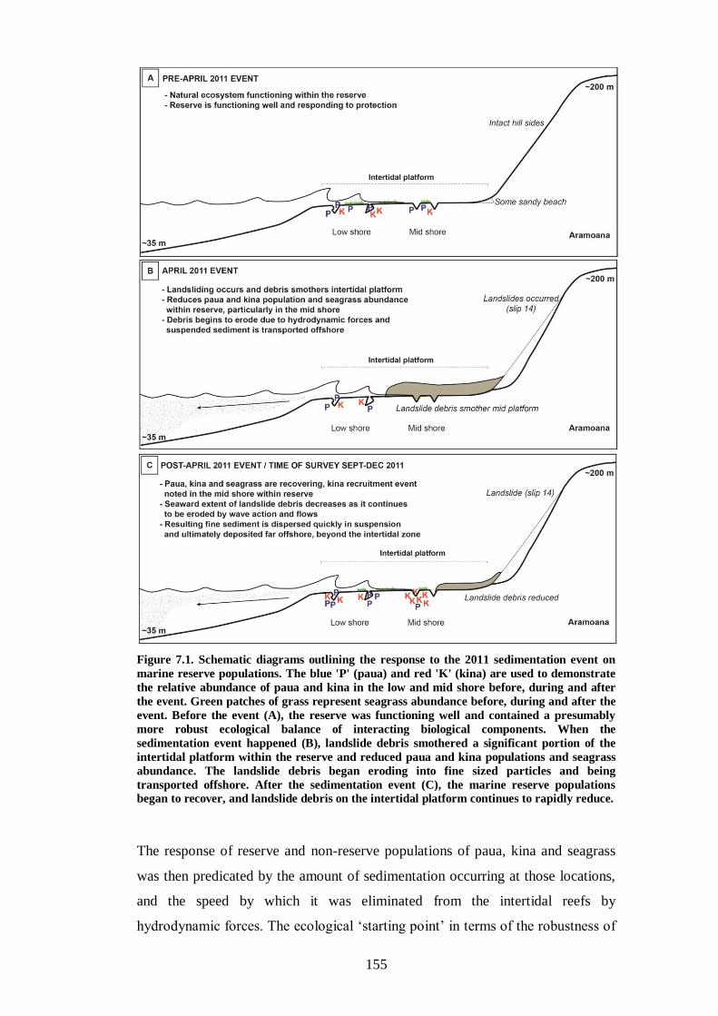
155
Figure 7.1. Schematic diagrams outlining the response to the 2011 sedimentation event on
marine reserve populations. The blue 'P' (paua) and red 'K' (kina) are used to demonstrate
the relative abundance of paua and kina in the low and mid shore before, during and after
the event. Green patches of grass represent seagrass abundance before, during and after the
event. Before the event (A), the reserve was functioning well and contained a presumably
more robust ecological balance of interacting biological components. When the
sedimentation event happened (B), landslide debris smothered a significant portion of the
intertidal platform within the reserve and reduced paua and kina populations and seagrass
abundance. The landslide debris began eroding into fine sized particles and being
transported offshore. After the sedimentation event (C), the marine reserve populations
began to recover, and landslide debris on the intertidal platform continues to rapidly reduce.
The response of reserve and non-reserve populations of paua, kina and seagrass
was then predicated by the amount of sedimentation occurring at those locations,
and the speed by which it was eliminated from the intertidal reefs by
hydrodynamic forces. The ecological ‘starting point’ in terms of the robustness of
156
the habitat at those locations (quasi natural at the reserve or human predated at
non-reserve locations) before the sedimentation event, together with the maturity
of the populations of kina and paua present, may have been a factor influencing
their response (albeit this latter hypothesis is difficult to substantiate without
much more comprehensive pre-event information). At Blackhead, the response is
clear. The ongoing human predation stress, with the additional sedimentation
stress, has arguably led to a dramatic drop in the paua population. This
observation is supported by the fact that previous monitoring surveys have found
paua there in the past.
Paua and kina demographics within the reserve are demonstrating upward trends
in the number of their average sizes. Abundance and average sizes (Figures 6.9
and 6.10) show a typical bell shaped curve, where the peak in the centre
represents reserve sites. This provides further confirmation of the likelihood of
human predation at reserve boundaries, and supports that the reserve populations
are coping well with any sedimentation impacts. These observations hint at a
resilience afforded by marine reserve status, as shown by the greater abundance of
adult paua and kina found within the reserve compared to non-reserve locations
(Table 6.4). The abundance of juveniles suggests that the reproductive output of
paua and kina has remained steady, although it is unclear whether the origin of
kina juveniles is sourced from inside the reserve. What is relevant however is that
the intertidal reserve habitat appears to be more conducive to supporting
recruitment of juveniles compared to non-reserve locations.
Overall, reserve populations of the species examined are indicating a reserve
effect, and this reserve effect is presumably overriding any negative sedimentation
effects. It is therefore tempting to accept the hypothesis that marine reserves do
indeed afford resilience to environmental stressors (especially since empirical
evidence of the effectiveness of marine reserves against disturbances is lacking
(Micheli et al. (2012)), but there could be alternate arguments for the observations
made. It could be that the geomorphology and nearshore current patterns of the
reserve location was always more likely to attract recruiting kina and paua, or that
simple stochastic events such as patchy recruitment episodes, and or variable
longevity of fine sediments remaining on the different areas of reef (sampling and

157
surveys occurred some months after the sedimentation event occurred) have
resulted in the patterns observed.
Seagrass
There was also an observed response in seagrass cover in areas directly smothered
by landslide debris. In the areas severely affected, the intertidal platform was
almost completely bare of macroalgae, including Neptune's necklace (Hormosira
banksii), which is otherwise of common occurrence on this reef (pers. observ.).
This decrease is probably due to a reduction in light caused by the suspended fine
sediment, or a consequence of direct smothering, resulting in significant loss of
seagrass (Figure 7.1B). At the time of the survey, seagrass had recovered well
(Figure 7.1C), and this could be indicative of an improvement in overall
community structure and health. This is because seagrasses are sensitive to fine
sediment and other disturbance, and are characteristic of highly productive
ecosystems (Turner & Schwarz, 2006).
Once the landslide debris began to reduce, and the sedimentation stress began to
ease, seagrass was able to begin re-establishment. Presence of sediments may
have even been favourable, since seagrass needs extensive soft sediment
substrates to establish their root system, which might explain the abundance of
seagrass that was sampled in the survey. While seagrasses are not likely to
directly influence kina and paua populations, the relevance of examining this
habitat was to assess wider ecosystem health for each reef region examined inside
and outside the reserve. Conditions that would be deleterious to seagrass would
also likely be deleterious to macroalgae that characterise paua and kina habitat.
There may also be some benefit in the likely sediment trapping effects from
extensive seagrass meadows that would benefit adjacent habitats.
7.5 PRE-EXISTING RESILIENCE IN EAST COAST
POPULATIONS AND A MARINE RESERVE EFFECT
Landsliding along the East Coast of North Island is common (Pettinga, 1980;
Gibb, 1978; section 4.3), and it is clearly evident that previous landsliding has
occurred on the coastal hills adjacent to the Te Angiangi Marine Reserve (Figures
4.3A and 4.5). Sediment delivery into the marine environment through coastal
158
landslides is therefore a common occurrence (Airoldi, 2003). One of the primary
means of sedimentation in the coastal marine environment is delivery through
fluvial systems (Griffiths & Glasby; 1985; Foster & Carter, 1997; Brackley et al.,
2010; Parra et al., 2012). There are large river systems that discharge to the north
of the Te Angiangi Marine Reserve at Hawke Bay and Poverty Bay, which carry
large amounts of fine suspended sediment (Griffiths & Glasby; 1985). Given the
susceptibility and occurrence of landsliding along the southern Hawke's Bay
coastline, as well as sediment contributions from rivers draining the catchments, it
could be said that marine populations in affected areas are already somewhat
resilient to sedimentation. However, the small amount of literature relating to
marine ecology along the southern Hawke's Bay coastline, apart from data
gathered from the Te Angiangi Marine Reserve monitoring efforts, remains
insufficient to permit any detailed evaluation of ecological trends that may
suggest enhanced recovery of populations (either from reserve or non-reserve
locations) along the Hawkes Bay coastline.
In isolated areas where the risk of human predation of the marine biota is smaller,
the marine populations are likely to exist in a more stable or more naturally
balanced ecosystem state, such that the concept of resilience to other disturbances
such as sedimentation can be entertained. This study has shown that there is a
significant within ‘reserve effect’, in that the paua and kina species studied appear
to be recovering more effectively inside the Te Angiangi Marine Reserve, than
those populations outside. As discussed above, there are a number of alternate
arguments for this and it is not within the scope of this study to make a definitive
conclusion. The work does however create a platform for further investigation,
which could most effectively be carried out with subtidal survey extensions to the
work presented here.
This study set out to examine possible linkages between a significant
sedimentation inundation event and aspects of coastal intertidal ecosystem
response. In conjunction, the study encompassed the unique opportunity to
examine population responses from inside and outside of a marine reserve. It is a
multi-disciplinary examination of a highly complex interaction and can be used as
a platform for future work.
159
REFERENCE LIST
Airoldi, L. (2003). The effects of sedimentation on rocky coast assemblages.
Oceanography and Marine Biology: an Annual Review, 41, 161-236.
Airoldi, L., & Cinelli, F. (1997). Effects of sedimentation on subtidal macroalgal
assemblages: an experimental study from a Mediterranean rocky shore.
Journal of Experimental Marine Biology and Ecology, 215(2), 269-288.
Allison, G. W., Gaines, S. D., Lubchenco, J., & Possingham, H. P. (2003).
Ensuring persistence of marine reserves: catastrophes require adopting an
insurance factor. Ecological Applications, 13(sp1), 8-24.
Allison, G. W., Lubchenco, J., & Carr, M. H. (1998). Marine reserves are
necessary but not sufficient for marine conservation. Ecological
applications, 8(1), 79-92.
Andrew, N. L. (1988). Ecological aspects of the common sea urchin, Evechinus
chloroticus, in northern New Zealand: a review. New Zealand journal of
marine and freshwater research, 22(3), 415-426.
Babcock, R. C., Kelly, S., Shears, N. T., Walker, J. W., & Willis, T. J. (1999).
Changes in community structure in temperate marine reserves. Marine
Ecology Progress Series, 189, 125-134.
Ballantine, W. J., & Langlois, T. J. (2008). Marine reserves: the need for systems.
Challenges to Marine Ecosystems, 35-44.
Barnes, P. M., & de Lepinay, B. M. (1997). Rates and mechanics of rapid frontal
accretion along the very obliquely convergent southern Hikurangi margin,
New Zealand. Journal of geophysical research, 102(11), 24,931 - 24,952.
Barnes, P. M., Lamarche, G., Bialas, J., Henrys, S., Pecher, I., Netzeband, G. L., .
. . Crutchley, G. (2010). Tectonic and geological framework for gas
hydrates and cold seeps on the Hikurangi subduction margin, New
Zealand. Marine Geology, 272(1), 26-48.
Barnes, P. M., Nicol, A., & Harrison, T. (2002). Late Cenozoic evolution and
earthquake potential of an active listric thrust complex above the
Hikurangi subduction zone, New Zealand. Geological Society of America
Bulletin, 114(11), 1379-1405.
Beanland, S., Melhuish, A., Nicol, A., & Ravens, J. (1998). Structure and
deformational history of the inner forearc region, Hikurangi subduction
margin, New Zealand. New Zealand journal of geology and geophysics,
41(4), 325-342.
Bjolykke, K. (1998). Clay mineral diagenesis in sedimentary basins-a key to the
prediction of rock properties. Examples from the North Sea Basin. Clay
minerals, 33(1), 15-34.
160
Bland, K. J., & Kamp, P. J. J. (2006). Geological structure of the forearc basin in
central Hawke’s Bay, eastern North Island. Paper presented at the New
Zealand Petroleum Conference.
Blott, S. J., & Pye, K. (2001). GRADISTAT: A grain size distribution and
statistics package for the analysis of unconsolidated sediments. Earth
Surface Processes and Landforms, 26, 1237-1248.
Boggs, S. (2006). Principles of sedimentology and stratigraphy: fourth edition.
New Jersey, U.S.A: Pearson Prentice Hall.
Brackley, H. L., Blair, N. E., Trustrum, N. A., Carter, L., Leithold, E. L., Canuel,
E. A., . . . Tate, K. R. (2010). Dispersal and transformation of organic
carbon across an episodic, high sediment discharge continental margin,
Waipaoa Sedimentary System, New Zealand. Marine Geology, 270(1),
202-212.
Brodie, J. W. (1960). Coastal surface currents around New Zealand. New Zealand
journal of geology and geophysics, 3(2), 235-252.
Butler, H., Clegg, E., Le Vaillant, C. and Thomas, L. (2010). Te Angiangi Marine
Reserve seagrass monitoring program. Unpublished report for the
Department of Conservation by postgraduate students, Victoria University
of Wellington.
Carroll, D., & Starkey, H. C. (1971). Reactivity of clay minerals with acids and
alkalies. Clays and clay minerals, 19, 321-335.
Cashman, S. M., Kelsey, H. M., Erdman, C. F., Cutten, H. N. C., & Berryman, K.
R. (1992). Strain partitioning between structural domains in the forearc of
the Hikurangi subduction zone, New Zealand. Tectonics, 11(2), 242-257.
Chester, R. (1993). Marine Geochemistry. London: Chapman and Hall.
Chiswell, S. M. (2000). The Wairarapa coastal current. New Zealand Journal of
Marine and Freshwater Research, 34(2), 303-315.
Chiswell, S. M. (2003). Circulation within the Wairarapa Eddy, New Zealand.
New Zealand journal of marine and freshwater research, 37(4), 691-704.
Costales, et. al. (2009). Paua and kina monitoring report. Unpublished
monitoring survey undertaken by postgraduate students. Victoria
University of Wellington.
Creswell, P. D., & Warren, E. J. (1990). The flora and fauna of the southern
Hawke’s Bay coast. East Coast Hawke’s Bay Conservancy: the
Department of Conservation.
Crozier, M. J., Eyles, R. J., Marx, S. L., McConchie, J. A., & Owen, R. C. (1980).
Distribution of landslips in the Wairarapa hill country. New Zealand
journal of geology and geophysics, 23(5-6), 575-586.
Crozier, M. J., Gage, M., Pettinga, J. R., Selby, M. J., & Wasson, R. J. (1992).
161
The Stability of Hillslopes. In J. M. Soons & M. J. Selby (Eds.),
Landforms of New Zealand second edition. Auckland, New Zealand:
Longman Paul.
Cummings, V. J., & Thrush, S. F. (2004). Behavioural response of juvenile
bivalves to terrestrial sediment deposits: implications for post-disturbance
recolonisation. Marine Ecology Progress Series, 278, 179-191.
Cummings, V. J., & Thrush, S. F. (2004). Behavioural response of juvenile
bivalves to terrestrial sediment deposits: implications for post-disturbance
recolonisation. Marine Ecology Progress Series, 278, 179-191.
Cummings, V. J., Vopel, K., & Thrush, S. (2009). Terrigenous deposits in coastal
marine habitats: influences on sediment geochemistry and behaviour of
post-settlement bivalves. Marine Ecology Progress Series, 383, 173-185.
Denny, C. M., Willis, T. J., & Babcock, R. C. (2004). Rapid recolonisation of
snapper Pagrus auratus: Sparidae within an offshore island marine reserve
after implementation of no-take status. Marine Ecology Progress Series,
272, 183-190.
Department of Conservation website: www.doc.govt.nz/conservation/marine-and-
coastal/marine-protected-areas/
Department of Conservation (1994a). Te Angiangi Marine Reserve Intertidal
baseline survey. Collection of survey notes held at the East Coast Hawke's
Bay Conservancy.
Department of Conservation. (1994b). Te Angiangi (Aramoana – Blackhead,
Central Hawke’s Bay) marine reserve application. Hawke’s Bay
Conservancy Series, 7, 86.
Department of Conservation. (2001). Te Angiangi Marine Reserve: Biological
Monitoring Plan. East Coast Hawke’s Bay Conservancy: Technical
Support (Marine & Freshwater).
Department of Conservation. (2003). Te Angiangi Marine Reserve Operational
Plan. Napier, New Zealand: Hawke's Bay Conservancy.
Department of Conservation. (2008). Te Angiangi Marine Reserve brochure,
Central Hawke's Bay. Department of Conservation.
Dymond, J. R., Ausseil, A. G., Shepherd, J. D., & Buettner, L. (2006). Validation
of a region-wide model of landslide susceptibility in the Manawatu–
Wanganui region of New Zealand. Geomorphology, 74(1), 70-79.
Ellis, J., Nicholls, P., Craggs, R., Hofstra, D., & Hewitt, J. (2004). Effects of
terrigenous sedimentation on mangrove physiology and associated
macrobenthic communities. Marine Ecology Progress Series, 270, 71-82.
Ellis, J. I., Norkko, A., & Thrush, S. F. (2000). Broad-scale disturbance of
intertidal and shallow sublittoral soft-sediment habitats; effects on the
162
benthic macrofauna. Journal of Aquatic Ecosystem Stress and Recovery,
7(1), 57-74.
Erdman, C. F., & Kelsey, H. M. (1992). Pliocene and Pleistocene stratigraphy and
tectonics, Ohara Depression and Wakarara Range, North Island, New
Zealand. New Zealand journal of geology and geophysics, 35(2), 177-192.
Fairweather, P. G., & Underwood, A. J. (1991). Experimental removals of a rocky
intertidal predator: variations within two habitats in the effects on prey.
Journal of Experimental Marine Biology and Ecology, 154(1), 29-75.
Field, B. D., Uruski, C. I. and others (1997). Cretaceous-Cenozoic geology and
petroleum systems of the East Coast Region, New Zealand. Institute of
Geological and Nuclear Sciences monograph 19. 301, 7 encolsures. Lower
Hutt, New Zealand: Institute of Geological and Nuclear Sciences Limited.
Flemming, et. al. (2009). Seagrass monitoring proposal. Unpublished monitoring
survey undertaken by postgraduate students. Victoria University of
Wellington
Fletcher, W. J. (1987). Interactions among subtidal Australian sea urchins,
gastropods, and algae: effects of experimental removals. Ecological
Monographs, 89-109.
Folk, R. L. (1954). The distinction between grain size and mineral composition in
sedimentary-rock nomenclature. The Journal of Geology, 344-359.
Folk, R. L. (1968). Petrology of sedimentary rocks. Austin, Texas: Hemphill.
Folk, R. L., & Ward, W. C. (1957). Brazos River bar: a study in the significance
of grain size parameters. Journal of Sedimentary Petrology, 27, 3-26.
Foster, G., & Carter, L. (1997). Mud sedimentation on the continental shelf at an
accretionary margin—Poverty Bay, New Zealand. New Zealand Journal of
Geology and Geophysics, 40(2), 157-173.
Freeman, D. J. (2001). Te Angiangi Marine Reserve intertidal paua and kina
monitoring 1999-2001. Unpublished report by the Department of
Conservation.
Freeman, D. J. (2006). Te Angiangi and Te Tapuwae o Rongokako Marine
Reserves: Intertidal paua and kina monitoring. Department of Conservation
Technical Support Series Number: 26.
Freeman, D. J., & Duffy, C. A. J. (2003). Te Angiangi Marine Reserve, Reef Fish
Monitoring, 1995-2003. Gisborne, New Zealand: Department of
Conservation.
Funnell, G., Hancock, N., Williston, T., & Drury, J. (2005). Tuingara to
Blackhead Point Habitat Mapping NIWA Client report HAM2004-094:
National Institute of Water and Atmospheric Research.
Game, E. T., Watts, M. E., Wooldridge, S., & Possingham, H. (2008). Planning
163
for persistence in marine reserves: a question of catastrophic importance.
Ecological applications, 18(3), 670-680.
Garner, D. M. (1961). Hydrology of Coastal Waters, 1955 (New Zealand
Oceanographic Institute Memoir No. 8, Department of Scientific and
Industrial Research Bulletin 138). Wellington, New Zealand: Department
of Scientific and Industrial Research.
Garner, D. M. (1969). The geopotential topography of the ocean surface around
New Zealand. New Zealand journal of marine and freshwater research,
3(2), 209-219.
Geological and Nuclear Sciences. (2011). GeoNet Magnitude 4.5 earthquake,
Hawke's Bay region, New Zealand Retrieved April, 2011, from
http://llists.geonet.org.nz/pipermail/eqnews/2011-April/004711.html
Gibb, J. G. (1978). Rates of coastal erosion and accretion in New Zealand. New
Zealand Journal of Marine and Freshwater Research 12, 429-456.
Gibb, J. G. (1981). Coastal hazard mapping as a planning technique for Waiapu
County, East Coast, North Island, New Zealand. In W. a. S. T. Publication
(Ed.), (pp. 63). Wellington, New Zealand: Water and Soil Division,
Ministry of Works and Development.
Gillespie, P. (2007). Potential effects of high sediment loads on the marine
environment of the East Coast of the North Island, East Cape - Hawke
Bay: A review of existing information. Nelson, New Zealand: Cawthron.
Glade, T. (2003). Landslide occurrence as a response to land use change: a review
of evidence from New Zealand. Catena, 51(3), 297-314.
Gorsline, D. S. (1985). Some thoughts on fine-grained sediment transport
deposition. Sedimentary Geology, 41, 113-130.
Grafton, R. Q., Van Ha, P., & Kompas, T. (2003). On marine reserves: rents,
resilience and ‘Rules of thumb’.
Griffiths, G & Glasby, G (1895). Input of river-derived sediment to the New
Zealand Continental Shelf: I. Mass. Estuarine, Coastal and Shelf Science,
21, 773-787.
Halpern, B. S. (2003). The impact of marine reserves: do they work and does
reserve size matter? Ecological Applications, 13(1), 117-137.
Heath, R. A. (1985). A review of the physical oceanography of the seas around
New Zealand—1982. New Zealand journal of marine and freshwater
research, 19(1), 79-124.
Hewitt, J. E., Cummings, V. J., Ellis, J. I., Funnell, G., Norkko, A., Talley, T. S.,
& Thrush, S. F. (2003). The role of waves in the colonisation of terrestrial
sediments deposited in the marine environment. Journal of Experimental
Marine Biology and Ecology, 290(1), 19-47.
164
James, P. (2006) Biology of kina (Evechinus chloroticus). A learning resource,
Unit Standard 20305: Seafood Industry Training Organisation.
John, O., Jimin, H., Graham, R., & Scott, S. (2006). Larval dispersal from Te
Taonga O Ngati Kere and Te Angiangi Marine Reserve: numerical model
simulations. Hamilton, New Zealand: National Institute of Water &
Atmospheric Research.
Jones, H. (2008). Coastal sedimentation: What we know and the information gaps.
Prepared for Environment Waikato: Environment Waikato Technical
Report 2008/12. Hamilton, New Zealand: Waikato Regional Council
Jones, K., Page, M., & Levick, S. (2011). Processing and classifying satellite
imagery to assess the April 2011 storm induced landsliding in Hawke's
Bay GNS Science Consultancy Report 2011/265: GNS Science.
Kamp, P. J. J. (1992). Landforms of Hawke's Bay and their origin: A plate
tectonic interpretation. In J. M. Soons & M. J. Selby (Eds.), Landforms of
New Zealand second edition (pp. 344-366). Auckland, New Zealand:
Longman Paul.
Kelly, S., Scott, D., MacDiarmid, A. B., & Babcock, R. C. (2000). Spiny lobster,
Jasus edwardsi, recovery in New Zealand marine reserves. Biological
Conservation, 92, 359-369.
Kelly, S., Scott, D., MacDiarmid, A. B., & Babcock, R. C. (2000). Spiny lobster,
Jasus edwardsi, recovery in New Zealand marine reserves. Biological
Conservation, 92, 359-369.
Kennedy, D. M., & Dickson, M. E. (2007). Cliffed coasts of New Zealand:
perspectives and future directions. Journal of the Royal Society of New
Zealand, 37(2), 41-57.
Kiest, K. (1993). The Influence of sediment from landslide plumes on sessile kelp
forest assemblages. MSc, San Jose State University.
Kingsford, M., & Battershill, C. (1998). Studying temperate marine environments:
A handbook for ecologists. Christchurch, New Zealand: Canterbury
University Press.
Lacoste, A., Loncke, L., Chanier, F., Bailleul, J., Vendeville, B. C., & Mahieux,
G. (2009). Morphology and structure of a landslide complex in an active
margin setting: The Waitawhiti complex, North Island, New Zealand.
Geomorphology, 109, 184-196.
Lee, J. M., Bland, K. J., Townsend, D. B., & Kamp, P. J. J. (2011). Geology of the
Hawke’s Bay Area. Institute of Geological & Nuclear Sciences 1:250 000
Geological Map 8.
Lee, J. M., Begg, J. G. (2002). Geology of the Wairarapa Area. Institute of
Geological & Nuclear Sciences 1:250 000 Geological Map 11.
165
Lewis, K. B. (1971). Marine geology of the Turnagain area. PhD, Victoria
University of Wellington.
Lewis, K. B., & Gibb, J. G. (1970). Turnagain sediments. New Zealand
Oceanographic Institute Chart, Coastal Series, 1:200,000
Lewis, K. B., & Pettinga, J. R. (1993). The emerging, imbricate frontal wedge of
the Hikurangi margin. In P. F. Balance & H. G. Reading (Eds.),
Sedimentation in Oblique-slip Mobile Zones (pp. 225-247). Oxford:
Blackwell Scientific Publications.
Li, G., Peacor, D. R., & Coombs, D. S. (1997). Transformation of smectite to illite
in bentonite and associated sediments from Kaka Point, New Zealand;
constrast in rate and mechanism. Clays and Clay Minerals, 45(1), 54-67.
Lillie, A. R. (1953). The geology of the Dannevirke Subdivision New Zealand
Geological Survey Bulletin No. 46. Wellington, New Zealand: Department
of Scientific and Industrial Research.
Lohrer, A. M., Hewitt, J. E., & Thrush, S. F. (2006b). Assessing far-field effects
of terrigenous sediment loading in the coastal marine environment. Marine
Ecology Progress Series, 315, 13.
Lohrer, A. M., Thrush, S. F., Hewitt, J. E., Berkenbusch, K., Ahrens, M., &
Cummings, V. J. (2004). Terrestrially derived sediment: response of
marine macrobenthic communities to thin terrigenous deposits. Marine
ecology. Progress series, 273, 121-138.
Lohrer, A. M., Thrush, S. F., Lundquist, C. J., Vopel, K., Hewitt, J. E., &
Nicholls, P. E. (2006a). Deposition of terrigenous sediment on subtidal
marine macirobenthos: response of two contrasting community types.
Marine Ecology Progress Series, 307, 115-125.
Micheli, F., Saenz-Arroyo, A., Greenley, A., Vazquez, L., Montes, J. A. E.,
Rossetto, M., & De Leo, G. A. (2012). Evidence That Marine Reserves
Enhance Resilience to Climatic Impacts. PloS one, 7(7), e40832.
Moon, V. (2010). ERTH241-10A (HAM): Engineering geomorphology. Earth and
Ocean Sciences, University of Waikato. Hamilton, New Zealand.
Moore, M. D., & Reynolds, R. C. (1997). X-ray diffraction and the identification
and analysis of clay minerals. Oxford: Oxford University Press.
Morrisey, S., Turner, S., & MacDiarmid, A. B. (1998). Subtidal assemblages of
soft substrata. In M. Kingsford & C. Battershill (Eds.), Studying temperate
marine environments: a handbook for ecologists. Christchurch, New
Zealand: Canterbury University Press.
National Institute of Water and Atmospheric Research. (2011a). National climate
summary Retrieved April, 2011, from http://www.niwa.co.nz/our-
science/climate/publications/all/cu/new-zealand-climate-update-143-a-
may-2011/current-climate---april-2011.
166
National Institute of Water and Atmospheric Research. (2011b). Climate
Statistics, Summary of the records of temperature, rainfall and sunshine,
April 2011, from http://www.niwa.co.nz/our-
science/climate/publications/all/cu/new-zealand-climate-update-143-a-
may-2011/current-climate---april-2011.
Norkko, A., Thrush, S. F., Hewitt, J. E., Cummings, V. J., Norkko, J., Ellis, J. I., .
. . MacDonald, I. (2002). Smothering of estuarine sandflats by terrigenous
clay: the role of wind-wave disturbance and bioturbation in site-dependant
macrofaunal recovery. Marine Ecology Progress Series, 234, , 23-42.
Nyman, S. L., Nelson, C. S., & Campbell, K. A. (2010). Miocene tubular
concretions in East Coast Basin, New Zealand: Analogue for the
subsurface plumbing of cold seeps. Marine Geology, 272(1), 319-336.
Olge, B. A. (1953). Geology of the Eel River Valley Area, Humboldt County,
California Bulletin 164. Ferry Building, San Fancisco: Department of
Natural Resources, Division of Mines.
Ollier, C. D. (1971). Causes of spheroidal weathering. Earth-Science Reviews,
7(3), 127-141.
Parker, K. R., & Wiens, J. A. (2005). Assessing recovery following environmental
accidents: environmental variation, ecological assumptions, and strategies.
Ecological applications, 15(6), 2037-2051.
Parra, J. G., Marsaglia, K. M., Rivera, K. S., Dawson, S. T., & Walsh, J. P.
(2012). Provenance of sand on the Poverty Bay shelf, the link between
source and sink sectors of the Waipaoa River sedimentary system.
Sedimentary Geology, 280 208-233.
Pettinga, J. R. (1980). Geology and Landslides of the Eastern Te Aute District,
Southern Hawke's Bay. PhD, University of Auckland, Auckland, New
Zealand.
Pettinga, J. R. (1982). Upper Cenozoic structural history, coastal southern
Hawke's Bay, New Zealand. New Zealand journal of geology and
geophysics, 25(2), 149-191.
Pettinga, J. R. (1987a). Waipoapoa Landslide: a deep seated complex block slide
in Tertiary weak-rock flysh, Southern Hawke's Bay, New Zealand. New
Zealand Journal of Geology and Geophysics, 30, 401-414.
Pettinga, J. R. (1987b). Ponui Landslide: a deep seated wedge failure in Tertiary
weak-rock flysh, Southern Hawke's Bay, New Zealand. New Zealand
Journal of Geology and Geophysics, 30, 415-430.
Pettinga, J. R. (2004). Three-stage massive gravitational collapse of the emergent
imbricate frontal wedge, Hikurangi Subduction Zone, New Zealand. New
Zealand journal of geology and geophysics, 47, 399-414.
Pickrill, R. A., & Mitchell, J. S. (1979). Ocean wave characteristics around New
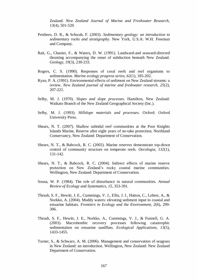
167
Zealand. New Zealand Journal of Marine and Freshwater Research,
13(4), 501-520.
Prothero, D. R., & Schwab, F. (2003). Sedimentary geology: an introduction to
sedimentary rocks and stratigraphy. New York, U.S.A: W.H. Freeman
and Company.
Rait, G., Chanier, F., & Waters, D. W. (1991). Landward-and seaward-directed
thrusting accompanying the onset of subduction beneath New Zealand.
Geology, 19(3), 230-233.
Rogers, C. S. (1990). Responses of coral reefs and reef organisms to
sedimentation. Marine ecology progress series, 62(1), 185-202.
Ryan, P. A. (1991). Environmental effects of sediment on New Zealand streams: a
review. New Zealand journal of marine and freshwater research, 25(2),
207-221.
Selby, M. J. (1970). Slopes and slope processes. Hamilton, New Zealand:
Waikato Branch of the New Zealand Geographical Society (Inc.).
Selby, M. J. (1993). Hillslope materials and processes. Oxford: Oxford
University Press.
Shears, N. T. (2007). Shallow subtidal reef communities at the Poor Knights
Islands Marine, Reserve after eight years of no-take protection. Northland
Conservancy, New Zealand: Department of Conservation.
Shears, N. T., & Babcock, R. C. (2002). Marine reserves demonstrate top-down
control of community structure on temperate reefs. Oecologia, 132(1),
131-142.
Shears, N. T., & Babcock, R. C. (2004). Indirect effects of marine reserve
protection on New Zealand’s rocky coastal marine communities.
Wellington, New Zealand: Department of Conservation.
Sousa, W. P. (1984). The role of disturbance in natural communities. Annual
Review of Ecology and Systematics, 15, 353-391.
Thrush, S. F., Hewitt, J. E., Cummings, V. J., Ellis, J. I., Hatton, C., Lohrer, A., &
Norkko, A. (2004). Muddy waters: elevating sediment input to coastal and
estuarine habitats. Frontiers in Ecology and the Environment, 2(6), 299-
306.
Thrush, S. F., Hewitt, J. E., Norkko, A., Cummings, V. J., & Funnell, G. A.
(2003). Macrobenthic recovery processes following catastrophic
sedimentation on estuarine sandflats. Ecological Applications, 13(5),
1433-1455.
Turner, S., & Schwarz, A. M. (2006). Management and conservation of seagrass
in New Zealand: an introduction. Wellington, New Zealand: New Zealand
Department of Conservation.
168
Varnes, D. J. (1978). Slope movement types and processes. In R. L. Schuster & R.
J. Krizek (Eds.), Special Report 176: Landslides: Analysis and Control
(pp. 11-33). Washington D. C.: Transportation and Road Research Board,
National Academy of Science.
Velde, B. (1992). Introduction to clay minerals: chemistry, origins, uses and
environmental significance. London: Chapman and Hall.
Vermaat, J. E., Agawin, N. S. R., Fortes, M., Uri, J., Duarte, C. M., Marba, N., . . .
Van Vierssen, W. (1997). The capacity of seagrasses to survive increased
turbidity and siltation: the significance of growth form and light use.
Ambio, 26, 499-504.
von Hochstetter, F. (1867). New Zealand: its physical geography, geology and
natural history: JG Cotta.

169
APPENDICIES
APPENDIX 1. GEOLOGICAL TIMESCALE
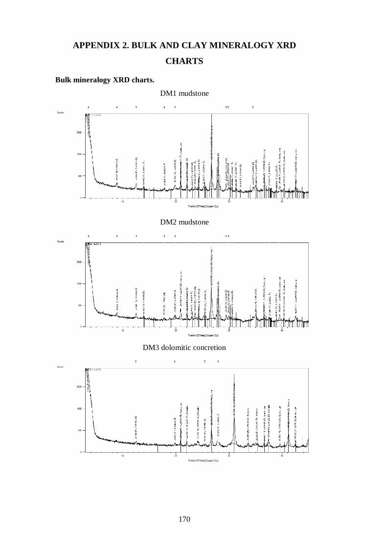
170
APPENDIX 2. BULK AND CLAY MINERALOGY XRD
CHARTS
Bulk mineralogy XRD charts.
DM1 mudstone
DM2 mudstone
DM3 dolomitic concretion
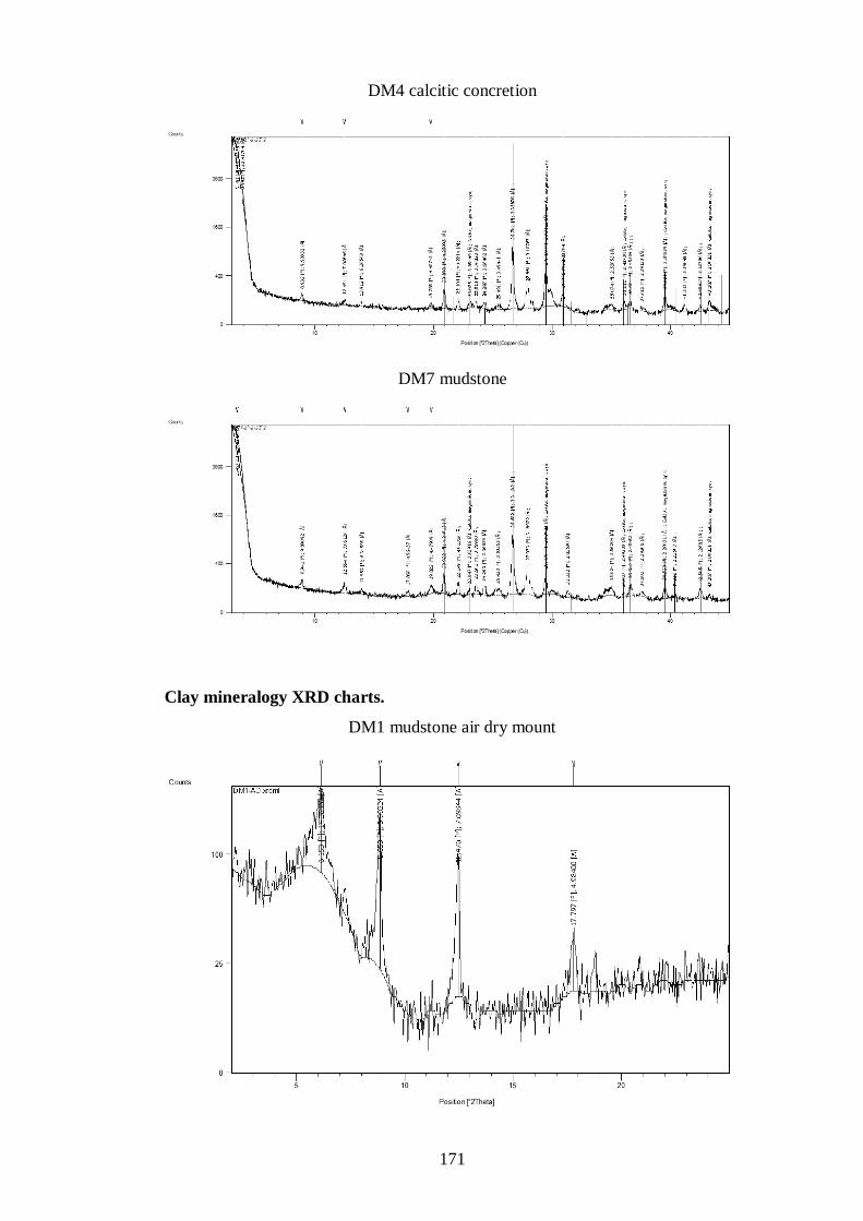
171
DM4 calcitic concretion
DM7 mudstone
Clay mineralogy XRD charts.
DM1 mudstone air dry mount
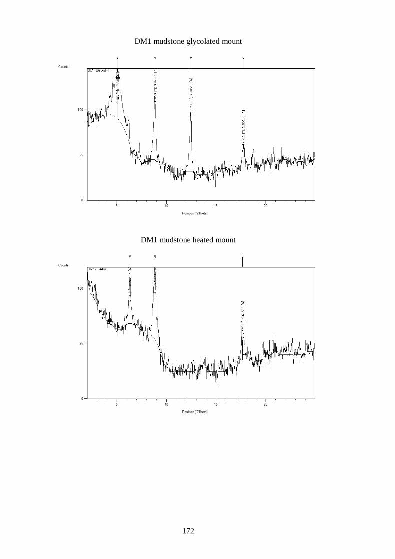
172
DM1 mudstone glycolated mount
DM1 mudstone heated mount
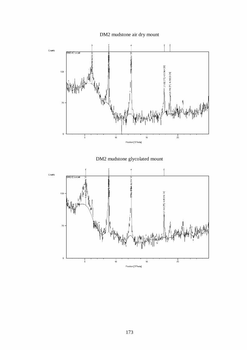
173
DM2 mudstone air dry mount
DM2 mudstone glycolated mount
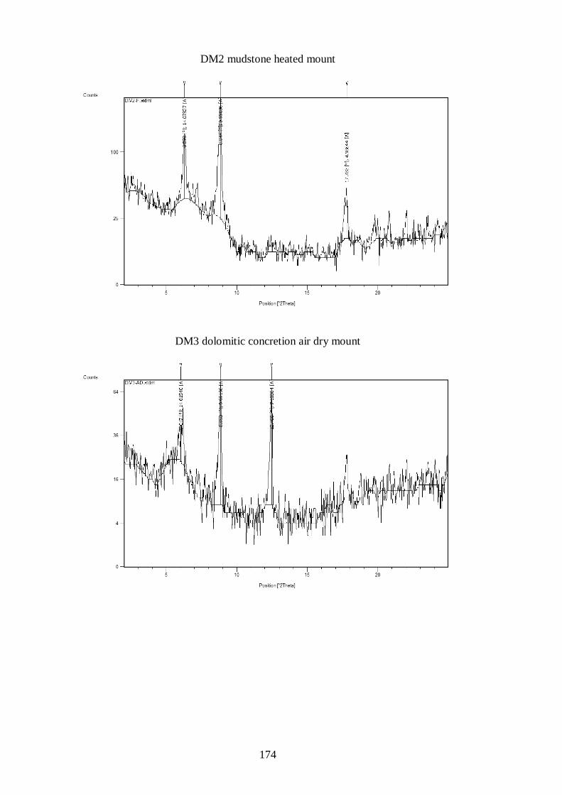
174
DM2 mudstone heated mount
DM3 dolomitic concretion air dry mount
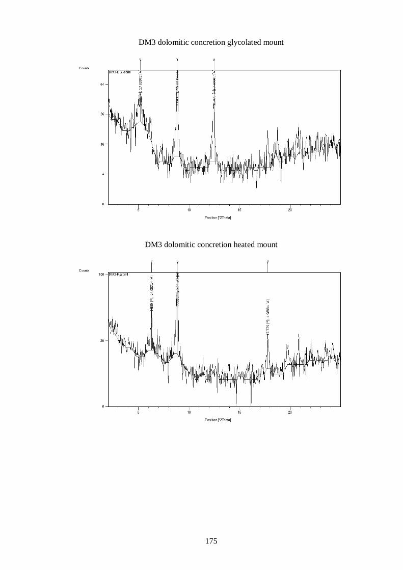
175
DM3 dolomitic concretion glycolated mount
DM3 dolomitic concretion heated mount
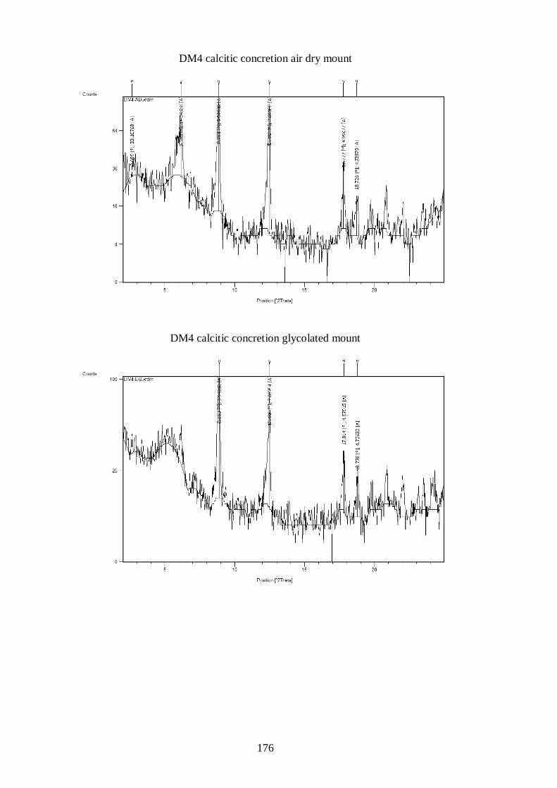
176
DM4 calcitic concretion air dry mount
DM4 calcitic concretion glycolated mount
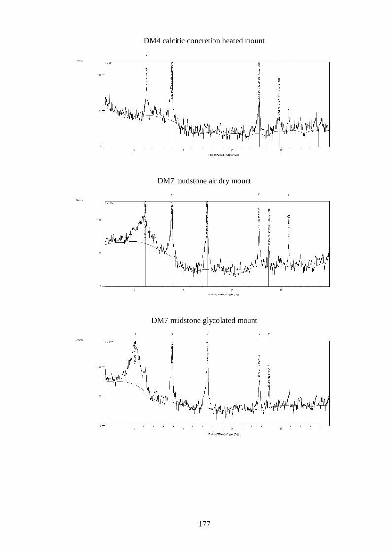
177
DM4 calcitic concretion heated mount
DM7 mudstone air dry mount
DM7 mudstone glycolated mount
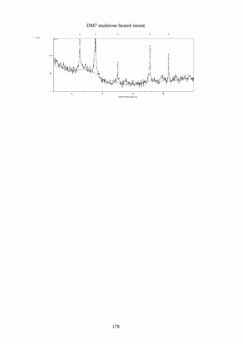
178
DM7 mudstone heated mount
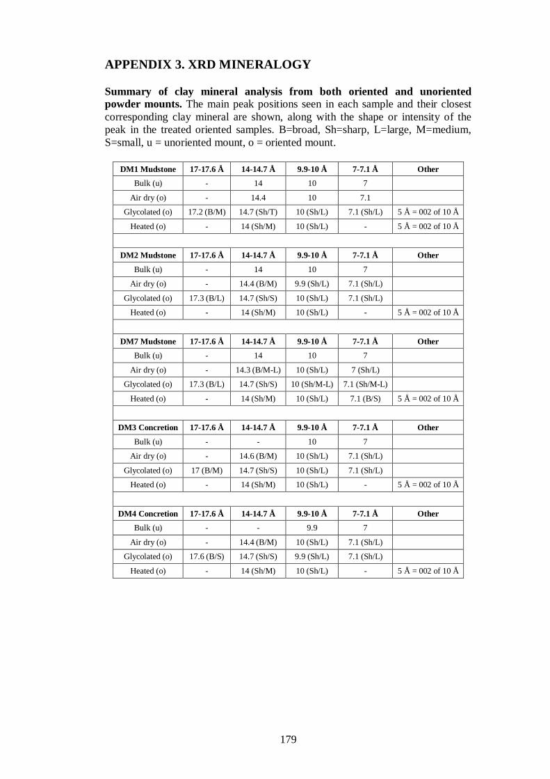
179
APPENDIX 3. XRD MINERALOGY
Summary of clay mineral analysis from both oriented and unoriented
powder mounts. The main peak positions seen in each sample and their closest
corresponding clay mineral are shown, along with the shape or intensity of the
peak in the treated oriented samples. B=broad, Sh=sharp, L=large, M=medium,
S=small, u = unoriented mount, o = oriented mount.
DM1 Mudstone 17-17.6 Å 14-14.7 Å 9.9-10 Å 7-7.1 Å Other
Bulk (u) - 14 10 7
Air dry (o) - 14.4 10 7.1
Glycolated (o) 17.2 (B/M) 14.7 (Sh/T) 10 (Sh/L) 7.1 (Sh/L) 5 Å = 002 of 10 Å
Heated (o) - 14 (Sh/M) 10 (Sh/L) - 5 Å = 002 of 10 Å
DM2 Mudstone 17-17.6 Å 14-14.7 Å 9.9-10 Å 7-7.1 Å Other
Bulk (u) - 14 10 7
Air dry (o) - 14.4 (B/M) 9.9 (Sh/L) 7.1 (Sh/L)
Glycolated (o) 17.3 (B/L) 14.7 (Sh/S) 10 (Sh/L) 7.1 (Sh/L)
Heated (o) - 14 (Sh/M) 10 (Sh/L) - 5 Å = 002 of 10 Å
DM7 Mudstone 17-17.6 Å 14-14.7 Å 9.9-10 Å 7-7.1 Å Other
Bulk (u) - 14 10 7
Air dry (o) - 14.3 (B/M-L) 10 (Sh/L) 7 (Sh/L)
Glycolated (o) 17.3 (B/L) 14.7 (Sh/S) 10 (Sh/M-L) 7.1 (Sh/M-L)
Heated (o) - 14 (Sh/M) 10 (Sh/L) 7.1 (B/S) 5 Å = 002 of 10 Å
DM3 Concretion 17-17.6 Å 14-14.7 Å 9.9-10 Å 7-7.1 Å Other
Bulk (u) - - 10 7
Air dry (o) - 14.6 (B/M) 10 (Sh/L) 7.1 (Sh/L)
Glycolated (o) 17 (B/M) 14.7 (Sh/S) 10 (Sh/L) 7.1 (Sh/L)
Heated (o) - 14 (Sh/M) 10 (Sh/L) - 5 Å = 002 of 10 Å
DM4 Concretion 17-17.6 Å 14-14.7 Å 9.9-10 Å 7-7.1 Å Other
Bulk (u) - - 9.9 7
Air dry (o) - 14.4 (B/M) 10 (Sh/L) 7.1 (Sh/L)
Glycolated (o) 17.6 (B/S) 14.7 (Sh/S) 9.9 (Sh/L) 7.1 (Sh/L)
Heated (o) - 14 (Sh/M) 10 (Sh/L) - 5 Å = 002 of 10 Å
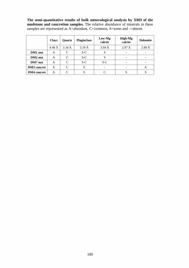
180
The semi-quantitative results of bulk mineralogical analysis by XRD of the
mudstone and concretion samples. The relative abundance of minerals in these
samples are represented as A=abundant, C=common, S=some and -=absent.
Clays Quartz Plagioclase
Low-Mg
calcite
High-Mg
calcite Dolomite
4.48 Å 3.34 Å 3.19 Å 3.04 Å 2.97 Å 2.89 Å
DM1 mst A C S-C S - -
DM2 mst A C S-C S - -
DM7 mst A C S-C S-C - -
DM3 concret A C S - - A
DM4 concret A C S C S S

181
APPENDIX 4. XRF GEOCHEMISTRY
Major element results. Results are in weight percent of the sample. Totals do not
equal 100 due to H2O(OH) loss in clay and CO2 loss in carbonate. * Fe2O3 is total
Fe and includes FeO.
Element DM1 DM2 DM7 DM3 DM4
SiO2 63.25 57.95 61.14 27.51 34.90
TiO2 0.68 0.57 0.67 0.28 0.37
Al2O3 15.87 14.09 15.29 7.64 9.01
Fe2O3* 5.62 4.64 5.44 3.43 3.79
MnO 0.07 0.06 0.07 0.07 0.11
MgO 3.15 3.04 3.08 16.49 6.07
CaO 4.36 2.30 5.90 19.15 23.65
Na2O 2.36 7.43 2.30 0.35 0.34
K2O 2.89 2.59 2.74 1.35 1.49
P2O5 0.17 0.14 0.17 0.17 0.32
Total 98.41 93.48 96.80 76.45 80.04
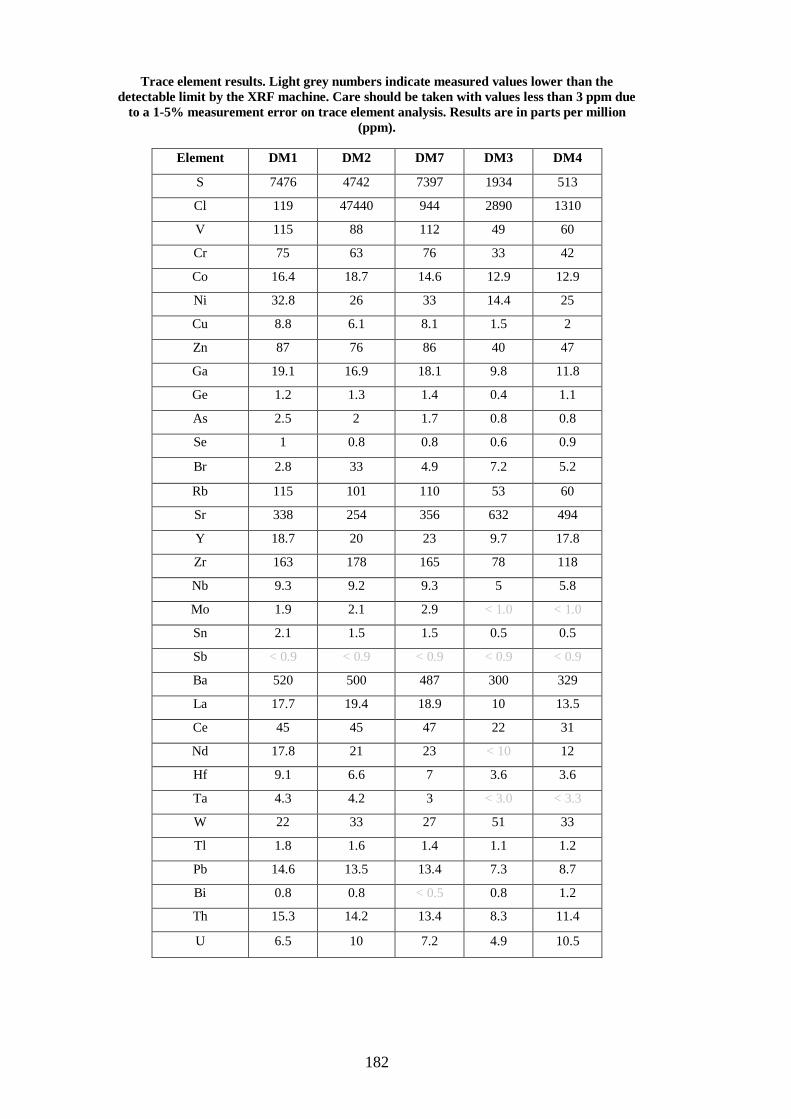
182
Trace element results. Light grey numbers indicate measured values lower than the
detectable limit by the XRF machine. Care should be taken with values less than 3 ppm due
to a 1-5% measurement error on trace element analysis. Results are in parts per million
(ppm).
Element DM1 DM2 DM7 DM3 DM4
S 7476 4742 7397 1934 513
Cl 119 47440 944 2890 1310
V 115 88 112 49 60
Cr 75 63 76 33 42
Co 16.4 18.7 14.6 12.9 12.9
Ni 32.8 26 33 14.4 25
Cu 8.8 6.1 8.1 1.5 2
Zn 87 76 86 40 47
Ga 19.1 16.9 18.1 9.8 11.8
Ge 1.2 1.3 1.4 0.4 1.1
As 2.5 2 1.7 0.8 0.8
Se 1 0.8 0.8 0.6 0.9
Br 2.8 33 4.9 7.2 5.2
Rb 115 101 110 53 60
Sr 338 254 356 632 494
Y 18.7 20 23 9.7 17.8
Zr 163 178 165 78 118
Nb 9.3 9.2 9.3 5 5.8
Mo 1.9 2.1 2.9 < 1.0 < 1.0
Sn 2.1 1.5 1.5 0.5 0.5
Sb < 0.9 < 0.9 < 0.9 < 0.9 < 0.9
Ba 520 500 487 300 329
La 17.7 19.4 18.9 10 13.5
Ce 45 45 47 22 31
Nd 17.8 21 23 < 10 12
Hf 9.1 6.6 7 3.6 3.6
Ta 4.3 4.2 3 < 3.0 < 3.3
W 22 33 27 51 33
Tl 1.8 1.6 1.4 1.1 1.2
Pb 14.6 13.5 13.4 7.3 8.7
Bi 0.8 0.8 < 0.5 0.8 1.2
Th 15.3 14.2 13.4 8.3 11.4
U 6.5 10 7.2 4.9 10.5
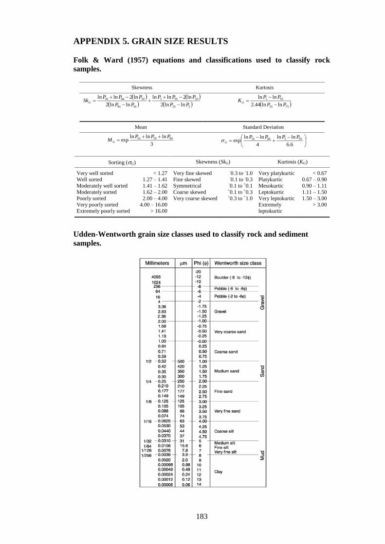
183
APPENDIX 5. GRAIN SIZE RESULTS
Folk & Ward (1957) equations and classifications used to classify rock
samples.
Udden-Wentworth grain size classes used to classify rock and sediment
samples.
Skewness Kurtosis
525
50955
1684
508416
lnln2
ln2lnln
lnln2
ln2lnln
PP
PPP
PP
PPPSkG
7525
955
lnln44.2
lnln
PP
PPKG
Mean Standard Deviation
3
lnlnlnexp 845016 PPP
MG
6.6
lnln
4
lnlnexp 9558416 PPPP
G
Sorting (G) Skewness (SkG) Kurtosis (KG)
Very well sorted
Well sorted
Moderately well sorted
Moderately sorted
Poorly sorted
Very poorly sorted
Extremely poorly sorted
< 1.27
1.27 – 1.41
1.41 – 1.62
1.62 – 2.00
2.00 – 4.00
4.00 – 16.00
> 16.00
Very fine skewed
Fine skewed
Symmetrical
Coarse skewed
Very coarse skewed
-0.3 to -1.0 -0.1 to -0.3
-0.1 to +0.1 +0.1 to +0.3 +0.3 to +1.0
Very platykurtic
Platykurtic
Mesokurtic
Leptokurtic
Very leptokurtic
Extremely
leptokurtic
< 0.67
0.67 – 0.90
0.90 – 1.11
1.11 – 1.50
1.50 – 3.00
> 3.00
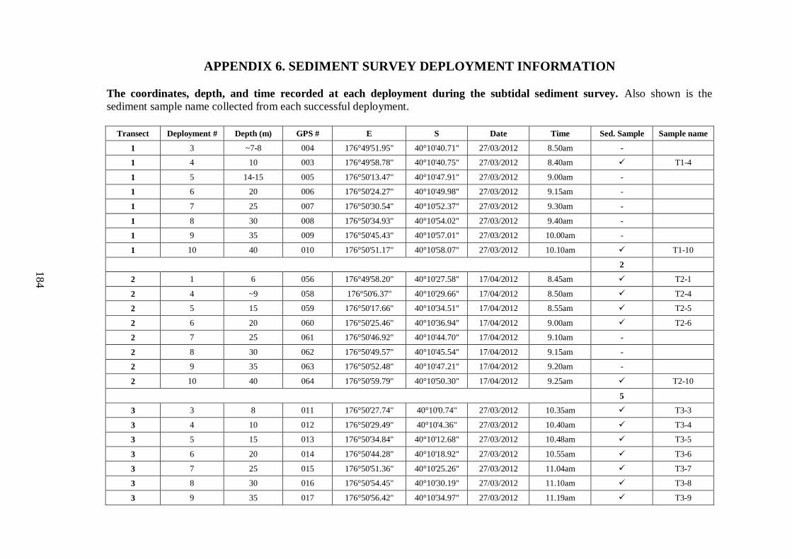
184
APPENDIX 6. SEDIMENT SURVEY DEPLOYMENT INFORMATION
The coordinates, depth, and time recorded at each deployment during the subtidal sediment survey. Also shown is the
sediment sample name collected from each successful deployment.
Transect Deployment # Depth (m) GPS # E S Date Time Sed. Sample Sample name
1 3 ~7-8 004 176°49'51.95" 40°10'40.71" 27/03/2012 8.50am -
1 4 10 003 176°49'58.78" 40°10'40.75" 27/03/2012 8.40am T1-4
1 5 14-15 005 176°50'13.47" 40°10'47.91" 27/03/2012 9.00am -
1 6 20 006 176°50'24.27" 40°10'49.98" 27/03/2012 9.15am -
1 7 25 007 176°50'30.54" 40°10'52.37" 27/03/2012 9.30am -
1 8 30 008 176°50'34.93" 40°10'54.02" 27/03/2012 9.40am -
1 9 35 009 176°50'45.43" 40°10'57.01" 27/03/2012 10.00am -
1 10 40 010 176°50'51.17" 40°10'58.07" 27/03/2012 10.10am T1-10
2
2 1 6 056 176°49'58.20" 40°10'27.58" 17/04/2012 8.45am T2-1
2 4 ~9 058 176°50'6.37" 40°10'29.66" 17/04/2012 8.50am T2-4
2 5 15 059 176°50'17.66" 40°10'34.51" 17/04/2012 8.55am T2-5
2 6 20 060 176°50'25.46" 40°10'36.94" 17/04/2012 9.00am T2-6
2 7 25 061 176°50'46.92" 40°10'44.70" 17/04/2012 9.10am -
2 8 30 062 176°50'49.57" 40°10'45.54" 17/04/2012 9.15am -
2 9 35 063 176°50'52.48" 40°10'47.21" 17/04/2012 9.20am -
2 10 40 064 176°50'59.79" 40°10'50.30" 17/04/2012 9.25am T2-10
5
3 3 8 011 176°50'27.74" 40°10'0.74" 27/03/2012 10.35am T3-3
3 4 10 012 176°50'29.49" 40°10'4.36" 27/03/2012 10.40am T3-4
3 5 15 013 176°50'34.84" 40°10'12.68" 27/03/2012 10.48am T3-5
3 6 20 014 176°50'44.28" 40°10'18.92" 27/03/2012 10.55am T3-6
3 7 25 015 176°50'51.36" 40°10'25.26" 27/03/2012 11.04am T3-7
3 8 30 016 176°50'54.45" 40°10'30.19" 27/03/2012 11.10am T3-8
3 9 35 017 176°50'56.42" 40°10'34.97" 27/03/2012 11.19am T3-9
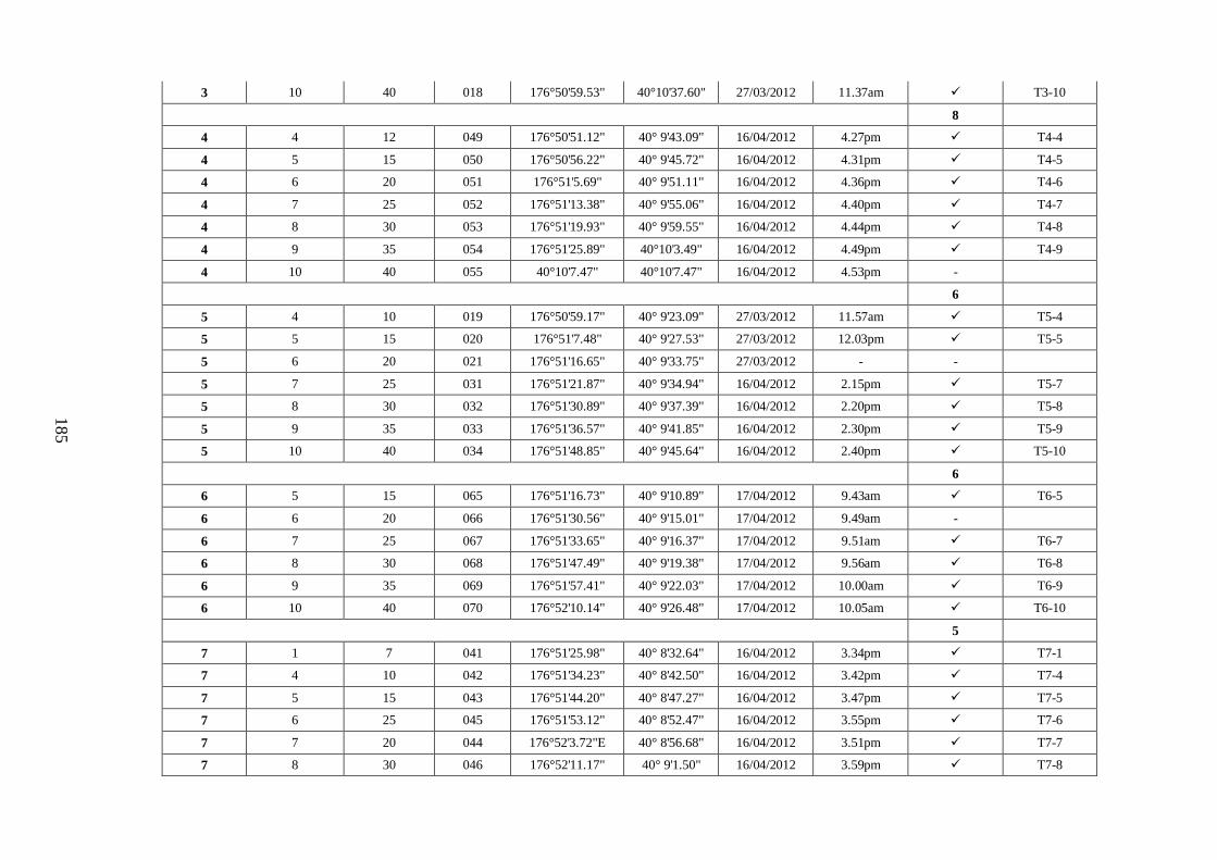
185
3 10 40 018 176°50'59.53" 40°10'37.60" 27/03/2012 11.37am T3-10
8
4 4 12 049 176°50'51.12" 40° 9'43.09" 16/04/2012 4.27pm T4-4
4 5 15 050 176°50'56.22" 40° 9'45.72" 16/04/2012 4.31pm T4-5
4 6 20 051 176°51'5.69" 40° 9'51.11" 16/04/2012 4.36pm T4-6
4 7 25 052 176°51'13.38" 40° 9'55.06" 16/04/2012 4.40pm T4-7
4 8 30 053 176°51'19.93" 40° 9'59.55" 16/04/2012 4.44pm T4-8
4 9 35 054 176°51'25.89" 40°10'3.49" 16/04/2012 4.49pm T4-9
4 10 40 055 40°10'7.47" 40°10'7.47" 16/04/2012 4.53pm -
6
5 4 10 019 176°50'59.17" 40° 9'23.09" 27/03/2012 11.57am T5-4
5 5 15 020 176°51'7.48" 40° 9'27.53" 27/03/2012 12.03pm T5-5
5 6 20 021 176°51'16.65" 40° 9'33.75" 27/03/2012 - -
5 7 25 031 176°51'21.87" 40° 9'34.94" 16/04/2012 2.15pm T5-7
5 8 30 032 176°51'30.89" 40° 9'37.39" 16/04/2012 2.20pm T5-8
5 9 35 033 176°51'36.57" 40° 9'41.85" 16/04/2012 2.30pm T5-9
5 10 40 034 176°51'48.85" 40° 9'45.64" 16/04/2012 2.40pm T5-10
6
6 5 15 065 176°51'16.73" 40° 9'10.89" 17/04/2012 9.43am T6-5
6 6 20 066 176°51'30.56" 40° 9'15.01" 17/04/2012 9.49am -
6 7 25 067 176°51'33.65" 40° 9'16.37" 17/04/2012 9.51am T6-7
6 8 30 068 176°51'47.49" 40° 9'19.38" 17/04/2012 9.56am T6-8
6 9 35 069 176°51'57.41" 40° 9'22.03" 17/04/2012 10.00am T6-9
6 10 40 070 176°52'10.14" 40° 9'26.48" 17/04/2012 10.05am T6-10
5
7 1 7 041 176°51'25.98" 40° 8'32.64" 16/04/2012 3.34pm T7-1
7 4 10 042 176°51'34.23" 40° 8'42.50" 16/04/2012 3.42pm T7-4
7 5 15 043 176°51'44.20" 40° 8'47.27" 16/04/2012 3.47pm T7-5
7 6 25 045 176°51'53.12" 40° 8'52.47" 16/04/2012 3.55pm T7-6
7 7 20 044 176°52'3.72"E 40° 8'56.68" 16/04/2012 3.51pm T7-7
7 8 30 046 176°52'11.17" 40° 9'1.50" 16/04/2012 3.59pm T7-8
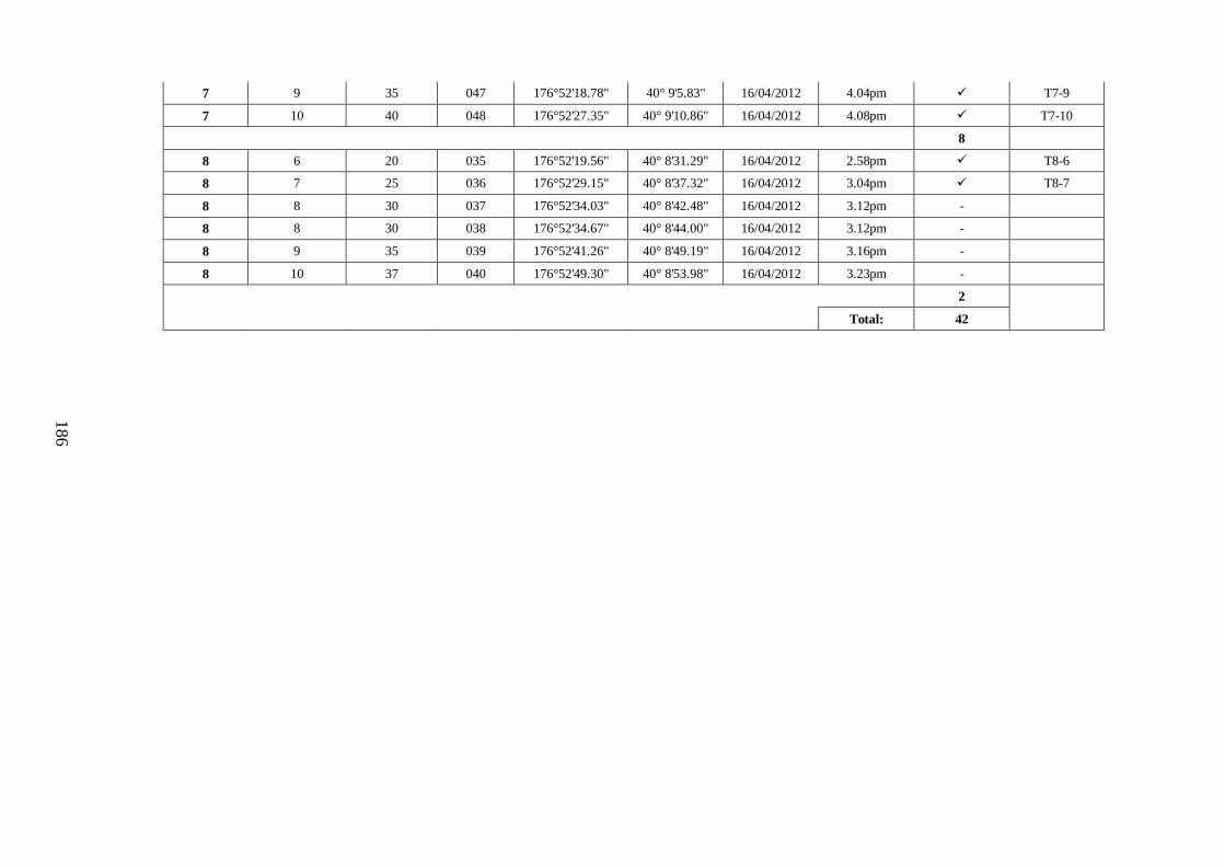
186
7 9 35 047 176°52'18.78" 40° 9'5.83" 16/04/2012 4.04pm T7-9
7 10 40 048 176°52'27.35" 40° 9'10.86" 16/04/2012 4.08pm T7-10
8
8 6 20 035 176°52'19.56" 40° 8'31.29" 16/04/2012 2.58pm T8-6
8 7 25 036 176°52'29.15" 40° 8'37.32" 16/04/2012 3.04pm T8-7
8 8 30 037 176°52'34.03" 40° 8'42.48" 16/04/2012 3.12pm -
8 8 30 038 176°52'34.67" 40° 8'44.00" 16/04/2012 3.12pm -
8 9 35 039 176°52'41.26" 40° 8'49.19" 16/04/2012 3.16pm -
8 10 37 040 176°52'49.30" 40° 8'53.98" 16/04/2012 3.23pm -
2
Total: 42
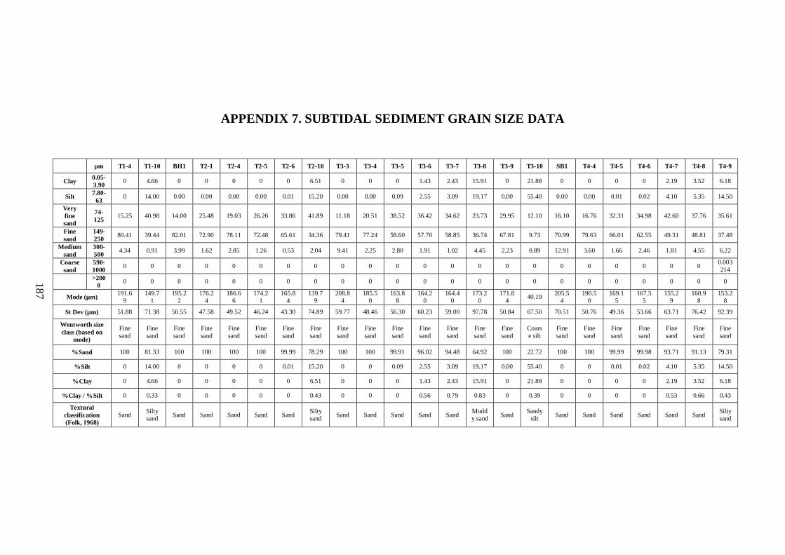
187
APPENDIX 7. SUBTIDAL SEDIMENT GRAIN SIZE DATA
µm T1-4 T1-10 BH1 T2-1 T2-4 T2-5 T2-6 T2-10 T3-3 T3-4 T3-5 T3-6 T3-7 T3-8 T3-9 T3-10 SB1 T4-4 T4-5 T4-6 T4-7 T4-8 T4-9
Clay 0.05-
3.90 0 4.66 0 0 0 0 0 6.51 0 0 0 1.43 2.43 15.91 0 21.88 0 0 0 0 2.19 3.52 6.18
Silt 7.80-
63 0 14.00 0.00 0.00 0.00 0.00 0.01 15.20 0.00 0.00 0.09 2.55 3.09 19.17 0.00 55.40 0.00 0.00 0.01 0.02 4.10 5.35 14.50
Very
fine
sand
74-
125 15.25 40.98 14.00 25.48 19.03 26.26 33.86 41.89 11.18 20.51 38.52 36.42 34.62 23.73 29.95 12.10 16.10 16.76 32.31 34.98 42.60 37.76 35.61
Fine
sand
149-
250 80.41 39.44 82.01 72.90 78.11 72.48 65.61 34.36 79.41 77.24 58.60 57.70 58.85 36.74 67.81 9.73 70.99 79.63 66.01 62.55 49.31 48.81 37.48
Medium
sand
300-
500 4.34 0.91 3.99 1.62 2.85 1.26 0.53 2.04 9.41 2.25 2.80 1.91 1.02 4.45 2.23 0.89 12.91 3.60 1.66 2.46 1.81 4.55 6.22
Coarse
sand
590-
1000 0 0 0 0 0 0 0 0 0 0 0 0 0 0 0 0 0 0 0 0 0 0
0.003
214
>200
0 0 0 0 0 0 0 0 0 0 0 0 0 0 0 0 0 0 0 0 0 0 0 0
Mode (µm) 191.6
9
149.7
1
195.2
2
176.2
4
186.6
6
174.2
1
165.8
4
139.7
9
208.8
4
185.5
0
163.8
8
164.2
0
164.4
0
173.2
0
171.8
4 40.19
205.5
4
190.5
0
169.1
5
167.5
5
155.2
9
160.9
8
153.2
8
St Dev (µm) 51.88 71.38 50.55 47.58 49.52 46.24 43.30 74.89 59.77 48.46 56.30 60.23 59.00 97.78 50.84 67.50 70.51 50.76 49.36 53.66 63.71 76.42 92.39
Wentworth size
class (based on
mode)
Fine
sand
Fine
sand
Fine
sand
Fine
sand
Fine
sand
Fine
sand
Fine
sand
Fine
sand
Fine
sand
Fine
sand
Fine
sand
Fine
sand
Fine
sand
Fine
sand
Fine
sand
Coars
e silt
Fine
sand
Fine
sand
Fine
sand
Fine
sand
Fine
sand
Fine
sand
Fine
sand
%Sand 100 81.33 100 100 100 100 99.99 78.29 100 100 99.91 96.02 94.48 64.92 100 22.72 100 100 99.99 99.98 93.71 91.13 79.31
%Silt 0 14.00 0 0 0 0 0.01 15.20 0 0 0.09 2.55 3.09 19.17 0.00 55.40 0 0 0.01 0.02 4.10 5.35 14.50
%Clay 0 4.66 0 0 0 0 0 6.51 0 0 0 1.43 2.43 15.91 0 21.88 0 0 0 0 2.19 3.52 6.18
%Clay / %Silt 0 0.33 0 0 0 0 0 0.43 0 0 0 0.56 0.79 0.83 0 0.39 0 0 0 0 0.53 0.66 0.43
Textural
classification
(Folk, 1968)
Sand Silty
sand Sand Sand Sand Sand Sand
Silty
sand Sand Sand Sand Sand Sand
Mudd
y sand Sand
Sandy
silt Sand Sand Sand Sand Sand Sand
Silty
sand
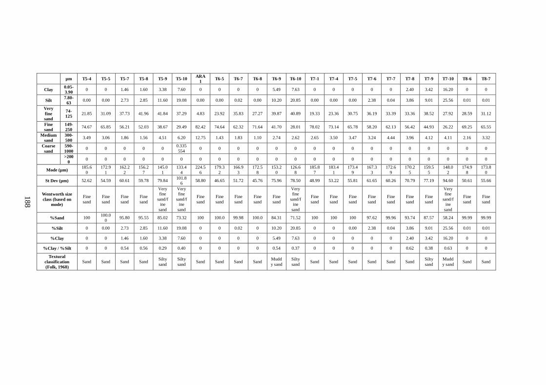
188
µm T5-4 T5-5 T5-7 T5-8 T5-9 T5-10 ARA
1 T6-5 T6-7 T6-8 T6-9 T6-10 T7-1 T7-4 T7-5 T7-6 T7-7 T7-8 T7-9 T7-10 T8-6 T8-7
Clay
0.05-
3.90 0 0 1.46 1.60 3.38 7.60 0 0 0 0 5.49 7.63 0 0 0 0 0 2.40 3.42 16.20 0 0
Silt
7.80-
63 0.00 0.00 2.73 2.85 11.60 19.08 0.00 0.00 0.02 0.00 10.20 20.85 0.00 0.00 0.00 2.38 0.04 3.86 9.01 25.56 0.01 0.01
Very
fine
sand
74-
125 21.85 31.09 37.73 41.96 41.84 37.29 4.83 23.92 35.83 27.27 39.87 40.89 19.33 23.36 30.75 36.19 33.39 33.36 38.52 27.92 28.59 31.12
Fine
sand
149-
250 74.67 65.85 56.21 52.03 38.67 29.49 82.42 74.64 62.32 71.64 41.70 28.01 78.02 73.14 65.78 58.20 62.13 56.42 44.93 26.22 69.25 65.55
Medium
sand
300-
500 3.49 3.06 1.86 1.56 4.51 6.20 12.75 1.43 1.83 1.10 2.74 2.62 2.65 3.50 3.47 3.24 4.44 3.96 4.12 4.11 2.16 3.32
Coarse
sand
590-
1000 0 0 0 0 0
0.335
554 0 0 0 0 0 0 0 0 0 0 0 0 0 0 0 0
>200
0 0 0 0 0 0 0 0 0 0 0 0 0 0 0 0 0 0 0 0 0 0 0
Mode (µm)
185.6
0
172.9
1
162.2
2
156.2
7
145.0
1
133.4
4
224.5
6
179.3
2
166.9
3
172.5
8
153.2
0
126.6
8
185.8
7
183.4
1
173.4
9
167.3
3
172.6
9
170.2
5
159.5
5
148.0
2
174.9
8
173.8
0
St Dev (µm) 52.62 54.59 60.61 59.78 79.84
101.8
6 58.80 46.65 51.72 45.76 75.96 78.50 48.99 53.22 55.81 61.65 60.26 70.79 77.19 94.60 50.61 55.66
Wentworth size
class (based on
mode)
Fine
sand
Fine
sand
Fine
sand
Fine
sand
Very
fine
sand/f
ine
sand
Very
fine
sand/f
ine
sand
Fine
sand
Fine
sand
Fine
sand
Fine
sand
Fine
sand
Very
fine
sand/f
ine
sand
Fine
sand
Fine
sand
Fine
sand
Fine
sand
Fine
sand
Fine
sand
Fine
sand
Very
fine
sand/f
ine
sand
Fine
sand
Fine
sand
%Sand 100
100.0
0 95.80 95.55 85.02 73.32 100 100.0 99.98 100.0 84.31 71.52 100 100 100 97.62 99.96 93.74 87.57 58.24 99.99 99.99
%Silt 0 0.00 2.73 2.85 11.60 19.08 0 0 0.02 0 10.20 20.85 0 0 0.00 2.38 0.04 3.86 9.01 25.56 0.01 0.01
%Clay 0 0 1.46 1.60 3.38 7.60 0 0 0 0 5.49 7.63 0 0 0 0 0 2.40 3.42 16.20 0 0
%Clay / %Silt 0 0 0.54 0.56 0.29 0.40 0 0 0 0 0.54 0.37 0 0 0 0 0 0.62 0.38 0.63 0 0
Textural
classification
(Folk, 1968)
Sand Sand Sand Sand Silty
sand
Silty
sand Sand Sand Sand Sand
Mudd
y sand
Silty
sand Sand Sand Sand Sand Sand Sand
Silty
sand
Mudd
y sand Sand Sand