Effects of atmospheric conditions on surface diffuse degassing

Effects of atmospheric conditions on surface diffuse degassing

A. P. Rinaldi,1,2 J. Vandemeulebrouck,3 M. Todesco,1 and F. Viveiros4

Received 30 May 2012; revised 18 September 2012; accepted 20 September 2012; published 7 November 2012.

[1] Diffuse degassing through the soil is commonly observed in volcanic areas andmonitoring of carbon dioxide flux at the surface can provide a safe and effective wayto infer the state of activity of the volcanic system. Continuous measurement stations areoften installed on active volcanoes such as Furnas (Azores archipelago), which featureslow temperature fumaroles, hot and cold CO2 rich springs, and several diffuse degassingareas. As in other volcanoes, fluxes measured at Furnas are often correlated withenvironmental variables, such as air temperature or barometric pressure, with daily andseasonal cycles that become more evident when gas emission is low. In this work, we studyhow changes in air temperature and barometric pressure may affect the gas emissionthrough the soil. The TOUGH2 geothermal simulator was used to simulate the gaspropagation through the soil as a function of fluctuating atmospheric conditions. Then,a dual parameters study was performed to assess how the rock permeability and the gassource properties affect the resulting fluxes. Numerical results are in good agreement withthe observed data at Furnas, and show that atmospheric variables may cause the observeddaily cycles in CO2 fluxes. The observed changes depend on soil permeability and onthe pressure driving the upward flux.

Citation: Rinaldi, A. P., J. Vandemeulebrouck, M. Todesco, and F. Viveiros (2012), Effects of atmospheric conditions onsurface diffuse degassing, J. Geophys. Res., 117, B11201, doi:10.1029/2012JB009490.

1. Introduction

[2] Continuous measurements of carbon dioxide flux arenow commonly used to monitor the degassing in volcanicenvironments [Chiodini et al., 1998, 2010; Hernández et al.,2001]. The transfer of the CO2 to the surface results fromtwo different physical processes, namely advection anddiffusion [e.g., Werner et al., 2000]. Advective transport ismainly induced by pressure gradient, and by temperaturegradients that create density differences. Diffusion, onthe other hand, is controlled by concentration gradients. Forboth advection and diffusion processes, the flux dependson the properties of the gas source, on the petrophysicalproperties of the soil (e.g., permeability) and on the condi-tions at the surface (e.g., vegetation cover, topographiceffects, drainage) [e.g., Granieri et al., 2003; Lewicki et al.,2007; Viveiros et al., 2008].[3] The impact of environmental variables on soil gas

emissions has been studied in several degassing areas in the

last decades [e.g., Clements and Wilkening, 1974; Reimer,1980; Klusman and Webster, 1981; Hinkle, 1990, 1994;Chiodini et al., 1998; McGee and Gerlach, 1998; McGeeet al., 2000; Rogie et al., 2001; Granieri et al., 2003,2010; Hernández et al., 2004; Lewicki et al., 2007; Viveiroset al., 2008, 2009; Cigolini et al., 2009]. However, very fewpapers were found in the literature that analyzed diurnalvariations for the soil CO2 flux in hydrothermal environ-ments. Chiodini et al. [1998] noticed that CO2 flux varia-tions at Vulcano (Aeolian Islands, Italy) were affected bybarometric pressure changes rather than by absolute atmo-spheric pressure value. Granieri et al. [2003] identified a24 h cycle in CO2 fluxes from Solfatara volcano between1998–2002, and Padrón et al. [2008] recognized diurnal andsemidiurnal fluctuations in the gas flux acquired during 2004in a station located at El Hierro (Canary Islands). Still inCanary Islands,Hernández et al. [2012] recognized 24 h cyclesin the soil CO2 flux time series registered in a permanentstation located in the island of Lanzarote. On the other side,diurnal and seasonal variations of CO2 flux derived from soilrespiration (biogenic origin) have been intensely studied asCO2 production is dependent on the temperature and the CO2

oscillations are positively correlated with the air/soil tem-perature changes [Witkamp, 1969; Bajracharya et al., 2000;Nakadai et al., 2002], as well as with the wind speed [Takleet al., 2004; Reicosky et al., 2008; Bowling and Massman,2011]. Biogenic fluxes are also influenced by atmosphericpressure [Massman, 2004]. These papers recorded the cor-relation but did not investigate the processes that cause andexplain the observed trends.

1Istituto Nazionale di Geofisica e Vulcanologia, Bologna, Italy.2Earth Sciences Division, Lawrence Berkeley National Laboratory,

Berkeley, California, USA.3ISTerre, CNRS, Université de Savoie, Chambery, France.4Centro de Vulcanologia e Avaliação de Riscos Geológicos, Universidade

dos Açores, Ponta Delgada, Portugal.

Corresponding author: A. P. Rinaldi, Earth Sciences Division,Lawrence Berkeley National Laboratory, 1 Cyclotron Rd., Berkeley,CA 94720, USA. ([email protected])

©2012. American Geophysical Union. All Rights Reserved.0148-0227/12/2012JB009490

JOURNAL OF GEOPHYSICAL RESEARCH, VOL. 117, B11201, doi:10.1029/2012JB009490, 2012

B11201 1 of 14

[4] Some studies have also recognized periodicities on222Rn concentration time series in the air [e.g., Rigby andLa Pointe, 1993; Pinault and Baubron, 1997; Robinsonet al., 1997; Groves-Kirkby et al., 2006; Steinitz et al.,2007; Richon et al., 2009] and in the soil [Aumento, 2002;Richon et al., 2003, 2011;Cigolini et al., 2009]. For example,Clements and Wilkening [1974] observed that pressurevariations of 1%–2% change the radon flux from 20%to 60%.[5] In this paper, we aim at modeling how the periodic

variations of air temperature and pressure at the soil surfacecan affect the CO2 flux signals by producing harmonicvariations at the same periods. A second goal is to understandif the monitoring of the periodic flux variations could beused to detect source or medium properties changes. Ourmodel will be tested on CO2 flux signal recorded at Furnasvolcano (Azores, Portugal). This work intends to understandthe influence of atmospheric and soil conditions on the gasrelease, by performing several simulations with TOUGH2geothermal simulator [Pruess et al., 1999]. Although sucha simulator is largely used in non-volcanological contests[e.g., Oldenburg and Rinaldi, 2011; Borgia et al., 2012;Mazzoldi et al., 2012], applications in volcanology arebecoming more common for the study of diffuse degassing[e.g., Todesco et al., 2010; Chiodini et al., 2010] and ofthe geophysical and geochemical signals related to hydro-thermal fluids circulation [e.g., Hutnak et al., 2009; Rinaldiet al., 2010, 2011]. We used the TOUGH2/EOS2 moduleto describe CO2 in gas phase fluid. Using a 1-D model, aparametric study was performed to understand the physicalmechanisms producing the observed variations. Numericalresults, in agreement with the observed data, show that theCO2 fluxes are strongly dependent on reservoir pressure,

temperature and pressure changes applied at the surface,and on domain permeability.

2. A Case Study: Influence of AtmosphericConditions on the CO2 Degassingat Furnas Volcano

[6] Secondary manifestations of volcanism in the Azoresarchipelago (Figure 1) include low temperature fumaroles(maximum temperature around 100�C), hot and cold CO2-richsprings, and several diffuse degassing areas. Continuousmonitoring of hydrothermal soil CO2 flux begun on Furnasvolcano, S. Miguel island, in October 2001, with the installa-tion of a permanent gas station that incorporates severalmeteorological sensors. Daily and seasonal cycles have beenobserved in the time series of soil CO2 flux and are coinci-dent with the periodical behavior of some meteorologicalparameters. Statistical analysis applied to the recorded timeseries shows that air temperature, barometric pressure, rainfall,and wind speed are the observables that better correlate withthe soil CO2 flux variations [Viveiros et al., 2008, 2009].These external parameters may also have a different effect onthe gas flux depending on the characteristics of the monitoringsite such as the physical properties of the soil, the topographyand the drainage area [e.g., Granieri et al., 2003; Viveiroset al., 2008, 2010].[7] Two permanent soil CO2 flux monitoring stations are

presently installed inside Furnas volcano caldera (S. MiguelIsland, Azores archipelago) (Figure 1). GFUR1 station,which was running between October 2001 and July 2006,was placed in a garden of the Furnas thermal baths, close toFurnas village fumarolic field. Average values measured ofCO2 flux were �260 g m�2 d�1 and soil temperature was

Figure 1. (a) Azores archipelago location highlighting S. Miguel Island, (b) digital elevation model ofthe S. Miguel Island, and (c) hydrothermal manifestations and location of the permanent soil CO2 stationsat Furnas volcano. Steam vents are mostly water vapor emission. Fumarole refers to emission stronglycharacterized by hydrothermal-volcanic gases.

RINALDI ET AL.: ATMOSPHERIC CONDITIONS AND DIFFUSE DEGASSING B11201B11201

2 of 14

about 17�C. The station was reinstalled (and renamed asGFUR3) in January 2008 closer to Furnas village mainfumaroles, in a thermally anomalous zone where the averagesoil temperature is 38�C at 30 cm depth, with a soil CO2 flux�650 g m�2 d�1. A soil CO2 flux station (named GFUR2)was also installed inside Furnas caldera in the vicinity ofFurnas Lake fumarolic ground in October 2004, wheresoil CO2 flux values around 350 g m�2 d�1 were measured.Average soil temperature at this site during the entiremonitored period (Jan 2005–June 2009) is �22�C at 30 cmof depth, with a temperature gradient of about 3�C m�1.According to Viveiros et al. [2010], the stations are allinstalled in diffuse degassing structures (DDS) that are fedby the hydrothermal sources.[8] The permanent flux stations perform measurements

based on the accumulation chamber method [Chiodini et al.,1998]. Every hour, a chamber is lowered on the ground andthe gas released at the ground surface is pumped into aninfrared gas analyzer (IRGA).[9] The soil CO2 flux value is computed as the linear best

fit of the flux curve during a predefined period of time.Measurements have a reproducibility within 10% for theCO2 range between 10 and 20000 g m�2 d�1 [Chiodiniet al., 1998]. The gas flux automatic stations are equippedwith meteorological sensors that acquire simultaneously thebarometric pressure, air temperature, air relative humidity,wind speed and direction, rainfall, soil water content andsoil temperature.[10] In the following subsection, we will present some of

the data recorded at Furnas. The main goal of the paper is tounderstand the effects of atmospheric perturbations on CO2

degassing. In order to have a good, reliable base case, wechoose to use some an example of data recorded at Furnas,where a good correlation between atmospheric variables anddegassing has generally been observed. Similar results for

spectral analysis can be retrieved from GFUR1 and GFUR3,and inclusion here of those data would be only redundant.

2.1. Acquired Data and Spectral Analysis Appliedto CO2 Flux Series

[11] We choose to analyze data registered at stationGFUR2 during the summers of the whole period (2005–2009, from May to September), since, in that period ofthe year, average monthly rainfall is low, and thus rainfalleffects on degassing can be considered as negligible. Inaddition, GFUR2 is the monitoring site with the longest recordat Furnas volcano. Soil CO2 flux average value was 398 gm�2 d�1 and varied between 7 and 907 g m�2 d�1 for theentire monitored period. During the summer months the gasflux varied from 11 to 698 g m�2 d�1 and the mean valuewas 372 g m�2 d�1. Seasonal periodicities and diurnal var-iations are observed on the CO2 time series concomitant withthe periodicity observed in some meteorological variables(e.g., air temperature, air relative humidity, and barometricpressure) [Viveiros, 2010].[12] Diurnal and semi-diurnal components are observed

in the soil CO2 flux time series spectrum (Figure 2), with24 h period peak significantly stronger than 12 h period peak.Air temperature, air relative humidity, barometric pressure,and wind speed recorded at GFUR2 site show as well dailyfluctuations [Viveiros, 2010].[13] The magnitude coherence coefficient (r) and the time

delay between the monitored atmospheric variables and the24 h and 12 h components of the soil CO2 for the summermonths were calculated. These values were computedapplying the transfer function available in the Tsof software[Van Camp and Vauterin, 2005; Vauterin and Van Camp,2008]. Table 1 shows the two maximum values for coher-ence. For each considered atmospheric variable the periodswhich best correlate with gas flux are always the 12 h and

Figure 2. Amplitude spectrum of the soil CO2 flux recorded at GFUR2 during summer months(2005–2009, from May to September). Red dot indicates the 24 h peak. Green dot indicates the 12 h peak.


3 of 14

the 24 h period. For the 24 h component, the soil CO2 pre-sents the highest correlation (r > 0.8) with wind speed, airtemperature, and air relative humidity. With respect to the12 h component, air temperature and wind speed are themeteorological variables that better correlate with the CO2

flux (r � 0.7). We considered the wind as a perturbation oflower period (less than 12 h), which means that its effect isvery shallow, with a penetration up to some decimeters butwith a large impact. Viveiros et al. [2008] recognized theinverse correlation between CO2 flux and wind speed andsuggested that during high wind speed events the soil gas isdiluted with atmospheric air pushed into the upper parts ofthe soil. This correlation is potentially favored by the soilporosity and permeability. Barometric pressure shows ingeneral a worse correlation with diffuse degassing, with thelowest coefficient found for the 24 h component, but itbetter correlates with the soil degassing for the 12 h compo-nent (r � 0.7). Table 1 also reports the time delay betweenthe different atmospheric parameters and the two harmoniccomponents of CO2 flux. Air relative humidity shows nodelay with respect to the diurnal component (24 h period).Air temperature and wind speed show a 10–11 h delay

with respect to the 24 h component, and a 6 h delay for the12 h component. The delay between barometric pressure andCO2 flux is about 6 h for the 24 h component and 4 h forthe 12 h component at GFUR2 monitoring site.[14] Figure 3 shows an example of a summer week vari-

ation of CO2 flux, air temperature, and barometric pressure,observed at GFUR2. The diffuse emission of carbon dioxidereaches maximum values early in the morning, when atmo-spheric pressure and temperature are lower. The week-longtime series in Figure 3 shows the gas flux starting frommidnight of day 1. After some hours, the CO2 flux reachesthe peak degassing, and at the same time, air temperatureand atmospheric pressure have a low value. Temperature andpressure time series are normalized in this figure withrespect to their own maximum and minimum value. Thesevariations of the two atmospheric parameters will be usedas an evolving, top boundary condition in the numericalsimulation (see next section). We want to point that theresults presented later in the text will hold also using somearbitrary pressure and temperature time series. Here we wantto use these real, measured data to get a more realisticscenario, through the simulation of a good, reliable base case.[15] The magnitude of soil CO2 fluxes as well as their

relative variations (usually from 50 to 100 g m�2 d�1 eachday) excludes the possibility of a biogenic origin of the CO2

variations observed at GFUR2 station. In fact, works pub-lished in biogenic environments [e.g., Nakadai et al.,2002] refer significantly lower daily amplitudes (about 5–6 g m�2 d�1), indicating that the site of the present study atFurnas is clearly fed by volcanic-hydrothermal sources.Moreover, in this study case, an inverse correlation isobserved between the hydrothermal CO2 flux and the airtemperature. This behavior is exactly the opposite to the oneobserved in areas where CO2 is entirely biogenic, in whichCO2 oscillations are positively correlated with temperature

Figure 3. Example of atmospheric and CO2 flux signals observed at GFUR2 station in a week of summer(7/9/2005–7/15/2005): air temperature (red, dashed), barometric pressure (black, dashed), and variationsaround the average CO2 flux (blue, solid). In this figure temperature and pressure time series are normal-ized with respect to their own minimum and maximum value.

Table 1. Coherence Magnitude and Time Delay Between Eachof the Meteorological Variables and the Soil CO2 Flux at GFUR2for the Summer Perioda

Coherence (r) Delay (h)

24 h Comp. 12 h Comp. 24 h Comp. 12 h Comp.

Air humidity 0.880 0.686 0 h 0 hAir temperature 0.890 0.721 11 h �6 hBarometric pressure 0.533 0.683 �6 h �4 hWind speed 0.904 0.727 10 h �6 h

aOnly values for the two maxima in the cross-correlation spectrum areshowed, and no higher values were found for other periods.


4 of 14

changes [Witkamp, 1969; Bajracharya et al., 2000; Nakadaiet al., 2002].

3. Numerical Simulation

[16] In order to compute the CO2 flux changes that arisefrom variations in atmospheric pressure and temperatureconditions and to understand the role played by rockpermeability and reservoir overpressure on observed delay,parameter studies of fluid circulation were carried out withthe TOUGH2/EOS2 multipurpose simulator for fluids flowin porous medium [Pruess et al., 1999]. Using an integralfinite difference method for mass and energy balance, anda first order finite difference for time discretization, fluidscan be simulated as multiphase and multicomponent, takinginto account both the effects of relative permeability of eachphase and capillarity pressure. The module EOS2, here usedto simulate the CO2 flux only, may account for the presenceof water and carbon dioxide. Heat transfer in TOUGH2occurs both by conduction and convection, and accounts forlatent heat effects. A thermodynamic equilibrium is assumedto be present between fluids and porous matrix. We do notaccount for chemical reaction nor deformation of the rockmatrix. At this time, we focus on the unsaturated, upperportion of the soil that we consider fully saturated withcarbon dioxide. We are aware that the presence of liquidwater may significantly alter the simulated CO2 flux, butthis effect is beyond the limits of the present work. Theequations solved in TOUGH2/EOS2 for single-phase con-ditions and CO2 as the only fluid component are shown inTable 2.[17] We aim to analyze the effects of the atmospheric

conditions on diffuse degassing looking at diurnal and semi-diurnal variation of CO2 flux, and for this reason we simu-lated a week-long variation of air temperature and barometricpressure, modifying the boundary conditions at the top of thedomain. A week-long is long enough to analyze diurnal andsemi-diurnal components. A longer period of simulationwould not add any further detail to the current formulation.The variations of the physical quantities correspond to datacollected at the GFUR2 station (Figure 3). Again, the choiceof using measured data is only needed to simulate a more

realistic case, but the following results would hold also whenassigning synthetic perturbations at the top boundary.[18] Figure 4 describes the 1-D domain, 1 m deep, with the

rock properties. The domain was discretized into 42 elementsof 2.5 cm. Here we assume that the observed surface CO2

flux is fed by a hydrothermal reservoir at depth, which isslightly hotter and pressurized with respect to atmosphericconditions. To represent such conditions, we assume that thebottom boundary of the domain (reservoir) is open to fluidflow, and has a fixed temperature, 3�C above the initialatmospheric temperature (Tatm = 17.23�C), and fixed reser-voir pressure, which is higher than initial atmosphericpressure (patm = 0.09927 MPa). Note that the initial atmo-spheric temperature value corresponds to the initial value ofthe temperature time series, which during the analyzed week-long series has a value slightly lower than the averagesoil temperature measured at GFUR2 (Sect. 2). Tempera-ture gradient follows observations at Furnas monitoring site[Viveiros, 2010], although changes in the initial temperaturedistribution do not affect the results (see next section).The choice of reservoir pressure (and hence the overpressureDp that drives the flow) depends on the considered simula-tion. The top boundary is open and at prescribed atmosphericpressure and temperature, which both change according tothe observed temporal variations.[19] Initial conditions correspond to a steady state that was

reached with a long simulation (hundreds of year), whichproduced a linear pressure and temperature gradients in themedium.

Figure 4. Numerical 1D domain and rock properties. f isthe porosity, rR is the rock density, C is the specific heat,and l is the thermal conductivity. These properties werekept constant during all the simulations. k is the range ofvariation for the rock permeability. Atmospheric pressureand temperature depend on the considered simulation. Forsteady state, initial conditions are Tatm = 17.5�C and patm =0.09927 MPa. Dp at the bottom is the range of variationfor the reservoir overpressure. Pressure and temperaturewithin the gas reservoir ( p = patm + Dp and T = Tatm + 3)are fixed during a single simulation as the initial steady statecondition, and do not change as patm and Tatm evolve in time.

Table 2. Governing Equations Solved in TOUGH2/EOS2 forSingle-Phase, Single-Component (CO2) Non-isothermal Casesa

Description Equation

Conservation of mass and energyd

dt

ZVn

MdV ¼ZGn

F � ndGþZVn

qVdV

Mass accumulation M = frThermal energy accumulation M 2ð Þ ¼ 1� fð ÞrRCRT þ fruCO2

Phase flux F ¼ �krm

rP � rgð ÞThermal energy flux F 2ð Þ ¼ �lrT þ hCO2F

aSymbols: V volume (m3), M mass accumulation term (kg m�3),G surface area (m2), F Darcy flux vector (kg m2 s�1), n outward unitnormal vector, qV volumetric source term (kg m�3 s�1), f porosity, r andrR fluid and rock density (kg m�3), CR heat capacity of the rock formation(J kg�1 K�1), T temperature, uCO2 internal energy (J kg�1), k permeability(m2), m dynamic viscosity (kg m�1 s�1), P total pressure (Pa), l thermalconductivity (J s�1 m�1 K�1), hCO2 enthalpy (J kg�1). Equations aregenerally solved for each component and the heat “component”. In thiscase we only consider a component, then the heat is considered as secondcomponent (superscript 2).


5 of 14

3.1. Base Case

[20] We first present a detailed analysis of a base case, inorder to describe which mechanisms drive and affect thedegassing. We would like to point out that the reproductionof the observed data is not the core of this paper. However, agood match with the observations is essential because itsuggests that we are working with a reasonable set ofvalues of the model parameters. For this reason, rock prop-erties and bottom boundaries conditions for this base casewere chosen to match the CO2 flow variation observed atGFUR2 during the considered week (Figure 3). We chosea domain permeability k = 2�10�14 m2 and an overpressurein the reservoir Dp = 0.05 MPa, with respect to the initialatmospheric pressure. At steady state conditions, the systemis characterized by temperature and pore pressure lineargradients, and by a stationary upward CO2 flow. Startingfrom these conditions, we run a week-long simulation,

imposing the observed variations (Figure 3) of atmo-spheric pressure and temperature along the top boundary.We choose to analyze a fully gas-saturated medium, althoughsoil humidity influences surface degassing. For this reason,we choose variation of the atmospheric condition during asummer week, when rainfall is very low, and hence soilhumidity (average water content less than 15% during theconsidered period) has a negligible effect on diffuse degas-sing. Further studies are needed to include the effects ofsoil humidity.[21] Figure 5 shows the results of the simulation on the

week-long record. The simulated CO2 flux (blue line)changes when the perturbation is applied to the surface andtends to be inversely correlated to both air temperature (redline) and pressure (black line). The simulated flux presents alarge diurnal change, reflecting the effect of the temperaturetime series. A longer-period variation, about 3 days long,also appears in the simulated CO2 flux, and is associated

Figure 5. (a) Simulated temporal CO2 flux changes (blue line) at the surface due to the application ofboth atmospheric pressure (black line) and temperature (red line) weekly variation. For this base casepermeability k = 2 � 10�14 m2 and reservoir overpressureDp = 0.05 MPa were considered. (b) Comparisonwith the real flux changes (blue line) observed at station GFUR2 at Furnas. (c) CO2 changes in timeand depth.


6 of 14

with atmospheric pressure changes, with the same period ofvariation. Gas flux also displays a semi-diurnal component,induced by atmospheric pressure changes, but of smalleramplitude. This pressure-induced effect can be clearly seenaround the hour 20, where the linear temperature changecannot be responsible of the 12 h-period change.[22] Results of modeled CO2 flux at the surface obtained

with the chosen permeability and gas reservoir overpressureare in good agreement with the changes observed at GFUR2(Figure 5b). Some discrepancy may result from the fact thatwe do not take into account effects of wind, air humidity,and soil water content.[23] The effects of the evolving boundary conditions are

not confined to the ground surface, but propagate down-ward, causing changes of the CO2 flux at surface propagatein the same way throughout the domain (Figure 5c). TheCO2 flux observed at the base of the domain presents almostthe same variation of the degassing simulated at groundsurface.[24] The applied pressure and temperature perturbations

propagate over the 1 m-high domain (Figures 6a–6d). Appliedatmospheric pressure changes are of the order of few hundredsPa, and this pressure perturbation often reaches most ofthe computational domain (Figure 6b). However, thesechanges are small compared to the average pressure withinthe system (order of 105 Pa). Although the initial pressuredistribution is mostly unaffected (Figure 6a), the changes in

the atmospheric pressure clearly influence the simulatedCO2 flux, implying that gas flux is dominated by an advec-tive transport, in accord with a gas saturated domain. On theother hand, the changes of air temperature (Figure 6d) arelarger compared to the average temperature of the wholesystem, and clearly alter the initial temperature distribution(Figure 6c). Both pressure and temperature perturbationscause changes of gas density (Figures 6e and 6f).

3.2. Analysis of the Power Spectra

[25] In order to understand which atmospheric perturba-tion has the largest effect on the resulting CO2 degassing,a spectral analysis has been performed. When a perturbationof a certain period generates large variations in the resultingtime series, then the data will show a large peak in thespectrum at that particular period.[26] Using as example the modeled Furnas case, analyzed

in the previous section, we now analyze the power spectrumof the gas flux time series to find out its characteristicfrequencies. In order to focus on the diurnal and semi-diurnalcomponents, we low-pass filtered the data of the week-longrecord, and keep only periods lower than 28 h (Figure 7).Without the longer periods, the pressure has amain 12 h period,with a very small component at 24 h. The temperature is onlyslightly affected by the filter, since it is mainly characterized byperiods shorter than 24 h. Temperature has a main peak at 24 h,and a twenty-times smaller peak at 12 h. The gas flux in

Figure 6. (left) Pressure, temperature and gas density in time and depth for the base case simulation.(right) Variation of p, T, and r in time and depth with respect to the initial steady state condition.


7 of 14

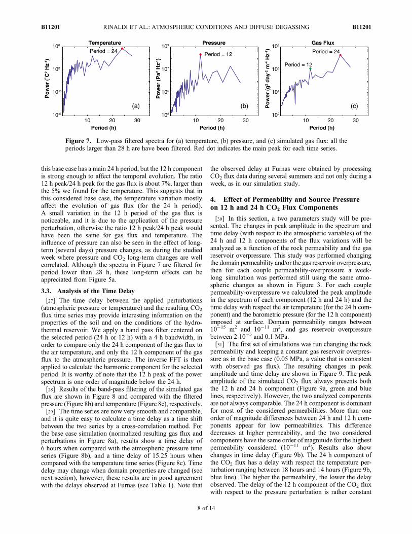
this base case has a main 24 h period, but the 12 h componentis strong enough to affect the temporal evolution. The ratio12 h peak/24 h peak for the gas flux is about 7%, larger thanthe 5% we found for the temperature. This suggests that inthis considered base case, the temperature variation mostlyaffect the evolution of gas flux (for the 24 h period).A small variation in the 12 h period of the gas flux isnoticeable, and it is due to the application of the pressureperturbation, otherwise the ratio 12 h peak/24 h peak wouldhave been the same for gas flux and temperature. Theinfluence of pressure can also be seen in the effect of long-term (several days) pressure changes, as during the studiedweek where pressure and CO2 long-term changes are wellcorrelated. Although the spectra in Figure 7 are filtered forperiod lower than 28 h, these long-term effects can beappreciated from Figure 5a.

3.3. Analysis of the Time Delay

[27] The time delay between the applied perturbations(atmospheric pressure or temperature) and the resulting CO2

flux time series may provide interesting information on theproperties of the soil and on the conditions of the hydro-thermal reservoir. We apply a band pass filter centered onthe selected period (24 h or 12 h) with a 4 h bandwidth, inorder to compare only the 24 h component of the gas flux tothe air temperature, and only the 12 h component of the gasflux to the atmospheric pressure. The inverse FFT is thenapplied to calculate the harmonic component for the selectedperiod. It is worthy of note that the 12 h peak of the powerspectrum is one order of magnitude below the 24 h.[28] Results of the band-pass filtering of the simulated gas

flux are shown in Figure 8 and compared with the filteredpressure (Figure 8b) and temperature (Figure 8c), respectively.[29] The time series are now very smooth and comparable,

and it is quite easy to calculate a time delay as a time shiftbetween the two series by a cross-correlation method. Forthe base case simulation (normalized resulting gas flux andperturbations in Figure 8a), results show a time delay of6 hours when compared with the atmospheric pressure timeseries (Figure 8b), and a time delay of 15.25 hours whencompared with the temperature time series (Figure 8c). Timedelay may change when domain properties are changed (seenext section), however, these results are in good agreementwith the delays observed at Furnas (see Table 1). Note that

the observed delay at Furnas were obtained by processingCO2 flux data during several summers and not only during aweek, as in our simulation study.

4. Effect of Permeability and Source Pressureon 12 h and 24 h CO2 Flux Components

[30] In this section, a two parameters study will be pre-sented. The changes in peak amplitude in the spectrum andtime delay (with respect to the atmospheric variables) of the24 h and 12 h components of the flux variations will beanalyzed as a function of the rock permeability and the gasreservoir overpressure. This study was performed changingthe domain permeability and/or the gas reservoir overpressure,then for each couple permeability-overpressure a week-long simulation was performed still using the same atmo-spheric changes as shown in Figure 3. For each couplepermeability-overpressure we calculated the peak amplitudein the spectrum of each component (12 h and 24 h) and thetime delay with respect the air temperature (for the 24 h com-ponent) and the barometric pressure (for the 12 h component)imposed at surface. Domain permeability ranges between10�15 m2 and 10�11 m2, and gas reservoir overpressurebetween 2�10�5 and 0.1 MPa.[31] The first set of simulations was run changing the rock

permeability and keeping a constant gas reservoir overpres-sure as in the base case (0.05 MPa, a value that is consistentwith observed gas flux). The resulting changes in peakamplitude and time delay are shown in Figure 9. The peakamplitude of the simulated CO2 flux always presents boththe 12 h and 24 h component (Figure 9a, green and bluelines, respectively). However, the two analyzed componentsare not always comparable. The 24 h component is dominantfor most of the considered permeabilities. More than oneorder of magnitude differences between 24 h and 12 h com-ponents appear for low permeabilities. This differencedecreases at higher permeability, and the two consideredcomponents have the same order of magnitude for the highestpermeability considered (10�11 m2). Results also showchanges in time delay (Figure 9b). The 24 h component ofthe CO2 flux has a delay with respect the temperature per-turbation ranging between 18 hours and 14 hours (Figure 9b,blue line). The higher the permeability, the lower the delayobserved. The delay of the 12 h component of the CO2 fluxwith respect to the pressure perturbation is rather constant

Figure 7. Low-pass filtered spectra for (a) temperature, (b) pressure, and (c) simulated gas flux: all theperiods larger than 28 h are have been filtered. Red dot indicates the main peak for each time series.


8 of 14

(�6 hours) for most of the simulated permeabilities, andincreases up to 8 hours only for permeability lower than10�14 m2 (Figure 9b, green line).[32] The second set of simulations was run keeping a con-

stant rock permeability, set as in the base case (2�10�14 m2),and changing the overpressure at the base of the domain.Figure 10 shows the changes in peak amplitude and timedelay as a function of the gas reservoir overpressure. Again,all the simulated cases present both the 12 h and 24 h com-ponents. The peak amplitude for the 12 h component of theCO2 flux has a constant value for low overpressure (up to0.01 MPa), then it exponentially decreases for higher over-pressure (Figure 10a, green line). The 24 h component fea-tures an opposite behavior: it starts to increase exponentiallyfor overpressure greater than few thousands Pa (Figure 10a,blue line). The ratio between the peak amplitudes of the twoconsidered components reaches a maximum of three ordersof magnitude for the highest simulated overpressure. Thismeans that for low overpressure the system seems to haveonly a 12 h component, which indicates that it is onlyaffected by pressure perturbations. At higher overpressures,

the CO2 flux appears to have only a 24 h component, whichmeans that only the temperature perturbation affects theresulting degassing. The time delay only slightly changes as afunction of the gas reservoir overpressure. The 12 h compo-nent has a constant delay of �6 hours with respect to thepressure for all the considered overpressure (Figure 10b,green line). The time delay of the 24 h component withrespect to the temperature is larger than 18 hours for lowoverpressure, and starts to decrease when the overpressure isgreater than one thousand Pa, up to a minimum, constantvalue of �15 hours for the highest overpressures simulated(0.05–0.1 MPa) (Figure 10b, blue line).[33] Figure 11 shows a dual parameters analysis of the time

delay and peak amplitude in the spectrum. Throughout thestudied parameters domain, the 12 h component of the CO2

flux presents a stable delay around 6 hours with respect thebarometric pressure (Figure 11a), and reaches a maximum of8 hours only for very low permeability (10�15 m2). The delayof the 24 h component with respect the atmospheric temper-ature is shown in Figure 11b. This delay remarkably changesin the parameters space: a high delay (�21 hours) is observed

Figure 8. (a) Normalized time series: pressure (black), temperature (red), and simulated gas flux (blue).(b) Normalized and filtered time series for the 12 h component: pressure (black) and simulated gas flux(blue). CO2 flux is 6 hours delayed with respect to the pressure time series. (c) Normalized and filteredtime series for the 24 h component: temperature (black) and simulated gas flux (blue). CO2 flux is15.25 hours delayed with respect to the temperature time series.


9 of 14

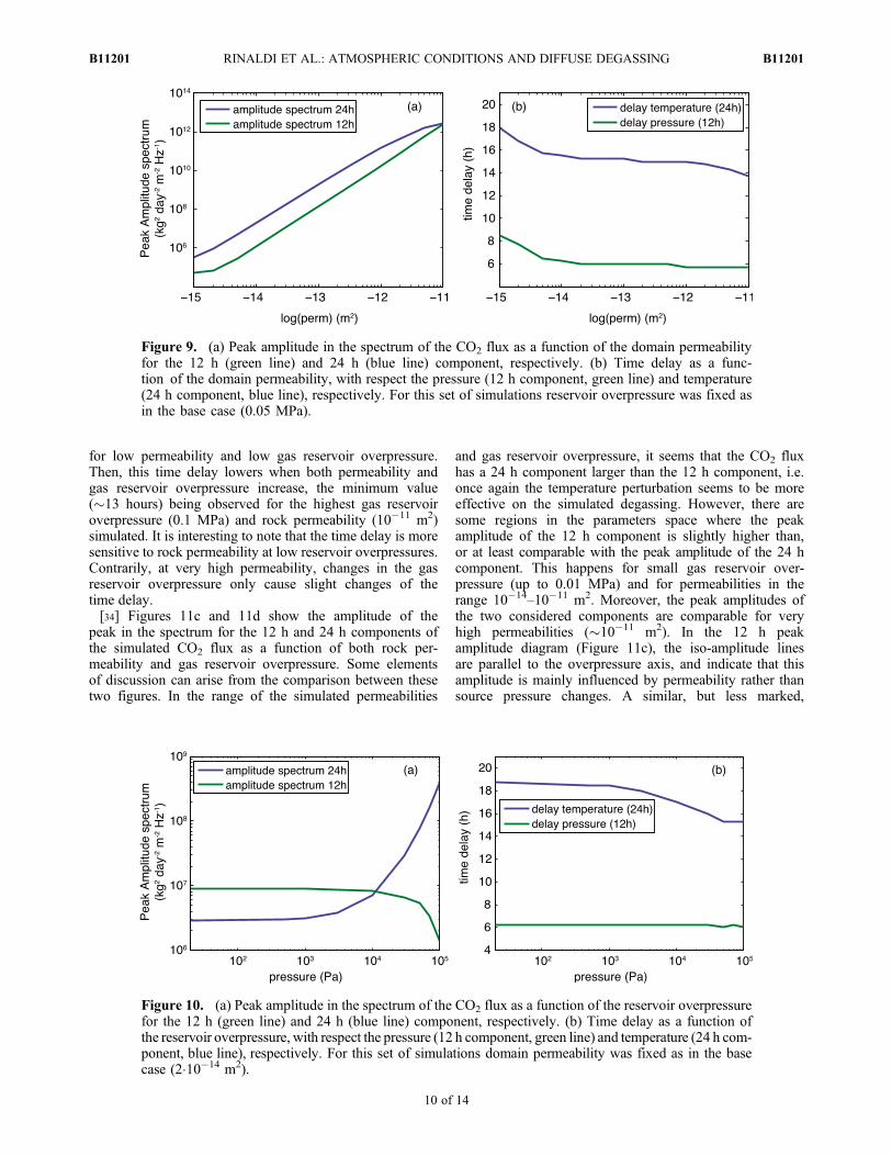
for low permeability and low gas reservoir overpressure.Then, this time delay lowers when both permeability andgas reservoir overpressure increase, the minimum value(�13 hours) being observed for the highest gas reservoiroverpressure (0.1 MPa) and rock permeability (10�11 m2)simulated. It is interesting to note that the time delay is moresensitive to rock permeability at low reservoir overpressures.Contrarily, at very high permeability, changes in the gasreservoir overpressure only cause slight changes of thetime delay.[34] Figures 11c and 11d show the amplitude of the

peak in the spectrum for the 12 h and 24 h components ofthe simulated CO2 flux as a function of both rock per-meability and gas reservoir overpressure. Some elementsof discussion can arise from the comparison between thesetwo figures. In the range of the simulated permeabilities

and gas reservoir overpressure, it seems that the CO2 fluxhas a 24 h component larger than the 12 h component, i.e.once again the temperature perturbation seems to be moreeffective on the simulated degassing. However, there aresome regions in the parameters space where the peakamplitude of the 12 h component is slightly higher than,or at least comparable with the peak amplitude of the 24 hcomponent. This happens for small gas reservoir over-pressure (up to 0.01 MPa) and for permeabilities in therange 10�14–10�11 m2. Moreover, the peak amplitudes ofthe two considered components are comparable for veryhigh permeabilities (�10�11 m2). In the 12 h peakamplitude diagram (Figure 11c), the iso-amplitude linesare parallel to the overpressure axis, and indicate that thisamplitude is mainly influenced by permeability rather thansource pressure changes. A similar, but less marked,

Figure 9. (a) Peak amplitude in the spectrum of the CO2 flux as a function of the domain permeabilityfor the 12 h (green line) and 24 h (blue line) component, respectively. (b) Time delay as a func-tion of the domain permeability, with respect the pressure (12 h component, green line) and temperature(24 h component, blue line), respectively. For this set of simulations reservoir overpressure was fixed asin the base case (0.05 MPa).

Figure 10. (a) Peak amplitude in the spectrum of the CO2 flux as a function of the reservoir overpressurefor the 12 h (green line) and 24 h (blue line) component, respectively. (b) Time delay as a function ofthe reservoir overpressure, with respect the pressure (12 h component, green line) and temperature (24 h com-ponent, blue line), respectively. For this set of simulations domain permeability was fixed as in the basecase (2�10�14 m2).


10 of 14

pattern is observed in Figure 11d for the amplitude ofthe 24 h component.[35] Analyzing the changes in 24 h and 12 h peak in the

spectrum, a change in soil permeability will provoke a remark-able and similar increase of both 12 h and 24 h components,while an increase in the gas reservoir overpressure willinduce a different behavior of the two components, with the24 h component increasing while the 12 h componentdecreases (or remains constant). Thus the observation of acorrelated change in the 12 h and 24 h peak amplitudes of the

gas flux spectrum may suggest a permeability change in thesoil, rather than a change in source conditions as a drivingmechanism. It is of note that for low permeabilities, theevolution of the 12 h component time delay can also help todistinguish a permeability change from a pressure change.[36] The described trend could be affected by our choice

of initial conditions. The simulations described above wereall run with an initial low temperature gradient (3�C/m).Additional simulations were performed to asses the role of theinitial temperature distribution. Results, shown in Figure 12,

Figure 11. Dual parameter study: time delays and peak amplitudes of the CO2 gas flux as a function ofboth gas reservoir overpressure and rock permeability. (a) Time delay of the 12 h component with respectto the barometric pressure. (b) Time delay of the 24 h component with respect to the air temperature.(c) Peak amplitude of the 12 h component. (d) Peak amplitude of the 24 h component. Black and green linerepresents in all figures the value used previously for the analysis of the degassing as a function of onlythe rock permeability or gas reservoir overpressure, respectively.

Figure 12. (a) Peak amplitude in the spectrum of the CO2 flux as a function of the temperature gradientfor the 12 h (green line) and 24 h (blue line) component, respectively. (b) Time delay as a function of thetemperature, with respect the pressure (12 h component, green line) and temperature (24 h component,blue line), respectively. For this set of simulations domain permeability and gas reservoir overpressurewere fixed as in the base case (2�10�14 m2, and 0.05 MPa, respectively).


11 of 14

suggest that the initial temperature gradient does not affect(or slightly affects) the resulting CO2 flux. The peak ampli-tude of both 12 h and 24 h components is constant in therange 3–30�C/m (Figure 12a), and the same is observedfor the time delay for both components (Figure 12b).

5. Discussion and Conclusion

[37] This work focused on the effects of the atmosphericconditions on soil diffuse degassing. Harmonic oscillationsare observed on the soil CO2 flux time series at Furnasvolcano in S. Miguel island in the Azores archipelago, andthese variations are correlated with the meteorological vari-ables monitored by permanent stations (wind velocity,barometric pressure and air temperature).[38] Numerical results performed with the TOUGH2/

EOS2 simulator show that the CO2 flux changes when airtemperature and barometric pressure change, and presents atime delay with respect to the applied perturbations inagreement with data observed at Furnas. The simulateddegassing presents both diurnal and semi-diurnal variations,as effects of applied temperature and pressure, respectively.Lower fluxes are observed when temperature and pressureare higher, in agreement with data from Furnas, where lowerdegassing is observed during the afternoon.[39] The variable conditions imposed along the upper

boundary of the domain affect the gas flux acting on theterms of the Darcy’s flow equation: the pressure gradientand the fluid properties. Air temperature acts on fluidmobility (i.e. the r/m term, see Table 2): lower temperaturescorrespond to higher CO2 density values and lower viscos-ity. Since the gas flow is directly proportional to its densityand inversely proportional to its viscosity (fourth equation inTable 2), a temperature drop has the overall effect ofincreasing the fluid flow, and viceversa. The gas density alsoenters in the buoyancy term in the Darcy’s flow equation(rP � rg). As we are dealing with uprising fluids, in thiscase higher density hinders the upward motion of the fluid.However, under the conditions considered here, the gasdensity is very small (on the order of 2 kg/m3) and this termis negligible with respect to the pressure gradient (the pres-sure difference across the domain is of the order of a fewthousands Pa).[40] The atmospheric pressure acts in different and oppo-

site ways. On one hand, it controls the pressure gradient. Inour degassing system, the pore pressure at depth is largerthan at the top. If the atmospheric pressure further dimin-ishes, the gradient across the surface increases, leading to ahigher gas flux. Pressure also acts on the CO2 density, whichin this case is directly proportional to it. A high atmosphericpressure act on gas flux reducing the pressure gradient, butincreasing the contribution due to density.[41] The overall value of the gas flux at the surface

depends on the complex interplay of all these differentcontributions, and on their relative magnitude. Under theconditions considered here, the largest changes in the sim-ulated gas flux are associated with the changes of CO2

mobility, which is mostly controlled by temperature. Pres-sure effects arise through the pressure gradient term, butaffect the degassing to a smaller extent. In this particularcase, temperature and pressure are both inversely propor-tional to gas flux, and their effects can sum up at particular

times, when they both follow similar increasing or declin-ing trends.[42] Applied perturbations and simulated gas flow chan-

ges are not only confined at the ground surface, but propa-gate down to the bottom of the simulated domain. This effectis mainly controlled by the chosen domain permeability andgas reservoir overpressure. The perturbation applied at thesurface as described above may be balanced before reachingthe reservoir at depth when the fluid flow is slow (as in thecase of very low permeability), or affect only the upper partof the domain when the pressure changes applied at thesurface are of the same order of magnitude or greater thanthe overpressure imposed at the reservoir.[43] Degassing may be affected by many parameters,

among which rainfall, air humidity, and wind speed, andthen it is not possible to directly compare the absolute valuesof simulated and observed CO2 flux. However, results for abase case show a variation in degassing of the same order ofmagnitude of the observed changes at Furnas. We calculatedtwo time delays: the correlation between the 24 h componentof the CO2 flux with respect the air temperature, andbetween the 12 h component of the gas flux with respect thebarometric pressure. Results highlight a delay of �15 hoursfor the 24 h component, and a delay of �6 hours for the 12 hcomponent, well in agreement with what observed in the realfield, although, even in this case, time delays may beaffected by other perturbations.[44] CO2 flux time series depend on both the domain

permeability and the overpressure in the gas reservoir.In order to understand the role played by the rock perme-ability and by an overpressure driving gas ascent, a dualparameters study was performed. The dual parameters studyhighlights changes in time delay and peak amplitude forboth the considered components of the CO2 flux (12 h and24 h).[45] Analyzing the time delay, on one hand a mostly

constant delay around 6 hours results for the 12 h compo-nent, and this delay slightly changes only for very low per-meabilities (up to 8 hours); on the other hand the delay forthe 24 h component presents remarkable changes, rangingfrom 13 hours for high permeability and overpressure, to 21hours when both the rock permeability and the gas reservoiroverpressure are low.[46] Amplitude of the peak in the spectrum for both com-

ponents also changes as a function of rock permeability andgas reservoir overpressure. This study highlights how theCO2 flux main period depends on the system properties.From the analysis of the peak amplitude, the resultingdegassing has mainly a 12 h period for low gas reservoiroverpressure (up to 0.01 MPa) and for permeability higherthan 10�14 m2. The peak amplitude for the two componentsare comparable for very high permeabilities, and the resultingdegassing will present in that case both the 12 h and the24 h period.[47] These results indicate that a coupled analysis of these

observables may provide useful hints to discriminate theparameter that is changing within the system. According toour model, the observation of correlated changes in thediurnal and semi-diurnal components of diffuse degassing,under the conditions described above, would be related to apermeability change in the soil. On the contrary, an unrelatedevolution of these components would indicate a change in the


12 of 14

source conditions. This is in agreement with the observa-tions of Richon et al. [2003] that correlated changes in the12 h cycle of Rn time series with a magnitude 7.1 earth-quake close to Taal volcano (Philippines), likely due to apermeability change in the soil. Permeability changes in avolcano/hydrothermal system can be generated by transientstresses, including distant earthquakes [Elkhoury et al.,2006; Manga et al., 2012], or may result from micro-fracturing associated with intrusive processes and mechanicaldisturbances, such as a dome collapse, or from mineral dis-solution or precipitation [White and Mroczek, 1998]. Themonitoring of harmonic components of the gas flux signalshould thus be integrated in volcano monitoring as it repre-sents a tool to understand the reasons of gas flux changesat the surface.

[48] Acknowledgments. This work was carried out when the firstauthor was enrolled in the Doctorate school at the University of Bologna,on a grant funded by the Istituto Nazionale di Geofisica e Vulcanologia-Sezione di Bologna. A. P. Rinaldi is currently supported by DOE-LBNLcontract DE-AC02-05CH11231. F. Viveiros is supported by a Postdocgrant from Fundo Regional da Ciência e Tecnologia. Comments from D.Granieri and an anonymous reviewer greatly helped improve and clarifysome aspects of the paper.

ReferencesAumento, F. (2002), Radon tides on an active volcanic island: Terceira,Azores, Geofis. Int., 41(4), 499–505.

Bajracharya, R. M., R. Lal, and J. N. Kimble (2000), Diurnal and seasonalCO2-C flux from soil as related to erosion phases in central Ohio, Soil Sci.Soc. Am. J., 64, 286–293.

Borgia, A., K. Pruess, T. J. Kneafsey, C. M. Oldenburg, and L. Pan (2012),Numerical simulation of salt precipitation in the fractures of a CO2-enhanced geothermal system, Geothermics, 44, 13–22, doi:10.1016/j.geothermics.2012.06.002.

Bowling, D. R., and W. J. Massman (2011), Persistent wind-inducedenhancement of diffuse CO2 transport in a mountain forest snowpeak,J. Geophys. Res., 116, G04006, doi:10.1029/2011JG001722.

Chiodini, G., R. Cioni, M. Guidi, B. Raco, and L. Marini (1998), Soil CO2flux measurements in volcanic and geothermal areas, Appl. Geochem.,13, 543–552.

Chiodini, G., S. Caliro, C. Cardellini, D. Granieri, R. Avino, A. Baldini,M. Donnini, and C. Minopoli (2010), Long term variations of the CampiFlegrei (Italy) volcanic system as revealed by the monitoring of hydrother-mal activity, J. Geophys. Res., 115, B03205, doi:10.1029/2008JB006258.

Cigolini, C., et al. (2009), Radon surveys and real-time monitoring atStromboli volcano: Influence of soil temperature, atmospheric pressureand tidal forces on 222Rn degassing, J. Volcanol. Geotherm. Res., 184,381–388.

Clements, W. E., and M. H. Wilkening (1974), Atmospheric pressureeffects on 222Rn transport across the Earth-air interface, J. Geophys.Res., 79(33), 5025–5029.

Elkhoury, J. E., E. E. Brodsky, and D. C. Agnew (2006), Seismic wavesincrease permeability, Nature, 441, 1135–1138, doi:10.1038/nature04798.

Granieri, D., G. Chiodini, W. Marzocchi, and R. Avino (2003), Continuousmonitoring of CO2 soil diffuse degassing at Phlegrean Fields (Italy):Influence of environmental and volcanic parameters, Earth Planet. Sci.Lett., 212, 167–179.

Granieri, D., R. Avino, and G. Chiodini (2010), Carbon dioxide diffuseemission from the soil: ten years of observations at Vesuvio and CampiFlegrei (Pozzuoli), and linkages with volcanic activity, Bull. Volcanol.,72, 103–118, doi:10.1007/s00445-009-0304-8.

Groves-Kirkby, C. J., A. R. Denman, R. G. M. Crockett, P. S. Phillips, andG. K. Gillmore (2006), Identification of tidal and climatic influenceswithin domestic radon time-series from Northamptonshire, UK, Sci. TotalEnviron., 367, 191–202.

Hernández, P. A., K. Notsu, J. M. Salazar, T. Mori, G. Natale, H. Okada,G. Virgili, Y. Shimoike, M. Sato, and N. M. Pérez (2001), Carbon dioxidedegassing by advective flow from Usu volcano, Japan, Science, 292,83–86, doi:10.1126/science.1058450.

Hernández, P. A., N. M. Pérez, J. Salazar, M. Reimer, K. Notsu, andH. Wakita (2004), Radon and helium in soil gases at Canadas Caldera,Tenerife, Canary Islands, Spain, J. Volcanol. Geotherm. Res., 131, 59–76.

Hernández, P. A., et al. (2012), Analysis of long- and short-term tempo-ral variations of the diffuse CO2 emission from Timanfaya volcano,Lanzarote, Canary Islands, Appl. Geochem., doi:10.1016/j.apgeochem.2012.08.008, in press.

Hinkle, M. E. (1990), Factors affecting concentrations of helium and carbondioxide in soil gases, in Geochemistry of Gaseous Elements and Com-pounds, edited by E. M. Durrance et al., pp. 421–448, TheophrastusPubl., Athens.

Hinkle, M. E. (1994), Environmental conditions affecting He, CO2, O2, andN2 in soil gases, Appl. Geochem., 9, 53–63.

Hutnak, M., S. Hurwitz, S. E. Ingebritsen, and P. A. Hsieh (2009), Numer-ical models of caldera deformation: Effects of multiphase and multicom-ponent hydrothermal fluid flow, J. Geophys. Res., 114, B04411,doi:10.1029/2008JB006151.

Klusman, R. W., and J. D. Webster (1981), Preliminary analysis of meteo-rological and seasonal influences on crustal gas emission relevant toearthquake prediction, Bull. Seismol. Soc. Am., 71(1), 211–222.

Lewicki, J. L., G. E. Hilley, T. Tosha, R. Aoyagi, K. Yamamoto, and S. M.Benson (2007), Dynamic coupling of volcanic CO2 flow and wind at theHorseshoe Lake tree kill, Mammoth Mountain, California, Geophys. Res.Lett., 34, L03401, doi:10.1029/2006GL028848.

Manga, M., I. Beresnev, E. E. Brodsky, J. E. Elkhoury, D. Elsworth, S. E.Ingebritsen, D. C. Mays, and C.-Y. Wang (2012), Changes in permeabil-ity caused by transient stresses: Field observations, experiments, andmechanisms, Rev. Geophys., 50, RG2004, doi:10.1029/2011RG000382.

Massman, W. J. (2004), Advective transport of CO2 in permeable mediainduced by atmospheric pressure fluctuations: 1. An analytical model,J. Geophys. Res., 111, G03004, doi:10.1029/2006JG000163.

Mazzoldi, A., A. P. Rinaldi, A. Borgia, and J. Rutqvist (2012), Inducedseismicity within GCS projects: Maximum earthquake magnitude andleakage potential from undetected faults, Int. J. Greenhouse GasControl, 10, 434–442, doi:10.1016/j.ijggc.2012.07.012.

McGee, K. A., and T. M. Gerlach (1998), Annual cycle of magmatic CO2 ina tree-kill soil at Mammoth Mountain, California: Implications for soilacidification, Geology, 26(5), 463–466.

McGee, K. A., T. M. Gerlach, R. Kessler, and M. P. Doukas (2000), Geo-chemical evidence for a magmatic CO2 degassing event at MammothMountain, California, September-October 1997, J. Geophys. Res., 105,8447–8456.

Nakadai, T., M. Yokozawa, H. Ikeda, and H. Koizumi (2002), Diurnalchanges of carbon dioxide flux from bare soil in agricultural field inJapan, App. Soil Ecol., 19, 161–171.

Oldenburg, C. M., and A. P. Rinaldi (2011), Buoyancy effects on upwardbrine displacement caused by CO2 injection, Transp. Porous Media, 87,525–540, doi:10.1007/s11242-010-9699-0.

Padrón, E., P. A. Hernández, T. Toulkeridis, N. M. Pérez, R. Marrero,F. Melián, G. Virgili, and K. Notsu (2008), Diffuse CO2 emissionrate from Pululahua and the lake-filled Cuicocha calderas, Ecuador,J. Volcanol. Geotherm. Res., 176, 163–169.

Pinault, J. L., and J. C. Baubron (1997), Signal processing of diurnal andsemidiurnal variations in radon and atmospheric pressure: A new toolfor accurate in situ measurement of soil gas velocity, pressure gradient,and tourtuosity, J. Geophys. Res., 102(B8), 18,101–18,120.

Pruess, K., C. M. Oldenburg, and G. Moridis (1999), TOUGH2 user’sguide version 2.0, Pap. LBNL-43134, Lawrence Berkeley Natl. Lab.,Berkeley, Calif.

Reicosky, D. C., R. W. Gesch, S. W. Wagner, R. A. Gilbert, C. D. Wente,and D. R. Morris (2008), Tillage and wind effects on soil CO2 concentra-tions in muck soils, Soil Tillage Res., 99, 221–231.

Reimer, G. M. (1980), Use of soil-gas helium concentrations for earthquakeprediction: Limitations imposed by diurnal variation, J. Geophys. Res.,85(B6), 3107–3115, doi:10.1029/JB085iB06p03107.

Richon, P., J. C. Sabroux,M.Halbwachs, J. Vandemeulebrouck, N. Poussielgue,J. Tabbagh, and R. Punongbayan (2003), Radon anomaly in the soil ofTaal volcano, the Philippines: A likely precursor of the M7.1 Mindoroearthquake (1994), Geophys. Res. Lett., 30(9), 1481, doi:10.1029/2003GL016902.

Richon, P., F. Perrier, E. Pili, and J. C. Sabroux (2009), Detectability andsignificance of 12 hr barometric tide in radon-222 signal, dripwater flowrate, air temperature and carbon dioxide concentration in an undergroundtunnel, Geophys. J. Int., 176, 683–694, doi:10.1111/j.1365-246X.2008.04000.x.

Richon, P., F. Perrier, B. P. Koirala, F. Girault, M. Bhattarai, and S. N. Sapkota(2011), Temporal signatures of advective versus diffusive radon transport ata geothermal zone in central Nepal, J. Environ. Radioactiv., 102(2), 88–102,doi:10.1016/j.jenvrad.2010.10.005.

Rigby, J. G., and D. D. La Pointe (1993), Wind and barometric pressureeffects on Radon in two mitigated houses, paper presented at International


13 of 14

Radon Conference, Am. Assoc. of Radon Sci. and Technol., Denver,Colo.

Rinaldi, A. P., M. Todesco, and M. Bonafede (2010), Hydrothermal insta-bility and ground displacement at the Campi Flegrei caldera, Phys. EarthPlanet. Int., 178, 155–161, doi:10.1016/j.pepi.2009.09.005.

Rinaldi, A. P., M. Todesco, J. Vandemeulebrouck, A. Revil, and M. Bonafede(2011), Electrical conductivity, ground displacement, gravity changes,and gas flow at Solfatara crater (Campi Flegrei caldera, Italy): Resultsfrom numerical modeling, J. Volcanol. Geotherm. Res., 207, 93–105,doi:10.1016/j.jvolgeores.2011.07.008.

Robinson, A. L., R. G. Sextro, and W. J. Riley (1997), Soil-gas entry intohouses driven by atmospheric pressure fluctuations—The influence ofsoil properties, Atmos. Environ., 31(10), 1487–1495.

Rogie, J. D., D. M. Kerrick, M. L. Sorey, G. Chiodini, and D. L. Galloway(2001), Dynamics of carbon dioxide emission at Mammoth Mountain,California, Earth Planet. Sci. Lett., 188, 535–541.

Steinitz, G., O. Piatibratova, and S. M. Barbosa (2007), Annual cycle ofmagmatic CO2 in a tree-kill soil at Mammoth Mountain, California:Implications for soil acidification, J. Geophys. Res., 112, B10211,doi:10.1029/2006JB004817.

Takle, E. S., W. J. Massman, J. R. Brandle, R. A. Schmiat, X. Zhou, I. V.Litvina, R. Garcia, G. Doyle, and C. W. Rice (2004), Influence of high-frequency ambient pressure pumping on carbon dioxide efflux from soil,Agric. Forest Meteor., 124, 193–206.

Todesco, M., A. P. Rinaldi, and M. Bonafede (2010), Modeling of unrestsignals in heterogeneous hydrothermal systems, J. Geophys. Res., 115,B09213, doi:10.1029/2010JB007474.

Van Camp, M., and P. Vauterin (2005), Tsoft: Graphical and interactivesoftware for the analysis of time series and Earth tides, Comput. Geosci.,31(5), 631–640.

Vauterin, P., and M. Van Camp (2008), TSoft Manual Version 2.1.2, 58 pp.,R. Obs. of Belgium, Brussels,

Viveiros, F. (2010), Soil CO2 flux variations at Furnas Volcano (SãoMiguel Island, Azores)), PhD thesis, Univ. of the Azores, Ponta Delgada,Portugal.

Viveiros, F., T. Ferreira, J. Cabral Vieira, C. Silva, and J. L. Gaspar (2008),Environmental influences on soil CO2 degassing at Furnas and Fogo vol-canoes (São Miguel Island, Azores archipelago), J. Volcanol. Geotherm.Res., 177, 883–893.

Viveiros, F., T. Ferreira, C. Silva, and J. L. Gaspar (2009), Meteorologicalfactors controlling soil gases and indoor CO2 concentration: A permanentrisk in degassing areas, Sci. Total Environ., 407, 1362–1372.

Viveiros, F., C. Cardellini, T. Ferreira, S. Caliro, G. Chiodini, and C. Silva(2010), Soil CO2 emissions at Furnas volcano, São Miguel Island, Azoresarchipelago: Volcano monitoring perspectives, geomorphologic studies,and land use planning application, J. Geophys. Res., 115, B12208,doi:10.1029/2010JB007555.

Werner, C., S. L. Brantley, and K. Boomer (2000), CO2 emission related tothe Yellowstone volcanic system: 2. Statistical sampling, total degassing,and transport mechanisms, J. Geophys. Res, 105(B5), 10,831–10,846.

White, S. P., and E. K.Mroczek (1998), Permeability changes during the evo-lution of a geothermal field due to the dissolution and precipitation ofquartz, Trans. Porous Media, 33, 81–101, doi:10.1023/A:1006541526010.

Witkamp, M. (1969), Environmental effects on microbial turnover ofsome mineral elements: Part II–Biotic factors, Soil Biol. Biochem.,1(3), 177–184, doi:10.1016/0038-0717(69)90017-0.


14 of 14

Effects of atmospheric conditions on surface diffuse degassing

Documents

Transcript of Effects of atmospheric conditions on surface diffuse degassing