Effects of Active Damping on Parametric Instability of Composite Cylindrical Shells Using Piezo...

November 24, 2006 7:44 RPS/INSTRUCTION FILE 00002

International Journal of Aerospace and Lightweight StructuresVol. 3, No. 4 (2014) 445–471c© Research Publishing ServicesDOI: 10.3850/S2010428614000026

EFFECTS OF ACTIVE DAMPING ON PARAMETRIC

INSTABILITY OF COMPOSITE CYLINDRICAL SHELLS

USING PIEZO FIBER COMPOSITES

Partha Bhattacharya1,a,∗, Debabrata Podder2, and Atanu Sahu1

1Department of Civil Engineering, Jadavpur University,

Kolkata – 700 032, Indiaap [email protected]

2Department of Ocean Engineering and Naval Architecture,

Indian Institute of Technology, Kharagpur – 721 302, India

Parametric instability due to longitudinal forces is becoming a critical issue forlightweight and flexible modern day aerospace vehicles. An attempt is made in the presentwork to develop a FE model for a piezoelectric actuated laminated composite shell panelsubjected to parametric edge excitation. A feedback control strategy is developed withthe piezo sensor output being fed back to the IDE-PFC actuators. Employing Hamilto-nian principle, governing differential equation taking the form of Mathieu-Hill equationis developed. The resulting equation is solved using the method of strained parame-ter. Results for various geometries, boundary conditions and lamination sequences areobtained and discussed.

Keywords: Parametric instability, IDE-PFC actuators, laminated composite shell,Mathieu-Hill equations, feedback damping.

1. Introduction

With the present day aerospace vehicles becoming lighter and more flexible, the

significance of the longitudinal forces due to vehicle thrust on the flexural vibration

characteristics of the vehicle is gaining importance. The aerospace engineers are

concerned about the oscillatory instability that may be affected by the pulsat-

ing inertial and thermal loads. Among the problems of the dynamic stability of

structures, probably the best known subclass can be constituted by the problems

of parametric excitation, or parametric resonance. Unlike forced vibration prob-

lems where resonances occur when the natural and exciting frequencies are equal,

parametric resonance occurs when the exciting frequency is twice the frequency

of free vibration (principal parametric resonance). Another essential difference of

parametric resonance lies in the possibility of exciting vibrations with frequencies

∗Author for all correspondence.

445

http://dx.doi.org/10.3850/S2010428614000026


446 Partha Bhattacharya et al.

smaller than the frequency of the principal resonance. Finally, it can be stated that

the existence of continuous regions of excitation (regions of dynamic instability) as

seen in parametric resonance, is an inimitable phenomenon unlike that observed

in forced vibration problems. Depending upon the magnitude and the frequency

of the pulsating axial load, the linear Hill or Mathieu equation defining the lat-

eral displacements of the column may yield bounded or unbounded values for these

displacements.

The phenomenon of parametric resonance was first observed by Faraday [1831].

He noted that the surface waves in a fluid-filled cylinder under vertical excitation

exhibited twice the period of the excitation itself. Beliaev [1924] was one of the ear-

liest researchers to have analyzed the response of a straight elastic hinged-hinged

column subjected to an axial periodic load of the form P (t) = P0 + P1 cosΩt. He

obtained a Mathieu equation for the dynamic response of the column and deter-

mined the principal parametric resonance frequency of the column. He demonstrated

that a column could be made to oscillate with an excitation frequency of 1/2Ω if the

said frequency is close to one of the natural frequencies of the lateral motion even

though the axial load may be below the static buckling load of the column. These

results were later verified experimentally by Gol’denblat [1947], Bolotin [1963], and

Evan-Iwanowski [1965]. Krylov and Bogoliubov [1935] used the Galerkin procedure

to determine the dynamic response of a column with arbitrary boundary conditions

under the influence of multi-harmonic axial forces.

It was only during the last decade of the last century, various researchers took

up studies on parametric instability of laminated composite structures. Srinivas

et al. [1986] was one of the earliest among them. Some other works in the similar

area can be attributed to Chen [1987] and Kwon [1991]. Argento and Scott [1993a,

1993b, and 1993c] presented a series of work on the dynamic instability behavior of

laminated circular cylindrical shells. They employed the perturbation technique to

solve the problem. Cederbaum [1992] used the method of multiple scales to analyze

parametrically excited circular cylindrical shells. A series of works on the behavior

of parametrically excited laminated composite shell structures were presented by

Datta and Sahu [2003], Ravi Kumar et al. [2003] and Patel et al. [2006]. Vibra-

tion, buckling and dynamic stability of cracked cylindrical shell was studied by

Javidruzi et al. [2004]. The dynamic instability of simply supported, finite-length,

circular cylindrical shells subjected to parametric excitation by axial loading were

investigated analytically by Birman and Bert [1988].

The influence of damping on the boundaries of the dynamic instability was dis-

cussed by several researchers [Mettler, 1942; Bolotin, 1963; Piszczek, 1955]. Afsar

and Massoud [1994] implemented a Lancaster type damper to suppress the vibra-

tion of a single degree of freedom system subjected to principal parametric reso-

nance. Mustafa and Ertas [1995] proposed a control mechanism for cantilever beams

with the addition of a tip pendulum. Oueini [1999] developed a nonlinear control

strategy for cantilever beams subjected to either primary excitation or parametric

excitation using strain gages and accelerometers as sensors and piezoceramics as


Effects of Active Damping on Parametric Instability 447

actuators. Bhattacharya et al. [2006], for the first time, introduced the concept of

feedback control on the instability behavior of laminated composite plates with sur-

face bonded piezo patch used both as sensor and actuator. They implemented the

strained parameter approach [Nayfeh and Mook, 1995] to determine the stability

boundary with and without damping.

The influence of damping on the parametrically excited shell structures is vir-

tually non-existent according to the review done by the present authors. The use of

piezoceramics as sensors and actuators for feedback control of parametrically excited

systems is also very rare. Therefore the authors felt it appropriate to undertake a

study on the parametrically excited laminated composite shell panels integrated

with active piezoelectric layers where the piezoelectric sensor-actuator pair con-

tributes to the damping mechanism. The structural form considered for the present

study consists of laminated composite circular cylindrical shell panels with surface

bonded monolithic piezo sensor patches and Inter-digitated Piezo Fiber Composite

(Fig. 1) actuator patches. A schematic of the cylindrical panel is shown in Fig. 2.

Two different boundary conditions, namely, (a) Cantilever and (b) Simply support

are considered for the present analysis. The governing finite element formulation

developed and presented in this paper is based on Sanders’ shallow shell theory

with Reissner’s correction [1945, 1950] to include shear deformation and rotary

inertia. The piezoelectric formulation is based on IEEE standard on piezoelectric-

ity. The feedback mechanism is based on sensor charge being fed back through a

Fig. 1. Mode of operation of PFC with inter-digitated electrode.

Fig. 2. Schematic diagram of the cylindrical shell configuration.



current amplifier with proportional gain on to the IDE – PFC actuators. Lagrange’s

formulation is then employed to develop the governing differential equation which

is subsequently reduced to obtain the governing equation in the Mathieu-Hill form

to determine the stability bounds. A detailed formulation is presented in the next

section.

2. Constitutive Equations

The laminated composite cylindrical shell panel considered for the present study is

assumed to be made up of perfectly bonded layers without any slip. The lamina

constitutive equations and subsequently the laminate behavior are presented below.

2.1. Lamina

The stress-strain relationship for an orthotropic lamina under plane stress condition

in the local material direction can be expressed as,

σ = [Q] ε (1)

where, [Q] is the elastic moduli matrix. Necessary transformation of Eq. (1) is

carried out to express the stress-strain relationship in the global coordinate, and

the relationship is as follows,

σ =[

Q]

ε (2)

where,

[

Q]

= [T ]T

[Q] [T ] (3)

and, [T] is the transformation matrix relating the local material coordinate with

the global principle coordinate system.

2.2. Piezoelectric

The linear constitutive relations for a piezoelectric material as per IEEE standard

[1987] under small field conditions can be written as,

D = [ξp] E + [d] σ (4)

ε = [d]TE + [s] σ (5)

where, [s] of size (6×6) is the compliance matrix and is defined as the inverse of the

elastic matrix[

Q]

. The vector D of size (3×1) is the electric displacement, ε is

the strain vector (6×1), σ is the stress vector (6×1). The piezoelectric constants

are the dielectric permittivity [ξp] of size (3×3) (Farad/m). The piezoelectric coeffi-



cient [d] defines strain per unit electric field E at constant stress (m/volt) and also

defines electric displacement per unit stress at constant electric field (Coulomb/N).

Eq. (4) describes the direct piezoelectric effect and Eq. (5) represents the converse

effect.

The governing equations for bonded or embedded piezoelectric layers assume

that the state of the crystal is homogeneous, both electrically and mechanically and

the equations are linear.

The electric field vector E is expressed as,

E =

E1

E2

E3

= −∇φ (6)

where, φ is the applied electric potential.

3. Displacement Modeling

The assumptions made for the displacement model for the laminated configuration

are as follows:

(i) The material behavior is linear and elastic.

(ii) The thickness of the laminate is small compared to other dimensions.

(iii) Analysis is carried out within the purview of small displacement theory.

(iv) Out of plane normal stresses are negligible.

(v) First order shear deformation along with rotary inertia are considered.

The first three assumptions follow Sanders’ shallow shell theory and the fifth

assumption is based on Reissner’s theory where generalized stresses are obtained

by integrating the three-dimensional stresses through the thickness of the shell.

Following these, the displacement relationships along the coordinate direction are

expressed as,

u(x, y, z, t) = u0(x, y, t) + zθy(x, y, t)

v(x, y, z, t) = v0(x, y, t) − zθx(x, y, t) (7)

w(x, y, z, t) = w0(x, y, t)

The terms ‘u’, ‘v’, and ‘w’ with superscript ‘0’ represents the mid-plane displacement

of the laminate along the global X-, Y- and Z-axis, respectively. The terms θx

and θy are the rotations of the normal to the mid-plane about the X- and Y-axis,

respectively.



3.1. Strain – Displacement Relationship

The assumed strain-displacement relations for the shell structure are as follows:

εxx =

(

∂u0

∂x−w0

Rx

)

+ z∂θy

∂x

εyy =

(

∂v0∂y

−w0

Ry

)

− z∂θx

∂y

γxy =

(

∂v0∂x

+∂u0

∂y−

2w0

Rxy

)

+ z

[

∂θy

∂y−∂θx

∂x

]

(8)

γyz =∂w0

∂y− θx

γzx =∂w0

∂x+ θy

where, εxx, εyy are the normal strains in X and Y directions respectively, and

γxy, γyz, γzx are the shear strains in X-Y, Y-Z, and X-Z plane respectively. The

curvatures are expressed as,

κx =∂θy

∂x; κy = −

∂θx

∂y; κxy =

∂θy

∂y−∂θx

∂x

4. Laminate Stress-Strain Relationship

The resultant forces and moments acting on a laminate are obtained by integrating

the stresses in each layer or lamina through the laminate thickness, as given by

Ni =

∫ t/2

−t/2

σidz; Mi =

∫ t/2

−t/2

σizdz (9)

Ni is the force resultant of the cross section of the laminate and Mi is the moment

resultant.

Now, following Eqs. (3), (7) and (9), one can express,

N

M

=

[

A B

B D

]

ε0

κ

(10)

and,

Ns

= [H] γ (11)

where, A is the in-plane matrix, D is the bending matrix and the B matrix couples

the in-plane and bending components.

The matrix [H ] is termed as shear matrix.



5. Potential Distribution within the Piezoelectric Layer

In the present study monolithic piezo patches are considered as sensor elements

and Interdigitated Piezo Fiber Composite (IDE-PFC) patches are considered as

actuator elements. The electric field for the sensor elements is assumed to be linearly

distributed through the thickness of the piezo layer with the electrode in contact

with the substrate being suitably grounded.

5.1. Actuator Model

In case of IDE-PFC patches (actuator), the electric field along the length of the

patch between two consecutive electrode fingers is assumed to be linearly distributed

with alternate electrodes being suitably grounded. There is a perfect bond between

the piezo layer and the elastic substrate (no-slip condition).

In the present development only d33 actuation induced by the interdigitated

electrode is considered (Fig. 1) and hence only E3 field is taken in the modeling.

Therefore, Eq. (6) takes the form,

E =

0

0

E3

(12)

Following the formulation for PFC with IDE as given by Azzouz et al. [2001],

the electric field is related to the electric potential as,

E =

E31

−

E3np

= −

1

h1

− 0

− − −

0 −1

hnp

φ1

−

φnp

(13)

In general h1, h2, . . . ,hnp are the spacing of interdigitated electrode for

1, 2, . . . ,np piezoelectric layer, though in the present case only one piezoelectric

actuator layer is considered.

The PFCs are composite materials comprising of uniaxially aligned active piezo-

ceramic fibers and a matrix phase and therefore the effective fibrous volume plays

an important part in the actuation mechanism. So, the right hand side of Eq. (13)

is to be suitably multiplied with fiber volume fraction.

The relation between the electric field and the electric potential (assumed con-

stant over the whole piezo patch) finally can be written as,

Ea = E3 = −

[

1

hide

]

φ1 = −1

hide

[1] φ1 (14)



The electro-mechanical coupling relationship is developed by assuming a uniform

voltage distributed over the entire piezo-element and therefore the electric field

within the IDE-PFC patch is,

Ea = −1

hide

[Bφ] φa (15)

where, [Bφ] is a unit matrix and hide is the spacing of IDE.

6. Finite Element Formulation

The problem considered in the present study consists of a laminated cylindrical

shell panel with surface mounted piezo actuators and sensors subjected to a dis-

tributed edge loading. The governing equations for such a system derived using the

Lagrange’s equations can be written as

d

dt

(

∂T

∂qi

)

−∂

∂qi(T − U) = Pi (16)

In the above equation T is the kinetic energy and U is the potential energy

consisting of mechanical strain energy and electrical potential energy. The work

done V due to axial external loading and the electrical loading on the actuator is

expressed as the generalized force Pi as follows,

Pi =∂V

∂qi(17)

In Eqs. (16) and (17), qi’s are the generalized coordinates.

In the present work a 4-node isoparametric 2-dimensional finite element is devel-

oped with five (5) displacement degrees of freedom per node (Eq. (7)). Additionally,

one actuator voltage per element is considered in the FE model. The sensor modeling

is presented in a separate section. Therefore, following the isoparametric formula-

tion, the mechanical degrees of freedom can be expressed in terms of the shape

functions as,

u =

4∑

i=1

Niui; v =

4∑

i=1

Nivi; w =

4∑

i=1

Niwi; θx =

4∑

i=1

Niθxi; θy =

4∑

i=1

Niθyi

where, u, v, w, θx, θy having a subscript ‘i’ are the nodal displacement degrees of

freedom. The elemental displacement can also be expressed in matrix form as,

u = [N]de (18)

Combining Eqs. (7), (8) and (18), the generalized strains are expressed as follows,

ε

κ

= [B]b

u

θ

(19a)



and,

γ = [B]s

u

θ

(19b)

The matrices, [B]b and [B]s represent the strain-displacement operator for bend-

ing and shear components, respectively.

Replacing the material models as given in Eqs. (2), (4) and (5) and using the

Eqs. (15), (19a) and (19b) one can express the total potential energy (U) of the

laminate as,

U =1

2

∫

A

[

deT[B]Tb

[

A B

B D

]

[B]bde + deT[B]Ts [H][B]sde

]

dA

−1

2

∫

V

dT[B]T[Z]T[e]

[

−1

h ide

]

[Bφ]φ3dV

−1

2

∫

V

φ3[Bφ]T[

−1

hide

]

[e]T[Z][B]dedV

−1

2

∫

V

φ3[Bφ]T[

−1

hide

]

[ξp]

[

−1

hide

]

[Bφ]φ3dV (20)

The work done due to mechanical load f and the specified surface charge

density Q on the actuator layer can be expressed as,

V =

∫

A

deTf dA +

∫

A

ϕaQ(x, y)dA (21)

The laminated shell structure, if partially covered with piezo patch, the second,

third and the fourth integral expressions of Eq. (20) and the second expression

in Eq. (21) do not contribute to the total potential calculation of the uncovered

portion.

The external axial mechanical load introduces an initial stress in the system and

the work done due to the loading can be expressed as

VM =

∫

v

εnLTσ0dV (22)

where, εnL is the Green-Lagrangian strain vector and σ0 is the initial stress devel-

oped due to external loading. In the present formulation only the in-plane contri-

bution (εxnL, εynL and γxynL) of the Green-Lagrangian strains and the associated

stress terms are considered.



The non-linear strains can be expressed as follows,

εxnL =1

2

[

(

∂u0

∂x

)2

+

(

∂v0∂x

)2

+

(

∂w0

∂x

)2

− 2w0

Rx

∂u0

∂x− 2

w0

Rxy

∂v0∂x

− 2∂w0

∂x

u0

Rx

+2z

(

∂u0

∂x

∂θy

∂x−∂θy

∂x

w0

Rx−∂v0∂x

∂θx

∂x+∂θx

∂x

w0

Rxy+u0

Rx

θy

Rx−θy

Rx

∂w0

∂x

)

+z2

(

(

∂θy

∂x

)2

+

(

∂θx

∂x

)2

+

(

θy

Rx

)2)

+

(

w0

Rx

)2

+

(

w0

Rxy

)2

+

(

u0

Rx

)2]

(23a)

εynL =1

2

[

(

∂u0

∂y

)2

+

(

∂v0∂y

)2

+

(

∂w0

∂y

)2

− 2w0

Rxy

∂u0

∂y− 2

w0

Ry

∂v0∂y

− 2∂w0

∂y

v0Ry

+2z

(

∂u0

∂y

∂θy

∂y−∂θy

∂y

w0

Rxy−∂v0∂y

∂θx

∂y+∂θx

∂y

w0

Ry−v0Ry

θx

Ry+θx

Ry

∂w0

∂y

)

+z2

(

∂θy

∂y

)2

+

(

∂θx

∂y

)2

+

(

θx

Ry

)2

+

(

w0

Rxy

)2

+

(

w0

Ry

)2

+

(

v0Ry

)2]

(23b)

and,

γxynL =

[

∂u0

∂x

∂u0

∂y+∂v0∂x

∂v0∂y

+∂w0

∂x

∂w0

∂y−∂u0

∂x

w0

Rxy−∂v0∂x

w0

Ry−∂v0∂y

w0

Rxy

−∂w0

∂x

v0Ry

−∂w0

∂y

u0

Rx−∂u0

∂y

w0

Rx+ z

(

∂u0

∂x

∂θy

∂y+∂θy

∂x

∂u0

∂y−∂θy

∂x

w0

Rxy

−∂v0∂x

∂θx

∂y−∂θx

∂x

∂v0∂y

+∂θx

∂x

w0

Ry+∂θx

∂y

w0

Rxy+∂w0

∂x

θx

Ry−u0

Rx

θx

Ry

−θy

Rx

∂w0

∂y+θy

Rx

v0Ry

−w0

Rx

∂θy

∂y

)

+ z2

(

∂θy

∂x

∂θy

∂y+∂θx

∂x

∂θx

∂y−θy

Rx

θx

Ry

)

+w0

Rxy

w0

Ry+u0

Rx

v0Ry

+w0

Rx

w0

Rxy

]

(23c)

and finally can be represented as,

εNL =1

2[R] χ (24)

where,

χ =

u0,xu0,yv0,xv0,yw0,xw0,yθx,xθx,yθy,yθy,xu0

Rx

v0Ry

w0

Rx

w0

Ry

w0

Rxy

θx

Ry

θy

Rx

(25)

and [R] is the differential operator relating the nonlinear strains with the χ vector

given in Eq. (25).



Now, χ can also be represented as,

χ = [BnL] de (26)

where, [BnL] is a nonlinear operator matrix.

The potential energy due to residual stresses can then be written as,

UnL =1

2

∫

V

deT

[BnL]T

[R]T σ0 dV (27)

and finally it can be expressed as,

UnL =1

2de

T [Kσ] de (28)

where, [Kσ] is called the stress stiffness matrix and is given by,

[Kσ] =

∫

A

[BnL]T

[Sσ] [BnL] dA (29)

and [Sσ] is termed as the stress matrix.

The kinetic energy, T, for a single element can be given by the following

expression

T =1

2de

T[M]de (30)

where, [M] is the mass matrix and is represented as,

[M] =

∫

A

[N]T[ρ][N]dA (31)

Now putting the energy terms as given in Eqs. (20), (21), (28) and (30) back

into the Lagrange’s equation and carrying out the necessary derivation, one can

obtain the governing equations at the elemental level which when assembled over

the whole structure can be written as,

[M]

d

+ [[KUU] + [Kσ]] d + [KUφ] φa = 0 (32)

[KφU]d − [Kφφ]φa = Fel (33)

The electro-elastic coupling matrix and the electrical stiffness matrix for the actu-

ator layer are expressed respectively as,

[Kuφ] =

∫

V

[B]T[Z]T[e]

(

−1

hide

)

[Bφ]dV (34)

and

[Kφφ] =

∫

V

(

1

h2ide

)

[Bφ]T [ξp][Bφ]dV (35)

However, in practice, the electric potential is specified on the actuators. In such

cases, the global system Eq. (32) is expressed in terms of the generalized mechanical



displacement coordinates with the known electric potential distribution on the actu-

ator surface appearing as external force through the electro-elastic coupling matrix

[Kuφ] and applied potential φa. In such a scenario, Eq. (33) is redundant.

In case the external axial mechanical load is dynamic and harmonic, the loading

function can be expressed as

FM = F0 + F1 cosωt (36)

where, F0 is the constant component of the load and F1 is the oscillatory compo-

nent of the applied load about F0. If it is further assumed that the nature of the

constant load component (F0) and that due to time variation (F1) is the same, the

stress matrix [Sσ] will have the same sense and hence the geometric stiffness can be

expressed as

[Kσ] = F0 [Kσ1] + F1cosωt [Kσ2] (37)

where, [Kσ1] and [Kσ2] can be defined as the stress stiffening factor associated with

F0 and F1, respectively.

In such a case the Eq. (32) can be written as

[M]

d

+ [[KUU] + F0 [Kσ1] + F1 cosωt [Kσ2]] d + [KUϕ] ϕa = 0 (38)

7. Sensor Modeling

As has been already mentioned in the piezoelectric modeling, the sensor applications

are based on the direct piezoelectric effect as described in Eq. (4). The electric dis-

placement developed on the sensor surface is directly proportional to the mechanical

strain acting on the sensor. When the sensor is deformed, both charge and electric

field are produced in addition to resulting stress in the piezoceramic material. By

using a zero-input – impedance circuit it is possible to marginalize the effect of the

first term in Eq. (4) (i.e., electric field is zero) and thus the sensor behaves like a

pure current source. For such a configuration, the charge developed for the ‘i’ th

sensor patch at z = hi+1 can be expressed as,

Qi(t) =

∫

Ai

D(x, y, hn+1, t)dA (39)

where, D(x, y, hn+1, t) = [e]Tε and ε = [Z][B]de.

The piezoelectric coefficient [e] defines electric displacement per unit strain at

constant electric field (Coulomb/m2) and is related to the piezoelectric coefficient [d]

through the compliance matrix [s]. The matrix [B] represents the linear strain-

displacement relationship.



The sensor current is proportional to the rate of charge developed

isensor =˙Q (40)

and the sensor output voltage becomes

φsensor = Rf isensor (41)

or,

φsensor = Rf [Kes]

T

de

(42)

where, [Kes ]

T =∫

Ai[e]

T[Z][B]dA is called the sensor stiffness and Rf is the resistance

offered by the piezo patch.

In the present formulation, the sensor voltage evaluated using Eq. (42) is fed

back with the necessary gain and applied on to the actuator. This voltage refers to

the electric potential φa specified on the actuators as given in Eq. (38). The final

governing equation is therefore given as below,

[M]

d

+ [Kuφ] .G.[Ks]Td + [[Kuu] + F0 [Kσ1] + F1 cosωt [Kσ2]] d = 0 (43)

where, G is the feedback gain which includes the resistance due to piezoelectric

patches and also the resistance offered by the ‘ac’ circuit.

8. Solution Methodology

It has been reported by Bolotin [1964] and Brown et al., [1968] that for certain

boundary conditions the governing differential equation can be uncoupled using the

orthogonal transformation as long as the vibration mode shapes and the buckling

mode shapes are similar. Utilizing this concept the governing differential equation

given in Eq. (43) is uncoupled using the modal state vectors and solved. The detailed

process is explained in this section.

The governing finite element equilibrium equation as presented in Eq. (43) is

first developed in a MATLAB 7.0 environment and solved for free vibration and

buckling. Once it is ensured that the free vibration mode shapes and the buckling

mode shapes are identical, the generalized displacements d are transformed into

the modal coordinates using the modal state vector, [ψ],

d = [ψ] u (44)

Hence Eq. (43) can be written as,

Mu + Cu +(

K + FKσ cosωt)

u = 0 (45)

which effectively are set of uncoupled equations.



Now introducing a normalized time scale, t∗ = tω2

, Eq. (45) can be written as,

u∗ +2C

Mωu∗ +

(

4K

Mω2+

4FKσ

Mω2cos2t∗

)

u∗ = 0 (46)

or,

u∗ + 2µ∗u∗ + (δ∗ + 2ψ∗ cos 2t∗)u∗ = 0 (47)

Eq. (47) is a standard form of the Mathieu-Hill equation and there are various

ways of solving it. In the present formulation, a method of strained parameter

approach is adopted which is briefly described below.

Following Nayfeh and Mook [1995], the objective is to seek the solutions of

Eq. (47) having periods of π and 2π and the equations for δ∗ = δ∗(ψ∗) in the form

of the following perturbation equations,

u∗ = u∗0 + ψ∗u∗1 + ψ∗2u∗1 + · · · · · · ·

and, δ∗ = δ∗0 + ψ∗δ∗1 + ψ∗2δ∗1 + · · · · · · ·

To determine the transition curves for the principal-resonance case, Lindstedt-

Poincare technique is adopted where one sets µ∗ = ψ∗µ and replacing u∗ and δ∗

in Eq. (47) and equating coefficients for the like powers of ψ∗, one obtains a set

of equations for u∗0, u∗

1, u∗

2, etc. which comprises of secular and non-secular terms.

Imposing the condition that makes u∗1, u∗

2, etc. periodic, one obtains a set of equa-

tions of which the first three are given below,

δ∗ = −1

2ψ∗2 +O(ψ∗3) (48a)

δ∗ = 1 ±(

ψ∗2 − 4µ∗2)

12 −

1

8ψ∗2 +O(ψ∗3) (48b)

δ∗ = 4 +1

6ψ∗2 ±

(

1

16ψ∗4 − 16µ∗2

)12

+O(ψ∗3) (48c)

Solving Eq. (48), one can obtain the transition curves representing the stability

plots at various resonances for the structures subjected to axial dynamic loading,

i.e., the stability features of structures due to parametric excitation with and with-

out damping.

9. Results and Discussion

9.1. Validation

The developed structural and the piezoelectric model is first validated with stan-

dard FE solution software ANSYS ver. 11.0 [2007] and with the results available in

the open literature. For the structural validation, the non-dimensional first natu-

ral frequency and the principle buckling factor for cantilever laminated composite

cylindrical shell panel (Length, L = 0.2m, Width, a = 0.05 m, Rx/a = 15) with eight



Table 1. Comparison of non-dimensional frequency and non-dimensional buck-ling load for cantilever cylindrical shell obtained using present FE model andSHELL99 element from ANSYS ver. 11.0. (L = 0.2 m, a = 0.05 m, Rx/a = 15,Fiber orientation (0/90/45/ − 45)s).

Non Dimensional Frequency (ω) Present FE 0.6234SHELL99 0.6348

Non Dimensional Buckling Load (λ) Present FE 0.0039SHELL99 0.0040

Note: ω = ωL2

r

“

ρ

E11t2

”

and λ = NxL2

E11t3.

layers (0/90/45/− 45)s is obtained and compared. The material properties consid-

ered for the lamina are as follows:

E11 = 105 GPa, E22 = 6.13 GPa, ν = .317, ρ = 1600 Kg/m3,

G12 = 2.28 GPa, G23 = 2.28 GPa, G31 = 2.28GPa

The results obtained from the present FE model and the ANSYS model using

SHELL99 elements are presented in Table 1 and are seen to compare very well.

The developed finite element is further validated for free vibration frequencies

and critical buckling load with the results available in the open literature. Non-

dimensional free vibration frequencies for simply supported cylindrical shell panels

with various fiber orientation and thickness to length ratios are presented in Table 2.

The results seem to compare well with the exact solution obtained by Reddy [1984].

Non-dimensional buckling loads for simply supported cylindrical shell panels

with different R/a ratio are obtained using the present FE model and are presented

in Table 3. The obtained results agree well with the FE results obtained by Sahu

and Datta [2001].

For validating the IDE-PFC model, the material properties considered are given

in Table 4 (Guennam et al., 2006).

An IDE-PFC patch (PZT-5H) measuring 0.05 m × 0.02m and having a thick-

ness of 0.001m and a fiber-volume ratio of unity with electrodes being placed at a

distance of 0.05 m along the length is modeled using the present FE formulation

and in ANSYS ver 11.0 using SOLID5 element. An electrical potential of unit (1)

Table 2. Non-dimensional fundamental frequencies, ω = ωazp

ρ/Ez/h, of simply-supportedcylindrical shell panel with various fiber orientation (L/a =1.0).

R/a 00/900 00/900/00 00/900/900/00

a/h = 100 a/h =10 a/h =100 a/h = 10 a/h =100 a/h = 10

10 Reddy (1984) 11.831 8.887 16.625 12.173 16.634 12.236Present FE 12.082 9.127 16.773 12.214 16.826 12.280

1030 (Plate) Reddy (1984) 9.687 8.899 15.183 12.162 15.184 12.226Present FE 9.693 8.921 15.189 12.168 15.191 12.241

Note: E1/E2 = 25; G23 = 0.2E2; G13 = G12 = 0.5E2; ν12 = 0.25.



Table 3. Non-dimensional buckling loads, λ =Nya

2

E22h3 for the simply sup-

ported singly-curved cylindrical panel a = 0.25m, L = 0.25m, h = 2.5mm,E11 = 2.07 × 1011 N/m2, E22 = 5.2 × 109 N/m2, G12 = 2.7 × 109 N/m2.

R/a Fiber Orientation Present FEM Sahu and Datta (2001)

1030 (Plate) 90/0 12.64 12.6310 90/0 17.632 17.629

Table 4. Elastic and Electromechanical properties of PZT-5H ceramic (Guennam et al., 2006).

Elastic (GPa)

C11 C12 C22 C31 C32 C33 C44 C55 C66

130.6 85.66 135.8 88.3 90.42 121.3 23.47 22.99 22.99Piezoelectric (C.m−2) Dielectric (×10−8 F.m−1)

e33 κ11 κ22 κ33

22.9 1.27 1.27 1.51Density (kg.m−3)

7740

voltage is applied across the electrode. The results showing the strain along the

direction of the applied voltage obtained from ANSYS is presented in Fig. 3. The

longitudinal strain obtained from the present FE model is 0.35069 × 10−8 which

compare extremely well with that obtained using ANSYS.

Subsequently, in-plane block force using the present FEM formulation is calcu-

lated and found to be 0.4580N/m which compare very well with the formulation

(N3 = e33E3tidepfc) given by Bent [1997] in his work (equation 6.9, page 163).

After establishing the validity of the developed formulation, studies are carried

out to obtain parametric instability behavior of laminated cylindrical shell panels

ν

ν

Fig. 3. Axial strain developed in IDE-PFC patch (PZT-5H) with L = 0.05m, W =0.02m andt= 0.001m for unit voltage and fiber-volume ratio of unity using SOLID5 element in ANSYSver. 11.0.



with and without feedback damping for various boundary conditions and geometry.

The results obtained are presented and discussed in the next few sections.

9.2. Material Properties

As discussed earlier, the piezo sensor and actuator patches are collocated and are

assumed to be perfectly bonded on the shell panel surface. It is further assumed

that the IDE-PFC is oriented along the Y – axis (Fig. 2) and the sensor-actuator

pair is placed at different locations for different boundary conditions. The material

properties considered for the structural substrate is kept identical as that used in

the validation studies for the eight-layer laminated panel. The material properties

for the piezoelectric actuator and sensor used in the present model are as follows,

9.2.1. IDE-PFC Actuator (PZT 5A)

Thickness of PFC actuator = 0.001m, hide = 0.0005m, Fiber volume fraction = 0.2

E = 69GPa; ν = 0.31; ρ = 7700Kg/m3

e33 = 34.52C/m2; ξp = 0.1153× 10−7 F/m

9.2.2. PVDF Sensor

Thickness of PVDF film sensor = 40µm

E = 2GPa; ν = 0.29;

e31 =e32 =0.046C/m2; ξp = 1062× 10−13 F/m

The effect of the fiber lamination sequence, boundary condition, shell geometry

and the feedback damping coefficient on the stability boundaries are studied in

details and are discussed in the next few sections.

9.3. Case I: Effect of Fiber Lay-Up Sequence

In this section, a study is performed to evaluate the effect of fiber lay-up sequence on

the feedback damping and the corresponding stability behavior of simply supported

cylindrical shell panels. In the present case study, stability plots are obtained for

cylindrical shell panels (L = 0.2m, a = 0.05m, Rx/a = 15) with and without feed-

back damping for different fiber orientations, namely, (a) 30/ − 30 (b) 45/ − 45

and (c) 0/90 with laminate thickness of 0.002m. For the present analysis and also

for all subsequent studies, a 16 × 16 finite element mesh is used to dicretize the

cylindrical panel. Simply support condition is simulated along the edges, y = 0 and

y = L. Axial edge load is applied along the edge at y = L. A piezo pair (sensor and

actuator) of size 0.05 m × 0.025m is placed centrally along the length and width

of the shell panel on the top and bottom surfaces. A constant feedback gain value

(G) of 4× 107 (Sirohi, 2000; Piezo Film Sensors Technical Manual, 1999) is consid-

ered (that includes resistance from the piezo patches and the impedance from the



(a) (b)

(c)

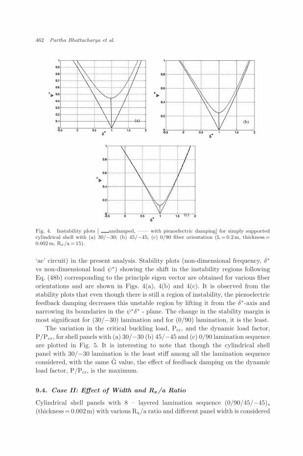
Fig. 4. Instability plots [ undamped, —— with piezoelectric damping] for simply supportedcylindrical shell with (a) 30/−30; (b) 45/−45; (c) 0/90 fiber orientation (L =0.2m, thickness =0.002 m, Rx/a =15).

‘ac’ circuit) in the present analysis. Stability plots (non-dimensional frequency, δ∗

vs non-dimensional load ψ∗) showing the shift in the instability regions following

Eq. (48b) corresponding to the principle eigen vector are obtained for various fiber

orientations and are shown in Figs. 4(a), 4(b) and 4(c). It is observed from the

stability plots that even though there is still a region of instability, the piezoelectric

feedback damping decreases this unstable region by lifting it from the δ∗-axis and

narrowing its boundaries in the ψ∗δ∗ - plane. The change in the stability margin is

most significant for (30/−30) lamination and for (0/90) lamination, it is the least.

The variation in the critical buckling load, Pcr, and the dynamic load factor,

P/Pcr, for shell panels with (a) 30/−30 (b) 45/−45 and (c) 0/90 lamination sequence

are plotted in Fig. 5. It is interesting to note that though the cylindrical shell

panel with 30/−30 lamination is the least stiff among all the lamination sequence

considered, with the same G value, the effect of feedback damping on the dynamic

load factor, P/Pcr, is the maximum.

9.4. Case II: Effect of Width and Rx/a Ratio

Cylindrical shell panels with 8 – layered lamination sequence (0/90/45/−45)s

(thickness = 0.002m) with various Rx/a ratio and different panel width is considered



Fig. 5. Variation in dynamic load factor, P/Pcr, (with feedback damping) and critical bucklingload, Pcr for simply supported cylindrical shells with different fiber orientations (a = 0.05 m,thickness = 0.002 m, L =0.2m, Rx/a =15).

for this study. Results are obtained for (i) simply supported and (ii) cantilever shell

panels. The four different Rx/a ratio used for the present study are (a) 15 (b) 50

(c) 100 and (d) 1030 (plate). The width, ‘a’, considered are (i) 0.05m (ii) 0.1m

and (iii) 0.2m. The length, L, of the shell panel is taken as 0.2 m for all the cases.

For cantilever panels, the edge along y = L is locked and along y = 0, axial load

is applied. For simply supported shell panels, pinned conditions are applied along

y = 0 and along y = L roller support is simulated. Axial load is applied along the

edge, y = L. The size, orientation and the feedback gain value for the piezo pair is

kept unaltered as considered in Case I. For simply supported case, the piezo pair

is located centrally along the panel length. For cantilever shell panel, the piezo

patches are placed at a distance of 0.0125m from the fixed end along the longitudi-

nal axis and centrally along the width. This is done to ensure the piezo patch can be

subjected to maximum strain under dynamic condition in the first vibration mode.

The effect on the dynamic load factor P/Pcr for cantilever shell panel due to

feed back damping for various Rx/a and varying width are presented in Fig. 6. In

Fig. 7, the results for simply supported shell panels are presented.

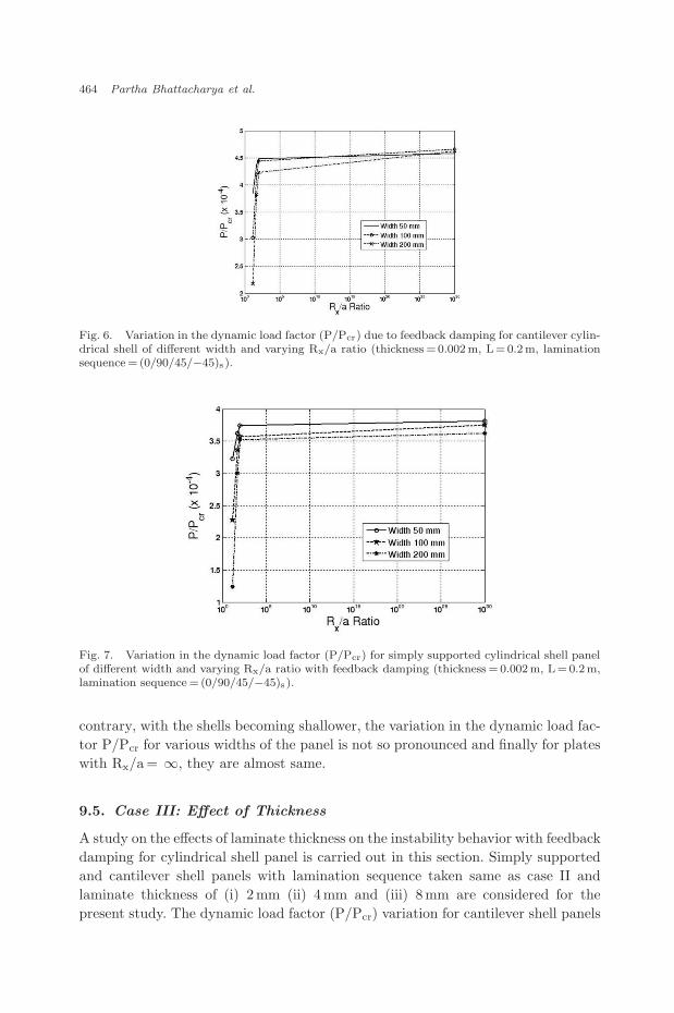
It is observed from Figs. 6 and 7 that the shift in the critical dynamic load

factor (P/Pcr) leading to the alteration of the stability zone with the introduction

of feedback damping is more pronounced for shallow shells with higher Rx/a ratio.

This can be explained from the fact that deep shells with low Rx/a ratio are stiffer in

comparison to shallow shells and hence have lower velocity amplitude. The feedback

damping is a function of the feedback voltage, which in turn is proportional to

velocity amplitude and hence the effectiveness of the feedback damping for deep

shells is less pronounced. Changing the feedback gain value, G one can further

widen the stability zone.

It is also seen that for deep shells, the panels with higher a/L ratio, the con-

trol effectiveness for the same amount of control gain is significantly less. On the



Fig. 6. Variation in the dynamic load factor (P/Pcr) due to feedback damping for cantilever cylin-drical shell of different width and varying Rx/a ratio (thickness =0.002 m, L= 0.2m, laminationsequence = (0/90/45/−45)s).

Fig. 7. Variation in the dynamic load factor (P/Pcr) for simply supported cylindrical shell panelof different width and varying Rx/a ratio with feedback damping (thickness = 0.002m, L = 0.2m,lamination sequence = (0/90/45/−45)s).

contrary, with the shells becoming shallower, the variation in the dynamic load fac-

tor P/Pcr for various widths of the panel is not so pronounced and finally for plates

with Rx/a = ∞, they are almost same.

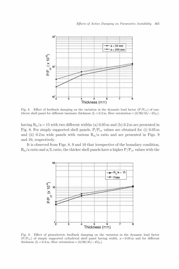
9.5. Case III: Effect of Thickness

A study on the effects of laminate thickness on the instability behavior with feedback

damping for cylindrical shell panel is carried out in this section. Simply supported

and cantilever shell panels with lamination sequence taken same as case II and

laminate thickness of (i) 2mm (ii) 4mm and (iii) 8mm are considered for the

present study. The dynamic load factor (P/Pcr) variation for cantilever shell panels



Fig. 8. Effect of feedback damping on the variation in the dynamic load factor (P/Pcr) of can-tilever shell panel for different laminate thickness (L =0.2 m, fiber orientation = (0/90/45/−45)s).

having Rx/a = 15 with two different widths (a) 0.05m and (b) 0.2m are presented in

Fig. 8. For simply supported shell panels, P/Pcr values are obtained for (i) 0.05m

and (ii) 0.2m wide panels with various Rx/a ratio and are presented in Figs. 9

and 10, respectively.

It is observed from Figs. 8, 9 and 10 that irrespective of the boundary condition,

Rx/a ratio and a/L ratio, the thicker shell panels have a higher P/Pcr values with the

Fig. 9. Effect of piezoelectric feedback damping on the variation in the dynamic load factor(P/Pcr) of simply supported cylindrical shell panel having width, a=0.05 m and for differentthickness (L = 0.2m, fiber orientation = (0/90/45/−45)s).



Fig. 10. Effect of feedback damping on the variation in the dynamic load factor (P/Pcr) of simplysupported shell having width, a = 0.2 m and for different thickness (L = 0.2m, fiber orientation =(0/90/45/−45)s).

introduction of piezoelectric damping for the same feedback gain value. This implies

that for thick shell panels the instability region narrows down more as compared to

thin shell panels in the ψ∗δ∗ - plane. The piezo patches are surface bonded and for

the thicker panels, the patches being located further away from the neutral axis,

the effectiveness of the patches increases.

The plots in Fig. 8 indicates that the change in the P/Pcr values for the cylin-

drical shell panels with higher aspect ratio, a/L, is more significantly affected with

the variation in the laminate thickness.

Comparing Figs. 9 and 10 it is observed that for simply supported cylindrical

shell panels with low Rx/a ratio (deep shell), the change in the P/Pcr values with

the variation in thickness is more significant in the panels having high aspect ratio,

a/L. Whereas, for plates (Rx/a = ∞), the variation in the P/Pcr values is identical

irrespective of the aspect ratio, a/L.

9.6. Case IV: Effect of Feedback Gain

In the present section the effect of feedback gain value on the stability margin of

a simply supported shell structure is studied. Circular cylindrical shell panel with

a 2-layered lamination sequence (30/−30) with length, L, of 0.2m, width, a, of

0.05m and Rx/a of 15 is considered for the present analysis. The different feedback

gain values G considered for the present study are (a) 4 × 107 (b) 6 × 107 (c)

1 × 108 (d) 2 × 108 and (e) 4 × 108. The effect of the variable feedback gain on the

stability margin is presented in Fig. 11 (a – e). It is observed that for the same shell



Fig. 11. Instability plots [ undamped, —— with piezoelectric damping] for simply supportedshell (L =0.2m and W= 0.5m and Rx/a= 15) with fiber orientation (30/−30) for different valuesof feedback damping a) 4 × 107; b) 6 × 107; c) 1 × 108; d) 2 × 108; e) 4 × 108.

configuration, higher the feedback gain greater is the stability margin which follows

the observation reported in Case II.

10. Conclusions

In the present paper parametric instability analysis with feedback damping for

laminated composite cylindrical shell panels has been carried out. The finite element

modeling of the shell panel is based on Sander’s shallow shell theory with first order

shear deformation and rotary inertia being taken into account. A feedback control

strategy involving PVDF sensor patches and IDE – PFC actuators is modeled.

The resulting dynamic equilibrium equation is reduced into the classical Mathieu-

Hill form and solved using the method of strained parameter. Effects of lamination

sequence, boundary condition, shell thickness, aspect ratio (a/L) and shell depth

(Rx/a ratio) with feedback damping on the instability behavior are examined.

It is evident that the effect of feedback damping on the dynamic load factor

(P/Pcr) is more pronounced for cantilever shells. Shell thickness plays a very impor-

tant role in the shift of the dynamic load factor, with the piezoelectric feedback



damping mechanism more effective for panels with higher thickness. It can also be

concluded that shell panels with low aspect ratio are better controllable in terms

of dynamic load factor for the same amount of control gain. The layup sequence

has also a major role in the change of instability behavior with the introduction

of feedback damping. It is further observed that with the increase in the feedback

damping constant one can significantly reduce the instability margins for paramet-

rically excited shell structures.

Appendix

List of Symbols

ε Strain vector

ν Poisson’s ratio[

ξP]

Electric permittivity or dielectric matrix

ρ Material Density

[ρ] Inertia matrix

σ Stress vector

φa Electric potential on actuator

φsensor Sensor voltage

[ψ] Modal state vector

ω Natural frequency

[C] Damping matrix

D Electrical displacement vector

d,

d

,

d

Generalized displacement, velocity and acceleration vector

E Electrical field vector

[d] Piezoelectric strain/electric field coefficient

[e] Piezoelectric stress/charge coefficient

E11, E22, E33 Young’s modulus

f Mechanical traction

Fel Electric load vector

FM Applied mechanical edge load

G12, G23, G31 Shear modulus

hide Spacing of interdigitated electrode

[Kuu] Mechanical stiffness matrix

[Kuφ] Electro-mechanical coupling stiffness matrix

[Kφφ] Electrical stiffness matrix

[Ks] Sensor stiffness matrix

[Kσ] Geometric stiffness matrix

[M] Mass Matrix

M, C, K, Kσ Modal Matrices

M Moment resultant

N In-plane force resultant



N3 Shear force resultant

P Applied axial edge load

Pcr Critical buckling load

[Q] Elastic modulli matrix

[Q] Transformed elastic modulli matrix

Q Electrical charge

Rx Radius of curvature along X axis

Ry Radius of curvature along Y axis

Rxy Radius of twist curvature

Rf Piezo resistance

[s] Compliance matrix

[Sσ] Stress Matrix

u Modal displacement vector

[Z] Position matrix of the Piezo patch, measured from

neutral axis

References

Afsar, K. R. and Masoud, K. K. [1994] “Damping of parametrically excited single degreeof freedom system,” International Journal of Nonlinear Mechanics, 29, 421–428.

ANSYS Users Manual, Release 11.0, ANSYS, Inc., 2007.Argento, A. and Scott, R. A. [1993a] “Dynamic instability of layered anisotropic circular

cylindrical shells, part I: theoretical development,” Journal of Sound and Vibration,162, 311–322.

Argento, A. and Scott, R. A. [1993b] “Dynamic instability of layered anisotropic circularcylindrical shells, part II: Numerical results,” Journal of Sound and Vibration, 162,323–332.

Argento, A. and Scott, R. A. [1993c] “Dynamic instability of a composite circular cylin-drical shell subjected to combined axial and torsional loading,” Journal of Composite

Materials, 27, 1722–1738.Azzouz, M. S., Mei, C., Bevan, J. S., and Ro, J. J. [2001] “Finite Element Modeling

of MFC/AFC actuators and performance of MFC,” Journal of Intelligent Material

System and Structures, 12, 601–612.Beliaev, N. M. [1924] “Stability of prismatic rods, subject to variable longitudinal

forces,” Collection of Papers: Engineering Construction and Structural Mechanics,Put’, (Leningrad), pp. 149–167.

Bent, A. A. [1997] “Active fiber composites for structural actuation,” PhD Thesis, MIT,USA.

Bhattacharya, P., Homann, S., and Rose, M. [2006] “A Study of the effects of Piezo Actu-ated Damping on Parametrically Excited Laminated Composite Plates,” Journal of

Reinforced Plastics and Composites, 25(8), 801–813.Birman, V. and Bert, C. W. [1988] “Parametric Instability of Thick, orthotropic, Circular

Cylindrical Shells,” Acta Mechanica, 71, 61–76.Bolotin, V. V. [1963] Non-conservative Problems of the Theory of Elastic Stability (Perg-

amon Press, New York).Bolotin, V. V. [1964] Dynamic Stability of Elastic Systems (Holden day, San Francisco)



Brown, J. E., Hutt, J. M., and Salama, A. E. [1968] “Finite Element Solution to DynamicStability of Bars”, AIAA Journal, 6, 1423–1425.

Cederbaum, G. [1992] “Analysis of parametrically excited laminated shells,” International

Journal of Mechanical Sciences, 34, 241–250.Chen, S. S. [1987] Flow Induced Vibration of Circular Cylindrical Structures (Hemisphere

Publishing Corporation, placeStateNew York).Datta, P. K. and Sahu, S. K. [2003] “Dynamic Stability of Curved Panels with Cutouts,”

Journal of Sound and Vibration, 251(4), 683–696.Evan Iwanowski, R. M. [1965] “On the parametric response of structures,” Applied Mechan-

ics Review, 18, 699–702.Faraday, M. [1831] “On a peculiar class of acoustical figures and on certain forms assumed

a group of particles upon vibrating elastic surfaces,” Philosophical Transactions of the

Royal Society of London, 20(258), 299–318.Gol’denblatt, I. I. [1947] Contemporary Problems of Vibrations and Stability of Engineering

Structures (Stroiizdat, Moscow).Guennam, A. E. and Luccioni, B. M. [2006] “FE modeling of a closed box beam with

piezoelectric fiber composite patches,” Smart Materials and Structures, 15, 1605–1615.Javidruzi, M. et al. [2004] “Vibration, buckling and dynamic stability of cracked cylindrical

shells,” Thin-Walled Structures, 42, 79–99.Krylov, N. M. and Bogoliubov, N. N. [1935] “Calculations of the vibrations of frame

construction with consideration of normal forces and with the help of the methods onnonlinear mechanics,” Investigation of Vibration of Structures, ONTI Kharkov/Kiev,5, 5–24.

Kwon, Y. W. [1991] “Finite element analysis of dynamic instability of layered compositeplates using a higher order bending theory,” Computers and Structures, 38(1), 57–62.

Mettler, E. [1942] “About the stability of a forced vibrations of elastic systems,” Ing-Arch,13, 97–103.

Mustafa, G. and Ertas, A. [1995] “Experimental evidence of quasi-periodicity and its break-down in the column-pendulum oscillator,” Journal of dynamic system, measurement

and control, 117, 128–225.Nayfeh, A. H. and Mook, D. T. [1995] Nonlinear Oscillations (John Willey and Sons, New

York).Oueini, S. S. [1999] “Techniques for controlling structural vibrations,” Ph.D. Thesis, Vir-

ginia Polytechnic and State University.Patel, S. N., Datta, P. K. and Sheikh, A. H. [2006] “Buckling and dynamic instability

analysis of stiffened shell panels,” Thin-Walled Structures, 44, 321–333.Piszczek, K. [1955] “Longitudinal and transversal vibrations of a rod subjected to an

axially pulsating force, taking into account nonlinear members into consideration,”Arch. Mech., 7, 345–362.

Ravi Kumar, L., Datta, P. K. and Prabhakara, D. L. [2003] “Tension buckling and dynamicstability behavior of laminated composite doubly curved panels subjected to partialedge loading,” Composite Structures, 60, 171–181.

Reddy, J. N. [1984] “Exact Solutions of Moderately Thick Laminated Shells,” Journal of

Engineering Mechanics, 10(5), 794–809.Reissner, E. [1945] “The effect of transverse shear deformation in bending of elastic plates,”

Journal of Applied Mechanics, 18, 69–77Reissner, E. [1950] “Small bending and stretching of sandwich type shells,” Report 975,

National Advisory Committee for Aeronautics, Washington DC.



Sahu, S. K. and Datta, P. K. [2001] “Parametric resonance characteristics of laminatedcomposite doubly curved shells subjected to non-uniform loading,” Journal of Rein-

forced Plastics and Composites, 20(18), 1556–1576.Sirohi, J. and Chopra, I. [2000] “Fundamental Understanding of Piezoelectric Strain Sen-

sors,” Journal of Intelligent Material Systems and Structures, 11, 246–257.Srinivasan, R. S. and Chellapandi, P. [1986] “Dynamic stability of rectangular laminated

composite plates,” Computers and Structures, 24(2), 233–238.IEEE Standard on Piezoelectricity, [1987], ANSI/IEEE Std. 176.Piezo Film Sensors Technical Manual, 1999] Measurements Specialities, Inc., Sensor Prod-

ucts Division.

Effects of Active Damping on Parametric Instability of Composite Cylindrical Shells Using Piezo...

Documents

Transcript of Effects of Active Damping on Parametric Instability of Composite Cylindrical Shells Using Piezo...