Effectiveness of Countercyclical Fiscal Policy: Time-Series Evidence from Developing Asia

This article appeared in a journal published by Elsevier. The attachedcopy is furnished to the author for internal non-commercial researchand education use, including for instruction at the authors institution

and sharing with colleagues.

Other uses, including reproduction and distribution, or selling orlicensing copies, or posting to personal, institutional or third party

websites are prohibited.

In most cases authors are permitted to post their version of thearticle (e.g. in Word or Tex form) to their personal website orinstitutional repository. Authors requiring further information

regarding Elsevier’s archiving and manuscript policies areencouraged to visit:

http://www.elsevier.com/authorsrights

http://www.elsevier.com/authorsrights

Author's personal copy

Effectiveness of countercyclical fiscal policy: Evidence fromdeveloping Asia q

Shikha Jha a, Sushanta K. Mallick b,⇑, Donghyun Park a, Pilipinas F. Quising a

a Asian Development Bank, Macroeconomics and Finance Research Division, Economics and Research Department, 6 ADB Avenue, Mandaluyong City, MetroManila 1550, Philippinesb Queen Mary University of London, School of Business and Management, Mile End Road, London E1 4NS, United Kingdom

a r t i c l e i n f o

Article history:Received 26 January 2013Accepted 18 February 2014Available online 1 March 2014

JEL classification:E60E62E63H20H50H60

Keywords:Countercyclical fiscal policySVARDeveloping AsiaStructural shocksTax cutsGovernment spending

a b s t r a c t

Can discretionary fiscal policy effectively stimulate output? This paper examines this ques-tion in the context of developing Asia, where many countries implemented fiscal stimulusmeasures to support domestic demand during the global crisis. Economic conditions nor-malized after the crisis but growth in Asia has slowed down since. We examine historicaldata from 10 emerging Asian countries to assess whether countercyclical fiscal policy cansupport future growth in the region. Our examination is based on identifying shocks byrestricting the contemporaneous relation between fiscal and non-fiscal variables. Our mostsignificant and consistent finding is that in developing Asia, tax cuts have a greater coun-tercyclical impact on output than government spending. This implies there is some scopefor countercyclical tax adjustments so long as fiscal sustainability is not compromised.

� 2014 Elsevier Inc. All rights reserved.

1. Introduction

The issue of whether fiscal policy enhances or retards long-run economic activity has long been debated in the literature.Among others, two contrasting views come from the basic Keynesian and Ricardian theories. In the simple Keynesian worldof rigid prices, aggregate demand determines output. In this world, consumption responds to current income, and fiscalexpansion has a multiplier effect on growth.1 In contrast, the fiscal multiplier is zero under Ricardian equivalence betweentaxes and debt in a dynamic framework. In this case, Ricardian consumers are forward-looking and fully aware of the

http://dx.doi.org/10.1016/j.jmacro.2014.02.0060164-0704/� 2014 Elsevier Inc. All rights reserved.

q We gratefully acknowledge the constructive comments by an anonymous referee of this journal and the editor, William D. Lastrapes, to improve theprevious version of this paper.⇑ Corresponding author. Tel.: +44 20 78827447; fax: +44 20 78823615.

E-mail addresses: [email protected] (S. Jha), [email protected] (S.K. Mallick), [email protected] (D. Park), [email protected] (P.F. Quising).1 Fiscal multiplier – the increase in output due to a one dollar increase in government spending or one dollar reduction in taxes – is the underlying concept

which measures how effectively tax cut or government spending stimulates output.

Journal of Macroeconomics 40 (2014) 82–98

Contents lists available at ScienceDirect

Journal of Macroeconomics

journal homepage: www.elsevier .com/ locate/ jmacro


government’s intertemporal budget constraint. Since they know that a tax cut today will be financed by higher taxes in the fu-ture, their consumption does not change because their permanent income is unaffected.2 Similarly, the knowledge that an in-crease in government spending by borrowing today will be offset by future spending cuts leaves output unaffected.

The effectiveness of countercyclical fiscal policy in reality will depend not only on its size but also on its composition –i.e., the relative importance of tax cuts versus government spending. Intuitively, it is tempting to believe that governmentspending has a bigger influence on output since it has a more immediate impact on aggregate demand. Public spending in-volves government’s direct purchase of goods and services including spending on public works and infrastructure such asroads and power plants. On the other hand, tax cuts have a less direct impact on aggregate demand since their effectivenessultimately depends on the willingness of households and firms to spend the additional income resulting from tax cuts. How-ever, the relative effectiveness of tax cuts versus government spending in boosting aggregate demand is ultimately an empir-ical issue which cannot be settled by economic intuition alone.

This paper therefore seeks to examine these issues in the context of developing Asia. While the region has a relativelylimited experience of using fiscal policy for countercyclical purposes, many Asian countries boldly implemented large fiscalstimulus programs during the global financial and economic crisis of 2008–2009. According to conventional wisdom, the fis-cal expansion helped the region stave off severe recession during the crisis by supporting aggregate demand at a time ofplummeting private and external demand. Going forward, the key question is whether countercyclical fiscal policy cansmooth out the business cycles in an uncertain and volatile post-crisis world.

Typically, fiscal policy tends to be less countercyclical in developing countries than in high-income countries. For exam-ple, Kaminsky et al. (2005) demonstrate that emerging markets’ fiscal policies are predominantly pro-cyclical and thus exac-erbate rather than moderate the business cycle. Moreover, in low-income countries, automatic stabilizers are pro-cyclicaldue to institutional failures and lack of access to finance during economic downturns, as in Kraay and Servén (2008). Thismeans that governments in these countries increase spending in good times and cut back in bad times, potentially impairingfiscal sustainability. Ilzetzki and Végh (2008) provide further evidence that fiscal policy, especially government expenditure,is indeed pro-cyclical in developing countries. Besides, with large informal sectors whose activities remain unrecorded,developing-country governments tend to face large fluctuations in their tax bases compared to advanced countries, as inTalvi and Végh (2005). Such cyclical fluctuations in tax bases can create large revenue shocks with bigger output effect, espe-cially since the tax-GDP ratio averages only about 9–11% in low-income countries, including those in South Asia and in EastAsia and Pacific, in comparison with 14–16% in high-income countries.3

In addition, since developing country governments do not follow strict fiscal policy rules (or automatic stabilizers),4 dis-cretionary fiscal policy could account for much of the changes in fiscal activity. In particular, the experience of developing Asiancountries shows that the role of automatic stabilizers is relatively small and fiscal policy interventions have been primarily dis-cretionary, as in Jansen (2004). Also, Ilzetzki et al. (2011) contribute to this debate on the real effects of fiscal stimuli by showingthat the output effect of an increase in government expenditure is larger in industrial than in developing countries. Finally, awidespread perception – a perception which will be empirically investigated in this paper – that fiscal stimulus mitigatedthe impact of the global crisis on Asia’s output during this crisis period has awakened interest in countercyclical fiscal policythroughout the region. All of these factors motivate us to examine the effectiveness of fiscal shocks in the context of Asia.

Using historical quarterly time-series data for 10 emerging Asian countries within a Structural Vector Auto-regression(SVAR) framework, this paper analyzes what type of fiscal policy – tax cuts versus higher spending – works best duringtroughs in business cycles. The most significant and consistent finding from our analysis is that a government revenue(tax) shock has a bigger countercyclical output effect than a government expenditure shock in developing Asia. More spe-cifically, the comparison of output multipliers reveals that deficit-financed tax cuts stimulate economic activity whereas def-icit spending has a largely insignificant impact on output.

2. Countercyclical fiscal policy – empirical evidence

Until recently the business cycle effects of fiscal policy were not given much attention. In this empirical literature, thereare substantial recent studies on this topic in the context of key major economies but much disagreement remains. Moststudies apply SVAR methods aiming at identifying the usual reactions of the aggregate variables to the exogenous shocksin fiscal policy. See for example Blanchard and Perotti (2002), Burnside et al. (2003), Galí et al. (2007), and more recentlyBurriel et al. (2010) and Mountford and Uhlig (2009). However, the evidence is mixed and most of the papers focus on OECD,G7 and other industrial economies.

The evidence from a large and growing number of studies that have estimated the size of the fiscal multiplier is far fromconclusive. Those studies have produced a wide range of estimates, ranging from negative to more than one. For example,according to Spilimbergo et al. (2009), the overall evidence from the literature indicates that the multiplier for governmentspending is larger than that for tax cuts. Spilimbergo et al. (2009) put forth the following rule of thumb for government

2 If a tax cut is permanent, then private consumption could go up, although it has inter-generational implications. Thus there is no unambiguous effect of atax-cut, making it an empirical issue for further investigation.

3 http://data.worldbank.org/indicator/GC.TAX.TOTL.GD.ZS/countries/8S-4E-XD-XM-XO?display=graph.4 For the spending stabilizer, there must be an automatic increase (reduction) in total government expenditure when output gap declines (increases),

whereas for the tax stabilizer, the tax rate should automatically fall (rise) when output gap falls (rises).

S. Jha et al. / Journal of Macroeconomics 40 (2014) 82–98 83


consumption – a multiplier of 1–1.5 in large countries, 0.5–1 in medium sized countries and 0.5 or less in small open econ-omies. The same rule of thumb postulates multipliers of only about half the above values for tax cuts and transfer paymentsand slightly larger multipliers for government investment. Baldacci et al. (2009) also find fiscal expansions based on govern-ment consumption to be more effective than those based on public investment or income tax cuts. Romer and Bernstein(2009) estimated the multipliers of US government spending and tax cuts to be 1.57 and 0.99 respectively.

Interestingly, a number of studies contradict the intuitively plausible notion that government spending has a bigger im-pact on output than tax cuts. For example, Caldara and Kamps (2008) present a VAR-based comparative analysis, using fourdifferent approaches: recursive, Blanchard–Perotti, sign-restrictions and event-study. They note that government spendingshocks yield very similar results both qualitatively and quantitatively but tax shocks yield strongly diverging results. Romerand Romer (2010) find that one dollar of tax cuts historically raised US GDP by about three dollars. A multiplier of 3 is farhigher than most of the estimated multipliers for government spending. For example, the empirical results of Ramey (2011)imply a government spending multiplier of 1.4, and this is on the high end of estimates. The somewhat surprising implica-tion is that tax cuts have a bigger effect on economic activity than government spending. However, Romer and Romer (2010)are not alone in uncovering a stronger impact of tax cuts. Applying the latest econometric methodology to US data,Mountford and Uhlig (2009) find that deficit-financed tax cuts have a bigger effect than deficit-financed spending ortax-financed spending.

In a comprehensive analysis of 91 episodes of fiscal expansions in 21 OECD countries since 1970, Alesina and Ardagna(2009) compared expansions which brought about output growth with those that failed to do so. Strikingly, successful fiscalstimulus programs were based almost entirely on tax cuts whereas unsuccessful programs were based mostly on additionalgovernment spending. Blanchard and Perotti (2002) find that higher taxes and higher government spending have a strongnegative effect on private investment. Similarly, Mountford and Uhlig (2009) find the cumulative multipliers for revenue(tax) shocks for the US to be typically greater than the spending shocks; and both increases in taxes and increases in gov-ernment spending have a negative effect on consumption and investment spending. This suggests a possible explanationfor why some studies find tax cuts to be more expansionary than government spending. Tax cuts may further boost outputby stimulating investment while the positive effect of government spending may be largely offset by lower private invest-ment. Perotti (1999) also finds that government revenue shocks have very different effects on private consumption in timesof fiscal stress than in normal times. In this context, for the US, Taylor (2009) and Cogan et al. (2010) find that the govern-ment spending multipliers from permanent increases in federal government purchases are much less in new Keynesianmodels than in old Keynesian models, with the multipliers being less than one as consumption and investment are crowdedout, and turning negative as the government purchases decline in the later years of their simulation. Besides, when the zerolower bound on nominal interest rates binds, monetary policy fails to provide appropriate stimulus; thus in a New Keynesianmodel, Correia et al. (2013) show that tax policy can deliver such stimulus at no cost and in a time-consistent manner ratherthan wasteful public spending or future commitments to low interest rates.

This lack of clear-cut empirical evidence helps explain why economists are deeply divided about the usefulness of coun-tercyclical fiscal policy as a tool for fighting recessions. Moreover, unlike the plethora of studies on industrialized countriesdebating whether tax cuts are more effective than government spending, there is only limited evidence about the issue in thedeveloping world. Hemming et al. (2002), who summarize theoretical and empirical literature on the effectiveness of fiscalpolicy in stimulating economic growth, note that given data deficiencies and institutional weaknesses, there is no clear con-clusion on the size and sign of fiscal multipliers in developing countries. To some extent, this simply mirrors the fact thatindustrialized countries have a longer tradition of using fiscal policy for countercyclical purposes. Using data from develop-ing Asia, this paper attempts to fill this gap in the literature by empirically examining the relative effectiveness of tax cutsversus government spending in boosting aggregate demand during troughs in business cycles and in so doing, gives the re-gion’s policymakers some guidance on how to maximize the impact of scarce fiscal resources.

3. Empirical framework

To analyze the dynamic effects of unexpected shocks in government spending and revenues on economic activity, whichcan be different across countries, this paper considers SVAR models using historical quarterly time-series from emergingAsian economies. It applies Mountford and Uhlig (2009) methodology to identify fiscal shocks alongside other shocks byimposing sign restrictions for the identification of each shock. Explicit identifying sign-restrictions are imposed to isolateexogenous and unanticipated changes in these variables by restricting the contemporaneous interaction of fiscal and non-fiscal variables. Although sign-restricted models by construction are restrictive in some sense relative to the standard SVARmodels (see Fry and Pagan, 2011), we use Uhlig’s penalty function approach which has the advantage of only picking up largeshocks and thereby reducing the variation in the identified shocks as we are trying to explain the variation in the macroeconomy using n or less number of shocks (where n is the dimension of the VAR).

The VAR model and its residuals can be represented as follows. Consider the reduced-form VAR that has a MArepresentation:

Yt ¼ A1Yt�1 þ ut

Yt ¼ ðI � A1LÞ�1ut ¼ BðLÞut

84 S. Jha et al. / Journal of Macroeconomics 40 (2014) 82–98


The usual SVAR approach assumes that the error terms, ut, are related to structural macroeconomic shocks, vt, via a matrix P:ut = Pvt, where P is the unique lower triangular matrix such that PP0 = Ru. The sign-restriction based orthogonalization can berecovered by post-multiplying P for a non-singular matrix K which exhibits orthonormal columns such that sign restrictionson the impulse responses are satisfied. It will then be possible to derive a new matrix C = PK, whose columns are the iden-tified impulse vectors.

Although the VAR model here includes eight macroeconomic variables, we identify only four structural shocks, whichmeans the shocks and the associated impulse vectors are selected by discarding those vectors which do not satisfy the im-posed sign restrictions. Since we identify four structural shocks, we leave some structural disturbances unidentified. Giventhe four identified shocks, the VAR residuals, ut, can be represented as:

ut ¼ C1vBCt þ C2vMP

t þ C3vGRt þ C4vGE

t þ bC 0v̂ t

where BC denotes the business cycle shock, MP denotes the monetary policy shock, GR denotes the government revenueshocks and GE denotes the government expenditure shock. With each structural shock, the associated impulse vector isCi. As there are less number of shocks than the number of variables in the VAR, the unidentified shocks in vector v̂ , are asso-ciated with the remaining columns of the matrix, bC . The horizon, k, of the imposed restrictions is four quarters in our model.Penalty function approach is employed which penalizes the opposite responses of the imposed sign restrictions for eachshock under minimization of a criterion function over four quarters. It is important to note that the Mountford–Uhlig tech-nique is computationally intensive, and takes a significant amount of time to run.

The basic intuition is that structural shocks can be identified by checking whether the signs of the corresponding impulseresponses are in line with the theoretical priors. Four identified structural shocks are: business cycle shocks, monetaryshocks, and fiscal shocks (revenue shocks and government spending shocks). A fiscal shock is a surprise change in fiscal pol-icy, which has two dimensions – government revenue or expenditure – and those fiscal shocks should be separated from(orthogonal to) business cycle or monetary shocks. By imposing sign restrictions on the shape of the impulse responses,the relative movements of endogenous variables are captured. Thus, whenever taxes and output move in the same direction,this is attributed to a business cycle shock. And, the reasoning holds similarly for spending and output. These sign restric-tions help identify the effects of unanticipated fiscal shocks and non-fiscal shocks on the following endogenous variables:GDP – real GDP; EXP – real government expenditure; REV – real government revenue; INT – interest rate (benchmark policyrate); MON – real broad money; DEF – GDP deflator; CON – real consumption; and INV – real investment.

All the variables are expressed in log levels except the interest rate and they depend on each other through their laggedvalues. The optimal lag length is determined endogenously. In Uhlig’s methodology, the VAR does not contain a constant or atime trend. But including a constant and a time trend does help smooth the impulse responses. Hence, we use a constant inthe VAR, as there could be several shifts in the data series for emerging economies. To see whether a particular theory (orchannel) is accepted, restrictions are imposed on the contemporaneous effects of shocks. The channel of transmission iseither government spending directly affecting output or a tax cut leading to higher private consumption or private invest-ment and thereby higher output. The responses can be sensitive depending on what variables and what sample periods areincluded in the model. The effectiveness depends on whether the cumulative multiplier of a policy shock is significant, andwhich type of policy (deficit financed tax cut or government spending) has a dominant effect.

The set of sign restrictions imposed to identify different shocks is presented in Table 1. In identifying the fiscal shocks, norestrictions are imposed on the variables of interest: GDP, consumption, investment, and inflation. Following a business cycleshock (output growth/contraction) which should be identified first, the monetary authority is more likely to change its policystance (a monetary shock should be identified next), and finally the fiscal authority introduces either a spending rise or taxcut (a fiscal shock). So the impact of these shocks is checked sequentially to investigate whether fiscal policy shocks do helpan economy to increase its output. From these effects, one can conclude in which countries fiscal policy is more effective. Wealso carry out a variance decomposition exercise to show which shock (tax cut or spending increase) has a dominant effecton the economy.

4. Data sources and adjustments

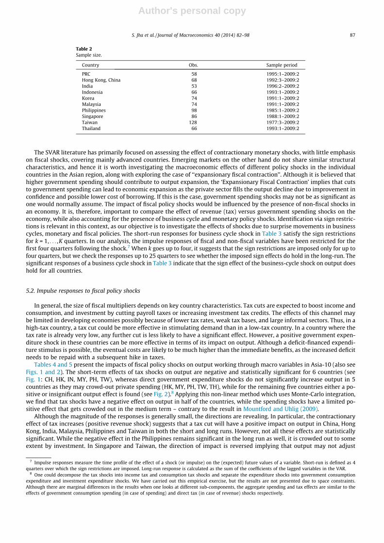
We use the current historical data which allow us to assess how quickly and in which direction a particular economy re-sponds to unexpected shocks. The series is based on quarterly data for 10 emerging Asian economies (‘Asia-10’ in short) –People’s Republic of China (PRC), Hong Kong, China; India, Indonesia, Korea, Malaysia, Philippines, Singapore, Taiwan; andThailand (Table 2). All variables are estimated with four lags for most countries, except India where we have used two lagsdue to relatively small sample leading to non-convergence with higher order lags.5

The data are compiled from CEIC and Datastream databases, and are adjusted as follows:

5 We have however checked the robustness of our VAR results with higher order lags up to 6, as raised in Kilian (2001), but the results remain consistent withhigher order lags; hence we presented the impulse response results with the optimal VAR lag length ranging from 2 to 5 for different countries following the lagorder selection criteria.



(1) Real and nominal GDP in local currency units are used. GDP deflator is derived as: (nominal/real GDP), and used as theprice series for all countries.

(2) Policy rate from each country is used as a proxy for short-term interest rate. The definition of policy rate however dif-fers across countries as follows: PRC: 1-year lending rate; Hong Kong, China: discount rate; India: repo rate; Indonesia:SBI rate; Korea: overnight call rate; Malaysia: overnight policy rate; Philippines: repurchase rate; Singapore: bench-mark SIBOR 3-months rate; Taiwan: rediscount rate; Thailand: BOT policy rate.

(3) Real private consumption and real fixed investment, in local currency units are used. Whenever these variables areavailable only in nominal terms, the series is deflated using the calculated GDP deflator. As the PRC does not releasequarterly statistics for its GDP components, we have generated quarterly series from the annual data for private con-sumption and gross capital formation in real terms from national accounts by using a temporal disaggregation tech-nique that follows the pattern in the quarterly Chinese real GDP while maintaining the sum of the new quarterly seriesto the original annual series over each period.

(4) Government total revenue and expenditure in current prices are deflated by the GDP deflator in order to be expressedin real terms. We have converted annual fiscal data to quarterly series for Indonesia before 2000, by using the quar-terly pattern in government consumption expenditure that is available on a quarterly basis from national accounts.

(5) Broad money supply is M2 for all countries. Nominal M2 values have been deflated by the GDP deflator to get realmoney balances.

To get a longer consistent time series for Indonesia, Malaysia and South Korea, we have also rebased all the earlier GDPdata and its components (2000 base year) to be comparable with the recent data (2005 base year). Given the different dataavailability across countries, the use of the Uhlig sign restriction identification methodology allows for a very similar iden-tification to be achieved across countries despite these data differences. This is because the Uhlig identification strategyidentifies shocks using mild restrictions on multiple time series in all economies regardless of how they are measuredand regardless of data idiosyncrasies and hence data definition used in an individual country for a particular variable is ofsecondary importance, see Rafiq and Mallick (2008) for details.

5. Results from the empirical analysis

5.1. Identification via Mountford–Uhlig sign-SVAR approach

The identification of the structural disturbances relies on the theoretical sign restrictions discussed earlier. The signrestrictions methodology is robust to the ordering of variables, which indeed makes the results sensitive in the case ofthe traditional recursive/non-recursive ordering in the standard SVAR approach.6 So the ordering of shocks is not relevantin the sign-SVAR since the restrictions on the signs of IRFs are doing the job of identifying the shocks. Both revenue (tax) shocksand spending shocks are identified with separate sign restrictions along with business cycle and monetary policy shocks, whichmeans the shocks are drawn orthogonal to one another i.e., the shocks are uncorrelated. Hence it is immaterial whether they areeither orthogonal only to the business cycle shock or orthogonal to both the business cycle and monetary policy shocks.Although one could check the effect of a fiscal shock by imposing weaker identifying restrictions, such as restricting governmentspending alone to be positive on impact, such identification will hide the presence of other shocks at the same time, and maynot uniquely identify the impact of a fiscal shock. Given that the structural shocks are orthogonally drawn and then the impulsevectors are derived, the order in which the shocks are established is less important for the results, as further discussed inMountford and Uhlig (2009) and Rafiq and Mallick (2008).

Table 1Identifying sign restrictions.

Non-fiscal and fiscal policyshocks

RealGDP

Real govt.expenditure

Real govt.revenue

Policyrate

Realmoney

GDPdeflator

Realconsumption

Realinvestment

Business cycle shock(growth)

+ ? + ? ? ? + +

Monetary policy shock(tightening)

? ? ? + � � ? ?

Govt. revenue shock ? ? + ? ? ? ? ?Govt expenditure shock ? + ? ? ? ? ? ?

Notes: The sign restrictions on the impulse responses for each identified shock are shown as ‘+’ (positive response for four quarters following the shock), ‘�’(negative response for four quarters following the shock) and ‘?’ (no restriction).

6 We have undertaken a non-recursive identification of fiscal policy shocks along the lines of Blanchard and Perotti (2002) before applying the sign-VARapproach. The reduced form residuals in Blanchard–Perotti approach capture automatic (cyclical), discretionary (systematic change in the tax rate in responseto the business cycle) and random discretionary components (structural fiscal shocks). By doing so, we are able to compare the impact effects of this approachwith the sign-restriction approach. The results remain consistent and are available upon request from the authors. They are omitted due to lack of space.



The SVAR literature has primarily focused on assessing the effect of contractionary monetary shocks, with little emphasison fiscal shocks, covering mainly advanced countries. Emerging markets on the other hand do not share similar structuralcharacteristics, and hence it is worth investigating the macroeconomic effects of different policy shocks in the individualcountries in the Asian region, along with exploring the case of ‘‘expansionary fiscal contraction’’. Although it is believed thathigher government spending should contribute to output expansion, the ‘Expansionary Fiscal Contraction’ implies that cutsto government spending can lead to economic expansion as the private sector fills the output decline due to improvement inconfidence and possible lower cost of borrowing. If this is the case, government spending shocks may not be as significant asone would normally assume. The impact of fiscal policy shocks would be influenced by the presence of non-fiscal shocks inan economy. It is, therefore, important to compare the effect of revenue (tax) versus government spending shocks on theeconomy, while also accounting for the presence of business cycle and monetary policy shocks. Identification via sign restric-tions is relevant in this context, as our objective is to investigate the effects of shocks due to surprise movements in businesscycles, monetary and fiscal policies. The short-run responses for business cycle shock in Table 3 satisfy the sign restrictionsfor k = 1, . . . ,K quarters. In our analysis, the impulse responses of fiscal and non-fiscal variables have been restricted for thefirst four quarters following the shock.7 When k goes up to four, it suggests that the sign restrictions are imposed only for up tofour quarters, but we check the responses up to 25 quarters to see whether the imposed sign effects do hold in the long-run. Thesignificant responses of a business cycle shock in Table 3 indicate that the sign effect of the business-cycle shock on output doeshold for all countries.

5.2. Impulse responses to fiscal policy shocks

In general, the size of fiscal multipliers depends on key country characteristics. Tax cuts are expected to boost income andconsumption, and investment by cutting payroll taxes or increasing investment tax credits. The effects of this channel maybe limited in developing economies possibly because of lower tax rates, weak tax bases, and large informal sectors. Thus, in ahigh-tax country, a tax cut could be more effective in stimulating demand than in a low-tax country. In a country where thetax rate is already very low, any further cut is less likely to have a significant effect. However, a positive government expen-diture shock in these countries can be more effective in terms of its impact on output. Although a deficit-financed expendi-ture stimulus is possible, the eventual costs are likely to be much higher than the immediate benefits, as the increased deficitneeds to be repaid with a subsequent hike in taxes.

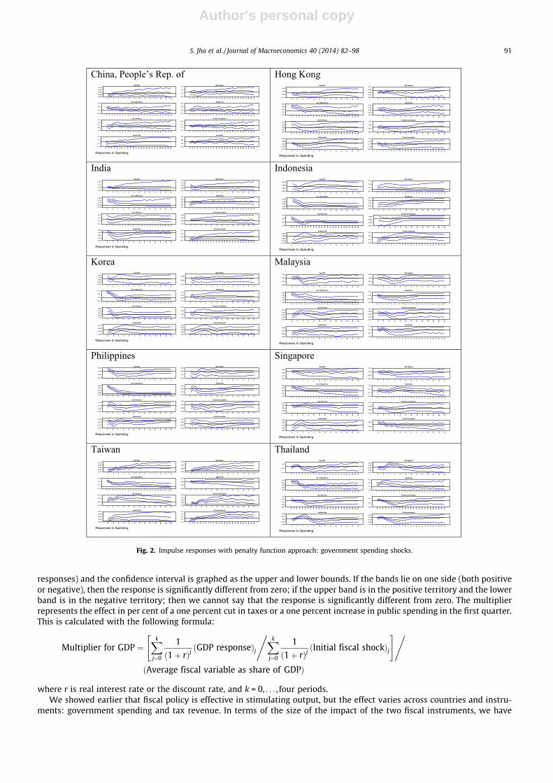
Tables 4 and 5 present the impacts of fiscal policy shocks on output working through macro variables in Asia-10 (also seeFigs. 1 and 2). The short-term effects of tax shocks on output are negative and statistically significant for 6 countries (seeFig. 1: CH, HK, IN, MY, PH, TW), whereas direct government expenditure shocks do not significantly increase output in 5countries as they may crowd-out private spending (HK, MY, PH, TW, TH), while for the remaining five countries either a po-sitive or insignificant output effect is found (see Fig. 2).8 Applying this non-linear method which uses Monte-Carlo integration,we find that tax shocks have a negative effect on output in half of the countries, while the spending shocks have a limited po-sitive effect that gets crowded out in the medium term – contrary to the result in Mountford and Uhlig (2009).

Although the magnitude of the responses is generally small, the directions are revealing. In particular, the contractionaryeffect of tax increases (positive revenue shock) suggests that a tax cut will have a positive impact on output in China, HongKong, India, Malaysia, Philippines and Taiwan in both the short and long runs. However, not all these effects are statisticallysignificant. While the negative effect in the Philippines remains significant in the long run as well, it is crowded out to someextent by investment. In Singapore and Taiwan, the direction of impact is reversed implying that output may not adjust

Table 2Sample size.

Country Obs. Sample period

PRC 58 1995:1–2009:2Hong Kong, China 68 1992:3–2009:2India 53 1996:2–2009:2Indonesia 66 1993:1–2009:2Korea 74 1991:1–2009:2Malaysia 74 1991:1–2009:2Philippines 98 1985:1–2009:2Singapore 86 1988:1–2009:2Taiwan 128 1977:3–2009:2Thailand 66 1993:1–2009:2

7 Impulse responses measure the time profile of the effect of a shock (or impulse) on the (expected) future values of a variable. Short-run is defined as 4quarters over which the sign restrictions are imposed. Long-run response is calculated as the sum of the coefficients of the lagged variables in the VAR.

8 One could decompose the tax shocks into income tax and consumption tax shocks and separate the expenditure shocks into government consumptionexpenditure and investment expenditure shocks. We have carried out this empirical exercise, but the results are not presented due to space constraints.Although there are marginal differences in the results when one looks at different sub-components, the aggregate spending and tax effects are similar to theeffects of government consumption spending (in case of spending) and direct tax (in case of revenue) shocks respectively.



favorably to tax changes, especially in Singapore where the results are significant. The short and long-run effects are mixedin the remaining two countries, namely, Korea and Taiwan. Taiwan shows the counterintuitive positive and significant long-run growth effect of higher taxes which is enhanced through higher consumption and investment. The apparently counter-intuitive result for Singapore and Taiwan may be depicting a case of expansionary fiscal contraction. That is, a fiscal contrac-tion by raising taxes (revenue) would reduce interest rates, thus increasing wealth, encouraging investment and leading tohigher output. This is supported by the fact that Singapore has traditionally followed a contractionary fiscal policy stance, asnoted by Simone (2000). A 2009 IMF study on Singapore notes that the counter-cyclical effect of discretionary fiscal policy is,at best, short-lived.9 The factors include high propensity to save among households and low consumption response, focus ofcounter-cyclical measures on easing the corporate cost burden through tax measures, and significant leakages of fiscal stimulusabroad through trade as well as remittances.

In contrast to tax shocks, positive government expenditure shocks seem to have limited effect on GDP. It is limited to apositive short-term impact in the Philippines (supported by higher investment) and Singapore, and negative long-term im-pact in Hong Kong and Thailand. Positive public spending shock discourages investment in Thailand in both the long run andthe short run. In other countries, higher government expenditure discourages investment, making the growth impact insig-nificant or, it increases inflation, thereby discouraging consumption. For example, in India, higher public expenditure drivesup short-run interest rate and crowds out private investment in both short and long runs, thereby making the growth impactinsignificant. Some of the remaining effects are negative, though insignificant. They might imply that cuts in unproductivespending, especially transfers, result in ‘expansionary fiscal contractions’. Given the insignificant coefficient of spendingshocks on output in several countries, one could argue that fiscal policy has had little de-stabilizing impact on real outputand it could reflect a pro-cyclical nature of fiscal policy from the spending side, whereas fiscal policy appears counter-cyclical

Table 3Impact effects of different shocks on GDP from the sign-VAR.

Shocks in ; PRC Hong Kong, China India Indonesia Korea Malaysia Philippines Singapore Taiwan Thailand

Business cycle +* +* +* +* +* +* +* +* +* +*

Monetary policy � � � � +* � � + + �Govt. spending + � + � + + +* +* � �Govt. revenue + �* � �* + �* �* +* � +

* Confidence interval (16th and 84th percentiles) being significantly different from zero.

Table 4Impulse responses to positive tax revenue shock (%).

Shocks on Impactsin

Real GDP Govt.expenditure

Govt.revenue

Interestrate

GDPdeflator

Realmoney

Privateconsumption

Fixedinvestment

PRC SR 0.0171 0.0399 0.0386* �0.0136 0.0035 �0.0006 0.0101 0.0163LR 0.0030 0.0634 0.0372* �0.0248 0.0023 �0.0029 0.0042 �0.0260

Hong Kong,China

SR �0.0061* 0.0028 0.0723* �0.0002 �0.0023 0.0028 �0.0025 0.0165

LR 0.0054 0.0616 0.2195* �0.0183* �0.0708* �0.0442 �0.0314 �0.0067

India SR �0.0017 0.0170 0.0698* �0.0016 �0.0039 �0.0021 �0.0044 �0.0280LR �0.0185 0.0086 0.1015* �0.0083 �0.0107 �0.0223 �0.0117 �0.1897

Indonesia SR �0.0039 �0.0259 0.0313* 0.0030 0.0136* �0.0120 �0.0060 �0.0016LR �0.0798* 0.1312 0.0474* �0.0004 0.5296* �0.0371 �0.0269 �0.0355

Korea SR 0.0006 0.0416 0.0643* 0.0002 0.0013 �0.0018 0.0003 �0.0267LR �0.0243* 0.0619 0.0456* 0.0018 �0.0083 0.0063 �0.0069 �0.0438

Malaysia SR �0.0070* 0.0164 0.0409* �0.0013 �0.0061 0.0048 0.0039 �0.0014LR �0.0087 �0.0206 0.0472 0.0012 �0.0112 �0.0080 0.0096 �0.0063

Philippines SR �0.0119* �0.0109 0.0345* 0.0008 �0.0025 �0.0010 �0.0021 �0.0453*

LR �0.0309* �0.0243 0.1081* 0.0258* �0.0859* 0.1164* �0.0088 0.0682*

Singapore SR 0.0063* �0.0021 0.0502* 0.0014* 0.0052* �0.0103* �0.0066* �0.0387LR 0.0529* 0.4124* 0.4135* 0.0050 0.0353* 0.1147* �0.0139 �0.0487

Taiwan SR �0.0021 0.0464* 0.0517* 0.0008 �0.0003 0.0017 0.0001 �0.0136*

LR 0.1222* 0.3508* 0.2236* 0.0132* 0.1389* 0.2212* 0.2182* 0.3846*

Thailand SR 0.0035 �0.0022 0.0150* 0.0017 �0.0063 0.0490 �0.0034 �0.0284LR 0.0076 �0.0127 0.0444 0.0024 �0.0098 �0.0821 0.0097 0.0587

Notes: Authors’ calculations. SR and LR refer to short run and long run respectively.* The impact being significantly different from zero (both upper (84th percentile) and lower (16th percentile) bands are significantly different from the zeroline).

9 Eskesen (2009a,b) confirm a case for counter-cyclical fiscal policy in Korea and Singapore.



from the revenue side. The pro-cyclicality could be because governments are too complacent to tighten fiscal policies duringgood times, leaving little room for fiscal stimulus during downturns. However, fiscal policy can have a different impact onthe future output growth in periods of low and high growth. Although we do not assess such non-linear effects of fiscal policyin this paper, there is still evidence in a non-linear framework that tax cuts focusing on income and corporate taxes are moreeffective in stimulating the economy, as in Arin and Spagnolo (2011).

Tax shocks that reduce revenue also lower inflation expectations in Indonesia and Singapore in both short and long runs.Government spending shocks increase inflation in India, Indonesia, Korea, Singapore and Taiwan, whereas in the remainingfive countries spending shocks do not have any inflationary impact. Any inflationary impact due to a spending shock canimpact real wages and the labour market, as discussed by Pappa (2009).10 Linnemann and Schabert (2006) show that govern-ment expenditures can lead to a rise in private consumption, real wages, and employment if the government share is not toolarge and public finance does not solely rely on distortionary taxation, whereas when government expenditures are partiallyfinanced by public debt, unit labour costs fall in response to a fiscal expansion, such that inflation tends to decline. Given thatmost Asian economies are running trade surpluses, there could be limited leakage of demand through imports and the effect ofthe fiscal expansion on the exchange rate is less likely to reduce this positive multiplier. Even if there is an increase in imports, itwould lead to depreciation of the exchange rate (at least in countries with flexible currency regimes), which will bring about arise in exports with some reversal of the rise in imports, so that there is not much change in net exports (see Corden, 2010). Thisis the reason why the open economy dimension has not been included in this study, aside from keeping the VAR dimensionmanageable and the same set of eight variables as in Mountford and Uhlig (2009).

Besides, in terms of financial variables, the interest rate and monetary liquidity partly reflect the financial transmission offiscal policy, and even if we consider other financial variables, the existing panel evidence from emerging market countriessuggests that the effect of revenue-based adjustment lowers sovereign risk spreads more than spending-based adjustment.This suggests that financial markets react more negatively to debt-financed spending compared to tax-financed spending, asin Akitoby and Stratmann (2008). Further, in emerging market economies, external debt remains within limit and has nothreat for fiscal policy, whereas high internal debt in advanced countries can influence the external credit rating of theseadvanced economies. In that sense, shocks on the debt front will not matter much in these emerging economies. Besides,spending shocks do not consistently increase interest rates across all countries, as it depends on how the spending is fi-nanced in different countries. The negative correlation in majority of the countries does suggest that the indirect crowd-ing-out effect of government spending probably dominates its direct crowding-in effect.11 Uhlig (2010) points to

Table 5Impulse responses to positive public spending shock.

Shocks on Impactsin

Real GDP Govt.expenditure

Govt.revenue

Interestrate

GDPdeflator

Realmoney

Privateconsumption

Fixedinvestment

PRC SR 0.0065 0.0322* 0.0211 �0.0549 �0.0186* 0.0110* 0.0038 0.0049LR �0.0100 0.0245 �0.0011 �0.4607 �0.0592* 0.0244 �0.0053 0.0059

Hong Kong,China

SR �0.0022 0.0793* 0.0727 �0.0001 �0.0033 0.0023 �0.0006 0.0049

LR �0.0038 0.1835* 0.2284* �0.0299* �0.1041* �0.0435* �0.0344* �0.0331

India SR 0.0027 0.0365* �0.0022 0.0018* 0.0108 �0.0052 �0.0013 �0.2229*

LR �0.0526 0.0724* �0.0184 �0.0122* �0.0072 �0.0952* �0.0237 �0.8518*

Indonesia SR 0.0004 0.0074* 0.0248 �0.0021 0.0163* �0.0201* �0.0054 �0.0059LR �0.0759 0.1886* 0.0068 �0.0043 0.6758* �0.0555* �0.0266 �0.0235

Korea SR 0.0086 0.0798* 0.0500* 0.0010 0.0015 �0.0016 �0.0004 �0.0185LR �0.0128 0.0798* 0.0320 0.0012 �0.0058 �0.0231 �0.0169 �0.0673

Malaysia SR 0.0023 0.0917* �0.0125 �0.0027* �0.0003 0.0007 0.0001 0.0192*

LR �0.0399* 0.2621* �0.0223 �0.0138 �0.0539* �0.0660 �0.0546* 0.0257

Philippines SR 0.0053* 0.0709* �0.0110 �0.0003 �0.0046 0.0072 �0.0002 0.0274*

LR �0.0369* 0.1104* �0.0600 �0.0095 �0.0727 �0.0019 �0.0140* 0.0743*

Singapore SR 0.0057* 0.1539* 0.0191 �0.0001 0.0016 �0.0002 �0.0006 �0.0912LR 0.0230 0.2883* 0.0496 0.0068 �0.0318 0.0877* 0.0268* �0.2211

Taiwan SR �0.0017 0.0709* 0.0449* 0.0004 �0.0019* 0.0037* 0.0014 �0.0150 *

LR 0.0921* 0.3527* 0.2092* 0.0134* 0.1061* 0.1580* 0.1879* 0.3369*

Thailand SR �0.0017 0.0776* 0.0029 �0.0029 �0.0039 0.0361 0.0042* �0.0587*

LR �0.0577* 0.0114 �0.1169* �0.0120* �0.0212 0.9564 �0.0470* �0.4033*

Notes: Authors’ calculations. SR and LR refer to short run and long run respectively.* The impact being significantly different from zero (both upper (84th percentile) and lower (16th percentile) bands are significantly different from the zeroline).

10 Given data on real wages, one could explore this further for developing Asian countries.11 See Buiter (2010) who distinguishes between three types of crowding out: financial crowding out (through the response of interest rates), real resource

crowding out (capital and labour bottlenecks constraining output expansion in response to a fiscal impulse), and direct crowding out (whether public spendingsubstitutes for or complements to private spending).



potentially drastic long term consequences of fiscal stimuli, showing that initially net present value fiscal multipliers for gov-ernment spending may exceed unity, as it is going to be financed by debt initially and by higher taxes eventually leading todecline in output. In contrast, Uhlig shows that for a tax cut and each discounted dollar given up in terms of taxing labour,one obtains an increase in discounted output eventually.

5.3. Cumulative output multipliers

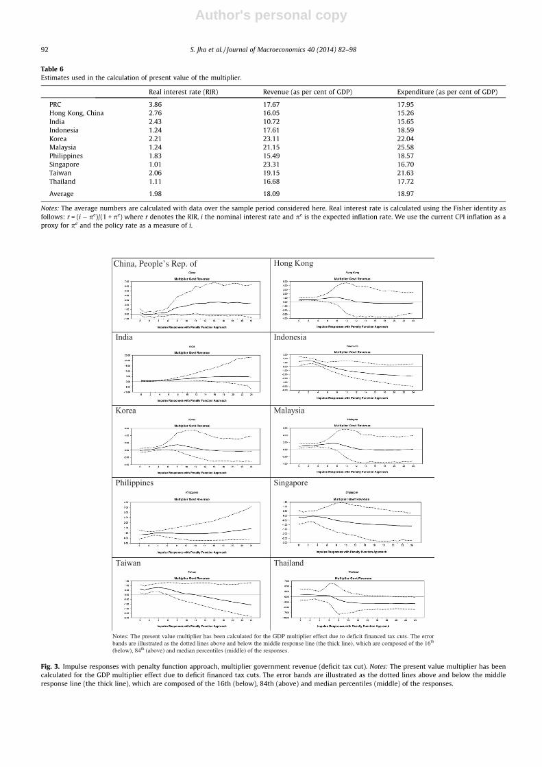
Having observed the impact effects, we next derive cumulative output multipliers for Asia-10 by undertaking two keypolicy experiments: a deficit financed tax cut policy scenario and a deficit-financed spending-increase fiscal policy scenario.Calculation of the present value multiplier uses information on average real interest rate, average government expenditureas a per cent of GDP, and average government revenue as per cent of GDP, which are shown in Table 6. Figs. 3 and 4 displaythe present value GDP multipliers for both the experiments. We calculate present value of these responses and then calculatethe multiplier for several quarters ahead. The multipliers given are the median multipliers (the 50th percentile of the

Fig. 1. Impulse responses with penalty function approach: government tax shocks.



responses) and the confidence interval is graphed as the upper and lower bounds. If the bands lie on one side (both positiveor negative), then the response is significantly different from zero; if the upper band is in the positive territory and the lowerband is in the negative territory; then we cannot say that the response is significantly different from zero. The multiplierrepresents the effect in per cent of a one percent cut in taxes or a one percent increase in public spending in the first quarter.This is calculated with the following formula:

Multiplier for GDP ¼Xk

j¼0

1

ð1þ rÞjðGDP responseÞj

" ,Xk

j¼0

1

ð1þ rÞjðInitial fiscal shockÞj

#,ðAverage fiscal variable as share of GDPÞ

where r is real interest rate or the discount rate, and k = 0, . . . , four periods.We showed earlier that fiscal policy is effective in stimulating output, but the effect varies across countries and instru-

ments: government spending and tax revenue. In terms of the size of the impact of the two fiscal instruments, we have

Fig. 2. Impulse responses with penalty function approach: government spending shocks.



Table 6Estimates used in the calculation of present value of the multiplier.

Real interest rate (RIR) Revenue (as per cent of GDP) Expenditure (as per cent of GDP)

PRC 3.86 17.67 17.95Hong Kong, China 2.76 16.05 15.26India 2.43 10.72 15.65Indonesia 1.24 17.61 18.59Korea 2.21 23.11 22.04Malaysia 1.24 21.15 25.58Philippines 1.83 15.49 18.57Singapore 1.01 23.31 16.70Taiwan 2.06 19.15 21.63Thailand 1.11 16.68 17.72

Average 1.98 18.09 18.97

Notes: The average numbers are calculated with data over the sample period considered here. Real interest rate is calculated using the Fisher identity asfollows: r = (i � pe)/(1 + pe) where r denotes the RIR, i the nominal interest rate and pe is the expected inflation rate. We use the current CPI inflation as aproxy for pe and the policy rate as a measure of i.

Fig. 3. Impulse responses with penalty function approach, multiplier government revenue (deficit tax cut). Notes: The present value multiplier has beencalculated for the GDP multiplier effect due to deficit financed tax cuts. The error bands are illustrated as the dotted lines above and below the middleresponse line (the thick line), which are composed of the 16th (below), 84th (above) and median percentiles (middle) of the responses.



calculated the multipliers using the above formula. The cumulative multiplier is defined as the cumulative change in outputover the cumulative change in fiscal shocks at some time horizon k. In present value terms, tax cuts have a much greatereffect on GDP than government spending, as tax cuts can produce a bigger boost in demand, not only by increasing consump-tion spending via a rise in disposable income but also by stimulating more investment spending. This result is broadly con-sistent with the empirical findings of Blanchard and Perotti, and Mountford and Uhlig, among others.

Moreover, by using the sign-VAR approach we undertake another robustness exercise to calculate present value multi-pliers until 25 quarters ahead, with a constant average discount rate of 1.98% for all 10 countries as opposed to different dis-count rates used earlier as in Table 6. We still find that a tax-cut policy experiment has significant positive effect on output inthe long run, while the effects of deficit financing are only short-lived and less effective in stimulating the economy with anegative impact (see Table 7). This is true in most countries, except India, Indonesia and the Philippines, where the big part ofthe labour force is still dependent on the traditional agricultural sector in which the role of government is important in stim-ulating demand. It is important to mention here that the negative relation between government spending and output is notuncommon, as there is evidence of strong negative correlation between government size and output volatility in the context

Fig. 4. Impulse responses with penalty function approach, multiplier government expenditure (deficit spending). Notes: The present value multiplier hasbeen calculated for the GDP multiplier effect due to deficit financed expenditure increase. The error bands are illustrated as the dotted lines above andbelow the middle response line (the thick line), which are composed of the 16th (below), 84th (above) and median percentiles (middle) of the responses.



of the OECD countries (see Fatás and Mihov, 2001). Blanchard and Perotti (2002) also find that both increases in taxes andincreases in government spending have a strong negative effect on private investment spending, contrary to the predictionsof traditional Keynesian theory.

As shown in Figs. 3 and 4, the median tax-cut multipliers range up to a maximum of around 2.0 across developing Asianeconomies in a two-year horizon, whereas the median government expenditure multipliers range up to a maximum ofaround 1.0 in the same two-year horizon. The median multipliers also turn out to be negative at different horizons over time.

Table 7Present value output multipliers of the policy scenarios with the average discount rate for Asia.

1 Qtr 5 Qtrs 9 Qtrs 14 Qtrs 20 Qtrs Maximum

People’s Rep. of ChinaDeficit-financed tax cut 0.30 0.23 1.46 2.32 2.39 2.57 (18th qtr)Deficit spending �0.46 �0.28 0.05 0.15 �0.006 0.25 (13th qtr)

Hong KongDeficit-financed tax cut 0.64 0.74 1.12 �0.05 �0.33 1.12 (9th qtr)Deficit spending 0.06 �0.41 �1.03 �1.43 �1.07 0.06 (1st qtr)

IndiaDeficit-financed tax cut 0.82 0.93 2.24 3.84 4.93 4.98 (22th qtr)Deficit spending 0.65 0.62 1.34 2.28 3.14 3.78 (25th qtr)

IndonesiaDeficit-financed tax cut 1.29 0.89 �0.49 �1.49 �2.16 1.44 (3rrd qtr)Deficit spending 2.52 0.58 �0.46 0.65 2.18 2.64 (25th qtr)

KoreaDeficit-financed tax cut �0.10 0.57 1.49 0.29 �0.28 1.49 (9th qtr)Deficit spending 0.12 0.19 0.42 �0.24 �0.33 0.43 (8th qtr)

MalaysiaDeficit-financed tax cut 0.89 1.29 1.69 0.07 �0.13 1.73 (8th qtr)Deficit spending �0.10 �0.21 �0.56 �0.73 �0.66 �0.02 (3rd qtr)

PhilippinesDeficit-financed tax cut 0.83 0.99 0.95 0.92 1.12 1.43 (25th qtr)Deficit spending 0.37 0.03 �0.46 �0.97 �1.07 0.37 (1st qtr)

SingaporeDeficit-financed tax cut �0.15 �0.09 �0.52 �0.86 �1.04 �0.03 (4th qtr)Deficit spending �0.17 �0.33 �0.66 �0.81 �0.74 0.37 (25th qtr)

TaiwanDeficit-financed tax cut 0.06 0.16 �0.10 �0.30 �0.87 0.18 (4th qtr)Deficit spending �0.27 �0.41 �0.14 0.06 0.38 0.45 (25th qtr)

ThailandDeficit-financed tax cut 0.95 0.65 �1.46 �3.09 �3.13 0.95 (1st qtr)Deficit spending �0.58 �0.47 �3.31 �3.76 4.22 5.76 (24th qtr)

0

25

50

75

100

Business cycle Monetary policy Govt. spending Govt. revenue

Fig. 5. Decomposition of variance (k = 25) for GDP (%). Notes: The shocks we have identified are four, when the number of variables in the VAR is eight. Eventhese four shocks still account for around 90% of the variation in GDP. If we identify eight shocks (same as the number of variables), then it will add up to100%. We have not presented here the decomposition of other variables, but they are available upon request from the authors.



So the multipliers obtained here remain consistent with what has been found in the literature for other advanced countrieswith some studies reporting multiplier values up to 4, but none of the studies calculated present value multipliers exceptMountford and Uhlig. The cumulative multiplier is the most appropriate measure, but it is typically larger than the impactor peak multipliers and hence it is rarely reported in empirical studies, with the exception of Mountford and Uhlig. As cumu-lative multipliers can be bigger numbers, there is a need to calculate the present value of those cumulative responses as hasbeen reported in this paper.

The present value of the GDP response to a deficit spending scenario is insignificant with the exception of India, Indonesiaand the Philippines, whereas that for the deficit-financed tax cut is significantly positive for seven countries, i.e., Hong Kong,India, Indonesia, Malaysia, Korea, Philippines, and Taiwan. For the remaining three countries, the impact is not significant,although the tax cut has a positive impact on output. The lack of significance in these countries could be due to data caveatsnamely very limited time dimension in some countries or they have already very low tax rates. This distinction becomesmore obvious from the variance decomposition results of all the four shocks and what they account for in terms of propor-tional variation in GDP.

Table 8Qualitative description of fiscal measures of selected Asian countries. Source: Compiled by authors from respective Government websites, Khatiwada (2009),SARD Flashnote, ADB, and UNESCAP (2009).

Country Public spending on goods andservices

Fiscal stimulus aimed atconsumers

Fiscal stimulus aimed at firms Estimatedvalue and % in2008 GDP offiscal stimuluspackages

People’s Rep. ofChina

Speeding up rural infrastructureconstruction; infrastructurespending on transport facilities;upgrading of power grids;increased spending on health andeducation in rural areas;enhancing construction of sewageand waste treatment facilities

Low-rent housing; raisingminimum grain purchase and farmsubsidies; subsidies for low-income residents; increasingnumber of pension funds

Tax cuts for 9 industries; supportand development of high-tech andservice industries; removal of loanquotas on commercial lenders

$791 billion(17.5% ofGDP)

Hong Kong, China Social transfers; educationalassistance; tax subsidies

Rental reduction for governmentland and properties; reduction andexemption of payment ofgovernment fees

$11.2 billion(5.2% of GDP)

India Infrastructure spending ontransport facilities and rural areas

Increased allocation for socialsector programs

Measures to help exporters andlabour-intensive industries; cut inexcise duty expedited

$40 billion(3.3% of GDP)

Indonesia Infrastructure spending Income tax cuts; tax and non-taxsubsidies

Corporate tax cuts; tax and non-tax subsidies


Rep. of Korea Infrastructure investment;communications, energy; medicalservices’

Social transfers to low-incomehouseholds

Tax incentives for SMES;assistance to SMEs; tax deductionon R&D investment; tax deductionand exemption to green-industryrelated financial products

$104.1 billion(11.2% ofGDP)

Malaysia Rural infrastructure investment;housing, school, and hospitalbuilding

Human capital developmentprogram; youth developmentprogram; price subsidies

Micro-credit programs to assistfarmers and agro-based smallbusinesses in rural areas; loanguarantees

$17.6 billion(9% of GDP)

Philippines Infrastructure investment; schooland hospital building

Income tax cuts; conditional cashtransfers; additional public healthinsurance benefits; training fordisplaced workers

Corporate tax cuts $7.4 billion(4.5% of GDP)

Singapore Infrastructure investment;housing, public facilities, andhospital building

Tax exemption on remittances; taxcredits; personal income taxrebates; fund assistance tostudents; public transportvouchers; rental rebates; skillstraining

Cash transfers for employers tocover part of wage bill; corporatetax cuts; loan guarantees; freezeon payment of government fees;sector-specific tax and dutiesreductions


Taiwan Infrastructure spending Subsidies on goods purchases;preferential home-purchase loans;consumption vouchers; zero-interest home loans for newlymarried couples; trainingprograms

Tax credits; strengtheningfinancing of SMEs; 5-year taxexemption for new investments bymanufacturing and service-relatedfirms


Thailand Housing and rural infrastructuredevelopment; increased spendingon health

Conditional cash transfers;subsidies; free education program;capacity building for theunemployed

Sector-specific industry promotion $46.4 billion(17% of GDP)

Note: Estimated values are based on published figures of cost of fiscal stimulus packages. Some fiscal stimulus packages may spread over a number of years.



5.4. Variance decomposition analysis

This section presents an analysis of the results of variance decomposition by finding the proportion of variance in GDPthat is explained by different shocks across countries. This decomposition (into discretionary and non-discretionary) is anex-post exercise, decomposing one-step ahead prediction error into the part that is explained by its own policy shock andthe (orthogonal) rest. This distinction cannot be made before identifying the shocks in SVAR exercise. The variance decom-position for the VAR model is presented in Fig. 5. In the variance decomposition analysis, nearly 50% of the variation in GDP isexplained by business cycle shocks, with the remaining being explained by monetary and fiscal shocks in several countries,except India, Indonesia, Korea, Philippines, and Singapore with higher proportions in GDP, whereas PRC; Hong Kong; Malay-sia; Taiwan; and Thailand have lower proportion of variation in GDP being explained by business cycle shocks. The high out-put variance due to a business cycle shock could reflect higher output volatility that could be due either to demand or supplyshocks. While the high output variance could be supply-driven in India, Indonesia and the Philippines as they rely on highlyvolatile agricultural sector, the output variance in the case of Korea and Singapore could be more demand-driven.

In most countries, notably PRC, Indonesia, Korea, Philippines, Singapore, Taiwan, and Thailand, government revenueshocks (due to a tax increase or tax cut) contribute more to output variance than spending shocks, as revenues have a sig-nificant negative impact on GDP than government expenditures. However, the share of variation in GDP is relatively less ex-plained by fiscal shocks in India where government revenue as a percent of GDP is lowest among the Asian emergingcountries. We also note that fiscal shocks are more important in PRC than in India. In terms of contribution of the shocksto the variance of GDP in Hong Kong, as a small open economy, business cycle shocks account for 45.8% of the variationin GDP, followed by monetary policy shock explaining 10.8% of the variation in GDP, whereas government expenditure ac-counts for 16.6% of the variation in GDP and revenue shock explaining 15.7% of GDP. Even for large economies, business cycleshocks account for a bigger proportion of the variation in GDP followed by fiscal shocks, with monetary shocks explaining thelowest proportion of variation in GDP.

Our results confirm that business cycle shocks potentially explain the largest part of the variation in output, with revenueand spending shocks explaining less of the variation. Following a negative business cycle shock (for example a downturn)output can contract; so an expansionary monetary policy can help reverse the downturn. But when the monetary policyinstrument is already at its lowest level or when a country has no independent monetary policy given a currency board typeof exchange rate arrangement (such as in Hong Kong) or a fixed regime (such as in the PRC), fiscal shocks are critical for anypossible recovery. The economies of South Korea, Singapore and Taiwan achieved high standards of infrastructure (physicaland social) with relatively low government spending, aided by complementary policies relating to macroeconomic stability

Table 9Fiscal indicators. Source: Asian Development Bank. Key Indicators for Asia and the Pacific 2010. http://www.adb.org/Documents/Books/Key_Indicators/2010/default.asp.

China, People’s Rep. of Hong Kong, China India Indonesia Korea

Average1990–2007

2008 Average1990–2007

2008 Average1990–2007

2008 Average1990–2007

2008 Average1990–2007

2008

% of total revenueTaxes 93.8 88.4 93.8 68.9 73.9 67.3 66.6 81.1 79.4 66.7Nontaxes 6.2 11.6 18.5 20.0 26.1 11.6 23.9 16.7 19.3 32.5

% of total expendituresCurrent expenditures 77.6 82.6 67.7 92.6 81.8 89.2 82.0 84.4Capital expenditures 22.4 17.4 32.3 7.4 18.2 10.8 18.0 15.6

% of GDPTotal revenue 14.1 19.5 17.4 18.9 17.4 19.8 10.4 10.3 19.9 24.4Taxes 13.1 17.3 11.0 13.0 12.8 13.3 6.9 8.4 15.6 16.3Total expenditure 16.8 19.9 16.4 18.6 18.1 19.9 15.2 16.2 18.0 22.7Overall budgetary balance (1.9) (0.4) 1.0 0.2 (0.7) (0.1) (4.8) (5.9) 0.1 1.2

Malaysia Philippines Singapore Taiwan Thailand

Average1990–2007

2008 Average1990–2007

2008 Average1990–2007

2008 Average1990–2007

2008 Average1990–2007

2008

% of total revenueTaxes 50.0 70.7 86.8 87.2 46.5 57.4 49.1 75.2 50.0 88.4Nontaxes 24.2 29.3 11.2 10.2 33.3 27.8 25.0 22.2 11.3 11.6

% of total expendituresCurrent expenditures 73.9 78.6 80.7 88.8 74.9 78.0 79.5 92.7Capital expenditures 26.1 21.4 19.3 11.2 25.1 22.0 20.5 7.3

% of GDPTotal revenue 22.4 21.6 16.8 14.6 26.2 24.0 13.4 13.0 17.3 18.2Taxes 17.0 15.2 14.6 12.8 13.7 13.8 9.6 9.8 15.4 16.1Total expenditure 24.6 26.4 18.9 18.2 17.4 16.4 15.4 13.8 17.9 18.8Overall budgetary balance (2.2) (4.8) (2.1) (3.9) 9.7 7.6 (2.0) (0.8) (0.8) (0.6)



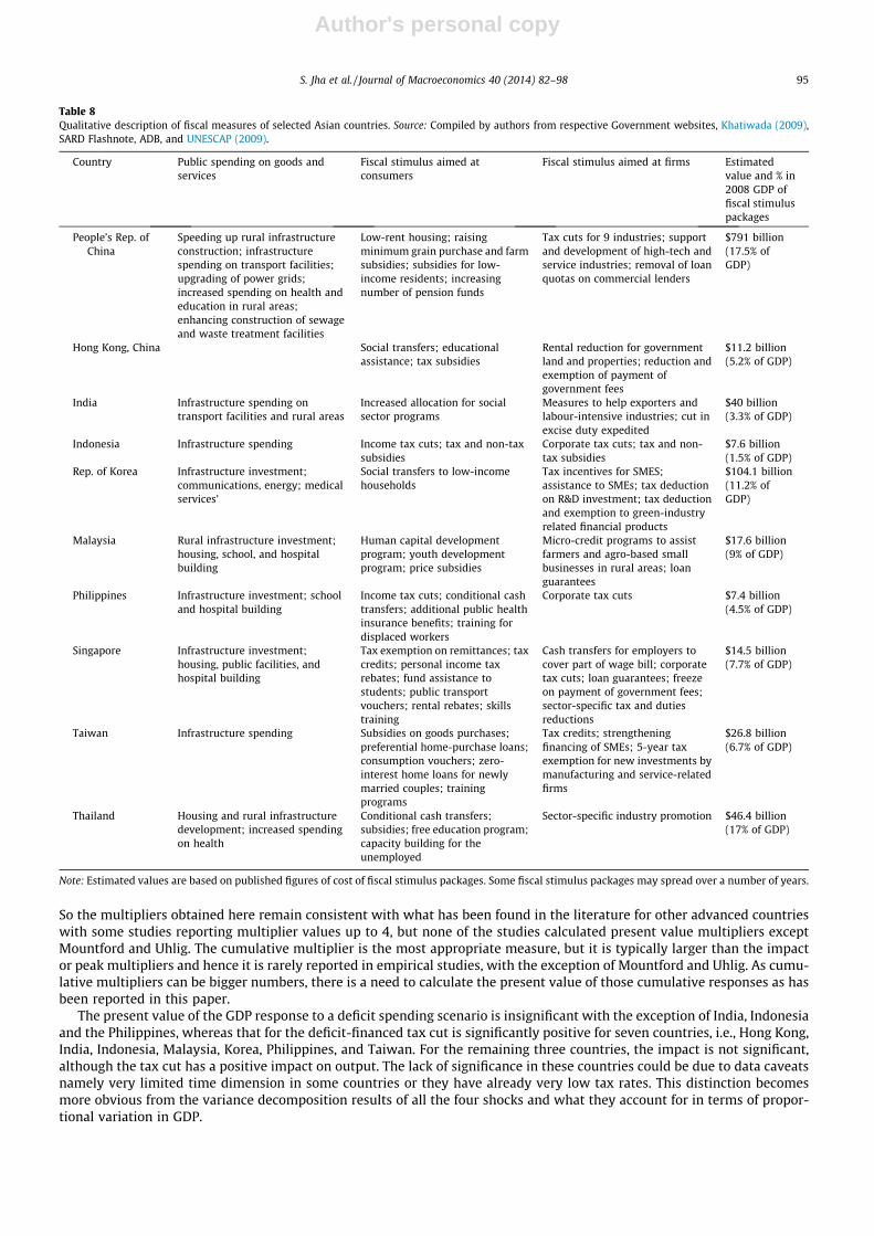
and involvement of private sector in providing quasi-public goods (see Rao, 1998). This probably explains why increase ingovernment spending does not have a positive impact on output in some of these Asian countries. In a qualitative sense, asdocumented in Table 8, tax cut has been an important feature of the fiscal stimulus measures implemented in most Asiancountries. This is also apparent in a drop in taxes as a per cent of total revenue in most countries in 2008 (see Table 9). Sinceaverage tax revenue for most countries accounts for over 75% of total revenue (see Table 9), we approximate the revenueshock as a shock in tax revenue.

It is worth mentioning here that government expenditure and revenue shocks are defined as surprise increases in expen-diture and revenues respectively, which can be termed as discretionary fiscal policy changes. It is possible that the changes ingovernment expenditures and revenues could be cyclical rather than being driven purely by discretionary changes in gov-ernment revenue and expenditure. For Asia-10, the variance decomposition suggests that the variation in governmentexpenditure due to its own discretionary shock is around 55%, while the other shocks explain around 45%, whereas for rev-enues, its own discretionary shock explains around 30%, whereas other shocks explain the most part of the variation in rev-enues, i.e., 70%. This decomposition of one-step ahead prediction error into the part that is explained by its own policy shockand the (orthogonal) rest suggests that a big part of the revenue shocks in developing Asia are non-discretionary. Thus giventhe non-discretionary nature of government revenues, a tax-cut policy may not be feasible to implement in developing Asiancountries, although unanticipated deficit-financed tax cuts can work as a (short-lived) stimulus to the economy as the aim ofthe fiscal stimulus is to reduce or eliminate any short-run output gap.

6. Concluding observations and policy recommendations

In response to the global financial and economic crisis, governments throughout developing Asia decisively implementedfiscal stimulus packages. According to Asian Development Bank (2010), developing Asia bounced back from the crisis muchfaster and stronger than widely expected as the sizable fiscal stimulus packages put into effect by governments helped kick-start the region’s struggling economies. The crisis, however, was not just another downturn in another business cycle butmarked the deepest global recession and biggest contraction of global trade in the postwar era. As such, the region’s stimulusmeasures represented an extraordinary policy response to an extraordinary crisis rather than conventional countercyclicalpolicy. Even though Asia’s fiscal stimulus packages were tilted toward higher government spending, they included tax cuts aswell. In light of the region’s slower growth and heightened uncertainty in the post-global crisis period, a timely and relevantchallenge for governments is to understand the relative effectiveness of tax cuts versus government spending in boostingaggregate demand and output.

Despite renewed interest in countercyclical fiscal policy, empirical literature on the issue is limited for developing econ-omies, including Asia. Much of the literature is devoted to industrialized countries which have a longer history of counter-cyclical fiscal policy. The central objective of this paper is to empirically examine the impact of an unexpected fiscal shock onoutput in developing Asia. We account for business cycle and monetary policy shocks to more accurately assess the effect offiscal shocks.

The effectiveness of countercyclical fiscal policy depends not only on its size but also its composition. More specifically,we investigate the relative effectiveness of tax cuts versus government spending in boosting aggregate demand by employ-ing a 2-stage empirical strategy. First, we examine the impact effects of expansionary expenditure shocks, contractionaryrevenue shocks, and other non-fiscal shocks on output. Second, on the basis of our estimated responses from the first stage,we perform and compare two policy experiments – deficit-financed expenditure increase versus deficit-financed tax cut – bycalculating the present value of GDP multiplier effects. Our evidence suggests that in Asia tax cuts may be more effective forcountercyclical purposes than higher spending. That is, unanticipated tax cuts stimulate economic activity more than publicspending.

However, we should exercise a great deal of caution in interpreting our results as a general call for more active use of taxcuts. For one, once introduced, tax cuts may become entrenched and prove difficult to reverse or adjust. This, in turn, mayjeopardize the fiscal sustainability that served the region so well during the crisis. By and large Asia’s fiscal environment ischaracterized by relatively small discretionary component of revenues which implies a limited scope for tax-cuts. Further-more, several Asian countries have weak tax bases and their primary fiscal priority is to improve the tax revenue collectioneffort. In general, improvements in tax systems, enlargement of tax base, and rationalization of tax administration still re-main as relevant as ever for macroeconomic stability and growth. Such measures help to reduce the cost of compliance fortax payers and generate larger fiscal space for the government. The relative ineffectiveness of government spending inincreasing output suggests a clear need to improve the design of countercyclical spending to enhance its impact in the future.In particular, the composition of discretionary expenditure matters. In the short term, shifting expenditures to uses with lar-ger multipliers will contribute to greater countercyclical effectiveness. In the long term, shifting expenditures towardsgrowth-conducive public goods such as infrastructure and social protection will help create the physical and human capitalrequired for growth.

Another way to increase the effectiveness of public expenditure is through the establishment of automatic stabilizers. Un-like discretionary public spending, automatic stabilizers have the advantages of speed, predictability and reversibility. Onceimplemented, these measures are outside the political process and automatically kick in when the economy slows down.Automatic stabilizers are especially valuable when fiscal institutions are weak, which is the case in many developing Asian



economies. Therefore, strengthening them will provide the region with an insurance mechanism against another economiccrisis.

References

Akitoby, B., Stratmann, T., 2008. Fiscal policy and financial markets. Econ. J. 118, 1971–1985.Alesina, A., Ardagna, S., 2009. Large Changes in Fiscal Policy: Taxes versus Spending. National Bureau of Economic Research (NBER) Working Paper No.

15438.Arin, K.P., Spagnolo, N., 2011. Short-term growth effects of fiscal policy revisited: a Markov-switching approach. Econ. Lett. 110 (3), 278–281.Asian Development Bank, 2010. Asian Development Outlook 2010: Macroeconomic Management beyond the Crisis. Asian Development Bank, Manila,

Philippines.Baldacci, E., Gupta, S., Mulas-Granados, C., 2009. How Effective is Fiscal Policy Response in Systemic Banking Crises? International Monetary Fund Working

Paper WP/09/160.Blanchard, O., Perotti, R., 2002. An empirical characterization of the dynamic effects of changes in government spending and taxes on output. Quart. J. Econ.

117 (4), 1329–1368.Buiter, W.H., 2010. The limits to fiscal stimulus. Oxford Rev. Econ. Policy 26 (1), 48–70.Burnside, C., Eichenbaum, M., Fisher, J., 2003. Fiscal shocks and their consequences. J. Econ. Theory 115 (1), 89–117.Burriel, P., De Castro, F., Garrote, D., Gordo, E., Paredes, J., Pérez, J.J., 2010. Fiscal policy shocks in the Euro Area and the US: an Empirical Assessment. Fiscal

Stud. 31, 251–285.Caldara, D., Kamps, C., 2008. What are the Effects of Fiscal Shocks? A VAR-Based Comparative Analysis. European Central Bank Working Paper Series 877.Cogan, J.F., Cwik, T., Taylor, J.B., Wieland, V., 2010. New Keynesian versus old Keynesian government spending multipliers. J. Econ. Dyn. Control 34 (3), 281–

295.Corden, W.M., 2010. The theory of the fiscal stimulus: how will a debt-financed stimulus affect the future? Oxford Rev. Econ. Policy 26 (1), 38–47.Correia, I., Farhi, E., Nicolini, J.P., Teles, P., 2013. Unconventional fiscal policy at the zero bound. Am. Econ. Rev. 103 (4), 1172–1211.Eskesen, L.L., 2009a. Countering the Cycle – The Effectiveness of Fiscal Policy in Korea. International Monetary Fund Working Paper 09/249.Eskesen, L.L., 2009b. The Role for Counter-Cyclical Fiscal Policy in Singapore. International Monetary Fund Working Paper 09/8.Fatás, A., Mihov, I., 2001. Government size and automatic stabilizers: international and intranational evidence. J. Int. Econ. 55 (1), 3–28.Fry, R., Pagan, A., 2011. Sign restrictions in structural vector autoregressions: a critical review. J. Econ. Lit. 49 (4), 938–960.Galí, J., López-Salido, J.D., Vallés, J., 2007. Understanding the effects of government spending on consumption. J. Eur. Econ. Assoc. 5 (1), 227–270.Hemming, R., Kell, M., Mahfouz, S., 2002. The Effectiveness of Fiscal Policy in Stimulating Economic Activity – A Review of the Literature. International

Monetary Fund Working Paper WP/02/208.Ilzetzki, E., Végh, C.A., 2008. Procyclical Fiscal Policy in Developing Countries: Truth or Fiction? NBER Working Paper No. 14191. NBER, Cambridge,

Massachusetts.Ilzetzki, E., Mendoza, E.G., Végh, C.A., 2011. How Big (Small?) Are Fiscal Multipliers? IMF Working Paper WP/11/52. International Monetary Fund,

Washington, DC.Jansen, K., 2004. The scope for fiscal policy: a case study of Thailand. Dev. Policy Rev. 22, 207–228.Kaminsky, G., Reinhart, C., Vegh, C., 2005. When it rains, it pours: procyclical capital flows and macroeconomic policies. In: Gertler, M., Rogoff, K. (Eds.),

NBER Macroeconomics Annual 2004. MIT Press, pp. 11–53.Khatiwada, S., 2009. Stimulus Packages to Counter Global Economic Crisis: A Review. International Institute for Labour Studies Discussion Paper 196/2009.

<http://www.ilo.org/public/english/bureau/inst/publications/.../dp19609.pdf>.Kilian, L., 2001. Impulse response analysis in vector autoregressions with unknown lag order. J. Forecast. 20, 161–179.Kraay, A., Servén, L., 2008. Fiscal Policy Responses to the Current Financial Crisis: Issues for Developing Countries. Research Brief, World Bank, December

2008. <http://go.worldbank.org/NME0S66FQ0>.Linnemann, L., Schabert, A., 2006. Productive government expenditure in monetary business cycle models. Scot. J. Polit. Econ. 53 (1), 28–46.Mountford, A., Uhlig, H., 2009. What are the effects of fiscal policy shocks? J. Appl. Econ. 24 (6), 960–992.Pappa, E., 2009. The effects of fiscal shocks on employment and the real wage. Int. Econ. Rev. 50, 217–244.Perotti, R., 1999. Fiscal policy in good times and bad. Quart. J. Econ. 114 (4), 1399–1436.Rafiq, M.S., Mallick, S.K., 2008. The effect of monetary policy on output in EMU3: a sign restriction approach. J. Macroecon. 30 (4), 1756–1791.Ramey, V., 2011. Identifying government spending shocks: it’s all in the timing. Quart. J. Econ. 126 (1), 1–50.Rao, M.G., 1998. Accommodating public expenditure policies: the case of fast growing Asian economies. World Dev. 26 (4), 673–694.Romer, C., Bernstein, J., 2009. The Job Impact of the American Recovery and Reinvestment Plan. Unpublished Mimeo.Romer, C.D., Romer, D.H., 2010. The macroeconomic effects of tax changes: estimates based on a new measure of fiscal shocks. Am. Econ. Rev. 100 (3), 763–

801.Simone, F.d.A.N.-D., 2000. Monetary and fiscal policy interaction in a small open economy: the case of Singapore. Asian Econ. J. 14, 211–231.Spilimbergo, A., Symansky, S., Schindler, M., 2009. Fiscal Multipliers. International Monetary Fund Staff Position Note SPN/09/11.Talvi, E., Végh, C.A., 2005. Tax base variability and procyclical fiscal policy in developing countries. J. Dev. Econ. 78 (1), 156–190.Taylor, J.B., 2009. The lack of an empirical rationale for a revival of discretionary fiscal policy. Am. Econ. Rev. 99 (2), 550–555.Uhlig, H., 2010. Some fiscal calculus. Am. Econ. Rev. 100 (2), 30–34.UNESCAP, 2009. Economic and Social Survey of Asia and the Pacific 2009. <http://www.unescap.org/pdd/publications/survey2009/>.


Effectiveness of Countercyclical Fiscal Policy: Time-Series Evidence from Developing Asia

Documents

Transcript of Effectiveness of Countercyclical Fiscal Policy: Time-Series Evidence from Developing Asia