International Journal of Control, 2015Vol. 88, No. 7, 1366–1378, http://dx.doi.org/10.1080/00207179.2014.942699

Effective variable switching point predictive current control for ac low-voltage drives

Peter Stolzea,∗, Petros Karamanakosa, Ralph Kennela, Stefanos Maniasb and Christian Endischc

aInstitute for Electrical Drive Systems and Power Electronics, Technische Universitat Munchen, Munich, Germany; bDepartment ofElectrical and Computer Engineering, National Technical University of Athens, Athens, Greece; cTechnische Hochschule Ingolstadt,

Ingolstadt, Germany

(Received 30 January 2014; accepted 3 July 2014)

This paper presents an effective model predictive current control scheme for induction machines driven by a three-level neutralpoint clamped inverter, called variable switching point predictive current control. Despite the fact that direct, enumeration-based model predictive control (MPC) strategies are very popular in the field of power electronics due to their numerousadvantages such as design simplicity and straightforward implementation procedure, they carry two major drawbacks. Theseare the increased computational effort and the high ripples on the controlled variables, resulting in a limited applicabilityof such methods. The high ripples occur because in direct MPC algorithms the actuating variable can only be changed atthe beginning of a sampling interval. A possible remedy for this would be to change the applied control input within thesampling interval, and thus to apply it for a shorter time than one sample. However, since such a solution would lead to anadditional overhead which is crucial especially for multilevel inverters, a heuristic preselection of the optimal control actionis adopted to keep the computational complexity at bay. Experimental results are provided to verify the potential advantagesof the proposed strategy.

Keywords: model predictive control (MPC); optimal control; variable switching point; three-level inverter; ac low-voltagedrives

1. Introduction

Over the past decades, field oriented control (FOC)(Kazmierkowski, Krishnan, & Blaabjerg, 2002) and di-rect torque control (DTC) (Depenbrock, 1988; Takahashi &Noguchi, 1986) have been shown to be reasonably effectivein controlling adjustable-speed ac drives. FOC makes use ofmodulators, whereas DTC utilises hysteresis controllers forboth flux and torque, and outputs a switching state which isdirectly commanded to the inverter. Because of the absenceof a modulator, DTC is known to show a faster transientresponse than FOC, whereas it normally produces highercurrent, flux and torque ripples.

Although model predictive control (MPC)(Maciejowski, 2002; Rawlings & Mayne, 2009) methodshave been widely used for more than 40 years in processand chemical engineering, the application of such strategiesto electrical drive systems and power electronics convertershas just recently been gaining more popularity (Correa,Pacas, & Rodrıguez, 2007; Geyer, 2012; Geyer & Mastel-lone, 2012; Geyer, Oikonomou, Papafotiou, & Kieferndorf,2012; Geyer, Papafotiou, & Morari, 2009; Miranda,Cortes, Yuz, & Rodrıguez, 2009; Oikonomou, Gutscher,Karamanakos, Kieferndorf, & Geyer, 2013; Papafotiou,Kley, Papadopoulos, Bohren, & Morari, 2009; Rodrıguezet al., 2012, 2013; Rojas et al., 2013). MPC-based

∗Corresponding author. Email: peter.stolze@tum.de

algorithms can be divided into modulator-based schemes,such as generalised predictive control (Linder, Kanchan,Kennel, & Stolze, 2010), and direct MPC strategies,where the optimisation problem is solved via enumerationapproaches (Cortes, Kazmierkowski, Kennel, Quevedo, &Rodrıguez, 2008; Geyer, 2005; Karamanakos, 2013). Thetwo main drawbacks of enumeration-based MPC methodsare the high computational complexity due to the completeenumeration of all control inputs, i.e. the switching states,and the high ripples on the controlled variables comparedto modulator-based approaches.

To alleviate the first problem, i.e. to reduce thenecessary computations, some strategies have been pro-posed in the past, see Karamanakos, Geyer, Oikonomou,Kieferndorf, and Manias (2014) and references therein. Inthis work a heuristic voltage vector preselection is adopted,initially proposed in Stolze, Landsmann, Kennel, and Mou-ton (2011) that can be effectively applied to MPC schemeswhere a longer prediction horizon is required for improvedplant performance. Furthermore, as shown in Stolze, Tom-linson, Kennel, and Mouton (2013), this strategy can besuccessfully applied to the current control loop of induc-tion machines (IMs).

The second problem of direct, enumeration-basedstrategies comes from the fact that a switching state is

C© 2014 Taylor & Francis

International Journal of Control 1367

applied for at least one sampling interval, resulting in highripples on the quantities that are either directly or indirectlycontrolled (e.g. the stator current and flux, and the elec-tromagnetic torque). If a modulator is used, active voltagevectors which in general lead to higher ripples than thezero ones1 can be applied for a much shorter time. Hence,in order to reduce ripples on the controlled variables, inKaramanakos, Stolze, Kennel, Manias, and du Toit Mouton(2014), Stolze, Karamanakos, Kennel, Manias, and Mouton(2013), Patsakis et al. (2013) an MPC strategy, called vari-able switching point predictive torque control (VSP2TC),was introduced showing promising results. According tothis algorithm, a variable switching point (VSP) in timetsw, with 0 ≤ tsw ≤ Ts, where Ts is the sampling interval,is calculated in order to minimise the torque ripple. How-ever, it should be mentioned that calculating a VSP furtherincreases the computational burden, resulting in a limitedapplicability of such methods, especially for multilevel in-verters.

To overcome the previously mentioned drawbacks ofdirect, enumeration-based methods, in this paper the basicprinciple that was used for the torque ripple minimisationin VSP2TC is applied to the current control loop of anIM. Furthermore, the proposed VSP strategy is combinedwith a heuristic preselection of the optimal voltage vectorto implement it in a computationally efficient manner. In afirst step the continuous-valued solution of the optimisationproblem (assuming that the continuous-valued voltage vec-tor is applied for a whole sampling interval) is determined.Then, the three integer solutions – related to the voltagevectors produced by the inverter – that lie in the neighbour-hood of the continuous-valued optimum are considered forthe MPC algorithm. Subsequently, an optimisation problemis formulated according to which a VSP is calculated suchthat the squared rms current error for both α and β com-ponents of the stator current i s is minimised. In this way,the twofold task is achieved: (1) the current ripples are ef-fectively reduced, and (2) the computational burden is keptlow, especially when compared to a complete enumerationof all possible solutions.

Apart from the above goals that the proposed algo-rithm meets, it comes with an additional advantage. Itholds true that in direct, enumeration-based MPC meth-ods the real switching frequency per device is lower thanhalf the sampling frequency, while it also highly dependson the operating point. Especially at low machine speedsthe switching frequency per device can reach values around100 Hz whereas it can be several kHz at higher speeds.The proposed method increases the switching frequency,especially at these operating points, and delivers signifi-cantly improved currents while not affecting the dynamicresponse of the system.

The suggested algorithm is applied to an IM fed bya three-level neutral point clamped (NPC) inverter. How-ever, the necessary dc-link voltage balancing can be easilyachieved by including an appropriate term in the proposed

objective function. Finally, it should be pointed out that theproposed strategy is very promising for low-voltage driveswhere, in contrast to medium- and high-voltage drives, agood quality of the controlled variables is much more im-portant than low switching frequencies.

The paper is organised as follows: Section 2 gives anoverview of the physical system; in Section 3 the controlalgorithm with heuristic preselection and the VSP calcula-tion is described. Section 4 contains experimental results toverify the proposed method and in Section 5 the conclusionand an outlook to further work are given.

2. Physical system

2.1 Three-level NPC inverter

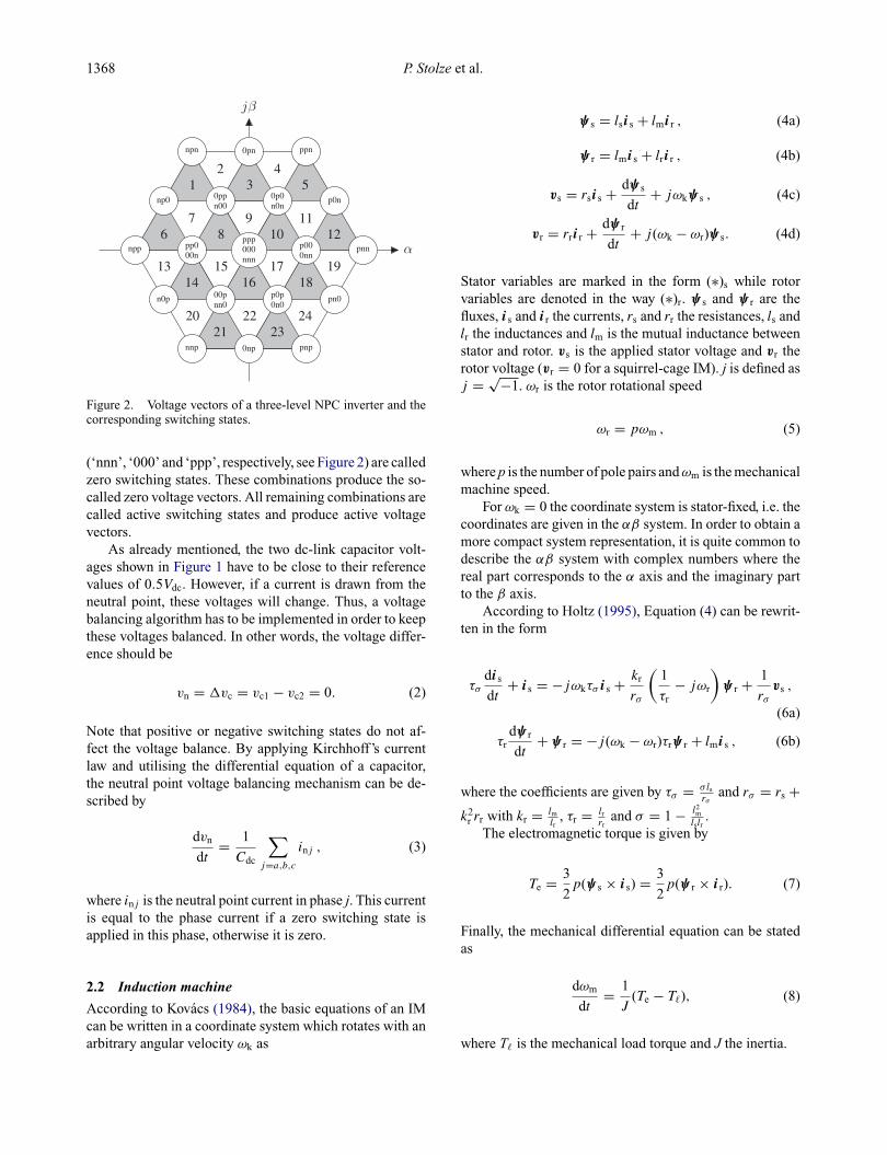
Figure 1 shows the three-level NPC inverter connectedto an IM. DC+ and DC- are the positive and negative dc-link rails, respectively. NP is the neutral (zero) point. Ideally,the two dc-link capacitor voltages vc1 and vc2 are equal to0.5Vdc, where Vdc is the dc-link voltage. Every phase hastwo complementary pairs of switches (Sj1/Sj3 and Sj2/Sj4, j ={a, b, c}), i.e. if one of the two complementary switches ison, the other one has to be off and vice versa. The invertercan produce the voltages −0.5Vdc, 0 V and 0.5Vdc in everyphase. This leads to 33 = 27 switching possibilities whichare modelled with −1, 0, 1 corresponding to the phasevoltages −0.5Vdc, 0V and 0.5Vdc, respectively.

By using the Clarke transformation, a variable in thethree-phase abc system (ξ abc = [ξaξbξc]T ) can be trans-formed to ξαβ = [ξαξβ]T in an equivalent but linearly in-dependent αβ coordinate system, resulting in 19 uniquevoltage vectors (see Figure 2 – positive switching statesare denoted with ‘p’, negative ones with ‘n’), throughξαβ = Kξ abc, with

K = 2

3

[1 − 1

2 − 12

0√

32 −

√3

2

]. (1)

For the sake of brevity, in the remainder of the paper theswitching combinations [ − 1 − 1 − 1]T, [000]T and [111]T

Sa1

Sa2

Sa3

Sa4

Cdcvc1

Cdcvc2

DC+

DC-

VdcNP

Sb1

Sb2

Sb3

Sb4

Sc1

Sc2

Sc3

Sc4

is,abc

IM

Figure 1. Three-level neutral point clamped (NPC) voltagesource inverter driving an induction machine (IM).

1368 P. Stolze et al.

α

jβ

ppp000nnn

p000nn

pp000n

0p0n0n

0ppn00

00pnn0

p0p0n0

pnn

p0n

ppn0pnnpn

np0

npp

n0p

nnp 0np pnp

pn0

10

17

9

16

8

15

1211

1918

67

1314

54

3

2423

22

21

2120

Figure 2. Voltage vectors of a three-level NPC inverter and thecorresponding switching states.

(‘nnn’, ‘000’ and ‘ppp’, respectively, see Figure 2) are calledzero switching states. These combinations produce the so-called zero voltage vectors. All remaining combinations arecalled active switching states and produce active voltagevectors.

As already mentioned, the two dc-link capacitor volt-ages shown in Figure 1 have to be close to their referencevalues of 0.5Vdc. However, if a current is drawn from theneutral point, these voltages will change. Thus, a voltagebalancing algorithm has to be implemented in order to keepthese voltages balanced. In other words, the voltage differ-ence should be

vn = �vc = vc1 − vc2 = 0. (2)

Note that positive or negative switching states do not af-fect the voltage balance. By applying Kirchhoff’s currentlaw and utilising the differential equation of a capacitor,the neutral point voltage balancing mechanism can be de-scribed by

dvn

dt= 1

Cdc

∑j=a,b,c

inj , (3)

where inj is the neutral point current in phase j. This currentis equal to the phase current if a zero switching state isapplied in this phase, otherwise it is zero.

2.2 Induction machine

According to Kovacs (1984), the basic equations of an IMcan be written in a coordinate system which rotates with anarbitrary angular velocity ωk as

ψ s = ls i s + lm i r , (4a)

ψ r = lm i s + lr i r , (4b)

vs = rs i s + dψ s

dt+ jωkψ s , (4c)

vr = rr i r + dψ r

dt+ j (ωk − ωr)ψ s. (4d)

Stator variables are marked in the form (∗)s while rotorvariables are denoted in the way (∗)r. ψ s and ψ r are thefluxes, i s and i r the currents, rs and rr the resistances, ls andlr the inductances and lm is the mutual inductance betweenstator and rotor. vs is the applied stator voltage and vr therotor voltage (vr = 0 for a squirrel-cage IM). j is defined asj = √−1. ωr is the rotor rotational speed

ωr = pωm , (5)

where p is the number of pole pairs and ωm is the mechanicalmachine speed.

For ωk = 0 the coordinate system is stator-fixed, i.e. thecoordinates are given in the αβ system. In order to obtain amore compact system representation, it is quite common todescribe the αβ system with complex numbers where thereal part corresponds to the α axis and the imaginary partto the β axis.

According to Holtz (1995), Equation (4) can be rewrit-ten in the form

τσ

di s

dt+ i s = −jωkτσ i s + kr

rσ

(1

τr− jωr

)ψ r + 1

rσ

vs ,

(6a)

τrdψ r

dt+ ψ r = −j (ωk − ωr)τrψ r + lm i s , (6b)

where the coefficients are given by τσ = σ lsrσ

and rσ = rs +k2

r rr with kr = lmlr

, τr = lrrr

and σ = 1 − l2m

lslr.

The electromagnetic torque is given by

Te = 3

2p(ψ s × i s) = 3

2p(ψ r × i r). (7)

Finally, the mechanical differential equation can be statedas

dωm

dt= 1

J(Te − T), (8)

where T is the mechanical load torque and J the inertia.

International Journal of Control 1369

IMHeuristicVSP2CCalgorithm

Rotor fluxand

back-EMFestimation

αβ

abc

dq

αβ

Te

isqPI

T ∗e

−ω∗r

|ψr|isd

i∗sα

i∗sβ|ψr|∗ sa

sb

sc

vc2

vc1

isa

isb

isα

isβ

ωr

ψr

vemf

ϕ

i∗sq

i∗sd

Figure 3. Block diagram of the heuristic variable switching point predictive current controller (VSP2CC).

3. Heuristic variable switching point predictivecurrent control (VSP2CC)

3.1 Discrete-time controller model

First, the continuous-time equations for the stator currenthave to be developed. In the αβ plane (ωk = 0) Equation(6a) can be rewritten as

di s

dt= − 1

τσ

i s + 1

rσ τσ

(vs − vemf), (9)

with the back-EMF voltage

vemf = −kr

(1

τr− jωr

)ψ r. (10)

For the rotor flux estimation Equation (6b) is used:

τrdψ r

dt+ ψ r = jωrτrψ r + lm i s. (11)

As it can be seen from Equation (9), the current control loopis a linear first-order system with an external disturbance.The back-EMF voltage vemf is changing slowly over thesampling interval and hence, it can be assumed as constantfor the whole prediction horizon.

In order to derive an adequate model of the drive systemto serve as an internal prediction model for MPC, Equations(9)–(11) are discretised with the sampling interval Ts. Thestator current, the rotor flux in the αβ plane and the neutralpoint potential, i.e. x = [isα isβ ψrα ψrβ vn]T are chosenas state variables. The switching states constitute the inputvector u = [ua ub uc]T ∈ {−1, 0, 1}3 and the output vectoris y = [isα isβ vn]T . By using the forward Euler approxima-tion, the derived state-space internal model of the physicalsystem is of the form

x(k + 1) = Ad x(k) + Bd1u(k) + Bd2 (x(k)) |u(k)| (12a)

y(k) = Cd x(k), (12b)

where the definition of the matrices Ad , Bd1, Bd2 and Cd

can be found in the Appendix.

3.2 Block diagram of the control algorithm

Figure 3 shows the block diagram of the proposed vari-able switching point predictive current control (VSP2CC)algorithm with heuristic voltage vector preselection. As thethree phase currents in the machine are balanced, only twoof them have to be measured. Furthermore, it is necessary

1370 P. Stolze et al.

to measure the machine speed. The torque reference is gen-erated by a conventional speed proportional–integral (PI)controller, while the reference value for the rotor flux mag-nitude is set to a constant value which can be limited iffield-weakening operation is desired. The speed PI con-troller was tuned such that the closed speed control loophas a bandwidth of 10 Hz and that good disturbance rejec-tion (load torque) can be achieved.

Reference values are denoted with a star superscript:(∗)∗. The d and q current references can be calculated fromthe torque and rotor flux references as follows:

i∗sd = |ψ r |∗lm

and i∗sq = Te∗32 · lm

lr|ψ r |∗

.

In FOC the PI controllers for both the field- (d) andtorque-producing (q) currents are operating in the dq coor-dinate system which is aligned with the rotor flux. However,for the enumeration-based predictive current control (PCC)algorithm, the control task is executed in the stationary αβ

system; in order to do the enumeration in dq coordinates, itwould be necessary to transform all possible voltage vec-tors to this system, too. Thus, it is computationally cheaperto transform the current references i∗sd and i∗sq to the αβ

coordinate system. For this operation the rotor flux angleϕ has to be calculated. Besides, the rotor flux ψ r is alsonecessary to estimate the back-EMF voltage vemf. Further-more, the dc-link capacitor voltages vc1 and vc2 have to bemeasured in order to perform the voltage balancing.

3.3 Heuristic voltage vector preselection

In order to reduce the computational complexity of theenumeration-based MPC strategy, a heuristic voltage vectorpreselection is employed (Stolze, Landsmann, et al., 2011),and explained in detail in the following. The goal is to findthe optimal solution, i.e. the combination of the switchingstates, not by enumerating all possible solutions, but bysearching in a subset of them. To do so, an optimisationproblem is formulated to calculate the continuous-valuedoptimal solution; the integer-valued optimal solution is oneof the vertices that form the sector wherein the continuous-valued one lies (see Figure 2).

To be more specific, the heuristic preselection strategyis based on the assumption that the discrete-valued optimalvalue is normally close to the continuous-valued optimum.Consequently, only the three closest voltage vectors withrespect to the continuous optimum are used for the optimi-sation for each single prediction step. The αβ plane withthe 19 voltage vectors in Figure 2 can be divided into 24regions. After the determination of the correct region onlythe three voltage vectors at its corners are taken into accountfor the following discrete-valued optimisation (instead ofall 19 ones).

Based on the above, the heuristic method for the re-duction of the candidate optimal solutions comprises thefollowing steps:

(1) Calculate the continuous-valued optimal solution.(2) Find the sector in which this continuous-valued op-

timal solution lies.(3) Consider only the points/vertices that form the pre-

vious calculated sector as candidate integer-valuedoptimal solutions to acquire the optimal one.

In order to obtain the continuous-valued solution for theoptimisation problem, the voltage balancing is not consid-ered. Thus, either a linear (1-norm) objective function

Jlin = ||i∗s − i s(k + 1)||1, (13)

or a quadratic (2-norm) objective function

Jquad = ||i∗s − i s(k + 1)||2, (14)

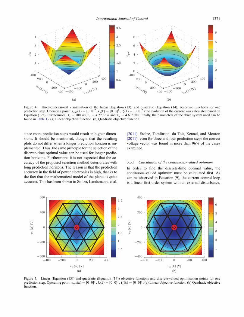
can be set up, where k is the current sample.To illustrate the described principle for the reduction

of the candidate solutions, both the linear (Equation (13))and the quadratic (Equation (14)) objective function val-ues for the current control loop are visualised in Figure 4for the operating point vemf(k) = [0 0]T , i s(k) = [0 0]T ,i∗

s (k) = [0 0]T . Note that despite the fact that the plotsdepicted in Figure 4 show only one prediction step andwere made under the assumption that the back-EMF volt-age vemf(k), the measured stator current i s(k) and the statorcurrent reference i∗

s (k) are zero, a different operating pointwould not change the general shape of the objective func-tion.

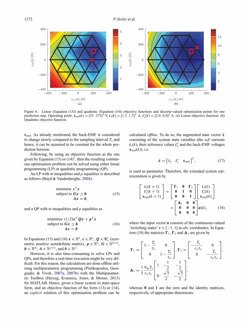
In Figure 5 the two objective functions (13) and (14) areillustrated in a two-dimensional plane for the same condi-tions as in the case shown in Figure 4. The feasible voltagevectors are marked by the two black hexagons (the inner andthe outer one). All voltage values lying within the two blackhexagons (formed by the discrete switching states) can becommanded by the inverter if a continuous-valued opti-misation is considered. The continuous-valued optimum ismarked with a red circle and the discrete optimum with ared ‘x’. As expected, when no current is flowing throughthe machine, no back-EMF is existing and since the currentreferences are equal to zero, the voltage vector leading to aminimum value of the objective function lies at the origin.

A second example is depicted in Figure 6, where thedrive is operating at a different operating point: for this ex-ample the back-EMF voltage, the measured stator currentsand their references are non-zero. From Figure 6(a) and6(b), it can be seen that the discrete-valued optimal valuediffers depending on the nature of the objective function.

For reasons of visualisation, the examples above depictthe objective functions for a one-step prediction horizon,

International Journal of Control 1371

−400−200

0200

400

−400

−200

0200

400

0

1

2

3

4

vα(k) [V]

vβ (k) [V]

j lin

0.5

1

1.5

2

2.5

3

3.5

(a)

−400−200

0200

400

−400

−200

0200

400

0

2

4

6

8

vα(k) [V]

vβ (k) [V]

j qua

d

1

2

3

4

5

6

(b)

Figure 4. Three-dimensional visualisation of the linear (Equation (13)) and quadratic (Equation (14)) objective functions for oneprediction step. Operating point: vemf(k) = [0 0]T , i s(k) = [0 0]T , i∗

s (k) = [0 0]T (the evolution of the current was calculated based onEquation (12a). Furthermore, Ts = 100 μs, rσ = 4.2779 � and τ σ = 4.635 ms. Finally, the parameters of the drive system used can befound in Table 1). (a) Linear objective function. (b) Quadratic objective function.

since more prediction steps would result in higher dimen-sions. It should be mentioned, though, that the resultingplots do not differ when a longer prediction horizon is im-plemented. Thus, the same principle for the selection of thediscrete-time optimal value can be used for longer predic-tion horizons. Furthermore, it is not expected that the ac-curacy of the proposed selection method deteriorates withlong prediction horizons. The reason is that the predictionaccuracy in the field of power electronics is high, thanks tothe fact that the mathematical model of the plants is quiteaccurate. This has been shown in Stolze, Landsmann, et al.

(2011), Stolze, Tomlinson, du Toit, Kennel, and Mouton(2011); even for three and four prediction steps the correctvoltage vector was found in more than 96% of the casesexamined.

3.3.1 Calculation of the continuous-valued optimum

In order to find the discrete-time optimal value, thecontinuous-valued optimum must be calculated first. Ascan be observed in Equation (9), the current control loopis a linear first-order system with an external disturbance,

−400 −200 0 200 400−400

−200

0

200

400

vα(k) [V]

vβ(k

)[V

]

0.5

1

1.5

2

2.5

3

3.5

(a)

−400 −200 0 200 400−400

−200

0

200

400

vα(k) [V]

vβ(k

)[V

]

1

2

3

4

5

6

(b)

Figure 5. Linear (Equation (13)) and quadratic (Equation (14)) objective functions and discrete-valued optimisation points for oneprediction step. Operating point: vemf(k) = [0 0]T , i s(k) = [0 0]T , i∗

s (k) = [0 0]T . (a) Linear objective function. (b) Quadratic objectivefunction.

1372 P. Stolze et al.

−400 −200 0 200 400−400

−200

0

200

400

vα(k) [V]

vβ(k

)[V

]

1

2

3

4

5

(a)

−400 −200 0 200 400−400

−200

0

200

400

vα(k) [V]

vβ(k

)[V

]

2

4

6

8

10

12

(b)

Figure 6. Linear (Equation (13)) and quadratic (Equation (14)) objective functions and discrete-valued optimisation points for oneprediction step. Operating point: vemf(k) = [55 275]T V, i s(k) = [1.3 1.7]T A, i∗

s (k) = [2.0 0.8]T A. (a) Linear objective function. (b)Quadratic objective function.

vemf. As already mentioned, the back-EMF is consideredto change slowly compared to the sampling interval Ts andhence, it can be assumed to be constant for the whole pre-diction horizon.

Following, by using an objective function as the onegiven by Equation (13) or (14)2, then the resulting continu-ous optimisation problem can be solved using either linearprogramming (LP) or quadratic programming (QP).

An LP with m inequalities and p equalities is describedas follows (Boyd & Vandenberghe, 2004):

minimise cT xsubject to Gx � h

Ax = b,

(15)

and a QP with m inequalities and p equalities as

minimise (1/2)xT Qx + pT xsubject to Gx � h

Ax = b.

(16)

In Equations (15) and (16) x ∈ Rn, c ∈ R

n, Q ∈ Sn+ (sym-

metric positive semidefinite matrix), p ∈ Rn, G ∈ R

m×n,h ∈ R

m, A ∈ Rp×n, and b ∈ R

p.However, it is also time-consuming to solve LPs and

QPs, and therefore a real-time execution might be very dif-ficult. For this reason, the calculations are done offline util-ising multiparametric programming (Pistikopoulos, Geor-giadis, & Vivek, 2007a, 2007b) with the Multiparamet-ric Toolbox (Herceg, Kvasnica, Jones, & Morari, 2013)for MATLAB. Hence, given a linear system in state-spaceform, and an objective function of the form (13) or (14),an explicit solution of this optimisation problem can be

calculated offline. To do so, the augmented state vector xconsisting of the system state variables (the αβ currentsi s(k), their reference values i∗

s and the back-EMF voltagesvemf(k)), i.e.

x = [i s i∗

s vemf]T

, (17)

is used as parameter. Therefore, the extended system rep-resentation is given by

⎡⎣ i s(k + 1)

i∗s (k + 1)

vemf(k + 1)

⎤⎦ =

⎡⎣�1 0 �2

0 1 00 0 1

⎤⎦

⎡⎣ i s(k)

i∗s (k)

vemf(k)

⎤⎦

+⎡⎣�1 0 0

0 0 00 0 0

⎤⎦u(k), (18)

where the input vector u consists of the continuous-valued‘switching states’ s ∈ [−1, 1] in abc coordinates. In Equa-tion (18) the matrices �1, �2 and �1 are given by

�1 =

⎡⎢⎣ 1 − Ts

τσ

0

0 1 − Ts

τσ

⎤⎥⎦,�2 =

⎡⎢⎣− Ts

rσ τσ

0

0 − Ts

rσ τσ

⎤⎥⎦,

�1 = 1

3

VdcTs

rσ τσ

⎡⎢⎢⎣

1 −1

2−1

2

0

√3

2−

√3

2

⎤⎥⎥⎦,

whereas 0 and 1 are the zero and the identity matrices,respectively, of appropriate dimensions.

International Journal of Control 1373

x2

x1

Iteration

0

1

2

3

1

2

3 4

5

1

2

3 4

5

1

2

3 4

5

3 1

2

4

5

1

2

Figure 7. Example of a two-dimensional binary search tree.

Based on the above, the objective function (13) is refor-mulated; its new form is

Jlin = || Qx||1, (19)

where the matrix Q is

Q =⎡⎣−1 1 0

0 0 00 0 0

⎤⎦.

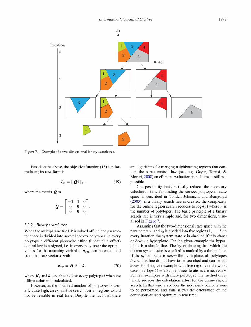
3.3.2 Binary search tree

When the multiparametric LP is solved offline, the parame-ter space is divided into several convex polytopes; in everypolytope a different piecewise affine (linear plus offset)control law is assigned, i.e. in every polytope i the optimalvalues for the actuating variables, uopt, can be calculatedfrom the state vector x with

uopt = H i x + ki , (20)

where H i and ki are obtained for every polytope i when theoffline solution is calculated.

However, as the obtained number of polytopes is usu-ally quite high, an exhaustive search over all regions wouldnot be feasible in real time. Despite the fact that there

are algorithms for merging neighbouring regions that con-tain the same control law (see e.g. Geyer, Torrisi, &Morari, 2008) an efficient evaluation in real time is still notpossible.

One possibility that drastically reduces the necessarycalculation time for finding the correct polytope in statespace is described in Tøndel, Johansen, and Bemporad(2003): if a binary search tree is created, the complexityfor the online region search reduces to log2(n) where n isthe number of polytopes. The basic principle of a binarysearch tree is very simple and, for two dimensions, visu-alised in Figure 7.

Assuming that the two-dimensional state space with theparameters x1 and x2 is divided into five regions 1, . . ., 5, inevery iteration the system state x is checked if it is aboveor below a hyperplane. For the given example the hyper-plane is a simple line. The hyperplane against which thecurrent system state is checked is marked by a dashed line.If the system state is above the hyperplane, all polytopesbelow this line do not have to be searched and can be cutaway. For the given example with five regions in the worstcase only log2(5) = 2.32, i.e. three iterations are necessary.For real examples with more polytopes this method dras-tically reduces the calculation effort for the online regionsearch. In this way, it reduces the necessary computationsto be performed, and thus allows the calculation of thecontinuous-valued optimum in real time.

1374 P. Stolze et al.

0

isα, isβ

tTs

isα(0)

isβ(0)

i∗sα

i∗sβ

tsw

m1α m2α

m1βm2β

Figure 8. Principle of the VSP calculation.

3.3.3 Sector determination

In a last step the sector wherein the continuous-valued opti-mum lies should be determined, i.e. the sector out of the 24in the αβ plane (see Figure 2). Assuming that the discrete-valued optimal value is close to the continuous-valued op-timum, only the three voltage vectors that are closest to thecontinuous-valued optimum are taken into consideration;the optimal voltage vector is one of the three that form thatsector.

Based on this principle, it can be concluded that theregion can be determined in the same way as for spacevector modulation. However, for multilevel inverters it canbecome a quite complex issue to find the correct sectorin which the optimal continuous voltage vector lies. Bytaking a closer look at the voltage vectors in Figure 2,though, it can be seen that all regions are triangles, whichalso holds true for multilevel inverters. Since triangles areconvex polytopes, the same procedure described above can

be adopted, i.e. the region can be found using a binarysearch tree.

3.4 Calculation of the variable switching point

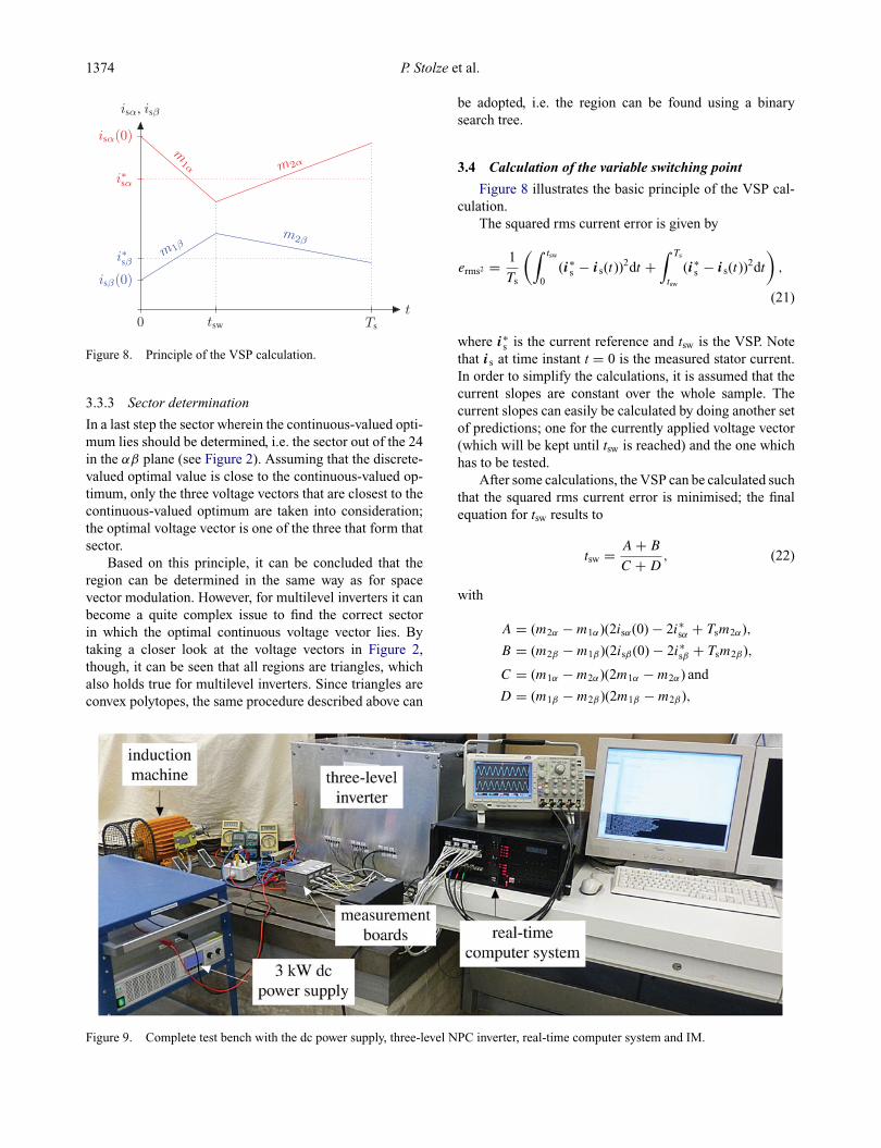
Figure 8 illustrates the basic principle of the VSP cal-culation.

The squared rms current error is given by

erms2 = 1

Ts

(∫ tsw

0(i∗

s − i s(t))2dt +

∫ Ts

tsw

(i∗s − i s(t))

2dt

),

(21)

where i∗s is the current reference and tsw is the VSP. Note

that i s at time instant t = 0 is the measured stator current.In order to simplify the calculations, it is assumed that thecurrent slopes are constant over the whole sample. Thecurrent slopes can easily be calculated by doing another setof predictions; one for the currently applied voltage vector(which will be kept until tsw is reached) and the one whichhas to be tested.

After some calculations, the VSP can be calculated suchthat the squared rms current error is minimised; the finalequation for tsw results to

tsw = A + B

C + D, (22)

with

A = (m2α − m1α)(2isα(0) − 2i∗sα + Tsm2α),

B = (m2β − m1β)(2isβ(0) − 2i∗sβ + Tsm2β),

C = (m1α − m2α)(2m1α − m2α) and

D = (m1β − m2β)(2m1β − m2β),

Figure 9. Complete test bench with the dc power supply, three-level NPC inverter, real-time computer system and IM.

International Journal of Control 1375

where m1 are the current slopes of the currently appliedvoltage vector and m2 those of the new voltage vectorwhich is tested.

3.5 Final optimisation and voltage balancing

When the VSP for a tested voltage vector/switching state(from the heuristically reduced set of voltage vectors) hasbeen calculated, an 2-norm (quadratic) cost function isused for the final optimisation:

J = (i∗

s − i s(k + nint))2 + λ�vc(k + nint)

2

+ (i∗

s − i s(k + 1))2 + λ�vc(k + 1)2, (23)

where nint = tsw/Ts ∈ [0, 1], and λ is the weighting factorfor the voltage balancing.

Because of the reduced set of voltage vectors it has tobe checked if the dc-link capacitor voltages can still bebalanced. The sum of all three phase currents is zero (bal-anced circuit) and positive and negative switching states donot affect the voltage balancing. Thus, no matter which zeroswitching state (‘ppp’, ‘000’ or ‘nnn’) is chosen, the voltagebalance will not be affected. By taking a closer look at thevoltage vectors on the inner hexagon in Figure 2, one of thetwo possible switching states results in zero phase voltagein one phase (e.g. in phase a), the other possible switching

Table 1. Parameters of the induction machine.

Parameter Value

Nominal power Pnom 2.2 kWSynchronous frequency fsyn 50 HzNominal current

∣∣i s,nom

∣∣ 8.5 APower factor cos (ϕ) 0.86Nominal speed ωnom 2830 rpmNumber of pole pairs p 1Stator resistance rs 2.1294 �Rotor resistance rr 2.2773 �Stator inductance ls 350.47 mHRotor inductance lr 350.47 mHMutual inductance lm 340.42 mHInertia J 0.002 kg m2

state results in zero phase voltage but in the other two phases(e.g. in phases b and c). Because of this the voltage balanc-ing for these voltage vectors can be done by choosing theappropriate switching state. Considering the outer hexagon,the switching states at the corners (‘pnn’, ‘ppn’, ‘npn’, etc.)do not affect the capacitor voltage. Thus, the only remain-ing switching states which can lead to voltage unbalancesare ‘p0n’, ‘0pn’, ‘np0’, ‘n0p’, ‘0np’ and ‘pn0’. However,as can be seen, all these voltage vectors belong to regionswhich also contain voltage vectors of the inner hexagon –because of this the voltage balance can be ensured despitethe heuristically reduced set of voltage vectors.

0 20 40 60 80 100-8

-4

0

4

8

Time [ms]

i∗ sα,i

sα[A

]

α current and its reference

0 20 40 60 80 100-8

-4

0

4

8

Time [ms]

i∗ sβ,i

sβ[A

]

β current and its reference

39.2 39.6 40.0 40.4 40.8 41.20

2

4

6

8

Time [ms]

i∗ sα,i

sα[A

]

α current and its reference

39.2 39.6 40.0 40.4 40.8 41.2-6

-4

-2

0

2

Time [ms]

i∗ sβ,i

sβ[A

]

β current and its reference

(a) (b)

Figure 10. Experimental results of a three-level NPC inverter driving an IM for a step change in the speed reference at t ≈ 40 ms. (a)(Larger time scale) top: α component of current (red line) and its reference (black line). Bottom: β component of current (red line) andits reference (black line). (b) (Detail during reference step) top: α component of current (red line) and its reference (black line). Bottom:β component of current (red line) and its reference (black line).

1376 P. Stolze et al.

0 0.2 0.4 0.6 0.8 1.0-2.5

-1.25

0

1.25

2.5

Time [s]

i sa

,isb

,isc

[A]

0 0.2 0.4 0.6 0.8 1.0-2.5

-1.25

0

1.25

2.5

Time [s]

i sa

,isb

,isc

[A]

(a) (b)

Figure 11. Phase currents in steady-state operation at 100 rpm produced by (a) the proposed strategy (VSP2CC – fsw ≈ 1.9 kHz), andby (b) an MPC strategy where a VSP is not calculated (PCC – fsw ≈ 0.85 kHz). (a) Phase currents in steady-state operation at 100 rpmfor VSP2CC. (b) Phase currents in steady-state operation at 100 rpm for PCC.

4. Experimental results

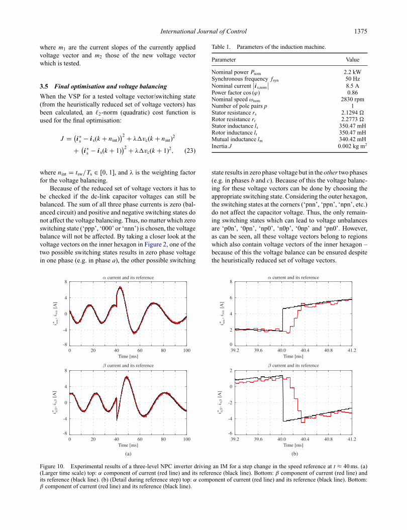
Several experiments have been performed in order to verifythe proposed control algorithm and to demonstrate its po-tentials. The experimental set-up shown in Figure 9 consistsof a three-level NPC inverter driving a 2.2 kW squirrel-cageIM whose parameters are shown in Table 1. The real-timecomputer system is an improved version of the one de-scribed in Al-Sheakh Ameen, Naassani, and Kennel (2010)with a 3.4 GHz Pentium 4 CPU (Stolze, Jung, Ebert, &Kennel, 2013). For all experiments the weighting factor forthe voltage balancing was set to λ = 0.01.

Figure 10 shows the transient response of the proposedcontrol algorithm. For this reason the speed reference wasstepped down from 2000 to 1000\,rpm at time t ≈ 40 ms.

As can be seen in Figure 10, the speed reference changeresults in a step change of both stator currents. It is clearlyvisible that the controller has no problems to track its refer-ences. After the normal delay of two samples (one due to thecalculations and one resulting from the fact that the optimi-sation has to be performed for the next sample) the currentsquickly follow their references within three samples.

The second experiment was conducted in order to com-pare the steady-state phase currents at 100 rpm for the pro-posed strategy to a PCC strategy without a VSP, i.e. to a con-ventional Finite Control-Set MPC method. The experimentwas conducted with a sampling interval of Ts = 62.5 μs.The result can be seen in Figure 11. As can be observed,the proposed control algorithm has a significant influence

0 10 20 30 40 50-2.5

-1.25

0

1.25

2.5

Time [ms]

i sa

,isb

,isc

[A]

0 10 20 30 40 50-2.5

-1.25

0

1.25

2.5

Time [ms]

i sa

,isb

,isc

[A]

(a) (b)

Figure 12. Phase currents in steady-state operation at 2830 rpm produced by (a) the proposed strategy (VSP2CC – fsw ≈ 2.1 kHz), andby (b) an MPC strategy where a VSP is not calculated (PCC – fsw ≈ 1.65 kHz). (a) Phase currents in steady-state operation at 2830 rpmfor VSP2CC. (b) Phase currents in steady-state operation at 2830 rpm for PCC.

International Journal of Control 1377

0 250 500 750 1000 1250 1500 1750 2000 2250 2500 27500

200

400

600

800

1000

1200

1400

1600

VSP2CC

PCC

Machine speed [rpm]

fsw

[Hz]

Figure 13. Average switching frequency of VSP2CC (green line)and PCC (blue line) (Ts = 100 μs).

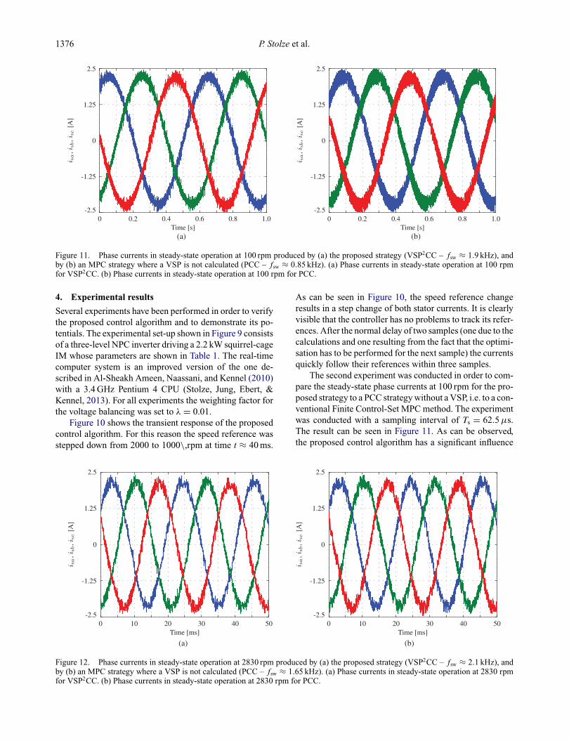
on the quality of the controlled currents. At this operatingpoint the VSP2CC strategy can operate with a much higherswitching frequency (fsw ≈ 1.9 kHz) than the conventionalPCC algorithm (fsw ≈ 850 Hz). This higher switching fre-quency results in less current ripples at this operating point.The same experiment was repeated at full nominal speed(2830 rpm). The results can be seen in Figure 12. At thisoperating point the VSP2CC strategy (Figure 12(a)) leadsto nearly the same switching frequency as plain PCC (Fig-ure 12(b)) and the current ripples are in the same range.

Finally, the results of the last experiment are shown inFigure 13. It was conducted in order to investigate moredeeply the effect of the VSP2CC strategy on the switchingfrequency depending on the operation point of the system.Thus, the average switching frequency per device was mea-sured in steps of 10 rpm from 0 rpm to full nominal speed(2830 rpm) for both control methods. It is clearly visiblethat VSP2CC leads to much higher switching frequenciesat low machine speeds and thus also to decreased currentripples. While the switching frequency for VSP2CC is al-ways higher than 900 Hz, it goes down to less than 100 Hzfor the conventional PCC algorithm. As verified in the pre-vious experiment, for higher machine speeds the switchingfrequencies are nearly the same for both strategies.

5. Conclusion and further work

In this paper a VSP2CC of induction motors (IMs) withheuristic voltage vector preselection was introduced. It pro-vides an effective solution for the two main drawbacks ofdirect, enumeration-based MPC methods, i.e. the high cal-culation effort and large ripples on the controlled variables.With regards to the first problem, a reduction of the can-didate optimal solutions set is proposed to keep the com-putational burden low. This is done by considering onlythe (three) discrete-valued solutions that form the sectorwherein the continuous-valued optimum lies. To overcome

the second drawback, the state of the inverter switches ischanged in between the sampling interval; the VSP is cal-culated based on an optimisation problem formulated tominimise the ripple of the stator currents. The experimen-tal results clearly verify that the controller shows excellentbehaviour during transients and in steady-state. Further de-velopments of the proposed method are the extension tofive-level inverters.

Notes1. The definition of the active and zero voltage vectors is given

in Section 2.2. Note that the back-EMF vemf is known.

ReferencesAl-Sheakh Ameen, N., Naassani, A.A., & Kennel, R.M. (2010).

Design of a digital system dedicated for electrical drive ap-plications. EPE Journal, 20, 37–44.

Boyd, S., & Vandenberghe, L. (2004). Convex optimization. Cam-bridge: Cambridge University Press.

Correa, P., Pacas, M., & Rodrıguez, J. (2007). Predic-tive torque control for inverter-fed induction machines.IEEE Transactions on Industrial Electronics, 54, 1073–1079.

Cortes, P., Kazmierkowski, M.P., Kennel, R.M., Quevedo, D.E., &Rodrıguez, J. (2008). Predictive control in power electronicsand drives. IEEE Transactions on Industrial Electronics, 55,4312–4324.

Depenbrock, M. (1988). Direct self-control (DSC) of inverter-fedinduction machines. IEEE Transactions on Power Electronics,3, 420–429.

Geyer, T. (2005). Low complexity model predictive control inpower electronics and power systems (PhD thesis). AutomaticControl Laboratory, ETH Zurich, Zurich, Switzerland.

Geyer, T. (2012). Model predictive direct current control: For-mulation of the stator current bounds and the concept of theswitching horizon. IEEE Industry Applications Magazine, 18,47–59.

Geyer, T., & Mastellone, S. (2012). Model predictive direct torquecontrol of a five-level ANPC converter drive system. IEEETransactions on Industry Applications, 48, 1565–1575.

Geyer, T., Oikonomou, N., Papafotiou, G., & Kieferndorf, F.D.(2012). Model predictive pulse pattern control. IEEE Trans-actions on Industry Applications, 48, 663–676.

Geyer, T., Papafotiou, G., & Morari, M. (2009). Model predictivedirect torque control – part I: Concept, algorithm and analysis.IEEE Transactions on Industrial Electronics, 56, 1894–1905.

Geyer, T., Torrisi, F.D., & Morari, M. (2008). Optimal complexityreduction of polyhedral piecewise affine systems. Automatica,44, 1728–1740.

Holtz, J. (1995). The representation of AC machine dynamics bycomplex signal flow graphs. IEEE Transactions on IndustrialElectronics, 42, 263–271.

Karamanakos, P. (2013). Model predictive control strategies forpower electronics converters and AC drives (PhD thesis).Electrical Machines and Power Electronics Laboratory, NTUAthens, Athens, Greece.

Karamanakos, P., Geyer, T., Oikonomou, N., Kieferndorf, F.D., &Manias, S. (2014). Direct model predictive control: A reviewof strategies that achieve long prediction intervals for powerelectronics. IEEE Industrial Electronics Magazine, 8, 32–43.

1378 P. Stolze et al.

Karamanakos, P., Stolze, P., Kennel, R.M., Manias, S., & du ToitMouton, H. (2014). Variable switching point predictive torquecontrol of induction machines. IEEE Journal of Emerging andSelected Topics in Power Electronics, 2, 285–295.

Kazmierkowski, M.P., Krishnan, R., & Blaabjerg, F. (2002). Con-trol in power electronics. New York, NY: Academic Press.

Kovacs, P. (1984). Transient phenomena in electrical machines.Amsterdam: Elsevier Science.

Herceg, M., Kvasnica, M., Jones, C.N., & Morari, M. (2013).Multi-Parametric Toolbox 3.0. Proceedings of the Euro-pean Control Conference (pp. 502–510). Zurich, Switzer-land. Retrieved from http://control.ee.ethz.ch/∼mpt/3/Main/CitationInfo

Linder, A., Kanchan, R., Kennel, R., & Stolze, P. (2010). Model-based predictive control of electric drives. Gottingen: Cuvil-lier Verlag.

Maciejowski, J.M. (2002). Predictive control with constraints.Englewood Cliffs, NJ: Prentice-Hall.

Miranda, H., Cortes, P., Yuz, J.I., & Rodrıguez, J. (2009). Pre-dictive torque control of induction machines based on state-space models. IEEE Transactions on Industrial Electronics,56, 1916–1924.

Oikonomou, N., Gutscher, C., Karamanakos, P., Kieferndorf, F.D.,& Geyer, T. (2013). Model predictive pulse pattern controlfor the five-level active neutral point clamped inverter. IEEETransactions on Industry Applications, 49, 2583–2592.

Papafotiou, G., Kley, J., Papadopoulos, K.G., Bohren, P., &Morari, M. (2009). Model predictive direct torque control– part II: Implementation and experimental evaluation. IEEETransactions on Industrial Electronics, 56, 1906–1915.

Patsakis, G., Karamanakos, P., Stolze, P., Manias, S., Kennel, R.,& Mouton, T. (2013, November). Variable switching pointpredictive torque control for the four-switch three-phase in-verter. Proceedings of the IEEE International Symposium onPredictive Control of Electrical Drives and Power Electronics,Munich, Germany.

Pistikopoulos, E., Georgiadis, M.C., & Vivek, D. (2007a). Multi-parametric model-based control. Volume 2 of Process SystemsEngineering. Weinheim: Wiley.

Pistikopoulos, E., Georgiadis, M.C., & Vivek, D. (2007b). Multi-parametric programming. Volume 1 of Process Systems Engi-neering. Weinheim: Wiley.

Rawlings, J.B., & Mayne, D.Q. (2009). Model predictive control:Theory and design. Madison, WI: Nob Hill.

Rodrıguez, J., Kazmierkowski, M., Espinoza, J.R., Zanchetta, P.,Abu-Rub, H., Young, H.A., & Rojas, C.A. (2013). State ofthe art of finite control set model predictive control in powerelectronics. IEEE Transactions on Industrial Informatics, 9,1003–1016.

Rodrıguez, J., Kennel, R., Espinoza, J.R., Trincado, M., Silva,C., & Rojas, C.A. (2012). High-performance control strate-gies for electrical drives: An experimental assessment. IEEETransactions on Industrial Electronics, 59, 812–820.

Rojas, C.A., Rodrıguez, J., Villaroel, F., Espinoza, J.R., Silva, C.,& Trincado, M. (2013). Predictive torque and flux controlwithout weighting factors. IEEE Transactions on IndustrialElectronics, 60, 681–690.

Stolze, P., Jung, J., Ebert, W., & Kennel, R. (2013, November).FPGA-basiertes Echtzeitrechner-System mit RTAI-Linux furAntriebssysteme. Proceedings of the SPS Drives Kongress,Nuremberg, Germany.

Stolze, P., Karamanakos, P., Kennel, R., Manias, S., & Mouton, T.(2013, September). Variable switching point predictive torquecontrol for the three-level neutral point clamped inverter. InProceedings of the European Conference on Power Electron-ics and Applications (pp. 1–10). Lille, France.

Stolze, P., Landsmann, P., Kennel, R., & Mouton, T. (2011,August/September). Finite-set model predictive control withheuristic voltage vector preselection for higher predictionhorizons. In Proceedings of the European Conference onPower Electronics and Applications (pp. 1–9). Birmingham,UK.

Stolze, P., Tomlinson, M., du Toit, D., Kennel, R., & Mouton, T.(2011, September). Predictive torque control of an inductionmachine fed by a flying capacitor converter. In Proceedings ofthe IEEE Conference Africon (pp. 1–6). Livingstone, Zambia.

Stolze, P., Tomlinson, M., Kennel, R., & Mouton, T. (2013, June).Heuristic finite-set model predictive current control for induc-tion machines. In Proceedings of the IEEE Energy ConversionCongress and Exposition Asia (pp. 1221–1226). Melbourne,Australia.

Takahashi, I., & Noguchi, T. (1986). A new quick-response andhigh-efficiency control strategy of an induction motor. IEEETransactions on Industry Applications, IA-22, 820–827.

Tøndel, P., Johansen, T.A., & Bemporad, A. (2003). Evaluation ofpiecewise affine control via binary search tree. Automatica,39, 945–950.

Appendix

The matrices Ad , Bd1, Bd2 and Cd of the drive model given byEquation (12) are as follows:

Ad = 1 + Ts

[A 00 0

], (24)

Bd1 = Ts

[B1

0

], (25)

Bd2 = Ts

[0

B2(x(k))

], (26)

Cd = C, (27)

where 1 is the identity matrix of appropriate dimensions, 0 is thezero matrix, or zero vector of appropriate dimensions, and

A =

⎡⎢⎢⎢⎢⎢⎢⎢⎢⎢⎣

− 1

τσ

0kr

rσ τσ τr

ωr

kr

rσ τσ

0 − 1

τσ

−ωr

kr

rσ τσ

kr

rσ τσ τrlm

τr

0 − 1

τr

−ωr

0lm

τr

ωr − 1

τr

⎤⎥⎥⎥⎥⎥⎥⎥⎥⎥⎦

, (28)

B1 = 1

rσ τσ

⎡⎢⎣

1 0 00 1 00 0 00 0 0

⎤⎥⎦Vdc

2K , (29)

B2(x(k)) = 1

2CxT (k)

⎡⎢⎢⎢⎣

1 0 00 1 00 0 00 0 00 0 0

⎤⎥⎥⎥⎦K−T , (30)

C =⎡⎣ 1 0 0 0 0

0 1 0 0 00 0 0 0 1

⎤⎦. (31)