
Effective Tax Rates on Consumption and Factor Incomes
57
Effective Tax Rates on Consumption and Factor Incomes: a quarterly frequency estimation for Brazil Cyntia Freitas Azevedo and Angelo Marsiglia Fasolo September, 2015 398
-
Upload
khangminh22 -
Category
Documents
-
view
0 -
download
0
Transcript of Effective Tax Rates on Consumption and Factor Incomes
Effective Tax Rates on Consumption and Factor Incomes: a quarterly frequency estimation for Brazil
Cyntia Freitas Azevedo and Angelo Marsiglia Fasolo
September, 2015
398

ISSN 1518-3548 CGC 00.038.166/0001-05
Working Paper Series Brasília n. 398 September 2015 p. 1-56

Working Paper Series
Edited by Research Department (Depep) – E-mail: [email protected]
Editor: Francisco Marcos Rodrigues Figueiredo – E-mail: [email protected]
Editorial Assistant: Jane Sofia Moita – E-mail: [email protected]
Head of Research Department: Eduardo José Araújo Lima – E-mail: [email protected]
The Banco Central do Brasil Working Papers are all evaluated in double blind referee process.
Reproduction is permitted only if source is stated as follows: Working Paper n. 398.
Authorized by Luiz Awazu Pereira da Silva, Deputy Governor for Economic Policy.
General Control of Publications
Banco Central do Brasil
Comun/Dipiv/Coivi
SBS – Quadra 3 – Bloco B – Edifício-Sede – 14º andar
Caixa Postal 8.670
70074-900 Brasília – DF – Brazil
Phones: +55 (61) 3414-3710 and 3414-3565
Fax: +55 (61) 3414-1898
E-mail: [email protected]
The views expressed in this work are those of the authors and do not necessarily reflect those of the Banco Central or
its members.
Although these Working Papers often represent preliminary work, citation of source is required when used or reproduced.
As opiniões expressas neste trabalho são exclusivamente do(s) autor(es) e não refletem, necessariamente, a visão do Banco
Central do Brasil.
Ainda que este artigo represente trabalho preliminar, é requerida a citação da fonte, mesmo quando reproduzido parcialmente.
Citizen Service Division
Banco Central do Brasil
Deati/Diate
SBS – Quadra 3 – Bloco B – Edifício-Sede – 2º subsolo
70074-900 Brasília – DF – Brazil
Toll Free: 0800 9792345
Fax: +55 (61) 3414-2553
Internet: <http//www.bcb.gov.br/?CONTACTUS>
Effective Tax Rates on Consumption andFactor Incomes: a quarterly frequency
estimation for Brazil∗
Cyntia Freitas Azevedo†
Angelo Marsiglia Fasolo‡
Abstract
The Working Papers should not be reported as representing the views of the
Banco Central do Brasil. The views expressed in the papers are those of the
author(s) and do not necessarily reflect those of the Banco Central do Brasil.
This paper estimates time series of effective tax rates for consumption and factor
incomes for Brazil, following the spirit of Mendoza et al (1994)[12]. The procedure
to generate quarterly estimates of the tax base, using microdata from populational
surveys, and the tax revenues seems to be appropriate, despite its simplicity, as
the time series of the tax burden and the effective tax rates are in line with the
historical Brazilian experience on fiscal policy. The estimated tax burden identifies
a positive trend over time, despite the partial interruption after the international
crisis in 2008. The paper also provides preliminary evidence on the properties of
the computed effective tax rates and their relation with the business cycles.
Keywords: Fiscal policy; Effective tax rates; Consumption tax; Factor income
taxes
JEL Classification: E62, F41
∗We would like to thank Luis Gonzaga de Queiroz Filho, André Minella and Jeferson Luis Bittencourt
on preliminary discussions and valuable information on data sources. We also thank Pierpaolo Benigno
and members of the Research Department of the Central Bank of Brazil that contributed with helpful
comments on the first draft of this paper. We also thank the DataZoom’s website portal team, of the
Economics Department of PUC-RJ, for the codes to access microdata from IBGE. We are also indebted
to Jose Deodoro de Oliveira Filho for his help with the system to read and convert PDF files to build our
dataset. All these people provided significant support while writing this paper, but the remaining errors
are our own fault.†Research Department, Banco Central do Brasil and PUC-Rio, e-mail: [email protected]‡Research Department, Banco Central do Brasil, e-mail: [email protected]
3
1 Introduction
The main purpose of this study is to construct quarterly time series of the effective tax
rates on consumption, labor and capital for Brazil. An appropriate measure of tax rates is
central for the construction of macroeconomic models that aim at evaluating the impacts
of fiscal policy. As pointed by Mendoza et al (1994)[12], "these tax rates are necessary both
to develop quantitative applications of the theory and to help transform the theory into
a policy-making tool". However, calculating these rates, specially at a higher frequency,
has proven to be a very challenging task. In Emerging Economies, where the quality and
availability of information on tax collection and its tax base are usually questionable, the
number of strong assumptions necessary to make inference about tax rates might prove
the exercise useless.
In Brazil, particularly, there are two types of problems associated with the computation
of average effective tax rates and its use as a policy-making tool. The first problem,
associated with the computation of the tax base, is a result of the lack of timely updates in
National Accounts necessary to keep the estimates of tax rates useful for policy exercises.
The National Accounts in Brazil provide estimates of labor and capital income at annual
frequency only and with very long delays. As of today, the last information available
from the Brazilian Institute of Geography and Statistics (IBGE, in Portuguese) finishes
in 2009. Thus, the construction of estimates of the effective tax rates at a frequency
higher than annual demands additional hypotheses to replace the available information
on capital and labor returns based on the National Accounts.
The second type of problem is related to information on fiscal policy in Brazil —
more specifically, on information from subnational entities of the Federation. Data on
revenues and expenses of the Federal Government are available at monthly frequency
with very little delay. For municipalities, however, detailed information from offi cial
authorities is available at annual frequency only, mostly from a recent comprehensive
dataset published by the National Treasury Secretariat ("Secretaria do Tesouro Nacional",
in Portuguese) called FINBRA. Also, in terms of tax collection, an annual study published
by the Secretariat of the Federal Revenue ("Secretaria da Receita Federal", in Portuguese)
estimates the total tax burden over the Brazilian economy for the previous fiscal year.
Building a real time estimate of effective tax rates in Brazil demands accessing information
on tax revenues and contributions to civil servants’social security system from sources
other than offi cial National authorities responsible for conducting fiscal policy in the
country.
This paper proposes solutions for these problems, trying to overcome the issues pre-
sented above using alternative sources of information and providing a detailed method-
ology to compute effective taxes in Brazil. In order to solve problems associated with
4
information from subnational entities, we built a system capable of downloading, read-
ing and compiling information from reports that each subnational government is required
to submit bimonthly to a public access database run by a federal public bank (Caixa
Econômica Federal) together with the National Treasury Secretariat1. Each report is
submitted in a standard form, converted to PDF format when made available for public
consultation. Thus, the computational system must be capable of: 1) downloading, for
each unit of subnational government, the bimonthly reports in PDF format; 2) converting
reports to a format in which other software is able to read the information; 3) compiling,
with the support of other computational tools, a single, aggregate dataset of each variable
for the use in our exercises. The idea of using such system to calculate tax revenues from
states and municipalities is not new: Orair et al (2013)[15], in a parallel effort from the
development of this paper, built a similar system to obtain monthly estimates of the total
tax burden applied over the Brazilian economy. In this paper, we take a step further,
collecting also information on government spending and civil servants’contributions to
their social security system from the same set of reports. We also take a simpler approach
in order to estimate gaps in the information from municipalities, combining data from
FINBRA to fill the missing gaps.
To construct a quarterly series on labor and capital income, instead of relying on in-
formation from the National Accounts, we use microdata from three population surveys
available at different frequencies. These surveys provide information on employment and
average wages, from which we compute the aggregate labor compensation in the econ-
omy. The use of data from three different surveys required a detailed evaluation of the
labor income distribution profile over time. This information is taken into account when
building the time series of total labor income for the Brazilian economy.
In this paper, we provide annual values of effective taxes for Brazil, from 1999 until
2009, based on information from the National Treasury Secretariat, Secretariat of the
Federal Revenue and the National Accounts. We also detail the methodology employed
to build a quarterly dataset using the reports provided by subnational governments and
population surveys. Under an additional set of assumptions, given the available amount
of information collected, we were able to construct a quarterly dataset on tax revenues
and the tax base from 1999 to 2014. The comparison of annual rates with the 4-quarter
cumulative rates computed using the high-frequency dataset shows some discrepancies,
most likely due to the quality of data provided by subnational governments. Gaps between
annual data and the high-frequency dataset mostly affects the composition between capital
1Starting in 2015, the National Treasury Secretariat introduced a new system for collecting andorganizing information on the public accounts. The new system (Siconfi) summarizes data on re-gional governments collected from both SISTN and annual data from FINBRA. It is available inhttps://siconfi.tesouro.gov.br/siconfi/index.jsf
5
and labor taxes, despite preserving the dynamics over time of both effective tax rates.
Given the final dataset on average effective tax rates, we also provide an initial analysis
on the sources of fluctuations in those rates. Changes in average effective tax rates are
associated with both changes in tax policy and changes in the overall state of the economy.
The paper is organized as follows. The next section discusses the literature on comput-
ing effective tax rates, with special focus on previous efforts documented for the Brazilian
economy. Section 3 outlines the methodology of computing average effective tax rates
for Brazil, following closely the work of Mendoza et al (1994)[12] and Lledó (2005)[10],
while also presenting the additional hypotheses necessary to move from the annual to the
quarterly estimates. Sections 4 and 5 apply the described methodology to compute effec-
tive rates at annual and quarterly frequencies, respectively, presenting all the necessary
adjustments due to the data collected —especially in terms of high-frequency database
on tax and contributions revenues and on the tax base. An empirical analysis of the
quarterly time series of effective tax rates is presented in section 6. Section 7 concludes.
2 Related Literature
The main reference on the computation of effective tax rates is the work of Mendoza
et al (1994)[12]. Their approach allows to estimate the effective tax rates on consumption
and factor incomes consistent with the tax distortions faced by a representative agent in
a general equilibrium framework. One of the advantages of their method is that it does
not require a rigorous treatment of the tax legislation. It is a simple method that requires
only data from the National Accounts and tax revenues statistics, allowing cross-country
comparisons. They point out to three objectives achieved by their approach: (i) it takes
into account the net effect of existing rules regarding credits, exemptions and deductions;
(ii) it separates taxes on labor income from taxes on capital income; and, (iii) it incor-
porates the effects of taxes not filed with individual income tax revenues, such as social
security contributions and property taxes, on factor income taxation. Given the authors
objective, it is an appropriate methodology to compute average tax rates, capturing the
effects of changes in tax deductions, tax credits and a general characterization of feed-
back effects on taxes from economic agents. It does not, however, measure important
movements in taxes with significant macroeconomic impacts, like changes in marginal tax
rates, as highlighted in Carey and Rabesona (2002)[3]. Average effective tax rates might
also be sensitive to other issues, like tax planning and the international taxation of capital
flows.
The work of Mendoza et al (1994)[12] and Carey and Rabesona (2002)[3] is focused on
the use of data compiled by OECD, usually available for large time spans, with detailed
6
definitions and good quality control of information across countries, allowing reasonably
appropriate cross-country comparisons. As mentioned in the introduction, datasets from
Emerging Economies usually show problems that might compromise the estimates of such
tax rates2. For Brazil, specifically, there is a growing literature on the evaluation of the
impacts of fiscal policies and tax reforms. In general, these studies apply some measure of
average effective tax rates in order to calibrate models or to perform econometric analysis.
Due to the problems listed here and in the introduction —namely, the lack of accurate and
updated data on fiscal variables for long periods of time, at higher frequency and with
little delay; and the lack of details and information with regular updates from the National
Accounts with respect to the returns of labor and capital for the Brazilian economy —,
the few studies that computed effective tax rates for Brazil used annual data only.
One example of a study using estimates of effective tax rates for Brazil is provided
by Araújo and Ferreira (1999)[1], who evaluate the allocative effects and welfare impacts
of a tax reform. The authors use a neoclassical model calibrated with information of
tax rates based on total tax revenues of 1995. Cavalcanti and Silva (2010)[5] use an
overlapping generations (OLG) model to study the impact of tax reforms on GDP, capital
accumulation and welfare. Simulations estimated the effects of capital and labor tax
exemption measures, compensated by increases in income tax. They compute tax rates
based on data from the National Accounts for the year of 2004.
One of the first attempts to apply the methodology from Mendoza et al (1994)[12]
for Brazil was made by Araújo Neto and Sousa (2001)[2] to study the comovements
between macroeconomic aggregates and average effective tax rates. They make a good
correspondence between the standard OECD coding for tax revenues used by Mendoza et
al (1994)[12] and the different sources of tax revenues in Brazil. The authors were able to
compute annual average tax rates on consumption, labor and capital using data on tax
revenues and the National Accounts from 1975 to 1999. They faced, however, problems to
construct the dataset due to missing data, despite still being able to provide a relatively
long time series.
Lledó (2005)[10] constructs a dynamic general equilibriummodel to analyze the macro-
economic and redistributive effects of replacing turnover and financial taxes in Brazil by
a consumption tax. He uses an OLG model calibrated with data for 2002, computing
effective tax rates based on the framework of Mendoza et al (1994)[12], modified to in-
corporate details of the Brazilian economy and features of the OLG model. Ferreira and
Pereira (2010)[7] follow the procedure presented by Lledó (2005)[10] to calibrate a simple
RBC model to analyze the impact of a tax reform in the Brazilian economy. They assume,
2Volkerink, Sturm and de Haan (2002)[18] note that even the use of OECD data might be flawed.They compute the effective tax rates for a group of OECD countries using data from local, nationalsources and find significant discrepancies in results compared to Mendoza et al (1994)[12].
7
from the first order conditions of the model, that the tax base is proportional to changes
in aggregate output, as the labor and capital shares are determined by a single parameter
of the production function.
While the previous two papers calibrate models using information from a single year,
Pereira (2009)[16] computes effective tax rates on consumption, individual income, labor
income and capital income from 2001 to 2005. The author follows the methodology pre-
sented by Mendoza et al (1994)[12], adapted to specific features of the Brazilian economy,
in order to build the dataset used to calibrate a model to analyze the impact of fiscal
policies on business cycles.
Finally, other alternatives to compute effective tax rates are based on a combination
of input-output tables and microdata, using disaggregated information to analyze the
inequality of the tax burden over the economy. While not avoiding the hypothesis of
a full pass-through of taxes to consumers, studies based on disaggregated data provide
useful information on marginal tax rates. For Brazil, Siqueira et al (2001)[17] use infor-
mation from input-output tables of 1995 to compute effective tax rates on consumption
for Brazil, disaggregating information on economic sectors and tax incidence over demand
components for Brazil. More recently, Nogueira et al (2013)[13] use microdata from two
population surveys to simulate a model, trying to estimate the tax burden inequality over
labor income for the Brazilian economy in 2009. The model simulated in Nogueira et al
(2013)[13] receives as an input not only survey data, but also information from Brazilian
legislation on tax rates. The idea of using information from the legislation as an input
for modelling purposes was adopted in Carvalho and Valli (2011)[4] to calibrate a DSGE
model for the Brazilian economy.
Previously mentioned literature worked only with annual data on tax revenues and
the National Accounts. To the best of our knowledge, the first attempt to construct a
high-frequency database on tax revenues for Brazil was made by Orair et al (2013)[15].
The authors estimate the Brazilian tax burden at monthly frequency from 2002 until
2012. Their estimation of subnational government information on taxes is very precise,
mostly by their effort on building a complex state-space model to estimate high-frequency
time series based on low-frequency information available. The compilation of a dataset
of tax revenues of subnational entities is analogous to what is done in this paper, with
the development of a system capable of reading several reports from PDF files. As said
before, the main focus of Orair et al (2013)[15] is on the evolution of the tax burden; our
paper, on the other hand, combines information on tax revenues with a high-frequency
inference on the tax base to compute effective tax rates.
8
3 Computing Effective Tax Rates
This section details the methodology employed to compute the average effective tax
rates for Brazil, both at the annual and quarterly frequencies. We closely follow the
presentation in Lledó (2005)[10], who adapted the basic methodology of Mendoza et al
(1994)[12] to Brazil, to discuss the computation of effective rates for the country. The
section starts providing some context on the way effective tax rates are computed here,
with possible applications in a general equilibrium framework. It follows with details
on the definitions of tax rates on consumption, labor and capital income, followed by
a presentation on the adjustments performed when working with quarterly data, with
the necessary adaptations to the specificities of the Brazilian tax system. A complete
description of datasets, along with a discussion on the appropriate separation of taxes
under each class, are presented in the next section.
3.1 Effective Tax Rates in General Equilibrium
This subsection relates the average effective tax rates computed in this paper with
a very broad framework of dynamic general equilibrium models. The objective is to
provide context on the incidence of taxes in theoretical models, while also outlining a few
diffi culties when dealing with Brazilian data. Despite its relevance, the general equilibrium
framework presented here does not include any form of heterogeneity on households or
firms. A few topics related to agents’ heterogeneity, like the effects of labor income
distribution on effective tax rates on labor, are discussed on section 6.
A general description of the budget constraint of a representative household includes
the total spending on consumption goods (ct), investment on capital goods (it) and gov-
ernment debt holdings (bt), on the expenses side. On the revenues side, it includes interest
received on previously held government debt (rtbt−1), returns on production factors (wthtand rkt kt as the returns on labor supply and capital rental, respectively) and firms’profits
(φt) (all variables in nominal terms). Spending on consumption goods includes the ex-
penditure on taxes levied exclusively on those goods and paid by households, τ c,h. Gross
capital and labor incomes are net of taxes paid by households —τ l,h and τ k,h, respectively.
In order to account for taxes levied on general income, that cannot be split in terms of
capital and labor, the budget constraint also includes an additional tax rate (τ y), equally
charging the household’s returns on the production factors3.
(1 + τ c,h) ct + it + bt = rtbt−1 + (1− τ l,h − τ y)wtht + (1− τ k,h − τ y) rkt kt + Φt (1)
3If the model does not allow for taxes on aggregate income, one can use (τ l,h + τy) as the effectivetax rate on labor and (τk,h + τy) as the effective tax rate on capital levied on households.
9
On the firms’side, profits are generated by the revenue of selling output, minus pay-
ments to labor and capital used during the production process. Output (yt) is consumed
by households (ct), and the government (gt) or used as investment good (it). Similar to
the equation describing the households’budget constraint, there are taxes levied on the
output sold as a consumption good4, τ c,f , on total payroll, τ l,f , and rented capital, τ k,fthat are paid by the firm.
Φt = (1− τ c,f ) (ct + gt) + it − (1 + τ l,f )wtht − (1 + τ k,f ) rkt kt (2)
yt = ct + gt + it = wtht + rkt kt (3)
In the analytical example described above, revenues from the general income tax rate
are given by5:
Ty = τ y(wtht + rkt kt
)Similarly, tax revenues on consumption, labor and capital income are computed using
the total revenues collected from households and firms:
Tc = (τ c,h + τ c,f ) (ct + gt) Tl = (τ l,h + τ l,f )wtht Tk = (τ k,h + τ k,f ) rkt kt
Once information on tax revenues is available, effective tax rates on consumption (τ c),
income (τ y), labor income (τ l) and capital income (τ k) are computed using the definition
of their respective tax bases:
τ c =Tc
ct + gtτ y =
Tywtht + rkt kt
τ l =Tlwtht
τ k =Tkrkt kt
The equations above highlight two important features of computing average effective
tax rates. First, calculating aggregate tax rates does not depend if taxes are levied on
households or firms, since, in general equilibrium, taxes levied on firms are also affecting
households’decisions, either through the pricing and production decisions of the firms, or
through the profits transferred to families. Only two pieces of information are necessary
to calculate such tax rates —tax revenues and the tax base —and this information does
not depend on the agent of the economy charged with the tax.
Second, disaggregated measures of effective tax rates are conditioned on the informa-
tion set on tax revenues. For Brazil, as sections 4 and 5 show, information on labor income
taxes allows a reasonable approximation of effective rates levied on firms and households,
τ l,h and τ l,f . Unfortunately, the same disaggregation is not possible with respect to taxes
4In this example, without loss of generality, assume that goods demanded for investment are not taxedby the government.
5For the sake of notation, define Tx as the total revenue from taxes over aggregate x. Define also τxas the effective tax rate over aggregate x.
10
on consumption and capital income.
Ideally, if data on tax revenues and the tax base were readily available, it would be
simple to compute average effective rates for a simple economy like the one described
above. The main challenge here is to build both types of datasets, specially at higher
frequency, where detailed information is scarce. The adjustments applied to Brazilian
data in order to compute the effective tax rates both at annual and quarterly frequencies
are discussed in the rest of the section.
3.2 Effective Tax Rate on Consumption
The effective average tax rate on sales of consumption goods is given by:
τ c =Tc
C +G−GW − Tc(4)
where Tc represents the total revenue from taxes on consumption of goods and services
and excise taxes. C and G are the National Accounts data on private and government
consumption, respectively. GW is the compensation of government employees. In order
to obtain the pre-tax value of consumption, which is the definition of the tax base, rev-
enues on consumption tax are discounted in the denominator, since the Brazilian National
Accounts measure consumption expenditures at post-tax prices.
For the sake of comparison, Pereira (2009)[16] does not include government consump-
tion on the tax base. Here, as in Mendoza et al (1994)[12], government consumption is
included, net of the compensation of government employees (G−GW ), as the tax revenuesstatistics include taxes paid by the government in the purchase of goods and nonfactor
services.
3.3 Effective Tax Rates on General Income
The major problem associated with the definition of tax rates on labor and capital
income is the identification of the tax burden over household’s labor and capital income.
The problem, pointed out by Mendoza et al (1994)[12] and also observed in Brazilian data,
is that information sources usually do not provide a clear breakdown of the tax incidence
over individual income. In order to overcome this problem, Mendoza et al (1994)[12]
assume that all sources of household’s income from labor supply and capital rental are
taxed at the same rate when directly taxed.
In the framework of Mendoza et al (1994)[12], the tax rate over individual income is
computed as a first step to obtain tax rates over labor and capital incomes. In the second
step, an exogenous parameter defining a constant labor share of income is used to split tax
revenues and tax base for each production factor. Lledó (2005)[10] points out that this
11
imputation assumes a symmetric tax treatment between labor and capital income. As in
Lledó (2005)[10], equation 1 allows an effective tax rate on household’s general income to
coexist with separate taxes on capital and labor. The effective tax rate on total individual
income is then given by:
τ y =Ty
W +RMB + EOB(5)
where Ty is the total revenue collected by the individual income tax rate. The denom-
inator is defined as the net domestic income, which is the sum of wages and salaries (W ),
gross mixed income6 (RMB) and the gross operating surplus (EOB), obtained from the
National Accounts. The sum W + RMB + EOB corresponds to the income households
receive from labor supply and capital rental, wtht + rkt kt.
3.4 Effective Tax Rates on Labor and Capital
Once income taxes are properly classified based on its incidence, the final step to
compute effective tax rates is to use information from the National Accounts to split
household’s income from labor supply (wtht) and capital rental (rkt kt). Mendoza et al
(1994)[12] define wages and salaries, W, as labor income, and the sum of RMB and EOB
as capital income. On the other hand, Lledó (2005)[10] considers the gross mixed income,
RMB, as part of labor compensation, arguing that most of this income is generated from
small labor-intensive unincorporated enterprises (physicians, attorneys, etc.).
Pereira (2009)[16] assumes that income distribution follows the shares of capital and
labor in a Cobb-Douglas production function (capital share defined here as α). These
shares are also used to distribute the pre-tax income of the economy, setting the tax base
for labor, (1− α) (W +RMB + EOB) , and capital taxes, α (W +RMB + EOB). This
method has the advantage of avoiding additional assumptions over income distribution.
However, the usual procedure to calibrate α sets restrictions for the source of gross mixed
income, RMB. At the same time, as said before, setting a single value for α imposes that
the share of labor and capital income are constant over time.
Following Lledó (2005)[10] and Considera and Pessoa (2011)[6], assume that labor
remuneration, wtht, is equal to wages and salaries plus gross mixed income, W + RMB,
while capital income, rkt kt, is given by EOB. Once the tax base is properly defined, the
tax rate on labor income is given by:
τ l =Tl
W +RMB(6)
where Tl is the total revenue of taxes over households’labor income and social security
6Gross mixed income is the compensation received by the owners of unincorporated enterprises (self-employed), which can not be separately identified between capital and labor.
12
contributions. In an analogous way, the tax rate on capital income is given by:
τ k =Tk
EOB(7)
where Tk is the total revenue obtained by taxes over capital income, especially income
from corporations and taxes on property and financial transactions.
3.5 Effective Tax Rates at Quarterly Frequency
Computing effective tax rates at quarterly frequency is not straightforward from the
framework outlined above. While the high-frequency database on tax revenues con-
structed in section 5.1 contains the same information of the annual database (Tc, Ty, Tl and Tk),
additional steps are necessary to compute quarterly time series of the tax base used in
equations 5, 6 and 7. The tax rate on consumption, τ c, is still given by equation 4, as
every component of the tax base is also available at quarterly frequency.
In Brazil, the National Accounts provides data on total factor income only at annual
frequency. In order to overcome this problem, notice first that, using the Income Approach
of National Accounts, the gross domestic income of the economy (Y ), net of taxes paid
over production, is given by the total income received by residents from labor (wtht) and
capital (rkt kt):
Y −Net Taxes = wtht + rkt kt = W +RMB + EOB (8)
In order to build the denominator in equation 5, the left-hand side of equation 8 is
approximated by the difference between gross domestic product (GDP) and a set of taxes
classified in Orair at al (2013)[15] as part in the National Accounts of total taxes on
production7, available at quarterly frequency. In Pereira (2009)[16], this denominator is
defined as the difference between GDP and total taxes on consumption, Y − Tc. While asignificant share of the so-called "taxes on production" is classified as taxes on consump-
tion, the procedure in Pereira (2009)[16] ignores that some taxes over labor income are
also significant in the actual composition of "net taxes" in the National Accounts8. Under
this assumption, the quarterly effective tax rate on individual income is given by:
τ y =Ty
Y −Net Taxes (9)
7The lack of quarterly information in the National Accounts forces a decision to ignore the value ofthe subsidies to production. We recognize that this procedure might not be appropriate, as subsidiesrepresent, on average, 1.8% of GDP over the period analyzed.
8The actual composition of our approximation of "net taxes" and the differences in classification oftaxes with respect to other papers in the literature are presented in section 4.
13
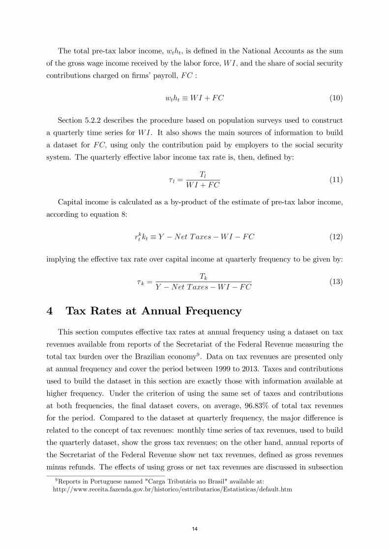
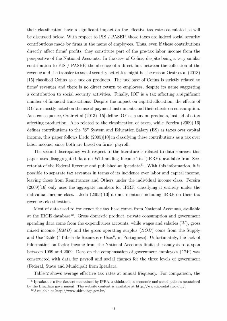
The total pre-tax labor income, wtht, is defined in the National Accounts as the sum
of the gross wage income received by the labor force, WI, and the share of social security
contributions charged on firms’payroll, FC :
wtht ≡ WI + FC (10)
Section 5.2.2 describes the procedure based on population surveys used to construct
a quarterly time series for WI. It also shows the main sources of information to build
a dataset for FC, using only the contribution paid by employers to the social security
system. The quarterly effective labor income tax rate is, then, defined by:
τ l =Tl
WI + FC(11)
Capital income is calculated as a by-product of the estimate of pre-tax labor income,
according to equation 8:
rkt kt ≡ Y −Net Taxes−WI − FC (12)
implying the effective tax rate over capital income at quarterly frequency to be given by:
τ k =Tk
Y −Net Taxes−WI − FC (13)
4 Tax Rates at Annual Frequency
This section computes effective tax rates at annual frequency using a dataset on tax
revenues available from reports of the Secretariat of the Federal Revenue measuring the
total tax burden over the Brazilian economy9. Data on tax revenues are presented only
at annual frequency and cover the period between 1999 to 2013. Taxes and contributions
used to build the dataset in this section are exactly those with information available at
higher frequency. Under the criterion of using the same set of taxes and contributions
at both frequencies, the final dataset covers, on average, 96.83% of total tax revenues
for the period. Compared to the dataset at quarterly frequency, the major difference is
related to the concept of tax revenues: monthly time series of tax revenues, used to build
the quarterly dataset, show the gross tax revenues; on the other hand, annual reports of
the Secretariat of the Federal Revenue show net tax revenues, defined as gross revenues
minus refunds. The effects of using gross or net tax revenues are discussed in subsection
9Reports in Portuguese named "Carga Tributária no Brasil" available at:http://www.receita.fazenda.gov.br/historico/esttributarios/Estatisticas/default.htm
14
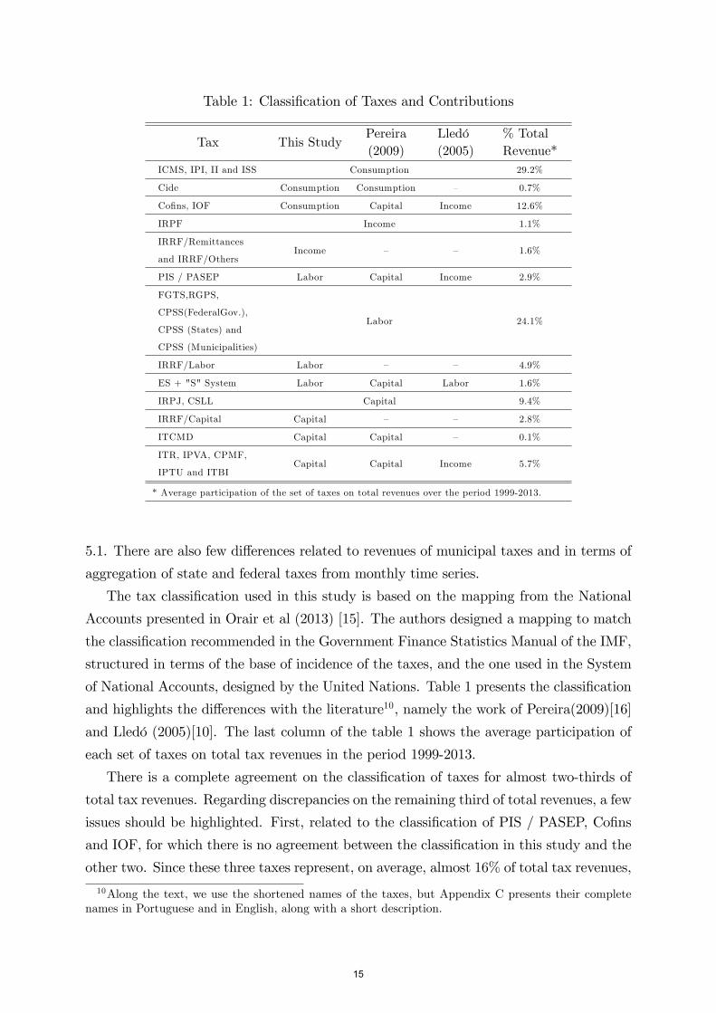
Table 1: Classification of Taxes and Contributions
Tax This StudyPereira(2009)
Lledó(2005)
% TotalRevenue*
ICMS, IPI, II and ISS Consumption 29.2%
Cide Consumption Consumption — 0.7%
Cofins, IOF Consumption Capital Income 12.6%
IRPF Income 1.1%
IRRF/Remittances
and IRRF/OthersIncome — — 1.6%
PIS / PASEP Labor Capital Income 2.9%
FGTS,RGPS,
CPSS(FederalGov.),
CPSS (States) and
CPSS (Municipalities)
Labor 24.1%
IRRF/Labor Labor — — 4.9%
ES + "S" System Labor Capital Labor 1.6%
IRPJ, CSLL Capital 9.4%
IRRF/Capital Capital — — 2.8%
ITCMD Capital Capital — 0.1%
ITR, IPVA, CPMF,
IPTU and ITBICapital Capital Income 5.7%
* Average participation of the set of taxes on total revenues over the period 1999-2013.
5.1. There are also few differences related to revenues of municipal taxes and in terms of
aggregation of state and federal taxes from monthly time series.
The tax classification used in this study is based on the mapping from the National
Accounts presented in Orair et al (2013) [15]. The authors designed a mapping to match
the classification recommended in the Government Finance Statistics Manual of the IMF,
structured in terms of the base of incidence of the taxes, and the one used in the System
of National Accounts, designed by the United Nations. Table 1 presents the classification
and highlights the differences with the literature10, namely the work of Pereira(2009)[16]
and Lledó (2005)[10]. The last column of the table 1 shows the average participation of
each set of taxes on total tax revenues in the period 1999-2013.
There is a complete agreement on the classification of taxes for almost two-thirds of
total tax revenues. Regarding discrepancies on the remaining third of total revenues, a few
issues should be highlighted. First, related to the classification of PIS / PASEP, Cofins
and IOF, for which there is no agreement between the classification in this study and the
other two. Since these three taxes represent, on average, almost 16% of total tax revenues,
10Along the text, we use the shortened names of the taxes, but Appendix C presents their completenames in Portuguese and in English, along with a short description.
15
their classification have a significant impact on the effective tax rates calculated as will
be discussed below. With respect to PIS / PASEP, those taxes are indeed social security
contributions made by firms in the name of employees. Thus, even if these contributions
directly affect firms’profits, they constitute part of the pre-tax labor income from the
perspective of the National Accounts. In the case of Cofins, despite being a very similar
contribution to PIS / PASEP, the absence of a direct link between the collection of the
revenue and the transfer to social security activities might be the reason Orair et al (2013)
[15] classified Cofins as a tax on products. The tax base of Cofins is strictly related to
firms’revenues and there is no direct return to employees, despite its name suggesting
a contribution to social security activities. Finally, IOF is a tax affecting a significant
number of financial transactions. Despite the impact on capital allocation, the effects of
IOF are mostly noted on the use of payment instruments and their effects on consumption.
As a consequence, Orair et al (2013) [15] define IOF as a tax on products, instead of a tax
affecting production. Also related to the classification of taxes, while Pereira (2009)[16]
defines contributions to the "S" System and Education Salary (ES) as taxes over capital
income, this paper follows Lledó (2005)[10] in classifying these contributions as a tax over
labor income, since both are based on firms’payroll.
The second discrepancy with respect to the literature is related to data sources: this
paper uses disaggregated data on Withholding Income Tax (IRRF), available from Sec-
retariat of the Federal Revenue and published at Ipeadata11. With this information, it is
possible to separate tax revenues in terms of its incidence over labor and capital income,
leaving those from Remittances and Others under the individual income class. Pereira
(2009)[16] only uses the aggregate numbers for IRRF, classifying it entirely under the
individual income class. Lledó (2005)[10] do not mention including IRRF on their tax
revenues classification.
Most of data used to construct the tax base comes from National Accounts, available
at the IBGE database12. Gross domestic product, private consumption and government
spending data come from the expenditures accounts, while wages and salaries (W ), gross
mixed income (RMB) and the gross operating surplus (EOB) come from the Supply
and Use Table ("Tabela de Recursos e Usos", in Portuguese). Unfortunately, the lack of
information on factor income from the National Accounts limits the analysis to a span
between 1999 and 2009. Data on the compensation of government employees (GW ) was
constructed with data for payroll and social charges for the three levels of government
(Federal, State and Municipal) from Ipeadata.
Table 2 shows average effective tax rates at annual frequency. For comparison, the
11Ipeadata is a free dataset mantained by IPEA, a thinktank in economic and social policies mantainedby the Brazilian government. The website content is available at http://www.ipeadata.gov.br/.12Available at http://www.sidra.ibge.gov.br/
16
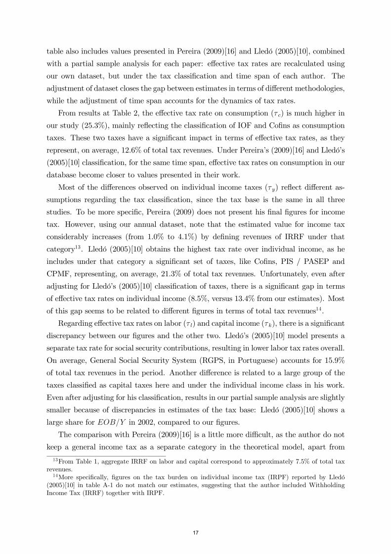
table also includes values presented in Pereira (2009)[16] and Lledó (2005)[10], combined
with a partial sample analysis for each paper: effective tax rates are recalculated using
our own dataset, but under the tax classification and time span of each author. The
adjustment of dataset closes the gap between estimates in terms of different methodologies,
while the adjustment of time span accounts for the dynamics of tax rates.
From results at Table 2, the effective tax rate on consumption (τ c) is much higher in
our study (25.3%), mainly reflecting the classification of IOF and Cofins as consumption
taxes. These two taxes have a significant impact in terms of effective tax rates, as they
represent, on average, 12.6% of total tax revenues. Under Pereira’s (2009)[16] and Lledó’s
(2005)[10] classification, for the same time span, effective tax rates on consumption in our
database become closer to values presented in their work.
Most of the differences observed on individual income taxes (τ y) reflect different as-
sumptions regarding the tax classification, since the tax base is the same in all three
studies. To be more specific, Pereira (2009) does not present his final figures for income
tax. However, using our annual dataset, note that the estimated value for income tax
considerably increases (from 1.0% to 4.1%) by defining revenues of IRRF under that
category13. Lledó (2005)[10] obtains the highest tax rate over individual income, as he
includes under that category a significant set of taxes, like Cofins, PIS / PASEP and
CPMF, representing, on average, 21.3% of total tax revenues. Unfortunately, even after
adjusting for Lledó’s (2005)[10] classification of taxes, there is a significant gap in terms
of effective tax rates on individual income (8.5%, versus 13.4% from our estimates). Most
of this gap seems to be related to different figures in terms of total tax revenues14.
Regarding effective tax rates on labor (τ l) and capital income (τ k), there is a significant
discrepancy between our figures and the other two. Lledó’s (2005)[10] model presents a
separate tax rate for social security contributions, resulting in lower labor tax rates overall.
On average, General Social Security System (RGPS, in Portuguese) accounts for 15.9%
of total tax revenues in the period. Another difference is related to a large group of the
taxes classified as capital taxes here and under the individual income class in his work.
Even after adjusting for his classification, results in our partial sample analysis are slightly
smaller because of discrepancies in estimates of the tax base: Lledó (2005)[10] shows a
large share for EOB/Y in 2002, compared to our figures.
The comparison with Pereira (2009)[16] is a little more diffi cult, as the author do not
keep a general income tax as a separate category in the theoretical model, apart from
13From Table 1, aggregate IRRF on labor and capital correspond to approximately 7.5% of total taxrevenues.14More specifically, figures on the tax burden on individual income tax (IRPF) reported by Lledó
(2005)[10] in table A-1 do not match our estimates, suggesting that the author included WithholdingIncome Tax (IRRF) together with IRPF.
17
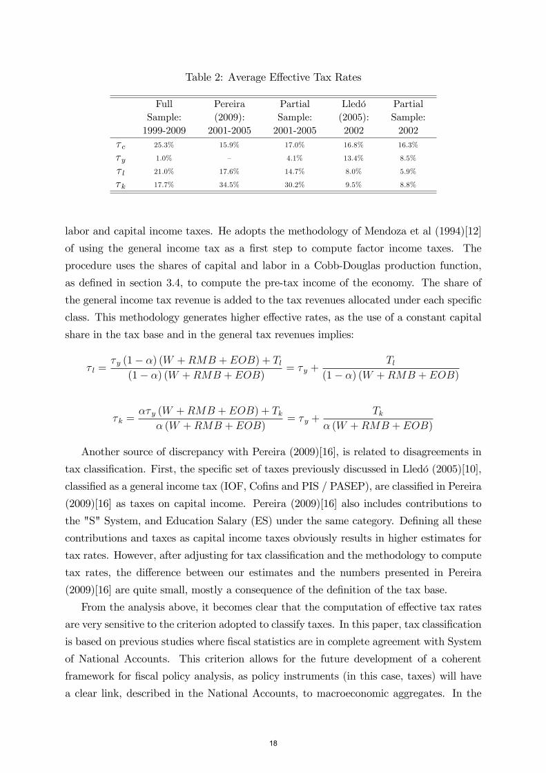
Table 2: Average Effective Tax Rates
FullSample:1999-2009
Pereira(2009):2001-2005
PartialSample:2001-2005
Lledó(2005):2002
PartialSample:2002
τ c 25.3% 15.9% 17.0% 16.8% 16.3%
τ y 1.0% — 4.1% 13.4% 8.5%
τ l 21.0% 17.6% 14.7% 8.0% 5.9%
τ k 17.7% 34.5% 30.2% 9.5% 8.8%
labor and capital income taxes. He adopts the methodology of Mendoza et al (1994)[12]
of using the general income tax as a first step to compute factor income taxes. The
procedure uses the shares of capital and labor in a Cobb-Douglas production function,
as defined in section 3.4, to compute the pre-tax income of the economy. The share of
the general income tax revenue is added to the tax revenues allocated under each specific
class. This methodology generates higher effective rates, as the use of a constant capital
share in the tax base and in the general tax revenues implies:
τ l =τ y (1− α) (W +RMB + EOB) + Tl
(1− α) (W +RMB + EOB)= τ y +
Tl(1− α) (W +RMB + EOB)
τ k =ατ y (W +RMB + EOB) + Tk
α (W +RMB + EOB)= τ y +
Tkα (W +RMB + EOB)
Another source of discrepancy with Pereira (2009)[16], is related to disagreements in
tax classification. First, the specific set of taxes previously discussed in Lledó (2005)[10],
classified as a general income tax (IOF, Cofins and PIS / PASEP), are classified in Pereira
(2009)[16] as taxes on capital income. Pereira (2009)[16] also includes contributions to
the "S" System, and Education Salary (ES) under the same category. Defining all these
contributions and taxes as capital income taxes obviously results in higher estimates for
tax rates. However, after adjusting for tax classification and the methodology to compute
tax rates, the difference between our estimates and the numbers presented in Pereira
(2009)[16] are quite small, mostly a consequence of the definition of the tax base.
From the analysis above, it becomes clear that the computation of effective tax rates
are very sensitive to the criterion adopted to classify taxes. In this paper, tax classification
is based on previous studies where fiscal statistics are in complete agreement with System
of National Accounts. This criterion allows for the future development of a coherent
framework for fiscal policy analysis, as policy instruments (in this case, taxes) will have
a clear link, described in the National Accounts, to macroeconomic aggregates. In the
18
next section, we present the main contribution of this paper, which is the estimation of
the effective tax rates at quarterly frequency.
5 Tax Rates at Quarterly Frequency
The main objective of this section is to calculate time series of effective tax rates
for consumption, individual, labor and capital incomes at quarterly frequency. While
most of the information on tax and contribution revenues at the federal level is avail-
able at monthly frequency, the main challenge to compute time series of the tax rates
were related to obtaining information on municipal taxes and the contributions for the
civil servants’social security system from subnational governments. In terms of the tax
base, data of expenditure from the National Accounts are readily available at quarterly
frequency, but the Supply and Use Table only provides delayed information at annual
frequency. As a consequence, this section also provides details on the procedures adopted
to estimate capital and labor compensations and payroll and social charges of subnational
governments.
5.1 Data Sources on Tax Revenues
Table 3 presents the dataset on taxes and contributions revenues at monthly frequency
considered here, with their respective classification, jurisdiction, data sources and time
span. The last column of table 3 shows the average share of each revenue on the total
classified revenues. Again, for the sake of reference, this dataset represents 96.83% of total
tax revenues of the country. Most of data on federal and state taxes are readily avail-
able at the website of Ipeadata. The series of contributions to the FGTS was obtained
from the FGTS website15. Data on Education Salary (ES) and Contributions to the "S"
System are from the Central Bank of Brazil’s Time Series Dataset16. Data on contri-
butions to RGPS and civil servants’social security contributions of federal government
employees (CPSS/Union) are obtained from the monthly report of the National Treasury
Secretariat17.
Most of the problems related to building a dataset on tax and contributions revenues
resided on obtaining information on municipal taxes (IPTU, ITBI and ISS) and contribu-
tions to the civil servants’social security system of subnational governments —CPSS/State
15Available at http://www.fgts.gov.br.16Website: http://www.bcb.gov.br/?TIMESERIESEN. The series is called "Previdência social (Fluxos)
—Despesas —Transferências a terceiros" under the identification number 2286. These are contributionsthat the National Institute of Social Security (INSS, in Portuguese) collects and transfers to the respectiveentities.17Available at www.tesouro.fazenda.gov.br/resultado-do-tesouro-nacional.
19
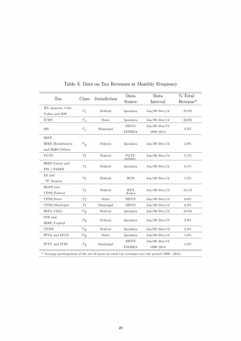
Table 3: Data on Tax Revenues at Monthly Frequency
Tax Class JurisdictionDataSource
DataInterval
% TotalRevenue*
IPI, Imports, Cide,
Cofins and IOFτ c Federal Ipeadata Jan/99—Dez/14 19.3%
ICMS τ c State Ipeadata Jan/99—Dez/14 22.6%
ISS τ c MunicipalSISTN
FINBRA
Jan/06—Dez/14
1999—20142.3%
IRPF,
IRRF/Remittances
and IRRF/Others
τ y Federal Ipeadata Jan/99—Dez/14 2.9%
FGTS τ l Federal FGTSwebsite
Jan/99—Dez/14 5.1%
IRRF/Labor and
PIS / PASEPτ l Federal Ipeadata Jan/99—Dez/14 8.1%
ES and
"S" Systemτ l Federal BCB Jan/99—Dez/14 1.5%
RGPS and
CPSS/Federalτ l Federal RTN
AnnexJan/99—Dez/14 18.1%
CPSS/State τ l State SISTN Jan/99—Dez/14 0.6%
CPSS/Municipal τ l Municipal SISTN Jan/99—Dez/14 0.2%
IRPJ, CSLL τ k Federal Ipeadata Jan/99—Dez/14 10.3%
ITR and
IRRF/Capitalτ k Federal Ipeadata Jan/99—Dez/14 2.9%
CPMF τ k Federal Ipeadata Jan/99—Mar/12 2.3%
IPVA and ITCD τ k State Ipeadata Jan/99—Dez/14 1.8%
IPTU and ITBI τ k MunicipalSISTN
FINBRA
Jan/06—Dez/14
1999—20141.8%
* Average participation of the set of taxes on total tax revenues over the period 1999 - 2014.
20
and CPSS/Municipal. The next subsections discuss: (i) the details of the procedure to
reconcile the few public datasets available on subnational government spending and rev-
enues; (ii) the final information set on tax revenues at quarterly frequency.
5.1.1 Subnational Governments Data Construction Using SISTN
Every year, the National Treasury Secretariat publishes a large dataset called FIN-
BRA18, with information on the annual balance of municipalities. Municipalities are
required to report detailed information, otherwise being subject to sanctions to finance
debt in financial markets19. The dataset consolidated by the National Treasury Secretariat
provides details on tax collection, but unfortunately misses information on social security
contributions and government employees payroll. One of the main sources of information
to FINBRA is a system called SISTN ("Sistema de Coleta de Dados Contábeis dos Entes
da Federação", in Portuguese), created in 2000 and with detailed information starting in
2006. Municipalities are required by law to send periodical reports to this system, where
those reports are made available for public consultation20.
One report submitted by states and municipalities to SISTN is particularly impor-
tant for our purposes: a simplified bimonthly report called RREO (Summary Report
of Budget Execution, "Relatório Resumido de Execução Orçamentária", in Portuguese)
provides details on the main taxes and contributions collected at subnational level. Al-
though RREOs are submitted bimonthly, the information on taxes and contributions are
presented at monthly frequency for the previous 12 months. RREOs also provide in-
formation on civil servants’social security contributions, at monthly frequency, and on
government employees payroll and social charges, at bimonthly frequency21.
Unfortunately, it is not possible to extract from SISTN a single report consolidating
information over time or across subnational entities. In order to work with SISTN, it
was necessary to build a system capable of downloading reports in PDF format for every
individual subnational government entity, for every period of time; convert the PDF
reports to a format able to read and process the information in those reports; and compile
the final dataset, summarizing information from all reports. This process demanded a
significant computational effort, where three VBA routines were developed to handle the
first two tasks. The first routine was built to download the correspondent PDF file for
18Available at http://www.tesouro.fazenda.gov.br/en/contas-anuais.19The requirement of sending reports to the Federal Government is described in sections II, III and IV
of the Fiscal Responsibility Law (Complementary Law 101, of May 4th, 2000).20Available at https://www.contaspublicas.caixa.gov.br/sistncon_internet/index.jsp . See footnote 1
about the modernized system implemented by the National Treasury.21Details on how we handle bimonthly information on payroll and social charges are presented in
subsection 5.2.1.
21
each RREO, for the 5568 municipalities, 26 states and the Federal District22, from 2006
to 201423. The second routine reads every PDF file and converts the information to TXT
files. The third routine reads the TXT files and extracts only information on tax revenues,
government spending and social security contributions to build the aggregate dataset.
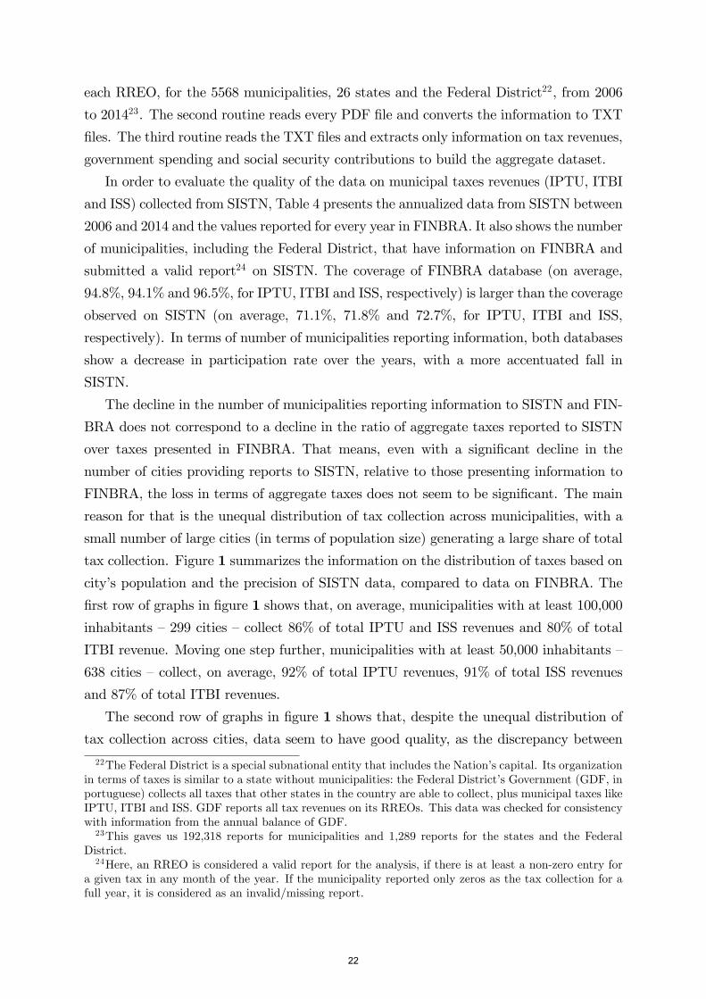
In order to evaluate the quality of the data on municipal taxes revenues (IPTU, ITBI
and ISS) collected from SISTN, Table 4 presents the annualized data from SISTN between
2006 and 2014 and the values reported for every year in FINBRA. It also shows the number
of municipalities, including the Federal District, that have information on FINBRA and
submitted a valid report24 on SISTN. The coverage of FINBRA database (on average,
94.8%, 94.1% and 96.5%, for IPTU, ITBI and ISS, respectively) is larger than the coverage
observed on SISTN (on average, 71.1%, 71.8% and 72.7%, for IPTU, ITBI and ISS,
respectively). In terms of number of municipalities reporting information, both databases
show a decrease in participation rate over the years, with a more accentuated fall in
SISTN.
The decline in the number of municipalities reporting information to SISTN and FIN-
BRA does not correspond to a decline in the ratio of aggregate taxes reported to SISTN
over taxes presented in FINBRA. That means, even with a significant decline in the
number of cities providing reports to SISTN, relative to those presenting information to
FINBRA, the loss in terms of aggregate taxes does not seem to be significant. The main
reason for that is the unequal distribution of tax collection across municipalities, with a
small number of large cities (in terms of population size) generating a large share of total
tax collection. Figure 1 summarizes the information on the distribution of taxes based on
city’s population and the precision of SISTN data, compared to data on FINBRA. The
first row of graphs in figure 1 shows that, on average, municipalities with at least 100,000
inhabitants —299 cities —collect 86% of total IPTU and ISS revenues and 80% of total
ITBI revenue. Moving one step further, municipalities with at least 50,000 inhabitants —
638 cities —collect, on average, 92% of total IPTU revenues, 91% of total ISS revenues
and 87% of total ITBI revenues.
The second row of graphs in figure 1 shows that, despite the unequal distribution of
tax collection across cities, data seem to have good quality, as the discrepancy between
22The Federal District is a special subnational entity that includes the Nation’s capital. Its organizationin terms of taxes is similar to a state without municipalities: the Federal District’s Government (GDF, inportuguese) collects all taxes that other states in the country are able to collect, plus municipal taxes likeIPTU, ITBI and ISS. GDF reports all tax revenues on its RREOs. This data was checked for consistencywith information from the annual balance of GDF.23This gaves us 192,318 reports for municipalities and 1,289 reports for the states and the Federal
District.24Here, an RREO is considered a valid report for the analysis, if there is at least a non-zero entry for
a given tax in any month of the year. If the municipality reported only zeros as the tax collection for afull year, it is considered as an invalid/missing report.
22
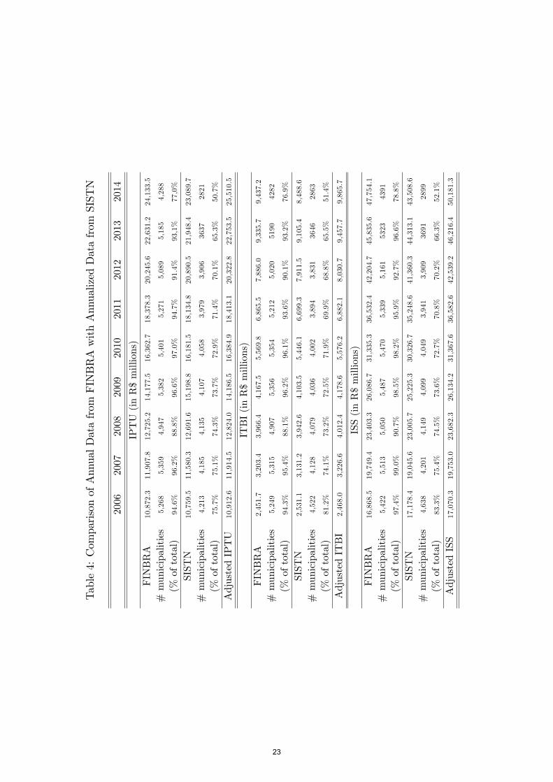
Table4:ComparisonofAnnualDatafrom
FINBRAwithAnnualizedDatafrom
SISTN
2006
2007
2008
2009
2010
2011
2012
2013
2014
IPTU(inR$millions)
FINBRA
10,872.3
11,907.8
12,725.2
14,177.5
16,362.7
18,378.3
20,245.6
22,631.2
24,133.5
#municipalities
5,268
5,359
4,947
5,382
5,401
5,271
5,089
5,185
4,288
(%oftotal)
94.6%
96.2%
88.8%
96.6%
97.0%
94.7%
91.4%
93,1%
77,0%
SISTN
10,759.5
11,580.3
12,691.6
15,198.8
16,181.5
18,134.8
20,890.5
21,948.4
23,089.7
#municipalities
4,213
4,185
4,135
4,107
4,058
3,979
3,906
3637
2821
(%oftotal)
75.7%
75.1%
74.3%
73.7%
72.9%
71.4%
70.1%
65.3%
50.7%
AdjustedIPTU
10,912.6
11,914.5
12,824.0
14,186.5
16,384.9
18,413.1
20,322.8
22,753.5
25,510.5
ITBI(inR$millions)
FINBRA
2,451.7
3,203.4
3,966.4
4,167.5
5,569.8
6,865.5
7,886.0
9,335.7
9,437.2
#municipalities
5,249
5,315
4,907
5,356
5,354
5,212
5,020
5190
4282
(%oftotal)
94.3%
95.4%
88.1%
96.2%
96.1%
93.6%
90.1%
93.2%
76.9%
SISTN
2,531.1
3,131.2
3,942.6
4,103.5
5,446.1
6,699.3
7,911.5
9,105.4
8,488.6
#municipalities
4,522
4,128
4,079
4,036
4,002
3,894
3,831
3646
2863
(%oftotal)
81.2%
74.1%
73.2%
72.5%
71.9%
69.9%
68.8%
65.5%
51.4%
AdjustedITBI
2,468.0
3,226.6
4,012.4
4,178.6
5,576.2
6,882.1
8,030.7
9,457.7
9,865.7
ISS(inR$millions)
FINBRA
16,868.5
19,749.4
23,403.3
26,086.7
31,335.3
36,532.4
42,204.7
45,835.6
47,754.1
#municipalities
5,422
5,513
5,050
5,487
5,470
5,339
5,161
5323
4391
(%oftotal)
97.4%
99.0%
90.7%
98.5%
98.2%
95.9%
92.7%
96.6%
78.8%
SISTN
17,178.4
19,045.6
23,005.7
25,225.3
30,326.7
35,248.6
41,360.3
44,313.1
43,508.6
#municipalities
4,638
4,201
4,149
4,099
4,049
3,941
3,909
3691
2899
(%oftotal)
83.3%
75.4%
74.5%
73.6%
72.7%
70.8%
70.2%
66.3%
52.1%
AdjustedISS
17,070.3
19,753.0
23,682.3
26,134.2
31,367.6
36,582.6
42,539.2
46,216.4
50,181.3
23
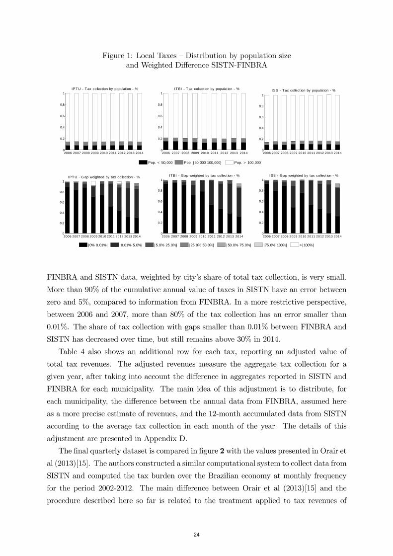
Figure 1: Local Taxes —Distribution by population sizeand Weighted Difference SISTN-FINBRA
2006 2007 2008 2009 2010 2011 2012 2013 20140
0.2
0.4
0.6
0.8
1IPT U T ax collect ion by populat ion %
Pop. < 50,000 Pop. [50,000 100,000] Pop. > 100,000
2006 2007 2008 2009 2010 2011 2012 2013 20140
0.2
0.4
0.6
0.8
1IT BI T ax collect ion by populat ion %
2006 2007 2008 2009 2010 2011 2012 2013 20140
0.2
0.4
0.6
0.8
1ISS T ax collect ion by populat ion %
2006 2007 2008 2009 2010 2011 2012 2013 20140
0.2
0.4
0.6
0.8
1IPT U G ap weighted by tax collect ion %
|0% 0.01%| |0.01% 5.0%| |5.0% 25.0%| |25.0% 50.0%| |50.0% 75.0%| |75.0% 100%| > |100%|
2006 2007 2008 2009 2010 2011 2012 2013 20140
0.2
0.4
0.6
0.8
1IT BI G ap weighted by tax collect ion %
2006 2007 2008 2009 2010 2011 2012 2013 20140
0.2
0.4
0.6
0.8
1ISS G ap weighted by tax collect ion %
FINBRA and SISTN data, weighted by city’s share of total tax collection, is very small.
More than 90% of the cumulative annual value of taxes in SISTN have an error between
zero and 5%, compared to information from FINBRA. In a more restrictive perspective,
between 2006 and 2007, more than 80% of the tax collection has an error smaller than
0.01%. The share of tax collection with gaps smaller than 0.01% between FINBRA and
SISTN has decreased over time, but still remains above 30% in 2014.
Table 4 also shows an additional row for each tax, reporting an adjusted value of
total tax revenues. The adjusted revenues measure the aggregate tax collection for a
given year, after taking into account the difference in aggregates reported in SISTN and
FINBRA for each municipality. The main idea of this adjustment is to distribute, for
each municipality, the difference between the annual data from FINBRA, assumed here
as a more precise estimate of revenues, and the 12-month accumulated data from SISTN
according to the average tax collection in each month of the year. The details of this
adjustment are presented in Appendix D.
The final quarterly dataset is compared in figure 2 with the values presented in Orair et
al (2013)[15]. The authors constructed a similar computational system to collect data from
SISTN and computed the tax burden over the Brazilian economy at monthly frequency
for the period 2002-2012. The main difference between Orair et al (2013)[15] and the
procedure described here so far is related to the treatment applied to tax revenues of
24
Figure 2: Tax BurdenAnnual and Quarterly Datasets x Orair et al (2013)
2 0 0 0 2 0 0 2 2 0 0 4 2 0 0 6 2 0 0 8 2 0 1 0 2 0 1 22 7
2 8
2 9
3 0
3 1
3 2
3 3
3 4
3 5
Tax
Bur
den
% o
f GD
P
Q u a rt e r ly D a t a A n n u a l D a t a O ra ir e t a l (2 0 1 3 )
subnational governments. The authors use temporal disaggregation and contemporaneous
forecasts through state-space econometric models to estimate the relevant series. Despite
the lack of advanced econometric techniques, the final time series on aggregate tax burden
computed here is not far from the information published in Orair et al (2013)[15]. On
average, our estimates of the total tax burden (total tax revenues as a proportion of
GDP) is 0.55p.p. below their estimate for the period between 2002 and 201225. The main
differences between the quarterly and annual estimates presented here and the values
presented in Orair et al (2013)[15] is related to the period before 2006, when information
from SISTN is not available to complement missing information on FINBRA. Note that,
for the period between 2002 and 2006, when only the annual dataset is comparable to
Orair et al (2013)[15], the total tax burden is very similar, both in terms of levels and
dynamics. After 2006, with the adjustments on revenues using SISTN and the availability
of information on contributions, the quarterly dataset tracks better the results of Orair
et al (2013)[15].
Besides data for municipal taxes revenues, RREOs collected from SISTN also offer
information on civil servants’ social security contributions in states and municipalities
25In March/2015, the National Accounts went through a major revision. The estimates presented inthis paper use the revised numbers. However, in Figure 2, in order to keep the estimates comparable tothose presented by Orair et al (2013) [15], the unrevised GDP numbers were used to compute the seriesfor the tax burden, both at annual and quarterly frequency.
25
(CPSS/States and CPSS/Municipal). Unfortunately, to the best of our knowledge, there
is not an annual dataset disaggregated by states and municipalities similar to FINBRA
available to check the accuracy of reports. The only source of information on CPSS/States
and CPSS/Municipal are the annual aggregated figures published by the National Trea-
sury Secretariat and the Secretariat of Federal Revenue. Given this limitation, the ad-
justment made on tax revenues using information from FINBRA was not repeated for
contributions of civil servants. Even without the adjustment, however, the comparison
of annual values from the National Treasury with figures from SISTN shows a small gap
between the two time series. Notably, the gap observed for Municipal contributions is
much smaller than the one obtained for States.
Another problem with information from CPSS is the lack of disaggregated data for
CPSS/States and CPSS/Municipal for the period before 2006. The short time span
with information available at monthly frequency after 2006, combined with the lack of
alternative datasets to check the accuracy of the procedure, suggests that it would not
be a good strategy to distribute aggregated annual data over monthly information. The
effects of missing high-frequency information for CPSS/States and CPSS/Municipal are
discussed next.
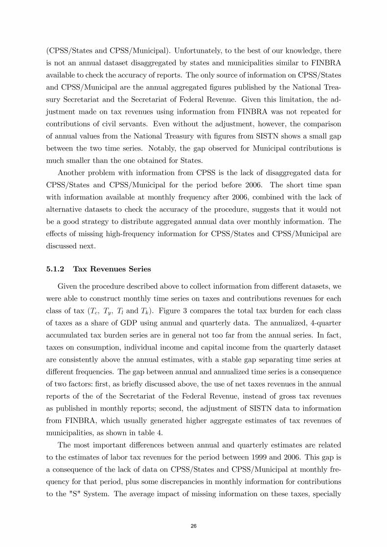
5.1.2 Tax Revenues Series
Given the procedure described above to collect information from different datasets, we
were able to construct monthly time series on taxes and contributions revenues for each
class of tax (Tc, Ty, Tl and Tk). Figure 3 compares the total tax burden for each class
of taxes as a share of GDP using annual and quarterly data. The annualized, 4-quarter
accumulated tax burden series are in general not too far from the annual series. In fact,
taxes on consumption, individual income and capital income from the quarterly dataset
are consistently above the annual estimates, with a stable gap separating time series at
different frequencies. The gap between annual and annualized time series is a consequence
of two factors: first, as briefly discussed above, the use of net taxes revenues in the annual
reports of the of the Secretariat of the Federal Revenue, instead of gross tax revenues
as published in monthly reports; second, the adjustment of SISTN data to information
from FINBRA, which usually generated higher aggregate estimates of tax revenues of
municipalities, as shown in table 4.
The most important differences between annual and quarterly estimates are related
to the estimates of labor tax revenues for the period between 1999 and 2006. This gap is
a consequence of the lack of data on CPSS/States and CPSS/Municipal at monthly fre-
quency for that period, plus some discrepancies in monthly information for contributions
to the "S" System. The average impact of missing information on these taxes, specially
26
Figure 3: Tax Burden by Tax Class
1999 2003 2007 2011 201412
13
14
15C ON SU MPTION
Tax
Bur
den
% o
f GD
P
Quarterly D ata Annual D ata
1999 2003 2007 2011 20140.7
0.8
0.9
1
1.1IN C OME
Tax
Bur
den
% o
f GD
P
1999 2003 2007 2011 20148
9
10
11
12
13LABOR
Tax
Bur
den
% o
f GD
P
1999 2003 2007 2011 20144
5
6
7
8C APITAL
Tax
Bur
den
% o
f GD
P
on CPSS/States and CPSS/Municipal, despite representing a small share of total tax
revenues26, on the total tax burden is estimated at 0.7p.p. of GDP.
Figure 3 shows an increase in the total tax burden over the Brazilian economy observed
in the last 16 years, based on the increase in tax revenues obtained from all sources.
The total tax burden increased around 6p.p. of GDP between 1999 and 2014, mostly
concentrated on labor (3.1p.p. of GDP) and consumption (2.0p.p. of GDP) taxes. After
the 2008 financial crisis, the burden fell for all classes of taxes, as the adoption of an
expansionary fiscal policy, based on selective tax rates cuts, combined with the natural
decrease in tax revenues due to slower economic activity, resulted in a temporary reduction
of tax burden as a proportion of GDP. Consumption taxes observed a significant drop
right after the crisis, but it has already returned to its pre-crisis values. In a smaller scale,
this temporary drop was also observed in individual income and labor tax burdens, with
a quick recovery of their upward trends. The same did not happen to the burden of tax
on capital income. It increased 2.3p.p of GDP until 2007, followed by a significant and
persistent decrease after the crisis. The beginning of the crises, however, coincides with
the extinction of CMPF in 2008. The burden of this tax alone represented on average
1.3p.p. of GDP between 1999 and 2007. An evaluation of the tax burden on capital
income, without including CPMF in the analysis, shows that the tax burden returned to
26CPSS/States and CPSS/Municipal represent 1.4% and 0.4%, respectively, of average total tax rev-enues, according to table 3.
27
its pre-crisis level by 2014.
5.2 Data Sources on the Tax Base
Two main sources were used to compute the tax base at quarterly frequency, given
the definitions presented in equations 4, 9, 11 and 12. First, to compute consumption
taxes, as in the case of effective taxes computed with annual data, the main source is
the National Accounts. Then, to compute factor income, population surveys are used to
make inference on total labor income. Beyond describing details of these two sources,
this section presents, first, the computation of government employee’s compensation at
quarterly frequency. After that, the details on the use of population surveys to estimate
labor and capital income are presented.
From the National Accounts perspective, beyond information on gross domestic out-
put, private consumption and government spending, it is necessary to build an estimate
of the economy’s value added at factor costs. As in the case of labor and capital income,
offi cial estimates available for the value added at factor costs are available only at annual
frequency and without constant updates. By the definition presented in equation 8, value
added at factor costs is computed by the difference between net domestic income and an
estimate of "net taxes on production". While estimates of the gross domestic product are
readily available, an approximation of "net taxes" is constructed, based on the definitions
of Orair et al (2013)[15], as the sum of IPI, ICMS, ISS, CIDE, II, IOF, Cofins, ES and
contributions to the "S" System. Figure 4 compares this approximation with information
on "taxes on production" from the Supply and Use Table, both measured as a proportion
of GDP. Our estimates based on quarterly data are, on average, 0.7p.p. below of the
Supply and Use Table, showing good accuracy, even with the problems reported before
on the database for quarterly data.
After generating an estimate of total factor income, W + RMB + EOB, by using
gross domestic product, Y −Net Taxes, the next two subsections show the procedure toconstruct time series for government employees’compensations, GW, and for labor and
capital income. Table 5 summarizes the data sources used to construct the series on the
tax base.
5.2.1 Constructing a Series for Government Employees’Compensations
In order to construct a quarterly time series on government employees’compensations
(GW in equation 4), information from SISTN was used to estimate figures for subna-
tional entities of the federation. Datasets from the National Treasury Secretariat pro-
vided annual information on payroll and social charges for the three levels of government.
28
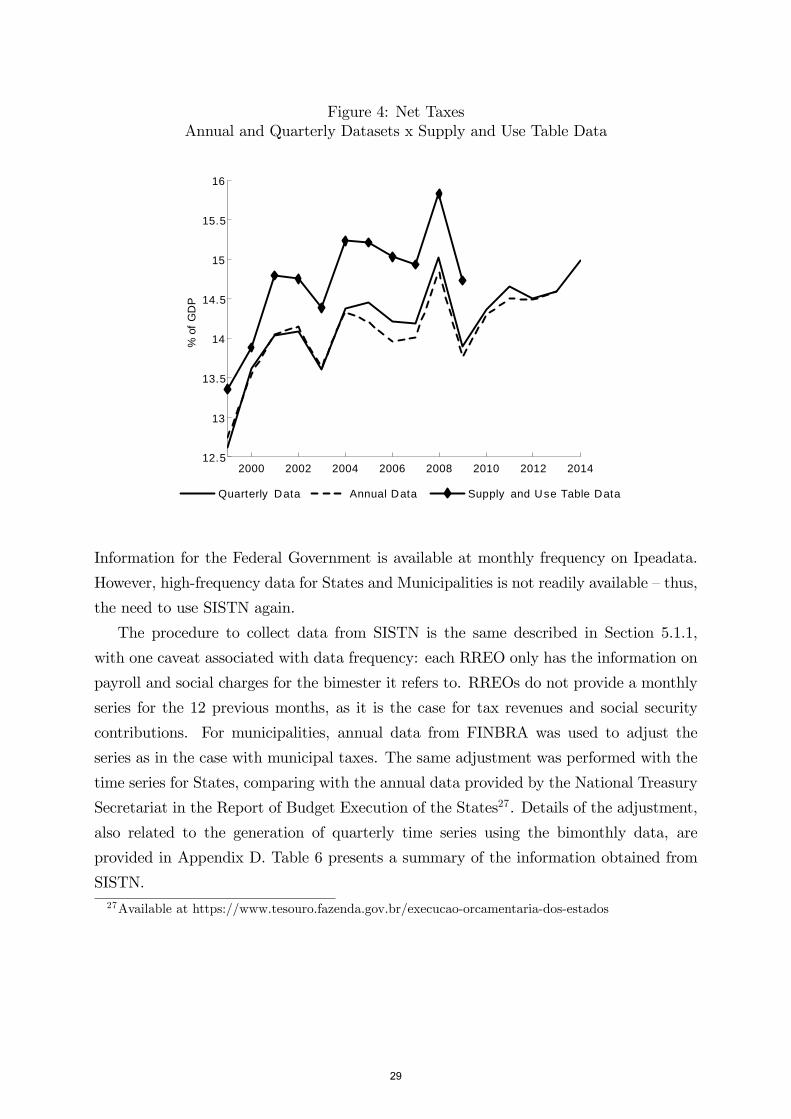
Figure 4: Net TaxesAnnual and Quarterly Datasets x Supply and Use Table Data
2000 2002 2004 2006 2008 2010 2012 201412.5
13
13.5
14
14.5
15
15.5
16%
of G
DP
Quarterly Data Annual Data Supply and Use Table Data
Information for the Federal Government is available at monthly frequency on Ipeadata.
However, high-frequency data for States and Municipalities is not readily available —thus,
the need to use SISTN again.
The procedure to collect data from SISTN is the same described in Section 5.1.1,
with one caveat associated with data frequency: each RREO only has the information on
payroll and social charges for the bimester it refers to. RREOs do not provide a monthly
series for the 12 previous months, as it is the case for tax revenues and social security
contributions. For municipalities, annual data from FINBRA was used to adjust the
series as in the case with municipal taxes. The same adjustment was performed with the
time series for States, comparing with the annual data provided by the National Treasury
Secretariat in the Report of Budget Execution of the States27. Details of the adjustment,
also related to the generation of quarterly time series using the bimonthly data, are
provided in Appendix D. Table 6 presents a summary of the information obtained from
SISTN.27Available at https://www.tesouro.fazenda.gov.br/execucao-orcamentaria-dos-estados
29
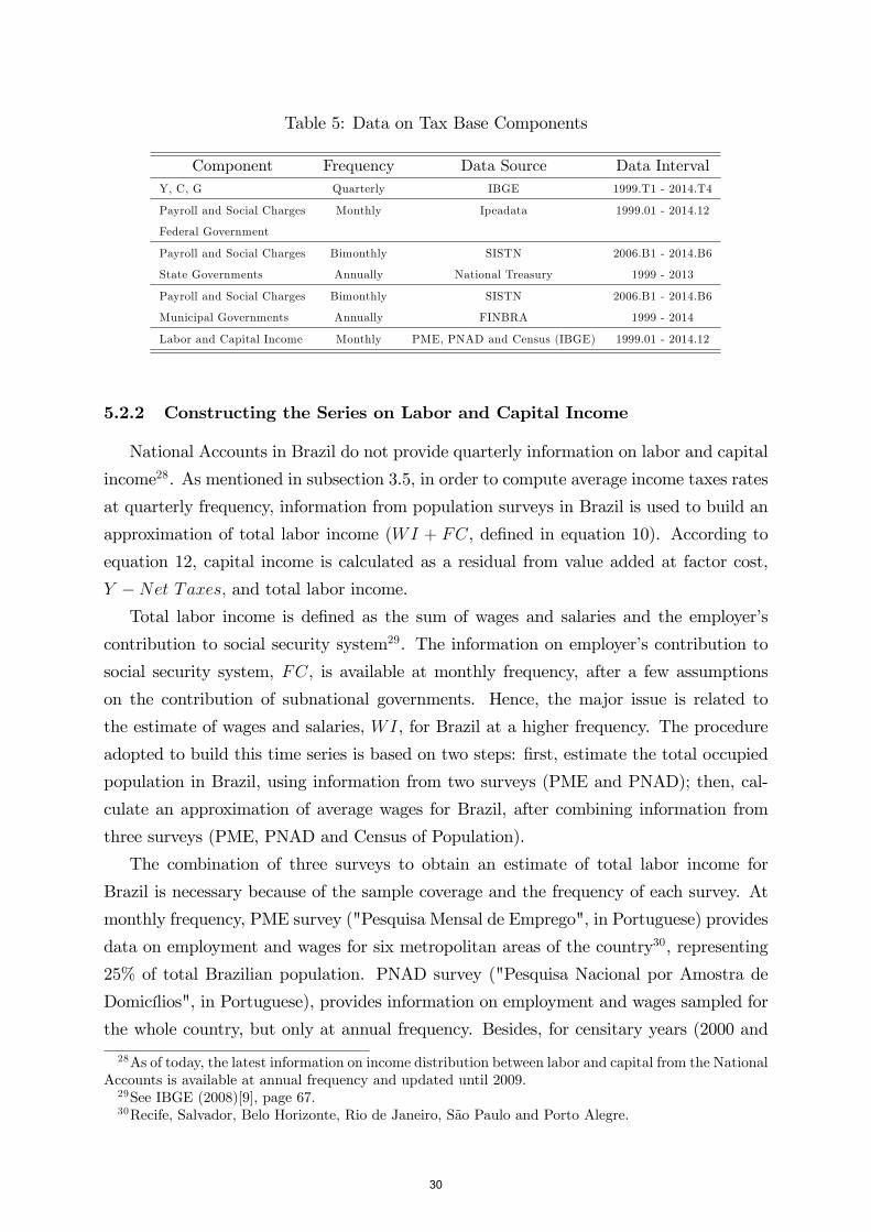
Table 5: Data on Tax Base Components
Component Frequency Data Source Data IntervalY, C, G Quarterly IBGE 1999.T1 - 2014.T4
Payroll and Social Charges Monthly Ipeadata 1999.01 - 2014.12
Federal Government
Payroll and Social Charges Bimonthly SISTN 2006.B1 - 2014.B6
State Governments Annually National Treasury 1999 - 2013
Payroll and Social Charges Bimonthly SISTN 2006.B1 - 2014.B6
Municipal Governments Annually FINBRA 1999 - 2014
Labor and Capital Income Monthly PME, PNAD and Census (IBGE) 1999.01 - 2014.12
5.2.2 Constructing the Series on Labor and Capital Income
National Accounts in Brazil do not provide quarterly information on labor and capital
income28. As mentioned in subsection 3.5, in order to compute average income taxes rates
at quarterly frequency, information from population surveys in Brazil is used to build an
approximation of total labor income (WI + FC, defined in equation 10). According to
equation 12, capital income is calculated as a residual from value added at factor cost,
Y −Net Taxes, and total labor income.Total labor income is defined as the sum of wages and salaries and the employer’s
contribution to social security system29. The information on employer’s contribution to
social security system, FC, is available at monthly frequency, after a few assumptions
on the contribution of subnational governments. Hence, the major issue is related to
the estimate of wages and salaries, WI, for Brazil at a higher frequency. The procedure
adopted to build this time series is based on two steps: first, estimate the total occupied
population in Brazil, using information from two surveys (PME and PNAD); then, cal-
culate an approximation of average wages for Brazil, after combining information from
three surveys (PME, PNAD and Census of Population).
The combination of three surveys to obtain an estimate of total labor income for
Brazil is necessary because of the sample coverage and the frequency of each survey. At
monthly frequency, PME survey ("Pesquisa Mensal de Emprego", in Portuguese) provides
data on employment and wages for six metropolitan areas of the country30, representing
25% of total Brazilian population. PNAD survey ("Pesquisa Nacional por Amostra de
Domicílios", in Portuguese), provides information on employment and wages sampled for
the whole country, but only at annual frequency. Besides, for censitary years (2000 and
28As of today, the latest information on income distribution between labor and capital from the NationalAccounts is available at annual frequency and updated until 2009.29See IBGE (2008)[9], page 67.30Recife, Salvador, Belo Horizonte, Rio de Janeiro, São Paulo and Porto Alegre.
30
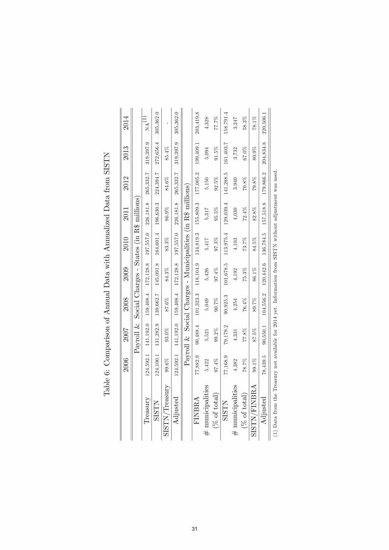
Table6:ComparisonofAnnualDatawithAnnualizedDatafrom
SISTN
2006
2007
2008
2009
2010
2011
2012
2013
2014
Payroll&SocialCharges-States(inR$millions)
Treasury
124,592.1
141,192.0
159,408.4
172,128.8
197,557.0
226,181.8
265,332.7
319,397.9
NA
(1)
SISTN
124,100.1
131,282.9
139,662.7
145,091.8
164,601.4
196,630.3
224,394.7
272,656.4
305,362.0
SISTN/Treasury
99.6%
93.0%
87.6%
84.3%
83.3%
86.9%
84.6%
85.4%
-
Adjusted
124,592.1
141,192.0
159,408.4
172,128.8
197,557.0
226,181.8
265,332.7
319,397.9
305,362.0
Payroll&SocialCharges-Municipalities(inR$millions)
FINBRA
77,882.9
90,488.4
101,323.3
118,104.9
134,819.3
155,809.3
177,005.2
199,409.1
203,419.8
#municipalities
5,422
5,521
5,049
5,426
5,417
5,317
5,150
5,094
4,328
(%oftotal)
97.4%
99.2%
90.7%
97.4%
97.3%
95.5%
92.5%
91.5%
77.7%
SISTN
77,168.9
79,179.2
90,925.3
101,678.5
113,975.4
129,039.4
141,288.5
161,403.7
158,791.4
#municipalities
4,382
4,331
4,254
4,192
4,103
4,030
3,940
3,732
3,247
(%oftotal)
78.7%
77.8%
76.4%
75.3%
73.7%
72.4%
70.8%
67.0%
58.3%
SISTN/FINBRA
99.1%
87.5%
89.7%
86.1%
84.5%
82.8%
79.8%
80.9%
78.1%
Adjusted
78,439.5
90,550.1
104,556.2
120,442.6
136,784.5
157,518.8
179,866.2
204,834.8
220,506.1
(1)Datafrom
theTreasurynotavailablefor2014yet.Informationfrom
SISTNwithoutadjustmentwasused.
31
2010 in our time span), PNAD survey is not available31.
Data from Census of Population also alleviates a problem related to the estimate of
average wages in Brazil. In the literature, Gomes, Bugarin and Ellery (2005)[8] compare
data from PNAD and the annual data on labor income presented in the National Ac-
counts. They estimate total labor income using PNAD data and suggest that, between
1992 and 1998, aggregate labor income was actually 26% higher than the number pre-
sented in the National Accounts. Census data provide greater coverage when compared
to PNAD, allowing for corrections on the measurement of average wages when the income
distribution is very skewed, as discussed later.
Proceeding with the estimation of total employed population in Brazil, assume that
the short run dynamics of employed population in the metropolitan areas covered by
PME is the same as the dynamics for the whole country32. The time series of employed
population is adjusted twice: first, by the gap generated from the difference in the def-
inition of employed people between PNAD and PME; second, by the share of employed
population in the region covered by PME over total employed population in Brazil. For
the first adjustment, the average ratio between 1999 and 2013 of employed population in
PME over employed population in PNAD is estimated at 0.94. This ratio is quite stable
over the sample, especially after 2002. For the second adjustment, the average share be-
tween employed population in metropolitan areas of PME and PNAD survey is estimated
at 0.246. The two ratios are uniformly applied over the PME time series of employed
population described above.
For a quarterly estimate of average wages for Brazil, assume, again, that the short run
dynamics of wages for the whole country is the same as the dynamics described by data
from PME33. Starting from PME dataset, three adjustments are performed: (i) for the
period between 1999 and 2002, adjust old data from PME to the average value of wages
for all occupations, instead of wages from the main occupation; (ii) estimate the average
gap between wages in PME and the values reported in Census for the same geographical
area, in order to correct the level of wages for differences in income distribution; (iii)
estimate wages for Brazil, taking into account the gap between the metropolitan areas
surveyed by PME and the whole country. These three steps are detailed below.
31PME, PNAD and Census microdata are obtained from the IBGE’s website (http://www.ibge.gov.br).32There was a methodological change in the definition of work, among other issues, in PME in 2002.
For the period between 1999 and 2002, the number of employed people is simply a retropolation of thenew definition of employed population over percentual changes of employed population observed in theold survey methodology.33As we are interested in total labor income, wages here are defined as "wages effectivelly accrued
by household" in each month. However, in order to compare the same variable across surveys, ratiospresented next relates to "wages usually accrued by household". This is the measure of income surveyedin PNAD and Census, and it is different from the former measure because it does not include bonusesand other temporary compensations for the household.
32
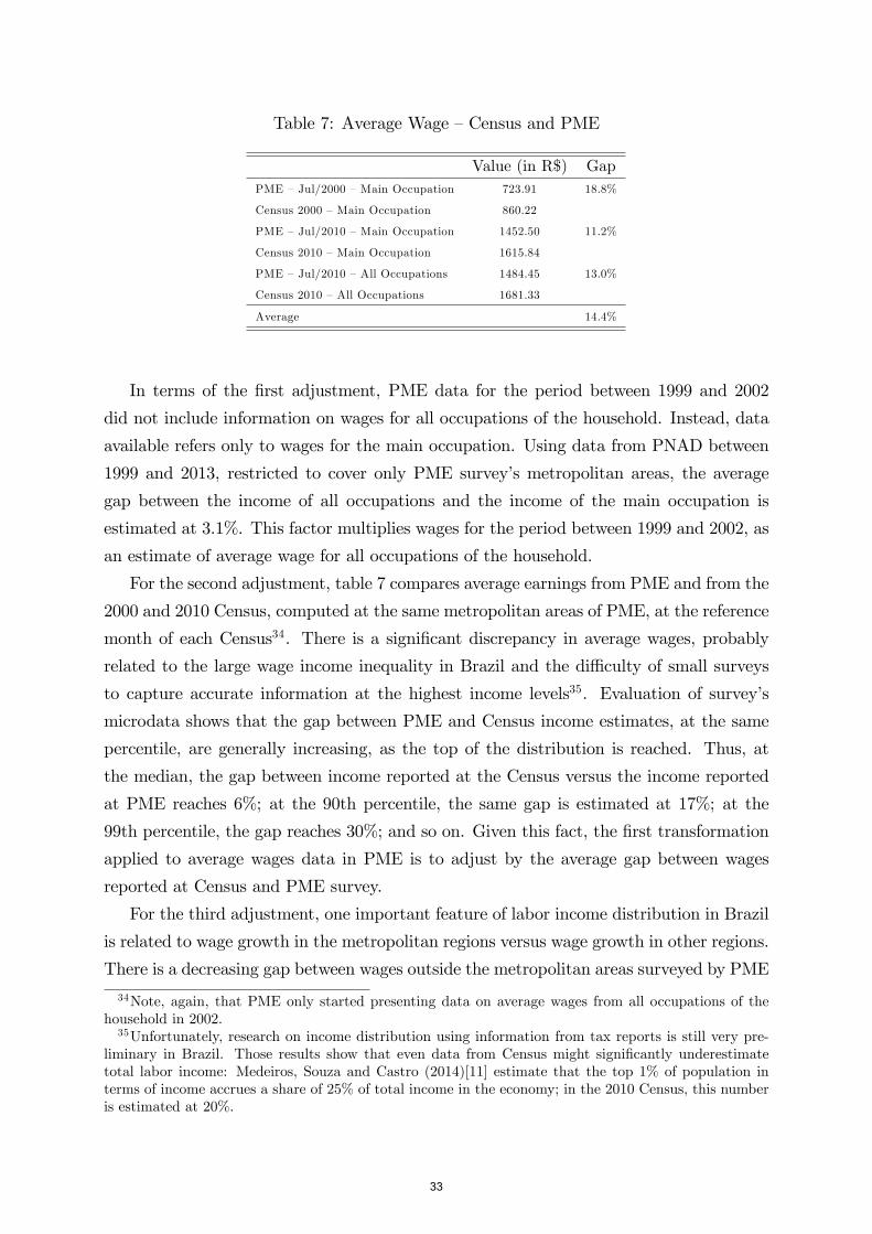
Table 7: Average Wage —Census and PME
Value (in R$) GapPME —Jul/2000 —Main Occupation 723.91 18.8%
Census 2000 —Main Occupation 860.22
PME —Jul/2010 —Main Occupation 1452.50 11.2%
Census 2010 —Main Occupation 1615.84
PME —Jul/2010 —All Occupations 1484.45 13.0%
Census 2010 —All Occupations 1681.33
Average 14.4%
In terms of the first adjustment, PME data for the period between 1999 and 2002
did not include information on wages for all occupations of the household. Instead, data
available refers only to wages for the main occupation. Using data from PNAD between
1999 and 2013, restricted to cover only PME survey’s metropolitan areas, the average
gap between the income of all occupations and the income of the main occupation is
estimated at 3.1%. This factor multiplies wages for the period between 1999 and 2002, as
an estimate of average wage for all occupations of the household.
For the second adjustment, table 7 compares average earnings from PME and from the
2000 and 2010 Census, computed at the same metropolitan areas of PME, at the reference
month of each Census34. There is a significant discrepancy in average wages, probably
related to the large wage income inequality in Brazil and the diffi culty of small surveys
to capture accurate information at the highest income levels35. Evaluation of survey’s
microdata shows that the gap between PME and Census income estimates, at the same
percentile, are generally increasing, as the top of the distribution is reached. Thus, at
the median, the gap between income reported at the Census versus the income reported
at PME reaches 6%; at the 90th percentile, the same gap is estimated at 17%; at the
99th percentile, the gap reaches 30%; and so on. Given this fact, the first transformation
applied to average wages data in PME is to adjust by the average gap between wages
reported at Census and PME survey.
For the third adjustment, one important feature of labor income distribution in Brazil
is related to wage growth in the metropolitan regions versus wage growth in other regions.
There is a decreasing gap between wages outside the metropolitan areas surveyed by PME
34Note, again, that PME only started presenting data on average wages from all occupations of thehousehold in 2002.35Unfortunately, research on income distribution using information from tax reports is still very pre-
liminary in Brazil. Those results show that even data from Census might significantly underestimatetotal labor income: Medeiros, Souza and Castro (2014)[11] estimate that the top 1% of population interms of income accrues a share of 25% of total income in the economy; in the 2010 Census, this numberis estimated at 20%.
33
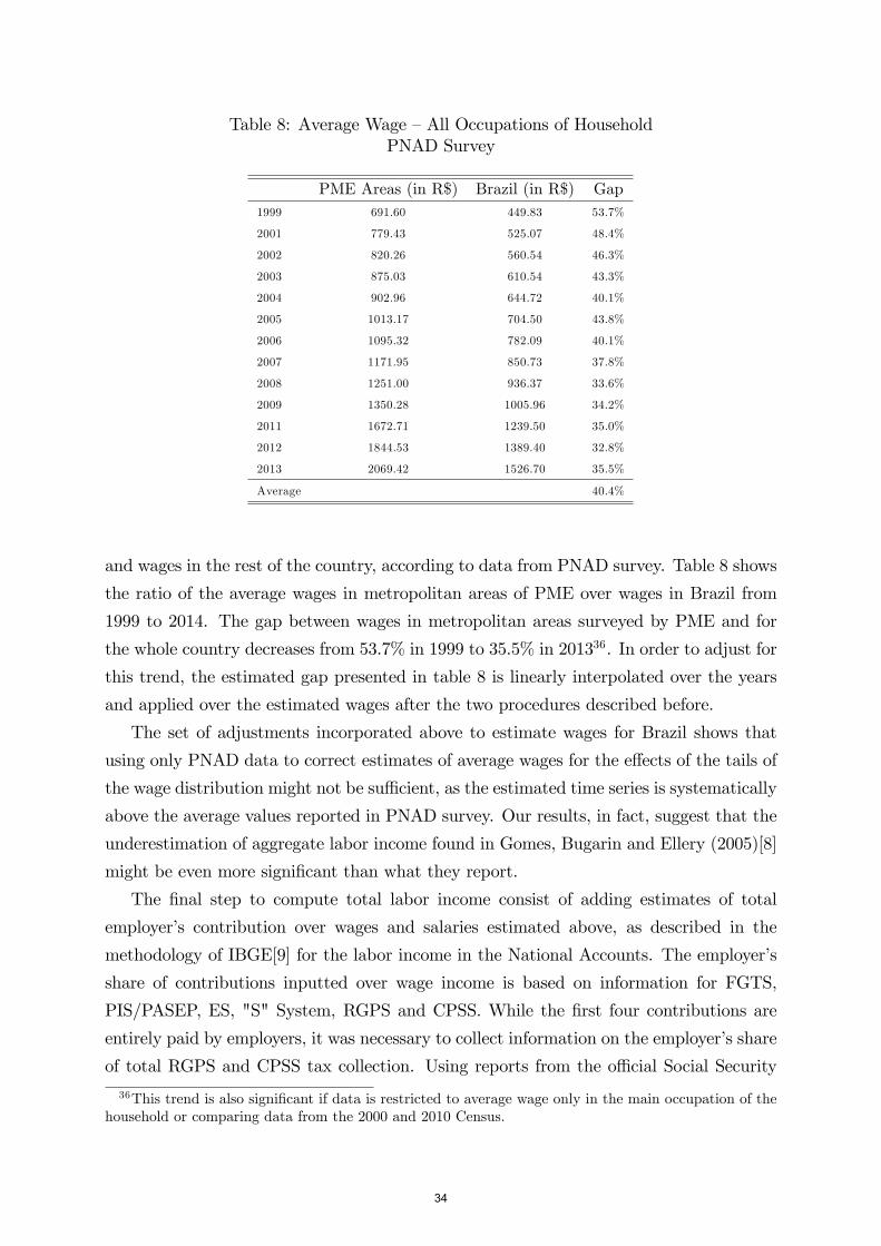
Table 8: Average Wage —All Occupations of HouseholdPNAD Survey
PME Areas (in R$) Brazil (in R$) Gap1999 691.60 449.83 53.7%
2001 779.43 525.07 48.4%
2002 820.26 560.54 46.3%
2003 875.03 610.54 43.3%
2004 902.96 644.72 40.1%
2005 1013.17 704.50 43.8%
2006 1095.32 782.09 40.1%
2007 1171.95 850.73 37.8%
2008 1251.00 936.37 33.6%
2009 1350.28 1005.96 34.2%
2011 1672.71 1239.50 35.0%
2012 1844.53 1389.40 32.8%
2013 2069.42 1526.70 35.5%
Average 40.4%
and wages in the rest of the country, according to data from PNAD survey. Table 8 shows
the ratio of the average wages in metropolitan areas of PME over wages in Brazil from
1999 to 2014. The gap between wages in metropolitan areas surveyed by PME and for
the whole country decreases from 53.7% in 1999 to 35.5% in 201336. In order to adjust for
this trend, the estimated gap presented in table 8 is linearly interpolated over the years
and applied over the estimated wages after the two procedures described before.
The set of adjustments incorporated above to estimate wages for Brazil shows that
using only PNAD data to correct estimates of average wages for the effects of the tails of
the wage distribution might not be suffi cient, as the estimated time series is systematically
above the average values reported in PNAD survey. Our results, in fact, suggest that the
underestimation of aggregate labor income found in Gomes, Bugarin and Ellery (2005)[8]
might be even more significant than what they report.
The final step to compute total labor income consist of adding estimates of total
employer’s contribution over wages and salaries estimated above, as described in the
methodology of IBGE[9] for the labor income in the National Accounts. The employer’s
share of contributions inputted over wage income is based on information for FGTS,
PIS/PASEP, ES, "S" System, RGPS and CPSS. While the first four contributions are
entirely paid by employers, it was necessary to collect information on the employer’s share
of total RGPS and CPSS tax collection. Using reports from the offi cial Social Security
36This trend is also significant if data is restricted to average wage only in the main occupation of thehousehold or comparing data from the 2000 and 2010 Census.
34
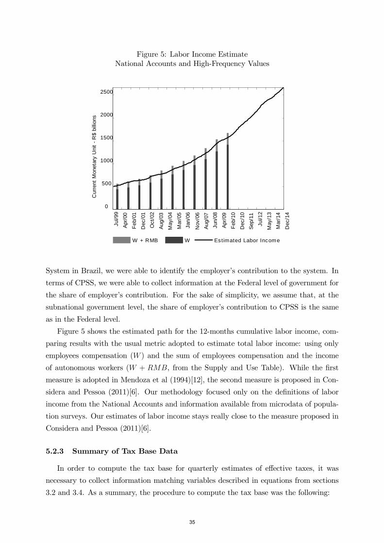
Figure 5: Labor Income EstimateNational Accounts and High-Frequency Values
Cur
rent
Mon
etar
y U
nit
R$
billio
ns
Jul/9
9Ap
r/00
Feb/
01
Dec
/01
Oct
/02
Aug/
03
May
/04
Mar
/05
Jan/
06
Nov
/06
Aug/
07Ju
n/08
Apr/0
9
Feb/
10
Dec
/10
Sep/
11
Jul/1
2
May
/13
Mar
/14
Dec
/14
0
500
1000
1500
2000
2500
W + RMB W Estimated Labor Income
System in Brazil, we were able to identify the employer’s contribution to the system. In
terms of CPSS, we were able to collect information at the Federal level of government for
the share of employer’s contribution. For the sake of simplicity, we assume that, at the
subnational government level, the share of employer’s contribution to CPSS is the same
as in the Federal level.
Figure 5 shows the estimated path for the 12-months cumulative labor income, com-
paring results with the usual metric adopted to estimate total labor income: using only
employees compensation (W ) and the sum of employees compensation and the income
of autonomous workers (W + RMB, from the Supply and Use Table). While the first
measure is adopted in Mendoza et al (1994)[12], the second measure is proposed in Con-
sidera and Pessoa (2011)[6]. Our methodology focused only on the definitions of labor
income from the National Accounts and information available from microdata of popula-
tion surveys. Our estimates of labor income stays really close to the measure proposed in
Considera and Pessoa (2011)[6].
5.2.3 Summary of Tax Base Data
In order to compute the tax base for quarterly estimates of effective taxes, it was
necessary to collect information matching variables described in equations from sections
3.2 and 3.4. As a summary, the procedure to compute the tax base was the following:
35
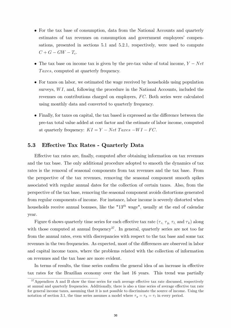
• For the tax base of consumption, data from the National Accounts and quarterly
estimates of tax revenues on consumption and government employees’ compen-
sations, presented in sections 5.1 and 5.2.1, respectively, were used to compute
C +G−GW − Tc.
• The tax base on income tax is given by the pre-tax value of total income, Y −NetTaxes, computed at quarterly frequency.
• For taxes on labor, we estimated the wage received by households using populationsurveys, WI, and, following the procedure in the National Accounts, included the
revenues on contributions charged on employers, FC. Both series were calculated
using monthly data and converted to quarterly frequency.
• Finally, for taxes on capital, the tax based is expressed as the difference between thepre-tax total value added at cost factor and the estimate of labor income, computed
at quarterly frequency: KI = Y −Net Taxes −WI − FC.
5.3 Effective Tax Rates - Quarterly Data
Effective tax rates are, finally, computed after obtaining information on tax revenues
and the tax base. The only additional procedure adopted to smooth the dynamics of tax
rates is the removal of seasonal components from tax revenues and the tax base. From
the perspective of the tax revenues, removing the seasonal component smooth spikes
associated with regular annual dates for the collection of certain taxes. Also, from the
perspective of the tax base, removing the seasonal component avoids distortions generated
from regular components of income. For instance, labor income is severely distorted when
households receive annual bonuses, like the "13th wage", usually at the end of calendar
year.
Figure 6 shows quarterly time series for each effective tax rate (τ c, τ y, τ l, and τ k) along
with those computed at annual frequency37. In general, quarterly series are not too far
from the annual rates, even with discrepancies with respect to the tax base and some tax
revenues in the two frequencies. As expected, most of the differences are observed in labor
and capital income taxes, where the problems related with the collection of information
on revenues and the tax base are more evident.
In terms of results, the time series confirm the general idea of an increase in effective
tax rates for the Brazilian economy over the last 16 years. This trend was partially
37Appendices A and B show the time series for each average effective tax rate discussed, respectivelyat annual and quarterly frequencies. Additionally, there is also a time series of average effective tax ratefor general income taxes, assuming that it is not possible to discriminate the source of income. Using thenotation of section 3.1, the time series assumes a model where τy = τk = τ l in every period.
36
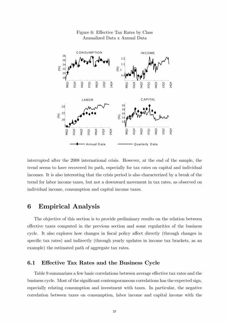
Figure 6: Effective Tax Rates by ClassAnnualized Data x Annual Data
C ON SU MPTION
(%)
99Q
1
01Q
4
04Q
2
07Q
1
09Q
3
12Q
2
14Q
4
182022242628
Annual D ata Quarterly D ata
IN C OME
(%)
99Q
1
01Q
4
04Q
2
07Q
1
09Q
3
12Q
2
14Q
4
0.9
1
1.1
1.2
LABOR
(%)
99Q
1
01Q
4
04Q
2
07Q
1
09Q
3
12Q
2
14Q
4
20
22
24
C APITAL
(%)
99Q
1
01Q
4
04Q
2
07Q
1
09Q
3
12Q
2
14Q
4
1214161820
interrupted after the 2008 international crisis. However, at the end of the sample, the
trend seems to have recovered its path, especially for tax rates on capital and individual
incomes. It is also interesting that the crisis period is also characterized by a break of the
trend for labor income taxes, but not a downward movement in tax rates, as observed on
individual income, consumption and capital income taxes.
6 Empirical Analysis
The objective of this section is to provide preliminary results on the relation between
effective taxes computed in the previous section and some regularities of the business
cycle. It also explores how changes in fiscal policy affect directly (through changes in
specific tax rates) and indirectly (through yearly updates in income tax brackets, as an
example) the estimated path of aggregate tax rates.
6.1 Effective Tax Rates and the Business Cycle
Table 9 summarizes a few basic correlations between average effective tax rates and the
business cycle. Most of the significant contemporaneous correlations has the expected sign,
especially relating consumption and investment with taxes. In particular, the negative
correlation between taxes on consumption, labor income and capital income with the
37
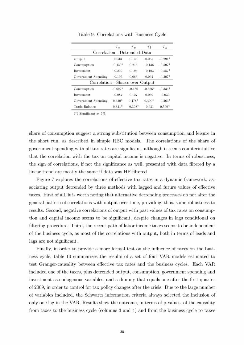
Table 9: Correlations with Business Cycle
τ c τ y τ l τ kCorrelation - Detrended Data
Output 0.033 0.146 0.035 -0.291*
Consumption -0.430* 0.215 -0.136 -0.597*
Investment -0.239 0.195 -0.103 -0.557*
Government Spending -0.195 0.083 0.062 -0.307*
Correlation - Shares over OutputConsumption -0.692* -0.186 -0.586* -0.334*
Investment -0.087 0.127 0.069 -0.030
Government Spending 0.330* 0.478* 0.490* -0.263*
Trade Balance 0.321* -0.398* -0.031 0.560*
(*) Significant at 5%.
share of consumption suggest a strong substitution between consumption and leisure in
the short run, as described in simple RBC models. The correlations of the share of
government spending with all tax rates are significant, although it seems counterintuitive
that the correlation with the tax on capital income is negative. In terms of robustness,
the sign of correlations, if not the significance as well, presented with data filtered by a
linear trend are mostly the same if data was HP-filtered.
Figure 7 explores the correlations of effective tax rates in a dynamic framework, as-
sociating output detrended by three methods with lagged and future values of effective
taxes. First of all, it is worth noting that alternative detrending processes do not alter the
general pattern of correlations with output over time, providing, thus, some robustness to
results. Second, negative correlations of output with past values of tax rates on consump-
tion and capital income seems to be significant, despite changes in lags conditional on
filtering procedure. Third, the recent path of labor income taxes seems to be independent
of the business cycle, as most of the correlations with output, both in terms of leads and
lags are not significant.
Finally, in order to provide a more formal test on the influence of taxes on the busi-
ness cycle, table 10 summarizes the results of a set of four VAR models estimated to
test Granger-causality between effective tax rates and the business cycles. Each VAR
included one of the taxes, plus detrended output, consumption, government spending and
investment as endogenous variables, and a dummy that equals one after the first quarter
of 2009, in order to control for tax policy changes after the crisis. Due to the large number
of variables included, the Schwartz information criteria always selected the inclusion of
only one lag in the VAR. Results show the outcome, in terms of p-values, of the causality
from taxes to the business cycle (columns 3 and 4) and from the business cycle to taxes
38
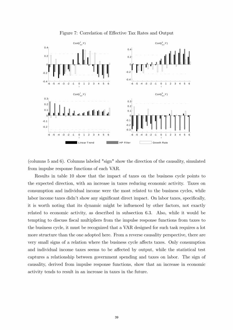
Figure 7: Correlation of Effective Tax Rates and Output
6 5 4 3 2 1 0 1 2 3 4 5 60.4
0.2
0
0.2
0.4
i
Corr(τct+i
,Y )
6 5 4 3 2 1 0 1 2 3 4 5 6
0.4
0.2
0
0.2
0.4
i
Corr(τyt+i
,Y )
6 5 4 3 2 1 0 1 2 3 4 5 6
0.2
0.1
0
0.1
0.2
0.3
i
Corr(τlt+i
,Y )
6 5 4 3 2 1 0 1 2 3 4 5 6
0.3
0.2
0.1
0
0.1
0.2
0.3
i
Corr(τkt+i
,Y )
Linear T rend HP Fil ter Growth Rate
(columns 5 and 6). Columns labeled "sign" show the direction of the causality, simulated
from impulse response functions of each VAR.
Results in table 10 show that the impact of taxes on the business cycle points to
the expected direction, with an increase in taxes reducing economic activity. Taxes on
consumption and individual income were the most related to the business cycles, while
labor income taxes didn’t show any significant direct impact. On labor taxes, specifically,
it is worth noting that its dynamic might be influenced by other factors, not exactly
related to economic activity, as described in subsection 6.3. Also, while it would be
tempting to discuss fiscal multipliers from the impulse response functions from taxes to
the business cycle, it must be recognized that a VAR designed for such task requires a lot
more structure than the one adopted here. From a reverse causality perspective, there are
very small signs of a relation where the business cycle affects taxes. Only consumption
and individual income taxes seems to be affected by output, while the statistical test
captures a relationship between government spending and taxes on labor. The sign of
causality, derived from impulse response functions, show that an increase in economic
activity tends to result in an increase in taxes in the future.
39
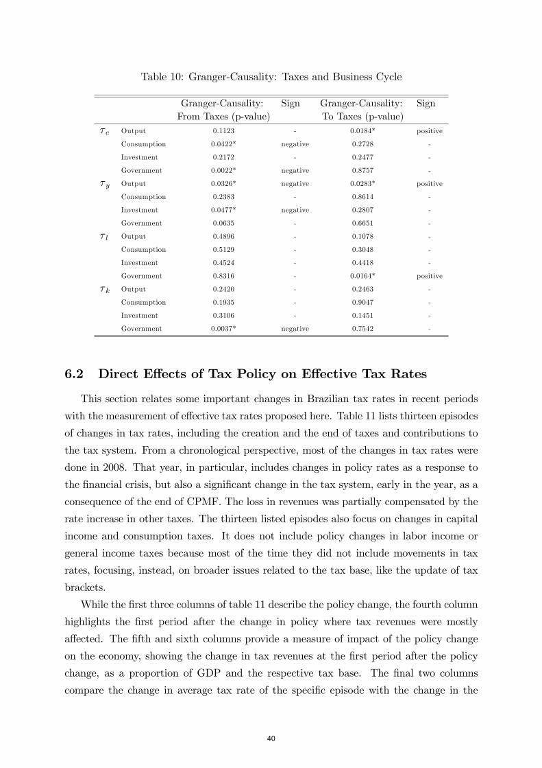
Table 10: Granger-Causality: Taxes and Business Cycle
Granger-Causality: Sign Granger-Causality: SignFrom Taxes (p-value) To Taxes (p-value)
τ c Output 0.1123 - 0.0184* positive
Consumption 0.0422* negative 0.2728 -
Investment 0.2172 - 0.2477 -
Government 0.0022* negative 0.8757 -
τ y Output 0.0326* negative 0.0283* positive
Consumption 0.2383 - 0.8614 -
Investment 0.0477* negative 0.2807 -
Government 0.0635 - 0.6651 -
τ l Output 0.4896 - 0.1078 -
Consumption 0.5129 - 0.3048 -
Investment 0.4524 - 0.4418 -
Government 0.8316 - 0.0164* positive
τ k Output 0.2420 - 0.2463 -
Consumption 0.1935 - 0.9047 -
Investment 0.3106 - 0.1451 -
Government 0.0037* negative 0.7542 -
6.2 Direct Effects of Tax Policy on Effective Tax Rates
This section relates some important changes in Brazilian tax rates in recent periods
with the measurement of effective tax rates proposed here. Table 11 lists thirteen episodes
of changes in tax rates, including the creation and the end of taxes and contributions to
the tax system. From a chronological perspective, most of the changes in tax rates were
done in 2008. That year, in particular, includes changes in policy rates as a response to
the financial crisis, but also a significant change in the tax system, early in the year, as a
consequence of the end of CPMF. The loss in revenues was partially compensated by the
rate increase in other taxes. The thirteen listed episodes also focus on changes in capital
income and consumption taxes. It does not include policy changes in labor income or
general income taxes because most of the time they did not include movements in tax
rates, focusing, instead, on broader issues related to the tax base, like the update of tax
brackets.
While the first three columns of table 11 describe the policy change, the fourth column
highlights the first period after the change in policy where tax revenues were mostly
affected. The fifth and sixth columns provide a measure of impact of the policy change
on the economy, showing the change in tax revenues at the first period after the policy
change, as a proportion of GDP and the respective tax base. The final two columns
compare the change in average tax rate of the specific episode with the change in the
40

aggregate measure of tax rate. As an example, in the first episode presented, setting a
tax rate of 0.38% for CPMF represented, in 1999Q3, an increase of revenues of 1.11p.p.
of GDP, or almost 3p.p. as a proportion of the tax base of capital rates. Setting a new
tax rate for CPMF represented approximately 83% of total variation in capital income
tax rates in 1999Q3 (2.96/3.56 ≈ 0.83).
The first result taken from a general overview of table 11 is that changes in policy
tax rates have a good matching to changes in the average effective tax rates, at least on
impact. There are only two cases where the change in a specific tax had an opposite
sign compared to the change in the aggregate tax rate: the increase in CSLL to financial
companies in 2008, when total tax on capital income reduced 0.42% due to the end of
CPMF and a reduction in tax rates charged in IRPJ; and the reduction in tax rates of
IOF for a few financial operations, when total taxes in consumption increased 0.10%.
Excluding those two episodes, changes in policy tax rates were responsible for 79.6% of
the change in the effective tax rate for the category. It is also worth noting that the
matching seems to be equally good for both large tax changes (in the sense of generating
large revenues as a proportion of GDP) and small movements in policy rates.
6.3 Indirect Changes on Effective Tax Rates
This section describes two indirect sources of changes in the measurement of average
effective tax rates that are not related to observed variation in tax rate policy: first,
this section explores the effects of annual revisions of tax brackets when labor income
distribution is changing over time; then, an evaluation of the cyclical behavior of tax
revenues provides an idea on the distortions to the measurement of effective tax rates
generated by the status of the business cycle. The two exercises, in a sense, complement
each other, as they evaluate indirect changes in average effective tax rates from both a
cross-sectional —i.e., when the heterogeneity of agents in the economy is one of the main
sources of fluctuations —and a time series perspective —especially in the last case, when
the state of the economy is the main source of changes in effective tax rates.
In order to analyze the effects of income heterogeneity on the measurement of effective
tax rates, consider the case of the update of tax brackets for the annual reports of income
taxes. This exercise is particularly important, as Brazil has recently experienced signifi-
cant real wages increases over time, combined with reduction of labor income inequality.
As an example on how updating tax brackets might affect average effective tax rates on
labor, consider the case of a household whose income is on the verge of reaching the lower
limit of the lowest tax bracket. Assume that the government decides not to update the
tax bracket from the previous year. If the household had any extra income gain in the
previous fiscal year, she must declare and pay taxes on her total income. That means
41
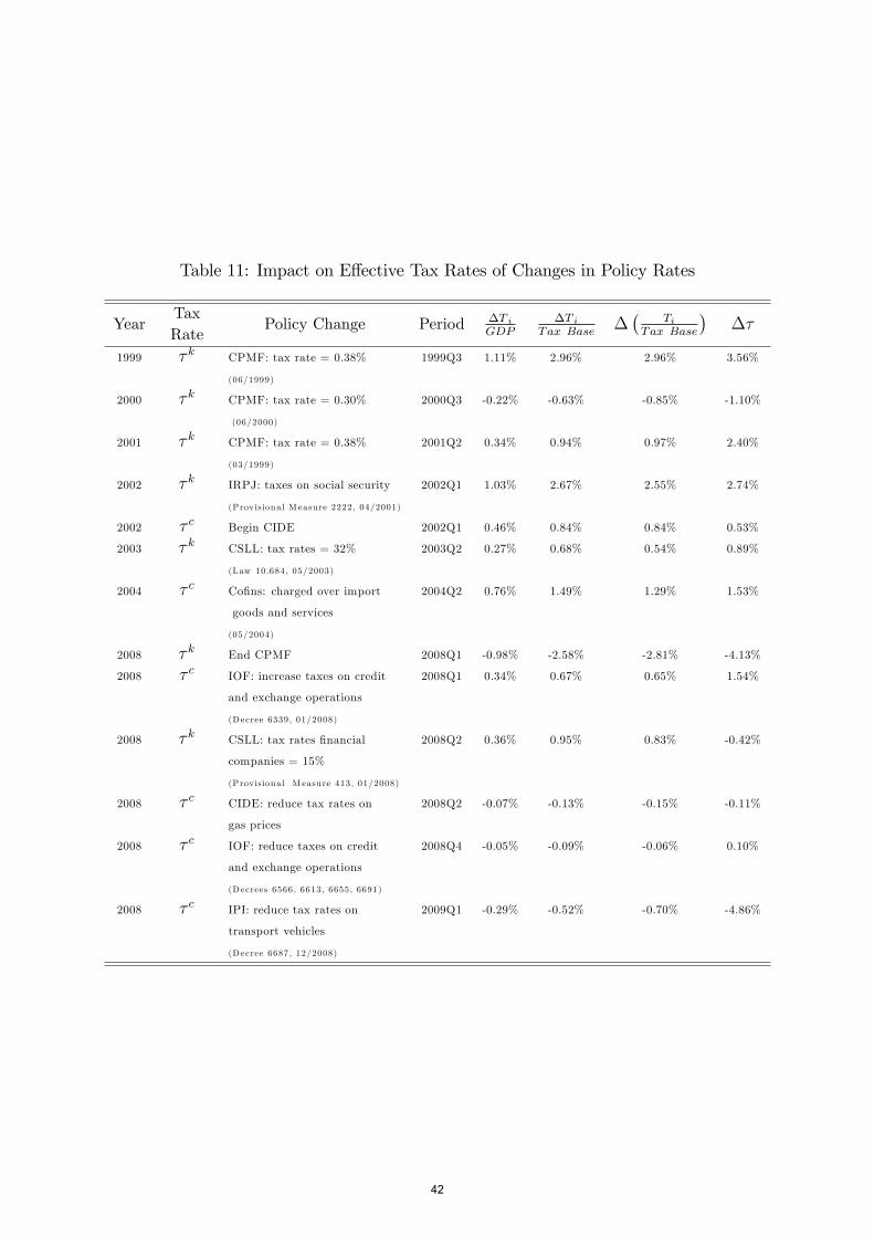
Table 11: Impact on Effective Tax Rates of Changes in Policy Rates
YearTaxRate
Policy Change Period ∆T iGDP
∆T iTax Base
∆(
TiTax Base
)∆τ
1999 τ k CPMF: tax rate = 0.38% 1999Q3 1.11% 2.96% 2.96% 3.56%
(06/1999)
2000 τ k CPMF: tax rate = 0.30% 2000Q3 -0.22% -0.63% -0.85% -1.10%
(06/2000)
2001 τ k CPMF: tax rate = 0.38% 2001Q2 0.34% 0.94% 0.97% 2.40%
(03/1999)
2002 τ k IRPJ: taxes on social security 2002Q1 1.03% 2.67% 2.55% 2.74%
(Provisional M easure 2222, 04/2001)
2002 τ c Begin CIDE 2002Q1 0.46% 0.84% 0.84% 0.53%
2003 τ k CSLL: tax rates = 32% 2003Q2 0.27% 0.68% 0.54% 0.89%
(Law 10.684, 05/2003)
2004 τ c Cofins: charged over import 2004Q2 0.76% 1.49% 1.29% 1.53%
goods and services
(05/2004)
2008 τ k End CPMF 2008Q1 -0.98% -2.58% -2.81% -4.13%
2008 τ c IOF: increase taxes on credit 2008Q1 0.34% 0.67% 0.65% 1.54%
and exchange operations
(Decree 6339, 01/2008)
2008 τ k CSLL: tax rates financial 2008Q2 0.36% 0.95% 0.83% -0.42%
companies = 15%
(Provisional M easure 413, 01/2008)
2008 τ c CIDE: reduce tax rates on 2008Q2 -0.07% -0.13% -0.15% -0.11%
gas prices
2008 τ c IOF: reduce taxes on credit 2008Q4 -0.05% -0.09% -0.06% 0.10%
and exchange operations
(Decrees 6566, 6613, 6655, 6691)
2008 τ c IPI: reduce tax rates on 2009Q1 -0.29% -0.52% -0.70% -4.86%
transport vehicles
(Decree 6687, 12/2008)
42
a larger increase on total tax revenues compared to the change in the tax base, as the
household was not paying taxes in the previous year. For the sake of computing average
effective tax rates, thus, an update of tax brackets that does not follow changes in real
income might generate a procyclical component on the time series.
The overall increase in the number of people paying labor income taxes might justify
the upward trend in labor income taxes shown in figure 6. In fact, Orair (2014)[14] re-
lates the increase in tax revenues from IRRF/Labor between 2004 and 2009 in different
economic sectors with the increase in formal labor participation in those sectors. From an
aggregate perspective, figure 8 shows the share of employed population with labor income
at least equal to the lower limit of the lowest tax bracket and the share of employed pop-
ulation earning at least the income defining the highest tax bracket, both as a proportion
of total population at least 10 years-old38. The figure shows a clear upward trend in the
share of employed population earning at least the minimum to pay labor income taxes,
from 7% in 2002Q1 to 17.25% in 2014Q4. On the other hand, there is a clear break in 2009
for the number of people paying the highest income tax rate: in that year, the Secretariat
of the Federal Revenue created two additional tax brackets, changing the income limit for
the highest bracket. The share of employed population charged with income taxes at the
highest bracket fluctuated between 2.7 to 4.4% of total population in the sample.
To evaluate the effects of changes in the share of employed population paying labor
income taxes, a VAR model is estimated, relating the labor income tax, the two shares
described above and the share of population working in the formal sector with respect
to total employed population. The numerator is defined as total employed population
in the formal, private sector. The 4-variable VAR, estimated with only one lag based
on information criteria, also includes as exogenous variable two lags of HP-Filter based
output gap and two dummy variables: the first dummy variable equals one after 2006,
adjusting for the break in the information set observed after that year; the second dummy
variable equals one after 2009, controlling for the change in the number of tax brackets.
Assuming an ordering where the share of employed population in the formal sector is
not contemporaneously affected by the other three variables in the system —the "most
exogenous variable" in the system — and the labor income tax is contemporaneously
affected by all other variables —the "most endogenous variable" —in the Choleski matrix
decomposition, figure 9 shows the impulse response functions of the labor income tax after
an exogenous shock in the shares of population39. Dotted lines show the 95% confidence
38The time series show the seasonally adjusted values at the end of each quarter. The time seriesshow only values of PME survey from the new methodology, since the gap between figures on employedpopulation between the old and the new methodology could be a problem in the time series analysisproposed below.39Results are not affected by the Choleski decomposition, as Generalized IRFs generates approximately
the same outcome.
43
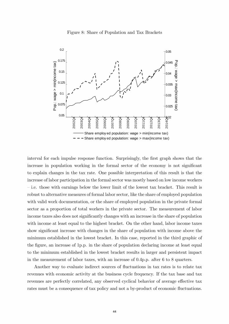
Figure 8: Share of Population and Tax Brackets
Pop
.: w
age
> m
in(in
com
e ta
x)
2002
Q4
2003
Q4
2004
Q4
2005
Q4
2006
Q4
2007
Q4
2008
Q4
2009
Q4
2010
Q4
2011
Q4
2012
Q4
2013
Q4
2014
Q4
0.05
0.075
0.1
0.125
0.15
0.175
0.2
0.02
0.025
0.03
0.035
0.04
0.045
0.05P
op.: wage > m
ax(income tax)
Share employ ed population: wage > min(income tax)Share employ ed population: wage > max(income tax)
interval for each impulse response function. Surprisingly, the first graph shows that the
increase in population working in the formal sector of the economy is not significant
to explain changes in the tax rate. One possible interpretation of this result is that the
increase of labor participation in the formal sector was mostly based on low income workers
—i.e. those with earnings below the lower limit of the lowest tax bracket. This result is
robust to alternative measures of formal labor sector, like the share of employed population
with valid work documentation, or the share of employed population in the private formal
sector as a proportion of total workers in the private sector. The measurement of labor
income taxes also does not significantly changes with an increase in the share of population
with income at least equal to the highest bracket. On the other hand, labor income taxes
show significant increase with changes in the share of population with income above the
minimum established in the lowest bracket. In this case, reported in the third graphic of
the figure, an increase of 1p.p. in the share of population declaring income at least equal
to the minimum established in the lowest bracket results in larger and persistent impact
in the measurement of labor taxes, with an increase of 0.4p.p. after 6 to 8 quarters.
Another way to evaluate indirect sources of fluctuations in tax rates is to relate tax
revenues with economic activity at the business cycle frequency. If the tax base and tax
revenues are perfectly correlated, any observed cyclical behavior of average effective tax
rates must be a consequence of tax policy and not a by-product of economic fluctuations.
44
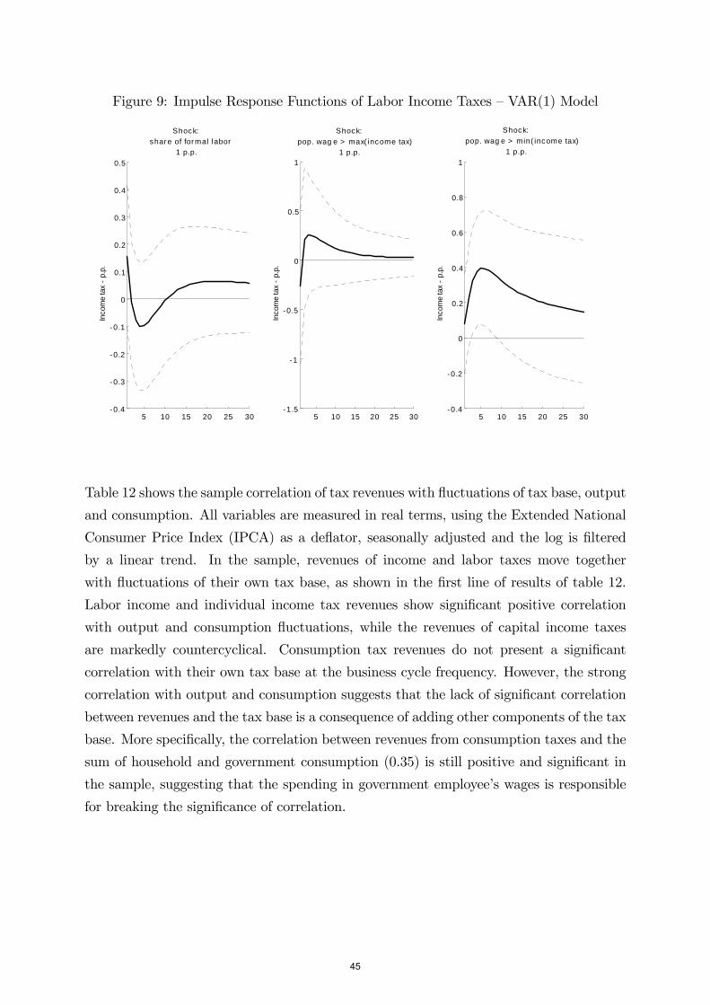
Figure 9: Impulse Response Functions of Labor Income Taxes —VAR(1) Model
5 10 15 20 25 300.4
0.3
0.2
0.1
0
0.1
0.2
0.3
0.4
0.5
Inco
me
tax
p.
p.
Shock:share of formal labor
1 p.p.
5 10 15 20 25 301.5
1
0.5
0
0.5
1
Inco
me
tax
p.
p.
Shock:pop. wag e > max( income tax)
1 p.p.
5 10 15 20 25 300.4
0.2
0
0.2
0.4
0.6
0.8
1
Inco
me
tax
p.
p.
Shock:pop. wag e > min( income tax)
1 p.p.
Table 12 shows the sample correlation of tax revenues with fluctuations of tax base, output
and consumption. All variables are measured in real terms, using the Extended National
Consumer Price Index (IPCA) as a deflator, seasonally adjusted and the log is filtered
by a linear trend. In the sample, revenues of income and labor taxes move together
with fluctuations of their own tax base, as shown in the first line of results of table 12.
Labor income and individual income tax revenues show significant positive correlation
with output and consumption fluctuations, while the revenues of capital income taxes
are markedly countercyclical. Consumption tax revenues do not present a significant
correlation with their own tax base at the business cycle frequency. However, the strong
correlation with output and consumption suggests that the lack of significant correlation
between revenues and the tax base is a consequence of adding other components of the tax
base. More specifically, the correlation between revenues from consumption taxes and the
sum of household and government consumption (0.35) is still positive and significant in
the sample, suggesting that the spending in government employee’s wages is responsible
for breaking the significance of correlation.
45
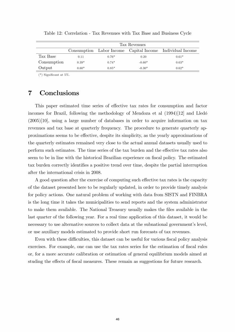
Table 12: Correlation - Tax Revenues with Tax Base and Business Cycle
Tax RevenuesConsumption Labor Income Capital Income Individual Income
Tax Base 0.11 0.76* 0.20 0.61*
Consumption 0.39* 0.74* -0.60* 0.63*
Output 0.60* 0.85* -0.30* 0.62*
(*) Significant at 5%.
7 Conclusions
This paper estimated time series of effective tax rates for consumption and factor
incomes for Brazil, following the methodology of Mendoza et al (1994)[12] and Lledó
(2005)[10], using a large number of databases in order to acquire information on tax
revenues and tax base at quarterly frequency. The procedure to generate quarterly ap-
proximations seems to be effective, despite its simplicity, as the yearly approximations of
the quarterly estimates remained very close to the actual annual datasets usually used to
perform such estimates. The time series of the tax burden and the effective tax rates also
seem to be in line with the historical Brazilian experience on fiscal policy. The estimated
tax burden correctly identifies a positive trend over time, despite the partial interruption
after the international crisis in 2008.
A good question after the exercise of computing such effective tax rates is the capacity
of the dataset presented here to be regularly updated, in order to provide timely analysis
for policy actions. One natural problem of working with data from SISTN and FINBRA
is the long time it takes the municipalities to send reports and the system administrator
to make them available. The National Treasury usually makes the files available in the
last quarter of the following year. For a real time application of this dataset, it would be
necessary to use alternative sources to collect data at the subnational government’s level,
or use auxiliary models estimated to provide short run forecasts of tax revenues.
Even with these diffi culties, this dataset can be useful for various fiscal policy analysis
exercises. For example, one can use the tax rates series for the estimation of fiscal rules
or, for a more accurate calibration or estimation of general equilibrium models aimed at
studing the effects of fiscal measures. These remain as suggestions for future research.
46
References
[1] C. H. Araújo and P. C. Ferreira. Reforma tributária, efeitos alocativos e impactos
de bem-estar. Revista Brasileira de Economia, 53(2):133—166, 1999.
[2] V. B. Araújo Neto and M. C. S. Sousa. Tributação da renda e do consumo no brasil:
Uma abordagemmacroeconômica. Proceedings of the 29th Brazilian Economics Meet-
ing from ANPEC, 2001.
[3] D. Carey and J. Rabesona. Tax ratios on labour and capital income and on con-
sumption. OECD Economic Studies, (35), 2002.
[4] F. A. Carvalho and M. Valli. Fiscal policy in brazil through the lens of an esti-
mated DSGE model. Working Papers Series 240, Central Bank of Brazil, Research
Department, 2011.
[5] M. A. F. H. Cavalcanti and N. L. C. Silva. Impactos de políticas de desoneração
do setor produtivo: Uma avaliação a partir de um modelo de gerações superpostas.
Estudos Econômicos, 40(4):943—966, 2010.
[6] C. M. Considera and S. A. Pessoa. A distribuição funcional da renda no Brasil: 1959-
2008. Textos para Discussão 277, Universidade Federal Fluminense - Faculdade de
Economia, 2011.
[7] P. C. Ferreira and R. A. C. Pereira. Avaliação dos impacto macroeconômicos e de
bem-estar da reforma tributária no brasil. Revista Brasileira de Economia, 64(2):149—
175, 2010.
[8] V. Gomes, M. N. S. Bugarin, and R. G. Ellery Jr. Long-run implications of the
Brazilian capital stock and income estimates. Brazilian Review of Econometrics,
25(1):67—88, May 2005.
[9] IBGE. Sistema de Contas Nacionais - Brasil. Technical report, Instituto Brasileiro
de Geografia e Estatística - IBGE, 2008.
[10] V. D. Lledó. Tax system under fiscal adjustment: A dynamic CGE analysis of the
Brazilian tax reform. IMF Working Paper 05/142, International Monetary Fund,
2005.
[11] M. Medeiros, P. H. G. F. Souza, and F. A. Castro. O topo da distribuição de renda
no Brasil: Primeiras estimativas com dados tributários e comparação com pesquisas
domiciliares, 2006-2012. Working paper, 2014.
47
[12] E. G. Mendoza, A. Razin, and L. L. Tesar. Effective tax rates in macroeconomics
cross-country estimates of tax rates on factor incomes and consumption. Journal of
Monetary Economics, 34:297—323, 1994.
[13] J. R. B. Nogueira, R. B. Siqueira, P. J. Santana, H. Levy, and E. S. Souza. A
carga tributária efetiva sobre o trabalho no Brasil: Nível, distribuição e composição.
Análise Econômica, 31(59), Apr. 2013.
[14] R. O. Orair. A dinâmica recente da carga tributária no Brasil: o que explica o para-
doxo do crescimento da carga tributária em meio a seguidas desonerações tributárias?
in: Finanças públicas e macroeconomia no Brasil: um registro da reflexão do Ipea
(2008 - 2014) volume 2, Instituto de Pesquisa Econômica Aplicada, 2014.
[15] R. O. Orair, S. W. Gobetti, E. M. Leal, andW. d. J. Silva. Carga tributária brasileira:
Estimação e análise dos determinantes da evolução recente - 2002-2012. IPEA Texto
para Discussão 1875, Instituto de Pesquisa Econômica Aplicada, 2013.
[16] F. M. Pereira. Modelos de Ciclos Reais de Negócios com Imposto e Setor Externo: O
Caso Brasileiro. PhD thesis, Departamento de Economia - Universidade de Brasília,
2009.
[17] R. B. Siqueira, J. R. Nogueira, and E. S. Souza. A incidência final dos impostos
indiretos no Brasil: Efeitos da tributação de insumos. Revista Brasileira de Economia,
55(4):513—544, Sept. 2001.
[18] B. Volkerink, J.-E. Sturm, and J. de Haan. Tax ratios in macroeconomics: Do taxes
really matter? Empirica, 29(3):209—224, 2002.
48
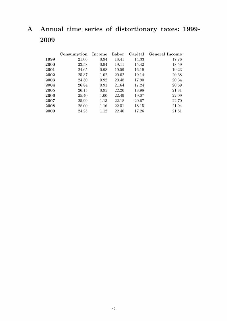
A Annual time series of distortionary taxes: 1999-
2009
Consumption Income Labor Capital General Income1999 21.06 0.94 18.41 14.33 17.762000 23.58 0.94 19.11 15.42 18.592001 24.65 0.98 19.59 16.19 19.232002 25.37 1.02 20.02 19.14 20.682003 24.30 0.92 20.48 17.90 20.342004 26.84 0.91 21.64 17.24 20.692005 26.15 0.95 22.20 18.98 21.812006 25.40 1.00 22.49 19.07 22.092007 25.99 1.13 22.18 20.67 22.702008 28.00 1.16 22.51 18.15 21.942009 24.25 1.12 22.40 17.26 21.51
49
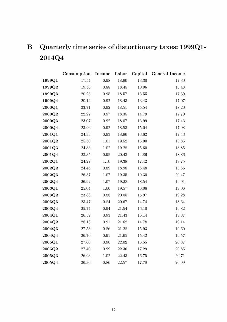
B Quarterly time series of distortionary taxes: 1999Q1-
2014Q4
Consumption Income Labor Capital General Income
1999Q1 17.54 0.98 18.90 13.30 17.30
1999Q2 19.36 0.88 18.45 10.06 15.48
1999Q3 20.25 0.95 18.57 13.55 17.39
1999Q4 20.12 0.92 18.43 13.43 17.07
2000Q1 23.71 0.92 18.51 15.54 18.20
2000Q2 22.27 0.97 18.35 14.79 17.70
2000Q3 23.07 0.92 18.07 13.99 17.43
2000Q4 23.96 0.92 18.53 15.04 17.98
2001Q1 24.33 0.93 18.96 13.62 17.43
2001Q2 25.30 1.01 19.52 15.90 18.85
2001Q3 24.83 1.02 19.28 15.60 18.85
2001Q4 23.35 0.95 20.43 14.86 18.86
2002Q1 24.27 1.10 19.38 17.42 19.75
2002Q2 24.46 0.89 18.98 16.48 18.56
2002Q3 26.37 1.07 19.35 19.30 20.47
2002Q4 26.92 1.07 19.28 18.54 19.91
2003Q1 25.04 1.06 19.57 16.06 19.06
2003Q2 23.88 0.88 20.05 16.97 19.28
2003Q3 23.47 0.84 20.67 14.74 18.64
2003Q4 25.74 0.94 21.54 16.10 19.82
2004Q1 26.52 0.93 21.43 16.14 19.87
2004Q2 28.13 0.91 21.62 14.78 19.14
2004Q3 27.53 0.86 21.28 15.93 19.60
2004Q4 26.70 0.91 21.65 15.42 19.57
2005Q1 27.60 0.90 22.02 16.55 20.37
2005Q2 27.40 0.99 22.36 17.29 20.85
2005Q3 26.93 1.02 22.43 16.75 20.71
2005Q4 26.36 0.86 22.57 17.78 20.99
50
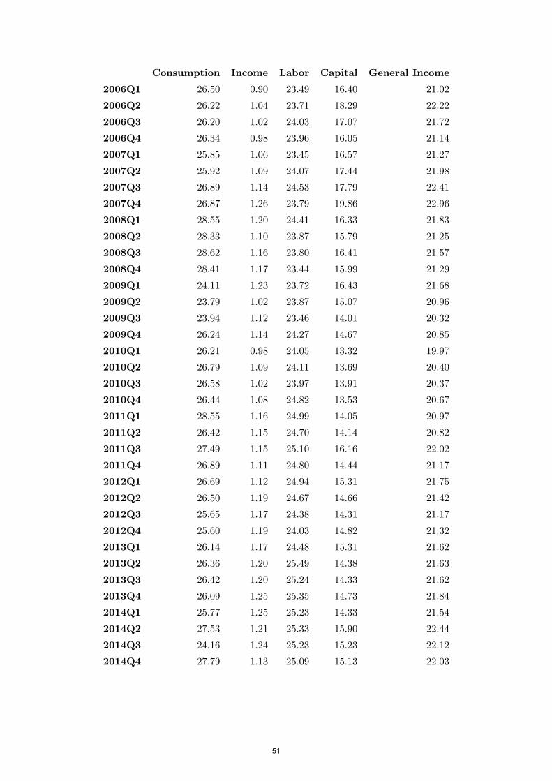
Consumption Income Labor Capital General Income
2006Q1 26.50 0.90 23.49 16.40 21.02
2006Q2 26.22 1.04 23.71 18.29 22.22
2006Q3 26.20 1.02 24.03 17.07 21.72
2006Q4 26.34 0.98 23.96 16.05 21.14
2007Q1 25.85 1.06 23.45 16.57 21.27
2007Q2 25.92 1.09 24.07 17.44 21.98
2007Q3 26.89 1.14 24.53 17.79 22.41
2007Q4 26.87 1.26 23.79 19.86 22.96
2008Q1 28.55 1.20 24.41 16.33 21.83
2008Q2 28.33 1.10 23.87 15.79 21.25
2008Q3 28.62 1.16 23.80 16.41 21.57
2008Q4 28.41 1.17 23.44 15.99 21.29
2009Q1 24.11 1.23 23.72 16.43 21.68
2009Q2 23.79 1.02 23.87 15.07 20.96
2009Q3 23.94 1.12 23.46 14.01 20.32
2009Q4 26.24 1.14 24.27 14.67 20.85
2010Q1 26.21 0.98 24.05 13.32 19.97
2010Q2 26.79 1.09 24.11 13.69 20.40
2010Q3 26.58 1.02 23.97 13.91 20.37
2010Q4 26.44 1.08 24.82 13.53 20.67
2011Q1 28.55 1.16 24.99 14.05 20.97
2011Q2 26.42 1.15 24.70 14.14 20.82
2011Q3 27.49 1.15 25.10 16.16 22.02
2011Q4 26.89 1.11 24.80 14.44 21.17
2012Q1 26.69 1.12 24.94 15.31 21.75
2012Q2 26.50 1.19 24.67 14.66 21.42
2012Q3 25.65 1.17 24.38 14.31 21.17
2012Q4 25.60 1.19 24.03 14.82 21.32
2013Q1 26.14 1.17 24.48 15.31 21.62
2013Q2 26.36 1.20 25.49 14.38 21.63
2013Q3 26.42 1.20 25.24 14.33 21.62
2013Q4 26.09 1.25 25.35 14.73 21.84
2014Q1 25.77 1.25 25.23 14.33 21.54
2014Q2 27.53 1.21 25.33 15.90 22.44
2014Q3 24.16 1.24 25.23 15.23 22.12
2014Q4 27.79 1.13 25.09 15.13 22.03
51
C Description of Taxes and Contributions
Here we give a short description of the taxes and contributions used in this study,
including their names in Portuguese40. They are broken down by jurisdiction (Federal,
State or Municipal). Although long, this list does not include all the taxes and contribu-
tions levied in Brazil, but the ones there were classified in one of the categories used in
this study.
C.1 Federal Government Taxes
Cide - Contribuição sobre Intervenção no Domínio Econômico (Contribution of Inter-
vention in the Economic Domain) - Tax levied on some specific products, the main one
being fuel.
CSLL - Contribuição Social sobre o Lucro Líquido (Social Contribution on Net Profit)
- Contribution levied on profit before income tax destined to finance the social security
system.
Cofins - Contribuição para o Financiamento da Seguridade Social (Contribution for
the Financing of the Social Security) - Contribution charged monthly on the gross revenue
from the sale of goods and services destined to finance the social security system.
CPMF - Contribuição Provisória sobre Movimentação ou Transmissão de Valores e
de Créditos e Direitos de Natureza Financeira (Provisional Contribution on Financial
Movement) - Contribution levied on bank debits of individuals or corporations.
CPSS/Federal - Contribuição para o Plano de Seguridade Social do Servidor - Fed-
eral (Civil Servants’Social Security Contribution - Union) - Contribution on the earnings
of federal civil servants to finance their social security system.
FGTS - Fundo de Garantia por Tempo de Serviço (Employee Indemnity Guaran-
tee Fund) - Contribution levied on the payroll of corporations or individuals (household
employers).
II - Imposto sobre Importação (Import Tax) - Import duty applied to the entrance of
foreign products.
IOF - Imposto sobre Operações Financeiras (Tax on Financial Operations) - Tax
levied on financial operations and assessed on different types of events, such as credit,
foreign exchange, securities and insurance.
IPI - Imposto sobre Produtos Industrializados (Tax on Industrialized Products) -
40Sources:http://www2.apexbrasil.com.br/en/invest-in-brazil/how-to-invest-in-brazil/tax-systemhttp://thebrazilbusiness.com/taxhttp://www.receita.fazenda.gov.br/principal/Ingles/SistemaTributarioBR/Taxes.htm
52
Value Added Tax paid by manufactures on behalf of their customers at the time of sale.
It is considered on the sale cost and transferred to the buyer.
IRPF - Imposto sobre a Renda da Pessoa Física (Individual Income Tax) - Tax levied
on individuals´ salaries and earnings.
IRPJ - Imposto de Renda de Pessoas Jurídicas (Corporate Income Tax) - Corporate
revenue tax applied to the net profits of any legal entity.
IRRF/Capital - Imposto de Renda Retido na Fonte - rendimento do capital (With-
holding Income Tax - Capital Income) - Tax levied on gross income on capital such as
equity, investments, stocks for individuals and corporations.
IRRF/Trabalho - Imposto de Renda Retido na Fonte - rendimento do trabalho
(Withholding Income Tax - Labor Income) - Tax levied on salaries and earnings withheld
by the payer.
IRRF/Remessas - Imposto de Renda Retido na Fonte - rendimento de remessa
p/ ext. (Withholding Income Tax - Income from remittances abroad) - Tax levied on
profits, dividends, interest and amortization, royalties, technical, scientific, administrative
or similar assistance, remitted abroad by individuals and corporations.
IRRF/Outros - Imposto de Renda Retido na Fonte - outros rendimentos (Withhold-
ing Income Tax - Others) - Tax on prizes and drawings, advertisement services, payment
of professional services, among others.
ITR - Imposto Territorial Rural (Tax on Rural Land Property) - Tax on the value of
rural property owned by individuals or corporations.
PASEP - Programa de Formação do Patrimônio do Servidor Público (Civil Servants’
Savings Program Contribution) - Contribution analogous to PIS, but applied to civil
servants.
PIS - Programa de Integração Social (Contribution to the Social Integration Program)
- Contribution destined to finance the payment of insurance, unemployment allowance and
participation in revenues from agencies and entities for public and private workers.
RGPS - Contribuição para o Regime Geral de Previdência Social (Contribution to the
General Social Security System) - Contribution on payroll and self-employment earnings.
SE - Salário Educação (Education Wage) - Social contribution intended to finance
projects, programs and actions oriented to public basic education.
Sistema "S" - Contribuições para o Sistema S (Contributions to the "S" System)
- Joint system of social contributions paid by companies in order to finance the Au-
tonomous Social Services (The so called "S" system is composed by the following bodies:
SENAR (National Rural Training Service), SENAI (National Industrial Training Service),
SESI (Social Service of Industry), SENAC (National Commercial Training Service), SESC
(Social Service of Commerce), SESCOOP (National Service of Cooperativism Apprentice-
53
ship), SEST (Social Service of the Transport Sector), SENAT (National Transportation
Training Service), SEBRAE (Brazilian Service of Micro and Small Size Companies Sup-
port), IEL (Euvaldo Lodi Institute), Aviation Fund and maritime Professional Education).
C.2 State Government Taxes
CPSS/States - Contribuição para o Plano de Seguridade Social do Servidor - Estados
(Civil Servants’Social Security Contribution - States) - Contribution on the earnings of
state civil servants to finance their social security system.
ICMS - Imposto sobre a Circulação de Mercadorias e Serviços (Tax on the Circula-
tion of Goods and Transportation and Communication Services) -Value Added Tax on
Circulation of Goods and Interstate and Intercity Transportation and Communication
Services.
IPVA - Imposto sobre a Propriedade de Veículos Automotores (Tax on Motor Vehi-
cles) - Tax charged over the property of motorized any vehicles.
ITCD - Imposto sobre Transmissão Causa Mortis e Doação (Tax on inheritance and
Gifts) - Tax payable by every person or legal entity that receives goods and rights such
as inheritance or donation.
C.3 Municipal Government Taxes
CPSS/Municipal - Contribuição para o Plano de Seguridade Social do Servidor -
Municípios (Civil Servants’Social Security Contribution - Municipalities) Contribution
on the earnings of municipal civil servants to finance their social security system.
IPTU - Imposto Predial e Territorial Urbano (Tax on Urban Land and Property) Tax
levied on the property of urban real estate.
ISS - Imposto Sobre Serviços de Qualquer natureza (Tax on Services of any kind) -
Tax applied to the services provided to a third party by a company or professional and is
paid by the service provider. Includes services not covered by ICMS.
ITBI - Imposto sobre a Transmissão de Bens Imóveis Inter-Vivos (Tax on Real Estate
Conveyance) - Tax on the onerous transfer of immovable property or rights related to it.
D Adjustment of Data from SISTN
In order to adjust the SISTN database for the differences from the data on FINBRA, we
use the monthly data of each tax revenue from SISTN, labeled SISTN_XI,J,K , whereX ∈{IPTU, ISS, ITBI} , for each municipality and the Federal District I ∈ {1, ..., 5569} ,in each month J ∈ {1, ...12} of each year K ∈ {2006, ..., 2014}. The first step of the
54
adjustment was to compute the individual average share for each month’s revenue over
the total revenue of the year. For instance, the individual average share for tax X in
January, for municipality I, is given by:
Share_XI,Jan =
2014∑K=2006
SISTN_XI,Jan,K
2014∑K=2006
12∑J=1
SISTN_XI,J,K
(14)
The individual average share was computed for each municipality in each month, using
only those municipalities with information for all the 12 months in a given year.
We also compute an aggregate average share for all municipalities, which will be used
to distribute the data of those municipalities that have data on FINBRA, but do not have
enough monthly data to compute its own share. So, for example, the aggregate average
share for January is given by:
Share_XAvg,Jan =
5569∑I=1
2014∑K=2006
SISTN_XI,Jan,K
5569∑I=1
2014∑K=2006
12∑J=1
SISTN_XI,J,K
(15)
Equation 15 provides an aggregate average share of tax collection for each month. For
the observations of the municipalities for which there is data available both on SISTN
and on FINBRA, we obtain an adjusted tax revenue XI,J,K distributing the difference be-
tween the annual data from FINBRA (FINBRA_XI,K) and the 12-month accumulated
data from SISTN(
12∑J=1
SISTN_XI,J,K
). For those municipalities that we were able to
compute the individual average share:
XI,J,K = SISTN_XI,J,K + Share_XI,J ×(FINBRA_XI,K −
12∑J=1
SISTN_XI,J,K
)(16)
In a case where, in a given year, information is missing from SISTN for a given
municipality, but there is data from FINBRA, if we were able to compute the individual
average share for that municipality, just distribute the annual observation from FINBRA
according to the respective shares:
XI,J,K = Share_XI,J × FINBRA_XI,K (17)
For the case where it was not possible to get an individual average share for that
55
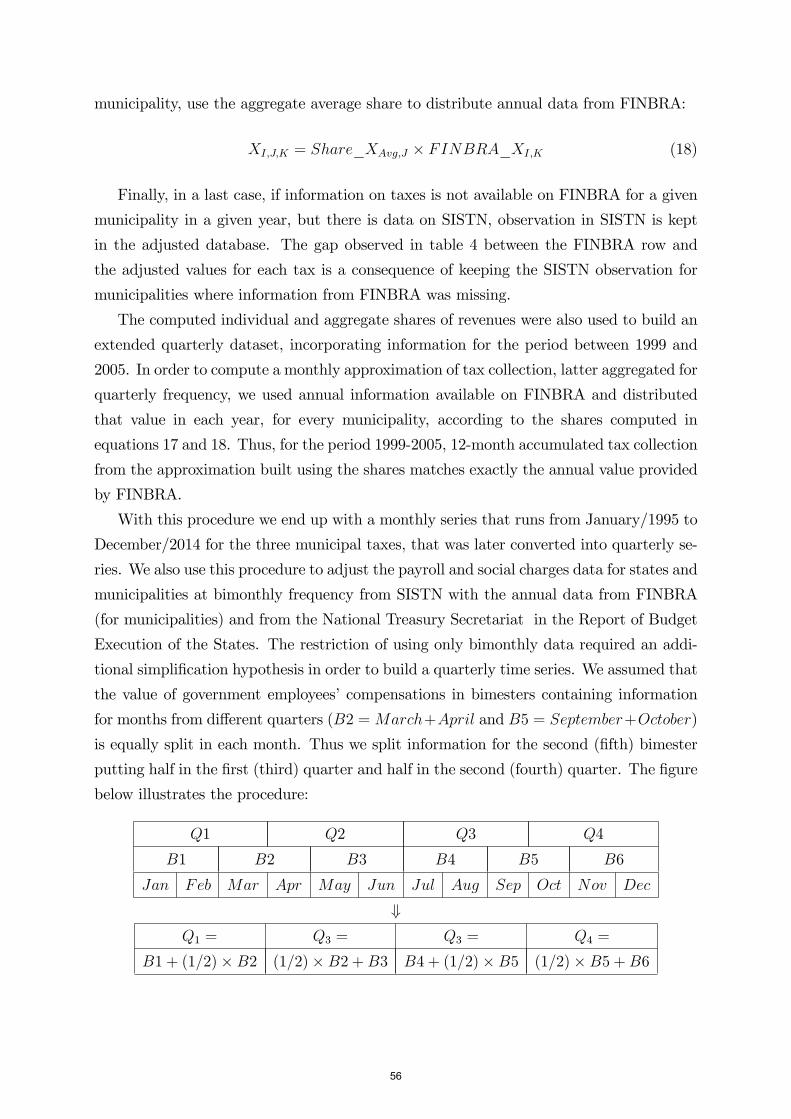
municipality, use the aggregate average share to distribute annual data from FINBRA:
XI,J,K = Share_XAvg,J × FINBRA_XI,K (18)
Finally, in a last case, if information on taxes is not available on FINBRA for a given
municipality in a given year, but there is data on SISTN, observation in SISTN is kept
in the adjusted database. The gap observed in table 4 between the FINBRA row and
the adjusted values for each tax is a consequence of keeping the SISTN observation for
municipalities where information from FINBRA was missing.
The computed individual and aggregate shares of revenues were also used to build an
extended quarterly dataset, incorporating information for the period between 1999 and
2005. In order to compute a monthly approximation of tax collection, latter aggregated for
quarterly frequency, we used annual information available on FINBRA and distributed
that value in each year, for every municipality, according to the shares computed in
equations 17 and 18. Thus, for the period 1999-2005, 12-month accumulated tax collection
from the approximation built using the shares matches exactly the annual value provided
by FINBRA.
With this procedure we end up with a monthly series that runs from January/1995 to
December/2014 for the three municipal taxes, that was later converted into quarterly se-
ries. We also use this procedure to adjust the payroll and social charges data for states and
municipalities at bimonthly frequency from SISTN with the annual data from FINBRA
(for municipalities) and from the National Treasury Secretariat in the Report of Budget
Execution of the States. The restriction of using only bimonthly data required an addi-
tional simplification hypothesis in order to build a quarterly time series. We assumed that
the value of government employees’compensations in bimesters containing information
for months from different quarters (B2 = March+April and B5 = September+October)
is equally split in each month. Thus we split information for the second (fifth) bimester
putting half in the first (third) quarter and half in the second (fourth) quarter. The figure
below illustrates the procedure:
Q1 Q2 Q3 Q4
B1 B2 B3 B4 B5 B6
Jan Feb Mar Apr May Jun Jul Aug Sep Oct Nov Dec
⇓Q1 = Q3 = Q3 = Q4 =
B1 + (1/2)×B2 (1/2)×B2 +B3 B4 + (1/2)×B5 (1/2)×B5 +B6
56