University of Calgary

PRISM: University of Calgary's Digital Repository

Graduate Studies The Vault: Electronic Theses and Dissertations

2017

Effective Data Analysis Framework for Financial

Variable Selection and Missing Data Discovery

Aghakhani, Sara

Aghakhani, S. (2017). Effective Data Analysis Framework for Financial Variable Selection and

Missing Data Discovery (Unpublished doctoral thesis). University of Calgary, Calgary, AB.

doi:10.11575/PRISM/25787

http://hdl.handle.net/11023/3790

doctoral thesis

University of Calgary graduate students retain copyright ownership and moral rights for their

thesis. You may use this material in any way that is permitted by the Copyright Act or through

licensing that has been assigned to the document. For uses that are not allowable under

copyright legislation or licensing, you are required to seek permission.

Downloaded from PRISM: https://prism.ucalgary.ca

UNIVERSITY OF CALGARY

Effective Data Analysis Framework for Financial Variable Selection and Missing Data

Discovery

by

Sara Aghakhani

A THESIS

SUBMITTED TO THE FACULTY OF GRADUATE STUDIES

IN PARTIAL FULFILMENT OF THE REQUIREMENTS FOR THE

DEGREE OF DOCTOR OF PHILOSOPHY

GRADUATE PROGRAM IN COMPUTER SCIENCE

CALGARY, ALBERTA

April, 2017

© Sara Aghakhani 2017

ii

Abstract

Quantitative evaluation of financial variables plays a foundational role in financial price modeling,

economic prediction, risk evaluation, portfolio management, etc. However, the problem suffers

from high dimensionality. Thus, financial variables should be selected in a way to reduce the

dimensionality of the financial model and make the model more efficient. In addition, it is quite

common for financial datasets to contain missing data due to a variety of limitations.

Consequently, in practical situations, it is difficult to choose the best subset of financial variables

due to the existence of missing values. The two problems are interrelated. Therefore, the central

idea in this research is to develop and examine new techniques for financial variable selection

based on estimating the missing values, while accounting for all the longitudinal and latitudinal

information.

This research proposes a novel methodology to minimize the problem associated with missing data

and find the best subset of financial variables that could be used for effective analysis. There are

two major steps; the first step concentrates on estimating missing data using Bayesian updating

and Kriging algorithms. The second step is to find the best subset of financial variables. In this

step a novel feature subset selection is proposed (LmRMR) which ranks the financial variables

and the best subset of variables is chosen by employing statistical techniques through Super

Secondary Target Correlation (SSTC) measurement. Some tests have been done to demonstrate

the applicability and effectiveness of the ideas presented in this research. In particular, the potential

application of the proposed methods in stock market trading model and stock price forecasting are

iii

studied. The experimental studies are conducted on Dow Jones Industrial Average financial

variables.

iv

Acknowledgements

This thesis could not have been accomplished without the support, encouragement and help of my

advisor, Dr. Reda Alhajj. I would like also to thank Dr. Philip Chang and Dr. Jon Rokne, my

committee members, for their time and advice throughout my studies at the University of Calgary.

My family has been a continued source of support. I would like to acknowledge the encouragement

of my parents Cheri and Jalal, my brothers Amirhossein and Shahriar and my in-laws Eli and

Saeed. Most importantly, I would like to thanks my husband Amir for his love, understanding and

support along the way.

v

Dedication

To my wonderful husband Amir

For your enduring love, support and encouragement

To my Parents Cheri and Jalal

For your guidance and unconditional love

vi

Table of Contents

Abstract ............................................................................................................................... ii Acknowledgements ............................................................................................................ iv

Dedication ............................................................................................................................v Table of Contents ............................................................................................................... vi List of Tables ..................................................................................................................... ix List of Figures and Illustrations ......................................................................................... xi List of Symbols, Abbreviations and Nomenclature ......................................................... xiv

CHAPTER 1: INTRODUCTION ........................................................................................1 1.1. Problem statement ....................................................................................................1

1.2. Solution overview .....................................................................................................3 1.3. Contributions............................................................................................................5 1.4. Organization of the Thesis ........................................................................................6

CHAPTER 2: LITERATURE REVIEW .............................................................................8

2.1. Feature Selection .......................................................................................................8 2.1.1. Filter Technique ..............................................................................................11

2.1.1.1. Chi Squared FS .....................................................................................12 2.1.1.2. Relief FS ...............................................................................................12 2.1.1.3. Correlation-Based FS ............................................................................13

2.1.1.4. Fast Correlated Based Filter .................................................................14 2.1.1.5. Minimum Redundancy Maximum Relevance (mRMR) ......................15

2.1.1.6. Uncorrelated Shrunken Centroid (USC) ...............................................17

2.1.2. Wrapper Technique ........................................................................................18

2.1.3. Embedded Method ..........................................................................................19 2.1.3.1. Ensemble classifiers ..............................................................................20

2.1.3.2. Random Forest ......................................................................................20 2.1.4. Feature Selection in Finance ..........................................................................21

2.1.4.1. Fraud Detection .....................................................................................21

2.1.4.2. Financial Distress ..................................................................................23 2.1.4.3. Financial Auditing ................................................................................25

2.1.4.4. Credit/Risk Evaluation ..........................................................................26 2.1.4.5. Stock/Portfolio Selection ......................................................................28

2.1.4.6. Price Modeling/Forecasting ..................................................................29

2.1.5. Proposed Feature Selection Technique ..........................................................33

2.2. Missing Data Analysis ............................................................................................34 2.2.1. Listwise Deletion ............................................................................................35 2.2.2. Single Imputation ...........................................................................................35

2.2.2.1. Similar Response Pattern Imputation (Hot-Deck Imputation) .............36 2.2.2.2. Mean Imputation ...................................................................................36

2.2.2.3. Regression Imputation ..........................................................................37 2.2.2.4. Composite Methods ..............................................................................37

2.2.3. Multiple Imputations (MI) ..............................................................................38 2.2.3.1. Multiple Imputation by Chained Equations (MICE) ............................39 2.2.3.2. Full Information Maximum Likelihood (FIML) ..................................39

vii

2.2.3.3. Expectation Maximization (EM) ..........................................................40 2.2.4. Tree Based Imputation ...................................................................................41 2.2.5. Neural Network Imputation ............................................................................42 2.2.6. Proposed Method ............................................................................................42

CHAPTER 3: FEATURE SELECTION ...........................................................................44 3.1. Financial Statements ...............................................................................................45 3.2. Proposed Methodology ...........................................................................................49

3.2.1. Rank Features .................................................................................................50 3.2.2. Subset Selection ..............................................................................................53

3.2.2.1. Likelihood Calculation .........................................................................54 3.2.2.2. LmRMR Algorithm ..............................................................................55

3.3. Dataset and Experimental Evaluations ...................................................................56 3.2.3.1. Dataset .........................................................................................................56 3.2.3.2. Correlation Measurements ...........................................................................58 3.2.3.3. Empirical Settings .......................................................................................59

3.2.3.4. Experimental Results and Discussion .........................................................64 3.4. Conclusions .............................................................................................................71

CHAPTER 4: MISSING DATA ANALYSIS ...................................................................73 4.1. Stationarity ..............................................................................................................74 4.2. Variogram ...............................................................................................................75

4.3. Kriging ....................................................................................................................77 4.4. Bayesian Updating ..................................................................................................79

4.5. Experimental Evaluations .......................................................................................85

4.5.1. Empirical Settings ..........................................................................................86

4.5.2. Experimental Results and Discussion ............................................................89 4.5.2.1. Synthetic Dataset ..................................................................................90

4.5.2.2. Dow Jones Industrial Average (DJIA) Dataset .....................................96 4.6. Conclusions ...........................................................................................................112

CHAPTER 5: APPLICATION IN DECISION ANALYSIS AND FORECASTING ....114

5.1. Fuzzy Inference Model .........................................................................................115 5.1.1. Fuzzy Sets & Membership Functions ...........................................................115 5.1.2. Fuzzy Relation ..............................................................................................116 5.1.3. Linguistic Variable .......................................................................................117

5.1.4. Fuzzy Reasoning ..........................................................................................118

5.1.5. Fuzzy Inferential Systems ............................................................................119

5.2. Application of Fuzzy Inference Model in Stock Trading Model ..........................122 5.2.1. Selected Financial Features in Fuzzy Recommendation Model ...................124

5.2.1.1. Share Price Rationality .......................................................................124 5.2.1.2. Profitability .........................................................................................124 5.2.1.3. Efficiency ............................................................................................126

5.2.1.4. Growth ................................................................................................126 5.2.1.5. Leverage ..............................................................................................127

5.2.2. Stock Market Trading Model (SMTM) ........................................................127

5.2.2.1. First Layer Design ..............................................................................129

viii

5.2.2.2. Final Design ........................................................................................133 5.3. Application in Price Forecasting ...........................................................................138

5.3.1. Cross Variogram ...........................................................................................140 5.3.2. Price Forecasting Potential ...........................................................................141

5.4. Conclusions ...........................................................................................................145

CHAPTER 6: CONCLUSION AND FUTURE WORK .................................................147 6.1. Summary and Conclusion .....................................................................................147 6.2. Future Work ..........................................................................................................149

ix

List of Tables

Table 3-1. List of all American companies of Dow Jones Industrial Average ............................. 58

Table 3-2. List of ranked DJIA features with non-missing intervals .......................................... 655

Table 3-3. Selected financial Features for non-missing dataset ................................................. 677

Table 3-4. LmRMR FS algorithm Evaluations ............................................................................. 70

Table 3-5. Correlation FS algorithm Evaluations ......................................................................... 70

Table 3-6. Selected financial variable using Correlation FS algorithm ........................................ 71

Table 4-1. Pearson Correlation Matrix ......................................................................................... 93

Table 4-2. Spearman Correlation Matrix ...................................................................................... 93

Table 4-3. RMSE Comparison Table............................................................................................ 95

Table 4-4. Feature matrix .............................................................................................................. 98

Table 4-5. NN Missing Data Imputation Evaluation Results using LmRMR FSS ...................... 99

Table 4-6. Selected features by LmRMR using NN imputation ................................................. 100

Table 4-7. Missing data percentage with related number of features and LmRMR SSTC value106

Table 4-8. Selected features by LmRMR using NN imputation ................................................. 107

Table 4-9. Missing data percentage with related number of features and LmRMR likelihood

value .................................................................................................................................... 109

Table 4-10. Selected features by LmRMR using OK imputation ............................................... 109

Table 4-11. Selected features by LmRMR using BU imputation ............................................... 111

Table 4-12. Missing data percentage with related number of features and LmRMR likelihood

value .................................................................................................................................... 112

Table 5-1. Financial features/ variables with related financial category .................................... 123

Table 5-2. Fuzzy values for Efficiency ....................................................................................... 134

Table 5-3. Fuzzy values for SharePriceRationality .................................................................... 134

Table 5-4. Fuzzy values for Growth ........................................................................................... 134

x

Table 5-5. Fuzzy values for Profitability .................................................................................... 134

Table 5-6. Fuzzy values for Leverage ......................................................................................... 134

Table 5-7. Defined Fuzzy rules for proposed FIM model .......................................................... 136

xi

List of Figures and Illustrations

Figure 1.1. This research outline architecture ................................................................................. 4

Figure 2.1. Feature Selection Techniques [13] ............................................................................. 10

Figure 2.2. Audited financial statement and related parties [PWC 2014] .................................... 25

Figure 3.1. Link between financial statements [187] .................................................................... 47

Figure 3.2. Cross plot of Total-Debt /Market-Cap versus Return of Stock AA UN .................... 60

Figure 3.3. Cross plot of Total-Debt (ST & LT Debt) versus Return of Stock AA UN ............... 60

Figure 3.4. Cross plot of Price-To-Book-Ratio versus Return ..................................................... 61

Figure 3.5. Cross plot of Increase_Per_Share vs Price; Left: NST of Combined Stocks

(Corr_val:0.65), Right: NST of Stocks Separately ............................................................... 63

Figure 3.6. Cross plot of Increase_Per_Share vs Price; Non-Normalized dataset (Pearson

Correlation: 0.59, Spearman Correlation: 0.63) .................................................................... 63

Figure 3.7. mRMR value for financial variables/features after ranking (horizontal axis) ............ 66

Figure 3.8. Cross plot of Stage two of LmRMR algorithm (Vertical axis: Likelihood value,

Horizontal axis: number of financial features) ..................................................................... 67

Figure 3.9. Error of ranked features (blue) versus selected subset (orange) ................................. 68

Figure 4.1. Fitted variogram computed based on different types; Spherical, exponential and

power function ...................................................................................................................... 76

Figure 4.2. Variogram characteristics ........................................................................................... 77

Figure 4.3. Latitudinal time series value for the part with missing values ................................... 79

Figure 4.4. Longitudinal time series value for the part with missing values ................................ 82

Figure 4.5. Bayesian Updating for time series data with missing values ..................................... 85

Figure 4.6. Histogram of transforming data into Normal score .................................................... 86

Figure 4.7. Cumulative Frequency of transforming data into Normal score ................................ 87

Figure 4.8. Scatterplot of two first step of variogram for ‘pretax -Increase-per-share’ variable .. 88

Figure 4.9. Variogram model ........................................................................................................ 89

xii

Figure 4.10. Primary data histogram ............................................................................................. 91

Figure 4.11. Primary and Secondary datasets ............................................................................... 91

Figure 4.12. Scatterplots of synthetic Primary and Secondary datasets ....................................... 93

Figure 4.13. Primary Data with missing values ............................................................................ 94

Figure 4.14. Estimated values with related uncertainty using Bayesian Updating ....................... 95

Figure 4.15. Estimated values with related uncertainty using Ordinary Kriging ......................... 96

Figure 4.16. Cross plot of SSTC Measurement using LmRMR algorithm on NN imputed

dataset ................................................................................................................................. 101

Figure 4.17. Variogram of financial feature ’Return on Assets’ for all DJINA stocks .............. 105

Figure 4.18. Cross plot of SSTC Measurement using LmRMR algorithm on SK imputed

dataset ................................................................................................................................. 108

Figure 4.19. Cross plot of SSTC Measurement using LmRMR algorithm on OK imputed

dataset ................................................................................................................................. 110

Figure 4.20. Estimated values with related uncertainty using Ordinary Kriging ....................... 110

Figure 5.1. Example of four classes of parameterized membership functions: Triangular (x;

15,60,70); (b) trapezoid (x; 10, 20, 70, 90); (c) Gaussian (x; 50,25); (d) bell (x; 20, 2,

50) [190] .............................................................................................................................. 116

Figure 5.2. Typical Membership Functions of term set T (Sustainable_Growth_Rate) ............. 118

Figure 5.3. Fuzzy inference system [190] [198] ......................................................................... 120

Figure 5.4. Defuzzification methods ........................................................................................... 121

Figure 5.5. fuzzy if- then rules and Fuzzy inference mechanism [190] [198] ............................ 122

Figure 5.6. The workflow of SMTM .......................................................................................... 128

Figure 5.7. Membership functions for BVPS and Sustainable growth ....................................... 129

Figure 5.8. MF surface plot for Growth ...................................................................................... 130

Figure 5.9. An example of Rule viewer for Growth ................................................................... 131

Figure 5.10. Membership functions for OIPS, CIPS and RPS ................................................... 132

Figure 5.11. SMTM Workflow ................................................................................................... 137

xiii

Figure 5.12. Benchmark model for SMTM ................................................................................ 138

Figure 5.13. Scatterplot of SS Variable and Price for Kraft Food Inc. ....................................... 139

Figure 5.14. Cross Variogram of Selected Features and Price for Kraft Food Inc. .................... 142

Figure 5.15. Cross Variogram of Super Secondary Variable and Price for Kraft Food Inc. ...... 143

Figure 5.16. Variables used for price forecasting ....................................................................... 144

xiv

List of Symbols, Abbreviations and Nomenclature

DJIA Dow Jones Industrial Average

PrMD Predicted Missing Data

PMD Prior Missing Data

LMD Likelihood Missing Data

mRMR Minimum Redundancy Maximum Relevance

RmRMR Ranked mRMR

Sel_SS Selected Sub Set

LmRMR Likelihood Minimum Redundancy Maximum

Relevance

SS Super Secondary

SSTC Super Secondary Target Correlation

SMTM Stock Market Trading Model

SPP Stock Price Prediction

CFS Correlation Feature Selection

CFSS Correlation Feature Subset Selection

FCFS Fast Correlation-based Feature Selection

USC Uncorrelated Shrunken Centroid

MDL Minimum Description Length

FCBF Fast Correlated-Based Filter

SU Symmetrical Uncertainty

USC Uncorrelated Shrunken Centroid

SC Shrunken Centroid

FFR Fraudulent Financial Reporting

BPNN Back Propagation Neural Network

RC Rough Classifier

NFC Neuro-Fuzzy Classifier

NST Normal Score Transform

PCA Principal Component Analysis

CAPM Capital Asset Pricing Model

APT Arbitrage Price Theory

ROI Return on Investment

BVPS Book Value Per Share

SGR Sustainable Growth Rate

OIPS Operating-Income-Per-share

CIPS Continuing-Income-Per-Share

RPS Revenue-Per-Share

SP Stock Price

SPD Stock Price Difference

OK Ordinary kriging

SK Simple Kriging

BU Bayesian Updating

MCAR Missing Completely At Random

MAR Missing At Random

NMAR Not Missing At Random

xv

NN Nearest Neighbor

AI Artificial Intelligence

ICA Independent Component Analysis

FBS Forward Backward Selection

RBF Radial Basis Function

MI Multiple Imputations

MICE Multiple Imputation by Chained Equations

FIML Full Information Maximum Likelihood

EM Expectation Maximization

BLUE Best Linear Unbiased Estimate

RMSE Root Mean Square Error

FIM Fuzzy Inference Model

MF Membership Function

COA Centroid Of Area

LMC Linear Model of Coregionalization

1

CHAPTER 1: INTRODUCTION

1.1. Problem statement

In recent years, several technologies produce large datasets characterized by enormous number of

features/variables. In practice, it is neither feasible nor necessary to consider all input

features/variables to approximate the underlying function between input and output of the system.

The main reason is existence of multiple less relevant variables affecting the learning process.

Also, the integration of all variables may result in high computational cost and increases the

processing time. Therefore, feature/variable selection techniques are implemented to reduce

computational time and cost, improve the learning performance and provide a better understanding

of the target dataset. That is why they have gained importance in many disciplines such as finance.

Financial variables can be used in different areas of finance such as fraud detection, financial

distress management, credit or risk evaluation, financial price modeling and portfolio evaluation,

among others [68] – [140]. In practice, there exists too many financial variables while their

integration in prospective models would result in inefficiencies. Therefore, traditionally most of

the previous studies focus on a few ‘known’ financial features/variables and their combinations.

This would limit exploring the full space of experimental studies and may result in deviation from

the optimal solutions for the target system. Therefore, selecting the best subset of financial

variables that reduces the dimensionality is essential, removes irrelevant data, and improves the

efficiency of the target model.

2

Another problem which occurs frequently in various application domains, including the area of

financial data analysis is the existence of missing values. Often, as soon as we want to reduce the

dimensionality of a system, we are faced with a difficult task of selecting financial variables based

on incomplete or missing data. Incomplete or missing data occur when there is not available data

for a specific financial variable or a part of it. While it is quite easy to recognize such problem, it

is hard to characterize the consequent problems and find a comprehensive solution.

It is not uncommon that in many financial research areas, missing data are ignored or a simple

imputation method such as mean imputation is used which may result in a bias. In fact, studying

and considering the mutual relationships between the financial variables that contain missing

values, and all the other variables as well as the predictability of the missing values through

statistical analysis of existing values for the same financial variable are of primary importance.

The primary objectives of this research are (1) to provide a novel solution (LmRMR) for the

problem of variable selection in the financial domain; (2) to develop a comprehensive and

comparative solution to predict the missing values in financial features leading to an improved

feature selection workflow; and (3) to investigate the value of the selected features in two financial

evaluation workflows, namely stock trading recommendations and price forecasting. The novel

feature selection technique (LmRMR) couples financial feature selection and missing values

analysis, where the best subset of financial features is selected while accounting for both time

series correlations (latitudinal data) and the cross-correlations between the financial variables

(longitudinal data). We believe that there has not been any other research which studies both

aspects of financial feature selections and missing data evaluations together.

3

1.2. Solution overview

With the growth of the financial domain and financial features/variables associated with stocks, it

has become impractical to determine financial variables based on pure financial means. Recently,

data mining and machine learning techniques have been used in the area of finance mainly to

uncover the relationship among financial and economic variables and also study their predictive

power.

The approach of selecting features/variables that maximizes the information content with respect

to the price/return of asset is of primary importance. It is quite common that many of the features

are redundant in the context of others or irrelevant to the task at hand. Learning in this situation

raises important issues such as over-fitting with respect to irrelevant features, and the

computational burden of processing of many similar features which have redundant information.

Also, it is quite common for features to contain missing values due to a variety of limitations.

Given the large number of financial variables with missing intervals, it becomes more difficult to

choose a subset of financial variables that are strong indicators of the system. In this research we

present a novel approach for financial feature subset selection employing missing data analysis.

4

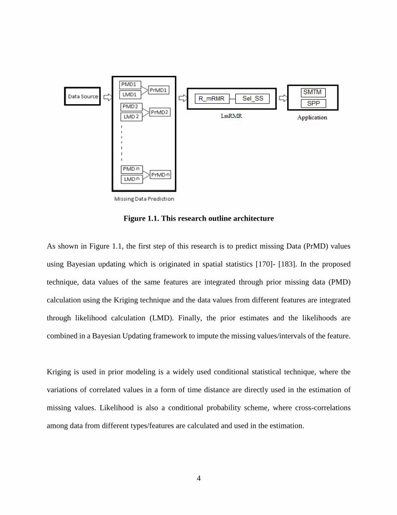
Figure 1.1. This research outline architecture

As shown in Figure 1.1, the first step of this research is to predict missing Data (PrMD) values

using Bayesian updating which is originated in spatial statistics [170]- [183]. In the proposed

technique, data values of the same features are integrated through prior missing data (PMD)

calculation using the Kriging technique and the data values from different features are integrated

through likelihood calculation (LMD). Finally, the prior estimates and the likelihoods are

combined in a Bayesian Updating framework to impute the missing values/intervals of the feature.

Kriging is used in prior modeling is a widely used conditional statistical technique, where the

variations of correlated values in a form of time distance are directly used in the estimation of

missing values. Likelihood is also a conditional probability scheme, where cross-correlations

among data from different types/features are calculated and used in the estimation.

5

In this research, a novel feature selection technique is also presented for selecting the best subset

of financial features/variables. In this technique, first the financial variables are ranked based on

minimum redundancy and maximum relevance of the features (R_mRMR) [32]. Then, in a forward

pass the best subset of features are selected (Sel_SS) using super-secondary-variable-target-

correlation (SSTC) measurement. The proposed feature selection technique is proved to be quite

efficient as the total number of feature subset evaluations does not exceed the total number of

features.

The final step of this research is to study the utilization of financial features/variables in practical

applications. There are several financial domains that utilize financial variables. In this thesis, two

financial evaluations workflows are considered; a fuzzy Stock Market Trading Model (SMTM)

and Stock Price Prediction (SPP). In practice, there are number of technical variables/indicators

that traders consider to find the market trend and make their decisions. SMTM tries to mimic the

human thinking suggesting an intelligent approach for a satisfactory recommendation as when to

buy, sell or hold the stocks. SPP studies the value of the previously selected financial features in

future stock price prediction. The effectiveness of present data in predicting future prices is studied

using a comprehensive analysis on lag and price modeling. With the use of cross-variograms of

the selected features, the Super Secondary (SS) variable and the stock prices, we study how the

reliability in the future price predictions erodes and uncertainty increases as the number of lags

increases.

1.3. Contributions

6

In the context of financial feature selection, this research aims at developing a novel, integrated

and optimal technique (Likelihood Minimum Redundancy Maximum Relevance or LmRMR) that

maximizes the utilization of information content of all the relevant financial features while

ensuring the efficiency of the system through (1) adaptation of an objective workflow, (2)

integration of features with relevant information content, even if they include partial missing

intervals, and (3) avoiding integration of features with redundant information content.

The LmRMR ensures objectivity and repeatability through implementation of a step-wise ranking

and multivariate statistical analysis process that stores and analyzes all the correlations and cross-

correlations between various variables. The stepwise approach also ensures and enhances the

optimality of the system by avoiding the data redundancy. The novel longitudinal-latitudinal

missing data analysis ensures the maximization of integration of all the features with the highest

level of information content.

The research also demonstrates the potential application of selected financial variables in two

practical financial evaluation applications: (1) development of a fuzzy stock trading model to

provide recommendation on when to buy/hold/sell; and (2) applicability in multi-quarter

forecasting and price modeling through lag analysis.

1.4. Organization of the Thesis

This thesis is organized into six chapters. Chapter 2 comprises of a comprehensive literature

review. Chapter 3 represents a detailed description of the proposed methodology in financial

7

variable/feature selection. Chapter 4 presents missing data analysis in financial domain and further

aims at demonstrating the resulting improvements in feature selection. Chapter 5 demonstrates

effectiveness of the selected financial variables and their application in a stock trading modeling

and multi-quarter price forecasting. Finally, chapter 6 summarizes and concludes this research and

suggests future research directions.

8

CHAPTER 2: LITERATURE REVIEW

With the growth of the financial domain and financial features/variables associated with stocks, it

has become impractical to determine financial variables based on pure financial means. In reality,

there are many financial variables with applications in different areas of financial modeling such

as credit and risk evaluations, portfolio managements and fraud detection.

Recently, data mining and machine learning techniques have been used in the area of finance

mainly to uncover the relation between financial and economic variables and their predictive

power. The approach for selecting variables becomes more important when there are lots of

variables with unknown relationships among them. However, given the large number of financial

variables that partially include missing intervals, it becomes more difficult to choose a subset of

financial variables that are strong indicators of the system.

This chapter is divided in two sections. In the first section main feature selections techniques; filter,

wrapper and embedded; as well as application of it in finance are discussed. In the second section,

some of the known missing data analysis techniques are discussed and then we discuss our

proposed method to solve these issues. The detailed proposal for each of these areas of research

are explained in details in the next chapters.

2.1. Feature Selection

9

Feature selection has been the focus of many researchers within statistics, pattern recognition and

machine learning areas and it has applications in gene expression array analysis, chemistry, text

processing of internet documents, finance, astronomy, remote sensing, etc. [1].

Feature selection is the process of selecting a subset of attributes in a set of data which are most

relevant to the predictive modelling problem. Usually a feature is relevant if it contains some

information about the target. Features are classified into three disjoint categories using an ideal

Bayes classifier: strongly relevant, weakly relevant, and irrelevant features as discussed in [2]. A

feature is considered to be strongly relevant when by its removal the prediction accuracy of the

classifier is deteriorated. A weakly relevant feature is not strongly relevant and the performance

of the ideal Bayes classifier is worse with not inclusion of that feature. Finally, a feature is defined

as irrelevant if it is neither strongly nor weakly relevant.

Also, two features are redundant to each other if their values are completely correlated [3], but it

might not be so easy to determine feature redundancy when a feature is correlated with a set of

features. According to [3], a feature is redundant and hence should be removed if it is weakly

relevant and has a Markov blanket [4] within the current set of features.

Advantages of applying feature selection techniques can be summarized to possibility of using

simpler models to reduce training and utilization times, better data visualization and

understanding, data reduction and limiting storage requirements, reducing costs and removing the

curse of dimensionality to improve prediction performance. Some of the areas which feature

10

selection has gained interest are in disciplines such as clustering [5, 6], regression [7, 8] and

classification [9, 10], in both supervised and unsupervised ways.

Overall, feature selection methods can be divided into individual evaluations and subset

evaluations [3]. Individual evaluation which is classifier-independent, assesses individual features

by assigning them weights according to their degrees of relevance. Subset evaluation which is

Classifier-dependent technique, produces candidate feature subsets using a search strategy. Then,

each candidate subset is evaluated by an evaluation measure and compared with the previous best

one with respect to this measure.

Both of these approaches have their own advantage and disadvantages. The shortcoming of the

individual evaluation technique is in incapability of removing redundant features. On the other

hand, the subset evaluation approach can handle feature redundancy with feature relevance but

these methods can suffer from problem of searching through all feature subsets required in the

subset generation step. In literature there are three categories of feature selection techniques: filter,

wrapper and embedded methods [12].

Figure 2.1. Feature Selection Techniques [13]

11

There exists several algorithms in the literature using the described methods or new methods

combining these approaches. Although, there does not exist “the best method” [13] and all the

proposed models try to find a good approach for their specific problem. One of the main focus of

these researches is to optimize accuracy with respect to minimizing training time and allocated

memory.

2.1.1. Filter Technique

Filter methods apply a statistical measure based on relevancy or separation of feature set and

then assign a score to each feature [14]. The measurements may vary from correlation

measurements, mutual information and inter/intra class distances to probabilistic independency

measurements. The assigned score represents the relation strength of the feature set and class

label. After assigning the score to the features, the features are ranked and either selected or

removed from the dataset.

The advantage of filter model is in its low computational cost and good generalization ability

[15]. However, it considers feature independently and might consider redundant features as they

do not consider the relationships between variables. There are two types of filter methods;

univariate and multivariate techniques. Univariate selection methods have some restrictions and

may lead to less accurate classifiers by not taking into account feature to feature interactions.

Therefore, multivariate methods are more popular due to the consideration of these relations or

correlations between features.

12

The application of filter methods can vary from simple techniques such as Chi squared test,

information gain [16], Relief [17] to multivariate techniques for simple bivariate interactions

[18] and even more advanced solutions exploring higher order interactions, such as correlation-

based feature selection (CFS) [19], Fast correlation-based feature selection (FCFS) [20] and

several variants of the Markov blanket filter method [21]- [23]. The Minimum Redundancy-

Maximum Relevance (mRMR) [24] and Uncorrelated Shrunken Centroid (USC) [25] algorithms

are two other solid multivariate filter procedures.

2.1.1.1. Chi Squared FS

Chi Square is one of the popular feature selection methods. It is originally used in statistics as a

test to represent the independence of two events. In Feature selection it tests the independent

occurrence of a term and a class. The terms are ranked with respect to the following quantity.

𝑋2(𝐷, 𝑡, 𝑐) = ∑ ∑(𝑁𝑒𝑡𝑒𝑐−𝐸𝑒𝑡𝑒𝑐)2

𝐸𝑒𝑡𝑒𝑐𝑒𝑐∈{1,0}𝑒𝑡∈{1,0} (1.1)

Where 𝑒𝑡 show whether term t exists in the document (𝑒𝑡 = 1) and 𝑒𝑐 represents the existence of

the document in the class (𝑒𝑐 = 1). N is the observed frequency in D and E is expected frequency.

As 𝑋2 is a measurement which represents the deviation of expected count E and observed count

N, the high scores on 𝑋2 indicate that the null hypothesis of independence should be rejected.

2.1.1.2. Relief FS

13

The main idea behind the original Relief algorithm [17] is to estimate the quality of attributes based

on how well their values distinguish between instances that are near to each other. Suppose that Ri

is a randomly selected instance, Relief searches for its two nearest neighbors: one from the same

class, called nearest hit H, and the other from the different class, called nearest miss M. Then, it

updates the quality estimate for all the features, depending on the values for xi, M, and H. If

instances Ri and H have different values of the target attribute, then the attribute separates two

instances with the same class which is not desirable and the quality estimation is decreased. If

instances Ri and M have different values of the attribute, then the attribute separates two instances

with different class values which is desirable so the quality estimation is increased. The original

RELIEF can deal with discrete and continuous features but is limited to two-class problems and

cannot deal with incomplete data.

An extension, Relief [26], not only deals with multiclass problems but it is also capable of dealing

with incomplete and noisy data. Relief was subsequently adapted for continuous class or regression

problems, resulting in the RRelief algorithm [27]. The Relief family of methods can be applied in

all situations with low bias. It also includes interaction among features and with their local

dependencies.

2.1.1.3. Correlation-Based FS

Correlation based Feature Selection (CFS) is a simple filter algorithm which ranks feature subsets

based on a correlation-based heuristic evaluation function [28]. The heuristic function evaluates

the usefulness of individual features to predict the class label considering the level of

14

intercorrelation among the features. The following equation is heuristic merit of a feature

subset S consisting of k features.

𝑀𝑒𝑟𝑖𝑡𝑆 =𝑘𝑟𝑐𝑓̅̅ ̅̅ ̅

√𝑘+𝑘(𝑘−1)𝑟𝑓𝑓̅̅ ̅̅ ̅ (1.2)

Where 𝑟𝑐𝑓̅̅ ̅̅ is the average of feature-class correlation and 𝑟𝑓𝑓̅̅ ̅̅ is the average feature-feature

interactions.

The variable correlations can be Pearson or Spearman correlation or different measurements of

relatedness such as Minimum Description Length (MDL) or symmetric uncertainty and relief as it

is described in [19].

The bias of the evaluation function is toward subsets that contain features that are highly correlated

with the class and uncorrelated with each other. Irrelevant features are ignored as they have low

correlation with the class and redundant features are screened out as they have high correlation

with one or more of the remaining features. The acceptance of a feature will depend on the extent

to which it predicts classes in areas of the instance space not already predicted by other features.

2.1.1.4. Fast Correlated Based Filter

The Fast Correlated-Based Filter (FCBF) method [29] is based on Symmetrical Uncertainty (SU)

[30], which is defined as the ratio between the information gain and the entropy of two features, x

and y to calculate dependencies of features. The formula is defined as follows.

𝑆𝑈(𝑥, 𝑦) = 2𝐼𝐺(𝑥|𝑦)

(𝐻(𝑥)+𝐻(𝑦)) (1.3)

15

𝐼𝐺(𝑥|𝑦) = 𝐻(𝑦) + 𝐻(𝑥) − 𝐻(𝑥, 𝑦) (1.4)

Where H(x) and H(x, y) are the entropy and joint entropy and IG is information gain. .

SU compensates for information gain’s bias toward features with more values and normalizes its

values to the range [0, 1]. The value “1” indicates that knowledge of the value of either x or y

completely predicts the value of the other and the value “0” indicating that x and y are independent.

Entropy-based measures require nominal features, but they can be applied to measure correlations

between continuous features as well, if the values are discretized properly in advance [31].

The FCBF method was designed for high-dimensionality data and has been shown to be effective

in removing both irrelevant and redundant features. However, it fails to take into consideration the

interaction between features.

2.1.1.5. Minimum Redundancy Maximum Relevance (mRMR)

In the process of feature selection, it is important to choose features that are relevant for prediction,

and are not redundant [24]. Relevancy means similarity between feature vector and target vector

and determines how well a variable discriminates between target classes. Some of the relevancy

measurements are mutual information [24] [32], correlation coefficient, Fit Criterion [33],

distance/similarity scores to select features [24].

16

The issue of redundancy and relevance for feature selection has been discussed in many papers

[34] [35]. Redundancy means similarity between features themselves. The redundancy between

two features X1, X2 and given class targets Y can be written as following formula.

𝑅𝑒𝑑(𝑋1, 𝑋2, 𝑌) =1

𝑑∑ ∆([𝑋1|𝑌 = 𝑐𝑖], [𝑋2|𝑌 = 𝑐𝑖])𝑑

𝑖=1 (1.5)

where [X1|Y = ci] denotes the distribution of feature 1, given class i and ∆, one of the distributional

similarity measures that will follow in this subsubsection. There are different redundancy criteria

which can be used such as correlation coefficient, mutual information, Redundancy Fit Criterion

[33].

mRMR algorithm penalize a feature's relevancy by its redundancy in the presence of the other

selected features and integrates relevance and redundancy information of each variable into a

single scoring mechanism [10] [7].

Formula 1.6 represents the relevance of feature set S for class c using mutual information criteria

𝐼(𝑓𝑖; 𝑐).

𝐷(𝑆, 𝑐) =1

|𝑆|∑ 𝐼(𝑓𝑖; 𝑐)𝑓𝑖∈𝑆 (1.6)

Also, redundancy can be explained by following formula:

𝑅(𝑆) =1

|𝑆|2∑ 𝐼(𝑓𝑖; 𝑓𝑗)𝑓𝑖,𝑓𝑗∈𝑆 (1.7)

Where 𝐼(𝑓𝑖; 𝑓𝑗) represents the mutual information value between two features fi and fj. Finally, the

mRMR is measured by below function.

𝑚𝑅𝑀𝑅 = max𝑆

[1

|𝑆|∑ 𝐼(𝑓𝑖; 𝑐)𝑓𝑖∈𝑆 −

1

|𝑆|2∑ 𝐼(𝑓𝑖; 𝑓𝑗)𝑓𝑖,𝑓𝑗∈𝑆 ] (1.8)

17

The following formula is based on formula 1.8 where xi=1 indicates presence and xi=0 indicates

absence of the feature fi in the global feature set.

𝑚𝑅𝑀𝑅 = max𝑥∈{0,1}𝑛

[∑ 𝑐𝑖𝑥𝑖

𝑛𝑖=1

∑ 𝑥𝑖𝑛𝑖=1

−∑ 𝑎𝑖𝑗𝑥𝑖𝑥𝑗

𝑛𝑖,𝑗=1

(∑ 𝑥𝑖𝑛𝑖=1 )2 ] (1.9)

Where 𝑐𝑖 = 𝐼(𝑓𝑖; 𝑐) and 𝑎𝑖𝑗 = 𝐼(𝑓𝑖; 𝑓𝑗). mRMR algorithm is more efficient comparing to the

theoretically optimal max-dependency selection, and can also produce a feature set with little

redundancy.

2.1.1.6. Uncorrelated Shrunken Centroid (USC)

The main idea behind USC algorithm is driven from Shrunken Centroid (CS) algorithm [36] which

was originally used in gene expression profile. The CS algorithm computes centroid of each class

which is done by averaging gene expression for each gene in each class and then divided by within

class standard deviation for that gene. After comparing the class centroids, the class whose centroid

is closest is considered as predicted class for that sample. The main difference of this method with

standard nearest centroid is in shrinking the class centroids toward the overall centroid for all

classes by a threshold amount. After shrinkage of centroids, the new sample is classified by nearest

centroid rule and using shrunken class centroids. Using this method makes classifier more accurate

and removes noisy genes as well as eliminating a gene from prediction rule if it is shrunk to zero

for all classes. The USC algorithm advances this method by removing highly correlated genes

which result to improvement of classification accuracy within a smaller set of genes.

18

2.1.2. Wrapper Technique

Wrapper Method evaluates the selection of a subset of features. Here the feature subset selection

is done by using an induction algorithm and it searches the space of feature subsets by using

training/validation accuracy of a particular classifier as the measure of utility for a candidate

subset. Feature subset that gives best performance is selected for final use. Though, if there exist

n features in total, there are 2^n possible searching subsets. This exhaustive search is impractical,

therefore most of wrapper methods use heuristic approach to narrow down search space. The

search strategy can be deterministic which does not involve randomness in the search procedure

and searching can be based on pre-specified schema which usually results in returning similar

subsets; or stochastic which involves randomizing the search scheme and therefore is not sensitive

to change in dataset [37]. Some of the searching methods which has been used in wrapper methods

are greedy forward/backward selection [38], swarm optimization [39], neighborhood search [40],

best first, simulated annealing and genetic algorithm [34]. The most common approach is

backward elimination which starts the search with all features and eliminate them one by one using

a feature scoring model until the optimal subset is selected. One of heuristic search methods is

Greedy search strategy which seems to be particularly computationally advantageous and robust

against overfitting. It comes in two format of forward selection and backward elimination. In

forward selection, variables are gradually added into larger subsets, whereas in backward

elimination it starts with the set of all variables and progressively eliminates the least suitable

variables.

19

Although wrapper methods can detect the possible interactions between variables, they can be

computationally expensive as a result of calling the learning algorithm for every subset of features

[41]. Also, there is the risk of overfitting if the number of observation is insufficient. However, the

interaction with the classifier in wrapper methods, tends to give better performance results than

filters methods.

2.1.3. Embedded Method

Embedded methods select features by the training process which is similar to wrapper methods.

They introduce additional constraints into the optimization of a predictive algorithm; such as a

regression algorithm; which leads to a lower complexity model. Although, they are mainly specific

to given learning machines, they still can capture dependencies at a lower computational cost than

wrappers. Embedded methods use a combined search model space of feature subsets and

hypotheses in order to find optimal feature subset is built into the classifier construction.

Embedded methods have gained more popularity among the research communities in recent years.

Examples of this method can be using random forests in an embedded feature evaluation [120]

[121], using weights of each feature as a measurement of relevance for each of them in linear

classifiers such as logistic regression [44] and SVM [45]. Recursive partitioning methods for

decision tress such as ID3, CART and C4.5 are examples of this method. Other examples of

embedded methods are LASSO [47], Elastic Net applied in microarray gene analysis [46].

20

2.1.3.1. Ensemble classifiers

Recently in the area of machine learning the concept of ensemble classifier has gained more

popularity. The main idea behind ensemble methods is to combine a set of models, where each of

them can solve the similar original task, in order to find a more accurate global model with better

estimation. Ensemble classifier is a technique of combining weaker learners in order to find a

stronger learner. Ensemble classifiers can vary from simple averaging of individually trained

neural network to combination of many of decision trees to build random forest [48] or even

improving weak classifiers to build a stronger classifier. Therefore, ensemble classifier is a

supervised learning algorithm itself. Although it might seem that the flexibility in ensemble

classifiers may lead to overfitting in training data, it is shown in practice that they can even reduce

this problem. Two of the reputed models which fulfill this concern are bagging [49] and random

forest [48].

2.1.3.2. Random Forest

Random forest is a ensemble classifier [50]-[52] which starts with a decision tree which

corresponds to the wealker learner. An input data in a decision tree can traverse the tree in a top

down format in order to bucketed into smaller sets. Random forest classifier uses this concept and

takes it to the next level by combing tree type classifiers where each classifier is trained on a

bootstrapped sample of original data and searches only cross randomly selected subset of the input

variables in order to determine a split for each node. In terms of classification, each tree in random

21

forest casts as a unit vote for most popular class in input x. Then, by majority votes of trees the

output of random forest for an unknown sample is decided.

Random forest technique is quite fast and is considered as one of the most accurate classifiers.

They can deal with unbalanced an incomplete data. Also, the computational complexity of this

algorith is reduced as the number of features for each split is bounded by random number of

features used for decision in each split. The computational time is 𝑐𝑇√𝑀𝑁𝑙𝑜𝑔(𝑁); where c is

constant, T is number of trees in ensemble, M is number of feaures and N is number of training

samples in dataset.

Random forests can handle high dimensional data by building large number of trees in ensemble

using a subset of features but they need fair amount of memory and they are not able to predict

beyond range of training data in case of regression techniques.

2.1.4. Feature Selection in Finance

In the previous section, main feature selection techniques have been discussed. Now in this section,

we are going to discuss different areas where feature selection is applied in finance.

2.1.4.1. Fraud Detection

Financial Fraud is increasing every year and it is becoming more sophisticated and difficult to be

identified and prevented as most of fraud instances are not the same. The process of fraud

investigation is also complex and time consuming. In 2009, PC global economic crime survey

22

suggested that around thirty percent of companies worldwide have reported being victims of fraud

[53].

There has been vast number of data mining techniques which tried to target this issue. Many of

these techniques tried to employ financial features/variables to build a more robust system.

Unfortunately, there has not been many intelligent approaches which consider feature selection in

an intelligent way.

Among these few techniques, in [54] authors considered ratios in financial statements as important

element in fraud detection. They have divided the financial ratios into five categories: Profitability

for return of sales and return of investments, solvency ratio, liquidity ratio, activity ratio and

structure ratio for asset and property. [55] utilizes the secondary data from audited financial

statements of the public listed firms in Malaysia. They categorized financial features into

independent, dependent and control variables. The seven firm’s financial ratios are considered,

which are financial leverage, profitability, asset composition, liquidity, capital turnover, size and

also overall financial condition. Then used a regression model to determine ratios related to

Fraudulent Financial Reporting (FFR).

Traditional practice of auditing financial statement is not effective anymore as auditors can become

overburdened with the too many company’s task of fraud detection. Based on [56], financial

statements are a company's basic documents to reflect its financial status. That’s why in [57]

consider financial statements such as Balance sheet, income statement, cash flow statement and

statement of retained earnings as the basis of their work. Then the financial ratios used in these

23

statements are categorized into liquidity, safety, profitability and efficiency and then authors

selected few ratios from each category. In literature, most of the researchers have used z-score

[58]to evaluate the financial health of companies which mostly is without consideration of any

intelligent technique to choose the selected financial variables and it seems that it is again based

on the experiments. Here the authors observed that some of the financial variables/features are

more important for the prediction purpose whereas some contributed negatively towards the

classification accuracies of the classifiers they used.

Therefore, they applied a statistical technique using the t-statistic [59] in order to rank features and

identify the most significant financial items that could detect the presence of financial statement

fraud. A feature with high t-statistic value indicates that the feature can highly discriminate

between the samples of fraudulent and non-fraudulent companies.

2.1.4.2. Financial Distress

Financial distress represents financial health of enterprises and individuals. Bankruptcy prediction

and credit scoring are two major issues in financial distress prediction [60] [61] where various

statistical and machine learning techniques have been employed to develop financial prediction

for them. In literature, bankruptcy prediction and credit scoring are mostly treated as two

predefined binary classifications; good and bad risk classes [62].

The pioneer study of this work using univariate statistic of financial ratios was originally done by

Beaver [63] and later by Altman [64]. Altman employed multiple discriminant analysis (MDA)

24

and financial ratios to predict financially distressed firms. However, the usage of MDA relies on

some restriction such as assumption of linear reparability, multivariate normality and

independence of the predictive variables. Unfortunately, these assumptions are violated by many

of the financial ratios. Recently more advanced techniques have been used to solve prediction

problem.

Techniques such as decision tree [65] [66], fuzzy set theory [67], case-based reasoning [68], [69],

genetic algorithm [70] [71], support vector machine [72] [73], several kinds of neural networks

such as Back Propagation Neural Network (BPNN) [74]-[79], PNN (probabilistic neural networks)

[80], Fuzzy neural network [81], SOM (selforganizing map) [77] [82], fuzzy rule based classifier

[83] and radial basis function [84] have been proposed as prediction techniques. Also, hybrid

systems were proposed for bankruptcy prediction such as Neuro-Fuzzy Classifier (NFC) and

Rough Classifier (RC) [85]. In [86] human judgement was considered as another factor besides

intelligent techniques for bank failure prediction.

In most of the proposed techniques, there is no generally agreed upon financial feature which can

be used directly. Therefore, feature selection is considered as pre-processing step for building

prediction models. The performance of the classifier after feature selection can be improved in

comparison to the performance of the same classifier before feature selection [87].

Both Filter and wrapper techniques which has been discussed in previous sections, have been

applied for feature selection in the area of bankruptcy prediction and credit scoring. Filter feature

selection techniques such as Principal Component Analysis (PCA), discriminant analysis, t-testing

25

and regression [88] - [93]. Wrapper methods which have been used such as Bayesian classifier,

prediction swarm optimization, fuzzy models, rough set and genetic algorithm [94] – [97].

2.1.4.3. Financial Auditing

Financial audit is an enhanced evaluation of an organization’s financial report and reporting

processes which evaluates the financial statements of companies. Financial statements provide

information about financial performance of companies. This information is used by a wide range

of stakeholders; e.g. investors; in their decision making.

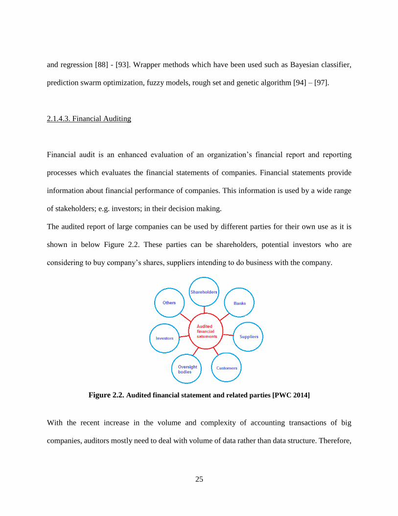
The audited report of large companies can be used by different parties for their own use as it is

shown in below Figure 2.2. These parties can be shareholders, potential investors who are

considering to buy company’s shares, suppliers intending to do business with the company.

Figure 2.2. Audited financial statement and related parties [PWC 2014]

With the recent increase in the volume and complexity of accounting transactions of big

companies, auditors mostly need to deal with volume of data rather than data structure. Therefore,

26

data mining and feature selection techniques can be applied and can help the process of extraction

the necessary information out of the large amount of data.

2.1.4.4. Credit/Risk Evaluation

There are many types of financial risks such as credit risk, asset backed risk, liquidity risk, foreign

investment risk, equity risk and currency risk. In most of the cases the default risk is credit risk.

Credit risk is associated with people who borrowed money and are not able to pay back the

borrowed money. Asset backed risk is related with the risk when asset-backed securities become

volatile considering if the underlying securities also change in value. The risks under asset-backed

risk include prepayment risk and interest rate risk. Liquidity risk refers to securities and assets that

cannot be purchased or sold fast enough to cut losses in a volatile market. Changes in prices

because of market differences, natural calamities, political changes or economic conflicts may lead

to volatile foreign investment conditions and foreign investment risk. Equity risk is caused by the

volatile price changes of shares of stock. Investors holding foreign currencies are exposed to

currency risk because of factors such as interest rate changes and monetary policy changes.

There are two types of risk associated with a company; systematic and unsystematic. Systematic

risk is the market-related risk which affects the whole market and not a specific stock or industry

whereas unsystematic risk affects a very specific group of securities or an individual

security. Unsystematic risk can be minimized through diversification. Although, the main concern

of investors is the systematic risk. The systematic risk is often determined by the Capital Asset

Pricing Model (CAPM) theory [98] (Sharpe, 1963, 1964; Litner, 1965). CAPM represents asset’s

27

non-diversifiable risk (market risk) by quantity beta (β) in the financial industry, as well as

the expected return of the market and the expected return of a risk-free asset. As CAPM is used in

price modeling as well, it is explained in the next section in details.

To measure the systematic risk of a system, traditional measures have focused on balance sheet

information such as non-performing loan ratios, earnings and profitability, liquidity and capital

adequacy ratios [99]. There are studies using balance sheet in different industries. In hospitality

section, [100] studied financial ratios in 58 quick service and full service restaurants from 1999 to

2003 and found Return on Investment (ROI) is related to Beta. In quick service restaurants, debt

to equity ratio also has a positive relation with Beta. [101] analyzed the airline industry from 1997

to 2002 and found that debt leverage (total debt to total assets), profitability (return on assets), firm

size (total assets) and EBIT growth are the financial variables that are significant predictors of

Beta. Debt leverage and firm size turned out to be positively related to systematic risk Beta. [102]

evaluated the current ratio, leverage ratio (total liabilities to total assets), asset turnover, and profit

margin of 35 casino firms and found that only asset turnover was significant and negatively

correlated with Beta. The effect of few financial ratios are represented on loan contracts which are

informative of credit risk of borrower or contract characteristics [103].

The balance sheet information is only available on a relatively low-frequency (typically quarterly)

basis and often with a significant lag. Therefore, more recent techniques consider information from

financial markets as well. For example, [104] suggest to employing liquid equity market data with

a modern portfolio credit risk technology.

28

The process of risk evaluation involve huge volumes of raw data and different financial feature.

Although, different techniques are proposed for financial risk evaluation decisions, still it needs

powerful tools/techniques for preprocessing the data and feature selection [105]. There are few

techniques which have considered preprocessing of feature selection. As an example [106]

proposed a feature selection method based on "Blurring" measure [107] and study its effects on

the classification performance of induced decision trees [108]. Also, results are compared with

feature selection with the Patrick-Fisher probabilistic distance measure and random feature

selection.

2.1.4.5. Stock/Portfolio Selection

Stock selection and portfolio analysis are challenging tasks for investors through their decision

making process. There are many assets available in the financial market [109] and it is crucial to

select assets with potential to outperform the market in the next period of quarters or years.

The modern portfolio theory was first suggested by Markowitz back in 1952 [110]. In this theory

he mentioned the link between risk and return and demonstrated that portfolio risk came from the

covariance of assets making up the portfolio. His theory targeted to identify the portfolio with the

highest return at each level of risk. This model optimizes the weights of stock in the portfolio with

the intention of minimizing the variance of the portfolio for a given value of the average return of

stocks. Overall, the model demonstrates that achieving a higher expected return requires taking on

more risk and therefore investors are faced with a trade-off between risk and expected return.

29

It is difficult to decide which selection or combination of finanial variables/features the investor

should focus on beyond expected returns. In most of empirical literature on portfolio, few

predeterminded choice of variables are discussed. Based on [111], investors try to analyze

companies on the basis of discounted cash flow valuation/features and try to find the undervalued

companies. [109] used SVM model for stock selection. They group financial indicators into eight

categories: Return on Capital, Profitability, Leverage, Investment, Growth, Short term Liquidity,

Return on Investment, Risk. Although, they did not mention which financial factors/features have

been selected. Both ANN and SVM have been used for stock selection. [112] use both of them

for Turkey stock analysis using few technical and fundamental features. Unfortunately, they did

not either consider preprocessing step of feature selection.

Overall, it was detected in the stock selection literature review that since the stocks being traded

in the stock exchange are from the different industries, the need for common fundamental analysis

variables for all of the stocks is a difficult task. Also, the financial parameters utilized in researches

are based on expertise and are limited to several variables. Therefore, the need for a preprocessing

feature selection techniques is necessary. The next section on price forecasting is interrelated to

this section as well.

2.1.4.6. Price Modeling/Forecasting

It has been widely accepted that predicting stock returns and stock price movement is not an easy

task since many market factors are involved and their structural relationships mostly are not linear.

30

Also, the existance of market volatility and complex events such as business cycles, monitory

policies, interest rates, political situations affect the stock market.

There has been extensive studies by both academics as well as practitioners for many years to

uncover the predictive relationships of numerous financial and economic variables and hidden

information in stock market data. It is shown that financial variables can be used for building a

return model of assets or portfolios and even predicting economic activities [113] [114].

One of the traditional asset pricing models is CAPM (Capital Asset Price modeling) which is used

for pricing an individual security or portfolio. CAPM is built on the Markowitz mean–variance-

efficiency model in which risk-averse investors care only about expected returns and the variance

of returns or related risk [115]. It states that the return of a stock depends on the time series stock

price and how the stock price follows the market as a whole. CAPM does not include the effect of

other financial factors/variables.

)()()(2

RFRRRFRRFRRCov

RFRRE MiM

M

iMi

(1.10)

In above CAPM formula MR is return of market, i is sensitivity of asset with market return and

iR is return of a stock.

Another price modeling is Arbitrage Price Theory (APT) . It considers the price modeling as a

linear function of the combination of financial factors/variables and is based on multifactor

modeling. Here the sensitivity with each factor is measured as a factor coefficient.

tonibbbRER ikikiiii 1,...)( 2211 (1.11)

31

In the above, the effect of the factor k on the asset i’s return is shown by ikb , k is representative of

factor k and i is the error term related to asset i’s return.

There are number of traditional statistical studies in literature based on APT which try to find the

best combination of financial factors in order to find a better price modeling or compare the effect

of each factor on price modeling. One of these studies is the three factor model introduced by Fama

and French [116]. It is based on fundamental factors/variables and time series regression model.

This model was developed to capture lack of variations in asset returns which CAPM

misses. Another famous multi-factor price model which was developed by Chen, Roll and Ross

[117], use six macro-economic variables to explain security returns. In this model, they tried to

remove the dependency among variables and studied the changes in the residuals.

The above approaches are traditional models which mostly assume that data has no correlation

during time. This assumption is not always true as the data can be taken in a period of a week or

less. In this way the dimensionality increases as well. More recent techniques have used data

mining and Artificial Intelligence (AI) for stock price/return forecasting, stock exchange modelin

and few to uncover the relation of financial features and nonlinear stock data.

One of the popular methods which have been used to deal with this problem is Principal

Component Analysis (PCA) [118]. It gained much attention as it tries to reduce the dimensionality

of data using covariance matrix and keeping all the variables. Also, Independent Component

Analysis (ICA) tried to find a pattern of variables by reducing the dimensionality of data with the

32

help of an independency algorithm such as distance measuring [119][120]. These methods find a

mapping between the original feature spaces to a lower dimensional feature space. However, they

could not solve the problem of selecting a subset of variables. In [121] the authors tried to use a

classification technique called GRASP (Greedy randomized Adaptive Search Procedure) for

financial ratios to find the best subset of ratios. They used greedy random search to find a global

solution and divide it to subgroups based on local search to choose the final subset of variables.

Another work is done in [122] which have used an optimization method based on minimizing the

noise or variance of selected set of variables. The set of variable are chosen based Forward

Backward Selection (FBS), finding nearest neighbor of variables to final output and then select

the group of variables based on minimum distance. Also, the authors in [123] used Genetic

algorithm as a financial variables selection in order to train a SVM model for predicting financial

distress. There are also intelligent approaches that build a unique pattern which leads to prediction

of movement in time series data. Radial Basis Function (RBF) [124], Neural network [125]-[127],

auto-regressions [128] [129] and SVM [130]-[132] are common machine learning/pattern

recognition algorithms used for stock price prediction. In the literature, there are techniques which

have used feature selection as a preprocesin pat of their price modeling. Techniques such as PCA

[133]-[135], GA [136][137], stepwise regresson [138], Information gain [139] ad Discrt Wavelet

Transforation (DWT) [140].

The problem is that in traditional financial variable selection methods used for price modeling and

even in new studies, they mainly consider a set of of known financial variables and then chose the

variables which are uncorrelated or have the minimum degree of correlation. The problem arises

when there are hundreds of financial variables and there can be many different combinations of

33

these variables. Selecting the relevant variables helps us in understanding the data, its visualization

and improving the performance of the model. On the other hand, considering all variables is

impossible as it causes the storage shortage and curse of dimensionality. Therefore, finding an

intelligent approach which tries to choose the best subset of financial variables and ranking them

is quite important.

2.1.5. Proposed Feature Selection Technique

Trading in stock market is a popular subject. The investment opportunities has been expanded for

both individuals as well as institutional investors due to diversity in financial indexes and stocks.

The problem is stock market trend is very complex and is influenced by various factors. Finding

effective factors in the stock market can be an asset to investor’s choices and can be achieved by

feature selection techniques.

In this thesis, we proposed a new technique for financial feature selction. The seleced features can

be used in any application used in selecting stocks to build a portfolio which outperforms the

market, predicting price movement, evaluating the finacial health of companies, credit risk

evaluaion and finally easier financial auditing.

The proposed method, evaluates and ranks features based on the relevance and redundancy of

features using mRMR algorithm. Then, a unified framework is considered for subset selection by

conditional likelihood [141] calculation using a super secondary variable [142][179]. More details

are given in Chapter four.

34

2.2. Missing Data Analysis

There exists a large literature for dealing with missing data. All researchers have faced the problem

of missing data at some point in their work. The existence of missing data can be caused by many

different reasons such as malfunction of measurement/recording equipment, refusal or inability of

respondent to answer some questions or failure of respondent to complete sections of questionnaire

because of lack of time or interest [143] [144]. Further, the data may become available

incrementally. Given the expense of collecting data, it is not possible to start over or to wait until

a guaranteed method is developed for gathering information [145]. Therefore, the decision of

handling the data with incomplete information becomes more essential.

Missing data can be divided in three different classes [143]. First is the case when data is

considered to be Missing Completely At Random (MCAR), where the probability of an instance

with missing value is independent of the values of that variable and also other variables in the

dataset. Often, this is not a considerable assumption in the literature [146]. The second class is

related to Missing At Random assumption (MAR). In this case, the probability of an instance with

missing value for an attribute depends on other variable-types in the dataset while the values of

the same variable-type with missing data are not considered. The main importance of this

assumption is that other variables’ information can be used for imputing the missing data. The last

class is Not Missing At Random (NMAR). Here the probability of an instance with missing data

for an attribute is dependent on values of the same variable and can also depends on other variables.

There are several missing data analysis approaches for MAR missing data calculation. NMAR

35

missing data needs special methods for estimating the missing values while MCAR missing data

is not common and can be removed from the analysis [146]. In the next sections some of the more

prominent missing data analysis techniques in literature and financial domain are discussed.

2.2.1. Listwise Deletion

Among conventional methods for handling missing data, Listwise deletion is the least problematic

and easiest way to deal with missing data. This technique removes the class with missing data from

the analysis. According to [146] around 94% of the articles published between 1993 and1997 in

social sciences applied this approach to overcome the missing value problem. Also among 1057

articles published in five financial journals between 1995 and 1998, there exist 175 articles with

missing data problem where 142 articles have used Listwise deletion; this is more that 78% of

them. The main reason that it gained attention is its easiness. Although, the main problem in

Listwise deletion is that it may result in the loss of anywhere between twenty percent and up to

half of the data [147]. More importantly, in the instances where missing data is not MCAR, the

outcome of the Listwise deletion for missing data will most likely result in a bias.

2.2.2. Single Imputation

Single imputation replaces the missing value with a single imputed value. The imputed values are

means or draws from a predictive distribution of the missing values. A technique is required to

find imputed values based on observed data. Some of these techniques are summarized in

following.

36

2.2.2.1. Similar Response Pattern Imputation (Hot-Deck Imputation)

The term “hot deck” comes from the use of punch cards for data storage. The deck is “hot” because

it was currently being processed, as opposed to the “cold deck” using pre-processed data as the

donors. In this method, the values of missing data are assigned by values of a respondent which

has similar answers on a set of variables similar to the respondent with missing data. This method

is preferred to the Listwise deletion method but still lead to a complete dataset which may lead to

wrong inference and bias [148].

2.2.2.2. Mean Imputation

Another common solution for missing data values is to replace the missing value with the mean of

corresponding variable. In this way, the variance of the variable will reduce dramatically as it uses

a similar value for all the missing values in the desired interval. However, in some datasets the

mean of the values is not meaningful. An example of this can be gender where the average of

variable is not meaningful. Beside, this approach does not make a proper use of information

contained in other variables and the variance of imputed data underestimate the real variance [149].

)1(

)1(ˆ 2

n

Sn kk (1.12)

As shown in above equation, the real variance is underestimated by a factor of )1/()1( nnk

where kn is observed entities, n is number of overall entities and kS is estimated variance of

37

observed data. To solve this issue, more recent techniques apply a modification to mean imputation

using nearest neighborhood technique [150] [151].

2.2.2.3. Regression Imputation

Regression imputation uses regression equations to predict incomplete variables from complete

variables. This method assumes that the imputed values fall directly on a regression line with a

nonzero slope. Stochastic regression imputation reduces the bias in the model by adding residual

term for each predicted score. This residual term is normally distributed with a mean of zero and

a variance similar to the residual variance of the predictor regression outcome.

The problem is that after estimating the values and finding complete data, it lacks variability as

the imputed values fall on the regression surface [148]. In other words, this approach does not

report the associated uncertainties in its original form.

2.2.2.4. Composite Methods

The combination of ideas from different methods can create composite methods. An example can

be combination of regression imputation and hot deck technique where after calculation the

predicted mean from a regression, a residual is added randomly chosen from the empirical

residuals [152] [153].

38

As mentioned in previous section, an important limitation of the single imputation methods is the

underestimation of the variance of estimates. Even if unbiased estimates can be constructed, single

imputation methods ignore the reduced variability of the predicted values and treats the imputed

values as fixed. Therefore, Multiple Imputation is considered which can handle the issue of

imputed values and its associated uncertainty in a more proper way.

2.2.3. Multiple Imputations (MI)

Multiple Imputation was originally designed for complex surveys to create public datasets. The

main idea behind this technique is to provide valid inference when reason of missing is not known

and also different missing analysis models are used by different users. In this approach missing

values for any variable are predicted using existing values from other variables.

There are three main steps for Multiple Imputation technique [154]. The first step is imputation

step. It creates several complete datasets which each of them can be analyzed differently. Here

missing values are replaced by values drawn from distribution specifically modeled for each

missing entry. The imputed values are different for each imputed dataset. The magnitude of these

differences represent the uncertainty of final imputed value. The second step is analysis step where

imputed dataset parameters are estimated using the technique used to complete the data. The last

step is pooling the results where analysis results are combined for one final result. This includes

both uncertainty in data and missing values. Under appropriate condition, the estimation output is

unbiased with correct statistical properties.

39

The below equation is with respect to parameter b, variance bs and mean b [155] [156] where there

is m imputed datasets and inference is drawn with respect to final variance and mean.

mb

m

i

im

m

i

i

m

i

i sm

ssbbm

ssm

sbm

b )1

1(,))(1

1,

1(,

1 2

111

(1.13)

2.2.3.1. Multiple Imputation by Chained Equations (MICE)

A popular approach for multiple imputation implementation is Multiple Imputation by Chained

Equations (MICE) [157] [158]. In this method, the missing values of Y1 are filled by imputed

value from a regression of the observed elements of Y1 on (Y2, Y3, etc.), the missing values of

Y2 are filled by imputed value from a regression of the observed elements of Y2 on (Y1, Y3, etc.)

and the missing values of Y3 are filled by imputed value from a regression of the observed

elements of Y3 on (Y1, Y2, etc.). This method is quite popular because of its flexibility where

each variable can be modeled by using a model tailored to its distribution and ability to impute a

subset of data. It also can handle different variable types (continuous, binary and categorical).

However, it is possible that this imputation method produces logically inconsistent imputation

models [159] and specifying the model for all variables with missing data is not an easy task when

the number of variables increase a lot.

2.2.3.2. Full Information Maximum Likelihood (FIML)

This approach is another well-known approach for estimation of missing data values [156] [160].

FIML uses all information of observed data, assuming multivariate Gaussianity and maximizes the

40

likelihood of the model with the given observed data. It includes the variance and mean of the

missing values of a variable with respect to the observed values of the other variables. It is effective

when the data is MAR and the modeling of the data is longitudinal [148]. FIML tries to minimize

the following equation:

)()(log)( ,,,

1

,,

1

, mimimmi

N

i

mimi

N

i

mmi yyC

(1.14)

where mmi, and mi, are the covariance matrix and mean vector for the observed row and columns

related to variable i and miy , is the observed portion of data for variable i..

2.2.3.3. Expectation Maximization (EM)

EM model is an iterative procedure using maximum likelihood estimates in parametric model

[156]. It repeats two steps of E which is Expectation step and calculates the conditional expectation

of the complete-data log likelihood given the observed data and parameter estimates such as the

mean vector and covariance matrix of multivariate normal distribution. The Maximizing step (M)

finds the parameter estimates to maximize the data log likelihood from E step. These two iterate

until the iterations converged. The equation below is for multivariate normal data with G groups

with missing pattern.

G

g

obsgobs YLogLYLLog1

)()( (1.15)

)()(2

1log

2)( gigg

ig

gigg

g

obsg yyn

YLogL (1.16)

41

2.2.4. Tree Based Imputation

There are two types of tree-based models used for missing data imputation: Classification tree and

regression tree models [153]. In categorical tree the response variable is categorical where in

regression tree the response variable is numerical. Common splitting rules in regression model

are least square and least absolute deviation. The measure of homogeneity for tree splits in

classification model can be F-test, Chi-square test, Likelihood ratio test, Gini Index or Twoing rule

[161].

In order to find the imputed value using tree based models, first both response variable and

variables without missing are considered. Then, a tree either classification or regression based

model is built based on distribution of the response variable in terms of values for complete

variables, finally an imputation approach is considered to find imputed values for missing data

[162].

CART [163] and C4.5 [143] [164] are two well-known tree-based algorithms which can handle

missing data. C4.5 uses information gain ratio to partition instances with the help of known

attributes. A probabilistic approach is used to partition missing values; if an instance has known

value, the probability or weight of an instance belongs to a subset Ti is one and other subsets are

zero. Meanwhile, if an instance has unknown value, it assigns to all partitions having different

weights or probability related to each one of them [143] [165]. CART [166] searches all possible

values and variables to find best split of two with maximum homogeneity and repeats it for each

42

fragments. The difference between these two is that C4.5 uses fractional cases whereas CART uses

so-called surrogate splits [153].

2.2.5. Neural Network Imputation

Neural networks are more sophisticated version of regression models for handling missing data

[167]. In this model use feed forward and back propagation. The model can be formulated as

following where kx , ty , x

N , y

N and h

N are independent variables, dependent variables, number of

independent variables, number of dependent variables and number of units in hidden layer and

parameter a, b, c and d are estimated.

yk

N

k

jkk

N

i

ijtt Nixcafdbfyxh

,...,1))*(*(11

(1.17)

The model is trained by back propagation to minimize the error associated with predicted value in

comparison to observed one. Then, best weights for the model is considered and imputed value is

calculated. The advantage of imputation using neural network is that the model can be considered

as a set of non-parametric and non-linear model. The downside of this approach is being

computational expensive.

2.2.6. Proposed Method

There are many techniques which tried to solve missing data values. MI, FIML and EMP are

common advanced Prediction models for estimating the missing values. Commonly in many

43

prediction models, the correlations between the variables/features are used for building the model.

It can also find the most frequent value among the k nearest neighbors or the mean of the k nearest

neighbors as substitution for the missing value [168] [165]. The main shortcoming of most of

approaches is that they are only effective when the data is MCAR or MAR, as they consider

attributes independent. As an alternative, we may also consider the class of Bayesian methods that

have been used in different areas such as supervised learning and spatial statistics.

In this research the concept of Bayesian updating is proposed to be adapted as a solution for the

treatment of missing values. The beauty of this approach is in considering both latitudinal relation

among the features and longitudinal relation of each feature in time series data. This approach

considered data as NMAR which makes it differentiated from the previously proposed

methodologies. This approach commonly consists of three steps: prior estimation using Kriging

considering longitudinal data, likelihood calculation considering latitudinal data, and posterior

calculation by combining the two with the help of Bayesian updating. These methods are explained

in the next section.

44

CHAPTER 3: FEATURE SELECTION

Selection of a subset of features/variables that maximizes the information content with respect to

the price/return of asset is of primary importance. It is quite common that many of the features are

redundant in the context of others or irrelevant to the task at hand. Learning in this situation raises

important issues such as over-fitting with respect to irrelevant features, and the computational

burden of processing many similar features which have redundant information. Therefore, it is

important to automatically identify meaningful smaller subsets of these variables. There are many

suggested heuristics models attempting to maximize feature relevancy and minimize redundancy

[186]. However, few of these models are associated with a solid theoretical foundation.

In this work we present a combinational technique for financial feature/variable selection by

ranking features first and then finding the best subset and uncertainty related to it using Super

Secondary (SS) evaluation. First, the well-known measurement formula of mRMR is considered

for ranking financial features using correlation similarity measurement and the concept of

minimum redundancy and maximum relevance of financial features and return/price of assets.

Then, the best subset of the ranked features is chosen using Super Secondary Target Correlation

(SSTC) measurement. In this step, likelihood calculations account for the mutual correlations

between the variables as well as between the variables and the return/price of assets and result in

a unique Super-Secondary (SS) value that has a correlation with the target price/return on asset

(SSTC). This value can be maximized by adding and removing variables from the subset. The

higher the SS’s correlation with the return on asset is, the lower mutual correlations of the variables

will be, and the higher the correlations of the variables with the return on asset will be.

45

In the following sections, we present the proposed methodology and experimental evaluations.

3.1. Financial Statements

Financial statements represent information concerning companies’ financial performance and

status [63]. Analyzing financial statements information which is also known as quantitative

analysis, is one of the most important elements in fundamental analysis evaluation as they can

show whether company is in crisis or is running smoothly. Also, financial statements are the basis

of investment decisions making for the banks and individuals. All of listed companies need to

publish their financial statements every quarter and every year. Financial statements include

balance sheet, income statement, cash flow statement and statement of change in equity. Brief

descriptions of these categories are described in following with Figure 3.1. representing the link

between financial statements.

Balance sheet: Balance sheet, also known as statement of financial position, represents the

financial position of an entity at a particular date, usually end of fiscal year. It has three parts:

Assets: Assets are items that a company owns or controls and expect that they will yield

future financial benefits. There are two types of assets; long-term and current. Example of

current assets can be cash, inventory or accounts receivable which can be converted to cash

within a year or operating cycle; whichever is longer. Long-term assets bring benefits

beyond a year. Examples of long-term assets can be buildings, machinery and equipment

which can be amortized as they are used.

46

Liabilities: It is the amount that a company owes and have to settle in future. Liabilities

can be either current liability or long-term liability. Current liabilities such as demand loans

need to be settle within a year or one operating cycle whichever is longer whereas long-

term liabilities are ongoing commitments such as loans and mortgages.

Shareholder’s equity: It represents the amount of capital after its assets are used to pay off

the business liability or in another word it is difference between assets and liabilities which

is known as net assets.

Income statement: Income statement, also known as profit and loss statement, represent

company’s income, expenses and profit or loss during a specific period typically annually,

quarterly or monthly. Income statement has two parts of income and expense which presents net

income or loss of the company.

Cash flow statement: A cash flow statement shows incoming and outgoing funds during a

particular period. It informs investors and creditors about where the company receives the cash

and how and where it is spent and can be helpful in determining the short term viability of a

company and specially in paying bills. The cash flow movement can be classified into three

groups:

Operating activities: It presents the movement of cash from primary revenue generating

activities of a company.

Investing activities: It presents movement of cash from investments; sale and purchase of

assets.

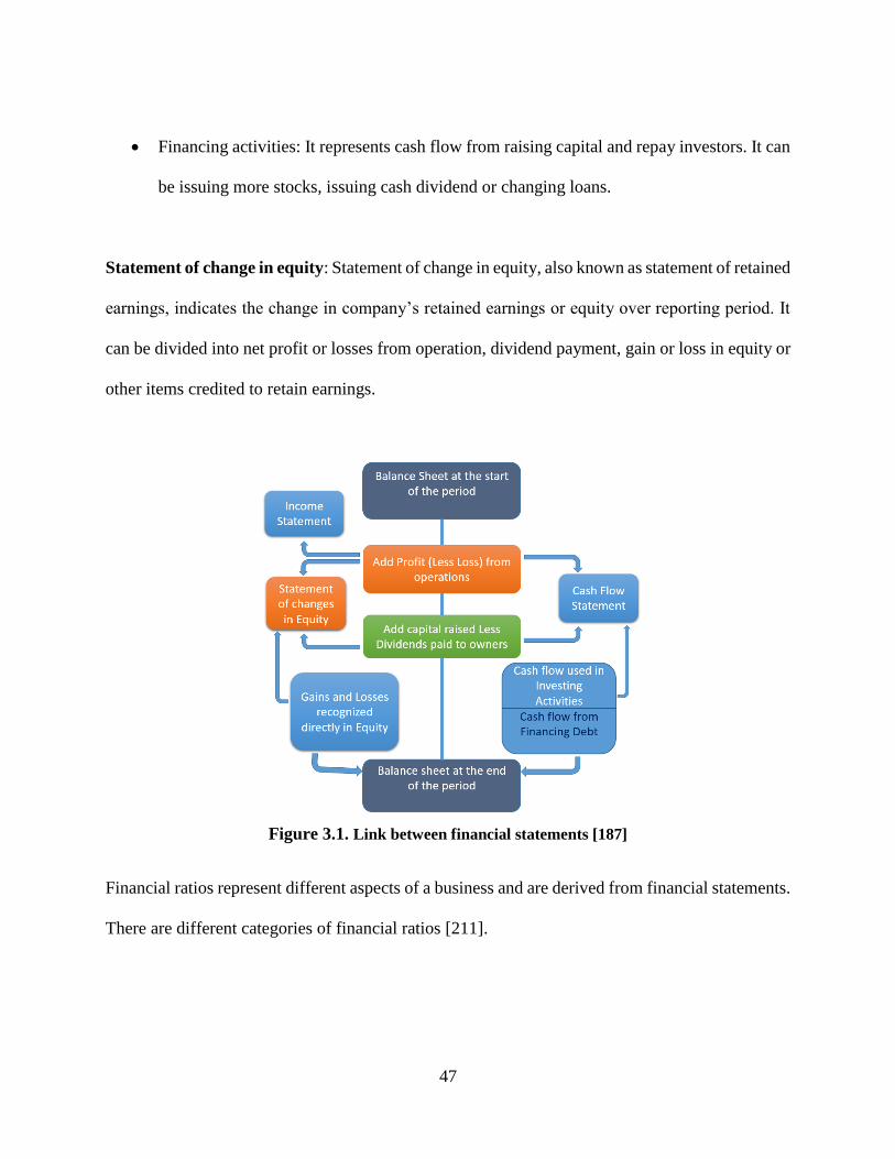
47

Financing activities: It represents cash flow from raising capital and repay investors. It can

be issuing more stocks, issuing cash dividend or changing loans.

Statement of change in equity: Statement of change in equity, also known as statement of retained

earnings, indicates the change in company’s retained earnings or equity over reporting period. It

can be divided into net profit or losses from operation, dividend payment, gain or loss in equity or

other items credited to retain earnings.

Figure 3.1. Link between financial statements [187]

Financial ratios represent different aspects of a business and are derived from financial statements.

There are different categories of financial ratios [211].

48

Liquidity or Solvency ratios: They indicate financial stability of a company. It measures

company’s debt with respect to its assets and liquidity or in another word it measures company’s

availability of cash after liquidation. A company with many debts may not be able to manage its

cash flow if business condition decline. Ratios higher than one means that company has more

assets than liability and in reality it is not common. This ratio category can be improved by paying

down debts, buying inventory when necessary or converting short term debts to long term. Some

of the important ratios of this category are cash ratio, quick ratio and current ratio.

Profitability ratio: It indicates current rate of return of a company/business or its ability to earn

profit for its owners. It is part of performance measurement of a company. Some of important

profitability ratios are gross profit margin, net profit margin, earning per share and return on assets.

Activity or Efficiency ratio: It measures measure how fast a company can convert non-cash assets

to cash assets. This ratio indicates the company’s current financial standing as it runs. Common

efficiency ratios are inventory turnover and receivable turn over. The former is ratio of cost of

goods sold to inventory. High value for this ratio means that company is successful in converting

its inventory to sales. Receivable turnover represents outstanding credit sale and is ratio of credit

sales to account receivable.

Leverage ratio: This ratio represents the company’s ability to pay off its long term debt and

leverage inherit in business. Also, it indicates the company’s capital structure and its related risk.

When it comes to setting the debt, this ratio measures company’s current financial standing similar

to liquidity ratio. Examples of leverage ratios can be debt-to-equity ratio or interest coverage.

49

Market ratio: This ratio evaluates the response of investors to company’s stock and look at the

company from outside of it with its shareholders and relationships with shareholders and its market

activity. Managers and investors are interested in market ratios in order to evaluate the firm's stock.

Example of this ratio can be market-to-book ratio and price-to-earnings ratio.

3.2. Proposed Methodology

As explained in previous chapter, financial variables are the main tools for fraud detection

including credit card fraud, firm fraud and money laundering, bankruptcy prediction, stock market

analysis and price forecasting, portfolio modeling and financial auditing dealing with voluminous

data and complicated data structure. Therefore, feature selection techniques play important role in

pre-processing step of data in financial domain. These techniques are used to extract and uncover

hidden truths behind large quantities of financial data, reduce complexity and expenses.

Features can be divided into three different classes: relevant, redundant and irrelevant. Relevant

features contain information data which can be helpful in solving the prediction problem. Our

information will be incomplete if we don’t include those features and also the prediction will be

poor. On the other hand, redundant features contain information which has already known from

other sources or features. Finally, irrelevant features which do not contain useful information about

the problem in hand. If these three categories of features be recognized, the task of feature selection

is an easy task where we can select relevant features and ignore the rest.

50

The main purpose of this section is to develop an efficient unsupervised algorithm to determine

optimal number of relevant financial features. Our approach considers to find increase relevancy

to the primary variable and decrease redundancy of features. The proposed methodology includes

two sections. In the first section, we find and rank candidate features using mRMR selection

algorithm. The next section, finds the best subset of features using Super Secondary Target

Correlation (SSTC) measurement where a Super-Secondary (SS) variable is built based on the

outcome of the likelihood calculation of financial features. Then, the correlation coefficient

between SS variable and Target price/ return (SSTC) is computed . Using this technique, the

relevant financial features are considered and redundant and irrelevant features are removed from

the subset.

3.2.1. Rank Features

In the first discussion for ranking variables, we should find a measurement to show the

relevancy/irrelevancy of feature and target variable/class and redundancy of features. In literature

there are different measurement techniques but the most common ones are correlation coefficient

and mutual information. Correlation coefficient use covariance in its measurement. Formula 3.1

and 3.2 show covariance and mutual information calculations.

xyyPxPyxPYXCov

yyPxxPxyyxPYEXEXYEYXCov

yx

yxyx

)]().(),([),(

))().()((),()()()(),(

,

,

(3.1)

51

yx

yPxPyxPyxPyPxP

yxPEYXI

,

))()(ln),()(ln,()()(

),(ln),( (3.2)

Although mutual information is not associated with linearity and covariance can be zero if

variables are stochastically dependent, the benefit of covariance is that it can be calculated directly

from data samples while we need to know the probability distribution of data for mutual

information calculation. Not knowing the distribution of data can lead to a lot of uncertainty. In

the case of financial variables, especially the quarterly data with limited number of data points, it

would be a stronger statement if we use correlation techniques. Considering the nonlinearity of the

nature of these types of data, we compare Pearson correlation and Spearman correlation

measurements applied on both non-normalized and normalized financial dataset. To normalized

the dataset, Normal Score Transform is used. As it is discussed in the section of empirical settings,

using Pearson correlation on normalized dataset is more efficient. Although, it is very similar to

ranked based Spearman technique with close results.

After deciding on the measurement technique, we look through an efficient technique to minimize

the redundancy of selected features while increasing the relevancy to the target feature/class.

Minimum Redundancy Maximum Relevance (mRMR) [24] is one of the most successful

techniques which has been used recently in the literature. In this technique, the selected features

have maximum dependency for first-order feature. In the original mRMR feature selection

technique, the best features are selected using two stages; first candidate features are selected using

mRMR incremental selection method. Then in second stage, a wrapper model such as Naïve Bayes

classifier is used to find the best feature subset and minimize classifier error using two forward

52

and backward selection model. In the forward selection the features are added to the subset in an

incremental way with consideration that the classification error does not increase where the

backward selection considers all features and then tries to remove redundant features at a time with

consideration that the classification error improves.

In this thesis we use only the mRMR measurement for feature evaluation and ranking. The mRMR

measurement is calculated for all features and then, features are ranked based on the outcoming

value in descending order. The relevance of financial features to the target feature is calculated

using formula 3.3 where ),( TFCorr iis the correlation of feature i and target feature

},...,,{ 21 NTTTT and S is the number of data in features set S. The relevance of a feature can be

calculated by correlation coefficient of the feature and target feature which in our case is

price/return. It is obvious if a feature is strongly differentiated from target price/return, the

correlation is close to zero. Here we try to maximize the relevancy and target features with more

similarity to the target feature.

SF

i

i

TFCorrS

MaximumD ),(1

(3.3)

Also, we target features with less redundancy to each other. The measurement of redundancy is

shown in 3.4 where ),( ji FFCorr represents the correlation between two feature i and j.

SFF

ji

ji

FFCorrS

MinimumR,

2),(

1 (3.4)

And finally the two formula in above are combined as a single function to minimize the redundancy

and maximize the relevance of a feature as discussed in mRMR and presented in equation 3.5. The

53

task is to find the associated mRMR value for each feature and then rank the features based on this

measurement value.

),(

1),(

12 jiiCorrD FFCorr

SabsTFCorr

SabsmRMR (3.5)

Unlike first stage of mRMR, we did not consider the maximum function and incremental search.

The main purpose of using mRMR is to rank features using its measurement formula. Then, we

build an unsupervised feature subset selection model which is explained in the next section.

3.2.2. Subset Selection

In feature selection, it is recognized that the knowing only good individual features is not the key

to have a good performance model. It is important to find the best subset of features. That is why

in the second stage of our feature selection we used a forward feature selection using SSTC

measurement. To find this measurement value, first a Secondary (SS) variable is built based on

the outcome of the likelihood calculation of financial features. Then, the correlation coefficient of

SS and target price/return (SSTC) is calculated as a single measurement value.

In the forward selection, a subset of m features out of N feature is selected in an incremental

manner. The first subset starts with highest ranked feature denoted by Z1. Then it adds a feature

from {Sn-Z1} set at each step. If the updated subset has a higher SSTC value, then, the feature is

considered in the subset. But if the added feature does not improve SSTC or depredates it, it will

54

be removed from the subset. This incremental selection repeats until there is no further

improvement in the SSTC value where )()1( kSSTCkSSTC

Below we have explained the likelihood calculation used for SS calculation as well as our proposed

algorithm.

3.2.2.1. Likelihood Calculation

Dependent data structures exist in many application areas. In the analysis of financial data,

dependency exists because of the similarity in the way variables are defined or because of the

repeated measurements made on the variables over a period of time. Likelihood calculation is

based on the similarity between groups of variables to the Secondary data while reducing the

dependency among the variables themselves. The selected secondary data should be available for

all features },,...,1),({ Aumjux j [179]. The defined secondary variable in this paper is

‘Return’. A linear model is used in order to find the mean of this distribution.

m

j

jiL uxuy1

)()( (3.6)

The weights of the above formula (3.6) are calculated based on the correlation of the financial

variables with each other. Based on equation (3.7), higher weights are assigned to the variables

which have higher correlations with the final return.

mkm

j

turnkkjj ,...,1,1

Re,,

(3.7)

55

Where m is the number of financial variables, kj , is the correlation between variable j and k and

finally, turnk Re, is the correlation between variable k and the Return. After finding the likelihood

mean, the likelihood variance can be calculated as follows.

m

j

turnjjL u1

Re,

2 1)( (3.8)

3.2.2.2. LmRMR Algorithm

As mentioned above, likelihood calculations are applied to build the Super-Secondary (SS)

variable. Then, the correlation coefficients between the SS variable and the final return/price is

computed as SSTC measurement. Below shows the proposed algorithm for financial features

subset selection.

L_mRMR Algorithm

Input: )Pr/Re,,...,,,( 321 iceturnFFFFS N // All Financial features and Return

// a predefined threshold

Output: BestS //Selected subset

1 For i= 1 to N do

2 Calculate CorrDmRMR for iF

3 End for

4 Order ),...,,,( 321 NFFFFS in descending value for CorrDmRMR result listDS

5 jF = Get first element of ( listDS )

6 Max = SSTC (1)

7 For j=2 to N do

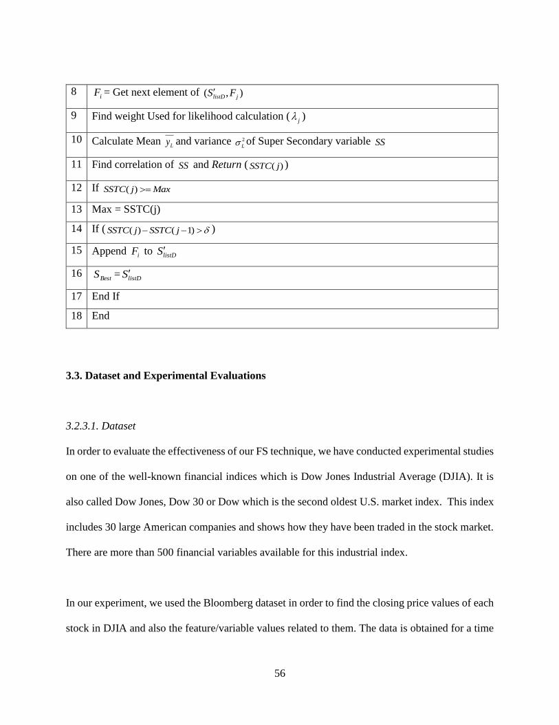
56

8 iF = Get next element of ),( jlistD FS

9 Find weight Used for likelihood calculation ( j )

10 Calculate Mean Ly and variance 2

L of Super Secondary variable SS

11 Find correlation of SS and Return ( )( jSSTC )

12 If MaxjSSTC )(

13 Max = SSTC(j)

14 If ( )1()( jSSTCjSSTC )

15 Append iF to listDS

16 BestS = listDS

17 End If

18 End

3.3. Dataset and Experimental Evaluations

3.2.3.1. Dataset

In order to evaluate the effectiveness of our FS technique, we have conducted experimental studies

on one of the well-known financial indices which is Dow Jones Industrial Average (DJIA). It is

also called Dow Jones, Dow 30 or Dow which is the second oldest U.S. market index. This index

includes 30 large American companies and shows how they have been traded in the stock market.

There are more than 500 financial variables available for this industrial index.

In our experiment, we used the Bloomberg dataset in order to find the closing price values of each

stock in DJIA and also the feature/variable values related to them. The data is obtained for a time

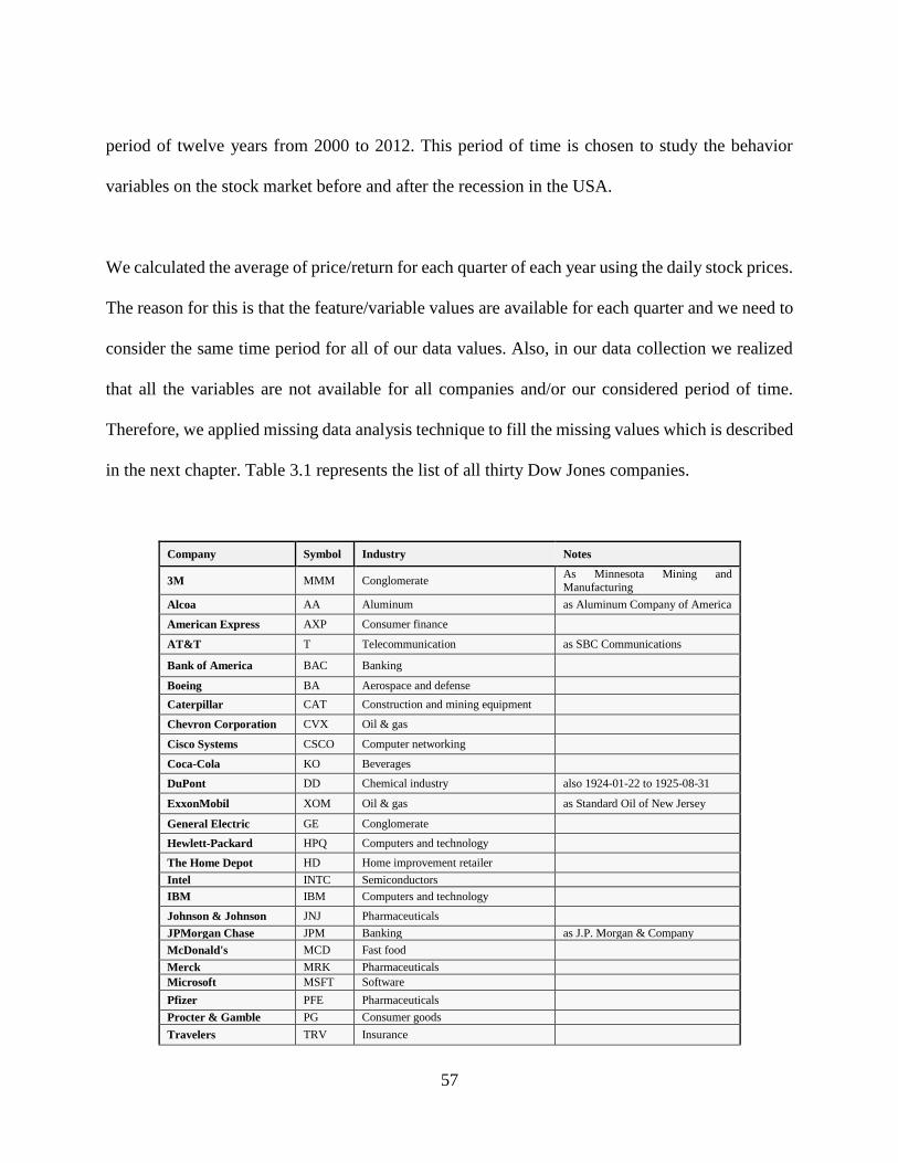
57

period of twelve years from 2000 to 2012. This period of time is chosen to study the behavior

variables on the stock market before and after the recession in the USA.

We calculated the average of price/return for each quarter of each year using the daily stock prices.

The reason for this is that the feature/variable values are available for each quarter and we need to

consider the same time period for all of our data values. Also, in our data collection we realized

that all the variables are not available for all companies and/or our considered period of time.

Therefore, we applied missing data analysis technique to fill the missing values which is described

in the next chapter. Table 3.1 represents the list of all thirty Dow Jones companies.

Company Symbol Industry Notes

3M MMM Conglomerate

As Minnesota Mining and Manufacturing

Alcoa AA Aluminum as Aluminum Company of America

American Express AXP Consumer finance

AT&T T Telecommunication as SBC Communications

Bank of America BAC Banking

Boeing BA Aerospace and defense

Caterpillar CAT Construction and mining equipment

Chevron Corporation CVX Oil & gas

Cisco Systems CSCO Computer networking

Coca-Cola KO Beverages

DuPont DD Chemical industry also 1924-01-22 to 1925-08-31

ExxonMobil XOM Oil & gas as Standard Oil of New Jersey

General Electric GE Conglomerate

Hewlett-Packard HPQ Computers and technology

The Home Depot HD Home improvement retailer

Intel INTC Semiconductors

IBM IBM Computers and technology

Johnson & Johnson JNJ Pharmaceuticals

JPMorgan Chase JPM Banking as J.P. Morgan & Company

McDonald's MCD Fast food

Merck MRK Pharmaceuticals

Microsoft MSFT Software

Pfizer PFE Pharmaceuticals

Procter & Gamble PG Consumer goods

Travelers TRV Insurance

58

UnitedHealth Group UNH Managed health care

UnitedHealth Group Inc. (UNH)

replaced Kraft Foods (KFT) Inc.

United Technologies

Corporation

UTX Conglomerate as United Aircraft

Verizon VZ Telecommunication

Wal-Mart WMT Retail

Walt Disney DIS Broadcasting and entertainment

Table 3-1. List of all American companies of Dow Jones Industrial Average

3.2.3.2. Correlation Measurements

Correlation is widely used in machine learning and statistics for relevance analysis. There are two

types of correlation calculation; linear and nonlinear. Pearson correlation consider the linear

relation of two variable X and Y with range of -1 and +1 where +1 represents completely positive

correlation of two variable, -1 show the negative correlation of two variables but still completely

correlated and 0 represents that the two variables are not correlated at all. In reality it is not always

safe to consider the linear correlation between features and that is why nonlinear correlations such

as Spearman is discussed. Spearman correlation is similar to Pearson correlation with the

consideration of nonlinearity of two variables and finding the correlation of the ranked variables.

Pearson correlation formula is represented in formula 3.9 where X is variance X, Y is variance

Y and ),( YXCOV is covariance X and Y.

YX

YX

YX

YX

YXEYXCOV

)])([(),(,

(3.9)

Below we first introduce our choice of correlation measure, then we describe our imperial

settings for choice of Pearson vs Spearman in our analysis.

59

3.2.3.3. Empirical Settings

The first experimental step of this research is to preprocess the dataset and prepare data for the

experimental studies. For this purpose, we follow below steps:

Remove Missing intervals: Remove financial variables with missing intervals for all

stocks. Using this approach reduced the size of data to less than 1/10 of its original size

and in total there are 28 common variables.

Pearson vs Spearman correlation: we tried to find the relation among variables by using

both Pearson and Spearman correlation coefficient. Comparing the results and looking at

the values, we discovered that simple Pearson correlation coefficient is not a suitable

candidate for this data. The main reason is that it is it is strongly biased towards linear

trends of some of financial variables. Figure 3.2 represents the cross plot of a financial

variable Total-Debt/Market-Cap versus Return of AA UN Equity which is one of the stocks

in Dow Jones dataset. As it is shown, the trend is monotonic and is not linear. Furthermore,

we also realized the existence of outliers in our dataset. As Spearman is less sensitive than

Pearson to the outliers, it would be a better choice. The existence of outlier is shown in

Figure 3.3. It demonstrates the outlier in the cross plot between Total-Debt (St &LT Debts)

and Return of Stock AA UN. As a result of the above discussion, we believe the idea of

applying Spearman correlation coefficient is suitable for analyzing financial variables of

Dow Jones Industrial Average dataset.

60

Figure 3.2. Cross plot of Total-Debt /Market-Cap versus Return of Stock AA UN

Figure 3.3. Cross plot of Total-Debt (ST & LT Debt) versus Return of Stock AA UN

Combine financial feature/variables: The next step in our implementation is to combine all

the features in different time steps versus the associated stocks. It is possible that the

correlation values of variables of one stock do not be as good as the correlation values of

the same variables for another stock. Also, the combined variable values of different stocks

0

5

10

15

20

25

30

35

40

45

0 0.2 0.4 0.6 0.8 1 1.2 1.4 1.6

Ret

urn

Total Debt/Market Cap Ratio

AA UN Equity

0

5

10

15

20

25

30

35

40

45

0.00 2,000.00 4,000.00 6,000.00 8,000.00 10,000.00 12,000.00

Ret

urn

Total Debt (ST & LT Debt)

AA UN Equity

61

may have a better correlation with the other combined variables than a stock separately.

Therefore, considering the combined variables may be the best option and can improve the

performance of the build model overall. Figure 3.4 represents the cross plot of three stocks

(AA UN Equity, AXP UN Equity and BAC UN Equity) for Price-To-Book-Ratio versus

Return. As it is shown, although there is correlation among the values of a stock, but

combining different stock values may improve the performance of the build model overall.

Figure 3.4. Cross plot of Price-To-Book-Ratio versus Return

Normal Score Transformation: There are two main approaches for normalizing the

datasets. The first approach is to assign a single value to the data using standardization

where the value is standardized by subtracting the minimum value of the dataset or

estimated mean and dividing by the range of dataset; maximum value minus minimum

value; or the estimated standard deviation. The other approach which is Normal Score

Transformation (NST) is to transform dataset into a normal distribution. This approach ranks values

of the dataset from lowest to the highest value and then assign a ranking value equivalent to the

0

10

20

30

40

50

60

70

0 2 4 6 8

Ret

urn

Price-to-Book Ratio

AA UN Equity

AXP UN Equity

BAC UN Equity

62

standard normal distribution. For ranking process of NST, both cumulative distribution and

frequency distribution can be used.

We compared the results of Pearson and Spearman correlation when dataset is not normalized and

when dataset is normalized for each stock separately and for combined stocks. The normalization

of the combined stocks keeps the overall data distributions of all stocks and their scaling. If we

normalize each stock separately and then combine them, it overrides the distribution of the data

and the combined values cannot keep their original values. Therefore, combined stocks are better

representative of our dataset as it preserves the bivariate relationship seen in original scores. Figure

3.5. represents the cross plot of one of the financial features (Increase Per Share) versus price. The

dataset is Normal Score Transform (NST) for combined and separate stocks.

Figure 3.6. represents the cross plot of the same variables (Increase Per Share vs. Price) for non-

normalized dataset. As it is shown, this figure confirms our previous discussion on prioritizing

Pearson to Spearman being biased towards linear correlation. This means that Spearman is superior

to Pearson in this case as it is a ranked based correlation measurement with non-linearity

correlation. In our study we realize that the value of Spearman correlation is closer to normalized

Pearson with ranking based normalization approach, where both have higher correlation values.

In this thesis Pearson correlation measurement is applied on the NST dataset using combined

stocks for each feature. This way we can select financial features that are better representative for

all stocks.

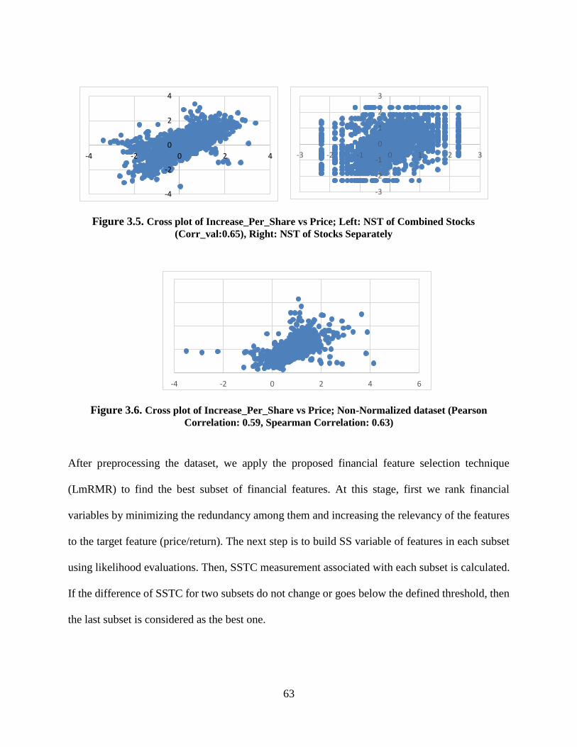
63

Figure 3.5. Cross plot of Increase_Per_Share vs Price; Left: NST of Combined Stocks

(Corr_val:0.65), Right: NST of Stocks Separately

Figure 3.6. Cross plot of Increase_Per_Share vs Price; Non-Normalized dataset (Pearson

Correlation: 0.59, Spearman Correlation: 0.63)

After preprocessing the dataset, we apply the proposed financial feature selection technique

(LmRMR) to find the best subset of financial features. At this stage, first we rank financial

variables by minimizing the redundancy among them and increasing the relevancy of the features

to the target feature (price/return). The next step is to build SS variable of features in each subset

using likelihood evaluations. Then, SSTC measurement associated with each subset is calculated.

If the difference of SSTC for two subsets do not change or goes below the defined threshold, then

the last subset is considered as the best one.

-4

-2

0

2

4

-4 -2 0 2 4

-3

-2

-1

0

1

2

3

-3 -2 -1 0 1 2 3

-4 -2 0 2 4 6

64

In this FS algorithm, the maximum number of the subset evaluations is the N where N represents

the total number of features. Although our experimental evaluations show that in most of the cases,

the total number of subset evaluations using LmRMR is less than half number of the features. This

makes this feature selection model time efficient. Also, because it does not use any target classifier,

it is not subjective.

3.2.3.4. Experimental Results and Discussion

As we discussed, in our experimental studies we used Dow Jones Industrial Average (DJIA)

financial statements variables/features. With the existence of missing values/intervals in the DJIA

financial variables, we need to find a solution to either impute these missing intervals or remove

them from the dataset. The missing value imputation is discussed in the next chapter. In this

chapter, we consider only the financial features that exist for all the stocks with no missing

values/interval being included. This results to consider only 28 features which is less than one

tenth of the total number of features.

As mentioned in LmRMR algorithm, this approach includes two main stages. In the first stage,

financial variables are ranked by considering all of their correlations as well as their relationship

with the final price/return in time series data of all stocks using mRMR measurement formula. The

features with no missing intervals are ranked and presented in the Table 3.2.

65

Table 3-2. List of ranked DJIA features with non-missing intervals

In the process of ranking DJIA features, we realized that some of the features do not have strong

relationship with the target feature which in this case is price. They might even end up having a

negative mRMR ranking value. The beauty of the subset selection is to consider the subset of

features and not individuals which can be a good representative of the target feature. Therefore,

even the features with negative ranking can be included in the final selected subset of features. As

it is shown in Figure 3.7, the mRMR values of features ranked 8th and above are negative. This

means that their correlation with target variable is not very strong individually. Later in this chapter

we show that some of these features are considered in the final selected subset of financial features

as they have improved our LmRMR algorithm performance and could build a strong subset

representing the target feature or price of stocks.

66

Figure 3.7. mRMR value for financial variables/features after ranking

The next step of LmRMR algorithm is finding the best subset of financial features. This process is

done in a forward pass with adding ranked features one by one to the subset. In this step, we build

the feature subsets starting by the first ranked feature. Then, other ranked features are added to the

subset in a forward pass. At each subset, the SS variable is calculated using the likelihood of

features within that subset. Then, the correlation of SS variable with target price is calculated as

SSTC measurement. If the value of SSTC improves beyond the threshold at each addition of

feature to the subset, then the feature is included in the subset. Otherwise, the feature is ignored

and the next ranked feature is added to the subset. Figure 3.8 represents SSTC measurement values

of the ranked features for all built subsets. This results to 28 subsets which is equal to the number

of features. In reality, this algorithm stops at 21th subset as the SSTC measurements start to

decrease. As it is shown the SSTC measurement value improves from feature 1 to 2 and 4 to 5 and

6 and then it remains steady. Therefore, using threshold 0.01, the best selected subset is {F1, F2,

F5, F6, F11, F18} while the SSTC measurement of selected subset is 72%.

-0.5

-0.4

-0.3

-0.2

-0.1

0

0.1

0.2

0.3

0.4

0.5

1 2 3 4 5 6 7 8 9 1011121314151617181920212223242526272829

mR

MR

Val

ues

Ranked Features

67

Figure 3.8. Cross plot of Stage two of LmRMR algorithm (Vertical axis: Likelihood value,

Horizontal axis: number of financial features)

In the above graph, SSTC increases until it reaches to a plateau and then start to decrease.

Therefore, the LmRMR algorithm stops at 21th iteration where there is no further improvement in

SSTC measurement.

All six selected features in the final selected subset are reported in Table 3.3. Based on the ranking

values of the features in Figure 3.7, the last three selected features are negatively ranked. We

discussed that our model adopts the relation of the selected subset of features with final target and

not their individual values. We realize that by the addition of the last two selected features (F11,

F18), our subset performance improves while SSTC increases from 66% to 72%.

Table 3-3. Selected financial Features for non-missing dataset

0.65

0.66

0.67

0.68

0.69

0.7

0.71

0.72

0.73

1 6 11 16 21 26

SSTC

Mea

sure

men

et

Feature Ranking

LmRMR

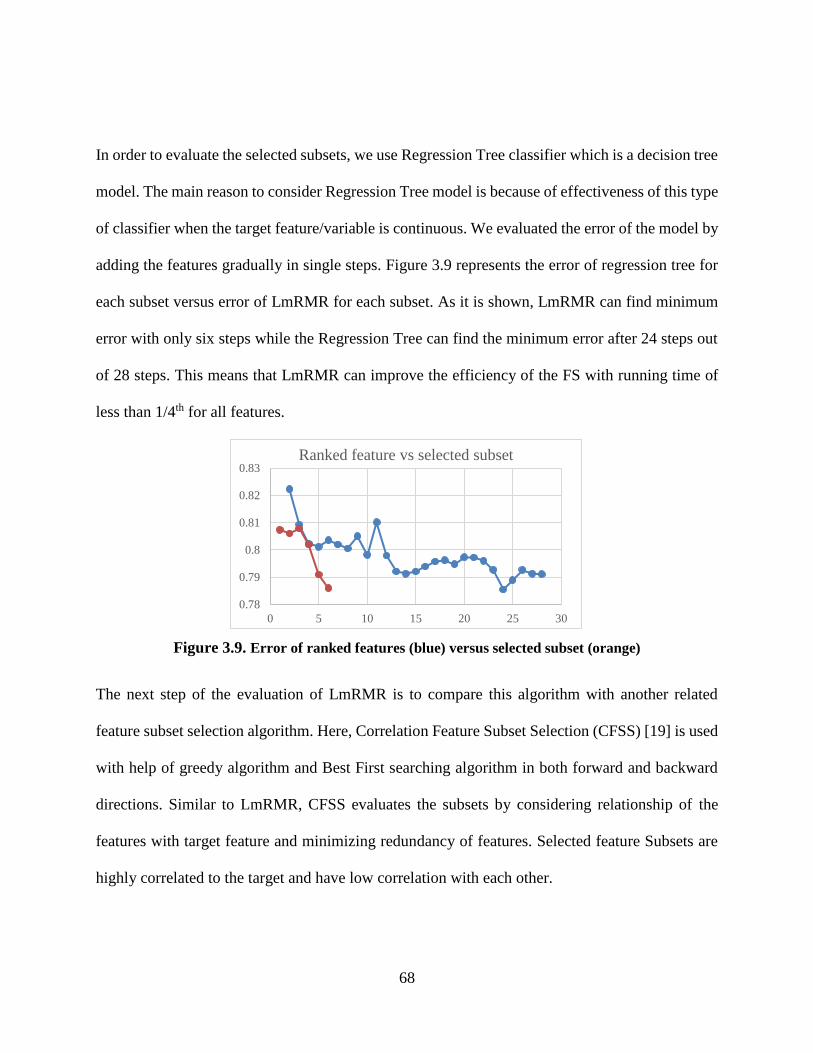
68

In order to evaluate the selected subsets, we use Regression Tree classifier which is a decision tree

model. The main reason to consider Regression Tree model is because of effectiveness of this type

of classifier when the target feature/variable is continuous. We evaluated the error of the model by

adding the features gradually in single steps. Figure 3.9 represents the error of regression tree for

each subset versus error of LmRMR for each subset. As it is shown, LmRMR can find minimum

error with only six steps while the Regression Tree can find the minimum error after 24 steps out

of 28 steps. This means that LmRMR can improve the efficiency of the FS with running time of

less than 1/4th for all features.

Figure 3.9. Error of ranked features (blue) versus selected subset (orange)

The next step of the evaluation of LmRMR is to compare this algorithm with another related

feature subset selection algorithm. Here, Correlation Feature Subset Selection (CFSS) [19] is used

with help of greedy algorithm and Best First searching algorithm in both forward and backward

directions. Similar to LmRMR, CFSS evaluates the subsets by considering relationship of the

features with target feature and minimizing redundancy of features. Selected feature Subsets are

highly correlated to the target and have low correlation with each other.

0.78

0.79

0.8

0.81

0.82

0.83

0 5 10 15 20 25 30

Ranked feature vs selected subset

69

The experimental evaluations for DJIA non-missing dataset shows LmRMR FS algorithm

outperforms Correlation Feature Subset Selection (CFSS). The evaluation measurement is

correlation between target feature (price) and likelihood of the features in the selected subsets

which we called in our algorithm as SSTC measurement. The reported SSTC for LmRMR and

CFSS is very close; 71% vs 69%.

LmRMR is also more efficient than CFSS with considering only 21 searching subsets versus 262

searching subsets. This is very important specially when the size of the dataset increases

dramatically and makes CFSS not to be time and computationally efficient. In these situations,

LmRMR can be a good alternative.

We also show the superiority of LmRMR when dealing with DJIA dataset after considering

imputed values for missing intervals which is discussed in the next chapter. In this case, the

correlation between SS and the target variable (SSTC) in our model goes up to 95% where using

the same dataset with CFSS, improve the SSTC only up to 76%. This is also another proof of

LmRMR effectiveness when it deals with larger dimension of the datasets. Table 3.4 represents

LmRMR algorithm evaluations outcomes. As it is shown in this table, the total number of financial

features increases from 28 features to 109 features after Ordinary kriging (OK) missing imputation.

Also, SSTC measurement improves from 71% to 95% which represents effectiveness of our

algorithm in predicting of target feature. Moreover, the number of subsets to be evaluated not only

increased but also decreased to less than 1/15th of total number of features.

70

Table 3-4. LmRMR FS algorithm Evaluations

Table 3.5 represents the outcome of CFSS algorithm evaluations. The datasets are the same as the

ones used in LmRMR algorithm with 28 features for dataset with no missing intervals and 109

features for dataset with imputed values using Ordinary Kriging (OK) missing imputation

technique. Although, the number of features have been increased but there is not a significant

improvement in the performance of the algorithm; 69% vs. 76%. Also, the total number of

searching subsets have been increased dramatically. This means that to select the best subset of

features for total features of 109, we need to search 943 combinations of the feature subsets. In

comparison to LmRMR with only 15 searching feature subsets, this algorithm is really inefficient.

Table 3-5. Correlation FS algorithm Evaluations

The selected financial features/variables using CFSS algorithm is shown in Table 3.6. where the first

column represents the selected features when the dataset removes missing values and second column

represents the selected features when OK is used as imputation technique for filling missing intervals. In

the next chapter, we discuss both of these missing data imputational techniques in details.

71

Table 3-6. Selected financial variable using Correlation FS algorithm

3.4. Conclusions

In this chapter we propose a novel feature selection technique with its application on financial

datasets. The proposed technique called LmRMR (Likelihood Minimum Redundancy Maximum

Relevance) use mRMR formula to rank the features. The advantage of using this ranking model is

to penalize redundant features and select features that are more correlated to the target

feature/variable. Then, a likelihood evaluation is applied for each selected subset which results in

building a Super Secondary (SS) variable. The correlation between target feature and SS variable

is called SSTC and consider as evaluation measurement. This algorithm adds each of the ranked

features to the selected subset in a forward pass. If the SSTC improves considering the threshold

value, we include the added feature in our selected subset.

We compared the performance of our proposed technique with Correlation based feature sub set

selection (CFSS) using greedy and best first search algorithms. The outcome shows the superiority

of our model both in subset evaluations and efficiency. We also, show that imputing the missing

72

intervals in the financial datasets, can improve the performance of our system and is essential. That

is why the next chapter of this thesis discuss missing data recovery with its application in finance.

73

CHAPTER 4: MISSING DATA ANALYSIS

In real world applications, it is quite common for datasets to contain missing data due to a variety

of limitations. In Literature, different techniques have been developed to address this problem and

impute the missing intervals. Most of these techniques consider data when it is Missing

Completely At Random (MCAR) or Missing At Random (MAR) with few discuss the uncertainty

related to them. In this chapter we bring the idea of spatial statistics techniques to deal with missing

intervals in the financial domain.

In the area of spatial modeling, covariance functions and variograms are the main tools. These

functions facilitate the optimal prediction of quantities of interest at the unsampled locations and

are estimated based on the sampled data. These are part of geostatistics modeling tools which has

been discussed in different literatures [170] – [177]. Geostatistical methods have been developed

to handle both stationarity and non-stationarity domains where in many instances they require the

Gaussianity of the dataset. In this chapter first we discuss the decision of stationarity as well as

variograms and covariance models. For the normality of data, we use normal score transformation

as we discussed in the previous chapter. We can also look at the histogram of our data in order to

check the normality. Then, we explained Kriging algorithm and Bayesian Updating model and its

application in financial dataset. Finally, we discuss our experimental studies on a synthetic dataset

and also Dow Jones Industrial Average dataset.

74

4.1. Stationarity

Let’s consider {𝑍(𝑠𝑖), 𝑖 = 1, … , 𝑛} denote the quantity Z of interest, observed at time 𝑠 ∈

𝑇 ∁ 𝑅𝑡where T is domain where observations are taken and t is dimension. For two variable Z(s)

and Z(t) and mean of 𝜇(𝑠) and 𝜇(𝑡), the covariance is as following.

𝐶𝑜𝑣[𝑍(𝑠), 𝑍(𝑡)] = 𝐸[(𝑍(𝑠) − 𝜇(𝑠))(𝑍(𝑡) − 𝜇(𝑡))] (4.1)

Also, the correlation function is based on the division of the covariance of the two variables over

their standard deviations. If the observations are independent, the covariance and correlation are

close to zero.

In general, stationarity represents quality of a variable in which mean and standard deviation of

the variable do not change with time.

𝐸[(𝑍(𝑠)] = 𝜇

𝐶𝑜𝑣[𝑍(𝑠), 𝑍(𝑡)] = 𝐶𝑜𝑣[𝑍(𝑠 + ℎ), 𝑍(𝑡 + ℎ)] for all shifts h (4.2)

The above formula represents the weakly stationarity where the process has a constant mean and

covariance function. Here the covariance depends on lag and does not change with time. The

strongly stationary process assumes that for any collection of k variables, 𝑍(𝑠𝑖), 𝑖 = 1, … , 𝑘, and

constants 𝑎𝑖, 𝑖 = 1, … , 𝑘, we have

𝑃[𝑍(𝑠1) ≪ 𝑎1, … . , 𝑍(𝑠𝑘) ≪ 𝑎𝑘] = 𝑃[𝑍(𝑠1 + ℎ) ≪ 𝑎1, … . , 𝑍(𝑠𝑘 + ℎ) ≪ 𝑎𝑘] (4.3)

For all shift vectors h. This indicates that the entire joint distribution of k variables in invariant

under shifts [172].

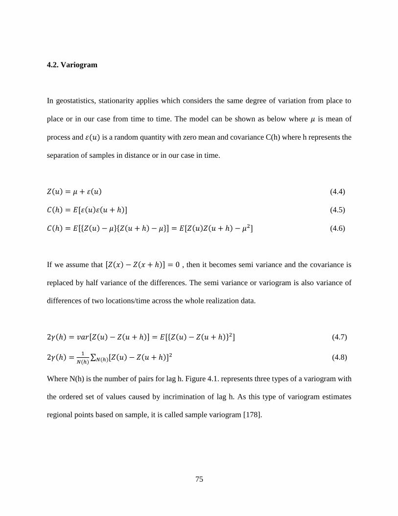
75

4.2. Variogram

In geostatistics, stationarity applies which considers the same degree of variation from place to

place or in our case from time to time. The model can be shown as below where 𝜇 is mean of

process and 𝜀(𝑢) is a random quantity with zero mean and covariance C(h) where h represents the

separation of samples in distance or in our case in time.

𝑍(𝑢) = 𝜇 + 𝜀(𝑢) (4.4)

𝐶(ℎ) = 𝐸[𝜀(𝑢)𝜀(𝑢 + ℎ)] (4.5)

𝐶(ℎ) = 𝐸[{𝑍(𝑢) − 𝜇}{𝑍(𝑢 + ℎ) − 𝜇}] = 𝐸[𝑍(𝑢)𝑍(𝑢 + ℎ) − 𝜇2] (4.6)

If we assume that [𝑍(𝑥) − 𝑍(𝑥 + ℎ)] = 0 , then it becomes semi variance and the covariance is

replaced by half variance of the differences. The semi variance or variogram is also variance of

differences of two locations/time across the whole realization data.

2𝛾(ℎ) = 𝑣𝑎𝑟[𝑍(𝑢) − 𝑍(𝑢 + ℎ)] = 𝐸[{𝑍(𝑢) − 𝑍(𝑢 + ℎ)}2] (4.7)

2𝛾(ℎ) =1

𝑁(ℎ)∑ [𝑍(𝑢) − 𝑍(𝑢 + ℎ)]2

𝑁(ℎ) (4.8)

Where N(h) is the number of pairs for lag h. Figure 4.1. represents three types of a variogram with

the ordered set of values caused by incrimination of lag h. As this type of variogram estimates

regional points based on sample, it is called sample variogram [178].

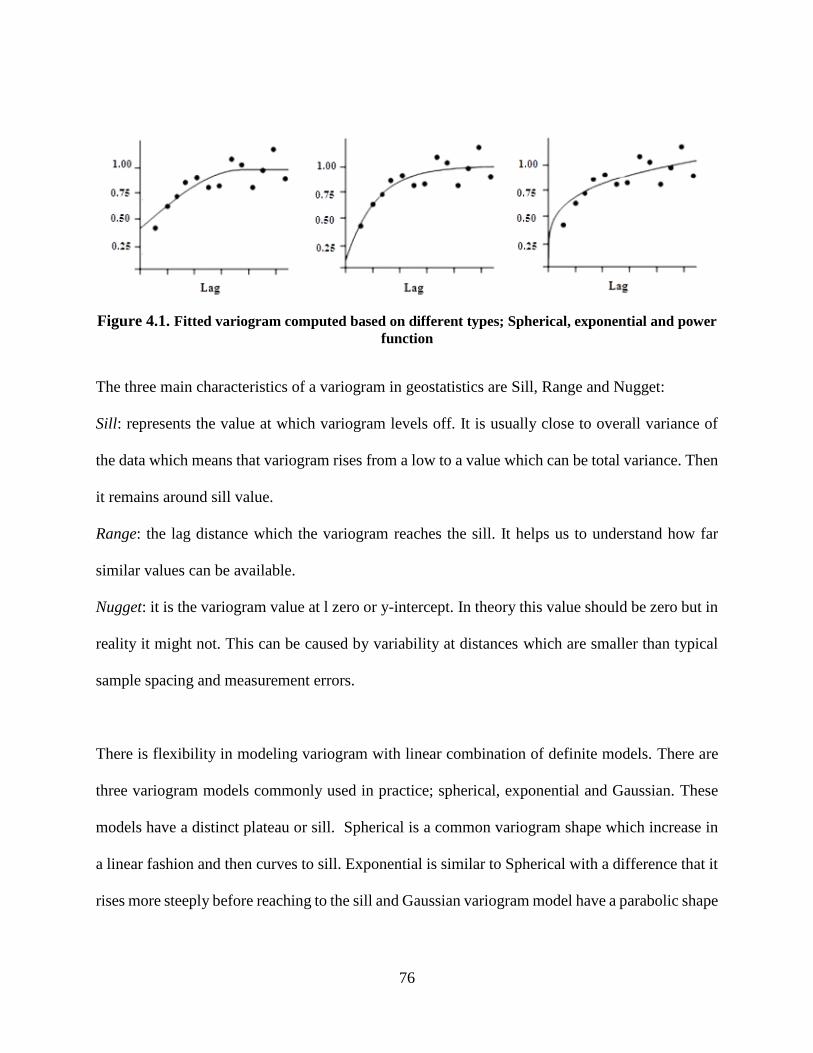
76

Figure 4.1. Fitted variogram computed based on different types; Spherical, exponential and power

function

The three main characteristics of a variogram in geostatistics are Sill, Range and Nugget:

Sill: represents the value at which variogram levels off. It is usually close to overall variance of

the data which means that variogram rises from a low to a value which can be total variance. Then

it remains around sill value.

Range: the lag distance which the variogram reaches the sill. It helps us to understand how far

similar values can be available.

Nugget: it is the variogram value at l zero or y-intercept. In theory this value should be zero but in

reality it might not. This can be caused by variability at distances which are smaller than typical

sample spacing and measurement errors.

There is flexibility in modeling variogram with linear combination of definite models. There are

three variogram models commonly used in practice; spherical, exponential and Gaussian. These

models have a distinct plateau or sill. Spherical is a common variogram shape which increase in

a linear fashion and then curves to sill. Exponential is similar to Spherical with a difference that it

rises more steeply before reaching to the sill and Gaussian variogram model have a parabolic shape

77

at short distances. All these three variogram models and other variogram characteristics are

represented in Figure 4.2. For Kriging modeling we need to find a suitable semivariogram.

Nugget: 𝑔(ℎ) = {0 𝑖𝑓 ℎ = 0𝑐 𝑜𝑡ℎ𝑒𝑟𝑤𝑖𝑠𝑒

(4.9)

Spherical: 𝑔(ℎ) = {𝑐. [1.5 (

ℎ

𝑎) − 0.5(

ℎ

𝑎)3] 𝑖𝑓 ℎ ≪ 𝑎

𝑐 𝑜𝑡ℎ𝑒𝑟𝑤𝑖𝑠𝑒 (4.10)

Exponential: 𝑔(ℎ) = 𝑐. [1 − exp (−3ℎ

𝑎)] (4.11)

Gaussian: 𝑔(ℎ) = 𝑐. [1 − exp (−3ℎ2

𝑎2 )] (4.12)

Where h is lag distance, a is range of the variogram and c is the sill.

Figure 4.2. Variogram characteristics

4.3. Kriging

Kriging algorithm was originally used for spatial data in order to estimate the value of unsampled

locations. It is a generalized linear regression technique to provide a Best Linear Unbiased

Estimate (BLUE) at unsampled locations. The “Best” means the Kriging estimator has minimum

78

error variance and “Unbiased” means the expected value of the error is zero. In general Kriging is

a generic name for a family of generalized least square regression algorithms with the innovatively

of Daniel Krige (1951) [179]- [181]. There are several forms of Kriging and one of them which is

used extensively and is explained in this proposal is simple Kriging.

Here the problem is to estimate the value of attribute z at missing data points of u, using only

available z-data. If there are n available data, it can be shown by {z(ui ) , i = 1 . . .n}, where ui is a

vector representing different data points of u.

The Kriging estimator is variant of regression estimator. The Kriging formula is given in (4.13)

for any missing data value u:

)]()()[()()()(

1

*

umuzuumuZun

i

(4.13)

In the above equation, m(u) and m( u ) are expected values of z(u) and z( u ). Also, )(u is the

weight assigned to data z( u ) and is calculated from the Kriging system of equation (4.14). It

considers data closeness and the correlation among them. It is also important to know that the

values that are closer to the missing value have higher weights.

n 2.., 1,=j),()()(1

jji

n

i

i uuCuuCu

(4.14)

In equation (4.14), C(ui−uj) is the covariance between data z(ui) and z(uj), and C(u−uj) is the

covariance between the missing data being estimated z(u) and data z(uj). The covariance function

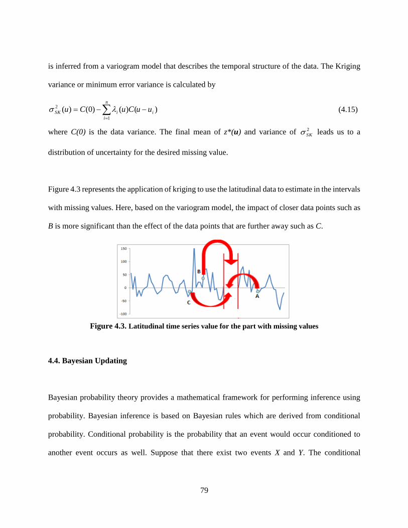
79

is inferred from a variogram model that describes the temporal structure of the data. The Kriging

variance or minimum error variance is calculated by

)()()0()(1

2

i

n

i

iSK uuCuCu

(4.15)

where C(0) is the data variance. The final mean of z*(u) and variance of 2

SK leads us to a

distribution of uncertainty for the desired missing value.

Figure 4.3 represents the application of kriging to use the latitudinal data to estimate in the intervals

with missing values. Here, based on the variogram model, the impact of closer data points such as

B is more significant than the effect of the data points that are further away such as C.

Figure 4.3. Latitudinal time series value for the part with missing values

4.4. Bayesian Updating

Bayesian probability theory provides a mathematical framework for performing inference using

probability. Bayesian inference is based on Bayesian rules which are derived from conditional

probability. Conditional probability is the probability that an event would occur conditioned to

another event occurs as well. Suppose that there exist two events X and Y. The conditional

80

probability of Y given X is shown as )( XYP . Also, the probability of X and Y can be represented

as joint probability as presented in equation (4.16). Here it is important to consider that 0)( XP .

)(

)()(

XP

XYPXYP

(4.16)

Which can also be presented by multiplying through and becomes:

)()()( XPXYPXYP (4.17)

And the generalized form is

)()()()( YXZPXYPXPZYXP (4.18)

Rearranging the equation (4.18) leads to equation (4.19).

)(

)()(

YP

YXPYXP

(4.19)

As )()( XYPYXP , then 4.16 formulas can be presented as:

)(

)()()(

XP

YXPYPXYP (4.20)

The posterior probability in Bayesian inference is calculated by equation (4.20). Bayesian

inference derives the posterior probability as consequent of two antecedents; a prior probability

and likelihood function which is derived from probability model of the data to be observed.

In equation (4.20), the probability of event X is the same for all possible models being considered

and does not enter in probabilities of different models. Therefore, the equation can be represented

by (4.21).

)()()( YXPYPXYP (4.21)

81

In the above equation )(YP is prior probability and it reflects the probability of Y before X is

observed. Also, )( YXP is called likelihood and is the probability of X given Y. Finally, )( XYP

is the probability of Y given X and after X is observed. It is called posterior probability.

Bayesian updating is based on Bayesian inference. It has been commonly used in data integration

[179]- [182]. As stated previously, the method is based on combining the prior and likelihood

estimates. The prior model is based on primary data or latitudinal data and the likelihood model is

built based on the secondary data or longitudinal data.

A primary variable consists of n vectors of primary data },...,1),({ niuy i , where iu is a vector

including missing value. It uses Kriging [181] to find the mean and variance of the missing data

as discussed before. Likelihood model is based on secondary data. The selected secondary data

should be available for all features },,...,1),({ Aumjux j [179]. The result of using secondary

data of different features is another conditional distribution which is called the likelihood

distribution. The following formula is used in order to find the mean of this distribution.

m

j

jiL uxuy1

)()(

(4.22)

The weights of the above formula are calculated based on the correlation of the features with each

other. It is calculated as below.

mkm

j

kkjj ,...,1,1

0,,

(4.23)

82

Where m is the number of features, kj , is the correlation between feature i and k and finally, 0,k

is the correlation between feature k and missing value. After finding the likelihood mean, the

likelihood variance should be calculated as following.

m

j

jjL u1

0,

2 1)( (4.24)

Figure 4.4 demonstrate an example of likelihood calculation. Here, F12, F13 and F14 represent

longitudinal data that are used to estimate the missing interval in the feature/variable with the

missing values (F11).

Figure 4.4. Longitudinal time series value for the part with missing values

Finally, prior and likelihood distributions are merged together in order to find the posterior

distribution. The posterior distribution shows uncertainty at the estimated missing value. The

posterior distribution for the estimated missing value is conditional distribution of primary data

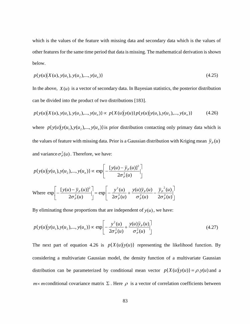
83

which is the values of the feature with missing data and secondary data which is the values of

other features for the same time period that data is missing. The mathematical derivation is shown

below.

)}(),...,(),(),()({ 21 nuyuyuyuXuyp (4.25)

In the above, )(uX is a vector of secondary data. In Bayesian statistics, the posterior distribution

can be divided into the product of two distributions [183].

)}(),...,(),()({)}()({)}(),...,(),(),()({ 2121 nn uyuyuyuypuyuXpuyuyuyuXuyp (4.26)

where )}(),...,(),()({ 21 nuyuyuyuyp is prior distribution contacting only primary data which is

the values of feature with missing data. Prior is a Gaussian distribution with Kriging mean )(uyP

and variance )(2 uP . Therefore, we have:

)(2

)]()([exp)}(),...,(),()({

2

2

21u

uyuyuyuyuyuyp

P

Pn

Where

)(2

)(

)(

)()(

)(2

)(exp

)(2

)]()([exp

2

2

22

2

2

2

u

uy

u

uyuy

u

uy

u

uyuy

P

P

P

P

PP

P

By eliminating those proportions that are independent of )(uy , we have:

)(

)()(

)(2

)(exp)}(),...,(),()({

22

2

21u

uyuy

u

uyuyuyuyuyp

P

P

P

n

(4.27)

The next part of equation 4.26 is )}()({ uyuXp representing the likelihood function. By

considering a multivariate Gaussian model, the density function of a multivariate Gaussian

distribution can be parameterized by conditional mean vector )(.)}()({ uyuyuXp and a

mm conditional covariance matrix . Here is a vector of correlation coefficients between

84

the primary variable and secondary data. In vector T

n ),..,,( 02010 , location u is dropped

for simplicity. The covariance matrix can be written as a matrix of correlation coefficients:

t

ij

nnn

n

nnn

n

00100

0101010

1

111

...

.........

...

...

.........

...

(4.28)

Likelihood function is a function of )(uy as the secondary data is known. Therefore, in the

following equation the constants which are independent of )(uy are eliminated.

)]]([)]([2

1exp[)}()({ 1 uyXuyXuyuXp t

And )]]([)]([2

1exp[)]]([)]([

2

1exp[ 11 uyXuyXuyXuyX ttt

)]]()(2[2

1exp[ 2111 uyuyXXX tttt

And the final outcome is: )](2

1)(exp[)}()({ 211 uyuyXuyuXp ttt (4.29)

Finally, the posterior is given by multiplying (4.27) and (4.29) as following:

)(]

)(

)()([)(]

)(

1[

2

1exp)}(),...,(),()({

2

12

2

1

21 uyu

uyuXuy

uuyuyuyuyp

P

pt

P

T

n

This equation is in the form of )exp( 2 BxAx , where mean and variance of the Gaussian kernel

are defined by A and B. Therefore, the posterior mean and variance are represented in equations

(4.30) and (4.31). The combination of prior (Figure 4.3) and likelihood (Figure 4.4) is presented

by BU in Figure 4.5.

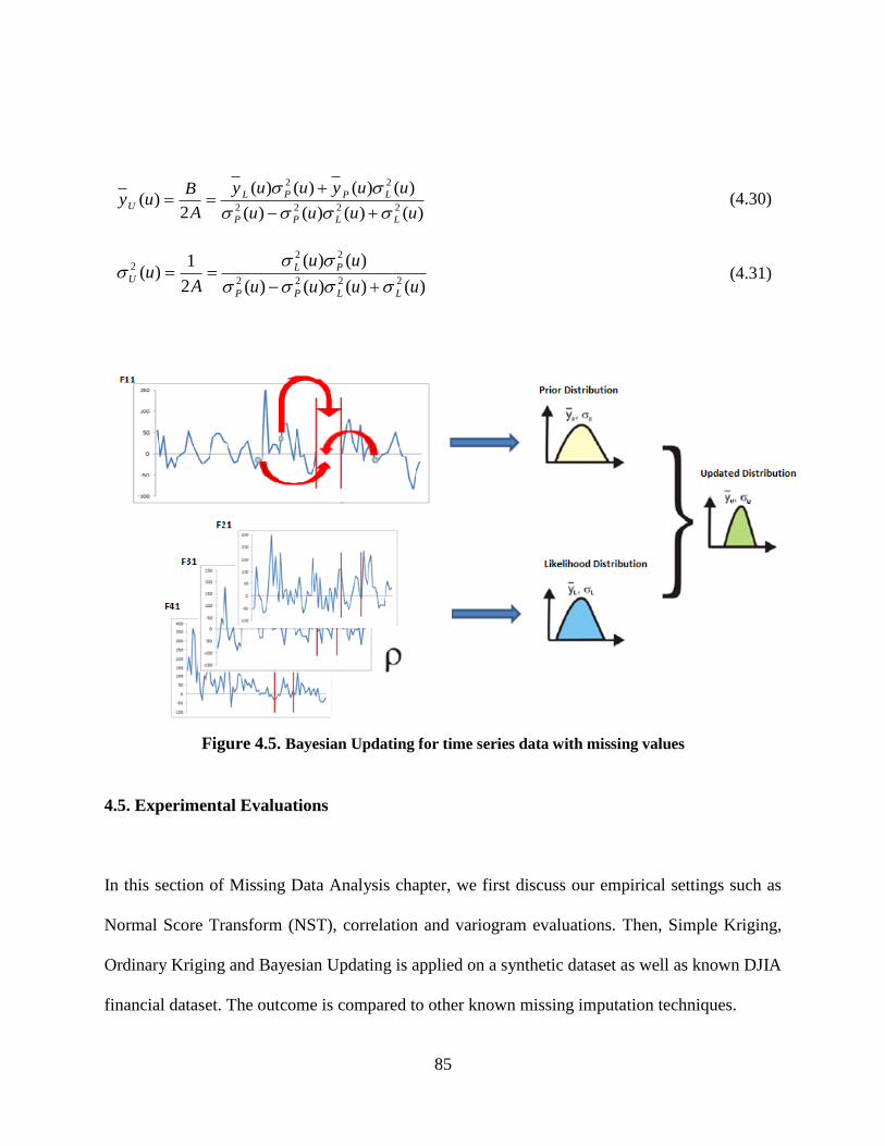
85

)()()()(

)()()()(

2)(

2222

22

uuuu

uuyuuy

A

Buy

LLPP

LPPL

U

(4.30)

)()()()(

)()(

2

1)(

2222

222

uuuu

uu

Au

LLPP

PLU

(4.31)

Figure 4.5. Bayesian Updating for time series data with missing values

4.5. Experimental Evaluations

In this section of Missing Data Analysis chapter, we first discuss our empirical settings such as

Normal Score Transform (NST), correlation and variogram evaluations. Then, Simple Kriging,

Ordinary Kriging and Bayesian Updating is applied on a synthetic dataset as well as known DJIA

financial dataset. The outcome is compared to other known missing imputation techniques.

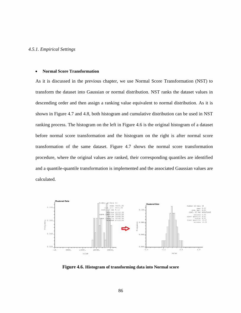
86

4.5.1. Empirical Settings

Normal Score Transformation

As it is discussed in the previous chapter, we use Normal Score Transformation (NST) to

transform the dataset into Gaussian or normal distribution. NST ranks the dataset values in

descending order and then assign a ranking value equivalent to normal distribution. As it is

shown in Figure 4.7 and 4.8, both histogram and cumulative distribution can be used in NST

ranking process. The histogram on the left in Figure 4.6 is the original histogram of a dataset

before normal score transformation and the histogram on the right is after normal score

transformation of the same dataset. Figure 4.7 shows the normal score transformation

procedure, where the original values are ranked, their corresponding quantiles are identified

and a quantile-quantile transformation is implemented and the associated Gaussian values are

calculated.

Figure 4.6. Histogram of transforming data into Normal score

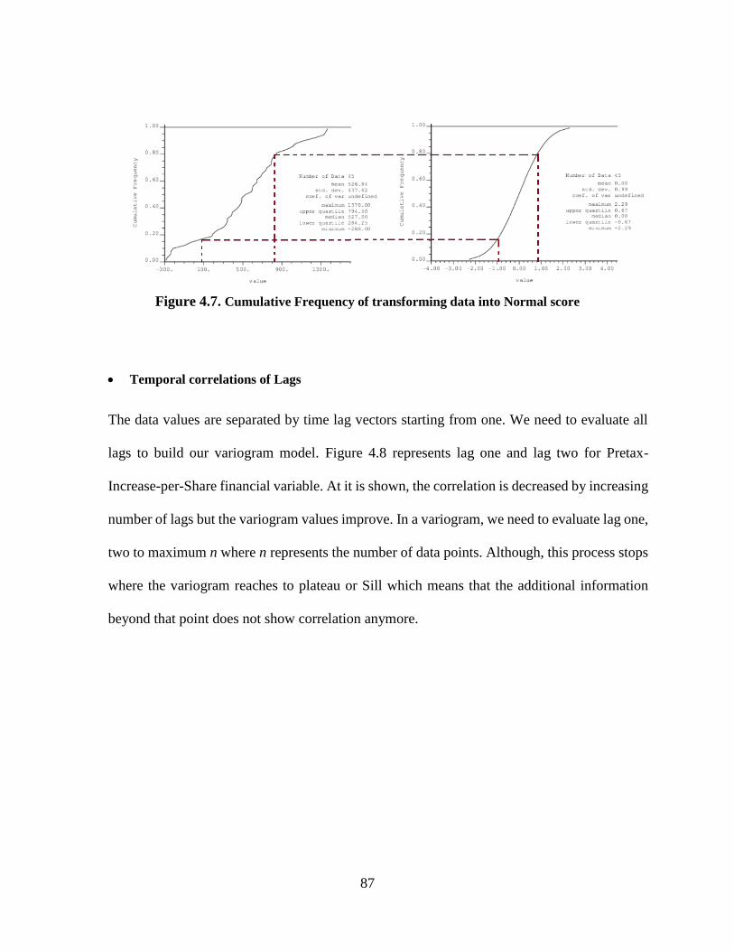
87

Figure 4.7. Cumulative Frequency of transforming data into Normal score

Temporal correlations of Lags

The data values are separated by time lag vectors starting from one. We need to evaluate all

lags to build our variogram model. Figure 4.8 represents lag one and lag two for Pretax-

Increase-per-Share financial variable. At it is shown, the correlation is decreased by increasing

number of lags but the variogram values improve. In a variogram, we need to evaluate lag one,

two to maximum n where n represents the number of data points. Although, this process stops

where the variogram reaches to plateau or Sill which means that the additional information

beyond that point does not show correlation anymore.

88

Figure 4.8. Scatterplot of two first step of variogram for ‘pretax -Increase-per-share’ variable

Calculating Variograms

Variogram starts with one lag. It starts at a node/ time step and compares values to all nodes/

time steps which fall in the lag tolerance. Then, it moves to next node and repeats the same

process for all nodes and all lags. Figure 4.9 represents a variogram with sill of 900 and range

of 50 where the variogram reaches the sill. This means that the value of variogram increases

and the correlation decreases by increasing the lags until it reaches the sill where there is not

correlation anymore. In another words, the addition of further data points beyond the lag 50

does not add any value to our model and those data points should be ignored.

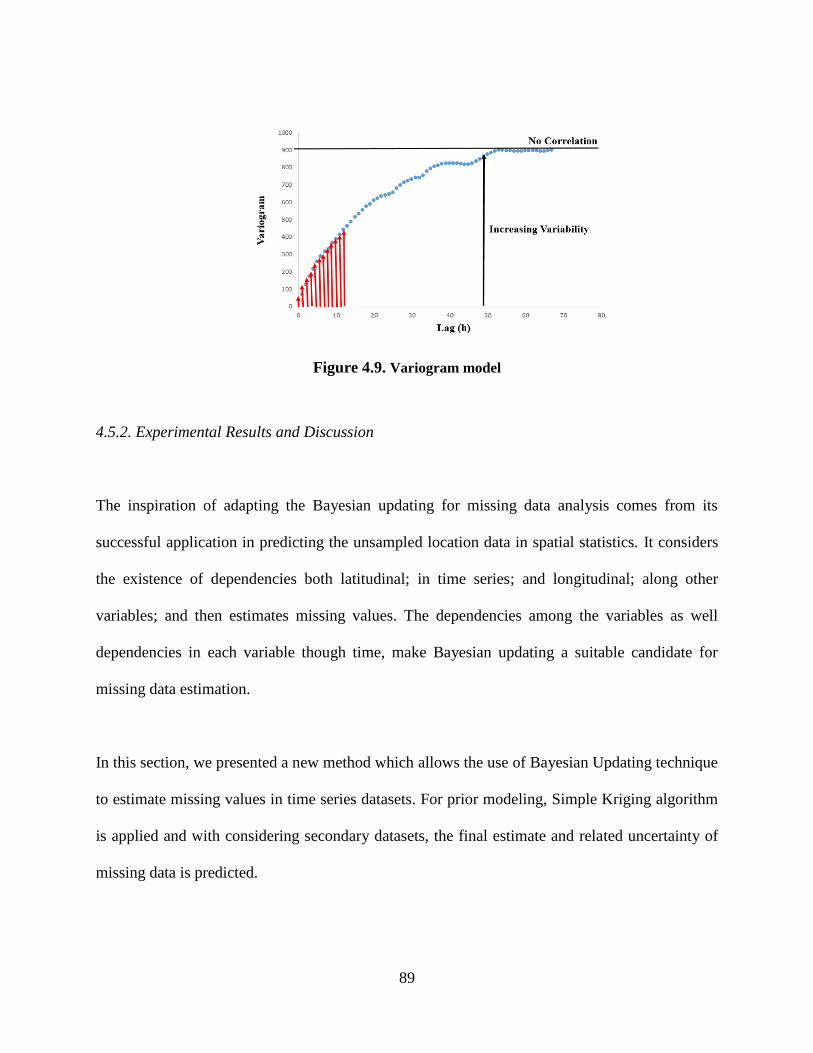
89

Figure 4.9. Variogram model

4.5.2. Experimental Results and Discussion

The inspiration of adapting the Bayesian updating for missing data analysis comes from its

successful application in predicting the unsampled location data in spatial statistics. It considers

the existence of dependencies both latitudinal; in time series; and longitudinal; along other

variables; and then estimates missing values. The dependencies among the variables as well

dependencies in each variable though time, make Bayesian updating a suitable candidate for

missing data estimation.

In this section, we presented a new method which allows the use of Bayesian Updating technique

to estimate missing values in time series datasets. For prior modeling, Simple Kriging algorithm

is applied and with considering secondary datasets, the final estimate and related uncertainty of

missing data is predicted.

90

In order to evaluate our results, first we have created a synthetic dataset and five different

techniques is used; four existing imputation techniques, Ordinary Kriging and Bayesian Updating.

Subsequently, the related RMSE value for each technique is calculated and the results are

compared. The results show that both Bayesian Updating and Ordinary Kriging are superior to the

other existing techniques. Then, same approach is applied on missing data discovery on Dow Jones

dataset in the area of financial time series where the outcome is similar to the synthetic dataset

with superiority of Bayesian Updating and Ordinary Kriging imputation techniques.

4.5.2.1. Synthetic Dataset

In this paper three synthetic datasets are used. The first dataset is considered as primary dataset

and a part of the data is removed randomly as missing part. The next two datasets are considered

as secondary datasets.

Each dataset is generated using a statistical simulation on one thousand data points which are

driven from a Gaussian distribution randomly and considered stationary. Also, the primary dataset

is generated in a way to have correlation with secondary datasets. Figure 4.10 represents the

primary dataset histogram with the associated statistics such as mean and standard deviation.

Figure 4.11 represent the generate primary and secondary datasets.

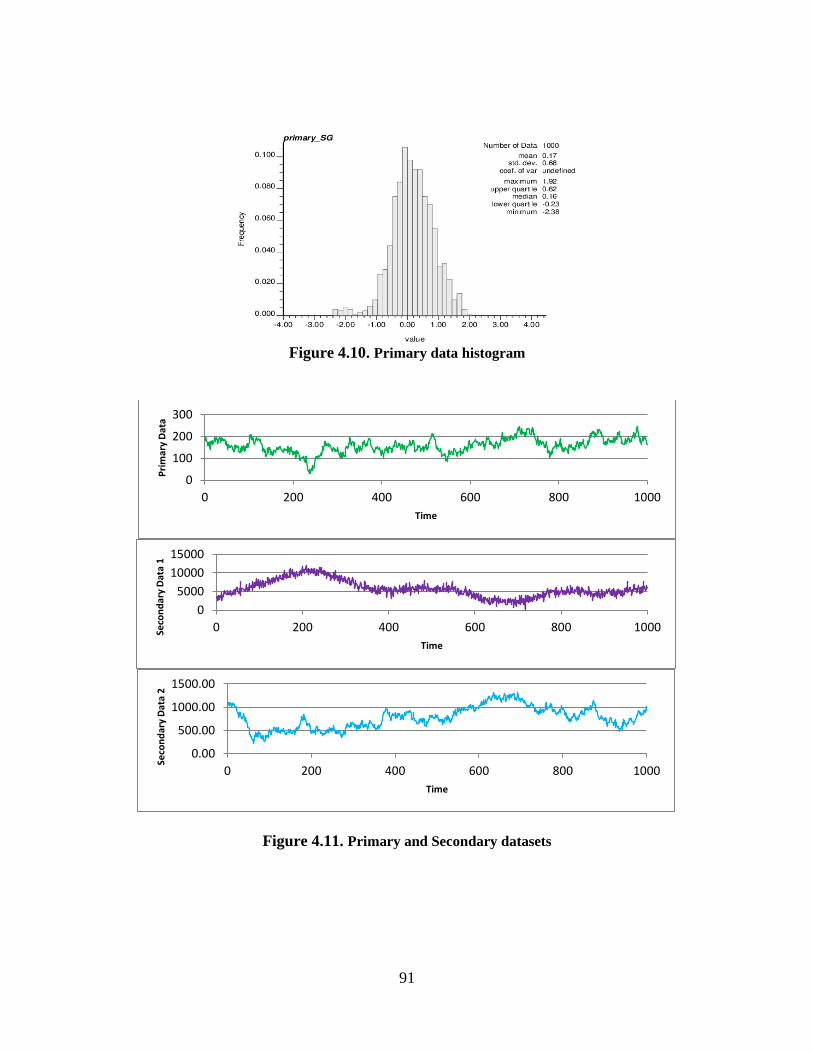
91

Figure 4.10. Primary data histogram

Figure 4.11. Primary and Secondary datasets

0

100

200

300

0 200 400 600 800 1000

Pri

mar

y D

ata

Time

0

5000

10000

15000

0 200 400 600 800 1000Seco

nd

ary

Dat

a 1

Time

0.00

500.00

1000.00

1500.00

0 200 400 600 800 1000

Seco

nd

ary

Dat

a 2

Time

92

Pearson versus Spearman

Pearson's correlation coefficient and Spearman's rank order correlation coefficient analyze the

degree to which the variables are related. Pearson's coefficient measures the linear

dependency between two points while Spearman's coefficient is a monotonic measure which

considers the rank order of the points.

n

i

i

n

i

i

n

i

ii

yx

yx

YYXX

YYXXyxCOV

1

2

1

2

1,

)()(

]))([(),(

(4.32)

Spearman correlation coefficient is defined based on Pearson correlation coefficient on the

ranked variables.

With looking at primary and secondary datasets in Figure 4.12, it can be realized that Pearson

correlation coefficient can be a suitable candidate as the trend is not quite far from being linear.

0.00

500.00

1000.00

1500.00

0 100 200 300

Seco

nd

ary

Dat

a 2

Primary Data

0

3000

6000

9000

12000

15000

0 100 200 300

Seco

nd

ary

Dat

a 1

Primary Data

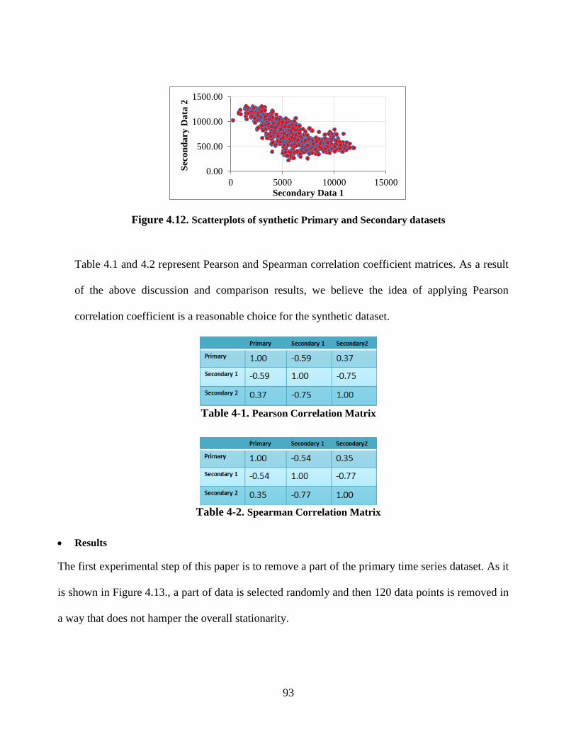
93

Figure 4.12. Scatterplots of synthetic Primary and Secondary datasets

Table 4.1 and 4.2 represent Pearson and Spearman correlation coefficient matrices. As a result

of the above discussion and comparison results, we believe the idea of applying Pearson

correlation coefficient is a reasonable choice for the synthetic dataset.

Table 4-1. Pearson Correlation Matrix

Table 4-2. Spearman Correlation Matrix

Results

The first experimental step of this paper is to remove a part of the primary time series dataset. As it

is shown in Figure 4.13., a part of data is selected randomly and then 120 data points is removed in

a way that does not hamper the overall stationarity.

0.00

500.00

1000.00

1500.00

0 5000 10000 15000S

eco

nd

ary

Da

ta 2

Secondary Data 1

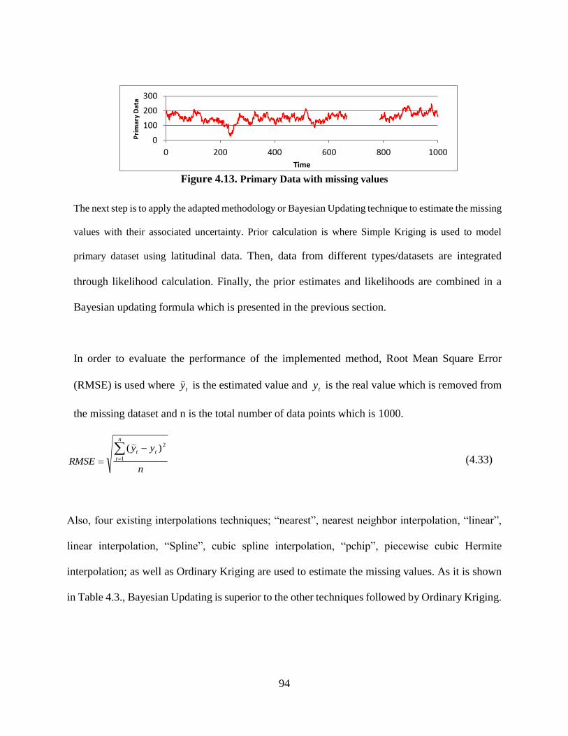
94

Figure 4.13. Primary Data with missing values

The next step is to apply the adapted methodology or Bayesian Updating technique to estimate the missing

values with their associated uncertainty. Prior calculation is where Simple Kriging is used to model

primary dataset using latitudinal data. Then, data from different types/datasets are integrated

through likelihood calculation. Finally, the prior estimates and likelihoods are combined in a

Bayesian updating formula which is presented in the previous section.

In order to evaluate the performance of the implemented method, Root Mean Square Error

(RMSE) is used where ty

is the estimated value and ty is the real value which is removed from

the missing dataset and n is the total number of data points which is 1000.

n

yy

RMSE

n

t

tt

1

2)(

(4.33)

Also, four existing interpolations techniques; “nearest”, nearest neighbor interpolation, “linear”,

linear interpolation, “Spline”, cubic spline interpolation, “pchip”, piecewise cubic Hermite

interpolation; as well as Ordinary Kriging are used to estimate the missing values. As it is shown

in Table 4.3., Bayesian Updating is superior to the other techniques followed by Ordinary Kriging.

0

100

200

300

0 200 400 600 800 1000

Pri

mar

y D

ata

Time

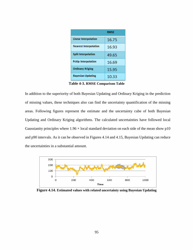
95

Table 4-3. RMSE Comparison Table

In addition to the superiority of both Bayesian Updating and Ordinary Kriging in the prediction

of missing values, these techniques also can find the uncertainty quantification of the missing

areas. Following figures represent the estimate and the uncertainty cube of both Bayesian

Updating and Ordinary Kriging algorithms. The calculated uncertainties have followed local

Gaussianity principles where 1.96 × local standard deviation on each side of the mean show p10

and p90 intervals. As it can be observed in Figures 4.14 and 4.15, Bayesian Updating can reduce

the uncertainties in a substantial amount.

Figure 4.14. Estimated values with related uncertainty using Bayesian Updating

96

Figure 4.15. Estimated values with related uncertainty using Ordinary Kriging

4.5.2.2. Dow Jones Industrial Average (DJIA) Dataset

In the previous chapter we applied the proposed feature selection (LmRMR) on DJIA dataset. In

this chapter, we extend our experiments and use the missing data analysis techniques such as

Nearest neighbor, Kriging and Bayesian updating. This is a basis for a comparison to find potential

improvement or deficiency in our feature selection technique. In the next sections, first we

represent our experimental evaluations on DJIA dataset using NN. Then, Simple and Ordinary

kriging results are presented and discussed. Finally, Bayesian Updating is discussed with its

advantages or shortcoming applying on this type of dataset.

Nearest Neighbor (NN)

First, we considered Nearest neighbor (NN) which is one the known techniques used for missing

data imputation. This technique can be easily adopted and has been applied in different research

areas. The drawback of this technique can be when it looks for similar instances, it needs to search

the whole dataset and in our case, looking at different stocks, the missing value might not be

available for the same time step in other stocks. This technique is based on the similarity

0

100

200

300

0 200 400 600 800 1000

Time

97

measurement computed between different samples which in our dataset is stocks, for a specific

feature. There has been different similarity distance measure such as Euclidean, Manhattan and

Minkowski. Euclidean distance is a common measurement which is recommended in literature

[18] [19] and it is used in this research.

In NN method, missing values of a sample are imputed based on the values of another sample

which minimize distance of these samples. The formula for Euclidean distance is defined as

following.

𝐸(𝑆𝑗 , 𝑆𝑘) = √∑ (𝑥𝑆𝑗,𝑖 − 𝑥𝑆𝑘,𝑖)2𝑖∈𝐷 (4.34)

Where 𝐸(𝑆𝑗, 𝑆𝑘) is distance between two case/stock j and k. 𝑥𝑆𝑗,𝑖 and 𝑥𝑆𝑘,𝑖 represent the values of

feature i in in cases 𝑆𝑗 and 𝑆𝑘 and finally, D is set of attributes with no missing values. The outcome

of using NN in our experiments is described in following.

In our experiments we found that there are 374 financial features/variables which has complete or

partial values for all stocks. This reduce the number of features to less than half as some of the

features are not considered in all stocks. Then, we applied NN imputation on each feature

considering values of other stocks for the same period that data is missing. As it is presented in

Table 4.4., the value of feature one (F1) for period t3 of Stock one (S1) is missing. NN technique

use the values of other stocks (S2, ..., Sn) for the same feature (F1) to fill This missing value.

98

S1 S2 S3 Sn

F1 t1 t1 t1 … t1

t2 t2 t2 … t2

NA t3 t3 … t3

t4 t4 NA t4

… … … … …

tn tn tn … tn

F2 t1 t1 t1 … t1

t2 t2 t2 … t2

… … … … …

tn tn tn … tn

… … … … … …

Fn t1 t1 t1 … t1

NA t2 NA … t2

NA t3 t3 … t3

t4 t4 NA … NA

… … … … …

tn tn tn … tn

Table 4-4. Feature matrix

We consider 5,10,15, 25 and 30 percent missing on each feature related to different stocks. At

the beginning five percent missing value is considered. The outcome shows that the total number

of features is increased to 81 from 28 which means that 53 additional features are recovered using

this imputation approach. The following steps are considered to apply this imputation technique

for DJIA dataset.

1. Organizing the dataset: combining all existing financial features for every stock regardless

of missing/ non missing values

2. Missing data imputation using Nearest neighbor: consider common features among all

stocks which has no missing or partial missing for a feature. Evaluate the minimum

distance between stocks for each feature separately based on Euclidean distance

measurement (4.34).

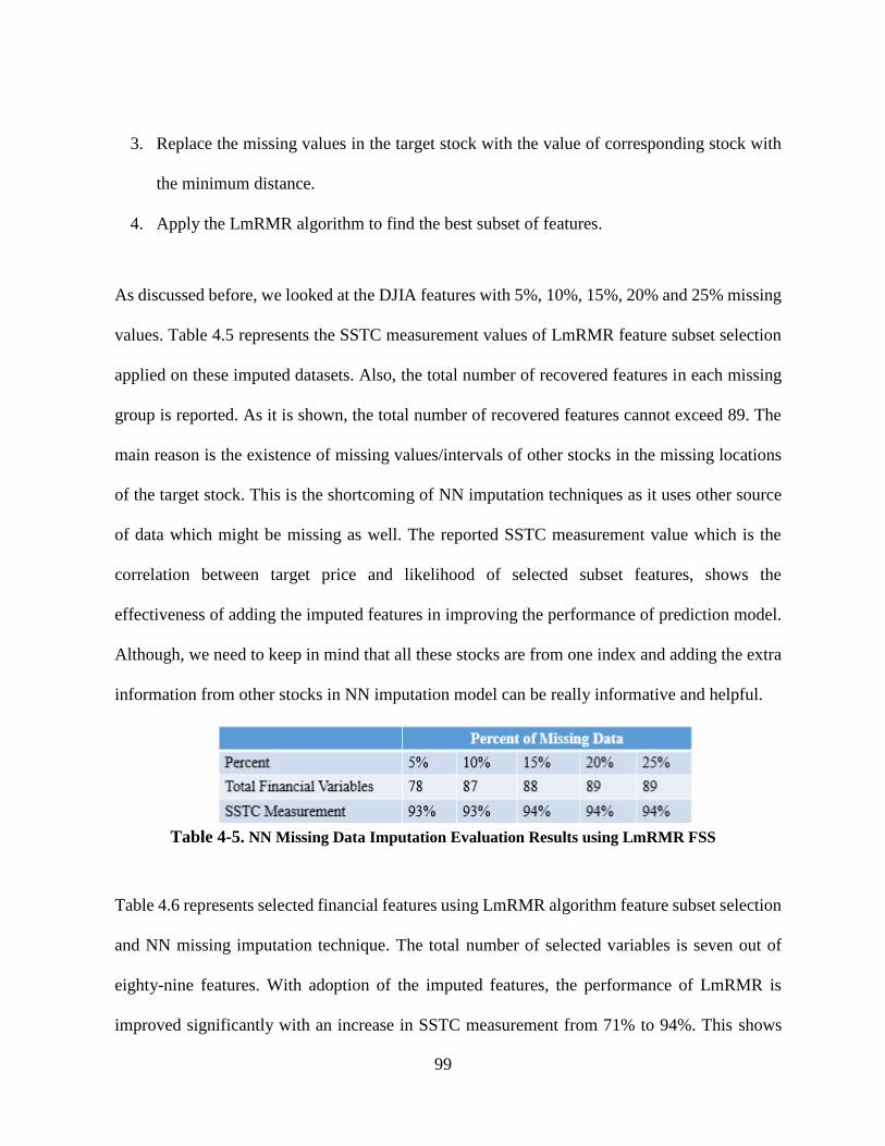
99

3. Replace the missing values in the target stock with the value of corresponding stock with

the minimum distance.

4. Apply the LmRMR algorithm to find the best subset of features.

As discussed before, we looked at the DJIA features with 5%, 10%, 15%, 20% and 25% missing

values. Table 4.5 represents the SSTC measurement values of LmRMR feature subset selection

applied on these imputed datasets. Also, the total number of recovered features in each missing

group is reported. As it is shown, the total number of recovered features cannot exceed 89. The

main reason is the existence of missing values/intervals of other stocks in the missing locations

of the target stock. This is the shortcoming of NN imputation techniques as it uses other source

of data which might be missing as well. The reported SSTC measurement value which is the

correlation between target price and likelihood of selected subset features, shows the

effectiveness of adding the imputed features in improving the performance of prediction model.

Although, we need to keep in mind that all these stocks are from one index and adding the extra

information from other stocks in NN imputation model can be really informative and helpful.

Table 4-5. NN Missing Data Imputation Evaluation Results using LmRMR FSS

Table 4.6 represents selected financial features using LmRMR algorithm feature subset selection

and NN missing imputation technique. The total number of selected variables is seven out of

eighty-nine features. With adoption of the imputed features, the performance of LmRMR is

improved significantly with an increase in SSTC measurement from 71% to 94%. This shows

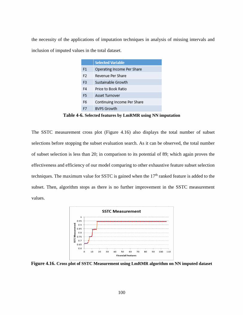
100

the necessity of the applications of imputation techniques in analysis of missing intervals and

inclusion of imputed values in the total dataset.

Table 4-6. Selected features by LmRMR using NN imputation

The SSTC measurement cross plot (Figure 4.16) also displays the total number of subset

selections before stopping the subset evaluation search. As it can be observed, the total number

of subset selection is less than 20; in comparison to its potential of 89; which again proves the

effectiveness and efficiency of our model comparing to other exhaustive feature subset selection

techniques. The maximum value for SSTC is gained when the 17th ranked feature is added to the

subset. Then, algorithm stops as there is no further improvement in the SSTC measurement

values.

Figure 4.16. Cross plot of SSTC Measurement using LmRMR algorithm on NN imputed dataset

101

Overall, NN technique can be a good missing data imputation technique when the extra data

information of other stocks of the index is added to the information of the stock with missing

intervals. As we discussed, addition of the missing features, can improve the correlation of the

super secondary variable; using likelihood of features in the selected subset; with target price

(SSTC measurement) to 94%. This means that missing data analysis, did a tremendous job in

improving the performance of financial feature selection.

This technique might not always work for financial features with missing intervals selected from

different indices. Also, features with the same missing interval of more than one stock, cannot

be recovered. Therefore, we need to find other techniques which includes information of other

time steps of feature with missing values along with information of other features/stocks.

Therefore, Kriging and Bayesian Updating techniques are proposed.

Kriging

As mentioned before, kriging is a collection of generalized linear regression techniques for

minimizing an estimated variance defined from a prior model using to estimate unsampled or

missing values [175]. The simplest form of kriging is simple kriging (SK) which estimates

missing values from neighboring data values. Another form of kriging is Ordinary Kriging (OK)

which is a variant of SK algorithm where sum of weights is constraint and equal to one. This

allows that OK estimator does not require prior knowledge of mean.

102

In this research first we apply SK and then OK for missing data analysis of financial variables

using neighborhood data of the same variable. This means that unlike Nearest neighbor technique

no other information (other variable’s value in the same time period) is considered.

The first step for this imputation technique is to find the variogram of variables with missing

data. As there are many variables with missing values, we represent only one variable for all

thirty stocks in Dow Jones dataset as it is shown in Figure 4. 17. The average range of variograms

in this case is six with minimum range of five and maximum of nineteen.

The next step is to consider variables with 5,10, 15, 20, 25 percent of missing considering that

the selected variables have values even partial for all stocks. In other words, a variable is not

included if it does not exist for a stock or is completely missing.

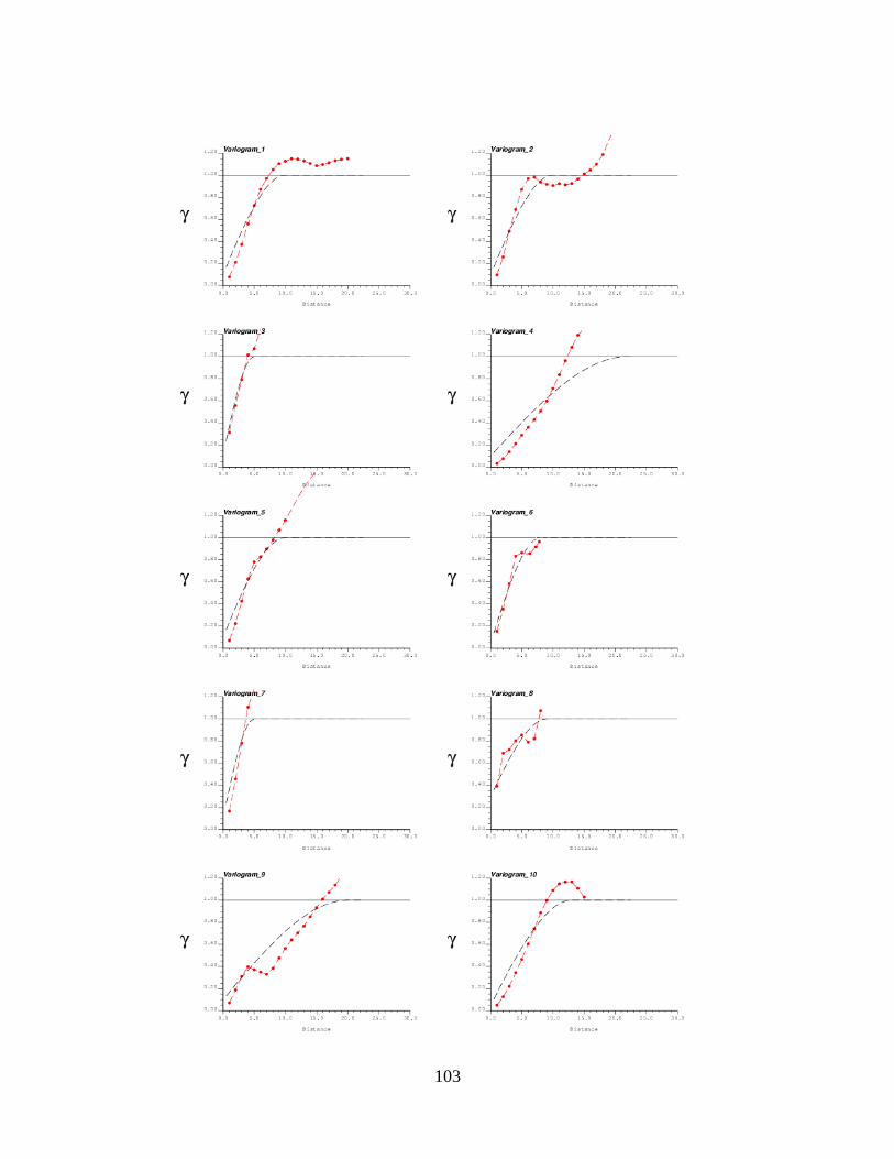
103

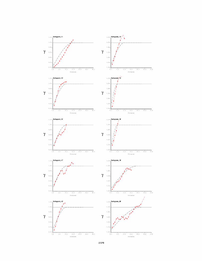
104

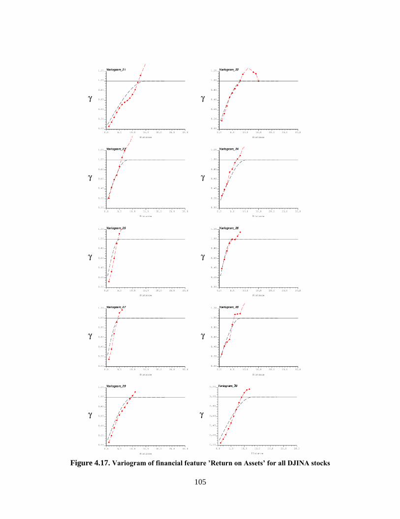
105

Figure 4.17. Variogram of financial feature ’Return on Assets’ for all DJINA stocks

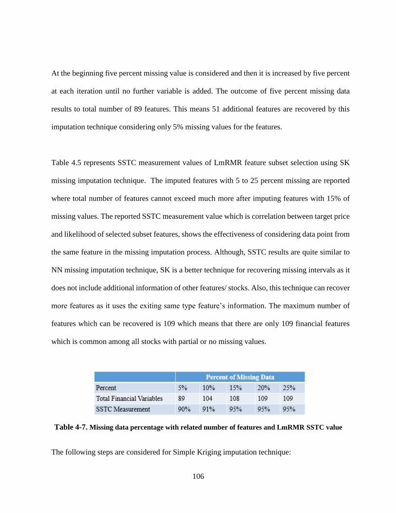
106

At the beginning five percent missing value is considered and then it is increased by five percent

at each iteration until no further variable is added. The outcome of five percent missing data

results to total number of 89 features. This means 51 additional features are recovered by this

imputation technique considering only 5% missing values for the features.

Table 4.5 represents SSTC measurement values of LmRMR feature subset selection using SK

missing imputation technique. The imputed features with 5 to 25 percent missing are reported

where total number of features cannot exceed much more after imputing features with 15% of

missing values. The reported SSTC measurement value which is correlation between target price

and likelihood of selected subset features, shows the effectiveness of considering data point from

the same feature in the missing imputation process. Although, SSTC results are quite similar to

NN missing imputation technique, SK is a better technique for recovering missing intervals as it

does not include additional information of other features/ stocks. Also, this technique can recover

more features as it uses the exiting same type feature’s information. The maximum number of

features which can be recovered is 109 which means that there are only 109 financial features

which is common among all stocks with partial or no missing values.

Table 4-7. Missing data percentage with related number of features and LmRMR SSTC value

The following steps are considered for Simple Kriging imputation technique:

107

Organizing the dataset: consider each feature/variable for each stock separately and normal

score transform them.

Missing data imputation using SK:

o Model the variogram related to each variable

o Apply simple kriging and find estimated value with related uncertainty (variance).

Then, fill missing intervals

Normal back transforms the variable: using the recorded normal distribution of the

variables

Normalize the feature: combining all financial variable’s value of all stocks and normalize

them together as it is discussed in previous chapter.

Apply the LmRMR algorithm and find the best subset of features using SSTC

measurement.

Table 4.8 represents selected features using SK imputation technique. The selected features here

are similar to the selected features with NN imputation technique. Although, SK approach is a

better candidate for imputing the missing values as it does not need additional information from

other features/ stocks and only use the existing values of the same feature for each stock.

Table 4-8. Selected features by LmRMR using SK imputation

108

Figure 4.18 is a very good demonstration of SSTC measurement evaluations of LmRMR algorithm

where ranked features are added gradually to the selected subsets. The maximum number of

recovered features by SK imputation technique is 109 where 104 of these features have only 10%

missing intervals or less. The maximum reported SSTC measurement using SK technique is 95%

which can be achieved with the evaluation of only less than 20 subsets.

Figure 4.18. Cross plot of SSTC Measurement using LmRMR algorithm on SK imputed dataset

The imputation steps for Ordinary Kriging is similar to Simple Kriging. Although, the results of

ordinary kriging are slightly superior to simple kriging and Nearest neighbor. This means that

using local mean of the interval around missing values is useful in imputing the missing values.

The results of LmRMR subset evaluations for 5 to 25 percent missing values are reported in Table

4.9. With adoption of OK as missing imputation technique, we can reach to 96% correlation of SS

variable and the target price in SSTC measurement. This SSTC measurement is reported for the

features with missing intervals of 10 percent or less. It means that most of the effective financial

features have less than 10 percent missing in their values. The selected subset of features using

0.6

0.65

0.7

0.75

0.8

0.85

0.9

0.95

1

0 10 20 30 40 50 60 70 80 90 100 110

109

OK imputation technique is reported in table 4.10. The selected features in this subset have less

than 10% missing interval and have a maximum 96% of correlation with the target feature.

Table 4-9. Missing data percentage with related number of features and LmRMR likelihood value

Table 4-10. Selected features by LmRMR using OK imputation

The cross plot of LmRMR algorithm using SSTC measurement for all imputed financial features

is presented in Figure 4.19. Again, the selected subset is found within the first seventeen ranked

features. After that the SSTC plot reaches to its maximum value, it stays plateau where LmRMR

algorithm stops.

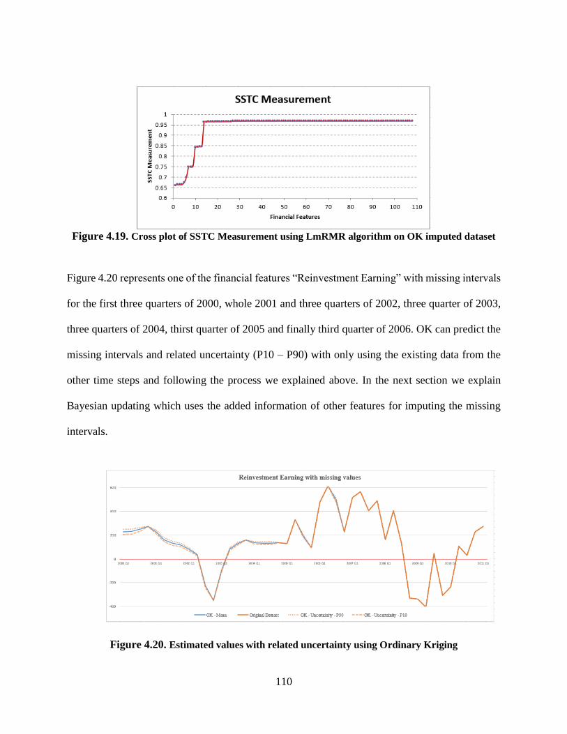
110

Figure 4.19. Cross plot of SSTC Measurement using LmRMR algorithm on OK imputed dataset

Figure 4.20 represents one of the financial features “Reinvestment Earning” with missing intervals

for the first three quarters of 2000, whole 2001 and three quarters of 2002, three quarter of 2003,

three quarters of 2004, thirst quarter of 2005 and finally third quarter of 2006. OK can predict the

missing intervals and related uncertainty (P10 – P90) with only using the existing data from the

other time steps and following the process we explained above. In the next section we explain

Bayesian updating which uses the added information of other features for imputing the missing

intervals.

Figure 4.20. Estimated values with related uncertainty using Ordinary Kriging

111

Bayesian Updating

In Bayesian updating we consider the effect of other variables and stocks. This means that

besides the information of the variable with missing value; Kriging; similar to NN

additional information is used to improve the performance of missing data imputation.

Similar to what we have done for the synthetic dataset, first prior calculation is done using

simple kriging. This considers the information of the same variable of the stock with

missing information and latitudinal data. Then, likelihood estimation is applied for missing

periods of the variable and other variables/stocks for the same period of time. The final

Bayesian Updating estimation is the combination of prior and likelihood using equations

4.28 and 4.29. Table 4.11 represents the selected features using BU missing imputation

technique and LmRMR algorithm. The selected features are similar to the ones selected

using SK and OK missing imputation techniques. The only difference is addition of F7

which is Debt to Market Capitalization. This means that the influenced of other features on

this feature is significant during the missing imputation process.

Table 4-11. Selected features by LmRMR using BU imputation

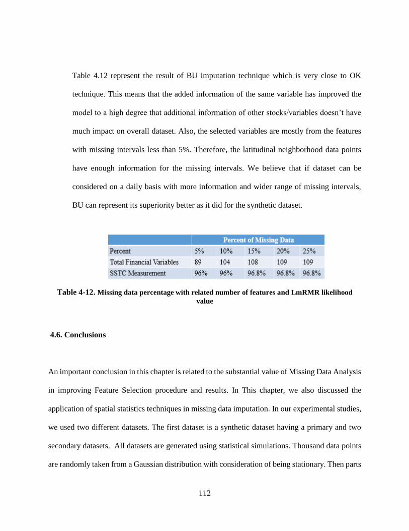
112

Table 4.12 represent the result of BU imputation technique which is very close to OK

technique. This means that the added information of the same variable has improved the

model to a high degree that additional information of other stocks/variables doesn’t have

much impact on overall dataset. Also, the selected variables are mostly from the features

with missing intervals less than 5%. Therefore, the latitudinal neighborhood data points

have enough information for the missing intervals. We believe that if dataset can be

considered on a daily basis with more information and wider range of missing intervals,

BU can represent its superiority better as it did for the synthetic dataset.

Table 4-12. Missing data percentage with related number of features and LmRMR likelihood

value

4.6. Conclusions

An important conclusion in this chapter is related to the substantial value of Missing Data Analysis

in improving Feature Selection procedure and results. In This chapter, we also discussed the

application of spatial statistics techniques in missing data imputation. In our experimental studies,

we used two different datasets. The first dataset is a synthetic dataset having a primary and two

secondary datasets. All datasets are generated using statistical simulations. Thousand data points

are randomly taken from a Gaussian distribution with consideration of being stationary. Then parts

113

of primary dataset are removed randomly. Both OK and BU showed their superiority in predicting

the missing intervals using RMSE measurement.

Then, we used DJIA dataset which is one of the most important financial indices. Again, OK and

BU were superior to other techniques both in the numbers of recovered features as well as

performance evaluations using SSTC measurement. The SSTC of BU is very close to OK

technique. This happens as most of the features in the selected subset, do not have long range of

missing intervals and using the information of the same features is really helpful. Therefore, adding

information of other features may not be very effective in improving the performance of the

imputation technique.

114

CHAPTER 5: APPLICATION IN DECISION ANALYSIS AND FORECASTING

In this chapter, we analyze the utilization of financial variables in practical applications after

implementation of feature selection. As discussed in chapter two, there are several financial

evaluation workflows that utilize financial variables. In this chapter, we study two financial

evaluation workflows, where the selected financial variables by the proposed feature selection

approach are utilized.

First, a fuzzy inference recommendation model for stock trading is presented and studied. Usually

there are number of technical variables/indicators that traders consider to find the market trend and

make their decisions. Here, with the use of only twelve fuzzy rules and appropriate fuzzy MFs on

the previously selected variables, we propose a technique that tries to mimic the human thinking

and suggest an intelligent approach for a satisfactory recommendation as when to buy, sell or hold

the stocks.

Second, we study the value of the previously selected financial features in future stock price

prediction. For this purpose, a comprehensive lag analysis in time series and price modeling is

implemented, where the effectiveness of the present data in predicting the next steps prices of

stocks is investigated. With the use of cross-variograms of the selected features, the SS variable

and the stock prices, we study how the confidence in the future price predictions erodes and

uncertainty increases as the number of lags increases.

115

Finally, a discussion on the actual multivariate stock prediction techniques and proposed future

research is presented, where is the concept of the Linear Model of Coregionalization (LMC) and

the associated multivariate statistical settings is introduced.

5.1. Fuzzy Inference Model

Applications of fuzzy logic have had an incredible improvement after the concept was introduced

by Zadeh [188] [189]. They have been utilized in many disciplines from home appliances such as

air conditioners and cameras to medical instruments such as blood pressure monitors, etc. Fuzzy

logic allows for gradual evaluation of the membership of elements in a set, and is based on two-

dimensional Membership Function (MF). It provides an organized calculus to solve vague and

incomplete information linguistically. Here the linguistic information is converted to numerical

values using linguistic labels specified by MF [190] [191]. A fuzzy inference system uses fuzzy

if-then rules to be able to model human expertise for a specific application.

5.1.1. Fuzzy Sets & Membership Functions

A fuzzy set describes the degree to which an element belongs to a set. If we consider X as a

collection of objects ( Xx ), then a type-1 fuzzy set A in X is a set of ordered pairs:

}))(,{( XxxxA A ]1,0[: XA (5.1)

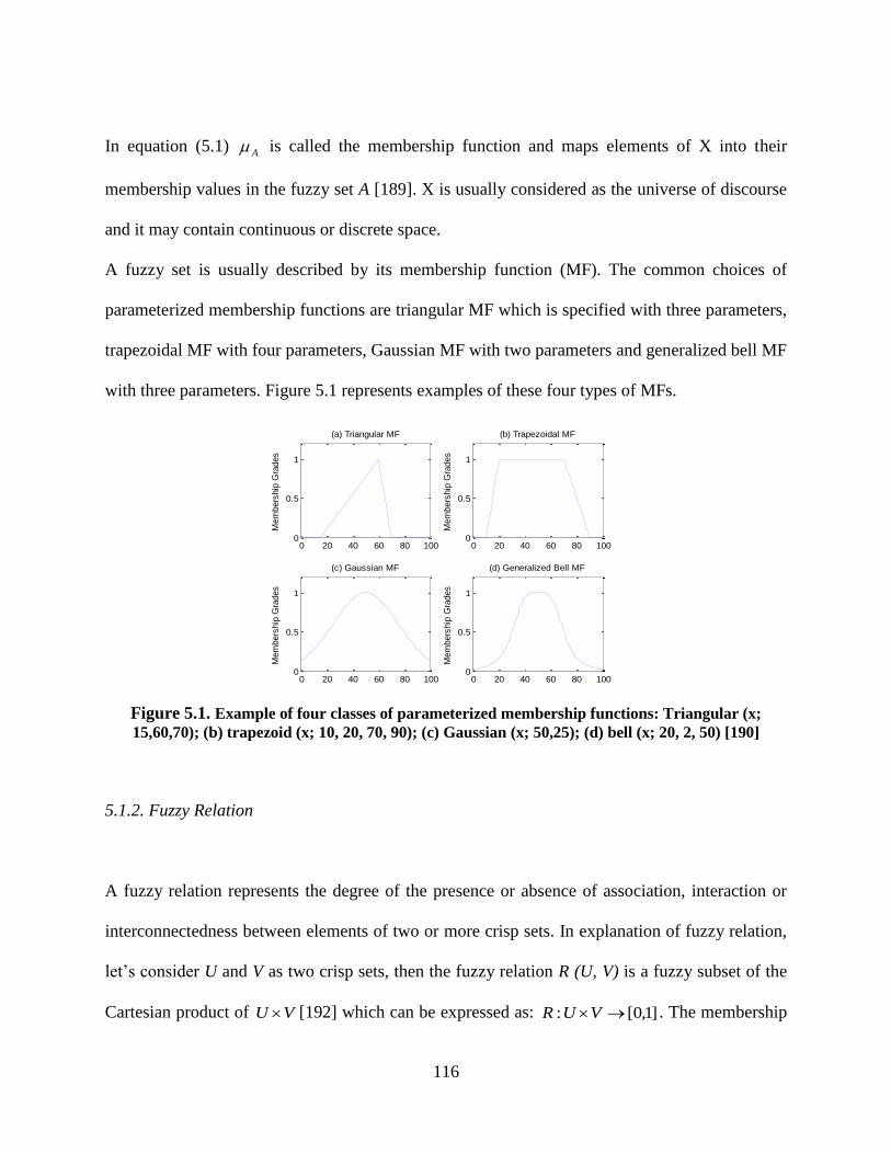
116

In equation (5.1) A is called the membership function and maps elements of X into their

membership values in the fuzzy set A [189]. X is usually considered as the universe of discourse

and it may contain continuous or discrete space.

A fuzzy set is usually described by its membership function (MF). The common choices of

parameterized membership functions are triangular MF which is specified with three parameters,

trapezoidal MF with four parameters, Gaussian MF with two parameters and generalized bell MF

with three parameters. Figure 5.1 represents examples of these four types of MFs.

Figure 5.1. Example of four classes of parameterized membership functions: Triangular (x;

15,60,70); (b) trapezoid (x; 10, 20, 70, 90); (c) Gaussian (x; 50,25); (d) bell (x; 20, 2, 50) [190]

5.1.2. Fuzzy Relation

A fuzzy relation represents the degree of the presence or absence of association, interaction or

interconnectedness between elements of two or more crisp sets. In explanation of fuzzy relation,

let’s consider U and V as two crisp sets, then the fuzzy relation R (U, V) is a fuzzy subset of the

Cartesian product of VU [192] which can be expressed as: ]1,0[: VUR . The membership

0 20 40 60 80 1000

0.5

1

Mem

bers

hip

Gra

des

(a) Triangular MF

0 20 40 60 80 1000

0.5

1

Mem

bers

hip

Gra

des

(b) Trapezoidal MF

0 20 40 60 80 1000

0.5

1

Mem

bers

hip

Gra

des

(c) Gaussian MF

0 20 40 60 80 1000

0.5

1

Mem

bers

hip

Gra

des

(d) Generalized Bell MF

117

function of R is ),( yxR where Ux and Vy .Here for each pair (x,y), there is a membership

value between zero and one. If ),( yxR =1, then it means that x and y are fully related and if ),( yxR

=0, it means that the two elements x and y are not related at all. Obviously the values between zero

and one for ),( yxR reflect the partial association.

5.1.3. Linguistic Variable

As it was mentioned by Zadeh [193], conventional techniques for system analysis are essentially

unsuitable for dealing with humanistic systems, whose behavior is strongly influenced by human

judgment. This is called principle of incompatibility:” As the complexity of a system increases,

our ability to make a precise and significant statement about its behavior diminishes until a

threshold is reached where precision and significance become almost mutually exclusive

characteristics” [193]. Because of this belief Zadeh proposed the concept of linguistic variables as

alternative approach to model human thinking. An example for linguistic variables can be the

“age”. For example, if a man at age 60 is old, then we don’t know whether a 58 years old man is

old or not. Hedges are not used too often; examples of them can be very, quite, more or less, etc.

So we can say that a 58 years old man is quit old. The formal definition of linguistic variables is

given below.

A linguistic variable is characterized by a 5-tuple (x, T(x), X, G, M) [194], where x is the name of

the variable, X is the universe of discourse, T is the term set, which is the set of terminal symbols

that can actually appear in a linguistic term. G is a syntactic rule which generates linguistic terms

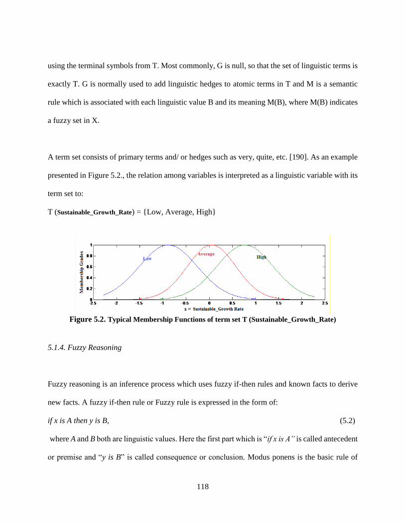
118

using the terminal symbols from T. Most commonly, G is null, so that the set of linguistic terms is

exactly T. G is normally used to add linguistic hedges to atomic terms in T and M is a semantic

rule which is associated with each linguistic value B and its meaning M(B), where M(B) indicates

a fuzzy set in X.

A term set consists of primary terms and/ or hedges such as very, quite, etc. [190]. As an example

presented in Figure 5.2., the relation among variables is interpreted as a linguistic variable with its

term set to:

T (Sustainable_Growth_Rate) = {Low, Average, High}

Figure 5.2. Typical Membership Functions of term set T (Sustainable_Growth_Rate)

5.1.4. Fuzzy Reasoning

Fuzzy reasoning is an inference process which uses fuzzy if-then rules and known facts to derive

new facts. A fuzzy if-then rule or Fuzzy rule is expressed in the form of:

if x is A then y is B, (5.2)

where A and B both are linguistic values. Here the first part which is “if x is A” is called antecedent

or premise and “y is B” is called consequence or conclusion. Modus ponens is the basic rule of

119

inference in traditional two-valued logic. Here the truth of proposition B can be determined from

the truth of A and the implication BA .

However, in most of human reasoning, modus ponens is used in an approximate manner.

premise1 (fact): x is A ,

premise2 (rule): if x is A then y is B

-------------------------------------------

Consequence (conclusion): y is B

where A is close to A and B is close to B. Also A, B, A and B all are fuzzy sets of approximate

universe. This inference procedure is called approximate reasoning or generalized modus ponens

[195]. The MF of B can be determined from Equation 1.7 where and are max and min:

)()]()([)],(),(min[max)( yxxyxxy BAAxRAyB (5.3)

5.1.5. Fuzzy Inferential Systems

A fuzzy inference system is based on fuzzy reasoning, fuzzy if-then rules and fuzzy set theory. Its

applications can be found in many fields such as decision analysis, time series prediction, expert

system, etc. As a fuzzy inference system is multi-disciplinary, it is known by many names [196]

[197] such as fuzzy model, fuzzy associative memory, etc.

Fuzzy inference systems are the most important modeling tool based on fuzzy set theory. The basic

components for the structure of a fuzzy inference system are: first a rule base, which is made up

of fuzzy rules; second a database, which stores membership functions used in fuzzy rules; third a

reasoning mechanism, which performs the inference procedure based on rules and given facts to

derive a reasonable output; fourth a fuzzification interface which converts crisp data inputs into

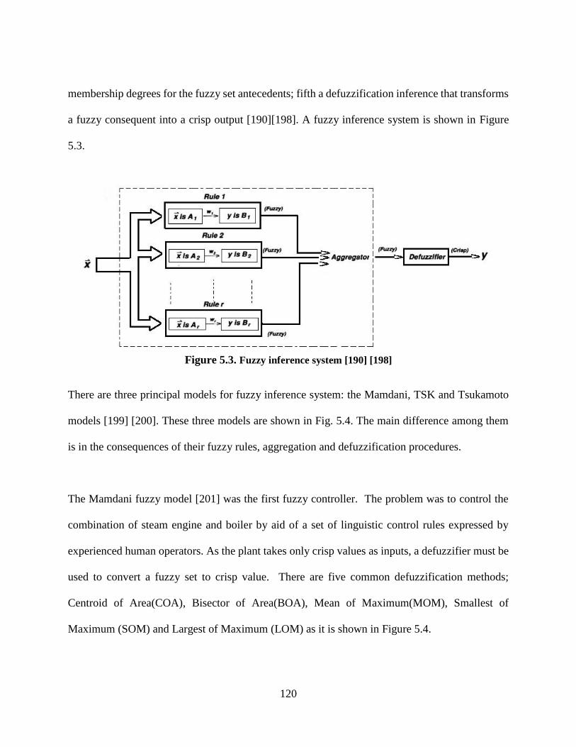
120

membership degrees for the fuzzy set antecedents; fifth a defuzzification inference that transforms

a fuzzy consequent into a crisp output [190][198]. A fuzzy inference system is shown in Figure

5.3.

Figure 5.3. Fuzzy inference system [190] [198]

There are three principal models for fuzzy inference system: the Mamdani, TSK and Tsukamoto

models [199] [200]. These three models are shown in Fig. 5.4. The main difference among them

is in the consequences of their fuzzy rules, aggregation and defuzzification procedures.

The Mamdani fuzzy model [201] was the first fuzzy controller. The problem was to control the

combination of steam engine and boiler by aid of a set of linguistic control rules expressed by

experienced human operators. As the plant takes only crisp values as inputs, a defuzzifier must be

used to convert a fuzzy set to crisp value. There are five common defuzzification methods;

Centroid of Area(COA), Bisector of Area(BOA), Mean of Maximum(MOM), Smallest of

Maximum (SOM) and Largest of Maximum (LOM) as it is shown in Figure 5.4.

121

Figure 5.4. Defuzzification methods

Sugeno fuzzy model which is also known as TSK fuzzy model was proposed by Takagi, Sugeno

and Kang [196] [198]. The aim of this model is to develop a systematic approach to generate fuzzy

rules from a given input-output data set. Here a typical fuzzy rule is presented like this:

If x is A and y is B then z = f(x, y) (5.4)

In 5.5 A and B are fuzzy sets in antecedent and z is a crisp function in the consequence. Mainly

f(x,y) is a polynomial function but it can be any function as far as it can completely represent the

output of a model within the fuzzy region defined by the antecedents of the rule. If the function is

first-order, then there is a first-order TSK fuzzy model and so on. The output level iz of each rule

is weighted by the firing strength iw of the rule. The final output is the weighted average of all

outputs represented as:

N

i

i

N

i

ii

z

zw

z

1

1 (5.5)

where iz is a first order polynomial.

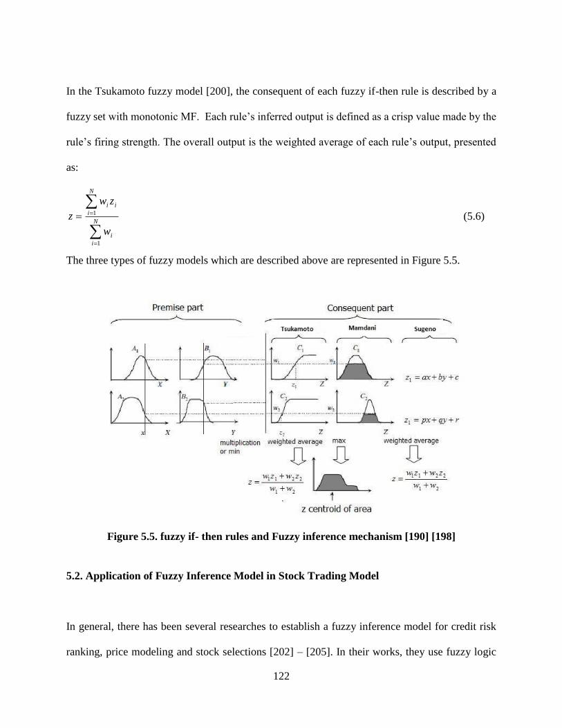
122

In the Tsukamoto fuzzy model [200], the consequent of each fuzzy if-then rule is described by a

fuzzy set with monotonic MF. Each rule’s inferred output is defined as a crisp value made by the

rule’s firing strength. The overall output is the weighted average of each rule’s output, presented

as:

N

i

i

N

i

ii

w

zw

z

1

1 (5.6)

The three types of fuzzy models which are described above are represented in Figure 5.5.

Figure 5.5. fuzzy if- then rules and Fuzzy inference mechanism [190] [198]

5.2. Application of Fuzzy Inference Model in Stock Trading Model

In general, there has been several researches to establish a fuzzy inference model for credit risk

ranking, price modeling and stock selections [202] – [205]. In their works, they use fuzzy logic

123

and other technical analysis tools with the help of financial indicators such as moving average to

help with financial decision making. Some works have proposed a fuzzy model to track the trend

of financial indices [206] while others proposed a fuzzy model for stock/price prediction [207]

[208] or a hybrid system for time series forecasting [209].

In this section, we have proposed a fuzzy inference model as recommendation model for stock

management using selected financial variables as outcome of previous chapters; feature selection

and missing data analysis. In the following, first a description and the associated categories of

selected financial variables for the proposed model is given. Then, with using the selected financial

features/variables, we present a practical Fuzzy Inference Model (FIM) to assess DJIA stocks and

their prices to buy, hold or sell the stocks. To access criteria influencing DJIA stock prices, all

selected financial features are examined and 5 groups influencing the stock price is proposed as it

is shown in Table 5.1. With the selected features and groups, we determine which situation leads

to a better management of stocks. MATLAB© fuzzy toolbox and coding is used for our

experimental modeling and evaluations.

Share Price Rationality

Price to Book Ratio

Profitability

Operating Income Per Share

Continuing Income Per Share

Revenue Per Share

Efficiency

Asset Turnover

Growth

Book Value of Equity Per Share

Growth Rate

Sustainable Growth Rate

Leverage

Debt to Market Cap

Table 5-1. Financial features/ variables with related financial category

124

5.2.1. Selected Financial Features in Fuzzy Recommendation Model

To evaluate the financial models, there are couple of categories which are studied in the

literarture such as profitability, efficiency and etc [211]. In the following we discusse the

selected features using LmRMR in their related financial categories.

5.2.1.1. Share Price Rationality

Price to Book Ratio

This is a financial ratio of company’s price divided by its book value. This ratio can be indicator

of how aggressively the market values a company and whether investors are over paying if the

company goes to bankruptcy immediately. It is one of the important financial variables in stock

evaluation model. With considering the fixed growth, the higher value of this variable means

that the company is less risky for the investment [98]. Here, growth is important as we can see

small, risky start-up companies with high price to earnings ratio. This means market’s

expectation of high growth rate for these companies.

Price to earnings ratio can be calculated in two ways; first company’s market cap is divided by

its total book value. Second way is using per share value and divide company’s current price

by book value per share. No matter which way is used, the outcome should be the same.

)eAssets(Intangibl-Assets Total

StockPrice

BookValue

StockPriceP/BRatio

sLiabilitie (5.7)

5.2.1.2. Profitability

Operating Income Per Share

This Financial variable is also defined as operating profit or EBIT (Earnings Before Interest

and Taxes). It is the profit earned from company’s business operations and does not cover the

125

profit of company’s investment. This ratio shows the earning power of the company

considering its ongoing operations and indicates the business potential profitability. It is

calculated as in Equation 5.8. The Operating Income Per Share is the same formula divide by

number of shares.

Operating Income= Revenue – Operating Costs (OPEX) (5.8)

Continuing Income Per Share

This financial variable indicates the income which is generated by the company’s continuing

operations. A company needs to generate earnings from operations to succeed in long term.

Therefore, analysts make a separate income statement which differentiates income from

continuing operations from non-recurring or non-operating items. The non-operating incomes

can be earnings from acquisitions, mergers, discounted products or discontinued operations.

Overall this financial variable represents what a company can expect from future earnings and

give the investors a realistic picture of how the company is faring.

Revenue Per Share

Revenue per share is the amount of money per share which a company or a company earns

from its business activities or companies’ client pay to the company. It is the heart of the

fundamental analysis of a company. If a company does not have revenue, the existence of it

is meaningless. If the revenue per share is calculated quarterly, formula 5.9 can represent it.

Revenue Per Share = Quarterly Revenue / Common Share Outstanding (5.9)

126

5.2.1.3. Efficiency

Asset Turnover

Asset turnover is a financial variable which represents the ability of a company to use its assets

to generate sales. Here all assets are considered either current or fixed. Overall this variable is

indicator of the efficiency of a company in using its assets for revenue generating. Higher

value of asset turnover shows that company’s performance is better. Below shows the formula

used for the calculation of this variable.

Asset Turnover = Revenue Or Sales – Total Assets (5.10)

5.2.1.4. Growth

Book Value of Equity Per Share Growth Rate

This fundamental financial variable represents the growth of stock’s Book Value of equity Per

Share (BVPS). Book value growth is one of the factors that investors use to determine the

value of stock and if it is undervalued. If this variable increases, investors consider this stock

more valuable and the price of the stock goes up. BVPS is calculated as it is shown in

following formula, by dividing the equity of shareholders by the number of shares issued.

Also, if the number of shares increase as a matter of issuing more shares equity financing or

exercising employee stock options, BVPS Growth rate decreases.

BVPS Growth = Value Of Common Equity / Number of Shares Outstanding (5.11)

Sustainable Growth Rate

Sustainable Growth Rate (SGR) represents the optimal growth of a company can have without

being force to increase its financial leverage or considering refinancing. In another word, it

127

shows company’s pace and depth of growth without borrowing money. If a company has

reached to its SGR ceiling, it means that besides its own resources, the company needs to

borrow funds or debt securities to facilitate its growth. Company’s SGR is calculated as

formula 5.12. It means that SGR is product of return of company’s equity and fraction of

remaining earnings after dividend being paid out.

SGR = Return on Equity * (1 – Dividend Payout Ratio) (5.12)

5.2.1.5. Leverage

Debt to Market Cap

This financial variable represents the amount of company’s debt; both short term and long term

liabilities; as a percentage of its total. It is a measurement of company’s leverage or the usage

of debt to purchase assets. Analysts and investors look at this variable to make sure the

company is healthy and suitable for investments. The formula is as following:

Debt to Market Capitalization =sEquityr'ShareHoldebtLongTermDeebtShortTermD

btLongTermDeebtShortTermD

(5.13)

5.2.2. Stock Market Trading Model (SMTM)

The proposed Stock trading recommendation model is based on Fuzzy Inference Model (FIM) and

the selected financial variables which we discussed in the previous chapters. The implementation

is a Mamdani FIM with Gaussian membership functions both for inputs and outputs. The model

includes two layers of FIM as it is shown in Figure 5.6; first layer considers inputs for growth

which are BVPS-Growth-Rate and Sustainable-Growth-Rate; and also profitability with three

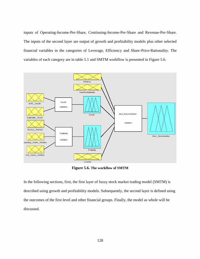
128

inputs of Operating-Income-Per-Share, Continuing-Income-Per-Share and Revenue-Per-Share.

The inputs of the second layer are output of growth and profitability models plus other selected

financial variables in the categories of Leverage, Efficiency and Share-Price-Rationality. The

variables of each category are in table 5.1 and SMTM workflow is presented in Figure 5.6.

Figure 5.6. The workflow of SMTM

In the following sections, first, the first layer of fuzzy stock market trading model (SMTM) is

described using growth and profitability models. Subsequently, the second layer is defined using

the outcomes of the first level and other financial groups. Finally, the model as whole will be

discussed.

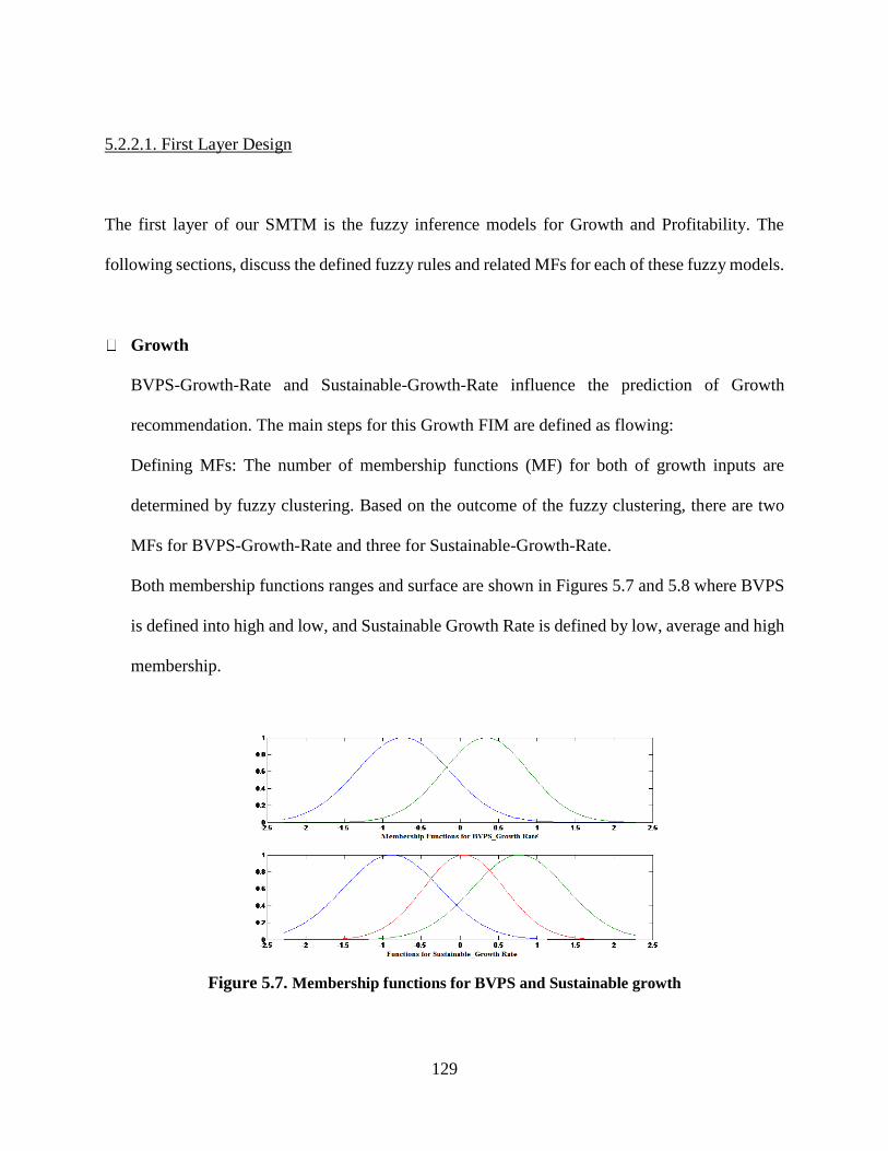
129

5.2.2.1. First Layer Design

The first layer of our SMTM is the fuzzy inference models for Growth and Profitability. The

following sections, discuss the defined fuzzy rules and related MFs for each of these fuzzy models.

Growth

BVPS-Growth-Rate and Sustainable-Growth-Rate influence the prediction of Growth

recommendation. The main steps for this Growth FIM are defined as flowing:

Defining MFs: The number of membership functions (MF) for both of growth inputs are

determined by fuzzy clustering. Based on the outcome of the fuzzy clustering, there are two

MFs for BVPS-Growth-Rate and three for Sustainable-Growth-Rate.

Both membership functions ranges and surface are shown in Figures 5.7 and 5.8 where BVPS

is defined into high and low, and Sustainable Growth Rate is defined by low, average and high

membership.

Figure 5.7. Membership functions for BVPS and Sustainable growth

130

Figure 5.8. MF surface plot for Growth

Decide number of rules: The number of rules for this model is six which are as presented as

following. Here BVPS_Growth and Sustainable_Growth are linguistic variables and Low,

Average and High are fuzzy sets on these variables. The antecedents are aggregated and results

single consequent output of the rule.

If BVPS_Growth is Low and Sustainable_Growth is Low, then Growth is Low

If BVPS_Growth is Low and Sustainable_Growth is Average, then Growth is Average

If BVPS_Growth is Low and Sustainable_Growth is High, then Growth is Average

If BVPS_Growth is High and Sustainable_Growth is Low, then Growth is Average

If BVPS_Growth is High and Sustainable_Growth is Average, then Growth is High

If BVPS_Growth is High and Sustainable_Growth is High, then Growth is High

Fuzzy reasoning for two inputs, single output: For each rule, compute the degree of

compatibility with respect to each antecedent MF. Then, compute the degree of compatibility

with respect to antecedents MFs in a rule using AND operator to form firing strength

representing the degree of satisfaction for antecedent part. This degree is applied to consequent

part of rule which Growth to generate into MF. Finally, all six consequent MFs are aggregate

to find the final output MF for Growth.

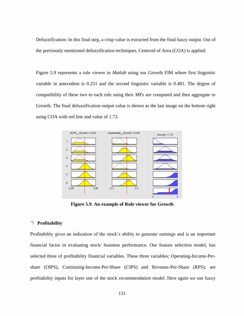
131

Defuzzification: In this final step, a crisp value is extracted from the final fuzzy output. Out of

the previously mentioned defuzzification techniques, Centroid of Area (COA) is applied.

Figure 5.9 represents a rule viewer in Matlab using our Growth FIM where first linguistic

variable in antecedent is 0.251 and the second linguistic variable is 0.481. The degree of

compatibility of these two to each rule using their MFs are computed and then aggregate to

Growth. The final defuzzification output value is shown as the last image on the bottom right

using COA with red line and value of 1.72.

Figure 5.9. An example of Rule viewer for Growth

Profitability

Profitability gives an indication of the stock’s ability to generate earnings and is an important

financial factor in evaluating stock/ business performance. Our feature selection model, has

selected three of profitability financial variables. These three variables; Operating-Income-Per-

share (OIPS), Continuing-Income-Per-Share (CIPS) and Revenue-Per-Share (RPS); are

profitability inputs for layer one of the stock recommendation model. Here again we use fuzzy

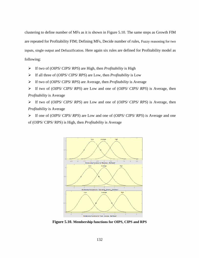
132

clustering to define number of MFs as it is shown in Figure 5.10. The same steps as Growth FIM

are repeated for Profitability FIM; Defining MFs, Decide number of rules, Fuzzy reasoning for two

inputs, single output and Defuzzification. Here again six rules are defined for Profitability model as

following:

If two of (OIPS/ CIPS/ RPS) are High, then Profitability is High

If all three of (OIPS/ CIPS/ RPS) are Low, then Profitability is Low

If two of (OIPS/ CIPS/ RPS) are Average, then Profitability is Average

If two of (OIPS/ CIPS/ RPS) are Low and one of (OIPS/ CIPS/ RPS) is Average, then

Profitability is Average

If two of (OIPS/ CIPS/ RPS) are Low and one of (OIPS/ CIPS/ RPS) is Average, then

Profitability is Average

If one of (OIPS/ CIPS/ RPS) are Low and one of (OIPS/ CIPS/ RPS) is Average and one

of (OIPS/ CIPS/ RPS) is High, then Profitability is Average

Figure 5.10. Membership functions for OIPS, CIPS and RPS

133

5.2.2.2. Final Design

In the implementation of this fuzzy model Mamdani fuzzy inference with Gaussian membership

functions are used both for input and outputs. Three membership functions for all inputs and output

of layer two are defined. This way it can give a better overview of Low, Average and High values

of selected features.

As discussed, fuzzy rules are based on If-Then conditions with linguistic variables. This way the

fuzzy model can mimic the human way of thinking and represent the uncertainty in the decision

makings. In Fuzzy Inference Modeling, usually after defining rules and membership functions, the

designer can refine the model with experimenting the rules and membership function to find

suitable results.

The inputs of the second layer consist of outputs of first layer (Growth and Profitability) and inputs

of Share-Price-Rationality, Leverage and Efficiency. The SMTM consists of seven components;

Database including Membership Function base, Fuzzy Rule base, Fuzzy Inference engine and

Defuzzification.

Membership Function base: it defines the membership function of linguistic variable terms. The

membership functions of the five financial categories are presented in tables 5.2. to 5.6.

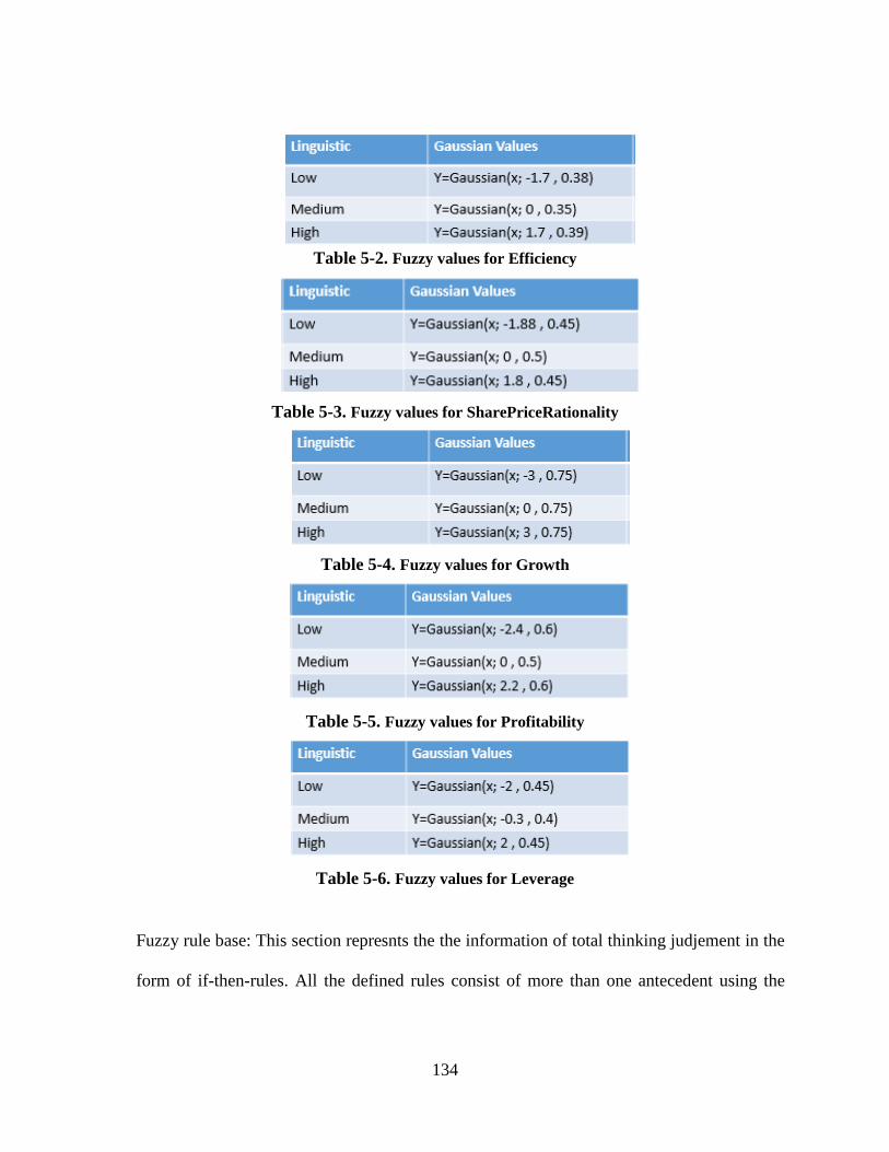
134

Table 5-2. Fuzzy values for Efficiency

Table 5-3. Fuzzy values for SharePriceRationality

Table 5-4. Fuzzy values for Growth

Table 5-5. Fuzzy values for Profitability

Table 5-6. Fuzzy values for Leverage

Fuzzy rule base: This section represnts the the information of total thinking judjement in the

form of if-then-rules. All the defined rules consist of more than one antecedent using the

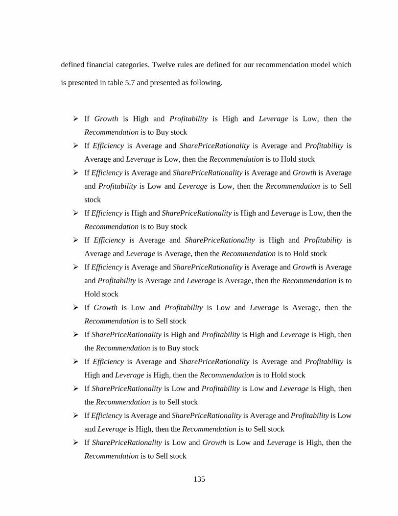
135

defined financial categories. Twelve rules are defined for our recommendation model which

is presented in table 5.7 and presented as following.

If Growth is High and Profitability is High and Leverage is Low, then the

Recommendation is to Buy stock

If Efficiency is Average and SharePriceRationality is Average and Profitability is

Average and Leverage is Low, then the Recommendation is to Hold stock

If Efficiency is Average and SharePriceRationality is Average and Growth is Average

and Profitability is Low and Leverage is Low, then the Recommendation is to Sell

stock

If Efficiency is High and SharePriceRationality is High and Leverage is Low, then the

Recommendation is to Buy stock

If Efficiency is Average and SharePriceRationality is High and Profitability is

Average and Leverage is Average, then the Recommendation is to Hold stock

If Efficiency is Average and SharePriceRationality is Average and Growth is Average

and Profitability is Average and Leverage is Average, then the Recommendation is to

Hold stock

If Growth is Low and Profitability is Low and Leverage is Average, then the

Recommendation is to Sell stock

If SharePriceRationality is High and Profitability is High and Leverage is High, then

the Recommendation is to Buy stock

If Efficiency is Average and SharePriceRationality is Average and Profitability is

High and Leverage is High, then the Recommendation is to Hold stock

If SharePriceRationality is Low and Profitability is Low and Leverage is High, then

the Recommendation is to Sell stock

If Efficiency is Average and SharePriceRationality is Average and Profitability is Low

and Leverage is High, then the Recommendation is to Sell stock

If SharePriceRationality is Low and Growth is Low and Leverage is High, then the

Recommendation is to Sell stock

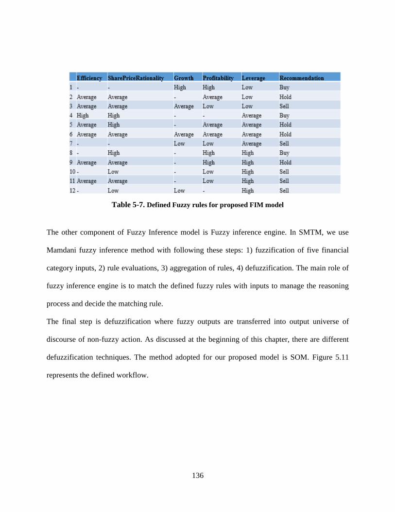
136

Table 5-7. Defined Fuzzy rules for proposed FIM model

The other component of Fuzzy Inference model is Fuzzy inference engine. In SMTM, we use

Mamdani fuzzy inference method with following these steps: 1) fuzzification of five financial

category inputs, 2) rule evaluations, 3) aggregation of rules, 4) defuzzification. The main role of

fuzzy inference engine is to match the defined fuzzy rules with inputs to manage the reasoning

process and decide the matching rule.

The final step is defuzzification where fuzzy outputs are transferred into output universe of

discourse of non-fuzzy action. As discussed at the beginning of this chapter, there are different

defuzzification techniques. The method adopted for our proposed model is SOM. Figure 5.11

represents the defined workflow.

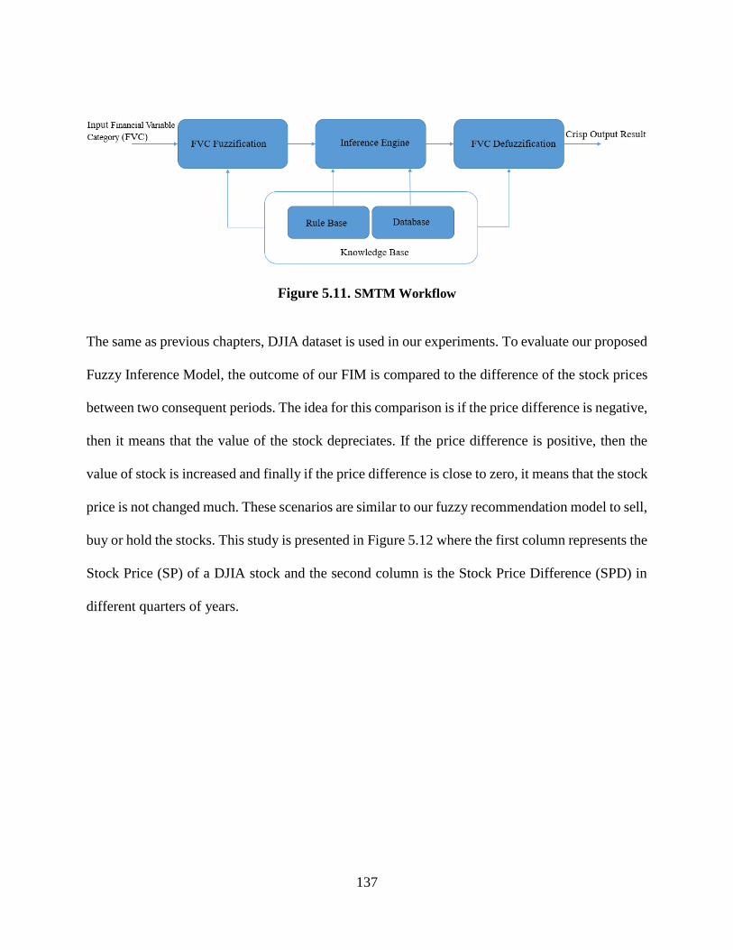
137

Figure 5.11. SMTM Workflow

The same as previous chapters, DJIA dataset is used in our experiments. To evaluate our proposed

Fuzzy Inference Model, the outcome of our FIM is compared to the difference of the stock prices

between two consequent periods. The idea for this comparison is if the price difference is negative,

then it means that the value of the stock depreciates. If the price difference is positive, then the

value of stock is increased and finally if the price difference is close to zero, it means that the stock

price is not changed much. These scenarios are similar to our fuzzy recommendation model to sell,

buy or hold the stocks. This study is presented in Figure 5.12 where the first column represents the

Stock Price (SP) of a DJIA stock and the second column is the Stock Price Difference (SPD) in

different quarters of years.

138

Figure 5.12. Benchmark model for SMTM

The results of the stock market fuzzy model are compared to the benchmark model using Root

Mean Square Error; equation 4.24. The outcome shows that our model can build the trading

model with only using twelve rules and error of less than 0.08.

5.3. Application in Price Forecasting

In this section, we want to study the application and value of previously selected features in stock

price forecasting. First, time series lag analysis is studied and the effectiveness of present data in

future price value is investigated. We show that by increase in number of lags, the uncertainty of

future price prediction increases.

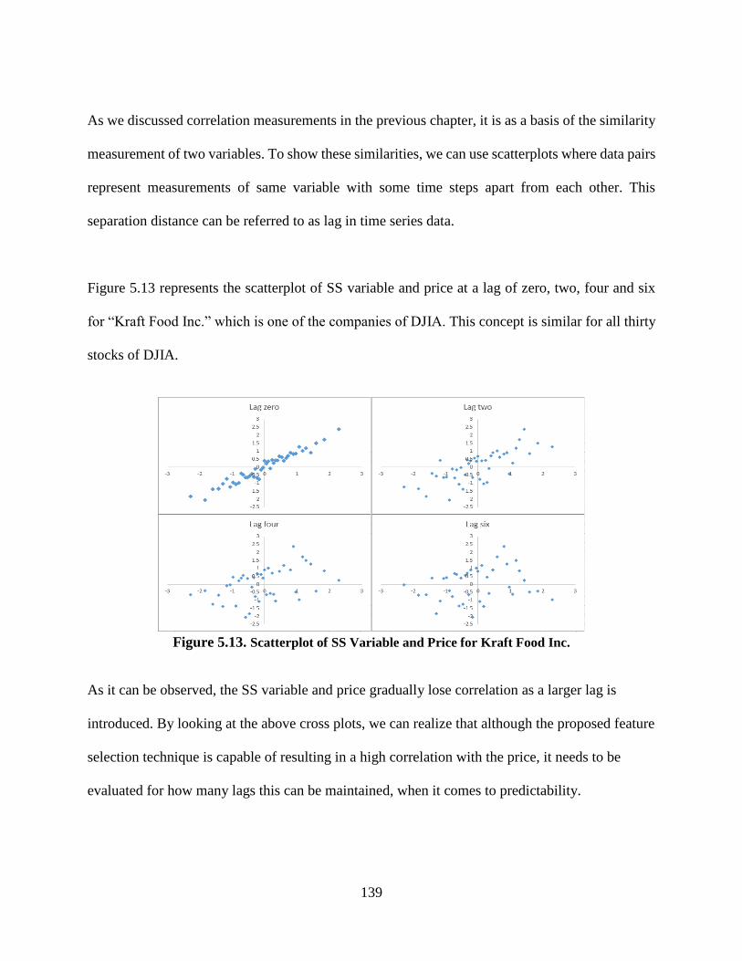
139

As we discussed correlation measurements in the previous chapter, it is as a basis of the similarity

measurement of two variables. To show these similarities, we can use scatterplots where data pairs

represent measurements of same variable with some time steps apart from each other. This

separation distance can be referred to as lag in time series data.

Figure 5.13 represents the scatterplot of SS variable and price at a lag of zero, two, four and six

for “Kraft Food Inc.” which is one of the companies of DJIA. This concept is similar for all thirty

stocks of DJIA.

Figure 5.13. Scatterplot of SS Variable and Price for Kraft Food Inc.

As it can be observed, the SS variable and price gradually lose correlation as a larger lag is

introduced. By looking at the above cross plots, we can realize that although the proposed feature

selection technique is capable of resulting in a high correlation with the price, it needs to be

evaluated for how many lags this can be maintained, when it comes to predictability.

140

5.3.1. Cross Variogram

There is a need to study and model the joint distributions of related features/variables. As discussed

above, the first assessment of the relation of two variables is the cross plot of collocated variables.

Generally, the relationship of the collocated variables does not represent the full relationship

between the two variables and cross temporal relationship between pairs of variables using lag

distance needs to be captured as well. Cross-variogram is a measure for this relationship between

two variables.

As discussed in the previous chapter, semi-variogram of one variable is represented by Equation

5.14. The extension of this formula for two variables (cross-variogram) is given by Equation 5.15.

))}()())(()({(2

1})]()({[

2

1)( 2

, huZuZhuZuZEhuZuZEhZZ (5.14)

))}()())(()({(2

1)(, huYuYhuZuZEhYZ (5.15)

As it is shown in the above formula, semi-variogram of two variables is the average product of

their differences for same location and lag distance.

If we standardize the dataset (Mean of zero and variance of one) then, we can replace covariance

with correlation coefficient and the equation can be expanded in Equation 5.16.

141

))}().()().()().()().({(2

1)(, huYhuZuYhuZhuYuZuYuZEhYZ

)]()([2

1)0()]0()()()0([

2

1)(, hChCCChChCCh YZZYZYZYYZZYZYYZ

)()0()]()([2

1)0()(, hhhh ZYZYYZZYZYYZ (5.16)

5.3.2. Price Forecasting Potential

As discussed in chapter two, there is a wide range of agreement that price evaluation and

forecasting are of primary importance in the financial domains. In order to determine an

appropriate and defensible range of price value and realistic assessment of the market, different

techniques are proposed.

In this research we study the value of previously selected financial features in future stock price

prediction. We study the lag analysis of our selected features, SS variable and price of our stocks.

Cross variogram modeling is used to discover the effectiveness of the present data in predicting

the next steps prices of stocks and also determine when the future price predictions erode and

uncertainty increases with increasing the number of lags.

The graphs in Figure 5.14. represent the cross-variograms of selected features and price for Craft

Food Inc which is one of the DJIA companies. The number of lags and ranges are given in each

cross variogram. The data point in graph at lag zero represents the correlation of the feature with

price. Among all the selected features, Asset-Turnover and Debt-To-Market-Cap have the highest

correlation with the price. As we can see, by the increase in the number of lags, the correlation of

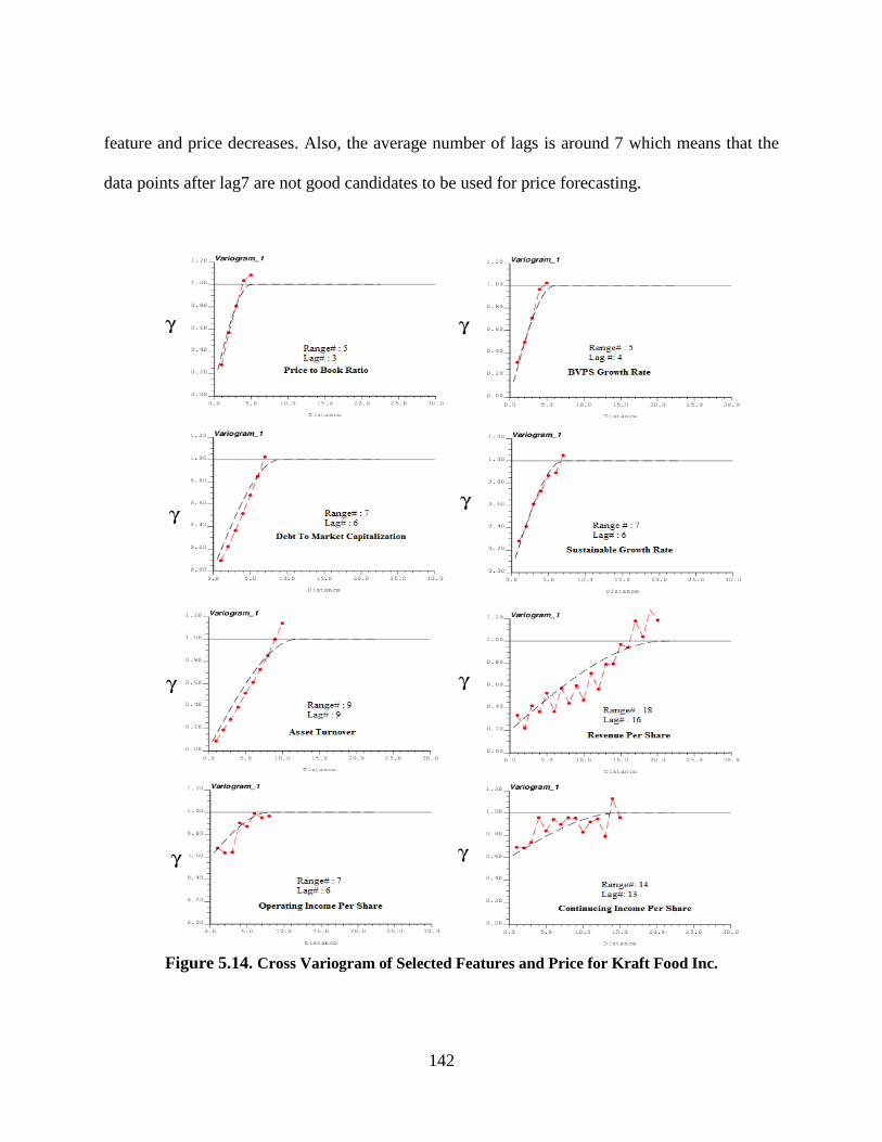
142

feature and price decreases. Also, the average number of lags is around 7 which means that the

data points after lag7 are not good candidates to be used for price forecasting.

Figure 5.14. Cross Variogram of Selected Features and Price for Kraft Food Inc.

143

Figure 5.15 captures cross plot of SS Variable and price for Kraft Food Inc., with the range of

seven and number of lags of seven. As expected, correlation of SS Variable and price at lag

zero is more than all other selected features individually with SSTC of 97%.

Figure 5.15. Cross Variogram of Super Secondary Variable and Price for Kraft Food Inc.

In above cross variogram, the range of data is reported as seven. This means that up to seven

lags, SS variable can be used for price prediction. This value is also consistent with average

number of lags for individual features of this dataset.

There are eight common selected features using missing imputation techniques: Price-Book-

Ratio, Tot-Debt-Mark-Cap, BVPS-Growth, Sust-Growth, Ass-Turnover, Cont-Inc-Per-Share,

Opt-Inc-Per-Share, Rev-Per-Share which are important factors affecting the price of stocks in

Dow Jones dataset. Evaluating their temporal variability using the features individually or their

combination in SS variable, can lead us to predicting the price of stocks. The effect of these

variables can be considered up to seven lags in future forecasting as discussed before. Figure

5.16 is a representation of this idea.

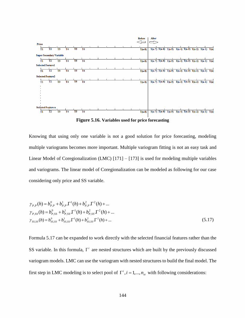
144

Figure 5.16. Variables used for price forecasting

Knowing that using only one variable is not a good solution for price forecasting, modeling

multiple variograms becomes more important. Multiple variogram fitting is not an easy task and

Linear Model of Coregionalization (LMC) [171] – [173] is used for modeling multiple variables

and variograms. The linear model of Coregionalization can be modeled as following for our case

considering only price and SS variable.

...)(.)(.)( 22

,

11

,

0

,, hbhbbh PPPPPPPP

...)(.)(.)( 22

,

11

,

0

,, hbhbbh SSPSSPSSPSSP

...)(.)(.)( 22

,

11

,

0

,, hbhbbh SSSSSSSSSSSSSSSS (5.17)

Formula 5.17 can be expanded to work directly with the selected financial features rather than the

SS variable. In this formula, i are nested structures which are built by the previously discussed

variogram models. LMC can use the variogram with nested structures to build the final model. The

first step in LMC modeling is to select pool of st

i ni ,...,1, with following considerations:

145

The sill parameters should consider some constraints:

i

SSP

i

SSP

i

SSSS

i

PP

i

SSSS

i

PP

i

bbbb

b

b

,,,,

,

,

0.0.

0

0

Each nested structure has a variogram type and reasonable range.

Besides, all the variables/features of variograms should be modeled by the selected nested

structures. As a future work, there are automatic fitting algorithms which can be used for this type

of modeling as well [173]. The above modeled variograms can be evaluated to be directly used in

multivariate statistical realm. But to be more holistic LMC is needed.

5.4. Conclusions

In this chapter, we presented two practical approaches to analyze the utilization of selected

financial features/variables in financial domains. As it is discussed in the previous chapters and

specifically in the literature review, there are different applications of financial feature selection

in financial domains. Two of these applications are stock trading and price modeling.

The first section of this chapter presented a fuzzy inference model for stock market trading; when

to buy, sell or hold the stocks. Usually traders consider couple of known factors/ features for their

analysis. There are also intelligent approaches in the literature. We suggest a model that with only

consideration of twelve simple rules using our selected features, can predict the performance of

market with more than 92% of accuracy. Then, we studied the effectiveness of our selected features

146

in price modeling by using cross variogram and presenting the number of lags and range of our

variables. A few potential future research ideas in this area are also suggested.

147

CHAPTER 6: CONCLUSION AND FUTURE WORK

In this PhD research a global data pre-processing methodology for financial variables/features is

presented. The two main components of the proposed methodology are Missing Data Analysis and

Financial Feature Selection including ranking features and feature subset selection. The developed

methodology is studied on Dow Jones Industrial Average (DJIA) dataset as well as a synthetic

dataset. It is shown that our methodology provides better input variables than similar existing

techniques. Finally, two financial applications of the selected features in stock market trading

model and price prediction are discussed.

In the following we summarize our contributions and results with outline future research

directions.

6.1. Summary and Conclusion

Financial variables are of primary importance in financial price modeling, economic predictions,

risk evaluations, portfolio management and etc. There usually exist many financial variables,

where their exhaustive integration in a model increases its dimensionality and the associated

computational time. We extensively tackle this problem in this research.

A novel approach is developed for feature selection based on the mutual relationships between the

financial variables as well as their relationships with the financial price/return as they are

collectively measured by Spearman correlation coefficients. It is then applied to evaluate the Dow

Jones Industrial Average financial features/variables. We conducted experiments to study the

148

effectiveness and applicability of the proposed approach both in terms of financial variable

selection as well as its application in stock market evaluations as well as price forecasting. The

performance is evaluated by Super Secondary Target Correlation (SSTC) measurement.

We also presented a new method which allows the use of spatial statistics such as Bayesian

Updating technique to estimate missing values in time series datasets. For prior modeling, Simple

Kriging algorithm is applied. The final estimate and related uncertainty of missing data is the

predicted through combining prior estimates with the super-secondary variables that are calculated

via likelihood modeling. The inspiration of adapting the Bayesian updating for missing data

analysis comes from its successful application in predicting the unsampled location data in spatial

statistics. It considers the existence of dependencies both latitudinal; in time series; and

longitudinal; along other variables; and then estimates missing values. The dependencies among

the variables as well dependencies in each variable though time, make Bayesian updating a suitable

candidate for missing data estimation. In order to evaluate our results, we have created a synthetic

dataset and five different techniques is used; four existing imputation techniques, Ordinary Kriging

and Bayesian Updating. Subsequently, the related RMSE value for each technique is calculated

and the results are compared. The same approach is applied on DJIA where missing intervals are

imputed using Nearest Neighborhood, Simple Kriging, Ordinary Kriging and Bayesian updating

imputation techniques are applied. The results show that both Bayesian Updating and Ordinary

Kriging are superior to the other existing techniques.

We also analyze the utilization of the selected financial variables in to two financial evaluation

workflows; stock market trading model and price forecasting. A fuzzy inference model is built for

149

the stock market trading model. The outcome represents the effectiveness of selected financial

variables as technical indicators which can be used by traders to study trend of market and make

decision on buy, sell or hold based on their observations. This system generates satisfactory

recommendations when output is compared with actual data. Then, we study the value of selected

features individually or after being combined through SS variable in future stock price forecasting

using lag analysis and cross variogram modeling. Also, the concept of LMC and multivariate

statistic is briefly touched on. As the scope of this study is very broad, it can be extended and

employed in future works.

6.2. Future Work

Financial features also called financial variables or indicators are main part of any financial

modeling, analysis or decision making with the use in corporate finance, accounting and

investment banking. The financial features can be studied in both microeconomic and

macroeconomic disciplines using fundamentals including the qualitative and quantitative

information.

In this thesis, the adopted financial features are mainly fundamental features/factors used for

company’s financial condition evaluation and are mostly available in the income statement or

balance sheets. In the literature these features are characterized into different subcategories such

as liquidity, profitability, efficiency and etc. Besides these fundamental features, there are

macroeconomic features/factors such as GDP Growth and inflation that affects the target financial

model as well. Other forms of financial features can be Analyst factors which is created by

150

financial analysts; or Social factors which is result of social concerns. Analyst factors can be the

outcome of a Wall Street analyst’s recommendation in predicting a stock return. An example of

financial factor is high-EPS-forecast which represents the highest analyst estimate for The firm’s

EPS. Also, an example of the Social factors can be management’s relation with employee which

is a fuzzy measurement affecting the financial model. Although the information of this factor is

fuzzy, still it may indicate an advantage/disadvantage in future firm’s performance. Consideration

of these additional financial factors can be an asset in improving the financial model performance.

This can be particularly the case for other financial datasets that have been out of scope of this

study.

Although data preprocessing is the basis of any financial decision making and analysis, it is

mostly neglected. Two important pre-processing steps are missing data analysis and feature

subset selection which are discussed in this research. We also study the applications of our

methodology in a stock trading recommendation model (SMTM) and price predictions. The

other potential future development of this research can be in the applications of our

preprocessing methodology in other areas of financial domain such as:

Financial distress evaluations including bankruptcy prediction and credit scoring,

Benchmarking financial performance of a firm/corporation against similar companies in

the same industry. This helps the corporation to realize its strength and weakness and if it

is needed, make improvement to meet the expectations.

Firm/company management decision making using scenario planning.

Study stock trend or pattern with potential profitability.

151

Analyzing the future performance of the companies’ stocks in Merger and acquisition of

the companies.

Building predictive models showing future activities such as Bond rating

Fraud discovery by identifying the most significant financial items detected in the

financial statement.

Financial risk modeling including credit risk, currency risk, foreign investment risk and

etc.

Stock ranking and portfolio selection

All of the above areas can be modeled and studied in depth. With the use of our preprocessing

methodology and an intelligent modeling tool, the performance of the target financial model can

be improved.

We also introduced the concept of LMC for multiple variable’s variogram modeling in chapter six.

It can be useful to adopt the concepts of automated LMC modeling and multiple variate statistics

in the price forecasting.

Finally, one of the main problems that financial analysts are faced with is the issue of scale or

frequency conversion. This means that they need to convert data in to the consistent time intervals.

The reported time intervals for financial datasets can be in formats such as daily, monthly,

quarterly or annually. In this research the adopted financial features found in companies’ balance

sheets are reported in quarterly time intervals. Therefore, we converted our daily price/return in to

quarterly frequency to be compatible with our features. One of the potential extensions of our

research is to study the temporal relationships between datasets with different frequencies and to

152

maximize utilization of information content available in higher frequency datasets. A simplest

form of this concept can be the frequency conversion of lower frequent data with quarterly

intervals in to higher frequent data with daily intervals. Maximizing the utilization of information

content in higher frequency datasets can improve our pre-processing methodology both in missing

data analysis and feature selection evaluations.

153

References

[1] Cantú-Paz, E., Newsam, S., & Kamath, C. (2004, August). Feature selection in scientific

applications. In Proceedings of the tenth ACM SIGKDD international conference on

Knowledge discovery and data mining (pp. 788-793). ACM.

[2] Kohavi, R., & John, G. H. (1997). Wrappers for feature subset selection. Artificial

intelligence, 97(1-2), 273-324.

[3] Yu, L., & Liu, H. (2004). Efficient feature selection via analysis of relevance and

redundancy. Journal of machine learning research, 5(Oct), 1205-1224.

[4] Koller, D., & Sahami, M. (1995). Toward optimal feature selection. 13th International

Conference on Machine Learning, (pp. 284–292).

[5] Boutsidis, C., Drineas, P., & Mahoney, M. W. (2009). Unsupervised feature selection for

the $ k $-means clustering problem. In Advances in Neural Information Processing

Systems (pp. 153-161).

[6] Roth, V., & Lange, T. (2003, December). Feature Selection in Clustering Problems. In

NIPS (pp. 473-480).

[7] Leardi, R., & Gonzalez, A. L. (1998). Genetic algorithms applied to feature selection in

PLS regression: how and when to use them. Chemometrics and intelligent laboratory

systems, 41(2), 195-207.

[8] Paul, D., Bair, E., Hastie, T., & Tibshirani, R. (2008). " Preconditioning" for feature

selection and regression in high-dimensional problems. The Annals of Statistics, 1595-

1618.

154

[9] Dash, M., & Liu, H. (1997). Feature selection for classification. Intelligent data analysis,

1(1-4), 131-156.

[10] Bonev, B. (2010). Feature selection based on information theory. Universidad de

Alicante.

[11] Pal, M., & Foody, G. M. (2010). Feature selection for classification of hyperspectral

data by SVM. IEEE Transactions on Geoscience and Remote Sensing, 48(5), 2297-2307.

[12] Guyon, I., Gunn, S., Nikravesh, M., & Zadeh, L. A. (Eds.). (2008). Feature

extraction: foundations and applications (Vol. 207). Springer.

[13] Destrero, A., Mosci, S., De Mol, C., Verri, A., & Odone, F. (2009). Feature

selection for high-dimensional data. Computational management science, 6(1), 25-40.

[14] Das, S. (2001, June). Filters, wrappers and a boosting-based hybrid for feature

selection. In ICML (Vol. 1, pp. 74-81).

[15] Langley, P. (1994, November). Selection of relevant features in machine learning.

In Proceedings of the AAAI Fall symposium on relevance (Vol. 184, pp. 245-271).

[16] Ben-Bassat, M. (1982) Pattern Recognition and Reduction of Dimensionality. In:

Krishnaiah, P.R. and Kanal, L.N., Eds., Handbook of Statistics-II, Vol. 1, North Holland,

Amsterdam, 773-791.

[17] Kira, K., & Rendell, L. A. (1992, July). A practical approach to feature selection.

In Proceedings of the ninth international workshop on Machine learning (pp. 249-256).

[18] Bø, T. H., & Jonassen, I. (2002). New feature subset selection procedures for

classification of expression profiles. Genome biology, 3(4), research0017-1.

[19] Hall, M. A. (1999). Correlation-based feature selection for machine learning

(Doctoral dissertation, The University of Waikato).

155

[20] Yu, L., & Liu, H. (2004). Efficient feature selection via analysis of relevance and

redundancy. Journal of machine learning research, 5(Oct), 1205-1224.

[21] Gevaert, O., De Smet, F., Timmerman, D., Moreau, Y., & De Moor, B. (2006).

Predicting the prognosis of breast cancer by integrating clinical and microarray data with

Bayesian networks. Bioinformatics, 22(14), e184-e190.

[22] Xing, E. P., Jordan, M. I., & Karp, R. M. (2001, June). Feature selection for high-

dimensional genomic microarray data. In ICML (Vol. 1, pp. 601-608).

[23] Fu, S., & Desmarais, M. C. (2010). Markov blanket based feature selection: a

review of past decade. In Proceedings of the world congress on engineering (Vol. 1, pp.

321-328).

[24] Peng, H., Long, F., & Ding, C. (2005). Feature selection based on mutual

information criteria of max-dependency, max-relevance, and min-redundancy. IEEE

Transactions on pattern analysis and machine intelligence, 27(8), 1226-1238.

[25] Yeung, K. Y., & Bumgarner, R. E. (2003). Multiclass classification of microarray

data with repeated measurements: application to cancer. Genome biology, 4(12), R83.

[26] Robnik-Šikonja, M., & Kononenko, I. (2003). Theoretical and empirical analysis

of ReliefF and RReliefF. Machine learning, 53(1-2), 23-69.

[27] Robnik-Šikonja, M., & Kononenko, I. (1997, July). An adaptation of Relief for

attribute estimation in regression. In Machine Learning: Proceedings of the Fourteenth

International Conference (ICML’97) (pp. 296-304).

[28] Hall, M. A. (1999). Correlation-based feature selection for machine learning

(Doctoral dissertation, The University of Waikato).

156

[29] Yu, L., & Liu, H. (2003, August). Feature selection for high-dimensional data: A

fast correlation-based filter solution. In ICML (Vol. 3, pp. 856-863).

[30] Teukolsky, S. A., Flannery, B. P., Press, W. H., & Vetterling, W. T. (1992).

Numerical recipes in C. SMR, 693, 1.

[31] Liu, H., Hussain, F., Tan, C. L., & Dash, M. (2002). Discretization: An enabling

technique. Data mining and knowledge discovery, 6(4), 393-423.

[32] Ding, C., & Peng, H. (2005). Minimum redundancy feature selection from

microarray gene expression data. Journal of bioinformatics and computational biology,

3(02), 185-205.

[33] Auffarth, B., López, M., & Cerquides, J. (2010, July). Comparison of redundancy

and relevance measures for feature selection in tissue classification of CT images. In

Industrial Conference on Data Mining (pp. 248-262). Springer Berlin Heidelberg.

[34] Kohavi, R., & John, G. H. (1997). Wrappers for feature subset selection. Artificial

intelligence, 97(1-2), 273-324.

[35] Guyon, I., & Elisseeff, A. (2003). An introduction to variable and feature selection.

Journal of machine learning research, 3(Mar), 1157-1182.

[36] Tibshirani, R., Hastie, T., Narasimhan, B., & Chu, G. (2002). Diagnosis of multiple

cancer types by shrunken centroids of gene expression. Proceedings of the National

Academy of Sciences, 99(10), 6567-6572.

[37] Liu, Y. (2004). A comparative study on feature selection methods for drug

discovery. Journal of chemical information and computer sciences, 44(5), 1823-1828.

157

[38] Figueroa, A., & Neumann, G. (2014). Category-specific models for ranking

effective paraphrases in community question answering. Expert Systems with

Applications, 41(10), 4730-4742.

[39] López, F. G., Torres, M. G., Batista, B. M., Pérez, J. A. M., & Moreno-Vega, J. M.

(2006). Solving feature subset selection problem by a parallel scatter search. European

Journal of Operational Research, 169(2), 477-489.

[40] Garcıa-Torres, M., Garcıa-López, F., Melián-Batista, B., Moreno-Pérez, J. A., &

Moreno-Vega, J. M. (2004). Solving feature subset selection problem by a hybrid

metaheuristic. Hybrid Metaheuristics, 59-68.

[41] Leng, J., Valli, C., & Armstrong, L. (2010). A wrapper-based feature selection for

analysis of large data sets, 3rd International Conference on Computer and Electrical

Engineering (ICCEE 2010), 166-170.

[42] Díaz-Uriarte, R., & De Andres, S. A. (2006). Gene selection and classification of

microarray data using random forest. BMC bioinformatics, 7(1), 3.

[43] Jiang, H., Deng, Y., Chen, H. S., Tao, L., Sha, Q., Chen, J., ... & Zhang, S. (2004).

Joint analysis of two microarray gene-expression data sets to select lung adenocarcinoma

marker genes. BMC bioinformatics, 5(1), 81.

[44] Ma, S., & Huang, J. (2005). Regularized ROC method for disease classification and

biomarker selection with microarray data. Bioinformatics, 21(24), 4356-4362.

[45] Guyon, I., Weston, J., Barnhill, S., & Vapnik, V. (2002). Gene selection for cancer

classification using support vector machines. Machine learning, 46(1), 389-422.

158

[46] Zou, H., & Hastie, T. (2005). Regularization and variable selection via the elastic

net. Journal of the Royal Statistical Society: Series B (Statistical Methodology), 67(2), 301-

320.

[47] Yuan, M., & Lin, Y. (2006). Model selection and estimation in regression with

grouped variables. Journal of the Royal Statistical Society: Series B (Statistical

Methodology), 68(1), 49-67.

[48] Deng, H., Runger, G., & Tuv, E. (2011). Bias of importance measures for multi-

valued attributes and solutions. Artificial neural networks and machine Learning–ICANN

2011, 293-300.

[49] Breiman, L. (1996). Bagging predictors. Machine learning, 24(2), 123-140.

[50] Ho, T. K. (1998). The random subspace method for constructing decision forests.

IEEE transactions on pattern analysis and machine intelligence, 20(8), 832-844.

[51] Ho, T. K. (1995, August). Random decision forests. In Document Analysis and

Recognition, 1995., Proceedings of the Third International Conference on (Vol. 1, pp. 278-

282). IEEE.

[52] Breiman, L. (2001). Random forests. Machine learning, 45(1), 5-32.

[53] PricewaterhouseCoopers LLP (2009). "2009 Global Economic Crime Survey".

Retrieved June 29

[54] Kanapickienė, R., & Grundienė, Ž. (2015). The Model of Fraud Detection in

Financial Statements by Means of Financial Ratios. Procedia-Social and Behavioral

Sciences, 213, 321-327.

159

[55] Dalnial, H., Kamaluddin, A., Sanusi, Z. M., & Khairuddin, K. S. (2014).

Accountability in financial reporting: detecting fraudulent firms. Procedia-Social and

Behavioral Sciences, 145, 61-69.

[56] Beaver, W. H. (1966). Financial ratios as predictors of failure. Journal of

accounting research, 71-111.

[57] Ravisankar, P., Ravi, V., Rao, G. R., & Bose, I. (2011). Detection of financial

statement fraud and feature selection using data mining techniques. Decision Support

Systems, 50(2), 491-500.

[58] Altman, E. I. (1968). Financial ratios, discriminant analysis and the prediction of

corporate bankruptcy. The journal of finance, 23(4), 589-609.

[59] Liu, H., Li, J., & Wong, L. (2002). A comparative study on feature selection and

classification methods using gene expression profiles and proteomic patterns. Genome

informatics, 13, 51-60.

[60] Serrano-Cinca, C., & GutiéRrez-Nieto, B. (2013). Partial least square discriminant

analysis for bankruptcy prediction. Decision Support Systems, 54(3), 1245-1255.

[61] Wang, G., Ma, J., Huang, L., & Xu, K. (2012). Two credit scoring models based

on dual strategy ensemble trees. Knowledge-Based Systems, 26, 61-68.

[62] Tsai, C. F. (2008). Financial decision support using neural networks and support

vector machines. Expert Systems, 25(4), 380-393.

[63] Beaver, W. H. (1966). Financial ratios as predictors of failure. Journal of

accounting research, 71-111.

[64] Altman, E. I. (1968). Financial ratios, discriminant analysis and the prediction of

corporate bankruptcy. The journal of finance, 23(4), 589-609.

160

[65] Frydman, H., Altman, E. I., & KAO, D. L. (1985). Introducing recursive

partitioning for financial classification: the case of financial distress. The Journal of

Finance, 40(1), 269-291.

[66] Marais, M. L., Patell, J. M., & Wolfson, M. A. (1984). The experimental design of

classification models: An application of recursive partitioning and bootstrapping to

commercial bank loan classifications. Journal of accounting Research, 87-114.

[67] Zimmermann, Hans-Jürgen. (1996). Fuzzy set theory—and its applications. Kluwer

Academic Publishers.

[68] Bryant, S. M. (1997). A case‐ based reasoning approach to bankruptcy prediction

modeling. Intelligent Systems in Accounting, Finance and Management, 6(3), 195-214.

[69] Park, C. S., & Han, I. (2002). A case-based reasoning with the feature weights

derived by analytic hierarchy process for bankruptcy prediction. Expert Systems with

Applications, 23(3), 255-264.

[70] Shin, K. S., & Lee, Y. J. (2002). A genetic algorithm application in bankruptcy

prediction modeling. Expert Systems with Applications, 23(3), 321-328.

[71] Varetto, F. (1998). Genetic algorithms applications in the analysis of insolvency

risk. Journal of Banking & Finance, 22(10), 1421-1439.

[72] Min, J. H., & Lee, Y. C. (2005). Bankruptcy prediction using support vector

machine with optimal choice of kernel function parameters. Expert systems with

applications, 28(4), 603-614.

[73] Shin, K. S., Lee, T. S., & Kim, H. J. (2005). An application of support vector

machines in bankruptcy prediction model. Expert Systems with Applications, 28(1), 127-

135.

161

[74] Atiya, A. F. (2001). Bankruptcy prediction for credit risk using neural networks: A

survey and new results. IEEE transactions on neural networks, 12(4), 929-935.

[75] Lam, M. (2004). Neural network techniques for financial performance prediction:

integrating fundamental and technical analysis. Decision support systems, 37(4), 567-581.

[76] Ohlson, J. A. (1980). Financial ratios and the probabilistic prediction of bankruptcy.

Journal of accounting research, 109-131.

[77] Swicegood, P., & Clark, J. A. (2001). Off‐ site monitoring systems for predicting

bank underperformance: a comparison of neural networks, discriminant analysis, and

professional human judgment. Intelligent Systems in Accounting, Finance and

Management, 10(3), 169-186.

[78] Odom, M. D., & Sharda, R. (1990, June). A neural network model for bankruptcy

prediction. In Neural Networks, 1990., 1990 IJCNN International Joint Conference on (pp.

163-168). IEEE.

[79] Tam, K. Y. (1991). Neural network models and the prediction of bank bankruptcy.

Omega, 19(5), 429-445.

[80] Yang, Z. R., Platt, M. B., & Platt, H. D. (1999). Probabilistic neural networks in

bankruptcy prediction. Journal of Business Research, 44(2), 67-74.

[81] Tung, W. L., Quek, C., & Cheng, P. (2004). GenSo-EWS: a novel neural-fuzzy

based early warning system for predicting bank failures. Neural networks, 17(4), 567-587.

[82] Kaski, S., Sinkkonen, J., & Peltonen, J. (2001). Bankruptcy analysis with self-

organizing maps in learning metrics. IEEE Transactions on Neural Networks, 12(4), 936-

947.

162

[83] Kumar, P. R., & Ravi, V. (2006, December). Bankruptcy prediction in banks by

fuzzy rule based classifier. In Digital Information Management, 2006 1st International

Conference on (pp. 222-227). IEEE.

[84] Ravi, V., Kumar, P. R., Srinivas, E. R., & Kasabov, N. K. (2008). A semi-online

training algorithm for the radial basis function neural networks: applications to bankruptcy

prediction in banks. In Advances in Banking Technology and Management: Impacts of

ICT and CRM (pp. 243-260). IGI Global.

[85] Gorzalczany, M. B., & Piasta, Z. (1999). Neuro-fuzzy approach versus rough-set

inspired methodology for intelligent decision support. Information Sciences, 120(1), 45-

68.

[86] Swicegood, P., & Clark, J. A. (2001). Off‐ site monitoring systems for predicting

bank underperformance: a comparison of neural networks, discriminant analysis, and

professional human judgment. Intelligent Systems in Accounting, Finance and

Management, 10(3), 169-186.

[87] Liang, D., Tsai, C. F., & Wu, H. T. (2015). The effect of feature selection on

financial distress prediction. Knowledge-Based Systems, 73, 289-297.

[88] Chandra, D. K., Ravi, V., & Bose, I. (2009). Failure prediction of dotcom

companies using hybrid intelligent techniques. Expert Systems with Applications, 36(3),

4830-4837.

[89] Cho, S., Hong, H., & Ha, B. C. (2010). A hybrid approach based on the combination

of variable selection using decision trees and case-based reasoning using the Mahalanobis

distance: For bankruptcy prediction. Expert Systems with Applications, 37(4), 3482-3488.

163

[90] Serrano-Cinca, C., & GutiéRrez-Nieto, B. (2013). Partial least square discriminant

analysis for bankruptcy prediction. Decision Support Systems, 54(3), 1245-1255.

[91] Li, H., & Sun, J. (2011). Principal component case-based reasoning ensemble for

business failure prediction. Information & Management, 48(6), 220-227.

[92] Tsai, C. F. (2009). Feature selection in bankruptcy prediction. Knowledge-Based

Systems, 22(2), 120-127.

[93] Yang, Z., You, W., & Ji, G. (2011). Using partial least squares and support vector

machines for bankruptcy prediction. Expert Systems with Applications, 38(7), 8336-8342.

[94] Feki, A., Ishak, A. B., & Feki, S. (2012). Feature selection using Bayesian and

multiclass Support Vector Machines approaches: Application to bank risk prediction.

Expert Systems with Applications, 39(3), 3087-3099.

[95] Martin, A., Gayathri, V., Saranya, G., Gayathri, P., & Venkatesan, P. (2011). A

hybrid model for bankruptcy prediction using genetic algorithm, fuzzy c-means and mars.

arXiv preprint arXiv:1103.2110.

[96] Ling, Y., CAO, Q., & Zhang, H. (2012). Credit scoring using multi-kernel support

vector machine and chaos particle swarm optimization. International Journal of

Computational Intelligence and Applications, 11(03), 1250019.

[97] Wang, J., Hedar, A. R., Wang, S., & Ma, J. (2012). Rough set and scatter search

metaheuristic based feature selection for credit scoring. Expert Systems with Applications,

39(6), 6123-6128.

[98] Z. Bodie, Z., Kane, A., Marcus, A., Perrakis, S., & Ryan, P. (2005). Investments,

McGrawHill

164

[99] Huang, X., Zhou, H., & Zhu, H. (2009). A framework for assessing the systemic

risk of major financial institutions. Journal of Banking & Finance, 33(11), 2036-2049.

[100] Kim, W. G., Ryan, B., & Ceschini, S. (2007). Factors affecting systematic risk in

the US restaurant industry. Tourism Economics, 13(2), 197-208.

[101] Lee, J., & Jang, S. (2007). The systematic-risk determinants of the US airline

industry. Tourism Management, 28, 434-442.

[102] Gu, Z., & Kim, H. (1998). Casino firms' risk features and their beta determinants.

Progress in Tourism and Hospitality Research, 4, 357-365.

[103] Demerjian, P. R. (2007). Financial ratios and credit risk: The selection of financial

ratio covenants in debt contracts.

[104] Chan-Lau, J. A., & Gravelle, T. (2005). The END: A new indicator of financial and

nonfinancial corporate sector vulnerability (Vol. 5). International Monetary Fund.

[105] R. MAKOS, R. (1995). Harnessing the Value of Information, Bank Management,

73-75.

[106] Piramuthu, S. (1999). Feature selection for financial credit-risk evaluation

decisions. INFORMS Journal on Computing, 11(3), 258-266.

[107] Rendell, L., & Ragavan, H. (1993, August). Improving the design of induction

methods by analyzing algorithm functionality and data-based concept complexity. In

IJCAI (pp. 952-959).

[108] Quinlan, J. R. (1990). Decision trees and decision-making. IEEE Transactions on

Systems, Man, and Cybernetics, 20(2), 339-346.

165

[109] Fan, A., & Palaniswami, M. (2001). Stock selection using support vector machines.

In Neural Networks, 2001. Proceedings. IJCNN'01. International Joint Conference on (Vol.

3, pp. 1793-1798). IEEE.

[110] Markowitz, H. (1952). Portfolio selection. The journal of finance, 7(1), 77-91.

[111] Vishwanath, S.R., and Krishnamurti, C. (2009), Investment Management: A

Modern Guide to Security Analysis and Stock Selection, Springer: Germany.

[112] Emir, S., Dinçer, H., & Timor, M. (2012). A stock selection model based on

fundamental and technical analysis variables by using artificial neural networks and

support vector machines. Review of Economics & Finance, 2, 106-122.

[113] Singh, T., Mehta, S., & Varsha, M. S. (2011). Macroeconomic factors and stock

returns: Evidence from Taiwan. Journal of economics and international finance, 3(4), 217.

[114] Reilly, F., Brown, K., Hedges, P., & Chang, P. (2010). Investment Analysis

Portfolio Management, 1st Canadian Edition, Nelson

[115] Fama, E. F., & French, K. R. (2004). The capital asset pricing model: Theory and

evidence. The Journal of Economic Perspectives, 18(3), 25-46.

[116] Fama, E. F., & French, K. R. (1992). The cross‐ section of expected stock returns.

the Journal of Finance, 47(2), 427-465.

[117] Chen, N. F., Roll, R., & Ross, S. A. (1986). Economic forces and the stock market.

Journal of business, 383-403.

[118] Tsay, R. S. (2005). Analysis of financial time series (Vol. 543). John Wiley & Sons.

[119] Chan, L. W., & Cha, S. M. (2001, December). Selection of independent factor

model in finance. In proceedings of 3rd International Conference on Independent

Component Analysis and blind Signal Separation.

166

[120] Cha, S. M., & Chan, L. W. (2000). Applying independent component analysis to

factor model in finance. Intelligent Data Engineering and Automated Learning—IDEAL

2000. Data Mining, Financial Engineering, and Intelligent Agents, 161-173.

[121] Gómez, O., Casado, S., Nuñez, L., & Pacheco, J. (2004). The problem of variable

selection for financial distress: Applying Grasp metaheuristics.

[122] Yu, Q., Séverin, E., & Lendasse, A. (2007). Variable selection for financial

modeling. In Computing in Economics and Finance.

[123] Huang, P. W., & Liu, C. L. (2006, October). Using genetic algorithms for feature

selection in predicting financial distresses with support vector machines. In Systems, Man

and Cybernetics, 2006. SMC'06. IEEE International Conference on (Vol. 6, pp. 4892-

4897). IEEE.

[124] Rout, M., Majhi, B., Mohapatra, U. M., & Mahapatra, R. (2012, December). Stock

indices prediction using radial basis function neural network. In International Conference

on Swarm, Evolutionary, and Memetic Computing (pp. 285-293). Springer Berlin

Heidelberg.

[125] Kohavi, R., & John, G. H. (1997). Wrappers for feature subset selection. Artificial

intelligence, 97(1-2), 273-324.

[126] Wang, K. (2006, August). Neural network approach to vibration feature selection

and multiple fault detection for mechanical systems. In Innovative Computing, Information

and Control, 2006. ICICIC'06. First International Conference on (Vol. 3, pp. 431-434).

IEEE.

167

[127] Brockett, P. L., Golden, L. L., Jang, J., & Yang, C. (2006). A comparison of neural

network, statistical methods, and variable choice for life insurers' financial distress

prediction. Journal of Risk and Insurance, 73(3), 397-419.

[128] Tsay, R. S. (2010). Analysis of financial time series. Wiley series, Third ed.

[129] Lo, A. W., & Repin, D. V. (2002). The psychophysiology of real-time financial risk

processing. Journal of cognitive neuroscience, 14(3), 323-339.

[130] Van Gestel, T., Suykens, J. A., Baestaens, D. E., Lambrechts, A., Lanckriet, G.,

Vandaele, B., ... & Vandewalle, J. (2001). Financial time series prediction using least

squares support vector machines within the evidence framework. IEEE Transactions on

neural networks, 12(4), 809-821.

[131] Kwon, Y. K., & Moon, B. R. (2007). A hybrid neurogenetic approach for stock

forecasting. IEEE Transactions on Neural Networks, 18(3), 851-864.

[132] Chen, W. H., Shih, J. Y., & Wu, S. (2006). Comparison of support-vector machines

and back propagation neural networks in forecasting the six major Asian stock markets.

International Journal of Electronic Finance, 1(1), 49-67.

[133] Abraham, A., Nath, B., & Mahanti, P. (2001). Hybrid intelligent systems for stock

market analysis. Computational science-ICCS 2001, 337-345.

[134] Lin, X., Yang, Z., & Song, Y. (2009). Short-term stock price prediction based on

echo state networks. Expert systems with applications, 36(3), 7313-7317.

[135] Ince, H., & Trafalis, T. B. (2007). Kernel principal component analysis and support

vector machines for stock price prediction. IIE Transactions, 39(6), 629-637.

[136] L. Yu, S. Wang, K.K. Lai, Mining stock market tendency using GA-based support

vector machines, Lecture Notes in Computer Science 3828 (2005) 336–345

168

[137] Kim, K. J., & Han, I. (2000). Genetic algorithms approach to feature discretization

in artificial neural networks for the prediction of stock price index. Expert systems with

Applications, 19(2), 125-132.

[138] Chang, P. C., & Liu, C. H. (2008). A TSK type fuzzy rule based system for stock

price prediction. Expert Systems with applications, 34(1), 135-144.

[139] Enke, D., & Thawornwong, S. (2005). The use of data mining and neural networks

for forecasting stock market returns. Expert Systems with applications, 29(4), 927-940.

[140] Li, S. T., & Kuo, S. C. (2008). Knowledge discovery in financial investment for

forecasting and trading strategy through wavelet-based SOM networks. Expert Systems

with applications, 34(2), 935-951.

[141] Brown, A. Pockok, A. J. Zhao and M. Lujan,“Conditional likelihood maximisation:

A unifying framework for information theoretic feature selection”, Journal of Machine

learning research, 2012, pp.27-

[142] Isaaks, E. H., & Srivastava, R. M. (1989). An introduction to applied geostatistics.

[143] Batista, G. E., & Monard, M. C. (2003). An analysis of four missing data treatment

methods for supervised learning. Applied artificial intelligence, 17(5-6), 519-533.

[144] Brick, J. M., & Kalton, G. (1996). Handling missing data in survey research.

Statistical methods in medical research, 5(3), 215-238.

[145] Pigott, T. D. (2001). A review of methods for missing data. Educational research

and evaluation, 7(4), 353-383.

[146] Tufiş, C. D. (2008). Multiple imputation as a solution to the missing data problem

in social sciences. Calitatea vieţii, (1-2), 199-212.

169

[147] Acock, AC (2005). Working with missing value. Journal of Marriage and Family,

67, 1012-1028

[148] Wothke, W. (2000). Longitudinal and multigroup modeling with missing data.

Practical issues, applied approaches, and specific examples, (pp. 219-240, 269-281).

Mahwah, NJ, US: Lawrence Erlbaum Associates Publishers, vii, 297 pp.

[149] Little, R. J., & Rubin, D. B. (1987). Statistical analysis with missing data. John

Wiley & Sons.

[150] Hastie, T., Tibshirani, R., Sherlock, G., Eisen, M., Brown, P., & Botsein, D. (1999).

Imputing missing values for gene expression arrays. Technical report, Divison of

Biostatistics, Stanford University.

[151] Myrtveit, I., Stensrud, E., & Olsson, U. H. (2001). Analyzing data sets with missing

data: An empirical evaluation of imputation methods and likelihood-based methods. IEEE

Transactions on Software Engineering, 27(11), 999-1013.

[152] David, M., Little, R. J., Samuhel, M. E., & Triest, R. K. (1986). Alternative methods

for CPS income imputation. Journal of the American Statistical Association, 81(393), 29-

41.

[153] He, Y. (2006). Missing data imputation for tree-based models (Doctoral

dissertation, University OF California Los Angeles).

[154] Harel, O., & Zhou, X. H. (2007). Multiple imputation: review of theory,

implementation and software. Statistics in medicine, 26(16), 3057-3077.

[155] Wayman, J. C. (2003, April). Multiple imputation for missing data: What is it and

how can I use it. In Annual Meeting of the American Educational Research Association,

Chicago, IL (pp. 2-16).

170

[156] Kofman, P., & Sharpe, I. G. (2000). Imputation methods for incomplete dependent

variables in finance. School of Finance and Economics, University of Techology, Sydney.

[157] Azur, M. J., Stuart, E. A., Frangakis, C., & Leaf, P. J. (2011). Multiple imputation

by chained equations: what is it and how does it work?. International journal of methods

in psychiatric research, 20(1), 40-49.

[158] White, I. R., Royston, P., & Wood, A. M. (2011). Multiple imputation using

chained equations: issues and guidance for practice. Statistics in medicine, 30(4), 377-399.

[159] Burgette, L. F., & Reiter, J. P. (2010). Multiple imputation for missing data via

sequential regression trees. American Journal of Epidemiology, 172(9), 1070-1076.

[160] Little, R.J.A., & Rubin, D. B. (1987). Statistical analysis with missing data. Wiley

series in probability and mathematical statistic

[161] Wasito, I. (2003). Least Squares Algorithms with Nearest Neighbour Techniques

for Imputing Missing Data Values (Doctoral dissertation, Birkbeck College).

[162] Mesa, D. M., Tsai, P., & Chambers, R. L. (2000). Using tree-based models for

missing data imputation: an evaluation using UK census data. Research Note, Department

of Social Statistics, University of Southampton, London.

[163] Breiman, L., Friedman, J. H., Olshen, R. A., & Stone, C. J. (1984). Classification

and Regression Trees (Wadsworth, Belmont, California).

[164] Quinlan, C. (1993). 5: programs for machine learning Morgan Kaufmann. San

Francisco, CA.

[165] Grzymala-Busse, J., & Hu, M. (2001). A comparison of several approaches to

missing attribute values in data mining. In Rough sets and current trends in computing (pp.

378-385). Springer Berlin/Heidelberg.

171

[166] Breiman, L., Friedman, J., Stone, C. J., & Olshen, R. A. (1984). Classification and

regression trees. CRC press.

[167] Nordbotten, S. (1995). Editing statistical records by neural networks. Journal of

Official Statistics, 11(4), 391.

[168] Shalizi, C. R. (2009). Dynamics of Bayesian updating with dependent data and

misspecified models. Electronic Journal of Statistics, 3, 1039-1074.

[169] Sherman, M. (2011). Spatial statistics and spatio-temporal data: covariance

functions and directional properties. John Wiley & Sons.

[170] Cassie, N. A. (1993). Statistics for Spatial Data: Revised Edition. John Wiley &

Sons.

[171] Deutsch, C.V. (2002). Geostatistical Reservoir Modeling, Oxford University Press.

[172] Deutsch, C.V., & Journel, A.G. (1998). GSLIB: Geostatistical Software Library

and User's Guide, Second Edition, Oxford University Press.

[173] Goovaerts, P. (1997). Geostatistics for Natural Resources Evaluation, Oxford

University Press.

[174] Isaaks, E.H., & Srivastava, R.M. (1989). An Introduction to Applied Geostatistics,

Oxford University Press.

[175] Kitanidis, P.K. (1997). Introduction to Geostatistics: Applications in

Hydrogeology, Cambridge University Press.

[176] Kelkar, M., & Perez, G. (2002). Applied Geostatistics for Reservoir

Characterization, Society of Petroleum Engineers Inc.

[177] Olea, R.A. (1999). Geostatistics for Engineers and Earth Scientists, Kluwer

Academic Publishers, 303 pages.

172

[178] Oliver, M. A., & Webster, R. (2014). A tutorial guide to geostatistics: Computing

and modelling variograms and kriging. Catena, 113, 56-69.

[179] Ren, W. (2007) Bayesian updating for Geostatistical analysis, PhD Thesis

University of Alberta.

[180] Shalizi, C. R. (2009). Dynamics of Bayesian updating with dependent data and

misspecified models. Electronic Journal of Statistics, 3, 1039-1074.

[181] Batista, G. E., & Monard, M. C. (2003). An analysis of four missing data treatment

methods for supervised learning. Applied artificial intelligence, 17(5-6), 519-533.

[182] Doyen, P. M., Psaila, D. E., Den Boer, L. D., & Jans, D. (1997, January).

Reconciling data at seismic and well log scales in 3-D earth modelling. In SPE Annual

Technical Conference and Exhibition. Society of Petroleum Engineers.

[183] Grzymala-Busse, J., & Hu, M. (2001). A comparison of several approaches to

missing attribute values in data mining. In Rough sets and current trends in computing (pp.

378-385). Springer Berlin/Heidelberg.

[184] Hastie, T., Tibshirani, R., Sherlock, G., Eisen, M., Brown, P., & Botstein, D.

(1999). Imputing missing data for gene expression arrays.

[185] Troyanskaya, O., Cantor, M., Sherlock, G., Brown, P., Hastie, T., Tibshirani, R., ...

& Altman, R. B. (2001). Missing value estimation methods for DNA microarrays.

Bioinformatics, 17(6), 520-525.

[186] W. Duch, W. (2006). Feature Extraction: Foundations and Applications, chapter 3,

Studies in Fuzziness & Soft Computing. Springer, 89–117.

[187] Ali, A., & Majid, A. (2010). "Title of the page". Available: accounting-

simplified.com. Last accessed 13 November 2014.

173

[188] Zadeh, L.A. (1965). “Fuzzy sets”, Inform. Control, (vol. 8), 808-821.

[189] Pedrycz, W., & Gomide, F. (2007). Fuzzy systems engineering: toward human-

centric computing. John Wiley & Sons.

[190] Jang, J. S. R., Sun, C. T., & Mizutani, E. (1997). Neuro-fuzzy and soft computing,

a computational approach to learning and machine intelligence.

[191] Klir, G. J., & Yuan, B. (1996). Fuzzy sets, fuzzy logic, and fuzzy systems: selected

papers by Lotfi A. Zadeh. World Scientific Publishing Co., Inc.

[192] L. A. Zadeh, L.A. (1971). Quantitative fuzzy semantics, Information Sciences, 159-

176.

[193] Zadeh, L. A. (1973). Outline of a new approach to the analysis of the complex

systems and decision processes, IEEE Transactions on Systems, Man, and Cybernetics, 28-

44, 1973.

[194] Aghakhani, S., & Dick, S. (2010, July). An on-line learning algorithm for complex

fuzzy logic. In Fuzzy Systems (FUZZ), 2010 IEEE International Conference on (pp. 1-7).

IEEE.

[195] A. Kandel, A. (1993). Fuzzy expert systems, CRC press.

[196] Sugeno, M., & Kang, G. T. (1988). Structure identification of fuzzy model. Fuzzy

sets and systems, 28(1), 15-33.

[197] Kosko, B. (1992). Neural networks and fuzzy systems: a dynamical systems

approach to machine intelligence/book and disk. Vol. 1Prentice hall.

[198] Jang, J. S. (1993). ANFIS: adaptive-network-based fuzzy inference system. IEEE

transactions on systems, man, and cybernetics, 23(3), 665-685.

174

[199] Mamdani, E. H. (1976, May). Application of fuzzy logic to approximate reasoning

using linguistic synthesis. In Proceedings of the sixth international symposium on

Multiple-valued logic (pp. 196-202). IEEE Computer Society Press.

[200] Tsukamoto Y., (1979). An approach to fuzzy reasoning method. In Madan M.

Gupta, Rammohan K, Ragade, and Ronald R. Yager, editors. Advances in Fuzzy Set

Theory and Applications, 137- 149.

[201] Mamdani, E. H., & Assilian, S. (1975). An experiment in linguistic synthesis with

a fuzzy logic controller. International journal of man-machine studies, 7(1), 1-13.

[202] Huang, C. F., Chang, B. R., Cheng, D. W., & Chang, C. H. (2012). Feature selection

and parameter optimization of a fuzzy-based stock selection model using genetic

algorithms. International Journal of Fuzzy Systems, 14(1), 65-75.

[203] Darwish, N. R., & Abdelghany, A. S. (2016). A Fuzzy Logic Model for Credit Risk

Rating of Egyptian Commercial Banks. International Journal of Computer Science and

Information Security, 14(2), 11.

[204] Ijegwa, A. D., Rebecca, V. O., Olusegun, F., & Isaac, O. O. (2014). A predictive

stock market technical analysis using fuzzy logic. Computer and Information Science, 7(3),

1.

[205] Fang, H. (2012). Adaptive neurofuzzy inference system in the application of the

financial crisis forecast. International Journal of Innovation, Management and Technology,

3(3), 250.

[206] Cheung, W. M., & Kaymak, U. (2007). A fuzzy logic based trading system. In

Proceedings of the Third European Symposium on Nature-inspired Smart Information

Systems (Vol. 59).

175

[207] Gamil, A. A., Elfouly, R. S., & Darwish, N. M. (2007, July). Stock Technical

Analysis using Multi Agent and Fuzzy Logic. In World Congress on Engineering (No. 4,

p. 6).

[208] Dourra, H., & Siy, P. (2002). Investment using technical analysis and fuzzy logic.

Fuzzy sets and systems, 127(2), 221-240.

[209] Kumar, H., Prashanth, K. B., & Nirmala, T. V. (2012). Neuro fuzzy based

techniques for predicting stock trends. futures, 1(3), 10.

[210] Tsay, R. S. (2010). Financial Time Series and Their Characteristics. Analysis of

Financial Time Series, Third Edition, Third Edition, 1-27.

[211] Groppelli, A.A. and E. Nikbakht, (2006), Finance (5th ed.), Barron's Educational

Series