Effect of plastic-viscous layering and strain softening on mode selection during lithospheric...

Effect of plastic-viscous layering and strain softening on mode

selection during lithospheric extension

Ritske S. Huismans, Susanne J. H. Buiter,1 and Christopher BeaumontGeodynamics Group, Department of Oceanography, Dalhousie University, Halifax, Nova Scotia, Canada

Received 29 March 2004; revised 7 October 2004; accepted 14 December 2004; published 24 February 2005.

[1] Factors controlling the selection of deformation modes during continental extensionare investigated using analytical and numerical methods. We view the lithosphere as alaminate and examine a simple system with a uniform plastic layer overlying a uniformlinear viscous layer. The rate of energy dissipation is analyzed for pure shear (PS),symmetric plug (SP), and asymmetric plug (AP) extension modes, and the analysis revealsthat the primary control is the relative rate of dissipation in the two layers. A basicdifference is that the plastic layer yield strength is independent of the strain rate, whereasthe viscous stress depends on strain rate; therefore dissipation scales linearly andquadratically with extension velocity for these respective layers. When other parameters,e.g., extension velocity, and properties are held constant, minimum dissipation predictsthat the modes AP, SP, and PS will be selected in this order with increasing viscosityof the lower layer. Transition viscosities between modes, hT1 and hT2 are 4 � 1021 Pa s and8 � 1022 Pa s, respectively, for our parameters values. Numerical models confirm theanalysis results, inferred mode controls, and order of mode selection when strain softeningof the plastic layer occurs during extension. Implications for lithosphere that acts as abonded plastic/viscous laminate include the following (1) asymmetric extension (APmode) is preferred when the extension rate and/or effective viscosity is low or the viscousregion temperature is high, (2) symmetric (SP mode) extension is preferred forintermediate combinations of parameters, and (3) overall pure shear (PS mode) may occurfor opposite end-member parameter combinations.

Citation: Huismans, R. S., S. J. H. Buiter, and C. Beaumont (2005), Effect of plastic-viscous layering and strain softening on mode

selection during lithospheric extension, J. Geophys. Res., 110, B02406, doi:10.1029/2004JB003114.

1. Introduction

[2] Whether extension at the crustal or lithosphere scalemay be symmetric or asymmetric [e.g., McKenzie, 1978;Wernicke and Burchfiel, 1982; Wernicke, 1985] is only partof the larger question concerning the factors that control thestyles or modes of continental extension. Observations ofmajor detachments along passive margins, as well asasymmetric half grabens and asymmetric exhumation ofhigh-grade core complexes along single detachments indi-cate that extension may be asymmetric (Figure 1), [Boillotet al., 1992; Louden and Chian, 1999; Sibuet, 1992; Brunand Gutscher, 1992; Whitmarsh et al., 2001]. On the otherhand, a range of rift basins as, for example, the Rio GrandeRift [Keller and Baldridge, 1999], Central Viking Graben[White, 1990], and core complexes with multiple oppositeverging detachments (e.g., Menderes Massif [Gessner et al.,2001]) indicate that extension may also be symmetric atdifferent scales (Figure 1). Although these observationsdemonstrate the importance of symmetry and asymmetry

and the role of faults and ductile detachments, other modesincluding lithospheric scale uniform pure shear withoutfocused deformation are also theoretically possible. To ourknowledge this mode has not been reported except in arecent paper by Karner et al. [2003].[3] Some insight exists concerning: (1) the factors that

control asymmetry and symmetry during the early stages ofextension and (2) the factors that cause a given mode to beabandoned during extension. Numerical models [Lavier etal., 1999; Frederiksen and Braun, 2001; Lavier and Buck,2002; Huismans and Beaumont, 2002, 2003] indicate thatstrain softening (or strain rate softening [Behn et al., 2002])may be a requirement for the initiation of asymmetricextension. Geometric hardening has been suggested as amain control that terminates asymmetric extension [Buck,1988, 1993; Lavier et al., 1999; Lavier and Buck, 2002].However, strain softening and geometrical hardening, forexample, are probably universal lithospheric properties, andtherefore extensional zones would have similar geometriesif these were the only important controls.[4] Here we propose at least a partial answer to the

questions of the additional factors that control the modesof lithospheric extension, and which mode is selected in aparticular circumstance. We base our approach on the viewthat the lithosphere is a composite laminated system, with

JOURNAL OF GEOPHYSICAL RESEARCH, VOL. 110, B02406, doi:10.1029/2004JB003114, 2005

1Now at Geological Survey of Norway, Trondheim, Norway.

Copyright 2005 by the American Geophysical Union.0148-0227/05/2004JB003114$09.00

B02406 1 of 17

viscous and plastic layers, in which the plastic layersweaken by focused deformation on faults and shear zones.We then use the principle of minimum rate of energydissipation to predict the extensional mode that will beselected.[5] Energy (dissipation) analysis of systems is a funda-

mental approach that allows system behavior to be predictedon the basis of the principle of minimum expenditure ofenergy (minimum work) [Bird and Yuen, 1979; Sleep et al.,1979; Masek and Duncan, 1998]. We use this technique togain insight into which of the three modes outlined belowand shown in Figure 2 will be selected. Although theminimum dissipation approach does not apply to all systems[Bird and Yuen, 1979], our main purpose is to compare theanalysis with equivalent finite element models which arebased on minimum dissipation.[6] To illustrate the approach, a simple two-dimensional,

plane strain system comprising a uniform brittle-plasticlayer overlying and bonded to a uniform linear viscouslayer is analyzed approximately to estimate the rate ofinternal energy dissipation during the early stages of exten-sion for three possible modes. These modes are (Figure 2)the PS mode, distributed uniform (pure shear) extension ofthe composite without focused deformation of the plasticlayer or differential shear between the plastic and viscouslayers; the SP mode, the symmetric single ‘‘plug’’ mode inwhich deformation in the plastic layer only occurs on twofocused shears that bound the plug and there is differentialshear between the plastic and viscous layers, and; the APmode, the asymmetric single plug mode in which the plasticdeformation is similar to that of the SP mode but is focusedon only one of the shear zones that bounds the plug. The

plastic layer may either be a von Mises or a frictional-plasticmaterial characterized by the cohesion or internal angle offriction, respectively. Strain softening results in a decreasein the value of these parameters with increasing strain,thereby weakening the plastic layer when deformation isfocused on shear zones.[7] For this simple system there are two main contribu-

tions to the rate of internal energy dissipation. (1) From theplastic layer, this rate of dissipation is the same for each ofthe modes except when it is reduced by strain softening ofthe localized shears. (2) From the viscous layer, this rateof dissipation ranges from that owing to pure shear in PS toa combination of pure shear and shear of the boundary layerat the top of the viscous layer when there is differentialextension between the two layers in SP and AP. Whichmode is selected depends on the trade-off between thereduction of the plastic dissipation owing to strain softeningin SP and AP versus the penalty of the increased rate ofdissipation owing to the viscous boundary layer in SP andAP. By considering these trade-offs the mode selection canbe predicted as a function of the layer properties and the rateof extension. The latter is important because the rate ofdissipation in the viscous layer depends on the strain rate.[8] The predictions of mode selection from the approxi-

mate rate of dissipation analysis is partly supported by analternative force balance analysis. It is also confirmed by aseries of finite element model experiments. These experi-ments range from the model used for the approximateanalysis to models with more realistic rheological layering.[9] The overall results demonstrate that the mode prefer-

ence is AP, SP and PS, and the modes will be selected in

Figure 1. Diagram illustrating simple end-member riftingmodes discussed in the paper.

Figure 2. Diagram showing geometry and kinematicsused for the dissipation analysis for (a) pure shear,(b) symmetric plug, and (c) asymmetric plug modes.

B02406 HUISMANS ET AL.: MODES OF LITHOSPHERIC EXTENSION

2 of 17

B02406

this order depending on the relative penalty of the viscousboundary layer rate of internal energy dissipation incurredby each mode. It is also demonstrated that for this systemthe external rate of energy dissipation, that is the rate ofwork done against gravity, and at free boundaries, plays aminor role in the mode selection during the early stages ofextension. Finally, the results also provide a basis fordefining the dominant and subordinate rheologies for eachof these modes, a concept which is addressed in thediscussion.[10] In the following sections we present (1) the descrip-

tion of the approximate dissipation analysis for the simplesystem and the results; (2) the design of the finite elementnumerical models, and choice of material parameters andboundary conditions; (3) the results of the numerical experi-ments; (4) the comparison of the numerical model resultswith the predictions of the dissipation analysis, and (5) adiscussion of the results, how they may be generalized, andtheir potential application to natural systems.

2. Energy Dissipation in Pure Shear, Symmetric,and Asymmetric Plug Modes

[11] We derive approximate velocity fields and corre-sponding rates of energy dissipation (termed dissipationfor brevity) for each of the three modes outlined in theintroduction and shown in Figure 2. Appendix A containsthe equivalent force balance analysis. The criteria for themode selection are based on the minimization of thedissipation.[12] Following Bird and Yuen [1979], we define the total

rate of energy dissipation as

_W ¼ZU

_wI þ _wGð ÞdU þZG

_wGdG ð1Þ

where _wI is half the rate of the internal viscous-plasticdissipation per unit volume, _wG is the rate of work doneagainst gravity, _wG is the work done against external forcesper unit length of free boundary, G, on which no velocity isspecified, and U is the volume of the domain. For a viscous-plastic medium the total dissipation power 2 _WI , as definedby Malvern [1969, p. 300] reduces to

2 _WI ¼ZU

tij � _�ijdU ð2Þ

for an incompressible medium, where tij and _�ij are thedeviatoric stress and the strain rate tensors, respectively. Thecorresponding total rate of work against gravity is given by

_WG ¼ZU

rgVz xð ÞdU ð3Þ

where r is density, g is the acceleration due to gravity, andVz(x) is vertical component of velocity. Work done againstgravity by raising material is considered positive and theconverse when material is lowered.[13] In the two-layer system (Figure 2) the upper uniform

cohesive or frictional-plastic layer, thickness hp, is bondedto the underlying uniform linear viscous layer, thickness hv.

The width of the system is 2L and it extends under velocity,V, applied uniformly with depth and equally and oppositelyto both sides. The base is free to slip horizontally but doesnot move vertically, and there is a stress-free upper surface;therefore the last term in equation (1) can be neglectedbecause work is not done against external forces on bound-aries where velocities are unspecified.[14] The criteria for the mode selection are based on the

argument that at a transition between two modes the totaldissipation in these modes is equal, i.e.,

_Wmode1I þ _Wmode1

G ¼ _Wmode2I þ _Wmode2

G ð4Þ

where modes 1 and 2 represent the AP, SP and PS modes.The analysis can be simplified considerably by demonstrat-ing (see Appendix B) that the difference in the values of _WG

between modes, i.e., D _WG, is much smaller than thecorresponding difference in D _WI.[15] For the analytical calculation we assume that there

are no dynamical stresses, that deformation is incompress-ible and that the simple models have a uniform density. Byconsidering mass conservation during extension and evalu-ating equation (3), _WG = �rgjVjh2, for the PS mode, whereh is the total thickness of the model and 2V is the total rateof extension (Figure 2 and Appendix B).[16] In Appendix B cases in which the model thickness

varies laterally, h = h(x), and the horizontal strain ratealso varies laterally _�xx = _�xx(x) are considered as pertur-bations to the PS mode. The corresponding perturbationsto _WG

ps, D _WG are estimated for cases where the perturba-tions are larger than those that occur in the AP and SPmodes. These estimates of D _WG are in the range 10�4 to10�2 of _WG

ps and are much smaller than D _WI, thechange in internal dissipation across either mode transi-tion. These results are also supported by the estimates of_WG and D _WG from the numerical models (section 3 andAppendix B).[17] Under these circumstances, mode selection is only

weakly dependent on the change in dissipation againstgravity across the mode boundary even though the absolutevalues of this dissipation may be large for all of the modes.Therefore mode selection for the simple models consideredhere can be estimated with sufficient accuracy from theinternal dissipation of the modes alone. We adopt thissimplification because our goal is to demonstrate the rela-tive order of mode selection, and not to estimate accuratevalues of the control parameters at the mode transitions. Thelatter is not possible because our analytical estimates of eachof the terms in equation (4) are approximate and the errorsin each of the estimates of the gravitational terms may belarger than their difference. In sections 2.1–2.4 we deriveapproximate analytical estimates of the internal dissipationof each of the three modes for both cohesive and frictional-plastic cases and then consider the implications for modeselection.

2.1. Pure Shear Mode, _WIps

[18] It is assumed that both the viscous and the plasticlayers deform in plane strain by pure shear. In this case theviscous layer exerts no shear traction along the base of theplastic layer (Figure 2a). In pure shear deformation _�xz = 0.For linear viscous materials tij = 2h _�ij, and the viscous


3 of 17

B02406

dissipation per unit length normal to the model planebecomes

_W ps�vI ¼ h

Z L

�L

Z hv

0

_�2xx þ _�2zz� �

dzdx ð5Þ

For pure shear _�xx = 2V/2L = � _�zz. Therefore

_�2xx þ _�2zz� �

¼ 2V 2

L2ð6Þ

and the viscous dissipation for the pure shear case is

_W ps�vI ¼ 4hV 2 hv

Lð7Þ

For a von Mises plastic layer (txx � tzz)/2 = C(�), whereC(�) is the cohesion which depends on strain � resultingfrom strain softening. Using that _�xx = � _�zz, fromincompressibility, gives the plastic dissipation:

_W ps�pI ¼

Z L

�L

Z hp

0

1

2txx � tzzð Þ _�xxdzdx

¼Z L

�L

Z hp

0

C �ð Þ _�xxdzdx

¼ 2VhpC �ð Þ ð8Þ

The total dissipation for the pure shear mode is therefore

_W psI ¼ 4hV 2 hv

Lþ 2VhpC �ð Þ ð9Þ

For the frictional-plastic case, hprgsin(f(�))/2 is substitutedfor C(�), which gives

_W psI ¼ 4hV 2 hv

Lþ Vh2prg sin f �ð Þð Þ ð10Þ

2.2. Symmetric Plug Mode, _WIsp

[19] In the symmetric plug mode the plastic layer extendsin plane strain by localized shear along the inclined shearzones in the center of the model (Figure 2b). This rigidtranslation of the plastic layer is resisted by a shear tractionin a viscous boundary layer below the base of the plasticlayer.[20] The viscous dissipation can be estimated assuming

that the viscous layer deforms by a combination of bound-ary layer deformation and pure shear below the boundarylayer. The horizontal differential velocity at the top of theboundary layer is given by

jDV j ¼ jV 1� x

L

� �j ð11Þ

We assume for simplicity that the boundary layer hasa constant thickness, hb(x) = hb. Assuming symmetry aboutx = 0, a velocity field satisfying these conditions, theunderlying pure shear, and incompressibility, but with a

small error in mass conservation if hb hv, is givenby

Vx ¼ Vx

Lþ V

z

hb1� x

L

� �

Vz ¼ �V

Lzþ 1

2

V

L

1

hbz2 � V

Lhv � hbð Þ

ð12Þ

for a local reference frame with z = 0 at the base of theboundary layer. The strain rate in the viscous boundarylayer is therefore given by

_�xx ¼V

L1� z

hb

� �

_�zz ¼ �V

L1� z

hb

� �

_�xz ¼1

2

V

hb1� x

L

� �ð13Þ

The dissipation in the viscous layer is given by

_W sp�vI ¼ h

Z L

�L

Z hv

0

_�2xx þ _�2zz þ 2 _�2xz� �

dzdx ð14Þ

We separate the dissipation into the boundary layer andunderlying pure shear below and substitute _�xx, _�zz, _�xz. Thedissipation in the boundary layer is given by

_W sp�vI ¼ 4

3hV 2 hb

Lþ 1

3hV 2 L

hbð15Þ

The viscous dissipation for the pure shear layer is

_W sp�vI ¼ 4hV 2 hv � hbð Þ

Lð16Þ

where hv � hb is the residual thickness. The dissipation fora cohesive von Mises plastic layer deforming in asymmetric plug mode is given by

_W sp�pI ¼ 2VhpC �ð Þ ð17Þ

where the slip rate on shears inclined at 45� is Vs =ffiffiffi2

pV.

Note that the plastic dissipation in this case is equal to theplastic dissipation in the pure shear mode unless there isstrain softening. The total dissipation for the symmetricplug mode is therefore given by

_W spI ¼ 4hV 2 hv � hbð Þ

Lþ 4

3hV 2 hb

Lþ 1

3hV 2 L

hbþ 2VhpC �ð Þ ð18Þ

and, equivalently, for the frictional-plastic case,

_W spI ¼ 4hV 2 hv � hbð Þ

Lþ 4

3hV 2 hb

Lþ 1

3hV 2 L

hbþ Vh2prg sin f �ð Þð Þ

ð19Þ


4 of 17

B02406

We consider two end-members, SP1 where C(�) or f(�) arenot strain softened (Cnss(�), fnss(�)), and SP2 where C(�) orf(�) are strain softened (Css(�), fss(�)).

2.3. Asymmetric Plug Mode, _WIap

[21] The velocity field in the asymmetric plane strain caseis most easily described in a reference frame in which theright (footwall) side of the model (Figure 2c) remainsstationary and the left side moves with velocity 2V withrespect to S. This reference frame emphasizes the asymme-try of the system and velocity in the more usual referenceframe is given by subtracting V everywhere. In this case thedifferential velocity in the boundary layer is

DV ¼ j2V 1� x

L

� �j; for x > 0

DV ¼ 0; for x < 0

ð20Þ

The velocity field is

Vx ¼ 2V

Lxþ 2V

z

hb1� x

L

� �

Vz ¼ �2V

Lzþ V

L

1

hbz2 � 2

V

Lhv � hbð Þ

ð21Þ

and corresponding strain rate terms in the viscous boundarylayer are

_�xx ¼ 2V

L1� 1

z

hb

� �

_�zz ¼ �2V

L1� z

hb

� �

_�xz ¼V

hb1� x

L

� �ð22Þ

With these terms the dissipation in the boundary layer canbe calculated. Below the boundary layer pure shear is againassumed. The plastic dissipation is the same as that for thesymmetric plug mode. The total rate of dissipation for theasymmetric plug mode is

_WapI ¼ 8hV 2 hv � hbð Þ

Lþ 8

3hV 2 hb

Lþ 2

3hV 2 L

hbþ 2VhpC �ð Þ ð23Þ

and, equivalently, for the frictional plastic case,

_WapI ¼ 8hV 2 hv � hbð Þ

Lþ 8

3hV 2 hb

Lþ 2

3hV 2 L

hbþ Vh2prg sin f �ð Þð Þ

ð24Þ

2.4. Implications for Mode Selection

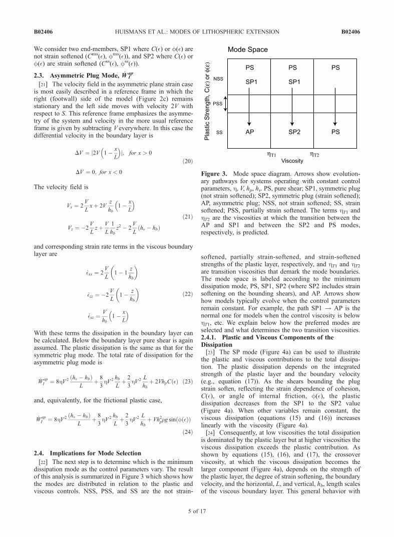
[22] The next step is to determine which is the minimumdissipation mode as the control parameters vary. The resultof this analysis is summarized in Figure 3 which shows howthe modes are distributed in relation to the plastic andviscous controls. NSS, PSS, and SS are the not strain-

softened, partially strain-softened, and strain-softenedstrengths of the plastic layer, respectively, and hT1 and hT2are transition viscosities that demark the mode boundaries.The mode space is labeled according to the minimumdissipation mode, PS, SP1, SP2 (where SP2 includes strainsoftening on the bounding shears), and AP. Arrows showhow models typically evolve when the control parametersremain constant. For example, the path SP1 ! AP is thenormal one for models when the control viscosity is belowhT1, etc. We explain below how the preferred modes areselected and what determines the two transition viscosities.2.4.1. Plastic and Viscous Components of theDissipation[23] The SP mode (Figure 4a) can be used to illustrate

the plastic and viscous contributions to the total dissipa-tion. The plastic dissipation depends on the integratedstrength of the plastic layer and the boundary velocity(e.g., equation (17)). As the shears bounding the plugstrain soften, reflecting the strain dependence of cohesion,C(�), or angle of internal friction, f(�), the plasticdissipation decreases from the SP1 to the SP2 value(Figure 4a). When other variables remain constant, theviscous dissipation (equations (15) and (16)) increaseslinearly with the viscosity (Figure 4a).[24] Consequently, at low viscosities the total dissipation

is dominated by the plastic layer but at higher viscosities theviscous dissipation exceeds the plastic contribution. Asshown by equations (15), (16), and (17), the crossoverviscosity, at which the viscous dissipation becomes thelarger component (Figure 4a), depends on the strength ofthe plastic layer, the degree of strain softening, the boundaryvelocity, and the horizontal, L, and vertical, hb, length scalesof the viscous boundary layer. This general behavior with

Figure 3. Mode space diagram. Arrows show evolution-ary pathways for systems operating with constant controlparameters, h, V, hp, hv. PS, pure shear; SP1, symmetric plug(not strain softened); SP2, symmetric plug (strain softened);AP, asymmetric plug; NSS, not strain softened; SS, strainsoftened; PSS, partially strain softened. The terms hT1 andhT2 are the viscosities at which the transition between theAP and SP1 and between the SP2 and PS modes,respectively, is predicted.


5 of 17

B02406

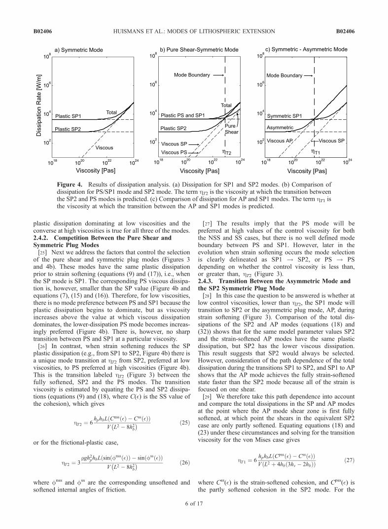
plastic dissipation dominating at low viscosities and theconverse at high viscosities is true for all three of the modes.2.4.2. Competition Between the Pure Shear andSymmetric Plug Modes[25] Next we address the factors that control the selection

of the pure shear and symmetric plug modes (Figures 3and 4b). These modes have the same plastic dissipationprior to strain softening (equations (9) and (17)), i.e., whenthe SP mode is SP1. The corresponding PS viscous dissipa-tion is, however, smaller than the SP value (Figure 4b andequations (7), (15) and (16)). Therefore, for low viscosities,there is no mode preference between PS and SP1 because theplastic dissipation begins to dominate, but as viscosityincreases above the value at which viscous dissipationdominates, the lower-dissipation PS mode becomes increas-ingly preferred (Figure 4b). There is, however, no sharptransition between PS and SP1 at a particular viscosity.[26] In contrast, when strain softening reduces the SP

plastic dissipation (e.g., from SP1 to SP2, Figure 4b) there isa unique mode transition at hT2 from SP2, preferred at lowviscosities, to PS preferred at high viscosities (Figure 4b).This is the transition labeled hT2 (Figure 3) between thefully softened, SP2 and the PS modes. The transitionviscosity is estimated by equating the PS and SP2 dissipa-tions (equations (9) and (18), where C(�) is the SS value ofthe cohesion), which gives

hT2 ¼ 6hphbL Cnss �ð Þ � Css �ð Þð Þ

V L2 � 8h2b� � ð25Þ

or for the frictional-plastic case,

hT2 ¼ 3rgh2phbL sin fnss �ð Þð Þ � sin fss �ð Þð Þð

V L2 � 8h2b� � ð26Þ

where fnss and fss are the corresponding unsoftened andsoftened internal angles of friction.

[27] The results imply that the PS mode will bepreferred at high values of the control viscosity for boththe NSS and SS cases, but there is no well defined modeboundary between PS and SP1. However, later in theevolution when strain softening occurs the mode selectionis clearly delineated as SP1 ! SP2, or PS ! PSdepending on whether the control viscosity is less than,or greater than, hT2 (Figure 3).2.4.3. Transition Between the Asymmetric Mode andthe SP2 Symmetric Plug Mode[28] In this case the question to be answered is whether at

low control viscosities, lower than hT2, the SP1 mode willtransition to SP2 or the asymmetric plug mode, AP, duringstrain softening (Figure 3). Comparison of the total dis-sipations of the SP2 and AP modes (equations (18) and(32)) shows that for the same model parameter values SP2and the strain-softened AP modes have the same plasticdissipation, but SP2 has the lower viscous dissipation.This result suggests that SP2 would always be selected.However, consideration of the path dependence of the totaldissipation during the transitions SP1 to SP2, and SP1 to APshows that the AP mode achieves the fully strain-softenedstate faster than the SP2 mode because all of the strain isfocused on one shear.[29] We therefore take this path dependence into account

and compare the total dissipations in the SP and AP modesat the point where the AP mode shear zone is first fullysoftened, at which point the shears in the equivalent SP2case are only partly softened. Equating equations (18) and(23) under these circumstances and solving for the transitionviscosity for the von Mises case gives

hT1 ¼ 6hphbL Cpss �ð Þ � Css �ð Þð ÞV L2 þ 4hb 3hv � 2hbð Þð Þ ð27Þ

where Css(�) is the strain-softened cohesion, and Cpss(�) isthe partly softened cohesion in the SP2 mode. For the

Figure 4. Results of dissipation analysis. (a) Dissipation for SP1 and SP2 modes. (b) Comparison ofdissipation for PS/SP1 mode and SP2 mode. The term hT2 is the viscosity at which the transition betweenthe SP2 and PS modes is predicted. (c) Comparison of dissipation for AP and SP1 modes. The term hT1 isthe viscosity at which the transition between the AP and SP1 modes is predicted.


6 of 17

B02406

frictional-plastic case the equivalent transition viscosity isgiven by

hT1 ¼ 3rgh2phbL sin fpss �ð Þð Þ � sin fss �ð Þð Þð

V L2 þ 4hb 3hv � 2hbð Þð Þ ð28Þ

Here fss(�) is the strain-softened internal angle of friction,and fpss(�) is the partly softened one.[30] An estimate of hT1 can be obtained by assuming

that when the AP shear becomes fully softened the SP1shears will not have softened significantly. In this casehT1 is given by equations (27) and (28) with Cpss andfpss replaced by their non strain-softened (nss) values.This value is an upper bound estimate of the transitionviscosity, hT1 between the AP and SP2 modes. Moregenerally, the value of hT1 depends on the differencebetween Cpss and Css (equation (27)), and therefore it willdecrease from the estimate given above as this differencebecomes smaller. AP will be the preferred mode when theviscosity is lower than hT1 (Figure 3).[31] This behavior can be interpreted physically in the

following manner. Any noise in the system will lead to theonset of strain softening on one of the SP bounding shearsbefore the other, and given the strong positive feedback thisshear will preferentially soften and reach its fully strain-softened state first. Therefore, everything being equal, thepreferred transition is SP1 ! AP because this is the paththat decreases the plastic dissipation most rapidly. However,this analysis ignores the competing effect of the viscousdissipation which increases during the SP1! AP transition.The mode that is selected is the one that decreases the totaldissipation most rapidly and this will depend on the controlviscosity. Below hT1 the path of the AP mode decreases thetotal dissipation the most rapidly, and therefore this modewill be selected despite the final higher viscous dissipationin this mode (Figure 3).2.4.4. Model Evolution and Pathways in Mode Space[32] Returning to Figure 3, it was stated above that the

arrows link the normal mode progression for models whenthe control parameters remain constant. It can now be seenthat there are three main regions of the mode spaceseparated by the transition viscosities hT1 and hT2 and thereare three corresponding normal mode progressions. Inmodels where the control viscosity is greater than hT2, PSis the only available mode and the others are forbiddenbecause they have a higher total dissipation even whenstrain softening of the plastic layer occurs. For controlviscosities between hT1 and hT2 the mode evolution isSP1 ! SP2. That is, the deformation remains symmetric.For control viscosities less than hT1 the mode evolution isSP1 ! AP, so that the deformation becomes asymmetric asthe plastic layer strain softens.[33] These model pathways in mode space provide the

basic insight concerning why the different modes areselected and why the style may be symmetric or asymmetricand even pure shear if the control viscosity is large enough.An interesting result is that the SP2 and AP modes areclearly separated even though both modes have the sameplastic dissipations. The symmetry versus asymmetry inthese cases is determined by the viscous layer properties,not by the plastic layer. This last result demonstrates that

minimum dissipation is not necessarily the sole criterion fora mode to be selected. Mode selection also depends on theaccessibility of the minimum dissipation mode and thisdepends on the dissipation path among the modes. Thestrain softened AP mode is a metastable mode from thestandpoint of total dissipation. The dissipation path can leadto the AP mode, which makes the lower-dissipation SP2mode inaccessible because the system must pass through ahigher level of dissipation, softening the second shear, inorder to reach the SP2 mode. The accessibility and selectionof modes is addressed in section 3 using numerical models.

3. Numerical Model Results

[34] The next step is to present four series of finiteelement model experiments designed to test the approxi-mate analytical theory. Series 1 and 2 are particular exam-ples that correspond to the two-layer lithosphere with eithera strain softening, cohesive (series 1) or frictional-plastic(series 2) layer, underlain and bonded to a uniform linearviscous layer. Series 3 introduces a more realistic depth-dependent rheology that does not prescribe the layer thick-nesses. Series 4 builds on series 2 by replacing the free slipbasal boundary condition with an underlying region of low-viscosity asthenosphere.

3.1. Model Description

[35] An Arbitrary Lagrangian-Eulerian (ALE) finite ele-ment method for the solution of mechanical plane strain,incompressible, viscous-plastic creeping flows [Fullsack,1995; Willett, 1999; Huismans and Beaumont, 2003] isused to investigate extension of models with a simple

Figure 5. Geometry of the numerical models showingupper plastic layer and lower viscous layer thicknesses,the weak seed, and the velocity boundary conditions, V.Extension is seeded by a small plastic weak seed. Themodel has a free top surface, and the other boundarieshave zero tangential stress (free slip). Sedimentation anderosion are not included in the model. There is, however,a small amount of numerical surface diffusion. TheEulerian grid has 401 and 121 nodes in the horizontaland vertical directions, respectively. Strain softening isachieved in a simple manner by a linear decrease of thecohesion or the angle of internal friction with deviatoriceffective strain (I 02).


7 of 17

B02406

geometry (Figure 5) and rheological structure (Table 1).Plastic deformation has a pressure-dependent Drucker-Prager yield criterion

J 02� �1=2¼ C cos feffð Þ þ p sin feffð Þ ð29Þ

where (J 02)1/2 = (1

2tijtij)

1/2 is the second invariant of thedeviatoric stress, C is the cohesion, feff is the effective

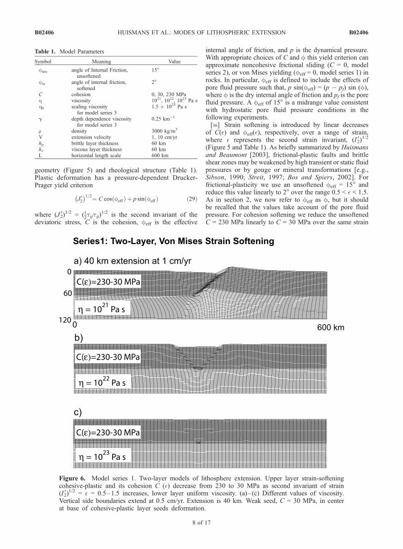
internal angle of friction, and p is the dynamical pressure.With appropriate choices of C and f this yield criterion canapproximate noncohesive frictional sliding (C = 0, modelseries 2), or von Mises yielding (feff = 0, model series 1) inrocks. In particular, feff is defined to include the effects ofpore fluid pressure such that, p sin(feff) = (p � pf) sin (f),where f is the dry internal angle of friction and pf is the porefluid pressure. A feff of 15� is a midrange value consistentwith hydrostatic pore fluid pressure conditions in thefollowing experiments.[36] Strain softening is introduced by linear decreases

of C(�) and feff(�), respectively, over a range of strain,where � represents the second strain invariant, (I 02)

1/2

(Figure 5 and Table 1). As briefly summarized by Huismansand Beaumont [2003], frictional-plastic faults and brittleshear zones may be weakened by high transient or static fluidpressures or by gouge or mineral transformations [e.g.,Sibson, 1990; Streit, 1997; Bos and Spiers, 2002]. Forfrictional-plasticity we use an unsoftened feff = 15� andreduce this value linearly to 2� over the range 0.5 < � < 1.5.As in section 2, we now refer to feff as f, but it shouldbe recalled that the values take account of the pore fluidpressure. For cohesion softening we reduce the unsoftenedC = 230 MPa linearly to C = 30 MPa over the same strain

Table 1. Model Parameters

Symbol Meaning Value

fnss angle of Internal Friction,unsoftened

15�

fss angle of internal friction,softened

2�

C cohesion 0, 30, 230 MPah viscosity 1021, 1022, 1023 Pa sh0 scaling viscosity

for model series 31.5 � 1023 Pa s

g depth dependence viscosityfor model series 3

0.25 km�1

r density 3000 kg/m3

V extension velocity 1, 10 cm/yrhp brittle layer thickness 60 kmhv viscous layer thickness 60 kmL horizontal length scale 600 km

Figure 6. Model series 1. Two-layer models of lithosphere extension. Upper layer strain-softeningcohesive-plastic and its cohesion C (�) decrease from 230 to 30 MPa as second invariant of strain(I 02)

1/2 = � = 0.5–1.5 increases, lower layer uniform viscosity. (a)–(c) Different values of viscosity.Vertical side boundaries extend at 0.5 cm/yr. Extension is 40 km. Weak seed, C = 30 MPa, in centerat base of cohesive-plastic layer seeds deformation.


8 of 17

B02406

range. The unrealistic high values of C were chosen sothat both series 1 and series 2 models have the sameintegrated strength of the plastic layer.

3.2. Model Series 1, Two--Layer, Cohesion Softening

[37] In series 1 a strain-softening cohesive plastic layeroverlies a uniform constant linear viscous layer, and theviscosity ranges from 1021 to 1023 Pa s (Figures 6a–6c).The results (Figure 6) are shown after 40 km total extensionat 1 cm/yr. At low viscosity (Figure 6a) the AP mode isselected. Strain softening has focused the plastic deforma-tion onto one shear and the extension is highly asymmetric.When h = 1022 Pa s (Figure 6b) asymmetry is suppressedand extension in the plastic layer occurs along two sym-metric shears in the SP2 mode. At high viscosity (Figure 6c)local deformation in the plastic layer is completely sup-pressed and extension of both layers occurs by pure shear,the PS mode.

3.3. Model Series 2, Two--Layer, Frictional--PlasticSoftening

[38] In series 2 a strain-softening frictional-plastic layeroverlies a uniform constant linear viscous layer, andthe viscosity ranges from 1021 to 1023 Pa s. The results(Figure 7) are also shown after 40 km total extension at

1 cm/yr. The results (Figure 7) exactly parallel those ofmodel series 1; the AP, SP2, and PS modes are selected withincreasing viscosity.

3.4. Model Series 3, Two--Layer, Depth--DependentRheology

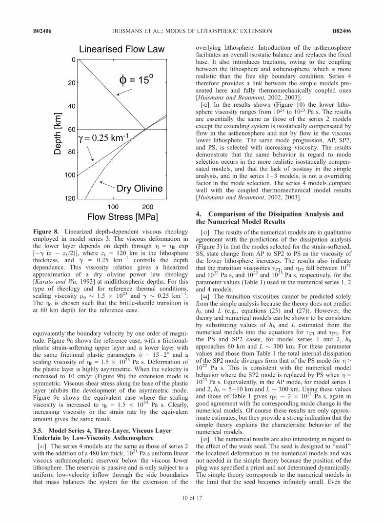
[39] Models series 3 attempts to address one limitation ofmodel series 1 and 2. The brittle-ductile transition in series 1and 2 is inherently fixed to the material interface betweenthe upper (brittle) and lower (viscous) layer. This inhibitsvariation with depth of the brittle ductile transitionresulting from variations in viscosity or strain rate. Inthis model series we now allow for depth-dependentrheology in the lower layer, that is it may behave eitherin a viscous or frictional-plastic manner. The viscousdeformation in the lower layer depends on depth throughh = h0 exp [�g(z � zL/2)], where zL = 120 km is thelithosphere thickness, and g = 0.25 km�1 controlsthe depth dependence. This viscosity relation gives alinearized approximation of a dry olivine power lawrheology [Karato and Wu, 1993] at midlithosphericdepths (Figure 8); h0 is chosen such that the brittle-ductile transition is at 60 km depth for the reference case.[40] In addition to varying the nominal scaling viscosity

of the lower layer we include one model where we vary

Figure 7. Model series 2. Two-layer models of lithosphere extension. Upper layer strain-softeningfrictional-plastic angle of internal friction f(�) decreases from 15� to 2� as second invariant of strain(I 02)

1/2 = � = 0.5–1.5 increases; cohesion C = 0, lower layer uniform viscosity. (a)–(c) Differentvalues of viscosity. Vertical side boundaries extend at 0.5 cm/yr. Extension is 40 km. Weak seed, f =2�, in center at base of frictional-plastic layer seeds deformation.


9 of 17

B02406

equivalently the boundary velocity by one order of magni-tude. Figure 9a shows the reference case, with a frictional-plastic strain-softening upper layer and a lower layer withthe same frictional plastic parameters f = 15–2� and ascaling viscosity of h0 = 1.5 � 1023 Pa s. Deformation ofthe plastic layer is highly asymmetric. When the velocity isincreased to 10 cm/yr (Figure 9b) the extension mode issymmetric. Viscous shear stress along the base of the plasticlayer inhibits the development of the asymmetric mode.Figure 9c shows the equivalent case where the scalingviscosity is increased to h0 = 1.5 � 1024 Pa s. Clearly,increasing viscosity or the strain rate by the equivalentamount gives the same result.

3.5. Model Series 4, Three-Layer, Viscous LayerUnderlain by Low-Viscosity Asthenosphere

[41] The series 4 models are the same as those of series 2with the addition of a 480 km thick, 1021 Pa s uniform linearviscous asthenospheric reservoir below the viscous lowerlithosphere. The reservoir is passive and is only subject to auniform low-velocity inflow through the side boundariesthat mass balances the system for the extension of the

overlying lithosphere. Introduction of the asthenospherefacilitates an overall isostatic balance and replaces the fixedbase. It also introduces tractions, owing to the couplingbetween the lithosphere and asthenosphere, which is morerealistic than the free slip boundary condition. Series 4therefore provides a link between the simple models pre-sented here and fully thermomechanically coupled ones[Huismans and Beaumont, 2002, 2003].[42] In the results shown (Figure 10) the lower litho-

sphere viscosity ranges from 1021 to 1023 Pa s. The resultsare essentially the same as those of the series 2 modelsexcept the extending system is isostatically compensated byflow in the asthenosphere and not by flow in the viscouslower lithosphere. The same mode progression, AP, SP2,and PS, is selected with increasing viscosity. The resultsdemonstrate that the same behavior in regard to modeselection occurs in the more realistic isostatically compen-sated models, and that the lack of isostasy in the simpleanalysis, and in the series 1–3 models, is not a overridingfactor in the mode selection. The series 4 models comparewell with the coupled thermomechanical model results[Huismans and Beaumont, 2002, 2003].

4. Comparison of the Dissipation Analysis andthe Numerical Model Results

[43] The results of the numerical models are in qualitativeagreement with the predictions of the dissipation analysis(Figure 3) in that the modes selected for the strain-softened,SS, state change from AP to SP2 to PS as the viscosity ofthe lower lithosphere increases. The results also indicatethat the transition viscosities hT1, and hT2 fall between 1021

and 1022 Pa s, and 1022 and 1023 Pa s, respectively, for theparameter values (Table 1) used in the numerical series 1, 2and 4 models.[44] The transition viscosities cannot be predicted solely

from the simple analysis because the theory does not predicthb and L (e.g., equations (25) and (27)). However, thetheory and numerical models can be shown to be consistentby substituting values of hb and L estimated from thenumerical models into the equations for hT1 and hT2. Forthe PS and SP2 cases, for model series 1 and 2, hbapproaches 60 km and L 300 km. For these parametervalues and those from Table 1 the total internal dissipationof the SP2 mode diverges from that of the PS mode for h >1022 Pa s. This is consistent with the numerical modelbehavior where the SP2 mode is replaced by PS when h =1023 Pa s. Equivalently, in the AP mode, for model series 1and 2, hb 5–10 km and L 300 km. Using these valuesand those of Table 1 gives hT1 2 � 1021 Pa s, again ingood agreement with the corresponding mode change in thenumerical models. Of course these results are only approx-imate estimates, but they provide a strong indication that thesimple theory explains the characteristic behavior of thenumerical models.[45] The numerical results are also interesting in regard to

the effect of the weak seed. The seed is designed to ‘‘seed’’the localized deformation in the numerical models and wasnot needed in the simple theory because the position of theplug was specified a priori and not determined dynamically.The simple theory corresponds to the numerical models inthe limit that the seed becomes infinitely small. Even the

Figure 8. Linearized depth-dependent viscous rheologyemployed in model series 3. The viscous deformation inthe lower layer depends on depth through h = h0 exp[�g (z � zL/2)], where zL = 120 km is the lithospherethickness, and g = 0.25 km�1 controls the depthdependence. This viscosity relation gives a linearizedapproximation of a dry olivine power law rheology[Karato and Wu, 1993] at midlithospheric depths. For thistype of rheology and for reference thermal conditions,scaling viscosity m0 1.5 � 1023 and g 0.25 km�1.The h0 is chosen such that the brittle-ductile transition isat 60 km depth for the reference case.


10 of 17

B02406

finite sized seed creates only a minor reduction in theintegrated strength of the plastic layer and therefore has aminor influence on the overall results. It is in this regard aninteresting result that when the viscosity of the lower layeris 1023 Pa s the seed is ignored and no local deformationoccurs, as predicted by the theory. This result is a nicedemonstration that inherited weaknesses may not be reac-tivated during lithospheric extension.

5. Discussion

5.1. Summary of the Dissipation Analysis andNumerical Model Results

[46] In section 2 it was demonstrated that mode selectionin models of lithospheric extension can be predicted basedon the minimization of rate of energy dissipation. However,our analytical descriptions of the modes may be incomplete,or there may be other lower dissipation modes that we havemissed. The dissipation analysis shows only which of theanalyzed modes is favored. That the series 1 and 2 finiteelement model experiments (section 3) confirm the approx-imate analysis (section 2) indicates that these modes are alsoaccessed as the system evolves, and provides some reassur-

ance that the approximate treatment is acceptable and thatother missed modes are not strongly preferred. Moreover, itappears that the basic analytical mode predictions, con-firmed by numerical model series 1 and 2, also applyequally to the numerical models with the more advancedrheologies (model series 3) and more realistic basal bound-ary conditions (model series 4).[47] The overall results can be summarized by describing

the final mode selection in relation to the viscosity of theviscous layer. When the viscous dissipation is negligible,the asymmetric plug (AP) mode is chosen because this is thefastest route to minimize the plastic dissipation by strainsoftening only one, not two, shear zones during partialstrain softening. As viscous dissipation increases, the modeselected will change from asymmetric plug (AP) to strainsoftened symmetric plug (SP2) at the transition viscosityhT1. Equation (27) when recast as

hT1V L2 þ 4hb 3hv � 2hbð Þð Þ

6hbL¼ hp Cpss �ð Þ � Css �ð Þð Þ ð30Þ

can be interpreted in terms of the trade-off between twodifferential forces, the differential ‘‘viscous penalty force’’

Figure 9. Model series 3. Two-layer models of lithosphere extension. Upper layer strain-softeningfrictional-plastic angle of internal friction f(�) decreases from 15� to 2� as second invariant of strain(I 02)

1/2 = � = 0.5–1.5 increases; cohesion C = 0, lower layer either frictional-plastic with sameparameters as upper layer or with viscosity depending exponentially on depth through h = h0 exp[�g (z � zL/2)]. Vertical side boundaries extend at 0.5 cm/yr. Extension is 40 km. Weak seed, f =2�, in center at base of frictional-plastic layer seeds deformation.


11 of 17

B02406

incurred by deforming in the AP as opposed to SP2 mode;and the differential ‘‘plastic gain force’’, the advantage ofthe fully strain-softened AP mode over the partially strain-softened SP2 mode. The mode switches at hT1, when thepenalty equals the gain.[48] There is no critical transition viscosity between the

non strain-softened symmetric plug (SP1) and pure shear(PS) modes, but PS becomes progressively advantaged asthe penalty of the differential viscous force between PS andSP1 modes increases. This implies that PS will be selectedwhen the viscous dissipation is high, as demonstrated by thenumerical model results (section 3). There is, however, a

critical transition viscosity, hT2, between the SP2 and PSmodes (Figure 3).[49] The physical insight provided by the analysis is that

the system behavior is determined not by the intrinsicproperties of either the plastic or viscous layers but, instead,by the trade-off in their combined behavior necessary tominimize the dissipation, or, equivalently, the trade-offbetween differential penalty-gain forces.

5.2. Generalization of the Results

[50] The analysis should be expandable to more complexmodels of the lithosphere comprising several plastic and

Figure 10. Model series 4. Three-layer models of lithosphere extension, including low-viscosityasthenosphere. Upper lithosphere layer strain-softening frictional-plastic angle of friction f(�) decreasesfrom 15� to 2� as second invariant of strain (I02)

1/2 = � = 0.5–1.5 increases; cohesion C = 0, lowerlithosphere layer uniform viscosity. Asthenosphere layer uniform viscosity h = 1 � 1021 Pa s. (a)–(c)Different values of ‘‘lithosphere’’ viscosity. Vertical side boundaries extend at 0.5 cm/yr. Extension is40 km. Weak seed, f = 2�, in center at base of frictional-plastic layer seeds deformation.


12 of 17

B02406

viscous layers if the analytical modes for these systems canbe described in relatively simple terms. In addition, thereare other modes, for example, those comprising multiplesymmetric and/or asymmetric plugs, that can be added tothe analysis. Wijns et al. [2003] have already shown thatthe viscosity of the lower layer influences the multishearband mode.[51] The multiple plug modes may help in an assessment

of the conditions that favor reactivation of inherited weakfaults or shear zones in the upper plastic crust duringlithospheric extension. The gain in reactivation is that theplastic dissipation can be reduced by comparison with theSP mode by any multiplug mode that utilizes and reactivatesthe weak, nominally SS, shears. However, there is anassociated ‘‘viscous penalty’’ from the small but finiteboundary layer viscous shear between the plastic andviscous layers. Equations equivalent to (27) and (30) cantherefore be used to predict when reactivation will and willnot lead to minimum dissipation [Buiter et al., 2004, alsopersonal communication, 2004]. If the multiplug, faultreactivation mode results in a differential viscous penaltyforce that is greater than the differential plastic gain forceachieved by reactivation, this mode will not be chosen. Theopposite end-member behavior is that the PS mode will bechosen and the whole system will extend by pure shearwithout fault reactivation, even though the upper crust maybe riddled with faults. Under these circumstances there is aclear transition viscosity between the PS and other modes.This is consistent with previous modeling results showingthe control of viscosity of the lower layer on the transitionbetween narrow and wide rift modes [Buck et al., 1999].[52] An additional mode (L. Moresi, personal communi-

cation, 2004) in which a plastic shear forms at the base ofthe upper layer, thereby decoupling it from the viscouslayer, can be shown to require higher dissipation than themodes considered here, which explains why it is notselected in the numerical models and probably is notfavored in the lithosphere.

5.3. Relationship to Previous Modeling Results:Dominant and Subordinate Rheologies

[53] Huismans and Beaumont [2003] introduced theconcept of dominant and subordinate rheologies to explainsome aspects of numerical model results. When either theplastic or viscous rheology becomes the main load bearingpart of the system it can be considered to be the dominantrheology and may force the weaker, subordinate part of thesystem into a compliant style of deformation. This compli-ant style may differ from the intrinsic mode that wouldhave been selected in the absence of forcing by thedominant rheology. This concept can now be quantifiedin terms of the minimum dissipation analysis and, inparticular, in terms of the trade-off between the differentialpenalty and gain forces.[54] When the system operates at a subcritical h, that is a

value below hT1 (e.g., equation (27), the AP mode, theintrinsic plastic layer minimum dissipation mode is selectedand the plastic rheology dominates. When, with increasingviscous dissipation the SP mode is chosen, the viscousdifferential penalty force is now large enough that theplastic layer is forced by the dominant viscous layer intoa mode that is not the one that would be chosen by the

plastic layer alone. At even higher levels of the viscousdifferential penalty force the viscous rheology becomeseven more dominant and forces the subordinate plastic layerto select the PS mode. Thus one rheology can be said todominate the other. The dominant and subordinate charac-teristics of the rheologies are determined by the relativesizes of the associate differential penalty and gain forces.[55] This explanation can be applied to the results of

models 2 and 9 [Huismans and Beaumont, 2003] in whichasymmetric, AP mode extension occurs when the riftingvelocity is 0.3 cm/yr but exactly the same system exhibitsSP mode extension when the rifting velocity is 10 cm/yr.The high-velocity increases the viscous dissipation and thedifferential viscous penalty force more than the differentialplastic gain force (equation (30)). The viscous rheologydominates and the mode switches. Essentially the sameresult is shown in Figure 10a. For even lower extensionvelocities, e.g., model 8 [Huismans and Beaumont, 2003],asymmetric AP mode extension is selected throughout therifting, implying that the differential viscous penalty force isalways sufficiently small that the viscous rheology issubordinate and therefore the lithosphere extends asymmet-rically under the control of the dominant plastic rheology.

5.4. Implications for Natural Systems: Symmetric andAsymmetric Lithospheric Extension

[56] The use of the minimum dissipation principle toanalyze lithospheric extension models, as employed here,is valid because we analyze a simple system which has afew well-defined properties, the strain-softening plasticrheologies and linear viscosity. Furthermore, the minimumdissipation approach is not used to construct the fullincremental finite deformation of the system as, for exam-ple, by Masek and Duncan [1998]. Instead, it is used in anapproximate analysis, as by Burbidge and Braun [2002] tochoose among a few well-defined modes.[57] It is also to be expected that equivalent finite element

model experiments will give the same results as theapproximate analysis, provided that our approximations ofthese modes (section 2) are reasonably accurate, and thatthe modal dissipations rank in the same order despite theseapproximations. The results should be the same because thevelocity-based viscous-plastic finite element formulationthat we have used [Fullsack, 1995] is based on the self-consistent Galerkin method which also minimizes the rateof energy dissipation.[58] One conclusion is that this approach is a useful way

to analyze and make physical interpretations of numericalmodel results, and that the same approach may be usefulwhen analyzing physical laboratory model behaviors. How-ever, as Bird and Yuen [1979] have pointed out, there is noguarantee that the dissipation analysis employed here can bedirectly extrapolated to natural lithospheric extension. Theprimary reasons are as follows: (1) only a subdomain of theEarth is chosen for analysis and it is not clear if this regioncan be treated in isolation (for example, a particular restric-tion is that we analyze a simplified two-dimensional system)and (2) other variations in properties not included in thecurrent models may allow even lower dissipation modes toexist. For example, viscous strain softening could be moreimportant than plastic strain softening. If so, the minimiza-tion should also include the variation of the functional


13 of 17

B02406

(equation (1)) with respect to the dependence of viscosityon strain and, more generally, power law flow and temper-ature [Bird and Yuen, 1979]. In addition, an equivalentanalysis of elastic-viscous-plastic behavior is required todetermine the importance of elasticity.

6. Primary Conclusions

[59] We started this paper with the general problem ofthe controls on the modes of lithospheric extension andunder what circumstances is extension asymmetric, sym-metric, or pure shear without fault reactivation. Theresults presented illustrate the application of the principleof minimum rate of dissipation to a simplified model ofthe lithosphere comprising a cohesive, or frictional-plasticupper layer bonded to an underlying linear viscous lowerlithosphere. The main conclusions (Figure 11) apply tothese simple models but the principles may also apply tothe natural system. Figure 11 illustrates the predictedmode selection pathways during strain softening of theplastic upper lithosphere (NSS ! PSS ! SS) andthe control of the mode selection by the viscosity ofthe underlying viscous layer. These conclusions arederived from an approximate analysis and are supportedby the finite element experiments.[60] Depending on the viscous dissipation the mode that

is chosen during the early phase of extension, before theonset of strain softening (i.e., the NSS regime), will be thesymmetric plug, SP1, or pure shear, PS, if the viscosity ofthe lower layer (equation (25)) is greater than the criticalvalue, hT2. Later, during partial strain softening, PSS,systems with viscosities greater than hT2 will ignore thepossibility of strain softening on the shears bounding the

plug and remain PS as they evolve. Systems with viscositylower than hT2 will adopt either the asymmetric plug,AP mode, or the strain-softened symmetric plug, SP2 mode,if the viscosity is greater than the critical value, hT1(equation (27)).[61] The mode selection depends on the minimization of

the internal rate of energy dissipation which is used toderive equations (25) and (27). The processes can beunderstood physically in terms of the trade-off betweenthe gain of reduced dissipation by selecting a lower-dissipation mode in the plastic layer versus the ‘‘penalty’’of higher viscous dissipation incurred in the viscous layer.This trade-off can be expressed through the differentialpenalty and gain forces (equation (30)) by the concept ofdominant and subordinate rheologies (section 5.3).[62] The potential application to lithospheric extension is

that the AP mode is preferred when the dissipation in theviscous crust or lower lithosphere is small, for any ofthe reasons that make h subcritical with respect to hT1(equation (27)), for example, extension is slow and thestrain rates are low, or the effective viscosity is intrinsicallylow because the viscous part of the lithosphere is hot andweak. The AP mode is therefore likely to be preferred forslow extension of viscously weak lithosphere, but there areother possibilities that make hT1 greater than h (equation (27)or (30)), for example, factors that make hT1 large; so theselection is always a relative one among the factors thatmake hT1 large.[63] Equivalently, the SP2 mode is predicted for faster

extension of colder, higher effective viscosity lithospherebut this is not unique, any factor that makes hT1 less than hand hT2 greater than h (equation (25)) will select this mode.Again, the choice is relative.

Figure 11. Diagram summarizing main results of dissipation analysis and numerical model results ofsimple two-layer models of extension.


14 of 17

B02406

[64] Whether the PS mode is observed on the Earth isdebatable. If it is not, it follows that lithospheric systems aresubcritical with respect to hT2. By implication, the differ-ential viscous penalty force is never large enough tooutweigh the differential plastic gain force for this mode.That is, the viscous rheology never dominates so stronglythat fault reactivation, or plastic stain softening on focusedshears is suppressed. This conclusion is probably wrong inan absolute sense in regard to natural systems but it offersinsight into the system behavior and the mechanisms thatcontrol the system.[65] Analysis of the simple two-layer system in terms of

dissipation and force balance leads to some equivalentresults but it appears that dissipation is the more sensitiveanalysis tool for systems composed of both viscous andplastic components. This difference occurs because dissipa-tion in the viscous part of the system is proportional to thesquare of strain rate, whereas forces are proportional tostrain rate.

Appendix A: Force Balance Estimate of ModeSwitching

[66] Here we give a parallel method to estimate modechanges using a comparison of the total force required forextension of the two-layer system under consideration. Weassume that the mode which requires the least total forcewill be the mode in which the systems deforms. The forcebalance approach is complementary to the dissipation anal-ysis. The results of the force balance analysis are consistentwith the mode transition between PS and SP predicted bythe dissipation analysis. The force balance approachappears, however, not sensitive enough to discriminatebetween SP and AP modes. In calculating the total forcewe use the same geometry and quantities as in the dissipa-tion analysis (Figure 2). The total force combines a viscousand a plastic component: F = Fv + Fp. The plastic force isgiven by the vertically integrated strength of the plasticlayer:

Fp ¼Z hp

0

txx dz ðA1Þ

The total viscous force is the sum of the integrated stress txxon a vertical section near or at the boundary and theintegrated shear stresses along the horizontal boundaries attop (and bottom) of the viscous layer:

Fv ¼Z hv

0

txx dzþZ L

�L

txz dx ðA2Þ

In the viscous pure shear case txx = 2h _�xx and txz = 0. As_�xx = V/L, the total force needed to extend the two-layersystem in pure shear mode is given by

Fps ¼ 2hVhv

Lþ hpC

nss �ð Þ ðA3Þ

for x > 0. In the symmetric plug mode case shear terms inthe boundary layer with thickness hb are given by _�xx = V/L(1 � z

hb) and _�xz =

12V(1 � x

L)/hb (equation (13), for x > 0 and

local reference frame with z = 0 at the base of the boundarylayer), while pure shear affects the remaining lower part ofthe layer with thickness (hv � hb). Thus the total forceneeded to extend the two-layer system in symmetric plugmode is approximately given by

Fsp ¼ 2hVhv � hbð Þ

Lþ hV

hb

Lþ hV

L

hbþ hpC

nss �ð Þ ðA4Þ

In the asymmetric plug mode case shear terms inthe boundary layer with thickness hb are given by _�xx =2V/L(1 � z

hb) and _�xz = V(1 � x

L)/hb (equation (22)), while

pure shear affects the remaining lower part of the layer withthickness (hv � hb). Thus the total force needed to extendthe two-layer system in asymmetric plug mode isapproximately given by

Fap ¼ 2hVhv � hbð Þ

Lþ 2hV

hb

Lþ hV

L

hbþ hpC

ss �ð Þ ðA5Þ

A comparison with the results for the total dissipationanalysis in the pure shear mode, the symmetric plug mode,and asymmetric plug mode cases, respectively, showsstrong similarities. Minor differences in multipliers of therespective terms relate to differences in integration constantsand the quadratic versus linear strain rate terms in theintegrands.

Appendix B: Evaluation of the Role of Gravity

[67] We first derive an analytical expression for therate of work against gravity for the PS mode. We thenderive an expression for the perturbation in the rate ofwork against gravity for other cases and use estimates ofits value to place bounds on the rate of work againstgravity for SP and AP modes. The work against gravity(equation (3)) is defined as

_WG ¼ZU

rgVzdU ðB1Þ

For uniform density and incompressible flow massconservation during pure shear gives

2LVz x; z ¼ hð Þ ¼ 2jV jh ðB2Þ

where h = hp + hv is the total model height (Figure 2,section 2). For pure shear extension (Figure 2a),

Vz x; zð Þ ¼ �jV j hL

z

h

� �¼ �jV j z

LðB3Þ

and the rate of work against gravity is

_W psG ¼ rg

Z L

�L

Z h

0

�jV j zLdzdx

¼ �rgjV jh2

¼ rgVz z ¼ hð ÞLh ðB4Þ


15 of 17

B02406

We can treat other modes as perturbations of the pureshear mode and write

_WG ¼ _W psG þ D _WG ðB5Þ

Let Vz = Vz(x, z) and h(x) = h + Dh(x), where h is theheight in the pure shear case. The perturbation mustconserve mass: Z L

�L

Dh x; z ¼ hð Þdx ¼ 0 ðB6Þ

We now assume that the vertical velocity Vz(x, z = h) isproportional to the height of the perturbation. Then

Vz x; zð Þ ¼ V psz x; zð Þ þ DVz x; zð Þ ðB7Þ

where DVz(x, z) = �jDVjz/L. Using mass conservationwithin any region of the model of width DL andassuming overall pure shear, the perturbed velocity fieldbecomes

DVz x; zð Þ ¼ D _�xxð Þz ðB8Þ

and the perturbation is

D _WG ¼ rgZ L

�L

Z h xð Þ

0

D _�xxð Þzdzdx ðB9Þ

Functional forms of D( _�xx) and Dh(x) can be calculatedfor specific modes. Here we use a more general functioncomprising a series of ‘‘box cars’’ for both functions,amplitudes a/2 and Dh/2 such that

D _�xx ¼ �a xð Þ2

jV jL

ðB10Þ

The result is independent of the number of box cars, ortheir width, provided the perturbation conserves mass. Theperturbation of the rate of work against gravity is then

D _WG ¼ rgZ 0

�L

Z hþDh=2

0

a2

jV jL

zdzdx

� rgZ L

0

Z h�Dh=2

0

a2

jV jL

zdzdx

¼ rgajV jhDh ðB11Þ

where the pure shear case is taken to be alreadyperturbed. For the case where a narrow region, widthL1, is subsiding between two long-wavelength flankuplifts, total width L2, a/2 has amplitude a1/2 over theregion of width L1 and a2/2 over the region of width L2,where L1 + L2 = 2L. The perturbation of the rate of workagainst gravity becomes

D _WG ¼ rgjV j a1

2L1

hþ Dhð Þ2

2

" #� a2

2L2

h� Dhð Þ2

2

" #" #ðB12Þ

Mass conservation requires, L1a1/2 = L2a2/2, and theresulting D _WG is the same as in equation (B11). Althoughthese estimates of D _WG are based on small perturbationsin h and Vz, the results are also correct for perturbationsin h that are not small, provided that the change in h

during the time interval for which D _WG is estimated issmall.[68] We now compare D _WG with the work against gravity

for the pure shear case e.g., _WGps = �rgjVjh2. At a litho-

spheric scale, for the case of a reference height, h = 100 km,with perturbation in topography, Dh 1 km, and forvariations in vertical velocity, a/2 = 1%, the perturbationof work against gravity is of the order D _WG = 10�4 _WG

ps.For the case of Dh 10 km and variations in verticalvelocity a/2 = 10%, D _WG = 10�2 _WG

ps.[69] If for the symmetric or asymmetric plug mode Dh is

of the order 5–10 km, and vertical velocities in the plugarea deviate order 10–20% from the pure shear case, theassociated range of the fractional perturbation D _WG/ _WG

ps is[4 � 10�3–1.6 � 10�2].[70] We have calculated the rate of work against gravity

in the numerical models of model series 2. The rate of workagainst gravity estimated for the pure shear case comparesvery well with the corresponding theoretical prediction andis 68.5 � 103 W/m. The difference in the rate of workagainst gravity for the transition between PS and SP modes,and for the transition from SP to AP modes is at most800 W/m and in general less than that. It is clear that thedifference in rate of work against gravity compared to theabsolute value for the pure shear case is of the order 10�2 orless. This is consistent with the estimate from the perturbationanalysis above. The difference in internal dissipation for therespective mode transitions is in the order of D _WI

PS–SP 2200 W/m, and D _WI

SP–AP 3000 W/m. The contribution ofthe differential rate of work against gravity (equation (4)) istherefore small compared with the corresponding rate of theinternal dissipation differential.

[71] Acknowledgments. We wish to thank the associate editor AdrianLenardic and the reviewers, Luc Lavier, Louis Moresi, and an anonymousreviewer. We acknowledge Philippe Fullsack and Glen Stockmal forstimulating discussions. This research was funded through an ACOA-Atlantic Innovation Fund contract, and an IBM-Shared University Researchgrant. C. Beaumont was funded by the Canada Research Chair in Geo-dynamics. Beaumont also acknowledges support through the Inco Fellow-ship of the Canadian Institute for Advanced Research. Numericalcalculations used software developed by Philippe Fullsack.

ReferencesBehn, M. D., J. Lin, and M. T. Zuber (2002), A continuum mechanicsmodel for normal faulting using a strain-rate softening rheology: Implica-tions for thermal and rheological controls on continental and oceanicrifting, Earth Planet. Sci. Lett., 202, 725–740.

Bird, P., and D. A. Yuen (1979), The use of minimum-dissipation principlein tectonophysics, Earth Planet. Sci. Lett., 45, 214–217.

Boillot, G., M.-O. Beslier, and M. Comas (1992), Seismic image of under-crusted serpentine beneath a rifted margin, Terra Nova, 4, 25–33.

Bos, B., and C. J. Spiers (2002), Frictional-viscous flow of phyllosilicate-bearing fault rock: Microphysical model and implications for crustalstrength profiles, J. Geophys. Res., 107(B2), 2028, doi:10.1029/2001JB000301.

Brun, J. P., and M. A. Gutscher (1992), Deep crustal structure of the RhineGraben from DEKORP-ECORS seismic reflection data: A summary,Tectonophysics, 208, 139–147.

Buck,W.R. (1988), Flexural rotation of normal faults,Tectonics, 7, 959–973.Buck, W. R. (1993), Effect of lithospheric thickness on the formation ofhigh- and low-angle normal faults, Geology, 21, 933–936.

Buck, W. R., L. L. Lavier, and A. B. N. Poliakov (1999), How to make a riftwide?, Philos. Trans. R. Soc., 357, 671–690.

Buiter, S. J. H., R. S. Huismans, and C. Beaumont (2004), Formation ofextensional sedimentary basins: The role of surface processes in modeselection, in Boll. Geophys., 45, 187–191.

Burbidge, D. R., and J. Braun (2002), Numerical models of the evolution ofaccretionary wedges and fold-and-thrust belts using the distinct elementmethod, Geophys. J. Int., 148, 542–561.


16 of 17

B02406

Frederiksen, S., and J. Braun (2001), Numerical modeling of strain locali-zation during extension of the continental lithosphere, Earth Planet. Sci.Lett., 188, 241–251.

Fullsack, P. (1995), An arbitrary Lagrangian-Eulerian formulation forcreeping flows and applications in tectonic models, Geophys. J. Int.,120, 1–23.

Gessner, K., U. Ring, C. Johnson, R. Hetzel, C. W. Passchier, andT. Gungor (2001), An active bivergent rolling-hinge detachmentsystem: Central Menderes metamorphic core complex in westernTurkey, Geology, 29, 611–614.

Huismans, R. S., and C. Beaumont (2002), Asymmetric lithospheric exten-sion: The role of frictional-plastic strain-softening inferred from numer-ical experiments, Geology, 30, 211–214.

Huismans, R. S., and C. Beaumont (2003), Symmetric and asymmetriclithospheric extension: Relative effects of frictional-plastic and viscousstrain softening, J. Geophys. Res., 108(B10), 2496, doi:10.1029/2002JB002026.

Karato, S., and P. Wu (1993), Rheology of the upper mantle, Science, 260,771–778.

Karner, G. D., N. W. Driscoll, and D. H. N. Barker (2003), Syn-riftregional subsidence across the West African continental margin: Therole of lower plate ductile extension, in Petroleum Geology of Africa:New Themes and Developing Technologies, edited by T. Arthur, D. S.Macgregor, and N. R. Cameron, Geol. Soc. Spec. Publ., 207, 105–130.

Keller, G. R., and W. S. Baldridge (1999), The Rio Grande Rift, A geolog-ical and geophysical review, Rocky Mt. Geol., 34, 131–148.

Lavier, L. L., and W. R. Buck (2002), Half graben versus large-offset low-angle normal fault: Importance of keeping cool during normal faulting,J. Geophys. Res., 107(B6), 2122, doi:10.1029/2001JB000513.

Lavier, L. L., W. R. Buck, and A. N. B. Poliakov (1999), Self-consistentrolling-hinge model for the evolution of large-offset low-angle normalfaults, Geology, 27, 1127–1130.

Louden, K. E., and D. Chian (1999), The deep structure of non-volcanicrifted continental margins, Philos. Trans. R. Soc. London, Ser. A, 357,767–804.

Malvern, L. E. (1969), Introduction to the Mechanics of a ContinuousMedium, 713 pp., Prentice-Hall, Upper Saddle, N. J.

Masek, J. G., and C. C. Duncan (1998), Minimum work mountain building,J. Geophys. Res., 103, 907–917.

McKenzie, D. (1978), Some remarks on the development of sedimentarybasins, Earth Planet. Sci. Lett., 40, 25–32.

Sibson, R. H. (1990), Conditions for fault-valve behaviour, in DeformationMechanisms, Rheology and Tectonics, edited by R. J. Knipe and E. H.Rutter, Geol. Soc. Spec. Publ., 54, 15–28.

Sibuet, J.-C. (1992), Formation of non-volcanic passive margins: A com-posite model applied to the conjugate Galicia and southeastern FlemishCap margins, Geophys. Res. Lett., 19, 769–773.

Sleep, N. H., S. Stein, R. J. Geller, and R. G. Gordon (1979), Comment on‘‘The use of minimum-dissipation principle in tectonophysics’’ by P. Birdand D. A. Yuen, Earth Planet. Sci. Lett., 45, 218–220.

Streit, J. E. (1997), Low frictional strength of upper crustal faults: A model,J. Geophys. Res., 102, 24,619–24,626.

Wernicke, B. (1985), Uniform-sense normal simple shear of the continentallithosphere, Can. J. Earth Sci., 22, 108–125.

Wernicke, B., and B. C. Burchfiel (1982), Modes of extensional tectonics,J. Struct. Geol., 4, 105–115.

White, N. (1990), Does the uniform stretching model work in the NorthSea, in Tectonic Evolution of the North Sea Rifts, edited by D. J. Blundelland A. D. Gibbs, pp. 217–240, Clarendon, Oxford, U.K.

Whitmarsh, R. B., G. Manatschal, and T. A. Minshull (2001), Evolutionof magma-poor continental margins from rifting to seafloor spreading,Nature, 413, 150–154.

Wijns, C., F. Boschetti, and L. Moresi (2003), Inverse modelling in geologyby interactive evolutionary computation, J. Struct. Geol., 25, 1615–1621.

Willett, S. D. (1999), Rheological dependence of extension in wedgemodels of convergent orogens, Tectonophysics, 305, 419–435.

��C. Beaumont and R. S. Huismans, Department of Oceanography,

Dalhousie University, B3H 4J1, Halifax, Nova Scotia, Canada. ([email protected]; [email protected])S. J. H. Buiter, Geological Survey of Norway, Leiv Eirikssons vei 39,

N-7491 Trondheim, Norway. ([email protected])


17 of 17

B02406

Effect of plastic-viscous layering and strain softening on mode selection during lithospheric...

Documents

Transcript of Effect of plastic-viscous layering and strain softening on mode selection during lithospheric...